
Jose´ Proenca¸ - HASLabhaslab.uminho.pt/joseproenca/files/thesis-colour.pdf · 6 Acknowledgments...
250
Synchronous Coordination of Distributed Components Jos´ e Proen¸ ca
Transcript of Jose´ Proenca¸ - HASLabhaslab.uminho.pt/joseproenca/files/thesis-colour.pdf · 6 Acknowledgments...
Synchronous Coordinationof Distributed Components
Jose Proenca

Synchronous Coordinationof Distributed Components


Synchronous Coordinationof Distributed Components
PROEFSCHRIFT
ter verkrijging vande graad van Doctor aan de Universiteit Leiden
op gezag van de Rector Magnificus prof. mr. P.F. van der Heijden,volgens besluit van het College voor Promoties
te verdigen op woensdag 11 mei 2011klokke 13.45 uur
door
Jose Miguel Paiva Proenca
geboren te Porto, Portugal, in 1982.

promotor: prof.dr. F. Arbab
copromotor: dr. D. Clarke, Katholieke Universiteit Leuven, Belgium
copromotor: dr. E. de Vink, Technische Universiteit Eindhoven
overige leden: prof.dr. T. Back
prof.dr. F.S. de Boer
dr. M.M. Bonsangue
prof.dr. J.-M. Jacquet, University of Namur, Belgium
prof.dr. J.N. Kok
prof.dr. J.J.M.M. Rutten, Radboud University Nijmegen
The work in this thesis was supported by the portuguese foundation FCT(Funcacao para a Ciencia e Tecnologia), grant 22485 – 2005, and has been car-ried out under the auspices of the research school IPA (Institute for Programmingresearch and Algorithmics).
Copyright c© 2011 by Jose Proenca
Cover design by Kseniya Rogova.Printed and published by Boxpress BV ‖ Proefschriftmaken.nl.
ISBN: 978-90-8891-265-8IPA Dissertation Series 2011-05
Acknowledgments
This thesis is the result of four years of work carried out at CWI, and completedwhile employed at the Katholieke Universteit Leuven, in Belgium. During thistime I faced many obstacles, which I was able to surpass only with the support ofall my friends and family. To all of you, a warm “thank you”!
I would like to thank my advisors: Farhad Arbab, Dave Clarke, and Erik deVink, for their friendship during these years. Farhad always found time in hisbusy schedule to discuss any topic, and gave the best and wisest personal advises.Furthermore, he is an incredible storyteller and prepares delicious Iranian food.Dave is a good friend and a very creative person, with whom I enjoyed manyconversations, and who later offered me my current position as a researcher inLeuven. I specially enjoyed our few mountain biking trips and our dinners atDomus. Erik is a patient and dedicated person, who helped me with the balancebetween private and working life. I got acquainted with the great research envi-ronment provided by CWI through David, also a PhD student by that time, andLuıs Barbosa, a brilliant writer and researcher at the University of Minho. Davidintroduced me to Farhad Arbab and Jan Rutten. I am grateful to them, amongmany others, for their personal commitment and enthusiasm that led me into thisfantastic four years journey.
David and Stephanie, both members of SEN3 and paranymphs of my defense,deserve a special gratitude. David is a good friend since my undergraduate times,with whom I shared my office and who deserves my trust and admiration. Notonly did we collaborate in the animation work, included in this thesis, but wealso shared amazing moments, such as our trips to Cambridge, Switzerland, andCroatia. Stephanie started her PhD at around the same time as I did. She showedme how to appreciate German precision and organisation. I recall with great plea-sure our waterski adventures, the fun game sessions that she organised, and thechallenging mathematical puzzles that she knows.
I am also thankful for all the moments and discussions with the remaining
5
6 Acknowledgments
members of SEN3, who made my days at work both interesting and exciting.A big “thank you” to Alexander, Alexandra, Behnaz, Christian, Clemens, Del-phine, Filippo, Frank, Helle, Helen, Immo, Jan, Lara, Mahdi, Marcello, Milad,Natallia, Sun Meng, Tom, Young-Joo, and Ziyan. I want to emphasise the partic-ular good time I had when killing monsters with Immo, eating Korean food withYoung-Joo, camping with Lara and Behnaz, swimming in Budapest’s thermal wa-ter with Christian, and climbing with Natallia. All these episodes gave a sweettouch to my PhD student life. I also had the great opportunity to attend severalIPA events, mainly organised by Tijn Borghuis, where I met Paul, Rena, Jorg, JosePedro Magalhaes, Sonja, Mark, among others. Furthermore, I also want to thankEinar Johnsen and Martin Steffen for the short time I spent in Oslo, and for all thediscussions we had in different places around the globe.
Within CWI I met incredible people, with whom I spent moments that I willnever forget. These include Bas, Bikkie, Christian and Sonja, Chretien, Domenico,Eike and Marta, Enav and Sigal (and Shai), Fernando, Hanna, Ishan, Jana and Petr,Jurjen, Katja, Krzysztof, Li Chao, Lorenzo, Marjan, Mathieu, Rodrigo, Romulo,Susanne, Yanjing, and Yunus. Life in Amsterdam was not centred only aroundresearch. I would also like to thank for the great time spent with other new friend-ships made during my stay in Amsterdam. A big thanks to Daniel and Stephanie(and Julian), Peter and Wendy, Nikolay, Ronny and Rocio, Dagmar, Sunny, Nils,Nynke, Ovideo, Jin, Joost and Dina, Tiago and Andreia, Miguel and Claudia, ZePedro Correia, Ivo, Levi, Luciano, and Jorge Laranjo. I recall the long lazy after-noons at the IJ brewery, enchanting tango salons, energetic salsa evenings, excitingclimbing sessions, numerous home parties, interesting house moves, and revital-ising trips away from Amsterdam.
Before coming to Amsterdam I lived in Braga, Portugal, and studied at theUniversity of Minho. There I met a group of great researchers who introducedme to the scientific world, and to whom I owe part of my interest in research. Inparticular, I wish to thank Jorge Sousa Pinto, Alcino Cunha, Jose Nuno Oliveira,Luıs Barbosa, Manuel Barbosa, Joao Saraiva, Luıs Pinto, Jose Joao Almeida, PedroHenriques, and Jose Manuel Valenca, among others. I am also immensely gratefulto all my friends back in Braga, who make me feel at home every time I visit mycosy country, including Jacome and Carina, Tercio e Marta, Goncalo, Ze Marques,Joao Paulo, Paulo Silva, Nuno, Daniel, Ana Ferreira, Miguel and Ricardo Vilaca,and many, many others. They all contributed to my mental sanity ever since I metthem.
Living for one year in Leuven, Belgium, I also want to thank all those whoplayed a special role in my daily life, such as Dave, Ilya, Radu, and Dimiter. Inparticular, I want to thank Kseniya. She gave me all the support and attention Ineeded, and more importantly, she showed me how beautiful life can be. For thatand so much more, a tender thankful potzelui!

Acknowledgments 7
Last, but not the least, I wish to thank the dearest and most important peo-ple to me: my beloved family. You have encouraged and supported me in allpossible and imaginative ways. I miss you all. . . A huge “thank you” to minhaMae Fernanda, to meu Pai Alberto, to minha maninha Miana, to minhas queridas avosTeresinha and Ruth, to minha tia Sao, to meu tio Paulo, to meus priminhos Ricardo,Pedro, and Rita, and to minha tiazinha Sensa.
Leuven Jose ProencaMarch, 2011.

Contents
Acknowledgments 5
1 Introduction 13
2 Dataflow-oriented coordination models 192.1 Introduction . . . . . . . . . . . . . . . . . . . . . . . . . . . . . . . . 192.2 Reo . . . . . . . . . . . . . . . . . . . . . . . . . . . . . . . . . . . . . 20
2.2.1 General description . . . . . . . . . . . . . . . . . . . . . . . . 212.2.2 Constraint automata . . . . . . . . . . . . . . . . . . . . . . . 262.2.3 NormalisedReo automata . . . . . . . . . . . . . . . . . . . 29
2.3 Linda . . . . . . . . . . . . . . . . . . . . . . . . . . . . . . . . . . . . 35
3 A stepwise coordination model 393.1 Introduction . . . . . . . . . . . . . . . . . . . . . . . . . . . . . . . . 393.2 Preliminaries . . . . . . . . . . . . . . . . . . . . . . . . . . . . . . . . 413.3 Atomic steps and concurrency predicates . . . . . . . . . . . . . . . 43
3.3.1 Labels and atomic steps . . . . . . . . . . . . . . . . . . . . . 433.3.2 Concurrency predicates . . . . . . . . . . . . . . . . . . . . . 46
3.4 Behavioural automata . . . . . . . . . . . . . . . . . . . . . . . . . . 483.4.1 Product of behavioural automata . . . . . . . . . . . . . . . . 493.4.2 Example: lossy alternator . . . . . . . . . . . . . . . . . . . . 50
3.5 Locality and grouping of atomic steps . . . . . . . . . . . . . . . . . 523.6 Concrete behavioural automata . . . . . . . . . . . . . . . . . . . . . 55
3.6.1 Constraint automata as behavioural automata . . . . . . . . 553.6.2 Reo automata as behavioural automata . . . . . . . . . . . . 583.6.3 Linda as behavioural automata . . . . . . . . . . . . . . . . . 60
3.7 Related concepts . . . . . . . . . . . . . . . . . . . . . . . . . . . . . 673.8 Conclusions . . . . . . . . . . . . . . . . . . . . . . . . . . . . . . . . 69
9
10 Contents
4 Connector colouring & animation 714.1 Introduction . . . . . . . . . . . . . . . . . . . . . . . . . . . . . . . . 714.2 Connector colouring overview . . . . . . . . . . . . . . . . . . . . . 734.3 Colourings . . . . . . . . . . . . . . . . . . . . . . . . . . . . . . . . . 754.4 Encoding into behavioural automata . . . . . . . . . . . . . . . . . . 77
4.4.1 Labels as colourings . . . . . . . . . . . . . . . . . . . . . . . 774.4.2 Local colourings . . . . . . . . . . . . . . . . . . . . . . . . . 784.4.3 Colouring tables as states . . . . . . . . . . . . . . . . . . . . 794.4.4 Data transfer . . . . . . . . . . . . . . . . . . . . . . . . . . . 80
4.5 Examples . . . . . . . . . . . . . . . . . . . . . . . . . . . . . . . . . . 814.5.1 Lossy-FIFO1 connector . . . . . . . . . . . . . . . . . . . . . . 814.5.2 Priority exclusive-router connector . . . . . . . . . . . . . . . 824.5.3 Alternating coordinator . . . . . . . . . . . . . . . . . . . . . 84
4.6 Connector animation . . . . . . . . . . . . . . . . . . . . . . . . . . . 854.6.1 Preliminaries . . . . . . . . . . . . . . . . . . . . . . . . . . . 864.6.2 Graphical notation . . . . . . . . . . . . . . . . . . . . . . . . 874.6.3 Animation specifications – Syntax . . . . . . . . . . . . . . . 884.6.4 Animation specifications – Semantics . . . . . . . . . . . . . 904.6.5 Producing visual animations . . . . . . . . . . . . . . . . . . 90
4.7 Related work . . . . . . . . . . . . . . . . . . . . . . . . . . . . . . . . 924.8 Discussion and conclusions . . . . . . . . . . . . . . . . . . . . . . . 94
5 Constraint-based models for Reo 975.1 Introduction . . . . . . . . . . . . . . . . . . . . . . . . . . . . . . . . 975.2 Reo overview . . . . . . . . . . . . . . . . . . . . . . . . . . . . . . . 985.3 Coordination via constraint satisfaction . . . . . . . . . . . . . . . . 99
5.3.1 Mathematical preliminaries . . . . . . . . . . . . . . . . . . . 1005.3.2 Encoding primitives as constraints . . . . . . . . . . . . . . . 1015.3.3 Combining connectors . . . . . . . . . . . . . . . . . . . . . . 103
5.4 Adding state . . . . . . . . . . . . . . . . . . . . . . . . . . . . . . . . 1055.4.1 Encoding state machines . . . . . . . . . . . . . . . . . . . . . 1055.4.2 A constraint satisfaction-based engine forReo . . . . . . . . 1065.4.3 Correctness via constraint automata . . . . . . . . . . . . . . 107
5.5 Adding context dependency . . . . . . . . . . . . . . . . . . . . . . . 1135.5.1 Connector colouring: an overview . . . . . . . . . . . . . . . 1135.5.2 Context constraints . . . . . . . . . . . . . . . . . . . . . . . . 1155.5.3 Correctness of context constraints . . . . . . . . . . . . . . . 117
5.6 Benchmarks . . . . . . . . . . . . . . . . . . . . . . . . . . . . . . . . 1235.6.1 Test cases . . . . . . . . . . . . . . . . . . . . . . . . . . . . . 1245.6.2 Results . . . . . . . . . . . . . . . . . . . . . . . . . . . . . . . 125
5.7 Guiding the constraint solver . . . . . . . . . . . . . . . . . . . . . . 1285.8 Implementing interaction . . . . . . . . . . . . . . . . . . . . . . . . 130
Contents 11
5.9 Comparison ofReo models . . . . . . . . . . . . . . . . . . . . . . . 1315.9.1 Reo models . . . . . . . . . . . . . . . . . . . . . . . . . . . . 1325.9.2 Reo engines . . . . . . . . . . . . . . . . . . . . . . . . . . . . 1365.9.3 Constraints in Dreams . . . . . . . . . . . . . . . . . . . . . . 138
5.10 Related work . . . . . . . . . . . . . . . . . . . . . . . . . . . . . . . . 1385.11 Conclusion and future work . . . . . . . . . . . . . . . . . . . . . . . 141
6 The Dreams framework 1436.1 Introduction . . . . . . . . . . . . . . . . . . . . . . . . . . . . . . . . 1436.2 Actors – overview . . . . . . . . . . . . . . . . . . . . . . . . . . . . . 1466.3 The big picture . . . . . . . . . . . . . . . . . . . . . . . . . . . . . . . 147
6.3.1 Coordination via a system of actors . . . . . . . . . . . . . . 1476.3.2 Synchronous regions . . . . . . . . . . . . . . . . . . . . . . . 1506.3.3 Evolution in Dreams . . . . . . . . . . . . . . . . . . . . . . . 151
6.4 Decoupled execution . . . . . . . . . . . . . . . . . . . . . . . . . . . 1556.4.1 Restricted actors . . . . . . . . . . . . . . . . . . . . . . . . . 1566.4.2 Splitting actors . . . . . . . . . . . . . . . . . . . . . . . . . . 158
6.5 Decoupled execution ofReo . . . . . . . . . . . . . . . . . . . . . . . 1606.5.1 Splitting the FIFO1 channel . . . . . . . . . . . . . . . . . . . 1616.5.2 The asynchronous drain cannot be split . . . . . . . . . . . . 1636.5.3 Splitting into synchronous regions . . . . . . . . . . . . . . . 1656.5.4 Discussion . . . . . . . . . . . . . . . . . . . . . . . . . . . . . 167
6.6 Related work . . . . . . . . . . . . . . . . . . . . . . . . . . . . . . . . 1696.7 Conclusions . . . . . . . . . . . . . . . . . . . . . . . . . . . . . . . . 171
7 Implementing Dreams 1737.1 Introduction . . . . . . . . . . . . . . . . . . . . . . . . . . . . . . . . 1737.2 Actor definition . . . . . . . . . . . . . . . . . . . . . . . . . . . . . . 1747.3 Distributed algorithm . . . . . . . . . . . . . . . . . . . . . . . . . . . 178
7.3.1 Actor phases . . . . . . . . . . . . . . . . . . . . . . . . . . . . 1807.3.2 Split actors . . . . . . . . . . . . . . . . . . . . . . . . . . . . . 1897.3.3 Proactive actors . . . . . . . . . . . . . . . . . . . . . . . . . . 190
7.4 DistributedReo . . . . . . . . . . . . . . . . . . . . . . . . . . . . . . 1927.4.1 Example: a reliable LossySync . . . . . . . . . . . . . . . . . 1927.4.2 Example: a split FIFO1 . . . . . . . . . . . . . . . . . . . . . . 1957.4.3 Dreams vs. d2pc . . . . . . . . . . . . . . . . . . . . . . . . . . 1957.4.4 Discussion . . . . . . . . . . . . . . . . . . . . . . . . . . . . . 198
7.5 Benchmarks . . . . . . . . . . . . . . . . . . . . . . . . . . . . . . . . 1997.5.1 Test cases . . . . . . . . . . . . . . . . . . . . . . . . . . . . . 2007.5.2 Results . . . . . . . . . . . . . . . . . . . . . . . . . . . . . . . 201
7.6 Scala implementation . . . . . . . . . . . . . . . . . . . . . . . . . . . 2067.6.1 Deployment . . . . . . . . . . . . . . . . . . . . . . . . . . . . 207
12 Contents
7.6.2 Proposed graphical plug-in . . . . . . . . . . . . . . . . . . . 2087.6.3 Distributed engines . . . . . . . . . . . . . . . . . . . . . . . . 2097.6.4 Existing graphical plug-in . . . . . . . . . . . . . . . . . . . . 2107.6.5 A guided example . . . . . . . . . . . . . . . . . . . . . . . . 212
7.7 Conclusions . . . . . . . . . . . . . . . . . . . . . . . . . . . . . . . . 214
8 Conclusions 217
Bibliography 223
Summary 233
Samenvatting 235
Chapter 1
Introduction
Coordination is a relatively recent field, considerably inspired by concurrency the-ory [83, 85, 91]. Coordination languages and models [90] are based on the philoso-phy that an application or a system should be divided into the parts that performcomputations, typically components or services, and the parts that coordinate theresults and resources required to perform the computations. The coordinationaspect focuses on the latter, describing how the components or services are con-nected. In this thesis we study a specific class of coordination models, namelysynchronous, exogenous, and composable models, and we exploit implementationtechniques for such models in distributed environments. Our work concentrateson theReo coordination model [8] as the main representative of this class of coor-dination models.
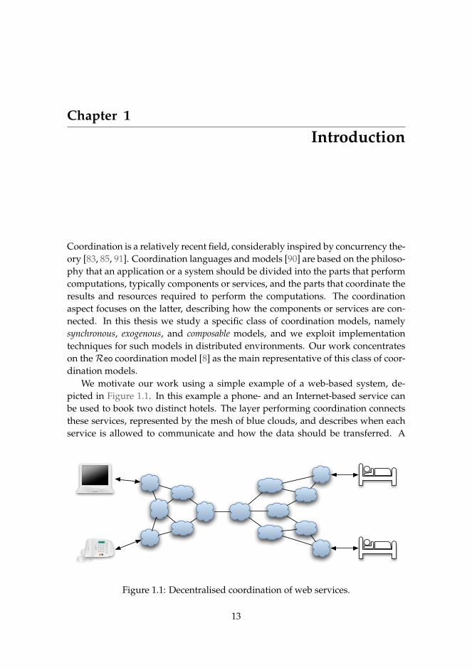
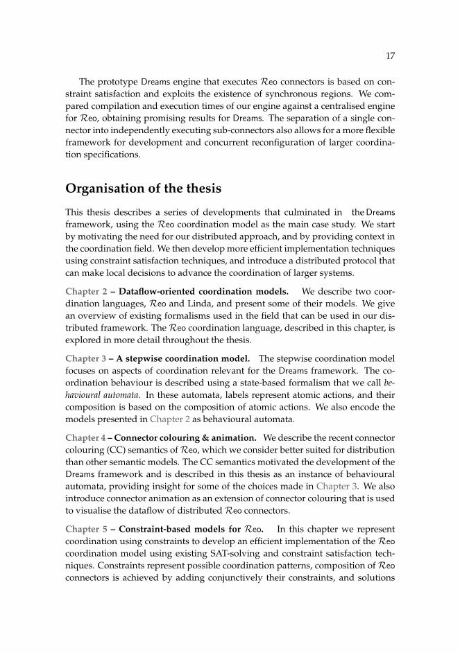
We motivate our work using a simple example of a web-based system, de-picted in Figure 1.1. In this example a phone- and an Internet-based service canbe used to book two distinct hotels. The layer performing coordination connectsthese services, represented by the mesh of blue clouds, and describes when eachservice is allowed to communicate and how the data should be transferred. A
Figure 1.1: Decentralised coordination of web services.
13
14 CHAPTER 1. INTRODUCTION
possible incarnation of the coordination layer is to allow either either the phone-or the Internet-based services to book a hotel at any given time, giving priority tothe phone when both services try to book a hotel simultaneously, and to alternatethe hotel that is booked. Many other alternative behaviours exist for our bookingexample.
In this thesis we target coordination models that are: (i) synchronous in thesense that the communication between elements is performed atomically in a per-round fashion, (ii) exogenous because the components or services are not aware ofthe coordination, which is described orthogonally, and (iii) composable since thebehaviour of the coordination layer can be completely described from its compo-sition of smaller building blocks. In our booking scenario, synchrony allows usto express, for example, that a request for booking a hotel using the phone-basedservice can only be sent if one of the hotels can receive this request. In Figure 1.1we emphasise the composability aspect using multiple clouds, each providing itsown contribution for the global behaviour. Furthermore, the existence of edgesbetween the clouds reflects our choice of a concurrent model for execution, whereeach cloud is regarded as an independent thread of computation that communi-cates only with its connected clouds.
In this thesis theReo coordination model is studied in detail. Reo is a channel-based coordination language with a graphical notation, introduced by Arbab in2001 [7], wherein complex connectors are built out of a simple set of primitiveconnectors. Compliant with our target,Reo is synchronous, exogenous, and com-posable, yielding an expressive and intuitive coordination model. TheReo modelis currently being used to specify coordination patterns and concurrent systems.More specifically, Reo has been used in a variety of different areas, such as sys-tems biology [36], service oriented computing [82], mashups [79], business pro-cess modelling [17, 103], model driven development [20], and multi-agent sys-tems [12]. Reo has also been extended to include, for example, timed behav-iour [13], probabilistic and stochastic models [21, 23, 88], quality of service [15],resource bounds [81], and reconfiguration [35, 72, 71, 77, 76]. Several tools havebeen developed to edit, verify, simulate, and execute Reo systems [16, 41, 75, 37].However, little effort has been spent so far on its (distributed) implementation as-pects.
Current engines that execute Reo [37, 16] allow the coordination layer to runonly in a single thread of execution, although the components can execute in par-allel or on a distributed platform. Furthermore, due to the synchrony aspect theseengines only support small systems, and do not scale. To address these limita-tions, our approach to implementReo-like models makes a tradeoff between pre-compiling the possible behaviour and calculating it at runtime. Furthermore, weexploit the fact that different parts of a connector can execute concurrently, andidentify parts of the system that can execute independently of each other.
15
Implementations of most models of concurrency and coordination typicallyinvolve synchronisation constructs. These constructs are either explicit, allowingthe users of a model to specify their own tailor-made synchrony, or implicit. Thisthesis supports the development of implementations that provide implicit syn-chronisation constructs, as well as the ones that, like Reo, support user-definedsynchrony. Our work contributes to the field of coordination, in particular toReo,by improving existing approaches to execute synchronisation models in three ma-jor ways:
1. by supporting decoupled execution and lightweight reconfiguration;
2. by increasing performance using constraint satisfaction techniques; and
3. by improving scalability by identifying synchronous regions.
We explain each of these three contributions in more detail below. Throughoutthis thesis we support our statements both in theory and in practice. We give for-mal arguments that show the correctness of our approach with respect to existingmodels, and present tools and benchmarks that confirm our claims.
Decoupled execution and lightweight reconfiguration
In this thesis we present the Dreams framework, a distributed framework for com-positional synchronous coordination models. The Dreams framework is based onthe actor model [1] and creates an actor for each building block of the coordinationmodel. Each actor consists of a concurrent thread of execution that communicatesasynchronously with other actors. We introduce a distributed protocol that allowsactors to reach consensus about data exchange, and performs the actual commu-nication of data. We developed a prototype Dreams engine to test this protocol,using an actor library for the Scala language [57].
Reconfiguring an instance of a coordination pattern consists of changing someof its parts. The Dreams framework assumes not only that the underlying coordi-nation model is compositional but also that it evolves in a stepwise manner. Thestepwise development combined with the decoupled execution of actors providethe necessary conditions for inexpensive reconfiguration, allowing systems thatare expected to be reconfigured frequently to do so in an incremental way, with-out requiring the full system to be changed. Reconfiguration of a small part ofthe system is independent of the execution or behaviour of unrelated parts of thesame system.
Coordination via constraint satisfaction
Computation within the Dreams framework evolves in a stepwise manner. In eachround, descriptions of the behaviour of all building blocks are combined and a
16 CHAPTER 1. INTRODUCTION
coordination pattern for the current round is chosen. In the case of the Reo coor-dination language, its present models do not come with an efficient (distributed)implementation technique. Hence, we develope a new semantic and executablemodel for Reo based on constraint satisfaction. A Reo connector is seen as a setof constraints, based on the way the primitives are connected and on their currentstate.
We identify the four main concepts that characterise coordination in Reo, viz.synchrony, data-awareness, state, and context dependency, and describe theseconcepts using logical constraints. Our approach is shown to be consistent withexisting Reo models. We apply available constraint satisfaction techniques to de-rive a more efficient implementation of Reo. Specifically, we developed an initialimplementation using a SAT-solver to search for possible solutions, and comparedits performance with an existingReo engine. The results strongly support the ideathat constraint satisfaction offers an appealing approach to implementing coordi-nation languages.
Scalability
Our stepwise approach to coordination is the first factor to contribute to the scal-ability of the Dreams framework. Implementations that require the knowledge ofall future actions, such as those based on a precomputed automaton, do not scale,since finding all possible behaviour for all possible states of a concurrent system,even when possible, can be very expensive and space inefficient. For example, thenumber of states generally doubles for every buffer in a connector, assuming allstates are reachable. In our approach infinite state spaces are excluded.
The coordination mechanism should be able to scale up to coordinate a largenumber of entities, possibly by exploiting multiple CPU cores or multiple com-puters across a network. Considering the behaviour for each round at a time isnot enough to achieve this level of scalability, because of the complexity of com-bining the behaviour of all entities. We improve scalability by identifying regionsthat can execute independently, thus achieving truly decoupled execution of con-nectors.
As mentioned above, we create an actor for each building block involved. Theresulting actors are organised in a graph structure, where edges represent com-munication links. We identify independent regions of the graph of actors, referredto as synchronous regions. Actors from each synchronous region can agree on thecoordination pattern to be executed at each round without considering the be-haviour of the actors outside of this region. Consequently, the constraint problemrepresenting the behaviour at each round is smaller and more easily solved. Weidentify these synchronous regions by recognising that some primitive connectorshave asynchronous behaviour, according to our formal characterisation of asyn-chronous behaviour.
17
The prototype Dreams engine that executes Reo connectors is based on con-straint satisfaction and exploits the existence of synchronous regions. We com-pared compilation and execution times of our engine against a centralised enginefor Reo, obtaining promising results for Dreams. The separation of a single con-nector into independently executing sub-connectors also allows for a more flexibleframework for development and concurrent reconfiguration of larger coordina-tion specifications.
Organisation of the thesis
This thesis describes a series of developments that culminated in the Dreams
framework, using the Reo coordination model as the main case study. We startby motivating the need for our distributed approach, and by providing context inthe coordination field. We then develop more efficient implementation techniquesusing constraint satisfaction techniques, and introduce a distributed protocol thatcan make local decisions to advance the coordination of larger systems.
Chapter 2 – Dataflow-oriented coordination models. We describe two coor-dination languages, Reo and Linda, and present some of their models. We givean overview of existing formalisms used in the field that can be used in our dis-tributed framework. The Reo coordination language, described in this chapter, isexplored in more detail throughout the thesis.
Chapter 3 – A stepwise coordination model. The stepwise coordination modelfocuses on aspects of coordination relevant for the Dreams framework. The co-ordination behaviour is described using a state-based formalism that we call be-havioural automata. In these automata, labels represent atomic actions, and theircomposition is based on the composition of atomic actions. We also encode themodels presented in Chapter 2 as behavioural automata.
Chapter 4 – Connector colouring & animation. We describe the recent connectorcolouring (CC) semantics ofReo, which we consider better suited for distributionthan other semantic models. The CC semantics motivated the development of theDreams framework and is described in this thesis as an instance of behaviouralautomata, providing insight for some of the choices made in Chapter 3. We alsointroduce connector animation as an extension of connector colouring that is usedto visualise the dataflow of distributedReo connectors.
Chapter 5 – Constraint-based models for Reo. In this chapter we representcoordination using constraints to develop an efficient implementation of the Reo
coordination model using existing SAT-solving and constraint satisfaction tech-niques. Constraints represent possible coordination patterns, composition of Reo
connectors is achieved by adding conjunctively their constraints, and solutions
18 CHAPTER 1. INTRODUCTION
to the constraints represent atomic actions that the system can perform. A com-parison between a prototype implementation using a SAT-solver and another ex-isting Reo engine based on connector colouring indicates the advantage of usingconstraint-solving techniques for coordination. We also present correctness proofswith respect to previousReo models, and make an extensive comparison of exist-ingReo models and implementation approaches.
Chapter 6 – Dreams framework. The Dreams chapter describes coordinationas an activity in a system of actors, where each actor is associated with a be-havioural automaton, and actors communicate with their neighbour actors us-ing asynchronous messages. We exploit the combination of the actor model withthe behavioural automata to partition the system of actors into synchronous re-gions. Actors within a synchronous region reach consensus before communicat-ing data values, while data exchanged between synchronous regions can be sentasynchronously. We formalise the correctness of this approach, and illustrate theintuition behind our approach usingReo.
Chapter 7 – Implementing Dreams This chapter describes the implementationdetails of the Dreams framework. We define how actors communicate with eachother, and describe the distributed protocol introduced in Dreams. To illustratethe protocol, we show traces of the execution of some Reo connectors in our dis-tributed framework. We also show how to use Dreams to deploy a connector in adistributed network, and we compare its performance against the performance ofa centralisedReo engine. The Dreams engine is integrated within an existingReo
toolkit [16].
The main contributions of this thesis result from two main observations re-garding the implementation of synchronous coordination models in a distributedenvironment. First, there is no need to pre-calculate all future behaviour at com-pile-time: shifting part of this computation to run-time increases scalability andeases reconfiguration. Second, not all communication in a synchronous system isperformed synchronously. By identifying parts with asynchronous communica-tion we can restrict the synchronisation process to smaller parts of the coordina-tion layer, thereby improving the overall performance of the coordination engine.
Chapter 2
Dataflow-oriented coordination models
2.1 Introduction
In a survey of coordination languages [10], Arbab distinguishes three differentapproaches to coordination: a data-oriented, a control-oriented, and a dataflow-oriented approach. The main goal of most data-oriented approaches is to providea mechanism to guarantee consistency among shared data. The code for coordi-nation and computation can be combined, without losing the separation of thesetwo concerns. In control-driven approaches the separation of coordination andcomputation is more explicit. The main focus of control-driven approaches is theprocessing or flow of control, and often the notion of a data value is not evenrequired. Finally, dataflow-oriented approaches sit between data- and control-oriented approaches, managing who can communicate, where data flow, and whatdata values are sent.
The most relevant work in this thesis results from an effort to implement adistributed engine for the Reo [8, 9] coordination language. The coordinationsurvey mentioned above refers to Reo as a dataflow-driven coordination model.An earlier survey by Arbab and Papadopoulos [90] also classifies Manifold [28],a predecessor of Reo, as a dataflow-driven coordination model. The implemen-tation approach taken in this thesis fits within a general dataflow-driven view ofcoordination languages.
In this chapter we describe different coordination languages and explain data-flow-driven aspects later in this thesis. We start by describing two important se-mantic models for Reo followed by two similar semantic models for Linda. InChapter 3 we will introduce the so-called stepwise coordination model to captureour view of dataflow-driven models, and we will present encodings of each ofthe coordination models described in this chapter into the stepwise coordinationmodel.
In this thesis, the Reo coordination language plays a more relevant role than
19
20 CHAPTER 2. DATAFLOW-ORIENTED COORDINATION MODELS
the other concrete models, as we use it as our main case-study for our distributedimplementation. We emphasise the Reo coordination language, since it is themain motivator of the work developed in this thesis. We describeReo in §2.2. Wedescribe the Linda coordination language in §2.3, be it less detailed Linda [54] isprobably the first and definitely the best known coordination model, categorisedin the surveys mentioned above as a data-oriented coordination model.
As Arbab and Papadopoulos indicate, the separation of data-driven vs. con-trol-driven coordination is not a clear cut one. For example, data-driven coordi-nation languages can be used in application domains where the data control theexecution of the components, and vice-versa. Dataflow-driven approaches sit be-tween control- and data-driven approaches, hence their separation is also not veryclear. We continue to explore the dataflow-oriented aspects of Linda in Chapter 3by presenting an encoding of Linda into the stepwise model, which follows a typ-ical dataflow-driven approach.
Contribution This chapter takes the first step toward the main goal of this thesis:an efficient distributed implementation of a synchronous coordination model. Theimplemented model, called the stepwise coordination model, is described in thenext chapter. In this chapter we present existing coordination models that can beencoded into the stepwise model. Furthermore, the stepwise model leaves someaspects partially unspecified, which depend on the concrete model being encodedinto the stepwise model.
2.2 Reo
Reo [8, 9] is presented as a channel-based coordination language wherein com-ponent connectors are compositionally constructed out of an open set of primitiveconnectors, also simply called primitives. Channels are special primitives with twoends. In this thesis we use a fixed set of primitives to illustrate the Reo language,although user defined primitives are also possible. Being able to compose connec-tors out of smaller primitives is one of the strengths ofReo. It allows, for example,multi-party synchronisation to be expressed as a composition of simple channels.Ends of primitives are regarded as ports. In addition,Reo has a graphical notationthat helps to bring some intuition about the behaviour of a connector, particularlyin conjunction with animation tools, which we will cover in more detail in §4.6.
MostReo-related tools are being integrated in a common framework known asEclipse Coordination Tools (ECT) [16]. The tools included in the ECT frameworkcomprise a Reo editor, an animation generator, model checkers, editors of Reo-specific automata, QoS modelling and analysis tools, and a code generator.
The behaviour of connectors is described in terms of dataflow through thechannels and the nodes connecting them, along with the synchronisation and mu-
2.2. REO 21
tual exclusion constraints they that impose. Components attached at the bound-ary of a connector either attempt to write data to or read data from the ends ofthe channels that they are connected to. The connector coordinates the compo-nents by determining when the writes and takes succeed, often by synchronisinga collection of such actions. Data flow from an end of a primitive to an end ofanother primitive to which it is connected, thus synchronising the two ends. Aprimitive decides, possibly non-deterministically, whether data is accepted or of-fered on an end based on the dataflow on its other ends and its state. In principle,data continue to flow like this through the connector, with primitives routing thedata based on their internal behavioural constraints and the possibilities offeredby the surrounding context. Primitives are executed by locally synchronising ac-tions or by excluding the possibility of actions occurring synchronously. These‘constraints’ are propagated through the connector, under the restriction that theonly communication between entities occurs through the channels. Consequently,the behaviour of a system depends upon the combined choices of primitives andwhat possibilities the components offer, none of which is known locally to theprimitives.
This section discusses the Reo language as follows. We start by giving a gen-eral description of Reo in §2.2.1 to introduce the main concepts, the visual nota-tion, and some motivating examples. We follow this general description by twoautomata models that give a precise and formal semantics to Reo. In §2.2.2 wepresent the constraint automata model, which emphasises how the value of datacan affect the dataflow. In §2.2.3 we present a more recent model that focuses onhow the availability of dataflow can affect the behaviour, known in the Reo com-munity as context dependency. Later in Chapters 4 and 5 we present two moreapproaches to describeReo.
2.2.1 General description
Reo connectors are constructed by composing more primitive connectors. Eachprimitive offers a variety of behavioural policies regarding synchronisation, buff-ering, lossiness, and even the direction of dataflow. Communication with a prim-itive occurs through its ports, called ends: primitives consume data through theirsource ends, and produce data through their sink ends. Source and sink ends cor-respond to the notion of source and sink in directed graphs, although the namesinput and output ends are sometimes used instead. Primitives are not only a meansfor communication, but they also impose relational constraints, such as synchroni-sation or mutual exclusion, on the timing of dataflow on their ends. The behaviourof such primitives is limited only by the model underlying a givenReo implemen-tation. For the purpose of this thesis, we do not distinguish between primitivessuch as channels used for coordination and the components being coordinated.Typically, the ‘coordinator’ has more control over the choice of the behaviour of
22 CHAPTER 2. DATAFLOW-ORIENTED COORDINATION MODELS
primitives, whereas component behaviour is externally determined.We present a description of Reo’s semantics in terms of general constraints.
The first thing to note is that the behaviour of each primitive depends upon itscurrent state.1 The semantics of a connector is described as a collection of possiblesteps for each state, and we call the change of state of the connector triggered byone of these steps a round. Dataflow on a primitive’s end occurs when a singledatum is passed through that end. Within any round dataflow may occur on somenumber of ends. The semantics of a connector is defined in terms of two kinds ofconstraints:
Synchronisation constraints describe the sets of ends that can be synchronisedin a particular step. For example, synchronous channel types typically permitdataflow either on both of their ends or on neither end, and asynchronous channeltypes typically permit dataflow on at most one of their two ends.
Dataflow constraints describe the data flowing on the ends that synchronise. Forexample, such a constraint may say that the data item flowing on the source end ofa synchronous channel is the same as the data item flowing on its sink end; or thatthere is no constraint on the dataflow, such as for a drain which simply discardsits data; or it may say that the data satisfies a particular predicate, as in the case ofa filter channel.
Connectors are formed by plugging the ends of primitives together in a one-to-one fashion to form nodes. A node is a logical place consisting of a sink end,a source end, or both a sink and a source end.2 We call nodes with a single endboundary nodes, represented by , and we call nodes with a sink end and a sourceend mixed nodes, represented by . Data flow through a connector from primi-tive to primitive through nodes, subject to the constraint that nodes cannot bufferdata. This means that the two ends in a node are synchronised and have the samedataflow—behaviourally, they are equal. Nodes can be handled transparently byusing the same name for the two ends on the node, as the synchronisation anddataflow at the two ends is identical.
We now give an informal description of some of the most commonly usedReo primitives. Note that for all of these primitives, no dataflow is one of thebehavioural possibilities.
1Note that mostReo primitives presented here have a single state.2Generalised nodes with multiple sink and source ends can be represented using binary mergers
and replicators [22, 37].
2.2. REO 23
ab
c
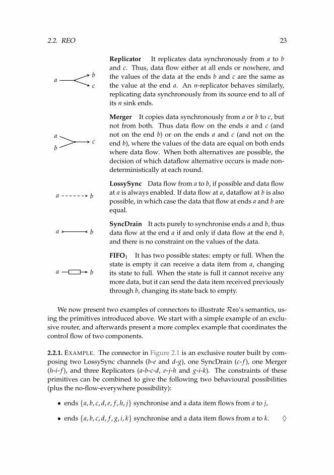
Replicator It replicates data synchronously from a to band c. Thus, data flow either at all ends or nowhere, andthe values of the data at the ends b and c are the same asthe value at the end a. An n-replicator behaves similarly,replicating data synchronously from its source end to all ofits n sink ends.
ca
b
Merger It copies data synchronously from a or b to c, butnot from both. Thus data flow on the ends a and c (andnot on the end b) or on the ends a and c (and not on theend b), where the values of the data are equal on both endswhere data flow. When both alternatives are possible, thedecision of which dataflow alternative occurs is made non-deterministically at each round.
a b
LossySync Data flow from a to b, if possible and data flowat a is always enabled. If data flow at a, dataflow at b is alsopossible, in which case the data that flow at ends a and b areequal.
a bSyncDrain It acts purely to synchronise ends a and b, thusdata flow at the end a if and only if data flow at the end b,and there is no constraint on the values of the data.
a b
FIFO1 It has two possible states: empty or full. When thestate is empty it can receive a data item from a, changingits state to full. When the state is full it cannot receive anymore data, but it can send the data item received previouslythrough b, changing its state back to empty.
We now present two examples of connectors to illustrate Reo’s semantics, us-ing the primitives introduced above. We start with a simple example of an exclu-sive router, and afterwards present a more complex example that coordinates thecontrol flow of two components.
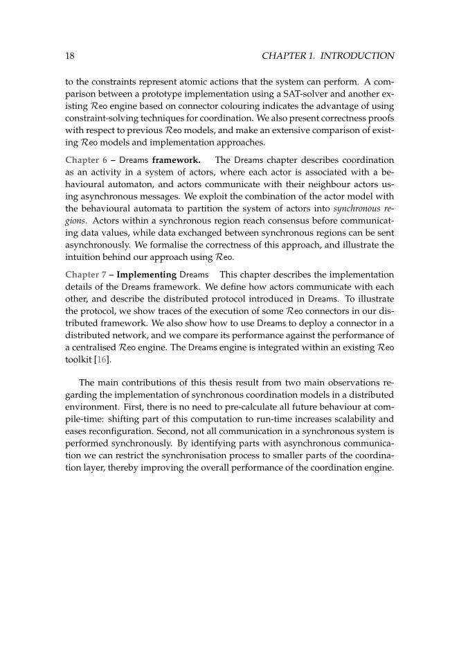
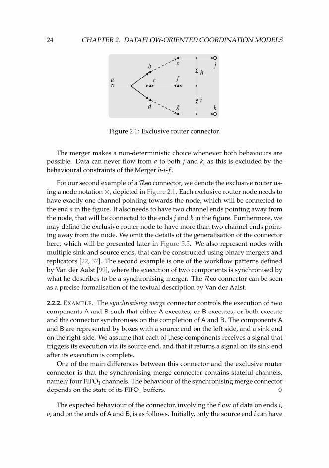
2.2.1. EXAMPLE. The connector in Figure 2.1 is an exclusive router built by com-posing two LossySync channels (b-e and d-g), one SyncDrain (c- f ), one Merger(h-i- f ), and three Replicators (a-b-c-d, e-j-h and g-i-k). The constraints of theseprimitives can be combined to give the following two behavioural possibilities(plus the no-flow-everywhere possibility):
• ends {a, b, c, d, e, f , h, j} synchronise and a data item flows from a to j,
• ends {a, b, c, d, f , g, i, k} synchronise and a data item flows from a to k. ♦
24 CHAPTER 2. DATAFLOW-ORIENTED COORDINATION MODELS
a c
b
d
f
e
g
h
i
j
k
Figure 2.1: Exclusive router connector.
The merger makes a non-deterministic choice whenever both behaviours arepossible. Data can never flow from a to both j and k, as this is excluded by thebehavioural constraints of the Merger h-i- f .
For our second example of aReo connector, we denote the exclusive router us-ing a node notation⊗, depicted in Figure 2.1. Each exclusive router node needs tohave exactly one channel pointing towards the node, which will be connected tothe end a in the figure. It also needs to have two channel ends pointing away fromthe node, that will be connected to the ends j and k in the figure. Furthermore, wemay define the exclusive router node to have more than two channel ends point-ing away from the node. We omit the details of the generalisation of the connectorhere, which will be presented later in Figure 5.5. We also represent nodes withmultiple sink and source ends, that can be constructed using binary mergers andreplicators [22, 37]. The second example is one of the workflow patterns definedby Van der Aalst [99], where the execution of two components is synchronised bywhat he describes to be a synchronising merger. The Reo connector can be seenas a precise formalisation of the textual description by Van der Aalst.
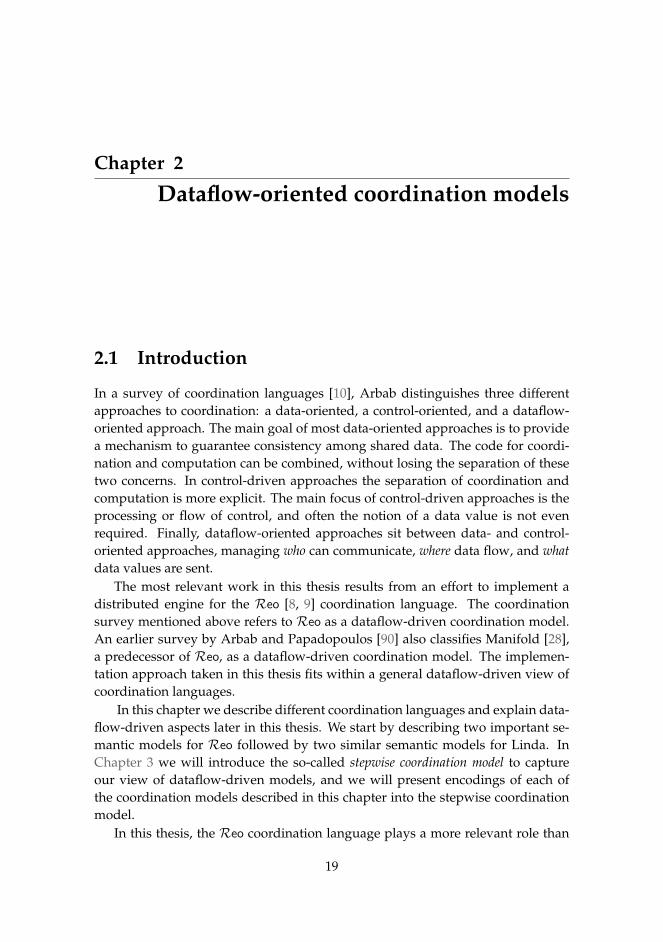
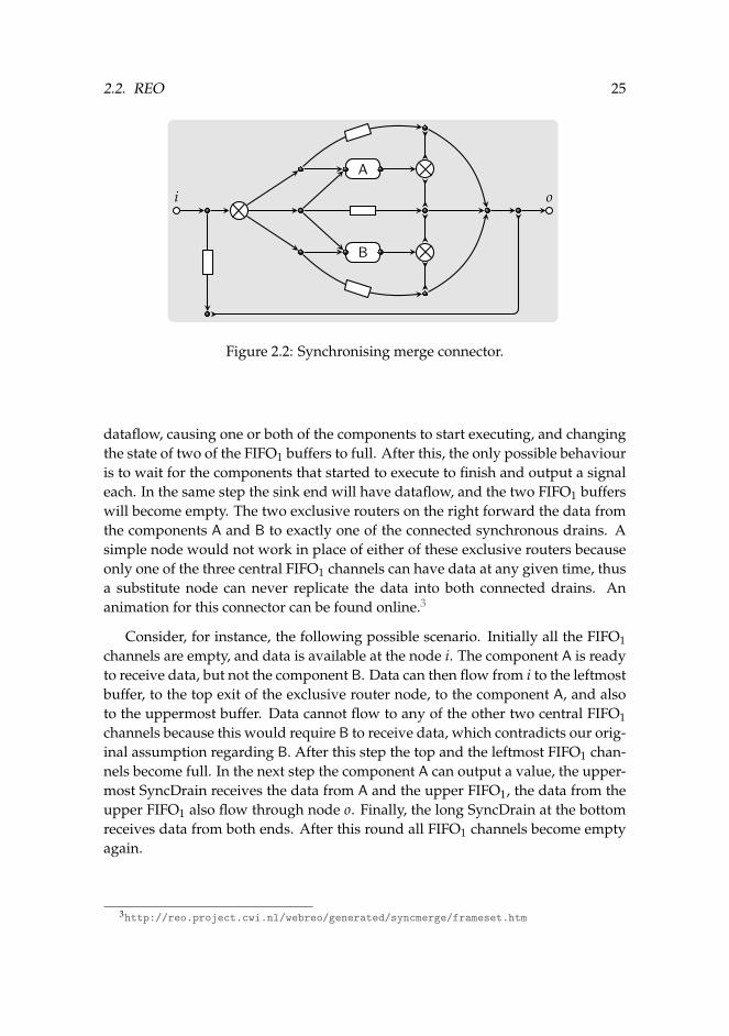
2.2.2. EXAMPLE. The synchronising merge connector controls the execution of twocomponents A and B such that either A executes, or B executes, or both executeand the connector synchronises on the completion of A and B. The components A
and B are represented by boxes with a source end on the left side, and a sink endon the right side. We assume that each of these components receives a signal thattriggers its execution via its source end, and that it returns a signal on its sink endafter its execution is complete.
One of the main differences between this connector and the exclusive routerconnector is that the synchronising merge connector contains stateful channels,namely four FIFO1 channels. The behaviour of the synchronising merge connectordepends on the state of its FIFO1 buffers. ♦
The expected behaviour of the connector, involving the flow of data on ends i,o, and on the ends of A and B, is as follows. Initially, only the source end i can have
2.2. REO 25
i o
A
B
Figure 2.2: Synchronising merge connector.
dataflow, causing one or both of the components to start executing, and changingthe state of two of the FIFO1 buffers to full. After this, the only possible behaviouris to wait for the components that started to execute to finish and output a signaleach. In the same step the sink end will have dataflow, and the two FIFO1 bufferswill become empty. The two exclusive routers on the right forward the data fromthe components A and B to exactly one of the connected synchronous drains. Asimple node would not work in place of either of these exclusive routers becauseonly one of the three central FIFO1 channels can have data at any given time, thusa substitute node can never replicate the data into both connected drains. Ananimation for this connector can be found online.3
Consider, for instance, the following possible scenario. Initially all the FIFO1channels are empty, and data is available at the node i. The component A is readyto receive data, but not the component B. Data can then flow from i to the leftmostbuffer, to the top exit of the exclusive router node, to the component A, and alsoto the uppermost buffer. Data cannot flow to any of the other two central FIFO1channels because this would require B to receive data, which contradicts our orig-inal assumption regarding B. After this step the top and the leftmost FIFO1 chan-nels become full. In the next step the component A can output a value, the upper-most SyncDrain receives the data from A and the upper FIFO1, the data from theupper FIFO1 also flow through node o. Finally, the long SyncDrain at the bottomreceives data from both ends. After this round all FIFO1 channels become emptyagain.
3http://reo.project.cwi.nl/webreo/generated/syncmerge/frameset.htm
26 CHAPTER 2. DATAFLOW-ORIENTED COORDINATION MODELS
2.2.2 Constraint automata
Constraint automata (CA) formalise the behaviour and the dataflow in aReo con-nector that controls the interaction of a set of anonymous components. Baier etal. [22] show that constraint automata can serve as a computational model forReo, using a coalgebraic semantics forReo connectors that assigns to a connectora relation over infinite timed data streams.
In this section we describe constraint automata and their composition. Thecomposition will be used later in this thesis in two ways. First, the next section de-fines the encoding of the constraint automata model in our behavioural automatamodel. The composition of the behavioural automata thus obtained from con-straint automata is based on the composition of constraint automata. Second, inChapter 5 we use constraint automata to show compositionality of the constraint-based model forReo.
Constraint automata use a finite set of port names N = {x1, . . . , xn}, where xiis the i-th port of a connector. When clear from the context, we write xyz insteadof {x, y, z} to enhance readability. We write xi to represent the data value flowingthrough the port xi, and use N to denote the set of data variables {x1, . . . , xn},for each xi ∈ N . We define DCX for each X ⊆ N to be a set of data constraintsover the variables in X, where the underlying data domain is a finite set D. Dataconstraints in DCN can be viewed as a symbolic representation of sets of data-assignments, and are generated by the following grammar:
g ::= tt∣∣ x = d
∣∣ g1 ∨ g2∣∣ ¬g
where x ∈ N and d ∈ D. The other logical connectives can be encoded as usual.We use the notation a = b as a shorthand for the constraint
(a = d1 ∧ b = d1) ∨ . . . ∨ (a = dn ∧ b = dn),
with D = {d1, . . . , dn}.
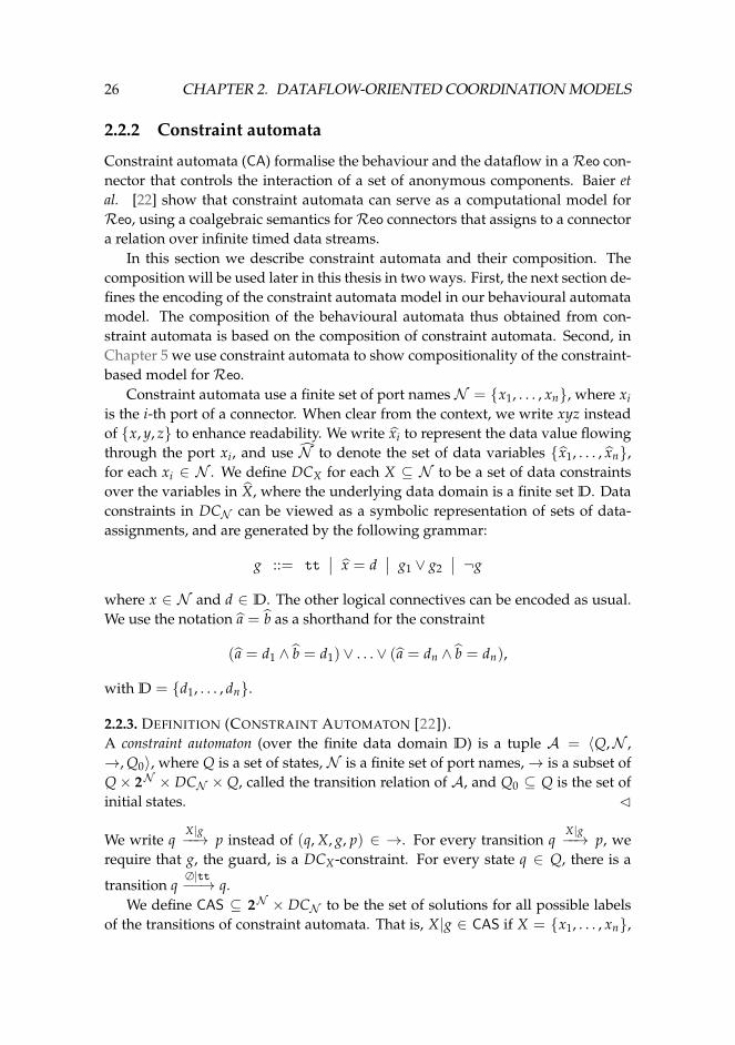
2.2.3. DEFINITION (CONSTRAINT AUTOMATON [22]).A constraint automaton (over the finite data domain D) is a tuple A = 〈Q,N ,→, Q0〉, where Q is a set of states, N is a finite set of port names,→ is a subset ofQ× 2N × DCN × Q, called the transition relation of A, and Q0 ⊆ Q is the set ofinitial states. C
We write qX|g−−→ p instead of (q, X, g, p) ∈ →. For every transition q
X|g−−→ p, werequire that g, the guard, is a DCX-constraint. For every state q ∈ Q, there is a
transition q∅|tt−−→ q.
We define CAS ⊆ 2N × DCN to be the set of solutions for all possible labelsof the transitions of constraint automata. That is, X|g ∈ CAS if X = {x1, . . . , xn},
2.2. REO 27
LossySync FIFO1
q
a tt
ab a = b
empty full(d)
b b = d
c c = d
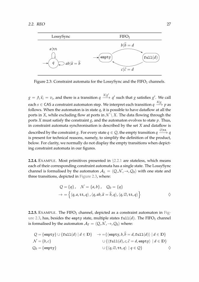
Figure 2.3: Constraint automata for the LossySync and the FIFO1 channels.
g =∧
xi = vi, and there is a transition qX|g′−−→ q′ such that g satisfies g′. We call
each s ∈ CAS a constraint automaton step. We interpret each transition qX|g−−→ p as
follows. When the automaton is in state q, it is possible to have dataflow at all theports in X, while excluding flow at ports in N \ X. The data flowing through theports X must satisfy the constraint g, and the automaton evolves to state p. Thus,in constraint automata synchronisation is described by the set X and dataflow is
described by the constraint g. For every state q ∈ Q, the empty transition q∅|tt−−→ q
is present for technical reasons, namely, to simplify the definition of the product,below. For clarity, we normally do not display the empty transitions when depict-ing constraint automata in our figures.
2.2.4. EXAMPLE. Most primitives presented in §2.2.1 are stateless, which meanseach of their corresponding constraint automata has a single state. The LossySyncchannel is formalised by the automaton AL = 〈Q,N ,→, Q0〉 with one state andthree transitions, depicted in Figure 2.3, where:
Q = {q} , N = {a, b} , Q0 = {q}
→ ={〈q, a, tt, q〉 , 〈q, ab, a = b, q〉, 〈q, ∅, tt, q〉
}♦
2.2.5. EXAMPLE. The FIFO1 channel, depicted as a constraint automaton in Fig-ure 2.3, has, besides the empty state, multiple states full(d). The FIFO1 channelis formalised by the automaton AF = 〈Q,N ,→, Q0〉 where:
Q = {empty} ∪ {full(d) | d ∈ D} → ={〈empty, b, b = d, full(d)〉 | d ∈ D}N = {b, c} ∪ {〈full(d), c, c = d, empty〉 | d ∈ D}Q0 = {empty} ∪ {〈q, ∅, tt, q〉 | q ∈ Q} ♦
28 CHAPTER 2. DATAFLOW-ORIENTED COORDINATION MODELS
Composition
Common port names correspond to the places where connectors are joined. Notethat Reo connectors can only be composed by connecting source ports to sinkports, such that each port is connected to at most one other port. Therefore, whencomposing two constraint automataA1 andA2 representing twoReo connectors,we require that common ports must be source ports in one connector and sinkports in the other. However, the constraint automata model does not distinguishsource and sink ends, and the restriction is only required forReo connectors.
2.2.6. DEFINITION (PRODUCT OF CONSTRAINT AUTOMATA [22]).Let A1 and A2 be two constraint automata, where Ai = 〈Qi,Ni,→i, Q0,i〉 for i ∈{1, 2}. The composition of A1 and A2 yields the constraint automaton
A1 ./ A2 = 〈Q1 ×Q2,N1 ∪N2,→, Q0,1 ×Q0,2〉 ,
where the transition relation→ is given by the condition below.
(q1, q2)X1∪X2|g1∧g2−−−−−−−→ (p1, p2) iff
q1X1|g1−−−→1 p1, q2
X2|g2−−−→2 p2, and X1 ∩N2 = X2 ∩N1 C
The requirement X1 ∩N2 = X2 ∩N1 states that the steps X1|g1 and X2|g2 can onlybe combined into a new transition in the automaton A1 ./ A2 when they agreeon the firing of all of their common ports in these transitions. I.e., for all portsx ∈ N1 ∩N2 it holds that x ∈ X1 ⇔ x ∈ X2.
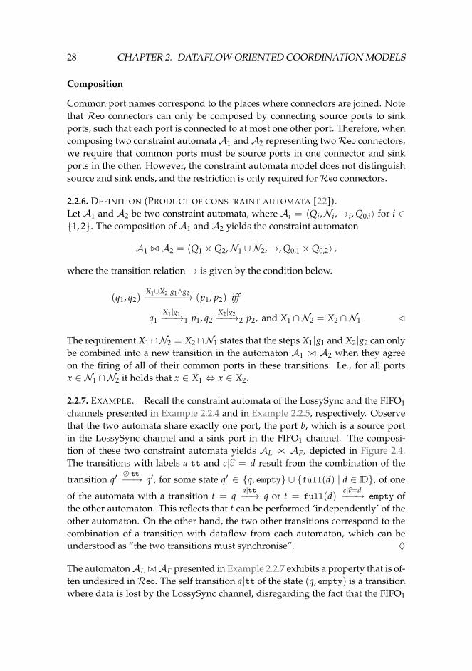
2.2.7. EXAMPLE. Recall the constraint automata of the LossySync and the FIFO1channels presented in Example 2.2.4 and in Example 2.2.5, respectively. Observethat the two automata share exactly one port, the port b, which is a source portin the LossySync channel and a sink port in the FIFO1 channel. The composi-tion of these two constraint automata yields AL ./ AF, depicted in Figure 2.4.The transitions with labels a|tt and c|c = d result from the combination of the
transition q′∅|tt−−→ q′, for some state q′ ∈ {q, empty} ∪ {full(d) | d ∈ D}, of one
of the automata with a transition t = qa|tt−−→ q or t = full(d)
c|c=d−−−→ empty ofthe other automaton. This reflects that t can be performed ‘independently’ of theother automaton. On the other hand, the two other transitions correspond to thecombination of a transition with dataflow from each automaton, which can beunderstood as “the two transitions must synchronise”. ♦
The automatonAL ./ AF presented in Example 2.2.7 exhibits a property that is of-ten undesired inReo. The self transition a|tt of the state (q, empty) is a transitionwhere data is lost by the LossySync channel, disregarding the fact that the FIFO1
2.2. REO 29
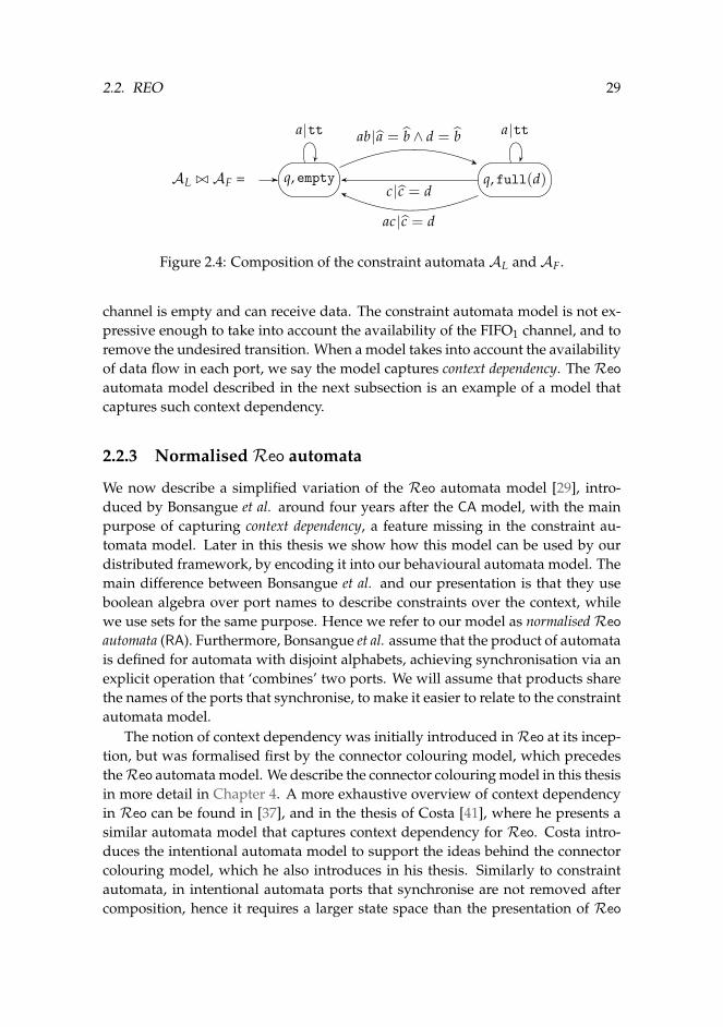
AL ./ AF = q, empty q, full(d)
a tt a ttab a = b ∧ d = b
c c = d
ac c = d
Figure 2.4: Composition of the constraint automata AL and AF.
channel is empty and can receive data. The constraint automata model is not ex-pressive enough to take into account the availability of the FIFO1 channel, and toremove the undesired transition. When a model takes into account the availabilityof data flow in each port, we say the model captures context dependency. The Reo
automata model described in the next subsection is an example of a model thatcaptures such context dependency.
2.2.3 NormalisedReo automata
We now describe a simplified variation of the Reo automata model [29], intro-duced by Bonsangue et al. around four years after the CA model, with the mainpurpose of capturing context dependency, a feature missing in the constraint au-tomata model. Later in this thesis we show how this model can be used by ourdistributed framework, by encoding it into our behavioural automata model. Themain difference between Bonsangue et al. and our presentation is that they useboolean algebra over port names to describe constraints over the context, whilewe use sets for the same purpose. Hence we refer to our model as normalised Reo
automata (RA). Furthermore, Bonsangue et al. assume that the product of automatais defined for automata with disjoint alphabets, achieving synchronisation via anexplicit operation that ‘combines’ two ports. We will assume that products sharethe names of the ports that synchronise, to make it easier to relate to the constraintautomata model.
The notion of context dependency was initially introduced inReo at its incep-tion, but was formalised first by the connector colouring model, which precedestheReo automata model. We describe the connector colouring model in this thesisin more detail in Chapter 4. A more exhaustive overview of context dependencyin Reo can be found in [37], and in the thesis of Costa [41], where he presents asimilar automata model that captures context dependency for Reo. Costa intro-duces the intentional automata model to support the ideas behind the connectorcolouring model, which he also introduces in his thesis. Similarly to constraintautomata, in intentional automata ports that synchronise are not removed aftercomposition, hence it requires a larger state space than the presentation of Reo
30 CHAPTER 2. DATAFLOW-ORIENTED COORDINATION MODELS
automata by Bonsangue et al. where these ports are discarded. Costa also givesa precise formalisation of the hiding operation of ports as intended initially [19].We do not consider this in this thesis because it does not influence the distributedimplementation of connectors.
Recall the constraint automaton AL ./ AF from Example 2.2.7. To avoid theundesired behaviour where data is lost when the FIFO1 buffer is empty the con-straint automata model is extended to capture context dependency, by addingexplicitly the context information to the transitions. Two important examples ofReo primitives that could not be represented in the CA model are:
Context-dependent LossySync This channel loses data written to its source onlyif the surrounding context is unable to accept the data through its sink; otherwisethe data flow through the channel. This corresponds to the initial intention of theLossySync channel [8].
Priority merger This is a special variant of a merger that favours one of its sinkports: if dataflow is possible at both sink ports, it prefers one port over the other.
The Reo automata model, when compared to the constraint automata model,abstracts away from data and introduces guards to capture the context in whicha Reo primitive is evaluated. In normalised Reo automata we assume that theproduct of automata synchronises and hides ports with shared names, followingthe convention of the Reo automata model, and the context is described by setsof literals. When possible, we keep the same notation as in the Reo automata pa-per [29], while trying to preserve the naming notation of the constraint automatamodel.
Normalised Reo automata use a finite set of port names N = {x1, ..., xn} asin constraint automata. A guard g is a set {a1, . . . , ak} of literals derived from N ,where ai ∈ {xi, xi} and xi ∈ N . We denote the set of all literals of N as LtN ,and X = {x1, . . . , xm}, where X = {x1, . . . , xm} is a set of ports. Observe that g ∈N ∪ N . A guard represents which ports have data available to flow, and whichports cannot have data available. The extra knowledge about the (im)possibility ofdataflow expressed by the guards characterises the context dependency modelledby the Reo automata model. As for constraint automata, we often write a1 . . . akinstead of {a1, . . . , ak} and g1g2 instead of g1 ∪ g2.
2.2.8. DEFINITION (NORMALISED Reo AUTOMATON [29]).A normalisedReo automaton over an alphabetN is a tripleA = 〈Q,N ,→〉whereQ is a finite set of states, and→ is a subset of Q× LtN × 2N ×Q called the transi-tion relation of A, such that for each 〈q, g, X, q′〉 ∈ → the context property X ⊆ gholds.4 C
4The original definition of the Reo automata model by Bonsangue et al. refers to the context prop-erty as reactivity property, and also includes a uniformity property, which they use to distinguish between
2.2. REO 31
Context dependentLossySync
PriorityMerger FIFO1
q
ab abab a
q
ac acabc bc
empty full
b b
c c
Figure 2.5: Normalised Reo automata of the context dependent LossySync, thepriority merger, and the FIFO1 primitives.
We write qg|X−−→ q′ as a shorthand for 〈q, g, X, q′〉 ∈ →. Informally, a normalised
Reo automaton over an alphabetN is a non-deterministic automaton with transi-tion labels RAS = LtN × 2N (Reo automata steps) that obey the context property.The intuition is that for each label g|X ∈ RAS the ports in X have dataflow when
the context respects g. For example, the transition qab|a−−→ q′ can be read as “the
automaton can evolve from q to q′ by having dataflow on a when the context isready to have dataflow on a and the context refuses dataflow on b (for the currentround)”. The context property reflects the fact that a port can have dataflow onlywhen the context is ready to accommodate it.
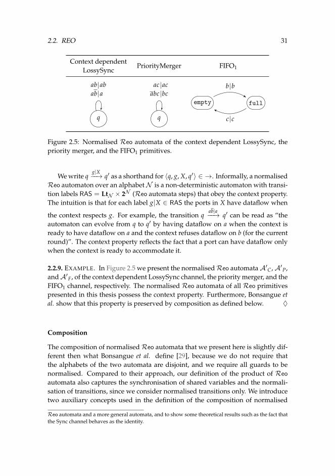
2.2.9. EXAMPLE. In Figure 2.5 we present the normalisedReo automataA′C,A′P,andA′F, of the context dependent LossySync channel, the priority merger, and theFIFO1 channel, respectively. The normalised Reo automata of all Reo primitivespresented in this thesis possess the context property. Furthermore, Bonsangue etal. show that this property is preserved by composition as defined below. ♦
Composition
The composition of normalisedReo automata that we present here is slightly dif-ferent then what Bonsangue et al. define [29], because we do not require thatthe alphabets of the two automata are disjoint, and we require all guards to benormalised. Compared to their approach, our definition of the product of Reo
automata also captures the synchronisation of shared variables and the normali-sation of transitions, since we consider normalised transitions only. We introducetwo auxiliary concepts used in the definition of the composition of normalised
Reo automata and a more general automata, and to show some theoretical results such as the fact thatthe Sync channel behaves as the identity.
32 CHAPTER 2. DATAFLOW-ORIENTED COORDINATION MODELS
Reo automata: (1) the set of unsatisfiable guards for a state q, denoted by q#, andthe (2) compatibility of two guards g1 and g2, denoted by g1
_ g2.Given a state q of a normalisedReo automaton A = 〈Q,N ,→〉, we define the
set of satisfiable guards of q as follows:
guards(q) = {g | q g|X−−→ q′}. (2.1)
We now define the set q# of all unsatisfiable guards based on guards(q):
q# = {a1 · · · an | guards(q) = {g1, . . . , gn} , ∀i∈1..n · ai ∈ gi} , (2.2)
where for any x ∈ N , x = x. Therefore the set of all unsatisfiable guards con-sists of all possible combinations of the negations of literals from each reachabletransition.
A remark is in order regarding the correctness of our definition of q# withrespect to the definition of q# presented in the original paper by Bonsangue et al.[29]. Let (·)◦ be a function that maps guards to logical formulæ in disjunctivenormal form:{
a11 · · · a1m1 , . . . , an1 · · · anmi
}◦= (a11 ∧ · · · ∧ a1m1) ∨ . . . ∨ (anm1 ∧ · · · ∧ anmi ),
where each aik is a literal and n, mi, i ∈N. Let q† = ¬(guards(q)◦) be the definitionof q# in the original formulation of Reo automata [29]. We prove that the twodefinitions of q#, i.e., q# as defined above and q†, are equivalent. Before relating q†
to q# we establish an auxiliary result.
2.2.10. LEMMA. Let{
aij | 1 ≤ i ≤ n, 1 ≤ j ≤ mi}
be a set of literals. Then
n∧i=1
mi∨j=1
aij
=∨{
n∧i=1
aij
∣∣∣ 1 ≤ j ≤ mi
}.
Proof. We proceed by induction on n. The base case when n = 1 is trivial. As tothe induction step, using the distributive laws for ∧ and ∨:
∧n+1i=1
(∨mij=1 aij
)=∧n
i=1
(∨mij=1 aij
)∧(∨mn+1
j=1 an+1,j
)=∨ {∧n
i=1 aij∣∣ 1 ≤ j ≤ mi
}∧(∨mn+1
k=1 an+1,k
)=∨mn+1
k=1
(∨ {∧ni=1 aij
∣∣ 1 ≤ j ≤ mi}∧ an+1,k
)=∨mn+1
k=1
(∨ {∧ni=1 aij ∧ an+1,k
∣∣ 1 ≤ j ≤ mi})
=∨ {∧n
i=1 aij ∧ an+1,k∣∣ 1 ≤ j ≤ mi, 1 ≤ k ≤ mn+1
}=∨{∧n+1
i=1 aij∣∣ 1 ≤ j ≤ mi
}. 2
Based on Lemma 2.2.10 we have the following.
2.2. REO 33
2.2.11. PROPERTY. q† = (q#)◦.
Proof. Suppose guards(q) = {g1, . . . , gn}, and let gi = ai1 · · · aimi , for i ∈ 1..n. Onthe one hand, by the definitions and the De Morgan laws we have:
q† = ¬(guards(q)◦) = ¬n∨
i=1
mi∧j=1
aij =n∧
i=1
mi∨j=1
aij.
On the other hand, by the definition of (·)◦ we have
(q#)◦ =∨{
n∧i=1
ai
∣∣∣ ai ∈ gi
}=
∨{n∧
i=1
aij
∣∣∣ 1 ≤ j ≤ mi
}
because ai ∈ gi if and only if ai = aij for some j where 1 ≤ j ≤ mi. Now theproperty follows directly from Lemma 2.2.10. 2
Finally, we define the compatibility of two guards g1 and g2 in N ∪N , written asg1
_ g2, as follows.
g1_ g2 ⇐⇒ g1 ∩ g2 ⊆ N ∧ ∀a ∈ g1g2 · a /∈ g1g2.
The first part of the definition of g1_ g2 states that g1 and g2 cannot expect the
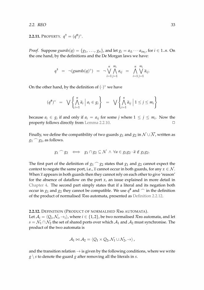
context to negate the same port, i.e., x cannot occur in both guards, for any x ∈ N .When x appears in both guards then they cannot rely on each other to give ‘reason’for the absence of dataflow on the port x, an issue explained in more detail inChapter 4. The second part simply states that if a literal and its negation bothoccur in g1 and g2 they cannot be compatible. We use q# and _ in the definitionof the product of normalisedReo automata, presented as Definition 2.2.12.
2.2.12. DEFINITION (PRODUCT OF NORMALISED Reo AUTOMATA).Let Ai = 〈Qi,Ni,→i〉, where i ∈ {1, 2}, be two normalisedReo automata, and lets = N1 ∩N2 the set of shared ports over which A1 and A2 must synchronise. Theproduct of the two automata is
A1 ./ A2 = 〈Q1 ×Q2,N1 ∪N2,→〉 ,
and the transition relation→ is given by the following conditions, where we writeg \ s to denote the guard g after removing all the literals in s.
34 CHAPTER 2. DATAFLOW-ORIENTED COORDINATION MODELS
(q1, q2)g1g2\ss |X1X2\s−−−−−−−−−→ (p1, p2) if
q1g1|X1−−−→1 p1, q2
g2|X2−−−→2 p2, g1_ g2, and X1 ∩N2 = X2 ∩N1 (2.3)
(q, p)gg′ |X−−−→ (q′, p) if
qg|X−−→1 q′, g′ ∈ q#, g_ g′, and X ∩N2 = ∅ (2.4)
(q, p)gg′ |X−−−→ (q, p′) if
pg|X−−→2 p′, g′ ∈ p#, g_ g′, and X ∩N1 = ∅ (2.5)
C
Condition 2.3 in Definition 2.2.12 is very similar to the composition of con-straint automata in Definition 2.2.6. The main differences are (1) the shared portss are removed from the label, (2) the guards must be compatible by not sharing anyatom of the form x, and (3) the data constraints do not play any role. TheReo au-tomata model disregards data constraints to focus on context dependency, but thedata constraints can be added orthogonally. The conditions (2.4) and (2.5) repre-sent the transitions build from only one of the original automata. In the constraintautomata model the same goal was achieved by assuming an ‘empty’ transition
q ∅,tt−−→ q for every state q of every constraint automaton. In the normalised Reo
automata model we add conjunctively to each guard g another guard g′ ∈ q# thatconfirms that no transition of the other automaton is ignored.
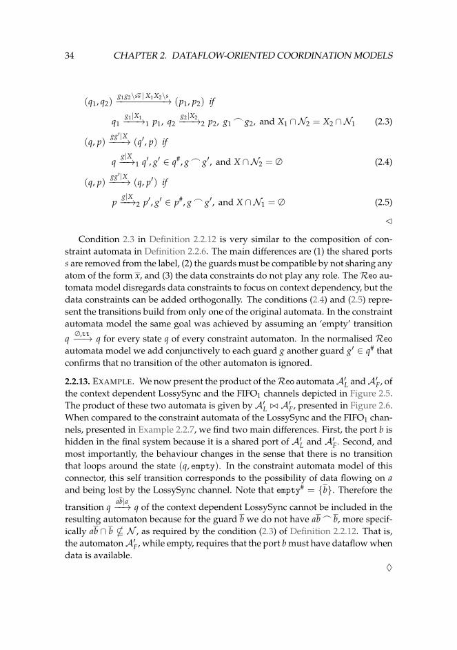
2.2.13. EXAMPLE. We now present the product of theReo automataA′L andA′F, ofthe context dependent LossySync and the FIFO1 channels depicted in Figure 2.5.The product of these two automata is given by A′L ./ A′F, presented in Figure 2.6.When compared to the constraint automata of the LossySync and the FIFO1 chan-nels, presented in Example 2.2.7, we find two main differences. First, the port b ishidden in the final system because it is a shared port of A′L and A′F. Second, andmost importantly, the behaviour changes in the sense that there is no transitionthat loops around the state (q, empty). In the constraint automata model of thisconnector, this self transition corresponds to the possibility of data flowing on aand being lost by the LossySync channel. Note that empty# = {b}. Therefore the
transition qab|a−−→ q of the context dependent LossySync cannot be included in the
resulting automaton because for the guard b we do not have ab_ b, more specif-ically ab ∩ b * N , as required by the condition (2.3) of Definition 2.2.12. That is,the automatonA′F, while empty, requires that the port b must have dataflow whendata is available.
♦
2.3. LINDA 35
A′L ./ A′F = q, empty q, full a a
a a
c c
ac c
Figure 2.6: Composition of theReo automata A′L and A′F.
2.3 Linda
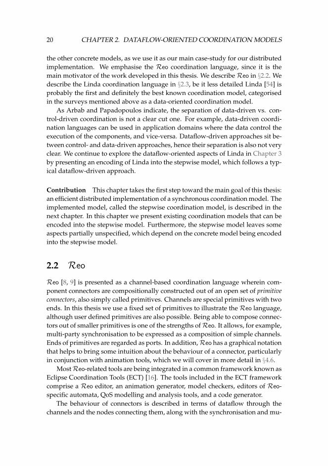
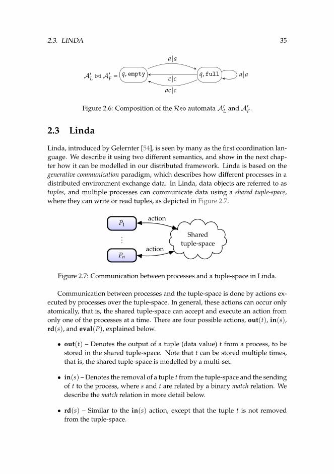
Linda, introduced by Gelernter [54], is seen by many as the first coordination lan-guage. We describe it using two different semantics, and show in the next chap-ter how it can be modelled in our distributed framework. Linda is based on thegenerative communication paradigm, which describes how different processes in adistributed environment exchange data. In Linda, data objects are referred to astuples, and multiple processes can communicate data using a shared tuple-space,where they can write or read tuples, as depicted in Figure 2.7.
P1
Pn
...Shared
tuple-space
action
action
Figure 2.7: Communication between processes and a tuple-space in Linda.
Communication between processes and the tuple-space is done by actions ex-ecuted by processes over the tuple-space. In general, these actions can occur onlyatomically, that is, the shared tuple-space can accept and execute an action fromonly one of the processes at a time. There are four possible actions, out(t), in(s),rd(s), and eval(P), explained below.
• out(t) – Denotes the output of a tuple (data value) t from a process, to bestored in the shared tuple-space. Note that t can be stored multiple times,that is, the shared tuple-space is modelled by a multi-set.
• in(s) – Denotes the removal of a tuple t from the tuple-space and the sendingof t to the process, where s and t are related by a binary match relation. Wedescribe the match relation in more detail below.
• rd(s) – Similar to the in(s) action, except that the tuple t is not removedfrom the tuple-space.
36 CHAPTER 2. DATAFLOW-ORIENTED COORDINATION MODELS
• eval(P) – Denotes the creation of a new process P that will run in parallelwith the other processes. In the literature [54, 90, 33] each process P is alsoreferred to as an active tuple, as opposed to passive tuples that represent datavalues.
More specifically, we write s and t to range over tuples, and we define eachtuple to be a sequence of parameters, generated by the following grammar, whereX ranges over a set of variables.
t ::= v ∈ D∣∣ X
∣∣ t; t
We denote by Tuple the set of all tuples generated by the above grammar. Eachparameter can be a data value v from a domain D (an actual parameter), or avariable x (a formal parameter). The interaction between processes and the tuple-space is based on a pattern-matching relation between tuples. We say t matches sif t has only D values, and there is a substitution γ whose domain is the set of freevariables of s, such that t = s[γ], where s[γ] denotes the tuple s after substitutingvariables in s according to γ. We write t γ-matches s when t matches s and t =
s[γ].Several variations of Linda were introduced later, such as Java’s popular im-
plementation JavaSpace of Jini [51], and the Klaim language [26], which considersmultiple distributed tuple-spaces. Other implementations of Linda can also befound in widespread programming languages such as Prolog [97], Ruby (Rinda),5
Python (PyLinda),6 C++ (CPPLINDA),7 Smalltalk [95], and Lisp [47]. Individ-ual tuple operations in Linda-like languages are atomic, but they do not providethe global synchronisation supported by Reo. In the remaining of this section weformalise Linda using the Linda-Calculus[43], and give both course-grained andfine-grained operational semantics for the Linda-Calculus.
The Linda-Calculus
We use the Linda-Calculus model, described by Goubault [43], to give a formaldescription of Linda, studied also by Ciancarini et al. [33] and others. The Linda-Calculus abstracts away from the local behaviour of processes, and focuses on thecommunication primitives between a store and a set of processes. Processes P aregenerated by the following grammar.
P ::= Act.P∣∣ X
∣∣ recX.P∣∣ P 2 P
∣∣ end (2.6)
Act ::= out(t)∣∣ in(s)
∣∣ rd(s)∣∣ eval(P) (2.7)
5http://ruby-doc.org/stdlib/libdoc/rinda/rdoc/index.html6http://code.google.com/p/pylinda/7http://sourceforge.net/projects/cpplinda/
2.3. LINDA 37
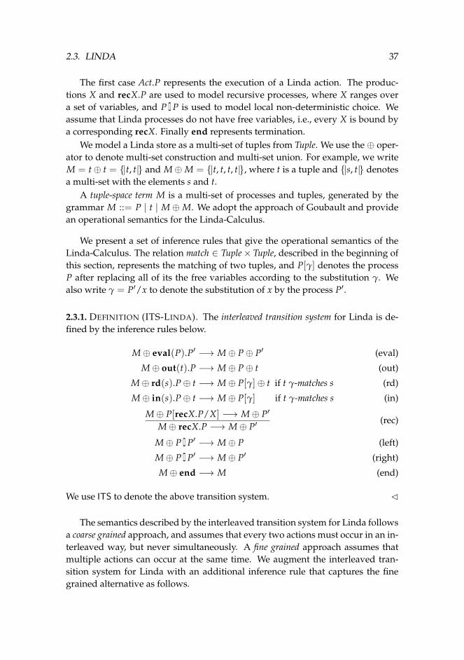
The first case Act.P represents the execution of a Linda action. The produc-tions X and recX.P are used to model recursive processes, where X ranges overa set of variables, and P 2 P is used to model local non-deterministic choice. Weassume that Linda processes do not have free variables, i.e., every X is bound bya corresponding recX. Finally end represents termination.
We model a Linda store as a multi-set of tuples from Tuple. We use the ⊕ oper-ator to denote multi-set construction and multi-set union. For example, we writeM = t⊕ t = {|t, t|} and M⊕M = {|t, t, t, t|}, where t is a tuple and {|s, t|} denotesa multi-set with the elements s and t.
A tuple-space term M is a multi-set of processes and tuples, generated by thegrammar M ::= P | t | M⊕M. We adopt the approach of Goubault and providean operational semantics for the Linda-Calculus.
We present a set of inference rules that give the operational semantics of theLinda-Calculus. The relation match ∈ Tuple× Tuple, described in the beginning ofthis section, represents the matching of two tuples, and P[γ] denotes the processP after replacing all of its the free variables according to the substitution γ. Wealso write γ = P′/x to denote the substitution of x by the process P′.
2.3.1. DEFINITION (ITS-LINDA). The interleaved transition system for Linda is de-fined by the inference rules below.
M⊕ eval(P).P′ −→ M⊕ P⊕ P′ (eval)
M⊕ out(t).P −→ M⊕ P⊕ t (out)
M⊕ rd(s).P⊕ t −→ M⊕ P[γ]⊕ t if t γ-matches s (rd)
M⊕ in(s).P⊕ t −→ M⊕ P[γ] if t γ-matches s (in)
M⊕ P[recX.P/X] −→ M⊕ P′
M⊕ recX.P −→ M⊕ P′(rec)
M⊕ P 2 P′ −→ M⊕ P (left)
M⊕ P 2 P′ −→ M⊕ P′ (right)
M⊕ end −→ M (end)
We use ITS to denote the above transition system. C
The semantics described by the interleaved transition system for Linda followsa coarse grained approach, and assumes that every two actions must occur in an in-terleaved way, but never simultaneously. A fine grained approach assumes thatmultiple actions can occur at the same time. We augment the interleaved tran-sition system for Linda with an additional inference rule that captures the finegrained alternative as follows.
38 CHAPTER 2. DATAFLOW-ORIENTED COORDINATION MODELS
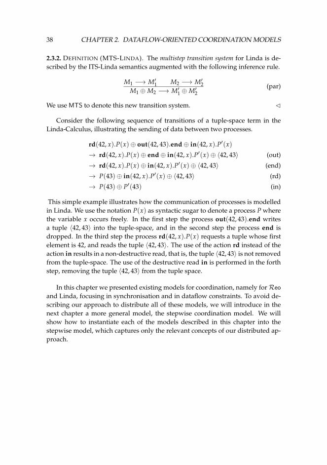
2.3.2. DEFINITION (MTS-LINDA). The multistep transition system for Linda is de-scribed by the ITS-Linda semantics augmented with the following inference rule.
M1 −→ M′1 M2 −→ M′2M1 ⊕M2 −→ M′1 ⊕M′2
(par)
We use MTS to denote this new transition system. C
Consider the following sequence of transitions of a tuple-space term in theLinda-Calculus, illustrating the sending of data between two processes.
rd(42, x).P(x)⊕ out(42, 43).end⊕ in(42, x).P′(x)
→ rd(42, x).P(x)⊕ end⊕ in(42, x).P′(x)⊕ 〈42, 43〉 (out)
→ rd(42, x).P(x)⊕ in(42, x).P′(x)⊕ 〈42, 43〉 (end)
→ P(43)⊕ in(42, x).P′(x)⊕ 〈42, 43〉 (rd)
→ P(43)⊕ P′(43) (in)
This simple example illustrates how the communication of processes is modelledin Linda. We use the notation P(x) as syntactic sugar to denote a process P wherethe variable x occurs freely. In the first step the process out(42, 43).end writesa tuple 〈42, 43〉 into the tuple-space, and in the second step the process end isdropped. In the third step the process rd(42, x).P(x) requests a tuple whose firstelement is 42, and reads the tuple 〈42, 43〉. The use of the action rd instead of theaction in results in a non-destructive read, that is, the tuple 〈42, 43〉 is not removedfrom the tuple-space. The use of the destructive read in is performed in the forthstep, removing the tuple 〈42, 43〉 from the tuple space.
In this chapter we presented existing models for coordination, namely forReo
and Linda, focusing in synchronisation and in dataflow constraints. To avoid de-scribing our approach to distribute all of these models, we will introduce in thenext chapter a more general model, the stepwise coordination model. We willshow how to instantiate each of the models described in this chapter into thestepwise model, which captures only the relevant concepts of our distributed ap-proach.
Chapter 3
A stepwise coordination model
3.1 Introduction
In this thesis we study the distributed implementation for a class of coordinationlanguages, in particular the Reo coordination language. Having presented someconcrete coordination models in Chapter 2, we take a step back and present amore abstract model that focuses on the aspects of coordination relevant for dis-tributed implementation. We call this model the stepwise coordination model, wherethe coordination behaviour is described by a state-based formalism which we callbehavioural automata. The goal of the stepwise coordination model is to justify theassumptions required by the Dreams framework, which is largely independent ofall the specific semantic models mentioned for Reo. The Dreams framework isdescribed later in Chapters 6 and 7. Also, we want to accommodate several ex-isting concrete models that can be implemented in the Dreams framework. Forexample, the constraint automata model for Reo can naturally be formulated inthe stepwise coordination model, by considering each transition in the stepwisecoordination model to correspond to a specific dataflow in a Reo connector. Ourmodel can also capture other aspects of coordination, such as context sensitivity,and does not require the assumption of a finite state space.
The stepwise coordination model serves as the basis for an implementation.The presentation of the model borrows ideas from the Tile model [53, 14], distin-guishing evolution in time (execution of the coordination system) and evolutionin space (composition of coordination systems). The key aspects of the stepwisecoordination model are composability of the coordination process and the atomicityof the execution of actions.
Composability We say a model is composed if it results from the compositionof smaller building blocks. However, not every composed model possesses theproperty of composability. The composability property holds for a model basedon a set of attributes of interest: a model is composed if it allows the attributes
39
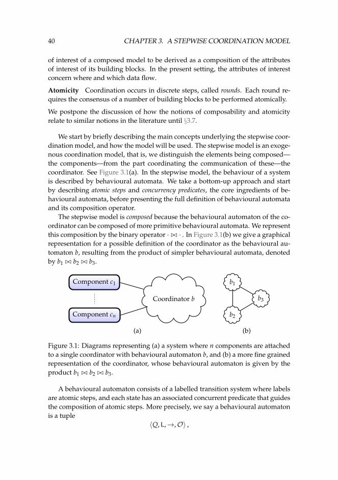
40 CHAPTER 3. A STEPWISE COORDINATION MODEL
of interest of a composed model to be derived as a composition of the attributesof interest of its building blocks. In the present setting, the attributes of interestconcern where and which data flow.
Atomicity Coordination occurs in discrete steps, called rounds. Each round re-quires the consensus of a number of building blocks to be performed atomically.
We postpone the discussion of how the notions of composability and atomicityrelate to similar notions in the literature until §3.7.
We start by briefly describing the main concepts underlying the stepwise coor-dination model, and how the model will be used. The stepwise model is an exoge-nous coordination model, that is, we distinguish the elements being composed—the components—from the part coordinating the communication of these—thecoordinator. See Figure 3.1(a). In the stepwise model, the behaviour of a systemis described by behavioural automata. We take a bottom-up approach and startby describing atomic steps and concurrency predicates, the core ingredients of be-havioural automata, before presenting the full definition of behavioural automataand its composition operator.
The stepwise model is composed because the behavioural automaton of the co-ordinator can be composed of more primitive behavioural automata. We representthis composition by the binary operator · ./ · . In Figure 3.1(b) we give a graphicalrepresentation for a possible definition of the coordinator as the behavioural au-tomaton b, resulting from the product of simpler behavioural automata, denotedby b1 ./ b2 ./ b3.
Component c1
Component cn
Coordinator b
b1
b2
b3
(a) (b)
Figure 3.1: Diagrams representing (a) a system where n components are attachedto a single coordinator with behavioural automaton b, and (b) a more fine grainedrepresentation of the coordinator, whose behavioural automaton is given by theproduct b1 ./ b2 ./ b3.
A behavioural automaton consists of a labelled transition system where labelsare atomic steps, and each state has an associated concurrent predicate that guidesthe composition of atomic steps. More precisely, we say a behavioural automatonis a tuple
〈Q, L,→,O〉 ,
3.2. PRELIMINARIES 41
where Q is a set of states, L is a set of labels, →⊆ Q× L× Q is a transition rela-tion, and O : Q → CP maps each state to its observation in CP, which stands for‘concurrency predicates’ over labels and will be used to guide the composition ofbehavioural automata. We will define atomic steps and concurrency predicatesbased on labels of transition systems from L. The atomicity aspect is captured bythe labels of behavioural automata transitions. A label represents a step in thesystem that has to be performed atomically. The composition of behavioural au-tomata is based on the composition of labels and on concurrency predicates, as weexplain later.
Organisation of the chapter We provide some preliminaries in §3.2 where weintroduce our notation and recall the definition of labelled transition systems. Wedefine labels, atomic steps, and concurrency predicates in §3.3, and present be-havioural automata in §3.4. We discuss some practical consequences of our modelin §3.5, namely locality properties and how to group similar atomic steps. In §3.6we describe the instantiation process of concrete coordination languages as be-havioural automata, including the encoding of constraint automata in §3.6.1, theencoding of normalised Reo automata in §3.6.2, and the encoding of the two se-mantics for Linda-Calculus in §3.6.3. We wrap up with some discussion and con-clusions in §3.7 and §3.8, respectively.
3.2 Preliminaries
We consider the coordination of a system as a set of constraints over the exchangesof data observed on a given set of ports and their flow between these ports. A portis an abstraction of a variable or an object that produces, consumes, or transportsdata, used to communicate values between elements of a coordination system. Weassume a global set of ports, written as P, and for each x ∈ P we write x to denotethe data value flowing through the port x in a specific round.1 We write D torepresent a global (possibly infinite) data domain. Given a set of ports P ⊆ P, wedefine P = {x | x ∈ P} to be the set of values x ∈ D that flow through the ports inP. A set of ports is often referred to as an alphabet.
Notation 2A denotes the powerset of A. f : A → B is a function with domainA and codomain B. A ⇀ B is a partial mapping from A to B, and is a shorthandfor A → (1 + B) where 1 = {⊥}. We write {a1 7→ b1, . . . , an 7→ bn} to denote apartial map m in A ⇀ B, where ai ∈ A, bi ∈ B, m(ai) = bi, and m(a) = ⊥ fora ∈ A\ {a1, . . . , an}. We also use the shorthands {a1, . . . , an 7→ b1, . . . , bn} and
1In the setting of automata models for Reo one can interpret the set P as the set N of port names,presented in Sections 2.2.2 and 2.2.3.
42 CHAPTER 3. A STEPWISE COORDINATION MODEL
{ai 7→ bi}ni=1 to denote the partial mapping {a1 7→ b1, . . . , an 7→ bn}. For a partial
mapping m : A ⇀ B, we write dom(m) to denote the elements in A for which mis defined, and codom(m) to denote the set B. For a pair of mappings m1, m2, wewrite m1
_m2 to denote that ∀x ∈ dom(m1) ∩ dom(m2) ·m1(x) = m2(x), and saym1 and m2 are compatible.
We represent the evolution over time of a coordination system by a labelledtransition system (LTS) with an observation function of states, where the labels ofthe transition relation range over a set Lb, and its states have observables in a setObs. The labels denote steps performed by the coordination system, while obser-vations denote properties of each state that we use later to compose behaviouralautomata.
3.2.1. DEFINITION (LTS). A labelled transition system over the labels Lb and theobservations Obs is a tuple 〈Q, Lb, Obs,→,O〉 where:
• Q is a set of states,
• Lb is a set of labels,
• Obs is a set of observations of states,
• O : Q→ Obs is an observation function, and
• →⊆ Q× Lb×Q is a transition relation. C
An example of a labelled transition system is the classical non-deterministicautomaton, where the labels of each transition are taken from some alphabet Lb,and each state has an observable value of true or false, indicating whether the stateis final or not. The stepwise coordination model we propose is a refinement of anLTS, where labels correspond to possible atomic executions of the system, and ob-servations are conditions required to compose LTS’s, represented by concurrencypredicates, both notions defined below.
3.2.2. EXAMPLE (ALTERNATING COORDINATOR). We present a toy example of analternating coordinator to illustrate the concepts introduced so far. The alternatingcoordinator is represented by AC in Figure 3.2(a). It receives data from two dif-ferent data writers W1 and W2, and sends data to a reader R. The componentsW1, W2 and R are connected, respectively, to the ports a, b and c of the alternatingcoordinator. The alternating coordinator describes how data can flow betweenthe connectors, and coordination is specified by the labelled transition system de-picted in Figure 3.2(b). Each transition of this labelled transition system representsa possible step in time of the coordinator AC, describing how the ports a, b, andc can have dataflow. Initially, the coordinator is in state q0, where only one stepcan be performed. This step consists of reading a value w from W1 through a and
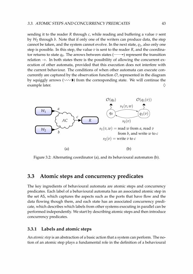
3.3. ATOMIC STEPS AND CONCURRENCY PREDICATES 43
sending it to the reader R through c, while reading and buffering a value v sentby W2 through b. Note that if only one of the writers can produce data, the stepcannot be taken, and the system cannot evolve. In the next state, q1, also only onestep is possible. In this step, the value v is sent to the reader R, and the coordina-tor returns to state q0. The arrows between states ( ) represent the transitionrelation →. In both states there is the possibility of allowing the concurrent ex-ecution of other automata, provided that this execution does not interfere withthe current behaviour. The conditions of when other automata can execute con-currently are captured by the observation function O, represented in the diagramby squiggly arrows ( ) from the corresponding state. We will continue theexample later. ♦
W1
W2
AC R
a
b
cq0 q1(v)
O(q0) O(q1(v))
s1(v, w)
s2(v)
s1(v, w) = read w from a, read vfrom b, and write w to c
s2(v) = write v to c
(a) (b)
Figure 3.2: Alternating coordinator (a), and its behavioural automaton (b).
3.3 Atomic steps and concurrency predicates
The key ingredients of behavioural automata are atomic steps and concurrencypredicates. Each label of a behavioural automata has an associated atomic step inthe set AS, which captures the aspects such as the ports that have flow and thedata flowing though them, and each state has an associated concurrency predi-cate, which describes which labels from other systems executing in parallel can beperformed independently. We start by describing atomic steps and then introduceconcurrency predicates.
3.3.1 Labels and atomic steps
An atomic step is an abstraction of a basic action that a system can perform. The no-tion of an atomic step plays a fundamental role in the definition of a behavioural
44 CHAPTER 3. A STEPWISE COORDINATION MODEL
automaton. We assume a global set of labels L for behavioural automata, a globalset of atomic steps AS, and a global function α : L→ AS that associates each labelto an atomic step. Recall also that P is a global set of ports and D is a global set ofdata values. We characterise the composition of labels based on their atomic steps,and define the composition of behavioural automata based only on the composi-tion of atomic steps and on concurrency predicates. An atomic step is definedover a set of ports P ⊆ P, and describes which ports can have dataflow, and howdata on different ports relate to each other.
3.3.1. DEFINITION (ATOMIC STEP). An atomic step over the alphabet P is a tuple〈P, F, IP, OP, data〉 where:
• P ⊆ P is a set of ports;
• F ⊆ P is the flow set;
• IP ⊆ F is a set of relevant input ports;
• OP ⊆ F is a set of relevant output ports;
• IP∩OP = ∅ relevant input and output ports are disjoint; and
• data : (IP∪OP)→ D is a data function. C
The flow set F is a set of ports that synchronise, i.e., that have data flowing in thesame atomic step. The sets IP and OP represent the input and output ports of theatomic step that have dataflow, and whose values are considered to be relevantwhen performing a step. Ports in F but not in IP or OP are ports with dataflow,but whose data values are not relevant, that is, they are used only for imposingsynchronisation constraints. The data values that flow through the relevant portsare given by the data function data. We distinguish IP and OP to capture thenotion of data dependencies that we use in the Dreams framework, and we donot relate these sets with source or sink ports. The intuition is that input portsare matched against output ports from elsewhere, and every input port must begiven a value by a matched output port or an explicit environment function. Laterin this chapter we explore the use of input ports and output ports to capture datadependency in more detail.
Notation We write AS[P] to denote the set of all atomic steps over the ports inP, and L[P] to denote the set of all labels ` such that α(`) ⊆ AS[P]. We use AS andL as shorthands for AS[P] and L[P], respectively. For simplicity, we write a1 . . . aninstead of {a1, . . . , an} in the definition of atomic steps when the intention is clearfrom the context.
Consider the example of a set of labels with flow on the ports a, b, c and x, y,whose intended behaviour is to receive data, natural numbers say, from a, b and c,
3.3. ATOMIC STEPS AND CONCURRENCY PREDICATES 45
and to produce data through x and y. Furthermore, the data value produced on xshould be the maximum of the data values obtained through a and b, if available,and data should flow from c to y directly. If x does not produce data values thenthere is no dataflow. The relevant input and output ports are therefore definedas IP = {a, b, c} and OP = {x, y}, respectively. We choose the flow set to beF = IP ∪OP, and assume that P is a set of ports containing at least F. Finally, wedefine the data domain D to be N, and the data function data[v1, v2, v3] as follows:
data[v1, v2, v3] = {a 7→ v1, b 7→ v2, c 7→ v3, x 7→ max(v1, v2), y 7→ v3} (3.1)
where max is the standard maximum function on N. We characterise these labelsby the set S of their associated atomic steps as follows.
S = {〈P, F, IP, OP, data[v1, v2, v3]〉 ∈ AS | v1, v2, v3 ∈ D}
The set S reflects that data flow from a and b to x, and from c to y. Using thenotation z for the dataflow on a port z we can represent the set of atomic stepsover a set of ports P as
x := max(a, b) and y := c
concisely describing the choice of the data values, max(a, b) and c, flowing on xand y in terms of the dataflow on a, b, and c.
Composition of labels
Let α : L → AS be a mapping from labels in L to atomic steps in AS, and let`1, `2 ∈ L be two labels. We assume to be given a binary composition operator ⊗on the set of labels L, such that certain properties hold for α(`1 ⊗ `2), describedbelow. We also write α(`1)⊗ α(`2) to denote the atomic step α(`1 ⊗ `2).
Composing `1 and `2 can be intuitively understood as “what is the step for asystem where part of it can perform `1 and another part can perform `2”. Such acomposition may not always be possible. Hence, ⊗ : L2 ⇀ L is a partial mapping.Moreover, for technical convenience, we require ⊗ to be associative and to havean identity element, denoted by idL. Thus, (L,⊗) is assumed to be a commutativepartial monoid 〈L,⊗〉.2 Below we will require for two labels `1 and `2 in L withatomic steps α(`1) = 〈P1, F1, IP1, OP1, data1〉, α(`2) = 〈P2, F2, IP2, OP2, data2〉, thecomposition `1⊗ `2 to be defined (but not necessarily exclusively) if the alphabetsP1 and P2 are disjoint. We say `1 and `2 are incompatible if `1 ⊗ `2 is undefined,which means that `1 and `2 cannot be performed simultaneously. If `1 and `2 arecompatible, then α(`1 ⊗ `2) = 〈P, F, IP, OP, data〉 satisfies:
2Not to be confused with partially commutative monoids, or partially trace monoids, where com-mutativity is partial [80].
46 CHAPTER 3. A STEPWISE COORDINATION MODEL
• P ⊆ P1 ∪ P2;
• IP ⊆ (IP1 ∪ IP2)\(OP1 ∪OP2);
• data1_ data2;
• F ⊆ F1 ∪ F2;
• OP ⊆ OP1 ∪OP2; and
• data = data1 ∪ data2.
Based on these conditions we require the identity to be idL to be such that α(idL) =〈∅, ∅, ∅, ∅, ∅〉. We introduced the notation m1
_m2 in §3.2 to represent that thevalues of the common domain of mappings m1 and m2 match. The requirementson the sets IP and OP reflect that when composing two atomic steps, the inputports that have an associated output port are no longer treated as input ports(since the dependencies have been met), and the output ports are combined.
3.3.2. EXAMPLE. Consider three labels `1, `2 and `3 with atomic steps α(`i) = sidefined below, where D = N and where we write abc instead of {a, b, c}, etc.
s1 = 〈ab, ab, a, b, {a, b 7→ 3, 5}〉s2 = 〈bc, bc, b, c, {b, c 7→ 5, 7}〉s3 = 〈cd, c, ∅, c, {c 7→ 6}〉
It is possible to define ⊗ such that s1 ⊗ s2 = 〈abc, abc, a, bc, {a, b, c 7→ 3, 5, 7}〉.An alternative definition can also yield s1 ⊗ s2 = 〈abc, ac, a, c, {a, c 7→ 3, 7}〉. Inthe alternative definition we ignore the flow of data on b after the composition,because it has become internal. However, s2 ⊗ s3 has to be undefined, becausetheir data functions are not compatible: {b, c 7→ 5, 7}_/ {c 7→ 6}. The oppositeholds for the composition s1 ⊗ s3, which has to be always defined because ab ∩cd = ∅. ♦
3.3.2 Concurrency predicates
We introduced atomic steps associated to labels of behavioural automata by afunction α. We now introduce concurrency predicates to represent observations ofstates by a function O. The intuition is that labels from two systems can be exe-cuted together (composing their steps using ⊗), but they can also be executed inparallel, independent of each other, using the concurrency predicates to controlwhen a label from a system can be interleaved with those from the other system.Recall that we assume a global set of ports P, a global set of labels L = L[P], anda global set of atomic steps AS = AS[P].
3.3.3. DEFINITION (CONCURRENCY PREDICATE). A concurrency predicate is a set oflabels in L. We write CP to denote the set 2L of all concurrency predicates. ForC ∈ CP and ` ∈ L, we write C(`) to denote ` ∈ C. C
3.3. ATOMIC STEPS AND CONCURRENCY PREDICATES 47
For a given state q, an observation function O, and a label `, the concurrencypredicate O(q)(`) can be understood as “the label ` from another behavioural au-tomata can be executed”. The name “concurrency predicate” reflects the maingoal of these observations: concurrency of systems. More specifically, the concur-rency predicate describes when two systems can execute independently, by listingfor each state the set of labels that do not affect the choice of the next transition.The composition of concurrency predicates is simply the intersection of sets, i.e.,the composition of two concurrency predicates C1 and C2 is C1 ∩ C2. Unlike thecomposition of labels, the composition of concurrency predicates is total, i.e., anytwo concurrency predicates can be composed.
The motivation for introducing concurrency predicates is twofold. First, it cap-tures a similar notion from various Reo models: the constraint automata modelassumes that every state has the transition ∅, tt (Definition 2.2.3), and theReo au-tomata model uses the condition q# when composing automata (Definition 2.2.12).We believe that this separation between steps and concurrency predicates is morenatural than assuming the existence of specific steps to make the composition be-have as expected. Second, by making explicit a condition that describes whensteps can be executed concurrently, we do not need to globally evaluate the coor-dination constraints. Hence, certain labels can be executed locally in a distributedenvironment independently of other systems running in parallel.
Notation In most of the following examples it is enough to define the observa-tion of a state based on the atomic steps of the labels of other systems. For thesecases, we introduce a notation to quickly define a concurrency predicate consist-ing of all labels that do not have dataflow in a set of ports P0. We write cp(P0) todenote the concurrency predicate
cp(P0) = {` | α(`) = 〈P, F, IP, OP, data〉 , P0 ∩ F = ∅} . (3.2)
Example
Recall the running example of the alternating coordinator from §3.2 on page 42. InFigure 3.2(b) we described each label and observation informally. In Table 3.1 wedefine each of these textual labels as atomic steps and concurrency predicates. Inall transitions, the alphabet P is always {a, b, c}, and the observations only allowsteps where none of the known ports has flow.
When composing two behavioural automata, the composition of labels is usedto combine all possible pairs of labels from the two automata, and the concurrencypredicates are used to include all labels that can be executed independently. Inthe next section we study in more detail labelled transition systems where labelshave associated atomic steps and states have associated concurrency predicates,assuming a possible definition for the composition of atomic steps.
48 CHAPTER 3. A STEPWISE COORDINATION MODEL
Labels Atomic steps
s1(v, w) – 〈P, abc, ab, c, {a, b, c 7→ w, v, w}〉s2(v) – 〈P, c, ∅, c, {c 7→ v}〉
States CP
q0 – cp(P)q1(v) – cp(P)
Table 3.1: Atomic steps of the labels and concurrency predicates of the states ofthe alternating coordinator, where v, w ∈ D.
3.4 Behavioural automata
Labels describe each round of the dynamic behaviour of a system. Recall thatwe assume a global set of ports P and a global data domain D. We now assumealso a global set of labels L = L[P] with atomic steps AS = AS[P], and with acomposition operator ⊗. Let α be the function that associates labels to atomicsteps. We refine the definition of LTS introduced in §3.2, using labels from L in thetransition relation and concurrency predicates from 2L as observations. We callthe resulting labelled transition systems behavioural automata.
3.4.1. DEFINITION (BEHAVIOURAL AUTOMATA). A behavioural automaton of a sys-tem over a set of ports P ⊆ P is a labelled transition system
〈Q, L[P],→,O〉 ,
where L[P] is the set of labels over P,→ ⊆ Q× L[P]×Q is the transition relation,and O : Q → 2L is the observation function that maps states to concurrencypredicates. C
Note that we omit set of possible observations with respect to Definition 3.2.1 of la-belled transition systems, because it is always CP = 2L. The set CP is fixed becauseof the assumption of a global set of atomic steps AS. Similarly, we do not include
the function α : L→ AS. We also use the notation q1`−→ q2 denoting 〈q1, `, q2〉 ∈→.
The observation function O returns a concurrency predicate for each state q, suchthat for any label ` from another behavioural automata, O(q)(`) = true meansthat ` ∈ O(q), that is, ` can execute while the current behavioural automaton is instate q. We will investigate the local execution of a behavioural automaton furtherin this section, exploring properties of the observation function.
Note that no assumption is made regarding the cardinality of the state set Q,the set of ports P, and the transition relation→. On one hand, assuming a finiteworld brings us to finite automata models, where we can formally verify a largeclass of properties. On the other hand, we can also assume a black box scenario,where the set of states, ports, or relations is not provided a priori, or even sce-narios where these are calculated and given on demand as the system evolves.This perspective has the advantage of allowing the execution of systems that are
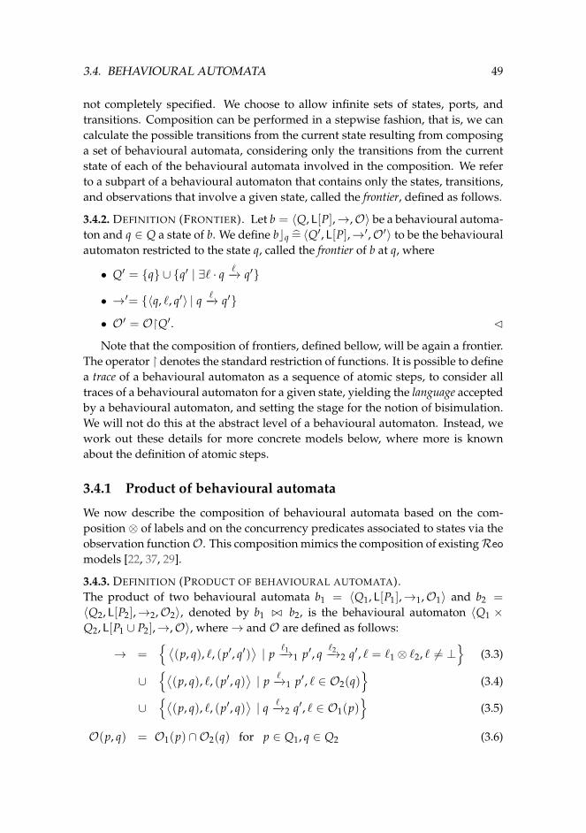
3.4. BEHAVIOURAL AUTOMATA 49
not completely specified. We choose to allow infinite sets of states, ports, andtransitions. Composition can be performed in a stepwise fashion, that is, we cancalculate the possible transitions from the current state resulting from composinga set of behavioural automata, considering only the transitions from the currentstate of each of the behavioural automata involved in the composition. We referto a subpart of a behavioural automaton that contains only the states, transitions,and observations that involve a given state, called the frontier, defined as follows.
3.4.2. DEFINITION (FRONTIER). Let b = 〈Q, L[P],→,O〉 be a behavioural automa-ton and q ∈ Q a state of b. We define bcq = 〈Q′, L[P],→′,O′〉 to be the behaviouralautomaton restricted to the state q, called the frontier of b at q, where
• Q′ = {q} ∪ {q′ | ∃` · q `−→ q′}
• →′= {〈q, `, q′〉 | q `−→ q′}
• O′ = O�Q′. C
Note that the composition of frontiers, defined bellow, will be again a frontier.The operator � denotes the standard restriction of functions. It is possible to definea trace of a behavioural automaton as a sequence of atomic steps, to consider alltraces of a behavioural automaton for a given state, yielding the language acceptedby a behavioural automaton, and setting the stage for the notion of bisimulation.We will not do this at the abstract level of a behavioural automaton. Instead, wework out these details for more concrete models below, where more is knownabout the definition of atomic steps.
3.4.1 Product of behavioural automata
We now describe the composition of behavioural automata based on the com-position ⊗ of labels and on the concurrency predicates associated to states via theobservation functionO. This composition mimics the composition of existingReo
models [22, 37, 29].
3.4.3. DEFINITION (PRODUCT OF BEHAVIOURAL AUTOMATA).The product of two behavioural automata b1 = 〈Q1, L[P1],→1,O1〉 and b2 =
〈Q2, L[P2],→2,O2〉, denoted by b1 ./ b2, is the behavioural automaton 〈Q1 ×Q2, L[P1 ∪ P2],→,O〉, where→ and O are defined as follows:
→ ={ ⟨
(p, q), `, (p′, q′)⟩| p
`1−→1 p′, q`2−→2 q′, ` = `1 ⊗ `2, ` 6= ⊥
}(3.3)
∪{⟨
(p, q), `, (p′, q)⟩| p `−→1 p′, ` ∈ O2(q)
}(3.4)
∪{⟨
(p, q), `, (p′, q)⟩| q `−→2 q′, ` ∈ O1(p)
}(3.5)
O(p, q) = O1(p) ∩O2(q) for p ∈ Q1, q ∈ Q2 (3.6)
50 CHAPTER 3. A STEPWISE COORDINATION MODEL
C
Case (3.3) composes all possible combinations of transitions from →1 and →2,reflecting both behavioural automata executing in parallel. Cases (3.4) and (3.5)cover the situation where one of the behavioural automata performs a step ad-mitted by the concurrency predicate of the other. Finally, case (3.6) defines thecomposition of two concurrency predicates, given by their intersection.
The empty behavioural automaton 〈{q} , ∅, ∅,O〉, whereO(q) = L, is denotedby 0BA. It is an identity of the operator ./ up to isomorphism, defined below. Theisomorphism captures the fact that the state names can differ. We formalise theproperties of 0BA in Proposition 3.4.5.
3.4.4. DEFINITION (ISOMORPHISM OF BEHAVIOURAL AUTOMATA).Given two behavioural automata b1 = 〈Q1, L[P1],→1,O1〉 and b2 = 〈Q2, L[P2],→2,O2〉we say that b1 and b2 are isomorphic, written as b1 ' b2, iff P1 = P2 and thereis a bijection f : Q1 → Q2 such that:
• q `−→1 q′ if and only if f (q) `−→2 f (q′); and
• O1(q) = O2( f (q)). C
3.4.5. PROPOSITION. We have that 0BA ./ b ' b and b ./ 0BA ' b, for every be-havioural automaton b. 2
3.4.2 Example: lossy alternator
Recall the behavioural automaton AC of our running example of the alternatingcoordinator, illustrated in Figure 3.2, whose atomic steps were formalised in Ta-ble 3.1. The alternating coordinator has two source ports, a and b, and a sink portc. Data is received always via ports a and b simultaneously, and sent via port c,alternating the values received from a and b. We now imagine the following sce-nario: the data on a becomes available always at a much faster rate than data onb. To adapt our alternating coordinator to this new scenario, we introduce a lossy-FIFO1 connector LF and combine it with the alternating coordinator, yielding avariation of the alternating coordinator LF ./ AC.
Recall the definition of cp : P→ L given by Equation (3.2), on page 47. The be-havioural automaton for the lossy-FIFO1 connector is depicted in Figure 3.3, andits atomics steps range over the set of ports {a, a′}, where a is an input port anda′ is an output port.3 Recall also that the alternating coordinator ranges over theset of ports {a, b, c}. We depict the interface of both of these connectors on top ofFigure 3.4. After combining the behavioural automata of the two connectors, they
3This lossy-FIFO is also known in the literature [8] as the shift-lossy FIFO1.

3.4. BEHAVIOURAL AUTOMATA 51
empty
full(v)
full(w)
cp(a, a′)
cp(a, a′)
cp(a, a′)
s3(v)
s3(w)s4(v)
s4(w)
s3(w)s3(v)
s3(v)
s3(w)
where:s3(v) = 〈aa′, a′, a′, ∅, {a′ 7→ v}〉s4(v) = 〈aa′, a, ∅, a, {a 7→ v}〉
Figure 3.3: Behavioural automaton of the lossy-FIFO connector.
become connected via their shared port a. The new variation of the alternatingcoordinator can then be connected to writers and readers by using the ports a′, band c, as depicted at the bottom of Figure 3.4.
LFa′ a
./ AC
a
b
c
LF ./ AC
a′
b
c
Figure 3.4: The sink and source ports of LF, AC, and their composition.
Intuitively, the lossy-FIFO connector receives data from the source port a′ andbuffers its value before sending it through port a. When the buffer is full it can alsoreceive data from a′, and the content of the buffer is replaced by the new receivedvalue. The connector resulting from the composition LF ./ AC is formalised inTable 3.2 and in Figure 3.5. The flow sets of the atomic steps of the labels s1(v, w),s2(v), s3(v) and s4(v) are, respectively, abc, c, a′, and a′a. The set of known ports inthis example is always P = {a′, a, b, c}. Let OLF be the observation function of LF,and OAC be the observation function of AC. The observation function OLF./AC
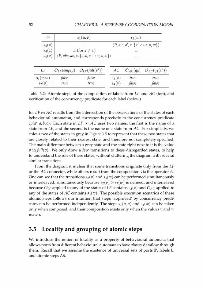
52 CHAPTER 3. A STEPWISE COORDINATION MODEL
⊗ s1(u, v) s2(w)
s3(y) ⊥ 〈P, a′c, a′, c, {a′, c 7→ y, w}〉s4(z) ⊥ (for z 6= v) ⊥s4(v) 〈P, abc, ab, c, {a, b, c 7→ v, u, v}〉 ⊥
LF OLF(empty) OLF(full(v′))
s1(v, w) false falses2(v) true true
AC OAC(q0) OAC(q1(v′))
s3(v) true trues4(v) false false
Table 3.2: Atomic steps of the composition of labels from LF and AC (top), andverification of the concurrency predicate for each label (below).
for LF ./ AC results from the intersection of the observations of the states of eachbehavioural automaton, and corresponds precisely to the concurrency predicatecp(a′, a, b, c). Each state in LF ./ AC uses two names, the first is the name of astate from LF, and the second is the name of a state from AC. For simplicity, wecolour two of the states in grey in Figure 3.5 to represent that these two states thatare closely related to their nearest state, and therefore not completely specified.The main difference between a grey state and the state right next to it is the valuev in full(v). We only draw a few transitions to these disregarded states, to helpto understand the role of these states, without cluttering the diagram with severalsimilar transitions.
From the diagram it is clear that some transitions originate only from the LFor the AC connector, while others result from the composition via the operator ⊗.One can see that the transitions s2(v) and s3(w) can be performed simultaneouslyor interleaved; simultaneously because s2(v)⊗ s3(w) is defined, and interleavedbecause OLF applied to any of the states of LF contains s2(v) and OAC applied toany of the states of AC contains s3(w). The possible execution scenarios of theseatomic steps follows our intuition that steps ‘approved’ by concurrency predi-cates can be performed independently. The steps s1(u, v) and s4(w) can be takenonly when composed, and their composition exists only when the values v and wmatch.
3.5 Locality and grouping of atomic steps
We introduce the notion of locality as a property of behavioural automata thatallows ports from different behavioural automata to have always dataflow throughthem. Recall that we assume the existence of universal sets of ports P, labels L,and atomic steps AS.
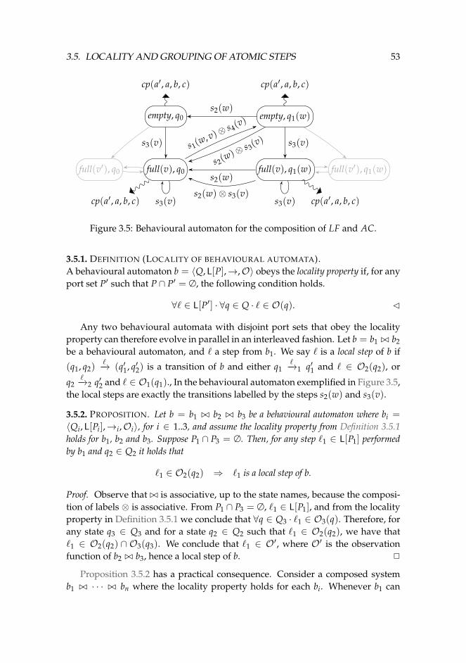
3.5. LOCALITY AND GROUPING OF ATOMIC STEPS 53
empty, q0 empty, q1(w)
full(v), q0 full(v), q1(w)
cp(a′, a, b, c) cp(a′, a, b, c)
cp(a′, a, b, c) cp(a′, a, b, c)
full(v′), q0 full(v′), q1(w)
s3(v)
s3(v)
s1(w, v)⊗
s4(v)
s2(w)
s2(w)⊗
s3(v) s3(v)
s3(v)
s2(w)
s2(w)⊗ s3(v)
Figure 3.5: Behavioural automaton for the composition of LF and AC.
3.5.1. DEFINITION (LOCALITY OF BEHAVIOURAL AUTOMATA).A behavioural automaton b = 〈Q, L[P],→,O〉 obeys the locality property if, for anyport set P′ such that P ∩ P′ = ∅, the following condition holds.
∀` ∈ L[P′] · ∀q ∈ Q · ` ∈ O(q). C
Any two behavioural automata with disjoint port sets that obey the localityproperty can therefore evolve in parallel in an interleaved fashion. Let b = b1 ./ b2be a behavioural automaton, and ` a step from b1. We say ` is a local step of b if
(q1, q2)`−→ (q′1, q′2) is a transition of b and either q1
`−→1 q′1 and ` ∈ O2(q2), or
q2`−→2 q′2 and ` ∈ O1(q1)., In the behavioural automaton exemplified in Figure 3.5,
the local steps are exactly the transitions labelled by the steps s2(w) and s3(v).
3.5.2. PROPOSITION. Let b = b1 ./ b2 ./ b3 be a behavioural automaton where bi =
〈Qi, L[Pi],→i,Oi〉, for i ∈ 1..3, and assume the locality property from Definition 3.5.1holds for b1, b2 and b3. Suppose P1 ∩ P3 = ∅. Then, for any step `1 ∈ L[P1] performedby b1 and q2 ∈ Q2 it holds that
`1 ∈ O2(q2) ⇒ `1 is a local step of b.
Proof. Observe that ./ is associative, up to the state names, because the composi-tion of labels ⊗ is associative. From P1 ∩ P3 = ∅, `1 ∈ L[P1], and from the localityproperty in Definition 3.5.1 we conclude that ∀q ∈ Q3 · `1 ∈ O3(q). Therefore, forany state q3 ∈ Q3 and for a state q2 ∈ Q2 such that `1 ∈ O2(q2), we have that`1 ∈ O2(q2) ∩ O3(q3). We conclude that `1 ∈ O′, where O′ is the observationfunction of b2 ./ b3, hence a local step of b. 2
Proposition 3.5.2 has a practical consequence. Consider a composed systemb1 ./ · · · ./ bn where the locality property holds for each bi. Whenever b1 can
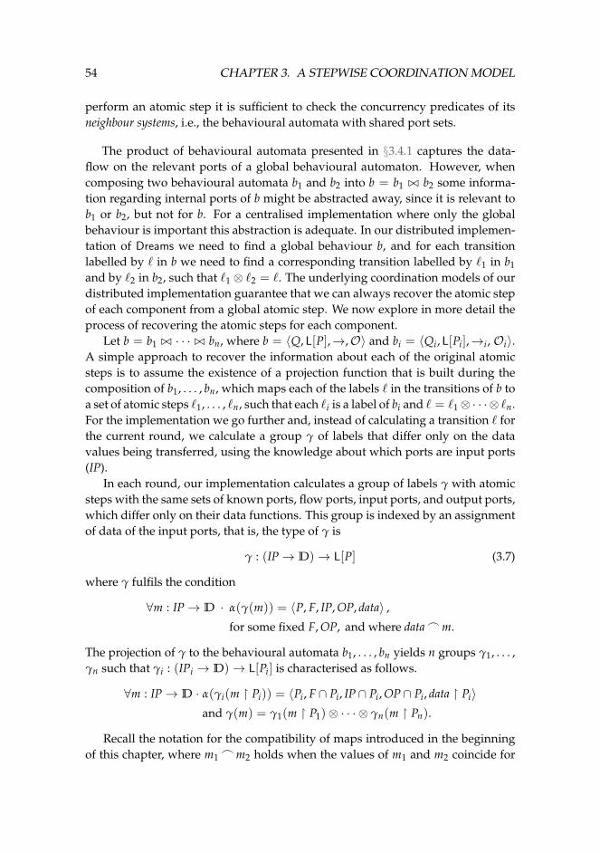
54 CHAPTER 3. A STEPWISE COORDINATION MODEL
perform an atomic step it is sufficient to check the concurrency predicates of itsneighbour systems, i.e., the behavioural automata with shared port sets.
The product of behavioural automata presented in §3.4.1 captures the data-flow on the relevant ports of a global behavioural automaton. However, whencomposing two behavioural automata b1 and b2 into b = b1 ./ b2 some informa-tion regarding internal ports of b might be abstracted away, since it is relevant tob1 or b2, but not for b. For a centralised implementation where only the globalbehaviour is important this abstraction is adequate. In our distributed implemen-tation of Dreams we need to find a global behaviour b, and for each transitionlabelled by ` in b we need to find a corresponding transition labelled by `1 in b1and by `2 in b2, such that `1 ⊗ `2 = `. The underlying coordination models of ourdistributed implementation guarantee that we can always recover the atomic stepof each component from a global atomic step. We now explore in more detail theprocess of recovering the atomic steps for each component.
Let b = b1 ./ · · · ./ bn, where b = 〈Q, L[P],→,O〉 and bi = 〈Qi, L[Pi],→i, Oi〉.A simple approach to recover the information about each of the original atomicsteps is to assume the existence of a projection function that is built during thecomposition of b1, . . . , bn, which maps each of the labels ` in the transitions of b toa set of atomic steps `1, . . . , `n, such that each `i is a label of bi and ` = `1⊗ · · ·⊗ `n.For the implementation we go further and, instead of calculating a transition ` forthe current round, we calculate a group γ of labels that differ only on the datavalues being transferred, using the knowledge about which ports are input ports(IP).
In each round, our implementation calculates a group of labels γ with atomicsteps with the same sets of known ports, flow ports, input ports, and output ports,which differ only on their data functions. This group is indexed by an assignmentof data of the input ports, that is, the type of γ is
γ : (IP→ D)→ L[P] (3.7)
where γ fulfils the condition
∀m : IP→ D · α(γ(m)) = 〈P, F, IP, OP, data〉 ,
for some fixed F, OP, and where data_m.
The projection of γ to the behavioural automata b1, . . . , bn yields n groups γ1, . . . ,γn such that γi : (IPi → D)→ L[Pi] is characterised as follows.
∀m : IP→ D · α(γi(m � Pi)) = 〈Pi, F ∩ Pi, IP∩ Pi, OP∩ Pi, data � Pi〉and γ(m) = γ1(m � P1)⊗ · · · ⊗ γn(m � Pn).
Recall the notation for the compatibility of maps introduced in the beginningof this chapter, where m1
_m2 holds when the values of m1 and m2 coincide for
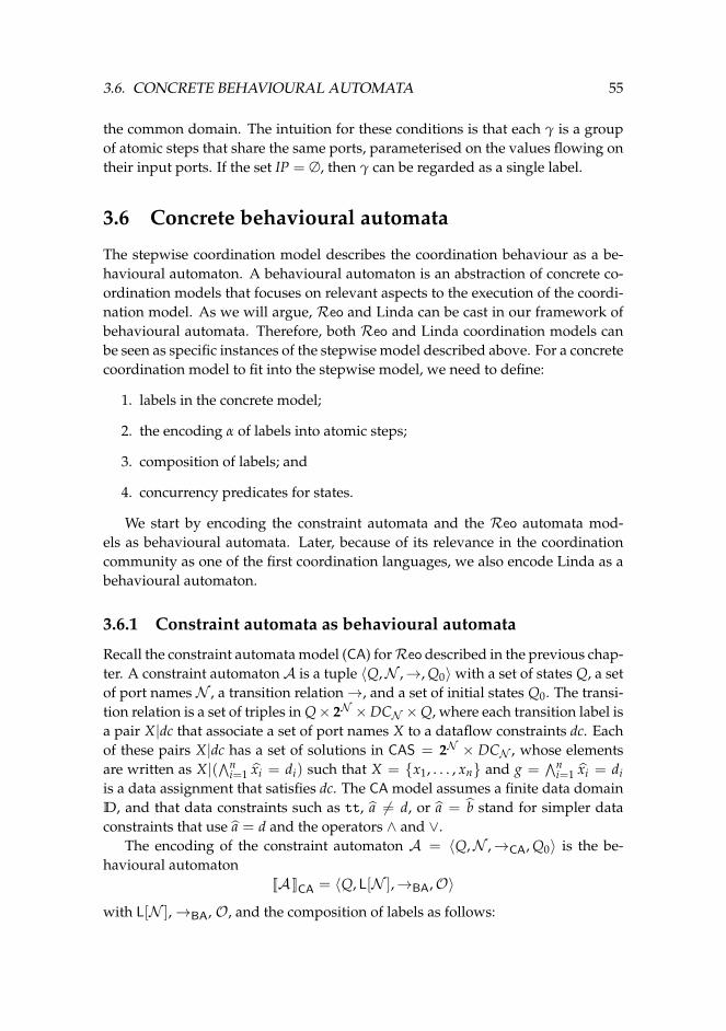
3.6. CONCRETE BEHAVIOURAL AUTOMATA 55
the common domain. The intuition for these conditions is that each γ is a groupof atomic steps that share the same ports, parameterised on the values flowing ontheir input ports. If the set IP = ∅, then γ can be regarded as a single label.
3.6 Concrete behavioural automata
The stepwise coordination model describes the coordination behaviour as a be-havioural automaton. A behavioural automaton is an abstraction of concrete co-ordination models that focuses on relevant aspects to the execution of the coordi-nation model. As we will argue, Reo and Linda can be cast in our framework ofbehavioural automata. Therefore, both Reo and Linda coordination models canbe seen as specific instances of the stepwise model described above. For a concretecoordination model to fit into the stepwise model, we need to define:
1. labels in the concrete model;
2. the encoding α of labels into atomic steps;
3. composition of labels; and
4. concurrency predicates for states.
We start by encoding the constraint automata and the Reo automata mod-els as behavioural automata. Later, because of its relevance in the coordinationcommunity as one of the first coordination languages, we also encode Linda as abehavioural automaton.
3.6.1 Constraint automata as behavioural automata
Recall the constraint automata model (CA) forReo described in the previous chap-ter. A constraint automaton A is a tuple 〈Q,N ,→, Q0〉 with a set of states Q, a setof port names N , a transition relation→, and a set of initial states Q0. The transi-tion relation is a set of triples in Q× 2N ×DCN ×Q, where each transition label isa pair X|dc that associate a set of port names X to a dataflow constraints dc. Eachof these pairs X|dc has a set of solutions in CAS = 2N × DCN , whose elementsare written as X|(∧n
i=1 xi = di) such that X = {x1, . . . , xn} and g =∧n
i=1 xi = diis a data assignment that satisfies dc. The CA model assumes a finite data domainD, and that data constraints such as tt, a 6= d, or a = b stand for simpler dataconstraints that use a = d and the operators ∧ and ∨.
The encoding of the constraint automaton A = 〈Q,N ,→CA, Q0〉 is the be-havioural automaton
JA KCA = 〈Q, L[N ],→BA,O〉
with L[N ],→BA, O, and the composition of labels as follows:
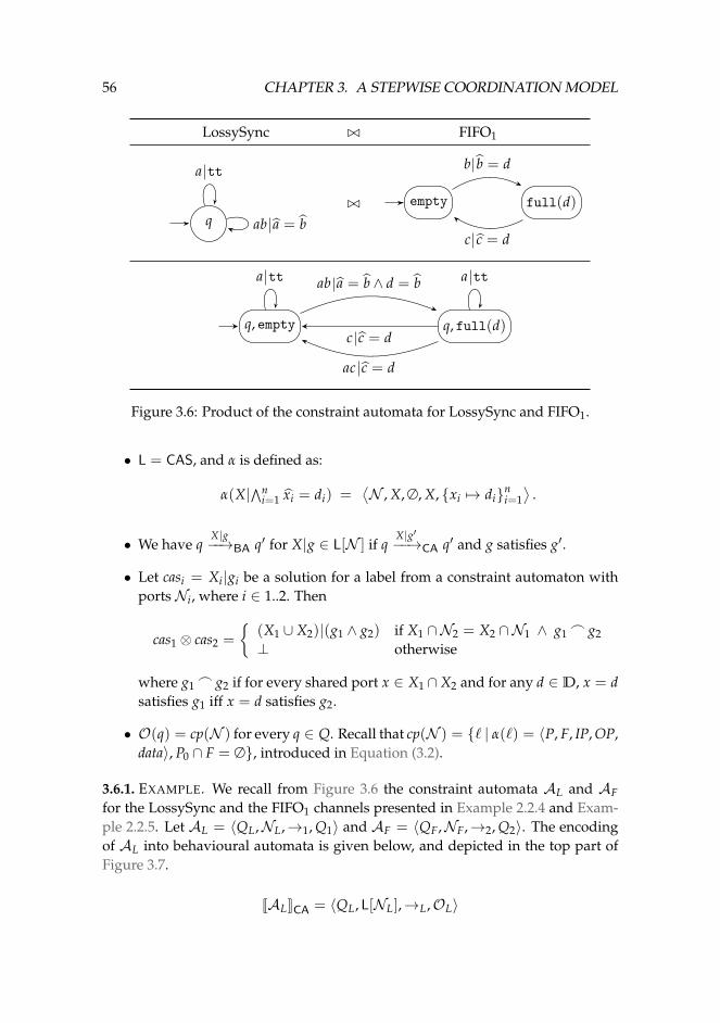
56 CHAPTER 3. A STEPWISE COORDINATION MODEL
LossySync ./ FIFO1
q
a tt
ab a = b./ empty full(d)
b b = d
c c = d
q, empty q, full(d)
a tt a ttab a = b ∧ d = b
c c = d
ac c = d
Figure 3.6: Product of the constraint automata for LossySync and FIFO1.
• L = CAS, and α is defined as:
α(X|∧ni=1 xi = di) =
⟨N , X, ∅, X, {xi 7→ di}n
i=1⟩
.
• We have qX|g−−→BA q′ for X|g ∈ L[N ] if q
X|g′−−→CA q′ and g satisfies g′.
• Let casi = Xi|gi be a solution for a label from a constraint automaton withports Ni, where i ∈ 1..2. Then
cas1 ⊗ cas2 =
{(X1 ∪ X2)|(g1 ∧ g2) if X1 ∩N2 = X2 ∩N1 ∧ g1
_ g2⊥ otherwise
where g1_ g2 if for every shared port x ∈ X1 ∩X2 and for any d ∈ D, x = d
satisfies g1 iff x = d satisfies g2.
• O(q) = cp(N ) for every q ∈ Q. Recall that cp(N ) = {` | α(`) = 〈P, F, IP, OP,data〉, P0 ∩ F = ∅}, introduced in Equation (3.2).
3.6.1. EXAMPLE. We recall from Figure 3.6 the constraint automata AL and AFfor the LossySync and the FIFO1 channels presented in Example 2.2.4 and Exam-ple 2.2.5. Let AL = 〈QL,NL,→1, Q1〉 and AF = 〈QF,NF,→2, Q2〉. The encodingof AL into behavioural automata is given below, and depicted in the top part ofFigure 3.7.
JALKCA = 〈QL, L[NL],→L,OL〉
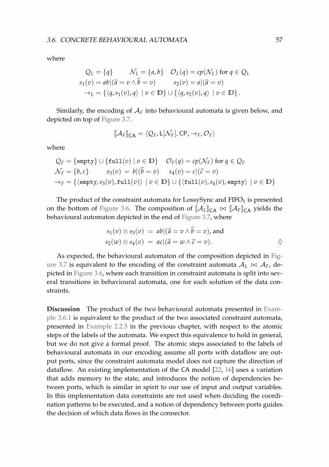
3.6. CONCRETE BEHAVIOURAL AUTOMATA 57
where
QL = {q} NL = {a, b} OL(q) = cp(NL) for q ∈ QL
s1(v) = ab|(a = v ∧ b = v) s2(v) = a|(a = v)
→L = {〈q, s1(v), q〉 | v ∈ D} ∪ {〈q, s2(v), q〉 | v ∈ D} .
Similarly, the encoding of AF into behavioural automata is given below, anddepicted on top of Figure 3.7.
JAFKCA = 〈QF, L[NF], CP,→F,OF〉
where
QF = {empty} ∪ {full(v) | v ∈ D} OF(q) = cp(NF) for q ∈ QF
NF = {b, c} s3(v) = b|(b = v) s4(v) = c|(c = v)
→F = {〈empty, s3(v), full(v)〉 | v ∈ D} ∪ {〈full(v), s4(v), empty〉 | v ∈ D}
The product of the constraint automata for LossySync and FIFO1 is presentedon the bottom of Figure 3.6. The composition of JALKCA ./ JAFKCA yields thebehavioural automaton depicted in the end of Figure 3.7, where
s1(v)⊗ s3(v) = ab|(a = v ∧ b = v), and
s2(w)⊗ s4(v) = ac|(a = w ∧ c = v). ♦
As expected, the behavioural automaton of the composition depicted in Fig-ure 3.7 is equivalent to the encoding of the constraint automata AL ./ AF, de-picted in Figure 3.6, where each transition in constraint automata is split into sev-eral transitions in behavioural automata, one for each solution of the data con-straints.
Discussion The product of the two behavioural automata presented in Exam-ple 3.6.1 is equivalent to the product of the two associated constraint automata,presented in Example 2.2.5 in the previous chapter, with respect to the atomicsteps of the labels of the automata. We expect this equivalence to hold in general,but we do not give a formal proof. The atomic steps associated to the labels ofbehavioural automata in our encoding assume all ports with dataflow are out-put ports, since the constraint automata model does not capture the direction ofdataflow. An existing implementation of the CA model [22, 16] uses a variationthat adds memory to the state, and introduces the notion of dependencies be-tween ports, which is similar in spirit to our use of input and output variables.In this implementation data constraints are not used when deciding the coordi-nation patterns to be executed, and a notion of dependency between ports guidesthe decision of which data flows in the connector.
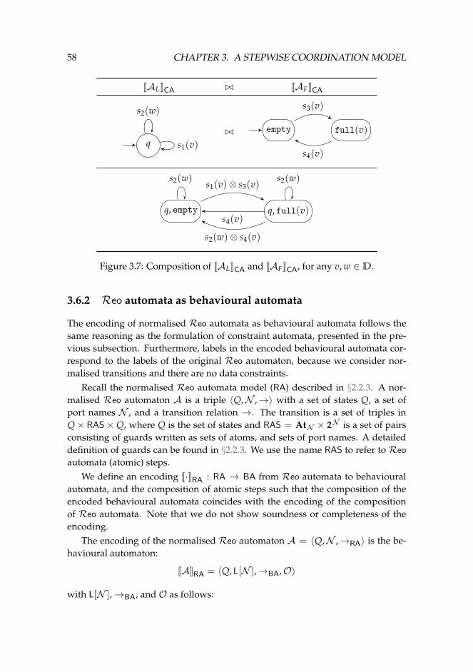
58 CHAPTER 3. A STEPWISE COORDINATION MODEL
JALKCA ./ JAFKCA
q
s2(w)
s1(v)./ empty full(v)
s3(v)
s4(v)
q, empty q, full(v)
s2(w) s2(w)s1(v)⊗ s3(v)
s4(v)
s2(w)⊗ s4(v)
Figure 3.7: Composition of JALKCA and JAFKCA, for any v, w ∈ D.
3.6.2 Reo automata as behavioural automata
The encoding of normalised Reo automata as behavioural automata follows thesame reasoning as the formulation of constraint automata, presented in the pre-vious subsection. Furthermore, labels in the encoded behavioural automata cor-respond to the labels of the original Reo automaton, because we consider nor-malised transitions and there are no data constraints.
Recall the normalised Reo automata model (RA) described in §2.2.3. A nor-malised Reo automaton A is a triple 〈Q,N ,→〉 with a set of states Q, a set ofport names N , and a transition relation →. The transition is a set of triples inQ× RAS× Q, where Q is the set of states and RAS = AtN × 2N is a set of pairsconsisting of guards written as sets of atoms, and sets of port names. A detaileddefinition of guards can be found in §2.2.3. We use the name RAS to refer to Reo
automata (atomic) steps.We define an encoding J·KRA : RA → BA from Reo automata to behavioural
automata, and the composition of atomic steps such that the composition of theencoded behavioural automata coincides with the encoding of the compositionof Reo automata. Note that we do not show soundness or completeness of theencoding.
The encoding of the normalised Reo automaton A = 〈Q,N ,→RA〉 is the be-havioural automaton:
JAKRA = 〈Q, L[N ],→BA,O〉
with L[N ],→BA, and O as follows:
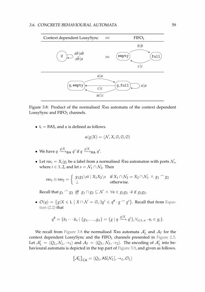
3.6. CONCRETE BEHAVIOURAL AUTOMATA 59
Context dependent LossySync ./ FIFO1
q ab abab a ./ empty full
b b
c c
q, empty q, full a a
a a
c c
ac c
Figure 3.8: Product of the normalised Reo automata of the context dependentLossySync and FIFO1 channels.
• L = RAS, and α is defined as follows.
α(g|X) = 〈N , X, ∅, ∅, ∅〉
• We have qg|X−−→BA q′ if q
g|X−−→RA q′.
• Let rasi = Xi|gi be a label from a normalised Reo automaton with ports Ni,where i ∈ 1..2, and let s = N1 ∩N2. Then
ras1 ⊗ ras2 =
{g1g2\ss | X1X2\s if X1 ∩N2 = X2 ∩N1 ∧ g1
_ g2⊥ otherwise.
Recall that g1_ g2 iff g1 ∩ g2 ⊆ N ∧ ∀a ∈ g1g2 · a /∈ g1g2.
• O(q) ={
g|X ∈ L∣∣ X ∩ N = ∅, ∃g′ ∈ q# · g_ g′
}. Recall that from Equa-
tion (2.2) that
q# = {a1 · · · an | {g1, . . . , gn} = {g | qg|X−−→ q′}, ∀i∈1..n · ai ∈ gi}.
We recall from Figure 3.8 the normalised Reo automata A′L and AF for thecontext dependent LossySync and the FIFO1 channels presented in Figure 2.5.Let A′L = 〈QL,NL,→1〉 and AF = 〈QF, NF,→2〉. The encoding of A′L into be-havioural automata is depicted in the top part of Figure 3.9, and given as follows.
qA′L
yCA = 〈QL, AS[NL],→L,OL〉
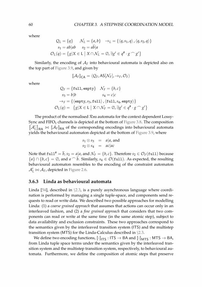
60 CHAPTER 3. A STEPWISE COORDINATION MODEL
whereQL = {q} NL = {a, b} →L = {〈q, s1, q〉 , 〈q, s2, q〉}s1 = ab|ab s2 = ab|a
OL(q) ={
g|X ∈ L∣∣ X ∩NL = ∅, ∃g′ ∈ q# · g_ g′
}Similarly, the encoding of AF into behavioural automata is depicted also on
the top part of Figure 3.9, and given by
JAFKCA = 〈QF, AS[NF],→F,OF〉
whereQF = {full, empty} NF = {b, c}s3 = b|b s4 = c|c→F = {〈empty, s3, full〉 , 〈full, s4, empty〉}
OL(q) ={
g|X ∈ L∣∣ X ∩NF = ∅, ∃g′ ∈ q# · g_ g′
}The product of the normalisedReo automata for the context dependent Lossy-
Sync and FIFO1 channels is depicted at the bottom of Figure 3.8. The compositionqA′L
yRA ./ JAFKRA of the corresponding encodings into behavioural automata
yields the behavioural automaton depicted at the bottom of Figure 3.9, where
s1 ⊗ s3 = a|a, ands2 ⊗ s4 = ac|ac
Note that full# = b, s2 = a|a, and NF = {b, c}. Therefore s2 ∈ OF(full) because{a} ∩ {b, c} = ∅, and a_ b. Similarly, s4 ∈ O(full). As expected, the resultingbehavioural automaton resembles to the encoding of the constraint automatonA′L ./ AF, depicted in Figure 2.6.
3.6.3 Linda as behavioural automata
Linda [54], described in §2.3, is a purely asynchronous language where coordi-nation is performed by managing a single tuple-space, and components send re-quests to read or write data. We described two possible approaches for modellingLinda: (1) a coarse grained approach that assumes that actions can occur only in aninterleaved fashion, and (2) a fine grained approach that considers that two com-ponents can read or write at the same time (in the same atomic step), subject todata availability and exclusion constraints. These two approaches correspond tothe semantics given by the interleaved transition system (ITS) and the multisteptransition system (MTS) for the Linda-Calculus described in §2.3.
We define two encoding functions, J·KITS : ITS→ BA and J·KMTS : MTS→ BA,from Linda tuple space terms under the semantics given by the interleaved tran-sition system and the multistep transition system, respectively, to behavioural au-tomata. Furthermore, we define the composition of atomic steps that preserve
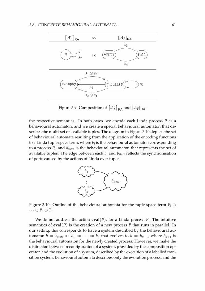
3.6. CONCRETE BEHAVIOURAL AUTOMATA 61
qA′L
yRA ./ JAFKRA
q s1s2
./ empty full
s3
s4
q, empty q, full(v) s2
s1 ⊗ s3
s4
s2 ⊗ s4
Figure 3.9: Composition ofqA′L
yRA and JAFKRA.
the respective semantics. In both cases, we encode each Linda process P as abehavioural automaton, and we create a special behavioural automaton that de-scribes the multi-set of available tuples. The diagram in Figure 3.10 depicts the setof behavioural automata resulting from the application of the encoding functionsto a Linda tuple space term, where bi is the behavioural automaton correspondingto a process Pi, and bstore is the behavioural automaton that represents the set ofavailable tuples. The edge between each bi and bstore reflects the synchronisationof ports caused by the actions of Linda over tuples.
b1
bn
... bstore
Figure 3.10: Outline of the behavioural automata for the tuple space term P1 ⊕· · · ⊕ Pn ⊕ T.
We do not address the action eval(P), for a Linda process P. The intuitivesemantics of eval(P) is the creation of a new process P that runs in parallel. Inour setting, this corresponds to have a system described by the behavioural au-tomaton b = bstore ./ b1 ./ · · · ./ bn that evolves to b ./ bn+1, where bn+1 isthe behavioural automaton for the newly created process. However, we make thedistinction between reconfiguration of a system, provided by the composition op-erator, and the evolution of a system, described by the execution of a labelled tran-sition system. Behavioural automata describes only the evolution process, and the
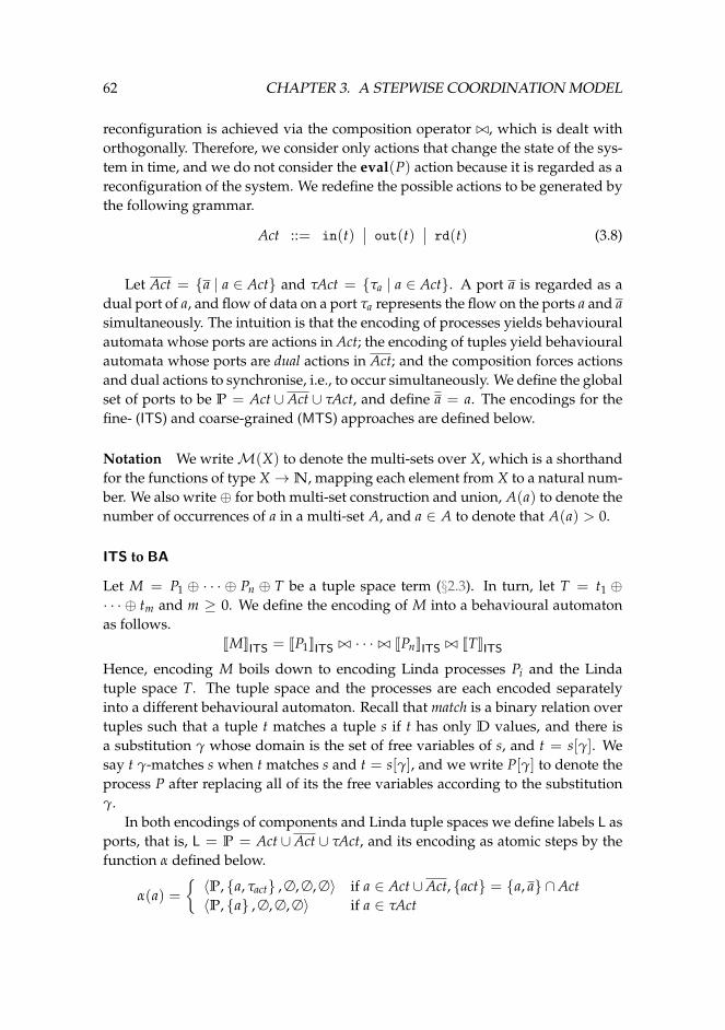
62 CHAPTER 3. A STEPWISE COORDINATION MODEL
reconfiguration is achieved via the composition operator ./, which is dealt withorthogonally. Therefore, we consider only actions that change the state of the sys-tem in time, and we do not consider the eval(P) action because it is regarded as areconfiguration of the system. We redefine the possible actions to be generated bythe following grammar.
Act ::= in(t)∣∣ out(t) ∣∣ rd(t) (3.8)
Let Act = {a | a ∈ Act} and τAct = {τa | a ∈ Act}. A port a is regarded as adual port of a, and flow of data on a port τa represents the flow on the ports a and asimultaneously. The intuition is that the encoding of processes yields behaviouralautomata whose ports are actions in Act; the encoding of tuples yield behaviouralautomata whose ports are dual actions in Act; and the composition forces actionsand dual actions to synchronise, i.e., to occur simultaneously. We define the globalset of ports to be P = Act ∪ Act ∪ τAct, and define a = a. The encodings for thefine- (ITS) and coarse-grained (MTS) approaches are defined below.
Notation We writeM(X) to denote the multi-sets over X, which is a shorthandfor the functions of type X →N, mapping each element from X to a natural num-ber. We also write⊕ for both multi-set construction and union, A(a) to denote thenumber of occurrences of a in a multi-set A, and a ∈ A to denote that A(a) > 0.
ITS to BA
Let M = P1 ⊕ · · · ⊕ Pn ⊕ T be a tuple space term (§2.3). In turn, let T = t1 ⊕· · · ⊕ tm and m ≥ 0. We define the encoding of M into a behavioural automatonas follows.
JMKITS = JP1KITS ./ · · · ./ JPnKITS ./ JTKITSHence, encoding M boils down to encoding Linda processes Pi and the Lindatuple space T. The tuple space and the processes are each encoded separatelyinto a different behavioural automaton. Recall that match is a binary relation overtuples such that a tuple t matches a tuple s if t has only D values, and there isa substitution γ whose domain is the set of free variables of s, and t = s[γ]. Wesay t γ-matches s when t matches s and t = s[γ], and we write P[γ] to denote theprocess P after replacing all of its the free variables according to the substitutionγ.
In both encodings of components and Linda tuple spaces we define labels L asports, that is, L = P = Act ∪ Act ∪ τAct, and its encoding as atomic steps by thefunction α defined below.
α(a) ={〈P, {a, τact} , ∅, ∅, ∅〉 if a ∈ Act∪Act, {act} = {a, a} ∩Act〈P, {a} , ∅, ∅, ∅〉 if a ∈ τAct
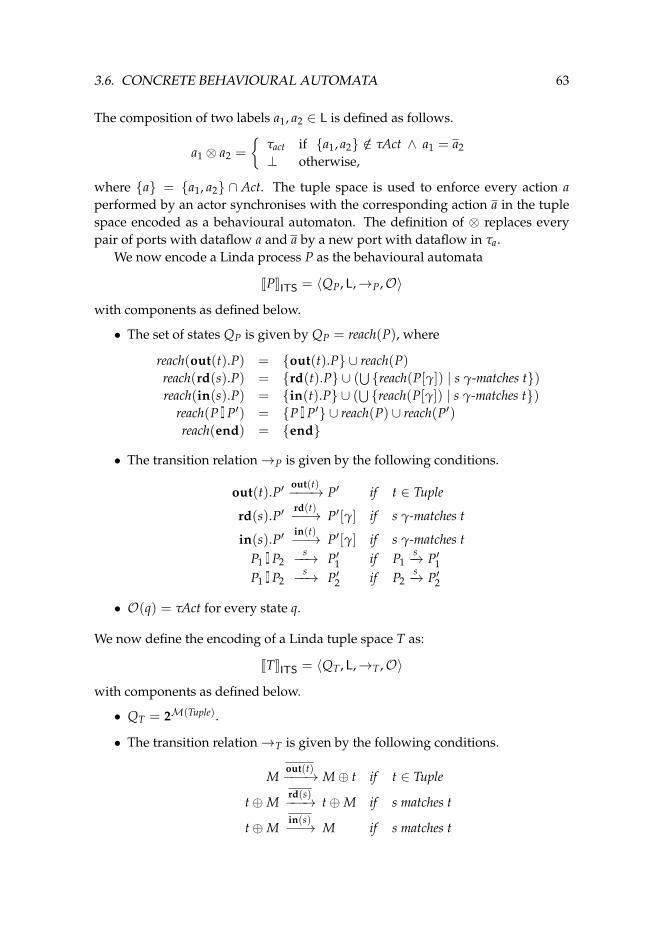
3.6. CONCRETE BEHAVIOURAL AUTOMATA 63
The composition of two labels a1, a2 ∈ L is defined as follows.
a1 ⊗ a2 =
{τact if {a1, a2} /∈ τAct ∧ a1 = a2⊥ otherwise,
where {a} = {a1, a2} ∩ Act. The tuple space is used to enforce every action aperformed by an actor synchronises with the corresponding action a in the tuplespace encoded as a behavioural automaton. The definition of ⊗ replaces everypair of ports with dataflow a and a by a new port with dataflow in τa.
We now encode a Linda process P as the behavioural automata
JPKITS = 〈QP, L,→P,O〉
with components as defined below.
• The set of states QP is given by QP = reach(P), where
reach(out(t).P) = {out(t).P} ∪ reach(P)reach(rd(s).P) = {rd(t).P} ∪ (
⋃{reach(P[γ]) | s γ-matches t})
reach(in(s).P) = {in(t).P} ∪ (⋃{reach(P[γ]) | s γ-matches t})
reach(P 2 P′) = {P 2 P′} ∪ reach(P) ∪ reach(P′)reach(end) = {end}
• The transition relation→P is given by the following conditions.
out(t).P′out(t)−−−→ P′ if t ∈ Tuple
rd(s).P′rd(t)−−→ P′[γ] if s γ-matches t
in(s).P′in(t)−−→ P′[γ] if s γ-matches t
P1 2 P2s−−→ P′1 if P1
s−→ P′1P1 2 P2
s−−→ P′2 if P2s−→ P′2
• O(q) = τAct for every state q.
We now define the encoding of a Linda tuple space T as:
JTKITS = 〈QT , L,→T ,O〉
with components as defined below.
• QT = 2M(Tuple).
• The transition relation→T is given by the following conditions.
Mout(t)−−−→ M⊕ t if t ∈ Tuple
t⊕Mrd(s)−−−→ t⊕M if s matches t
t⊕Min(s)−−→ M if s matches t
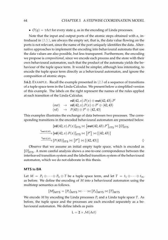
64 CHAPTER 3. A STEPWISE COORDINATION MODEL
• O(q) = τAct for every state q, as in the encoding of Linda processes.
Note that the input and output ports of the atomic steps obtained with α, in-troduced in §3.3.1, are always the empty set, that is, the data value flowing on theports is not relevant, since the name of the port uniquely identifies the data. Alter-native approaches to implement the encoding into behavioural automata that usethe data values are also possible, but less transparent. Furthermore, the encodingwe propose is compositional, since we encode each process and the store with theirown behavioural automaton, such that the product of the automata yields the be-haviour of the tuple space term. It would be simpler, although less interesting, toencode the tuple space term directly as a behavioural automaton, and ignore thecomposition of atomic steps.
3.6.2. EXAMPLE. Recall the example presented in §2.3 of a sequence of transitionsof a tuple space term in the Linda-Calculus. We present below a simplified versionof this example. The labels on the right represent the names of the rules appliedat each transition of the Linda-Calculus.
rd(42, x).P(x)⊕ out(42, 43).P′
(out) → rd(42, x).P(x)⊕ P′ ⊕ 〈42, 43〉(rd) → P(43)⊕ P′ ⊕ 〈42, 43〉
This examples illustrates the exchange of data between two processes. The corre-sponding transitions in the encoded behavioural automaton are presented below.
Jrd(42, x).P(x)KITS ./q
out(42, 43).P′yITS ./ J∅KITS
τout(42,43)−−−−−→ Jrd(42, x).P(x)KITS ./q
P′y./ J〈42, 43〉K
τrd(42,43)−−−−→ JP(43)KITS ./q
P′y./ J〈42, 43〉K ♦
Observe that we assume an initial empty tuple space, which is encoded asJ∅KITS. A more careful analysis shows a one-to-one correspondence between theinterleaved transition system and the labelled transition system of the behaviouralautomaton, which we do not elaborate in this thesis.
MTS to BA
Let M = P1 ⊕ · · · ⊕ Pn ⊕ T be a tuple space term, and let T = t1 ⊕ · · · ⊕ tm,as before. We define the encoding of M into a behavioural automaton using themultistep semantics as follows.
JMKMTS = JP1KMTS ./ · · · ./ JPnKMTS ./ JTKMTS
We encode M by encoding the Linda processes Pi and a Linda tuple space T. Asbefore, the tuple space and the processes are each encoded separately as a be-havioural automaton. We define labels as pairs
L = 2×M(Act)
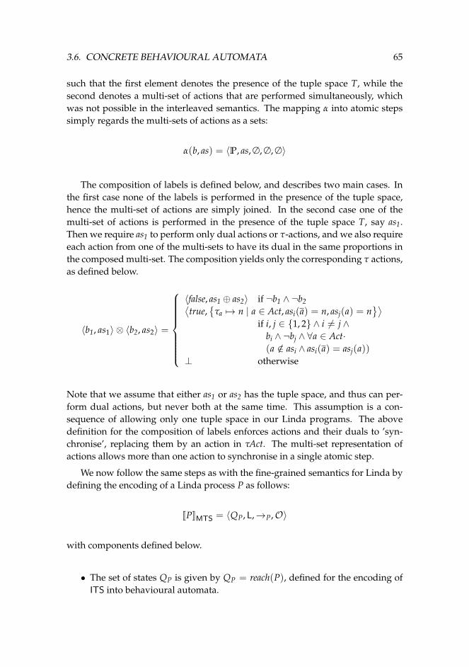
3.6. CONCRETE BEHAVIOURAL AUTOMATA 65
such that the first element denotes the presence of the tuple space T, while thesecond denotes a multi-set of actions that are performed simultaneously, whichwas not possible in the interleaved semantics. The mapping α into atomic stepssimply regards the multi-sets of actions as a sets:
α(b, as) = 〈P, as, ∅, ∅, ∅〉
The composition of labels is defined below, and describes two main cases. Inthe first case none of the labels is performed in the presence of the tuple space,hence the multi-set of actions are simply joined. In the second case one of themulti-set of actions is performed in the presence of the tuple space T, say as1.Then we require as1 to perform only dual actions or τ-actions, and we also requireeach action from one of the multi-sets to have its dual in the same proportions inthe composed multi-set. The composition yields only the corresponding τ actions,as defined below.
〈b1, as1〉 ⊗ 〈b2, as2〉 =
〈false, as1 ⊕ as2〉 if ¬b1 ∧ ¬b2⟨true,
{τa 7→ n | a ∈ Act, asi(a) = n, asj(a) = n
}⟩if i, j ∈ {1, 2} ∧ i 6= j ∧
bi ∧ ¬bj ∧ ∀a ∈ Act·(a /∈ asi ∧ asi(a) = asj(a))
⊥ otherwise
Note that we assume that either as1 or as2 has the tuple space, and thus can per-form dual actions, but never both at the same time. This assumption is a con-sequence of allowing only one tuple space in our Linda programs. The abovedefinition for the composition of labels enforces actions and their duals to ’syn-chronise’, replacing them by an action in τAct. The multi-set representation ofactions allows more than one action to synchronise in a single atomic step.
We now follow the same steps as with the fine-grained semantics for Linda bydefining the encoding of a Linda process P as follows:
JPKMTS = 〈QP, L,→P,O〉
with components defined below.
• The set of states QP is given by QP = reach(P), defined for the encoding ofITS into behavioural automata.
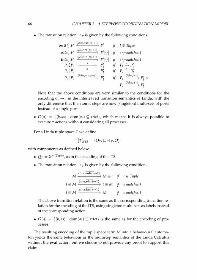
66 CHAPTER 3. A STEPWISE COORDINATION MODEL
• The transition relation→P is given by the following conditions.
out(t).P′〈false,out(t) 7→1〉−−−−−−−−−→ P′ if t ∈ Tuple
rd(s).P′〈false,rd(t) 7→1〉−−−−−−−−→ P′[γ] if s γ-matches t
in(s).P′〈false,in(t) 7→1〉−−−−−−−−→ P′[γ] if s γ-matches t
P1 2 P2s−−−−−−−→ P′1 if P1
s−→ P′1P1 2 P2
s−−−−−−−→ P′2 if P2s−→ P′2
P1 2 P2〈false,as1⊗as2〉−−−−−−−→ P′2 if P1
〈false,as1〉−−−−−→ P′1 ∧
P2〈false,as2〉−−−−−→ P′2
Note that the above conditions are very similar to the conditions for theencoding of →P in the interleaved transition semantics of Linda, with theonly difference that the atomic steps are now (singleton) multi-sets of portsinstead of a single port.
• O(q) = {〈b, as〉 | dom(as) ⊆ τAct}, which means it is always possible toexecute τ actions without considering all processes.
For a Linda tuple space T we define
JTKITS = 〈QT , L,→T ,O〉
with components as defined below.
• QT = 2M(Tuple), as in the encoding of the ITS.
• The transition relation→T is given by the following conditions.
M〈true,out(t) 7→1〉−−−−−−−−−→ M⊕ t if t ∈ Tuple
t⊕M〈true,rd(s) 7→1〉−−−−−−−−→ t⊕M if s matches t
t⊕M〈true,in(s) 7→1〉−−−−−−−−→ M if s matches t
The above transition relation is the same as the corresponding transition re-lation for the encoding of the ITS, using singleton multi-sets as labels insteadof the corresponding action.
• O(q) = {〈b, as〉 | dom(as) ⊆ τAct} is the same as for the encoding of pro-cesses.
The resulting encoding of the tuple space term M into a behavioural automa-ton yields the same behaviour as the multistep semantics of the Linda Calculuswithout the eval action, but we choose to not provide any proof to support thisclaim.
3.7. RELATED CONCEPTS 67
3.7 Related concepts
In this chapter we present a stepwise coordination model based on behaviouralautomata. This model represents our view of a dataflow-driven coordination sys-tem, following the categorisation of Arbab [10]. Each transition in a behaviouralautomaton represents the atomic execution of a number of actions by the coordina-tion system. The behaviour of a system in our stepwise model is described by thecomposition of the behaviour of its sub-systems running concurrently, each withits own behavioural automaton. Furthermore, we allow the data values exchangedover the coordination layer to influence the choice of how components commu-nicate with each other as well. We now present a brief discussion about how thethree main concepts that underlie our stepwise model—atomicity, composability,and dataflow—are viewed in the computer science community. The goal of thislimited survey is to clarify the differences between these three concepts and othersimilar concepts that are sometimes interpreted as being synonymous. Further-more, it explains in what sense our stepwise coordination model is (and is not)synchronous and composable, and how (and how not) it uses the dataflow infor-mation.
Atomicity. The notions of atomicity, synchrony, and transactional execution havebeen frequently used in similar settings, with similar, although different, mean-ings. Atomicity is usually associated with a sequence of instructions that are guar-anteed to execute atomically, i.e., without being interleaved with interfering in-structions. Achieving atomicity typically involves solving a locking problem: howto protect shared resources to guarantee that only a single thread or process hasaccess to it at a given time. Mutexes and semaphores provide common solutionsto achieve atomicity [42]. Synchronisation provides a restricted sense of atomicity,and it is associated with the notions of causality and time. We interpret synchro-nisation as synchronisation of actions, and two actions synchronise if they occurat the same time. Note that true synchrony is not possible in distributed systems,because there is no way to guarantee that two actions in different computers areperformed at the exact same time. Action synchronisation captures the main ideaunderlying process synchronisation [44] and data synchronisation [49], whose distinc-tion in the literature simply reflects that the execution of different processes mustevolve at the same time, or that multiple copies of the same data must be keptcoherent. Finally, atomicity is known in the database community in the context oftransactions, where actions can be rolled back when necessary.
Our stepwise coordination model is synchronous in the sense of atomicity asexplained above. A set of actions (also referred to as a set of steps) S executesatomically if no other action can interfere in between the time when the first a ∈ Sstarts to execute and when the execution of all of the actions in S is complete.
68 CHAPTER 3. A STEPWISE COORDINATION MODEL
Other actions can still occur in the same time frame, as long as they do not interferewith the actions in S. The synchronisation of two or more actions yields a newaction, obtained by applying a composition operator ⊗.
Composability. Composability is closely related to concurrency and distribution.We first clarify the distinction between distributed and concurrent systems. Dis-tribution involves the execution of a coordination system at multiple locations,where locations can be computers, networks, but also CPU’s. Concurrency de-scribes how to approach a given problem using independent and communicatingthreads of execution. A non-concurrent program executes its instructions sequen-tially. Clearly a concurrent program does not have to be distributed across mul-tiple locations. Furthermore, a program executing in a distributed network doesnot have to be concurrent either. A non-concurrent program can be executed ina distributed network using mechanisms that involve replication and guaranteeconsistency of the state of different replicas (e.g., to provide redundancy for faulttolerance, or to exploit special resources available at only specific locations). Thus,concurrency can be seen as a means to have more effective distribution, that is,distributed implementations typically gain from being concurrent.
We now describe what we mean by composability. The systems studied in thisthesis have an underlying abstract model representing their coordination. Havingan abstract coordination model facilitates the proof of interesting properties, suchas correctness or deadlock freedom, and helps us to reason about the behaviourof the coordination system. A composable coordination model is constructed outof building blocks that can be analysed independently. The composition of thebuilding blocks describes how they interact with each other. But are implemen-tations of a composable coordination model always concurrent? No. Althougha composable coordination model can describe its behaviour using simpler con-current composable blocks, its implementation can still require a (partially) non-concurrent execution. Note that the components or services being coordinated canexecute concurrently. The coordination model we present in this thesis describesa concurrent description of a concurrent model which, at first sight, seems to re-quire a non-concurrent execution, due to its synchronisation constraints (but, infact, it does not).
Dataflow networks and dataflow analysis. Important research on dataflow net-works can be found in Kahn’s seminal work [66] about Kahn Networks (KN) andin Kok’s work about the semantics of dataflow for parallel computation [73, 74].Kahn introduced KN’s back in 1974 to model how processes, executing in se-quence or in parallel, transform infinite streams of data, using atomic data tokensas the smallest unit of data being transferred. Kok presents two fully abstractsemantics for a class of dataflow nets introduced by Kahn, emphasising on their
3.8. CONCLUSIONS 69
compositionality aspects. Dataflow models and Kahn networks can be viewedas specialised channel-based models with respect to Reo that incorporate somebasic constructs for primitive coordination, as discussed by Arbab [8]. The di-luted notion of local time in Reo, which is used to express atomicity and order-ing of events, differentiates otherwise ‘equivalent behaviour’ of networks in otherdataflow models that lead to the Brock-Ackerman anomalies [31].
The field of dataflow analysis studies the execution of programs as a series oftransformations of the program state by performing code statements. A simpleoverview of dataflow analysis can be found, for example, in the book of Aho etal. on compilers [3]. A general approach is to relate the possible states before andafter each statement, referred to as the inputs and outputs, by a transfer function.Multiple predecessor statements can be connected to the input, in which case theyare combined by a meet operator, assuming a meet semilattice over a set of valuesD. Multiple successors can also be connected to the output, in which case the datais replicated. Furthermore, they assume that the set of all transfer functions hasan identity function and is closed under composition. In this setting it is possibleto identify properties of dataflow schemas, and prove the implication of theseproperties on the correctness, precision, and convergence of a dataflow algorithm.This relation between inputs and outputs of statements is closely related to thenotion of data constraints in the context of coordination, using a compositionalmodel. However, this thesis focuses on synchronisation constraints and does notexploit this direction.
3.8 Conclusions
We defined the stepwise coordination model to capture the characteristics of themodels that can be used by the Dreams framework. The stepwise coordinationmodel abstracts from the definition and composition of labels, and imposes generalproperties over atomic steps associated with transportation labels and their com-position. Each of the concrete models defined in Chapter 2 is formulated as aninstance of a behavioural automaton.
By defining and composing labels only in the concrete models, we focus on theproperties provided by behavioural automata which, under certain assumptions,allows aspects other than synchronisation and data to be incorporated in our dis-tributed framework. As an example, we have presented how to incorporate thenotion of context dependency (§3.6.2). Other aspects like time [13], quality-of-service guarantees [15], resource bounds [81], or probability [21, 23, 88], can beused in the Dreams framework as well. Note that each label has an associatedatomic step, but the opposite does not necessary hold, with the exception of theidentity atomic step which we assume to have a special identity label.
The encoded behavioural automata from automata models forReo are closely
70 CHAPTER 3. A STEPWISE COORDINATION MODEL
related to its original semantic models, but this is not the case for Linda. We kepta compositional approach in our encoding of Linda as behavioural automata toallow the execution of Linda in our framework over multiple locations, possiblydeploying each Linda process and the tuple space in a different location. Alterna-tively, we could have encoded a tuple space term M = P1 ⊕ · · · ⊕ Pn ⊕ T simplyby considering the labelled transition system presented in §2.3, and disregardingthe composition of the resulting behavioural automata. The specific encoding ofeach label as an atomic step is not relevant, because in this alternative approachatomic steps never need to be composed. The downside of such an approach isthe loss of concurrency, making it less interesting in the context of this thesis.
Chapter 4
Connector colouring & animation
4.1 Introduction
Connector colouring (CC), introduced by Clarke et al. [37], further developed inCosta’s Ph.D. thesis [41], and extended by Arbab et al. using the tile model [14],provides a semantics for the Reo coordination language [8] which improves itspreceding semantics in three main aspects.
1. It is the first semantic model of Reo introducing a precise notion of contextdependency, as explained in §2.2.3 when describing theReo automata model.We recall this notion below.
2. It is more intuitive, in the sense that it exploits Reo’s graphical notation,marking each part of a Reo connector with a ‘colour’ describing its be-haviour. The intuition provided by the graphical representation of connectorcolouring is further explored by the animation framework that we describelater in this chapter.
3. It is better suited for distribution. The main support for this claim are the for-mal properties of the main composition operator, namely associativity, com-mutativity, and idempotency. Furthermore, in previous (automata) modelsfor Reo, the composition of a pair of connectors c1 and c2 yields a new con-nector c3 that discards c1 and c2 as individual parts of the new connector, andconsiders only the new global behaviour. Instead, the connector colouringsemantics describes the new behaviour of c1 and c2 after their composition.
The need for a context dependent semantics for Reo has been motivated andexplained in §2.2.3. We recall the basic ideas behind Reo in §4.2, presented in de-tail in §2.2. Using a context dependent semantics, we distinguish two differentkinds of absence of flow: (1) the possibility of not having dataflow, and (2) the needto have no dataflow. This distinction allows the definition of behaviour where
71
72 CHAPTER 4. CONNECTOR COLOURING & ANIMATION
the absence of flow can be either imposed or required. For example, the context-dependent LossySync is a synchronous channel with a source and a sink end, suchdata can either be transferred between these two ends or lost after flowing throughthe source end. However, the channel does not lose data non-deterministically,but it allows data to be lost if the sink end cannot have dataflow. On the otherhand, an empty FIFO1 channel always imposes the absence of dataflow on its sinkend. The composition operator defined in the connector colouring semantics re-quires all absence of flow to have at least one end imposing its absence, extendingthe expressive power of its preceding semantics.
Motivated by the second and third contribution mentioned above, we devel-oped in joint work with David Costa a compositional animation framework basedon connector colouring. The results are explained in detail in Costa’s thesis [41],and are more briefly explained in this chapter. The goal of our animation frame-work is to automatically derive visual animations to help the developer of Reo
connectors understand the precise behaviour of his/her own connectors. Ourprocess of generating animations was incorporated in a visual editor for Reo byChristian Krause [16]. These tools and the animations of someReo connectors canbe found online.1
Contribution to the thesis Although we presentedReo and its formal semanticsin §2.2, we dedicate a chapter for connector colouring and animations becauseof the relevance of the connector colouring in the remainder of the thesis. Theconnector colouring focuses on the possible behaviour for a single round of Reo,and preserves the information regarding the behaviour of each of the primitivesin the connector. These two factors make connector colouring suitable as a basisfor a distributed implementation and motivated the development of the Dreams
framework.We encode the connector colouring model as behavioural automata, stress-
ing the choices we made when defining behavioural automata, and extend it withdata-related information and with concurrency predicates, which yield a new con-cept of local colourings. Finally, the animation framework exhibits the need to in-clude the information regarding how data is flowing, which is not modelled by theconnector colouring semantics, making the animation framework the first meansto model the dataflow of distributedReo connectors.
Organisation of the chapter We briefly recall Reo and explain the intuition be-hind the use of colours to describe the behaviour ofReo in §4.2. We then formalisethe connector colouring semantics in §4.3, and its encoding into behavioural au-tomata in §4.4. We exemplify the connector colouring semantics with three con-nectors in §4.5. Our animation framework is described in §4.6, and we wrap up
1Available at reo.project.cwi.nl.
4.2. CONNECTOR COLOURING OVERVIEW 73
by describing related workin §4.7 and presenting some conclusions in §4.8.
4.2 Connector colouring overview
The Reo coordination language [8, 9], described in §2.2, is a channel-based lan-guage where connectors are compositionally built out of a simple set of primitivesconnectors. Each primitive connector, also referred to as a primitive, has a set ofends which act as input or output points of data. For consistency with Chap-ter 3, we say ‘port’ to each primitive end, and assume a global set of ports P.Channels are special primitives with two ports. Some of the most commonly usedReo channels and primitives are presented in the left columns of Tables 4.1 and4.2, respectively. The composition of two connectors is performed by joining theshared ports. Ports are joined in a one-to-one manner, and a source port (port thatreceives data) can only be joined to a sink port (port that sends data). A mixednode, depicted by , is the logical place resulting from joining of two ports, and aboundary node, depicted by , is the logical place with only one port.
The connector colouring (CC) semantics, as presented by Clarke et al. [37],is based on the idea of colouring the ports of a connector using a set of threecolours—for orientation, indicates the port. The colour marks ports in theconnector where data flow, and the two colours and mark the absenceof dataflow. The main idea is that every absence of flow must have a reason forexcluding the flow of data, for example, because an empty FIFO1 buffer cannotproduce data. The different no-flow colours mark the direction from where thereason originates. The colour denotes that the reason for no-flow originatesfrom the context, by exhibiting an arrow coming from the port, and we say thatthe port requires a reason for no-flow. Similarly, indicates that the reason forno-flow originates from the primitive, using an arrow pointing in the direction ofthe port, and we say that the port gives a reason for no-flow.
Colouring a connector means associating colours to each of its ports in such away that the colours of two connected ports match. The colours of two ports matchif both represent flow, or if the reason for no-flow comes from at least one of theports. That is, the valid combinations are: , , and .Invalid matches of colours include and ; the first pair representsthe case when there is dataflow only in one of two connected ports, and the secondpair represents a reason being created when joining the ports, which is undesir-able in connector colouring. Each primitive has only a specific set of admissiblecolourings, which determine its synchronisation constraints. Each colouring is amapping from the ports of a primitive to a colour, and the set of the colourings ofa connector is called its colouring table. Thus, a colouring table represents the set ofall possible behaviour of a Reo connector. Tables 4.1 and 4.2 present all possiblebehaviour of the most commonly used Reo primitives. Composition of two con-
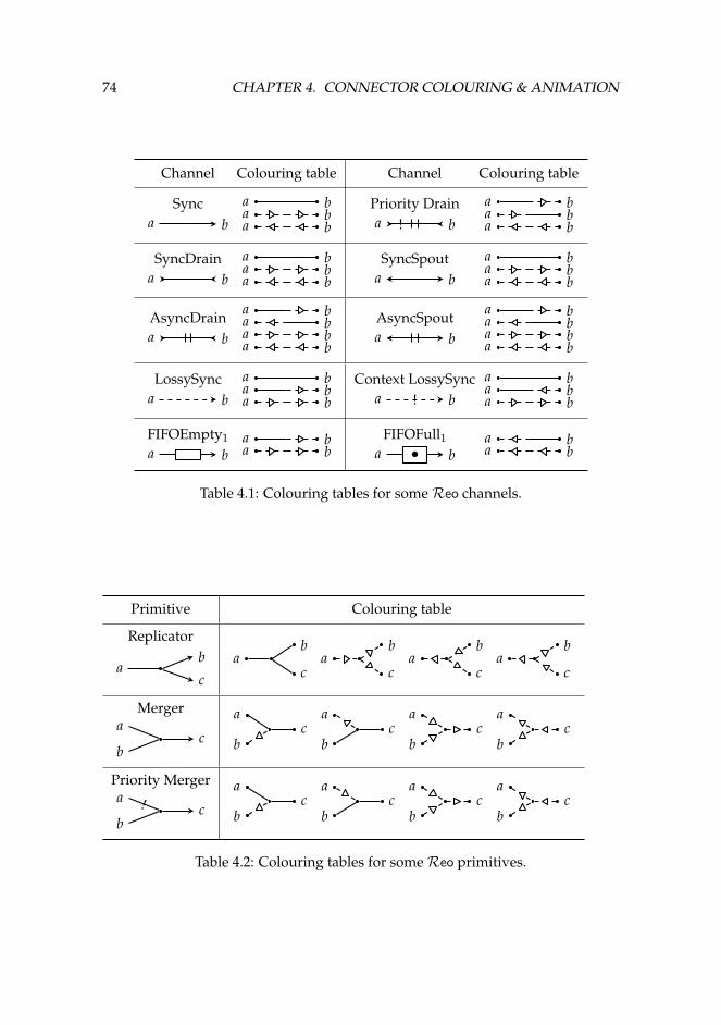
74 CHAPTER 4. CONNECTOR COLOURING & ANIMATION
Channel Colouring table Channel Colouring table
Synca b
a ba ba b
Priority Draina b!
a ba ba b
SyncDraina b
a ba ba b
SyncSpouta b
a ba ba b
AsyncDraina b
a ba ba ba b
AsyncSpouta b
a ba ba ba b
LossySynca b
a ba ba b
Context LossySynca b!
a ba ba b
FIFOEmpty1a b
a ba b
FIFOFull1a b•
a ba b
Table 4.1: Colouring tables for someReo channels.
Primitive Colouring table
Replicator
ab
ca
b
ca
b
ca
b
ca
b
c
Merger
ca
b
ca
bc
a
bc
a
bc
a
b
Priority Merger
ca
b! c
a
bc
a
bc
a
bc
a
b
Table 4.2: Colouring tables for someReo primitives.
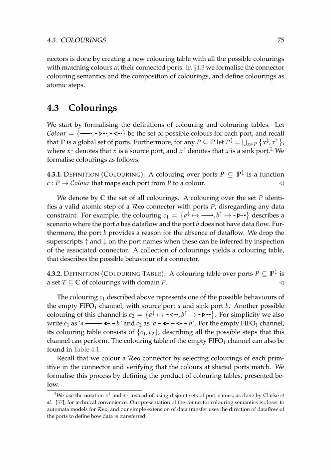
4.3. COLOURINGS 75
nectors is done by creating a new colouring table with all the possible colouringswith matching colours at their connected ports. In §4.3 we formalise the connectorcolouring semantics and the composition of colourings, and define colourings asatomic steps.
4.3 Colourings
We start by formalising the definitions of colouring and colouring tables. LetColour = { , , } be the set of possible colours for each port, and recallthat P is a global set of ports. Furthermore, for any P ⊆ P let Pl =
⋃x∈P
{x↓, x↑
},
where x↓ denotes that x is a source port, and x↑ denotes that x is a sink port.2 Weformalise colourings as follows.
4.3.1. DEFINITION (COLOURING). A colouring over ports P ⊆ Pl is a functionc : P→ Colour that maps each port from P to a colour. C
We denote by C the set of all colourings. A colouring over the set P identi-fies a valid atomic step of a Reo connector with ports P, disregarding any dataconstraint. For example, the colouring c1 =
{a↓ 7→ , b↑ 7→
}describes a
scenario where the port a has dataflow and the port b does not have data flow. Fur-thermore, the port b provides a reason for the absence of dataflow. We drop thesuperscripts ↑ and ↓ on the port names when these can be inferred by inspectionof the associated connector. A collection of colourings yields a colouring table,that describes the possible behaviour of a connector.
4.3.2. DEFINITION (COLOURING TABLE). A colouring table over ports P ⊆ Pl isa set T ⊆ C of colourings with domain P. C
The colouring c1 described above represents one of the possible behaviours ofthe empty FIFO1 channel, with source port a and sink port b. Another possiblecolouring of this channel is c2 =
{a↓ 7→ , b↑ 7→
}. For simplicity we also
write c1 as ‘a b ’ and c2 as ‘a b ’. For the empty FIFO1 channel,its colouring table consists of {c1, c2}, describing all the possible steps that thischannel can perform. The colouring table of the empty FIFO1 channel can also befound in Table 4.1.
Recall that we colour a Reo connector by selecting colourings of each prim-itive in the connector and verifying that the colours at shared ports match. Weformalise this process by defining the product of colouring tables, presented be-low.
2We use the notation x↑ and x↓ instead of using disjoint sets of port names, as done by Clarke etal. [37], for technical convenience. Our presentation of the connector colouring semantics is closer toautomata models for Reo, and our simple extension of data transfer uses the direction of dataflow ofthe ports to define how data is transferred.
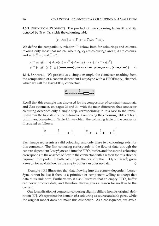
76 CHAPTER 4. CONNECTOR COLOURING & ANIMATION
4.3.3. DEFINITION (PRODUCT). The product of two colouring tables T1 and T2,denoted by T1 ./ T2, yields the colouring table
{c1 ∪ c2 | c1 ∈ T1, c2 ∈ T2, c1_ c2}.
We define the compatibility relation _ below, both for colourings and colours,relating only those that match, where c1, c2 are colourings and a, b are colours,and with ↑ =↓ and ↓ =↑ :
c1_ c2 iff x◦ ∈ dom(c1) ∧ x◦ ∈ dom(c2)⇒ c1(x◦)_ c2(x◦)
a_ b iff 〈a, b〉 ∈ {〈 , 〉 , 〈 , 〉 , 〈 , 〉 , 〈 , 〉} C
4.3.4. EXAMPLE. We present as a simple example the connector resulting fromthe composition of a context-dependent LossySync with a FIFOEmpty1 channel,which we call the lossy-FIFO1 connector:
a b c!
Recall that this example was also used for the composition of constraint automataand Reo automata, on pages 28 and 34, with the main difference that connectorcolouring describes only a single step, corresponding in this case to the transi-tions from the first state of the automata. Composing the colouring tables of bothprimitives, presented in Table 4.1, we obtain the colouring table of the connectorillustrated as follows:
a b c a b c
Each image represents a valid colouring, and only these two colourings exist forthis connector. The first colouring corresponds to the flow of data through thecontext-dependent LossySync and into the FIFO1 buffer, and the second colouringcorresponds to the absence of flow in the connector, with a reason for this absencerequired from port a. In both colourings, the port c of the FIFO1 buffer (c↓) givesa reason for no dataflow, as the empty buffer can offer no data. ♦
Example 4.3.4 illustrates that data flowing into the context-dependent Lossy-Sync cannot be lost if there is a primitive or component willing to accept thatdata at its sink port. Furthermore, it also illustrates that an empty FIFO1 buffercan never produce data, and therefore always gives a reason for no flow to thecontext.
Our formalisation of connector colouring slightly differs from its original defi-nition [37]. We represent the domain of a colouring as source and sink ports, whilethe original model does not make this distinction. As a consequence, we avoid
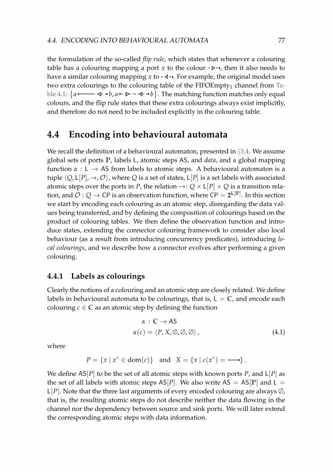
4.4. ENCODING INTO BEHAVIOURAL AUTOMATA 77
the formulation of the so-called flip rule, which states that whenever a colouringtable has a colouring mapping a port x to the colour , then it also needs tohave a similar colouring mapping x to . For example, the original model usestwo extra colourings to the colouring table of the FIFOEmpty1 channel from Ta-ble 4.1:
{a b, a b
}. The matching function matches only equal
colours, and the flip rule states that these extra colourings always exist implicitly,and therefore do not need to be included explicitly in the colouring table.
4.4 Encoding into behavioural automata
We recall the definition of a behavioural automaton, presented in §3.4. We assumeglobal sets of ports P, labels L, atomic steps AS, and data, and a global mappingfunction α : L → AS from labels to atomic steps. A behavioural automaton is atuple 〈Q, L[P],→,O〉, where Q is a set of states, L[P] is a set labels with associatedatomic steps over the ports in P, the relation→: Q× L[P]×Q is a transition rela-tion, andO : Q→ CP is an observation function, where CP = 2L[P]. In this sectionwe start by encoding each colouring as an atomic step, disregarding the data val-ues being transferred, and by defining the composition of colourings based on theproduct of colouring tables. We then define the observation function and intro-duce states, extending the connector colouring framework to consider also localbehaviour (as a result from introducing concurrency predicates), introducing lo-cal colourings, and we describe how a connector evolves after performing a givencolouring.
4.4.1 Labels as colourings
Clearly the notions of a colouring and an atomic step are closely related. We definelabels in behavioural automata to be colourings, that is, L = C, and encode eachcolouring c ∈ C as an atomic step by defining the function
α : C→ AS
α(c) = 〈P, X, ∅, ∅, ∅〉 , (4.1)
where
P = {x | x◦ ∈ dom(c)} and X = {x | c(x◦) = } .
We define AS[P] to be the set of all atomic steps with known ports P, and L[P] asthe set of all labels with atomic steps AS[P]. We also write AS = AS[P] and L =
L[P]. Note that the three last arguments of every encoded colouring are always ∅,that is, the resulting atomic steps do not describe neither the data flowing in thechannel nor the dependency between source and sink ports. We will later extendthe corresponding atomic steps with data information.
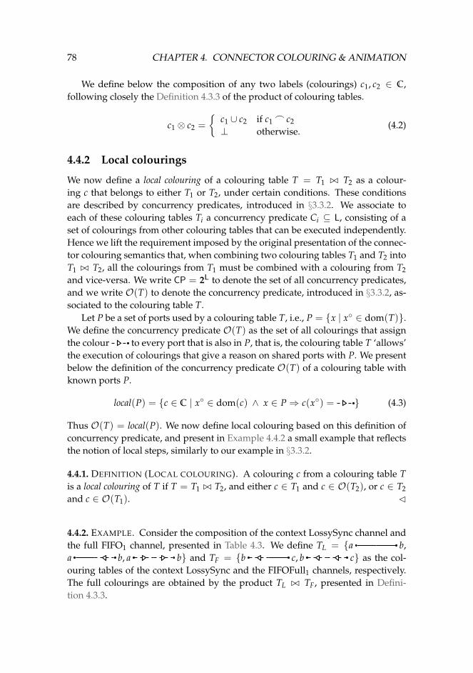
78 CHAPTER 4. CONNECTOR COLOURING & ANIMATION
We define below the composition of any two labels (colourings) c1, c2 ∈ C,following closely the Definition 4.3.3 of the product of colouring tables.
c1 ⊗ c2 =
{c1 ∪ c2 if c1
_ c2⊥ otherwise.
(4.2)
4.4.2 Local colourings
We now define a local colouring of a colouring table T = T1 ./ T2 as a colour-ing c that belongs to either T1 or T2, under certain conditions. These conditionsare described by concurrency predicates, introduced in §3.3.2. We associate toeach of these colouring tables Ti a concurrency predicate Ci ⊆ L, consisting of aset of colourings from other colouring tables that can be executed independently.Hence we lift the requirement imposed by the original presentation of the connec-tor colouring semantics that, when combining two colouring tables T1 and T2 intoT1 ./ T2, all the colourings from T1 must be combined with a colouring from T2and vice-versa. We write CP = 2L to denote the set of all concurrency predicates,and we write O(T) to denote the concurrency predicate, introduced in §3.3.2, as-sociated to the colouring table T.
Let P be a set of ports used by a colouring table T, i.e., P = {x | x◦ ∈ dom(T)}.We define the concurrency predicate O(T) as the set of all colourings that assignthe colour to every port that is also in P, that is, the colouring table T ‘allows’the execution of colourings that give a reason on shared ports with P. We presentbelow the definition of the concurrency predicate O(T) of a colouring table withknown ports P.
local(P) = {c ∈ C | x◦ ∈ dom(c) ∧ x ∈ P⇒ c(x◦) = } (4.3)
Thus O(T) = local(P). We now define local colouring based on this definition ofconcurrency predicate, and present in Example 4.4.2 a small example that reflectsthe notion of local steps, similarly to our example in §3.3.2.
4.4.1. DEFINITION (LOCAL COLOURING). A colouring c from a colouring table Tis a local colouring of T if T = T1 ./ T2, and either c ∈ T1 and c ∈ O(T2), or c ∈ T2and c ∈ O(T1). C
4.4.2. EXAMPLE. Consider the composition of the context LossySync channel andthe full FIFO1 channel, presented in Table 4.3. We define TL = {a b,a b, a b} and TF = {b c, b c} as the col-ouring tables of the context LossySync and the FIFOFull1 channels, respectively.The full colourings are obtained by the product TL ./ TF, presented in Defini-tion 4.3.3.
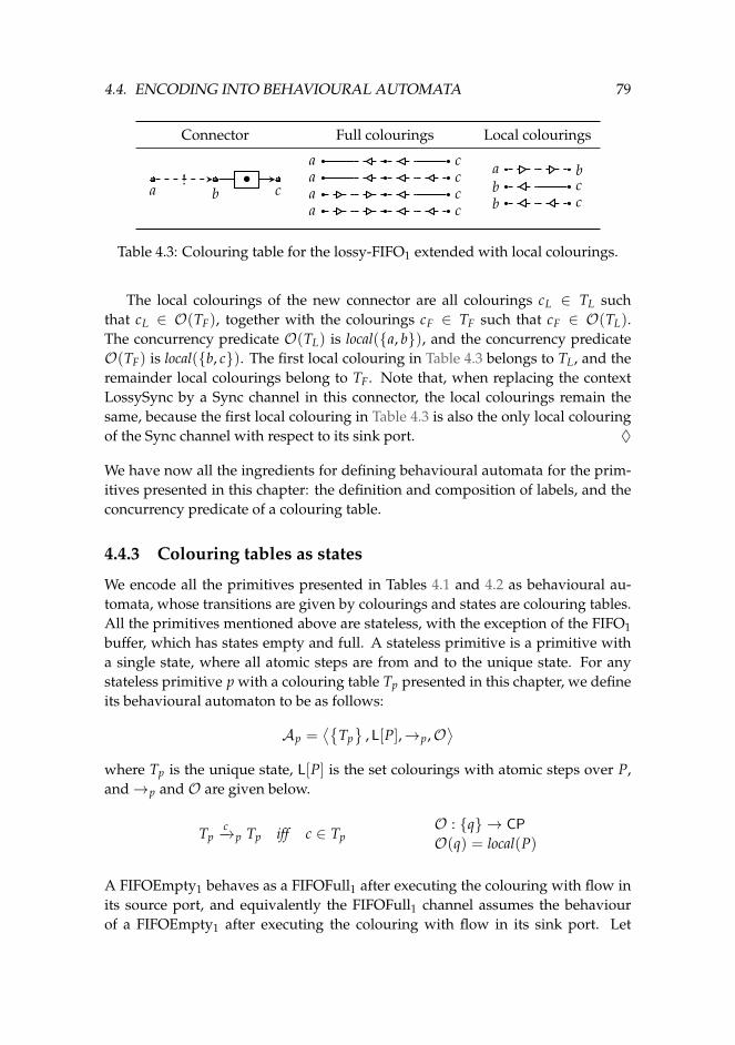
4.4. ENCODING INTO BEHAVIOURAL AUTOMATA 79
Connector Full colourings Local colourings
a b c! •
a ca ca ca c
a bb cb c
Table 4.3: Colouring table for the lossy-FIFO1 extended with local colourings.
The local colourings of the new connector are all colourings cL ∈ TL suchthat cL ∈ O(TF), together with the colourings cF ∈ TF such that cF ∈ O(TL).The concurrency predicate O(TL) is local({a, b}), and the concurrency predicateO(TF) is local({b, c}). The first local colouring in Table 4.3 belongs to TL, and theremainder local colourings belong to TF. Note that, when replacing the contextLossySync by a Sync channel in this connector, the local colourings remain thesame, because the first local colouring in Table 4.3 is also the only local colouringof the Sync channel with respect to its sink port. ♦
We have now all the ingredients for defining behavioural automata for the prim-itives presented in this chapter: the definition and composition of labels, and theconcurrency predicate of a colouring table.
4.4.3 Colouring tables as states
We encode all the primitives presented in Tables 4.1 and 4.2 as behavioural au-tomata, whose transitions are given by colourings and states are colouring tables.All the primitives mentioned above are stateless, with the exception of the FIFO1buffer, which has states empty and full. A stateless primitive is a primitive witha single state, where all atomic steps are from and to the unique state. For anystateless primitive p with a colouring table Tp presented in this chapter, we defineits behavioural automaton to be as follows:
Ap =⟨{
Tp}
, L[P],→p,O⟩
where Tp is the unique state, L[P] is the set colourings with atomic steps over P,and→p and O are given below.
Tpc−→p Tp iff c ∈ Tp
O : {q} → CP
O(q) = local(P)
A FIFOEmpty1 behaves as a FIFOFull1 after executing the colouring with flow inits source port, and equivalently the FIFOFull1 channel assumes the behaviourof a FIFOEmpty1 after executing the colouring with flow in its sink port. Let
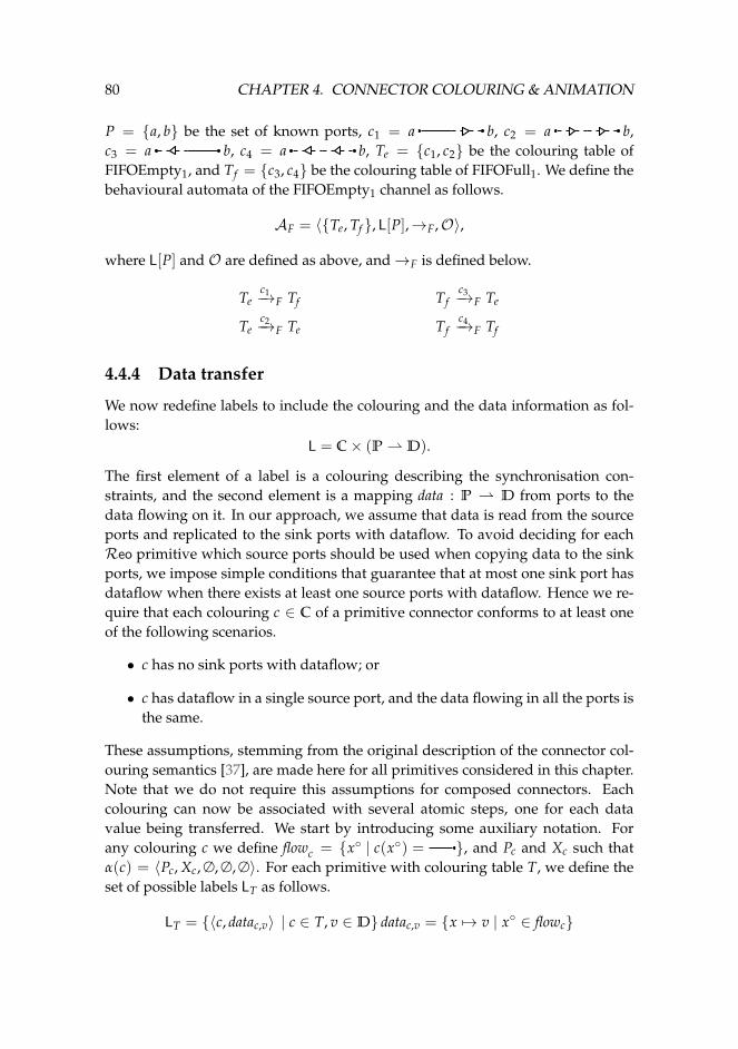
80 CHAPTER 4. CONNECTOR COLOURING & ANIMATION
P = {a, b} be the set of known ports, c1 = a b, c2 = a b,c3 = a b, c4 = a b, Te = {c1, c2} be the colouring table ofFIFOEmpty1, and Tf = {c3, c4} be the colouring table of FIFOFull1. We define thebehavioural automata of the FIFOEmpty1 channel as follows.
AF = 〈{Te, Tf }, L[P],→F,O〉,
where L[P] and O are defined as above, and→F is defined below.
Tec1−→F Tf Tf
c3−→F Te
Tec2−→F Te Tf
c4−→F Tf
4.4.4 Data transfer
We now redefine labels to include the colouring and the data information as fol-lows:
L = C× (P ⇀ D).
The first element of a label is a colouring describing the synchronisation con-straints, and the second element is a mapping data : P ⇀ D from ports to thedata flowing on it. In our approach, we assume that data is read from the sourceports and replicated to the sink ports with dataflow. To avoid deciding for eachReo primitive which source ports should be used when copying data to the sinkports, we impose simple conditions that guarantee that at most one sink port hasdataflow when there exists at least one source ports with dataflow. Hence we re-quire that each colouring c ∈ C of a primitive connector conforms to at least oneof the following scenarios.
• c has no sink ports with dataflow; or
• c has dataflow in a single source port, and the data flowing in all the ports isthe same.
These assumptions, stemming from the original description of the connector col-ouring semantics [37], are made here for all primitives considered in this chapter.Note that we do not require this assumptions for composed connectors. Eachcolouring can now be associated with several atomic steps, one for each datavalue being transferred. We start by introducing some auxiliary notation. Forany colouring c we define flowc = {x◦ | c(x◦) = }, and Pc and Xc such thatα(c) = 〈Pc, Xc, ∅, ∅, ∅〉. For each primitive with colouring table T, we define theset of possible labels LT as follows.
LT = {〈c, datac,v〉 | c ∈ T, v ∈ D} datac,v = {x 7→ v | x◦ ∈ flowc}
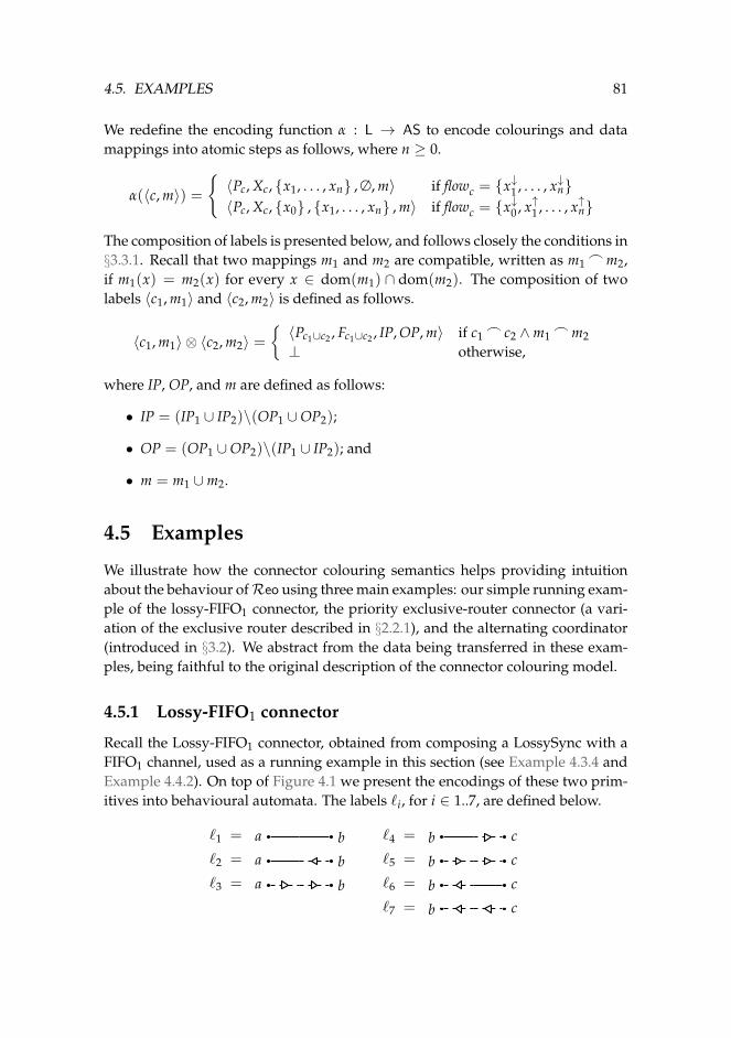
4.5. EXAMPLES 81
We redefine the encoding function α : L → AS to encode colourings and datamappings into atomic steps as follows, where n ≥ 0.
α(〈c, m〉) ={〈Pc, Xc, {x1, . . . , xn} , ∅, m〉 if flowc = {x
↓1 , . . . , x↓n}
〈Pc, Xc, {x0} , {x1, . . . , xn} , m〉 if flowc = {x↓0 , x↑1 , . . . , x↑n}
The composition of labels is presented below, and follows closely the conditions in§3.3.1. Recall that two mappings m1 and m2 are compatible, written as m1
_m2,if m1(x) = m2(x) for every x ∈ dom(m1) ∩ dom(m2). The composition of twolabels 〈c1, m1〉 and 〈c2, m2〉 is defined as follows.
〈c1, m1〉 ⊗ 〈c2, m2〉 ={〈Pc1∪c2 , Fc1∪c2 , IP, OP, m〉 if c1
_ c2 ∧m1_m2
⊥ otherwise,
where IP, OP, and m are defined as follows:
• IP = (IP1 ∪ IP2)\(OP1 ∪OP2);
• OP = (OP1 ∪OP2)\(IP1 ∪ IP2); and
• m = m1 ∪m2.
4.5 Examples
We illustrate how the connector colouring semantics helps providing intuitionabout the behaviour ofReo using three main examples: our simple running exam-ple of the lossy-FIFO1 connector, the priority exclusive-router connector (a vari-ation of the exclusive router described in §2.2.1), and the alternating coordinator(introduced in §3.2). We abstract from the data being transferred in these exam-ples, being faithful to the original description of the connector colouring model.
4.5.1 Lossy-FIFO1 connector
Recall the Lossy-FIFO1 connector, obtained from composing a LossySync with aFIFO1 channel, used as a running example in this section (see Example 4.3.4 andExample 4.4.2). On top of Figure 4.1 we present the encodings of these two prim-itives into behavioural automata. The labels `i, for i ∈ 1..7, are defined below.
`1 = a b`2 = a b`3 = a b
`4 = b c
`5 = b c
`6 = b c
`7 = b c
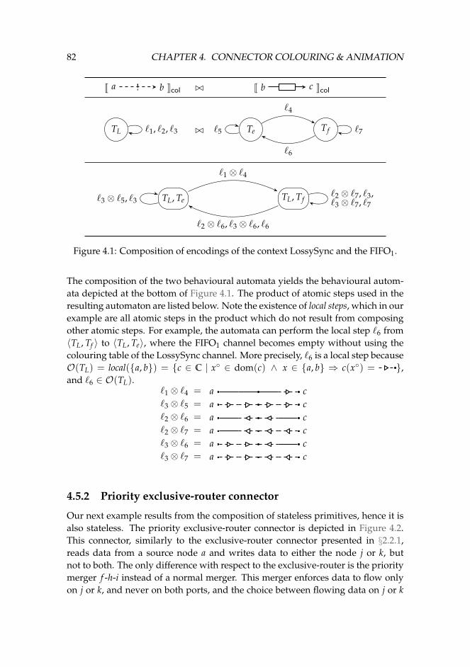
82 CHAPTER 4. CONNECTOR COLOURING & ANIMATION
J a b! Kcol ./ J b c Kcol
TL `1, `2, `3 ./ Te Tf
`4
`6
`5 `7
TL, Te TL, Tf`3 ⊗ `5, `3
`1 ⊗ `4
`2 ⊗ `7, `3,`3 ⊗ `7, `7
`2 ⊗ `6, `3 ⊗ `6, `6
Figure 4.1: Composition of encodings of the context LossySync and the FIFO1.
The composition of the two behavioural automata yields the behavioural autom-ata depicted at the bottom of Figure 4.1. The product of atomic steps used in theresulting automaton are listed below. Note the existence of local steps, which in ourexample are all atomic steps in the product which do not result from composingother atomic steps. For example, the automata can perform the local step `6 from〈TL, Tf 〉 to 〈TL, Te〉, where the FIFO1 channel becomes empty without using thecolouring table of the LossySync channel. More precisely, `6 is a local step becauseO(TL) = local({a, b}) = {c ∈ C | x◦ ∈ dom(c) ∧ x ∈ {a, b} ⇒ c(x◦) = },and `6 ∈ O(TL).
`1 ⊗ `4 = a c`3 ⊗ `5 = a c`2 ⊗ `6 = a c`2 ⊗ `7 = a c`3 ⊗ `6 = a c`3 ⊗ `7 = a c
4.5.2 Priority exclusive-router connector
Our next example results from the composition of stateless primitives, hence it isalso stateless. The priority exclusive-router connector is depicted in Figure 4.2.This connector, similarly to the exclusive-router connector presented in §2.2.1,reads data from a source node a and writes data to either the node j or k, butnot to both. The only difference with respect to the exclusive-router is the prioritymerger f -h-i instead of a normal merger. This merger enforces data to flow onlyon j or k, and never on both ports, and the choice between flowing data on j or k
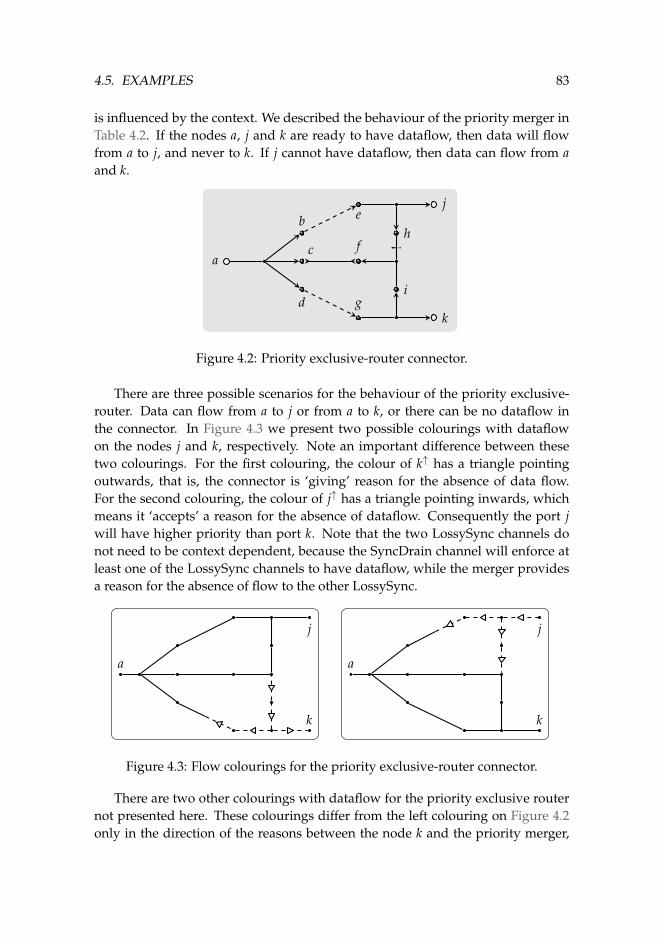
4.5. EXAMPLES 83
is influenced by the context. We described the behaviour of the priority merger inTable 4.2. If the nodes a, j and k are ready to have dataflow, then data will flowfrom a to j, and never to k. If j cannot have dataflow, then data can flow from aand k.
ac
b
d
f
e
g
h
i
j
k
!
Figure 4.2: Priority exclusive-router connector.
There are three possible scenarios for the behaviour of the priority exclusive-router. Data can flow from a to j or from a to k, or there can be no dataflow inthe connector. In Figure 4.3 we present two possible colourings with dataflowon the nodes j and k, respectively. Note an important difference between thesetwo colourings. For the first colouring, the colour of k↑ has a triangle pointingoutwards, that is, the connector is ‘giving’ reason for the absence of data flow.For the second colouring, the colour of j↑ has a triangle pointing inwards, whichmeans it ‘accepts’ a reason for the absence of dataflow. Consequently the port jwill have higher priority than port k. Note that the two LossySync channels donot need to be context dependent, because the SyncDrain channel will enforce atleast one of the LossySync channels to have dataflow, while the merger providesa reason for the absence of flow to the other LossySync.
a
j
k
a
j
k
Figure 4.3: Flow colourings for the priority exclusive-router connector.
There are two other colourings with dataflow for the priority exclusive routernot presented here. These colourings differ from the left colouring on Figure 4.2only in the direction of the reasons between the node k and the priority merger,
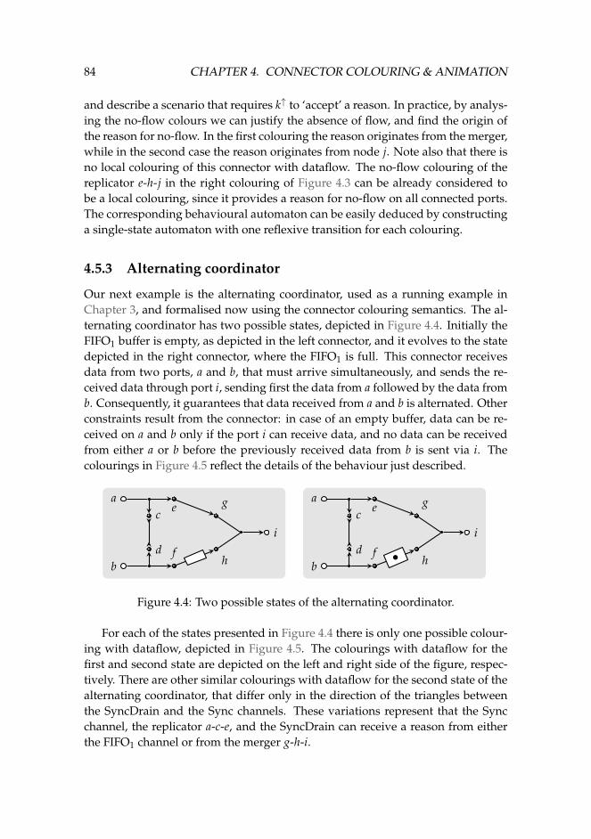
84 CHAPTER 4. CONNECTOR COLOURING & ANIMATION
and describe a scenario that requires k↑ to ‘accept’ a reason. In practice, by analys-ing the no-flow colours we can justify the absence of flow, and find the origin ofthe reason for no-flow. In the first colouring the reason originates from the merger,while in the second case the reason originates from node j. Note also that there isno local colouring of this connector with dataflow. The no-flow colouring of thereplicator e-h-j in the right colouring of Figure 4.3 can be already considered tobe a local colouring, since it provides a reason for no-flow on all connected ports.The corresponding behavioural automaton can be easily deduced by constructinga single-state automaton with one reflexive transition for each colouring.
4.5.3 Alternating coordinator
Our next example is the alternating coordinator, used as a running example inChapter 3, and formalised now using the connector colouring semantics. The al-ternating coordinator has two possible states, depicted in Figure 4.4. Initially theFIFO1 buffer is empty, as depicted in the left connector, and it evolves to the statedepicted in the right connector, where the FIFO1 is full. This connector receivesdata from two ports, a and b, that must arrive simultaneously, and sends the re-ceived data through port i, sending first the data from a followed by the data fromb. Consequently, it guarantees that data received from a and b is alternated. Otherconstraints result from the connector: in case of an empty buffer, data can be re-ceived on a and b only if the port i can receive data, and no data can be receivedfrom either a or b before the previously received data from b is sent via i. Thecolourings in Figure 4.5 reflect the details of the behaviour just described.
ac
db
e
f
g
h
i
ac
db
e
f
g
h
i
•
Figure 4.4: Two possible states of the alternating coordinator.
For each of the states presented in Figure 4.4 there is only one possible colour-ing with dataflow, depicted in Figure 4.5. The colourings with dataflow for thefirst and second state are depicted on the left and right side of the figure, respec-tively. There are other similar colourings with dataflow for the second state of thealternating coordinator, that differ only in the direction of the triangles betweenthe SyncDrain and the Sync channels. These variations represent that the Syncchannel, the replicator a-c-e, and the SyncDrain can receive a reason from eitherthe FIFO1 channel or from the merger g-h-i.
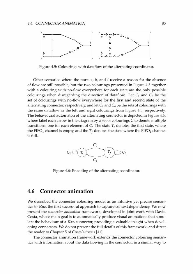
4.6. CONNECTOR ANIMATION 85
a
b
ia
b
i
Figure 4.5: Colourings with dataflow of the alternating coordinator.
Other scenarios where the ports a, b, and i receive a reason for the absenceof flow are still possible, but the two colourings presented in Figure 4.5 togetherwith a colouring with no-flow everywhere for each state are the only possiblecolourings when disregarding the direction of dataflow. Let C1 and C3 be theset of colourings with no-flow everywhere for the first and second state of thealternating connector, respectively, and let C2 and C4 be the sets of colourings withthe same dataflow as the left and right colourings from Figure 4.5, respectively.The behavioural automaton of the alternating connector is depicted in Figure 4.6,where label each arrow in the diagram by a set of colourings C to denote multipletransitions, one for each element of C. The state Te denotes the first state, wherethe FIFO1 channel is empty, and the Tf denotes the state where the FIFO1 channelis full.
Te TfC1
C2
C3
C4
Figure 4.6: Encoding of the alternating coordinator.
4.6 Connector animation
We described the connector colouring model as an intuitive yet precise seman-tics to Reo, the first successful approach to capture context dependency. We nowpresent the connector animation framework, developed in joint work with DavidCosta, whose main goal is to automatically produce visual animations that simu-late the behaviour of a Reo connector, providing a valuable insight when devel-oping connectors. We do not present the full details of this framework, and directthe reader to Chapter 5 of Costa’s thesis [41].
The connector animation framework extends the connector colouring seman-tics with information about the data flowing in the connector, in a similar way to
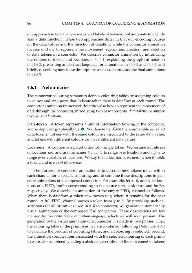
86 CHAPTER 4. CONNECTOR COLOURING & ANIMATION
our approach in §4.4.4 where we extend labels of behavioural automata to includealso a data function. These two approaches differ in that our encoding focuseson the data values and the direction of dataflow, while the connector animationfocuses on how to represent the movement, replication, creation, and deletionof data tokens in a connector. We describe connector animation by introducingthe notions of tokens and locations in §4.6.1, explaining the graphical notationin §4.6.2, presenting an abstract language for animations in §4.6.3 and §4.6.4, andbriefly describing how these descriptions are used to produce the final animationsin §4.6.5.
4.6.1 Preliminaries
The connector colouring semantics defines colouring tables by assigning coloursto source and sink ports that indicate where there is dataflow at each round. Theconnector animation framework describes also how to represent the movement ofdata through the connector, introducing two new concepts: data-tokens, or simplytokens, and locations.
Data-token A token represents a unit of information flowing in the connector,and is depicted graphically by . We denote by Token the enumerable set of alldata-tokens. Tokens with the same colour are associated to the same data value,and tokens with different colours can have different data values.
Locations A location is a placeholder for a single token. We assume a finite setof locations Loc, and use the names `1, . . . , `n to range over locations and α, β, γ torange over variables of locations. We say that a location is occupied when it holdsa token, and is vacant otherwise.
The purpose of connector animation is to describe how tokens move withineach channel, for a specific colouring, and to combine these descriptions to gen-erate animations of a composed connector. For example, let α, β, and γ be loca-tions of a FIFO1 buffer corresponding to the source port, sink port, and buffer,respectively. We describe an animation of the empty FIFO1 channel as follows.When there is dataflow, a token at α moves to γ where it remains for the nextround. A full FIFO1 channel moves a token from γ to β. By providing such de-scriptions for all primitives used in a Reo connector, we generate automaticallyvisual animations of the composed Reo connectors. These descriptions are for-malised by the animation specification language, which we will soon present. Thegeneration of the visual animation of a connector c is made in two phases. First,the colouring table of the primitives in c are combined, following Definition 4.3.3to calculate the product of colouring tables, and a colouring is selected. Second,the animation specifications associated with the selected colouring of each primi-tive are also combined, yielding a abstract description of the movement of tokens
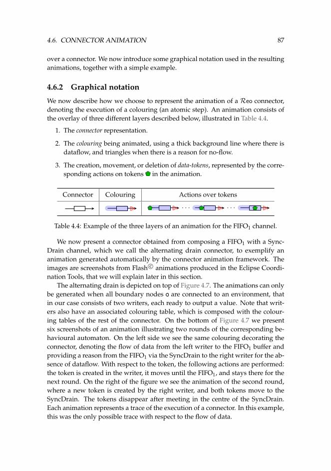
4.6. CONNECTOR ANIMATION 87
over a connector. We now introduce some graphical notation used in the resultinganimations, together with a simple example.
4.6.2 Graphical notation
We now describe how we choose to represent the animation of a Reo connector,denoting the execution of a colouring (an atomic step). An animation consists ofthe overlay of three different layers described below, illustrated in Table 4.4.
1. The connector representation.
2. The colouring being animated, using a thick background line where there isdataflow, and triangles when there is a reason for no-flow.
3. The creation, movement, or deletion of data-tokens, represented by the corre-sponding actions on tokens in the animation.
Connector Colouring Actions over tokens
· · · · · ·
Table 4.4: Example of the three layers of an animation for the FIFO1 channel.
We now present a connector obtained from composing a FIFO1 with a Sync-Drain channel, which we call the alternating drain connector, to exemplify ananimation generated automatically by the connector animation framework. Theimages are screenshots from Flash c© animations produced in the Eclipse Coordi-nation Tools, that we will explain later in this section.
The alternating drain is depicted on top of Figure 4.7. The animations can onlybe generated when all boundary nodes are connected to an environment, thatin our case consists of two writers, each ready to output a value. Note that writ-ers also have an associated colouring table, which is composed with the colour-ing tables of the rest of the connector. On the bottom of Figure 4.7 we presentsix screenshots of an animation illustrating two rounds of the corresponding be-havioural automaton. On the left side we see the same colouring decorating theconnector, denoting the flow of data from the left writer to the FIFO1 buffer andproviding a reason from the FIFO1 via the SyncDrain to the right writer for the ab-sence of dataflow. With respect to the token, the following actions are performed:the token is created in the writer, it moves until the FIFO1, and stays there for thenext round. On the right of the figure we see the animation of the second round,where a new token is created by the right writer, and both tokens move to theSyncDrain. The tokens disappear after meeting in the centre of the SyncDrain.Each animation represents a trace of the execution of a connector. In this example,this was the only possible trace with respect to the flow of data.
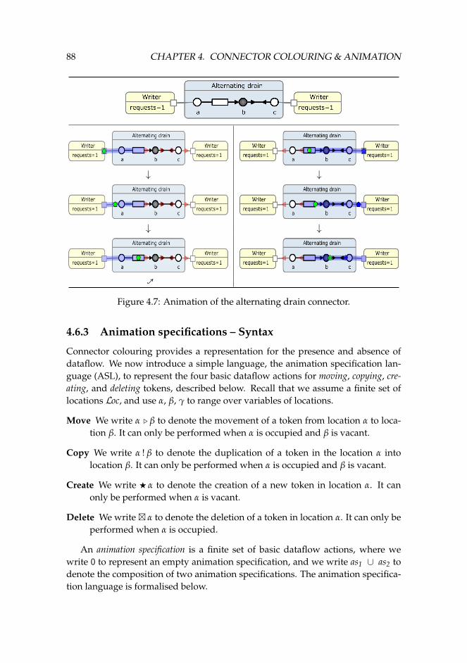
88 CHAPTER 4. CONNECTOR COLOURING & ANIMATION
↓ ↓
↓ ↓
4
Figure 4.7: Animation of the alternating drain connector.
4.6.3 Animation specifications – Syntax
Connector colouring provides a representation for the presence and absence ofdataflow. We now introduce a simple language, the animation specification lan-guage (ASL), to represent the four basic dataflow actions for moving, copying, cre-ating, and deleting tokens, described below. Recall that we assume a finite set oflocations Loc, and use α, β, γ to range over variables of locations.
Move We write α . β to denote the movement of a token from location α to loca-tion β. It can only be performed when α is occupied and β is vacant.
Copy We write α ! β to denote the duplication of a token in the location α intolocation β. It can only be performed when α is occupied and β is vacant.
Create We write F α to denote the creation of a new token in location α. It canonly be performed when α is vacant.
Delete We write� α to denote the deletion of a token in location α. It can only beperformed when α is occupied.
An animation specification is a finite set of basic dataflow actions, where wewrite 0 to represent an empty animation specification, and we write as1 ∪ as2 todenote the composition of two animation specifications. The animation specifica-tion language is formalised below.
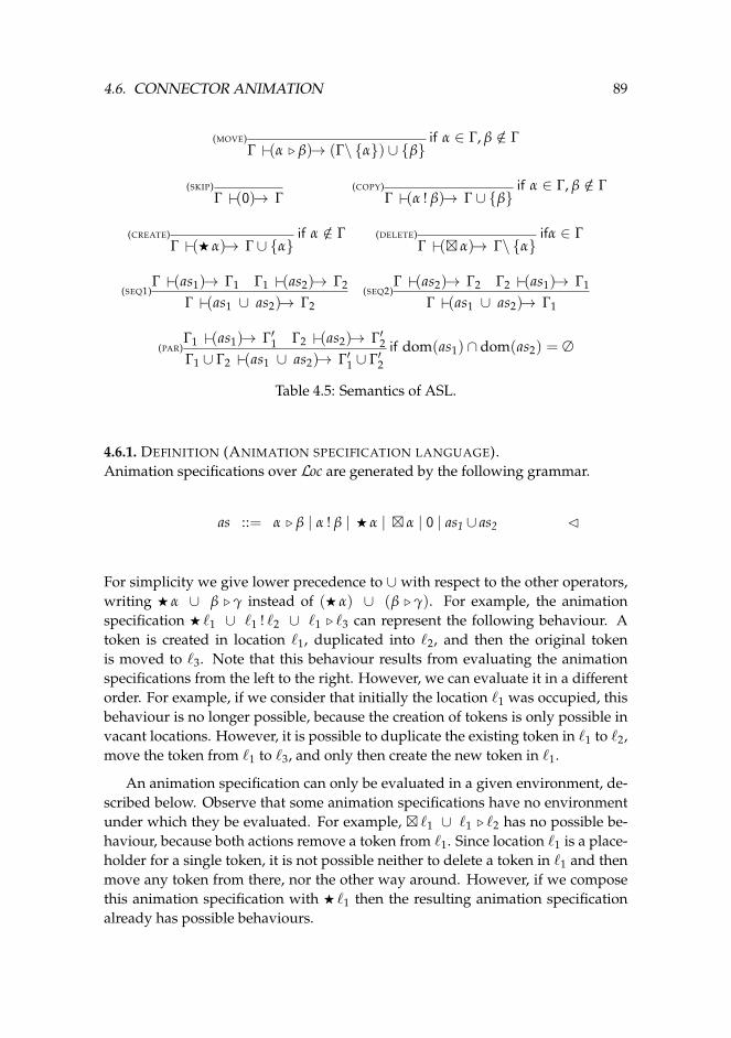
4.6. CONNECTOR ANIMATION 89
(MOVE)Γ (α . β)→ (Γ\ {α}) ∪ {β}
if α ∈ Γ, β /∈ Γ
(SKIP)Γ (0)→ Γ
(COPY)Γ (α ! β)→ Γ ∪ {β}
if α ∈ Γ, β /∈ Γ
(CREATE)Γ (F α)→ Γ ∪ {α}
if α /∈ Γ (DELETE)Γ (� α)→ Γ\ {α}
ifα ∈ Γ
(SEQ1)Γ (as1)→ Γ1 Γ1 (as2)→ Γ2
Γ (as1 ∪ as2)→ Γ2(SEQ2)
Γ (as2)→ Γ2 Γ2 (as1)→ Γ1
Γ (as1 ∪ as2)→ Γ1
(PAR)Γ1 (as1)→ Γ′1 Γ2 (as2)→ Γ′2Γ1 ∪ Γ2 (as1 ∪ as2)→ Γ′1 ∪ Γ′2
if dom(as1) ∩ dom(as2) = ∅
Table 4.5: Semantics of ASL.
4.6.1. DEFINITION (ANIMATION SPECIFICATION LANGUAGE).Animation specifications over Loc are generated by the following grammar.
as ::= α . β | α ! β | F α | � α | 0 | as1 ∪ as2 C
For simplicity we give lower precedence to ∪ with respect to the other operators,writing F α ∪ β . γ instead of (F α) ∪ (β . γ). For example, the animationspecification F `1 ∪ `1 ! `2 ∪ `1 . `3 can represent the following behaviour. Atoken is created in location `1, duplicated into `2, and then the original tokenis moved to `3. Note that this behaviour results from evaluating the animationspecifications from the left to the right. However, we can evaluate it in a differentorder. For example, if we consider that initially the location `1 was occupied, thisbehaviour is no longer possible, because the creation of tokens is only possible invacant locations. However, it is possible to duplicate the existing token in `1 to `2,move the token from `1 to `3, and only then create the new token in `1.
An animation specification can only be evaluated in a given environment, de-scribed below. Observe that some animation specifications have no environmentunder which they be evaluated. For example, � `1 ∪ `1 . `2 has no possible be-haviour, because both actions remove a token from `1. Since location `1 is a place-holder for a single token, it is not possible neither to delete a token in `1 and thenmove any token from there, nor the other way around. However, if we composethis animation specification with F `1 then the resulting animation specificationalready has possible behaviours.
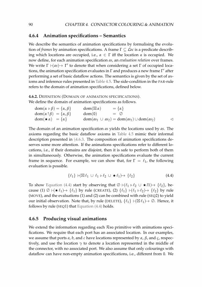
90 CHAPTER 4. CONNECTOR COLOURING & ANIMATION
4.6.4 Animation specifications – Semantics
We describe the semantics of animation specifications by formalising the evolu-tion of frames by animation specifications. A frame Γ ⊆ Loc is a predicate describ-ing which locations are occupied, i.e., α ∈ Γ iff the location α is occupied. Wenow define, for each animation specification as, an evaluation relation over frames.We write Γ (as)→ Γ′ to denote that when considering a set Γ of occupied loca-tions, the animation specification evaluates in Γ and produces a new frame Γ′ afterperforming a set of basic dataflow actions. The semantics is given by the set of ax-ioms and inference rules presented in Table 4.5. The side-condition in the PAR-rulerefers to the domain of animation specifications, defined below.
4.6.2. DEFINITION (DOMAIN OF ANIMATION SPECIFICATIONS).We define the domain of animation specifications as follows.
dom(α . β) = {α, β} dom(� α) = {α}dom(α ! β) = {α, β} dom(0) = ∅dom(F α) = {α} dom(as1 ∪ as2) = dom(as1) ∪ dom(as2) C
The domain of an animation specification as yields the locations used by as. Theaxioms regarding the basic dataflow axioms in Table 4.5 mimic their informaldescription presented in §4.6.3. The composition of animation specifications de-serves some more attention. If the animations specifications refer to different lo-cations, i.e., if their domains are disjoint, then it is safe to perform both of themin simultaneously. Otherwise, the animation specifications evaluate the currentframe in sequence. For example, we can show that, for Γ = `1, the followingevaluation is possible.
{`1} (� `1 ∪ `1 . `2 ∪ F `1)→ {`2} (4.4)
To show Equation (4.4) start by observing that ∅ (`1 . `2 ∪ F l1)→ {`2}, be-cause (1) ∅ (F `1)→ {`1} by rule (CREATE), (2) {`1} (`1 . `2)→ {`2} by rule(MOVE), and the evaluations (1) and (2) can be combined with rule (SEQ2) to yieldour initial observation. Note that, by rule (DELETE), {`1} (� `1)→ ∅. Hence, itfollows by rule (SEQ1) that Equation (4.4) holds.
4.6.5 Producing visual animations
We extend the information regarding each Reo primitive with animations speci-fications. We require that each port has an associated location. In our examples,we assume that ports a, b, and c have locations represented by α, β, and ς, respec-tively, and use the location γ to denote a location represented in the middle ofthe connector, with no associated port. We also assume that only colourings withdataflow can have non-empty animation specifications, i.e., different from 0. We
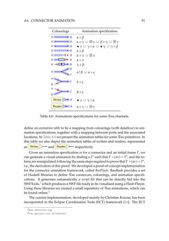
4.6. CONNECTOR ANIMATION 91
Colourings Animation specification
a b α . βa b α . γ ∪ �γ ∪ β . γ ∪ �γa b Fγ ∪ γ . α ∪ Fγ ∪ γ . βa b α . βa b α . γ ∪ �γa b α . γa b• γ . β
ab
cα ! β ∪ α . ς
ca
b!
α . ς
ca
b!
β . ς
Writer a Fγ ∪ γ . α
Reader a α . γ ∪ �γ
Table 4.6: Animations specifications for someReo channels.
define an animation table to be a mapping from colourings (with dataflow) to ani-mation specifications, together with a mapping between ports and the associatedlocations. In Table 4.6 we present the animation tables for someReo primitives. Inthis table we also depict the animation tables of writers and readers, represented
as Writer and Reader respectively.
Given an animation specification as for a connector and an initial frame Γ, wecan generate a visual animation by finding a Γ′ such that Γ (as)→ Γ′, and the to-kens are manipulated following the same steps required to prove that Γ (as)→ Γ′,i.e., the derivation of this proof. We developed a proof-of-concept implementationfor the connector animation framework, called ReoFlash. Reoflash provides a setof Haskell libraries to define Reo connecors, colourings, and animation specifi-cations. It generates automatically a script file that can be directly fed into theSWFTools,3 which produces a SWF file ready to be visualised using a Flash Player.Using these libraries we created a small repository of Reo animations, which canbe found online.4
The current implementation, developed mainly by Christian Krause, has beenincorporated in the Eclipse Coordination Tools (ECT) framework [16]. The ECT
3www.swftools.org4reo.project.cwi.nl/webreo/
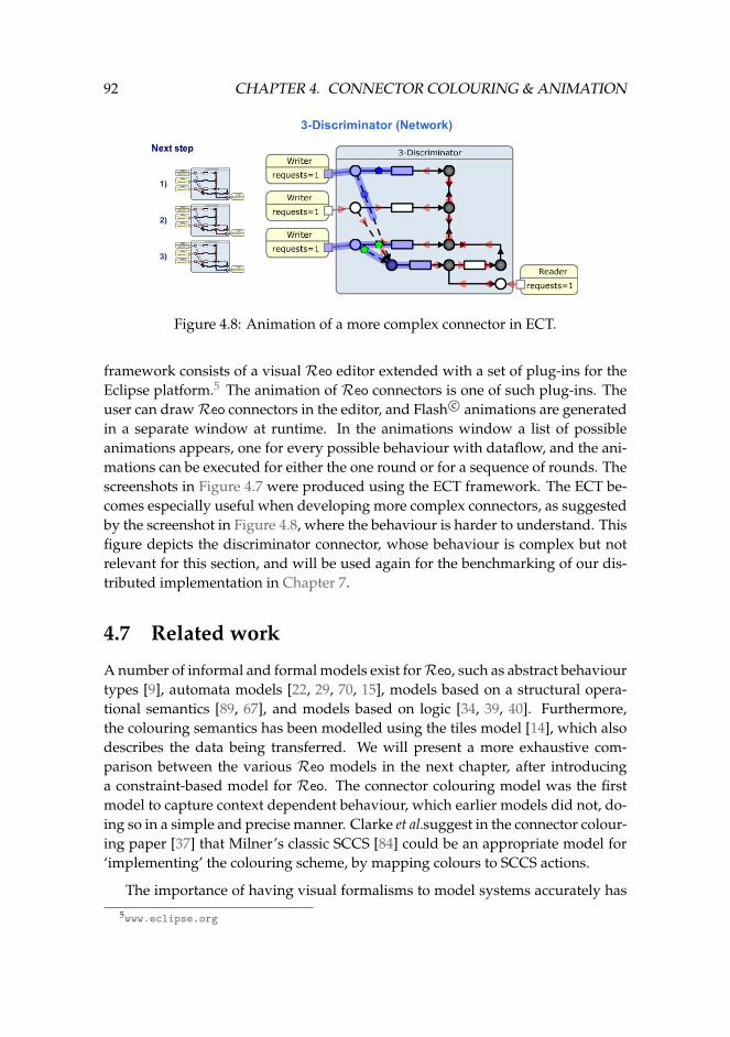
92 CHAPTER 4. CONNECTOR COLOURING & ANIMATION
Figure 4.8: Animation of a more complex connector in ECT.
framework consists of a visual Reo editor extended with a set of plug-ins for theEclipse platform.5 The animation of Reo connectors is one of such plug-ins. Theuser can drawReo connectors in the editor, and Flash c© animations are generatedin a separate window at runtime. In the animations window a list of possibleanimations appears, one for every possible behaviour with dataflow, and the ani-mations can be executed for either the one round or for a sequence of rounds. Thescreenshots in Figure 4.7 were produced using the ECT framework. The ECT be-comes especially useful when developing more complex connectors, as suggestedby the screenshot in Figure 4.8, where the behaviour is harder to understand. Thisfigure depicts the discriminator connector, whose behaviour is complex but notrelevant for this section, and will be used again for the benchmarking of our dis-tributed implementation in Chapter 7.
4.7 Related work
A number of informal and formal models exist forReo, such as abstract behaviourtypes [9], automata models [22, 29, 70, 15], models based on a structural opera-tional semantics [89, 67], and models based on logic [34, 39, 40]. Furthermore,the colouring semantics has been modelled using the tiles model [14], which alsodescribes the data being transferred. We will present a more exhaustive com-parison between the various Reo models in the next chapter, after introducinga constraint-based model for Reo. The connector colouring model was the firstmodel to capture context dependent behaviour, which earlier models did not, do-ing so in a simple and precise manner. Clarke et al.suggest in the connector colour-ing paper [37] that Milner’s classic SCCS [84] could be an appropriate model for‘implementing’ the colouring scheme, by mapping colours to SCCS actions.
The importance of having visual formalisms to model systems accurately has
5www.eclipse.org
4.7. RELATED WORK 93
been long recognised in the scientific community. Visual languages like PetriNets [91], sequence charts [62] and statecharts [58, 59] were introduced to helpbuilding visual system models. For example, for Statecharts, introduced in 1987by David Harel, the tool Rhapsody [61] that generate running code for Statechartsmodels, and use simple animations to facilitate the process of model develop-ment, specification and analysis. Similarly connector animation facilitates the im-plementation of tools that support developers in the design and analysis of Reo
connectors, by means of animations. Motivated by the importance of representingreal world animations, Harel et al. proposed an architecture where the executablemodel is separated from the animations, called reactive animations [60, 45]. Theypresented examples of the Rhapsody tool communicating with flash animations,where the animations are based on the current state of the executable model. TheEclipse Coordination Tool suite uses the Reactive Animation principle, and the an-imations are generated and updated on the fly every time a connector is changed,but independently of the calculation of the semantics of the connector.
The benefits of using animations is also advocated by the workflow patternscommunity. Notably Van der Aalst et al. [99] use it to compare different work-flow patterns. To explain the differences between the workflow patterns they havehand-programmed insightful Flash c© animations and offer them together with ad-ditional information on the web.6 The visual appearance of our animations islargely influenced by their work. Our approach to obtain the animations differs,though. We generate the animations automatically according to the formal seman-tics, while in the approach of Van der Aalst it al. animations are created manually,according to the textual description of their intended workflow semantics.
Animation of formal models has proven to facilitate the communication be-tween developers and stakeholders. Hung Tran Van et al. present animations forGoal-Oriented Requirements [98]. They propose to animate UML state diagramsto visualise and simulate a specific model using visual elements that representreal-life actions of the system to be modelled, such as representing a video withtwo doors opening associated to the execution of a method called open-door.Multiple users can interact with an execution of the model, and property viola-tions are monitored at animation time. Westergaard and Lassen present the BRIT-NeY Suite Animation tool [102], a tool to create visualisations of formal models,specially of coloured Petri nets (CPN), which is already integrated in the CPNTools. Our experience with Connector Animation is that it greatly facilitates thetask ofReo developers. Connector animation produces, on the fly, quality anima-tions that comply with the formal semantics of Reo, allowing Reo developers tofocus entirely on the design of new connectors. In contrast, approaches such asthe use of goal-oriented requirements force developers to construct both a modelfor the system and an additional model for its animation.
6http://www.workflowpatterns.com
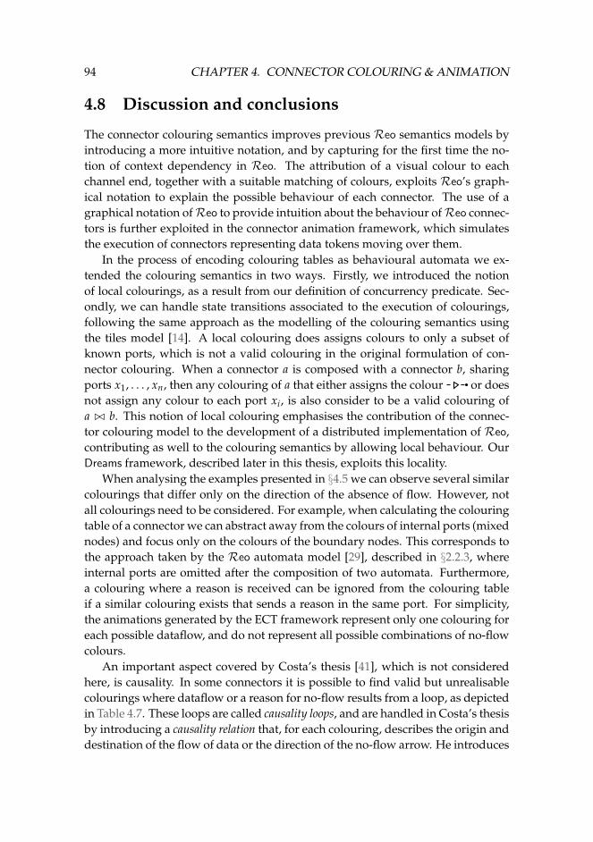
94 CHAPTER 4. CONNECTOR COLOURING & ANIMATION
4.8 Discussion and conclusions
The connector colouring semantics improves previous Reo semantics models byintroducing a more intuitive notation, and by capturing for the first time the no-tion of context dependency in Reo. The attribution of a visual colour to eachchannel end, together with a suitable matching of colours, exploits Reo’s graph-ical notation to explain the possible behaviour of each connector. The use of agraphical notation ofReo to provide intuition about the behaviour ofReo connec-tors is further exploited in the connector animation framework, which simulatesthe execution of connectors representing data tokens moving over them.
In the process of encoding colouring tables as behavioural automata we ex-tended the colouring semantics in two ways. Firstly, we introduced the notionof local colourings, as a result from our definition of concurrency predicate. Sec-ondly, we can handle state transitions associated to the execution of colourings,following the same approach as the modelling of the colouring semantics usingthe tiles model [14]. A local colouring does assigns colours to only a subset ofknown ports, which is not a valid colouring in the original formulation of con-nector colouring. When a connector a is composed with a connector b, sharingports x1, . . . , xn, then any colouring of a that either assigns the colour or doesnot assign any colour to each port xi, is also consider to be a valid colouring ofa ./ b. This notion of local colouring emphasises the contribution of the connec-tor colouring model to the development of a distributed implementation of Reo,contributing as well to the colouring semantics by allowing local behaviour. OurDreams framework, described later in this thesis, exploits this locality.
When analysing the examples presented in §4.5 we can observe several similarcolourings that differ only on the direction of the absence of flow. However, notall colourings need to be considered. For example, when calculating the colouringtable of a connector we can abstract away from the colours of internal ports (mixednodes) and focus only on the colours of the boundary nodes. This corresponds tothe approach taken by the Reo automata model [29], described in §2.2.3, whereinternal ports are omitted after the composition of two automata. Furthermore,a colouring where a reason is received can be ignored from the colouring tableif a similar colouring exists that sends a reason in the same port. For simplicity,the animations generated by the ECT framework represent only one colouring foreach possible dataflow, and do not represent all possible combinations of no-flowcolours.
An important aspect covered by Costa’s thesis [41], which is not consideredhere, is causality. In some connectors it is possible to find valid but unrealisablecolourings where dataflow or a reason for no-flow results from a loop, as depictedin Table 4.7. These loops are called causality loops, and are handled in Costa’s thesisby introducing a causality relation that, for each colouring, describes the origin anddestination of the flow of data or the direction of the no-flow arrow. He introduces
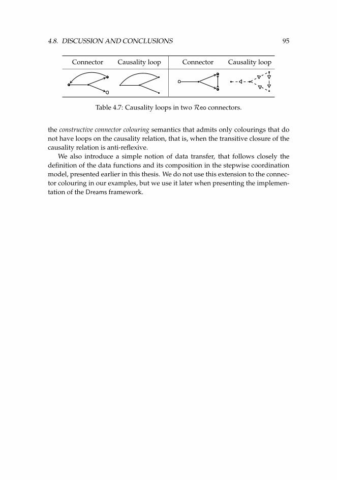
4.8. DISCUSSION AND CONCLUSIONS 95
Connector Causality loop Connector Causality loop
Table 4.7: Causality loops in twoReo connectors.
the constructive connector colouring semantics that admits only colourings that donot have loops on the causality relation, that is, when the transitive closure of thecausality relation is anti-reflexive.
We also introduce a simple notion of data transfer, that follows closely thedefinition of the data functions and its composition in the stepwise coordinationmodel, presented earlier in this thesis. We do not use this extension to the connec-tor colouring in our examples, but we use it later when presenting the implemen-tation of the Dreams framework.

Chapter 5
Constraint-based models forReo
5.1 Introduction
Wegner describes coordination as constrained interaction [101]. We take this idealiterally and represent coordination using constraints to develop an efficient im-plementation of the Reo coordination model [8]. We will adopt the view that aReo connector specifies a series of constraint satisfaction problems, and that validinteraction between a connector and its environment (in each state) correspondsto the solutions of such constraints [11]. This idea diverges from the existing de-scriptions of Reo, which are based on dataflow through channels, but we claimthat the viewpoint of constraint satisfaction not only is an appealing alternativeway of thinking about Reo connectors, but it also opens the door to more effi-cient implementation techniques—a claim supported by experimental results in§5.6. We use constraints to describe the semantics of Reo connectors in order todevelop more efficient implementation techniques for Reo, utilising existing SATsolving and constraint satisfaction techniques.
The chapter makes the following technical contributions:
• a constraint-based semantic description ofReo connectors; and
• competitive SAT- and CSP-based implementation techniques for Reo con-nectors.
Organisation of the chapter This chapter is organised as follows. We briefly re-call the Reo coordination model in §5.2, where we also present an example of aReo connector for illustrative purposes further on. §5.3 describes our encodingof Reo-style coordination as a constraint satisfaction problem. §5.4 describes anextension of this encoding to incorporate state, so that connector semantics canbe completely internalised as constraints. Correctness and compositionality prop-erties are also presented. §5.5 describes how to encode context dependency, as
97
98 CHAPTER 5. CONSTRAINT-BASED MODELS FOR REO
formulated in the connector colouring model [37], into constraints. §5.6 presentssome benchmarking results comparing an existing engine for Reo based on con-nector colouring with a prototype engine based on constraint solving techniques,with and without context dependency. §5.7 describes how to guide the underly-ing constraint solver to achieve fairness and priority. §5.8 presents some imple-mentation issues, in particular, it gives a description of an alternative interactionmodel that constraint satisfaction enables. §5.9 discusses and compares existingReo models and implementations with our constraint-based approach, and dis-cusses the position of this approach with respect to the Dreams framework. Finally,§5.10 and §5.11 present related work and our conclusions.
5.2 Reo overview
Reo [8, 9] has been explained in detail in Chapters 2 and 4. We briefly recallthe most relevant aspects of Reo for the sake of presentation. Reo is a channel-based coordination model, wherein coordinating connectors are constructed com-positionally out of more primitive connectors, which we call primitives. Primitivescommunicate through its ports, also called ends: primitives consume data throughtheir source ports, and produce data through their sink ports. The behaviour ofeach primitive depends upon its current state. The semantics of a connector isdescribed as a collection of possible steps for each state, and we refer to a roundas the change of state triggered by one of these steps.
Some of the most commonly used Reo primitives are depicted in Table 5.1.For the purposes of this chapter, we do not distinguish between primitives suchas channels used for coordination and the components being coordinated, in thatboth will offer constraints describing their behavioural possibilities. The main dif-ference between primitives and components is that the connector has more controlover and more knowledge about the possible behaviour of the former than the lat-ter, though this distinction is blurred in the present framework.
Connectors are formed by plugging the ports of primitives together in a one-to-one fashion, connecting a sink port to a source port, to form nodes. A node is alogical place consisting of a sink port, a source port, or both a sink and a sourceport. We call nodes with a single port boundary nodes, represented by , and wecall nodes with a sink and a source port mixed nodes, represented by . Data flowthrough a connector from primitive to primitive through nodes, subject to the con-straint that nodes cannot buffer data. This means that the two ports in a node aresynchronised and have the same dataflow—behaviourally, they are equal. Nodescan be handled transparently by using the same name for the two ports on thenode, as the synchronisation and dataflow at the two ports is identical. We re-call the example of the exclusive router connector in Example 5.2.1, introduced inChapter 2, to illustrateReo’s semantics.
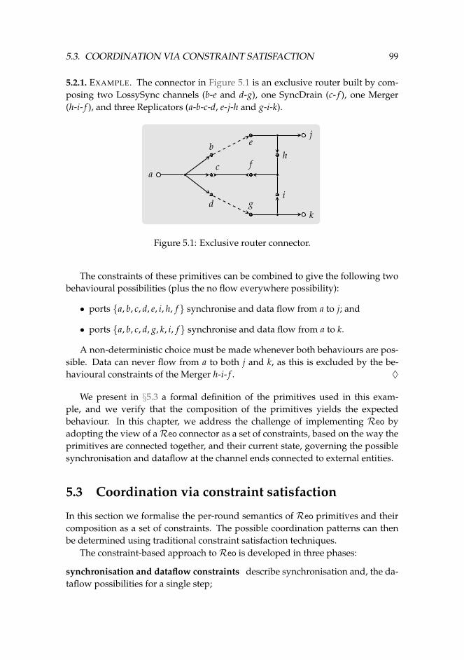
5.3. COORDINATION VIA CONSTRAINT SATISFACTION 99
5.2.1. EXAMPLE. The connector in Figure 5.1 is an exclusive router built by com-posing two LossySync channels (b-e and d-g), one SyncDrain (c- f ), one Merger(h-i- f ), and three Replicators (a-b-c-d, e-j-h and g-i-k).
ac
b
d
f
e
g
h
i
j
k
Figure 5.1: Exclusive router connector.
The constraints of these primitives can be combined to give the following twobehavioural possibilities (plus the no flow everywhere possibility):
• ports {a, b, c, d, e, i, h, f } synchronise and data flow from a to j; and
• ports {a, b, c, d, g, k, i, f } synchronise and data flow from a to k.
A non-deterministic choice must be made whenever both behaviours are pos-sible. Data can never flow from a to both j and k, as this is excluded by the be-havioural constraints of the Merger h-i- f . ♦
We present in §5.3 a formal definition of the primitives used in this exam-ple, and we verify that the composition of the primitives yields the expectedbehaviour. In this chapter, we address the challenge of implementing Reo byadopting the view of aReo connector as a set of constraints, based on the way theprimitives are connected together, and their current state, governing the possiblesynchronisation and dataflow at the channel ends connected to external entities.
5.3 Coordination via constraint satisfaction
In this section we formalise the per-round semantics of Reo primitives and theircomposition as a set of constraints. The possible coordination patterns can thenbe determined using traditional constraint satisfaction techniques.
The constraint-based approach toReo is developed in three phases:
synchronisation and dataflow constraints describe synchronisation and, the da-taflow possibilities for a single step;
100 CHAPTER 5. CONSTRAINT-BASED MODELS FOR REO
state constraints incorporate next state behaviour into the constraints, enablingthe complete description of behaviour in terms of constraints; and
context constraints capture the availability of dataflow for a single step.
The resulting model significantly extends Reo implementations with data-awareand context dependent behaviour, and enables more efficient implementation tech-niques. We start by focusing on synchronisation constraints (SC) and dataflowconstraints (DFC), showing its correctness with respect to the constraint automatamodel of Reo, before exploring the context constraints and its relation with theconnector colouring model.
5.3.1 Mathematical preliminaries
Let P be a global set of ports of Reo connectors. Let P denote the set of vari-ables of P decorated with a little hat. Let D be the domain of data, and defineD⊥
def=D ∪ {NO-FLOW}, where NO-FLOW /∈ D represents ‘no dataflow.’ Constraints
are expressed in quantifier-free, first-order logic over two kinds of variables: syn-chronisation variables x ∈ P, which are boolean variables, and dataflow variablesx ∈ P, which are variables over D⊥. Constraints are formula in the followinggrammar:
t ::= x | d (terms)
a ::= x | R(t1, . . . , tn) (atoms)
ψ ::= a | > | ψ ∧ ψ | ¬ψ (formulæ)
where d ∈ D⊥ is a data item, > is true, and R is an n-ary predicate over terms.One such predicate is equality, which is denoted using the standard infix notationt1 = t2. The other logical connectives can be encoded as usual.
A solution to a formula ψ defined over ports P ⊆ P is a pair of assignments oftypes σ : P → {⊥,>} and δ : P → D⊥, such that σ and δ satisfy ψ, according tothe satisfaction relation σ, δ � ψ, defined as follows:
σ, δ � > σ, δ � ψ1 ∧ ψ2 iff σ, δ � ψ1 and σ, δ � ψ2σ, δ � x iff σ(x) = > σ, δ � ¬ψ iff σ, δ 2 ψ
σ, δ � R(t1, . . . , tn) iff (δ′ ◦ (t1), . . . , δ′(tn)) ∈ I(R)
Each n-ary predicate symbol R has an associated interpretation, denoted by I(R),such that I(R) ⊆ Dn
⊥. The data item δ′(t) is either δ(x) or d, depending on t beingthe variable x or the constant d, respectively.
The logic with constraints over boolean variables, plus equality constraintsover dataflow variables, arbitrary terms over the flat D domain, and top-levelexistential quantifiers is in NP [100].
5.3. COORDINATION VIA CONSTRAINT SATISFACTION 101
The NO-FLOW value is used in constraints as a special value when no dataflowoccurs. A synchronisation variable set to⊥ plays exactly the same role. These twofacts are linked by the following constraint, which combines synchronisation anddataflow by capturing the relationship between no flow on port x ∈ P and thevalue NO-FLOW:
¬x ↔ (x = NO-FLOW) (flow axiom)
This axiom applies to all ports in the connector. Let Flow(P) denote∧
x∈P (¬x↔ (x = NO-FLOW)), where P ⊆ P. A solution to a set of constraints that satisfiesFlow(P) is called a firing. Since we are exclusively interested in finding firings(as opposed to other solutions), we assume that the flow axiom holds for all portsinvolved.
5.3.2 Encoding primitives as constraints
Two kinds of constraints describe connector behaviour: synchronisation constraints(SC) and dataflow constraints (DFC). The former are constraints over a set P ofboolean variables, describing the presence or absence of dataflow at each port—that is, whether or not those ports synchronise. The latter constraints involvein addition dataflow variables from P to describe the dataflow at the ports thatsynchronise.
Table 5.1 provides the semantics of some commonly used channels and otherprimitives in terms of synchronisation constraints and dataflow constraints. Notethat some of our connectors can have an infinite number of states, especially whendata is involved—a complete account of stateful connectors is given in §5.4 wherestate handling is introduced into constraints.
Sync, SyncDrain and SyncSpout channels All three synchronous channels allowdataflow to occur only synchronously at both channel ends. SyncDrains can beviewed as data consumers, and SyncSpouts can be viewed as data generators. Apossible variant uses predicates R and Q to constrain the data produced, with adataflow constraint such as a→ (R(a) ∧Q(b)).
AsyncDrain and AsyncSpout These asynchronous channels allow flow on atmost one of their two ports per round. A refined variant of the AsyncSpout hasdataflow constraint a→ R(a) ∧ b→ Q(b).
Non-deterministic LossySync A LossySync always allows dataflow on port a.It can in addition, non-deterministically, it allows dataflow on port b, in whichcase the data from a is passed to b. Note that the LossySync here is not context-dependent, i.e., it may lose data when b can accept data. We return to contextdependency in §5.5.
Merger A merger permits dataflow synchronously through one of its sourceports, exclusively, to its sink port.
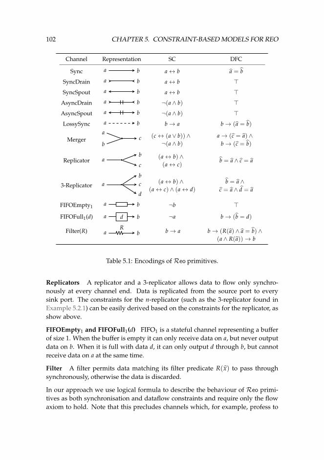
102 CHAPTER 5. CONSTRAINT-BASED MODELS FOR REO
Channel Representation SC DFC
Sync a b a↔ b a = b
SyncDrain a b a↔ b >
SyncSpout a b a↔ b >
AsyncDrain a b ¬(a ∧ b) >
AsyncSpout a b ¬(a ∧ b) >
LossySync a b b→ a b→ (a = b)
Merger ca
b(c↔ (a ∨ b)) ∧¬(a ∧ b)
a→ (c = a) ∧b→ (c = b)
Replicator ab
c(a↔ b) ∧(a↔ c)
b = a ∧ c = a
3-Replicator a cb
d
(a↔ b) ∧(a↔ c) ∧ (a↔ d)
b = a ∧c = a ∧ d = a
FIFOEmpty1 a b ¬b >
FIFOFull1(d) a bd ¬a b→ (b = d)
Filter(R) a bR b→ a b→ (R(a) ∧ a = b) ∧
(a ∧ R(a))→ b
Table 5.1: Encodings ofReo primitives.
Replicators A replicator and a 3-replicator allows data to flow only synchro-nously at every channel end. Data is replicated from the source port to everysink port. The constraints for the n-replicator (such as the 3-replicator found inExample 5.2.1) can be easily derived based on the constraints for the replicator, asshow above.
FIFOEmpty1 and FIFOFull1(d) FIFO1 is a stateful channel representing a bufferof size 1. When the buffer is empty it can only receive data on a, but never outputdata on b. When it is full with data d, it can only output d through b, but cannotreceive data on a at the same time.
Filter A filter permits data matching its filter predicate R(x) to pass throughsynchronously, otherwise the data is discarded.
In our approach we use logical formula to describe the behaviour of Reo primi-tives as both synchronisation and dataflow constraints and require only the flowaxiom to hold. Note that this precludes channels which, for example, profess to
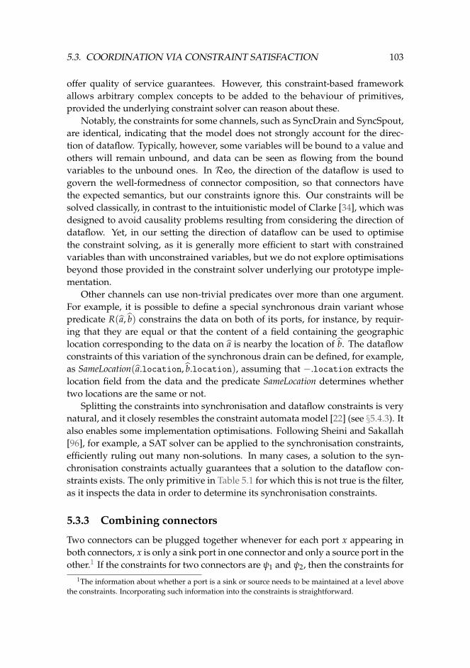
5.3. COORDINATION VIA CONSTRAINT SATISFACTION 103
offer quality of service guarantees. However, this constraint-based frameworkallows arbitrary complex concepts to be added to the behaviour of primitives,provided the underlying constraint solver can reason about these.
Notably, the constraints for some channels, such as SyncDrain and SyncSpout,are identical, indicating that the model does not strongly account for the direc-tion of dataflow. Typically, however, some variables will be bound to a value andothers will remain unbound, and data can be seen as flowing from the boundvariables to the unbound ones. In Reo, the direction of the dataflow is used togovern the well-formedness of connector composition, so that connectors havethe expected semantics, but our constraints ignore this. Our constraints will besolved classically, in contrast to the intuitionistic model of Clarke [34], which wasdesigned to avoid causality problems resulting from considering the direction ofdataflow. Yet, in our setting the direction of dataflow can be used to optimisethe constraint solving, as it is generally more efficient to start with constrainedvariables than with unconstrained variables, but we do not explore optimisationsbeyond those provided in the constraint solver underlying our prototype imple-mentation.
Other channels can use non-trivial predicates over more than one argument.For example, it is possible to define a special synchronous drain variant whosepredicate R(a, b) constrains the data on both of its ports, for instance, by requir-ing that they are equal or that the content of a field containing the geographiclocation corresponding to the data on a is nearby the location of b. The dataflowconstraints of this variation of the synchronous drain can be defined, for example,as SameLocation(a.location, b.location), assuming that −.location extracts thelocation field from the data and the predicate SameLocation determines whethertwo locations are the same or not.
Splitting the constraints into synchronisation and dataflow constraints is verynatural, and it closely resembles the constraint automata model [22] (see §5.4.3). Italso enables some implementation optimisations. Following Sheini and Sakallah[96], for example, a SAT solver can be applied to the synchronisation constraints,efficiently ruling out many non-solutions. In many cases, a solution to the syn-chronisation constraints actually guarantees that a solution to the dataflow con-straints exists. The only primitive in Table 5.1 for which this is not true is the filter,as it inspects the data in order to determine its synchronisation constraints.
5.3.3 Combining connectors
Two connectors can be plugged together whenever for each port x appearing inboth connectors, x is only a sink port in one connector and only a source port in theother.1 If the constraints for two connectors are ψ1 and ψ2, then the constraints for
1The information about whether a port is a sink or source needs to be maintained at a level abovethe constraints. Incorporating such information into the constraints is straightforward.
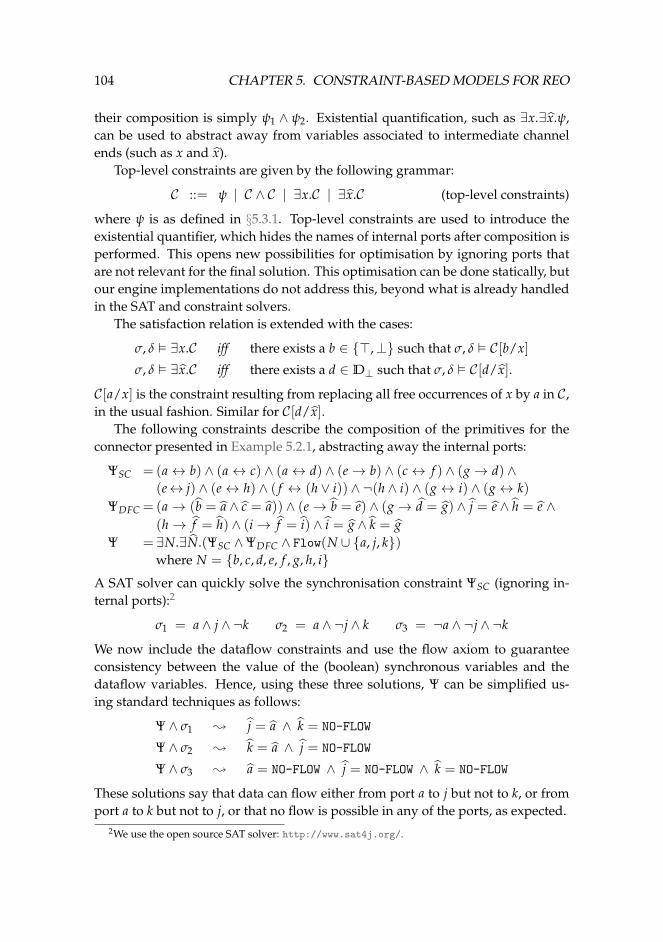
104 CHAPTER 5. CONSTRAINT-BASED MODELS FOR REO
their composition is simply ψ1 ∧ ψ2. Existential quantification, such as ∃x.∃x.ψ,can be used to abstract away from variables associated to intermediate channelends (such as x and x).
Top-level constraints are given by the following grammar:
C ::= ψ | C ∧ C | ∃x.C | ∃x.C (top-level constraints)
where ψ is as defined in §5.3.1. Top-level constraints are used to introduce theexistential quantifier, which hides the names of internal ports after composition isperformed. This opens new possibilities for optimisation by ignoring ports thatare not relevant for the final solution. This optimisation can be done statically, butour engine implementations do not address this, beyond what is already handledin the SAT and constraint solvers.
The satisfaction relation is extended with the cases:
σ, δ � ∃x.C iff there exists a b ∈ {>,⊥} such that σ, δ � C[b/x]
σ, δ � ∃x.C iff there exists a d ∈ D⊥ such that σ, δ � C[d/x].
C[a/x] is the constraint resulting from replacing all free occurrences of x by a in C,in the usual fashion. Similar for C[d/x].
The following constraints describe the composition of the primitives for theconnector presented in Example 5.2.1, abstracting away the internal ports:
ΨSC = (a↔ b) ∧ (a↔ c) ∧ (a↔ d) ∧ (e→ b) ∧ (c↔ f ) ∧ (g→ d) ∧(e↔ j) ∧ (e↔ h) ∧ ( f ↔ (h ∨ i)) ∧ ¬(h ∧ i) ∧ (g↔ i) ∧ (g↔ k)
ΨDFC = (a→ (b = a ∧ c = a)) ∧ (e→ b = e) ∧ (g→ d = g) ∧ j = e ∧ h = e ∧(h→ f = h) ∧ (i→ f = i) ∧ i = g ∧ k = g
Ψ = ∃N.∃N.(ΨSC ∧ΨDFC ∧ Flow(N ∪ {a, j, k})where N = {b, c, d, e, f , g, h, i}
A SAT solver can quickly solve the synchronisation constraint ΨSC (ignoring in-ternal ports):2
σ1 = a ∧ j ∧ ¬k σ2 = a ∧ ¬j ∧ k σ3 = ¬a ∧ ¬j ∧ ¬k
We now include the dataflow constraints and use the flow axiom to guaranteeconsistency between the value of the (boolean) synchronous variables and thedataflow variables. Hence, using these three solutions, Ψ can be simplified us-ing standard techniques as follows:
Ψ ∧ σ1 ; j = a ∧ k = NO-FLOW
Ψ ∧ σ2 ; k = a ∧ j = NO-FLOW
Ψ ∧ σ3 ; a = NO-FLOW ∧ j = NO-FLOW ∧ k = NO-FLOW
These solutions say that data can flow either from port a to j but not to k, or fromport a to k but not to j, or that no flow is possible in any of the ports, as expected.
2We use the open source SAT solver: http://www.sat4j.org/.
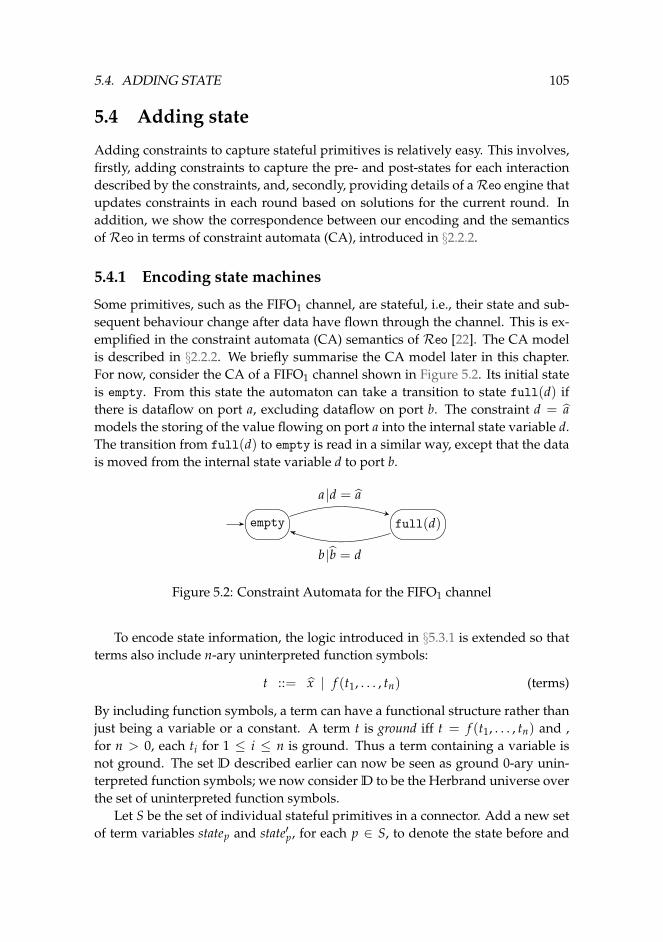
5.4. ADDING STATE 105
5.4 Adding state
Adding constraints to capture stateful primitives is relatively easy. This involves,firstly, adding constraints to capture the pre- and post-states for each interactiondescribed by the constraints, and, secondly, providing details of aReo engine thatupdates constraints in each round based on solutions for the current round. Inaddition, we show the correspondence between our encoding and the semanticsofReo in terms of constraint automata (CA), introduced in §2.2.2.
5.4.1 Encoding state machines
Some primitives, such as the FIFO1 channel, are stateful, i.e., their state and sub-sequent behaviour change after data have flown through the channel. This is ex-emplified in the constraint automata (CA) semantics of Reo [22]. The CA modelis described in §2.2.2. We briefly summarise the CA model later in this chapter.For now, consider the CA of a FIFO1 channel shown in Figure 5.2. Its initial stateis empty. From this state the automaton can take a transition to state full(d) ifthere is dataflow on port a, excluding dataflow on port b. The constraint d = amodels the storing of the value flowing on port a into the internal state variable d.The transition from full(d) to empty is read in a similar way, except that the datais moved from the internal state variable d to port b.
empty full(d)
a d = a
b b = d
Figure 5.2: Constraint Automata for the FIFO1 channel
To encode state information, the logic introduced in §5.3.1 is extended so thatterms also include n-ary uninterpreted function symbols:
t ::= x | f (t1, . . . , tn) (terms)
By including function symbols, a term can have a functional structure rather thanjust being a variable or a constant. A term t is ground iff t = f (t1, . . . , tn) and ,for n > 0, each ti for 1 ≤ i ≤ n is ground. Thus a term containing a variable isnot ground. The set D described earlier can now be seen as ground 0-ary unin-terpreted function symbols; we now consider D to be the Herbrand universe overthe set of uninterpreted function symbols.
Let S be the set of individual stateful primitives in a connector. Add a new setof term variables statep and state′p, for each p ∈ S, to denote the state before and
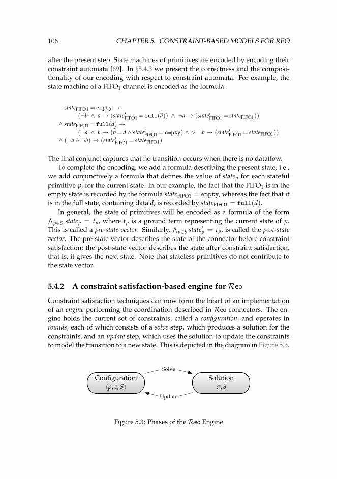
106 CHAPTER 5. CONSTRAINT-BASED MODELS FOR REO
after the present step. State machines of primitives are encoded by encoding theirconstraint automata [69]. In §5.4.3 we present the correctness and the composi-tionality of our encoding with respect to constraint automata. For example, thestate machine of a FIFO1 channel is encoded as the formula:
stateFIFO1 = empty→(¬b ∧ a→ (state′FIFO1 = full(a)) ∧ ¬a→ (state′FIFO1 = stateFIFO1))
∧ stateFIFO1 = full(d)→(¬a ∧ b→ (b= d ∧ state′FIFO1 = empty) ∧ > ¬b→ (state′FIFO1 = stateFIFO1))
∧ (¬a ∧ ¬b)→ (state′FIFO1 = stateFIFO1)
The final conjunct captures that no transition occurs when there is no dataflow.To complete the encoding, we add a formula describing the present state, i.e.,
we add conjunctively a formula that defines the value of statep for each statefulprimitive p, for the current state. In our example, the fact that the FIFO1 is in theempty state is recorded by the formula stateFIFO1 = empty, whereas the fact that itis in the full state, containing data d, is recorded by stateFIFO1 = full(d).
In general, the state of primitives will be encoded as a formula of the form∧p∈S statep = tp, where tp is a ground term representing the current state of p.
This is called a pre-state vector. Similarly,∧
p∈S state′p = tp, is called the post-statevector. The pre-state vector describes the state of the connector before constraintsatisfaction; the post-state vector describes the state after constraint satisfaction,that is, it gives the next state. Note that stateless primitives do not contribute tothe state vector.
5.4.2 A constraint satisfaction-based engine forReo
Constraint satisfaction techniques can now form the heart of an implementationof an engine performing the coordination described in Reo connectors. The en-gine holds the current set of constraints, called a configuration, and operates inrounds, each of which consists of a solve step, which produces a solution for theconstraints, and an update step, which uses the solution to update the constraintsto model the transition to a new state. This is depicted in the diagram in Figure 5.3.
Configuration〈ρ, ε, S〉
Solutionσ, δ
Solve
Update
Figure 5.3: Phases of theReo Engine
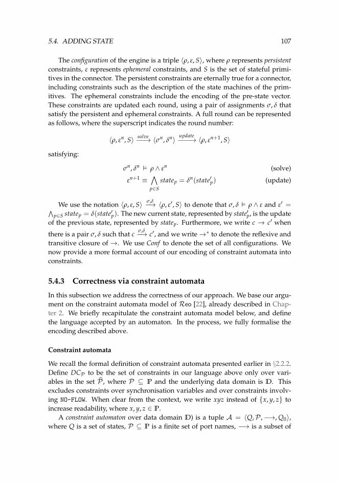
5.4. ADDING STATE 107
The configuration of the engine is a triple 〈ρ, ε, S〉, where ρ represents persistentconstraints, ε represents ephemeral constraints, and S is the set of stateful primi-tives in the connector. The persistent constraints are eternally true for a connector,including constraints such as the description of the state machines of the prim-itives. The ephemeral constraints include the encoding of the pre-state vector.These constraints are updated each round, using a pair of assignments σ, δ thatsatisfy the persistent and ephemeral constraints. A full round can be representedas follows, where the superscript indicates the round number:
〈ρ, εn, S〉 solve−−→ 〈σn, δn〉update−−−→ 〈ρ, εn+1, S〉
satisfying:
σn, δn � ρ ∧ εn (solve)
εn+1 ≡∧p∈S
statep = δn(state′p) (update)
We use the notation 〈ρ, ε, S〉 σ,δ−→ 〈ρ, ε′, S〉 to denote that σ, δ � ρ ∧ ε and ε′ =∧p∈S statep = δ(state′p). The new current state, represented by state′p, is the update
of the previous state, represented by statep. Furthermore, we write c → c′ when
there is a pair σ, δ such that c σ,δ−→ c′, and we write→∗ to denote the reflexive andtransitive closure of →. We use Conf to denote the set of all configurations. Wenow provide a more formal account of our encoding of constraint automata intoconstraints.
5.4.3 Correctness via constraint automata
In this subsection we address the correctness of our approach. We base our argu-ment on the constraint automata model of Reo [22], already described in Chap-ter 2. We briefly recapitulate the constraint automata model below, and definethe language accepted by an automaton. In the process, we fully formalise theencoding described above.
Constraint automata
We recall the formal definition of constraint automata presented earlier in §2.2.2.Define DCP to be the set of constraints in our language above only over vari-ables in the set P , where P ⊆ P and the underlying data domain is D. Thisexcludes constraints over synchronisation variables and over constraints involv-ing NO-FLOW. When clear from the context, we write xyz instead of {x, y, z} toincrease readability, where x, y, z ∈ P.
A constraint automaton over data domain D) is a tuple A = 〈Q,P ,−→, Q0〉,where Q is a set of states, P ⊆ P is a finite set of port names, −→ is a subset of
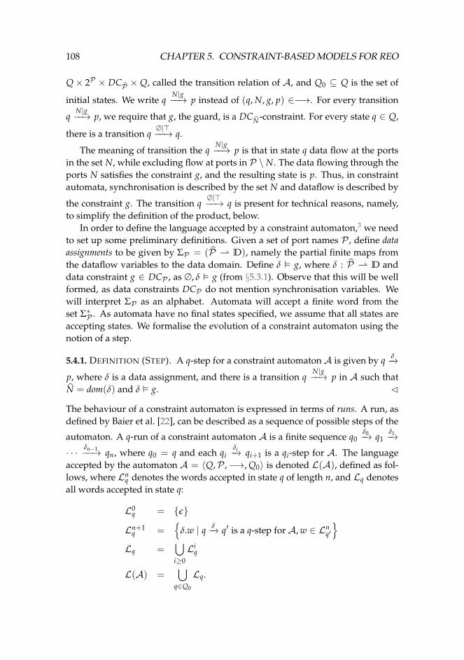
108 CHAPTER 5. CONSTRAINT-BASED MODELS FOR REO
Q× 2P × DCP × Q, called the transition relation of A, and Q0 ⊆ Q is the set of
initial states. We write qN|g−−→ p instead of (q, N, g, p) ∈−→. For every transition
qN|g−−→ p, we require that g, the guard, is a DCN-constraint. For every state q ∈ Q,
there is a transition q∅|>−−→ q.
The meaning of transition the qN|g−−→ p is that in state q data flow at the ports
in the set N, while excluding flow at ports in P \ N. The data flowing through theports N satisfies the constraint g, and the resulting state is p. Thus, in constraintautomata, synchronisation is described by the set N and dataflow is described by
the constraint g. The transition q∅|>−−→ q is present for technical reasons, namely,
to simplify the definition of the product, below.In order to define the language accepted by a constraint automaton,3 we need
to set up some preliminary definitions. Given a set of port names P , define dataassignments to be given by ΣP = (P ⇀ D), namely the partial finite maps fromthe dataflow variables to the data domain. Define δ � g, where δ : P ⇀ D anddata constraint g ∈ DCP , as ∅, δ � g (from §5.3.1). Observe that this will be wellformed, as data constraints DCP do not mention synchronisation variables. Wewill interpret ΣP as an alphabet. Automata will accept a finite word from theset Σ∗P . As automata have no final states specified, we assume that all states areaccepting states. We formalise the evolution of a constraint automaton using thenotion of a step.
5.4.1. DEFINITION (STEP). A q-step for a constraint automaton A is given by q δ−→p, where δ is a data assignment, and there is a transition q
N|g−−→ p in A such thatN = dom(δ) and δ � g. C
The behaviour of a constraint automaton is expressed in terms of runs. A run, asdefined by Baier et al. [22], can be described as a sequence of possible steps of the
automaton. A q-run of a constraint automaton A is a finite sequence q0δ0−→ q1
δ1−→· · · δn−1−−→ qn, where q0 = q and each qi
δi−→ qi+1 is a qi-step for A. The languageaccepted by the automaton A = 〈Q,P ,−→, Q0〉 is denoted L(A), defined as fol-lows, where Ln
q denotes the words accepted in state q of length n, and Lq denotesall words accepted in state q:
L0q = {ε}
Ln+1q =
{δ.w | q δ−→ q′ is a q-step for A, w ∈ Ln
q′
}Lq =
⋃i≥0
Liq
L(A) =⋃
q∈Q0
Lq.
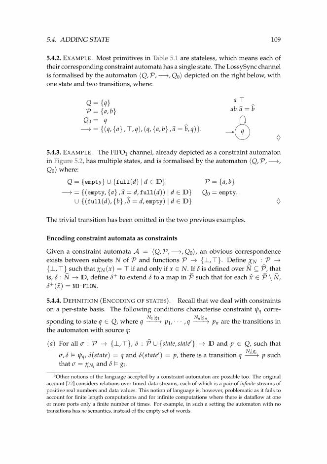
5.4. ADDING STATE 109
5.4.2. EXAMPLE. Most primitives in Table 5.1 are stateless, which means each oftheir corresponding constraint automata has a single state. The LossySync channelis formalised by the automaton 〈Q,P ,−→, Q0〉 depicted on the right below, withone state and two transitions, where:
Q = {q}P = {a, b}
Q0 = q−→ = {(q, {a} ,>, q), (q, {a, b} , a = b, q)}. q
a >ab a = b
♦
5.4.3. EXAMPLE. The FIFO1 channel, already depicted as a constraint automatonin Figure 5.2, has multiple states, and is formalised by the automaton 〈Q,P ,−→,Q0〉 where:
Q = {empty} ∪ {full(d) | d ∈ D} P = {a, b}−→ = {(empty, {a} , a = d, full(d)) | d ∈ D} Q0 = empty.∪ {(full(d), {b} , b = d, empty) | d ∈ D} ♦
The trivial transition has been omitted in the two previous examples.
Encoding constraint automata as constraints
Given a constraint automata A = 〈Q,P ,−→, Q0〉, an obvious correspondenceexists between subsets N of P and functions P → {⊥,>}. Define χN : P →{⊥,>} such that χN(x) = > if and only if x ∈ N. If δ is defined over N ⊆ P , thatis, δ : N → D, define δ+ to extend δ to a map in P such that for each x ∈ P \ N,δ+(x) = NO-FLOW.
5.4.4. DEFINITION (ENCODING OF STATES). Recall that we deal with constraintson a per-state basis. The following conditions characterise constraint ψq corre-
sponding to state q ∈ Q, where qN1|g1−−−→ p1, · · · , q
Nn |gn−−−→ pn are the transitions inthe automaton with source q:
(a) For all σ : P → {⊥,>}, δ : P ∪ {state, state′} → D and p ∈ Q, such that
σ, δ � ψq, δ(state) = q and δ(state′) = p, there is a transition qNi |gi−−→ p such
that σ = χNi and δ � gi.
3Other notions of the language accepted by a constraint automaton are possible too. The originalaccount [22] considers relations over timed data streams, each of which is a pair of infinite streams ofpositive real numbers and data values. This notion of language is, however, problematic as it fails toaccount for finite length computations and for infinite computations where there is dataflow at oneor more ports only a finite number of times. For example, in such a setting the automaton with notransitions has no semantics, instead of the empty set of words.
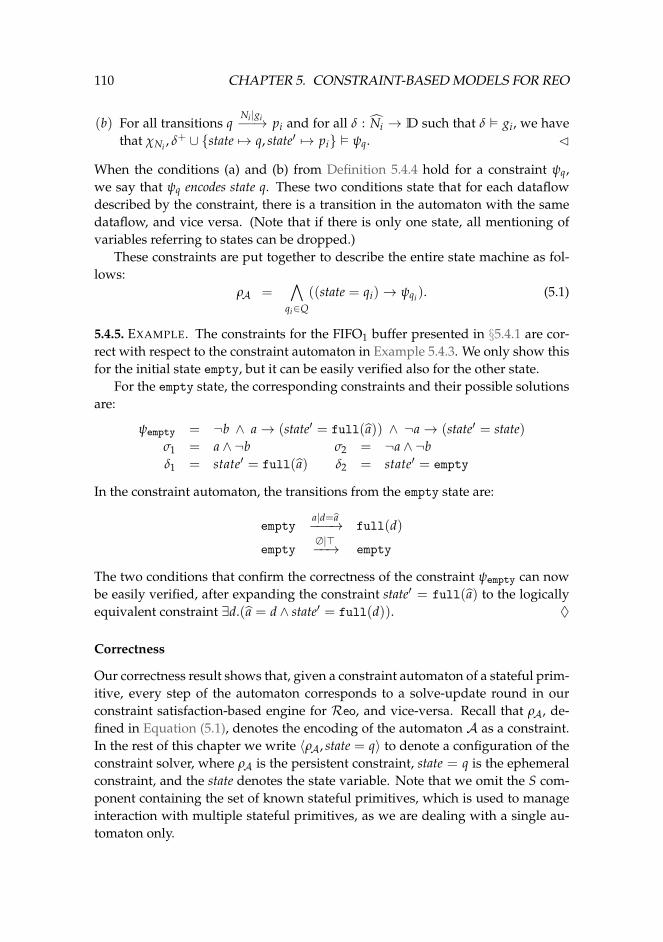
110 CHAPTER 5. CONSTRAINT-BASED MODELS FOR REO
(b) For all transitions qNi |gi−−→ pi and for all δ : Ni → D such that δ � gi, we have
that χNi , δ+ ∪ {state 7→ q, state′ 7→ pi} � ψq. C
When the conditions (a) and (b) from Definition 5.4.4 hold for a constraint ψq,we say that ψq encodes state q. These two conditions state that for each dataflowdescribed by the constraint, there is a transition in the automaton with the samedataflow, and vice versa. (Note that if there is only one state, all mentioning ofvariables referring to states can be dropped.)
These constraints are put together to describe the entire state machine as fol-lows:
ρA =∧
qi∈Q((state = qi)→ ψqi ). (5.1)
5.4.5. EXAMPLE. The constraints for the FIFO1 buffer presented in §5.4.1 are cor-rect with respect to the constraint automaton in Example 5.4.3. We only show thisfor the initial state empty, but it can be easily verified also for the other state.
For the empty state, the corresponding constraints and their possible solutionsare:
ψempty = ¬b ∧ a→ (state′ = full(a)) ∧ ¬a→ (state′ = state)σ1 = a ∧ ¬b σ2 = ¬a ∧ ¬bδ1 = state′ = full(a) δ2 = state′ = empty
In the constraint automaton, the transitions from the empty state are:
emptya|d=a−−−→ full(d)
empty∅|>−−→ empty
The two conditions that confirm the correctness of the constraint ψempty can nowbe easily verified, after expanding the constraint state′ = full(a) to the logicallyequivalent constraint ∃d.(a = d ∧ state′ = full(d)). ♦
Correctness
Our correctness result shows that, given a constraint automaton of a stateful prim-itive, every step of the automaton corresponds to a solve-update round in ourconstraint satisfaction-based engine for Reo, and vice-versa. Recall that ρA, de-fined in Equation (5.1), denotes the encoding of the automaton A as a constraint.In the rest of this chapter we write 〈ρA, state = q〉 to denote a configuration of theconstraint solver, where ρA is the persistent constraint, state = q is the ephemeralconstraint, and the state denotes the state variable. Note that we omit the S com-ponent containing the set of known stateful primitives, which is used to manageinteraction with multiple stateful primitives, as we are dealing with a single au-tomaton only.
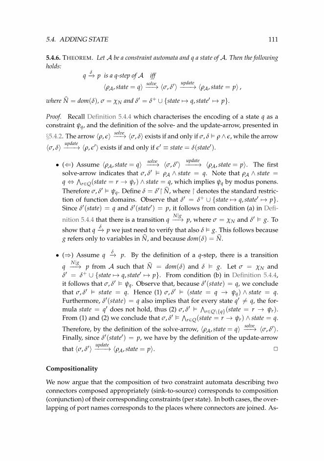
5.4. ADDING STATE 111
5.4.6. THEOREM. Let A be a constraint automata and q a state of A. Then the followingholds:
q δ−→ p is a q-step of A iff
〈ρA, state = q〉 solve−−→ 〈σ, δ′〉update−−−→ 〈ρA, state = p〉 ,
where N = dom(δ), σ = χN and δ′ = δ+ ∪ {state 7→ q, state′ 7→ p}.
Proof. Recall Definition 5.4.4 which characterises the encoding of a state q as aconstraint ψq, and the definition of the solve- and the update-arrow, presented in
§5.4.2. The arrow 〈ρ, ε〉 solve−−→ 〈σ, δ〉 exists if and only if σ, δ � ρ∧ ε, while the arrow
〈σ, δ〉update−−−→ 〈ρ, ε′〉 exists if and only if ε′ ≡ state = δ(state′).
• (⇐) Assume 〈ρA, state = q〉 solve−−→ 〈σ, δ′〉update−−−→ 〈ρA, state = p〉. The first
solve-arrow indicates that σ, δ′ � ρA ∧ state = q. Note that ρA ∧ state =
q ⇔ ∧r∈Q(state = r → ψr) ∧ state = q, which implies ψq by modus ponens.
Therefore σ, δ′ � ψq. Define δ = δ′� N, where � denotes the standard restric-tion of function domains. Observe that δ′ = δ+ ∪ {state 7→ q, state′ 7→ p}.Since δ′(state) = q and δ′(state′) = p, it follows from condition (a) in Defi-
nition 5.4.4 that there is a transition qN|g−−→ p, where σ = χN and δ′ � g. To
show that q δ−→ p we just need to verify that also δ � g. This follows becauseg refers only to variables in N, and because dom(δ) = N.
• (⇒) Assume q δ−→ p. By the definition of a q-step, there is a transition
qN|g−−→ p from A such that N = dom(δ) and δ � g. Let σ = χN and
δ′ = δ+ ∪ {state 7→ q, state′ 7→ p}. From condition (b) in Definition 5.4.4,it follows that σ, δ′ � ψq. Observe that, because δ′(state) = q, we concludethat σ, δ′ � state = q. Hence (1) σ, δ′ � (state = q → ψq) ∧ state = q.Furthermore, δ′(state) = q also implies that for every state q′ 6= q, the for-mula state = q′ does not hold, thus (2) σ, δ′ �
∧r∈Q\{q}(state = r → ψr).
From (1) and (2) we conclude that σ, δ′ �∧
r∈Q(state = r → ψr) ∧ state = q.
Therefore, by the definition of the solve-arrow, 〈ρA, state = q〉 solve−−→ 〈σ, δ′〉.Finally, since δ′(state′) = p, we have by the definition of the update-arrow
that 〈σ, δ′〉update−−−→ 〈ρA, state = p〉. 2
Compositionality
We now argue that the composition of two constraint automata describing twoconnectors composed appropriately (sink-to-source) corresponds to composition(conjunction) of their corresponding constraints (per state). In both cases, the over-lapping of port names corresponds to the places where connectors are joined. As-
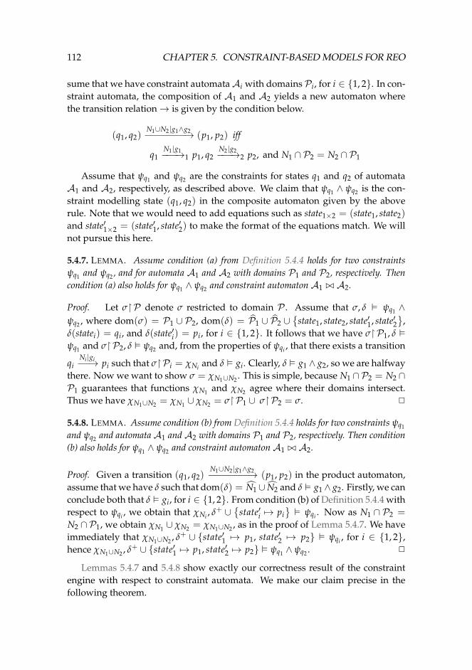
112 CHAPTER 5. CONSTRAINT-BASED MODELS FOR REO
sume that we have constraint automataAi with domains Pi, for i ∈ {1, 2}. In con-straint automata, the composition of A1 and A2 yields a new automaton wherethe transition relation→ is given by the condition below.
(q1, q2)N1∪N2|g1∧g2−−−−−−−→ (p1, p2) iff
q1N1|g1−−−→1 p1, q2
N2|g2−−−→2 p2, and N1 ∩ P2 = N2 ∩ P1
Assume that ψq1 and ψq2 are the constraints for states q1 and q2 of automataA1 and A2, respectively, as described above. We claim that ψq1 ∧ ψq2 is the con-straint modelling state (q1, q2) in the composite automaton given by the aboverule. Note that we would need to add equations such as state1×2 = (state1, state2)
and state′1×2 = (state′1, state′2) to make the format of the equations match. We willnot pursue this here.
5.4.7. LEMMA. Assume condition (a) from Definition 5.4.4 holds for two constraintsψq1 and ψq2 , and for automata A1 and A2 with domains P1 and P2, respectively. Thencondition (a) also holds for ψq1 ∧ ψq2 and constraint automaton A1 ./ A2.
Proof. Let σ�P denote σ restricted to domain P . Assume that σ, δ � ψq1 ∧ψq2 , where dom(σ) = P1 ∪ P2, dom(δ) = P1 ∪ P2 ∪
{state1, state2, state′1, state′2
},
δ(statei) = qi, and δ(state′i) = pi, for i ∈ {1, 2}. It follows that we have σ�P1, δ �ψq1 and σ�P2, δ � ψq2 and, from the properties of ψqi , that there exists a transition
qiNi |gi−−→ pi such that σ�Pi = χNi and δ � gi. Clearly, δ � g1 ∧ g2, so we are halfway
there. Now we want to show σ = χN1∪N2 . This is simple, because N1 ∩P2 = N2 ∩P1 guarantees that functions χN1 and χN2 agree where their domains intersect.Thus we have χN1∪N2 = χN1 ∪ χN2 = σ�P1 ∪ σ�P2 = σ. 2
5.4.8. LEMMA. Assume condition (b) from Definition 5.4.4 holds for two constraints ψq1
and ψq2 and automata A1 and A2 with domains P1 and P2, respectively. Then condition(b) also holds for ψq1 ∧ ψq2 and constraint automaton A1 ./ A2.
Proof. Given a transition (q1, q2)N1∪N2|g1∧g2−−−−−−−→ (p1, p2) in the product automaton,
assume that we have δ such that dom(δ) = N1 ∪ N2 and δ � g1 ∧ g2. Firstly, we canconclude both that δ � gi, for i ∈ {1, 2}. From condition (b) of Definition 5.4.4 withrespect to ψqi , we obtain that χNi , δ+ ∪
{state′i 7→ pi
}� ψqi . Now as N1 ∩ P2 =
N2 ∩ P1, we obtain χN1 ∪ χN2 = χN1∪N2 , as in the proof of Lemma 5.4.7. We haveimmediately that χN1∪N2 , δ+ ∪ {state′1 7→ p1, state′2 7→ p2} � ψqi , for i ∈ {1, 2},hence χN1∪N2 , δ+ ∪ {state′1 7→ p1, state′2 7→ p2} � ψq1 ∧ ψq2 . 2
Lemmas 5.4.7 and 5.4.8 show exactly our correctness result of the constraintengine with respect to constraint automata. We make our claim precise in thefollowing theorem.
5.5. ADDING CONTEXT DEPENDENCY 113
5.4.9. THEOREM. If ψq1 encodes state q1 from automaton A1 and ψq2 encodes state q2from automaton A2, then ψq1 ∧ ψq2 encodes state (q1, q2) from automaton A1 ./ A2.
Proof. Directly from Lemmas 5.4.7 and 5.4.8. 2
5.5 Adding context dependency
We have introduced three different types of constraints to capture the behaviour ofReo connectors, namely synchronisation, data flow, and state constraints. We nowexplore one further possibility and present context dependency as an additionalextension that can be modelled by constraints.
One of the main contributions of the connector colouring (CC) framework [37]is a Reo semantics that expresses context dependency, a feature missing from theconstraint automata model. A primitive depends on its context if its behaviourchanges when there is an increase of data flowing on its ports. That is, when addi-tional dataflow is possible, earlier valid behaviour is not displayed anymore. Twoimportant example primitives that cannot be represented in previous semanticmodels are:
Context-dependent LossySync This channel loses data written to its source onlyif the surrounding context is unable to accept the data through its sink; otherwisethe data flow through the channel. This corresponds to the original intention ofthe LossySync channel [8].
Priority merger This is a special variant of a merger that favours one of its sinkports: if dataflow is possible at both sink ports, it prefers a particular port over theother.
Context dependency, as described by the CC semantics, supports a more expres-sive model than otherReo semantics which lack this notion. Context dependencyin Reo is presented in more detail in §2.2.3, where we describe the Reo automatamodel [29], and in §4.3, where we describe the connector colouring semantics [37].In the rest of this section we recall the relevant definitions of the connector colour-ing semantics, which we encode as constraints and use to show the correctness ofour approach.
5.5.1 Connector colouring: an overview
We now briefly recall the connector colouring (CC) semantics presented in Chap-ter 4, that we use as the basis to describe context dependency in our constraintframework. The connector colouring (CC) semantics, as presented by Clarke etal. [37], is based on the idea of colouring the ports of a connector using a setColour of three colours—for orientation, the indicates the port. One colour ( )
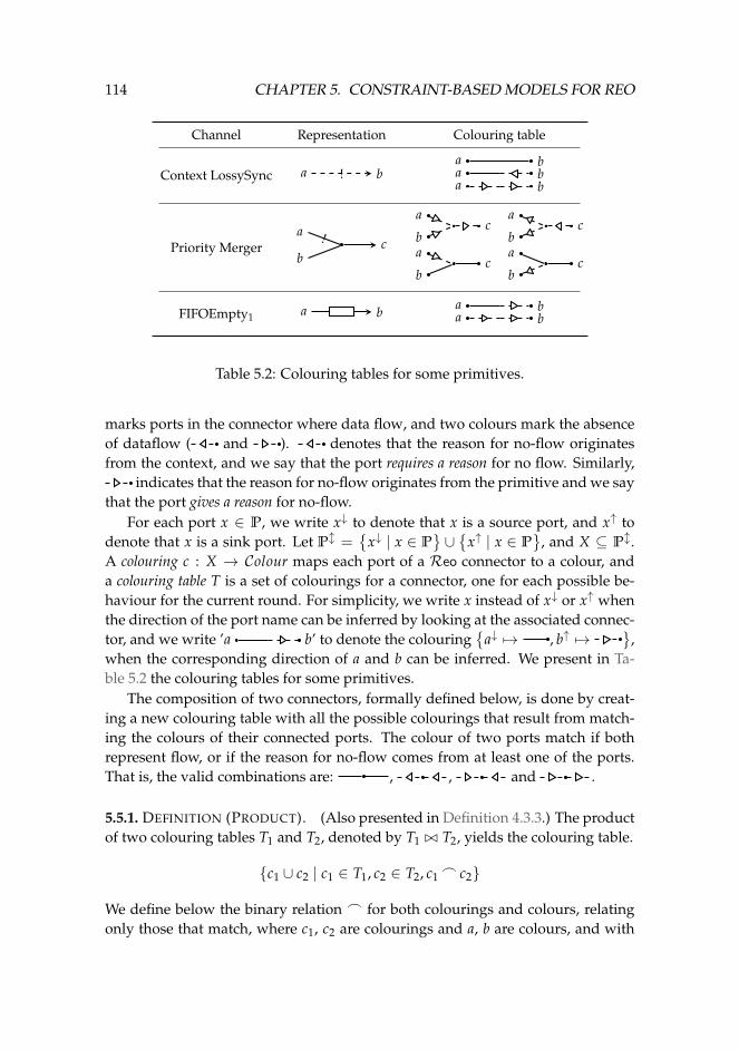
114 CHAPTER 5. CONSTRAINT-BASED MODELS FOR REO
Channel Representation Colouring table
Context LossySync a b!a ba ba b
Priority Merger ca
b!
ca
bc
a
b
ca
bc
a
b
FIFOEmpty1 a b a ba b
Table 5.2: Colouring tables for some primitives.
marks ports in the connector where data flow, and two colours mark the absenceof dataflow ( and ). denotes that the reason for no-flow originatesfrom the context, and we say that the port requires a reason for no flow. Similarly,
indicates that the reason for no-flow originates from the primitive and we saythat the port gives a reason for no-flow.
For each port x ∈ P, we write x↓ to denote that x is a source port, and x↑ todenote that x is a sink port. Let Pl =
{x↓ | x ∈ P
}∪{
x↑ | x ∈ P}
, and X ⊆ Pl.A colouring c : X → Colour maps each port of a Reo connector to a colour, anda colouring table T is a set of colourings for a connector, one for each possible be-haviour for the current round. For simplicity, we write x instead of x↓ or x↑ whenthe direction of the port name can be inferred by looking at the associated connec-tor, and we write ’a b’ to denote the colouring
{a↓ 7→ , b↑ 7→
},
when the corresponding direction of a and b can be inferred. We present in Ta-ble 5.2 the colouring tables for some primitives.
The composition of two connectors, formally defined below, is done by creat-ing a new colouring table with all the possible colourings that result from match-ing the colours of their connected ports. The colour of two ports match if bothrepresent flow, or if the reason for no-flow comes from at least one of the ports.That is, the valid combinations are: , , and .
5.5.1. DEFINITION (PRODUCT). (Also presented in Definition 4.3.3.) The productof two colouring tables T1 and T2, denoted by T1 ./ T2, yields the colouring table.
{c1 ∪ c2 | c1 ∈ T1, c2 ∈ T2, c1_ c2}
We define below the binary relation _ for both colourings and colours, relatingonly those that match, where c1, c2 are colourings and a, b are colours, and with
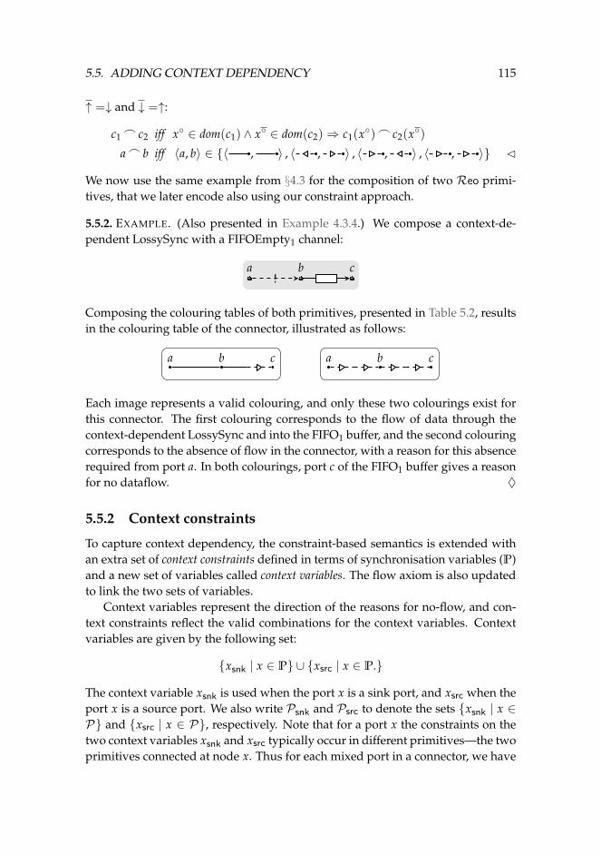
5.5. ADDING CONTEXT DEPENDENCY 115
↑ =↓ and ↓ =↑:
c1_ c2 iff x◦ ∈ dom(c1) ∧ x◦ ∈ dom(c2)⇒ c1(x◦)_ c2(x◦)
a_ b iff 〈a, b〉 ∈ {〈 , 〉 , 〈 , 〉 , 〈 , 〉 , 〈 , 〉} C
We now use the same example from §4.3 for the composition of two Reo primi-tives, that we later encode also using our constraint approach.
5.5.2. EXAMPLE. (Also presented in Example 4.3.4.) We compose a context-de-pendent LossySync with a FIFOEmpty1 channel:
a b c!
Composing the colouring tables of both primitives, presented in Table 5.2, resultsin the colouring table of the connector, illustrated as follows:
a b c a b c
Each image represents a valid colouring, and only these two colourings exist forthis connector. The first colouring corresponds to the flow of data through thecontext-dependent LossySync and into the FIFO1 buffer, and the second colouringcorresponds to the absence of flow in the connector, with a reason for this absencerequired from port a. In both colourings, port c of the FIFO1 buffer gives a reasonfor no dataflow. ♦
5.5.2 Context constraints
To capture context dependency, the constraint-based semantics is extended withan extra set of context constraints defined in terms of synchronisation variables (P)and a new set of variables called context variables. The flow axiom is also updatedto link the two sets of variables.
Context variables represent the direction of the reasons for no-flow, and con-text constraints reflect the valid combinations for the context variables. Contextvariables are given by the following set:
{xsnk | x ∈ P} ∪ {xsrc | x ∈ P.}
The context variable xsnk is used when the port x is a sink port, and xsrc when theport x is a source port. We also write Psnk and Psrc to denote the sets {xsnk | x ∈P} and {xsrc | x ∈ P}, respectively. Note that for a port x the constraints on thetwo context variables xsnk and xsrc typically occur in different primitives—the twoprimitives connected at node x. Thus for each mixed port in a connector, we have
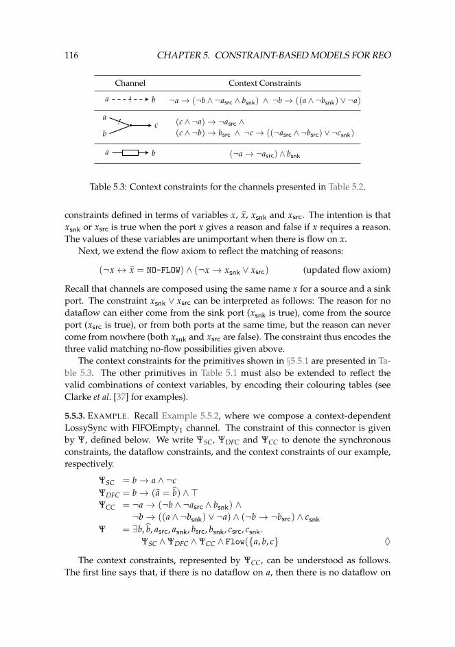
116 CHAPTER 5. CONSTRAINT-BASED MODELS FOR REO
Channel Context Constraints
a b! ¬a→ (¬b ∧ ¬asrc ∧ bsnk) ∧ ¬b→ ((a ∧ ¬bsnk) ∨ ¬a)
ca
b! (c ∧ ¬a)→ ¬asrc ∧
(c ∧ ¬b)→ bsrc ∧ ¬c→ ((¬asrc ∧ ¬bsrc) ∨ ¬csnk)
a b (¬a→ ¬asrc) ∧ bsnk
Table 5.3: Context constraints for the channels presented in Table 5.2.
constraints defined in terms of variables x, x, xsnk and xsrc. The intention is thatxsnk or xsrc is true when the port x gives a reason and false if x requires a reason.The values of these variables are unimportant when there is flow on x.
Next, we extend the flow axiom to reflect the matching of reasons:
(¬x ↔ x = NO-FLOW) ∧ (¬x → xsnk ∨ xsrc) (updated flow axiom)
Recall that channels are composed using the same name x for a source and a sinkport. The constraint xsnk ∨ xsrc can be interpreted as follows: The reason for nodataflow can either come from the sink port (xsnk is true), come from the sourceport (xsrc is true), or from both ports at the same time, but the reason can nevercome from nowhere (both xsnk and xsrc are false). The constraint thus encodes thethree valid matching no-flow possibilities given above.
The context constraints for the primitives shown in §5.5.1 are presented in Ta-ble 5.3. The other primitives in Table 5.1 must also be extended to reflect thevalid combinations of context variables, by encoding their colouring tables (seeClarke et al. [37] for examples).
5.5.3. EXAMPLE. Recall Example 5.5.2, where we compose a context-dependentLossySync with FIFOEmpty1 channel. The constraint of this connector is givenby Ψ, defined below. We write ΨSC, ΨDFC and ΨCC to denote the synchronousconstraints, the dataflow constraints, and the context constraints of our example,respectively.
ΨSC = b→ a ∧ ¬cΨDFC = b→ (a = b) ∧>ΨCC = ¬a→ (¬b ∧ ¬asrc ∧ bsnk) ∧
¬b→ ((a ∧ ¬bsnk) ∨ ¬a) ∧ (¬b→ ¬bsrc) ∧ csnkΨ = ∃b, b, asrc, asnk, bsrc, bsnk, csrc, csnk.
ΨSC ∧ΨDFC ∧ΨCC ∧ Flow({a, b, c} ♦
The context constraints, represented by ΨCC, can be understood as follows.The first line says that, if there is no dataflow on a, then there is no dataflow on
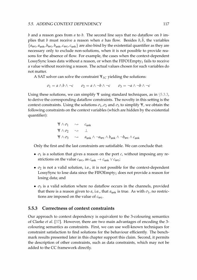
5.5. ADDING CONTEXT DEPENDENCY 117
b and a reason goes from a to b. The second line says that no dataflow on b im-plies that b must receive a reason when a has flow. Besides b, b, the variables{asrc, asnk, bsrc, bsnk, csrc, csnk} are also bind by the existential quantifier as they arenecessary only to exclude non-solutions, when it is not possible to provide rea-sons for the absence of flow. For example, the cases when the context-dependentLossySync loses data without a reason, or when the FIFO1Empty1 fails to receivea value without receiving a reason. The actual values chosen for such variables donot matter.
A SAT solver can solve the constraint ΨSC yielding the solutions:
σ1 = a ∧ b ∧ ¬c σ2 = a ∧ ¬b ∧ ¬c σ3 = ¬a ∧ ¬b ∧ ¬c
Using these solutions, we can simplify Ψ using standard techniques, as in §5.3.3,to derive the corresponding dataflow constraints. The novelty in this setting is thecontext constraints. Using the solutions σ1, σ2 and σ3 to simplify Ψ, we obtain thefollowing constraints on the context variables (which are hidden by the existentialquantifier):
Ψ ∧ σ1 ; csnkΨ ∧ σ2 ; ⊥Ψ ∧ σ3 ; asnk ∧ ¬asrc ∧ bsnk ∧ ¬bsrc ∧ csnk
Only the first and the last constraints are satisfiable. We can conclude that:
• σ1 is a solution that gives a reason on the port c, without imposing any re-strictions on the value csrc, as csnk → csnk ∨ csrc;
• σ2 is not a valid solution, i.e., it is not possible for the context-dependentLossySync to lose data since the FIFOEmpty1 does not provide a reason forlosing data; and
• σ3 is a valid solution where no dataflow occurs in the channels, providedthat there is a reason given to a, i.e., that asnk is true. As with σ1, no restric-tions are imposed on the value of csrc.
5.5.3 Correctness of context constraints
Our approach to context dependency is equivalent to the 3-colouring semanticsof Clarke et al. [37]. However, there are two main advantages of encoding the 3-colouring semantics as constraints. First, we can use well-known techniques forconstraint satisfaction to find solutions for the behaviour efficiently. The bench-mark results presented later in this chapter support this claim. Second, it permitsthe description of other constraints, such as data constraints, which may not beadded to the CC framework directly.
118 CHAPTER 5. CONSTRAINT-BASED MODELS FOR REO
σ f (σ) σ f (σ)
x x↓ 7→ x x↑ 7→¬x ∧ xsrc x↓ 7→ ¬x ∧ xsnk x↑ 7→¬x ∧ ¬xsrc x↓ 7→ ¬x ∧ ¬xsnk x↑ 7→
Table 5.4: Definition of f .
In this subsection we formalise the equivalence between these two approaches.We start by introducing some auxiliary definitions, and present our main claim inTheorem 5.5.5. The equivalence of our approach with the 3-colouring follows byconstruction. The proof of this equivalence results from the following observa-tions.
1. The constraints of each primitive p are defined so that there is a surjection f ,defined in Table 5.4, from the solutions of the synchronisation and contextconstraints onto the entries of the colouring table of p.
2. The mapping f is compositional, namely, when composing two primitives pand q with a shared variable x, composing their colouring tables and apply-ing f to find the possible solutions is equivalent to apply f to each colouringtable and then finding the solutions for the conjunction of these constraintsand the updated flow axiom.
Let σ be an assignment. For each pair x, xs ∈ dom(σ), where s ∈ {src, snk},f (σ) is the colouring table that maps x↓ or x↑ to the colouring represented in Ta-ble 5.4. Furthermore, by the definition of f every colouring is associated to a fixedset of possible solutions, which can be trivially written as a constraint. That is, theinverse function f−1 will always produce solutions of possible constraints. It canbe easily shown that the colouring tables of the primitives in Table 5.2 are obtainedby applying f to the solutions of the synchronisation and context constraints pre-sented in Table 5.3. For example, the synchronisation and context constraints forthe FIFOEmpty1 are ¬b ∧ (¬a→ ¬asrc) ∧ bsnk, and its possible solutions are:
σ1 =a ∧ asrc ∧ ¬b ∧ bsnk;
σ2 =a ∧ ¬asrc ∧ ¬b ∧ bsnk; and
σ3 =¬a ∧ ¬asrc ∧ ¬b ∧ bsnk.
It follows from the definition of f that f (σ1) = f (σ2) = a b, and f (σ3) =
a b, which is what we expect.Observe that for every Reo connector the set of variables used in its synchro-
nisation and context constraints must obey certain properties, captured by thenotion of variable set defined below.
5.5. ADDING CONTEXT DEPENDENCY 119
5.5.4. DEFINITION. A variable set is a finite set V ⊆ P∪Psrc ∪Psnk such that
x ∈ V ∩P iff xsrc ∈ V ∩Psrc ∨ xsnk ∈ V ∩Psnk. C
We write V to denote the set of all variable sets. We say two sets of variables V1and V2 are compatible, written as V1
_V2, if V1 and V2 are variable sets, and forevery x ∈ V1 ∩V2 ∩P, x is a sink port in V1 and a source port in V2 or vice-versa,that is,
V1_V2 iff V1, V2 ∈ V ∧ V1 ∩V2 ⊆ P (5.2)
Note that if V1, V2 ∈ V then V1 ∪ V2 ∈ V, that is, V is closed under union. Intu-itively, two connectors with constraints over the variable sets V1 and V2 can onlybe composed if the source and sink ports are connected in a one-to-one fashion.Recall that the composition of two Reo connectors, introduced in §5.3.3, requiresthat every shared port of the composed connectors is a source port in one of theconnectors, and a sink port in the other connector.
We now assume that, for every primitive p, the colouring table is given by thesurjection f defined in Table 5.4 with respect to the solutions of the synchroni-sation and context constraints. Let fv(·) be a function that returns the free vari-ables of a constraint. A constraint Ψ is defined over a variable set V wheneverfv(Ψ) ⊆ V. Let also [[·]]V be a function that yields the set of all possible solutionsof Ψ over V, that is,
[[Ψ]]V = {σ | σ � Ψ, dom(σ) = V} .
Define F to be the lifting of f to sets, i.e., F(Σ) = { f (σ) | σ ∈ Σ}. Finally, let �denote the composition of two synchronisation and context constraints Ψ1 overthe set V1 and Ψ2 over the set V2, where V1
_V2, defined as follows:
Ψ1 �Ψ2 = Ψ1 ∧Ψ2 ∧∧
x∈V1∩V2
(¬x → xsnk ∨ xsrc),
where the last constraint reflects the update on the flow axiom. The correctnessof the composition of our encoding as constraints with respect to the connectorcolouring semantics is formalised by the following theorem.
5.5.5. THEOREM. For any pair of constraints Ψp over the variable set V1 and Ψq over thevariable set V2 such that V1
_V2, it holds that:
F([[Ψp]]V1) ./ F([[Ψq]])V2 = F([[Ψp �Ψp]]V1∪V2).
Before proving this theorem we prove four auxiliary lemmas. The first lemmarelates shared variables of Reo connectors and the domain of the colourings de-rived from specific solutions of the same connectors. In the following we use thesymbol ◦ to range over {↑, ↓}, and define ↑ =↓ and ↓ =↑.
120 CHAPTER 5. CONSTRAINT-BASED MODELS FOR REO
5.5.6. LEMMA. Let σ1 and σ2 be assignments for variable sets V1 and V2, and V1_V2.
Then the following holds.
x◦ ∈ dom( f (σ1)) ∧ x◦ ∈ dom( f (σ2)) iff x ∈ V1 ∩V2.
Proof. Let x be such that x◦ ∈ dom( f (σ1)) and x◦ ∈ dom( f (σ2)). By the definitionof f , if x◦ ∈ dom( f (σ1)) then x must occur also in dom(σ1), and similarly, x mustalso occur in dom(σ2). Therefore x ∈ V1 ∩ V2. For the other implication, assumethat x ∈ V1 ∩V2. Also x ∈ P because V1
_V2. By the definitions of f and becauseV1, V2 ∈ V, we conclude that x↑ ∈ dom( f (σ1)) and x↓ ∈ dom( f (σ2)) or x↓ ∈dom( f (σ1)) and x↑ ∈ dom( f (σ2)). 2
We say two assignments σ1 and σ2 are compatible, written as σ1_ σ2, iff ∀x ∈
dom(σ1) ∩ dom(σ2) · σ1(x) = σ2(x). The second lemma provides a sufficient con-dition for any two assignments σ1 and σ2 be compatible.
5.5.7. LEMMA. Let σ1 and σ2 be assignments for variable sets V1 and V2, where V1_V2,
and ∀x ∈ V1 ∩ V2 · f (σ1)(x◦)_ f (σ2)(x◦). Then σ1_ σ2. Moreover, we have that
f (σ1) ∪ f (σ2) = f (σ1 ∪ σ2).
Proof. We prove σ1_ σ2 by contraposition. Assuming ¬(σ1
_ σ2), there existsx ∈ V1 ∩ V2 such that σ1(x) 6= σ2(x). Note that from Equation (5.2) we con-clude that x ∈ P. Without loss of generality assume σ1(x) = > and σ2(x) =
⊥. Then f (σ1)(x◦) = and f (σ2)(x◦) 6= , for some ◦ ∈ {↑, ↓}. Thus¬( f (σ1)_ f (σ2)). Similarly for σ1(x) = ⊥, σ2(x) = >. We conclude that σ1
_ σ2.2
The next lemma relates the new constraint from the updated flow axiom to thematching of colourings.
5.5.8. LEMMA. For the constraint ¬x → (xsnk ∨ xsrc), where {x, xsrc, xsnk} ⊆ V, itholds that:
c ∈ F([[¬x → (xsrc ∨ xsnk)]]V) iff c(x↓)_ c(x↑). (5.3)
Proof. The proof follows by unfolding the definitions of F, and by applyingLemma 5.5.7.
c ∈ F([[¬x → (xsrc ∨ xsnk)]]V)
≡ 〈By the definition of F〉c = f (σ), σ � ¬x → (xsrc ∨ xsnk), and dom(σ) = V
≡ 〈Partition σ into σ′ and σ′′ such that dom(σ′) = {x, xsrc, xsnk}〉c = f (σ′ ∪ σ′′), σ′ � ¬x → (xsrc ∨ xsnk), and dom(σ′′) = V\ {x, xsrc, xsnk}
5.5. ADDING CONTEXT DEPENDENCY 121
Observe now that σ′_ σ′′, hence we know that f (σ′ ∪ σ′′) = f (σ′) ∪ f (σ′′).Furthermore, the possible solutions for σ′ are the following:
x ∧ xsrc ∧ xsnk x ∧ ¬xsrc ∧ xsnk ¬x ∧ xsrc ∧ xsnk ¬x ∧ ¬xsrc ∧ xsnkx ∧ xsrc ∧ ¬xsnk x ∧ ¬xsrc ∧ ¬xsnk ¬x ∧ xsrc ∧ ¬xsnk .
Let Σ be this set. The last step of the proof above is equivalent to
c = f (σ′) ∪ f (σ′′), σ′ ∈ Σ, and dom(σ′′) = V\ {x, xsrc, xsnk} .
Observe that f (σ′), for σ′ ∈ Σ, are exactly the set of all possible colourings c′ suchthat c′(x↓)_ c′(x↑), where dom(c′) =
{x↓, x↑
}. It is now sufficient to observe
that f (σ′′) yields any possible colouring, assigning colours to all the remainingports apart from x, not mentioned on the right-hand-side of the equivalence inEquation (5.3). 2
Our final lemma leading to the proof of Theorem 5.5.5 relates the matchingof the colouring yield by two different assignments and a new assignment thatsatisfies the constraint ¬x → xsrc ∨ xsnk.
5.5.9. LEMMA. For σ1 and σ2 such that dom(σi) = Vi, for i ∈ {1, 2}, σ1_ σ2, and
V1_V2:
f (σ1)(x◦)_ f (σ2)(x◦) iff
(σ1 ∪ σ2) � ¬x → xsrc ∨ xsnk and {x, xsrc, xsnk} ⊆ dom(σ1 ∪ σ2).
Proof. For simplicity let c1 = f (σ1) and c2 = f (σ2). Let also {x, xsrc, xsnk} ⊆ V.Note that c1 and c2 will have disjoint domains, because V1
_V2. Observe that:
c1(x◦)_ c2(x◦)
= 〈Because dom(c1) and dom(c2) are disjoint〉(c1 ∪ c2)(x◦)_(c1 ∪ c2)(x◦)
= 〈By Lemma 5.5.8〉c1 ∪ c2 ∈ F([[¬x → xsrc ∨ xsnk]]V)
= 〈By the definition of F and [[·]]V〉c1 ∪ c2 ∈ { f (σ) | σ � ¬x → xsrc ∨ xsnk, dom(σ) = V}
= 〈Because σ1_ σ2 and ci = f (σi)〉
f (σ1 ∪ σ2) ∈ { f (σ) | σ � ¬x → xsrc ∨ xsnk, dom(σ) = V}= 〈By set inclusion and because V ⊆ {x, xsrc, xsnk}〉
(σ1 ∪ σ2) � ¬x → xsrc ∨ xsnk and {x, xsrc, xsnk} ⊆ dom(σ1 ∪ σ2) 2
We are now in a position to prove Theorem 5.5.5.
122 CHAPTER 5. CONSTRAINT-BASED MODELS FOR REO
Proof. (Theorem 5.5.5)
F([[Ψp]])V1 ./ F([[Ψq]])V2
= 〈By the definition of F〉{f (σ1) | σ1 ∈ [[Ψp]]V1
}./{
f (σ2) | σ2 ∈ [[Ψq]]V2
}= 〈By the definition of [[·]]V〉{
f (σ1) | σ1 � Ψp, dom(σ1) = V1}./{
f (σ2) | σ2 � Ψq, dom(σ2) = V2}
= 〈By the definition of ./〉{ f (σ1) ∪ f (σ2) | σ1 � Ψp, σ2 � Ψq, dom(σ1) = V1, dom(σ2) = V2,
x◦ ∈ dom( f (σ1)) ∧ x◦ ∈ dom( f (σ2))⇒ f (σ1)(x◦)_ f (σ2)(x◦)}= 〈By Lemma 5.5.6〉{ f (σ1) ∪ f (σ2) | σ1 � Ψp, σ2 � Ψq, dom(σ1) = V1, dom(σ2) = V2,
x ∈ V1 ∩V2 ⇒ f (σ1)(x◦)_ f (σ2)(x◦)}= 〈By Lemma 5.5.7, from where we also conclude that σ1
_ σ2〉{ f (σ1 ∪ σ2) | σ1 � Ψp, σ2 � Ψq, dom(σ1 ∪ σ2) = V1 ∪V2,
x ∈ V1 ∩V2 ⇒ f (σ1)(x◦)_ f (σ2)(x◦)}= 〈By Lemma 5.5.9, and because σ1
_ σ2 and dom(σ1 ∪ σ2) = V1 ∪V2〉{ f (σ1 ∪ σ2) | σ1 � Ψp, σ2 � Ψq, dom(σ1 ∪ σ2) = V1 ∪V2,
x ∈ V1 ∩V2 ⇒ (σ1 ∪ σ2) � ¬x → xsrc ∨ xsnk}= 〈Because σ1
_ σ2〉{ f (σ1 ∪ σ2) | (σ1 ∪ σ2) � Ψp, (σ1 ∪ σ2) � Ψq, dom(σ1 ∪ σ2) = V1 ∪V2,
x ∈ V1 ∩V2 ⇒ (σ1 ∪ σ2) � ¬x → xsrc ∨ xsnk}= 〈Using σ = σ1 ∪ σ2 and replacing implication by an universal quantifier〉{ f (σ) | σ � Ψp, σ � Ψq, dom(σ) = V1 ∪V2, ∀x∈V1∩V2 · σ � ¬x → xsrc ∨ xsnk}
= 〈Because σ � Ψ1 and σ � Ψ2 iff σ � Ψ1 ∧Ψ2〉{ f (σ) | σ � Ψp ∧Ψq ∧
∧x∈V1∩V2
¬x → xsrc ∨ xsnk, dom(σ) = V1 ∪V2}= 〈By the definition of �〉{ f (σ) | σ � Ψp �Ψq, dom(σ) = V1 ∪V2}
= 〈By the definition of F and [[·]]V〉F([[Ψp �Ψq]]V1∪V2).
2
By proving Theorem 5.5.5 we show that our constraint-based approach fordescribing context dependency is equivalent to the 3-colouring semantics. As aresult, searching for valid colourings is reduced to a SAT solving problem, that is,the set of solutions for synchronous and context constraints of a connector coin-cide with its valid colourings. In the next section we exploit the practical conse-
5.6. BENCHMARKS 123
quences of this equivalence, and compare the execution times of an engine basedon the connector colouring semantics with our constraint-based engine.
5.6 Benchmarks
We compare two prototype engines based on constraint satisfaction with an opti-mised engine for Reo based on the connector colouring semantics [37]. For this,the data constraints are ignored, and solving the constraints only yields where datacan flow, but not which data flow. We evaluate the constraints-based approachusing implementations based on both context independent (CI) and context de-pendent (CD) semantics (§5.5). In the connector colouring semantics, the CI se-mantics corresponds to using two colours while the CD semantics correspondsto using three colours. We have implemented the context dependent semanticsfor only one of the constraint engines, as the results we present already providesolid evidence that the constraint-based approach is significantly better than usingconnector colouring. A few more words regarding the three engines:
CC engine We use an optimised engine based on connector colouring [37] as areference for our benchmark results. The engine has been incorporated intothe Eclipse Coordination Tools.4 This engine supports both context depen-dent and independent semantics, as explained in §5.5, and it is, to the bestof our knowledge, the fastest existing implementation that computes the be-haviour ofReo connectors on-the-fly.
SAT engine This is a constraint engine using the SAT4J Java libraries,5 which arefree and included in the Eclipse standard libraries. The main concern of theproject responsible for the SAT4J libraries is the efficiency of the SAT solver.We chose SAT4J because it is a well known library for SAT solving, withthe portability advantages provided by the Java platform. We avoid solu-tions that have no dataflow by adding conjunctively the constraint
∨x∈P x
to the constraints of the connector for the CI semantics. We do not add thisdisjunction in the CD semantics because the context dependency alreadyguarantees that the data flow unless there is an explicit reason that forbidsthe flow of data.
CHOCO engine We developed a second prototype constraint engine using theCHOCO open-source constraint solver6 which offers, among other things,state-of-the-art algorithms and techniques,and user-defined constraints, do-mains and variables. In the future, we expect to achieve finer control over
4http://reo.project.cwi.nl/cgi-bin/trac.cgi/reo/wiki/Tools5http://www.sat4j.org/6http://choco.emn.fr/
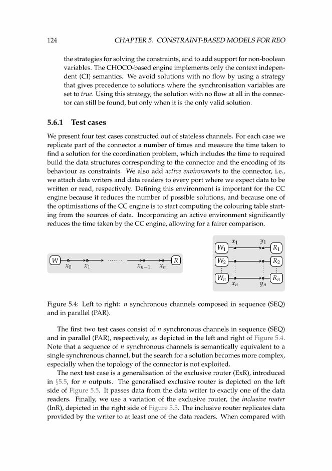
124 CHAPTER 5. CONSTRAINT-BASED MODELS FOR REO
the strategies for solving the constraints, and to add support for non-booleanvariables. The CHOCO-based engine implements only the context indepen-dent (CI) semantics. We avoid solutions with no flow by using a strategythat gives precedence to solutions where the synchronisation variables areset to true. Using this strategy, the solution with no flow at all in the connec-tor can still be found, but only when it is the only valid solution.
5.6.1 Test cases
We present four test cases constructed out of stateless channels. For each case wereplicate part of the connector a number of times and measure the time taken tofind a solution for the coordination problem, which includes the time to requiredbuild the data structures corresponding to the connector and the encoding of itsbehaviour as constraints. We also add active environments to the connector, i.e.,we attach data writers and data readers to every port where we expect data to bewritten or read, respectively. Defining this environment is important for the CCengine because it reduces the number of possible solutions, and because one ofthe optimisations of the CC engine is to start computing the colouring table start-ing from the sources of data. Incorporating an active environment significantlyreduces the time taken by the CC engine, allowing for a fairer comparison.
x0 x1 xn−1 xnW R
x1 y1
xn yn
W1 R1
W2 R2
Wn Rn
Figure 5.4: Left to right: n synchronous channels composed in sequence (SEQ)and in parallel (PAR).
The first two test cases consist of n synchronous channels in sequence (SEQ)and in parallel (PAR), respectively, as depicted in the left and right of Figure 5.4.Note that a sequence of n synchronous channels is semantically equivalent to asingle synchronous channel, but the search for a solution becomes more complex,especially when the topology of the connector is not exploited.
The next test case is a generalisation of the exclusive router (ExR), introducedin §5.5, for n outputs. The generalised exclusive router is depicted on the leftside of Figure 5.5. It passes data from the data writer to exactly one of the datareaders. Finally, we use a variation of the exclusive router, the inclusive router(InR), depicted in the right side of Figure 5.5. The inclusive router replicates dataprovided by the writer to at least one of the data readers. When compared with
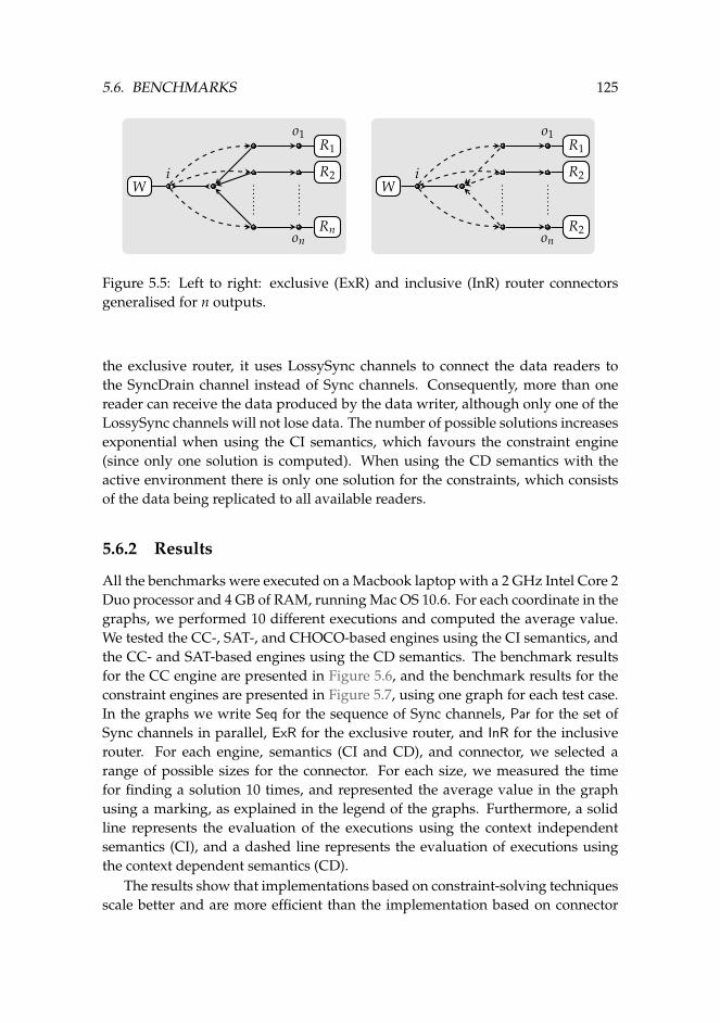
5.6. BENCHMARKS 125
i
o1
on
W
R1
R2
Rn
i
o1
on
W
R1
R2
R2
Figure 5.5: Left to right: exclusive (ExR) and inclusive (InR) router connectorsgeneralised for n outputs.
the exclusive router, it uses LossySync channels to connect the data readers tothe SyncDrain channel instead of Sync channels. Consequently, more than onereader can receive the data produced by the data writer, although only one of theLossySync channels will not lose data. The number of possible solutions increasesexponential when using the CI semantics, which favours the constraint engine(since only one solution is computed). When using the CD semantics with theactive environment there is only one solution for the constraints, which consistsof the data being replicated to all available readers.
5.6.2 Results
All the benchmarks were executed on a Macbook laptop with a 2 GHz Intel Core 2Duo processor and 4 GB of RAM, running Mac OS 10.6. For each coordinate in thegraphs, we performed 10 different executions and computed the average value.We tested the CC-, SAT-, and CHOCO-based engines using the CI semantics, andthe CC- and SAT-based engines using the CD semantics. The benchmark resultsfor the CC engine are presented in Figure 5.6, and the benchmark results for theconstraint engines are presented in Figure 5.7, using one graph for each test case.In the graphs we write Seq for the sequence of Sync channels, Par for the set ofSync channels in parallel, ExR for the exclusive router, and InR for the inclusiverouter. For each engine, semantics (CI and CD), and connector, we selected arange of possible sizes for the connector. For each size, we measured the timefor finding a solution 10 times, and represented the average value in the graphusing a marking, as explained in the legend of the graphs. Furthermore, a solidline represents the evaluation of the executions using the context independentsemantics (CI), and a dashed line represents the evaluation of executions usingthe context dependent semantics (CD).
The results show that implementations based on constraint-solving techniquesscale better and are more efficient than the implementation based on connector
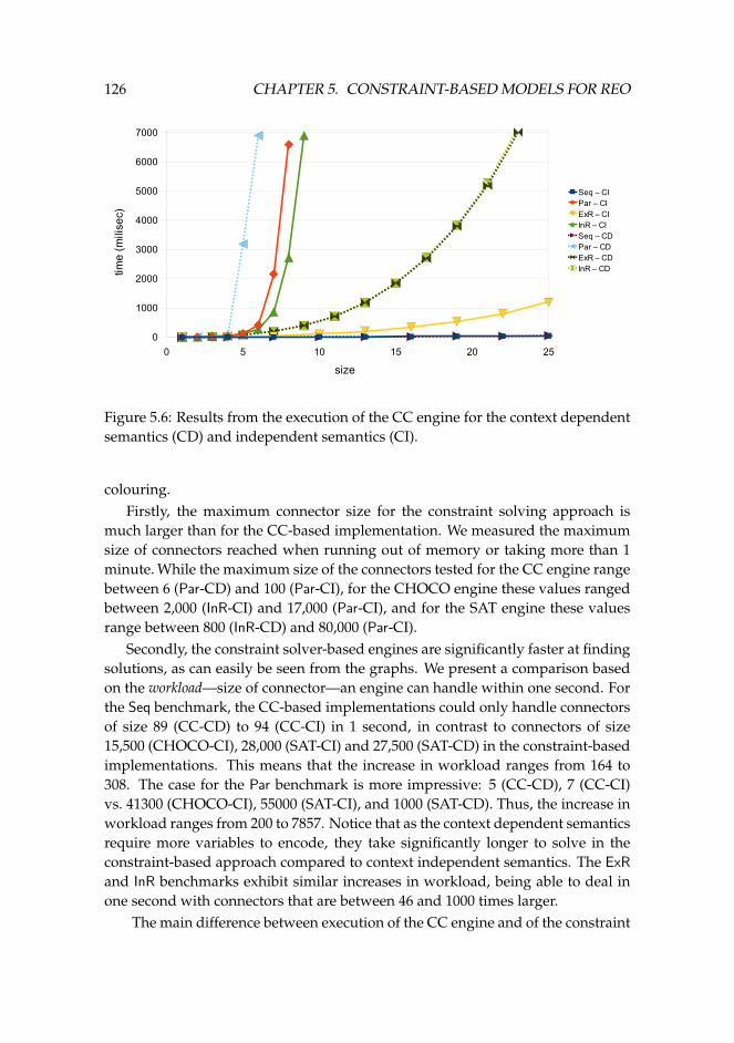
126 CHAPTER 5. CONSTRAINT-BASED MODELS FOR REO
0 5 10 15 20 250
1000
2000
3000
4000
5000
6000
7000
Seq – CIPar – CIExR – CIInR – CISeq – CDPar – CDExR – CDInR – CD
size
time
(mili
sec)
Figure 5.6: Results from the execution of the CC engine for the context dependentsemantics (CD) and independent semantics (CI).
colouring.Firstly, the maximum connector size for the constraint solving approach is
much larger than for the CC-based implementation. We measured the maximumsize of connectors reached when running out of memory or taking more than 1minute. While the maximum size of the connectors tested for the CC engine rangebetween 6 (Par-CD) and 100 (Par-CI), for the CHOCO engine these values rangedbetween 2,000 (InR-CI) and 17,000 (Par-CI), and for the SAT engine these valuesrange between 800 (InR-CD) and 80,000 (Par-CI).
Secondly, the constraint solver-based engines are significantly faster at findingsolutions, as can easily be seen from the graphs. We present a comparison basedon the workload—size of connector—an engine can handle within one second. Forthe Seq benchmark, the CC-based implementations could only handle connectorsof size 89 (CC-CD) to 94 (CC-CI) in 1 second, in contrast to connectors of size15,500 (CHOCO-CI), 28,000 (SAT-CI) and 27,500 (SAT-CD) in the constraint-basedimplementations. This means that the increase in workload ranges from 164 to308. The case for the Par benchmark is more impressive: 5 (CC-CD), 7 (CC-CI)vs. 41300 (CHOCO-CI), 55000 (SAT-CI), and 1000 (SAT-CD). Thus, the increase inworkload ranges from 200 to 7857. Notice that as the context dependent semanticsrequire more variables to encode, they take significantly longer to solve in theconstraint-based approach compared to context independent semantics. The ExR
and InR benchmarks exhibit similar increases in workload, being able to deal inone second with connectors that are between 46 and 1000 times larger.
The main difference between execution of the CC engine and of the constraint
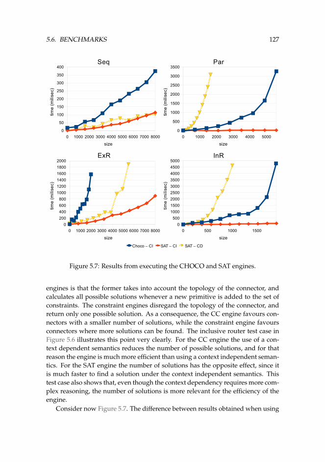
5.6. BENCHMARKS 127
Choco – CI SAT – CI SAT – CD
0 1000 2000 3000 4000 50000
500
1000
1500
2000
2500
3000
3500Par
size
time
(mili
sec)
0 1000 2000 3000 4000 5000 6000 7000 80000
50
100
150
200
250
300
350
400Seq
size
time
(mili
sec)
0 500 1000 15000
500100015002000250030003500400045005000
InR
size
time
(mili
sec)
0 1000 2000 3000 4000 5000 6000 7000 80000
200400600800
100012001400160018002000
ExR
size
time
(mili
sec)
Figure 5.7: Results from executing the CHOCO and SAT engines.
engines is that the former takes into account the topology of the connector, andcalculates all possible solutions whenever a new primitive is added to the set ofconstraints. The constraint engines disregard the topology of the connector, andreturn only one possible solution. As a consequence, the CC engine favours con-nectors with a smaller number of solutions, while the constraint engine favoursconnectors where more solutions can be found. The inclusive router test case inFigure 5.6 illustrates this point very clearly. For the CC engine the use of a con-text dependent semantics reduces the number of possible solutions, and for thatreason the engine is much more efficient than using a context independent seman-tics. For the SAT engine the number of solutions has the opposite effect, since itis much faster to find a solution under the context independent semantics. Thistest case also shows that, even though the context dependency requires more com-plex reasoning, the number of solutions is more relevant for the efficiency of theengine.
Consider now Figure 5.7. The difference between results obtained when using
128 CHAPTER 5. CONSTRAINT-BASED MODELS FOR REO
the CHOCO-based engine and the SAT-based engine are smaller in the connec-tor with a sequence of Sync channels. This is due to the way we avoid no-flowsolutions in both cases. By avoiding no-flow solutions, there is only one possiblesolution to the constraints consisting of data flowing from the writer to the reader.In the CHOCO engine we give precedence to the flow on the ports, so the engineonly has to verify that it is in fact a solution. The SAT engine starts by trying theno-flow assignment for each port, with the additional constraint that at least oneport has to have flow, which is not optimal for this scenario. And the context haslittle influence in this case because the variables that deal with the context are notrelevant (and thus unconstrained) when the synchronisation variables are set totrue.
When performing the benchmarking we also noticed that in certain cases thesolution is found unusually rapid. This happened quite frequently, for example,when executing the inclusive router using the context dependent semantics. Theexistence of these lucky runs reflects that the heuristics used by the constraintsolver are not as predictable as the compositional method used by the CC en-gine. The graphs do not exhibit this phenomenon because we only represent theaverage of the executions.
5.7 Guiding the constraint solver
Constraint satisfaction is performed by splitting the domain of a variable into twoor more parts and by propagating constraints [6]. It is well known that the per-formance of the solver depends on the order in which variables are resolved. Wechoose to exploit this ‘flexibility’ for a variety of goals, namely, fairness, priority,avoiding no-flow solutions, and efficiency. This section suggests how the con-straint solver can be guided with respect to these goals, but it is not yet supportedby tools.
The following criteria, often used in conjunction, can help to guide the con-straint solving process:
Variable ordering — Choose which variables to resolve first. For example, tryevaluating variables corresponding to ports with data, such as from exter-nal components or from a full FIFO1 buffer, or select variable correspondingto high priority choices. Variables can be ordered locally, within a primi-tive to achieve a local notion of priority, or across parts of the connector oreven globally across the entire connector to achieve a more global notion ofpriority by making the solver consider particular connectors before others.
Solution ordering — Choose the order in which that values are examined foreach variable. For example, try solving constraints with a synchronisationvariable set to > before trying with ⊥. Solution ordering can be applied
5.7. GUIDING THE CONSTRAINT SOLVER 129
to other data domains, though it is not immediately clear what the conse-quences of this would be.
We now describe how this can be used. In general, the ordering imposedon variables is partial, leaving room for the constraint solver to makes its ownchoices.
Fairness — To implement nondeterministic choice fairly, the constraint solverneeds to avoid resolving constraints in the same order each time it runs.Otherwise, it is possible that the same solution is always chosen. This canbe achieved by randomising the variable ordering each time the constraintsolver is invoked and/or changing the order in which the values of splitvariables are explored. In the presence of other constraints on the variable/-value ordering, randomisation can occur modulo the imposed ordering.
Priority — Priority can be achieved by appropriately ordering the variables and/-or the solutions to achieve the desired effect. The more global or comprehen-sive the ordering, that is, the more variables the ordering talks about, themore global the notion of priority. Purely local notions concerning as few asone variable are also sensible. For example, preferring flow over no-flow onthe output port of a LossySync achieves a local preference for dataflowingthrough the LossySync.
Avoiding no-flow solutions — To give priority of flow over no-flow, the solver isforced to try x = > before x = ⊥ when resolving synchronisation variablesx ∈ P. This needs to be done for all variables corresponding to sources ofdata.
Efficiency — In general, the most efficient way to solve constraints is by startingwith sources of data (such as inputs from components or full FIFO1 buffers),and moving in the direction of dataflow. Thus, the topology of the connectorcan also be used to help determine the variable ordering.
5.7.1. EXAMPLE. Consider again the Priority Merger channel from Table 5.3. Itperforms a merge of ports a and b into port c, giving priority to port a wheneverboth a and b are possible. The ordering constraints to achieve this consist of visit-ing variable a before visiting b, and then considering a = > before a = ⊥. ♦
The exact degree to which the underlying constraint solver can be manipu-lated depends upon the implementation of the constraint solver. For instance,CHOCO7 provides some control, such as setting the order of values for a set ofvariable, though not to the extent described here. In other settings, the client ofthe constraint solver may have little influence on its internal algorithms. We also
7CHOCO constraint programming system, available at http://choco.sourceforge.net/
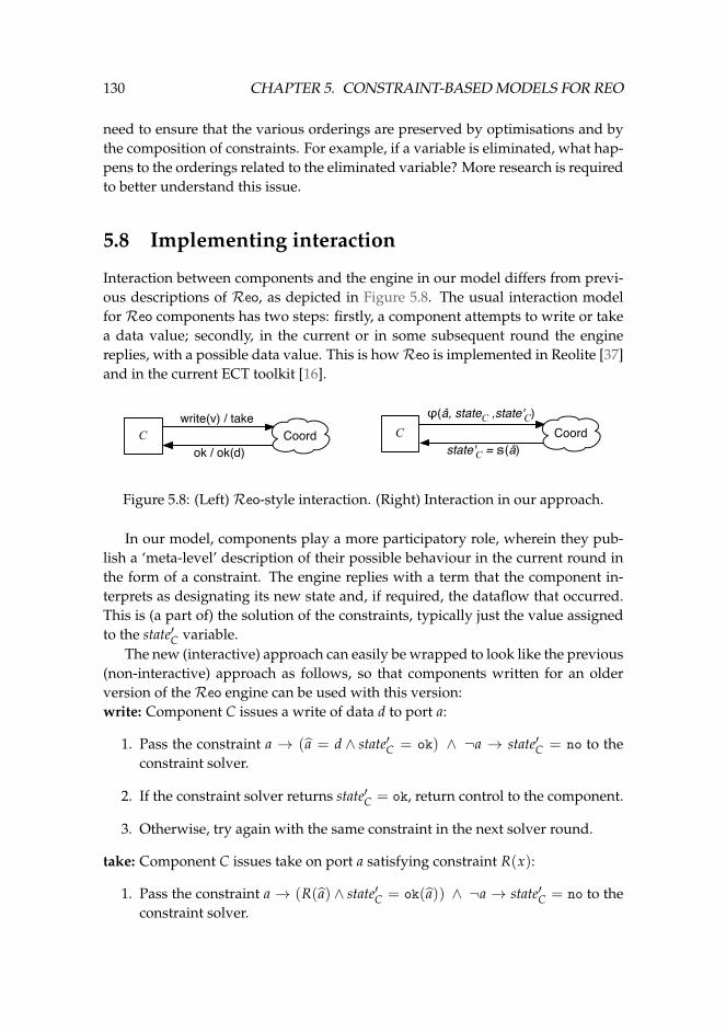
130 CHAPTER 5. CONSTRAINT-BASED MODELS FOR REO
need to ensure that the various orderings are preserved by optimisations and bythe composition of constraints. For example, if a variable is eliminated, what hap-pens to the orderings related to the eliminated variable? More research is requiredto better understand this issue.
5.8 Implementing interaction
Interaction between components and the engine in our model differs from previ-ous descriptions of Reo, as depicted in Figure 5.8. The usual interaction modelfor Reo components has two steps: firstly, a component attempts to write or takea data value; secondly, in the current or in some subsequent round the enginereplies, with a possible data value. This is howReo is implemented in Reolite [37]and in the current ECT toolkit [16].
C
ok / ok(d)
write(v) / take
Coord C
state'C = s(â)
!(â, stateC ,state'
C)
CoordC
ok / ok(d)
write(v) / take
Coord C
state'C = s(â)
!(â, stateC ,state'
C)
Coord
Figure 5.8: (Left)Reo-style interaction. (Right) Interaction in our approach.
In our model, components play a more participatory role, wherein they pub-lish a ‘meta-level’ description of their possible behaviour in the current round inthe form of a constraint. The engine replies with a term that the component in-terprets as designating its new state and, if required, the dataflow that occurred.This is (a part of) the solution of the constraints, typically just the value assignedto the state′C variable.
The new (interactive) approach can easily be wrapped to look like the previous(non-interactive) approach as follows, so that components written for an olderversion of theReo engine can be used with this version:write: Component C issues a write of data d to port a:
1. Pass the constraint a → (a = d ∧ state′C = ok) ∧ ¬a → state′C = no to theconstraint solver.
2. If the constraint solver returns state′C = ok, return control to the component.
3. Otherwise, try again with the same constraint in the next solver round.
take: Component C issues take on port a satisfying constraint R(x):
1. Pass the constraint a → (R(a) ∧ state′C = ok(a)) ∧ ¬a → state′C = no to theconstraint solver.
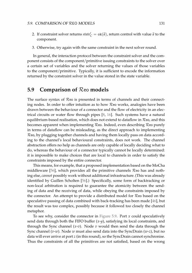
5.9. COMPARISON OFREO MODELS 131
2. If constraint solver returns state′C = ok(a), return control with value a to thecomponent.
3. Otherwise, try again with the same constraint in the next solver round.
In general, the interaction protocol between the constraint solver and the com-ponent consists of the component/primitive issuing constraints to the solver overa certain set of variables and the solver returning the values of those variablesto the component/primitive. Typically, it is sufficient to encode the informationreturned by the constraint solver in the value stored in the state variable.
5.9 Comparison ofReo models
The surface syntax of Reo is presented in terms of channels and their connect-ing nodes. In order to offer intuition as to how Reo works, analogies have beendrawn between the behaviour of a connector and the flow of electricity in an elec-trical circuits or water flow through pipes [8, 16]. Such systems have a naturalequilibrium-based realisation, which does not extend to dataflow inReo, and thisbecomes apparent when implementing Reo. Indeed, even describing Reo purelyin terms of dataflow can be misleading, as the direct approach to implementingReo, by plugging together channels and having them locally pass on data accord-ing to the channel’s local behavioural constraints, does not work. The channelabstraction offers no help as channels are only capable of locally deciding what todo, whereas the behaviour of a connector typically cannot be locally determined:it is impossible to make choices that are local to channels in order to satisfy theconstraints imposed by the entire connector.
This means, for example, that a proposed implementation based on the MoChamiddleware [56], which provides all the primitive channels Reo has and noth-ing else, cannot possibly work without additional infrastructure. (This was alreadyidentified by Guillen Scholten [56].) Specifically, some form of backtracking ornon-local arbitration is required to guarantee the atomicity between the send-ing of data and the receiving of data, while obeying the constraints imposed bythe connector. An attempt to provide a distributed model for Reo based on thespeculative passing of data combined with back-tracking has been made [46], butthe result was too complex, possibly because it followed too closely the channelmetaphor.
To see why, consider the connector in Figure 5.9. Port x could speculativelysend data through both the FIFO buffer (x-y), satisfying its local constraints, andthrough the Sync channel (x-v). Node v would then send the data through theSync channel (v-w). Node w must also send data into the SyncDrain (w-z), but nodata will ever arrive at port z (in this round), so the SyncDrain cannot synchronise.Thus the constraints of all the primitives are not satisfied, based on the wrong
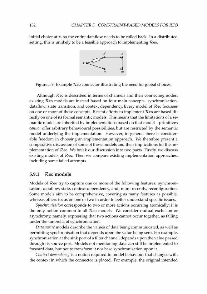
132 CHAPTER 5. CONSTRAINT-BASED MODELS FOR REO
initial choice at x, so the entire dataflow needs to be rolled back. In a distributedsetting, this is unlikely to be a feasible approach to implementingReo.
y
v
x
z
w
Figure 5.9: ExampleReo connector illustrating the need for global choices.
Although Reo is described in terms of channels and their connecting nodes,existing Reo models are instead based on four main concepts: synchronisation,dataflow, state transition, and context dependency. Every model of Reo focusseson one or more of these concepts. Recent efforts to implement Reo are based di-rectly on one of its formal semantic models. This means that the limitations of a se-mantic model are inherited by implementations based on that model—primitivescannot offer arbitrary behavioural possibilities, but are restricted by the semanticmodel underlying the implementation. However, in general there is consider-able freedom in choosing an implementation approach. We therefore present acomparative discussion of some of these models and their implications for the im-plementation of Reo. We break our discussion into two parts. Firstly, we discussexisting models of Reo. Then we compare existing implementation approaches,including some failed attempts.
5.9.1 Reo models
Models of Reo try to capture one or more of the following features: synchroni-sation, dataflow, state, context dependency, and, more recently, reconfiguration.Some models aim to be comprehensive, covering as many features as possible,whereas others focus on one or two in order to better understand specific issues.
Synchronisation corresponds to two or more actions occurring atomically; it isthe only notion common to all Reo models. We consider mutual exclusion orasynchrony, namely, expressing that two actions cannot occur together, as fallingunder the umbrella of synchronisation.
Data aware models describe the values of data being communicated, as well aspermitting synchronisation that depends upon the value being sent. For example,synchronisation at the sink port of a filter channel, depends upon the value passedthrough its source port. Models not mentioning data can still be implemented toforward data, but not to transform it nor base synchronisation upon it.
Context dependency is a notion required to model behaviour that changes withthe context in which the connector is placed. For example, the original intended
5.9. COMPARISON OFREO MODELS 133
behaviour of a LossySync channel is that it will lose data only if the primitive con-nected to its sink port does not accept the data [8]. Related to context dependencyare the notions of priority, which prefers one transition (in an automata model)over another whenever both are possible, and maximal flow, which prefers datato spread as far as possible into a connector (all other things being equal) [89].Different approaches have been explored, as it is unclear from the informal de-scriptions of Reo what exactly context dependency should mean, in particular,regarding its interaction with non-determinism.
Reconfiguration occurs when channels are unplugged from each other and re-plugged in a new configuration. This can be initiated from within a connectoror as an external action. We did not mention reconfiguration before, but recentwork proposes a number of approaches [35, 77, 71]. The contemporary Ph.D. the-sis of Krausse [76] focuses mainly in the reconfiguration of Reo connectors. Forthis discussion we restrict to the impact that facilitating reconfiguration has ondetermining the behaviour of a connector.
Abstract behaviour types The original semantics of Reo is defined in termsof abstract behaviour types [9], which are co-inductively defined relations overtimed data streams (a timed stream paired with a value stream). These models ac-count for synchronisation, dataflow, and, implicitly, state changes. They mentionneither context dependency nor reconfiguration.
This semantics provides little guidance for implementing Reo, so we do notconsider it further.
Automata-based models Various automata-based models for Reo exist. Weconsider the following four: constraint automata (CA) [22], intensional constraintautomata (ICA) [41], port automata (PA) [70], andReo automata (RA) [29]. Thesemodels provide the semantics of each Reo primitive and their composition, byrepresenting the synchronisation possible in a connector and possibly a descrip-tion of the dataflow in the transitions of the automata. In all of these models syn-chronisation is represented by a set of ports in each transition, and the dataflowby constraints.
CA is the only automata model ofReo that captures data, as the other modelsfocus on different issues. PA were devised to study decomposition of automata,and hence they capture only synchronisation and state. Neither CA nor PA havecontext dependency, so they can only express a variant of LossySync which makesa non-deterministic choice between passing the data onwards and losing it. Con-text dependency was later incorporated in an automata model, firstly in ICA, byreverse engineering ideas from connector colouring, and, subsequently and morecompactly, in RA.
Reconfiguration in the presence of an automaton-based model requires both
134 CHAPTER 5. CONSTRAINT-BASED MODELS FOR REO
maintaining a description of the connector and completely re-computing the un-derlying semantics of a connector whenever reconfiguration occurs [35].
Additional variants of constraint automata proposed as Reo models includenotions of time [13], resource bounds [81], quality-of-service guarantees [15], orprobability [21, 23, 88].
Connector colouring Connector colouring [37] is based on the simple idea thatports in a connector where data flow and where data does not flow can be col-oured with different colours (see §5.5). Each primitive has a set of colourings de-scribing its possible behaviours. The semantics of a connector is determined byplugging together the colourings of the primitives in such a way that the coloursmatch, meaning that dataflow either occurs or does not occur at the node. Con-nector colouring follows the shape of the connector, and computes all possiblebehaviours for the given step.
Two variants of connector colouring exist. The first, called 2-colouring (CC2),has one colour representing dataflow and one representing no dataflow. The sec-ond, called 3-colouring (CC3), splits the no dataflow colour into two to capturecontext, as described in §5.5. CC2 captures only synchronisation, whereas CC3captures both synchronisation and context dependency. Both connector colouringschemes abstract away from the data passed and state transition, but this infor-mation can be added in implementations, as long as the value of the data does notaffect synchronisation and it is not transformed.
As connector colouring is computed on-the-fly, reconfiguration has no impacton the computation of connector semantics, as the most recent version of the con-nector is used to compute the colouring table.
SOS Mousavi et al. present a structural operational semantics (SOS) formalisa-tion of Reo using Maude [89]. Two versions of the semantics were developed:the original formulation (SOS) and an extension with a notion of maximal flow tocapture a notion of context dependency (SOS+FLOW), which is not as flexible asthe corresponding notion enforced by 3-colouring. Khosravi et al. further explorethis idea using Alloy [67]. One advantage of the SOS approach is that it deals withcausality issues in connectors (which we deliberately ignore, as most other mod-els of Reo do). Clarke [34] explores causality in depth, presenting Reo semanticsin terms of the proof theory of intuitionistic linear logic and zero-safe Petri nets.These approaches do not consider reconfiguration.
An alternative operational semantics is based on the Tile Model [53, 14]. Tilescan be composed in three different ways to generate proof steps: horizontally, ver-tically, or in parallel. Horizontal composition represents synchronisation, and canbe performed only when the effect of one tile matches the trigger for another tile.Vertical composition represents changes of the system in time, requiring that the
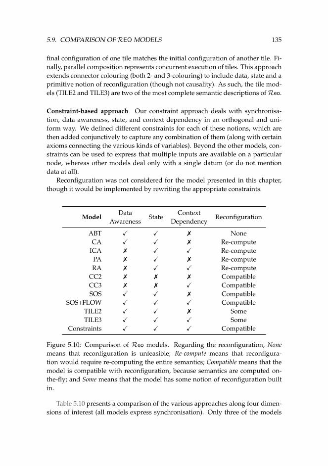
5.9. COMPARISON OFREO MODELS 135
final configuration of one tile matches the initial configuration of another tile. Fi-nally, parallel composition represents concurrent execution of tiles. This approachextends connector colouring (both 2- and 3-colouring) to include data, state and aprimitive notion of reconfiguration (though not causality). As such, the tile mod-els (TILE2 and TILE3) are two of the most complete semantic descriptions ofReo.
Constraint-based approach Our constraint approach deals with synchronisa-tion, data awareness, state, and context dependency in an orthogonal and uni-form way. We defined different constraints for each of these notions, which arethen added conjunctively to capture any combination of them (along with certainaxioms connecting the various kinds of variables). Beyond the other models, con-straints can be used to express that multiple inputs are available on a particularnode, whereas other models deal only with a single datum (or do not mentiondata at all).
Reconfiguration was not considered for the model presented in this chapter,though it would be implemented by rewriting the appropriate constraints.
ModelData
AwarenessState
ContextDependency
Reconfiguration
ABT X X 7 NoneCA X X 7 Re-compute
ICA 7 X X Re-computePA 7 X 7 Re-computeRA 7 X X Re-compute
CC2 7 7 7 CompatibleCC3 7 7 X CompatibleSOS X X 7 Compatible
SOS+FLOW X X X CompatibleTILE2 X X 7 SomeTILE3 X X X Some
Constraints X X X Compatible
Figure 5.10: Comparison of Reo models. Regarding the reconfiguration, Nonemeans that reconfiguration is unfeasible; Re-compute means that reconfigura-tion would require re-computing the entire semantics; Compatible means that themodel is compatible with reconfiguration, because semantics are computed on-the-fly; and Some means that the model has some notion of reconfiguration builtin.
Table 5.10 presents a comparison of the various approaches along four dimen-sions of interest (all models express synchronisation). Only three of the models
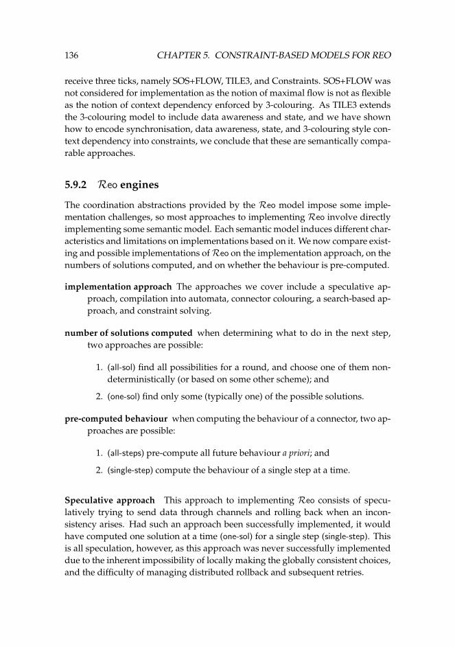
136 CHAPTER 5. CONSTRAINT-BASED MODELS FOR REO
receive three ticks, namely SOS+FLOW, TILE3, and Constraints. SOS+FLOW wasnot considered for implementation as the notion of maximal flow is not as flexibleas the notion of context dependency enforced by 3-colouring. As TILE3 extendsthe 3-colouring model to include data awareness and state, and we have shownhow to encode synchronisation, data awareness, state, and 3-colouring style con-text dependency into constraints, we conclude that these are semantically compa-rable approaches.
5.9.2 Reo engines
The coordination abstractions provided by the Reo model impose some imple-mentation challenges, so most approaches to implementing Reo involve directlyimplementing some semantic model. Each semantic model induces different char-acteristics and limitations on implementations based on it. We now compare exist-ing and possible implementations ofReo on the implementation approach, on thenumbers of solutions computed, and on whether the behaviour is pre-computed.
implementation approach The approaches we cover include a speculative ap-proach, compilation into automata, connector colouring, a search-based ap-proach, and constraint solving.
number of solutions computed when determining what to do in the next step,two approaches are possible:
1. (all-sol) find all possibilities for a round, and choose one of them non-deterministically (or based on some other scheme); and
2. (one-sol) find only some (typically one) of the possible solutions.
pre-computed behaviour when computing the behaviour of a connector, two ap-proaches are possible:
1. (all-steps) pre-compute all future behaviour a priori; and
2. (single-step) compute the behaviour of a single step at a time.
Speculative approach This approach to implementing Reo consists of specu-latively trying to send data through channels and rolling back when an incon-sistency arises. Had such an approach been successfully implemented, it wouldhave computed one solution at a time (one-sol) for a single step (single-step). Thisis all speculation, however, as this approach was never successfully implementeddue to the inherent impossibility of locally making the globally consistent choices,and the difficulty of managing distributed rollback and subsequent retries.
5.9. COMPARISON OFREO MODELS 137
Automata-based implementations This approach to implementing Reo com-piles the behaviour of a connector into an automaton [79], and thus pre-computesall future behaviour at compile-time (all-steps, all-sol). Implementations of all-stepssemantics do not scale, since finding all possible behaviour for all possible statesof a concurrent system is very expensive and space inefficient. For example, thenumber of states generally doubles for every FIFO1 buffer in a connector, assum-ing all states are reachable. Certainly, infinite state spaces are excluded. Further-more, implementations based on automata models are inherently centralised, andlose all potential parallelism, as a connector is implemented using a single au-tomaton. On the other hand, this means that they can be efficient at run-time,though they need to be re-computed when reconfiguration occurs. They trade offrun-time efficiency for flexibility.
Connector colouring-based implementations These implementations encodethe behaviour of the next step of a connector as a colouring table and compose thecolouring tables using a notion of matching, as described above in §5.5. Imple-mentations based on this approach compute all solutions (all-sol) for a single step(single-step). The disadvantage of computing all steps is the overhead of comput-ing choices that are not used.
Reolite [37] was the first prototype implementation based on connector colour-ing. A more recent and efficient engine is incorporated into the Reo toolset [16].The latter version was used as a comparison in our benchmarking. Connector col-ouring also forms the basis of our upcoming distributed implementation, whichwe discuss below in §5.9.3.
Search-based implementation These include implementations based on theSOS models and, hypothetically, on the Tile models. The Maude implementa-tion of SOS [89] could find a single solution (one-sol), whereas the implemen-tation of SOS+FLOW [89] computed all possibilities (all-sol), which were thenordered based on a maximal flow test. The result was extremely inefficient, al-though the encoding of SOS+FLOW in Alloy [67] potentially offers a better one-
sol-implementation technique using SAT solving. Unfortunately, no benchmarkswere presented in that paper, and as the implementation is very much a prototype,we have not included it here for comparison. We are not aware of an implemen-tation of TILE2 or TILE3 using Maude, as for SOS.
Constraint satisfaction The implementation approach described in this chapteris based on constraint satisfaction techniques to derive efficient executable imple-mentations of Reo. The constraints are solved per round (single-step) and use theheuristics of the constraint solver to stop the search for solutions once a singlesolution is found, avoiding exploring the full solution space (one-sol).
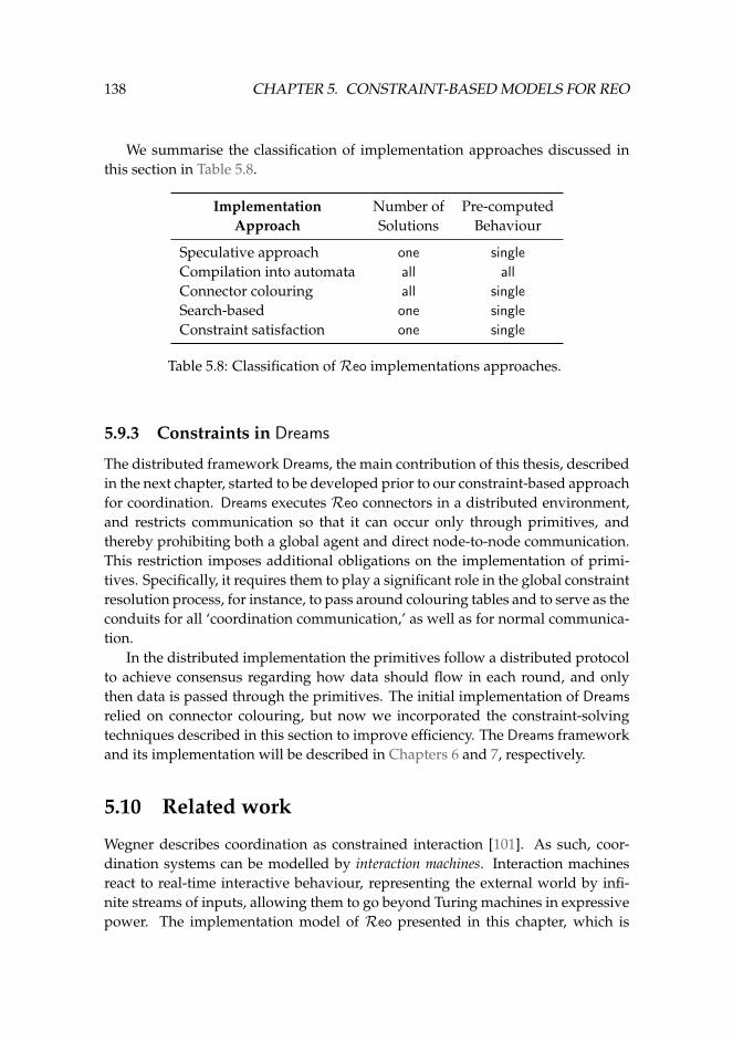
138 CHAPTER 5. CONSTRAINT-BASED MODELS FOR REO
We summarise the classification of implementation approaches discussed inthis section in Table 5.8.
ImplementationApproach
Number ofSolutions
Pre-computedBehaviour
Speculative approach one single
Compilation into automata all all
Connector colouring all single
Search-based one single
Constraint satisfaction one single
Table 5.8: Classification ofReo implementations approaches.
5.9.3 Constraints in Dreams
The distributed framework Dreams, the main contribution of this thesis, describedin the next chapter, started to be developed prior to our constraint-based approachfor coordination. Dreams executes Reo connectors in a distributed environment,and restricts communication so that it can occur only through primitives, andthereby prohibiting both a global agent and direct node-to-node communication.This restriction imposes additional obligations on the implementation of primi-tives. Specifically, it requires them to play a significant role in the global constraintresolution process, for instance, to pass around colouring tables and to serve as theconduits for all ‘coordination communication,’ as well as for normal communica-tion.
In the distributed implementation the primitives follow a distributed protocolto achieve consensus regarding how data should flow in each round, and onlythen data is passed through the primitives. The initial implementation of Dreams
relied on connector colouring, but now we incorporated the constraint-solvingtechniques described in this section to improve efficiency. The Dreams frameworkand its implementation will be described in Chapters 6 and 7, respectively.
5.10 Related work
Wegner describes coordination as constrained interaction [101]. As such, coor-dination systems can be modelled by interaction machines. Interaction machinesreact to real-time interactive behaviour, representing the external world by infi-nite streams of inputs, allowing them to go beyond Turing machines in expressivepower. The implementation model of Reo presented in this chapter, which is
5.10. RELATED WORK 139
extended with an interaction layer, can be regarded as a concrete realisation ofWegner’s interaction machine.
However, surprisingly little work takes Wegner’s view of coordination as con-strained interaction literally, representing coordination as constraints. Montanariand Rossi express coordination as a constraint satisfaction problem, in a similarbut more general way [87]. They describe how to solve synchronisation problemsusing constraint solving techniques. Networks are viewed as graphs, and the tilemodel is used to distinguish between synchronisation and sequential compositionof the coordination pieces. In our approach, we clarify one possible semantics ofthe coordination language Reo in these terms, giving a clear meaning for eachvariable, and describing the interaction with the external world within the solveand update stages. Lazovik et al. also utilise constraints to solve a coordinationproblem [78]. They provide a choreography framework for web services, wherechoreography is formalised as a constraint programming task, and where boththe Business Process and the requests are modelled as a set of constraints. This isan example of a concrete application of constraints to coordination, using a cen-tralised and non-compositional approach.
Taking a more practical approach, Minsky and Ungureanu introduce the Law-Governed Interaction (LGI) mechanism [86], implemented by the Moses toolkit.This mechanism targets distributed coordination of heterogenous agents using apolicy that enforces extensible laws. Laws are constraints specified in a Prolog-like language, enforced on regulated events of the agents, such as the sending orreceiving of messages. The authors give a special emphasis to the deploymentand execution of the mechanism, where a trusted server provides certified con-trollers which enforce the laws, instead of relying on a centralised coordinationmechanism. However, laws are local, in the sense that can only refer to the agentbeing regulated. This allows them to achieve good performance using LGI. In thepresence of true global constraints, as in Reo, LGI would require more complexalgorithms.
Frølund [52] presents synchronisers as a part of an actor coordination frame-work. He gives semantics for these constructs in terms of constraints, but does notuse constraint solving as an implementation technique. The constraints performthe matching of atomic sets of actions along with pattern matching of data, butthey do not deal with the communication of data, as our model does. Frølund’ssynchronisers cannot be plugged together like channels, but they can be com-posed by overlapping the domains of multiple synchronisers.
The analogy between Reo constraints and constraint solving problems has al-ready been drawn in general publications about Reo [10]. Since then more spe-cific approaches that utilise a constraint-based perspective over Reo have beenproposed. Examples of these approaches consider model checking and at theuse of mashups. Kluppelholz and Baier describe a symbolic model checking ap-
140 CHAPTER 5. CONSTRAINT-BASED MODELS FOR REO
proach for Reo [69]. Constraint automata are represented by binary decision di-agrams, encoded as propositional formulæ. Their encoding is similar to ours,though they use exclusively boolean variables, whilst we deal with a richer datadomain. Maraikar et al. [79] present a service composition platform based onReo,adopting a mashup’s data-centric approach. They combine several RSS feeds intoa user interface using a Reo connector, that is executed using the CHOCO con-straint solver (referred in §5.7 and §5.6). The work by Maraikar et al. can be seenas an example of an application of the basic ideas that we present in this chapter.
The timed concurrent constraint (tcc) programming framework [94] was in-troduced by Saraswat et al. to integrate the concurrent constraint (cc) program-ming paradigm [93] with synchronous languages. Time units are rounds, all theconstraints are updated in each round, as ours are, whereas inside each roundthe constraints are computed to quiescence. cc programs are compiled into anautomata model, where states are cc programs and transitions represent evolu-tion within a round while solving the constraints. In contrast, transitions in theconstraint automata model for Reo describe the evolution between rounds. Fur-thermore, the tcc approach avoids non-determinism as it targets synchronous lan-guages, whilstReo, as a coordination language, embraces non-determinism.
Andreoli et al. [5, 4] also use (linear) logic as the basis for coordination, com-bining it with the object-oriented paradigm. They utilise proof search to reasonabout coordination, as opposed to the use of constraint satisfaction techniques toderive efficient implementations. Clarke follows a similar approach and presentsa Reo semantics, also based on proof search, using an extension of linear logicwith temporal modalities in an intuitionistic setting [34].
A small overview of other coordination models and its relation with Reo,briefly discussed in §3.1, is now in order. The survey of Papadopoulos and Arbab[90] compares several coordination languages, classifying languages based ontuple spaces as data-driven models, as opposed to Reo’s channel-driven model.Manifold [28] is another example of a channel-driven model presented in the sur-vey, upon whichReo was built. Linda [54], one of the first coordination languages,provides a simple executable model consisting of a shared tuple space that com-ponents use to exchange values. Several other variations, such as Java’s popularimplementation JavaSpace of Jini [51], and the Klaim language [26], which consid-ers multiple distributed tuple spaces, followed the basic ideas behind Linda. Thefoundations of Klaim are presented as a process calculus, in particular as a variantof the π-calculus [85] with process distribution and mobility, where communica-tion occurs via shared located repositories instead of channel-based communica-tion primitives. Individual tuple operations in Linda-like languages are atomic,though they do not provide the global synchronisation imposed byReo.
Coordination languages such as SRML [48] and Orc [68] are oriented towardsthe coordination of web-services. SRML is a language developed in the context
5.11. CONCLUSION AND FUTURE WORK 141
of the SENSORIA project, where the interaction between two component servicescan be either synchronous or asynchronous, depending on whether an acknowl-edgement is required or not. Orc assumes a centralised coordinator that commu-nicate with the component services only via asynchronous messages, instead ofdescribing one to one communication. It also assumes that each service can replyat most once. Reo takes the same exogenous approach as Orc, moving the coor-dination logic from the components to the coordinator, and introduces new syn-chronisation capabilities, not captured by the Orc language. An exhaustive formalcomparison betweenReo and Orc was performed by Proenca and Clarke [92].
Coordination models have been applied to coordinate solvers of distributedconstraint satisfaction problems (DCSP) [18]. Our coordination model comes fullcircle and is based on (D)CSP.
5.11 Conclusion and future work
We presented a new semantics and executable model for the Reo coordinationmodel based on constraint satisfaction. This was motivated by one main concern.There is no efficient implementation technique for the existing models of Reo.The channel-view of aReo connector becomes a mere a metaphor. Instead, aReo
connector is seen as a set of constraints, based on the way the primitives are con-nected together, and their current state, governing the possible synchronisationand dataflow at the channel ends connected to external entities. The circuit repre-sentation of aReo connector then serves as a convenient graphical representationof how primitive constraints compose to yield the constrained interaction that itexpresses.
We contribute to the state-of-the-art ofReo in two ways:
• We identify the four main concepts that characterise the Reo coordination,synchrony, data-awareness, state, and context dependency, and describethese concepts using logical constraints. We show the correctness of our ap-proach with respect to the first three concepts using the constraint automatamodel as a reference, and we give full proof of correctness for the latter con-cept based on the connector colouring semantics.
• We reuse existing constraint satisfaction techniques to derive more efficientimplementations of Reo. Specifically, we developed two prototype imple-mentations, one which uses a SAT solver and another which uses a con-straint solver to search for possible solutions, and compared their perfor-mance with an existing Reo engine based on connector colouring. The re-sults strongly support the idea that constraint solving is a viable approachfor implementing coordination languages.
142 CHAPTER 5. CONSTRAINT-BASED MODELS FOR REO
In our first publication of this work [39], we explored the decomposition ofReo into constraints, extended the framework presented here to model interactionwith an unknown external world, beyond what is currently possible in existingimplementations ofReo. In that paper we assume that parts of the constraints arestill unknown in the beginning of the constraint solving phase. The correspond-ing constraints could be requested from external entities when required. Clarkeand Proenca introduced a local logic [38], wherein constraints from only part ofa connector need be consulted when searching for valid solutions. This meansthat partial solutions over only some of the variables are admitted, making thisapproach more scalable. Furthermore, partiality allows one to reason about ‘in-complete’ constraints, which can be extended during the constraint satisfactionprocess, enabling a new model of interaction with the external world.
Ongoing work on Reo tools and on the distributed engine of Reo in Dreams
seek to extend the support based on the model proposed here. In particular, thedistributed engine currently uses constraint solving techniques for synchronisa-tion and context variables only. This means that data constraints are not incorpo-rated, and the only interaction allowed is writing and reading on channel ends, asexplained in §5.8, which can be improved using the constraint-based model withdata proposed in this chapter. Constraints provide a uniform and flexible frame-work in which one may foresee in the future an assimilation of other constraintbased notions, such as service-level agreements. Future work will explore thesedirections, in particular the increased expressiveness offered by constraints andthe external interaction modes the model offers. In addition, we plan to exploitthe parallelism inherent in constraints.
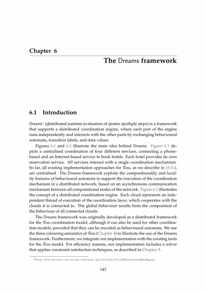
Chapter 6
The Dreams framework
6.1 Introduction
Dreams1 (distributed runtime evaluation of atomic multiple steps) is a frameworkthat supports a distributed coordination engine, where each part of the engineruns independently and interacts with the other parts by exchanging behaviouralautomata, transition labels, and data values.
Figures 6.1 and 6.2 illustrate the main idea behind Dreams. Figure 6.1 de-picts a centralised coordination of four different services, connecting a phone-based and an Internet-based service to book hotels. Each hotel provides its ownreservation service. All services interact with a single coordination mechanism.So far, all existing implementation approaches for Reo, as we describe in §6.5.4,are centralised. The Dreams framework exploits the compositionality and local-ity features of behavioural automata to support the execution of the coordinationmechanism in a distributed network, based on an asynchronous communicationmechanism between all computational nodes of the network. Figure 6.2 illustratesthe concept of a distributed coordination engine. Each cloud represents an inde-pendent thread of execution of the coordination layer, which cooperates with theclouds it is connected to. The global behaviour results from the composition ofthe behaviour of all connected clouds.
The Dreams framework was originally developed as a distributed frameworkfor the Reo coordination model, although it can also be used for other coordina-tion models, provided that they can be encoded as behavioural automata. We usethe three colouring semantics ofReo (Chapter 4) to illustrate the use of the Dreams
framework. Furthermore, we integrate our implementation with the existing toolsfor the Reo model. For efficiency reasons, our implementation includes a solverthat applies constraint satisfaction techniques, as described in Chapter 5.
1http://reo.project.cwi.nl/cgi-bin/trac.cgi/reo/wiki/Tools#DistributedReoEngine
143
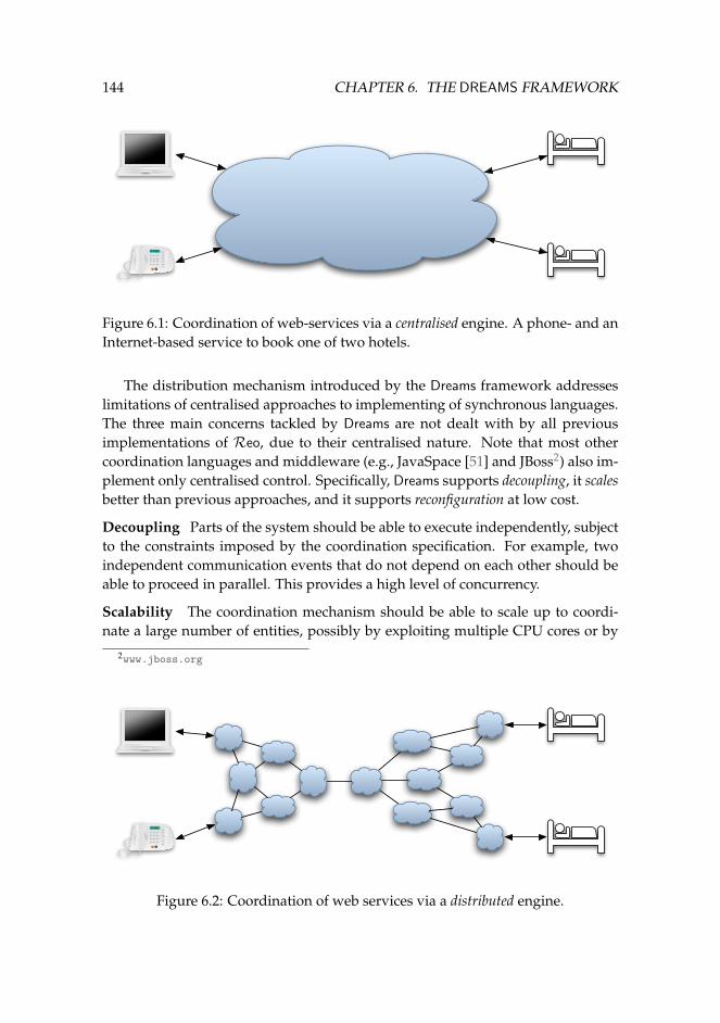
144 CHAPTER 6. THE DREAMS FRAMEWORK
Figure 6.1: Coordination of web-services via a centralised engine. A phone- and anInternet-based service to book one of two hotels.
The distribution mechanism introduced by the Dreams framework addresseslimitations of centralised approaches to implementing of synchronous languages.The three main concerns tackled by Dreams are not dealt with by all previousimplementations of Reo, due to their centralised nature. Note that most othercoordination languages and middleware (e.g., JavaSpace [51] and JBoss2) also im-plement only centralised control. Specifically, Dreams supports decoupling, it scalesbetter than previous approaches, and it supports reconfiguration at low cost.
Decoupling Parts of the system should be able to execute independently, subjectto the constraints imposed by the coordination specification. For example, twoindependent communication events that do not depend on each other should beable to proceed in parallel. This provides a high level of concurrency.
Scalability The coordination mechanism should be able to scale up to coordi-nate a large number of entities, possibly by exploiting multiple CPU cores or by
2www.jboss.org
Figure 6.2: Coordination of web services via a distributed engine.
6.1. INTRODUCTION 145
distributed execution.
Reconfigurability Reconfiguring an instance of a coordination pattern consistsof changing some of its parts. Systems that are expected to be reconfigured fre-quently should be able to do it in an incremental manner, without requiring thefull system to be changed. Furthermore, reconfigurations applied to a small partof the system should be independent of the execution or the behaviour of unre-lated parts of the same system.
Dreams achieves decoupled execution in two steps. The core idea behind de-coupled execution is the use of an underlying actor model [1, 2]. Primitive coor-dinators, which we simply call actors, exchange asynchronous messages amongstthemselves. In the Reo setting, an actor of Dreams manages one or more Reo
channels, Reo nodes, or connectors. The communication among actors followsthe graph structure of the corresponding Reo connector, which restricts the po-tential communication partners of each actor to its neighbours only. In the secondpart of this chapter we explore the locality aspect described in §3.4 and in §4.4.2.By identifying independent regions of the graph of actors, the Dreams frameworkrestricts the number of actors involved in each round of the coordination process,relaxing the restriction that all actors must be involved in every round. We donot address failure in the Dreams framework, and assume that the exchange ofmessages between actors always succeeds in finite time. However, we envisagefailure addressed orthogonally at a later stage, outside this thesis, as suggested byexisting techniques for distributed programming [55].
In this following we explain the Dreams framework in two steps. This chapterfocuses on how the actors should be connected to guarantee the desired global be-havioural automaton, based on the behavioural automata of the individual actors.In Chapter 7 we describe how actors can agree and execute their parts of a globalbehaviour, and present a distributed algorithm for the involved actors.
Organisation of the chapter In this chapter we present the Dreams framework,described as a system of actors each with two distinct kinds of behaviour. In§6.2 we introduce the notion of an actor, and make the distinction between reac-tive behaviour and coordination behaviour. In §6.3 we describe how actors are con-nected in the Dreams framework, present the basic assumptions regarding theirbehaviour, introduce the concept of synchronous regions, and present an overviewof the evolution of the system of actors in time. We explore aspects of locality andthe behaviour of actors to define the necessary conditions under which parts of asystem can evolve independently of the rest of the system in §6.4. These indepen-dent parts are the so-called synchronous regions. We present the ideas behind theDreams framework in §6.5 using the Reo coordination language to illustrate theapproach. We also compare Dreams with other existing ways to implement Reo,
146 CHAPTER 6. THE DREAMS FRAMEWORK
and explain how we improve on the state of the art. We finish with a descriptionof related work outside theReo world and draw conclusions in §6.6 and §6.7.
6.2 Actors – overview
The primitive entities in the Dreams framework are actors. An actor is an activeentity that runs concurrently with other actors and communicates with them us-ing a reliable, order-preserving asynchronous message passing mechanism. Wedescribe actors at two different levels of abstraction. At a lower level we use theactor model reference to describe how each actor communicates with others andhow the message passing mechanism works. We call this the reactive behaviour.The actor model is a well studied formal model of concurrent computation, intro-duced already in 1973 by Hewitt, Bishop and Steiger [63]. We refer the interestedreader to Agha’s work for an overview of the actor model [1, 2]. At a higher level,we incorporate a specific behavioural automaton into each actor that describes thecoordination protocol, and we call this the coordination behaviour.
Reactive behaviour The reactive behaviour describes how each actor reacts toincoming messages, following the actor model. In this model actors are primitiveentities that communicate via asynchronous messages. Actors receive messages,and react by making local decisions, by (1) creating more actors, (2) sending mes-sages, and (3) adapting to respond to future messages.
Coordination behaviour The Dreams framework provides the means to coordi-nate a set of components or services according to some behavioural automaton(BA), as we define in Chapter 3. We associate with each actor a behavioural au-tomaton, and the coordination behaviour of a system in the Dreams framework isdefined by the composition of the behavioural automata of all actors in the system.
In Dreams the execution of a behavioural automaton occurs in rounds, andin each round there is a consensus on which step should be executed next. Thereactive behaviour describes how to exchange behavioural automata restricted tothe current state, referred to as frontiers (at page 49), among a set of connectedactors, and also describes how to transfer data between components based on theresulting composition of the frontiers.
A system in the actor model is called a configuration, and consists of a collec-tion of concurrently executing actors together with a collection of messages thathave been sent but not yet received. Message sending is fair, i.e., the delivery ofmessages can be delayed only for an arbitrary finite but bounded amount of time.Every actor has a unique name and reacts to the messages it receives according toa specific behaviour. The behaviour of an actor is deterministic, and is defined interms of three basic operations:
1. create new actors;
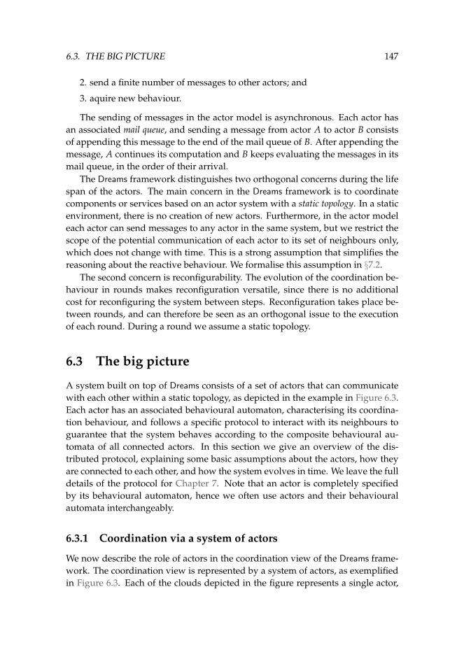
6.3. THE BIG PICTURE 147
2. send a finite number of messages to other actors; and
3. aquire new behaviour.
The sending of messages in the actor model is asynchronous. Each actor hasan associated mail queue, and sending a message from actor A to actor B consistsof appending this message to the end of the mail queue of B. After appending themessage, A continues its computation and B keeps evaluating the messages in itsmail queue, in the order of their arrival.
The Dreams framework distinguishes two orthogonal concerns during the lifespan of the actors. The main concern in the Dreams framework is to coordinatecomponents or services based on an actor system with a static topology. In a staticenvironment, there is no creation of new actors. Furthermore, in the actor modeleach actor can send messages to any actor in the same system, but we restrict thescope of the potential communication of each actor to its set of neighbours only,which does not change with time. This is a strong assumption that simplifies thereasoning about the reactive behaviour. We formalise this assumption in §7.2.
The second concern is reconfigurability. The evolution of the coordination be-haviour in rounds makes reconfiguration versatile, since there is no additionalcost for reconfiguring the system between steps. Reconfiguration takes place be-tween rounds, and can therefore be seen as an orthogonal issue to the executionof each round. During a round we assume a static topology.
6.3 The big picture
A system built on top of Dreams consists of a set of actors that can communicatewith each other within a static topology, as depicted in the example in Figure 6.3.Each actor has an associated behavioural automaton, characterising its coordina-tion behaviour, and follows a specific protocol to interact with its neighbours toguarantee that the system behaves according to the composite behavioural au-tomata of all connected actors. In this section we give an overview of the dis-tributed protocol, explaining some basic assumptions about the actors, how theyare connected to each other, and how the system evolves in time. We leave the fulldetails of the protocol for Chapter 7. Note that an actor is completely specifiedby its behavioural automaton, hence we often use actors and their behaviouralautomata interchangeably.
6.3.1 Coordination via a system of actors
We now describe the role of actors in the coordination view of the Dreams frame-work. The coordination view is represented by a system of actors, as exemplifiedin Figure 6.3. Each of the clouds depicted in the figure represents a single actor,
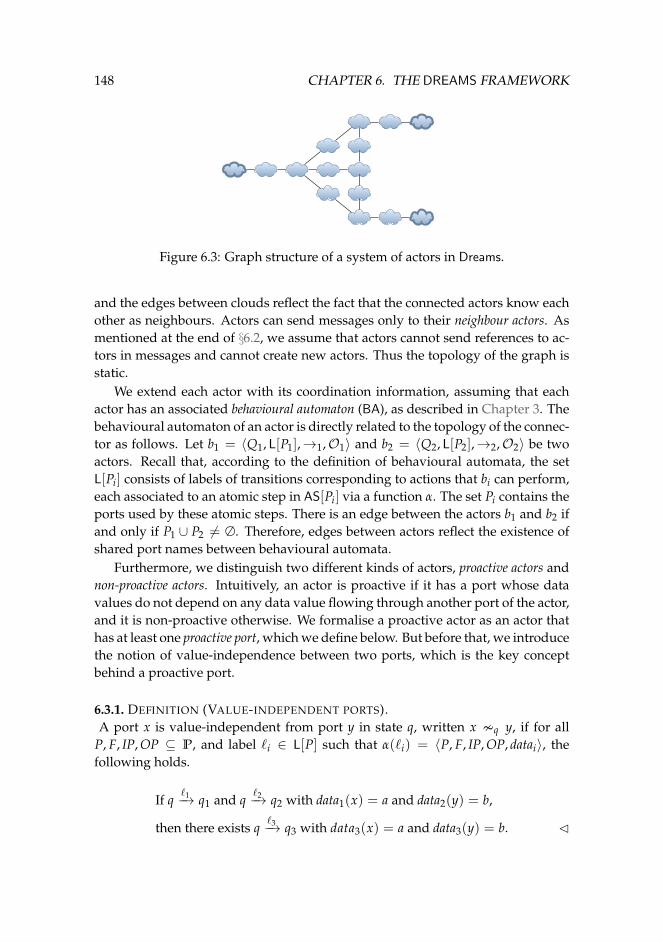
148 CHAPTER 6. THE DREAMS FRAMEWORK
Figure 6.3: Graph structure of a system of actors in Dreams.
and the edges between clouds reflect the fact that the connected actors know eachother as neighbours. Actors can send messages only to their neighbour actors. Asmentioned at the end of §6.2, we assume that actors cannot send references to ac-tors in messages and cannot create new actors. Thus the topology of the graph isstatic.
We extend each actor with its coordination information, assuming that eachactor has an associated behavioural automaton (BA), as described in Chapter 3. Thebehavioural automaton of an actor is directly related to the topology of the connec-tor as follows. Let b1 = 〈Q1, L[P1],→1,O1〉 and b2 = 〈Q2, L[P2],→2,O2〉 be twoactors. Recall that, according to the definition of behavioural automata, the setL[Pi] consists of labels of transitions corresponding to actions that bi can perform,each associated to an atomic step in AS[Pi] via a function α. The set Pi contains theports used by these atomic steps. There is an edge between the actors b1 and b2 ifand only if P1 ∪ P2 6= ∅. Therefore, edges between actors reflect the existence ofshared port names between behavioural automata.
Furthermore, we distinguish two different kinds of actors, proactive actors andnon-proactive actors. Intuitively, an actor is proactive if it has a port whose datavalues do not depend on any data value flowing through another port of the actor,and it is non-proactive otherwise. We formalise a proactive actor as an actor thathas at least one proactive port, which we define below. But before that, we introducethe notion of value-independence between two ports, which is the key conceptbehind a proactive port.
6.3.1. DEFINITION (VALUE-INDEPENDENT PORTS).A port x is value-independent from port y in state q, written x �q y, if for all
P, F, IP, OP ⊆ P, and label `i ∈ L[P] such that α(`i) = 〈P, F, IP, OP, datai〉, thefollowing holds.
If q`1−→ q1 and q
`2−→ q2 with data1(x) = a and data2(y) = b,
then there exists q`3−→ q3 with data3(x) = a and data3(y) = b. C
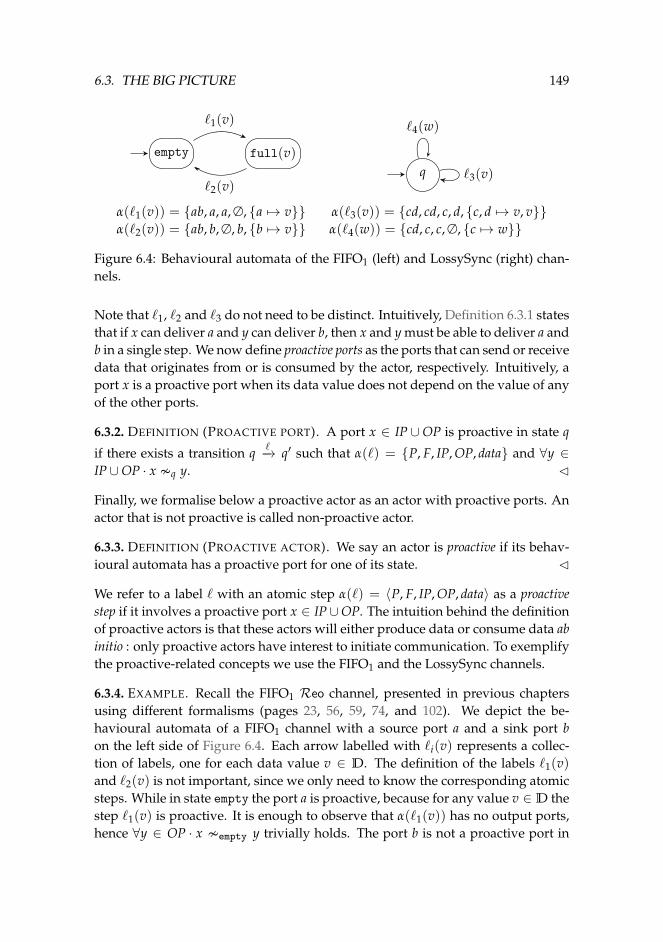
6.3. THE BIG PICTURE 149
empty full(v)
`1(v)
`2(v)q
`4(w)
`3(v)
α(`1(v)) = {ab, a, a, ∅, {a 7→ v}}α(`2(v)) = {ab, b, ∅, b, {b 7→ v}}
α(`3(v)) = {cd, cd, c, d, {c, d 7→ v, v}}α(`4(w)) = {cd, c, c, ∅, {c 7→ w}}
Figure 6.4: Behavioural automata of the FIFO1 (left) and LossySync (right) chan-nels.
Note that `1, `2 and `3 do not need to be distinct. Intuitively, Definition 6.3.1 statesthat if x can deliver a and y can deliver b, then x and y must be able to deliver a andb in a single step. We now define proactive ports as the ports that can send or receivedata that originates from or is consumed by the actor, respectively. Intuitively, aport x is a proactive port when its data value does not depend on the value of anyof the other ports.
6.3.2. DEFINITION (PROACTIVE PORT). A port x ∈ IP ∪OP is proactive in state q
if there exists a transition q `−→ q′ such that α(`) = {P, F, IP, OP, data} and ∀y ∈IP∪OP · x �q y. C
Finally, we formalise below a proactive actor as an actor with proactive ports. Anactor that is not proactive is called non-proactive actor.
6.3.3. DEFINITION (PROACTIVE ACTOR). We say an actor is proactive if its behav-ioural automata has a proactive port for one of its state. C
We refer to a label ` with an atomic step α(`) = 〈P, F, IP, OP, data〉 as a proactivestep if it involves a proactive port x ∈ IP∪OP. The intuition behind the definitionof proactive actors is that these actors will either produce data or consume data abinitio : only proactive actors have interest to initiate communication. To exemplifythe proactive-related concepts we use the FIFO1 and the LossySync channels.
6.3.4. EXAMPLE. Recall the FIFO1 Reo channel, presented in previous chaptersusing different formalisms (pages 23, 56, 59, 74, and 102). We depict the be-havioural automata of a FIFO1 channel with a source port a and a sink port bon the left side of Figure 6.4. Each arrow labelled with `i(v) represents a collec-tion of labels, one for each data value v ∈ D. The definition of the labels `1(v)and `2(v) is not important, since we only need to know the corresponding atomicsteps. While in state empty the port a is proactive, because for any value v ∈ D thestep `1(v) is proactive. It is enough to observe that α(`1(v)) has no output ports,hence ∀y ∈ OP · x �empty y trivially holds. The port b is not a proactive port in
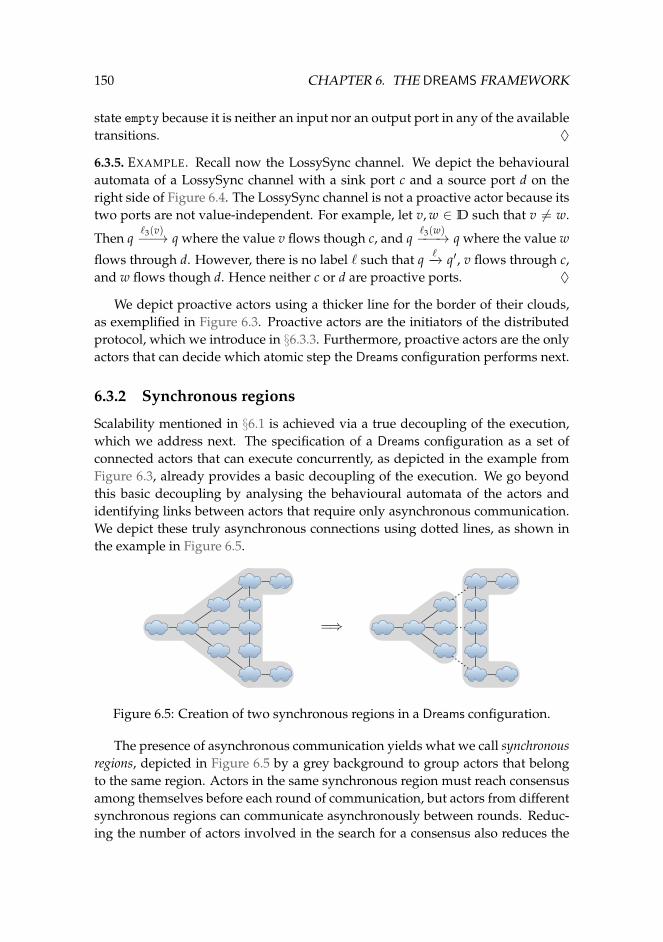
150 CHAPTER 6. THE DREAMS FRAMEWORK
state empty because it is neither an input nor an output port in any of the availabletransitions. ♦
6.3.5. EXAMPLE. Recall now the LossySync channel. We depict the behaviouralautomata of a LossySync channel with a sink port c and a source port d on theright side of Figure 6.4. The LossySync channel is not a proactive actor because itstwo ports are not value-independent. For example, let v, w ∈ D such that v 6= w.
Then q`3(v)−−→ q where the value v flows though c, and q
`3(w)−−−→ q where the value w
flows through d. However, there is no label ` such that q `−→ q′, v flows through c,and w flows though d. Hence neither c or d are proactive ports. ♦
We depict proactive actors using a thicker line for the border of their clouds,as exemplified in Figure 6.3. Proactive actors are the initiators of the distributedprotocol, which we introduce in §6.3.3. Furthermore, proactive actors are the onlyactors that can decide which atomic step the Dreams configuration performs next.
6.3.2 Synchronous regions
Scalability mentioned in §6.1 is achieved via a true decoupling of the execution,which we address next. The specification of a Dreams configuration as a set ofconnected actors that can execute concurrently, as depicted in the example fromFigure 6.3, already provides a basic decoupling of the execution. We go beyondthis basic decoupling by analysing the behavioural automata of the actors andidentifying links between actors that require only asynchronous communication.We depict these truly asynchronous connections using dotted lines, as shown inthe example in Figure 6.5.
=⇒
Figure 6.5: Creation of two synchronous regions in a Dreams configuration.
The presence of asynchronous communication yields what we call synchronousregions, depicted in Figure 6.5 by a grey background to group actors that belongto the same region. Actors in the same synchronous region must reach consensusamong themselves before each round of communication, but actors from differentsynchronous regions can communicate asynchronously between rounds. Reduc-ing the number of actors involved in the search for a consensus also reduces the
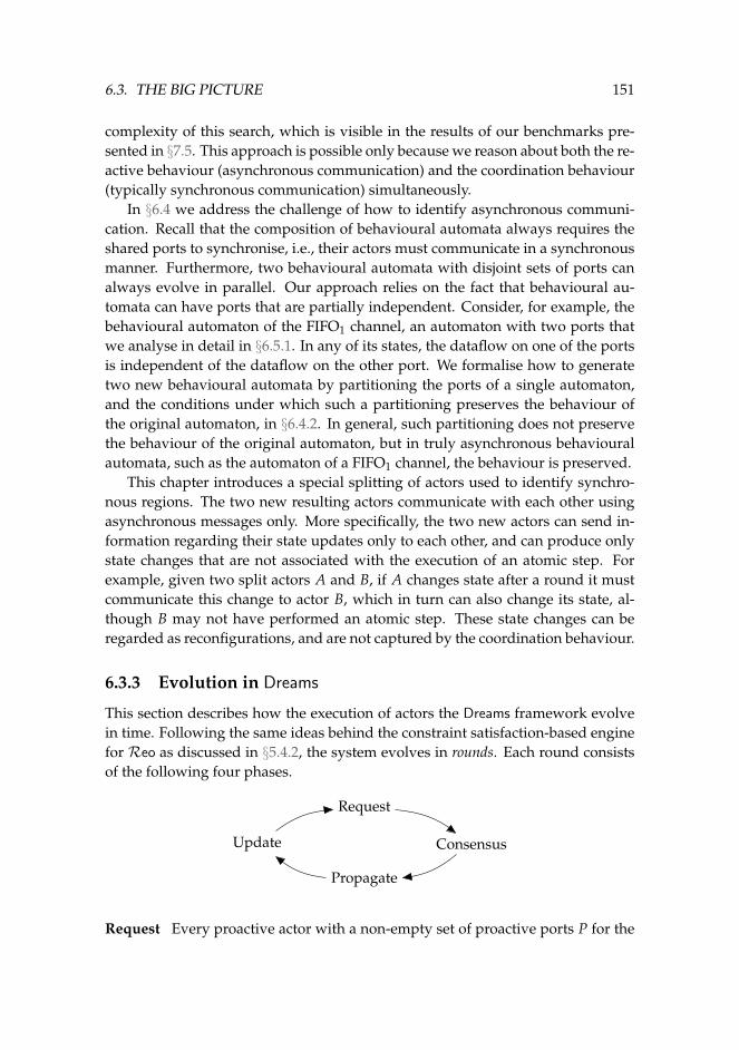
6.3. THE BIG PICTURE 151
complexity of this search, which is visible in the results of our benchmarks pre-sented in §7.5. This approach is possible only because we reason about both the re-active behaviour (asynchronous communication) and the coordination behaviour(typically synchronous communication) simultaneously.
In §6.4 we address the challenge of how to identify asynchronous communi-cation. Recall that the composition of behavioural automata always requires theshared ports to synchronise, i.e., their actors must communicate in a synchronousmanner. Furthermore, two behavioural automata with disjoint sets of ports canalways evolve in parallel. Our approach relies on the fact that behavioural au-tomata can have ports that are partially independent. Consider, for example, thebehavioural automaton of the FIFO1 channel, an automaton with two ports thatwe analyse in detail in §6.5.1. In any of its states, the dataflow on one of the portsis independent of the dataflow on the other port. We formalise how to generatetwo new behavioural automata by partitioning the ports of a single automaton,and the conditions under which such a partitioning preserves the behaviour ofthe original automaton, in §6.4.2. In general, such partitioning does not preservethe behaviour of the original automaton, but in truly asynchronous behaviouralautomata, such as the automaton of a FIFO1 channel, the behaviour is preserved.
This chapter introduces a special splitting of actors used to identify synchro-nous regions. The two new resulting actors communicate with each other usingasynchronous messages only. More specifically, the two new actors can send in-formation regarding their state updates only to each other, and can produce onlystate changes that are not associated with the execution of an atomic step. Forexample, given two split actors A and B, if A changes state after a round it mustcommunicate this change to actor B, which in turn can also change its state, al-though B may not have performed an atomic step. These state changes can beregarded as reconfigurations, and are not captured by the coordination behaviour.
6.3.3 Evolution in Dreams
This section describes how the execution of actors the Dreams framework evolvein time. Following the same ideas behind the constraint satisfaction-based enginefor Reo as discussed in §5.4.2, the system evolves in rounds. Each round consistsof the following four phases.
Request
Consensus
Propagate
Update
Request Every proactive actor with a non-empty set of proactive ports P for the
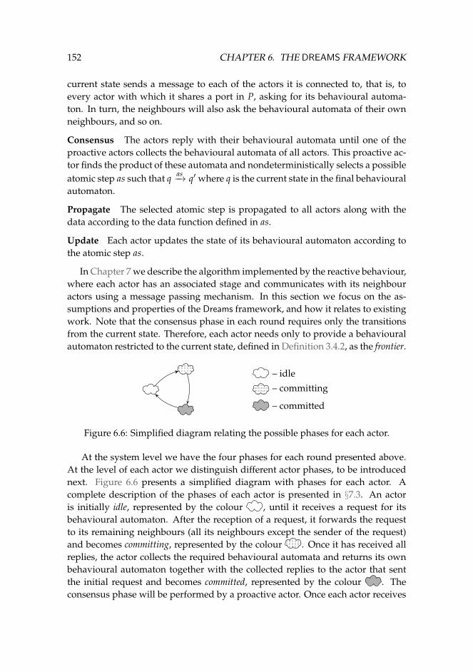
152 CHAPTER 6. THE DREAMS FRAMEWORK
current state sends a message to each of the actors it is connected to, that is, toevery actor with which it shares a port in P, asking for its behavioural automa-ton. In turn, the neighbours will also ask the behavioural automata of their ownneighbours, and so on.
Consensus The actors reply with their behavioural automata until one of theproactive actors collects the behavioural automata of all actors. This proactive ac-tor finds the product of these automata and nondeterministically selects a possibleatomic step as such that q as−→ q′ where q is the current state in the final behaviouralautomaton.
Propagate The selected atomic step is propagated to all actors along with thedata according to the data function defined in as.
Update Each actor updates the state of its behavioural automaton according tothe atomic step as.
In Chapter 7 we describe the algorithm implemented by the reactive behaviour,where each actor has an associated stage and communicates with its neighbouractors using a message passing mechanism. In this section we focus on the as-sumptions and properties of the Dreams framework, and how it relates to existingwork. Note that the consensus phase in each round requires only the transitionsfrom the current state. Therefore, each actor needs only to provide a behaviouralautomaton restricted to the current state, defined in Definition 3.4.2, as the frontier.
– idle
– committing
– committed
Figure 6.6: Simplified diagram relating the possible phases for each actor.
At the system level we have the four phases for each round presented above.At the level of each actor we distinguish different actor phases, to be introducednext. Figure 6.6 presents a simplified diagram with phases for each actor. Acomplete description of the phases of each actor is presented in §7.3. An actoris initially idle, represented by the colour , until it receives a request for itsbehavioural automaton. After the reception of a request, it forwards the requestto its remaining neighbours (all its neighbours except the sender of the request)and becomes committing, represented by the colour . Once it has received allreplies, the actor collects the required behavioural automata and returns its ownbehavioural automaton together with the collected replies to the actor that sentthe initial request and becomes committed, represented by the colour . Theconsensus phase will be performed by a proactive actor. Once each actor receives
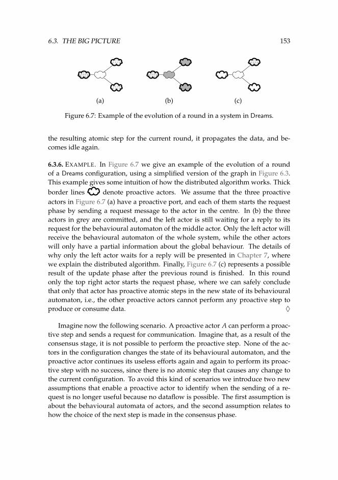
6.3. THE BIG PICTURE 153
(a) (b) (c)
Figure 6.7: Example of the evolution of a round in a system in Dreams.
the resulting atomic step for the current round, it propagates the data, and be-comes idle again.
6.3.6. EXAMPLE. In Figure 6.7 we give an example of the evolution of a roundof a Dreams configuration, using a simplified version of the graph in Figure 6.3.This example gives some intuition of how the distributed algorithm works. Thickborder lines denote proactive actors. We assume that the three proactiveactors in Figure 6.7 (a) have a proactive port, and each of them starts the requestphase by sending a request message to the actor in the centre. In (b) the threeactors in grey are committed, and the left actor is still waiting for a reply to itsrequest for the behavioural automaton of the middle actor. Only the left actor willreceive the behavioural automaton of the whole system, while the other actorswill only have a partial information about the global behaviour. The details ofwhy only the left actor waits for a reply will be presented in Chapter 7, wherewe explain the distributed algorithm. Finally, Figure 6.7 (c) represents a possibleresult of the update phase after the previous round is finished. In this roundonly the top right actor starts the request phase, where we can safely concludethat only that actor has proactive atomic steps in the new state of its behaviouralautomaton, i.e., the other proactive actors cannot perform any proactive step toproduce or consume data. ♦
Imagine now the following scenario. A proactive actor A can perform a proac-tive step and sends a request for communication. Imagine that, as a result of theconsensus stage, it is not possible to perform the proactive step. None of the ac-tors in the configuration changes the state of its behavioural automaton, and theproactive actor continues its useless efforts again and again to perform its proac-tive step with no success, since there is no atomic step that causes any change tothe current configuration. To avoid this kind of scenarios we introduce two newassumptions that enable a proactive actor to identify when the sending of a re-quest is no longer useful because no dataflow is possible. The first assumption isabout the behavioural automata of actors, and the second assumption relates tohow the choice of the next step is made in the consensus phase.
154 CHAPTER 6. THE DREAMS FRAMEWORK
6.3.7. ASSUMPTION (SILENT NO-FLOW). Let b be a behavioural automaton of an actor,
and q1`−→ q2 a transition where α(`) = 〈P, F, IP, OP, data〉. We assume that if F = ∅,
then q1 = q2, i.e., transitions that do not have dataflow in any of the ports do not changethe state of a behavioural automaton.
6.3.8. ASSUMPTION (AVOID NO-FLOW). When a proactive actor selects a label ` in theconsensus phase, where α(`) = 〈P, ∅, ∅, ∅, ∅〉, and performs the corresponding tran-sition, then there is no other label `′ starting from the current state such that α(`′) =⟨
P′, F′, IP′, OP′, data′⟩
and F′ 6= ∅, that is, transitions with dataflow have precedenceover transitions without dataflow.
Using these two assumptions we can guarantee that no dataflow can occur inthe current configuration after a step with no dataflow is taken. We make thisstatement precise in the following proposition.
6.3.9. PROPOSITION. When all actors comply with the Assumptions 6.3.7 and 6.3.8,whenever a no-flow atomic step is taken (with the empty flow set) all following atomicsteps will also be no-flow atomic steps.
Proof. Let q `−→ q′ be a transition performed by a behavioural automaton such thatα(`) = 〈P, F, IP, OP, data〉 and F = ∅. By Definition 3.3.1 of an atomic step, alsoIP = ∅, OP = ∅ and data = ∅. By Assumption 6.3.7 q = q′, that is, there is nostate change, and by Assumption 6.3.8 there is no transition with dataflow, whichcould trigger a state change. 2
This proposition justifies why a proactive actor does not need to send a requestwhile idle if the previous consensus phase selected a transition with an atomic step〈P, ∅, IP, OP, D〉.
We now argue why we consider these assumptions to be reasonable. The gen-eral idea is that only dataflow is observable of atomic steps. Since we expectto observe all state changes, transitions with no dataflow should not cause statechanges. Assumption 6.3.7 formalises the intuition that a behavioural automatoncan change only when there is dataflow. Alternatively, we could have extendedthe definition of an atomic step with a new boolean to represent whether a statechange occurs. We believe that the model is clear and more intuitive without los-ing expressiveness if we simply forbid state changes labelled with atomic stepswith no dataflow. Assumption 6.3.8 justifies the implementation choice of not toperform atomic steps with no dataflow.
Note that inReo, the context dependency described in Subsections §2.2.3, §4.3,and §5.5.2, conforms to and reinforces Assumption 6.3.8: when data is availablein a context, it must flow unless there is a reason for no flow. Furthermore, in ourconstraint-solving approach for Reo without context dependency, we impose anadditional constraint
∨P, which states that only solutions where one of the ports
has flow are relevant.
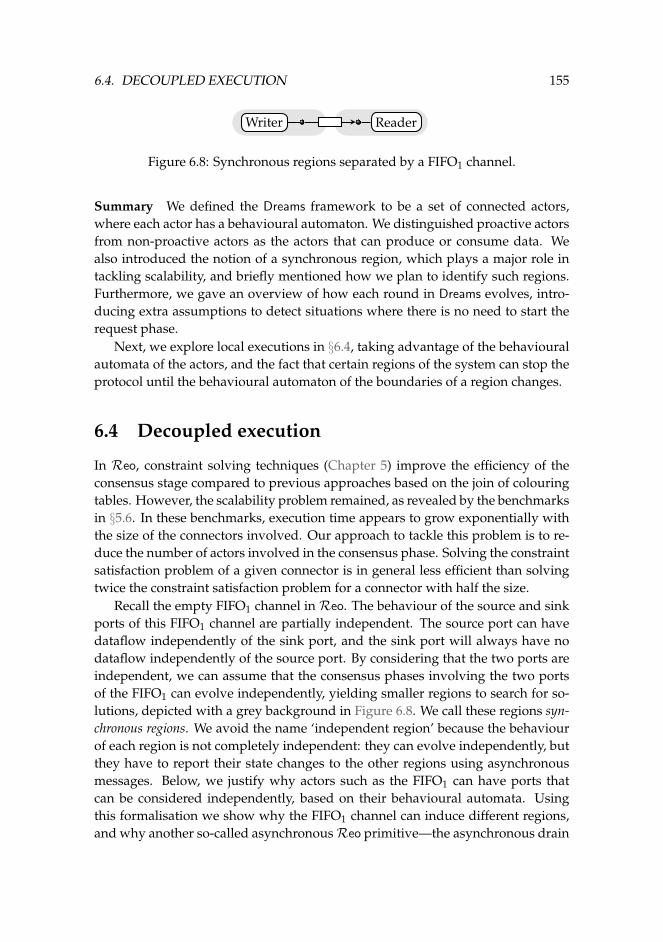
6.4. DECOUPLED EXECUTION 155
Writer Reader
Figure 6.8: Synchronous regions separated by a FIFO1 channel.
Summary We defined the Dreams framework to be a set of connected actors,where each actor has a behavioural automaton. We distinguished proactive actorsfrom non-proactive actors as the actors that can produce or consume data. Wealso introduced the notion of a synchronous region, which plays a major role intackling scalability, and briefly mentioned how we plan to identify such regions.Furthermore, we gave an overview of how each round in Dreams evolves, intro-ducing extra assumptions to detect situations where there is no need to start therequest phase.
Next, we explore local executions in §6.4, taking advantage of the behaviouralautomata of the actors, and the fact that certain regions of the system can stop theprotocol until the behavioural automaton of the boundaries of a region changes.
6.4 Decoupled execution
In Reo, constraint solving techniques (Chapter 5) improve the efficiency of theconsensus stage compared to previous approaches based on the join of colouringtables. However, the scalability problem remained, as revealed by the benchmarksin §5.6. In these benchmarks, execution time appears to grow exponentially withthe size of the connectors involved. Our approach to tackle this problem is to re-duce the number of actors involved in the consensus phase. Solving the constraintsatisfaction problem of a given connector is in general less efficient than solvingtwice the constraint satisfaction problem for a connector with half the size.
Recall the empty FIFO1 channel in Reo. The behaviour of the source and sinkports of this FIFO1 channel are partially independent. The source port can havedataflow independently of the sink port, and the sink port will always have nodataflow independently of the source port. By considering that the two ports areindependent, we can assume that the consensus phases involving the two portsof the FIFO1 can evolve independently, yielding smaller regions to search for so-lutions, depicted with a grey background in Figure 6.8. We call these regions syn-chronous regions. We avoid the name ‘independent region’ because the behaviourof each region is not completely independent: they can evolve independently, butthey have to report their state changes to the other regions using asynchronousmessages. Below, we justify why actors such as the FIFO1 can have ports thatcan be considered independently, based on their behavioural automata. Usingthis formalisation we show why the FIFO1 channel can induce different regions,and why another so-called asynchronousReo primitive—the asynchronous drain
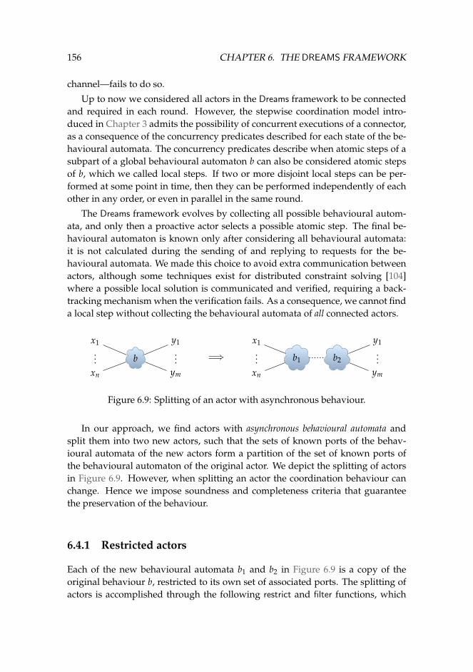
156 CHAPTER 6. THE DREAMS FRAMEWORK
channel—fails to do so.
Up to now we considered all actors in the Dreams framework to be connectedand required in each round. However, the stepwise coordination model intro-duced in Chapter 3 admits the possibility of concurrent executions of a connector,as a consequence of the concurrency predicates described for each state of the be-havioural automata. The concurrency predicates describe when atomic steps of asubpart of a global behavioural automaton b can also be considered atomic stepsof b, which we called local steps. If two or more disjoint local steps can be per-formed at some point in time, then they can be performed independently of eachother in any order, or even in parallel in the same round.
The Dreams framework evolves by collecting all possible behavioural autom-ata, and only then a proactive actor selects a possible atomic step. The final be-havioural automaton is known only after considering all behavioural automata:it is not calculated during the sending of and replying to requests for the be-havioural automata. We made this choice to avoid extra communication betweenactors, although some techniques exist for distributed constraint solving [104]where a possible local solution is communicated and verified, requiring a back-tracking mechanism when the verification fails. As a consequence, we cannot finda local step without collecting the behavioural automata of all connected actors.
b...
x1
xn
...
y1
ym
=⇒ b1...
x1
xn
b2...
y1
ym
Figure 6.9: Splitting of an actor with asynchronous behaviour.
In our approach, we find actors with asynchronous behavioural automata andsplit them into two new actors, such that the sets of known ports of the behav-ioural automata of the new actors form a partition of the set of known ports ofthe behavioural automaton of the original actor. We depict the splitting of actorsin Figure 6.9. However, when splitting an actor the coordination behaviour canchange. Hence we impose soundness and completeness criteria that guaranteethe preservation of the behaviour.
6.4.1 Restricted actors
Each of the new behavioural automata b1 and b2 in Figure 6.9 is a copy of theoriginal behaviour b, restricted to its own set of associated ports. The splitting ofactors is accomplished through the following restrict and filter functions, which
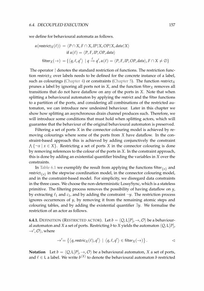
6.4. DECOUPLED EXECUTION 157
we define for behavioural automata as follows.
α(restrictX(`)) = 〈P ∩ X, F ∩ X, IP�X, OP�X, data�X〉if α(`) = 〈P, F, IP, OP, data〉
filterX(→) = {⟨q, `, q′
⟩| q `−→ q′, α(`) = 〈P, F, IP, OP, data〉, F ∩ X 6= ∅}
The operator � denotes the standard restriction of functions. The restriction func-tion restrictX over labels needs to be defined for the concrete instance of a label,such as colourings (Chapter 4) or constraints (Chapter 5). The function restrictXprunes a label by ignoring all ports not in X, and the function filterX removes alltransitions that do not have dataflow on any of the ports in X. Note that whensplitting a behavioural automaton by applying the restrict and the filter functionsto a partition of the ports, and considering all combinations of the restricted au-tomaton, we can introduce new undesired behaviour. Later in this chapter weshow how splitting an asynchronous drain channel produces such. Therefore, wewill introduce some conditions that must hold when splitting actors, which willguarantee that the behaviour of the original behavioural automaton is preserved.
Filtering a set of ports X in the connector colouring model is achieved by re-moving colourings where some of the ports from X have dataflow. In the con-straint-based approach this is achieved by adding conjunctively the constraint∧{¬x | x ∈ X}. Restricting a set of ports X in the connector colouring is done
by removing references to the colour of the ports in X. In the constraint approach,this is done by adding an existential quantifier binding the variables in X over theconstraints.
In Table 6.1 we exemplify the result from applying the functions filter{x} andrestrict{x} in the stepwise coordination model, in the connector colouring model,and in the constraint-based model. For simplicity, we disregard data constraintsin the three cases. We choose the non-deterministic LossySync, which is a statelessprimitive. The filtering process removes the possibility of having dataflow on y,by extracting `1 and c1, and by adding the constraint ¬y. The restriction processignores occurrences of y, by removing it from the remaining atomic steps andcolouring tables, and by adding the existential quantifier ∃y. We formalise therestriction of an actor as follows.
6.4.1. DEFINITION (RESTRICTED ACTOR). Let b = 〈Q, L[P],→,O〉 be a behaviour-al automaton and X a set of ports. Restricting b to X yields the automaton 〈Q, L[P],→′,O〉, where
→′={⟨
q, restricX(`), q′⟩|⟨q, `, q′
⟩∈ filterX(→)
}. C
Notation Let b = 〈Q, L[P],→,O〉 be a behavioural automaton, X a set of ports,and ` ∈ L a label. We write b(X) to denote the behavioural automaton b restricted
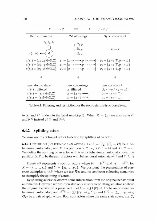
158 CHAPTER 6. THE DREAMS FRAMEWORK
x y =⇒ x y/ / / /
Beh. automaton 2-Colourings Sync. constraint
q¬ {x, y}
`1, `2, `3 qc1−→ q
qc2−→ q
qc3−→ q
y→ x
α(`1) = 〈xy,xy,∅,∅,∅〉α(`2) = 〈xy, y,∅,∅,∅〉α(`3) = 〈xy, ∅,∅,∅,∅〉
c1 = {x 7→ , y 7→ }c2 = {x 7→ , y 7→ }c3 = {x 7→ , y 7→ }
σ1 = {x 7→ >, y 7→ ⊥}σ2 = {x 7→ >, y 7→ ⊥}σ3 = {x 7→ ⊥, y 7→ ⊥}
⇓ ⇓ ⇓
new atomic steps:α(`1) : filteredα(`2) = 〈x, x,∅,∅,∅〉α(`3) = 〈x,∅,∅,∅,∅〉
new colourings:c1: filteredc2 = {x 7→ }c3 = {x 7→ }
new constraint:∃y · (¬y ∧ (y→ x))σ2 = {x 7→ >}σ3 = {x 7→ ⊥}
Table 6.1: Filtering and restriction for the non-deterministic LossySync.
to X, and `X to denote the label restrictX(`). When X = {x} we also write `x
and b(x) instead of `X and b(X).
6.4.2 Splitting actors
We now use restriction of actors to define the splitting of an actor.
6.4.2. DEFINITION (SPLITTING OF AN ACTOR). Let b = 〈Q, L[P],→,O〉 be a be-havioural automaton, and X, Y a partition of P, i.e., X ∩ Y = ∅ and X ∪ Y = P.We define the splitting of an actor with b as its behavioural automaton over thepartition X, Y to be the pair of actors with behavioural automata b(X) and b(Y). C
Figure 6.9 represents a split of actors where b1 = b(X) and b2 = b(Y), forX = {x1, . . . , xn} and Y = {y1, . . . , ym}. We postpone the presentation of con-crete examples to §6.5, where we use Reo and its connector colouring semanticsto exemplify the splitting of actors.
By splitting actors we discard some information from the original behaviouralautomaton. However, we are interested only in specific splitting situations, wherethe original behaviour is preserved. Let b = 〈Q, L[P],→,O〉 be an original be-havioural automaton, and b(X) = 〈Q, L[PX ],→X ,OX〉 and b(Y) = 〈Q, L[PY],→Y,OY〉 be a pair of split actors. Both split actors share the same state space, viz. Q,
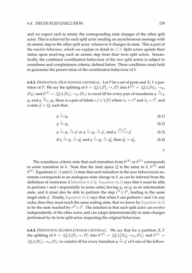
6.4. DECOUPLED EXECUTION 159
and we expect each to mimic the corresponding state changes of the other splitactor. This is achieved by each split actor sending an asynchronous message withits atomic step to the other split actor. whenever it changes its state. This is part ofthe reactive behaviour, which we explain in detail in §7.3. Split actors update theirstatus upon receiving such an atomic step from their twin split actors. Seman-tically, the combined coordination behaviour of the two split actors is subject tosoundness and completeness criteria, defined below. These conditions must holdto guarantee the preservation of the coordination behaviour of b.
6.4.3. DEFINITION (SOUNDNESS CRITERIA). Let P be a set of ports and X, Y a par-tition of P. We say the splitting of b = 〈Q, L[P],→, O〉 into b(X) = 〈Q, L[PX ],→X ,
OX〉 and b(Y) = 〈Q, L[PY],→Y,OY〉 is sound iff for every pair of transitions q`1−→X
q1 and q`2−→Y q2, there is a pair of labels r, t ∈ L[P] where `1 = rX and `2 = tY, and
a state q′ ∈ Q, such that:
q r−→ q1 (6.1)
q t−→ q2 (6.2)
q r−→ q1t−→ q′ or q t−→ q2
r−→ q′, and q rX⊗ tY−−−→ q′ (6.3)
if q r−→ q1t−→ q′1 and q t−→ q2
r−→ q′2, then q′1 = q′2. (6.4)
C
The soundness criteria state that each transition from b(X) or b(Y) correspondsto some transition in b. Note that the state space Q is the same in b, b(X) andb(Y). Equations (6.1) and (6.2) state that each transition in the new behavioural au-tomata corresponds to an analogous state change in b, as can be inferred from thedefinition of restriction (Definition 6.4.1). Equation (6.3) says that b must be ableto perform r and t sequentially in some order, having q1 or q2 as an intermediatestate, and it must also be able to perform the step rX⊗ tY, leading to the sametarget state q′. Finally, Equation (6.4) says that when b can perform r and t in anyorder, then they must reach the same ending state, that we know by Equation (6.3)to be the state reached by rX⊗ tY. The intuition is that each split actor can evolveindependently of the other actor, and can adapt deterministically to state changesperformed by its twin split actor, respecting the original behaviour.
6.4.4. DEFINITION (COMPLETENESS CRITERIA). We say that for a partition X, Ythe splitting of b = 〈Q, L[P],→, O〉 into b(X) = 〈Q, L[PX ],→X ,OX〉 and b(Y) =
〈Q, L[PY],→Y,OY〉 is complete iff for every transition q `−→ q′ of b one of the follow-
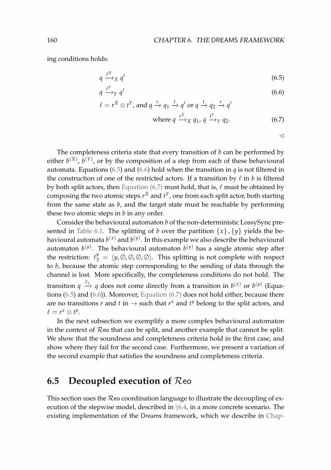
160 CHAPTER 6. THE DREAMS FRAMEWORK
ing conditions holds:
q `X−→X q′ (6.5)
q `Y−→Y q′ (6.6)
` = rX ⊗ tY, and q r−→ q1t−→ q′ or q t−→ q2
r−→ q′
where q rX−→X q1, q tY
−→Y q2. (6.7)
C
The completeness criteria state that every transition of b can be performed byeither b(X), b(Y), or by the composition of a step from each of these behaviouralautomata. Equations (6.5) and (6.6) hold when the transition in q is not filtered inthe construction of one of the restricted actors. If a transition by ` in b is filteredby both split actors, then Equation (6.7) must hold, that is, ` must be obtained bycomposing the two atomic steps rX and tY, one from each split actor, both startingfrom the same state as b, and the target state must be reachable by performingthese two atomic steps in b in any order.
Consider the behavioural automaton b of the non-deterministic LossySync pre-sented in Table 6.1. The splitting of b over the partition {x} , {y} yields the be-havioural automata b(x) and b(y). In this example we also describe the behaviouralautomaton b(y). The behavioural automaton b(y) has a single atomic step afterthe restriction: `
y3 = 〈y, ∅, ∅, ∅, ∅〉. This splitting is not complete with respect
to b, because the atomic step corresponding to the sending of data through thechannel is lost. More specifically, the completeness conditions do not hold. The
transition q`1−→ q does not come directly from a transition in b(x) or b(y) (Equa-
tions (6.5) and (6.6)). Moreover, Equation (6.7) does not hold either, because thereare no transitions r and t in→ such that rx and ty belong to the split actors, and` = rx ⊗ ty.
In the next subsection we exemplify a more complex behavioural automatonin the context of Reo that can be split, and another example that cannot be split.We show that the soundness and completeness criteria hold in the first case, andshow where they fail for the second case. Furthermore, we present a variation ofthe second example that satisfies the soundness and completeness criteria.
6.5 Decoupled execution ofReo
This section uses theReo coordination language to illustrate the decoupling of ex-ecution of the stepwise model, described in §6.4, in a more concrete scenario. Theexisting implementation of the Dreams framework, which we describe in Chap-
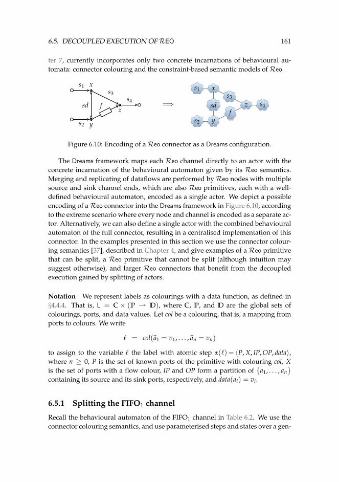
6.5. DECOUPLED EXECUTION OFREO 161
ter 7, currently incorporates only two concrete incarnations of behavioural au-tomata: connector colouring and the constraint-based semantic models ofReo.
x
y
sdz
s1
s2
s3
fs4
=⇒
s1
s2
x
y
sd zs3
fs4
Figure 6.10: Encoding of aReo connector as a Dreams configuration.
The Dreams framework maps each Reo channel directly to an actor with theconcrete incarnation of the behavioural automaton given by its Reo semantics.Merging and replicating of dataflows are performed by Reo nodes with multiplesource and sink channel ends, which are also Reo primitives, each with a well-defined behavioural automaton, encoded as a single actor. We depict a possibleencoding of aReo connector into the Dreams framework in Figure 6.10, accordingto the extreme scenario where every node and channel is encoded as a separate ac-tor. Alternatively, we can also define a single actor with the combined behaviouralautomaton of the full connector, resulting in a centralised implementation of thisconnector. In the examples presented in this section we use the connector colour-ing semantics [37], described in Chapter 4, and give examples of a Reo primitivethat can be split, a Reo primitive that cannot be split (although intuition maysuggest otherwise), and larger Reo connectors that benefit from the decoupledexecution gained by splitting of actors.
Notation We represent labels as colourings with a data function, as defined in§4.4.4. That is, L = C × (P ⇀ D), where C, P, and D are the global sets ofcolourings, ports, and data values. Let col be a colouring, that is, a mapping fromports to colours. We write
` = col(a1 = v1, . . . , an = vn)
to assign to the variable ` the label with atomic step α(`) = 〈P, X, IP, OP, data〉,where n ≥ 0, P is the set of known ports of the primitive with colouring col, Xis the set of ports with a flow colour, IP and OP form a partition of {a1, . . . , an}containing its source and its sink ports, respectively, and data(ai) = vi.
6.5.1 Splitting the FIFO1 channel
Recall the behavioural automaton of the FIFO1 channel in Table 6.2. We use theconnector colouring semantics, and use parameterised steps and states over a gen-
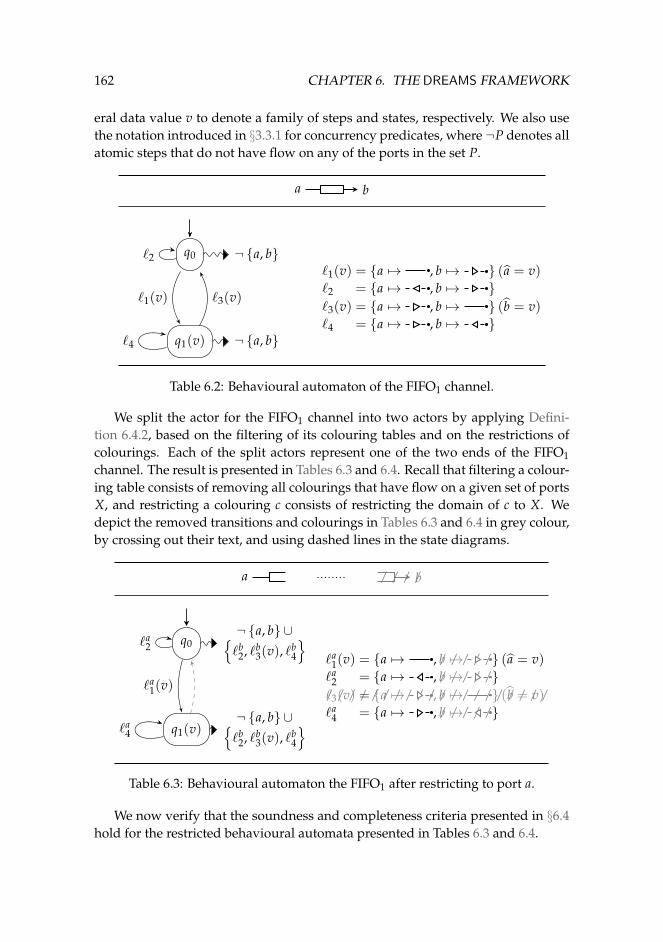
162 CHAPTER 6. THE DREAMS FRAMEWORK
eral data value v to denote a family of steps and states, respectively. We also usethe notation introduced in §3.3.1 for concurrency predicates, where ¬P denotes allatomic steps that do not have flow on any of the ports in the set P.
a b
q0
q1(v) ¬ {a, b}
¬ {a, b}
`1(v)
`2
`3(v)
`4
`1(v) = {a 7→ , b 7→ } (a = v)`2 = {a 7→ , b 7→ }`3(v) = {a 7→ , b 7→ } (b = v)`4 = {a 7→ , b 7→ }
Table 6.2: Behavioural automaton of the FIFO1 channel.
We split the actor for the FIFO1 channel into two actors by applying Defini-tion 6.4.2, based on the filtering of its colouring tables and on the restrictions ofcolourings. Each of the split actors represent one of the two ends of the FIFO1channel. The result is presented in Tables 6.3 and 6.4. Recall that filtering a colour-ing table consists of removing all colourings that have flow on a given set of portsX, and restricting a colouring c consists of restricting the domain of c to X. Wedepict the removed transitions and colourings in Tables 6.3 and 6.4 in grey colour,by crossing out their text, and using dashed lines in the state diagrams.
a b/ / / /
q0
q1(v)¬ {a, b} ∪{`b
2, `b3(v), `
b4
}
¬ {a, b} ∪{`b
2, `b3(v), `
b4
}`a
1(v)
`a2
`a4
`a1(v) = {a 7→ , / / / / /b 7→ } (a = v)`a
2 = {a 7→ , / / / / /b 7→ }/ / / / / / / / / / / / / / / / / / / /`3(v) = {a 7→ , b 7→ } (b = v)`a
4 = {a 7→ , / / / / /b 7→ }
Table 6.3: Behavioural automaton the FIFO1 after restricting to port a.
We now verify that the soundness and completeness criteria presented in §6.4hold for the restricted behavioural automata presented in Tables 6.3 and 6.4.
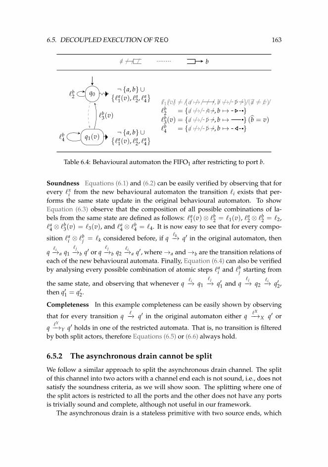
6.5. DECOUPLED EXECUTION OFREO 163
a/ / / / b
q0
q1(v)¬ {a, b} ∪{`a
1(v), `a2, `a
4}
¬ {a, b} ∪{`a
1(v), `a2, `a
4}`b
2
`b3(v)
`b4
/ / / / / / / / / / / / / / / / / / / /`1(v) = {a 7→ , b 7→ } (a = v)`b
2 = {/ / / / /a 7→ , b 7→ }`b
3(v) = {/ / / / /a 7→ , b 7→ } (b = v)`b
4 = {/ / / / /a 7→ , b 7→ }
Table 6.4: Behavioural automaton the FIFO1 after restricting to port b.
Soundness Equations (6.1) and (6.2) can be easily verified by observing that forevery `x
i from the new behavioural automaton the transition `i exists that per-forms the same state update in the original behavioural automaton. To showEquation (6.3) observe that the composition of all possible combinations of la-bels from the same state are defined as follows: `a
1(v)⊗ `b2 = `1(v), `a
2 ⊗ `b2 = `2,
`a4 ⊗ `b
3(v) = `3(v), and `a4 ⊗ `b
4 = `4. It is now easy to see that for every compo-
sition `ai ⊗ `b
j = `k considered before, if q`k−→ q′ in the original automaton, then
q`i−→a q1
`j−→b q′ or q`j−→b q2
`i−→a q′, where→a and→b are the transition relations ofeach of the new behavioural automata. Finally, Equation (6.4) can also be verifiedby analysing every possible combination of atomic steps `a
i and `bj starting from
the same state, and observing that whenever q`i−→ q1
`j−→ q′1 and q`j−→ q2
`i−→ q′2,then q′1 = q′2.
Completeness In this example completeness can be easily shown by observing
that for every transition q `−→ q′ in the original automaton either q `X−→X q′ or
q `Y−→Y q′ holds in one of the restricted automata. That is, no transition is filtered
by both split actors, therefore Equations (6.5) or (6.6) always hold.
6.5.2 The asynchronous drain cannot be split
We follow a similar approach to split the asynchronous drain channel. The splitof this channel into two actors with a channel end each is not sound, i.e., does notsatisfy the soundness criteria, as we will show soon. The splitting where one ofthe split actors is restricted to all the ports and the other does not have any portsis trivially sound and complete, although not useful in our framework.
The asynchronous drain is a stateless primitive with two source ends, which
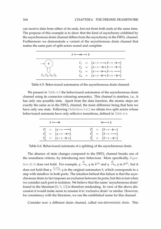
164 CHAPTER 6. THE DREAMS FRAMEWORK
can receive data from either of its ends, but not from both ends at the same time.The purpose of this example is to show that the kind of asynchrony exhibited bythe asynchronous drain channel differs from the asynchrony in the FIFO1 channel.Furthermore we demonstrate a variant of the asynchronous drain channel thatmakes the same pair of split actors sound and complete.
a b
q
`1, `2, `3, `4
`1 = {a 7→ , b 7→ }`2 = {a 7→ , b 7→ }`3 = {a 7→ , b 7→ }`4 = {a 7→ , b 7→ }
Table 6.5: Behavioural automaton of the asynchronous drain channel.
We present in Table 6.5 the behavioural automaton of the asynchronous drainchannel using its connector colouring semantics. This channel is stateless, i.e., ithas only one possible state. Apart from the data function, the atomic steps areexactly the same as in the FIFO1 channel, the main difference being that here wehave only one state. Following Definition 6.4.2 we obtain two split actors whosebehavioural automata have only reflexive transitions, defined in Table 6.6.
a b
`a1 = {a 7→ }`a
2 = {a 7→ }`a
4 = {a 7→ }
`b2 = {b 7→ }`b
3 = {b 7→ }`b
4 = {b 7→ }
Table 6.6: Behavioural automata of a splitting of the asynchronous drain.
The absence of state changes compared to the FIFO1 channel breaks one ofthe soundness criteria, by introducing new behaviour. More specifically, Equa-
tion (6.3) does not hold. For example, q`a
1−→a q in b(a) and q`b
3−→b q in b(b), but it
does not hold that q`1⊗`3−−−→ q in the original automaton b, which corresponds to a
step with dataflow in both ports. The intuition behind this failure is that the asyn-chronous drain in fact imposes an exclusion between its ports, but this is lost whenwe consider each port in isolation. We believe that the name ‘asynchronous drain’found in the literature [8, 9, 22] is therefore misleading. In view of the above dis-cussion it would make sense to rename it to ‘exclusive drain’ or similar. However,for consistency with the literature, we use the established name for this channel.
Consider now a different drain channel, called non-deterministic drain. This
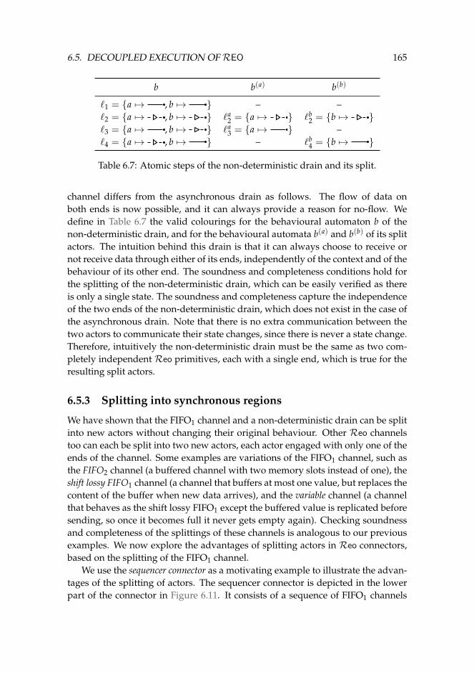
6.5. DECOUPLED EXECUTION OFREO 165
b b(a) b(b)
`1 = {a 7→ , b 7→ } – –`2 = {a 7→ , b 7→ } `a
2 = {a 7→ } `b2 = {b 7→ }
`3 = {a 7→ , b 7→ } `a3 = {a 7→ } –
`4 = {a 7→ , b 7→ } – `b4 = {b 7→ }
Table 6.7: Atomic steps of the non-deterministic drain and its split.
channel differs from the asynchronous drain as follows. The flow of data onboth ends is now possible, and it can always provide a reason for no-flow. Wedefine in Table 6.7 the valid colourings for the behavioural automaton b of thenon-deterministic drain, and for the behavioural automata b(a) and b(b) of its splitactors. The intuition behind this drain is that it can always choose to receive ornot receive data through either of its ends, independently of the context and of thebehaviour of its other end. The soundness and completeness conditions hold forthe splitting of the non-deterministic drain, which can be easily verified as thereis only a single state. The soundness and completeness capture the independenceof the two ends of the non-deterministic drain, which does not exist in the case ofthe asynchronous drain. Note that there is no extra communication between thetwo actors to communicate their state changes, since there is never a state change.Therefore, intuitively the non-deterministic drain must be the same as two com-pletely independent Reo primitives, each with a single end, which is true for theresulting split actors.
6.5.3 Splitting into synchronous regions
We have shown that the FIFO1 channel and a non-deterministic drain can be splitinto new actors without changing their original behaviour. Other Reo channelstoo can each be split into two new actors, each actor engaged with only one of theends of the channel. Some examples are variations of the FIFO1 channel, such asthe FIFO2 channel (a buffered channel with two memory slots instead of one), theshift lossy FIFO1 channel (a channel that buffers at most one value, but replaces thecontent of the buffer when new data arrives), and the variable channel (a channelthat behaves as the shift lossy FIFO1 except the buffered value is replicated beforesending, so once it becomes full it never gets empty again). Checking soundnessand completeness of the splittings of these channels is analogous to our previousexamples. We now explore the advantages of splitting actors in Reo connectors,based on the splitting of the FIFO1 channel.
We use the sequencer connector as a motivating example to illustrate the advan-tages of the splitting of actors. The sequencer connector is depicted in the lowerpart of the connector in Figure 6.11. It consists of a sequence of FIFO1 channels
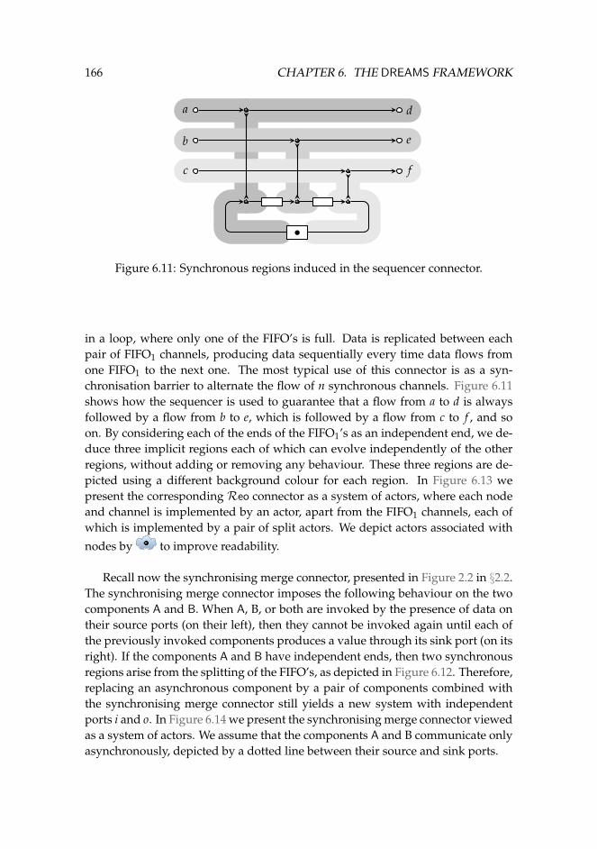
166 CHAPTER 6. THE DREAMS FRAMEWORK
a
b
c f
e
d
•
Figure 6.11: Synchronous regions induced in the sequencer connector.
in a loop, where only one of the FIFO’s is full. Data is replicated between eachpair of FIFO1 channels, producing data sequentially every time data flows fromone FIFO1 to the next one. The most typical use of this connector is as a syn-chronisation barrier to alternate the flow of n synchronous channels. Figure 6.11shows how the sequencer is used to guarantee that a flow from a to d is alwaysfollowed by a flow from b to e, which is followed by a flow from c to f , and soon. By considering each of the ends of the FIFO1’s as an independent end, we de-duce three implicit regions each of which can evolve independently of the otherregions, without adding or removing any behaviour. These three regions are de-picted using a different background colour for each region. In Figure 6.13 wepresent the corresponding Reo connector as a system of actors, where each nodeand channel is implemented by an actor, apart from the FIFO1 channels, each ofwhich is implemented by a pair of split actors. We depict actors associated with
nodes by to improve readability.
Recall now the synchronising merge connector, presented in Figure 2.2 in §2.2.The synchronising merge connector imposes the following behaviour on the twocomponents A and B. When A, B, or both are invoked by the presence of data ontheir source ports (on their left), then they cannot be invoked again until each ofthe previously invoked components produces a value through its sink port (on itsright). If the components A and B have independent ends, then two synchronousregions arise from the splitting of the FIFO’s, as depicted in Figure 6.12. Therefore,replacing an asynchronous component by a pair of components combined withthe synchronising merge connector still yields a new system with independentports i and o. In Figure 6.14 we present the synchronising merge connector viewedas a system of actors. We assume that the components A and B communicate onlyasynchronously, depicted by a dotted line between their source and sink ports.
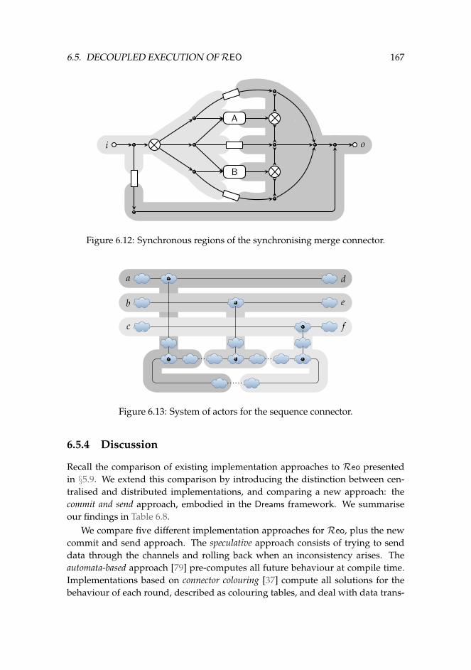
6.5. DECOUPLED EXECUTION OFREO 167
i o
A
B
Figure 6.12: Synchronous regions of the synchronising merge connector.
a
b
c f
e
d
Figure 6.13: System of actors for the sequence connector.
6.5.4 Discussion
Recall the comparison of existing implementation approaches to Reo presentedin §5.9. We extend this comparison by introducing the distinction between cen-tralised and distributed implementations, and comparing a new approach: thecommit and send approach, embodied in the Dreams framework. We summariseour findings in Table 6.8.
We compare five different implementation approaches for Reo, plus the newcommit and send approach. The speculative approach consists of trying to senddata through the channels and rolling back when an inconsistency arises. Theautomata-based approach [79] pre-computes all future behaviour at compile time.Implementations based on connector colouring [37] compute all solutions for thebehaviour of each round, described as colouring tables, and deal with data trans-
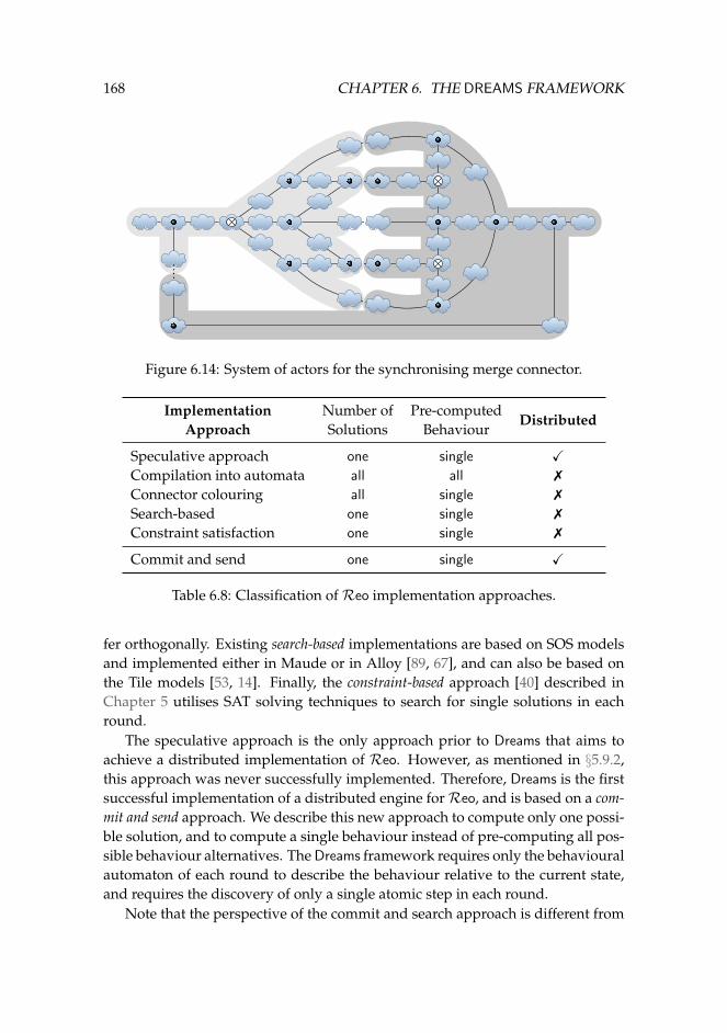
168 CHAPTER 6. THE DREAMS FRAMEWORK
Figure 6.14: System of actors for the synchronising merge connector.
ImplementationApproach
Number ofSolutions
Pre-computedBehaviour
Distributed
Speculative approach one single XCompilation into automata all all 7
Connector colouring all single 7
Search-based one single 7
Constraint satisfaction one single 7
Commit and send one single X
Table 6.8: Classification ofReo implementation approaches.
fer orthogonally. Existing search-based implementations are based on SOS modelsand implemented either in Maude or in Alloy [89, 67], and can also be based onthe Tile models [53, 14]. Finally, the constraint-based approach [40] described inChapter 5 utilises SAT solving techniques to search for single solutions in eachround.
The speculative approach is the only approach prior to Dreams that aims toachieve a distributed implementation of Reo. However, as mentioned in §5.9.2,this approach was never successfully implemented. Therefore, Dreams is the firstsuccessful implementation of a distributed engine forReo, and is based on a com-mit and send approach. We describe this new approach to compute only one possi-ble solution, and to compute a single behaviour instead of pre-computing all pos-sible behaviour alternatives. The Dreams framework requires only the behaviouralautomaton of each round to describe the behaviour relative to the current state,and requires the discovery of only a single atomic step in each round.
Note that the perspective of the commit and search approach is different from
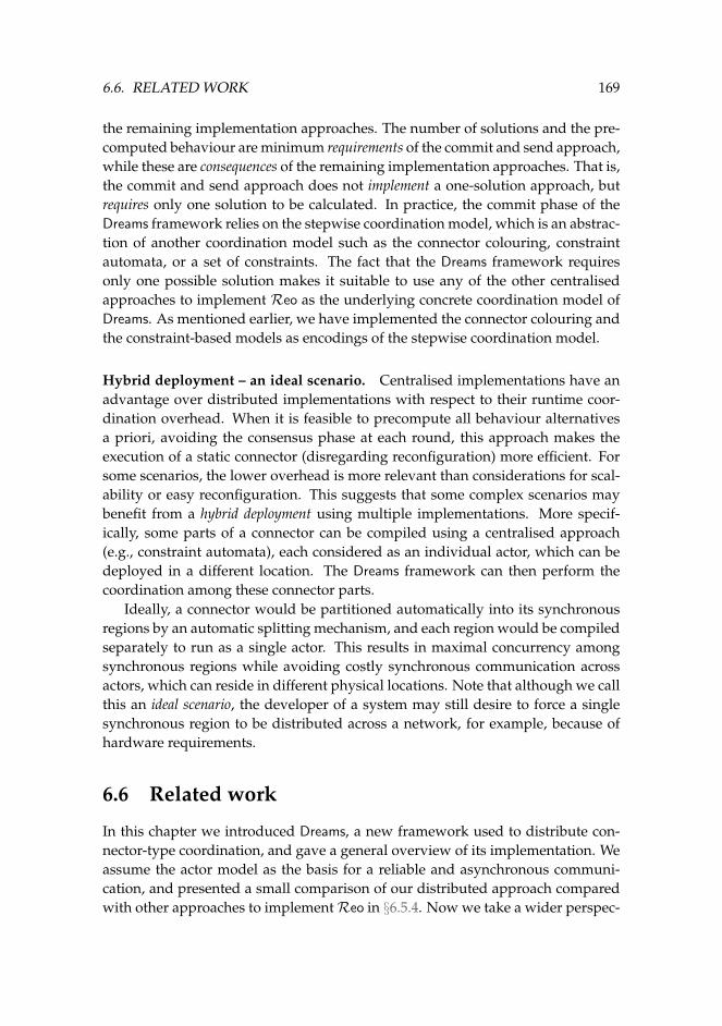
6.6. RELATED WORK 169
the remaining implementation approaches. The number of solutions and the pre-computed behaviour are minimum requirements of the commit and send approach,while these are consequences of the remaining implementation approaches. That is,the commit and send approach does not implement a one-solution approach, butrequires only one solution to be calculated. In practice, the commit phase of theDreams framework relies on the stepwise coordination model, which is an abstrac-tion of another coordination model such as the connector colouring, constraintautomata, or a set of constraints. The fact that the Dreams framework requiresonly one possible solution makes it suitable to use any of the other centralisedapproaches to implement Reo as the underlying concrete coordination model ofDreams. As mentioned earlier, we have implemented the connector colouring andthe constraint-based models as encodings of the stepwise coordination model.
Hybrid deployment – an ideal scenario. Centralised implementations have anadvantage over distributed implementations with respect to their runtime coor-dination overhead. When it is feasible to precompute all behaviour alternativesa priori, avoiding the consensus phase at each round, this approach makes theexecution of a static connector (disregarding reconfiguration) more efficient. Forsome scenarios, the lower overhead is more relevant than considerations for scal-ability or easy reconfiguration. This suggests that some complex scenarios maybenefit from a hybrid deployment using multiple implementations. More specif-ically, some parts of a connector can be compiled using a centralised approach(e.g., constraint automata), each considered as an individual actor, which can bedeployed in a different location. The Dreams framework can then perform thecoordination among these connector parts.
Ideally, a connector would be partitioned automatically into its synchronousregions by an automatic splitting mechanism, and each region would be compiledseparately to run as a single actor. This results in maximal concurrency amongsynchronous regions while avoiding costly synchronous communication acrossactors, which can reside in different physical locations. Note that although we callthis an ideal scenario, the developer of a system may still desire to force a singlesynchronous region to be distributed across a network, for example, because ofhardware requirements.
6.6 Related work
In this chapter we introduced Dreams, a new framework used to distribute con-nector-type coordination, and gave a general overview of its implementation. Weassume the actor model as the basis for a reliable and asynchronous communi-cation, and presented a small comparison of our distributed approach comparedwith other approaches to implementReo in §6.5.4. Now we take a wider perspec-
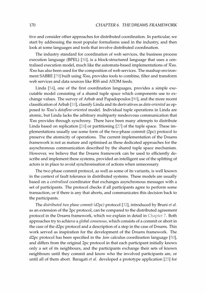
170 CHAPTER 6. THE DREAMS FRAMEWORK
tive and consider other approaches for distributed coordination. In particular, westart by addressing the most popular formalisms used in the industry, and thenlook at some languages and tools that involve distributed coordination.
The industry standard for coordination of web services, the business processexecution language (BPEL) [30], is a block-structured language that uses a cen-tralised execution model, much like the automata-based implementations ofReo.Reo has also been used for the composition of web services. The mashup environ-ment SABRE [79] built usingReo, provides tools to combine, filter and transformweb services and data sources like RSS and ATOM feeds.
Linda [54], one of the first coordination languages, provides a simple exe-cutable model consisting of a shared tuple space which components use to ex-change values. The survey of Arbab and Papadopoulos [90], and the more recentclassification of Arbab [10], classify Linda and its derivatives as data-oriented as op-posed to Reo’s dataflow-oriented model. Individual tuple operations in Linda areatomic, but Linda lacks the arbitrary multiparty rendezvous communication thatReo provides through synchrony. There have been many attempts to distributeLinda based on replication [24] or partitioning [27] of the tuple space. These im-plementations usually use some form of the two-phase commit (2pc) protocol topreserve the atomicity of operations. The current implementation of the Dreams
framework is not as mature and optimised as these dedicated approaches for theasynchronous communication described by the shared tuple space mechanism.However, we believe that the Dreams framework can be used to efficiently de-scribe and implement these systems, provided an intelligent use of the splitting ofactors is in place to avoid synchronisation of actions when unnecessary.
The two phase commit protocol, as well as some of its variants, is well knownin the context of fault tolerance in distributed systems. These models are usuallybased on a centralised coordinator that exchanges asynchronous messages with aset of participants. The protocol checks if all participants agree to perform sometransaction, or if there is any that aborts, and communicates this decision back tothe participants.
The distributed two phase commit (d2pc) protocol [32], introduced by Bruni et al.as an extension of the 2pc protocol, can be compared to the distributed agreementprotocol in the Dreams framework, which we explain in detail in Chapter 7. Bothapproaches try to achieve a global consensus, which consists of a commit or abort inthe case of the d2pc protocol and a description of a step in the case of Dreams. Thiswork served as inspiration for the development of the Dreams framework. Thed2pc protocol has been specified in the Join calculus coordination language [50],and differs from the original 2pc protocol in that each participant initially knowsonly a set of its neighbours, and the participants exchange their sets of knownneighbours until they commit and know who the involved participants are, oruntil all of them abort. Baragati et al. developed a prototype application [25] for
6.7. CONCLUSIONS 171
two different platforms based on the d2pc protocol, using as a case study a rescueunit composed of a central base and several teams. Experiments in the Dreams
framework involving real case studies have not been performed yet.We now describe a more practical approach, taken by Minsky and Ungure-
anu, who developed the Law-Governed Interaction (LGI) mechanism [86], imple-mented by the Moses toolkit. This mechanism coordinates distributed heteroge-neous agents, using a policy that enforces extensible laws. Agents execute eventsthat are regulated by some controllers that enforce the laws. Laws are specified ina Prolog-like language, but as opposed to Reo, they reflect local properties onlyand do not require non-local synchronisation. The authors emphasise the need toreplace a centralised controller imposing the laws of the full system by certifiedcontrollers, one for each connection. As with Linda and the 2pc protocol, this re-flects a need to decentralise coordination, which is the main concern of the Dreams
framework.The Dreams framework attempts to solve (coordination) constraints imposed
on concurrent actors, which makes it natural to consider existing techniques forconstraint solving in a distributed setting. The constraint-based approach hasbeen successfully applied in the domain ofReo, as described in Chapter 5. Yokooaddresses the distributed constraint satisfaction problem [104] typically by usingpartial solutions that are exchanged among different participants, and differenttypes of search algorithms such as backtracking and hill climbing. This suggeststhat the use of a constraint-based approach to implement Reo can open new pos-sibilities for optimising the distributed execution ofReo connectors.
6.7 Conclusions
In this chapter we introduced Dreams, a framework that provides a distributedimplementation based on the actor model for coordination models that can beencoded with behavioural automata, and how it is used in the context ofReo. Wesummarise below our analysis that shows how the Dreams framework achievesthe goals we set out in the introduction.
Decoupling The basic building blocks of the Dreams framework are actors, whichexecute concurrently. Dreams takes advantage of this concurrency by identifyingparts of the connector that can be executed independently. We call these partssynchronous regions. We propose a simple approach to exploit these synchronousregions, without computing them statically, yielding a true decoupling of execu-tion.
Scalability As a consequence of decoupling the execution of the instances ofstepwise models such as Reo connectors, no global consensus is required. Fur-thermore, the behaviour is computed only for each step, avoiding the state explo-
172 CHAPTER 6. THE DREAMS FRAMEWORK
sion resulting from computing all possible future behaviour. These two factorsform the basis for a scalable implementation. The implementation of Dreams alsoallows different parts of a connector to execute across physical machine bound-aries.
Reconfiguration The single-step semantics provides a very low deploymentoverhead, reducing the cost of reconfiguration. Furthermore, reconfiguring a con-nector affects only the synchronous regions that it modifies, while the rest of theconnector continues to execute.
Currently we have a functioning implementation of the Dreams framework.We describe the details of the implementation of Dreams in Chapter 7 – Imple-menting Dreams. The distributed implementation benefits from some of the im-plementation optimisations offered by centralised schemes, specifically the com-pilation of a connector into the automata of its synchronous regions.
Chapter 7
Implementing Dreams
7.1 Introduction
The Dreams framework coordinates a set of components or services using a collec-tion of independent executing entities which we call actors. Actors communicatewith each other using asynchronous message passing, and their behaviour is de-scribed from two different perspectives. The coordination behaviour is given by thestepwise coordination model, and describes how data should be propagated be-tween components in each round. The reactive behaviour describes how each actorsends and reacts to incoming messages.
In Chapter 6 we described the basic assumptions of the reactive behaviour, andwe explained in detail how the coordination behaviour is used. In this chapter wepresent a more detailed definition of the reactive behaviour:
• by introducing a syntax for specifying the reactive behaviour in a variationof SAL (Simple Actor Language);
• by specifying a fixed set of messages that actors can send; and
• by defining how each actor reacts to each message.
An actor is initially idle, and can evolve in two different ways. It can eitherparticipate in a round in the coordination process, or it can enter a suspensionphase where the actor can be reconfigured. Either way, it eventually returns tothe idle phase. We depict these two scenarios in the simplified diagram in Fig-ure 7.1. The messages exchanged between actors can represent requests for thebehavioural automaton for the current round, requests for data, replies with a be-havioural automaton or with data, steps for the current round with an optionaldata value, or suspension and reconfiguration messages.
Our implementation of Dreams is distributed in the sense that actors executeconcurrently, and messages are sent asynchronously. Furthermore, the splitting
173
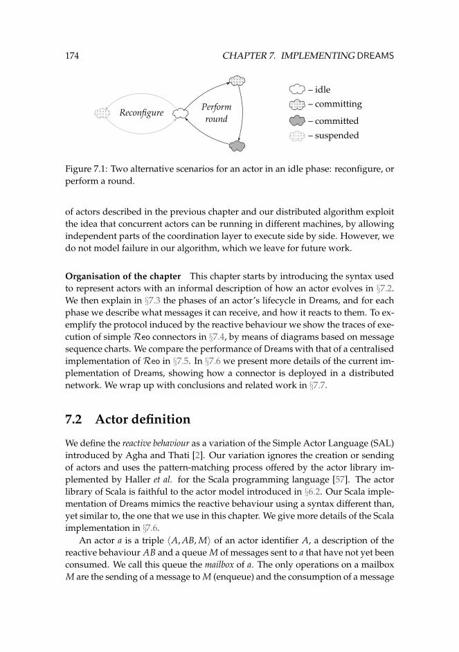
174 CHAPTER 7. IMPLEMENTING DREAMS
ReconfigurePerformround
– idle
– committing
– committed
– suspended
Figure 7.1: Two alternative scenarios for an actor in an idle phase: reconfigure, orperform a round.
of actors described in the previous chapter and our distributed algorithm exploitthe idea that concurrent actors can be running in different machines, by allowingindependent parts of the coordination layer to execute side by side. However, wedo not model failure in our algorithm, which we leave for future work.
Organisation of the chapter This chapter starts by introducing the syntax usedto represent actors with an informal description of how an actor evolves in §7.2.We then explain in §7.3 the phases of an actor’s lifecycle in Dreams, and for eachphase we describe what messages it can receive, and how it reacts to them. To ex-emplify the protocol induced by the reactive behaviour we show the traces of exe-cution of simple Reo connectors in §7.4, by means of diagrams based on messagesequence charts. We compare the performance of Dreams with that of a centralisedimplementation of Reo in §7.5. In §7.6 we present more details of the current im-plementation of Dreams, showing how a connector is deployed in a distributednetwork. We wrap up with conclusions and related work in §7.7.
7.2 Actor definition
We define the reactive behaviour as a variation of the Simple Actor Language (SAL)introduced by Agha and Thati [2]. Our variation ignores the creation or sendingof actors and uses the pattern-matching process offered by the actor library im-plemented by Haller et al. for the Scala programming language [57]. The actorlibrary of Scala is faithful to the actor model introduced in §6.2. Our Scala imple-mentation of Dreams mimics the reactive behaviour using a syntax different than,yet similar to, the one that we use in this chapter. We give more details of the Scalaimplementation in §7.6.
An actor a is a triple 〈A, AB, M〉 of an actor identifier A, a description of thereactive behaviour AB and a queue M of messages sent to a that have not yet beenconsumed. We call this queue the mailbox of a. The only operations on a mailboxM are the sending of a message to M (enqueue) and the consumption of a message
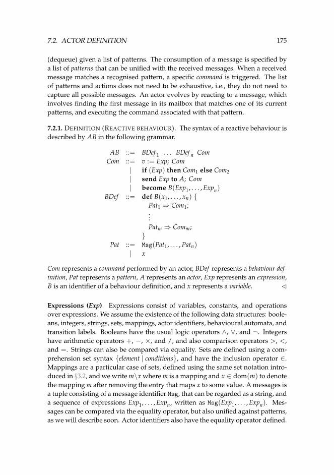
7.2. ACTOR DEFINITION 175
(dequeue) given a list of patterns. The consumption of a message is specified bya list of patterns that can be unified with the received messages. When a receivedmessage matches a recognised pattern, a specific command is triggered. The listof patterns and actions does not need to be exhaustive, i.e., they do not need tocapture all possible messages. An actor evolves by reacting to a message, whichinvolves finding the first message in its mailbox that matches one of its currentpatterns, and executing the command associated with that pattern.
7.2.1. DEFINITION (REACTIVE BEHAVIOUR). The syntax of a reactive behaviour isdescribed by AB in the following grammar.
AB ::= BDef 1 . . . BDef n ComCom ::= v := Exp; Com
| if (Exp) then Com1 else Com2| send Exp to A; Com| become B(Exp1, . . . , Expn)
BDef ::= def B(x1, . . . , xn) {Pat1 ⇒ Com1;...Patm ⇒ Comm;}
Pat ::= Msg(Pat1, . . . , Patn)
| x
Com represents a command performed by an actor, BDef represents a behaviour def-inition, Pat represents a pattern, A represents an actor, Exp represents an expression,B is an identifier of a behaviour definition, and x represents a variable. C
Expressions (Exp) Expressions consist of variables, constants, and operationsover expressions. We assume the existence of the following data structures: boole-ans, integers, strings, sets, mappings, actor identifiers, behavioural automata, andtransition labels. Booleans have the usual logic operators ∧, ∨, and ¬. Integershave arithmetic operators +, −, ×, and /, and also comparison operators >, <,and =. Strings can also be compared via equality. Sets are defined using a com-prehension set syntax {element | conditions}, and have the inclusion operator ∈.Mappings are a particular case of sets, defined using the same set notation intro-duced in §3.2, and we write m\x where m is a mapping and x ∈ dom(m) to denotethe mapping m after removing the entry that maps x to some value. A messages isa tuple consisting of a message identifier Msg, that can be regarded as a string, anda sequence of expressions Exp1, . . . , Expn, written as Msg(Exp1, . . . , Expn). Mes-sages can be compared via the equality operator, but also unified against patterns,as we will describe soon. Actor identifiers also have the equality operator defined.
176 CHAPTER 7. IMPLEMENTING DREAMS
Finally, behavioural automata and their transition labels have equality operatorsand specific operators to evolve a behavioural automaton or to select an label fromthe current state of a behavioural automaton. We will introduce the notation forthese operations during the explanation of the distributed algorithm in §7.3. Wedo not present any type restrictions, although they are present in Scala’s imple-mentation.
Commands (Com) A command is given by the grammar above, and can takeone of four different forms. The command “v := Exp; Com” represents the def-inition of a fresh variable v that can be used only inside the command Com fol-lowing the attribution. The command “if (Exp) then Com1 else Com2” is a tra-ditional if-then-else, where the expression Exp yields either true or false. Thecommand “send Exp to A; Com” represents the enqueueing of a message Expat the end of the mailbox of the actor with identifier A, followed by the evalua-tion of the command Com. Finally, a command typically finishes with “becomeB(Exp1, . . . , Expn)”, where the actor assumes a new reactive behaviour, given bythe definition B with actual parameters Exp1, . . . , Expn. Note that, syntactically, acommand can be seen as a sequence of instructions terminating on a become or anif-then-else command (each of whose branches must eventually terminate with abecome). As a consequence, the syntax ensures that actors never terminate.
Behaviour definitions (BDef ) A definition of a reactive behaviour consists of anidentifier B with a list of variables acting as formal parameters, and a body witha list of possible reactions to messages. The formal parameters are accessible onlywithin the body. Each reaction has a pattern that can be unified with messagesfrom the mailbox. An actor evolves by trying to unify the head of the mailbox withone of the patterns, in their order of appearance. If no pattern is is unified, thenthe next message in the mailbox is tested against the patterns until all messagesare tested or a pattern unifies with a message. In the first case the actor waitsfor new messages, and in the second case it removes the message from the listand performs the command associated with the pattern, replacing the variablesof the pattern with the unified values in the command. When a match is found,the executed command will end up in some “become B(Exp1, . . . , Expn)”. Afterthis, the actor will try to evaluate the head of the mailbox again, using the reactivebehaviour defined by B.
Patterns (Pat) A pattern can be either a variable or a message identifier witha sequence of patterns. We say a message matches a pattern if the pattern is avariable, or if the message identifier is the same as the message identifier of thepattern, and the arguments of the message match the arguments of the pattern.
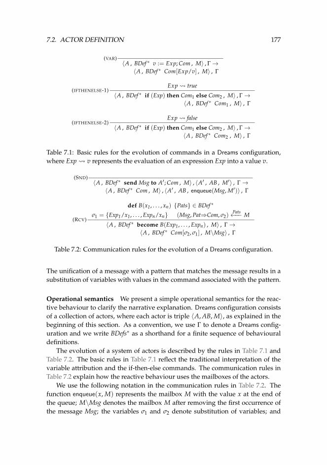
7.2. ACTOR DEFINITION 177
(VAR)〈A , BDef ∗ v := Exp; Com , M〉 , Γ→〈A , BDef ∗ Com[Exp/v] , M〉 , Γ
(IFTHENELSE-1)Exp true
〈A , BDef ∗ if (Exp) then Com1 else Com2 , M〉 , Γ→〈A , BDef ∗ Com1 , M〉 , Γ
(IFTHENELSE-2)Exp false
〈A , BDef ∗ if (Exp) then Com1 else Com2 , M〉 , Γ→〈A , BDef ∗ Com2 , M〉 , Γ
Table 7.1: Basic rules for the evolution of commands in a Dreams configuration,where Exp v represents the evaluation of an expression Exp into a value v.
(SND)〈A , BDef ∗ send Msg to A′; Com , M〉 , 〈A′ , AB , M′〉 , Γ→〈A , BDef ∗ Com , M〉 , 〈A′ , AB , enqueue(Msg, M′)〉 , Γ
(RCV)
def B(x1, . . . , xn) {Pats} ∈ BDef ∗
σ1 = {Exp1/x1, . . . , Expn/xn} (Msg, Pat⇒Com, σ2)Pats←−− M
〈A , BDef ∗ become B(Exp1, . . . , Expn) , M〉 , Γ→〈A , BDef ∗ Com[σ2, σ1] , M\Msg〉 , Γ
Table 7.2: Communication rules for the evolution of a Dreams configuration.
The unification of a message with a pattern that matches the message results in asubstitution of variables with values in the command associated with the pattern.
Operational semantics We present a simple operational semantics for the reac-tive behaviour to clarify the narrative explanation. Dreams configuration consistsof a collection of actors, where each actor is triple 〈A, AB, M〉, as explained in thebeginning of this section. As a convention, we use Γ to denote a Dreams config-uration and we write BDefs∗ as a shorthand for a finite sequence of behaviouraldefinitions.
The evolution of a system of actors is described by the rules in Table 7.1 andTable 7.2. The basic rules in Table 7.1 reflect the traditional interpretation of thevariable attribution and the if-then-else commands. The communication rules inTable 7.2 explain how the reactive behaviour uses the mailboxes of the actors.
We use the following notation in the communication rules in Table 7.2. Thefunction enqueue(x, M) represents the mailbox M with the value x at the end ofthe queue; M\Msg denotes the mailbox M after removing the first occurrence ofthe message Msg; the variables σ1 and σ2 denote substitution of variables; and
178 CHAPTER 7. IMPLEMENTING DREAMS
Com[σ1, σ2] represents the command Com after applying the substitutions σ1 and
then σ2. Finally, (Msg, Pat⇒Com, σ2)Pats←−− M denotes a successful search for the
first message in M that matches the a pattern from Pats. The result of the search isa triple, where Msg is the message found in M, Pat⇒Com is the first pattern foundin Pats that matches Msg, and σ is the substitution obtained by unifying Msg withPat.
7.3 Distributed algorithm
We now describe the behaviour of each actor in the Dreams framework. The com-bined behaviour of all actors yields the evolution of Dreams as described in §6.3.3.Proactive actors initiate the algorithm by requesting the behavioural automata oftheir neighbours, which in turn send requests to their own neighbours. An ac-tor replies to the request for its behavioural automaton once it has collected allinformation about its neighbours, which results in a breadth-first traversal of thegraph of actors. The graph traversal is not managed by any global entity, and theexistence of multiple proactive actors introduces some extra complications.
Recall from §6.2 that the underlying actor model assumes the existence of aunique name for each actor. The Dreams framework assumes also a total orderamong actors based on their unique names.1 More specifically, it assumes a totalorder among proactive actors. We specify the order by introducing a unique in-teger value rank associated with each proactive actor, such that the decisions of aproactive actor with a higher rank prevails over decisions by an actor with a lowerrank. We do not address which actors should have higher rank, nor do we exploita scenario where the order changes during the evolution of an actor. After theinitial request of each proactive actor is sent only the proactive actor with highestrank will get a reply with the behavioural automaton of the full system. At thisstage the winning proactive actor chooses a step from the behavioural automatonand sends it to its neighbours, who propagate the data across the graph of actorsaccording to the chosen step.
Figure 7.2 depicts the possible phases of an actor. Each phase represents adifferent reactive behaviour, i.e., it has its own behaviour definition, and reactsdifferently to received messages. The labels of the diagram depict the receivedmessages, and the messages Reply, AS and Data are shorthands for a set of relatedmessages. We will explain each of these messages later in this chapter. Note thateach actor reacts deterministically to each received message, as it will be clear afterdescribing the details of the distributed algorithm, although the simplifications inthe diagram from Figure 7.2 suggest otherwise. An actor changes phase when itperforms the command become B(Exp1, . . . , Expn), where B is the new behaviour
1One can, for instance, imagine the rank of an actor to be the binary representation of the uniquestring Name of the actor, interpreted as an integer.
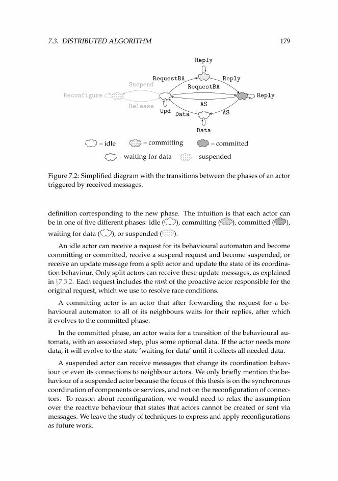
7.3. DISTRIBUTED ALGORITHM 179
RequestBA Reply
AS
RequestBA
AS
Data
Reply
Reply
Data
Upd
Reconfigure
Suspend
Release
– idle – committing – committed
– waiting for data – suspended
Figure 7.2: Simplified diagram with the transitions between the phases of an actortriggered by received messages.
definition corresponding to the new phase. The intuition is that each actor canbe in one of five different phases: idle ( ), committing ( ), committed ( ),
waiting for data ( ), or suspended ( ).
An idle actor can receive a request for its behavioural automaton and becomecommitting or committed, receive a suspend request and become suspended, orreceive an update message from a split actor and update the state of its coordina-tion behaviour. Only split actors can receive these update messages, as explainedin §7.3.2. Each request includes the rank of the proactive actor responsible for theoriginal request, which we use to resolve race conditions.
A committing actor is an actor that after forwarding the request for a be-havioural automaton to all of its neighbours waits for their replies, after whichit evolves to the committed phase.
In the committed phase, an actor waits for a transition of the behavioural au-tomata, with an associated step, plus some optional data. If the actor needs moredata, it will evolve to the state ‘waiting for data’ until it collects all needed data.
A suspended actor can receive messages that change its coordination behav-iour or even its connections to neighbour actors. We only briefly mention the be-haviour of a suspended actor because the focus of this thesis is on the synchronouscoordination of components or services, and not on the reconfiguration of connec-tors. To reason about reconfiguration, we would need to relax the assumptionover the reactive behaviour that states that actors cannot be created or sent viamessages. We leave the study of techniques to express and apply reconfigurationsas future work.
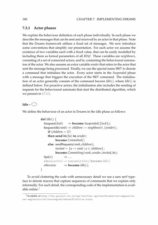
180 CHAPTER 7. IMPLEMENTING DREAMS
7.3.1 Actor phases
We explain the behaviour definition of each phase individually. In each phase wedescribe the messages that can be sent and received by an actor in that phase. Notethat the Dreams framework utilises a fixed set of messages. We now introducesome conventions that simplify our presentation. For each actor we assume theexistence of two variables each with a fixed value, that can be easily modelled byincluding them as formal parameters of all BDef . These variables are neighbours,consisting of a set of connected actors, and ba, containing the behavioural automa-ton of the actor. We also assume an extra variable sender that refers to the actor thatsent the message being processed. Finally, we use the special name INIT to denotea command that initialises the actor. Every actor starts in the Suspended phasewith a message that triggers the execution of the INIT command. The initialisa-tion of an actor generally consists of the command become Idle(), where Idle() isdefined below. For proactive actors, the initialisation also includes the sending ofrequests for the behavioural automata that start the distributed algorithm, whichwe present in §7.3.3.
Idle –
We define the behaviour of an actor in Dreams in the idle phase as follows:
def Idle() {Suspend(lock) ⇒ become Suspended({lock});RequestBA(rank)⇒ children := neighbours\ {sender} ;
if (children = ∅)
then send BA(ba) to sender;become Committed()
else sendRequests(rank, children);invited = {a 7→ rank | a ∈ children} ;become Committing(rank, sender, invited, ba);
Upd(s) ⇒ . . .Admin(action)⇒ execute(action); become Idle()otherwise ⇒ become Idle();
}
To avoid cluttering the code with unnecessary detail we use a sans serif type-face to denote macros that capture sequences of commands that we explain onlyinformally. For such detail, the corresponding code of the implementation is avail-able online.2
2Available at http://reo.project.cwi.nl/cgi-bin/trac.cgi/reo/browser/reo-engine/cwi.reo.engine/src/cwi/reo/engine/redrum/Primitive.scala.
7.3. DISTRIBUTED ALGORITHM 181
When an actor executes the reactive behaviour Idle() it always consumes thefirst message in the mailbox, because every message can match one of the patterns.In particular, the last pattern otherwise is just a variable that can be unified with anymessage. This pattern simply discards the message, removing it from the mailbox.For the other patterns, we have four possible cases.
1. The received message is Suspend(lock), where lock is a string that identifieswho requested the suspension. In this case the actor changes its reactivebehaviour to Suspended. The only argument of the new phase is the set oflocks that the actor waits on their release before it becomes Idle again, in thiscase {lock};
2. The received message is RequestBA(rank), where rank is an integer repre-senting the ranking of the proactive actor that initiated the request. In thiscase the actor tries to collect the behavioural automaton of all of its con-nected actors, contained in the variable children. When the actor is not con-nected to any other actor, it immediately replies to the requester with itsown behavioural automaton, and becomes Committed. Otherwise it for-wards the request to all of its children and changes its reactive behaviourto the Committing phase, where it waits for the replies from its children.sendRequests(rank, children) is a macro for a sequence of
send RequestBA(rank) to a
commands, for all a ∈ children. The arguments of the new Committing phaseare, respectively: the rank of the requester; the actor to whom to reply af-ter collecting all behaviour; a set of invited neighbours to return their be-havioural automaton, each associated with the rank used in the sending ofthe request; and the behavioural automaton obtained from the replies of thechildren (initially the behavioural automata ba of the actor). Note the redun-dancy of adding the value rank both as an argument of Committing as well asassociating it with each invited actor. We will clarify this when we describethe Committing phase, but the intuition is to allow the actor to update itsrank parameter without sending new requests for a behavioural automatonwith the new rank, or send new requests with a new rank to just some of theinvited actors.
3. The Upd(s) message can be received only by a split actor, and represents astate update of the behavioural automaton by the step s of the receiver’ssplit actor. We leave this command undefined for now, and will return to itin §7.3.2.
4. The Admin(action) messages represent administration operations, and arepresent for the sake of completeness with respect to the existing implemen-tation. Possible actions include monitoring operations of the actor, such as
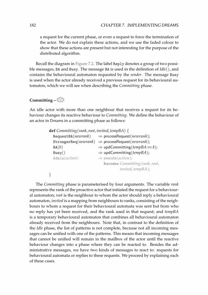
182 CHAPTER 7. IMPLEMENTING DREAMS
a request for the current phase, or even a request to force the termination ofthe actor. We do not explain these actions, and we use the faded colour toshow that these actions are present but not interesting for the purpose of thedistributed algorithm.
Recall the diagram in Figure 7.2. The label Reply denotes a group of two possi-ble messages, BA and Busy. The message BA is used in the definition of Idle(), andcontains the behavioural automaton requested by the sender. The message Busy
is used when the actor already received a previous request for its behavioural au-tomaton, which we will see when describing the Committing phase.
Committing –
An idle actor with more than one neighbour that receives a request for its be-haviour changes its reactive behaviour to Committing. We define the behaviour ofan actor in Dreams in a committing phase as follows:
def Committing(rank, root, invited, tempBA) {RequestBA(newrank) ⇒ processRequest(newrank);StrongerReq(newrank) ⇒ processRequest(newrank);BA(b) ⇒ updCommitting(tempBA ./ b);Busy() ⇒ updCommitting(tempBA);Admin(action) ⇒ execute(action);
become Committing(rank, root,invited, tempBA);
}
The Committing phase is parameterised by four arguments. The variable rankrepresents the rank of the proactive actor that initiated the request for a behaviour-al automaton; root is the neighbour to whom the actor should reply a behaviouralautomaton, invited is a mapping from neighbours to ranks, consisting of the neigh-bours to whom a request for their behavioural automata was sent but from whono reply has yet been received, and the rank used in that request; and tempBAis a temporary behavioural automaton that combines all behavioural automatonalready received from the neighbours. Note that, in contrast to the definition ofthe Idle phase, the list of patterns is not complete, because not all incoming mes-sages can be unified with one of the patterns. This means that incoming messagesthat cannot be unified will remain in the mailbox of the actor until the reactivebehaviour changes into a phase where they can be reacted to. Besides the ad-ministrative messages, we have two kinds of messages to react to: requests forbehavioural automata or replies to these requests. We proceed by explaining eachof these cases.
7.3. DISTRIBUTED ALGORITHM 183
Requests The Dreams framework recognises two different messages for sendingrequests, RequestBA and StrongerReq, which are not distinguished in thedefinition of Committing. We will explain this distinction when describingthe reactive behaviour of the Committed phase. The processRequest macroexecutes the following commands in sequence:
1. If newrank = rank then the actor starts by performing the command
updCommitting(tempBA).
Recall that invited(a) = i represents that a request to the actor a wassent with rank i, but a reply has not yet been processed. Note also thatsender ∈ dom(invited), which we explain only informally. The mappinginvited contains all the neighbours except the root, who sent the requestresponsible for the actor becoming Committing, and the neighbours thatalready replied to the actor, who cannot have sent another request inthe current round. If invited(sender) < newrank, then the actor alsoperforms the following command before the updCommitting command:
send Busy to sender.
2. If invited(sender) ≤ newrank < rank then the actor sends a strongerrequest with the command
send StrongerReq(rank) to sender.
3. If newrank < invited(sender) ≤ rank then the message is consumed anddiscarded, because the actor has already sent a request with a rankgreater than newrank to sender.
4. If newrank > rank then the value of root of the Committing phase changesto the sender. The root is the neighbour to who the actor has to replya behavioural automata. A naive approach is for the actor to send astronger request for their behavioural automata to all its neighbours.Instead of sending new invitations we simply update the value of rank,and postpone the sending of stronger invitations until a reply is re-ceived from the invited actors, that may or may not trigger the sendof the stronger request. This behaviour is achieved by executing themacro changeRoot, defined below.
changeRoot =
send RequestBA(newrank) to root;invited′ := (invited\ {sender}) ∪ {root 7→ newrank} ;become Committing(newrank, sender, invited′, tempBA).
184 CHAPTER 7. IMPLEMENTING DREAMS
Replies The possible replies for requests of behavioural automata consist of BA(b)and Busy messages. The first message is received when a neighbour replieswith a behavioural automaton b, and the second when a neighbour decidesit does not need to return a behavioural automaton, since it will do so to an-other root. The actor evolves by removing the sender from the invited list, ex-ecuting the macro updCommitting(b′), where b′ is the combined behaviouralautomaton of the invited neighbours. In order to accomodate proative ac-tors, a slightly more complex version of this macro (page 191) is necessary.Ignoring this, for now we define updCommitting as follows.
updCommitting(b′) =invited′ := invited\ {sender} ;if (invited′ 6= ∅)
then become Committing(rank, root, invited′, b′)else send BA(b′) to sender;
become Committed()
Note that some of the received RequestBA messages are also interpreted asreplies, when the rank of the request is the same as the rank of the commit-ting actor, as shown before.
Committed –
A Committed actor has already sent its own behavioural automaton in a reply,together with the behavioural automaton of its other neighbours, and is waitingfor a step for the current round. The step can arrive from any of its neighbours,and not only from the root of the Committing phase.
def Committed() {StrongerReq(rank)⇒ send Busy to sender;
become Committed();AS(s) ⇒ processAS(s);AS+Req(s) ⇒ processAS+req(s);AS+Data(s, d) ⇒ processAS+data(s, d);Data(d) ⇒ become Committed();Admin(action) ⇒ execute(action);
become Committed();}
We distinguish between the RequestBA and StrongerReq messages in the def-inition of the Committed phase. Whenever a StrongerReq message is received, theactor replies with a Busy message, and remains Committed. A Committed actor can-not change its previously replied behavioural automaton. The roots of the current
7.3. DISTRIBUTED ALGORITHM 185
actor and the sender will also eventually intersect, because the StrongerReq mes-sage is only sent when invitations from more than one neighbour have the samerank, that is, the sender was previously in a Committing phase with rank value rank.
The incoming RequestBA messages do not match any of the patterns in thisphase, and are therefore kept in the mailbox of the actor until they can be pro-cessed (in the Idle phase).
Apart from the StrongerReq messages and administrative messages, a Com-mitted actor reacts only to messages with a step s, denoted in Figure 7.2 simply asAS. We admit three different forms for the messages represented in this diagramas AS: AS(s), AS+Req(s) and AS+Data(s, d). The message AS(s) is received whenthere is no data communication between the sender and the Committed actor. Themessage AS+Req(s) is received when the sender provides the step for the currentround, but it stays in the phase ‘waiting for data’, to whom the Committed actorshould provide a data value. Finally, the message AS+Data(s, d) is received whenthere is a data value d sent from the sender to the Committed actor.
Steps as groups of labels As discussed in §3.5, the step s consists of a groupγs of labels of transitions from the global behavioural automata b, whose atomicsteps differ only in the data-values flowing through the ports. We recall belowthe properties of γs. This approach allows a label to be chosen without deciding apriori which data values will be transferred. Let b = 〈Q, L[P],→,O〉. The groupγs is indexed by an assignment of data of the input ports, that is, the type of γs is
γs : (IP→ D)→ L[P].
The conditions over γs are specified as follows.
∀m : IP→ D · α(γs(m)) = 〈P, F, IP, OP, datam〉 ,
for some fixed F, IP, OP, and where datam _m
Recall that m1_m2 if the values of m1 and m2 coincide for the common domain
of both maps, and α is a global function that maps each label ` ∈ L of transitionsof behavioural automata into an atomic step.
Let b = b1 ./ · · · ./ bn, where each bi is the behavioural automata of eachof the actors involved in the current round, and let bi = 〈Qi, L[Pi],→i, Oi〉. Asmentioned in Chapter 3, the group γs can be projected into each behavioural au-tomaton bi, denoted by γs[bi], whose labels have atomic steps restricted to the setof ports Pi. In the rest of this chapter we write datas[m](x) = d if there exists adata value d such that, for all data functions datas of the atomic steps associatedto labels in γs[bi], datas(x) = d. Furthermore, we refer to such groups of labelssimply as ‘steps’.
186 CHAPTER 7. IMPLEMENTING DREAMS
Processing of a step We now describe the processAS+data macro, and explainhow the macros processAS and processAS+req differ from it. The processAS+data
macro analyses the projection γs[b] and deduces the neighbours from which adata value should be requested, the neighbours to which a data value should besent, and the neighbours which require only the step s. The details of this macrofollow below. The macro describes the sending of the appropriate messages to therespective neighbours.
1. Define γs[b] to be the projection of s for the behavioural automata b, andP, IP, and OP to be the sets of known, input, and output ports, respec-tively, from the atomic steps of the labels in range(γs[b]). Also define rcvd :={sender 7→ d}, which is a mapping of the data values received so far.
2. Send the step s to all the neighbours whose ports are neither in IP nor inOP. Note that each neighbour is represented in the actor by the port that isshared with the neighbour. For all x ∈ P \ (IP∪OP) perform the command:
send AS(s) to x.
3. Send the step s with a request for data to all ports in ip ∈ IP \ {sender}, byperforming the following command:
send AS+Req(s) to ip.
4. Send the step s to all output ports whose data value is already known. Recallthat datas[m](x) = d if there exists a data value d ∈ D such that datas(x) = d,for all data functions datas ∈ range(γs[b]). Then, for all ports op ∈ OP suchthat there exists a data value d ∈ D where datas[rcvd](op) = d, we performthe command:
send AS+Data(s, d) to op.
5. Define R = IP \ dom(rcvd) to be the set of the remaining input ports whosedata values are unknown. If R = ∅, then IP ⊆ dom(rcvd) and γs[rcvd] ={sb}, because of the properties of γs[b] described above, where sb is thestep that b will perform. Consequently, the actor updates the state of itsbehavioural automaton and becomes idle. If R 6= ∅, then the actor waits forthe replies from actors in IP. This is achieved by the command:
if (R = ∅)
then updBA(γ[rcvd])else become WaitingData(R, ∅, rcvd, s)
The macro updBA(γ[rcvd]) updates the behavioural automaton b of the actor,evolving b by the step sb. After updating the behaviour, updBA initialises the
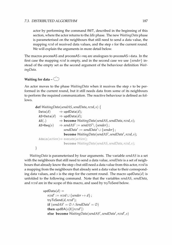
7.3. DISTRIBUTED ALGORITHM 187
actor by performing the command INIT, described in the beginning of thissection, where the actor returns to the Idle phase. The new WaitingData phaseis parameterised on the neighbours that still need to send a data value, themapping rcvd of received data values, and the step s for the current round.We will explain the arguments in more detail below.
The macros processAS and processAS+req are analogues to processAS+data. In thefirst case the mapping rcvd is empty, and in the second case we use {sender} in-stead of the empty set as the second argument of the behaviour definition Wait-ingData.
Waiting for data –
An actor moves to the phase WaitingData when it receives the step s to be per-formed in the current round, but it still needs data from some of its neighboursto perform the required communication. The reactive behaviour is defined as fol-lows.
def WaitingData(sendAS, sendData, rcvd, s) {Data(d) ⇒ updData(d);AS+Data(d) ⇒ updData(d);AS( ) ⇒ become WaitingData(sendAS, sendData, rcvd, s);AS+Req(s) ⇒ sendAS′ := sendAS′\ {sender} ;
sendData′ := sendData′ ∪ {sender} ;become WaitingData(sendAS′, sendData′, rcvd, s);
Admin(action)⇒ execute(action);become WaitingData(sendAS, sendData, rcvd, s);
}
WaitingData is parameterised by four arguments. The variable sendAS is a setwith the neighbours that still need to send a data value, sendData is a set of neigh-bours that already know the step s but still need a data value from this actor, rcvd isa mapping from the neighbours that already sent a data value to their correspond-ing data values, and s is the step for the current round. The macro updData(d) isunfolded to the following command. Note that the variables sendAS, sendData,and rcvd are in the scope of this macro, and used by tryToSend below.
updData(d) =rcvd′ := rcvd∪ {sender 7→ d} ;tryToSend(d, rcvd′);if (sendAS′ = ∅ ∧ SendData′ = ∅)
then updBA(s[b][rcvd′])else become WaitingData(sendAS′, sendData′, rcvd′, s)
188 CHAPTER 7. IMPLEMENTING DREAMS
The macro updData(d) starts by storing the information about the data valuesalready received in the variable rcvd′, and the macro tryToSend(d, rcvd′) checks ifthe data for any of the actors in sendAS or sendData is available after receiving d.The macro tryToSend sends the message AS+Data(s,d’) to every actor a ∈ sendASsuch that there is a value d′ ∈ D where datas[rcvd′](a) = d′ with respect to theprojection γs[b], and similarly it sends the message Data(d′) for every actor insendData with an associated data value d′. The variables sendAS′ and sendData′
are defined to be the updated variables of sendAS and sendData after removing theactors that were replied to. The last if-then-else checks if there are still actors thatare waiting for data. If not, the actor evolves it’s behavioural automaton and ini-tialises again by performing the macro updBA, described for the Committed phase.Otherwise, the parameters of WaitingData are updated. Note that γs[b][rcvd′] willalways be a singleton set because sendAS′ = ∅ and SendData′ = ∅, which implythat all the input ports in IP are completely defined by rcvd′.
When the message AS is received the actor consumes and discards messagewith the step, because the step for the current round is already known. Finally,when a message AS+Req is received the actor updates the values of sendAS andsendData, since the sender does not need the step anymore, but only its data value.
Suspended –
Every actor is created in the Suspended phase, with a message Release() in themailbox to release this suspension. Therefore the definition of Suspended(locks)presented below plays two roles: (1) initialise the reactive behaviour, and (2) al-low the reconfiguration of the actor without interfering with the coordination be-haviour. The initialisation is achieved by executing INIT, introduced in the begin-ning of §7.3.1. We incorporate these two roles into the same reactive behaviourbecause every time an actor stops being suspended it has to be considered to be anew actor, since it could have been reconfigured.
An idle actor becomes suspended by receiving the Suspend(lock) message. Itsreactive behaviour is described by Suspended(lock), defined below. The variablelock identifies who requested the suspension, to permit the suspension of an actorfrom independent entities. We do not explore the reconfiguration aspect in thisthesis, and simply use a general Reconfigure message parameterised on an in-struction inst. Reconfiguration plays an orthogonal role to the communication ofdata, and can be dealt with independently.
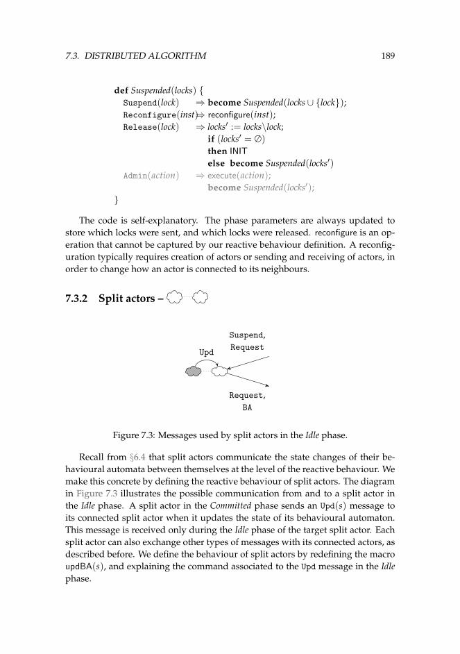
7.3. DISTRIBUTED ALGORITHM 189
def Suspended(locks) {Suspend(lock) ⇒ become Suspended(locks∪ {lock});Reconfigure(inst)⇒ reconfigure(inst);Release(lock) ⇒ locks′ := locks\lock;
if (locks′ = ∅)
then INIT
else become Suspended(locks′)Admin(action) ⇒ execute(action);
become Suspended(locks′);}
The code is self-explanatory. The phase parameters are always updated tostore which locks were sent, and which locks were released. reconfigure is an op-eration that cannot be captured by our reactive behaviour definition. A reconfig-uration typically requires creation of actors or sending and receiving of actors, inorder to change how an actor is connected to its neighbours.
7.3.2 Split actors –
Upd
Suspend,Request
Request,BA
Figure 7.3: Messages used by split actors in the Idle phase.
Recall from §6.4 that split actors communicate the state changes of their be-havioural automata between themselves at the level of the reactive behaviour. Wemake this concrete by defining the reactive behaviour of split actors. The diagramin Figure 7.3 illustrates the possible communication from and to a split actor inthe Idle phase. A split actor in the Committed phase sends an Upd(s) message toits connected split actor when it updates the state of its behavioural automaton.This message is received only during the Idle phase of the target split actor. Eachsplit actor can also exchange other types of messages with its connected actors, asdescribed before. We define the behaviour of split actors by redefining the macroupdBA(s), and explaining the command associated to the Upd message in the Idlephase.
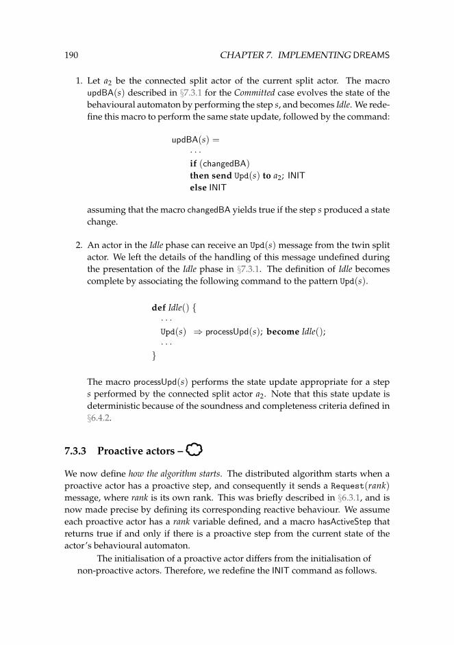
190 CHAPTER 7. IMPLEMENTING DREAMS
1. Let a2 be the connected split actor of the current split actor. The macroupdBA(s) described in §7.3.1 for the Committed case evolves the state of thebehavioural automaton by performing the step s, and becomes Idle. We rede-fine this macro to perform the same state update, followed by the command:
updBA(s) =· · ·if (changedBA)
then send Upd(s) to a2; INIT
else INIT
assuming that the macro changedBA yields true if the step s produced a statechange.
2. An actor in the Idle phase can receive an Upd(s) message from the twin splitactor. We left the details of the handling of this message undefined duringthe presentation of the Idle phase in §7.3.1. The definition of Idle becomescomplete by associating the following command to the pattern Upd(s).
def Idle() {· · ·Upd(s) ⇒ processUpd(s); become Idle();· · ·}
The macro processUpd(s) performs the state update appropriate for a steps performed by the connected split actor a2. Note that this state update isdeterministic because of the soundness and completeness criteria defined in§6.4.2.
7.3.3 Proactive actors –
We now define how the algorithm starts. The distributed algorithm starts when aproactive actor has a proactive step, and consequently it sends a Request(rank)message, where rank is its own rank. This was briefly described in §6.3.1, and isnow made precise by defining its corresponding reactive behaviour. We assumeeach proactive actor has a rank variable defined, and a macro hasActiveStep thatreturns true if and only if there is a proactive step from the current state of theactor’s behavioural automaton.
The initialisation of a proactive actor differs from the initialisation ofnon-proactive actors. Therefore, we redefine the INIT command as follows.
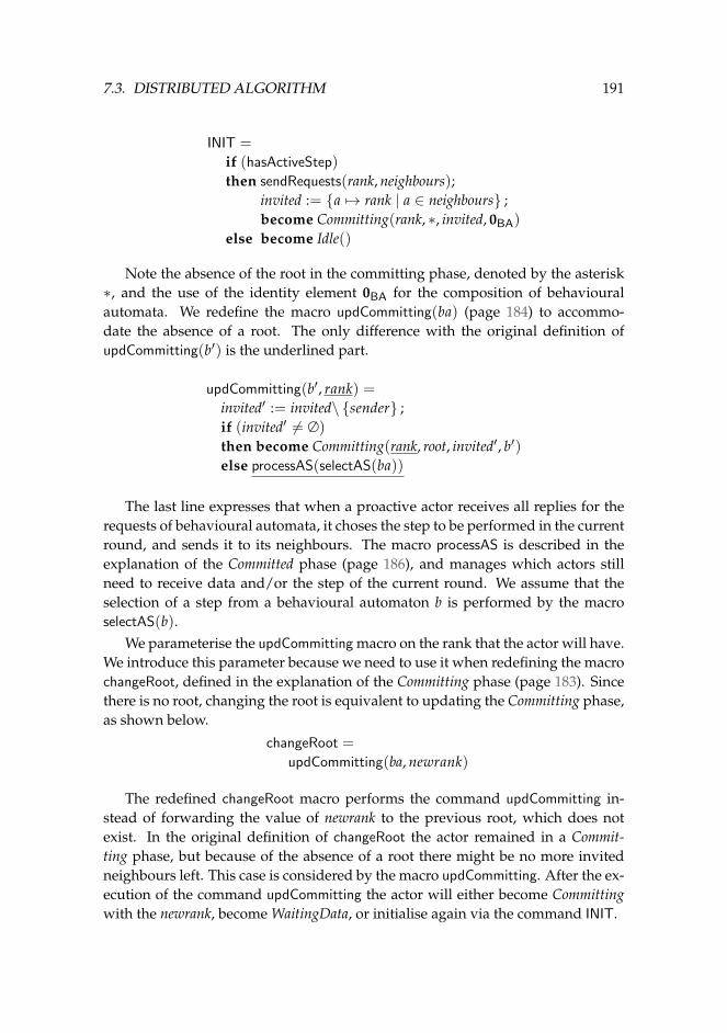
7.3. DISTRIBUTED ALGORITHM 191
INIT =
if (hasActiveStep)
then sendRequests(rank, neighbours);invited := {a 7→ rank | a ∈ neighbours} ;become Committing(rank, ∗, invited, 0BA)
else become Idle()
Note the absence of the root in the committing phase, denoted by the asterisk∗, and the use of the identity element 0BA for the composition of behaviouralautomata. We redefine the macro updCommitting(ba) (page 184) to accommo-date the absence of a root. The only difference with the original definition ofupdCommitting(b′) is the underlined part.
updCommitting(b′, rank) =invited′ := invited\ {sender} ;if (invited′ 6= ∅)
then become Committing(rank, root, invited′, b′)else processAS(selectAS(ba))
The last line expresses that when a proactive actor receives all replies for therequests of behavioural automata, it choses the step to be performed in the currentround, and sends it to its neighbours. The macro processAS is described in theexplanation of the Committed phase (page 186), and manages which actors stillneed to receive data and/or the step of the current round. We assume that theselection of a step from a behavioural automaton b is performed by the macroselectAS(b).
We parameterise the updCommitting macro on the rank that the actor will have.We introduce this parameter because we need to use it when redefining the macrochangeRoot, defined in the explanation of the Committing phase (page 183). Sincethere is no root, changing the root is equivalent to updating the Committing phase,as shown below.
changeRoot =
updCommitting(ba, newrank)
The redefined changeRoot macro performs the command updCommitting in-stead of forwarding the value of newrank to the previous root, which does notexist. In the original definition of changeRoot the actor remained in a Commit-ting phase, but because of the absence of a root there might be no more invitedneighbours left. This case is considered by the macro updCommitting. After the ex-ecution of the command updCommitting the actor will either become Committingwith the newrank, become WaitingData, or initialise again via the command INIT.
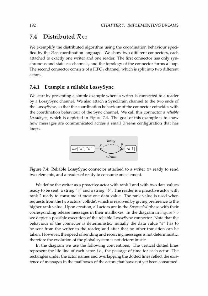
192 CHAPTER 7. IMPLEMENTING DREAMS
7.4 DistributedReo
We exemplify the distributed algorithm using the coordination behaviour speci-fied by the Reo coordination language. We show two different connectors, eachattached to exactly one writer and one reader. The first connector has only syn-chronous and stateless channels, and the topology of the connector forms a loop.The second connector consists of a FIFO1 channel, which is split into two differentactors.
7.4.1 Example: a reliable LossySync
We start by presenting a simple example where a writer is connected to a readerby a LossySync channel. We also attach a SyncDrain channel to the two ends ofthe LossySync, so that the coordination behaviour of the connector coincides withthe coordination behaviour of the Sync channel. We call this connector a reliableLossySync, which is depicted in Figure 7.4. The goal of this example is to showhow messages are communicated across a small Dreams configuration that hasloops.
x ywr[“a”, “b”] rd[1]
lossy
sdrain
Figure 7.4: Reliable LossySync connector attached to a writer wr ready to sendtwo elements, and a reader rd ready to consume one element.
We define the writer as a proactive actor with rank 1 and with two data valuesready to be sent: a string “a” and a string “b”. The reader is a proactive actor withrank 2 ready to consume at most one data value. The rank value is used whenrequests from the two actors ‘collide’, which is resolved by giving preference to thehigher rank value. Upon creation, all actors are in the Suspended phase with theircorresponding release messages in their mailboxes. In the diagram in Figure 7.5we depict a possible execution of the reliable LossySync connector. Note that thebehaviour of the connector is deterministic: initially the data value “a” has tobe sent from the writer to the reader, and after that no other transition can betaken. However, the speed of sending and receiving messages is not deterministic,therefore the evolution of the global system is not deterministic.
In the diagram we use the following conventions. The vertical dotted linesrepresent the life line of each actor, i.e., the passage of time for each actor. Therectangles under the actor names and overlapping the dotted lines reflect the exis-tence of messages in the mailboxes of the actors that have not yet been consumed.
7.4. DISTRIBUTEDREO 193
Arrows between life lines of actors represent the sending of a messages to themailboxes of other actors, but not their consumption, i.e., not the matching of themessage to a pattern. The clouds at the ends of the life lines represent the phasesof the reactive behaviours at the end of the trace. In this case, all actors are com-mitting with the exception of the reader who is idle. Furthermore, only the actory has messages in its mailbox at the end of the trace, depicted by drawing therectangle until the cloud on the bottom.
Some comments about the trace of the execution of the reliable LossySyncin Figure 7.5 are now in order. Initially all actors are suspended with a Releasemessage in each of their mailboxes, and they are initialised via the INIT commandonce the message is received. The trace depicted in the diagram starts after theRelease message is consumed. In the beginning, only the writer and the readersend a request each, as a result of being released from their suspension, becomeCommitting, and all of the other actors become Idle. Consider now the top rectangleon the life line of actor x. Observe that three requests for a behavioural automatonarrive in the mailbox of actor x before it sends a message. The messages are pro-cessed in the order they were sent, and as a consequence x starts to propagate thefirst (weaker) request to all of its neighbours. Because of the delay in sending therequest, we assume x sends a request for a behavioural automaton to lossy evenafter lossy sent a (stronger) request, and the same happens between x and sdrain.Once x receives the request from lossy it sends a new request to the writer, but itdoes not send any request to sdrain since it is still waiting for the reply to its initial(weaker) request. Also when the Req(2) message from lossy is received x replies bysending a Busy message to lossy. When wr receives Req(2) it becomes committedand replies by sending its behavioural automaton to x. Reacting to this message, xreplies with its behavioural automaton together with wr’s behavioural automatonto lossy, and lossy replies with the received behavioural automaton and its ownbehavioural automaton to y. Meanwhile, sdrain also replies with its behaviouralautomaton to y, and y sends the composition of the received behavioural automataand its own behavioural automaton to rd. Finally, rd receives the reply to its ini-tial request with the behavioural automaton of the rest of the connector. At thispoint the reader, rd, composes the received behavioural automaton with its ownbehavioural automaton, selects a step s1 from this automaton, sends the step to-gether with a request for data, and changes its phase to WaitingData. Note thatonce the writer receives the step s1 it sends the data value, followed by a requestfor a behavioural automaton for the next round. Therefore, the writer is alreadycommitting, while the sdrain is still committed and waiting for the step of the pre-vious round. This is not problematic because the step will always be sent to sdrainbefore the request for the new behavioural automaton.
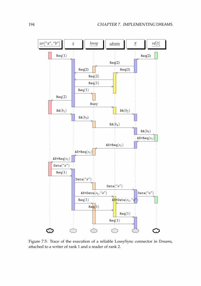
194 CHAPTER 7. IMPLEMENTING DREAMS
wr[“a”, “b”] x lossy sdrain y rd[1]
Req(1)
BA(b1)
Data(“a”)
Req(1)
Req(1)
Req(1)
Req(2)
Busy
BA(b3)
AS+Req(s1)
Data(“a”)
AS+Data(s1, “a”)
Req(1)
Req(1)
Req(2)
BA(b4)
AS+Req(s1)
Data(“a”)
Req(1)
Req(2)
BA(b2)
Req(1)
Req(2)
Req(2)
BA(b5)
AS+Req(s1)
Data(“a”)
AS+Data(s1, “a”)
Req(2)
AS+Req(s1)
Figure 7.5: Trace of the execution of a reliable LossySync connector in Dreams,attached to a writer of rank 1 and a reader of rank 2.
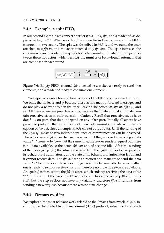
7.4. DISTRIBUTEDREO 195
7.4.2 Example: a split FIFO1
In our second example we connect a writer wr, a FIFO1 fifo, and a reader rd, as de-picted in Figure 7.6. When encoding the connector in Dreams, we split the FIFO1channel into two actors. The split was described in §6.5.1, and we name the actorattached to x fifo-in, and the actor attached to y fifo-out. The split increases theconcurrency and avoids the requests for behavioural automata to propagate be-tween these two actors, which restricts the number of behavioural automata thatare composed in each round.
x ywr[“a”, “b”] rd[1]
fifo
Figure 7.6: Empty FIFO1 channel fifo attached to a writer wr ready to send twoelements, and a reader rd ready to consume one element.
We depict a possible trace of the execution of the FIFO1 connector in Figure 7.7.We omit the nodes x and y because these actors mainly forward messages anddo not play a relevant role in the trace, leaving the actors wr, fifo-in, fifo-out, andrd. All these actors are proactive actors, because their behavioural automata con-tain proactive steps in their transition relations. Recall that proactive steps havedataflow on ports that do not depend on any other port. Initially all actors haveproactive ports for the current state of their behavioural automata with the ex-ception of fifo-out, since an empty FIFO1 cannot output data. Until the sending ofthe Upd(s1) message two independent lines of communication can be observed.The actors wr and fifo-in exchange messages until they succeed in sending a datavalue “a” from wr to fifo-in. At the same time, the reader sends a request but thereis no data available, so the actors fifo-out and rd become idle. After the sendingof the message Upd(s1) the situation is inverted. The fifo-in replies to a request forits behavioural automaton, but the state of its behavioural automaton is full andit cannot receive data. The fifo-out sends a request and manages to send the datavalue “a” to the reader. The actors for fifo-out and rd become idle, because neitherone is ready to send or receive data, and therefore no proactive steps are available.An Upd(s4) is then sent to the fifo-in actor, which ends up receiving the data value“b”. In the end of the trace, the fifo-out actor still has an active step (the buffer isfull), but the step s5 does not have any dataflow, therefore fifo-out refrains fromsending a new request, because there was no state change.
7.4.3 Dreams vs. d2pc
We explored the most relevant work related to the Dreams framework in §6.6, in-cluding the distributed two phase commit (d2pc) protocol, introduced and stud-
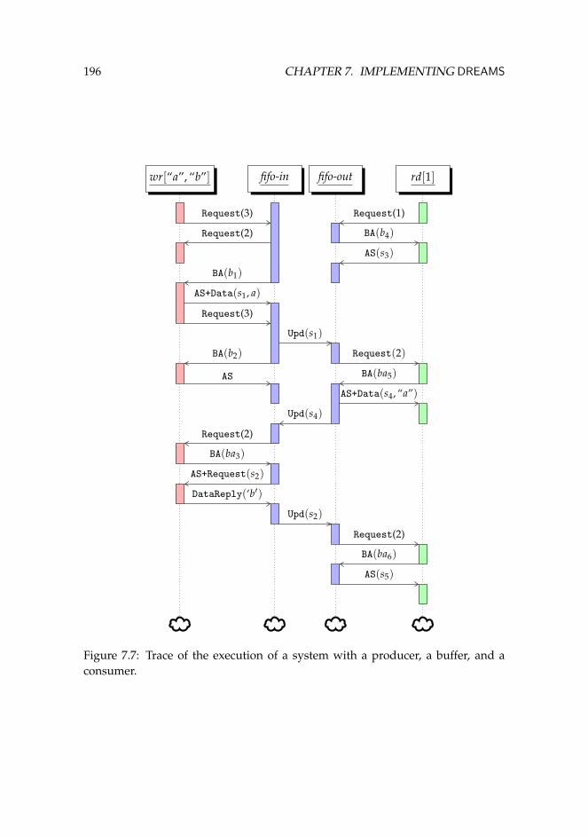
196 CHAPTER 7. IMPLEMENTING DREAMS
wr[“a”, “b”] fifo-in fifo-out rd[1]
Request(3)
AS+Data(s1, a)
Request(3)
AS
BA(ba3)
DataReply(‘b′)
Request(2)
BA(b1)
Upd(s1)
BA(b2)
Request(2)
AS+Request(s2)
Upd(s2)
BA(b4)
Request(2)
AS+Data(s4, “a”)
Upd(s4)
Request(2)
AS(s5)
Request(1)
AS(s3)
BA(ba5)
BA(ba6)
Figure 7.7: Trace of the execution of a system with a producer, a buffer, and aconsumer.
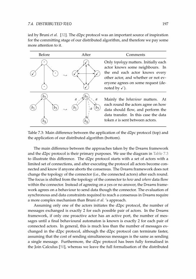
7.4. DISTRIBUTEDREO 197
ied by Bruni et al. [32]. The d2pc protocol was an important source of inspirationfor the committing stage of our distributed algorithm, and therefore we pay somemore attention to it.
Before After Comments
X
-
-
-
; X
X
X
X
Only topology matters. Initially eachactor knows some neighbours. Inthe end each actor knows everyother actor, and whether or not ev-eryone agrees on some request (de-noted byX).
b1
b2
b3
b4
;b1
b2
b3
b4
a a
a
Mainly the behaviour matters. Ateach round the actors agree on howdata should flow, and perform thedata transfer. In this case the datatoken a is sent between actors.
Table 7.3: Main difference between the application of the d2pc protocol (top) andthe application of our distributed algorithm (bottom).
The main difference between the approaches taken by the Dreams frameworkand the d2pc protocol is their primary purposes. We use the diagram in Table 7.3to illustrate this difference. The d2pc protocol starts with a set of actors with alimited set of connections, and after executing the protocol all actors become con-nected and know if anyone aborts the consensus. The Dreams framework does notchange the topology of the connector (i.e., the connected actors) after each round.The focus is shifted from the topology of the connector to how and where data flowwithin the connector. Instead of agreeing on a yes or no answer, the Dreams frame-work agrees on a behaviour to send data though the connector. The evaluation ofsynchronous and data constraints required to reach a consensus in Dreams requirea more complex mechanism than Bruni et al. ’s approach.
Assuming only one of the actors initiates the d2pc protocol, the number ofmessages exchanged is exactly 2 for each possible pair of actors. In the Dreams
framework, if only one proactive actor has an active port, the number of mes-sages until a final behavioural automaton is known is exactly 2 for each pair ofconnected actors. In general, this is much less than the number of messages ex-changed in the d2pc protocol, although the d2pc protocol can terminate faster,assuming that the cost of sending simultaneous messages is the same as sendinga single message. Furthermore, the d2pc protocol has been fully formalised inthe Join Calculus [50], whereas we leave the full formalisation of the distributed
198 CHAPTER 7. IMPLEMENTING DREAMS
algorithm as future work.
7.4.4 Discussion
In the reliable LossySync example we saw that it is possible for actors in differentstates and rounds to coexist in the same snapshot of the connector. We claim thatthis is not problematic because the order of messages sent will always guarantee acorrect behaviour. This scenario reveals that the distributed algorithm introducesa level of concurrency not permitted before by previous implementations of Reo,which makes it a non-trivial problem to guarantee that the system always evolvesaccording to the global behaviour of all actors. We support this claim based onthe runs of the Dreams framework only, and not by formal verification, which weleave as future work.
Together with Jaghoori, we have modelled in Rebeca [64, 65] a simplified caseof a sequence of two and of three split FIFO1 buffers. The behavioural automataof the current round were reduced to simple booleans stating whether the FIFO1buffers were empty or full, and we used a data domain with a single element.Furthermore, we assumed an infinite producer of data on the source port of theconnector, and a reader that can always accept data on its sink port. As a result,we managed to fix a few mistakes in the then-current version of the algorithm,and we verified that the following properties hold for the simplified Rebeca im-plementation:
1. the actors never deadlock, i.e., can always send and receive messages;
2. each actor never has more than five messages in its mailbox; and
3. each FIFO1 buffer changes its state infinitely often.
The first and second properties are specified as part of the model to be verified.The third property is specified as a separate LTL (linear temporal logic) formula.The generated model used to verify the first two properties has 254 states for twoFIFO1 channels, and it has 1820 states for three FIFO1 channels. The generatedmodel used to verify the third property, using three FIFO1 channels, already has5013 states. For this small example the size of the generated models are man-ageable. However, the fast growth of the number of states clearly shows thatonly small examples can be model checked. The analysis of traces and the formalverification of a simple connector lead us to believe that the algorithm is correct,although to claim correctness we expect to extend the formal verification to thefull algorithm described in this chapter in the future.
We now stress the practical relevance of the actor splitting, and the resultingsynchronous regions. The conditions for splitting an actor reflect the indepen-dence of each of the split actors from the other. It also pinpoints the parts of the
7.5. BENCHMARKS 199
connector that always communicate in an asynchronous manner. This is also sup-ported by our example of the split FIFO1, and a trace of its execution in Figure 7.7.Between the two split actors there is no agreement before communication, and thetransition labels are sent after being performed. Therefore, we say splitting yieldslocal autonomy. The result of a splitting is a pair of split actors, each of whichbelongs to an independent synchronous region. The actors in a synchronous re-gion do not have to interact with the actors in any other synchronous region todecide how to evolve. Specifically, a split actor does not need to consult with itsconnected split actor before deciding how to evolve. It only need to report itscommitted choices to its twin split actor.
In our distributed implementation we do not capture the notion of failure,which is a dominant concern in distributed systems. Instead, we rely on theactor model and assume that all communication is reliable. Note that existingdistributed programming techniques typically treat reliable communication as anorthogonal problem, as suggested, for example, by Guerraoui and Rodrigues [55].However, there are still open questions about how the system should react whensome actors become disconnected during the run of the distributed algorithm.Some of such failures may also require changes in the coordination behaviour. Weleave such questions out of the scope of this thesis.
7.5 Benchmarks
We evaluate the performance of our implementation of the Dreams framework byconsidering the time to create aReo connector and to perform the communicationto pass a sequence of data values from some writers to some readers. For compar-ison we use the constraint automata-based implementation of Reo, described inChapter 5, which we call the CA engine. However, our main concern in our com-parison in this chapter is different than the benchmarks performed in §5.6. For theanalysis of the constraint-based approach for Reo we compared the performanceof composing the possible behavioural automaton for a single round. Now wecompare the performance of a connector that evolves in time, acknowledging thetime to deploy a connector and the time to send data through the connector. Wepresent examples of stateful connectors, with one exception for comparison. Moredetails about the two engines used in our benchmark follow below.
CA engine The CA engine is a code generator and interpreter of Reo connectorsincluded in the suite of Eclipse3 plug-ins for Reo [16].4 It uses the contextindependent semantics of Reo, following the ideas of port automata [70]
3http://www.eclipse.org4Available at http://reo.project.cwi.nl/cgi-bin/trac.cgi/reo/browser/ea-codegen
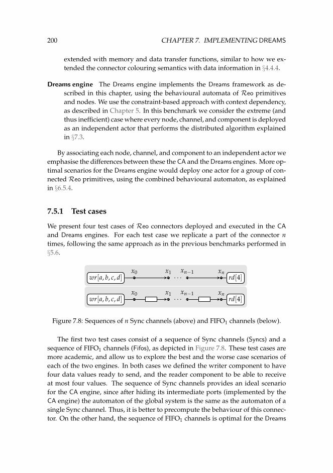
200 CHAPTER 7. IMPLEMENTING DREAMS
extended with memory and data transfer functions, similar to how we ex-tended the connector colouring semantics with data information in §4.4.4.
Dreams engine The Dreams engine implements the Dreams framework as de-scribed in this chapter, using the behavioural automata of Reo primitivesand nodes. We use the constraint-based approach with context dependency,as described in Chapter 5. In this benchmark we consider the extreme (andthus inefficient) case where every node, channel, and component is deployedas an independent actor that performs the distributed algorithm explainedin §7.3.
By associating each node, channel, and component to an independent actor weemphasise the differences between these the CA and the Dreams engines. More op-timal scenarios for the Dreams engine would deploy one actor for a group of con-nected Reo primitives, using the combined behavioural automaton, as explainedin §6.5.4.
7.5.1 Test cases
We present four test cases of Reo connectors deployed and executed in the CA
and Dreams engines. For each test case we replicate a part of the connector ntimes, following the same approach as in the previous benchmarks performed in§5.6.
x0 x1 xn−1 xnwr[a, b, c, d] rd[4]. . .
x0 x1 xn−1 xnwr[a, b, c, d] rd[4]. . .
Figure 7.8: Sequences of n Sync channels (above) and FIFO1 channels (below).
The first two test cases consist of a sequence of Sync channels (Syncs) and asequence of FIFO1 channels (Fifos), as depicted in Figure 7.8. These test cases aremore academic, and allow us to explore the best and the worse case scenarios ofeach of the two engines. In both cases we defined the writer component to havefour data values ready to send, and the reader component to be able to receiveat most four values. The sequence of Sync channels provides an ideal scenariofor the CA engine, since after hiding its intermediate ports (implemented by theCA engine) the automaton of the global system is the same as the automaton of asingle Sync channel. Thus, it is better to precompute the behaviour of this connec-tor. On the other hand, the sequence of FIFO1 channels is optimal for the Dreams
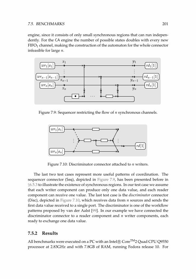
7.5. BENCHMARKS 201
engine, since it consists of only small synchronous regions that can run indepen-dently. For the CA engine the number of possible states doubles with every newFIFO1 channel, making the construction of the automaton for the whole connectorinfeasible for large n.
x1
xn−1
xn
...
yn
yn−1
y1
...
wr1[a1]
wrn−1[an−1]
wrn[an]
rd1[1]
rdn−1[1]
rdn[1]
. . .•
Figure 7.9: Sequencer restricting the flow of n synchronous channels.
...
wr1[a1]
wrn[an]
...rd[1]
Figure 7.10: Discriminator connector attached to n writers.
The last two test cases represent more useful patterns of coordination. Thesequencer connector (Seq), depicted in Figure 7.9, has been presented before in§6.5.3 to illustrate the existence of synchronous regions. In our test case we assumethat each writer component can produce only one data value, and each readercomponent can receive one value. The last test case is the discriminator connector(Disc), depicted in Figure 7.10, which receives data from n sources and sends thefirst data value received to a single port. The discriminator is one of the workflowpatterns proposed by van der Aalst [99]. In our example we have connected thediscriminator connector to a reader component and n writer components, eachready to exchange one data value.
7.5.2 Results
All benchmarks were executed on a PC with an Intel R©CoreTM2 Quad CPU Q9550processor at 2.83GHz and with 7.8GB of RAM, running Fedora release 10. For
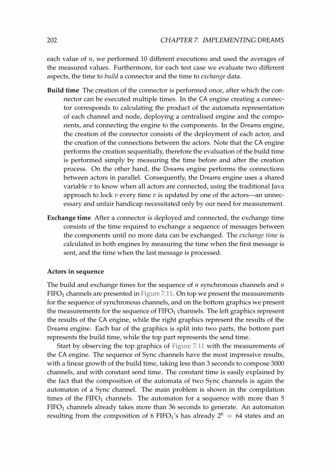
202 CHAPTER 7. IMPLEMENTING DREAMS
each value of n, we performed 10 different executions and used the averages ofthe measured values. Furthermore, for each test case we evaluate two differentaspects, the time to build a connector and the time to exchange data.
Build time The creation of the connector is performed once, after which the con-nector can be executed multiple times. In the CA engine creating a connec-tor corresponds to calculating the product of the automata representationof each channel and node, deploying a centralised engine and the compo-nents, and connecting the engine to the components. In the Dreams engine,the creation of the connector consists of the deployment of each actor, andthe creation of the connections between the actors. Note that the CA engineperforms the creation sequentially, therefore the evaluation of the build timeis performed simply by measuring the time before and after the creationprocess. On the other hand, the Dreams engine performs the connectionsbetween actors in parallel. Consequently, the Dreams engine uses a sharedvariable v to know when all actors are connected, using the traditional Javaapproach to lock v every time v is updated by one of the actors—an unnec-essary and unfair handicap necessitated only by our need for measurement.
Exchange time After a connector is deployed and connected, the exchange timeconsists of the time required to exchange a sequence of messages betweenthe components until no more data can be exchanged. The exchange time iscalculated in both engines by measuring the time when the first message issent, and the time when the last message is processed.
Actors in sequence
The build and exchange times for the sequence of n synchronous channels and nFIFO1 channels are presented in Figure 7.11. On top we present the measurementsfor the sequence of synchronous channels, and on the bottom graphics we presentthe measurements for the sequence of FIFO1 channels. The left graphics representthe results of the CA engine, while the right graphics represent the results of theDreams engine. Each bar of the graphics is split into two parts, the bottom partrepresents the build time, while the top part represents the send time.
Start by observing the top graphics of Figure 7.11 with the measurements ofthe CA engine. The sequence of Sync channels have the most impressive results,with a linear growth of the build time, taking less than 3 seconds to compose 3000channels, and with constant send time. The constant time is easily explained bythe fact that the composition of the automata of two Sync channels is again theautomaton of a Sync channel. The main problem is shown in the compilationtimes of the FIFO1 channels. The automaton for a sequence with more than 5FIFO1 channels already takes more than 36 seconds to generate. An automatonresulting from the composition of 6 FIFO1’s has already 26 = 64 states and an
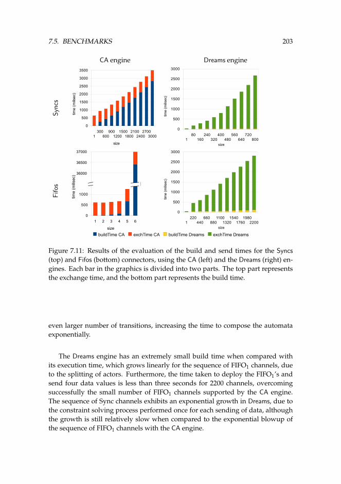
7.5. BENCHMARKS 203
CA engine Dreams engineS
yncs
1300
600900
12001500
18002100
24002700
3000
0
500
1000
1500
2000
2500
3000
3500
size
time
(milis
ec)
180
160240
320400
480560
640720
800
0
500
1000
1500
2000
2500
3000
size
time
(milis
ec)
Fif
os
1 2 3 4 5 60
500
1000
1500
2000
2500
3000
size
time
(milis
ec)
37000
36500
36000
1220
440660
8801100
13201540
17601980
2200
0
500
1000
1500
2000
2500
3000
size
time
(milis
ec)
buildTime CA exchTime CA buildTime Dreams exchTime Dreams
Figure 7.11: Results of the evaluation of the build and send times for the Syncs
(top) and Fifos (bottom) connectors, using the CA (left) and the Dreams (right) en-gines. Each bar in the graphics is divided into two parts. The top part representsthe exchange time, and the bottom part represents the build time.
even larger number of transitions, increasing the time to compose the automataexponentially.
The Dreams engine has an extremely small build time when compared withits execution time, which grows linearly for the sequence of FIFO1 channels, dueto the splitting of actors. Furthermore, the time taken to deploy the FIFO1’s andsend four data values is less than three seconds for 2200 channels, overcomingsuccessfully the small number of FIFO1 channels supported by the CA engine.The sequence of Sync channels exhibits an exponential growth in Dreams, due tothe constraint solving process performed once for each sending of data, althoughthe growth is still relatively slow when compared to the exponential blowup ofthe sequence of FIFO1 channels with the CA engine.
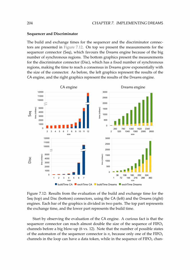
204 CHAPTER 7. IMPLEMENTING DREAMS
Sequencer and Discriminator
The build and exchange times for the sequencer and the discriminator connec-tors are presented in Figure 7.12. On top we present the measurements for thesequencer connector (Seq), which favours the Dreams engine because of the bignumber of synchronous regions. The bottom graphics present the measurementsfor the discriminator connector (Disc), which has a fixed number of synchronousregions, making the time to reach a consensus in Dreams grow exponentially withthe size of the connector. As before, the left graphics represent the results of theCA engine, and the right graphics represent the results of the Dreams engine.
CA engine Dreams engine
Seq
2 3 4 5 6 7 8 9 10 11 120
1000
2000
3000
4000
5000
6000
7000
8000
9000
size
time
(milis
ec)
12000
11000
10000
2260
520780
10401300
15601820
20802340
2600
0
500
1000
1500
2000
2500
3000
size
time
(milis
ec)
Dis
c
1 2 3 4 5 6 70
1000
2000
3000
4000
5000
6000
7000
8000
9000
size
time
(milis
ec)
12000
11000
10000
136
72108
144180
216252
288324
360
0
500
1000
1500
2000
2500
3000
size
time
(mili
sec)
buildTime CA exchTime CA buildTime Dreams exchTime Dreams
Figure 7.12: Results from the evaluation of the build and exchange time for theSeq (top) and Disc (bottom) connectors, using the CA (left) and the Dreams (right)engines. Each bar of the graphics is divided in two parts. The top part representsthe exchange time, and the lower part represents the build time.
Start by observing the evaluation of the CA engine. A curious fact is that thesequencer connector can reach almost double the size of the sequence of FIFO1channels before a big blow-up (6 vs. 12). Note that the number of possible statesof the automaton of the sequencer connector is n, because only one of the FIFO1channels in the loop can have a data token, while in the sequence of FIFO1 chan-
7.5. BENCHMARKS 205
nels any combination of empty and full FIFO1’s is possible. However, intuitionsays that the sequencer connector of size n would still need to calculate the be-haviour of a sequence of n − 1 FIFO1 channels before the loop can be closed,reducing the number of possible states. So, why is it that the CA engine canhandle more FIFO1’s in the sequencer connector than in the case of a series ofFIFO1’s? This is explained by the order in which the CA engine composes itsautomata. Instead of composing the automata in sequence (a1 ./ a2) . . . ./ an,it builds a balanced tree to with the automata to be composed and calculates(a1 . . . ./ . . . an/2) ./ (an/2+1 . . . ./ . . . an). The goal of this heuristic is to com-pose automata with similar sizes, assuming that in general the composition oftwo automata yields a larger automaton than any of the initial automata. Hencewhen calculating the sequencer with twelve FIFO1’s, the CA engine calculates twoautomata with six FIFO1’s each, which should take around 2 × 3700, and onlythan calculates its composition, which will yield a much smaller automaton. Thebuild time of the discriminator also explodes for relatively small connectors, asexpected.
The Dreams execution of Disc reveals an unexpected observation. The buildtime appears to grows exponentially, as opposed to the previous examples whereit grows linearly. This is explained by a choice in the current implementation ofthe nodes in the Dreams engine. When a new port is added to a node, the Dreams
engine builds the new constraint for the coordination behaviour of the node fromscratch, disregarding its previous constraint. Therefore, to build a node with nports the engine finds the constraints for 1 port, then for 2 ports, until n ports. Asimple optimisation is to postpone the calculation of the coordination behaviouruntil the suspension is released.
Discussion
These four examples show that the Dreams engine is specially relevant in two mainsituations: (1) when the connector needs to be re-compiled (or reconfigured) fre-quently, and (2) when the pre-computation is infeasible because of the excessivetime required to compile it. These benchmarks also support the discussion in§6.5.4, where we claim that an ideal scenario needs to have a good balance of pre-computation (as implemented in the CA engine) and on-the-fly computation (asimplemented in the Dreams engine).
The key insight obtained from these benchmarks is how automata-based im-plementations fail to execute more complex connectors, where the number ofpossible states explodes exponentially. It highlights the tradeoff between pre-computation and on-the-fly computation, suggesting different scenarios requiredifferent approaches. Note, however, that the true power of the automata modelsis in the verification of systems, which is not addressed by the Dreams framework.In fact, the Dreams framework exploits the fact that discovering only one possible
206 CHAPTER 7. IMPLEMENTING DREAMS
step at each round is enough for the execution of a connector, and the fact thatnot all actors require synchronous communication. Furthermore, Dreams doesnot require any further knowledge beyond the next step, which may not even beavailable or known for some primitives.
7.6 Scala implementation
The Dreams framework is implemented in Scala,5 a language that integrates fea-tures of object-oriented and functional languages, and that is fully interoperablewith Java. More specifically, Dreams uses the actor library of Scala [57]. Scalaprograms are compiled into Java binary classes.
The most recent version of the source code of our implementation is availablein our Reo repository.6 The source code is grouped into packages. The mostrelevant packages are presented below. Later in this section we describe otherpackages, also available in our repository.
• cwi.reo.engine.common – defines behavioural automata and atomic steps;
• cwi.reo.engine.redrum7 – definesReo primitives;
• cwi.reo.engine.colouring – defines the CC semantics as behavioural au-tomata;
• cwi.reo.engine.SAT – defines the constraint-based semantics as behaviour-al automata.
The definitions ofReo primitives follow directly the definitions of the reactivebehaviour presented in §7.3. We define proactive actors as an extension of normalprimitives, which we call initiators in the source code. The behaviour of each Reo
primitive, such as a Reo channel or a Reo node, is defined inside the colouring
and the SAT packages. We implemented the context sensitive semantics for boththe CC (using three colours) and for the constraint-based approach (using contextvariables, as described in §5.5.2).
We also performed an optimisation with respect to the data function. The be-havioural automata of the primitives encoded using the CC and constraint-basedsemantics do not depend on the data to agree on the final behavioural automa-ton. Furthermore, by knowing which step to perform without the data function,each primitive can deduce how data should be transferred. This step correspondsto the notion of group of labels with the same sets of ports with dataflow, as de-scribed in §3.5. Therefore, we store the data functions within each primitive, andwe do not include it in the behavioural automaton.
5http://www.scala-lang.org6http://reo.project.cwi.nl/cgi-bin/trac.cgi/reo/browser/reo-engine7The name ‘redrum’ stands forReo distributed machine.
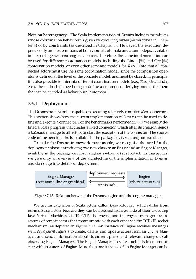
7.6. SCALA IMPLEMENTATION 207
Note on heterogenety The Scala implementation of Dreams includes primitiveswhose coordination behaviour is given by colouring tables (as described in Chap-ter 4) or by constraints (as described in Chapter 5). However, the execution de-pends only on the definitions of behavioural automata and atomic steps, availablein the package cwi.reo.engine.common. Therefore, the same implementation canbe used for different coordination models, including the Linda [54] and Orc [68]coordination models, or even other semantic models for Reo. Note that all con-nected actors must use the same coordination model, since the composition oper-ator is defined at the level of the concrete model, and must be closed. In principle,it is also possible to intermix different coordination models (e.g.,Reo, Orc, Linda,etc.), the main challenge being to define a common underlying model for themthat can be encoded as behavioural automata.
7.6.1 Deployment
The Dreams framework is capable of executing relatively complexReo connectors.This section shows how the current implementation of Dreams can be used to de-fine and execute a connector. For the benchmarks performed in §7.5 we simply de-fined a Scala program that creates a fixed connector, which after its creation, sendsa Release message to all actors to start the execution of the connector. The sourcecode of the benchmarks is available in the package cwi.reo.engine.sandbox.
To make the Dreams framework more usable, we recognise the need for thedeployment phase, introducing two new classes: an Engine and an Engine Manager,available in the package cwi.reo.engine.redrum.distributed. In this sectionwe give only an overview of the architecture of the implementation of Dreams,and do not go into details of deployment.
Engine Manager
(command line or graphical)Engine
(where actors run)
deployment requests
status info.
Figure 7.13: Relation between the Dreams engine and the engine manager.
We use an extension of Scala actors called RemoteActors, which differ fromnormal Scala actors because they can be accessed from outside of their executingJava Virtual Machines via TCP/IP. The engine and the engine manager are in-stances of remote actors that communicate with each other via the TCP/IP socketmechanism, as depicted in Figure 7.13. An instance of Engine receives messageswith deployment requests to create, delete, and update actors from an Engine Man-
ager, and sends information about its current phase and relevant changes to allobserving Engine Managers. The Engine Manager provides methods to communi-cate with instances of Engine. More than one instance of an Engine Manager can be
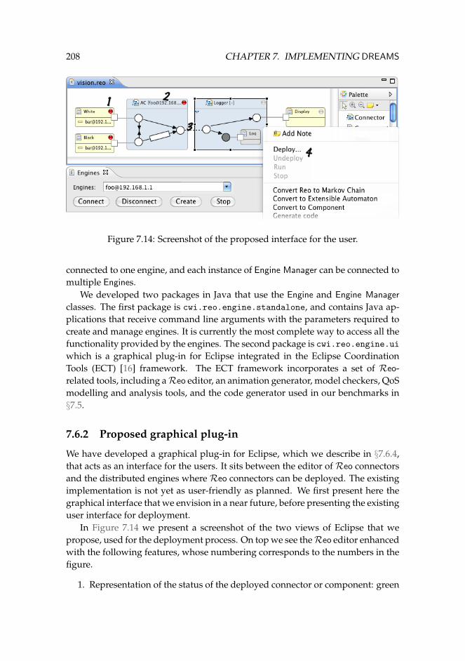
208 CHAPTER 7. IMPLEMENTING DREAMS
Figure 7.14: Screenshot of the proposed interface for the user.
connected to one engine, and each instance of Engine Manager can be connected tomultiple Engines.
We developed two packages in Java that use the Engine and Engine Manager
classes. The first package is cwi.reo.engine.standalone, and contains Java ap-plications that receive command line arguments with the parameters required tocreate and manage engines. It is currently the most complete way to access all thefunctionality provided by the engines. The second package is cwi.reo.engine.uiwhich is a graphical plug-in for Eclipse integrated in the Eclipse CoordinationTools (ECT) [16] framework. The ECT framework incorporates a set of Reo-related tools, including aReo editor, an animation generator, model checkers, QoSmodelling and analysis tools, and the code generator used in our benchmarks in§7.5.
7.6.2 Proposed graphical plug-in
We have developed a graphical plug-in for Eclipse, which we describe in §7.6.4,that acts as an interface for the users. It sits between the editor of Reo connectorsand the distributed engines where Reo connectors can be deployed. The existingimplementation is not yet as user-friendly as planned. We first present here thegraphical interface that we envision in a near future, before presenting the existinguser interface for deployment.
In Figure 7.14 we present a screenshot of the two views of Eclipse that wepropose, used for the deployment process. On top we see theReo editor enhancedwith the following features, whose numbering corresponds to the numbers in thefigure.
1. Representation of the status of the deployed connector or component: green
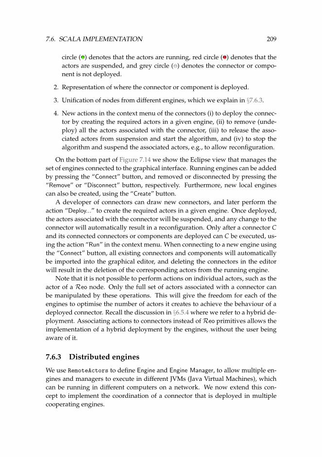
7.6. SCALA IMPLEMENTATION 209
circle ( ) denotes that the actors are running, red circle ( ) denotes that theactors are suspended, and grey circle ( ) denotes the connector or compo-nent is not deployed.
2. Representation of where the connector or component is deployed.
3. Unification of nodes from different engines, which we explain in §7.6.3.
4. New actions in the context menu of the connectors (i) to deploy the connec-tor by creating the required actors in a given engine, (ii) to remove (unde-ploy) all the actors associated with the connector, (iii) to release the asso-ciated actors from suspension and start the algorithm, and (iv) to stop thealgorithm and suspend the associated actors, e.g., to allow reconfiguration.
On the bottom part of Figure 7.14 we show the Eclipse view that manages theset of engines connected to the graphical interface. Running engines can be addedby pressing the “Connect” button, and removed or disconnected by pressing the“Remove” or “Disconnect” button, respectively. Furthermore, new local enginescan also be created, using the “Create” button.
A developer of connectors can draw new connectors, and later perform theaction “Deploy...” to create the required actors in a given engine. Once deployed,the actors associated with the connector will be suspended, and any change to theconnector will automatically result in a reconfiguration. Only after a connector Cand its connected connectors or components are deployed can C be executed, us-ing the action “Run” in the context menu. When connecting to a new engine usingthe “Connect” button, all existing connectors and components will automaticallybe imported into the graphical editor, and deleting the connectors in the editorwill result in the deletion of the corresponding actors from the running engine.
Note that it is not possible to perform actions on individual actors, such as theactor of a Reo node. Only the full set of actors associated with a connector canbe manipulated by these operations. This will give the freedom for each of theengines to optimise the number of actors it creates to achieve the behaviour of adeployed connector. Recall the discussion in §6.5.4 where we refer to a hybrid de-ployment. Associating actions to connectors instead of Reo primitives allows theimplementation of a hybrid deployment by the engines, without the user beingaware of it.
7.6.3 Distributed engines
We use RemoteActors to define Engine and Engine Manager, to allow multiple en-gines and managers to execute in different JVMs (Java Virtual Machines), whichcan be running in different computers on a network. We now extend this con-cept to implement the coordination of a connector that is deployed in multiplecooperating engines.
210 CHAPTER 7. IMPLEMENTING DREAMS
...
x1
xn
...
y1
ym
=⇒ ...
x1
xn
...
y1
ym
Figure 7.15: Unification of remote nodes.
A naive approach is to assume that all actors are remote actors, accessible fromthe outside of their JVMs. We avoid the overhead of making all actors accessiblefrom the outside, and restrict the remote actors to only a new Reo primitive thatwe call remote node. Consequently, all remote communication is embodied in asingle type of actor. Note that we do not forbid the creation of other remote actors,although in most scenarios this is not required. An interesting direction wouldbe to define remote split actors for efficiency reasons, since this requires fewermessages to be exchanged. However, as we will see shortly, remote split actorsare not as general as remote nodes.
A remote node is an actor with the same behavioural automaton as that of atraditionalReo node. However, a remote node is also accessible from other JVMs,and can be unified with other remote nodes, as depicted in Figure 7.15. When tworemote nodes are unified they exhibit the same behavioural automaton as that ofa single Reo node with the union of all their ports. More than two remote nodescan be unified in a pairwise fashion. A pair of unified remote nodes share theinformation regarding which ports they have, and follow the same distributedalgorithm described in this chapter. We have adapted the algorithm presentedearlier in §7.3 to accommodate the communication between unified nodes becausein this case communication can occur in both directions depending on the step ofthe current round, but we omit these details here.
We extend the idea of connected engines via remote nodes to allow generalcomponents to be connected to already runningReo connectors. We define a newclass ComponentPort that wraps a variation of a data writer or reader connectedtogether with a remote node. The component ports are made available to any Javadeveloper, providing methods to send data to or receive data from the compo-nent port, as well as to unify other remote nodes. The source code of the remotenodes and the source code of the component ports are available in the packagecwi.reo.engine.redrum.distributed. Furthermore, small examples of the useof the component ports can be found in the package cwi.reo.engine.standalone.
7.6.4 Existing graphical plug-in
The existing graphical deployment plug-in for Eclipse is depicted in Figure 7.16.It uses theReo editor included in the ECT framework to extract information from
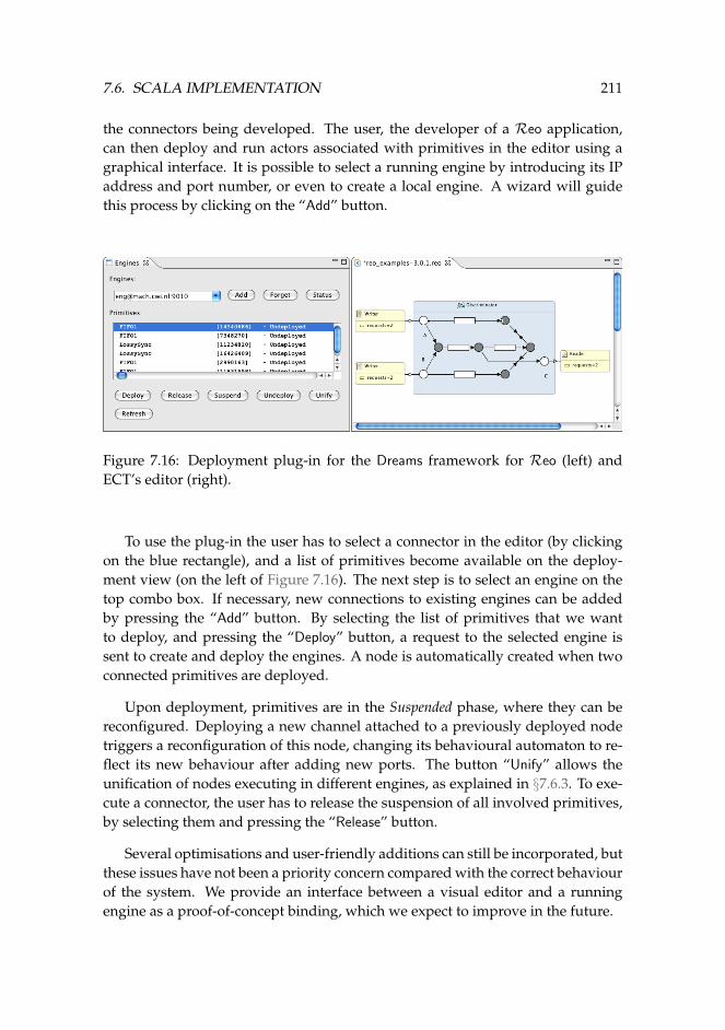
7.6. SCALA IMPLEMENTATION 211
the connectors being developed. The user, the developer of a Reo application,can then deploy and run actors associated with primitives in the editor using agraphical interface. It is possible to select a running engine by introducing its IPaddress and port number, or even to create a local engine. A wizard will guidethis process by clicking on the “Add” button.
Figure 7.16: Deployment plug-in for the Dreams framework for Reo (left) andECT’s editor (right).
To use the plug-in the user has to select a connector in the editor (by clickingon the blue rectangle), and a list of primitives become available on the deploy-ment view (on the left of Figure 7.16). The next step is to select an engine on thetop combo box. If necessary, new connections to existing engines can be addedby pressing the “Add” button. By selecting the list of primitives that we wantto deploy, and pressing the “Deploy” button, a request to the selected engine issent to create and deploy the engines. A node is automatically created when twoconnected primitives are deployed.
Upon deployment, primitives are in the Suspended phase, where they can bereconfigured. Deploying a new channel attached to a previously deployed nodetriggers a reconfiguration of this node, changing its behavioural automaton to re-flect its new behaviour after adding new ports. The button “Unify” allows theunification of nodes executing in different engines, as explained in §7.6.3. To exe-cute a connector, the user has to release the suspension of all involved primitives,by selecting them and pressing the “Release” button.
Several optimisations and user-friendly additions can still be incorporated, butthese issues have not been a priority concern compared with the correct behaviourof the system. We provide an interface between a visual editor and a runningengine as a proof-of-concept binding, which we expect to improve in the future.
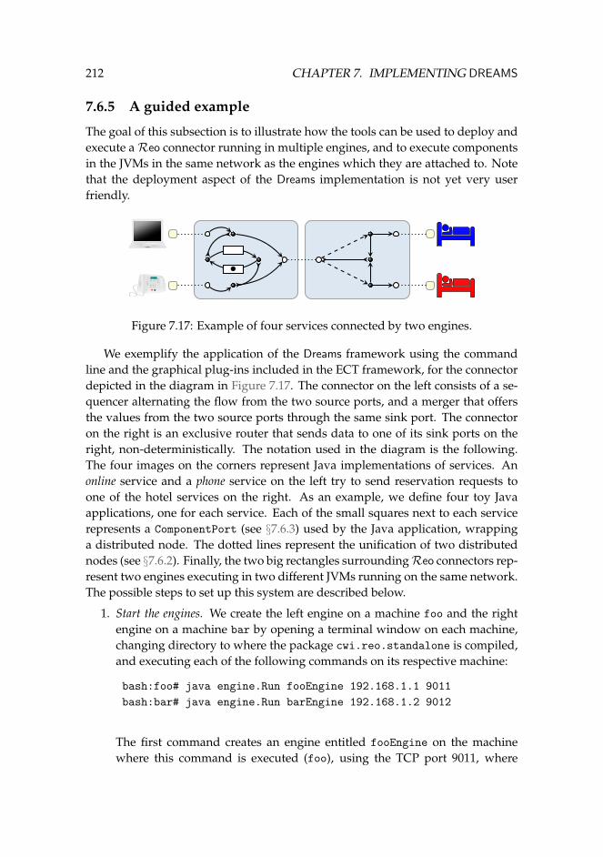
212 CHAPTER 7. IMPLEMENTING DREAMS
7.6.5 A guided example
The goal of this subsection is to illustrate how the tools can be used to deploy andexecute aReo connector running in multiple engines, and to execute componentsin the JVMs in the same network as the engines which they are attached to. Notethat the deployment aspect of the Dreams implementation is not yet very userfriendly.
•
Figure 7.17: Example of four services connected by two engines.
We exemplify the application of the Dreams framework using the commandline and the graphical plug-ins included in the ECT framework, for the connectordepicted in the diagram in Figure 7.17. The connector on the left consists of a se-quencer alternating the flow from the two source ports, and a merger that offersthe values from the two source ports through the same sink port. The connectoron the right is an exclusive router that sends data to one of its sink ports on theright, non-deterministically. The notation used in the diagram is the following.The four images on the corners represent Java implementations of services. Anonline service and a phone service on the left try to send reservation requests toone of the hotel services on the right. As an example, we define four toy Javaapplications, one for each service. Each of the small squares next to each servicerepresents a ComponentPort (see §7.6.3) used by the Java application, wrappinga distributed node. The dotted lines represent the unification of two distributednodes (see §7.6.2). Finally, the two big rectangles surroundingReo connectors rep-resent two engines executing in two different JVMs running on the same network.The possible steps to set up this system are described below.
1. Start the engines. We create the left engine on a machine foo and the rightengine on a machine bar by opening a terminal window on each machine,changing directory to where the package cwi.reo.standalone is compiled,and executing each of the following commands on its respective machine:
bash:foo# java engine.Run fooEngine 192.168.1.1 9011
bash:bar# java engine.Run barEngine 192.168.1.2 9012
The first command creates an engine entitled fooEngine on the machinewhere this command is executed (foo), using the TCP port 9011, where
7.6. SCALA IMPLEMENTATION 213
192.168.1.1 is the IP address used to access this machine. Similarly, thesecond command creates an engine called barEngine on the machine wherethis command is executed (bar), using the TCP port 9012, with IP address192.168.1.2.
2. Deploy the connectors. The connectors will be created using the graphical de-ployment plug-in, depicted in Figure 7.16. For that we open Eclipse on amachine in the same network as foo and bar with the editor and deploy-ment views. In the deployment view we click the “Add” button in the en-gines area, and insert the information regarding the fooEngine, and repeatthe same for the barEngine. We create two connectors in the editor, one foreach part (the two central boxes) of the connector in Figure 7.17. We clickon the left connector, and the list of primitives in the deployment view isupdated. We select the fooEngine, then all primitives in the list, and pressthe Deploy button. We repeat this process for the barEngine with the rightconnector.
3. Connect the engines. We unify the sink node of the left connector with thesource node of the right connector using the Eclipse plug-in. We select thetwo nodes that we want to unify in the Reo editor, and press the “Unify”button in the deployment view. We make the boundary nodes that willbe attached to components accessible via TCP/IP using the manager in thecommand-line tools. We read the identifier prim of the channel attached toeach boundary node from the list of primitives in the graphical deploymentplug-in, and use the manager in the package cwi.reo.engine.standalone
as follows.
bash:foo# java engine.Manager fooEngine 192.168.1.1 9011 \
Awake prim 9013
The command-line instruction above assumes the correct classpath is de-fined and prim is the identifier of a boundary node deployed in fooEngine.
4. Create the components. The components are developed in plain Java, import-ing the relevant Java binaries resulting from the compilation of the Scalaimplementation of Dreams. In Listing 7.1 we present a Java program On-
lineBooking that can be used to implement the online service in Figure 7.17.We abstract from certain technicalities such as error handling. The programuses an extension of ComponentPort called SinkPort, imported in line 1 andinstantiated as port in line 17. The method addDatum used in line 32 adds thestring stored in variable line (obtained earlier on line 25 from the standard in-put) to the queue of available messages to be sent by the remote node in thecomponent port. How the component port is connected is not of concern in-side the OnlineBooking program: it is the responsibility of the coordination
214 CHAPTER 7. IMPLEMENTING DREAMS
engine. The other components can be created in a similar way, using theextension SourcePort of ComponentPort instead of SinkPort for the hotelservices. The source code of these extensions of component ports is avail-able in the package cwi.reo.engine.redrum.distributed, and examplesof simple Java programs that send and receive text to component ports areavailable in the package cwi.reo.engine.standalone. components.
5. Running the system. The execution of the OnlineBooking Java program con-nects to the distributed node identified in its command line arguments uponcreation of the SinkPort. The port is initially suspended with a default lock,and is released when its release method is invoked in line 17. After its re-lease it becomes idle because no data is available for it to send. We repeatthe same process for the other components. The OnlineBooking programcan try to send a booking request already, but its message will not be con-sumed by the connector because the other actors are still suspended. Werelease the connector using the deployment view in the Eclipse plug-in, byselecting all channels and pressing the Release button. The componentscan now request data to be sent or received, changing the states of their be-havioural automata when they become idle, and engage in the distributedalgorithm described in this chapter.
7.7 Conclusions
This chapter takes a more practical view of the Dreams framework, and presentshow the distributed algorithm for committing to a behavioural automaton andsending data operates in detail. It also shows how a developer of Reo connectorscan use the current implementation of Dreams in the context of ECT.
The interplay between synchrony and asynchrony, reactive behaviour and co-ordination behaviour, open new possibilities for scalability and reconfigurationof synchronous languages such as Reo. We showed based on benchmarks thatprecompiling the full behaviour is not always possible or advantageous. The sep-aration of a single connector into independently executing sub-connectors alsoallows for a more flexible framework for development and concurrent reconfigu-ration of larger coordination specifications.
For future work we aim to compare the execution of connectors on multiplecomputers. At the moment the process of deploying a connector over a networkis not yet fully automatised, leaving new research questions. These questionsinclude: how to optimise the number of actors and behavioural automata for agiven connector; how to automatically chose in which machine should each actorbe deployed, and how to dynamically adapt a running connector based propertiesof the network and demand for communication.
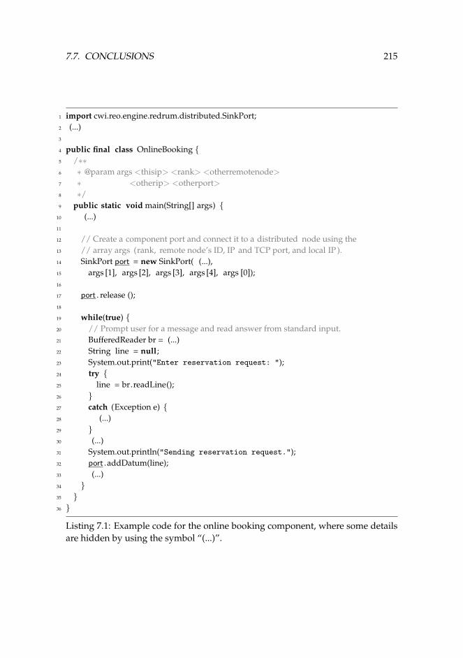
7.7. CONCLUSIONS 215
1 import cwi.reo.engine.redrum.distributed.SinkPort;2 (...)3
4 public final class OnlineBooking {5 /∗∗6 ∗ @param args <thisip> <rank> <otherremotenode>7 ∗ <otherip> <otherport>8 ∗/9 public static void main(String[] args) {
10 (...)11
12 // Create a component port and connect it to a distributed node using the13 // array args (rank, remote node’s ID, IP and TCP port, and local IP ).14 SinkPort port = new SinkPort( (...),15 args [1], args [2], args [3], args [4], args [0]);16
17 port . release ();18
19 while(true) {20 // Prompt user for a message and read answer from standard input.21 BufferedReader br = (...)22 String line = null;23 System.out.print("Enter reservation request: ");24 try {25 line = br.readLine();26 }27 catch (Exception e) {28 (...)29 }30 (...)31 System.out.println("Sending reservation request.");32 port .addDatum(line);33 (...)34 }35 }36 }
Listing 7.1: Example code for the online booking component, where some detailsare hidden by using the symbol “(...)”.

Chapter 8
Conclusions
This thesis is an exploration in the field of coordination, with special focus onmodels with synchronisation constructs. Most of the work was developed to sup-port the coordination language Reo, although the results extend beyond and areapplicable outside the scope ofReo.
The main question addressed in this thesis is how to manage the complex-ity of synchronous models. Hitherto existing implementations of Reo representa connector by a monolithic state-based system that controls all communication.However, this approach does not scale up to larger connectors, due to the expo-nential growth of connectors obtained when composing the building blocks of anelaborate coordination layer.
Our key contribution is the development of new implementation techniquesfor Reo-like languages, which exploits concurrency and shifts part of the calcula-tion of the coordination behaviour into runtime. We successfully deal with largerconnectors than previousReo engines, and we can execute such synchronous con-nectors in a distributed network.
Main contributions
In Chapters 2, 3, and 4 of this thesis, we gave a formal presentation of existing co-ordination models and introduced the stepwise coordination model. We exploredhow to use the connector colouring semantics in a distributed implementation.The stepwise model focuses on the same key concerns as the connector colour-ing semantics: the compositional development of synchronous coordination sys-tems. We encoded connector colouring in the stepwise model, extending it withstate changes, with data constraints, and with the notion of local colourings. Wealso presented an animation framework to exemplify the challenges of using theconnector colouring semantics as the basis of an implementation that sends dataacross aReo connector. The animation framework provided the starting point fordeveloping the Dreams distributed engine, introduced in this thesis.
217
218 CHAPTER 8. CONCLUSIONS
In Chapters 5, 6, and 7, we improved existing techniques to execute synchro-nous coordination models such asReo in three ways:
• by increasing performance using constraint satisfaction techniques;
• by improving scalability by identifying synchronous regions; and
• by supporting decoupled execution and lightweight reconfiguration.
We briefly review each of these contributions below.
Constraint satisfaction This work alleviates some of the performance and scal-ability limitations of existing implementation of Reo by shifting part of the com-putation of the composition of behaviour from compile time to runtime. As ex-plained in Chapter 5, we used existing constraint satisfaction techniques to calcu-late the coordination behaviour of each atomic step, reducing the complexity ofthe composition operation.
Synchronous regions In Chapter 6 we introduced Dreams, a framework that pro-vides a distributed implementation based on the stepwise coordination model,using the actor model to describe the primitive communication between concur-rent elements. Equipped with the notion of locality from the stepwise model andthe asynchronous properties of the actor model, we statically find parts of the co-ordination system that can perform local atomic steps. We refer to these regionsas synchronous regions. Synchronous regions communicate with each other usingonly asynchronous requests for state updates, without changing the behaviour ofthe overall system. Hence, adding new synchronous regions to a connector doesnot affect the behaviour of each of the synchronous regions, allowing scalable im-plementations.
Decoupled execution The Dreams framework is structured as an Actor Mod-el [1]. Its implementation, described in Chapter 7, uses the actor library of Scala.Actors are primitives that communicate with each other using a reliable and order-preserving message passing mechanism. Our main contribution is to assign toeach actor a description of the coordination behaviour, given by the stepwisemodel, and to send data through the connector according the composed behaviourof all actors. We developed a distributed algorithm where actors associated withthe same synchronous region reach a consensus regarding the atomic step to beperformed before sending the data through the connector. The computation ofthis atomic step is performed by one of the actors of the synchronous region, andnot by a centralised entity.
As an orthogonal contribution, this thesis addressed Reo’s semantics, givingan exhaustive comparison of existing models and implementations, with specialemphasis on to three particular models. We explained what is salient in Reo and
219
what aspects of coordination are left uncovered. We argue that, common to all ex-isting models, are synchronous constraints over ports in a compositional framework.We use these notions in our implementation, and include dataflow informationand locality aspects.
Future work
The stepwise coordination model described in Chapter 3 presents only the re-quired aspects of coordination for our distributed framework. As future work, weleave a more complete formal treatment of this model, that is, we leave open thequestion of how to reuse formal proofs over the stepwise coordination model thatcan be directly applied in more concrete models. Furthermore, we provide an in-formal description of the correctness of the instantiation of concrete coordinationmodels into the stepwise model, leaving as future work a complete formalisationof these proofs.
The animation framework, presented in Chapter 4, creates visual animations ofReo representing differently different data elements flowing in the network, andincluding state information. A possible way to improve the current animationengine is to include local steps, and to show the behaviour of only a subset ofa connector. Furthermore, the animations can be extended with new informationregarding, for example, properties of the underlying network, amount of expectedtraffic, or security level of the data channels.
In Chapter 5 we use constraint satisfaction techniques to calculate the coor-dination behaviour of each step. Regarding this a number of questions remainunaddressed in this thesis.
• What other relevant notions, besides synchronisation, data, and context de-pendency, are useful to model existing coordination systems?
• How can a constraint solver be guided more efficiently to find coordinationsolutions?
• How can the existing constraints be extended, e.g., with special symbols thatare initially unknown, but are replaced by their interpretations only whenneeded?
• How to perform constraint solving using these special symbols?
• How to find a solution σ for a subset of a conjunctive collection of con-straints, such that σ is also a solution for the global collection? This wouldallow, for example, to represent constraints that grow in a per-need basis,without size restrictions.
220 CHAPTER 8. CONCLUSIONS
We gave several suggestions how to guide the constraint solver in §5.7, withoutgoing into detail. The last two questions are partially addressed in existing workregarding constraint-based coordination [38, 40]. Furthermore, we presented inthis thesis an alternative approach to search for solutions for only a subset of con-straints based on synchronous regions, described below. We statically identify acollection of constraints whose solutions will always be solutions of a more globalset of constraints. However, how to allow these sets to be discovered dynamicallyduring constraint satisfaction is ongoing work.
The Dreams framework is introduced in Chapter 6, where we describe how andwhy different regions, dubbed synchronous regions, can evolve in parallel with-out requiring a global consensus at each step. We identify two possible directionsof future work regarding the use of synchronous regions.
• Partition a connector into its synchronous regions by an automatic splittingmechanism. Currently we analyse manually each building block of the co-ordination model and try to find ports that communicate asynchronously,without any tool support. Ideally, this process would be automated, or al-ternatively, the discovery of synchronous regions can happen at runtime, assuggested in the discussion above regarding constraint satisfaction.
• Find a balance between pre-compilation and runtime computation of thecoordination behaviour, as discussed in §6.5.4. We utilise the extreme casewhere the behaviour of every building block is composed only at runtime,to better evaluate the pros and cons of our approach compared to static ap-proaches. In practice, it makes sense to precompile the behaviour of someparts of the connector, in particular when these do not change over time andalways require synchronous communication.
In Chapter 7, the last one of this thesis, we describe the communication be-tween actors in more detail, and provide more technical details regarding theimplementation of the Dreams framework. This implementation can still be im-proved in several ways. We list some possible directions.
• Integrate Dreams with existing web-service protocols, using, for example,SOAP messages.1
• Automate of the deployment process as suggested in §7.6.2.
• Benchmark the execution of connectors in a distributed network. That is,consider the time to send messages between different machines and not onlybetween threads.
1http://www.w3.org/TR/#tr_SOAP
221
• Optimise the number of actors for a given connector, by composing simpleractors into more complex actors at compile time.
• Find automatically on which machine each actor should be deployed.
• Dynamically adapt a running connector based on properties of the networkand demand for communication.
• Model failure, that is, describe how the system should behave if, at any time,the connection between two actors is broken.
In conclusion, the Dreams framework answers questions raised concerningthe applicability of synchronous coordination models: are they too complex tobe practically useful? The techniques proposed in this thesis provide increasedperformance of synchronous coordination systems by diminishing the computa-tional complexity of their execution. We believe our contributions of exploitingconstraint-solving and introducing independent asynchrony indeed make syn-chronous coordination practically useful.

Bibliography
[1] Gul Agha. Actors: a model of concurrent computation in distributed systems.MIT Press, Cambridge, MA, USA, 1986. 1, 6.1, 6.2, 8
[2] Gul Agha and Prasanna Thati. An algebraic theory of actors and its ap-plication to a simple object-based language. In Olaf Owe, Stein Krogdahl,and Tom Lyche, editors, Essays in Memory of Ole-Johan Dahl, volume 2635 ofLecture Notes in Computer Science, pages 26–57. Springer, 2004. 6.1, 6.2, 7.2
[3] Alfred V. Aho, Ravi Sethi, and Jeffrey D. Ullman. Compilers: principles, tech-niques, and tools. Addison-Wesley Longman Publishing Co., Inc., Boston,MA, USA, 1986. 3.7
[4] Jean-Marc Andreoli, Steve Freeman, and Remo Pareschi. The coordinationlanguage facility: coordination of distributed objects. Theory and Practice ofObject Systems, 2(2):77–94, 1996. 5.10
[5] Jean-Marc Andreoli and Remo Pareschi. Linear objects: logical processeswith built-in inheritance. New Generation Computing, pages 495–510, 1990.5.10
[6] Krzysztof Apt. Principles of Constraint Programming. Cambridge UniversityPress, 2003. 5.7
[7] Farhad Arbab. Coordination of mobile components. Electronic Notes in The-oretical Computer Science, 54, 2001. 1
[8] Farhad Arbab. Reo: a channel-based coordination model for componentcomposition. Mathematical Structures in Computer Science, 14(3):329–366,2004. 1, 2.1, 2.2, 2.2.3, 3, 3.7, 4.1, 4.2, 5.1, 5.2, 5.5, 5.9, 5.9.1, 6.5.2
[9] Farhad Arbab. Abstract behavior types: a foundation model for compo-nents and their composition. Science of Computer Programming, 55:3–52, 2005.2.1, 2.2, 4.2, 4.7, 5.2, 5.9.1, 6.5.2
223
224 Bibliography
[10] Farhad Arbab. Composition of Interacting Computations, chapter 12, pages277–321. Springer-Verlag New York, Inc., Secaucus, NJ, USA, 2006. 2.1, 3.7,5.10, 6.6
[11] Farhad Arbab. Elements of interaction. In Marc Aiguier, Francis Bre-taudeau, and Daniel Krob, editors, Complex Systems Design and Management,pages 1–28. Springer Berlin Heidelberg, October 2010. 5.1
[12] Farhad Arbab, Lacramioara Astefanoaei, Frank S. de Boer, Mehdi Dastani,John-Jules Ch. Meyer, and Nick A. M. Tinnemeier. Reo connectors as co-ordination artifacts in 2apl systems. In The Duy Bui, Tuong Vinh Ho, andQuang-Thuy Ha, editors, PRIMA, volume 5357 of Lecture Notes in ComputerScience, pages 42–53. Springer, 2008. 1
[13] Farhad Arbab, Christel Baier, Frank S. de Boer, and Jan J. M. M. Rutten.Models and temporal logical specifications for timed component connec-tors. Software and System Modeling, 6(1):59–82, 2007. 1, 3.8, 5.9.1
[14] Farhad Arbab, Roberto Bruni, Dave Clarke, Ivan Lanese, and Ugo Monta-nari. Tiles for Reo. In Andrea Corradini and Ugo Montanari, editors, RecentTrends in Algebraic Development Techniques, volume 5486 of Lecture Notes inComputer Science, pages 37–55. Springer Berlin/Heidelberg, 2009. 3.1, 4.1,4.7, 4.8, 5.9.1, 6.5.4
[15] Farhad Arbab, Tom Chothia, Sun Meng, and Young-Joo Moon. Componentconnectors with QoS guarantees. In Amy L. Murphy and Jan Vitek, editors,COORDINATION, volume 4467 of Lecture Notes in Computer Science, pages286–304. Springer, 2007. 1, 3.8, 4.7, 5.9.1
[16] Farhad Arbab, Christian Koehler, Ziyan Maraikar, Young-Joo Moon, andJose Proenca. Modeling, testing and executing Reo connectors with theEclipse Coordination Tools. In Proceedings of FACS, SCP, 2008. Toolsavailable at http://reo.project.cwi.nl/cgi-bin/trac.cgi/reo/wiki/
Tools. 1, 1, 2.2, 3.6.1, 4.1, 4.6.5, 5.8, 5.9, 5.9.2, 7.5, 7.6.1
[17] Farhad Arbab, Natallia Kokash, and Sun Meng. Towards using Reo forcompliance-aware business process modeling. In Tiziana Margaria andBernhard Steffen, editors, ISoLA, volume 17 of Communications in Computerand Information Science, pages 108–123. Springer, 2008. 1
[18] Farhad Arbab and Eric Monfroy. Coordination of heterogeneous distributedcooperative constraint solving. SIGAPP Applied Computing Review, 6(2):4–17,1998. 5.10
[19] Farhad Arbab and Jan J. M. M. Rutten. A coinductive calculus of compo-nent connectors. In Martin Wirsing, Dirk Pattinson, and Rolf Hennicker,
Bibliography 225
editors, WADT, volume 2755 of Lecture Notes in Computer Science, pages 34–55. Springer, 2002. 2.2.3
[20] Farhad Arbab, Meng Sun, and Christel Baier. Synthesis of Reo circuits fromscenario-based specifications. Electronic Notes in Theoretical Computer Science,229(2):21–41, 2009. 1
[21] Christel Baier. Probabilistic models for Reo connector circuits. Journal ofUniversal Computer Science, 11(10):1718–1748, 2005. 1, 3.8, 5.9.1
[22] Christel Baier, Marjan Sirjani, Farhad Arbab, and Jan J. M. M. Rutten. Mod-eling component connectors in Reo by constraint automata. Science of Com-puter Programming, 61(2):75–113, 2006. 2, 2.2.1, 2.2.2, 2.2.3, 2.2.6, 3.4.1, 3.6.1,4.7, 5.3.2, 5.4.1, 5.4.3, 5.4.3, 3, 5.9.1, 6.5.2
[23] Christel Baier and Verena Wolf. Stochastic reasoning about channel-basedcomponent connectors. In Paolo Ciancarini and Herbert Wiklicky, editors,COORDINATION, volume 4038 of Lecture Notes in Computer Science, pages1–15. Springer, 2006. 1, 3.8, 5.9.1
[24] David E. Bakken and Richard D. Schlichting. Supporting fault-tolerant par-allel programming in Linda. IEEE Transactions on Parallel and DistributedSystems, 6, 1995. 6.6
[25] Alberto Baragatti, Roberto Bruni, Hernan Melgratti, Ugo Montanari, andGiorgio Spagnolo. Prototype platforms for distributed agreements. Elec-tronic Notes in Theoretical Computer Science, 180(2):21–40, 2007. 6.6
[26] Lorenzo Bettini, Viviana Bono, Rocco De Nicola, Gianluigi Ferrari, DanieleGorla, Michele Loreti, Eugenio Moggi, Rosario Pugliese, Emilio Tuosto, andBetti Venneri. The Klaim project: Theory and practice. In Global Comput-ing: Programming Environments, Languages, Security and Analysis of Systems,volume 2874 of Lecture Notes in Computer Science, pages 88–150. Springer-Verlag, 2003. 2.3, 5.10
[27] Robert D. Bjornson. Linda on distributed memory multiprocessors. PhD thesis,Yale University, New Haven, CT, USA, 1993. 6.6
[28] Marcello M. Bonsangue, Farhad Arbab, Jaco de Bakker, Jan J. M. M. Rutten,Adriano Scutella, and Gianluigi Zavattaro. A transition system semanticsfor the control-driven coordination language Manifold. Theoretical ComputerScience, 240(1):3–47, 2000. 2.1, 5.10
[29] Marcello M. Bonsangue, Dave Clarke, and Alexandra Silva. Automata forcontext-dependent connectors. In John Field and Vasco Thudichum Vascon-celos, editors, COORDINATION, volume 5521 of Lecture Notes in Computer
226 Bibliography
Science, pages 184–203. Springer, 2009. 2.2.3, 2.2.8, 2.2.3, 2.2.3, 3.4.1, 4.7, 4.8,5.5, 5.9.1
[30] BPEL4WS. Business Process Execution Language for Web Services, May 2003.6.6
[31] Jarvis Dean Brock and William Ackerman. Scenarios: A model of non-determinate computation. In J. Dıaz and I. Ramos, editors, Formalizationof Programming Concepts, volume 107 of Lecture Notes in Computer Science,pages 252–259. Springer Berlin / Heidelberg, 1981. 10.1007/3-540-10699-5-102. 3.7
[32] Roberto Bruni, Cosimo Laneve, and Ugo Montanari. Orchestrating trans-actions in Join calculus. In Lubos Brim, Petr Jancar, Mojmır Kretınsky, andAntonın Kucera, editors, CONCUR, volume 2421 of Lecture Notes in Com-puter Science, pages 321–337. Springer, 2002. 6.6, 7.4.3
[33] Paolo Ciancarini, Keld K. Jensen, and Daniel Yankelevich. On the oper-ational semantics of a coordination language. In Paolo Ciancarini, OscarNierstrasz, and Akinori Yonezawa, editors, Object-Based Models and Lan-guages for Concurrent Systems, volume 924 of Lecture Notes in Computer Sci-ence, pages 77–106. Springer-Verlag, 1995. 2.3, 2.3
[34] Dave Clarke. Coordination: Reo, nets, and logic. In Frank S. de Boer, Mar-cello M. Bonsangue, Susanne Graf, and Willem P. de Roever, editors, FMCO,volume 5382 of Lecture Notes in Computer Science, pages 226–256. Springer,2007. 4.7, 5.3.2, 5.9.1, 5.10
[35] Dave Clarke. A basic logic for reasoning about connector reconfiguration.Fundamenta Informaticae, 82(4):361–390, 2008. 1, 5.9.1, 5.9.1
[36] Dave Clarke, David Costa, and Farhad Arbab. Modelling coordination in bi-ological systems. In Tiziana Margaria and Bernhard Steffen, editors, Leverag-ing Applications of Formal Methods, volume 4313 of Lecture Notes in ComputerScience, pages 9–25. Springer Berlin, 2006. 1
[37] Dave Clarke, David Costa, and Farhad Arbab. Connector colouring I: Syn-chronisation and context dependency. Science of Computer Programming,66(3):205–225, May 2007. 1, 2, 2.2.1, 2.2.3, 3.4.1, 4.1, 4.2, 2, 4.3, 4.4.4, 4.7,5.1, 5.5, 5.5.1, 5.5.2, 5.5.3, 5.6, 5.8, 5.9.1, 5.9.2, 6.5, 6.5.4
[38] Dave Clarke and Jose Proenca. Coordination via interaction constraints i:Local logic. CoRR, abs/0911.5445, 2009. 5.11, 8
[39] Dave Clarke, Jose Proenca, Alexander Lazovik, and Farhad Arbab. Decon-structing Reo. In Proceedings of the International Workshop on the Foundations of
Bibliography 227
Coordination Languages and Software Architecture (FOCLASA). Elsevier, 2008.4.7, 5.11
[40] Dave Clarke, Jose Proenca, Alexander Lazovik, and Farhad Arbab.Channel-based coordination via constraint satisfaction. Science of ComputerProgramming, In Press, Accepted Manuscript, 2010. 4.7, 6.5.4, 8
[41] David Costa. Formal Methods for Component Connectors. PhD thesis, VrijeUniversiteit Amsterdam, 2010. 1, 2.2.3, 4.1, 4.1, 4.6, 4.8, 5.9.1
[42] Pierre J. Courtois, F. Heymans, and David L. Parnas. Concurrent controlwith “readers” and “writers”. Commun. ACM, 14(10):667–668, 1971. 3.7
[43] Regis Cridlig and Eric Goubault. Semantics and analysis of linda-basedlanguages. In Patrick Cousot, Moreno Falaschi, Gilberto File, and AntoineRauzy, editors, WSA, volume 724 of Lecture Notes in Computer Science, pages72–86. Springer, 1993. 2.3, 2.3
[44] Allen B. Downey. The Little Book of Semaphores. Green Tea Press, secondedition, 2007. 3.7
[45] Sol Efroni, David Harel, and Irun R. Cohen. Reactive Animation: Realisticmodelling of complex dynamics systems. Computer, 38(1):38–47, 2005. 4.7
[46] Kees Everaars, David Costa, Nikolay Diakov, and Farhad Arbab. A dis-tributed computational model for Reo. Technical Report SEN-E0601, CWI,Amsterdam, The Netherlands, February 2006. 5.9
[47] Ming-Dong Feng, Weng-Fai Wong, and Chung-Kwong Yuen. Balinda lisp:Design and implementation. Computer Languages, 22(4):205–214, 1996. 2.3
[48] Jose Luiz Fiadeiro, Antonia Lopes, and Laura Bocchi. A formal approach toservice component architecture. In Mario Bravetti, Manuel Nunez, and Gi-anluigi Zavattaro, editors, WS-FM, volume 4184 of Lecture Notes in ComputerScience, pages 193–213. Springer, 2006. 5.10
[49] Nate Foster, Michael B. Greenwald, Christian Kirkegaard, Benjamin C.Pierce, and Alan Schmitt. Exploiting schemas in data synchronization. InGavin M. Bierman and Christoph Koch, editors, DBPL, volume 3774 of Lec-ture Notes in Computer Science, pages 42–57. Springer, 2005. 3.7
[50] Cedric Fournet and Georges Gonthier. The join calculus: A language fordistributed mobile programming. In Gilles Barthe, Peter Dybjer, Luis Pinto,and Joao Saraiva, editors, APPSEM, volume 2395 of Lecture Notes in Com-puter Science, pages 268–332. Springer, 2000. 6.6, 7.4.3
228 Bibliography
[51] Eric Freeman, Ken Arnold, and Susanne Hupfer. JavaSpaces Principles, Pat-terns, and Practice. Addison-Wesley Longman Ltd., Essex, UK, UK, 1999. 2.3,5.10, 6.1
[52] Svend Frølund. Coordinating Distributed Objects. The MIT Press, Cambridge,Massachusetts, USA, 1996. 5.10
[53] Fabio Gadducci and Ugo Montanari. The tile model, pages 133–166. MITPress, Cambridge, MA, USA, 2000. 3.1, 5.9.1, 6.5.4
[54] David Gelernter. Generative communication in Linda. ACM Transactionson Programming Languages and Systems, 7(1):80–112, 1985. 2.1, 2.3, 2.3, 3.6.3,5.10, 6.6, 7.6
[55] Rachid Guerraoui and Luıs Rodrigues. Introduction to Reliable DistributedProgramming. Springer-Verlag New York, Inc., Secaucus, NJ, USA, 2006. 6.1,7.4.4
[56] Juan Visente Guillen Scholten. Mobile channels for exogenous coordination ofdistributed systems : semantics, implementation and composition. PhD thesis,LIACS, Faculty of Mathematics and Natural Sciences, Leiden University,January 2007. 5.9
[57] Philipp Haller and Martin Odersky. Scala actors: Unifying thread-basedand event-based programming. Theoretical Computer Science, 410(2-3):202–220, 2009. 1, 7.2, 7.6
[58] David Harel. Statecharts: A visual formalism for complex systems. Scienceof Computer Programming, 8(3):231–274, June 1987. 4.7
[59] David Harel. On visual formalisms. Communications of the ACM, 31(5):514–530, 1988. 4.7
[60] David Harel, Sol Efroni, and Irun R. Cohen. Reactive Animation. InFMCO 2002, volume 2852 of Lecture Notes In Computer Science, pages 13–153.Springer Verlag, 2003. 4.7
[61] David Harel and Hillel Kugler. The Rhapsody Semantics of Statecharts (or,on the executable core of the UML). Lecture notes in computer science, 2004.4.7
[62] David Harel and P. S. Thiagarajan. Message sequence charts, pages 77–105.Kluwer Academic Publishers, Norwell, MA, USA, 2003. 4.7
[63] Carl Hewitt, Peter Bishop, and Richard Steiger. A universal modular actorformalism for artificial intelligence. In IJCAI, pages 235–245, 1973. 6.2
Bibliography 229
[64] Mohammad Mahdi Jaghoori, Ali Movaghar, and Marjan Sirjani. Modere:the model-checking engine of Rebeca. In Hisham Haddad, editor, SAC,pages 1810–1815. ACM, 2006. 7.4.4
[65] Mohammad Mahdi Jaghoori, Marjan Sirjani, Mohammad Reza Mousavi,Ehsan Khamespanah, and Ali Movaghar. Symmetry and partial order re-duction techniques in model checking rebeca. Acta Informatica, 47(1):33–66,2010. 7.4.4
[66] Gilles Kahn. The semantics of simple language for parallel programming.In IFIP Congress, pages 471–475, 1974. 3.7
[67] Ramtin Khosravi, Marjan Sirjani, Nesa Asoudeh, Shaghayegh Sahebi, andHamed Iravanchi. Modeling and analysis of Reo connectors using Alloy. InDoug Lea and Gianluigi Zavattaro, editors, COORDINATION, volume 5052of Lecture Notes in Computer Science, pages 169–183. Springer, 2008. 4.7, 5.9.1,5.9.2, 6.5.4
[68] David Kitchin, William R. Cook, and Jayadev Misra. A language for taskorchestration and its semantic properties. In Christel Baier and Holger Her-manns, editors, CONCUR, volume 4137 of Lecture Notes in Computer Science,pages 477–491. Springer, 2006. 5.10, 7.6
[69] Sascha Kluppelholz and Christel Baier. Symbolic model checking forchannel-based component connectors. Electronic Notes in Theoretical Com-puter Science, 175(2):19–37, 2007. 5.4.1, 5.10
[70] Christian Koehler and Dave Clarke. Decomposing port automata. In SAC’09: Proceedings of the 2009 ACM symposium on Applied Computing, pages1369–1373, New York, NY, USA, 2009. ACM. 4.7, 5.9.1, 7.5
[71] Christian Koehler, David Costa, Jose Proenca, and Farhad Arbab. Recon-figuration of Reo connectors triggered by dataflow. In GT-VMT’08: Proc.7th International Workshop on Graph Transformation and Visual Modeling Tech-niques, volume 10 of Electronic Communications of the EASST, 2008. 1, 5.9.1
[72] Christian Koehler, Alexander Lazovik, and Farhad Arbab. Connectorrewriting with high-level replacement systems. Electronic Notes in TheoreticalComputer Science, 194(4):77–92, 2008. 1
[73] Joost N. Kok. Denotational semantics of nets with nondeterminism. InBernard Robinet and Reinhard Wilhelm, editors, ESOP, volume 213 of Lec-ture Notes in Computer Science, pages 237–249. Springer, 1986. 3.7
230 Bibliography
[74] Joost N. Kok. A fully abstract semantics for data flow nets. In J. W.de Bakker, A. J. Nijman, and Philip C. Treleaven, editors, PARLE (2), vol-ume 259 of Lecture Notes in Computer Science, pages 351–368. Springer, 1987.3.7
[75] Natallia Kokash, Christian Krause, and Erik P. de Vink. Data-aware designand verification of service compositions with Reo and mCRL2. In SAC’10:Proc. of the 2010 ACM Symposium on Applied Computing, pages 2406–2413,New York, NY, USA, 2010. ACM. 1
[76] Christian Krause. Reconfigurable component connectors. PhD thesis, LIACS,Faculty of Mathematics and Natural Sciences, Leiden University, 2011. 1,5.9.1
[77] Christian Krause, Ziyan Maraikar, Alexander Lazovik, and Farhad Arbab.Modeling dynamic reconfigurations in Reo using high-level replacementsystems. Science of Computer Programming, 76(1):23–36, 2011. 1, 5.9.1
[78] Alexander Lazovik, Marco Aiello, and Rosella Gennari. Choreographies:Using constraints to satisfy service requests. In AICT-ICIW ’06: Proceedings ofthe Advanced International Conference on Telecommunications and InternationalConference on Internet and Web Applications and Services, page 150, Washing-ton, DC, USA, 2006. IEEE Computer Society. 5.10
[79] Ziyan Maraikar, Alexander Lazovik, and Farhad Arbab. Building mashupsfor the enterprise with SABRE. In Athman Bouguettaya, Ingolf Kruger, andTiziana Margaria, editors, ICSOC, volume 5364 of Lecture Notes in ComputerScience, pages 70–83, 2008. 1, 5.9.2, 5.10, 6.5.4, 6.6
[80] Antoni Mazurkiewicz. Concurrent program schemes and their interpreta-tions. Aarhus Universitet. Department of Computer Science; DAIMI-PB 78.Aarhus, 1977. 2
[81] Sun Meng and Farhad Arbab. On resource-sensitive timed componentconnectors. In Marcello M. Bonsangue and Einar Broch Johnsen, editors,FMOODS, volume 4468 of Lecture Notes in Computer Science, pages 301–316.Springer, 2007. 1, 3.8, 5.9.1
[82] Sun Meng and Farhad Arbab. Web services choreography and orchestrationin Reo and constraint automata. In SAC ’07: Proceedings of the 2007 ACMsymposium on Applied computing, pages 346–353, New York, NY, USA, 2007.ACM. 1
[83] Robin Milner. A Calculus of Communicating Systems. Springer-Verlag NewYork, Inc., Secaucus, NJ, USA, 1982. 1
Bibliography 231
[84] Robin Milner. Calculi for synchrony and asynchrony. Theoretical ComputerScience, 25:267–310, 1983. 4.7
[85] Robin Milner. Communicating and Mobile Systems: the Pi-Calculus. Cam-bridge University Press, June 1999. 1, 5.10
[86] Naftaly H. Minsky and Victoria Ungureanu. Law-governed interaction:a coordination and control mechanism for heterogeneous distributed sys-tems. ACM Transactions on Software Engineering and Methodology, 9(3):273–305, 2000. 5.10, 6.6
[87] Ugo Montanari and Francesca Rossi. Modeling process coordination viatiles, graphs, and constraints. In 3rd Biennial World Conference on IntegratedDesign and Process Technology, volume 4, pages 1–8, 1998. 5.10
[88] Young-Joo Moon, Alexandra Silva, Christian Krause, and Farhad Arbab. Acompositional semantics for stochastic Reo connectors. In Mohammad RezaMousavi and Gwen Salaun, editors, FOCLASA, volume 30 of EPTCS, pages93–107, 2010. 1, 3.8, 5.9.1
[89] MohammadReza Mousavi, Marjan Sirjani, and Farhad Arbab. Formal se-mantics and analysis of component connectors in Reo. Electronic Notes inTheoretical Computer Science, 154(1):83–99, 2006. 4.7, 5.9.1, 5.9.1, 5.9.2, 6.5.4
[90] George A. Papadopoulos and Farhad Arbab. Coordination models and lan-guages. In M. Zelkowitz (Ed.), The Engineering of Large Systems, volume 46of Advances in Computers, pages 329–400. Academic Press, 1998. 1, 2.1, 2.3,5.10, 6.6
[91] Carl Adam Petri and Wolfgang Reisig. Petri net. Scholarpedia, 3(4):6477,2008. 1, 4.7
[92] Jose Proenca and Dave Clarke. Coordination Models Orc And Reo Com-pared. In Proceedings of the International Workshop on the Foundations of Coor-dination Languages and Software Architecture (FOCLASA). Elsevier, 2007. 5.10
[93] Vijay A. Saraswat. Concurrent constraint programming. MIT Press, Cam-bridge, MA, USA, 1993. 5.10
[94] Vijay A. Saraswat, Radhakrishnan Jagadeesan, and Vineet Gupta. Timeddefault concurrent constraint programming. Journal of Symbolic Computation,22(5–6):475–520, November–December 1996. Extended abstract appearedin the Proceedings of the 22nd ACM Symposium on Principles of ProgrammingLanguages, San Francisco, January 1995. 5.10
232 Bibliography
[95] Edward Joseph Segall. Tuple space operations: multiple-key search, on-linematching and wait-free synchronization. PhD thesis, Department of Electricaland Computer Engineering, Rutgers University, New Brunswick, NJ, USA,1993. 2.3
[96] Hossein M. Sheini and Karem A. Sakallah. From propositional satisfiabil-ity to satisfiability modulo theories. In Armin Biere and Carla P. Gomes,editors, SAT, volume 4121 of Lecture Notes in Computer Science, pages 1–9.Springer, 2006. 5.3.2
[97] Geoff Sutcliffe. Prolog-d-linda v2: A new embedding of linda in SICStusprolog. In Proc. Workshop on Blackboard-based Logic Programming, pages 105–117, 1993. 2.3
[98] Hung Tran Van, Axel van Lamsweerde, Philippe Massonet, and ChristophePonsard. Goal-oriented requirements animation. In RE, pages 218–228. IEEEComputer Society, 2004. 4.7
[99] Wil M. P. van der Aalst, Arthur H. M. ter Hofstede, Bartek Kiepuszewski,and Alistair P. Barros. Workflow patterns. Distributed Parallel Databases,14(1):5–51, 2003. 2.2.1, 4.7, 7.5.1
[100] K. N. Venkataraman. Decidability of the purely existential fragment of thetheory of term algebras. J. ACM, 34(2):492–510, 1987. 5.3.1
[101] Peter Wegner. Coordination as constrained interaction (extended abstract).In Coordination Languages and Models, volume 1061 of Lecture Notes in Com-puter Science, pages 28–33, 1996. 5.1, 5.10
[102] Michael Westergaard and Kristian Bisgaard Lassen. The BRITNeY Suite An-imation Tool. In Susanna Donatelli and P. S. Thiagarajan, editors, ICATPN,volume 4024 of Lecture Notes in Computer Science, pages 431–440. Springer,2006. 4.7
[103] Min Xie. Specification Of E-Business Process Model For PayPal Online Pay-ment Process Using Reo. Master’s thesis, Leiden University, the Nether-lands, 2005. 1
[104] Makoto Yokoo. Distributed constraint satisfaction: foundations of cooperation inmulti-agent systems. Springer-Verlag, London, UK, 2001. 6.4, 6.6
Index
actor, 146, 174behaviour, 146, 175configuration, 146mail queue, 147, 174non-proactive, 149phase, 180proactive, 149, 190rank, 178restricted (b(X)), 157split, 189splitting, see splitting
animation specification, 88animation table, 90atomicity, 39, 67
behavioural automaton, 48
colouring (c ∈ C), 75colouring table (T ⊆ C), 75local, 78
compatibility (_)of colourings, 76of colours, 76of functions, 42of guards, 33of mappings, 42, 46, 120of variable sets, 119
composability, 39, 68composition of
atomic steps (⊗), 45behavioural automata (./), 49colouring tables (./), 75, 114constraint automata (./), 28context constraints (�), 119Reo automata (./), 33
concurrency predicate (C ∈ CP), 46connector
alternating, 51, 84, 87chain of FIFO1 channels, 124chain of Sync channels, 124discriminator, 92exclusive router, 23, 99lossy-FIFO, 51, 76, 78, 81, 115n-exclusive router, 124n-inclusive router, 124priority exclusive router, 82sequencer, 165synchronising merge, 24, 166
connector animation, 85connector colouring, 73, 113constraint automaton (CA), 26
q-run, 108q-step, 108
constraintsdata constraints (DCX), 26data constraints (DCP), 107dataflow constraints, 101engine, 106
233
234 Index
ground term, 105satisfaction (�), 100, 104solution, 100synchronisation constraints, 101
context variables (xsnk, xsrc ∈ Psnk, Psrc),115
coordination behaviour, 146
d2pc protocol, 170, 195data domain (D), 26, 41, 105data-token, 86dataflow, 68dataflow variable (x ∈ P), 100decoupling, 15, 144, 171deployment, 207Dreams, 143, 173
ECT, 20, 91, 208encoding into behavioural automata
ofReo automata, 58of constraint automata, 55of Linda, 60
end, see portexogenous coordination, 14, 40
FIFO1, 23, 27, 31, 149firing, 101frame, 90frontier, 49
grouping of atomic steps, 54guard
of constraint automata, 26of Reo automata, 30
identityof atomic steps (idAS), 46of behavioural automata (0BA),
50
label (` ∈ L), 43labelled transition system (LTS), 42Linda, 35
-Calculus, 36action (a ∈ Act), 36, 62dual action (a ∈ Act), 62interleaved transition system, 37multistep transition system, 37process, 36store, 36
locality, 52location (` ∈ Loc), 86
occupied, 86vacant, 86
LossySync, 23, 31context-dependent, 113
merger, 23multi-set, 62
construction of (⊕), 62membership (∈), 62union of (⊕), 62
node, 22, 73, 98boundary, 22, 73mixed, 22, 73sink, 98source, 98
port, 21, 41global set of (P), 41, 100port names (N ), 26proactive, 149sink, 21source, 21value-independent (x �q y), 148
primitive, 20, 98priority merger, 113product, see composition
reconfigurability, 145reconfiguration, 172Reo, 20, 98Reo automaton (RA), 29Reo engine, 136replicator, 23
Index 235
restrictionof actors, see actor, restrictedof atomic steps (`X), 157of behavioural automata (bcq), 49of functions ( f �X), 49, 112, 157of labels (`X), 157
round, 22, 39, 151
scalability, 16, 144, 171splitting, 158
completeness, 159into synchronous regions, 165of the AsyncDrain, 163of the FIFO1, 161soundness, 159
stepatomic (AS), 43local, 52of constraint automata (CAS), 26of Reo automata (RAS), 31proactive, 149
stepwise coordination model, 39SyncDrain, 23synchronisation variable (x ∈ P), 100synchronous region, 150, 155
tuple (t ∈ Tuple), 36match of, 36tuple-space term (M), 37
variable set, 118

Summary
Coordination is a relatively recent field, considerably inspired by concurrency the-ory. Coordination languages and models are based on the philosophy that an ap-plication or a system should be divided into the parts that perform computations,typically components or services, and the parts that coordinate the results and re-sources required to perform the computations. The coordination aspect focuses onthe latter, describing how the components or services are connected. We study aspecific class of coordination models, namely synchronous, exogenous, and com-posable models, and we exploit implementation techniques for such models indistributed environments. Our work concentrates on theReo coordination modelas the main representative of this class of coordination models.
Current engines that executeReo allow the coordination layer to run only in asingle thread of execution, although the components can execute in parallel or ona distributed platform. Furthermore, due to the synchrony aspect these enginesonly support small systems, and do not scale. To address these limitations, ourapproach to implementReo-like models makes a tradeoff between pre-compilingthe possible behaviour and calculating it at runtime.
Our work contributes to the field of coordination, in particular to Reo, byimproving existing approaches to execute synchronisation models in three majorways. First, this work supports decoupled execution and lightweight reconfiguration.We introduce a distributed protocol that allows actors to reach consensus aboutdata exchange, and performs the actual communication of data. We developed aprototype Dreams engine to test this protocol, using an actor library for the Scalalanguage. Reconfiguration of a small part of the system is independent of the ex-ecution or behaviour of unrelated parts of the same system. Second, Dreams out-performs previous Reo engines by using constraint satisfaction techniques. In eachround of the execution of the Dreams framework, descriptions of the behaviour ofall building blocks are combined and a coordination pattern for the current roundis chosen. This choice is made using constraint satisfaction techniques, requiringless time than previous approaches that collect all patterns before selecting one.
237
238 Summary
Third, our work improves scalability by identifying synchronous regions. We stat-ically discover regions of the coordination layer that can execute independently,thus achieving a truly decoupled execution of connectors. Consequently, the con-straint problem representing the behaviour at each round is smaller and moreeasily solved.
Samenvatting
Coordinatie is een relatief jong onderzoeksgebied dat aanzienlijk geınspireerdis door concurrency theory. Coordinatietalen en -modellen zijn gebaseerd op defilosofie dat een toepassing of een systeem moet worden opgesplitst, enerzijdsin de onderdelen die berekeningen uitvoeren, meestal componenten of dienstengenoemd, en anderzijds onderdelen die de berekeningen en de middelen die hi-ervoor nodig coordineren. Het coordinatiegedeelte richt zich op het laatste enbeschrijft hoe de componenten of diensten verbonden zijn. We bestuderen eenspecifieke klasse van coordinatiemodellen, namelijk synchrone, exogene en sa-mengestelde modellen, en we verkennen de implementatietechnieken voor dergeli-jke modellen in gedistribueerde omgevingen. Ons werk concentreert zich op hetReo-coordinatiemodel als de belangrijkste vertegenwoordiger van deze klassevan de coordinatiemodellen. De huidige engines die Reo uitvoeren laten de co-ordinatielaag slechts toe om in n enkele thread te draaien hoewel componentenparallel of op een gedistribueerd platform uitgevoerd kunnen worden. Boven-dien ondersteunen deze engines, vanwege synchronisatie, alleen kleine systemenen zijn ze slecht schaalbaar. Om deze beperkingen te verzachten maakt onze aan-pak omReo en vergelijkbare modellen te implementeren een afweging tussen hetvoorcompileren van het mogelijke gedrag enerzijds en het te berekenen tijdens deuitvoeringsfase anderzijds.
Ons werk draagt bij aan het onderzoek naar coordinatie, en in het bijzonderbetreffende Reo, door bestaande aanpakken om synchronisatiemodellen te ex-ecuteren te verbeteren op drie belangrijke vlakken. Ten eerste ondersteunt hetwerk ontkoppelde uitvoering en lichtgewicht herconfiguratie. We introducereneen gedistribueerd protocol waarmee actoren consensus kunnen bereiken over deuitwisseling van gegevens, en dat de eigenlijke communicatie van de gegevensuitvoert. We ontwikkelden een prototype, de Dreams engine, om dit protocol tetesten met behulp van een bibliotheek voor de Scala-taal. Herconfiguratie van eenklein deel van het systeem is onafhankelijk van de uitvoering of het gedrag vanniet-verbonden delen van hetzelfde systeem. Ten tweede, is Dreams een verbe-
239
240 Samenvatting
tering ten opzichte van eerdere Reo engines door het gebruik van constraint sat-isfaction-technieken. In elke uitvoeringsronde van het Dreams-raamwerk wordenbeschrijvingen van het gedrag van alle bouwstenen gecombineerd en wordt eencoordinatiepatroon voor de huidige ronde gekozen. Deze keuze wordt gemaaktmet behulp van constraint solving dat tijdsefficienter is in vergelijking met andereaanpakken, waarbij alle patronen verzameld worden alvorens een te selecteren.Ten derde verbetert ons werk de schaalbaarheid door het identificeren van syn-chrone regio’s. Er wordt statisch naar regio’s gezocht die zelfstandig uitgevo-erd kunnen worden en een ontkoppelde uitvoering van connectoren mogelijk is.Daardoor is het constraint satisfaction-probleem dat het gedrag bij elke ronde rep-resenteert kleiner en eenvoudig op te lossen.
Titles in the IPA Dissertation Series since 2005
E. Abraham. An Assertional Proof Sys-tem for Multithreaded Java -Theory andTool Support- . Faculty of Mathematicsand Natural Sciences, UL. 2005-01
R. Ruimerman. Modeling and Remodel-ing in Bone Tissue. Faculty of Biomedi-cal Engineering, TU/e. 2005-02
C.N. Chong. Experiments in RightsControl - Expression and Enforcement.Faculty of Electrical Engineering,Mathematics & Computer Science, UT.2005-03
H. Gao. Design and Verification ofLock-free Parallel Algorithms. Facultyof Mathematics and Computing Sci-ences, RUG. 2005-04
H.M.A. van Beek. Specification andAnalysis of Internet Applications. Fac-ulty of Mathematics and ComputerScience, TU/e. 2005-05
M.T. Ionita. Scenario-Based System Ar-chitecting - A Systematic Approach toDeveloping Future-Proof System Archi-tectures. Faculty of Mathematics andComputing Sciences, TU/e. 2005-06
G. Lenzini. Integration of Analy-sis Techniques in Security and Fault-Tolerance. Faculty of Electrical En-gineering, Mathematics & ComputerScience, UT. 2005-07
I. Kurtev. Adaptability of Model Trans-formations. Faculty of Electrical En-gineering, Mathematics & ComputerScience, UT. 2005-08
T. Wolle. Computational Aspects ofTreewidth - Lower Bounds and Network
Reliability. Faculty of Science, UU.2005-09
O. Tveretina. Decision Procedures forEquality Logic with Uninterpreted Func-tions. Faculty of Mathematics andComputer Science, TU/e. 2005-10
A.M.L. Liekens. Evolution of FinitePopulations in Dynamic Environments.Faculty of Biomedical Engineering,TU/e. 2005-11
J. Eggermont. Data Mining using Ge-netic Programming: Classification andSymbolic Regression. Faculty of Mathe-matics and Natural Sciences, UL. 2005-12
B.J. Heeren. Top Quality Type Er-ror Messages. Faculty of Science, UU.2005-13
G.F. Frehse. Compositional Verificationof Hybrid Systems using Simulation Rela-tions. Faculty of Science, Mathematicsand Computer Science, RU. 2005-14
M.R. Mousavi. Structuring StructuralOperational Semantics. Faculty of Math-ematics and Computer Science, TU/e.2005-15
A. Sokolova. Coalgebraic Analysis ofProbabilistic Systems. Faculty of Math-ematics and Computer Science, TU/e.2005-16
T. Gelsema. Effective Models for theStructure of pi-Calculus Processes withReplication. Faculty of Mathematicsand Natural Sciences, UL. 2005-17
P. Zoeteweij. Composing ConstraintSolvers. Faculty of Natural Sciences,
Mathematics, and Computer Science,UvA. 2005-18
J.J. Vinju. Analysis and Transformationof Source Code by Parsing and Rewrit-ing. Faculty of Natural Sciences, Math-ematics, and Computer Science, UvA.2005-19
M.Valero Espada. Modal Abstractionand Replication of Processes with Data.Faculty of Sciences, Division of Math-ematics and Computer Science, VUA.2005-20
A. Dijkstra. Stepping through Haskell.Faculty of Science, UU. 2005-21
Y.W. Law. Key management and link-layer security of wireless sensor networks:energy-efficient attack and defense. Fac-ulty of Electrical Engineering, Mathe-matics & Computer Science, UT. 2005-22
E. Dolstra. The Purely Functional Soft-ware Deployment Model. Faculty of Sci-ence, UU. 2006-01
R.J. Corin. Analysis Models for Secu-rity Protocols. Faculty of Electrical En-gineering, Mathematics & ComputerScience, UT. 2006-02
P.R.A. Verbaan. The ComputationalComplexity of Evolving Systems. Facultyof Science, UU. 2006-03
K.L. Man and R.R.H. Schiffelers. For-mal Specification and Analysis of HybridSystems. Faculty of Mathematics andComputer Science and Faculty of Me-chanical Engineering, TU/e. 2006-04
M. Kyas. Verifying OCL Specifications ofUML Models: Tool Support and Composi-tionality. Faculty of Mathematics andNatural Sciences, UL. 2006-05
M. Hendriks. Model Checking TimedAutomata - Techniques and Applications.Faculty of Science, Mathematics andComputer Science, RU. 2006-06
J. Ketema. Bohm-Like Trees for Rewrit-ing. Faculty of Sciences, VUA. 2006-07
C.-B. Breunesse. On JML: topics intool-assisted verification of JML programs.Faculty of Science, Mathematics andComputer Science, RU. 2006-08
B. Markvoort. Towards Hybrid Molecu-lar Simulations. Faculty of BiomedicalEngineering, TU/e. 2006-09
S.G.R. Nijssen. Mining StructuredData. Faculty of Mathematics and Nat-ural Sciences, UL. 2006-10
G. Russello. Separation and Adapta-tion of Concerns in a Shared Data Space.Faculty of Mathematics and ComputerScience, TU/e. 2006-11
L. Cheung. Reconciling Nondeterminis-tic and Probabilistic Choices. Faculty ofScience, Mathematics and ComputerScience, RU. 2006-12
B. Badban. Verification techniques forExtensions of Equality Logic. Faculty ofSciences, Division of Mathematics andComputer Science, VUA. 2006-13
A.J. Mooij. Constructive formal methodsand protocol standardization. Faculty ofMathematics and Computer Science,TU/e. 2006-14
T. Krilavicius. Hybrid Techniques forHybrid Systems. Faculty of Electri-cal Engineering, Mathematics & Com-puter Science, UT. 2006-15
M.E. Warnier. Language Based Secu-rity for Java and JML. Faculty of Sci-ence, Mathematics and Computer Sci-ence, RU. 2006-16
V. Sundramoorthy. At Home In Ser-vice Discovery. Faculty of Electrical En-gineering, Mathematics & ComputerScience, UT. 2006-17
B. Gebremichael. Expressivity of TimedAutomata Models. Faculty of Science,Mathematics and Computer Science,RU. 2006-18
L.C.M. van Gool. Formalising InterfaceSpecifications. Faculty of Mathematicsand Computer Science, TU/e. 2006-19
C.J.F. Cremers. Scyther - Semantics andVerification of Security Protocols. Fac-ulty of Mathematics and ComputerScience, TU/e. 2006-20
J.V. Guillen Scholten. Mobile Chan-nels for Exogenous Coordination of Dis-tributed Systems: Semantics, Implemen-tation and Composition. Faculty ofMathematics and Natural Sciences,UL. 2006-21
H.A. de Jong. Flexible HeterogeneousSoftware Systems. Faculty of NaturalSciences, Mathematics, and ComputerScience, UvA. 2007-01
N.K. Kavaldjiev. A run-time recon-figurable Network-on-Chip for streamingDSP applications. Faculty of Electri-cal Engineering, Mathematics & Com-puter Science, UT. 2007-02
M. van Veelen. Considerations on Mod-eling for Early Detection of Abnormali-ties in Locally Autonomous DistributedSystems. Faculty of Mathematics andComputing Sciences, RUG. 2007-03
T.D. Vu. Semantics and Applications ofProcess and Program Algebra. Facultyof Natural Sciences, Mathematics, andComputer Science, UvA. 2007-04
L. Brandan Briones. Theories forModel-based Testing: Real-time and Cov-erage. Faculty of Electrical Engineer-ing, Mathematics & Computer Sci-ence, UT. 2007-05
I. Loeb. Natural Deduction: Sharing byPresentation. Faculty of Science, Math-ematics and Computer Science, RU.2007-06
M.W.A. Streppel. Multifunctional Ge-ometric Data Structures. Faculty ofMathematics and Computer Science,TU/e. 2007-07
N. Trcka. Silent Steps in Transition Sys-tems and Markov Chains. Faculty ofMathematics and Computer Science,TU/e. 2007-08
R. Brinkman. Searching in encrypteddata. Faculty of Electrical Engineering,Mathematics & Computer Science, UT.2007-09
A. van Weelden. Putting types to gooduse. Faculty of Science, Mathematicsand Computer Science, RU. 2007-10
J.A.R. Noppen. Imperfect Informationin Software Development Processes. Fac-ulty of Electrical Engineering, Mathe-matics & Computer Science, UT. 2007-11
R. Boumen. Integration and Testplans for Complex Manufacturing Sys-tems. Faculty of Mechanical Engineer-ing, TU/e. 2007-12
A.J. Wijs. What to do Next?: Analysingand Optimising System Behaviour in
Time. Faculty of Sciences, Division ofMathematics and Computer Science,VUA. 2007-13
C.F.J. Lange. Assessing and Improvingthe Quality of Modeling: A Series of Em-pirical Studies about the UML. Faculty ofMathematics and Computer Science,TU/e. 2007-14
T. van der Storm. Component-basedConfiguration, Integration and Delivery.Faculty of Natural Sciences, Mathe-matics, and Computer Science,UvA.2007-15
B.S. Graaf. Model-Driven Evolution ofSoftware Architectures. Faculty of Elec-trical Engineering, Mathematics, andComputer Science, TUD. 2007-16
A.H.J. Mathijssen. Logical Calculi forReasoning with Binding. Faculty ofMathematics and Computer Science,TU/e. 2007-17
D. Jarnikov. QoS framework for VideoStreaming in Home Networks. Faculty ofMathematics and Computer Science,TU/e. 2007-18
M. A. Abam. New Data Structures andAlgorithms for Mobile Data. Faculty ofMathematics and Computer Science,TU/e. 2007-19
W. Pieters. La Volonte Machinale: Un-derstanding the Electronic Voting Contro-versy. Faculty of Science, Mathematicsand Computer Science, RU. 2008-01
A.L. de Groot. Practical Automa-ton Proofs in PVS. Faculty of Science,Mathematics and Computer Science,RU. 2008-02
M. Bruntink. Renovation of IdiomaticCrosscutting Concerns in Embedded Sys-tems. Faculty of Electrical Engineering,Mathematics, and Computer Science,TUD. 2008-03
A.M. Marin. An Integrated System toManage Crosscutting Concerns in SourceCode. Faculty of Electrical Engineer-ing, Mathematics, and Computer Sci-ence, TUD. 2008-04
N.C.W.M. Braspenning. Model-basedIntegration and Testing of High-techMulti-disciplinary Systems. Faculty ofMechanical Engineering, TU/e. 2008-05
M. Bravenboer. Exercises in Free Syn-tax: Syntax Definition, Parsing, andAssimilation of Language Conglomerates.Faculty of Science, UU. 2008-06
M. Torabi Dashti. Keeping FairnessAlive: Design and Formal Verification ofOptimistic Fair Exchange Protocols. Fac-ulty of Sciences, Division of Mathe-matics and Computer Science, VUA.2008-07
I.S.M. de Jong. Integration and TestStrategies for Complex ManufacturingMachines. Faculty of Mechanical Engi-neering, TU/e. 2008-08
I. Hasuo. Tracing Anonymity with Coal-gebras. Faculty of Science, Mathemat-ics and Computer Science, RU. 2008-09
L.G.W.A. Cleophas. Tree Algorithms:Two Taxonomies and a Toolkit. Faculty ofMathematics and Computer Science,TU/e. 2008-10
I.S. Zapreev. Model Checking MarkovChains: Techniques and Tools. Faculty of
Electrical Engineering, Mathematics &Computer Science, UT. 2008-11
M. Farshi. A Theoretical and Experimen-tal Study of Geometric Networks. Fac-ulty of Mathematics and ComputerScience, TU/e. 2008-12
G. Gulesir. Evolvable Behavior Spec-ifications Using Context-Sensitive Wild-cards. Faculty of Electrical Engineer-ing, Mathematics & Computer Sci-ence, UT. 2008-13
F.D. Garcia. Formal and Computa-tional Cryptography: Protocols, Hashesand Commitments. Faculty of Science,Mathematics and Computer Science,RU. 2008-14
P. E. A. Durr. Resource-based Veri-fication for Robust Composition of As-pects. Faculty of Electrical Engineer-ing, Mathematics & Computer Sci-ence, UT. 2008-15
E.M. Bortnik. Formal Methods in Sup-port of SMC Design. Faculty of Me-chanical Engineering, TU/e. 2008-16
R.H. Mak. Design and PerformanceAnalysis of Data-Independent StreamProcessing Systems. Faculty of Mathe-matics and Computer Science, TU/e.2008-17
M. van der Horst. Scalable Block Pro-cessing Algorithms. Faculty of Mathe-matics and Computer Science, TU/e.2008-18
C.M. Gray. Algorithms for Fat Ob-jects: Decompositions and Applications.Faculty of Mathematics and ComputerScience, TU/e. 2008-19
J.R. Calame. Testing Reactive Systemswith Data - Enumerative Methods andConstraint Solving. Faculty of Electri-cal Engineering, Mathematics & Com-puter Science, UT. 2008-20
E. Mumford. Drawing Graphs for Car-tographic Applications. Faculty of Math-ematics and Computer Science, TU/e.2008-21
E.H. de Graaf. Mining Semi-structuredData, Theoretical and Experimental As-pects of Pattern Evaluation. Facultyof Mathematics and Natural Sciences,UL. 2008-22
R. Brijder. Models of Natural Computa-tion: Gene Assembly and Membrane Sys-tems. Faculty of Mathematics and Nat-ural Sciences, UL. 2008-23
A. Koprowski. Termination of Rewrit-ing and Its Certification. Faculty ofMathematics and Computer Science,TU/e. 2008-24
U. Khadim. Process Algebras for HybridSystems: Comparison and Development.Faculty of Mathematics and ComputerScience, TU/e. 2008-25
J. Markovski. Real and Stochastic Timein Process Algebras for Performance Eval-uation. Faculty of Mathematics andComputer Science, TU/e. 2008-26
H. Kastenberg. Graph-Based SoftwareSpecification and Verification. Faculty ofElectrical Engineering, Mathematics &Computer Science, UT. 2008-27
I.R. Buhan. Cryptographic Keys fromNoisy Data Theory and Applications.Faculty of Electrical Engineering,Mathematics & Computer Science, UT.2008-28
R.S. Marin-Perianu. Wireless SensorNetworks in Motion: Clustering Algo-rithms for Service Discovery and Pro-visioning. Faculty of Electrical En-gineering, Mathematics & ComputerScience, UT. 2008-29
M.H.G. Verhoef. Modeling and Vali-dating Distributed Embedded Real-TimeControl Systems. Faculty of Science,Mathematics and Computer Science,RU. 2009-01
M. de Mol. Reasoning about FunctionalPrograms: Sparkle, a proof assistant forClean. Faculty of Science, Mathematicsand Computer Science, RU. 2009-02
M. Lormans. Managing RequirementsEvolution. Faculty of Electrical Engi-neering, Mathematics, and ComputerScience, TUD. 2009-03
M.P.W.J. van Osch. Automated Model-based Testing of Hybrid Systems. Fac-ulty of Mathematics and ComputerScience, TU/e. 2009-04
H. Sozer. Architecting Fault-TolerantSoftware Systems. Faculty of Electri-cal Engineering, Mathematics & Com-puter Science, UT. 2009-05
M.J. van Weerdenburg. EfficientRewriting Techniques. Faculty of Math-ematics and Computer Science, TU/e.2009-06
H.H. Hansen. Coalgebraic Modelling:Applications in Automata Theory andModal Logic. Faculty of Sciences, Di-vision of Mathematics and ComputerScience, VUA. 2009-07
A. Mesbah. Analysis and Testingof Ajax-based Single-page Web Applica-
tions. Faculty of Electrical Engineer-ing, Mathematics, and Computer Sci-ence, TUD. 2009-08
A.L. Rodriguez Yakushev. TowardsGetting Generic Programming Ready forPrime Time. Faculty of Science, UU.2009-9
K.R. Olmos Joffre. Strategies for Con-text Sensitive Program Transformation.Faculty of Science, UU. 2009-10
J.A.G.M. van den Berg. Reasoningabout Java programs in PVS using JML.Faculty of Science, Mathematics andComputer Science, RU. 2009-11
M.G. Khatib. MEMS-Based Storage De-vices. Integration in Energy-ConstrainedMobile Systems. Faculty of Electri-cal Engineering, Mathematics & Com-puter Science, UT. 2009-12
S.G.M. Cornelissen. Evaluating Dy-namic Analysis Techniques for ProgramComprehension. Faculty of ElectricalEngineering, Mathematics, and Com-puter Science, TUD. 2009-13
D. Bolzoni. Revisiting Anomaly-based Network Intrusion Detection Sys-tems. Faculty of Electrical Engineering,Mathematics & Computer Science, UT.2009-14
H.L. Jonker. Security Matters: Privacyin Voting and Fairness in Digital Ex-change. Faculty of Mathematics andComputer Science, TU/e. 2009-15
M.R. Czenko. TuLiP - Reshaping TrustManagement. Faculty of Electrical En-gineering, Mathematics & ComputerScience, UT. 2009-16
T. Chen. Clocks, Dice and Processes.Faculty of Sciences, Division of Math-ematics and Computer Science, VUA.2009-17
C. Kaliszyk. Correctness and Availabil-ity: Building Computer Algebra on top ofProof Assistants and making Proof Assis-tants available over the Web. Faculty ofScience, Mathematics and ComputerScience, RU. 2009-18
R.S.S. O’Connor. Incompleteness &Completeness: Formalizing Logic andAnalysis in Type Theory. Faculty of Sci-ence, Mathematics and Computer Sci-ence, RU. 2009-19
B. Ploeger. Improved Verification Meth-ods for Concurrent Systems. Faculty ofMathematics and Computer Science,TU/e. 2009-20
T. Han. Diagnosis, Synthesis and Anal-ysis of Probabilistic Models. Faculty ofElectrical Engineering, Mathematics &Computer Science, UT. 2009-21
R. Li. Mixed-Integer Evolution Strate-gies for Parameter Optimization and TheirApplications to Medical Image Analysis.Faculty of Mathematics and NaturalSciences, UL. 2009-22
J.H.P. Kwisthout. The ComputationalComplexity of Probabilistic Networks.Faculty of Science, UU. 2009-23
T.K. Cocx. Algorithmic Tools for Data-Oriented Law Enforcement. Facultyof Mathematics and Natural Sciences,UL. 2009-24
A.I. Baars. Embedded Compilers. Fac-ulty of Science, UU. 2009-25
M.A.C. Dekker. Flexible Access Con-trol for Dynamic Collaborative Environ-ments. Faculty of Electrical Engineer-ing, Mathematics & Computer Sci-ence, UT. 2009-26
J.F.J. Laros. Metrics and Visualisation forCrime Analysis and Genomics. Facultyof Mathematics and Natural Sciences,UL. 2009-27
C.J. Boogerd. Focusing Automatic CodeInspections. Faculty of Electrical Engi-neering, Mathematics, and ComputerScience, TUD. 2010-01
M.R. Neuhaußer. Model Checking Non-deterministic and Randomly Timed Sys-tems. Faculty of Electrical Engineering,Mathematics & Computer Science, UT.2010-02
J. Endrullis. Termination and Produc-tivity. Faculty of Sciences, Division ofMathematics and Computer Science,VUA. 2010-03
T. Staijen. Graph-Based Specificationand Verification for Aspect-Oriented Lan-guages. Faculty of Electrical Engineer-ing, Mathematics & Computer Sci-ence, UT. 2010-04
Y. Wang. Epistemic Modelling and Proto-col Dynamics. Faculty of Science, UvA.2010-05
J.K. Berendsen. Abstraction, Prices andProbability in Model Checking Timed Au-tomata. Faculty of Science, Mathemat-ics and Computer Science, RU. 2010-06
A. Nugroho. The Effects of UML Mod-eling on the Quality of Software. Facultyof Mathematics and Natural Sciences,UL. 2010-07
A. Silva. Kleene Coalgebra. Faculty ofScience, Mathematics and ComputerScience, RU. 2010-08
J.S. de Bruin. Service-Oriented Dis-covery of Knowledge - Foundations, Im-plementations and Applications. Facultyof Mathematics and Natural Sciences,UL. 2010-09
D. Costa. Formal Models for ComponentConnectors. Faculty of Sciences, Di-vision of Mathematics and ComputerScience, VUA. 2010-10
M.M. Jaghoori. Time at Your Service:Schedulability Analysis of Real-Time andDistributed Services. Faculty of Mathe-matics and Natural Sciences, UL. 2010-11
R. Bakhshi. Gossiping Models: FormalAnalysis of Epidemic Protocols. Faculty
of Sciences, Department of ComputerScience, VUA. 2011-01
B.J. Arnoldus. An Illumination of theTemplate Enigma: Software Code Gener-ation with Templates. Faculty of Math-ematics and Computer Science, TU/e.2011-02
E. Zambon. Towards Optimal IT Avail-ability Planning: Methods and Tools. Fac-ulty of Electrical Engineering, Mathe-matics & Computer Science, UT. 2011-03
L. Astefanoaei. An Executable Theoryof Multi-Agent Systems Refinement. Fac-ulty of Mathematics and Natural Sci-ences, UL. 2011-04
J. Proenca. Synchronous Coordinationof Distributed Components. Facultyof Mathematics and Natural Sciences,UL. 2011-05