
JorgeManuel XenomaiLab-UmaPlataformaparaControlo ... · UniversidadedeAveiro Departamentode...
180
Universidade de Aveiro Departamento de Electrónica, Telecomunicações e Informática, 2011 Jorge Manuel Coelho Amado de Azevedo Xenomai Lab - Uma Plataforma para Controlo Digital em Tempo-Real Xenomai Lab - A Platform for Digital Real-Time Control
Transcript of JorgeManuel XenomaiLab-UmaPlataformaparaControlo ... · UniversidadedeAveiro Departamentode...
Universidade de AveiroDepartamento deElectrónica, Telecomunicações e Informática,
2011
Jorge ManuelCoelho Amadode Azevedo
Xenomai Lab - Uma Plataforma para ControloDigital em Tempo-Real
Xenomai Lab - A Platform for Digital Real-TimeControl

Universidade de AveiroDepartamento deElectrónica, Telecomunicações e Informática,
2011
Jorge ManuelCoelho Amadode Azevedo
Xenomai Lab - Uma Plataforma para ControloDigital em Tempo-Real
Xenomai Lab - A Platform for Digital Real-TimeControl
Dissertação apresentada à Universidade de Aveiro para cumprimento dosrequesitos necessários à obtenção do grau de Mestre em Engenharia Elec-trónica e de Telecomunicações, realizada sob a orientação científica de Dr.Alexandre Mota, Professor do Departamento de Electrónica, Telecomuni-cações e Informática da Universidade de Aveiro

o júri / the jury
presidente / president Prof. Doutor José Alberto Gouveia FonsecaProfessor Associado da Universidade de Aveiro
vogais / examiners committee Prof. Doutor Alexandre Manuel Moutela Nunes da MotaProfessor Associado da Universidade de Aveiro (orientador)
Prof. Doutor Paulo Bacelar Reis PedreirasProfessor Auxiliar da Universidade de Aveiro (co-orientador)
Profa. Doutora Ana Luisa Lopes AntunesProfessora Adjunta do Departamento de Engenharia Eletrotécnica da EscolaSuperior de Tecnologia de Setúbal do Instituto Politécnico de Setúbal

agradecimentos /acknowledgements
Ao Prof. Doutor Alexandre Mota por me ter sugerido este tópico paraa dissertação. Sem essa primeira abordagem, nenhum deste trabalhoteria sido possível. Embora haja uma divergência clara ao nível dogosto em rock clássico, há um equilíbrio nos nossos interesses técnicosque fez o trabalho ser produtivo e relaxado ao mesmo tempo ao longodestes meses.Ao Prof. Doutor Paulo Pedreiras pela orientação e disponibilidadepraticamente constante. Por me mostrar, vez após vez, onde estavaerrado e pacientemente me colocar no caminho certo. Infelizmente nãopartilhamos um gosto por rock clássico.Ao Prof. Doutor Rui Escadas por não ter hesitado em dispensar partedo seu tempo para me ajudar a montar o circuito de benchmarkingusado nesta dissertação. Também divergimos ao nível do rock clás-sico, mas consideravelmente menos do que no caso do Prof. DoutorAlexandre Mota. São escolas diferentes, no fundo.Ao Diego Mendes por me ter disponibilizado a sua biblioteca de ma-trizes e, claro, por ter coragem de usar a minha aplicação para fazer adissertação dele. É de homem.Ao Tiago Gonçalves por me ter ajudado a montar e ter ensinado comofazer o PCB para o pêndulo invertido.Ao Bruno César Almeida por ter desenhado o logotipo do XenomaiLab e me ter revisto parte do grafismo nesta dissertação. Para umignorante do pantone, foi uma ajuda fundamental.Aos meus pais pois sem eles nada disto seria possível. À minha irmãpor estar sempre e incondicionalmente lá.

Palavras-Chave Xenomai, Temp-Real, Controlo Digital, Sistemas de Controlo, Dia-grama de Blocos
Resumo O Xenomai Lab é uma plataforma open-source que permite a umutilizador projectar gráficamente um sistema de controlo recorrendo aum diagrama de blocos. O sistema projectado pode ser executado emtempo-real a uma frequência de operação de até 10KHz pela frame-work de tempo-real Xenomai. Execução pode ser uma mera simulaçãonumérica, ou uma interacção com o mundo real recorrendo a blocosde input e output. A instalação traz de origem vários blocos poten-cialmente úteis, como um osciloscópio, um gerador de sinais, interfacecom perfis de setpoint feitos em MATLAB, entre outros. É tambémincluída documentação e alguns exemplos ilustrativos.O desenvolvimento do Xenomai Lab teve por base uma pesquisa ex-austiva de sistemas operativos de tempo-real baseados em GNU/Linux.As performances de Linux, do patch PREEEMPT_RT, do RTAI e doXenomai foram medidas recorrendo a um mesmo teste. Desta forma,tornou-se possível fazer uma comparação directa entre as diferentestecnologias. De acordo com os nossos testes, o Xenomai apresentaum balanço ideal entre performance e facilidade de utilização. O jitterde escalonamento esteve sempre abaixo de 35µs num computador desecretária.O Xenomai Lab foi desenvolvido de forma a ser fácil de utilizar. Estaé a característica chave que o distingue de software semelhante. Al-goritmos de controlo são programados em linguagem C, não sendonecessário nenhum conhecimento específico de Xenomai ou mesmo desistemas de tempo-real em geral. Assim, o Xenomai Lab é adequadopara engenheiros da área de controlo sem experiência em GNU/Linuxou sistemas operativos de tempo-real ou mesmo estudantes de en-genharia de controlo, robótica e outras áreas técnicas. Utilizadoresavançados sentir-se-ão imediatamente em casa.

Keywords Xenomai, Real-Time, Digital Control, Control Systems, Block Dia-grams
Abstract Xenomai Lab is a free software suite that allows a user to graphicallydesign control systems using block diagrams. The designed system canbe executed in real-time with operating frequencies of up to 10KHzusing the Xenomai framework. Execution can be merely a numeri-cal simulation or an interaction with the real-world via input/outputblocks. Several useful blocks are included in the default installation,such as an oscilloscope, a signal generator, MATLAB setpoint profileloader, and others. A rich set of documentation and examples is alsoprovided.Development of Xenomai Lab was supported by a thorough study ofreal-time operating systems based on GNU/Linux. The performancesof standard Linux, the PREEEMPT_RT patchset, RTAI and Xenomaiwere benchmarked using a standard test. This allowed for a direct com-parison between them. Xenomai was found to have the ideal balancebetween performance and ease of use, with scheduling jitter bellow35µs on a desktop computer.Ease of use was one of Xenomai Lab’s main goals. This distinguishesit from alternatives. Control algorithms are programmed in C and noprior knowledge of Xenomai, or real-time operating systems in generalfor that matter, is needed. This makes our system adequate for useby control engineers unfamiliar with GNU/Linux and by entry levelstudents of control engineering, robotics, and other equally technicalareas. Advanced users will feel right at home.

Contents
Contents i
List of Figures v
I Introduction 1
1 Motivation 31.1 Objectives . . . . . . . . . . . . . . . . . . . . . . . . . . . . . . . . . . . . 51.2 Organization . . . . . . . . . . . . . . . . . . . . . . . . . . . . . . . . . . 5
2 Control Systems 72.1 Overview . . . . . . . . . . . . . . . . . . . . . . . . . . . . . . . . . . . . . 72.2 Digital Control . . . . . . . . . . . . . . . . . . . . . . . . . . . . . . . . . 10
3 Real Time Operating Systems 153.1 In Tune and On Time . . . . . . . . . . . . . . . . . . . . . . . . . . . . . 153.2 Real-Time Essentials . . . . . . . . . . . . . . . . . . . . . . . . . . . . . . 173.3 Operating Systems and Purposes . . . . . . . . . . . . . . . . . . . . . . . 19
II Real-Time Linux 23
4 Linux 254.1 Linux 101 - An Introduction . . . . . . . . . . . . . . . . . . . . . . . . . . 25
4.1.1 User Space vs. Kernel Space . . . . . . . . . . . . . . . . . . . . . . 264.1.2 Processes and Scheduling . . . . . . . . . . . . . . . . . . . . . . . . 274.1.3 Interrupts . . . . . . . . . . . . . . . . . . . . . . . . . . . . . . . . 29
i
4.1.4 Timers . . . . . . . . . . . . . . . . . . . . . . . . . . . . . . . . . . 304.2 Real-time Isn’t Fair . . . . . . . . . . . . . . . . . . . . . . . . . . . . . . . 314.3 High Resolution Timers . . . . . . . . . . . . . . . . . . . . . . . . . . . . 32
4.3.1 Performance . . . . . . . . . . . . . . . . . . . . . . . . . . . . . . . 334.3.2 Kernel Space . . . . . . . . . . . . . . . . . . . . . . . . . . . . . . 334.3.3 User Space . . . . . . . . . . . . . . . . . . . . . . . . . . . . . . . . 34
4.4 PREEMPT_RT . . . . . . . . . . . . . . . . . . . . . . . . . . . . . . . . . 364.4.1 Spinlocks and semaphores . . . . . . . . . . . . . . . . . . . . . . . 364.4.2 Interrupt Handlers . . . . . . . . . . . . . . . . . . . . . . . . . . . 384.4.3 Usage . . . . . . . . . . . . . . . . . . . . . . . . . . . . . . . . . . 394.4.4 Performance . . . . . . . . . . . . . . . . . . . . . . . . . . . . . . . 394.4.5 Kernel Space . . . . . . . . . . . . . . . . . . . . . . . . . . . . . . 404.4.6 User Space . . . . . . . . . . . . . . . . . . . . . . . . . . . . . . . . 40
4.5 Conclusion . . . . . . . . . . . . . . . . . . . . . . . . . . . . . . . . . . . . 40
5 The Dual Kernel Approach 455.1 A Brief History of Real-Time . . . . . . . . . . . . . . . . . . . . . . . . . 455.2 Xenomai . . . . . . . . . . . . . . . . . . . . . . . . . . . . . . . . . . . . . 47
5.2.1 Features . . . . . . . . . . . . . . . . . . . . . . . . . . . . . . . . . 485.2.2 Usage . . . . . . . . . . . . . . . . . . . . . . . . . . . . . . . . . . 495.2.3 Performance . . . . . . . . . . . . . . . . . . . . . . . . . . . . . . . 505.2.4 Kernel Space . . . . . . . . . . . . . . . . . . . . . . . . . . . . . . 505.2.5 User Space . . . . . . . . . . . . . . . . . . . . . . . . . . . . . . . . 50
5.3 RTAI . . . . . . . . . . . . . . . . . . . . . . . . . . . . . . . . . . . . . . . 505.3.1 Features . . . . . . . . . . . . . . . . . . . . . . . . . . . . . . . . . 535.3.2 Usage . . . . . . . . . . . . . . . . . . . . . . . . . . . . . . . . . . 545.3.3 Performance . . . . . . . . . . . . . . . . . . . . . . . . . . . . . . . 545.3.4 Kernel Space . . . . . . . . . . . . . . . . . . . . . . . . . . . . . . 545.3.5 User Space . . . . . . . . . . . . . . . . . . . . . . . . . . . . . . . . 54
5.4 Conclusion . . . . . . . . . . . . . . . . . . . . . . . . . . . . . . . . . . . . 57
6 Conclusion 596.1 Results . . . . . . . . . . . . . . . . . . . . . . . . . . . . . . . . . . . . . . 596.2 Conclusion . . . . . . . . . . . . . . . . . . . . . . . . . . . . . . . . . . . . 60
ii
III Xenomai Lab 63
7 Introduction 657.1 Keep it Simple, Stupid . . . . . . . . . . . . . . . . . . . . . . . . . . . . . 657.2 Why build something new ? . . . . . . . . . . . . . . . . . . . . . . . . . . 667.3 Why Xenomai ? . . . . . . . . . . . . . . . . . . . . . . . . . . . . . . . . . 677.4 Why Qt ? . . . . . . . . . . . . . . . . . . . . . . . . . . . . . . . . . . . . 68
8 Xenomai Lab 718.1 Head First . . . . . . . . . . . . . . . . . . . . . . . . . . . . . . . . . . . . 718.2 Blocks . . . . . . . . . . . . . . . . . . . . . . . . . . . . . . . . . . . . . . 73
8.2.1 Anatomy of a Block . . . . . . . . . . . . . . . . . . . . . . . . . . 778.2.2 The Real-Time Block Executable . . . . . . . . . . . . . . . . . . . 788.2.3 Settings . . . . . . . . . . . . . . . . . . . . . . . . . . . . . . . . . 79
8.3 The Lab . . . . . . . . . . . . . . . . . . . . . . . . . . . . . . . . . . . . . 828.3.1 Functionality . . . . . . . . . . . . . . . . . . . . . . . . . . . . . . 84
8.4 Implementation . . . . . . . . . . . . . . . . . . . . . . . . . . . . . . . . . 898.4.1 Model . . . . . . . . . . . . . . . . . . . . . . . . . . . . . . . . . . 898.4.2 View . . . . . . . . . . . . . . . . . . . . . . . . . . . . . . . . . . . 938.4.3 Controller . . . . . . . . . . . . . . . . . . . . . . . . . . . . . . . . 94
9 Experiments 959.1 Are you experienced ? . . . . . . . . . . . . . . . . . . . . . . . . . . . . . 959.2 Black Box . . . . . . . . . . . . . . . . . . . . . . . . . . . . . . . . . . . . 95
9.2.1 Signal Generator . . . . . . . . . . . . . . . . . . . . . . . . . . . . 969.2.2 Oscilloscope . . . . . . . . . . . . . . . . . . . . . . . . . . . . . . . 96
9.3 Inverted Pendulum . . . . . . . . . . . . . . . . . . . . . . . . . . . . . . . 97
IV Conclusion 101
10 Conclusion 10310.1 Future Work . . . . . . . . . . . . . . . . . . . . . . . . . . . . . . . . . . . 104
iii
V Appendixes 105
A The Testsuite 107A.1 Rationale . . . . . . . . . . . . . . . . . . . . . . . . . . . . . . . . . . . . 107A.2 Experimental setup . . . . . . . . . . . . . . . . . . . . . . . . . . . . . . . 108A.3 PIC . . . . . . . . . . . . . . . . . . . . . . . . . . . . . . . . . . . . . . . 109A.4 Validation . . . . . . . . . . . . . . . . . . . . . . . . . . . . . . . . . . . . 111
B The Xenomai Lab Block Library 113B.0.1 Non real-time blocks . . . . . . . . . . . . . . . . . . . . . . . . . . 119
C Sources 121
D Xenomai Ubuntu Installation Guide 131
E RTAI Ubuntu Installation Guide 139
F Inverted Pendulum Schematic 147
G Inverted Pendulum Printed Circuit Board 149
Bibliography 151
Bibliography 151
iv
List of Figures
2.1 Graphical representation of a system as a block. . . . . . . . . . . . . . . . 82.2 Block diagram of an open-loop control system . . . . . . . . . . . . . . . . 82.3 Block diagram of a closed-loop control system . . . . . . . . . . . . . . . . 92.4 Block diagram of a closed-loop control system . . . . . . . . . . . . . . . . 102.5 The four stages in an analog to digital conversion . . . . . . . . . . . . . . 112.6 The four stages in a digital to analog conversion . . . . . . . . . . . . . . . 122.7 Detail of the consequences of jitter during sampling . . . . . . . . . . . . . 13
3.1 A non real-time system A and a real-time system B periodically producinga frame. A missed deadline is marked red. . . . . . . . . . . . . . . . . . . 16
3.2 Common latencies during system operation. . . . . . . . . . . . . . . . . . 173.3 The most important figures characterizing a real-time task. . . . . . . . . . 18
4.1 Conceptual structure of the operating system. . . . . . . . . . . . . . . . . 264.2 Jitter analysis for hrtimers. . . . . . . . . . . . . . . . . . . . . . . . . . . 35
(a) Distribution. . . . . . . . . . . . . . . . . . . . . . . . . . . . . . . . 35(b) Statistical analysis. . . . . . . . . . . . . . . . . . . . . . . . . . . . . 35(c) Statistical analysis. All values in µs . . . . . . . . . . . . . . . . . . . 35
4.3 Jitter analysis for POSIX timers. . . . . . . . . . . . . . . . . . . . . . . . 37(a) Distribution. . . . . . . . . . . . . . . . . . . . . . . . . . . . . . . . 37(b) Statistical analysis. . . . . . . . . . . . . . . . . . . . . . . . . . . . . 37(c) Statistical analysis. All values in µs . . . . . . . . . . . . . . . . . . . 37
4.4 PREEMPT_RT implementation of interrupt handling. . . . . . . . . . . . 394.5 Jitter analysis for hrtimers (PREEMPT_RT). . . . . . . . . . . . . . . . . 41
(a) Distribution. . . . . . . . . . . . . . . . . . . . . . . . . . . . . . . . 41(b) Statistical analysis. . . . . . . . . . . . . . . . . . . . . . . . . . . . . 41
v
(c) Statistical analysis. All values in µs . . . . . . . . . . . . . . . . . . . 414.6 Jitter analysis for POSIX timers. . . . . . . . . . . . . . . . . . . . . . . . 42
(a) Distribution. . . . . . . . . . . . . . . . . . . . . . . . . . . . . . . . 42(b) Statistical analysis. . . . . . . . . . . . . . . . . . . . . . . . . . . . . 42(c) Statistical analysis. All values in µs . . . . . . . . . . . . . . . . . . . 42
4.7 Worst-case jitter for vanilla and PREEMPT_RT kernels. . . . . . . . . . . 43
5.1 The original RTLinux architecture . . . . . . . . . . . . . . . . . . . . . . . 465.2 The Xenomai architecture . . . . . . . . . . . . . . . . . . . . . . . . . . . 485.3 Xenomai Nucleus . . . . . . . . . . . . . . . . . . . . . . . . . . . . . . . . 495.4 Jitter analysis for Xenomai (Kernel Space) . . . . . . . . . . . . . . . . . . 51
(a) Distribution. . . . . . . . . . . . . . . . . . . . . . . . . . . . . . . . 51(b) Statistical analysis. . . . . . . . . . . . . . . . . . . . . . . . . . . . . 51(c) Statistical analysis. All values in µs . . . . . . . . . . . . . . . . . . . 51
5.5 Jitter analysis for Xenomai (User Space) . . . . . . . . . . . . . . . . . . . 52(a) Distribution. . . . . . . . . . . . . . . . . . . . . . . . . . . . . . . . 52(b) Statistical analysis. . . . . . . . . . . . . . . . . . . . . . . . . . . . . 52(c) Statistical analysis. All values in µs . . . . . . . . . . . . . . . . . . . 52
5.6 The RTAI architecture . . . . . . . . . . . . . . . . . . . . . . . . . . . . . 535.7 Jitter analysis for RTAI (Kernel Space) . . . . . . . . . . . . . . . . . . . . 55
(a) Distribution. . . . . . . . . . . . . . . . . . . . . . . . . . . . . . . . 55(b) Statistical analysis. . . . . . . . . . . . . . . . . . . . . . . . . . . . . 55(c) Statistical analysis. All values in µs . . . . . . . . . . . . . . . . . . . 55
5.8 Jitter analysis for RTAI (User Space) . . . . . . . . . . . . . . . . . . . . . 56(a) Distribution. . . . . . . . . . . . . . . . . . . . . . . . . . . . . . . . 56(b) Statistical analysis. . . . . . . . . . . . . . . . . . . . . . . . . . . . . 56(c) Statistical analysis. All values in µs . . . . . . . . . . . . . . . . . . . 56
5.9 A comparisson of worst case jitter for Xenomai and RTAI. . . . . . . . . . 58(a) Worst-case jitter for RTAI and Xenomai. . . . . . . . . . . . . . . . . 58(b) Worst-case jitter for RTAI and Xenomai in Idle. . . . . . . . . . . . . 58
6.1 The Linux Real-Time Scale . . . . . . . . . . . . . . . . . . . . . . . . . . 60
8.1 Xenomai Lab . . . . . . . . . . . . . . . . . . . . . . . . . . . . . . . . . . 728.2 An Open Loop System . . . . . . . . . . . . . . . . . . . . . . . . . . . . . 73
vi
(a) Diagram. . . . . . . . . . . . . . . . . . . . . . . . . . . . . . . . . . 73(b) Scope. Setpoint and response are plotted as black and blue, respectively. 73
8.3 A Closed Loop System with a PID controller. . . . . . . . . . . . . . . . . 74(a) Diagram. . . . . . . . . . . . . . . . . . . . . . . . . . . . . . . . . . 74(b) Scope. Setpoint and response are plotted in black and blue, respectively. 74
8.4 File structure of the gain block. An asterisk marks the executables. . . . . 778.5 gain.c (detail) . . . . . . . . . . . . . . . . . . . . . . . . . . . . . . . . . . 788.6 gain.conf . . . . . . . . . . . . . . . . . . . . . . . . . . . . . . . . . . . . . 798.7 gain_settings.h (Detail) . . . . . . . . . . . . . . . . . . . . . . . . . . . . 798.8 gain_settings.c (Detail) . . . . . . . . . . . . . . . . . . . . . . . . . . . . 808.9 Settings interface for the gain block. . . . . . . . . . . . . . . . . . . . . . . 818.10 mainwindow.cpp (Detail) . . . . . . . . . . . . . . . . . . . . . . . . . . . . 818.11 File structure of .xenomailab . . . . . . . . . . . . . . . . . . . . . . . . . . 838.12 blocks.conf . . . . . . . . . . . . . . . . . . . . . . . . . . . . . . . . . . . . 838.13 Placing a signal generator block. . . . . . . . . . . . . . . . . . . . . . . . . 858.14 Making a connection between 2 blocks. . . . . . . . . . . . . . . . . . . . . 858.15 The evolution of the logic graph when creating a basic block diagram. . . . 868.16 Diagram actions toolbar . . . . . . . . . . . . . . . . . . . . . . . . . . . . 878.17 Block actions toolbar . . . . . . . . . . . . . . . . . . . . . . . . . . . . . . 888.18 Block context menu . . . . . . . . . . . . . . . . . . . . . . . . . . . . . . . 888.19 File menu . . . . . . . . . . . . . . . . . . . . . . . . . . . . . . . . . . . . 898.20 The basic diagram of the MVC design pattern. . . . . . . . . . . . . . . . . 908.21 MVC redux. . . . . . . . . . . . . . . . . . . . . . . . . . . . . . . . . . . . 908.22 BlockDiagram and supporting classes. . . . . . . . . . . . . . . . . . . . . . 918.23 Workspace and supporting classes. . . . . . . . . . . . . . . . . . . . . . . 928.24 DiagramScene and supporting classes. . . . . . . . . . . . . . . . . . . . . . 938.25 MainWindow and supporting classes. . . . . . . . . . . . . . . . . . . . . . 94
9.1 BlackBox signal generation. Oscilloscope displayed with 5ms and 0.5V/div. 96(a) dac12bpp block test. . . . . . . . . . . . . . . . . . . . . . . . . . . . 96(b) T=1000µs . . . . . . . . . . . . . . . . . . . . . . . . . . . . . . . . . 96(c) T=100uµs . . . . . . . . . . . . . . . . . . . . . . . . . . . . . . . . . 96
9.2 BlackBox signal input. . . . . . . . . . . . . . . . . . . . . . . . . . . . . . 97(a) adc12bpp block test. . . . . . . . . . . . . . . . . . . . . . . . . . . . 97(b) Oscilloscope reading a 2Hz sine wave . . . . . . . . . . . . . . . . . . 97
vii
(c) Oscilloscope reading a 250 Hz sine wave . . . . . . . . . . . . . . . . 979.3 Picture of the inverted pendulum setup. . . . . . . . . . . . . . . . . . . . 989.4 A simple control system for the inverted pendulum. . . . . . . . . . . . . . 99
(a) Diagram. . . . . . . . . . . . . . . . . . . . . . . . . . . . . . . . . . 99(b) Scope. Angle measurements are plotted in blue color. . . . . . . . . . 99
9.5 A more advanced control system for the inverted pendulum. . . . . . . . . 100(a) Diagram. . . . . . . . . . . . . . . . . . . . . . . . . . . . . . . . . . 100(b) Scope. Angle and position measurements are plotted in black and blue
color, respectively. . . . . . . . . . . . . . . . . . . . . . . . . . . . . 100
A.1 Experimental setup . . . . . . . . . . . . . . . . . . . . . . . . . . . . . . . 109A.2 The difference between the wave duration and what the PIC measures. . . 110A.3 OCO half-period as measured by our setup. . . . . . . . . . . . . . . . . . 112
B.1 Graphical representation of the architecture of a block. . . . . . . . . . . . 114B.2 I/O functions of rt_block_io.h . . . . . . . . . . . . . . . . . . . . . . . . 115B.3 Task functions of rt_block_io.h . . . . . . . . . . . . . . . . . . . . . . . . 116B.4 Settings functions of rt_block_io.h . . . . . . . . . . . . . . . . . . . . . . 117B.5 Functions of rt_block_io.h related to stopping execution. . . . . . . . . . . 117B.6 Graphical representation of the architecture of a block. . . . . . . . . . . . 118B.7 Functions in blockbase.h to generate entries. . . . . . . . . . . . . . . . . . 118
viii
AcronymsAD Analog to Digital
ADEOS Adaptive Domain Environment for Operating Systems
API Application Programming Interface
APIC Advanced Programmable Interrupt Controller
ARM Advanced RISC Machine
ASCII American Standard Code for Information Interchange
CD Compact Disc
CFS Completely Fair Scheduler
CPU Central Processing Unit
CTW Cascading Timer Wheel
DA Digital to Analog
DIAPM Dipartimento de Ingegneria Aerospaziale Politecnico di Milano
DMA Direct Memory Access
EDF Earliest Deadline First
FAQ Frequently Asked Questions
FIFO First-In First-Out
FSR Full-Scale Range
GNU GNU’s Not Unix
GPOS General Purpose Operating System
GUI Graphical User Interface
HAL Hardware Abstraction Unit
ix
IDE Integrated Development Environment
IPC Inter-Process Communication
IRQ Interrupt Request Line
ISR Interrupt Service Routine
KISS Keep It Simple, Stupid
MVC Model-View-Controller
NRT Non Real-Time
OCO Oven Controlled Oscillator
OS Operating System
PC Personal Computer
PCB Printed Circuit Board
PCI Peripheral Component Interconnect
PIT Programmable Interrupt Timer
POSIX Portable Operating System Interface
PWM Pulse-Width Modulation
RAM Random-Access Memory
RCU Read-Copy-Update
RM Rate Monotonic
ROM Read-Only Memory
RT Real-Time
RTAI Real-Time Application Interface
RTDM Real-Time Driver Model
RTOS Real-Time Operating System
x
SAL System Abstraction Layer
SHM Shared Memory
TSC Timestamp Counter
TTL Transistor-Transistor Logic
USART Universal Serial Asynchronous Receiver Transmitter
XL Xenomai Lab
xi

xii

Part I
Introduction
1

2
Chapter 1
Motivation
A real-time operating system (RTOS) is an operating system specially designed tosupport applications with very precise timing requirements. RTOSs are used in embeddedsystems to provide reliable multimedia, reliable network communications and other dis-tinct, time sensitive operations. One of the possible uses of RTOSs is for control systems.
Control is an engineering discipline that tries to manipulate the behavior of a givensystem, called the plant, to behave according to a predefined rule. This objective is fulfilledby monitoring the plant’s outputs and manipulating its inputs, the relation between whichis defined by a controller. Control systems are abundant in nature. As an example,consider the balance of the human body. To remain upright, one needs to adjust hisposition constantly. If one were to let the muscle fully relax, the body would naturallyfall to the ground. Control systems are also abundant in our daily lives. Pre-heating anoven requires that we merely adjust the dial to the desired temperature. The built-incontrol system of the oven will make sure that the heating resistances stay on until thedesired temperature is reached, and then turned off when the temperature is exceed, andturned back on when the temperature drop bellow a certain threshold, and so on. In theearlier part of the 20th century it was common to implement a controller as a machine oran electrical circuit. Since then, due to the availability of quality digital computers at alow price, controllers are mostly implemented in software and interact with the real wordthrough an interface [1].
The availability of free software RTOSs based on GNU/Linux make them ideal candi-dates for control engineers to build their systems upon. Reality, however, tells us a differentstory. These OSs are seldom used within the control community, while other, proprietary,OSs are commonplace. To understand why this happens, let us first take a brief look at
3
what free software is, and where it came from.The free software movement began in the early 80’s when Richard Stallman lead an
initiative to build a free implementation of UNIX. By free implementation Stallman didnot mean free as in “free beer” but rather free as in freedom. The source code was to beavailable free of charge and be free to study, modify and distribute. It was named GNU,a recursive acronym for GNU’s Not Unix [2].
The project intended to develop everything from a compiler to a kernel, even games.By the early 90’s, most of the major pieces of a complete OS were built, except for one - thekernel. In 1991 Linus Torvalds announced to an unsuspecting world that he had completeda working version of his Linux kernel [3]. Linux was a monolithic and simple kernel thatoffered very little in the way of features, but was immediately incorporated into GNU andhas developed at a very fast rate ever since.
GNU/Linux has seen mass adoption in certain areas, while in others it lacks penetration.Almost 90% of super computers run some modified version of GNU/Linux [4], over 60%of the Internet’s servers run GNU/Linux [5] and Android, the number one smartphoneoperating system in the world, runs Linux in the background. In the desktop, adoption isusually held to be around 1%[6]. Justifying why these numbers are as they are is a matterof opinion. It is the opinion of the author and the team behind this work that the highadoption of GNU/Linux among computer scientists and software engineers attests for itssuperior quality. On the other hand, the lack of adoption in less computer literate sectorsattests for its lack of user friendliness. By this we mean that GNU/Linux has a steeplearning curve to install and to use.
Having said that, let us return to the issue at hand. There is an enormous potential inutilizing GNU/Linux for real-time control, yet this potential has never really been fulfilled.Xenomai Lab and this document are an attempt to bridge the gap between control engineersand real-time GNU/Linux. The effort is two fold.
First, we intend to assert the expected real-time performance on a desktop computer.This allows an engineer to easily assert if the system is suitable for his needs. Prior workhas been done in this field and we intend our work to confirm and build upon these pastresults.
Having established the performance, our second effort consists in building an applicationwhere control systems can be easily modeled and tested in real-time. Control systems areusually projected by use of a block diagram, where different elements of the system aremodeled by use of a transfer function. Xenomai Lab allows the user to project his own
4
block diagram with pre-built blocks or by programming his own. The user can test hissystem by simulating a plant, or he can use one of the computer’s I/O ports (such as theparallel, or centronics, port) to control a real plant. All of this work is done using theC language and is mostly decoupled from any specific notions of RTOSs. In addition toall this, our objective is to make installation as painless as possible by use of intelligentpackaging. The end result is that any control engineer can jump right in with almost noadditional knowledge. The knowledge that is needed, we intend to fully document with arich set of examples and guides.
In a nutshell, our objective is to completely bridge the gap between control engineersand real-time GNU/Linux. By reducing the entry barrier to almost zero, it is our hopethat GNU/Linux can take a greater position in both the teaching of control systems andthe control industry.
1.1 ObjectivesThe formal objectives of this dissertation can be summarized in the following points:
• To study the most important real-time Linux solutions available today;
• To put forth a quantitative analysis of operational jitter in signal generation;
• To build a platform where control systems can be easily designed and tested.
1.2 OrganizationThis dissertation has been divided into four distinct logical components.In Part I, the theoretical fundamentals of control systems and RTOSs are presented as
support to later stages of the work. In chapter 1 we state the motivation and outline theobjectives for our work. In chapter 2 we present the elements of digital control systems,while in chapter 3 we present a brief overview of the most important real-time concepts inoperating system design.
Part II sees Linux and all the main approaches to improving its real-time behav-ior analyzed. Chapter 4 presents the most important elements of Linux’s architectureand benchmarks the high resolution timer mechanism and the PREEMPT_RT patchset.Chapter 5 is dedicated to the study of the co-kernel approach to performance improve-ment. In this chapter we explain the historical context, introduce and benchmark RTAI
5
and Xenomai. Finally, chapter 6 compares and contrasts the different results obtained andaligns them with previous results obtained in the field.
Part III is dedicated to Xenomai Lab. Chapter 7 provides an introduction to thesoftware suite, explaining the fundamental design choices and analyzing some of its al-ternatives. Chapter 8 contains an in-depth look at the architecture of the program. Inchapter 9 the program is tested under different circumstances and an attempt is made atcontrolling an inverted pendulum via the parallel port.
Part IV is our conclusion. Chapter 10 gathers the most important conclusions of theentire document and presents opportunities for future work.
Part V contains the appendixes. These are documents that are important enough tobe present, but are either too specific or inappropriate to be placed in the main body ofwork.
6
Chapter 2
Control Systems
In this chapter we present an overview of the most important concepts associated withcontrol systems. A fairly in-depth look at the process of analog to digital and digital toanalog is presented. An emphasis is given on the negative consequences of jitter in thesampling frequency.
2.1 OverviewIn chapter 1 we’ve seen how control systems are abundant in nature and in our modern
lives. These intuitive notions are important to familiarize one’s self with the fundamentalconcepts of control, but a more formal definition is necessary to gain further understandingof the subject.
A control system is built as an interaction between several smaller systems to fulfillan objective. A system can be defined as [7]
“A combination of components that act together to perform a function notpossible with any of the individual parts.”
There are many types of systems with varying degrees of complexity. The engine of a caris an example of a mechanical system, a hi-fi audio amplifier an example of an electronicsystem, etc.
In general, all systems have inputs and outputs and impose a relation between the two.The collection of mathematical equations that define the input/output relation of a systemis that system’s mathematical model. Rarely are mathematical models exact, the morecommon case is that the model is an approximation of the system [8]. A very complex
7
Input OutputSystem
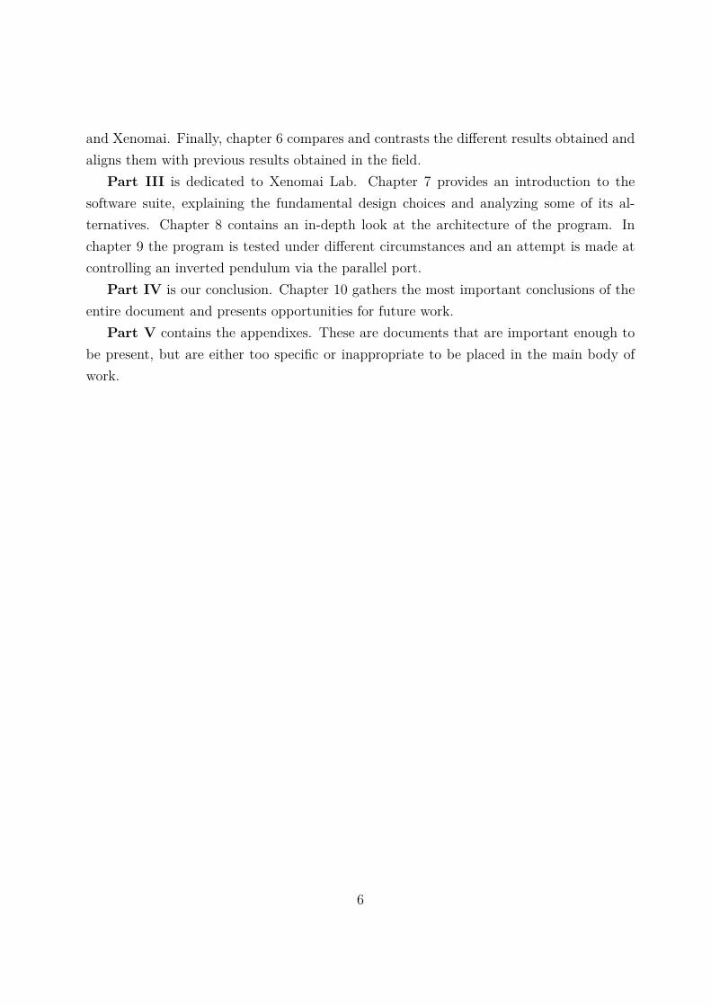
Figure 2.1: Graphical representation of a system as a block.
Setpoint Controller OutputPlant
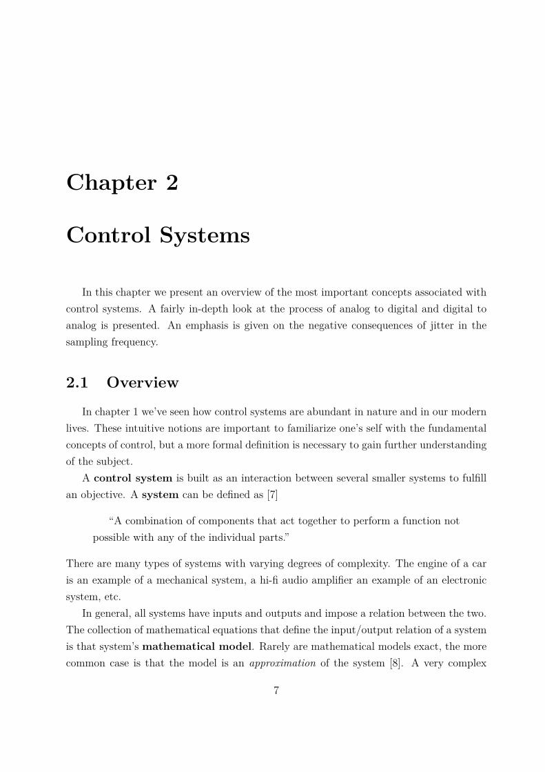
Figure 2.2: Block diagram of an open-loop control system
model can be composed of a large number of equations and go beyond the I/O relation andreveal the inner workings of the system. The behavior is predicted with a high degree ofprecision. A simpler model can be a coarse approximation of the behavior but be easier tounderstand and manipulate. Models come in very different forms and are used accordingto the precision required.
Mathematical modeling is a very powerful tool for understanding and ultimately ma-nipulating the natural world. Fig. 2.1 shows a simplified representation of a system as ablock. A block acts as a black box that, given an input, or a cause, produces an output,or an effect, according to a transfer function.
A transfer function is the I/O relation of the system. They are commonly writtenas differential equations in time, although other options exist. A transfer function revealsnothing about the nature of the block. The same transfer function can represent mechan-ical, hydraulic, thermal or even electrical phenomena. Even though their nature seemsradically different at a first glance, they abide by the same rules. One might say that allsystems were created equal in the eyes of mathematics, if one were so biblically inclined.
In a control system, the system under control, the plant, has its inputs manipulated insuch a way as to produce a desired output. Fig. 2.2 illustrates this as a block diagram,where both elements are represented as system blocks and their connections by directedlines. This variety of control system is the simplest form of control and is usually calledopen-loop control, as no loop is formed.
In this system, the output of the plant does not affect the action of the controller. Aconceptual example of such a system is a hand dryer operated by a timed button. Thedesired output is dried hands, and by pushing the button the air heater is on for 15 seconds.The fact that one’s hands aren’t dried by the end of the cycle does not make the hand
8
OutputErrorSetpoint PlantController∑
+-
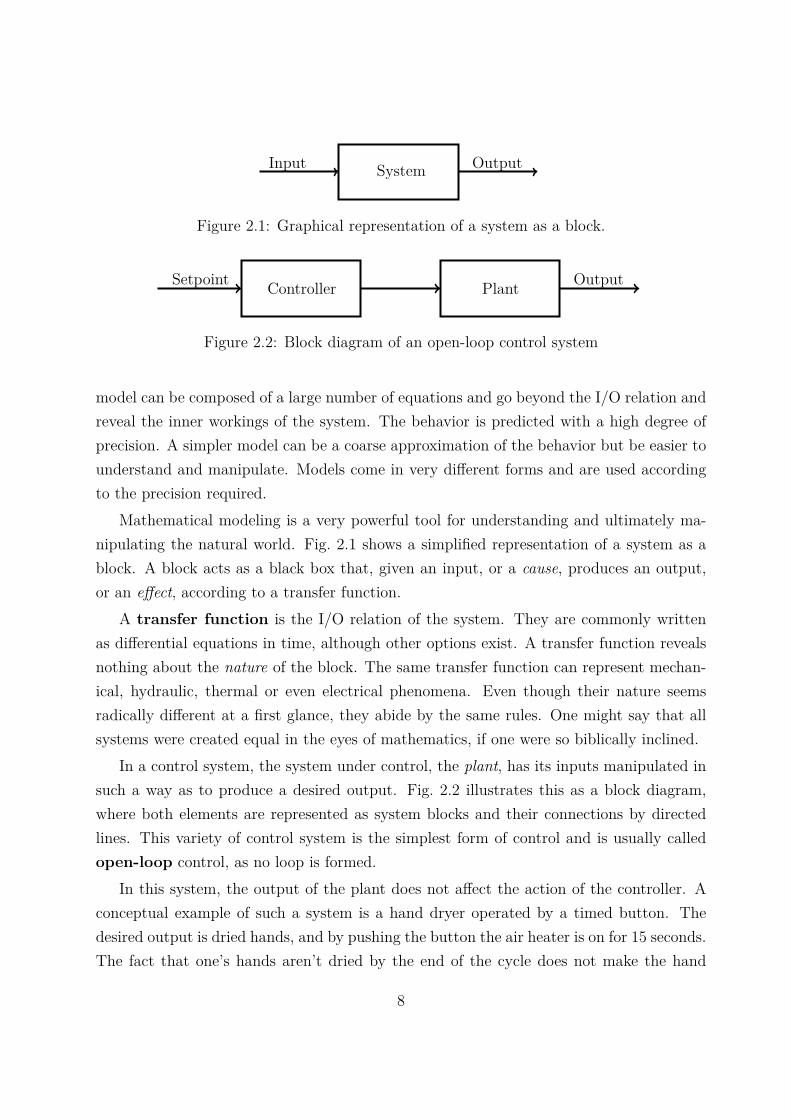
Figure 2.3: Block diagram of a closed-loop control system
dryer stay on any longer. It is a one way street.
Fig. 2.3 illustrates a closed-loop system. Here the output is fed back to the controllerafter being subtracted to the desired output, called the reference or setpoint. The resultof the subtraction is the difference between the desired and the current output, called theerror.
The controller acts upon the plant so as to make the error equal zero, at which pointthe desired output has been achieved. A system such as this is a negative feedbackloop. An example of such a system is a hot-air balloon. In it, the operator of the burnerkeeps adjusting the hot-air production until the desired altitude is reached. If the altitudesuddenly decreases, the operator re-ignites the burner until the altitude is reached onceagain.
If the error signal were to be made to grow continuously it would be a positive feed-back loop. It is one of these loops that occurs when there’s “feedback” during a live musicshow. What happens is that the microphones on stage pick up the sound coming out ofthe loudspeakers. A loop is formed where the amplified sound is amplified again and again.This causes the audio equipment to ultimately saturate, with the resulting sound being aloud high-pitch noise at the frequency of resonance of the equipment.
Each of these strategies has its advantages and disadvantages. An open loop is cheaperbecause it has less components but is limited in function and requires a very precise knowl-edge of the plant. Within a closed loop, a controller can adjust its operation to account forimperfections in the plant at a cost of greater system complexity. This makes a closed loopsystem much less sensitive to external disturbances or internal variations of the plant’sparameters [1].
9
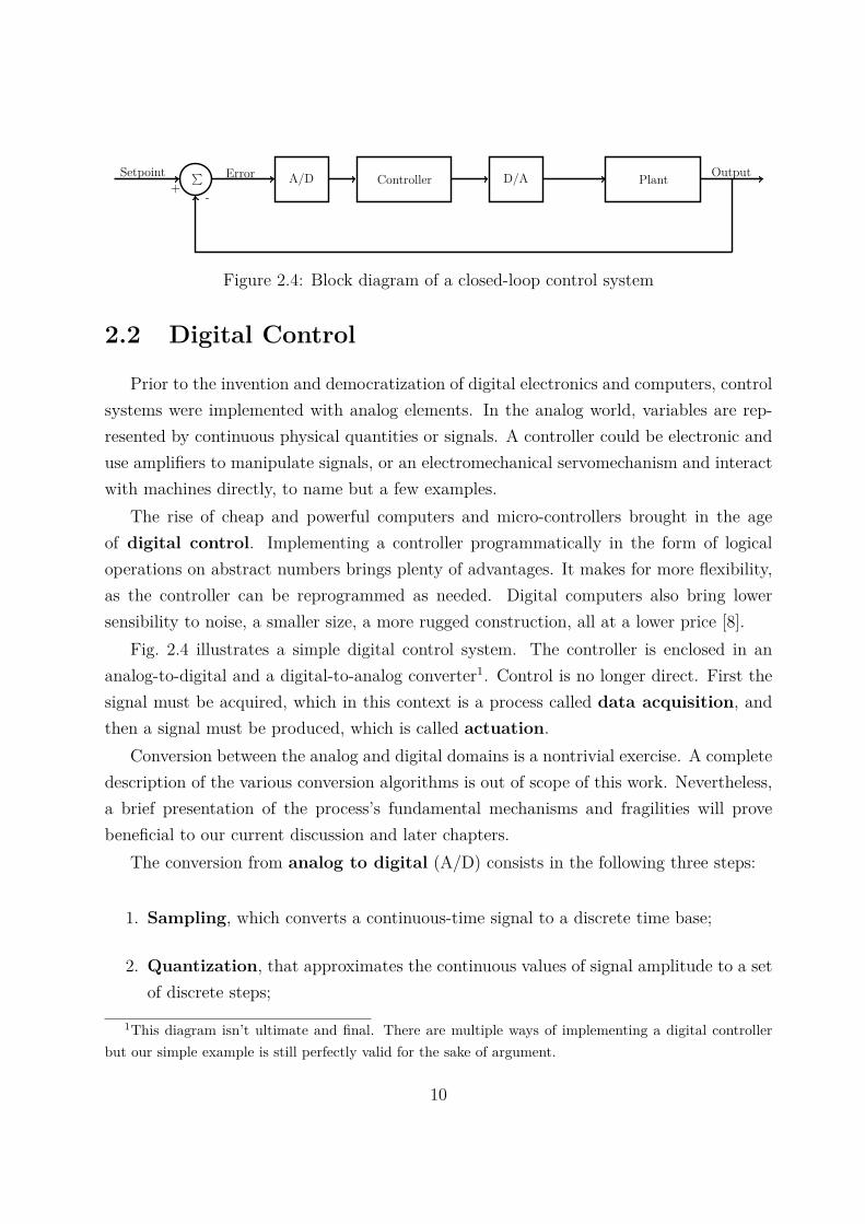
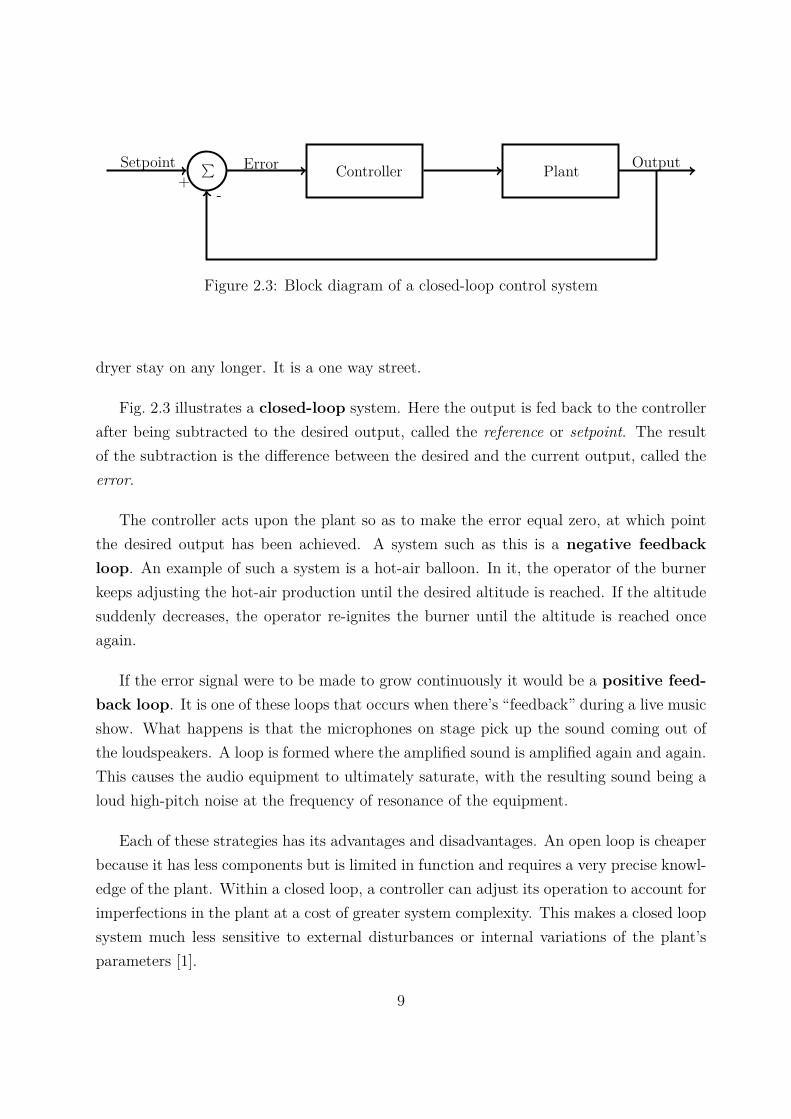
ErrorSetpoint ControllerA/D∑ OutputPlantD/A+
-
Figure 2.4: Block diagram of a closed-loop control system
2.2 Digital Control
Prior to the invention and democratization of digital electronics and computers, controlsystems were implemented with analog elements. In the analog world, variables are rep-resented by continuous physical quantities or signals. A controller could be electronic anduse amplifiers to manipulate signals, or an electromechanical servomechanism and interactwith machines directly, to name but a few examples.
The rise of cheap and powerful computers and micro-controllers brought in the ageof digital control. Implementing a controller programmatically in the form of logicaloperations on abstract numbers brings plenty of advantages. It makes for more flexibility,as the controller can be reprogrammed as needed. Digital computers also bring lowersensibility to noise, a smaller size, a more rugged construction, all at a lower price [8].
Fig. 2.4 illustrates a simple digital control system. The controller is enclosed in ananalog-to-digital and a digital-to-analog converter1. Control is no longer direct. First thesignal must be acquired, which in this context is a process called data acquisition, andthen a signal must be produced, which is called actuation.
Conversion between the analog and digital domains is a nontrivial exercise. A completedescription of the various conversion algorithms is out of scope of this work. Nevertheless,a brief presentation of the process’s fundamental mechanisms and fragilities will provebeneficial to our current discussion and later chapters.
The conversion from analog to digital (A/D) consists in the following three steps:
1. Sampling, which converts a continuous-time signal to a discrete time base;
2. Quantization, that approximates the continuous values of signal amplitude to a setof discrete steps;
1This diagram isn’t ultimate and final. There are multiple ways of implementing a digital controllerbut our simple example is still perfectly valid for the sake of argument.
10
{4,5,5,4,3,2,1,1,2,3...}
t
t
t
V V
V
Continuous time Discrete Time
ContinuousAmplitude
DiscreteAmplitude
ContinuousAmplitude
Discrete Time
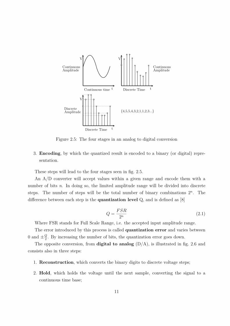
Figure 2.5: The four stages in an analog to digital conversion
3. Encoding, by which the quantized result is encoded to a binary (or digital) repre-sentation.
These steps will lead to the four stages seen in fig. 2.5.An A/D converter will accept values within a given range and encode them with a
number of bits n. In doing so, the limited amplitude range will be divided into discretesteps. The number of steps will be the total number of binary combinations 2n. Thedifference between each step is the quantization level Q, and is defined as [8]
Q = FSR
2n(2.1)
Where FSR stands for Full Scale Range, i.e. the accepted input amplitude range.The error introduced by this process is called quantization error and varies between
0 and ±Q2 . By increasing the number of bits, the quantization error goes down.
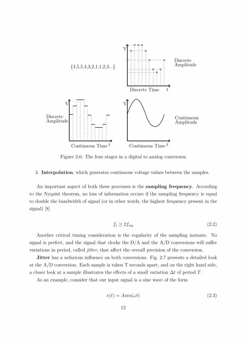
The opposite conversion, from digital to analog (D/A), is illustrated in fig. 2.6 andconsists also in three steps:
1. Reconstruction, which converts the binary digits to discrete voltage steps;
2. Hold, which holds the voltage until the next sample, converting the signal to acontinuous time base;
11
{4,5,5,4,3,2,1,1,2,3...}
t
V
V
tt
V
DiscreteAmplitude
Discrete Time
Continuous Time
ContinuousAmplitude
Continuous Time
DiscreteAmplitude
Figure 2.6: The four stages in a digital to analog conversion
3. Interpolation, which generates continuous voltage values between the samples.
An important aspect of both these processes is the sampling frequency. Accordingto the Nyquist theorem, no loss of information occurs if the sampling frequency is equalto double the bandwidth of signal (or in other words, the highest frequency present in thesignal) [8]
fs ≥ 2fsig (2.2)
Another critical timing consideration is the regularity of the sampling instants. Nosignal is perfect, and the signal that clocks the D/A and the A/D conversions will suffervariations in period, called jitter, that affect the overall precision of the conversion.
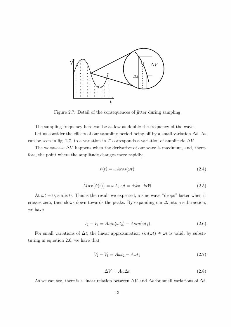
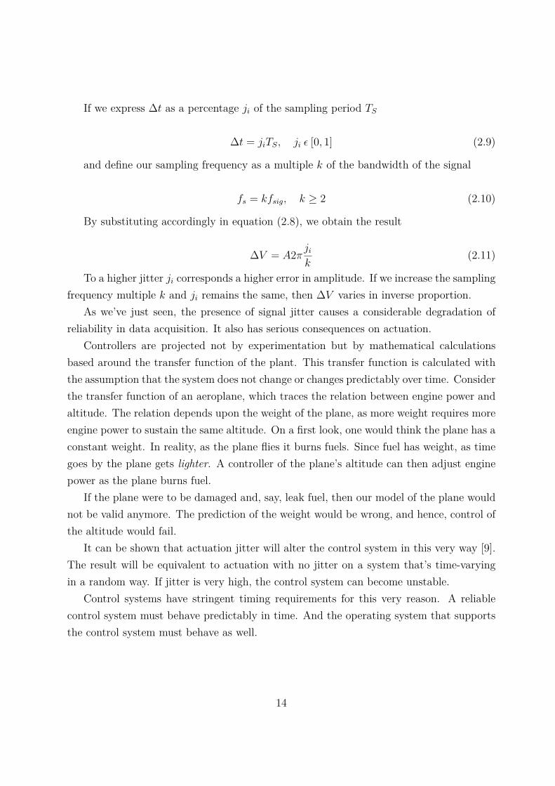
Jitter has a nefarious influence on both conversions. Fig. 2.7 presents a detailed lookat the A/D conversion. Each sample is taken T seconds apart, and on the right hand side,a closer look at a sample illustrates the effects of a small variation ∆t of period T .
As an example, consider that our input signal is a sine wave of the form
v(t) = Asin(ωt) (2.3)
12
∆t
∆V
t
V
Figure 2.7: Detail of the consequences of jitter during sampling
The sampling frequency here can be as low as double the frequency of the wave.Let us consider the effects of our sampling period being off by a small variation ∆t. As
can be seen in fig. 2.7, to a variation in T corresponds a variation of amplitude ∆V .The worst-case ∆V happens when the derivative of our wave is maximum, and, there-
fore, the point where the amplitude changes more rapidly.
v̇(t) = ωAcos(ωt) (2.4)
Max{v̇(t)} = ωA, ωt = ±kπ, kεN (2.5)
At ωt = 0, sin is 0. This is the result we expected, a sine wave “drops” faster when itcrosses zero, then slows down towards the peaks. By expanding our ∆ into a subtraction,we have
V2 − V1 = Asin(ωt2) − Asin(ωt1) (2.6)
For small variations of ∆t, the linear approximation sin(ωt) u ωt is valid, by substi-tuting in equation 2.6, we have that
V2 − V1 = Aωt2 − Aωt1 (2.7)
∆V = Aω∆t (2.8)
As we can see, there is a linear relation between ∆V and ∆t for small variations of ∆t.
13
If we express ∆t as a percentage ji of the sampling period TS
∆t = jiTS, ji ε [0, 1] (2.9)
and define our sampling frequency as a multiple k of the bandwidth of the signal
fs = kfsig, k ≥ 2 (2.10)
By substituting accordingly in equation (2.8), we obtain the result
∆V = A2πji
k(2.11)
To a higher jitter ji corresponds a higher error in amplitude. If we increase the samplingfrequency multiple k and ji remains the same, then ∆V varies in inverse proportion.
As we’ve just seen, the presence of signal jitter causes a considerable degradation ofreliability in data acquisition. It also has serious consequences on actuation.
Controllers are projected not by experimentation but by mathematical calculationsbased around the transfer function of the plant. This transfer function is calculated withthe assumption that the system does not change or changes predictably over time. Considerthe transfer function of an aeroplane, which traces the relation between engine power andaltitude. The relation depends upon the weight of the plane, as more weight requires moreengine power to sustain the same altitude. On a first look, one would think the plane has aconstant weight. In reality, as the plane flies it burns fuels. Since fuel has weight, as timegoes by the plane gets lighter. A controller of the plane’s altitude can then adjust enginepower as the plane burns fuel.
If the plane were to be damaged and, say, leak fuel, then our model of the plane wouldnot be valid anymore. The prediction of the weight would be wrong, and hence, control ofthe altitude would fail.
It can be shown that actuation jitter will alter the control system in this very way [9].The result will be equivalent to actuation with no jitter on a system that’s time-varyingin a random way. If jitter is very high, the control system can become unstable.
Control systems have stringent timing requirements for this very reason. A reliablecontrol system must behave predictably in time. And the operating system that supportsthe control system must behave as well.
14
Chapter 3
Real Time Operating Systems
In this chapter the fundamental tenets of real-time and non real-time operating systemsare presented. Concepts such as latency, jitter, deadlines and scheduling are discussed atlength.
3.1 In Tune and On TimeThe canonical definition of a real-time system, according to the real-time computing
FAQ, is the following [10]:
“A real-time system is one in which the correctness of the computations notonly depends upon the logical correctness of the computation but also upon thetime at which the result is produced. If the timing constraints of the systemare not met, system failure is said to have occurred.”
In less technical terms, real-time computing is when what matters isn’t solely the result,but when the result is produced. Compressing a folder into a zip file is an example of non-real time computing. We want the result to be logically correct, i.e. the files compressedwithout errors. If the operation takes two seconds instead of one, the quality of servicehas been degraded but the result is still correct. The system didn’t perform as well but itdidn’t fail. Watching a video, on the other hand, requires an image displayed every 40ms1.If a frame is late then it’s not worth displaying anymore. A late result, is, in essence,equivalent to no result at all. If many frames are lost, the result is no longer a video andthe system is said to have failed.
1This is equivalent to a frame rate of 25 frames per second.
15
A
B
t(ms)40 80 120 1600 200 240 280
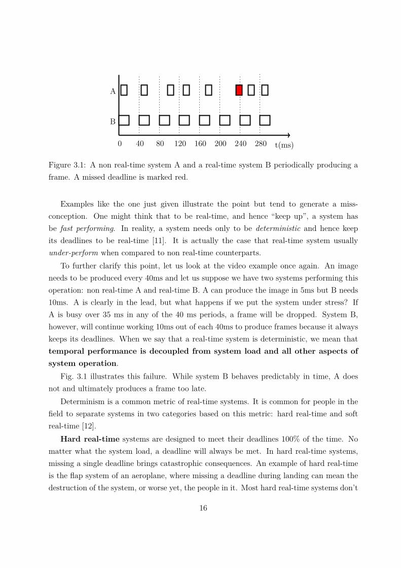
Figure 3.1: A non real-time system A and a real-time system B periodically producing aframe. A missed deadline is marked red.
Examples like the one just given illustrate the point but tend to generate a miss-conception. One might think that to be real-time, and hence “keep up”, a system hasbe fast performing. In reality, a system needs only to be deterministic and hence keepits deadlines to be real-time [11]. It is actually the case that real-time system usuallyunder-perform when compared to non real-time counterparts.
To further clarify this point, let us look at the video example once again. An imageneeds to be produced every 40ms and let us suppose we have two systems performing thisoperation: non real-time A and real-time B. A can produce the image in 5ms but B needs10ms. A is clearly in the lead, but what happens if we put the system under stress? IfA is busy over 35 ms in any of the 40 ms periods, a frame will be dropped. System B,however, will continue working 10ms out of each 40ms to produce frames because it alwayskeeps its deadlines. When we say that a real-time system is deterministic, we mean thattemporal performance is decoupled from system load and all other aspects ofsystem operation.
Fig. 3.1 illustrates this failure. While system B behaves predictably in time, A doesnot and ultimately produces a frame too late.
Determinism is a common metric of real-time systems. It is common for people in thefield to separate systems in two categories based on this metric: hard real-time and softreal-time [12].
Hard real-time systems are designed to meet their deadlines 100% of the time. Nomatter what the system load, a deadline will always be met. In hard real-time systems,missing a single deadline brings catastrophic consequences. An example of hard real-timeis the flap system of an aeroplane, where missing a deadline during landing can mean thedestruction of the system, or worse yet, the people in it. Most hard real-time systems don’t
16
tISR
SCHED
TASK
interrupt
interruptlatency
schedulinglatency
Figure 3.2: Common latencies during system operation.
have failures as deadly as our example, but need their deadlines met nonetheless.Soft real-time system can meet their deadlines most of the time, but not always. In
soft real-time systems missing a deadline means a degradation of quality of service, butnothing catastrophic. Our video example falls in this category.
3.2 Real-Time Essentials
As we’ve seen, real-time systems are defined by their temporal performance. There aremany ways to characterize a system’s behavior in time, and it’s helpful for our purposesto review the most important definitions.
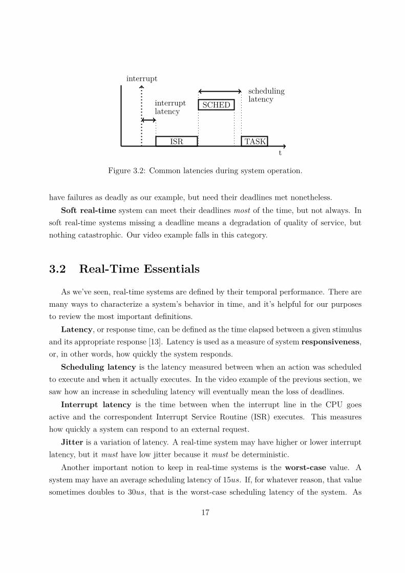
Latency, or response time, can be defined as the time elapsed between a given stimulusand its appropriate response [13]. Latency is used as a measure of system responsiveness,or, in other words, how quickly the system responds.
Scheduling latency is the latency measured between when an action was scheduledto execute and when it actually executes. In the video example of the previous section, wesaw how an increase in scheduling latency will eventually mean the loss of deadlines.
Interrupt latency is the time between when the interrupt line in the CPU goesactive and the correspondent Interrupt Service Routine (ISR) executes. This measureshow quickly a system can respond to an external request.
Jitter is a variation of latency. A real-time system may have higher or lower interruptlatency, but it must have low jitter because it must be deterministic.
Another important notion to keep in real-time systems is the worst-case value. Asystem may have an average scheduling latency of 15us. If, for whatever reason, that valuesometimes doubles to 30us, that is the worst-case scheduling latency of the system. As
17
tTASK
ri si fi
Ci
di
Figure 3.3: The most important figures characterizing a real-time task.
we’ve seen, for hard real-time system where a deadline can never be missed, the fact thaton average the scheduling latency is 15us is irrelevant because it cannot be guaranteed100% of the time.
Fig. 3.2 attempts to illustrate these concepts. When an interrupt occurs, a certaininterrupt latency elapses before the ISR is ran. When the ISR finishes, the scheduler iscalled, and after some time a task of interest starts executing.
These metrics characterize the system running our real-time tasks, but don’t charac-terize the tasks themselves. As we’ve seen in the previous section, real-time tasks are ofa different nature than non real-time. Recalling our video example, what jumps to mindis that real-time tasks are periodic. This needn’t be the case, as a task can be aperiodicand still be real-time. The key characteristic is that real-time tasks have deadlines, or inother words, a point in time after which the result is undesirable or useless.
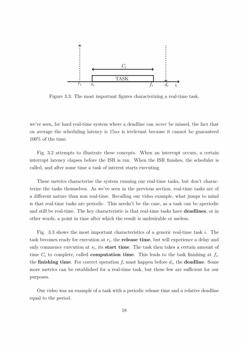
Fig. 3.3 shows the most important characteristics of a generic real-time task i. Thetask becomes ready for execution at ri, the release time, but will experience a delay andonly commence execution at si, its start time. The task then takes a certain amount oftime Ci to complete, called computation time. This leads to the task finishing at fi,the finishing time. For correct operation fi must happen before di, the deadline. Somemore metrics can be established for a real-time task, but these few are sufficient for ourpurposes.
Our video was an example of a task with a periodic release time and a relative deadlineequal to the period.
18
3.3 Operating Systems and PurposesAn RTOS is an OS built towards achieving temporal determinism and the support of
real-time operations. Examples of RTOSs are OSs such as Vx-Works [14] or QNX [15]. Onthe other end of the spectrum we have General Purpose Operating Systems (GPOS), suchas Linux or Windows.
This distinction is important because GPOS and RTOS have opposing goals. By ex-ploring this opposition, it will become apparent why transforming Linux into an RTOS issuch a complex task.
An operating system provides an abstraction layer between the system’s hardware andthe application programs that interest the user. It strives to be transparent, to decouplethe usage of a given user program from the hardware. This way, an application is built foran OS and will run in that OS regardless of the underlying hardware. In providing thisfunctionality an operating system implements three fundamental mechanisms [16]:
1. Abstraction. By providing an abstract interface to concrete hardware, an OS allowsfor simpler and portable application design. An example of such an abstraction is aread operation. This allows an application to read a variable number of bytes from agiven file and deposit them in some location. The read operation is specified in thesame way whether the file is on a flash disk, a hard drive or a CD-ROM. The readcall hides the inherent complexity of talking to all the different I/O controllers withspecific timings and handle the multitude of errors that may arise.
2. Virtualization. Most OSs support execution of multiple applications simultane-ously, even on systems with a single CPU. The available resources must then beshared among applications. OSs provide this feature by assigning a virtual machinefor each application. This allows applications to be written as though they have theresources all to themselves, when in reality they are competing for them. An exampleof this is virtual memory. Each application gets from the OS a continuous block ofmemory that in reality may be split among the RAM, the CPU cache or the swapfile on disk.
3. Resource Management. Since the applications are isolated from the underlyinghardware, it is up to the OS to manage the concurrent access to all the availableresources. The management is done in a way that will maximize overall systemperformance while assuring that no application gets neglected.
19
The difference between OSs lie in the fine details of the implementation of these threebasic concepts. For instance, part of the resource management duties of an OS is toschedule programs for execution in the CPU according to a given rule. This process iscalled scheduling, and the rule is usually called a scheduling policy. A GPOS will tryto schedule tasks so that on average each task spends a fair amount of time executing.“Fair” is not a precise concept. As such, an ideal policy does not exist as it depends onnumerous factors, such as what kind of tasks are being ran by the user. An RTOS, on theother hand, is an OS where the applications that interest the user are real-time tasks (asdefined in the previous section). Scheduling should then be done in such a way that allreal-time tasks are serviced before their deadlines no matter what.
Let us consider that an RTOS is trying to schedule a set of n periodic real-time tasks, nbeing an integer greater than zero. Each individual task i belonging to the set is of periodTi and computation time Ci. Let’s assume that these parameters do not change duringsystem operation. If we normalize Ci in relation to Ti and add them for all our set, thenwe will obtain the CPU utilization U , hence defined as [17]
U =n∑
i=1
Ci
Ti
(3.1)
As an example, consider that, when combined, our set of n tasks require 0.7s of com-putation time each second. This yields a U of 70%. With this metric it is immediate tosee if the hardware is suitable for the intended operation. If a set of tasks require a U ofover 100%, then a faster CPU is needed to cope with the load. Even if U is bellow 100%,it is not guaranteed that the set can be successfully scheduled. Let us look at two basicexamples of real-time scheduling policies and their impact in CPU utilization.
Rate Monotonic Scheduling (RM) is a scheduling policy where tasks with higherfrequency are given higher priority. If we assume that task frequencies don’t change mid-system operation, RM is an example of a fixed priority scheduling policy.
It is possible to assert if a given group of real-time tasks can be successfully scheduledby RM with no missed deadlines. If we were to assume that in addition to constant Ti andCi, the relative deadline di is equal to the period Ti and that our tasks are independentfrom one another and fully preemptible, then it has been shown that a sufficient conditionfor successful scheduling is [17]
U ≤ n(21/n − 1) (3.2)
20
For an increase in n, U tends towards ln2 u 70%. This means that if our set of real-time tasks, whatever they may be, don’t need CPU more than 70% of the time, an RMscheduling policy will successfully schedule the set. This leaves 30% of the CPU idle. Thiscan be quite wasteful, and our next example improves upon this result.
Earliest Deadline First (EDF) is a scheduling policy in which priorities are assignedbased not on the length of the deadline, but rather in its proximity to the present time. Thismeans that priorities are continuously being updated to reflect imminent deadlines, whichmakes EDF a dynamic-priority assignment policy. It has been shown that for the sameassumptions we’ve established for RM, a necessary and sufficient condition for successfulscheduling under EDF is
U ≤ 1 (3.3)
EDF guarantees that if the computation requirement of the task set does not exceedthe capacity of the CPU, the tasks can be successfully scheduled.
Having finished this analysis, the more astute reader will probably ask – Why can’t suchscheduling policies be integrated in a GPOS? Real-time tasks could remain high priorityand be scheduled by RM while the idle time could be managed by some other schedulingpolicy.
Firstly, the more astute reader would be advised to lower his voice as his thoughts maybe trespassing intellectual property [18]. Secondly, merging policies is perfectly valid, itis done in Linux and Windows, for example. However, it solves only part of the problem.The fission between a GPOS and an RTOS is far greater than merely the scheduling policy,as the CPU isn’t the only resource managed by the OS. Let us look at an example.
A valid strategy for a GPOS to implement virtual memory is to use paging [16]. Bydividing each memory space into 1-16KB blocks, or pages, the OS can easily manage whichmemory is currently in RAM or stored in swap. If a program needs access to a page thatis not in RAM, a page fault occurs and the OS responds by trying to load the respectivepage into memory. If no memory is available, the process may sleep indefinitely [16].
In an RTOS, the performance emphasis is on temporal determinism and reduced laten-cies. A paging strategy as we’ve just described is, therefore, not acceptable. With it, thecomputation time of a task is dependent on a page being on memory. If a page fault occurs,the time at which the task resumes execution is unknown. There are many other exam-ples of GPOS strategies of resource usage optimization that directly conflict with real-timeobjectives. We will look at this issue further when discussing Linux’ implementation.
21

22
Part II
Real-Time Linux
23

24
Chapter 4
Linux
In this chapter a complete overview of the most important Linux concepts is pre-sented. The major attempts at improving Linux’ real-time performance are analyzed andbenchmarked. These are the hrtimers mechanism and the PREEMPT_RT patchset. Thechapter closes with a direct comparison of the benchmarking results obtained.
4.1 Linux 101 - An IntroductionLinux is a monolithic kernel. It runs as a single process in a single address space. This
does not mean that the kernel needs to be compiled as one big static binary. Linux supportsloading and unloading components (called modules) during execution time. Typically,the more essential kernel systems are statically compiled, while hardware support (i.e.drivers) are compiled as modules and loaded during boot. The essential kernel systems arecomponents such as a process scheduler to coordinate access to processor execution time,memory management, interrupt handlers, networking, etc.
The kernel process runs in an elevated privilege mode, while secondary processes layon top of the kernel in an unprivileged mode. The rationale is that potentially destructiveoperations such as direct hardware access are reserved for the kernel. Any other processneeding elevated privileges operations asks the kernel to do it for them, using a mechanismcalled system calls. The kernel then acts as a proxy between the untrusted process andthe operation it wants done on a restricted system, e.g. write 1024 bytes to a file on disk.
This dichotomy between privilege and lack thereof is the difference between kernelspace and user space.
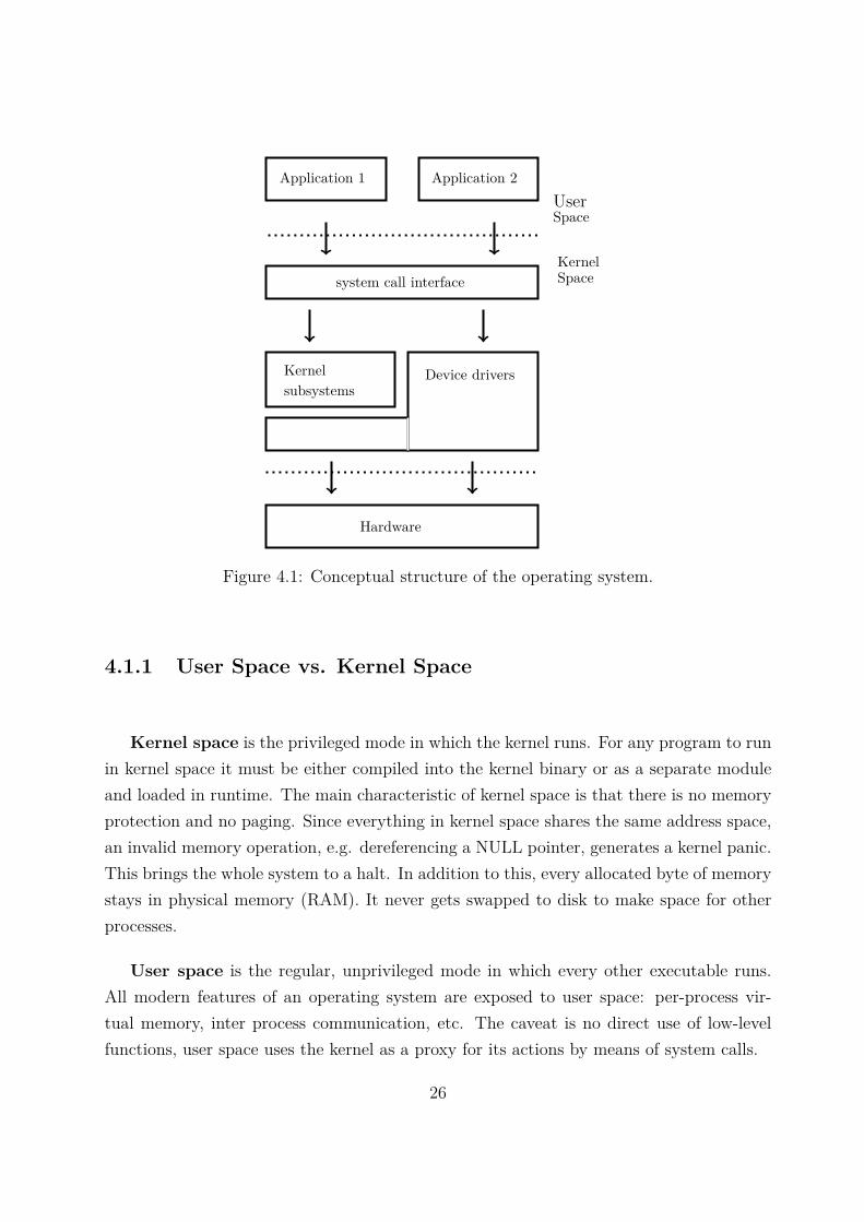
Fig. 4.1 illustrates the previous points.
25
Hardware
Device driversKernelsubsystems
system call interface
UserApplication 1 Application 2
Space
KernelSpace
Figure 4.1: Conceptual structure of the operating system.
4.1.1 User Space vs. Kernel Space
Kernel space is the privileged mode in which the kernel runs. For any program to runin kernel space it must be either compiled into the kernel binary or as a separate moduleand loaded in runtime. The main characteristic of kernel space is that there is no memoryprotection and no paging. Since everything in kernel space shares the same address space,an invalid memory operation, e.g. dereferencing a NULL pointer, generates a kernel panic.This brings the whole system to a halt. In addition to this, every allocated byte of memorystays in physical memory (RAM). It never gets swapped to disk to make space for otherprocesses.
User space is the regular, unprivileged mode in which every other executable runs.All modern features of an operating system are exposed to user space: per-process vir-tual memory, inter process communication, etc. The caveat is no direct use of low-levelfunctions, user space uses the kernel as a proxy for its actions by means of system calls.
26
4.1.2 Processes and Scheduling
In Linux, a process is made of two parts: the active task, meaning the binary exe-cutable, and its related resources such as its priority, current state, opened files, identitynumber, etc. Both of them are brought together in the process descriptor, a data struc-ture that holds all the process’ associated variables. Notice that when we speak of a processwe imply execution, not a program stored in disk to be executed in the future.
Linux supports multitasking, that is, the concurrent execution of different processes.Since there are usually many more processes than CPUs to execute them, processing timehas to be shared. To coordinate this concurrent access to the processor is the purpose ofthe scheduler. As the name implies, the scheduler schedules processes for execution. Itdoes this by assigning a lease of processor time to each process, usually called a timeslice.Different processes get different timeslices according to a given norm, called the schedulingpolicy. When execution switches from one process to another, the previous state of theCPU (the context) has to be saved and a new state has to be loaded1. This is calleda context switch. A context switch from one process to another may be voluntary orinvoluntary. When a process yields its execution to another by directly calling the schedulerwe call it yielding. When a process is interrupted by the scheduler so that another cantake its place, we say that the process has been preempted by the scheduler, and hence wecall it preemption.
Examples of both yielding and preemption are numerous throughout the kernel. Forinstance, when a process issues a read call to read information stored on the disk, it willsleep until the disk retrieves the information. To do this, the process will remove itself fromthe list of schedulable processes and directly call the scheduler so that another process cantake its place on the CPU. This leaves the task blocked (or sleeping) and is an example ofyielding execution. Preemption is more common. For instance, when an interrupt occurswhatever process is running is preempted as to allow the interrupt handler to run.
The heart of the scheduler is the scheduling policy. It is beyond the scope of this workto analyze this subject at depth since it is an area of constant flux – algorithms are adoptedand discarded fairly rapidly. The problem of scheduling offers no perfect solution since itis inherently contradictory. To maximize efficiency we need to minimize context switches,to reduce latency and improve interactivity we need more preemption.
It is important to refer that Linux supports multiple scheduling policies at the same1The state of the CPU includes all of the CPU’s register and other important elements, such as the
virtual memory mapping and stack information, among others.
27
time and switching between them at runtime. There are three “normal” scheduling policies– SCHED_OTHER, SCHED_BATCH and SCHED_IDLE – and two real-time schedulingpolicies – SCHED_FIFO and SCHED_RR. A process can assign itself a scheduling policyand a static priority between 0 and 99.
Processes assigned to SCHED_FIFO or SCHED_RR must have a static prioritybetween and 1 and 99, while for the other scheduling policies the priority is always 0. Thismeans that real-time processes will always preempt any normal process that happens tobe running. The difference between the two real-time policies is that a SCHED_FIFOprocess runs until it decides to yield, while SCHED_RR processes are assigned a timesliceafter which they are preempted.
SCHED_BATCH is intended for “batch” type processes, i.e. processes that requireno user interaction and usually run in the background. SCHED_IDLE are for processeswith the lowest possible priority and will only run when no other processes are available.
SCHED_OTHER is the default scheduling policy which most user space applicationsuse. This policy implements an algorithm that can be defined as a boot parameter. Typicalchoices are the Completely Fair Schedule (CFS), O(1), and others.
Given that yielding generally only happens when a task intends to block, most of thecontext switches and calls to the scheduler occur via preemption. However, some areas ofthe kernel are not preemptible. This fact greatly affects Linux’s real-time performance. Ifa timer is to go off at a time when the kernel is not preemptible the latency will be higherthan during a preemptible section. This variability is a clear degradation of performance.
User space preemption happens in two situations: when the execution is returning touser space from a system call and from an interrupt handler. In other words, wheneverthere’s a system call or an interrupt, the scheduler is called. This vulnerability to inter-rupts means that user space is fully preemptable as long as interrupts are not explicitlydeactivated (which is a rare and looked down upon practice).
In kernel space we have a different story. It is preemptible, but not fully preemptible.In general, the kernel is not preemptible if it holds a spinlock (which means it is executinga critical section) or if preemption is explicitly disabled. Therefore, the kernel is subject topreemption when an interrupt handler exits, when it releases a lock and when preemptionis explicitly re-enabled. All of these result in calls to the scheduler. We will look furtherinto kernel preemption points later in this chapter.
28
4.1.3 Interrupts
Interrupts are signals asynchronously generated by external hardware that interrupt theregular processing flow of the CPU. Upon receiving an interrupt on its Interrupt RequestLine (IRQ), the CPU will make a context switch to a predefined interrupt handler (alsocalled an Interrupt Service Routine, or ISR for short). Interrupts can also be generatedby software using a specific processor instruction, in which case they’re called softwareinterrupts. Upon completion of the interrupt handler, the system resumes execution of theprevious state.
Linux separates the interrupt handler into two separate parts: the top half and thebottom half. The top half is the actual ISR. It does only the absolutely essential work(e.g. acknowledge the interrupt, copy available information into memory). The bottomhalf is the non-urgent part of the work that can be postponed for execution at a moreconvenient time. Note that because interrupts can arrive at any moment, they may interferewith potentially important and time-sensitive operations. By separating ISR’s in twocomponents, the interference is kept to a minimum.
Bottom halves have three distinct implementations: softirqs, tasklets and work queues.Softirqs are statically defined bottom halves. They are registered only during kernel
compilation and cannot be dynamically created by, say, a kernel module. Top halfs usuallymark their corresponding softirq for execution (called raising a softirq) before exiting. Ata more convenient time, the system checks for raised softirqs and runs them. Note thatsoftirqs are not processes. The scheduler does not see them and they cannot block.This means that once a softirq begins execution it cannot be preempted for rescheduling.Softirqs only yield execution when they terminate. If the system is under load and manysoftirqs are raised, user space starvation can occur. When, then, should softirqs be run?Softirqs can run when the top half returns, they can be explicitly called from code inthe kernel and by per-cpu ksoftirq threads. These threads are an attempt to curb thepossible starvation due to softirq overload. When a softirq raises itself (which happens, forinstance, in the network softirq) it will only be executed when the corresponding ksoftirqthread is scheduled. Because the thread is marked as low priority, the system won’t starveas much. This is a very important point that will explain some of the performance resultsobtained later in this chapter, so it is worth pointing out again: due to their non-preemptivenature, softirqs may induce user space starvation.
Due to all of the above, softirq usage is very limited. In order of priority, the systemsthat use them in the kernel under test are: high priority tasklets, kernel timers, networking,
29
block devices, regular tasklets, scheduler, high resolution timers and RCU locking [3].System strain can then be induced by overload of tasklets, timers and heavy networkingand disk I/O operation (which is what our benchmarking suite does).
Tasklets are very similar to softirqs. The main difference is that they can be createddynamically. The implementation defines two softirqs associated with groups of high andlow priority tasklets. When one of these softirqs is able to run, its group of associatedtasklets also runs. And like softirqs, they cannot block.
Finally, work queues are implemented as kernel threads. They run with the samescheduling constraints of any other process under SCHED_OTHER. Since they are inde-pendent of softirqs, they suffer none of their problems (they can block, for instance), butalso have none of their benefits.
4.1.4 Timers
Introduced in version 2.0, the classic Linux timing architecture is based upon the notionof a periodic tick. At boot, the system timer2 is programmed to generate an interruptaccording to the predefined tick rate. This rate is defined at compile time by a staticpreprocessor define called HZ. Typical values of HZ are 100, 250 and 1000 Hz. The timerinterrupt handler would then be responsible for operations such as updating the system’suptime and wall time, updating resource and processor usage statistics, and run any kerneltimers that might have expired.
Kernel timers are the basic kernel support for timing operations. They operate solelyin one-shot mode. In fact, the timer does not have a period but an absolute expirationdate measured in jiffies. jiffies is a 64 bit integer that counts the number of ticks since boot.Therefore, the maximum frequency achievable with these timers is equal to or a fraction ofHZ. Precision wise, these timers offer no guarantees. The only guarantee is that the timercallback function will not execute before the expiration date. The delay can be as high asthe next tick [3].
2The exact hardware varies between architectures. On x86 the programmable interrupt timer (PIT)and the Advanced Programmable Interrupt Controller (APIC) are the usual suspects. The processor’stime stamp counter (TSC) can also be used to keep track of time.
30
4.2 Real-time Isn’t Fair
All of Linux’ mechanisms were developed with desktop and server usage in mind. Thismeans high throughput and fair access to hardware resources for all processes. But, as we’vepreviously seen, real-time isn’t fair, and its requirements are usually in direct contradictionwith other computing paradigms. As a general purpose OS, Linux excels. As a real-timeOS, however, the situation is rather different.
Linux’ scheduling of processes is temporally non-deterministic. It is highly dependenton system load and promotes fair access to processor time. By registering a process withthe SCHED_FIFO policy we mostly bypass the later problem, but the fact that kernelspace isn’t fully preemptible keeps the first problem in place.
Within kernel space, the situation is better but still poor. Softirqs, spinlocks andother non-preemptable sections of the kernel are fundamentally destructive of real-timepredictability. In addition to this, the timing architecture offers a deficient support for pe-riodic operation and its architectural simplicity brings serious problems. Firstly, althoughthe periodic tick conceptualization seems like a natural way for an operating system tokeep track of time, it is highly inefficient. The system keeps ticking even when it is idle,which represents unnecessary power consumption. The tick rate itself is a tricky and in-flexible trade-off since the whole infrastructure relies on it. Too low and the timing is verycoarse, too high and the CPU might spend an unreasonable amount of time executing thetimer interrupt handler. Secondly, the fact that timers operate not in time units but injiffies makes precise timing operations unportable and unreliable. The API allows settingan expiration date 2ms from now, but on a system with HZ=100, the expiration date willbe silently rounded off to 10ms.
Over the past 10 years, several solutions were developed that greatly improved Linux’real-time performance and overall predictability. The High Resolution Timers projectredesigned the timing architecture and is now a standard of the mainline kernel. ThePREEMPT_RT patchset tries to address the lack of preemptability of the kernel with aneye for reducing latency. Other projects such as RTAI and Xenomai completely bypassLinux and its problems. Instead, they introduce a micro kernel between Linux and thehardware that directly handles interrupts and scheduling [19][20]. Several other solutionsexist, such as ARTiS which splits tasks between real-time and non-real-time CPUs [21].We will dedicate a full chapter to the dual kernel approach. For now, let us look at thefirst two approaches.
31
4.3 High Resolution Timers
High resolution timers (hrtimers) were introduced in kernel version 2.6.16 [22]. Theyare part of an effort lead by Thomas Gleixner and Ingo Molnar to completely redesign thetiming infrastructure [23]. Some of the objectives of this undertaking were:
• To engineer a new abstraction of time that will minimize platform specific code and,hence, maximize maintainability.
• An infrastructure that can support both ticked and tickless (or dynamic) operation
• A new timer infrastructure that supports high resolution timing, measured in nanoseconds, and complements the legacy concepts but is entirely independent of them.
The project was an enormous success and brought a much needed refresh to the datedcode, not to mention welcomed functionality and performance improvements. The fruitsof this work also made it to user space in the form of itimers and an implementation of thePOSIX 1003.1b real-time clock/timer specification [24]. These include a timer functionalityand the nanosleep system call.
This new architecture is rather complex (due to all its platform-agnostic abstractions)and a complete description of it is out of the scope of this work. We present, however,some of the most important highlights.
The decision to introduce a new API for high resolution timing instead of upgrading theexisting timing infrastructure to, say, a sub-jiffie granularity was the fruit of some carefuland practical considerations. Two distinct use cases of timers were identified. Timeouts areused to detect a rare failure. They do not require high resolution, and are almost alwaysdeleted before expiring. Much like a watchdog timer, a timeout isn’t supposed to go off, butit’s there to react in case of a system failure. It’s very commonly used in the networkingstack for protocol timeouts, for instance. Timers are the opposite usecase. They’re used toschedule events, run periodic functions, and other carefully timed scenarios. They requirehigh resolution and usually expire.
This distinction is important because they call for different supporting implementations[25]. The classical architecture is called the Cascading Timer Wheel (CTW) and worksphenomenally well for timeouts. It has low overhead for inserting and removing timers(O(1)) because it sorts timers based on their expiration date very coarsely. Every so often,however, the timer wheel has to be fully sorted, a very time consuming operation that
32
completely disrupts any ambition of precise timing. hrtimers keep timers sorted in a red-black tree3. It has higher overhead for inserting and removing timers (O(log(n))), but thesorting is already taken care of. In a nutshell, the CTW tries to push sorting timers as faroff into the future as possible. The red-black tree sorts timers as soon as they arrive. Theformer lends itself well for timers that are usually removed before they expire, the latteris ideal for the opposite.
Why use both? Maintaining the legacy architecture keeps compatibility with oldercode and avoids an unnecessary rewrite of several core sections of the kernel. But besidescompatibility, notice that the bigger the red-black tree, the slower the insertion and removaltimes. By separating the architecture into two components, both the CTW and the red-black tree are kept in a sizable form. The solution developed was to tie the CTW not toan interrupt issued by a system timer, but to an hrtimer [26]. This frees the hardwarefrom CTW’s hands, and makes way for an easier implementation of tickless operation andnanosecond timers. Which is exactly what was done by the same team for Linux 2.6.21and remains valid until the time of writing.
4.3.1 Performance
To assert the performance of hrtimers (and all systems henceforth) a standard testsuitewas developed. It was aptly named “The Testsuite” and its implementation can be reviewedin appendix A.
In a nutshell, the system under test is programmed to generate a square wave on theparallel port with period 2ms. Then, the jitter of the wave is measured using an externalmicrocontroller. The jitter is measured in four distinct situations. In Idle, the system isessentialy in stand-by, in CPU a video is played that occupies 100% of the CPU, in I/O afile is constantly moved between partitions, in Net a file is constantly moved between thecomputer running the test to another computer via ethernet. The result is subject to anuncertainty of ±100ns and a systematic error of -1.3µs, which is immediately corrected.
4.3.2 Kernel Space
The testsuite was performed on an hrtimer running in kernel space. The code used ispresented in listing C.1.
3A red-black tree is a type of self-balancing binary search tree. This means that the data it contains iscontinuously sorted.
33
Fig. 4.2 shows the results obtained. Fig. 4.2a plots the jitter distribution while 4.2bpresents a statistical approach highlighting the worst-case jitter. Table 4.2c presents theprecise values used to plot fig. 4.2b
The average jitter is about −200ns on all cases. This means that the wave is in reality200ns shorter than what it should be. Under Idle, I/O and Net the exact period is onlymeasured 15-20% of times, evidenced by the peaks. Under CPU, that value drops bellow5%.
Although fig. 4.2a shows jitter between -4 and 4 µs, the worst-case jitter is much higher.In fig. 4.2b we can see that it lies within the 100-200µs range. The lower jitter is naturallyin Idle, the higher ones are I/O and Net. This is to be expected because both tests overloadthe system with softirqs.
As we’ve seen in section 4.1.3, hrtimers, I/O and the network interface all use softirqs.The hrtimer softirq, being of inferior priority than both I/O and Net experiences greaterdelays. The interrupt latency can double, as evidenced by the doubling in worst-case jitter.
In spite of this, we see that even though the system is overloaded, the hrtimer is neverstarved. Delay can double, but it is still serviced in a reasonable amount of time.
4.3.3 User Space
Recalling section 4.3, hrtimers are exposed to user space as an implementation of POSIXnorm 1003.1b. This norm contains the timer that was used to generate the wave, thecode for which can be reviewed in listing C.2. The program was scheduled with theSCHED_FIFO policy for maximum real-time performance.
Fig. 4.3 shows the results obtained, similar in presentation to our previous results4
As can be immediately seen, although hrtimers are also being used, in user space thescenario is strikingly different. The fact that the timer handler is executed in processcontext makes all the difference.
As we can see in fig.4.3a there is a small peak under the exact period, but jitter ismostly spread out between -1 and -1µs. Under CPU the graph goes almost flat.
In fig. 4.3b we can see that worst case is much higher than in our previous analysis.In Idle and CPU, the worst-case is held between 500/800µs. In I/O, the worst-case sky
4Unfortunately, the network load is not presented due to an irrecoverable glitch in the measurements.Due to time considerations, it was not possible to re-run the testsuite. Fortunately this is the only glitchin the +24 hours of testing undertaken for this dissertation and no such errors will be present beyond thispoint.
34
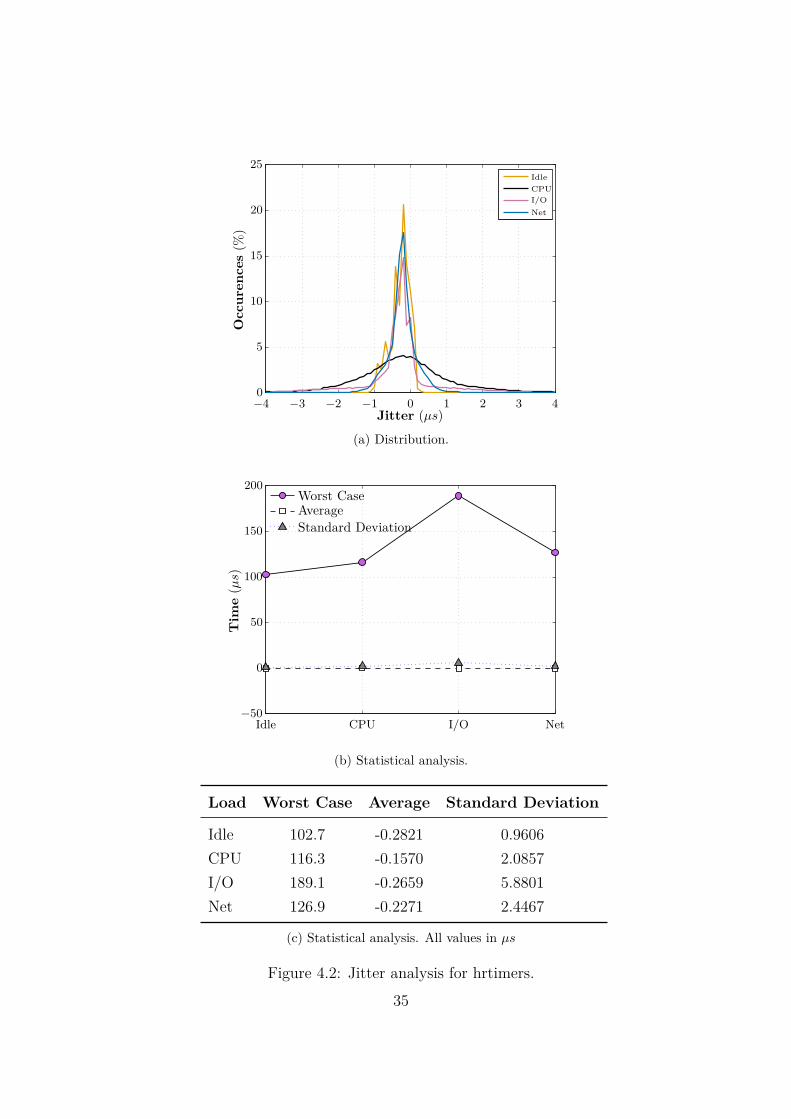
NetI/OCPUIdle
Occ
uren
ces
(%)
Jitter (µs)−4 −3 −2 −1 0 1 2 3 40
5
10
15
20
25
(a) Distribution.
Tim
e(µ
s)
Standard DeviationAverageWorst Case
Idle CPU I/O Net−50
0
50
100
150
200
(b) Statistical analysis.
Load Worst Case Average Standard Deviation
Idle 102.7 -0.2821 0.9606CPU 116.3 -0.1570 2.0857I/O 189.1 -0.2659 5.8801Net 126.9 -0.2271 2.4467
(c) Statistical analysis. All values in µs
Figure 4.2: Jitter analysis for hrtimers.35
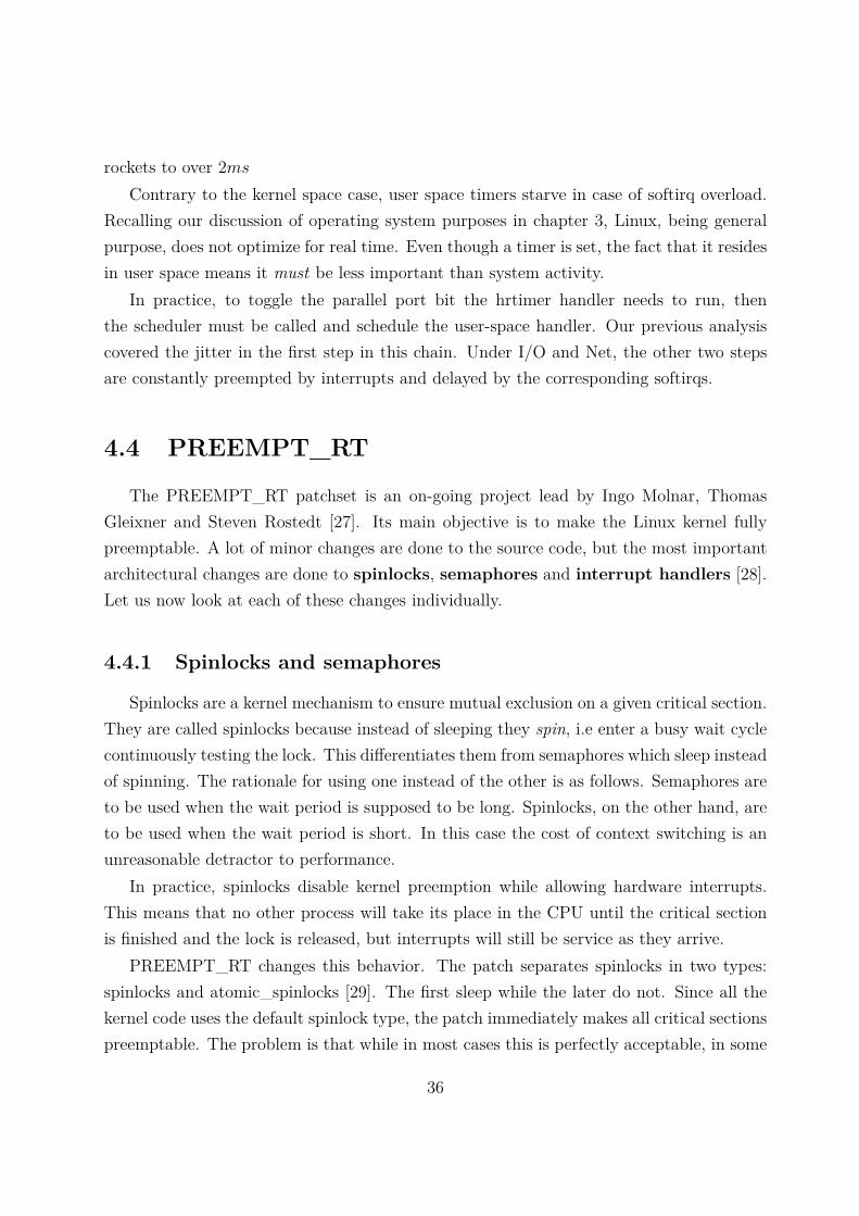
rockets to over 2msContrary to the kernel space case, user space timers starve in case of softirq overload.
Recalling our discussion of operating system purposes in chapter 3, Linux, being generalpurpose, does not optimize for real time. Even though a timer is set, the fact that it residesin user space means it must be less important than system activity.
In practice, to toggle the parallel port bit the hrtimer handler needs to run, thenthe scheduler must be called and schedule the user-space handler. Our previous analysiscovered the jitter in the first step in this chain. Under I/O and Net, the other two stepsare constantly preempted by interrupts and delayed by the corresponding softirqs.
4.4 PREEMPT_RT
The PREEMPT_RT patchset is an on-going project lead by Ingo Molnar, ThomasGleixner and Steven Rostedt [27]. Its main objective is to make the Linux kernel fullypreemptable. A lot of minor changes are done to the source code, but the most importantarchitectural changes are done to spinlocks, semaphores and interrupt handlers [28].Let us now look at each of these changes individually.
4.4.1 Spinlocks and semaphores
Spinlocks are a kernel mechanism to ensure mutual exclusion on a given critical section.They are called spinlocks because instead of sleeping they spin, i.e enter a busy wait cyclecontinuously testing the lock. This differentiates them from semaphores which sleep insteadof spinning. The rationale for using one instead of the other is as follows. Semaphores areto be used when the wait period is supposed to be long. Spinlocks, on the other hand, areto be used when the wait period is short. In this case the cost of context switching is anunreasonable detractor to performance.
In practice, spinlocks disable kernel preemption while allowing hardware interrupts.This means that no other process will take its place in the CPU until the critical sectionis finished and the lock is released, but interrupts will still be service as they arrive.
PREEMPT_RT changes this behavior. The patch separates spinlocks in two types:spinlocks and atomic_spinlocks [29]. The first sleep while the later do not. Since all thekernel code uses the default spinlock type, the patch immediately makes all critical sectionspreemptable. The problem is that while in most cases this is perfectly acceptable, in some
36
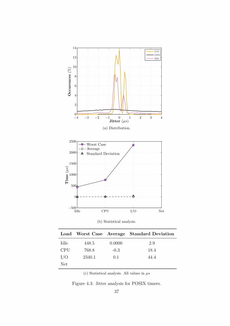
IdleCPUI/O
Occ
uren
ces
(%)
Jitter (µs)−4 −3 −2 −1 0 1 2 3 40
2
4
6
8
10
12
14
(a) Distribution.
Tim
e(µ
s)
Standard DeviationAverageWorst Case
Idle CPU I/O Net−500
0
500
1000
1500
2000
2500
(b) Statistical analysis.
Load Worst Case Average Standard Deviation
Idle 448.5 0.0000 2.9CPU 768.8 -0.3 18.4I/O 2340.1 0.1 44.4Net
(c) Statistical analysis. All values in µs
Figure 4.3: Jitter analysis for POSIX timers.37
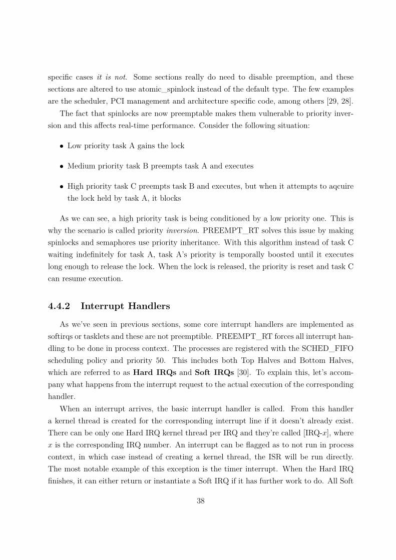
specific cases it is not. Some sections really do need to disable preemption, and thesesections are altered to use atomic_spinlock instead of the default type. The few examplesare the scheduler, PCI management and architecture specific code, among others [29, 28].
The fact that spinlocks are now preemptable makes them vulnerable to priority inver-sion and this affects real-time performance. Consider the following situation:
• Low priority task A gains the lock
• Medium priority task B preempts task A and executes
• High priority task C preempts task B and executes, but when it attempts to aqcuirethe lock held by task A, it blocks
As we can see, a high priority task is being conditioned by a low priority one. This iswhy the scenario is called priority inversion. PREEMPT_RT solves this issue by makingspinlocks and semaphores use priority inheritance. With this algorithm instead of task Cwaiting indefinitely for task A, task A’s priority is temporally boosted until it executeslong enough to release the lock. When the lock is released, the priority is reset and task Ccan resume execution.
4.4.2 Interrupt Handlers
As we’ve seen in previous sections, some core interrupt handlers are implemented assoftirqs or tasklets and these are not preemptible. PREEMPT_RT forces all interrupt han-dling to be done in process context. The processes are registered with the SCHED_FIFOscheduling policy and priority 50. This includes both Top Halves and Bottom Halves,which are referred to as Hard IRQs and Soft IRQs [30]. To explain this, let’s accom-pany what happens from the interrupt request to the actual execution of the correspondinghandler.
When an interrupt arrives, the basic interrupt handler is called. From this handlera kernel thread is created for the corresponding interrupt line if it doesn’t already exist.There can be only one Hard IRQ kernel thread per IRQ and they’re called [IRQ-x], wherex is the corresponding IRQ number. An interrupt can be flagged as to not run in processcontext, in which case instead of creating a kernel thread, the ISR will be run directly.The most notable example of this exception is the timer interrupt. When the Hard IRQfinishes, it can either return or instantiate a Soft IRQ if it has further work to do. All Soft
38
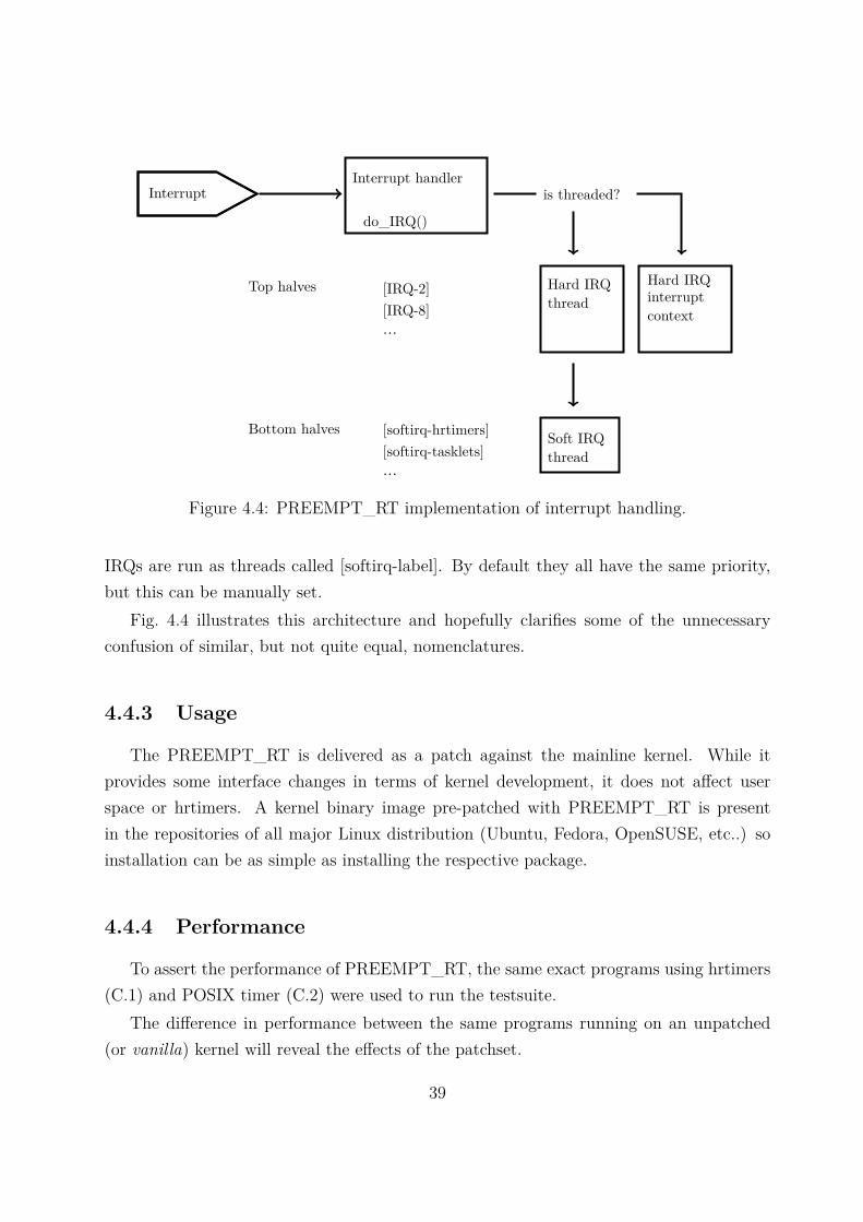
Interrupt handler
do_IRQ()
Hard IRQthread
is threaded?
Hard IRQinterruptcontext
Soft IRQthread
[IRQ-2][IRQ-8]...
[softirq-hrtimers][softirq-tasklets]...
Interrupt
Top halves
Bottom halves
Figure 4.4: PREEMPT_RT implementation of interrupt handling.
IRQs are run as threads called [softirq-label]. By default they all have the same priority,but this can be manually set.
Fig. 4.4 illustrates this architecture and hopefully clarifies some of the unnecessaryconfusion of similar, but not quite equal, nomenclatures.
4.4.3 Usage
The PREEMPT_RT is delivered as a patch against the mainline kernel. While itprovides some interface changes in terms of kernel development, it does not affect userspace or hrtimers. A kernel binary image pre-patched with PREEMPT_RT is presentin the repositories of all major Linux distribution (Ubuntu, Fedora, OpenSUSE, etc..) soinstallation can be as simple as installing the respective package.
4.4.4 Performance
To assert the performance of PREEMPT_RT, the same exact programs using hrtimers(C.1) and POSIX timer (C.2) were used to run the testsuite.
The difference in performance between the same programs running on an unpatched(or vanilla) kernel will reveal the effects of the patchset.
39
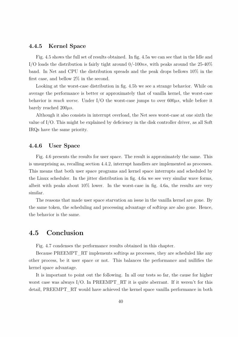
4.4.5 Kernel Space
Fig. 4.5 shows the full set of results obtained. In fig. 4.5a we can see that in the Idle andI/O loads the distribution is fairly tight around 0/-100ns, with peaks around the 25-40%band. In Net and CPU the distribution spreads and the peak drops bellows 10% in thefirst case, and bellow 2% in the second.
Looking at the worst-case distribution in fig. 4.5b we see a strange behavior. While onaverage the performance is better or approximately that of vanilla kernel, the worst-casebehavior is much worse. Under I/O the worst-case jumps to over 600µs, while before itbarely reached 200µs.
Although it also consists in interrupt overload, the Net sees worst-case at one sixth thevalue of I/O. This might be explained by deficiency in the disk controller driver, as all SoftIRQs have the same priority.
4.4.6 User Space
Fig. 4.6 presents the results for user space. The result is approximately the same. Thisis unsurprising as, recalling section 4.4.2, interrupt handlers are implemented as processes.This means that both user space programs and kernel space interrupts and scheduled bythe Linux scheduler. In the jitter distribution in fig. 4.6a we see very similar wave forms,albeit with peaks about 10% lower. In the worst-case in fig. 4.6a, the results are verysimilar.
The reasons that made user space starvation an issue in the vanilla kernel are gone. Bythe same token, the scheduling and processing advantage of softirqs are also gone. Hence,the behavior is the same.
4.5 ConclusionFig. 4.7 condenses the performance results obtained in this chapter.Because PREEMPT_RT implements softirqs as processes, they are scheduled like any
other process, be it user space or not. This balances the performance and nullifies thekernel space advantage.
It is important to point out the following. In all our tests so far, the cause for higherworst case was always I/O. In PREEMPT_RT it is quite aberrant. If it weren’t for thisdetail, PREEMPT_RT would have achieved the kernel space vanilla performance in both
40
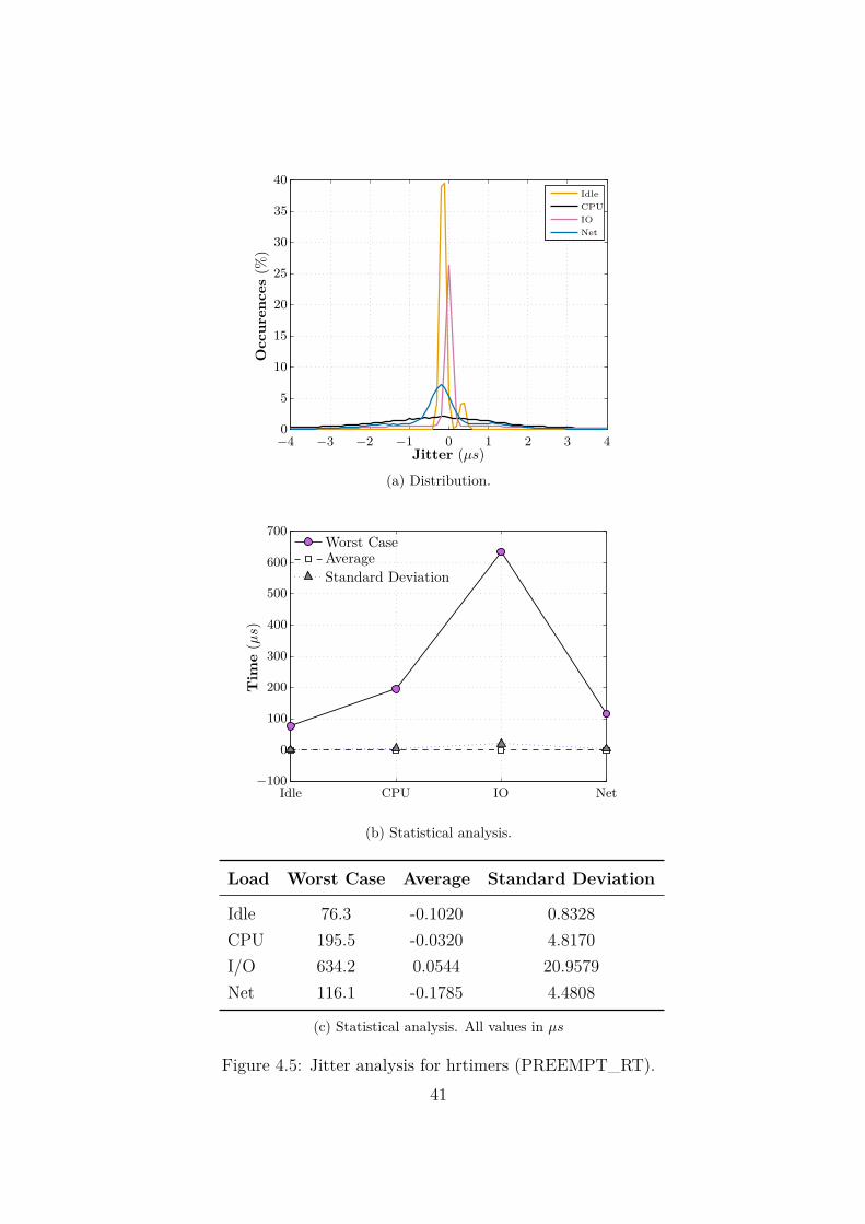
NetIOCPUIdle
Occ
uren
ces
(%)
Jitter (µs)−4 −3 −2 −1 0 1 2 3 40
5
10
15
20
25
30
35
40
(a) Distribution.
Tim
e(µ
s)
Standard DeviationAverageWorst Case
Idle CPU IO Net−100
0
100
200
300
400
500
600
700
(b) Statistical analysis.
Load Worst Case Average Standard Deviation
Idle 76.3 -0.1020 0.8328CPU 195.5 -0.0320 4.8170I/O 634.2 0.0544 20.9579Net 116.1 -0.1785 4.4808
(c) Statistical analysis. All values in µs
Figure 4.5: Jitter analysis for hrtimers (PREEMPT_RT).41
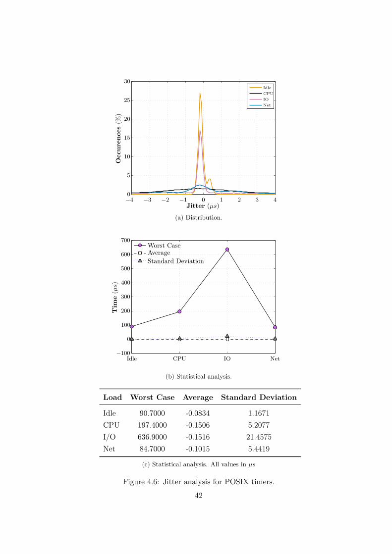
NetIOCPUIdle
Occ
uren
ces
(%)
Jitter (µs)−4 −3 −2 −1 0 1 2 3 40
5
10
15
20
25
30
(a) Distribution.
Tim
e(µ
s)
Standard DeviationAverageWorst Case
Idle CPU IO Net−100
0
100
200
300
400
500
600
700
(b) Statistical analysis.
Load Worst Case Average Standard Deviation
Idle 90.7000 -0.0834 1.1671CPU 197.4000 -0.1506 5.2077I/O 636.9000 -0.1516 21.4575Net 84.7000 -0.1015 5.4419
(c) Statistical analysis. All values in µs
Figure 4.6: Jitter analysis for POSIX timers.42
User SpaceKernel Spa.
Kernel
Jitt
er(m
s)
Vanilla PREEMPT0
0.5
1
1.5
2
2.5
Figure 4.7: Worst-case jitter for vanilla and PREEMPT_RT kernels.
kernel and user space. Our contention is that PREEMPT_RT exposes some fault in thedisk driver code. It might be the case that some of the sections aren’t preemptable. Thatwould fully explain the results obtained and point towards a way to fixing the issue.
43

44
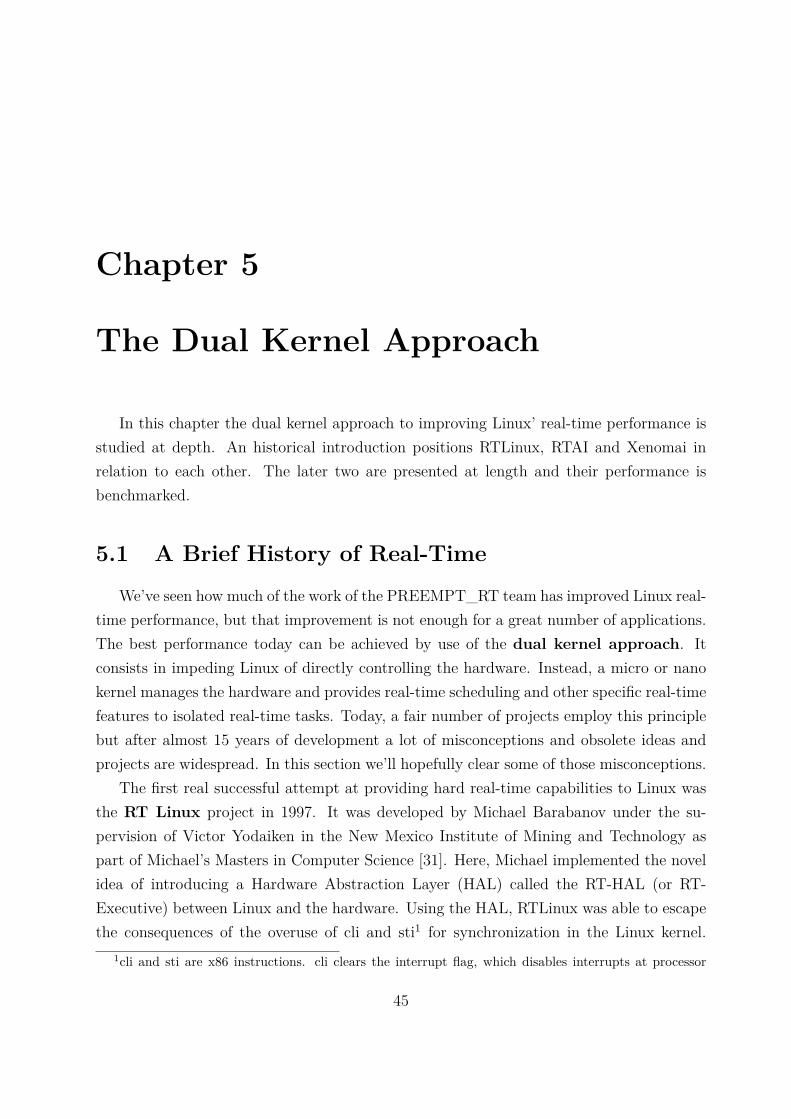
Chapter 5
The Dual Kernel Approach
In this chapter the dual kernel approach to improving Linux’ real-time performance isstudied at depth. An historical introduction positions RTLinux, RTAI and Xenomai inrelation to each other. The later two are presented at length and their performance isbenchmarked.
5.1 A Brief History of Real-TimeWe’ve seen how much of the work of the PREEMPT_RT team has improved Linux real-
time performance, but that improvement is not enough for a great number of applications.The best performance today can be achieved by use of the dual kernel approach. Itconsists in impeding Linux of directly controlling the hardware. Instead, a micro or nanokernel manages the hardware and provides real-time scheduling and other specific real-timefeatures to isolated real-time tasks. Today, a fair number of projects employ this principlebut after almost 15 years of development a lot of misconceptions and obsolete ideas andprojects are widespread. In this section we’ll hopefully clear some of those misconceptions.
The first real successful attempt at providing hard real-time capabilities to Linux wasthe RT Linux project in 1997. It was developed by Michael Barabanov under the su-pervision of Victor Yodaiken in the New Mexico Institute of Mining and Technology aspart of Michael’s Masters in Computer Science [31]. Here, Michael implemented the novelidea of introducing a Hardware Abstraction Layer (HAL) called the RT-HAL (or RT-Executive) between Linux and the hardware. Using the HAL, RTLinux was able to escapethe consequences of the overuse of cli and sti1 for synchronization in the Linux kernel.
1cli and sti are x86 instructions. cli clears the interrupt flag, which disables interrupts at processor
45
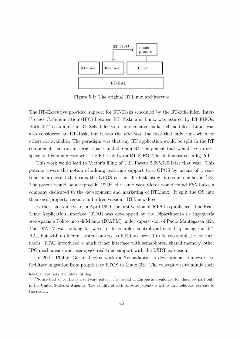
RT-Task RT-Task
RT-HAL
Linux
Linuxprocess
RT-FIFO
Figure 5.1: The original RTLinux architecture
The RT-Executive provided support for RT-Tasks scheduled by the RT-Scheduler. Inter-Process Communication (IPC) between RT-Tasks and Linux was assured by RT-FIFOs.Both RT-Tasks and the RT-Scheduler were implemented as kernel modules. Linux wasalso considered an RT-Task, but it was the idle task, the task that only runs when noothers are available. The paradigm was that any RT application would be split in the RTcomponent that ran in kernel space, and the non RT component that would live in userspace and communicate with the RT task by an RT-FIFO. This is illustrated in fig. 5.1.
This work would lead to Victor’s filing of U.S. Patent 5,995,745 later that year. Thispatents covers the notion of adding real-time support to a GPOS by means of a real-time micro-kernel that runs the GPOS as the idle task using interrupt emulation [18].The patent would be accepted in 19992, the same year Victor would found FSMLabs, acompany dedicated to the development and marketing of RTLinux. It split the OS intotheir own property version and a free version - RTLinux/Free.
Earlier that same year, in April 1999, the first version of RTAI is published. The Real-Time Application Interface (RTAI) was developped by the Dipartimento de IngegneriaAerospaziale Politecnico di Milano (DIAPM) under supervision of Paolo Mantegazza [32].The DIAPM was looking for ways to do complex control and ended up using the RT-HAL but with a different system on top, as RTLinux proved to be too simplistic for theirneeds. RTAI introduced a much richer interface with semaphores, shared memory, otherIPC mechanisms and user space real-time support with the LXRT extension.
In 2001, Philipe Gerum begins work on Xenoadaptor, a development framework tofacilitate migration from proprietary RTOS to Linux [33]. The concept was to mimic their
level, and sti sets the interrupt flag.2Notice that since this is a software patent it is invalid in Europe and enforced for the most part only
in the United States of America. The validity of such software patents is left as an intelectual exercise tothe reader.
46
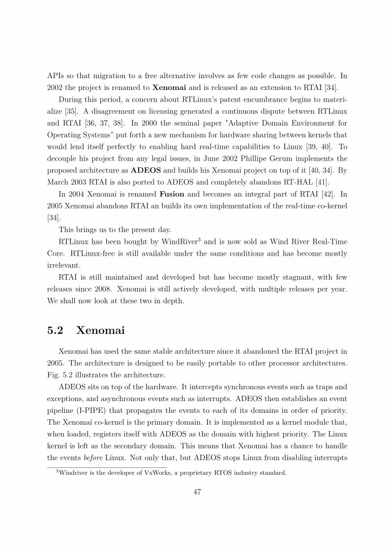
APIs so that migration to a free alternative involves as few code changes as possible. In2002 the project is renamed to Xenomai and is released as an extension to RTAI [34].
During this period, a concern about RTLinux’s patent encumbrance begins to materi-alize [35]. A disagreement on licensing generated a continuous dispute between RTLinuxand RTAI [36, 37, 38]. In 2000 the seminal paper "Adaptive Domain Environment forOperating Systems” put forth a new mechanism for hardware sharing between kernels thatwould lend itself perfectly to enabling hard real-time capabilities to Linux [39, 40]. Todecouple his project from any legal issues, in June 2002 Phillipe Gerum implements theproposed architecture as ADEOS and builds his Xenomai project on top of it [40, 34]. ByMarch 2003 RTAI is also ported to ADEOS and completely abandons RT-HAL [41].
In 2004 Xenomai is renamed Fusion and becomes an integral part of RTAI [42]. In2005 Xenomai abandons RTAI an builds its own implementation of the real-time co-kernel[34].
This brings us to the present day.RTLinux has been bought by WindRiver3 and is now sold as Wind River Real-Time
Core. RTLinux-free is still available under the same conditions and has become mostlyirrelevant.
RTAI is still maintained and developed but has become mostly stagnant, with fewreleases since 2008. Xenomai is still actively developed, with multiple releases per year.We shall now look at these two in depth.
5.2 XenomaiXenomai has used the same stable architecture since it abandoned the RTAI project in
2005. The architecture is designed to be easily portable to other processor architectures.Fig. 5.2 illustrates the architecture.
ADEOS sits on top of the hardware. It intercepts synchronous events such as traps andexceptions, and asynchronous events such as interrupts. ADEOS then establishes an eventpipeline (I-PIPE) that propagates the events to each of its domains in order of priority.The Xenomai co-kernel is the primary domain. It is implemented as a kernel module that,when loaded, registers itself with ADEOS as the domain with highest priority. The Linuxkernel is left as the secondary domain. This means that Xenomai has a chance to handlethe events before Linux. Not only that, but ADEOS stops Linux from disabling interrupts
3Windriver is the developer of VxWorks, a proprietary RTOS industry standard.
47
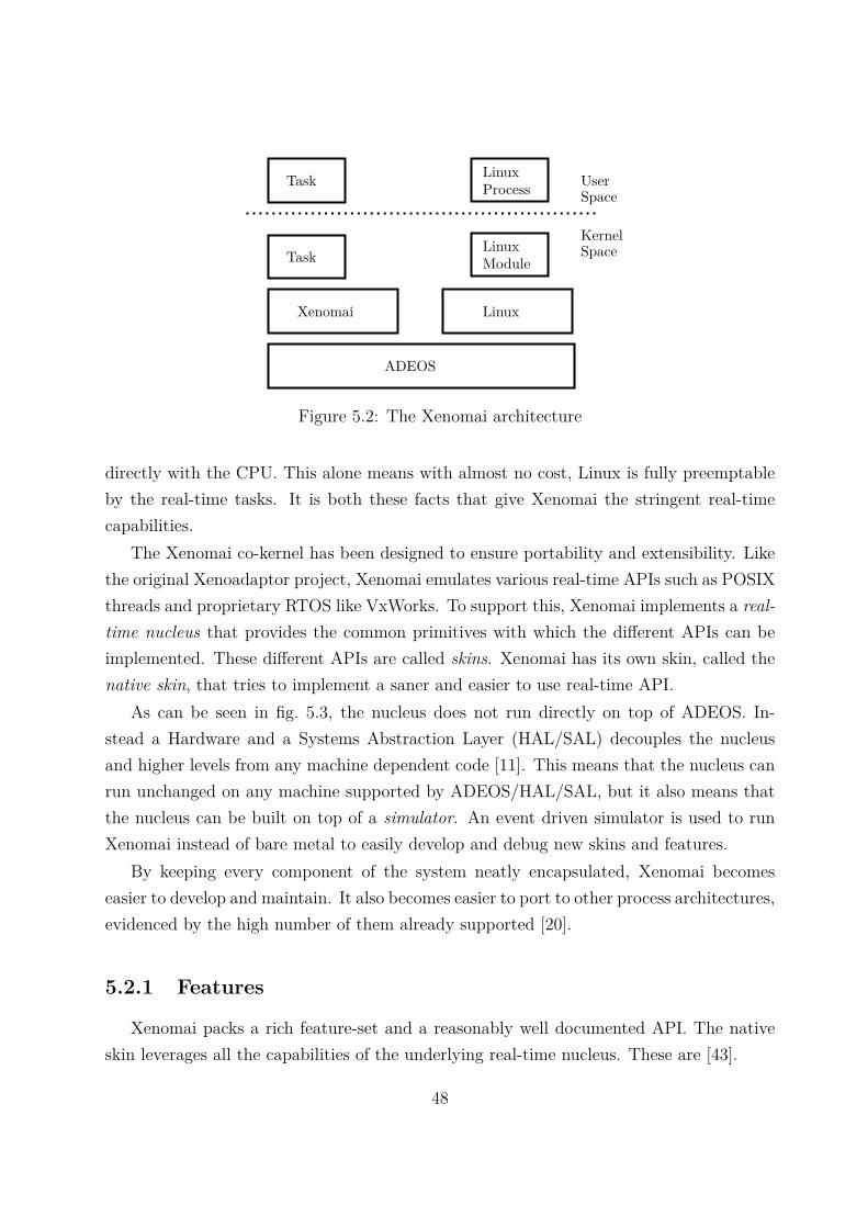
ADEOS
Xenomai
LinuxModule
Linux
Task
Task LinuxProcess User
Space
KernelSpace
Figure 5.2: The Xenomai architecture
directly with the CPU. This alone means with almost no cost, Linux is fully preemptableby the real-time tasks. It is both these facts that give Xenomai the stringent real-timecapabilities.
The Xenomai co-kernel has been designed to ensure portability and extensibility. Likethe original Xenoadaptor project, Xenomai emulates various real-time APIs such as POSIXthreads and proprietary RTOS like VxWorks. To support this, Xenomai implements a real-time nucleus that provides the common primitives with which the different APIs can beimplemented. These different APIs are called skins. Xenomai has its own skin, called thenative skin, that tries to implement a saner and easier to use real-time API.
As can be seen in fig. 5.3, the nucleus does not run directly on top of ADEOS. In-stead a Hardware and a Systems Abstraction Layer (HAL/SAL) decouples the nucleusand higher levels from any machine dependent code [11]. This means that the nucleus canrun unchanged on any machine supported by ADEOS/HAL/SAL, but it also means thatthe nucleus can be built on top of a simulator. An event driven simulator is used to runXenomai instead of bare metal to easily develop and debug new skins and features.
By keeping every component of the system neatly encapsulated, Xenomai becomeseasier to develop and maintain. It also becomes easier to port to other process architectures,evidenced by the high number of them already supported [20].
5.2.1 Features
Xenomai packs a rich feature-set and a reasonably well documented API. The nativeskin leverages all the capabilities of the underlying real-time nucleus. These are [43].
48
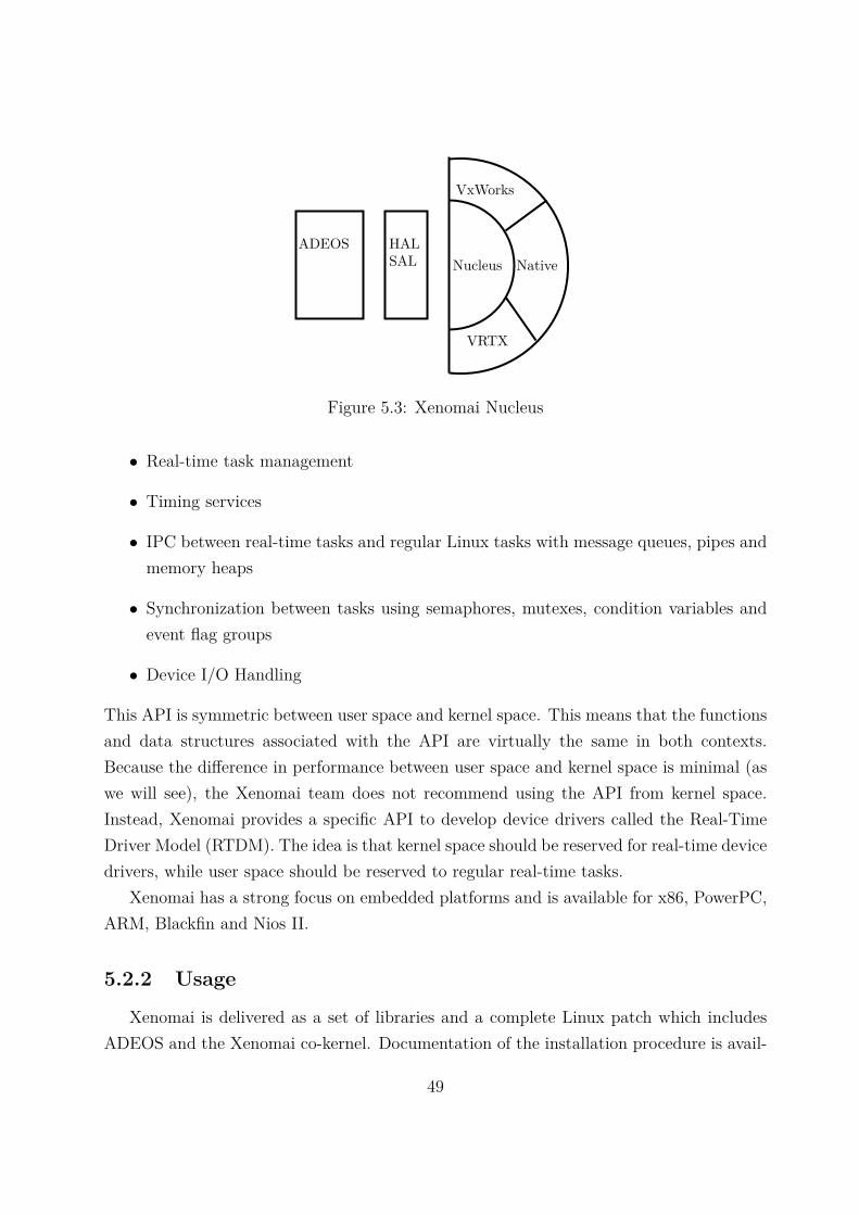
HALSAL
ADEOSNucleus Native
VxWorks
VRTX
Figure 5.3: Xenomai Nucleus
• Real-time task management
• Timing services
• IPC between real-time tasks and regular Linux tasks with message queues, pipes andmemory heaps
• Synchronization between tasks using semaphores, mutexes, condition variables andevent flag groups
• Device I/O Handling
This API is symmetric between user space and kernel space. This means that the functionsand data structures associated with the API are virtually the same in both contexts.Because the difference in performance between user space and kernel space is minimal (aswe will see), the Xenomai team does not recommend using the API from kernel space.Instead, Xenomai provides a specific API to develop device drivers called the Real-TimeDriver Model (RTDM). The idea is that kernel space should be reserved for real-time devicedrivers, while user space should be reserved to regular real-time tasks.
Xenomai has a strong focus on embedded platforms and is available for x86, PowerPC,ARM, Blackfin and Nios II.
5.2.2 Usage
Xenomai is delivered as a set of libraries and a complete Linux patch which includesADEOS and the Xenomai co-kernel. Documentation of the installation procedure is avail-
49
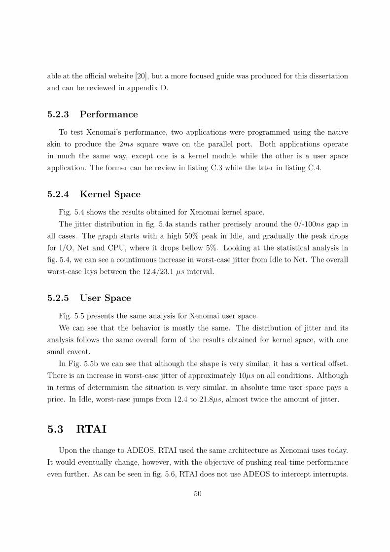
able at the official website [20], but a more focused guide was produced for this dissertationand can be reviewed in appendix D.
5.2.3 Performance
To test Xenomai’s performance, two applications were programmed using the nativeskin to produce the 2ms square wave on the parallel port. Both applications operatein much the same way, except one is a kernel module while the other is a user spaceapplication. The former can be review in listing C.3 while the later in listing C.4.
5.2.4 Kernel Space
Fig. 5.4 shows the results obtained for Xenomai kernel space.The jitter distribution in fig. 5.4a stands rather precisely around the 0/-100ns gap in
all cases. The graph starts with a high 50% peak in Idle, and gradually the peak dropsfor I/O, Net and CPU, where it drops bellow 5%. Looking at the statistical analysis infig. 5.4, we can see a countinuous increase in worst-case jitter from Idle to Net. The overallworst-case lays between the 12.4/23.1 µs interval.
5.2.5 User Space
Fig. 5.5 presents the same analysis for Xenomai user space.We can see that the behavior is mostly the same. The distribution of jitter and its
analysis follows the same overall form of the results obtained for kernel space, with onesmall caveat.
In Fig. 5.5b we can see that although the shape is very similar, it has a vertical offset.There is an increase in worst-case jitter of approximately 10µs on all conditions. Althoughin terms of determinism the situation is very similar, in absolute time user space pays aprice. In Idle, worst-case jumps from 12.4 to 21.8µs, almost twice the amount of jitter.
5.3 RTAIUpon the change to ADEOS, RTAI used the same architecture as Xenomai uses today.
It would eventually change, however, with the objective of pushing real-time performanceeven further. As can be seen in fig. 5.6, RTAI does not use ADEOS to intercept interrupts.
50
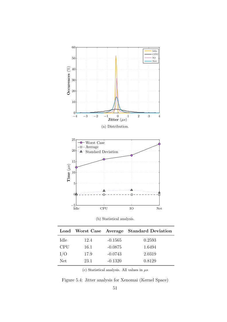
NetIOCPUIdle
Occ
uren
ces
(%)
Jitter (µs)−4 −3 −2 −1 0 1 2 3 40
10
20
30
40
50
60
(a) Distribution.
Tim
e(µ
s)
Standard DeviationAverageWorst Case
Idle CPU IO Net−5
0
5
10
15
20
25
(b) Statistical analysis.
Load Worst Case Average Standard Deviation
Idle 12.4 -0.1565 0.2593CPU 16.1 -0.0875 1.6494I/O 17.9 -0.0743 2.0319Net 23.1 -0.1320 0.8129
(c) Statistical analysis. All values in µs
Figure 5.4: Jitter analysis for Xenomai (Kernel Space)51
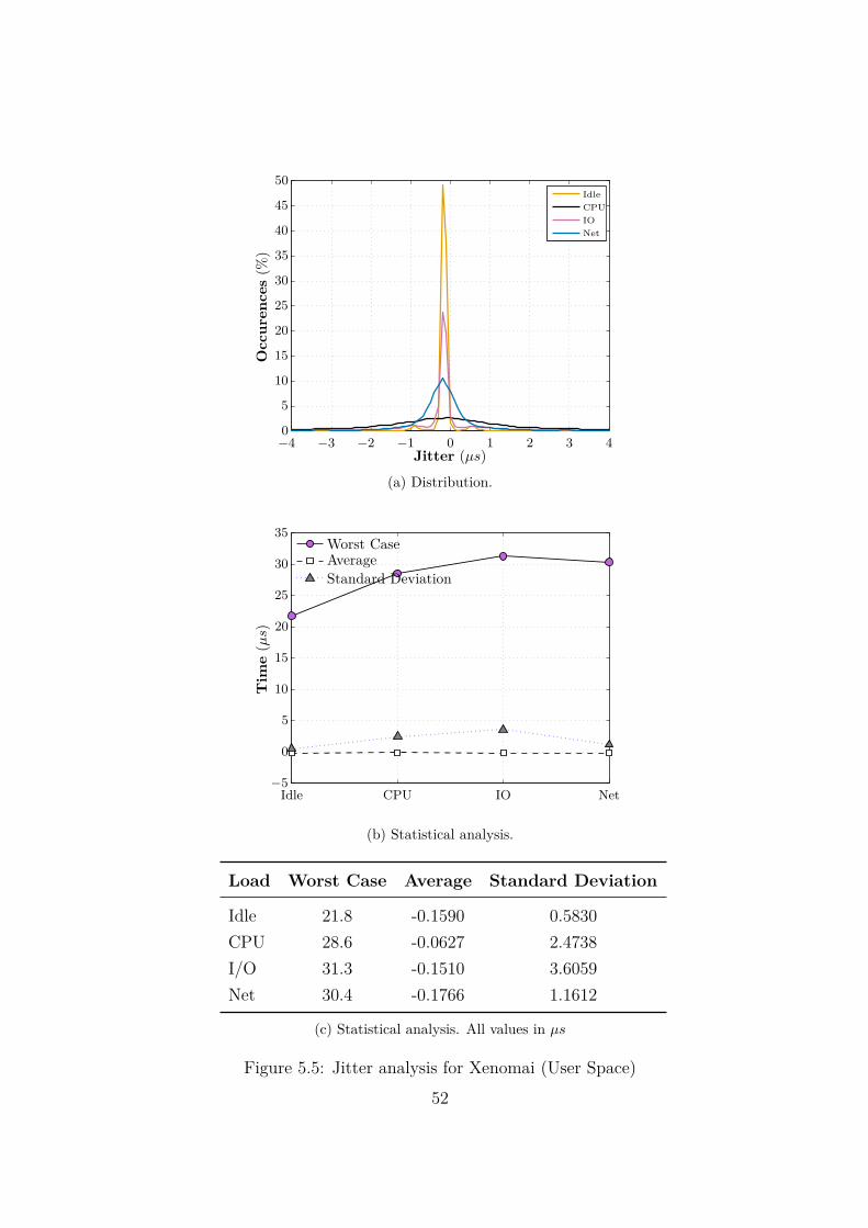
NetIOCPUIdle
Occ
uren
ces
(%)
Jitter (µs)−4 −3 −2 −1 0 1 2 3 40
5
10
15
20
25
30
35
40
45
50
(a) Distribution.
Tim
e(µ
s)
Standard DeviationAverageWorst Case
Idle CPU IO Net−5
0
5
10
15
20
25
30
35
(b) Statistical analysis.
Load Worst Case Average Standard Deviation
Idle 21.8 -0.1590 0.5830CPU 28.6 -0.0627 2.4738I/O 31.3 -0.1510 3.6059Net 30.4 -0.1766 1.1612
(c) Statistical analysis. All values in µs
Figure 5.5: Jitter analysis for Xenomai (User Space)52
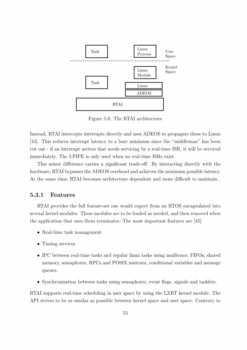
RTAI
LinuxModule
LinuxTask
Task LinuxProcess User
Space
KernelSpace
ADEOS
Figure 5.6: The RTAI architecture
Instead, RTAI intercepts interrupts directly and uses ADEOS to propagate these to Linux[44]. This reduces interrupt latency to a bare minimum since the “middleman” has beencut out - if an interrupt arrives that needs servicing by a real-time ISR, it will be servicedimmediately. The I-PIPE is only used when no real-time ISRs exist.
This minor difference carries a significant trade-off. By interacting directly with thehardware, RTAI bypasses the ADEOS overhead and achieves the minimum possible latency.At the same time, RTAI becomes architecture dependent and more difficult to maintain.
5.3.1 Features
RTAI provides the full feature-set one would expect from an RTOS encapsulated intoseveral kernel modules. These modules are to be loaded as needed, and then removed whenthe application that uses them terminates. The most important features are [45]:
• Real-time task management
• Timing services
• IPC between real-time tasks and regular linux tasks using mailboxes, FIFOs, sharedmemory, semaphores, RPCs and POSIX mutexes, conditional variables and messagequeues.
• Synchronization between tasks using semaphores, event flags, signals and tasklets.
RTAI supports real-time scheduling in user space by using the LXRT kernel module. TheAPI strives to be as similar as possible between kernel space and user space. Contrary to
53
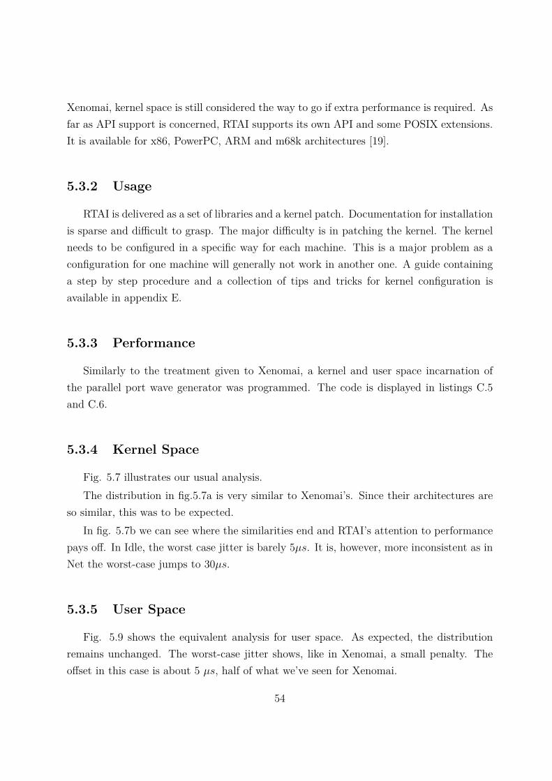
Xenomai, kernel space is still considered the way to go if extra performance is required. Asfar as API support is concerned, RTAI supports its own API and some POSIX extensions.It is available for x86, PowerPC, ARM and m68k architectures [19].
5.3.2 Usage
RTAI is delivered as a set of libraries and a kernel patch. Documentation for installationis sparse and difficult to grasp. The major difficulty is in patching the kernel. The kernelneeds to be configured in a specific way for each machine. This is a major problem as aconfiguration for one machine will generally not work in another one. A guide containinga step by step procedure and a collection of tips and tricks for kernel configuration isavailable in appendix E.
5.3.3 Performance
Similarly to the treatment given to Xenomai, a kernel and user space incarnation ofthe parallel port wave generator was programmed. The code is displayed in listings C.5and C.6.
5.3.4 Kernel Space
Fig. 5.7 illustrates our usual analysis.The distribution in fig.5.7a is very similar to Xenomai’s. Since their architectures are
so similar, this was to be expected.In fig. 5.7b we can see where the similarities end and RTAI’s attention to performance
pays off. In Idle, the worst case jitter is barely 5µs. It is, however, more inconsistent as inNet the worst-case jumps to 30µs.
5.3.5 User Space
Fig. 5.9 shows the equivalent analysis for user space. As expected, the distributionremains unchanged. The worst-case jitter shows, like in Xenomai, a small penalty. Theoffset in this case is about 5 µs, half of what we’ve seen for Xenomai.
54
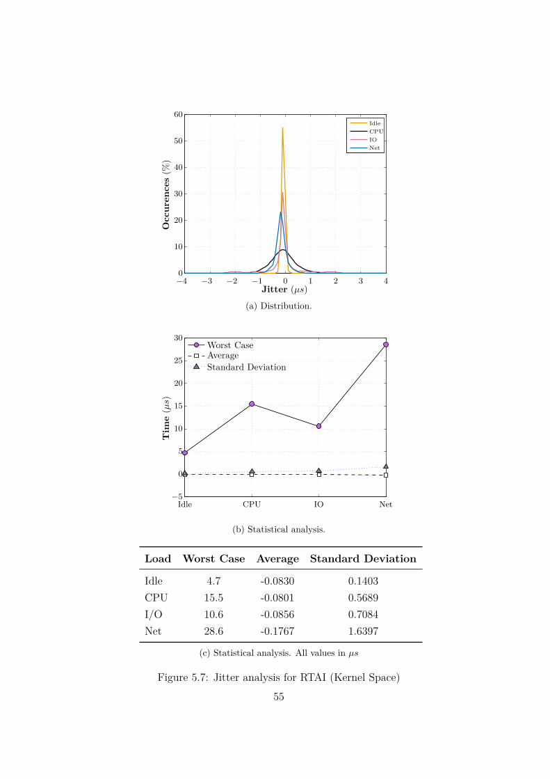
NetIOCPUIdle
Occ
uren
ces
(%)
Jitter (µs)−4 −3 −2 −1 0 1 2 3 40
10
20
30
40
50
60
(a) Distribution.
Tim
e(µ
s)
Standard DeviationAverageWorst Case
Idle CPU IO Net−5
0
5
10
15
20
25
30
(b) Statistical analysis.
Load Worst Case Average Standard Deviation
Idle 4.7 -0.0830 0.1403CPU 15.5 -0.0801 0.5689I/O 10.6 -0.0856 0.7084Net 28.6 -0.1767 1.6397
(c) Statistical analysis. All values in µs
Figure 5.7: Jitter analysis for RTAI (Kernel Space)55
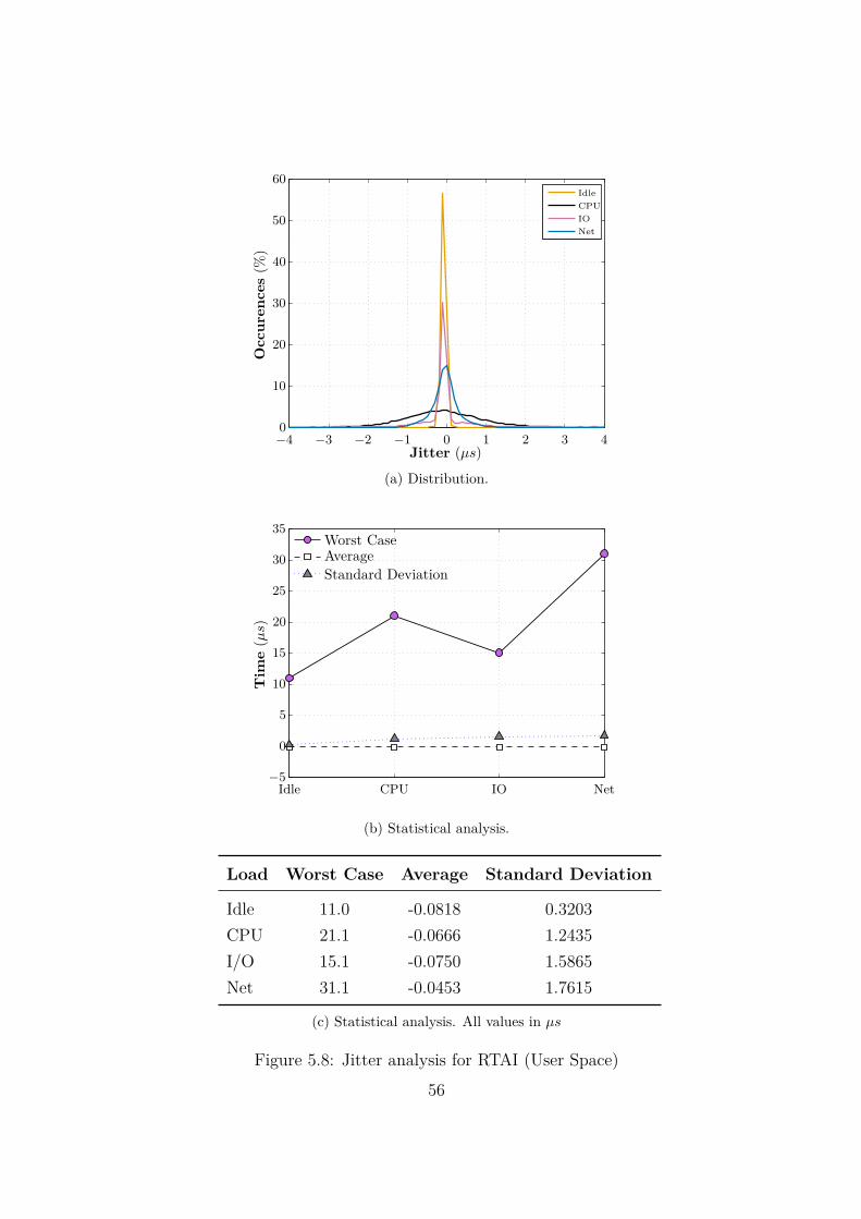
NetIOCPUIdle
Occ
uren
ces
(%)
Jitter (µs)−4 −3 −2 −1 0 1 2 3 40
10
20
30
40
50
60
(a) Distribution.
Tim
e(µ
s)
Standard DeviationAverageWorst Case
Idle CPU IO Net−5
0
5
10
15
20
25
30
35
(b) Statistical analysis.
Load Worst Case Average Standard Deviation
Idle 11.0 -0.0818 0.3203CPU 21.1 -0.0666 1.2435I/O 15.1 -0.0750 1.5865Net 31.1 -0.0453 1.7615
(c) Statistical analysis. All values in µs
Figure 5.8: Jitter analysis for RTAI (User Space)56
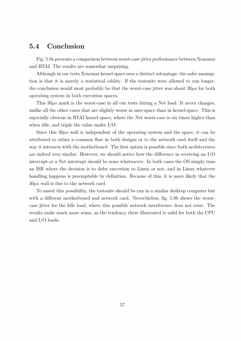
5.4 ConclusionFig. 5.9a presents a comparison between worst-case jitter performance between Xenomai
and RTAI. The results are somewhat surprising.Although in our tests Xenomai kernel space sees a distinct advantage, the safer assump-
tion is that it is merely a statistical oddity. If the testsuite were allowed to run longer,the conclusion would most probably be that the worst-case jitter was about 30µs for bothoperating system in both execution spaces.
This 30µs mark is the worst-case in all our tests during a Net load. It never changes,unlike all the other cases that are slightly worse in user-space than in kernel-space. This isespecially obvious in RTAI kernel space, where the Net worst-case is six times higher thanwhen idle, and triple the value under I/O.
Since this 30µs wall is independent of the operating system and the space, it can beattributed to either a common flaw in both designs or to the network card itself and theway it interacts with the motherboard. The first option is possible since both architecturesare indeed very similar. However, we should notice how the difference in receiving an I/Ointerrupt or a Net interrupt should be none whatsoever. In both cases the OS simply runsan ISR where the decision is to defer execution to Linux or not, and in Linux whateverhandling happens is preemptable by definition. Because of this, it is more likely that the30µs wall is due to the network card.
To assert this possibility, the testsuite should be run in a similar desktop computer butwith a different motherboard and network card. Nevertheless, fig. 5.9b shows the worst-case jitter for the Idle load, where this possible network interference does not exist. Theresults make much more sense, as the tendency there illustrated is valid for both the CPUand I/O loads.
57
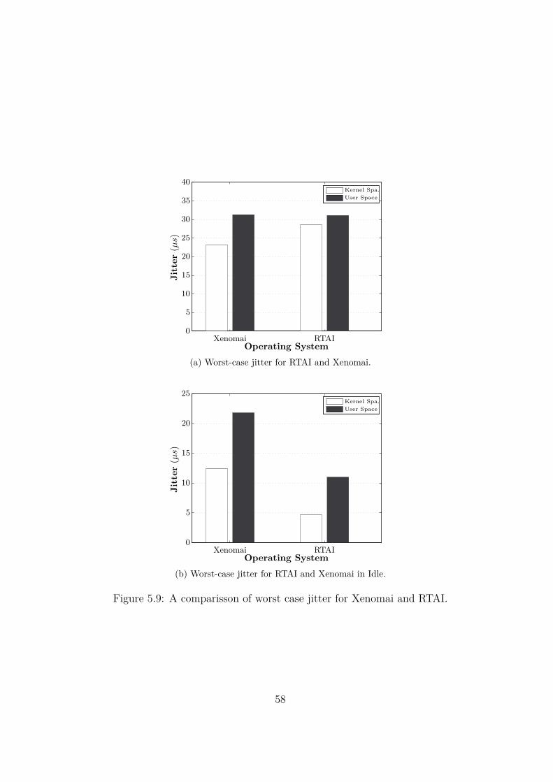
User SpaceKernel Spa.
Operating System
Jitt
er(µ
s)
Xenomai RTAI0
5
10
15
20
25
30
35
40
(a) Worst-case jitter for RTAI and Xenomai.
User SpaceKernel Spa.
Operating System
Jitt
er(µ
s)
Xenomai RTAI0
5
10
15
20
25
(b) Worst-case jitter for RTAI and Xenomai in Idle.
Figure 5.9: A comparisson of worst case jitter for Xenomai and RTAI.
58
Chapter 6
Conclusion
In this chapter conclusions encompassing the whole of Part II are presented. The mostimportant benchmarking results are compiled into a Linux real-time scale – an ordered listof worst-performing to best-performing system. As closure, the results obtained thus farare compared to other work done in the field.
6.1 ResultsIn this second part of the dissertation, a total of 32 different performance tests were
performed with the help of our testsuite. With all this data in hand, we are able to builtthe Linux real-time scale presented in fig. 6.1.
On the x axis we have the target’s initials. On the right a U means “User Space” whileK means “Kernel Space”. On the left, V stands for “Vanilla”, P for “PREEMPT_RT”, Xfor “Xenomai” and R for “RTAI”.
From this scale, we can draw some immediate conclusions. Focusing on regular Linuxfirst, we can see that Linux user space offers the worst performance. The best performancecan be obtained with vanilla kernel space, although on an Idle computer PREEMPT_RTwould offer equal performance on user space. The large gap between Idle and worst overallin PREEMPT_RT might be explained by a deficiency in the disk driver, since it is highI/O that’s pushing the worst-case so high.
Be that as it may, regular Linux can not bring worst-case bellow the 100s of microseconds. With the dual kernel approach we can lower this value to the tens of microseconds – an order of magnitude lower.
The best in class for this category is RTAI running in kernel space. 5 µs was the lowest
59
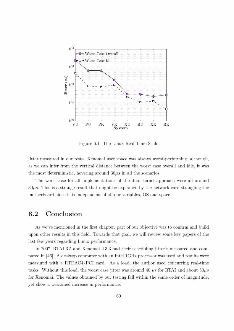
System
Jitt
er(µ
s)Worst Case Idle
Worst Case Overall
VU PU PK VK XU RU XK RK100
101
102
103
104
Figure 6.1: The Linux Real-Time Scale
jitter measured in our tests. Xenomai user space was always worst-performing, although,as we can infer from the vertical distance between the worst case overall and idle, it wasthe most deterministic, hovering around 30µs in all the scenarios.
The worst-case for all implementations of the dual kernel approach were all around30µs. This is a strange result that might be explained by the network card strangling themotherboard since it is independent of all our variables, OS and space.
6.2 Conclusion
As we’ve mentioned in the first chapter, part of our objective was to confirm and buildupon other results in this field. Towards that goal, we will review some key papers of thelast few years regarding Linux performance.
In 2007, RTAI 3.5 and Xenomai 2.3.3 had their scheduling jitter’s measured and com-pared in [46]. A desktop computer with an Intel 1GHz processor was used and results weremeasured with a RTDAC4/PCI card. As a load, the author used concurring real-timetasks. Without this load, the worst case jitter was around 40 µs for RTAI and about 50µsfor Xenomai. The values obtained by our testing fall within the same order of magnitude,yet show a welcomed increase in performance.
60
In 2008 a comparison between RTAI, Xenomai, Linux and the proprietary RTOS Vx-Works was performed in [44]. The OSs were installed on single board Motorola boardwith a PowerPC CPU and the resulting interrupt latency was measured. As we opted formeasuring scheduling jitter instead of interrupt latency, our results are unrelated.
In 2009 the difference in scheduling jitter between vanilla and PREEMP_RT was testedin [47]. Linux version 2.6.25 was installed on a machine with a 2.66GHz Core2Duo E6750.A user space task was made periodic by the use of POSIX timers and CPU and I/O systemloads were prepared. The results are quite interesting. The jitter was measured by callinggettimeofday() and storing the task activation time. Vanilla kernel jitter stood between 20µs and 18 ms under I/O, while PREEMPT_RT stood between 70 µs and 300µs. The2.6.32 Linux version used for our tests has greatly improved native real-time performance.For PREEMPT_RT we can induce that our values are similar to those obtained, as thosewere merely the scheduling jitter, and ours had the additional jitter of producing a signalon the parallel port.
In 2010 RTAI’s scheduling jitter was analyzed in [48] on a Pentium 4 machine similarto ours. Code was auto-generated by Scicos and hence ran in user space. Results wereobtained by applying varying I/O load using data acquisition boards. RTAI respondedwith worst-case jitter from 30 µs on minimum I/O Load to about 400µs. This exposed asensitivity to the over use of the acquisition board. Our I/O load would be comparable tothe minimum I/O load used by that team, so our values are well in agreement.
Although the Linux real-time scale we present in fig. 6.1 is, by no means, writtenin stone, the overall picture it paints is in line with previous research on the matter.PREEMPT_RT improves upon vanilla kernel and obtains jitter values on the hundreds ofµs range. Xenomai and RTAI bring this value down to the tens of µs, and RTAI usuallyoutperforms Xenomai.
61

62
Part III
Xenomai Lab
63

64
Chapter 7
Introduction
In this chapter, the conceptual basis for Xenomai Lab is discussed. The reasoning be-hind its architecture as well as the main technological choices that steered its developmentare presented.
7.1 Keep it Simple, Stupid
Xenomai Lab is a fresh approach to designing control systems in Linux. It allows theuser to graphically design a block diagram of a control system and execute it in real-time. It also provides an open application programming interface (API) to easily programnew blocks. Control algorithms are programmed in straight C, with library support formatrices. Any engineer will feel right at home.
The platform was designed with the intent of decoupling control algorithms from RTOSconcepts, while, above all, keeping it simple. A simple system in the KISS sense is simpleto use and simple in the implementation. This makes it easy to debug and expand withnew features. Xenomai Lab is distinctive because it is a pure Linux affair - it uses nativewidgets for the interface and plays well with package management. In Debian systemssuch as Ubuntu, installation is as easy as a double click1. These things matter becauseusability matters. An application that is easy to install is much more likely to be triedthan one that puts up an initial barrier.
Having presented the application, let us now try to answer the most important questionsregarding motivation and design decisions.
1At this moment, only with Xenomai already installed.
65
7.2 Why build something new ?Digital control systems have been designed for more than half a century. The longevity
of the area inevitably means that it has industry standards and established workflows.Designing a control systems usually consists in the following steps:
1. A mathematical model of the plant is deduced, and a controller is projected thatachieves the desired performance metrics. The system is tested via numerical simu-lation, which means the results are merely theoretical approximations. This modelingis normally done in proprietary industry standards such as MATLAB/Simulink orLabVIEW.
2. Communication with the plant is built and tested. This means setting up the propersensors, actuators, A/D and D/A converters. Usually an acquisition board is used.Some custom electronics may need to be designed in this process to filter the signalscoming from the sensors to maximize efficiency in the data acquisition.
3. The theoretical controller is tested with the real plant instead of its mathematicalmodel. As the plant model is merely an approximation, inevitably the designer needsto adapt his controller and/or hardware to make it work as intended.
The controller can be implemented in a desktop computer, in an embedded system or ina microcontroller. The control system can be monolithic, distributed, network controlled,or any other. Whatever the case may be, the workflow remains essentially unchanged.
To develop a system using this workflow in Linux, one has but a few options. Themore mature one would be the RTAI-Lab/SciLab/SciCos combo. SciLab is a softwarepackage similar to MATLAB. It provides a high-level language similar to MATLAB’s andSciCos is akin to Simulink. SciLab sits in a software uncanny valley where everything isvaguely familiar but not quite. One might argue that in engineering functionality, and notconcepts such as usability or user friendly, is the most important thing. In the opinion ofthe team behind this work, the low adoption rates of SciLab/SciCos speak for themselveson this matter. RTAI-Lab implements code generation from SciCos to RTAI executablesand has a graphical application with scopes and other such graphical utilities to monitorexecution.
An engineer’s time is worth money. Although a software package like RTAI-Lab andSciLab/SciCos can provide almost the same functionality by no price, they cost time. Time
66
to install, learn how to use, test and debug. This can easily incur in higher costs then usingindustrial grade tools. The fact that proprietary software has thorough documentationand is widely used overshadows the price. RTAI-Lab was last released in 2006 and itsdocumentation remains unchanged since 2008.
The other option would be to continue modeling using whatever software is used, butthen implement the control system using Xenomai or RTAI’s API. In reality, this is nooption at all. Block diagrams provide function decomposition and expose a system’s in-ner signals. By programming a monolithic program, the internals are not exposed anddecomposition is lost.
Xenomai Lab tries to be the RTAI-Lab/SciCos combo for Xenomai, but done in adifferent way, with none of its problems. Application related coding is done directly inC instead of another language. This means that no new language has to be learned, asall engineers inevitably know C. The fact that the application-related code is not auto-generated means that it’s faster and easier to debug. The interface is simplified and isspecific to the application. It does less things which means it is focused. There is almostnothing between the user and the control algorithms.
7.3 Why Xenomai ?
Both RTAI and Xenomai can deliver real-time performance suitable for control appli-cations. However, a choice had to be made between the two, and it is our objective in thissection to explain why we chose Xenomai.
RTAI is the obvious choice for applications requiring maximum performance. The 5µsworst-case jitter obtained for a kernel space module in section 5.3.4 is an impressive figureof merit. It is the opinion of the team behind this work is that the biggest issue withRTAI is that it is difficult to use. Granted, these are relative notions. For any advancedLinux user there is nothing in RTAI that is particularly out of the ordinary. Difficultyis necessarily in the “eye of the beholder”. Be that as it may, the knowledge required touse RTAI without major issues is very specific. Software has to be manually compiledand installed through the command line, and not only that, real-time applications are notexecuted directly by a call to the binary. The RTAI paradigm is that a loader script loadsthe necessary kernel support before the binary is executed, and unloads them after theprogram completed.
Xenomai, on the other hand, strives to be flexible and easy to use. What Xenomai does
67
not have in performance, it compensates in usability. This is much more important forour purposes. If a user’s main concern is maximum achievable performance, then XenomaiLab isn’t a good option to begin with because it increases execution latency and usesmuch more resources than programming a monolithic C program. Of course, a monolithicC program requires much more work than the graphical diagram approach. Organizing asystem in blocks lends itself naturally to code reuse, which at the end of the day meansgreater functionality with less coding.
Xenomai’s installation procedure has been adapted for Debian systems. Rather thenrunning a typical old-school make install command, Xenomai can be compiled into a De-bian package. This makes Xenomai integrate extremely well with the system. The usualchannels for installing and uninstalling can be used. In fact, the Xenomai libraries can bedirectly installed from the Ubuntu Software Center as they are present in the repositories.A kernel must still be manually compiled, however.
Since we intend to develop our application in Ubuntu, which is a Debian system, Xeno-mai is a much more attractive solution.
In addition to this, Xenomai 3 (latest version at the time of writing is 2.6) is just aroundthe corner and will bring an unbeatable feature - the implementation of the Xenomai APIover a PREEMPT_RT kernel. This nullifies the difficulty in installation and will makeXenomai Lab installation truly a double-click affair. Of course, the dual kernel approachwill still be available for those who need its performance.
7.4 Why Qt ?
Qt is a cross-platform C++ application framework that runs on Linux, Mac OS andWindows, among other platforms [49]. Qt is one of the major toolkits for building Linuxapplications. The other major toolkit is GTK, which is an integral part of the GNU project.GTK is the toolkit used by the GNOME desktop, while Qt is the toolkit behind KDE, theother major Linux desktop.
Xenomai Lab was programmed in Qt for various reasons. It integrates better withthe GNOME and KDE desktops than the other way around, it natively uses C++ ratherthan plain C which is a major advantage when programming graphically, but above all,it has an Integrated Development Environment (IDE). Qt Creator provides in a singleapplication the ability to code, build, debug, control versions, consult documentation, andevery other feature one would expect from a modern IDE. No such application exists for
68
GTK development. The only IDE for programming GTK is the Mono framework, whichis a reimplementation of the Microsoft .NET and C# technology.
There were other options, such as Java, but Qt provides the ideal balance betweenperformance and ease of use for our purposes.
69

70
Chapter 8
Xenomai Lab
In this chapter a thorough analysis of Xenomai Lab’s usage and implementation ispresented, as well as experimental results of both simulation and real-world interaction.By the end of this chapter, the reader will be able to easily program his own blocks or evendwell into hacking new functions into the lab.
8.1 Head First
The easiest way to understand what Xenomai Lab (XL) does is to see it in action.Fig. 8.1 shows XL’s main window. It consists of a big white area, the canvas, where
block diagrams can be drawn. To the left is the block list, where two set of blocks can beused: real-time and non real-time. Across the top rest three toolbars for interaction withthe block diagram.
Blocks can be chosen from the block list and dropped on the canvas. Lines can thenbe drawn between blocks. Blocks can accept any number of inputs. They can also outputa result to any number of blocks.
As an example, let us consider we intend to project a controller for a plant defined bythe following transfer function:
G(s) = 100s+ 100 (8.1)
For a sampling period h = 1ms, the transfer function becomes
H(q) = 0.0952q − 0.9048 (8.2)
71
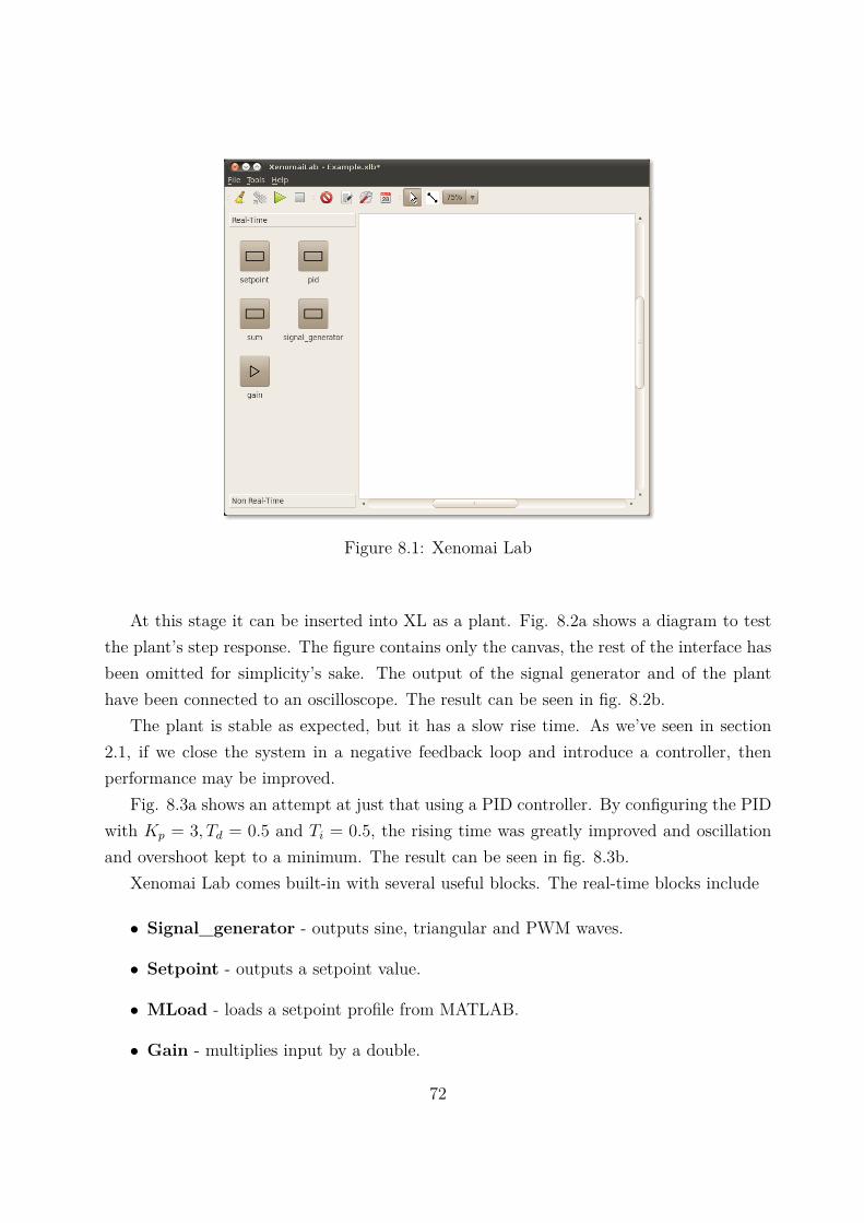
Figure 8.1: Xenomai Lab
At this stage it can be inserted into XL as a plant. Fig. 8.2a shows a diagram to testthe plant’s step response. The figure contains only the canvas, the rest of the interface hasbeen omitted for simplicity’s sake. The output of the signal generator and of the planthave been connected to an oscilloscope. The result can be seen in fig. 8.2b.
The plant is stable as expected, but it has a slow rise time. As we’ve seen in section2.1, if we close the system in a negative feedback loop and introduce a controller, thenperformance may be improved.
Fig. 8.3a shows an attempt at just that using a PID controller. By configuring the PIDwith Kp = 3, Td = 0.5 and Ti = 0.5, the rising time was greatly improved and oscillationand overshoot kept to a minimum. The result can be seen in fig. 8.3b.
Xenomai Lab comes built-in with several useful blocks. The real-time blocks include
• Signal_generator - outputs sine, triangular and PWM waves.
• Setpoint - outputs a setpoint value.
• MLoad - loads a setpoint profile from MATLAB.
• Gain - multiplies input by a double.
72
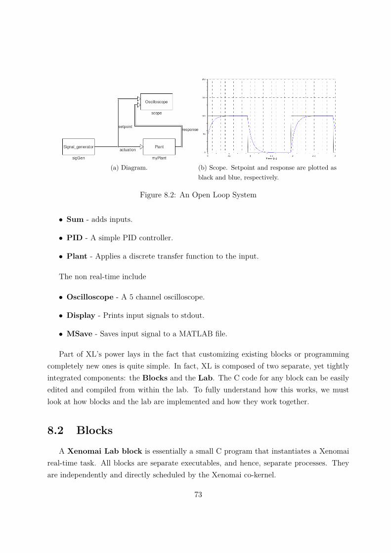
(a) Diagram. (b) Scope. Setpoint and response are plotted asblack and blue, respectively.
Figure 8.2: An Open Loop System
• Sum - adds inputs.
• PID - A simple PID controller.
• Plant - Applies a discrete transfer function to the input.
The non real-time include
• Oscilloscope - A 5 channel oscilloscope.
• Display - Prints input signals to stdout.
• MSave - Saves input signal to a MATLAB file.
Part of XL’s power lays in the fact that customizing existing blocks or programmingcompletely new ones is quite simple. In fact, XL is composed of two separate, yet tightlyintegrated components: the Blocks and the Lab. The C code for any block can be easilyedited and compiled from within the lab. To fully understand how this works, we mustlook at how blocks and the lab are implemented and how they work together.
8.2 BlocksA Xenomai Lab block is essentially a small C program that instantiates a Xenomai
real-time task. All blocks are separate executables, and hence, separate processes. Theyare independently and directly scheduled by the Xenomai co-kernel.
73
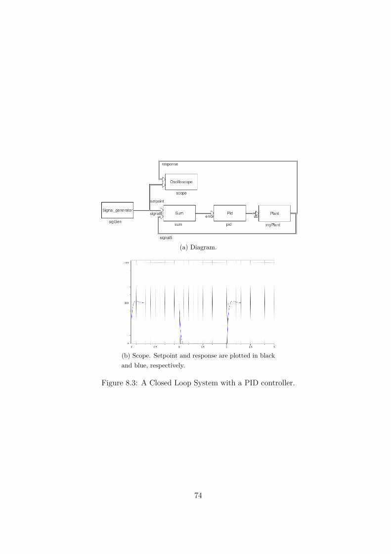
(a) Diagram.
(b) Scope. Setpoint and response are plotted in blackand blue, respectively.
Figure 8.3: A Closed Loop System with a PID controller.
74
Each block has a list of input and output channels. The channels are passed as inputarguments to the executable. Consider the following call to the gain block
./gain −i error −o plant
Here, gain will read the error channel, manipulate it and write the result to the plantchannel. There is no limit in the number of channels, a block accepts a list of commaseparated channel names of any size.
./sum −i setpoint,ad,noise −o error
Here, sum will add the values of setpoint, ad and noise and write the result to the errorchannel.
A channel is a communication bridge between two blocks. Blocks use channels toexchange information. The information exchanged are floating point numbers, but insteadof using double or float, blocks communicate using a custom Matrix type. The Matrixtype is part of a matrix library developed by Diego Mendes who was kind enough to allowintegration of his work with Xenomai Lab. By using Matrix, blocks are able to exchange agroup of floating point numbers with double precision. Scalars, vectors and matrices canall be encapsulated into the Matrix type. The library also comprises a set of standardmatrix operations such as calculating determinants, eigen values, etc. These functions canbe used within the block to perform common computations.
Not all elements in a block diagram implement control functions. Some blocks existsolely for monitoring purposes. We might want to save a signal to a file and analyzeit later, for example. These operations don’t have the strict real-time requirements thatcontrol operations have. To support this fundamental difference, blocks can be eitherreal-time or non real-time. Non real-time blocks operate in much the same way as theirreal-time counterparts.
./display −i setpoint,error,actuation
Here, display is reading 3 input channels which will then be displayed to the user. Bydefinition, non real-time blocks have no outputs in the context of Xenomai Lab. Never-theless, non real-time blocks are regular Linux C programs detached from any Xenomaispecificities. This means that, in reality, they can be programmed to do anything with theinformation they get from the input channels. The block can service a web server with
75
real-time data from a process, or send experimental results through a UNIX socket to theother side of the globe. No restrictions are imposed by XL.
Communication between real-time and non real-time blocks is strictly unidirectional,from real-time to non real-time. A special kind of channel, called a pipe, is used for thisspecial case.
./gain −i error −o plant −p actuation
Here, gain outputs its result to an extra non real-time channel called actuation. A nonreal-time block can then open it like in the previous example.
Blocks have parameters, or operational settings. A PID controller, for example, hasits operation conditioned by three gains – Kp, Td and Ti. Nothing stops these parametersfrom being hardcoded in the controller implementation, but this approach brings severalproblems.
One block diagram might have multiple blocks of the same type. For example, it isperfectly common to have a block diagram with several gain blocks. If the value of gainwere hardcoded in the code, this means that every gain block would apply the same gain.It would be unfeasible to design a diagram of complexity above trivial with such a system.One would need as many gain blocks as many different gain values were needed. A gainblock of gain -1, another of gain 4, and so forth.
Bearing this in mind and following the UNIX tradition, each block has a configurationfile that defines its operational settings. This way one single block, (meaning one singleexecutable and one single source file) can run with different settings depending on theconfiguration file. A single block executable can have multiple instances, and hence, wecan also refer to the configuration file as a block instance.
./gain −i error −o plant −p actuation Gain4
Here, we added an instance to the end of the gain call. gain would then look for aGain4.conf file and load its parameters from it.
The problem doesn’t end here however. A reasonable expectation of such a systemwould be the ability to change these parameters in runtime, when the block diagram isrunning in real-time. If a plant is being controlled by a PID, for instance, it is essentialto be able to change the parameters in real-time and watch how the variation affects thecontrol.
76
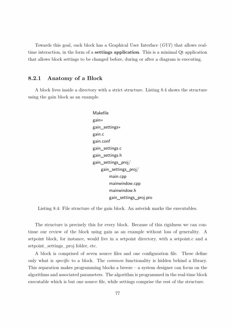
Towards this goal, each block has a Graphical User Interface (GUI ) that allows real-time interaction, in the form of a settings application. This is a minimal Qt applicationthat allows block settings to be changed before, during or after a diagram is executing.
8.2.1 Anatomy of a Block
A block lives inside a directory with a strict structure. Listing 8.4 shows the structureusing the gain block as an example.
Makefilegain∗gain_settings∗gain.cgain.confgain_settings.cgain_settings.hgain_settings_proj/
gain_settings_proj/main.cppmainwindow.cppmainwindow.hgain_settings_proj.pro
Listing 8.4: File structure of the gain block. An asterisk marks the executables.
The structure is precisely this for every block. Because of this rigidness we can con-tinue our review of the block using gain as an example without loss of generality. Asetpoint block, for instance, would live in a setpoint directory, with a setpoint.c and asetpoint_settings_proj folder, etc.
A block is comprised of seven source files and one configuration file. These defineonly what is specific to a block. The common functionality is hidden behind a library.This separation makes programming blocks a breeze – a system designer can focus on thealgorithms and associated parameters. The algorithm is programmed in the real-time blockexecutable which is but one source file, while settings comprise the rest of the structure.
77
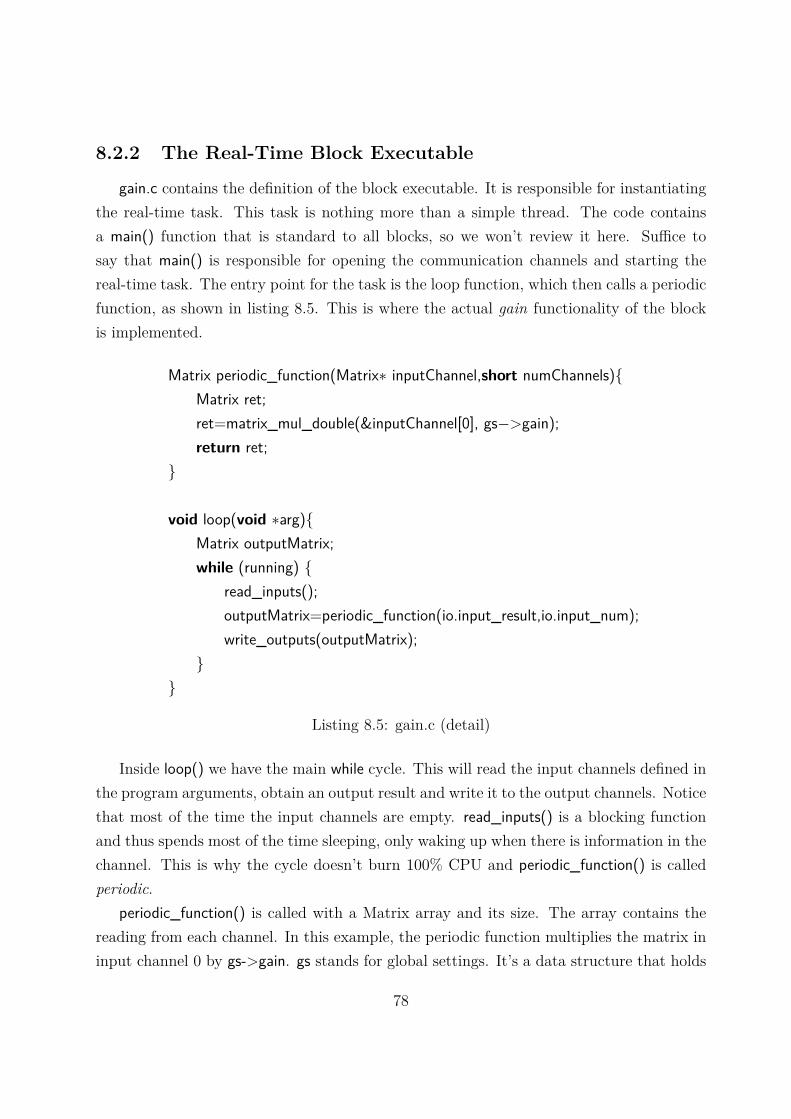
8.2.2 The Real-Time Block Executable
gain.c contains the definition of the block executable. It is responsible for instantiatingthe real-time task. This task is nothing more than a simple thread. The code containsa main() function that is standard to all blocks, so we won’t review it here. Suffice tosay that main() is responsible for opening the communication channels and starting thereal-time task. The entry point for the task is the loop function, which then calls a periodicfunction, as shown in listing 8.5. This is where the actual gain functionality of the blockis implemented.
Matrix periodic_function(Matrix∗ inputChannel,short numChannels){Matrix ret;ret=matrix_mul_double(&inputChannel[0], gs−>gain);return ret;
}
void loop(void ∗arg){Matrix outputMatrix;while (running) {
read_inputs();outputMatrix=periodic_function(io.input_result,io.input_num);write_outputs(outputMatrix);
}}
Listing 8.5: gain.c (detail)
Inside loop() we have the main while cycle. This will read the input channels defined inthe program arguments, obtain an output result and write it to the output channels. Noticethat most of the time the input channels are empty. read_inputs() is a blocking functionand thus spends most of the time sleeping, only waking up when there is information in thechannel. This is why the cycle doesn’t burn 100% CPU and periodic_function() is calledperiodic.
periodic_function() is called with a Matrix array and its size. The array contains thereading from each channel. In this example, the periodic function multiplies the matrix ininput channel 0 by gs->gain. gs stands for global settings. It’s a data structure that holds
78
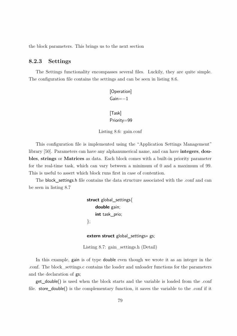
the block parameters. This brings us to the next section
8.2.3 Settings
The Settings functionality encompasses several files. Luckily, they are quite simple.The configuration file contains the settings and can be seen in listing 8.6.
[Operation]Gain=−1
[Task]Priority=99
Listing 8.6: gain.conf
This configuration file is implemented using the “Application Settings Management”library [50]. Parameters can have any alphanumerical name, and can have integers, dou-bles, strings or Matrices as data. Each block comes with a built-in priority parameterfor the real-time task, which can vary between a minimum of 0 and a maximum of 99.This is useful to assert which block runs first in case of contention.
The block_settings.h file contains the data structure associated with the .conf and canbe seen in listing 8.7
struct global_settings{double gain;int task_prio;
};
extern struct global_settings∗ gs;
Listing 8.7: gain_settings.h (Detail)
In this example, gain is of type double even though we wrote it as an integer in the.conf. The block_settings.c contains the loader and unloader functions for the parametersand the declaration of gs;
get_double() is used when the block starts and the variable is loaded from the .conffile. store_double() is the complementary function, it saves the variable to the .conf if it
79
struct global_settings∗ gs;
void load_gs(void){get_double("Operation","Gain",&gs−>gain);get_int("Task","Priority",&gs−>task_prio);
}
void unload_gs(void){store_double("Operation", "Gain", gs−>gain);store_int("Task","Priority",gs−>task_prio);
}
Listing 8.8: gain_settings.c (Detail)
was changed during execution. Variations of these functions exist for integer, strings andmatrices.
In block_settings_proj, we have a small Qt project for the settings interface. Themain.cpp for the project is completely standard Qt boilerplate code. The only differenceis a call to a static function from the library that supports the settings interface. Thisinstantiates the required data structures and handles the executable inputs. Settings needan instance passed to it as input
./gain_settings gain1
Here, gain_settings will look for gain1.conf in the same way the block does. By defaultinstances should be in the workspace directory, which we will talk about in the nextsection.
Once settings has an instance, it creates the window seen in fig. 8.9. As is common inQt, the main window of an application is built using a MainWindow class.
As can be seen in listing 8.10, MainWindow derives from BlockBase, the class thatimplements the settings functionality common to all blocks and encapsulates everythingabout settings creation and management. The MainWindow constructor in listing 8.10 callsfillDialog with the name of the block and a small description. This description accepts basichtml notation, like a <BR> tag for line breaks, or <b></b> for bold text.
setSettings is a pure virtual member of BlockBase, which means it must be imple-mented by any derived classes. This function is akin to load_gs() and unload_gs() in
80
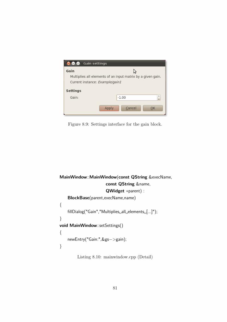
Figure 8.9: Settings interface for the gain block.
MainWindow::MainWindow(const QString &execName,const QString &name,QWidget ∗parent) :
BlockBase(parent,execName,name){
fillDialog("Gain","Multiplies␣all␣elements␣[...]");}void MainWindow::setSettings(){
newEntry("Gain:",&gs−>gain);}
Listing 8.10: mainwindow.cpp (Detail)
81
block_settings.c, but all within one function. We establish a new parameter entry and passit the pointer to the respective gs variable.
This concludes our walkthrough of the block stack. There is no more code. Thecomplete set of data to define a block is then
• A name
• A periodic function
• A collection of parameters and functions to load and unload them to and from mem-ory
• A small description
The real magic lays behind the curtain, hidden in the library files. A brief walkthroughof the main library components can be found in appendix B. As a side note, it is importantto mention that a template block is shipped along with the regular blocks. This blockscomes accompanied with a script that automatically renames it to a chosen name. This iscurrently the preferred way to programming new blocks.
8.3 The LabXenomai Lab is nothing more than an abstract way of interacting with the blocks.
There is nothing the Lab does that one could not do by hand in the terminal. For this towork, Xenomai Lab expects blocks to be positioned in specific directories.
The heart of Xenomai Lab lies in the ~/.xenomailab folder1. This directory is structuredas can be seen in listing 8.11.
The blocks folder contains blocks individualized in separate directories. Inside thatdirectory lives the structure we’ve presented in the previous section. blocks.conf registersthe blocks with a symbol. An excerpt is presented in listing 8.12.
The include folder contains the library files that blocks need. These are described atlength in appendix B.
The examples directory contains sample projects and reference implementations ofI/O blocks. These blocks were developed as part of validation of the program. They aredistributed along with the application as a reference. Since they are specific to customhardware they are useless to users, but very useful as an example.
1~/ is the user’s home folder.
82
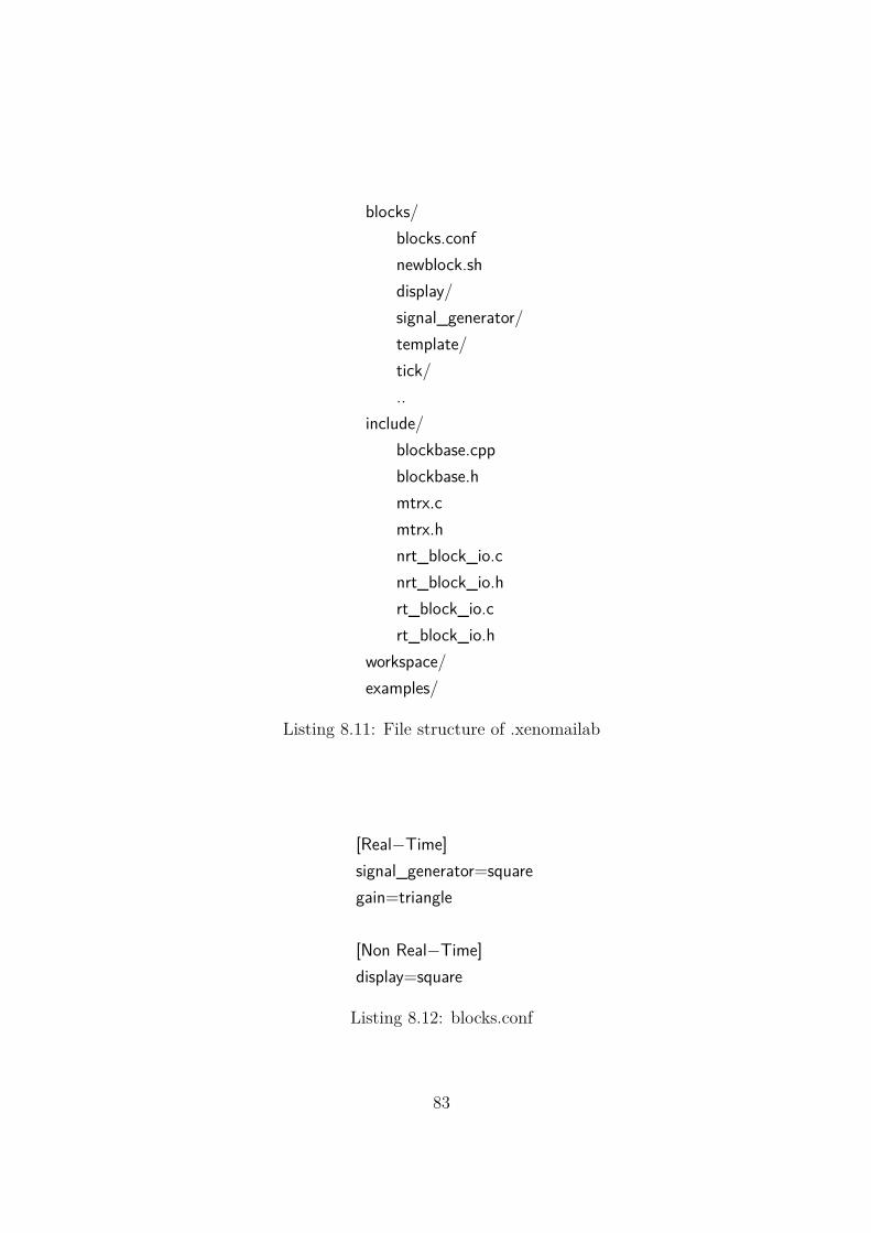
blocks/blocks.confnewblock.shdisplay/signal_generator/template/tick/..
include/blockbase.cppblockbase.hmtrx.cmtrx.hnrt_block_io.cnrt_block_io.hrt_block_io.crt_block_io.h
workspace/examples/
Listing 8.11: File structure of .xenomailab
[Real−Time]signal_generator=squaregain=triangle
[Non Real−Time]display=square
Listing 8.12: blocks.conf
83
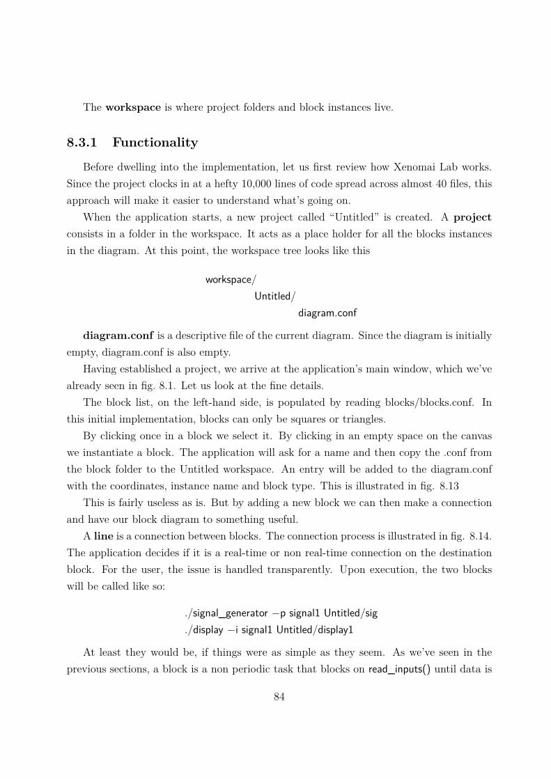
The workspace is where project folders and block instances live.
8.3.1 Functionality
Before dwelling into the implementation, let us first review how Xenomai Lab works.Since the project clocks in at a hefty 10,000 lines of code spread across almost 40 files, thisapproach will make it easier to understand what’s going on.
When the application starts, a new project called “Untitled” is created. A projectconsists in a folder in the workspace. It acts as a place holder for all the blocks instancesin the diagram. At this point, the workspace tree looks like this
workspace/Untitled/
diagram.conf
diagram.conf is a descriptive file of the current diagram. Since the diagram is initiallyempty, diagram.conf is also empty.
Having established a project, we arrive at the application’s main window, which we’vealready seen in fig. 8.1. Let us look at the fine details.
The block list, on the left-hand side, is populated by reading blocks/blocks.conf. Inthis initial implementation, blocks can only be squares or triangles.
By clicking once in a block we select it. By clicking in an empty space on the canvaswe instantiate a block. The application will ask for a name and then copy the .conf fromthe block folder to the Untitled workspace. An entry will be added to the diagram.confwith the coordinates, instance name and block type. This is illustrated in fig. 8.13
This is fairly useless as is. But by adding a new block we can then make a connectionand have our block diagram to something useful.
A line is a connection between blocks. The connection process is illustrated in fig. 8.14.The application decides if it is a real-time or non real-time connection on the destinationblock. For the user, the issue is handled transparently. Upon execution, the two blockswill be called like so:
./signal_generator −p signal1 Untitled/sig
./display −i signal1 Untitled/display1
At least they would be, if things were as simple as they seem. As we’ve seen in theprevious sections, a block is a non periodic task that blocks on read_inputs() until data is
84
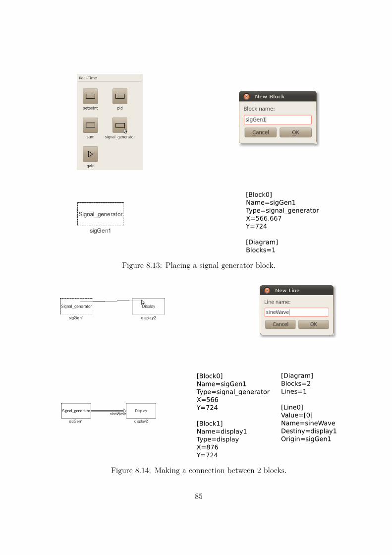
[Block0]
Name=sigGen1
Type=signal_generator
X=566.667
Y=724
[Diagram]
Blocks=1
Figure 8.13: Placing a signal generator block.
[Block0]
Name=sigGen1
Type=signal_generator
X=566
Y=724
[Block1]
Name=display1
Type=display
X=876
Y=724
[Diagram]
Blocks=2
Lines=1
[Line0]
Value=[0]
Name=sineWave
Destiny=display1
Origin=sigGen1
Figure 8.14: Making a connection between 2 blocks.
85
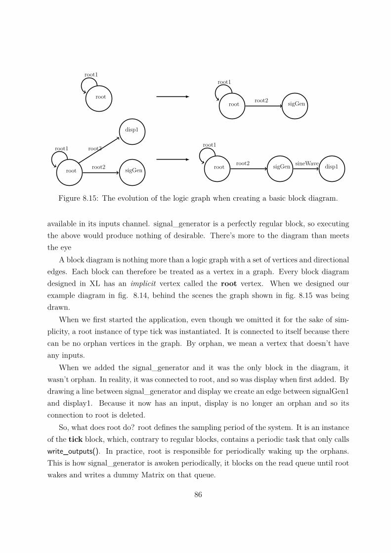
root
root1
root
root1
sigGenroot2
root
root1
sigGenroot2
disp1
root3
root
root1
sigGenroot2 disp1sineWave
Figure 8.15: The evolution of the logic graph when creating a basic block diagram.
available in its inputs channel. signal_generator is a perfectly regular block, so executingthe above would produce nothing of desirable. There’s more to the diagram than meetsthe eye
A block diagram is nothing more than a logic graph with a set of vertices and directionaledges. Each block can therefore be treated as a vertex in a graph. Every block diagramdesigned in XL has an implicit vertex called the root vertex. When we designed ourexample diagram in fig. 8.14, behind the scenes the graph shown in fig. 8.15 was beingdrawn.
When we first started the application, even though we omitted it for the sake of sim-plicity, a root instance of type tick was instantiated. It is connected to itself because therecan be no orphan vertices in the graph. By orphan, we mean a vertex that doesn’t haveany inputs.
When we added the signal_generator and it was the only block in the diagram, itwasn’t orphan. In reality, it was connected to root, and so was display when first added. Bydrawing a line between signal_generator and display we create an edge between signalGen1and display1. Because it now has an input, display is no longer an orphan and so itsconnection to root is deleted.
So, what does root do? root defines the sampling period of the system. It is an instanceof the tick block, which, contrary to regular blocks, contains a periodic task that only callswrite_outputs(). In practice, root is responsible for periodically waking up the orphans.This is how signal_generator is awoken periodically, it blocks on the read queue until rootwakes and writes a dummy Matrix on that queue.
86
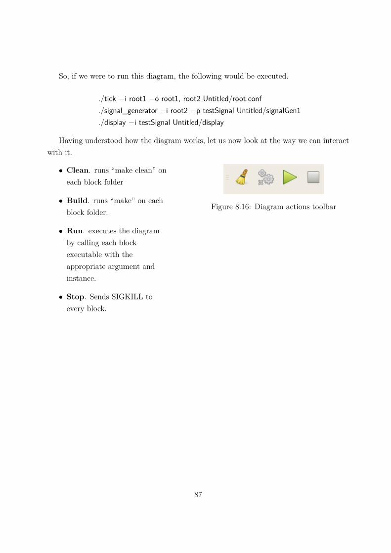
So, if we were to run this diagram, the following would be executed.
./tick −i root1 −o root1, root2 Untitled/root.conf
./signal_generator −i root2 −p testSignal Untitled/signalGen1
./display −i testSignal Untitled/display
Having understood how the diagram works, let us now look at the way we can interactwith it.
• Clean. runs “make clean” oneach block folder
• Build. runs “make” on eachblock folder.
• Run. executes the diagramby calling each blockexecutable with theappropriate argument andinstance.
• Stop. Sends SIGKILL toevery block.
Figure 8.16: Diagram actions toolbar
87
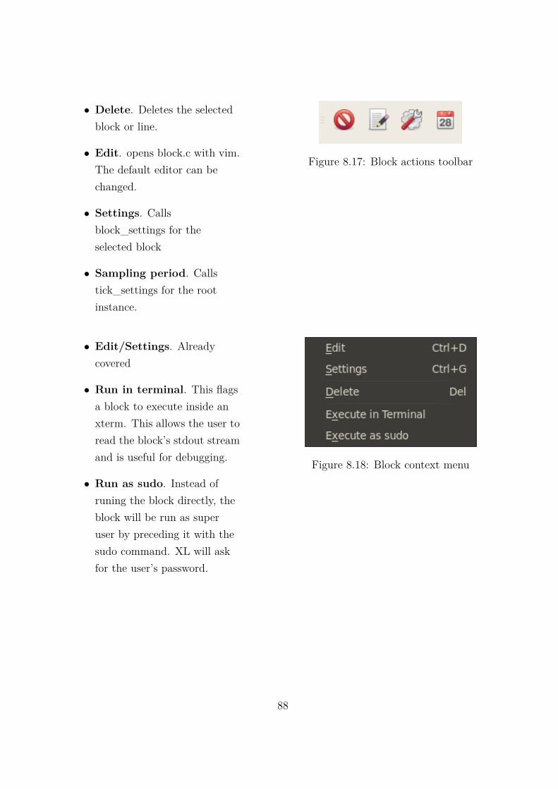
• Delete. Deletes the selectedblock or line.
• Edit. opens block.c with vim.The default editor can bechanged.
• Settings. Callsblock_settings for theselected block
• Sampling period. Callstick_settings for the rootinstance.
Figure 8.17: Block actions toolbar
• Edit/Settings. Alreadycovered
• Run in terminal. This flagsa block to execute inside anxterm. This allows the user toread the block’s stdout streamand is useful for debugging.
• Run as sudo. Instead ofruning the block directly, theblock will be run as superuser by preceding it with thesudo command. XL will askfor the user’s password.
Figure 8.18: Block context menu
88
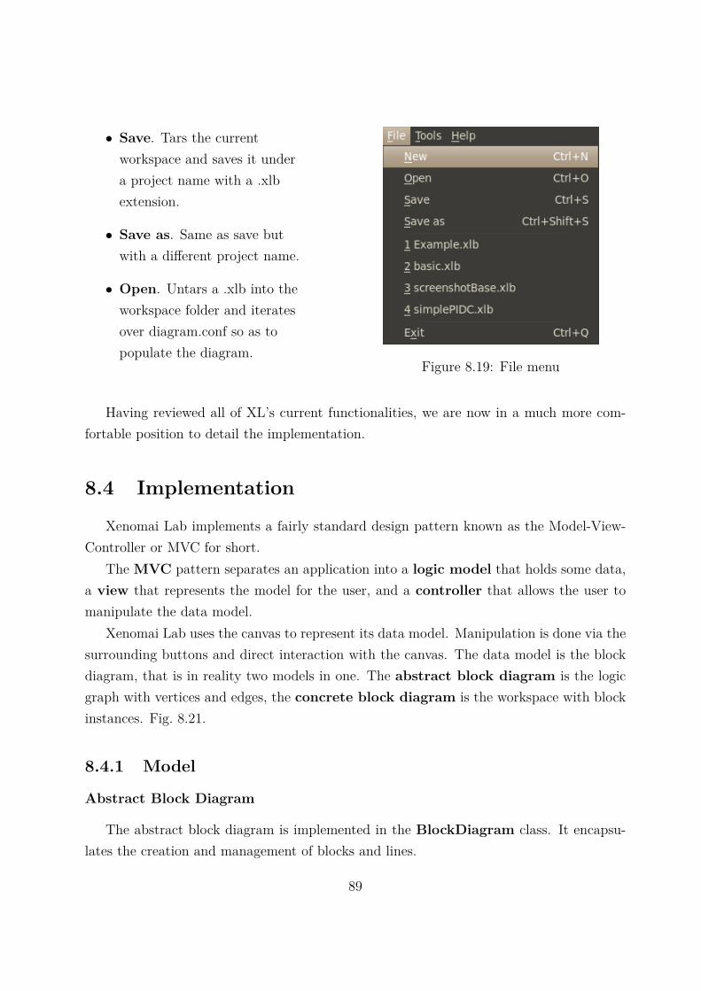
• Save. Tars the currentworkspace and saves it undera project name with a .xlbextension.
• Save as. Same as save butwith a different project name.
• Open. Untars a .xlb into theworkspace folder and iteratesover diagram.conf so as topopulate the diagram.
Figure 8.19: File menu
Having reviewed all of XL’s current functionalities, we are now in a much more com-fortable position to detail the implementation.
8.4 ImplementationXenomai Lab implements a fairly standard design pattern known as the Model-View-
Controller or MVC for short.The MVC pattern separates an application into a logic model that holds some data,
a view that represents the model for the user, and a controller that allows the user tomanipulate the data model.
Xenomai Lab uses the canvas to represent its data model. Manipulation is done via thesurrounding buttons and direct interaction with the canvas. The data model is the blockdiagram, that is in reality two models in one. The abstract block diagram is the logicgraph with vertices and edges, the concrete block diagram is the workspace with blockinstances. Fig. 8.21.
8.4.1 Model
Abstract Block Diagram
The abstract block diagram is implemented in the BlockDiagram class. It encapsu-lates the creation and management of blocks and lines.
89
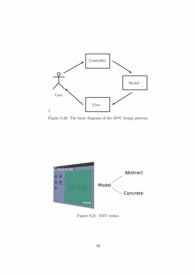
1
User
Controller
Model
View
Figure 8.20: The basic diagram of the MVC design pattern.
Model
Abstract
Concrete
Figure 8.21: MVC redux.
90
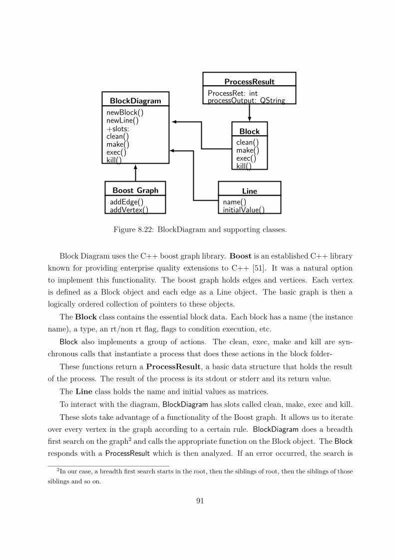
BlockDiagramnewBlock()newLine()+slots:clean()make()exec()kill()
Blockclean()make()exec()kill()
ProcessResultProcessRet: intprocessOutput: QString
Boost GraphaddEdge()addVertex()
Linename()initialValue()
Figure 8.22: BlockDiagram and supporting classes.
Block Diagram uses the C++ boost graph library. Boost is an established C++ libraryknown for providing enterprise quality extensions to C++ [51]. It was a natural optionto implement this functionality. The boost graph holds edges and vertices. Each vertexis defined as a Block object and each edge as a Line object. The basic graph is then alogically ordered collection of pointers to these objects.
The Block class contains the essential block data. Each block has a name (the instancename), a type, an rt/non rt flag, flags to condition execution, etc.
Block also implements a group of actions. The clean, exec, make and kill are syn-chronous calls that instantiate a process that does these actions in the block folder-
These functions return a ProcessResult, a basic data structure that holds the resultof the process. The result of the process is its stdout or stderr and its return value.
The Line class holds the name and initial values as matrices.To interact with the diagram, BlockDiagram has slots called clean, make, exec and kill.These slots take advantage of a functionality of the Boost graph. It allows us to iterate
over every vertex in the graph according to a certain rule. BlockDiagram does a breadthfirst search on the graph2 and calls the appropriate function on the Block object. The Blockresponds with a ProcessResult which is then analyzed. If an error occurred, the search is
2In our case, a breadth first search starts in the root, then the siblings of root, then the siblings of thosesiblings and so on.
91
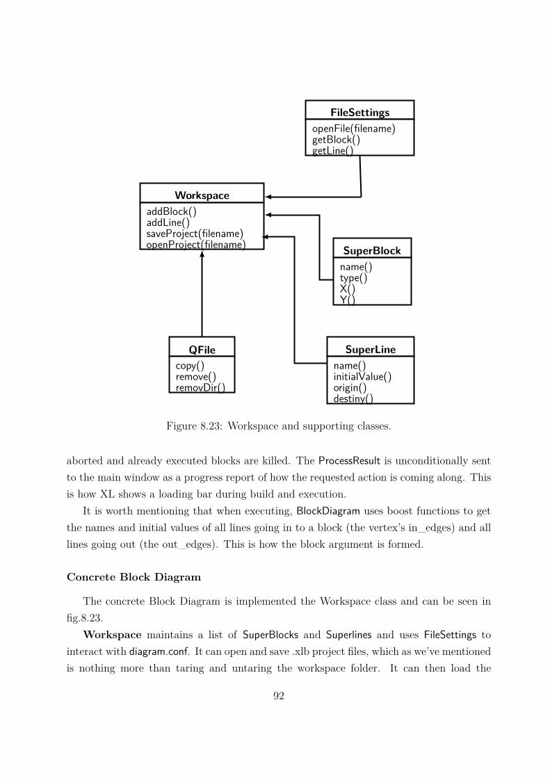
WorkspaceaddBlock()addLine()saveProject(filename)openProject(filename) SuperBlock
name()type()X()Y()
FileSettingsopenFile(filename)getBlock()getLine()
QFilecopy()remove()removDir()
SuperLinename()initialValue()origin()destiny()
Figure 8.23: Workspace and supporting classes.
aborted and already executed blocks are killed. The ProcessResult is unconditionally sentto the main window as a progress report of how the requested action is coming along. Thisis how XL shows a loading bar during build and execution.
It is worth mentioning that when executing, BlockDiagram uses boost functions to getthe names and initial values of all lines going in to a block (the vertex’s in_edges) and alllines going out (the out_edges). This is how the block argument is formed.
Concrete Block Diagram
The concrete Block Diagram is implemented the Workspace class and can be seen infig.8.23.
Workspace maintains a list of SuperBlocks and Superlines and uses FileSettings tointeract with diagram.conf. It can open and save .xlb project files, which as we’ve mentionedis nothing more than taring and untaring the workspace folder. It can then load the
92
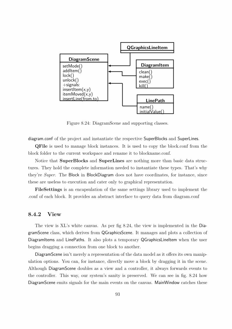
DiagramScenesetMode()addItem()lock()unlock()+signals:insertItem(x,y)itemMoved(x,y)insertLine(from,to)
DiagramItemclean()make()exec()kill()
QGraphicsLineItem
LinePathname()initialValue()
Figure 8.24: DiagramScene and supporting classes.
diagram.conf of the project and instantiate the respective SuperBlocks and SuperLines.QFile is used to manage block instances. It is used to copy the block.conf from the
block folder to the current workspace and rename it to blockname.conf.Notice that SuperBlocks and SuperLines are nothing more than basic data struc-
tures. They hold the complete information needed to instantiate these types. That’s whythey’re Super. The Block in BlockDiagram does not have coordinates, for instance, sincethese are useless to execution and cater only to graphical representation.
FileSettings is an encapsulation of the same settings library used to implement the.conf of each block. It provides an abstract interface to query data from diagram.conf
8.4.2 View
The view is XL’s white canvas. As per fig 8.24, the view is implemented in the Dia-gramScene class, which derives from QGraphicsScene. It manages and plots a collection ofDiagramItems and LinePaths. It also plots a temporary QGraphicsLineItem when the userbegins dragging a connection from one block to another.
DiagramScene isn’t merely a representation of the data model as it offers its own manip-ulation options. You can, for instance, directly move a block by dragging it in the scene.Although DiagramScene doubles as a view and a controller, it always forwards events tothe controller. This way, our system’s sanity is preserved. We can see in fig. 8.24 howDiagramScene emits signals for the main events on the canvas. MainWindow catches these
93
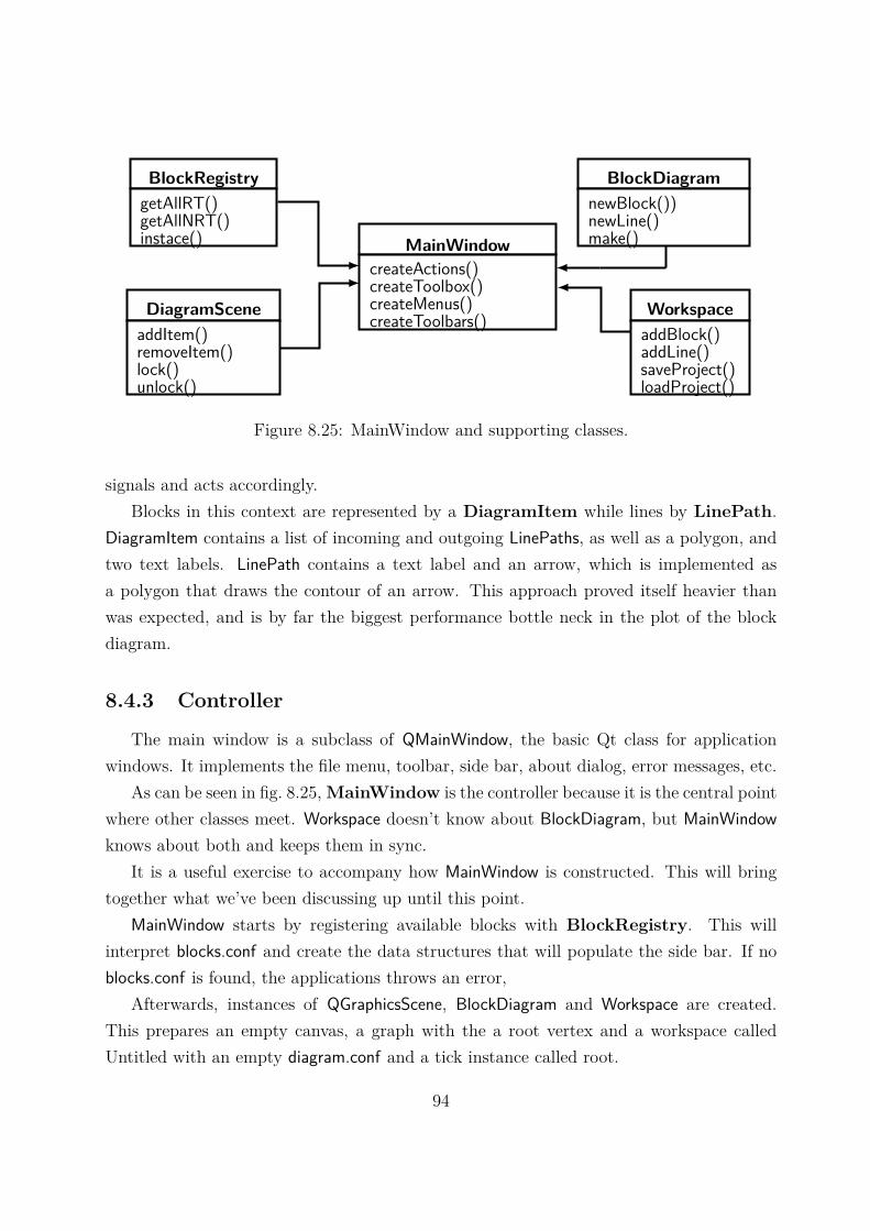
MainWindowcreateActions()createToolbox()createMenus()createToolbars() Workspace
addBlock()addLine()saveProject()loadProject()
BlockDiagramnewBlock())newLine()make()
BlockRegistrygetAllRT()getAllNRT()instace()
DiagramSceneaddItem()removeItem()lock()unlock()
Figure 8.25: MainWindow and supporting classes.
signals and acts accordingly.Blocks in this context are represented by a DiagramItem while lines by LinePath.
DiagramItem contains a list of incoming and outgoing LinePaths, as well as a polygon, andtwo text labels. LinePath contains a text label and an arrow, which is implemented asa polygon that draws the contour of an arrow. This approach proved itself heavier thanwas expected, and is by far the biggest performance bottle neck in the plot of the blockdiagram.
8.4.3 Controller
The main window is a subclass of QMainWindow, the basic Qt class for applicationwindows. It implements the file menu, toolbar, side bar, about dialog, error messages, etc.
As can be seen in fig. 8.25,MainWindow is the controller because it is the central pointwhere other classes meet. Workspace doesn’t know about BlockDiagram, but MainWindowknows about both and keeps them in sync.
It is a useful exercise to accompany how MainWindow is constructed. This will bringtogether what we’ve been discussing up until this point.
MainWindow starts by registering available blocks with BlockRegistry. This willinterpret blocks.conf and create the data structures that will populate the side bar. If noblocks.conf is found, the applications throws an error,
Afterwards, instances of QGraphicsScene, BlockDiagram and Workspace are created.This prepares an empty canvas, a graph with the a root vertex and a workspace calledUntitled with an empty diagram.conf and a tick instance called root.
94
Chapter 9
Experiments
In this chapter block diagrams that actuate on and acquire data from the real-worldare presented. The experiments were conducted with the objective of verifying XenomaiLab’s real-time performance and establishing it as a validated control platform.
9.1 Are you experienced ?
It is important to test XL’s capabilities as a digital control platform. Towards this goal,two experiments we named the “Black Box” and the “Inverted Pendulum” were conducted.We shall review these in turn.
9.2 Black Box
The black box consists in a 12 bit A/D D/A combo enclosed in a single (black) package.The box connects to a computer via parallel port. It was developed in-house in the goneyear of 1998, when DOS and its lack of parallelism was still a familiar site instead of anold joke.
The developer put together a small driver that consisted in 2 functions: one to write avalue between 0 and 4096 on the D/A, one to read an int from the A/D.
To test it with XenomaiLab two blocks were developed: dac12bpp and adc12bpp. Thistook less than one hour of coding. Let us look at the some of the results
95
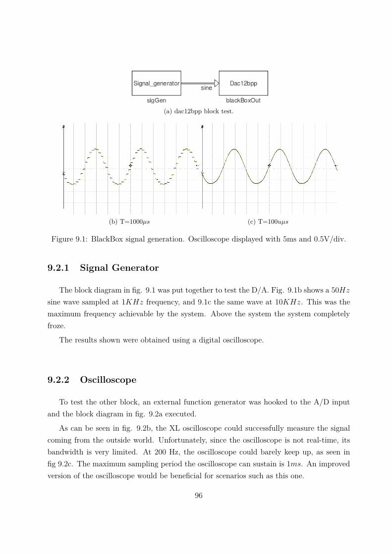
(a) dac12bpp block test.
(b) T=1000µs (c) T=100uµs
Figure 9.1: BlackBox signal generation. Oscilloscope displayed with 5ms and 0.5V/div.
9.2.1 Signal Generator
The block diagram in fig. 9.1 was put together to test the D/A. Fig. 9.1b shows a 50Hzsine wave sampled at 1KHz frequency, and 9.1c the same wave at 10KHz. This was themaximum frequency achievable by the system. Above the system the system completelyfroze.
The results shown were obtained using a digital oscilloscope.
9.2.2 Oscilloscope
To test the other block, an external function generator was hooked to the A/D inputand the block diagram in fig. 9.2a executed.
As can be seen in fig. 9.2b, the XL oscilloscope could successfully measure the signalcoming from the outside world. Unfortunately, since the oscilloscope is not real-time, itsbandwidth is very limited. At 200 Hz, the oscilloscope could barely keep up, as seen infig 9.2c. The maximum sampling period the oscilloscope can sustain is 1ms. An improvedversion of the oscilloscope would be beneficial for scenarios such as this one.
96
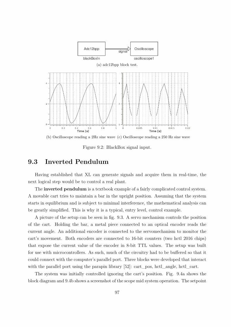
(a) adc12bpp block test.
(b) Oscilloscope reading a 2Hz sine wave (c) Oscilloscope reading a 250 Hz sine wave
Figure 9.2: BlackBox signal input.
9.3 Inverted Pendulum
Having established that XL can generate signals and acquire them in real-time, thenext logical step would be to control a real plant.
The inverted pendulum is a textbook example of a fairly complicated control system.A movable cart tries to maintain a bar in the upright position. Assuming that the systemstarts in equilibrium and is subject to minimal interference, the mathematical analysis canbe greatly simplified. This is why it is a typical, entry level, control example.
A picture of the setup can be seen in fig. 9.3. A servo mechanism controls the positionof the cart. Holding the bar, a metal piece connected to an optical encoder reads thecurrent angle. An additional encoder is connected to the servomechanism to monitor thecart’s movement. Both encoders are connected to 16-bit counters (two hctl 2016 chips)that expose the current value of the encoder in 8-bit TTL values. The setup was builtfor use with microcontrollers. As such, much of the circuitry had to be buffered so that itcould connect with the computer’s parallel port. Three blocks were developed that interactwith the parallel port using the parapin library [52]: cart_pos, hctl_angle, hctl_cart.
The system was initially controlled ignoring the cart’s position. Fig. 9.4a shows theblock diagram and 9.4b shows a screenshot of the scope mid system operation. The setpoint
97
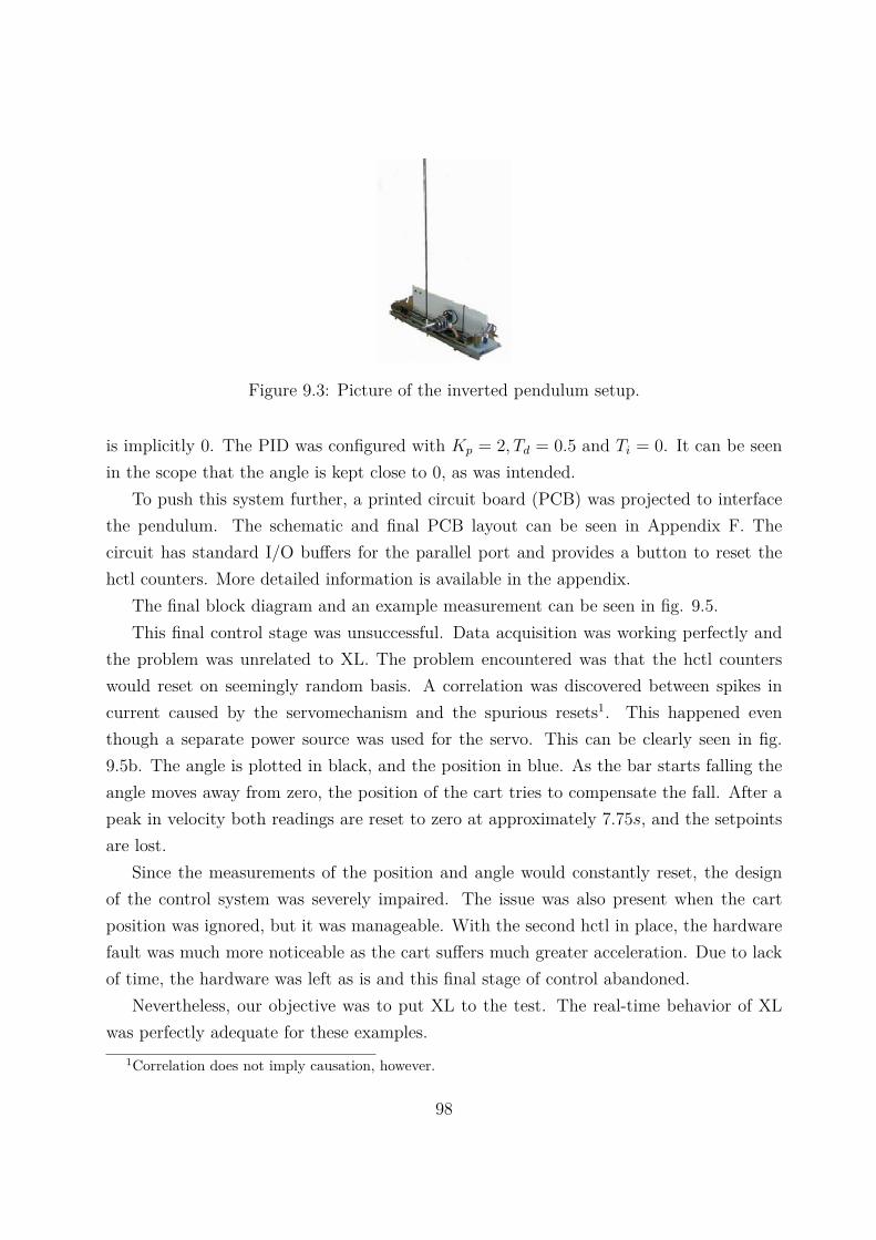
Figure 9.3: Picture of the inverted pendulum setup.
is implicitly 0. The PID was configured with Kp = 2, Td = 0.5 and Ti = 0. It can be seenin the scope that the angle is kept close to 0, as was intended.
To push this system further, a printed circuit board (PCB) was projected to interfacethe pendulum. The schematic and final PCB layout can be seen in Appendix F. Thecircuit has standard I/O buffers for the parallel port and provides a button to reset thehctl counters. More detailed information is available in the appendix.
The final block diagram and an example measurement can be seen in fig. 9.5.This final control stage was unsuccessful. Data acquisition was working perfectly and
the problem was unrelated to XL. The problem encountered was that the hctl counterswould reset on seemingly random basis. A correlation was discovered between spikes incurrent caused by the servomechanism and the spurious resets1. This happened eventhough a separate power source was used for the servo. This can be clearly seen in fig.9.5b. The angle is plotted in black, and the position in blue. As the bar starts falling theangle moves away from zero, the position of the cart tries to compensate the fall. After apeak in velocity both readings are reset to zero at approximately 7.75s, and the setpointsare lost.
Since the measurements of the position and angle would constantly reset, the designof the control system was severely impaired. The issue was also present when the cartposition was ignored, but it was manageable. With the second hctl in place, the hardwarefault was much more noticeable as the cart suffers much greater acceleration. Due to lackof time, the hardware was left as is and this final stage of control abandoned.
Nevertheless, our objective was to put XL to the test. The real-time behavior of XLwas perfectly adequate for these examples.
1Correlation does not imply causation, however.
98
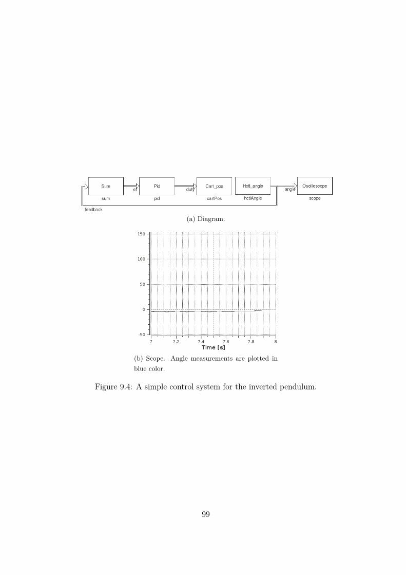
(a) Diagram.
(b) Scope. Angle measurements are plotted inblue color.
Figure 9.4: A simple control system for the inverted pendulum.
99
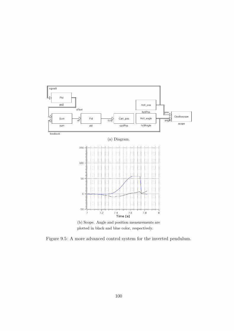
(a) Diagram.
(b) Scope. Angle and position measurements areplotted in black and blue color, respectively.
Figure 9.5: A more advanced control system for the inverted pendulum.
100

Part IV
Conclusion
101

102
Chapter 10
Conclusion
The main objective of this dissertation was two-fold: to study the real-time performanceachievable today with Linux and to present a platform for digital control that decouplescontrol algorithms from RTOSs concepts.
Regarding the first objective, a quantitative analysis was made of all major playersin the real-time Linux world. The analysis was based on the jitter of a square waveproduced on the parallel port. By putting the systems under various types of loads, amore complete picture was painted. Several fragilities were thus identified. A real-timeLinux scale was established that helps a systems designer position himself in the midstof so many different solutions.
Regarding the second objective, a platform for digital control using Xenomai was de-veloped. Xenomai Lab includes a graphical application to design block diagrams, and ablock API to easily program new blocks. The development cycle was unfortunately notentirely finished as it takes more time than a dissertation allows. The platform needs somemore work and feedback from people in the field. Such things are lurking on the horizon,however, as a dissertation to implement adaptive control algorithms using XenomaiLab is already in its early stages and will be completed in 2012. In the University of Wro-claw, Poland, a teaching package using Xenomai Lab is being prepared. The projectuses several pandaboards (a single board computer with a dual-core ARM chip) runningUbuntu 11.04 and challenges students to use them to control some in-class experimentalsetups. Students can program a real-time driver to interface with the setup and then useXenomai Lab to deal with higher level control. Work on this is on-going, Xenomai Labshould make its debut in polish classrooms as early as February 2012. Contacts are alsobeing made to mention Xenomai Lab in the official Xenomai wiki, which would bring a
103
much needed exposure to the platform.The validation of Xenomai Lab with a real-world setup, an inverted pendulum in a cart
was not entirely successful. This was not due to some intrinsic fault of Xenomai Lab butdue to hardware issues and a lacking control algorithm. With some more time investedthe issue would probably have been solved. Nevertheless, the successful experiments wereenough to prove that Xenomai Lab’s performance is sufficient. Reading and producingelectrical signals was demonstrated to work, and a simplified inverted pendulum setup wassuccessfully controlled.
10.1 Future WorkOn benchmarking real-time performance, the same test could be run on the latest
versions of every operating system and track improvements and possible regressions. Asimilar test could also be run to benchmark interrupt latency from the parallel port. Thiswould provide the last major real-time benchmark.
Xenomai Lab presents endless possibilities for future work. The sky is indeed the limit.New features that are simple to implement and would benefit the lab greatly include:
• A way to export block diagrams as self-contained executables for easier deployment.
• A tighter monitoring of block execution for better error handling
• An improved oscilloscope with higher bandwidth and more advanced features suchas signal memory navigation, auto triggering and auto scale
• Direct deployment to remote targets, as to enable development of networked con-trolled systems. This can be implemented with clever scripting.
• The concept of blockset would be beneficial to separate blocks into categories otherthan real and non real-time. As the application grows in exposure, the number ofblocks might grow rapidly.
• Profiling of computation time for each block, with relevant static values (mean, min-imum, maximum, covariance, etc...) presented within the lab.
104

Part V
Appendixes
105

106
Appendix A
The Testsuite
A.1 Rationale
Given that we intend to implement a control system using a desktop computer, it makessense to benchmark the OS’s scheduling jitter. However, to produce an electrical signaloutside of the computer, the scheduling jitter is only part of the equation. We intend touse the parallel port for I/O, and this means the signal has to cross the motherboard beforeit reaches the outside world. The motherboard is filled with asynchronous activities to theCPU such as DMA transfers and operations on the PCI bus. These will delay the signalfor seemingly random intervals. If we were to generate a square wave on the parallel portand measure its jitter, we would have an approximation of precisely this compound jitter.
Several aspects interest us when analyzing the results. For a hard real-time system,the worst-case jitter is the definitive figure of merit. Hard real-time systems have strictdeadlines, so the maximum delay has to be within well-defined limits. The worst-case jitterdoes not, however, characterize a system extensively. It can be that a system has a higherworst-case, but a better average and a smaller standard deviation. It can be that a systemhas a lower worst-case at a first glance, but may be disrupted by a high network load.Different systems call for different solutions, and a worst-case oriented analysis paints toosmall a picture.
Bearing all this in mind, the performance test we devised consists in producing a squarewave on the parallel port and then measure the time between transitions under differentusage scenarios: Idle, under CPU stress, under I/O stress and under Network stress. Bydoing this we can see how the determinism of each system holds up in the face of commondesktop operations.
107
A.2 Experimental setup
Ubuntu 10.04.2 was installed on a single-core Pentium 4 machine with 1.5GB of RAMand an ATI Radeon 9200 video card. The following versions of the Linux kernel were alsoinstalled:
• Linux 2.6.32-32
• Linux 2.6.33 with the PREEMPT_RT patchset
• Linux 2.6.32-20 with Xenomai 2.5.5.2
• Linux 2.6.32-11 with RTAI 3.8.1
Eight different applications (one kernel module and one user space program for eachsystem) were prepared for generating a square wave, the code for which is available inappendix C. Each application uses methods that describe in the respective chapters toexecute the following function every millisecond
void toggle(void){static char byte=1;
outb(byte,0x378);byte=~byte;
}
As was explained in the previous section, the computer is put under four different typesof loads.
• Idle: The system is cold booted and the test is launched.
• I/O: A large file is continuously moved between partitions until the end of the test.
• CPU: The classic horror film “Night of the Living Dead”1 in 1080p is played in theVLC player as to load 100% of the CPU.
• NET: A large file is continuously moved from the real-time computer to the secondcomputer via Ethernet.
1Public domain. Available free of charge from the Internet Archive at www.archive.org
108
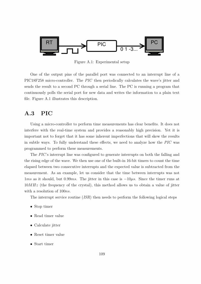
PICRT
0 1 -3...
PC
Figure A.1: Experimental setup
One of the output pins of the parallel port was connected to an interrupt line of aPIC18F258 micro-controller. The PIC then periodically calculates the wave’s jitter andsends the result to a second PC through a serial line. The PC is running a program thatcontinuously polls the serial port for new data and writes the information to a plain textfile. Figure A.1 illustrates this description.
A.3 PICUsing a micro-controller to perform time measurements has clear benefits. It does not
interfere with the real-time system and provides a reasonably high precision. Yet it isimportant not to forget that it has some inherent imperfections that will skew the resultsin subtle ways. To fully understand these effects, we need to analyze how the PIC wasprogrammed to perform these measurements.
The PIC ’s interrupt line was configured to generate interrupts on both the falling andthe rising edge of the wave. We then use one of the built-in 16-bit timers to count the timeelapsed between two consecutive interrupts and the expected value is subtracted from themeasurement. As an example, let us consider that the time between interrupts was not1ms as it should, but 0.99ms. The jitter in this case is −10µs. Since the timer runs at10MHz (the frequency of the crystal), this method allows us to obtain a value of jitterwith a resolution of 100ns.
The interrupt service routine (ISR) then needs to perform the following logical steps
• Stop timer
• Read timer value
• Calculate jitter
• Reset timer value
• Start timer
109
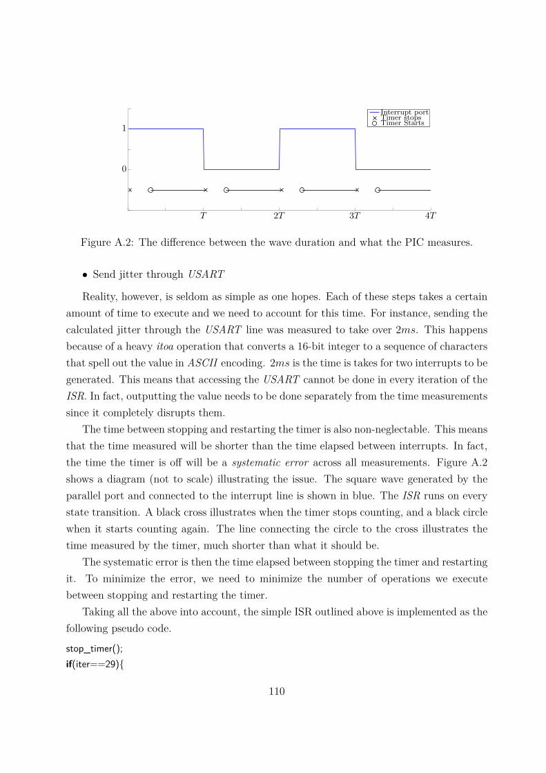
Timer StartsTimer stopsInterrupt port
T 2T 3T 4T
0
1
Figure A.2: The difference between the wave duration and what the PIC measures.
• Send jitter through USART
Reality, however, is seldom as simple as one hopes. Each of these steps takes a certainamount of time to execute and we need to account for this time. For instance, sending thecalculated jitter through the USART line was measured to take over 2ms. This happensbecause of a heavy itoa operation that converts a 16-bit integer to a sequence of charactersthat spell out the value in ASCII encoding. 2ms is the time is takes for two interrupts to begenerated. This means that accessing the USART cannot be done in every iteration of theISR. In fact, outputting the value needs to be done separately from the time measurementssince it completely disrupts them.
The time between stopping and restarting the timer is also non-neglectable. This meansthat the time measured will be shorter than the time elapsed between interrupts. In fact,the time the timer is off will be a systematic error across all measurements. Figure A.2shows a diagram (not to scale) illustrating the issue. The square wave generated by theparallel port and connected to the interrupt line is shown in blue. The ISR runs on everystate transition. A black cross illustrates when the timer stops counting, and a black circlewhen it starts counting again. The line connecting the circle to the cross illustrates thetime measured by the timer, much shorter than what it should be.
The systematic error is then the time elapsed between stopping the timer and restartingit. To minimize the error, we need to minimize the number of operations we executebetween stopping and restarting the timer.
Taking all the above into account, the simple ISR outlined above is implemented as thefollowing pseudo code.
stop_timer();if(iter==29){
110
read_timer();calculate_jitter();usart_send();iter=0;
}else{
reset_timer();start_timer();
}
iter++;
Each 30 iterations, instead of measuring time, we read a measurement, calculate itsjitter and send it through the USART line. This way, accessing the serial line neverinterferes with our measurements.
This ISR was measured to yield a systematic error of 1.3µs. This means that the ifstatement and the reset_timer() function take 13 instruction cycles to execute. For anunoptimized compiler, this figure is perfectly within reason.
A.4 Validation
To validate our system, a reference wave of known period needs to be correctly measuredby our device. Towards that end, an Oven Controlled Oscillator (OCO) of frequency equalto that of the PIC ’s crystal (10MHz) was connected to a binary counter that divided thewave’s frequency 216 times, down to a period of 6, 553, 600ns. The OCO used was a devicedeveloped in-house to achieve minimum jitter and drift, in the other of ps. Considering theaccuracy of the PIC, the OCO’s jitter is in practical terms null. The PIC was then used tomeasured this period during an hour long experiment. The expected result would be halfthe wave’s period minus the systematic error of 1.3µs, 3, 275, 500ns. Fig. A.3 shows theresults obtained. In over 90% of the cases the half-period was in fact 100ns short. Thisfact reveals both the nature of interrupt processing in the PIC and the differences betweenthe system’s internal crystals.
The time between the state transition on the interrupt line and the time at whichthe ISR begins execution is called interrupt latency. For external interrupt sources such asours, the PIC ’s interrupt latency is not fixed but variable between 3 to 4 instructions cycles
111
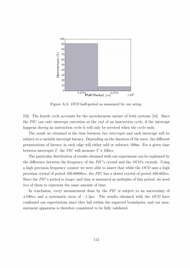
PSfrag repla ements
O urren es(%
)
Half-Period (ns) ×1063.2754 3.2755
0
10
20
30
40
50
60
70
80
90
100
Figure A.3: OCO half-period as measured by our setup.
[53]. The fourth cycle accounts for the asynchronous nature of both systems [54]. Sincethe PIC can only interrupt execution at the end of an instruction cycle, if the interrupthappens during an instruction cycle it will only be serviced when the cycle ends.
The result we obtained is the time between two interrupts and each interrupt will besubject to a variable interrupt latency. Depending on the duration of the wave, the differentpermutations of latency in each edge will either add or subtract 100ns. For a given timebetween interrupts T , the PIC will measure T ± 100ns.
The particular distribution of results obtained with our experiment can be explained bythe difference between the frequency of the PIC ’s crystal and the OCO’s crystals. Usinga high precision frequency counter we were able to assert that while the OCO uses a highprecision crystal of period 100.00008ns, the PIC has a slower crystal of period 100.002ns.Since the PIC ’s period is longer and time is measured as multiples of this period, we needless of them to represent the same amount of time.
In conclusion, every measurement done by the PIC is subject to an uncertainty of±100ns and a systematic error of −1.3µs. The results obtained with the OCO haveconfirmed our expectations since they fall within the expected boundaries, and our mea-surement apparatus is therefore considered to be fully validated.
112
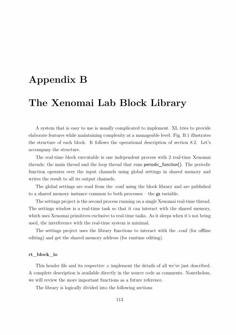
Appendix B
The Xenomai Lab Block Library
A system that is easy to use is usually complicated to implement. XL tries to provideelaborate features while maintaining complexity at a manageable level. Fig. B.1 illustratesthe structure of each block. It follows the operational description of section 8.2. Let’saccompany the structure.
The real-time block executable is one independent process with 2 real-time Xenomaithreads: the main thread and the loop thread that runs periodic_function(). The periodicfunction operates over the input channels using global settings in shared memory andwrites the result to all its output channels.
The global settings are read from the .conf using the block library and are publishedto a shared memory instance common to both processes – the gs variable.
The settings project is the second process running on a single Xenomai real-time thread.The settings window is a real-time task so that it can interact with the shared memory,which uses Xenomai primitives exclusive to real-time tasks. As it sleeps when it’s not beingused, the interference with the real-time system is minimal.
The settings project uses the library functions to interact with the .conf (for offlineediting) and get the shared memory address (for runtime editing).
rt_block_io
This header file and its respective .c implement the details of all we’ve just described.A complete description is available directly in the source code as comments. Nonetheless,we will review the more important functions as a future reference.
The library is logically divided into the following sections
113
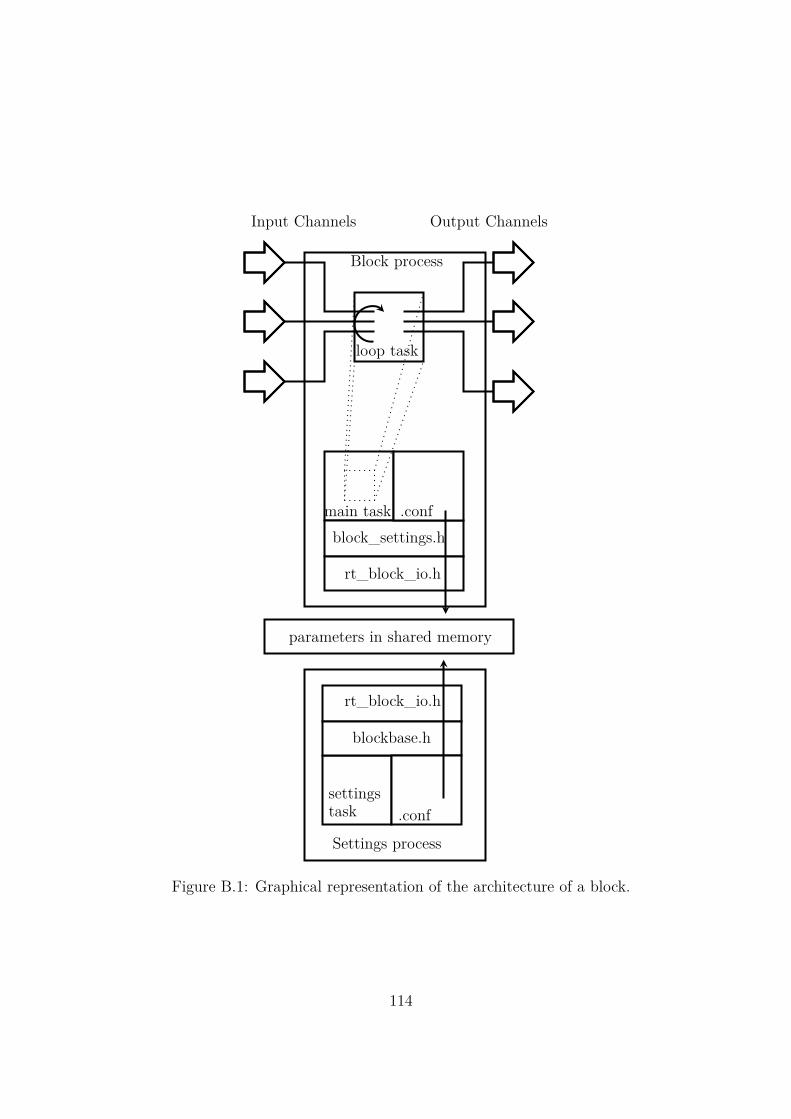
main task
loop task
block_settings.h
rt_block_io.h
.conf
Input Channels Output Channels
parameters in shared memory
Block process
settingstask
rt_block_io.h
blockbase.h
.conf
Settings process
Figure B.1: Graphical representation of the architecture of a block.
114
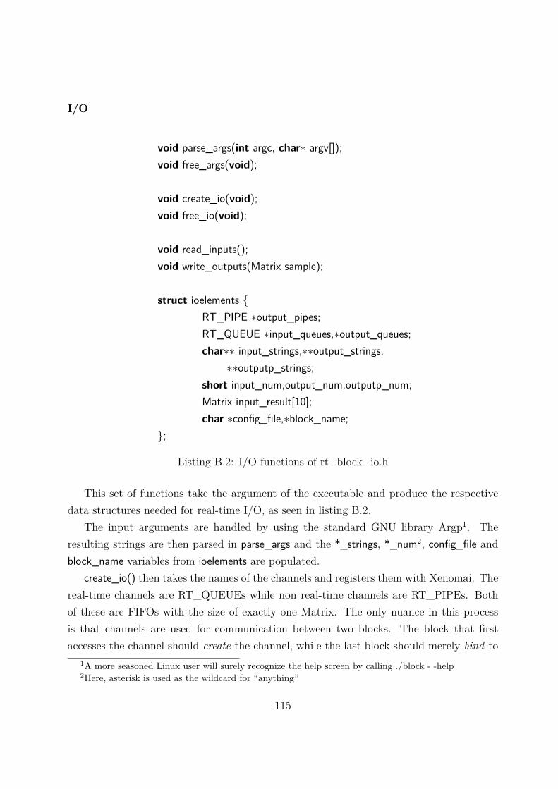
I/O
void parse_args(int argc, char∗ argv[]);void free_args(void);
void create_io(void);void free_io(void);
void read_inputs();void write_outputs(Matrix sample);
struct ioelements {RT_PIPE ∗output_pipes;RT_QUEUE ∗input_queues,∗output_queues;char∗∗ input_strings,∗∗output_strings,
∗∗outputp_strings;short input_num,output_num,outputp_num;Matrix input_result[10];char ∗config_file,∗block_name;
};
Listing B.2: I/O functions of rt_block_io.h
This set of functions take the argument of the executable and produce the respectivedata structures needed for real-time I/O, as seen in listing B.2.
The input arguments are handled by using the standard GNU library Argp1. Theresulting strings are then parsed in parse_args and the *_strings, *_num2, config_file andblock_name variables from ioelements are populated.
create_io() then takes the names of the channels and registers them with Xenomai. Thereal-time channels are RT_QUEUEs while non real-time channels are RT_PIPEs. Bothof these are FIFOs with the size of exactly one Matrix. The only nuance in this processis that channels are used for communication between two blocks. The block that firstaccesses the channel should create the channel, while the last block should merely bind to
1A more seasoned Linux user will surely recognize the help screen by calling ./block - -help2Here, asterisk is used as the wildcard for “anything”
115
the channel. This can quickly become a problem when we add feedback to a diagram or ifwe launch blocks out of order. The solution is quite simple. Each block tries to create theRT_QUEUE, if it fails it tries to bind, and if it that fails the block exits with an error.If the block creates the RT_QUEUE, it immediately writes a dummy Matrix so that thequeue is never empty. This nullifies the precedence problem created by feedback loops.
Task
RT_TASK loop_task,main_task;
void wait_for_task_end();void start_task(int priority, void∗ task_function);
Listing B.3: Task functions of rt_block_io.h
These functions are used to create the loop and the main task. Each task is based onan RT_TASK data structure. Ideally, both loop_task and main_task should be inside theioelements struct instead of being global variables and thereby polluting the namespace.Unfortunately, this is a Xenomai limitation – some variables must be global.
Settings
This set of functions is responsible for managing the shared memory structure and inter-acting with the .conf. The SHM instance is protected by an RT_MUTEX from concurrentaccess from the GUI and the block. This is how we assure that parameters don’t changemid periodic_function() execution – read_inputs() locks the settings and write_outputs()unlocks them.
Much like in the I/O case, the settings feature presents a complicated problem ofprecedence. Whoever runs first, the block or the GUI, must parse the .conf, allocate theglobal settings structure in shared memory and create the mutex. Who comes after mustmerely bind to the structure. So far so good, but due to Xenomai’s implementation ofshared memory, whoever created it must delete it. This means that the first to executemust always be the last to exit.
Like in the I/O case, precedence is established by creating and in case of failure bindingto the shared memory. This information is stored in the variable settings_owner and is
116
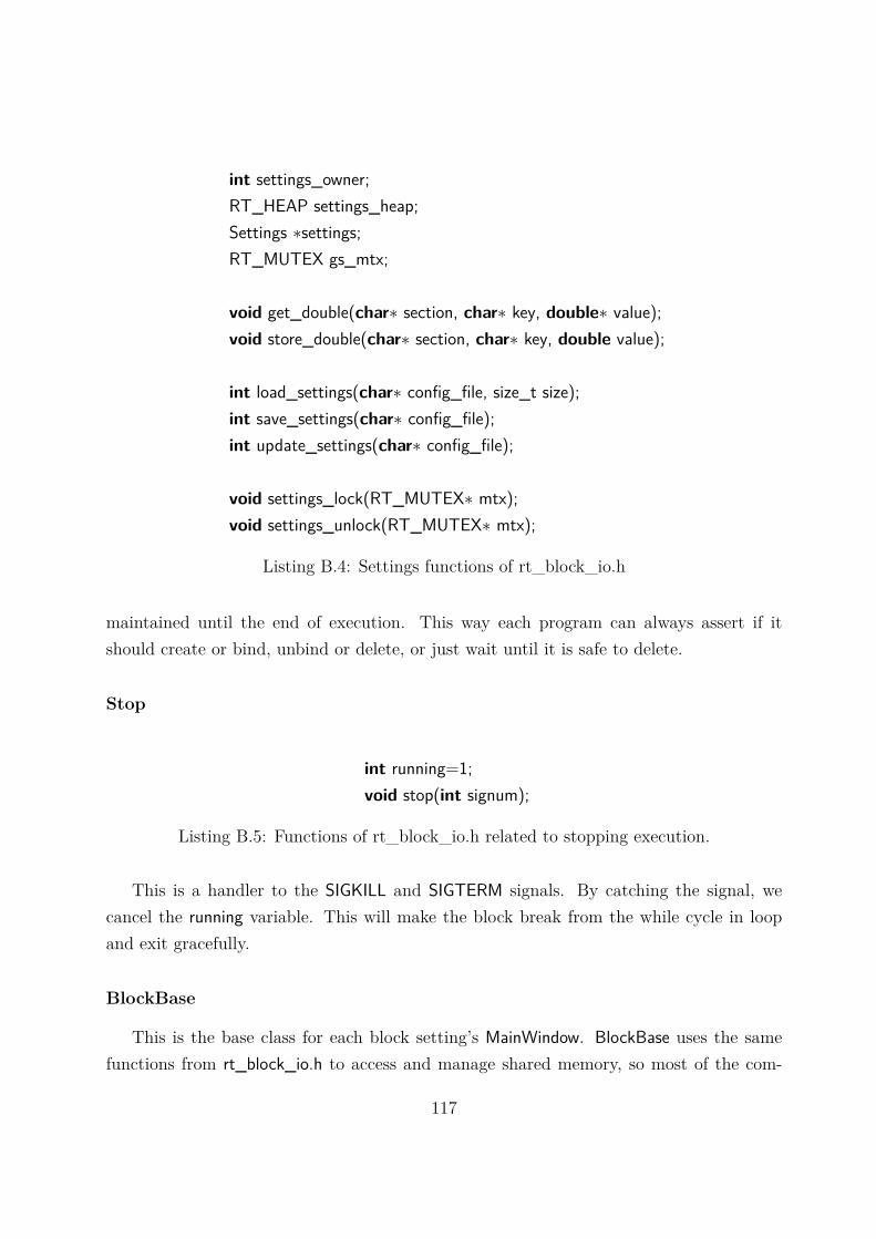
int settings_owner;RT_HEAP settings_heap;Settings ∗settings;RT_MUTEX gs_mtx;
void get_double(char∗ section, char∗ key, double∗ value);void store_double(char∗ section, char∗ key, double value);
int load_settings(char∗ config_file, size_t size);int save_settings(char∗ config_file);int update_settings(char∗ config_file);
void settings_lock(RT_MUTEX∗ mtx);void settings_unlock(RT_MUTEX∗ mtx);
Listing B.4: Settings functions of rt_block_io.h
maintained until the end of execution. This way each program can always assert if itshould create or bind, unbind or delete, or just wait until it is safe to delete.
Stop
int running=1;void stop(int signum);
Listing B.5: Functions of rt_block_io.h related to stopping execution.
This is a handler to the SIGKILL and SIGTERM signals. By catching the signal, wecancel the running variable. This will make the block break from the while cycle in loopand exit gracefully.
BlockBase
This is the base class for each block setting’s MainWindow. BlockBase uses the samefunctions from rt_block_io.h to access and manage shared memory, so most of the com-
117
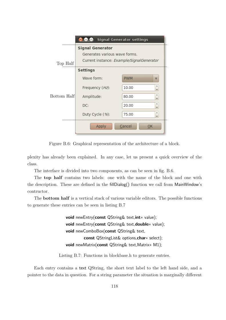
Top Half
Bottom Half
Figure B.6: Graphical representation of the architecture of a block.
plexity has already been explained. In any case, let us present a quick overview of theclass.
The interface is divided into two components, as can be seen in fig. B.6.The top half contains two labels: one with the name of the block and one with
the description. These are defined in the fillDialog() function we call from MainWindow’scontructor.
The bottom half is a vertical stack of various variable editors. The possible functionsto generate these entries can be seen in listing B.7
void newEntry(const QString& text,int∗ value);void newEntry(const QString& text,double∗ value);void newComboBox(const QString& text,
const QStringList& options,char∗ select);void newMatrix(const QString& text,Matrix∗ M1);
Listing B.7: Functions in blockbase.h to generate entries.
Each entry contains a text QString, the short text label to the left hand side, and apointer to the data in question. For a string parameter the situation is marginally different
118
as the user must create a string list with the different options that will appear in the combobox. In the case of fig. B.6, a QStringList with “PWM”, “Sine” and “Triangular”is givento the newComboBox() call.
Notice that by writing in these entries, one is writing directly into the gs structure andhence to shared memory. This may be a source of confusion due to the Apply, Cancel andOK buttons at the bottom.
The buttons refer to the instance file. By clicking Apply, whatever values are in sharedmemory are committed to the .conf. The Cancel button resets the shared memory to theoriginal values. OK does Apply, then exits.
B.0.1 Non real-time blocks
NRT blocks don’t use any Xenomai concepts. They are simple Linux applications thatread input pipes and do something with the value. Current usage is mostly for loggingpurposes, i.e., save a signal to a file, display using printf, etc.
The supporting nrt_block_io library implements the same API but using linux con-cepts. read_inputs, for instance, uses a standard read call.
119

120
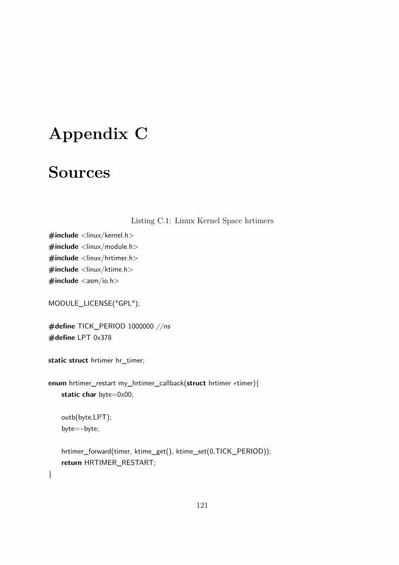
Appendix C
Sources
Listing C.1: Linux Kernel Space hrtimers
#include <linux/kernel.h>#include <linux/module.h>#include <linux/hrtimer.h>#include <linux/ktime.h>#include <asm/io.h>
MODULE_LICENSE("GPL");
#define TICK_PERIOD 1000000 //ns#define LPT 0x378
static struct hrtimer hr_timer;
enum hrtimer_restart my_hrtimer_callback(struct hrtimer ∗timer){static char byte=0x00;
outb(byte,LPT);byte=~byte;
hrtimer_forward(timer, ktime_get(), ktime_set(0,TICK_PERIOD));return HRTIMER_RESTART;
}
121
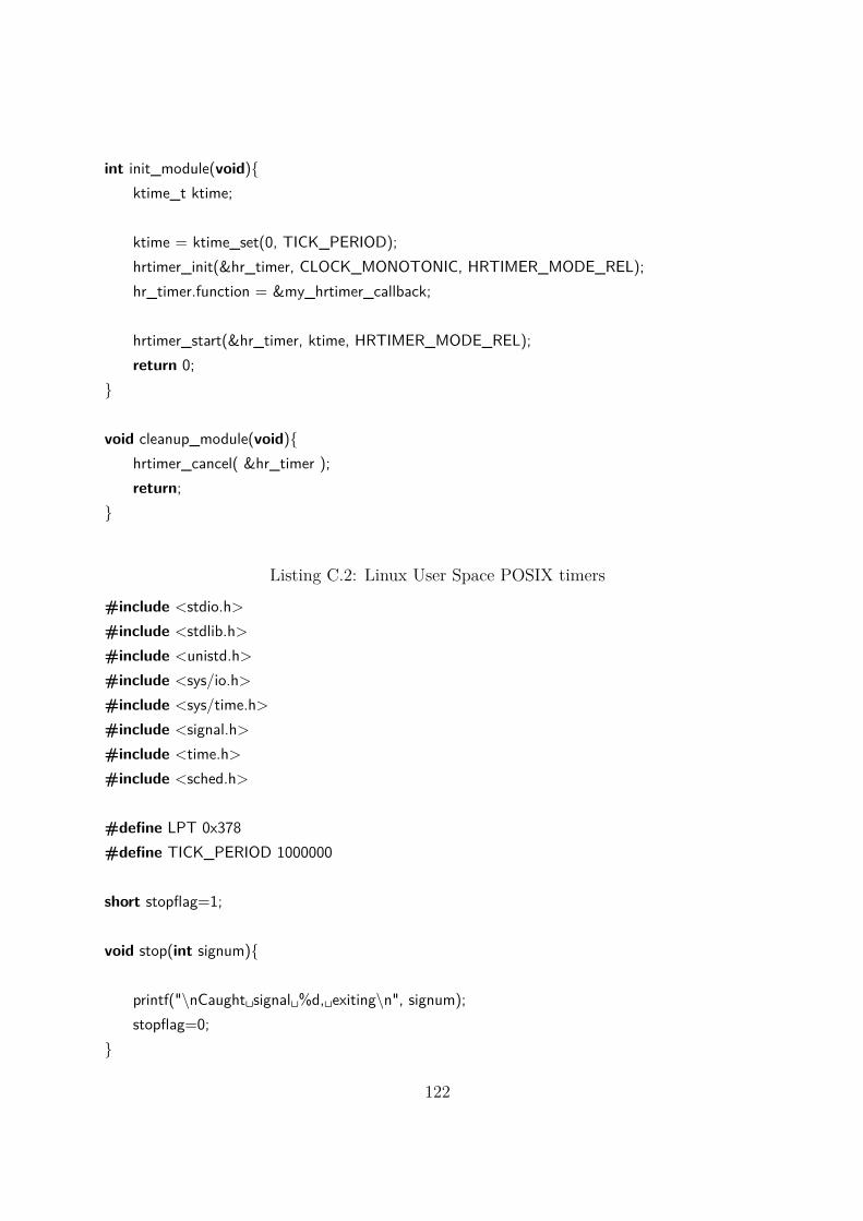
int init_module(void){ktime_t ktime;
ktime = ktime_set(0, TICK_PERIOD);hrtimer_init(&hr_timer, CLOCK_MONOTONIC, HRTIMER_MODE_REL);hr_timer.function = &my_hrtimer_callback;
hrtimer_start(&hr_timer, ktime, HRTIMER_MODE_REL);return 0;
}
void cleanup_module(void){hrtimer_cancel( &hr_timer );return;
}
Listing C.2: Linux User Space POSIX timers
#include <stdio.h>#include <stdlib.h>#include <unistd.h>#include <sys/io.h>#include <sys/time.h>#include <signal.h>#include <time.h>#include <sched.h>
#define LPT 0x378#define TICK_PERIOD 1000000
short stopflag=1;
void stop(int signum){
printf("\nCaught␣signal␣%d,␣exiting\n", signum);stopflag=0;
}
122
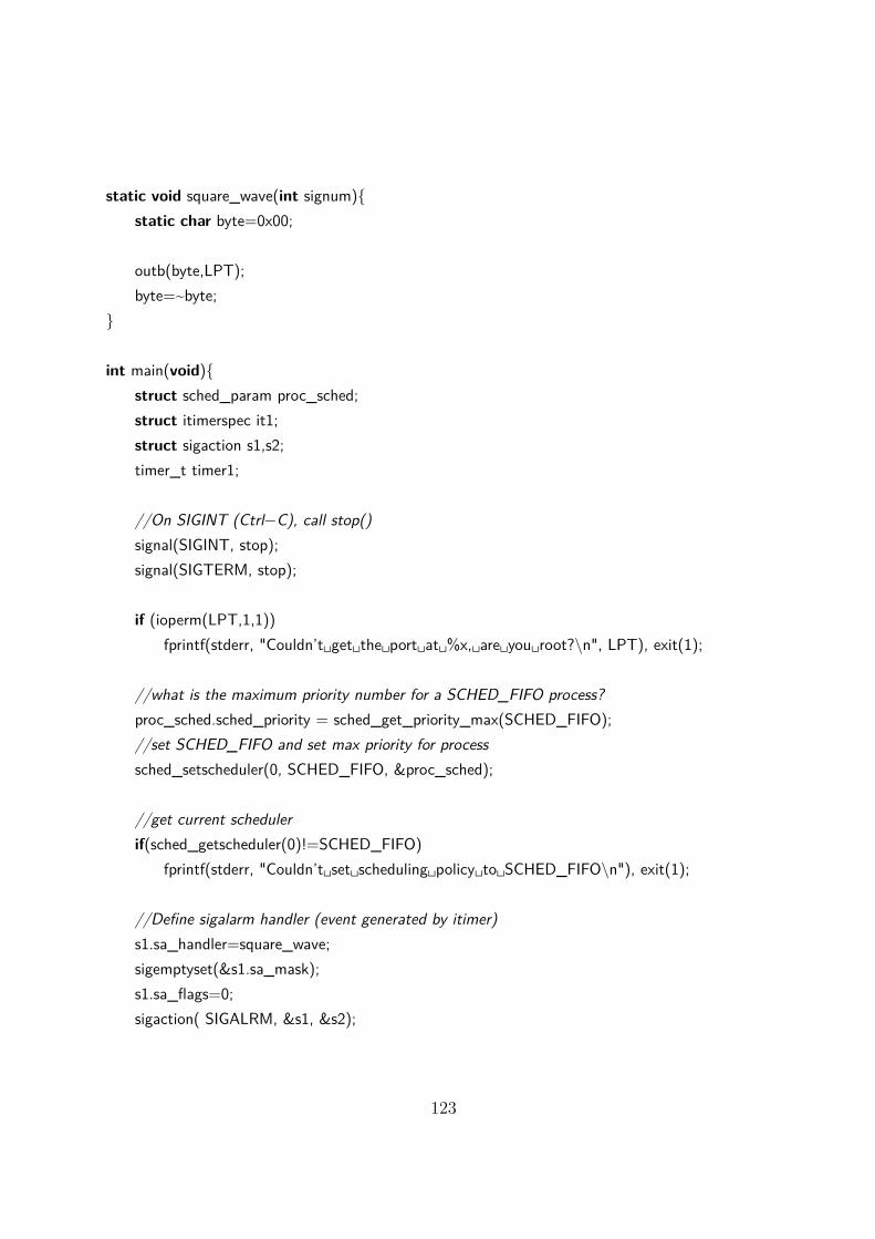
static void square_wave(int signum){static char byte=0x00;
outb(byte,LPT);byte=~byte;
}
int main(void){struct sched_param proc_sched;struct itimerspec it1;struct sigaction s1,s2;timer_t timer1;
//On SIGINT (Ctrl−C), call stop()signal(SIGINT, stop);signal(SIGTERM, stop);
if (ioperm(LPT,1,1))fprintf(stderr, "Couldn’t␣get␣the␣port␣at␣%x,␣are␣you␣root?\n", LPT), exit(1);
//what is the maximum priority number for a SCHED_FIFO process?proc_sched.sched_priority = sched_get_priority_max(SCHED_FIFO);//set SCHED_FIFO and set max priority for processsched_setscheduler(0, SCHED_FIFO, &proc_sched);
//get current schedulerif(sched_getscheduler(0)!=SCHED_FIFO)
fprintf(stderr, "Couldn’t␣set␣scheduling␣policy␣to␣SCHED_FIFO\n"), exit(1);
//Define sigalarm handler (event generated by itimer)s1.sa_handler=square_wave;sigemptyset(&s1.sa_mask);s1.sa_flags=0;sigaction( SIGALRM, &s1, &s2);
123
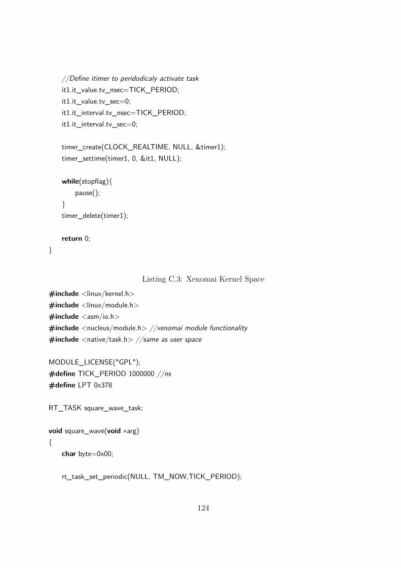
//Define itimer to peridodicaly activate taskit1.it_value.tv_nsec=TICK_PERIOD;it1.it_value.tv_sec=0;it1.it_interval.tv_nsec=TICK_PERIOD;it1.it_interval.tv_sec=0;
timer_create(CLOCK_REALTIME, NULL, &timer1);timer_settime(timer1, 0, &it1, NULL);
while(stopflag){pause();
}timer_delete(timer1);
return 0;}
Listing C.3: Xenomai Kernel Space
#include <linux/kernel.h>#include <linux/module.h>#include <asm/io.h>#include <nucleus/module.h> //xenomai module functionality#include <native/task.h> //same as user space
MODULE_LICENSE("GPL");#define TICK_PERIOD 1000000 //ns#define LPT 0x378
RT_TASK square_wave_task;
void square_wave(void ∗arg){
char byte=0x00;
rt_task_set_periodic(NULL, TM_NOW,TICK_PERIOD);
124
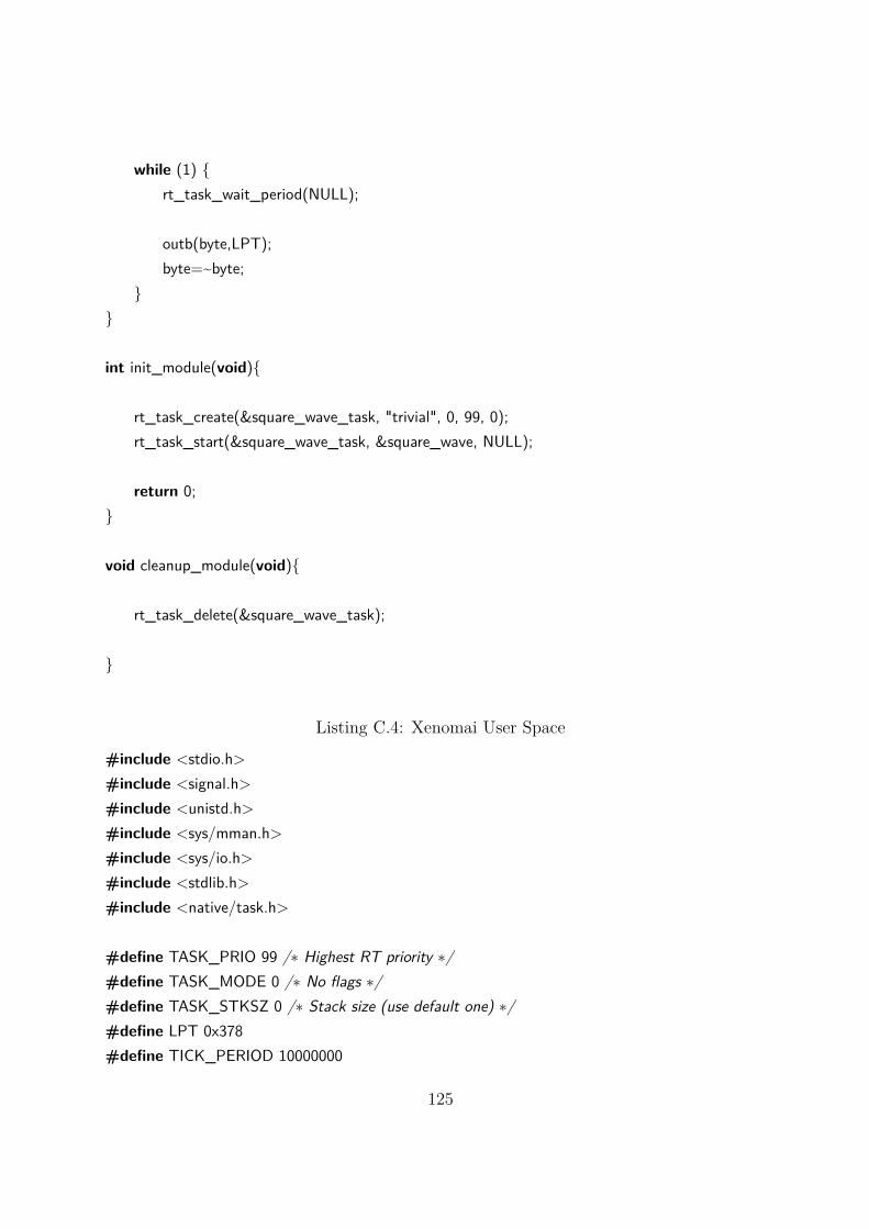
while (1) {rt_task_wait_period(NULL);
outb(byte,LPT);byte=~byte;
}}
int init_module(void){
rt_task_create(&square_wave_task, "trivial", 0, 99, 0);rt_task_start(&square_wave_task, &square_wave, NULL);
return 0;}
void cleanup_module(void){
rt_task_delete(&square_wave_task);
}
Listing C.4: Xenomai User Space
#include <stdio.h>#include <signal.h>#include <unistd.h>#include <sys/mman.h>#include <sys/io.h>#include <stdlib.h>#include <native/task.h>
#define TASK_PRIO 99 /∗ Highest RT priority ∗/#define TASK_MODE 0 /∗ No flags ∗/#define TASK_STKSZ 0 /∗ Stack size (use default one) ∗/#define LPT 0x378#define TICK_PERIOD 10000000
125
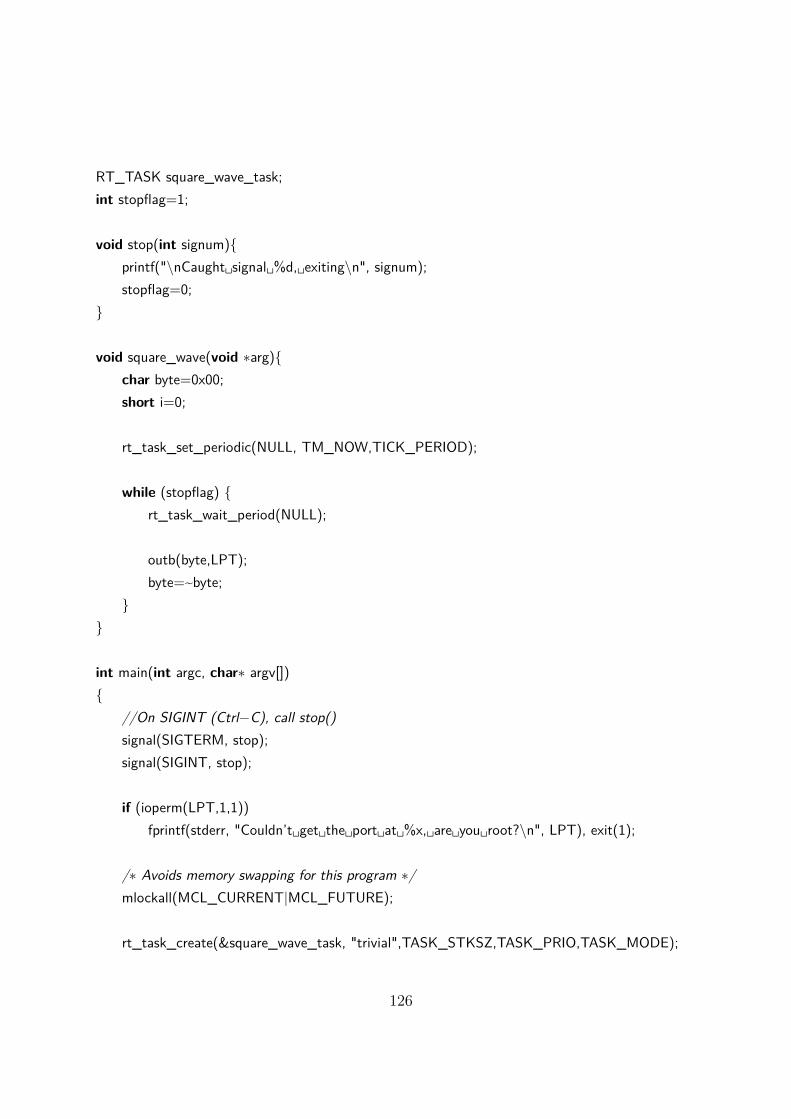
RT_TASK square_wave_task;int stopflag=1;
void stop(int signum){printf("\nCaught␣signal␣%d,␣exiting\n", signum);stopflag=0;
}
void square_wave(void ∗arg){char byte=0x00;short i=0;
rt_task_set_periodic(NULL, TM_NOW,TICK_PERIOD);
while (stopflag) {rt_task_wait_period(NULL);
outb(byte,LPT);byte=~byte;
}}
int main(int argc, char∗ argv[]){
//On SIGINT (Ctrl−C), call stop()signal(SIGTERM, stop);signal(SIGINT, stop);
if (ioperm(LPT,1,1))fprintf(stderr, "Couldn’t␣get␣the␣port␣at␣%x,␣are␣you␣root?\n", LPT), exit(1);
/∗ Avoids memory swapping for this program ∗/mlockall(MCL_CURRENT|MCL_FUTURE);
rt_task_create(&square_wave_task, "trivial",TASK_STKSZ,TASK_PRIO,TASK_MODE);
126
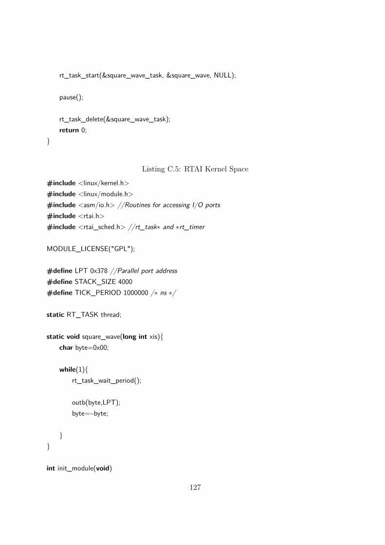
rt_task_start(&square_wave_task, &square_wave, NULL);
pause();
rt_task_delete(&square_wave_task);return 0;
}
Listing C.5: RTAI Kernel Space
#include <linux/kernel.h>#include <linux/module.h>#include <asm/io.h> //Routines for accessing I/O ports#include <rtai.h>#include <rtai_sched.h> //rt_task∗ and ∗rt_timer
MODULE_LICENSE("GPL");
#define LPT 0x378 //Parallel port address#define STACK_SIZE 4000#define TICK_PERIOD 1000000 /∗ ns ∗/
static RT_TASK thread;
static void square_wave(long int xis){char byte=0x00;
while(1){rt_task_wait_period();
outb(byte,LPT);byte=~byte;
}}
int init_module(void)
127
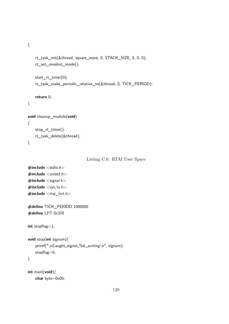
{
rt_task_init(&thread, square_wave, 0, STACK_SIZE, 0, 0, 0);rt_set_oneshot_mode();
start_rt_timer(0);rt_task_make_periodic_relative_ns(&thread, 0, TICK_PERIOD);
return 0;}
void cleanup_module(void){
stop_rt_timer();rt_task_delete(&thread);
}
Listing C.6: RTAI User Space
#include <stdio.h>#include <unistd.h>#include <signal.h>#include <sys/io.h>#include <rtai_lxrt.h>
#define TICK_PERIOD 1000000#define LPT 0x378
int stopflag=1;
void stop(int signum){printf("\nCaught␣signal␣%d,␣exiting\n", signum);stopflag=0;
}
int main(void){char byte=0x00;
128
RT_TASK ∗task;RTIME internal_count;
if (ioperm(LPT,1,1))fprintf(stderr, "Couldn’t␣get␣the␣port␣at␣%x,␣are␣you␣root?\n", LPT), exit(1);
//On SIGINT (Ctrl−C), call stop()signal(SIGINT, stop);
//Create RT_TASK with name MYTASK and change scheduling policy to SCHED_FIFOtask = rt_task_init_schmod(nam2num("MYTASK"), 9, 0, 0, SCHED_FIFO, 0xF);
rt_set_oneshot_mode();internal_count = start_rt_timer(nano2count(TICK_PERIOD));
//lock all memory so we don’t have paging (and therefore, no page faults)mlockall(MCL_CURRENT | MCL_FUTURE);
rt_make_hard_real_time();
rt_task_make_periodic_relative_ns(task,0+0∗TICK_PERIOD,TICK_PERIOD);
while(stopflag){rt_task_wait_period();outb(byte,LPT);byte=~byte;
}
rt_make_soft_real_time();stop_rt_timer();rt_task_delete(task);
return 0;}
129

130
Appendix D
Xenomai Ubuntu Installation Guide
131
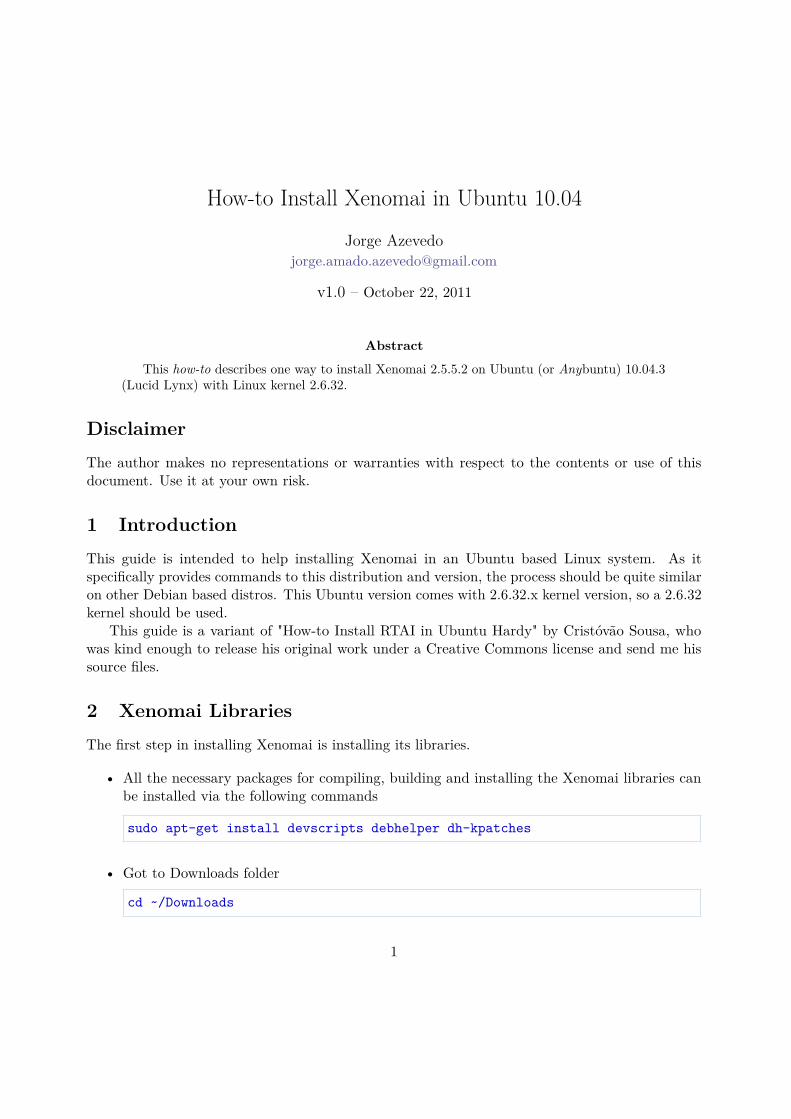
How-to Install Xenomai in Ubuntu 10.04Jorge Azevedo
v1.0 – October 22, 2011
AbstractThis how-to describes one way to install Xenomai 2.5.5.2 on Ubuntu (or Anybuntu) 10.04.3
(Lucid Lynx) with Linux kernel 2.6.32.
DisclaimerThe author makes no representations or warranties with respect to the contents or use of thisdocument. Use it at your own risk.
1 IntroductionThis guide is intended to help installing Xenomai in an Ubuntu based Linux system. As itspecifically provides commands to this distribution and version, the process should be quite similaron other Debian based distros. This Ubuntu version comes with 2.6.32.x kernel version, so a 2.6.32kernel should be used.
This guide is a variant of "How-to Install RTAI in Ubuntu Hardy" by Cristóvão Sousa, whowas kind enough to release his original work under a Creative Commons license and send me hissource files.
2 Xenomai LibrariesThe first step in installing Xenomai is installing its libraries.
• All the necessary packages for compiling, building and installing the Xenomai libraries canbe installed via the following commands
sudo apt-get install devscripts debhelper dh-kpatches
• Got to Downloads folder
cd ~/Downloads
1
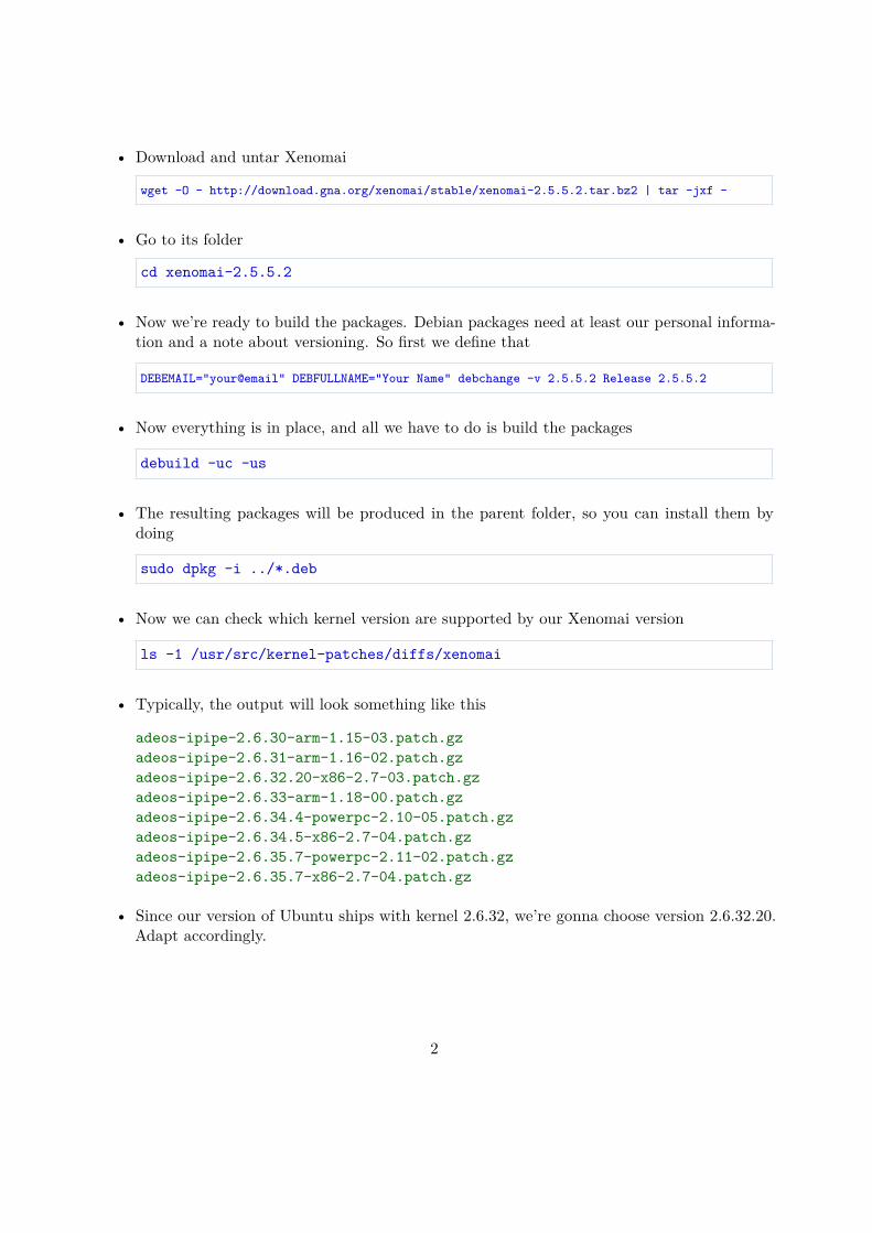
• Download and untar Xenomai
wget -O - http://download.gna.org/xenomai/stable/xenomai-2.5.5.2.tar.bz2 | tar -jxf -
• Go to its folder
cd xenomai-2.5.5.2
• Now we’re ready to build the packages. Debian packages need at least our personal informa-tion and a note about versioning. So first we define that
DEBEMAIL="your@email" DEBFULLNAME="Your Name" debchange -v 2.5.5.2 Release 2.5.5.2
• Now everything is in place, and all we have to do is build the packages
debuild -uc -us
• The resulting packages will be produced in the parent folder, so you can install them bydoing
sudo dpkg -i ../*.deb
• Now we can check which kernel version are supported by our Xenomai version
ls -1 /usr/src/kernel-patches/diffs/xenomai
• Typically, the output will look something like this
adeos-ipipe-2.6.30-arm-1.15-03.patch.gzadeos-ipipe-2.6.31-arm-1.16-02.patch.gzadeos-ipipe-2.6.32.20-x86-2.7-03.patch.gzadeos-ipipe-2.6.33-arm-1.18-00.patch.gzadeos-ipipe-2.6.34.4-powerpc-2.10-05.patch.gzadeos-ipipe-2.6.34.5-x86-2.7-04.patch.gzadeos-ipipe-2.6.35.7-powerpc-2.11-02.patch.gzadeos-ipipe-2.6.35.7-x86-2.7-04.patch.gz
• Since our version of Ubuntu ships with kernel 2.6.32, we’re gonna choose version 2.6.32.20.Adapt accordingly.
2
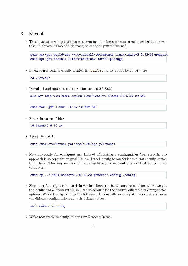
3 Kernel• These packages will prepare your system for building a custom kernel package (these will
take up almost 300mb of disk space, so consider yourself warned).
sudo apt-get build-dep --no-install-recommends linux-image-2.6.32-21-genericsudo apt-get install libncurses5-dev kernel-package
• Linux source code is usually located in /usr/src, so let’s start by going there
cd /usr/src
• Download and untar kernel source for version 2.6.32.20
sudo wget http://www.kernel.org/pub/linux/kernel/v2.6/linux-2.6.32.20.tar.bz2
sudo tar -jxf linux-2.6.32.20.tar.bz2
• Enter the source folder
cd linux-2.6.32.20
• Apply the patch
sudo /usr/src/kernel-patches/i386/apply/xenomai
• Now our ready for configuration. Instead of starting a configuration from scratch, ourapproach is to copy the original Ubuntu kernel .config to our folder and start configurationfrom there. This way we know for sure we have a kernel configuration that boots in ourcomputer.
sudo cp ../linux-headers-2.6.32-33-generic/.config .config
• Since there’s a slight missmatch in versions between the Ubuntu kernel from which we gotthe .config and our own kernel, we need to account for the possivel difference in configurationoptions. We do this by running the following. It is usually safe to just press enter and leavethe different configurations at their default values.
sudo make oldconfig
• We’re now ready to configure our new Xenomai kernel.
3
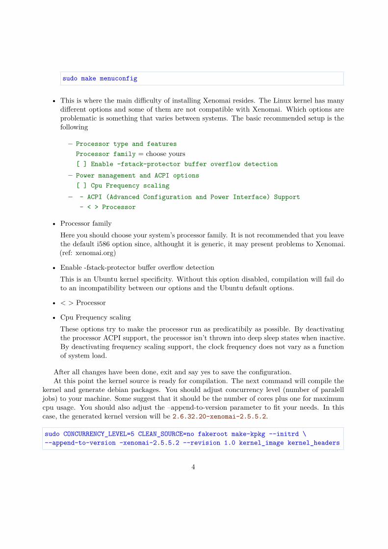
sudo make menuconfig
• This is where the main difficulty of installing Xenomai resides. The Linux kernel has manydifferent options and some of them are not compatible with Xenomai. Which options areproblematic is something that varies between systems. The basic recommended setup is thefollowing
– Processor type and featuresProcessor family = choose yours[ ] Enable -fstack-protector buffer overflow detection
– Power management and ACPI options[ ] Cpu Frequency scaling
– - ACPI (Advanced Configuration and Power Interface) Support- < > Processor
• Processor familyHere you should choose your system’s processor family. It is not recommended that you leavethe default i586 option since, althought it is generic, it may present problems to Xenomai.(ref: xenomai.org)
• Enable -fstack-protector buffer overflow detectionThis is an Ubuntu kernel specificity. Without this option disabled, compilation will fail doto an incompatibility between our options and the Ubuntu default options.
• < > Processor
• Cpu Frequency scalingThese options try to make the processor run as predicatibily as possible. By deactivatingthe processor ACPI support, the processor isn’t thrown into deep sleep states when inactive.By deactivating frequency scaling support, the clock frequency does not vary as a functionof system load.
After all changes have been done, exit and say yes to save the configuration.At this point the kernel source is ready for compilation. The next command will compile the
kernel and generate debian packages. You should adjust concurrency level (number of paralelljobs) to your machine. Some suggest that it should be the number of cores plus one for maximumcpu usage. You should also adjust the –append-to-version parameter to fit your needs. In thiscase, the generated kernel version will be 2.6.32.20-xenomai-2.5.5.2.
sudo CONCURRENCY_LEVEL=5 CLEAN_SOURCE=no fakeroot make-kpkg --initrd \--append-to-version -xenomai-2.5.5.2 --revision 1.0 kernel_image kernel_headers
4
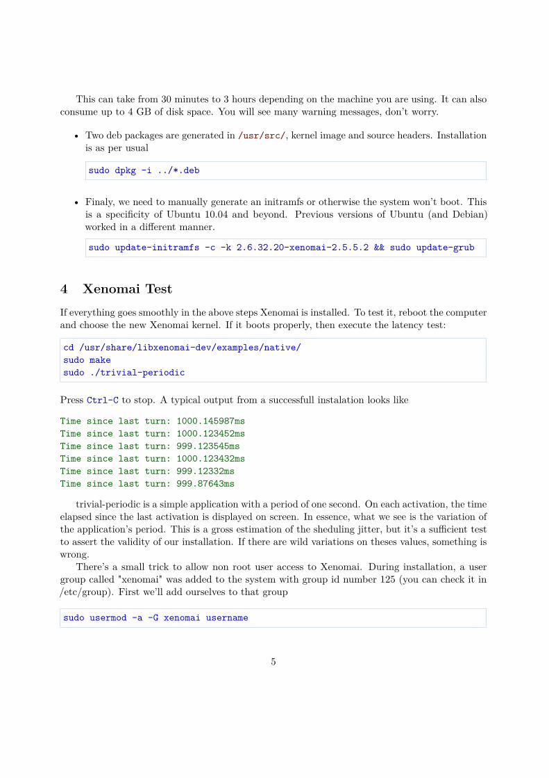
This can take from 30 minutes to 3 hours depending on the machine you are using. It can alsoconsume up to 4 GB of disk space. You will see many warning messages, don’t worry.
• Two deb packages are generated in /usr/src/, kernel image and source headers. Installationis as per usual
sudo dpkg -i ../*.deb
• Finaly, we need to manually generate an initramfs or otherwise the system won’t boot. Thisis a specificity of Ubuntu 10.04 and beyond. Previous versions of Ubuntu (and Debian)worked in a different manner.
sudo update-initramfs -c -k 2.6.32.20-xenomai-2.5.5.2 && sudo update-grub
4 Xenomai TestIf everything goes smoothly in the above steps Xenomai is installed. To test it, reboot the computerand choose the new Xenomai kernel. If it boots properly, then execute the latency test:
cd /usr/share/libxenomai-dev/examples/native/sudo makesudo ./trivial-periodic
Press Ctrl-C to stop. A typical output from a successfull instalation looks like
Time since last turn: 1000.145987msTime since last turn: 1000.123452msTime since last turn: 999.123545msTime since last turn: 1000.123432msTime since last turn: 999.12332msTime since last turn: 999.87643ms
trivial-periodic is a simple application with a period of one second. On each activation, the timeelapsed since the last activation is displayed on screen. In essence, what we see is the variation ofthe application’s period. This is a gross estimation of the sheduling jitter, but it’s a sufficient testto assert the validity of our installation. If there are wild variations on theses values, something iswrong.
There’s a small trick to allow non root user access to Xenomai. During installation, a usergroup called "xenomai" was added to the system with group id number 125 (you can check it in/etc/group). First we’ll add ourselves to that group
sudo usermod -a -G xenomai username
5
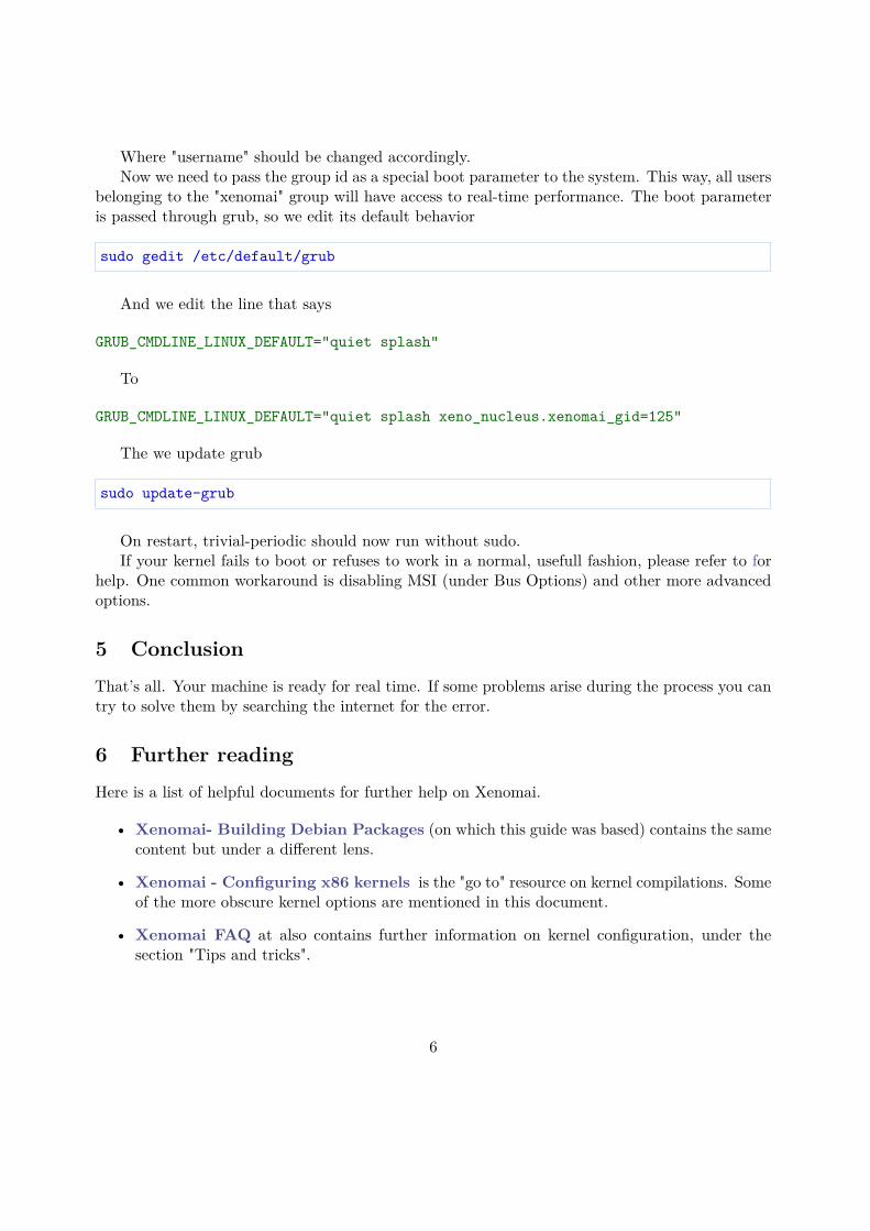
Where "username" should be changed accordingly.Now we need to pass the group id as a special boot parameter to the system. This way, all users
belonging to the "xenomai" group will have access to real-time performance. The boot parameteris passed through grub, so we edit its default behavior
sudo gedit /etc/default/grub
And we edit the line that says
GRUB_CMDLINE_LINUX_DEFAULT="quiet splash"
To
GRUB_CMDLINE_LINUX_DEFAULT="quiet splash xeno_nucleus.xenomai_gid=125"
The we update grub
sudo update-grub
On restart, trivial-periodic should now run without sudo.If your kernel fails to boot or refuses to work in a normal, usefull fashion, please refer to for
help. One common workaround is disabling MSI (under Bus Options) and other more advancedoptions.
5 ConclusionThat’s all. Your machine is ready for real time. If some problems arise during the process you cantry to solve them by searching the internet for the error.
6 Further readingHere is a list of helpful documents for further help on Xenomai.
• Xenomai- Building Debian Packages (on which this guide was based) contains the samecontent but under a different lens.
• Xenomai - Configuring x86 kernels is the "go to" resource on kernel compilations. Someof the more obscure kernel options are mentioned in this document.
• Xenomai FAQ at also contains further information on kernel configuration, under thesection "Tips and tricks".
6

138
Appendix E
RTAI Ubuntu Installation Guide
139
How-to Install RTAI in Ubuntu 10.04Jorge Azevedo
v1.0 – April 21, 2011
AbstractThis how-to describes one way to install RTAI 3.8.1 on Ubuntu (or Anybuntu) 10.04 (Lucid
Lynx) with Linux kernel 2.6.32.
DisclaimerThe author makes no representations or warranties with respect to the contents or use of thisdocument. Use it at your own risk.
1 IntroductionThis guide is intended to help installing RTAI in an Ubuntu based Linux system. As it specificallyprovides commands to this distribution and version, the process should be quite similar on otherDebian based distros. This Ubuntu version comes with 2.6.32.x kernel version, so a 2.6.32 kernelshould be used1.
This guide is an updated version of "How-to Install RTAI in Ubuntu Hardy" by CristóvãoSousa, who was kind enough to release his original work under a Creative Commons license andsend me his source files.
2 PreparationThe first step in installing RTAI is installing the necessary packages from the repositories. Thesewill prepare your system for building a custom kernel. The second step is downloading the necessarysource code.
• All the necessary packages for compiling, configuring and generating a package can beinstalled via the following commands
sudo apt-get build-dep linux-image-2.6.32-21-genericsudo apt-get install libncurses5-dev kernel-package
1Please note that the latest 64 bit kernel supported by RTAI is version 2.6.23.
1
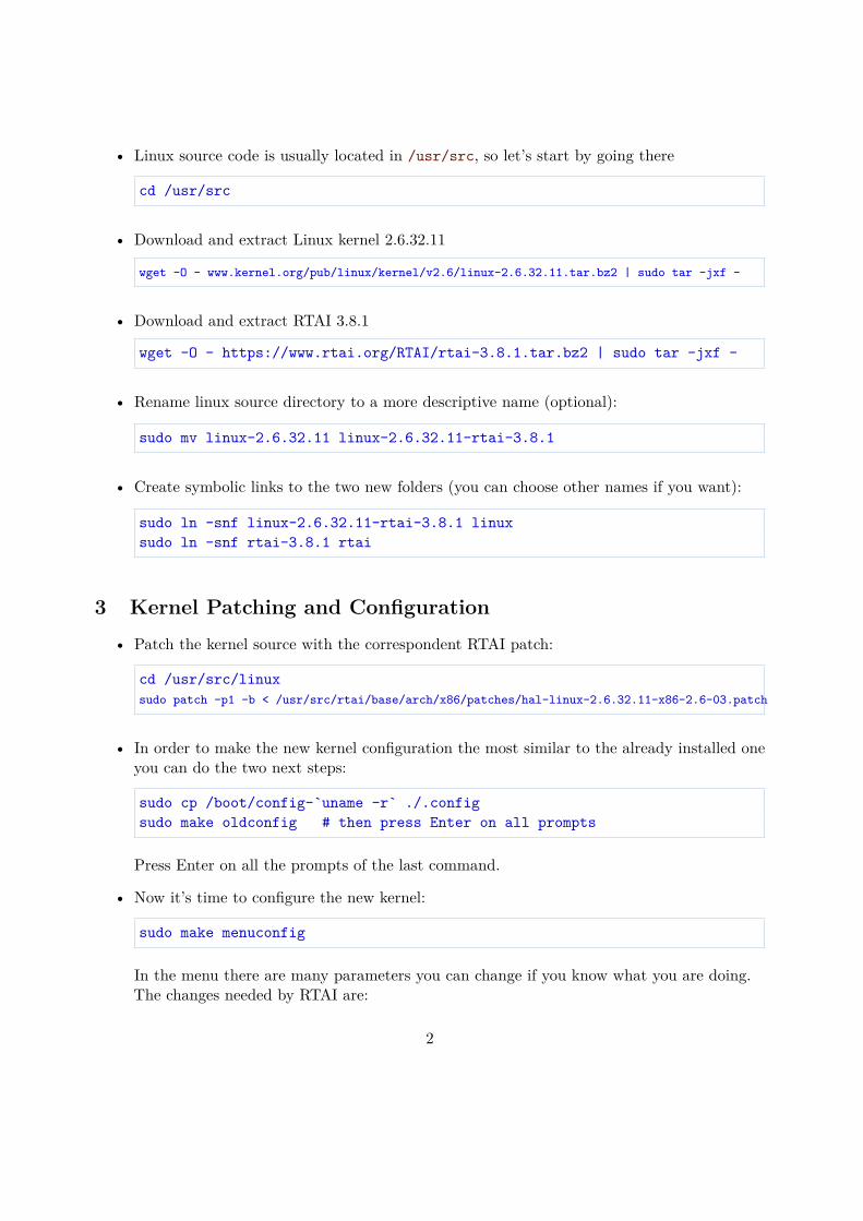
• Linux source code is usually located in /usr/src, so let’s start by going there
cd /usr/src
• Download and extract Linux kernel 2.6.32.11
wget -O - www.kernel.org/pub/linux/kernel/v2.6/linux-2.6.32.11.tar.bz2 | sudo tar -jxf -
• Download and extract RTAI 3.8.1
wget -O - https://www.rtai.org/RTAI/rtai-3.8.1.tar.bz2 | sudo tar -jxf -
• Rename linux source directory to a more descriptive name (optional):
sudo mv linux-2.6.32.11 linux-2.6.32.11-rtai-3.8.1
• Create symbolic links to the two new folders (you can choose other names if you want):
sudo ln -snf linux-2.6.32.11-rtai-3.8.1 linuxsudo ln -snf rtai-3.8.1 rtai
3 Kernel Patching and Configuration• Patch the kernel source with the correspondent RTAI patch:
cd /usr/src/linuxsudo patch -p1 -b < /usr/src/rtai/base/arch/x86/patches/hal-linux-2.6.32.11-x86-2.6-03.patch
• In order to make the new kernel configuration the most similar to the already installed oneyou can do the two next steps:
sudo cp /boot/config-`uname -r` ./.configsudo make oldconfig # then press Enter on all prompts
Press Enter on all the prompts of the last command.
• Now it’s time to configure the new kernel:
sudo make menuconfig
In the menu there are many parameters you can change if you know what you are doing.The changes needed by RTAI are:
2
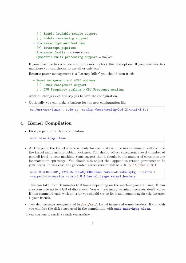
– [ ] Enable loadable module support[ ] Module versioning support
– Processor type and features[*] Interrupt pipelineProcessor family = choose yoursSymmetric multi-processing support = no/yes
If your machine has a single core processor uncheck this last option. If your machine hasmulticore you can choose to use all or only one2.Because power management is a "latency killer" you should turn it off:
– Power management and ACPI options[ ] Power Management support[ ] CPU Frequency scaling > CPU Frequency scaling
After all changes exit and say yes to save the configuration.
• Optionally you can make a backup for the new configuration file:
cd /usr/src/linux ; sudo cp .config /boot/config-2.6.24-rtai-3.6.1
4 Kernel Compilation• First prepare for a clean compilation
sudo make-kpkg clean
• At this point the kernel source is ready for compilation. The next command will compilethe kernel and generate debian packages. You should adjust concurrency level (number ofparalell jobs) to your machine. Some suggest that it should be the number of cores plus onefor maximum cpu usage. You should also adjust the –append-to-version parameter to fityour needs. In this case, the generated kernel version will be 2.6.32.11-rtai-3.8.1.
sudo CONCURRENCY_LEVEL=5 CLEAN_SOURCE=no fakeroot make-kpkg --initrd \--append-to-version -rtai-3.8.1 kernel_image kernel_headers
This can take from 30 minutes to 3 hours depending on the machine you are using. It canalso consume up to 4 GB of disk space. You will see many warning messages, don’t worry.If this command ends with an error you should try to fix it and compile again (the internetis your friend).
• Two deb packages are generated in /usr/src/, kernel image and source headers. If you wishyou can free the disk space used in the compilation with sudo make-kpkg clean.
2In case you want to simulate a single core machine.
3
5 Kernel Installation• Go to the packages directory:
cd /usr/src/
• Install the kernel image and source headers packages:
sudo dpkg -i linux-headers-2.6.32.11-rtai-3.8.1_2.6.32.11-rtai-3.8.1-10.00.Custom_i386.debsudo dpkg -i linux-image-2.6.32.11-rtai-3.8.1_2.6.32.11-rtai-3.8.1-10.00.Custom_i386.deb
• Although the package installation creates a new grub entry, it doesn’t create a new initramfsimage and therefore the kernel is unbootable. Notice that all kernels installed in your systemcan be listed with
ls /lib/modules
To generate a new initramfs and update grub run
sudo update-initramfs -c -k 2.6.32.11-rtai-3.8.1 && sudo update-grub
• Due to a bug in Grub 2, the system is still unbootable. While removing Grub 2 and installingGrub 1 will solve the issue, a more practical solution is to edit directly the grub.cfg entryfor the newly compiled kernel and add 16 to end of the word linux and initrd. So, with yourfavorite editor you can edit grub.cfg
sudo vim /etc/grub/grub.cfg
And change the entry so that instead of
linux /boot/vmlinuz-2.6.32.11-rtai-3.8.1 (...)initrd /boot/initrd.img-2.6.32.11-rtai-3.8.1
it reads
linux16 /boot/vmlinuz-2.6.32.11-rtai-3.8.1 (...)initrd16 /boot/initrd.img-2.6.32.11-rtai-3.8.1
You should now force save your changes since grub.cfg is a read only file. Please bear inmind that any call to update-grub will generate a fresh grub.cfg. The workaround will haveto be applied manually every time.
• Now, you must reboot. Choose the new RTAI patched kernel in Grub. If the process fails, themost likely problem is a faulty kernel configuration. You might be interested in consultingsection 9.
4
6 RTAI Configuration and Installation• Creating a build tree separated from the source tree of RTAI is advised by RTAI people, so
do
cd /usr/src/rtaisudo mkdir buildcd build
• Configure and compile RTAI:
sudo make -f ../makefile menuconfig
– General > Linux source tree = /usr/src/linux-2.6.32.11-rtai-3.8.1– Machine (x86) > Number of CPUs (SMP-only) = the right number (if applicable)
At the end exit and say yes to save the configuration. RTAI will be compiled.
• If there were no errors, install RTAI:
sudo make install
• Configure RTAI dynamic libraries to be wide available:
sudo -secho /usr/realtime/lib/ > /etc/ld.so.conf.d/rtai.confexitsudo ldconfig
• The RTAI binaries directory can be added automatically to the $PATH variable. To do that,add the line
PATH="$PATH:/usr/realtime/bin"
to the end of ~/.profile (user) and/or /root/.profile (root). It also comes in handy todefine an alias for sudo so that it inherits the $PATH variable. To do this, add
alias sudo="sudo env PATH=$PATH"
to ~/.bashrc.
5
7 RTAI TestIf everything goes smoothly in the above steps RTAI is readily installed. To be sure execute thelatency test:
cd /usr/realtime/testsuite/kern/latency/sudo ./run
Press Ctrl-C to stop. A typical output from a successfull instalation looks like
RTAI Testsuite - KERNEL latency (all data in nanoseconds)RTH| lat min| ovl min| lat avg| lat max| ovl max| overrunsRTD| -1566| -1566| -1525| -995| -995| 0RTD| -1571| -1571| -1489| 8257| 8257| 0RTD| -1569| -1571| -1527| -89| 8257| 0RTD| -1566| -1571| -1525| -481| 8257| 0RTD| -1566| -1571| -1529| -1049| 8257| 0RTD| -1566| -1571| -1529| -939| 8257| 0
8 ConclusionThat’s all. Your machine is ready for real time. If some problems arise during the process you cantry to solve them by searching the internet for the error sentence.
9 Further readingHere is a list of helpful documents for further help on RTAI.
• How-to Install RTAI in Ubuntu Hardy (on which this guide was based) and RTAITutorial by Cristóvão Sousa contain valuable information about both installation andprogramming using the RTAI API.
• RTAI Installation Complete Guide and Building Your Way Through RTAI byJoão Monteiro approach the same matters as the previous set of documents, but with a morein-depth view of the RTAI API.
• A Guide to Installing RTAI Linux by Keith Shortridge is a more extensive look at theinstallation procedure than the more practical approach developed in this guide.
• RTAI 3.8 on Ubuntu(9.10)-Linux-kernel : 2.6.31.8 by Manuel Arturo Deza is anotherinstallation guide.
6

146
Appendix F
Inverted Pendulum Schematic
147
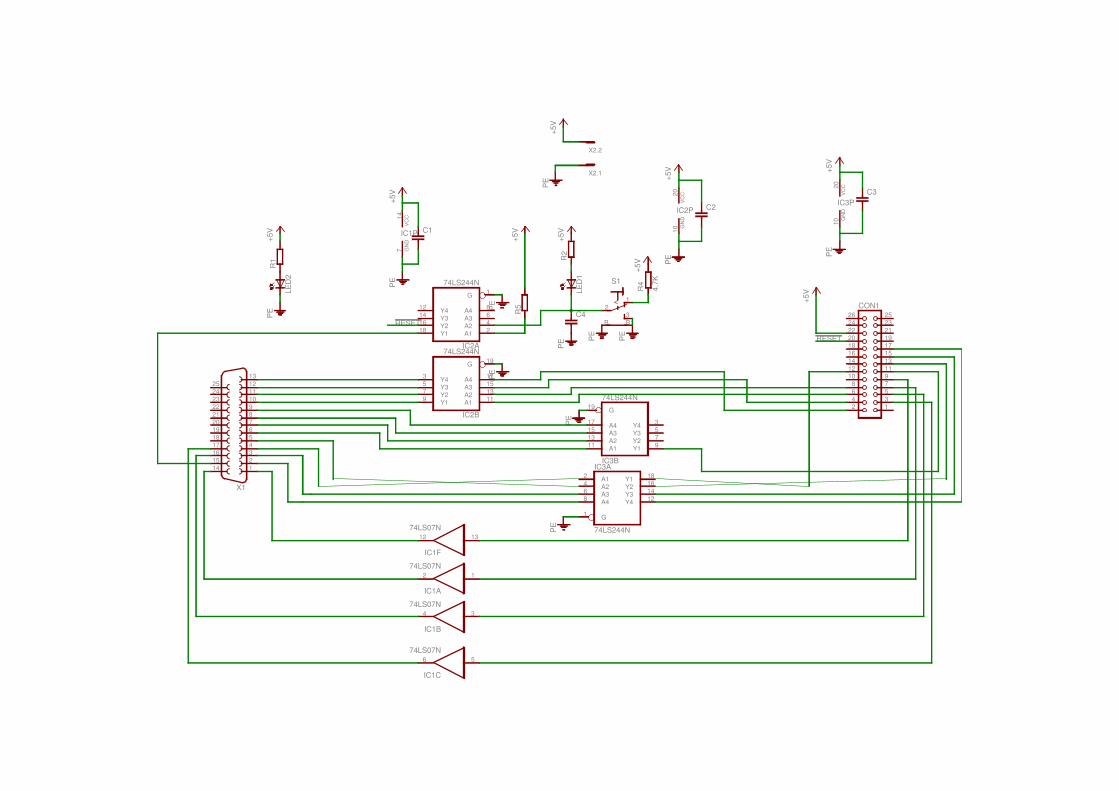
74LS07N
74LS07N
74LS07N
74LS07N
74LS244N
74LS244N
74LS244N
74LS244N
4.7K
PE
+5V
+5V +5
V
+5V
PE P
E
PE
+5V
+5V
+5V
PE P
E
PE
+5V
PE
PE
PE
PE
PE
+5V
11421531641751861972082192210231124122513
X1
12
IC1A
34
IC1B
56
IC1C
1312
IC1F
714
IC1P
GN
DV
CC
G 1
A1 2A2 4A3 6A4 8Y412
Y314
Y216
Y118
IC2A
G 19
A1 11A2 13A3 15A4 17Y43
Y35
Y27
Y19
IC2B
1020
IC2P
GN
DV
CC
23
1
B B1
S1
G1
A12
A24
A36
A48 Y4 12Y3 14Y2 16Y1 18
IC3A
G19
A111A213A315A417 Y4 3
Y3 5
Y2 7
Y1 9
IC3B
1020
IC3P
GN
DV
CC
LED
1
LED
2
R1 R
2
R4
R5
C1
C2
C3
C4
1234567891011121314151617181920212223242526
CON1
X2.1
X2.2
RESET
RESET
Appendix G
Inverted Pendulum Printed CircuitBoard
149
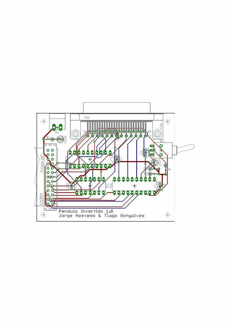
1 1314 25
2,54
F25
1
R-C
able
26P
X1
IC1
IC2
S1
IC3
LED
1
LED
2R1
R2 R4R5
C1
C2
C3
C4
CO
N1
X2
Bibliography
[1] K. Ogata, Modern Control Engineering. Upper Saddle River, NJ, USA: Prentice HallPTR, 4th ed., 2001.
[2] E. S. Raymond, The Cathedral and the Bazaar. Sebastopol, CA, USA: O’Reilly &Associates, Inc., 1st ed., 1999.
[3] R. Love, Linux kernel development. Developer’s Library, Addison-Wesley, 2009.
[4] S. J. Vaughan-Nichols, “Linux: It doesn’t get any faster.” http://blogs.computerworld.com/linux_it_doesnt_get_any_faster, June 2009.
[5] J. Niccolai, “Ballmer still searching for an answer to google.” http://www.pcworld.com/businesscenter/article/151568/ballmer_still_searching_for_an_answer_to_google.html, September 2008.
[6] B. Byfield, “Linux desktop market share: Greater than onepercent?.” http://itmanagement.earthweb.com/open-source/Linux-Desktop-Market-Share-Greater-Than-One-Percent-3818696.htm, May2009.
[7] J. D’Azzo, C. Houpis, and S. Sheldon, Linear control system analysis and design withMATLAB. No. v. 1 in Control engineering, Marcel Dekker, 2003.
[8] K. Ogata, Discrete-time control systems. Prentice Hall, 1995.
[9] A. L. L. Antunes, Algoritmos de Controlo Distribuído em Sistemas Baseados em Mi-croprocessadores. PhD, Departamento de Electrónica, Telecomunicacoes e Informática– Universidade de Aveiro (DETI/UA), 2008.
[10] D. Gillies, “Real-time computing faq.” http://www.faqs.org/faqs/realtime-computing/faq/.
151
[11] K. Yaghmour, Building embedded Linux systems. O’Reilly Series, O’Reilly, 2003.
[12] V. Yodaiken et al., “The rtlinux manifesto,” in Proc. of the 5th Linux Expo, 1999.
[13] K. Koolwal and R. Engineer, “Myths and realities of real-time linux software systems,”in Proc. Real-Time Linux Workshop (RTLWS 2009), 2009.
[14] W. River, “Vxworks offical website.” http://www.windriver.com/products/vxworks/.
[15] Q. S. Systems, “Qnx offical website.” http://www.qnx.com/.
[16] L. Bic and A. Shaw, Operating systems principles. Prentice Hall, 2003.
[17] C. Liu and J. Layland, “Scheduling algorithms for multiprogramming in a hard-real-time environment,” Journal of the ACM (JACM), vol. 20, no. 1, pp. 46–61, 1973.
[18] V. J. Yodaiken, “Adding real-time support to general purpose operating systems,” 111999.
[19] DIAPM, “Rtai official website.” http://www.rtai.org/.
[20] Xenomai, “Xenomai official website.” http://www.xenomai.org/.
[21] P. Marquet, É. Piel, J. Soula, J. Dekeyser, et al., “Implementation of artis, an asym-metric real-time extension of smp linux,” in Sixth Real-Time Linux Workshop, Singa-pore, 2004.
[22] T. Gleixner and D. Niehaus, “Hrtimers and beyond: Transforming the linux timesubsystem,” Proc. Linux Symposium, Ottawa, Ontario, Canada, July 2006.
[23] T. Gleixner, “hrtimer - high-resolution timer subsystem.” http://lwn.net/Articles/162773/, December 2005.
[24] T. Gleixner, “ktimer subsystem.” http://lwn.net/Articles/152363/, September2005.
[25] T. Gleixner, “A new approach to kernel timers.” http://lwn.net/Articles/152436/,September 2005.
[26] T. Gleixner, “Clockevents and dyntick.” http://lwn.net/Articles/223185/, Febru-ary 2007.
152
[27] PREEMPTRT, “Preemptrt official website.” http://rt.wiki.kernel.org/.
[28] P. McKenney, “A realtime preemption overview.” http://lwn.net/Articles/146861/, August 2005.
[29] J. Cobert, “The realtime preemption endgame.” http://lwn.net/Articles/345076/, August 2009.
[30] S. Rostedt and D. V. Hart, “Internals of the rt patch,” Proc. Linux Symposium,Ottawa, Ontario, Canada, June 2007.
[31] M. Barabanov, “A linux-based real-time operating system,” Master’s thesis, New Mex-ico Institude of Mining and Technology, June 1997.
[32] P. Cloutier, P. Mantegazza, S. Papacharalambous, I. Soanes, S. Hughes, and K. Yagh-mour, “Diapm-rtai position paper,” RTSS 2000 - Real Time Operating Systems Work-shop, 2000.
[33] P. Gerum, “Announce: xenodaptor.” http://www.mail-archive.com/[email protected]/msg01156.html, August 2001.
[34] Xenomai, “Project history.” http://www.xenomai.org/index.php/Xenomai:History.
[35] J. Cobert and E. O. Coolbaugh, “Real-time linux is patented.” http://lwn.net/2000/0210/, February 2000.
[36] J. Cobert and E. O. Coolbaugh, “The rtlinux patent.” http://lwn.net/2001/0215/,February 2001.
[37] J. Cobert and E. O. Coolbaugh, “The other free software war.” http://lwn.net/2000/0914/, September 2000.
[38] L. Devices, “Ceo interview: Victor yodaiken, fsmlabs.” http://www.linuxfordevices.com/c/a/Linux-For-Devices-Articles/CEO-Interview-Victor-Yodaiken-FSMLabs/, December 2003.
[39] K. Yaghmour, “Adaptive domain environment for operating systems,” Opersys inc,2001.
153
http://www.linuxfordevices.com/c/a/Linux-For-Devices-Articles/CEO-Interview-Victor-Yodaiken-FSMLabs/
[40] M. Roy, “Interview with philippe gerum.” http://www.advogato.org/article/803.html, October 2004.
[41] L. Dozio and P. Mantegazza, “Real time distributed control systems using rtai,” inObject-Oriented Real-Time Distributed Computing, 2003. Sixth IEEE InternationalSymposium on, pp. 11–18, IEEE, 2003.
[42] P. Mantegazza, “What’s ahead.” http://article.gmane.org/gmane.linux.real-time.rtai/7754, April 2004.
[43] P. Gerum, “A tour of the native api.” http://www.xenomai.org/documentation/xenomai-2.0/pdf/Native-API-Tour.pdf, 2006.
[44] A. Barbalace, A. Luchetta, G. Manduchi, M. Moro, A. Soppelsa, and C. Taliercio,“Performance comparison of vxworks, linux, rtai and xenomai in a hard real-timeapplication,” in Real-Time Conference, 2007 15th IEEE-NPSS, pp. 1 –5, 29 2007-may4 2007.
[45] DIAPM, “Rtai 3.4 user manual.” https://www.rtai.org/index.php?module=documents&JAS_DocumentManager_op=viewDocument&JAS_Document_id=44, 2006.
[46] M. Piątek, “Real-time application interface and xenomai modified gnu/linux real-timeoperating systems dedicated to control,”
[47] W. Betz, M. Cereia, and I. Bertolotti, “Experimental evaluation of the linux rtpatch for real-time applications,” in Emerging Technologies Factory Automation, 2009.ETFA 2009. IEEE Conference on, pp. 1 –4, sept. 2009.
[48] M. Chiandone and G. Sulligoi, “Performance assessment of a motion control appli-cation based on linux rtai,” in Power Electronics Electrical Drives Automation andMotion (SPEEDAM), 2010 International Symposium on, pp. 687 –692, june 2010.
[49] J. Blanchette and M. Summerfield, C++ GUI programming with Qt 4. Prentice Hallopen source software development series, Prentice Hall in association with TrolltechPress, 2008.
[50] P. O. Kristensson, “Ansi c applications settings management.” http://pokristensson.com/settings.html.
[51] Boost, “Boost c++ library.” http://www.boost.org/.
154

[52] J. Elson, “Parapin – a parallel port pin programming library for linux.” http://parapin.sourceforge.net/.
[53] Microchip Technology Inc., PIC18FXX8 Data Sheet, 2003.
[54] Microchip Technology Inc., PICmicroTMMid-Range MCU Family Reference Manual,1997.
155

156