Fiscal Multipliers with an Informal Sector ∗

Harris Dellas†

Dimitris Malliaropulos‡

Dimitris Papageorgiou�

Evangelia Vourvachaki¶

December 25, 2018

Abstract

The shadow economy exaggerates the e�ect of �scal policy on both o�cial and trueeconomic activity. We measure these e�ects using a model with an informal sectorin the context of the recent�2010-15�Greek �scal consolidation experience. We �ndthat formal output declined by 50% more than projected (26% vs 18%) whereas, dueto the large increase in the share of the informal sector (by 50%), true output declinedby much less (17%). Almost 1/3 of the formal GDP decline was due to income taxrate increases (which failed to raise extra tax revenue). Our model predicts that hadthe informal sector been contained to its pre-crisis size, at least one-quarter of thedecline in GDP could have been averted. And that the capital controls imposed in2015 may inadvertently have, within a year, contributed to a reduction of the shareof the informal sector by almost �ve percentage points and to an increase in formalGDP by 2.6%.

JEL class: E26, E32, E62, E65, H26, H68

Keywords: Shadow informal economy, �scal consolidation, Greece multi-

pliers, true output

∗We want to thank George-Marios Angeletos, John Geanakoplos, Christos Kotsoyannis, Dirk Niepelt,Nikos Vettas as well as participants at seminars at the Bank of Greece, the University of Vienna, TheCatholic University of Louvain, the European Stability Mechanism as well as in the CRETE, AMEF, andGlobal Macro conferences for valuable comments. The views expressed in this article are those of theauthors and do not necessarily re�ect the views of the Bank of Greece.†Corresponding author: Department of Economics, University of Bern, Shanzeneckstr 1, 3012 Bern,

Switzerland, harris.dellas@vwi.unibe.ch‡Bank of Greece, Economic Analysis and Research Department and University of Piraeus, DMalliarop-

ulos@bankofgreece.gr�Bank of Greece, Economic Analysis and Research Department, DPapageorgiou@bankofgreece.gr¶Bank of Greece, Economic Analysis and Research Department, EVourvachaki@bankofgreece.gr

1

1 Introduction

Following the outbreak of the sovereign debt crisis, Greece undertook a large, �scal con-

solidation program. O�cial economic activity collapsed and, in spite of the signi�cant,

across the board tax increases, tax revenue as a percentage of GDP barely moved whereas

the debt to GDP ratio grew. These developments seem to have been by and large unan-

ticipated: the typical scenario put forward by Greece's o�cial creditors (the EZ countries

and the IMF) predicted a milder and shorter downturn and the quick achievement of debt

sustainability.1

Blanchard and Leigh, 2013, �nd that the errors made in o�cial forecasts of the e�ects of

�scal consolidation were pervasive across many countries. Pappa et al, 2015, attribute such

errors to the fact that standard models do not contain an informal sector.2 In these models,

when taxes go up, agents may choose to work and invest less. But in an economy with an

informal sector, economic agents have an additional option, namely, to shift activities to

the underground economy. This facilitates a larger out�ow of resources from the formal

sector, leading to a larger decline in recorded output and tax revenue.

In addition to mis-forecasting, the standard model contains another signi�cant �aw, namely,

the mis-measurement of the true (total) level of economic activity. The footloose resources

that �ee the formal sector are employed in the informal sector, so the decline in true (for-

mal plus informal) output can be quite smaller than that in recorded output: a recession

may turn out to be worse than its forecast but it may also not be as bad as it appears.

These points seem uncontroversial. They have not, however, been taken into account in

evaluations of actual �scal consolidation episodes.3 Their inclusion seems valuable for

a number of reasons. First, it produces a more accurate measurement of the e�ects on

true economic activity, �austerity� and welfare. Second, it o�ers an explanation of why

some types of consolidation �spending based� produce better outcomes than other� tax

based� (Alesina and Giavazzi, 2015) without requiring implausible labor-leisure elasticities.

Third, it can be used to run counterfactuals whose results can form the basis for designing

more e�ective policies. For instance, to the extent that the informal sector is elastic in

size, policies that increase tax rates and ignore tax enforcement can prove self-defeating.

1Over the 2009-2015 period, Greek GDP declined by 26% and the unemployment rate peaked at 27%in 2013 (from 9.5% in 2009). The o�cial projections at the start of the Economic Adjustment Programpostulated a decline of real GDP of 6.6% over the following two years and an increase in the rate ofunemployment to 15.3% by 2012 (see European Commission: The Economic Adjustment Programme forGreece, Occasional Papers 61, May, 2010.

2For the debt crisis a�icted countries, Schneider, 2015, reports values for the shadow economy thatrange from 11% for Ireland to 25% for Greece.

3Pappa et al, 2015, represents an important exception. It produces useful insights but does not addressany particular episode/country and only studies mis-forecasting.

Greece's �scal odyssey exempli�es this problem.

The objective of this paper is to �ll this gap in the literature by studying the experience

of the country that has been at center stage on this front during the last decade, namely,

Greece. We use the DSGE model of the Bank of Greece (BOGGEM), augmented with

an informal sector and the actual �scal package implemented by Greece over the period

2010-2015 to: a) provide an estimate of the forecast error as well of the size of the mis-

measurement of economic activity (compute �true� �scal multipliers); b) carry out useful

counterfactuals regarding how economic conditions in Greece may have evolved di�erently

had the government been able to tame or, simply limit any further expansion in the in-

formal sector following the increases in tax rates during the program. We believe that the

results from such counterfactuals will prove useful in the design of better �scal adjustment

programs in countries with a large and/or elastic, informal sector.

The model used is of the New Keynesian DSGE variety. But the results reported are very

robust to using simpler �or, more involved� versions of the model, including those with

�exible prices.4. The main �ndings are summarized below.

The recorded decline in o�cial GDP in Greece over 2010-15 was 26%. When fed with the

actual �scal package,5 our model mimics this decline. Neglecting the informal sector leads

the model to under-predict the GDP decline (17%) and generates tax multipliers that are

about half the size of those in the economy with an informal sector. The mis-measurement

of true output is comparably large: for instance, under perfect foresight, the model implies

that true output decreases by 17.5%. It is even larger for employment: the reduction in

true employment (hours) is 2-3% and that in o�cial employment 14%. The size of the

mis-measurement re�ects both the large size and the large increase in the share of the

black economy, which according to our model, grew from 25% to 37% of o�cial output.

The model also allows us to compute the relative contribution of the individual �scal

instruments to the decline in output. The increase in tax rates accounts for about two-

thirds of the decline in GDP, with the income tax being the most signi�cant culprit (about

one-third of the total output decline). Remarkably, the increases in the income tax rates

seem to have been counterproductive: they landed the biggest blow on economic activity

but did not manage to generate higher tax revenue. On this front, consumption taxes seem

to have been the most benign, having made a positive contribution to tax revenues with a

relatively limited negative impact on economic activity.

Note also that while the �ight to informal activities dampened the e�ects of �scal ad-

4This is re-assuring because the normal framework of price rigidity must have been severely disruptedduring the crisis.

5As the model is dynamic, we need to make assumptions about the nature of expectations about the�scal instruments. We consider the two polar assumptions of perfect foresight and random walk.

2

justment on output and employment, it ampli�ed those on tax revenue. Not taking into

account the existence and growth of the informal sector leads to a prediction of a surge

in annual tax revenues by about 5% of GDP. When the model takes this into account, it

implies a much lower increase, about 1% (a �gure close to the actual one).

The picture painted by these �ndings is that the black economy, in combination with

reliance on unsuitable tax instruments (income taxes), was a key factor behind the failure

of the �scal consolidation exercise in Greece. Economic activity collapsed and little extra

tax revenue was raised. On the surface, the black economy seems to have mitigated some

of the adverse e�ects on output and employment. But this is misleading because, given the

tax revenue requirements associated with the de�cit targets imposed by Greece's o�cial

creditors, it worsened the vicious circle of continually higher tax rates chasing after a fast

shrinking tax base.

How would the outcomes of �scal consolidation have been di�erent6 had the o�cial cred-

itors focused more on and the Greek authorities had taken stronger action to contain the

informal sector, say to its pre-crisis size? Fixing the size of black economy to its pre-crisis

level while implementing the same �scal package, the model predicts a cumulative decline

in GDP by 19.5% and of true output by 16% (instead of 26% and 17.5% when the black

economy is allowed to grow). That is, limiting growth in informal activities would have

saved 6.5% of o�cial and 1.5% of total output(17.5%− 16%).

These �gures represent a lower bound because they do not take into account the positive

e�ects of a smaller black economy on tax revenue/tax rates. To get a sense of the impor-

tance of these e�ects, we have run counterfactuals where we keep the size of the informal

economy �xed at the pre-crisis level, determine the income tax rates that can support

certain amounts of extra annual tax revenue �while �xing the values of the other �scal

instruments to their historical values� and use them to calculate the equilibrium alloca-

tions. We �nd that controlling the size of the black economy would have allowed the Greek

government to increase tax revenue by about 1% per year with a decrease in the income

tax rate and in the process only su�er a cumulative output decline of less than 10%!.

The crucial role played by the black sector in the failure of the �scal consolidation experi-

ence in Greece and thus the importance of measures to control tax evasion for tax revenue

and economic activity can be further illuminated by considering the natural experiment

that took place in Greece in the summer of 2015, namely, the imposition of capital controls.

In order to prevent a bank run triggered by doubts about Greece's Eurozone membership,

the Greek government imposed limits on the amount of cash that depositors could with-

6There is a large set of other useful counterfactuals that can be readily conducted in our model, suchas considering the e�ects of di�erent �scal packages.

3

draw from their bank accounts. Hondroyannis and Papaoikonomou, 2017, report that this

forced a switch from cash to card payments: the share of card payments in private con-

sumption went from 4% to 12% over the next year. This led to a massive, unexpected

increase in VAT revenue. Using their estimated elasticity of VAT revenue to credit card

usage, our model implies that the capital controls may have contributed, during the year

following their introduction, to an increase in o�cial economic activity by 2.6% and to a

reduction in the share of the informal sector by almost �ve percentage points.7

These �ndings support the following conclusions: First, the large misjudgment of the

e�ects of �scal consolidation in Greece by its o�cial creditors can be explained by the

standard modeling practice of neglecting the informal sector. Second, much (about 1/3)

of the reduction in o�cial GDP was o�set by the large expansion of the underground

sector (by almost 50%). And third, the existence of the black economy played havoc

with tax revenues, contributing to both excessively high tax rates and weaker economic

activity. Fiscal consolidation in Greece may have proved more successful had more rigorous

policies to limit pervasive tax evasion been pursued. Admittedly, the structure of economic

activity (a large share of self-employed individuals and small, family operated businesses)

and prevailing mentality in Greece made this a daunting task. Nonetheless, the rate of

return on tax evasion prevention policies was so high as to have justi�ed the devotion of a

much larger amount of resources to it.

The rest of the paper is organized as follows. In section 1 we describe a variant of the

DSGE model of the Bank of Greece (henceforth, BOGGEM) that contains an informal

sector, and compute �true� �scal multipliers at the steady state. In section 2, we derive

the implications of the actual �scal instruments employed during the �scal consolidation in

Greece during 2010-2015 for o�cial and total output as well as for tax revenue. In section

3 we carry out a number of relevant counterfactuals.

2 The BOGGEM with an Informal Sector

2.1 Preliminaries

In our de�nition, the informal economy consists of activities that lead to economic trans-

actions on the marketplace and which escape government monitoring and taxation and

are hence not included in gross national product (home production is thus not part of

the shadow economy). Informal and formal goods may be perfect substitutes from the

production point of view (produced by the same technology) with the sales of the former

7A caveat is in order. Our model abstracts from possible negative e�ects of capital controls, such asthose arising from their impact on business and import �nancing. To the extent that capital controls haveother negative side e�ects, the numbers reported here should be interpreted as an upper bound.

4

being hidden from the state in order to evade taxes and/or regulation; they may be per-

fect substitutes from the point of view of the buyers (generate the same services) with

the former being purchased because of a lower price; and, �nally, they may be imperfect

substitutes in production and/or in consumption. Imperfect substitutability in production

may arise from the interaction of technological and government monitoring considerations.

For instance, a �rm may choose to operate at an ine�ciently low scale in order to reduce

the probability of being monitored (make it not worthwhile for tax inspectors to moni-

tor it due to the presence of �xed costs in inspection). This motivation seems to explain

the disproportionately large share of very small (family) �rms in the total population of

�rms in Greece. Imperfect substitutability in consumption may arise when informal goods

lack certain characteristics of their formal counterparts (such as product repair or return

guarantees, quality control certi�cates, etc.).

There are three alternative ways to guarantee an interior solution in the allocation of

resources between the formal and informal sectors. We can assume that the perspective

goods are imperfect substitutes in production (so that the production possibility frontier is

non-linear). Or, that they are imperfect substitutes in consumption (so that the indi�erence

curves are non-linear). If the goods are perfect substitutes on both the production and

consumption (demand) side then in order to get an internal solution we need to introduce

curvature somewhere else in the model. A simple way to do so is to assume that the

probability of being monitored or the size of the �ne paid when caught is increasing in the

degree of tax evasion. A suitable choice of the detection/�ne schedule can always support

an interior equilibrium.

From the point of view of the focus of the present paper, all three ways are interchangeable

and lead to similar equilibria. We have opted to make the goods imperfect substitutes

in production for two reasons. First, this makes our model more comparable to the ex-

tant literature, in particular, to the paper by Pappa et al. (2015). And second, because

informality is typically �at least outside the group of rich countries� associated with less

e�cient production (Murphy et al., 1989, Docquier et al, 2017). Maloney (2004) and de

Paula and Scheinkman (2011) provide evidence that informal �rms are managed by less

able entrepreneurs, are smaller, and exhibit low capital-labor ratios. Similarly, La Porta

and Shleifer (2008) report evidence of a substantial di�erence between registered and un-

registered �rms regarding the skills of their managers, quality of inputs and the cost of

capital. Greece is characterized by a disproportionately large number of small �rms and

self-employed agents. It is well understood that many of these economic units select an

ine�ciently low scale/method of production in order to evade taxation.

5

2.2 The Model

BOGGEM does not contain an informal sector. It captures well many key features of

the o�cial Greek economy (as shown in Papageorgiou, 2014) and thus provides a suitable

vehicle for carrying out a quantitative exploration of the e�ects of �scal policy. We augment

it by including an informal sector and use it to address various questions pertaining to the

actual Greek �scal consolidation experience. In this section, we compute the degree of

over-optimism in forecasts about the e�ects of �scal policy as well as the degree of mis-

measurement of true economic activity in the steady state of the model. In the following

section, we study the dynamic path of the Greek economy by feeding into the model the

actual paths of the �scal instruments during the consolidation period 2010-2015. Finally,

in section 4 we use the model to carry out counterfactuals about the outcomes of �scal

consolidation if the Greek government had managed to limit informal activities.

We delegate the presentation of the formal model to the Appendix and only o�er here

a description of its main features as well as its key equations pertaining to the informal

sector. In the appendix, we also use a stripped down version of the model with �exible

prices and without any bells and whistles to establish that the key properties of the baseline

DSGE model are quite general.

Goods

The economy contains �rms that operate at di�erent stages of production. In the �rst

stage, we have perfectly competitive �rms that use either capital and labour (formal sec-

tor) or labour alone (informal sector) to produce a homogeneous, intermediate good. In

the second stage, we have imperfectly competitive �rms that convert part of the formal,

homogeneous intermediate good (the rest being exported) into a formal, di�erentiated in-

termediate good. At this stage the �rms also convert an imported, homogeneous good

into a di�erentiated, foreign, intermediate good. The assumption of imperfect competi-

tion is made in order to facilitate the introduction of standard price stickiness. In stage

three, �rms combine the domestic varieties of intermediate goods with the varieties of

the imported good to produce a homogeneous, formal, �nal good, which can be used for

consumption and investment purposes. The informal, homogeneous, intermediate good is

used only for household consumption.

Labour markets

They are assumed to be perfectly competitive.8

8BOGGEM assumes imperfectly competitive labour markets. We dropped this assumption as it hadnegligible quantitative e�ects on our computed multipliers. Nonetheless, in the Appendix we report resultsfor a version of the model with distorted labor markets.

6

Price setting

All prices are �exible except for the formal, intermediate goods (both domestic and foreign)

that are subject to the standard Calvo pricing friction.

Asset markets

The economy is small. Its residents can hold foreign currency bonds that are subject to

adjustment costs that depend on actual relative to steady state holdings. The domestic

�rms are owned by domestic residents.9

Government �nances

The government raises revenue through four distortionary taxes, namely, taxes on the

revenue of the �rms in the sector that produces the formal, homogeneous intermediate

good (stage 1); taxes on labour and capital income from the same sector; and taxes on

consumption of the formal, �nal good. The government also raises revenue through a

lump sum tax, that is used as a residual to cover any discrepancy that arises between

distortionary tax revenue and government spending (recall that we abstract from public

debt, see below). Government spending takes four forms: government consumption, public

investment, wages paid to public employees and government transfers. In spite of the fact

that public debt has played an important role in the Greek crisis, we abstract from it

for two reasons: The model lacks proper sovereign debt features; and its level has varied

signi�cantly due to factors that are completely outside the model (such as the revision to

include previously hidden debt, debt restructuring, bank recapitalization, etc.).

Tax evasion

Tax evasion at the �rm level involves the �rms not reporting the revenue from the sale of

the informal good they produce. If a �rm gets caught �which happens with an exogenous

probability� then it has to pay a �ne, which is a multiple of the revenue tax rate. Similarly,

workers employed in the production of the informal good do not declare their labor income.

If they get caught they get �ned. While the most natural scenario involves a simultaneous

detection of undeclared �rm revenue and labour income in the informal sector, we have

also considered independent detection of �rms and workers tax evasion. The results are

not a�ected by the characteristics of the detection scheme.

Monetary Policy

9The full version of BOGGEM has two types of households, Ricardian and non-Ricardian. The formerown all the �rms in the economy and receive their pro�ts as dividends. They can save by investing inphysical capital and by buying domestic currency government bonds and foreign currency bonds. Thelatter do not own any assets and consume their current consumable income. We have also carried outthe analysis using the distinction between Ricardian and non-Ricardian households. The results are verysimilar. We discuss them in the section on robustness.

7

The exchange rate is �xed. The domestic interest rate equals an exogenously given, risk-

free, world interest rate.

Some key equations of the model

Household consumption

Ci,t = Cpi,t + Cui,t + ϑY gt

Cpi,t is consumption goods produced in the formal sector, Cui,t, goods produced in the

informal sector and Y gt per-capita public goods and services produced by the government.

We assume that the household is indi�erent between the formally and informally produced

private consumption goods, so their relative price is unity.

Household budget constraint

(1 + τ ct )Cpi,t +P utP ct

Cui,t +P itP ctIi,t +

StFi,t+1

P ct=

= (1− τ lt )(Wpt H

pi,t +W g

t Hgi,t) + (1− πφW )W u

t Hui,t + (1− τkt )rkt ui,tK

pi,t + (1)

+Divi,t +RHt−1

StFi,tP ct

− Tt − Γhi,t,

where P ct and P ut are respectively the prices of a unit of formal and informal consumption

good; P it is the price of a unit of investment good and St is the nominal exchange rate

expressed in terms of the domestic currency per unit of foreign currency.

In each period t, the household earns labour income by working Hpi,t hours in the formal

sector at the real wage rate W pt , by working Hg

i,t hours in the public sector at the real

wage rate W gt and Hu

i,t hours in the informal sector at the real wage rate W ut . It also

receives capital income from renting capital services to �rms, ui,tKpi,t, where ui,t is the

capital utilization rate and Kpi,t is the physical private capital stock; r

kt is the rental rate

of capital. The household can save by investing in physical capital, Ii,t, and by buying

foreign bonds, Fi,t+1, that pay a nominal gross interest RHt . Households own all �rms in

the economy and receive their pro�ts as dividends, Divi,t. A consumption tax, τ ct ∈ (0, 1) is

levied on the formal consumption good, while a labour income tax, τ lt ∈ (0, 1), and a capital

tax, τkt ∈ (0, 1), are levied on the income earned in the formal sector. The household may

evade the tax on the part of the labour income that is earned by working in the informal

sector. This income can be detected with the constant probability π, in which case a �ne

is imposed that is a �xed share φW of the labour income earned informally. Finally, Tt

denotes lump-sum taxes/transfers.

Production of homogeneous, intermediate good �rms

The homogeneous intermediate goods sector is composed of a continuum of perfectly com-

petitive intermediate good �rms indexed by j ∈ [0, 1]. Each �rm j can produce the

8

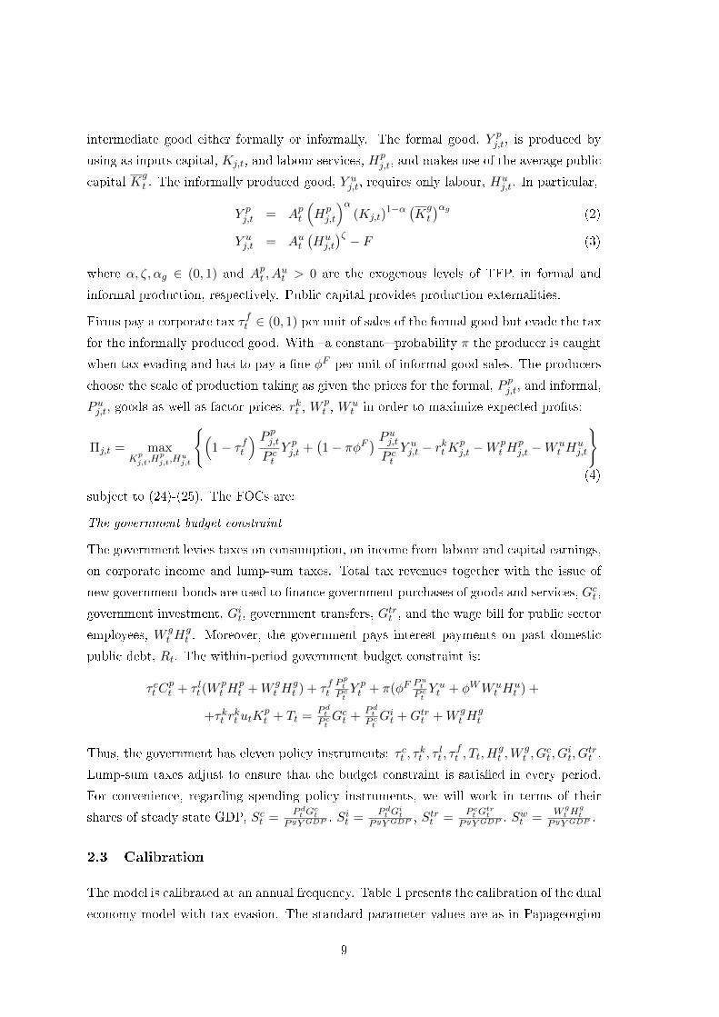
intermediate good either formally or informally. The formal good, Y pj,t, is produced by

using as inputs capital, Kj,t, and labour services, Hpj,t, and makes use of the average public

capital Kgt . The informally produced good, Y u

j,t, requires only labour, Huj,t. In particular,

Y pj,t = Apt

(Hpj,t

)α(Kj,t)

1−α (Kgt

)αg(2)

Y uj,t = Aut

(Huj,t

)ζ − F (3)

where α, ζ, αg ∈ (0, 1) and Apt , Aut > 0 are the exogenous levels of TFP. in formal and

informal production, respectively. Public capital provides production externalities.

Firms pay a corporate tax τ ft ∈ (0, 1) per unit of sales of the formal good but evade the tax

for the informally produced good. With �a constant� probability π the producer is caught

when tax evading and has to pay a �ne φF per unit of informal good sales. The producers

choose the scale of production taking as given the prices for the formal, P pj,t, and informal,

P uj,t, goods as well as factor prices, rkt , W

pt , W

ut in order to maximize expected pro�ts:

Πj,t = maxKpj,t,H

pj,t,H

uj,t

{(1− τ ft

) P pj,tP ct

Y pj,t +

(1− πφF

) P uj,tP ct

Y uj,t − rktK

pj,t −W

pt H

pj,t −W

ut H

uj,t

}(4)

subject to (24)-(25). The FOCs are:

The government budget constraint

The government levies taxes on consumption, on income from labour and capital earnings,

on corporate income and lump-sum taxes. Total tax revenues together with the issue of

new government bonds are used to �nance government purchases of goods and services, Gct ,

government investment, Git, government transfers, Gtrt , and the wage bill for public sector

employees, W gt H

gt . Moreover, the government pays interest payments on past domestic

public debt, Rt. The within-period government budget constraint is:

τ ct Cpt + τ lt (W

pt H

pt +W g

t Hgt ) + τ ft

P ptP ctY pt + π(φF

PutP ctY ut + φWW u

t Hut ) +

+τkt rkt utK

pt + Tt =

P dtP ctGct +

P dtP ctGit +Gtrt +W g

t Hgt

Thus, the government has eleven policy instruments: τ ct , τkt , τ

lt , τ

ft , Tt, H

gt ,W

gt , G

ct , G

it, G

trt .

Lump-sum taxes adjust to ensure that the budget constraint is satis�ed in every period.

For convenience, regarding spending policy instruments, we will work in terms of their

shares of steady state GDP, Sct =P dt G

ct

P yY GDP, Sit =

P dt Git

P yY GDP, Strt =

P ct Gtrt

P yY GDP, Swt =

W gt H

gt

P yY GDP.

2.3 Calibration

The model is calibrated at an annual frequency. Table 1 presents the calibration of the dual

economy model with tax evasion. The standard parameter values are as in Papageorgiou

9

(2014). The data source for the �scal policy variables is Eurostat. The consumption and

labour tax rate values have been set to 0.15 and 0.34 respectively. The corporate revenue

tax rate has been set so that, given the average pro�ts to sales ratio, it corresponds to a

pro�t tax10 of around 25%. The share of government consumption in GDP is set equal to

its value in the data. The labour share in the formal sector, α, is computed using data from

AMECO. The same value is used for the labour share in the informal sector. The �xed

cost parameter in the production function of the informal sector is set so that pro�ts are

zero in the steady state. The coe�cient of risk aversion and the inverse labour elasticity

are both set equal to 1.

We have normalized the scale parameter in the production function of the o�cial sector,

Ap, to unity and have selected the scale parameters in the informal sector so that the

informal sector in the baseline speci�cation is 25% of GDP11 the share of the shadow

economy in Greece as reported in Schneider and Williams (2013).

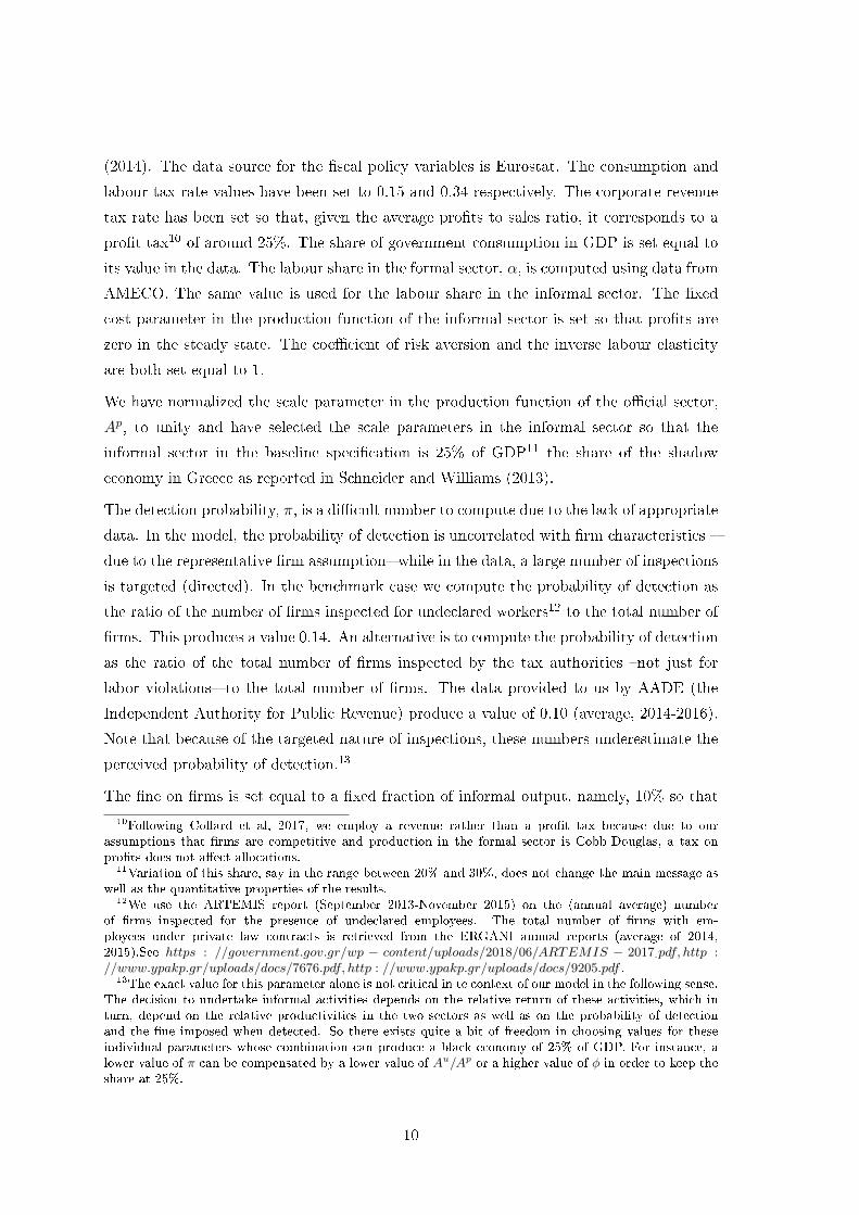
The detection probability, π, is a di�cult number to compute due to the lack of appropriate

data. In the model, the probability of detection is uncorrelated with �rm characteristics �

due to the representative �rm assumption� while in the data, a large number of inspections

is targeted (directed). In the benchmark case we compute the probability of detection as

the ratio of the number of �rms inspected for undeclared workers12 to the total number of

�rms. This produces a value 0.14. An alternative is to compute the probability of detection

as the ratio of the total number of �rms inspected by the tax authorities �not just for

labor violations� to the total number of �rms. The data provided to us by AADE (the

Independent Authority for Public Revenue) produce a value of 0.10 (average, 2014-2016).

Note that because of the targeted nature of inspections, these numbers underestimate the

perceived probability of detection.13

The �ne on �rms is set equal to a �xed fraction of informal output, namely, 10% so that

10Following Collard et al, 2017, we employ a revenue rather than a pro�t tax because due to ourassumptions that �rms are competitive and production in the formal sector is Cobb-Douglas, a tax onpro�ts does not a�ect allocations.

11Variation of this share, say in the range between 20% and 30%, does not change the main message aswell as the quantitative properties of the results.

12We use the ARTEMIS report (September 2013-November 2015) on the (annual average) numberof �rms inspected for the presence of undeclared employees. The total number of �rms with em-ployees under private law contracts is retrieved from the ERGANI annual reports (average of 2014,2015).See https : //government.gov.gr/wp − content/uploads/2018/06/ARTEMIS − 2017.pdf, http ://www.ypakp.gr/uploads/docs/7676.pdf, http : //www.ypakp.gr/uploads/docs/9205.pdf .

13The exact value for this parameter alone is not critical in te context of our model in the following sense.The decision to undertake informal activities depends on the relative return of these activities, which inturn, depend on the relative productivities in the two sectors as well as on the probability of detectionand the �ne imposed when detected. So there exists quite a bit of freedom in choosing values for theseindividual parameters whose combination can produce a black economy of 25% of GDP. For instance, alower value of π can be compensated by a lower value of Au/Ap or a higher value of φ in order to keep theshare at 25%.

10

in the baseline case, detection results in a tax liability that is roughly double of that of

the law abiding �rms. The �ne on tax evading households, φW , is set equal to 0.5 (that is,

50% more than the income tax rate).

The exponent of public capital in production, αg, is set equal to the average value of

the public investment-to-GDP ratio in the data over the period 2000-2009. We set the

adjustment cost on private capital, ξk, at 2.5 and calibrate the value for the adjustment

cost parameter on private foreign assets, ξf , to the lowest possible value so as to ensure that

the equilibrium solution for foreign assets is stationary. The Calvo parameters, θd, θx, θm,

are set equal to 0.35, implying that �rms adjust their prices every about 6 quarters, which

is in the range of estimates for the euro area countries (see e.g. Christo�el et al. 2008).

2.4 Steady-State Fiscal Multipliers

We compute steady state �scal multipliers for all the �scal instruments considered. For the

sake of space, we only present the e�ects associated with an increase in the steady state

level of the taxes on labour income as well as with a decrease in the level of government

consumption. The e�ects of the remaining instruments are described in Appendix. A full

dynamic analysis in the DSGE model is carried out in the following section.

Table 2 shows the e�ects of increases in the tax rate on labor in the dual economy (formal

and informal sectors) that result in higher tax receipts of one percentage point of GDP.

Let us focus on the column with the benchmark calibration (τ f = 0.34). Increasing the

tax rate from 34% to 35.64% (second row), increases income tax revenue as a percentage

points of GDP, from 19.16% to 20.16% (�rst row). The share of informal output increases

from 25% to 26.4% (row su) and informal employment increases from 34.8% to 36.4%.

(row shu).

Rows dyp and dyT report the corresponding e�ect on o�cial and true output as percentage

deviation from the steady state. Recorded output declines by −2.5% and true output by

−1.6%, that is, the recorded decline in economic activity exaggerates the true one by more

than 50%. Row dyu shows that the higher tax rate induces and increase of the informal

output by 3.3%. Rows dTRf

dτfand dTRt

dτfreport the e�ect of the tax increase on narrow

(source) and broad (from all sources) tax revenue. Income tax collections increase by 0.36

while total tax revenue increases by 0.060 units. Total revenue increases by less because

the switch of activity to the informal sector decreases the tax base for the other taxes

11

Table 1: Calibration, DSGE

Parameter Description Value

Ap TFP formal sector 1

Au TFP informal sector 0.53

α Labour share formal sector 0.6

ζ Labour share informal sector 0.6

αg Public capital elasticity in production 0.053

F Fixed cost informal sector 0.060

δp Private capital depreciation rate 0.069

δg Public capital depreciation rate 0.043

ξk Private capital adjustment cost parameter 2.5

ξf Adjustment cost parameter for froreign assets 0.05

ξc Habit persistence 0.6

ψ Elasticity of marginal depreciation costs 1.5814

β Discount factor 0.9615

σ Risk aversion 1

γ Inverse of labour elasticity 1

ϑ Substitutability/complementarity between private and public goods 0.05

π Probability of detection 0.14

φF Fine for �rms 0.1

φW Fine for households 0.5

θd, θx, θm Calvo parameters 0.35

µd Markup - domestic market 1.35

µx Markup - foreign market 1.1

µm Markup - importing �rms 1.35

xd, xx, xm Indexation parameters 0.256

ωc Home bias in the production of consumption goods 0.65

ωi Home bias in the production of investment goods 0.3

εc Elasticity of substitution between imported and domestic consumption goods 3.351

εi Elasticity of substitution between imported and domestic investment goods 6.352

εx Elasticity of exports 1.463

f Target level of net private foreign assets-to-GDP ratio 0

x Productivity of public spending on goods and services 0.29

Gc/Y Govt intermediate cons./GDP 0.1024

Gi/Y Govt investment /GDP 0.057

W gHg/Y Govt wage bill /GDP 0.1307

Gtr/Y Govt transfers/GDP 0.2059

τf Tax rate on revenue 0.04

τ l Tax rate on labour 0.34

τk Tax rate on capital 0.20

τ c Tax rate on consumption 0.15Note: For the detection probability we use the ARTEMIS report (September 2013-November 2015) data on the (yearly average) number of �rms inspected for the pres-ence of undeclared and underdeclared dependent employment. The total numberof �rms with employees under private law contracts is retrieved from the ERGANIannual reports (average of 2014, 2015).

12

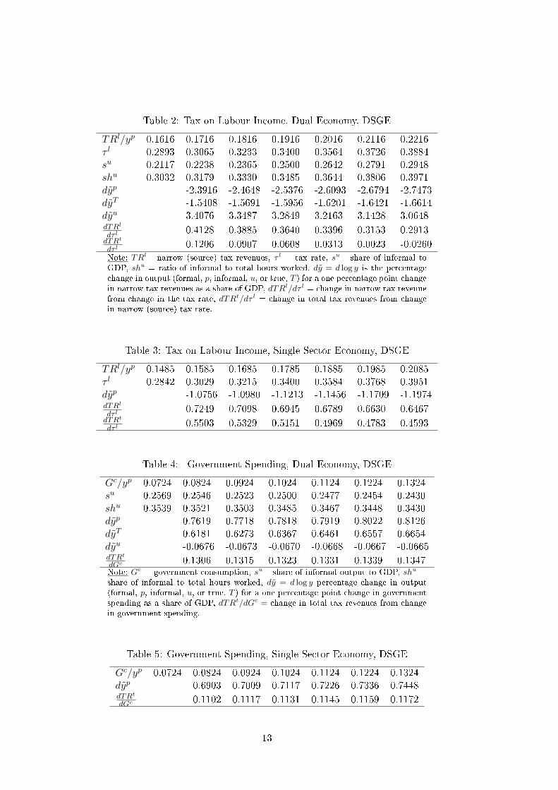
Table 2: Tax on Labour Income, Dual Economy, DSGE

TRl/yp 0.1616 0.1716 0.1816 0.1916 0.2016 0.2116 0.2216τ l 0.2893 0.3065 0.3233 0.3400 0.3564 0.3726 0.3884su 0.2117 0.2238 0.2365 0.2500 0.2642 0.2791 0.2948shu 0.3032 0.3179 0.3330 0.3485 0.3644 0.3806 0.3971dyp -2.3916 -2.4648 -2.5376 -2.6093 -2.6794 -2.7473dyT -1.5408 -1.5691 -1.5956 -1.6201 -1.6421 -1.6614dyu 3.4076 3.3487 3.2849 3.2163 3.1428 3.0648dTRl

dτ l0.4128 0.3885 0.3640 0.3396 0.3153 0.2913

dTRt

dτ l0.1206 0.0907 0.0608 0.0313 0.0023 -0.0260

Note: TRl= narrow (source) tax revenues, τ l = tax rate, su= share of informal toGDP, shu = ratio of informal to total hours worked, dy = d log y is the percentagechange in output (formal, p, informal, u, or true, T ) for a one percentage point changein narrow tax revenues as a share of GDP, dTRl/dτ l = change in narrow tax revenuefrom change in the tax rate, dTRt/dτ l = change in total tax revenues from changein narrow (source) tax rate.

Table 3: Tax on Labour Income, Single Sector Economy, DSGE

TRl/yp 0.1485 0.1585 0.1685 0.1785 0.1885 0.1985 0.2085τ l 0.2842 0.3029 0.3215 0.3400 0.3584 0.3768 0.3951dyp -1.0756 -1.0980 -1.1213 -1.1456 -1.1709 -1.1974dTRl

dτ l0.7249 0.7098 0.6945 0.6789 0.6630 0.6467

dTRt

dτ l0.5503 0.5329 0.5151 0.4969 0.4783 0.4593

Table 4: Government Spending, Dual Economy, DSGE

Gc/yp 0.0724 0.0824 0.0924 0.1024 0.1124 0.1224 0.1324su 0.2569 0.2546 0.2523 0.2500 0.2477 0.2454 0.2430shu 0.3539 0.3521 0.3503 0.3485 0.3467 0.3448 0.3430dyp 0.7619 0.7718 0.7818 0.7919 0.8022 0.8126dyT 0.6181 0.6273 0.6367 0.6461 0.6557 0.6654dyu -0.0676 -0.0673 -0.0670 -0.0668 -0.0667 -0.0665dTRt

dGc 0.1306 0.1315 0.1323 0.1331 0.1339 0.1347Note: Gc = government consumption, su= share of informal output to GDP, shu =share of informal to total hours worked, dy = d log y percentage change in output(formal, p, informal, u, or true, T ) for a one percentage point change in governmentspending as a share of GDP, dTRt/dGc = change in total tax revenues from changein government spending.

Table 5: Government Spending, Single Sector Economy, DSGE

Gc/yp 0.0724 0.0824 0.0924 0.1024 0.1124 0.1224 0.1324dyp 0.6903 0.7009 0.7117 0.7226 0.7336 0.7448dTRt

dGc 0.1102 0.1117 0.1131 0.1145 0.1159 0.1172

13

too.14

It is worth mentioning that the computed multipliers fall in the range reported in the

empirical multiplier literature as well as that suggested by quantitative DSGE models (see

Schmidt et al. (2015) for a comparative study of multipliers in the euro area), notwith-

standing the large variation in existing estimates. For instance, Mertens and Ravn, 2014,

report values in the range of 2 and 3.

Table 3 performs the same exercise in the version of the model without an underground

economy. In this case, an (analogous) increase in the labor income tax (from a 34% to a

35.8%) exhibits a weaker negative e�ect on economic activity (-1.12%), a stronger positive

e�ect on tax collection from that source and a positive (but smaller due the negative

spillover on the tax base of the other taxes) e�ect on total tax collection. Comparison

of Tables 2 and 3 shows that projections of the e�ects of a tax rise on output and tax

revenue are bound to be signi�cantly more optimistic when the model does not contain

a shadow economy, as they do not take into account the migration of economic activity

to the underground economy. And that the size of both the forecast error (the di�erence

between Tables 2 and 3 in row dyp) and the exaggeration of the true e�ect (the di�erence

between rows dyp and dyT in Table 2 is increasing in the relative size of the black economy.

The same property also characterizes the forecast error in projections of tax revenues (the

di�erences between the �corresponding� last two rows across Tables 2 and 3).

The model's pessimistic predictions about tax revenue collection are clearly in line with

the recent Greek experience. According to a recent report15 �...Since 2010, Athens has

introduced revenue boosting measures worth almost 37 billion EUR in total but the result

is quite disappointing as the European Commission's o�cial data show that state revenues

have declined by 9.2 billion EUR in the same period...In the same period GDP has shrunk

about 26%.�

Tables 4 and 5 report the e�ects of changes in government spending, holding the distor-

tionary tax rates constant and using lump sum taxes to balance the budget. Note that the

share of the formal sector increases with an increase in the share of government spending

as the latter type of spending falls exclusively on formal goods. The main �nding is that

while the e�ects are qualitatively similar across the two types of �scal consolidation (like a

tax hike, lower public spending increases the share of the informal sector), both the fore-

cast and measurement errors are quite small: model misspeci�cation regarding the shadow

economy does not distort quantitatively the implications regarding the e�ects of changes in

government spending (spending multipliers). It suggests that �scal consolidation is more

14 Note that total tax revenue includes the average value of the �nes collected from all the agents ��rmsand workers� detected.

15Hatzinikolaou and Nikas, Kathimerini, November 12, 2016.

14

likely to succeed and its outcome is less uncertain16 when it relies on spending rather than

on tax measures.

These �ndings are consistent with and can also provide a possible explanation for the those

reported in Alesina and Giavazzi, 2015. They argue that �...The accumulated evidence from

over 40 years of �scal adjustments across the OECD speaks loud and clear: ... adjustments

achieved through spending cuts are less recessionary than those achieved through tax

increases...�. We �nd this to be the case not only in a standard model and for o�cial

output but also in the dual economy with an informal sector and for true output. They

also argue that �...only spending-based adjustments have eventually led to a permanent

consolidation of the budget, as measured by the stabilisation (at least) if not reduction

of debt-to-GDP ratios...�. Our analysis provides an explanation for this �nding that does

not hinge on implausibly large labor elasticities. Even when the total supply of labour is

inelastic, as is commonly accepted, changes in tax rates and real wages may still matter

for employment in the o�cial sector if labor can move across sectors.

Our framework thus implies that from the point of view of debt sustainability, and to

a much larger extent than that predicted by the standard, one sector model, spending

reductions are more potent means for improving the �scal position and restraining debt

growth than tax increases. Moreover, their e�ects are less likely to be distorted by the

presence of a shadow economy, which helps make policy more reliable.

In the next section, we will use the actual paths of the �scal instruments in the model during

the consolidation period in order to evaluate their quantitative e�ects on macroeconomic

activity and tax revenue in Greece during the crisis.

3 Fiscal Consolidation in Greece

We solve the model under two alternative, informational assumptions about the paths of

the �scal instruments: perfect foresight; and random walk. Under the former, we start

the economy in its steady state and then plug in the model the actual values of the �scal

(tax-spending) instruments for the period 2010-2015. After 2015, the �scal instruments

are assumed to gradually return to their pre-crisis 2009 values. In particular, we assume

that they follow an autoregressive process using as initial values the 2015 values and an

autoregressive coe�cient equal to 0.9. We allow lump-sum transfers to �ll any government

�nancing gaps. Under the random walk informational assumption, we assume that during

the consolidation period, people expect the current �scal policy stance to remain the same

16Less uncertain because the computation of spending multipliers is less sensitive to the size of the blackeconomy, which is hard to measure.

15

in the next period, so any change is perfectly unanticipated. In reality, some of the changes

were known as the plans were drawn for more that one year. But at the same time, there

were many ex post, unanticipated changes as often the plans had to be revised mid-course

due to failure to achieve the de�cit-debt paths and new, harsher �scal measures had to be

introduced. So the true expectations may lie somewhere between these two polar extremes.

We present the results from the perfect foresight exercise below and delegate the results

from the random walk exercise (which are quite similar) to the Appendix.

The actual paths of the �scal instruments are depicted in Figure 7 in the Appendix. A

discussion of the computation of the tax rates can be found in Appendix 7.1.

Figure 1: The e�ects of the Greek �scal consolidation package on economic activity: Perfectforesight

2010 2011 2012 2013 2014 2015 2016 2017

Year

-30

-25

-20

-15

-10

-5

0

% D

evia

tion

Output

Model with tax evasion - Formal outputModel with tax evasion - True ouputOne sector model

2010 2011 2012 2013 2014 2015 2016 2017

Year

-15

-10

-5

0

5

% D

evia

tion

Consumption

Model with tax evasionOne sector model

2010 2011 2012 2013 2014 2015 2016 2017

Year

-40

-35

-30

-25

-20

-15

-10

-5

% D

evia

tion

Private investment

Model with tax evasionOne sector model

2010 2011 2012 2013 2014 2015 2016 2017

Year

-25

-20

-15

-10

-5

0

% D

evia

tion

Hours worked

Model with tax evasion - Formal hours workedModel with tax evasion - True hours workedOne sector model

Note: Fiscal Instruments: 2009, steady state values. From 2010-2015, actual values. From 2016 onward,projected values under the assumption that they return to their 2009 values according to an AR(1) processwith persistence 0.9.

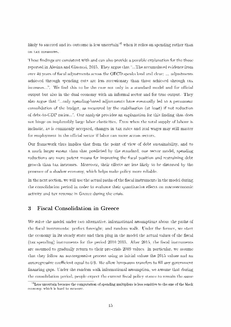
The model is solved non-linearly in Dynare. Figure 1 plots the path of formal and true

(total) GDP, consumption, private investment and employment along with the paths of

the corresponding variables of the one sector model. The dual economy model implies a

cumulative decline in GDP by 2015 that is similar to that observed in the data (26%).

The true decline, though, is signi�cantly lower (about 17%). Interestingly, the decline

predicted by the model that abstracts from the underground economy is fairly close to

the true one. The di�erences across the three measures are greater for employment. The

16

recorded cumulative decrease in employment (hours) is 21%, that implied by the single

sector model is 11% and the true one is only 4%. Note that there is nothing in the

calibration that targets the decline in economic activity; and that it is not problematic for

a model to explain all of the actual decline as this is not a variance decomposition exercise.

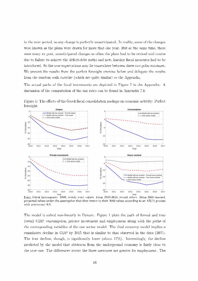
Figure 2: Contribution of individual, �scal instruments: Perfect foresight

2010 2011 2012 2013 2014 2015 2016 2017

Year

-25

-20

-15

-10

-5

0

% D

evia

tion

Labour income tax rateConsumption tax rateCapital income tax rateTax rate on corporate revenueGovernment wagesGovernment consumptionGovernment investment

Note: Each �scal instrument is introduced sequentially. Note that the contributions are not orthogonal.

Figure 2 plots the e�ects of the individual �scal instruments. It shows that the labour

income tax had the biggest e�ect, accounting for about 1/3 of the decrease in GDP (8%).

It is followed by the capital income tax and the decrease in the public employment wage

bill (4% each). In general, tax increases accounted for about 2/3 of the total decline in

o�cial output and spending cuts for the remaining 1/3.

Figure 3 depicts the paths of the individual tax revenue categories over the period 2010�

2015 in the economy with and without an informal sector. Note that these paths are plotted

against the path of all the �scal instruments during the consolidation period. They do not

thus capture the corresponding tax La�er curves as well as Table 3 does. Nonetheless, they

are quite revealing regarding the size of over-optimism in tax revenue projections as well

as the limited revenue e�ectiveness of the package implemented. In particular, Figure 3

shows that while the single sector model predicts that the e�ect of the tax package adopted

would have increased the tax revenue to GDP share in 2012 by more than six percentage

points, the increase in the dual economy is less than half of that.

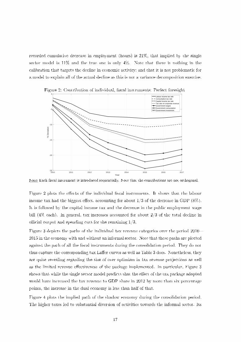
Figure 4 plots the implied path of the shadow economy during the consolidation period.

The higher taxes led to substantial diversion of activities towards the informal sector. Its

17

Figure 3: The e�ects of individual taxes on tax revenue with and without tax evasion:Perfect foresight

2010 2012 2014 2016

Year

0

1

2

3

4

5

6

7

% P

oint

Dev

iatio

n

Total Tax Revenue / Initial GDP

2010 2012 2014 2016

Year

-1.5

-1

-0.5

0

0.5

1

1.5

2

% P

oint

Dev

iatio

n

Labour income tax revenues / Initial GDP

2010 2012 2014 2016

Year

-1

-0.5

0

0.5

1

1.5

2

% P

oint

Dev

iatio

n

Capital income tax revenues / Initial GDP

2010 2012 2014 2016

Year

1

1.5

2

2.5

3

3.5

4

4.5

% P

oint

Dev

iatio

n

Consumption tax revenues / Initial GDP

Model with tax evasionOne sector model

2010 2012 2014 2016

Year

-0.5

0

0.5

% P

oint

Dev

iatio

n

Corporate tax revenues / Initial GDP

Note: In each graph, the path of the corresponding �scal variable is as described in the footnote of Figure1, while the remaining �scal instruments are held at their steady state values.

share, according to the model, increased by 13 percentage points from 2010 and 2015. The

model's prediction about an increase is born out by: a) anecdotal evidence; b) reports

on the outcomes of tax inspections by the Independent Agency for Public Finances (see

www.aade.gr).

4 Counterfactuals

In order to highlight the role played by the informal sector in shaping the outcomes of the

�scal consolidation experience in Greece, we perform several counterfactuals. We also use

the recent imposition of capital controls in the model to get estimates of its e�ects on the

size of the black economy and GDP growth.

In the �rst counterfactual, we feed the actual paths of the �scal instruments into the model

with tax evasion �exactly as we did in the previous section� while at the same time varying

the probability of detection in order to keep the size of the informal economy constant at

its pre crisis level. This exercise is meant to answer the question of how the Greek economy

would have fared under the exact same policy package if it had managed to restrict growth

18

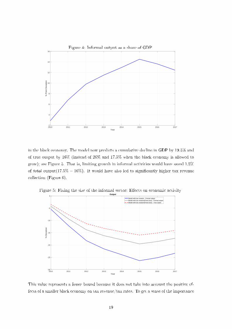
Figure 4: Informal output as a share of GDP

2010 2011 2012 2013 2014 2015 2016 2017

Year

2

4

6

8

10

12

14

16

% P

oint

Dev

iatio

n

in the black economy. The model now predicts a cumulative decline in GDP by 19.5% and

of true output by 16% (instead of 26% and 17.5% when the black economy is allowed to

grow); see Figure 5. That is, limiting growth in informal activities would have saved 1.5%

of total output(17.5% − 16%). It would have also led to signi�cantly higher tax revenue

collection (Figure 6).

Figure 5: Fixing the size of the informal sector: E�ects on economic activity

2010 2011 2012 2013 2014 2015 2016 2017

Year

-30

-25

-20

-15

-10

-5

0

% D

evia

tion

Output

Model with tax evasion - Formal outputModel with tax evasion(Fixed size) - Formal outputModel with tax evasion(Fixed size) - True ouput

This value represents a lower bound because it does not take into account the positive ef-

fects of a smaller black economy on tax revenue/tax rates. To get a sense of the importance

19

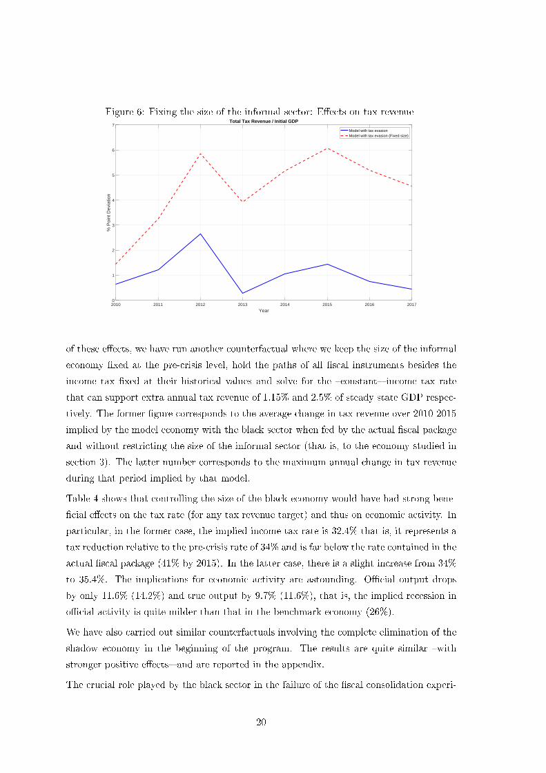
Figure 6: Fixing the size of the informal sector: E�ects on tax revenue

2010 2011 2012 2013 2014 2015 2016 2017

Year

0

1

2

3

4

5

6

7

% P

oint

Dev

iatio

n

Total Tax Revenue / Initial GDP

Model with tax evasionModel with tax evasion (Fixed size)

of these e�ects, we have run another counterfactual where we keep the size of the informal

economy �xed at the pre-crisis level, hold the paths of all �scal instruments besides the

income tax �xed at their historical values and solve for the �constant� income tax rate

that can support extra annual tax revenue of 1.15% and 2.5% of steady state GDP respec-

tively. The former �gure corresponds to the average change in tax revenue over 2010-2015

implied by the model economy with the black sector when fed by the actual �scal package

and without restricting the size of the informal sector (that is, to the economy studied in

section 3). The latter number corresponds to the maximum annual change in tax revenue

during that period implied by that model.

Table 4 shows that controlling the size of the black economy would have had strong bene-

�cial e�ects on the tax rate (for any tax revenue target) and thus on economic activity. In

particular, in the former case, the implied income tax rate is 32.4% that is, it represents a

tax reduction relative to the pre-crisis rate of 34% and is far below the rate contained in the

actual �scal package (41% by 2015). In the latter case, there is a slight increase from 34%

to 35.4%. The implications for economic activity are astounding. O�cial output drops

by only 11.6% (14.2%) and true output by 9.7% (11.6%), that is, the implied recession in

o�cial activity is quite milder than that in the benchmark economy (26%).

We have also carried out similar counterfactuals involving the complete elimination of the

shadow economy in the beginning of the program. The results are quite similar �with

stronger positive e�ects� and are reported in the appendix.

The crucial role played by the black sector in the failure of the �scal consolidation experi-

20

Table 6: Counterfactual: Fiscal consolidation when �xing the size of the informal sectorfor certain tax revenue requirements

GDP true output

Increase in tax revenues by 1.15%τ l = 0.324 -11.86% -9.74%

Increase in tax revenues by 2.52%τ l = 0.354 -14.2% -11.64

Note: Labor income tax�relative to its steady state value� needed to raise 1.15% and2.52% extra �relative to the steady state� tax revenue per annum when all other �scalinstruments take their 2010�2015 historical values and the black economy is �xed atits pre-crisis level.

Table 7: Counterfactual experiment: Impact of the imposition of capital controls

GDP True output Informal/formal Prob. detection

2015 2016 2015 2016 2015 2016 2015 2016

Baseline -2.38 -1.16 -1.41 0.72 1.60 -0.90 0.14 0.14

Counterfactual 2.64 4.23 -0.51 1.63 -4.78 -4.09 0.33 0.40

Note: GDP, true output: percentage change from previous year;informal/formal share: percent-age points, change relative to previous year.

ence in Greece and thus the importance of measures to control tax evasion for tax revenue

and economic activity can be further illuminated by considering the natural experiment

that took place in Greece in the summer of 2015, namely, the imposition of capital controls.

In order to prevent a bank run triggered by doubts about Greece's Eurozone membership,

the Greek government imposed limits on the amount of cash that depositors could withdraw

from their bank accounts. Hondroyannis and Papaoikonomou, 2017, report that this forced

a switch from cash to card payments: the share of card payments in private consumption

went from 4% to 12% over the next year. This led to a massive, unexpected increase in

VAT revenue. Using their estimated elasticity of VAT revenue to credit card usage, our

model implies that the capital controls may have contributed during the year following

their introduction to an increase in o�cial economic activity by 2.6% and to a reduction

in the share of the informal sector by almost �ve percentage points. The cumulative e�ect

after two years is 7% and 9 percentage points, respectively.17

These results are striking. They help establish quantitatively that the existence of a large

shadow economy made �scal consolidation in Greece a much more challenging endeavor

than it would have otherwise been: it led to �excessive� increases in tax rates that did not

17A caveat is in order. Our model abstracts from negative e�ects of capital controls, such as their impacton business and import �nancing. To the extent that capital controls have other negative side e�ects, thenumbers reported here should be interpreted as the upper bound of the possible e�ects.

21

translate into large increases in tax revenue, but led instead to a severe and protracted

downturn. Had the informal economy been better controlled, the �scal consolidation could

have been milder both in terms of the tax burden for households and �rms and in terms

of the implied output loss.

4.1 Sensitivity

We have carried out an extensive set of sensitivity exercises. In particular, we have also

considered speci�cations of the model with the following features: a) Ricardian and non-

Ricardian households; b) imperfect competition in the labour markets with labour unions

setting wages; c) nominal and real wage rigidity; d) inclusion of the public wage bill in

government consumption; e) variation of the following parameters: (i) value of 0.5 �instead

of 0.9� for the persistence parameter in the �scal instruments autoregressive rules after

2015; (ii) a value of zero for the �ne on workers who are caught working in the informal

sector (φW ); (iii) a value of two for the coe�cient of relative risk aversion σ; (iv) a value

of two for the Frisch elasticity γ; (v) we also varied the Calvo parameters, the disutility

from working in the informal sector as well as the �ne imposed on tax evading �rms.

Some of these exercises are reported in the Appendix while the remaining are available

from the authors. Figures 9 and 12 and Tables 19 and 22 show the results associated

with the model that contains features (a)-(d). This version of the model implies a decline

in GDP of about 26% too. One can thus conclude that the quantitative results reported

above are very robust to changes in the speci�cation of the model. We also �nd that the

greatest sensitivity is with regard to the coe�cient of relative risk aversion.

5 Conclusion

Following the outbreak of the sovereign debt crisis in Greece, the country undertook an

ambitious �scal consolidation program. At the outset of the program, Greece's o�cial

creditors were predicting that the adjustment, while substantial, would be manageable

and that the resulting recession would be limited and short lived. The actual experience

de�ed these predictions by a wide margin. Tax rates kept on increasing, yet tax revenue

grew little with the public debt to GDP ratio exploding. And the economy plunged into a

deep and protracted recession.

Our paper has provided an explanation for these facts that centers on the existence of a

substantial informal sector in Greece. Failure to account for this sector led to overoptimistic

projections about the size of the required �scal adjustment as well as about the severity of

GDP and employment contraction. Had the model underlying the projections contained a

22

dual economy, the predictions would have been quite more pessimistic (and more realistic)

both on the tax revenue and the economic activity front.

We have also argued that the true (total) decline in economic activity may have been

considerably smaller than that reported about o�cial activity. That is, recorded �austerity�

may have appeared more severe than it actually was because of the omission of the informal

economy.

Finally, we have highlighted the important, negative role played by the black economy

for the outcomes of in the �scal consolidation experience in Greece by arguing that, had

the Greek government been able to prevent further growth in the black economy, the

recession would have been signi�cantly milder. The key policy lesson learned from this

is that a better designed �scal adjustment program should focus more on tax compliance

issues. The unintended positive e�ects on tax revenue and o�cial activity of the capital

controls imposed in 2015 in Greece and which led to a large switch from cash to credit card

payments, thus reducing black market activities, provides strong support to this assertion.

23

6 References

Alesina, A. and Giavazzi, F., (2015), The e�ects of austerity: Recent research, NBER

Reporter 2015 Number 3, Research Summary.

Blanchard, O and Leigh, D., (2013), Growth forecast errors and �scal multipliers, American

Economic Review: Papers and Proceedings, 103(3), pp. 117�120.

Christiano, L.J., Eichenbaum, M., and Evans, C., (2005), Nominal rigidities and the dy-

namic e�ects of a shock to monetary policy, Journal of Political Economy 113, 1�45.

Corsetti, G., (2012), Has austerity gone too far?, Vox.eu, 2 April 2012.

de Paula, A. and Scheinkman, J. A. (2011). The Informal sector: An equilibrium model

and some empirical evidence from Brazil, Review of Income and Wealth, 57, pp. S8-?S26.

Docquier, F., Mueller, T, and J. Naval, (2017). Informality and long-run growth, Scandi-

navian Journal of Economics, 119(4), pp. 1040�1085.

Hondroyannis, G. and Papaoikonomou, D., (2017), The e�ect of card payments on VAT

revenue: New evidence from Greece, Economics Letters, 157, pp. 17�20.

La Porta, R. and Shleifer, A. (2008), The uno�cial economy and economic development,

Brookings Papers on Economic Activity, 39, pp. 275-?363.

Maloney, W. F. (2004), Informality revisited, World Development 32, pp. 1159�1178.

Mendoza, E., Razin, A., Tesar, L., (1994), E�ective tax rates in macroeconomics:cross-

country estimates of tax rates on factor incomes and consumption, Journal of Monetary

Economics, 34, 297-323.

Mertens, K., Ravn, M., (2014), A reconciliation of SVAR and narrative estimates of tax

multipliers, Journal of Monetary Economics, 68, S1-S19.

Murphy, K. M., Shleifer, A., and Vishny, R. W. (1989), Industrialization and the big push,

Journal of Political Economy 97, pp. 1003�1026.

Papageorgiou, D. (2014), BoGGEM: A dynamic stochastic general equilibrium model for

policy simulations. Bank of Greece Working Paper. no. 182.

Pappa, E., Sajedi, R. and Vella, E., (2015), Fiscal consolidation with tax evasion and

corruption, Journal of International Economics, 96 pp. S56�S75.

Schneider, F., Williams, C. (2013), The shadow economy, The Institute of Economic Af-

fairs.

Schneider, F. (2015), Size and development of the shadow economy of 31 European and 5

other OECD countries from 2003 to 2015: Di�erent developments, mimeo, Department of

24

Economics, Johannes Kepler University.

Schmidt, S., Kilponen, J., Pisani, M., Corbo, V., Hledik, T., Hollmayr, J., Hurtado, S.,

Júlio, P., Kulikov, D., Lemoine, M., Lozej, M., Lundvall, H., Maria, J., Micallef, B.,

Papageorgiou, D., Rysanek, J., Sideris, D., Thomas, C., Walque, G., (2015), Comparing

�scal multipliers across models and countries in Europe, European Central Bank, Working

Paper Series, No. 1760

25

7 Appendix

7.1 Tax rate computation, 2010-2015

The methodology followed for constructing the e�ective tax rates is based on the work

of Mendoza et al. (1994). Broadly speaking, the e�ective tax rates are estimated as the

ratios between the tax revenues from particular taxes and the corresponding tax bases

using information from the National Accounts. The data set comprises of annual data that

cover the period 2000-2015. The data source is Eurostat. The macroeconomic variables

used for the computation of the e�ective tax rates are:

• HY : Taxes on individual or household income including holding gains

• WSSE : Compensation of employees

• SSCER: Employers' actual social security contributions

• SSCH : Households' actual social security contributions

• GOSH : Gross operating surplus and mixed income of households

• CFCH : Consumption of �xed capital of households

• IYRH : Interest income received by households

• IYPH : Interest income paid by households

• CORY : Taxes on the income or pro�ts of corporations including holding gains

• STAMP : Stamp taxes

• TFCT : Taxes on �nancial and capital transactions

• TLG : Taxes on winnings from lottery or gambling

• CTC : Current taxes on capital

• CAT : Capital taxes

• OTP : Other taxes on production

• NFYT : Taxes on income paid by non-�nancial corporations

• FYT : Taxes on income paid by �nancial corporations

• GOS : Gross operating surplus, Total economy

• CFC : Consumption of �xed capital, Total economy

• TPI : Taxes on production and imports

• GIC : Intermediate consumption, government

• HC : Household and NPISH �nal consumption expenditure

• GOSNFC : Gross operating surplus and mixed income of non-�nancial corporations

• GOSFC : Gross operating surplus and mixed income of �nancial corporations

• CFCNFC : Consumption of �xed capital of non-�nancial corporations

• CFCFC : Consumption of �xed capital of �nancial corporations

26

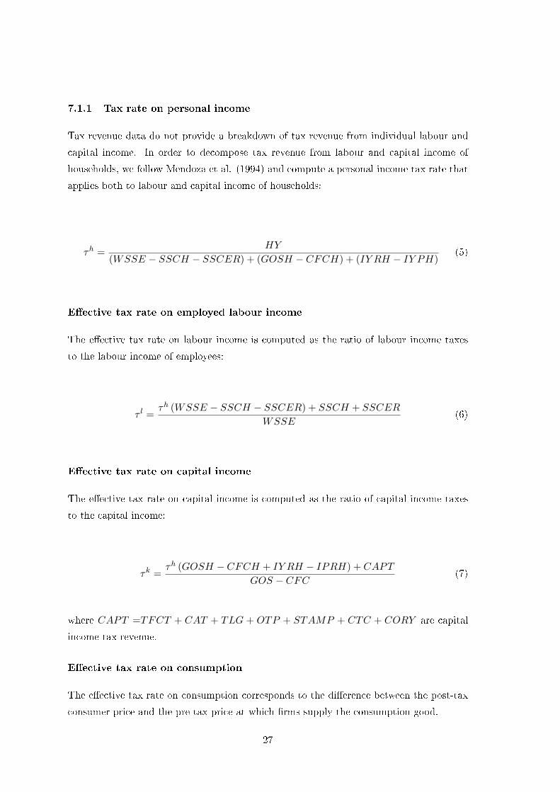
7.1.1 Tax rate on personal income

Tax revenue data do not provide a breakdown of tax revenue from individual labour and

capital income. In order to decompose tax revenue from labour and capital income of

households, we follow Mendoza et al. (1994) and compute a personal income tax rate that

applies both to labour and capital income of households:

τh =HY

(WSSE − SSCH − SSCER) + (GOSH − CFCH) + (IY RH − IY PH)(5)

E�ective tax rate on employed labour income

The e�ective tax rate on labour income is computed as the ratio of labour income taxes

to the labour income of employees:

τ l =τh (WSSE − SSCH − SSCER) + SSCH + SSCER

WSSE(6)

E�ective tax rate on capital income

The e�ective tax rate on capital income is computed as the ratio of capital income taxes

to the capital income:

τk =τh (GOSH − CFCH + IY RH − IPRH) + CAPT

GOS − CFC(7)

where CAPT =TFCT + CAT + TLG + OTP + STAMP + CTC + CORY are capital

income tax revenue.

E�ective tax rate on consumption

The e�ective tax rate on consumption corresponds to the di�erence between the post-tax

consumer price and the pre-tax price at which �rms supply the consumption good.

27

τ c =CT

HC +GIC − CT(8)

where CT = TPI − TFCT − TLG − OTP are total tax revenue from indirect taxation,

which by de�nition are equal to the di�erence between the nominal value of aggregate con-

sumption at post-tax and pre-tax prices. Note that we deduct the categories TFCT, TLG

and OTP, from TPI since these categories include mainly capital and labour income taxes.

The denominator is the base of the consumption tax, which is the pre-tax value of con-

sumption.

Tax rate on corporate revenue

In computing the tax rate on corporate revenue (sales) we assume that the tax rate is

proportional to the tax rate on corporate income. Speci�cally we calculate the tax rate on

corporate revenue as:

τ s = τ corpprofits

sales(9)

where τ corp is the e�ective tax rate on corporate income estimated as:

τ corp =FY T +NFY T

GOSNFC +GOSFC − CFCNFC − CFCF(10)

The data source for total profits (pro�ts before taxes and depreciation) and total sales

correspond to the aggregate of these measures for the Greek listed �rms for the years

2007-2008. The datasource is DataStream.

28

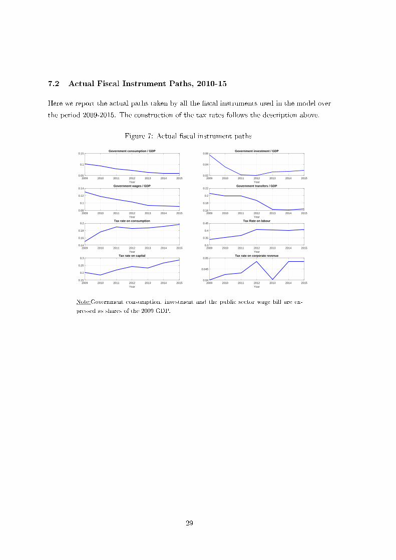
7.2 Actual Fiscal Instrument Paths, 2010-15

Here we report the actual paths taken by all the �scal instruments used in the model over

the period 2009-2015. The construction of the tax rates follows the description above.

Figure 7: Actual �scal instrument paths

2009 2010 2011 2012 2013 2014 2015Year

0.05

0.1

0.15Government consumption / GDP

2009 2010 2011 2012 2013 2014 2015Year

0.02

0.04

0.06Government investment / GDP

2009 2010 2011 2012 2013 2014 2015Year

0.08

0.1

0.12

0.14Government wages / GDP

2009 2010 2011 2012 2013 2014 2015Year

0.16

0.18

0.2

0.22Government transfers / GDP

2009 2010 2011 2012 2013 2014 2015Year

0.14

0.16

0.18

0.2Tax rate on consumption

2009 2010 2011 2012 2013 2014 2015Year

0.3

0.35

0.4

0.45Tax Rate on labour

2009 2010 2011 2012 2013 2014 2015Year

0.15

0.2

0.25

0.3Tax rate on capital

2009 2010 2011 2012 2013 2014 2015Year

0.04

0.045

0.05Tax rate on corporate revenue

Note:Government consumption, investment and the public sector wage bill are ex-

pressed as shares of the 2009 GDP.

29

NOT FOR PUBLICATION

7.3 BOGGEM: Additional Fiscal Instruments, Baseline Version

7.3.1 Steady State Results

Table 8: Tax on Firm Revenue, Dual Economy, BOGGEM

TRf/yp 0.0109 0.0209 0.0309 0.0409 0.0509 0.0609τ f 0.0112 0.0256 0.0400 0.0545 0.0691 0.0837su 0.2242 0.2367 0.2500 0.2641 0.2790 0.2949shu 0.3217 0.3349 0.3485 0.3625 0.3768 0.3915dyp -2.7325 -2.8065 -2.8829 -2.9614 -3.0421dyT -1.8445 -1.8683 -1.8915 -1.9141 -1.9360dyu 3.0281 2.9928 2.9554 2.9157 2.8737dTRf

dτf0.7305 0.6900 0.6498 0.6100 0.5707

dTRt

dτf-0.0648 -0.0907 -0.1156 -0.1395 -0.1622

Note: TRf= narrow (source) tax revenues, τf = tax rate on �rm revenue, su= share ofinformal output to GDP, shu = ratio of informal to total hours worked, dy = d log y :percentage change in output (formal, p, informal, u, or true, T ) for a one percentagepoint change in the narrow tax revenues as share of GDP, dTRf/dτf = change innarrow tax revenue from change in the tax rate, dTRt/dτf = change in total taxrevenues from change in the tax rate.

Table 9: Tax on Firm Revenue, Single Sector Economy, BOGGEM

TRf/yp 0.0174 0.0274 0.0374 0.0474 0.0574τ f 0.0254 0.0400 0.0547 0.0694 0.0842dyp -1.4480 -1.4663 -1.4854 -1.5053dTRf

dτf1.0352 1.0051 0.9753 0.9456

dTRt

dτf0.3116 0.2918 0.2721 0.2526

30

Table 10: Consumption Tax, Dual Economy, BOGGEM

TRc/yp 0.0692 0.0792 0.0892 0.0992 0.1092 0.1192 0.1292τ c 0.1037 0.1191 0.1345 0.1500 0.1656 0.1814 0.1972su 0.2189 0.2290 0.2393 0.2500 0.2610 0.2724 0.2842shu 0.3231 0.3315 0.3400 0.3485 0.3570 0.3655 0.3740dyp -1.3899 -1.3939 -1.3979 -1.4017 -1.4055 -1.4091dyT -0.8817 -0.8781 -0.8745 -0.8709 -0.8672 -0.8634dyu 1.8531 1.8090 1.7661 1.7243 1.6836 1.6440dTRc

dτc 0.6410 0.6204 0.6002 0.5804 0.5611 0.5421dTRt

dτc 0.4604 0.4437 0.4275 0.4117 0.3963 0.3813Note: TRc = narrow (source) tax revenues,τ c = tax rate on consumption, su= share ofinformal output to GDP, shu = ratio of informal to total hours worked, dy = d log yis the percentage change in output (formal, p, informal, u, or true, T ) for a onepercentage point change in the narrow tax revenue as share of GDP, dTRc/dτ c =change in narrow tax revenue from change in the tax rate, dTRt/dτ c = change intotal tax revenues from change in the tax rate.

Table 11: Consumption Tax, Single Sector Economy, BOGGEM

TRc/yp 0.0692 0.0792 0.0892 0.0992 0.1092 0.1192 0.1292τ c 0.1043 0.1195 0.1347 0.1500 0.1653 0.1807 0.1960dyp -0.5569 -0.5500 -0.5433 -0.5368 -0.5304 -0.5242dTRc

dτc 0.9938 0.9821 0.9708 0.9597 0.9489 0.9384dTRt

dτc 0.8711 0.8619 0.8529 0.8441 0.8356 0.8273

31

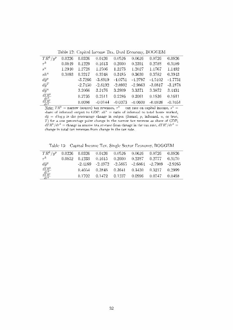
Table 12: Capital Income Tax, Dual Economy, BOGGEM

TRk/yp 0.0226 0.0326 0.0426 0.0526 0.0626 0.0726 0.0826τk 0.0849 0.1229 0.1613 0.2000 0.2391 0.2788 0.3189su 1.2940 1.2728 1.2506 1.2273 1.2027 1.1767 1.1492shu 0.3093 0.3217 0.3348 0.3485 0.3630 0.3782 0.3943dyp -3.7266 -3.8919 -4.0751 -4.2797 -4.5102 -4.7731dyT -2.7450 -2.8192 -2.8992 -2.9863 -3.0817 -3.1878dyu 3.2066 3.2476 3.2909 3.3371 3.3872 3.4431dTRk

dτk0.2735 0.2511 0.2286 0.2061 0.1836 0.1611

dTRt

dτk0.0086 -0.0144 -0.0373 -0.0600 -0.0826 -0.1051

Note: TRk = narrow (source) tax revenues, τk = tax rate on capital income, su =share of informal output to GDP, shu = ratio of informal to total hours worked,dy = d log y is the percentage change in output (formal, p, informal, u, or true,T ) for a one percentage point change in the narrow tax revenue as share of GDP,dTRk/dτk = change in narrow tax revenue from change in the tax rate, dTRt/dτk =change in total tax revenues from change in the tax rate.

Table 13: Capital Income Tax, Single Sector Economy, BOGGEM

TRk/yp 0.0226 0.0326 0.0426 0.0526 0.0626 0.0726 0.0826τk 0.0852 0.1233 0.1615 0.2000 0.2387 0.2777 0.3170dyp -2.4169 -2.4972 -2.5865 -2.6864 -2.7989 -2.9265dTRk

dτk0.4054 0.3848 0.3641 0.3430 0.3217 0.2999

dTRt

dτk0.1702 0.1472 0.1237 0.0996 0.0747 0.0488

32

Table 14: Government Investment, Dual Economy, BOGGEM

Gi/yp 0.0270 0.0370 0.0470 0.0570 0.0670 0.0770su 0.2986 0.2778 0.2623 0.2500 0.2398 0.2311shu 0.3852 0.3700 0.3582 0.3485 0.3402 0.3329dyp 4.6122 3.6295 3.0293 2.6233 2.3295dyT 3.1137 2.5176 2.1463 1.8915 1.7048dyu -2.9782 -2.3565 -1.9613 -1.6865 -1.4832dTRt

dGi1.1249 0.8677 0.7097 0.6028 0.5254

Note: Gi = government consumption, yu/yp = ratio of informal to formal output,hu/hp = = ratio of informal to formal employment, dy = d log y percentage changein output (formal, p, informal, u, or total, T ) for a one percentage point change ingovernment spending as a share of GDP, dTRt/dGi = change in total tax revenuesfrom change in government spending.

Table 15: Government Investment, Single Sector Economy, BOGGEM

Gi/yp 0.0270 0.0370 0.0470 0.0570 0.0670 0.0770dyp 2.8508 2.3239 1.9993 1.7782 1.6174dTRt

dGi0.7274 0.5730 0.4779 0.4133 0.3663

33

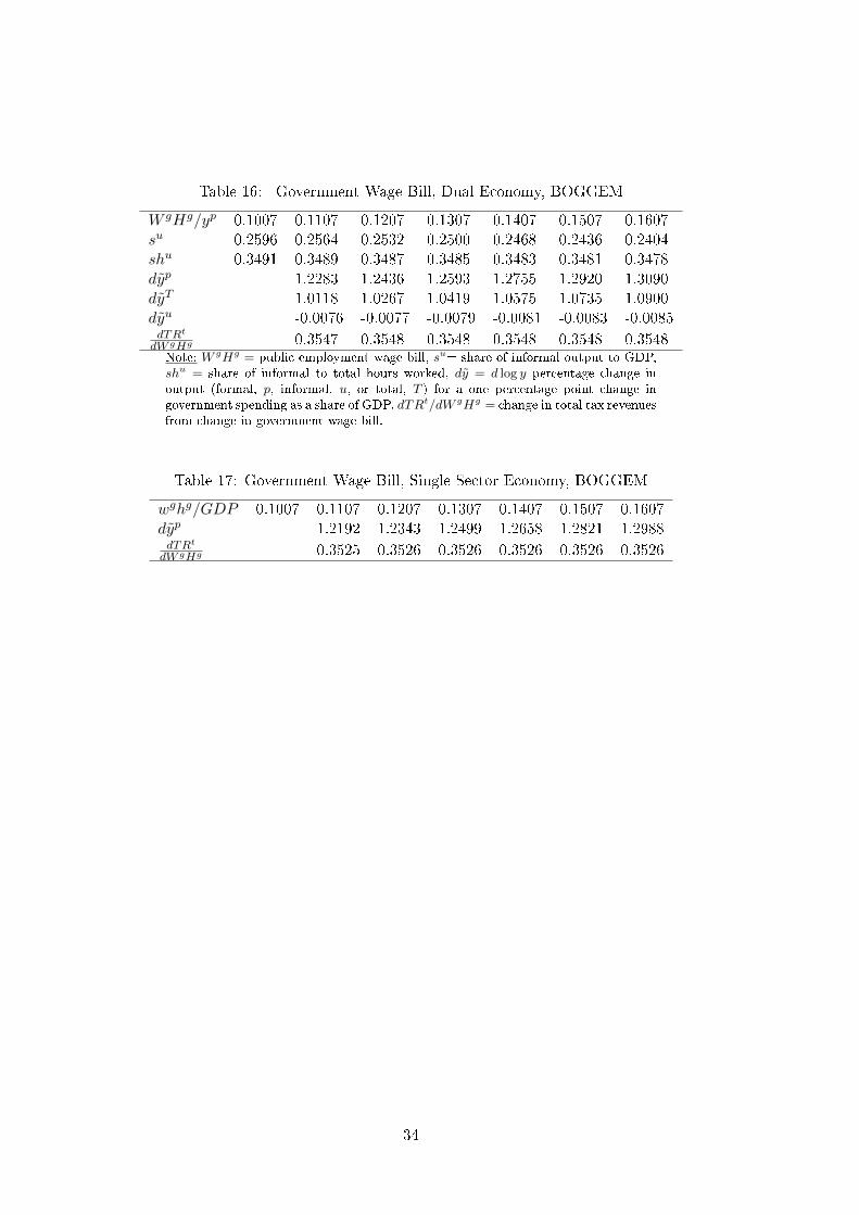
Table 16: Government Wage Bill, Dual Economy, BOGGEM

W gHg/yp 0.1007 0.1107 0.1207 0.1307 0.1407 0.1507 0.1607su 0.2596 0.2564 0.2532 0.2500 0.2468 0.2436 0.2404shu 0.3491 0.3489 0.3487 0.3485 0.3483 0.3481 0.3478dyp 1.2283 1.2436 1.2593 1.2755 1.2920 1.3090dyT 1.0118 1.0267 1.0419 1.0575 1.0735 1.0900dyu -0.0076 -0.0077 -0.0079 -0.0081 -0.0083 -0.0085dTRt

dW gHg 0.3547 0.3548 0.3548 0.3548 0.3548 0.3548Note: W gHg = public employment wage bill, su= share of informal output to GDP,shu = share of informal to total hours worked, dy = d log y percentage change inoutput (formal, p, informal, u, or total, T ) for a one percentage point change ingovernment spending as a share of GDP, dTRt/dW gHg = change in total tax revenuesfrom change in government wage bill.

Table 17: Government Wage Bill, Single Sector Economy, BOGGEM

wghg/GDP 0.1007 0.1107 0.1207 0.1307 0.1407 0.1507 0.1607dyp 1.2192 1.2343 1.2499 1.2658 1.2821 1.2988dTRt

dW gHg 0.3525 0.3526 0.3526 0.3526 0.3526 0.3526

34

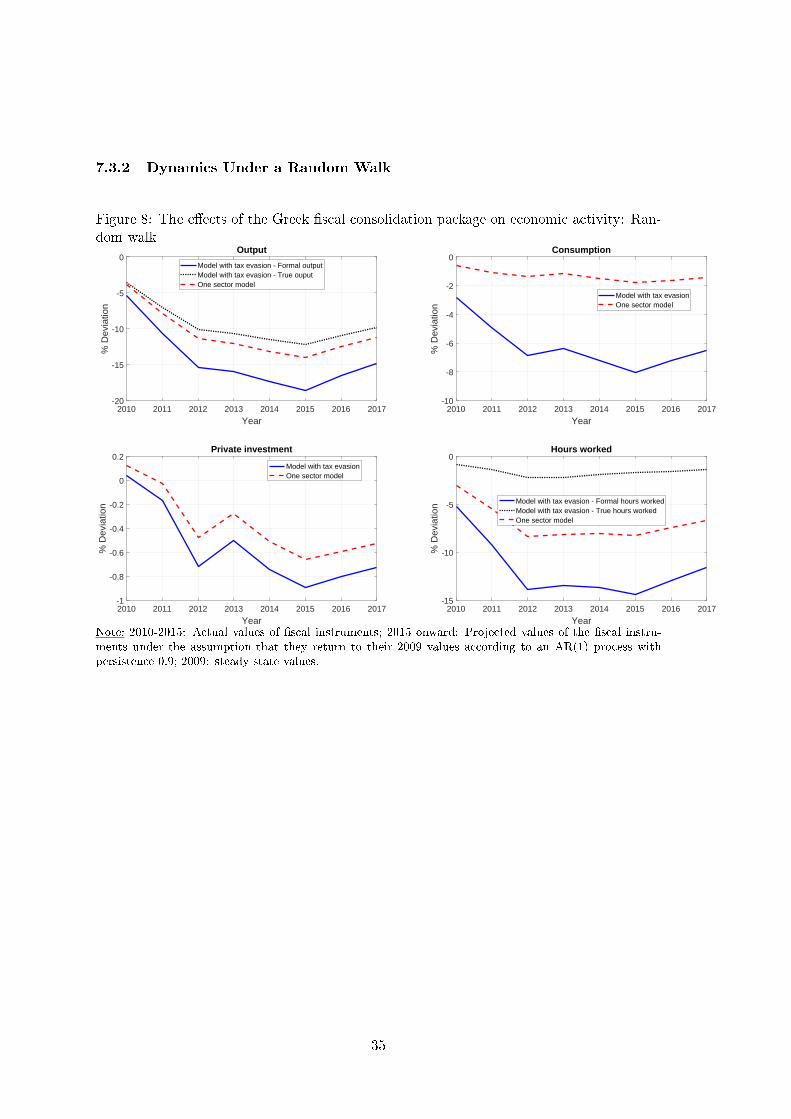
7.3.2 Dynamics Under a Random Walk

Figure 8: The e�ects of the Greek �scal consolidation package on economic activity: Ran-dom walk

2010 2011 2012 2013 2014 2015 2016 2017

Year

-20

-15

-10

-5

0

% D

evia

tion

Output

Model with tax evasion - Formal outputModel with tax evasion - True ouputOne sector model

2010 2011 2012 2013 2014 2015 2016 2017

Year

-10

-8

-6

-4

-2

0

% D

evia

tion

Consumption

Model with tax evasionOne sector model

2010 2011 2012 2013 2014 2015 2016 2017

Year

-1

-0.8

-0.6

-0.4

-0.2

0

0.2

% D

evia

tion

Private investment

Model with tax evasionOne sector model

2010 2011 2012 2013 2014 2015 2016 2017

Year

-15

-10

-5

0

% D

evia

tion

Hours worked

Model with tax evasion - Formal hours workedModel with tax evasion - True hours workedOne sector model

Note: 2010-2015: Actual values of �scal instruments; 2015 onward: Projected values of the �scal instru-ments under the assumption that they return to their 2009 values according to an AR(1) process withpersistence 0.9; 2009: steady state values.

35

7.4 Counterfactuals: Complete Elimination of the Informal Sector in

the Beginning of the Consolidation

We calculate the paths of the extra revenue raised in the dual economy in Greece from

2010 to 2015 (relative to the steady state). We then ask how much labour and capital

income taxes would have to increase in each period � relative to their steady state values

� in the economy that is free of an informal sector in order to generate this extra revenue.

We carry this exercise using the average annual (about 1 billion EUR) and the maximum

annual value (about 2 billion EUR) of the change in the tax revenues in the dual economy

observed over the 2010-2015 period.

Table 18 reports the corresponding average tax rates in the single sector model as well as

the cumulative total change in GDP. As can be seen in the Table, the changes in the tax

rates are quite small. For instance, raising the tax rates from τ l = 0.34 to 0.342, and from

τk = 0.20 to 0.201 could generate about 1 more billion EUR.

The general equilibrium e�ects on economic activity are also signi�cant. The cumulative

decline in economic activity would have been 10.2% rather than the �true� decline of 17%

in the dual economy. That is, in the absence of an informal sector, Greece would have been

able to raise the revenue it actually did by relying in much smaller increases in tax rates

and would have experienced a recession of the order of −2% per year, much less than the

−5% recorded. This is a big di�erence.

Table 18: A Counterfactual: Fiscal consolidation without a black economy

Impact on GDP

1 billion pa τ l : 0.34→ 0.342, τk : 0.20→ 0.201 -10.2%

2 billions pa τ l : 0.34→ 0.365, τk : 0.20→ 0.215 -12.4%Note: Labor and capital income taxes�relative to their steady state values� neededto raise the amount of tax revenue raised per annum (pa) by the actual Greek �scalinstruments over 2010�2015 in the dual economy.

36

7.5 Sensitivity Analysis

7.5.1 All inclusive BOGDSGE: Ricardian and non Ricardian Agents, Labour

Unions, Wage Rigidity

Table 19: Tax on Labour Income, Dual Economy

TRl/yp 0.1616 0.1716 0.1816 0.1916 0.2016 0.2116 0.2216τ l 0.2890 0.3062 0.3232 0.3400 0.3566 0.3729 0.3890su 0.2127 0.2245 0.2369 0.2500 0.2638 0.2783 0.2934shu 0.3039 0.3184 0.3332 0.3485 0.3641 0.3801 0.3963dyp -2.3059 -2.3659 -2.4256 -2.4845 -2.5453 -2.5984dyT -1.4695 -1.4869 -1.5029 -1.5171 -1.5924 -1.5396dTRl

dτ l0.3497 0.3315 0.3133 0.2952 0.2773 0.2597

dTRt

dτ l0.1031 0.0815 0.0601 0.3090 0.0184 -0.0016

Note: TRl= tax revenue from labor income,τ l = tax rate on labor income, su=share of informal output to GDP, shu = share of informal to total hours worked,dy = d log y: percentage change in output (formal, p, or true, T ) for a one percentagepoint change in the narrow (source) tax revenue as share in GDP, dTRl/dτ l = changein narrow tax revenue from change in the tax rate, dTRt/dτ l = change in total taxrevenue (from all sources) from change in the tax rate.

Table 20: Tax on Labour Income, Single Sector Economy

TRl/yp 0.1485 0.1585 0.1685 0.1785 0.1885 0.1985 0.2085τ l 0.2743 0.2956 0.3175 0.3400 0.3631 0.3870 0.4116dyp -1.3125 -1.3752 -1.4453 -1.5243 -1.6142 -1.7175dTRl

dτf0.5975 0.5830 0.5679 0.5522 0.5356 0.5182

dTRt

dτ l0.4336 0.4177 0.4010 0.3836 0.3651 0.3456

Table 21: Government Spending, Dual Economy

Gc/yp 0.0724 0.0824 0.0924 0.1024 0.1124 0.1224 0.1324su 0.2571 0.2548 0.2524 0.2500 0.2476 0.2452 0.2428shu 0.3540 0.3522 0.3504 0.3485 0.3466 0.3447 0.3428dyp 0.8491 0.8608 0.8726 0.8846 0.8969 0.9094dyT 0.6990 0.7100 0.7211 0.7325 0.7441 0.7559dTRt

dGc 0.1568 0.1577 0.1585 0.1594 0.1602 0.1610Note: See note in Table 19. Gc = government spending (consumption).

37

Table 22: Government Spending, Single Sector Economy

Gc/yp 0.0724 0.0824 0.0924 0.1024 0.1124 0.1224 0.1324dyp 0.7937 0.8066 0.8197 0.8331 0.8468 0.8608dTRt

dGc 0.1408 0.1424 0.1439 0.1454 0.1469 0.1484

Figure 9: The e�ects of the Greek �scal consolidation package on economic activity: fullBOGDSGE model, Perfect foresight

2010 2011 2012 2013 2014 2015 2016 2017

Year

-30

-25

-20

-15

-10

-5

0

% D

evia

tion

Output

Model with tax evasion - Formal outputModel with tax evasion - True ouputOne sector model

2010 2011 2012 2013 2014 2015 2016 2017

Year

-14

-12

-10

-8

-6

-4

-2

0

% D

evia

tion

Consumption

Model with tax evasionOne sector model

2010 2011 2012 2013 2014 2015 2016 2017

Year

-35

-30

-25

-20

-15

-10

-5

% D

evia

tion

Private investment

Model with tax evasionOne sector model

2010 2011 2012 2013 2014 2015 2016 2017

Year

-25

-20

-15

-10

-5

0

% D

evia

tion

Hours worked

Model with tax evasion - Formal hours workedModel with tax evasion - True hours workedOne sector model

Note: 2010-2015: Actual values of �scal instruments; 2015-2022: Projected values of the �scal instruments

under the assumption that they return to their 2009 values according to an AR(1) process with persistence

0.9; 2009: steady state values.

38

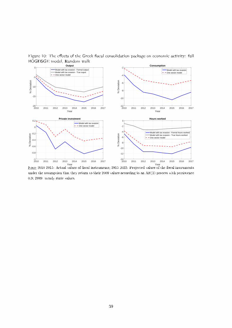
Figure 10: The e�ects of the Greek �scal consolidation package on economic activity: fullBOGDSGE model, Random walk

2010 2011 2012 2013 2014 2015 2016 2017

Year

-20

-15

-10

-5

0

% D

evia

tion

Output

Model with tax evasion - Formal outputModel with tax evasion - True ouputOne sector model

2010 2011 2012 2013 2014 2015 2016 2017

Year

-12

-10

-8

-6

-4

-2

% D

evia

tion

Consumption

Model with tax evasionOne sector model

2010 2011 2012 2013 2014 2015 2016 2017

Year

-1

-0.8

-0.6

-0.4

-0.2

0

0.2

% D

evia

tion

Private investment

Model with tax evasionOne sector model

2010 2011 2012 2013 2014 2015 2016 2017

Year

-14

-12

-10

-8

-6

-4

-2

0%

Dev

iatio

nHours worked

Model with tax evasion - Formal hours workedModel with tax evasion - True hours workedOne sector model

Note: 2010-2015: Actual values of �scal instruments; 2015-2022: Projected values of the �scal instruments

under the assumption that they return to their 2009 values according to an AR(1) process with persistence

0.9; 2009: steady state values.

39

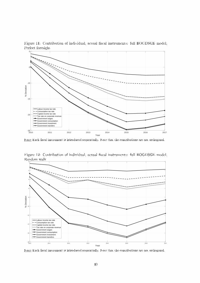
Figure 11: Contribution of individual, actual �scal instruments: full BOGDSGE model,Perfect foresight

2010 2011 2012 2013 2014 2015 2016 2017

Year

-25

-20

-15

-10

-5

0

% D

evia

tion

Labour income tax rateConsumption tax rateCapital income tax rateTax rate on corporate revenueGovernment wagesGovernment consumptionGovernment investmentGovernment transfers

Note: Each �scal instrument is introduced sequentially. Note that the contributions are not orthogonal.

Figure 12: Contribution of individual, actual �scal instruments: full BOGDSGE model,Random walk

2010 2011 2012 2013 2014 2015 2016 2017

Year

-18

-16

-14

-12

-10

-8

-6

-4

-2

0

% D

evia

tion

Labour income tax rateConsumption tax rateCapital income tax rateTax rate on corporate revenueGovernment wagesGovernment consumptionGovernment investmentGovernment transfers

Note: Each �scal instrument is introduced sequentially. Note that the contributions are not orthogonal.

40

7.5.2 Robustness with Regard to Variation in the Model Parameters

We consider variation in the values of various parameters (see the box in the �rst gigure

of each row). Figures 13-14 report the results.

Figure 13: Sensitivity analysis with respect to various parameters (perfect foresight)

2010 2011 2012 2013 2014 2015 2016 2017

Year

-30

-20

-10

0

% D

evia

tion

Real GDP

BaselineLow persistence after 2015

2010 2011 2012 2013 2014 2015 2016 2017

Year

0

5

10

15

20

% D

evia

tion

Informal Output

BaselineLow persistence after 2015

2010 2011 2012 2013 2014 2015 2016 2017

Year

-20

-15

-10

-5

0

% D

evia

tion

True Output

BaselineLow persistence after 2015

2010 2011 2012 2013 2014 2015 2016 2017

Year

-30

-20

-10

0

% D

evia

tion

Real GDP

BaselineW=0

2010 2011 2012 2013 2014 2015 2016 2017

Year

0

5

10

15

20

% D

evia

tion

Informal Output

BaselineW=0

2010 2011 2012 2013 2014 2015 2016 2017

Year

-20

-15

-10

-5

0

% D

evia

tion

True Output

BaselineW=0

2010 2011 2012 2013 2014 2015 2016 2017

Year

-30

-20

-10

0

% D

evia

tion

Real GDP

Baseline=2

2010 2011 2012 2013 2014 2015 2016 2017

Year

0

5

10

15

20

% D

evia

tion

Informal Output

Baseline=2

2010 2011 2012 2013 2014 2015 2016 2017

Year

-20

-15

-10

-5

0

% D

evia

tion

True Output

Baseline=2

2010 2011 2012 2013 2014 2015 2016 2017

Year

-30

-20

-10

0

% D

evia

tion

Real GDP

Baseline=2

2010 2011 2012 2013 2014 2015 2016 2017

Year

0

5

10

15

20

% D

evia

tion

Informal Output

Baseline=2

2010 2011 2012 2013 2014 2015 2016 2017

Year

-20

-15

-10

-5

0

% D

evia

tion

True Output

Baseline=2

Figure 14: Sensitivity analysis with respect to various parameters (perfect foresight)

2010 2011 2012 2013 2014 2015 2016 2017

Year

-30

-25

-20

-15

-10

-5

% D

evia

tion

Real GDP

BaselineHigher Calvo

2010 2011 2012 2013 2014 2015 2016 2017

Year

0

5

10

15

20

% D

evia

tion

Informal Output

BaselineHigher Calvo

2010 2011 2012 2013 2014 2015 2016 2017

Year

-20

-15

-10

-5

0

% D

evia

tion

True Output

BaselineHigher Calvo

2010 2011 2012 2013 2014 2015 2016 2017

Year

-30

-25

-20

-15

-10

-5

% D

evia

tion

Real GDP

BaselineDisutility from informal labour

2010 2011 2012 2013 2014 2015 2016 2017

Year

0

5

10

15

20

25

% D

evia

tion

Informal Output

BaselineDisutility from informal labour

2010 2011 2012 2013 2014 2015 2016 2017

Year

-20

-15

-10

-5

0

% D

evia

tion

True Output

BaselineDisutility from informal labour

2010 2011 2012 2013 2014 2015 2016 2017

Year

-30

-25

-20

-15

-10

-5

% D

evia

tion

Real GDP

BaselineF=0.5

2010 2011 2012 2013 2014 2015 2016 2017

Year

0

5

10

15

20

% D

evia

tion

Informal Output

BaselineF=0.5

2010 2011 2012 2013 2014 2015 2016 2017

Year

-20

-15

-10

-5

0

% D

evia

tion

True Output

BaselineF=0.5

41

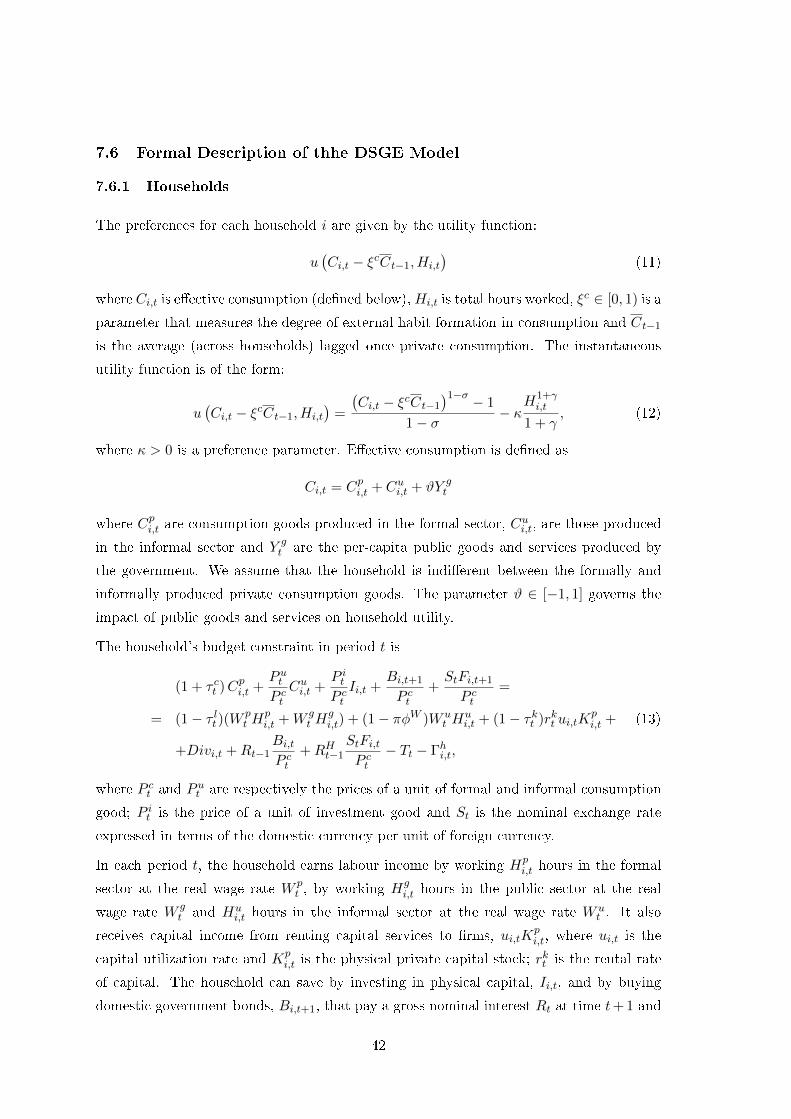
7.6 Formal Description of thhe DSGE Model

7.6.1 Households

The preferences for each household i are given by the utility function:

u(Ci,t − ξcCt−1, Hi,t

)(11)

where Ci,t is e�ective consumption (de�ned below),Hi,t is total hours worked, ξc ∈ [0, 1) is a

parameter that measures the degree of external habit formation in consumption and Ct−1

is the average (across households) lagged once private consumption. The instantaneous

utility function is of the form:

u(Ci,t − ξcCt−1, Hi,t

)=

(Ci,t − ξcCt−1

)1−σ − 1

1− σ− κ

H1+γi,t

1 + γ, (12)

where κ > 0 is a preference parameter. E�ective consumption is de�ned as

Ci,t = Cpi,t + Cui,t + ϑY gt

where Cpi,t are consumption goods produced in the formal sector, Cui,t, are those produced

in the informal sector and Y gt are the per-capita public goods and services produced by

the government. We assume that the household is indi�erent between the formally and

informally produced private consumption goods. The parameter ϑ ∈ [−1, 1] governs the

impact of public goods and services on household utility.

The household's budget constraint in period t is

(1 + τ ct )Cpi,t +P utP ct

Cui,t +P itP ctIi,t +

Bi,t+1

P ct+StFi,t+1

P ct=

= (1− τ lt )(Wpt H

pi,t +W g

t Hgi,t) + (1− πφW )W u

t Hui,t + (1− τkt )rkt ui,tK

pi,t + (13)

+Divi,t +Rt−1Bi,tP ct

+RHt−1

StFi,tP ct

− Tt − Γhi,t,

where P ct and P ut are respectively the prices of a unit of formal and informal consumption

good; P it is the price of a unit of investment good and St is the nominal exchange rate

expressed in terms of the domestic currency per unit of foreign currency.

In each period t, the household earns labour income by working Hpi,t hours in the formal

sector at the real wage rate W pt , by working Hg

i,t hours in the public sector at the real

wage rate W gt and Hu

i,t hours in the informal sector at the real wage rate W ut . It also

receives capital income from renting capital services to �rms, ui,tKpi,t, where ui,t is the

capital utilization rate and Kpi,t is the physical private capital stock; r

kt is the rental rate

of capital. The household can save by investing in physical capital, Ii,t, and by buying

domestic government bonds, Bi,t+1, that pay a gross nominal interest Rt at time t+ 1 and

42

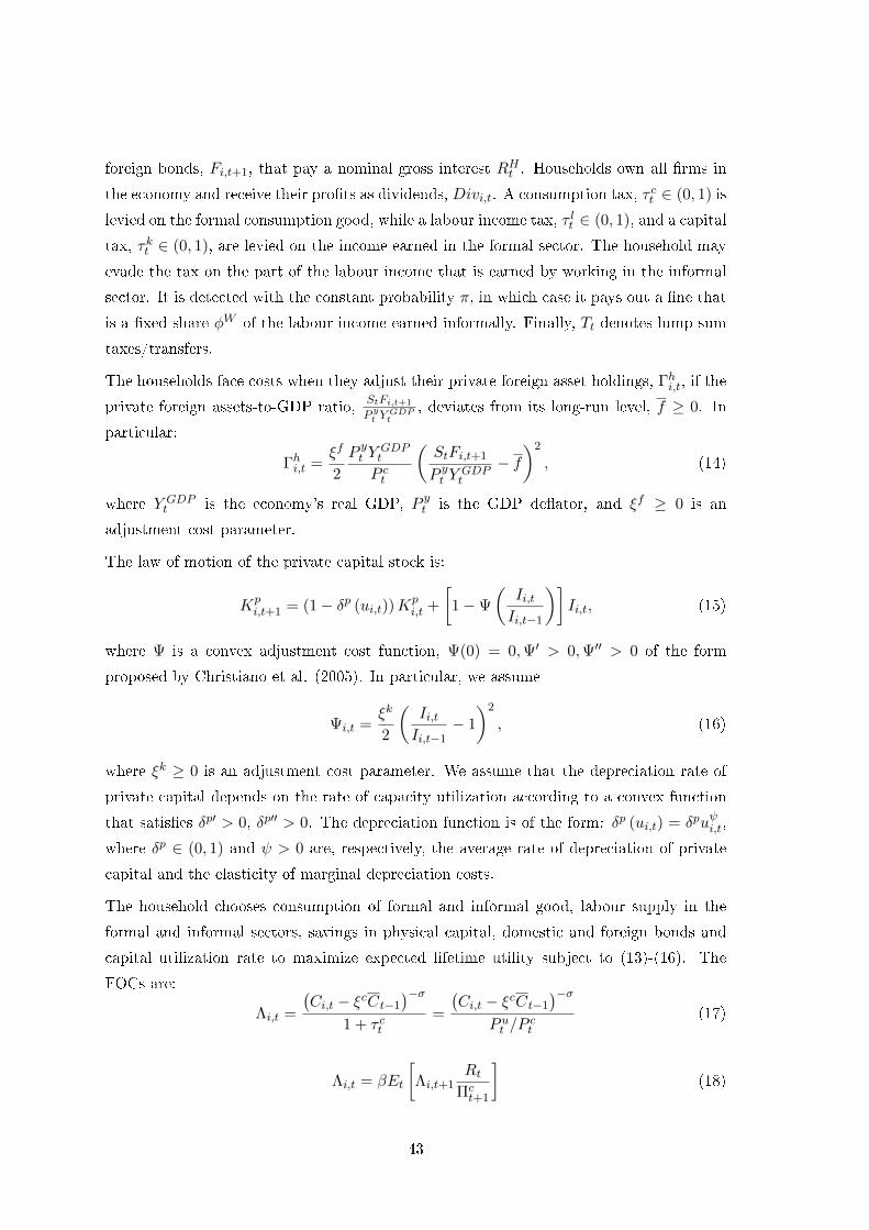
foreign bonds, Fi,t+1, that pay a nominal gross interest RHt . Households own all �rms in

the economy and receive their pro�ts as dividends, Divi,t. A consumption tax, τ ct ∈ (0, 1) is

levied on the formal consumption good, while a labour income tax, τ lt ∈ (0, 1), and a capital

tax, τkt ∈ (0, 1), are levied on the income earned in the formal sector. The household may

evade the tax on the part of the labour income that is earned by working in the informal

sector. It is detected with the constant probability π, in which case it pays out a �ne that

is a �xed share φW of the labour income earned informally. Finally, Tt denotes lump-sum

taxes/transfers.

The households face costs when they adjust their private foreign asset holdings, Γhi,t, if the

private foreign assets-to-GDP ratio,StFi,t+1

P yt YGDPt

, deviates from its long-run level, f ≥ 0. In

particular:

Γhi,t =ξf

2

P yt YGDPt

P ct

(StFi,t+1

P yt YGDPt

− f)2

, (14)

where Y GDPt is the economy's real GDP, P yt is the GDP de�ator, and ξf ≥ 0 is an

adjustment cost parameter.

The law of motion of the private capital stock is:

Kpi,t+1 = (1− δp (ui,t))K

pi,t +

[1−Ψ

(Ii,tIi,t−1

)]Ii,t, (15)

where Ψ is a convex adjustment cost function, Ψ(0) = 0,Ψ′ > 0,Ψ′′ > 0 of the form

proposed by Christiano et al. (2005). In particular, we assume

Ψi,t =ξk

2

(Ii,tIi,t−1

− 1

)2

, (16)

where ξk ≥ 0 is an adjustment cost parameter. We assume that the depreciation rate of

private capital depends on the rate of capacity utilization according to a convex function

that satis�es δp′ > 0, δp′′ > 0. The depreciation function is of the form: δp (ui,t) = δpuψi,t,

where δp ∈ (0, 1) and ψ > 0 are, respectively, the average rate of depreciation of private

capital and the elasticity of marginal depreciation costs.

The household chooses consumption of formal and informal good, labour supply in the

formal and informal sectors, savings in physical capital, domestic and foreign bonds and

capital utilization rate to maximize expected lifetime utility subject to (13)-(16). The

FOCs are:

Λi,t =

(Ci,t − ξcCt−1

)−σ1 + τ ct

=

(Ci,t − ξcCt−1

)−σP ut /P

ct

(17)

Λi,t = βEt

[Λi,t+1

RtΠct+1

](18)

43

Λi,t

[1 + ξf

(StFi,t+1

P yt YGDPt

− f)]

= βEt

[Λi,t+1

RHtΠct+1

st+1

](19)

(1− τkt

)rkt = qi,tδ

p′(ui,t) (20)

P itP ct

= qi,t

[1−Ψi,t −Ψ′i,t

Ii,tIi,t−1

]+

+βEt

[qi,t+1

Λi,t+1

Λi,tΨ′i,t

(Ii,t+1

Ii,t

)2]

(21)

qi,t = βEtΛi,t+1

Λi,t

[(1− τkt+1

)rkt+1ui,t+1 + qi,t+1 (1− δp (ui,t+1))

](22)

(1− τ lt

)W pt = W u

t =κHγ

Λi,t(23)

where β is the discount factor, Λi,t is the marginal utility of a unit of consumption good,

Πct = P ct /P

ct−1 is the gross rate of the consumption price index (CPI) in�ation of the formal

consumption good, st = St/St−1 is the gross growth rate of the nominal exchange rate and

qi,t = Qi,t/Λi,t is the shadow price of a unit of capital.

7.6.2 Production

Homogeneous intermediate good �rms

The homogeneous intermediate goods sector is composed of a continuum of perfectly com-

petitive intermediate good �rms indexed by j ∈ [0, 1]. Each �rm j can produce the

intermediate good either formally or informally. The formal good, Y pj,t, is produced by

using as inputs capital, Kj,t, and labour services, Hpj,t, and makes use of the average public

capital Kgt . The informally produced good, Y u

j,t, requires only labour, Huj,t. In particular,

Y pj,t = Apt

(Hpj,t

)α(Kj,t)

1−α (Kgt

)αg(24)

Y uj,t = Aut

(Huj,t

)ζ − F (25)

where α, ζ, αg ∈ (0, 1) and Apt , Aut > 0 are the exogenous levels of productivity in formal

and informal production, respectively. Public capital provides production externalities, so

that the production function of the formal sector exhibits increasing returns to scale with

respect to all inputs.

Firms pay a corporate tax τ ft ∈ (0, 1) per unit of sales of the formal good but evade the tax

for the informally produced good. With �a constant� probability π the producer is caught

44

when tax evading and has to pay a �ne φF per unit of informal good sales. Without loss

of generality, we assume the same probability of tax evasion for �rms and workers. The

producers choose the scale of production taking as given the prices for the formal, P pj,t, and

informal, P uj,t, goods as well as factor prices, rkt , W

pt , W

ut in order to maximize expected

pro�ts:

Πj,t = maxKpj,t,H

pj,t,H

uj,t

{(1− τ ft

) P pj,tP ct

Y pj,t +

(1− πφF

) P uj,tP ct

Y uj,t − rktK

pj,t −W

pt H

pj,t −W

ut H

uj,t

}(26)

subject to (24)-(25). The FOCs are:

W pt =

(1− τ ft

)αP pj,tP ct

Y pj,t

Hpj,t

W ut =

(1− πφF

)ζP uj,tP ct

Y uj,t

Huj,t

rkt =(

1− τ ft)

(1− α)P pj,tP ct

Y pj,t

Kpj,t

The absence of market power ensures that P pj,t = P pt and P uj,t = P ut and that all producers

choose the same level of production in both goods, i.e. Y pj,t = Y p

t , Hpj,t = Hp

t and Yuj,t = Y u

t ,

Huj,t = Hu

t .

Di�erentiated Intermediate Goods

We have imperfectly competitive domestic �rms, indexed f ∈ [0, 1], that convert the formal,

homogeneous good into formal, di�erentiated intermediate goods that are either used for

the domestic �nal good production, or are exported. There are also importing �rms,

indexed fm ∈ [0, 1], that convert the imported, homogeneous good into a di�erentiated,

foreign intermediate good. The assumption of imperfect competition is made in order to

facilitate the introduction of standard price stickiness.

We assume price stickiness à la Calvo (1983) for the formal, di�erentiated intermediate

goods, whether produced domestically or abroad. In particular, in each period t, a �rm f

can optimally reset its price with a constant probability 1− θd when it sells domestically

formal, di�erentiated goods and 1−θx when it exports these goods. Similarly, for importing

goods there is a constant probability 1 − θm that the importing �rm fm optimally resets

its price in each period. An intermediate good �rm that cannot reoptimize its price, will

partially index their prices to the aggregate past in�ation according to the following price

indexation schemes if it produces domestic, exported, or imported goods, respectively:

P df,t = P df,t−1

(Πdt−1

)xd,

P xf,t = P xf,t−1

(Πxt−1

)xx ,Pmfm,t = Pmfm,t−1

(Πmt−1

)xm ,45

where Πdt = P dt /P

dt−1, Πx

t = P xt /Pxt−1 and Πm

t = Pmt /Pmt−1 and the indexation parameters

xd, xx, xm ∈ [0, 1] determine the weights given to past in�ation (unit value denotes full

indexation).

The price of a �rm producing formal, di�erentiated goods that are sold domestically

and has not been able to reoptimize for τ periods in the domestic market is P df,t+τ =

P df,tΠτs=1

(Πdt+s−1

)xd . Each �rm that reoptimizes its price in the domestic market in period

t, chooses the optimal price P ∗df,t to maximize the discounted sum of expected real pro�ts

(in terms of the formal, �nal consumption good P ct ), by taking aggregate domestic demand

Y dt and the aggregate price index in the domestic market, P dt , as given. Thus, each �rm

maximizes:

maxP df,t

Et

∞∑t=0

(βθd)τ Λt+τ

Λt

{P dt+τP ct+τ

[Πτs=1

(Πdt+s−1

)xd P df,tP dt+τ

−mcdt+τ

]Y df,t+τ

}(27)

subject to

Y df,t =

(Πτs=1

(Πdt+s−1

)xd P df,tP dt+τ

)− µdt+τ

µdt+τ−1

Y dt+τ (28)

where mcdt = P ctmcpt /P

dt is the average real marginal cost in terms of the domestic price

index of the formal, di�erentiated goods, mcpt = P pt /Pct is the marginal cost expressed

in terms of the formal consumption good, Λt+τ/Λt is the intertemporal marginal rate of

substitution of the households according to which �rms value future pro�ts andµdtµdt−1

> 1

is the elasticity of substitution between the varieties of formal intermediate goods. Given

that all �rms face the same marginal cost and take aggregate variables as given it follows

that they set the same optimal price P ∗df,t = P ∗dt . Thus, the �rst order condition of the

above problem is:

Et

(βθd)τ

Λt+τΛt

[Πτs=1

(Πdt+s−1)xd

Πdt+s

P ∗dtP dt

]− µdt+τµdt+τ−1

Y dt+τ

P dt+τP ct+τ

Πτs=1

(Πdt+s−1)xd

Πdt+s

P ∗dtP dt−

−µdt+τmcdt+τ}

= 0 (29)

According to (29), �rms set nominal prices so as to equate the average future expected

marginal revenues to average future expected costs. To facilitate solution, we express (29)

in recursive form, so that we de�ne:

46

gd1t = µdtmcdtY

dt Λt

P dtP ct

+ βθdEt

[(Πdt

)xdΠdt+1

]− µdtµdt−1

gd1t+1

gd2t = Π∗dt Ydt Λt

P dtP ct

+ βθpdEt

[(Πdt

)xdΠdt+1

]1− µdtµdt−1 Π∗dt

Π∗dt+1

gd2t+1

gd3t = gd2t

where Π∗dt = P ∗dt /P dt .

The aggregate domestic index evolves according to:

P dt =

{(1− θd

)(P ∗dt

) 1

1−µdt + θd[P dt−1

(Πdt−1

)xd] 1

1−µdt

}1−µdt

The maximization problem for the part of the formal, di�erentiated intermediate goods

that are exported is de�ned in a similar manner. Each �rm maximizes:

maxPxf,t

Et

∞∑t=0

(βθx)τΛt+τΛt

{P xt+τP ct+τ

[Πτs=1

(Πxt+s−1

)xx P xf,tP xt+τ

−mcxt+τ]Y xf,t+τ

}(30)

subject to

Y xf,t =

(Πτs=1

(Πxt+s−1

)xx P xf,tP xt+τ

)− µxt+τµxt+τ−1

Y xt+τ (31)

where mcxt = P ctmcpt /P

xt is the average real marginal cost in terms of the aggregate export

price index andµxtµxt−1 > 1 is the elasticity of substitution between the varieties of formal

intermediate goods that are exported. The �rst order condition of the above problem is:

Et

(βθx)τ Λt+τΛt

[Πτs=1

(Πxt+s−1)xx

Πxt+s

P ∗xtPxt

]− µxt+τµxt+τ−1

Y xt+τ

Pxt+τPxt+τ

Πτs=1

(Πxt+s−1)xx

Πxt+s

P ∗xtPxt−

−µxt+τmcxt+τ}

= 0

and the aggregate domestic index is:

P xt =

{(1− θx) (P ∗xt )

11−µxt + θx

[P xt−1

(Πxt−1

)xx] 11−µxt

}1−µxt

47

Finally, each importing �rm fm buys di�erentiated intermediate goods at the international

price StP∗yt and sells them domestically at a price Pmfm,t. Each �rm maximizes:

maxPmfm,t

Et

∞∑t=0

(βθm)τΛt+τΛt

{Pmt+τP ct+τ

[Πτs=1

(Πmt+s−1

)xm Pmfm,tPmt+τ

−mcmt+τ]Y mfm,t+τ

}(32)

subject to

Y mfm,t =

(Πτs=1

(Πmt+s−1

)xm Pmfm,tPmt+τ

)− µmt+τµmt+τ−1

Y mt (33)

where mcmt = StP∗yt /Pmt is the average real marginal cost and

µmtµmt −1 > 1 is the elasticity

of substitution between the varieties of imported intermediate goods. The �rst order

condition is:

Et

(βθm)τ Λt+τΛt

[Πτs=1

(Πmt+s−1)xm

Πmt+s

P ∗mtPmt

]− µmt+τµmt+τ−1

Y mt+τ

Pmt+τPmt+τ

Πτs=1

(Πmt+s−1)xm

Πmt+s

P ∗mtPmt−

−µmt+τmcmt+τ}

= 0

The aggregate domestic index evolves according to:

Pmt =

{(1− θm) (P ∗mt )

11−µmt + θm

[Pmt−1

(Πmt−1

)xm] 11−µmt

}1−µmt(34)

Final good �rms

Perfectly competitive �nal good �rms combine domestic and imported formal, di�erenti-

ated intermediate goods to produce �nal consumption and investment goods. The infor-

mally produced homogeneous intermediate good is used for consumption purposes only, so

that Y ut = Cut .

The representative producer of the private consumption good combines a bundle of formal,

di�erentiated intermediate consumption goods, Cdt =

(∫ 10

(Cdf,t

) 1

µdt df

)µdt, with a bundle

of di�erentiated intermediate consumption goods that are imported, Cmt =

(∫ 10

(Cmfm,t

) 1µmt dfm

)µmt,

to generate a composite consumption �nal good, Cpt , by using a constant elasticity of sub-

stitution (CES) production function:

Cpt =

[ω

1εcc

(Cdt

) εc−1εc + (1− ωc)

1εc (Cmt )

εc−1εc

]where ωc ∈ [0, 1] measures the home bias in the production of the �nal consumption good

that determines the degree of openness in the long run, and εc > 0 is the elasticity of

substitution between domestic and imported consumption goods.

48

The �nal consumption good producer solves a two-stage problem. In the �rst stage, he

takes as given the retail prices of the varieties of the domestic formal intermediate goods,

P df,t, and imported intermediate goods, Pmfm,t, and optimally chooses his demand of di�er-

entiated varieties Cdf,t, Cmfm,t to minimize expenditures:

∫ 10 P

df,tC

df,tdf +

∫ 10 P

mfm,tC

mfm,tdf

m,

subject to the respective CES bundle technologies. Optimal demand satis�es Cdf,t =(P df,tP dt

)−µdt−1

µdt Cdt and Cmfm,t =(Pmfm,tPmt

)−µmt −1

µmt Cmt , where P dt =

(∫ 10

(P df,t

) 1

1−µdt df

)1−µdt

and Pmt =

(∫ 10

(Pmfm,t

) 11−µmt dfm

)1−µmtare the aggregate price indexes of the domestic

formal and imported, di�erentiated intermediate goods, respectively. In the second stage,

the �nal consumption good producer chooses his output, Cct , and inputs, Cdt , Cmt to max-

imize pro�ts Πct = P ct C

pt − P dt Cdt − Pmt Cmt , taking aggregate prices P dt , P

mt , and P ct , as

given, which implies:

Cdt = ωc

(P dtP ct

)−εcCpt ,

Cmt = (1− ωc)(PmtP ct

)−εcCpt

and

P ct =

[ωc

(P dt

)1−εc+ (1− ωc) (Pmt )1−εc

] 11−εc

.

The production of the �nal private investment good is modeled in an analogous manner.

In particular, the representative producer combines a bundle of domestically produced

intermediate investment varieties, Idt =

(∫ 10

(Idf,t

) 1

µdt df

)µdt, with a bundle of imported

intermediate varieties, Imt =

(∫ 10

(Imfm,t

) 1µmt dfm

)µmt, to generate a composite �nal private

investment good, Ipt , using the CES technology:

Ipt =

[ω

1εii

(Idt

) εi−1

εi + (1− ωi)1εi (Imt )

εi−1

εi

]

where ωi ∈ [0, 1] measures home bias in the production of the �nal investment good, εi > 0

is the elasticity of substitution between domestic and imported investment goods. The

demand functions for the bundles of the domestically produced intermediate goods and im-

ported intermediate goods are respectively Idt = ωi

(P dtP ct

)−εiIpt , and I

mt = (1− ωi)

(PmtP ct

)−εiIpt .

The aggregate price index of the �nal investment good is P it =[ωi(P dt)1−εi + (1− ωi) (Pmt )1−εi

] 11−εi .

Foreign �rms and export market

The exporting �rm takes the prices of the exported di�erentiated goods P xf,t/St as given,

and chooses the optimal amounts of di�erentiated inputs to minimize the total input costs,

49

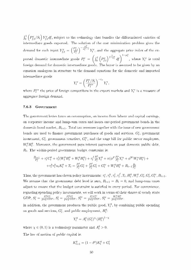
∫ 10

(P xf,t/St

)Y xf,tdf , subject to the technology that bundles the di�erentiated varieties of

intermediate goods exported. The solution of the cost minimization problem gives the

demand for each input Y xf,t =

(Pxf,tPxt

)− µxtµxt −1

Y xt , and the aggregate price index of the ex-

ported domestic intermediate goods P xt =

(∫ 10

(P xf,t

) 11−µxt df

)1−µxt, where Y x

t is total

foreign demand for domestic intermediate goods. The latter is assumed to be given by an

equation analogous in structure to the demand equations for the domestic and imported

intermediate goods

Y xt =

(P xt /StP x∗t

)−εxY ∗t ,

where P x∗t the price of foreign competitors in the export markets and Y ∗t is a measure of

aggregate foreign demand.

7.6.3 Government

The government levies taxes on consumption, on income from labour and capital earnings,

on corporate income and lump-sum taxes and issues one-period government bonds in the

domestic bond market, Bt+1. Total tax revenues together with the issue of new government

bonds are used to �nance government purchases of goods and services, Gct , government

investment, Git, government transfers, Gtrt , and the wage bill for public sector employees,

W gt H

gt . Moreover, the government pays interest payments on past domestic public debt,

Rt. The within-period government budget constraint is:

Bt+1

P ct+ τ ct C

pt + τ lt (W

pt H

pt +W g

t Hgt ) + τ ft

P ptP ctY pt + π(φF

PutP ctY ut + φWW u

t Hut ) +

+τkt rkt utK

pt + Tt =

P dtP ctGct +

P dtP ctGit +Gtrt +W g

t Hgt +Rt−1

BtP ct

Thus, the government has eleven policy instruments: τ ct , τkt , τ

lt , τ

ft , Tt, H

gt ,W

gt , G

ct , G

it, G

trt , Bt+1.

We assume that the government debt level is zero, Bt+1 = Bt = 0, and lump-sum taxes

adjust to ensure that the budget constraint is satis�ed in every period. For convenience,

regarding spending policy instruments, we will work in terms of their shares of steady state

GDP, Sct =P dt G

ct

P yY GDP, Sit =

P dt Git

P yY GDP, Strt =

P ct Gtrt

P yY GDP, Swt =

W gt H

gt

P yY GDP.

In addition, the government produces the public good, Y gt , by combining public spending

on goods and services, Gct , and public employment, Hgt :

Y gt = Agt (Gct)

χ (Hgt )

1−χ

where χ ∈ (0, 1) is a technology parameter and Agt > 0.

The law of motion of public capital is:

Kgt+1 = (1− δg)Kg

t +Git

50

where δg ∈ (0, 1) is the depreciation rate for public capital stock and Kg0 > 0 is given.

7.6.4 Monetary policy regime

The domestic economy is modeled as a member of a currency union in the sense that the

nominal exchange rate, St, is exogenously set and there is no monetary policy independence.

We assume that that the domestic nominal interest rate, RHt , equals an exogenously given

risk-free world interest rate, R∗t .

7.6.5 Market clearing conditions

Ht = Hpt +Hu

t +Hgt

Kt = utKpt

Y pt = udtY

dt + uxt Y

xt

Y dt = Cdt + Idt +Gct +Git

Y ut = Cut

Mt = umt Ymt

Y mt = Cmt + Imt

pyt YGDPt = pyt Y

pt +W g

t Hgt

pyt YGDPt = pdtY

dt + pxY x

t

where prices in small letters denote prices in terms of the formal consumption good, e.g.

pyt ≡ Pyt /P

ct , and u

dt , u

xt and umt are price dispersion measures, de�ned as:

udt =

∫ 1

0

(P df,t

P dt

)− µdtµdt−1df

uxt =

∫ 1

0

(P xf,tP xt

)− µxtµxt −1df

umt =

∫ 1

0

(Pmfm,tPmt

)− µmtµmt −1dfm

that evolve respectively according to:

51

udt =(

1− θd)(

Π∗dt

)− µdtµdt−1 + θd

[(Πdt−1

)xdΠd

]− µdtµdt−1

udt−1

uxt = (1− θx) (Π∗xt )− µxtµxt −1 + θx

[(Πxt−1

)xxΠx

]− µxtµxt −1

uxt−1

umt = (1− θm) (Π∗mt )− µmtµmt −1 + θm

[(Πmt−1

)xmΠm

]− µmtµmt −1

umt−1

Exports market equilibrium is:

Y xt =

(pxt /p

yt

qext px∗t

)−εxY ∗t

where qext =StP

∗yt

P yt= qext−1

stΠ∗yt

Πytis the real e�ective exchange rate.

The evolution of net foreign assets includes the adjustment costs su�ered by the domestic

agents on their foreign asset holdings. The balance of payments is given by the following

equation:

StFt+1

P ct= RHt−1

StFtP ct

+P xtP ct

Y xt − qext

P ytP ct

Mt −ξf

2

P yt YGDPt

P ct

(StFt+1

P yt YGDPt

− f)2

Finally, we de�ne true output as

Y Tt ≡Y GDP

t + Y ut

Pro�ts of the intermediate good producers, retailers and importing �rms are allocated as

dividends:

Divt = Ξt + Ξdt + Ξmt

Ξt = Πt =(

1− τ ft)pptY

pt + (1− πφ) put Y

ut − rktKt −W p

t Hpt −W u

t Hut

Ξdt = Y dt

(pdt −mc

pt

)+ Y x

t (pxt −mcpt )

Ξmt = pmt Ymt − qext p

ytMt

52

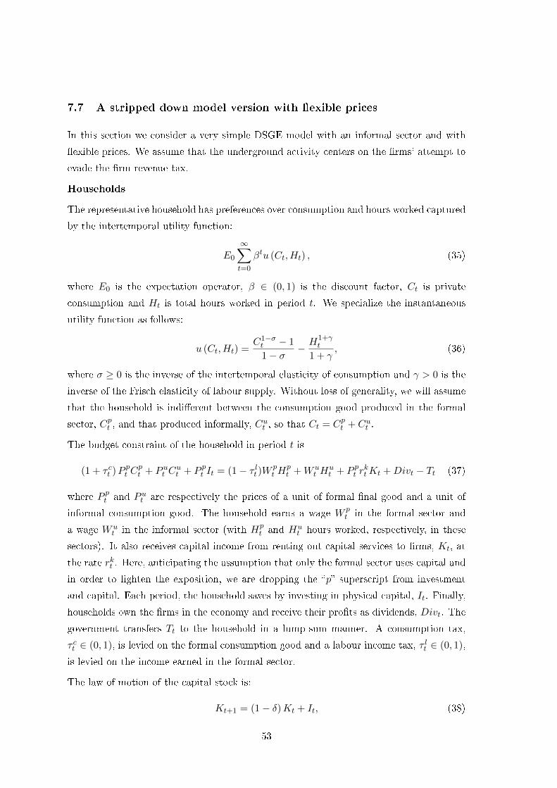
7.7 A stripped down model version with �exible prices

In this section we consider a very simple DSGE model with an informal sector and with

�exible prices. We assume that the underground activity centers on the �rms' attempt to

evade the �rm revenue tax.

Households

The representative household has preferences over consumption and hours worked captured

by the intertemporal utility function:

E0

∞∑t=0

βtu (Ct, Ht) , (35)

where E0 is the expectation operator, β ∈ (0, 1) is the discount factor, Ct is private

consumption and Ht is total hours worked in period t. We specialize the instantaneous

utility function as follows:

u (Ct, Ht) =C1−σt − 1

1− σ− H1+γ

t

1 + γ, (36)

where σ ≥ 0 is the inverse of the intertemporal elasticity of consumption and γ > 0 is the

inverse of the Frisch elasticity of labour supply. Without loss of generality, we will assume

that the household is indi�erent between the consumption good produced in the formal

sector, Cpt , and that produced informally, Cut , so that Ct = Cpt + Cut .

The budget constraint of the household in period t is

(1 + τ ct )P pt Cpt + P ut C

ut + P pt It = (1− τ lt )W

pt H

pt +W u

t Hut + P pt r

ktKt +Divt − Tt (37)

where P pt and P ut are respectively the prices of a unit of formal �nal good and a unit of

informal consumption good. The household earns a wage W pt in the formal sector and

a wage W ut in the informal sector (with Hp

t and Hut hours worked, respectively, in these

sectors). It also receives capital income from renting out capital services to �rms, Kt, at

the rate rkt . Here, anticipating the assumption that only the formal sector uses capital and

in order to lighten the exposition, we are dropping the �p� superscript from investment

and capital. Each period, the household saves by investing in physical capital, It. Finally,

households own the �rms in the economy and receive their pro�ts as dividends, Divt. The

government transfers Tt to the household in a lump-sum manner. A consumption tax,

τ ct ∈ (0, 1), is levied on the formal consumption good and a labour income tax, τ lt ∈ (0, 1),

is levied on the income earned in the formal sector.

The law of motion of the capital stock is:

Kt+1 = (1− δ)Kt + It, (38)

53

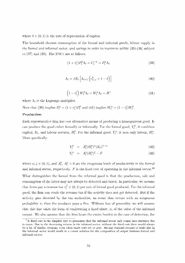
where δ ∈ (0, 1) is the rate of depreciation of capital.

The household chooses consumption of the formal and informal goods, labour supply in

the formal and informal sector, and savings in order to maximize utility (35)-(36) subject

to (37) and (38). The FOCs are as follows:

(1 + τ ct )P pt Λt = C−σt = P ut Λt (39)

Λt = βEt

[Λt+1

(rkt+1 + 1− δ

)](40)

(1− τ lt

)W pt Λt = W u

t Λt = Hγ (41)

where Λt is the Lagrange multiplier.

Note that (39) implies P ut = (1 + τ ct )P pt and (41) implies W ut = (1− τ lt )W

pt .

Production

Each representative �rm has two alternative means of producing a homogeneous good. It

can produce the good either formally or informally. For the formal good, Y pt , it combines

capital, Kt, and labour services, Hpt . For the informal good, Y u

t , it uses only labour, Hut .

More speci�cally:

Y pt = Apt (H

pt )α(Kt)

1−α (42)

Y ut = Aut (Hu

t )ζ − F (43)

where α, ζ ∈ (0, 1), and Apt , Aut > 0 are the exogenous levels of productivity in the formal

and informal sector, respectively. F is the �xed cost of operating in the informal sector.18

What distinguishes the formal from the informal good is that the production, sale and

consumption of the latter may not always be detected and taxed. In particular, we assume

that �rms pay a revenue tax τ ft ∈ (0, 1) per unit of formal good produced. For the informal

good, the �rm can evade the revenue tax if the activity does not get detected. But if the

activity gets detected by the tax authorities, an event that occurs with an exogenous

probability π, then the producer pays a �ne. Without loss of generality, we will assume

that this �ne takes the form of con�scating a �xed share, φ, of the value of the informal

output. We also assume that the �rm bears the entire burden in the case of detection, the

18A �xed cost is the simplest way to guarantee that the informal sector only comes into existence dueto taxes. Due to the decreasing returns in the informal sector, without the �xed cost there would alwaysbe a bit of shadow economy even when taxes were set to zero. Having constant returns to scale also inthe informal sector would result in a corner solution for the composition of output between formal andinformal output.

54

workers who produced (and did not declare their labour income) and the consumers who

consumed the informal good do not su�er any consequences. In the next section and for

the larger model, we allow �nes to be imposed also on other participating agents besides

�rms.

The producers choose the scale and composition of production in order to maximize ex-

pected pro�ts, taking as given �nal output prices for formal, P pt , and informal, P ut , goods

as well as factor prices, rkt , Wpt , W

ut :

Πt = maxKpt ,H

pt ,H

ut

{(1− τ ft

)P pt Y

pt + (1− πφ)P ut Y

ut − rktKt −W p

t Hpt −W u

t Hut − JFt

}(44)

subject to (42)-(43). J is an indicator function that takes the value of 1 if Y ut is positive

and zero if Y ut is zero. The FOCs are as follows:

W pt =

(1− τ ft

)αP pt

Y pt

Hpt

W ut = (1− πφ) ζP ut

Y ut

Hut

rkt =(

1− τ ft)

(1− α)P ptY pt

Kt

The informal goods are only used for consumption, hence

Y ut = Cut

The formal goods are used for consumption, Cpt , investment, It, and public consumption,

Gct , purposes.

Y pt = Cpt + Ipt +Gct

Government

The government budget constraint is

τ ct Ppt C

pt + τ ltW

pt H

pt + τ ft P

pt Y

pt + πφtP

ut Y

ut + Tt = P pt G

ct

We assume that when the shadow activity is detected, any amount of the informal good

that is con�scated is returned to the households via a lump sum transfer. That is, the

government only consumes the formal good. As a result the private consumption of the

informal good is equal to the production of that good (net of the �xed cost, F ).

55

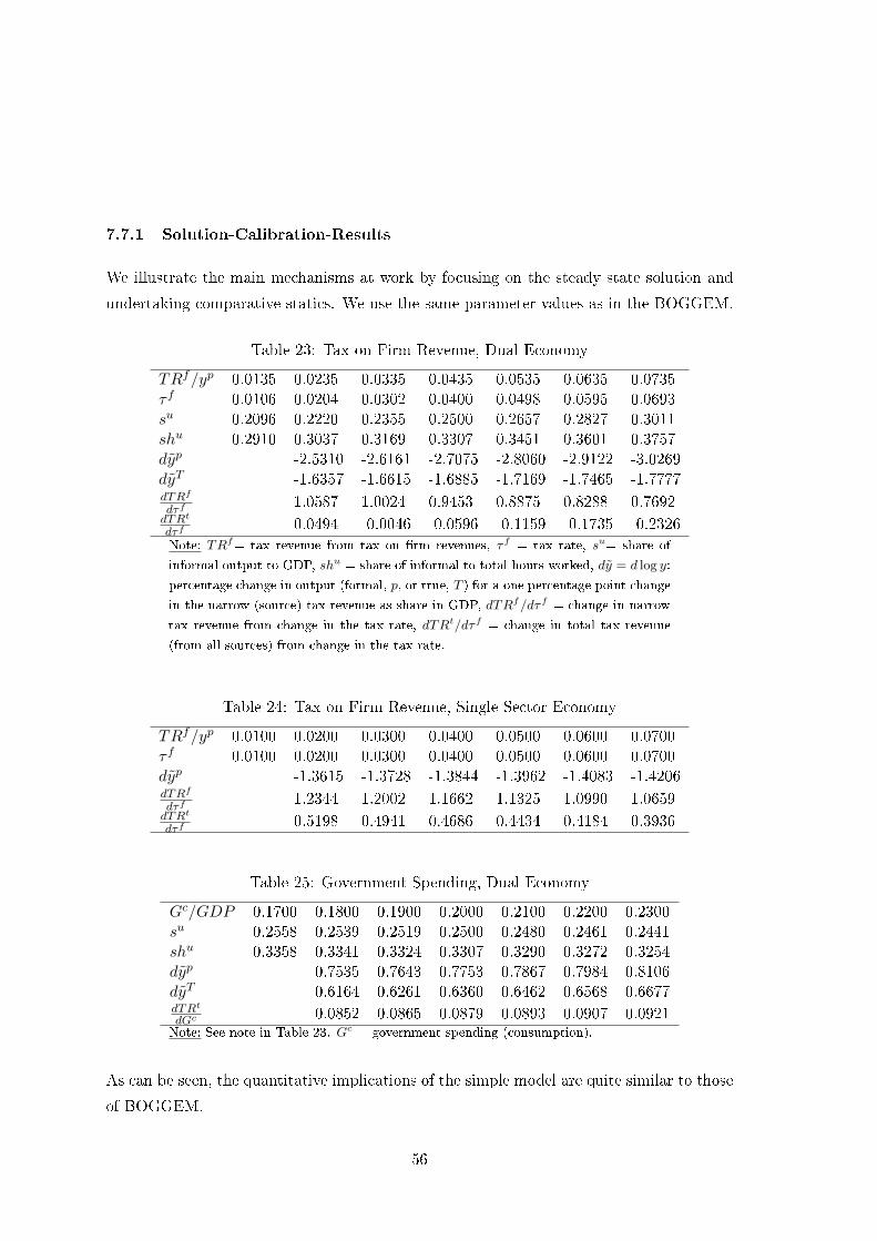
7.7.1 Solution-Calibration-Results

We illustrate the main mechanisms at work by focusing on the steady state solution and

undertaking comparative statics. We use the same parameter values as in the BOGGEM.

Table 23: Tax on Firm Revenue, Dual Economy

TRf/yp 0.0135 0.0235 0.0335 0.0435 0.0535 0.0635 0.0735τ f 0.0106 0.0204 0.0302 0.0400 0.0498 0.0595 0.0693su 0.2096 0.2220 0.2355 0.2500 0.2657 0.2827 0.3011shu 0.2910 0.3037 0.3169 0.3307 0.3451 0.3601 0.3757dyp -2.5310 -2.6161 -2.7075 -2.8060 -2.9122 -3.0269dyT -1.6357 -1.6615 -1.6885 -1.7169 -1.7465 -1.7777dTRf

dτf1.0587 1.0024 0.9453 0.8875 0.8288 0.7692

dTRt

dτf0.0494 -0.0046 -0.0596 -0.1159 -0.1735 -0.2326

Note: TRf= tax revenue from tax on �rm revenues, τf = tax rate, su= share of

informal output to GDP, shu = share of informal to total hours worked, dy = d log y:

percentage change in output (formal, p, or true, T ) for a one percentage point change

in the narrow (source) tax revenue as share in GDP, dTRf/dτf = change in narrow

tax revenue from change in the tax rate, dTRt/dτf = change in total tax revenue

(from all sources) from change in the tax rate.

Table 24: Tax on Firm Revenue, Single Sector Economy

TRf/yp 0.0100 0.0200 0.0300 0.0400 0.0500 0.0600 0.0700τ f 0.0100 0.0200 0.0300 0.0400 0.0500 0.0600 0.0700dyp -1.3615 -1.3728 -1.3844 -1.3962 -1.4083 -1.4206dTRf

dτf1.2344 1.2002 1.1662 1.1325 1.0990 1.0659

dTRt

dτf0.5198 0.4941 0.4686 0.4434 0.4184 0.3936

Table 25: Government Spending, Dual Economy

Gc/GDP 0.1700 0.1800 0.1900 0.2000 0.2100 0.2200 0.2300su 0.2558 0.2539 0.2519 0.2500 0.2480 0.2461 0.2441shu 0.3358 0.3341 0.3324 0.3307 0.3290 0.3272 0.3254dyp 0.7535 0.7643 0.7753 0.7867 0.7984 0.8106dyT 0.6164 0.6261 0.6360 0.6462 0.6568 0.6677dTRt

dGc 0.0852 0.0865 0.0879 0.0893 0.0907 0.0921Note: See note in Table 23. Gc = government spending (consumption).

As can be seen, the quantitative implications of the simple model are quite similar to those

of BOGGEM.

56

Table 26: Government Spending, Single Sector Economy

Gc/GDP 0.1700 0.1800 0.1900 0.2000 0.2100 0.2200 0.2300dyp 0.8156 0.8291 0.8431 0.8576 0.8725 0.8880dTRt

dGc 0.1021 0.1039 0.1057 0.1076 0.1094 0.1114

57