UNIVERSITEIT GENT FACULTEIT WETENSCHAPPEN

Academiejaar 1998-1999

DISTRIBUTION AND DYNAMICS OF PROTIST COMMUNITIES IN A FRESHWATER TIDAL ESTUARY

VERSPREIDING EN DYNAMIEK VAN PROTISTENGEMEENSCHAPPEN IN EEN

ZOETWATERGETIJDENGEBIED

Proefschrift ingediend tot het behalen van de graad van Doctor in de Wetenschappen (Biologie) Promotor: Prof. Dr. W. Vyverman Co-promotor: Prof. Dr. E. Coppejans

Vakgroep Biologie Lab. Plantkunde

Sectie Protistologie & Aquatische Ecologie

K.L. Ledeganckstraat 35, 9000 Gent, Belgium

103

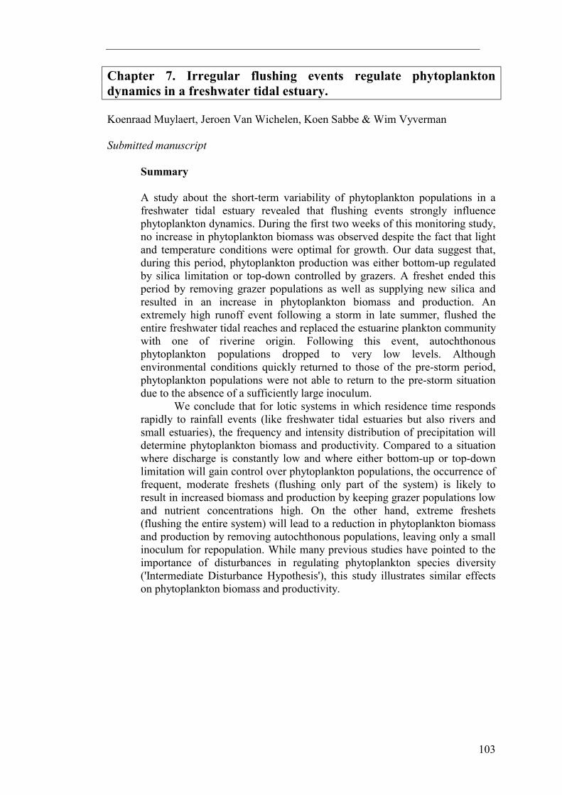
Chapter 7. Irregular flushing events regulate phytoplankton dynamics in a freshwater tidal estuary. Koenraad Muylaert, Jeroen Van Wichelen, Koen Sabbe & Wim Vyverman Submitted manuscript

Summary A study about the short-term variability of phytoplankton populations in a freshwater tidal estuary revealed that flushing events strongly influence phytoplankton dynamics. During the first two weeks of this monitoring study, no increase in phytoplankton biomass was observed despite the fact that light and temperature conditions were optimal for growth. Our data suggest that, during this period, phytoplankton production was either bottom-up regulated by silica limitation or top-down controlled by grazers. A freshet ended this period by removing grazer populations as well as supplying new silica and resulted in an increase in phytoplankton biomass and production. An extremely high runoff event following a storm in late summer, flushed the entire freshwater tidal reaches and replaced the estuarine plankton community with one of riverine origin. Following this event, autochthonous phytoplankton populations dropped to very low levels. Although environmental conditions quickly returned to those of the pre-storm period, phytoplankton populations were not able to return to the pre-storm situation due to the absence of a sufficiently large inoculum. We conclude that for lotic systems in which residence time responds rapidly to rainfall events (like freshwater tidal estuaries but also rivers and small estuaries), the frequency and intensity distribution of precipitation will determine phytoplankton biomass and productivity. Compared to a situation where discharge is constantly low and where either bottom-up or top-down limitation will gain control over phytoplankton populations, the occurrence of frequent, moderate freshets (flushing only part of the system) is likely to result in increased biomass and production by keeping grazer populations low and nutrient concentrations high. On the other hand, extreme freshets (flushing the entire system) will lead to a reduction in phytoplankton biomass and production by removing autochthonous populations, leaving only a small inoculum for repopulation. While many previous studies have pointed to the importance of disturbances in regulating phytoplankton species diversity ('Intermediate Disturbance Hypothesis'), this study illustrates similar effects on phytoplankton biomass and productivity.

Introduction During the last two decades, much research has focused on the effects of disturbances on ecosystems and, at present, the importance of disturbances as an essential process for ecosystem functioning is fully appreciated. Most studies, however, have dealt with the impact of disturbances on community structure (Sousa 1984). In particular, the 'Intermediate Disturbance Hypothesis' (IDH), developed by Connell (1978), has been proven very succesfull in explaining, for example, the high diversity maintained in tropical rainforests and coral reefs. However, disturbances might also directly or indirectly impact other ecosystem features than community structure, such as productivity and biomass (Pickett et al. 1989). In pelagic environments, disturbances are mostly caused by physical events (e.g. destratification by wind forcing or flushing by discharge increases, Reynolds 1993). In these systems, the IDH has been used to explain Hutchinson's (1961) paradox, i.e. the high diversity of phytoplankton in an apparently homogeneous environment (Padisák et al. 1993) while the effects of disturbances on ecosystem productivity and biomass have received much less attention. Nevertheless, they can be expected to be equally important at that level. For instance, in coastal environments (Sakshaug 1997), irregular storm events cause a destratification of the water column resulting in an increase in nutrient levels within the photic zone, thus stimulating primary production. Climate in Western Europe is strongly influenced by an irregular run of atmospheric depressions which originate above the Atlantic ocean and, especially in summer, precipitation patterns in Western Europe are characterized by dry periods interrupted by short spells of intense rainfall. In many lotic systems characterised by high flushing rates, such as rivers (e.g. Ferrari et al. 1989), small estuaries (e.g. Garcia-Soto et al. 1990) and freshwater tidal estuaries (e.g. Claessens 1988), these increases in precipitation induce flushing events or freshets. In these systems, freshets fulfil the ecological role of disturbances and they have been shown to have a strong impact on phytoplankton community structure (e.g. Descy 1993). In lotic environments, the short residence time and often low light levels put severe physical constraints on phytoplankton growth and it is only during low discharge periods that these constraints are alleviated and nutrient limitation or grazing can control primary producers (Reynolds et al. 1994, Reynolds & Descy 1996). Consequently, in rivers, nutrient limitation (Basu & Pick 1996) as well as grazing pressure (Gosselain et al. 1998) have been found to be negatively related to flushing rate. As disturbances often put back the system into an earlier successional stage (Round 1971, Reynolds 1993, Reynolds 1997), irregular flushing events may strongly influence phytoplankton development in lotic ecosystems. Given the generally short generation times of phytoplankters, monitoring aquatic systems with a temporal resolution of two days provides the appropriate time-scale to investigate into detail the processes regulating phytoplankton dynamics. In this study, this approach was applied in the freshwater tidal reaches of a coastal plain estuary, primarily to assess what factors regulate phytoplankton biomass during the maxima in summer and which processes are of importance in terminating these aestival blooms. During the sampling period, river discharge was rather constant except for two important flushing events. The aim of this paper is to evaluate the direct and indirect effects of these freshets on phytoplankton biomass and production. A comparison is made with similar lotic systems (rivers and small estuaries), where identical control mechanisms are likely to occur.

105

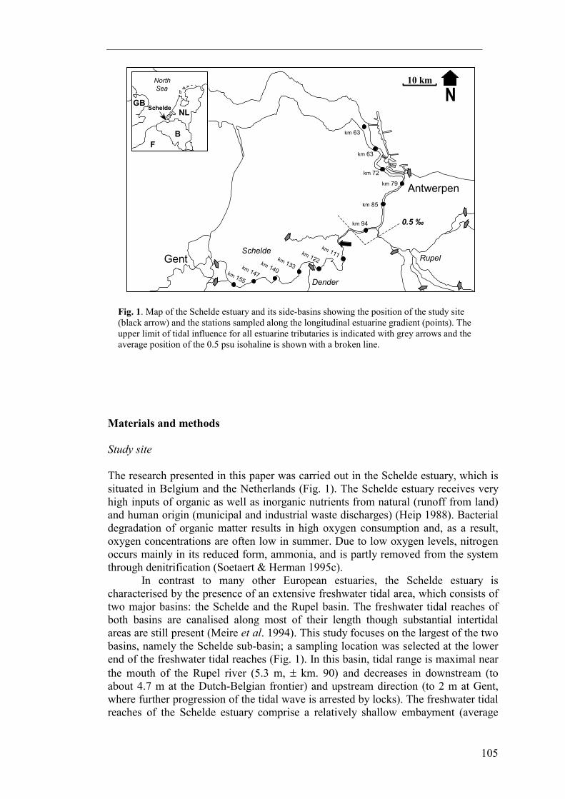
Materials and methods Study site The research presented in this paper was carried out in the Schelde estuary, which is situated in Belgium and the Netherlands (Fig. 1). The Schelde estuary receives very high inputs of organic as well as inorganic nutrients from natural (runoff from land) and human origin (municipal and industrial waste discharges) (Heip 1988). Bacterial degradation of organic matter results in high oxygen consumption and, as a result, oxygen concentrations are often low in summer. Due to low oxygen levels, nitrogen occurs mainly in its reduced form, ammonia, and is partly removed from the system through denitrification (Soetaert & Herman 1995c). In contrast to many other European estuaries, the Schelde estuary is characterised by the presence of an extensive freshwater tidal area, which consists of two major basins: the Schelde and the Rupel basin. The freshwater tidal reaches of both basins are canalised along most of their length though substantial intertidal areas are still present (Meire et al. 1994). This study focuses on the largest of the two basins, namely the Schelde sub-basin; a sampling location was selected at the lower end of the freshwater tidal reaches (Fig. 1). In this basin, tidal range is maximal near the mouth of the Rupel river (5.3 m, ± km. 90) and decreases in downstream (to about 4.7 m at the Dutch-Belgian frontier) and upstream direction (to 2 m at Gent, where further progression of the tidal wave is arrested by locks). The freshwater tidal reaches of the Schelde estuary comprise a relatively shallow embayment (average

Gent

Antwerpen

10 km

NNorth Sea

Schelde

B

NLGB

F

km 155

km 147

km 140

km 133

km 122

km 111

km 94

km 85

km 79

km 72

km 63

km 63

RupelSchelde

Dender

0.5 ‰

Fig. 1. Map of the Schelde estuary and its side-basins showing the position of the study site (black arrow) and the stations sampled along the longitudinal estuarine gradient (points). The upper limit of tidal influence for all estuarine tributaries is indicated with grey arrows and the average position of the 0.5 psu isohaline is shown with a broken line.

depth of 2-6 m in the Schelde sub-basin) characterised by a silty bedload. Tidal currents are strong and cause intense resuspension of bottom sediments, which results in a very turbid water column. At the sampling location, depth is on average 5.6 m and the estuary is about 150 m wide. Based on measurements on bathymetrical maps, the volume of the estuarine basin upstream the sampling location was estimated at 23.8 106 m3. During the study period, discharge at the sampling location was on average 20 m3 s-1; residence time in the freshwater tidal reaches of the Schelde sub-basin can then roughly be estimated at about 14 days. This is relatively long and overlaps with the time-scale of processes regulating phytoplankton dynamics. As a result, during periods of relatively constant river discharge, observed changes in the phytoplankton community at the monitoring station can be interpreted as being the result of processes taking place within the estuary. Sampling Subsurface samples were collected between August to October 1996 at exactly low tide from a jetty, about 5 m from the bank. To obtain information on the spatial distribution of phytoplankton populations, additional samples were taken along a longitudinal transect (Fig. 1) on three occasions during the sampling period (Julian days 226, 247 and 283). Temperature (measured with a WTW LF91) and Secchi depth (measured by means of a black and white disc, 0.25 m diameter) were recorded in situ. 50 ml samples for phytoplankton analysis were fixed in the field with the lugol-formaline-thiosulphate method (Sherr et al. 1989). Metazoan zooplankton was collected by filtering 10 l of water over a 50 µm mesh size plankton net. Zooplankton samples were fixed with formalin up to a final concentration of 3-4 %; sugar was added to the formalin to avoid lysis of zooplankton (Haney & Hall 1973). Phytoplankton samples and samples for salinity, nutrient and chlorophyll a analysis were stored refrigerated in the dark until they were processed in the lab (within 12 h). Analyses Salinity and nutrient samples were first filtered over Whatman GF/F filters. Chlorinity was measured titrimetrically by means of Mohr-Knudsen titration and subsequently converted to salinity (Strickland & Parsons 1975). Concentrations of dissolved nitrate, ammonium, phosphate and silicate were determined automatically with a Skalar (type AII flow system) auto-analyser using standard procedures. Data on rainfall and irradiance (measurements at Ukkel, situated at about 40 km from the sampling station) were retrieved from monthly publications of the Belgian Royal Meteorological Institute. River discharge data were obtained from Taverniers (1997). For chlorophyll a analysis, 300 ml samples were filtered over Whatmann GF/F filters. Filters were stored at –80°C until extraction in acetone and subsequent analysis by High Pressure Liquid Chromatography (protocol according to Mantoura & Llewellyn 1983). For quantifying ultraphytoplankton (< 5 µm), 2 ml aliquots of the phytoplankton sample were filtered onto 0.2 µm pore size, black Nuclepore polycarbonate filters. Filters were mounted in Cargille A immersion oil and ultraphytoplankton was enumerated at 1000x magnification using an epifluorescence microscope equipped with blue and green light illumination (Caldwell 1977, McIsaac & Stockner 1993). About 200 cells were counted in at least 35 random fields. Other phytoplankton (> 5 µm) was counted using an inverted microscope at 200x magnification (Utermöhl 1958, Hasle 1978a). Rose bengal B was added to the

107

samples to distinguish living phytoplankton cells from detritus and sediment particles (Throndsen 1978). At least 200 cells were counted and identified up to species or genus level; care was taken that, for the most common taxa, at least 50 cells were counted. For all phytoplankton taxa, 30-100 cells were measured and the cell volume was calculated using standard formulas. Cell volumes were converted to carbon content according to the equations of Eppley in Smayda (1978). Total phytoplankton carbon was then calculated by multiplying the cell number of each species with its average carbon content and making the sum for all species. Zooplankton samples were also stained with Bengal rose B to distinguish between detritus and animals. The entire 10 l concentrate was enumerated to determine cladoceran and copepod densities. For rotifer counts, subsamples were enumerated until more than 100 organisms were counted. Asterocaelum algophilum Canter, an abundant amoeboid microzooplankter, was enumerated during the phytoplankton cell counts; numbers were converted to biomass using a carbon to volume conversion factor of 0.15 pg C µm-3 (Sheldon et al. 1986). Estimates of primary production and growth rate In turbid, nutrient-rich systems, gross primary production can often be accurately estimated using a light-limited model (Pennock 1985, Cloern 1987, Grobbelaar 1990). Therefore, to evaluate the combined effects of irradiance, temperature and water column turbidity on phytoplankton growth we tried to model phytoplankton primary production using published values of phytoplankton physiological parameters and data on chlorophyll a concentration, temperature, irradiance, daylength and Secchi depth as input variables. For each sampling date, daily areal gross production (Pg,a) was calculated based on a formulation given by Behrenfeld & Falkowski (1997):

Pg,a = [ ]

+

⋅⋅⋅⋅ 82.0ln *

**

m

avg

d

m

PE

KDLPchla α

In this equation, [chla] is the chlorophyll a concentration (in mg m-3), DL is daylength and Kd is the extinction coefficient for downward irradiance. Kd was calculated from Secchi depth readings (Kd = 1.8 Secchi-1, Wofsy 1983). In the original equation of Behrenfeld & Falkowski (1997), we replaced P*opt (the maximum specific photosynthetic rate as measured under conditions of variable irradiance) with P*m (the maximum specific photosynthetic rate) and E*k (the light saturation parameter) with P*m/α*, α* being the maximum light utilization coefficient. As input value for E0 (surface irradiance) we used Eavg, which is the average daily irradiance at the surface (in µEinst m-2 s-1). The values of P*m and α* were arbitrarily set at 5 mg C (mg chl a)-1 h-1 for P*m at 10°C and 0.05 mg C (mg chl a)-1 h-1[µEinst m-2 s -1] -1 for α*, which is within the range of values given in estuarine primary production studies (Malone & Neale 1981, Van Spaendonk et al. 1993, Joint & Pomroy 1981, Cole et al. 1992). P*m is strongly temperature-dependent, having a Q10 of about 2.3 (Joint & Pomroy 1981, Malone 1977) while α* does not vary with temperature (Kirk 1994). Eavg was calculated by dividing total daily irradiance by DL. Average irradiance of the day of the sampling and the previous day were used as input in the model.

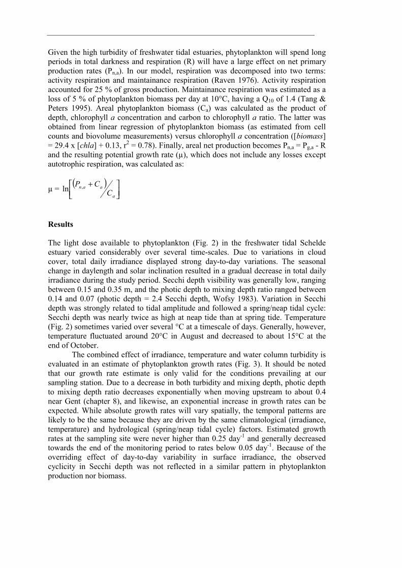
Given the high turbidity of freshwater tidal estuaries, phytoplankton will spend long periods in total darkness and respiration (R) will have a large effect on net primary production rates (Pn,a). In our model, respiration was decomposed into two terms: activity respiration and maintainance respiration (Raven 1976). Activity respiration accounted for 25 % of gross production. Maintainance respiration was estimated as a loss of 5 % of phytoplankton biomass per day at 10°C, having a Q10 of 1.4 (Tang & Peters 1995). Areal phytoplankton biomass (Ca) was calculated as the product of depth, chlorophyll a concentration and carbon to chlorophyll a ratio. The latter was obtained from linear regression of phytoplankton biomass (as estimated from cell counts and biovolume measurements) versus chlorophyll a concentration ([biomass] = 29.4 x [chla] + 0.13, r2 = 0.78). Finally, areal net production becomes Pn,a = Pg,a - R and the resulting potential growth rate (µ), which does not include any losses except autotrophic respiration, was calculated as:

µ = ( )

+

a

aanC

CP ,ln

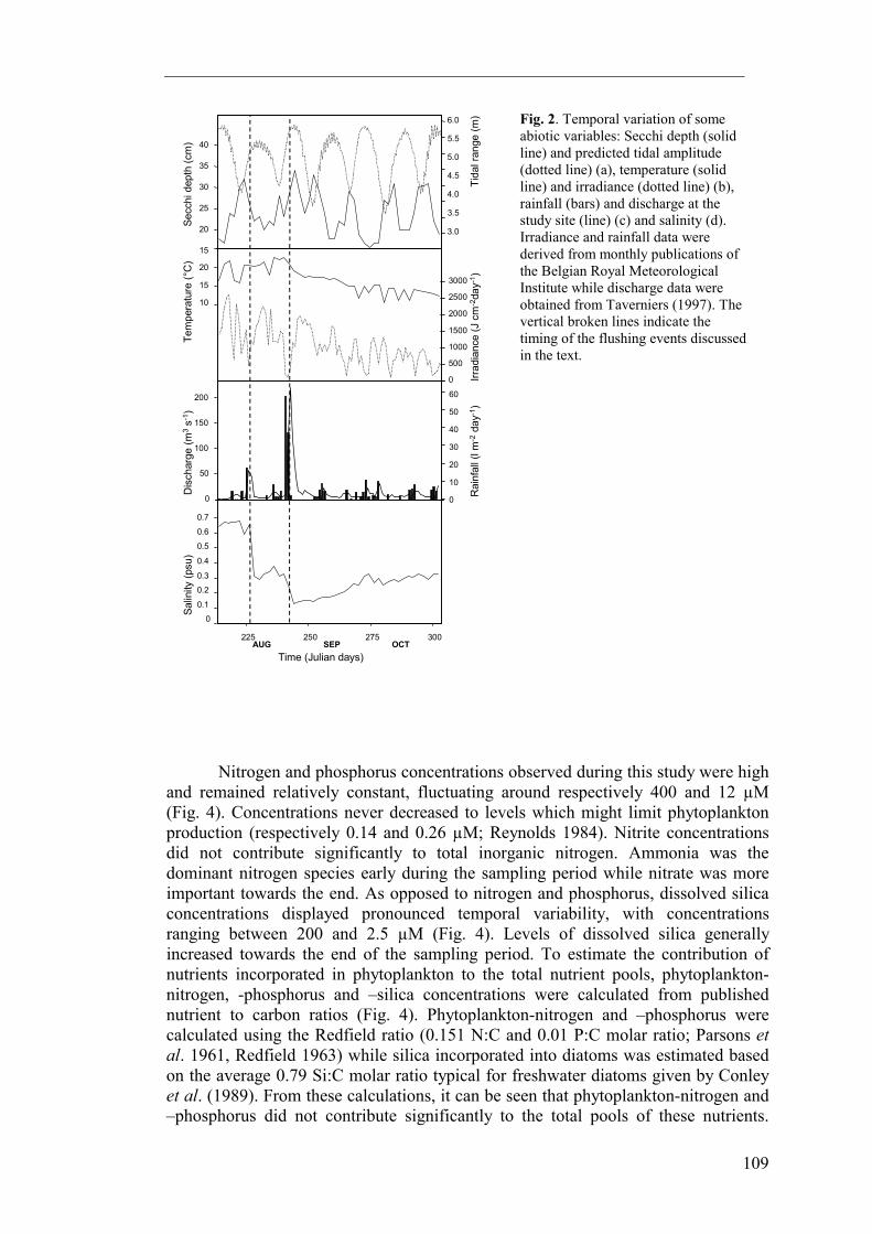
Results The light dose available to phytoplankton (Fig. 2) in the freshwater tidal Schelde estuary varied considerably over several time-scales. Due to variations in cloud cover, total daily irradiance displayed strong day-to-day variations. The seasonal change in daylength and solar inclination resulted in a gradual decrease in total daily irradiance during the study period. Secchi depth visibility was generally low, ranging between 0.15 and 0.35 m, and the photic depth to mixing depth ratio ranged between 0.14 and 0.07 (photic depth = 2.4 Secchi depth, Wofsy 1983). Variation in Secchi depth was strongly related to tidal amplitude and followed a spring/neap tidal cycle: Secchi depth was nearly twice as high at neap tide than at spring tide. Temperature (Fig. 2) sometimes varied over several °C at a timescale of days. Generally, however, temperature fluctuated around 20°C in August and decreased to about 15°C at the end of October. The combined effect of irradiance, temperature and water column turbidity is evaluated in an estimate of phytoplankton growth rates (Fig. 3). It should be noted that our growth rate estimate is only valid for the conditions prevailing at our sampling station. Due to a decrease in both turbidity and mixing depth, photic depth to mixing depth ratio decreases exponentially when moving upstream to about 0.4 near Gent (chapter 8), and likewise, an exponential increase in growth rates can be expected. While absolute growth rates will vary spatially, the temporal patterns are likely to be the same because they are driven by the same climatological (irradiance, temperature) and hydrological (spring/neap tidal cycle) factors. Estimated growth rates at the sampling site were never higher than 0.25 day-1 and generally decreased towards the end of the monitoring period to rates below 0.05 day-1. Because of the overriding effect of day-to-day variability in surface irradiance, the observed cyclicity in Secchi depth was not reflected in a similar pattern in phytoplankton production nor biomass.

109

Nitrogen and phosphorus concentrations observed during this study were high and remained relatively constant, fluctuating around respectively 400 and 12 µM (Fig. 4). Concentrations never decreased to levels which might limit phytoplankton production (respectively 0.14 and 0.26 µM; Reynolds 1984). Nitrite concentrations did not contribute significantly to total inorganic nitrogen. Ammonia was the dominant nitrogen species early during the sampling period while nitrate was more important towards the end. As opposed to nitrogen and phosphorus, dissolved silica concentrations displayed pronounced temporal variability, with concentrations ranging between 200 and 2.5 µM (Fig. 4). Levels of dissolved silica generally increased towards the end of the sampling period. To estimate the contribution of nutrients incorporated in phytoplankton to the total nutrient pools, phytoplankton-nitrogen, -phosphorus and –silica concentrations were calculated from published nutrient to carbon ratios (Fig. 4). Phytoplankton-nitrogen and –phosphorus were calculated using the Redfield ratio (0.151 N:C and 0.01 P:C molar ratio; Parsons et al. 1961, Redfield 1963) while silica incorporated into diatoms was estimated based on the average 0.79 Si:C molar ratio typical for freshwater diatoms given by Conley et al. (1989). From these calculations, it can be seen that phytoplankton-nitrogen and –phosphorus did not contribute significantly to the total pools of these nutrients.

35

15

20

30

25

40

225 250 275 300AUG SEP OCT

3.0

4.0

5.0

6.0

4.5

5.5

3.5

Tida

l ran

ge (m

)

Secc

hi d

epth

(cm

)

15

20

10

0

500

1000

1500

2000

2500

3000

Irrad

ianc

e (J

cm

-2da

y-1 )

Tem

pera

ture

(°C

)

200

0

50

150

100

Dis

char

ge (m

3 s-1

)

40

0

10

30

20

50

60

Rai

nfal

l (l m

-2 d

ay-1

)

0

0.2

0.4

0.6

0.3

0.5

0.1

0.7

Salin

ity (p

su)

Time (Julian days)

Fig. 2. Temporal variation of some abiotic variables: Secchi depth (solid line) and predicted tidal amplitude (dotted line) (a), temperature (solid line) and irradiance (dotted line) (b), rainfall (bars) and discharge at the study site (line) (c) and salinity (d). Irradiance and rainfall data were derived from monthly publications of the Belgian Royal Meteorological Institute while discharge data were obtained from Taverniers (1997). The vertical broken lines indicate the timing of the flushing events discussed in the text.

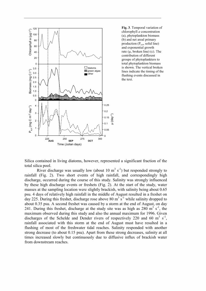
Silica contained in living diatoms, however, represented a significant fraction of the total silica pool. River discharge was usually low (about 10 m3 s-1) but responded strongly to rainfall (Fig. 2). Two short events of high rainfall, and correspondingly high discharge, occurred during the course of this study. Salinity was strongly influenced by these high discharge events or freshets (Fig. 2). At the start of the study, water masses at the sampling location were slightly brackish, with salinity being about 0.65 psu. 4 days of relatively high rainfall in the middle of August resulted in a freshet on day 225. During this freshet, discharge rose above 80 m3 s-1 while salinity dropped to about 0.35 psu. A second freshet was caused by a storm at the end of August, on day 241. During this freshet, discharge at the study site was as high as 280 m3 s-1, the maximum observed during this study and also the annual maximum for 1996. Given discharges of the Schelde and Dender rivers of respectively 220 and 60 m3 s-1, rainfall associated with this storm at the end of August must have resulted in a flushing of most of the freshwater tidal reaches. Salinity responded with another strong decrease (to about 0.15 psu). Apart from these strong decreases, salinity at all times increased slowly but continuously due to diffusive influx of brackish water from downstream reaches.

225 250 275 300AUG SEP OCT

80

0

20

60

40

100

120C

hlor

ophy

ll a

(µg

l-1)

0

1.0

2.0

3.0

1.5

2.5

0.5

3.5

Biom

ass

(mg

C l-

1 )

diatomsgreen algaeother

µ (d

ay-1

)

P a,n

(mg

C m

-2 d

ay-1

)

Time (Julian days)

0

1

2

3

4

0

0.05

0.1

0.15

0.2

0.25

Fig. 3. Temporal variation of chlorophyll a concentration (a), phytoplankton biomass (b) and net areal primary production (Pa,n, solid line) and exponential growth rate (µ, broken line) (c). The contribution of different groups of phytoplankters to total phytoplankton biomass is shown. The vertical broken lines indicate the timing of the flushing events discussed in the text.

111

The phytoplankton community was generally dominated by diatoms (Fig. 3). Coccal green algae (predominantly Scenedesmus spp.) become relatively more important in terms of biomass towards the end of the monitoring period. Other taxa (Cyanobacteria and cryptophycean phytoflagellates) were commonly observed but never important in terms of abundancy nor biomass. Although numerically important, ultraphytoplankton (mainly eukaryotic coccal cells < 5 µm present in densities up to 30 000 cells ml-1) never contributed to more than 5 % of total phytoplankton biomass. The three most dominant phytoplankton taxa were Cyclotella atomus, C. scaldensis and Scenedesmus spp. Their combined biomass on average contributed to 60 % of the phytoplankton total. The two freshets mentioned above marked transitions between three periods characterised by distinct plankton communities. The first period encompassed the first 2 weeks of August (from the beginning of the survey to day 225) and ended a very long period (> 1 month) of low river discharge. Average growth rate during this period was 0.166 day-1. However, no increase in phytoplankton biomass was observed (Fig. 3). Chlorophyll a concentrations and total phytoplankton biomass were on average respectively 61 µg l-1 and 2.0 mg C l-1. Estimated primary production was on average 1760 mg C m-2 day-1. Cyclotella atomus was the dominant phytoplankter and reached cell densities of 57 000 cells ml-1 (Fig. 5). During this period, silica concentrations were low (with a minimum of 2.5 µM) and much of the silica was incorporated into diatoms (Fig. 4). Dense grazer populations

225 250 275 300AUG SEP OCT

Time (Julian days)

0

50

100

150

200

250

0

5

10

20

250

100

200

300

400

500

600

Nitr

ogen

(µM

N)

Phos

phat

e (µ

M P

)Si

licat

e (µ

M S

i)

NitrateAmmonia

Phytoplankton-N

Phytoplankton-P

Phytoplankton-Si

Fig. 4. Temporal variation of nutrient concentrations: ammonia, nitrate and phyto-N (a), phosphate and phyto-P (b) and silicate and phyto-Si (c). Phyto-N, -P and Si represent the fraction of the respective nutrients which is incorporated within the phytoplankton; for their calculation, see text. The vertical broken line indicates the timing of the flushing events discussed in the text.

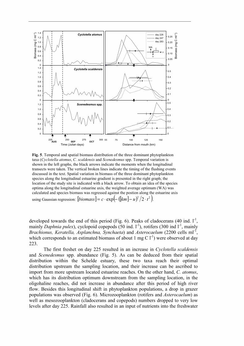
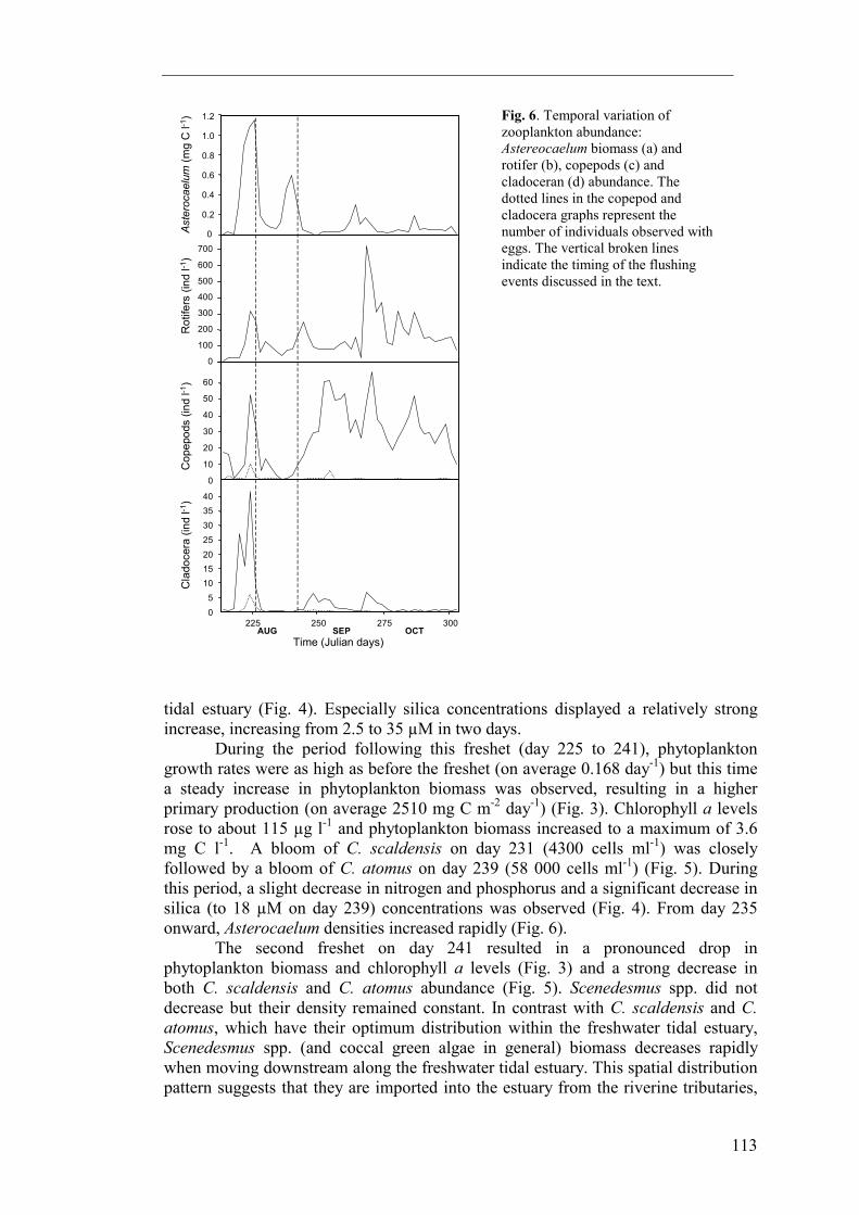
developed towards the end of this period (Fig. 6). Peaks of cladocerans (40 ind. l-1, mainly Daphnia pulex), cyclopoid copepods (50 ind. l-1), rotifers (300 ind l-1, mainly Brachionus, Keratella, Asplanchna, Synchaeta) and Asterocaelum (2200 cells ml-1, which corresponds to an estimated biomass of about 1 mg C l-1) were observed at day 223. The first freshet on day 225 resulted in an increase in Cyclotella scaldensis and Scenedesmus spp. abundance (Fig. 5). As can be deduced from their spatial distribution within the Schelde estuary, these two taxa reach their optimal distribution upstream the sampling location, and their increase can be ascribed to import from more upstream located estuarine reaches. On the other hand, C. atomus, which has its distribution optimum downstream from the sampling location, in the oligohaline reaches, did not increase in abundance after this period of high river flow. Besides this longitudinal shift in phytoplankton populations, a drop in grazer populations was observed (Fig. 6). Microzooplankton (rotifers and Asterocaelum) as well as mesozooplankton (cladocerans and copepods) numbers dropped to very low levels after day 225. Rainfall also resulted in an input of nutrients into the freshwater

225 250 275 300AUG SEP OCT

75 100 125 15055

0

0.1

0.2

0.3

0.4

0.50

0.1

0.2

0.3

0.4

0.5

0

0.05

0.10

0.15

0.20

0.25

0

0.2

0.4

0.6

0.8

1.0

1.4

1.2

0

0.2

0.4

0.6

0.8

1.0

1.4

1.2

0

0.2

0.4

0.6

0.8

1.0

1.2 Scenedesmus spp.

Biom

ass

(mg

C m

l-1)

Biom

ass

(mg

C m

l-1)Cyclotella atomus

Cyclotella scaldensis

Distance from mouth (km)Time (Julian days)

u

ctWA

day 226 day 247day 283

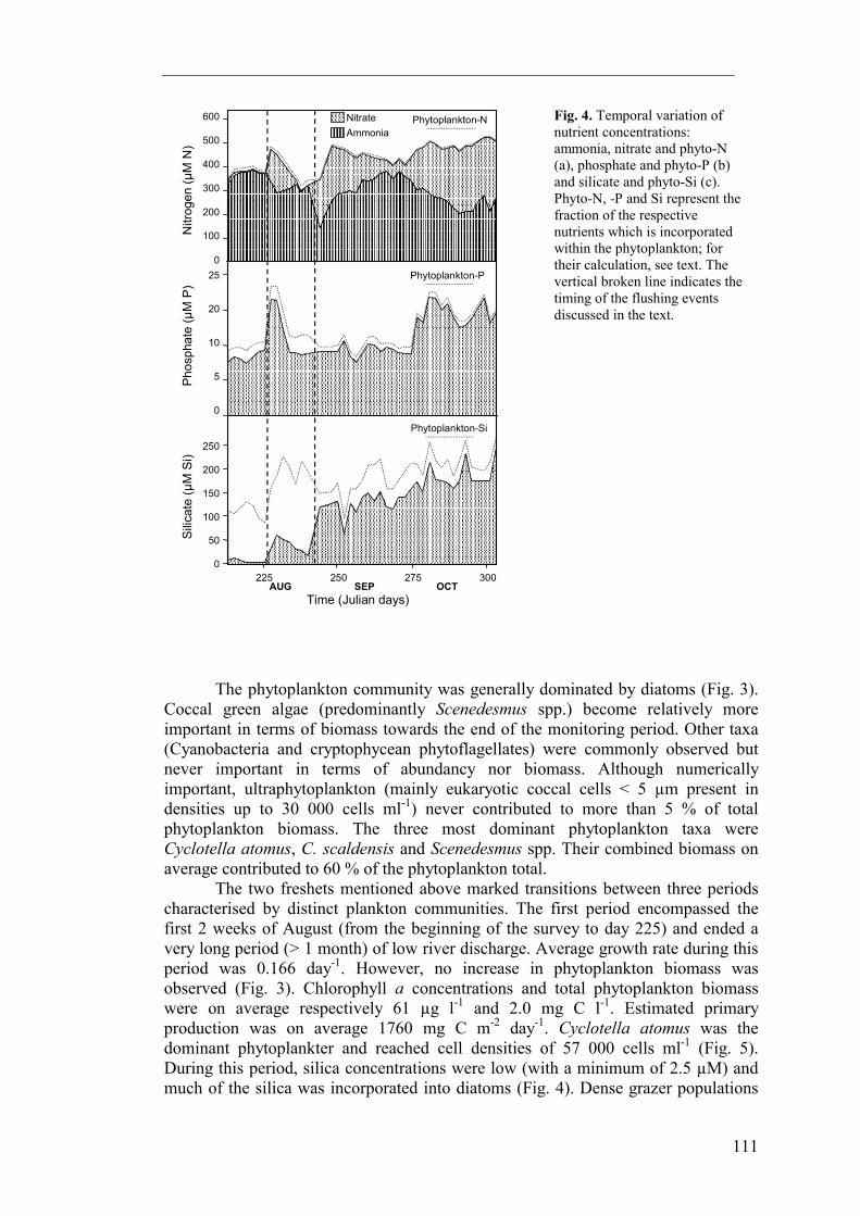
Fig. 5. Temporal and spatial biomass distribution of the three dominant phytoplankton taxa (Cyclotella atomus, C. scaldensis and Scenedesmus spp. Temporal variation is shown in the left graphs, the black arrows indicate the moments when the longitudinal transects were taken. The vertical broken lines indicate the timing of the flushing events discussed in the text. Spatial variation in biomass of the three dominant phytoplankton species along the longitudinal estuarine gradient is presented in the right graph; the location of the study site is indicated with a black arrow. To obtain an idea of the species optima along the longitudinal estuarine axis, the weighted average optimum (WA) was calculated and species biomass was regressed against the postion along the estuarine axis using Gaussian regression: [ ] [ ]( )( )22 2exp tukmcbiomass ⋅−−⋅= .

113

tidal estuary (Fig. 4). Especially silica concentrations displayed a relatively strong increase, increasing from 2.5 to 35 µM in two days. During the period following this freshet (day 225 to 241), phytoplankton growth rates were as high as before the freshet (on average 0.168 day-1) but this time a steady increase in phytoplankton biomass was observed, resulting in a higher primary production (on average 2510 mg C m-2 day-1) (Fig. 3). Chlorophyll a levels rose to about 115 µg l-1 and phytoplankton biomass increased to a maximum of 3.6 mg C l-1. A bloom of C. scaldensis on day 231 (4300 cells ml-1) was closely followed by a bloom of C. atomus on day 239 (58 000 cells ml-1) (Fig. 5). During this period, a slight decrease in nitrogen and phosphorus and a significant decrease in silica (to 18 µM on day 239) concentrations was observed (Fig. 4). From day 235 onward, Asterocaelum densities increased rapidly (Fig. 6). The second freshet on day 241 resulted in a pronounced drop in phytoplankton biomass and chlorophyll a levels (Fig. 3) and a strong decrease in both C. scaldensis and C. atomus abundance (Fig. 5). Scenedesmus spp. did not decrease but their density remained constant. In contrast with C. scaldensis and C. atomus, which have their optimum distribution within the freshwater tidal estuary, Scenedesmus spp. (and coccal green algae in general) biomass decreases rapidly when moving downstream along the freshwater tidal estuary. This spatial distribution pattern suggests that they are imported into the estuary from the riverine tributaries,

225 250 275 300AUG SEP OCT

Time (Julian days)

40

0

10

30

20

50

60

20

05

1510

25303540

Cla

doce

ra (i

nd l-1

)C

opep

ods

(ind

l-1)

400

0

100

300

200

500

600

700

Rot

ifers

(ind

l-1)

Aste

roca

elum

(mg

C l-1

)

0.8

0

0.2

0.6

0.4

1.0

1.2 Fig. 6. Temporal variation of zooplankton abundance: Astereocaelum biomass (a) and rotifer (b), copepods (c) and cladoceran (d) abundance. The dotted lines in the copepod and cladocera graphs represent the number of individuals observed with eggs. The vertical broken lines indicate the timing of the flushing events discussed in the text.

especially from the river Schelde, while little or no growth occurs within the estuary. Apparently, the flushing of the freshwater tidal reaches resulted in a replacement of estuarine phytoplankton with populations of riverine origin. The Asterocaelum population which had developed earlier disappeared while cladoceran (mainly Bosmina longirostris), cyclopoid copepod and rotifer (Brachionus, Keratella, Filinia) densities increased after the storm (Fig. 6). It is likely that these are, like Scenedesmus, imported into the estuary from the riverine tributaries (cf. Roper et al. 1992). As it was the case after the first rainfall event, nutrient concentrations increased and again, silica displayed the strongest response (Fig. 4). Although freshets are known to induce an increase in turbidity in rivers (Reynolds et al. 1994), Secchi depth following the storm was higher than would be expected given the high tidal range at that time (Fig. 2). This could be explained by the replacement of turbid estuarine water by relatively clear riverine water and/or dilution with rainwater. In the period following this second freshet (from day 241 to the end of the monitoring period), phytoplankton populations did not recover and chlorophyll a and phytoplankton biomass levels remained relatively low (average concentrations respectively 31 µg l-1 and 0.96 mg C l-1) (Fig. 3). Due to a general decrease in irradiance and temperature (Fig. 2), phytoplankton growth rates decreased steadily during this period. Average growth rate and estimated primary production for this period were low, respectively 0.05 day-1 and 270 mg C m-2 day-1. Copepods, followed later by rotifers, established dense populations in the period after the storm (Fig. 6). The fact that their densities were maximal when phytoplankton biomass was lowest suggests they do not only depend on phytoplankton as a food source. Possibly, these populations fed on heterotrophic protists, which are abundant in the estuary (chapter 5). Discussion During the first (day 213-225) and second (day 225-241) period of this monitoring study, light and temperature conditions were very similar and estimated growth rates were nearly identical. While phytoplankton increased substantially during the second period, no increase was observed during the first. This suggests that during the first period phytoplankton populations were either bottom-up or top-down limited. At that time dissolved silica concentrations were very low and may have limited production of diatoms (Willén 1991, Paasche 1980), which were at all times the dominant phytoplankters in the freshwater tidal reaches. The large fraction of the total silica pool contained in diatoms suggest that, during this period, diatoms had taken up most of the dissolved silica supplied by the river. Exhaustion of dissolved silica in freshwater tidal estuaries caused by diatom blooms has been observed before (Anderson 1986, and studies cited herein). While human activities often lead to increased nitrogen and phosphorus levels, silica concentrations are rarely affected by eutrophication. This often leads to silica limitation of diatoms in many marine and freshwater systems (Conley et al. 1993), including rivers (Admiraal et al. 1993, Garnier et al. 1995) and brackish estuarine reaches (Conley & Malone 1992). The same might hold true for the freshwater tidal Schelde estuary and other freshwater tidal estuaries, which often receive high nutrient inputs through human activities (industrial and municipal waste discharges). Sediments, however, can be active sites of silica regeneration (Bailey-Watts 1976, Yamada & D'Elia 1984). In estuaries, efflux of regenerated silica from these sediments may even equal inputs from

115

freshwater sources (Wilke & Dayal 1982, Anderson 1986) and is known to give rise to secondary diatom blooms (Conley et al. 1988, Del Amo et al. 1997). As such, it remains questionable to what extent silica limits primary production in freshwater tidal estuaries. In rivers, silica limitation of diatoms induces a switch to a phytoplankton community dominated by green algae (Garnier et al. 1995). This type of succession did not occur in the freshwater tidal Schelde estuary. Although this might suggest a minimal role for silica limitation, it is more likely that this system is too turbid to sustain green algae, which generally grow inefficiently at low light intensities (Richardson et al. 1983). As can be seen from the spatial distribution of Scenedesmus spp., green algae disappear quickly following import into the estuary, where, like in most freshwater tidal estuaries, diatoms dominate (e.g. De Sève 1993). Simultaneously, grazer populations were very dense at the sampling location. At these densities, grazers might have had a strong top-down impact on phytoplankton by cropping new production and preventing an increase in phytoplankton biomass (Gosselain et al. 1998). Among the different grazers, Asterocaelum deserves special attention. Asterocaelum is an amoeboid protist known to feed primarily on centric diatoms, mainly Stephanodiscus and Cyclotella species (Canter 1973, Canter 1980). During this study, it was observed feeding on C. atomus and C. scaldensis. At its maximum population density, its biomass nearly equaled that of its prey, making it an important grazer on centric diatoms. This organism has rarely been reported in ecological studies (Bailey-Watts & Lund 1973), although it was commonly observed during previous studies in the Schelde estuary, its side basins and tributaries (unpublished results). It is also known to be a common component of the plankton of several Dutch rivers (Ton Joosten, personal communication). During this study, its rapid increase in abundance suggests high growth rates, comparable to the growth rates of 0.5 day-1 observed in cultures (Bailey-Watts & Lund 1973). The data available from this study do not allow us to conclude whether phytoplankton growth was limited by bottom-up or top-down effects or by a combination of both. It should be noted that, if silica was limiting diatom production, our primary production and growth rate estimates are probably overrated. What our observations show is that, in summer, when growth conditions are optimal, after prolonged periods of constant and relatively low discharge, a point is reached where exponential increase of phytoplankton populations is arrested. Planktonic organisms depend primarily on the physical processes which influence the medium they are embedded in and flushing rate is known to have a strong impact on plankton communities. Given their relatively long generation times, mesozooplankters in lotic systems are particularly sensitive to low residence times (Pace et al. 1992, Thorp et al. 1994, Basu & Pick 1996). Rotifers (Ferrari et al. 1989) and other microzooplankters (Vranowský 1995) have also been found to decrease when discharge increases while the relatively low biomass of phytoplankton in rivers when compared to lakes of similar trophic status has also been ascribed to low residence time (Søballe & Kimmel 1987). Therefore, it was not surprising to find that the freshets which occurred during our monitoring period resulted in a longitudinal transport of plankton communities and, ultimately, a removal of biomass from the freshwater tidal estuary. The first freshet (on day 225) comprised a partial flushing of the freshwater tidal reaches and resulted in a removal of grazer populations. The second freshet (on day 241) involved a flushing of the entire freshwater tidal estuary and removed most of the estuarine zoo- and phytoplankton populations present at

that time (respectively Asterocaelum and Cyclotella spp.), replacing them with a riverine plankton community. Apparently, flushing events have a stronger impact on zooplankton than on phytoplankton, as, following the first freshet, zooplankton decreased while phytoplankton biomass remained constant. In lotic systems, potamoplankton blooms originate in the downstream reaches and populations develop in upstream direction (Greenberg 1964). Being dependent on threshold food concentrations and having generally longer generation times, herbivorous zooplankton growth lags behind on the phytoplankton (de Ruyter van Steveninck et al. 1990, Garnier et al. 1995). Consequently, the peak in zooplankton will usually be situated downstream from the phytoplankton peak and, as such, zooplankton will be more easily removed by flushing events than phytoplankton. This is in agreement with Basu & Pick (1996), who observed a much stronger influence of residence time on zooplankton than on phytoplankton populations. If only part of the system is flushed (moderate freshet, e.g. day 225), the impact on zooplankton will be higher than on phytoplankton while if the entire system is flushed (extreme freshet, e.g. day 241), a negative effect on both zoo- and phytoplankton can be expected. The first freshet, on day 225, indirectly stimulated phytoplankton as both biomass and production increased in the following period. If grazing pressure was important during the preceeding period, this increase must be ascribed to the differential removal of zooplankton over phytoplankton from the system (see above), which would stimulate phytoplankton population growth by removing grazing losses. On the other hand, if phytoplankton was nutrient limited, the increase in silica levels observed after the freshet will be responsible for the biomass increase. Precipitation in the watershed washes deposited nutrients off the land and concentrates them in the water. As such, in systems which are strongly influenced by rainfall, freshets will lead to a strong increase in total nutrient concentrations (cf. Garcia-Soto et al. 1990, Rudek et al. 1991, Mallin et al. 1993) and thus not only remove nutrient limitation but also result in a temporal increase in the total carrying capacity of the system. If phytoplankton is bottom-up or top-down limited in lotic systems, moderate freshets are likely to remove the source of limitation and, thus, stimulate primary production. During the freshet on day 241, the entire estuarine phytoplankton community in the freshwater tidal Schelde estuary was removed and populations were not able to re-establish afterwards. Although climatic conditions following this freshet rapidly returned to those before the storm, growth rates started to decrease significantly after one week. As only a small inoculum of estuarine phytoplankton was left after the freshet, this period was too short for phytoplankton populations to recover. As such, this storm event put an abrupt end to the phytoplankton growth season. Through this 'inoculum-effect' (Reynolds 1993), extreme flushing events can have a strong negative impact on phytoplankton dynamics by removing the entire autochthonous phytoplankton population (Reynolds & Lund 1988, Klarer & Millie 1994). Conclusion In this study, we showed how, in lotic enviroments where discharge responds rapidly to variations in precipitation (rivers, freshwater tidal estuaries and small estuaries in general), freshets will have an important impact on phytoplankton dynamics. While a constant low discharge will result in bottom-up or top-down limited primary production, the occurrence of frequent, moderate freshets is likely to significantly increase this production by removing grazers and replenishing nutrient stocks. On the other hand, extreme freshets, which flush the entire system, will have a negative

117

effect on primary production by removing the entire autochthonous plankton community, in which case recovery of the phytoplankton populations can be slow due to the absence of a sufficiently large inoculum. Consequently, the frequency-intensity distribution of precipitation during the phytoplankton growth season will determine phytoplankton dynamics in the system and may be an important source of interannual variability in biomass and productivity. These conclusions also support the hypothesis that frequent hydrologic perturbations are crucial to sustain the high productivity of riverine systems (Power et al. 1995). While the importance of annual flood events on a variety of organisms over a range of lotic systems is widely accepted, smaller variations over shorter time-scales may be equally important, especially in regulating dynamics of the planktonic food web, which is dominated by organisms having short life-cycles.

Many rivers are of economical importance as transport routes, waste removal systems or sources of drink- or irrigation water and have for several millenia been influenced by human activities. Ecological principles, however, have up to recently played only a minor role in the managament of large rivers (Wehr & Descy 1998). Many activities in river basins involve construction of dams, which strongly influence discharge by reducing peak flows (Ligon et al. 1995) and can, according to our results, be expected to have profound impacts on the primary productivity in rivers and the estuaries they drain into. With this study, we hope to provide a conceptual framework which allows to evaluate the impact of hydrological changes on the primary producers in lotic ecosystems.

Acknowledgements - The research presented in this paper was carried out in the framework of the Flemish OMES project ('Onderzoek naar de Milieu-Effekten van het Sigmaplan'), coordinated by Prof. P. Meire, which aims at studying the effects of dike constructions and waterworks on ecosystem functioning in the Schelde estuary. We thank D. Van Gansbeke for performing the chlorophyll a and nutrient analyses and S. De Clerck and H. Segers for assistance in zooplankton enumeration and identification. Koenraad Muylaert is research assistant for the Fund for Scientific Research (Flanders). Koen Sabbe and Wim Vyverman are post-doctoral fellows of the Fund.