Definability for Model CountingI

Jean-Marie Lagnieza, Emmanuel Loncab, Pierre Marquisc

aHuawei Technologies Ltd,2012 Lab / CSI Paris / DC – 20 quai du Point du Jour, F-92100 Boulogne-Billancourt France

bCRIL, CNRS UMR8188 - Univ Artois,rue Jean Souvraz – F-62307 Lens France

cCRIL, CNRS UMR8188 - Univ Artois & Institut Universitaire de France,rue Jean Souvraz – F-62307 Lens France

Abstract

We define and evaluate a new preprocessing technique for propositional modelcounting. This technique leverages definability, i.e., the ability to determine thatsome gates are implied by the input formula Σ. Such gates can be exploited tosimplify Σ without modifying its number of models. Unlike previous techniquesbased on gate detection and replacement, gates do not need to be made explicit inour approach. Our preprocessing technique thus consists of two phases: comput-ing a bipartition 〈I, O〉 of the variables of Σ where the variables from O are definedin Σ in terms of I, then eliminating some variables of O in Σ. Our experimentsshow the computational benefits which can be achieved by taking advantage ofour preprocessing technique for model counting.

Keywords: definability, model counting.

IThis is an extended version of the paper entitled “Improving Model Counting by LeveragingDefinability” published in the proceedings of the 25thInternational Joint Conference on ArtificialIntelligence (IJCAI’16), New York City, 2016 (751-757).

Email addresses: jean.marie.lagniez@huawei.com (Jean-Marie Lagniez),lonca@cril.univ-artois.fr (Emmanuel Lonca),marquis@cril.univ-artois.fr (Pierre Marquis)

Preprint submitted to Artificial Intelligence Journal January 2, 2020

1. Introduction

Propositional model counting (also known as the #SAT problem) is the task ofcomputing the number of models of a given propositional formula Σ. This prob-lem and its direct generalization, weighted model counting,1 are central to manyAI problems including probabilistic inference [1, 2, 3, 4] and forms of planning[5, 6]. They have also many applications outside AI, like in SAT-based automatictest pattern generation, for evaluating the vulnerability to malicious fault attacksin hardware circuits (see e.g., [7]).

However, propositional model counting (as well as WMC, which can be re-duced to #SAT [8]) are computationally hard (they are #P-complete problems[9, 10, 11]), actually much harder in practice than the satisfiability problem (SAT).The power offered by the ability to count efficiently and, dually, the difficultyto do it, are well-reflected by Toda’s theorem, showing that PH ⊆ P#P, i.e., ev-ery problem from the polynomial hierarchy PH can be solved in polynomial timeprovided that a #P oracle is available [12]. Nevertheless, the significance of #SAT

explains why much effort has been spent for the last decade in developing new al-gorithms for model counting (either exact or approximate), which prove practicalfor larger and larger instances, see e.g., [13, 14, 15, 16, 17, 18].

In this paper, we present a new preprocessing technique for improving ex-act model counting from the computational side. Preprocessing techniques arenowadays acknowledged as computationally valuable for a number of automatedreasoning tasks, especially SAT solving and QBF solving [19, 20, 21, 22, 23, 24,25, 26, 27]. As such, they are now embodied in state-of-the-art SAT solvers,like Glucose [28] which takes advantage of the SatELite preprocessor [22],Lingeling [29] which has an internal preprocessor, and Riss [30] which takesadvantage of the Coprocessor preprocessor [31].

Our approach elaborates on previous preprocessing techniques [32] that canbe exploited for improving the model counting task from a computational stand-point. Among them is gate detection and replacement. Basically, every variabley of the input formula Σ that turns out to be defined in Σ in terms of other vari-ables X = x1, . . . , xk can be replaced by the corresponding gate ΦX, whilepreserving the number of models of Σ. Indeed, whenever a partial assignment

1In weighted model counting (WMC), each literal is associated with a real number, the weightof an interpretation is the product of the weights of the literals it sets to true, and the weight of aformula is the sum of the weights of its models. Accordingly, WMC amounts to model countingwhen each literal has weight 1.

2

over the variables of X is considered, either it is jointly inconsistent with Σ orin every model of Σ that extends this partial assignment, y has the same truthvalue. Literal equivalences, AND/OR gates and XOR gates can be detected (ei-ther syntactically or using Boolean constraint propagation). The correspondingpreprocessing techniques are integrated into a preprocessor, called pmc. The em-pirical results reported in [32] clearly show that huge computational benefits canbe achieved through the detection and the replacement of gates. However, pmcremains limited due to the small number of families of gates which are targeted(literal, AND, XOR gates and their negations).

In order to fill the gap, we present in this paper a preprocessing technique tomodel counting that exploits in a much more aggressive way the gates that can befound in the input formula Σ. The key idea underlying this preprocessing tech-nique is that one does not need to identify the gates themselves but determiningthat they exist is enough. To be more precise, it proves sufficient to detect thatsome definability relations between variables hold, without needing to identifythe corresponding gates. This distinction is of tremendous importance for tworeasons. On the one hand, the search space for the possible gates ΦX is very large:it contains 22k

elements up to logical equivalence, when X contains k variables.On the other hand, in the general case, the size of any explicit gate ΦX of y in Σis not polynomially bounded in |Σ| + |X| unless NP ∩ coNP ⊆ P/poly (which isconsidered unlikely in complexity theory) [33].

What this paper mainly gives is the description and the evaluation of a newpreprocessor for model counting, called B + E. The preprocessor B + E associateswith a given CNF formula Σ a CNF formula Φ which has the same number of mod-els as Σ, but is at least as simple as Σ with respect to the number of variables andthe number of clauses. Requiring the input Σ to be a CNF formula is not a majorrestriction since any propositional circuit Σ can be turned in time linear in its sizeinto a CNF formula having the same number of models, thanks to Tseitin’s trans-formation [34]. Indeed, this transformation consists in adding gates to the input sothat the new variables which are introduced are defined from the original ones. Bythe way, it is worth noting that other CNF translations, like Plaisted/Greenbaum’sone [35], cannot be used. Indeed, Plaisted/Greenbaum’s transformation preservesthe satisfiability of the input circuit (and actually a bit more, namely the set oflogical consequences of Σ over its set of variables) but not its number of models.

Example 1. For instance, using Tseitin’s transformation, the input DNF formulaΣ = (a ∧ b) ∨ (b ∧ c) is associated with the CNF formula s0 ∧ (¬s0 ∨ s1 ∨ s2)∧(s0 ∨ ¬s1) ∧(s0 ∨ ¬s2) ∧(¬s1 ∨ a) ∧(¬s1 ∨ b) ∧(s1 ∨ ¬a ∨ ¬b) ∧(¬s2 ∨ b)

3

∧(¬s1∨c) ∧(s2∨¬b∨¬c). This CNF formula is equivalent to s0∧[s0 ↔ (s1∨s2)]∧[s1 ↔ (a ∧ b)] ∧[s2 ↔ (b ∧ c)], and it has precisely the same number of modelsover its set of variables as Σ over a, b, c, viz 3. Using Plaisted/Greenbaum’stransformation, Σ is associated with the CNF formula s0∧(¬s0∨s1∨s2)∧(¬s1∨a)∧(¬s1 ∨ b) ∧(¬s2 ∨ b) ∧(¬s1 ∨ c). This CNF formula is equivalent to s0 ∧ [s0 →(s1 ∨ s2)] ∧[s1 → (a ∧ b)] ∧[s2 → (b ∧ c)], which has 5 models (and not 3) overits set of variables.

Interestingly, the CNF format is the one considered by state-of-the-art modelcounters. As its name suggests it, B + E consists of two parts: B which aims todetermine a Bipartition 〈I, O〉 of the variables of Σ such that every variable of Ois defined in Σ in terms of the remaining variables (in I), and E which aims toEliminate in Σ some variables of O.

More in detail, the contribution of the paper consists of the presentation ofthe algorithms B and E, a property establishing the correctness of the prepro-cessing technique used, and some empirical evidence showing the computationalimprovements achieved by B + E compared to the case when no preprocessor isused upstream, and also to the case when pmc is used. This paper significantly ex-tends the results presented in [36], by providing several new contributions. Someof them are theory-oriented, including the identification of the complexity of de-ciding whether a definability bipartition is a subset-minimal one, and the proofthat the bipartition component of our preprocessor actually computes a subset-minimal definability bipartition. Other contributions consist of empirical results;thus, some empirical evidence related to the use of d4 [37] as a downstream modelcounter has been added. Compared to [36], we also consider the use of B + Efor approximate compilation with controllable variables, report some additionalexperimental results concerning classical planning benchmarks, and discuss theconnections between approximate compilation with controllable variables and theprojected model counting task [38, 39]. In addition, we show our approach asclosely related to the notion of independent support used for approximate modelcounting. Especially, we compare the bipartitioner B used in our approach withthe one (called MIS) used in [40].

The benchmarks used, the implementation (binary code) of B + E, and detailedempirical results are available online on www.cril.fr/KC/.

The rest of the paper is organized as follows. Section 2 gives some backgroundon propositional definability. In Section 3, we introduce our preprocessor B + Eand prove that the preprocessing technique it implements is correct. Section 4presents results from our large scale experiments, showing B + E as a competitive

4

preprocessor for model counting, especially when compared with pmc. Someother related work is discussed in Section 6. Finally, Section 7 concludes thepaper and lists some perspectives for further research.

2. Propositional Logic and Definability

The formal setting of our study is classical propositional logic (see e.g., [41]).Let LP be the propositional language defined inductively from a non-empty, finiteset P of propositional variables, the usual connectives (¬, ∨, ∧,↔, etc.) and in-cluding the Boolean constants > and ⊥. Formulae are interpreted in the classicalway. The cardinality of a set S of formulae is denoted by #(S). An interpretationω is a mapping from P to 0, 1. An interpretation ω is a model (resp. a coun-termodel) of a formula Σ ∈ LP if and only if ω makes Σ true (resp. false) in theusual truth functional way. Whenever a formula has a model, it is said to be con-sistent (or satisfiable). In the remaining case, it is inconsistent (or unsatisfiable).When a formula has no countermodel, it is a valid formula. For any pair of for-mulae Σ1 and Σ2, Σ2 is a logical consequence of Σ1, noted Σ1 |= Σ2, wheneverevery model of Σ1 is a model of Σ2; Σ1 and Σ2 are logically equivalent, notedΣ1 ≡ Σ2, whenever they have the same models. For any formula Σ from LP ,Var(Σ) is the set of variables from P occurring in Σ, and ‖Σ‖ is the number ofmodels of Σ over Var(Σ).

Among the formulae are the literals, the terms, the clauses and the CNF for-mulae. A literal ` is a propositional variable x (in this case, ` is a positive literal),or a negated variable ¬x (in this case, ` is a negative literal). When ` is a literalover x, i.e., ` = x or ` = ¬x, its complementary literal ∼` is given by ∼` = ¬xif ` = x and ∼` = x if ` = ¬x. var(`) denotes the variable upon which ` is built,i.e., var(x) = var(¬x) = x. A term is a conjunction of literals or >, and a clauseis a disjunction of literals or ⊥. Terms and clauses are also viewed as sets of liter-als when it is convenient (the empty set corresponds to > when the set of literalsmust be interpreted as a term – the empty conjunction of literals – and to ⊥ whenit must be interpreted as a clause – the empty disjunction of literals). > is the solevalid term, and ⊥ is the sole inconsistent clause. A canonical term γX over X is aconsistent term in which every variable from X appears (either as a positive literalor as a negative one, i.e., as a negated variable). A CNF formula is a conjunctionof clauses, also viewed as a set of clauses when this is convenient.

Let X be any finite subset of P . The conditioning of a formula Σ by a consis-tent term γ is the formula Σ | γ obtained by substituting in Σ for every literal `

5

of γ such that var(`) = x every occurrence of x by ⊥ (resp. >) if ` is a negative(resp. a positive) literal.

Example 2. Suppose that Σ is the CNF formula (a∨d)∧(a∨b)∧(¬b∨c) and thatγ = ¬a∧ b. Then Σ | γ is the formula (⊥∨ d)∧ (⊥∨>)∧ (¬>∨ c). This formulacan be simplified in polynomial time into the equivalent CNF formula d ∧ c usingsimple laws of Boolean calculus.

A formula ϕ is independent of a set X of variables if and only if ϕ is equivalentto a formula ψ such that Var(ψ) ∩ X = ∅. ∃X.Σ denotes a formula from LPequivalent to the forgetting of X in Σ, i.e., the strongest logical consequence of Σ(up to logical equivalence), that is independent of X [42]. ”Logically strongest”means that for every formula ϕ that is independent of X and such that Σ |= ϕ, wehave ∃X.Σ |= ϕ. The formula ∃X.Σ can be defined inductively as follows:

• ∃∅.Σ = Σ,

• ∃x.Σ = (Σ | ¬x) ∨ (Σ | x),

• ∃X′ ∪ x.Σ = ∃X′.(∃x.Σ).

When Σ =∧k

i=1 δi is a CNF formula and X = x ∪ X′, a formula equivalentto ∃X.Σ can be computed in a recursive way by eliminating x in Σ, obtainingthus a new CNF formula equivalent to ∃x.Σ, in which the variables of X′ arethen eliminated. Eliminating x in Σ basically amounts to applying the resolutionprinciple: ∃x.Σ is equivalent to the CNF formula consisting of the clauses δi ofΣ such that x 6∈ Var(δi) conjoined with all the resolvents on x of the clauses of Σ.

Example 3. As a matter of illustration, suppose that Σ is the CNF formula (a ∨d)∧ (a∨ b)∧ (¬b∨ c) and that X = b. Then ∃X.Σ is the formula ((a∨ d)∧ (a∨⊥)∧ (¬⊥∨ c))∨ ((a∨ d)∧ (a∨>)∧ (¬>∨ c)). This formula is equivalent to theCNF formula (a ∨ d) ∧ (a ∨ c) obtained by eliminating b in Σ: the clause a ∨ d ofΣ which does not contain b is kept, and the resolvent a ∨ c of a ∨ b and ¬b ∨ c onb is conjoined to it.

Observe that, by construction, the set of variables of ∃Var(Σ).Σ is empty, sothat the formula ∃Var(Σ).Σ either is inconsistent or is valid, and this can be testedin linear time from ∃Var(Σ).Σ. Since ∃Var(Σ).Σ is valid precisely when Σ isconsistent, eliminating in a CNF formula Σ every variable occurring in it is a way

6

to decide its satisfiability: it is the Davis-Putnam’s algorithm for SAT [43] (we willreturn to it in Section 6).

Let us now recall the two (equivalent) forms under which the concept of de-finability in (classical) propositional logic can be encountered:

Definition 1 (Implicit Definability). Let Σ ∈ LP , X a finite subset of P , andy ∈ P . The formula Σ implicitly defines the variable y in terms of X if and onlyif for every canonical term γX over X, we have γX ∧ Σ |= y or γX ∧ Σ |= ¬y.

Definition 2 (Explicit Definability). Let Σ ∈ LP , X a finite subset of P , andy ∈ P . The formula Σ explicitly defines the variable y in terms of X if and onlyif there exists a formula ΦX ∈ LX such that Σ |= (ΦX ↔ y). In such a case, ΦXis called a definition (or gate) of y on X in Σ, y is the output variable of the gate,and X are its input variables.

Let us illustrate the two notions of implicit definability and explicit definabilityusing a simple example.

Example 4. Let Σ be the CNF formula consisting of the following clauses:

a ∨ b,a ∨ c ∨ ¬e,a ∨ ¬d,b ∨ c ∨ ¬d,

¬a ∨ ¬b ∨ d,¬a ∨ ¬c ∨ d,¬a ∨ ¬b ∨ c ∨ ¬e,¬a ∨ b ∨ ¬c ∨ ¬e,

a ∨ e,b ∨ c ∨ e,¬b ∨ ¬c ∨ e.

Variables d and e are implicitly defined in Σ in terms of X = a, b, c. For instance,the canonical term γX = a ∧ b ∧ ¬c is such that γX ∧ Σ |= d ∧ ¬e. On the otherhand, γ ′X = ¬a ∧ ¬b ∧ ¬c is such that γ ′X ∧ Σ is inconsistent. Variables d and eare also explicitly defined in Σ in terms of X = a, b, c since Σ implies

d↔ [a ∧ (b ∨ c)] and e↔ [¬a ∨ (b↔ c)].

What happens in this example is not fortuitous due to the following theorem:

Theorem 1 ( [44]). Let Σ ∈ LP , X a finite subset of P , and y ∈ P . The formulaΣ implicitly defines the variable y in terms of X if and only if Σ explicitly definesy in terms of X.

7

Since implicit definability and explicit definability coincide, one can simplysay that y is defined in terms of X in Σ. More generally, we state that a subset Yof variables from P is defined in terms of X in Σ when every variable y ∈ Y isdefined in terms of X in Σ.

An interesting consequence of Theorem 1 is that it is not mandatory to pointout a gate ΦX of y on X in order to prove that such a gate exists. Indeed, it isenough to show that Σ implicitly defines y in terms of X to do the job, and thisproblem is ”only” coNP-complete [33]. To prove it, we can take advantage of thefollowing result (Padoa’s theorem), restricted to propositional logic and recalledin [33]; this theorem gives an entailment-based characterization of (implicit) de-finability:

Theorem 2 ([45]). For any Σ ∈ LP and X a finite subset of P , let Σ′X be theformula obtained by substituting in Σ every occurrence of a propositional variablez from Var(Σ) \X by a new propositional variable z′. Let y ∈ P . If y 6∈ X, then Σ(implicitly) defines y in terms of X if and only if Σ∧Σ′X∧y∧¬y′ is inconsistent.2

3. A New Preprocessing Technique for Model Counting

3.1. The B + E PreprocessorInstead of detecting gates and replacing them in Σ in order to remove output

variables, our preprocessing technique consists in detecting output variables, thenin forgetting them in Σ. Thus, the first objective is to find a definability bipartition〈I, O〉 of Σ. The notion of definability bipartition is given by:

Definition 3 (Definability Bipartition). Let Σ ∈ LP . A definability bipartitionof Σ is a pair 〈I, O〉 such that I ∪ O = Var(Σ), I ∩ O = ∅, and Σ defines everyvariable o ∈ O in terms of I.

The most interesting bipartitions are those for which I is ”minimal” to someextent. Two notions of minimality can be considered here, since the minimality ofI can be evaluated either at the set of variables itself, or as the cardinality of thisset. Thus, a definability bipartition 〈I, O〉 of a formula Σ will be said to be

• a subset-minimal bipartition of Σ if and only if every pair 〈I′, O′〉 such thatI′ ∪ O′ = Var(Σ), I′ ∩ O′ = ∅, and I′ ⊂ I is not a definability bipartition ofΣ,

2Obviously enough, in the remaining case when y ∈ X, Σ defines y in terms of X.

8

• a smallest bipartition of Σ if and only if every pair 〈I′, O′〉 such that I′∪O′ =Var(Σ), I′ ∩ O′ = ∅, and #(I′) < #(I) is not a definability bipartition of Σ.

Accordingly, 〈I, O〉 is a subset-minimal definability bipartition of Σ if and onlyif I is a minimal defining family (or base) for O with respect to Σ [33].

Clearly enough, every smallest bipartition of Σ is a subset-minimal bipartitionof Σ, but not vice-versa. Furthermore, every formula Σ has a definability biparti-tion since 〈I = Var(Σ), O = ∅〉 is a bipartition of Σ. This bipartition is a smallestbipartition of Σ (hence a subset-minimal one) when every variable y ∈ Var(Σ) isundefinable in Σ, which means that for every X ⊆ P , Σ defines y in terms of X ifand only if y ∈ X [33]. Since Var(Σ) is a finite set, this shows that every formulaΣ has a smallest (hence a subset-minimal) bipartition.

Then, in a second step, the objective is to forget variables from O in Σ so as tosimplify Σ. This leads to the two-step preprocessing algorithm B + E (B(ipartition),then E(liminate)) given at Algorithm 1, and reported here for the sake of complete-ness. The soundness of B + E is based on the following result:

Algorithm 1: B + Einput : a CNF formula Σoutput: a CNF formula Φ such that ‖Φ‖ = ‖Σ‖

1 O←B(Σ);2 Φ←E(O, Σ);3 return Φ

Proposition 1. Let Σ ∈ LP . Let 〈I, O〉 be a definability bipartition of Σ. LetE ⊆ O. Then ‖Σ‖ = ‖∃E.Σ‖.

Proof: Let E = y1, . . . , ym be a subset of O. Since every yi (i ∈ 1, . . . , m) isdefinable in terms of I in Σ, there exists a formula Φ

yiI over I such that

Σ |= (yi ↔ ΦyiI )

(i.e., a gate ΦyiI of yi on I in Σ exists).

Let Σ[yi ← ΦyiI ]i∈1,...,m be the formula obtained by replacing in Σ every oc-

currence of yi by ΦyiI . Let γI be a canonical term over I. If γI∧Σ is consistent, then

there exists a unique model ωγI of Σ over Var(Σ) that is a model of γI. Accord-ingly, every model of Σ is fully characterized by its restriction over I, so that ‖Σ‖is equal to the number of canonical terms γI over I such that γI ∧ Σ is consistent.

9

Now, by construction, we have

Σ ≡m∧

i=1

(yi ↔ ΦyiI ) ∧ Σ[yi ← Φ

yiI ]i∈1,...,m.

Hence γI ∧ Σ is equivalent to

γI ∧m∧

i=1

(yi ↔ ΦyiI ) ∧ Σ[yi ← Φ

yiI ]i∈1,...,m.

Since γI is a canonical term over I and Var(ΦyiI ) ⊆ I for every i ∈ 1, . . . , m, we

have that γI∧ΦyiI is consistent if and only if γI |= Φ

yiI , so that γI∧

∧mi=1(yi ↔ Φ

yiI )

is equivalent to γI ∧∧m

i=1 y∗i where y∗i (i ∈ 1, . . . , m) is yi when γI |= ΦyiI and is

¬yi otherwise. Therefore,

γI ∧m∧

i=1

(yi ↔ ΦyiI ) ∧ Σ[yi ← Φ

yiI ]i∈1,...,m

is equivalent to

γI ∧ (m∧

i=1

y∗i ) ∧ Σ[yi ← ΦyiI ]i∈1,...,m.

In addition, since Var(γI∧Σ[yi ← ΦyiI ]i∈1,...,m) ⊆ I, Var(

∧mi=1 y∗i ) ⊆ O and I∩O =

∅, γI∧Σ is consistent if and only if γI∧Σ[yi ← ΦyiI ]i∈1,...,m is consistent. But since

γI is a canonical term over I and Var(Σ[yi ← ΦyiI ]i∈1,...,m) ⊆ I, this is precisely

the case when γI |= Σ[yi ← ΦyiI ]i∈1,...,m. Thus the number of canonical terms γI

over I such that γI ∧ Σ is consistent is equal to the number of models of Σ[yi ←Φ

yiI ]i∈1,...,m over I. Stated otherwise, we have ‖Σ‖ = ‖Σ[yi ← Φ

yiI ]i∈1,...,m‖.

Since Var(Σ[yi ← ΦyiI ]i∈1,...,m)∩E = ∅, we have that ∃E.Σ which is equivalent

to

∃E.((m∧

i=1

(yi ↔ ΦyiI ) ∧ Σ[yi ← Φ

yiI ]i∈1,...,m),

is also equivalent to

(∃E.(m∧

i=1

(yi ↔ ΦyiI ))) ∧ Σ[yi ← Φ

yiI ]i∈1,...,m.

10

Finally, since Var(ΦyiI ) ∩ E = ∅, we also have that ∃E.(

∧mi=1(y ↔ Φ

yiI )) is equiv-

alent to∧m

i=1(∃yi.(yi ↔ ΦyiI )). But each ∃yi.(yi ↔ Φ

yiI ) (i ∈ 1, . . . , m) is a valid

formula. Hence we have

∃E.Σ ≡ Σ[yi ← ΦyiI ]i∈1,...,m,

which implies that‖∃E.Σ‖ = ‖Σ[yi ← Φ

yiI ]i∈1,...,m‖,

and thus that ‖Σ‖ = ‖∃E.Σ‖.

Example 5 (Example 4 cont’ed). No literal equivalences, AND/OR gates or XORgates are logical consequences of Σ. Nevertheless, since Σ implies

d↔ [a ∧ (b ∨ c)] and e↔ [¬a ∨ (b↔ c)]

a definability bipartition of Σ is 〈a, b, c, d, e〉. Now, eliminating d and e inΣ using the resolution principle leads to the generation of two clauses a ∨ c anda∨ b∨ c (the other resolvents that are produced are valid clauses, hence they canbe omitted). Therefore, a CNF formula equivalent to ∃d, e.Σ can be computedas the conjunction of:

a ∨ b, a ∨ c, a ∨ b ∨ c,

which can be simplified further into (a ∨ b) ∧ (a ∨ c). This CNF formula hasonly 5 models over a, b, c. From Proposition 3, this is also the case of Σ overa, b, c, d, e.

The ability to identify any subset O of the full set of output variables in the bi-partition generation phase, and to consider only a subset E of O in the eliminationphase are two important features for the efficiency purpose.

On the one hand, computing a subset-minimal definability bipartition of Σturns out to be computationally easier than computing a smallest definability bi-partition of Σ. Indeed, given a definability bipartition 〈I, O〉 of Σ, determiningwhether it is a subset-minimal one does not require to check that each of the (ex-ponentially many) subsets of I does not define in Σ every variable of Var(Σ). Tobe more precise, it is enough to consider only the (linearly many) subsets I \ xwith x ∈ I (see the proof of Proposition 2). Thus, only one source of complex-ity (coming from the definability test) must be dealt with when one looks for asubset-minimal definability bipartition. Formally:

11

Definition 4 (SUBSET-MINIMAL BIPARTITION).SUBSET-MINIMAL BIPARTITION is the following decision problem:

• Input: a CNF formula Σ, and a definability bipartition 〈I, O〉 of Σ.

• Question: is 〈I, O〉 a subset-minimal bipartition of Σ?

Proposition 2. SUBSET-MINIMAL BIPARTITION is NP-complete.

Proof:

• Membership in NP. We first show that a given definability bipartition 〈I, O〉of Σ is not a subset-minimal one if and only if there exists x ∈ I such that〈I \ x, O ∪ x〉 is a definability bipartition of Σ, which is precisely thesame as stating that there exists x ∈ I such that I \ x defines in Σ everyvariable of Var(Σ) (1). Clearly, by definition, a definability bipartition 〈I, O〉of Σ is not a subset-minimal one if and only if there exists J ⊂ I such thatJ defines in Σ every variable of Var(Σ) (2). Obviously, (1) implies (2) (justtake J = I \ x). Conversely, we also have that (2) implies (1), due tothe monotonicity property offered by definability [33]. This property statesthat if J defines in Σ every variable of Var(Σ), then every superset of J alsodefines in Σ every variable of Var(Σ). Indeed, if (2) holds, then for any J ⊂ Isuch that J defines in Σ every variable of Var(Σ), there exists x ∈ I such thatJ ⊆ I ∪ x; thanks to the monotonicity property, we get that for any suchJ, the superset I ∪ x of J also defines in Σ every variable of Var(Σ), and(1) is satisfied.

As a consequence, a given definability bipartition 〈I, O〉 of Σ is a subset-minimal bipartition of Σ if and only if O ∪ x is not defined in terms ofI \ x in Σ whatever x ∈ I. Thus, deciding whether a given definabil-ity bipartition 〈I, O〉 of Σ is a subset-minimal bipartition of Σ amounts tosolving #(I) independent instances (one for each possible x ∈ I) of the NON-DEFINABILITY problem given by

– Input: a formula Σ, and two sets of variables I \ x and O ∪ x.– Question: is O ∪ x not defined in terms of I \ x in Σ?

The complementary problem to NON-DEFINABILITY, namely DEFINABIL-ITY, has been shown coNP-complete [33], hence NON-DEFINABILITY ∈

12

NP. Consequently, the problem consisting of deciding given 〈Σ, I, O〉 whe-ther 〈Σ, I\x, O∪x〉 (where x belongs to I) belongs to NON-DEFINABI-LITY is in NP as well.

Let REPEATED-NON-DEFINABILITY be the language defined as the unionfor all integers k > 0 up to #(P) (the number of variables in the languageLP ) of the languages k-REPEATED-NON-DEFINABILITY taking as inputsk-tuples (where k is fixed) gathering instances of the NON-DEFINABILITY

problem.

Consider now the following mapping: with any instance of SUBSET-MINI-MAL BIPARTITION given by Σ, I = x1, . . . , xk, and O, we associatethe k-tuple 〈〈Σ, I \ x1, O ∪ x1〉, . . . , 〈Σ, I \ xk, O ∪ xk〉〉 whereeach 〈Σ, I \ xi, O ∪ xi〉 (i ∈ 1, . . . , k) is an instance of the NON-DEFINABILITY problem. This mapping is a polynomial-time many-onereduction from SUBSET-MINIMAL BIPARTITION to REPEATED-NON-DEFI-NABILITY.

Since the Cartesian product of languages from NP is in NP, for any finite k,k-REPEATED-NON-DEFINABILITY belongs to NP. Hence, the finite unionREPEATED-NON-DEFINABILITY of such languages belongs to NP as well.

Finally, since NP is closed under polynomial-time many-one reductions,SUBSET-MINIMAL BIPARTITION belongs to NP, and this concludes theproof (membership part).

• NP-hardness. One reduces SAT, the satisfiability problem for CNF formu-lae, which is the canonical NP-complete problem [46], to SUBSET-MINIMAL

BIPARTITION. Let α be a CNF formula. We associate with it in polynomialtime the instance given by Σ = α ∨ new where new is a fresh variable (notoccurring in Var(α)), I = Var(Σ) and O = ∅. Clearly, 〈I, O〉 is a definabil-ity bipartition of Σ. We now show that it is a subset-minimal bipartition ofΣ precisely when α is consistent. Consider first any variable x ∈ Var(α).(Σ | x) ∧ (Σ | ¬x) is consistent since every interpretation satisfying newis a model of it. Thus x is undefinable in Σ. Hence, in any definabilitybipartition of Σ, Var(α) must be a subset of the set of input variables. Fur-thermore, (Σ | new) ∧ (Σ | ¬new) ≡ α. Hence, new is undefinable in Σprecisely when α is consistent. Thus, if α is consistent, then 〈Var(Σ), ∅〉is the unique definability bipartition of Σ; therefore, it is a subset-minimalbipartition of Σ. In the remaining case when α is inconsistent, we have

13

Σ ≡ new, thus 〈Var(α), new〉 is a definability bipartition of Σ, showingthat 〈Var(Σ), ∅〉 is not a subset-minimal bipartition of Σ.

Clearly enough, the complexity of SUBSET-MINIMAL BIPARTITION identi-fied in Proposition 2 coheres with Theorem 24 from [33], showing that checkingwhether a given set X of variables is a minimal defining family for a variable ywith respect to Σ is NP-complete.

On the other hand, while forgetting variables in Σ obviously leads to reducingthe number of variables occurring in it, it may also lead to an exponential increaseof its size. This is why one refrains from eliminating in the CNF formula Σ everyvariable of O but focuses instead on a subset E of O, containing those variables forwhich the elimination step will not increase the size of Σ (similar to what is donewith the NiVER approach [20]), or only by a negligible factor. More generally,the elimination of an output variable from O is committed (i.e., this variable isconsidered to belong to E) only if the size of Σ after the elimination of this vari-able in Σ remains small enough, once some additional preprocessing techniqueshave been applied. Among the equivalence-preserving preprocessing techniquesof interest are occurrence simplification [21] and vivification [23] (already con-sidered in [32]), which aim to shorten some clauses (for occurrence simplificationand vivification), and to remove some clauses (for vivification). The removal ofsubsumed resolvents can also be achieved at each step.

Let us now detail successively the two steps of B + E, namely B (computing abipartition 〈I, O〉 of Σ), and E (eliminating in Σ some variables from O).

3.2. B(ipartition)Algorithm 2 shows how a bipartition 〈I, O〉 of Var(Σ) is computed by B in

a greedy fashion. At line 1, backbone(Σ) computes the backbone of Σ (i.e.,the set of all literals implied by Σ). This backbone is computed using the algo-rithm backboneSimpl reported in [32]. backbone(Σ) also initializes O withthe variables of the backbone of Σ (indeed, a literal ` belongs to the backboneof Σ precisely when var(`) is defined in Σ in terms of ∅). Boolean constraintpropagation is also done on Σ completed by its backbone (this typically leads tosimplifying Σ). While the variables of the backbone can be simplified away in Σby fixing their values, they are nevertheless kept in O in order to ensure that the setO of variables returned by B is such that 〈I, O〉 is a bipartition of Var(Σ). At line 2,the set V of remaining variables occurring in Σ (after simplification) is sorted by

14

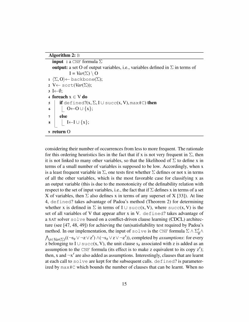
Algorithm 2: Binput : a CNF formula Σoutput: a set O of output variables, i.e., variables defined in Σ in terms of

I = Var(Σ) \ O1 〈Σ, O〉← backbone(Σ);2 V← sort(Var(Σ));3 I←∅;4 foreach x ∈ V do5 if defined?(x, Σ, I ∪ succ(x, V),max#C) then6 O←O ∪ x;7 else8 I←I ∪ x;

9 return O

considering their number of occurrences from less to more frequent. The rationalefor this ordering heuristics lies in the fact that if x is not very frequent in Σ, thenit is not linked to many other variables, so that the likelihood of Σ to define x interms of a small number of variables is supposed to be low. Accordingly, when xis a least frequent variable in Σ, one tests first whether Σ defines or not x in termsof all the other variables, which is the most favorable case for classifying x asan output variable (this is due to the monotonicity of the definability relation withrespect to the set of input variables, i.e., the fact that if Σ defines x in terms of a setX of variables, then Σ also defines x in terms of any superset of X [33]). At line4, defined? takes advantage of Padoa’s method (Theorem 2) for determiningwhether x is defined in Σ in terms of I ∪ succ(x, V), where succ(x, V) is theset of all variables of V that appear after x in V. defined? takes advantage ofa SAT solver solve based on a conflict-driven clause learning (CDCL) architec-ture (see [47, 48, 49]) for achieving the (un)satisfiability test required by Padoa’smethod. In our implementation, the input of solve is the CNF formula Σ∧Σ′∅∧∧

z∈Var(Σ)((¬sz∨¬z∨z′) ∧(¬sz∨z∨¬z′)), completed by assumptions: for everyz belonging to I ∪ succ(x, V), the unit clause sz associated with z is added as anassumption to the CNF formula (its effect is to make z equivalent to its copy z′);then, x and ¬x′ are also added as assumptions. Interestingly, clauses that are learntat each call to solve are kept for the subsequent calls. defined? is parameter-ized by max#C which bounds the number of clauses that can be learnt. When no

15

contradiction has been found before max#C is reached, defined? returns false(i.e., x is considered as not defined in Σ in terms of I ∪ succ(x, V), while thiscould be questioned had a larger bound be considered).

Clearly enough, the number of output variables found by B cannot be guar-anteed to be as large as possible (or equivalently, the number of input variablesfound by B is not guaranteed to be as small as possible). This is due to the factthat the insertion of a variable in I at line 8 of B cannot be questioned by the ex-ecution of a subsequent instruction of this algorithm. But, as already explained,this lack of optimality is on purpose, for the sake of efficiency. Indeed, in B, thenumber of calls to solve does not exceed the number of variables occurring inΣ. Nevertheless, one can ensure that:

Proposition 3. Let Σ be a CNF formula. The set O computed by B is such that〈I, O〉 where I = Var(Σ) \ O is a subset-minimal definability bipartition of Σ.

Proof: First of all, every variable x of Var(Σ) such that x or ¬x belongs to thebackbone of Σ is such that x is defined in Σ in terms of ∅. Thus, any subset-minimal definability bipartition 〈I, O〉 of Σ must guarantee that those variables xbelong to O. This is ensured in B by the instruction at line 1.

Let us now focus on the remaining set V of variables. In B, the variablesx ∈ V are considered from the ones having the smallest number of occurrencesin Σ (after simplification) to those having the greatest number of occurrences inΣ (after simplification). However, the result stated in Proposition 3 actually holdswhatever the ordering<with respect to which the variables of V are visited. Thus,we prove by induction on k = #(succ(x, V)) that every variable x put into O atline 6 of B is defined in Σ in terms of I. The base case is when k = 0 so thatx is the last variable of V with respect to <. In that case, succ(x, V) = ∅ sothat x is put into O when the test at line 5 is evaluated to true, i.e., when x isdefined in Σ in terms of I, and we are done. Suppose now that the property holdsfor k = p ≥ 1 and let us show that it still holds for k = p + 1. So, let x bethe variable of V such that #(succ(x, V)) = p + 1. Line 5 of B ensures that xis put into O when the corresponding test is evaluated to true. At the step whenx is processed, the current value of I is the set Ix which contains the variablesthat will be in I at the end of the execution of B and are before x with respectto <. Thus, assuming that prec(x, V) denotes the set of variables of V that areconsidered before x with respect to <, we have Ix = I ∩ prec(x, V) and x isput into O when defined?(x, Σ, Ix ∪ succ(x, V),max#C) is evaluated to true,i.e., when x is defined in Σ in terms of Ix ∪ succ(x, V). But Ix ∪ succ(x, V) =

16

(I ∩ prec(x, V)) ∪ succ(x, V) = (I ∩ prec(x, V)) ∪ (I ∩ succ(x, V)) ∪ (O ∩succ(x, V)) = (I ∩ (V \ x)) ∪ (O ∩ succ(x, V)). Furthermore, if x is put inO, then x does not belong to I. Therefore, in this case, we have that x is definedin Σ in terms of Ix ∪ succ(x, V) = I ∪ (O ∩ succ(x, V)). Now, by inductionhypothesis, every variable y ∈ succ(x, V) belongs to O if and only if y is definedin Σ in terms of I. Thus, all the variables y from O ∩ succ(x, V) can be removedfrom I ∪ (O ∩ succ(x, V)) while preserving the fact that x is defined in Σ. Weget that if x is put into O at line 6 of B, then x is defined in Σ in terms of I. Thisimplies that every variable in O is defined in Σ in terms of I, hence the pair 〈I, O〉returned by B is a definability bipartition of Σ.

Finally, it remains to prove that this definability bipartition 〈I, O〉 is subset-minimal. Towards a contradiction, suppose that there exists x ∈ I such that 〈I \x, O ∪ x〉 is a definability bipartition of Σ. Since x has been put into I byB, it must be the case that defined?(x, Σ, Ix ∪ succ(x, V),max#C) has beenevaluated to false, i.e., x is not defined in Σ from (I ∩ prec(x, V)) ∪ succ(x, V).Furthermore, we have that I \ x = I ∩ (prec(x, V) ∪ succ(x, V)) = (I ∩prec(x, V))∪ (I∩succ(x, V)) ⊆ (I∩prec(x, V))∪succ(x, V). However, if xis not defined in Σ from (I∩ prec(x, V))∪ succ(x, V), then x cannot be definedin Σ from a subset I \ x of it. This contradicts the fact that 〈I \ x, O ∪ x〉 isa definability bipartition of Σ.

Note that it would be easy to derive an ”anytime” version of B without ques-tioning the fact that its output O is such that 〈I = Var(Σ) \ O, O〉 is a definabil-ity bipartition of Σ. Indeed, when the time limit under consideration would bereached, it would be enough to put into I every variable that has not been put intoO at this point.

Interestingly, the correctness of B (as given by Proposition 3) does not requireany assumption on the representation of Σ (i.e., Σ is not necessarily a CNF for-mula from LP ). Thus, the approach followed (i.e., find a definability bipartitionof Σ, then eliminate some output variables) is sound when the input is not a CNFformula, and in such a case, it can be less demanding from a computational stand-point than the case when CNF inputs are considered. Consider for instance thecase when Σ is a DNF formula. While computing ‖Σ‖ is still #P-complete whenΣ is a DNF formula, the definability problem (determine whether Σ defines a givenx in terms of a given X) and the variable elimination problem can be solved in (de-terministic) polynomial time (see Lemma 27 in [33] and Propositions 17 and 18 in[42]). Thus, when Σ is a DNF formula, it makes sense to consider a more aggres-sive strategy for computing a definability bipartition (since each definability testis not very time consuming, one can try to minimize the cardinality of I), and to

17

eliminate every variable from O in the variable elimination step (this can be donein linear time in the size of Σ and can reduce significantly the size of Σ). However,this does not imply that exploiting duality and computing ‖Σ‖ for a CNF formulaΣ as 2#Var(Σ) – ‖¬Σ‖ is always a good idea from a computational point of view.Indeed, even if a DNF formula equivalent to ¬Σ can be computed in time linear inthe size of Σ, it is in general not the case that Σ and ¬Σ define the same variables.Thus, it can easily be the case that a definability bipartition of Σ with a ”small”I exists, while every variable of Var(Σ) is undefinable in ¬Σ. For instance, con-sider Σ =

∧ni=1 xi. Every xi (i ∈ 1, . . . , n) belongs to the backbone of Σ so that

〈∅, Var(Σ)〉 is a definability bipartition of Σ such that I = ∅ is of smallest cardinal-ity; conversely, every xi (i ∈ 1, . . . , n) is undefinable in ¬Σ which is equivalentto

∨ni=1 ¬xi.

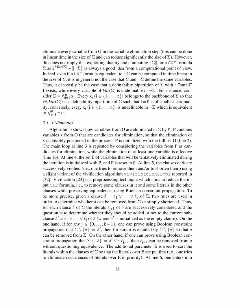
3.3. E(liminate)Algorithm 3 shows how variables from O are eliminated in Σ by E. P contains

variables x from O that are candidates for elimination, so that the elimination ofx is possibly postponed in the process. P is initialized with the full set O (line 2).The main loop at line 3 is repeated by considering the variables from P as can-didates for elimination, while the elimination of at least one variable is effective(line 16). At line 4, the set E of variables that will be tentatively eliminated duringthe iteration is initialized with P, and P is reset to ∅. At line 5, the clauses of Φ aresuccessively vivified (i.e., one tries to remove them and/or to shorten them) usinga slight variant of the vivification algorithm vivificationSimpl reported in[32]. Vivification [23] is a preprocessing technique which aims to reduce the in-put CNF formula, i.e., to remove some clauses in it and some literals in the otherclauses while preserving equivalence, using Boolean constraint propagation. Tobe more precise, given a clause δ = `1 ∨ . . . ∨ `k of Σ, two rules are used inorder to determine whether δ can be removed from Σ or simply shortened. Thus,for each clause δ of Σ the literals `j+1 of δ are successively considered and thequestion is to determine whether they should be added or not to the current sub-clause δ′ = `1 ∨ . . . ∨ `j of δ (where δ′ is initialized as the empty clause). On theone hand, if for any j ∈ 0, . . . , k – 1, one can prove using Boolean constraintpropagation that Σ \ δ |= δ′, then for sure δ is entailed by Σ \ δ so that δcan be removed from Σ. On the other hand, if one can prove using Boolean con-straint propagation that Σ \ δ |= δ′ ∨ ∼`j+1, then `j+1 can be removed from δwithout questioning equivalence. The additional parameter E is used to sort theliterals within the clauses of Σ so that the literals over E are put first (i.e., one triesto eliminate occurrences of literals over E in priority). At line 6, one enters into

18

Algorithm 3: Einput : a CNF formula Σ and a set of output variables O ⊆ Var(Σ)output: a CNF formula Φ such that Φ ≡ ∃E.Σ for some E ⊆ O

1 Φ←Σ;2 iterate←true; P←O;3 while iterate do4 E←P; P←∅; iterate←false;5 Φ←vivificationSimpl(Φ, E);6 while E 6= ∅ do7 x←select(E, Φ);8 E←E \ x;9 Φ←occurrenceSimpl(Φ, x);

10 if #(Φx)× #(Φ¬x) > max#Res then11 P←P ∪ x12 else13 R←removeSub(Res(x, Φ), Φ);14 if #((Φ \ Φx,¬x) ∪ R) ≤ #(Φ) then15 Φ←(Φ \ Φx,¬x) ∪ R;16 iterate←true;

17 else18 P←P ∪ x

19 return Φ

19

the inner loop that operates while there are remaining variables in E. At line 7,a variable x is selected in E for being possibly eliminated by counting the num-ber #(Φx) of clauses of Φ where x appears as a positive literal, and the number#(Φ¬x) of clauses of Φ where ¬x appears as a negative literal; x is retained if itminimizes #(Φx)×#(Φ¬x), which is an upper bound of the number of resolventsthat the elimination of x in Φ may generate. At line 8, x is removed from E. Then,at line 9, one tries first to eliminate in Φ some occurrences of variable x usingoccurrenceSimpl. occurrenceSimpl is a restriction of the algorithm foroccurrence simplification reported in [32], where instead of considering the wholeset of literals occurring in Φ, we just focus on those in x,¬x. At line 10, onerecomputes #(Φx)×#(Φ¬x) and checks whether it exceeds or not a preset boundmax#Res. If this is the case, then we possibly postpone the elimination of x inΦ at the next iteration by adding it to P (line 11). Otherwise, we compute the setRes(x, Φ) of all non-valid resolvents of clauses from Φ on x and we remove fromit using removeSub every clause that is properly subsumed by a clause of Φ oranother clause from Res(x, Φ); the resulting set of clauses is R (line 13). At line14, we test whether the elimination of x in Φ, obtained by removing from Φ itssubset Φx,¬x of the clauses into which variable x occurs (either as a positive literalor as a negative literal), and adding the resolvents from R, leads or not to increas-ing the number of clauses in Φ. If so, then we possibly postpone the eliminationof x in Φ at the next iteration by adding it to P (line 18). If not, the elimination ofx in Φ is committed (line 15).

The worst-case time complexity of Algorithm E is in O(|O|2 · |Σ|3). Indeed,the inner loop is executed only if at least one variable has been eliminated atthe previous step, hence every variable of O cannot be considered more than aquadratic number of times as a candidate for being eliminated. The worst-casetime complexity of Boolean constraint propagation is linear in the input size [50],but quadratic when the set of clauses considered by solve is implemented usingwatched literals [49], which is the case in our implementation.3 Under this as-sumption, the vivification algorithm used in the outer loop has a time complexitythat is cubic in its input size, and the occurrence simplification algorithm usedin the inner loop has a time complexity that is cubic in the size of its input. Ateach step, the size of the CNF formula under consideration can only increase by aconstant term, which can be neglected.

It is easy to show that Algorithm E is correct:

3In practice, it typically runs in sublinear time in the input size.

20

Proposition 4. Let Σ be a CNF formula and O be a set of variables of Σ. TheCNF formula Φ computed by E is such that Φ ≡ ∃E.Σ for some E ⊆ O.

Proof: The result comes directly from three observations:(1) the fact that vivificationSimpl is an equivalence-preserving prepro-cessing technique, (2) the variables x that are eliminated belong to O (see lines 2,4 and 7 of E), and (3) ∃x.Σ is equivalent to the formula obtained by adding firstto Σ all resolvents on x of the clauses of Σ, then removing in the resulting set allthe clauses containing x as a variable. This is performed by the instructions atlines 13 and 15 of E (the additional suppression of valid or subsumed resolventsachieved by removeSub is harmless since it is equivalence-preserving).

Again, it would be easy to derive an ”anytime” version of E without ques-tioning its correctness. Indeed, when the time limit under consideration would bereached, it would be enough to stop the elimination process at this point (i.e., notconsidering the variables of O that are in E or in P).

4. Empirical Results

Let us now present the experiments which have been done for evaluating B + Eand comparing it with pmc, our previous preprocessor for model counting.

4.1. Empirical SettingIn our experiments, we have considered 703 CNF instances from the SATLIB4

and other repositories (for instance, the benchmarks from the BN family (Bayesiannetworks) come from http://reasoning.cs.ucla.edu/ace/). All thebenchmarks used in our experiments can be downloaded from http://www.cril.univ-artois.fr/KC/bpe2.html. They are gathered into 8 datasets, as follows: BN (192), BMC (Bounded Model Checking) (18), Circuit (41),Configuration (35), Handmade (58), Planning (248), Random (104), Qif (7) (Quan-titative Information Flow analysis - security).

All the experiments have been conducted on a cluster of Intel Xeon E5-2643(3.30 GHz) quad core processors with 32 GiB RAM. The kernel used was CentOS7, Linux version 3.10.0-514.16.1.el7.x86 64. The compiler used was gcc version5.3.1. Hyperthreading was disabled, and no cache share between cores was al-lowed. A time-out of 1h and a memory-out of 7.6 GiB has been considered for

4www.cs.ubc.ca/˜hoos/SATLIB/index-ubc.html

21

each instance. We set max#Res to 500. We took advantage of the runsolver5

tool [51] for controlling the resources used by the SAT solver solve used in ourexperiments, namely the incremental version of Glucose described in [52] (runwith its default setting).

As a matter of comparison, we have considered the pmc preprocessor formodel counting, described in [32] and available on www.cril.fr/KC/. To bemore precise, we considered pmc equipped with the #eq combination of prepro-cessing techniques, which combines backbone simplification, occurrence elimi-nation, vivification and gates detection and replacement. pmc equipped with #eqproved empirically as a very efficient preprocessor for model counting [32].

We evaluated the impact of B + E (for several values of max#C) by couplingit with exact model counters. We considered the search-based model countersCachet6 [53] and SharpSAT7 [54], run with their default settings. Thoughcompilation-based approaches do much more than model counting (since theycompute equivalent, compiled representations of the input CNF formula Σ andnot only the number of models of Σ), some of them appear as competitive forthe model counting purpose. Thus, we also took advantage of such compilers,namely C2D8 [55, 56] and d49 [37]. Those compilers generate a Decision-DNNFrepresentation Σ∗ of the input Σ. The size of Σ∗ is exponential in the size of Σin the worst case, but the number of models of Σ conditioned by any consistentterm γ can be computed efficiently from Σ∗ in every case. And when γ is >, onegets the number of models of Σ. C2D has been invoked with the following options-count -in memory -smooth all, which are suited when C2D is used asa model counter. d4 has been invoked with its default options.

4.2. ResultsTable 1 makes precise the number of instances (out of 703) solved within

1h by each of the model counters Cachet, SharpSAT, C2D and d4 (first col-umn), when no preprocessing technique has been applied (second column), pmc(equipped with #eq) has been applied first (third column), and finally B + E(Σ)for several values of max#C has been applied first (the remaining columns). The

5www.cril.fr/˜roussel/runsolver6www.cs.rochester.edu/˜kautz/Cachet/7sites.google.com/site/marcthurley/sharpsat8reasoning.cs.ucla.edu/c2d/9www.cril.univ-artois.fr/KC/d4.html

22

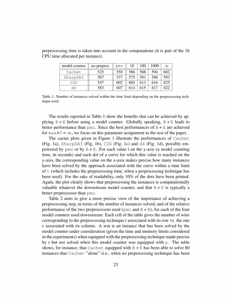
preprocessing time is taken into account in the computations (it is part of the 1hCPU time allocated per instance).

model counter no preproc. pmc 10 100 1000 ∞Cachet 525 558 586 588 594 602SharpSAT 507 537 575 581 586 593

C2D 547 602 605 613 616 625d4 583 607 614 615 617 622

Table 1: Number of instances solved within the time limit depending on the preprocessing tech-nique used.

The results reported in Table 1 show the benefits that can be achieved by ap-plying B + E before using a model counter. Globally speaking, B + E leads tobetter performance than pmc. Since the best performances of B + E are achievedfor max#C =∞, we focus on this parameter assignment in the rest of the paper.

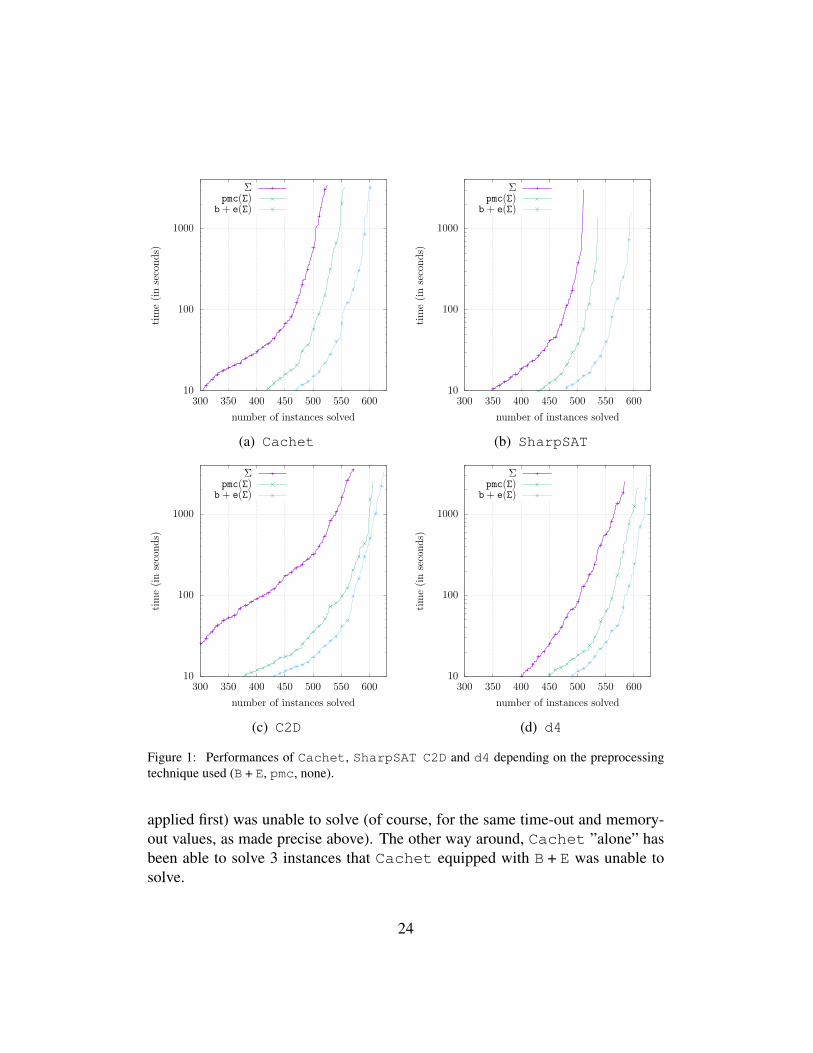
The cactus plots given in Figure 1 illustrate the performances of Cachet(Fig. 1a), SharpSAT (Fig. 1b), C2D (Fig. 1c) and d4 (Fig. 1d), possibly em-powered by pmc or by B + E. For each value t on the y-axis (a model countingtime, in seconds) and each dot of a curve for which this value is reached on they-axis, the corresponding value on the x-axis makes precise how many instanceshave been solved by the approach associated with the curve within a time limitof t (which includes the preprocessing time, when a preprocessing technique hasbeen used). For the sake of readability, only 10% of the dots have been printed.Again, the plot clearly shows that preprocessing the instances is computationallyvaluable whatever the downstream model counter, and that B + E is typically abetter preprocessor than pmc.

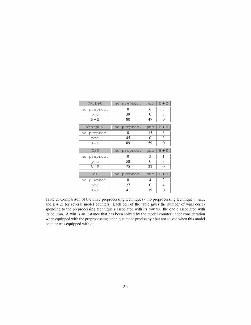
Table 2 aims to give a more precise view of the importance of achieving apreprocessing step, in terms of the number of instances solved, and of the relativeperformance of the two preprocessors used (pmc and B + E), for each of the fourmodel counters used downstream. Each cell of the table gives the number of winscorresponding to the preprocessing technique r associated with its row vs. the onec associated with its column. A win is an instance that has been solved by themodel counter under consideration (given the time and memory limits consideredin the experiments) when equipped with the preprocessing technique made preciseby r but not solved when this model counter was equipped with c. The tableshows, for instance, that Cachet equipped with B + E has been able to solve 80instances that Cachet ”alone” (i.e., when no preprocessing technique has been

23

10

100

1000

300 350 400 450 500 550 600

tim

e(i

nse

cond

s)

number of instances solved

Σpmc(Σ)

b + e(Σ)

(a) Cachet

10

100

1000

300 350 400 450 500 550 600

tim

e(i

nse

cond

s)number of instances solved

Σpmc(Σ)

b + e(Σ)

(b) SharpSAT

10

100

1000

300 350 400 450 500 550 600

tim

e(i

nse

cond

s)

number of instances solved

Σpmc(Σ)

b + e(Σ)

(c) C2D

10

100

1000

300 350 400 450 500 550 600

tim

e(i

nse

cond

s)

number of instances solved

Σpmc(Σ)

b + e(Σ)

(d) d4

Figure 1: Performances of Cachet, SharpSAT C2D and d4 depending on the preprocessingtechnique used (B + E, pmc, none).

applied first) was unable to solve (of course, for the same time-out and memory-out values, as made precise above). The other way around, Cachet ”alone” hasbeen able to solve 3 instances that Cachet equipped with B + E was unable tosolve.

24

Cachet no preproc. pmc B + Eno preproc. 0 6 3

pmc 39 0 3B + E 80 47 0

SharpSAT no preproc. pmc B + Eno preproc. 0 15 3

pmc 45 0 3B + E 89 59 0

C2D no preproc. pmc B + Eno preproc. 0 3 1

pmc 58 0 3B + E 75 22 0

d4 no preproc. pmc B + Eno preproc. 0 4 3

pmc 27 0 4B + E 41 19 0

Table 2: Comparison of the three preprocessing techniques (”no preprocessing technique”, pmc,and B + E) for several model counters. Each cell of the table gives the number of wins corre-sponding to the preprocessing technique r associated with its row vs. the one c associated withits column. A win is an instance that has been solved by the model counter under considerationwhen equipped with the preprocessing technique made precise by r but not solved when this modelcounter was equipped with c.

25

Clearly enough, the results reported in Table 2 show that adding a preprocess-ing step is in general useful, and that B + E typically performs better than pmc,even if those observations cannot be lifted to each instance taken separately. Thefact that a preprocessing technique does not always help is easy to understandsince, for instance, it can be the case that no reductions of the input instance arefeasible (this is often the case when this instance has already been preprocessed).Thus, when no gates exist in the input CNF formula, the time used to search forthem is just wasted (and this wasted time can be much higher when B + E is used,compared to pmc since, so to say, B + E has the potential to ”find out” many moregates than the ones pmc can discover in the input).

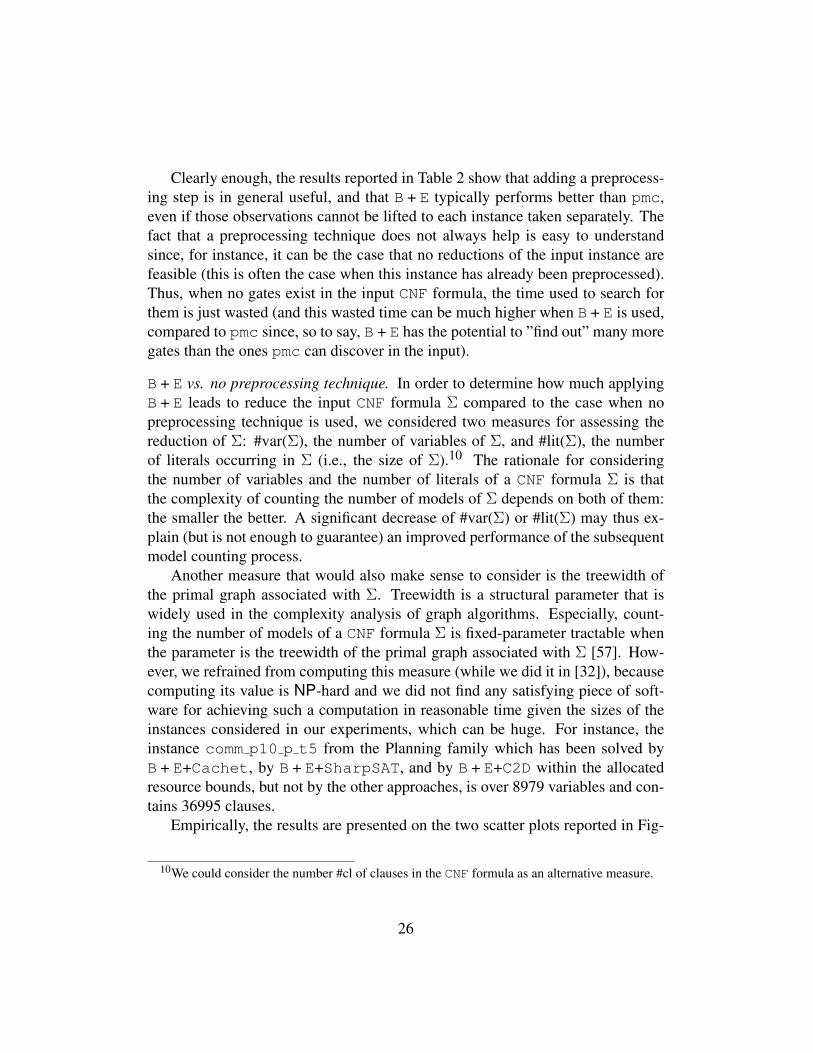
B + E vs. no preprocessing technique. In order to determine how much applyingB + E leads to reduce the input CNF formula Σ compared to the case when nopreprocessing technique is used, we considered two measures for assessing thereduction of Σ: #var(Σ), the number of variables of Σ, and #lit(Σ), the numberof literals occurring in Σ (i.e., the size of Σ).10 The rationale for consideringthe number of variables and the number of literals of a CNF formula Σ is thatthe complexity of counting the number of models of Σ depends on both of them:the smaller the better. A significant decrease of #var(Σ) or #lit(Σ) may thus ex-plain (but is not enough to guarantee) an improved performance of the subsequentmodel counting process.

Another measure that would also make sense to consider is the treewidth ofthe primal graph associated with Σ. Treewidth is a structural parameter that iswidely used in the complexity analysis of graph algorithms. Especially, count-ing the number of models of a CNF formula Σ is fixed-parameter tractable whenthe parameter is the treewidth of the primal graph associated with Σ [57]. How-ever, we refrained from computing this measure (while we did it in [32]), becausecomputing its value is NP-hard and we did not find any satisfying piece of soft-ware for achieving such a computation in reasonable time given the sizes of theinstances considered in our experiments, which can be huge. For instance, theinstance comm p10 p t5 from the Planning family which has been solved byB + E+Cachet, by B + E+SharpSAT, and by B + E+C2D within the allocatedresource bounds, but not by the other approaches, is over 8979 variables and con-tains 36995 clauses.

Empirically, the results are presented on the two scatter plots reported in Fig-

10We could consider the number #cl of clauses in the CNF formula as an alternative measure.

26

101

102

103

104

105

101 102 103 104 105

B+E(Σ,∞

)

Σ

QifHandmadePlanningCircuit

ConfigurationRandom

BMCBN

(a) #var reductions

101

102

103

104

105

106

101 102 103 104 105 106

B+E(Σ,∞

)Σ

QifHandmadePlanningCircuit

ConfigurationRandom

BMCBN

(b) #lit reductions

Figure 2: Reductions achieved by B + E in terms of number of variables and in terms of the size ofthe formula (comparison with the case when no preprocessing technique has been applied). Eachpoint corresponds to an instance Σ, its x-coordinate corresponds to the value of the measure (#varor #lit) when no pre-processing is used, while its y-coordinate corresponds to the value of the samemeasure on B + E(Σ).

ure 9a, and Figure 9b. In these figures, each point corresponds to an instanceΣ, its x-coordinate corresponds to the value of the measure (#var or #lit) whenno pre-processing is used, while its y-coordinate corresponds to the value of thesame measure on B + E(Σ) (with max#Conflicts = ∞). The scales used forboth coordinates are logarithmic.

Clearly enough, using B + E often leads to large reductions for both measures.The benefits appear as very significant for instances from the Planning family, theBMC family, and, to some extent, for the BN family. As to #lit reduction, wecan observe that for some benchmarks it is, so to say, ”negative”, that is, the sizeof the output CNF formula is sometimes slightly larger than the size of the input.This comes from the fact that E only ensures that the number of clauses does notincrease whenever a variable is eliminated (which is not the same as guaranteeingthat the number of literals will not increase).

We have also evaluated how much B + E leads to reduction of the overallmodel counting time compared to the case when no preprocessing technique isused. The results are presented on the four scatter plots (with logarithmic scales)reported in Figure 3a, Figure 3b, Figure 3c, and Figure 3d for the ”direct” model

27

counters Cachet and SharpSAT and the compilation-based counters C2D andd4 considered downstream.

Each point corresponds to an instance Σ (a CNF formula), its x-coordinatecorresponds to the time (in seconds) required to compute ‖Σ‖ by calling the modelcounter on it, while its y-coordinate corresponds to the time required to compute‖Σ‖ by computing B + E(Σ) (with max#Conflicts=∞) first, then calling themodel counter on the resulting CNF formula. Again, whatever the downstreammodel counter, applying B + E appears as useful in many cases, when the overallmodel counting time can be significantly reduced. This is particularly the case forthe model counter C2D, for which improvements are obtained very often (actually,for 624 instances over 703). This comes from the fact that the cutsets of the nodesof the decomposition tree of B + E(Σ) used by C2D for guiding the decompositionprocess and generating a Decision-DNNF representation are typically of smallersize than the cutsets of the nodes of the decomposition tree of Σ.

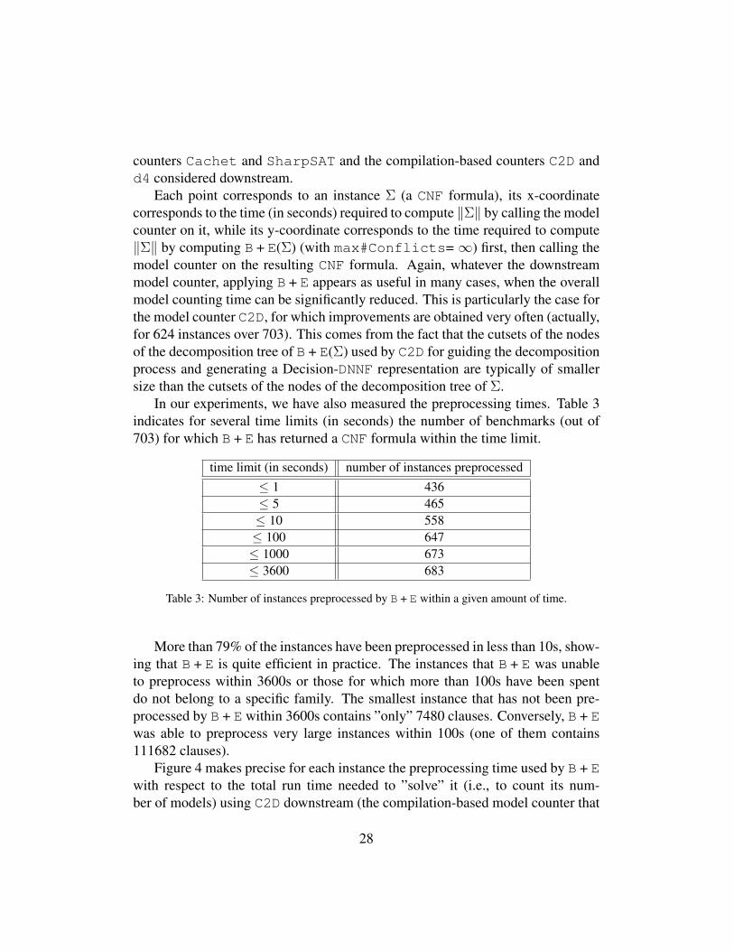
In our experiments, we have also measured the preprocessing times. Table 3indicates for several time limits (in seconds) the number of benchmarks (out of703) for which B + E has returned a CNF formula within the time limit.

time limit (in seconds) number of instances preprocessed≤ 1 436≤ 5 465≤ 10 558≤ 100 647≤ 1000 673≤ 3600 683

Table 3: Number of instances preprocessed by B + E within a given amount of time.

More than 79% of the instances have been preprocessed in less than 10s, show-ing that B + E is quite efficient in practice. The instances that B + E was unableto preprocess within 3600s or those for which more than 100s have been spentdo not belong to a specific family. The smallest instance that has not been pre-processed by B + E within 3600s contains ”only” 7480 clauses. Conversely, B + Ewas able to preprocess very large instances within 100s (one of them contains111682 clauses).

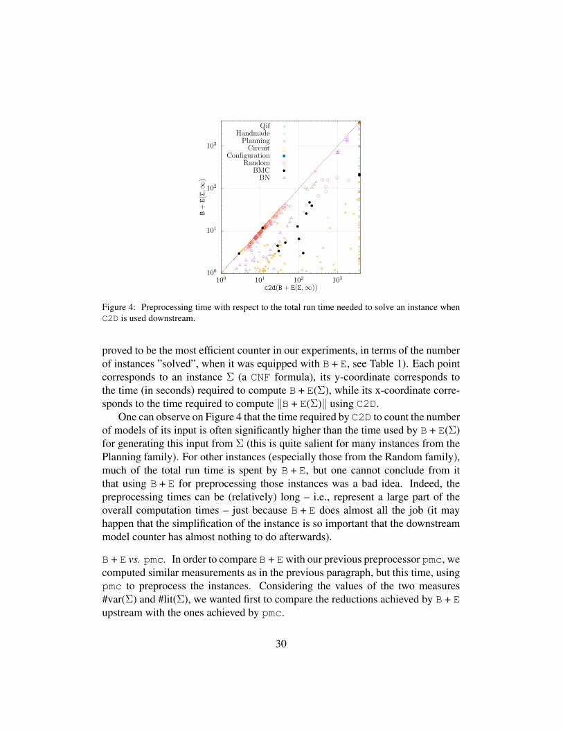
Figure 4 makes precise for each instance the preprocessing time used by B + Ewith respect to the total run time needed to ”solve” it (i.e., to count its num-ber of models) using C2D downstream (the compilation-based model counter that

28

10−1

100

101

102

103

10−1 100 101 102 103

Cachet(B

+E(Σ,∞

))

Cachet(Σ)

QifHandmadePlanningCircuit

ConfigurationRandom

BMCBN

(a) Cachet

10−1

100

101

102

103

10−1 100 101 102 103

Cachet(B

+E(Σ,∞

))

Cachet(Σ)

QifHandmadePlanningCircuit

ConfigurationRandom

BMCBN

(b) SharpSAT

10−1

100

101

102

103

10−1 100 101 102 103

Cachet(B

+E(Σ,∞

))

Cachet(Σ)

QifHandmadePlanningCircuit

ConfigurationRandom

BMCBN

(c) C2D

10−1

100

101

102

103

10−1 100 101 102 103

Cachet(B

+E(Σ,∞

))

Cachet(Σ)

QifHandmadePlanningCircuit

ConfigurationRandom

BMCBN

(d) d4

Figure 3: Performances of the model counters depending on the preprocessing technique used(B + E vs. no preprocessing technique). Each point corresponds to an instance Σ, its x-coordinatecorresponds to the time (in seconds) required to compute ‖Σ‖ by calling the model counter on it,while its y-coordinate corresponds to the time required to compute ‖Σ‖ by computing B + E(Σ)first, then calling the model counter on the resulting CNF formula.

29

100

101

102

103

100 101 102 103

B+E(Σ,∞

)

c2d(B+ E(Σ,∞))

QifHandmadePlanningCircuit

ConfigurationRandom

BMCBN

Figure 4: Preprocessing time with respect to the total run time needed to solve an instance whenC2D is used downstream.

proved to be the most efficient counter in our experiments, in terms of the numberof instances ”solved”, when it was equipped with B + E, see Table 1). Each pointcorresponds to an instance Σ (a CNF formula), its y-coordinate corresponds tothe time (in seconds) required to compute B + E(Σ), while its x-coordinate corre-sponds to the time required to compute ‖B + E(Σ)‖ using C2D.

One can observe on Figure 4 that the time required by C2D to count the numberof models of its input is often significantly higher than the time used by B + E(Σ)for generating this input from Σ (this is quite salient for many instances from thePlanning family). For other instances (especially those from the Random family),much of the total run time is spent by B + E, but one cannot conclude from itthat using B + E for preprocessing those instances was a bad idea. Indeed, thepreprocessing times can be (relatively) long – i.e., represent a large part of theoverall computation times – just because B + E does almost all the job (it mayhappen that the simplification of the instance is so important that the downstreammodel counter has almost nothing to do afterwards).

B + E vs. pmc. In order to compare B + Ewith our previous preprocessor pmc, wecomputed similar measurements as in the previous paragraph, but this time, usingpmc to preprocess the instances. Considering the values of the two measures#var(Σ) and #lit(Σ), we wanted first to compare the reductions achieved by B + Eupstream with the ones achieved by pmc.

30

101

102

103

104

105

106

101 102 103 104 105 106

B+E(Σ,∞

)

pmc(Σ)

QifHandmadePlanningCircuit

ConfigurationRandom

BMCBN

(a) #var reductions

101

102

103

104

105

106

101 102 103 104 105 106

B+E(Σ,∞

)pmc(Σ)

QifHandmadePlanningCircuit

ConfigurationRandom

BMCBN

(b) #lit reductions

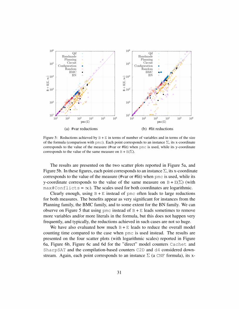
Figure 5: Reductions achieved by B + E in terms of number of variables and in terms of the sizeof the formula (comparison with pmc). Each point corresponds to an instance Σ, its x-coordinatecorresponds to the value of the measure (#var or #lit) when pmc is used, while its y-coordinatecorresponds to the value of the same measure on B + E(Σ).

The results are presented on the two scatter plots reported in Figure 5a, andFigure 5b. In these figures, each point corresponds to an instance Σ, its x-coordinatecorresponds to the value of the measure (#var or #lit) when pmc is used, while itsy-coordinate corresponds to the value of the same measure on B + E(Σ) (withmax#Conflicts =∞). The scales used for both coordinates are logarithmic.

Clearly enough, using B + E instead of pmc often leads to large reductionsfor both measures. The benefits appear as very significant for instances from thePlanning family, the BMC family, and to some extent for the BN family. We canobserve on Figure 5 that using pmc instead of B + E leads sometimes to removemore variables and/or more literals in the formula, but this does not happen veryfrequently, and typically, the reductions achieved in such cases are not so huge.

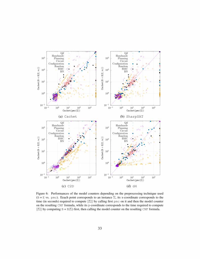
We have also evaluated how much B + E leads to reduce the overall modelcounting time compared to the case when pmc is used instead. The results arepresented on the four scatter plots (with logarithmic scales) reported in Figure6a, Figure 6b, Figure 6c and 6d for the ”direct” model counters Cachet andSharpSAT and the compilation-based counters C2D and d4 considered down-stream. Again, each point corresponds to an instance Σ (a CNF formula), its x-

31

coordinate corresponds to the time (in seconds) required to compute ‖Σ‖ by call-ing first pmc on it and then the model counter on the resulting CNF formula, whileits y-coordinate corresponds to the time required to compute ‖Σ‖ by computingB + E(Σ) (with max#Conflicts= ∞) first, then calling the model counter onthe resulting CNF formula.

We can observe that whatever the downstream model counter among the fourones we have considered, B + E appears typically as a better preprocessor thanpmc in the sense that it leads typically to improved performances (smaller com-putation times). The rightmost parts of the two scatter plots cohere with the resultsreported in Table 1, showing a number of instances that can be solved by any ofthe model counters when B + E has been applied first, while they cannot be solvedwithin the time limit of 1h when pmc is used instead. Of course, the computationalbenefits that are reported on these plots are less impressive than those offered byB + E compared to the case when no preprocessing technique is applied (pmc isquite a ”good” preprocessor in many cases).

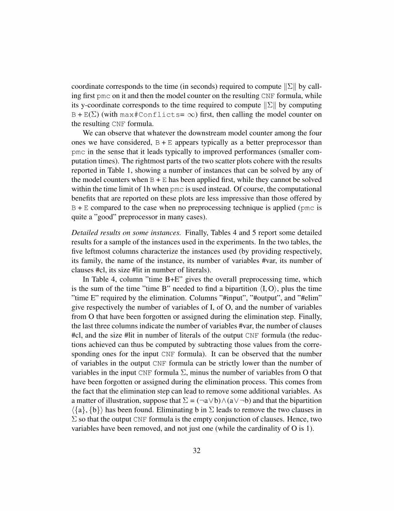
Detailed results on some instances. Finally, Tables 4 and 5 report some detailedresults for a sample of the instances used in the experiments. In the two tables, thefive leftmost columns characterize the instances used (by providing respectively,its family, the name of the instance, its number of variables #var, its number ofclauses #cl, its size #lit in number of literals).

In Table 4, column ”time B+E” gives the overall preprocessing time, whichis the sum of the time ”time B” needed to find a bipartition 〈I, O〉, plus the time”time E” required by the elimination. Columns ”#input”, ”#output”, and ”#elim”give respectively the number of variables of I, of O, and the number of variablesfrom O that have been forgotten or assigned during the elimination step. Finally,the last three columns indicate the number of variables #var, the number of clauses#cl, and the size #lit in number of literals of the output CNF formula (the reduc-tions achieved can thus be computed by subtracting those values from the corre-sponding ones for the input CNF formula). It can be observed that the numberof variables in the output CNF formula can be strictly lower than the number ofvariables in the input CNF formula Σ, minus the number of variables from O thathave been forgotten or assigned during the elimination process. This comes fromthe fact that the elimination step can lead to remove some additional variables. Asa matter of illustration, suppose that Σ = (¬a∨b)∧(a∨¬b) and that the bipartition〈a, b〉 has been found. Eliminating b in Σ leads to remove the two clauses inΣ so that the output CNF formula is the empty conjunction of clauses. Hence, twovariables have been removed, and not just one (while the cardinality of O is 1).

32

10−1

100

101

102

103

10−1 100 101 102 103

Cachet(B

+E(Σ,∞

))

Cachet(pmc(Σ))

QifHandmadePlanningCircuit

ConfigurationRandom

BMCBN

(a) Cachet

10−1

100

101

102

103

10−1 100 101 102 103

Cachet(B

+E(Σ,∞

))

Cachet(pmc(Σ))

QifHandmadePlanningCircuit

ConfigurationRandom

BMCBN

(b) SharpSAT

10−1

100

101

102

103

10−1 100 101 102 103

Cachet(B

+E(Σ,∞

))

Cachet(pmc(Σ))

QifHandmadePlanningCircuit

ConfigurationRandom

BMCBN

(c) C2D

10−1

100

101

102

103

10−1 100 101 102 103

Cachet(B

+E(Σ,∞

))

Cachet(pmc(Σ))

QifHandmadePlanningCircuit

ConfigurationRandom

BMCBN

(d) d4

Figure 6: Performances of the model counters depending on the preprocessing technique used(B + E vs. pmc). Eeach point corresponds to an instance Σ, its x-coordinate corresponds to thetime (in seconds) required to compute ‖Σ‖ by calling first pmc on it and then the model counteron the resulting CNF formula, while its y-coordinate corresponds to the time required to compute‖Σ‖ by computing B + E(Σ) first, then calling the model counter on the resulting CNF formula.

33

In Table 5, after the description of the input CNF instance Σ (five first columns),one can find three groups of columns, corresponding to the model counting task ofΣ for three scenarios: no preprocessing technique (group Σ), use of pmc (grouppmc(Σ)), and use of B + E (group B + E(Σ)). Within in each group, one canfind the time (in seconds) needed by each one of the four counters Cachet,SharpSAT, C2D and d4 for making its job (it includes the preprocessing time, ifany). ”TO” means that a time out has been reached, and ”MO” that the process hasaborted due to insufficient memory. When a preprocessing technique took place(groups pmc(Σ) and B + E(Σ)), columns ”time pmc” and ”time B+E” indicate(respectively) the time spent by the application of the preprocessing technique.Columns #var, #cl, #lit indicate (respectively) the number of variables, number ofclauses, and size of the CNF formula that has resulted from the application of thepreprocessing technique and then be used as input of the model counters.

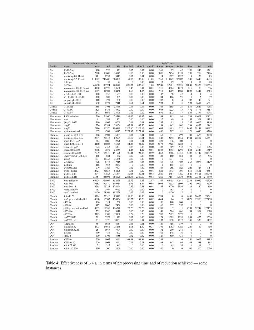
Benchmark Informations B+E(Σ,∞)Family Name #var #cl #lit time B+E time B time E #input #output #elim #var #cl #litBN 50-10-9-q 460 720 1921 0.03 0.02 0.00 361 99 42 196 340 1261BN 90-50-9-q 12300 19600 34149 16.86 16.85 0.00 9806 2494 1959 390 709 2426BN blockmap 05 01.net 1411 2737 5413 0.02 0.01 0.00 14 1397 1027 19 28 65BN blockmap 22 03.net 119003 247486 504902 57.15 36.09 21.05 261 118742 93182 585 1640 4915BN fs-01.net 32 38 74 0 0.00 0.00 13 19 9 11 12 28BN fs-19.net 65930 113924 260642 698.32 696.68 1.63 27949 37981 28025 32889 52573 131575BN mastermind 03 08 04.net 4720 10920 23608 0.46 0.44 0.01 216 4504 4119 216 180 376BN mastermind 10 08 03.net 5887 12901 28468 1.60 1.55 0.04 918 4969 4604 1093 1444 3383BN or-50-5-1-UC-10 100 250 653 0.00 0.00 0.00 42 58 47 4 1 4BN or-100-20-10-UC-10 200 500 1309 0.00 0.00 0.00 84 116 91 18 5 19BN sat-grid-pbl-0010 110 191 738 0.00 0.00 0.00 102 8 4 102 143 521BN sat-grid-pbl-0030 930 1771 7018 0.61 0.61 0.00 922 8 5 922 1697 6671Config C129 FR 1888 7404 23769 0.13 0.13 0.00 703 1185 21 554 2643 7998Config C140 FC 1828 5451 14572 0.10 0.10 0.00 605 1223 13 472 1793 5887Config C140 FV 1843 8056 33705 0.12 0.12 0.00 671 1172 17 539 2173 6948Handmade 5 100 sd schur 500 26860 78510 289.65 289.63 0.01 388 112 98 388 11669 52832Handmade ais6 61 581 1351 0.00 0.00 0.00 12 49 8 53 361 1105Handmade fphp-015-020 300 4965 10200 0.01 0.01 0.00 285 15 15 285 4665 13110Handmade lang12 576 13584 28134 42.59 42.55 0.04 134 442 102 384 4872 12142Handmade lang23 2116 96370 196489 2522.80 2522.13 0.67 633 1483 322 1495 38141 93997Handmade ls10-normalized 657 4761 10017 2277.82 2277.81 0.00 440 217 81 576 4680 16290Planning blocks right 2 p t5 406 1901 5407 0.02 0.01 0.00 65 341 299 107 678 2210Planning blocks right 6 p t6 3337 30517 82699 58.59 58.11 0.48 545 2792 1554 1784 22512 65591Planning bomb b5 t1 p t5 564 1086 2796 0.01 0.01 0.00 228 336 300 0 0 0Planning bomb b20 t5 p t10 14100 28025 75525 34.27 34.07 0.20 6575 7525 7250 0 0 0Planning coins p01 p t5 872 2353 5901 0.06 0.06 0.00 303 569 532 176 560 1256Planning coins p10 p t10 3898 9879 24559 1.43 1.42 0.01 1505 2393 2294 634 2443 5569Planning comm p10 p t10 17539 75516 191696 25.44 24.85 0.59 3853 13686 10353 6402 37147 104679Planning emptyroom d4 g2 p t5 188 584 1532 0.00 0.00 0.00 28 160 152 44 168 576Planning hanoi5 1931 14468 35856 0.00 0.00 0.00 0 1931 16 0 0 0Planning logistics.a 828 6718 17915 0.05 0.04 0.00 153 675 489 265 1078 3129Planning medium 116 953 2133 0 0.00 0.00 1 115 35 0 0 0Planning prob001.pddl 939 3785 7727 0.02 0.02 0.00 183 756 168 209 444 1061Planning prob012.pddl 2324 31857 64476 0.51 0.49 0.01 681 1643 701 850 4681 10551Planning uts k10 p t6 13047 89563 215484 39.94 39.41 0.53 2580 10467 6366 3880 54591 121740Planning uts k10 p t10 21451 148891 358620 2281.53 2280.69 0.84 4260 17191 10130 6920 93351 211340BMC bmc-galileo-9 63624 326999 852078 22.72 19.85 2.87 169 63455 30641 2238 11032 42720BMC bmc-ibm-1 9685 55870 149914 1.91 1.87 0.03 1033 8652 2809 392 1002 3616BMC bmc-ibm-13 13215 65728 174164 0.32 0.31 0.01 145 13070 2986 29 30 150BMC cnt06.shuffled 762 2469 6753 0.00 0.00 0.00 0 762 5 0 0 0BMC cnt10.shuffled 20470 68561 187229 0.02 0.02 0.00 0 20470 17 0 0 0Circuit 3bitadd 32 8704 32316 89472 158.56 158.56 0.00 8704 0 0 4480 26475 70341Circuit alu2 gr rcs w8.shuffled 4080 83902 170864 86.22 86.20 0.02 4064 16 2 4078 83900 172438Circuit c432.isc 196 514 1258 0.00 0.00 0.00 36 160 160 0 0 0Circuit c880.isc 417 1060 2466 0.00 0.00 0.00 60 357 357 0 0 0Circuit c880 gr rcs w7.shuffled 4592 61745 126770 23.26 23.26 0.00 4585 7 1 4591 61744 127153Circuit c1355.isc 555 1546 3610 0.06 0.06 0.00 41 514 461 94 304 1080Circuit c7552.isc 3185 8588 19808 0.29 0.28 0.00 208 2977 2977 5 5 18Circuit ssa7552-038 1501 3575 11823 0.07 0.06 0.00 179 1322 1055 239 475 1536Circuit ssa7552-160 1391 3126 10151 0.05 0.04 0.00 133 1258 1017 180 330 1112QIF 10random 587 1685 4157 0.01 0.01 0.00 129 458 379 0 0 0QIF binsearch.32 4473 14011 35245 1.64 1.42 0.21 391 4082 3788 227 87 600QIF binsearch.32.pp 251 1917 7304 0.00 0.00 0.00 32 219 218 0 0 0QIF mixdup 309 452 1092 0.00 0.00 0.00 161 148 76 0 0 0QIF sum.32 639 1708 4356 0.02 0.02 0.00 129 510 438 0 0 0Random uf250-01 250 1065 3195 168.94 168.94 0.00 249 1 0 250 1065 3195Random uf250-0100 250 1065 3195 0.21 0.21 0.00 103 147 93 143 338 868Random wff.3.75.315 75 315 945 0 0.00 0.00 10 65 55 10 11 22Random wff.4.100.500 100 500 2000 0.00 0.00 0.00 100 0 0 100 500 2000

Table 4: Effectiveness of B + E in terms of preprocessing time and of reduction achieved — someinstances.

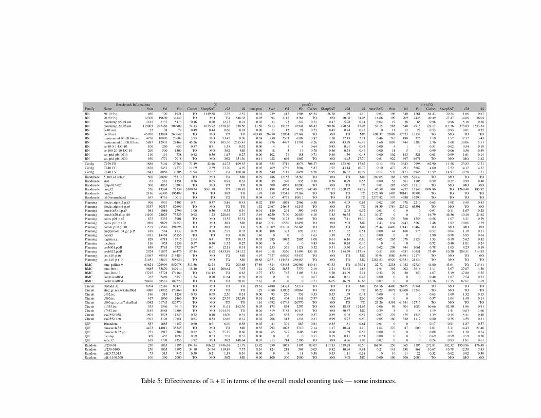
Benchmark Informations Σ pmc(Σ) B + E(Σ)Family Name #var #cl #lit Cachet SharpSAT c2d d4 time pmc #var #cl #lit Cachet SharpSAT c2d d4 time B+E #var #cl #lit Cachet SharpSAT c2d d4BN 50-10-9-q 460 720 1921 TO 1149.58 2.38 2.52 0.01 239 412 1508 65.54 28.28 1.49 1.10 0.03 196 340 1261 64.43 20.24 1.06 0.67BN 90-50-9-q 12300 19600 34149 TO MO TO 1848.38 8.05 1094 2117 6761 TO MO 20.08 34.03 16.86 390 709 2426 40.49 27.47 34.88 26.04BN blockmap 05 01.net 1411 2737 5413 0.46 0.20 12.72 0.24 0.03 33 92 247 0.72 0.47 5.28 0.41 0.02 19 28 65 0.58 0.98 5.16 0.38BN blockmap 22 03.net 119003 247486 504902 74.13 1075.92 1370.26 338.56 81.50 5413 18167 47548 86.43 90.36 490.64 87.03 57.15 585 1640 4915 122.17 117.76 573.83 1553.54BN fs-01.net 32 38 74 0.49 0.44 0.66 0.24 0.00 11 12 28 0.73 0.45 0.74 0.42 0 11 12 28 0.53 0.93 0.61 0.25BN fs-19.net 65930 113924 260642 TO MO TO TO 403.49 26950 52934 127148 TO MO TO MO 698.32 32889 52573 13157 TO MO TO TOBN mastermind 03 08 04.net 4720 10920 23608 3.75 MO 53.45 9.30 0.24 750 2533 6799 3.82 1.50 22.43 2.71 0.46 216 180 376 1.10 1.57 17.37 3.43BN mastermind 10 08 03.net 5887 12901 28468 45.26 MO 105.30 2555.43 0.86 1776 4497 11791 19.26 MO 43.79 46.45 1.60 1093 1444 3383 2.76 3.08 30.06 5.51BN or-50-5-1-UC-10 100 250 653 0.57 0.51 1.55 0.52 0.00 4 1 4 0.64 0.45 0.91 0.43 0.00 4 1 4 0.51 0.02 0.54 0.19BN or-100-20-10-UC-10 200 500 1309 TO MO MO MO 0.00 18 5 19 0.70 0.46 0.74 0.46 0.00 18 5 19 0.99 0.06 0.50 0.39BN sat-grid-pbl-0010 110 191 738 0.62 0.50 1.67 0.27 0.00 102 71 188 0.71 0.40 1.39 0.48 0.00 102 143 521 0.63 0.99 1.61 0.14BN sat-grid-pbl-0030 930 1771 7018 TO MO MO 651.30 0.11 922 669 1867 TO MO 4.45 27.70 0.61 922 1697 6671 TO MO MO 3.42Config C129 FR 1888 7404 23769 71.49 42.46 44.72 109.55 0.08 555 2711 8076 308.27 MO 122.80 17.62 0.13 554 2643 7998 162.90 11.58 23.82 12.21Config C140 FC 1828 5451 14572 11.69 2.59 33.20 4.97 0.05 469 1781 5804 5.87 1.92 43.14 10.72 0.10 472 1793 5887 4.60 2.52 14.12 4.52Config C140 FV 1843 8056 33705 21.94 22.67 TO 160.04 0.09 540 2115 6491 18.58 15.95 16.37 16.97 0.12 539 2173 6948 12.59 14.97 30.50 7.57Handmade 5 100 sd schur 500 26860 78510 TO MO TO MO 0.79 486 12155 35263 TO MO TO MO 289.65 388 11669 52832 TO MO TO TOHandmade ais6 61 581 1351 0.56 0.65 0.98 0.33 0.00 59 390 935 0.50 0.58 0.99 0.55 0.00 53 361 1105 0.59 0.17 0.99 0.40Handmade fphp-015-020 300 4965 10200 TO MO TO TO 0.08 300 4965 10200 TO MO TO TO 0.01 285 4665 13110 TO MO MO MOHandmade lang12 576 13584 28134 3300.24 3061.78 TO 210.83 0.11 198 4724 9970 947.49 1272.12 1360.22 48.28 42.59 384 4872 12142 1999.86 TO 1269.40 185.92Handmade lang23 2116 96370 196489 TO TO MO TO 1.93 759 37515 77169 TO TO TO TO 2522.80 1495 38141 93997 TO TO TO TOHandmade ls10-normalized 657 4761 10017 TO TO TO TO 0.04 657 4761 10017 TO TO TO TO 2277.82 576 4680 16290 TO TO TO TOPlanning blocks right 2 p t5 406 1901 5407 0.71 0.37 5.86 0.43 0.02 189 1078 2966 0.58 0.59 4.05 0.64 0.02 107 678 2210 0.65 1.08 3.48 0.43Planning blocks right 6 p t6 3337 30517 82699 TO MO TO TO 1.52 2467 24643 61245 TO MO TO TO 58.59 1784 22512 65591 TO MO TO MOPlanning bomb b5 t1 p t5 564 1086 2796 1.00 0.30 9.33 0.34 0.01 180 208 590 0.93 0.54 2.03 0.52 0.01 0 0 0 0.91 0.11 1.67 0.28Planning bomb b20 t5 p t10 14100 28025 75525 0.92 1.23 228.69 2.37 5.49 6750 7100 20450 6.10 5.85 86.52 5.49 34.27 0 0 0 16.79 46.36 40.40 21.62Planning coins p01 p t5 872 2353 5901 TO MO 13.55 35.51 0.10 390 1173 3069 TO MO 7.11 19.30 0.06 176 560 1256 0.58 1.07 6.21 0.29Planning coins p10 p t10 3898 9879 24559 TO MO MO MO 0.48 2051 6556 16491 TO MO MO MO 1.43 634 2443 5569 2.48 1.82 20.06 2.59Planning comm p10 p t10 17539 75516 191696 TO MO MO TO 5.90 11209 61138 156145 TO MO TO MO 25.44 6402 37147 10467 TO MO MO MOPlanning emptyroom d4 g2 p t5 188 584 1532 0.69 0.28 2.95 0.35 0.00 108 323 892 0.52 0.52 1.82 0.51 0.00 44 168 576 0.52 0.04 1.30 0.31Planning hanoi5 1931 14468 35856 TO TO TO 0.88 1.46 0 0 0 1.63 3.39 1.55 1.70 0.00 0 0 0 1.90 0.58 6.95 0.64Planning logistics.a 828 6718 17915 2.64 0.41 TO 10.15 0.05 285 1082 2805 1.08 0.61 6.16 0.80 0.05 265 1078 3129 1.53 0.19 5.62 0.82Planning medium 116 953 2133 0.57 0.30 1.72 0.27 0.00 0 0 0 0.83 0.46 0.24 0.46 0 0 0 0 0.72 0.40 1.01 0.24Planning prob001.pddl 939 3785 7727 0.67 0.61 12.11 0.31 0.01 255 531 1128 0.52 0.51 5.70 0.46 0.02 209 444 1061 0.78 1.03 4.23 0.19Planning prob012.pddl 2324 31857 64476 57.44 8.92 1453.89 681.12 0.44 1018 5576 11494 155.10 5.33 184.59 117.48 0.51 850 4681 10551 75.49 10.20 284.51 314.93Planning uts k10 p t6 13047 89563 215484 TO MO TO MO 4.93 7627 68520 153437 TO MO TO MO 39.94 3880 54591 12174 TO MO TO MOPlanning uts k10 p t10 21451 148891 358620 TO MO TO MO 10.88 12671 114438 256483 TO MO TO MO 2281.53 6920 93351 21134 TO MO TO TOBMC bmc-galileo-9 63624 326999 852078 313.56 42.24 TO 203.68 87.89 4524 93463 260369 140.41 93.33 TO 1179.31 22.72 2238 11032 42720 41.00 43.61 TO 215.41BMC bmc-ibm-1 9685 55870 149914 15.40 2.14 260.64 7.55 1.24 1242 2855 7370 2.19 2.21 33.62 1.86 1.91 392 1002 3616 3.11 3.67 27.07 4.50BMC bmc-ibm-13 13215 65728 174164 TO 114.12 TO 8.83 2.77 172 745 2105 5.34 5.20 43.09 5.14 0.32 29 30 150 4.67 5.19 47.80 5.25BMC cnt06.shuffled 762 2469 6753 1.34 0.20 11.64 0.39 0.01 0 0 0 0.67 0.46 0.81 0.42 0.00 0 0 0 0.48 1.07 2.54 0.33BMC cnt10.shuffled 20470 68561 187229 TO MO TO 20.10 2.63 0 0 0 17.71 16.05 16.39 16.63 0.02 0 0 0 16.76 17.15 87.61 11.69Circuit 3bitadd 32 8704 32316 89472 TO MO TO TO 19.61 4480 24323 55214 TO TO TO MO 158.56 4480 26475 70341 TO MO TO TOCircuit alu2 gr rcs w8.shuffled 4080 83902 170864 TO MO TO TO 1.29 4080 83902 170864 TO MO TO TO 86.22 4078 83900 17243 TO MO TO TOCircuit c432.isc 196 514 1258 0.73 0.68 2.50 0.31 0.00 93 266 733 0.53 0.55 1.69 0.43 0.00 0 0 0 0.63 1.09 1.32 0.15Circuit c880.isc 417 1060 2466 TO MO 25.79 242.89 0.01 142 404 1141 15.97 4.32 2.84 2.00 0.00 0 0 0 0.57 1.04 1.48 0.14Circuit c880 gr rcs w7.shuffled 4592 61745 126770 TO MO TO TO 1.16 4592 61745 126770 TO MO TO TO 23.26 4591 61744 12715 TO MO TO TOCircuit c1355.isc 555 1546 3610 TO MO 11.61 162.36 0.03 175 854 2297 TO MO 18.93 124.67 0.06 94 304 1080 60.66 82.50 1.96 0.91Circuit c7552.isc 3185 8588 19808 TO MO 1014.39 TO 0.26 819 3158 10113 TO MO 50.87 MO 0.29 5 5 18 1.19 1.41 10.63 1.66Circuit ssa7552-038 1501 3575 11823 0.72 0.40 14.06 0.34 0.03 263 532 1548 0.57 0.59 5.05 0.57 0.07 239 475 1536 1.29 0.15 5.41 0.40Circuit ssa7552-160 1391 3126 10151 0.63 0.34 12.66 0.32 0.02 208 413 1236 0.31 0.99 5.27 0.50 0.05 180 330 1112 0.80 0.75 4.59 0.31QIF 10random 587 1685 4157 0.60 0.61 6.40 0.58 0.03 41 301 883 0.61 0.35 1.81 0.61 0.01 0 0 0 0.17 0.81 1.87 0.57QIF binsearch.32 4473 14011 35245 TO MO TO MO 0.55 292 1022 2710 2.14 1.17 10.94 1.10 1.64 227 87 600 2.01 3.11 14.43 21.46QIF binsearch.32.pp 251 1917 7304 0.82 6.07 25.15 0.68 0.04 65 595 1606 0.49 0.60 1.59 0.58 0.00 0 0 0 0.08 0.21 1.30 0.54QIF mixdup 309 452 1092 0.59 0.53 2.07 0.52 0.00 0 0 0 0.57 0.59 0.11 0.51 0.00 0 0 0 0.69 0.59 0.59 0.30QIF sum.32 639 1708 4356 3.92 MO MO 148.64 0.01 213 714 2386 TO MO 4.96 1.03 0.02 0 0 0 0.24 0.83 1.81 0.61Random uf250-01 250 1065 3195 194.54 106.22 1746.68 21.79 13.92 250 1065 3195 83.07 117.83 1739.28 30.50 168.94 250 1065 3195 272.81 302.32 1950.96 176.48Random uf250-0100 250 1065 3195 34.10 24.74 119.89 7.75 8.34 124 218 501 10.05 9.82 10.94 9.91 0.21 143 338 868 10.67 10.78 12.58 7.43Random wff.3.75.315 75 315 945 0.59 0.21 1.39 0.34 0.00 9 9 18 0.38 0.45 1.11 0.38 0 10 11 22 0.52 0.62 0.92 0.30Random wff.4.100.500 100 500 2000 TO MO MO MO 0.00 100 500 2000 TO MO MO MO 0.00 100 500 2000 TO MO MO MO

Table 5: Effectiveness of B + E in terms of the overall model counting task — some instances.

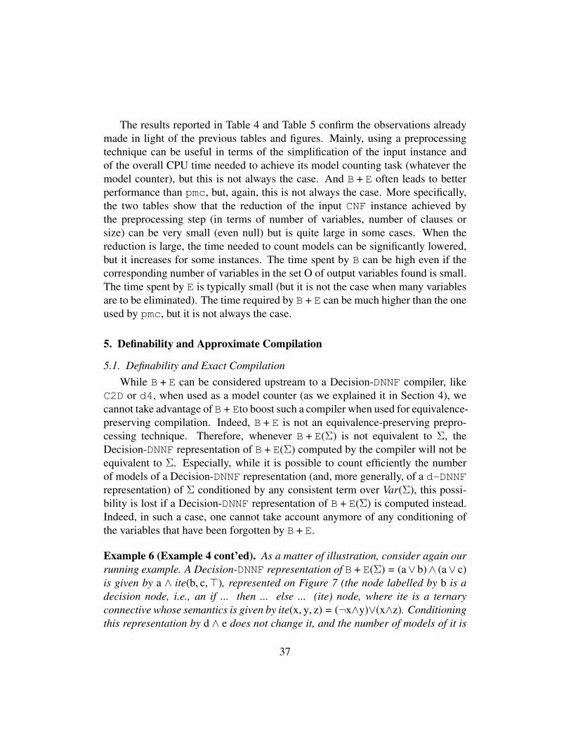
The results reported in Table 4 and Table 5 confirm the observations alreadymade in light of the previous tables and figures. Mainly, using a preprocessingtechnique can be useful in terms of the simplification of the input instance andof the overall CPU time needed to achieve its model counting task (whatever themodel counter), but this is not always the case. And B + E often leads to betterperformance than pmc, but, again, this is not always the case. More specifically,the two tables show that the reduction of the input CNF instance achieved bythe preprocessing step (in terms of number of variables, number of clauses orsize) can be very small (even null) but is quite large in some cases. When thereduction is large, the time needed to count models can be significantly lowered,but it increases for some instances. The time spent by B can be high even if thecorresponding number of variables in the set O of output variables found is small.The time spent by E is typically small (but it is not the case when many variablesare to be eliminated). The time required by B + E can be much higher than the oneused by pmc, but it is not always the case.

5. Definability and Approximate Compilation

5.1. Definability and Exact CompilationWhile B + E can be considered upstream to a Decision-DNNF compiler, like

C2D or d4, when used as a model counter (as we explained it in Section 4), wecannot take advantage of B + Eto boost such a compiler when used for equivalence-preserving compilation. Indeed, B + E is not an equivalence-preserving prepro-cessing technique. Therefore, whenever B + E(Σ) is not equivalent to Σ, theDecision-DNNF representation of B + E(Σ) computed by the compiler will not beequivalent to Σ. Especially, while it is possible to count efficiently the numberof models of a Decision-DNNF representation (and, more generally, of a d-DNNFrepresentation) of Σ conditioned by any consistent term over Var(Σ), this possi-bility is lost if a Decision-DNNF representation of B + E(Σ) is computed instead.Indeed, in such a case, one cannot take account anymore of any conditioning ofthe variables that have been forgotten by B + E.

Example 6 (Example 4 cont’ed). As a matter of illustration, consider again ourrunning example. A Decision-DNNF representation of B + E(Σ) = (a∨ b)∧ (a∨ c)is given by a ∧ ite(b, c,>), represented on Figure 7 (the node labelled by b is adecision node, i.e., an if ... then ... else ... (ite) node, where ite is a ternaryconnective whose semantics is given by ite(x, y, z) = (¬x∧y)∨(x∧z). Conditioningthis representation by d ∧ e does not change it, and the number of models of it is

37

∧

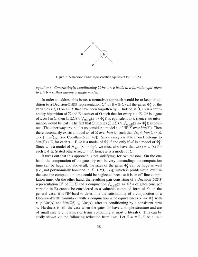
a b

c >

Figure 7: A Decision-DNNF representation equivalent to B + E(Σ).

equal to 3. Contrastingly, conditioning Σ by d ∧ e leads to a formula equivalentto a ∧ b ∧ c, thus having a single model.

In order to address this issue, a (tentative) approach would be to keep in ad-dition to a Decision-DNNF representation Σ∗ of B + E(Σ) all the gates Φx

I of thevariables x ∈ O on I in Σ that have been forgotten by E. Indeed, if 〈I, O〉 is a defin-ability bipartition of Σ and E a subset of O such that for every x ∈ E, Φx

I is a gateof x on I in Σ, then (∃E.Σ)∧ (

∧x∈E(x↔ Φx

I )) is equivalent to Σ (hence, no infor-mation would be lost). The fact that Σ implies (∃E.Σ)∧ (

∧x∈E(x↔ Φx

I )) is obvi-ous. The other way around, let us consider a model ω of ∃E.Σ over Var(Σ). Thenthere necessarily exists a model ω′ of Σ over Var(Σ) such that ∀xi ∈ Var(Σ) \ E,ω(xi) = ω′(xi) (see Corollary 5 in [42]). Since every variable from I belongs toVar(Σ) \ E, for each x ∈ E, ω is a model of Φx

I if and only if ω′ is a model of ΦxI .

Since ω is a model of∧

x∈E(x ↔ ΦxI ), we must also have that ω(x) = ω′(x) for

each x ∈ E. Stated otherwise, ω = ω′, hence ω is a model of Σ.It turns out that this approach is not satisfying, for two reasons. On the one

hand, the computation of the gates ΦxI can be very demanding: the computation

time can be huge, and above all, the sizes of the gates ΦxI can be huge as well

(i.e., not polynomially bounded in |Σ| + #(I) [33]) which is problematic, even inthe case the computation time could be neglected because it is an off-line compi-lation time. On the other hand, the resulting pair consisting of a Decision-DNNFrepresentation Σ∗ of ∃E.Σ and a conjunction

∧x∈E(x ↔ Φx

I )〉 of gates (one pervariable in E) cannot be considered as a valuable compiled form of Σ: in thegeneral case, it is NP-hard to determine the satisfiability of a conjunction of aDecision-DNNF formula α with a conjunction κ of equivalences x ↔ Φx

I withx 6∈ Var(α) and Var(Φx

I ) ⊆ Var(α), after its conditioning by a consistent termγ. Hardness is still the case when the gates Φx

I have a simple structure and areof small size (e.g., clauses or terms containing at most 3 literals). This can beeasily shown via the following reduction from SAT. Let β =

∧mi=1 δi be a CNF

38

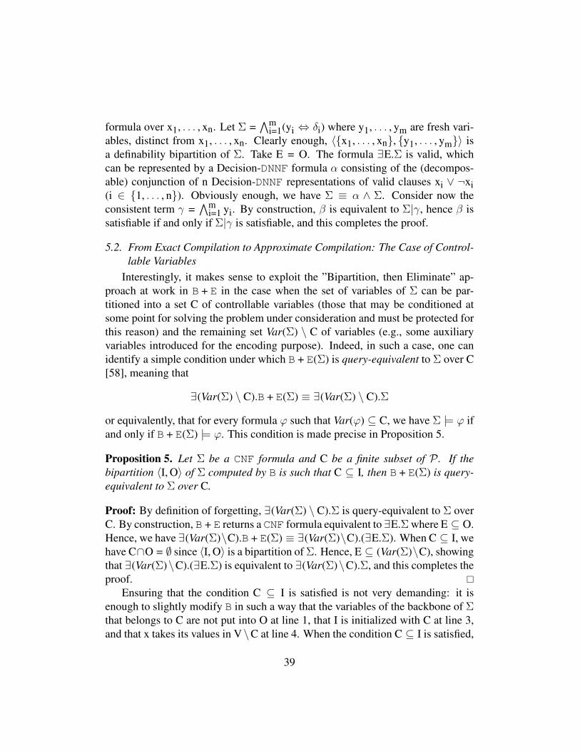
formula over x1, . . . , xn. Let Σ =∧m

i=1(yi ⇔ δi) where y1, . . . , ym are fresh vari-ables, distinct from x1, . . . , xn. Clearly enough, 〈x1, . . . , xn, y1, . . . , ym〉 isa definability bipartition of Σ. Take E = O. The formula ∃E.Σ is valid, whichcan be represented by a Decision-DNNF formula α consisting of the (decompos-able) conjunction of n Decision-DNNF representations of valid clauses xi ∨ ¬xi(i ∈ 1, . . . , n). Obviously enough, we have Σ ≡ α ∧ Σ. Consider now theconsistent term γ =

∧mi=1 yi. By construction, β is equivalent to Σ|γ, hence β is

satisfiable if and only if Σ|γ is satisfiable, and this completes the proof.

5.2. From Exact Compilation to Approximate Compilation: The Case of Control-lable Variables

Interestingly, it makes sense to exploit the ”Bipartition, then Eliminate” ap-proach at work in B + E in the case when the set of variables of Σ can be par-titioned into a set C of controllable variables (those that may be conditioned atsome point for solving the problem under consideration and must be protected forthis reason) and the remaining set Var(Σ) \ C of variables (e.g., some auxiliaryvariables introduced for the encoding purpose). Indeed, in such a case, one canidentify a simple condition under which B + E(Σ) is query-equivalent to Σ over C[58], meaning that

∃(Var(Σ) \ C).B + E(Σ) ≡ ∃(Var(Σ) \ C).Σ

or equivalently, that for every formula ϕ such that Var(ϕ) ⊆ C, we have Σ |= ϕ ifand only if B + E(Σ) |= ϕ. This condition is made precise in Proposition 5.

Proposition 5. Let Σ be a CNF formula and C be a finite subset of P . If thebipartition 〈I, O〉 of Σ computed by B is such that C ⊆ I, then B + E(Σ) is query-equivalent to Σ over C.

Proof: By definition of forgetting, ∃(Var(Σ) \ C).Σ is query-equivalent to Σ overC. By construction, B + E returns a CNF formula equivalent to ∃E.Σ where E ⊆ O.Hence, we have ∃(Var(Σ)\C).B + E(Σ) ≡ ∃(Var(Σ)\C).(∃E.Σ). When C ⊆ I, wehave C∩O = ∅ since 〈I, O〉 is a bipartition of Σ. Hence, E ⊆ (Var(Σ)\C), showingthat ∃(Var(Σ)\C).(∃E.Σ) is equivalent to ∃(Var(Σ)\C).Σ, and this completes theproof.

Ensuring that the condition C ⊆ I is satisfied is not very demanding: it isenough to slightly modify B in such a way that the variables of the backbone of Σthat belongs to C are not put into O at line 1, that I is initialized with C at line 3,and that x takes its values in V\C at line 4. When the condition C ⊆ I is satisfied,

39

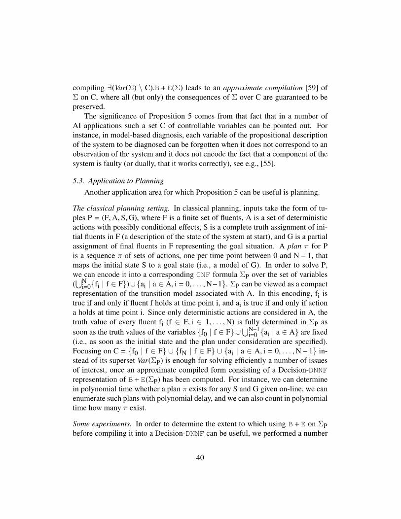
compiling ∃(Var(Σ) \ C).B + E(Σ) leads to an approximate compilation [59] ofΣ on C, where all (but only) the consequences of Σ over C are guaranteed to bepreserved.

The significance of Proposition 5 comes from that fact that in a number ofAI applications such a set C of controllable variables can be pointed out. Forinstance, in model-based diagnosis, each variable of the propositional descriptionof the system to be diagnosed can be forgotten when it does not correspond to anobservation of the system and it does not encode the fact that a component of thesystem is faulty (or dually, that it works correctly), see e.g., [55].

5.3. Application to PlanningAnother application area for which Proposition 5 can be useful is planning.

The classical planning setting. In classical planning, inputs take the form of tu-ples P = (F, A, S, G), where F is a finite set of fluents, A is a set of deterministicactions with possibly conditional effects, S is a complete truth assignment of ini-tial fluents in F (a description of the state of the system at start), and G is a partialassignment of final fluents in F representing the goal situation. A plan π for Pis a sequence π of sets of actions, one per time point between 0 and N – 1, thatmaps the initial state S to a goal state (i.e., a model of G). In order to solve P,we can encode it into a corresponding CNF formula ΣP over the set of variables(⋃N

i=0fi | f ∈ F)∪ai | a ∈ A, i = 0, . . . , N – 1. ΣP can be viewed as a compactrepresentation of the transition model associated with A. In this encoding, fi istrue if and only if fluent f holds at time point i, and ai is true if and only if actiona holds at time point i. Since only deterministic actions are considered in A, thetruth value of every fluent fi (f ∈ F, i ∈ 1, . . . , N) is fully determined in ΣP assoon as the truth values of the variables f0 | f ∈ F∪⋃N–1

i=0 ai | a ∈ A are fixed(i.e., as soon as the initial state and the plan under consideration are specified).Focusing on C = f0 | f ∈ F ∪ fN | f ∈ F ∪ ai | a ∈ A, i = 0, . . . , N – 1 in-stead of its superset Var(ΣP) is enough for solving efficiently a number of issuesof interest, once an approximate compiled form consisting of a Decision-DNNFrepresentation of B + E(ΣP) has been computed. For instance, we can determinein polynomial time whether a plan π exists for any S and G given on-line, we canenumerate such plans with polynomial delay, and we can also count in polynomialtime how many π exist.

Some experiments. In order to determine the extent to which using B + E on ΣPbefore compiling it into a Decision-DNNF can be useful, we performed a number

40

of experiments, focusing on the 530 planning instances used in [60] and availableon www.cril.fr/KC/. Those instances cover a range of different planningbenchmarks, with varying horizon length. “blocks-n” refers to the famous blocks-world domain with n blocks. “bomb-m-n” is another popular domain involvingm bombs, n toilets, and 2 actions (“dunking” a bomb into a toilet, and “flushing”a clogged toilet). “comm-m-n” is an IPC5 problem about communication signalswith m stages, n packets, and 5 actions. “emptyroom-n” is about navigating arobot in an n × n empty grid. Finally, “safe-n” is about opening a safe with npossible combinations.

All instances described in PDDL were translated into CNF theories using theDIMACS format, and then compiled using C2D and/or d4. For each instance,the set of controllable variables C consist of the variables corresponding to theactions in A (whatever the instant when they occur), the variables correspondingto the initial state S (all the fluents at time 0), and those corresponding to the goal(all the fluents at time N). B has been modified to ensure that C ⊆ I in the resultingbipartition, as explained above (which is mandatory to guarantee that no variablein C has been eliminated).

Figure 8 (a–b–c–d) contains scatter plots showing the impact of using B + E asa preprocessor before compiling the encodings ΣP of the instances into Decision-DNNF representations. Each point corresponds to a planning instance. The twocompilers C2D (a–b) and d4 (c–d) have been considered. Both the compilationtimes (a–c) in seconds and the sizes of the compiled forms (b–d) in number ofedges have been measured. As usual, the times reported include the preprocessingtimes if any.

The scatter plots in Figure 8 show that in general some computational benefitsare obtained when using B + E. They concern both the compilation times andthe sizes of the compiled form, whatever the downstream compiler. Especially,within the ressources allocated (1h CPU time and 7.6 GiB memory), C2D hasbeen able to solve 423 instances without any preprocessing technique and 451instances when B + E was used first as a preprocessor, while d4 has been ableto solve 422 instances without preprocessing technique and 443 instances whenB + E was used first as a preprocessor.

5.4. Projected Model CountingTo close the section, it is worth mentioning that approximate compilation with

controllable variables, as described before, is strongly connected to the projectedmodel counting task, as considered in [38, 39, 61].

41

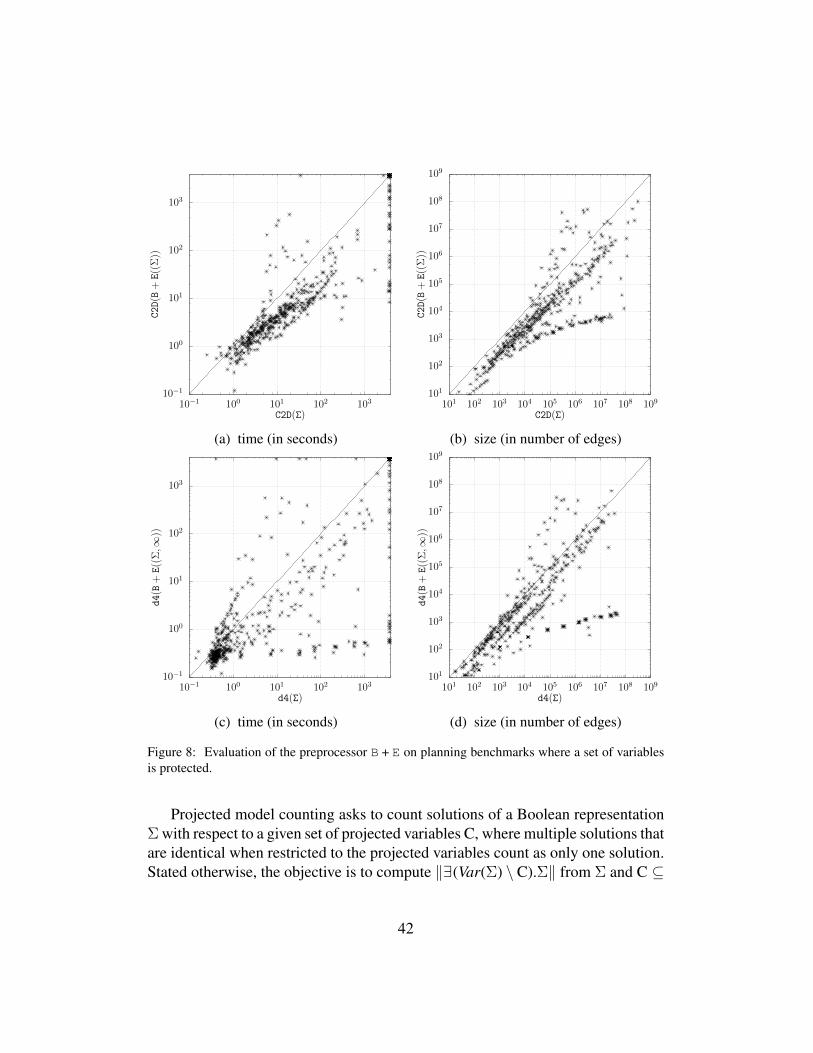
10−1

100

101

102

103

10−1 100 101 102 103

C2D(B

+E((

Σ))

C2D(Σ)

(a) time (in seconds)

101

102

103

104

105

106

107

108

109

101 102 103 104 105 106 107 108 109

C2D(B

+E((

Σ))

C2D(Σ)

(b) size (in number of edges)

10−1

100

101

102

103

10−1 100 101 102 103

d4(B

+E((

Σ,∞

))

d4(Σ)

(c) time (in seconds)

101

102

103

104

105

106

107

108

109

101 102 103 104 105 106 107 108 109

d4(B

+E((

Σ,∞

))

d4(Σ)

(d) size (in number of edges)

Figure 8: Evaluation of the preprocessor B + E on planning benchmarks where a set of variablesis protected.

Projected model counting asks to count solutions of a Boolean representationΣ with respect to a given set of projected variables C, where multiple solutions thatare identical when restricted to the projected variables count as only one solution.Stated otherwise, the objective is to compute ‖∃(Var(Σ) \ C).Σ‖ from Σ and C ⊆

42

P . Obviously, the projected model counting problem is a generalization of themodel counting one (take C = Var(Σ)), and its complexity is known to be evenharder than the one of #SAT, namely complete for the class #NP [62]. Projectedmodel counting is useful for a number of problems, especially for planning, andalso for SAT-based analysis and quantification of information flow in programs[63]. Several projected model counters have been developed accordingly [39].

Clearly enough, generating an approximate compilation of Σ when C is theset of controllable variables is an approach for determining ‖∃(Var(Σ) \ C).Σ‖.Indeed, ‖∃(Var(Σ) \C).Σ‖ can be computed in polynomial time from a Decision-DNNF representation of ∃(Var(Σ)\C).Σ or (equivalently) of ∃(Var(Σ)\C).B + E(Σ),provided that C ⊆ I is ensured. Whenever the equivalence

∃(Var(Σ) \ C).Σ ≡ ∃(Var(Σ) \ C).B + E(Σ)

holds, ‖∃(Var(Σ) \ C).Σ‖ can be easily derived from ‖∃(Var(Σ) \ C).B + E(Σ)‖(to get the former, just multiply the latter by 2r where

r = #((Var(Σ) \ Var(B + E(Σ)) ∩ C)

is the number of variables of C that have been removed from Σ by running thepreprocessor B + E on it). As a consequence, if C is the set of variables ontowhich Σ must be projected, then B + E(Σ) can be used instead of Σ as the inputof the projected model counter under consideration, provided that it is ensuredthat C is a subset of the variables I computed by B. Since the variables from thecorresponding set O have anyway to be forgotten from Σ, an alternative to lettingthe whole forgetting job to be achieved by the projected model counter is to useE in addition during a preprocessing step. Due to the reduction of the instance Σachieved by the B + E preprocessor both with respect to the number of variablesand to the number of clauses, it can easily be the case that the performance of theprojected model counter used downstream is improved.

More generally, it turns out that, when the goal is ”only” to compute thevalue ‖∃(Var(Σ) \ C).Σ‖ but no approximate compilation of Σ on C is expectedto be generated, the condition C ⊆ I imposed on the bipartition found by Bcan be relaxed. Indeed, as a direct consequence of Craig/Lyndon interpolationtheorem [64], for every variable y ∈ C, a formula ΦC is a gate of y on C in∃(Var(Σ) \ C).Σ if and only if ΦC is a gate of y on C in Σ. Stated otherwise, thegates of ∃(Var(Σ) \ C).Σ that contain only variables of C are precisely the gatesof Σ that contain only variables of C. Thanks to this result, such gates can beidentified from Σ without needing to compute explicitly ∃(Var(Σ) \ C).Σ, which

43

would be prohibitive in the general case (variable elimination is often expensivewhen many variables are to be eliminated). When the gates have been identi-fied, the corresponding output variables y can be forgotten from Σ since we have‖∃(Var(Σ)\C).Σ‖ = ‖∃y.(∃(Var(Σ)\C).Σ)‖ = ‖∃(Var(Σ)\C).(∃y.Σ)‖. The elim-ination of y in Σ can be achieved by using E or just by removing y from C andletting the projected model counter finish the job. Interestingly, B can be easilymodified to identify gates on C with output variables in C: at line 2, it is enoughto replace Var(Σ) by Var(Σ)∩C (which is the set of variables of ∃(Var(Σ)\C).Σ).Once a definability bipartition of the variables of Var(Σ) ∩ C has been computed,there are two options: either B stops and returns the set of output variables, or theloop at line 4 is executed once more, V being set this time to Var(Σ) \ C; in thelatter case, gates on Var(Σ) with output variables in Var(Σ) \ C can be identified,so that the corresponding output variables can be (tentatively) eliminated using E.Finally, the output variables y ∈ Var(Σ) \ C that have been found by B and noteliminated by E can be exploited when the projected model counter considereddownstream is based on top-down search with detection of disjoint components:though, in the general case, one has ‖∃y.Σ‖ 6= ‖Σ | ¬y‖ + ‖Σ | y‖, the equation‖∃y.Σ‖ = ‖Σ | ¬y‖+‖Σ | y‖ holds whenever y is defined in terms of Var(Σ)\yin Σ. Thus, the constraint of searching on priority variables first (those of C) thatis at the core of some projected model counters (especially, DsharpP) [39] canbe relaxed by adding to the priority variables those that are definable in the currentformula. This gives to the projected model counter the opportunity of being moreefficient via an earlier discovery of disjoint components.

6. Other Related Work

Before concluding, let us compare our approach with some additional relatedwork, concerning the two key mechanisms at work in B + E, namely variable elim-ination and definability bipartition.

6.1. Variable EliminationVariable elimination (i.e., computing ∃X.Σ from X and Σ) is a fundamen-

tal automated reasoning task. First of all, it is the approach on which the goodold Davis-Putnam’s algorithm for solving SAT was based [43]. In AI, it has manyapplications in various domains (including planning, diagnosis, belief update, rea-soning under inconsistency, etc., see [42] for details). In the area of formal verifi-cation, variable elimination also finds applications in unbounded model checking,

44

information flow analysis, predicate abstraction, etc (see e.g., [65]). In car con-figuration, it proves useful for projecting the feasible solutions (the models of agiven constraint) onto the customer codes (i.e., forgetting the manufacturer con-trol codes) [66]. More generally, in every domain where propositional encodingsare exploited, variable elimination is an important issue. Thus, it is not surprisingthat variable elimination gave rise to an extensive literature and that a number ofapproaches have been proposed so far for this purpose.

Some approaches take advantage of the fact that variable elimination can beachieved in polynomial time when the input formula Σ is a DNF formula. Ba-sically, starting with a CNF formula Σ, those approaches consist in enumerating(using a SAT solver) implicants of Σ which are then projected onto Var(Σ) \ X,resulting in terms γ over Var(Σ) \ X (see [67, 68]). By construction, each such γis an implicant of ∃X.Σ. Each time such a γ is found, a clause equivalent to ¬γ isadded to Σ and the process is repeated up to exhaustion (i.e., when the resultingΣ becomes inconsistent). The disjunction of all the γ that have been generated isa DNF formula D equivalent to ∃X.Σ. In order to keep the size of D sufficientlysmall (if possible), focusing on prime implicants (as in [69]) or even on shortestimplicants (as in [65]) prove useful.

If a CNF formula C equivalent to ∃X.Σ is expected, then the DNF formula Dmust be turned into CNF. Several techniques can be used to this end. One of themconsists in computing incrementally an OBDD representation of the DNF formulaD: starting with an OBDD representation R equivalent to > (R consists of a singlenode 1), each time a term γ is generated, an OBDD representation of it is disjoinedwith the current OBDD representation R, leading to a new OBDD representation[70]. The time needed by each step is in O(|γ| · |R|). Then, when no additionalγ is to be considered, the OBDD representation R is turned into a CNF formula,by following all paths leading to the 0 sink (corresponding to terms which areimplicants of ¬∃X.Σ) and generating their negations (which are thus implicatesof ∃X.Σ). Their conjunction is, by construction, a CNF formula C equivalent to∃X.Σ.

Another approach to compute C from D consists in exploiting duality. First,since D is a DNF formula, we can compute in linear time from it a CNF representa-tion of ¬D. Then we can apply once more the same process as above, with X = ∅and ¬D instead of Σ. Thus, one generates using a SAT solver a DNF representationof ¬D, by enumerating some implicants of it. Finally, we compute in linear timefrom it a CNF representation of ¬¬D, that is a CNF representation C of D.

Because the languages DNF and CNF are incomparable with respect to suc-cinctness [71], it can be the case that the translation to CNF leads to a formula

45

the size of which is exponentially larger (resp. smaller) than the size of the DNFformula. Furthermore, when one takes advantage of the OBDD-based approach,since the language OBDD is incomparable with respect to succinctness with DNF,it can also be the case that the OBDD obtained as an intermediate representationhas a size which is exponentially larger (resp. smaller) than the size of the DNFformula, and since OBDD is also incomparable with respect to succinctness withCNF, it can also be the case that the size of the output CNF is exponentially larger(resp. smaller) than the size of the OBDD representation.

While all those approaches can be used for the variable elimination step, itturns out that it would not make sense to take advantage of any of them givenour very objective (counting the number of models of ∃X.Σ). Indeed, those ap-proaches are not incremental in essence (the variables are eliminated as a whole,and not one by one). Clearly enough, it would not make sense to eliminate thevariables incrementally using them (by repeating the elimination process focus-ing on a single variable at each step), since as soon as a DNF formula equivalentto ∃x.Σ has been generated (with x the first variable of X to be eliminated), theelimination of all the other variables of X can be achieved easily. Incremental-ity is important since one wants to possibly avoid eliminating a variable would itbe too computationally expensive to do so. More importantly, the computationaleffort spent for computing D is much more than one expects for a preprocess-ing technique for model counting. Indeed, the DNF formula D is by constructionan irredundant, yet deterministic implicant cover of ∃X.Σ: on the one hand, re-moving a term from D might not preserve the equivalence D ≡ ∃X.Σ, and onthe other hand the terms in D are pairwise inconsistent (if gammai denotes theterm generated at step i, then each γi is an implicant of ¬γ1 ∧ . . . ∧ ¬γi–1). As aconsequence, ‖D‖ = ‖∃X.Σ‖ can be computed in polynomial time from D. Ac-cordingly, those approaches can be considered as compilation-based techniquesfor model counting.

Other approaches rely on a substitute-then-simplify principle. Basically, ap-plying this principle consists in considering the variables x of X successively andfor each of them, to replace Σ by (Σ | ¬x)∨(Σ | x) once simplified (using the lawsof Boolean calculus). By construction, the formula obtained once all the variableshave been eliminated is equivalent to ∃X.Σ. Clearly enough, such approachesare incremental ones but in spite of it, they are not suited to our purpose: theydo not ensure that the output formula ∃X.Σ is in CNF format or in DNF format(which is a requirement here since one wants to use a model counter downstream,and existing model counters take CNF formulae as inputs). Indeed, when Σ is aCNF formula, the formula generated is a disjunction of CNF formulae. Turning

46

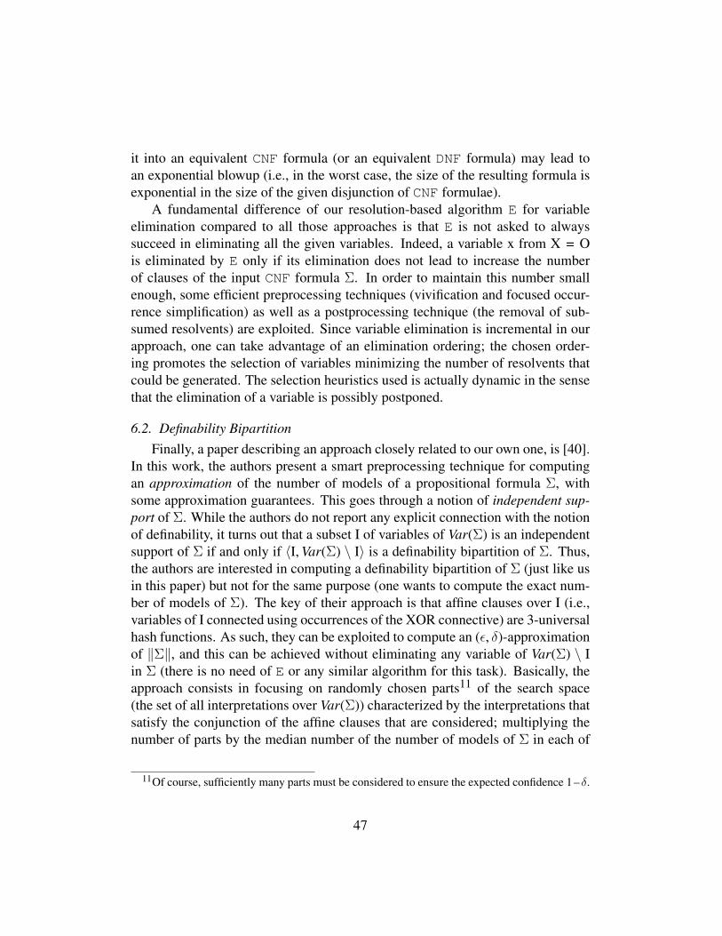
it into an equivalent CNF formula (or an equivalent DNF formula) may lead toan exponential blowup (i.e., in the worst case, the size of the resulting formula isexponential in the size of the given disjunction of CNF formulae).

A fundamental difference of our resolution-based algorithm E for variableelimination compared to all those approaches is that E is not asked to alwayssucceed in eliminating all the given variables. Indeed, a variable x from X = Ois eliminated by E only if its elimination does not lead to increase the numberof clauses of the input CNF formula Σ. In order to maintain this number smallenough, some efficient preprocessing techniques (vivification and focused occur-rence simplification) as well as a postprocessing technique (the removal of sub-sumed resolvents) are exploited. Since variable elimination is incremental in ourapproach, one can take advantage of an elimination ordering; the chosen order-ing promotes the selection of variables minimizing the number of resolvents thatcould be generated. The selection heuristics used is actually dynamic in the sensethat the elimination of a variable is possibly postponed.

6.2. Definability BipartitionFinally, a paper describing an approach closely related to our own one, is [40].

In this work, the authors present a smart preprocessing technique for computingan approximation of the number of models of a propositional formula Σ, withsome approximation guarantees. This goes through a notion of independent sup-port of Σ. While the authors do not report any explicit connection with the notionof definability, it turns out that a subset I of variables of Var(Σ) is an independentsupport of Σ if and only if 〈I, Var(Σ) \ I〉 is a definability bipartition of Σ. Thus,the authors are interested in computing a definability bipartition of Σ (just like usin this paper) but not for the same purpose (one wants to compute the exact num-ber of models of Σ). The key of their approach is that affine clauses over I (i.e.,variables of I connected using occurrences of the XOR connective) are 3-universalhash functions. As such, they can be exploited to compute an (ε, δ)-approximationof ‖Σ‖, and this can be achieved without eliminating any variable of Var(Σ) \ Iin Σ (there is no need of E or any similar algorithm for this task). Basically, theapproach consists in focusing on randomly chosen parts11 of the search space(the set of all interpretations over Var(Σ)) characterized by the interpretations thatsatisfy the conjunction of the affine clauses that are considered; multiplying thenumber of parts by the median number of the number of models of Σ in each of

11Of course, sufficiently many parts must be considered to ensure the expected confidence 1 – δ.

47

those parts then gives an estimate of ‖Σ‖. In practice, considering affine clauseswith low density (i.e., based on a ”small” set I) leads to much improved perfor-mances of the solvers used to count the number of models of Σ in each cell. Thisjustifies to look for ”small” independent sets.

To do the job, the authors exhibit a reduction from the problem of computingan independent support of a CNF formula Σ to the problem of computing a group-oriented unsatisfiable subset of clauses of a CNF formula. More generally, theyshow that the problem of computing a subset-minimal (resp. a smallest) indepen-dent support of Σ amounts to computing a GMUS, i.e., a group-oriented minimalunsatisfiable subset (resp. an SGMUS, i.e., a minimum-sized group-oriented min-imal unsatisfiable subset) of a formula that can be computed in time polynomialin the size of Σ (see [40] for details). Formally, a GMUS (resp. SGMUS) of a set∆ of propositional formulae can be defined as follows (see e.g., [72, 73]):

Definition 5 (GMUS, SGMUS). Let ∆ be the union (⋃n

i=1 ∆i)∪Ω of (finite) setsof propositional formulae, forming a partition, such that ∆ is unsatisfiable.

• A group-oriented minimal unsatisfiable subset (GMUS) (also referred to ashigh-level MUS) of ∆ is a set of formulae Φ = (

⋃ni=1 Φi) ∪ Ω such that:

– ∀i ∈ 1, . . . , n, Φi ⊆ ∆i,

– Φ is unsatisfiable,

– ∀i ∈ 1, . . . , n, Φ \ Φi is satisfiable.

• A minimum-sized group-oriented minimal unsatisfiable subset (SGMUS) of∆ is a GMUS of ∆ of minimal cardinality.

The reduction used in [40] can be viewed as an extension of Padoa’s approach(as reflected by Theorem 2) for checking the definability in Σ on I of the wholeset of variables Var(Σ) \ I (instead of doing it one variable after the other, as it isthe case in B). Since the concept of MUS (and its ”neighborhood”) has given riseto an abundant literature (together with the implementation of several solvers) forthe past few years (see e.g., [72, 74, 75, 73, 52, 76, 77, 78]), the reduction gives theopportunity to take advantage of GMUS and SGMUS extractors for implement-ing pieces of software for computing independent supports of Σ that are subset-minimal independent supports or among the smallest independent supports. Thus,the solver MIS for computing subset-minimal independent supports is based onthe GMUS extractor MUSer2 [73], while the solver SMIS for computing smallestindependent supports is based on the SGMUS extractor forqes [78].

48

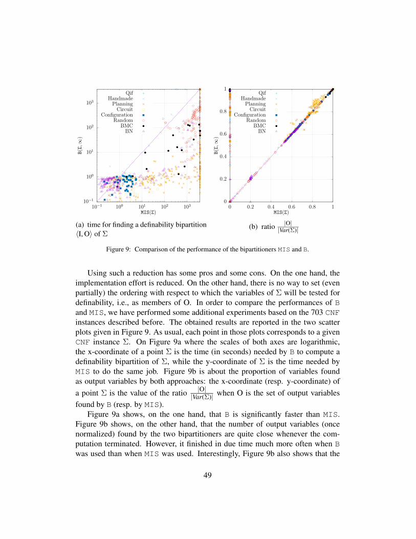
10−1

100

101

102

103

10−1 100 101 102 103

B(Σ,∞

)

MIS(Σ)

QifHandmadePlanningCircuit

ConfigurationRandom

BMCBN

(a) time for finding a definability bipartition〈I, O〉 of Σ

0

0.2

0.4

0.6

0.8

1

0 0.2 0.4 0.6 0.8 1

B(Σ,∞

)MIS(Σ)

QifHandmadePlanningCircuit

ConfigurationRandom

BMCBN

(b) ratio |O||Var(Σ)|

Figure 9: Comparison of the performance of the bipartitioners MIS and B.

Using such a reduction has some pros and some cons. On the one hand, theimplementation effort is reduced. On the other hand, there is no way to set (evenpartially) the ordering with respect to which the variables of Σ will be tested fordefinability, i.e., as members of O. In order to compare the performances of Band MIS, we have performed some additional experiments based on the 703 CNFinstances described before. The obtained results are reported in the two scatterplots given in Figure 9. As usual, each point in those plots corresponds to a givenCNF instance Σ. On Figure 9a where the scales of both axes are logarithmic,the x-coordinate of a point Σ is the time (in seconds) needed by B to compute adefinability bipartition of Σ, while the y-coordinate of Σ is the time needed byMIS to do the same job. Figure 9b is about the proportion of variables foundas output variables by both approaches: the x-coordinate (resp. y-coordinate) ofa point Σ is the value of the ratio |O|

|Var(Σ)| when O is the set of output variablesfound by B (resp. by MIS).

Figure 9a shows, on the one hand, that B is significantly faster than MIS.Figure 9b shows, on the other hand, that the number of output variables (oncenormalized) found by the two bipartitioners are quite close whenever the com-putation terminated. However, it finished in due time much more often when Bwas used than when MIS was used. Interestingly, Figure 9b also shows that the

49

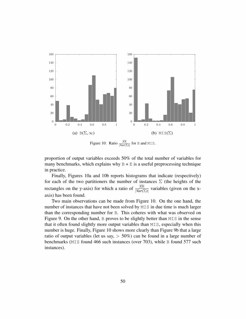
0

20

40

60

80

100

120

140

160

0 0.2 0.4 0.6 0.8 1

(a) B(Σ,∞)

0

20

40

60

80

100

120

140

160

0 0.2 0.4 0.6 0.8 1

(b) MIS(Σ)

Figure 10: Ratio |O||Var(Σ)| for B and MIS.

proportion of output variables exceeds 50% of the total number of variables formany benchmarks, which explains why B + E is a useful preprocessing techniquein practice.

Finally, Figures 10a and 10b reports histograms that indicate (respectively)for each of the two partitioners the number of instances Σ (the heights of therectangles on the y-axis) for which a ratio of |O|

|Var(Σ)| variables (given on the x-axis) has been found.

Two main observations can be made from Figure 10. On the one hand, thenumber of instances that have not been solved by MIS in due time is much largerthan the corresponding number for B. This coheres with what was observed onFigure 9. On the other hand, B proves to be slightly better than MIS in the sensethat it often found slightly more output variables than MIS, especially when thisnumber is huge. Finally, Figure 10 shows more clearly than Figure 9b that a largeratio of output variables (let us say, > 50%) can be found in a large number ofbenchmarks (MIS found 466 such instances (over 703), while B found 577 suchinstances).

50

7. Conclusion

We have defined and evaluated a new preprocessing technique for counting themodels of a propositional CNF formula Σ. This technique consists in determiningfirst a definability bipartition of Σ into a set I of input variables and a set O ofoutput variables, then to eliminate in Σ some variables of O. The soundness ofthis technique is based on standard theorems in classical logic by Beth and Padoa.While those results are quite old, they prove useful for defining a quite effectivepreprocessing technique to model counting.

More in detail, in order to evaluate the performances of our approach on CNFformulae, we have designed and implemented a preprocessor B + E that is basedon it. B + E associates with a given CNF formula Σ a CNF formula B + E(Σ)which has the same number of models as Σ, but is often simpler with respectto the number of variables and size. We tested B + E over many benchmarksfrom different data sets. Experiments have shown that for many instances Σ,the overall computation time needed to calculate ‖B + E(Σ)‖ using state-of-theart exact model counters is often much lower than the time needed to compute‖Σ‖ with the same counters. This performance shift can be explained by the twofollowing facts: on the one hand, for many instances, a large number of gatesexist; on the other hand, such gates can be detected and eliminated using B + E.

In our experiments, we have also considered the possibility to combine the twopreprocessors pmc and B + E in sequence before model counting, in order to deter-mine whether some synergetic effects can be obtained via an improved reductionof the instances. Generally speaking, the results show only slight improvementsfor the two combinations (pmc then B + E, and B + E then pmc), both in terms ofthe reductions of the number of variables and of the size of the instances, and alsoin terms of reduction of the subsequent model counting time (whatever the modelcounter among the four used). For this reason, and since the paper is already quitelong, we refrained from reporting the corresponding results (they can be obtainedfrom the authors on demand).

This work opens a number of perspectives for further research. Consideringother heuristics in B for determining a definability bipartition and determininghow to tune the constants max#C and max#Res depending on the instance athand will deserve to be investigated.

Another perspective consists in trying to improve E by exploiting in it someadditional preprocessing techniques p. Indeed, it is not mandatory for p to beequivalence-preserving. Actually, p can be exploited as soon as it satisfies theequivalence ∃E.p(Σ) ≡ ∃E.Σ, which is less demanding than p(Σ) ≡ Σ. This

51

is the case for instance for some specializations to variables from E of existingpreprocessing techniques, such as the pure output literal rule (removing everyclause containing a pure literal from E) or the output blocked clause eliminationrule (removing every clause containing a variable from E such that every resolventin Σ obtained by resolving on this variable is a valid clause) [79].

It would be also useful to evaluate the benefits that could be obtained in prac-tice by considering more computationally demanding versions of B and of E whenthe objective is to compute an approximate compilation of Σ on a set of control-lable variables. Indeed, in such a case, both the B step and the E step are performedoff-line. Thus, it makes sense to spend some extra time (even if it is significant)to compute a ”better” definability bipartition (especially, a smallest definabilitybipartition) and to eliminate more output variables if this leads to a smaller com-piled form. Some experiments will be conducted to try to figure out what a goodtime/space trade-off could be.

Other perspectives concern the interface between definability, model countingand projected model counting. When the objective is to compute ‖Σ‖, instead oftaking advantage of B + E followed by any model counter as discussed before, wecould instead use B followed by any projected model counter (where the projectionis onto I). The other way around, when the objective is to compute ‖∃(Var(Σ) \C).Σ‖, we could refrain from using B and exploit E directly on Var(Σ) \ C andΣ as a preprocessing for projected model counting. It would be interesting toimplement both approaches and to determine whether they are helpful in practice.

Acknowledgements

This work has been achieved while Jean-Marie Lagniez was with CRIL, CNRSUMR8188 - Univ Artois. This work has been partly supported by the PING/ACKproject of the French National Agency for Research (ANR-18-CE40-0011).

References

[1] T. Sang, P. Beame, H. A. Kautz, Performing Bayesian Inference by WeightedModel Counting, in: M. M. Veloso, S. Kambhampati (Eds.), Proceedings,The Twentieth National Conference on Artificial Intelligence and the Sev-enteenth Innovative Applications of Artificial Intelligence Conference, July9-13, 2005, Pittsburgh, Pennsylvania, USA, AAAI Press / The MIT Press,2005, pp. 475–482.

52

[2] M. Chavira, A. Darwiche, On probabilistic inference by weightedmodel counting, Artif. Intell. 172 (6-7) (2008) 772–799. doi:10.1016/j.artint.2007.11.002.

[3] U. Apsel, R. I. Brafman, Lifted MEU by weighted model counting, in:J. Hoffmann, B. Selman (Eds.), Proceedings of the Twenty-Sixth AAAIConference on Artificial Intelligence, July 22-26, 2012, Toronto, Ontario,Canada., AAAI Press, 2012, pp. 1861–1867.

[4] A. Choi, D. Kisa, A. Darwiche, Compiling probabilistic graphical modelsusing sentential decision diagrams, in: L. C. van der Gaag (Ed.), Symbolicand Quantitative Approaches to Reasoning with Uncertainty - 12th EuropeanConference, ECSQARU 2013, Utrecht, The Netherlands, July 8-10, 2013.Proceedings, Vol. 7958 of Lecture Notes in Computer Science, Springer,2013, pp. 121–132. doi:10.1007/978-3-642-39091-3\_11.

[5] H. Palacios, B. Bonet, A. Darwiche, H. Geffner, Pruning Conformant Plansby Counting Models on Compiled d-DNNF Representations, in: S. Biundo,K. L. Myers, K. Rajan (Eds.), Proceedings of the Fifteenth InternationalConference on Automated Planning and Scheduling (ICAPS 2005), June 5-10 2005, Monterey, California, USA, AAAI, 2005, pp. 141–150.

[6] C. Domshlak, J. Hoffmann, Fast probabilistic planning through weightedmodel counting, in: D. Long, S. F. Smith, D. Borrajo, L. McCluskey (Eds.),Proceedings of the Sixteenth International Conference on Automated Plan-ning and Scheduling, ICAPS 2006, Cumbria, UK, June 6-10, 2006, AAAI,2006, pp. 243–252.

[7] L. Feiten, M. Sauer, T. Schubert, A. Czutro, E. Bohl, I. Polian, B. Becker,#SAT-based vulnerability analysis of security components - A case study,in: 2012 IEEE International Symposium on Defect and Fault Tolerancein VLSI and Nanotechnology Systems, DFT 2012, Austin, TX, USA,October 3-5, 2012, IEEE Computer Society, 2012, pp. 49–54. doi:10.1109/DFT.2012.6378198.

[8] S. Chakraborty, D. Fried, K. S. Meel, M. Y. Vardi, From weighted to un-weighted model counting, in: Q. Yang, M. Wooldridge (Eds.), Proceed-ings of the Twenty-Fourth International Joint Conference on Artificial In-telligence, IJCAI 2015, Buenos Aires, Argentina, July 25-31, 2015, AAAIPress, 2015, pp. 689–695.

53

[9] L. G. Valiant, The complexity of computing the permanent, Theor. Comput.Sci. 8 (1979) 189–201. doi:10.1016/0304-3975(79)90044-6.

[10] D. Roth, On the hardness of approximate reasoning, Artif. Intell. 82 (1-2)(1996) 273–302. doi:10.1016/0004-3702(94)00092-1.

[11] M. E. Dyer, L. A. Goldberg, M. Jerrum, The complexity of weightedBoolean #CSP, SIAM J. Comput. 38 (5) (2009) 1970–1986. doi:10.1137/070690201.

[12] S. Toda, PP is as hard as the polynomial-time hierarchy, SIAM J. Comput.20 (5) (1991) 865–877. doi:10.1137/0220053.

[13] M. Samer, S. Szeider, Algorithms for propositional modelcounting, J. Discrete Algorithms 8 (1) (2010) 50–64. doi:10.1016/j.jda.2009.06.002.

[14] F. Bacchus, S. Dalmao, T. Pitassi, Algorithms and Complexity Results for#SAT and Bayesian Inference, in: 44th Symposium on Foundations ofComputer Science (FOCS 2003), 11-14 October 2003, Cambridge, MA,USA, Proceedings, IEEE Computer Society, 2003, pp. 340–351. doi:10.1109/SFCS.2003.1238208.

[15] C. P. Gomes, A. Sabharwal, B. Selman, Model counting, in: A. Biere,M. Heule, H. van Maaren, T. Walsh (Eds.), Handbook of Satisfiability, Vol.185 of Frontiers in Artificial Intelligence and Applications, IOS Press, 2009,pp. 633–654. doi:10.3233/978-1-58603-929-5-633.

[16] D. Achlioptas, Z. Hammoudeh, P. Theodoropoulos, Fast and flexible prob-abilistic model counting, in: Beyersdorff and Wintersteiger [80], pp. 148–164. doi:10.1007/978-3-319-94144-8\_10.

[17] D. Achlioptas, P. Theodoropoulos, Probabilistic model counting with shortXORs, in: S. Gaspers, T. Walsh (Eds.), Theory and Applications of Sat-isfiability Testing - SAT 2017 - 20th International Conference, Melbourne,VIC, Australia, August 28 - September 1, 2017, Proceedings, Vol. 10491of Lecture Notes in Computer Science, Springer, 2017, pp. 3–19. doi:10.1007/978-3-319-66263-3\_1.

54

[18] S. Chakraborty, K. S. Meel, M. Y. Vardi, Algorithmic improvements in ap-proximate counting for probabilistic inference: From linear to logarithmicSAT calls, in: Kambhampati [81], pp. 3569–3576.

[19] F. Bacchus, J. Winter, Effective preprocessing with hyper-resolution andequality reduction, in: E. Giunchiglia, A. Tacchella (Eds.), Theory and Ap-plications of Satisfiability Testing, 6th International Conference, SAT 2003.Santa Margherita Ligure, Italy, May 5-8, 2003 Selected Revised Papers, Vol.2919 of Lecture Notes in Computer Science, Springer, 2003, pp. 341–355.doi:10.1007/978-3-540-24605-3\_26.

[20] S. Subbarayan, D. K. Pradhan, Niver: Non increasing variable eliminationresolution for preprocessing SAT instances, in: SAT 2004 - The SeventhInternational Conference on Theory and Applications of Satisfiability Test-ing, 10-13 May 2004, Vancouver, BC, Canada, Online Proceedings [82], pp.276–291.

[21] I. Lynce, J. P. Marques Silva, Probing-based preprocessing techniquesfor propositional satisfiability, in: 15th IEEE International Conference onTools with Artificial Intelligence (ICTAI 2003), 3-5 November 2003, Sacra-mento, California, USA, IEEE Computer Society, 2003, p. 105. doi:10.1109/TAI.2003.1250177.

[22] N. Een, A. Biere, Effective preprocessing in SAT through variable and clauseelimination, in: F. Bacchus, T. Walsh (Eds.), Theory and Applications ofSatisfiability Testing, 8th International Conference, SAT 2005, St. Andrews,UK, June 19-23, 2005, Proceedings, Vol. 3569 of Lecture Notes in ComputerScience, Springer, 2005, pp. 61–75. doi:10.1007/11499107\_5.

[23] C. Piette, Y. Hamadi, L. Sais, Vivifying propositional clausal formulae,in: M. Ghallab, C. D. Spyropoulos, N. Fakotakis, N. M. Avouris (Eds.),ECAI 2008 - 18th European Conference on Artificial Intelligence, Patras,Greece, July 21-25, 2008, Proceedings, Vol. 178 of Frontiers in Artifi-cial Intelligence and Applications, IOS Press, 2008, pp. 525–529. doi:10.3233/978-1-58603-891-5-525.

[24] H. Han, F. Somenzi, Alembic: An efficient algorithm for CNF prepro-cessing, in: Proceedings of the 44th Design Automation Conference, DAC2007, San Diego, CA, USA, June 4-8, 2007, IEEE, 2007, pp. 582–587.doi:10.1145/1278480.1278628.

55

[25] M. Heule, M. Jarvisalo, A. Biere, Clause elimination procedures for CNFformulas, in: C. G. Fermuller, A. Voronkov (Eds.), Logic for Program-ming, Artificial Intelligence, and Reasoning - 17th International Conference,LPAR-17, Yogyakarta, Indonesia, October 10-15, 2010. Proceedings, Vol.6397 of Lecture Notes in Computer Science, Springer, 2010, pp. 357–371.doi:10.1007/978-3-642-16242-8\_26.

[26] M. Jarvisalo, A. Biere, M. Heule, Simulating circuit-level simplifica-tions on CNF, J. Autom. Reasoning 49 (4) (2012) 583–619. doi:10.1007/s10817-011-9239-9.

[27] M. Heule, M. Jarvisalo, A. Biere, Efficient CNF simplification based on bi-nary implication graphs, in: K. A. Sakallah, L. Simon (Eds.), Theory andApplications of Satisfiability Testing - SAT 2011 - 14th International Con-ference, SAT 2011, Ann Arbor, MI, USA, June 19-22, 2011. Proceedings,Vol. 6695 of Lecture Notes in Computer Science, Springer, 2011, pp. 201–215. doi:10.1007/978-3-642-21581-0\_17.

[28] G. Audemard, L. Simon, Predicting learnt clauses quality in modern SATsolvers, in: C. Boutilier (Ed.), IJCAI 2009, Proceedings of the 21st Inter-national Joint Conference on Artificial Intelligence, Pasadena, California,USA, July 11-17, 2009, 2009, pp. 399–404.

[29] A. Biere, Lingeling essentials, A tutorial on design and implementation as-pects of the the SAT solver lingeling, in: D. Le Berre (Ed.), POS-14. FifthPragmatics of SAT workshop, a workshop of the SAT 2014 conference, partof FLoC 2014 during the Vienna Summer of Logic, July 13, 2014, Vienna,Austria, Vol. 27 of EPiC Series in Computing, EasyChair, 2014, p. 88.

[30] N. Manthey, Solver description of RISS 2.0 and PRISS 2.0, Tech. rep., TUDresden, Knowledge Representation and Reasoning (2012).

[31] N. Manthey, Coprocessor 2.0 - A flexible CNF simplifier - (tool pre-sentation), in: Cimatti and Sebastiani [83], pp. 436–441. doi:10.1007/978-3-642-31612-8\_34.

[32] J.-M. Lagniez, P. Marquis, On preprocessing techniques and their impact onpropositional model counting, J. Autom. Reasoning 58 (4) (2017) 413–481.doi:10.1007/s10817-016-9370-8.URL https://doi.org/10.1007/s10817-016-9370-8

56

[33] J. Lang, P. Marquis, On propositional definability, Artif. Intell. 172 (8-9)(2008) 991–1017. doi:10.1016/j.artint.2007.12.003.

[34] G. Tseitin, On the complexity of derivation in propositional calculus, SteklovMathematical Institute, 1968, Ch. Structures in Constructive Mathematicsand Mathematical Logic, pp. 115–125.

[35] D. A. Plaisted, S. Greenbaum, A structure-preserving clause formtranslation, J. Symb. Comput. 2 (3) (1986) 293–304. doi:10.1016/S0747-7171(86)80028-1.

[36] J.-M. Lagniez, E. Lonca, P. Marquis, Improving model counting by leverag-ing definability, in: Kambhampati [81], pp. 751–757.

[37] J.-M. Lagniez, P. Marquis, An Improved Decision-DNNF Compiler, in:C. Sierra (Ed.), Proceedings of the Twenty-Sixth International JointConference on Artificial Intelligence, IJCAI 2017, Melbourne, Aus-tralia, August 19-25, 2017, ijcai.org, 2017, pp. 667–673. doi:10.24963/ijcai.2017/93.

[38] M. Gebser, B. Kaufmann, T. Schaub, Solution enumeration for projectedBoolean search problems, in: W. J. van Hoeve, J. N. Hooker (Eds.), In-tegration of AI and OR Techniques in Constraint Programming for Com-binatorial Optimization Problems, 6th International Conference, CPAIOR2009, Pittsburgh, PA, USA, May 27-31, 2009, Proceedings, Vol. 5547 ofLecture Notes in Computer Science, Springer, 2009, pp. 71–86. doi:10.1007/978-3-642-01929-6\_7.

[39] R. A. Aziz, G. Chu, C. J. Muise, P. J. Stuckey, #∃SAT: Projectedmodel counting, in: M. Heule, S. Weaver (Eds.), Theory and Applica-tions of Satisfiability Testing - SAT 2015 - 18th International Conference,Austin, TX, USA, September 24-27, 2015, Proceedings, Vol. 9340 of Lec-ture Notes in Computer Science, Springer, 2015, pp. 121–137. doi:10.1007/978-3-319-24318-4\_10.

[40] A. Ivrii, S. Malik, K. S. Meel, M. Y. Vardi, On computing minimal inde-pendent support and its applications to sampling and counting, Constraints21 (1) (2016) 41–58. doi:10.1007/s10601-015-9204-z.

[41] H. B. Enderton, A mathematical introduction to logic, Academic Press,1972.

57

[42] J. Lang, P. Liberatore, P. Marquis, Propositional independence: Formula-variable independence and forgetting, J. Artif. Intell. Res. 18 (2003) 391–443. doi:10.1613/jair.1113.

[43] M. Davis, H. Putnam, A computing procedure for quantification theory, J.ACM 7 (3) (1960) 201–215. doi:10.1145/321033.321034.

[44] E. Beth, On Padoa’s method in the theory of definition, Indagationes mathe-maticae 15 (1953) 330–339.

[45] A. Padoa, Essai d’une theorie algebrique des nombres entiers, precede d’uneintroduction logique a une theorie deductive quelconque, in: Bibliothequedu Congres International de Philosophie, Paris, 1903, pp. 309–365.

[46] S. A. Cook, The complexity of theorem-proving procedures, in: M. A. Harri-son, R. B. Banerji, J. D. Ullman (Eds.), Proceedings of the 3rd Annual ACMSymposium on Theory of Computing, May 3-5, 1971, Shaker Heights, Ohio,USA, ACM, 1971, pp. 151–158. doi:10.1145/800157.805047.

[47] J. P. Marques Silva, K. A. Sakallah, GRASP - a new search al-gorithm for satisfiability, in: ICCAD, 1996, pp. 220–227. doi:10.1109/ICCAD.1996.569607.URL https://doi.org/10.1109/ICCAD.1996.569607

[48] J. P. Marques Silva, K. A. Sakallah, GRASP: A search algorithm for propo-sitional satisfiability, IEEE Trans. Computers 48 (5) (1999) 506–521. doi:10.1109/12.769433.URL https://doi.org/10.1109/12.769433

[49] M. W. Moskewicz, C. F. Madigan, Y. Zhao, L. Zhang, S. Malik, Chaff: En-gineering an efficient SAT solver, in: Proceedings of the 38th Design Au-tomation Conference, DAC 2001, Las Vegas, NV, USA, June 18-22, 2001,ACM, 2001, pp. 530–535. doi:10.1145/378239.379017.URL https://doi.org/10.1145/378239.379017

[50] H. Zhang, M. E. Stickel, An efficient algorithm for unit propagation, in: InProceedings of the Fourth International Symposium on Artificial Intelligenceand Mathematics (AI-MATH’96), Fort Lauderdale (Florida USA, 1996, pp.166–169.

58

[51] O. Roussel, Controlling a solver execution with the runsolver tool, JSAT7 (4) (2011) 139–144.URL https://satassociation.org/jsat/index.php/jsat/article/view/90

[52] G. Audemard, J.-M. Lagniez, L. Simon, Improving glucose for incrementalSAT solving with assumptions: Application to MUS extraction, in: Jarvisaloand Gelder [84], pp. 309–317. doi:10.1007/978-3-642-39071-5\_23.

[53] T. Sang, F. Bacchus, P. Beame, H. A. Kautz, T. Pitassi, Combining com-ponent caching and clause learning for effective model counting, in: SAT2004 - The Seventh International Conference on Theory and Applicationsof Satisfiability Testing, 10-13 May 2004, Vancouver, BC, Canada, OnlineProceedings [82], pp. 20–28.

[54] M. Thurley, sharpSAT - counting models with advanced component cachingand implicit BCP, in: A. Biere, C. P. Gomes (Eds.), Theory and Appli-cations of Satisfiability Testing - SAT 2006, 9th International Conference,Seattle, WA, USA, August 12-15, 2006, Proceedings, Vol. 4121 of Lec-ture Notes in Computer Science, Springer, 2006, pp. 424–429. doi:10.1007/11814948\_38.

[55] A. Darwiche, Decomposable negation normal form, J. ACM 48 (4) (2001)608–647. doi:10.1145/502090.502091.

[56] A. Darwiche, New advances in compiling CNF into decomposable negationnormal form, in: R. L. de Mantaras, L. Saitta (Eds.), Proceedings of the16th Eureopean Conference on Artificial Intelligence, ECAI’2004, includingPrestigious Applicants of Intelligent Systems, PAIS 2004, Valencia, Spain,August 22-27, 2004, IOS Press, 2004, pp. 328–332.

[57] M. Samer, S. Szeider, Algorithms for propositional modelcounting, J. Discrete Algorithms 8 (1) (2010) 50–64. doi:10.1016/j.jda.2009.06.002.

[58] M. Cadoli, F. M. Donini, M. Schaerf, R. Silvestri, On compact representa-tions of propositional circumscription, Theor. Comput. Sci. 182 (1-2) (1997)183–202. doi:10.1016/S0304-3975(96)00182-X.

59

[59] A. del Val, An analysis of approximate knowledge compilation, in: Proceed-ings of the Fourteenth International Joint Conference on Artificial Intelli-gence, IJCAI 95, Montreal Quebec, Canada, August 20-25 1995, 2 Volumes,Morgan Kaufmann, 1995, pp. 830–836.

[60] A. Bart, F. Koriche, J.-M. Lagniez, P. Marquis, Symmetry-driven deci-sion diagrams for knowledge compilation, in: T. Schaub, G. Friedrich,B. O’Sullivan (Eds.), ECAI 2014 - 21st European Conference on ArtificialIntelligence, 18-22 August 2014, Prague, Czech Republic - Including Pres-tigious Applications of Intelligent Systems (PAIS 2014), Vol. 263 of Fron-tiers in Artificial Intelligence and Applications, IOS Press, 2014, pp. 51–56.doi:10.3233/978-1-61499-419-0-51.

[61] J. K. Fichte, M. Hecher, M. Morak, S. Woltran, Exploiting treewidth forprojected model counting and its limits, in: Beyersdorff and Wintersteiger[80], pp. 165–184. doi:10.1007/978-3-319-94144-8\_11.

[62] A. Durand, M. Hermann, P. G. Kolaitis, Subtractive reductions and com-plete problems for counting complexity classes, Theor. Comput. Sci. 340 (3)(2005) 496–513. doi:10.1016/j.tcs.2005.03.012.

[63] V. Klebanov, N. Manthey, C. J. Muise, SAT-based analysis and quan-tification of information flow in programs, in: K. R. Joshi, M. Siegle,M. Stoelinga, P. R. D’Argenio (Eds.), Quantitative Evaluation of Sys-tems - 10th International Conference, QEST 2013, Buenos Aires,Argentina, August 27-30, 2013. Proceedings, Vol. 8054 of LectureNotes in Computer Science, Springer, 2013, pp. 177–192. doi:10.1007/978-3-642-40196-1\_16.

[64] W. Craig, Three uses of the Herbrand-Gentzen theorem in relating modeltheory and proof theory, Journal of Symbolic Logic 22 (1957) 269–285.

[65] J. Brauer, A. King, J. Kriener, Existential quantification as incremental SAT,in: G. Gopalakrishnan, S. Qadeer (Eds.), Computer Aided Verification - 23rdInternational Conference, CAV 2011, Snowbird, UT, USA, July 14-20, 2011.Proceedings, Vol. 6806 of Lecture Notes in Computer Science, Springer,2011, pp. 191–207. doi:10.1007/978-3-642-22110-1\_17.

[66] C. Zengler, W. Kuchlin, Boolean quantifier elimination for automotive con-figuration - A case study, in: C. Pecheur, M. Dierkes (Eds.), Formal Meth-ods for Industrial Critical Systems - 18th International Workshop, FMICS

60

2013, Madrid, Spain, September 23-24, 2013. Proceedings, Vol. 8187 ofLecture Notes in Computer Science, Springer, 2013, pp. 48–62. doi:10.1007/978-3-642-41010-9\_4.

[67] J. Brauer, A. King, Approximate Quantifier Elimination for PropositionalBoolean Formulae, in: M. G. Bobaru, K. Havelund, G. J. Holzmann,R. Joshi (Eds.), NASA Formal Methods - Third International Symposium,NFM 2011, Pasadena, CA, USA, April 18-20, 2011. Proceedings, Vol.6617 of Lecture Notes in Computer Science, Springer, 2011, pp. 73–88.doi:10.1007/978-3-642-20398-5\_7.

[68] D. Monniaux, Quantifier elimination by lazy model enumeration, in:T. Touili, B. Cook, P. B. Jackson (Eds.), Computer Aided Verification, 22ndInternational Conference, CAV 2010, Edinburgh, UK, July 15-19, 2010. Pro-ceedings, Vol. 6174 of Lecture Notes in Computer Science, Springer, 2010,pp. 585–599. doi:10.1007/978-3-642-14295-6\_51.

[69] R. Schrag, Compilation for critically constrained knowledge bases, in: W. J.Clancey, D. S. Weld (Eds.), Proceedings of the Thirteenth National Confer-ence on Artificial Intelligence and Eighth Innovative Applications of Artifi-cial Intelligence Conference, AAAI 96, IAAI 96, Portland, Oregon, USA,August 4-8, 1996, Volume 1., AAAI Press / The MIT Press, 1996, pp. 510–515.

[70] A. Gupta, Z. Yang, P. Ashar, A. Gupta, SAT-based image computation withapplication in reachability analysis, in: W. A. H. Jr., S. D. Johnson (Eds.),Formal Methods in Computer-Aided Design, Third International Confer-ence, FMCAD 2000, Austin, Texas, USA, November 1-3, 2000, Proceed-ings, Vol. 1954 of Lecture Notes in Computer Science, Springer, 2000, pp.354–371. doi:10.1007/3-540-40922-X\_22.

[71] A. Darwiche, P. Marquis, A knowledge compilation map, J. Artif. Intell.Res. 17 (2002) 229–264. doi:10.1613/jair.989.

[72] A. Nadel, Boosting minimal unsatisfiable core extraction, in: R. Bloem,N. Sharygina (Eds.), Proceedings of 10th International Conference on For-mal Methods in Computer-Aided Design, FMCAD 2010, Lugano, Switzer-land, October 20-23, IEEE, 2010, pp. 221–229.URL http://ieeexplore.ieee.org/document/5770953/

61

[73] A. Belov, J. P. Marques Silva, Muser2: An efficient MUS extractor, JSAT8 (3/4) (2012) 123–128.

[74] M. Janota, J. P. Marques Silva, On deciding MUS membership with QBF,in: J. H. Lee (Ed.), Principles and Practice of Constraint Programming - CP2011 - 17th International Conference, CP 2011, Perugia, Italy, September12-16, 2011. Proceedings, Vol. 6876 of Lecture Notes in Computer Science,Springer, 2011, pp. 414–428. doi:10.1007/978-3-642-23786-7\_32.

[75] A. Belov, A. Ivrii, A. Matsliah, J. P. Marques Silva, On efficient computationof variable MUSes, in: Cimatti and Sebastiani [83], pp. 298–311. doi:10.1007/978-3-642-31612-8\_23.

[76] J.-M. Lagniez, A. Biere, Factoring out assumptions to speed up MUSextraction, in: Jarvisalo and Gelder [84], pp. 276–292. doi:10.1007/978-3-642-39071-5\_21.

[77] J. P. Marques Silva, A. Previti, On Computing Preferred MUSes and MCSes,in: C. Sinz, U. Egly (Eds.), Theory and Applications of Satisfiability Testing- SAT 2014 - 17th International Conference, Held as Part of the Vienna Sum-mer of Logic, VSL 2014, Vienna, Austria, July 14-17, 2014. Proceedings,Vol. 8561 of Lecture Notes in Computer Science, Springer, 2014, pp. 58–74.doi:10.1007/978-3-319-09284-3\_6.

[78] A. Ignatiev, A. Previti, M. H. Liffiton, J. P. Marques Silva, Smallest MUSextraction with minimal hitting set dualization, in: G. Pesant (Ed.), Prin-ciples and Practice of Constraint Programming - 21st International Confer-ence, CP 2015, Cork, Ireland, August 31 - September 4, 2015, Proceedings,Vol. 9255 of Lecture Notes in Computer Science, Springer, 2015, pp. 173–182. doi:10.1007/978-3-319-23219-5\_13.

[79] O. Kullmann, On a generalization of extended resolution, Dis-crete Applied Mathematics 96-97 (1999) 149–176. doi:10.1016/S0166-218X(99)00037-2.

[80] O. Beyersdorff, C. M. Wintersteiger (Eds.), Theory and Applications of Sat-isfiability Testing - SAT 2018 - 21st International Conference, SAT 2018,Held as Part of the Federated Logic Conference, FloC 2018, Oxford, UK,

62

July 9-12, 2018, Proceedings, Vol. 10929 of Lecture Notes in Computer Sci-ence, Springer, 2018. doi:10.1007/978-3-319-94144-8.

[81] S. Kambhampati (Ed.), Proceedings of the Twenty-Fifth International JointConference on Artificial Intelligence, IJCAI 2016, New York, NY, USA,9-15 July 2016, IJCAI/AAAI Press, 2016.

[82] SAT 2004 - The Seventh International Conference on Theory and Appli-cations of Satisfiability Testing, 10-13 May 2004, Vancouver, BC, Canada,Online Proceedings.

[83] A. Cimatti, R. Sebastiani (Eds.), Theory and Applications of SatisfiabilityTesting - SAT 2012 - 15th International Conference, Trento, Italy, June 17-20, 2012. Proceedings, Vol. 7317 of Lecture Notes in Computer Science,Springer, 2012. doi:10.1007/978-3-642-31612-8.

[84] M. Jarvisalo, A. V. Gelder (Eds.), Theory and Applications of SatisfiabilityTesting - SAT 2013 - 16th International Conference, Helsinki, Finland, July8-12, 2013. Proceedings, Vol. 7962 of Lecture Notes in Computer Science,Springer, 2013. doi:10.1007/978-3-642-39071-5.

63