
David Van Cauwenberge - Ghent University...
132
Transcript of David Van Cauwenberge - Ghent University...

David Van Cauwenberge
steam cracking reactorsComputational Fluid Dynamics based design of finned
Academiejaar 2011-2012Faculteit Ingenieurswetenschappen en ArchitectuurVoorzitter: prof. dr. ir. Guy MarinVakgroep Chemische Proceskunde en Technische Chemie
Master in de ingenieurswetenschappen: chemische technologieMasterproef ingediend tot het behalen van de academische graad van
Begeleider: Carl SchietekatPromotor: prof. dr. ir. Kevin Van Geem

Computational Fluid Dynamics based design of finned
steam cracking reactor
David Van Cauwenberge
Scriptie ingediend tot het behalen van de academische graad van Master in de
ingenieurswetenschappen: Chemische Technologie
Academiejaar: 2011-2012
Promotor: prof. dr. ir. K.M. Van Geem
Begeleider: ir. C. Schietekat
UNIVERSITEIT GENT
Faculteit Ingenieurswetenschappen en Architectuur
Vakgroep Chemische Proceskunde en Technische Chemie
Laboratorium voor Chemische Technologie
Directeur: prof. dr. ir. G.B. Marin
Abstract
The application of longitudinally and helicoidally finned tubes as steam cracker coils was studied
to evaluate the effect on product distribution and coke formation. An extensive parametric study
was performed to analyze the effect of the finned tube geometry on pressure drop and heat
transfer increase. The results were compared with bare tubes and optimal parameter values were
proposed. Finally 1D and 3D reactive simulations of an industrial propane cracker were performed
for finned tubes. Applying some of the optimal parameters showed considerable tube metal
temperature and run length improvements, although the loss in ethylene selectivity remains
limited to about 1wt%.
Keywords: steam cracking, coking, finned tubes, CFD, friction, heat transfer

FACULTEIT INGENIEURSWETENSCHAPPEN
EN ARCHITECTUUR
Laboratorium voor Chemische Technologie • Krijgslaan 281 S5, B-9000 Gent • www.lct.ugent.be
Secretariaat : T +32 (0)9 264 45 16 • F +32 (0)9 264 49 99 • [email protected]
Laboratorium voor Chemische Technologie
Verklaring in verband met de toegankelijkheid van de scriptie
Ondergetekende, David Van Cauwenberge, afgestudeerd aan de UGent in het
academiejaar 2011-2012 en auteur van de scriptie met als titel: Computational Fluid
Dynamics based design of finned steam cracking reactors.
verklaart hierbij:
1. dat hij/zij geopteerd heeft voor de hierna aangestipte mogelijkheid in verband
met de consultatie van zijn/haar scriptie:
de scriptie mag steeds ter beschikking gesteld worden van elke
aanvrager
█ de scriptie mag enkel ter beschikking gesteld worden met uitdrukkelijke,
schriftelijke goedkeuring van de auteur
de scriptie mag ter beschikking gesteld worden van een aanvrager na
een wachttijd van…………jaar
de scriptie mag nooit ter beschikking gesteld worden van een aanvrager
2. dat elke gebruiker te allen tijde gehouden is aan een correcte en volledige
bronverwijzing
Gent,
(Handtekening)
Vakgroep Chemische Proceskunde en Technische Chemie
Laboratorium voor Chemische Technologie
Directeur: Prof. Dr. Ir. Guy B. Marin
D
Computational Fluid Dynamics based design of
finned steam cracking reactors
David Van Cauwenberge
Supervisor(s): Prof. Dr. Ir. Kevin Van Geem, Ir. Carl Schietekat
Abstract: The application of longitudinally and helicoidally
finned tubes as steam cracker coils was studied to evaluate the
effect on product distribution and coke formation. An extensive
parametric study was performed to analyze the effect of the
finned tube geometry on pressure drop and heat transfer
increase. The results were compared with bare tubes and optimal
parameter values were proposed. Finally 1D and 3D reactive
simulations of an industrial propane cracker were performed for
finned tubes. Applying some of the optimal parameters showed
considerable tube metal temperature and run length
improvements, although the loss in ethylene selectivity remains
limited to about 1wt%.
Keywords: CFD, friction, heat transfer, finned tubes, steam
cracking, coking
I. INTRODUCTION
Steam cracking of hydrocarbons is the predominant
commercial method for producing light olefins such as
ethylene, propylene and butadiene. Due to the formation of a
coke layer on the reactor wall, heat transfer from the furnace
to the process gas is reduced, resulting in a lower efficiency of
the furnace. Moreover the flow area is reduced and hence the
pressure drop increases. Decoking of industrial reactors is thus
inevitable. This is economically very undesirable as for about
two days production is halted. Much effort has been made to
reduce coking through the use of additives, metal surface
technologies and mechanical devices. In the category of
mechanical devices, the introduction of fins inside the coils is
a widely applied method to increase the heat transfer surface.
Because of this enhanced heating, lower tube metal
temperatures are obtained and coke reduction is significantly
lowered.
II. MODEL VALIDATION
A. Non-reactive Simulation Setup
A computational study on the heat transfer and pressure
drop characteristics of air flow through finned tubes was
performed. The commercial CFD packageAnsys FLUENT
13.0 was adopted. For the longitudinal fins, the applied
turbulence model was the RNG kε-model. The swirl flow
induced by helicoidally fined tubes required the use of the
more computationally demanding Reynolds Stress Model. For
solving the laminar boundary layer, FLUENT’s two-layer
wall-treatment with enhanced wall functions was applied.
Discretization was performed by use of the QUICK scheme.
Mesh refinement tests indicated that a high number of cells
were required for a good accuracy level. As such, the
computational domain was refined and limited to a single fin
that was extruded in the axial direction, applying a certain
twist angle for the helicoidal fins. Symmetry boundary
conditions were applied to the longitudinal fins, while the
helicoidal fins made use of rotationally periodic boundaries.
An outer tube skin temperature profile was set. The inlet
was specified as a constant mass flow inlet while the outlet
was taken to be at atmospheric pressure.
B. Results
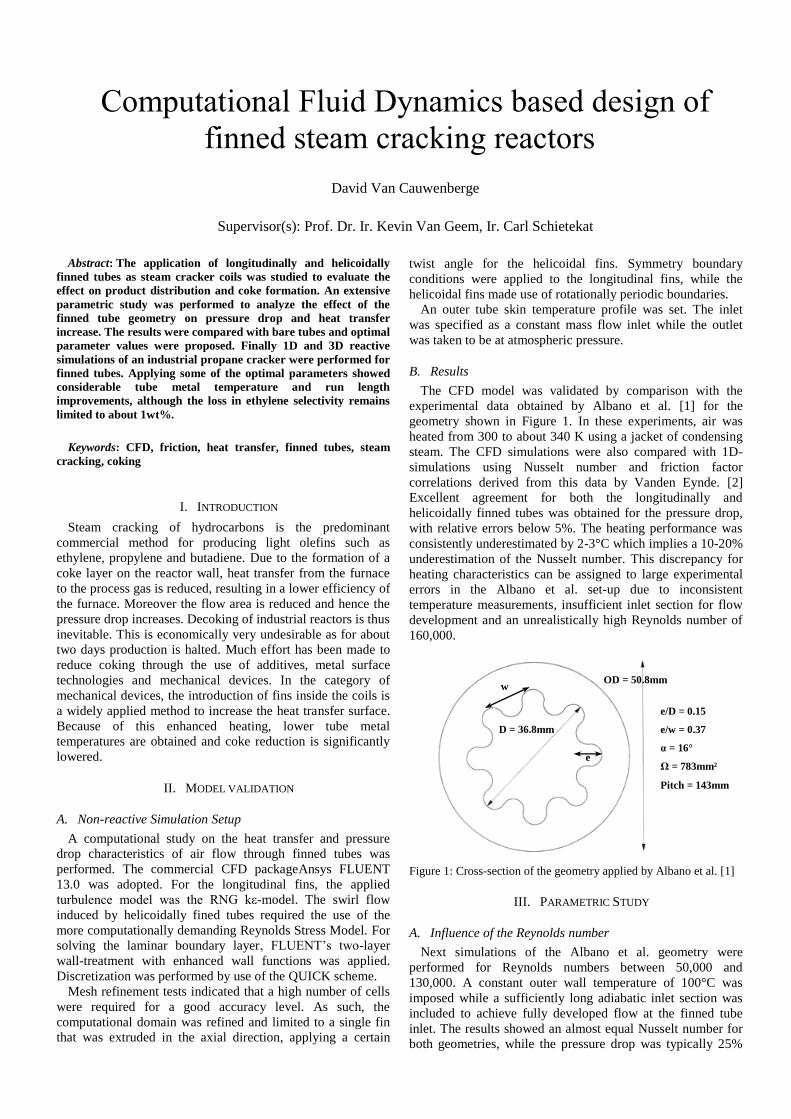
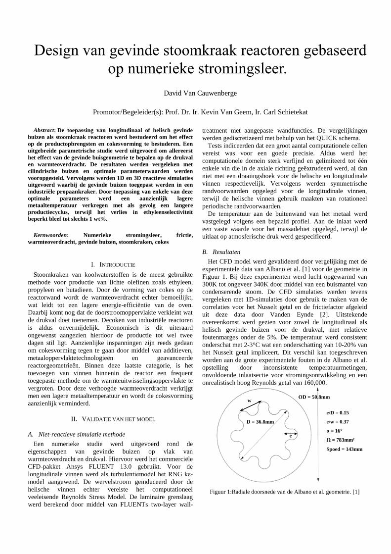
The CFD model was validated by comparison with the
experimental data obtained by Albano et al. [1] for the
geometry shown in Figure 1. In these experiments, air was
heated from 300 to about 340 K using a jacket of condensing
steam. The CFD simulations were also compared with 1D-
simulations using Nusselt number and friction factor
correlations derived from this data by Vanden Eynde. [2]
Excellent agreement for both the longitudinally and
helicoidally finned tubes was obtained for the pressure drop,
with relative errors below 5%. The heating performance was
consistently underestimated by 2-3°C which implies a 10-20%
underestimation of the Nusselt number. This discrepancy for
heating characteristics can be assigned to large experimental
errors in the Albano et al. set-up due to inconsistent
temperature measurements, insufficient inlet section for flow
development and an unrealistically high Reynolds number of
160,000.
Figure 1: Cross-section of the geometry applied by Albano et al. [1]
III. PARAMETRIC STUDY
A. Influence of the Reynolds number
Next simulations of the Albano et al. geometry were
performed for Reynolds numbers between 50,000 and
130,000. A constant outer wall temperature of 100°C was
imposed while a sufficiently long adiabatic inlet section was
included to achieve fully developed flow at the finned tube
inlet. The results showed an almost equal Nusselt number for
both geometries, while the pressure drop was typically 25%
w
D = 36.8mm
e
OD = 50.8mm
e/D = 0.15
e/w = 0.37
α = 16°
Ω = 783mm²
Pitch = 143mm
higher for the helicoidal fins. Confirming previous studies,
these fins were simulated to have a decreased Reynolds
number dependency as well, indicating improved relative
performance at lower flow rates.
B. Influence of the fin height
The fin height-to-diameter ratio for both tube types was
varied from 0.02 to 0.2. The straight fin showed a perfectly
linear relationship between heat transfer, pressure drop and
increased internal surface, suggesting that the fin height does
not induce significant flow pattern changes. For the helicoidal
fins a steep increase in heat transfer was seen for increasing
fin height-to-diameter ratio up until an (e/D) value of 0.11,
after which the relative improvement diminished. This was
confirmed by plotting a temperature variation coefficient for
each of the geometries from which it was made clear that the
radial temperature uniformity significantly decreased at
height-to-diameter values above 0.11.
At increased Reynolds numbers, similar effects were seen,
although the flow uniformity improvements were much less
pronounced. This indicates a tendency towards so-called
“coring” flow regime where the air passes by the helicoidal
fins rather than flowing through them and inducing swirl flow,
which confirms the findings of Albano et al. [1] and Jensen
and Vlakancic. [3]
C. Influence of the number of fins
For fins with a fin height-to-diameter ratio of 0.15, the
number of fins was varied from 4 to 12 while for a lower
value of 0.04 a variation from 8 to 32 was studied. For both
series of experiments a linear trend was seen for the pressure
drop, while the heat transfer followed a subtle S-shape. It was
found that the fin height-to-width ratio is the most critical
parameter to be optimized rather than the number of fins. An
optimal value of 0.35 was found from simulations and showed
little dependency on the Reynolds number.
D. Influence of the helix angle
The helix angle of the helicoidally finned tubes was varied
from 0° (straight) to 49°. Although significant heating
improvements were determined for the higher helix angles,
the combination with tall fins caused excessive pressure
drops. Tubes with reduced fin height optimally benefited from
the high degree of swirl flow and excellent flow uniformity
was achieved for a moderate pressure drop. For the fin height
of the Albano setup an angle of 25° was seen to provide a
good trade-off between heating characteristics and pressure
drop.
E. Conclusions
For Reynolds numbers around and below 90,000, a tube
with a fin height-to-diameter ratio of 0.04, 45° helix angle and
24 fins performed significantly better than a longitudinally
finned or bare coil. Compared to a bare tube, a 35%
improvement in heating characteristics was seen at the cost of
a doubled pressure drop. At higher Reynolds number a tube
with e/D ratio of 0.11 suffered less from the coring effect than
the small fins and as such was able of achieving a 25%
improvement in heat transfer compared to a bare tube, at a
mere 56% increase in pressure drop.
IV. REACTIVE SIMULATIONS
Based on the non-reactive simulations, correlations were
derived for Nusselt number and friction factor of finned tubes.
These correlations were included in the COILSIM1D steam
cracker simulation program developed at the Laboratory for
Chemical Technology. The shooting method option was used
to adjust the heat flux and inlet pressure to achieve a certain
cracking severity and outlet pressure. These values were
chosen according to typical industrial conditions for
Millisecond propane cracking reactors. [4] Four different
reactor geometries were studied; a bare tube, an industrially
adopted helicoidally finned tube, a longitudinally finned tube
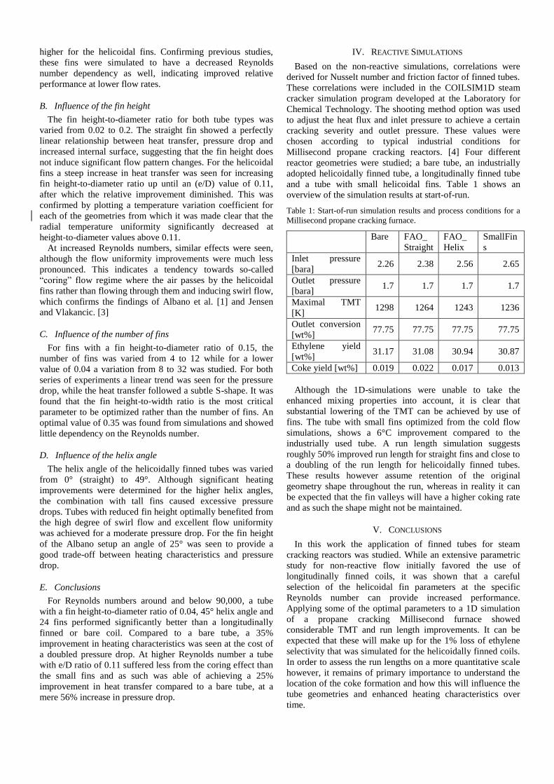
and a tube with small helicoidal fins. Table 1 shows an
overview of the simulation results at start-of-run.
Table 1: Start-of-run simulation results and process conditions for a
Millisecond propane cracking furnace.
Bare FAO_
Straight
FAO_
Helix
SmallFin
s
Inlet pressure
[bara] 2.26 2.38 2.56 2.65
Outlet pressure
[bara] 1.7 1.7 1.7 1.7
Maximal TMT
[K] 1298 1264 1243 1236
Outlet conversion
[wt%] 77.75 77.75 77.75 77.75
Ethylene yield
[wt%] 31.17 31.08 30.94 30.87
Coke yield [wt%] 0.019 0.022 0.017 0.013
Although the 1D-simulations were unable to take the
enhanced mixing properties into account, it is clear that
substantial lowering of the TMT can be achieved by use of
fins. The tube with small fins optimized from the cold flow
simulations, shows a 6°C improvement compared to the
industrially used tube. A run length simulation suggests
roughly 50% improved run length for straight fins and close to
a doubling of the run length for helicoidally finned tubes.
These results however assume retention of the original
geometry shape throughout the run, whereas in reality it can
be expected that the fin valleys will have a higher coking rate
and as such the shape might not be maintained.
V. CONCLUSIONS
In this work the application of finned tubes for steam
cracking reactors was studied. While an extensive parametric
study for non-reactive flow initially favored the use of
longitudinally finned coils, it was shown that a careful
selection of the helicoidal fin parameters at the specific
Reynolds number can provide increased performance.
Applying some of the optimal parameters to a 1D simulation
of a propane cracking Millisecond furnace showed
considerable TMT and run length improvements. It can be
expected that these will make up for the 1% loss of ethylene
selectivity that was simulated for the helicoidally finned coils.
In order to assess the run lengths on a more quantitative scale
however, it remains of primary importance to understand the
location of the coke formation and how this will influence the
tube geometries and enhanced heating characteristics over
time.

REFERENCES
[1] 1. J. V. Albano, K. M. Sundaram, M. J. Maddock, Applications of
extended surfaces in pyrolysis coils. Energy Progress, 1988. 8(3):
p. 9. [2] 2. Saegher, Johan J. De, Modellering van stroming, warmtetransport en
reactie in reactoren voor de thermische kraking van
koolwaterstoffen, in Laboratorium voor Petrochemische Techniek1994, Universiteit Gent.
[3] 3. Gregory J. Zdaniuk, Louay M. Chamra, Pedro J. Mago,
Experimental determination of heat transfer and friction in helically-finned tubes. Experimental Thermal and Fluid Science,
2008. 32: p. 15. [4] 4. Heynderickx, Geraldine J., Modellering en Simulatie van Huidige en
Nieuwe Technologieën voor de Thermische Kraking van
Koolwaterstoffen, in Laboratorium voor Petrochemische Techniek1993, Universiteit Gent: Faculteit van de Toegepaste
Wetenschappen.
Design van gevinde stoomkraak reactoren gebaseerd
op numerieke stromingsleer.
David Van Cauwenberge
Promotor/Begeleider(s): Prof. Dr. Ir. Kevin Van Geem, Ir. Carl Schietekat
Abstract: De toepassing van longitudinaal of helisch gevinde
buizen als stoomkraak reactoren werd bestudeerd om het effect
op de productopbrengsten en cokesvorming te bestuderen. Een
uitgebreide parametrische studie werd uitgevoerd om allereerst
het effect van de gevinde buisgeometrie te bepalen op de drukval
en warmteoverdracht. De resultaten werden vergeleken met
cilindrische buizen en optimale parameterwaarden werden
vooropgesteld. Vervolgens werden 1D en 3D reactieve simulaties
uitgevoerd waarbij de gevinde buizen toegepast werden in een
industriële propaankraker. Door toepassing van enkele van deze
optimale parameters werd een aanzienlijk lagere
metaaltemperatuur verkregen met als gevolg een langere
productiecyclus, terwijl het verlies in ethyleenselectiviteit
beperkt bleef tot slechts 1 wt%.
Kernwoorden: Numerieke stromingsleer, frictie,
warmteoverdracht, gevinde buizen, stoomkraken, cokes
I. INTRODUCTIE
Stoomkraken van koolwaterstoffen is de meest gebruikte
methode voor productie van lichte olefinen zoals ethyleen,
propyleen en butadieen. Door de vorming van cokes op de
reactorwand wordt de warmteoverdracht echter bemoeilijkt,
wat leidt tot een lagere energie-efficiëntie van de oven.
Daarbij komt nog dat de doorstroomoppervlakte verkleint wat
de drukval doet toenemen. Decoken van industriële reactoren
is aldus onvermijdelijk. Economisch is dit uiteraard
ongewenst aangezien hierdoor de productie tot wel twee
dagen stil ligt. Aanzienlijke inspanningen zijn reeds gedaan
om cokesvorming tegen te gaan door middel van additieven,
metaaloppervlaktetechnologieën en geavanceerde
reactorgeometrieën. Binnen deze laatste categorie, is het
toevoegen van vinnen binnenin de reactor een frequent
toegepaste methode om de warmteuitwisselingsoppervlakte te
vergroten. Door deze verhoogde warmteoverdracht verkrijgt
men een lagere metaaltemperatuur en wordt de cokesvorming
aanzienlijk verminderd.
II. VALIDATIE VAN HET MODEL
A. Niet-reactieve simulatie methode
Een numerieke studie werd uitgevoerd rond de
eigenschappen van gevinde buizen op vlak van
warmteoverdracht en drukval. Hiervoor werd het commerciële
CFD-pakket Ansys FLUENT 13.0 gebruikt. Voor de
longitudinale vinnen werd als turbulentiemodel het RNG kε-
model aangewend. De wervelstroom geïnduceerd door de
helische vinnen echter vereiste het computationeel
veeleisende Reynolds Stress Model. De laminaire grenslaag
werd berekend door middel van FLUENTs two-layer wall-
treatment met aangepaste wandfuncties. De vergelijkingen
werden gediscretizeerd met behulp van het QUICK schema.
Tests indiceerden dat een groot aantal computationele cellen
vereist was voor een goede precisie. Aldus werd het
computationele domein sterk verfijnd en gelimiteerd tot één
enkele vin die in de axiale richting geëxtrudeerd werd, al dan
niet met een draaiingshoek voor de helische en longitudinale
vinnen respectievelijk. Vervolgens werden symmetrische
randvoorwaarden opgelegd voor de longitudinale vinnen,
terwijl de helische vinnen gebruik maakten van rotationeel
periodische randvoorwaarden.
De temperatuur aan de buitenwand van het metaal werd
vastgelegd volgens een bepaald profiel. Aan de inlaat werd
een vaste waarde voor het massadebiet opgelegd, terwijl de
uitlaat op atmosferische druk werd gespecifieerd.
B. Resultaten
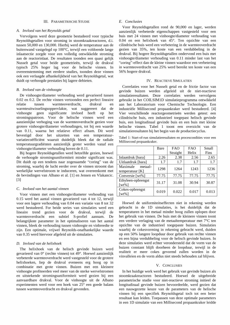
Het CFD model werd gevalideerd door vergelijking met de
experimentele data van Albano et al. [1] voor de geometrie in
Figuur 1. Bij deze experimenten werd lucht opgewarmd van
300K tot ongeveer 340K door middel van een buismantel van
condenserende stoom. De CFD simulaties werden tevens
vergeleken met 1D-simulaties door gebruik te maken van de
correlaties voor het Nusselt getal en de frictiefactor afgeleid
uit deze data door Vanden Eynde [2]. Uitstekende
overeenkomst werd gezien voor zowel de longitudinaal als
helisch gevinde buizen voor de drukval, met relatieve
foutenmarges onder de 5%. De temperatuur werd consistent
onderschat met 2-3°C wat een onderschatting van 10-20% van
het Nusselt getal impliceert. Dit verschil kan toegeschreven
worden aan de grote experimentele fouten in de Albano et al.
opstelling door inconsistente temperatuurmetingen,
onvoldoende inlaatsectie voor stromingsontwikkeling en een
onrealistisch hoog Reynolds getal van 160,000.
Figuur 1:Radiale doorsnede van de Albano et al. geometrie. [1]
w
D = 36.8mm
e
OD = 50.8mm
e/D = 0.15
e/w = 0.37
α = 16°
Ω = 783mm²
Spoed = 143mm
III. PARAMETRISCHE STUDIE
A. Invloed van het Reynolds getal
Vervolgens werd deze geometrie bestudeerd voor typische
Reynoldsgetallen voor stroming in stoomkraakreactoren, d.i.
tussen 50,000 en 130,000. Hierbij werd de temperatuur aan de
buitenwand vastgelegd op 100°C, terwijl een voldoende lange
inlaatsectie zorgde voor een volledig ontwikkelde stroming
aan de reactorinlaat. De resultaten toonden een quasi gelijk
Nusselt getal voor beide geometrieën, terwijl de drukval
typisch 25% hoger lag voor de helische vinnen. In
overeenstemming met eerdere studies, toonden deze vinnen
ook een verlaagde afhankelijkheid van het Reynoldsgetal, wat
duidt op verhoogde prestaties bij lagere debieten.
B. Invloed van de vinhoogte
De vinhoogte/diameter verhouding werd gevarieerd tussen
0.02 en 0.2. De rechte vinnen vertoonden een perfect lineaire
relatie tussen warmteoverdracht, drukval en
warmteuitwisselingsoppervlakte, wat suggereert dat de
vinhoogte geen significante invloed heeft op het
stromingspatroon. Voor de helische vinnen werd een
aanzienlijke verhoging van de warmteoverdracht gezien voor
grotere vinhoogte/diameter verhoudingen, tot bij een waarde
van 0.11, waarna het relatieve effect afnam. Dit werd
bevestigd door het uitzetten van een temperatuur-
variatiecoëfficiënt waaruit duidelijk bleek dat de radiale
temperatuurgradiënten aanzienlijk groter werden vanaf een
vinhoogte/diameter verhouding boven de 0.11.
Bij hogere Reynoldsgetallen werd hetzelfde gezien, hoewel
de verhoogde stromingsuniformiteit minder significant was.
Dit duidt op een tendens naar zogenaamde “coring” van de
stroming, waarbij de lucht eerder over de vinnen stroomt dan
werkelijke wervelstroom te induceren, wat overeenkomt met
de bevindingen van Albano et al. [1] en Jensen en Vlakancic.
[3]
C. Invloed van het aantal vinnen
Voor vinnen met een vinhoogte/diameter verhouding van
0.15 werd het aantal vinnen gevarieerd van 4 tot 12, terwijl
voor een lagere verhouding van 0.04 een variatie van 8 tot 32
werd bestudeerd. For beide series van simulaties werd een
lineaire trend gezien voor de drukval, terwijl de
warmteoverdracht een subtiel S-profiel aannam. De
belangrijkste parameter in het optimaliseren van het aantal
vinnen, bleek de verhouding tussen vinhoogte en vinbreedte te
zijn. Een optimale, vrijwel Reynolds-onafhankelijke waarde
van 0.35 werd hiervoor afgeleid uit de simulaties.
D. Invloed van de helixhoek
The helixhoek van de helisch gevinde buizen werd
gevarieerd van 0° (rechte vinnen) tot 49°. Hoewel aanzienlijk
verbeterde warmteoverdracht werd vastgesteld voor de grotere
helixhoeken, liep de drukval eveneens erg hoog op in
combinatie met grote vinnen. Buizen met een kleinere
vinhoogte profiteerden veel meer van de sterke wervelstromen
en uitstekende stromingsuniformiteit werd gezien bij een
aanvaardbare drukval. Voor de vinhoogte uit de Albano
experimenten werd voor een hoek van 25° een goede balans
tussen warmteoverdracht en drukval gevonden.
E. Conclusies
Voor Reynoldsgetallen rond de 90,000 en lager, werden
aanzienlijk verbeterde eigenschappen vastgesteld voor een
buis met 24 vinnen met vinhoogte/diameter verhouding van
0.04 en een helixhoek van 45°. Ten opzichte van een
cilindrische buis werd een verbetering in de warmteoverdracht
gezien van 35%, ten koste van een verdubbeling in de
drukval. Bij hogere Reynoldsgetallen ondervond een buis met
vinhoogte/diameter verhouding van 0.11 minder last van het
“coring”-effect dan de kleine vinnen waardoor een verbetering
in warmteoverdracht van 25% werd bereikt ten koste van een
56% hogere drukval.
IV. REACTIEVE SIMULATIES
Correlaties voor het Nusselt getal en de frictie factor van
gevinde buizen werden afgeleid uit de niet-reactieve
simulatieresultaten. Deze correlaties werden vervolgens
gebruikt in het COILSIM1D simulatieprogramma ontwikkeld
aan het Laboratorium voor Chemische Technologie. Een
industriële Millisecond propaankraker werd bestudeerd. [4]
Vier verschillende reactorgeometrieën werden getest: een
cilindrische buis, een industrieel toegepast helisch gevinde
buis, een longitudinaal gevinde buis en een buis met kleine
helische vinnen. Tabel 1 toont een overzicht van de
simulatieresultaten bij het begin van de productiecyclus.
Tabel 1: Start-of-run simulatieresultaten en procescondities voor een
Millisecond propaankraker.
Bare FAO
Straight
FAO
Helix
Small
Fins
Inlaatdruk [bara] 2.26 2.38 2.56 2.65
Uitlaatdruk [bara] 1.7 1.7 1.7 1.7
Maximale metaal-
temperatuur [K] 1298 1264 1243 1236
Conversie [wt%] 77.75 77.75 77.75 77.75
Ethyleen-opbrengst
[wt%] 31.17 31.08 30.94 30.87
Cokes-opbrengst
[wt%] 0.019 0.022 0.017 0.013
Hoewel de uniformiteitseffecten niet in rekening werden
gebracht in de 1D simulaties, is het duidelijk dat de
temperaturen in het metaal minder hoog zullen oplopen door
het gebruik van vinnen. De buis met de kleinere vinnen toont
een verdere verlaging van de metaaltemperatuur met 7°C ten
opzichte van de industrieel toegepaste buizen. Simulaties
waarbij de cokesvorming in rekening gebracht werd, duiden
op een 50% langere loopduur door gebruik van rechte vinnen
en een bijna verdubbeling voor de helisch gevinde buizen. In
deze simulaties werd echter verondersteld dat de vorm van de
buizen constant blijft doorheen de loopduur, terwijl in de
realiteit er meer cokes gevormd zullen worden in de
vinvalleien en de vorm aldus niet steeds behouden zal blijven.
V. CONCLUSIES
In het huidige werk werd het gebruik van gevinde buizen als
stoomkraakreactoren bestudeerd. Hoewel de uitgebreide
parametrische studie voor niet-reactieve stroming initieel de
longitudinaal gevinde buizen bevoordeelde, werd gezien dat
een nauwgezette keuze van de parameters van de helische
vinnen bij een specifiek Reynoldsgetal toch tot een beter
resultaat kan leiden. Toepassen van deze optimale parameters
in een 1D simulatie van een Millisecond propaankraker leidde
tot aanzienlijk verbeterde metaaltemperaturen en lengte van
de productiecycli. Hoewel een selectiviteitsverlies aan
ethyleen van 1% werd berekend voor de helisch gevinde
buizen, wordt verwacht dat dit goedgemaakt zal worden door
deze eigenschappen. Om een kwantitatieve evaluatie van de
lengte van de productiecycli te maken echter, blijft het van
primair belang om een grondiger begrip te krijgen rond de
locatie van de cokesvorming en hoe dit de buisgeometrie en
aangepaste warmteoverdracht zal beïnvloeden.
BIBLIOGRAFIE
1. J. V. Albano, K. M. Sundaram, M. J. Maddock, Applications of extended surfaces in pyrolysis coils. Energy Progress, 1988. 8(3): p. 9.
2. De Saegher, J. J., T. Detemmerman, and Gilbert Froment, Three
dimensional simulation of high severity internally finned cracking coils for olefins production. Revue de l'Institut Francais du Petrole, 1996.
51(2): p. 245-260.
3. Gregory J. Zdaniuk, Louay M. Chamra, Pedro J. Mago, Experimental determination of heat transfer and friction in helically-finned tubes.
Experimental Thermal and Fluid Science, 2008. 32: p. 15.
4. Heynderickx, Geraldine J., Modellering en Simulatie van Huidige en Nieuwe Technologieën voor de Thermische Kraking van
Koolwaterstoffen, in Laboratorium voor Petrochemische
Techniek1993, Universiteit Gent: Faculteit van de Toegepaste Wetenschappen.
Dankwoord
Dit eindwerk is tot stand gekomen met de hulp en steun van vele mensen. Via deze weg wil ik die
personen van harte bedanken.
Allereerst wens ik mijn promotor, prof. dr. Ir. Kevin Van Geem, samen met prof. dr. ir. Guy B. Marin, te
bedanken om me de kans te bieden dit onderwerp aan te vatten. Hierbij wil ik in het bijzonder Kevin
bedanken voor zijn begeleiding en feedback doorheen het jaar, alsook voor het scheppen van
uitdagende perspectieven in de vorm van een mogelijk doctoraat op dit onderwerp. Ondanks de niet
eenzijdig-positieve invloeden dat dit mogelijks had op mijn eindwerk, wil ik ook professor Marin
wederom bedanken voor de verrijkende ervaring die mij aangeboden werd door mijn eerste semester in
het buitenland te mogen doorbrengen.
De grootste dank gaat zonder twijfel uit naar mijn begeleider, Carl Schietekat. Zonder zijn kennis en
ervaring betreffende het onderwerp zou dit eindwerk nooit tot een goed einde gebracht zijn. Verder wil
ik Carl bedanken voor de constante aanmoedigingen en de verzekering dat het “allemaal wel slim komt”
als de resultaten eens wat minder geslaagd waren. Dank gaat verder ook uit naar Georges en Maarten
die steeds klaarstonden om alle mogelijke software-kwaaltjes te verhelpen.
I would also like to offer my gratitude to Amit for his expertise while dealing with all sorts of CFD issues
throughout the year.
Verder wil ik mijn medestudenten Cederik, Lieselot, Yumi, Maxime, Ben, Steven en Jonas bedanken voor
de aangename koffie-, middag-, avond- en nachtpauzes. In het bijzonder wens ik Lieselot, Yumi en Jeroen
te bedanken voor de uitstekende sfeer in ons kleine bureautje.
Ten slotte wil ik mijn ouders, broers en zus bedanken voor de nooit aflatende morele (en financiële)
steun gedurende mijn studieloopbaan. Als laatste wil ik mijn vriendin Roshanak van harte bedanken om
er altijd voor mij te zijn tijdens deze soms moeilijke maanden. Op één jaar tijd zowel een Erasmus als een
thesis doorstaan, toont toch nog maar eens hoe sterk onze relatie wel is…
Bedankt!
David Van Cauwenberge
Confidential - I -
Table of contents
Nomenclature ............................................................................................................................................ IV
Chapter 1 - Introduction ........................................................................................................................... 1
1.1 Steam cracking .............................................................................................................................. 1
1.1.1 General principles .................................................................................................................. 1
1.1.2 Coking .................................................................................................................................... 2
1.2 Problem description ...................................................................................................................... 3
1.3 Outline ........................................................................................................................................... 4
References ................................................................................................................................................. 5
Chapter 2 - Literature review .................................................................................................................. 6
2.1 Mechanical devices for coke reduction ......................................................................................... 6
2.2 Increased internal surface area ..................................................................................................... 7
2.2.1 Albano et al. ........................................................................................................................... 8
2.2.2 De Saegher et al. .................................................................................................................. 10
2.2.3 Other fin structures ............................................................................................................. 11
2.3 Enhanced mixing ......................................................................................................................... 13
2.3.1 Mixing Element Radiant Tube ............................................................................................. 13
2.3.2 Helical and Lemniscate Coils ............................................................................................... 15
2.3.3 SMall Amplitude Helical Tube ............................................................................................. 16
2.3.4 Coil inserts ........................................................................................................................... 18
References ............................................................................................................................................... 21
Chapter 3 - Computational study of pressure drop and heat transfer in finned tubes ............. 23
3.1 Mathematical formulation .......................................................................................................... 23
Governing equations ........................................................................................................... 23 3.1.1
Confidential - II -
3.2 Turbulence modeling ................................................................................................................... 25
The k-ε model ...................................................................................................................... 26 3.2.1
Reynolds Stress Models (RSM) ............................................................................................ 28 3.2.2
Boundary conditions............................................................................................................ 29 3.2.3
3.3 Finite volume method ................................................................................................................. 31
3.4 Discretization schemes ................................................................................................................ 32
3.5 Meshing ....................................................................................................................................... 33
3.6 Non-reactive CFD model ............................................................................................................. 35
3.7 Model validation.......................................................................................................................... 36
Experimental data ............................................................................................................... 36 3.7.1
Full setup simulations .......................................................................................................... 39 3.7.2
Experimental setup shortcomings ....................................................................................... 43 3.7.3
3.8 Reynolds number dependency of friction factors and Nusselt numbers .................................... 44
3.9 Influence of fin height on pressure drop and heat transfer in finned tubes............................... 48
Constant Reynolds number ................................................................................................. 50 3.9.1
Influence of Reynolds number ............................................................................................ 57 3.9.2
3.10 Influence of pitch on pressure drop and heat transfer in helicoidally finned tubes ................... 61
Constant Reynolds number ................................................................................................. 63 3.10.1
Influence of the Reynolds Number...................................................................................... 68 3.10.2
3.11 Influence of number of fins on pressure drop and heat transfer in finned tubes ...................... 71
Constant Reynolds number ................................................................................................. 72 3.11.1
Influence of Reynolds number ............................................................................................ 77 3.11.2
3.12 Geometry optimization - Conclusions ......................................................................................... 79
References ............................................................................................................................................... 84
Chapter 4 - Simulation of reactive flow ............................................................................................... 85
4.1 Introduction ................................................................................................................................. 85
4.2 Reactor specifications ................................................................................................................. 86
4.2.1 The Kellog Millisecond reactor ............................................................................................ 86
4.2.2 Process conditions ............................................................................................................... 87
4.2.3 Base geometry ..................................................................................................................... 88
4.3 One-dimensional simulations using COILSIM1D ......................................................................... 89
Confidential - III -
4.3.1 Introduction ......................................................................................................................... 89
4.3.2 Friction factor and Nusselt number correlations ................................................................ 91
4.3.3 Methodology ....................................................................................................................... 93
4.3.4 Results ................................................................................................................................. 93
4.3.5 Additional considerations .................................................................................................... 98
4.4 Three-dimensional FLUENT simulations ...................................................................................... 99
4.4.1 Reaction network ................................................................................................................ 99
4.4.2 Tube geometries ................................................................................................................ 100
4.4.3 Methodology ..................................................................................................................... 101
4.4.4 Results ............................................................................................................................... 101
References ............................................................................................................................................. 102
Chapter 5 - Conclusions and future work ......................................................................................... 103
5.1 Conclusions ................................................................................................................................ 103
5.2 Future work ............................................................................................................................... 105
References ............................................................................................................................................. 106
Annex A - Performed Simulations ...................................................................................................... 107

Confidential - III -
Nomenclature Acronyms
Confidential - IV -
Nomenclature
Acronyms
TLE Transfer line exchanger
TMT Tube metal temperatures
MERT Mixing element Radiant Tube
CIP Coil inlet pressure [bara]
COP Coil outlet pressure [bara]
SMAHT Small Amplitude Helical Tube
IHT Intensified Heat Technology
SRT Short Residence Time
RANS Reynolds-Averaged Navier-Stokes
RNG Renormalization Group Methods
RSM Reynolds Stress Model
PDE Partial Differential Equation
QUICK Quadratic Upstream Interpolation for Convective Kinetics
CoV Coefficient of variation [-]
HC Hydrocarbon
FAO Fina Antwerp Olefins
SOR Start of run
EOR End of run
Nomenclature Roman symbols
Confidential - V -
Roman symbols
Q Heat transfer [J/s]
T Temperature [K]
p Pressure [Pa]
A Surface area [m²]
Nu Nusselt number [-]
Re Reynolds number [-]
Pr Prandtl number [-]
j Colburn j-factor (Nu/RePr1/3) [-]
f Fanning friction factor [-]
De Dean number [-]
h Convection coefficient [J/sm²K]
ui Velocity in the i-direction [m/s]
t Time [s]
F Body forces [Pa.s]
e Internal energy [J/kg]
k Turbulent kinetic energy [J/kg]
l Characteristic length scale [m]
Cx Turbulence model constants [-]
u+ Dimensionless velocity [-]
y+ Dimensionless wall distance [-]
P (Wetted) perimeter [m]
Cp Specific heat capacity [J/kgK]
e Roughness height / Fin height [m]
D Diameter [m]

Nomenclature Greek symbols
Confidential - VI -
P Helicoidal pitch length [m]
w Fin width [m]
Greek symbols
ρ Density [kg/m³]
τij Shear stress [Pa.s]
µ Dynamic viscosity [Pa.s]
ν Kinematic viscosity [m²/s]
ε Turbulent kinetic energy dissipation rate [J/kg.s]
δij Kronecker-delta 0 or 1
κ von Kármán constant 0.42
φ Arbitrary conserved flow property [?]
λ Thermal conductivity [W/mK]
φm Mass flow rate [kg/s]
α Helix angle [°]
1 Introduction Steam cracking
Confidential - 1 -
1 Introduction
1.1 Steam cracking .......................................................................................................................... 1
1.2 Problem description .................................................................................................................. 3
1.3 Outline ...................................................................................................................................... 4
References .................................................................................................................................................. 5
1.1 Steam cracking
1.1.1 General principles
Steam cracking of hydrocarbons is the predominant commercial method for producing light olefins such
as ethylene, propylene and butadiene. These low-molecular-weight olefins are widely used in the
manufacture of high volume polymeric materials and commercially important chemical intermediates.
Worldwide annual ethylene production capacity is around 148 x 106 tons with growth projections of 4%
per year [1, 2]. Depending on the feedstock used to produce the olefins, steam cracking can produce a
benzene-rich liquid by-product called pyrolysis gasoline. With an additional extraction process, benzene,
toluene and xylenes can be recovered [3]. In Europe this represents over 50% of the total benzene
production, while in the U.S. catalytic reforming is the most used method of production for these
aromatics [4]. Modern steam cracking plants form the core of a petrochemical process, producing
500,000 to 1,500,000 tons per year of ethylene, the main petrochemical building block [5].
A steam cracking plant consists of furnaces and a separation train. The furnace has a radiant section, a
convection section and a transfer line exchanger (TLE) and typically consists of a set of coils with an
1 Introduction Steam cracking
Confidential - 2 -
internal diameter of 30-100mm and a length of 10-100m. In the convection section, feed and steam are
preheated up to approximately 600°C in order to recover the sensible heat contained in the flue gases
leaving the radiant section. In the radiant section the process gas temperature is increased to 820-900°C,
providing the required heat for the endothermic reactions. Under these conditions, the feedstock is
converted through free-radical reactions to the products. Ethylene yield is typically 25-30% for naphtha
crackers and over 50% for ethane crackers [1]. In a generalized and very simplified form, the complex
kinetics of cracking hydrocarbons can be summarized as a set of primary reactions leading to production
of olefins, hydrogen and methane, while secondary reactions lead to C4-C7 fractions and aromatics.
From these fundamental considerations, it can easily be understood that ethylene selectivity will be
favored by short residence times. As the secondary reactions are generally bimolecular reactions, these
will occur more prominently at higher hydrocarbon partial pressures [1, 6]. As such, increasing ethylene
selectivity is one of the reasons dilution steam is added to the feed-stock. Since this obviously leads to
higher energy requirements on the furnace, the steam-to-hydrocarbon mass ratio is usually limited from
0.3 for ethane to 0.7 for naphtha and heavier fractions [1, 5].
1.1.2 Coking
Of primary concern in all steam cracking process configurations is the formation of coke. When
hydrocarbon feedstocks are subjected to the heating conditions prevalent in a steam cracking furnace,
coke deposits form on the inner walls of the tubular cracking coils. This carbonaceous coke layer leads to
an increased pressure drop over the reactor which further leads to higher hydrocarbon partial pressures
and a loss of ethylene selectivity. Additionally, these coke deposits interfere with heat flow into the
reactant stream. To maintain the same cracking severity, this increased heat transfer resistance is
compensated by increasing the heat input from the furnace burners, leading to higher tube metal
temperatures (TMT) of up to 1100°C. Eventually either the metallurgic constraints of the coils or the
excessive pressure drop will force the operators to cease production and decoke the furnace. Typical
runlengths for industrial furnaces vary between 30-100 days, depending on cracking conditions and feed-
stock. The dilution steam lowers the partial pressures of high-boiling aromatics and tarry materials,
reducing their tendency to deposit and will even react with already deposited coke to form carbon
monoxide/dioxide and hydrogen [1]. Decoking is carried out by passing an air/steam mixture through the
coils at high temperature. The coke is thus removed by a combination of combustion and
erosion/spalling. For the latter case, some of this spalled coke can be in the form of large particles that
may plug the coils before or during decoking. As there is a tendency towards decreasing tube diameters,
1 Introduction Problem description
Confidential - 3 -
this has become an even greater concern. Typically decoking will require operation to be interrupted for
12-48 hours, having a considerable adverse effect on the economics of the process.
Furthermore, coke formation will influence the service life of the reactor coils. In the radiant section of
the furnace, the tubes are heated with side wall burners and/or long-flame floor burners from opposite
sides. This causes each of the tubes to have two light sides, facing the burners, and dark sides which are
offset by a 90° angle. The mean tube metal temperature, i.e. the difference between the TMT on the
light side and the dark side, leads to internal stresses and therefore determines the service life of the
tubes [7]. This effect will further be enhanced by the insulating coke layer. Although the chromium-
nickel-steel alloys used have a high resistance to carburization, carbon will diffuse into the tube wall
possibly leading to carbon contents of 1% to 3%, associated with considerable embrittlement of the tube
material [7].
1.2 Problem description
In light of all the encountered problems, efforts are being made towards the development of
technologies to reduce coke formation. These technologies can be grouped according to three main
focuses: the use of additives, metal surface technologies and mechanical devices. As additives mainly
sulfur containing components have been investigated. While a general consensus exists on the beneficial
effect for the suppression of CO production, the reported effect on coke formation is contradictory [8, 9].
Besides sulfur-containing, components containing phosphor, silicon, alkali and alkaline earth metal salts
or tin and antimony have also been investigated [9, 10]. For metal surface technologies, much progress
has been made in high temperature alloys, low-coking alloys and (catalytic) coatings [11-13]. Finally, in
the category of mechanical devices, three-dimensional reactor configurations are used to improve the
heat transfer, which will form the main point of focus in the present work.
As decoking is generally initiated when the TMT reaches a certain temperature threshold, this point can
be delayed by improving the heating characteristics of the tube. This can be achieved by introducing
three-dimensional structures inside the reactor coils that increase the internal surface and/or promote
convection by improving the radial uniformity of the flow. Although these techniques have been widely
applied and studied for heat exchangers, the problem in steam cracking reactors is slightly more
sensitive because of the additional pressure drop these structures induce. This pressure drop will cause
prolonged residence times which in turn will lead to reduced ethylene selectivity.
1 Introduction Outline
Confidential - 4 -
The presented problem as such consists of finding three-dimensional reactor structures that improve the
heat transfer, allowing increased run lengths, while limiting the pressure drop and loss of ethylene
selectivity.
1.3 Outline
The course that was followed in this Master’s Thesis consists firstly of a literature study on a number of
three-dimensional structures that have already been applied or show considerable promise for use in
steam cracking reactors.
In Chapter 3, a brief summary of the CFD basics is given, in order to have a better understanding of the
optimal model for simulating flow inside this type of tubes. Following this, the CFD model is validated by
comparison of the Ansys Fluent 13.0 simulation results with experimental data obtained for a given
geometry over a range of Reynolds numbers. Having done this, a parametric study will be performed for
the longitudinally and helicoidally finned coils. The influence of the fin height, the amount of fins and the
helix pitch angle is investigated for two different Reynolds numbers. Based upon the results obtained
from these simulations, optimal values for the specific parameters are proposed and assembled into a
few “optimized” geometries for which simulations were performed as well.
Having concluded the parametric study, it obviously remains of primary importance to evaluate the
effects on steam cracking of both improved heat transfer and additional pressure drop. This is covered in
Chapter 4 where the results of the parametric study allow derivation of correlations for the Nusselt
number and friction factors of these tubes. One-dimensional reactive simulation is then performed by
combining these obtained correlations with the extensive radical reaction network of the COILSIM1D
program. Using the built-in shooting method, it is possible to simulate the coking rates and run lengths
for the investigated finned tubes. Finally, three-dimensional simulations using a simplified molecular
reaction network are performed to directly assess any potential benefits provided by the enhanced
heating and mixing characteristics of the finned reactor coils.
1 Introduction References
Confidential - 5 -
References
1. Zimmermann, Heinz and Roland Walzl, Ethylene, in Ullmann's Encyclopedia of Industrial
Chemistry2000, Wiley-VCH Verlag GmbH & Co. KGaA.
2. Plastemart. Overcapacity expected in ethylene uptil 2013. 2010 [cited 2012 May 3rd]; Available
from: http://www.plastemart.com/Plastic-Technical-
Article.asp?LiteratureID=1380&Paper=overcapacity-ethylene-demand-growth-2013.
3. SABIC. Pygas (Pyrolysis Gasoline). 2012 [cited 2012 May 3rd]; Available from:
http://www.sabic.com/me/en/productsandservices/chemicals/pygas.aspx.
4. Netzer, David, Benzene Supply Trends and Proposed Method for Enhanced Recovery, in 2005
World Petrochemical Conference2005: Houston, Texas.
5. J. Towfighi, R. Karimzadeh, SHAHAB-A PC-Based Software for Simulation of Steam Cracking
Furnaces (Ethane and Naphtha). Iranian Journal of Chemical Engineering, 2004. 1(2): p. 14.
6. Nicolantonio, Arthur Di, Pyrolysis furnace with an internally finned U-shaped radiant coil, E.
Chemical, Editor 2002: United States.
7. Peter Wolbert, Benno Ganser, Dietlinde Jakobi, Rolf Kirchheiner, Process and finned tube for the
thermal cracking of hydrocarbons, 2005: United States.
8. Wang, Jidong, Marie-Françoise Reyniers, and Guy B. Marin, Influence of Dimethyl Disulfide on
Coke Formation during Steam Cracking of Hydrocarbons. Industrial & Engineering Chemistry
Research, 2007. 46(Inconel 600): p. 15.
9. Jidong Wang, Marie-Françoise Reyniers, Kevin M. Van Geem and Guy B. Marin, Influence of
Silicon and Silicon/Sulfur-Containing Additives on Coke Formation during Steam Cracking of
Hydrocarbons. Ind. Eng. Chem. Res., 2008. 47: p. 15.
10. Wang, Jidong, Marie-Françoise Reyniers, and Guy B. Marin, The influence of phosphorus
containing compounds on steam cracking of n-hexane. Journal of Analytical and Applied
Pyrolysis, 2006. 77(2): p. 133-148.
11. Györffy, Michael, MERT Technology Update: X-MERT, in AlCHE: Ethylene Producers
Meeting2009: Tampa Bay.
12. Kubota, Alloy Data Sheet, KHR 45A, 1999.
13. Zhou, Jianxin, Zhiyuan Wang, Xiaojian Luan, and Hong Xu, Anti-coking property of the SiO2/S
coating during light naphtha steam cracking in a pilot plant setup. Journal of Analytical and
Applied Pyrolysis, 2011. 90(1): p. 7-12.

2 Literature review Mechanical devices for coke reduction
Confidential - 5 -
2 Literature review Mechanical devices for coke reduction
Confidential - 6 -
2 Literature review
2.1 Mechanical devices for coke reduction ......................................................................................... 6
2.2 Increased internal surface area ..................................................................................................... 7
2.2.1 Albano et al. ......................................................................................................................... 8
2.2.2 De Saegher et al. ................................................................................................................ 10
2.2.3 Other fin structures ........................................................................................................... 11
2.3 Enhanced mixing .......................................................................................................................... 13
2.3.1 Mixing Element Radiant Tube ............................................................................................ 13
2.3.2 Helical and Lemniscate Coils .............................................................................................. 15
2.3.3 SMall Amplitude Helical Tube ............................................................................................ 16
2.3.4 Coil inserts ......................................................................................................................... 18
References ........................................................................................................................................... 21
2.1 Mechanical devices for coke reduction
The focus of this work will lie in the development of three-dimensional reactor configurations. Therefore
an overview will be given on previously investigated and applied methods in steam crackers. In general
the mechanical devices can be divided in two classes based on the physical reason behind the increased
heat transfer. Heat transfer in its most basic form can be written as:
Q = A.U.ΔT (1)
2 Literature review Increased internal surface area
Confidential - 7 -
, with Q being the transferred amount of heat, A the contact area, U the overall heat transfer coefficient
(including all convection and conduction contributions) and ΔT the difference in temperature between a
solid surface and the bulk of a fluid. It is easy to understand that increasing the heat transfer area will
have a direct effect. This can be achieved by decreasing the pipe diameter, which has been a main trend
over the previous decades, but which also is limited by the occurrence of pipe plugging during the
decoking phase as explained above. Devices that increase the internal surface area by means of fin-like
structures will represent a first type of reactor configuration used in order to reduce coke formation.
Secondly, the U-factor can be increased to increase heat transfer. This overall heat transfer coefficient is
greatly influenced by the measure of flow turbulence. Mixing will be greater at higher Reynolds numbers
and for more complex flow patterns but both of these will lead to greater pressure drops, which in turn
lead to reduced selectivity to ethylene [1]. Finding three-dimensional structures that achieve this
improved mixing while limiting the extra head loss will constitute the second type of reactor
configurations. It may be clear that for some mechanical devices an increase in heat transfer is achieved
by a combination of both mechanisms.
2.2 Increased internal surface area
Fins constitute a commonly used method for increasing internal surface area. In the case of steam
cracking, both helically and longitudinally finned tubes have been studied and applied industrially. As
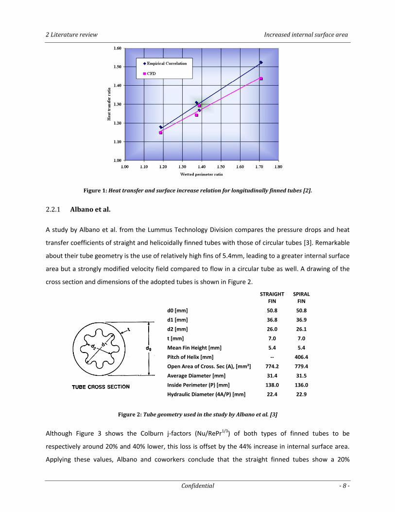
shown in Figure 1 from Stone & Webster for straight finned tubes, a linear relationship exists between
the ratio of heat transfer improvement and the ratio of surface increase [2].
2 Literature review Increased internal surface area
Confidential - 8 -
Figure 1: Heat transfer and surface increase relation for longitudinally finned tubes [2].
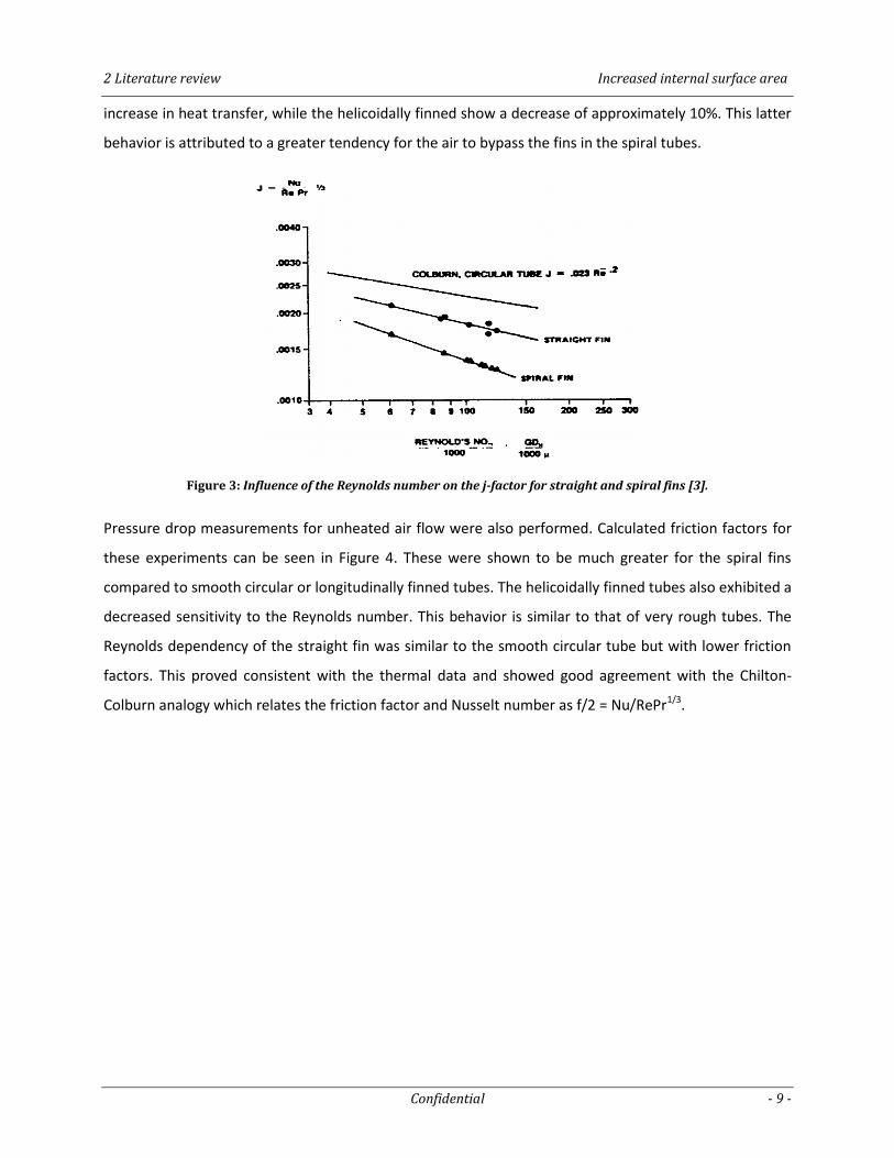
2.2.1 Albano et al.
A study by Albano et al. from the Lummus Technology Division compares the pressure drops and heat
transfer coefficients of straight and helicoidally finned tubes with those of circular tubes [3]. Remarkable
about their tube geometry is the use of relatively high fins of 5.4mm, leading to a greater internal surface
area but a strongly modified velocity field compared to flow in a circular tube as well. A drawing of the
cross section and dimensions of the adopted tubes is shown in Figure 2.
STRAIGHT
FIN SPIRAL
FIN
d0 [mm] 50.8 50.8
d1 [mm] 36.8 36.9
d2 [mm] 26.0 26.1
t [mm] 7.0 7.0
Mean Fin Height [mm] 5.4 5.4
Pitch of Helix [mm] -- 406.4
Open Area of Cross. Sec (A), [mm²] 774.2 779.4
Average Diameter [mm] 31.4 31.5
Inside Perimeter (P) [mm] 138.0 136.0
Hydraulic Diameter (4A/P) [mm] 22.4 22.9
Figure 2: Tube geometry used in the study by Albano et al. [3]
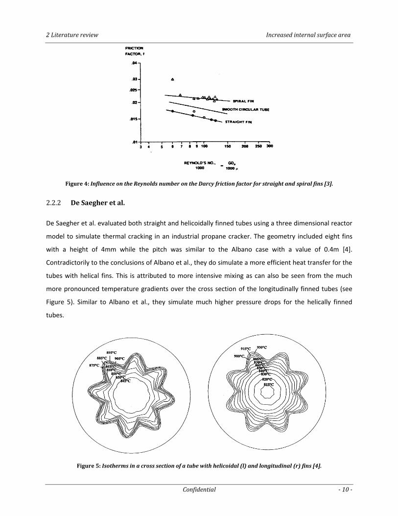
Although Figure 3 shows the Colburn j-factors (Nu/RePr1/3) of both types of finned tubes to be
respectively around 20% and 40% lower, this loss is offset by the 44% increase in internal surface area.
Applying these values, Albano and coworkers conclude that the straight finned tubes show a 20%
2 Literature review Increased internal surface area
Confidential - 9 -
increase in heat transfer, while the helicoidally finned show a decrease of approximately 10%. This latter
behavior is attributed to a greater tendency for the air to bypass the fins in the spiral tubes.
Figure 3: Influence of the Reynolds number on the j-factor for straight and spiral fins [3].
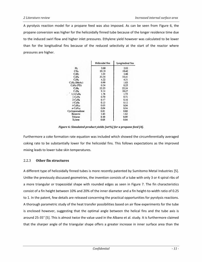
Pressure drop measurements for unheated air flow were also performed. Calculated friction factors for
these experiments can be seen in Figure 4. These were shown to be much greater for the spiral fins
compared to smooth circular or longitudinally finned tubes. The helicoidally finned tubes also exhibited a
decreased sensitivity to the Reynolds number. This behavior is similar to that of very rough tubes. The
Reynolds dependency of the straight fin was similar to the smooth circular tube but with lower friction
factors. This proved consistent with the thermal data and showed good agreement with the Chilton-
Colburn analogy which relates the friction factor and Nusselt number as f/2 = Nu/RePr1/3.
2 Literature review Increased internal surface area
Confidential - 10 -
Figure 4: Influence on the Reynolds number on the Darcy friction factor for straight and spiral fins [3].
2.2.2 De Saegher et al.
De Saegher et al. evaluated both straight and helicoidally finned tubes using a three dimensional reactor
model to simulate thermal cracking in an industrial propane cracker. The geometry included eight fins
with a height of 4mm while the pitch was similar to the Albano case with a value of 0.4m [4].
Contradictorily to the conclusions of Albano et al., they do simulate a more efficient heat transfer for the
tubes with helical fins. This is attributed to more intensive mixing as can also be seen from the much
more pronounced temperature gradients over the cross section of the longitudinally finned tubes (see
Figure 5). Similar to Albano et al., they simulate much higher pressure drops for the helically finned
tubes.
Figure 5: Isotherms in a cross section of a tube with helicoidal (l) and longitudinal (r) fins [4].
2 Literature review Increased internal surface area
Confidential - 11 -
A pyrolysis reaction model for a propane feed was also imposed. As can be seen from Figure 6, the
propane conversion was higher for the helicoidally finned tube because of the longer residence time due
to the induced swirl flow and higher inlet pressures. Ethylene yield however was calculated to be lower
than for the longitudinal fins because of the reduced selectivity at the start of the reactor where
pressures are higher.
Figure 6: Simulated product yields [wt%] for a propane feed [4].
Furthermore a coke formation rate equation was included which showed the circumferentially averaged
coking rate to be substantially lower for the helicoidal fins. This follows expectations as the improved
mixing leads to lower tube skin temperatures.
2.2.3 Other fin structures
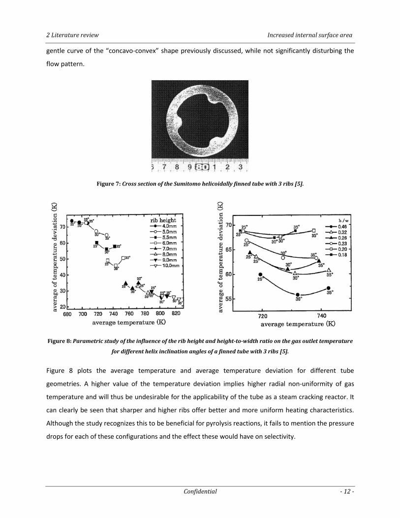
A different type of helicoidally finned tubes is more recently patented by Sumitomo Metal Industries [5].
Unlike the previously discussed geometries, the invention consists of a tube with only 3 or 4 spiral ribs of
a more triangular or trapezoidal shape with rounded edges as seen in Figure 7. The fin characteristics
consist of a fin height between 10% and 20% of the inner diameter and a fin height-to-width ratio of 0.25
to 1. In the patent, few details are released concerning the practical opportunities for pyrolysis reactions.
A thorough parametric study of the heat transfer possibilities based on air flow experiments for the tube
is enclosed however, suggesting that the optimal angle between the helical fins and the tube axis is
around 25-35° [5]. This is almost twice the value used in the Albano et al. study. It is furthermore claimed
that the sharper angle of the triangular shape offers a greater increase in inner surface area than the
2 Literature review Increased internal surface area
Confidential - 12 -
gentle curve of the “concavo-convex” shape previously discussed, while not significantly disturbing the
flow pattern.
Figure 7: Cross section of the Sumitomo helicoidally finned tube with 3 ribs [5].
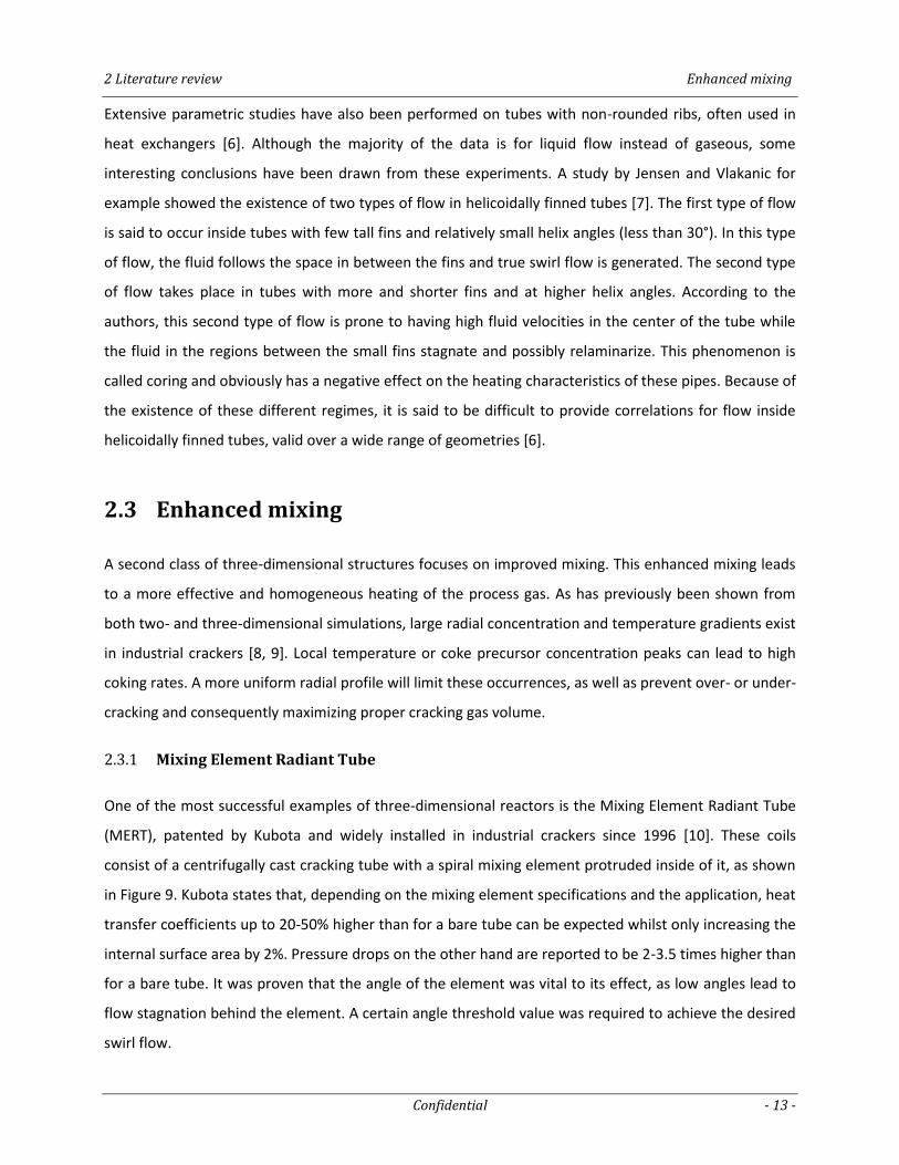
Figure 8: Parametric study of the influence of the rib height and height-to-width ratio on the gas outlet temperature
for different helix inclination angles of a finned tube with 3 ribs [5].
Figure 8 plots the average temperature and average temperature deviation for different tube
geometries. A higher value of the temperature deviation implies higher radial non-uniformity of gas
temperature and will thus be undesirable for the applicability of the tube as a steam cracking reactor. It
can clearly be seen that sharper and higher ribs offer better and more uniform heating characteristics.
Although the study recognizes this to be beneficial for pyrolysis reactions, it fails to mention the pressure
drops for each of these configurations and the effect these would have on selectivity.
2 Literature review Enhanced mixing
Confidential - 13 -
Extensive parametric studies have also been performed on tubes with non-rounded ribs, often used in
heat exchangers [6]. Although the majority of the data is for liquid flow instead of gaseous, some
interesting conclusions have been drawn from these experiments. A study by Jensen and Vlakanic for
example showed the existence of two types of flow in helicoidally finned tubes [7]. The first type of flow
is said to occur inside tubes with few tall fins and relatively small helix angles (less than 30°). In this type
of flow, the fluid follows the space in between the fins and true swirl flow is generated. The second type
of flow takes place in tubes with more and shorter fins and at higher helix angles. According to the
authors, this second type of flow is prone to having high fluid velocities in the center of the tube while
the fluid in the regions between the small fins stagnate and possibly relaminarize. This phenomenon is
called coring and obviously has a negative effect on the heating characteristics of these pipes. Because of
the existence of these different regimes, it is said to be difficult to provide correlations for flow inside
helicoidally finned tubes, valid over a wide range of geometries [6].
2.3 Enhanced mixing
A second class of three-dimensional structures focuses on improved mixing. This enhanced mixing leads
to a more effective and homogeneous heating of the process gas. As has previously been shown from
both two- and three-dimensional simulations, large radial concentration and temperature gradients exist
in industrial crackers [8, 9]. Local temperature or coke precursor concentration peaks can lead to high
coking rates. A more uniform radial profile will limit these occurrences, as well as prevent over- or under-
cracking and consequently maximizing proper cracking gas volume.
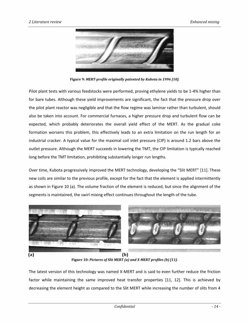
2.3.1 Mixing Element Radiant Tube
One of the most successful examples of three-dimensional reactors is the Mixing Element Radiant Tube
(MERT), patented by Kubota and widely installed in industrial crackers since 1996 [10]. These coils
consist of a centrifugally cast cracking tube with a spiral mixing element protruded inside of it, as shown
in Figure 9. Kubota states that, depending on the mixing element specifications and the application, heat
transfer coefficients up to 20-50% higher than for a bare tube can be expected whilst only increasing the
internal surface area by 2%. Pressure drops on the other hand are reported to be 2-3.5 times higher than
for a bare tube. It was proven that the angle of the element was vital to its effect, as low angles lead to
flow stagnation behind the element. A certain angle threshold value was required to achieve the desired
swirl flow.
2 Literature review Enhanced mixing
Confidential - 14 -
Figure 9: MERT-profile originally patented by Kubota in 1996 [10].
Pilot plant tests with various feedstocks were performed, proving ethylene yields to be 1-4% higher than
for bare tubes. Although these yield improvements are significant, the fact that the pressure drop over
the pilot plant reactor was negligible and that the flow regime was laminar rather than turbulent, should
also be taken into account. For commercial furnaces, a higher pressure drop and turbulent flow can be
expected, which probably deteriorates the overall yield effect of the MERT. As the gradual coke
formation worsens this problem, this effectively leads to an extra limitation on the run length for an
industrial cracker. A typical value for the maximal coil inlet pressure (CIP) is around 1.2 bars above the
outlet pressure. Although the MERT succeeds in lowering the TMT, the CIP limitation is typically reached
long before the TMT limitation, prohibiting substantially longer run lengths.
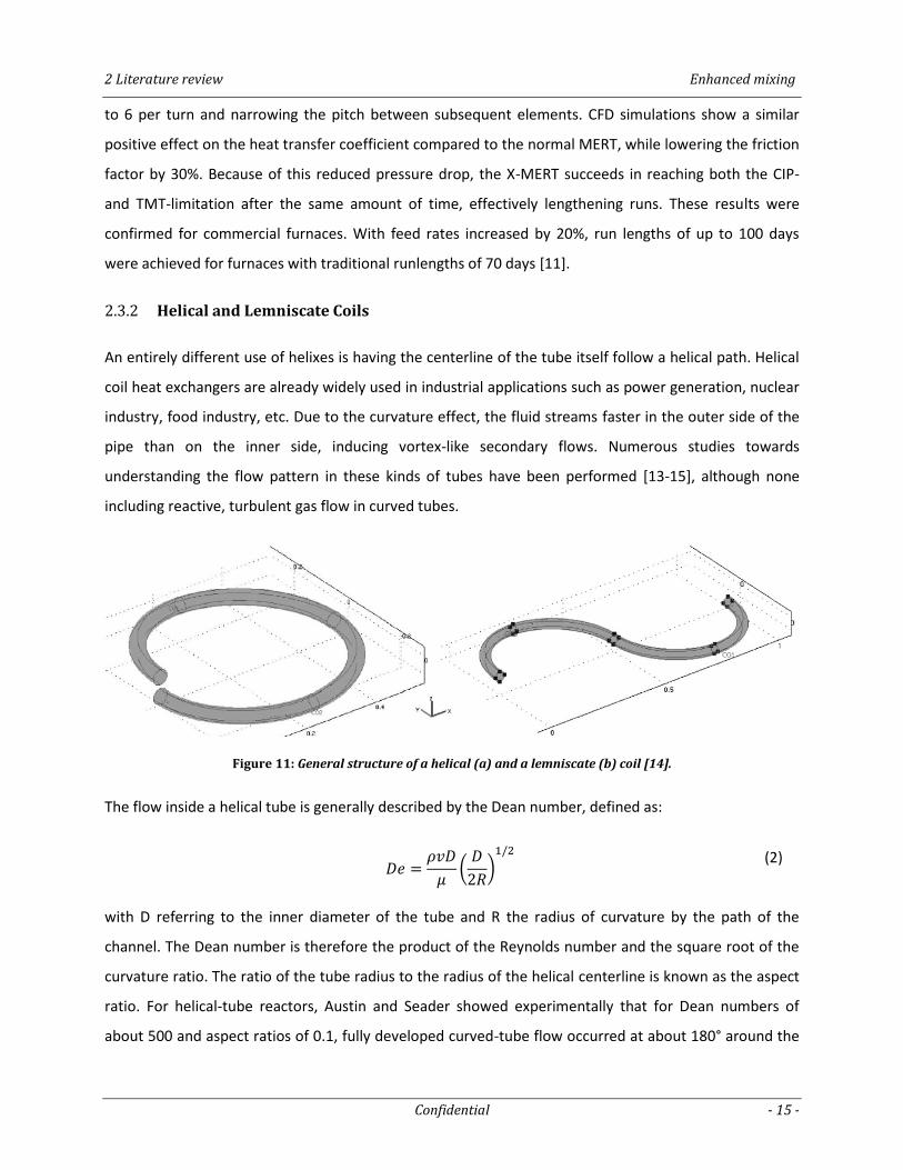
Over time, Kubota progressively improved the MERT technology, developing the “Slit MERT” [11]. These
new coils are similar to the previous profile, except for the fact that the element is applied intermittently
as shown in Figure 10 (a). The volume fraction of the element is reduced, but since the alignment of the
segments is maintained, the swirl mixing effect continues throughout the length of the tube.
Figure 10: Pictures of Slit MERT (a) and X-MERT profiles (b) [11].
The latest version of this technology was named X-MERT and is said to even further reduce the friction
factor while maintaining the same improved heat transfer properties [11, 12]. This is achieved by
decreasing the element height as compared to the Slit MERT while increasing the number of slits from 4
(a) (b)
2 Literature review Enhanced mixing
Confidential - 15 -
to 6 per turn and narrowing the pitch between subsequent elements. CFD simulations show a similar
positive effect on the heat transfer coefficient compared to the normal MERT, while lowering the friction
factor by 30%. Because of this reduced pressure drop, the X-MERT succeeds in reaching both the CIP-
and TMT-limitation after the same amount of time, effectively lengthening runs. These results were
confirmed for commercial furnaces. With feed rates increased by 20%, run lengths of up to 100 days
were achieved for furnaces with traditional runlengths of 70 days [11].
2.3.2 Helical and Lemniscate Coils
An entirely different use of helixes is having the centerline of the tube itself follow a helical path. Helical
coil heat exchangers are already widely used in industrial applications such as power generation, nuclear
industry, food industry, etc. Due to the curvature effect, the fluid streams faster in the outer side of the
pipe than on the inner side, inducing vortex-like secondary flows. Numerous studies towards
understanding the flow pattern in these kinds of tubes have been performed [13-15], although none
including reactive, turbulent gas flow in curved tubes.
Figure 11: General structure of a helical (a) and a lemniscate (b) coil [14].
The flow inside a helical tube is generally described by the Dean number, defined as:
(
)
(2)
with D referring to the inner diameter of the tube and R the radius of curvature by the path of the
channel. The Dean number is therefore the product of the Reynolds number and the square root of the
curvature ratio. The ratio of the tube radius to the radius of the helical centerline is known as the aspect
ratio. For helical-tube reactors, Austin and Seader showed experimentally that for Dean numbers of
about 500 and aspect ratios of 0.1, fully developed curved-tube flow occurred at about 180° around the
2 Literature review Enhanced mixing
Confidential - 16 -
turn [15]. If the flow direction is then changed, as in a lemniscate tube (Figure 11 (b)), the flow crosses
from one side of the tube to the other at the intersection of the lemniscate lobes, resulting in even
greater uniformity. Slominski and Seader also performed a computational study including the aqueous
saponification reaction of ethyl acetate with sodium hydroxide. From this study it was seen that the
conversion for the lemniscate tube very nearly approximated that of an ideal plug flow reactor (no radial
concentration gradients) [14]. They concluded that a tube with curvature in different directions could
prove an effective means of enhancing conversion in tubular reactors.
The main disadvantage towards use as steam cracking reactors is that the shape of these coils makes
radiative heating in a gas-fired furnace problematic. It would be impossible to apply this kind of tubes in
existing furnaces without a total redesign of the steam cracker radiation section.
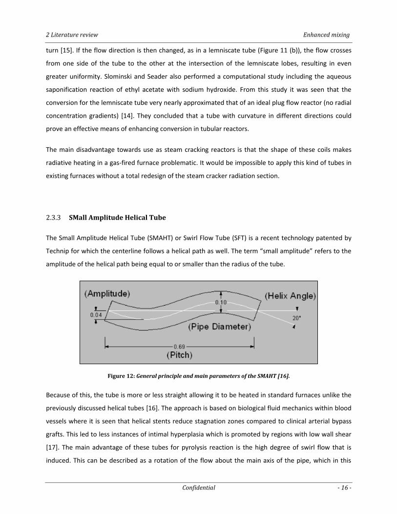
2.3.3 SMall Amplitude Helical Tube
The Small Amplitude Helical Tube (SMAHT) or Swirl Flow Tube (SFT) is a recent technology patented by
Technip for which the centerline follows a helical path as well. The term “small amplitude” refers to the
amplitude of the helical path being equal to or smaller than the radius of the tube.
Figure 12: General principle and main parameters of the SMAHT [16].
Because of this, the tube is more or less straight allowing it to be heated in standard furnaces unlike the
previously discussed helical tubes [16]. The approach is based on biological fluid mechanics within blood
vessels where it is seen that helical stents reduce stagnation zones compared to clinical arterial bypass
grafts. This led to less instances of intimal hyperplasia which is promoted by regions with low wall shear
[17]. The main advantage of these tubes for pyrolysis reaction is the high degree of swirl flow that is
induced. This can be described as a rotation of the flow about the main axis of the pipe, which in this
2 Literature review Enhanced mixing
Confidential - 17 -
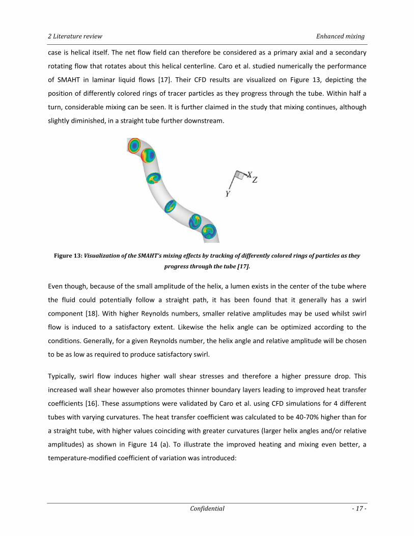
case is helical itself. The net flow field can therefore be considered as a primary axial and a secondary
rotating flow that rotates about this helical centerline. Caro et al. studied numerically the performance
of SMAHT in laminar liquid flows [17]. Their CFD results are visualized on Figure 13, depicting the
position of differently colored rings of tracer particles as they progress through the tube. Within half a
turn, considerable mixing can be seen. It is further claimed in the study that mixing continues, although
slightly diminished, in a straight tube further downstream.
Figure 13: Visualization of the SMAHT‘s mixing effects by tracking of differently colored rings of particles as they
progress through the tube [17].
Even though, because of the small amplitude of the helix, a lumen exists in the center of the tube where
the fluid could potentially follow a straight path, it has been found that it generally has a swirl
component [18]. With higher Reynolds numbers, smaller relative amplitudes may be used whilst swirl
flow is induced to a satisfactory extent. Likewise the helix angle can be optimized according to the
conditions. Generally, for a given Reynolds number, the helix angle and relative amplitude will be chosen
to be as low as required to produce satisfactory swirl.
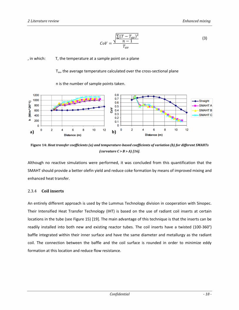
Typically, swirl flow induces higher wall shear stresses and therefore a higher pressure drop. This
increased wall shear however also promotes thinner boundary layers leading to improved heat transfer
coefficients [16]. These assumptions were validated by Caro et al. using CFD simulations for 4 different
tubes with varying curvatures. The heat transfer coefficient was calculated to be 40-70% higher than for
a straight tube, with higher values coinciding with greater curvatures (larger helix angles and/or relative
amplitudes) as shown in Figure 14 (a). To illustrate the improved heating and mixing even better, a
temperature-modified coefficient of variation was introduced:
2 Literature review Enhanced mixing
Confidential - 18 -
√∑( )
(3)
, in which: T, the temperature at a sample point on a plane
Tav, the average temperature calculated over the cross-sectional plane
n is the number of sample points taken.
Figure 14: Heat transfer coefficients (a) and temperature-based coefficients of variation (b) for different SMAHTs
(curvature C > B > A) [16].
Although no reactive simulations were performed, it was concluded from this quantification that the
SMAHT should provide a better olefin yield and reduce coke formation by means of improved mixing and
enhanced heat transfer.
2.3.4 Coil inserts
An entirely different approach is used by the Lummus Technology division in cooperation with Sinopec.
Their Intensified Heat Transfer Technology (IHT) is based on the use of radiant coil inserts at certain
locations in the tube (see Figure 15) [19]. The main advantage of this technique is that the inserts can be
readily installed into both new and existing reactor tubes. The coil inserts have a twisted (100-360°)
baffle integrated within their inner surface and have the same diameter and metallurgy as the radiant
coil. The connection between the baffle and the coil surface is rounded in order to minimize eddy
formation at this location and reduce flow resistance.
a) b)
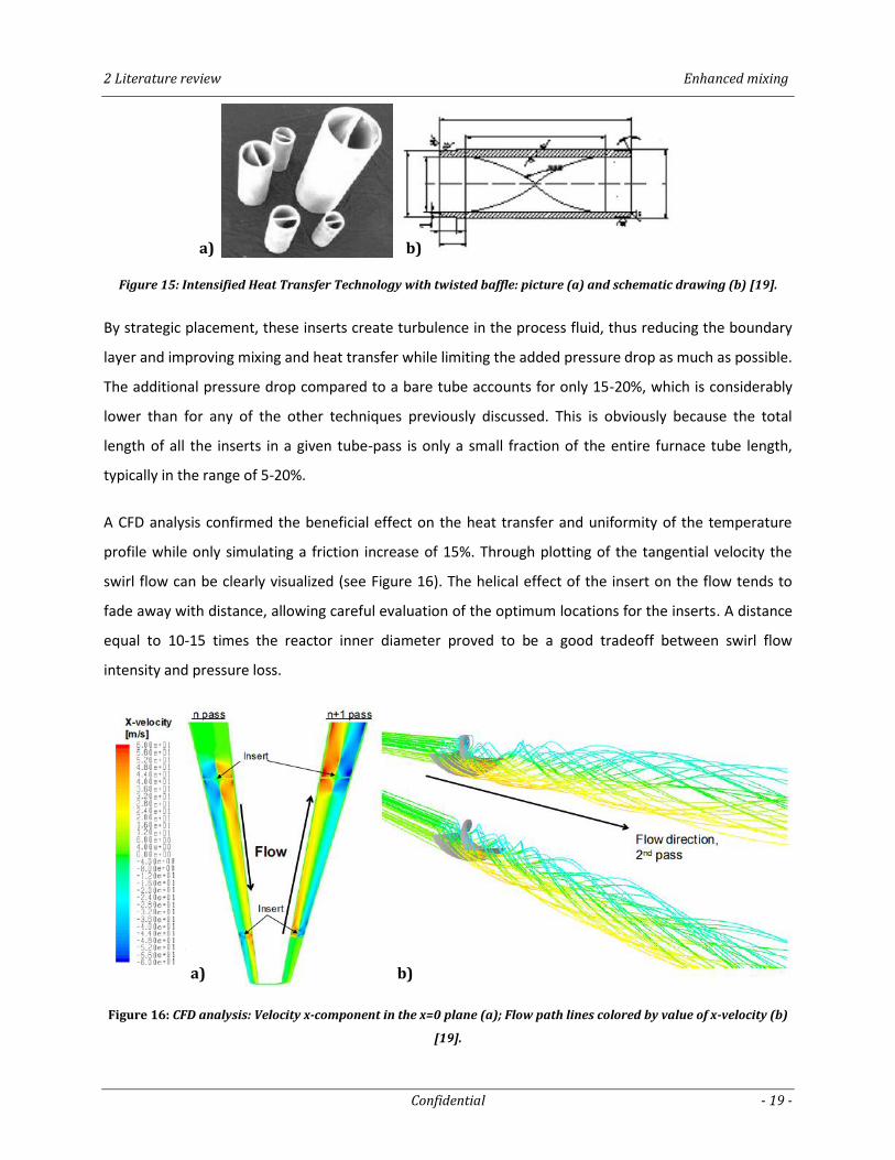
2 Literature review Enhanced mixing
Confidential - 19 -
Figure 15: Intensified Heat Transfer Technology with twisted baffle: picture (a) and schematic drawing (b) [19].
By strategic placement, these inserts create turbulence in the process fluid, thus reducing the boundary
layer and improving mixing and heat transfer while limiting the added pressure drop as much as possible.
The additional pressure drop compared to a bare tube accounts for only 15-20%, which is considerably
lower than for any of the other techniques previously discussed. This is obviously because the total
length of all the inserts in a given tube-pass is only a small fraction of the entire furnace tube length,
typically in the range of 5-20%.
A CFD analysis confirmed the beneficial effect on the heat transfer and uniformity of the temperature
profile while only simulating a friction increase of 15%. Through plotting of the tangential velocity the
swirl flow can be clearly visualized (see Figure 16). The helical effect of the insert on the flow tends to
fade away with distance, allowing careful evaluation of the optimum locations for the inserts. A distance
equal to 10-15 times the reactor inner diameter proved to be a good tradeoff between swirl flow
intensity and pressure loss.
Figure 16: CFD analysis: Velocity x-component in the x=0 plane (a); Flow path lines colored by value of x-velocity (b)
[19].
a) b)
a) b)
2 Literature review Enhanced mixing
Confidential - 20 -
In order to further prove the benefits of the IHT for pyrolysis reactions, a kinetic scheme was also
devised to estimate the coke formation at the tube surface. The model assumed the coking rate to be
first order with respect to butadiene. Although the total amount of coke-precursor was about the same
with or without the inserts, the stronger radial mixing distributed it more evenly through the cross-
section. This lower butadiene concentration near the wall, along with a TMT that was 25°C lower than
for a bare, resulted in 47% less coke generated on the surface. This difference in coke build-up rate and
TMT, translates into a theoretical run length that is approximately doubled using the inserts.
A commercial test in a SRT-IV furnace cracking light naphtha proved successful as well. The configuration
with the inserts allowed operation at 107% load, using the same feedstock. At comparable propylene-to-
ethylene ratio, the run length was 85 days compared to the original 55 days. When operated at 100%
load, run length could even be increased up to 105 days. Commercial tests also show that yields do not
deteriorate in spite of the 20% pressure drop increase. The reason stated for this is that the inserts
flatten the cross-sectional temperature profile, making it unnecessary to over-crack near the wall to get
the same average yield. It can be assumed however that these differences in selectivity will be small and
hard to measure in an industrial setting. Currently over 50 furnaces in China use this type of inserts with
run lengths typically being extended by a factor of 1.2 to 2 times [19]. A crucial weakness of the IHT that
was not mentioned in the study, is that spalled coke can build up on top of an insert. This could lead to a
local hot spot for further coke formation causing tube blockage at the insert, leading to advanced need
for decoking.
2 Literature review References
Confidential - 21 -
References
1. Nicolantonio, Arthur Di, Pyrolysis furnace with an internally finned U-shaped radiant coil, E.
Chemical, Editor 2002: United States.
2. David J. Brown, Stone & Webster, Inc., Internally Finned Radiant Coils: a Valuable Tool for
Improving Ethylene Plant Economics, in 6th EMEA Petrochemicals Technology Conference2004:
London, UK.
3. J. V. Albano, K. M. Sundaram, M. J. Maddock, Applications of extended surfaces in pyrolysis
coils. Energy Progress, 1988. 8(3): p. 9.
4. De Saegher, J. J., T. Detemmerman, and Gilbert Froment, Three dimensional simulation of high
severity internally finned cracking coils for olefins production. Revue de l'Institut Francais du
Petrole, 1996. 51(2): p. 245-260.
5. Higuchi, Junichi, Metal Tube for Pyrolysis Reaction, 2012, Sumitomo Metal Industries: United
States.
6. Gregory J. Zdaniuk, Louay M. Chamra, Pedro J. Mago, Experimental determination of heat
transfer and friction in helically-finned tubes. Experimental Thermal and Fluid Science, 2008. 32:
p. 15.
7. M.K. Jensen, A. Vlakancic, Experimental investigation of turbulent heat transfer and fluid flow in
internally finned tubes. International Journal of Heat and Mass Transfer, 1999. 42: p. 9.
8. Van Geem, K. M., G. J. Heynderickx, and G. B. Marin, Effect of radial temperature profiles on
yields in steam cracking. AIChE Journal, 2004. 50(1): p. 173-183.
9. Guihua Hu et al., Kevin Van Geem, Comprehensive CFD simulation of product yields and coking
rates for a floor and wall fired naphtha cracking furnace. Industrial & Engineering Chemistry
Research, 2011: p. 39.
10. Torigoe, T., Mixing Element Radiant Tube (MERT) Improves Cracking Furnace Performance, K.
Corporation, Editor 2001.
11. Györffy, Michael, MERT Technology Update: X-MERT, in AlCHE: Ethylene Producers
Meeting2009: Tampa Bay.
12. Hamada, Masahiro Inui; Kaoru, Cracking Tubes Having Helical Fins, 2009, Kubota Organisation:
United States.
13. J.S. Jayakumar, S.M. Mahajani, J.C. Mandal, K.N. Iyer, P.K. Vijayan, CFD Analysis of single-
phase flows inside helically coiled tubes. Computers and Chemical Engineering, 2010. 34: p. 17.
14. Seader, Charles G. Slominski; Warren D. Seider; J.D., Helical and Lemniscate Tubular Reactors.
Industrial & Engineering Chemistry Research, 2011.
2 Literature review References
Confidential - 22 -
15. Austin, L.R.; Seader, J.D., Entry Region for Steady Viscous Flow in Coiled Circular Pipes.
AIChE Journal, 1974. 20: p. 3.
16. W. Tallis, C. Caro, C. Dang, A novel approach to ethylene furnace coil design, in 18th Annual
Ethylene Producers’ Conference2006: Orlando, FL.
17. Colin G. Caro, Nick J. Cheshire and Nick Watkins, Preliminary comparative study of small
amplitude helical and conventional ePTFE arteriovenous shunts in pigs. Journal of the Royal
Society Interface, 2005. 2: p. 6.
18. Caro, Colin Gerald, Olefin production furnace with a helical tube, T.F. S.A.S., Editor 2005.
19. Carrillo, Alejandro, Intensified Heat Transfer Technology – CFD Analysis to Explain How and
Why IHT Increases Runlength in Commercial Furnaces, in AIChE and EPC 2010 Spring National
Meeting2010: San Antonio, TX.
3 Computational study of pressure drop and heat transfer in finned tubes Mathematical formulation
Confidential - 23 -
3 Computational study of pressure drop and heat transfer in finned
tubes
3.1 Mathematical formulation ........................................................................................................... 23
3.2 Turbulence modeling ................................................................................................................... 25
3.3 Finite volume method .................................................................................................................. 31
3.4 Discretization schemes ................................................................................................................ 32
3.5 Meshing........................................................................................................................................ 33
3.6 Model validation .......................................................................................................................... 36
3.7 Reynolds number dependency of friction factors and Nusselt numbers .................................... 44
3.8 Influence of fin height on pressure drop and heat transfer in finned tubes ............................... 48
3.9 Influence of pitch on pressure drop and heat transfer in helicoidally finned tubes ................... 61
3.10 Influence of number of fins on pressure drop and heat transfer in finned tubes ....................... 71
3.11 Geometry optimization - Conclusions ......................................................................................... 79
References ................................................................................................................................................ 84
3.1 Mathematical formulation
Governing equations 3.1.1
In this paragraph an overview of the model equations is presented, based on “Computational Fluid
Dynamics for Chemical Engineers” by Bengt Andersson (2011) [1], “An Introduction to Computational
3 Computational study of pressure drop and heat transfer in finned tubes
Mathematical formulation
Confidential - 24 -
Fluid Dynamics” by H.K. Versteeg (1995) [2] and some lectures from the University of Queensland by M.
Macrossan (2008) [3]. The governing equations of fluid flow represent mathematical formulations of the
laws of conservation.
Continuity 0
u
t
(1)
Momentum Fτu
ij pDt
D
(2)
Energy Φqu
t
Q
Dt
De)(
(3)
Where ρ is the fluid density, u is the fluid velocity vector, τij is the viscous stress tensor, p is pressure, F
are the body forces, e is the internal energy, Q is the heat source term, t is time, is the dissipation
term and q is the heat loss by conduction.
A more useful form of the conservation laws is obtained by introducing a suitable model for the
unknown viscous stresses τij. In a Newtonian fluid the viscous stresses are proportional to the local strain
rate. In three-dimensional flow, the local strain rate is composed of the linear deformation rate and the
volumetric deformation rate. The rate of linear deformation of a fluid element has nine components in
three dimensions, six of which are independent in isotropic fluids such as gasses, while the volumetric
deformation is given by the divergence of the velocity vector. The three-dimensional form of Newton’s
law of viscosity for compressible flows involves two constants of proportionality: the dynamic viscosity µ
which relates stresses to linear deformations and a second viscosity λ to relate stresses to the volumetric
deformation. The nine viscous stress components are then given by:
u
i
iii
x
u2
i
j
j
ijiij
x
u
x
u (4)
In practice the effect of the second viscosity is small. For gases a good working approximation can be
obtained by taking the value λ=-2/3 µ. Substitution of the above shear stresses into the momentum
equation (2) yields the three Navier-Stokes equations:
3 Computational study of pressure drop and heat transfer in finned tubes
Turbulence modeling
Confidential - 25 -
iij
l
l
i
j
j
i
ji
ji
j
i Fx
u
x
u
x
u
xx
puu
xu
t
3
2 (5)
Along with p = p(ρ,T) and e= e(ρ,T), Eq. (1), (3) and (5) amount to 7 equations with 7 unknowns. With an
equal number of equations and unknown functions this system is mathematically closed, i.e. it can be
solved provided that suitable initial and boundary conditions and supplied.
3.2 Turbulence modeling
As the Reynolds number in steam cracking reactors is between 30,000 and 120,000 , the flow inside the
coils is highly turbulent. In this regime, the motion has unsteady fluctuations around a time-averaged
value, even with constant steady boundary conditions imposed. The velocity and other flow properties
vary in a random and chaotic way. Because of this random nature, computations based on a complete
description of the motion of all the fluid particles become impossible. Even in flows where the mean
velocities and temperatures vary in only one or two space dimensions, turbulent fluctuations always
have a three-dimensional spatial character. These observed rotational flow structures are called
turbulent eddies and exist on a wide range of length and time scales. Particles of fluid which are initially
separated by a long distance can be brought close together by the eddying motions of the turbulent
flow, leading to much more effective exchange of heat, mass and momentum.
Although it is obvious that these eddies should be included in the calculation of the mean flow
characteristics, present day computing power comes nowhere near the computational requirements for
direct solution of the time-dependent Navier-Stokes equations for practical engineering applications.
Luckily, for most applications interest lies with the mean flow characteristics which can still be obtained
by a careful consideration of the additional turbulence influences. Typically this is achieved by
decomposing the velocity into a steady mean value ̅ with a fluctuating component u’(t) superimposed
on it. Symbolically this implies substituting u(t) = ̅ + u’(t) in Eq.(5), thus obtaining the so-called Reynolds-
averaged Navier-Stokes equations (RANS):
''
3
2ji
j
iij
i
i
i
j
j
i
ji
ji
j
i uux
Fx
u
x
u
x
u
xx
puu
xu
t
(6)
3 Computational study of pressure drop and heat transfer in finned tubes
Turbulence modeling
Confidential - 26 -
By performing this time-averaging, the equations become easier but a great deal of information is lost as
well. As a result, an additional tensor of stresses is generated, characterizing the transfer of momentum
by turbulence. These stresses are called the Reynolds stresses: ''
ji
t
ij uu . Since the tensor is
symmetric, this adds six additional unknowns to the momentum equation. It is the main task of
turbulence modeling to develop computational methods of sufficient accuracy and generality to predict
the Reynolds stresses and thus the additional scalar transport terms.
The k-ε model 3.2.1
The Boussinesq approximation
One way to achieve closure for these additional unknowns is by relating them to the dependent variables
they are meant to transport. A simple approximation is to express the Reynolds stress tensor in terms of
the mean velocity itself. This is the basis of the Boussinesq approximation, which proposes that the
transport of momentum by turbulence is a diffusive process. As such, the Reynolds stresses can be
modeled using an eddy viscosity which is the turbulent analog to molecular viscosity.
ij
i
it
i
j
j
itji
t
ij
x
uk
x
u
x
uuu
3
2'' (7)
Regardless of the approach used to determine this turbulent viscosity, there are several limitations with
the Boussinesq approximation as it is based on the assumption that eddies behave like molecules. First
of all, the size of eddies is comparable in size to the scale of the flow, much larger than molecules.
Furthermore molecules participate in a lot of collisions because their mean free path is short. This
implies that they have a lot of opportunities to reach local equilibrium with regards to momentum
whereas the mean free path of eddies is of comparable scale to the scale of the flow. By introducing the
turbulent viscosity factor, it is also assumed that the turbulence is isotropic, although it is known that
turbulence is always a three-dimensional occurrence and considerable anisotropy is present in some
applications. Despite these shortcomings, the Boussinesq approximation is one of the cornerstones in
several turbulence models as sufficiently accurate results can be obtained with it for most engineering
applications while the cost of more elaborate turbulence models is significantly higher.
Turbulent kinetic energy and dissipation rate
3 Computational study of pressure drop and heat transfer in finned tubes
Turbulence modeling
Confidential - 27 -
As part of quantitative turbulence modeling, this eddy viscosity, t , must be determined. When it comes
to turbulence modeling based on the RANS-equations and the eddy viscosity concept, the turbulence
model can be seen as the set of equations that are needed to determine this viscosity. Similar to kinetic
theory of gases the viscosity is proportional to velocity multiplied by distance. The turbulent viscosity
models are based on an appropriate velocity, u, and length scale, l, describing the local turbulent
viscosity, t . As the dimension of viscosity is [m²/s], the product of these two scales gives the right
dimension, that is:
ulCt (8)
In this expression u and l are the characteristic scales for the large turbulent eddies and C a
proportionality constant.
As it takes two quantities to characterize the length and velocity scales of turbulent flows, the most
successful models to determine these scales consist of two or more transport equations. A
straightforward approach to model the scales is to solve the turbulent kinetic energy equation for the
velocity scale and the l-equation for the length scale. This approach is called a k-l model. More often
however the second transport equation describes transport of another property than the length scale,
provided it remains possible to explicitly determine the length scale from this property.
The most commonly used variable is the energy dissipation rate ε. The length scale can then be obtained
by multiplying the turbulent velocity, k , with the lifetime of the turbulent eddies /k . The turbulent
viscosity is thus given by:
223
21 k
Ck
kCt (9)
After careful modeling of the turbulent kinetic energy production, dissipation and transport terms, the
equation for k and ε is obtained as:
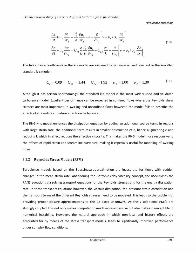
3 Computational study of pressure drop and heat transfer in finned tubes
Turbulence modeling
Confidential - 28 -
j
t
jj
i
t
ij
j
j
j
kt
jj
i
t
ij
j
j
xxkC
x
u
kC
xu
t
x
k
xx
u
x
ku
t
k
/
/
2
21
(10)
The five closure coefficients in the k-ε model are assumed to be universal and constant in the so-called
standard k-ε model:
09.0C 44.11 C 92.12 C 00.1k 30.1 (11)
Although it has certain shortcomings, the standard k-ε model is the most widely used and validated
turbulence model. Excellent performance can be expected in confined flows where the Reynolds shear
stresses are most important. In swirling and unconfined flows however, the model fails to describe the
effects of streamline curvature effects on turbulence.
The RNG k- ε model enhances the dissipation equation by adding an additional source term. In regions
with large strain rate, the additional term results in smaller destruction of ε, hence augmenting ε and
reducing k which in effect reduces the effective viscosity. This makes the RNG model more responsive to
the effects of rapid strain and streamline curvature, making it especially useful for modeling of swirling
flows.
Reynolds Stress Models (RSM) 3.2.2
Turbulence models based on the Boussinesq-approximation are inaccurate for flows with sudden
changes in the mean strain rate. Abandoning the isotropic eddy viscosity concept, the RSM closes the
RANS equations via solving transport equations for the Reynolds stresses and for the energy dissipation
rate. In these transport equations however, the viscous dissipation, the pressure-strain correlation and
the transport terms of the different Reynolds stresses need to be modeled. This leads to the problem of
providing proper closure approximations to the 22 extra unknowns. As the 7 additional PDE’s are
strongly coupled, this not only makes computation much more expensive but also makes it susceptible to
numerical instability. However, the natural approach in which non-local and history effects are
accounted for by means of the stress transport models, leads to significantly improved performance
under complex flow conditions.
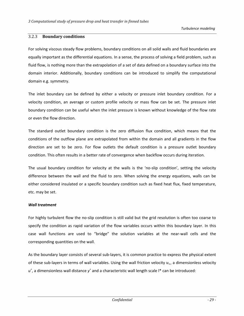
3 Computational study of pressure drop and heat transfer in finned tubes
Turbulence modeling
Confidential - 29 -
Boundary conditions 3.2.3
For solving viscous steady flow problems, boundary conditions on all solid walls and fluid boundaries are
equally important as the differential equations. In a sense, the process of solving a field problem, such as
fluid flow, is nothing more than the extrapolation of a set of data defined on a boundary surface into the
domain interior. Additionally, boundary conditions can be introduced to simplify the computational
domain e.g. symmetry.
The inlet boundary can be defined by either a velocity or pressure inlet boundary condition. For a
velocity condition, an average or custom profile velocity or mass flow can be set. The pressure inlet
boundary condition can be useful when the inlet pressure is known without knowledge of the flow rate
or even the flow direction.
The standard outlet boundary condition is the zero diffusion flux condition, which means that the
conditions of the outflow plane are extrapolated from within the domain and all gradients in the flow
direction are set to be zero. For flow outlets the default condition is a pressure outlet boundary
condition. This often results in a better rate of convergence when backflow occurs during iteration.
The usual boundary condition for velocity at the walls is the ‘no-slip condition’, setting the velocity
difference between the wall and the fluid to zero. When solving the energy equations, walls can be
either considered insulated or a specific boundary condition such as fixed heat flux, fixed temperature,
etc. may be set.
Wall treatment
For highly turbulent flow the no-slip condition is still valid but the grid resolution is often too coarse to
specify the condition as rapid variation of the flow variables occurs within this boundary layer. In this
case wall functions are used to “bridge” the solution variables at the near-wall cells and the
corresponding quantities on the wall.
As the boundary layer consists of several sub-layers, it is common practice to express the physical extent
of these sub-layers in terms of wall variables. Using the wall friction velocity , a dimensionless velocity
u+, a dimensionless wall distance y+ and a characteristic wall length scale l* can be introduced:
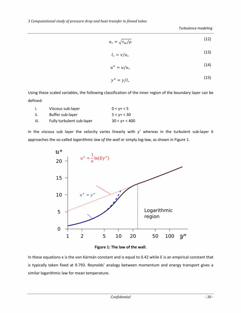
3 Computational study of pressure drop and heat transfer in finned tubes
Turbulence modeling
Confidential - 30 -
√ (12)
(13)
(14)
(15)
Using these scaled variables, the following classification of the inner region of the boundary layer can be
defined:
i. Viscous sub-layer 0 < y+ < 5
ii. Buffer sub-layer 5 < y+ < 30
iii. Fully turbulent sub-layer 30 < y+ < 400
In the viscous sub layer the velocity varies linearly with y+ whereas in the turbulent sub-layer it
approaches the so-called logarithmic law of the wall or simply log-law, as shown in Figure 1.
Figure 1: The law of the wall.
In these equations κ is the von Kármán constant and is equal to 0.42 while E is an empirical constant that
is typically taken fixed at 9.793. Reynolds’ analogy between momentum and energy transport gives a
similar logarithmic law for mean temperature.
𝑢 1
𝜅ln 𝐸𝑦
𝑢 𝑦
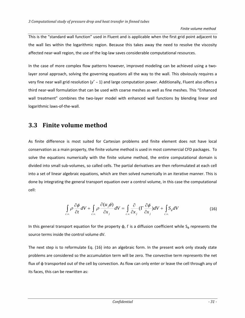
3 Computational study of pressure drop and heat transfer in finned tubes
Finite volume method
Confidential - 31 -
This is the “standard wall function” used in Fluent and is applicable when the first grid point adjacent to
the wall lies within the logarithmic region. Because this takes away the need to resolve the viscosity
affected near-wall region, the use of the log-law saves considerable computational resources.
In the case of more complex flow patterns however, improved modeling can be achieved using a two-
layer zonal approach, solving the governing equations all the way to the wall. This obviously requires a
very fine near wall grid resolution (y+ 1) and large computation power. Additionally, Fluent also offers a
third near-wall formulation that can be used with coarse meshes as well as fine meshes. This “Enhanced
wall treatment” combines the two-layer model with enhanced wall functions by blending linear and
logarithmic laws-of-the-wall.
3.3 Finite volume method
As finite difference is most suited for Cartesian problems and finite element does not have local
conservation as a main property, the finite volume method is used in most commercial CFD packages. To
solve the equations numerically with the finite volume method, the entire computational domain is
divided into small sub-volumes, so called cells. The partial derivatives are then reformulated at each cell
into a set of linear algebraic equations, which are then solved numerically in an iterative manner. This is
done by integrating the general transport equation over a control volume, in this case the computational
cell:
In this general transport equation for the property φ, Γ is a diffusion coefficient while Sφ represents the
source terms inside the control volume dV.
The next step is to reformulate Eq. (16) into an algebraic form. In the present work only steady state
problems are considered so the accumulation term will be zero. The convective term represents the net
flux of φ transported out of the cell by convection. As flow can only enter or leave the cell through any of
its faces, this can be rewritten as:
........
)()(
vcvc jjvc j
j
vc
dVSdVxx
dVx
udV
t
(16)
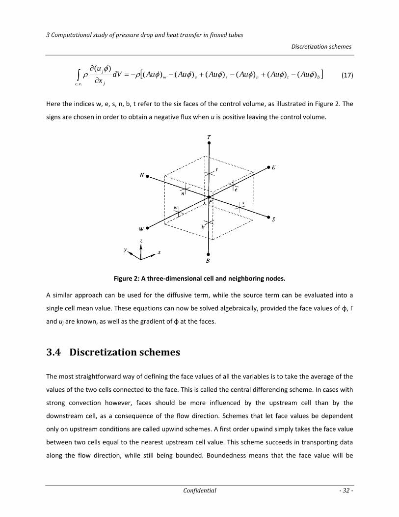
3 Computational study of pressure drop and heat transfer in finned tubes
Discretization schemes
Confidential - 32 -
btnsew
vc j
jAuAuAuAuAuAudV
x
u)()()()()()(
)(
..
(17)
Here the indices w, e, s, n, b, t refer to the six faces of the control volume, as illustrated in Figure 2. The
signs are chosen in order to obtain a negative flux when u is positive leaving the control volume.
Figure 2: A three-dimensional cell and neighboring nodes.
A similar approach can be used for the diffusive term, while the source term can be evaluated into a
single cell mean value. These equations can now be solved algebraically, provided the face values of φ, Γ
and uj are known, as well as the gradient of φ at the faces.
3.4 Discretization schemes
The most straightforward way of defining the face values of all the variables is to take the average of the
values of the two cells connected to the face. This is called the central differencing scheme. In cases with
strong convection however, faces should be more influenced by the upstream cell than by the
downstream cell, as a consequence of the flow direction. Schemes that let face values be dependent
only on upstream conditions are called upwind schemes. A first order upwind simply takes the face value
between two cells equal to the nearest upstream cell value. This scheme succeeds in transporting data
along the flow direction, while still being bounded. Boundedness means that the face value will be
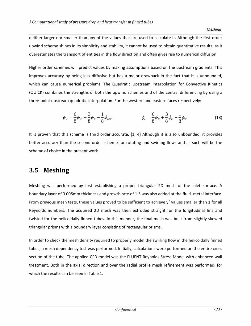
3 Computational study of pressure drop and heat transfer in finned tubes
Meshing
Confidential - 33 -
neither larger nor smaller than any of the values that are used to calculate it. Although the first order
upwind scheme shines in its simplicity and stability, it cannot be used to obtain quantitative results, as it
overestimates the transport of entities in the flow direction and often gives rise to numerical diffusion.
Higher order schemes will predict values by making assumptions based on the upstream gradients. This
improves accuracy by being less diffusive but has a major drawback in the fact that it is unbounded,
which can cause numerical problems. The Quadratic Upstream Interpolation for Convective Kinetics
(QUICK) combines the strengths of both the upwind schemes and of the central differencing by using a
three-point upstream quadratic interpolation. For the western and eastern faces respectively:
WWPWw 8
1
8
3
8
6 WEPe
8
1
8
3
8
6 (18)
It is proven that this scheme is third order accurate. [1, 4] Although it is also unbounded, it provides
better accuracy than the second-order scheme for rotating and swirling flows and as such will be the
scheme of choice in the present work.
3.5 Meshing
Meshing was performed by first establishing a proper triangular 2D mesh of the inlet surface. A
boundary layer of 0.005mm thickness and growth rate of 1.5 was also added at the fluid–metal interface.
From previous mesh tests, these values proved to be sufficient to achieve y+ values smaller than 1 for all
Reynolds numbers. The acquired 2D mesh was then extruded straight for the longitudinal fins and
twisted for the helicoidally finned tubes. In this manner, the final mesh was built from slightly skewed
triangular prisms with a boundary layer consisting of rectangular prisms.
In order to check the mesh density required to properly model the swirling flow in the helicoidally finned
tubes, a mesh dependency test was performed. Initially, calculations were performed on the entire cross
section of the tube. The applied CFD model was the FLUENT Reynolds Stress Model with enhanced wall
treatment. Both in the axial direction and over the radial profile mesh refinement was performed, for
which the results can be seen in Table 1.
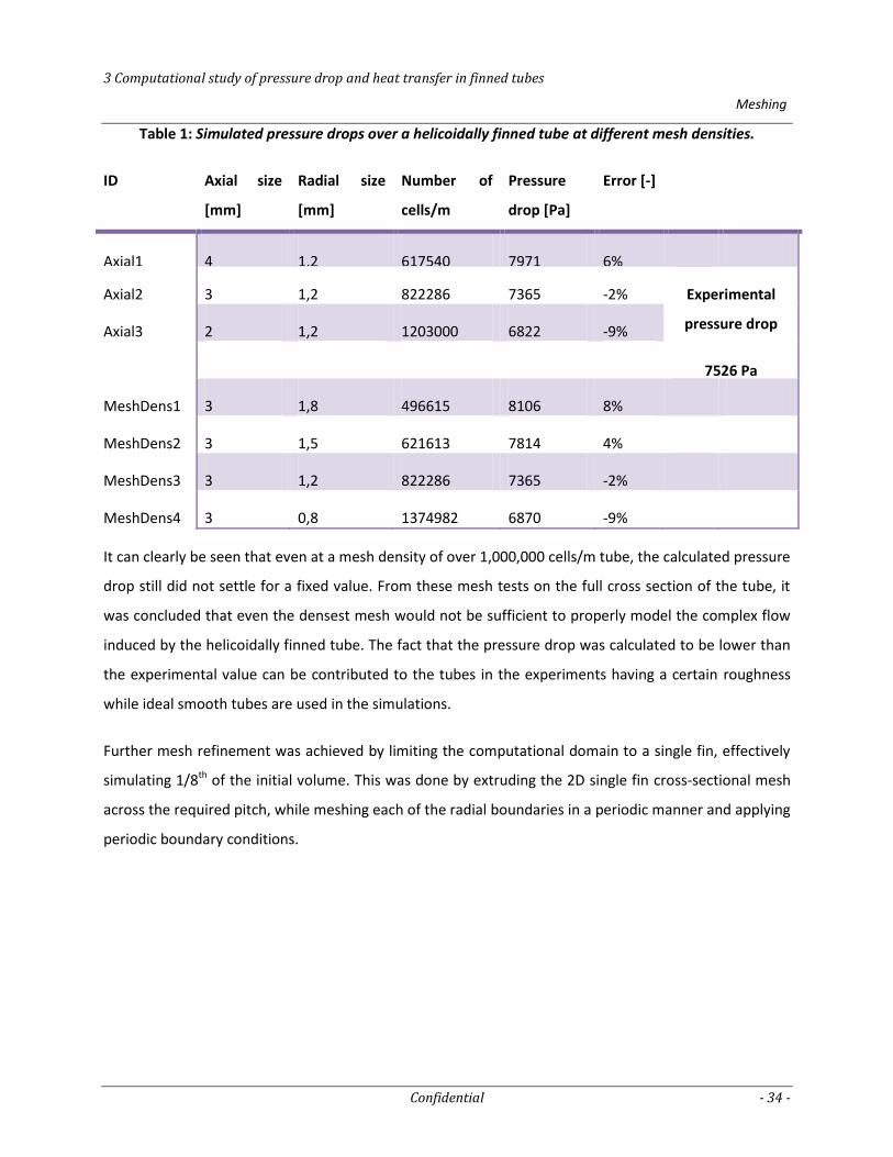
3 Computational study of pressure drop and heat transfer in finned tubes
Meshing
Confidential - 34 -
Table 1: Simulated pressure drops over a helicoidally finned tube at different mesh densities.
ID Axial size
[mm]
Radial size
[mm]
Number of
cells/m
Pressure
drop [Pa]
Error [-]
Axial1 4 1,2 617540 7971 6%
Axial2 3 1,2 822286 7365 -2% Experimental
pressure drop
7526 Pa
Axial3 2 1,2 1203000 6822 -9%
MeshDens1 3 1,8 496615 8106 8%
MeshDens2 3 1,5 621613 7814 4%
MeshDens3 3 1,2 822286 7365 -2%
MeshDens4 3 0,8 1374982 6870 -9%
It can clearly be seen that even at a mesh density of over 1,000,000 cells/m tube, the calculated pressure
drop still did not settle for a fixed value. From these mesh tests on the full cross section of the tube, it
was concluded that even the densest mesh would not be sufficient to properly model the complex flow
induced by the helicoidally finned tube. The fact that the pressure drop was calculated to be lower than
the experimental value can be contributed to the tubes in the experiments having a certain roughness
while ideal smooth tubes are used in the simulations.
Further mesh refinement was achieved by limiting the computational domain to a single fin, effectively
simulating 1/8th of the initial volume. This was done by extruding the 2D single fin cross-sectional mesh
across the required pitch, while meshing each of the radial boundaries in a periodic manner and applying
periodic boundary conditions.
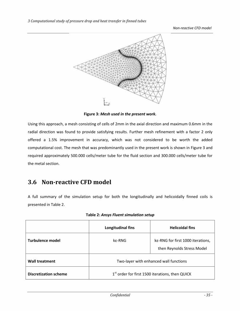
3 Computational study of pressure drop and heat transfer in finned tubes
Non-reactive CFD model
Confidential - 35 -
Figure 3: Mesh used in the present work.
Using this approach, a mesh consisting of cells of 2mm in the axial direction and maximum 0.6mm in the
radial direction was found to provide satisfying results. Further mesh refinement with a factor 2 only
offered a 1.5% improvement in accuracy, which was not considered to be worth the added
computational cost. The mesh that was predominantly used in the present work is shown in Figure 3 and
required approximately 500.000 cells/meter tube for the fluid section and 300.000 cells/meter tube for
the metal section.
3.6 Non-reactive CFD model
A full summary of the simulation setup for both the longitudinally and helicoidally finned coils is
presented in Table 2.
Table 2: Ansys Fluent simulation setup
Longitudinal fins Helicoidal fins
Turbulence model kε-RNG kε-RNG for first 1000 iterations,
then Reynolds Stress Model
Wall treatment Two-layer with enhanced wall functions
Discretization scheme 1st order for first 1500 iterations, then QUICK
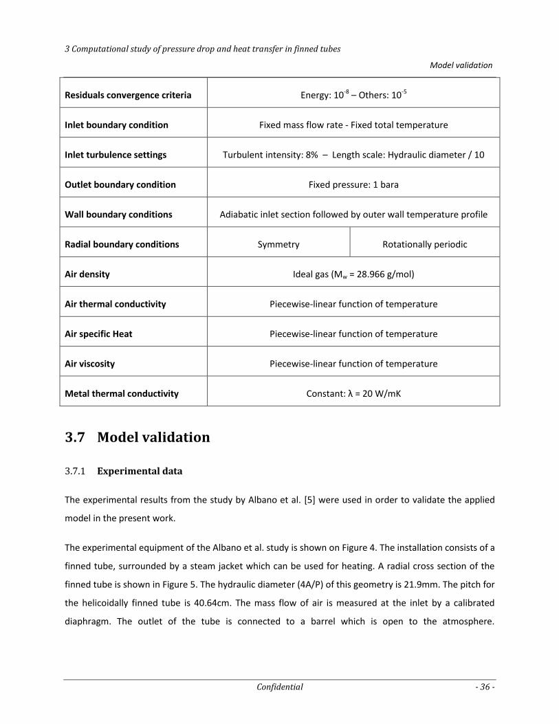
3 Computational study of pressure drop and heat transfer in finned tubes
Model validation
Confidential - 36 -
Residuals convergence criteria Energy: 10-8 – Others: 10-5
Inlet boundary condition Fixed mass flow rate - Fixed total temperature
Inlet turbulence settings Turbulent intensity: 8% – Length scale: Hydraulic diameter / 10
Outlet boundary condition Fixed pressure: 1 bara
Wall boundary conditions Adiabatic inlet section followed by outer wall temperature profile
Radial boundary conditions Symmetry Rotationally periodic
Air density Ideal gas (Mw = 28.966 g/mol)
Air thermal conductivity Piecewise-linear function of temperature
Air specific Heat Piecewise-linear function of temperature
Air viscosity Piecewise-linear function of temperature
Metal thermal conductivity Constant: λ = 20 W/mK
3.7 Model validation
Experimental data 3.7.1
The experimental results from the study by Albano et al. [5] were used in order to validate the applied
model in the present work.
The experimental equipment of the Albano et al. study is shown on Figure 4. The installation consists of a
finned tube, surrounded by a steam jacket which can be used for heating. A radial cross section of the
finned tube is shown in Figure 5. The hydraulic diameter (4A/P) of this geometry is 21.9mm. The pitch for
the helicoidally finned tube is 40.64cm. The mass flow of air is measured at the inlet by a calibrated
diaphragm. The outlet of the tube is connected to a barrel which is open to the atmosphere.
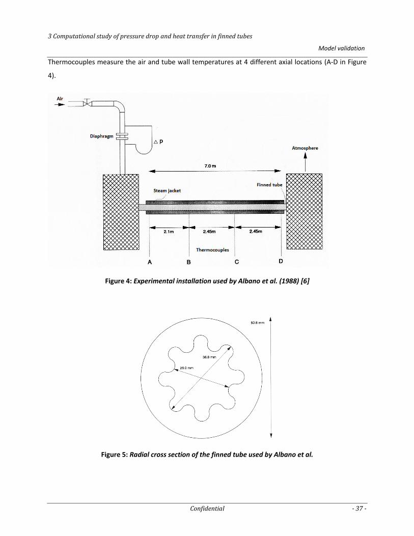
3 Computational study of pressure drop and heat transfer in finned tubes
Model validation
Confidential - 37 -
Thermocouples measure the air and tube wall temperatures at 4 different axial locations (A-D in Figure
4).
Figure 4: Experimental installation used by Albano et al. (1988) [6]
Figure 5: Radial cross section of the finned tube used by Albano et al.
3 Computational study of pressure drop and heat transfer in finned tubes
Model validation
Confidential - 38 -
Using this equipment, both longitudinally and helicoidally finned tubes were tested. The data covered a
Reynolds number range of 60,000 to 120,000 based on hydraulic diameter, which is comparable to
typical commercial steam cracking reactor operating conditions. A heat transfer rate was computed from
the mass flow rate of the air, and the temperature rise:
(19)
Using this and the axial mean temperature difference between the wall temperature and the air
temperature, an average inside convection heat transfer coefficient was determined.
(20)
Similarly for the pressure drop data, a mean friction coefficient was calculated.
(
)
(21)
From the obtained data, the following correlations for the Nusselt number and Darcy friction factor were
derived by Vanden Eynde (1989) [6] for helicoidally finned tubes:
1 1 (22)
1 (23)
And for longitudinally finned tubes:
(24)
(25)
As the tube parameters such as the fin height, number of fins and pitch length do not explicitly appear in
these correlations, the applicability range is most likely limited to the applied geometry.
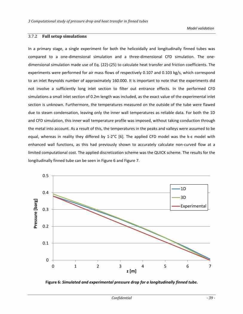
3 Computational study of pressure drop and heat transfer in finned tubes
Model validation
Confidential - 39 -
Full setup simulations 3.7.2
In a primary stage, a single experiment for both the helicoidally and longitudinally finned tubes was
compared to a one-dimensional simulation and a three-dimensional CFD simulation. The one-
dimensional simulation made use of Eq. (22)-(25) to calculate heat transfer and friction coefficients. The
experiments were performed for air mass flows of respectively 0.107 and 0.103 kg/s, which correspond
to an inlet Reynolds number of approximately 160.000. It is important to note that the experiments did
not involve a sufficiently long inlet section to filter out entrance effects. In the performed CFD
simulations a small inlet section of 0.2m length was included, as the exact value of the experimental inlet
section is unknown. Furthermore, the temperatures measured on the outside of the tube were flawed
due to steam condensation, leaving only the inner wall temperatures as reliable data. For both the 1D
and CFD simulation, this inner wall temperature profile was imposed, without taking conduction through
the metal into account. As a result of this, the temperatures in the peaks and valleys were assumed to be
equal, whereas in reality they differed by 1-2°C [6]. The applied CFD model was the k-ε model with
enhanced wall functions, as this had previously shown to accurately calculate non-curved flow at a
limited computational cost. The applied discretization scheme was the QUICK scheme. The results for the
longitudinally finned tube can be seen in Figure 6 and Figure 7.
Figure 6: Simulated and experimental pressure drop for a longitudinally finned tube.
0
0.1
0.2
0.3
0.4
0.5
0 1 2 3 4 5 6 7
Pre
ssu
re [
bar
g]
z [m]
1D
3D
Experimental
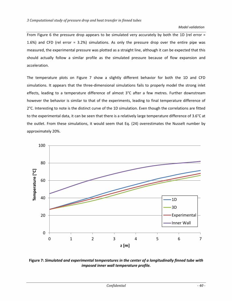
3 Computational study of pressure drop and heat transfer in finned tubes
Model validation
Confidential - 40 -
From Figure 6 the pressure drop appears to be simulated very accurately by both the 1D (rel error =
1.6%) and CFD (rel error = 3.2%) simulations. As only the pressure drop over the entire pipe was
measured, the experimental pressure was plotted as a straight line, although it can be expected that this
should actually follow a similar profile as the simulated pressure because of flow expansion and
acceleration.
The temperature plots on Figure 7 show a slightly different behavior for both the 1D and CFD
simulations. It appears that the three-dimensional simulations fails to properly model the strong inlet
effects, leading to a temperature difference of almost 3°C after a few metres. Further downstream
however the behavior is similar to that of the experiments, leading to final temperature difference of
2°C. Interesting to note is the distinct curve of the 1D simulation. Even though the correlations are fitted
to the experimental data, it can be seen that there is a relatively large temperature difference of 3.6°C at
the outlet. From these simulations, it would seem that Eq. (24) overestimates the Nusselt number by
approximately 20%.
Figure 7: Simulated and experimental temperatures in the center of a longitudinally finned tube with imposed inner wall temperature profile.
0
20
40
60
80
100
0 1 2 3 4 5 6 7
Tem
per
atu
re [
°C]
z [m]
1D
3D
Experimental
Inner Wall
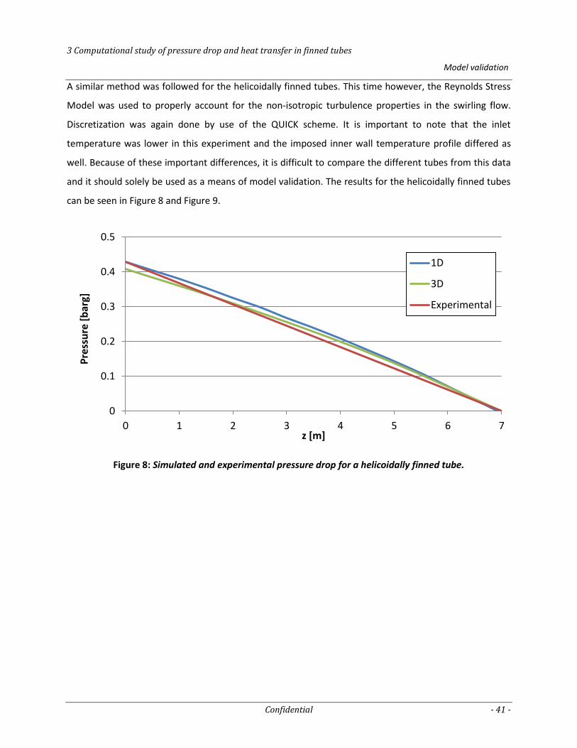
3 Computational study of pressure drop and heat transfer in finned tubes
Model validation
Confidential - 41 -
A similar method was followed for the helicoidally finned tubes. This time however, the Reynolds Stress
Model was used to properly account for the non-isotropic turbulence properties in the swirling flow.
Discretization was again done by use of the QUICK scheme. It is important to note that the inlet
temperature was lower in this experiment and the imposed inner wall temperature profile differed as
well. Because of these important differences, it is difficult to compare the different tubes from this data
and it should solely be used as a means of model validation. The results for the helicoidally finned tubes
can be seen in Figure 8 and Figure 9.
Figure 8: Simulated and experimental pressure drop for a helicoidally finned tube.
0
0.1
0.2
0.3
0.4
0.5
0 1 2 3 4 5 6 7
Pre
ssu
re [
bar
g]
z [m]
1D
3D
Experimental
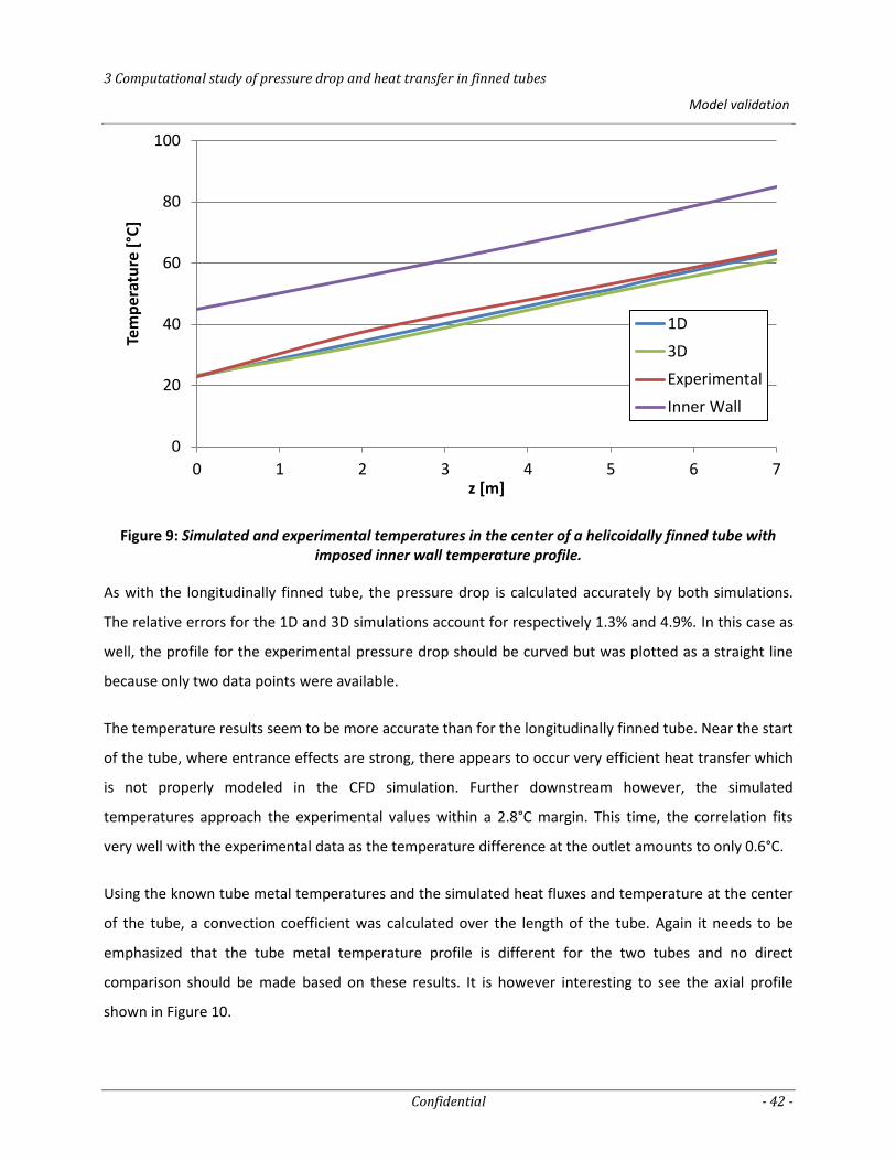
3 Computational study of pressure drop and heat transfer in finned tubes
Model validation
Confidential - 42 -
Figure 9: Simulated and experimental temperatures in the center of a helicoidally finned tube with imposed inner wall temperature profile.
As with the longitudinally finned tube, the pressure drop is calculated accurately by both simulations.
The relative errors for the 1D and 3D simulations account for respectively 1.3% and 4.9%. In this case as
well, the profile for the experimental pressure drop should be curved but was plotted as a straight line
because only two data points were available.
The temperature results seem to be more accurate than for the longitudinally finned tube. Near the start
of the tube, where entrance effects are strong, there appears to occur very efficient heat transfer which
is not properly modeled in the CFD simulation. Further downstream however, the simulated
temperatures approach the experimental values within a 2.8°C margin. This time, the correlation fits
very well with the experimental data as the temperature difference at the outlet amounts to only 0.6°C.
Using the known tube metal temperatures and the simulated heat fluxes and temperature at the center
of the tube, a convection coefficient was calculated over the length of the tube. Again it needs to be
emphasized that the tube metal temperature profile is different for the two tubes and no direct
comparison should be made based on these results. It is however interesting to see the axial profile
shown in Figure 10.
0
20
40
60
80
100
0 1 2 3 4 5 6 7
Tem
per
atu
re [
°C]
z [m]
1D
3D
Experimental
Inner Wall
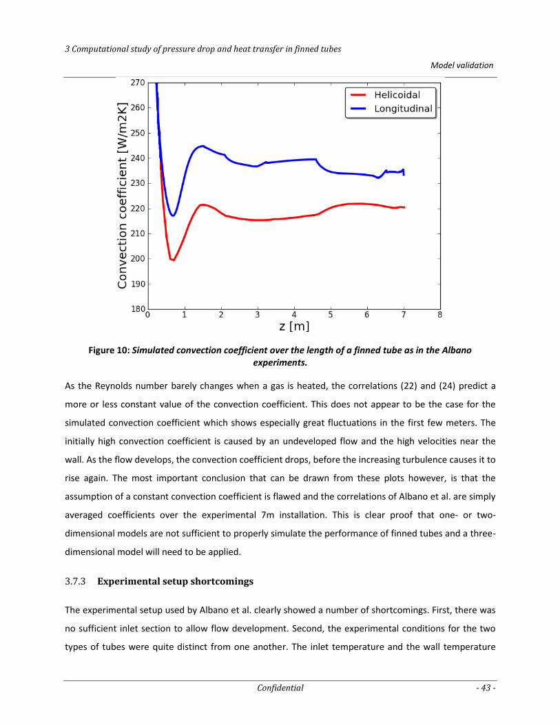
3 Computational study of pressure drop and heat transfer in finned tubes
Model validation
Confidential - 43 -
Figure 10: Simulated convection coefficient over the length of a finned tube as in the Albano experiments.
As the Reynolds number barely changes when a gas is heated, the correlations (22) and (24) predict a
more or less constant value of the convection coefficient. This does not appear to be the case for the
simulated convection coefficient which shows especially great fluctuations in the first few meters. The
initially high convection coefficient is caused by an undeveloped flow and the high velocities near the
wall. As the flow develops, the convection coefficient drops, before the increasing turbulence causes it to
rise again. The most important conclusion that can be drawn from these plots however, is that the
assumption of a constant convection coefficient is flawed and the correlations of Albano et al. are simply
averaged coefficients over the experimental 7m installation. This is clear proof that one- or two-
dimensional models are not sufficient to properly simulate the performance of finned tubes and a three-
dimensional model will need to be applied.
Experimental setup shortcomings 3.7.3
The experimental setup used by Albano et al. clearly showed a number of shortcomings. First, there was
no sufficient inlet section to allow flow development. Second, the experimental conditions for the two
types of tubes were quite distinct from one another. The inlet temperature and the wall temperature
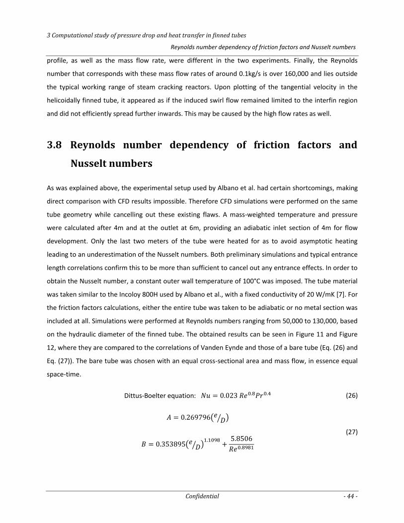
3 Computational study of pressure drop and heat transfer in finned tubes
Reynolds number dependency of friction factors and Nusselt numbers
Confidential - 44 -
profile, as well as the mass flow rate, were different in the two experiments. Finally, the Reynolds
number that corresponds with these mass flow rates of around 0.1kg/s is over 160,000 and lies outside
the typical working range of steam cracking reactors. Upon plotting of the tangential velocity in the
helicoidally finned tube, it appeared as if the induced swirl flow remained limited to the interfin region
and did not efficiently spread further inwards. This may be caused by the high flow rates as well.
3.8 Reynolds number dependency of friction factors and
Nusselt numbers
As was explained above, the experimental setup used by Albano et al. had certain shortcomings, making
direct comparison with CFD results impossible. Therefore CFD simulations were performed on the same
tube geometry while cancelling out these existing flaws. A mass-weighted temperature and pressure
were calculated after 4m and at the outlet at 6m, providing an adiabatic inlet section of 4m for flow
development. Only the last two meters of the tube were heated for as to avoid asymptotic heating
leading to an underestimation of the Nusselt numbers. Both preliminary simulations and typical entrance
length correlations confirm this to be more than sufficient to cancel out any entrance effects. In order to
obtain the Nusselt number, a constant outer wall temperature of 100°C was imposed. The tube material
was taken similar to the Incoloy 800H used by Albano et al., with a fixed conductivity of 20 W/mK [7]. For
the friction factors calculations, either the entire tube was taken to be adiabatic or no metal section was
included at all. Simulations were performed at Reynolds numbers ranging from 50,000 to 130,000, based
on the hydraulic diameter of the finned tube. The obtained results can be seen in Figure 11 and Figure
12, where they are compared to the correlations of Vanden Eynde and those of a bare tube (Eq. (26) and
Eq. (27)). The bare tube was chosen with an equal cross-sectional area and mass flow, in essence equal
space-time.
Dittus-Boelter equation: (26)
( ⁄ )
( ⁄ )
(27)
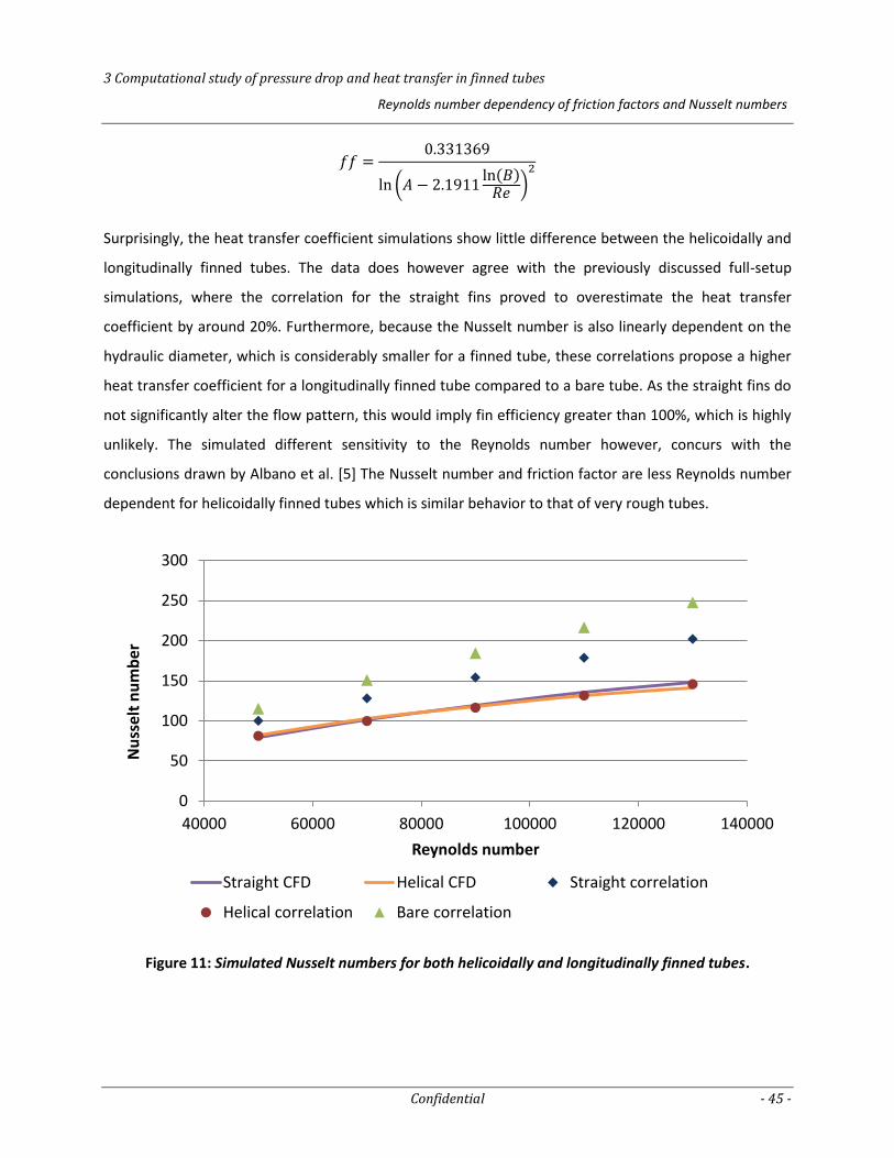
3 Computational study of pressure drop and heat transfer in finned tubes
Reynolds number dependency of friction factors and Nusselt numbers
Confidential - 45 -
1
ln ( 1 11ln
)
Surprisingly, the heat transfer coefficient simulations show little difference between the helicoidally and
longitudinally finned tubes. The data does however agree with the previously discussed full-setup
simulations, where the correlation for the straight fins proved to overestimate the heat transfer
coefficient by around 20%. Furthermore, because the Nusselt number is also linearly dependent on the
hydraulic diameter, which is considerably smaller for a finned tube, these correlations propose a higher
heat transfer coefficient for a longitudinally finned tube compared to a bare tube. As the straight fins do
not significantly alter the flow pattern, this would imply fin efficiency greater than 100%, which is highly
unlikely. The simulated different sensitivity to the Reynolds number however, concurs with the
conclusions drawn by Albano et al. [5] The Nusselt number and friction factor are less Reynolds number
dependent for helicoidally finned tubes which is similar behavior to that of very rough tubes.
Figure 11: Simulated Nusselt numbers for both helicoidally and longitudinally finned tubes.
0
50
100
150
200
250
300
40000 60000 80000 100000 120000 140000
Nu
sse
lt n
um
be
r
Reynolds number
Straight CFD Helical CFD Straight correlation
Helical correlation Bare correlation
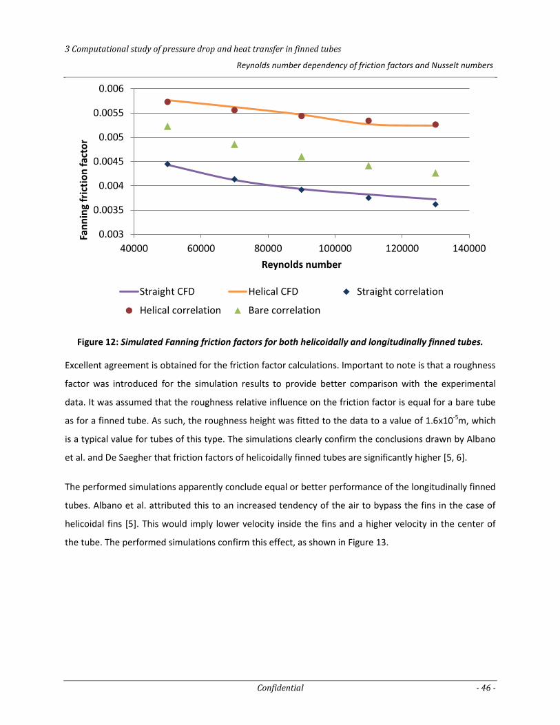
3 Computational study of pressure drop and heat transfer in finned tubes
Reynolds number dependency of friction factors and Nusselt numbers
Confidential - 46 -
Figure 12: Simulated Fanning friction factors for both helicoidally and longitudinally finned tubes.
Excellent agreement is obtained for the friction factor calculations. Important to note is that a roughness
factor was introduced for the simulation results to provide better comparison with the experimental
data. It was assumed that the roughness relative influence on the friction factor is equal for a bare tube
as for a finned tube. As such, the roughness height was fitted to the data to a value of 1.6x10⁻⁵m, which
is a typical value for tubes of this type. The simulations clearly confirm the conclusions drawn by Albano
et al. and De Saegher that friction factors of helicoidally finned tubes are significantly higher [5, 6].
The performed simulations apparently conclude equal or better performance of the longitudinally finned
tubes. Albano et al. attributed this to an increased tendency of the air to bypass the fins in the case of
helicoidal fins [5]. This would imply lower velocity inside the fins and a higher velocity in the center of
the tube. The performed simulations confirm this effect, as shown in Figure 13.
0.003
0.0035
0.004
0.0045
0.005
0.0055
0.006
40000 60000 80000 100000 120000 140000
Fan
nin
g fr
icti
on
fact
or
Reynolds number
Straight CFD Helical CFD Straight correlation
Helical correlation Bare correlation
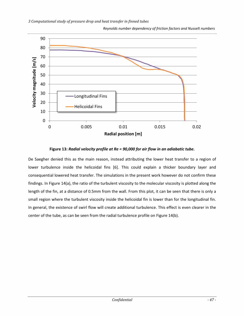
3 Computational study of pressure drop and heat transfer in finned tubes
Reynolds number dependency of friction factors and Nusselt numbers
Confidential - 47 -
Figure 13: Radial velocity profile at Re = 90,000 for air flow in an adiabatic tube.
De Saegher denied this as the main reason, instead attributing the lower heat transfer to a region of
lower turbulence inside the helicoidal fins [6]. This could explain a thicker boundary layer and
consequential lowered heat transfer. The simulations in the present work however do not confirm these
findings. In Figure 14(a), the ratio of the turbulent viscosity to the molecular viscosity is plotted along the
length of the fin, at a distance of 0.5mm from the wall. From this plot, it can be seen that there is only a
small region where the turbulent viscosity inside the helicoidal fin is lower than for the longitudinal fin.
In general, the existence of swirl flow will create additional turbulence. This effect is even clearer in the
center of the tube, as can be seen from the radial turbulence profile on Figure 14(b).
0
10
20
30
40
50
60
70
80
90
0 0.005 0.01 0.015 0.02
Vel
oci
ty m
agn
itu
de
[m/s
]
Radial position [m]
Longitudinal Fins
Helicoidal Fins
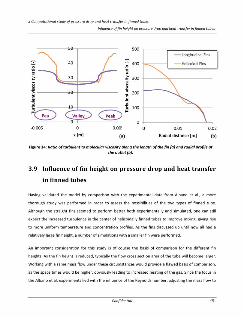
3 Computational study of pressure drop and heat transfer in finned tubes
Influence of fin height on pressure drop and heat transfer in finned tubes
Confidential - 48 -
3.9 Influence of fin height on pressure drop and heat transfer
in finned tubes
Having validated the model by comparison with the experimental data from Albano et al., a more
thorough study was performed in order to assess the possibilities of the two types of finned tube.
Although the straight fins seemed to perform better both experimentally and simulated, one can still
expect the increased turbulence in the center of helicoidally finned tubes to improve mixing, giving rise
to more uniform temperature and concentration profiles. As the fins discussed up until now all had a
relatively large fin height, a number of simulations with a smaller fin were performed.
An important consideration for this study is of course the basis of comparison for the different fin
heights. As the fin height is reduced, typically the flow cross section area of the tube will become larger.
Working with a same mass flow under these circumstances would provide a flawed basis of comparison,
as the space times would be higher, obviously leading to increased heating of the gas. Since the focus in
the Albano et al. experiments lied with the influence of the Reynolds number, adjusting the mass flow to
0
10
20
30
40
50
-0.005 0 0.005
Turb
ule
nt
visc
osi
ty r
atio
[-]
x [m]
Peak Pea Valley
Figure 14: Ratio of turbulent to molecular viscosity along the length of the fin (a) and radial profile at the outlet (b).
(a) (b)
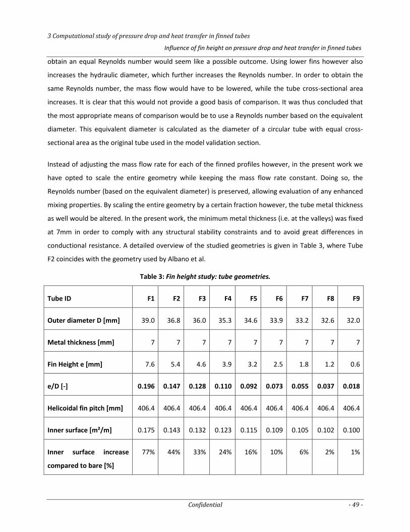
3 Computational study of pressure drop and heat transfer in finned tubes
Influence of fin height on pressure drop and heat transfer in finned tubes
Confidential - 49 -
obtain an equal Reynolds number would seem like a possible outcome. Using lower fins however also
increases the hydraulic diameter, which further increases the Reynolds number. In order to obtain the
same Reynolds number, the mass flow would have to be lowered, while the tube cross-sectional area
increases. It is clear that this would not provide a good basis of comparison. It was thus concluded that
the most appropriate means of comparison would be to use a Reynolds number based on the equivalent
diameter. This equivalent diameter is calculated as the diameter of a circular tube with equal cross-
sectional area as the original tube used in the model validation section.
Instead of adjusting the mass flow rate for each of the finned profiles however, in the present work we
have opted to scale the entire geometry while keeping the mass flow rate constant. Doing so, the
Reynolds number (based on the equivalent diameter) is preserved, allowing evaluation of any enhanced
mixing properties. By scaling the entire geometry by a certain fraction however, the tube metal thickness
as well would be altered. In the present work, the minimum metal thickness (i.e. at the valleys) was fixed
at 7mm in order to comply with any structural stability constraints and to avoid great differences in
conductional resistance. A detailed overview of the studied geometries is given in Table 3, where Tube
F2 coincides with the geometry used by Albano et al.
Table 3: Fin height study: tube geometries.
Tube ID F1 F2 F3 F4 F5 F6 F7 F8 F9
Outer diameter D [mm] 39.0 36.8 36.0 35.3 34.6 33.9 33.2 32.6 32.0
Metal thickness [mm] 7 7 7 7 7 7 7 7 7
Fin Height e [mm] 7.6 5.4 4.6 3.9 3.2 2.5 1.8 1.2 0.6
e/D [-] 0.196 0.147 0.128 0.110 0.092 0.073 0.055 0.037 0.018
Helicoidal fin pitch [mm] 406.4 406.4 406.4 406.4 406.4 406.4 406.4 406.4 406.4
Inner surface [m²/m] 0.175 0.143 0.132 0.123 0.115 0.109 0.105 0.102 0.100
Inner surface increase
compared to bare [%]
77% 44% 33% 24% 16% 10% 6% 2% 1%
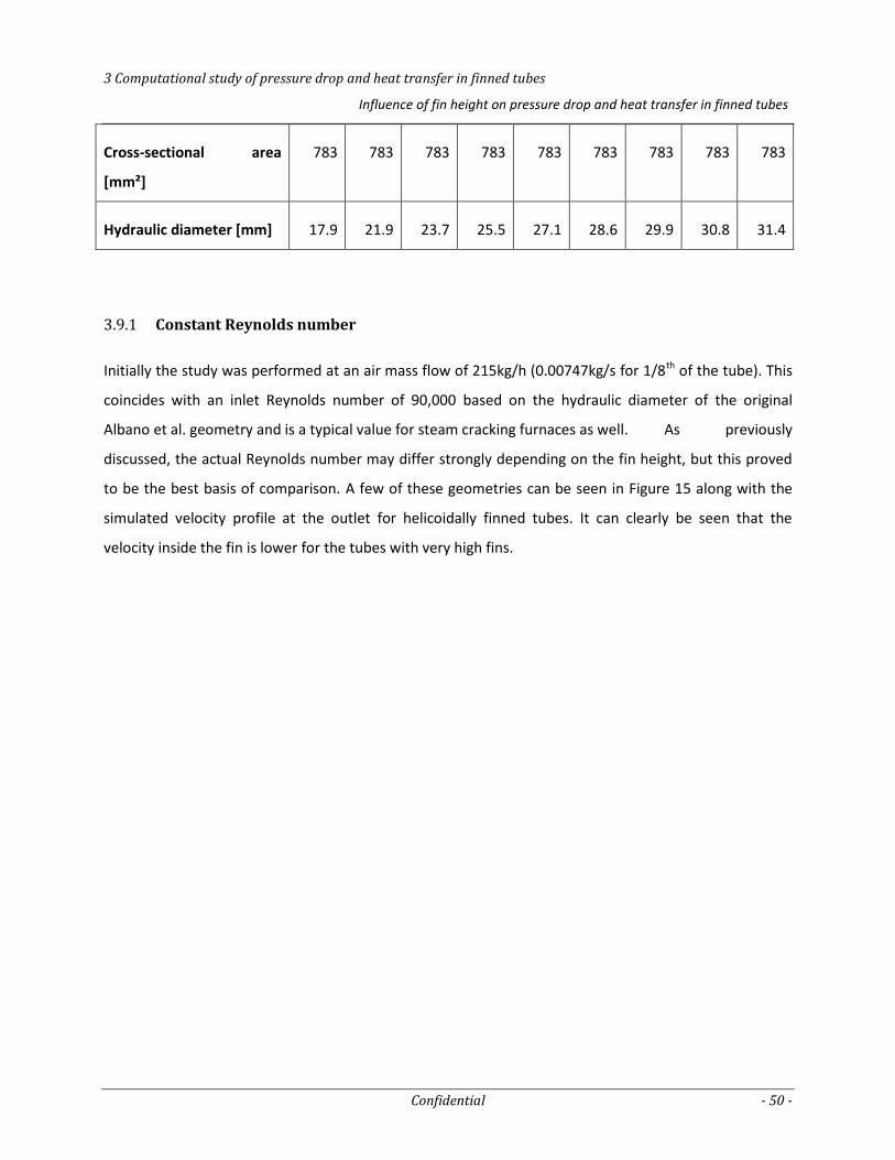
3 Computational study of pressure drop and heat transfer in finned tubes
Influence of fin height on pressure drop and heat transfer in finned tubes
Confidential - 50 -
Cross-sectional area
[mm²]
783 783 783 783 783 783 783 783 783
Hydraulic diameter [mm] 17.9 21.9 23.7 25.5 27.1 28.6 29.9 30.8 31.4
Constant Reynolds number 3.9.1
Initially the study was performed at an air mass flow of 215kg/h (0.00747kg/s for 1/8th of the tube). This
coincides with an inlet Reynolds number of 90,000 based on the hydraulic diameter of the original
Albano et al. geometry and is a typical value for steam cracking furnaces as well. As previously
discussed, the actual Reynolds number may differ strongly depending on the fin height, but this proved
to be the best basis of comparison. A few of these geometries can be seen in Figure 15 along with the
simulated velocity profile at the outlet for helicoidally finned tubes. It can clearly be seen that the
velocity inside the fin is lower for the tubes with very high fins.
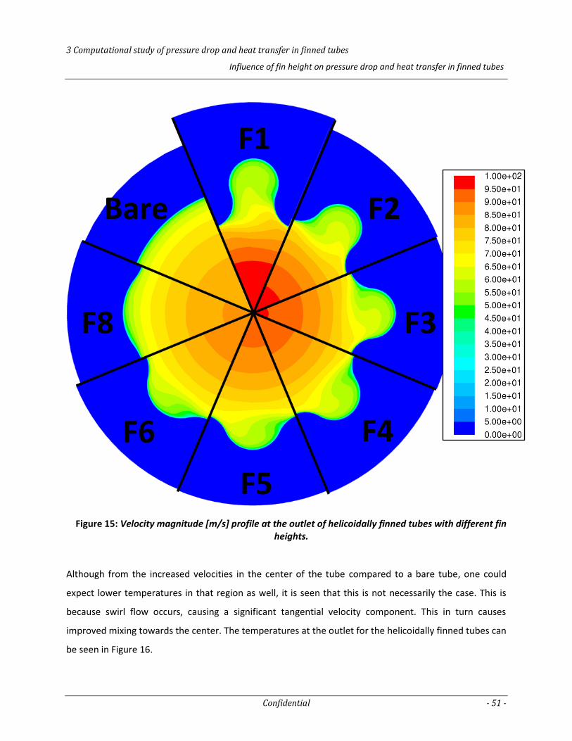
3 Computational study of pressure drop and heat transfer in finned tubes
Influence of fin height on pressure drop and heat transfer in finned tubes
Confidential - 51 -
Although from the increased velocities in the center of the tube compared to a bare tube, one could
expect lower temperatures in that region as well, it is seen that this is not necessarily the case. This is
because swirl flow occurs, causing a significant tangential velocity component. This in turn causes
improved mixing towards the center. The temperatures at the outlet for the helicoidally finned tubes can
be seen in Figure 16.
Figure 15: Velocity magnitude [m/s] profile at the outlet of helicoidally finned tubes with different fin heights.
F1
F2
F3
F4
F5
F6
F8
Bare
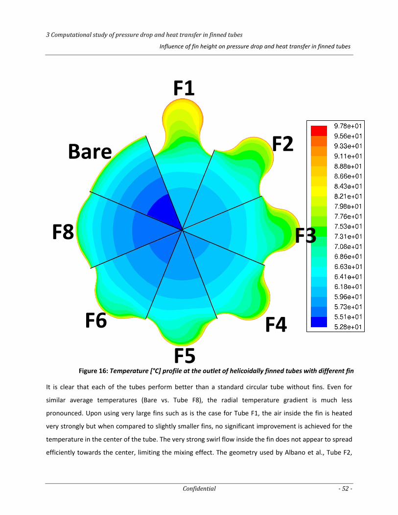
3 Computational study of pressure drop and heat transfer in finned tubes
Influence of fin height on pressure drop and heat transfer in finned tubes
Confidential - 52 -
It is clear that each of the tubes perform better than a standard circular tube without fins. Even for
similar average temperatures (Bare vs. Tube F8), the radial temperature gradient is much less
pronounced. Upon using very large fins such as is the case for Tube F1, the air inside the fin is heated
very strongly but when compared to slightly smaller fins, no significant improvement is achieved for the
temperature in the center of the tube. The very strong swirl flow inside the fin does not appear to spread
efficiently towards the center, limiting the mixing effect. The geometry used by Albano et al., Tube F2,
Figure 16: Temperature [°C] profile at the outlet of helicoidally finned tubes with different fin heights.
F1
F2
F3
F4
F5
F6
F8
Bare
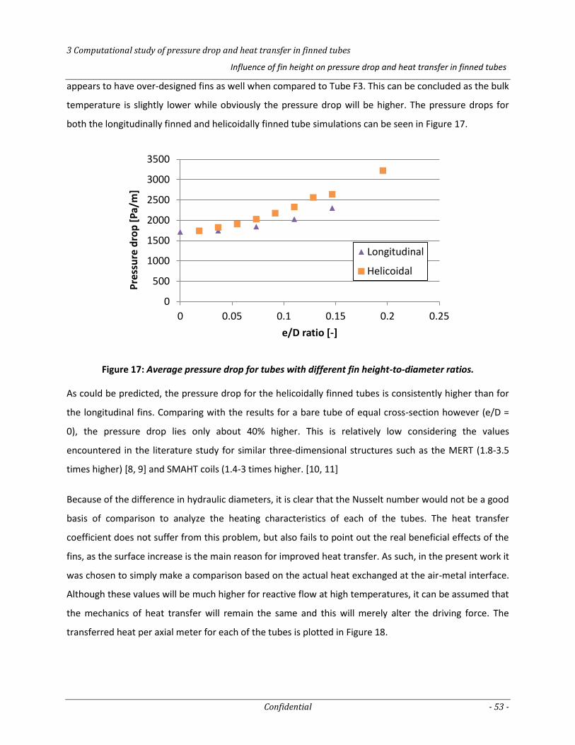
3 Computational study of pressure drop and heat transfer in finned tubes
Influence of fin height on pressure drop and heat transfer in finned tubes
Confidential - 53 -
appears to have over-designed fins as well when compared to Tube F3. This can be concluded as the bulk
temperature is slightly lower while obviously the pressure drop will be higher. The pressure drops for
both the longitudinally finned and helicoidally finned tube simulations can be seen in Figure 17.
Figure 17: Average pressure drop for tubes with different fin height-to-diameter ratios.
As could be predicted, the pressure drop for the helicoidally finned tubes is consistently higher than for
the longitudinal fins. Comparing with the results for a bare tube of equal cross-section however (e/D =
0), the pressure drop lies only about 40% higher. This is relatively low considering the values
encountered in the literature study for similar three-dimensional structures such as the MERT (1.8-3.5
times higher) [8, 9] and SMAHT coils (1.4-3 times higher. [10, 11]
Because of the difference in hydraulic diameters, it is clear that the Nusselt number would not be a good
basis of comparison to analyze the heating characteristics of each of the tubes. The heat transfer
coefficient does not suffer from this problem, but also fails to point out the real beneficial effects of the
fins, as the surface increase is the main reason for improved heat transfer. As such, in the present work it
was chosen to simply make a comparison based on the actual heat exchanged at the air-metal interface.
Although these values will be much higher for reactive flow at high temperatures, it can be assumed that
the mechanics of heat transfer will remain the same and this will merely alter the driving force. The
transferred heat per axial meter for each of the tubes is plotted in Figure 18.
0
500
1000
1500
2000
2500
3000
3500
0 0.05 0.1 0.15 0.2 0.25
Pre
ssu
re d
rop
[P
a/m
]
e/D ratio [-]
Longitudinal
Helicoidal
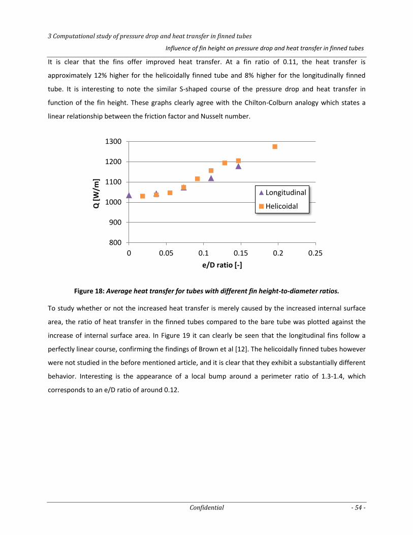
3 Computational study of pressure drop and heat transfer in finned tubes
Influence of fin height on pressure drop and heat transfer in finned tubes
Confidential - 54 -
It is clear that the fins offer improved heat transfer. At a fin ratio of 0.11, the heat transfer is
approximately 12% higher for the helicoidally finned tube and 8% higher for the longitudinally finned
tube. It is interesting to note the similar S-shaped course of the pressure drop and heat transfer in
function of the fin height. These graphs clearly agree with the Chilton-Colburn analogy which states a
linear relationship between the friction factor and Nusselt number.
Figure 18: Average heat transfer for tubes with different fin height-to-diameter ratios.
To study whether or not the increased heat transfer is merely caused by the increased internal surface
area, the ratio of heat transfer in the finned tubes compared to the bare tube was plotted against the
increase of internal surface area. In Figure 19 it can clearly be seen that the longitudinal fins follow a
perfectly linear course, confirming the findings of Brown et al [12]. The helicoidally finned tubes however
were not studied in the before mentioned article, and it is clear that they exhibit a substantially different
behavior. Interesting is the appearance of a local bump around a perimeter ratio of 1.3-1.4, which
corresponds to an e/D ratio of around 0.12.
800
900
1000
1100
1200
1300
0 0.05 0.1 0.15 0.2 0.25
Q [
W/m
]
e/D ratio [-]
Longitudinal
Helicoidal
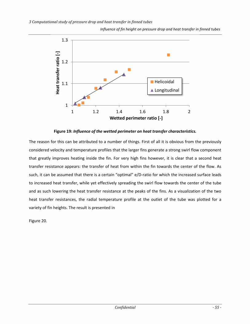
3 Computational study of pressure drop and heat transfer in finned tubes
Influence of fin height on pressure drop and heat transfer in finned tubes
Confidential - 55 -
Figure 19: Influence of the wetted perimeter on heat transfer characteristics.
The reason for this can be attributed to a number of things. First of all it is obvious from the previously
considered velocity and temperature profiles that the larger fins generate a strong swirl flow component
that greatly improves heating inside the fin. For very high fins however, it is clear that a second heat
transfer resistance appears: the transfer of heat from within the fin towards the center of the flow. As
such, it can be assumed that there is a certain “optimal” e/D-ratio for which the increased surface leads
to increased heat transfer, while yet effectively spreading the swirl flow towards the center of the tube
and as such lowering the heat transfer resistance at the peaks of the fins. As a visualization of the two
heat transfer resistances, the radial temperature profile at the outlet of the tube was plotted for a
variety of fin heights. The result is presented in
Figure 20.
1
1.1
1.2
1.3
1 1.2 1.4 1.6 1.8 2
Hea
t tr
ansf
er r
atio
[-]
Wetted perimeter ratio [-]
Helicoidal
Longitudinal
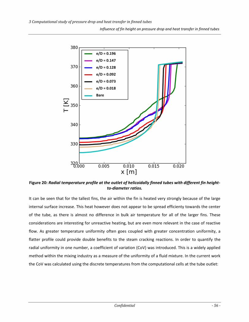
3 Computational study of pressure drop and heat transfer in finned tubes
Influence of fin height on pressure drop and heat transfer in finned tubes
Confidential - 56 -
Figure 20: Radial temperature profile at the outlet of helicoidally finned tubes with different fin height-to-diameter ratios.
It can be seen that for the tallest fins, the air within the fin is heated very strongly because of the large
internal surface increase. This heat however does not appear to be spread efficienty towards the center
of the tube, as there is almost no difference in bulk air temperature for all of the larger fins. These
considerations are interesting for unreactive heating, but are even more relevant in the case of reactive
flow. As greater temperature uniformity often goes coupled with greater concentration uniformity, a
flatter profile could provide double benefits to the steam cracking reactions. In order to quantify the
radial uniformity in one number, a coefficient of variation (CoV) was introduced. This is a widely applied
method within the mixing industry as a measure of the uniformity of a fluid mixture. In the current work
the CoV was calculated using the discrete temperatures from the computational cells at the tube outlet:
e/D = 0.196
e/D = 0.147
e/D = 0.128
e/D = 0.092
e/D = 0.073
e/D = 0.018
Bare
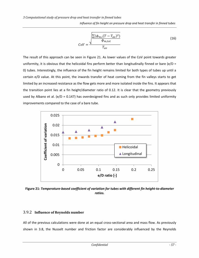
3 Computational study of pressure drop and heat transfer in finned tubes
Influence of fin height on pressure drop and heat transfer in finned tubes
Confidential - 57 -
√∑
(16)
The result of this approach can be seen in Figure 21. As lower values of the CoV point towards greater
uniformity, it is obvious that the helicoidal fins perform better than longitudinally finned or bare (e/D =
0) tubes. Interestingly, the influence of the fin height remains limited for both types of tubes up until a
certain e/D value. At this point, the inwards transfer of heat coming from the fin valleys starts to get
limited by an increased resistance as the flow gets more and more isolated inside the fins. It appears that
the transition point lies at a fin height/diameter ratio of 0.12. It is clear that the geometry previously
used by Albano et al. (e/D = 0.147) has overdesigned fins and as such only provides limited uniformity
improvements compared to the case of a bare tube.
Figure 21: Temperature-based coefficient of variation for tubes with different fin height-to-diameter ratios.
Influence of Reynolds number 3.9.2
All of the previous calculations were done at an equal cross-sectional area and mass flow. As previously
shown in 3.8, the Nusselt number and friction factor are considerably influenced by the Reynolds
0
0.005
0.01
0.015
0.02
0.025
0 0.05 0.1 0.15 0.2 0.25
Co
effi
cien
t o
f va
riat
ion
e/D ratio [-]
Helicoidal
Longitudinal
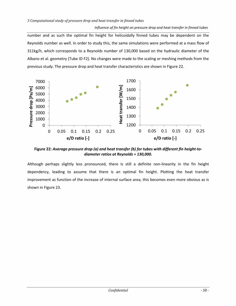
3 Computational study of pressure drop and heat transfer in finned tubes
Influence of fin height on pressure drop and heat transfer in finned tubes
Confidential - 58 -
number and as such the optimal fin height for helicoidally finned tubes may be dependent on the
Reynolds number as well. In order to study this, the same simulations were performed at a mass flow of
311kg/h, which corresponds to a Reynolds number of 130,000 based on the hydraulic diameter of the
Albano et al. geometry (Tube ID F2). No changes were made to the scaling or meshing methods from the
previous study. The pressure drop and heat transfer characteristics are shown in Figure 22.
Figure 22: Average pressure drop (a) and heat transfer (b) for tubes with different fin height-to-diameter ratios at Reynolds = 130,000.
Although perhaps slightly less pronounced, there Is still a definite non-linearity in the fin height
dependency, leading to assume that there is an optimal fin height. Plotting the heat transfer
improvement as function of the increase of internal surface area, this becomes even more obvious as is
shown in Figure 23.
0
1000
2000
3000
4000
5000
6000
7000
0 0.05 0.1 0.15 0.2 0.25
Pre
ssu
re d
rop
[P
a/m
]
e/D ratio [-]
1200
1300
1400
1500
1600
1700
0 0.05 0.1 0.15 0.2 0.25
Hea
t tr
ansf
er [
W/m
]
e/D ratio [-]
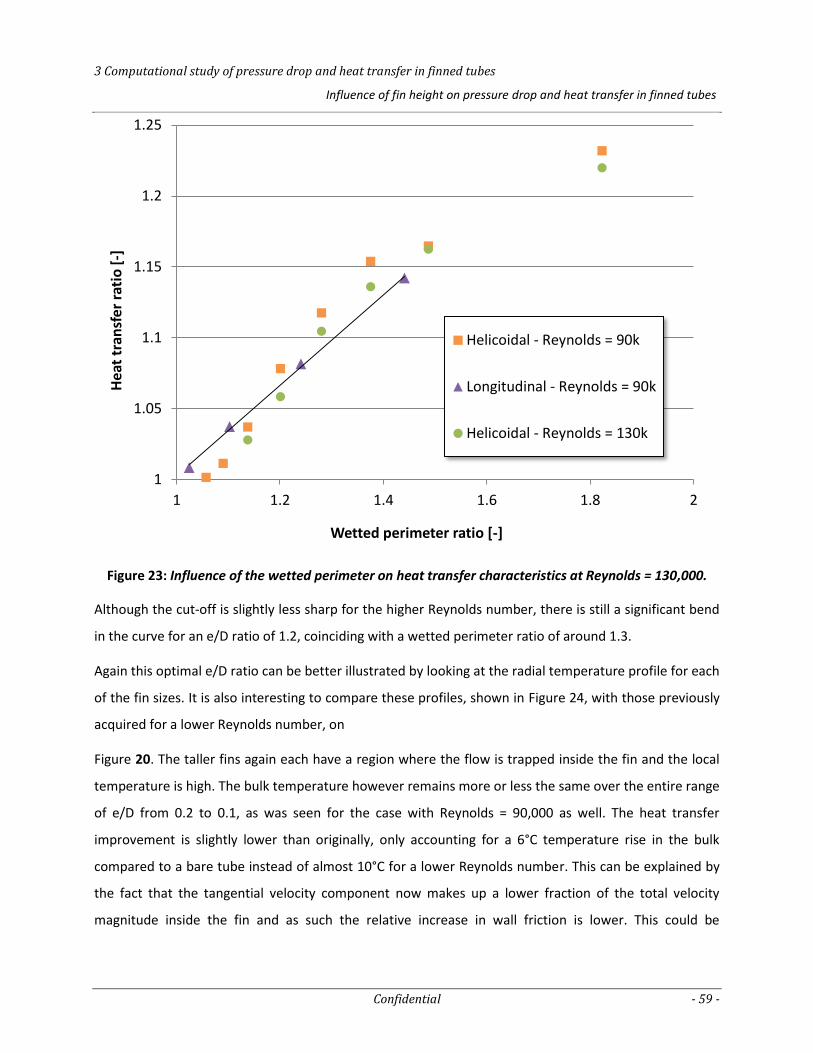
3 Computational study of pressure drop and heat transfer in finned tubes
Influence of fin height on pressure drop and heat transfer in finned tubes
Confidential - 59 -
Figure 23: Influence of the wetted perimeter on heat transfer characteristics at Reynolds = 130,000.
Although the cut-off is slightly less sharp for the higher Reynolds number, there is still a significant bend
in the curve for an e/D ratio of 1.2, coinciding with a wetted perimeter ratio of around 1.3.
Again this optimal e/D ratio can be better illustrated by looking at the radial temperature profile for each
of the fin sizes. It is also interesting to compare these profiles, shown in Figure 24, with those previously
acquired for a lower Reynolds number, on
Figure 20. The taller fins again each have a region where the flow is trapped inside the fin and the local
temperature is high. The bulk temperature however remains more or less the same over the entire range
of e/D from 0.2 to 0.1, as was seen for the case with Reynolds = 90,000 as well. The heat transfer
improvement is slightly lower than originally, only accounting for a 6°C temperature rise in the bulk
compared to a bare tube instead of almost 10°C for a lower Reynolds number. This can be explained by
the fact that the tangential velocity component now makes up a lower fraction of the total velocity
magnitude inside the fin and as such the relative increase in wall friction is lower. This could be
1
1.05
1.1
1.15
1.2
1.25
1 1.2 1.4 1.6 1.8 2
Hea
t tr
ansf
er r
atio
[-]
Wetted perimeter ratio [-]
Helicoidal - Reynolds = 90k
Longitudinal - Reynolds = 90k
Helicoidal - Reynolds = 130k
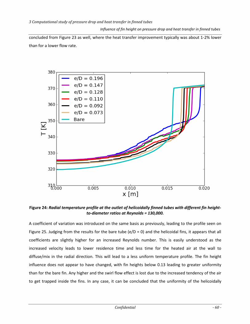
3 Computational study of pressure drop and heat transfer in finned tubes
Influence of fin height on pressure drop and heat transfer in finned tubes
Confidential - 60 -
concluded from Figure 23 as well, where the heat transfer improvement typically was about 1-2% lower
than for a lower flow rate.
Figure 24: Radial temperature profile at the outlet of helicoidally finned tubes with different fin height-to-diameter ratios at Reynolds = 130,000.
A coefficient of variation was introduced on the same basis as previously, leading to the profile seen on
Figure 25. Judging from the results for the bare tube (e/D = 0) and the helicoidal fins, it appears that all
coefficients are slightly higher for an increased Reynolds number. This is easily understood as the
increased velocity leads to lower residence time and less time for the heated air at the wall to
diffuse/mix in the radial direction. This will lead to a less uniform temperature profile. The fin height
influence does not appear to have changed, with fin heights below 0.13 leading to greater uniformity
than for the bare fin. Any higher and the swirl flow effect is lost due to the increased tendency of the air
to get trapped inside the fins. In any case, it can be concluded that the uniformity of the helicoidally
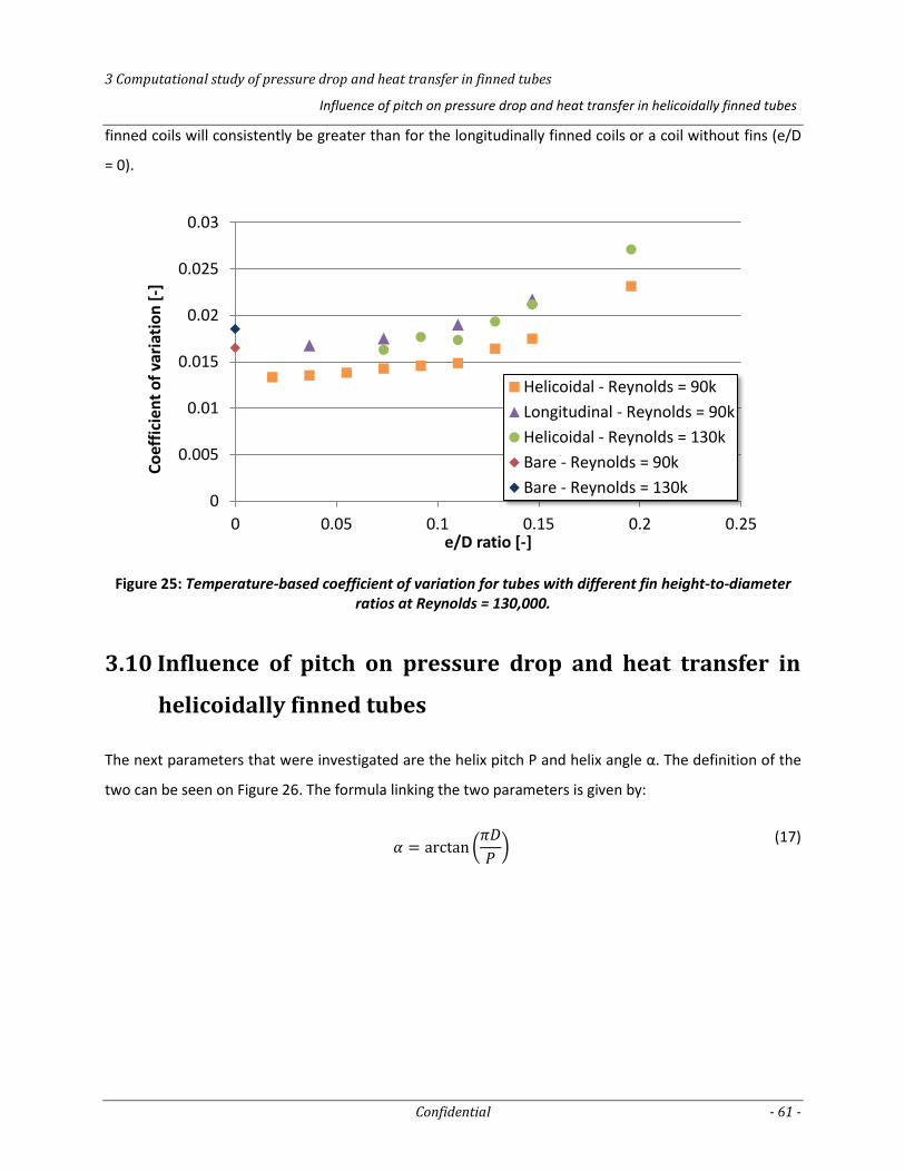
3 Computational study of pressure drop and heat transfer in finned tubes
Influence of pitch on pressure drop and heat transfer in helicoidally finned tubes
Confidential - 61 -
finned coils will consistently be greater than for the longitudinally finned coils or a coil without fins (e/D
= 0).
Figure 25: Temperature-based coefficient of variation for tubes with different fin height-to-diameter ratios at Reynolds = 130,000.
3.10 Influence of pitch on pressure drop and heat transfer in
helicoidally finned tubes
The next parameters that were investigated are the helix pitch P and helix angle α. The definition of the
two can be seen on Figure 26. The formula linking the two parameters is given by:
n (
)
(17)
0
0.005
0.01
0.015
0.02
0.025
0.03
0 0.05 0.1 0.15 0.2 0.25
Co
effi
cien
t o
f va
riat
ion
[-]
e/D ratio [-]
Helicoidal - Reynolds = 90k
Longitudinal - Reynolds = 90k
Helicoidal - Reynolds = 130k
Bare - Reynolds = 90k
Bare - Reynolds = 130k
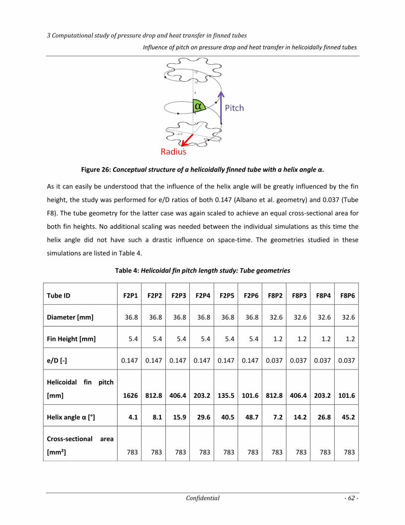
3 Computational study of pressure drop and heat transfer in finned tubes
Influence of pitch on pressure drop and heat transfer in helicoidally finned tubes
Confidential - 62 -
Figure 26: Conceptual structure of a helicoidally finned tube with a helix angle α.
As it can easily be understood that the influence of the helix angle will be greatly influenced by the fin
height, the study was performed for e/D ratios of both 0.147 (Albano et al. geometry) and 0.037 (Tube
F8). The tube geometry for the latter case was again scaled to achieve an equal cross-sectional area for
both fin heights. No additional scaling was needed between the individual simulations as this time the
helix angle did not have such a drastic influence on space-time. The geometries studied in these
simulations are listed in Table 4.
Table 4: Helicoidal fin pitch length study: Tube geometries
Tube ID F2P1 F2P2 F2P3 F2P4 F2P5 F2P6 F8P2 F8P3 F8P4 F8P6
Diameter [mm] 36.8 36.8 36.8 36.8 36.8 36.8 32.6 32.6 32.6 32.6
Fin Height [mm] 5.4 5.4 5.4 5.4 5.4 5.4 1.2 1.2 1.2 1.2
e/D [-] 0.147 0.147 0.147 0.147 0.147 0.147 0.037 0.037 0.037 0.037
Helicoidal fin pitch
[mm] 1626 812.8 406.4 203.2 135.5 101.6 812.8 406.4 203.2 101.6
Helix angle α [°] 4.1 8.1 15.9 29.6 40.5 48.7 7.2 14.2 26.8 45.2
Cross-sectional area
[mm²] 783 783 783 783 783 783 783 783 783 783
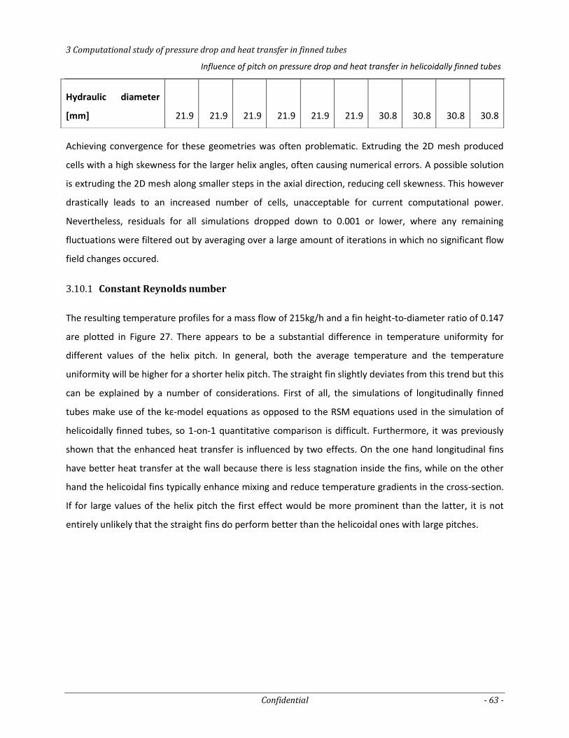
3 Computational study of pressure drop and heat transfer in finned tubes
Influence of pitch on pressure drop and heat transfer in helicoidally finned tubes
Confidential - 63 -
Achieving convergence for these geometries was often problematic. Extruding the 2D mesh produced
cells with a high skewness for the larger helix angles, often causing numerical errors. A possible solution
is extruding the 2D mesh along smaller steps in the axial direction, reducing cell skewness. This however
drastically leads to an increased number of cells, unacceptable for current computational power.
Nevertheless, residuals for all simulations dropped down to 0.001 or lower, where any remaining
fluctuations were filtered out by averaging over a large amount of iterations in which no significant flow
field changes occured.
Constant Reynolds number 3.10.1
The resulting temperature profiles for a mass flow of 215kg/h and a fin height-to-diameter ratio of 0.147
are plotted in Figure 27. There appears to be a substantial difference in temperature uniformity for
different values of the helix pitch. In general, both the average temperature and the temperature
uniformity will be higher for a shorter helix pitch. The straight fin slightly deviates from this trend but this
can be explained by a number of considerations. First of all, the simulations of longitudinally finned
tubes make use of the kε-model equations as opposed to the RSM equations used in the simulation of
helicoidally finned tubes, so 1-on-1 quantitative comparison is difficult. Furthermore, it was previously
shown that the enhanced heat transfer is influenced by two effects. On the one hand longitudinal fins
have better heat transfer at the wall because there is less stagnation inside the fins, while on the other
hand the helicoidal fins typically enhance mixing and reduce temperature gradients in the cross-section.
If for large values of the helix pitch the first effect would be more prominent than the latter, it is not
entirely unlikely that the straight fins do perform better than the helicoidal ones with large pitches.
Hydraulic diameter
[mm] 21.9 21.9 21.9 21.9 21.9 21.9 30.8 30.8 30.8 30.8
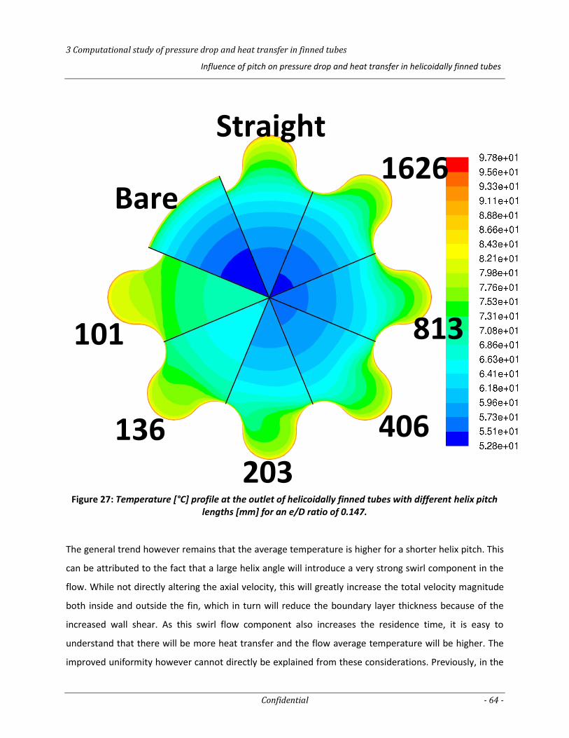
3 Computational study of pressure drop and heat transfer in finned tubes
Influence of pitch on pressure drop and heat transfer in helicoidally finned tubes
Confidential - 64 -
The general trend however remains that the average temperature is higher for a shorter helix pitch. This
can be attributed to the fact that a large helix angle will introduce a very strong swirl component in the
flow. While not directly altering the axial velocity, this will greatly increase the total velocity magnitude
both inside and outside the fin, which in turn will reduce the boundary layer thickness because of the
increased wall shear. As this swirl flow component also increases the residence time, it is easy to
understand that there will be more heat transfer and the flow average temperature will be higher. The
improved uniformity however cannot directly be explained from these considerations. Previously, in the
1626
813
203
136
101
Bare
Straight
Figure 27: Temperature [°C] profile at the outlet of helicoidally finned tubes with different helix pitch lengths [mm] for an e/D ratio of 0.147.
406
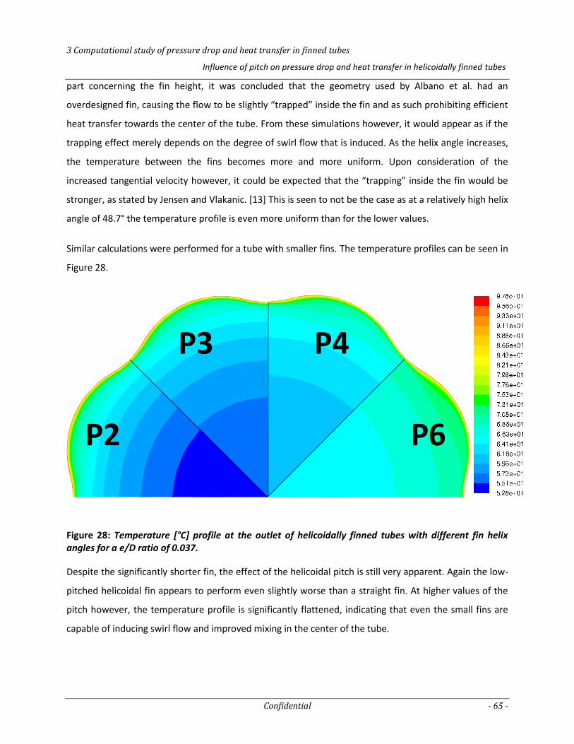
3 Computational study of pressure drop and heat transfer in finned tubes
Influence of pitch on pressure drop and heat transfer in helicoidally finned tubes
Confidential - 65 -
part concerning the fin height, it was concluded that the geometry used by Albano et al. had an
overdesigned fin, causing the flow to be slightly “trapped” inside the fin and as such prohibiting efficient
heat transfer towards the center of the tube. From these simulations however, it would appear as if the
trapping effect merely depends on the degree of swirl flow that is induced. As the helix angle increases,
the temperature between the fins becomes more and more uniform. Upon consideration of the
increased tangential velocity however, it could be expected that the “trapping” inside the fin would be
stronger, as stated by Jensen and Vlakanic. [13] This is seen to not be the case as at a relatively high helix
angle of 48.7° the temperature profile is even more uniform than for the lower values.
Similar calculations were performed for a tube with smaller fins. The temperature profiles can be seen in
Figure 28.
Figure 28: Temperature [°C] profile at the outlet of helicoidally finned tubes with different fin helix angles for a e/D ratio of 0.037.
Despite the significantly shorter fin, the effect of the helicoidal pitch is still very apparent. Again the low-
pitched helicoidal fin appears to perform even slightly worse than a straight fin. At higher values of the
pitch however, the temperature profile is significantly flattened, indicating that even the small fins are
capable of inducing swirl flow and improved mixing in the center of the tube.
P2
P3 P4
P6
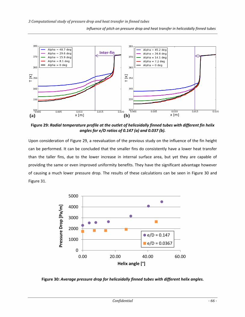
3 Computational study of pressure drop and heat transfer in finned tubes
Influence of pitch on pressure drop and heat transfer in helicoidally finned tubes
Confidential - 66 -
Figure 29: Radial temperature profile at the outlet of helicoidally finned tubes with different fin helix angles for e/D ratios of 0.147 (a) and 0.037 (b).
Upon consideration of Figure 29, a reevaluation of the previous study on the influence of the fin height
can be performed. It can be concluded that the smaller fins do consistently have a lower heat transfer
than the taller fins, due to the lower increase in internal surface area, but yet they are capable of
providing the same or even improved uniformity benefits. They have the significant advantage however
of causing a much lower pressure drop. The results of these calculations can be seen in Figure 30 and
Figure 31.
Figure 30: Average pressure drop for helicoidally finned tubes with different helix angles.
0
1000
2000
3000
4000
5000
0.00 20.00 40.00 60.00
Pre
ssu
re D
rop
[P
a/m
]
Helix angle [°]
e/D = 0.147
e/D = 0.0367
Inter-fin
(a) (b)
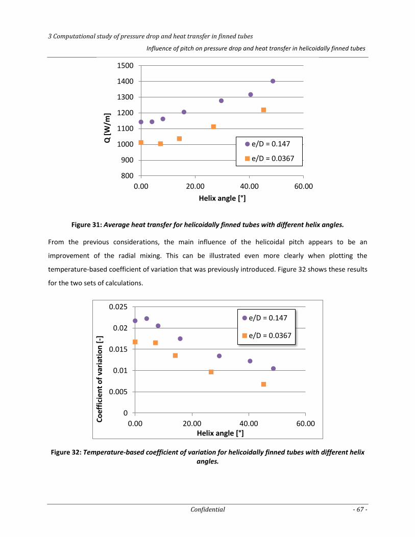
3 Computational study of pressure drop and heat transfer in finned tubes
Influence of pitch on pressure drop and heat transfer in helicoidally finned tubes
Confidential - 67 -
Figure 31: Average heat transfer for helicoidally finned tubes with different helix angles.
From the previous considerations, the main influence of the helicoidal pitch appears to be an
improvement of the radial mixing. This can be illustrated even more clearly when plotting the
temperature-based coefficient of variation that was previously introduced. Figure 32 shows these results
for the two sets of calculations.
Figure 32: Temperature-based coefficient of variation for helicoidally finned tubes with different helix angles.
800
900
1000
1100
1200
1300
1400
1500
0.00 20.00 40.00 60.00
Q [
W/m
]
Helix angle [°]
e/D = 0.147
e/D = 0.0367
0
0.005
0.01
0.015
0.02
0.025
0.00 20.00 40.00 60.00Co
effi
cien
t o
f va
riat
ion
[-]
Helix angle [°]
e/D = 0.147
e/D = 0.0367
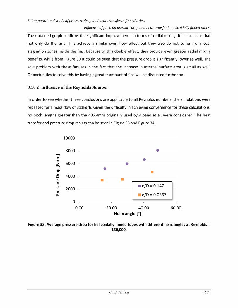
3 Computational study of pressure drop and heat transfer in finned tubes
Influence of pitch on pressure drop and heat transfer in helicoidally finned tubes
Confidential - 68 -
The obtained graph confirms the significant improvements in terms of radial mixing. It is also clear that
not only do the small fins achieve a similar swirl flow effect but they also do not suffer from local
stagnation zones inside the fins. Because of this double effect, they provide even greater radial mixing
benefits, while from Figure 30 it could be seen that the pressure drop is significantly lower as well. The
sole problem with these fins lies in the fact that the increase in internal surface area is small as well.
Opportunities to solve this by having a greater amount of fins will be discussed further on.
Influence of the Reynolds Number 3.10.2
In order to see whether these conclusions are applicable to all Reynolds numbers, the simulations were
repeated for a mass flow of 311kg/h. Given the difficulty in achieving convergence for these calculations,
no pitch lengths greater than the 406.4mm originally used by Albano et al. were considered. The heat
transfer and pressure drop results can be seen in Figure 33 and Figure 34.
Figure 33: Average pressure drop for helicoidally finned tubes with different helix angles at Reynolds = 130,000.
0
2000
4000
6000
8000
10000
0.00 20.00 40.00 60.00
Pre
ssu
re D
rop
[P
a/m
]
Helix angle [°]
e/D = 0.147
e/D = 0.0367
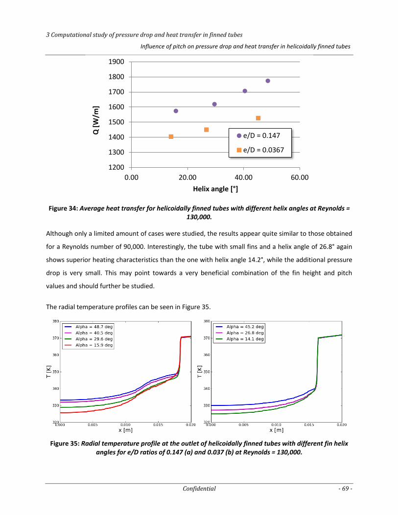
3 Computational study of pressure drop and heat transfer in finned tubes
Influence of pitch on pressure drop and heat transfer in helicoidally finned tubes
Confidential - 69 -
Figure 34: Average heat transfer for helicoidally finned tubes with different helix angles at Reynolds = 130,000.
Although only a limited amount of cases were studied, the results appear quite similar to those obtained
for a Reynolds number of 90,000. Interestingly, the tube with small fins and a helix angle of 26.8° again
shows superior heating characteristics than the one with helix angle 14.2°, while the additional pressure
drop is very small. This may point towards a very beneficial combination of the fin height and pitch
values and should further be studied.
The radial temperature profiles can be seen in Figure 35.
Figure 35: Radial temperature profile at the outlet of helicoidally finned tubes with different fin helix angles for e/D ratios of 0.147 (a) and 0.037 (b) at Reynolds = 130,000.
1200
1300
1400
1500
1600
1700
1800
1900
0.00 20.00 40.00 60.00
Q [
W/m
]
Helix angle [°]
e/D = 0.147
e/D = 0.0367
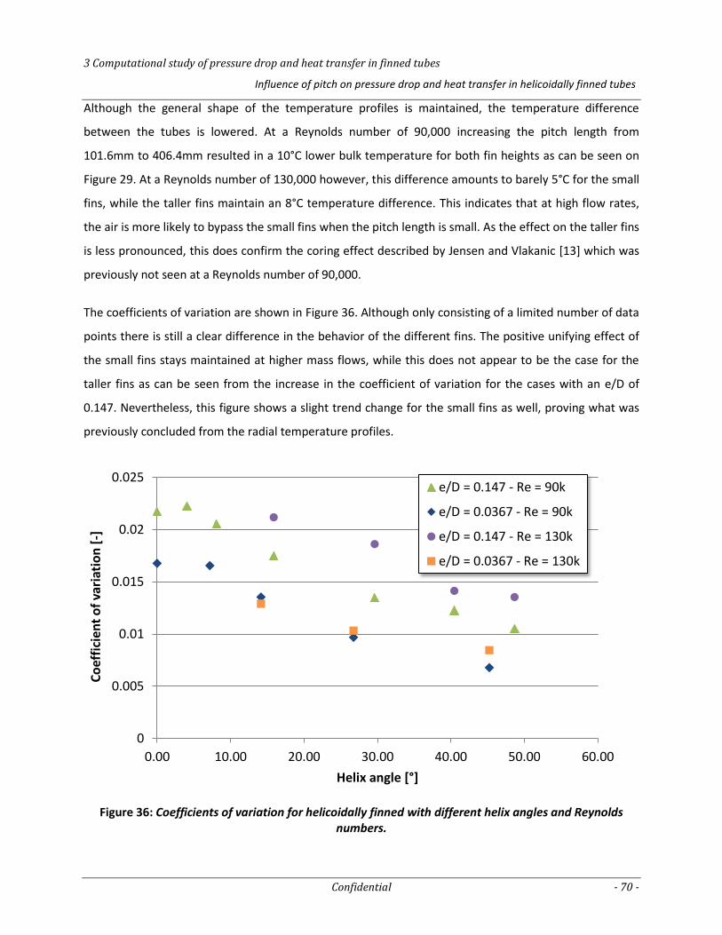
3 Computational study of pressure drop and heat transfer in finned tubes
Influence of pitch on pressure drop and heat transfer in helicoidally finned tubes
Confidential - 70 -
Although the general shape of the temperature profiles is maintained, the temperature difference
between the tubes is lowered. At a Reynolds number of 90,000 increasing the pitch length from
101.6mm to 406.4mm resulted in a 10°C lower bulk temperature for both fin heights as can be seen on
Figure 29. At a Reynolds number of 130,000 however, this difference amounts to barely 5°C for the small
fins, while the taller fins maintain an 8°C temperature difference. This indicates that at high flow rates,
the air is more likely to bypass the small fins when the pitch length is small. As the effect on the taller fins
is less pronounced, this does confirm the coring effect described by Jensen and Vlakanic [13] which was
previously not seen at a Reynolds number of 90,000.
The coefficients of variation are shown in Figure 36. Although only consisting of a limited number of data
points there is still a clear difference in the behavior of the different fins. The positive unifying effect of
the small fins stays maintained at higher mass flows, while this does not appear to be the case for the
taller fins as can be seen from the increase in the coefficient of variation for the cases with an e/D of
0.147. Nevertheless, this figure shows a slight trend change for the small fins as well, proving what was
previously concluded from the radial temperature profiles.
Figure 36: Coefficients of variation for helicoidally finned with different helix angles and Reynolds numbers.
0
0.005
0.01
0.015
0.02
0.025
0.00 10.00 20.00 30.00 40.00 50.00 60.00
Co
effi
cien
t o
f va
riat
ion
[-]
Helix angle [°]
e/D = 0.147 - Re = 90k
e/D = 0.0367 - Re = 90k
e/D = 0.147 - Re = 130k
e/D = 0.0367 - Re = 130k
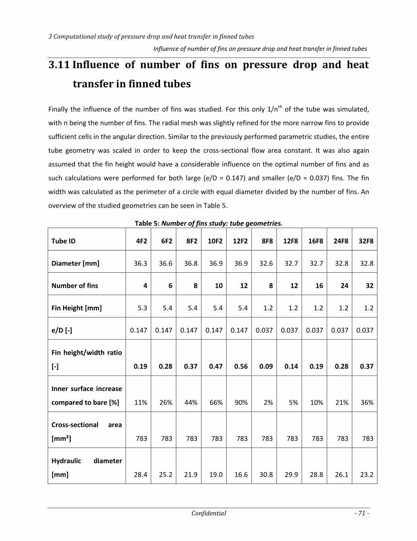
3 Computational study of pressure drop and heat transfer in finned tubes
Influence of number of fins on pressure drop and heat transfer in finned tubes
Confidential - 71 -
3.11 Influence of number of fins on pressure drop and heat
transfer in finned tubes
Finally the influence of the number of fins was studied. For this only 1/nth of the tube was simulated,
with n being the number of fins. The radial mesh was slightly refined for the more narrow fins to provide
sufficient cells in the angular direction. Similar to the previously performed parametric studies, the entire
tube geometry was scaled in order to keep the cross-sectional flow area constant. It was also again
assumed that the fin height would have a considerable influence on the optimal number of fins and as
such calculations were performed for both large (e/D = 0.147) and smaller (e/D = 0.037) fins. The fin
width was calculated as the perimeter of a circle with equal diameter divided by the number of fins. An
overview of the studied geometries can be seen in Table 5.
Table 5: Number of fins study: tube geometries.
Tube ID 4F2 6F2 8F2 10F2 12F2 8F8 12F8 16F8 24F8 32F8
Diameter [mm] 36.3 36.6 36.8 36.9 36.9 32.6 32.7 32.7 32.8 32.8
Number of fins 4 6 8 10 12 8 12 16 24 32
Fin Height [mm] 5.3 5.4 5.4 5.4 5.4 1.2 1.2 1.2 1.2 1.2
e/D [-] 0.147 0.147 0.147 0.147 0.147 0.037 0.037 0.037 0.037 0.037
Fin height/width ratio
[-] 0.19 0.28 0.37 0.47 0.56 0.09 0.14 0.19 0.28 0.37
Inner surface increase
compared to bare [%] 11% 26% 44% 66% 90% 2% 5% 10% 21% 36%
Cross-sectional area
[mm²] 783 783 783 783 783 783 783 783 783 783
Hydraulic diameter
[mm] 28.4 25.2 21.9 19.0 16.6 30.8 29.9 28.8 26.1 23.2
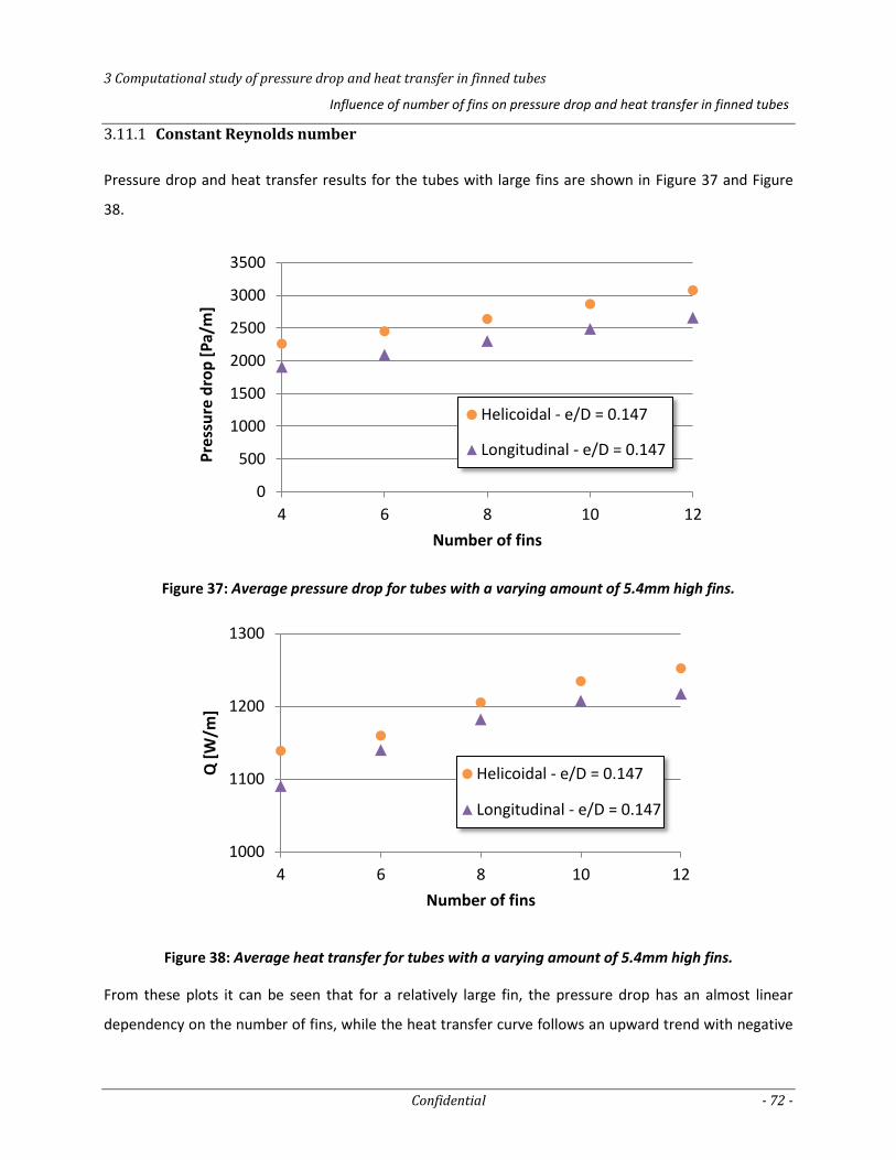
3 Computational study of pressure drop and heat transfer in finned tubes
Influence of number of fins on pressure drop and heat transfer in finned tubes
Confidential - 72 -
Constant Reynolds number 3.11.1
Pressure drop and heat transfer results for the tubes with large fins are shown in Figure 37 and Figure
38.
Figure 37: Average pressure drop for tubes with a varying amount of 5.4mm high fins.
Figure 38: Average heat transfer for tubes with a varying amount of 5.4mm high fins.
From these plots it can be seen that for a relatively large fin, the pressure drop has an almost linear
dependency on the number of fins, while the heat transfer curve follows an upward trend with negative
0
500
1000
1500
2000
2500
3000
3500
4 6 8 10 12
Pre
ssu
re d
rop
[P
a/m
]
Number of fins
Helicoidal - e/D = 0.147
Longitudinal - e/D = 0.147
1000
1100
1200
1300
4 6 8 10 12
Q [
W/m
]
Number of fins
Helicoidal - e/D = 0.147
Longitudinal - e/D = 0.147
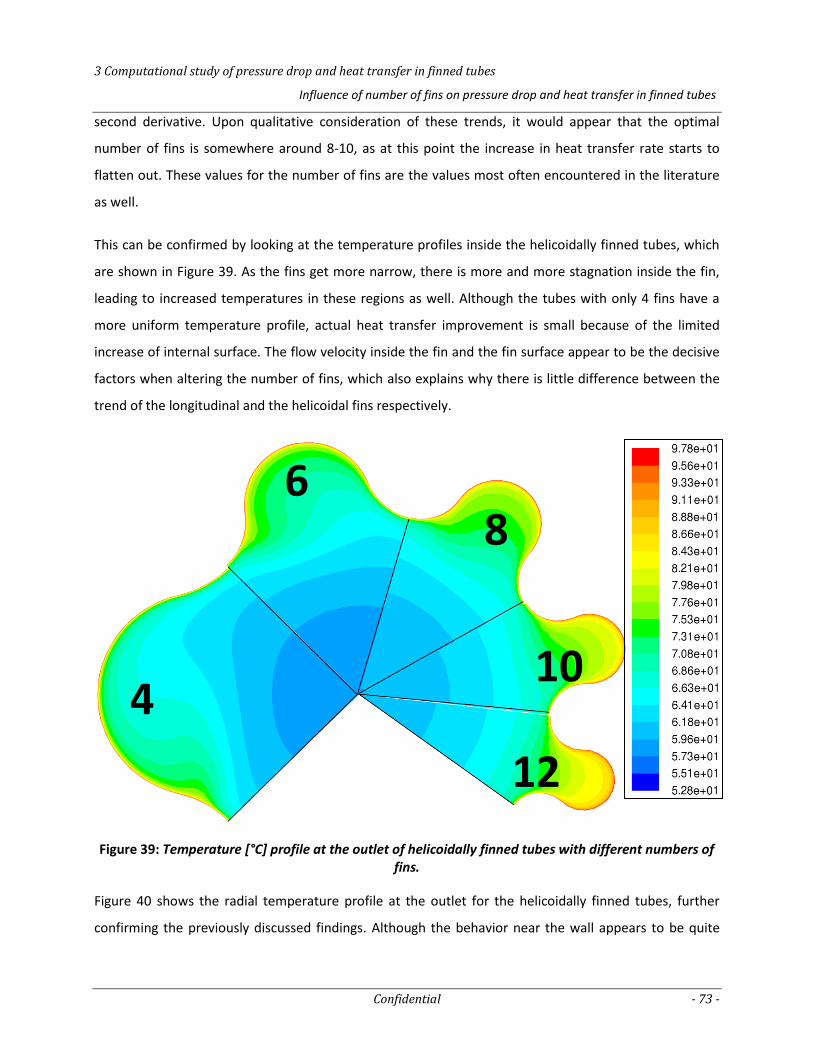
3 Computational study of pressure drop and heat transfer in finned tubes
Influence of number of fins on pressure drop and heat transfer in finned tubes
Confidential - 73 -
second derivative. Upon qualitative consideration of these trends, it would appear that the optimal
number of fins is somewhere around 8-10, as at this point the increase in heat transfer rate starts to
flatten out. These values for the number of fins are the values most often encountered in the literature
as well.
This can be confirmed by looking at the temperature profiles inside the helicoidally finned tubes, which
are shown in Figure 39. As the fins get more narrow, there is more and more stagnation inside the fin,
leading to increased temperatures in these regions as well. Although the tubes with only 4 fins have a
more uniform temperature profile, actual heat transfer improvement is small because of the limited
increase of internal surface. The flow velocity inside the fin and the fin surface appear to be the decisive
factors when altering the number of fins, which also explains why there is little difference between the
trend of the longitudinal and the helicoidal fins respectively.
Figure 39: Temperature [°C] profile at the outlet of helicoidally finned tubes with different numbers of fins.
Figure 40 shows the radial temperature profile at the outlet for the helicoidally finned tubes, further
confirming the previously discussed findings. Although the behavior near the wall appears to be quite
6
4
8
10
12
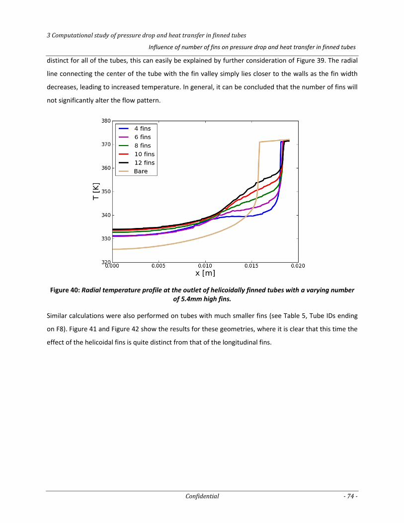
3 Computational study of pressure drop and heat transfer in finned tubes
Influence of number of fins on pressure drop and heat transfer in finned tubes
Confidential - 74 -
distinct for all of the tubes, this can easily be explained by further consideration of Figure 39. The radial
line connecting the center of the tube with the fin valley simply lies closer to the walls as the fin width
decreases, leading to increased temperature. In general, it can be concluded that the number of fins will
not significantly alter the flow pattern.
Figure 40: Radial temperature profile at the outlet of helicoidally finned tubes with a varying number of 5.4mm high fins.
Similar calculations were also performed on tubes with much smaller fins (see Table 5, Tube IDs ending
on F8). Figure 41 and Figure 42 show the results for these geometries, where it is clear that this time the
effect of the helicoidal fins is quite distinct from that of the longitudinal fins.
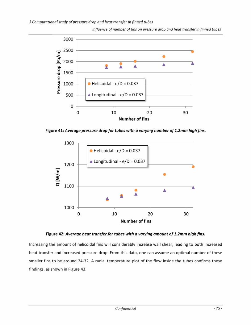
3 Computational study of pressure drop and heat transfer in finned tubes
Influence of number of fins on pressure drop and heat transfer in finned tubes
Confidential - 75 -
Figure 41: Average pressure drop for tubes with a varying number of 1.2mm high fins.
Figure 42: Average heat transfer for tubes with a varying amount of 1.2mm high fins.
Increasing the amount of helicoidal fins will considerably increase wall shear, leading to both increased
heat transfer and increased pressure drop. From this data, one can assume an optimal number of these
smaller fins to be around 24-32. A radial temperature plot of the flow inside the tubes confirms these
findings, as shown in Figure 43.
0
500
1000
1500
2000
2500
3000
0 10 20 30
Pre
ssu
re d
rop
[P
a/m
]
Number of fins
Helicoidal - e/D = 0.037
Longitudinal - e/D = 0.037
1000
1100
1200
1300
0 10 20 30
Q [
W/m
]
Number of fins
Helicoidal - e/D = 0.037
Longitudinal - e/D = 0.037
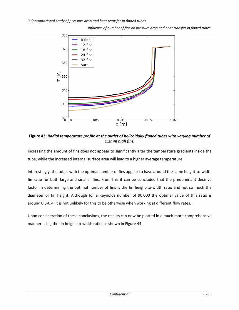
3 Computational study of pressure drop and heat transfer in finned tubes
Influence of number of fins on pressure drop and heat transfer in finned tubes
Confidential - 76 -
Figure 43: Radial temperature profile at the outlet of helicoidally finned tubes with varying number of 1.2mm high fins.
Increasing the amount of fins does not appear to significantly alter the temperature gradients inside the
tube, while the increased internal surface area will lead to a higher average temperature.
Interestingly, the tubes with the optimal number of fins appear to have around the same height-to-width
fin ratio for both large and smaller fins. From this it can be concluded that the predominant decisive
factor in determining the optimal number of fins is the fin height-to-width ratio and not so much the
diameter or fin height. Although for a Reynolds number of 90,000 the optimal value of this ratio is
around 0.3-0.4, it is not unlikely for this to be otherwise when working at different flow rates.
Upon consideration of these conclusions, the results can now be plotted in a much more comprehensive
manner using the fin height-to-width ratio, as shown in Figure 44.
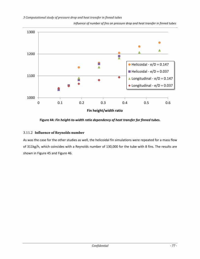
3 Computational study of pressure drop and heat transfer in finned tubes
Influence of number of fins on pressure drop and heat transfer in finned tubes
Confidential - 77 -
Figure 44: Fin height-to-width ratio dependency of heat transfer for finned tubes.
Influence of Reynolds number 3.11.2
As was the case for the other studies as well, the helicoidal fin simulations were repeated for a mass flow
of 311kg/h, which coincides with a Reynolds number of 130,000 for the tube with 8 fins. The results are
shown in Figure 45 and Figure 46.
1000
1100
1200
1300
0 0.1 0.2 0.3 0.4 0.5 0.6
Fin height/width ratio
Helicoidal - e/D = 0.147
Helicoidal - e/D = 0.037
Longitudinal - e/D = 0.147
Longitudinal - e/D = 0.037
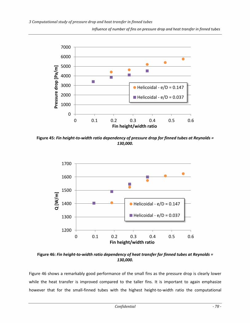
3 Computational study of pressure drop and heat transfer in finned tubes
Influence of number of fins on pressure drop and heat transfer in finned tubes
Confidential - 78 -
Figure 45: Fin height-to-width ratio dependency of pressure drop for finned tubes at Reynolds = 130,000.
Figure 46: Fin height-to-width ratio dependency of heat transfer for finned tubes at Reynolds = 130,000.
Figure 46 shows a remarkably good performance of the small fins as the pressure drop is clearly lower
while the heat transfer is improved compared to the taller fins. It is important to again emphasize
however that for the small-finned tubes with the highest height-to-width ratio the computational
0
1000
2000
3000
4000
5000
6000
7000
0 0.1 0.2 0.3 0.4 0.5 0.6
Pre
ssu
re d
rop
[P
a/m
]
Fin height/width ratio
Helicoidal - e/D = 0.147
Helicoidal - e/D = 0.037
1200
1300
1400
1500
1600
1700
0 0.1 0.2 0.3 0.4 0.5 0.6
Q [
W/m
]
Fin height/width ratio
Helicoidal - e/D = 0.147
Helicoidal - e/D = 0.037
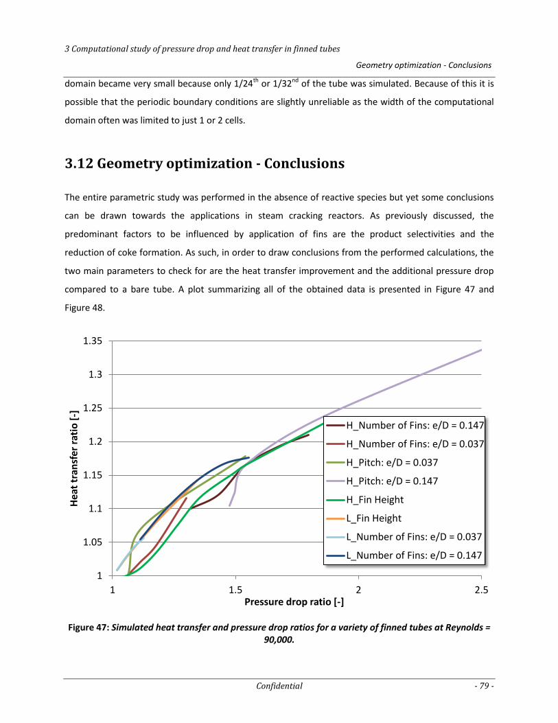
3 Computational study of pressure drop and heat transfer in finned tubes
Geometry optimization - Conclusions
Confidential - 79 -
domain became very small because only 1/24th or 1/32nd of the tube was simulated. Because of this it is
possible that the periodic boundary conditions are slightly unreliable as the width of the computational
domain often was limited to just 1 or 2 cells.
3.12 Geometry optimization - Conclusions
The entire parametric study was performed in the absence of reactive species but yet some conclusions
can be drawn towards the applications in steam cracking reactors. As previously discussed, the
predominant factors to be influenced by application of fins are the product selectivities and the
reduction of coke formation. As such, in order to draw conclusions from the performed calculations, the
two main parameters to check for are the heat transfer improvement and the additional pressure drop
compared to a bare tube. A plot summarizing all of the obtained data is presented in Figure 47 and
Figure 48.
Figure 47: Simulated heat transfer and pressure drop ratios for a variety of finned tubes at Reynolds = 90,000.
1
1.05
1.1
1.15
1.2
1.25
1.3
1.35
1 1.5 2 2.5
Hea
t tr
ansf
er r
atio
[-]
Pressure drop ratio [-]
H_Number of Fins: e/D = 0.147
H_Number of Fins: e/D = 0.037
H_Pitch: e/D = 0.037
H_Pitch: e/D = 0.147
H_Fin Height
L_Fin Height
L_Number of Fins: e/D = 0.037
L_Number of Fins: e/D = 0.147
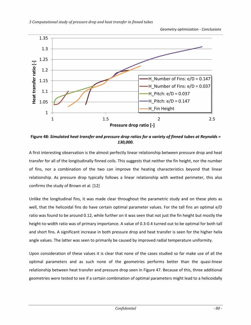
3 Computational study of pressure drop and heat transfer in finned tubes
Geometry optimization - Conclusions
Confidential - 80 -
Figure 48: Simulated heat transfer and pressure drop ratios for a variety of finned tubes at Reynolds = 130,000.
A first interesting observation is the almost perfectly linear relationship between pressure drop and heat
transfer for all of the longitudinally finned coils. This suggests that neither the fin height, nor the number
of fins, nor a combination of the two can improve the heating characteristics beyond that linear
relationship. As pressure drop typically follows a linear relationship with wetted perimeter, this also
confirms the study of Brown et al. [12]
Unlike the longitudinal fins, it was made clear throughout the parametric study and on these plots as
well, that the helicoidal fins do have certain optimal parameter values. For the tall fins an optimal e/D
ratio was found to be around 0.12, while further on it was seen that not just the fin height but mostly the
height-to-width ratio was of primary importance. A value of 0.3-0.4 turned out to be optimal for both tall
and short fins. A significant increase in both pressure drop and heat transfer is seen for the higher helix
angle values. The latter was seen to primarily be caused by improved radial temperature uniformity.
Upon consideration of these values it is clear that none of the cases studied so far make use of all the
optimal parameters and as such none of the geometries performs better than the quasi-linear
relationship between heat transfer and pressure drop seen in Figure 47. Because of this, three additional
geometries were tested to see if a certain combination of optimal parameters might lead to a helicoidally
1
1.05
1.1
1.15
1.2
1.25
1.3
1.35
1 1.5 2 2.5
Hea
t tr
ansf
er r
atio
[-]
Pressure drop ratio [-]
H_Number of Fins: e/D = 0.147
H_Number of Fins: e/D = 0.037
H_Pitch: e/D = 0.037
H_Pitch: e/D = 0.147
H_Fin Height
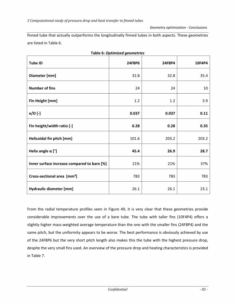
3 Computational study of pressure drop and heat transfer in finned tubes
Geometry optimization - Conclusions
Confidential - 81 -
finned tube that actually outperforms the longitudinally finned tubes in both aspects. These geometries
are listed in Table 6.
Table 6: Optimized geometries
Tube ID 24F8P6 24F8P4 10F4P4
Diameter [mm] 32.8 32.8 35.4
Number of fins 24 24 10
Fin Height [mm] 1.2 1.2 3.9
e/D [-] 0.037 0.037 0.11
Fin height/width ratio [-] 0.28 0.28 0.35
Helicoidal fin pitch [mm] 101.6 203.2 203.2
Helix angle α [°] 45.4 26.9 28.7
Inner surface increase compared to bare [%] 21% 21% 37%
Cross-sectional area [mm²] 783 783 783
Hydraulic diameter [mm] 26.1 26.1 23.1
From the radial temperature profiles seen in Figure 49, it is very clear that these geometries provide
considerable improvements over the use of a bare tube. The tube with taller fins (10F4P4) offers a
slightly higher mass-weighted average temperature than the one with the smaller fins (24F8P4) and the
same pitch, but the uniformity appears to be worse. The best performance is obviously achieved by use
of the 24F8P6 but the very short pitch length also makes this the tube with the highest pressure drop,
despite the very small fins used. An overview of the pressure drop and heating characteristics is provided
in Table 7.
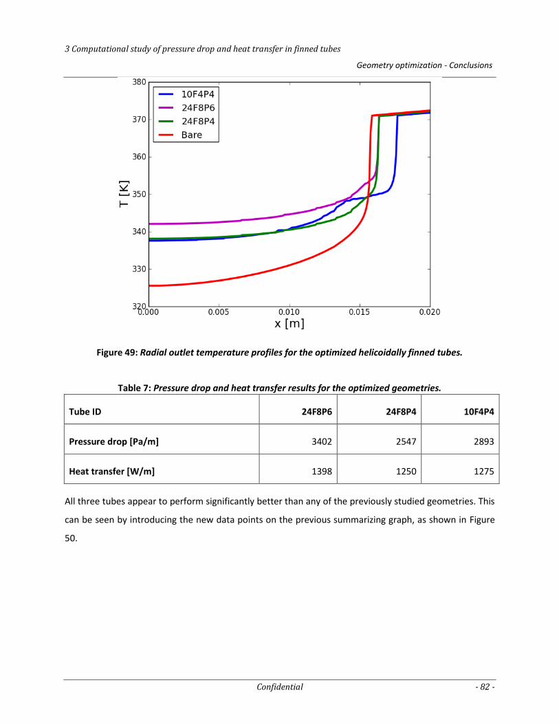
3 Computational study of pressure drop and heat transfer in finned tubes
Geometry optimization - Conclusions
Confidential - 82 -
Figure 49: Radial outlet temperature profiles for the optimized helicoidally finned tubes.
Table 7: Pressure drop and heat transfer results for the optimized geometries.
Tube ID 24F8P6 24F8P4 10F4P4
Pressure drop [Pa/m] 3402 2547 2893
Heat transfer [W/m] 1398 1250 1275
All three tubes appear to perform significantly better than any of the previously studied geometries. This
can be seen by introducing the new data points on the previous summarizing graph, as shown in Figure
50.
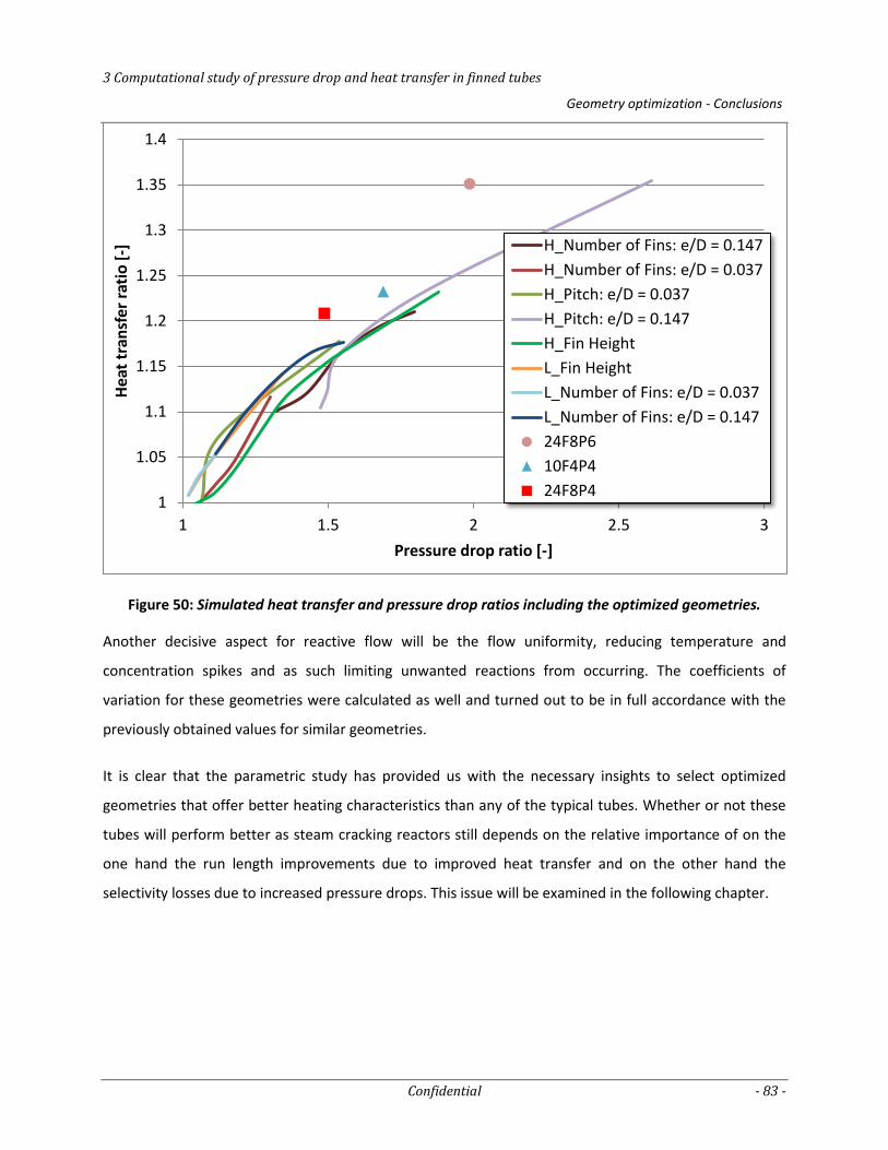
3 Computational study of pressure drop and heat transfer in finned tubes
Geometry optimization - Conclusions
Confidential - 83 -
Figure 50: Simulated heat transfer and pressure drop ratios including the optimized geometries.
Another decisive aspect for reactive flow will be the flow uniformity, reducing temperature and
concentration spikes and as such limiting unwanted reactions from occurring. The coefficients of
variation for these geometries were calculated as well and turned out to be in full accordance with the
previously obtained values for similar geometries.
It is clear that the parametric study has provided us with the necessary insights to select optimized
geometries that offer better heating characteristics than any of the typical tubes. Whether or not these
tubes will perform better as steam cracking reactors still depends on the relative importance of on the
one hand the run length improvements due to improved heat transfer and on the other hand the
selectivity losses due to increased pressure drops. This issue will be examined in the following chapter.
1
1.05
1.1
1.15
1.2
1.25
1.3
1.35
1.4
1 1.5 2 2.5 3
Hea
t tr
ansf
er r
atio
[-]
Pressure drop ratio [-]
H_Number of Fins: e/D = 0.147
H_Number of Fins: e/D = 0.037
H_Pitch: e/D = 0.037
H_Pitch: e/D = 0.147
H_Fin Height
L_Fin Height
L_Number of Fins: e/D = 0.037
L_Number of Fins: e/D = 0.147
24F8P6
10F4P4
24F8P4
3 Computational study of pressure drop and heat transfer in finned tubes
References
Confidential - 84 -
References
1. Bengt Andersson, Ronnie Andersson, Love Hakansson, Mikael Mortensen, Rahman Sudiyo,
Berend van Wachem, Computational Fluid Dynamics for Chemical Engineers. 7th ed2011,
Gothenburg, Sweden.
2. H. K. Versteeg, W. Malalasekera, An introduction to computational fluid dynamics - The
finite volume method1995: Longman.
3. Macrossan, Dr. Michael. Practical Turbulence Modelling in Fluent. 2008; Available from:
http://www.mech.uq.edu.au/courses/mech4480/turb2.pdf.
4. Leonard, B.P., Order of accuracy of QUICK and related convection-diffusion schemes. Appl.
Math. Modelling, 1995. 19(November): p. 14.
5. J. V. Albano, K. M. Sundaram, M. J. Maddock, Applications of extended surfaces in pyrolysis
coils. Energy Progress, 1988. 8(3): p. 9.
6. Saegher, Johan J. De, Modellering van stroming, warmtetransport en reactie in reactoren voor
de thermische kraking van koolwaterstoffen, in Laboratorium voor Petrochemische
Techniek1994, Universiteit Gent.
7. Corporation, Special Metals, Incoloy alloy 800, 2004.
8. Torigoe, T., Mixing Element Radiant Tube (MERT) Improves Cracking Furnace Performance,
K. Corporation, Editor 2001.
9. Györffy, Michael, MERT Technology Update: X-MERT, in AlCHE: Ethylene Producers
Meeting2009: Tampa Bay.
10. W. Tallis, C. Caro, C. Dang, A novel approach to ethylene furnace coil design, in 18th Annual
Ethylene Producers’ Conference2006: Orlando, FL.
11. A.N. Cookson, D.J. Doorly, S.J. Sherwin, Mixing Through Stirring of Steady Flow in Small
Amplitude Helical Pipes. 2008.
12. David J. Brown, Stone & Webster, Inc., Internally Finned Radiant Coils: a Valuable Tool for
Improving Ethylene Plant Economics, in 6th EMEA Petrochemicals Technology
Conference2004: London, UK.
13. Gregory J. Zdaniuk, Louay M. Chamra, Pedro J. Mago, Experimental determination of heat
transfer and friction in helically-finned tubes. Experimental Thermal and Fluid Science, 2008.
32: p. 15.
4 Simulation of reactive flow Introduction
Confidential - 85 -
4 Simulation of reactive flow
4.1 Introduction ................................................................................................................................. 85
4.2 Reactor specifications .................................................................................................................. 86
4.3 One-dimensional simulations using COILSIM1D .......................................................................... 89
4.4 Three-dimensional FLUENT simulations ...................................................................................... 99
References .............................................................................................................................................. 102
4.1 Introduction
In the previous chapter an extensive study was performed on the heating characteristics of finned tubes
for unreactive air flow. Although a number of optimal geometries were identified, it still remains to be
seen what the actual influence of these geometries will be on product selectivity and coking rate in
steam cracking reactors. The improved heat transfer will allow the reactor to run at a lower metal
temperature, which will lead to reduced coking and increased runlengths, having a direct economic
impact. The higher pressure drop however will lead to reduced selectivity to olefins. Finding a balance
between these two aspects is decisive.
The detailed steam cracking chemistry however is extensive and requires an enormous amount of
compounds to be considered. Although computing capacity has drastically increased over the past
decades, computational fluid dynamics software remains unable of simulating networks of this
complexity for practical engineering geometries. Because of these considerations, a double approach
was followed in order to provide both a qualitative and quantitative analysis.
4 Simulation of reactive flow Reactor specifications
Confidential - 86 -
The first method makes use of the COILSIM1D program, developed at the Laboratory for Chemical
Technology. Although this program makes use of a 1-dimensional reactor model, it is capable of
performing these simulations using a reaction network with over 700 compounds. Additionally, it
contains two coking models, allowing an indication of the coking performance of the tubes. Run length
simulations can be performed as well to simulate the influence of the tube performance on the decoking
frequency. To take into account the heating characteristics of the finned coils, the code was altered to
include friction factor and Nusselt number correlations constructed from the data gathered in the
previous chapter.
The second method consists of 3D simulations using Ansys FLUENT 13.0 which was used in the previous
chapter as well. Using a simplified molecular reaction network, full reactor simulations were performed.
As computation time for these simulations ran well over 400 hours on 12 cores in order to achieve
convergence, only a limited amount of geometries were considered.
These two methods were applied to an industrial propane cracker which makes use of a so-called
Millisecond reactor.
4.2 Reactor specifications
4.2.1 The Kellog Millisecond reactor
As a reactor type the Kellogg Millisecond reactor was chosen. This design was based on the series of
experiments conducted by M.W. Kellog’s R&D Center, to determine the effects of temperature,
residence time and hydrocarbon partial pressures on the olefin yields of various feedstocks [1]. At a
given cracking temperature and hydrocarbon pressure, it was seen that the optimal residence time was
in the range of 0.05 – 0.1 seconds, which is the range in which commercial Millisecond furnaces operate.
To accommodate this requirement, the furnace differs from conventional cracking furnaces in a number
of ways. The cracking coils are made of a large number (typically 100-200) of small diameter single-pass
tubes, in contrast to conventional coils that employ slightly larger tubes and employ return bends for
multiple passes. A conceptual sketch of the Millisecond furnace design is shown in Figure 1.
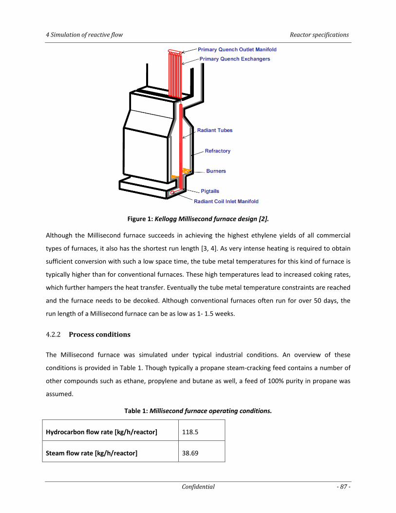
4 Simulation of reactive flow Reactor specifications
Confidential - 87 -
Figure 1: Kellogg Millisecond furnace design [2].
Although the Millisecond furnace succeeds in achieving the highest ethylene yields of all commercial
types of furnaces, it also has the shortest run length [3, 4]. As very intense heating is required to obtain
sufficient conversion with such a low space time, the tube metal temperatures for this kind of furnace is
typically higher than for conventional furnaces. These high temperatures lead to increased coking rates,
which further hampers the heat transfer. Eventually the tube metal temperature constraints are reached
and the furnace needs to be decoked. Although conventional furnaces often run for over 50 days, the
run length of a Millisecond furnace can be as low as 1- 1.5 weeks.
4.2.2 Process conditions
The Millisecond furnace was simulated under typical industrial conditions. An overview of these
conditions is provided in Table 1. Though typically a propane steam-cracking feed contains a number of
other compounds such as ethane, propylene and butane as well, a feed of 100% purity in propane was
assumed.
Table 1: Millisecond furnace operating conditions.
Hydrocarbon flow rate [kg/h/reactor] 118.5
Steam flow rate [kg/h/reactor] 38.69
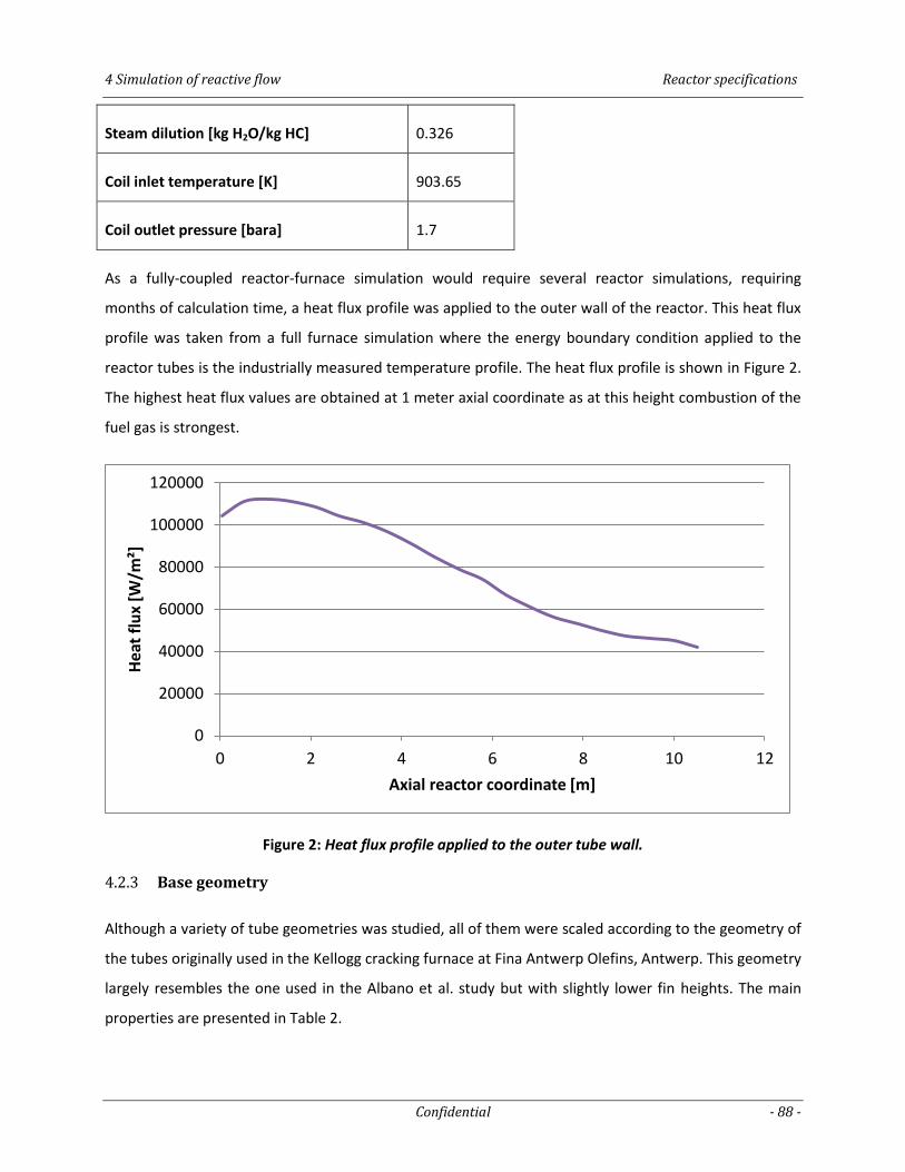
4 Simulation of reactive flow Reactor specifications
Confidential - 88 -
Steam dilution [kg H2O/kg HC] 0.326
Coil inlet temperature [K] 903.65
Coil outlet pressure [bara] 1.7
As a fully-coupled reactor-furnace simulation would require several reactor simulations, requiring
months of calculation time, a heat flux profile was applied to the outer wall of the reactor. This heat flux
profile was taken from a full furnace simulation where the energy boundary condition applied to the
reactor tubes is the industrially measured temperature profile. The heat flux profile is shown in Figure 2.
The highest heat flux values are obtained at 1 meter axial coordinate as at this height combustion of the
fuel gas is strongest.
Figure 2: Heat flux profile applied to the outer tube wall.
4.2.3 Base geometry
Although a variety of tube geometries was studied, all of them were scaled according to the geometry of
the tubes originally used in the Kellogg cracking furnace at Fina Antwerp Olefins, Antwerp. This geometry
largely resembles the one used in the Albano et al. study but with slightly lower fin heights. The main
properties are presented in Table 2.
0
20000
40000
60000
80000
100000
120000
0 2 4 6 8 10 12
Hea
t fl
ux
[W/m
²]
Axial reactor coordinate [m]
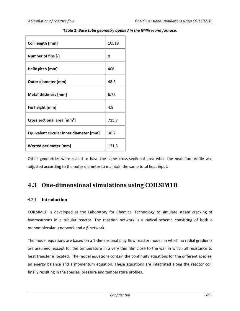
4 Simulation of reactive flow One-dimensional simulations using COILSIM1D
Confidential - 89 -
Table 2: Base tube geometry applied in the Millisecond furnace.
Coil length [mm] 10518
Number of fins [-] 8
Helix pitch [mm] 406
Outer diameter [mm] 48.3
Metal thickness [mm] 6.75
Fin height [mm] 4.8
Cross sectional area [mm²] 715.7
Equivalent circular inner diameter [mm] 30.2
Wetted perimeter [mm] 131.5
Other geometries were scaled to have the same cross-sectional area while the heat flux profile was
adjusted according to the outer diameter to maintain the same total heat input.
4.3 One-dimensional simulations using COILSIM1D
4.3.1 Introduction
COILSIM1D is developed at the Laboratory for Chemical Technology to simulate steam cracking of
hydrocarbons in a tubular reactor. The reaction network is a radical scheme consisting of both a
monomolecular µ network and a β network.
The model equations are based on a 1-dimensional plug flow reactor model, in which no radial gradients
are assumed, except for the temperature in a very thin film close to the wall in which all resistance to
heat transfer is located. The model equations contain the continuity equations for the different species,
an energy balance and a momentum equation. These equations are integrated along the reactor coil,
finally resulting in the species, pressure and temperature profiles.
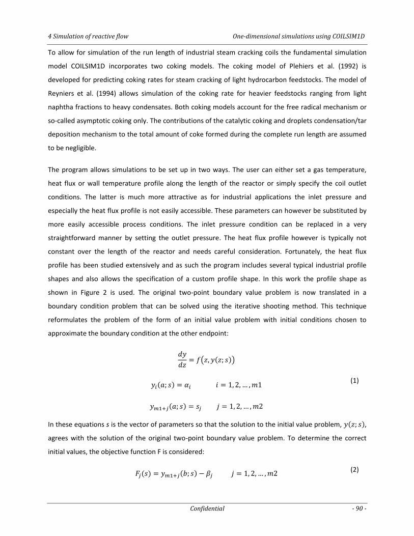
4 Simulation of reactive flow One-dimensional simulations using COILSIM1D
Confidential - 90 -
To allow for simulation of the run length of industrial steam cracking coils the fundamental simulation
model COILSIM1D incorporates two coking models. The coking model of Plehiers et al. (1992) is
developed for predicting coking rates for steam cracking of light hydrocarbon feedstocks. The model of
Reyniers et al. (1994) allows simulation of the coking rate for heavier feedstocks ranging from light
naphtha fractions to heavy condensates. Both coking models account for the free radical mechanism or
so-called asymptotic coking only. The contributions of the catalytic coking and droplets condensation/tar
deposition mechanism to the total amount of coke formed during the complete run length are assumed
to be negligible.
The program allows simulations to be set up in two ways. The user can either set a gas temperature,
heat flux or wall temperature profile along the length of the reactor or simply specify the coil outlet
conditions. The latter is much more attractive as for industrial applications the inlet pressure and
especially the heat flux profile is not easily accessible. These parameters can however be substituted by
more easily accessible process conditions. The inlet pressure condition can be replaced in a very
straightforward manner by setting the outlet pressure. The heat flux profile however is typically not
constant over the length of the reactor and needs careful consideration. Fortunately, the heat flux
profile has been studied extensively and as such the program includes several typical industrial profile
shapes and also allows the specification of a custom profile shape. In this work the profile shape as
shown in Figure 2 is used. The original two-point boundary value problem is now translated in a
boundary condition problem that can be solved using the iterative shooting method. This technique
reformulates the problem of the form of an initial value problem with initial conditions chosen to
approximate the boundary condition at the other endpoint:
( ( ))
( ) (1)
( )
In these equations s is the vector of parameters so that the solution to the initial value problem, ( ),
agrees with the solution of the original two-point boundary value problem. To determine the correct
initial values, the objective function F is considered:
( ) ( ) (2)
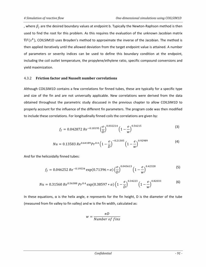
4 Simulation of reactive flow One-dimensional simulations using COILSIM1D
Confidential - 91 -
, where are the desired boundary values at endpoint b. Typically the Newton-Raphson method is then
used to find the root for this problem. As this requires the evaluation of the unknown Jacobian matrix
( ), COILSIM1D uses Broyden’s method to approximate the inverse of the Jacobian. The method is
then applied iteratively until the allowed deviation from the target endpoint value is attained. A number
of parameters or severity indices can be used to define this boundary condition at the endpoint,
including the coil outlet temperature, the propylene/ethylene ratio, specific compound conversions and
yield maximization.
4.3.2 Friction factor and Nusselt number correlations
Although COILSIM1D contains a few correlations for finned tubes, these are typically for a specific type
and size of the fin and are not universally applicable. New correlations were derived from the data
obtained throughout the parametric study discussed in the previous chapter to allow COILSIM1D to
properly account for the influence of the different fin parameters. The program code was then modified
to include these correlations. For longitudinally finned coils the correlations are given by:
(
)
(
)
(3)
(
)
(
)
(4)
And for the helicoidally finned tubes:
( ) (
)
(
)
(5)
( ) (
)
(
)
(6)
In these equations, α is the helix angle, e represents for the fin height, D is the diameter of the tube
(measured from fin valley to fin valley) and w is the fin width, calculated as:
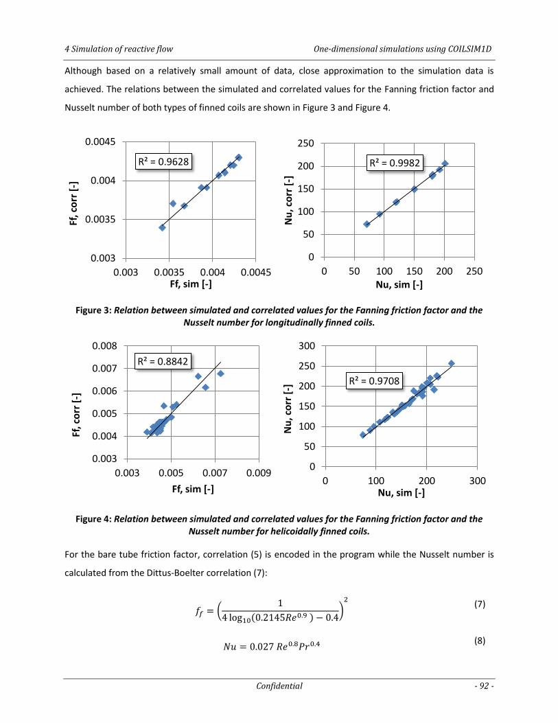
4 Simulation of reactive flow One-dimensional simulations using COILSIM1D
Confidential - 92 -
Although based on a relatively small amount of data, close approximation to the simulation data is
achieved. The relations between the simulated and correlated values for the Fanning friction factor and
Nusselt number of both types of finned coils are shown in Figure 3 and Figure 4.
Figure 3: Relation between simulated and correlated values for the Fanning friction factor and the Nusselt number for longitudinally finned coils.
Figure 4: Relation between simulated and correlated values for the Fanning friction factor and the Nusselt number for helicoidally finned coils.
For the bare tube friction factor, correlation (5) is encoded in the program while the Nusselt number is
calculated from the Dittus-Boelter correlation (7):
(
( )
)
(7)
(8)
R² = 0.9628
0.003
0.0035
0.004
0.0045
0.003 0.0035 0.004 0.0045
Ff, c
orr
[-]
Ff, sim [-]
R² = 0.9982
0
50
100
150
200
250
0 50 100 150 200 250
Nu
, co
rr [
-]
Nu, sim [-]
R² = 0.8842
0.003
0.004
0.005
0.006
0.007
0.008
0.003 0.005 0.007 0.009
Ff, c
orr
[-]
Ff, sim [-]
R² = 0.9708
0
50
100
150
200
250
300
0 100 200 300
Nu
, co
rr [
-]
Nu, sim [-]
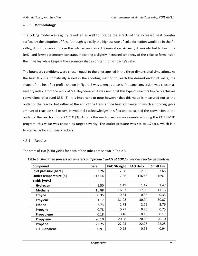
4 Simulation of reactive flow One-dimensional simulations using COILSIM1D
Confidential - 93 -
4.3.3 Methodology
The coking model was slightly rewritten as well to include the effects of the increased heat transfer
surface by the adoption of fins. Although typically the highest rate of coke formation would be in the fin
valley, it is impossible to take this into account in a 1D simulation. As such, it was elected to keep the
(e/D) and (e/w) parameters constant, indicating a slightly increased tendency of the coke to form inside
the fin valley while keeping the geometry shape constant for simplicity’s sake.
The boundary conditions were chosen equal to the ones applied in the three-dimensional simulations. As
the heat flux is automatically scaled in the shooting method to reach the desired endpoint value, the
shape of the heat flux profile shown in Figure 2 was taken as a basis. Propane conversion was chosen as
severity index. From the work of G.J. Heynderickx, it was seen that this type of reactors typically achieves
conversions of around 83% [3]. It is important to note however that this value is measured not at the
outlet of the reactor but rather at the end of the transfer line heat exchanger in which a non-negligible
amount of reaction still occurs. Heynderickx acknowledges this fact and calculated the conversion at the
outlet of the reactor to be 77.75% [3]. As only the reactor section was simulated using the COILSIM1D
program, this value was chosen as target severity. The outlet pressure was set to 1.7bara, which is a
typical value for industrial crackers.
4.3.4 Results
The start-of-run (SOR) yields for each of the tubes are shown in Table 3.
Table 3: Simulated process parameters and product yields at SOR for various reactor geometries.
Compound Bare FAO Straight FAO Helix Small Fins
Inlet pressure [bara] 2.26 2.38 2.56 2.65
Outlet temperature [K] 1171.4 1170.6 1169.6 1169.1
Yields [wt%] Hydrogen 1.50 1.49 1.47 1.47
Methane 16.88 16.97 17.08 17.13
Ethyne 0.35 0.34 0.33 0.33
Ethylene 31.17 31.08 30.94 30.87
Ethane 2.73 2.73 2.75 2.76
Propyne 0.78 0.77 0.75 0.75
Propadiene 0.18 0.18 0.18 0.17
Propylene 20.10 20.08 20.09 20.10
Propane 22.25 22.25 22.25 22.25
1,3-Butadiene 0.91 0.92 0.93 0.94
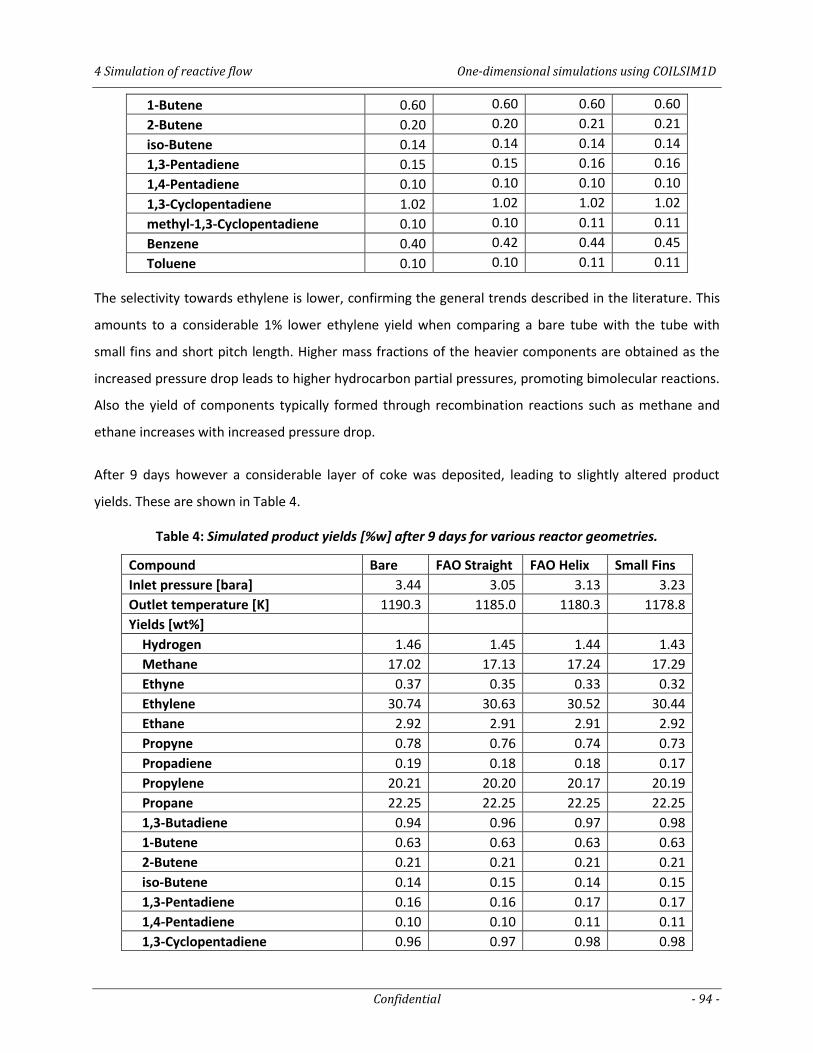
4 Simulation of reactive flow One-dimensional simulations using COILSIM1D
Confidential - 94 -
1-Butene 0.60 0.60 0.60 0.60
2-Butene 0.20 0.20 0.21 0.21
iso-Butene 0.14 0.14 0.14 0.14
1,3-Pentadiene 0.15 0.15 0.16 0.16
1,4-Pentadiene 0.10 0.10 0.10 0.10
1,3-Cyclopentadiene 1.02 1.02 1.02 1.02
methyl-1,3-Cyclopentadiene 0.10 0.10 0.11 0.11
Benzene 0.40 0.42 0.44 0.45
Toluene 0.10 0.10 0.11 0.11
The selectivity towards ethylene is lower, confirming the general trends described in the literature. This
amounts to a considerable 1% lower ethylene yield when comparing a bare tube with the tube with
small fins and short pitch length. Higher mass fractions of the heavier components are obtained as the
increased pressure drop leads to higher hydrocarbon partial pressures, promoting bimolecular reactions.
Also the yield of components typically formed through recombination reactions such as methane and
ethane increases with increased pressure drop.
After 9 days however a considerable layer of coke was deposited, leading to slightly altered product
yields. These are shown in Table 4.
Table 4: Simulated product yields [%w] after 9 days for various reactor geometries.
Compound Bare FAO Straight FAO Helix Small Fins
Inlet pressure [bara] 3.44 3.05 3.13 3.23
Outlet temperature [K] 1190.3 1185.0 1180.3 1178.8
Yields [wt%]
Hydrogen 1.46 1.45 1.44 1.43
Methane 17.02 17.13 17.24 17.29
Ethyne 0.37 0.35 0.33 0.32
Ethylene 30.74 30.63 30.52 30.44
Ethane 2.92 2.91 2.91 2.92
Propyne 0.78 0.76 0.74 0.73
Propadiene 0.19 0.18 0.18 0.17
Propylene 20.21 20.20 20.17 20.19
Propane 22.25 22.25 22.25 22.25
1,3-Butadiene 0.94 0.96 0.97 0.98
1-Butene 0.63 0.63 0.63 0.63
2-Butene 0.21 0.21 0.21 0.21
iso-Butene 0.14 0.15 0.14 0.15
1,3-Pentadiene 0.16 0.16 0.17 0.17
1,4-Pentadiene 0.10 0.10 0.11 0.11
1,3-Cyclopentadiene 0.96 0.97 0.98 0.98
4 Simulation of reactive flow One-dimensional simulations using COILSIM1D
Confidential - 95 -
methyl-1,3-Cyclopentadiene 0.10 0.10 0.11 0.11
Benzene 0.38 0.41 0.44 0.45
Toluene 0.09 0.09 0.10 0.10
It is clear that the coke layer leads to reduced ethylene selectivity. While this is the case for all the coils,
this drop appears to be more severe for the bare and longitudinally finned tubes. The evolution of the
ethylene selectivity is shown in Figure 5.
Figure 5: Evolution of ethylene yield in function of the run time.
The reason for this drop in ethylene selectivity is made clear by plotting the coil inlet pressure (CIP) as a
function of run time, as presented in Figure 6.
30.3
30.4
30.5
30.6
30.7
30.8
30.9
31
31.1
31.2
0 2 4 6 8 10 12
Eth
ylen
e y
ield
[%
w]
Run time [days]
FAO Helix
FAO Straight
Small Fins
Bare
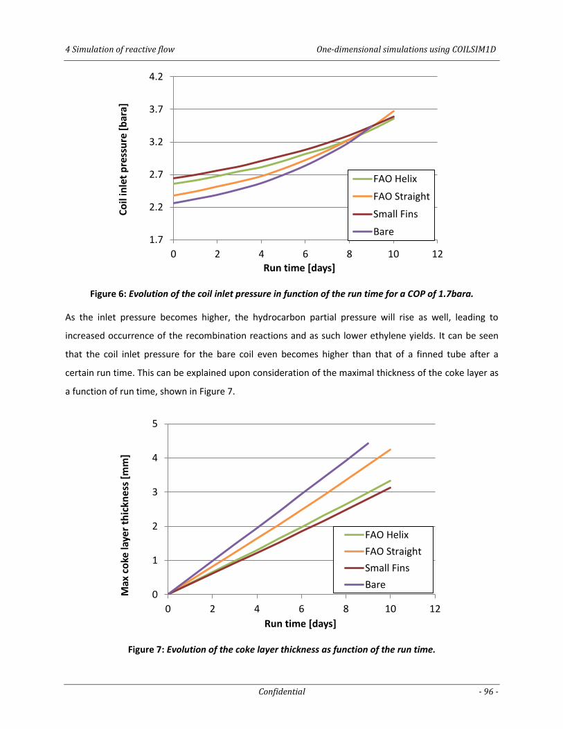
4 Simulation of reactive flow One-dimensional simulations using COILSIM1D
Confidential - 96 -
Figure 6: Evolution of the coil inlet pressure in function of the run time for a COP of 1.7bara.
As the inlet pressure becomes higher, the hydrocarbon partial pressure will rise as well, leading to
increased occurrence of the recombination reactions and as such lower ethylene yields. It can be seen
that the coil inlet pressure for the bare coil even becomes higher than that of a finned tube after a
certain run time. This can be explained upon consideration of the maximal thickness of the coke layer as
a function of run time, shown in Figure 7.
Figure 7: Evolution of the coke layer thickness as function of the run time.
1.7
2.2
2.7
3.2
3.7
4.2
0 2 4 6 8 10 12
Co
il in
let
pre
ssu
re [
bar
a]
Run time [days]
FAO Helix
FAO Straight
Small Fins
Bare
0
1
2
3
4
5
0 2 4 6 8 10 12
Max
co
ke la
yer
thic
kne
ss [
mm
]
Run time [days]
FAO Helix
FAO Straight
Small Fins
Bare
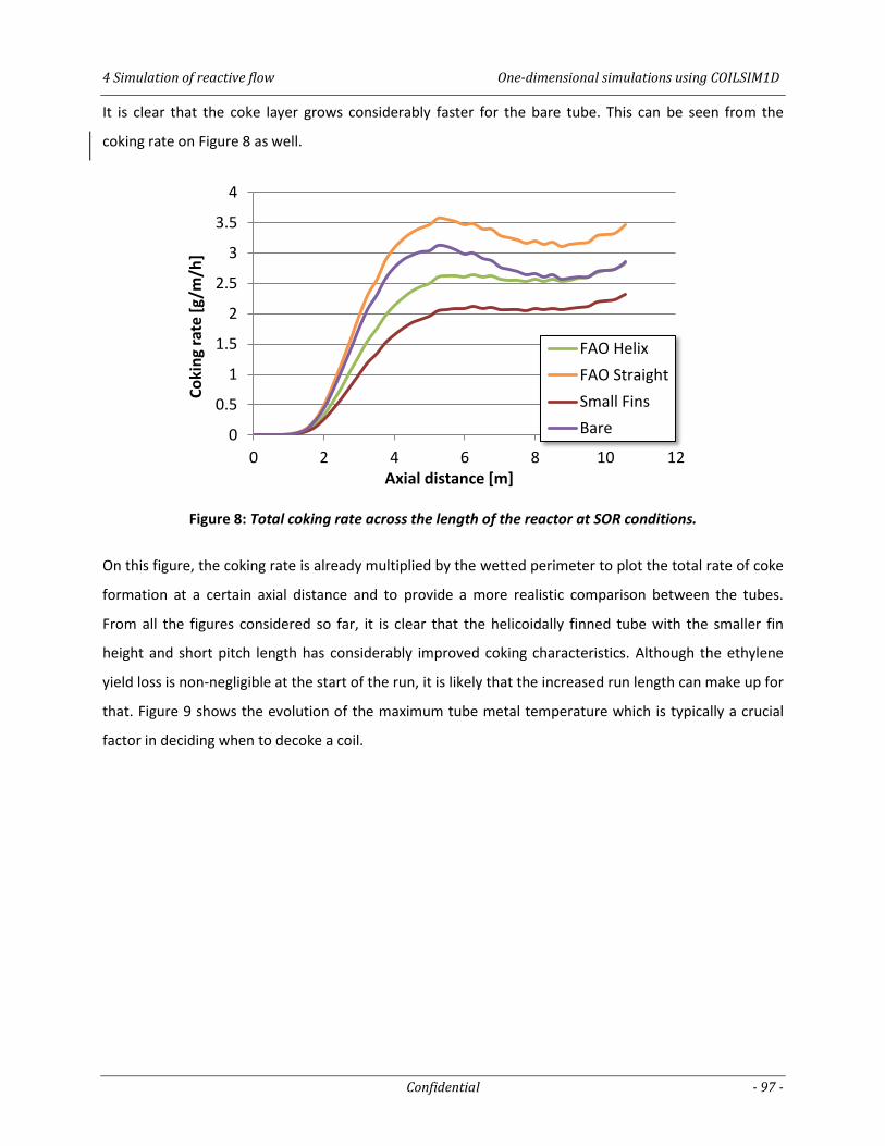
4 Simulation of reactive flow One-dimensional simulations using COILSIM1D
Confidential - 97 -
It is clear that the coke layer grows considerably faster for the bare tube. This can be seen from the
coking rate on Figure 8 as well.
Figure 8: Total coking rate across the length of the reactor at SOR conditions.
On this figure, the coking rate is already multiplied by the wetted perimeter to plot the total rate of coke
formation at a certain axial distance and to provide a more realistic comparison between the tubes.
From all the figures considered so far, it is clear that the helicoidally finned tube with the smaller fin
height and short pitch length has considerably improved coking characteristics. Although the ethylene
yield loss is non-negligible at the start of the run, it is likely that the increased run length can make up for
that. Figure 9 shows the evolution of the maximum tube metal temperature which is typically a crucial
factor in deciding when to decoke a coil.
0
0.5
1
1.5
2
2.5
3
3.5
4
0 2 4 6 8 10 12
Co
kin
g ra
te [
g/m
/h]
Axial distance [m]
FAO Helix
FAO Straight
Small Fins
Bare
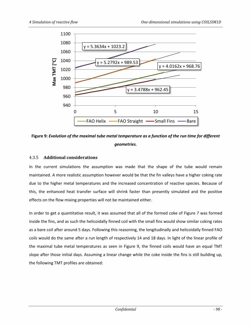
4 Simulation of reactive flow One-dimensional simulations using COILSIM1D
Confidential - 98 -
Figure 9: Evolution of the maximal tube metal temperature as a function of the run time for different
geometries.
4.3.5 Additional considerations
In the current simulations the assumption was made that the shape of the tube would remain
maintained. A more realistic assumption however would be that the fin valleys have a higher coking rate
due to the higher metal temperatures and the increased concentration of reactive species. Because of
this, the enhanced heat transfer surface will shrink faster than presently simulated and the positive
effects on the flow mixing properties will not be maintained either.
In order to get a quantitative result, it was assumed that all of the formed coke of Figure 7 was formed
inside the fins, and as such the helicoidally finned coil with the small fins would show similar coking rates
as a bare coil after around 5 days. Following this reasoning, the longitudinally and helicoidally finned FAO
coils would do the same after a run length of respectively 14 and 18 days. In light of the linear profile of
the maximal tube metal temperatures as seen in Figure 9, the finned coils would have an equal TMT
slope after those initial days. Assuming a linear change while the coke inside the fins is still building up,
the following TMT profiles are obtained:
y = 4.0162x + 968.76 y = 5.2792x + 989.53
y = 3.4788x + 962.45
y = 5.3634x + 1023.2
940
960
980
1000
1020
1040
1060
1080
1100
0 5 10 15
Max
TM
T [°
C]
Run time [days] FAO Helix FAO Straight Small Fins Bare
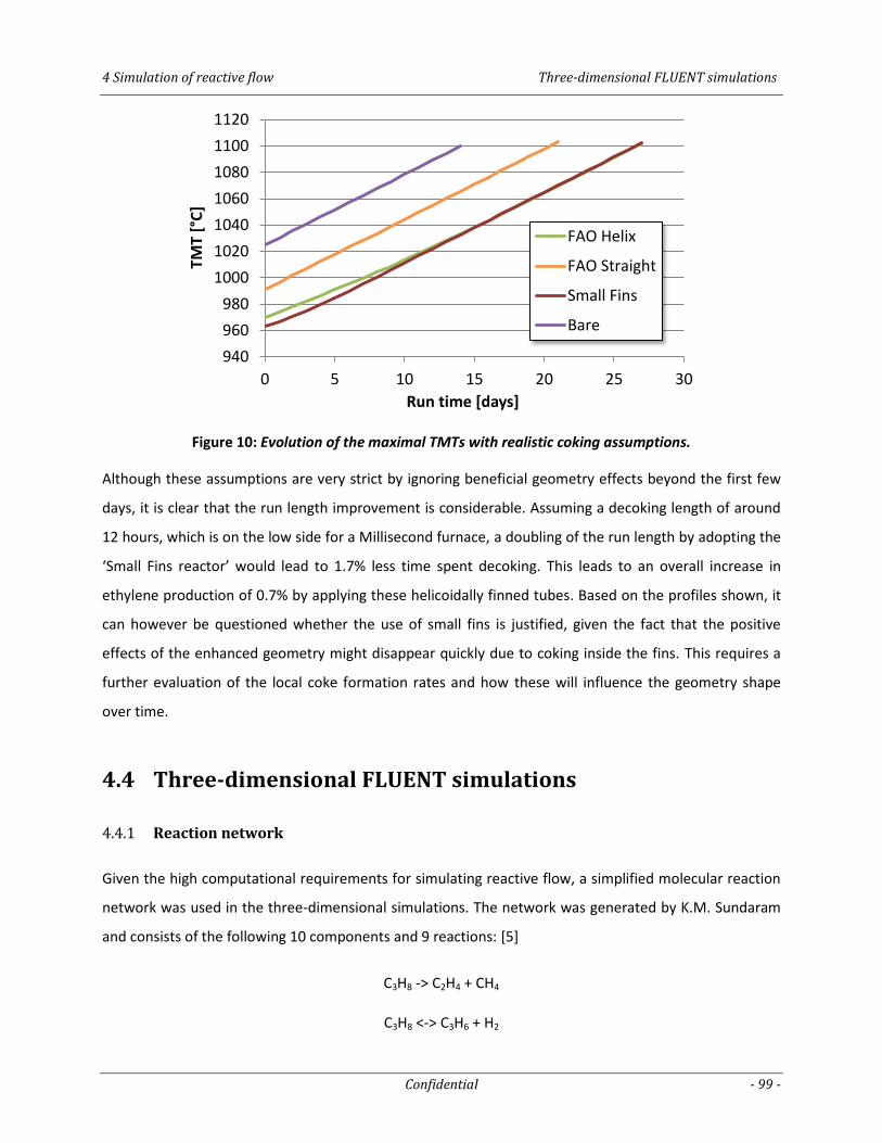
4 Simulation of reactive flow Three-dimensional FLUENT simulations
Confidential - 99 -
Figure 10: Evolution of the maximal TMTs with realistic coking assumptions.
Although these assumptions are very strict by ignoring beneficial geometry effects beyond the first few
days, it is clear that the run length improvement is considerable. Assuming a decoking length of around
12 hours, which is on the low side for a Millisecond furnace, a doubling of the run length by adopting the
‘Small Fins reactor’ would lead to 1.7% less time spent decoking. This leads to an overall increase in
ethylene production of 0.7% by applying these helicoidally finned tubes. Based on the profiles shown, it
can however be questioned whether the use of small fins is justified, given the fact that the positive
effects of the enhanced geometry might disappear quickly due to coking inside the fins. This requires a
further evaluation of the local coke formation rates and how these will influence the geometry shape
over time.
4.4 Three-dimensional FLUENT simulations
4.4.1 Reaction network
Given the high computational requirements for simulating reactive flow, a simplified molecular reaction
network was used in the three-dimensional simulations. The network was generated by K.M. Sundaram
and consists of the following 10 components and 9 reactions: [5]
C3H8 -> C2H4 + CH4
C3H8 <-> C3H6 + H2
940
960
980
1000
1020
1040
1060
1080
1100
1120
0 5 10 15 20 25 30
TMT
[°C
]
Run time [days]
FAO Helix
FAO Straight
Small Fins
Bare
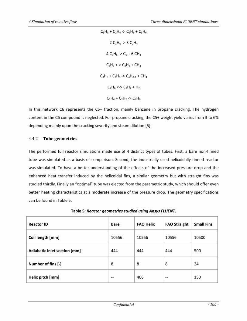
4 Simulation of reactive flow Three-dimensional FLUENT simulations
Confidential - 100 -
C3H8 + C2H4 -> C2H6 + C3H6
2 C3H6 -> 3 C2H4
4 C3H6 -> C6 + 6 CH4
C3H6 <-> C2H2 + CH4
C3H6 + C2H6 -> C4H8-1 + CH4
C2H6 <-> C2H4 + H2
C2H4 + C2H2 -> C4H6
In this network C6 represents the C5+ fraction, mainly benzene in propane cracking. The hydrogen
content in the C6 compound is neglected. For propane cracking, the C5+ weight yield varies from 3 to 6%
depending mainly upon the cracking severity and steam dilution [5].
4.4.2 Tube geometries
The performed full reactor simulations made use of 4 distinct types of tubes. First, a bare non-finned
tube was simulated as a basis of comparison. Second, the industrially used helicoidally finned reactor
was simulated. To have a better understanding of the effects of the increased pressure drop and the
enhanced heat transfer induced by the helicoidal fins, a similar geometry but with straight fins was
studied thirdly. Finally an “optimal” tube was elected from the parametric study, which should offer even
better heating characteristics at a moderate increase of the pressure drop. The geometry specifications
can be found in Table 5.
Table 5: Reactor geometries studied using Ansys FLUENT.
Reactor ID Bare FAO Helix FAO Straight Small Fins
Coil length [mm] 10556 10556 10556 10500
Adiabatic inlet section [mm] 444 444 444 500
Number of fins [-] 8 8 8 24
Helix pitch [mm] -- 406 -- 150
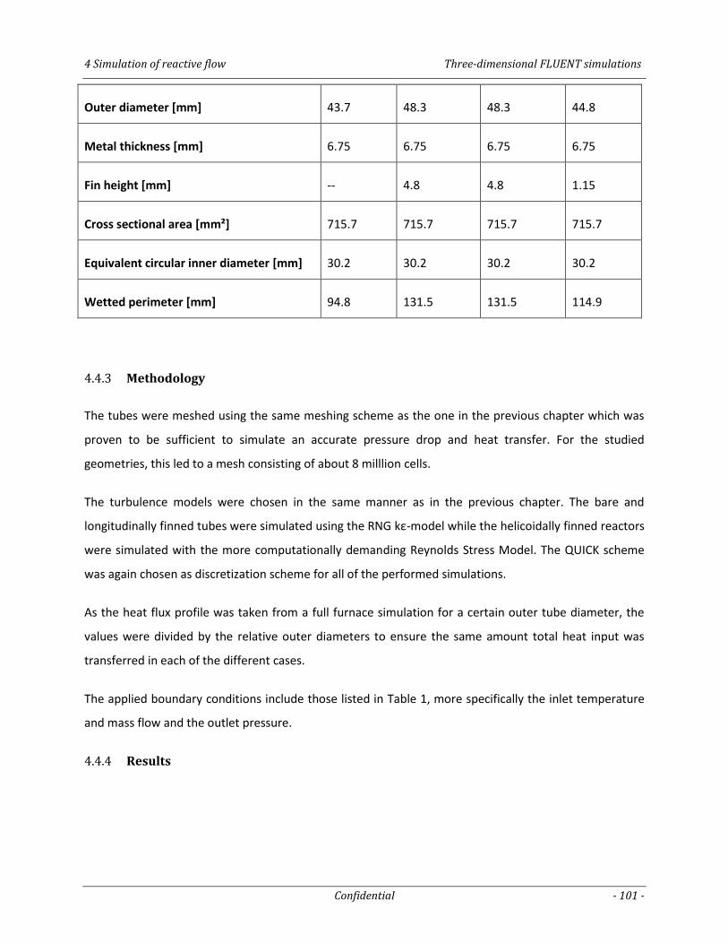
4 Simulation of reactive flow Three-dimensional FLUENT simulations
Confidential - 101 -
Outer diameter [mm] 43.7 48.3 48.3 44.8
Metal thickness [mm] 6.75 6.75 6.75 6.75
Fin height [mm] -- 4.8 4.8 1.15
Cross sectional area [mm²] 715.7 715.7 715.7 715.7
Equivalent circular inner diameter [mm] 30.2 30.2 30.2 30.2
Wetted perimeter [mm] 94.8 131.5 131.5 114.9
4.4.3 Methodology
The tubes were meshed using the same meshing scheme as the one in the previous chapter which was
proven to be sufficient to simulate an accurate pressure drop and heat transfer. For the studied
geometries, this led to a mesh consisting of about 8 milllion cells.
The turbulence models were chosen in the same manner as in the previous chapter. The bare and
longitudinally finned tubes were simulated using the RNG kε-model while the helicoidally finned reactors
were simulated with the more computationally demanding Reynolds Stress Model. The QUICK scheme
was again chosen as discretization scheme for all of the performed simulations.
As the heat flux profile was taken from a full furnace simulation for a certain outer tube diameter, the
values were divided by the relative outer diameters to ensure the same amount total heat input was
transferred in each of the different cases.
The applied boundary conditions include those listed in Table 1, more specifically the inlet temperature
and mass flow and the outlet pressure.
4.4.4 Results

4 Simulation of reactive flow References
Confidential - 102 -
References
1. Aly, Sherif, Ethylene from naphtha by Millisecond SM cracking with front-end demethanization -
Aspen Model Documentation. 2000.
2. Scott, Tom, SCORE Features for Millisecond Furnaces: The Borealis Furnace Revamp Project,
in Furnace Technology Conference, KBR, Editor 2009: Dubai, U.A.E.
3. Heynderickx, Geraldine J., Modellering en Simulatie van Huidige en Nieuwe Technologieën voor
de Thermische Kraking van Koolwaterstoffen, in Laboratorium voor Petrochemische
Techniek1993, Universiteit Gent: Faculteit van de Toegepaste Wetenschappen.
4. Ramin Karimzadeh, Amin Hematian, Mohammad Reza Omidkhah, The Effect of Coil
Configuration on Run Length of Thermal Cracking Reactors. International Journal of Chemical
Reactor Engineering, 2007. 5(A118): p. 17.
5. Sundaram, K.M., Kinetic Modeling of Thermal Cracking as a basis for Reactor Simulation, in
Laboratorium voor Petrochemische Techniek1977, Universiteit Gent.
5 Conclusions and future work Conclusions
Confidential - 103 -
5 Conclusions and future work
5.1 Conclusions ................................................................................................................................ 103
5.2 Future work ................................................................................................................................ 105
5.1 Conclusions
In this study, the effects of both longitudinally and helicoidally finned tubes for steam cracking
applications was investigated.
In chapter two, a literature review was performed on a number of recent advances in three-dimensional
structures for enhanced mixing, as well as existent and commercially applied technologies.
Chapter 3 describes the non-reactive simulations performed in this work. First a grid independency study
was performed. It was seen that an axial and radial cell length of 2mm and 0.6mm respectively gave grid
independent results. A typical simulation setup contained about 800.000 cells per meter reactor.
Doubling the number of cells only resulted in a 1.5% accuracy improvement. The model was validated
against a limited amount of experimental data points retrieved from Albano et al. [1] General agreement
was seen to be satisfactory, with relative errors below 5% for the friction factors, while the Nusselt
number was simulated with respectively 23% and 3% relative error for the longitudinally and helicoidally
finned tubes. After model validation, a parametric study was elaborated where the effect of the
geometry parameters on pressure drop and heat transfer was analyzed. From this study it was made
clear that all of the longitudinally finned tubes follow a linear relationship between heat transfer
increase and heat transfer area. Neither fin height, nor amount of fins influenced this relationship as the
5 Conclusions and future work Conclusions
Confidential - 104 -
linear relationship is maintained up until a wetted perimeter ratio of 1.5-1.6, after which further surface
increase shows reduced benefits.
The helicoidal fins on the other hand were found to have optimal parameters, of which the fin height-to-
width ratio appears to be of primary importance. From the parametric study, it was shown that the
optimal value for this relationship lies around 0.35. Upon assessing the mixing properties of variable fin
heights for this value it was seen that a larger number of small fins induce even stronger swirl flow and
improved mixing inside the tube than the 8-10 tall fins typically used. At higher Reynolds numbers
however, this effect considerably weakens and flow coring can occur, as the fluid no longer follows the
small fins but bypasses them.
Shortening the pitch length and thus increasing the helix angle leads to a significant increase in wall
shear and as a result much higher heat transfer and pressure drop. Small fins provide great benefits at
these short pitch lengths while still only causing a moderate increase in pressure drop. Although the
additional pressure drop is significant, it appears that the optimal helix angle for the tall-finned tubes is
around 30° instead of the 16° angle of the geometry adopted by Albano et al.
From the findings of the parametrical study three new optimized geometries were assembled that each
showed significantly improved heating characteristics from the previously seen linear relationship for
longitudinally finned tubes. At moderate Reynolds numbers (i.e. below 90,000) a tube with short pitch
length and a large number of small fins (fin height-to-diameter ratio around 0.04) offered a 35%
increased heat transfer over a bare tube at the cost of a slightly less than doubled pressure drop. At
higher Reynolds numbers a tube with relatively tall fins (fin height-to-diameter ratio of 0.11)
outperformed the bare tube by 24% whilst increasing the pressure drop by a factor of 1.55. Comparing
these values with the industrially applied MERT and X-MERT technology which both provide a 40%
improvement of heat transfer while multiplying the pressure drop by respectively 3 and 2.1 [2, 3], it can
be concluded that the presently studied geometries show similar performance.
In chapter 4, correlations were derived from the data of the parametric study. These correlations were
added to the in-house developed COILSIM1D software which simulated an 11% decreased coking rate for
the tube with tall helicoidal fins and a decrease of over 28% for the tube with small fins and a short helix
pitch length. These 1D simulations obviously neglect the increased mixing and assume a radially uniform
coke deposition. Three-dimensional simulations however predict higher temperatures and hence higher
coke deposition in the fin valleys. Nevertheless, a considerably increased run length can be expected.
5 Conclusions and future work Future work
Confidential - 105 -
The cost of the additional pressure drop was calculated to be a maximal loss in ethylene selectivity of 1%
at start of run conditions. Assuming the fins retain their original shape however, the CIP of the bare tube
rises faster than that of the finned coils. Averaged over the entire run length, this may eventually even
lead to a selectivity gain for these reactors.
As the three-dimensional simulations using Fluent applied a heat flux profile to the outer wall, the main
difference between these simulations lies in the increased gas temperature and hence improved
conversion for the finned reactors. The achieved conversion increase compared to bare was between
XXX% and XXX%, with the higher value corresponding to the optimized helicoidally finned tube. Although
the reaction network was greatly simplified, the yields were close to the values obtained through 1D plug
flow simulations. An ethylene selectivity loss of XXX% was measured for the optimized reactor. Although
non-negligible, it can be assumed that the increased run length will make up for this.
5.2 Future work
Although the heat transfer improvements have been confirmed in the present work, it remains uncertain
how fin valleys will fill up with coke and how well the heat transfer and the improved flow pattern will be
preserved as a consequence of this. The use of dynamic meshing to model the influence of coke
formation on the fin structure would provide significantly more insights into the flow pattern changes
over time and is an area that requires further examination.
A significant problem in the evaluation of the present work was also the lack of experimental data for
this type of structures. If the change in product yields and TMT evolution over time were known from
e.g. pilot plant experiments, this could already provide a significant indication on the influence of the
cokes and how to best model this for future CFD simulations.
In order to obtain more accurate results for the CFD simulations, it would also be advised to incorporate
a radical reaction network instead of the presently applied molecular network. This however would
greatly increase the computational cost and, given the high reactivity of these species, significantly
decrease the stability of the calculations due to increase stiffness of the set of governing equations.
Furthermore it would be interesting to incorporate the oven and burners in the simulations, as it is not
unlikely that the shape of the reactor might influence the heat flux. Also it was previously noted that real
5 Conclusions and future work References
Confidential - 106 -
reactor tubes always have a significant temperature difference between their light and dark side due to
the burners at either side of the reactor.
Finally, in the present work only a Millisecond reactor was investigated. As these typically run at higher
Reynolds numbers while applying more intense heating, further studies are necessary to analyze the
influence of finned tubes for other industrial reactors. As it was seen that helicoidally finned tubes have a
lower Reynolds number dependency on the Nusselt number, it can be assumed that the relative
improvement might be greater for these reactors.
References
1. J. V. Albano, K. M. Sundaram, M. J. Maddock, Applications of extended surfaces in pyrolysis
coils. Energy Progress, 1988. 8(3): p. 9.
2. Torigoe, T., Mixing Element Radiant Tube (MERT) Improves Cracking Furnace Performance, K.
Corporation, Editor 2001.
3. Györffy, Michael, MERT Technology Update: X-MERT, in AlCHE: Ethylene Producers
Meeting2009: Tampa Bay.

Annex A – Performed Simulations Mesh Tests
Confidential - 107 -
A Performed Simulations
Mesh Tests
Full geometry
CFDfiles/djvcauwe/MasterThesis/MeshTests/Full/R70
CFDfiles/djvcauwe/MasterThesis/MeshTests/Full/R90
Boundary Layer tests
CFDfiles/djvcauwe/MasterThesis/MeshTests/BL/BL1
CFDfiles/djvcauwe/MasterThesis/MeshTests/BL/BL1_RSM
CFDfiles/djvcauwe/MasterThesis/MeshTests/BL/BL2
CFDfiles/djvcauwe/MasterThesis/MeshTests/BL/BL3
CFDfiles/djvcauwe/MasterThesis/MeshTests/BL/BL3_RSM
CFDfiles/djvcauwe/MasterThesis/MeshTests/BL/BL4
CFDfiles/djvcauwe/MasterThesis/MeshTests/BL/BL5
CFDfiles/djvcauwe/MasterThesis/MeshTests/BL/BL6
CFDfiles/djvcauwe/MasterThesis/MeshTests/BL/FC1
CFDfiles/djvcauwe/MasterThesis/MeshTests/BL/FC4
CFDfiles/djvcauwe/MasterThesis/MeshTests/BL/F1
CFDfiles/djvcauwe/MasterThesis/MeshTests/BL/F2
CFDfiles/djvcauwe/MasterThesis/MeshTests/BL/F3
CFDfiles/djvcauwe/MasterThesis/MeshTests/BL/F4
CFDfiles/djvcauwe/MasterThesis/MeshTests/BL/FF1
Annex A – Performed Simulations Full Albano Setup
Confidential - 108 -
CFDfiles/djvcauwe/MasterThesis/MeshTests/BL/FF3
CFDfiles/djvcauwe/MasterThesis/MeshTests/BL/FFC4
CFDfiles/djvcauwe/MasterThesis/MeshTests/BL/FFC4_RSM
CFDfiles/djvcauwe/MasterThesis/MeshTests/BL/FFF4
CFDfiles/djvcauwe/MasterThesis/MeshTests/BL/1C1
CFDfiles/djvcauwe/MasterThesis/MeshTests/BL/1BL1
CFDfiles/djvcauwe/MasterThesis/MeshTests/BL/1F1
CFDfiles/djvcauwe/MasterThesis/MeshTests/BL/1F1_RSM
CFDfiles/djvcauwe/MasterThesis/MeshTests/BL/1FF1
CFDfiles/djvcauwe/MasterThesis/MeshTests/BL/1FFF1
CFDfiles/djvcauwe/MasterThesis/MeshTests/BL/Rot_test
CFDfiles/djvcauwe/MasterThesis/MeshTests/BL/Rot_test_RSM
Single Fin Tests
CFDfiles/djvcauwe/MasterThesis/MeshTests/SF/Q_Albano_N2_RSM
CFDfiles/djvcauwe/MasterThesis/MeshTests/SF/Q_Albano_N3_RSM
CFDfiles/djvcauwe/MasterThesis/MeshTests/SF/Q_Albano_N_RSM
CFDfiles/djvcauwe/MasterThesis/MeshTests/SF/Q_Albano_F_RSM
CFDfiles/djvcauwe/MasterThesis/MeshTests/SF/Q_Albano_FF_RSM
Full Albano Setup
CFDfiles/djvcauwe/MasterThesis/Albano_Full/Helix
CFDfiles/djvcauwe/MasterThesis/Albano_Full/Straight
Albano geometry – Friction factors
CFDfiles/djvcauwe/MasterThesis/Albano_Cold/Helix_R50
CFDfiles/djvcauwe/MasterThesis/Albano_Cold/Helix _R70
CFDfiles/djvcauwe/MasterThesis/Albano_Cold/Helix _R90
CFDfiles/djvcauwe/MasterThesis/Albano_Cold/Helix _R110
CFDfiles/djvcauwe/MasterThesis/Albano_Cold/Helix _R130
Annex A – Performed Simulations Albano geometry – Heated flow
Confidential - 109 -
CFDfiles/djvcauwe/MasterThesis/Albano_Cold/Straight_R50
CFDfiles/djvcauwe/MasterThesis/Albano_Cold/Straight_R70
CFDfiles/djvcauwe/MasterThesis/Albano_Cold/Straight_R90
CFDfiles/djvcauwe/MasterThesis/Albano_Cold/Straight_R110
CFDfiles/djvcauwe/MasterThesis/Albano_Cold/Straight_R130
Albano geometry – Heated flow
CFDfiles/djvcauwe/MasterThesis/Albano_Hot/Tests/Albano_S2
CFDfiles/djvcauwe/MasterThesis/Albano_Hot/Tests/Albano_S2
CFDfiles/djvcauwe/MasterThesis/Albano_Hot/Helix_R50
CFDfiles/djvcauwe/MasterThesis/Albano_Hot/Helix_R70
CFDfiles/djvcauwe/MasterThesis/Albano_Hot/Helix_R90
CFDfiles/djvcauwe/MasterThesis/Albano_Hot/Helix_R110
CFDfiles/djvcauwe/MasterThesis/Albano_Hot/Helix_R130
CFDfiles/djvcauwe/MasterThesis/Albano_Hot/Straight_R50
CFDfiles/djvcauwe/MasterThesis/Albano_Hot/Straight_R70
CFDfiles/djvcauwe/MasterThesis/Albano_Hot/Straight_R90
CFDfiles/djvcauwe/MasterThesis/Albano_Hot/Straight_R110
CFDfiles/djvcauwe/MasterThesis/Albano_Hot/Straight_R130
Bare tube
CFDfiles/djvcauwe/MasterThesis/Bare/R50
CFDfiles/djvcauwe/MasterThesis/Bare/R70
CFDfiles/djvcauwe/MasterThesis/Bare/R90
CFDfiles/djvcauwe/MasterThesis/Bare/R110
CFDfiles/djvcauwe/MasterThesis/Bare/R130
Parametric study – Fin Height
CFDfiles/djvcauwe/MasterThesis/Fin_Height/HF4
CFDfiles/djvcauwe/MasterThesis/Fin_Height/HF5
Annex A – Performed Simulations Parametric study – Pitch
Confidential - 110 -
CFDfiles/djvcauwe/MasterThesis/Fin_Height/HF6
CFDfiles/djvcauwe/MasterThesis/Fin_Height/HF0.5
CFDfiles/djvcauwe/MasterThesis/Fin_Height/HF1.5
CFDfiles/djvcauwe/MasterThesis/Fin_Height/HF1
CFDfiles/djvcauwe/MasterThesis/Fin_Height/HF2
CFDfiles/djvcauwe/MasterThesis/Fin_Height/HF3
CFDfiles/djvcauwe/MasterThesis/Fin_Height/HF6_R130
CFDfiles/djvcauwe/MasterThesis/Fin_Height/HF0.5_R130
CFDfiles/djvcauwe/MasterThesis/Fin_Height/HF1.5_R130
CFDfiles/djvcauwe/MasterThesis/Fin_Height/HF1_R130
CFDfiles/djvcauwe/MasterThesis/Fin_Height/HF2_R130
CFDfiles/djvcauwe/MasterThesis/Fin_Height/HF3_R130
CFDfiles/djvcauwe/MasterThesis/Fin_Height/SF1
CFDfiles/djvcauwe/MasterThesis/Fin_Height/SF2
CFDfiles/djvcauwe/MasterThesis/Fin_Height/SF3
CFDfiles/djvcauwe/MasterThesis/Fin_Height/SF4
Parametric study – Pitch
CFDfiles/djvcauwe/MasterThesis/Pitch/HP1
CFDfiles/djvcauwe/MasterThesis/Pitch/HP1.5
CFDfiles/djvcauwe/MasterThesis/Pitch/HP2
CFDfiles/djvcauwe/MasterThesis/Pitch/HP3
CFDfiles/djvcauwe/MasterThesis/Pitch/HP4
CFDfiles/djvcauwe/MasterThesis/Pitch/HP1_R130
CFDfiles/djvcauwe/MasterThesis/Pitch/HP1.5_R130
CFDfiles/djvcauwe/MasterThesis/Pitch/HP2_R130
CFDfiles/djvcauwe/MasterThesis/Pitch/HF3P1
CFDfiles/djvcauwe/MasterThesis/Pitch/HF3P2
CFDfiles/djvcauwe/MasterThesis/Pitch/HF3P3
CFDfiles/djvcauwe/MasterThesis/Pitch/HF3P1_R130
CFDfiles/djvcauwe/MasterThesis/Pitch/HF3P2_R130
Annex A – Performed Simulations Parametric study – Number of fins
Confidential - 111 -
CFDfiles/djvcauwe/MasterThesis/Pitch/HF3P3_R130
Parametric study – Number of fins
CFDfiles/djvcauwe/MasterThesis/Num_Fin/H4Base
CFDfiles/djvcauwe/MasterThesis/Num_Fin/H6Base
CFDfiles/djvcauwe/MasterThesis/Num_Fin/H10Base
CFDfiles/djvcauwe/MasterThesis/Num_Fin/H12Base
CFDfiles/djvcauwe/MasterThesis/Num_Fin/H4Base_R130
CFDfiles/djvcauwe/MasterThesis/Num_Fin/H6Base_R130
CFDfiles/djvcauwe/MasterThesis/Num_Fin/H10Base_R130
CFDfiles/djvcauwe/MasterThesis/Num_Fin/H12Base_R130
CFDfiles/djvcauwe/MasterThesis/Num_Fin/H12F3
CFDfiles/djvcauwe/MasterThesis/Num_Fin/H16F3
CFDfiles/djvcauwe/MasterThesis/Num_Fin/H16F3n
CFDfiles/djvcauwe/MasterThesis/Num_Fin/H24F3
CFDfiles/djvcauwe/MasterThesis/Num_Fin/H32F3
CFDfiles/djvcauwe/MasterThesis/Num_Fin/H12F3_R130
CFDfiles/djvcauwe/MasterThesis/Num_Fin/H16F3_R130
CFDfiles/djvcauwe/MasterThesis/Num_Fin/H24F3_R130
CFDfiles/djvcauwe/MasterThesis/Num_Fin/H32F3_R130
CFDfiles/djvcauwe/MasterThesis/Num_Fin/S4Base
CFDfiles/djvcauwe/MasterThesis/Num_Fin/S6Base
CFDfiles/djvcauwe/MasterThesis/Num_Fin/S10Base
CFDfiles/djvcauwe/MasterThesis/Num_Fin/S12Base
CFDfiles/djvcauwe/MasterThesis/Num_Fin/S12F3
CFDfiles/djvcauwe/MasterThesis/Num_Fin/S16F3
CFDfiles/djvcauwe/MasterThesis/Num_Fin/S24F3
CFDfiles/djvcauwe/MasterThesis/Num_Fin/S32F3
Parametric study – Optimized geometries
CFDfiles/djvcauwe/MasterThesis/Optimized/H24F3P1
Annex A – Performed Simulations Reactive simulations
Confidential - 112 -
CFDfiles/djvcauwe/MasterThesis/Optimized/H24F3P1_R130
CFDfiles/djvcauwe/MasterThesis/Optimized/H24F3P2
CFDfiles/djvcauwe/MasterThesis/Optimized/H24F3P2_R130
CFDfiles/djvcauwe/MasterThesis/Optimized/H10F1P2
CFDfiles/djvcauwe/MasterThesis/Optimized/H10F1P2_R130
Reactive simulations
CFDfiles/djvcauwe/MasterThesis/Reactive/FAO
CFDfiles/djvcauwe/MasterThesis/Reactive/FAO_Straight
CFDfiles/djvcauwe/MasterThesis/Reactive/Bare
CFDfiles/djvcauwe/MasterThesis/Reactive/SmallFins