Bayesian Music Transcription - SNN · 2006-02-13 · Bayesian Music Transcription Een...
125
Bayesian Music Transcription Een wetenschappelijke proeve op het gebied van de Natuurwetenschappen, Wiskunde en Informatica Proefschrift ter verkrijging van de graad van doctor aan de Radboud Universiteit Nijmegen op gezag van de Rector Magnificus prof. dr. C.W.P.M. Blom, volgens besluit van het College van Decanen in het openbaar te verdedigen op dinsdag 14 September 2004 des namiddags om 1:30 uur precies door Ali Taylan Cemgil geboren op 28 Januari 1970 te Ankara, Turkije
Transcript of Bayesian Music Transcription - SNN · 2006-02-13 · Bayesian Music Transcription Een...
Bayesian Music Transcription
Een wetenschappelijke proeve op het gebied van deNatuurwetenschappen, Wiskunde en Informatica
Proefschrift
ter verkrijging van de graad van doctoraan de Radboud Universiteit Nijmegen
op gezag van de Rector Magnificus prof. dr. C.W.P.M. Blom,volgens besluit van het College van Decanen
in het openbaar te verdedigenop dinsdag 14 September 2004
des namiddags om 1:30 uur precies
door
Ali Taylan Cemgil
geboren op 28 Januari 1970 te Ankara, Turkije
Promotor : prof. dr. C.C.A.M. GielenCo-promotor : dr. H. J. Kappen
Manuscript commissie : dr. S.J. Godsill, University of Cambridgeprof. dr. F.C.A. Groen, University of Amsterdamprof. dr. M. Leman, University of Gent
c©2004 Ali Taylan Cemgil
ISBN 90-9018454-6
The research described in this thesis is fully supported by the Technology Foun-dation STW, applied science division of NWO and the technology programme ofthe Dutch Ministry of Economic Affairs.

Contents
1 Introduction 11.1 Rhythm Quantization and Tempo Tracking . . . . . . . . . . . . . .. . . . . . . . 3
1.1.1 Related Work . . . . . . . . . . . . . . . . . . . . . . . . . . . . . . . . . 61.2 Polyphonic Pitch Tracking . . . . . . . . . . . . . . . . . . . . . . . . .. . . . . 6
1.2.1 Related Work . . . . . . . . . . . . . . . . . . . . . . . . . . . . . . . . . 71.3 Probabilistic Modelling and Music Transcription . . . . .. . . . . . . . . . . . . 9
1.3.1 Bayesian Inference . . . . . . . . . . . . . . . . . . . . . . . . . . . . .. 91.4 A toy example . . . . . . . . . . . . . . . . . . . . . . . . . . . . . . . . . . . . .111.5 Outline of the thesis . . . . . . . . . . . . . . . . . . . . . . . . . . . . . .. . . . 131.6 Future Directions and Conclusions . . . . . . . . . . . . . . . . . .. . . . . . . . 13
2 Rhythm Quantization 152.1 Introduction . . . . . . . . . . . . . . . . . . . . . . . . . . . . . . . . . . . .. . 152.2 Rhythm Quantization Problem . . . . . . . . . . . . . . . . . . . . . . .. . . . . 16
2.2.1 Definitions . . . . . . . . . . . . . . . . . . . . . . . . . . . . . . . . . . 162.2.2 Performance Model . . . . . . . . . . . . . . . . . . . . . . . . . . . . . .192.2.3 Bayes Theorem . . . . . . . . . . . . . . . . . . . . . . . . . . . . . . . . 192.2.4 Example 1: Scalar Quantizer (Grid Quantizer) . . . . . . .. . . . . . . . 202.2.5 Example 2: Vector Quantizer . . . . . . . . . . . . . . . . . . . . . .. . . 21
2.3 Verification of the Model . . . . . . . . . . . . . . . . . . . . . . . . . . .. . . . 242.3.1 Perception Task . . . . . . . . . . . . . . . . . . . . . . . . . . . . . . . .252.3.2 Production Task . . . . . . . . . . . . . . . . . . . . . . . . . . . . . . . 262.3.3 Estimation of model parameters . . . . . . . . . . . . . . . . . . .. . . . 272.3.4 Results . . . . . . . . . . . . . . . . . . . . . . . . . . . . . . . . . . . . 28
2.4 Discussion and Conclusion . . . . . . . . . . . . . . . . . . . . . . . . .. . . . . 302.A Estimation of the posterior from subject responses . . . .. . . . . . . . . . . . . . 31
3 Tempo Tracking 333.1 Introduction . . . . . . . . . . . . . . . . . . . . . . . . . . . . . . . . . . . .. . 333.2 Dynamical Systems and the Kalman Filter . . . . . . . . . . . . . .. . . . . . . . 34
3.2.1 Extensions . . . . . . . . . . . . . . . . . . . . . . . . . . . . . . . . . . 363.3 Tempogram Representation . . . . . . . . . . . . . . . . . . . . . . . . .. . . . . 363.4 Model Training . . . . . . . . . . . . . . . . . . . . . . . . . . . . . . . . . . .. 39
3.4.1 Estimation ofτj from performance data . . . . . . . . . . . . . . . . . . . 403.4.2 Estimation of state transition parameters . . . . . . . . .. . . . . . . . . 403.4.3 Estimation of switch parameters . . . . . . . . . . . . . . . . . .. . . . . 403.4.4 Estimation of Tempogram parameters . . . . . . . . . . . . . . .. . . . . 41
3.5 Evaluation . . . . . . . . . . . . . . . . . . . . . . . . . . . . . . . . . . . . . .. 413.5.1 Data . . . . . . . . . . . . . . . . . . . . . . . . . . . . . . . . . . . . . . 41
i
ii CONTENTS
3.5.2 Kalman Filter Training results . . . . . . . . . . . . . . . . . . .. . . . . 423.5.3 Tempogram Training Results . . . . . . . . . . . . . . . . . . . . . .. . . 433.5.4 Initialization . . . . . . . . . . . . . . . . . . . . . . . . . . . . . . . .. 433.5.5 Evaluation of tempo tracking performance . . . . . . . . . .. . . . . . . . 433.5.6 Results . . . . . . . . . . . . . . . . . . . . . . . . . . . . . . . . . . . . 44
3.6 Discussion and Conclusions . . . . . . . . . . . . . . . . . . . . . . . .. . . . . 45
4 Integrating Tempo Tracking and Quantization 474.1 Introduction . . . . . . . . . . . . . . . . . . . . . . . . . . . . . . . . . . . .. . 474.2 Model . . . . . . . . . . . . . . . . . . . . . . . . . . . . . . . . . . . . . . . . . 49
4.2.1 Score prior . . . . . . . . . . . . . . . . . . . . . . . . . . . . . . . . . . 504.2.2 Tempo prior . . . . . . . . . . . . . . . . . . . . . . . . . . . . . . . . . . 514.2.3 Extensions . . . . . . . . . . . . . . . . . . . . . . . . . . . . . . . . . . 524.2.4 Problem Definition . . . . . . . . . . . . . . . . . . . . . . . . . . . . . .53
4.3 Monte Carlo Simulation . . . . . . . . . . . . . . . . . . . . . . . . . . . .. . . 554.3.1 Simulated Annealing and Iterative Improvement . . . . .. . . . . . . . . 564.3.2 The Switching State Space Model and MAP Estimation . . .. . . . . . . 564.3.3 Sequential Monte Carlo . . . . . . . . . . . . . . . . . . . . . . . . . .. 584.3.4 SMC for the Switching State Space Model . . . . . . . . . . . . .. . . . 604.3.5 SMC and estimation of the MAP trajectory . . . . . . . . . . . .. . . . . 61
4.4 Simulations . . . . . . . . . . . . . . . . . . . . . . . . . . . . . . . . . . . . .. 624.4.1 Artificial data: Clave pattern . . . . . . . . . . . . . . . . . . . .. . . . . 624.4.2 Real Data: Beatles . . . . . . . . . . . . . . . . . . . . . . . . . . . . . .63
4.5 Discussion . . . . . . . . . . . . . . . . . . . . . . . . . . . . . . . . . . . . . .. 674.A A generic prior model for score positions . . . . . . . . . . . . .. . . . . . . . . 724.B Derivation of two pass Kalman filtering Equations . . . . . .. . . . . . . . . . . . 72
4.B.1 The Kalman Filter Recursions . . . . . . . . . . . . . . . . . . . . .. . . 734.C Rao-Blackwellized SMC for the Switching State space Model . . . . . . . . . . . 75
5 Piano-Roll Inference 775.1 Introduction . . . . . . . . . . . . . . . . . . . . . . . . . . . . . . . . . . . .. . 77
5.1.1 Music Transcription . . . . . . . . . . . . . . . . . . . . . . . . . . . .. 775.1.2 Approach . . . . . . . . . . . . . . . . . . . . . . . . . . . . . . . . . . . 78
5.2 Polyphonic Model . . . . . . . . . . . . . . . . . . . . . . . . . . . . . . . . .. . 795.2.1 Modelling a single note . . . . . . . . . . . . . . . . . . . . . . . . . .. . 805.2.2 From Piano-Roll to Microphone . . . . . . . . . . . . . . . . . . . .. . . 815.2.3 Inference . . . . . . . . . . . . . . . . . . . . . . . . . . . . . . . . . . . 83
5.3 Monophonic Model . . . . . . . . . . . . . . . . . . . . . . . . . . . . . . . . .. 845.4 Polyphonic Inference . . . . . . . . . . . . . . . . . . . . . . . . . . . . .. . . . 87
5.4.1 Vertical Problem: Chord identification . . . . . . . . . . . .. . . . . . . . 885.4.2 Piano-Roll inference Problem: Joint Chord and Melodyidentification . . . 91
5.5 Learning . . . . . . . . . . . . . . . . . . . . . . . . . . . . . . . . . . . . . . . .915.6 Discussion . . . . . . . . . . . . . . . . . . . . . . . . . . . . . . . . . . . . . .. 94
5.6.1 Future work . . . . . . . . . . . . . . . . . . . . . . . . . . . . . . . . . . 975.A Derivation of message propagation algorithms . . . . . . . .. . . . . . . . . . . . 98
5.A.1 Computation of the evidencep(y1:T ) . . . . . . . . . . . . . . . . . . . . . 985.6.2 Computation of MAP configurationr∗1:T . . . . . . . . . . . . . . . . . . . 1005.A.3 Inference for monophonic pitch tracking . . . . . . . . . . .. . . . . . . . 1015.A.4 Monophonic pitch tracking with varying fundamental frequency . . . . . . 102
5.B Computational Simplifications . . . . . . . . . . . . . . . . . . . . .. . . . . . . 103

CONTENTS iii
5.B.1 Pruning . . . . . . . . . . . . . . . . . . . . . . . . . . . . . . . . . . . . 1035.B.2 Kalman filtering in a reduced dimension . . . . . . . . . . . . .. . . . . . 103
Publications 105
Bibliography 107
Samenvatting 115
Dankwoord 117
Curriculum Vitae 119

iv CONTENTS

Chapter 1
Introduction
Music transcription refers to extraction of a human readable and interpretable description froma recording of a music performance. The interest into this problem is mainly motivated by thedesire to implement a program to infer automatically a musical notation (such as the traditionalwestern music notation) that lists the pitch levels of notesand corresponding timestamps in a givenperformance.
Besides being an interesting problem of its own, automated extraction of a score (or a score-likedescription) is potentially very useful in a broad spectrumof applications such as interactive musicperformance systems, music information retrieval and musicological analysis of musical perfor-mances. However, in its most unconstrained form, i.e., whenoperating on an arbitrary acousticalinput, music transcription stays yet as a very hard problem and is arguably “AI-complete”, i.e.requires simulation of a human-level intelligence. Nevertheless, we believe that an eventual practi-cal engineering solution is possible by an interplay of scientific knowledge from cognitive science,musicology, musical acoustics and computational techniques from artificial intelligence, machinelearning and digital signal processing. In this context, the aim of this thesis is to integrate thisvast amount of prior knowledge in a consistent and transparent computational framework and todemonstrate the feasibility of such an approach in moving uscloser to a practical solution to musictranscription.
In a statistical sense, music transcription is an inferenceproblem where, given a signal, wewant to find a score that is consistent with the encoded music.In this context, a score can be con-templated as a collection of “musical objects” (e.g., note events) that are rendered by a performerto generate the observed signal. The term “musical object” comes directly from an analogy tovisual scene analysis where a scene is “explained” by a list of objects along with a descriptionof their intrinsic properties such as shape, color or relative position. We view music transcriptionfrom the same perspective, where we want to “explain” individual samples of a music signal interms of a collection of musical objects where each object has a set of intrinsic properties such aspitch, tempo, loudness, duration or score position. It is inthis respect that a score is a high leveldescription of music.
Musical signals have a very rich temporal structure, and it is natural to think of them as beingorganized in a hierarchical way. On the highest level of thisorganization, which we may callas the cognitive (symbolic) level, we have a score of the piece, as, for instance, intended by acomposer1. The performers add their interpretation to music and render the score into a collectionof “control signals”. Further down on the physical level, the control signals trigger various musicalinstruments that synthesize the actual sound signal. We illustrate these generative processes usinga hierarchical graphical model (See Figure 1.1), where the arcs represent generative links.
1In reality the music may be improvised and there may be actually not a written score. However, for doingtranscription we have to assume the existence a score as our starting point.
1

2 Introduction
Score Expression
Piano-Roll
Signal
Figure 1.1: A hierarchical generative model for music signals. In this model, an unknown score isrendered by a performer into a piano-roll. The performer introduces expressive timing deviationsand tempo fluctuations. The piano-roll is rendered into audio by a synthesis model. The pianoroll can be viewed as a symbolic representation, analogous to a sequence of MIDI events. Giventhe observations, transcription can be viewed as inferenceof the score by “inverting” the model.Somewhat simplified, the transcription methods described in this thesis can be viewed as inferencetechniques as applied to subgraphs of this graphical model.Rhythm quantization (Chapter 2) isinference of the score given onsets from a piano-roll (i.e. alist of onset times) and tempo. Tempotracking, as described in Chapter 3 corresponds to inference of the expressive deviations introducedby the performer, given onsets and a score. Joint quantization and tempo tracking (Chapter 4) infersboth the tempo and score simultaneously, given only onsets.Polyphonic pitch tracking (Chapter 5)is inference of a piano-roll given the audio signal.

1.1. RHYTHM QUANTIZATION AND TEMPO TRACKING 3
This architecture is of course anything but new, and in fact underlies any music generatingcomputer program such as a sequencer. The main difference ofour model from a conventionalsequencer is that the links are probabilistic, instead of deterministic. We use the sequencer analogyin describing a realistic generative process for a large class of music signals.
In describing music, we are usually interested in a symbolicrepresentation and not so muchin the “details” of the actual waveform. To abstract away from the signal details, we define anintermediate layer, that represent the control signals. This layer, that we call a “piano-roll”, formsthe interface between a symbolic process and the actual signal process. Roughly, the symbolicprocess describes how a piece is composed and performed. Conditioned on the piano-roll, thesignal process describes how the actual waveform is synthesized. Conceptually, the transcriptiontask is then to “invert” this generative model and recover back the original score.
In the next section, we will describe three subproblems of music transcription in this frame-work. First we introduce models forRhythm QuantizationandTempo Tracking, where we assumethat exact timing information of notes is available, for example as a stream of MIDI2 events froma digital keyboard. In the second part, we focus onpolyphonic pitch tracking, where we estimatenote events from acoustical input.
1.1 Rhythm Quantization and Tempo Tracking
In conventional music notation, the onset time of each note is implicitly represented by the cu-mulative sum of durations of previous notes. Durations are encoded by simple rational numbers(e.g., quarter note, eighth note), consequently all eventsin music are placed on a discrete grid. Sothe basic task in MIDI transcription is to associate onset times with discrete grid locations, i.e.,quantization.
However, unless the music is performed with mechanical precision, identification of the cor-rect association becomes difficult. This is due to the fact that musicians introduce intentional (andunintentional) deviations from a mechanical prescription. For example timing of events can bedeliberately delayed or pushed. Moreover, the tempo can fluctuate by slowing down or acceler-ating. In fact, such deviations are natural aspects of expressive performance; in the absence ofthese, music tends to sound rather dull and mechanical. On the other hand, if these deviations arenot accounted for during transcription, resulting scores have often very poor quality. Figure 1.2demonstrates an instance of this.
A computational model for tempo tracking and transcriptionfrom a MIDI-like music repre-sentation is useful in automatic score typesetting, the musical analog of word processing. Almostall score typesetting applications provide a means of automatic generation of a conventional musicnotation from MIDI data. Robust and fast quantization and tempo tracking is also an importantrequirement for interactive performance systems; applications that “listen” to a performer for gen-erating an accompaniment or improvisation in real time (Raphael, 2001b; Thom, 2000).
From a theoretical perspective, simultaneous quantization and tempo tracking is a “chicken-and-egg” problem: the quantization depends upon the intended tempo interpretation and the tempointerpretation depends upon the quantization (See Figure 1.3).
Apparently, human listeners can resolve this ambiguity in most cases without much effort.Even persons without any musical training are able to determine the beat and the tempo veryrapidly. However, it is still unclear what precisely constitutes tempo and how it relates to the
2Musical Instruments Digital Interface. A standard communication protocol especially designed for digital instru-ments such as keyboards. Each time a key is pressed, a MIDI keyboard generates a short message containing pitchand key velocity. A computer can tag each received message bya timestamp for real-time processing and/or recordinginto a file.
4 Introduction
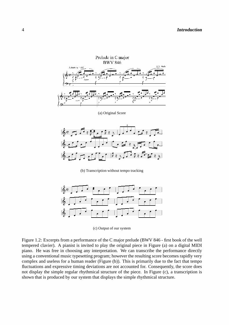
(a) Original Score
Ä ä t t t t e tZt tt t t tZ e tIı
t t t t t t t e t t t
Ä t t t t tıt
t t t t t t t t e tJ t t t t t tÄ t t t
t t t t t t t t tZ e tI t t t tZ e t t t t e tJ
(b) Transcription without tempo tracking� � � � � � �� � � � � � � � � � � �� � � � � � � � � � � � � � � � �� � � � � � � � � � � � � � � � �
(c) Output of our system
Figure 1.2: Excerpts from a performance of the C major prelude (BWV 846 - first book of the welltempered clavier). A pianist is invited to play the originalpiece in Figure (a) on a digital MIDIpiano. He was free in choosing any interpretation. We can transcribe the performance directlyusing a conventional music typesetting program; however the resulting score becomes rapidly verycomplex and useless for a human reader (Figure (b)). This is primarily due to the fact that tempofluctuations and expressive timing deviations are not accounted for. Consequently, the score doesnot display the simple regular rhythmical structure of the piece. In Figure (c), a transcription isshown that is produced by our system that displays the simplerhythmical structure.
1.1. RHYTHM QUANTIZATION AND TEMPO TRACKING 5
0
1.18
1.77
2.06
2.4
2.84
3.18
3.57
4.17
4.8
5.1
5.38
5.68
6.03
7.22
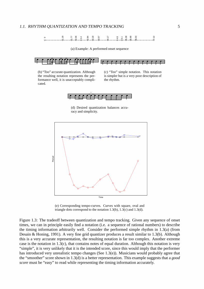
(a) Example: A performed onset sequence� � � � � � �� � � � � � � � � � � � � � � � � �(b) “Too” accurate quantization. Althoughthe resulting notation represents the per-formance well, it is unacceptably compli-cated.
� � � � � � � � � � � � � �(c) “Too” simple notation. This notationis simpler but is a very poor description ofthe rhythm.� � � � � 3� � � � � � � � � �
(d) Desired quantization balances accu-racy and simplicity.
Time
Per
iod
(e) Corresponding tempo-curves. Curves with square, oval andtriangle dots correspond to the notation 1.3(b), 1.3(c) and1.3(d).
Figure 1.3: The tradeoff between quantization and tempo tracking. Given any sequence of onsettimes, we can in principle easily find a notation (i.e. a sequence of rational numbers) to describethe timing information arbitrarily well. Consider the performed simple rhythm in 1.3(a) (fromDesain & Honing, 1991). A very fine grid quantizer produces a result similar to 1.3(b). Althoughthis is a very accurate representation, the resulting notation is far too complex. Another extremecase is the notation in 1.3(c), that contains notes of equal duration. Although this notation is very“simple”, it is very unlikely that it is the intended score, since this would imply that the performerhas introduced very unrealistic tempo changes (See 1.3(e)). Musicians would probably agree thatthe “smoother” score shown in 1.3(d) is a better representation. This example suggests that agoodscoremust be “easy” to read while representing the timing information accurately.

6 Introduction
perception of the beat, rhythmical structure, pitch, styleof music etc. Tempo is a perceptualconstruct and cannot directly be measured in a performance.
1.1.1 Related Work
The goal of understanding tempo perception has stimulated asignificant body of research on psy-chological and computational modelling aspects of tempo tracking and beat induction. Early workby (Michon, 1967) describes a systematic study on the modelling of human behaviour in trackingtempo fluctuations in artificially constructed stimuli. (Longuet-Higgins, 1976) proposes a musicalparser that produces a metrical interpretation of performed music while tracking tempo changes.Knowledge about meter helps the tempo tracker to quantize a performance.
Large and Jones (1999) describe an empirical study on tempo tracking, interpreting the ob-served human behaviour in terms of an oscillator model. A peculiar characteristic of this modelis that it is insensitive (or becomes so after enough evidence is gathered) to material in betweenexpected beats, suggesting that the perception tempo change is indifferent to events in this interval.(Toiviainen, 1999) discusses some problems regarding phase adaptation.
Another class of tempo tracking models are developed in the context of interactive performancesystems and score following. These models make use of prior knowledge in the form of an anno-tated score (Dannenberg, 1984; Vercoe & Puckette, 1985). More recently, Raphael (2001b) hasdemonstrated an interactive real-time system that followsa solo player and schedules accompani-ment events according to the player’s tempo interpretation.
More recently attempts are made to deal directly with the audio signal (Goto & Muraoka, 1998;Scheirer, 1998) without using any prior knowledge. However, these models assume constant tempo(albeit timing fluctuations may be present). Although successful for music with a steady beat (e.g.,popular music), they report problems with syncopated data (e.g., reggae or jazz music).
Many tempo tracking models assume an initial tempo (or beat length) to be known to start upthe tempo tracking process (e.g., (Longuet-Higgins, 1976;Large & Jones, 1999). There is fewresearch addressing how to arrive at a reasonable first estimate. (Longuet-Higgins & Lee, 1982)propose a model based on score data, (Scheirer, 1998) one foraudio data. A complete modelshould incorporate both aspects.
Tempo tracking is crucial for quantization, since one can not uniquely quantize onsets withouthaving an estimate of tempo and the beat. The converse, that quantization can help in identificationof the correct tempo interpretation has already been noted by Desain and Honing (1991). Here, onedefines correct tempo as the one that results in a simpler quantization. However, such a schemahas never been fully implemented in practice due to computational complexity of obtaining aperceptually plausible quantization. Hence quantizationmethods proposed in the literature eitherestimate the tempo using simple heuristics (Longuet-Higgins, 1987; Pressing & Lawrence, 1993;Agon, Assayag, Fineberg, & Rueda, 1994) or assume that the tempo is known or constant (Desain& Honing, 1991; Cambouropoulos, 2000; Hamanaka, Goto, Asoh, & Otsu, 2001).
1.2 Polyphonic Pitch Tracking
To transcribe a music performance from acoustical input, one needs a mechanism to sense andcharacterize individual events produced by the instrumentalist. One potential solution is to usededicated hardware and install special sensors on to the instrument body: this solution has re-stricted flexibility and is applicable only to instruments designed specifically for such a purpose.Discounting the ‘hardware’ solution, we shall assume that we capture the sound with a singlemicrophone, so that the computer receives no further input other than the pure acoustic informa-tion. In this context, polyphonic pitch tracking refers to identification of (possibly simultaneous)
1.2. POLYPHONIC PITCH TRACKING 7
0 500 1000 1500 2000 2500
Time/Samples
Note
Index
Fre
quen
cyM
agnitude
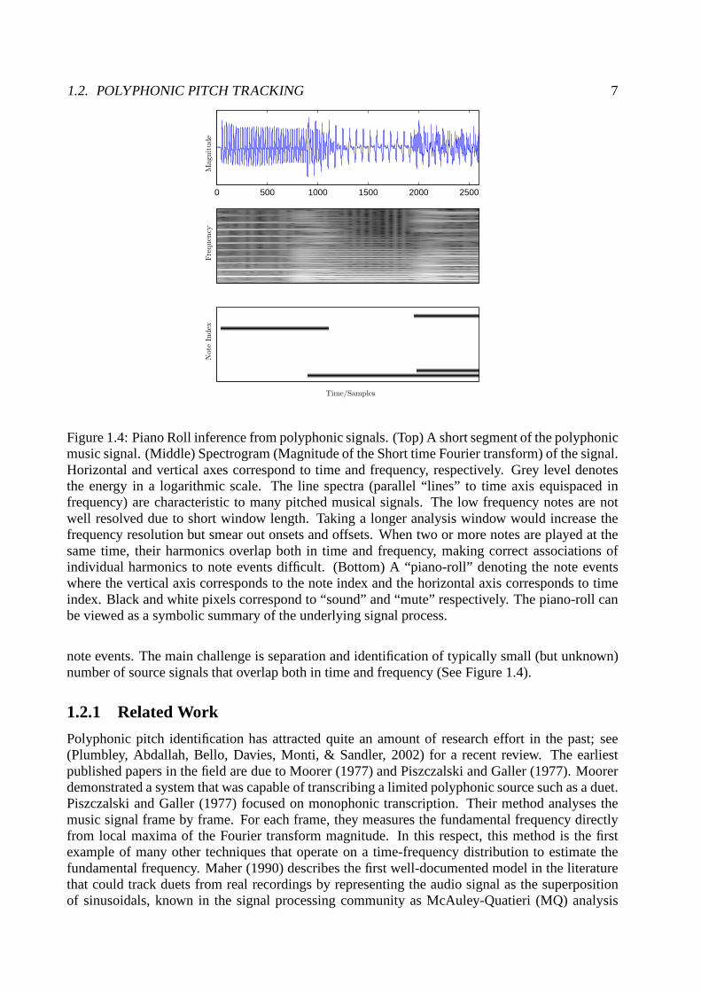
Figure 1.4: Piano Roll inference from polyphonic signals. (Top) A short segment of the polyphonicmusic signal. (Middle) Spectrogram (Magnitude of the Shorttime Fourier transform) of the signal.Horizontal and vertical axes correspond to time and frequency, respectively. Grey level denotesthe energy in a logarithmic scale. The line spectra (parallel “lines” to time axis equispaced infrequency) are characteristic to many pitched musical signals. The low frequency notes are notwell resolved due to short window length. Taking a longer analysis window would increase thefrequency resolution but smear out onsets and offsets. Whentwo or more notes are played at thesame time, their harmonics overlap both in time and frequency, making correct associations ofindividual harmonics to note events difficult. (Bottom) A “piano-roll” denoting the note eventswhere the vertical axis corresponds to the note index and thehorizontal axis corresponds to timeindex. Black and white pixels correspond to “sound” and “mute” respectively. The piano-roll canbe viewed as a symbolic summary of the underlying signal process.
note events. The main challenge is separation and identification of typically small (but unknown)number of source signals that overlap both in time and frequency (See Figure 1.4).
1.2.1 Related Work
Polyphonic pitch identification has attracted quite an amount of research effort in the past; see(Plumbley, Abdallah, Bello, Davies, Monti, & Sandler, 2002) for a recent review. The earliestpublished papers in the field are due to Moorer (1977) and Piszczalski and Galler (1977). Moorerdemonstrated a system that was capable of transcribing a limited polyphonic source such as a duet.Piszczalski and Galler (1977) focused on monophonic transcription. Their method analyses themusic signal frame by frame. For each frame, they measures the fundamental frequency directlyfrom local maxima of the Fourier transform magnitude. In this respect, this method is the firstexample of many other techniques that operate on a time-frequency distribution to estimate thefundamental frequency. Maher (1990) describes the first well-documented model in the literaturethat could track duets from real recordings by representingthe audio signal as the superpositionof sinusoidals, known in the signal processing community asMcAuley-Quatieri (MQ) analysis

8 Introduction
(1986). Mellinger (1991) employed a cochleagram representation (a time-scale representationbased on an auditory model (Slaney, 1995)). He proposed a setof directional filters for extractingfeatures from this representation. Recently, Klapuri et al. (2001) proposed an iterative schema thatoperates on the frequency spectrum. They estimate a single dominant pitch, remove it from the en-ergy spectrum and reestimate recursively on the residual. They report that the system outperformsexpert human transcribers on a chord identification task.
Other attempts have been made to incorporate low level (physical) or high level (musical struc-ture and cognitive) information for the processing of musical signals. Rossi, Girolami, and Leca(1997) reported a system that is based on matched filters estimated from piano sounds for poly-phonic pitch identification for piano music. Martin (1999) has demonstrated use of a “blackboardarchitecture” (Klassner, Lesser, & Nawab, 1998; Mani, 1999) to transcribe polyphonic piano music(Bach chorales), that contained at most four different voices (bass-tenor-alto-soprano ) simultane-ously. Essentially, this is an expert system that encodes prior knowledge about physical soundcharacteristics, auditory physiology and high level musical structure such as rules of harmony.This direction is further exploited by (Bello, 2003). Good results reported by Rossi et al., Martinand Bello support the intuitive claim that combining prior information from both lower and higherlevels can be very useful for transcription of musical signals.
In speech processing, tracking the pitch of a single speakeris a fundamental problem and meth-ods proposed in the literature fill many volumes (Rabiner, Chen, Rosenberg, & McGonegal, 1976;Hess, 1983). Many of these techniques can readily be appliedto monophonic music signals (de laCuadra, Master, & Sapp, 2001; de Cheveigne & Kawahara, 2002). A closely related researcheffort to transcription is developing real-time pitch tracking and score following methods for in-teractive performance systems (Vercoe, 1984), or for fast sound to MIDI conversion (Lane, 1990).Score following applications can also be considered as pitch trackers with a very informative prior(i.e. they know what to look for). In such a context, Grubb (1998) developed a system that cantrack a vocalist given a score. A vast majority of pitch detection algorithms are based on heuristics(e.g., picking high energy peaks of a spectrogram, correlogram, auditory filter bank, e.t.c.) andtheir formulation usually lacks an explicit objective function or a explicit model. Hence, it is of-ten difficult to theoretically justify merits and shortcomings of a proposed algorithm, compare itobjectively to alternatives or extend it to more complex scenarios such as polyphony.
Pitch tracking is inherently related to detection and estimation of sinusoidals. Estimation andtracking of single or multiple sinusoidals is a fundamentalproblem in many branches of appliedsciences so it is less surprising that the topic has also beendeeply investigated in statistics, (e.g.see Quinn & Hannan, 2001). However, ideas from statistics seem to be not widely applied in thecontext of musical sound analysis, with only a few exceptions (Irizarry, 2001, 2002) who presentfrequentist techniques for very detailed analysis of musical sounds with particular focus on de-composition of periodic and transient components. (Saul, Lee, Isbell, & LeCun, 2002) presentedreal-time monophonic pitch tracking application based on Laplace approximation to the poste-rior parameter distribution of a second order autoregressive process (AR(2)) model (Truong-Van,1990; Quinn & Hannan, 2001, page 19). Their method, with somerather simple preprocessing,outperforms several standard pitch tracking algorithms for speech, suggesting potential practicalbenefits of an approximate Bayesian treatment. For monophonic speech, a Kalman filter basedpitch tracker is proposed by Parra and Jain (2001) that tracks parameters of a harmonic plus noisemodel (HNM). They propose the use of Laplace approximation around the predicted mean insteadof the extended Kalman filter (EKF).
Statistical techniques have been applied for polyphonic transcription. Kashino is, to our knowl-edge, the first author to apply graphical models explicitly to the problem of music transcription.In Kashino et al. (1995), they construct a model to representhigher level musical knowledge andsolve pitch identification separately. Sterian (1999) described a system that viewed transcriptionas a model driven segmentation of a time-frequency distribution. They use a Kalman filter model
1.3. PROBABILISTIC MODELLING AND MUSIC TRANSCRIPTION 9
to track partials on this image. Walmsley (2000) treats transcription and source separation in a fullBayesian framework. He employs a frame based generalized linear model (a sinusoidal model)and proposes a reversible-jump Markov Chain Monte Carlo (MCMC) (Andrieu & Doucet, 1999)inference algorithm. A very attractive feature of the modelis that it does not make strong as-sumptions about the signal generation mechanism, and viewsthe number of sources as well asthe number of harmonics as unknown model parameters. Davy and Godsill (2003) address someof the shortcomings of his model and allow changing amplitudes and deviations in frequencies ofpartials from integer ratios. The reported results are good, however the method is computationallyexpensive. In a faster method, (Raphael, 2002) uses the short time Fourier Transform to makefeatures and uses an HMM to infer most likely chord hypothesis.
In machine learning community, probabilistic models are widely applied for source separation,a.k.a. blind deconvolution, independent components analysis (ICA) (Hyvarinen, Karhunen, & Oja,2001). Related techniques for source separation in music are investigated by (Casey, 1998). ICAmodels attempt source separation by forcing a factorized hidden state distribution, which can beinterpreted as a “not-very-informative” prior. Thereforeone needs typically multiple sensors forsource separation. When the prior is more informative, one can attempt separation even from asingle channel (Roweis, 2001; Jang & Lee, 2002; Hu & Wang, 2001).
Most of the authors view automated music transcription as a “audio to piano-roll” conversionand usually view “piano-roll to score” as a separate problem. This view is partially justified, sincesource separation and transcription from a polyphonic source is already a challenging task. Onthe other hand, automated generation of a human readable score includes nontrivial tasks such astempo tracking, rhythm quantization, meter and key induction (Raphael, 2001a; Temperley, 2001).We argue that models described in this thesis allow for principled integration of higher level sym-bolic prior knowledge with low level signal analysis. Such an approach can guide and potentiallyimprove the inference of a score , both in terms of quality of the solution and computation time.
1.3 Probabilistic Modelling and Music Transcription
We view music transcription, in particular rhythm quantization, tempo tracking and polyphonicpitch identification, as latent state estimation problems.In rhythm quantization or tempo tracking,given a sequence of onsets, we identify the most likely scoreor tempo trajectory. In polyphonicpitch identification, given the audio samples, we infer a piano-roll that represents the onset times,note durations and the pitch classes of individual notes.
Our general approach considers the quantities we wish to infer as a sequence of ‘hidden’ vari-ables, which we denote simply byx. For each problem, we define a probability model, that relatesthe observations sequencey to the hiddensx, possibly using a set of parametersθ. Given theobservations, transcription can be viewed as a Bayesian inference problem, where we compute aposterior distribution over hidden quantities by “inverting” the model using the Bayes theorem.
1.3.1 Bayesian Inference
In Bayesian statistics, probability models are viewed as data structures that represent a modelbuilders knowledge about a (possibly uncertain) phenomenon. The central quantity is a joint prob-ability distribution:
p(y, x, θ) = p(y|θ, x)p(x, θ)
that relates unknown variablesx and unknown parametersθ to observationsy. In probabilisticmodelling, there is no fundamental difference between unknown variables and unknown model
10 Introduction
θ
x
y
(a)
r θ
s
y
(b)
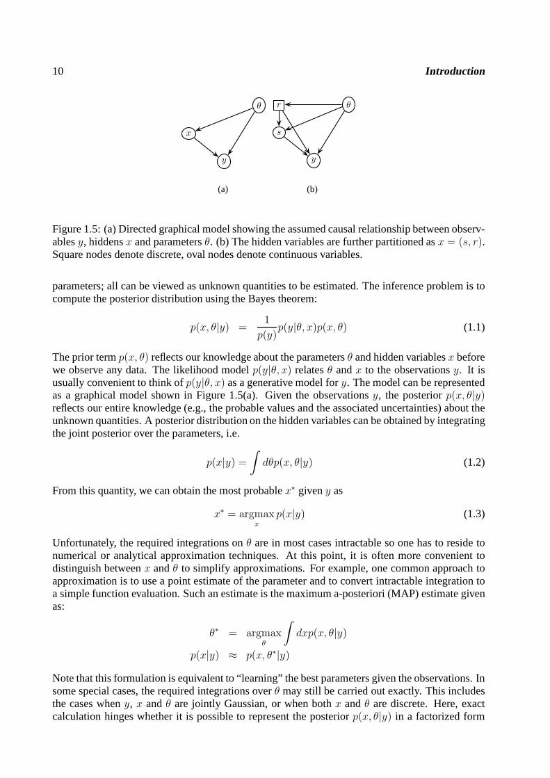
Figure 1.5: (a) Directed graphical model showing the assumed causal relationship between observ-ablesy, hiddensx and parametersθ. (b) The hidden variables are further partitioned asx = (s, r).Square nodes denote discrete, oval nodes denote continuousvariables.
parameters; all can be viewed as unknown quantities to be estimated. The inference problem is tocompute the posterior distribution using the Bayes theorem:
p(x, θ|y) =1
p(y)p(y|θ, x)p(x, θ) (1.1)
The prior termp(x, θ) reflects our knowledge about the parametersθ and hidden variablesx beforewe observe any data. The likelihood modelp(y|θ, x) relatesθ andx to the observationsy. It isusually convenient to think ofp(y|θ, x) as a generative model fory. The model can be representedas a graphical model shown in Figure 1.5(a). Given the observationsy, the posteriorp(x, θ|y)reflects our entire knowledge (e.g., the probable values andthe associated uncertainties) about theunknown quantities. A posterior distribution on the hiddenvariables can be obtained by integratingthe joint posterior over the parameters, i.e.
p(x|y) =
∫
dθp(x, θ|y) (1.2)
From this quantity, we can obtain the most probablex∗ giveny as
x∗ = argmaxx
p(x|y) (1.3)
Unfortunately, the required integrations onθ are in most cases intractable so one has to reside tonumerical or analytical approximation techniques. At thispoint, it is often more convenient todistinguish betweenx andθ to simplify approximations. For example, one common approach toapproximation is to use a point estimate of the parameter andto convert intractable integration toa simple function evaluation. Such an estimate is the maximum a-posteriori (MAP) estimate givenas:
θ∗ = argmaxθ
∫
dxp(x, θ|y)
p(x|y) ≈ p(x, θ∗|y)
Note that this formulation is equivalent to “learning” the best parameters given the observations. Insome special cases, the required integrations overθ may still be carried out exactly. This includesthe cases wheny, x andθ are jointly Gaussian, or when bothx andθ are discrete. Here, exactcalculation hinges whether it is possible to represent the posteriorp(x, θ|y) in a factorized form

1.4. A TOY EXAMPLE 11
using a data structure such as thejunction tree(See (Smyth, Heckerman, & Jordan, 1996) andreferences herein).
Another source of intractability is reflected in combinatorial explosion. In some special hybridmodel classes (such as switching linear dynamical systems (Murphy, 1998; Lerner & Parr, 2001)),we can divide the hidden variables in two setsx = (s, r) wherer is discrete ands given r isconditionally Gaussian (See Figure. 1.5(b)). We will use such models extensively in the thesis. Toinfer the most likelyr consistent with the observations, we need to compute
r∗ = argmaxr
∫
dsdθp(r, s, θ|y)
If we assume that model parametersθ are known, (e.g. suppose we have estimatedθ∗ on a trainingset wherer was known) we can simplify the problem as:
r∗ ≈ argmaxr
p(r|y) = argmaxr
∫
dsp(y|r, s)p(s|r)p(r) (1.4)
Here, we have omitted explicit conditioning onθ∗. We can evaluate the integral in Eq.1.4 for anygivenr. However, in order to find the optimal solutionr∗ exactly, we still need to evaluate the theintegral separately for everyr in the configuration space. Apart from some special cases, wherewe can derive exact polynomial time algorithms; in general the only exact method is exhaustivesearch. Fortunately, although findingr∗ is intractable in general, in practice a useful solution maybe found by approximate methods. Intuitively, this is due tofact that realistic priorsp(r) are usuallyvery informative (most of the configurationsr have very small probability) and the likelihood termp(y|r) is quite crisp. All this factors tend to render the posteriorunimodal.
1.4 A toy example
We will now illustrate the basic ideas of Bayesian inferencedeveloped in the previous sectionon a toy sequencer model. The sequencer model is quite simpleand is able to generate outputsignals of length one only. We denote this output signal asy. The “scores” that it can processare equally limited and can consist of at most two “notes”. Hence, the “musical universe” ofour sequencer is limited only to4 possible scores, namelysilence, two single note melodies andone two note chord. Given any one of the four possible scores,the sequencer generates controlsignals which we will call a “piano-roll”. In this representation, we will encode each note by a bitrj ∈ {“sound”, “mute”} for j = 1, 2. This indicator bit denotes simply whether thej’th note ispresent in the score or not. In this simplistic example, there is no distinction between a score and apiano-roll and the latter is merely an encoding of the former; but for longer signals there will be adistinction. We specify next what waveform the sequencer should generate when a note is presentor absent. We will denote this waveform bysj
sj|rj ∼ [rj = sound]N (sj;µj, Ps) + [rj = mute]N (sj; 0, Pm)
Here the notation[x = text] has value equal to 1 when variablex is in state text, and is zerootherwise. The symbolN (s;µ, P ) denotes a Gaussian distribution on variables with meanµ andvarianceP . Verbally, the above equation means that whenrj = mute,sj ≈ 0 ± √Pm and whenrj = sound,sj ≈ µj ±
√Ps. Here theµj, Ps andPm are known parameters of the signal model.
Finally, the output signal is given by summing up each waveform of individual notes
y =∑
j
sj
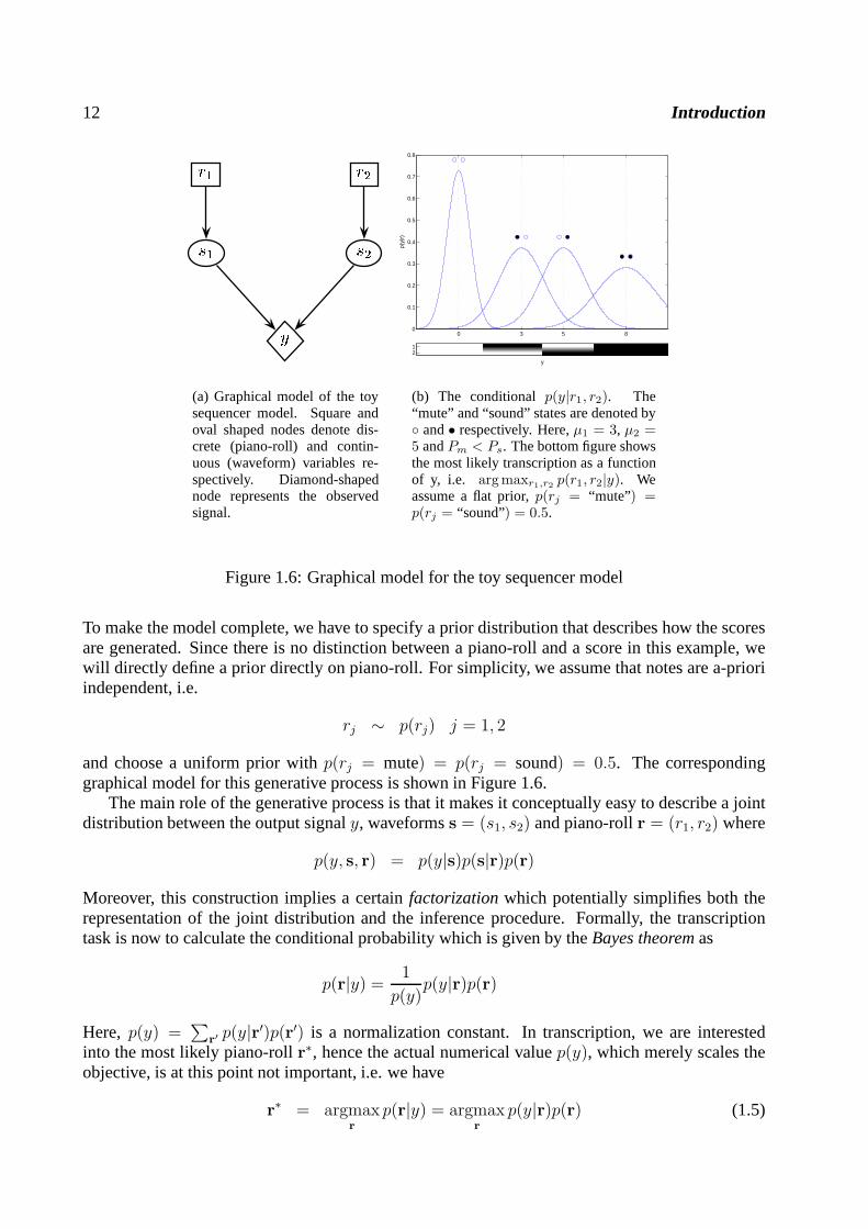
12 Introductionr1 r2s1 s2y(a) Graphical model of the toysequencer model. Square andoval shaped nodes denote dis-crete (piano-roll) and contin-uous (waveform) variables re-spectively. Diamond-shapednode represents the observedsignal.
0 3 5 80
0.1
0.2
0.3
0.4
0.5
0.6
0.7
0.8
p(y|
r)
y
12
(b) The conditionalp(y|r1, r2). The“mute” and “sound” states are denoted by◦ and• respectively. Here,µ1 = 3, µ2 =5 andPm < Ps. The bottom figure showsthe most likely transcription as a functionof y, i.e. argmaxr1,r2
p(r1, r2|y). Weassume a flat prior,p(rj = “mute”) =p(rj = “sound”) = 0.5.
Figure 1.6: Graphical model for the toy sequencer model
To make the model complete, we have to specify a prior distribution that describes how the scoresare generated. Since there is no distinction between a piano-roll and a score in this example, wewill directly define a prior directly on piano-roll. For simplicity, we assume that notes are a-prioriindependent, i.e.
rj ∼ p(rj) j = 1, 2
and choose a uniform prior withp(rj = mute) = p(rj = sound) = 0.5. The correspondinggraphical model for this generative process is shown in Figure 1.6.
The main role of the generative process is that it makes it conceptually easy to describe a jointdistribution between the output signaly, waveformss = (s1, s2) and piano-rollr = (r1, r2) where
p(y, s, r) = p(y|s)p(s|r)p(r)
Moreover, this construction implies a certainfactorizationwhich potentially simplifies both therepresentation of the joint distribution and the inferenceprocedure. Formally, the transcriptiontask is now to calculate the conditional probability which is given by theBayes theoremas
p(r|y) =1
p(y)p(y|r)p(r)
Here, p(y) =∑
r′p(y|r′)p(r′) is a normalization constant. In transcription, we are interested
into the most likely piano-rollr∗, hence the actual numerical valuep(y), which merely scales theobjective, is at this point not important, i.e. we have
r∗ = argmaxr
p(r|y) = argmaxr
p(y|r)p(r) (1.5)
1.5. OUTLINE OF THE THESIS 13
The prior factorp(r) is already specified. The other term can be calculated byintegrating outthewaveformss, i.e.
p(y|r) =
∫
dsp(y, s|r) =
∫
dsp(y|s)p(s|r)
Conditioned on anyr, this quantity can be found analytically. For example, whenr1 = r2 =“sound”,p(y|r) = N (y;µ1 + µ2, 2Ps). A numeric example is shown in Figure 1.6.
This simple toy example exhibits the key idea in our approach. Basically, by just carefullydescribing the sound generation procedure, we were able to formulate an optimization problem(Eq. 1.5) for doing polyphonic transcription! The derivation is entirely mechanical and ensuresthat the objective function consistently incorporates ourprior knowledge about scores and about thesound generation procedure (throughp(r) andp(s|r)). Of course, in reality,y and each ofrj andsj
will be time series and both the score and sound generation process will be far more complex. Butmost importantly, we have divided the problem into two parts, in one part formulating a realisticmodel, on the other part finding an efficient inference algorithm.
1.5 Outline of the thesis
In the following chapters, we describe several methods for transcription. For each subproblem,we define a probability model, that relates the observations, hiddens and parameters. The partic-ular definition of these quantities will depend on the context, but observables and hiddens will besequences of random variables. For a given observation sequence, we will compute the posteriordistribution or some posterior features such as the MAP.
In Chapter 2, we describe a model that relates short scores with corresponding onset times ofevents in an expressive performance. The parameters of the model is trained on data resulting froma psychoacoustical experiment to mimic the behaviour of a human transcriber on this task. Thischapter addresses the issue that there is not a single “ground truth” in music transcription. Even forvery simple rhythms, well trained human subjects show significant variations in their responses.We demonstrate how this uncertainty problem can be addressed naturally using a probabilisticmodel.
Chapter 3 focuses on tempo tracking from onsets. The observation model is a multiscale rep-resentation (analogous to a wavelet transform ). The tempo prior is modelled as a Gauss-Markovprocess. The tempo is viewed as a hidden state variable and isestimated by approximate Kalmanfiltering.
We introduce in Chapter 4 a generative model to combine rhythm quantization and tempotracking. The model is a switching state space model in whichcomputation of exact probabilitiesbecomes intractable. We introduce approximation techniques based on simulation, namely MarkovChain Monte Carlo (MCMC) and sequential Monte Carlo (SMC).
In Chapter 5, we propose a generative model for polyphonic transcription from audio signals.The model, formulated as a Dynamical Bayesian Network, describes the relationship betweenpolyphonic audio signal and an underlying piano roll. This model is also a special case of the,generally intractable, switching state space model. Wherepossible, we derive, exact polynomialtime inference procedures, and otherwise efficient approximations.
1.6 Future Directions and Conclusions
When transcribing music, human experts rely heavily on prior knowledge about the musical struc-ture – harmony, tempo, timbre, expression, e.t.c. As partially demonstrated in this thesis and else-where (e.g. (Raphael & Stoddard, 2003)), such structure canbe captured by training probabilistic
14 Introduction
generative models on a corpus of example compositions, performances or sounds by collectingstatistics over selected features. One of the important advantages of our approach is that, at leastin principle, prior knowledge about any type of musical structure can be consistently integrated.An attempt in this direction is made in (Cemgil, Kappen, & Barber, 2003), where we described amodel that combines low level signal analysis with high level knowledge. However, the computa-tional obstacles and software engineering issues are yet tobe overcome. I believe that investigationof this direction is important in designing robust and practical music transcription systems.
In my view, the most attractive feature of probabilistic modelling and Bayesian inference formusic transcription is the decoupling of modelling from inference. In this framework, the modelclearly describes the objective and the question how we actually solve the objective, whilst equallyimportant, becomes an entirely algorithmic and computational issue. Particularly in music tran-scription, as in many other perceptual tasks, the answer to the question of “what to optimize” is farfrom trivial. This thesis tries to answer this question by defining an objective by using probabilisticgenerative models and touches upon some state-of-the-art inference techniques for its solution.
I argue that practical polyphonic music transcription can be made computationally easy; thedifficulty of the problem lies in formulating precisely whatthe objective is. This is in contrastwith traditional problems of computer science, such as the travelling salesman problem, which arevery easy to formulate but difficult to solve exactly. In my view, this fundamental difference inthe nature of the music transcription problem requires a model-centred approach rather than analgorithm-centred approach. One can argue that objectivesformulated in the context of probabilis-tic models are often intractable. I answer this by paraphrasing John Tukey, who in the 50’s said“An approximate solution of the exact problem is often more useful than the exact solution of anapproximate problem”.

Chapter 2
Rhythm Quantization
One important task in music transcription is rhythm quantiz ation that refers to categoriza-tion of note durations. Although quantization of a pure mechanical performance is ratherstraightforward, the task becomes increasingly difficult in presence of musical expression,i.e. systematic variations in timing of notes and in tempo. In this chapter, we assume thatthe tempo is known. Expressive deviations are modelled by a probabilistic performancemodel from which the corresponding optimal quantizer is derived by Bayes theorem. Wedemonstrate that many different quantization schemata canbe derived in this frameworkby proposing suitable prior and likelihood distributions. The derived quantizer operates onshort groups of onsets and is thus flexible both in capturing the structure of timing devia-tions and in controlling the complexity of resulting notations. The model is trained on dataresulting from a psychoacoustical experiment and thus can mimic the behaviour of a humantranscriber on this task.
Adapted from A.T. Cemgil, P. Desain, and H.J. Kappen. Rhythmquantiza-tion for transcription.Computer Music Journal, pages 60–75, 2000.
2.1 Introduction
One important task in music transcription is rhythm quantization that refers to categorization ofnote durations. Quantization of a “mechanical” performance is rather straightforward. On theother hand, the task becomes increasingly difficult in presence of expressive variations, that canbe thought as systematic deviations from a pure mechanical performance. In such unconstrainedperformance conditions, mainly two types of systematic deviations from exact values do occur.At small time scale notes can be played accented or delayed. At large scale tempo can vary, forexample the musician(s) can accelerate (or decelerate) during performance or slow down (ritard)at the end of the piece. In any case, these timing variations usually obey a certain structure sincethey are mostly intended by the performer. Moreover, they are linked to several attributes of theperformance such as meter, phrase, form, style etc. (Clarke, 1985). To devise a general compu-tational model (i.e. a performance model) which takes all these factors into account, seems to bequite hard.
Another observation important for quantization is that we perceive a rhythmic pattern not as asequence of isolated onsets but rather as a perceptual entity made of onsets. This also suggests thatattributes of neighboring onsets such as duration, timing deviation etc. are correlated in some way.
This correlation structure is not fully exploited in commercial music packages, which do auto-mated music transcription and score type setting. The usualapproach taken is to assume a constanttempo throughout the piece, and to quantize each onset to thenearest grid point implied by thetempo and a suitable pre-specified minimum note duration (e.g. eight, sixteenth etc.). Such a grid
15

16 Rhythm Quantization
quantization schema implies that each onset is quantized tothe nearest grid pointindependentofits neighbours and thus all of its attributes are assumed to be independent, hence the correlationstructure is not employed. The consequence of this restriction is that users are required to playalong with a fixed metronome and without any expression. The quality of the resulting quanti-zation is only satisfactory if the music is performed according to the assumptions made by thequantization algorithm. In the case of grid-quantization this is a mechanical performance withsmall and independent random deviations.
More elaborate models for rhythm quantization indirectly take the correlation structure of ex-pressive deviations into account. In one of the first attemptto quantization, (Longuet-Higgins,1987) described a method in which he uses hierarchical structure of musical rhythms to do quanti-zation. (Desain, Honing, & de Rijk, 1992) use a relaxation network in which pairs of time intervalsare attracted to simple integer ratios. (Pressing & Lawrence, 1993) use several template grids andcompare both onsets and inter-onset intervals (IOI’s) to the grid and select the best quantizationaccording to some distance criterion. The Kant system (Agonet al., 1994) developed at IRCAMuses more sophisticated heuristics but is in principle similar to (Pressing & Lawrence, 1993).
The common critic to all of these models is that the assumptions about the expressive devia-tions are implicit and are usually hidden in the model, thus it is not always clear how a particulardesign choice effects the overall performance for a full range of musical styles. Moreover it is notdirectly possible to use experimental data to tune model parameters to enhance the quantizationperformance.
In this chapter, we describe a method for quantization of onset sequences. The paper is or-ganized as follows: First, we state the transcription problem and define the terminology. Usingthe Bayesian framework we briefly introduce, we describe probabilistic models for expressive de-viation and notation complexity and show how different quantizers can be derived from them.Consequently, we train the resulting model on experimentaldata obtained from a psychoacousticalexperiment and compare its performance to simple quantization strategies.
2.2 Rhythm Quantization Problem
2.2.1 Definitions
A performed rhythmis denoted by a sequence[ti]1 where each entry is the time of occurrence of
an onset. For example, the performed rhythm in Figure 1.3(a)is represented byt1 = 0, t2 = 1.18,t3 = 1.77, t4 = 2.06 etc. We will also use the termsperformanceor rhythminterchangeably whenwe refer to an onset sequence.
A very important subtask in transcription is tempo tracking, i.e. the induction of a sequenceof points (i.e.beats) in time, which coincides with the human sense of rhythm (e.g. foot tapping)when listening to music. We call such a sequence of beats atempo trackand denote it by~τ = [τj ]whereτj is the time at whichj’th beat occurs. We note that for automatic transcription,~τ is to beestimated from[ti].
Once a tempo track~τ is given, the rhythm can be segmented into a sequence of segments,each of durationτj − τj−1. The j’th segment will containKj onsets, which we enumerate byk = 1 . . .Kj . The onsets in each segment are normalized and denoted bytj = [tkj ], i.e. for allτj−1 ≤ ti < τj where
tkj =ti − τj−1
τj − τj−1(2.1)
1We will denote a set with the typical elementxj as{xj}. If the elements are ordered (e.g. to form a vector) wewill use [xj ].

2.2. RHYTHM QUANTIZATION PROBLEM 17
Note that this is merely a reindexing from single indexi to double index(k, j) 2. In other wordsthe onsets are scaled and translated such that an onset just at the end of the segment is mappedto one and another just at the beginning to zero. The segmentation of a performance is given inFigure 2.1.
1.77
0.29
0.34
0.44
0.34
0.99
0.63
0.3
0.28
0.3
0.35
1.19
0
0.4
75
0.7
17
0
0.3
67
0.6
5
0.4
75
0
0.2
5
0.4
83
0.7
33
0.0
25
0.01
67
∆ = 1.2
Figure 2.1: Segmentation of a performance by a tempo track (vertical dashed lines)~τ =[0.0, 1.2, 2.4, 3.6, 4.8, 6.0, 7.2, 8.4]. The resulting segments aret0 = [0], t1 = [0.475, 0.717] etc.
0 1/2 1
0
1
2
3
c
dept
h
d(c|S)
Figure 2.2: Depth of gridpointc by subdivision schemaS = [3, 2, 2]
Once a segmentation is given, quantization reduces to mapping onsets to locations, whichcan be described by simple rational numbers. Since in western music tradition, notations aregenerated by recursive subdivisions of a whole note, it is also convenient to generate possibleonset quantization locations by regular subdivisions. We letS = [si] denote a subdivision schema,where[si] is a sequence of small prime numbers. Possible quantizationlocations are generatedby subdividing the unit interval[0, 1]. At each new iterationi, the intervals already generated aredivided further intosi equal parts and the resulting endpoints are added to a setC. Note thatthis procedure places the quantization locations on a grid of pointscn where two neighboring gridpoints have the distance1/
∏
i si. We will denote the first iteration number at which the grid pointc is added toC as thedepthof c with respect toS. This number will be denoted asd(c|S).
As an example consider the subdivisionS = [3, 2, 2]. The unit interval is divided first into threeequal pieces, then the resulting intervals into 2 and etc. Ateach iteration, generated endpoints are
2When an argument applies to all segments, we will drop the indexj.
18 Rhythm Quantization�� � � � 3� � � ? -� � � � � �(a) Notation
18 3 3 4 4 10 6 3 3 3 3 12
0 18 21 24 28 32 42 48 51 54 57 60 72
(b) Score
0
1.77
2.06
2.4
2.84
3.18
4.17
4.8
5.1
5.38
5.68
6.03
7.22
(c) Performance
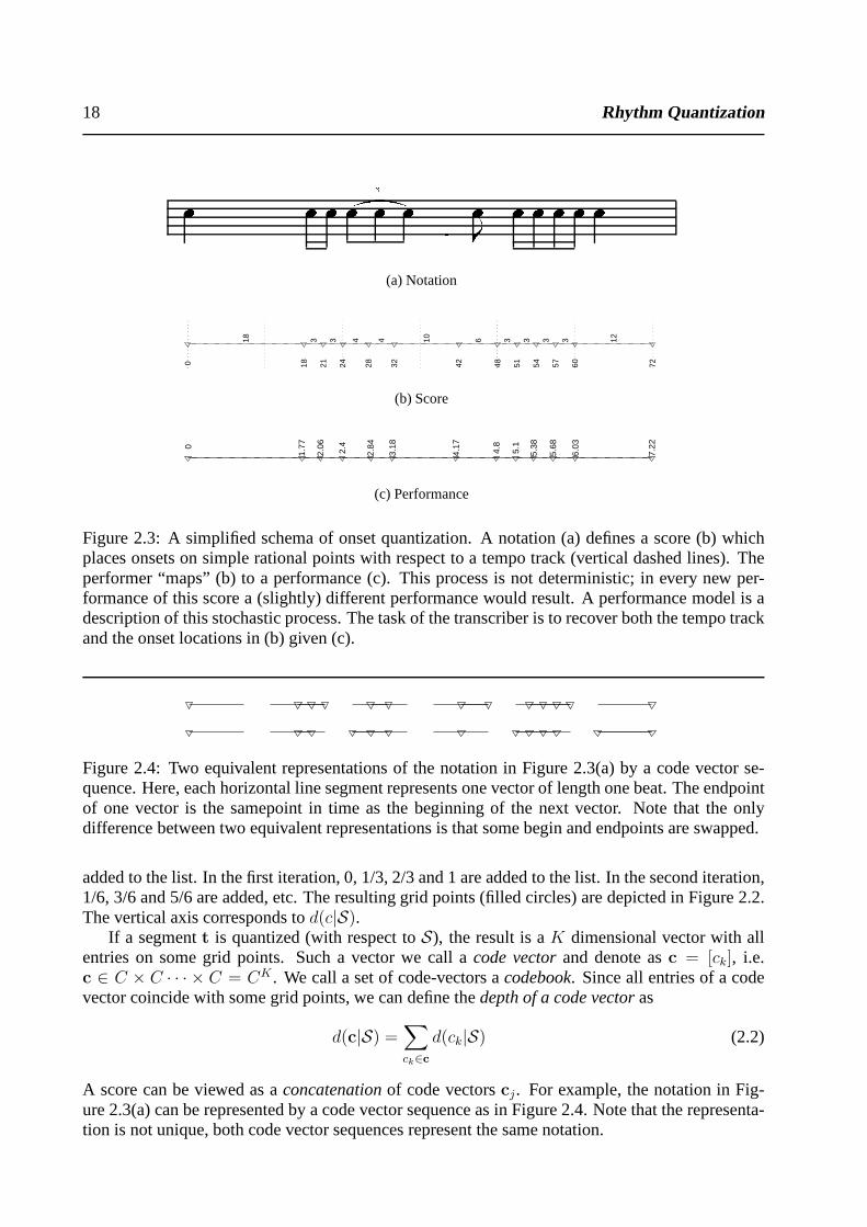
Figure 2.3: A simplified schema of onset quantization. A notation (a) defines a score (b) whichplaces onsets on simple rational points with respect to a tempo track (vertical dashed lines). Theperformer “maps” (b) to a performance (c). This process is not deterministic; in every new per-formance of this score a (slightly) different performance would result. A performance model is adescription of this stochastic process. The task of the transcriber is to recover both the tempo trackand the onset locations in (b) given (c).
Figure 2.4: Two equivalent representations of the notationin Figure 2.3(a) by a code vector se-quence. Here, each horizontal line segment represents one vector of length one beat. The endpointof one vector is the samepoint in time as the beginning of the next vector. Note that the onlydifference between two equivalent representations is thatsome begin and endpoints are swapped.
added to the list. In the first iteration, 0, 1/3, 2/3 and 1 are added to the list. In the second iteration,1/6, 3/6 and 5/6 are added, etc. The resulting grid points (filled circles) are depicted in Figure 2.2.The vertical axis corresponds tod(c|S).
If a segmentt is quantized (with respect toS), the result is aK dimensional vector with allentries on some grid points. Such a vector we call acode vectorand denote asc = [ck], i.e.c ∈ C × C · · · × C = CK . We call a set of code-vectors acodebook. Since all entries of a codevector coincide with some grid points, we can define thedepth of a code vectoras
d(c|S) =∑
ck∈c
d(ck|S) (2.2)
A score can be viewed as aconcatenationof code vectorscj. For example, the notation in Fig-ure 2.3(a) can be represented by a code vector sequence as in Figure 2.4. Note that the representa-tion is not unique, both code vector sequences represent thesame notation.
2.2. RHYTHM QUANTIZATION PROBLEM 19
2.2.2 Performance Model
As described in the introduction section, natural music performance is subject to several systematicdeviations. In lack of such deviations, every score would have only one possible interpretation.Clearly, two natural performances of a piece of music are never the same, even performance ofvery short rhythms show deviations from a strict mechanicalperformance. In general terms, aperformance modelis a mathematical description of such deviations, i.e. it describes how likelyit is that a score is mapped into a performance (Figure 2.3). Before we describe a probabilisticperformance model, we briefly review a basic theorem of probability theory.
2.2.3 Bayes Theorem
The joint probabilityp(A,B) of two random variablesA andB defined over the respective statespacesSA andSB can be factorized in two ways:
p(A,B) = p(B|A)p(A) = p(A|B)p(B) (2.3)
wherep(A|B) denotes the conditional probability ofA givenB: for each value ofB, this isa probability distribution overA. Therefore
∑
A p(A|B) = 1 for any fixedB. The marginaldistribution of a variable can be found from the joint distribution by summing over all states of theother variable, e.g.:
p(A) =∑
B∈SB
p(A,B) =∑
B∈SB
p(A|B)p(B) (2.4)
It is understood that summation is to be replaced by integration if the state space is continuous.Bayes theorem results from Eq. 2.3 and Eq. 2.4 as:
p(B|A) =p(A|B)p(B)
∑
B∈SBp(A|B)p(B)
(2.5)
∝ p(A|B)p(B) (2.6)
The proportionality follows from the fact that the denominator does not depend onB, sinceB isalready summed over. This rather simple looking “formula” has surprisingly far reaching conse-quences and can be directly applied to quantization. Consider the case thatB is a score andSB isthe set of all possible scores. LetA be the observed performance. Then Eq 2.5 can be written as
p(Score|Performance) ∝ p(Performance|Score)× p(Score) (2.7)
posterior ∝ likelihood× prior (2.8)
The intuitive meaning of this equation can be better understood, if we think of quantization as ascore selection problem. Since there is usually not a singletrue notation for a given performance,there will be several possibilities. The most reasonable choice is selecting the scorec which hasthe highest probability given the performancet. Technically, we name this probability distributionas the posteriorp(c|t). The name posterior comes from the fact that this quantity appearsafterwe observe the performancet. Note that the posterior is a function overc, and assigns a numberto each notation after we fixt. We look for the notationc that maximizes this function. Bayestheorem tells us that the posterior is proportional to the product of two quantities, the likelihoodp(t|c) and the priorp(c). Before we explain the interpretation of the likelihood andthe prior inthis context, we first summerize the ideas in compact notation as
p(c|t) ∝ p(t|c)p(c). (2.9)

20 Rhythm Quantization
The best code vectorc∗ is given by
c∗ = argmaxc∈CK
p(c|t) (2.10)
In technical terms, this problem is called a maximum a-posteriori (MAP) estimation problem andc∗ is called the MAP solution of this problem. We can also define arelated quantityL (minus log-posterior) and try to minimize this quantity rather then maximizing Eq. 2.9 directly. This simplifiesthe form of the objective function without changing the locations of local extrema sincelog(x) isa monotonically increasing function.
L = − log p(c|t) ∝ − log p(t|c) + log1
p(c)(2.11)
The− log p(t|c) term in Equation 2.11, which is the minus logarithm of the likelihood, can beinterpreted as a distance measuring how far the rhythmt is played from the perfect mechanicalperformancec. For example, ifp(t|c) would be of formexp(−(t− c)2), then− log(t|c) would be(t− c)2, the square of the distance fromt to c. This quantity can be made arbitrary small if we usea very fine grid, however, as mentioned in the introduction section, this eventually would resultin a complex notation. A suitable prior distribution prevents this undesired result. Thelog 1
p(c)
term, which is large when the prior probabilityp(c) of the codevector is small, can be interpretedas a complexity term, which penalizes complex notations. The best quantization balances thelikelihood and the prior in an optimal way. The precise form of the prior will be discussed in alater section.
The form of a performance model, i.e. the likelihood, can be in general very complicated.However, in this article we will consider a subclass of performance models where the expressivetiming is assumed to be an additive noise component which depends onc. The model is given by
tj = cj + εj (2.12)
whereεj is a vector which denotes theexpressive timing deviation. In this paper we will assumethatε is normal distributed with zero mean and covariance matrixΣε(c), i.e. the correlation struc-ture depends upon the code vector. We denote this distribution asε ∼ N (0,Σε(c)). Note thatwhenε is the zero vector, (Σε → 0), the model reduces to a so-called “mechanical” performance.
2.2.4 Example 1: Scalar Quantizer (Grid Quantizer)
We will now demonstrate on a simple example how these ideas are applied to quantization.Consider a one-onset segmentt = [0.45]. Suppose we wish to quantize the onset to one of the
endpoints, i.e. we are using effectively the codebookC = {[0], [1]}. The obvious strategy is toquantize the onset to the nearest grid point (e.g. a grid quantizer) and so the code-vectorc = [0] ischosen as the winner.
The Bayesian interpretation of this decision can be demonstrated by computing the correspond-ing likelihoodp(t|c) and the priorp(c). It is reasonable to assume that the probability of observinga performancet given a particularc decreases with the distance|c− t|. A probability distributionhaving this property is the normal distribution. Since there is only one onset, the dimensionK = 1and the likelihood is given by
p(t|c) =1√2πσ
exp(−(t− c)2
2σ2)
2.2. RHYTHM QUANTIZATION PROBLEM 21
0 0.5 1
p(t|c
)
t
p(t|c1)p(c
1) p(t|c
2)p(c
2)
p(c1) = 0.5
p(c1) = 0.3
0.45
c1
c2
t
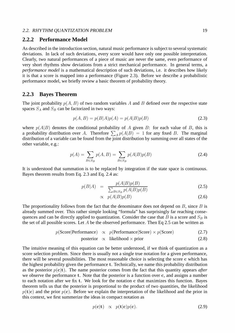
Figure 2.5: Quantization of an onset as Bayesian Inference.Whenp(c) = [1/2, 1/2], at eacht, theposteriorp(c|t) is proportional to the solid lines, and the decision boundary is at t = 0.5. Whenthe prior is changed top(c) = [0.3, 0.7] (dashed), the decision boundary moves towards0.
If both codevectors are equally probable, a flat prior can be choosen, i.e.p(c) = [1/2, 1/2]. Theresulting posteriorp(c|t) is plotted in 2.5. The decision boundary is att = 0.5, wherep(c1|t) =p(c2|t). The winner is given as in Eq. 2.10
c∗ = argmaxc
p(c|t)
Different quantization strategies can be implemented by changing the prior. For example ifc = [0]is assumed to be less probable, we can choose another prior, e.g. p(c) = [0.3, 0.7]. In this case thedecision boundary shifts from0.5 towards0 as expected.
2.2.5 Example 2: Vector Quantizer
Assigning different prior probabilities to notations is only one way of implementing different quan-tization strategies. Further decision regions can be implemented by varying the conditional prob-ability distributionp(t|c). In this section we will demonstrate the flexibility of this approach forquantization of groups of onsets.
0.45
0.52
Figure 2.6: Two Onsets
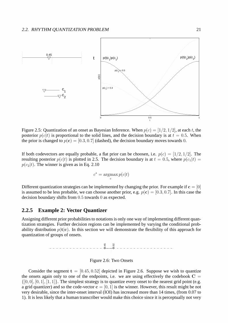
Consider the segmentt = [0.45, 0.52] depicted in Figure 2.6. Suppose we wish to quantizethe onsets again only to one of the endpoints, i.e. we are using effectively the codebookC ={[0, 0], [0, 1], [1, 1]}. The simplest strategy is to quantize every onset to the nearest grid point (e.g.a grid quantizer) and so the code-vectorc = [0, 1] is the winner. However, this result might be notvery desirable, since the inter-onset interval (IOI) has increased more than 14 times, (from 0.07 to1). It is less likely that a human transcriber would make thischoice since it is perceptually not very
22 Rhythm Quantization
realistic. We could try to solve this problem by employing another strategy : Ifδ = t2 − t1 > 0.5,we use the code-vector[0, 1]. If δ ≤ 0.5, we quantize to one of the code-vectors[0, 0] or [1, 1]depending upon the average of the onsets. In this strategy the quantization of[0.45, 0.52] is [0, 0].
0 1/2 1
0
1/2
1
t1
t 2
ρ = 0
0 1/2 1
0
1/2
1
t1
t 2
ρ = 0.3
0 1/2 1
0
1/2
1
t1
t 2
ρ = 0.7
0 1/2 1
0
1/2
1
t1
t 2
ρ = 1
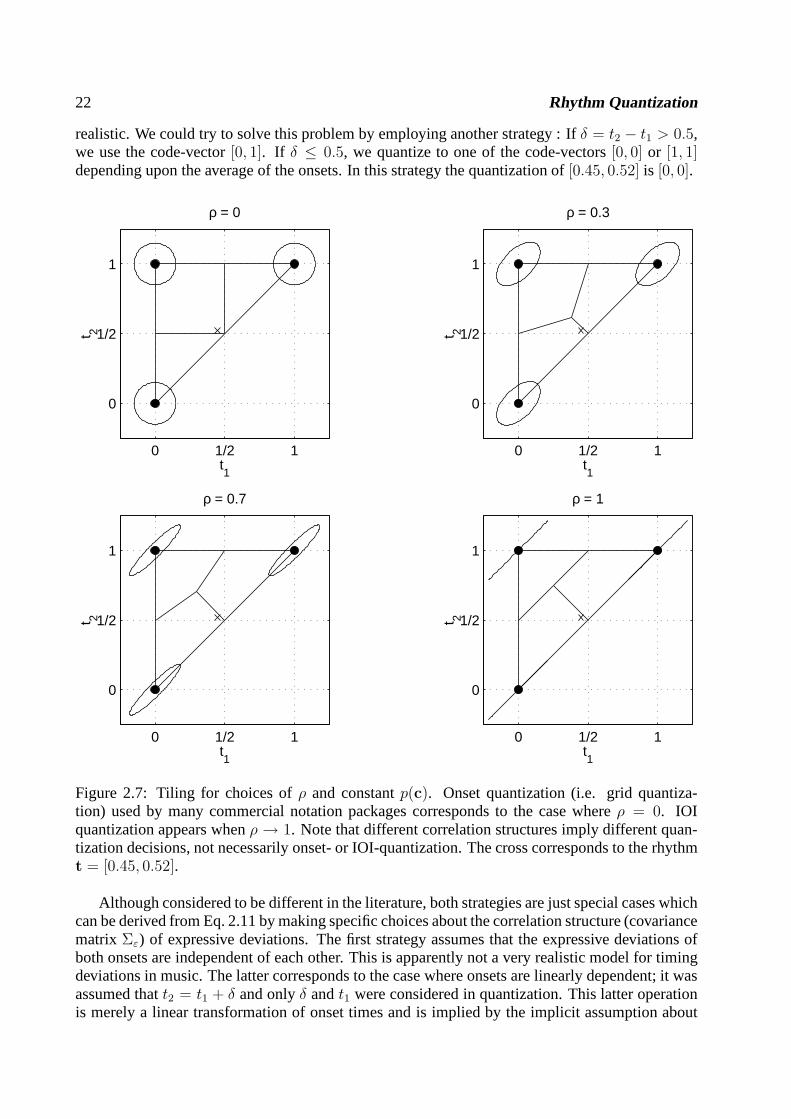
Figure 2.7: Tiling for choices ofρ and constantp(c). Onset quantization (i.e. grid quantiza-tion) used by many commercial notation packages corresponds to the case whereρ = 0. IOIquantization appears whenρ → 1. Note that different correlation structures imply different quan-tization decisions, not necessarily onset- or IOI-quantization. The cross corresponds to the rhythmt = [0.45, 0.52].
Although considered to be different in the literature, bothstrategies are just special cases whichcan be derived from Eq. 2.11 by making specific choices about the correlation structure (covariancematrix Σε) of expressive deviations. The first strategy assumes that the expressive deviations ofboth onsets are independent of each other. This is apparently not a very realistic model for timingdeviations in music. The latter corresponds to the case where onsets are linearly dependent; it wasassumed thatt2 = t1 + δ and onlyδ andt1 were considered in quantization. This latter operationis merely a linear transformation of onset times and is implied by the implicit assumption about
2.2. RHYTHM QUANTIZATION PROBLEM 23
the correlation structure. Indeed some quantization models in the literature focus directly on IOI’srather then on onset times.
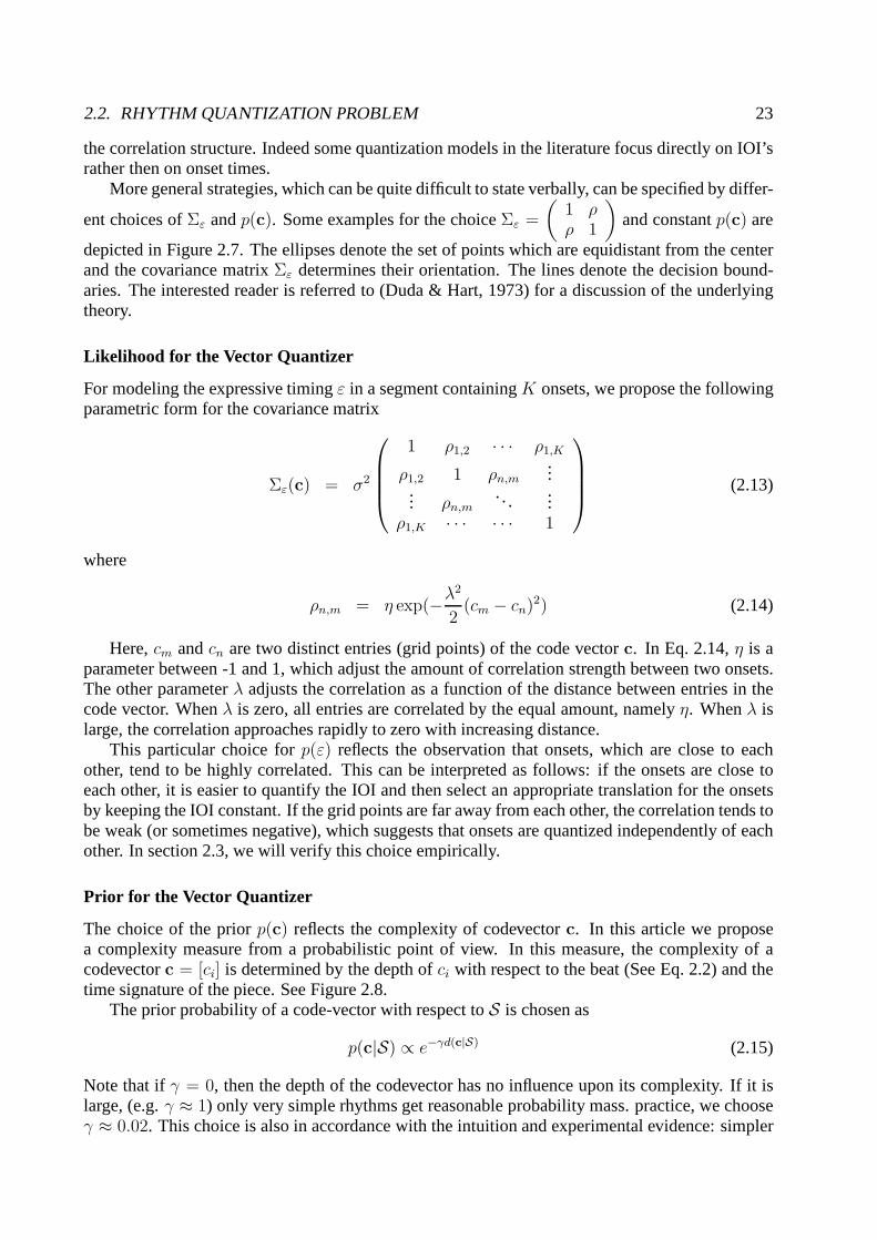
More general strategies, which can be quite difficult to state verbally, can be specified by differ-
ent choices ofΣε andp(c). Some examples for the choiceΣε =
(
1 ρρ 1
)
and constantp(c) are
depicted in Figure 2.7. The ellipses denote the set of pointswhich are equidistant from the centerand the covariance matrixΣε determines their orientation. The lines denote the decision bound-aries. The interested reader is referred to (Duda & Hart, 1973) for a discussion of the underlyingtheory.
Likelihood for the Vector Quantizer
For modeling the expressive timingε in a segment containingK onsets, we propose the followingparametric form for the covariance matrix
Σε(c) = σ2
1 ρ1,2 · · · ρ1,K
ρ1,2 1 ρn,m...
... ρn,m. . .
...ρ1,K · · · · · · 1
(2.13)
where
ρn,m = η exp(−λ2
2(cm − cn)2) (2.14)
Here,cm andcn are two distinct entries (grid points) of the code vectorc. In Eq. 2.14,η is aparameter between -1 and 1, which adjust the amount of correlation strength between two onsets.The other parameterλ adjusts the correlation as a function of the distance between entries in thecode vector. Whenλ is zero, all entries are correlated by the equal amount, namely η. Whenλ islarge, the correlation approaches rapidly to zero with increasing distance.
This particular choice forp(ε) reflects the observation that onsets, which are close to eachother, tend to be highly correlated. This can be interpretedas follows: if the onsets are close toeach other, it is easier to quantify the IOI and then select anappropriate translation for the onsetsby keeping the IOI constant. If the grid points are far away from each other, the correlation tends tobe weak (or sometimes negative), which suggests that onsetsare quantized independently of eachother. In section 2.3, we will verify this choice empirically.
Prior for the Vector Quantizer
The choice of the priorp(c) reflects the complexity of codevectorc. In this article we proposea complexity measure from a probabilistic point of view. In this measure, the complexity of acodevectorc = [ci] is determined by the depth ofci with respect to the beat (See Eq. 2.2) and thetime signature of the piece. See Figure 2.8.
The prior probability of a code-vector with respect toS is chosen as
p(c|S) ∝ e−γd(c|S) (2.15)
Note that ifγ = 0, then the depth of the codevector has no influence upon its complexity. If it islarge, (e.g.γ ≈ 1) only very simple rhythms get reasonable probability mass.practice, we chooseγ ≈ 0.02. This choice is also in accordance with the intuition and experimental evidence: simpler

24 Rhythm Quantization44 @ -�� � � �� � � �� � � �� � � � �(a) In lack of any other context, both onset sequences will sound the same.However the first notation is more complex44 � � � � � 3� � 34 �� � � � � � � �� � � �
(b) Assumed time signature determines the complexity of a notation
Figure 2.8: Complexity of a notation
rhythms are more frequently used then complex ones. The marginal prior of a codevector is foundby summing out all possible subdivision schemes.
p(c) =∑
S
p(c|S)p(S) (2.16)
wherep(S) is the prior distribution of subdivision schemas. For example, one can select possiblesubdivision schemas asS1 = [2, 2, 2], S2 = [3, 2, 2], S3 = [2, 3, 2]. If we have a preference towardsthe time signature (4/4), the prior can be taken asp(S) = [1/2, 1/4, 1/4]. In general, this choiceshould reflect the relative frequency of time signatures. Wepropose the following form for theprior of S = [si]
Table 2.1:w(si)
si 2 3 5 7 11 13 17 o/ww(si) 0 1 2 3 4 5 6 ∞
p(S) ∝ e−ξ∑
i w(si) (2.17)
wherew(si) is a simple weighting function given in Table 2.1. This form prefers subdivisions bysmall prime numbers, which reflects the intuition that rhythmic subdivisions by prime numberssuch as 7 or 11 are far less common then subdivisions such as 2 or 3. The parameterξ distributesprobability mass over the primes. Whenξ = 0, all subdivision schemata are equally probable. Asξ →∞, only subdivisions withsi = 2 have non-zero probability.
2.3 Verification of the Model
To choose the likelihoodp(t|c) and the priorp(c) in a way which is perceptually meaningful, weanalyzed data obtained from an psychoacoustical experiment where ten well trained subjects (nineconservatory students and a conservatory professor) have participated (Desain, Aarts, Cemgil,Kappen, van Thienen, & Trilsbeek, 1999). The experiment consisted of a perception task anda production task.
2.3. VERIFICATION OF THE MODEL 25
2.3.1 Perception Task
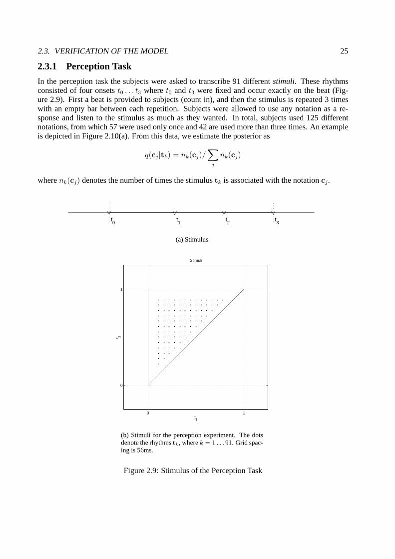
In the perception task the subjects were asked to transcribe91 differentstimuli. These rhythmsconsisted of four onsetst0 . . . t3 wheret0 and t3 were fixed and occur exactly on the beat (Fig-ure 2.9). First a beat is provided to subjects (count in), andthen the stimulus is repeated 3 timeswith an empty bar between each repetition. Subjects were allowed to use any notation as a re-sponse and listen to the stimulus as much as they wanted. In total, subjects used 125 differentnotations, from which 57 were used only once and 42 are used more than three times. An exampleis depicted in Figure 2.10(a). From this data, we estimate the posterior as
q(cj|tk) = nk(cj)/∑
j
nk(cj)
wherenk(cj) denotes the number of times the stimulustk is associated with the notationcj.
t0
t1
t2
t3
(a) Stimulus
0 1
0
1
t1
t 2
Stimuli
(b) Stimuli for the perception experiment. The dotsdenote the rhythmstk, wherek = 1 . . . 91. Grid spac-ing is 56ms.
Figure 2.9: Stimulus of the Perception Task
26 Rhythm Quantization
0 1/4 1/3 1/2 2/3 3/4 10
1/4
1/3
1/2
2/3
3/4
1
t1
t 2
(a) Perception
0 1/4 1/3 1/2 2/3 3/4 10
1/4
1/3
1/2
2/3
3/4
1
t1
t 2
(b) Production
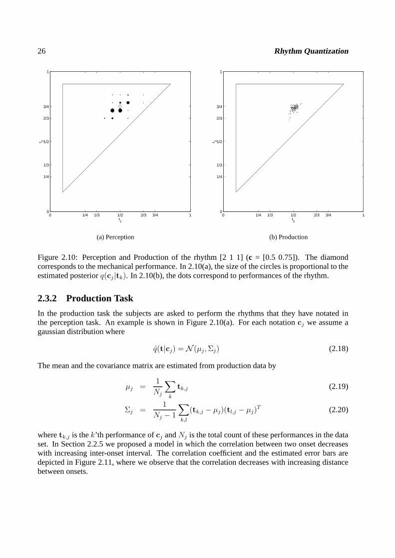
Figure 2.10: Perception and Production of the rhythm [2 1 1] (c = [0.5 0.75]). The diamondcorresponds to the mechanical performance. In 2.10(a), thesize of the circles is proportional to theestimated posteriorq(cj|tk). In 2.10(b), the dots correspond to performances of the rhythm.
2.3.2 Production Task
In the production task the subjects are asked to perform the rhythms that they have notated inthe perception task. An example is shown in Figure 2.10(a). For each notationcj we assume agaussian distribution where
q(t|cj) = N (µj,Σj) (2.18)
The mean and the covariance matrix are estimated from production data by
µj =1
Nj
∑
k
tk,j (2.19)
Σj =1
Nj − 1
∑
k,l
(tk,j − µj)(tl,j − µj)T (2.20)
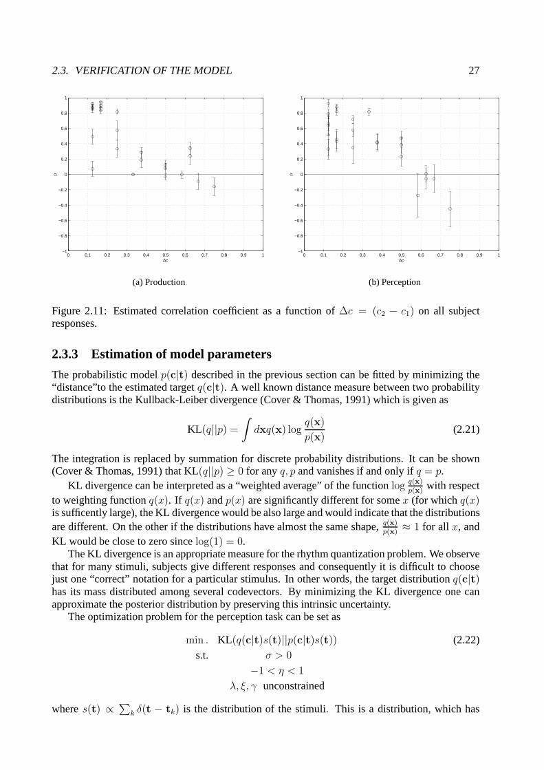
wheretk,j is thek’th performance ofcj andNj is the total count of these performances in the dataset. In Section 2.2.5 we proposed a model in which the correlation between two onset decreaseswith increasing inter-onset interval. The correlation coefficient and the estimated error bars aredepicted in Figure 2.11, where we observe that the correlation decreases with increasing distancebetween onsets.
2.3. VERIFICATION OF THE MODEL 27
0 0.1 0.2 0.3 0.4 0.5 0.6 0.7 0.8 0.9 1−1
−0.8
−0.6
−0.4
−0.2
0
0.2
0.4
0.6
0.8
1
∆c
ρ
(a) Production
0 0.1 0.2 0.3 0.4 0.5 0.6 0.7 0.8 0.9 1−1
−0.8
−0.6
−0.4
−0.2
0
0.2
0.4
0.6
0.8
1
∆c
ρ(b) Perception
Figure 2.11: Estimated correlation coefficient as a function of ∆c = (c2 − c1) on all subjectresponses.
2.3.3 Estimation of model parameters
The probabilistic modelp(c|t) described in the previous section can be fitted by minimizingthe“distance”to the estimated targetq(c|t). A well known distance measure between two probabilitydistributions is the Kullback-Leiber divergence (Cover & Thomas, 1991) which is given as
KL(q||p) =
∫
dxq(x) logq(x)
p(x)(2.21)
The integration is replaced by summation for discrete probability distributions. It can be shown(Cover & Thomas, 1991) that KL(q||p) ≥ 0 for anyq, p and vanishes if and only ifq = p.
KL divergence can be interpreted as a “weighted average” of the functionlog q(x)p(x)
with respectto weighting functionq(x). If q(x) andp(x) are significantly different for somex (for which q(x)is sufficently large), the KL divergence would be also large and would indicate that the distributionsare different. On the other if the distributions have almostthe same shape,q(x)
p(x)≈ 1 for all x, and
KL would be close to zero sincelog(1) = 0.The KL divergence is an appropriate measure for the rhythm quantization problem. We observe
that for many stimuli, subjects give different responses and consequently it is difficult to choosejust one “correct” notation for a particular stimulus. In other words, the target distributionq(c|t)has its mass distributed among several codevectors. By minimizing the KL divergence one canapproximate the posterior distribution by preserving thisintrinsic uncertainty.
The optimization problem for the perception task can be set as
min . KL(q(c|t)s(t)||p(c|t)s(t)) (2.22)
s.t. σ > 0
−1 < η < 1
λ, ξ, γ unconstrained
wheres(t) ∝ ∑k δ(t − tk) is the distribution of the stimuli. This is a distribution, which has
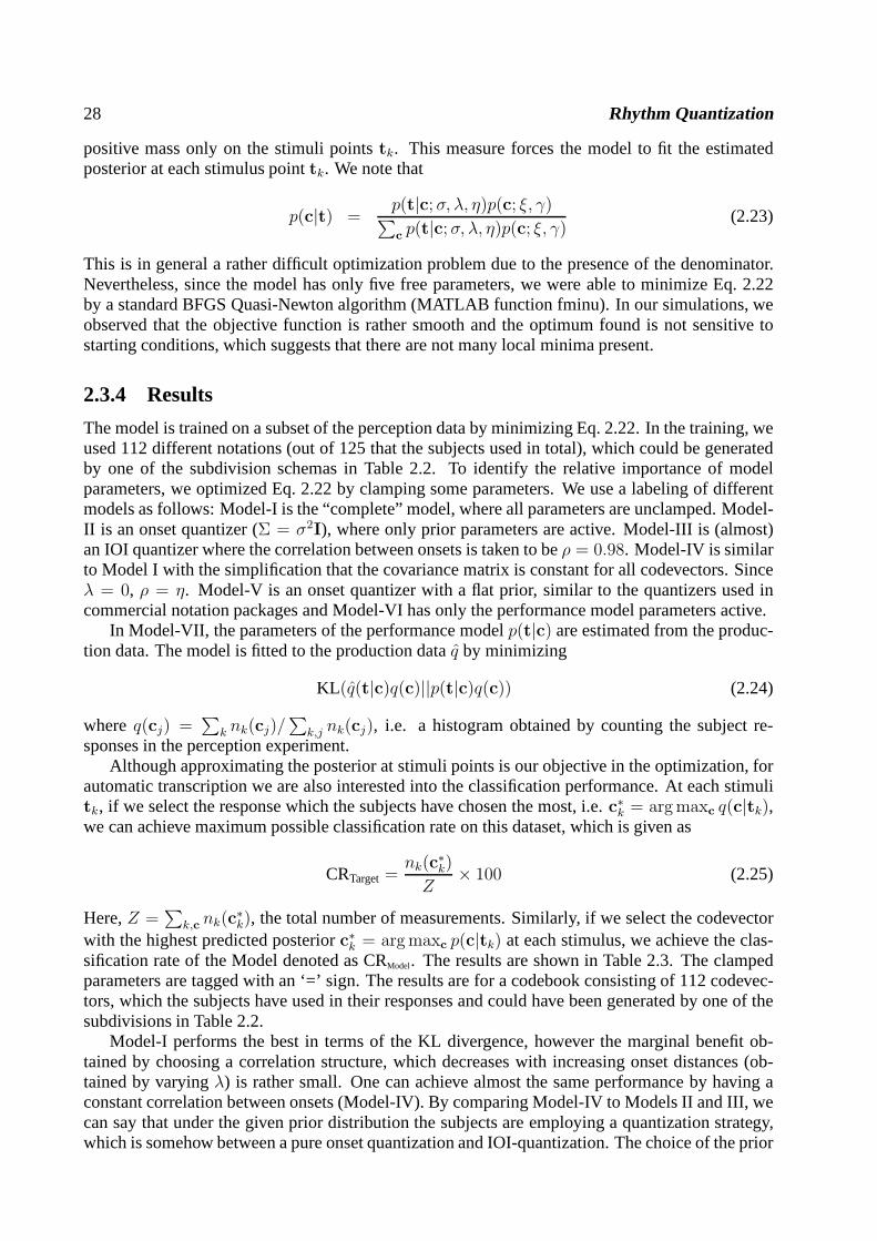
28 Rhythm Quantization
positive mass only on the stimuli pointstk. This measure forces the model to fit the estimatedposterior at each stimulus pointtk. We note that
p(c|t) =p(t|c; σ, λ, η)p(c; ξ, γ)
∑
cp(t|c; σ, λ, η)p(c; ξ, γ)
(2.23)
This is in general a rather difficult optimization problem due to the presence of the denominator.Nevertheless, since the model has only five free parameters,we were able to minimize Eq. 2.22by a standard BFGS Quasi-Newton algorithm (MATLAB functionfminu). In our simulations, weobserved that the objective function is rather smooth and the optimum found is not sensitive tostarting conditions, which suggests that there are not manylocal minima present.
2.3.4 Results
The model is trained on a subset of the perception data by minimizing Eq. 2.22. In the training, weused 112 different notations (out of 125 that the subjects used in total), which could be generatedby one of the subdivision schemas in Table 2.2. To identify the relative importance of modelparameters, we optimized Eq. 2.22 by clamping some parameters. We use a labeling of differentmodels as follows: Model-I is the “complete” model, where all parameters are unclamped. Model-II is an onset quantizer (Σ = σ2I), where only prior parameters are active. Model-III is (almost)an IOI quantizer where the correlation between onsets is taken to beρ = 0.98. Model-IV is similarto Model I with the simplification that the covariance matrixis constant for all codevectors. Sinceλ = 0, ρ = η. Model-V is an onset quantizer with a flat prior, similar to the quantizers used incommercial notation packages and Model-VI has only the performance model parameters active.
In Model-VII, the parameters of the performance modelp(t|c) are estimated from the produc-tion data. The model is fitted to the production dataq by minimizing
KL(q(t|c)q(c)||p(t|c)q(c)) (2.24)
whereq(cj) =∑
k nk(cj)/∑
k,j nk(cj), i.e. a histogram obtained by counting the subject re-sponses in the perception experiment.
Although approximating the posterior at stimuli points is our objective in the optimization, forautomatic transcription we are also interested into the classification performance. At each stimulitk, if we select the response which the subjects have chosen themost, i.e.c∗k = arg maxc q(c|tk),we can achieve maximum possible classification rate on this dataset, which is given as
CRTarget =nk(c
∗k)
Z× 100 (2.25)
Here,Z =∑
k,c nk(c∗k), the total number of measurements. Similarly, if we select the codevector
with the highest predicted posteriorc∗k = arg maxc p(c|tk) at each stimulus, we achieve the clas-sification rate of the Model denoted as CRModel. The results are shown in Table 2.3. The clampedparameters are tagged with an ‘=’ sign. The results are for a codebook consisting of 112 codevec-tors, which the subjects have used in their responses and could have been generated by one of thesubdivisions in Table 2.2.
Model-I performs the best in terms of the KL divergence, however the marginal benefit ob-tained by choosing a correlation structure, which decreases with increasing onset distances (ob-tained by varyingλ) is rather small. One can achieve almost the same performance by having aconstant correlation between onsets (Model-IV). By comparing Model-IV to Models II and III, wecan say that under the given prior distribution the subjectsare employing a quantization strategy,which is somehow between a pure onset quantization and IOI-quantization. The choice of the prior
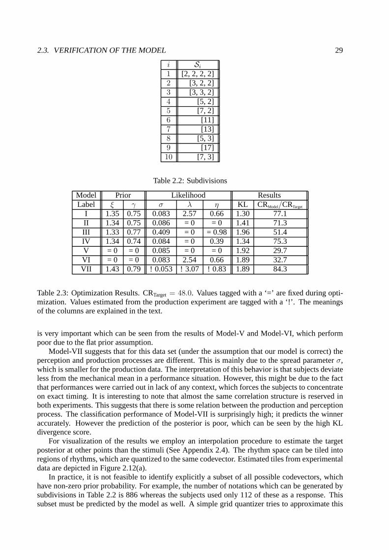
2.3. VERIFICATION OF THE MODEL 29
i Si
1 [2, 2, 2, 2]2 [3, 2, 2]3 [3, 3, 2]4 [5, 2]5 [7, 2]6 [11]7 [13]8 [5, 3]9 [17]10 [7, 3]
Table 2.2: Subdivisions
Model Prior Likelihood ResultsLabel ξ γ σ λ η KL CRModel/CRTarget
I 1.35 0.75 0.083 2.57 0.66 1.30 77.1II 1.34 0.75 0.086 = 0 = 0 1.41 71.3III 1.33 0.77 0.409 = 0 = 0.98 1.96 51.4IV 1.34 0.74 0.084 = 0 0.39 1.34 75.3V = 0 = 0 0.085 = 0 = 0 1.92 29.7VI = 0 = 0 0.083 2.54 0.66 1.89 32.7VII 1.43 0.79 ! 0.053 ! 3.07 ! 0.83 1.89 84.3
Table 2.3: Optimization Results. CRTarget = 48.0. Values tagged with a ‘=’ are fixed during opti-mization. Values estimated from the production experimentare tagged with a ‘!’. The meaningsof the columns are explained in the text.
is very important which can be seen from the results of Model-V and Model-VI, which performpoor due to the flat prior assumption.
Model-VII suggests that for this data set (under the assumption that our model is correct) theperception and production processes are different. This ismainly due to the spread parameterσ,which is smaller for the production data. The interpretation of this behavior is that subjects deviateless from the mechanical mean in a performance situation. However, this might be due to the factthat performances were carried out in lack of any context, which forces the subjects to concentrateon exact timing. It is interesting to note that almost the same correlation structure is reserved inboth experiments. This suggests that there is some relationbetween the production and perceptionprocess. The classification performance of Model-VII is surprisingly high; it predicts the winneraccurately. However the prediction of the posterior is poor, which can be seen by the high KLdivergence score.
For visualization of the results we employ an interpolationprocedure to estimate the targetposterior at other points than the stimuli (See Appendix 2.4). The rhythm space can be tiled intoregions of rhythms, which are quantized to the same codevector. Estimated tiles from experimentaldata are depicted in Figure 2.12(a).
In practice, it is not feasible to identify explicitly a subset of all possible codevectors, whichhave non-zero prior probability. For example, the number ofnotations which can be generated bysubdivisions in Table 2.2 is 886 whereas the subjects used only 112 of these as a response. Thissubset must be predicted by the model as well. A simple grid quantizer tries to approximate this
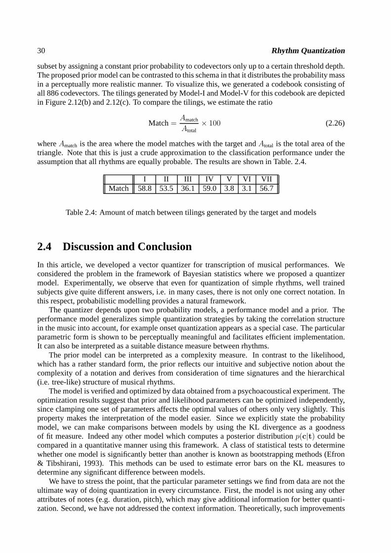
30 Rhythm Quantization
subset by assigning a constant prior probability to codevectors only up to a certain threshold depth.The proposed prior model can be contrasted to this schema in that it distributes the probability massin a perceptually more realistic manner. To visualize this,we generated a codebook consisting ofall 886 codevectors. The tilings generated by Model-I and Model-V for this codebook are depictedin Figure 2.12(b) and 2.12(c). To compare the tilings, we estimate the ratio
Match=Amatch
Atotal× 100 (2.26)
whereAmatch is the area where the model matches with the target andAtotal is the total area of thetriangle. Note that this is just a crude approximation to theclassification performance under theassumption that all rhythms are equally probable. The results are shown in Table. 2.4.
I II III IV V VI VIIMatch 58.8 53.5 36.1 59.0 3.8 3.1 56.7
Table 2.4: Amount of match between tilings generated by the target and models
2.4 Discussion and Conclusion
In this article, we developed a vector quantizer for transcription of musical performances. Weconsidered the problem in the framework of Bayesian statistics where we proposed a quantizermodel. Experimentally, we observe that even for quantization of simple rhythms, well trainedsubjects give quite different answers, i.e. in many cases, there is not only one correct notation. Inthis respect, probabilistic modelling provides a natural framework.
The quantizer depends upon two probability models, a performance model and a prior. Theperformance model generalizes simple quantization strategies by taking the correlation structurein the music into account, for example onset quantization appears as a special case. The particularparametric form is shown to be perceptually meaningful and facilitates efficient implementation.It can also be interpreted as a suitable distance measure between rhythms.
The prior model can be interpreted as a complexity measure. In contrast to the likelihood,which has a rather standard form, the prior reflects our intuitive and subjective notion about thecomplexity of a notation and derives from consideration of time signatures and the hierarchical(i.e. tree-like) structure of musical rhythms.
The model is verified and optimized by data obtained from a psychoacoustical experiment. Theoptimization results suggest that prior and likelihood parameters can be optimized independently,since clamping one set of parameters affects the optimal values of others only very slightly. Thisproperty makes the interpretation of the model easier. Since we explicitly state the probabilitymodel, we can make comparisons between models by using the KLdivergence as a goodnessof fit measure. Indeed any other model which computes a posterior distributionp(c|t) could becompared in a quantitative manner using this framework. A class of statistical tests to determinewhether one model is significantly better than another is known as bootstrapping methods (Efron& Tibshirani, 1993). This methods can be used to estimate error bars on the KL measures todetermine any significant difference between models.
We have to stress the point, that the particular parameter settings we find from data are not theultimate way of doing quantization in every circumstance. First, the model is not using any otherattributes of notes (e.g. duration, pitch), which may give additional information for better quanti-zation. Second, we have not addressed the context information. Theoretically, such improvements
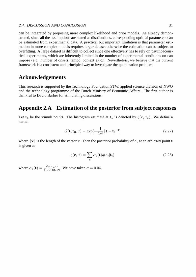
2.4. DISCUSSION AND CONCLUSION 31
can be integrated by proposing more complex likelihood and prior models. As already demon-strated, since all the assumptions are stated as distributions, corresponding optimal parameters canbe estimated from experimental data. A practical but important limitation is that parameter esti-mation in more complex models requires larger dataset otherwise the estimation can be subject tooverfitting. A large dataset is difficult to collect since oneeffectively has to rely on psychoacous-tical experiments, which are inherently limited in the number of experimental conditions on canimpose (e.g. number of onsets, tempo, context e.t.c.). Nevertheless, we believe that the currentframework is a consistent and principled way to investigatethe quantization problem.
Acknowledgements
This research is supported by the Technology Foundation STW, applied science division of NWOand the technology programme of the Dutch Ministry of Economic Affairs. The first author isthankful to David Barber for stimulating discussions.
Appendix 2.A Estimation of the posterior from subject responses
Let tk be the stimuli points. The histogram estimate attk is denoted byq(cj|tk). We define akernel
G(t; t0, σ) = exp(− 1
2σ2‖t− t0‖2) (2.27)
where‖x‖ is the length of the vectorx. Then the posterior probability ofcj at an arbitrary pointtis given as
q(cj|t) =∑
k
αk(t)q(cj|ti) (2.28)
whereαk(t) = G(t;tk,σ)∑
r G(t;tr,σ). We have takenσ = 0.04.

32 Rhythm Quantization
0 1/4 1/3 1/2 2/3 3/4 10
1/4
1/3
1/2
2/3
3/4
1
t1
t 2
(a) Target
0 1/4 1/3 1/2 2/3 3/4 10
1/4
1/3
1/2
2/3
3/4
1
t1
t 2
(b) Model-I: (ξ, γ, σ, λ, η) =
(1.35, 0.75, 0.083, 2.57, 0.66)
0 1/4 1/3 1/2 2/3 3/4 10
1/4
1/3
1/2
2/3
3/4
1
t1
t 2
(c) Model-V:(ξ, γ, σ, λ, η) = (0, 0, 0.085, 0, 0)
Figure 2.12: Tilings of the rhythm space byc∗ = argmaxc
p(c|t). The tiles denote the sets of
rhythms, which would be quantized to the same codevector. Both Model-I and Model-V usethe same codebook of 886 codevectors. Since Model-V assignsthe same prior probability toall codevectors, the best codevector is always the nearest codevector (in Euclidian distance) andconsequently the rhythm space is highly fragmented.
Chapter 3
Tempo Tracking
We formulate tempo tracking in a Bayesian framework where a tempo tracker is modeled asa stochastic dynamical system. The tempo is modeled as a hidden state variable of the systemand is estimated by aKalman filter. The Kalman filter operates on aTempogram, a wavelet-like multiscale expansion of a real performance. An important advantage of our approach isthat it is possible to formulate both off-line or real-time algorithms. The simulation resultson a systematically collected set of MIDI piano performances of Yesterday and Michelle bythe Beatles shows accurate tracking of approximately%90 of the beats.
Adapted from: A. T. Cemgil, H. J. Kappen, P. Desain, and H. Honing. Ontempo tracking: Tempogram representation and Kalman filtering. Journalof New Music Research, 28:4:259-273, 2001.
3.1 Introduction
An important and interesting subtask in automatic music transcription is tempo tracking: how tofollow the tempo in a performance that contains expressive timing and tempo variations. Whenthese tempo fluctuations are correctly identified it becomesmuch easier to separate the continuousexpressive timing from the discrete note categories (i.e. quantization). The sense of tempo seemsto be carried by the beats and thus tempo tracking is related to the study of beat induction, theperception of beats or pulse while listening to music (see (Desain & Honing, 1994)). However, itis still unclear what precisely constitutes tempo and how itrelates to the perception of rhythmicalstructure. Tempo is a perceptual construct and cannot directly be measured in a performance.
In the context of tempo tracking, wavelet analysis and related techniques are already investi-gated by various researchers (Smith, 1999; Todd, 1994). A similar comb filter basis is used by(Scheirer, 1998). The tempogram is also related to the periodicity transform proposed by (Sethares& Staley, 1999), but uses a time localized basis. Kalman filters are already applied in the musicdomain such as polyphonic pitch tracking (Sterian, 1999) and audio restoration (Godsill & Rayner,1998). From the modeling point of view, the framework discussed in this paper has also some re-semblance to the work of (Sterian, 1999), who views transcription as a model based segmentationof a time-frequency image.
The outline of the paper is as follows: We first consider the problem of tapping along a “noisy”metronome and introduce the Kalman filter and its extensions. Subsequently, we introduce theTempogram representation to extract beats from performances and discuss the probabilistic in-terpretation. Consequently, we discuss parameter estimation issues from data. Finally we reportsimulation results of the system on a systematically collected data set, solo piano performances oftwo Beatles songs, Yesterday and Michelle.
33

34 Tempo Tracking
3.2 Dynamical Systems and the Kalman Filter
Mathematically, a dynamical system is characterized by a set of state variablesand a set ofstatetransition equationsthat describe how state variables evolve with time. For example, a perfectmetronome can be described as a dynamical system with two state variables: a beatτ and a period∆. Given the values of state variables atj − 1’th step asτj−1 and∆j−1, the next beat occurs atτj = τj−1 + ∆j−1. The period of a perfect metronome is constant so∆j = ∆j−1. By using vectornotation and by lettingsj = [τj , ∆j]
T we can write a linear state transition model as
sj =
(
1 10 1
)
sj−1 = Asj−1 (3.1)
When the initial states0 = [τ0, ∆0]T is given, the system is fully specified. For example if the
metronom clicks at a tempo 60 beats per minute (∆0 = 1 sec.) and first click occurs at timeτ0 = 0sec., next beats occur atτ1 = 1, τ2 = 2 e.t.c. Since the metronom is perfect the period staysconstant.
Such a deterministic model is not realistic for natural music performance and can not be usedfor tracking the tempo in presence of tempo fluctuations and expressive timing deviations. Tempofluctuations may be modeled by introducing a noise term that “corrupts” the state vector
sj = Asj−1 + vj (3.2)
wherev is a Gaussian random vector with mean0 and diagonal covariance matrixQ, i.e. v ∼N (0,Q)1. The tempo will drift from the initial tempo quickly if the variance ofv is large. On theother hand whenQ→ 0, we have the constant tempo case.
In a music performance, the actual beatτ and the period∆ can not be observed directly. Byactual beat we refer to the beat iterpretation that coincides with human perception when listening tomusic. For example, suppose, an expert drummer is tapping along a performance at the beat leveland we assume her beats as the correct tempo track. If the taskwould be repeated on the samepiece, we would observe each time a slightly different tempotrack. As an alternative, suppose wewould know the score of the performance and identify onsets that coincide with the beat. However,due to small scale expressive timing deviations, these onsets will be also noisy, i.e. we can at bestobserve “noisy” versions of actual beats. We will denote this noisy beat byτ in contrast to theactual but unobservable beatτ . Mathematically we have
τj = τj + wj (3.3)
wherewj ∼ N (0,R). Here,τj is the beat at stepj that we get from a (noisy) observation process.In this formulation, tempo tracking corresponds to the estimation of hidden variablesτj givenobservations uptoj’th step. We note that in a “blind” tempo tracking task, i.e. when the score isnot known, the (noisy) beatτj can not be directly observed since there is no expert drummerwhois tapping along, neither a score to guide us. The noisy-beatitself has to beinducedfrom events inthe music. In the next section we will present a technique to estimate both a noisy beatτj as wella noisy period∆j from a real performance.
1A random vectorx is said to be Gaussian with meanµ and covariance matrixP if it has the probability density
p(x) = |2πP|−1/2 exp−1
2(x− µ)T P−1(x− µ)
In this case we writex ∼ N (µ,P)

3.2. DYNAMICAL SYSTEMS AND THE KALMAN FILTER 35
Equations 3.2 and 3.3 define alinear dynamical system, because all noises are assumed tobe Gaussian and all relationships between variables are linear. Hence, all state vectorssj haveGaussian distributions. A Gaussian distribution is fully characterized by its mean and covariancematrix and in the context of linear dynamical systems, thesequantities can be estimated veryefficiently by aKalman filter(Kalman, 1960; Roweis & Ghahramani, 1999). The operation ofthefilter is illustrated in Figure 3.1.
(a) The algorithm starts withthe initial state estimateN (µ1|0, P1|0). In presence ofno evidence this state estimategives rise to a prediction inthe observableτ space,
(b) The beat is observedat τ1, The state is updatedto N (µ1|1, P1|1) according tothe new evidence. Note thatthe uncertainty “shrinks”,
(c) On the basis of cur-rent state a new predictionN (µ2|1, P2|1) is made,
(d) Steps are repeated un-til all evidence is processedto obtain filtered estimatesN (µj|j , Pj|j), j = 1 . . .N . Inthis caseN = 3.
(e) Filtered estimates areupdated by backtracking toobtain smoothed estimatesN (µi|N , Pi|N ) (Kalmansmoothing).
Figure 3.1:Operation of the Kalman Filter and Smoother. The system is given by Equations 3.2 and 3.3.In each subfigure, the above coordinate system represents the hidden state space[τ , ∆]T and the belowcoordinate system represent the observable spaceτ . In the hidden space, the x and y axes represent thephaseτ period∆ of the tracker. The ellipse and its center correspond to the covariance and the mean of thehidden state estimatep(sj |τ1 . . . τk) = N (µj|k, Pj|k) whereµj|k andPj|k denote the estimated mean andcovariance given observationsτ1 . . . τk. In the observable space, the vertical axis represents the predictiveprobability distributionp(τj |τj−1 . . . τ1).
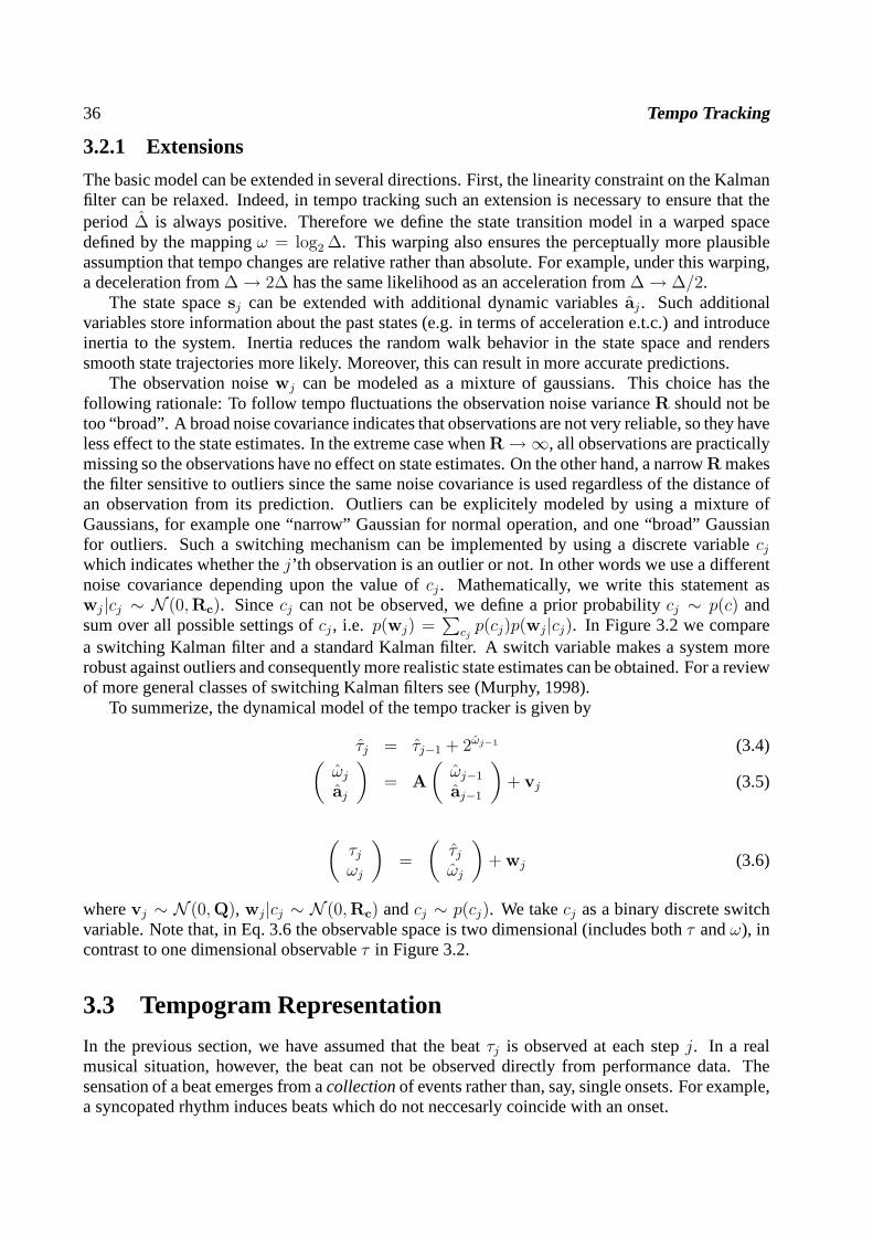
36 Tempo Tracking
3.2.1 Extensions
The basic model can be extended in several directions. First, the linearity constraint on the Kalmanfilter can be relaxed. Indeed, in tempo tracking such an extension is necessary to ensure that theperiod ∆ is always positive. Therefore we define the state transitionmodel in a warped spacedefined by the mappingω = log2 ∆. This warping also ensures the perceptually more plausibleassumption that tempo changes are relative rather than absolute. For example, under this warping,a deceleration from∆→ 2∆ has the same likelihood as an acceleration from∆→ ∆/2.
The state spacesj can be extended with additional dynamic variablesaj . Such additionalvariables store information about the past states (e.g. in terms of acceleration e.t.c.) and introduceinertia to the system. Inertia reduces the random walk behavior in the state space and renderssmooth state trajectories more likely. Moreover, this can result in more accurate predictions.
The observation noisewj can be modeled as a mixture of gaussians. This choice has thefollowing rationale: To follow tempo fluctuations the observation noise varianceR should not betoo “broad”. A broad noise covariance indicates that observations are not very reliable, so they haveless effect to the state estimates. In the extreme case whenR→∞, all observations are practicallymissing so the observations have no effect on state estimates. On the other hand, a narrowR makesthe filter sensitive to outliers since the same noise covariance is used regardless of the distance ofan observation from its prediction. Outliers can be explicitely modeled by using a mixture ofGaussians, for example one “narrow” Gaussian for normal operation, and one “broad” Gaussianfor outliers. Such a switching mechanism can be implementedby using a discrete variablecjwhich indicates whether thej’th observation is an outlier or not. In other words we use a differentnoise covariance depending upon the value ofcj . Mathematically, we write this statement aswj |cj ∼ N (0,Rc). Sincecj can not be observed, we define a prior probabilitycj ∼ p(c) andsum over all possible settings ofcj , i.e. p(wj) =
∑
cjp(cj)p(wj |cj). In Figure 3.2 we compare
a switching Kalman filter and a standard Kalman filter. A switch variable makes a system morerobust against outliers and consequently more realistic state estimates can be obtained. For a reviewof more general classes of switching Kalman filters see (Murphy, 1998).
To summerize, the dynamical model of the tempo tracker is given by
τj = τj−1 + 2ωj−1 (3.4)(
ωj
aj
)
= A
(
ωj−1
aj−1
)
+ vj (3.5)
(
τjωj
)
=
(
τjωj
)
+ wj (3.6)
wherevj ∼ N (0,Q), wj|cj ∼ N (0,Rc) andcj ∼ p(cj). We takecj as a binary discrete switchvariable. Note that, in Eq. 3.6 the observable space is two dimensional (includes bothτ andω), incontrast to one dimensional observableτ in Figure 3.2.
3.3 Tempogram Representation
In the previous section, we have assumed that the beatτj is observed at each stepj. In a realmusical situation, however, the beat can not be observed directly from performance data. Thesensation of a beat emerges from acollectionof events rather than, say, single onsets. For example,a syncopated rhythm induces beats which do not neccesarly coincide with an onset.
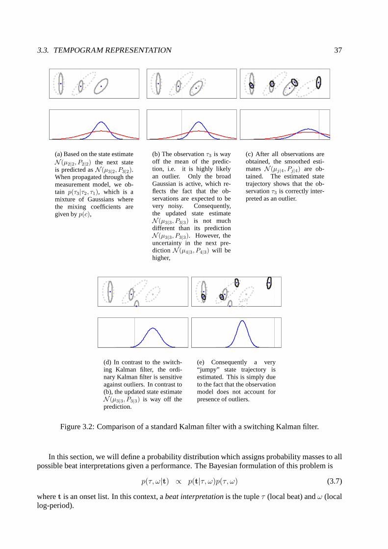
3.3. TEMPOGRAM REPRESENTATION 37
(a) Based on the state estimateN (µ2|2, P2|2) the next stateis predicted asN (µ3|2, P3|2).When propagated through themeasurement model, we ob-tain p(τ3|τ2, τ1), which is amixture of Gaussians wherethe mixing coefficients aregiven byp(c),
(b) The observationτ3 is wayoff the mean of the predic-tion, i.e. it is highly likelyan outlier. Only the broadGaussian is active, which re-flects the fact that the ob-servations are expected to bevery noisy. Consequently,the updated state estimateN (µ3|3, P3|3) is not muchdifferent than its predictionN (µ3|3, P3|3). However, theuncertainty in the next pre-diction N (µ4|3, P4|3) will behigher,
(c) After all observations areobtained, the smoothed esti-matesN (µj|4, Pj|4) are ob-tained. The estimated statetrajectory shows that the ob-servationτ3 is correctly inter-preted as an outlier.
(d) In contrast to the switch-ing Kalman filter, the ordi-nary Kalman filter is sensitiveagainst outliers. In contrast to(b), the updated state estimateN (µ3|3, P3|3) is way off theprediction.
(e) Consequently a very“jumpy” state trajectory isestimated. This is simply dueto the fact that the observationmodel does not account forpresence of outliers.
Figure 3.2: Comparison of a standard Kalman filter with a switching Kalman filter.
In this section, we will define a probability distribution which assigns probability masses to allpossible beat interpretations given a performance. The Bayesian formulation of this problem is
p(τ, ω|t) ∝ p(t|τ, ω)p(τ, ω) (3.7)
wheret is an onset list. In this context, abeat interpretationis the tupleτ (local beat) andω (locallog-period).
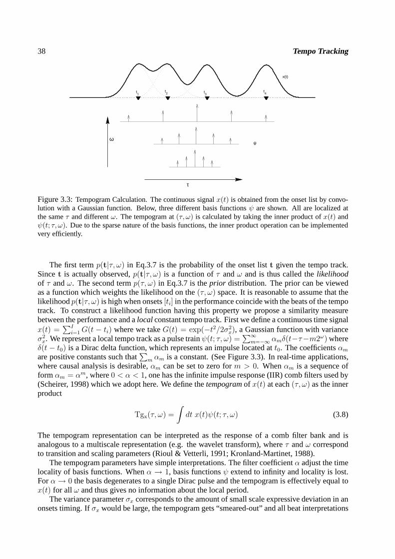
38 Tempo Tracking
τ
ω
x(t)
t1 t
2 t
3 t
4
ψ
Figure 3.3:Tempogram Calculation. The continuous signalx(t) is obtained from the onset list by convo-lution with a Gaussian function. Below, three different basis functionsψ are shown. All are localized atthe sameτ and differentω. The tempogram at(τ, ω) is calculated by taking the inner product ofx(t) andψ(t; τ, ω). Due to the sparse nature of the basis functions, the inner product operation can be implementedvery efficiently.
The first termp(t|τ, ω) in Eq.3.7 is the probability of the onset listt given the tempo track.Sincet is actually observed,p(t|τ, ω) is a function ofτ andω and is thus called thelikelihoodof τ andω. The second termp(τ, ω) in Eq.3.7 is theprior distribution. The prior can be viewedas a function which weights the likelihood on the(τ, ω) space. It is reasonable to assume that thelikelihoodp(t|τ, ω) is high when onsets[ti] in the performance coincide with the beats of the tempotrack. To construct a likelihood function having this property we propose a similarity measurebetween the performance and alocalconstant tempo track. First we define a continuous time signalx(t) =
∑Ii=1G(t − ti) where we takeG(t) = exp(−t2/2σ2
x), a Gaussian function with varianceσ2
x. We represent a local tempo track as a pulse trainψ(t; τ, ω) =∑∞
m=−∞ αmδ(t−τ−m2ω) whereδ(t − t0) is a Dirac delta function, which represents an impulse located att0. The coefficientsαm
are positive constants such that∑
m αm is a constant. (See Figure 3.3). In real-time applications,where causal analysis is desirable,αm can be set to zero form > 0. Whenαm is a sequence offormαm = αm, where0 < α < 1, one has the infinite impulse response (IIR) comb filters usedby(Scheirer, 1998) which we adopt here. We define thetempogramof x(t) at each(τ, ω) as the innerproduct
Tgx(τ, ω) =
∫
dt x(t)ψ(t; τ, ω) (3.8)
The tempogram representation can be interpreted as the response of a comb filter bank and isanalogous to a multiscale representation (e.g. the wavelettransform), whereτ andω correspondto transition and scaling parameters (Rioul & Vetterli, 1991; Kronland-Martinet, 1988).
The tempogram parameters have simple interpretations. Thefilter coefficientα adjust the timelocality of basis functions. Whenα → 1, basis functionsψ extend to infinity and locality is lost.Forα → 0 the basis degenerates to a single Dirac pulse and the tempogram is effectively equal tox(t) for all ω and thus gives no information about the local period.
The variance parameterσx corresponds to the amount of small scale expressive deviation in anonsets timing. Ifσx would be large, the tempogram gets “smeared-out” and all beat interpretations
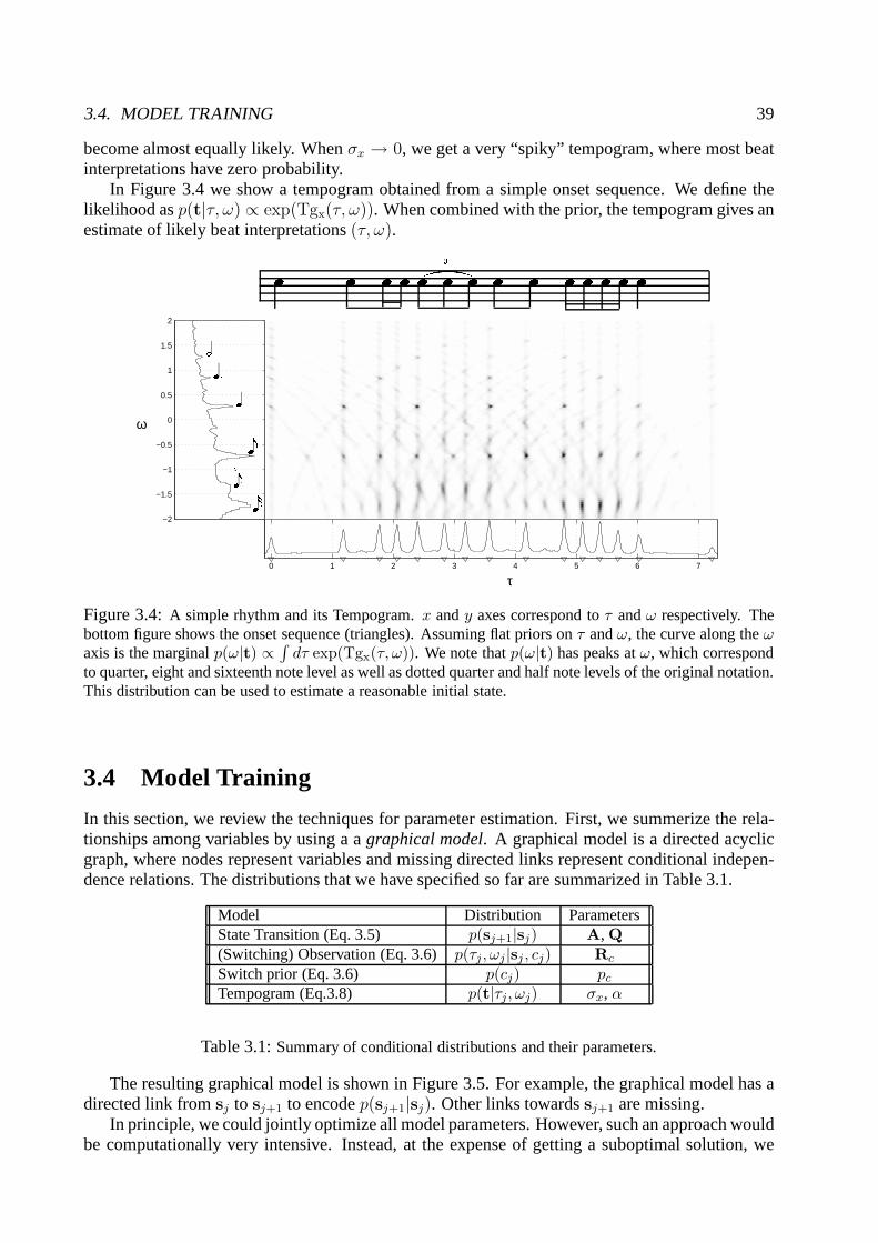
3.4. MODEL TRAINING 39
become almost equally likely. Whenσx → 0, we get a very “spiky” tempogram, where most beatinterpretations have zero probability.
In Figure 3.4 we show a tempogram obtained from a simple onsetsequence. We define thelikelihood asp(t|τ, ω) ∝ exp(Tgx(τ, ω)). When combined with the prior, the tempogram gives anestimate of likely beat interpretations(τ, ω).
−2
−1.5
−1
−0.5
0
0.5
1
1.5
2
0 1 2 3 4 5 6 7
� � � � � 3� � � � � � � � � �(� )�
� �� �3 (�
ω
τ
Figure 3.4:A simple rhythm and its Tempogram.x andy axes correspond toτ andω respectively. Thebottom figure shows the onset sequence (triangles). Assuming flat priors onτ andω, the curve along theωaxis is the marginalp(ω|t) ∝
∫
dτ exp(Tgx(τ, ω)). We note thatp(ω|t) has peaks atω, which correspondto quarter, eight and sixteenth note level as well as dotted quarter and half note levels of the original notation.This distribution can be used to estimate a reasonable initial state.
3.4 Model Training
In this section, we review the techniques for parameter estimation. First, we summerize the rela-tionships among variables by using a agraphical model. A graphical model is a directed acyclicgraph, where nodes represent variables and missing directed links represent conditional indepen-dence relations. The distributions that we have specified sofar are summarized in Table 3.1.
Model Distribution ParametersState Transition (Eq. 3.5) p(sj+1|sj) A, Q(Switching) Observation (Eq. 3.6)p(τj, ωj |sj , cj) Rc
Switch prior (Eq. 3.6) p(cj) pc
Tempogram (Eq.3.8) p(t|τj, ωj) σx, α
Table 3.1:Summary of conditional distributions and their parameters.
The resulting graphical model is shown in Figure 3.5. For example, the graphical model has adirected link fromsj to sj+1 to encodep(sj+1|sj). Other links towardssj+1 are missing.
In principle, we could jointly optimize all model parameters. However, such an approach wouldbe computationally very intensive. Instead, at the expenseof getting a suboptimal solution, we
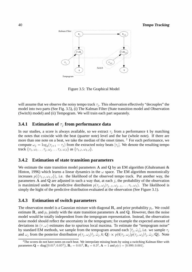
40 Tempo Tracking
c j
s j
[ τ,∆] j
t
c j+1
s j+1
[ τ,∆] j+1
t
Kalman Filter
Tempogram
Switch
Figure 3.5: The Graphical Model
will assume that we observe the noisy tempo trackτj . This observation effectively “decouples” themodel into two parts (See Fig. 3.5), (i) The Kalman Filter (State transition model and Observation(Switch) model) and (ii) Tempogram. We will train each part separately.
3.4.1 Estimation ofτj from performance data
In our studies, a score is always available, so we extractτj from a performancet by matchingthe notes that coincide with the beat (quarter note) level and the bar (whole note). If there aremore than one note on a beat, we take the median of the onset times.2 For each performance, wecomputeωj = log2(τj+1 − τj) from the extracted noisy beats[τj ]. We denote the resulting tempotrack{τ1, ω1 . . . τj , ωj . . . τJ , ωJ} as{τ1:J , ω1:J}.
3.4.2 Estimation of state transition parameters
We estimate the state transition model parametersA andQ by an EM algorithm (Ghahramani &Hinton, 1996) which learns a linear dynamics in theω space. The EM algorithm monotonicallyincreasesp({τ1:J , ω1:J}), i.e. the likelihood of the observed tempo track. Put another way, theparametersA andQ are adjusted in such a way that, at eachj, the probability of the observationis maximized under the predictive distributionp(τj , ωj|τj−1, ωj−1, . . . τ1, ω1). The likelihood issimply the hight of the predictive distribution evaluated at the observation (See Figure 3.1).
3.4.3 Estimation of switch parameters
The observation model is a Gaussian mixture with diagonalRc and prior probabilitypc. We couldestimateRc andpc jointly with the state transition parametersA andQ. However, then the noisemodel would be totally independent from the tempogram representation. Instead, the observationnoise model should reflect the uncertainty in the tempogram;for example the expected amount ofdeviations in(τ, ω) estimates due to spurious local maxima. To estimate the “tempogram noise”by standard EM methods, we sample from the tempogram around each[τj , ωj], i.e. we sampleτjandωj from the posterior distributionp(τj , ωj|τj , ωj, t;Q) ∝ p(t|τj, ωj)p(τj, ωj|τj , ωj;Q). Note
2The scores do not have notes on each beat. We interpolate missing beats by using a switching Kalman filter withparametersQ = diag([0.012, 0.052]), R1 = 0.012, R2 = 0.32, A = 1 andp(c) = [0.999, 0.001].

3.5. EVALUATION 41
that [τj , ωj] are estimated during the E step of the EM algorithm when finding the parametersAandQ.
3.4.4 Estimation of Tempogram parameters
We have already defined the tempogram as a likelihoodp(t|τ, ω; θ) whereθ denotes the tempogramparameters (e.g.θ = {α, σx}). If we assume a uniform priorp(τ, ω) then the posterior probabilitycan be written as
p(τ, ω|t; θ) =p(t|τ, ω; θ)
p(t|θ) (3.9)
where the normalization constant is given byp(t|θ) =∫
dτdωp(t|τ, ω; θ). Now, we can estimatetempogram parametersθ by a maximum likelihood approach. We write the log-likelihood of anobserved tempo track{τ1:J , ω1:J} as
log p({τ1:J , ω1:J}|t; θ) =∑
j
log p(τj , ωj|t; θ) (3.10)
Note that the quantity in Equation 3.10 is a function of the parametersθ. If we havek tempo tracksin the dataset, the complete data log-likelihood is simply the sum of all individual log-likelihoods.i.e.
L =∑
k
log p({τ1:J , ω1:J}k|tk;α, σx) (3.11)
wheretk is thek’th performance and{τ1:J , ω1:J}k is the corresponding tempo track.
3.5 Evaluation
Many tempo trackers described in the introduction are oftentested with ad hoc examples. However,to validate tempo tracking models, more systematic data andrigorous testing is necessary. Atempo tracker can be evaluated by systematically modulating the tempo of the data, for instance byapplying instantaneous or gradual tempo changes and comparing the models responses to humanbehavior (Michon, 1967; Dannenberg, 1993). Another approach is to evaluate tempo trackers ona systematically collected set of natural data, monitoringpiano performances in which the use ofexpressive tempo change is free. This type of data has the advantage of reflecting the type of dataone expects automated music transcription systems to deal with. The latter approach was adoptedin this study.
3.5.1 Data
For the experiment 12 pianists were invited to play arrangements of two Beatles songs, Michelleand Yesterday. Both pieces have a relatively simple rhythmic structure with ample opportunity toadd expressiveness by fluctuating the tempo. The subjects consisted of four professional jazz play-ers (PJ), four professional classical performers (PC) and four amateur classical pianists (AC). Eacharrangement had to be played in three tempo conditions, three repetitions per tempo condition. Thetempo conditions were normal, slow and fast tempo (all in a musically realistic range and all ac-cording to the judgment of the performer). We present here the results for twelve subjects (12 sub-jects× 3 tempi× 3 repetitions× 2 pieces= 216 performances). The performances were recorded
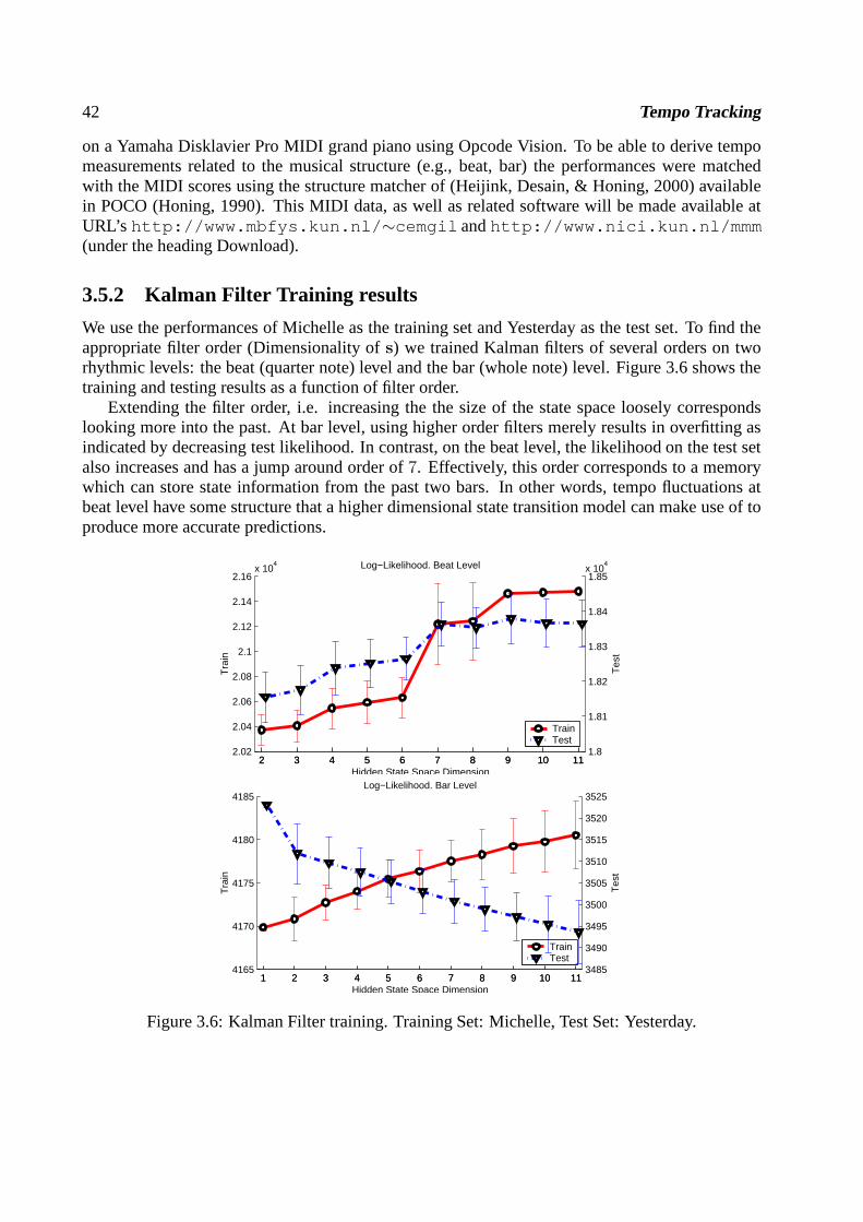
42 Tempo Tracking
on a Yamaha Disklavier Pro MIDI grand piano using Opcode Vision. To be able to derive tempomeasurements related to the musical structure (e.g., beat,bar) the performances were matchedwith the MIDI scores using the structure matcher of (Heijink, Desain, & Honing, 2000) availablein POCO (Honing, 1990). This MIDI data, as well as related software will be made available atURL’s http://www.mbfys.kun.nl/∼cemgil andhttp://www.nici.kun.nl/mmm(under the heading Download).
3.5.2 Kalman Filter Training results
We use the performances of Michelle as the training set and Yesterday as the test set. To find theappropriate filter order (Dimensionality ofs) we trained Kalman filters of several orders on tworhythmic levels: the beat (quarter note) level and the bar (whole note) level. Figure 3.6 shows thetraining and testing results as a function of filter order.
Extending the filter order, i.e. increasing the the size of the state space loosely correspondslooking more into the past. At bar level, using higher order filters merely results in overfitting asindicated by decreasing test likelihood. In contrast, on the beat level, the likelihood on the test setalso increases and has a jump around order of7. Effectively, this order corresponds to a memorywhich can store state information from the past two bars. In other words, tempo fluctuations atbeat level have some structure that a higher dimensional state transition model can make use of toproduce more accurate predictions.
2 3 4 5 6 7 8 9 10 112.02
2.04
2.06
2.08
2.1
2.12
2.14
2.16x 10
4
Tra
in
TrainTest
2 3 4 5 6 7 8 9 10 111.8
1.81
1.82
1.83
1.84
1.85x 10
4
Tes
t
Log−Likelihood. Beat Level
Hidden State Space Dimension
1 2 3 4 5 6 7 8 9 10 114165
4170
4175
4180
4185
Tra
in
TrainTest
1 2 3 4 5 6 7 8 9 10 113485
3490
3495
3500
3505
3510
3515
3520
3525
Tes
t
Log−Likelihood. Bar Level
Hidden State Space Dimension
Figure 3.6: Kalman Filter training. Training Set: Michelle, Test Set: Yesterday.
3.5. EVALUATION 43
3.5.3 Tempogram Training Results
We use a tempogram model with a first order IIR comb basis. Thischoice leaves two free pa-rameters that need to be estimated from data, namelyα, the coefficient of the comb filter andσx,the width of the Gaussian window. We obtain optimal parameter values by maximization of thelog-likelihood in Equation 3.11 on the Michelle dataset. The optimal parameters are shown inTable 3.2.
α σx
Non-Causal 0.55 0.017Causal 0.73 0.023
Table 3.2:Optimal tempogram parameters.
3.5.4 Initialization
To have a fully automated tempo tracker, the initial states0 has to be estimated from data aswell. In the tracking experiments, we have initialized the filter to the beat level by computinga tempogram for the first5 seconds of each performance. By assuming a flat prior onτ andω we compute the posterior marginalp(ω|t) =
∫
dτp(ω, τ |t). Note that this is operation is justequivalent to summation along theτ dimension of the tempogram (See Figure 3.4). For the Beatlesdataset, we have observed that for all performances of a given piece, the most likely log-periodω∗ = arg maxω p(ω|t) corresponds always to the same level, i.e. theω∗ estimate was alwaysconsistent. For “Michelle”, this level is the beat level andfor “Yesterday” the half-beat (eighthnote) level. The latter piece begins with an arpeggio of eight notes; based on onset informationonly, and without any other prior knowledge, half-beat level is also a reasonable solution. For“Yesterday”, to test the tracking performance, we corrected the estimate to the beat level.
We could estimateτ ∗ using a similar procedure, however since all performances in our dataset started “on the beat”, we have chosenτ ∗ = t1, the first onset of the piece. All the other statevariablesa0 are set to zero. We have chosen a broad initial state covarianceP0 = 9Q.
3.5.5 Evaluation of tempo tracking performance
We evaluated the accuracy of the tempo tracking performanceof the complete model. The accuracyof tempo tracking is measured by using the following criterion:
ρ(ψ, t) =
∑
i maxj W (ψi − tj)(I + J)/2
× 100
where [ψi] i = 1 . . . I is the target (true) tempo track and[tj ] j = 1 . . . J is the estimatedtempo track.W is a window function. In the following results we have used a Gaussian windowfunctionW (d) = exp(−d2/2σ2
e). The width of the window is chosen asσe = 0.04 sec whichcorresponds roughly to the spread of onsets from their mechanical means during performance ofshort rhythms (Cemgil, Desain, & Kappen, 2000).
It can be checked that0 ≤ ρ ≤ 100 andρ = 100 if and only ifψ = t. Intuitively, this measureis similar to a normalized inner-product (as in the tempogram calculation); the difference is in themax operator which merely avoids double counting. For example,if the target isψ = [0, 1, 2]and we havet = [0, 0, 0], the ordinary inner product would still giveρ = 100 while only one beatis correct(t = 0). The proposed measure givesρ = 33 in this case. The tracking indexρ can be
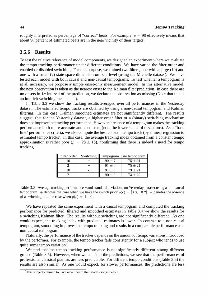
44 Tempo Tracking
roughly interpreted as percentage of “correct” beats. For example,ρ = 90 effectively means thatabout90 percent of estimated beats are in the near vicinity of their targets.
3.5.6 Results
To test the relative relevance of model components, we designed an experiment where we evaluatethe tempo tracking performance under different conditions. We have varied the filter order andenabled or disabled switching. For this purpose, we trainedtwo filters, one with a large (10) andone with a small (2) state space dimension on beat level (using the Michelle dataset). We havetested each model with both causal and non-causal tempograms. To test whether a tempogram isat all necessary, we propose a simple onset-only measurement model. In this alternative model,the next observation is taken as the nearest onset to the Kalman filter prediction. In case there areno onsets in1σ interval of the prediction, we declare the observation as missing (Note that this isan implicit switching mechanism).
In Table 3.3 we show the tracking results averaged over all performances in the Yesterdaydataset. The estimated tempo tracks are obtained by using a non-causal tempogram and Kalmanfiltering. In this case, Kalman smoothed estimates are not significantly different. The resultssuggest, that for the Yesterday dataset, a higher order filter or a (binary) switching mechanismdoes not improve the tracking performance. However, presence of a tempogram makes the trackingperformance both more accurate and consistent (note the lower standard deviations). As a “baseline” performance criteria, we also compute the best constant tempo track (by a linear regression toestimated tempo tracks). In this case, the average trackingindex obtained from a constant tempoapproximation is rather poor (ρ = 28 ± 18), confirming that there is indeed a need for tempotracking.
Filter order Switching tempogram no tempogram10 + 92± 7 75± 212 + 91± 9 75± 2110 - 91± 6 73± 212 - 90± 9 73± 22
Table 3.3:Average tracking performanceρ and standard deviations on Yesterday dataset using a non-causaltempogram.+ denotes the case when we have the switch priorp(c) = [0.8, 0.2]. − denotes the absenceof a switching, i.e. the case whenp(c) = [1, 0].
We have repeated the same experiment with a causal tempogramand computed the trackingperformance for predicted, filtered and smoothed estimatesIn Table 3.4 we show the results fora switching Kalman filter. The results without switching arenot significantly different. As onewould expect, the tracking index with predicted estimates is lower. In contrast to a non-causaltempogram, smoothing improves the tempo tracking and results in a comparable performance as anon-causal tempogram.
Naturally, the performance of the tracker depends on the amount of tempo variations introducedby the performer. For example, the tempo tracker fails consistently for a subject who tends to usequite some tempo variation3.
We find that the tempo tracking performance is not significantly different among differentgroups (Table 3.5). However, when we consider the predictions, we see that the performances ofprofessional classical pianists are less predictable. Fordifferent tempo conditions (Table 3.6) theresults are also similar. As one would expect, for slower performances, the predictions are less
3This subject claimed to have never heard the Beatles songs before.

3.6. DISCUSSION AND CONCLUSIONS 45
causalFilter order predicted filtered smoothed
10 74± 12 86± 9 91± 82 73± 12 85± 8 90± 8
Table 3.4:Average tracking performanceρ on Yesterday dataset. Figures indicate tracking indexρ fol-lowed by the standard deviation. The label “non-causal” refers to a tempogram calculated using non-causalcomb filters. The labels predicted, filtered and smoothed refer to state estimates obtained by the Kalmanfilter/smoother.
accurate. This might have two potential reasons. First, theperformance criteriaρ is independentof the absolute tempo, i.e. the windowW is always fixed. Second, for slower performances thereis more room for adding expression.
non-causal causalSubject Group filtered predicted filtered smoothed Best const.
Prof. Jazz 95 ± 3 81± 7 92± 4 94± 3 34± 22Amateur Classical 92 ± 8 74± 7 88± 5 92± 4 24± 19
Prof. Classical 89 ± 7 66± 14 82± 11 86± 11 27± 12
Table 3.5:Tracking Averages on subject groups. As a reference, the right most column shows the resultsobtained by the best constant tempo track. The label “non-causal” refers to a tempogram calculated usingnon-causal comb filters. The labels predicted, filtered and smoothed refer to state estimates obtained by theKalman filter/smoother.
non-causal causalCondition filtered predicted filtered smoothed Best const.
fast 94± 5 79± 9 90± 6 93± 6 39± 21normal 92± 8 74± 9 88± 6 92± 4 25± 13slow 90± 7 68± 14 84± 10 87± 11 21± 14
Table 3.6:Tracking Averages on tempo conditions. As a reference, the right most column shows the resultsobtained by the best constant tempo track. The label “non-causal” refers to a tempogram calculated usingnon-causal comb filters. The labels predicted, filtered and smoothed refer to state estimates obtained by theKalman filter/smoother.
3.6 Discussion and Conclusions
In this paper, we have formulated a tempo tracking model in a probabilistic framework. Theproposed model consist of a dynamical system (a Kalman Filter) and a measurement model (Tem-pogram). Although many of the methods proposed in the literature can be viewed as particularchoices of a dynamical model and a measurement model, a Bayesian formulation exhibits severaladvantages in contrast to other models for tempo tracking. First, components in our model havenatural probabilistic interpretations. An important and very practical consequence of such an inter-pretation is that uncertainties can be easily quantified andintegrated into the system. Moreover, alldesired quantities can be inferred consistently. For example once we quantify the distribution of
46 Tempo Tracking
tempo deviations and expressive timing, the actual behavior of the tempo tracker arises automati-cally from these a-priori assumptions. This is in contrast to other models where one has to inventad-hoc methods to avoid undesired or unexpected behavior onreal data.
Additionally, prior knowledge (such as smoothness constraints in the state transition model andthe particular choice of measurement model) are explicit and can be changed when needed. Forexample, the same state transition model can be used for bothaudio and MIDI; only the measure-ment model needs to be elaborated. Another advantage is that, for a large class of related modelsefficient inference and learning algorithms are well understood (Ghahramani & Hinton, 1996).This is appealing since we can train tempo trackers with different properties automatically fromdata. Indeed, we have demonstrated that all model parameters can be estimated from experimentaldata.
We have investigated several potential directions in whichthe basic dynamical model can beimproved or simplified. We have tested the relative relevance of the filter order, switching and thetempogram representation on a systematically collected set of natural data. The dataset consists ofpolyphonic piano performances of two Beatles songs (Yesterday and Michelle) and contains a lotof tempo fluctuation as indicated by the poor constant tempo fits.
The test results on the Beatles dataset suggest that using a high order filter does not improvetempo tracking performance.Although beat level filters capture some structure in tempo deviations(and hence can generate more accurate predictions), this additional precision seems to be not veryimportant in tempo tracking. This indifference may be due tothe fact that training criteria (max-imum likelihood) and testing criteria (tracking index), whilst related, are not identical. However,one can imagine scenarios where accurate prediction is crucial. An example would be a real-timeaccompaniment situation, where the application needs to generate events for the next bar.
Test results also indicate that a simple switching mechanism is not very useful. It seems that atempogram already gives a robust local estimate of likely beat and tempo values so the correct beatcan unambiguously be identified. The indifference of switching could as well be an artifact of thedataset which lacks extensive syncopations. Nevertheless, the switching noise model can furtherbe elaborated to replace the tempogram by a rhythm quantizer(Cemgil et al., 2000).
To test the relevance of the proposed tempogram representation on tracking performance wehave compared it to a simpler, onset based alternative. The results indicate that in the onset-onlycase, tracking performance significantly decreases, suggesting that a tempogram is an importantcomponent of the system.
It must be noted that the choice of a comb basis set for tempogram calculation is rather arbi-trary. In principle, one could formulate a “richer” tempogram model, for example by includingparameters that control the shape of basis functions. The parameters of such a model can sim-ilarly be optimized by likelihood maximization on target tempo tracks. Unfortunately, such anoptimization (e.g. with a generic technique such as gradient descent) requires the computation ofa tempogram at each step and is thus computationally quite expensive. Moreover, a model withmany adjustable parameters might eventually overfit.
We have also demonstrated that the model can be used both online (filtering) and offline(smoothing). Online processing is necessary for real time applications such as automatic accom-paniment and offline processing is desirable for transcription applications.
Chapter 4
Integrating Tempo Tracking andQuantization
We present a probabilistic generative model for timing deviations in expressive music perfor-mance. The structure of the proposed model is equivalent to aswitching state space model.The switch variables correspond to discrete note locationsas in a musical score. The con-tinuous hidden variables denote the tempo. We formulate twowell known music recognitionproblems, namely tempo tracking and automatic transcription (rhythm quantization) as fil-tering and maximum a posteriori (MAP) state estimation tasks. Exact computation of poste-rior features such as the MAP state is intractable in this model class, so we introduce MonteCarlo methods for integration and optimization. We compareMarkov Chain Monte Carlo(MCMC) methods (such as Gibbs sampling, simulated annealing and iterative improvement)and sequential Monte Carlo methods (particle filters). Our simulation results suggest betterresults with sequential methods. The methods can be appliedin both online and batch sce-narios such as tempo tracking and transcription and are thuspotentially useful in a numberof music applications such as adaptive automatic accompaniment, score typesetting and mu-sic information retrieval.
Adapted from: A. T. Cemgil and H. J. Kappen.Monte Carlo methods fortempo tracking and rhythm quantization.Journal of Artificial IntelligenceResearch, 18:45-81, 2003.
4.1 Introduction
Automatic music transcription refers to extraction of a human readable and interpretable descrip-tion from a recording of a musical performance. Traditionalmusic notation is such a descriptionthat lists the pitch levels (notes) and corresponding timestamps.
Ideally, one would like to recover a score directly from the audio signal. Such a representationof the surface structure of music would be very useful in music information retrieval (Music-IR)and content description of musical material in large audio databases. However, when operating onsampled audio data from polyphonic acoustical signals, extraction of a score-like description is avery challenging auditory scene analysis task (Vercoe, Gardner, & Scheirer, 1998).
In this paper, we focus on a subproblem in music-ir, where we assume that exact timing infor-mation of notes is available, for example as a stream of MIDI1 events from a digital keyboard.
1Musical Instruments Digital Interface. A standard communication protocol especially designed for digital instru-ments such as keyboards. Each time a key is pressed, a MIDI keyboard generates a short message containing pitchand key velocity. A computer can tag each received message bya timestamp for real-time processing and/or recordinginto a file.
47
48 Integrating Tempo Tracking and Quantization
A model for tempo tracking and transcription from a MIDI-like music representation is usefulin a broad spectrum of applications. One example is automatic score typesetting, the musicalanalog of word processing. Almost all score typesetting applications provide a means of automaticgeneration of a conventional music notation from MIDI data.
In conventional music notation, the onset time of each note is implicitly represented by thecumulative sum of durations of previous notes. Durations are encoded by simple rational numbers(e.g., quarter note, eighth note), consequently all eventsin music are placed on a discrete grid. Sothe basic task in MIDI transcription is to associate onset times with discrete grid locations, i.e.,quantization.
However, unless the music is performed with mechanical precision, identification of the cor-rect association becomes difficult. This is due to the fact that musicians introduce intentional (andunintentional) deviations from a mechanical prescription. For example timing of events can bedeliberately delayed or pushed. Moreover, the tempo can fluctuate by slowing down or accelerat-ing. In fact, such deviations are natural aspects of expressive performance; in the absence of these,music tends to sound rather dull and mechanical. On the otherhand, if these deviations are notaccounted for during transcription, resulting scores haveoften very poor quality.
Robust and fast quantization and tempo tracking is also an important requirement for interactiveperformance systems; applications that “listen” to a performer for generating an accompaniment orimprovisation in real time (Raphael, 2001b; Thom, 2000). Atlast, such models are also useful inmusicology for systematic study and characterization of expressive timing by principled analysisof existing performance data.
From a theoretical perspective, simultaneous quantization and tempo tracking is a “chicken-and-egg” problem: the quantization depends upon the intended tempo interpretation and the tempointerpretation depends upon the quantization. Apparently, human listeners can resolve this ambi-guity (in most cases) without any effort. Even persons without any musical training are able todetermine the beat and the tempo very rapidly. However, it isstill unclear what precisely consti-tutes tempo and how it relates to the perception of the beat, rhythmical structure, pitch, style ofmusic etc. Tempo is a perceptual construct and cannot directly be measured in a performance.
The goal of understanding tempo perception has stimulated asignificant body of research onthe psychological and computational modeling aspects of tempo tracking and beat induction, e.g.,see (Desain & Honing, 1994; Large & Jones, 1999; Toiviainen,1999). These papers assume thatevents are presented as an onset list. Attempts are also madeto deal directly with the audio signal(Goto & Muraoka, 1998; Scheirer, 1998; Dixon & Cambouropoulos, 2000).
Another class of tempo tracking models are developed in the context of interactive performancesystems and score following. These models make use of prior knowledge in the form of an anno-tated score (Dannenberg, 1984; Vercoe & Puckette, 1985). More recently, Raphael (2001b) hasdemonstrated an interactive real-time system that followsa solo player and schedules accompani-ment events according to the player’s tempo interpretation.
Tempo tracking is crucial for quantization, since one can not uniquely quantize onsets withouthaving an estimate of tempo and the beat. The converse, that quantization can help in identificationof the correct tempo interpretation has already been noted by Desain and Honing (1991). Here, onedefines correct tempo as the one that results in a simpler quantization. However, such a schemahas never been fully implemented in practice due to computational complexity of obtaining aperceptually plausible quantization. Hence quantizationmethods proposed in the literature eitherestimate the tempo using simple heuristics (Longuet-Higgins, 1987; Pressing & Lawrence, 1993;Agon et al., 1994) or assume that the tempo is known or constant (Desain & Honing, 1991;Cambouropoulos, 2000; Hamanaka et al., 2001).
Our approach to transcription and tempo tracking is from a probabilistic, i.e., Bayesian mod-eling perspective. In Cemgil et al. (2000), we introduced a probabilistic approach to perceptuallyrealistic quantization. This work also assumed that the tempo was known or was estimated by an

4.2. MODEL 49
external procedure. For tempo tracking, we introduced a Kalman filter model (Cemgil, Kappen,Desain, & Honing, 2001). In this approach, we modeled the tempo as a smoothly varying hiddenstate variable of a stochastic dynamical system.
In the current paper, we integrate quantization and tempo tracking. Basically, our model bal-ances score complexity versus smoothness in tempo deviations. The correct tempo interpretationresults in a simple quantization and the correct quantization results in a smooth tempo fluctuation.An essentially similar model is proposed recently also by Raphael (2001a). However, Raphaeluses an inference technique that only applies for small models; namely when the continuous hid-den state is one dimensional. This severely restricts the models one can consider. In the currentpaper, we survey general and widely used state-of-the-art techniques for inference.
The outline of the paper is as follows: In Section 4.2, we propose a probabilistic model for tim-ing deviations in expressive music performance. Given the model, we will define tempo trackingand quantization as inference of posterior quantities. It will turn out that our model is a switch-ing state space model in which computation of exact probabilities becomes intractable. In Sec-tion 4.3, we will introduce approximation techniques basedon simulation, namely Markov ChainMonte Carlo (MCMC) and sequential Monte Carlo (SMC) (Doucet, de Freitas, & Gordon, 2001;Andrieu, de Freitas, Doucet, & Jordan, 2002). Both approaches provide flexible and powerfulinference methods that have been successfully applied in diverse fields of applied sciences suchas robotics (Fox, Burgard, & Thrun, 1999), aircraft tracking (Gordon, Salmond, & Smith, 1993),computer vision (Isard & Blake, 1996), econometrics (Tanizaki, 2001). Finally we will presentsimulation results and conclusions.
4.2 Model
Assume that a pianist is improvising and we are recording theexact onset times of each key shepresses during the performance. We denote these observed onset times byy0, y1, y2 . . . yk . . . yK
or more compactly byy0:K . We neither have access to a musical notation of the piece norknowthe initial tempo she has started her performance with. Moreover, the pianist is allowed to freelychange the tempo or introduce expression. Given only onset time informationy0:K , we wish tofind a scoreγ1:K and track her tempo fluctuationsz0:K . We will refine the meaning ofγ andz later.
This problem is apparently ill-posed. If the pianist is allowed to change the tempo arbitrarily itis not possible to assign a “correct” score to a given performance. In other words any performancey0:K can be represented by using a suitable combination of an arbitrary score with an arbitrarytempo trajectory. Fortunately, the Bayes theorem providesan elegant and principled guideline toformulate the problem. Given the onsetsy0:K , the best scoreγ1:K and tempo trajectoryz0:K can bederived from theposteriordistribution that is given by
p(γ1:K, z0:K |y0:K) =1
p(y0:K)p(y0:K|γ1:K , z0:K)p(γ1:K , z0:K)
a quantity, that is proportional to the product of thelikelihoodtermp(y0:K |γ1:K, z0:K) and thepriortermp(γ1:K , z0:K).
In rhythm transcription and tempo tracking, the prior encodes our background knowledge aboutthe nature of musical scores and tempo deviations. For example, we can construct a prior thatprefers “simple” scores and smooth tempo variations.
The likelihood term relates the tempo and the score to actualobserved onset times. In thisrespect, the likelihood is a model for short time expressivetiming deviations and motor errors thatare introduced by the performer.

50 Integrating Tempo Tracking and Quantization
c0 //""EEEEEEEEE c1 //�� ""EEEEEEEEE c2 //�� !!CCCCCCCCCC . . . // ##FFFFFFFFFF ck−1//�� ##HHHHHHHHH ck //�� !!CCCCCCCCCC . . .Score Positions
γ1
��γ2
��. . . γk−1
��γk
��. . . Score
∆0 !!BBBBBBBBBB // ∆1 !!BBBBBBBBBB // ∆2 ���������� // . . . // ∆k−1// ""EEEEEEEEEE ∆k
// ���������� . . .Tempo Trajectory
τ0�� // τ1�� // τ2�� // . . . // τk−1 //�� τk //�� . . .Noiseless onsets
y0 y1 y2 . . . yk−1 yk . . .Observed Onsets
Figure 4.1: Graphical Model. Square and oval nodes correspond to discrete and continuous vari-ables respectively. In the text, we sometimes refer to the continuous hidden variables(τk,∆k) byzk. The dependence betweenγ andc is deterministic. Allc, γ , τ and∆ are hidden; only onsetsyare observed.
4.2.1 Score prior
To define a scoreγ1:K , we first introduce a sequence ofscore positionsc0:K . A score positionckspecifies the score time of thek’th onset. We letγk denote the interval between score positions oftwo consecutive onsets
γk = ck − ck−1 (4.1)
For example consider the conventional music notation� � � which encodes the scoreγ1:3 = [1 0.5 0.5].Corresponding score positions arec0:3 = [0 1 1.5 2].
One simple way of defining a prior distribution on score positionsp(ck) is specifying a tableof probabilities forck mod 1 (the fraction ofck). For example if we wish to allow for scoresthat have sixteenth notes and triplets, we define a table of probabilities for the statesc mod 1 ={0, 0.25, 0.5, 0.75} ∪ {0, 0.33, 0.67}. Technically, the resulting priorp(ck) is periodic andimproper (sinceck are in principle unbounded so we can not normalize the distribution).
However, if the number of states ofck mod 1 is large, it may be difficult to estimate theparameters of the prior reliably. For such situations we propose a “generic” prior as follows: Wedefine the probability, that thek’th onset gets quantized at locationck, by p(ck) ∝ exp(−λd(ck))whered(ck) is the number of significant digits in thebinaryexpansion ofck mod 1. For exampled(1) = 0, d(1.5) = 1, d(7 + 9/32) = 5 etc. The positive parameterλ is used to penalize scorepositions that require more bits to be represented. Assuming that score positions of onsets areindependent a-priori, (besides being increasing ink, i.e., ck ≥ ck−1), the prior probability of asequence of score positions is given byp(c0:K) ∝ exp(−λ∑K
k=0 d(ck)). We further assume thatc0 ∈ [0, 1). One can check that such a prior prefers simpler notations, e.g.,p( �� � 6 �� � 6 � ) < p( � � � ).We can generalize this prior to other subdivisions such triplets and quintiplets in Appendix 4.5.
Formally, given a distribution onc0:K , the prior of a scoreγ1:K is given by
p(γ1:K) =∑
c0:K
p(γ1:K|c0:K)p(c0:K) (4.2)
4.2. MODEL 51
Since the relationship betweenc0:K andγ1:K is deterministic,p(γ1:K|c0:K) is degenerate for anygivenc0:K , so we have
p(γ1:K) ∝ exp
(
−λK∑
k=1
d(
k∑
k′=1
γk′)
)
(4.3)
One might be tempted to specify a prior directly onγ1:K and get rid ofc0:K entirely. However, withthis simpler approach it is not easy to devise realistic priors. For example, consider a sequence ofnote durations[1 1/16 1 1 1 . . . ]. Assuming a factorized prior onγ that penalizes shortnote durations, this rhythm would have relatively high probability whereas it is quite uncommonin conventional music.
4.2.2 Tempo prior
We represent the tempo in terms of its inverse, i.e., the period, and denote it with∆. For examplea tempo of120 beats per minute (bpm) corresponds to∆ = 60/120 = 0.5 seconds. At each onsetthe tempo changes by an unknown amountζ∆k
. We assume the changeζ∆kis iid with N (0, Q∆).
2 We assume a first order Gauss-Markov process for the tempo
∆k = ∆k−1 + ζ∆k(4.4)
Eq. 4.4 defines a distribution over tempo sequences∆0:K . Given a tempo sequence, the “ideal” or“intended” timeτk of the next onset is given by
τk = τk−1 + γk∆k−1 + ζτk(4.5)
The noise termζτkdenotes the amount of accentuation (that is deliberately playing a note ahead or
back in time) without causing the tempo to be changed. We assumeζτk∼ N (0, Qτ). Ideal onsets
and actually observed “noisy” onsets are related by
yk = τk + ǫk (4.6)
The noise termǫk models small scale expressive deviations or motor errors intiming of individualnotes. In this paper we will assume thatǫk has a Gaussian distribution parameterized byN (0, R).
The initial tempo distributionp(∆0) specifies a range of reasonable tempi and is given by aGaussian with a broad variance. We assume an uninformative (flat) prior onτ0. The conditionalindependence structure is given by the graphical model in Figure 4.1. Table 4.1 shows a possiblerealization from the model.
We note that our model is a particular instance of the well known switching state space model(also known as conditionally linear dynamical system, jumpMarkov linear system, switchingKalman filter) (See, e.g., Bar-Shalom & Li, 1993; Doucet & Andrieu, 2001; Murphy, 2002).
In the following sections, we will sometimes refer usezk = (τk,∆k)T and refer toz0:K as a
tempo trajectory. Given this definition, we can compactly represent Eq. 4.4 and Eq. 4.5 by
zk =
(
1 γk
0 1
)
zk−1 + ζk (4.7)
whereζk = (ζτk, ζ∆k
).
2We denote a (scalar or multivariate) Gaussian distributionp(x) with mean vectorµ and covariance matrixP byN (µ, P )=|2πP |− 1
2 exp(− 1
2(x− µ)TP−1(x− µ)).
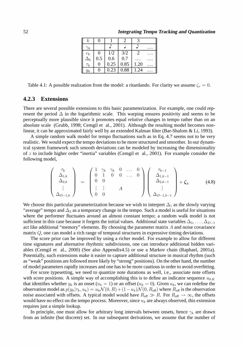
52 Integrating Tempo Tracking and Quantization
k 0 1 2 3γk (� � (� . . .ck 0 1/2 3/2 2 . . .∆k 0.5 0.6 0.7 . . . . . .τk 0 0.25 0.85 1.20 . . .yk 0 0.23 0.88 1.24 . . .
Table 4.1: A possible realization from the model: a ritardando. For clarity we assumeζτ = 0.
4.2.3 Extensions
There are several possible extensions to this basic parameterization. For example, one could rep-resent the period∆ in the logarithmic scale. This warping ensures positivity and seems to beperceptually more plausible since it promotes equalrelative changes in tempo rather than on anabsolute scale (Grubb, 1998; Cemgil et al., 2001). Althoughthe resulting model becomes non-linear, it can be approximated fairly well by an extended Kalman filter (Bar-Shalom & Li, 1993).
A simple random walk model for tempo fluctuations such as in Eq. 4.7 seems not to be veryrealistic. We would expect the tempo deviations to be more structured and smoother. In our dynam-ical system framework such smooth deviations can be modeledby increasing the dimensionalityof z to include higher order “inertia” variables (Cemgil et al.,2001). For example consider thefollowing model,
τk∆1,k
∆2,k...
∆D−1,k
=
1 γk γk 0 . . . 00 1 0 0 . . . 00 0...
... A0 0
τk−1
∆1,k−1
∆2,k−1...
∆D−1,k−1
+ ζk (4.8)
We choose this particular parameterization because we wishto interpret∆1 as the slowly varying“average” tempo and∆2 as a temporary change in the tempo. Such a model is useful for situationswhere the performer fluctuates around an almost constant tempo; a random walk model is notsufficient in this case because it forgets the initial values. Additional state variables∆3, . . . ,∆D−1
act like additional “memory” elements. By choosing the parameter matrixA and noise covariancematrixQ, one can model a rich range of temporal structures in expressive timing deviations.
The score prior can be improved by using a richer model. For example to allow for differenttime signatures and alternative rhythmic subdivisions, one can introduce additional hidden vari-ables (Cemgil et al., 2000) (See also Appendix4.5) or use a Markov chain (Raphael, 2001a).Potentially, such extensions make it easier to capture additional structure in musical rhythm (suchas “weak” positions are followed more likely by “strong” positions). On the other hand, the numberof model parameters rapidly increases and one has to be more cautious in order to avoid overfitting.
For score typesetting, we need to quantize note durations aswell, i.e., associate note offsetswith score positions. A simple way of accomplishing this is to define an indicator sequenceu0:K
that identifies whetheryk is an onset (uk = 1) or an offset (uk = 0). Givenuk, we can redefine theobservation model asp(yk|τk, uk) = ukN (0, R)+(1−uk)N (0, Roff) whereRoff is the observationnoise associated with offsets. A typical model would haveRoff ≫ R. ForRoff → ∞, the offsetswould have no effect on the tempo process. Moreover, sinceuk are always observed, this extensionrequires just a simple lookup.
In principle, one must allow for arbitrary long intervals between onsets, henceγk are drawnfrom an infinite (but discrete) set. In our subsequent derivations, we assume that the number of

4.2. MODEL 53
possible intervals is fixed a-priori. Given an estimate ofzk−1 and observationyk, almost all ofthe virtually infinite number of choices forγk will have almost zero probability and it is easy toidentify candidates that would have significant probability mass.
Conceptually, all of the above listed extensions are easy toincorporate into the model and noneof them introduces a fundamental computational difficulty to the basic problems of quantizationand tempo tracking.
4.2.4 Problem Definition
Given the model, we define rhythm transcription, i.e., quantization as a MAP state estimationproblem
γ∗1:K = argmaxγ1:K
p(γ1:K |y0:K) (4.9)
p(γ1:K |y0:K) =
∫
dz0:Kp(γ1:K , z0:K |y0:K)
and tempo tracking as a filtering problem
z∗k = argmaxzk
∑
γ1:k
p(γ1:k, zk|y0:k) (4.10)
The quantization problem is a smoothing problem: we wish to find the most likely scoreγ∗1:Kgiven all the onsets in the performance. This is useful in “offline” applications such as scoretypesetting.
For real-time interaction, we need to have an online estimate of the tempo/beatzk. This in-formation is carried forth by the filtering densityp(γ1:k, zk|y0:k) in Eq.4.10. Our definition of thebest tempoz∗k as the maximum is somewhat arbitrary. Depending upon the requirements of anapplication, one can make use of other features of the filtering density. For example, the varianceof∑
γ1:kp(γ1:k, zk|y0:k) can be used to estimate “amount of confidence” in tempo interpretation or
arg maxzk,γ1:kp(γ1:k, zk|y0:k) to estimate most likely score-tempo pair so far.
Unfortunately, the quantities in Eq. 4.9 and Eq. 4.10 are intractable due to the explosion inthe number of mixture components required to represent the exact posterior at each stepk (SeeFigure 4.2). For example, to calculate the exact posterior in Eq. 4.9 we need to evaluate thefollowing expression:
p(γ1:K |y0:K) =1
Z
∫
dz0:Kp(y0:K |z0:K , γ1:K)p(z0:K |γ1:K)p(γ1:K) (4.11)
=1
Zp(y0:K |γ1:K)p(γ1:K) (4.12)
where the normalization constant is given byZ = p(y0:K) =∑
γ1:Kp(y0:K |γ1:K)p(γ1:K). For
each trajectoryγ1:K , the integral overz0:K can be computed stepwise ink by the Kalman filter(See appendix 4.5). However, to find the MAP state of Eq. 4.11,we need to evaluatep(y0:K |γ1:K)independently for each of the exponentially many trajectories. Consequently, the quantizationproblem in Eq. 4.9 can only be solved approximately.
For accurate approximation, we wish to exploit any inherentindependence structure of the ex-act posterior. Unfortunately, sincez andc are integrated over, allγk become coupled and in generalp(γ1:K |y0:K) does not possess any conditional independence structure (e.g., a Markov chain) thatwould facilitate efficient calculation. Consequently, we will resort to numerical approximationtechniques.

54 Integrating Tempo Tracking and Quantization
−0.5 0 0.5 1 1.5 2 2.5 3 3.5−0.8
−0.6
−0.4
−0.2
0
0.2
0.4
0.6
−5.0002
2.6972
τ
ω
(a) −0.5 0 0.5 1 1.5 2 2.5 3 3.5−0.8
−0.6
−0.4
−0.2
0
0.2
0.4
0.6
4.6765
−10.5474
−3.2828
−2.2769
τ
ω
(b)
−0.5 0 0.5 1 1.5 2 2.5 3 3.5−0.8
−0.6
−0.4
−0.2
0
0.2
0.4
0.6
−7.90366.6343
0.76292
−10.3422
−10.1982−2.393
−2.7957
−0.4593
τ
ω
(c)
Figure 4.2: Example demonstrating the explosion of the number of components to represent the exactposterior. Ellipses denote the conditional marginalsp(τk, ωk|c0:k, y0:k). (We show the period in logarithmicscale whereωk = log2 ∆k). In this toy example, we assume that a score consists only ofnotes of length(� and � , i.e., γk can be either1/2 or 1. (a) We start with a unimodal posteriorp(τ0, ω0|c0, y0), e.g., aGaussian centered at(τ, ω) = (0, 0). Since we assume that a score can only consist of eight- and quarternotes, i.e.,γk ∈ {1/2, 1}. the predictive distributionp(τ1, ω1|c0:1, y0) is bimodal where the modes arecentered at(0.5, 0) and(1, 0) respectively (shown with a dashed contour line). Once the next observationy1
is observed (shown with a dashed vertical line aroundτ = 0.5), the predictive distribution is updated to yieldp(τ1, ω1|c0:1, y0:1). The numbers denote the respective log-posterior weight ofeach mixture component.(b)The predictive distributionp(τ2, ω2|c0:1, y0:1) at stepk = 2 has now4 modes, two for each component ofp(τ1, ω1|c0:1, y0:1). (c) The number of components grows exponentially withk.
4.3. MONTE CARLO SIMULATION 55
4.3 Monte Carlo Simulation
Consider a high dimensional probability distribution
p(x) =1
Zp∗(x) (4.13)
where the normalization constantZ =∫
dxp∗(x) is not known butp∗(x) can be evaluated at anyparticularx. Suppose we want to estimate the expectation of a functionf(x) under the distributionp(x) denoted as
〈f(x)〉p(x) =
∫
dxf(x)p(x)
e.g., the mean ofx underp(x) is given by〈x〉. The intractable integration can be approximated byan average if we can findN pointsx(i), i = 1 . . .N from p(x)
〈f(x)〉p(x) ≈1
N
N∑
i=1
f(x(i)) (4.14)
Whenx(i) are generated by independently sampling fromp(x), it can be shown that asN ap-proaches infinity, the approximation becomes exact.
However, generating independent samples fromp(x) is a difficult task in high dimensions butit is usually easier to generatedependentsamples, that is we generatex(i+1) by making use ofx(i). It is somewhat surprising, that even ifx(i) andx(i+1) are correlated (and provided ergodicityconditions are satisfied), Eq. 4.14 remains still valid and estimated quantities converge to their truevalues when number of samplesN goes to infinity.
A sequence of dependent samplesx(i) is generated by using a Markov chain that has the sta-tionary distributionp(x). The chain is defined by a collection of transition probabilities, i.e., atransition kernelT (x(i+1)|x(i)). The definition of the kernel is implicit, in the sense that one de-fines a procedure to generate thex(i+1) givenx(i). TheMetropolisalgorithm (Metropolis & Ulam,1949; Metropolis, Rosenbluth, Rosenbluth, Teller, & Teller, 1953) provides a simple way of defin-ing an ergodic kernel that has the desired stationary distributionp(x). Suppose we have a samplex(i). A candidatex′ is generated by sampling from a symmetric proposal distribution q(x′|x(i))(for example a Gaussian centered atx(i)). The candidatex′ is accepted as the next samplex(i+1)
if p(x′) > p(x(i)). If x′ has a lower probability, it can be still accepted, but only with probabil-ity p(x′)/p(x(i)). The algorithm is initialized by generating the first samplex(0) according to an(arbitrary) proposal distribution.
However for a given transition kernelT , it is hard to assess the time required to converge tothe stationary distribution so in practice one has to run thesimulation until a very large numberof samples have been obtained, (see e.g., Roberts & Rosenthal, 1998). The choice of the proposaldistributionq is also very critical. A poor choice may lead to the rejectionof many candidatesx′
hence resulting in a very slow convergence to the stationarydistribution.For a large class of probability models, where the full posterior p(x) is intractable, one can still
efficiently compute marginals of formp(xk|x−k), x−k = x1 . . . xk−1, xk+1, . . . xK exactly. In thiscase one can apply a more specialized Markov chain Monte Carlo (MCMC) algorithm, theGibbssamplergiven below.
1. Initializex(0)1:K by sampling from a proposalq(x1:K)
2. Fori = 0 . . .N − 1

56 Integrating Tempo Tracking and Quantization
• Fork = 1, . . . , K, Sample
x(i+1)k ∼ p(xk|x(i+1)
1:k−1, x(i)k+1:K) (4.15)
In contrast to the Metropolis algorithm, where the new candidate is a vectorx′, the Gibbssampler uses the exact marginalp(xk|x−k) as the proposal distribution. At each step, the samplerupdates only one coordinate of the current statex, namelyxk, and the new candidate is guaranteedto be accepted.
Note that, in principle we don’t need to samplexk sequentially, i.e., we can choosek randomlyprovided that each slice is visited equally often in the limit. However, a deterministic scan algo-rithm wherek = 1, . . .K, provides important time savings in the type of models that we considerhere.
4.3.1 Simulated Annealing and Iterative Improvement
Now we shift our focus from sampling to MAP state estimation.In principle, one can use thesamples generated by any sampling algorithm (Metropolis-Hastings or Gibbs) to estimate the MAPstatex∗ of p(x) by argmax
i=1:Np(x(i)). However, unless the posterior is very much concentrated
around the MAP state, the sampler may not visitx∗ even though the samplesx(i) are obtainedfrom the stationary distribution. In this case, the problemcan be simply reformulated to samplenot from p(x) but from a distribution that is concentrated at local maximaof p(x). One suchclass of distributions are given bypρj
(x) ∝ p(x)ρj . A sequence of exponentsρ1 < ρ2 < · · · <ρj < . . . is called to be acooling scheduleor annealing scheduleowing to the inverse temperatureinterpretation ofρj in statistical mechanics, hence the nameSimulated Annealing(SA) (Aarts &van Laarhoven, 1985). Whenρj → ∞ sufficiently slowly inj, the cascade of MCMC samplerseach with the stationary distributionpρj
(x) is guaranteed (in the limit) to converge to the globalmaximum ofp(x). Unfortunately, for this convergence result to hold, the cooling schedule mustgo very slowly (in fact, logarithmically) to infinity. In practice, faster cooling schedules must beemployed.
Iterative improvement(II) (Aarts & van Laarhoven, 1985) is a heuristic simulated annealingalgorithm with a very fast cooling schedule. In fact,ρj = ∞ for all j. The eventual advantageof this greedy algorithm is that it converges in a few iterations to a local maximum. By restartingmany times from different initial configurationsx, one hopes to find different local maxima ofp(x)and eventually visit the MAP statex∗. In practice, by using the II heuristic one may find bettersolutions than SA for a limited computation time.
From an implementation point of view, it is trivial to convert MCMC code to SA (or II) code.For example, consider the Gibbs sampler. To implement SA, weneed to construct a cascade ofGibbs samplers, each with stationary distributionp(x)ρj . The exact one time slice marginal ofthis distribution isp(xk|x−k)
ρj . So, SA just samples from the actual (temperature=1) marginalp(xk|x−k) raised to a powerρj .
4.3.2 The Switching State Space Model and MAP Estimation
To solve the rhythm quantization problem, we need to calculate the MAP state of the posterior inEq. 4.11
p(γ1:K |y0:K) ∝ p(γ1:K)
∫
dz0:Kp(y0:K |z0:K , γ1:K)p(z0:K |γ1:K) (4.16)
This is a combinatorial optimization problem: we seek the maximum of a functionp(γ1:K |y0:K)that associates a number with each of the discrete configurationsγ1:K . Since it is not feasible to
4.3. MONTE CARLO SIMULATION 57
visit all of the exponentially many configurations to find themaximizing configurationγ∗1:K , wewill resort to stochastic search algorithms such as simulated annealing (SA) and iterative improve-ment (II). Due to the strong relationship between the Gibbs sampler and SA (or II), we will firstreview the Gibbs sampler for the switching state space model.
The first important observation is that, conditioned onγ1:K , the model becomes a linear statespace model and the integration onz0:K can be computed analytically using Kalman filtering equa-tions. Consequently, one can sample onlyγ1:K and integrate outz. The analytical marginalization,calledRao-Blackwellization(Casella & Robert, 1996), improves the efficiency of the sampler (e.g.,see Doucet, de Freitas, Murphy, & Russell, 2000a).
Suppose now that each switch variableγk can haveS distinct states and we wish to generateN samples (i.e trajectories){γ(i)
1:K, i = 1 . . . N}. A naive implementation of the Gibbs samplerrequires that at each stepk we run the Kalman filterS times on the whole observation sequencey0:K to compute the proposalp(γk|γ(i)
1:k−1, γ(i−1)k+1:K, y0:K). This would result in an algorithm of time
complexityO(NK2S) that is prohibitively slow whenK is large. Carter and Kohn (1996) haveproposed a much more time efficient deterministic scan Gibbssampler that circumvents the needto run the Kalman filtering equations at each stepk on the whole observation sequencey0:K . Seealso (Doucet & Andrieu, 2001; Murphy, 2002).
The method is based on the observation that the proposal distribution p(γk| ·) can be factor-ized as a product of terms that either depend on past observationsy0:k or the future observationsyk+1:K . So the contribution of the future can be computed a-priori by a backward filtering pass.Subsequently, the proposal is computed and samplesγ
(i)k are generated during the forward pass.
The sampling distribution is given by
p(γk|γ−k, y0:K) ∝ p(γk|γ−k)p(y0:K |γ1:K) (4.17)
where the first term is proportional to the joint priorp(γk|γ−k) ∝ p(γk,γ−k). The second termcan be decomposed as
p(y0:K |γ1:K) =
∫
dzkp(yk+1:K|y0:k, zk, γ1:K)p(y0:k, zk|γ1:K) (4.18)
=
∫
dzkp(yk+1:K|zk, γk+1:K)p(y0:k, zk|γ1:k) (4.19)
Both terms are (unnormalized) Gaussian potentials hence the integral can be evaluated analytically.The termp(yk+1:K|zk, γk+1:K) is an unnormalized Gaussian potential inzk and can be computed bybackwards filtering. The second term is just the filtering distributionp(zk|y0:k, γ1:k) scaled by thelikelihoodp(y0:k|γ1:k) and can be computed during forward filtering. The outline of the algorithmis given below, see the appendix 4.5 for details.
1. Initializeγ(0)1:K by sampling from a proposalq(γ1:K)
2. Fori = 1 . . .N
• Fork = K − 1, . . . , 0,
– Computep(yk+1:K|zk, γ(i−1)k+1:K)
• Fork = 1, . . . , K,
– Fors = 1 . . . S
∗ Compute the proposal
p(γk = s|· ) ∝ p(γk = s,γ−k)
∫
dzkp(y0:k, zk|γ(i)1:k−1, γk = s)p(yk+1:K|zk, γ
(i−1)k+1:K)
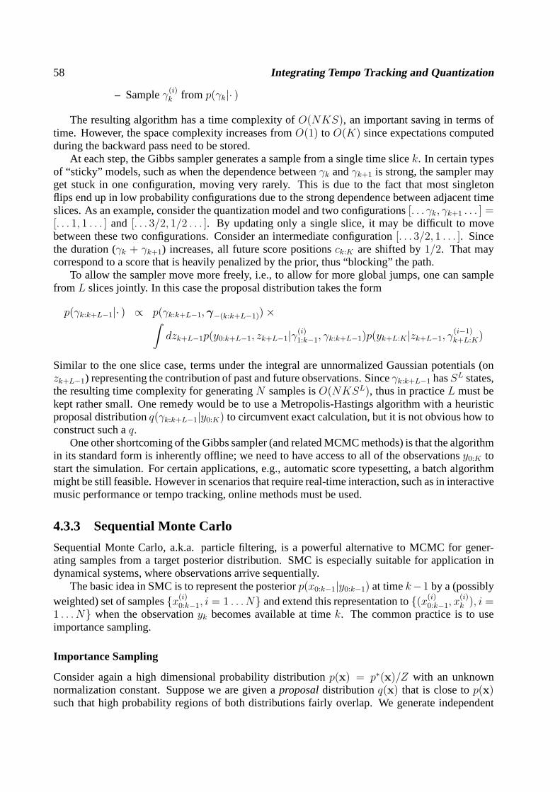
58 Integrating Tempo Tracking and Quantization
– Sampleγ(i)k from p(γk|· )
The resulting algorithm has a time complexity ofO(NKS), an important saving in terms oftime. However, the space complexity increases fromO(1) toO(K) since expectations computedduring the backward pass need to be stored.
At each step, the Gibbs sampler generates a sample from a single time slicek. In certain typesof “sticky” models, such as when the dependence betweenγk andγk+1 is strong, the sampler mayget stuck in one configuration, moving very rarely. This is due to the fact that most singletonflips end up in low probability configurations due to the strong dependence between adjacent timeslices. As an example, consider the quantization model and two configurations[. . . γk, γk+1 . . . ] =[. . . 1, 1 . . . ] and [. . . 3/2, 1/2 . . . ]. By updating only a single slice, it may be difficult to movebetween these two configurations. Consider an intermediateconfiguration[. . . 3/2, 1 . . . ]. Sincethe duration (γk + γk+1) increases, all future score positionsck:K are shifted by1/2. That maycorrespond to a score that is heavily penalized by the prior,thus “blocking” the path.
To allow the sampler move more freely, i.e., to allow for moreglobal jumps, one can samplefrom L slices jointly. In this case the proposal distribution takes the form
p(γk:k+L−1|· ) ∝ p(γk:k+L−1,γ−(k:k+L−1))×∫
dzk+L−1p(y0:k+L−1, zk+L−1|γ(i)1:k−1, γk:k+L−1)p(yk+L:K|zk+L−1, γ
(i−1)k+L:K)
Similar to the one slice case, terms under the integral are unnormalized Gaussian potentials (onzk+L−1) representing the contribution of past and future observations. Sinceγk:k+L−1 hasSL states,the resulting time complexity for generatingN samples isO(NKSL), thus in practiceL must bekept rather small. One remedy would be to use a Metropolis-Hastings algorithm with a heuristicproposal distributionq(γk:k+L−1|y0:K) to circumvent exact calculation, but it is not obvious how toconstruct such aq.
One other shortcoming of the Gibbs sampler (and related MCMCmethods) is that the algorithmin its standard form is inherently offline; we need to have access to all of the observationsy0:K tostart the simulation. For certain applications, e.g., automatic score typesetting, a batch algorithmmight be still feasible. However in scenarios that require real-time interaction, such as in interactivemusic performance or tempo tracking, online methods must beused.
4.3.3 Sequential Monte Carlo
Sequential Monte Carlo, a.k.a. particle filtering, is a powerful alternative to MCMC for gener-ating samples from a target posterior distribution. SMC is especially suitable for application indynamical systems, where observations arrive sequentially.
The basic idea in SMC is to represent the posteriorp(x0:k−1|y0:k−1) at timek−1 by a (possiblyweighted) set of samples{x(i)
0:k−1, i = 1 . . .N} and extend this representation to{(x(i)0:k−1, x
(i)k ), i =
1 . . . N} when the observationyk becomes available at timek. The common practice is to useimportance sampling.
Importance Sampling
Consider again a high dimensional probability distribution p(x) = p∗(x)/Z with an unknownnormalization constant. Suppose we are given aproposaldistributionq(x) that is close top(x)such that high probability regions of both distributions fairly overlap. We generate independent
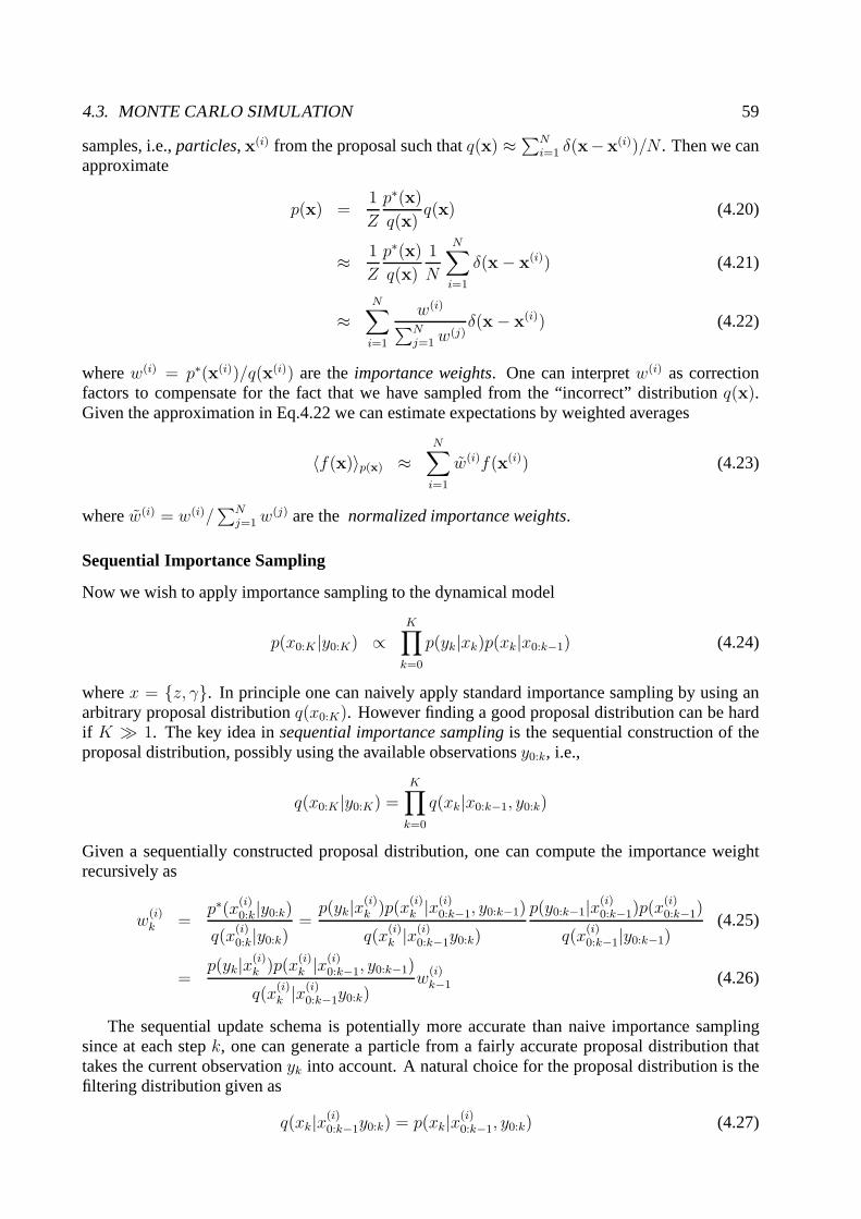
4.3. MONTE CARLO SIMULATION 59
samples, i.e.,particles, x(i) from the proposal such thatq(x) ≈∑Ni=1 δ(x−x(i))/N . Then we can
approximate
p(x) =1
Z
p∗(x)
q(x)q(x) (4.20)
≈ 1
Z
p∗(x)
q(x)
1
N
N∑
i=1
δ(x− x(i)) (4.21)
≈N∑
i=1
w(i)
∑Nj=1w
(j)δ(x− x(i)) (4.22)
wherew(i) = p∗(x(i))/q(x(i)) are theimportance weights. One can interpretw(i) as correctionfactors to compensate for the fact that we have sampled from the “incorrect” distributionq(x).Given the approximation in Eq.4.22 we can estimate expectations by weighted averages
〈f(x)〉p(x) ≈N∑
i=1
w(i)f(x(i)) (4.23)
wherew(i) = w(i)/∑N
j=1w(j) are thenormalized importance weights.
Sequential Importance Sampling
Now we wish to apply importance sampling to the dynamical model
p(x0:K |y0:K) ∝K∏
k=0
p(yk|xk)p(xk|x0:k−1) (4.24)
wherex = {z, γ}. In principle one can naively apply standard importance sampling by using anarbitrary proposal distributionq(x0:K). However finding a good proposal distribution can be hardif K ≫ 1. The key idea insequential importance samplingis the sequential construction of theproposal distribution, possibly using the available observationsy0:k, i.e.,
q(x0:K |y0:K) =
K∏
k=0
q(xk|x0:k−1, y0:k)
Given a sequentially constructed proposal distribution, one can compute the importance weightrecursively as
w(i)k =
p∗(x(i)0:k|y0:k)
q(x(i)0:k|y0:k)
=p(yk|x(i)
k )p(x(i)k |x
(i)0:k−1, y0:k−1)
q(x(i)k |x
(i)0:k−1y0:k)
p(y0:k−1|x(i)0:k−1)p(x
(i)0:k−1)
q(x(i)0:k−1|y0:k−1)
(4.25)
=p(yk|x(i)
k )p(x(i)k |x
(i)0:k−1, y0:k−1)
q(x(i)k |x
(i)0:k−1y0:k)
w(i)k−1 (4.26)
The sequential update schema is potentially more accurate than naive importance samplingsince at each stepk, one can generate a particle from a fairly accurate proposaldistribution thattakes the current observationyk into account. A natural choice for the proposal distribution is thefiltering distribution given as
q(xk|x(i)0:k−1y0:k) = p(xk|x(i)
0:k−1, y0:k) (4.27)
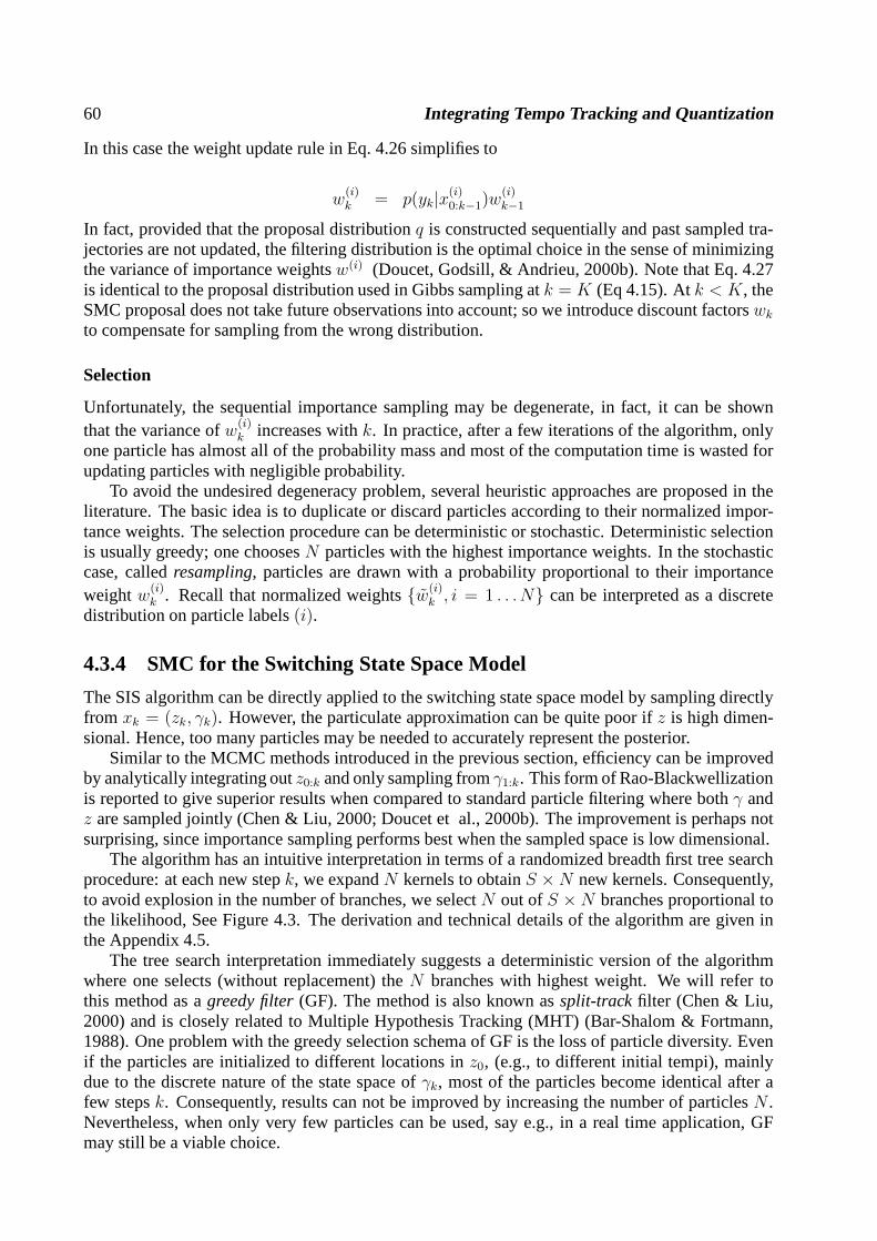
60 Integrating Tempo Tracking and Quantization
In this case the weight update rule in Eq. 4.26 simplifies to
w(i)k = p(yk|x(i)
0:k−1)w(i)k−1
In fact, provided that the proposal distributionq is constructed sequentially and past sampled tra-jectories are not updated, the filtering distribution is theoptimal choice in the sense of minimizingthe variance of importance weightsw(i) (Doucet, Godsill, & Andrieu, 2000b). Note that Eq. 4.27is identical to the proposal distribution used in Gibbs sampling atk = K (Eq 4.15). Atk < K, theSMC proposal does not take future observations into account; so we introduce discount factorswk
to compensate for sampling from the wrong distribution.
Selection
Unfortunately, the sequential importance sampling may be degenerate, in fact, it can be shownthat the variance ofw(i)
k increases withk. In practice, after a few iterations of the algorithm, onlyone particle has almost all of the probability mass and most of the computation time is wasted forupdating particles with negligible probability.
To avoid the undesired degeneracy problem, several heuristic approaches are proposed in theliterature. The basic idea is to duplicate or discard particles according to their normalized impor-tance weights. The selection procedure can be deterministic or stochastic. Deterministic selectionis usually greedy; one choosesN particles with the highest importance weights. In the stochasticcase, calledresampling, particles are drawn with a probability proportional to their importanceweightw(i)
k . Recall that normalized weights{w(i)k , i = 1 . . .N} can be interpreted as a discrete
distribution on particle labels(i).
4.3.4 SMC for the Switching State Space Model
The SIS algorithm can be directly applied to the switching state space model by sampling directlyfrom xk = (zk, γk). However, the particulate approximation can be quite poor if z is high dimen-sional. Hence, too many particles may be needed to accurately represent the posterior.
Similar to the MCMC methods introduced in the previous section, efficiency can be improvedby analytically integrating outz0:k and only sampling fromγ1:k. This form of Rao-Blackwellizationis reported to give superior results when compared to standard particle filtering where bothγ andz are sampled jointly (Chen & Liu, 2000; Doucet et al., 2000b).The improvement is perhaps notsurprising, since importance sampling performs best when the sampled space is low dimensional.
The algorithm has an intuitive interpretation in terms of a randomized breadth first tree searchprocedure: at each new stepk, we expandN kernels to obtainS ×N new kernels. Consequently,to avoid explosion in the number of branches, we selectN out ofS ×N branches proportional tothe likelihood, See Figure 4.3. The derivation and technical details of the algorithm are given inthe Appendix 4.5.
The tree search interpretation immediately suggests a deterministic version of the algorithmwhere one selects (without replacement) theN branches with highest weight. We will refer tothis method as agreedy filter(GF). The method is also known assplit-trackfilter (Chen & Liu,2000) and is closely related to Multiple Hypothesis Tracking (MHT) (Bar-Shalom & Fortmann,1988). One problem with the greedy selection schema of GF is the loss of particle diversity. Evenif the particles are initialized to different locations inz0, (e.g., to different initial tempi), mainlydue to the discrete nature of the state space ofγk, most of the particles become identical after afew stepsk. Consequently, results can not be improved by increasing the number of particlesN .Nevertheless, when only very few particles can be used, say e.g., in a real time application, GFmay still be a viable choice.
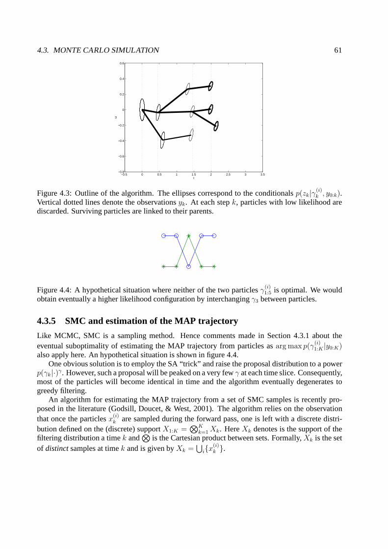
4.3. MONTE CARLO SIMULATION 61
−0.5 0 0.5 1 1.5 2 2.5 3 3.5−0.8
−0.6
−0.4
−0.2
0
0.2
0.4
0.6
τ
ω
Figure 4.3: Outline of the algorithm. The ellipses correspond to the conditionalsp(zk|γ(i)k , y0:k).
Vertical dotted lines denote the observationsyk. At each stepk, particles with low likelihood arediscarded. Surviving particles are linked to their parents.
Figure 4.4: A hypothetical situation where neither of the two particlesγ(i)1:5 is optimal. We would
obtain eventually a higher likelihood configuration by interchangingγ3 between particles.
4.3.5 SMC and estimation of the MAP trajectory
Like MCMC, SMC is a sampling method. Hence comments made in Section 4.3.1 about theeventual suboptimality of estimating the MAP trajectory from particles asarg max p(γ
(i)1:K |y0:K)
also apply here. An hypothetical situation is shown in figure4.4.One obvious solution is to employ the SA “trick” and raise theproposal distribution to a power
p(γk|·)γ. However, such a proposal will be peaked on a very fewγ at each time slice. Consequently,most of the particles will become identical in time and the algorithm eventually degenerates togreedy filtering.
An algorithm for estimating the MAP trajectory from a set of SMC samples is recently pro-posed in the literature (Godsill, Doucet, & West, 2001). Thealgorithm relies on the observationthat once the particlesx(i)
k are sampled during the forward pass, one is left with a discrete distri-bution defined on the (discrete) supportX1:K =
⊗Kk=1Xk. HereXk denotes is the support of the
filtering distribution a timek and⊗
is the Cartesian product between sets. Formally,Xk is the setof distinctsamples at timek and is given byXk =
⋃
i{x(i)k }.
62 Integrating Tempo Tracking and Quantization
The distributionp(X1:K |y1:K)3 is Markovian because the original state transition model isMarkovian, i.e., the posterior can be represented exactly by
p(X1:K |y1:K) ∝K∏
k=1
p(yk|Xk)p(Xk|Xk−1)
Consequently, one can find the best MAP trajectoryarg max p(X1:K) by using an algorithm thatis analogous to the Viterbi algorithm for hidden Markov models (Rabiner, 1989).
However, this idea does not carry directly to the case when one applies Rao-Blackwellization.In general, when a subset of the hidden variables is integrated out, all time slices of the posteriorp(Γ1:K |y1:k) are coupled, whereΓ1:K =
⊗Kk=1 Γk andΓk =
⋃
i{γ(i)k }. One can still employ a chain
approximation and run Viterbi, (e.g., Cemgil & Kappen, 2002), but this does not guarantee to findarg max p(Γ1:K |y1:k).
On the other hand, becauseγ(i)k are drawn from a discrete set, several particles become identical
soΓk has usually a small cardinality when compared to the number of particlesN . Consequently,it becomes feasible to employ SA or II on the reduced state spaceΓ1:K ; possibly using a proposaldistribution that extends over several time slicesL.
In practice, for finding the MAP solution from the particle set {γ(i)1:K , i = 1 . . . N}, we propose
to find the best trajectoryi∗ = arg maxi p(y0:K |γ(i)1:K)p(γ
(i)1:K) and apply iterative improvement
starting from the initial configurationγ(i∗)1:K .
4.4 Simulations
We have compared the inference methods in terms of the quality of the solution and executiontime. The tests are carried out both on artificial and real data.
Given the true notationγtrue1:K , we measure the quality of a solution in terms of the log-likelihood
difference
∆L = logp(y0:K |γ1:K)p(γ1:K)
p(y0:K |γtrue1:K)p(γtrue
1:K)
and in terms ofedit distance
e(γ1:K) =
K∑
k=1
(1− δ(γk − γtruek ))
The edit distancee(γ1:K) gives simply the number of notes that are quantized wrongly.
4.4.1 Artificial data: Clave pattern
The synthetic example is a repeating “son-clave” pattern7 > � � > �� �� � 7 (c = [1, 2, 4, 5.5, 7 . . . ])with fluctuating tempo. We repeat the pattern6 times and obtain a scoreγ1:K with K = 30.
Such syncopated rhythms are usually hard to transcribe and make it difficult to track the tempoeven for experienced human listeners. Moreover, since onsets are absent at prominent beat loca-tions, standard beat tracking algorithms usually loose track.
3By a slight abuse of notation we use the symbolXk both as a set and as a general element when used in theargument of a density,p(yk|Xk) meansp(yk|xk) s.t.xk ∈ Xk
4.4. SIMULATIONS 63
Given scoreγ1:K, we have generated100 observation sequencesy0:K by sampling from thetempo model in Eq. 4.7. We have parameterized the observation noise variance4 asQ = γkQa+Qb.In this formulation, the variance depends on the length of the interval between consecutive onsets;longer notes in the score allow for more tempo and timing fluctuation. For the tests on the claveexample we have not used a prior model that reflects true source statistics, instead, we have usedthe generic prior model defined in Section 4.2.1 withλ = 1.
All the example cases are sampled from the same score (clave pattern). However, due to theuse of the generic prior (that does not capture the exact source statistics well) and a relativelybroad noise model, the MAP trajectoryγ∗1:K giveny0:K is not always identical to the original clavepattern. For thei’th example, we have defined the “ground truth”γtrue,i
1:K as the highest likelihood so-lution found using any sampling technique during any independent run. Although this definition ofthe ground truth introduces some bias, we have found this exercise more realistic as well as morediscriminative among various methods when compared to, e.g.,, using a dataset with essentiallyshorter sequences where the exact MAP trajectory can be computed by exhaustive enumeration.The wish to stress that the main aim of the simulations on synthetic dataset is to compare effec-tiveness of different inference techniques; we postpone the actual test whether the model is a goodone to our simulations on real data.
We have tested the MCMC methods, namely Gibbs sampling (Gibbs), simulated annealing(SA) and iterative improvement (II) with one and two time slice optimal proposal and for10 and50 sweeps. For each onsetyk, the optimal proposalp(γk|·) is computed always on a fixed set,Γ = {0, 1/4, 2/4 . . .3}. Figure 4.6 shows a typical run of MCMC.
Similarly, we have implemented the SMC forN = {1, 5, 10, 50, 100} particles. The selectionschema was random drawing from the optimal proposalp(γk|·) computed using one or two timeslices. Only in the special case of greedy filtering (GF), i.e., whenN = 1, we have selected theswitch with maximum probability. An example run is shown in Figure 4.5.
We observe that on average SMC results are superior to MCMC (Figure 4.7). We observe that,increasing the number of sweeps for MCMC does not improve thesolution significantly. On theother hand, increasing the number of particles seems to improve the quality of the SMC solutionmonotonically. Moreover, the results suggest that sampling from two time slices jointly (with theexception of SA ) does not have a big effect. GF outperforms a particle filter with 5 particles thatdraws randomly from the proposal. That suggests that for PF with a small number of particlesN ,it may be desirable to use a hybrid selection schema that selects the particle with maximum weightautomatically and randomly selects the remainingN − 1.
We compare inference methods in terms of execution time and the quality of solutions (asmeasured by edit distance). As Figure 4.8 suggests, using a two slice proposal is not justified.Moreover it seems that for comparable computational effort, SMC tends to outperform all MCMCmethods.
4.4.2 Real Data: Beatles
We evaluate the performance of the model on polyphonic pianoperformances. 12 pianists wereinvited to play two Beatles songs, Michelle and Yesterday. Both pieces have a relatively simplerhythmic structure with ample opportunity to add expressiveness by fluctuating the tempo. Theoriginal score is shown in Figure 4.9(a). The subjects had different musical education and back-ground: four professional jazz players, four professionalclassical performers and four amateurclassical pianists. Each arrangement had to be played in three tempo conditions, three repetitionsper tempo condition. The tempo conditions were normal, slowand fast tempo (all in a musically
4The noise covariance parameters wereR = 0.022,Qa = 0.062I andQb = 0.022I. I is a2× 2 identity matrix.

64 Integrating Tempo Tracking and Quantization
0 2 4 6 8 10 12 14 16−1
−0.8
−0.6
−0.4
−0.2
0
0.2
0.4
0.6
0.8
1
τ
ω
Figure 4.5: Particle filtering on clave example with4 particles. Each circle denotes the mean(τ
(n)k , ω
(n)k ) whereω(n)
k = log2 ∆k. The diameter of each particle is proportional to the normalizedimportance weight at each generation. ’*’ denote the true(τ, ω) pairs; here we have modulatedthe tempo deterministically according toωk = 0.3 sin(2πck/32), observation noise variance isR = 0.0252.
1 10 20 30 40 50−40
−30
−20
−10
0
Gibbs Sweep
Log
Like
lihoo
d
Gibbs SA II GF Desired
Figure 4.6:Typical runs of Gibbs sampling, Simulated Annealing (SA) and Iterative Improvement (II) onclave example. All algorithms are initialized to the greedyfilter solution. The annealing schedule for SAwas linear fromρ1 = 0.1 to ρ33 = 10 and than proceeding deterministically byρ34:50 = ∞. When SAor II converge to a configuration, we reinitialize by a particle filter with one particle that draws randomlyproportional to the optimal proposal. Sharp drops in the likelihood correspond to reinitializations. We seethat, at the first sweep, the greedy filter solution can only beslightly improved by II. Consequently thesampler reinitializes. The likelihood of SA drops considerably, mainly due to the high temperature, andconsequently stabilizes at a suboptimal solution. The Gibbs sampler seems to explore the support of theposterior but is no able to visit the MAP state in this run.
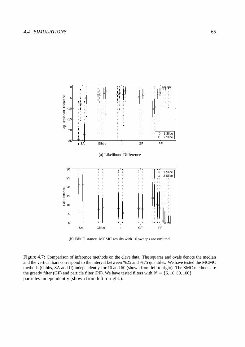
4.4. SIMULATIONS 65
SA Gibbs II GF PF−25
−20
−15
−10
−5
0
Log
Like
lihoo
d D
iffer
ence
1 Slice2 Slice
(a) Likelihood Difference
SA Gibbs II GF PF
0
5
10
15
20
25
30
Edi
t Dis
tanc
e
1 Slice2 Slice
(b) Edit Distance. MCMC results with10 sweeps are omitted.
Figure 4.7:Comparison of inference methods on the clave data. The squares and ovals denote the medianand the vertical bars correspond to the interval between %25and %75 quantiles. We have tested the MCMCmethods (Gibbs, SA and II) independently for10 and50 (shown from left to right). The SMC methods arethe greedy filter (GF) and particle filter (PF). We have testedfilters withN = {5, 10, 50, 100}particles independently (shown from left to right.).
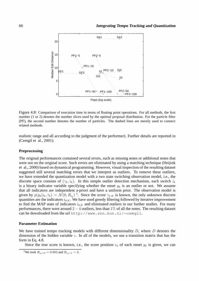
66 Integrating Tempo Tracking and Quantization
0
5
10
15
20
Gi1
SA1
II1 Gi2
SA2
II2
PF1−5
PF1−10
PF1−50 PF1−100
PF2−5
PF2−10
PF2−50PF2−100
GF1 GF2
Med
ian
Edi
t Dis
tanc
e
Flops (log scale)
Figure 4.8:Comparison of execution time in terms of floating point operations. For all methods, the firstnumber (1 or 2) denotes the number slices used by the optimal proposal distribution. For the particle filter(PF), the second number denotes the number of particles. Thedashed lines are merely used to connectrelated methods.
realistic range and all according to the judgment of the performer). Further details are reported in(Cemgil et al., 2001).
Preprocessing
The original performances contained several errors, such as missing notes or additional notes thatwere not on the original score. Such errors are eliminated byusing a matching technique (Heijinket al., 2000) based on dynamical programming. However, visual inspection of the resulting datasetsuggested still several matching errors that we interpret as outliers. To remove these outliers,we have extended the quantization model with a two state switching observation model, i.e., thediscrete space consists of(γk, ik). In this simple outlier detection mechanism, each switchikis a binary indicator variable specifying whether the onsetyk is an outlier or not. We assumethat all indicators are independent a-priori and have a uniform prior. The observation model isgiven byp(yk|ik, τk) = N (0, Rik)
5. Since the scoreγ1:K is known, the only unknown discretequantities are the indicatorsi0:K . We have used greedy filtering followed by iterative improvementto find the MAP state of indicatorsi0:K and eliminated outliers in our further studies. For manyperformances, there were around2− 4 outliers, less than1% of all the notes. The resulting datasetcan be downloaded from the urlhttp://www.snn.kun.nl/∼cemgil.
Parameter Estimation
We have trained tempo tracking models with different dimensionality D, whereD denotes thedimension of the hidden variablez. In all of the models, we use a transition matrix that has theform in Eq. 4.8.
Since the true score is known, i.e., the score positionck of each onsetyk is given, we can
5We tookRik=0 = 0.002 andRik=1 = 2.

4.5. DISCUSSION 67
clamp all the discrete variables in the model. Consequently, we can estimate the observation noisevarianceR, the transition noise varianceQ and the transition matrix coefficientsA from data.
We have optimized the parameters by Expectation-Maximization (EM) for the linear dynam-ical systems (Shumway & Stoffer, 1982; Ghahramani & Hinton,1996) using all performancesof “Yesterday” as training data. Similarly, the score priorparameters are estimated by frequencycounts from the score of “Yesterday”6 . All tests are carried out on “Michelle”.
Results
In Figure 4.9 we show the result of typesetting a performancewith and without tempo tracking.Due to fluctuations in tempo, the quality of the automatically generated score is very poor. Thequality can be significantly improved by using our model.
Figure 4.10 shows some tempo tracking examples on Michelle dataset for pianists from differ-ent background and training. We observe that in most cases the results are satisfactory.
In Figure 4.11, we give a summary of test results on Michelle data in terms of the loglikeli-hood and edit distance as a function of model order and numberof particles used for inference.Figure 4.11(a) shows that the median likelihood on test datais increasing with model order. Thissuggests that a higher order filter is able to capture structure in pianists’ expressive timing. More-over, as for the sythetic data, we see a somewhat monotonic increase in the likelihood of solutionsfound when using more particles.
The edit distance between the original score and the estimates are given in Figure 4.11(b). Sinceboth pieces are arranged for piano, due to polyphony, there are many onsets that are associated withthe same score position. Consequently, manyγtrue
k in the original score are effectively zero. In suchcases, typically, the corresponding inter onset intervalyk − yk−1 is also very small and the correctquantization (namelyγk = 0) can be identified even if the tempo estimate is completely wrong.As a consequence, the edit distance remains small. To make the task slightly more challenging, weexclude the onsets withγtrue
k = 0 from edit distance calculation.We observe that the extra prediction ability obtained usinga higher order model does not
directly translate to a better transcription. The errors are around5% for all models. On the otherhand, the variance of edit distance for higher order models is smaller suggesting an increasedrobustness towards divergence from the tempo track impliedby the original score.
4.5 Discussion
We have presented a switching state space model for joint rhythm quantization and tempo tracking.The model describes the rhythmic structure of musical pieces by a prior distribution over scorepositions. In this representation, it is easy to construct ageneric prior that prefers simpler notationsand to learn parameters from a data set. The prior on score positions c0:K translates to a non-Markovian distribution over a scoreγ1:K.
Timing deviations introduced by performers (tempo fluctuation, accentuations and motor er-rors) are modeled as independent Gaussian noise sources. Performer specific timing preferencesare captured by the parameters of these distributions.
Given the model, we have formulated rhythm quantization as aMAP state estimation prob-lem and tempo tracking as a filtering problem. We have introduced Markov chain Monte Carlo(MCMC) and sequential Monte Carlo (SMC) to approximate the respective distributions.
6The maximum likelihood parameters for a model of dimensionD = 3 are found to be:a = −0.072,R = 0.0132
andqτ = 0.0082, q∆1= 0.0072 andq∆2
= 0.0502. The priorp(c) is p(0) = 0.80, p(1/3) = 0.0082, p(1/2) = 0.15p(5/6) = 0.0418. Remainingp(c) are set to10−6.
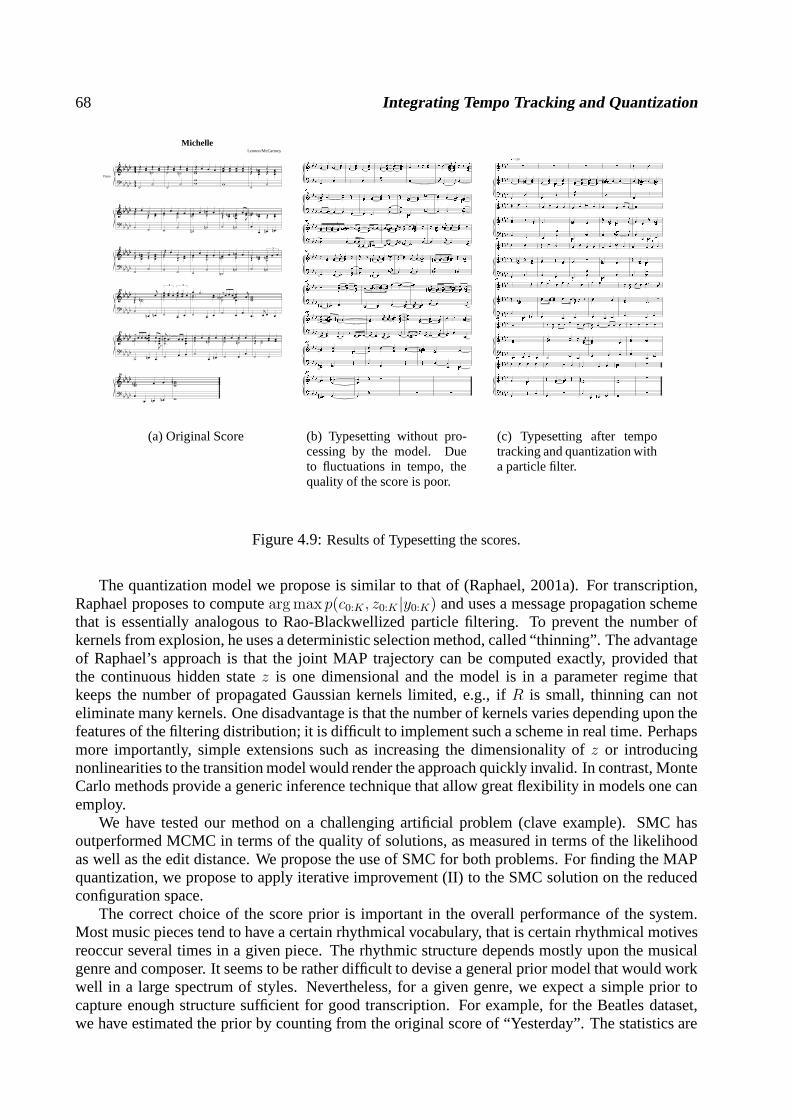
68 Integrating Tempo Tracking and Quantization
Piano
&&?bb bbb b b b
b b b b4444
44
1
˙ ˙n1 Œ œœ Œ œœ
˙ ˙˙ ˙nŒ œœ Œ œœ
˙ ˙
Œ œ œ œwwww
œœœ œœ œœ œœw
˙ ˙Œ œœœn Œ œœœ˙ ˙
&&?bb bbb b b b
b b b b
6 Œ œ ˙6
˙ Œ œœ˙ ˙
œ œ œ œ˙ ˙
˙ ˙œ œ œn œ˙n ˙
˙n ˙n˙ œ œ œŒ œœn ..œœn Jœ˙ ˙n
wœ œœn Œ œœœ œ œn œn
&&?bb bbb b b b
b b b b
11 ˙ ˙11
Œ œœœn Œ œœœ˙ ˙
Œ œ ˙˙ Œ œœ˙ ˙
œ œ œ œ˙ ˙
˙ ˙œ œ œn œ˙n ˙
˙n ˙n˙
3
œ œ œŒ œœn ˙n˙ ˙n
&&?bb bbb b b b
b b b b
16
.˙jœ16
Œ ..˙n˙ œn œn
3
œœ œœ œ3
œœ œœ œ˙ ˙
˙ œ œ
œ .˙..˙ œœ
˙ œ œ
‰œ œ œ .œ jœ˙˙˙b ...œœœ˙ œ œ
www
.œ jœ œ œ
&&?bb bbb b b b
b b b b
21 ‰ œ œ œ œ œ œ21 ˙˙ œœœ ‰ Jœœ
˙ œn œ
jœ .œ œ œ œ..˙ œœ˙ œ œ
œ œ œ œ˙ ˙n˙ œ œn
œ œ œ œ˙ ˙n˙ œ œ
˙ œœ œœŒ ˙
˙ ˙
&&?bb bbb b b b
b b b b
26
˙ œ œ26
wwnœ œ œn œn
wn www
Lennon/McCartney
Michelle
(a) Original Score
����� � ��� �� ��� � ��� �� ��� �� ��� ��������� �� ������� �� ������������������ � � � � �� � ��� ��� ����� ��� �� �� � �� �� ��� � � ��� ��� �� �� � ���� �������� � ��� � � � � �� �� �� �� � � ���������� ������ �������� �� ����� ���� ����� ��������� �� ������ � � ��� ��� �� ��� ����� �� � ������� � ��� � ������� � �� � �� �������� � �� ������� � � � �������� ��� �� �� ������ ��� ��� ������ ������ ���� � ������� �� ��� ��� ���� ���� �� �� �� ��� ��������� � ���� ���� ���� � ������ ���� ��� � �� ���� ����� ������� ������� ���� �������� �� ��� � � �� �� �� �� ��� � �� �������� ��� ������ ��� �� ���� ��������� ���� ��� �� ������ �� � �� �������� ��� �� ����� ��� ��� �� ����� ��� �� ���� �������� �� �� �� �� � ��� �� ������ ��� ������ ��� �� � � � � � � �� ��������� �� ��� �� �� � � � ����� ��� �� � � � � �(b) Typesetting without pro-cessing by the model. Dueto fluctuations in tempo, thequality of the score is poor.
� = 130����� � � � � ����� ! !!! !!� !!! ! !!! !" !!! !! !!! !!!! !!!! !!!"# ! ! !!!!"# ! !!!!"$���� %% % &����� ' ! ! ! ! ! ! ! !� ! ! !! %����� ' !! ( " ' !!� !" ) !* ! ! ' !!�$���� " � !!� )) !* ! ! !" !�++����� ' ! ! ! ! ! ! ! !� ! !!!,����� ' !!!" ' !!! ' !! ( " ' !!� "$���� " � �+&����� ) !) ! ! !, ! ! !, ! ) - !. !!!) !*����� ' � )) !!)) !!!!) !) !!/0- )) ! � !) -$���� !" !� ! ! ! ! ! !12����� % - !. !!! !! !. !) !!! ! ! ! !����� %% !! - !!* )) ! �$���� !) !*! ! !� ! ! ! ! !�13����� ! ! ! ! ! ! ! ! %" ������ " ' !! !!! ' %%� %% �$���� ' ! ( ! ! !" !� % �
(c) Typesetting after tempotracking and quantization witha particle filter.
Figure 4.9:Results of Typesetting the scores.
The quantization model we propose is similar to that of (Raphael, 2001a). For transcription,Raphael proposes to computearg max p(c0:K , z0:K |y0:K) and uses a message propagation schemethat is essentially analogous to Rao-Blackwellized particle filtering. To prevent the number ofkernels from explosion, he uses a deterministic selection method, called “thinning”. The advantageof Raphael’s approach is that the joint MAP trajectory can becomputed exactly, provided thatthe continuous hidden statez is one dimensional and the model is in a parameter regime thatkeeps the number of propagated Gaussian kernels limited, e.g., if R is small, thinning can noteliminate many kernels. One disadvantage is that the numberof kernels varies depending upon thefeatures of the filtering distribution; it is difficult to implement such a scheme in real time. Perhapsmore importantly, simple extensions such as increasing thedimensionality ofz or introducingnonlinearities to the transition model would render the approach quickly invalid. In contrast, MonteCarlo methods provide a generic inference technique that allow great flexibility in models one canemploy.
We have tested our method on a challenging artificial problem(clave example). SMC hasoutperformed MCMC in terms of the quality of solutions, as measured in terms of the likelihoodas well as the edit distance. We propose the use of SMC for bothproblems. For finding the MAPquantization, we propose to apply iterative improvement (II) to the SMC solution on the reducedconfiguration space.
The correct choice of the score prior is important in the overall performance of the system.Most music pieces tend to have a certain rhythmical vocabulary, that is certain rhythmical motivesreoccur several times in a given piece. The rhythmic structure depends mostly upon the musicalgenre and composer. It seems to be rather difficult to devise ageneral prior model that would workwell in a large spectrum of styles. Nevertheless, for a givengenre, we expect a simple prior tocapture enough structure sufficient for good transcription. For example, for the Beatles dataset,we have estimated the prior by counting from the original score of “Yesterday”. The statistics are
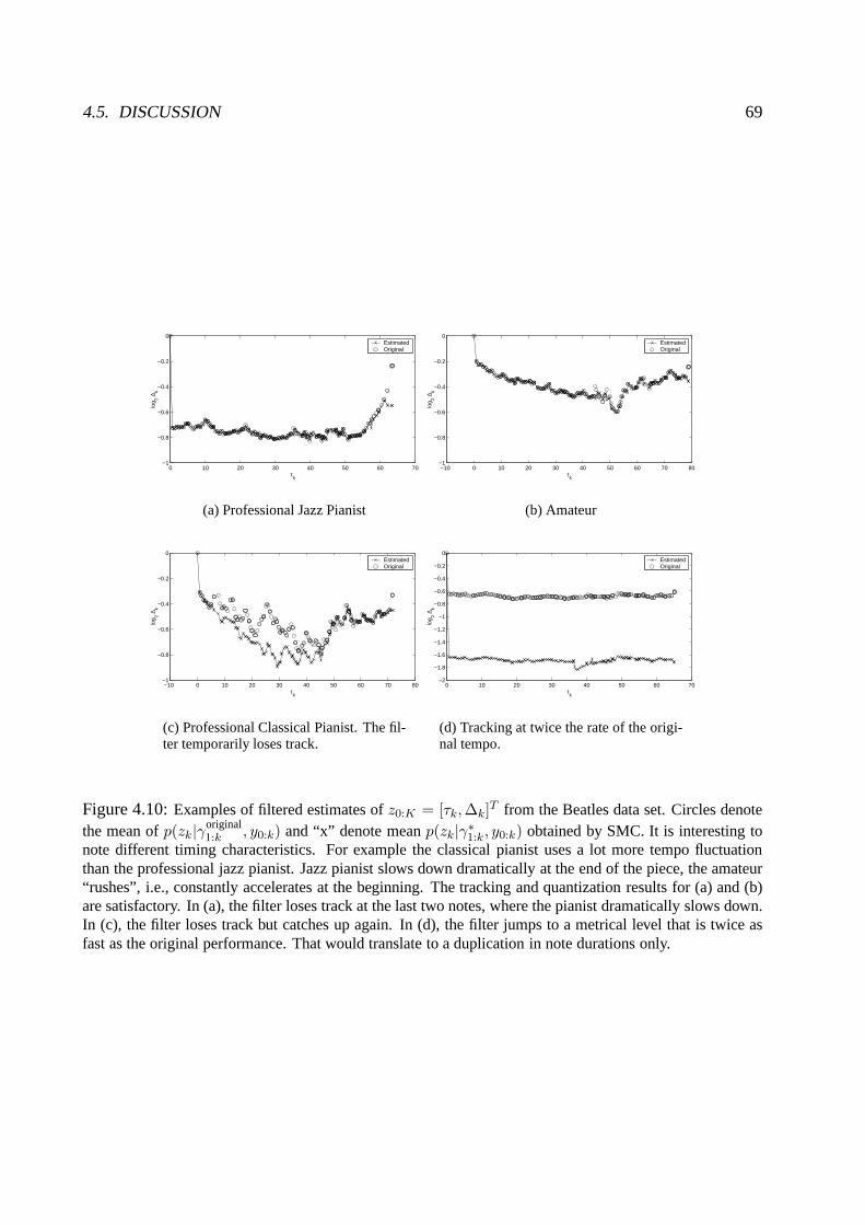
4.5. DISCUSSION 69
0 10 20 30 40 50 60 70−1
−0.8
−0.6
−0.4
−0.2
0
log 2 ∆
k
τk
EstimatedOriginal
(a) Professional Jazz Pianist
−10 0 10 20 30 40 50 60 70 80−1
−0.8
−0.6
−0.4
−0.2
0
log 2 ∆
k
τk
EstimatedOriginal
(b) Amateur
−10 0 10 20 30 40 50 60 70 80−1
−0.8
−0.6
−0.4
−0.2
0
log 2 ∆
k
τk
EstimatedOriginal
(c) Professional Classical Pianist. The fil-ter temporarily loses track.
0 10 20 30 40 50 60 70−2
−1.8
−1.6
−1.4
−1.2
−1
−0.8
−0.6
−0.4
−0.2
0
log 2 ∆
k
τk
EstimatedOriginal
(d) Tracking at twice the rate of the origi-nal tempo.
Figure 4.10:Examples of filtered estimates ofz0:K = [τk,∆k]T from the Beatles data set. Circles denote
the mean ofp(zk|γoriginal1:k , y0:k) and “x” denote meanp(zk|γ∗1:k, y0:k) obtained by SMC. It is interesting to
note different timing characteristics. For example the classical pianist uses a lot more tempo fluctuationthan the professional jazz pianist. Jazz pianist slows downdramatically at the end of the piece, the amateur“rushes”, i.e., constantly accelerates at the beginning. The tracking and quantization results for (a) and (b)are satisfactory. In (a), the filter loses track at the last two notes, where the pianist dramatically slows down.In (c), the filter loses track but catches up again. In (d), thefilter jumps to a metrical level that is twice asfast as the original performance. That would translate to a duplication in note durations only.
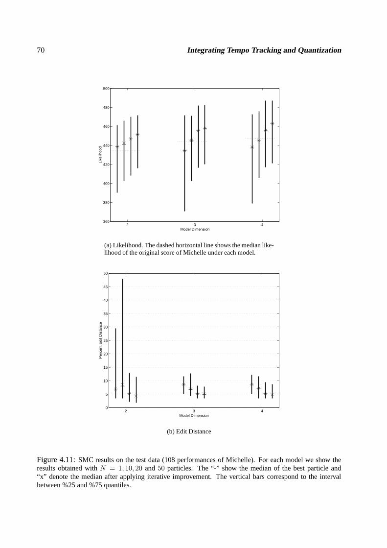
70 Integrating Tempo Tracking and Quantization
2 3 4360
380
400
420
440
460
480
500
Model Dimension
Like
lihoo
d
(a) Likelihood. The dashed horizontal line shows the medianlike-lihood of the original score of Michelle under each model.
2 3 40
5
10
15
20
25
30
35
40
45
50
Model Dimension
Per
cent
Edi
t Dis
tanc
e
(b) Edit Distance
Figure 4.11:SMC results on the test data (108 performances of Michelle).For each model we show theresults obtained withN = 1, 10, 20 and50 particles. The “-” show the median of the best particle and“x” denote the median after applying iterative improvement. The vertical bars correspond to the intervalbetween %25 and %75 quantiles.
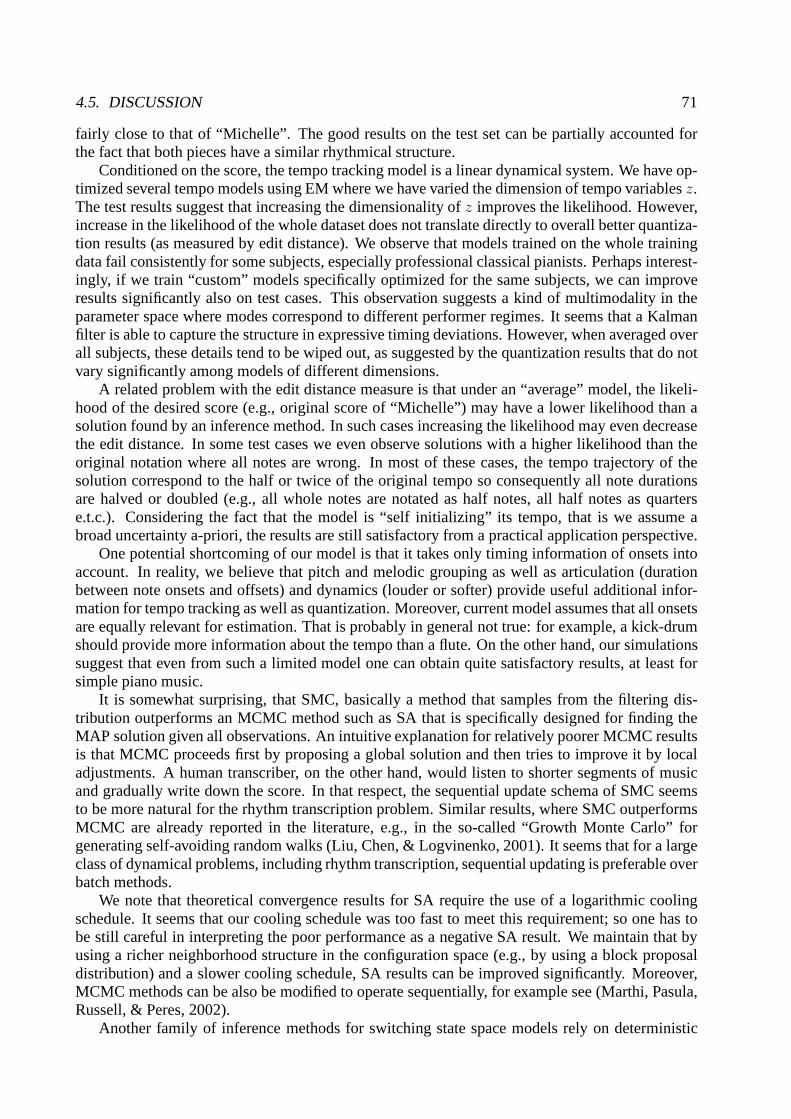
4.5. DISCUSSION 71
fairly close to that of “Michelle”. The good results on the test set can be partially accounted forthe fact that both pieces have a similar rhythmical structure.
Conditioned on the score, the tempo tracking model is a linear dynamical system. We have op-timized several tempo models using EM where we have varied the dimension of tempo variablesz.The test results suggest that increasing the dimensionality of z improves the likelihood. However,increase in the likelihood of the whole dataset does not translate directly to overall better quantiza-tion results (as measured by edit distance). We observe thatmodels trained on the whole trainingdata fail consistently for some subjects, especially professional classical pianists. Perhaps interest-ingly, if we train “custom” models specifically optimized for the same subjects, we can improveresults significantly also on test cases. This observation suggests a kind of multimodality in theparameter space where modes correspond to different performer regimes. It seems that a Kalmanfilter is able to capture the structure in expressive timing deviations. However, when averaged overall subjects, these details tend to be wiped out, as suggested by the quantization results that do notvary significantly among models of different dimensions.
A related problem with the edit distance measure is that under an “average” model, the likeli-hood of the desired score (e.g., original score of “Michelle”) may have a lower likelihood than asolution found by an inference method. In such cases increasing the likelihood may even decreasethe edit distance. In some test cases we even observe solutions with a higher likelihood than theoriginal notation where all notes are wrong. In most of thesecases, the tempo trajectory of thesolution correspond to the half or twice of the original tempo so consequently all note durationsare halved or doubled (e.g., all whole notes are notated as half notes, all half notes as quarterse.t.c.). Considering the fact that the model is “self initializing” its tempo, that is we assume abroad uncertainty a-priori, the results are still satisfactory from a practical application perspective.
One potential shortcoming of our model is that it takes only timing information of onsets intoaccount. In reality, we believe that pitch and melodic grouping as well as articulation (durationbetween note onsets and offsets) and dynamics (louder or softer) provide useful additional infor-mation for tempo tracking as well as quantization. Moreover, current model assumes that all onsetsare equally relevant for estimation. That is probably in general not true: for example, a kick-drumshould provide more information about the tempo than a flute.On the other hand, our simulationssuggest that even from such a limited model one can obtain quite satisfactory results, at least forsimple piano music.
It is somewhat surprising, that SMC, basically a method thatsamples from the filtering dis-tribution outperforms an MCMC method such as SA that is specifically designed for finding theMAP solution given all observations. An intuitive explanation for relatively poorer MCMC resultsis that MCMC proceeds first by proposing a global solution andthen tries to improve it by localadjustments. A human transcriber, on the other hand, would listen to shorter segments of musicand gradually write down the score. In that respect, the sequential update schema of SMC seemsto be more natural for the rhythm transcription problem. Similar results, where SMC outperformsMCMC are already reported in the literature, e.g., in the so-called “Growth Monte Carlo” forgenerating self-avoiding random walks (Liu, Chen, & Logvinenko, 2001). It seems that for a largeclass of dynamical problems, including rhythm transcription, sequential updating is preferable overbatch methods.
We note that theoretical convergence results for SA requirethe use of a logarithmic coolingschedule. It seems that our cooling schedule was too fast to meet this requirement; so one has tobe still careful in interpreting the poor performance as a negative SA result. We maintain that byusing a richer neighborhood structure in the configuration space (e.g., by using a block proposaldistribution) and a slower cooling schedule, SA results canbe improved significantly. Moreover,MCMC methods can be also be modified to operate sequentially,for example see (Marthi, Pasula,Russell, & Peres, 2002).
Another family of inference methods for switching state space models rely on deterministic
72 Integrating Tempo Tracking and Quantization
approximate methods. This family includes variational approximations (Ghahramani & Hinton,1998) and expectation propagation (Heskes, 2002). It remains an interesting open question whetherdeterministic approximation methods provide an advantagein terms of computation time and ac-curacy; in particular for the quantization problem and for other switching state space models. Apotential application of the deterministic approximationtechniques in a MCMC schema can be indesigning proposal distributions that extend over severaltime slices. Such a schema would cir-cumvent the burden for computing the optimal proposal distribution exhaustively hence allowingmore global moves for the sampler.
Our current results suggest the superiority of SMC for our problem. Perhaps the most importantadvantage of SMC is that it is essentially an “anytime” algorithm; if we have a faster computer wecan increase the number of particles to make use of the additional computational power. Whencomputing time becomes short one can decrease the number of samples. These features makeSMC very attractive for real-time applications where one can easily tune the quality/computation-time tradeoff.
Motivated by the practical advantages of SMC and our positive simulation results, we have im-plemented a prototype of SMC method in real-time. Our current computer system (a 800 MHz P3laptop PC running MS Windows) allows us to use up to 5 particles with almost no delay even dur-ing busy passages. We expect to significantly improve the efficiency by translating the MATLABc©
constructs to native C code. Hence, the method can be used as atempo tracker in an automaticinteractive performance system and as a quantizer in an automatic score typesetting program.
Appendix 4.A A generic prior model for score positions
In traditional western music notation, note durations are generated by recursive subdivisions start-ing from a whole note, hence it is also convenient to generatescore positions in a similar fash-ion by regular subdivisions. We decompose a score position into an integer part and a fraction:c = ⌊c⌋+ (c mod 1). For defining a prior, we will only use the fraction.
The set of all fractions can be generated by recursively subdividing the unit interval[0, 1). Welet S = [si] denote a subdivision schema, where[si] is a (finite) sequence of arbitrary integers(usually small primes such as 2,3 or 5). The choice of a particular S depends mainly on theassumed time signature. We generate the set of fractionsC as follows: At first iteration, we dividethe unit interval intos1 intervals of equal length and append the endpointsc′ of resulting intervalsinto the setC. At each following iterationi, we subdivide all intervals generated by the previousiteration intosi equal parts and append all resulting endpoints toC. Note that this proceduregenerates a regular grid where two neighboring grid points have the distance1/
∏
i si. We denotethe iteration number at which the endpointc′ is first inserted toC as thedepthof c′ (with respectto S). This number will be denoted asd(c′|S). It is easy to see that this definition ofd coincideswith the number of significant bits to representc mod 1 whenS = [2, 2, . . . ].
As an illustirative example consider the subdivisionS = [3, 2]. At the first iteration, the unitinterval is divided intos1 = 3 equal intervals, and the resulting endpoints0, 1/3, and2/3 areinserted intoC with depthsd(0) = d(1/3) = d(2/3) = 1. At the second iteration, the newendpoints1/6, 3/6 and5/6 are inserted toC and are assigned the depth2.
Given anS, we can define a distribution on score positions
p(ck|S) ∝ exp(−λd(ck mod 1|S))
If we wish to consider several time signatures, i.e., different subdivision schemata, we can inter-pretS as a hidden indicator variable and define a priorp(S). In this case, the prior becomes amultinomial mixture given byp(ck) =
∑
S p(ck|S)p(S). For further details and empirical resultsjustifying such a choice see (Cemgil et al., 2000).

4.5. DISCUSSION 73
Appendix 4.B Derivation of two pass Kalman filtering Equa-tions
Consider a Gaussian potential with meanµ and covarianceΣ defined on some domain indexed byx.
φ(x) = Z ×N (µ,Σ) = Z|2πΣ|− 12 exp(−1
2(x− µ)TΣ−1(x− µ)) (4.28)
where∫
dxφ(x) = Z > 0. If Z = 1 the potential is normalized. The exponent in Eq. 4.28 is aquadratic form so the potential can be written as
φ(x) = exp(g + hTx− 1
2xTKx) (4.29)
where
K = Σ−1 h= Σ−1µ g = logZ +1
2log |K
2π| − 1
2hTK−1h
To denote a potential in canonical form we will use the notation
φ(x) = Z ×N (µ,Σ) ≡ [h,K, g]
and we will refer tog, h andK ascanonicalparameters. Now we consider a Gaussian potentialon (x1, x2)
T . The canonical representation is
φ(x1, x2) =
[(
h1
h2
)
,
(
K11 K12
K21 K22
)
, g
]
In models where several variables are interacting, one can find desired quantities by applyingthree basic operations defined on Gaussian potentials. Those aremultiplication, conditioning, andmarginalization. The multiplication of two Gaussian potentials on the same index setx followsdirectly from Eq. 4.29 and is given by
φ′(x) = φa(x)× φb(x)
[h′, K ′, g′] = [ha, Ka, ga]× [hb, Kb, gb] = [ha + hb, Ka +Kb, ga + gb]
If the domain ofφa andφb only overlaps on a subset, then potentials are extended to the appropriatedomain by appending zeros to the corresponding dimensions.
The marginalization operation is given by
φ(x1) =
∫
x2
φ(x1, x2) = [h1 −K12K−122 h2, K11 −K12K
−122 K21, g
′]
whereg′ = g − 12log |K22/2π| + 1
2h2
T (K22)−1h2 andg is the initial constant term ofφ(x1, x2).
The conditioning operation is given by
φ(x1, x2 = x2) = [h1 −K12x2, K11, g′]
whereg′ = g + hT2 x2 − 1
2xT
2K22x2.
74 Integrating Tempo Tracking and Quantization
4.B.1 The Kalman Filter Recursions
Suppose we are given the following linear model subject to noise
zk = Azk−1 + ζkyk = Czk + ǫk
whereA andC are constant matrices,ζk ∼ N (0, Q) andǫk ∼ N (0, R)The model encodes the joint distribution
p(z1:K , y1:K) =
K∏
k=1
p(yk|zk)p(zk|zk−1) (4.30)
p(z1|z0) = p(z1) (4.31)
p(z1) = [P−1µ, P−1,−1
2log |2πP | − 1
2µTP−1µ]
p(y1|z1) =
[(
00
)
,
(
CTR−1C −CTR−1
−R−1C R−1
)
,−1
2log |2πR|
]
p(y1 = y1|z1) = [0 + CTR−1y1, CTR−1C,−1
2log |2πR| − 1
2yT
1 R−1y1]
p(z2|z1) =
[(
00
)
,
(
ATQ−1A −ATQ−1
−Q−1A Q−1
)
,−1
2log |2πQ|
]
. . .
Forward Message Passing
Suppose we wish to compute the likelihood
p(y1:K) =
∫
zK
p(yK |zK) . . .
∫
z2
p(z3|z2)p(y2|z2)∫
z1
p(z2|z1)p(y1|z1)p(z1)
7We can compute this integral by starting fromz1 and proceeding tozK . We define forward“messages”α as
• α1|0 = p(z1)
• k = 1 : K
– αk|k = p(yk = yk|zk)αk|k−1
– αk+1|k =∫
zkp(zk+1|zk)αk|k
The forward recursion is given by
• α1|0 = [P−1µ, P−1,−12log |2πP | − 1
2µTP−1µ]
• k = 1 . . .K
– αk|k = [hk|k, Kk|k, gk|k]
7We let∫
z≡∫
dz
4.5. DISCUSSION 75
hk|k = CTR−1yk + hk|k−1
Kk|k = CTR−1C +Kk|k−1
gk|k = gk|k−1 − 12log |2πR| − 1
2yT
1 R−1yk
– αk+1|k = [hk+1|k, Kk+1|k, gk+1|k]
Mk = (ATQ−1A +Kk|k)−1
hk+1|k = Q−1AMkhk|k
Kk+1|k = Q−1 −Q−1AMkATQ−1
gk+1|k = gk|k − 12log |2πQ|+ 1
2log |2πMk|+ 1
2hT
k|kMkhk|k
Backward Message Passing
We can compute the likelihood also by starting fromyK .
p(y1:K) =
∫
z1
p(z1)p(y1|z1)∫
z2
p(z2|z1)p(y2|z2) . . .∫
zK
p(zK |zK−1)p(yK|zK)
In this case the backward propagation can be summarized as
• βK|K+1 = 1
• k = K . . . 1
– βk|k = p(yk = yk|zk)βk|k+1
– βk−1|k =∫
zkp(zk|zk−1)βk|k
The recursion is given by
• [h∗K|K+1, K∗K|K+1, g
∗K|K+1] = [0, 0, 0]
• k = K . . . 1
– βk|k = [h∗k|k, K∗k|k, g
∗k|k]
h∗k|k = CTR−1yk + h∗k|k+1
K∗k|k = CTR−1C +K∗
k|k+1
g∗k|k = −12log |2πR| − 1
2yT
kR−1yk + g∗k|k+1
– βk−1|k = [h∗k−1|k, K∗k−1|k, g
∗k−1|k]
M∗k = (Q−1 +K∗
k|k)−1
h∗k−1|k = ATQ−1M∗kh
∗k|k
K∗k−1|k = ATQ−1(Q−M∗
k )Q−1A
g∗k−1|k = g∗k|k − 12log |2πQ|+ 1
2log |2πM∗
k |+ 12h∗T
k|kM∗kh
∗k|k
Kalman Smoothing
Suppose we wish to find the distribution of a particularzk given all the observationsy1:K. We justhave to combine forward and backward messages as
p(zk|y1:K) ∝ p(yk+1:K, zk, y1:k)
= p(y1:k, zk)p(yk+1:K|zk)
= αk|k × βk|k+1
= [hk|k + h∗k|k+1, Kk|k +K∗k|k+1, gk|k + g∗k|k+1]
76 Integrating Tempo Tracking and Quantization
Appendix 4.C Rao-Blackwellized SMC for the Switching Statespace Model
We leti = 1 . . . N be an index over particles ands = 1 . . . S an index over states ofγ. We denotethe (unnormalized) filtering distribution at timek − 1 by
φ(i)k−1 = p(y0:k−1, zk−1|γ(i)
1:k−1)
Sincey0:k−1 are observed,φ(i)k−1 is a Gaussian potential onzk−1 with parametersZ(i)
k−1×N (µ(i)k−1,Σ
(i)k−1).
Note that the normalization constantZ(i)k−1 is the data likelihoodp(y0:k−1|γ(i)
1:k−1) =∫
dzkφ(i)k−1.
Similarly, we denote the filtered distribution at the next slice conditioned onγk = s by
φ(s|i)k =
∫
dzk−1p(yk|zk)p(zk|zk−1, γk = s)φ(i)k−1 (4.32)
= p(y0:k, zk|γ(i)1:k−1, γk = s)
We denote the normalization constant ofφ(s|i)k by Z(s|i)
k . Hence the joint proposal ons and(i) isgiven by
q(s|i)k =
∫
dzkφ(s|i)k × p(γk = s, γ
(i)1:k−1)
= p(γk = s, γ(i)1:k−1, y0:k)
The outline of the algorithm is given below:
• Initialize. Fori = 1 . . .N , φ(i)0 ← p(y0, x0)
• Fork = 1 . . .K
– For i = 1 . . . N , s = 1 . . . S
Computeφ(s|i)k from φ
(i)k−1 using Eq.4.32.
q(s|i)k ← Z
(s|i)k × p(γk = s, γ
(i)1:k−1)
– For i = 1 . . . N
Select a tuple(s|j) ∼ qk
γ(i)1:k ← (γ
(j)1:k−1, γk = s)
φ(i)k ← φ
(s|j)k
w(i)k ←
∑
s q(s|j)k
Note that the procedure has a “built-in” resampling schema for eliminating particles with smallimportance weight. Sampling jointly on(s|i) is equivalent to sampling a singles for eachi andthen resamplingi according to the weightsw(i)
k . One can also check that, since we are using theoptimal proposal distribution of Eq.4.27, the weight at each step is given byw(i)
k = p(γ(i)1:k−1, y0:k).

Chapter 5
Piano-Roll Inference
In this paper we present a graphical model for polyphonic music transcription. Our model,formulated as a Dynamical Bayesian Network, embodies a transparent and computationallytractable approach to this acoustic analysis problem. An advantage of our approach is that itplaces emphasis on explicitly modelling the sound generation procedure. It provides a clearframework in which both high level (cognitive) prior inform ation on music structure can becoupled with low level (acoustic physical) information in aprincipled manner to performthe analysis. The model is a special case of the, generally intractable, switching Kalmanfilter model. Where possible, we derive, exact polynomial time inference procedures, andotherwise efficient approximations. We argue that our generative model based approachis computationally feasible for many music applications and is readily extensible to moregeneral auditory scene analysis scenarios.
Adapted from A. T. Cemgil, H. J. Kappen, and D. Barber.A generativemodel for music transcription. Accepted to IEEE Transactions on Speechand Audio Processing, 2004.
5.1 Introduction
When humans listen to sound, they are able to associate acoustical signals generated by differentmechanisms with individual symbolic events (Bregman, 1990). The study and computational mod-elling of this human ability forms the focus of computational auditory scene analysis (CASA) andmachine listening (Brown & Cooke, 1994). Research in this area seeks solutions to a broad rangeof problems such as the cocktail party problem, (for exampleautomatically separating voices oftwo or more simultaneously speaking persons, see e.g. (Weintraub, 1985; Roweis, 2001)), identi-fication of environmental sound objects (Ellis, 1996) and musical scene analysis (Scheirer, 2000).Traditionally, the focus of most research activities has been in speech applications. Recently,analysis of musical scenes is drawing increasingly more attention, primarily because of the needfor content based retrieval in very large digital audio databases (Tzanetakis, 2002) and increasinginterest in interactive music performance systems (Rowe, 2001).
5.1.1 Music Transcription
One of the hard problems in musical scene analysis is automatic music transcription, that is, theextraction of a human readable and interpretable description from a recording of a music per-formance. Ultimately, we wish to infer automatically a musical notation (such as the traditionalwestern music notation) listing the pitch levels of notes and corresponding time-stamps for a givenperformance. Such a representation of the surface structure of music would be very useful in a
77
78 Piano-Roll Inference
broad spectrum of applications such as interactive music performance systems, music informa-tion retrieval (Music-IR) and content description of musical material in large audio databases, aswell as in the analysis of performances. In its most unconstrained form, i.e., when operating onan arbitrary polyphonic acoustical input possibly containing an unknown number of different in-struments, automatic music transcription remains a great challenge. Our aim in this paper is toconsider a computational framework to move us closer to a practical solution of this problem.
Music transcription has attracted significant research effort in the past – see (Scheirer, 2000)and (Plumbley et al., 2002) for a detailed review of early andmore recent work, respectively.In speech processing, the related task of tracking the pitchof a single speaker is a fundamentalproblem and methods proposed in the literature are well studied(Hess, 1983). However, mostcurrent pitch detection algorithms are based largely on heuristics (e.g., picking high energy peaksof a spectrogram, correlogram, auditory filter bank, etc.) and their formulation usually lacks anexplicit objective function or signal model. It is often difficult to theoretically justify the meritsand shortcomings of such algorithms, and compare them objectively to alternatives or extend themto more complex scenarios.
Pitch tracking is inherently related to the detection and estimation of sinusoids. The estimationand tracking of single or multiple sinusoids is a fundamental problem in many branches of ap-plied sciences, so it is less surprising that the topic has also been deeply investigated in statistics,(e.g. see (Quinn & Hannan, 2001)). However, ideas from statistics seem to be not widely appliedin the context of musical sound analysis, with only a few exceptions (Irizarry, 2001, 2002) whopresent frequentist techniques for very detailed analysisof musical sounds with particular focuson decomposition of periodic and transient components. Saul et al. (2002) has presented real-timemonophonic pitch tracking application based on a Laplace approximation to the posterior param-eter distribution of an AR(2) model (Truong-Van, 1990; Quinn & Hannan, 2001, page 19). Theirmethod outperforms several standard pitch tracking algorithms for speech, suggesting potentialpractical benefits of an approximate Bayesian treatment. For monophonic speech, a Kalman filterbased pitch tracker is proposed by Parra and Jain (2001) thattracks parameters of a harmonic plusnoise model (HNM). They propose the use of Laplace approximation around the predicted meaninstead of the extended Kalman filter (EKF). For both methods, however, it is not obvious how toextend them to polyphony.
Kashino Kashino et al. (1995) is, to our knowledge, the first author to apply graphical mod-els explicitly to the problem of polyphonic music transcription. Sterian Sterian (1999) describeda system that viewed transcription as a model driven segmentation of a time-frequency image.Walmsley Walmsley (2000) treats transcription and source separation in a full Bayesian frame-work. He employs a frame based generalized linear model (a sinusoidal model) and proposesinference by reversible-jump Markov Chain Monte Carlo (MCMC) algorithm. The main advan-tage of the model is that it makes no strong assumptions aboutthe signal generation mechanism,and views the number of sources as well as the number of harmonics as unknown model parame-ters. Davy and Godsill Davy and Godsill (2003) address some of the shortcomings of his modeland allow changing amplitudes and frequency deviations. The reported results are encouraging,although the method is computationally very expensive.
5.1.2 Approach
Musical signals have a very rich temporal structure, both ona physical (signal) and a cognitive(symbolic) level. From a statistical modelling point of view, such a hierarchical structure inducesvery long range correlations that are difficult to capture with conventional signal models. More-over, in many music applications, such as transcription or score following, we are usually inter-ested in a symbolic representation (such as a score) and not so much in the “details” of the actualwaveform. To abstract away from the signal details, we definea set of intermediate variables (a
5.2. POLYPHONIC MODEL 79
sequence of indicators), somewhat analogous to a “piano-roll” representation. This intermediatelayer forms the “interface” between a symbolic process and the actual signal process. Roughly,the symbolic process describes how a piece is composed and performed. We view this process asa prior distribution on the piano-roll. Conditioned on the piano-roll, the signal process describeshow the actual waveform is synthesized.
Most authors view automated music transcription as an “audio to piano-roll” conversion andusually consider “piano-roll to score” a separate problem.This view is partially justified, sincesource separation and transcription from a polyphonic source is already a challenging task. Onthe other hand, automated generation of a human readable score includes nontrivial tasks such astempo tracking, rhythm quantization, meter and key induction (Raphael, 2001a; Temperley, 2001;Cemgil & Kappen, 2003). As also noted by other authors (e.g. (Kashino et al., 1995; Martin,1999; Klapuri, Virtanen, & Holm, 2000)), we believe that a model that integrates this higher levelsymbolic prior knowledge can guide and potentially improvethe inferences, both in terms qualityof a solution and computation time.
There are many different natural generative models for piano-rolls. In (Cemgil et al., 2003), weproposed a realistic hierarchical prior model. In this paper, we consider computationally simplerprior models and focus more on developing efficient inference techniques of a piano-roll repre-sentation. The organization of the paper is as follows: We will first present a generative model,inspired by additive synthesis, that describes the signal generation procedure. In the sequel, wewill formulate two subproblems related to music transcription: melody identification and chordidentification. We will show that both problems can be easilyformulated as combinatorial opti-mization problems in the framework of our model, merely by redefining the prior on piano-rolls.Under our model assumptions, melody identification can be solved exactly in polynomial time (inthe number of samples). By deterministic pruning, we obtaina practical approximation that worksin linear time. Chord identification suffers from combinatorial explosion. For this case, we pro-pose a greedy search algorithm based on iterative improvement. Consequently, we combine bothalgorithms for polyphonic music transcription. Finally, we demonstrate how (hyper-)parametersof the signal process can be estimated from real data.
5.2 Polyphonic Model
In a statistical sense, music transcription, (as many otherperceptual tasks such as visual objectrecognition or robot localization) can be viewed as a latentstate estimation problem: given theaudio signal, we wish to identify the sequence of events (e.g. notes) that gave rise to the observedaudio signal.
This problem can be conveniently described in a Bayesian framework: given the audio sam-ples, we wish to infer a piano-roll that represents the onsettimes (e.g. times at which a ‘string’ is‘plucked’), note durations and the pitch classes of individual notes. We assume that we have onemicrophone, so that at each timet we have a one dimensional observed quantityyt. Multiple mi-crophones (such as required for processing stereo recordings) would be straightforward to includein our model. We denote the temporal sequence of audio samples {y1, y2, . . . , yt, . . . , yT} by theshorthand notationy1:T . A constant sampling frequencyFs is assumed.
Our approach considers the quantities we wish to infer as a collection of ‘hidden’ variables,whilst acoustic recording valuesy1:T are ‘visible’ (observed). For each observed sampleyt, wewish to associate a higher, unobserved quantity that labelsthe sampleyt appropriately. Let usdenote the unobserved quantities byH1:T where eachHt is a vector. Our hidden variables willcontain, in addition to a piano-roll, other variables required to complete the sound generation

80 Piano-Roll Inference
procedure. We will elucidate their meaning later. As a general inference problem, the posteriordistribution is given by Bayes’ rule
p(H1:T |y1:T ) ∝ p(y1:T |H1:T )p(H1:T ) (5.1)
The likelihood termp(y1:T |H1:T ) in (5.1) requires us to specify a generative process that gives riseto the observed audio samples. The prior termp(H1:T ) reflects our knowledge about piano-rollsand other hidden variables. Our modelling task is thereforeto specify both how, knowing thehidden variable states (essentially the piano-roll), the microphone samples will be generated, andalso to state a prior on likely piano-rolls. Initially, we concentrate on the sound generation processof a single note.
5.2.1 Modelling a single note
Musical instruments tend to create oscillations with modesthat are roughly related by integer ra-tios, albeit with strong damping effects and transient attack characteristics (Fletcher & Rossing,1998). It is common to model such signals as the sum of a periodic component and a transientnon-periodic component (See e.g. (Serra & Smith, 1991; Rodet, 1998; Irizarry, 2002)). The sinu-soidal model (McAulay & Quatieri, 1986) is often a good approximation that provides a compactrepresentation for the periodic component. The transient component can be modelled as a corre-lated Gaussian noise process (Parra & Jain, 2001; Davy & Godsill, 2003). Our signal model is alsoin the same spirit, but we will define it in state space form, because this provides a natural way tocouple the signal model with the piano-roll representation. Similar formulations are used in theeconometrics literature to model seasonal fluctuations, e.g. see (Harvey, 1989; West & Harrison,1997). Here we omit the transient component and focus on the periodic component. It is concep-tually straightforward to include the transient componentas this does not effect the complexity ofour inference algorithms.
First we consider how to generate a damped sinusoidyt through time, with angular frequencyω. Consider a Gaussian process where typical realizationsy1:T are damped “noisy” sinusoidalsignals with angular frequencyω:
st ∼ N (ρtB(ω)st−1, Q) (5.2)
yt ∼ N (Cst, R) (5.3)
s0 ∼ N (0, S) (5.4)
B(ω) =
(
cos(ω) − sin(ω)sin(ω) cos(ω)
)
(5.5)
We useN (µ,Σ) to denote a multivariate Gaussian distribution with meanµ and covarianceΣ.HereB(ω) is a Givens rotation matrix that rotates two dimensional vector st byω degrees counter-clockwise.C is a projection matrix defined asC = [1, 0]. The phase and amplitude characteristicsof yt are determined by the initial conditions0 drawn from a prior with covarianceS. The dampingfactor0 ≤ ρt ≤ 1 specifies the rate at whichst contracts to0. See Figure 5.1 for an example. Thetransition noise varianceQ is used to model deviations from an entirely deterministic linear model.The observation noise varianceR models background noise.
In reality, musical instruments (with a definite pitch) haveseveral modes of oscillation that are
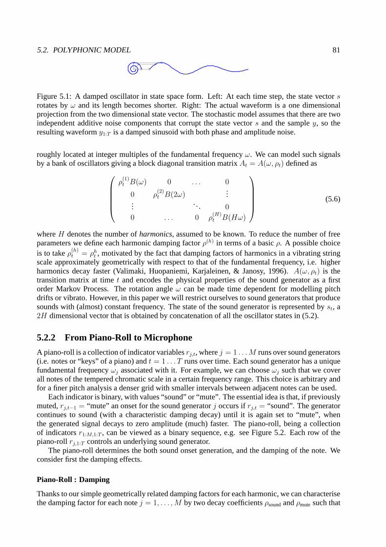
5.2. POLYPHONIC MODEL 81
Figure 5.1: A damped oscillator in state space form. Left: Ateach time step, the state vectorsrotates byω and its length becomes shorter. Right: The actual waveform is a one dimensionalprojection from the two dimensional state vector. The stochastic model assumes that there are twoindependent additive noise components that corrupt the state vectors and the sampley, so theresulting waveformy1:T is a damped sinusoid with both phase and amplitude noise.
roughly located at integer multiples of the fundamental frequencyω. We can model such signalsby a bank of oscillators giving a block diagonal transition matrixAt = A(ω, ρt) defined as
ρ(1)t B(ω) 0 . . . 0
0 ρ(2)t B(2ω)
......
. .. 0
0 . . . 0 ρ(H)t B(Hω)
(5.6)
whereH denotes the number ofharmonics, assumed to be known. To reduce the number of freeparameters we define each harmonic damping factorρ(h) in terms of a basicρ. A possible choiceis to takeρ(h)
t = ρht , motivated by the fact that damping factors of harmonics in avibrating string
scale approximately geometrically with respect to that of the fundamental frequency, i.e. higherharmonics decay faster (Valimaki, Huopaniemi, Karjaleinen, & Janosy, 1996).A(ω, ρt) is thetransition matrix at timet and encodes the physical properties of the sound generator as a firstorder Markov Process. The rotation angleω can be made time dependent for modelling pitchdrifts or vibrato. However, in this paper we will restrict ourselves to sound generators that producesounds with (almost) constant frequency. The state of the sound generator is represented byst, a2H dimensional vector that is obtained by concatenation of allthe oscillator states in (5.2).
5.2.2 From Piano-Roll to Microphone
A piano-roll is a collection of indicator variablesrj,t, wherej = 1 . . .M runs over sound generators(i.e. notes or “keys” of a piano) andt = 1 . . . T runs over time. Each sound generator has a uniquefundamental frequencyωj associated with it. For example, we can chooseωj such that we coverall notes of the tempered chromatic scale in a certain frequency range. This choice is arbitrary andfor a finer pitch analysis a denser grid with smaller intervals between adjacent notes can be used.
Each indicator is binary, with values “sound” or “mute”. Theessential idea is that, if previouslymuted,rj,t−1 = “mute” an onset for the sound generatorj occurs ifrj,t = “sound”. The generatorcontinues to sound (with a characteristic damping decay) until it is again set to “mute”, whenthe generated signal decays to zero amplitude (much) faster. The piano-roll, being a collectionof indicatorsr1:M,1:T , can be viewed as a binary sequence, e.g. see Figure 5.2. Eachrow of thepiano-rollrj,1:T controls an underlying sound generator.
The piano-roll determines the both sound onset generation,and the damping of the note. Weconsider first the damping effects.
Piano-Roll : Damping
Thanks to our simple geometrically related damping factorsfor each harmonic, we can characterisethe damping factor for each notej = 1, . . . ,M by two decay coefficientsρsoundandρmute such that
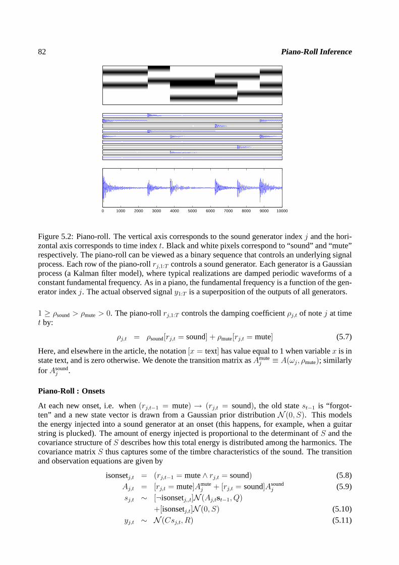
82 Piano-Roll Inference
0 1000 2000 3000 4000 5000 6000 7000 8000 9000 10000
Figure 5.2: Piano-roll. The vertical axis corresponds to the sound generator indexj and the hori-zontal axis corresponds to time indext. Black and white pixels correspond to “sound” and “mute”respectively. The piano-roll can be viewed as a binary sequence that controls an underlying signalprocess. Each row of the piano-rollrj,1:T controls a sound generator. Each generator is a Gaussianprocess (a Kalman filter model), where typical realizationsare damped periodic waveforms of aconstant fundamental frequency. As in a piano, the fundamental frequency is a function of the gen-erator indexj. The actual observed signaly1:T is a superposition of the outputs of all generators.
1 ≥ ρsound> ρmute> 0. The piano-rollrj,1:T controls the damping coefficientρj,t of notej at timet by:
ρj,t = ρsound[rj,t = sound] + ρmute[rj,t = mute] (5.7)
Here, and elsewhere in the article, the notation[x = text] has value equal to 1 when variablex is instate text, and is zero otherwise. We denote the transition matrix asAmute
j ≡ A(ωj, ρmute); similarlyfor Asound
j .
Piano-Roll : Onsets
At each new onset, i.e. when(rj,t−1 = mute) → (rj,t = sound), the old statest−1 is “forgot-ten” and a new state vector is drawn from a Gaussian prior distributionN (0, S). This modelsthe energy injected into a sound generator at an onset (this happens, for example, when a guitarstring is plucked). The amount of energy injected is proportional to the determinant ofS and thecovariance structure ofS describes how this total energy is distributed among the harmonics. Thecovariance matrixS thus captures some of the timbre characteristics of the sound. The transitionand observation equations are given by
isonsetj,t = (rj,t−1 = mute∧ rj,t = sound) (5.8)
Aj,t = [rj,t = mute]Amutej + [rj,t = sound]Asound
j (5.9)
sj,t ∼ [¬isonsetj,,t]N (Aj,tst−1, Q)
+[isonsetj,t]N (0, S) (5.10)
yj,t ∼ N (Csj,t, R) (5.11)

5.2. POLYPHONIC MODEL 83
M
rj,1 rj,2 . . . rj,t
sj,1 sj,2 . . . sj,t
yj,1 yj,2 . . . yj,t
y1 y2 . . . yt
Figure 5.3: Graphical Model. The rectangle box denotes “plates”,M replications of the nodesinside. Each plate,j = 1, . . . ,M represents the sound generator (note) variables through time.
In the above,C is a1×2H projection matrixC = [1, 0, 1, 0, . . . , 1, 0] with zero entries on the evencomponents. Henceyj,t has a mean being the sum of the damped harmonic oscillators.R modelsthe variance of the noise in the output of each sound generator. Finally, the observed audio signalis the superposition of the outputs of all sound generators,
yt =∑
j
yj,t (5.12)
The generative model (5.7)-(5.12) can be described qualitatively by the graphical model inFigure 5.3. Equations (5.11) and (5.12) definep(y1:T |s1:M,1:T ). Equations (5.7) (5.9) and (5.10)relater ands and definep(s1:M,1:T |r1:M,1:T ). In this paper, the prior modelp(r1:M,1:T ) is Markovianand has the following factorial structure1:
p(r1:M,1:T ) =∏
m
∏
t
p(rm,t|rm,t−1)
5.2.3 Inference
Given the polyphonic model described in section 5.2, to infer the most likely piano-roll we needto compute
r∗1:M,1:T = argmaxr1:M,1:T
p(r1:M,1:T |y1:T ) (5.13)
where the posterior is given by
p(r1:M,1:T |y1:T ) =1
p(y1:T )
∫
s1:M,1:T
p(y1:T |s1:M,1:T )
×p(s1:M,1:T |r1:M,1:T )p(r1:M,1:T )
1In the simulations we have fixed the transition parameterp(r = mute|r = sound) = p(r = sound|r = mute) =10−7
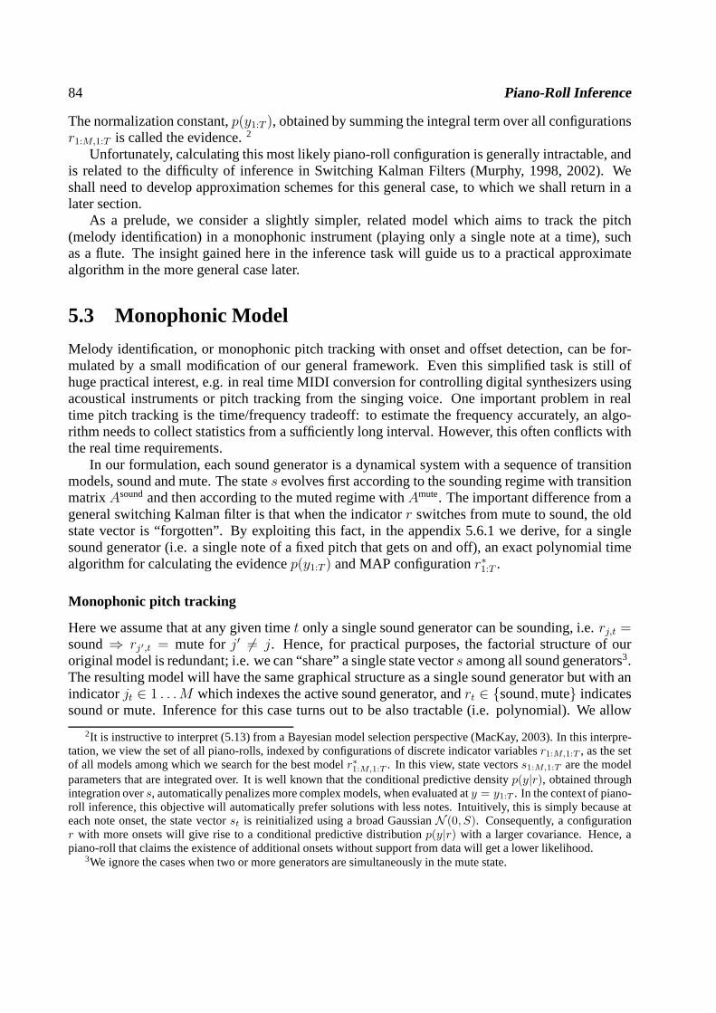
84 Piano-Roll Inference
The normalization constant,p(y1:T ), obtained by summing the integral term over all configurationsr1:M,1:T is called the evidence.2
Unfortunately, calculating this most likely piano-roll configuration is generally intractable, andis related to the difficulty of inference in Switching KalmanFilters (Murphy, 1998, 2002). Weshall need to develop approximation schemes for this general case, to which we shall return in alater section.
As a prelude, we consider a slightly simpler, related model which aims to track the pitch(melody identification) in a monophonic instrument (playing only a single note at a time), suchas a flute. The insight gained here in the inference task will guide us to a practical approximatealgorithm in the more general case later.
5.3 Monophonic Model
Melody identification, or monophonic pitch tracking with onset and offset detection, can be for-mulated by a small modification of our general framework. Even this simplified task is still ofhuge practical interest, e.g. in real time MIDI conversion for controlling digital synthesizers usingacoustical instruments or pitch tracking from the singing voice. One important problem in realtime pitch tracking is the time/frequency tradeoff: to estimate the frequency accurately, an algo-rithm needs to collect statistics from a sufficiently long interval. However, this often conflicts withthe real time requirements.
In our formulation, each sound generator is a dynamical system with a sequence of transitionmodels, sound and mute. The states evolves first according to the sounding regime with transitionmatrixAsoundand then according to the muted regime withAmute. The important difference from ageneral switching Kalman filter is that when the indicatorr switches from mute to sound, the oldstate vector is “forgotten”. By exploiting this fact, in theappendix 5.6.1 we derive, for a singlesound generator (i.e. a single note of a fixed pitch that gets on and off), an exact polynomial timealgorithm for calculating the evidencep(y1:T ) and MAP configurationr∗1:T .
Monophonic pitch tracking
Here we assume that at any given timet only a single sound generator can be sounding, i.e.rj,t =sound⇒ rj′,t = mute forj′ 6= j. Hence, for practical purposes, the factorial structure ofouroriginal model is redundant; i.e. we can “share” a single state vectors among all sound generators3.The resulting model will have the same graphical structure as a single sound generator but with anindicatorjt ∈ 1 . . .M which indexes the active sound generator, andrt ∈ {sound,mute} indicatessound or mute. Inference for this case turns out to be also tractable (i.e. polynomial). We allow
2It is instructive to interpret (5.13) from a Bayesian model selection perspective (MacKay, 2003). In this interpre-tation, we view the set of all piano-rolls, indexed by configurations of discrete indicator variablesr1:M,1:T , as the setof all models among which we search for the best modelr∗
1:M,1:T . In this view, state vectorss1:M,1:T are the modelparameters that are integrated over. It is well known that the conditional predictive densityp(y|r), obtained throughintegration overs, automatically penalizes more complex models, when evaluated aty = y1:T . In the context of piano-roll inference, this objective will automatically prefer solutions with less notes. Intuitively, this is simply because ateach note onset, the state vectorst is reinitialized using a broad GaussianN (0, S). Consequently, a configurationr with more onsets will give rise to a conditional predictive distribution p(y|r) with a larger covariance. Hence, apiano-roll that claims the existence of additional onsets without support from data will get a lower likelihood.
3We ignore the cases when two or more generators are simultaneously in the mute state.
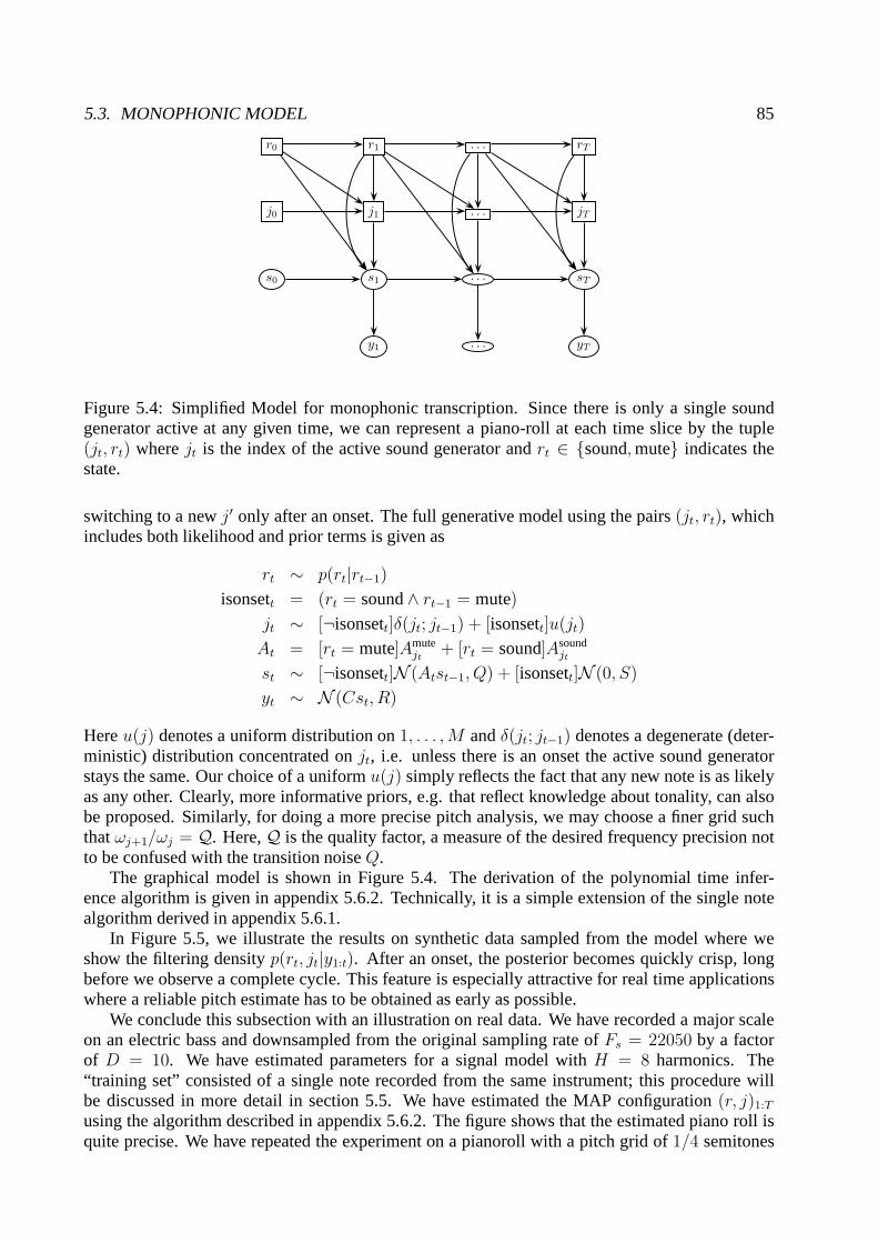
5.3. MONOPHONIC MODEL 85
r0 r1 . . . rT
j0 j1 . . . jT
s0 s1 . . . sT
y1 . . . yT
Figure 5.4: Simplified Model for monophonic transcription.Since there is only a single soundgenerator active at any given time, we can represent a piano-roll at each time slice by the tuple(jt, rt) wherejt is the index of the active sound generator andrt ∈ {sound,mute} indicates thestate.
switching to a newj′ only after an onset. The full generative model using the pairs (jt, rt), whichincludes both likelihood and prior terms is given as
rt ∼ p(rt|rt−1)
isonsett = (rt = sound∧ rt−1 = mute)
jt ∼ [¬isonsett]δ(jt; jt−1) + [isonsett]u(jt)
At = [rt = mute]Amutejt
+ [rt = sound]Asoundjt
st ∼ [¬isonsett]N (Atst−1, Q) + [isonsett]N (0, S)
yt ∼ N (Cst, R)
Hereu(j) denotes a uniform distribution on1, . . . ,M andδ(jt; jt−1) denotes a degenerate (deter-ministic) distribution concentrated onjt, i.e. unless there is an onset the active sound generatorstays the same. Our choice of a uniformu(j) simply reflects the fact that any new note is as likelyas any other. Clearly, more informative priors, e.g. that reflect knowledge about tonality, can alsobe proposed. Similarly, for doing a more precise pitch analysis, we may choose a finer grid suchthatωj+1/ωj = Q. Here,Q is the quality factor, a measure of the desired frequency precision notto be confused with the transition noiseQ.
The graphical model is shown in Figure 5.4. The derivation ofthe polynomial time infer-ence algorithm is given in appendix 5.6.2. Technically, it is a simple extension of the single notealgorithm derived in appendix 5.6.1.
In Figure 5.5, we illustrate the results on synthetic data sampled from the model where weshow the filtering densityp(rt, jt|y1:t). After an onset, the posterior becomes quickly crisp, longbefore we observe a complete cycle. This feature is especially attractive for real time applicationswhere a reliable pitch estimate has to be obtained as early aspossible.
We conclude this subsection with an illustration on real data. We have recorded a major scaleon an electric bass and downsampled from the original sampling rate ofFs = 22050 by a factorof D = 10. We have estimated parameters for a signal model withH = 8 harmonics. The“training set” consisted of a single note recorded from the same instrument; this procedure willbe discussed in more detail in section 5.5. We have estimatedthe MAP configuration(r, j)1:T
using the algorithm described in appendix 5.6.2. The figure shows that the estimated piano roll isquite precise. We have repeated the experiment on a pianoroll with a pitch grid of1/4 semitones

86 Piano-Roll Inference
100 200 300 400 500 600 700 800 900 1000−100
−50
0
50
100 200 300 400 500 600 700 800 900 1000
5
10
15
Figure 5.5: Monophonic pitch tracking. (Top) Synthetic data sampled from model in Figure 5.4.Vertical bars denote the onset and offset times. (Bottom) The filtering densityp(rt, jt|y1:t). Thevertical axis denotes the sound generator indexjt and the gray level denotes the posterior proba-bility p(rt = sound, jt|y1:t) where black corresponds to1.
500 1000 1500 2000 2500 3000 3500
500 1000 1500 2000 2500 3000 3500 500 1000 1500 2000 2500 3000 3500
Figure 5.6: Monophonic pitch estimation on real data. (Top,left) F major scale played on anelectric bass. (Top, right) Estimated MAP configuration(r, j)1:T . (Bottom, left) A finer analysiswithQ = 21/48 reveals that the 5’th and 7’th degree of the scale are intonated slightly low. (Bottom,right) Poorer results may be obtained when signal model parameters are not set correctly.
(Q = 21/48). The results reveal that the5’th and7’th degree of the scale were intonated slightlylow, which didn’t had much effect on the estimation of the pitch class when using a coarser grid.In the last experiment we have trained the model parameters using a note sung by a vocalist. Asexpected, the results are poorer; in particular we observe that5’ths or octaves are confused due tothe different harmonic structure and transition characteristics.
Extension to vibrato and legato
The monophonic model has been constructed such that the rotation angleω remains constant.Although the the transition noise with varianceQ still allows for small and independent deviationsin frequencies of the harmonics, the model is not realistic for situations with systematic pitchdrift or fluctuation, e.g. as is the case with vibrato. Moreover, on many musical instruments,it is possible to playlegato, that is without an explicit onset between note boundaries.In our
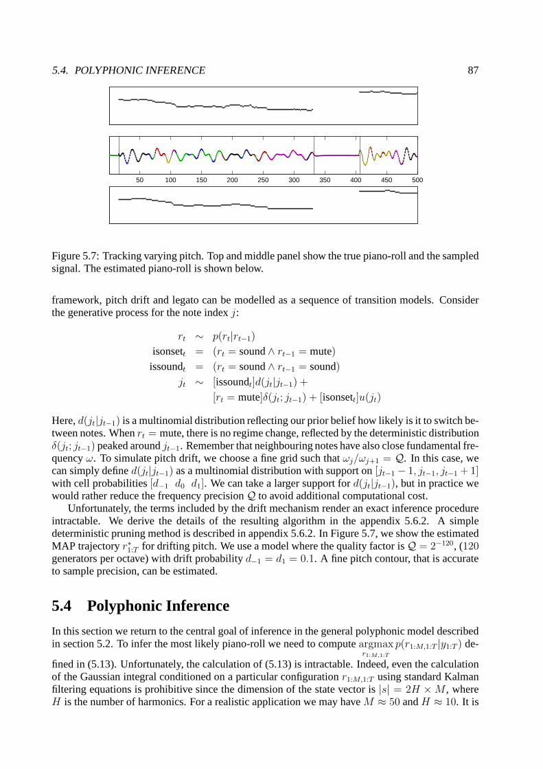
5.4. POLYPHONIC INFERENCE 87
50 100 150 200 250 300 350 400 450 500
Figure 5.7: Tracking varying pitch. Top and middle panel show the true piano-roll and the sampledsignal. The estimated piano-roll is shown below.
framework, pitch drift and legato can be modelled as a sequence of transition models. Considerthe generative process for the note indexj:
rt ∼ p(rt|rt−1)
isonsett = (rt = sound∧ rt−1 = mute)
issoundt = (rt = sound∧ rt−1 = sound)
jt ∼ [issoundt]d(jt|jt−1) +
[rt = mute]δ(jt; jt−1) + [isonsett]u(jt)
Here,d(jt|jt−1) is a multinomial distribution reflecting our prior belief how likely is it to switch be-tween notes. Whenrt = mute, there is no regime change, reflected by the deterministic distributionδ(jt; jt−1) peaked aroundjt−1. Remember that neighbouring notes have also close fundamental fre-quencyω. To simulate pitch drift, we choose a fine grid such thatωj/ωj+1 = Q. In this case, wecan simply defined(jt|jt−1) as a multinomial distribution with support on[jt−1 − 1, jt−1, jt−1 + 1]with cell probabilities[d−1 d0 d1]. We can take a larger support ford(jt|jt−1), but in practice wewould rather reduce the frequency precisionQ to avoid additional computational cost.
Unfortunately, the terms included by the drift mechanism render an exact inference procedureintractable. We derive the details of the resulting algorithm in the appendix 5.6.2. A simpledeterministic pruning method is described in appendix 5.6.2. In Figure 5.7, we show the estimatedMAP trajectoryr∗1:T for drifting pitch. We use a model where the quality factor isQ = 2−120, (120generators per octave) with drift probabilityd−1 = d1 = 0.1. A fine pitch contour, that is accurateto sample precision, can be estimated.
5.4 Polyphonic Inference
In this section we return to the central goal of inference in the general polyphonic model describedin section 5.2. To infer the most likely piano-roll we need tocomputeargmax
r1:M,1:T
p(r1:M,1:T |y1:T ) de-
fined in (5.13). Unfortunately, the calculation of (5.13) isintractable. Indeed, even the calculationof the Gaussian integral conditioned on a particular configurationr1:M,1:T using standard Kalmanfiltering equations is prohibitive since the dimension of the state vector is|s| = 2H ×M , whereH is the number of harmonics. For a realistic application we may haveM ≈ 50 andH ≈ 10. It is
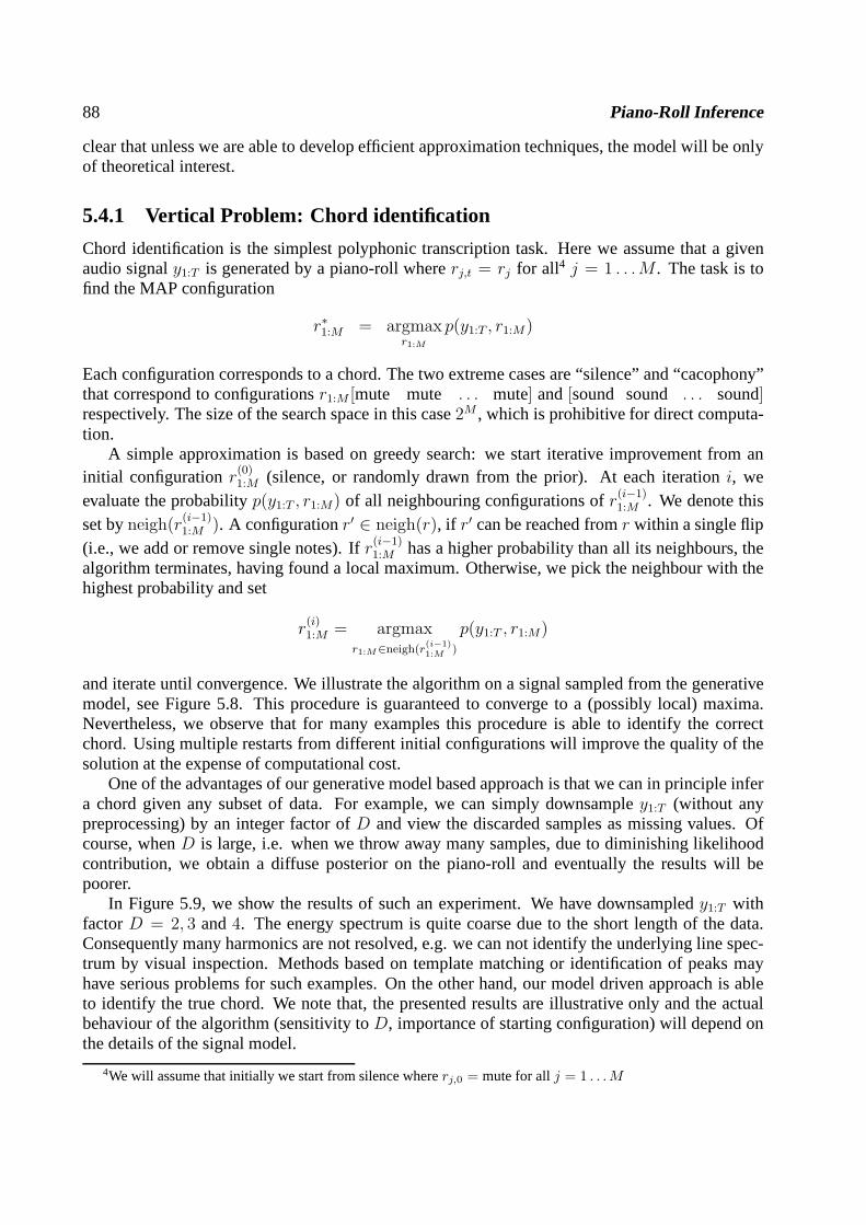
88 Piano-Roll Inference
clear that unless we are able to develop efficient approximation techniques, the model will be onlyof theoretical interest.
5.4.1 Vertical Problem: Chord identification
Chord identification is the simplest polyphonic transcription task. Here we assume that a givenaudio signaly1:T is generated by a piano-roll whererj,t = rj for all4 j = 1 . . .M . The task is tofind the MAP configuration
r∗1:M = argmaxr1:M
p(y1:T , r1:M)
Each configuration corresponds to a chord. The two extreme cases are “silence” and “cacophony”that correspond to configurationsr1:M [mute mute . . . mute] and[sound sound . . . sound]respectively. The size of the search space in this case2M , which is prohibitive for direct computa-tion.
A simple approximation is based on greedy search: we start iterative improvement from aninitial configurationr(0)
1:M (silence, or randomly drawn from the prior). At each iteration i, weevaluate the probabilityp(y1:T , r1:M) of all neighbouring configurations ofr(i−1)
1:M . We denote thisset byneigh(r
(i−1)1:M ). A configurationr′ ∈ neigh(r), if r′ can be reached fromr within a single flip
(i.e., we add or remove single notes). Ifr(i−1)1:M has a higher probability than all its neighbours, the
algorithm terminates, having found a local maximum. Otherwise, we pick the neighbour with thehighest probability and set
r(i)1:M = argmax
r1:M∈neigh(r(i−1)1:M )
p(y1:T , r1:M)
and iterate until convergence. We illustrate the algorithmon a signal sampled from the generativemodel, see Figure 5.8. This procedure is guaranteed to converge to a (possibly local) maxima.Nevertheless, we observe that for many examples this procedure is able to identify the correctchord. Using multiple restarts from different initial configurations will improve the quality of thesolution at the expense of computational cost.
One of the advantages of our generative model based approachis that we can in principle infera chord given any subset of data. For example, we can simply downsampley1:T (without anypreprocessing) by an integer factor ofD and view the discarded samples as missing values. Ofcourse, whenD is large, i.e. when we throw away many samples, due to diminishing likelihoodcontribution, we obtain a diffuse posterior on the piano-roll and eventually the results will bepoorer.
In Figure 5.9, we show the results of such an experiment. We have downsampledy1:T withfactorD = 2, 3 and4. The energy spectrum is quite coarse due to the short length of the data.Consequently many harmonics are not resolved, e.g. we can not identify the underlying line spec-trum by visual inspection. Methods based on template matching or identification of peaks mayhave serious problems for such examples. On the other hand, our model driven approach is ableto identify the true chord. We note that, the presented results are illustrative only and the actualbehaviour of the algorithm (sensitivity toD, importance of starting configuration) will depend onthe details of the signal model.
4We will assume that initially we start from silence whererj,0 = mute for allj = 1 . . .M
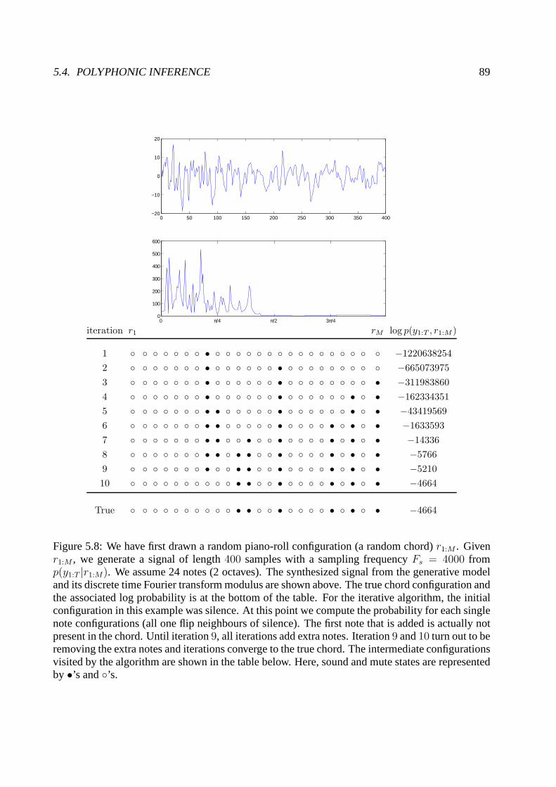
5.4. POLYPHONIC INFERENCE 89
0 50 100 150 200 250 300 350 400−20
−10
0
10
20
0 π/4 π/2 3π/40
100
200
300
400
500
600
iteration r1 rM log p(y1:T , r1:M )
1 ◦ ◦ ◦ ◦ ◦ ◦ ◦ • ◦ ◦ ◦ ◦ ◦ ◦ ◦ ◦ ◦ ◦ ◦ ◦ ◦ ◦ ◦ ◦ −1220638254
2 ◦ ◦ ◦ ◦ ◦ ◦ ◦ • ◦ ◦ ◦ ◦ ◦ ◦ • ◦ ◦ ◦ ◦ ◦ ◦ ◦ ◦ ◦ −665073975
3 ◦ ◦ ◦ ◦ ◦ ◦ ◦ • ◦ ◦ ◦ ◦ ◦ ◦ • ◦ ◦ ◦ ◦ ◦ ◦ ◦ ◦ • −311983860
4 ◦ ◦ ◦ ◦ ◦ ◦ ◦ • ◦ ◦ ◦ ◦ ◦ ◦ • ◦ ◦ ◦ ◦ ◦ ◦ • ◦ • −162334351
5 ◦ ◦ ◦ ◦ ◦ ◦ ◦ • • ◦ ◦ ◦ ◦ ◦ • ◦ ◦ ◦ ◦ ◦ ◦ • ◦ • −43419569
6 ◦ ◦ ◦ ◦ ◦ ◦ ◦ • • ◦ ◦ ◦ ◦ ◦ • ◦ ◦ ◦ ◦ • ◦ • ◦ • −1633593
7 ◦ ◦ ◦ ◦ ◦ ◦ ◦ • • ◦ ◦ • ◦ ◦ • ◦ ◦ ◦ ◦ • ◦ • ◦ • −14336
8 ◦ ◦ ◦ ◦ ◦ ◦ ◦ • • ◦ • • ◦ ◦ • ◦ ◦ ◦ ◦ • ◦ • ◦ • −5766
9 ◦ ◦ ◦ ◦ ◦ ◦ ◦ • ◦ ◦ • • ◦ ◦ • ◦ ◦ ◦ ◦ • ◦ • ◦ • −5210
10 ◦ ◦ ◦ ◦ ◦ ◦ ◦ ◦ ◦ ◦ • • ◦ ◦ • ◦ ◦ ◦ ◦ • ◦ • ◦ • −4664
True ◦ ◦ ◦ ◦ ◦ ◦ ◦ ◦ ◦ ◦ • • ◦ ◦ • ◦ ◦ ◦ ◦ • ◦ • ◦ • −4664
Figure 5.8: We have first drawn a random piano-roll configuration (a random chord)r1:M . Givenr1:M , we generate a signal of length400 samples with a sampling frequencyFs = 4000 fromp(y1:T |r1:M). We assume 24 notes (2 octaves). The synthesized signal fromthe generative modeland its discrete time Fourier transform modulus are shown above. The true chord configuration andthe associated log probability is at the bottom of the table.For the iterative algorithm, the initialconfiguration in this example was silence. At this point we compute the probability for each singlenote configurations (all one flip neighbours of silence). Thefirst note that is added is actually notpresent in the chord. Until iteration9, all iterations add extra notes. Iteration9 and10 turn out to beremoving the extra notes and iterations converge to the truechord. The intermediate configurationsvisited by the algorithm are shown in the table below. Here, sound and mute states are representedby •’s and◦’s.

90 Piano-Roll Inference
0 20 40 60 80 100 120 140 160 180 200−20
−10
0
10
20
0 π/4 π/2 3π/40
50
100
150
200
250
300
0 20 40 60 80 100 120 140−20
−15
−10
−5
0
5
10
15
0 π/4 π/2 3π/40
50
100
150
200
250
0 10 20 30 40 50 60 70 80 90 100−20
−10
0
10
20
0 π/4 π/2 3π/40
50
100
150
D p(y1:D:T , r1:M ) Init
2 ◦ ◦ ◦ ◦ ◦ ◦ ◦ ◦ ◦ ◦ • • ◦ ◦ • ◦ ◦ ◦ ◦ • ◦ • ◦ • −2685 True
◦ ◦ ◦ ◦ ◦ ◦ ◦ ◦ ◦ ◦ • ◦ ◦ • • ◦ ◦ • ◦ • ◦ • ◦ • −3179 Silence
◦ ◦ ◦ ◦ ◦ ◦ ◦ ◦ ◦ ◦ • • ◦ ◦ • ◦ ◦ ◦ ◦ • ◦ • ◦ • −2685 Random
3 ◦ ◦ ◦ ◦ ◦ ◦ ◦ ◦ ◦ ◦ • • ◦ ◦ • ◦ ◦ ◦ ◦ • ◦ • ◦ • −2057 True
◦ ◦ ◦ ◦ ◦ ◦ ◦ ◦ ◦ ◦ • • ◦ ◦ • ◦ ◦ ◦ ◦ • ◦ • ◦ • −2057 Silence
◦ ◦ ◦ ◦ ◦ ◦ ◦ ◦ ◦ • ◦ ◦ • ◦ • ◦ ◦ • • • • ◦ ◦ • −2616 Random
4 ◦ ◦ ◦ ◦ ◦ ◦ ◦ ◦ ◦ ◦ • • ◦ ◦ • ◦ ◦ ◦ ◦ • ◦ • ◦ • −1605 True
◦ ◦ ◦ ◦ ◦ ◦ ◦ ◦ • ◦ • • ◦ ◦ • ◦ • ◦ ◦ • ◦ ◦ ◦ ◦ −1668 Silence
◦ ◦ ◦ ◦ ◦ ◦ ◦ ◦ ◦ ◦ • • ◦ ◦ • ◦ ◦ ◦ ◦ • ◦ • ◦ ◦ −1591 Random
Figure 5.9: Iterative improvement results when data are subsampled by a factor ofD = 2, 3 and4, respectively. For each factorD, the top line shows the true configuration and the correspondingprobability. The second line is the solution found by starting from silence and the third line isstarting from a random configuration drawn form the prior (best of3 independent runs).
5.5. LEARNING 91
5.4.2 Piano-Roll inference Problem: Joint Chord and Melodyidentification
The piano-roll estimation problem can be viewed as an extension of chord identification in that wealso detect onsets and offsets for each note within the analysis frame. A practical approach is toanalyze the signal in sufficiently short time windows and assume that for each note, at most onechangepoint can occur within the window.
Consider data in a short window, sayy1:W . We start iterative improvement from a configurationr(0)1:M,1:W , where each time slicer(0)
1:M,t for t = 1 . . .W is equal to a “chord”r1:M,0. The chordr1:M,0
can be silence or, during a frame by frame analysis, the last time slice of the best configurationfound in the previous analysis window. Let the configurationat i − 1’th iteration be denoted asr(i−1)1:M,1:W . At each new iterationi, we evaluate the posterior probabilityp(y1,W , r1:M,1:W ), where
r1:M,1:W runs over all neighbouring configuration ofr(i−1)1:M,1:W . Each memberr1:M,1:W of the neigh-
bourhood is generated as follows: For eachj = 1 . . .M , we clamp all the other rows, i.e. we setrj′,1:W = r
(i−1)j′,1:W for j′ 6= j. For each time stept = 1 . . .W , we generate a new configuration such
that the switches up to timet are equal to the initial switchrj,0, and its opposite¬rj,0 after t, i.e.rj,t′ = rj,0[t
′ < t] + ¬rj,0[t′ ≥ t]. This is equivalent to saying that a sounding note may get muted,
or a muted note may start to sound. The computational advantage of allowing only one change-point at each row is that the probability of all neighbouringconfigurations for a fixedj can becomputed by a single backward, forward pass (Cemgil & Kappen, 2003; Murphy, 2002). Finally,we pick the neighbour with the maximum probability. The algorithm is illustrated in Figure 5.10.
The analysis for the whole sequence proceeds as follows: Consider two successive analy-sis windowsYprev ≡ y1:W andY ≡ yW+1:2W . Suppose we have obtained a solutionR∗
prev ≡r∗1:M,1:W obtained by iterative improvement. Conditioned onR∗
prev, we compute the posteriorp(s1:M,W |Yprev, R
∗prev) by Kalman filtering. This density is the prior ofs for the current analysis
window Y . The search starts from a chord equal to the last time slice ofR∗prev. In Fig. 5.11 we
show an illustrative result obtained by this algorithm on synthetic data. In similar experiments withsynthetic data, we are often able to identify the correct piano-roll.
This simple greedy search procedure is somewhat sensitive to location of onsets within theanalysis window. Especially, when an onset occurs near the end of an analysis window, it may beassociated with an incorrect pitch. The correct pitch is often identified in the next analysis window,when a longer portion of the signal is observed. However, since the basic algorithm does not allowfor correcting the previous estimate by retrospection, this introduces some artifacts. A possiblemethod to overcome this problem is to use a fixed lag smoothingapproach, where we simply carryout the analysis on overlapping windows. For example, for ananalysis windowYprev ≡ y1:W , wefind r∗1:M,1:W . The next analysis window is taken asyL+1:W+L whereL ≤ W . We find the priorp(s1:M,L|y1:L, r
∗1:M,1:L) by Kalman filtering. On the other hand, obviously, the algorithm becomes
slower by a factor ofL/W .An optimal choice forL andW will depend upon many factors such as signal characteristics,
sampling frequency, downsampling factorD, onset/offset positions, number of active sound gen-erators at a given time as well as the amount of CPU time available. In practice, these values maybe critical and they need to be determined by trial and error.On the other hand, it is importantto note thatL andW just determine how the approximation is made but not enter the underlyingmodel.
5.5 Learning
In the previous sections, we assumed that the correct signalmodel parametersθ = (S, ρ,Q,R)were known. These include in particular the damping coefficientsρsound, ρmute, transition noisevarianceQ, observation noiseR and the initial prior covariance matrixS after an onset. In practice,
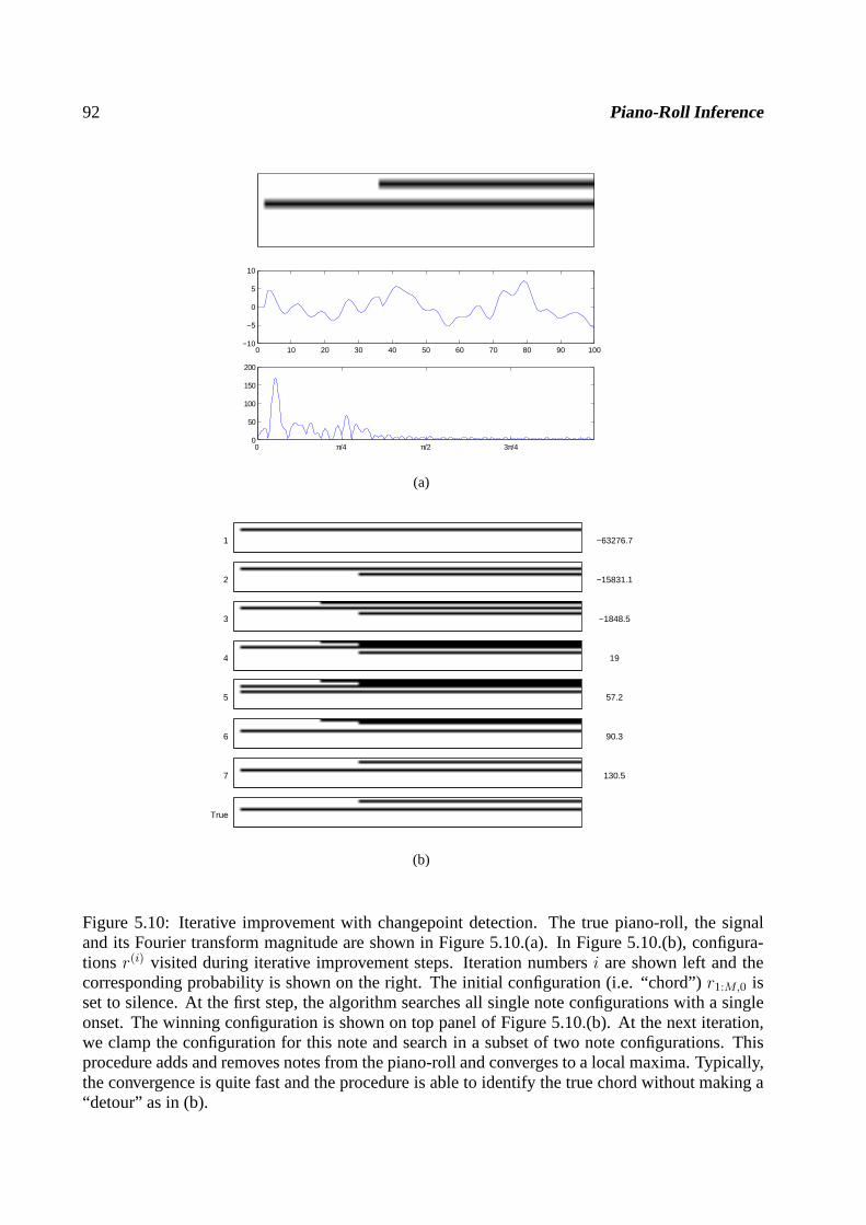
92 Piano-Roll Inference
0 10 20 30 40 50 60 70 80 90 100−10
−5
0
5
10
0 π/4 π/2 3π/40
50
100
150
200
(a)
1 −63276.7
2 −15831.1
3 −1848.5
4 19
5 57.2
6 90.3
7 130.5
True
(b)
Figure 5.10: Iterative improvement with changepoint detection. The true piano-roll, the signaland its Fourier transform magnitude are shown in Figure 5.10.(a). In Figure 5.10.(b), configura-tions r(i) visited during iterative improvement steps. Iteration numbersi are shown left and thecorresponding probability is shown on the right. The initial configuration (i.e. “chord”)r1:M,0 isset to silence. At the first step, the algorithm searches all single note configurations with a singleonset. The winning configuration is shown on top panel of Figure 5.10.(b). At the next iteration,we clamp the configuration for this note and search in a subsetof two note configurations. Thisprocedure adds and removes notes from the piano-roll and converges to a local maxima. Typically,the convergence is quite fast and the procedure is able to identify the true chord without making a“detour” as in (b).
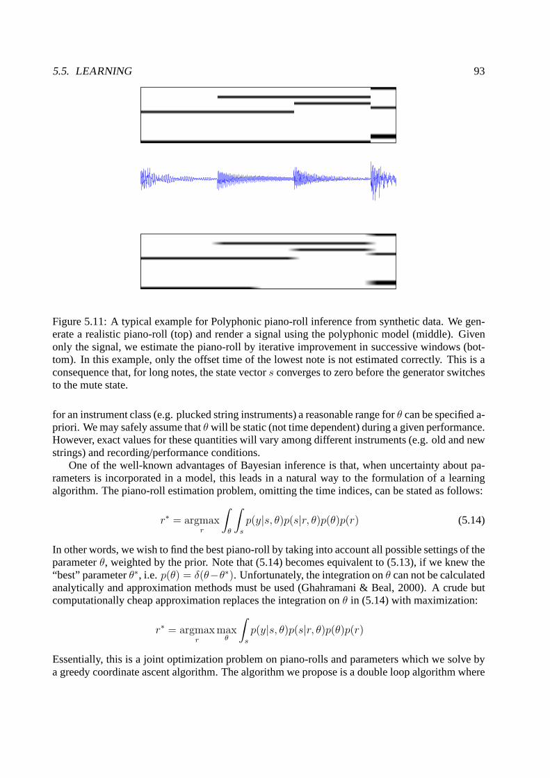
5.5. LEARNING 93
Figure 5.11: A typical example for Polyphonic piano-roll inference from synthetic data. We gen-erate a realistic piano-roll (top) and render a signal usingthe polyphonic model (middle). Givenonly the signal, we estimate the piano-roll by iterative improvement in successive windows (bot-tom). In this example, only the offset time of the lowest noteis not estimated correctly. This is aconsequence that, for long notes, the state vectors converges to zero before the generator switchesto the mute state.
for an instrument class (e.g. plucked string instruments) areasonable range forθ can be specified a-priori. We may safely assume thatθ will be static (not time dependent) during a given performance.However, exact values for these quantities will vary among different instruments (e.g. old and newstrings) and recording/performance conditions.
One of the well-known advantages of Bayesian inference is that, when uncertainty about pa-rameters is incorporated in a model, this leads in a natural way to the formulation of a learningalgorithm. The piano-roll estimation problem, omitting the time indices, can be stated as follows:
r∗ = argmaxr
∫
θ
∫
s
p(y|s, θ)p(s|r, θ)p(θ)p(r) (5.14)
In other words, we wish to find the best piano-roll by taking into account all possible settings of theparameterθ, weighted by the prior. Note that (5.14) becomes equivalentto (5.13), if we knew the“best” parameterθ∗, i.e. p(θ) = δ(θ−θ∗). Unfortunately, the integration onθ can not be calculatedanalytically and approximation methods must be used (Ghahramani & Beal, 2000). A crude butcomputationally cheap approximation replaces the integration onθ in (5.14) with maximization:
r∗ = argmaxr
maxθ
∫
s
p(y|s, θ)p(s|r, θ)p(θ)p(r)
Essentially, this is a joint optimization problem on piano-rolls and parameters which we solve bya greedy coordinate ascent algorithm. The algorithm we propose is a double loop algorithm where
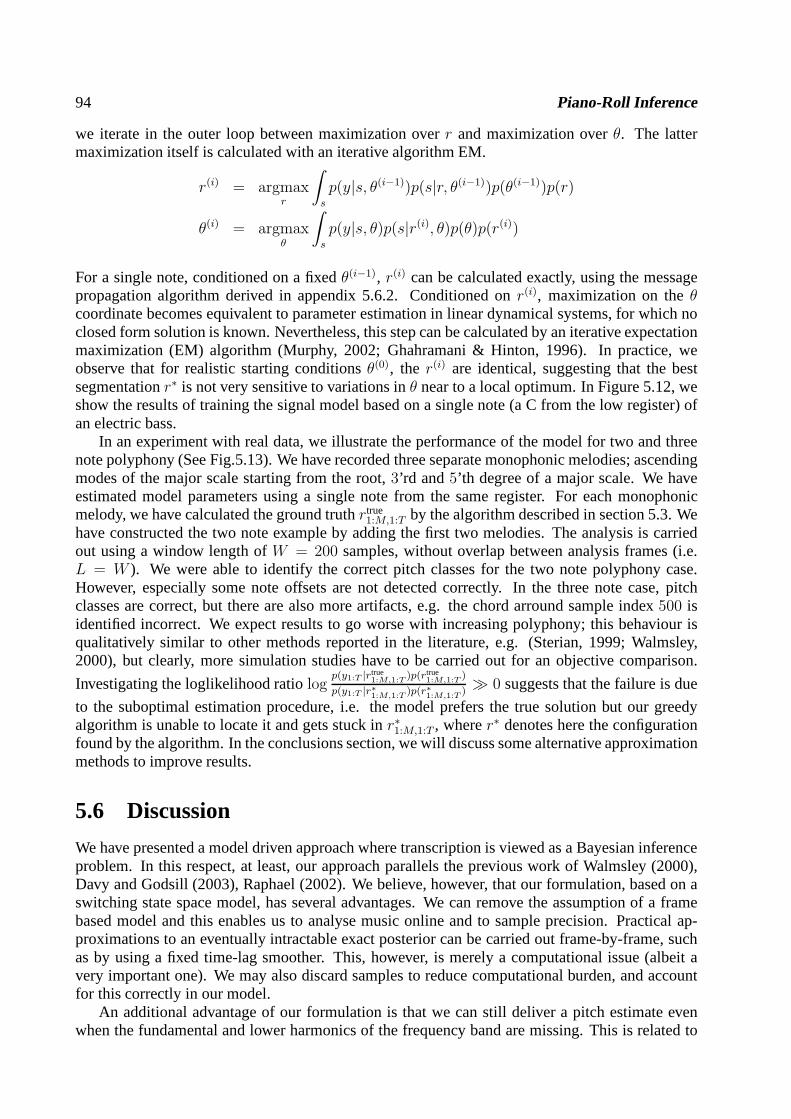
94 Piano-Roll Inference
we iterate in the outer loop between maximization overr and maximization overθ. The lattermaximization itself is calculated with an iterative algorithm EM.
r(i) = argmaxr
∫
s
p(y|s, θ(i−1))p(s|r, θ(i−1))p(θ(i−1))p(r)
θ(i) = argmaxθ
∫
s
p(y|s, θ)p(s|r(i), θ)p(θ)p(r(i))
For a single note, conditioned on a fixedθ(i−1), r(i) can be calculated exactly, using the messagepropagation algorithm derived in appendix 5.6.2. Conditioned onr(i), maximization on theθcoordinate becomes equivalent to parameter estimation in linear dynamical systems, for which noclosed form solution is known. Nevertheless, this step can be calculated by an iterative expectationmaximization (EM) algorithm (Murphy, 2002; Ghahramani & Hinton, 1996). In practice, weobserve that for realistic starting conditionsθ(0), the r(i) are identical, suggesting that the bestsegmentationr∗ is not very sensitive to variations inθ near to a local optimum. In Figure 5.12, weshow the results of training the signal model based on a single note (a C from the low register) ofan electric bass.
In an experiment with real data, we illustrate the performance of the model for two and threenote polyphony (See Fig.5.13). We have recorded three separate monophonic melodies; ascendingmodes of the major scale starting from the root,3’rd and5’th degree of a major scale. We haveestimated model parameters using a single note from the sameregister. For each monophonicmelody, we have calculated the ground truthrtrue
1:M,1:T by the algorithm described in section 5.3. Wehave constructed the two note example by adding the first two melodies. The analysis is carriedout using a window length ofW = 200 samples, without overlap between analysis frames (i.e.L = W ). We were able to identify the correct pitch classes for the two note polyphony case.However, especially some note offsets are not detected correctly. In the three note case, pitchclasses are correct, but there are also more artifacts, e.g.the chord arround sample index500 isidentified incorrect. We expect results to go worse with increasing polyphony; this behaviour isqualitatively similar to other methods reported in the literature, e.g. (Sterian, 1999; Walmsley,2000), but clearly, more simulation studies have to be carried out for an objective comparison.
Investigating the loglikelihood ratiologp(y1:T |rtrue
1:M,1:T )p(rtrue1:M,1:T )
p(y1:T |r∗1:M,1:T )p(r∗1:M,1:T )≫ 0 suggests that the failure is due
to the suboptimal estimation procedure, i.e. the model prefers the true solution but our greedyalgorithm is unable to locate it and gets stuck inr∗1:M,1:T , wherer∗ denotes here the configurationfound by the algorithm. In the conclusions section, we will discuss some alternative approximationmethods to improve results.
5.6 Discussion
We have presented a model driven approach where transcription is viewed as a Bayesian inferenceproblem. In this respect, at least, our approach parallels the previous work of Walmsley (2000),Davy and Godsill (2003), Raphael (2002). We believe, however, that our formulation, based on aswitching state space model, has several advantages. We canremove the assumption of a framebased model and this enables us to analyse music online and tosample precision. Practical ap-proximations to an eventually intractable exact posteriorcan be carried out frame-by-frame, suchas by using a fixed time-lag smoother. This, however, is merely a computational issue (albeit avery important one). We may also discard samples to reduce computational burden, and accountfor this correctly in our model.
An additional advantage of our formulation is that we can still deliver a pitch estimate evenwhen the fundamental and lower harmonics of the frequency band are missing. This is related to
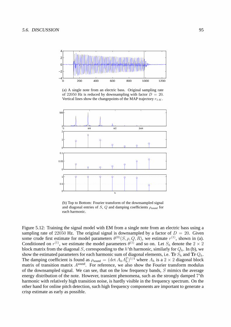
5.6. DISCUSSION 95
0 200 400 600 800 1000 1200−4
−2
0
2
4
(a) A single note from an electric bass. Original sampling rateof 22050 Hz is reduced by downsampling with factorD = 20.Vertical lines show the changepoints of the MAP trajectoryr1:K .
0 π/4 π/2 3π/40
500
0
1
2
0
0.05
0.1
0
0.5
1
h
(b) Top to Bottom: Fourier transform of the downsampled signaland diagonal entries ofS, Q and damping coefficientsρsound foreach harmonic.
Figure 5.12: Training the signal model with EM from a single note from an electric bass using asampling rate of22050 Hz. The original signal is downsampled by a factor ofD = 20. Givensome crude first estimate for model parametersθ(0)(S, ρ,Q,R), we estimater(1), shown in (a).Conditioned onr(1), we estimate the model parametersθ(1) and so on. LetSh denote the2 × 2block matrix from the diagonalS, corresponding to theh’th harmonic, similarly forQh. In (b), weshow the estimated parameters for each harmonic sum of diagonal elements, i.e.TrSh andTrQh.The damping coefficient is found asρsound = (detAhA
Th )1/4 whereAh is a2 × 2 diagonal block
matrix of transition matrixAsound. For reference, we also show the Fourier transform modulusof the downsampled signal. We can see, that on the low frequency bands,S mimics the averageenergy distribution of the note. However, transient phenomena, such as the strongly damped7’thharmonic with relatively high transition noise, is hardly visible in the frequency spectrum. On theother hand for online pitch detection, such high frequency components are important to generate acrisp estimate as early as possible.
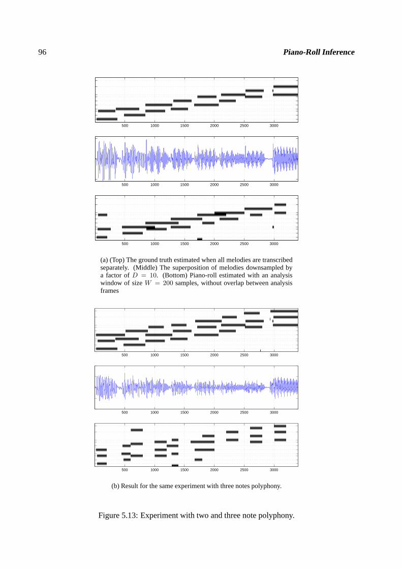
96 Piano-Roll Inference
500 1000 1500 2000 2500 3000
500 1000 1500 2000 2500 3000
500 1000 1500 2000 2500 3000
(a) (Top) The ground truth estimated when all melodies are transcribedseparately. (Middle) The superposition of melodies downsampled bya factor ofD = 10. (Bottom) Piano-roll estimated with an analysiswindow of sizeW = 200 samples, without overlap between analysisframes
500 1000 1500 2000 2500 3000
500 1000 1500 2000 2500 3000
500 1000 1500 2000 2500 3000
(b) Result for the same experiment with three notes polyphony.
Figure 5.13: Experiment with two and three note polyphony.
5.6. DISCUSSION 97
so calledvirtual pitch perception (Terhardt, 1974): we tend to associate notes with a pitch classdepending on the relationship between harmonics rather than the frequency of the fundamentalcomponent itself.
There is a strong link between model selection and polyphonic music transcription. In chordidentification we need to compare models with different number of notes, and in melody identi-fication we need to deduce the number of onsets. Model selection becomes conceptually harderwhen one needs to compare models of different size. We partially circumvent this difficulty byusing switch variables, which implicitly represent the number of components.
Following the established signal processing jargon, we maycall our approach a time-domainmethod, since we are not explicitly calculating a discrete-time Fourier transform. On the otherhand, the signal model presented here has close links to the Fourier analysis and sinusoidal mod-elling. Our analysis can be interpreted as a search procedure for a sparse representation on a setof basis vectors. In contrast to Fourier analysis, where thebasis vectors are sinusoids (e.g. see(Qi, Minka, & Picard, 2002) for a Bayesian treatment), we represent the observed signal implic-itly using signals drawn from a stochastic process which typically generates decaying periodicoscillations (e.g. notes) with occasional changepoints. The sparsity of this representation is a con-sequence of the onset mechanism, that effectively puts a mixture prior over the hidden state vectors. This prior is peaked around zero and has broad tails, indicating that most of the sources aremuted and only a few are sounding. It is well known that such Gaussian mixture priors inducesparse representations, e.g. see (Attias, 1999; Olshausen& Millman, 2000) for applications in thecontext of source separation.
5.6.1 Future work
Although our approach has many desirable features (automatically deducing number of correctnotes, high temporal resolution e.t.c.), one of the main disadvantage of our method is computa-tional cost associated with updating large covariance matrices in Kalman filtering. It would bevery desirable to investigate approximation schemas that employ fast transformations such as theFFT to accelerate computations.
When transcribing music, human experts rely heavily on prior knowledge about the musicalstructure – harmony, tempo or expression. Such structure can be captured by training probabilis-tic generative models on a corpus of compositions and performances by collecting statistics overselected features (e.g. (Raphael & Stoddard, 2003)). One ofthe important advantages of ourapproach is that such prior knowledge about the musical structure can be formulated as an in-formative prior on a piano-roll; thus can be integrated in signal analysis in a consistent manner.We believe that investigation of this direction is important in designing robust and practical musictranscription systems.
Our signal model considered here is inspired by additive synthesis. An advantage of our linearformulation is that we can use the Kalman filter recursions tointegrate out the continuous latentstate analytically. An alternative would be to formulate a nonlinear dynamical system that imple-ments a nonlinear synthesis model (e.g. FM synthesis, waveshaping synthesis, or even a physicalmodel(Smith, 1992)). Such an approach would reduce the dimensionality of the latent state spacebut force us to use approximate integration methods such as particle filters or EKF/UKF (Doucetet al., 2001). It remains an interesting open question whether, in practice, one should trade-offanalytical tractability versus reduced latent state dimension.
In this paper, for polyphonic transcription, we have used a relatively simple deterministic infer-ence method based on iterative improvement. The basic greedy algorithm, whilst still potentiallyuseful in practice, may get stuck in poor solutions. We believe that, using our model as a frame-work, better polyphonic transcriptions can be achieved using more elaborate inference or searchmethods. For example, computation time associated with exhaustive search of the neighbourhood
98 Piano-Roll Inference
for all visited configuations could be significantly reducedby randomizing the local search (e.g. byMetropolis-Hastings moves) or use heuristic proposal distributions derived from easy-to-computefeatures such as the energy spectrum. Alternatively, sequential Monte Carlo methods or determin-istic message propagation algorithms such as Expectation propagation (EP) (Minka, 2001) couldbe also used.
We have not yet tested our model for more general scenarios, such as music fragments con-taining percussive instruments or bell sounds with inharmonic spectra. Our simple periodic signalmodel would be clearly inadequate for such a scenario. On theother hand, we stress the fact that theframework presented here is not only limited to the analysisof signals with harmonic spectra, andin principle applicable to any family of signals that can be represented by a switching state spacemodel. This is already a large class since many real-world acoustic processes can be approximatedwell with piecewise linear regimes. We can also formulate a joint estimation schema for unknownparameters as in (5.14) and integrate them out (e.g. see Davyand Godsill (2003)). However, thisis currently a hard and computationally expensive task. If efficient and accurate approximate in-tegration methods can be developed, our model will be applicable to mixtures of many differenttypes of acoustical signals and may be useful in more generalauditory scene analysis problems.
Appendix 5.A Derivation of message propagation algorithms
In the appendix, we derive several exact message propagation algorithms. Our derivation closelyfollows the standard derivation of recursive prediction and update equations for the Kalman filter(Bar-Shalom & Li, 1993). First we focus on a single sound generator. In appendix 5.6.1 and 5.6.2,we derive polynomial time algorithms for calculating the evidencep(y1:T ) and MAP configurationr∗1:T = argmax
r1:T
p(y1:T , r1:T ) respectively. The MAP configuration is useful for onset/offset detec-
tion. In the following section, we extend the onset/offset detection algorithms to monophonic pitchtracking with constant frequency. We derive a polynomial time algorithm for this case in appendix5.6.2. The case for varying fundamental frequency is derived in the following appendix 5.6.2. Inappendix 5.6.2 we describe heuristics to reduce the amount of computations.
5.A.1 Computation of the evidencep(y1:T ) for a single sound generator byforward filtering
We assume a Markovian prior on the indicatorsrt wherep(rt = i|rt−1 = j) ≡ pi,j. For conve-nience, we repeat the generative model for a single sound generator by omitting the note indexj.
rt ∼ p(rt|rt−1)
isonsett = (rt = sound∧ rt−1 = mute)
st ∼ [¬isonsett]N (Artst−1, Q) + [isonsett]N (0, S)
yt ∼ N (Cst, R)
For simplicity, we will sometime use the labels1 and2 to denote sound and mute respectively. Weenumerate the transition models asfrt
(st|st−1) = N (Artst−1, Q). We define the filtering potential
as
αt ≡ p(y1:t, st, rt, rt−1) =∑
r1:t−2
∫
s0:t−1
p(y1:t, s0:t, r1:t)

5.6. DISCUSSION 99
We assume thaty is always observed, hence we use the term potential to indicate the fact thatp(y1:t, st, rt, rt−1) is not normalized. The filtering potential is in general a conditional Gaussianmixture, i.e. a mixture of Gaussians for each configuration of rt−1:t. We will highlight this datastructure by using the following notation
αt ≡{
α1,1t α1,2
t
α2,1t α2,2
t
}
where eachαi,jt = p(y1:t, st, rt = i, rt−1 = j) for i, j = 1 . . . 2 are also Gaussian mixture poten-
tials. We will denote the conditional normalization constants as
Z it ≡ p(y1:t, rt = i) =
∑
rt−1
∫
st
αi,rt−1
t
Consequently the evidence is given by
Zt ≡ p(y1:t) =∑
rt
∑
rt−1
∫
st
αt =∑
i
Z it
We also define the predictive density
αt|t−1 ≡ p(y1:t−1, st, rt, rt−1)
=∑
rt−2
∫
st−1
p(st|st−1, rt, rt−1)p(rt|rt−1)αt−1
In general, for switching Kalman filters, calculating exactposterior features, such as the evi-denceZt = p(y1:t), is not tractable. This is a consequence of the fact that the number of mixturecomponents to required to represent the exact filtering density αt grows exponentially with timestepk (i.e. one Gaussian for each of the exponentially many configurationsr1:t). Luckily, for themodel we are considering here, the growth is polynomial ink only. See also (Fearnhead, 2003).
To see this, suppose we have the filtering density available at time t − 1 asαt−1. The tran-sition models can be organized also in a table wherei’th row and j’th column correspond top(st|st−1, rt = i, rt−1 = j)
p(st|st−1, rt, rt−1) =
{
f1(st|st−1) π(st)f2(st|st−1) f2(st|st−1)
}
Calculation of the predictive potential is straightforward. First, summation overrt−2 yields
∑
rt−2
αt−1 =
{
α1,1t−1 + α1,2
t−1
α2,1t−1 + α2,2
t−1
}
≡{
ξ1t−1
ξ2t−1
}
Integration overst−1 and multiplication byp(rt|rt−1) yields the predictive potential
αt|t−1 =
{
p1,1ψ11(st) p1,2Z
2t−1π(st)
p2,1ψ12(st) p2,2ψ
22(st)
}
where we define
Z2t−1 ≡
∫
st−1
ξ2t−1 ψj
i (st) ≡∫
st−1
fi(st|st−1)ξjt−1

100 Piano-Roll Inference
The potentialsψji can be computed by applying the standard Kalman prediction equations to each
component ofξjt−1. The updated potential is given byαt = p(yt|st)αt|t−1. This quantity can be
computed by applying standard Kalman update equations to each component ofαt|t−1.From the above derivation, it is clear thatα1,2
t has only a single Gaussian component. Thishas the consequence that the number of Gaussian components in α1,1
t increases only linearly (thefirst row-sum termsξ1
t−1 propagated throughf1). The second row sum termξ2t is more costly; it
increases at every time slice by the number of components inξ1t−1. Since the size ofξ1
t−1 growslinearly, the size ofξ2
t grows quadratically with timet.
5.6.2 Computation of MAP configuration r∗1:T
The MAP state is defined as
r∗1:T = argmaxr1:T
∫
s0:T
p(y1:T , s0:T , r1:T )
≡ argmaxr1:T
∫
s0:T
φ(s0:T , r1:T )
For finding the MAP state, we replace summations overrt by maximization. One potentialtechnical difficulty is that, unlike in the case for evidencecalculation, maximization and integrationdo not commute. Consider a conditional Gaussian potential
φ(s, r) ≡ {φ(s, r = 1), φ(s, r = 2)}whereφ(s, r) are Gaussian potentials for each configuration ofr. We can compute the MAPconfiguration
r∗ = argmaxr
∫
s
φ(s, r) = argmax{
Z1, Z2}
whereZj =∫
sφ(s, r = j). We evaluate the normalization of each component (i.e. integrate over
the continuous hidden variables first) and finally find the maximum of all normalization constants.However, direct calculation ofr∗1:T is not feasible because of exponential explosion in the num-
ber of distinct configurations. Fortunately, for our model,we can introduce a deterministic pruningschema that reduces the number of kernels to a polynomial order and meanwhile guarantees thatwe will never eliminate the MAP configuration. This exact pruning method hinges on the factor-ization of the posterior for the assignment of variablesrt = 1, rt−1 = 2 (mute to sound transition)that breaks the direct link betweenst andst−1:
φ(s0:T , r1:t−2, rt−1 = 2, rt = 1, rt+1:T ) =
φ(s0:t−1, r1:t−2, rt−1 = 2)φ(st:T , rt+1:T , rt = 1|rt−1 = 2) (5.15)
In this case:
maxr1:T
∫
s0:Tφ(s0:T , r1:t−2, rt−1 = 2, rt = 1, rt+1:T )
= maxr1:t−1
∫
s0:t−1φ(s0:t−1, r1:t−2, rt−1 = 2)
×maxrt:T
∫
st:Tφ(st:T , rt+1:T , rt = 1|rt−1 = 2)
= Z2t ×maxrt+1:T
∫
st:Tφ(st:T , rt+1:T , rt = 1|rt−1 = 2) (5.16)
This Equation shows that whenever we have an onset, we can calculate the maximum over the pastand future configurations separately. Put differently, provided that the MAP configuration has theform r∗1:T = [r∗1:t−3, rt−1 = 2, rt = 1, r∗t+1:T ], the prefix[r∗1:t−3, rt−1 = 2] will be the solution forthe reduced maximization problemarg maxr1:t−1
∫
s0:t−1φ(s0:t−1, r1:t−1).

5.6. DISCUSSION 101
Forward pass
Suppose we have a collection of Gaussian potentials
δt−1 ≡{
δ1,1t−1 δ1,2
t−1
δ2,1t−1 δ2,2
t−1
}
≡{
δ1t−1
δ2t−1
}
with the property that the Gaussian kernel corresponding the prefixr∗1:t−1 of the MAP state is amember ofδt−1, i.e.φ(st−1, r
∗1:t−1) ∈ δt−1 s.t. r∗1:T = [r∗1:t−1, r
∗t:T ]. We also define the subsets
δi,jt−1 = {φ(st−1, r1:t−1) : φ ∈ δt−1andrt−1 = i, rt−2 = j}δit−1 =
⋃
j
δi,jt−1
We show how we findδt. The prediction is given by
δt|t−1 =
∫
st−1
p(st|st−1, rt, rt−1)p(rt|rt−1)δt−1
The multiplication byp(rt|rt−1) and integration overst−1 yields the predictive potentialδt|t−1
{
p1,1
∫
st−1f1(st|st−1)δ
1t−1 p1,2π(st)
∫
st−1δ2t−1
p2,1
∫
st−1f2(st|st−1)δ
1t−1 p2,2
∫
st−1f2(st|st−1)δ
2t−1
}
By the (5.16), we can replace the collection of numbers∫
st−1δ2t−1 with with the scalarZ2
t−1 ≡max
∫
st−1δ2t−1 without changing the optimum solution:
δ1,2t|t−1 = p1,2Z
2t−1π(st)
The updated potential is given byδt = p(yt|st)δt|t−1. The analysis of the number of kernelsproceeds as in the previous section.
Decoding
During the forward pass, we tag each Gaussian component ofδt with its past history ofr1:t. TheMAP state can be found by a simple search in the collection of polynomially many numbers andreporting the associated tag:
r∗1:T = argmaxr1:T
∫
sT
δT
We finally conclude that the forward filtering and MAP (Viterbi path) estimation algorithms areessentially identical with summation replaced by maximization and an additional tagging requiredfor decoding.
5.A.3 Inference for monophonic pitch tracking
In this section we derive an exact message propagation algorithm for monophonic pitch tracking.Perhaps surprisingly, inference in this case turns out to bestill tractable. Even though the sizeof the configuration spacer1:M,1:T is of size(M + 1)T = O(2T log M), the space complexity of anexact algorithm remains quadratic int. First, we define a “mega” indicator nodezt = (jt, rt) where
102 Piano-Roll Inference
jt ∈ 1 . . .M indicates the index of the active sound generator andrt ∈ {sound,mute} indicates itsstate. The transition modelp(zt|zt−1) is a large sparse transition table with probabilities
p1,1 p1,2/M . . . p1,2/M. . .
.... . .
...p1,1 p1,2/M . . . p1,2/M
p2,1 p2,2
. . . . . .p2,1 p2,2
(5.17)
where the transitionsp(zt = (j, r)|zt−1 = (j′, r′)) are organized at then’th row andm’th columnwheren = r×M + j− 1 andm = r′×M + j′− 1. (5.17). The transition modelsp(st|st−1, zt =(j, r), zt−1 = (j′, r′)) can be organized similarly:
f1,1 π(st) . . . π(st). . .
.... . .
...f1,M π(st) . . . π(st)
f2,1 f2,1
. . . . . .f2,M f2,M
Here,fr,j ≡ fr,j(st|st−1) denotes the transition model of thej’th sound generator when in stater.The derivation for filtering follows the same lines as the onset/offset detection model, with onlyslightly more tedious indexing. Suppose we have the filtering density available at timet − 1 asαt−1. We first calculate the predictive potential. Summation over zt−2 yields the row sums
ξ(r,j)t−1 =
∑
r′,j′
α(r,j),(r′,j′)t−1
Integration overst−1 and multiplication byp(zt|zt−1) yields the predictive potentialαt|t−1. Thecomponents are given as
α(r,j)(r′,j′)t|t−1 =
{
(1/M)pr,r′π(st)Z(r′,j′)t−1 r = 1 ∧ r′ = 2
[j = j′]× pr,r′ψ(r,j)(r′,j′)t otherwise
(5.18)
where we define
Z(r′,j′)t−1 ≡
∫
st−1
ξ(r′,j′)t−1
ψ(r,j)(r′,j′)t ≡
∫
st−1
fr,j(st|st−1)ξ(r′,j′)t−1
The potentialsψ can be computed by applying the standard Kalman prediction equations to eachcomponent ofξ. Note that the forward messages have the same sparsity structure as the prior, i.e.α
(r,j)(r′,j′)t−1 6= 0 whenp(rt = r, jt = j|rt−1 = r′, jt = j′) is nonzero. The updated potential is
given byαt = p(yt|st)αt|t−1. This quantity can be computed by applying standard Kalman updateequations to each nonzero component ofαt|t−1.
5.6. DISCUSSION 103
5.A.4 Monophonic pitch tracking with varying fundamental f requency
We model pitch drift by a sequence of transition models. We choose a grid such thatωj/ωj+1 = Q,whereQ is close to one. Unfortunately, the subdiagonal terms introduced to the prior transitionmatrixp(zt = (1, jt)|zt−1 = (1, jt−1))
p1,1 ×
(d0 + d1) d−1
d1 d0 d−1
d1. . . . . .. . . d0 d−1
d1 (d0 + d−1)
(5.19)
render an exact algorithm exponential int. The recursive update equations, starting withαt−1, areobtained by summing overzt−2, integration overst−1 and multiplication byp(zt|zt−1). The onlydifference is that the prediction equation (5.18) needs to be changed to
α(r,j)(r′,j′)t|t−1 =
d(j − j′)× pr,r′ψ(r,j)(r′,j′)t r = 1 ∧ r′ = 1
(1/M)pr,r′π(st)Z(r′,j′)t−1 r = 1 ∧ r′ = 2
[j = j′]× pr,r′ψ(r,j)(r′,j′)t r = 2
whereψ and Z are defined in (5.19). The reason for the exponential growth is the follow-ing: Remember that eachψ(r,j)(r′,j′) has as many components as an entire row sum ofξ
(r,j)t−1 =
∑
r′,j′ α(r,j),(r′,j′)t−1 . Unlike the inference for piecewise constant pitch estimation, now at some rows
there are two or more messages (e.g.α(1,j)(1,j)t|t−1 andα(1,j)(1,j+1)
t|t−1 ) that depend onψ.
Appendix 5.B Computational Simplifications
5.B.1 Pruning
Exponential growth in message size renders an algorithm useless in practice. Even in specialcases, where the message size increases only polynomially in T , this growth is still prohibitive formany applications. A cheaper approximate algorithm can be obtained by pruning the messages.To keep the size of messages bounded, we limit the number of components toN and store onlycomponents with the highest evidence. An alternative is discarding components of a message thatcontribute less than a given fraction (e.g.0.0001) to the total evidence. More sophisticated pruningmethods with profound theoretical justification, such as resampling (Cemgil & Kappen, 2003) orcollapsation (Heskes, 2002), are viable alternatives but these are computationally more expensive.In our simulations, we observe that using a simple pruning method with the maximum number ofcomponents per message set toN = 100, we can obtain results very close to an exact algorithm.
5.B.2 Kalman filtering in a reduced dimension
Kalman filtering with a large state dimension|s| at typical audio sampling ratesFs ≈ 40 kHzmay be prohibitive with generic hardware. This problem becomes more severe when the numberof notesM is large, (which is typically around50 − 60), than even conditioned on a particularconfigurationr1:M , the calculation of the filtering density is expensive. Hence, in an implementa-tion, tricks of precomputing the covariance matrices can beconsidered (Bar-Shalom & Li, 1993)to further reduce the computational burden.

104 Piano-Roll Inference
Another important simplification is less obvious from the graphical structure and is a conse-quence of the inherent asymmetry between the sound and mute states. Typically, when a noteswitches and stays for a short period in the mute state, i.e.rj,t = mute for some period, themarginal posterior over the state vectorsj,t will converge quickly to a zero mean Gaussian with asmall covariance matrixregardlessof observationsy. We exploit this property to save computa-tions by clamping the hidden states for sequences ofsj,t:t′ to zero forrj,t:t′ = “mute”. This reducesthe hidden state dimension, since typically, only a few sound generators will be in sound state.
Publications
International refereed journals
• A. T. Cemgil, H. J. Kappen, and D. Barber.A generative model for music transcription.Accepted to IEEE Transactions on Speech and Audio Processing, 2004.
• A. T. Cemgil and H. J. Kappen.Monte Carlo methods for tempo tracking and rhythm quan-tization. Journal of Artificial Intelligence Research, 18:45-81, 2003.
• A. T. Cemgil, H. J. Kappen, P. Desain, and H. Honing.On tempo tracking: Tempogramrepresentation and Kalman filtering.Journal of New Music Research, 28:4:259-273, 2001.
• A. T. Cemgil, P. Desain, and H. J. Kappen.Rhythm quantization for transcription. ComputerMusic Journal, 24:2:60-76, 2000.
Selected Conference Proceedings
• A. T. Cemgil, H. J. Kappen, and D. Barber. Generative model based polyphonic musictranscription. In Proc. of IEEE WASPAA, New Paltz, NY, October 2003. IEEE Workshopon Applications of Signal Processing to Audio and Acoustics.
• A.T. Cemgil, D. Barber, and H. J. Kappen. A dynamical bayesian network for tempo andpolyphonic pitch tracking. In Proceedings of ICANN, Istanbul/Turkey, 2003.
• A.T. Cemgil and H. J. Kappen. Integrating tempo tracking andquantization using particlefiltering. In Proceedings of the 2002 International Computer Music Conference, pages 419-422, Gothenburg/Sweden, 2002.
• A. T. Cemgil and H. J. Kappen. Rhythm quantization and tempo tracking by sequentialMonte Carlo. In Thomas G. Dietterich, Sue Becker, and ZoubinGhahramani, editors, Ad-vances in Neural Information Processing Systems 14, pages 1361-1368. MIT Press, 2002.
• A.T. Cemgil and H. J. Kappen. Bayesian real-time adaptationfor interactive performancesystems. In Proceedings of the 2001 International ComputerMusic Conference, pages 147-150, Habana/Cuba, 2001.
• A.T. Cemgil, H. J. Kappen, P. Desain, and H. Honing. On tempo tracking: Tempogramrepresentation and kalman filtering. In Proceedings of the 2000 International ComputerMusic Conference, pages 352-355, Berlin, 2000. (This paperhas received the Swets andZeitlinger Distinguished Paper Award of the ICMC 2000).
105

106 Publications
• A. T. Cemgil, P. Desain, and H. J. Kappen. Rhythm quantization for transcription. In Pro-ceedings of the AISB’99 Symposium on Musical Creativity, pages 140-146, Edinburgh, UK,April 1999. AISB.
• A.T Cemgil and C. Erkut. Calibration of physical models using artifical neural networkswith application to plucked string instruments. In Proceedings of ISMA97, InternationalSymposium on Musical Acoustics, Edinburgh UK, 1997.
• A. T. Cemgil and E. Caglar, H. Anarim. Comparison of wavelet filters for pitch detection ofmonophonic music signals. In Proceedings of European Conference on Circuit Theory andDesign, (ECCTD95), 1995.
Bibliography
Aarts, E. H. L., & van Laarhoven, P. J. M. (1985). Statisticalcooling: A general approach tocombinatorial optimization problems.Philips Journal of Research, 40(4), 193–226.
Agon, C., Assayag, G., Fineberg, J., & Rueda, C. (1994). Kant: A critique of pure quantification. InProceedings of the International Computer Music Conference, pp. 52–9, Aarhus, Denmark.International Computer Music Association.
Andrieu, C., de Freitas, N., Doucet, A., & Jordan, M. I. (2002). An introduction to MCMC formachine learning.Machine Learning, to appear.
Andrieu, C., & Doucet, A. (1999). Joint bayesian model selection and estimation of noisy sinusoidsvia reversible jump mcmc.IEEE Trans. on Signal Processing, 47(10), 2667–2676.
Attias, H. (1999). Independent factor analysis.Neural Computation, 11(4), 803–851.
Bar-Shalom, Y., & Fortmann, T. E. (1988).Tracking and Data Association. Academic Press.
Bar-Shalom, Y., & Li, X.-R. (1993).Estimation and Tracking: Principles, Techniques and Soft-ware. Artech House, Boston.
Bello, J. (2003).Towards the Automated Analysis of simple polyphonic music:A knowledge-basedapproach. Ph.D. thesis, King’s College London - Queen Mary, University of London.
Bregman, A. (1990).Auditory Scene Analysis. MIT Press.
Brown, G. J., & Cooke, M. (1994). Computational auditory scene analysis.Computer Speech andLanguage, 8(2), 297–336.
Cambouropoulos, E. (2000). From MIDI to traditional musical notation. InProceedings of theAAAI Workshop on Artificial Intelligence and Music: TowardsFormal Models for Composi-tion, Performance and Analysis, Austin, Texas.
Carter, C. K., & Kohn, R. (1996). Markov Chain Monte Carlo in conditionally Gaussian statespace models.Biometrika, 83(3), 589–601.
Casella, G., & Robert, C. P. (1996). Rao-Blackwellisation of sampling schemas.Biometrika, 83,81–94.
Casey, M. A. (1998).Auditory Group Theory with Applications to Statistical Basis Methods forStructured Audio. Ph.D. thesis, MIT Media Laboratory, Cambridge MA.
Cemgil, A. T., Desain, P., & Kappen, H. J. (2000). Rhythm quantization for transcription.Com-puter Music Journal, 24:2, 60–76.
Cemgil, A. T., & Kappen, H. J. (2002). Rhythm quantization and tempo tracking by sequentialMonte Carlo. In Dietterich, T. G., Becker, S., & Ghahramani,Z. (Eds.),Advances in NeuralInformation Processing Systems 14, pp. 1361–1368. MIT Press.
Cemgil, A. T., & Kappen, H. J. (2003). Monte Carlo methods fortempo tracking and rhythmquantization.Journal of Artificial Intelligence Research, 18, 45–81.
107
108 Bibliography
Cemgil, A. T., Kappen, H. J., & Barber, D. (2003). Generativemodel based polyphonic musictranscription. InProc. of IEEE WASPAA, New Paltz, NY. IEEE Workshop on Applicationsof Signal Processing to Audio and Acoustics.
Cemgil, A. T., Kappen, H. J., Desain, P., & Honing, H. (2001).On tempo tracking: Tempogramrepresentation and Kalman filtering.Journal of New Music Research, 28:4, 259–273.
Chen, R., & Liu, J. S. (2000). Mixture Kalman filters.J. R. Statist. Soc., 10.
Clarke, E. F. (1985). Structure and expression in rhythmic performance. In Howell, P., Cross, I.,& West, R. (Eds.),Musical structure and cognition. Academic Press, Inc., London.
Cover, T. M., & Thomas, J. A. (1991).Elements of Information Theory. John Wiley & Sons, Inc.,New York.
Dannenberg, R. (1984). An on-line algorithm for real-time accompaniment. InProceedings ofICMC, pp. 193–198, San Francisco.
Dannenberg, R. (1993). Music understanding by computer. InProceedings of the InternationalWorkshop on Knowledge Technology in the Arts.
Davy, M., & Godsill, S. J. (2003). Bayesian harmonic models for musical signal analysis. InBayesian Statistics 7.
de Cheveigne, A., & Kawahara, H. (2002). YIN, a fundamentalfrequency estimator for speechand music.J. Acoust. Soc. Am., pp. 1917–1930.
de la Cuadra, P., Master, A., & Sapp, C. (2001). Efficient pitch detection techniques for interactivemusic. InProceedings of the 2001 International Computer Music Conference, La Habana,Cuba.
Desain, P., Aarts, R., Cemgil, A. T., Kappen, B., van Thienen, H., & Trilsbeek, P. (1999). Robusttime-quantization for music. InPreprint of the AES 106th Convention, p. 4905(H4), Munich,Germany. AES.
Desain, P., & Honing, H. (1991). Quantization of musical time: a connectionist approach. In Todd,P. M., & Loy, D. G. (Eds.),Music and Connectionism., pp. 150–167. MIT Press., Cambridge,Mass.
Desain, P., & Honing, H. (1994). A brief introduction to beatinduction. InProceedings of ICMC,San Francisco.
Desain, P., Honing, H., & de Rijk, K. (1992). The quantization of musical time: a connectionistapproach. InMusic, Mind and Machine: Studies in Computer Music, Music Cognition andArtificial Intelligence, pp. 59–78. Thesis Publishers, Amsterdam.
Dixon, S., & Cambouropoulos, E. (2000). Beat tracking with musical knowledge. In Horn, W.(Ed.),Proceedings of ECAI 2000 (14th European Conference on Artificial Intelligence), Am-sterdam.
Doucet, A., & Andrieu, C. (2001). Iterative algorithms for state estimation of jump Markov linearsystems.IEEE Trans. on Signal Processing, 49(6), 1216–1227.
Doucet, A., de Freitas, N., & Gordon, N. J. (Eds.). (2001).Sequential Monte Carlo Methods inPractice. Springer-Verlag, New York.
Doucet, A., de Freitas, N., Murphy, K., & Russell, S. (2000a). Rao-Blackwellised particle filteringfor dynamic Bayesian networks. InUncertainty in Artificial Intelligence.
Doucet, A., Godsill, S., & Andrieu, C. (2000b). On sequential Monte Carlo sampling methods forBayesian filtering.Statistics and Computing, 10(3), 197–208.
Bibliography 109
Duda, R. O., & Hart, P. E. (1973).Pattern Classification and Scene Analysis. John Wiley & Sons,Inc., New York.
Efron, B., & Tibshirani, R. J. (1993).An Introduction to the Bootstrap. Chapman and Hall, NewYork.
Ellis, D. P. W. (1996).Prediction-Driven Computational Auditory Scene Analysis. Ph.D. thesis,MIT, Dept. of Electrical Engineering and Computer Science,Cambridge MA.
Fearnhead, P. (2003). Exact and efficient bayesian inference for multiple changepoint problems.Tech. rep., Dept. of Math. and Stat., Lancaster University.
Fletcher, N. H., & Rossing, T. (1998).The Physics of Musical Instruments. Springer.
Fox, D., Burgard, W., & Thrun, S. (1999). Markov localization for mobile robots in dynamicenvironments.Journal of Artificial Intelligence Research (JAIR), 11.
Ghahramani, Z., & Beal, M. (2000). Propagation algorithms for variational Bayesian learning. InNeural Information Processing Systems 13.
Ghahramani, Z., & Hinton, G. (1998). Variational learning for switching state-space models.Neu-ral Computation, 12(4), 963–996.
Ghahramani, Z., & Hinton, G. E. (1996). Parameter estimation for linear dynamical systems.(crg-tr-96-2). Tech. rep., University of Totronto. Dept. of Computer Science.
Godsill, S., Doucet, A., & West, M. (2001). Maximum a posteriori sequence estimation usingMonte Carlo particle filters.Annals of the Institute of Statistical Mathematics, 52(1), 82–96.
Godsill, S. J., & Rayner, P. J. W. (1998).Digital Audio Restoration - A Statistical Model-BasedApproach. Springer-Verlag.
Gordon, N. J., Salmond, D. J., & Smith, A. F. M. (1993). Novel approach to nonlinear/non-Gaussian Bayesian state estimation. InIEE Proceedings Part F, Radar and Signal Process-ing, Vol. 140(2), pp. 107–113.
Goto, M., & Muraoka, Y. (1998). Music understanding at the beat level: Real-time beat trackingfor audio signals. In Rosenthal, D. F., & Okuno, H. G. (Eds.),Computational Auditory SceneAnalysis.
Grubb, L. (1998).A Probabilistic Method for Tracking a Vocalist. Ph.D. thesis, School of Com-puter Science, Carnegie Mellon University, Pittsburgh, PA.
Hamanaka, M., Goto, M., Asoh, H., & Otsu, N. (2001). A learning-based quantization: Estimationof onset times in a musical score. InProceedings of the 5th World Multi-conference onSystemics, Cybernetics and Informatics (SCI 2001), Vol. X, pp. 374–379.
Harvey, A. C. (1989).Forecasting, Structural Time Series Models and the Kalman Filter. Cam-bridge Univ. Press, Cambridge, U.K.
Heijink, H., Desain, P., & Honing, H. (2000). Make me a match:An evaluation of different ap-proaches to score-performance matching.Computer Music Journal, 24(1), 43–56.
Heskes, T. Zoeter, O. (2002). Expectation propagation for approximate inference in dynamicBayesian networks. InProceedings UAI.
Hess, W. J. (1983).Pitch Determination of Speech Signal. Springer, New York.
Honing, H. (1990). Poco: An environment for analysing, modifying, and generating expression inmusic.. InProceedings of ICMC, pp. 364–368, San Francisco.
Hu, G., & Wang, D. (2001). Monaural speech segregation basedon pitch tracking and amplitudemodulation. Tech. rep. OSU-CISRC-12/01-TR25, Ohio State University.
110 Bibliography
Hyvarinen, A., Karhunen, J., & Oja, E. (2001).Independent Component Analysis. John Wiley &Sons.
Irizarry, R. A. (2001). Local harmonic estimation in musical sound signals.Journal of the Ameri-can Statistical Association, to appear.
Irizarry, R. A. (2002). Weighted estimation of harmonic components in a musical sound signal.Journal of Time Series Analysis, 23.
Isard, M., & Blake, A. (1996). Contour tracking by stochastic propagation of conditional density.In ECCV (1), pp. 343–356.
Jang, G. J., & Lee, T. W. (2002). A probabilistic approach to single channel blind signal separation.In Neural Information Processing Systems, NIPS*2002, Vancouver.
Kalman, R. E. (1960). A new approach to linear filtering and prediction problems.Transaction ofthe ASME-Journal of Basic Engineering, 35–45.
Kashino, K., Nakadai, K., Kinoshita, T., & Tanaka, H. (1995). Application of bayesian probabilitynetwork to music scene analysis. InProc. IJCAI Workshop on CASA, pp. 52–59, Montreal.
Klapuri, A., Virtanen, ., Eronen, ., & Seppanen, . (2001). Automatic transcription of musicalrecordings. InCRAC-01, Consistent and Reliable Acoustic Cues Workshop, Aalborg, Den-mark.
Klapuri, A., Virtanen, T., & Holm, J.-M. (2000). Robust multipitch estimation for the analysisand manipulation of polyphonic musical signals. InCOST-G6, Conference on Digital AudioEffects.
Klassner, F., Lesser, V., & Nawab, S. (1998). The IPUS blackboard architecture as a framework forcomputational auditory scene analysis. In Rosenthal/Okuno (Ed.),Computational AuditoryScene Analysis. Lawrence Erlbaum Inc.
Kronland-Martinet, R. (1988). The wavelet transform for analysis, synthesis and processing ofspeech and music sounds.Computer Music Journal, 12(4), 11–17.
Lane, . (1990). Pitch detection using a tunable IIR filter.Computer Music Journal, pp. 46–?
Large, E. W., & Jones, M. R. (1999). The dynamics of attending: How we track time-varyingevents.Psychological Review, 106, 119–159.
Lerner, U., & Parr, R. (2001). Inference in hybrid networks:Theoretical limits and practical algo-rithms. InProc. UAI-01, pp. 310–318, Seattle, Washington.
Liu, J. S., Chen, R., & Logvinenko, T. (2001). A theoretical framework for sequential importancesampling with resaampling. In Doucet, A., de Freitas, N., & Gordon, N. J. (Eds.),SequentialMonte Carlo Methods in Practice, pp. 225–246. Springer Verlag.
Longuet-Higgins, H. C., & Lee, C. (1982). Perception of musical rhythms.Perception.
Longuet-Higgins, H. C. (1987).Mental Processes: Studies in Cognitive Science. MIT Press,Cambridge. 424p.
Longuet-Higgins, H. (1976). The perception of melodies.Nature, 263, 646–653.
MacKay, D. J. C. (2003).Information Theory, Inference and Learning Algorithms. CambridgeUniversity Press.
Maher, R. C. (1990). Evaluation of a method for separating digitized duet signals.Journal of theAudio Engineering Society, 38(12), 956–979.
Mani, R. (1999). Knowledge-based processing of multicomponent signals in a musical application.Signal Processing, 74(1), 47–69.
Bibliography 111
Marthi, B., Pasula, H., Russell, S., & Peres, Y. (2002). Decayed MCMC filtering. InProceedingsof UAI.
Martin, K. (1999).Sound-Source recognition. Ph.D. thesis, MIT.
McAulay, R. J., & Quatieri, T. F. (1986). Speech analysis/synthesis based on a sinusoidal repre-sentation.IEEE Transactions on Acoustics, Speech, and Signal Processing, 34(4), 744–754.
Mellinger, D. K. (1991).Event Formation and Separation in Musical Sound. Ph.D. thesis, StanfordUniversity Dept. of Computer Science.
Metropolis, N., Rosenbluth, A., Rosenbluth, M., Teller, A., & Teller, E. (1953). Equations of statecalculations by fast computing machines.Journal of Chemical Physics, 21, 1087–1091.
Metropolis, N., & Ulam, S. (1949). The Monte Carlo method.Journal of the American StatisticalAssoc., 44(247), 335–341.
Michon, J. (1967).Timing in Temporal Tracking. Soesterberg: RVO TNO.
Minka, T. (2001). Expectation Propagation for approximate Bayesian inference. Ph.D. thesis,MIT.
Moorer, J. (1977). On the transcription of musical sound by computer.Computer Music Journal,1(4), 32–38.
Murphy, K. P. (1998). Switching Kalman filters. Tech. rep., Dept. of Computer Science, Universityof California, Berkeley.
Murphy, K. P. (2002). Dynamic Bayesian Networks: Representation, Inference andLearning.Ph.D. thesis, University of California, Berkeley.
Olshausen, B., & Millman, J. (2000). Learning sparse codes with a mixture-of-Gaussians prior. InNIPS, Vol. 12, pp. 841–847. MIT Press.
Parra, L., & Jain, U. (2001). Approximate Kalman filtering for the harmonic plus noise model. InProc. of IEEE WASPAA, New Paltz.
Piszczalski, M., & Galler, B. (1977). Automatic music transcription. Computer Music Journal,1(3), 24–31.
Plumbley, M., Abdallah, S., Bello, J. P., Davies, M., Monti,G., & Sandler, M. (2002). Automaticmusic transcription and audio source separation.Cybernetics and Systems, 33(6), 603–627.
Pressing, J., & Lawrence, P. (1993). Transcribe: A comprehensive autotranscription program.. InProceedings of the International Computer Music Conference, pp. 343–345, Tokyo. Com-puter Music Association.
Qi, Y., Minka, T. P., & Picard, R. W. (2002). Bayesian spectrum estimation of unevenly samplednonstationary data. Tech. rep. Vismod-TR-556, MIT Media Lab.
Quinn, B. G., & Hannan, E. J. (2001).The Estimation and Tracking of Frequency. CambridgeUniversity Press.
Rabiner, L. R. (1989). A tutorial in hidden Markov models andselected applications in speechrecognation.Proc. of the IEEE, 77(2), 257–286.
Rabiner, L. R., Chen, M. J., Rosenberg, A. E., & McGonegal, A.(1976). A comperative studyof several pitch detection algorithms.IEEE Transactions on Acoustics, Speech and SignalProcessing, 23, 552–557.
Raphael, C. (2001a). A mixed graphical model for rhythmic parsing. InProc. of 17th Conf. onUncertainty in Artif. Int.Morgan Kaufmann.
112 Bibliography
Raphael, C. (2001b). A probabilistic expert system for automatic musical accompaniment.Journalof Computational and Graphical Statistics, 10(3), 467–512.
Raphael, C. (2002). Automatic transcription of piano music. In Proc. ISMIR.
Raphael, C., & Stoddard, J. (2003). Harmonic analysis with probabilistic graphical models. InProc. ISMIR.
Raphael, C. (2002). Automatic transcription of piano music. In Proceedings of the InternationalSymposium on Music Information Retrieval, IRCAM/Paris.
Rioul, O., & Vetterli, M. (1991). Wavelets and signal processing. IEEE Signal Processing Maga-zine, October, 14–38.
Roberts, G. O., & Rosenthal, J. S. (1998). Markov Chain MonteCarlo: Some practical implicationsof theoretical results.Canadian Journal of Statistics, 26, 5–31.
Rodet, X. (1998). Musical sound signals analysis/synthesis: Sinusoidal + residual and elementarywaveform models.Applied Signal Processing.
Rossi, L., Girolami, G., & Leca, M. (1997). Identification ofpolyphonic piano signals.Acustica,83(6), 1077–1084.
Rowe, R. (2001).Machine Musichanship. MIT Press.
Roweis, S. (2001). One microphone source separation. InNeural Information Processing Systems,NIPS*2000.
Roweis, S., & Ghahramani, Z. (1999). A unifying review of linear gaussian models.NeuralComputation, 11(2), 305–345.
Saul, K. L., Lee, D. D., Isbell, C. L., & LeCun, Y. (2002). Realtime voice processing withaudiovisual feedback: toward autonomous agents with perfect pitch. InNeural InformationProcessing Systems, NIPS*2002, Vancouver.
Scheirer, E. D. (1998). Tempo and beat analysis of acoustic musical signals.Journal of AcousticalSociety of America, 103:1, 588–601.
Scheirer, E. D. (2000).Music-Listening Systems. Ph.D. thesis, Massachusetts Institute of Technol-ogy.
Serra, X., & Smith, J. O. (1991). Spectral modeling synthesis: A sound analysis/synthesis systembased on deterministic plus stochastic decomposition.Computer Music Journal, 14(4), 12–24.
Sethares, W. A., & Staley, T. W. (1999). Periodicity transforms. IEEE Transactions on SignalProcessing, 47(11), 2953–2964.
Shumway, R. H., & Stoffer, D. S. (1982). An approach to time series smoothing and forecastingusing the em algorithm.J. Time Series Analysis, 3(4), 253–264.
Slaney, M. (1995). Pattern playback from 1950 to 1995. InProceedings of 1995 IEEE Systems,Man and Cybernetics Conference, Vancouver, Canada. IEEE.
Smith, J. O. (1992). Physical modeling using digital waveguides.Computer Music Journal, 16(4),74–87.
Smith, L. (1999). A Multiresolution Time-Frequency Analysis and Interpretation of MusicalRhythm. Ph.D. thesis, University of Western Australia.
Smyth, P., Heckerman, D., & Jordan, M. I. (1996). Probabilistic independence networks for hiddenmarkov probability models MSR-TR-96-03. Tech. rep., Microsof Research.
Bibliography 113
Sterian, A. (1999).Model-Based Segmentation of Time-Frequency Images for Musical Transcrip-tion. Ph.D. thesis, University of Michigan, Ann Arbor.
Tanizaki, H. (2001). Nonlinear and non-Gaussian state-space modeling with Monte Carlo tech-niques: A survey and comparative study. In Rao, C., & Shanbhag, D. (Eds.),Handbook ofStatistics, Vol.21: Stochastic Processes: Modeling and Simulation. North-Holland.
Temperley, D. (2001).The Cognition of Basic Musical Structures. MIT Press.
Terhardt, E. (1974). Pitch, consonance and harmony.Journal of the Acoustical Society of America,55(5), 1061–1069.
Thom, B. (2000). Unsupervised learning and interactive jazz/blues improvisation. InProceedingsof the AAAI2000. AAAI Press.
Todd, N. P. M. (1994). The auditory “primal sketch”: A multiscale model of rhythmic grouping..Journal of new music Research.
Toiviainen, P. (1999). An interactive midi accompanist.Computer Music Journal, 22:4, 63–75.
Truong-Van, B. (1990). A new approach to frequency analysiswith amplified harmonics.J. RoyalStatistics Society B, pp. 203–222.
Tzanetakis, G. (2002).Manipulation, Analysis and Retrieval Systems for Audio Signals. Ph.D.thesis, Princeton University.
Valimaki, V., Huopaniemi, J., Karjaleinen, & Janosy, Z. (1996). Physical modeling of pluckedstring instruments with application to real-time sound synthesis. J. Audio Eng. Society,44(5), 331–353.
Vercoe, B. (1984). The synthetic performer in the context oflive performance. InProceedings ofICMC, pp. 199–200, San Francisco. International Computer MusicAssociation.
Vercoe, B., & Puckette, M. (1985). The synthetic rehearsal:Training the synthetic performer. InProceedings of ICMC, pp. 275–278, San Francisco. International Computer MusicAssocia-tion.
Vercoe, B. L., Gardner, W. G., & Scheirer, E. D. (1998). Structured audio: Creation, transmission,and rendering of parametric sound representations.Proc. IEEE, 86:5, 922–940.
Walmsley, P. J. (2000).Signal Separation of Musical Instruments. Ph.D. thesis, University ofCambridge.
Weintraub, M. (1985).A Theory and Computational Model of Auditory Monaural SoundSepara-tion. Ph.D. thesis, Stanford University Dept. of Electrical Engineering.
West, M., & Harrison, J. (1997).Bayesian Forecasting and Dynamic Models(Second edition).Springer-Verlag.

114 Bibliography
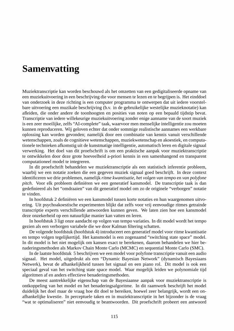
Samenvatting
Muziektranscriptie kan worden beschouwd als het omzetten van een gedigitaliseerde opname vaneen muziekuitvoering in een beschrijving die voor mensen telezen en te begrijpen is. Het einddoelvan onderzoek in deze richting is een computer programma te ontwerpen dat uit iedere voorstel-bare uitvoering een muzikale beschrijving (b.v. in de gebruikelijke westelijke muzieknotatie) kanafleiden, die onder andere de toonhoogten en posities van noten op een bepaald tijdstip bevat.Transcriptie van iedere willekeurige muziekuitvoering zonder enige aanname van de soort muziekis een zeer moeilijke, zelfs “AI-complete” taak, waarvoor men menselijke intelligentie zou moetenkunnen reproduceren. Wij geloven echter dat onder sommige realistische aannames een werkbareoplossing kan worden gevonden; namelijk door een combinatie van kennis vanuit verschillendewetenschappen, zoals de cognitieve wetenschappen, muziekwetenschap en akoestiek, en computa-tionele technieken afkomstig uit de kunstmatige intelligentie, automatisch leren en digitale signaalverwerking. Het doel van dit proefschrift is om een praktische aanpak voor muziektranscriptiete ontwikkelen door deze grote hoeveelheid a-priori kennisin een samenhangend en transparentcomputationeel model te integreren.
In dit proefschrift behandelen we muziektranscriptie als een statistisch inferentie probleem,waarbij we een notatie zoeken die een gegeven muziek signaalgoed beschrijft. In deze contextidentificeren we drie problemen, namelijkritme kwantisatie, het volgen van tempoenvan polyfonepitch. Voor elk probleem definieren we een generatief kansmodel.De transcriptie taak is dangedefinieerd als het “omdraaien” van dit generatief model omzo de originele “verborgen” notatiete vinden.
In hoofdstuk 2 definieren we een kansmodel tussen korte notaties en hun waargenomen uitvo-ering. Uit psychoakoestische experimenten blijkt dat zelfs voor vrij eenvoudige ritmes getraindetranscriptie experts verschillende antwoorden kunnen geven. We laten zien hoe een kansmodeldeze onzekerheid op een natuurlijke manier kan vatten en leren.
In hoofdstuk 3 ligt onze aandacht op volgen van tempo variaties. In dit model wordt het tempogezien als een verborgen variabele die we door Kalman filtering schatten.
De volgende hoofdstuk (hoofdstuk 4) introduceert een generatief model voor ritme kwantisatieen tempo volgen tegelijkertijd. Het kansmodel is een zogenaamd “switching state space” model.In dit model is het niet mogelijk om kansen exact te berekenen, daarom behandelen we hier be-naderingsmethoden als Markov Chain Monte Carlo (MCMC) en sequential Monte Carlo (SMC).
In de laatste hoofdstuk 5 beschrijven we een model voor polyfone transcriptie vanuit een audiosignaal. Het model, uitgedrukt als een “Dynamic Bayesian Network” (dynamisch BayesiaansNetwerk), bevat de afhankelijkheid tussen het signaal en een piano rol. Dit model is ook eenspeciaal geval van het switching state space model. Waar mogelijk leiden we polynomiale tijdalgoritmen af en anders effectieve benaderingsmethoden.
De meest aantrekkelijke eigenschap van de Bayesiaanse aanpak voor muziektranscriptie isontkoppeling van het model en het benaderingsalgoritme. Indit raamwerk beschrijft het modelduidelijk het doel maar de vraag hoe dit doel te bereiken, hoewel zeer belangrijk, wordt een on-afhankelijke kwestie. In perceptuele taken en in muziektranscriptie in het bijzonder is de vraag“wat te optimaliseren” niet eenvoudig te beantwoorden. Ditproefschrift probeert een antwoord
115

116 Samenvatting
te geven door doelfuncties te definieren geschreven als probabilistische grafische modellen en in-troduceert benaderende en exacte inferentie technieken omeen acceptabele oplossing efficient tevinden.
translated and edited with Matthijs Spaan
Dankwoord
Sometime around November of 97, I was randomly browsing through the internet and totally coin-cidentially, ended up reading archives of a mailing list. A job advertisement on music transcriptiondraw my attention and although the application deadline hasalready passed, (deadlines are madefor passing, right?), I decided to send in my CV. To my surprise, I was invited to give a talk andeven was offered the job! I would be working as a computer scientist in a music related projectat a biophysics department located in a medical faculty withcolaboration of researchers from psy-chology. Although, frankly speaking, that wasn’t exactly the setup I was expecting, I accepted thekind offer without much hesitation.
The start of the research described in this thesis may be marked by this occasion, but it wouldnever have been finished without collaboration, support andinput from many others. From thebeginning until the end, Bert has been always there both as a friend and as an advisor in shapingthe research direction while giving me enough freedom to explore. This thesis would never havereached its level without his encouragement, support, critical atittitude and his enormous expertise.
Perhaps I was the most lucky because David was a postdoc at SNNwhen I was starting. Talk-ing to him has been (and still is) a constant source of inspiration and learning experience. I amvery greatful to the other members of SNN (past and present),Wim, Tom, Machiel (ne haberabi), Onno, Martijn and Alex; I have always benefited from their constructive critics, impromptudiscussions and inspiration. I am also greatful to Stan for creating and sustaining such a greatwork environment to make all this happen and Annet for her support in providing shelter, food,transportation; practically solving every “real-life” problem but most of all for her friendship.
Without the collaboration of Peter and Henkjan, I would havebeen most probabily ignorantabout many music perception issues and it would have not beenpossible to test the models on sys-tematically collected data. Therefore, I would like to thank them and other members of the Music,Mind and Machine group: Paul, Rinus, Chris and Huub. I am indepted to STW for providing thefunding for my research and extensive worldwide travel. Without this, I would not have been ableto pursue my research with the freedom I enjoyed. I also wouldlike to thank Ben Krose for lettingme finish up in Amsterdam, and other members of the Amsterdam crowd, especially to Nikos, whohas provided his support and feedback in many ways and to Matthijs; who was very helpful in theDutch translation of the summary.
And last, but not the least, I wish to thank my office-mate, theother member of the holy “tea-room” brotherhood: Niels “Sonny-Rollins” Cornelisse. He has been the primary victim of thecolateral damage caused by my tempo tracking experiments but I have always enjoyed our endlessjazz-chats and the sco-coltrane-jamesbrown-chrispotter-jaco mix we have been broadcasting to thecorridor. Many thanks to Marjan, Noel, Vivek, Sonja, Marcel, Paul, Anton, Thom and everyoneelse in the lab who have made it a fun place to be. I want to mention and thank the supportgroup, Gunter and Ger who made sure everything works properly, and Hans for helping in fixingup broken things.
I am deeply thankful to my former professors from BogaziciUniversity, in particular to AlpEden for a short but wonderful journey through the “ivory castle” of mathematics and EthemAlpaydın for introducing and teaching me to the basic methods of machine learning. My special
117
118 Dankwoord
thanks go to Khalid Sayood not only for being a wonderful teacher in data compression, signalprocessing and information theory but most of all for his attitude and great spirit that has been veryinfluential on me. During this period, I had also the very goodfortune to have Cuneyt as a friendand a college to exchange ideas. I had also the privillige to have great friends, who happenedto be also “natural born experts” in various fields of music from whom I learned a lot : AlperMaral, CaglayanOrge, Cengiz Baysal, Sarp Maden, Tulug Tırpan, Tolga Tuz¨un, Selim Benba andCumhur Erkut.
Finally, I want to thank Caglayan, Selma, Oguz,Ilknur, the members of our small but fullyconnected Amsterdam clique. Without your music, support and friendship, it would have beenimpossible to maintain a decent level of sanity througout the difficult times.
To express my gratitute to my family, I have to switch to my native language; although I surelybelieve it would have been hard to express this in any language.
Annem ve Babama; Anneanneme; Babaannem ve Dedeme, hayatta bir seyler basarabildiysemsizin omuzlarınızda durdugum icindir.
Aslı’cıgıma, her zaman yanımda oldugunu ve olacagını hissettirdigi icin, (Aslı’cım, ...)
Nazife (1912-2003) ve Adnan (1909-2001) Cemgil’in anısına

Curriculum Vitae
Ali Taylan Cemgil was born 28 January 1970, in Ankara, Turkey. He grew up in Istanbul and ob-tained his secondary education from Istanbul Erkek Lisesi.After highschool, he entered BogaziciUniversity, Istanbul, to study computer engineering. During the university years, parallel to hisstudies, he started to perform in local clubs as a jazz musician (electric bass). During the last yearof his undergraduate studies, he become interested in computer music, signal processing and arti-ficial intelligence. After graduating from the university in 1993, besides working as a professionalmusician, he worked for a year as a programmer but eventuallydecided to attend the graduate stud-ies program in Computer Engineering at Bogazici University, where he would be employed as ateaching assistant until 1998. He obtained a masters degreein 1995 where he has investigated sub-band coding techniques (wavelets) for music transcription. The same year, he enrolled to the PhDprogram and decided to focus on probabilistic models for music analysis. In 1998, he moved to theNetherlands and joined SNN, Nijmegen University as a Ph.D. student under supervision of BertKappen to work on Bayesian methods and their application to music transcription. Between 2001and 2004, he also studied at the jazz department of the Amsterdam Conservatory. Since 2003, heis working as a researcher at Intelligent Autonomous Systems group at University of Amsterdam.
119