2016•2017 FACULTEIT INDUSTRIËLE … · 2016•2017 Faculteit Industriële...

2016•2017FACULTEIT INDUSTRIËLE INGENIEURSWETENSCHAPPENmaster in de industriële wetenschappen:verpakkingstechnologie

MasterproefOptimisation and characterisation of nano-hydroxyapatite/polylactidecomposites using Fused Deposition Modelling technology

Promotor :Prof. dr. ir. Mieke BUNTINX

Promotor :Prof. ISABELLE VROMAN

Copromotor :PhD. GEOFFREY GINOUX

Erwin Oris Scriptie ingediend tot het behalen van de graad van master in de industriëlewetenschappen: verpakkingstechnologie

Gezamenlijke opleiding Universiteit Hasselt en KU Leuven

2016•2017Faculteit Industriëleingenieurswetenschappenmaster in de industriële wetenschappen:verpakkingstechnologie

MasterproefOptimisation and characterisation of nano-hydroxyapatite/polylactide composites using Fused Deposition Modelling technology

Promotor :Prof. dr. ir. Mieke BUNTINX

Promotor : Copromotor :Prof. ISABELLE VROMAN PhD. GEOFFREY GINOUX

Erwin Oris Scriptie ingediend tot het behalen van de graad van master in de industriëlewetenschappen: verpakkingstechnologie

Acknowledgements I would like to thank Prof. dr. ir. Mieke Buntinx, Prof. Isabelle Vroman and Mr. Geoffrey Ginoux for

their work as supervisors and their continued support throughout this thesis. Without their guidance,

the completion of this thesis would have been much harder.

Additionally, I would also like to thank the people of ESIReims, in particular Prof. Damien Erre, Mr.

Philippe Dony and Ms. Nathalie Choiselle, for their guidance throughout this thesis and their aid during

the sample preparation and sample analysis. Of course, I would also like to thank the people of the

IFTS for their help and guidance, especially Dr. Sébastien Alix and Ms. Laurine Renaux. I cannot forget

the people of VerpakkingsCentrum IMO-IMOMEC, especially ing. Dimitri Adons, without their swift

work and quick responses to my questions, this thesis would not have been possible. I would also like

to thank the University of Haute-Alsace for the TEM analysis they executed for this thesis. I would like

to thank Catherine Lacoste and the people of the international office of the University of Reims

Champagne-Ardenne for helping me integrate with local and Erasmus students.

I would like to thank my friends and family for their support throughout this thesis.

Finally, I would like to thank the Erasmus+ programme of the European Union for allowing me to

participate in the Erasmus exchange programme. Thanks to this programme I was able to conduct my

thesis abroad while experiencing a new culture. “The European Commission support for the production

of this publication does not constitute an endorsement of the contents which reflects the views only of

the authors, and the Commission cannot be held responsible for any use which may be made of the

information contained therein.” This thesis was also part of «PolyFabAdd». «PolyFabAdd» is co-funded

by the European Union. Europe invests in Champagne-Ardenne with the European Regional

Development Fund.

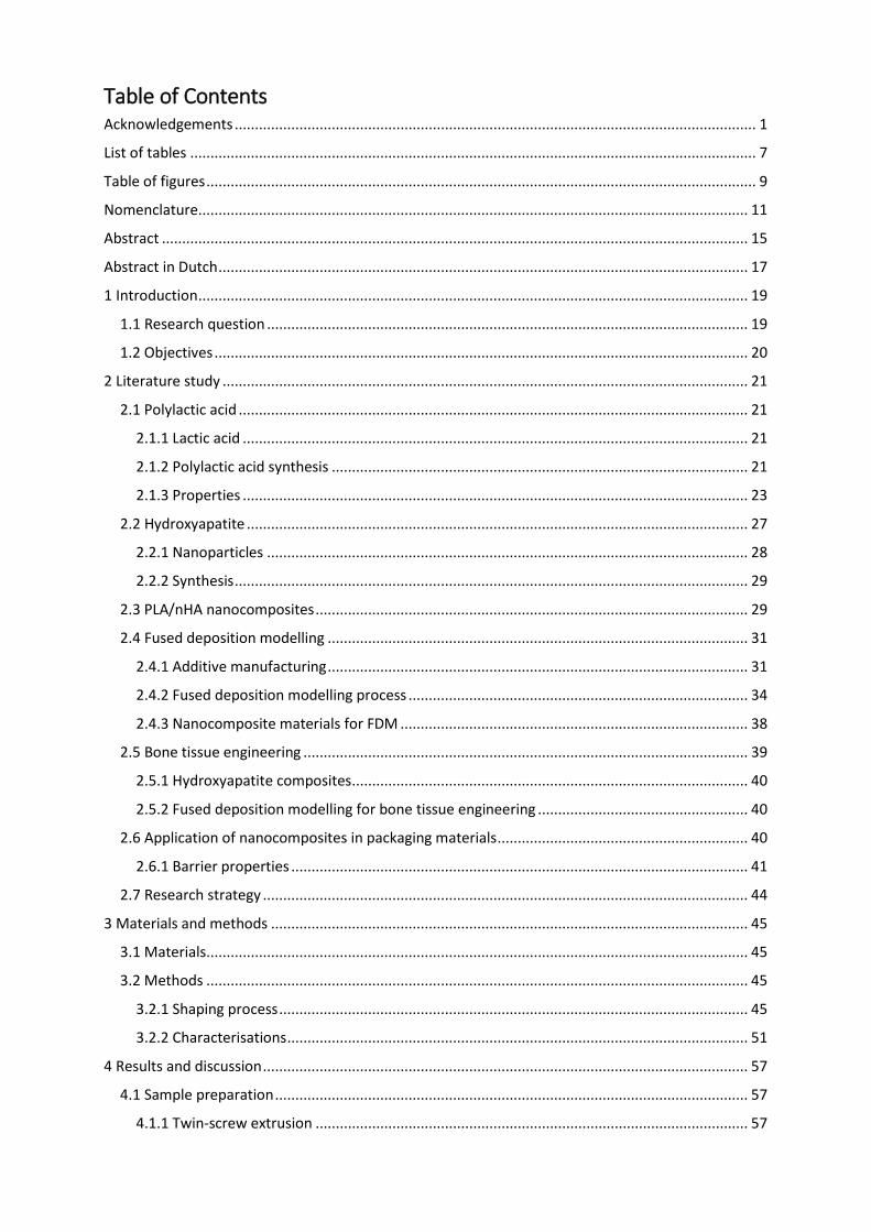
Table of Contents Acknowledgements ................................................................................................................................. 1

List of tables ............................................................................................................................................ 7

Table of figures ........................................................................................................................................ 9

Nomenclature ........................................................................................................................................ 11

Abstract ................................................................................................................................................. 15

Abstract in Dutch ................................................................................................................................... 17

1 Introduction ........................................................................................................................................ 19

1.1 Research question ....................................................................................................................... 19

1.2 Objectives .................................................................................................................................... 20

2 Literature study .................................................................................................................................. 21

2.1 Polylactic acid .............................................................................................................................. 21

2.1.1 Lactic acid ............................................................................................................................. 21

2.1.2 Polylactic acid synthesis ....................................................................................................... 21

2.1.3 Properties ............................................................................................................................. 23

2.2 Hydroxyapatite ............................................................................................................................ 27

2.2.1 Nanoparticles ....................................................................................................................... 28

2.2.2 Synthesis ............................................................................................................................... 29

2.3 PLA/nHA nanocomposites ........................................................................................................... 29

2.4 Fused deposition modelling ........................................................................................................ 31

2.4.1 Additive manufacturing ........................................................................................................ 31

2.4.2 Fused deposition modelling process .................................................................................... 34

2.4.3 Nanocomposite materials for FDM ...................................................................................... 38

2.5 Bone tissue engineering .............................................................................................................. 39

2.5.1 Hydroxyapatite composites .................................................................................................. 40

2.5.2 Fused deposition modelling for bone tissue engineering .................................................... 40

2.6 Application of nanocomposites in packaging materials .............................................................. 40

2.6.1 Barrier properties ................................................................................................................. 41

2.7 Research strategy ........................................................................................................................ 44

3 Materials and methods ...................................................................................................................... 45

3.1 Materials ...................................................................................................................................... 45

3.2 Methods ...................................................................................................................................... 45

3.2.1 Shaping process .................................................................................................................... 45

3.2.2 Characterisations .................................................................................................................. 51

4 Results and discussion ........................................................................................................................ 57

4.1 Sample preparation ..................................................................................................................... 57

4.1.1 Twin-screw extrusion ........................................................................................................... 57

4.1.2 Single-screw extrusion.......................................................................................................... 59

4.1.3 Fused deposition modelling ................................................................................................. 60

4.1.4 Injection moulding ................................................................................................................ 61

4.1.5 Heated hydraulic press ......................................................................................................... 61

4.2 Thermogravimetric analysis ........................................................................................................ 62

4.2.1 Introduction .......................................................................................................................... 62

4.2.2 Results .................................................................................................................................. 62

4.2.3 Conclusion ............................................................................................................................ 73

4.3 Differential scanning calorimetry ................................................................................................ 73

4.3.1 Introduction .......................................................................................................................... 73

4.3.2 Results .................................................................................................................................. 74

4.3.3 Conclusion ............................................................................................................................ 84

4.4 Oscillatory rheology ..................................................................................................................... 84

4.4.1 Introduction .......................................................................................................................... 84

4.4.2 Results .................................................................................................................................. 85

4.2.4 Conclusion ............................................................................................................................ 89

4.5 Tensile tests ................................................................................................................................. 89

4.5.1 Introduction .......................................................................................................................... 89

4.5.2 Design of experiments with printed specimens ................................................................... 89

4.5.3 Results injection moulded specimens .................................................................................. 95

4.5.4 Conclusion ............................................................................................................................ 96

4.6 Dynamic mechanical analysis ...................................................................................................... 97

4.6.1 Introduction .......................................................................................................................... 97

4.6.2 Results .................................................................................................................................. 97

4.6.3 Conclusion .......................................................................................................................... 106

4.7 Wide angle X-ray diffraction on powder analysis...................................................................... 107

4.7.1 Introduction ........................................................................................................................ 107

4.7.2 Results ................................................................................................................................ 107

4.7.3 Conclusion .......................................................................................................................... 110

4.8 Transmission electron microscopy ............................................................................................ 110

4.8.1 Introduction ........................................................................................................................ 110

4.8.2 Results ................................................................................................................................ 111

4.8.3 Conclusion .......................................................................................................................... 114

4.9 Permeability tests ...................................................................................................................... 115

4.9.1 Introduction ........................................................................................................................ 115

4.9.2 Results ................................................................................................................................ 115

4.9.3 Conclusion .......................................................................................................................... 115

5 Conclusion ........................................................................................................................................ 117

References ........................................................................................................................................... 119

Annexes ............................................................................................................................................... 137

List of tables Table 1 Classification of plastics [25]..................................................................................................... 26

Table 2 Summary AM processes [116]. ................................................................................................. 31

Table 3 Process parameters [121]. ........................................................................................................ 34

Table 4 Screw profile. ............................................................................................................................ 46

Table 5 Measurement points corresponding to the Doehlert matrix. .................................................. 49

Table 6 Temperature profile TGA. ......................................................................................................... 52

Table 7 Temperature profile DSC analysis. ........................................................................................... 53

Table 8 Temperature profile extruder. ................................................................................................. 57

Table 9 Parameters extrusion mixtures. ............................................................................................... 58

Table 10 Obtained mass mixtures after each extrusion. ...................................................................... 59

Table 11 Temperatures single-screw extrusion mixtures. .................................................................... 59

Table 12 Results single-screw extrusion. .............................................................................................. 60

Table 13 Temperature and pressure settings injection moulding process. .......................................... 61

Table 14 Thermogravimetric analysis PLE 005. ..................................................................................... 63

Table 15 Thermogravimetric analysis PLA extruded (Continued). ........................................................ 63

Table 16 Thermogravimetric analysis PLA/HA 0.5%. ............................................................................ 63

Table 17 Thermogravimetric analysis PLA/HA 1%. ............................................................................... 64



Table 20 Summary temperatures thermogravimetric analysis. ............................................................ 66

Table 21 Summary mass loss thermogravimetric analysis mixtures. .................................................... 67

Table 22 Onset, peak degradation and degradation end temperature, and the temperature range in

which degradation occurs of the filaments. .......................................................................................... 69

Table 23 Remaining mass, percentage HA and maximum degradation speed of the filaments. ......... 70

Table 24 The degradation onset, peak and end temperature; and the temperature in which

degradation occurred for the FDM specimens. .................................................................................... 72

Table 25 The remaining mass, the HA percentage and the maximum mass loss per minute for the

FDM specimens. .................................................................................................................................... 73

Table 26 Cold crystallisation peak and the relaxation peak after the Tg. .............................................. 74

Table 27 Summary of the crystallisation during the cooling cycle. ....................................................... 76

Table 28 Temperatures characterising the glass transition and the height of the glass transition (ΔCp).

............................................................................................................................................................... 78

Table 29 Summary melting peak PLE 005 and composites. .................................................................. 80

Table 30 Starting crystallinity filaments. ............................................................................................... 81

Table 31 Summary crystallisation filaments.......................................................................................... 81

Table 32 Summary glass transition filaments. ...................................................................................... 82

Table 33 Summary melt peak filaments. ............................................................................................... 82

Table 34 Starting crystallinity FDM specimens. .................................................................................... 82

Table 35 Summary crystallisation FDM specimens. .............................................................................. 83

Table 36 Summary glass transitions FDM specimens. .......................................................................... 83

Table 37 Summary melt peak FDM specimens. .................................................................................... 84

Table 38 The parameters of the Carreau-Yasuda model of the different mixtures. ............................. 88

Table 39 Results tensile tests PLA/HA 0%. ............................................................................................ 89

Table 40 Coefficients theoretical Doehlert model, p-values coefficients and the determination

coefficient of PLA/HA 0%. ..................................................................................................................... 90

Table 41 Results tensile tests PLA/HA 0.5%. ......................................................................................... 91

Table 42 Coefficients theoretical Doehlert model PLA/HA 0.5%. ......................................................... 92


Table 44 Coefficients theoretical Doehlert model PLA/HA 1%. ............................................................ 92





Table 49 Young modulus and ultimate strength injection moulded tensile test specimens. ............... 95

Table 50 Onset and end rapid decrease storage modulus. ................................................................... 98

Table 51 Peak storage modulus FDM samples. ..................................................................................... 99

Table 52 End glass transition and onset cold crystallisation storage modulus. .................................. 100

Table 53 Minimum storage modulus in between the end of the glass transition and the beginning of

the cold crystallisation. ....................................................................................................................... 101

Table 54 Storage moduli at the end of the measurement. ................................................................. 101

Table 55 Onset and end peak loss modulus. ....................................................................................... 102

Table 56 Peak loss modulus for the pressed and printed composites. ............................................... 102

Table 57 Minimum loss moduli composites and corresponding temperatures. ................................ 103

Table 58 Loss moduli at the end of the experiment. .......................................................................... 104

Table 59 Onset and end tan δ peak..................................................................................................... 105

Table 60 Temperature and Tan δ values corresponding to the tan δ peak. ....................................... 105

Table 61 Temperatures and Tan δ values corresponding to the second Tan δ peak. ........................ 106

Table 62 Bragg angle, Miller index and interplanar distances corresponding to the PLA peaks. ....... 108

Table 63 Bragg angle, Miller index and interplanar distances corresponding to the HA peaks. ........ 109

Table 64 Crystal sizes of PLA for extruded PLA and the composites................................................... 109

Table 65 Crystal sizes of HA. ................................................................................................................ 109

Table 66 WVTR values found for the PLA/HA composites and PLE 005. ............................................ 115

Table 67 OTR values PLA/HA composites and PLE 005. ...................................................................... 115

Table of figures Figure 1 Synthesis of PLA from l- and d-lactic acids [33]. ...................................................................... 22

Figure 2 Stereoforms of lactides [31]. ................................................................................................... 23

Figure 3 Stepwise process to both recycle and separate PLA and PET mixed waste [72]. ................... 27

Figure 4 Apatite structure viewed along the c-crystallographic axis: green = calcium, red = oxygen,

orange = phosphorus, white = fluorine, chlorine, or hydroxyl [73]. ..................................................... 28

Figure 5 TEM of HA for P120 (original magnification ×23 000) [79]. .................................................... 28

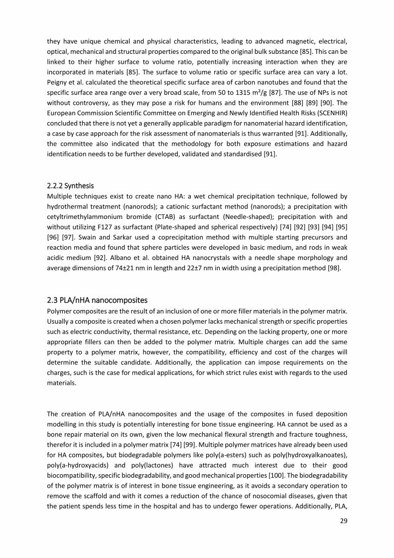
Figure 6 Schemes of two types of stereolithography setups. Left: a bottom-up system with scanning

laser. Right: a top-down setup with digital light projection [114]. ....................................................... 32

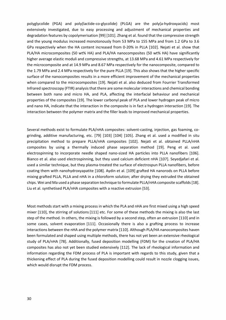
Figure 7 A typical SLS machine layout [117]. ......................................................................................... 32

Figure 8 Schematic representation of a typical 3DP™ setup. A roller spreads a thin layer of polymer

powder over the previously formed layer, and is subsequently solidified by the spatially controlled

delivery of a liquid binder [119]. ........................................................................................................... 33

Figure 9 Fused filament fabrication apparatus and schematic [125]. ................................................... 35

Figure 10 Procedure for fused deposition modelling [123]. ................................................................. 35

Figure 11 FDM Build Parameters [122]. ................................................................................................ 36

Figure 12 XYZ build orientation based on ASTM F2921-1, which has been replaced by

ISO/ASTM52921-13 [122] [126] [131]. .................................................................................................. 37

Figure 13 Levels of Analysis for FDM Prototypes [132]......................................................................... 37

Figure 14 Bond Formation Process Between Two Filaments: (1) surface contacting, (2) neck growth,

(3) diffusion at interface, (4) randomization [132]. .............................................................................. 38

Figure 15 Screw profile extrusion.......................................................................................................... 46

Figure 16 Schematic representation Doehlert matrix. .......................................................................... 48

Figure 17 Thermogravimetric analysis PLE 005. .................................................................................... 62

Figure 18 The degradation onset of PLE 005 and PLA/nHA nanocomposites plotted against the HA

content. ................................................................................................................................................. 65

Figure 19 Temperature at which the maximum degradation speed occurs plotted against the HA

content for the formulations. ................................................................................................................ 65

Figure 20 Temperature at which the degradation ends plotted against the HA content. .................... 66

Figure 21 Temperatures at which the degradation starts for the different composites and the

extruded PLA. ........................................................................................................................................ 68

Figure 22 Temperatures at which the maximal degradation speed occurs for the composites and the

extruded PLA. ........................................................................................................................................ 68

Figure 23 Temperature at which the degradation ends for the composites and the extruded PLA. ... 69

Figure 24 The degradation onset temperature of the FDM specimens. ............................................... 71

Figure 25 The temperature at which the degradation speed was maximal for the FDM specimens. .. 71

Figure 26 The temperatures at which the degradation ended for the FDM specimens....................... 72

Figure 27 The DSC curves of the PLE 005. ............................................................................................. 74

Figure 28 The onset, peak and end of the crystallisation during the cooling cycle. ............................. 75

Figure 29 The crystallinity obtained during the cooling cycle of the composites. ................................ 76

Figure 30 DSC curves of PLE 005 (bright green and blue) and PLA extruded (pink and dark green). ... 76

Figure 31 Glass transition PLE 005 and PLA/nHA composites............................................................... 77

Figure 32 The height of the glass transition of the PLE 005 and the PLA/nHA composites. ................. 77

Figure 33 Onset, peak and end temperature melting peak PLE 005 and the composites. ................... 79

Figure 34 Multi melt peak PLA/Nha 5%. ............................................................................................... 79

Figure 35 Crystallinity obtained from the melt peak of the PLE 005 and the composites. .................. 80

Figure 36 Starting crystallinity filaments visualised. ............................................................................. 81

Figure 37 Starting crystallinity FDM specimens. ................................................................................... 83

Figure 38 The average storage modulus of the mixtures. .................................................................... 85

Figure 39 The average loss modulus of the mixtures............................................................................ 86

Figure 40 The average loss angle of the mixtures. ................................................................................ 87

Figure 41 The average complex viscosity of the mixtures. ................................................................... 88

Figure 42 Response surface Young modulus PLA/HA 0%. ..................................................................... 90

Figure 43 Response surface ultimate strength PLA/HA 0% (Horse saddle shape). ............................... 91

Figure 44 Response surface Young modulus PLA/HA 3%. ..................................................................... 94

Figure 45 Comparison Young modulus between the injection moulded and printed tensile specimens

for different concentrations of HA. ....................................................................................................... 96

Figure 46 Comparison ultimate strength between the injection moulded and the printed tensile

specimens for different concentrations of HA. ..................................................................................... 96

Figure 47 Storage moduli pressed (red: neat PLA; purple: PLA/HA 3%) and FDM printed (black: neat

PLA; blue: PLA/HA 3%) samples. ......................................................................................................... 100

Figure 48 Loss moduli PLA/HA composites. ........................................................................................ 103

Figure 49 Tan δ in function of the temperature for the pressed and printed samples. ..................... 106

Figure 50 Diffractogram HA powder and extruded PLA powder. ....................................................... 108

Figure 51 Diffractogram PLA/HA composites. ..................................................................................... 108

Figure 52 Diffractogram HA and the reference peaks and their intensity of the reference HA 9432. 110

Figure 53 High resolution TEM image of nanoXIM HAp paste [225]. ................................................. 110

Figure 54 TEM image PLA/HA 1% granules (scale 1 µm)..................................................................... 111

Figure 55 TEM image PLA/HA 1% granules (scale 100 nm). ................................................................ 111

Figure 56 TEM image PLA/HA 1% granules (scale 20 nm). .................................................................. 111

Figure 57 TEM image PLA/HA 5% granules (scale 1 µm)..................................................................... 112

Figure 58 TEM image PLA/HA 5% granules (100 nm).......................................................................... 112

Figure 59 TEM image PLA/HA 5% granules (scale 20 nm). .................................................................. 112

Figure 60 TEM image PLA/HA 1% FDM specimen (scale 1 µm). ......................................................... 113

Figure 61 TEM image PLA/HA 1% FDM specimen (scale 100 nm). ..................................................... 113

Figure 62 TEM image PLA/HA 1% FDM specimen (scale 20 nm). ....................................................... 113

Figure 63 TEM image PLA/HA 5% FDM specimen (scale 1µm). .......................................................... 114

Figure 64 TEM image PLA/HA 5% FDM specimen (scale 100 nm). ..................................................... 114

Figure 65 TEM image PLA/HA 5% FDM specimen (scale 20 nm). ....................................................... 114

Nomenclature 3DP = Three Dimensional Printing

ABS = Acrylonitrile Butadiene Styrene

AM = Additive Manufacturing

ANOVA = Analysis of Variance

BTE = Bone Tissue Engineering

c = concentration

CAD = Computer Aided Design

CTAB = Cetyltrimethylammonium Bromide

CW = Contour Width

D = Diffusion

DMA = Dynamic mechanical analysis

DSC = Differential Scanning Calorimetry

ERDF = European Regional Development Fund

FDM = Fused Deposition Modelling

FFF = Fused Filament Fabrication

FTIR = Fourrier Transformed Infrared spectroscopy

G’ = Storage modulus

G” = Loss modulus

HA = Hydroxyapatite

IFTS = Institute of Higher Technical Training

J = the permeation flux

LA = Lactic Acid

LISM = Laboratory of Engineering and Materials Science

nHA = nanohydroxyapatite

NPs = Nanoparticles

OCP = Octacalcium Phosphate

OTR = Oxygen Transmission Rate

P = Permeation

p = pressure

PC = Polycarbonate

PCL = Polycaprolactone

PDLLA = Poly-DL-Lactide

PE = Polyethene

PET = Polyethylene Terephthalate

PGA = Polyglycolide

PLA = polylactide / polylactic acid

PLGA = poly(lactide-co-glycolide)

PLLA = Poly-LL-Lactide

PP = Polypropylene

PP = Polypropylene

PPSU = polyphenylenesulfone

PS = Polystyrene

PVC = Polyvinyl chloride

R&D = Research and Development

R² = Coefficient of Determination

RA = Raster Angle

RH = the relative humidity

RRAG = Raster to Raster Air Gap

RW = Raster Width

S = Solubility

SCENHIR = European Commission Scientific Committee on Emerging and Newly Identified Health

Risks

SLA = Stereolithography

SLS = Selective Laster Sintering

SSE = Single-screw Extruder

T = Temperature

Tc = Crystallisation Temperature

Tcc = Cold Crystallisation temperature

TCP = Tricalcium Phosphate

TetTCP = Tetracalcium Phosphate

Tg = Glass transition Temperature

TGA = Thermogravimetric Analysis

Tm = Melting temperature

TSE = Twin-screw Extruder

WAXD-P = Wide Angle X-ray Diffraction on Powder

WVTR = Water Vapour Transmission Rate

Xc = the crystallinity

ΔH°m = Theoretical melt enthalpy for enantiopure PLA with 100% crystallinity

ΔHm = Melt enthalpy

η = the viscosity

η0 = the viscosity at zero shear

τ = the mean particle size of the crystal

Abstract In this study, polylactide/nanohydroxyapatite (PLA/nHA) composites were produced for fused

deposition modelling (FDM), which is an additive manufacturing technology commonly used for

prototyping and production applications. First, PLA/nHA composites (0.5%, 1%, 3%, 5 wt.%) were

compounded using a twin-screw extruder, subsequently, these were shaped into filaments with a

single-screw extruder. Thirdly, specimens for dynamic mechanical analysis (DMA) and tensile testing

were FDM printed. Doehlert response surface methodology was applied to optimise the tensile

properties of each formulation. A comparison of the mechanical properties of the printed tensile test

specimens with injection moulded specimens showed a lower Young’s modulus and ultimate

strength and a higher storage modulus for the printed samples. Additionally, the same ultimate

strength decreased with higher HA content. HA induced nucleation of PLA, but also a reduction of the

degradation temperature, as shown by differential scanning calorimetry and thermogravimetric

analysis respectively. Oscillatory rheological analysis showed the presence of a Newtonian plateau,

followed by a shear thinning behaviour. The first HA addition resulted in a thickening effect,

decreasing upon addition of HA, up to a thinning effect at 5 wt.%. In conclusion, this study proves

successful printing of PLA/nHA nanocomposites using FDM, which might be promising e.g. for bone

tissue engineering.

Abstract in Dutch In deze studie werden polylactide/nanohydroxyapatiet (PLA/nHA) composieten geproduceerd voor

fused deposition modelling (FDM). Eerst werden PLA/nHA composieten (0.5%, 1%, 3%, 5 wt.%)

gemaakt met een twin-screw extruder, deze werden dan omgevormd tot filamenten met een single-

screw extruder. Ten slotte werden de filamenten omgevormd tot dynamische mechanische analyse

(DMA) en trekproefmonsters via een FDM proces. Doehlert response surface methodologie werd

gebruikt om de trekeigenschappen te optimaliseren voor elk composiet. Een vergelijking van de

mechanische eigenschappen van de geprinte trekproefstukken met de gespuitgiete monsters gaf aan

dat de Young modulus en treksterkte hoger waren en de storage modulus lager was voor de geprinte

proefstukken. Bovendien daalde de treksterkte met toenemende HA inhoud. Uit de differentiële

scanning calorimetrie en de thermogravimetrische analyse volgde dat HA een nucleatie veroorzaakte

in PLA en een daling van de degradatietemperatuur te weeg bracht. Oscillerende rheologische

analyse toonde de aanwezigheid van een Newtonisch plateau, gevolgd door shearthinning. De eerste

toevoeging van HA resulteerde in een verdikkingseffect, waarna bijkomende HA-inhoud resulteerde

in een daling van het verdikkingseffect en zelfs een verdunningseffect bij toevoeging van 5 wt.% HA.

In conclusie, PLA/nHA nanocomposieten werden succesvol geprint met FDM in deze studie, dit kan

veelbelovend zijn voor bv. bone tissue engineering.

1 Introduction This thesis was conducted within the innovative materials branch of the Laboratory of Engineering and

Materials Science (LISM) at Reims, French research group EA 4695. “The LISM was established in

January 2012 and gathers researchers who focus on developing, formatting and analysing materials

and their properties” [1]. The LISM has multiple sites, but this thesis was executed on the sites of the

Engineering school of Reims (ESIReims) and the Institute of Higher Technical Training (IFTS) at

Charleville-Mézières, both situated in France.

The thesis is a part of the PhD study of Mr. Geoffrey Ginoux, which is funded by the European Regional

Development Fund (ERDF). The topic of the PhD is PolyFabAdd (Charged Polymers in Additive

Manufacturing). PolyFabAdd focuses on the utilisation of charged polymers within additive

manufacturing (AM) processes. The scientific and technological objectives of the PhD project are (i) a

better understanding of the relationship between the rheological behaviour of polymer systems and

their ability to shaping by additive manufacturing technologies (FDM® in particular), (ii) the

development of polymer-based formulations from biological resources adapted to these technologies

and providing multi-functionality [2]. Examples of this multi-functionality are the use of

nanostructured polylactic acid (PLA) materials for packaging and tissue engineering as discussed by [3].

Additive manufacturing consists of multiple technologies, one of these technologies is Fused

Deposition Modelling® (FDM®) [4] [5]. Fused deposition modelling®, often wrongly referred to as

three-dimensional printing, is traditionally used for rapid prototyping. The main reasons behind this

trend are the short time between the design phase and the building phase, the fast build time and the

cheap printing materials. However, despite its rise in popularity, full scale application of the technology

has not gained much emphasis. This due to a lack of compatibility of available materials [6]. Sood et al.

identify two approaches to overcome this limitation: The development of new materials with superior

characteristics than conventional materials and the adjustment of the process parameters during the

fabrication stage to improve properties [6].

1.1 Research question

In FDM processes, neither the materials nor the process have been studied in a systematic manner

towards functional components production, with adjusted mechanical properties, or with the

objective of getting competitive production time/cost (for small/medium production series),

respectively [7]. This results in a lack of accuracy when creating small series with FDM, an effect of the

lack of accuracy is sample porosity, which lowers the mechanical properties of the samples. Due to the

poorly characterised impact of process parameters on the sample quality and the low amount of

available printing materials (Mainly Acrylonitrile butadiene styrene (ABS), Polycaprolactone (PCL), PLA

and Polypropylene (PP)), the expansion of the technique is limited [7] [8] [9] [10] [11].

The lack of standardisation in articles, when characterising different materials for FDM, makes it hard

to compare different test results with each other. In recent years, there has been an improvement

with regards to the characterisation as more mathematical approaches are being used, yet most

20

studies do not consider the printing speed and printing temperature as important parameters [12] [13]

[14] [15].

By researching charged polymers, new potential materials and charges can be proposed for the FDM

printing process. Thus, leading to the expansion of the available materials for FDM and AM in general.

With the addition of the charges and their specific properties, the potential applications of FDM in the

future can increase. Nano charges are preferred over micro charges, since they do not cause clogging

of the FDM printing nozzle [16]. One should keep in mind that materials react differently on changing

process parameters. In this thesis, the properties of PLA and PLA charged with hydroxyapatite, chosen

for its application in bone tissue engineering (BTE), are determined throughout the production chain

“From formulation to finished parts” and for varying FDM printing parameters [17] [18] [19] [20] [21].

With the characterisation of PLA/nHA, the amount of available materials can potentially go up as

polymers charged with nanoparticles can be considered for the FDM printing process.

PLA is a biodegradable polymer created from bio resources [22]. Its biodegradability in combination

with its bio origin, has led to an increased industrial interest in recent years. However, a decrease of

the permeability of PLA can increase its use for packaging applications [23]. The addition of

hydroxyapatite to the PLA matrix might increase its crystallinity fraction, which in turn could lead to a

reduced permeability [13] [24]. PLA can also be used in FDM for the creation of small series of

packaging.

1.2 Objectives As mentioned above, there is a limited number of available materials and a lack of knowledge with

regards to the effect of process parameters on the properties of FDM printed workpieces. A better

understanding can be achieved by tracking the properties throughout the production chain. Following

Carneiro et al., the printed test samples will be compared with injection moulded test samples made

from the same pellets. Additionally, the relation between different process steps and the properties

of the tested materials was determined. After which the FDM process was optimised, according to the

rheological behaviour. Special attention should be given to the filaments, a homogenic filament results

in more easily controlled process parameters and thus improved properties [7].

In summary, this thesis aims at achieving the following objectives:

(i) Formulate nano-charged materials of PLA/nHA;

(ii) Apply these materials in FDM and injection moulding;

(iii) Characterise the materials;

(iv) Compare the impact of the FDM process and the injection moulding on the mechanical

behaviour of the tensile test specimens;

(v) Determine the dispersion state of the nano-charges in the polymer matrix;

(vi) Create PLA/nHA films from the charged pellets;

(vii) Test the permeability of the PLA/nHA films.

21

2 Literature study

2.1 Polylactic acid

Polylactic acid (PLA) is a biodegradable polymer [25] [26]. Some of the biggest producers of PLA in the

world are NatureWorks® LLC (Oyobo), Dai Nippon Printing Co., Mitsui Chemicals, Shimadzu, NEC,

Toyota (Japan), PURAC Biomaterials, Hycail (The Netherlands), Galactic (Belgium), Cereplast (U.S.A.),

FkuR, Biomer, Stanelco, Inventa-Fischer (Germany), and Snamprogetti (China) [27] [28] [29]. While the

cost of some biodegradable polymers is high compared with conventional polymers, PLA has a

relatively low production cost [28]. PLA has the following processing possibilities: Injection moulding,

extrusion, cast film extrusion, blow moulding, fibre spinning and thermoforming [29]. Thermoforming

of trays and containers for food packaging and foodservice applications is the main market application

of PLA [28]. The usage of PLA in other areas such as films and labels, injection stretch blow moulded

bottles and jars, specialty cards and fibres is being developed [28].

2.1.1 Lactic acid

Lactic acid (2-hydroxy propanoic acid), produced via fermentation or chemical synthesis, is the single

monomer of PLA [29] [30] [31]. LA synthesis can result in the L or the D stereoisomer or a racemic

mixture depending on the used synthesis route [30] [31]. The synthesis via fermentation, the chemical

breakdown of a substance by bacteria, yeasts, or other microorganisms, of a renewable agricultural

source corn can result in the L or D stereoisomers depending on the microorganisms used. Lactobacilli

amylophilus, Lactobacilli bavaricus, Lactobacilli casei, Lactobacilli maltaromicus, and Lactobacilli

salivarius predominantly yield the L isomer, while strains such as Lactobacilli delbrueckii, Lactobacilli

jensenii, or Lactobacilliacidophilus yield the d-isomer or mixtures of both [31]. Chemical synthesis

results in a racemic mixture of D- and L-lactic acid [30] [31]. Fermentation is advantageous compared

to chemical synthesis, as it allows the production of optically pure L- or D-lactic acid, has a low

substrate cost, a low production temperature and a low energy consumption [31].

2.1.2 Polylactic acid synthesis

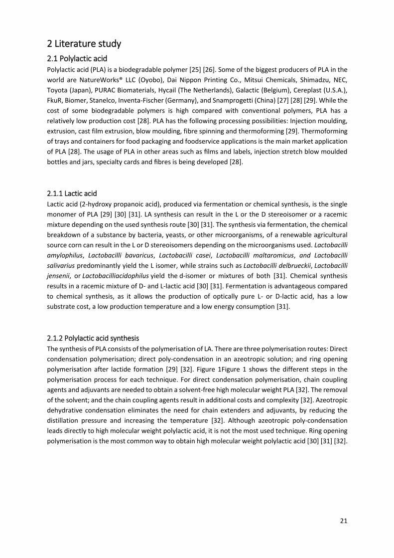
The synthesis of PLA consists of the polymerisation of LA. There are three polymerisation routes: Direct

condensation polymerisation; direct poly-condensation in an azeotropic solution; and ring opening

polymerisation after lactide formation [29] [32]. Figure 1Figure 1 shows the different steps in the

polymerisation process for each technique. For direct condensation polymerisation, chain coupling

agents and adjuvants are needed to obtain a solvent-free high molecular weight PLA [32]. The removal

of the solvent; and the chain coupling agents result in additional costs and complexity [32]. Azeotropic

dehydrative condensation eliminates the need for chain extenders and adjuvants, by reducing the

distillation pressure and increasing the temperature [32]. Although azeotropic poly-condensation

leads directly to high molecular weight polylactic acid, it is not the most used technique. Ring opening

polymerisation is the most common way to obtain high molecular weight polylactic acid [30] [31] [32].

22

Figure 1 Synthesis of PLA from l- and d-lactic acids [33].

Before ring opening polymerisation can take place, a cyclic lactide dimer has to be formed [31].

Lactides are formed in two steps. The first step consists of evaporating the condensation product,

water, during the oligomerisation of the L-lactic acid, D-lactic acid or a mixture of both stereoisomers

[30] [31] [34]. The resulting low molecular weight polylactic acid oligomers are then catalytically

depolymerised through internal transesterification, by ‘back-biting’ reaction to lactide during the

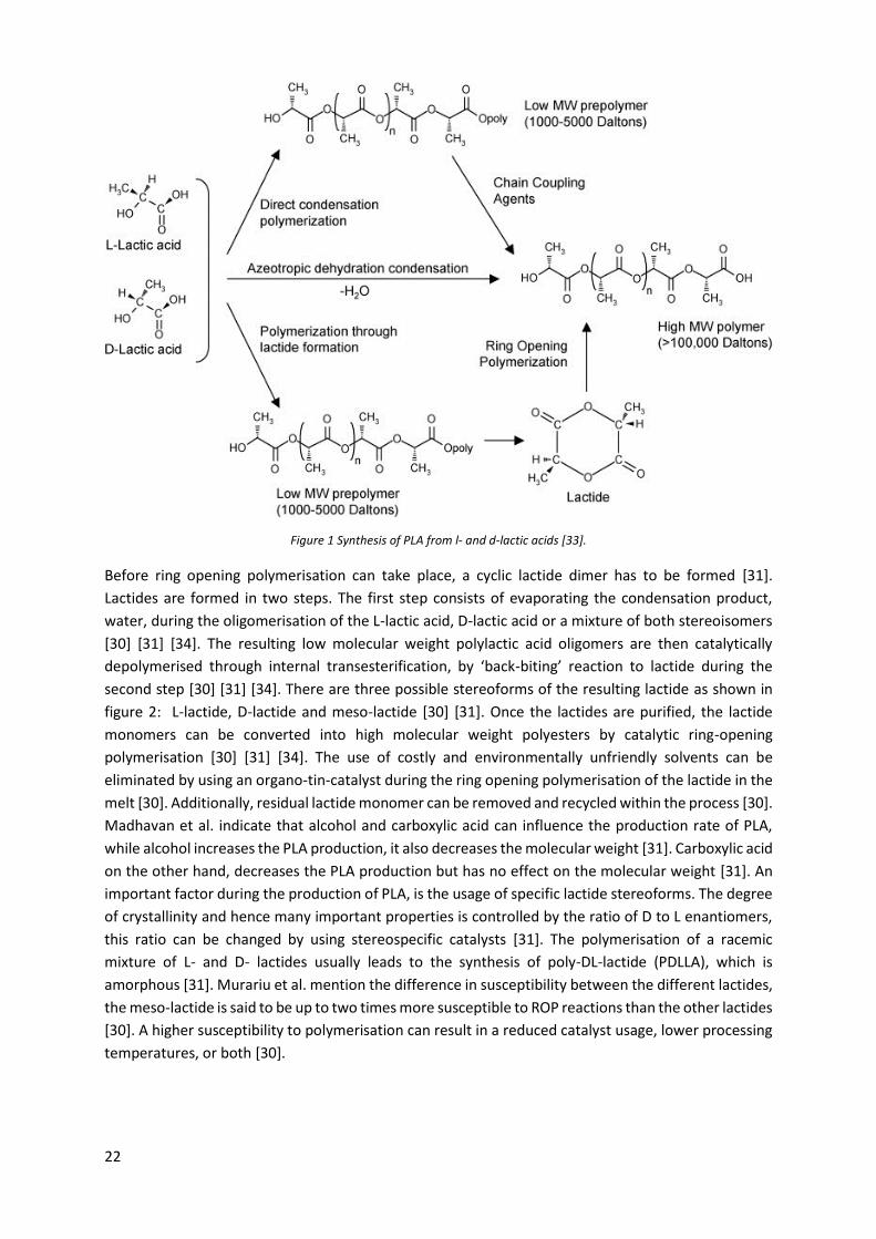
second step [30] [31] [34]. There are three possible stereoforms of the resulting lactide as shown in

figure 2: L-lactide, D-lactide and meso-lactide [30] [31]. Once the lactides are purified, the lactide

monomers can be converted into high molecular weight polyesters by catalytic ring-opening

polymerisation [30] [31] [34]. The use of costly and environmentally unfriendly solvents can be

eliminated by using an organo-tin-catalyst during the ring opening polymerisation of the lactide in the

melt [30]. Additionally, residual lactide monomer can be removed and recycled within the process [30].

Madhavan et al. indicate that alcohol and carboxylic acid can influence the production rate of PLA,

while alcohol increases the PLA production, it also decreases the molecular weight [31]. Carboxylic acid

on the other hand, decreases the PLA production but has no effect on the molecular weight [31]. An

important factor during the production of PLA, is the usage of specific lactide stereoforms. The degree

of crystallinity and hence many important properties is controlled by the ratio of D to L enantiomers,

this ratio can be changed by using stereospecific catalysts [31]. The polymerisation of a racemic

mixture of L- and D- lactides usually leads to the synthesis of poly-DL-lactide (PDLLA), which is

amorphous [31]. Murariu et al. mention the difference in susceptibility between the different lactides,

the meso-lactide is said to be up to two times more susceptible to ROP reactions than the other lactides

[30]. A higher susceptibility to polymerisation can result in a reduced catalyst usage, lower processing

temperatures, or both [30].

23

Figure 2 Stereoforms of lactides [31].

2.1.3 Properties

2.1.3.1 Crystallinity & thermal, mechanical and rheological properties

As mentioned above, the stereoforms of the lactides used for the PLA production influence the

resulting PLA properties. Besides the stereochemistry, the processing temperature, the annealing time

and the molar mass also affect the properties of PLA [35] [36]. The crystallinity of a polymer, which is

an indication of the amount of crystalline region in the polymer with respect to the amorphous region,

is directly influenced by the stereochemistry, molar mass and the thermal history [29] [35] [36] [37].

Additionally, the crystallinity influences the hardness, modulus, tensile strength, stiffness, crease and

melting points of polymers [29] [36].

There are three different PLA crystals, depending on the structural positions in which the crystals grow:

α, β and γ [36] [38]. Each of the crystals is characterised by different helix conformations and cell

symmetries, which are the result of different thermal and/or mechanical treatments [36] [38]. The α

form grows upon melt or cold crystallisation, and from solution-spinning processes at low drawing

temperatures and/or low hot-draw ratios [36] [38]. When the α form undergoes mechanical stretching,

the β form is formed [36] [38]. Additionally, the β form can also be formed from solution-spinning

processes conducted at high temperatures and/or high hot-draw ratios [38] [39]. The last form, the γ

form, has been reported to develop on hexamethylbenzene substrates by epitaxial crystallisation at a

crystallisation temperature (Tc) around 140°C [38] [40]. The α form is more stable and has a melting

temperature (Tm) of 185°C compared to the β form, which has a Tm of 175°C [32].

Controlling the resulting crystal structure is very important as the optical purity influences the thermal

and mechanical properties. One proposed way of controlling the crystallinity, is the use of special

catalysts that control the ratio and sequence of the D- and L-lactic acid units in the final polymer [36]

[41]. Fully amorphous materials can be made by the inclusion of a relatively high D content (>20%),

whereas highly crystalline material is obtained when the D content is low (<2%) [41] [42] [43] [44].

Alternatively, a highly crystalline material can also be obtained by introducing a low amount of L-lactic

acid units in D-lactic acid. The crystallinity can also be promoted with nucleating agents in certain

processes such as injection moulding with relatively short moulding cycles [32]. PLA has a rather slow

24

crystallisation rate when compared to many other thermoplastics [30]. Anderson et al. show that the

crystallisation rate can be increased with the addition of 3%wt poly(D-lactic acid) (PDLA), this resulted

in faster crystallisation rates than common nucleating agents such as talk [45]. The L-lactic acid units

also influence the Tm and the glass transition temperature (Tg).

Besides the optical purity, the thermal history and the molar mass also influence the Tg and the Tm [37].

Tg and Tm decrease with decreasing poly(L-lactic acid) (PLLA) content [32] [36] [46] [47]. The Tg

influences physical characteristics such as density, heat capacity and mechanical and rheological

properties of PLA [36]. For amorphous PLA, important changes in polymer chain mobility take place at

and above the Tg. Both Tg and Tm are important physical parameters to predict PLA behaviour for semi

crystalline PLA [36]. Farah et al. found the most referred value of the estimated melt enthalpy (ΔH°m)

for enantiopure PLA with 100% crystallinity to be 93 J/g [36]. The density depends greatly on the

stereoforms of the lactide used, for amorphous PLLA a density of 1.248g/cm³ has been reported and

for crystalline PLLA a density of 1.290g/cm³ [33]. While the density of solid polylactide has been

reported as 1.36g/cm³ for L-lactide, 1.33g/cm³ for meso-lactide, 1.36g/cm³ for crystalline polylactide

and 1.25g/cm³ for amorphous polylactide [33].

In the literature, the thermogravimetric analysis of PLA shows a sigmodal curve with the degradation

starting around 300°C and ending before 400°C [48] [49] [50]. Mróz et al. found the highest PLA

decomposition rate at 352.3°C for a heating rate of 10 °C/min and under argon atmosphere [50]. The

differential scanning calorimetry of PLA results in curves with a Tg, a Tcc and a Tm. Ozkoc and Kemaloglu

found a Tg of 59.9°C, a Tcc of 106.1°C and a Tm of 152.6°C for neat PLA [51]. Additionally, they found a

ΔHm of 19.9 J/g, which corresponded to a calculated crystallinity of 21.4% [51]. The crystallinity was

calculated with the enthalpy for enantiopure PLA with 100% crystallinity being the previously reported

93 J/g. Kulinski and Piorkowska determined the Tg from the E” and tangent δ peaks of dynamic

mechanical analysis and found E” peaks of 58°C and 60°C for amorphous and semicrystalline PLA

respectively; and a tangent δ peak of 65°C for both amorphous and semicrystalline PLA [52]. Ozkoc

and Kemaloglu found a maximum strength of 33.58 MPa and a Young’s modulus of 1406 MPa for neat

PLA after tensile tests [51]. Liu et al. discuss the rheological properties of PLA/HA, they show that the

complex viscosity decreases as the angular frequency increases, which they attribute to a

pseudoplastic behaviour [53]. The Newtonian plateau of PLA/HA was found at almost 6000 Pa.s, with

the HA in nanoform [53].

2.1.3.2 Degradability

PLA is very susceptible to degradation; its stability is vital for many applications. It is thus key to

understand the degradation processes and how they can be controlled and/or prevented. Above 200°C

PLA undergoes thermal degradation by hydrolysis, lactide reformation, oxidative main chain scission

and inter- or intramolecular transesterification reactions [36] [37] [54]. Time, temperature, low

molecular weight impurities and catalyst concentration impact the degradation of PLA [36] [54]. The

degradation temperature decreases while the degradation rate increases with the addition of catalyst

and oligomers, in addition they can also cause viscosity and rheological changes, fuming during

processing and poor mechanical properties [54]. Given the above-mentioned Tm of 185°C for α crystals,

the processing temperatures of PLA have to be in excess of this temperature. In the literature, the

25

required processing temperatures are in excess of 185-190°C [36] [54]. Unzipping and chain scission

reaction leading to thermal degradation and loss of molecular weight are known to occur at these

temperatures [36] [54]. The most common way to prevent degradation is the inclusion of lactide

enantiomers with the opposite configuration, this results in PDLLA and a significant decrease in

crystallinity and crystallisation rates [36] [54]. Carrasco et al. found that injection and extrusion

processes resulted in a lower viscosity, which was linked to a decrease in molecular weight due to

degradation [48]. They also found that thermal decomposition occurred within the temperature range

of 325-375°C for processed material, while raw material had a slightly higher thermal stability [48].

Farah et al. mention a molecular weight reduction ranging from 21.85% to 41.00% when PDLLA was

injection moulded and extruded respectively [36]. Thermal degradation was found to be due to chain

splitting and not hydrolysis [36] [55].

Although the thermal degradation of PLA starts at temperatures lower than the Tm, the degradation

rate can be limited by reducing the time at which PLA is held at temperatures above its Tm since the

degradation rate rapidly increases above Tm [29] [36]. Additionally, the degradation rate can also be

limited by reducing the moisture content [29] [56] [57]. Other factors that influence the degradation

rate are: particle size and shape of the polymer; crystallinity, % D-isomer, residual lactic acid

concentration, molecular weight distribution, water diffusion, and metal impurities from the catalyst

[29]. Hyon et al. found that residual monomer enhanced hydrolytic degradation of the polymer, this

due to the creation of a porous structure which enhances water diffusion [58]. They also studied the

impact of the molecular weight and found that a higher molecular weight resulted in a longer retention

of the initial properties such as molecular weight and tensile strength [58]. Crystallinity and % D-isomer

both play a role in preventing hydrolytic degradation. Amorphous material allows for easier hydrolytic

degradation, while crystalline material hinders water diffusion. Mathematical models have been

proposed to describe the molecular weight changes caused by degradation [59].

2.1.3.3 Biodegradability

Bio-based polymers are derived in whole or in part of biological products issued from the biomass [60].

Despite their name, bio-based polymers are not always environmentally friendly, biocompatible or

biodegradable, a lot depends on the polymer structure [60]. Environmentally friendly or eco-

compatible polymers have a minimal deleterious impact on the environment, as determined by a life

cycle assessment [60]. Eco-compatibility complements biocompatibility, which indicates that a

polymer will not produce an adverse effect when put into contact with a living system [60].

Biodegradable polymers have macromolecules that are susceptible to degradation by biological

activity, resulting in a molar mass reduction [60]. Table 1 classifies polymers into four categories based

on their biodegradability and raw materials, as proposed by Iwata et al. [25]. Not all bio-based

polymers are biodegradable while some fossil based polymers are biodegradable.

26

Table 1 Classification of plastics [25].

Biodegradation is a degradation catalysed by microorganisms, ultimately leading to the formation of

carbon dioxide, water and new biomass [61]. The degree of biodegradation and the impact of the

polymer bioproducts are important when defining biodegradability [61] [62]. For the complete

biodegradation or mineralisation, the original product is completely converted into gaseous products

and salts by bacteria, fungi, yeasts and their enzymes [61] [63]. There are four environments in which

biodegradation occurs: Aerobic aquatic, aerobic solid, anaerobic aquatic, and anaerobic solid

environments [61]. Equations (1) and (2) show which chemical process occurs based on the presence

of oxygen.

𝐶𝑝𝑜𝑙𝑦𝑚𝑒𝑟 + 𝑂2 → 𝐶𝑂2 + 𝐻2𝑂 + 𝐶𝑟𝑒𝑠𝑖𝑑𝑢 + 𝐶𝐵𝑖𝑜𝑚𝑎𝑠𝑠 + 𝑠𝑎𝑙𝑡𝑠 (1) [61]

𝐶𝑝𝑜𝑙𝑦𝑚𝑒𝑟 → 𝐶𝑂2 + 𝐶𝐻4 + 𝐻2𝑂 + 𝐶𝑟𝑒𝑠𝑖𝑑𝑢 + 𝐶𝐵𝑖𝑜𝑚𝑎𝑠𝑠 + 𝑠𝑎𝑙𝑡𝑠 (2) [61]

Grima et al. identify two stages in complete biodegradation: the depolymerisation/molecular weight

reduction of the plastic, and the mineralisation [61]. The first stage consists of the depolymerisation

of the macromolecules into shorter chains. This stage usually takes place outside of the organism due

to the size of the polymer chain and the insoluble nature of many polymers and is the result of extra-

cellular enzymes and abiotic reactions [64]. Degradation caused by enzymes can be observed in both

biotic and abiotic conditions, but only degradation due to cell bioactivity can be called biodegradation

[60]. In the next stage, these shorter polymer chains are absorbed and undergo aerobic or anaerobic

microbial degradation [61]. Important for biodegradation is the existence of microorganisms capable

of producing enzymes that can initiate the depolymerisation process and capable of mineralising the

formed oligomers and monomers [61] [63]. Additionally, the environment is also important, the

microorganisms need certain environmental conditions and the presence of certain elements to

construct the enzymes [61]. Finally, the polymer structure also influences the biodegradation process;

the water solubility, the molecular weight distribution, the chemical bonding, the branching, the

degree of polymerisation and the crystallinity will influence the availability of the polymer for the

microorganisms [61] [63] [64]. The crystallinity is a very important factor, as the amorphous phases

are more accessible for the enzymes and thus more easily degraded [63].

Aliphatic polyesters such as PLA are readily degraded by microorganisms present in the environment,

this unlike conventional plastics such as polyethene (PE), polypropylene (PP), polystyrene (PS), and

polyvincyl chloride (PVC) which are resistant to microbial attacks [29]. In the human body, PLA is

initially degraded by hydrolysis and then the soluble oligomers are metabolised by cells [29].

Biodegradation of PLA in the environment under ambient conditions is more difficult since it is largely

resistant to attacks of microorganisms in soil or sewage [29] [46] [47]. In addition, PLA degrading

microorganisms are not widely distributed in the natural environment, reducing PLA’s susceptibility to

Bio-based plastics (renewable resources) Oil-based plastics (fossil resources)

Biodegradable plastics poly(lactic acid) (PLA) poly(ε-caprolactone) (PCL)

polyhydroxyalkanoate (PHA) poly(butylene succinate/adipate) (PBS/A)

polysaccharide derivatives (low DS) [a] poly(butylene adipate-co-terephthalate) (PBA/T)

poly(amino acid)

Non-biodegradable plastics polysaccharide derivatives (high DS) [a] polyethylene (PE)

polyol–polyurethane bio-polyethylene (bio-PE) polypropylene (PP)

bio-poly(ethylene terephthalate) (bio-PET) polystyrene (PS) poly(ethylene terephthalate) (PET)

poly(ethylene terephthalate) (PET)

[a] DS=degree of substitution.

27

microbial attacks [65]. An initial hydrolysis step at elevated temperatures is needed to reduce the

molecular weight and facilitate the biodegradation. Kale et al. studied the degradation of PLA bottles

in real composting conditions and found that the bottles were completely degraded after 30 days [66].

Microbial and enzymatic degradations are interesting since they do not require high temperatures

[29]. Enzymes that have been found to degrade PLA in different scales are proteinase K, alkaline

protease, serine proteases, cutinase-like enzyme, lipase and PLLA depolymerase [29] [67] [68] [69].

Biodegradation of PLA follows the previously discussed steps, first there is a molecular weight

reduction after which the mineralisation step will take place.

2.1.3.4 Recyclability

There are two methods for PLA recycling, hydrolysis or solvolysis to L-lactic acid or L-lactic acid based

compounds and depolymerisation to the cyclic dimer, L-lactide [70] [71]. Both methods have the

problem of a low yield of monomers in a short period and require the removal of catalysts and additives

for hydrolysis, solvolysis, or depolymerisation [70]. Additionally, crystalline residues, resulting from

selective hydrolysis in amorphous regions, will prolong the hydrolysis due to permeability problems

and will decrease the yield of L-lactic acid when the hydrolysis period is short [70]. This problem can

be overcome by carrying out the hydrolysis at temperatures above the Tm, an additional advantage of

the higher temperature is the fact that no catalyst is needed [70]. The recycling of PLA did raise some

concerns as PLA and polyethylene terephthalate (PET) are hard to distinguish and the PLA recycle

stream is relatively low [29]. Contamination of the PET recycle stream would result in chemical and

property differences. However, studies showed the capability of the current equipment to distinguish

PET and PLA with an effectiveness of up to 93% [29]. Additionally, new processing techniques are being

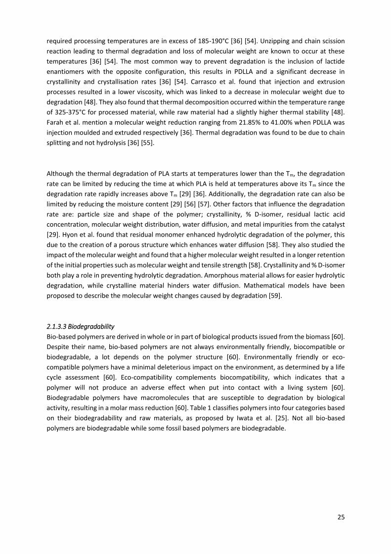
proposed. Carné et al. propose a stepwise process to both recycle and separate PLA and PET mixed

waste [72]. This process, shown in figure 3, takes advantage of the different reactivity to alcoholysis of

the two plastics, resulting in a selective depolymerisation process [72].

Figure 3 Stepwise process to both recycle and separate PLA and PET mixed waste [72].

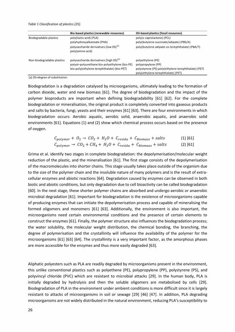
2.2 Hydroxyapatite Apatites (biominerals) are calcium phosphates with generic formula Ca5(PO4)3(F, Cl, OH), they are

characterised by phosphorus tetrahedrons which share oxygen with nine-coordinated calcium sites

and singly charged anion lattice sites hosting F, Cl or OH that are surrounded by a planar arrangement

of three calcium atoms, as shown in figure 4 [73]. Based on the present anion, the apatites can be

divided into chlorapatite (chlorine-rich variety); Dahllite (carbonate-bearing hydroxyapatite);

fluorapatite (fluorine-rich variety); francolite (carbonate-rich variety); and hydroxyapatite (hydroxyl-

rich variety) [73]. Calcium phosphates are major components of natural bone and have bioactive and

28

biocompatible properties [74]. Hydroxyapatite (Ca10(PO4)6(OH)2, HA), dicalcium phosphate dihydrate

(CaHPO4·2H2O, DCPD), tricalcium phosphate (Ca3(PO4)2, TCP), tetracalcium phosphate (Ca4P2O9,

TetTCP) and octacalcium phosphate (Ca8H2(PO4)6, OCP) are all calcium phosphates that have been

studied for application in medical fields [74].

Figure 4 Apatite structure viewed along the c-crystallographic axis: green = calcium, red = oxygen, orange = phosphorus,

white = fluorine, chlorine, or hydroxyl [73].

HA is, at 65 wt%, a major bone component, providing most of the stiffness and strength of the bone

[75] [76]. Additionally, the morphology and dimensions of HA crystals in bone affects its mechanical

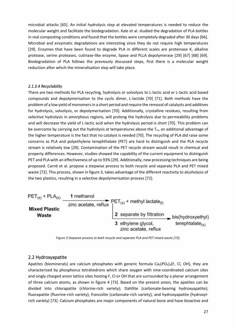
properties [75]. Su et al. found that HA crystals in the body can be nano-sized, with the average sizes

of mature human bone crystals being ~50 nm in length and ~25 nm in width [77]. Maas et al. found

that the HA powders used for ceramics consist of characteristic needle-like HA nanocrystals with a

length varying from 25-50 nm and a diameter around 5 nm [78]. Figure 5 shows the transmission

electron micrograph of a typical HA nanopowder. Montjovent et al. found a specific surface of 62.53

m²/g for nano HA powders [79]. Ramakrishna et al. found a modulus of 95 GPa and a tensile strength

of 50 MPa for hydroxyapatite [80]. The theoretical density of HA corresponds to 3.16 g/cm³, which is

much higher than that of human bones (1.89 g/cm³) [81] [82] [83]. Figueiredo et al. found that calcined

samples exhibited skeletal densities near to 3 g/cm³, which is close to the theoretical density of HA

[81].

Figure 5 TEM of HA for P120 (original magnification ×23 000) [84].

2.2.1 Nanoparticles

Nanoparticles (NPs) are particles with at least one dimension between 1 and 100 nm [85]. Based on

the number of dimensions under 100 nm, NPs can be divided into isodimensional NPs (3 dimensions),

nanotubes or nanowhiskers (2 dimensions) and nanosheets (1 dimension) [86]. Due to their small size,

29

they have unique chemical and physical characteristics, leading to advanced magnetic, electrical,

optical, mechanical and structural properties compared to the original bulk substance [85]. This can be

linked to their higher surface to volume ratio, potentially increasing interaction when they are

incorporated in materials [85]. The surface to volume ratio or specific surface area can vary a lot.

Peigny et al. calculated the theoretical specific surface area of carbon nanotubes and found that the

specific surface area range over a very broad scale, from 50 to 1315 m²/g [87]. The use of NPs is not

without controversy, as they may pose a risk for humans and the environment [88] [89] [90]. The

European Commission Scientific Committee on Emerging and Newly Identified Health Risks (SCENHIR)

concluded that there is not yet a generally applicable paradigm for nanomaterial hazard identification,

a case by case approach for the risk assessment of nanomaterials is thus warranted [91]. Additionally,

the committee also indicated that the methodology for both exposure estimations and hazard

identification needs to be further developed, validated and standardised [91].

2.2.2 Synthesis

Multiple techniques exist to create nano HA: a wet chemical precipitation technique, followed by

hydrothermal treatment (nanorods); a cationic surfactant method (nanorods); a precipitation with

cetyltrimethylammonium bromide (CTAB) as surfactant (Needle-shaped); precipitation with and

without utilizing F127 as surfactant (Plate-shaped and spherical respectively) [74] [92] [93] [94] [95]

[96] [97]. Swain and Sarkar used a coprecipitation method with multiple starting precursors and

reaction media and found that sphere particles were developed in basic medium, and rods in weak

acidic medium [92]. Albano et al. obtained HA nanocrystals with a needle shape morphology and

average dimensions of 74±21 nm in length and 22±7 nm in width using a precipitation method [98].

2.3 PLA/nHA nanocomposites

Polymer composites are the result of an inclusion of one or more filler materials in the polymer matrix.

Usually a composite is created when a chosen polymer lacks mechanical strength or specific properties

such as electric conductivity, thermal resistance, etc. Depending on the lacking property, one or more

appropriate fillers can then be added to the polymer matrix. Multiple charges can add the same

property to a polymer matrix, however, the compatibility, efficiency and cost of the charges will

determine the suitable candidate. Additionally, the application can impose requirements on the

charges, such is the case for medical applications, for which strict rules exist with regards to the used

materials.

The creation of PLA/nHA nanocomposites and the usage of the composites in fused deposition

modelling in this study is potentially interesting for bone tissue engineering. HA cannot be used as a

bone repair material on its own, given the low mechanical flexural strength and fracture toughness,

therefor it is included in a polymer matrix [74] [99]. Multiple polymer matrices have already been used

for HA composites, but biodegradable polymers like poly(a-esters) such as poly(hydroxyalkanoates),

poly(a-hydroxyacids) and poly(lactones) have attracted much interest due to their good

biocompatibility, specific biodegradability, and good mechanical properties [100]. The biodegradability

of the polymer matrix is of interest in bone tissue engineering, as it avoids a secondary operation to

remove the scaffold and with it comes a reduction of the chance of nosocomial diseases, given that

the patient spends less time in the hospital and has to undergo fewer operations. Additionally, PLA,

30

polyglycolide (PGA) and poly(lactide-co-glycolide) (PLGA) are the poly(a-hydroxyacids) most

extensively investigated, due to easy processing and adjustment of mechanical properties and

degradation features by copolymerisation [99] [101]. Zhang et al. found that the compressive strength

and the young modulus increased monotonously from 53 MPa to 155 MPa and from 1.2 GPa to 3.6

GPa respectively when the HA content increased from 0-20% in PLLA [102]. Nejati et al. show that

PLA/HA microcomposites (50 wt% HA) and PLA/HA nanocomposites (50 wt% HA) have significantly

higher average elastic moduli and compressive strengths, at 13.68 MPa and 4.61 MPa respectively for

the microcomposite and at 14.9 MPa and 8.67 MPa respectively for the nanocomposite, compared to

the 1.79 MPa and 2.4 MPa respectively for the pure PLLA [19]. This also shows that the higher specific

surface of the nanocomposites results in a more efficient improvement of the mechanical properties

when compared to the microcomposites [19]. Nejati et al. also deduced from Fourrier Transformed

Infrared spectroscopy (FTIR) analysis that there are some molecular interactions and chemical bonding

between both nano and micro HA, and PLA, affecting the interfacial behaviour and mechanical

properties of the composites [19]. The lower carbonyl peak of PLA and lower hydrogen peak of micro

and nano HA, indicate that the interaction in the composite is in fact a hydrogen interaction [19]. The

interaction between the polymer matrix and the filler leads to improved mechanical properties.

Several methods exist to formulate PLA/nHA composites: solvent-casting, injection, gas foaming, co-

grinding, additive manufacturing, etc. [79] [103] [104] [105]. Zhang et al. used a modified in situ

precipitation method to prepare PLLA/nHA composites [102]. Nejati et al. obtained PLLA/nHA

composites by using a thermally induced phase separation method [19]. Peng et al. used

electrospinning to incorporate needle shaped nano-sized HA particles into PLLA nanofibers [106].

Bianco et al. also used electrospinning, but they used calcium deficient nHA [107]. Seyedjafari et al.

used a similar technique, but they plasma-treated the surface of electrospun PLLA nanofibers, before

coating them with nanohydroxyapatite [108]. Aydin et al. [109] grafted HA nanorods on PLLA before

mixing grafted PLLA, PLLA and nHA in a chloroform solution; after drying they extruded the obtained

chips. Wei and Ma used a phase separation technique to formulate PLLA/nHA composite scaffolds [18].

Liu et al. synthetised PLA/nHA composites with a reactive extrusion [53].

Most methods start with a mixing process in which the PLA and nHA are first mixed using a high speed

mixer [110], the stirring of solutions [111] etc. For some of these methods the mixing is also the last

step of the method. In others, the mixing is followed by a second step, often an extrusion [110] and in

some cases, solvent evaporation [111]. Occasionally there is also a grafting process to increase

interactions between the nHA and the polymer matrix [110]. Although PLA/HA nanocomposites haven

been formulated and shaped using multiple methods, there has not yet been an extensive rheological

study of PLA/nHA [78]. Additionally, fused deposition modelling (FDM) for the creation of PLA/HA

composites has also not yet been studied extensively [112]. The lack of rheological information and

information regarding the FDM process of PLA is important with regards to this study, given that a

thickening effect of PLA during the fused deposition modelling could result in nozzle clogging issues,

which would disrupt the FDM process.

31

2.4 Fused deposition modelling

2.4.1 Additive manufacturing

The first successful additive manufacturing (AM) process was patented in 1972 by Ciraud, it consisted

of a powder deposition method with an energy beam [113]. Bourell et al. consider the layerwise

creation of parts is an essential part of AM processes [113]. Over the years multiple AM processes have

been patented, driven by the creation of parts with complex forms, impossible to create with

traditional techniques, or by the creation of parts at a lower cost. Multiple AM processes exist:

stereolitography (SLA), fused deposition modelling® (FDM®), selective laser sintering (SLS), three

dimensional printing, etc. [4] [5] [113] [114] [115]. Table 2 summarises the additive manufacturing

techniques.

Table 2 Summary AM processes [116].

Stereolitography uses the spatially controlled solidification of a liquid resin by photo-polymerisation,

using a computer-controlled laser beam or a digital light project with a computer-driven building stage

[114]. A pattern is illuminated on the surface of the resin, solidifying the lit areas to a predefined depth,

after which the support platform is lowered, recoating the surface of the solidified areas in liquid, to

prepare the next layer [114]. The main limitation of stereolitography is the limited number of

commercially available resins for processing [114]. A resin has to be a liquid that rapidly solidifies upon

illumination with light [114]. Figure 6 visualises the stereolitography process.

32

Figure 6 Schemes of two types of stereolithography setups. Left: a bottom-up system with scanning laser. Right: a top-down

setup with digital light projection [114].

Unlike stereolithography, which uses a liquid, SLS uses a powder. In SLS, complex three dimensional

parts are generated by consolidating successive layers of powder material on top of each other [117].

The consolidation is obtained by processing the selected areas using the thermal energy supplied by a

focused laser beam, which is guided using a beam deflection system [117]. A powder deposition system

is used for the deposition of successive powder layers [117]. Figure 7 shows the SLS process.

Figure 7 A typical SLS machine layout [117].

Three-dimensional printing (3DP) fabricates three dimensional structures by printing liquid binder

solution onto a powder bed with an inkjet [118]. As with the other additive manufacturing processes,

3DP is also a layerwise process. The unbound powder is removed at the end of the manufacturing

process. Additionally, the local composition can be manipulated by specifying the appropriate

printhead and the appropriate binder (printing parameters alter the local microstructure) [118]. Figure

8 visualises the 3DP process.

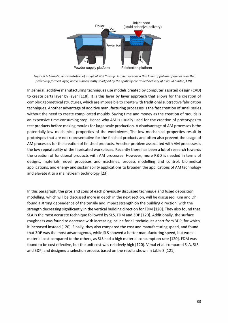
33

Figure 8 Schematic representation of a typical 3DP™ setup. A roller spreads a thin layer of polymer powder over the

previously formed layer, and is subsequently solidified by the spatially controlled delivery of a liquid binder [119].

In general, additive manufacturing techniques use models created by computer assisted design (CAD)

to create parts layer by layer [118]. It is this layer by layer approach that allows for the creation of

complex geometrical structures, which are impossible to create with traditional subtractive fabrication

techniques. Another advantage of additive manufacturing processes is the fast creation of small series

without the need to create complicated moulds. Saving time and money as the creation of moulds is

an expensive time-consuming step. Hence why AM is usually used for the creation of prototypes to

test products before making moulds for large scale production. A disadvantage of AM processes is the

potentially low mechanical properties of the workpieces. The low mechanical properties result in

prototypes that are not representative for the finished products and often also prevent the usage of

AM processes for the creation of finished products. Another problem associated with AM processes is

the low repeatability of the fabricated workpieces. Recently there has been a lot of research towards

the creation of functional products with AM processes. However, more R&D is needed in terms of

designs, materials, novel processes and machines, process modelling and control, biomedical

applications, and energy and sustainability applications to broaden the applications of AM technology

and elevate it to a mainstream technology [23].

In this paragraph, the pros and cons of each previously discussed technique and fused deposition

modelling, which will be discussed more in depth in the next section, will be discussed. Kim and Oh

found a strong dependence of the tensile and impact strength on the building direction, with the

strength decreasing significantly in the vertical building direction for FDM [120]. They also found that

SLA is the most accurate technique followed by SLS, FDM and 3DP [120]. Additionally, the surface

roughness was found to decrease with increasing incline for all techniques apart from 3DP, for which

it increased instead [120]. Finally, they also compared the cost and manufacturing speed, and found

that 3DP was the most advantageous, while SLS showed a better manufacturing speed, but worse

material cost compared to the others, as SLS had a high material consumption rate [120]. FDM was

found to be cost effective, but the unit cost was relatively high [120]. Vimal et al. compared SLA, SLS

and 3DP, and designed a selection process based on the results shown in table 3 [121].

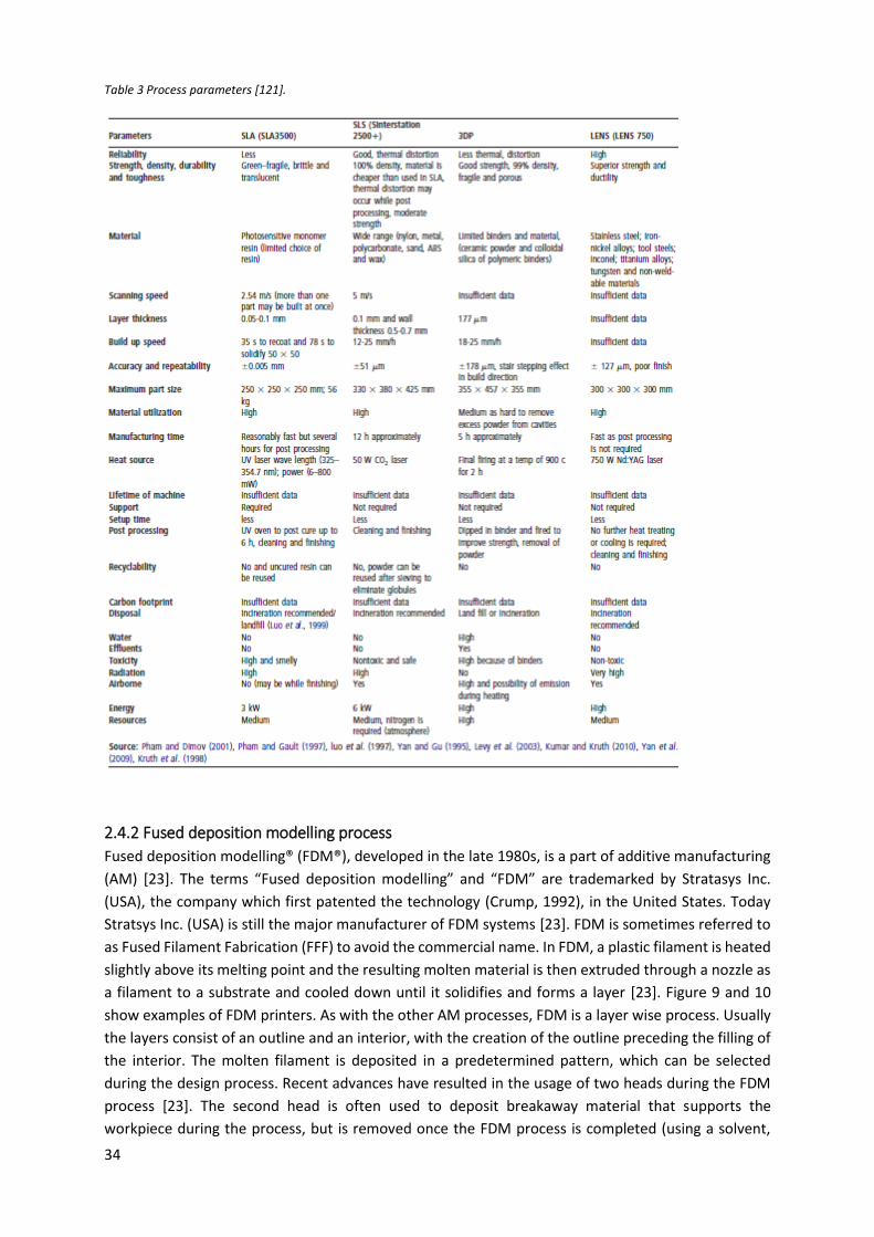
34

Table 3 Process parameters [121].

2.4.2 Fused deposition modelling process

Fused deposition modelling® (FDM®), developed in the late 1980s, is a part of additive manufacturing

(AM) [23]. The terms “Fused deposition modelling” and “FDM” are trademarked by Stratasys Inc.

(USA), the company which first patented the technology (Crump, 1992), in the United States. Today

Stratsys Inc. (USA) is still the major manufacturer of FDM systems [23]. FDM is sometimes referred to

as Fused Filament Fabrication (FFF) to avoid the commercial name. In FDM, a plastic filament is heated

slightly above its melting point and the resulting molten material is then extruded through a nozzle as

a filament to a substrate and cooled down until it solidifies and forms a layer [23]. Figure 9 and 10

show examples of FDM printers. As with the other AM processes, FDM is a layer wise process. Usually

the layers consist of an outline and an interior, with the creation of the outline preceding the filling of

the interior. The molten filament is deposited in a predetermined pattern, which can be selected

during the design process. Recent advances have resulted in the usage of two heads during the FDM

process [23]. The second head is often used to deposit breakaway material that supports the

workpiece during the process, but is removed once the FDM process is completed (using a solvent,

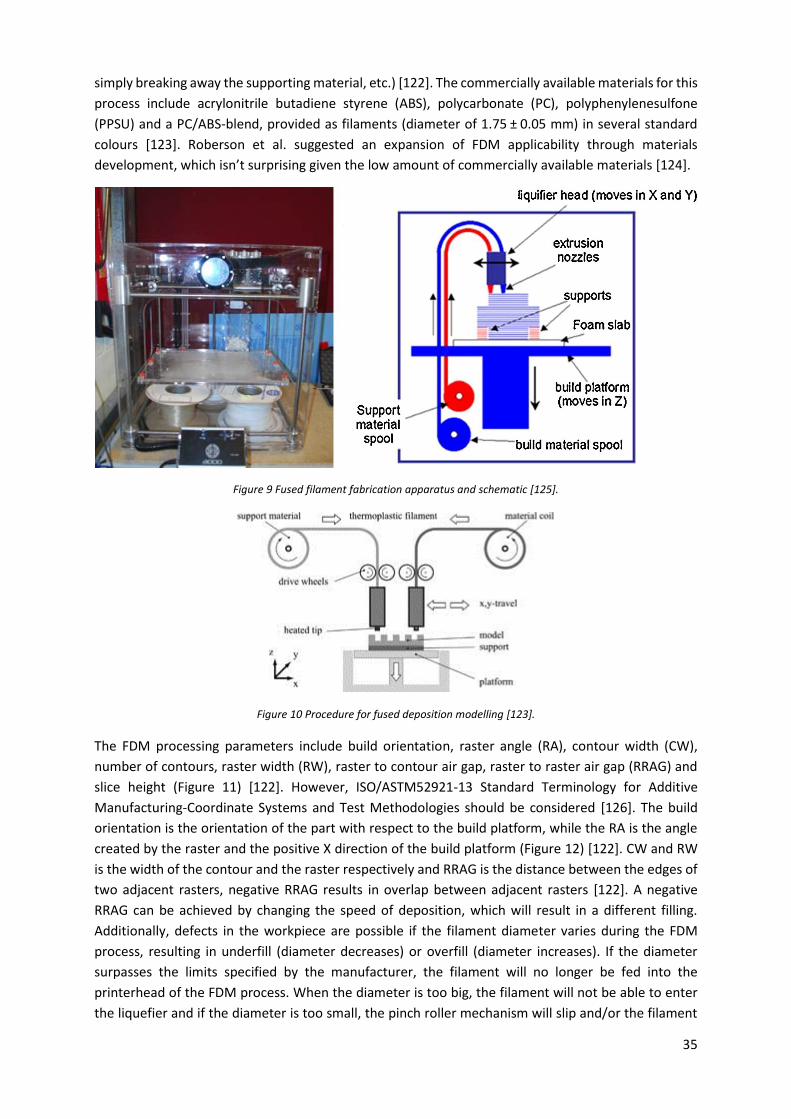
35

simply breaking away the supporting material, etc.) [122]. The commercially available materials for this

process include acrylonitrile butadiene styrene (ABS), polycarbonate (PC), polyphenylenesulfone

(PPSU) and a PC/ABS-blend, provided as filaments (diameter of 1.75 ± 0.05 mm) in several standard

colours [123]. Roberson et al. suggested an expansion of FDM applicability through materials

development, which isn’t surprising given the low amount of commercially available materials [124].

Figure 9 Fused filament fabrication apparatus and schematic [125].

Figure 10 Procedure for fused deposition modelling [123].

The FDM processing parameters include build orientation, raster angle (RA), contour width (CW),

number of contours, raster width (RW), raster to contour air gap, raster to raster air gap (RRAG) and

slice height (Figure 11) [122]. However, ISO/ASTM52921-13 Standard Terminology for Additive

Manufacturing-Coordinate Systems and Test Methodologies should be considered [126]. The build

orientation is the orientation of the part with respect to the build platform, while the RA is the angle

created by the raster and the positive X direction of the build platform (Figure 12) [122]. CW and RW

is the width of the contour and the raster respectively and RRAG is the distance between the edges of

two adjacent rasters, negative RRAG results in overlap between adjacent rasters [122]. A negative

RRAG can be achieved by changing the speed of deposition, which will result in a different filling.

Additionally, defects in the workpiece are possible if the filament diameter varies during the FDM

process, resulting in underfill (diameter decreases) or overfill (diameter increases). If the diameter

surpasses the limits specified by the manufacturer, the filament will no longer be fed into the

printerhead of the FDM process. When the diameter is too big, the filament will not be able to enter

the liquefier and if the diameter is too small, the pinch roller mechanism will slip and/or the filament

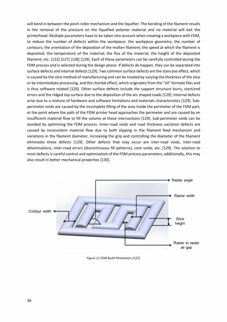
36

will bend in between the pinch roller mechanism and the liquefier. The bending of the filament results

in the removal of the pressure on the liquefied polymer material and no material will exit the

printerhead. Multiple parameters have to be taken into account when creating a workpiece with FDM,

to reduce the number of defects within the workpiece: the workpiece geometry; the number of

contours; the orientation of the deposition of the molten filament; the speed at which the filament is

deposited; the temperature of the material; the flux of the material; the height of the deposited

filament; etc. [122] [127] [128] [129]. Each of these parameters can be carefully controlled during the

FDM process and is selected during the design phase. If defects do happen, they can be separated into

surface defects and internal defects [129]. Two common surface defects are the staircase effect, which

is caused by the slice method of manufacturing and can be treated by varying the thickness of the slice

or by intermediate processing, and the chordal effect, which originates from the “stl” formate files and

is thus software related [129]. Other surface defects include the support structure burrs, start/end

errors and the ridged top surface due to the deposition of the arc shaped roads [129]. Internal defects

arise due to a mixture of hardware and software limitations and materials characteristics [129]. Sub-

perimeter voids are caused by the incomplete filling of the area inside the perimeter of the FDM part,

at the point where the path of the FDM printer head approaches the perimeter and are caused by an

insufficient material flow to fill the volume at these intersections [129]. Sub-perimeter voids can be

avoided by optimising the FDM process. Inner-road voids and road thickness variation defects are

caused by inconsistent material flow due to both slipping in the filament feed mechanism and

variations in the filament diameter, increasing the grip and controlling the diameter of the filament

eliminates these defects [129]. Other defects that may occur are inter-road voids, inter-road

delaminations, inter-road errors (discontinuous fill patterns), core voids, etc. [129]. The solution to

most defects is careful control and optimisation of the FDM process parameters, additionally, this may

also result in better mechanical properties [130].

Figure 11 FDM Build Parameters [122].

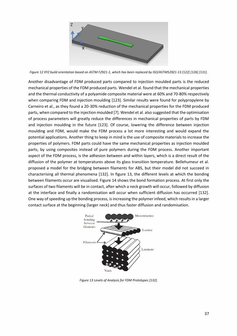
37

Figure 12 XYZ build orientation based on ASTM F2921-1, which has been replaced by ISO/ASTM52921-13 [122] [126] [131].

Another disadvantage of FDM produced parts compared to injection moulded parts is the reduced

mechanical properties of the FDM produced parts. Wendel et al. found that the mechanical properties

and the thermal conductivity of a polyamide composite material were at 60% and 70-80% respectively

when comparing FDM and injection moulding [123]. Similar results were found for polypropylene by

Carneiro et al., as they found a 20-30% reduction of the mechanical properties for the FDM produced

parts, when compared to the injection moulded [7]. Wendel et al. also suggested that the optimisation

of process parameters will greatly reduce the differences in mechanical properties of parts by FDM

and injection moulding in the future [123]. Of course, lowering the difference between injection

moulding and FDM, would make the FDM process a lot more interesting and would expand the

potential applications. Another thing to keep in mind is the use of composite materials to increase the

properties of polymers. FDM parts could have the same mechanical properties as injection moulded

parts, by using composites instead of pure polymers during the FDM process. Another important

aspect of the FDM process, is the adhesion between and within layers, which is a direct result of the

diffusion of the polymer at temperatures above its glass transition temperature. Bellehumeur et al.

proposed a model for the bridging between filaments for ABS, but their model did not succeed in

characterising all thermal phenomena [132]. In figure 13, the different levels at which the bonding

between filaments occur are visualised. Figure 14 shows the bond formation process. At first only the

surfaces of two filaments will be in contact, after which a neck growth will occur, followed by diffusion

at the interface and finally a randomisation will occur when sufficient diffusion has occurred [132].

One way of speeding up the bonding process, is increasing the polymer infeed, which results in a larger

contact surface at the beginning (larger neck) and thus faster diffusion and randomisation.

Figure 13 Levels of Analysis for FDM Prototypes [132].

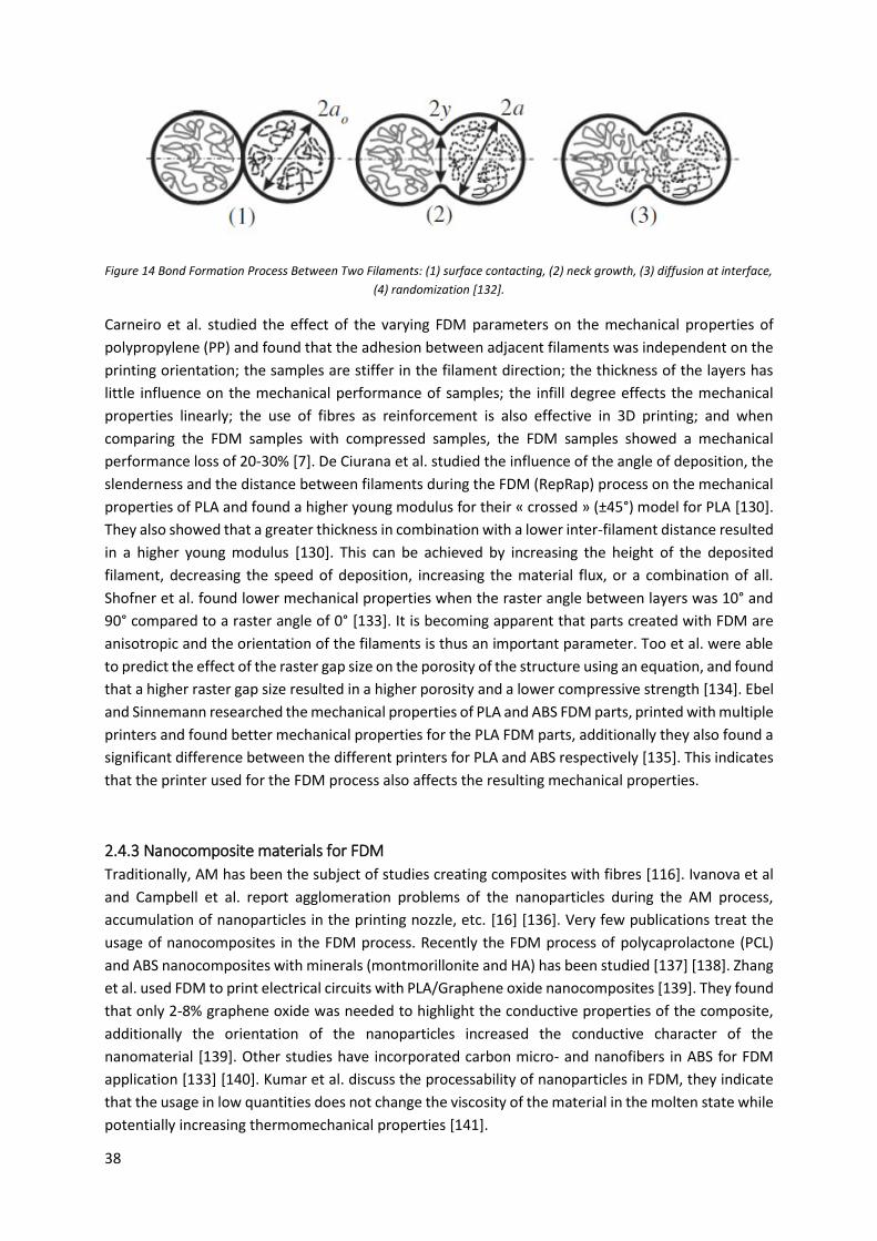
38

Figure 14 Bond Formation Process Between Two Filaments: (1) surface contacting, (2) neck growth, (3) diffusion at interface,

(4) randomization [132].

Carneiro et al. studied the effect of the varying FDM parameters on the mechanical properties of

polypropylene (PP) and found that the adhesion between adjacent filaments was independent on the

printing orientation; the samples are stiffer in the filament direction; the thickness of the layers has

little influence on the mechanical performance of samples; the infill degree effects the mechanical

properties linearly; the use of fibres as reinforcement is also effective in 3D printing; and when

comparing the FDM samples with compressed samples, the FDM samples showed a mechanical

performance loss of 20-30% [7]. De Ciurana et al. studied the influence of the angle of deposition, the

slenderness and the distance between filaments during the FDM (RepRap) process on the mechanical

properties of PLA and found a higher young modulus for their « crossed » (±45°) model for PLA [130].

They also showed that a greater thickness in combination with a lower inter-filament distance resulted

in a higher young modulus [130]. This can be achieved by increasing the height of the deposited

filament, decreasing the speed of deposition, increasing the material flux, or a combination of all.

Shofner et al. found lower mechanical properties when the raster angle between layers was 10° and

90° compared to a raster angle of 0° [133]. It is becoming apparent that parts created with FDM are

anisotropic and the orientation of the filaments is thus an important parameter. Too et al. were able

to predict the effect of the raster gap size on the porosity of the structure using an equation, and found

that a higher raster gap size resulted in a higher porosity and a lower compressive strength [134]. Ebel

and Sinnemann researched the mechanical properties of PLA and ABS FDM parts, printed with multiple

printers and found better mechanical properties for the PLA FDM parts, additionally they also found a

significant difference between the different printers for PLA and ABS respectively [135]. This indicates

that the printer used for the FDM process also affects the resulting mechanical properties.

2.4.3 Nanocomposite materials for FDM

Traditionally, AM has been the subject of studies creating composites with fibres [116]. Ivanova et al

and Campbell et al. report agglomeration problems of the nanoparticles during the AM process,

accumulation of nanoparticles in the printing nozzle, etc. [16] [136]. Very few publications treat the

usage of nanocomposites in the FDM process. Recently the FDM process of polycaprolactone (PCL)

and ABS nanocomposites with minerals (montmorillonite and HA) has been studied [137] [138]. Zhang

et al. used FDM to print electrical circuits with PLA/Graphene oxide nanocomposites [139]. They found

that only 2-8% graphene oxide was needed to highlight the conductive properties of the composite,

additionally the orientation of the nanoparticles increased the conductive character of the

nanomaterial [139]. Other studies have incorporated carbon micro- and nanofibers in ABS for FDM

application [133] [140]. Kumar et al. discuss the processability of nanoparticles in FDM, they indicate

that the usage in low quantities does not change the viscosity of the material in the molten state while

potentially increasing thermomechanical properties [141].

39

2.5 Bone tissue engineering

Bone plays multiple roles in the human body, it is integral for the locomotion as it ensures the skeleton

has adequate load-bearing capacity and protects the internal organs of the body [142]. Additionally,

bone also regulates the Ca and P ions concentration in the blood and remodels throughout the lifetime

of an individual [142]. Bone tissue engineering is a complex and dynamic process that initiates with

migration and recruitment of osteoprogenitor cells followed by their proliferation, differentiation and

matrix formation along with remodelling of the bone [143]. The American Academy of Orthopaedic

Surgeons estimates 6.3 million fractures annually in the United States, with over 500,000 bone graft

procedures being performed in the U.S., of which 90% were either autograft or allograft bone tissues,

and mounting to an estimated cost of $2.5 billion [144]. Autograft (taken from patients own bone

tissue), allograft (human donor bone tissue) and xenograft (nonhuman donor bone tissue) bone tissues

have disadvantages, there’s only a limited amount of autograft material available; allograft and

xenograft require a donor, which comes with potential compatibility issues and disease transmission;

and all are viable to contamination [144]. Synthetic or alloplastic bone grafts are osteoconductive

materials that are abundantly available and eliminate the risk of disease transfer and procurement

morbidity [145]. Ideally, the synthetic bone graft material should mimic bone in both mechanical and

osteogenic properties, which leads to the following four characteristics that an ideal bone graft

material should possess [145]:

- Osteointegration, the ability to chemically bond to the surface of bone without an intervening

layer of fibrous tissue.

- Osteoconduction, the ability to support the growth of bone over its surface.

- Osteoinduction, the ability to induce differentiation of pluripontential stem cells from

surrounding tissue to an osteoplastic phenotype.

These characteristics can be linked to the following key properties that an implant should possess as

identified by authors in the literature [144] [146] [147] [148] [149]:

- Biocompatibility: An implant cannot be rejected by the organism; nor can it be toxic,

mutagenic, antigenic or carcinogenic.

- A structure similar to the naturally occurring extracellular structure, to promote cell

proliferation and cell-specific matrix production and to avoid stress shielding (Chemical

modification is an option [116]).

- An open-pore geometry with a highly porous surface and microstructure with interconnected

porous networks, that allows cell in-growth and reorganization in vitro and provides the

necessary space for neovascularization from surrounding tissues in vivo (50-90% porosity;

macropores of 200-400 µm and micropores of 20-125 µm).

- Mechanical properties similar to bone,

- Sterilisable,

- Controlled degradation that allows for the reconstruction of bone, which gradually takes the

place of the implant. Additionally, the implant should retain some of its mechanical properties

during the degradation.

The degradation of the implant results in space for bone growth, which makes a second operation to

remove the implant unnecessary [148] [150]. By reducing the number of operations, the usage of

40

degradable implants indirectly results in freeing operating theaters and reducing the probability of

nosocomial disease for a patient. A degradable implant has to be degradable by either hydrolysis or

enzymatic activity, in a slow enough fashion to allow for the bone to regenerate.

2.5.1 Hydroxyapatite composites

Synthetic HA is a calcium phosphate bioceramic with chemical composition (Ca/P ¼ 1.67) and structure

similar to the main inorganic constituent of natural bone; it has bioactive, biocompatible,

biodegradable and osteoconductive properties [94] [95] [99]. HA has been intensively investigated as

bone repair material, but a low mechanical flexural strength and fracture toughness (high brittleness)

restrict its application in regeneration and repairing of new bone tissue at load-bearing sites [74] [99].

One way of overcoming this weakness, is the combination with polymers. The HA will act as a

reinforcing material to improve the mechanical properties of the polymer and can improve the

osteoconductivity of the polymer [94]. The advantage of the polymer lies within its matrix being though

and flexible, improving the toughness of the whole system [99]. PLA, PGA and PLGA have been widely

reviewed and considered as polymer matrices in HA based composites for applications in medical

devices, and scaffolds for bone tissue engineering [99] [151] [152] [153]. Nejati et al. showed the

interest of PLA, given the interaction between the hydroxyl group of HA and carbonyl group of PLA as

mentioned before [19].

2.5.2 Fused deposition modelling for bone tissue engineering

FDM allows for the rapid manufacturing of custom implants within hours of the patient’s arrival in the

hospital. Additionally, due to the computer aided design (CAD) employed during the creation of the

implant for the FDM process, the pore network and pore size can be controlled. This could result in

better cell in-growth and reorganization and provide the necessary space for neovascularization from

surrounding tissues. The materials utilisable are restricted to those available, but among the available

materials there is PLA. PLA is a biodegradable material that also degrades in the human body, as

discussed earlier. The degradation products are also produced by the body, reducing the toxicity of the

implant, but inflammation of surrounding tissue can still be problematic. Due to the fact PLA degrades

by hydrolysis in the human body, the control of the porosity, pore network and molar mass also results

in the control of the degradation speed, the higher the contact surface the faster the degradation. So

far the usage of PLA nanocomposites has not yet been studied extensively for the FDM process.

However, PLA/HA nanocomposites could prove to be very interesting for the creation of implants with

FDM.

2.6 Application of nanocomposites in packaging materials

The addition of nanoparticles to improve material properties, has been the interest of scientists for a

few decades [99]. Specific types of nanofillers can enhance several properties of a neat polymer in a

synergetic manner; broadening the field of application of the nanoparticles [99]. Organoclays,

hydroxyapatite and carbon nanotubes have been widely used in polymer nanocomposites [99].

41

2.6.1 Barrier properties

Barrier materials restrict the passage of gases, vapours and organic liquids through their boundaries,

polymers dominate the packaging industry but are also used in other industries [154]. An absolute

barrier does not exist; barrier properties depend mainly on the used polymer structure and should be

adapted for each application [155]. Permeation through polymer materials is the result of two

processes: diffusion (kinetic quantity) and solubility (thermodynamic quantity) [156].

𝑃 = 𝐷 ∗ 𝑆 (3) [156]

Solubility can be linked to the chemical relationship between the permeant molecule and the polymer

[154]. The diffusion rate is dependent upon the size of the permeant molecule and the amorphous

configuration of the polymer [154]. Diffusion is a flow of matter resulting from a chemical potential

difference of migrant material in different locations of the system [155]. The permeability of a certain

permeant is the amount of permeant that passes through a sample surface within a certain time and

under a certain pressure. The permeation flux (J) is defined as the quantity of matter that passes

through the material; the permeation flux follows Fick’s first law, which establishes the proportion

between J and the concentration gradient of the permeant normal to the cross-section of the sample

[157] [158].

𝐽 = −𝐷𝜕𝐶

𝜕𝑥 (4) [157] [158]

The diffusion and solubility coefficients are considered independent of the permeant concentration;

therefore, the steady-state flux can be related to the permeability and the pressure difference by

permeating through the membrane by the following relationship [155]:

𝐽 = 𝐷 ∗ 𝑆 ∗ ∆𝑝

𝑒= 𝑃 ∗

∆𝑝

𝑒 (5) [155]

𝑃 = 𝐽 ∗ 𝑒

∆𝑝=

𝑄∗𝑒

𝑆∗𝑡∗∆𝑝 (6) [155]

With Q = the quantity of permeant traversing the sample,

S = the sample surface,

e = the sample thickness,

t = the time,

Δp = the pressure difference between the two sides of the sample.

It is important to know that the permeability coefficient measures relative permeation behaviour and

is used to compare the permeability of different polymers [154]. Permeability is the proportionality

constant in the general equation for mass transport of a penetrant across a barrier, as seen in equation

7 [154].

∆𝑚𝑝𝑒𝑛𝑒𝑡𝑟𝑎𝑛𝑡

∆𝑡= 𝑃

𝐴 ∆𝑝

𝑙 (7) [154]

P = the permeability of the barrier material,

∆𝑚𝑝𝑒𝑛𝑒𝑡𝑟𝑎𝑛𝑡 ∆𝑡⁄ = the transmission rate,

A = the surface area of the barrier,

Δp = the partial pressure difference across the barrier,

l = the thickness of the barrier.

The permeant (gas or vapour) will undergo three stages during permeability tests: in the first stage the

permeant is absorbed in the polymer material; in the second stage the permeant will diffuse through

42

the polymer matrix under the influence of a concentration gradient; and in the third and final stage

the permeant undergoes desorption through the polymer wall and is evaporated from the polymer

surface [154]. When measuring the permeability, there will be a transition from a pseudo steady-state

to a steady-state, as the polymer will slowly become saturated with the permeant. Once saturated,

the permeability remains constant. Unless if the permeant affects the polymer matrix, in which case

the permeability might increase or decrease over time depending on the effect of the permeant on

the polymer matrix. Factors influencing the permeability through a polymeric film can be divided into

three categories: external; due to the permeant; and due to the polymer [156] [159] [160]. External

factors such as temperature (T), pressure (p), concentration (c), humidity (RH), etc. are often kept

constant or carefully controlled throughout the permeability measurements. The influence of the

permeant is a direct result of its solubility, molecular shape, weight, etc. Shogren et al. found that the

values of the water vapour transmission rate (WVTR) were positively correlated with higher polymer

solubility parameters, lower crystallinities, and higher free volumes [161]. Poley et al. found that the

permeability decreased when the size of the molecules increased [162]. They also showed that for

certain permeants, the dependence of the permeability coefficients on the temperature can be

defined by an Arrhenius equation [162]:

𝑃 = 𝑃0 exp (−𝐸𝑝

𝑅𝑇) (8) [162]

Tsuji et al. show that changes of the molecular average weight from 9*104-5*105 g/mol and D-lactide

content of PLA films in the range of 0-50% have insignificant effects on their WVTR [163], while the

WVTR decreased monotonically with increasing crystallinity from 0 to 20% and levelled off from

crystallinities exceeding 30%. Song et al. showed that the incorporation of hydrophobic-modified

nano-cellulose fibres into the PLA matrix resulted in a lower WVTR [164]. Dong et al. compared the

barrier behaviour of both stretched and annealed PLA films with regular PLA films, they found an

increase in oxygen and water vapour barrier for annealed and stretched PLA films compared to

undrawn PLA at middle draw ratio (Further stretching reduced the barrier properties) [165]. Dong et

al. found the annealed PLA film to have higher barrier ability than that of the stretched PLA film,

additionally, they also found an increasing oxygen transmission rate (OTR) with increasing

temperature, while the WVTR reduced slightly; and both OTR and WVTR were insensitive to the

humidity [165]. Ducruet et al. studied the effect of the crystallinity of PLA samples plasticised with

acetyl butyl citrate on the barrier properties against ethyl acetate and oxygen and found increased

barrier properties against ethyl acetate, but no effect of the crystallinity on the OTR of PLA [166].

Colomines et al. found similar results for normal PLA films and concluded that the crystallinity does

not influence the OTR of PLA [167]. Chowdhury et al. reported a decreasing permeability with the

inclusion of layered nano-silicates in the PLA matrix, which they linked to the creation of a tortuous

path, linked to the shape of the platelets (Platelets were considered parallel) [168]. Others have also

turned to nanocomposites to reduce the OTR & WTVTR of polymers, relying on the creation of a

tortuous path [160] [169] [170] [171].

OTR is usually reported in cubic centimetres of gas that pass through a square meter of film in 24h

when the gas pressure differential on one side of the film, at a specified temperature, is one

atmosphere greater than that on the other side (Normalised units: cm³*mm/m²*day*atm) [154].

WVTR is reported as grams of water which will pass through a given area of material in a specified

time, the usual units are grams per 1 square meter per 24 h at a specified temperature and humidity

differential (Normalised units: g*mm/m²*day) [154]. Different methods exist to determine the gas

43

permeability (OTR & carbon dioxide transmission rate) and the water vapour permeability of polymer

films. OTR methods can be divided into isobaric methods, variable pressure methods, differential

methods and a fluorescence-based oxygen sensor method [155] [172] [173]. WVTR methods can be

divided into gravimetric methods, electrolytic sensor detection method, infrared detection sensor

method, humidity detection sensor method [174]. The methods used in practise to determine the

permeability, mostly correspond to the ones described in the norms. Norms differ from country to

country, but also within companies.

Gravimetric detection WVTR:

- ISO/FDIS 2528: Sheet materials, determination of water vapour transmission rate Gravimetric

(dish) method [175].

- ASTM E96/E96M-16: Standard Test Methods for Water Vapor Transmission of Materials [176].

- ASTM D1653-13: Standard Test Methods for Water Vapor Transmission of Organic Coating

Films [177].

Electrolytic detection WVTR:

- ISO 15106-3:2003: Plastics, film and sheeting, determination of water vapour transmission

rate (Part 3) [178].

Infrared detection WVTR:



- ASTM F1249-13: Standard Test Method for Water Vapor Transmission Rate Through Plastic

Film and Sheeting Using a Modulated Infrared Sensor [180].

- TAPPI T557: Water vapor transmission rate through plastic films and sheeting using a

modulated infrared sensor [181].

Humidity sensor for WVTR detection:



- ASTM E398-13: Standard Test Method for Water Vapor Transmission Rate of Sheet Materials

Using Dynamic Relative Humidity Measurement [183].

- TAPPI T523: Dynamic Measurement of Water Vapor Transfer Through Sheet Materials [184].

OTR methods:

- ASTM D3985- 05(2010)e1: Standard Test Method for Oxygen Gas Transmission Rate Through

Plastic Film and Sheeting Using a Coulometric Sensor [185].

- ASTM F1307-14: Standard Test Method for Oxygen Transmission Rate Through Dry Packages

Using a Coulometric Sensor [186].

44

- ASTM F2622-8: Standard Test Method for Oxygen Gas Transmission Rate Through Plastic Film

and Sheeting Using Various Sensors [187].

- ASTM F1927-14: Standard Test Method for Determination of Oxygen Gas Transmission Rate,

Permeability and Permeance at Controlled Relative Humidity Through Barrier Materials Using

a Coulometric Detector [188].

2.7 Research strategy

In this study, the PLA and HA will be melt-mixed using a twin-screw extruder (TSE), similar to the

process described by Öner and İlhan for the creation of poly(3-hydroxybutyrate-co-3-hydroxyvalerate)

hydroxyapatite nanocomposites [189]. The characterisation of the materials will be done with the

following techniques: thermogravimetric analysis, differential scanning calorimetry, oscillatory

rheology, tensile tests, dynamic mechanical analysis, wide-angle x-ray diffraction analysis, transmission

electron microscopy and permeability test [53] [97] [99] [127] [163] [166] [190]. The

thermogravimetric analysis helps determine the start of the degradation of the PLA composites, with

this information it is possible to determine the maximum printing temperatures of the FDM process.

Additionally, the thermogravimetric analysis also helps determine the HA content in the composites.

Differential scanning calorimetry analysis help determine the fusion temperature of the obtained PLA

composites for different process steps. Especially the fusion temperature of the filaments is important,

as this is the minimum printing temperature during the FDM process. The differential scanning

calorimetry also aids in the determination of the crystallinity of the composites for different process

steps, which might explain certain phenomena. Oscillatory rheology helps predict nozzle clogging

during the FDM process, as it shows potential thickening effects and thus helps assure the continuity

of the FDM process. Tensile tests will be used to compare the mechanical properties of composites

with different HA content. Doehlert response surface methodology is used to determine the maximum

mechanical properties of each composite for the comparison. Additionally, the FDM printed tensile

samples will be compared with injection moulded samples to determine the influence of the FDM

process on the mechanical properties of the composites. The dynamic mechanical analysis, will help

verify the glass transition temperature of the composites. Results of the dynamic mechanical analysis

will also be used to compare the mechanical properties of the composites. The influence of the FDM

process will be determined by comparing the printed samples with compression moulded samples.

Following Carneiro et al., who used compression moulding as a reference process due to its simplicity

and the low degree of resulting anisotropy, the injection moulding and compression moulding are

reference processes for the FDM process [7]. Additionally, they also help verify whether the addition

of filler resulted in a recovery of the mechanical properties, potentially lost by the FDM process. The

interest of the wide-angle x-ray diffraction analysis lies in the determination of the inter crystal

distance, which is an indication for the size of the HA particles, which in turn will be verified with

transmission electron microscopy. Finally, the permeability of the composites is determined by

creating composite films and consecutive permeability tests. These tests help determine the porosity

of the composites and the results could be interesting for bone tissue engineering applications.

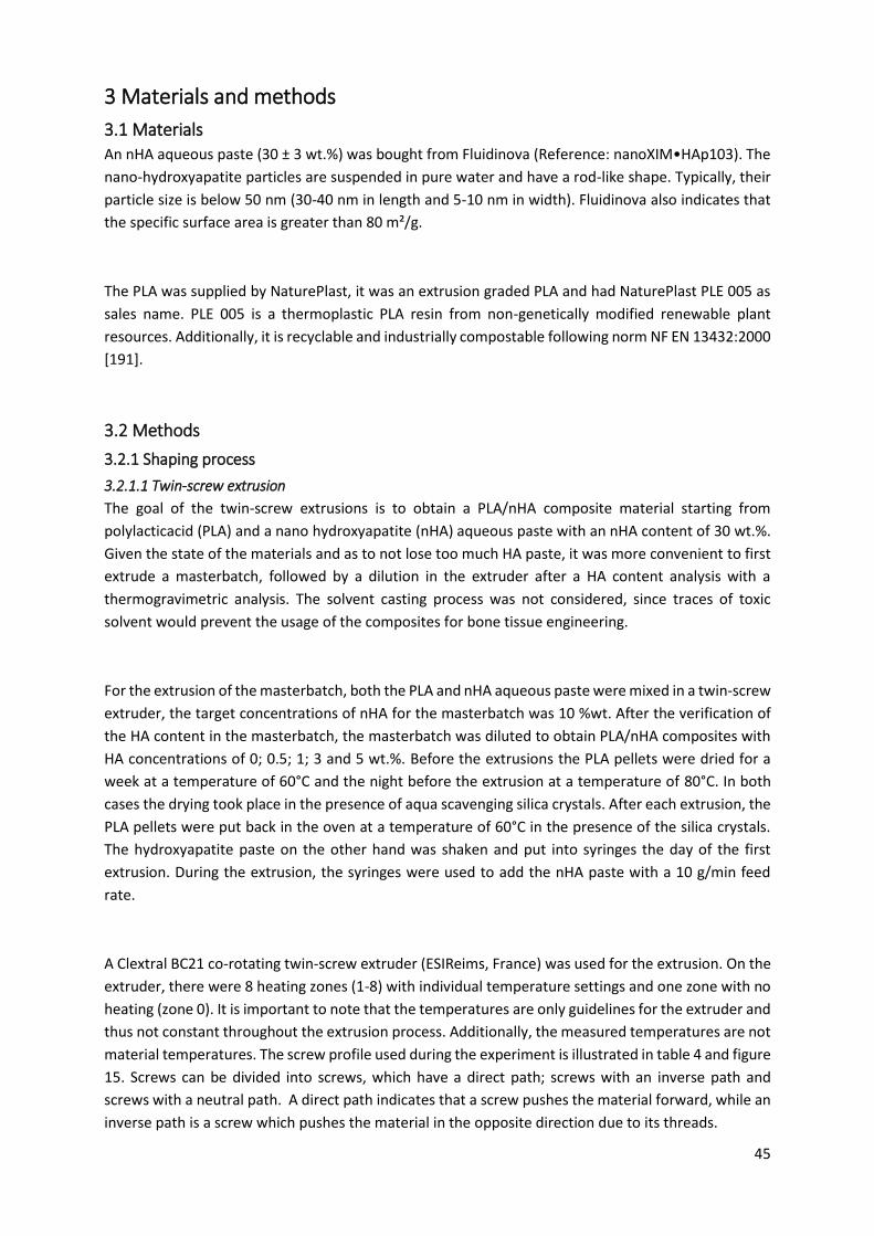
45

3 Materials and methods

3.1 Materials

An nHA aqueous paste (30 ± 3 wt.%) was bought from Fluidinova (Reference: nanoXIM•HAp103). The

nano-hydroxyapatite particles are suspended in pure water and have a rod-like shape. Typically, their

particle size is below 50 nm (30-40 nm in length and 5-10 nm in width). Fluidinova also indicates that

the specific surface area is greater than 80 m²/g.

The PLA was supplied by NaturePlast, it was an extrusion graded PLA and had NaturePlast PLE 005 as

sales name. PLE 005 is a thermoplastic PLA resin from non-genetically modified renewable plant

resources. Additionally, it is recyclable and industrially compostable following norm NF EN 13432:2000

[191].

3.2 Methods

3.2.1 Shaping process

3.2.1.1 Twin-screw extrusion

The goal of the twin-screw extrusions is to obtain a PLA/nHA composite material starting from

polylacticacid (PLA) and a nano hydroxyapatite (nHA) aqueous paste with an nHA content of 30 wt.%.

Given the state of the materials and as to not lose too much HA paste, it was more convenient to first

extrude a masterbatch, followed by a dilution in the extruder after a HA content analysis with a

thermogravimetric analysis. The solvent casting process was not considered, since traces of toxic

solvent would prevent the usage of the composites for bone tissue engineering.

For the extrusion of the masterbatch, both the PLA and nHA aqueous paste were mixed in a twin-screw

extruder, the target concentrations of nHA for the masterbatch was 10 %wt. After the verification of

the HA content in the masterbatch, the masterbatch was diluted to obtain PLA/nHA composites with

HA concentrations of 0; 0.5; 1; 3 and 5 wt.%. Before the extrusions the PLA pellets were dried for a

week at a temperature of 60°C and the night before the extrusion at a temperature of 80°C. In both

cases the drying took place in the presence of aqua scavenging silica crystals. After each extrusion, the

PLA pellets were put back in the oven at a temperature of 60°C in the presence of the silica crystals.

The hydroxyapatite paste on the other hand was shaken and put into syringes the day of the first

extrusion. During the extrusion, the syringes were used to add the nHA paste with a 10 g/min feed

rate.

A Clextral BC21 co-rotating twin-screw extruder (ESIReims, France) was used for the extrusion. On the

extruder, there were 8 heating zones (1-8) with individual temperature settings and one zone with no

heating (zone 0). It is important to note that the temperatures are only guidelines for the extruder and

thus not constant throughout the extrusion process. Additionally, the measured temperatures are not

material temperatures. The screw profile used during the experiment is illustrated in table 4 and figure

15. Screws can be divided into screws, which have a direct path; screws with an inverse path and

screws with a neutral path. A direct path indicates that a screw pushes the material forward, while an

inverse path is a screw which pushes the material in the opposite direction due to its threads.

46

Table 4 Screw profile.

Figure 15 Screw profile extrusion.

During the extrusion process polymer pellets were put into the granules section of the extruder. At the

bottom of this section there was a feed screw with adjustable speed. This screw controlled the polymer

feed and thus the output flow of the extruder. When the screw turned, polymer pellets dropped into

zone 0, the feed zone of the co-rotating screws. From here they were transported through the 8

heating zones towards the exit of the extruder. In zone 3 the hydroxyapatite paste was added to the

N° Screw type Thread length per period (mm) Screw length (mm) Path Thread type Angle

1 conveying 33 50 direct U

2 conveying 33 50 direct U

22 conveying 25 50 direct V


27 conveying 25 25 inverse Grooved V

18 mixer 16 25 direct V

50 mixer 25 50 90






53 conveying 25 12,5 inverse V

56 conveying 25 12,5 inverse V







7 mixer 25 25 inverse - 45

44 mixer 25 25 inverse - 45





\ = conveying screw with a direct path

Screws with inverted path (/): 7, 27, 44, 53, 56

x = mixer

1 2 3 4 5 6 7 8

Exit

\ \ \ \ // \\ x x \ \ \ \ \ \ //// \ \ \ \ \ \ \ \ \ \ \ \ \ \\ x x \ \ \ \ \ \

Screw identity 1+2 22+6 27+18+50 45+15+1624+19+53+56 48+21 47+17+41 51+7+44 46+5+25+26 Ø 5 mm

Zone 0

Granules

\ \ \ \

Screw feed

Zone

\ \ \ \

47

polymer material after which the polymer material and the hydroxyapatite paste turned into one

supposed homogenous flow of material.

Once the material left the extruder, it passed through a water bath leading up to a rolling carpet, which

pulled the polymer filament towards the Scamia granulator 960001 GR (ESIReims, France). The final

step of the extrusion consisted of the collection of the newly formed polymer pellets at the bottom of

the granulator.

3.2.1.2 Single-screw extrusion

An AXON BX 10 single-screw extruder (IFTS, Charleville-Mézières, France) with a constant extrusion

speed, at 20% of its maximum speed, was used to convert the PLA/HA composite pellets into filaments.

The infeed of the pellets into the extruder was done with a simple gravity system. The extruder had 3

heating zones, the temperature of each zone could be adjusted separately. Directly after the extruder

there was a water bath to cool down the polymer material. In this case, it was a hot water bath as the

water circulation was turned off to avoid filament distortion by making the quenching step less abrupt.

After the bath, a pinch roller mechanism of a Haake PP1 granulator (IFTS, Charleville-Mézières, France)

was used to pull the filament with a constant speed. This to obtain a constant diameter, which was

important for the FDM process, which only worked with filament diameters of 1.5-1.6 mm. The final

step consisted of the winding of the filaments on coils.

3.2.1.3 Fused deposition modelling and Doehlert methodology

3.2.1.3.1 Fused deposition modelling

FDM was done with a Makerbot Replicator 2 (IFTS, Charleville-Mézières, France) and the printed

samples were conforming with 5A-type tensile test specimen from ISO 527-2 [192]. In FDM an electric

motor-controlled pinch roller mechanism is used to supply a filament to a heated liquefier. The

filament supplied to the liquefier has two states, in the first state the filament is still solid and will exert

pressure on polymer material that is already in the liquefier. The second state consists of melted

filament, that is pushed through a print nozzle by filament in the first state. The combination of the

liquefier and the print nozzle will be called the “printer head”, although an alternative name could be

the “extruder head” as the process is very similar to an extrusion albeit without screw. Note that the

diameter of the liquefier (1.8 mm) is significantly larger than the diameter of the opening in the print

nozzle (0.4 mm). As material is pushed through the print nozzle, the printer head moves across a

platform, on which the polymer material is deposited. The printer head only moves in the horizontal

plane, while the platform is lowered after the completion of each layer.

The speed of the printer head can be varied depending on the section of the printed object. In this

case, the speed was kept constant throughout the entire printing process. A printed object consists of

multiple layers; each layer consists of a contour and a raster filling. Within each layer, the orientation

in which the material is deposited can vary. In this case, the print orientation was rotated 90° after

each layer. Additionally, the contour consisted of two lines that followed the shape of the printed

object and the raster filling was 100%, indicating that theoretically there were no air gaps between

neighbouring raster lines. Besides the orientation of the material, the height of the deposited polymer

material could also be adjusted, however the height was kept constant at 0.2 mm. This height is a

compromise between the printing resolution, the manufacturing time and the ability to deposit the

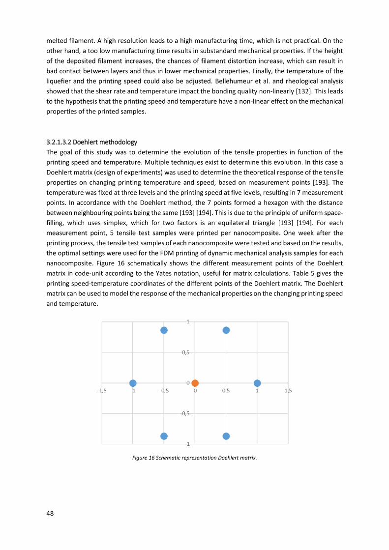
48

melted filament. A high resolution leads to a high manufacturing time, which is not practical. On the

other hand, a too low manufacturing time results in substandard mechanical properties. If the height

of the deposited filament increases, the chances of filament distortion increase, which can result in

bad contact between layers and thus in lower mechanical properties. Finally, the temperature of the

liquefier and the printing speed could also be adjusted. Bellehumeur et al. and rheological analysis

showed that the shear rate and temperature impact the bonding quality non-linearly [132]. This leads

to the hypothesis that the printing speed and temperature have a non-linear effect on the mechanical

properties of the printed samples.

3.2.1.3.2 Doehlert methodology

The goal of this study was to determine the evolution of the tensile properties in function of the

printing speed and temperature. Multiple techniques exist to determine this evolution. In this case a

Doehlert matrix (design of experiments) was used to determine the theoretical response of the tensile

properties on changing printing temperature and speed, based on measurement points [193]. The

temperature was fixed at three levels and the printing speed at five levels, resulting in 7 measurement

points. In accordance with the Doehlert method, the 7 points formed a hexagon with the distance

between neighbouring points being the same [193] [194]. This is due to the principle of uniform space-

filling, which uses simplex, which for two factors is an equilateral triangle [193] [194]. For each

measurement point, 5 tensile test samples were printed per nanocomposite. One week after the

printing process, the tensile test samples of each nanocomposite were tested and based on the results,

the optimal settings were used for the FDM printing of dynamic mechanical analysis samples for each

nanocomposite. Figure 16 schematically shows the different measurement points of the Doehlert

matrix in code-unit according to the Yates notation, useful for matrix calculations. Table 5 gives the

printing speed-temperature coordinates of the different points of the Doehlert matrix. The Doehlert

matrix can be used to model the response of the mechanical properties on the changing printing speed

and temperature.

Figure 16 Schematic representation Doehlert matrix.

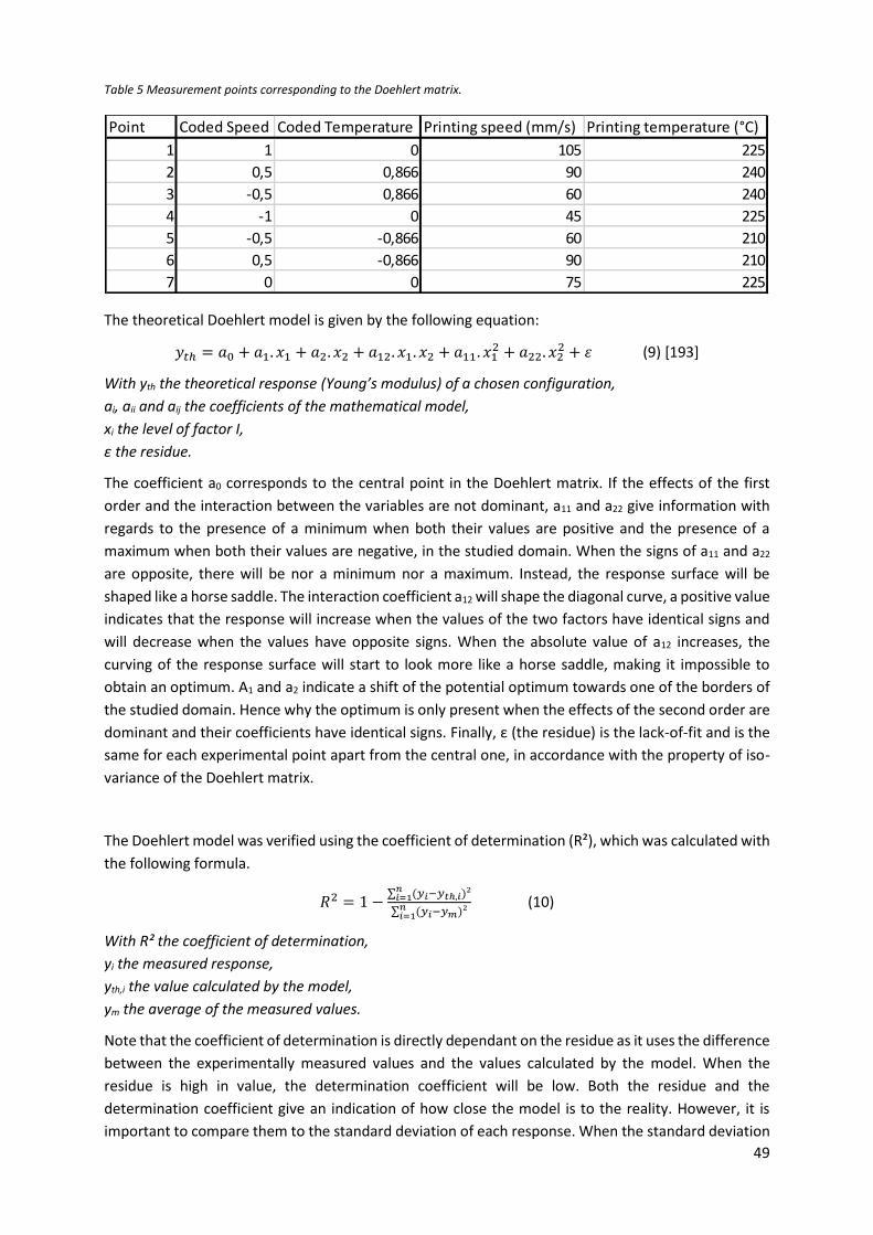
49

Table 5 Measurement points corresponding to the Doehlert matrix.

The theoretical Doehlert model is given by the following equation:

𝑦𝑡ℎ = 𝑎0 + 𝑎1. 𝑥1 + 𝑎2. 𝑥2 + 𝑎12. 𝑥1. 𝑥2 + 𝑎11. 𝑥12 + 𝑎22. 𝑥2

2 + 휀 (9) [193]

With yth the theoretical response (Young’s modulus) of a chosen configuration,

ai, aii and aij the coefficients of the mathematical model,

xi the level of factor I,

ε the residue.

The coefficient a0 corresponds to the central point in the Doehlert matrix. If the effects of the first

order and the interaction between the variables are not dominant, a11 and a22 give information with

regards to the presence of a minimum when both their values are positive and the presence of a

maximum when both their values are negative, in the studied domain. When the signs of a11 and a22

are opposite, there will be nor a minimum nor a maximum. Instead, the response surface will be

shaped like a horse saddle. The interaction coefficient a12 will shape the diagonal curve, a positive value

indicates that the response will increase when the values of the two factors have identical signs and

will decrease when the values have opposite signs. When the absolute value of a12 increases, the

curving of the response surface will start to look more like a horse saddle, making it impossible to

obtain an optimum. A1 and a2 indicate a shift of the potential optimum towards one of the borders of

the studied domain. Hence why the optimum is only present when the effects of the second order are

dominant and their coefficients have identical signs. Finally, ε (the residue) is the lack-of-fit and is the

same for each experimental point apart from the central one, in accordance with the property of iso-

variance of the Doehlert matrix.

The Doehlert model was verified using the coefficient of determination (R²), which was calculated with

the following formula.

𝑅2 = 1 −∑ (𝑦𝑖−𝑦𝑡ℎ,𝑖)²𝑛

𝑖=1

∑ (𝑦𝑖−𝑦𝑚)²𝑛𝑖=1

(10)

With R² the coefficient of determination,

yi the measured response,

yth,i the value calculated by the model,

ym the average of the measured values.

Note that the coefficient of determination is directly dependant on the residue as it uses the difference

between the experimentally measured values and the values calculated by the model. When the

residue is high in value, the determination coefficient will be low. Both the residue and the

determination coefficient give an indication of how close the model is to the reality. However, it is

important to compare them to the standard deviation of each response. When the standard deviation

Point Coded Speed Coded Temperature Printing speed (mm/s) Printing temperature (°C)

1 1 0 105 225

2 0,5 0,866 90 240

3 -0,5 0,866 60 240

4 -1 0 45 225

5 -0,5 -0,866 60 210

6 0,5 -0,866 90 210

7 0 0 75 225

50

of each experimental point is higher than the residue in value, the interpretation of the model becomes

impossible. This since the fit of the model, indicated by R², could be a coincidence.

Tensile tests were carried out on the printed ISO 527-2 5A tensile test samples of each formulation, to

determine the mechanical properties [192]. A pairwise analysis of variance (ANOVA) test was carried

out between different points of the Doehlert matrix of the same formulation. The results of the ANOVA

test indicated whether the two mean values were different or whether it was impossible to conclude

about a possible difference. For all mixtures, the theoretical models were temporarily accepted when

the determination coefficient was bigger than 0.8 and if the inter formulation ANOVA tests resulted in

at least one pair of coordinates that differed from each other. If this was the case, the p-value was

calculated for each coefficient of the theoretical model of the respective formulation and when the p-

values of each coefficient were smaller than 0.1, the models were accepted. However, the p-value of

a coefficients only gives an indication about the low probability that the respective coefficient is zero.

As mentioned before, if the standard deviation is high, then a perfect fit could potentially be a

coincidence. Hence why the ANOVA tests are important, the obtained ANOVA p-values between

experimental points had to be low and in combination with a high R² value. Where the low ANOVA p-

values between experimental points validate the experimentations, allowing for an impact caused by

changing parameter values. The high R² value, validates the model.

3.2.1.4 Injection moulding

The injection moulding of tensile test samples was done with a Babyplast 6/10P (INRA, Reims, France).

Before the injection moulding, PLA pellets of each nanocomposite and pure PLA were dried for a week

at a temperature of 60°C and in the night before the injection moulding at 80°C. The Babyplast was

equipped with a preheated and humidity controlled pellet container (Moullo X Dry air). Polymer

material was inserted into this preheated container from which it was fed into the Babyplast. Inside

the Babyplast, an Ø 18 mm screw passed the polymer material through the three heating zones before

being injected into the mould. In this case the Babyplast was equipped with an ISO 527-2 5A tensile

test sample mould [192]. During the injection, the polymer material was injected into the mould in two

cycles. The pressure during the cycles was not the same, during the second cycle the pressure was

much lower. Additionally, the mould was water cooled as the Babyplast was equipped with a fridge for

the cooling of the mould after injection. Once the cooling process was done, the mould would open

and the tensile test sample was automatically ejected.

3.2.1.5 Heated hydraulic press

The compression moulding of dynamic mechanical analysis and oscillatory rheology samples was done

with a Carver press (ESIReims, France). Dynamical mechanical analysis samples consisted of 60x13x2

mm beams, while the oscillatory rheology samples were discs with a 25 mm diameter and a 2 mm

height. PLA/HA pellets of each formulation and PLE 005 were dried at 60°C under vacuum for an hour,

followed by continuous storage under vacuum at ambient temperature. Right before the pressing, 10

g of each formulation was divided over 4 moulds each for the dynamic mechanical analysis. For the

oscillatory rheology samples, 21 g of each formulation was divided over 3 moulds. The moulds

consisted of an upper plate, a bottom plate and a middle plate which held the forms and canals to help

surplus material leave. All the plates were separated from each other with Teflon sheets, which

51

facilitated the separation of the plates after pressing. The Carver press was preheated at 210°C and set

to compress at 490.5 kPA. The following pressing procedure was used:

- The press was preheated at 210°C.

- The mould filled with polymer material was brought into contact with the preheated press

for 30 minutes.

- After 30 minutes, the pressure was increased to 490.5 kPA and kept there for 15 minutes.

- After the additional 15 minutes of pressing (total time: 45 minutes), the mould was removed

from the press and left to cool down at room temperature.

- Once the mould was cool, the test samples were removed and stored under vacuum to

prevent moisture absorption.

A Specac Atlas press (ESIReims, France) was used to create films for permeability tests. The films had

an average thickness of 90 µm and a diameter of 5 cm. An aluminium mould was created using two

thin sheets of aluminium and a 100 µm sheet with a 9 cm Ø hole, the thin sheets had to be replaced

after each session, while the thick sheet was reusable. Films were created for each of the formulations

following the same procedure. First the press was preheated at 210°C, after which, 0.4 g of granules,

in an aluminium mould, were inserted in the press. The first 5 minutes, the press was only put into

contact with the mould to allow the granules to melt. After that, the pressure was increased to 1 ton

for 30 seconds. Once the 30 seconds had past, the pressure was removed, but the mould was kept in

the press for an additional 30 seconds. Finally, the aluminium mould was exited from the press. When

the mould was at room temperature, the aluminium mould was opened and the resulting films were

removed from the mould.

3.2.2 Characterisations

3.2.2.1 Thermogravimetric analysis

A Netzsch TG 209 F3 (ESIReims, France) was used for the thermogravimetric analysis (TGA) of the PLA

as well as the extruded PLA/nHA (0%; 0,5%; 1%; 3% and 5%) composite granules, filaments and FDM

printed samples. Every thermogravimetric analysis took place under oxidising conditions and each

formulation was tested at least 3 times to ensure repeatability.

Before the thermogravimetric analysis polymer pellets of each mixture were dried under vacuum at

60°C for one hour, followed by continuous storage under vacuum at ambient temperature for a week.

A portion of the pellets was then stored in smaller containers, without controlled atmosphere. This

resulted in a minimum recovery of moisture from the atmosphere, but reduced the mass gain during

the weight measuring process, making it more stable. Each measurement was preceded by the

cleaning of the crucible.

First the balance was tared, after which the crucible was weighted, after which a second tare was

executed, followed by the weighting of the sample. Finally, a last tare was executed before starting the

test. During the test the temperature profile illustrated in table 6 was used. After the weighting of the

crucible, this was removed from the machine to be filled with polymer material. For each mixture, at

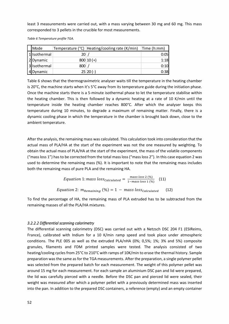
52

least 3 measurements were carried out, with a mass varying between 30 mg and 60 mg. This mass

corresponded to 3 pellets in the crucible for most measurements.

Table 6 Temperature profile TGA.

Table 6 shows that the thermogravimetric analyser waits till the temperature in the heating chamber

is 20°C, the machine starts when it’s 5°C away from its temperature guide during the initiation phase.

Once the machine starts there is a 5-minute isothermal phase to let the temperature stabilise within

the heating chamber. This is then followed by a dynamic heating at a rate of 10 K/min until the

temperature inside the heating chamber reaches 800°C. After which the analyser keeps this

temperature during 10 minutes, to degrade a maximum of remaining matter. Finally, there is a

dynamic cooling phase in which the temperature in the chamber is brought back down, close to the

ambient temperature.

After the analysis, the remaining mass was calculated. This calculation took into consideration that the

actual mass of PLA/HA at the start of the experiment was not the one measured by weighting. To

obtain the actual mass of PLA/HA at the start of the experiment, the mass of the volatile components

(“mass loss 1”) has to be corrected from the total mass loss (“mass loss 2”). In this case equation 2 was

used to determine the remaining mass (%). It is important to note that the remaining mass includes

both the remaining mass of pure PLA and the remaining HA.

𝐸𝑞𝑢𝑎𝑡𝑖𝑜𝑛 1: 𝑚𝑎𝑠𝑠 𝑙𝑜𝑠𝑠𝐶𝑎𝑙𝑐𝑢𝑙𝑎𝑡𝑒𝑑 = 𝑚𝑎𝑠𝑠 𝑙𝑜𝑠𝑠 2 (%)

1−𝑚𝑎𝑠𝑠 𝑙𝑜𝑠𝑠 1 (%) (11)

𝐸𝑞𝑢𝑎𝑡𝑖𝑜𝑛 2: 𝑚𝑅𝑒𝑚𝑎𝑖𝑛𝑖𝑛𝑔 (%) = 1 − 𝑚𝑎𝑠𝑠 𝑙𝑜𝑠𝑠𝐶𝑎𝑙𝑐𝑢𝑙𝑎𝑡𝑒𝑑 (12)

To find the percentage of HA, the remaining mass of PLA extruded has to be subtracted from the

remaining masses of all the PLA/HA mixtures.

3.2.2.2 Differential scanning calorimetry

The differential scanning calorimetry (DSC) was carried out with a Netzsch DSC 204 F1 (ESIReims,

France), calibrated with Indium for a 10 K/min ramp speed and took place under atmospheric

conditions. The PLE 005 as well as the extruded PLA/nHA (0%; 0,5%; 1%; 3% and 5%) composite

granules, filaments and FDM printed samples were tested. The analysis consisted of two

heating/cooling cycles from 25°C to 210°C with ramps of 10K/min to erase the thermal history. Sample

preparation was the same as for the TGA measurements. After the preparation, a single polymer pellet

was selected from the prepared batch for each measurement. The weight of this polymer pellet was

around 15 mg for each measurement. For each sample an aluminium DSC pan and lid were prepared,

the lid was carefully pierced with a needle. Before the DSC pan and pierced lid were sealed, their

weight was measured after which a polymer pellet with a previously determined mass was inserted

into the pan. In addition to the prepared DSC containers, a reference (empty) and an empty container

Mode Temperature (°C) Heating/cooling rate (K/min) Time (h:mm)

1 Isothermal 20 / 0:05

2 Dynamic 800 10 (+) 1:18


4 Dynamic 25 20 (-) 0:38

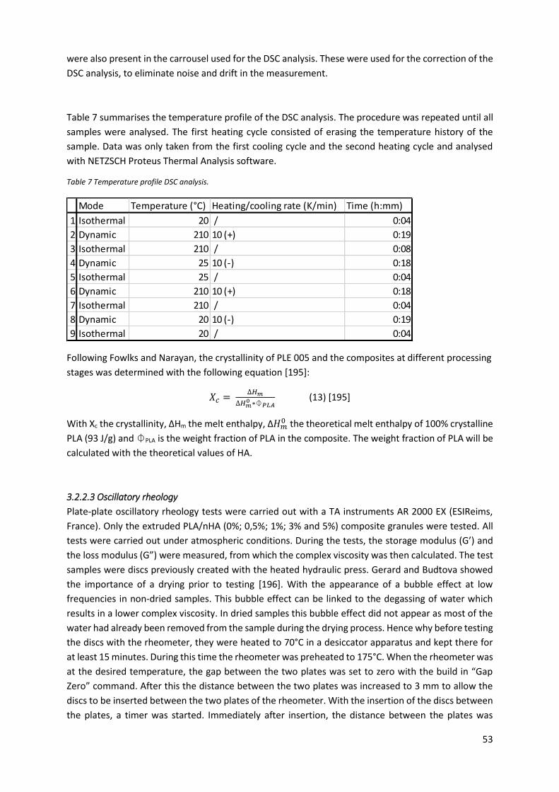
53

were also present in the carrousel used for the DSC analysis. These were used for the correction of the

DSC analysis, to eliminate noise and drift in the measurement.

Table 7 summarises the temperature profile of the DSC analysis. The procedure was repeated until all

samples were analysed. The first heating cycle consisted of erasing the temperature history of the

sample. Data was only taken from the first cooling cycle and the second heating cycle and analysed

with NETZSCH Proteus Thermal Analysis software.

Table 7 Temperature profile DSC analysis.

Following Fowlks and Narayan, the crystallinity of PLE 005 and the composites at different processing

stages was determined with the following equation [195]:

𝑋𝑐 = ∆𝐻𝑚

∆𝐻𝑚0 ∗⏀𝑃𝐿𝐴

(13) [195]

With Xc the crystallinity, ΔHm the melt enthalpy, Δ𝐻𝑚0 the theoretical melt enthalpy of 100% crystalline

PLA (93 J/g) and ⏀PLA is the weight fraction of PLA in the composite. The weight fraction of PLA will be

calculated with the theoretical values of HA.

3.2.2.3 Oscillatory rheology

Plate-plate oscillatory rheology tests were carried out with a TA instruments AR 2000 EX (ESIReims,

France). Only the extruded PLA/nHA (0%; 0,5%; 1%; 3% and 5%) composite granules were tested. All

tests were carried out under atmospheric conditions. During the tests, the storage modulus (G’) and

the loss modulus (G”) were measured, from which the complex viscosity was then calculated. The test

samples were discs previously created with the heated hydraulic press. Gerard and Budtova showed

the importance of a drying prior to testing [196]. With the appearance of a bubble effect at low

frequencies in non-dried samples. This bubble effect can be linked to the degassing of water which

results in a lower complex viscosity. In dried samples this bubble effect did not appear as most of the

water had already been removed from the sample during the drying process. Hence why before testing

the discs with the rheometer, they were heated to 70°C in a desiccator apparatus and kept there for

at least 15 minutes. During this time the rheometer was preheated to 175°C. When the rheometer was

at the desired temperature, the gap between the two plates was set to zero with the build in “Gap

Zero” command. After this the distance between the two plates was increased to 3 mm to allow the

discs to be inserted between the two plates of the rheometer. With the insertion of the discs between

the plates, a timer was started. Immediately after insertion, the distance between the plates was

Mode Temperature (°C) Heating/cooling rate (K/min) Time (h:mm)


2 Dynamic 210 10 (+) 0:19


4 Dynamic 25 10 (-) 0:18


6 Dynamic 210 10 (+) 0:18


8 Dynamic 20 10 (-) 0:19


54

decreased to 2 mm. Two minutes later the surplus material that had built up around the edges of the

plate due to the reduced height was removed. Three minutes after the insertion, the distance between

the plates was further reduced to 1.8 mm, followed by the removal of the excess material. Six minutes

after the insertion the rheological tests were started. The timing of the different steps was important

because the time sweeps showed a slight decrease. Thus, to compare the results, the measurements

have to be launched at the same time and after undergoing the same procedure.

Two different tests were carried out with the plate-plate oscillatory rheometer. The first test consisted

of a time sweep, which measured the moduli (G’ and G”) at a constant frequency during a specified

amount of time, this to determine whether the material would last long enough under the test

conditions without degrading. The second test was a frequency sweep, during which the complex

viscosity was measured at multiple frequencies to determine the rheological behaviour of the tested

material. For the time sweep, the time was set to 1 hour at a strain percentage of 1%, a frequency of

1 Hz and a temperature of 175°C. The frequency sweep was carried out at a temperature of 175°C and

a strain percentage of 1% with a frequency that decreased from 100 to 0.1 Hz. No strain sweep was

carried out to find the maximum strain before materials leave elastic behaviour, since this measure

was already carried out by several authors and former PhD students.

After the tests the results were analysed with TA Universal Analysis software. Additionally, a Carreau-

Yasuda model was used to model the viscosity of the PLA/HA at different shear rates [190]. The

Carreau-Yassuda model could only be used after applying the Cox-Merz rule, which gives the

equivalence between the shear rate and the frequency of the Rheometer [190] [197]. This was

necessary, since the results from the rheometer were in function of the frequency and the Carreau-

Yasuda model uses the shear rate [190]. The Carreau-Yasuda model is given by the following equation

[190].

𝜂(�̇�) = 𝜂0[1 + (𝜆�̇�)𝑎]𝑛−1

𝑎 (14) [190]

With η the viscosity in Pa.s, η0 the viscosity at zero shear in Pa.s, λ the relaxation time in s

(corresponding to the onset of the fluidification), a the Yasuda index (which determines the curve of

the fluidification transition) and n the index of the power law. Le Marec et al. Analysed the impact of

the molecular mass on the viscosity of PLA and found that at lower molecular masses the viscosity

decreases [198]. They used a power law and the Carreay-Yasuda model to characterize the viscosity

[190] [198]. The following equation contains the power law [198].

𝜂 = 𝐾. |�̇�|𝑛−1 (15) [198]

With η the viscosity in Pa.s,

K the consistency in Pa.sn

and n the index of the power law.

3.2.2.4 Tensile tests

The Young modulus and the ultimate strength of FDM printed and injection moulded 5A-type tensile

test specimen from ISO 527-2 were determined using an Instron 33R4204 (ESIReims, France) [192].

The tensile test conditions used were: a cross head speed of 5 mm/s and a 1 kN charge. All tests were

55

carried out under ambient conditions. For each nanocomposite, there were 7 different conditions of

FDM printed tensile specimen and one type of injection moulded specimen. A minimum of 5

measurements was carried out for each type of tensile specimen to ensure repeatability. The injection

moulded tensile specimens received a thermal pre-treatment. The specimens were crystallised by

keeping them at 70°C for 24 hours prior to testing.

3.2.2.5 Dynamic mechanical analysis

Dynamic mechanical analysis was carried out with a TA instruments Q800 (ESIReims, France), the

temperature varied from 30 to 140°C, with a 3 K/min heating ramp. The strain was kept constant at

0.1% and the frequency was kept constant at 1Hz. Test samples for the dynamic mechanical analysis

were created using two methods. A first batch of samples was created with fused deposition modelling

(FDM) and a second batch of samples was created with compression moulding. For the FDM printing

process, the previously extruded PLA/nHA composite filaments were used. For each composite, the

printing temperature was set to 215°C and the printing speed to 75 mm/s with a 90°/0° alternating

printing angle; 5 test samples were printed for each composite. The printed test samples were stored

in ambient conditions for a week, after which the samples were tested. Unlike the printed samples,

the compressed samples were stored under vacuum to prevent moisture absorption and before

testing the pressed samples were annealed at 70°C for 15 minutes.

A minimum of three tests was carried out for the printed and compressed samples. Each of the three

tests took place on the same day, this to reduce the influence of the ambient conditions on the

repeatability of the test results. The DMA took place in a non-climatized room, making it susceptible

to the changing environmental conditions (humidity and temperature). After testing, the results were

analysed with TA Universal software.

3.2.2.1 Wide angle X-ray diffraction on powder analysis

The wide angle X-ray diffraction on powder (WAXD-P) analysis were carried out with a D8 Advance

Bruker AXS (LISM, Reims, France), at room temperature and under Bragg conditions. The analysis took

place in the 2°-60° interval, with steps of 0.06° (2 seconds per step) and a Cu K-α X-ray source was used

at 40 mA and 40 kV. Powders were required for the analysis, therefore a Retsch ZM1000 (ESIReims,

France) was used to turn extruded PLA, PLA/HA 1% (granules and FDM specimens) and PLA/HA 5%

(granules and FDM specimens) into usable powders. The aqueous hydroxyapatite paste (30 wt.%) was

air dried to obtain a powder.

After the analysis, the Bragg and Scherrer formulas were used to determine the interplanar distance

and the mean particle size of hydroxyapatite and PLA crystals respectively [199] [200].

Bragg: 𝑛 𝜆 = 2 𝑑 sin 𝜃 (16)

With n (1), a positive integer that denotes the order of the diffraction band;

λ (nm), the X-ray wavelength;

dhkl (nm), the interplanar distance;

and θ (°), the Bragg angle.

56

Scherrer: 𝜏 = 𝐾 𝜆

𝛽 cos 𝜃 (17)

With τ (nm), the mean particle size of the crystals;

K (0.9), the dimensionless shape factor;

λ (nm), the X-ray wavelength;

β (rad), the width of the maximum intensity peak at half of its intensity;

and θ (°), the Bragg angle.

3.2.2.7 Transmission electron microscopy

Transmission electron microscopy (TEM) tests were conducted with a Philips CM200 (University of

Haute-Alsace, Haute-Alsace) with an acceleration voltage of 200 kV. The TEM samples were prepared

by ultramicrotomy with a Leica EM UC7 (University of Haute-Alsace, Haute-Alsace) at room

temperature and each sample had a thickness of approximately 90 nm. Per sample, 5 different zones

were observed, each zone was observed with 5 different magnitudes for a total of 25 photos per

sample.

3.2.2.8 Permeability tests

WVTR tests were conducted with a Mocon Permatron-W Model 3/31 water vapour permeability

(ESIReims, France). OTR tests were conducted with a Mocon Ox-Tran SH1 (VerpakkingsCentrum,

Belgium). The tests were conducted at a temperature of 23°C and a RH of 50%. All tests were carried

out in duplicate, before testing, the samples were conditioned at 23°C and 50% RH. The thickness of

the samples was measured with an Electronic Digital Micrometer and a MTS Adamel Lhomargie Mi20.

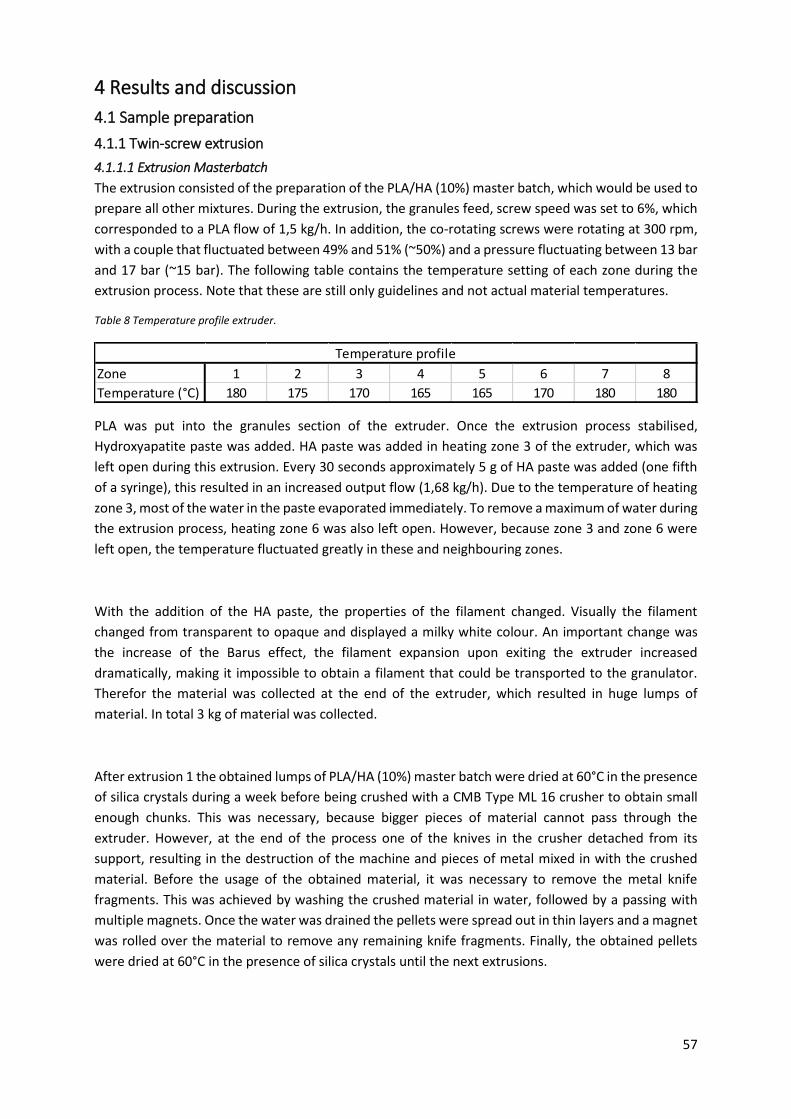
57

4 Results and discussion

4.1 Sample preparation

4.1.1 Twin-screw extrusion

4.1.1.1 Extrusion Masterbatch

The extrusion consisted of the preparation of the PLA/HA (10%) master batch, which would be used to

prepare all other mixtures. During the extrusion, the granules feed, screw speed was set to 6%, which

corresponded to a PLA flow of 1,5 kg/h. In addition, the co-rotating screws were rotating at 300 rpm,

with a couple that fluctuated between 49% and 51% (~50%) and a pressure fluctuating between 13 bar

and 17 bar (~15 bar). The following table contains the temperature setting of each zone during the

extrusion process. Note that these are still only guidelines and not actual material temperatures.

Table 8 Temperature profile extruder.

PLA was put into the granules section of the extruder. Once the extrusion process stabilised,

Hydroxyapatite paste was added. HA paste was added in heating zone 3 of the extruder, which was

left open during this extrusion. Every 30 seconds approximately 5 g of HA paste was added (one fifth

of a syringe), this resulted in an increased output flow (1,68 kg/h). Due to the temperature of heating

zone 3, most of the water in the paste evaporated immediately. To remove a maximum of water during

the extrusion process, heating zone 6 was also left open. However, because zone 3 and zone 6 were

left open, the temperature fluctuated greatly in these and neighbouring zones.

With the addition of the HA paste, the properties of the filament changed. Visually the filament

changed from transparent to opaque and displayed a milky white colour. An important change was

the increase of the Barus effect, the filament expansion upon exiting the extruder increased

dramatically, making it impossible to obtain a filament that could be transported to the granulator.

Therefor the material was collected at the end of the extruder, which resulted in huge lumps of

material. In total 3 kg of material was collected.

After extrusion 1 the obtained lumps of PLA/HA (10%) master batch were dried at 60°C in the presence

of silica crystals during a week before being crushed with a CMB Type ML 16 crusher to obtain small

enough chunks. This was necessary, because bigger pieces of material cannot pass through the

extruder. However, at the end of the process one of the knives in the crusher detached from its

support, resulting in the destruction of the machine and pieces of metal mixed in with the crushed

material. Before the usage of the obtained material, it was necessary to remove the metal knife

fragments. This was achieved by washing the crushed material in water, followed by a passing with

multiple magnets. Once the water was drained the pellets were spread out in thin layers and a magnet

was rolled over the material to remove any remaining knife fragments. Finally, the obtained pellets

were dried at 60°C in the presence of silica crystals until the next extrusions.

Zone 1 2 3 4 5 6 7 8

Temperature (°C) 180 175 170 165 165 170 180 180

Temperature profile

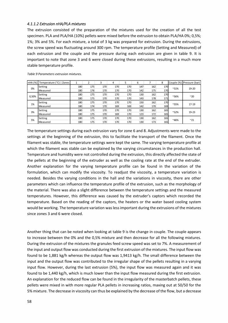
58

4.1.1.2 Extrusion nHA/PLA mixtures

The extrusion consisted of the preparation of the mixtures used for the creation of all the test

specimen. PLA and PLA/HA (10%) pellets were mixed before the extrusion to obtain PLA/HA 0%; 0,5%;

1%; 3% and 5%. For each mixture, a total of 3 kg was prepared for extrusion. During the extrusions,

the screw speed was fluctuating around 300 rpm. The temperature profile (Setting and Measured) of

each extrusion and the couple and the pressure during each extrusion are given in table 9. It is

important to note that zone 3 and 6 were closed during these extrusions, resulting in a much more

stable temperature profile.

Table 9 Parameters extrusion mixtures.

The temperature settings during each extrusion vary for zone 6 and 8. Adjustments were made to the

settings at the beginning of the extrusion, this to facilitate the transport of the filament. Once the

filament was stable, the temperature settings were kept the same. The varying temperature profile at

which the filament was stable can be explained by the varying circumstances in the production hall.

Temperature and humidity were not controlled during the extrusion, this directly affected the state of

the pellets at the beginning of the extruder as well as the cooling rate at the end of the extruder.

Another explanation for the varying temperature profile can be found in the variation of the

formulation, which can modify the viscosity. To readjust the viscosity, a temperature variation is

needed. Besides the varying conditions in the hall and the variations in viscosity, there are other

parameters which can influence the temperature profile of the extrusion, such as the morphology of

the material. There was also a slight difference between the temperature settings and the measured

temperatures. However, this difference was caused by the extruder’s captors which recorded the

temperature. Based on the reading of the captors, the heaters or the water based cooling system

would be working. The temperature variation was less important during the extrusions of the mixtures

since zones 3 and 6 were closed.

Another thing that can be noted when looking at table 9 is the change in couple. The couple appears

to increase between the 0% and the 0,5% mixture and then decrease for all the following mixtures.

During the extrusion of the mixtures the granules feed screw speed was set to 7%. A measurement of

the input and output flow was conducted during the first extrusion of the mixtures. The input flow was

found to be 1,881 kg/h whereas the output flow was 1,9413 kg/h. The small difference between the

input and the output flow was contributed to the irregular shape of the pellets resulting in a varying

input flow. However, during the last extrusion (5%), the input flow was measured again and it was

found to be 1,440 kg/h, which is much lower than the input flow measured during the first extrusion.

An explanation for the reduced flow can be found in the irregularity of the masterbatch pellets, these

pellets were mixed in with more regular PLA pellets in increasing ratios, maxing out at 50/50 for the

5% mixture. The decrease in viscosity can thus be explained by the decrease of the flow, but a decrease

nHA (%) Temperature (°C) | Zones 1 2 3 4 5 6 7 8 Couple (%) Pressure (bar)

Setting 180 175 170 170 170 147 162 170

Measured 180 176 170 170 170 142 175 170

Setting 180 175 170 170 170 130 162 170

Measured 180 175 170 170 170 143 178 171

Setting 180 175 170 170 170 150 162 170

Measured 180 174 170 169 169 142 170 169

Setting 180 175 170 170 170 130 162 165

Measured 180 175 170 169 170 123 172 165

Setting 180 175 170 170 170 130 162 165

Measured 180 175 170 170 170 130 173 165

~51%

~56%

~55%

~52%

~46%

19-20

~20

17-19

19-23

~21

0%

0,50%

1%

3%

5%

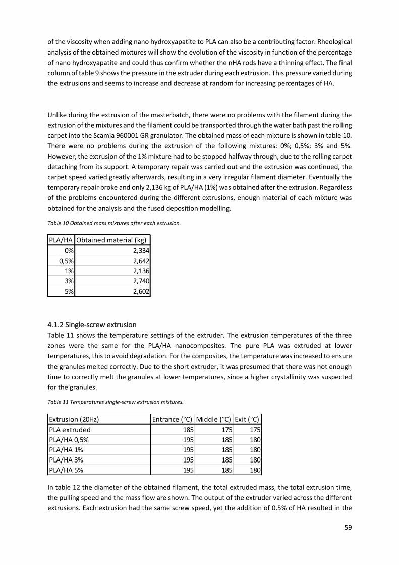
59

of the viscosity when adding nano hydroxyapatite to PLA can also be a contributing factor. Rheological

analysis of the obtained mixtures will show the evolution of the viscosity in function of the percentage

of nano hydroxyapatite and could thus confirm whether the nHA rods have a thinning effect. The final

column of table 9 shows the pressure in the extruder during each extrusion. This pressure varied during

the extrusions and seems to increase and decrease at random for increasing percentages of HA.

Unlike during the extrusion of the masterbatch, there were no problems with the filament during the

extrusion of the mixtures and the filament could be transported through the water bath past the rolling

carpet into the Scamia 960001 GR granulator. The obtained mass of each mixture is shown in table 10.

There were no problems during the extrusion of the following mixtures: 0%; 0,5%; 3% and 5%.

However, the extrusion of the 1% mixture had to be stopped halfway through, due to the rolling carpet

detaching from its support. A temporary repair was carried out and the extrusion was continued, the

carpet speed varied greatly afterwards, resulting in a very irregular filament diameter. Eventually the

temporary repair broke and only 2,136 kg of PLA/HA (1%) was obtained after the extrusion. Regardless

of the problems encountered during the different extrusions, enough material of each mixture was

obtained for the analysis and the fused deposition modelling.

Table 10 Obtained mass mixtures after each extrusion.

4.1.2 Single-screw extrusion

Table 11 shows the temperature settings of the extruder. The extrusion temperatures of the three

zones were the same for the PLA/HA nanocomposites. The pure PLA was extruded at lower

temperatures, this to avoid degradation. For the composites, the temperature was increased to ensure

the granules melted correctly. Due to the short extruder, it was presumed that there was not enough

time to correctly melt the granules at lower temperatures, since a higher crystallinity was suspected

for the granules.

Table 11 Temperatures single-screw extrusion mixtures.

In table 12 the diameter of the obtained filament, the total extruded mass, the total extrusion time,

the pulling speed and the mass flow are shown. The output of the extruder varied across the different

extrusions. Each extrusion had the same screw speed, yet the addition of 0.5% of HA resulted in the

PLA/HA Obtained material (kg)

0% 2,334

0,5% 2,642

1% 2,136

3% 2,740

5% 2,602

Extrusion (20Hz) Entrance (°C) Middle (°C) Exit (°C)

PLA extruded 185 175 175

PLA/HA 0,5% 195 185 180

PLA/HA 1% 195 185 180

PLA/HA 3% 195 185 180

PLA/HA 5% 195 185 180

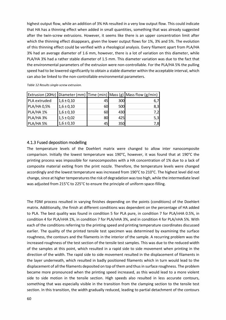
60

highest output flow, while an addition of 3% HA resulted in a very low output flow. This could indicate

that HA has a thinning effect when added in small quantities, something that was already suggested

after the twin-screw extrusions. However, it seems like there is an upper concentration limit after

which the thinning effect disappears, given the lower output flows for 1%, 3% and 5%. The evolution

of this thinning effect could be verified with a rheological analysis. Every filament apart from PLA/HA

3% had an average diameter of 1.6 mm, however, there is a lot of variation on this diameter, while

PLA/HA 3% had a rather stable diameter of 1.5 mm. This diameter variation was due to the fact that

the environmental parameters of the extrusion were non-controllable. For the PLA/HA 5% the pulling

speed had to be lowered significantly to obtain a stable diameter within the acceptable interval, which

can also be linked to the non-controllable environmental parameters.

Table 12 Results single-screw extrusion.

4.1.3 Fused deposition modelling

The temperature levels of the Doehlert matrix were changed to allow inter nanocomposite

comparison. Initially the lowest temperature was 190°C, however, it was found that at 190°C the

printing process was impossible for nanocomposites with a HA concentration of 1% due to a lack of

composite material exiting from the print nozzle. Therefore, the temperature levels were changed

accordingly and the lowest temperature was increased from 190°C to 210°C. The highest level did not

change, since at higher temperatures the risk of degradation was too high, while the intermediate level

was adjusted from 215°C to 225°C to ensure the principle of uniform space-filling.

The FDM process resulted in varying finishes depending on the points (conditions) of the Doehlert

matrix. Additionally, the finish at different conditions was dependent on the percentage of HA added

to PLA. The best quality was found in condition 5 for PLA pure, in condition 7 for PLA/nHA 0.5%, in

condition 4 for PLA/nHA 1%, in condition 7 for PLA/nHA 3%, and in condition 4 for PLA/nHA 5%. With

each of the conditions referring to the printing speed and printing temperature coordinates discussed

earlier. The quality of the printed tensile test specimen was determined by examining the surface

roughness, the contours and the filaments in the interior of the sample. A recurring problem was the

increased roughness of the test section of the tensile test samples. This was due to the reduced width

of the samples at this point, which resulted in a rapid side to side movement when printing in the

direction of the width. The rapid side to side movement resulted in the displacement of filaments in

the layer underneath, which resulted in badly positioned filaments which in turn would lead to the

displacement of all the filaments deposited on top of them and thus in surface roughness. The problem

became more pronounced when the printing speed increased, as this would lead to a more violent

side to side motion in the tensile section. High speeds also resulted in less accurate contours,

something that was especially visible in the transition from the clamping section to the tensile test

section. In this transition, the width gradually reduced, leading to partial detachment of the contours

Extrusion (20Hz) Diameter (mm) Time (min) Mass (g) Mass flow (g/min)

PLA extruded 1,6 ± 0,10 45 300 6,7

PLA/HA 0,5% 1,6 ± 0,10 60 500 8,3

PLA/HA 1% 1,6 ± 0,10 60 430 7,2

PLA/HA 3% 1,5 ± 0,02 80 425 5,3

PLA/HA 5% 1,6 ± 0,10 45 350 7,8

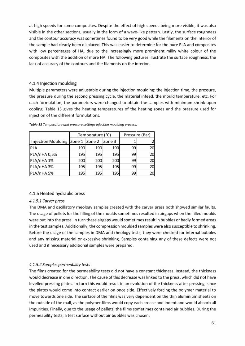
61

at high speeds for some composites. Despite the effect of high speeds being more visible, it was also

visible in the other sections, usually in the form of a wave-like pattern. Lastly, the surface roughness

and the contour accuracy was sometimes found to be very good while the filaments on the interior of

the sample had clearly been displaced. This was easier to determine for the pure PLA and composites

with low percentages of HA, due to the increasingly more prominent milky white colour of the

composites with the addition of more HA. The following pictures illustrate the surface roughness, the

lack of accuracy of the contours and the filaments on the interior.

4.1.4 Injection moulding

Multiple parameters were adjustable during the injection moulding: the injection time, the pressure,

the pressure during the second pressing cycle, the material infeed, the mould temperature, etc. For

each formulation, the parameters were changed to obtain the samples with minimum shrink upon

cooling. Table 13 gives the heating temperatures of the heating zones and the pressure used for

injection of the different formulations.

Table 13 Temperature and pressure settings injection moulding process.

4.1.5 Heated hydraulic press

4.1.5.1 Carver press

The DMA and oscillatory rheology samples created with the carver press both showed similar faults.

The usage of pellets for the filling of the moulds sometimes resulted in airgaps when the filled moulds

were put into the press. In turn these airgaps would sometimes result in bubbles or badly formed areas

in the test samples. Additionally, the compression moulded samples were also susceptible to shrinking.

Before the usage of the samples in DMA and rheology tests, they were checked for internal bubbles

and any missing material or excessive shrinking. Samples containing any of these defects were not

used and if necessary additional samples were prepared.

4.1.5.2 Samples permeability tests

The films created for the permeability tests did not have a constant thickness. Instead, the thickness

would decrease in one direction. The cause of this decrease was linked to the press, which did not have

levelled pressing plates. In turn this would result in an evolution of the thickness after pressing, since

the plates would come into contact earlier on once side. Effectively forcing the polymer material to

move towards one side. The surface of the films was very dependent on the thin aluminium sheets on

the outside of the mall, as the polymer films would copy each crease and indent and would absorb all

impurities. Finally, due to the usage of pellets, the films sometimes contained air bubbles. During the

permeability tests, a test surface without air bubbles was chosen.

Zone 1 Zone 2 Zone 3 1 2

PLA 190 190 190 99 20

PLA/nHA 0,5% 195 195 195 99 20

PLA/nHA 1% 200 200 200 99 20

PLA/nHA 3% 195 195 195 99 20

PLA/nHA 5% 195 195 195 99 20

Temperature (°C) Pressure (Bar)

Injection Moulding

62

4.2 Thermogravimetric analysis

4.2.1 Introduction

The goal of the thermogravimetric analysis is firstly to verify the remaining mass after the degradation

of PLA, secondly to verify the concentration of HA in the nanocomposites, and thirdly to compare the

degradations of each analysed material. Additionally, the results of the TGA will be used to help

determine the maximum printing temperature of the FDM process.

4.2.2 Results

4.2.2.1 Granules

The results of the thermogravimetric analysis of the granules will be discussed in this section. First each

mixture will be discussed separately, then the averages of each mixture will be compared with each

other. The following data was obtained from each analysis: The mass change between the room

temperature and 200°C; The mass change between 200°C and 700°C; The onset and the end of the

degradation between 200°C and 700°C; and the degradation peak along with its mass loss (%/min).

The mass change between the starting temperature and 200°C corresponds to the removal of water

and the partial removal of other volatile components such as the lactic acid monomer. Feng et al. found

that the temperature interval, in which the lactic acid monomer is removed from PLLA for samples

dried under vacuum at 70°C for 12 hours, is 100-250°C [201]. The mass change between 200°C and

700°C corresponds to the main degradation of material during the analysis and the removal of the

remaining volatile compounds. The degradation peak temperature is the temperature corresponding

to the peak of the first derivative of the curve. An example of all these results is given in figure 17.

Figure 17 Thermogravimetric analysis PLE 005.

In table 14, the results of the thermogravimetric analysis of PLE 005 are given, the standard deviation

of the remaining mass is very high. An explanation for the high standard deviation can be found in the

amount of mass used. The starting mass of the sample is between 30 mg and 60 mg, which results in

a remaining mass in the µg range and thus near the limit of the sensitivity of the used balance. Hence

why minor variations caused by a too large time interval between consecutive mass measurements at

the start of the experiment, result in large deviations of the remaining mass. Prime examples of the

effect on the remaining mass are measurement 4 and 6. Measurement 4 has a negative remaining

mass, which is impossible; and measurement 6 has a too high remaining mass. However, table 14

63

shows that the degradation profile of the PLE 005 is very similar for each measurement, indicating that

the degradation profile is very repeatable.

Table 14 Thermogravimetric analysis PLE 005.

For the extruded PLA, the same problem occurred and the measurements were repeated. The first

measurements resulted in a remaining mass of 0.10±0.25%, which is an improvement compared to the

standard deviations found for PLE, but still a rather high standard deviation compared to the value of

the average. The results of the repetition are shown in table 15. For the extruded PLA, the additional

testing, with reduced time between consecutive weighting steps, resulted in a much smaller standard

deviation. The average remaining mass was found to be 0.17%, this result will be used to calculate the

hydroxyapatite content for all the mixtures. As with the PLE 005, the degradation profile of the

extruded PLA was very repeatable, given that all the standard deviations are small.

Table 15 Thermogravimetric analysis PLA extruded (Continued).

Table 16 shows the results of the thermogravimetric analysis of PLA/HA 0.5%. As with PLE 005 and the

extruded PLA, this measurement was also executed with too much time between the measurement of

the crucible and the sample weight. However, the standard deviation is low enough. Additionally, the

average remaining mass was found to be 0.62%. By subtracting 0.17%, the average remaining mass of

the extruded PLA, from the average remaining mass, the hydroxyapatite content was found to be

0.45%.

Table 16 Thermogravimetric analysis PLA/HA 0.5%.

In table 17 the results of the thermogravimetric analysis of PLA/HA 1% are shown. For these

measurements, the time in between the weighting of the crucible and the sample mass was reduced

significantly, resulting in a much more accurate measurement. The remaining mass was found to be

1.08%, by subtracting the remaining mass of the extruded PLA, the percentage of HA was found to be

0.91% on average.

Mass loss per minute (%/min) Temperature range

1 2 Calculated Remaining mass Peak Onset Peak Endset Degradation (°C)

4 0,09% 100,15% 100,24% -0,24% 31,96 351,7 372,2 384,8 33,1

5 0,02% 99,82% 99,84% 0,16% 31,01 351,6 372,3 385,3 33,7

6 0,03% 99,02% 99,05% 0,95% 31,00 351,5 373,7 385,1 33,6

7 0,04% 99,82% 99,86% 0,14% 31,15 351,4 372,2 385,0 33,6

Average (4-7) 0,05% 99,70% 99,75% 0,25% 31,28 351,6 372,6 385,1 33,5

STDEV 0,03% 0,48% 0,50% 0,50% 0,46 0,1 0,7 0,2 0,3

PLE 005

Mass loss T (°C)



4 0,02% 99,82% 99,84% 0,16% 30,93 349,3 372,8 383,7 34,4

5 0,04% 99,78% 99,82% 0,18% 30,97 349,6 372,3 383,8 34,2

6 0,00% 99,84% 99,84% 0,16% 30,75 349,9 372,0 383,6 33,7

7 0,00% 99,84% 99,84% 0,16% 30,91 349,6 372,7 383,5 33,9

Average (4-7) 0,02% 99,82% 99,83% 0,17% 30,89 349,6 372,5 383,7 34,1

STDEV 0,02% 0,03% 0,01% 0,01% 0,11 0,2 0,4 0,2 0,3

PLA extruded

Mass loss T (°C)



1 0,01% 99,38% 99,39% 0,61% 30,69 348,1 373,7 386,8 38,7

2 0,05% 99,37% 99,42% 0,58% 32,51 349,4 370,8 383,9 34,5

3 0,01% 99,33% 99,34% 0,66% 33,94 349,0 370,2 382,6 33,6

Average 0,02% 99,36% 99,38% 0,62% 32,38 348,8 371,6 384,4 35,6

STDEV 0,02% 0,03% 0,04% 0,04% 1,63 0,7 1,9 2,2 2,7

Mass loss T (°C)

PLA/HA 0,5%

64

Table 17 Thermogravimetric analysis PLA/HA 1%.

In table 18 the results of the thermogravimetric analysis of PLA/HA 3% are shown. The average mass

of HA was found to be 3.12% and thus corresponds well to the targeted 3%.


Table 19 shows the results of the thermogravimetric analysis of PLA/HA 5%. The average mass of HA

was found to be 4.99% after the subtraction of the remaining mass of the extruded PLA.


The onset, peak and end temperature of the degradation are shown in figure 18, figure 19 and figure

20 and table 20. Figure 18 shows that the degradation of PLA starts at lower temperatures when PLA

is extruded and when more HA is added. Once extruded, the temperature at which the degradation

starts, lowers with the addition of HA. The catalyst effect of HA on the degradation onset appears to

be linear up to the addition of 1% HA, after which the onset temperature decreases less. However, the

standard deviation of the onset is very high for the 0.5% composite, especially when compared to the

other composites. The decrease in onset temperatures increases again when 5% of HA is added. It can

thus be concluded that PLA becomes more susceptible to degradation at lower temperatures with the

addition of HA.



5 0,01% 98,85% 98,86% 1,14% 31,86 347,8 372,0 384,6 36,8

6 0,03% 98,89% 98,92% 1,08% 31,52 347,7 372,6 385,2 37,5

7 0,05% 98,92% 98,97% 1,03% 31,91 348,0 372,3 385,3 37,3

Average 0,03% 98,89% 98,92% 1,08% 31,76 347,8 372,3 385,0 37,2

STDEV 0,02% 0,04% 0,05% 0,05% 0,21 0,2 0,3 0,4 0,4

T (°C)Mass loss (%)

PLA/HA 0,1%



1 0,09% 96,69% 96,78% 3,22% 32,28 346,8 369,8 382,6 35,8

2 0,07% 96,69% 96,76% 3,24% 32,82 346,4 368,3 381,9 35,5

3 0,11% 96,50% 96,61% 3,39% 31,80 347,0 369,9 383,2 36,2

Average 0,09% 96,63% 96,71% 3,29% 32,30 346,7 369,3 382,6 35,8

STDEV 0,02% 0,11% 0,09% 0,09% 0,51 0,3 0,9 0,7 0,4

T (°C)Mass loss

PLA/HA 3%



1 0,08% 94,78% 94,86% 5,14% 30,66 344,7 371,0 383,5 38,8

2 0,14% 94,63% 94,76% 5,24% 30,74 344,6 372,0 384,3 39,7

3 0,15% 94,77% 94,91% 5,09% 30,61 344,1 372,5 385,0 40,9

Average 0,12% 94,73% 94,84% 5,16% 30,67 344,5 371,8 384,3 39,8

STDEV 0,04% 0,08% 0,08% 0,08% 0,07 0,3 0,8 0,8 1,1

T (°C)Mass loss

PLA/HA 5%

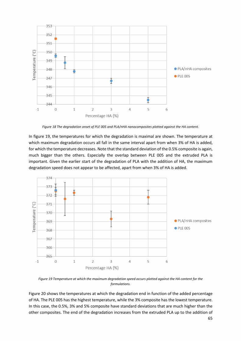
65

Figure 18 The degradation onset of PLE 005 and PLA/nHA nanocomposites plotted against the HA content.

In figure 19, the temperatures for which the degradation is maximal are shown. The temperature at

which maximum degradation occurs all fall in the same interval apart from when 3% of HA is added,

for which the temperature decreases. Note that the standard deviation of the 0.5% composite is again,

much bigger than the others. Especially the overlap between PLE 005 and the extruded PLA is

important. Given the earlier start of the degradation of PLA with the addition of HA, the maximum

degradation speed does not appear to be affected, apart from when 3% of HA is added.

Figure 19 Temperature at which the maximum degradation speed occurs plotted against the HA content for the

formulations.

Figure 20 shows the temperatures at which the degradation end in function of the added percentage

of HA. The PLE 005 has the highest temperature, while the 3% composite has the lowest temperature.

In this case, the 0.5%, 3% and 5% composite have standard deviations that are much higher than the

other composites. The end of the degradation increases from the extruded PLA up to the addition of

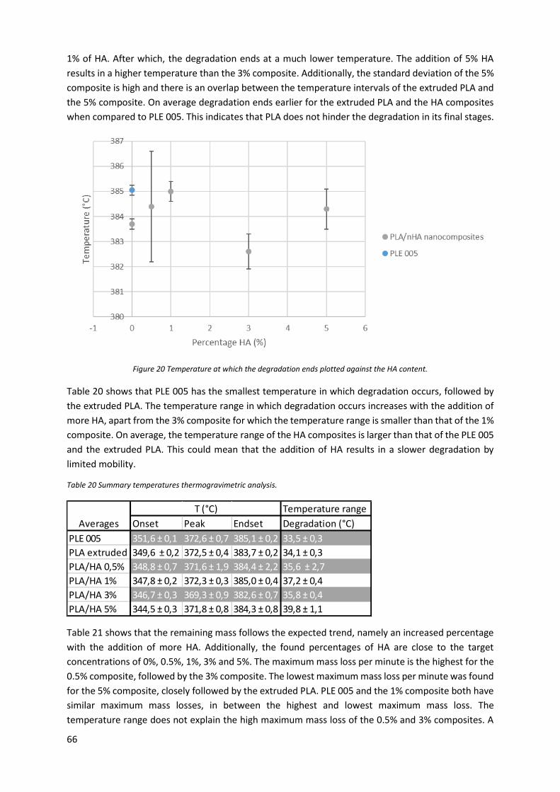
66

1% of HA. After which, the degradation ends at a much lower temperature. The addition of 5% HA

results in a higher temperature than the 3% composite. Additionally, the standard deviation of the 5%

composite is high and there is an overlap between the temperature intervals of the extruded PLA and

the 5% composite. On average degradation ends earlier for the extruded PLA and the HA composites

when compared to PLE 005. This indicates that PLA does not hinder the degradation in its final stages.

Figure 20 Temperature at which the degradation ends plotted against the HA content.

Table 20 shows that PLE 005 has the smallest temperature in which degradation occurs, followed by

the extruded PLA. The temperature range in which degradation occurs increases with the addition of

more HA, apart from the 3% composite for which the temperature range is smaller than that of the 1%

composite. On average, the temperature range of the HA composites is larger than that of the PLE 005

and the extruded PLA. This could mean that the addition of HA results in a slower degradation by

limited mobility.

Table 20 Summary temperatures thermogravimetric analysis.

Table 21 shows that the remaining mass follows the expected trend, namely an increased percentage

with the addition of more HA. Additionally, the found percentages of HA are close to the target

concentrations of 0%, 0.5%, 1%, 3% and 5%. The maximum mass loss per minute is the highest for the

0.5% composite, followed by the 3% composite. The lowest maximum mass loss per minute was found

for the 5% composite, closely followed by the extruded PLA. PLE 005 and the 1% composite both have

similar maximum mass losses, in between the highest and lowest maximum mass loss. The

temperature range does not explain the high maximum mass loss of the 0.5% and 3% composites. A

Temperature range

Onset Peak Endset Degradation (°C)

PLE 005 351,6 ± 0,1 372,6 ± 0,7 385,1 ± 0,2 33,5 ± 0,3

PLA extruded 349,6 ± 0,2 372,5 ± 0,4 383,7 ± 0,2 34,1 ± 0,3

PLA/HA 0,5% 348,8 ± 0,7 371,6 ± 1,9 384,4 ± 2,2 35,6 ± 2,7

PLA/HA 1% 347,8 ± 0,2 372,3 ± 0,3 385,0 ± 0,4 37,2 ± 0,4

PLA/HA 3% 346,7 ± 0,3 369,3 ± 0,9 382,6 ± 0,7 35,8 ± 0,4

PLA/HA 5% 344,5 ± 0,3 371,8 ± 0,8 384,3 ± 0,8 39,8 ± 1,1

Averages

T (°C)

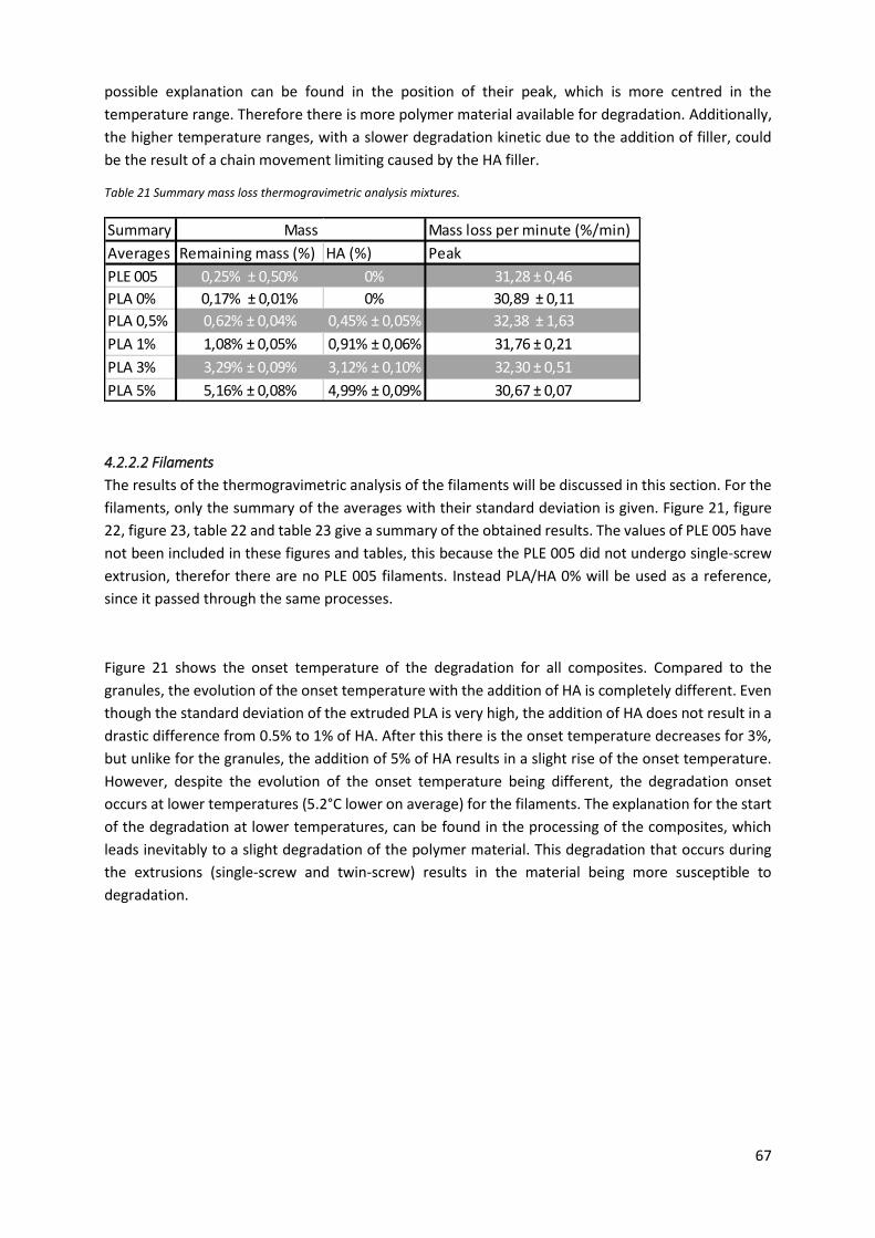
67

possible explanation can be found in the position of their peak, which is more centred in the

temperature range. Therefore there is more polymer material available for degradation. Additionally,

the higher temperature ranges, with a slower degradation kinetic due to the addition of filler, could

be the result of a chain movement limiting caused by the HA filler.

Table 21 Summary mass loss thermogravimetric analysis mixtures.

4.2.2.2 Filaments

The results of the thermogravimetric analysis of the filaments will be discussed in this section. For the

filaments, only the summary of the averages with their standard deviation is given. Figure 21, figure

22, figure 23, table 22 and table 23 give a summary of the obtained results. The values of PLE 005 have

not been included in these figures and tables, this because the PLE 005 did not undergo single-screw

extrusion, therefor there are no PLE 005 filaments. Instead PLA/HA 0% will be used as a reference,

since it passed through the same processes.

Figure 21 shows the onset temperature of the degradation for all composites. Compared to the

granules, the evolution of the onset temperature with the addition of HA is completely different. Even

though the standard deviation of the extruded PLA is very high, the addition of HA does not result in a

drastic difference from 0.5% to 1% of HA. After this there is the onset temperature decreases for 3%,

but unlike for the granules, the addition of 5% of HA results in a slight rise of the onset temperature.

However, despite the evolution of the onset temperature being different, the degradation onset

occurs at lower temperatures (5.2°C lower on average) for the filaments. The explanation for the start

of the degradation at lower temperatures, can be found in the processing of the composites, which

leads inevitably to a slight degradation of the polymer material. This degradation that occurs during

the extrusions (single-screw and twin-screw) results in the material being more susceptible to

degradation.

Summary Mass loss per minute (%/min)

Averages Remaining mass (%) HA (%) Peak

PLE 005 0,25% ± 0,50% 0% 31,28 ± 0,46

PLA 0% 0,17% ± 0,01% 0% 30,89 ± 0,11

PLA 0,5% 0,62% ± 0,04% 0,45% ± 0,05% 32,38 ± 1,63

PLA 1% 1,08% ± 0,05% 0,91% ± 0,06% 31,76 ± 0,21

PLA 3% 3,29% ± 0,09% 3,12% ± 0,10% 32,30 ± 0,51

PLA 5% 5,16% ± 0,08% 4,99% ± 0,09% 30,67 ± 0,07

Mass

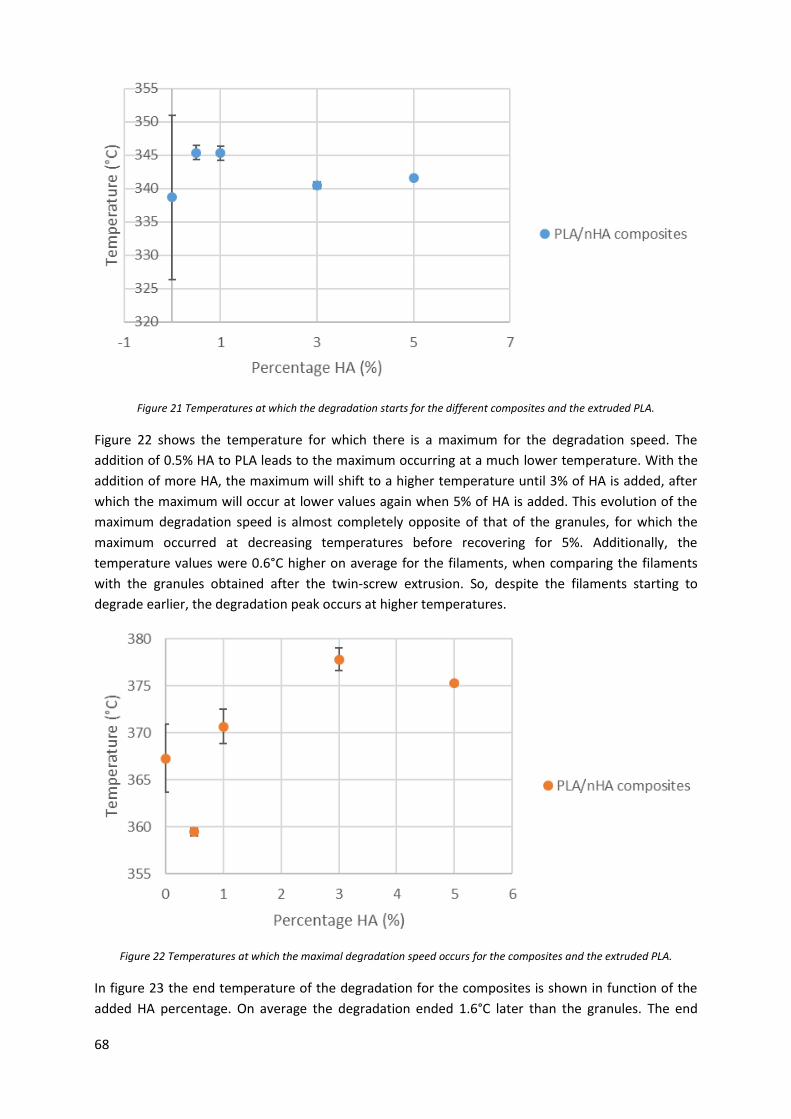
68

Figure 21 Temperatures at which the degradation starts for the different composites and the extruded PLA.

Figure 22 shows the temperature for which there is a maximum for the degradation speed. The

addition of 0.5% HA to PLA leads to the maximum occurring at a much lower temperature. With the

addition of more HA, the maximum will shift to a higher temperature until 3% of HA is added, after

which the maximum will occur at lower values again when 5% of HA is added. This evolution of the

maximum degradation speed is almost completely opposite of that of the granules, for which the

maximum occurred at decreasing temperatures before recovering for 5%. Additionally, the

temperature values were 0.6°C higher on average for the filaments, when comparing the filaments

with the granules obtained after the twin-screw extrusion. So, despite the filaments starting to

degrade earlier, the degradation peak occurs at higher temperatures.

Figure 22 Temperatures at which the maximal degradation speed occurs for the composites and the extruded PLA.

In figure 23 the end temperature of the degradation for the composites is shown in function of the

added HA percentage. On average the degradation ended 1.6°C later than the granules. The end

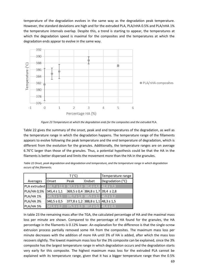
69

temperature of the degradation evolves in the same way as the degradation peak temperature.

However, the standard deviations are high and for the extruded PLA, PLA/nHA 0.5% and PLA/nHA 1%

the temperature intervals overlap. Despite this, a trend is starting to appear, the temperatures at

which the degradation speed is maximal for the composites and the temperatures at which the

degradation ends appear to evolve in the same way.

Figure 23 Temperature at which the degradation ends for the composites and the extruded PLA.

Table 22 gives the summary of the onset, peak and end temperatures of the degradation, as well as

the temperature range in which the degradation happens. The temperature range of the fillaments

appears to evolve following the peak temperature and the end temperature of degradation, which is

different from the evolution for the granules. Additionally, the temperature ranges are on average

6.76°C larger than those of the granules. Thus, a potential hypothesis could be that the HA in the

filaments is better dispersed and limits the movement more than the HA in the granules.

Table 22 Onset, peak degradation and degradation end temperature, and the temperature range in which degradation

occurs of the filaments.

In table 23 the remaining mass after the TGA, the calculated percentage of HA and the maximal mass

loss per minute are shown. Compared to the percentage of HA found for the granules, the HA

percentage in the filaments is 0.12% lower. An explanation for the difference is that the single-screw

extrusion process partially removed some HA from the composites. The maximum mass loss per

minute decreases with the addition of more HA until 3% of HA is added, after which the mass loss

recovers slightly. The lowest maximum mass loss for the 3% composite can be explained, since the 3%

composite has the largest temperature range in which degradation occurs and the degradation starts

very early for this composite. The highest maximum mass loss for the extruded PLA cannot be

explained with its temperature range, given that it has a bigger temperature range than the 0.5%

Temperature range


PLA extruded 338,7 ± 12,3 367,3 ± 3,6 381,6 ± 4,8 42,8 ± 7,9

PLA/HA 0,5% 345,4 ± 1,1 369,5 ± 0,4 384,8 ± 1,7 39,4 ± 2,8

PLA/HA 1% 345,3 ± 1,1 370,7 ± 1,8 385,5 ± 2,1 40,2 ± 3,2

PLA/HA 3% 340,5 ± 0,5 377,8 ± 1,2 388,8 ± 1,1 48,3 ± 1,5

PLA/HA 5% 341,6 ± 0,2 375,3 ± 0,3 387,2 ± 0,3 45,6 ± 0,3

Averages

T (°C)

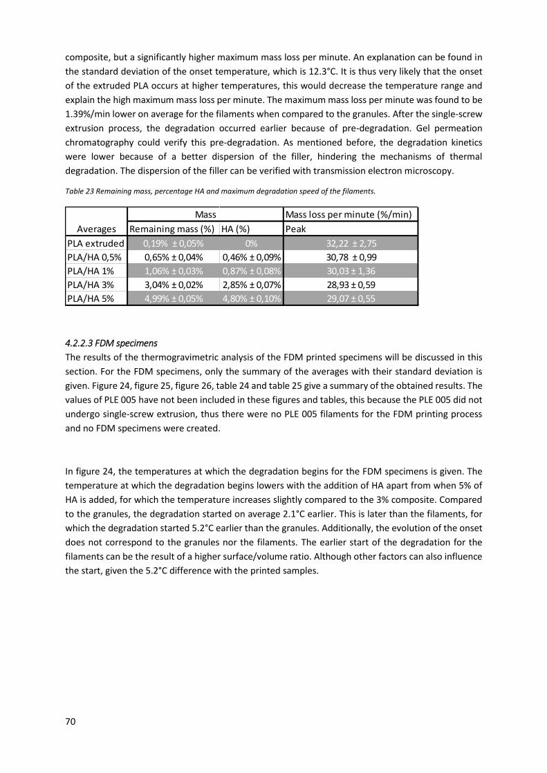
70

composite, but a significantly higher maximum mass loss per minute. An explanation can be found in

the standard deviation of the onset temperature, which is 12.3°C. It is thus very likely that the onset

of the extruded PLA occurs at higher temperatures, this would decrease the temperature range and

explain the high maximum mass loss per minute. The maximum mass loss per minute was found to be

1.39%/min lower on average for the filaments when compared to the granules. After the single-screw

extrusion process, the degradation occurred earlier because of pre-degradation. Gel permeation

chromatography could verify this pre-degradation. As mentioned before, the degradation kinetics

were lower because of a better dispersion of the filler, hindering the mechanisms of thermal

degradation. The dispersion of the filler can be verified with transmission electron microscopy.

Table 23 Remaining mass, percentage HA and maximum degradation speed of the filaments.

4.2.2.3 FDM specimens

The results of the thermogravimetric analysis of the FDM printed specimens will be discussed in this

section. For the FDM specimens, only the summary of the averages with their standard deviation is

given. Figure 24, figure 25, figure 26, table 24 and table 25 give a summary of the obtained results. The

values of PLE 005 have not been included in these figures and tables, this because the PLE 005 did not

undergo single-screw extrusion, thus there were no PLE 005 filaments for the FDM printing process

and no FDM specimens were created.

In figure 24, the temperatures at which the degradation begins for the FDM specimens is given. The

temperature at which the degradation begins lowers with the addition of HA apart from when 5% of

HA is added, for which the temperature increases slightly compared to the 3% composite. Compared

to the granules, the degradation started on average 2.1°C earlier. This is later than the filaments, for

which the degradation started 5.2°C earlier than the granules. Additionally, the evolution of the onset

does not correspond to the granules nor the filaments. The earlier start of the degradation for the

filaments can be the result of a higher surface/volume ratio. Although other factors can also influence

the start, given the 5.2°C difference with the printed samples.

Mass loss per minute (%/min)

Remaining mass (%) HA (%) Peak

PLA extruded 0,19% ± 0,05% 0% 32,22 ± 2,75

PLA/HA 0,5% 0,65% ± 0,04% 0,46% ± 0,09% 30,78 ± 0,99

PLA/HA 1% 1,06% ± 0,03% 0,87% ± 0,08% 30,03 ± 1,36

PLA/HA 3% 3,04% ± 0,02% 2,85% ± 0,07% 28,93 ± 0,59

PLA/HA 5% 4,99% ± 0,05% 4,80% ± 0,10% 29,07 ± 0,55

Mass

Averages

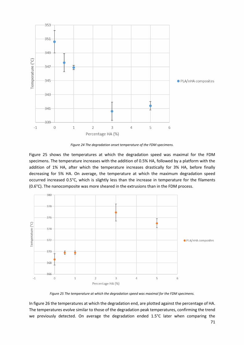
71

Figure 24 The degradation onset temperature of the FDM specimens.

Figure 25 shows the temperatures at which the degradation speed was maximal for the FDM

specimens. The temperature increases with the addition of 0.5% HA, followed by a platform with the

addition of 1% HA, after which the temperature increases drastically for 3% HA, before finally

decreasing for 5% HA. On average, the temperature at which the maximum degradation speed

occurred increased 0.5°C, which is slightly less than the increase in temperature for the filaments

(0.6°C). The nanocomposite was more sheared in the extrusions than in the FDM process.

Figure 25 The temperature at which the degradation speed was maximal for the FDM specimens.

In figure 26 the temperatures at which the degradation end, are plotted against the percentage of HA.

The temperatures evolve similar to those of the degradation peak temperatures, confirming the trend

we previously detected. On average the degradation ended 1.5°C later when comparing the

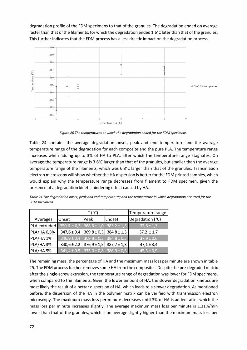
72

degradation profile of the FDM specimens to that of the granules. The degradation ended on average

faster than that of the filaments, for which the degradation ended 1.6°C later than that of the granules.

This further indicates that the FDM process has a less drastic impact on the degradation process.

Figure 26 The temperatures at which the degradation ended for the FDM specimens.

Table 24 contains the average degradation onset, peak and end temperature and the average

temperature range of the degradation for each composite and the pure PLA. The temperature range

increases when adding up to 3% of HA to PLA, after which the temperature range stagnates. On

average the temperature range is 3.6°C larger than that of the granules, but smaller than the average

temperature range of the filaments, which was 6.8°C larger than that of the granules. Transmission

electron microscopy will show whether the HA dispersion is better for the FDM printed samples, which

would explain why the temperature range decreases from filament to FDM specimen, given the

presence of a degradation kinetic hindering effect caused by HA.

Table 24 The degradation onset, peak and end temperature; and the temperature in which degradation occurred for the

FDM specimens.

The remaining mass, the percentage of HA and the maximum mass loss per minute are shown in table

25. The FDM process further removes some HA from the composites. Despite the pre-degraded matrix

after the single-screw extrusion, the temperature range of degradation was lower for FDM specimens,

when compared to the filaments. Given the lower amount of HA, the slower degradation kinetics are

most likely the result of a better dispersion of HA, which leads to a slower degradation. As mentioned

before, the dispersion of the HA in the polymer matrix can be verified with transmission electron

microscopy. The maximum mass loss per minute decreases until 3% of HA is added, after which the

mass loss per minute increases slightly. The average maximum mass loss per minute is 1.31%/min

lower than that of the granules, which is on average slightly higher than the maximum mass loss per

Temperature range


PLA extruded 350,6 ± 0,5 368,6 ± 1,0 383,2 ± 1,6 32,6 ± 1,7

PLA/HA 0,5% 347,6 ± 0,4 369,8 ± 0,3 384,8 ± 1,3 37,2 ± 1,7

PLA/HA 1% 346,9 ± 0,4 369,8 ± 0,3 384,8 ± 0,3 37,9 ± 0,6

PLA/HA 3% 340,6 ± 2,2 376,9 ± 1,5 387,7 ± 1,3 47,1 ± 3,4

PLA/HA 5% 341,4 ± 0,5 375,0 ± 0,8 386,9 ± 0,6 45,5 ± 0,9

Averages

T (°C)

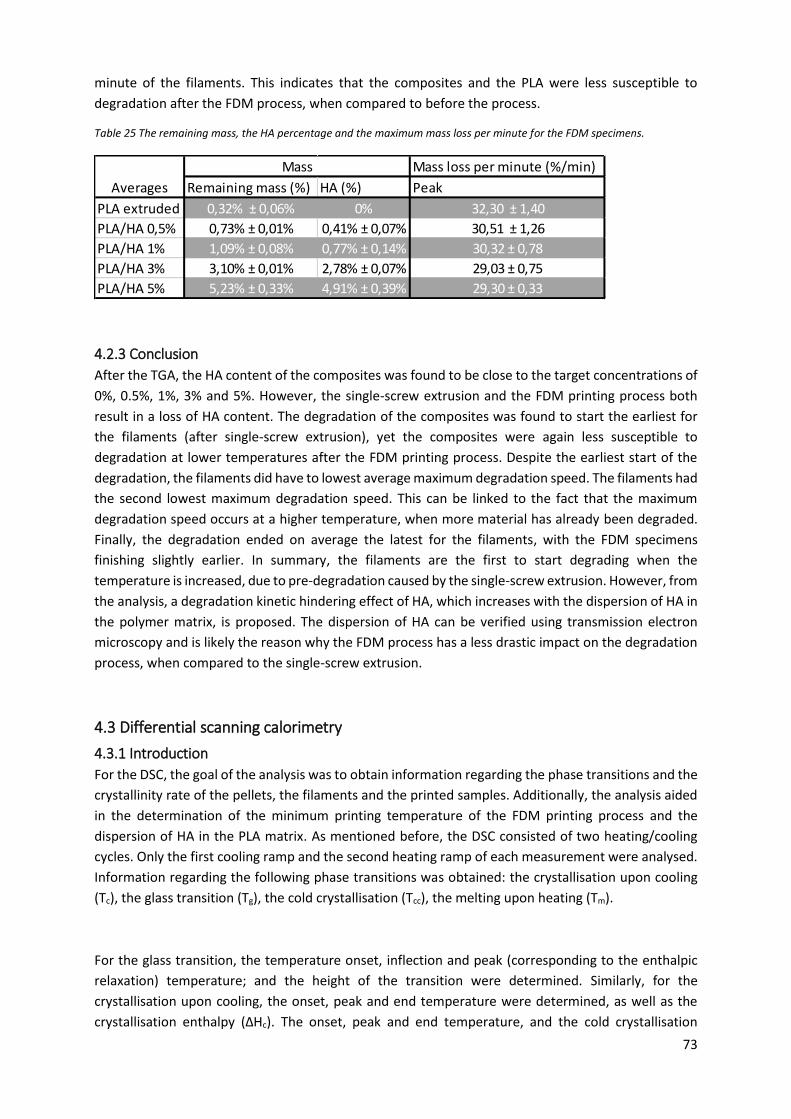
73

minute of the filaments. This indicates that the composites and the PLA were less susceptible to

degradation after the FDM process, when compared to before the process.

Table 25 The remaining mass, the HA percentage and the maximum mass loss per minute for the FDM specimens.

4.2.3 Conclusion

After the TGA, the HA content of the composites was found to be close to the target concentrations of

0%, 0.5%, 1%, 3% and 5%. However, the single-screw extrusion and the FDM printing process both

result in a loss of HA content. The degradation of the composites was found to start the earliest for

the filaments (after single-screw extrusion), yet the composites were again less susceptible to

degradation at lower temperatures after the FDM printing process. Despite the earliest start of the

degradation, the filaments did have to lowest average maximum degradation speed. The filaments had

the second lowest maximum degradation speed. This can be linked to the fact that the maximum

degradation speed occurs at a higher temperature, when more material has already been degraded.

Finally, the degradation ended on average the latest for the filaments, with the FDM specimens

finishing slightly earlier. In summary, the filaments are the first to start degrading when the

temperature is increased, due to pre-degradation caused by the single-screw extrusion. However, from

the analysis, a degradation kinetic hindering effect of HA, which increases with the dispersion of HA in

the polymer matrix, is proposed. The dispersion of HA can be verified using transmission electron

microscopy and is likely the reason why the FDM process has a less drastic impact on the degradation

process, when compared to the single-screw extrusion.

4.3 Differential scanning calorimetry

4.3.1 Introduction

For the DSC, the goal of the analysis was to obtain information regarding the phase transitions and the

crystallinity rate of the pellets, the filaments and the printed samples. Additionally, the analysis aided

in the determination of the minimum printing temperature of the FDM printing process and the

dispersion of HA in the PLA matrix. As mentioned before, the DSC consisted of two heating/cooling

cycles. Only the first cooling ramp and the second heating ramp of each measurement were analysed.

Information regarding the following phase transitions was obtained: the crystallisation upon cooling

(Tc), the glass transition (Tg), the cold crystallisation (Tcc), the melting upon heating (Tm).

For the glass transition, the temperature onset, inflection and peak (corresponding to the enthalpic

relaxation) temperature; and the height of the transition were determined. Similarly, for the

crystallisation upon cooling, the onset, peak and end temperature were determined, as well as the

crystallisation enthalpy (ΔHc). The onset, peak and end temperature, and the cold crystallisation

Mass loss per minute (%/min)

Remaining mass (%) HA (%) Peak

PLA extruded 0,32% ± 0,06% 0% 32,30 ± 1,40

PLA/HA 0,5% 0,73% ± 0,01% 0,41% ± 0,07% 30,51 ± 1,26

PLA/HA 1% 1,09% ± 0,08% 0,77% ± 0,14% 30,32 ± 0,78

PLA/HA 3% 3,10% ± 0,01% 2,78% ± 0,07% 29,03 ± 0,75

PLA/HA 5% 5,23% ± 0,33% 4,91% ± 0,39% 29,30 ± 0,33

Averages

Mass

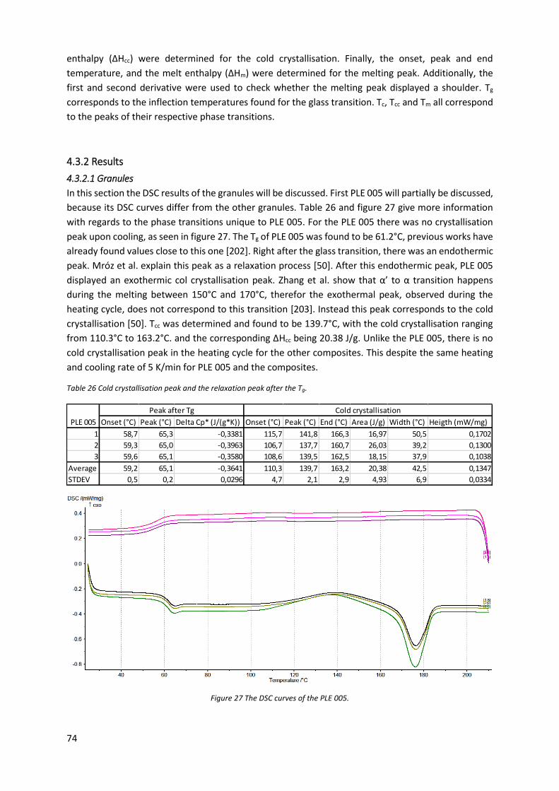
74

enthalpy (ΔHcc) were determined for the cold crystallisation. Finally, the onset, peak and end

temperature, and the melt enthalpy (ΔHm) were determined for the melting peak. Additionally, the

first and second derivative were used to check whether the melting peak displayed a shoulder. Tg

corresponds to the inflection temperatures found for the glass transition. Tc, Tcc and Tm all correspond

to the peaks of their respective phase transitions.

4.3.2 Results

4.3.2.1 Granules

In this section the DSC results of the granules will be discussed. First PLE 005 will partially be discussed,

because its DSC curves differ from the other granules. Table 26 and figure 27 give more information

with regards to the phase transitions unique to PLE 005. For the PLE 005 there was no crystallisation

peak upon cooling, as seen in figure 27. The Tg of PLE 005 was found to be 61.2°C, previous works have

already found values close to this one [202]. Right after the glass transition, there was an endothermic

peak. Mróz et al. explain this peak as a relaxation process [50]. After this endothermic peak, PLE 005

displayed an exothermic col crystallisation peak. Zhang et al. show that α’ to α transition happens

during the melting between 150°C and 170°C, therefor the exothermal peak, observed during the

heating cycle, does not correspond to this transition [203]. Instead this peak corresponds to the cold

crystallisation [50]. Tcc was determined and found to be 139.7°C, with the cold crystallisation ranging

from 110.3°C to 163.2°C. and the corresponding ΔHcc being 20.38 J/g. Unlike the PLE 005, there is no

cold crystallisation peak in the heating cycle for the other composites. This despite the same heating

and cooling rate of 5 K/min for PLE 005 and the composites.

Table 26 Cold crystallisation peak and the relaxation peak after the Tg.

Figure 27 The DSC curves of the PLE 005.

Onset (°C) Peak (°C) Delta Cp* (J/(g*K)) Onset (°C) Peak (°C) End (°C) Area (J/g) Width (°C) Heigth (mW/mg)

1 58,7 65,3 -0,3381 115,7 141,8 166,3 16,97 50,5 0,1702

2 59,3 65,0 -0,3963 106,7 137,7 160,7 26,03 39,2 0,1300

3 59,6 65,1 -0,3580 108,6 139,5 162,5 18,15 37,9 0,1038

Average 59,2 65,1 -0,3641 110,3 139,7 163,2 20,38 42,5 0,1347

STDEV 0,5 0,2 0,0296 4,7 2,1 2,9 4,93 6,9 0,0334

Cold crystallisation

PLE 005

Peak after Tg

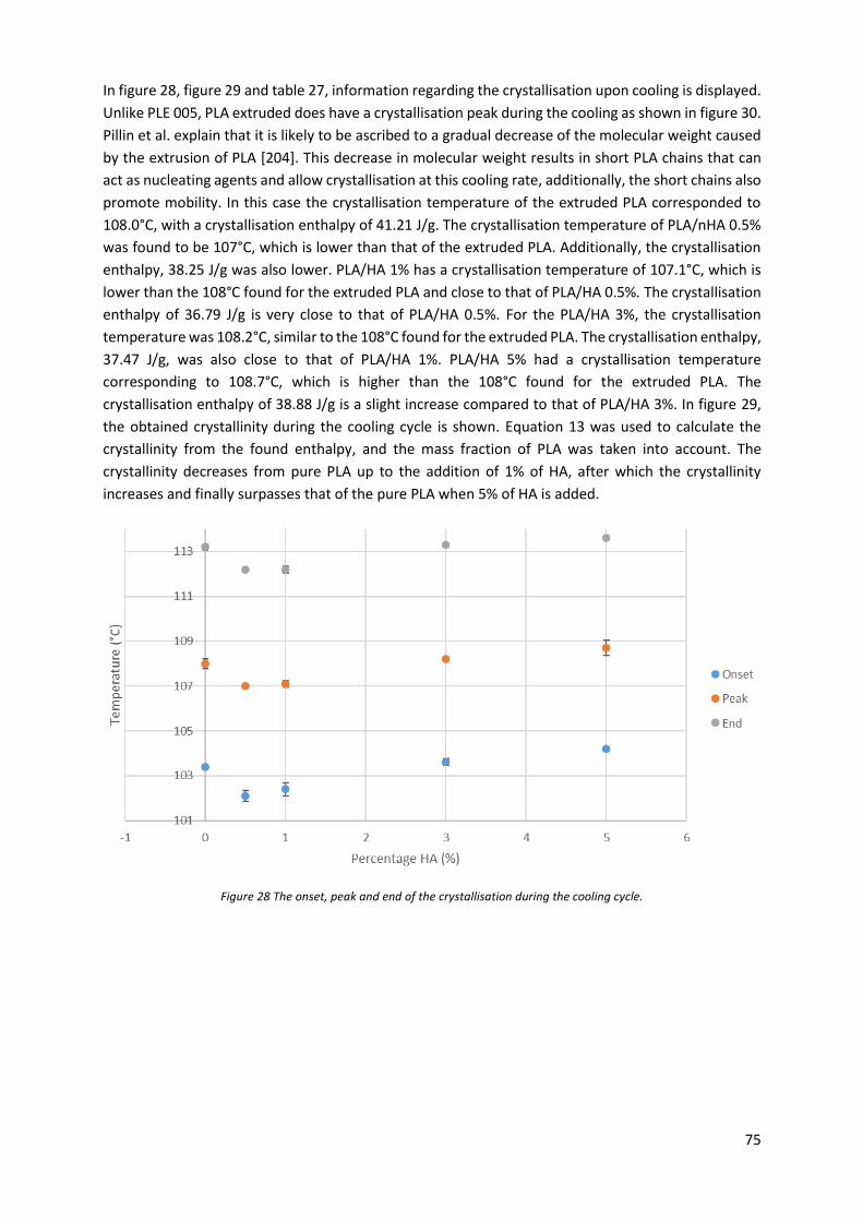
75

In figure 28, figure 29 and table 27, information regarding the crystallisation upon cooling is displayed.

Unlike PLE 005, PLA extruded does have a crystallisation peak during the cooling as shown in figure 30.

Pillin et al. explain that it is likely to be ascribed to a gradual decrease of the molecular weight caused

by the extrusion of PLA [204]. This decrease in molecular weight results in short PLA chains that can

act as nucleating agents and allow crystallisation at this cooling rate, additionally, the short chains also

promote mobility. In this case the crystallisation temperature of the extruded PLA corresponded to

108.0°C, with a crystallisation enthalpy of 41.21 J/g. The crystallisation temperature of PLA/nHA 0.5%

was found to be 107°C, which is lower than that of the extruded PLA. Additionally, the crystallisation

enthalpy, 38.25 J/g was also lower. PLA/HA 1% has a crystallisation temperature of 107.1°C, which is

lower than the 108°C found for the extruded PLA and close to that of PLA/HA 0.5%. The crystallisation

enthalpy of 36.79 J/g is very close to that of PLA/HA 0.5%. For the PLA/HA 3%, the crystallisation

temperature was 108.2°C, similar to the 108°C found for the extruded PLA. The crystallisation enthalpy,

37.47 J/g, was also close to that of PLA/HA 1%. PLA/HA 5% had a crystallisation temperature

corresponding to 108.7°C, which is higher than the 108°C found for the extruded PLA. The

crystallisation enthalpy of 38.88 J/g is a slight increase compared to that of PLA/HA 3%. In figure 29,

the obtained crystallinity during the cooling cycle is shown. Equation 13 was used to calculate the

crystallinity from the found enthalpy, and the mass fraction of PLA was taken into account. The

crystallinity decreases from pure PLA up to the addition of 1% of HA, after which the crystallinity

increases and finally surpasses that of the pure PLA when 5% of HA is added.

Figure 28 The onset, peak and end of the crystallisation during the cooling cycle.

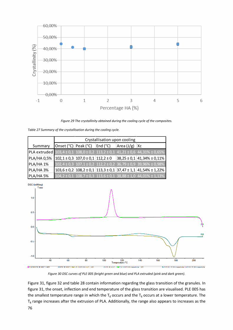
76

Figure 29 The crystallinity obtained during the cooling cycle of the composites.

Table 27 Summary of the crystallisation during the cooling cycle.

Figure 30 DSC curves of PLE 005 (bright green and blue) and PLA extruded (pink and dark green).

Figure 31, figure 32 and table 28 contain information regarding the glass transition of the granules. In

figure 31, the onset, inflection and end temperature of the glass transition are visualised. PLE 005 has

the smallest temperature range in which the Tg occurs and the Tg occurs at a lower temperature. The

Tg range increases after the extrusion of PLA. Additionally, the range also appears to increases as the

Onset (°C) Peak (°C) End (°C) Area (J/g) Xc

PLA extruded 103,4 ± 0,1 108,0 ± 0,2 113,2 ± 0,1 41,21 ± 0,6 44,31% ± 0,65%

PLA/HA 0,5% 102,1 ± 0,3 107,0 ± 0,1 112,2 ± 0 38,25 ± 0,1 41,34% ± 0,11%

PLA/HA 1% 102,4 ± 0,3 107,1 ± 0,2 112,2 ± 0,2 36,79 ± 0,9 39,96% ± 0,98%

PLA/HA 3% 103,6 ± 0,2 108,2 ± 0,1 113,3 ± 0,1 37,47 ± 1,1 41,54% ± 1,22%

PLA/HA 5% 104,2 ± 0,1 108,7 ± 0,3 113,6 ± 0,1 38,88 ± 1,0 44,01% ± 1,13%

Summary

Crystallisation upon cooling

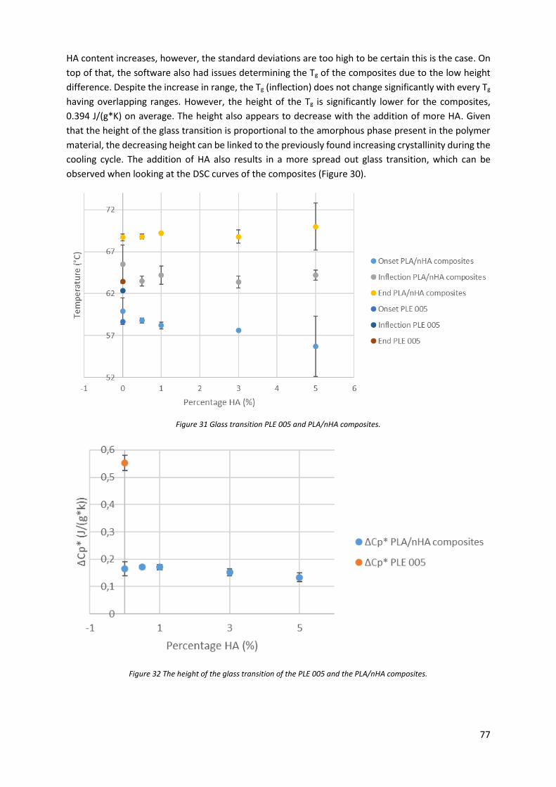
77

HA content increases, however, the standard deviations are too high to be certain this is the case. On

top of that, the software also had issues determining the Tg of the composites due to the low height

difference. Despite the increase in range, the Tg (inflection) does not change significantly with every Tg

having overlapping ranges. However, the height of the Tg is significantly lower for the composites,

0.394 J/(g*K) on average. The height also appears to decrease with the addition of more HA. Given

that the height of the glass transition is proportional to the amorphous phase present in the polymer

material, the decreasing height can be linked to the previously found increasing crystallinity during the

cooling cycle. The addition of HA also results in a more spread out glass transition, which can be

observed when looking at the DSC curves of the composites (Figure 30).

Figure 31 Glass transition PLE 005 and PLA/nHA composites.

Figure 32 The height of the glass transition of the PLE 005 and the PLA/nHA composites.

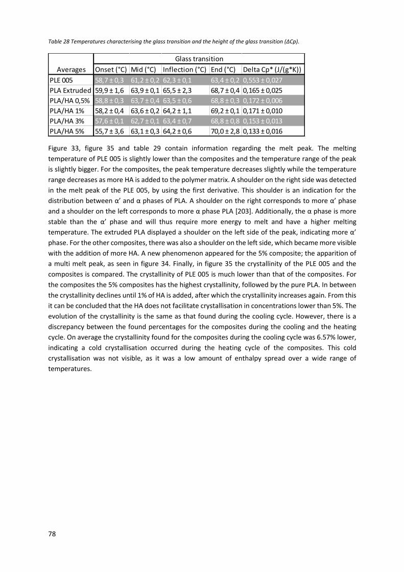
78

Table 28 Temperatures characterising the glass transition and the height of the glass transition (ΔCp).

Figure 33, figure 35 and table 29 contain information regarding the melt peak. The melting

temperature of PLE 005 is slightly lower than the composites and the temperature range of the peak

is slightly bigger. For the composites, the peak temperature decreases slightly while the temperature

range decreases as more HA is added to the polymer matrix. A shoulder on the right side was detected

in the melt peak of the PLE 005, by using the first derivative. This shoulder is an indication for the

distribution between α’ and α phases of PLA. A shoulder on the right corresponds to more α’ phase

and a shoulder on the left corresponds to more α phase PLA [203]. Additionally, the α phase is more

stable than the α’ phase and will thus require more energy to melt and have a higher melting

temperature. The extruded PLA displayed a shoulder on the left side of the peak, indicating more α’

phase. For the other composites, there was also a shoulder on the left side, which became more visible

with the addition of more HA. A new phenomenon appeared for the 5% composite; the apparition of

a multi melt peak, as seen in figure 34. Finally, in figure 35 the crystallinity of the PLE 005 and the

composites is compared. The crystallinity of PLE 005 is much lower than that of the composites. For

the composites the 5% composites has the highest crystallinity, followed by the pure PLA. In between

the crystallinity declines until 1% of HA is added, after which the crystallinity increases again. From this

it can be concluded that the HA does not facilitate crystallisation in concentrations lower than 5%. The

evolution of the crystallinity is the same as that found during the cooling cycle. However, there is a

discrepancy between the found percentages for the composites during the cooling and the heating

cycle. On average the crystallinity found for the composites during the cooling cycle was 6.57% lower,

indicating a cold crystallisation occurred during the heating cycle of the composites. This cold

crystallisation was not visible, as it was a low amount of enthalpy spread over a wide range of

temperatures.

Onset (°C) Mid (°C) Inflection (°C) End (°C) Delta Cp* (J/(g*K))

PLE 005 58,7 ± 0,3 61,2 ± 0,2 62,3 ± 0,1 63,4 ± 0,2 0,553 ± 0,027

PLA Extruded 59,9 ± 1,6 63,9 ± 0,1 65,5 ± 2,3 68,7 ± 0,4 0,165 ± 0,025

PLA/HA 0,5% 58,8 ± 0,3 63,7 ± 0,4 63,5 ± 0,6 68,8 ± 0,3 0,172 ± 0,006

PLA/HA 1% 58,2 ± 0,4 63,6 ± 0,2 64,2 ± 1,1 69,2 ± 0,1 0,171 ± 0,010

PLA/HA 3% 57,6 ± 0,1 62,7 ± 0,1 63,4 ± 0,7 68,8 ± 0,8 0,153 ± 0,013

PLA/HA 5% 55,7 ± 3,6 63,1 ± 0,3 64,2 ± 0,6 70,0 ± 2,8 0,133 ± 0,016

Averages

Glass transition

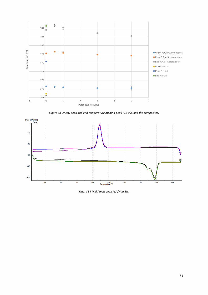
79

Figure 33 Onset, peak and end temperature melting peak PLE 005 and the composites.

Figure 34 Multi melt peak PLA/Nha 5%.

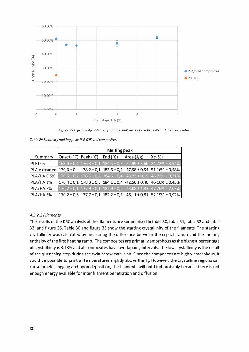
80

Figure 35 Crystallinity obtained from the melt peak of the PLE 005 and the composites.

Table 29 Summary melting peak PLE 005 and composites.

4.3.2.2 Filaments

The results of the DSC analysis of the filaments are summarised in table 30, table 31, table 32 and table

33, and figure 36. Table 30 and figure 36 show the starting crystallinity of the filaments. The starting

crystallinity was calculated by measuring the difference between the crystallisation and the melting

enthalpy of the first heating ramp. The composites are primarily amorphous as the highest percentage

of crystallinity is 3.48% and all composites have overlapping intervals. The low crystallinity is the result

of the quenching step during the twin-screw extrusion. Since the composites are highly amorphous, it

could be possible to print at temperatures slightly above the Tg. However, the crystalline regions can

cause nozzle clogging and upon deposition, the filaments will not bind probably because there is not

enough energy available for inter filament penetration and diffusion.

Onset (°C) Peak (°C) End (°C) Area (J/g) Xc (%)

PLE 005 168,9 ± 0,4 176,3 ± 0,1 184,5 ± 0,3 -22,99 ± 3,66 24,72% ± 3,94%

PLA extruded 170,6 ± 0 178,2 ± 0,1 183,6 ± 0,1 -47,58 ± 0,54 51,16% ± 0,58%

PLA/HA 0,5% 170,5 ± 0,2 178,6 ± 0,2 184,6 ± 0,4 -43,23 ± 0,19 46,72% ± 0,21%

PLA/HA 1% 170,4 ± 0,1 178,3 ± 0,3 184,1 ± 0,4 -42,50 ± 0,40 46,16% ± 0,43%

PLA/HA 3% 170,2 ± 0,1 177,9 ± 0,1 182,9 ± 0,2 -43,08 ± 1,83 47,76% ± 2,03%

PLA/HA 5% 170,2 ± 0,5 177,7 ± 0,1 182,2 ± 0,1 -46,11 ± 0,81 52,19% ± 0,92%

Summary

Melting peak

81

Table 30 Starting crystallinity filaments.

Figure 36 Starting crystallinity filaments visualised.

Table 31 gives information regarding the crystallisation peak upon cooling. The peak occurred around

the same temperatures as for the granules, but evolved in a different way. There was a gradual

increase of the crystallisation temperature with the addition of HA, except between 0.5% and 1%

where the value remained the same. Additionally, the crystallinity obtained after cooling was on

average 1.29% lower for the filaments, when compared to the granules. The crystallinity followed the

same evolution as the crystallisation temperature when the HA content increased, which was different

than the pattern found for the granules. Note that the crystallinity of the filaments is an important

parameter for the FDM process, as amorphous filaments can be printed at lower temperatures (in

theory just above the Tg). The danger of crystallinity is nozzle clogging, when the temperature of the

FDM process is too low. However, higher properties can be reached if the printed samples can easily

crystallise.

Table 31 Summary crystallisation filaments.

Filaments Starting crystallinity (%)

PLA/HA 0% 2,32% ± 0,94%

PLA/HA 0,5% 2,95% ± 0,83%

PLA/HA 1% 2,83% ± 0,90%

PLA/HA 3% 3,07% ± 0,36%

PLA/HA 5% 3,48% ± 1,18%


PLA extruded 102,6 ± 0,3 107,4 ± 0,1 113,0 ± 0,2 36,97 ± 0,90 39,75% ± 0,97%

PLA/HA 0,5% 103,3 ± 0,3 107,7 ± 0,2 112,6 ± 0,1 37,33 ± 0,70 40,34% ± 0,76%

PLA/HA 1% 103,0 ± 0,5 107,7 ± 0,1 112,5 ± 0,1 37,11 ± 0,38 40,31% ± 0,76%

PLA/HA 3% 104,2 ± 0,2 108,5 ± 0,1 113,5 ± 0,1 37,54 ± 1,21 41,61% ± 1,34%

PLA/HA 5% 104,8 ± 0,2 108,9 ± 0,1 113,9 ± 0,1 37,71 ± 0,13 42,68% ± 0,15%

Summary

Crystallisation filaments upon cooling

82

For the filaments, the glass transition was very similar to that of the granules. All the composites had

a low glass transition height and the Tg was around the same temperature (Table 32). As with the

granules, the analysis software had difficulties determining the Tg. The standard deviation on the

obtained values was much higher this time, indicating the software had more difficulties.

Table 32 Summary glass transition filaments.

The values corresponding to the melting peak of the filaments are shown in table 33. The peak followed

the same evolution as for the granules and happened around the same temperatures, it also showed

the multi melt peak. However, the crystallinity determined for the composites is on average 1.17%

lower for the filaments. There also was a discrepancy of 6.70% between the cooling enthalpy and the

melt enthalpy. As for the granules, the crystallinity followed the same pattern as the previously found

pattern for the cooling cycle with the addition of HA. This was different from the pattern obtained for

the granules.

Table 33 Summary melt peak filaments.


The results of the DSC analysis of the FDM specimens are summarised in table 34, table 35, table 36

and table 37 and figure 37. Table 34 and figure 37, show the starting crystallinity of the FDM specimens.

Apart from the neat PLA, the composites all have a higher crystallinity after the FDM process when

compared to the crystallinity of the filaments. All composites have overlapping intervals, apart from

the 3% composite, which only has an overlapping interval with the 1% composite. The higher

crystallinity could help explain improved mechanical properties.

Table 34 Starting crystallinity FDM specimens.


PLA Extruded 65,4 ± 9,3 68,2 ± 5,3 63,7 ± 0,8 70,5 ± 1,7 0,1427 ± 0,0890

PLA/HA 0,5% 62,2 ± 4,0 67,1 ± 4,3 63,3 ± 2,6 67,9 ± 2,3 0,1170 ± 0,0840

PLA/HA 1% 65,2 ± 12,0 66,2 ± 11,5 64,4 ± 2,1 69,9 ± 1,9 0,1470 ± 0,1790

PLA/HA 3% 43,2 ± 14,6 47,8 ± 0,5 50,5 ± 15,8 52,3 ± 13,6 0,1400 ± 0,1796

PLA/HA 5% 55,5 ± 2,7 64,8 ± 1,7 68,4 ± 12,3 74,6 ± 5,9 0,2610 ± 0,1890

Averages

Glass transition


PLA extruded 171,0 ± 0,2 178,1 ± 0,2 183,4 ± 0,2 -43,17 ± 0,94 46,42% ± 1,01%

PLA/HA 0,5% 171,0 ± 0,0 177,9 ± 0,3 182,8 ± 0,6 -43,60 ± 0,64 47,12% ± 0,69%

PLA/HA 1% 170,9 ± 0,1 177,9 ± 0,1 182,8 ± 0,3 -43,18 ± 0,64 46,90% ± 0,70%

PLA/HA 3% 170,4 ± 0,1 177,6 ± 0,1 182,3 ± 0,2 -43,72 ± 1,24 48,46% ± 1,37%

PLA/HA 5% 170,4 ± 0,1 177,3 ± 0,1 180,9 ± 0,6 -43,53 ± 0,37 49,27% ± 0,42%

Summary

Melt peak filaments

FDM Starting crystallinity (%)

PLA/HA 0% 2,58% ± 0,31%

PLA/HA 0,5% 8,71% ± 2,85%

PLA/HA 1% 5,96% ± 2,23%

PLA/HA 3% 5,58% ± 0,16%

PLA/HA 5% 6,40% ± 0,64%

83

Figure 37 Starting crystallinity FDM specimens.

In table 35, information regarding the crystallisation peak is displayed. The evolution of the peak is

close to that of the granules and occurs around the same temperatures, apart from the peak of pure

PLA, which occurred at a lower temperature than the other composites. For the crystallinity, the

evolution was different from the granules. The crystallinity increased with the addition of more HA and

was on average 1.19% lower for the FDM specimens, when compared to the crystallinity upon cooling

of the granules. The lower crystallinity of the FDM specimens could be linked to the reduced HA

content, as shown by the TGA.

Table 35 Summary crystallisation FDM specimens.

As for the filaments and the granules, the Tg occurred in the same temperature area and yet again

the height was very low, as seen in table 36.

Table 36 Summary glass transitions FDM specimens.


PLA extruded 100,5 ± 0,7 106,3 ± 0,4 112,2 ± 0,2 36,64 ± 0,34 39,40% ± 0,37%

PLA/HA 0,5% 101,8 ± 0,4 106,9 ± 0,3 112,0 ± 0,3 37,89 ± 0,80 40,95% ± 0,86%

PLA/HA 1% 101,6 ± 0,5 106,7 ± 0,3 111,9 ± 0,2 36,82 ± 0,61 39,99% ± 0,66%

PLA/HA 3% 102,7 ± 0,7 107,7 ± 0,4 113,0 ± 0,2 37,90 ± 0,33 42,01% ± 0,37%

PLA/HA 5% 103,5 ± 0,5 108,3 ± 0,3 113,5 ± 0,2 37,85 ± 0,78 42,84% ± 0,88%

Summary

Crystallisation FDM specimens upon cooling


PLA Extruded 60,7 ± 2,5 66,6 ± 1,8 66,0 ± 0,2 70,8 ± 0,7 0,165 ± 0,031

PLA/HA 0,5% 59,8 ± 0,4 65,6 ± 0,1 64,2 ± 0,3 70,4 ± 0,4 0,172 ± 0,000

PLA/HA 1% 59,8 ± 0,4 65,3 ± 0,7 64,0 ± 0,4 70,0 ± 0,5 0,155 ± 0,006

PLA/HA 3% 59,5 ± 0,7 65,4 ± 0,9 63,0 ± 0,4 70,3 ± 0,4 0,143 ± 0,021

PLA/HA 5% 57,1 ± 0,1 64,5 ± 0,6 62,2 ± 2,0 70,6 ± 0,2 0,153 ± 0,011

Averages

Glass transition FDM specimens

84

Table 37, shows information regarding the melt peak of the FDM specimens. Melting occurs in the

same temperature range, but the melting behaviour is different from the granules. There is no multi

melt peak and the pure PLA has the highest melt temperature followed by a gradually lowering

temperature as more HA is added. As for the granules and the filaments, the melt crystallinity evolved

similar to the crystallinity upon cooling. The crystallinity increased with the addition of more HA. On

average, the melt crystallinity was found to be 7.14% higher than the crystallinity found upon cooling.

However, this was still 0.62% lower than the melt crystallinity found for the granules.

Table 37 Summary melt peak FDM specimens.

4.3.3 Conclusion

Based on the results from the DSC analysis, the minimum printing temperature of the FDM process

has to exceed 183.4°C as this is the maximal end temperature of the melt peak found for the filaments.

However, in practise the needed temperature was found to be greater than 190°C, which exceeds even

the maximum end temperature of the FDM specimens (186.6°C). This is due to the heating ramp of

the DSC process being much lower than the heating ramp applied to the material in the FDM process.

The calculated starting crystallinity of the filaments indicated that printing could also be possible in

between the glass transition and the crystallisation onset, however, crystalline regions could lead to

nozzle clogging and printing at lower temperature does not allow for a good inter filament penetration

and diffusion, ultimately leading to lower mechanical properties. A higher calculated starting

crystallinity for the FDM composites, when comparing them to the neat PLA, could indicate that the

mechanical properties of the composites are better. This will be verified through the tensile testing

and DMA analysis. The crystallinity calculated from the cooling cycle and the second heating cycle was

found to be lower for the filaments and the FDM specimens, when compared with the granules for

both cycles.

4.4 Oscillatory rheology

4.4.1 Introduction

The oscillatory rheology tests were carried out to help understand the rheological behaviour of the

composite material during the different processing steps. Especially the behaviour at high sheer rates

is important, as this can be linked to the printing speed of the FDM process. For each composite the

following data was obtained with the oscillatory plate-plate rheometer: the storage modulus (G’); the

loss modulus (G”); the shift between the elastic and the loss modulus: the loss angle; and the complex

viscosity (|η*|). The parameters of the Carreau-Yasuda model for the complex viscosity were

determined using the results of the tensile tests and an Excel solver.


PLA extruded 170,6 ± 0,2 179,6 ± 0,4 186,6 ± 1,0 -42,67 ± 0,12 45,88% ± 0,13%

PLA/HA 0,5% 170,4 ± 0,1 179,0 ± 0,4 185,1 ± 0,5 -44,65 ± 0,62 48,25% ± 0,67%

PLA/HA 1% 170,4 ± 0,1 179,1 ± 0,4 185,3 ± 0,5 -43,23 ± 0,24 46,95% ± 0,26%

PLA/HA 3% 170,2 ± 0,6 178,9 ± 0,6 184,5 ± 1,2 -43,99 ± 0,21 48,76% ± 0,23%

PLA/HA 5% 170,1 ± 0,5 178,3 ± 0,6 183,4 ± 0,6 -45,11 ± 1,11 51,06% ± 1,26%

Summary

Melt peak FDM specimens

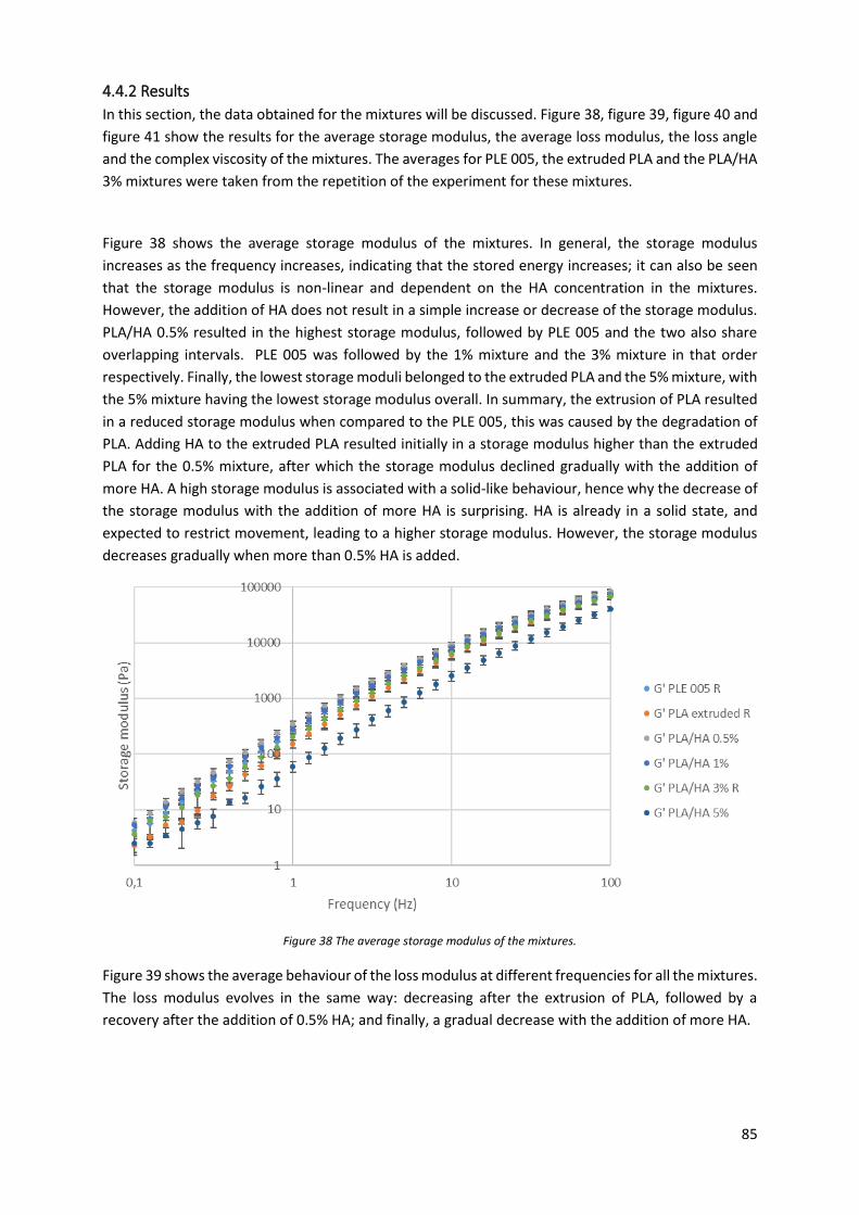
85

4.4.2 Results

In this section, the data obtained for the mixtures will be discussed. Figure 38, figure 39, figure 40 and

figure 41 show the results for the average storage modulus, the average loss modulus, the loss angle

and the complex viscosity of the mixtures. The averages for PLE 005, the extruded PLA and the PLA/HA

3% mixtures were taken from the repetition of the experiment for these mixtures.

Figure 38 shows the average storage modulus of the mixtures. In general, the storage modulus

increases as the frequency increases, indicating that the stored energy increases; it can also be seen

that the storage modulus is non-linear and dependent on the HA concentration in the mixtures.

However, the addition of HA does not result in a simple increase or decrease of the storage modulus.

PLA/HA 0.5% resulted in the highest storage modulus, followed by PLE 005 and the two also share

overlapping intervals. PLE 005 was followed by the 1% mixture and the 3% mixture in that order

respectively. Finally, the lowest storage moduli belonged to the extruded PLA and the 5% mixture, with

the 5% mixture having the lowest storage modulus overall. In summary, the extrusion of PLA resulted

in a reduced storage modulus when compared to the PLE 005, this was caused by the degradation of

PLA. Adding HA to the extruded PLA resulted initially in a storage modulus higher than the extruded

PLA for the 0.5% mixture, after which the storage modulus declined gradually with the addition of

more HA. A high storage modulus is associated with a solid-like behaviour, hence why the decrease of

the storage modulus with the addition of more HA is surprising. HA is already in a solid state, and

expected to restrict movement, leading to a higher storage modulus. However, the storage modulus

decreases gradually when more than 0.5% HA is added.

Figure 38 The average storage modulus of the mixtures.

Figure 39 shows the average behaviour of the loss modulus at different frequencies for all the mixtures.

The loss modulus evolves in the same way: decreasing after the extrusion of PLA, followed by a

recovery after the addition of 0.5% HA; and finally, a gradual decrease with the addition of more HA.

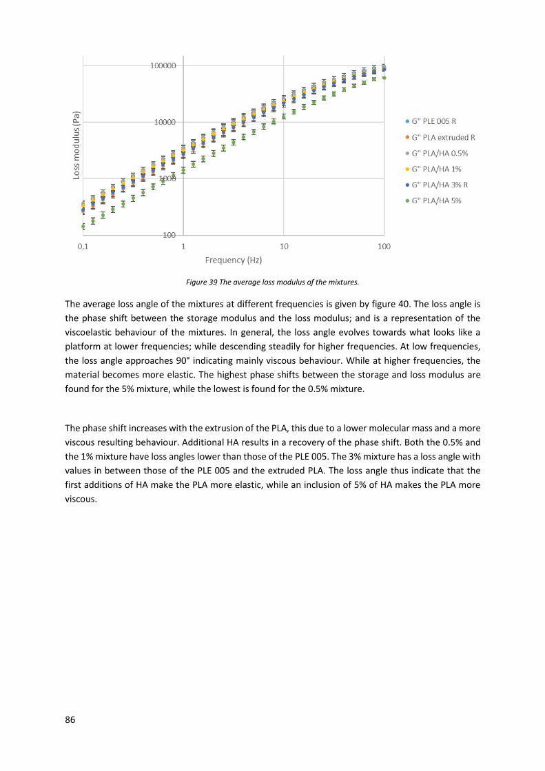
86

Figure 39 The average loss modulus of the mixtures.

The average loss angle of the mixtures at different frequencies is given by figure 40. The loss angle is

the phase shift between the storage modulus and the loss modulus; and is a representation of the

viscoelastic behaviour of the mixtures. In general, the loss angle evolves towards what looks like a

platform at lower frequencies; while descending steadily for higher frequencies. At low frequencies,

the loss angle approaches 90° indicating mainly viscous behaviour. While at higher frequencies, the

material becomes more elastic. The highest phase shifts between the storage and loss modulus are

found for the 5% mixture, while the lowest is found for the 0.5% mixture.

The phase shift increases with the extrusion of the PLA, this due to a lower molecular mass and a more

viscous resulting behaviour. Additional HA results in a recovery of the phase shift. Both the 0.5% and

the 1% mixture have loss angles lower than those of the PLE 005. The 3% mixture has a loss angle with

values in between those of the PLE 005 and the extruded PLA. The loss angle thus indicate that the

first additions of HA make the PLA more elastic, while an inclusion of 5% of HA makes the PLA more

viscous.

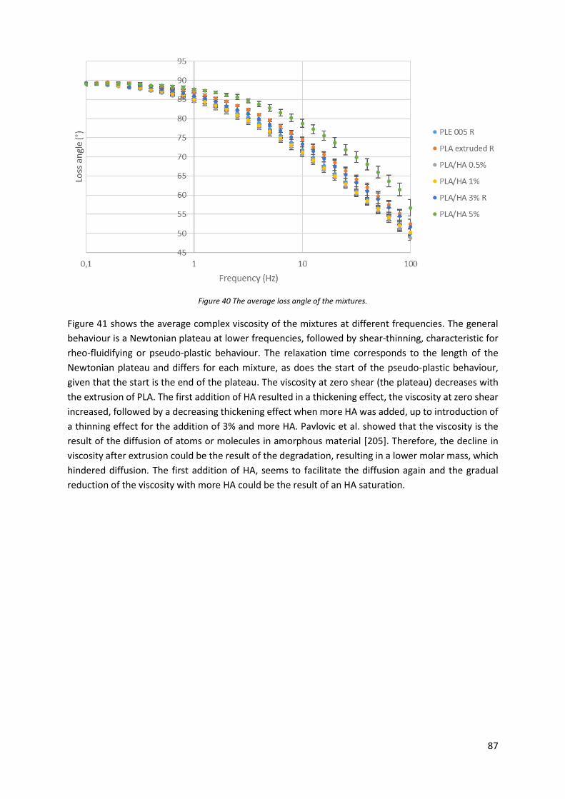
87

Figure 40 The average loss angle of the mixtures.

Figure 41 shows the average complex viscosity of the mixtures at different frequencies. The general

behaviour is a Newtonian plateau at lower frequencies, followed by shear-thinning, characteristic for

rheo-fluidifying or pseudo-plastic behaviour. The relaxation time corresponds to the length of the

Newtonian plateau and differs for each mixture, as does the start of the pseudo-plastic behaviour,

given that the start is the end of the plateau. The viscosity at zero shear (the plateau) decreases with

the extrusion of PLA. The first addition of HA resulted in a thickening effect, the viscosity at zero shear

increased, followed by a decreasing thickening effect when more HA was added, up to introduction of

a thinning effect for the addition of 3% and more HA. Pavlovic et al. showed that the viscosity is the

result of the diffusion of atoms or molecules in amorphous material [205]. Therefore, the decline in

viscosity after extrusion could be the result of the degradation, resulting in a lower molar mass, which

hindered diffusion. The first addition of HA, seems to facilitate the diffusion again and the gradual

reduction of the viscosity with more HA could be the result of an HA saturation.

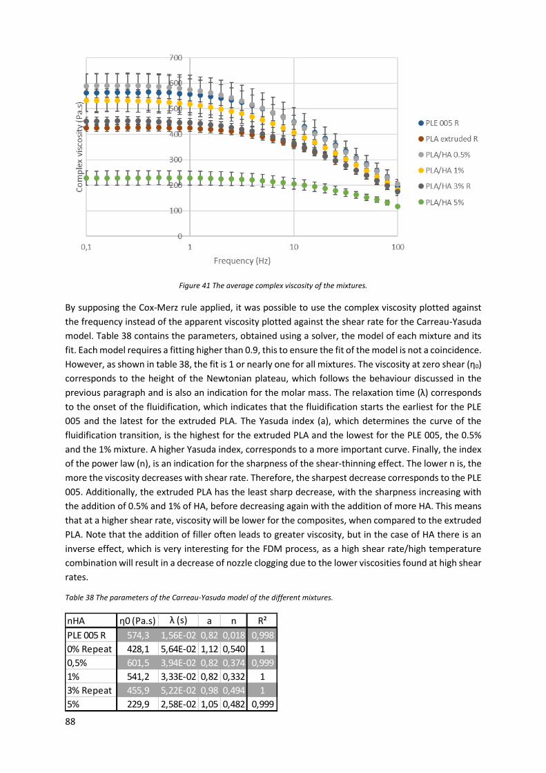
88

Figure 41 The average complex viscosity of the mixtures.

By supposing the Cox-Merz rule applied, it was possible to use the complex viscosity plotted against

the frequency instead of the apparent viscosity plotted against the shear rate for the Carreau-Yasuda

model. Table 38 contains the parameters, obtained using a solver, the model of each mixture and its

fit. Each model requires a fitting higher than 0.9, this to ensure the fit of the model is not a coincidence.

However, as shown in table 38, the fit is 1 or nearly one for all mixtures. The viscosity at zero shear (η0)

corresponds to the height of the Newtonian plateau, which follows the behaviour discussed in the

previous paragraph and is also an indication for the molar mass. The relaxation time (λ) corresponds

to the onset of the fluidification, which indicates that the fluidification starts the earliest for the PLE

005 and the latest for the extruded PLA. The Yasuda index (a), which determines the curve of the

fluidification transition, is the highest for the extruded PLA and the lowest for the PLE 005, the 0.5%

and the 1% mixture. A higher Yasuda index, corresponds to a more important curve. Finally, the index

of the power law (n), is an indication for the sharpness of the shear-thinning effect. The lower n is, the

more the viscosity decreases with shear rate. Therefore, the sharpest decrease corresponds to the PLE

005. Additionally, the extruded PLA has the least sharp decrease, with the sharpness increasing with

the addition of 0.5% and 1% of HA, before decreasing again with the addition of more HA. This means

that at a higher shear rate, viscosity will be lower for the composites, when compared to the extruded

PLA. Note that the addition of filler often leads to greater viscosity, but in the case of HA there is an

inverse effect, which is very interesting for the FDM process, as a high shear rate/high temperature

combination will result in a decrease of nozzle clogging due to the lower viscosities found at high shear

rates.

Table 38 The parameters of the Carreau-Yasuda model of the different mixtures.

nHA η0 (Pa.s) λ (s) a n R²

PLE 005 R 574,3 1,56E-02 0,82 0,018 0,998

0% Repeat 428,1 5,64E-02 1,12 0,540 1

0,5% 601,5 3,94E-02 0,82 0,374 0,999

1% 541,2 3,33E-02 0,82 0,332 1

3% Repeat 455,9 5,22E-02 0,98 0,494 1

5% 229,9 2,58E-02 1,05 0,482 0,999

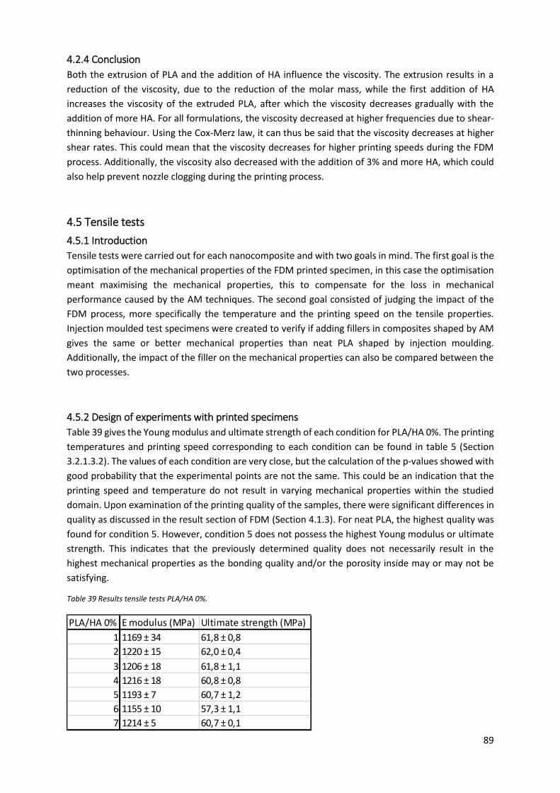
89

4.2.4 Conclusion

Both the extrusion of PLA and the addition of HA influence the viscosity. The extrusion results in a

reduction of the viscosity, due to the reduction of the molar mass, while the first addition of HA

increases the viscosity of the extruded PLA, after which the viscosity decreases gradually with the

addition of more HA. For all formulations, the viscosity decreased at higher frequencies due to shear-

thinning behaviour. Using the Cox-Merz law, it can thus be said that the viscosity decreases at higher

shear rates. This could mean that the viscosity decreases for higher printing speeds during the FDM

process. Additionally, the viscosity also decreased with the addition of 3% and more HA, which could

also help prevent nozzle clogging during the printing process.

4.5 Tensile tests

4.5.1 Introduction

Tensile tests were carried out for each nanocomposite and with two goals in mind. The first goal is the

optimisation of the mechanical properties of the FDM printed specimen, in this case the optimisation

meant maximising the mechanical properties, this to compensate for the loss in mechanical

performance caused by the AM techniques. The second goal consisted of judging the impact of the

FDM process, more specifically the temperature and the printing speed on the tensile properties.

Injection moulded test specimens were created to verify if adding fillers in composites shaped by AM

gives the same or better mechanical properties than neat PLA shaped by injection moulding.

Additionally, the impact of the filler on the mechanical properties can also be compared between the

two processes.

4.5.2 Design of experiments with printed specimens

Table 39 gives the Young modulus and ultimate strength of each condition for PLA/HA 0%. The printing

temperatures and printing speed corresponding to each condition can be found in table 5 (Section

3.2.1.3.2). The values of each condition are very close, but the calculation of the p-values showed with

good probability that the experimental points are not the same. This could be an indication that the

printing speed and temperature do not result in varying mechanical properties within the studied

domain. Upon examination of the printing quality of the samples, there were significant differences in

quality as discussed in the result section of FDM (Section 4.1.3). For neat PLA, the highest quality was

found for condition 5. However, condition 5 does not possess the highest Young modulus or ultimate

strength. This indicates that the previously determined quality does not necessarily result in the

highest mechanical properties as the bonding quality and/or the porosity inside may or may not be

satisfying.

Table 39 Results tensile tests PLA/HA 0%.

PLA/HA 0% E modulus (MPa) Ultimate strength (MPa)

1 1169 ± 34 61,8 ± 0,8

2 1220 ± 15 62,0 ± 0,4

3 1206 ± 18 61,8 ± 1,1

4 1216 ± 18 60,8 ± 0,8

5 1193 ± 7 60,7 ± 1,2

6 1155 ± 10 57,3 ± 1,1

7 1214 ± 5 60,7 ± 0,1

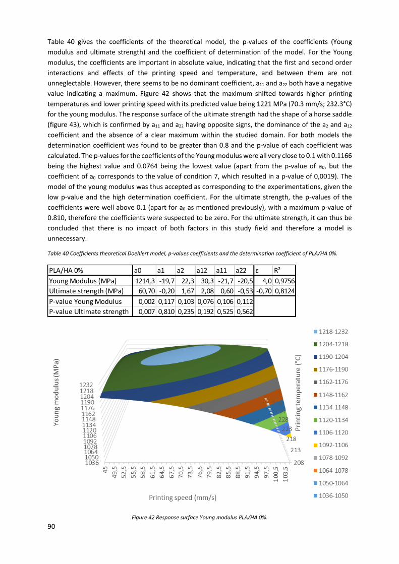
90

Table 40 gives the coefficients of the theoretical model, the p-values of the coefficients (Young

modulus and ultimate strength) and the coefficient of determination of the model. For the Young

modulus, the coefficients are important in absolute value, indicating that the first and second order

interactions and effects of the printing speed and temperature, and between them are not

unneglectable. However, there seems to be no dominant coefficient, a11 and a22 both have a negative

value indicating a maximum. Figure 42 shows that the maximum shifted towards higher printing

temperatures and lower printing speed with its predicted value being 1221 MPa (70.3 mm/s; 232.3°C)

for the young modulus. The response surface of the ultimate strength had the shape of a horse saddle

(figure 43), which is confirmed by a11 and a22 having opposite signs, the dominance of the a2 and a12

coefficient and the absence of a clear maximum within the studied domain. For both models the

determination coefficient was found to be greater than 0.8 and the p-value of each coefficient was

calculated. The p-values for the coefficients of the Young modulus were all very close to 0.1 with 0.1166

being the highest value and 0.0764 being the lowest value (apart from the p-value of a0, but the

coefficient of a0 corresponds to the value of condition 7, which resulted in a p-value of 0,0019). The

model of the young modulus was thus accepted as corresponding to the experimentations, given the

low p-value and the high determination coefficient. For the ultimate strength, the p-values of the

coefficients were well above 0.1 (apart for a0 as mentioned previously), with a maximum p-value of

0.810, therefore the coefficients were suspected to be zero. For the ultimate strength, it can thus be

concluded that there is no impact of both factors in this study field and therefore a model is

unnecessary.

Table 40 Coefficients theoretical Doehlert model, p-values coefficients and the determination coefficient of PLA/HA 0%.

Figure 42 Response surface Young modulus PLA/HA 0%.

PLA/HA 0% a0 a1 a2 a12 a11 a22 ε R²

Young Modulus (MPa) 1214,3 -19,7 22,3 30,3 -21,7 -20,5 4,0 0,9756

Ultimate strength (MPa) 60,70 -0,20 1,67 2,08 0,60 -0,53 -0,70 0,8124

P-value Young Modulus 0,002 0,117 0,103 0,076 0,106 0,112

P-value Ultimate strength 0,007 0,810 0,235 0,192 0,525 0,562

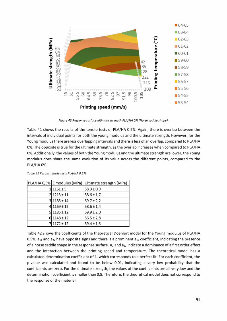
91

Figure 43 Response surface ultimate strength PLA/HA 0% (Horse saddle shape).

Table 41 shows the results of the tensile tests of PLA/HA 0.5%. Again, there is overlap between the

intervals of individual points for both the young modulus and the ultimate strength. However, for the

Young modulus there are less overlapping intervals and there is less of an overlap, compared to PLA/HA

0%. The opposite is true for the ultimate strength, as the overlap increases when compared to PLA/HA

0%. Additionally, the values of both the Young modulus and the ultimate strength are lower, the Young

modulus does share the same evolution of its value across the different points, compared to the

PLA/HA 0%.

Table 41 Results tensile tests PLA/HA 0.5%.

Table 42 shows the coefficients of the theoretical Doehlert model for the Young modulus of PLA/HA

0.5%, a11 and a22 have opposite signs and there is a prominent a12 coefficient, indicating the presence

of a horse saddle shape in the response surface. A2 and a12 indicate a dominance of a first order effect

and the interaction between the printing speed and temperature. The theoretical model has a

calculated determination coefficient of 1, which corresponds to a perfect fit. For each coefficient, the

p-value was calculated and found to be below 0.01, indicating a very low probability that the

coefficients are zero. For the ultimate strength, the values of the coefficients are all very low and the

determination coefficient is smaller than 0.8. Therefore, the theoretical model does not correspond to

the response of the material.

PLA/HA 0,5% E modulus (MPa) Ultimate strength (MPa)

1 1161 ± 5 58,3 ± 0,9

2 1213 ± 11 58,6 ± 1,7

3 1185 ± 14 59,7 ± 2,2

4 1169 ± 12 58,6 ± 1,4

5 1185 ± 12 59,9 ± 2,0

6 1148 ± 12 56,5 ± 2,8

7 1172 ± 12 59,4 ± 1,3

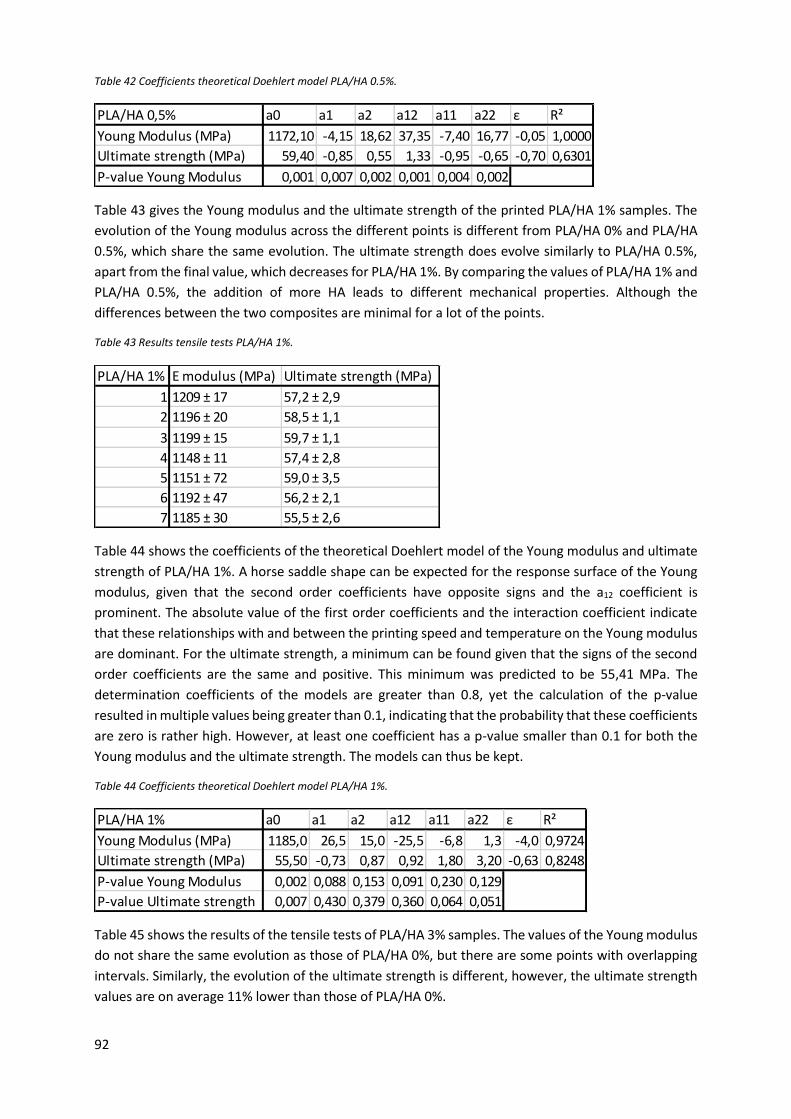
92

Table 42 Coefficients theoretical Doehlert model PLA/HA 0.5%.

Table 43 gives the Young modulus and the ultimate strength of the printed PLA/HA 1% samples. The

evolution of the Young modulus across the different points is different from PLA/HA 0% and PLA/HA

0.5%, which share the same evolution. The ultimate strength does evolve similarly to PLA/HA 0.5%,

apart from the final value, which decreases for PLA/HA 1%. By comparing the values of PLA/HA 1% and

PLA/HA 0.5%, the addition of more HA leads to different mechanical properties. Although the

differences between the two composites are minimal for a lot of the points.


Table 44 shows the coefficients of the theoretical Doehlert model of the Young modulus and ultimate

strength of PLA/HA 1%. A horse saddle shape can be expected for the response surface of the Young

modulus, given that the second order coefficients have opposite signs and the a12 coefficient is

prominent. The absolute value of the first order coefficients and the interaction coefficient indicate

that these relationships with and between the printing speed and temperature on the Young modulus

are dominant. For the ultimate strength, a minimum can be found given that the signs of the second

order coefficients are the same and positive. This minimum was predicted to be 55,41 MPa. The

determination coefficients of the models are greater than 0.8, yet the calculation of the p-value

resulted in multiple values being greater than 0.1, indicating that the probability that these coefficients

are zero is rather high. However, at least one coefficient has a p-value smaller than 0.1 for both the

Young modulus and the ultimate strength. The models can thus be kept.

Table 44 Coefficients theoretical Doehlert model PLA/HA 1%.

Table 45 shows the results of the tensile tests of PLA/HA 3% samples. The values of the Young modulus

do not share the same evolution as those of PLA/HA 0%, but there are some points with overlapping

intervals. Similarly, the evolution of the ultimate strength is different, however, the ultimate strength

values are on average 11% lower than those of PLA/HA 0%.

PLA/HA 0,5% a0 a1 a2 a12 a11 a22 ε R²

Young Modulus (MPa) 1172,10 -4,15 18,62 37,35 -7,40 16,77 -0,05 1,0000

Ultimate strength (MPa) 59,40 -0,85 0,55 1,33 -0,95 -0,65 -0,70 0,6301



1 1209 ± 17 57,2 ± 2,9

2 1196 ± 20 58,5 ± 1,1

3 1199 ± 15 59,7 ± 1,1

4 1148 ± 11 57,4 ± 2,8

5 1151 ± 72 59,0 ± 3,5

6 1192 ± 47 56,2 ± 2,1

7 1185 ± 30 55,5 ± 2,6

PLA/HA 1% a0 a1 a2 a12 a11 a22 ε R²

Young Modulus (MPa) 1185,0 26,5 15,0 -25,5 -6,8 1,3 -4,0 0,9724

Ultimate strength (MPa) 55,50 -0,73 0,87 0,92 1,80 3,20 -0,63 0,8248


P-value Ultimate strength 0,007 0,430 0,379 0,360 0,064 0,051

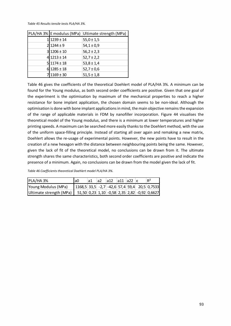
93


Table 46 gives the coefficients of the theoretical Doehlert model of PLA/HA 3%. A minimum can be

found for the Young modulus, as both second order coefficients are positive. Given that one goal of

the experiment is the optimisation by maximum of the mechanical properties to reach a higher

resistance for bone implant application, the chosen domain seems to be non-ideal. Although the

optimisation is done with bone implant applications in mind, the main objective remains the expansion

of the range of applicable materials in FDM by nanofiller incorporation. Figure 44 visualises the

theoretical model of the Young modulus, and there is a minimum at lower temperatures and higher

printing speeds. A maximum can be searched more easily thanks to the Doehlert method, with the use

of the uniform space-filling principle. Instead of starting all over again and remaking a new matrix,

Doehlert allows the re-usage of experimental points. However, the new points have to result in the

creation of a new hexagon with the distance between neighbouring points being the same. However,

given the lack of fit of the theoretical model, no conclusions can be drawn from it. The ultimate

strength shares the same characteristics, both second order coefficients are positive and indicate the

presence of a minimum. Again, no conclusions can be drawn from the model given the lack of fit.



1 1239 ± 14 55,0 ± 1,5

2 1244 ± 9 54,1 ± 0,9

3 1206 ± 10 56,2 ± 2,3

4 1213 ± 14 52,7 ± 2,2

5 1174 ± 18 53,8 ± 1,4

6 1285 ± 18 52,7 ± 0,6

7 1169 ± 30 51,5 ± 1,8

PLA/HA 3% a0 a1 a2 a12 a11 a22 ε R²

Young Modulus (MPa) 1168,5 33,5 -2,7 -42,6 57,4 59,4 20,5 0,7533

Ultimate strength (MPa) 51,50 0,23 1,10 -0,58 2,35 2,82 -0,92 0,6627

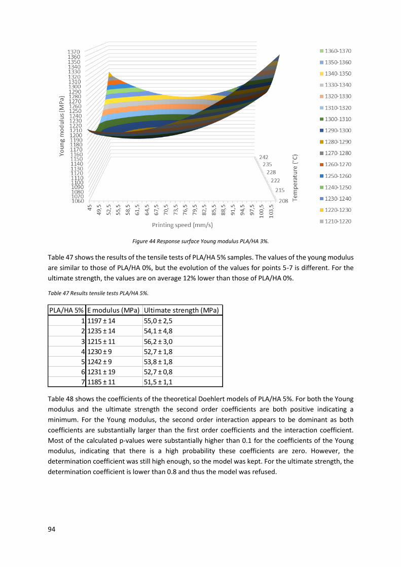
94

Figure 44 Response surface Young modulus PLA/HA 3%.

Table 47 shows the results of the tensile tests of PLA/HA 5% samples. The values of the young modulus

are similar to those of PLA/HA 0%, but the evolution of the values for points 5-7 is different. For the

ultimate strength, the values are on average 12% lower than those of PLA/HA 0%.


Table 48 shows the coefficients of the theoretical Doehlert models of PLA/HA 5%. For both the Young

modulus and the ultimate strength the second order coefficients are both positive indicating a

minimum. For the Young modulus, the second order interaction appears to be dominant as both

coefficients are substantially larger than the first order coefficients and the interaction coefficient.

Most of the calculated p-values were substantially higher than 0.1 for the coefficients of the Young

modulus, indicating that there is a high probability these coefficients are zero. However, the

determination coefficient was still high enough, so the model was kept. For the ultimate strength, the

determination coefficient is lower than 0.8 and thus the model was refused.


1 1197 ± 14 55,0 ± 2,5

2 1235 ± 14 54,1 ± 4,8

3 1215 ± 11 56,2 ± 3,0

4 1230 ± 9 52,7 ± 1,8

5 1242 ± 9 53,8 ± 1,8

6 1231 ± 19 52,7 ± 0,8

7 1185 ± 11 51,5 ± 1,1

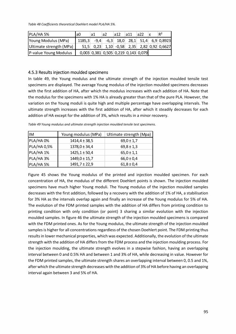
95


4.5.3 Results injection moulded specimens

In table 49, the Young modulus and the ultimate strength of the injection moulded tensile test

specimens are displayed. The average Young modulus of the injection moulded specimens decreases

with the first addition of HA, after which the modulus increases with each addition of HA. Note that

the modulus for the specimens with 1% HA is already greater than that of the pure PLA. However, the

variation on the Young moduli is quite high and multiple percentage have overlapping intervals. The

ultimate strength increases with the first addition of HA, after which it steadily decreases for each

addition of HA except for the addition of 3%, which results in a minor recovery.

Table 49 Young modulus and ultimate strength injection moulded tensile test specimens.

Figure 45 shows the Young modulus of the printed and injection moulded specimen. For each

concentration of HA, the modulus of the different Doehlert points is shown. The injection moulded

specimens have much higher Young moduli. The Young modulus of the injection moulded samples

decreases with the first addition, followed by a recovery with the addition of 1% of HA, a stabilisation

for 3% HA as the intervals overlap again and finally an increase of the Young modulus for 5% of HA.

The evolution of the FDM printed samples with the addition of HA differs from printing condition to

printing condition with only condition (or point) 3 sharing a similar evolution with the injection

moulded samples. In figure 46 the ultimate strength of the injection moulded specimens is compared

with the FDM printed ones. As for the Young modulus, the ultimate strength of the injection moulded

samples is higher for all concentrations regardless of the chosen Doehlert point. The FDM printing thus

results in lower mechanical properties, which was expected. Additionally, the evolution of the ultimate

strength with the addition of HA differs from the FDM process and the injection moulding process. For

the injection moulding, the ultimate strength evolves in a stepwise fashion, having an overlapping

interval between 0 and 0.5% HA and between 1 and 3% of HA, while decreasing in value. However for

the FDM printed samples, the ultimate strength shares an overlapping interval between 0, 0.5 and 1%,

after which the ultimate strength decreases with the addition of 3% of HA before having an overlapping

interval again between 3 and 5% of HA.

PLA/HA 5% a0 a1 a2 a12 a11 a22 ε R²

Young Modulus (MPa) 1185,3 -9,4 -6,3 18,0 28,1 51,4 6,9 0,8923

Ultimate strength (MPa) 51,5 0,23 1,10 -0,58 2,35 2,82 0,92 0,6627


IM Young modulus (MPa) Ultimate strength (Mpa)

PLA/HA 0% 1414,4 ± 38,5 69,0 ± 1,7

PLA/HA 0,5% 1378,0 ± 34,4 69,8 ± 1,3

PLA/HA 1% 1425,1 ± 50,4 65,0 ± 1,1

PLA/HA 3% 1449,0 ± 15,7 66,0 ± 0,4

PLA/HA 5% 1491,7 ± 22,9 61,8 ± 0,4

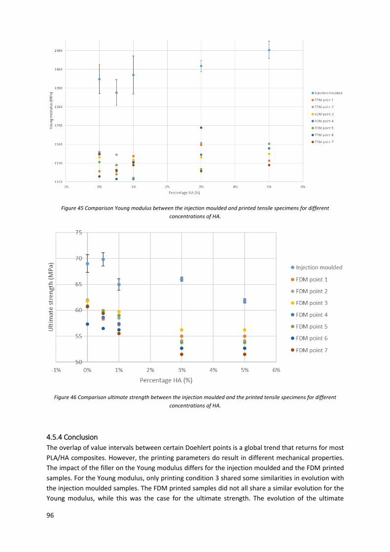
96

Figure 45 Comparison Young modulus between the injection moulded and printed tensile specimens for different

concentrations of HA.

Figure 46 Comparison ultimate strength between the injection moulded and the printed tensile specimens for different

concentrations of HA.

4.5.4 Conclusion

The overlap of value intervals between certain Doehlert points is a global trend that returns for most

PLA/HA composites. However, the printing parameters do result in different mechanical properties.

The impact of the filler on the Young modulus differs for the injection moulded and the FDM printed

samples. For the Young modulus, only printing condition 3 shared some similarities in evolution with

the injection moulded samples. The FDM printed samples did not all share a similar evolution for the

Young modulus, while this was the case for the ultimate strength. The evolution of the ultimate

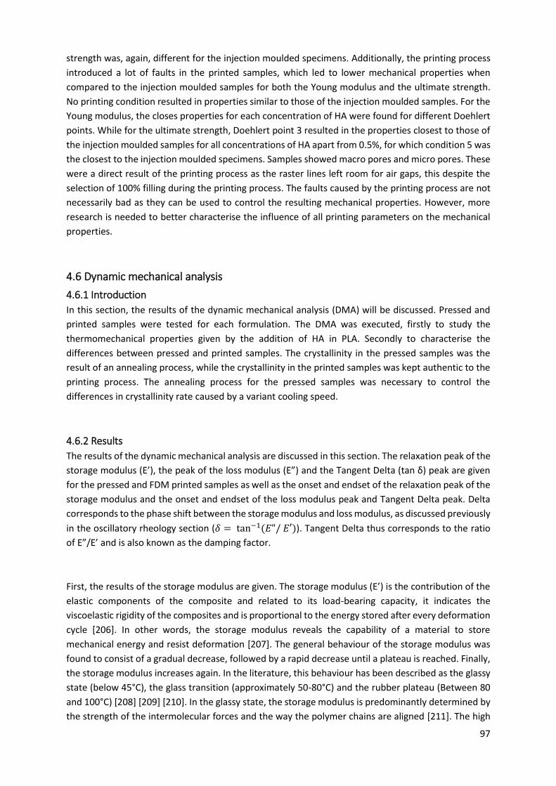
97

strength was, again, different for the injection moulded specimens. Additionally, the printing process

introduced a lot of faults in the printed samples, which led to lower mechanical properties when

compared to the injection moulded samples for both the Young modulus and the ultimate strength.

No printing condition resulted in properties similar to those of the injection moulded samples. For the

Young modulus, the closes properties for each concentration of HA were found for different Doehlert

points. While for the ultimate strength, Doehlert point 3 resulted in the properties closest to those of

the injection moulded samples for all concentrations of HA apart from 0.5%, for which condition 5 was

the closest to the injection moulded specimens. Samples showed macro pores and micro pores. These

were a direct result of the printing process as the raster lines left room for air gaps, this despite the

selection of 100% filling during the printing process. The faults caused by the printing process are not

necessarily bad as they can be used to control the resulting mechanical properties. However, more

research is needed to better characterise the influence of all printing parameters on the mechanical

properties.

4.6 Dynamic mechanical analysis

4.6.1 Introduction

In this section, the results of the dynamic mechanical analysis (DMA) will be discussed. Pressed and

printed samples were tested for each formulation. The DMA was executed, firstly to study the

thermomechanical properties given by the addition of HA in PLA. Secondly to characterise the

differences between pressed and printed samples. The crystallinity in the pressed samples was the

result of an annealing process, while the crystallinity in the printed samples was kept authentic to the

printing process. The annealing process for the pressed samples was necessary to control the

differences in crystallinity rate caused by a variant cooling speed.

4.6.2 Results

The results of the dynamic mechanical analysis are discussed in this section. The relaxation peak of the

storage modulus (E’), the peak of the loss modulus (E”) and the Tangent Delta (tan δ) peak are given

for the pressed and FDM printed samples as well as the onset and endset of the relaxation peak of the

storage modulus and the onset and endset of the loss modulus peak and Tangent Delta peak. Delta

corresponds to the phase shift between the storage modulus and loss modulus, as discussed previously

in the oscillatory rheology section (𝛿 = tan−1(𝐸"/ 𝐸′)). Tangent Delta thus corresponds to the ratio

of E”/E’ and is also known as the damping factor.

First, the results of the storage modulus are given. The storage modulus (E’) is the contribution of the

elastic components of the composite and related to its load-bearing capacity, it indicates the

viscoelastic rigidity of the composites and is proportional to the energy stored after every deformation

cycle [206]. In other words, the storage modulus reveals the capability of a material to store

mechanical energy and resist deformation [207]. The general behaviour of the storage modulus was

found to consist of a gradual decrease, followed by a rapid decrease until a plateau is reached. Finally,

the storage modulus increases again. In the literature, this behaviour has been described as the glassy

state (below 45°C), the glass transition (approximately 50-80°C) and the rubber plateau (Between 80

and 100°C) [208] [209] [210]. In the glassy state, the storage modulus is predominantly determined by

the strength of the intermolecular forces and the way the polymer chains are aligned [211]. The high

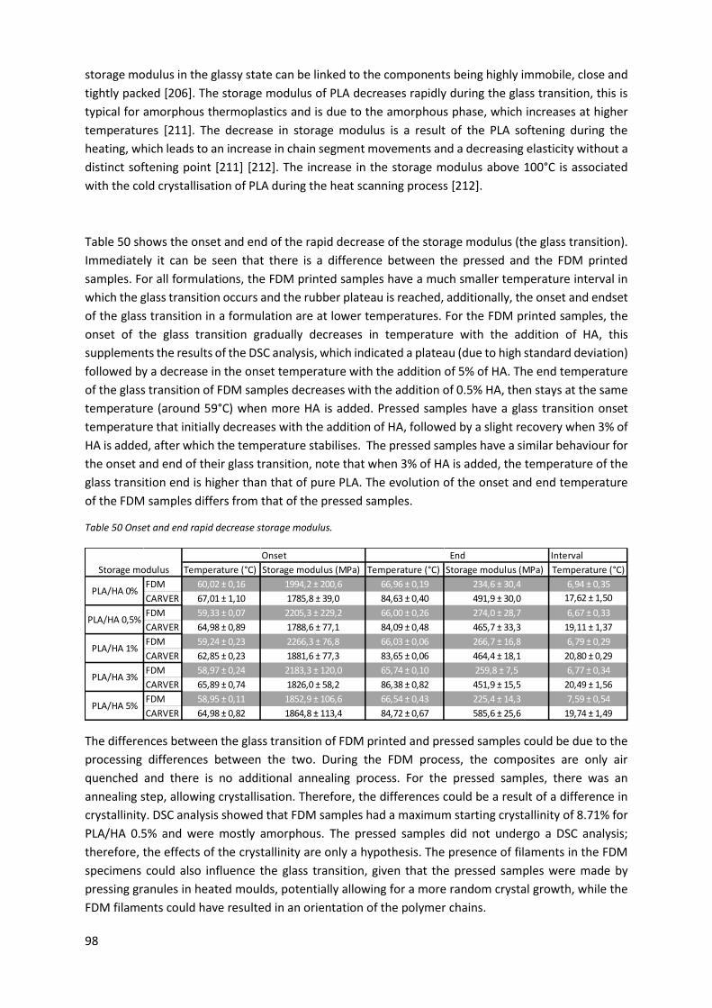
98

storage modulus in the glassy state can be linked to the components being highly immobile, close and

tightly packed [206]. The storage modulus of PLA decreases rapidly during the glass transition, this is

typical for amorphous thermoplastics and is due to the amorphous phase, which increases at higher

temperatures [211]. The decrease in storage modulus is a result of the PLA softening during the

heating, which leads to an increase in chain segment movements and a decreasing elasticity without a

distinct softening point [211] [212]. The increase in the storage modulus above 100°C is associated

with the cold crystallisation of PLA during the heat scanning process [212].

Table 50 shows the onset and end of the rapid decrease of the storage modulus (the glass transition).

Immediately it can be seen that there is a difference between the pressed and the FDM printed

samples. For all formulations, the FDM printed samples have a much smaller temperature interval in

which the glass transition occurs and the rubber plateau is reached, additionally, the onset and endset

of the glass transition in a formulation are at lower temperatures. For the FDM printed samples, the

onset of the glass transition gradually decreases in temperature with the addition of HA, this

supplements the results of the DSC analysis, which indicated a plateau (due to high standard deviation)

followed by a decrease in the onset temperature with the addition of 5% of HA. The end temperature

of the glass transition of FDM samples decreases with the addition of 0.5% HA, then stays at the same

temperature (around 59°C) when more HA is added. Pressed samples have a glass transition onset

temperature that initially decreases with the addition of HA, followed by a slight recovery when 3% of

HA is added, after which the temperature stabilises. The pressed samples have a similar behaviour for

the onset and end of their glass transition, note that when 3% of HA is added, the temperature of the

glass transition end is higher than that of pure PLA. The evolution of the onset and end temperature

of the FDM samples differs from that of the pressed samples.

Table 50 Onset and end rapid decrease storage modulus.

The differences between the glass transition of FDM printed and pressed samples could be due to the

processing differences between the two. During the FDM process, the composites are only air

quenched and there is no additional annealing process. For the pressed samples, there was an

annealing step, allowing crystallisation. Therefore, the differences could be a result of a difference in

crystallinity. DSC analysis showed that FDM samples had a maximum starting crystallinity of 8.71% for

PLA/HA 0.5% and were mostly amorphous. The pressed samples did not undergo a DSC analysis;

therefore, the effects of the crystallinity are only a hypothesis. The presence of filaments in the FDM

specimens could also influence the glass transition, given that the pressed samples were made by

pressing granules in heated moulds, potentially allowing for a more random crystal growth, while the

FDM filaments could have resulted in an orientation of the polymer chains.

Interval

Temperature (°C) Storage modulus (MPa) Temperature (°C) Storage modulus (MPa) Temperature (°C)

FDM 60,02 ± 0,16 1994,2 ± 200,6 66,96 ± 0,19 234,6 ± 30,4 6,94 ± 0,35

CARVER 67,01 ± 1,10 1785,8 ± 39,0 84,63 ± 0,40 491,9 ± 30,0 17,62 ± 1,50

FDM 59,33 ± 0,07 2205,3 ± 229,2 66,00 ± 0,26 274,0 ± 28,7 6,67 ± 0,33

CARVER 64,98 ± 0,89 1788,6 ± 77,1 84,09 ± 0,48 465,7 ± 33,3 19,11 ± 1,37

FDM 59,24 ± 0,23 2266,3 ± 76,8 66,03 ± 0,06 266,7 ± 16,8 6,79 ± 0,29

CARVER 62,85 ± 0,23 1881,6 ± 77,3 83,65 ± 0,06 464,4 ± 18,1 20,80 ± 0,29

FDM 58,97 ± 0,24 2183,3 ± 120,0 65,74 ± 0,10 259,8 ± 7,5 6,77 ± 0,34

CARVER 65,89 ± 0,74 1826,0 ± 58,2 86,38 ± 0,82 451,9 ± 15,5 20,49 ± 1,56

FDM 58,95 ± 0,11 1852,9 ± 106,6 66,54 ± 0,43 225,4 ± 14,3 7,59 ± 0,54

CARVER 64,98 ± 0,82 1864,8 ± 113,4 84,72 ± 0,67 585,6 ± 25,6 19,74 ± 1,49

Storage modulus

Onset End

PLA/HA 0%

PLA/HA 0,5%

PLA/HA 1%

PLA/HA 3%

PLA/HA 5%

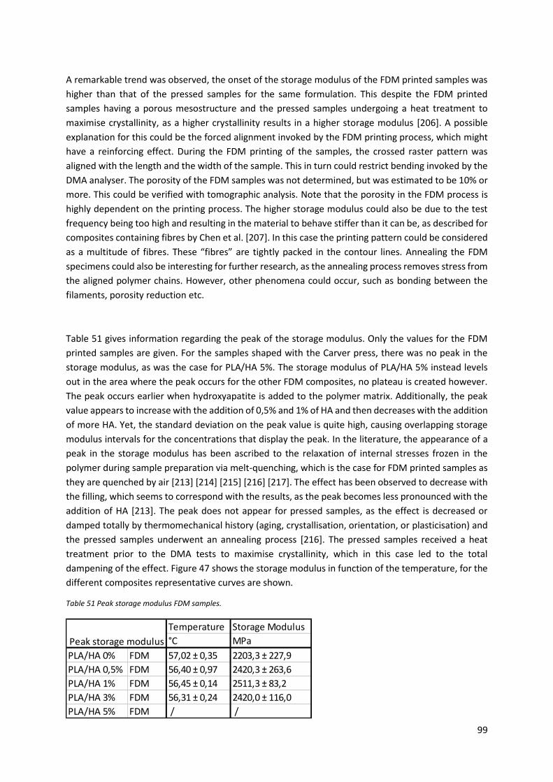
99

A remarkable trend was observed, the onset of the storage modulus of the FDM printed samples was

higher than that of the pressed samples for the same formulation. This despite the FDM printed

samples having a porous mesostructure and the pressed samples undergoing a heat treatment to

maximise crystallinity, as a higher crystallinity results in a higher storage modulus [206]. A possible

explanation for this could be the forced alignment invoked by the FDM printing process, which might

have a reinforcing effect. During the FDM printing of the samples, the crossed raster pattern was

aligned with the length and the width of the sample. This in turn could restrict bending invoked by the

DMA analyser. The porosity of the FDM samples was not determined, but was estimated to be 10% or

more. This could be verified with tomographic analysis. Note that the porosity in the FDM process is

highly dependent on the printing process. The higher storage modulus could also be due to the test

frequency being too high and resulting in the material to behave stiffer than it can be, as described for

composites containing fibres by Chen et al. [207]. In this case the printing pattern could be considered

as a multitude of fibres. These “fibres” are tightly packed in the contour lines. Annealing the FDM

specimens could also be interesting for further research, as the annealing process removes stress from

the aligned polymer chains. However, other phenomena could occur, such as bonding between the

filaments, porosity reduction etc.

Table 51 gives information regarding the peak of the storage modulus. Only the values for the FDM

printed samples are given. For the samples shaped with the Carver press, there was no peak in the

storage modulus, as was the case for PLA/HA 5%. The storage modulus of PLA/HA 5% instead levels

out in the area where the peak occurs for the other FDM composites, no plateau is created however.

The peak occurs earlier when hydroxyapatite is added to the polymer matrix. Additionally, the peak

value appears to increase with the addition of 0,5% and 1% of HA and then decreases with the addition

of more HA. Yet, the standard deviation on the peak value is quite high, causing overlapping storage

modulus intervals for the concentrations that display the peak. In the literature, the appearance of a

peak in the storage modulus has been ascribed to the relaxation of internal stresses frozen in the

polymer during sample preparation via melt-quenching, which is the case for FDM printed samples as

they are quenched by air [213] [214] [215] [216] [217]. The effect has been observed to decrease with

the filling, which seems to correspond with the results, as the peak becomes less pronounced with the

addition of HA [213]. The peak does not appear for pressed samples, as the effect is decreased or

damped totally by thermomechanical history (aging, crystallisation, orientation, or plasticisation) and

the pressed samples underwent an annealing process [216]. The pressed samples received a heat

treatment prior to the DMA tests to maximise crystallinity, which in this case led to the total

dampening of the effect. Figure 47 shows the storage modulus in function of the temperature, for the

different composites representative curves are shown.

Table 51 Peak storage modulus FDM samples.

Temperature Storage Modulus

°C MPa

PLA/HA 0% FDM 57,02 ± 0,35 2203,3 ± 227,9

PLA/HA 0,5% FDM 56,40 ± 0,97 2420,3 ± 263,6

PLA/HA 1% FDM 56,45 ± 0,14 2511,3 ± 83,2

PLA/HA 3% FDM 56,31 ± 0,24 2420,0 ± 116,0

PLA/HA 5% FDM / /

Peak storage modulus

100

Figure 47 Storage moduli pressed (red: neat PLA; purple: PLA/HA 3%) and FDM printed (black: neat PLA; blue: PLA/HA 3%)

samples.

Table 52 shows the temperatures at which the rubber plateau and the cold crystallisation begin for the

FDM printed samples. The cold crystallisation increases the height of the rubber plateau, due to the

reinforcing effect of the crystalline phase. For the pressed samples, there was no cold crystallisation.

This is more than likely a result of the annealing process. If the annealing resulted in a higher

crystallinity, the amount of amorphous phase would decrease. Due to the reduced amorphous phase,

the glass transition is less significant as there is less material which undergoes this transition.

Additionally, the increased crystallinity could also result in a restriction of the movement of the

amorphous material. This in turn would result in a wider temperature range in which the glass

transition takes place, due to the slow kinetic of the transition.

Table 52 End glass transition and onset cold crystallisation storage modulus.

Table 53 gives the minimum values of the storage modulus of the FDM specimens in between the end

of the glass transition and the beginning of the cold crystallisation. The minimum storage modulus

approaches zero for all the mixtures. The minimum value increases with the addition of HA, but does

not vary inter HA formulations. All HA formulations have overlapping intervals, when considering the

standard deviation.

l

l

l

l

l

l

l

l

l

l

l l l

l l l l

p

p

p

p

p

p

p

p

p

p

p

p pp

p

pp p

ª

ª

ª

ª

ª

ª

ª

ª

ª

ª

ªª

ªª

£

£

£

£

£

£

£

£

£

£

£

£ £

£

£

0

500

1000

1500

2000

2500

3000

Sto

rag

e M

od

ulu

s (

MP

a)

20 40 60 80 100 120 140

Temperature (°C)

170214_PLA0FDM_02.001––––––– 170216_PLA3FDM_02.001– – – – 170301_PLA0C_02.001––––– · 170306_PLA3C_02.001––– – –

Universal V4.5A TA Instruments

End glass transition Onset cold crystallisation

Temperature (°C) Temperature (°C)

PLA/HA 0% FDM 66,96 ± 0,19 95,58 ± 0,69

PLA/HA 0,5% FDM 66,00 ± 0,26 92,15 ± 0,46

PLA/HA 1% FDM 66,03 ± 0,06 94,08 ± 0,93

PLA/HA 3% FDM 65,74 ± 0,10 93,42 ± 0,14

PLA/HA 5% FDM 66,54 ± 0,43 91,43 ± 0,18

Storage modulus

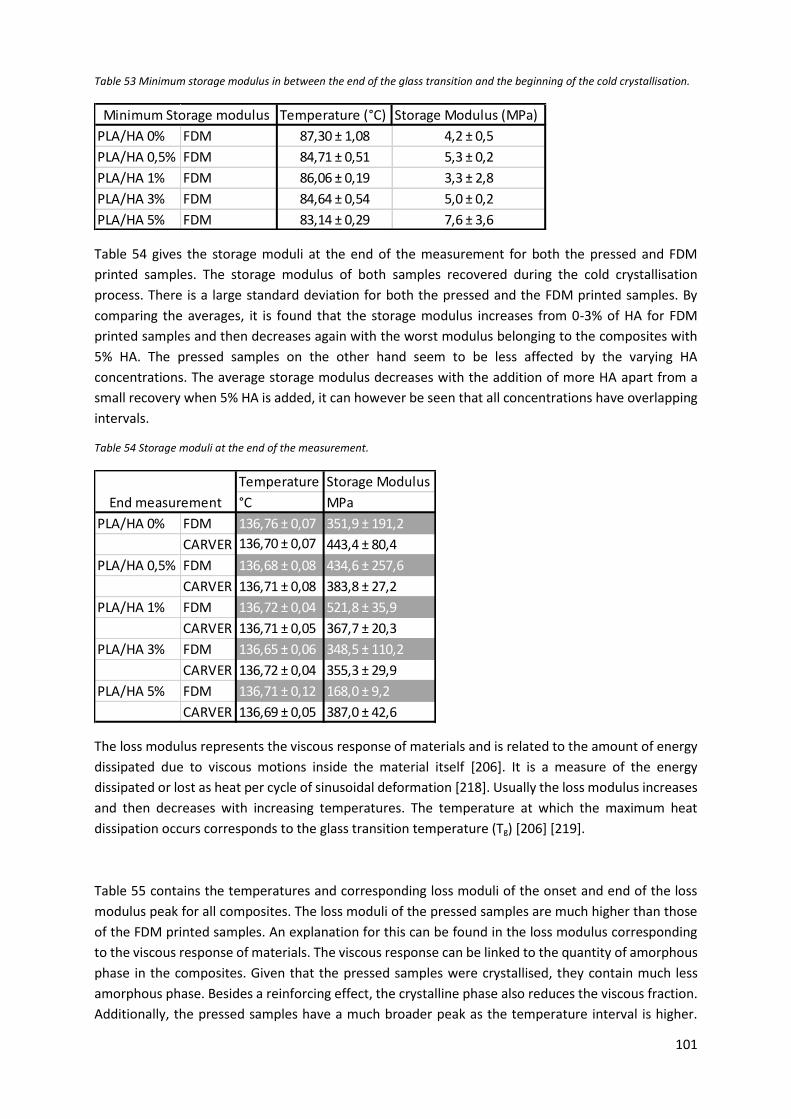
101

Table 53 Minimum storage modulus in between the end of the glass transition and the beginning of the cold crystallisation.

Table 54 gives the storage moduli at the end of the measurement for both the pressed and FDM

printed samples. The storage modulus of both samples recovered during the cold crystallisation

process. There is a large standard deviation for both the pressed and the FDM printed samples. By

comparing the averages, it is found that the storage modulus increases from 0-3% of HA for FDM

printed samples and then decreases again with the worst modulus belonging to the composites with

5% HA. The pressed samples on the other hand seem to be less affected by the varying HA

concentrations. The average storage modulus decreases with the addition of more HA apart from a

small recovery when 5% HA is added, it can however be seen that all concentrations have overlapping

intervals.

Table 54 Storage moduli at the end of the measurement.

The loss modulus represents the viscous response of materials and is related to the amount of energy

dissipated due to viscous motions inside the material itself [206]. It is a measure of the energy

dissipated or lost as heat per cycle of sinusoidal deformation [218]. Usually the loss modulus increases

and then decreases with increasing temperatures. The temperature at which the maximum heat

dissipation occurs corresponds to the glass transition temperature (Tg) [206] [219].

Table 55 contains the temperatures and corresponding loss moduli of the onset and end of the loss

modulus peak for all composites. The loss moduli of the pressed samples are much higher than those

of the FDM printed samples. An explanation for this can be found in the loss modulus corresponding

to the viscous response of materials. The viscous response can be linked to the quantity of amorphous

phase in the composites. Given that the pressed samples were crystallised, they contain much less

amorphous phase. Besides a reinforcing effect, the crystalline phase also reduces the viscous fraction.

Additionally, the pressed samples have a much broader peak as the temperature interval is higher.

Temperature (°C) Storage Modulus (MPa)

PLA/HA 0% FDM 87,30 ± 1,08 4,2 ± 0,5

PLA/HA 0,5% FDM 84,71 ± 0,51 5,3 ± 0,2

PLA/HA 1% FDM 86,06 ± 0,19 3,3 ± 2,8

PLA/HA 3% FDM 84,64 ± 0,54 5,0 ± 0,2

PLA/HA 5% FDM 83,14 ± 0,29 7,6 ± 3,6

Minimum Storage modulus

Temperature Storage Modulus

°C MPa

PLA/HA 0% FDM 136,76 ± 0,07 351,9 ± 191,2

CARVER 136,70 ± 0,07 443,4 ± 80,4

PLA/HA 0,5% FDM 136,68 ± 0,08 434,6 ± 257,6

CARVER 136,71 ± 0,08 383,8 ± 27,2

PLA/HA 1% FDM 136,72 ± 0,04 521,8 ± 35,9

CARVER 136,71 ± 0,05 367,7 ± 20,3

PLA/HA 3% FDM 136,65 ± 0,06 348,5 ± 110,2

CARVER 136,72 ± 0,04 355,3 ± 29,9

PLA/HA 5% FDM 136,71 ± 0,12 168,0 ± 9,2

CARVER 136,69 ± 0,05 387,0 ± 42,6

End measurement

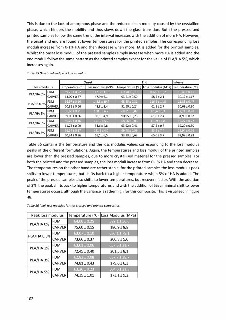
102

This is due to the lack of amorphous phase and the reduced chain mobility caused by the crystalline

phase, which hinders the mobility and thus slows down the glass transition. Both the pressed and

printed samples follow the same trend, the interval increases with the addition of more HA. However,

the onset and end are found at lower temperatures for the printed samples. The corresponding loss

moduli increase from 0-1% HA and then decrease when more HA is added for the printed samples.

Whilst the onset loss moduli of the pressed samples simply increase when more HA is added and the

end moduli follow the same pattern as the printed samples except for the value of PLA/HA 5%, which

increases again.

Table 55 Onset and end peak loss modulus.

Table 56 contains the temperature and the loss modulus values corresponding to the loss modulus

peaks of the different formulations. Again, the temperatures and loss moduli of the printed samples

are lower than the pressed samples, due to more crystallised material for the pressed samples. For

both the printed and the pressed samples, the loss moduli increase from 0-1% HA and then decrease.

The temperatures on the other hand are rather stable, for the printed samples the loss modulus peak

shifts to lower temperatures, but shifts back to a higher temperature when 5% of HA is added. The

peak of the pressed samples also shifts to lower temperatures, but recovers faster. With the addition

of 3%, the peak shifts back to higher temperatures and with the addition of 5% a minimal shift to lower

temperatures occurs, although the variance is rather high for this composite. This is visualised in figure

48.

Table 56 Peak loss modulus for the pressed and printed composites.

Interval

Temperature (°C) Loss modulus (MPa) Temperature (°C) Loss modulus (Mpa) Temperature (°C)

FDM 59,25 ± 0,22 142,3 ± 11,8 69,70 ± 0,19 106,0 ± 10,2 10,45 ± 0,41

CARVER 63,09 ± 0,67 47,9 ± 6,1 93,21 ± 0,50 58,5 ± 2,1 30,12 ± 1,17

FDM 56,97 ± 0,16 148,8 ± 19,7 68,85 ± 0,31 116,2 ± 14,5 11,88 ± 0,47

CARVER 60,81 ± 0,56 48,8 ± 2,4 91,50 ± 0,24 61,8 ± 2,7 30,69 ± 0,80

FDM 56,60 ± 0,21 158,5 ± 6,7 68,81 ± 0,07 120,6 ± 5,3 12,21 ± 0,28

CARVER 59,05 ± 0,36 50,1 ± 4,9 90,95 ± 0,26 61,0 ± 2,4 31,90 ± 0,62

FDM 56,29 ± 0,16 151,9 ± 5,2 68,56 ± 0,06 116,9 ± 4,8 12,27 ± 0,22

CARVER 61,72 ± 0,09 54,6 ± 4,8 93,92 ± 0,41 57,5 ± 0,7 32,20 ± 0,50

FDM 56,54 ± 0,17 121,2 ± 4,0 69,48 ± 0,59 95,2 ± 7,4 12,94 ± 0,76

CARVER 60,34 ± 0,36 61,1 ± 6,5 93,33 ± 0,63 65,0 ± 3,7 32,99 ± 0,99

Loss modulus

Onset End

PLA/HA 0%

PLA/HA 0,5%

PLA/HA 1%

PLA/HA 3%

PLA/HA 5%

Temperature (°C) Loss Modulus (MPa)

FDM 64,00 ± 0,25 582,1 ± 56,6

CARVER 75,60 ± 0,15 180,9 ± 8,8

FDM 63,07 ± 0,10 630,1 ± 79,1

CARVER 73,66 ± 0,37 200,8 ± 5,0

FDM 63,01 ± 0,06 657,5 ± 21,7

CARVER 72,45 ± 0,40 201,5 ± 8,1

FDM 62,82 ± 0,08 637,7 ± 28,7

CARVER 74,81 ± 0,43 179,6 ± 6,3

FDM 63,26 ± 0,23 504,6 ± 21,3

CARVER 74,35 ± 1,01 173,1 ± 9,2

Peak loss modulus

PLA/HA 0%

PLA/HA 0,5%

PLA/HA 1%

PLA/HA 3%

PLA/HA 5%

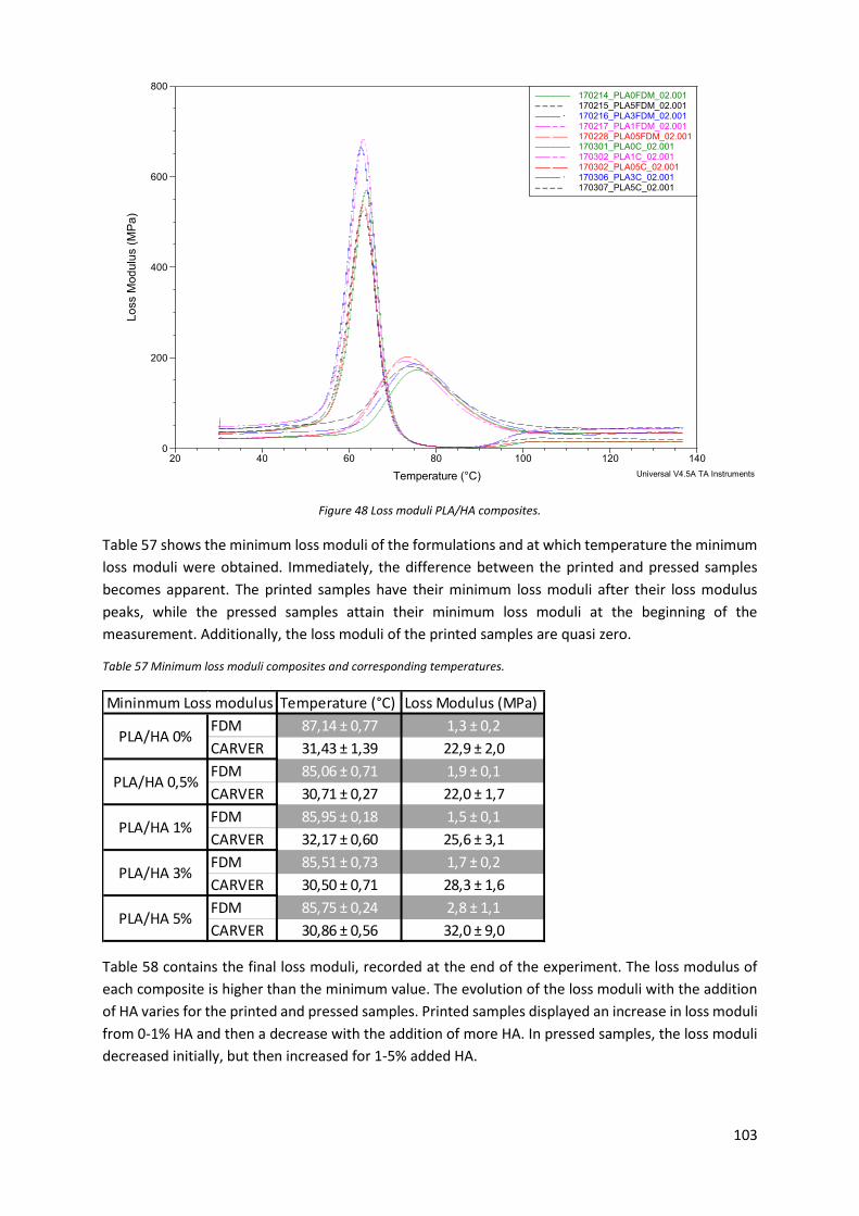
103

Figure 48 Loss moduli PLA/HA composites.

Table 57 shows the minimum loss moduli of the formulations and at which temperature the minimum

loss moduli were obtained. Immediately, the difference between the printed and pressed samples

becomes apparent. The printed samples have their minimum loss moduli after their loss modulus

peaks, while the pressed samples attain their minimum loss moduli at the beginning of the

measurement. Additionally, the loss moduli of the printed samples are quasi zero.

Table 57 Minimum loss moduli composites and corresponding temperatures.

Table 58 contains the final loss moduli, recorded at the end of the experiment. The loss modulus of

each composite is higher than the minimum value. The evolution of the loss moduli with the addition

of HA varies for the printed and pressed samples. Printed samples displayed an increase in loss moduli

from 0-1% HA and then a decrease with the addition of more HA. In pressed samples, the loss moduli

decreased initially, but then increased for 1-5% added HA.

0

200

400

600

800

Lo

ss M

odu

lus (

MP

a)

20 40 60 80 100 120 140

Temperature (°C)

170214_PLA0FDM_02.001––––––– 170215_PLA5FDM_02.001– – – – 170216_PLA3FDM_02.001––––– · 170217_PLA1FDM_02.001––– – – 170228_PLA05FDM_02.001––– ––– 170301_PLA0C_02.001––––––– 170302_PLA1C_02.001––– – – 170302_PLA05C_02.001––– ––– 170306_PLA3C_02.001––––– · 170307_PLA5C_02.001– – – –


Temperature (°C) Loss Modulus (MPa)

FDM 87,14 ± 0,77 1,3 ± 0,2

CARVER 31,43 ± 1,39 22,9 ± 2,0

FDM 85,06 ± 0,71 1,9 ± 0,1

CARVER 30,71 ± 0,27 22,0 ± 1,7

FDM 85,95 ± 0,18 1,5 ± 0,1

CARVER 32,17 ± 0,60 25,6 ± 3,1

FDM 85,51 ± 0,73 1,7 ± 0,2

CARVER 30,50 ± 0,71 28,3 ± 1,6

FDM 85,75 ± 0,24 2,8 ± 1,1

CARVER 30,86 ± 0,56 32,0 ± 9,0PLA/HA 5%

Mininmum Loss modulus

PLA/HA 0%

PLA/HA 0,5%

PLA/HA 1%

PLA/HA 3%

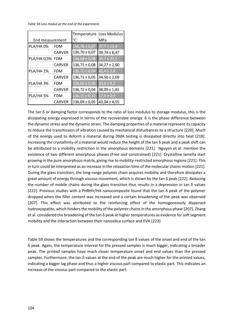
104

Table 58 Loss moduli at the end of the experiment.

The tan δ or damping factor corresponds to the ratio of loss modulus to storage modulus, this is the

dissipating energy expressed in terms of the recoverable energy. δ is the phase difference between

the dynamic stress and the dynamic strain. The damping properties of a material represent its capacity

to reduce the transmission of vibration caused by mechanical disturbances to a structure [220]. Much

of the energy used to deform a material during DMA testing is dissipated directly into heat [218].

Increasing the crystallinity of a material would reduce the height of the tan δ peak and a peak shift can

be attributed to a mobility restriction in the amorphous domains [221]. Nguyen et al. mention the

existence of two different amorphous phases (Free and constrained) [221]. Crystalline lamella start

growing in the pure amorphous matrix, giving rise to mobility-restricted amorphous regions [221]. This

in turn could be interpreted as an increase in the relaxation time of the molecular chains motion [221].

During the glass transition, the long-range polymer chain acquires mobility and therefore dissipates a

great amount of energy through viscous movement, which is shown by the tan δ peak [222]. Reducing

the number of mobile chains during the glass transition thus results in a depression in tan δ values

[222]. Previous studies with a PHBHV/HA nanocomposite found that the tan δ peak of the polymer

dropped when the filler content was increased and a certain broadening of the peak was observed

[207]. This effect was attributed to the reinforcing effect of the homogeneously dispersed

hydroxyapatite, which hinders the mobility of the polymer chains in the amorphous phase [207]. Zhang

et al. considered the broadening of the tan δ peak at higher temperatures as evidence for soft segment

mobility and the interaction between their nanosilica surface and EVA [223].

Table 59 shows the temperatures and the corresponding tan δ values of the onset and end of the tan

δ peak. Again, the temperature interval for the pressed samples is much bigger, indicating a broader

peak. The printed samples have much closer temperature onset and end values than the pressed

samples. Furthermore, the tan δ values at the end of the peak are much higher for the printed values,

indicating a bigger lag phase and thus a higher viscous part compared to elastic part. This indicates an

increase of the viscous part compared to the elastic part.

Temperature Loss Modulus

°C MPa

PLA/HA 0% FDM 136,76 ± 0,07 27,7 ± 13,4

CARVER 136,70 ± 0,07 39,74 ± 8,47

PLA/HA 0,5% FDM 136,68 ± 0,08 35,7 ± 20,1

CARVER 136,71 ± 0,08 34,27 ± 2,00

PLA/HA 1% FDM 136,72 ± 0,04 42,4 ± 2,8

CARVER 136,71 ± 0,05 34,50 ± 2,09

PLA/HA 3% FDM 136,65 ± 0,06 33,6 ± 9,2

CARVER 136,72 ± 0,04 38,09 ± 1,81

PLA/HA 5% FDM 136,71 ± 0,12 17,9 ± 0,9

CARVER 136,69 ± 0,05 43,04 ± 4,55

End measurement

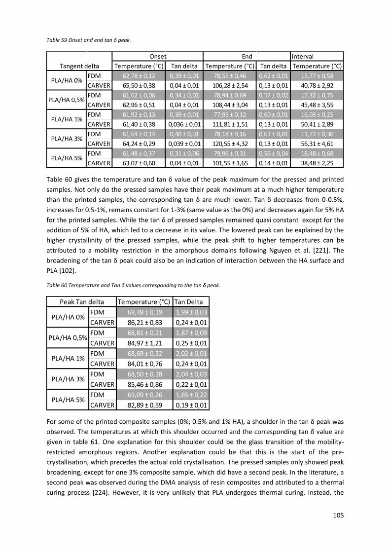
105

Table 59 Onset and end tan δ peak.

Table 60 gives the temperature and tan δ value of the peak maximum for the pressed and printed

samples. Not only do the pressed samples have their peak maximum at a much higher temperature

than the printed samples, the corresponding tan δ are much lower. Tan δ decreases from 0-0.5%,

increases for 0.5-1%, remains constant for 1-3% (same value as the 0%) and decreases again for 5% HA

for the printed samples. While the tan δ of pressed samples remained quasi constant except for the

addition of 5% of HA, which led to a decrease in its value. The lowered peak can be explained by the

higher crystallinity of the pressed samples, while the peak shift to higher temperatures can be

attributed to a mobility restriction in the amorphous domains following Nguyen et al. [221]. The

broadening of the tan δ peak could also be an indication of interaction between the HA surface and

PLA [102].

Table 60 Temperature and Tan δ values corresponding to the tan δ peak.

For some of the printed composite samples (0%; 0.5% and 1% HA), a shoulder in the tan δ peak was

observed. The temperatures at which this shoulder occurred and the corresponding tan δ value are

given in table 61. One explanation for this shoulder could be the glass transition of the mobility-

restricted amorphous regions. Another explanation could be that this is the start of the pre-

crystallisation, which precedes the actual cold crystallisation. The pressed samples only showed peak

broadening, except for one 3% composite sample, which did have a second peak. In the literature, a

second peak was observed during the DMA analysis of resin composites and attributed to a thermal

curing process [224]. However, it is very unlikely that PLA undergoes thermal curing. Instead, the

Interval

Temperature (°C) Tan delta Temperature (°C) Tan delta Temperature (°C)

FDM 62,78 ± 0,12 0,39 ± 0,01 78,55 ± 0,46 0,62 ± 0,01 15,77 ± 0,58

CARVER 65,50 ± 0,38 0,04 ± 0,01 106,28 ± 2,54 0,13 ± 0,01 40,78 ± 2,92

FDM 61,62 ± 0,06 0,34 ± 0,02 78,94 ± 0,69 0,57 ± 0,02 17,32 ± 0,75

CARVER 62,96 ± 0,51 0,04 ± 0,01 108,44 ± 3,04 0,13 ± 0,01 45,48 ± 3,55

FDM 61,92 ± 0,13 0,39 ± 0,01 77,95 ± 0,12 0,60 ± 0,01 16,03 ± 0,25

CARVER 61,40 ± 0,38 0,036 ± 0,01 111,81 ± 1,51 0,13 ± 0,01 50,41 ± 2,89

FDM 61,64 ± 0,14 0,40 ± 0,01 78,18 ± 0,16 0,63 ± 0,01 11,77 ± 0,30

CARVER 64,24 ± 0,29 0,039 ± 0,01 120,55 ± 4,32 0,13 ± 0,01 56,31 ± 4,61

FDM 61,48 ± 0,37 0,31 ± 0,06 79,96 ± 0,31 0,56 ± 0,04 18,48 ± 0,68

CARVER 63,07 ± 0,60 0,04 ± 0,01 101,55 ± 1,65 0,14 ± 0,01 38,48 ± 2,25

PLA/HA 1%

PLA/HA 3%

PLA/HA 5%

Tangent delta

Onset End

PLA/HA 0%

PLA/HA 0,5%

Temperature (°C) Tan Delta

FDM 69,49 ± 0,19 1,99 ± 0,03

CARVER 86,21 ± 0,83 0,24 ± 0,01

FDM 68,81 ± 0,21 1,87 ± 0,09

CARVER 84,97 ± 1,21 0,25 ± 0,01

FDM 68,69 ± 0,32 2,02 ± 0,01

CARVER 84,01 ± 0,76 0,24 ± 0,01

FDM 68,50 ± 0,18 2,04 ± 0,03

CARVER 85,46 ± 0,86 0,22 ± 0,01

FDM 69,09 ± 0,26 1,65 ± 0,22

CARVER 82,89 ± 0,59 0,19 ± 0,01

Peak Tan delta

PLA/HA 0%

PLA/HA 0,5%

PLA/HA 1%

PLA/HA 3%

PLA/HA 5%

106

preceding thermal crystallisation process might have resulted in mobility restricted amorphous phases.

Figure 49 gives a visual representation of the tan δ behaviour of pressed and printed samples.

Table 61 Temperatures and Tan δ values corresponding to the second Tan δ peak.

Figure 49 Tan δ in function of the temperature for the pressed and printed samples.

4.6.3 Conclusion

The results of the DMA analysis showed a different behaviour for the FDM printed and compression

moulded samples. For the storage modulus of the compression moulded samples, the rubber phase

did not display itself as a plateau, while this was the case for the FDM printed samples. Additionally,

despite the annealing process, the FDM printed samples had a higher starting storage modulus. This

could be the result of the alignment caused by the FDM process. The evolution of the onset of the

decrease in storage modulus differed for the FDM printed and pressed samples, while the onset

happened at earlier temperatures until the addition of 1% of HA after which the temperature remained

Temperature (°C) Tan Delta

FDM 87,98 ± 0,92 0,32 ± 0,02

CARVER / /

FDM 84,45 ± 1,53 0,37 ± 0,01

CARVER / /

FDM 86,10 ± 0,18 0,31 ± 0,01

CARVER / /

FDM / /

CARVER / /

FDM / /

CARVER / /

Peak 2 Tan delta

PLA/HA 0%

PLA/HA 0,5%

PLA/HA 1%

PLA/HA 3%

PLA/HA 5%

l l ll

l

l

l

l

l

l

l

l

l

l

l

l

l

l

ll l l l

p p p

p

p

p

p

p

p

p

p

p

p

p

p

p

p

p p p p

ª ª ª ªª

ª

ª ª

ªª ª ª

£ £ £ ££

££

££ £ £ £

0.0

0.5

1.0

1.5

2.0

2.5

Ta

n D

elta

20 40 60 80 100 120 140

Temperature (°C)

170214_PLA0FDM_02.001––––––– 170215_PLA5FDM_02.001– – – – 170301_PLA0C_02.001––––– · 170307_PLA5C_02.001––– – –


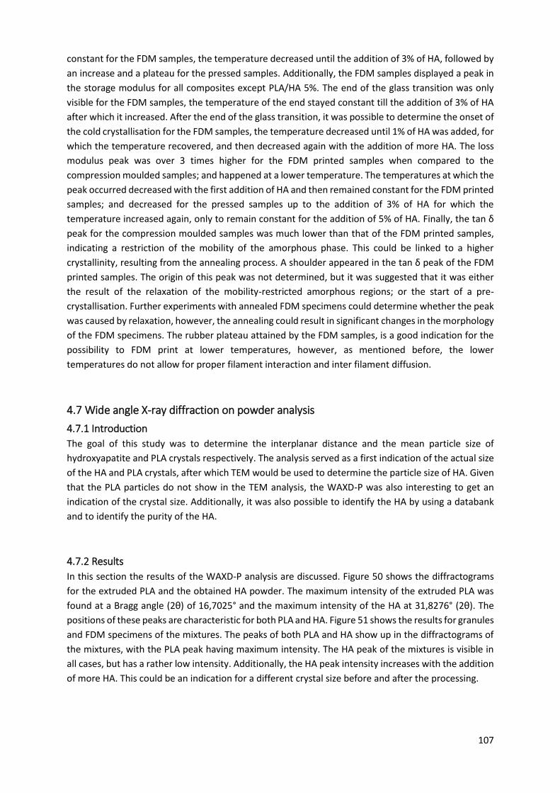
107

constant for the FDM samples, the temperature decreased until the addition of 3% of HA, followed by

an increase and a plateau for the pressed samples. Additionally, the FDM samples displayed a peak in

the storage modulus for all composites except PLA/HA 5%. The end of the glass transition was only

visible for the FDM samples, the temperature of the end stayed constant till the addition of 3% of HA

after which it increased. After the end of the glass transition, it was possible to determine the onset of

the cold crystallisation for the FDM samples, the temperature decreased until 1% of HA was added, for

which the temperature recovered, and then decreased again with the addition of more HA. The loss

modulus peak was over 3 times higher for the FDM printed samples when compared to the

compression moulded samples; and happened at a lower temperature. The temperatures at which the

peak occurred decreased with the first addition of HA and then remained constant for the FDM printed

samples; and decreased for the pressed samples up to the addition of 3% of HA for which the

temperature increased again, only to remain constant for the addition of 5% of HA. Finally, the tan δ

peak for the compression moulded samples was much lower than that of the FDM printed samples,

indicating a restriction of the mobility of the amorphous phase. This could be linked to a higher

crystallinity, resulting from the annealing process. A shoulder appeared in the tan δ peak of the FDM

printed samples. The origin of this peak was not determined, but it was suggested that it was either

the result of the relaxation of the mobility-restricted amorphous regions; or the start of a pre-

crystallisation. Further experiments with annealed FDM specimens could determine whether the peak

was caused by relaxation, however, the annealing could result in significant changes in the morphology

of the FDM specimens. The rubber plateau attained by the FDM samples, is a good indication for the

possibility to FDM print at lower temperatures, however, as mentioned before, the lower

temperatures do not allow for proper filament interaction and inter filament diffusion.

4.7 Wide angle X-ray diffraction on powder analysis

4.7.1 Introduction

The goal of this study was to determine the interplanar distance and the mean particle size of

hydroxyapatite and PLA crystals respectively. The analysis served as a first indication of the actual size

of the HA and PLA crystals, after which TEM would be used to determine the particle size of HA. Given

that the PLA particles do not show in the TEM analysis, the WAXD-P was also interesting to get an

indication of the crystal size. Additionally, it was also possible to identify the HA by using a databank

and to identify the purity of the HA.

4.7.2 Results

In this section the results of the WAXD-P analysis are discussed. Figure 50 shows the diffractograms

for the extruded PLA and the obtained HA powder. The maximum intensity of the extruded PLA was

found at a Bragg angle (2θ) of 16,7025° and the maximum intensity of the HA at 31,8276° (2θ). The

positions of these peaks are characteristic for both PLA and HA. Figure 51 shows the results for granules

and FDM specimens of the mixtures. The peaks of both PLA and HA show up in the diffractograms of

the mixtures, with the PLA peak having maximum intensity. The HA peak of the mixtures is visible in

all cases, but has a rather low intensity. Additionally, the HA peak intensity increases with the addition

of more HA. This could be an indication for a different crystal size before and after the processing.

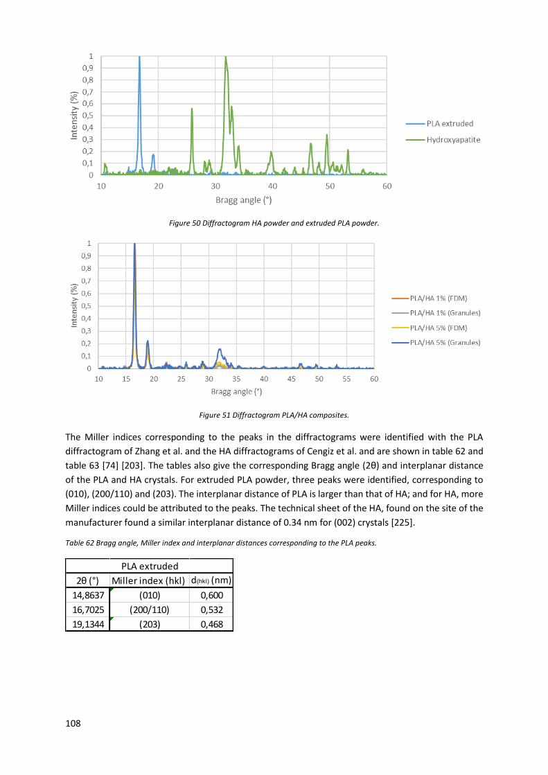
108

Figure 50 Diffractogram HA powder and extruded PLA powder.

Figure 51 Diffractogram PLA/HA composites.

The Miller indices corresponding to the peaks in the diffractograms were identified with the PLA

diffractogram of Zhang et al. and the HA diffractograms of Cengiz et al. and are shown in table 62 and

table 63 [74] [203]. The tables also give the corresponding Bragg angle (2θ) and interplanar distance

of the PLA and HA crystals. For extruded PLA powder, three peaks were identified, corresponding to

(010), (200/110) and (203). The interplanar distance of PLA is larger than that of HA; and for HA, more

Miller indices could be attributed to the peaks. The technical sheet of the HA, found on the site of the

manufacturer found a similar interplanar distance of 0.34 nm for (002) crystals [225].

Table 62 Bragg angle, Miller index and interplanar distances corresponding to the PLA peaks.

2θ (°) Miller index (hkl) d(hkl) (nm)

14,8637 (010) 0,600

16,7025 (200/110) 0,532

19,1344 (203) 0,468

PLA extruded

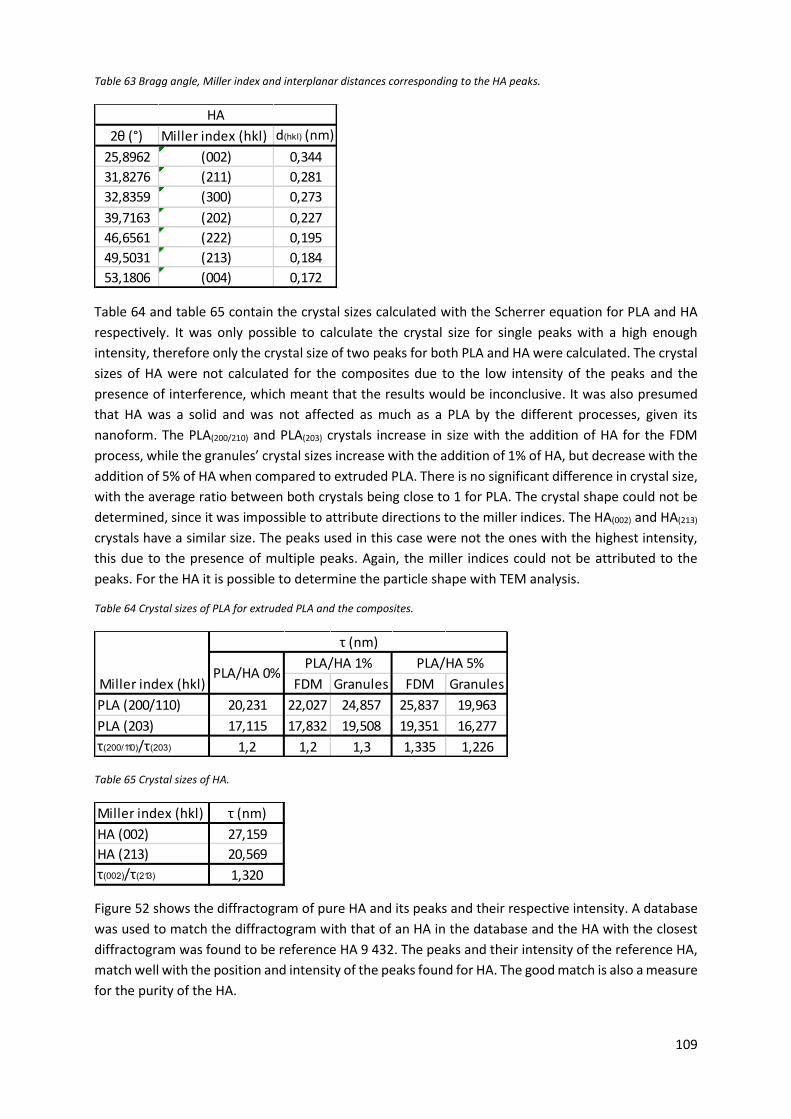
109

Table 63 Bragg angle, Miller index and interplanar distances corresponding to the HA peaks.

Table 64 and table 65 contain the crystal sizes calculated with the Scherrer equation for PLA and HA

respectively. It was only possible to calculate the crystal size for single peaks with a high enough

intensity, therefore only the crystal size of two peaks for both PLA and HA were calculated. The crystal

sizes of HA were not calculated for the composites due to the low intensity of the peaks and the

presence of interference, which meant that the results would be inconclusive. It was also presumed

that HA was a solid and was not affected as much as a PLA by the different processes, given its

nanoform. The PLA(200/210) and PLA(203) crystals increase in size with the addition of HA for the FDM

process, while the granules’ crystal sizes increase with the addition of 1% of HA, but decrease with the

addition of 5% of HA when compared to extruded PLA. There is no significant difference in crystal size,

with the average ratio between both crystals being close to 1 for PLA. The crystal shape could not be

determined, since it was impossible to attribute directions to the miller indices. The HA(002) and HA(213)

crystals have a similar size. The peaks used in this case were not the ones with the highest intensity,

this due to the presence of multiple peaks. Again, the miller indices could not be attributed to the

peaks. For the HA it is possible to determine the particle shape with TEM analysis.

Table 64 Crystal sizes of PLA for extruded PLA and the composites.

Table 65 Crystal sizes of HA.

Figure 52 shows the diffractogram of pure HA and its peaks and their respective intensity. A database

was used to match the diffractogram with that of an HA in the database and the HA with the closest

diffractogram was found to be reference HA 9 432. The peaks and their intensity of the reference HA,

match well with the position and intensity of the peaks found for HA. The good match is also a measure

for the purity of the HA.

2θ (°) Miller index (hkl) d(hkl) (nm)

25,8962 (002) 0,344

31,8276 (211) 0,281

32,8359 (300) 0,273

39,7163 (202) 0,227

46,6561 (222) 0,195

49,5031 (213) 0,184

53,1806 (004) 0,172

HA

FDM Granules FDM Granules

PLA (200/110) 20,231 22,027 24,857 25,837 19,963

PLA (203) 17,115 17,832 19,508 19,351 16,277

τ(200/110)/τ(203) 1,2 1,2 1,3 1,335 1,226

τ (nm)

PLA/HA 0%Miller index (hkl)

PLA/HA 1% PLA/HA 5%

Miller index (hkl) τ (nm)

HA (002) 27,159

HA (213) 20,569

τ(002)/τ(213) 1,320

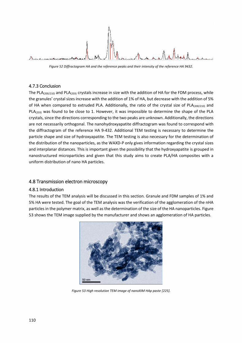
110

Figure 52 Diffractogram HA and the reference peaks and their intensity of the reference HA 9432.

4.7.3 Conclusion

The PLA(200/210) and PLA(203) crystals increase in size with the addition of HA for the FDM process, while

the granules’ crystal sizes increase with the addition of 1% of HA, but decrease with the addition of 5%

of HA when compared to extruded PLA. Additionally, the ratio of the crystal size of PLA(200/210) and

PLA(203) was found to be close to 1. However, it was impossible to determine the shape of the PLA

crystals, since the directions corresponding to the two peaks are unknown. Additionally, the directions

are not necessarily orthogonal. The nanohydroxyapatite diffractogram was found to correspond with

the diffractogram of the reference HA 9-432. Additional TEM testing is necessary to determine the

particle shape and size of hydroxyapatite. The TEM testing is also necessary for the determination of

the distribution of the nanoparticles, as the WAXD-P only gives information regarding the crystal sizes

and interplanar distances. This is important given the possibility that the hydroxyapatite is grouped in

nanostructured microparticles and given that this study aims to create PLA/HA composites with a

uniform distribution of nano HA particles.

4.8 Transmission electron microscopy

4.8.1 Introduction

The results of the TEM analysis will be discussed in this section. Granule and FDM samples of 1% and

5% HA were tested. The goal of the TEM analysis was the verification of the agglomeration of the nHA

particles in the polymer matrix, as well as the determination of the size of the HA nanoparticles. Figure

53 shows the TEM image supplied by the manufacturer and shows an agglomeration of HA particles.

Figure 53 High resolution TEM image of nanoXIM HAp paste [225].

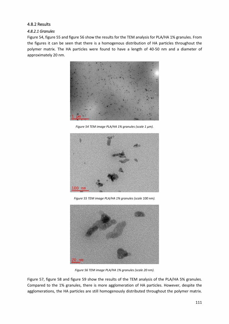
111

4.8.2 Results

4.8.2.1 Granules

Figure 54, figure 55 and figure 56 show the results for the TEM analysis for PLA/HA 1% granules. From

the figures it can be seen that there is a homogenous distribution of HA particles throughout the

polymer matrix. The HA particles were found to have a length of 40-50 nm and a diameter of

approximately 20 nm.

Figure 54 TEM image PLA/HA 1% granules (scale 1 µm).

Figure 55 TEM image PLA/HA 1% granules (scale 100 nm).


Figure 57, figure 58 and figure 59 show the results of the TEM analysis of the PLA/HA 5% granules.

Compared to the 1% granules, there is more agglomeration of HA particles. However, despite the

agglomerations, the HA particles are still homogenously distributed throughout the polymer matrix.

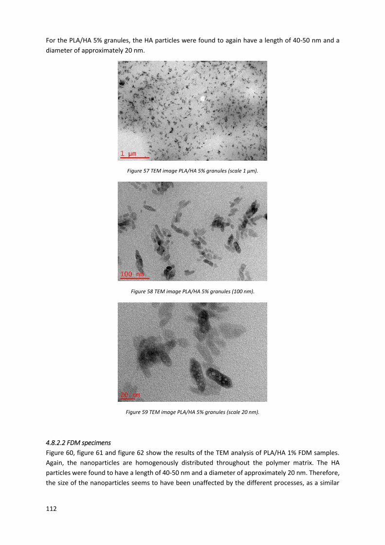
112

For the PLA/HA 5% granules, the HA particles were found to again have a length of 40-50 nm and a

diameter of approximately 20 nm.

Figure 57 TEM image PLA/HA 5% granules (scale 1 µm).

Figure 58 TEM image PLA/HA 5% granules (100 nm).



Figure 60, figure 61 and figure 62 show the results of the TEM analysis of PLA/HA 1% FDM samples.

Again, the nanoparticles are homogenously distributed throughout the polymer matrix. The HA

particles were found to have a length of 40-50 nm and a diameter of approximately 20 nm. Therefore,

the size of the nanoparticles seems to have been unaffected by the different processes, as a similar

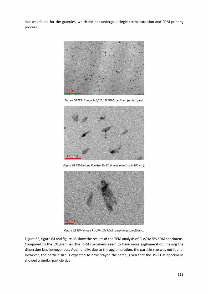
113

size was found for the granules, which did not undergo a single-screw extrusion and FDM printing

process.

Figure 60 TEM image PLA/HA 1% FDM specimen (scale 1 µm).

Figure 61 TEM image PLA/HA 1% FDM specimen (scale 100 nm).


Figure 63, figure 64 and figure 65 show the results of the TEM analysis of PLA/HA 5% FDM specimens.

Compared to the 5% granules, the FDM specimens seem to have more agglomeration, making the

dispersion less homogenous. Additionally, due to the agglomeration, the particle size was not found.

However, the particle size is expected to have stayed the same, given that the 1% FDM specimens

showed a similar particle size.

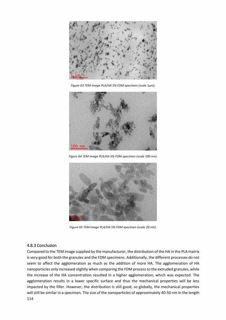
114

Figure 63 TEM image PLA/HA 5% FDM specimen (scale 1µm).



4.8.3 Conclusion

Compared to the TEM image supplied by the manufacturer, the distribution of the HA in the PLA matrix

is very good for both the granules and the FDM specimens. Additionally, the different processes do not

seem to affect the agglomeration as much as the addition of more HA. The agglomeration of HA

nanoparticles only increased slightly when comparing the FDM process to the extruded granules, while

the increase of the HA concentration resulted in a higher agglomeration, which was expected. The

agglomeration results in a lower specific surface and thus the mechanical properties will be less

impacted by the filler. However, the distribution is still good, so globally, the mechanical properties

will still be similar in a specimen. The size of the nanoparticles of approximately 40-50 nm in the length

115

and 20 nm for the diameter indicates that each particle is composed of one to two crystals, when

considering that the Scherrer calculation resulted in a crystal size of 27.159 nm for the (002) crystals

and 20.569 nm for the (213) crystals. It can thus be supposed that the particles are mono- or bi-

crystalline.

4.9 Permeability tests

4.9.1 Introduction

In this section, the results of the permeability tests will be discussed. Compression moulded films of

the formulations were tested for WVTR and OTR. The results of the permeability tests were used to

verify the influence of the HA content on the WVTR and OTR.

4.9.2 Results

Table 66 shows the results of the WVTR tests. The table shows that the first addition of HA increases

the WVTR, adding 3% of HA results in a recovery to the WVTR of PLE 005, adding 5% of HA results in

another increase and adding 10% of HA results in a decrease in WVTR up to values under that of the

PLE 005. The initial increase in WVTR, could be due to the degradation caused by extrusion. The

recovery of the WVTR with the addition of 3% and more HA, could be linked to the crystallinity. Tsuji

et al. found that the WVTR of PLA decreased monotonically with the addition of HA [163].

Table 66 WVTR values found for the PLA/HA composites and PLE 005.

Table 67 shows the results of the OTR tests. The OTR of PLA decreases with the addition of HA.

Additionally, the OTR decreased over time, which was especially notable for the PLE 005. The

difference between PLE 005 and the HA composites can be explained by the higher molar weight of

the PLE 005.

Table 67 OTR values PLA/HA composites and PLE 005.

4.9.3 Conclusion

The addition of nHA to PLA does not seem to affect the WVTR and the OTR greatly. For PLA, an

interesting behaviour was observed during the testing, the OTR decreased over time for repeated

measurements on the same sample, especially for the neat PLA. Under 38°C and 50% RH, the neat PLA

also displayed an interesting behaviour for the WVTR, given that the WVTR was found to be lower

WVTR (g*mm/[m²*day*bar])

PLE 005 124

PLA/HA 0,5% 136

PLA/HA 3% 124

PLA/HA 5% 128

PLA/HA 10% 118

OTR

Sample 1 Sample 2 Sample 1 Sample 2 cc/[m²-day]

PLE 005 93,8 ± 1,4 94,2 ± 1,9 15,14 14,68 178,2 ± 3,0

PLA/HA 5% 92,3 ± 2,1 90,3 ± 3,1 14,07 14,44 161,5 ± 4,6

PLA/HA 10% 93,6 ± 1,5 93,3 ± 1,5 14,77 14,44 152,0 ± 0,1

Thickness (µm) Test area (cm²)

116

compared to WVTR tests at 23°C and 50% RH. Given the low impact of the nHA on the OTR and the

WVTR, nHA cannot be used to control the permeability of PLA, this would have been interesting for

BTE and packaging applications.

117

5 Conclusion The first goal of this study was to formulate PLA/nHA (0 wt.%; 0.5 wt.%; 1 wt.%; 3 wt.% and 5 wt.%)

nanocomposites from polylactide acid and an aqueous hydroxyapatite paste. This was done

successfully, by melt mixing PLA and nHA in a twin-screw extruder. To achieve the second goal, the

application of the nanocomposites in fused deposition modelling and injection moulding, the

composites were turned into filaments with a single-screw extruder. After which the filaments were

used in fused deposition modelling, with 7 different printing conditions, as described by the doehler

matrix.

The characterisation of the obtained materials was the third goal of this study. The hydroxyapatite

content before and after each process was verified with a thermogravimetric analysis and the results

indicated that after each process, the hydroxyapatite content was slightly reduced. Processes also

affected the degradation profile of the different formulations, with the degradation starting the

earliest for the filaments. Differential scanning calorimetry was used to determine the minimum

printing temperature for the fused deposition modelling process. However, the minimum temperature

of 183.4°C did not correspond to the actual minimum printing temperature, as printing temperatures

were required to exceed 190°C for certain formulations. This was attributed to the difference in

heating ramp between the analysis and the printing process. Oscillatory rheology results showed that

the extrusion and the addition of hydroxyapatite both influence the viscosity. The extrusion resulted

in a reduction of the viscosity, due to the reduction of the molar mass, while the first addition of HA

increases the viscosity of the extruded PLA, after which the viscosity decreases gradually with the

addition of more HA. Additionally, there was also a thinning effect after 3% of HA was added. The

evolution of the viscosity was linked to the fused deposition printing process and it was suggested that

the viscosity decreases for higher printing speeds. Consequently, there is no risk of nozzle clogging

when using PLA with a high HA content during the FDM printing process, which was suggested by the

literature. Finally, dynamic mechanical analysis indicated that the storage modulus of fused deposition

modelling printed samples was higher, when compared to compression moulded samples. It was

suggested that the higher storage modulus was the result of alignment caused by the fused deposition

modelling process.

The fourth goal of this study was the comparison of the impact of the fused deposition modelling

process and injection moulding on the tensile properties of the composites. Doehlert response surface

methodology was used to determine the impact of the fused deposition modelling process on the

tensile properties. However, the used model was found to be inadequate to describe the evolution of

the tensile properties of all formulations. The tensile test results of the injection moulded samples

showed that the tensile properties of these samples were much higher when compared to samples

obtained by fused deposition modelling process. Although the printing parameters used during the

fused deposition modelling process did influence the tensile properties, the lower tensile properties

were mainly attributed to the process given that it introduced a lot of faults into the tensile specimens.

Determining the dispersion state of the nano-charges in the polymer matrix was the fifth goal of this

study. A combination of x-ray diffraction analysis and transmission electron microscopy was used to

determine the dispersion of the nano-charges. The x-ray diffraction analysis also allowed for the

118

identification of the used hydroxyapatite, which was found to be HA 9-432 (reference). The crystal size

of HA was found to be 27.159 nm for (002) HA crystals and 20.569 nm for (213) HA crystals. TEM

analysis showed that the HA particles were 40-50 nm long and had a diameter of approximately 20

nm, from which it was concluded that the particles were mono- or bicrystalline. Additionally, for both

the granules and the FDM process, the dispersion was found to have improved when compared to the

TEM image supplied by the manufacturer.

The final objectives of this study were the creation of composite films and the testing of the

permeability of these films. A heated press was successfully used to create composite films with an

average thickness of 90 µm. However, the results of the WVTR and the OTR tests showed that the HA

did not have a major impact on these properties.

In perspective, the results of this study can be used as starting points for future research. Doehlert

response surface methodology indicated that the used model for the characterisation of the tensile

properties of fused deposition modelling specimens was inadequate. Therefore, future studies can

focus on the determination of the exact model. Additionally, more tests are needed with regards to

the influence of the parameters used in the fused deposition modelling process on the process.

Especially the control of the porosity, measured by tomography, could be an interesting study, given

that this would be of interest for bone tissue engineering applications. The tensile tests were used to

study the bonding quality of the FDM printed samples, but for BTE compression tests are more used,

since this is the type of strain will be applied to the implants. The use of hydroxyapatite microcharges

in the fused deposition modelling process could also be tested, this would greatly reduce the cost.

Additionally, the micro charges could impact the material differently, however, nozzle clogging is a

very real threat, since micro charges are much larger and can more easily obstruct the nozzle. Dynamic

mechanical analysis resulted in a higher storage modulus for the fused deposition modelling printed

samples, which was surprising and thus requires more testing to validate and understand this

phenomenon. Finally, the results of the oscillatory rheology indicate a complex behaviour with the

addition of hydroxyapatite. More tests are needed, at different temperatures and using capillary

rheology. A time temperature superposition is needed to model the rheological behaviour; this was

difficult to obtain with the oscillatory rheometer due to the flowing of the polymer material. The

capillary rheometer is needed to model the behaviour at higher shear rates and temperatures.

119

References

[1] Université de Reims Champagne-Ardenne, “Laboratory of Engineering and Materials

Sciences (LISM - EA 4695),” [Online]. Available: http://www.univ-reims.eu/about-the-

university/organisation/organisation,77,18761.html?&args=bl3P8HNScfah65Uek-

amZ3pu4GPo7H2TaI_qTyAn0FRSQJsWGb61Uw1V_7X1Ji_3cmFA1GMa4KqDRaUhgRZ_qA.

[Accessed 1 March 2017].

[2] G. Ginoux, “PolyFabAdd - Polymères chargés en fabrication additive,” [Online]. Available:

http://www.theses.fr/s143395. [Accessed 1 March 2017].

[3] I. Armentano, N. Bitinis, E. Fortunati, S. Mattioli, N. Rescignano, R. Verdejo, M. A. Lopez-

Manchado and J. M. Kenny, “Multifunctional nanostructured PLA materials for packaging

and tissue engineering,” Progress in Polymer Science, vol. 38, no. 10-11, pp. 1720-1747,

2013.

[4] B. N. Turner and S. A. Gold, “A review of melt extrusion additive manufacturing processes:

II. Materials, dimensional accuracy, and surface roughness,” Rapid Prototyping Journal;

Bradford, vol. 21, no. 3, pp. 261-250, 2015.

[5] B. N. Turner, R. Strong and S. A. Gold, “A review of melt extrusion additive manufacturing

processes: I. Process design and modeling,” Rapid Prototyping Journal; Bradford, vol. 20,

no. 3, pp. 192-204, 2014.

[6] A. K. Sood, R. K. Ohdar and S. S. Mahapatra, “Parametric appraisal of mechanical property

of fused deposition modelling processed parts,” Materials & Design, vol. 31, no. 1, pp. 287-

295, 2010.

[7] O. S. Carneiro, A. F. Silva and R. Gomes, “Fused deposition modeling with polypropylene,”

Materials & Design, vol. 83, pp. 768-776, 2015.

[8] Anonymous, “3D Printing Materials | Stratasys,” [Online]. Available:

http://www.stratasys.com/materials. [Accessed 22 March 2017].

[9] Anonymous, “FDM materials: PLA and ABS,” [Online]. Available:

https://3faktur.com/en/3d-printing-materials-technologies/fdm-materials-pla-and-abs/.

[Accessed 22 March 2017].

[10] Anonymous, “Materialise,” [Online]. Available:

http://www.materialise.com/en/manufacturing/technologies-materials/fused-deposition-

modeling. [Accessed 3 March 2017].

[11] Anonymous, “Page 2 | 3d Printer Filaments Shop | Nexeo 3D,” [Online]. Available:

https://www.nexeo3d.com/en/products.html?%3Fgclid=CL2GruTd6NICFcSfGwod8JgItQ&p

=2. [Accessed 3 March 2017].

[12] F. Rayegani and G. C. Onwubolu, “Fused deposition modelling (FDM) process parameter

prediction and optimization using group method for data handling (GMDH) and differential

evolution (DE),” The International Journal of Advanced Manufacturing Technology, vol. 73,

no. 1-4, pp. 509-519, 2014.

120

[13] A. Mahboubi Soufiani, M. Salehi, M. Skrifvars, M. Persson and S.-W. Cho,

“Thermomechanical properties of poly(lactic acid) films reinforced with hydroxyapatite

and regenerated cellulose microfibers,” Journal of Applied Polymer Science, vol. 131, no.

20, p. n/a, 2014.

[14] O. A. Mohamed, S. H. Masood, J. L. Bhowmik, M. Nikzad and J. Azadmanjiri, “Effect of

Process Parameters on Dynamic Mechanical Performance of FDM PC/ABS Printed Parts

Through Design of Experiment,” Journal of Materials Engineering and Performance, vol. 25,

no. 7, pp. 2922-2935, 2016.

[15] J. Torres, J. Cotelo, J. Karl and A. P. Gordon, “Mechanical Property Optimization of FDM

PLA in Shear with Multiple Objectives,” The Journal of The Minerals, Metals & Materials

Society (TMS), vol. 67, no. 5, pp. 1183-1193, 2015.

[16] O. Ivanova, C. Williams and T. Campbell, “Additive manufacturing (AM) and

nanotechnology: promises and challenges,” Rapid Prototyping Journal; Bradford, vol. 19,

no. 5, pp. 353-364, 2013.

[17] Q. Yao, B. Wei, Y. Guo, C. Jin, X. Du, C. Yan, J. Yan, W. Hu, Y. Xu, Z. Zhou, Y. Wang and L.

Wang, “Design, construction and mechanical testing of digital 3D anatomical data-based

PCL-HA bone tissue engineering scaffold,” Journal of Materials Science : Materials in

Medicine, vol. 26, no. 1, pp. 1-9, 2015.

[18] G. Wei and P. X. Ma, “Structure and properties of nano-hydroxyapatite/polymer composite

scaffolds for bone tissue engineering,” Biomaterials, vol. 25, no. 19, pp. 4749-4757, 2004.

[19] E. Nejati, H. Mirzadeh and M. Zandi, “Synthesis and characterization of nano-

hydroxyapatite rods/poly(l-lactide acid) composite scaffolds for bone tissue engineering,”

Composites Part A: Applied Science and Manufacturing, vol. 30, no. 10, pp. 1589-1596,

2008.

[20] H.-T. Liao, C. Yo-Yu, L. Yu-Ting, M.-F. Hsieh and J. Cho-Pei, “The Osteogenesis of Bone

Marrow Stem Cells on mPEG-PCL-mPEG/Hydroxyapatite Composite Scaffold via Solid

Freeform Fabrication,” BioMed Research International, vol. 2014, p. 13, 2014.

[21] A. B. Kutkov and J. Song, “An amphiphilic degradable polymer/hydroxyapatite composite

with enhanced handling characteristics promotes osteogenic gene expression in bone

marrow stromal cells,” Acta Biomaterialia, vol. 9, no. 9, pp. 8354-8364, 2013.

[22] L. Han, C. Han, H. Zhang, S. Chen and L. Dong, “Morphology and properties of

biodegradable and biosourced polylactide blends with poly(3-hydroxybutyrate-co-4-

hydroxybutyrate),” Polymer Composites, vol. 33, no. 6, pp. 850-859, 2012.

[23] Y. Guo, K. Yang, X. Zuo, Y. Xue, C. Marmorat, Y. Liu, C.-C. Chang and M. H. Rafailovich,

“Effects of clay platelets and natural nanotubes on mechanical properties and gas

permeability of Poly (lactic acid) nanocomposites,” Polymer, vol. 83, pp. 246-259, 2016.

[24] E. Picard, E. Espuche and R. Fulchiron, “Effect of an organo-modified montmorillonite on

PLA crystallization and gas barrier properties,” Applied Clay Science, vol. 53, no. 1, pp. 58-

65, 2011.

121

[25] T. Iwata, “Biodegradable and Bio-Based Polymers: Future Prospects of Eco-Friendly

Plastics,” Angewandte Chemie INternational Edition, vol. 54, no. 11, pp. 3210-3215, 2015.

[26] K. Van de Velde and P. Kiekens, “Biopolymers: overview of several properties and

consequences on their applications,” Polymer Testing, vol. 21, no. 4, pp. 433-442, 2002.

[27] M. Patel, F. Marscheider-Weidemann, J. Schleich, B. Hüsing and G. Angerer, “Techno-

economic feasibility of large-scale production of bio-based polymers in Europe,” Technical

Report EUR 22103 EN, 2005.

[28] D. K. Platt, Biodegradable Polymers: Market report, Shrewsbury, UK: Smithers Rapra

Limited, 2006.

[29] M. Jamshidian, E. A. Tehrany, M. Imran, M. Jacquot and S. Desobry, “Poly-Lactic Acid:

Production, Applications, Nanocomposites, and Release Studies,” Comprehensive Reviews

in Food Science and Food Safety, vol. 9, no. 5, pp. 552-571, 2010.

[30] M. Murariu and P. Dubois, “PLA composites: From production to properties,” Advanced

Drug Delivery Reviews, vol. 107, no. 15, pp. 17-46, 2016.

[31] K. Madhavan Nampoothiri, N. R. Nair and R. P. John, “An overview of the recent

developments in polylactide (PLA) research,” Bioresource Technology, vol. 101, no. 22, pp.

8493-8501, 2010.

[32] L.-T. Lim, R. Auras and M. Rubino, “Processing technologies for poly(lactic acid),” Progress

in Polymer Science, vol. 33, no. 8, pp. 820-852, 2008.

[33] R. Auras, B. Harte and S. Selke, “An Overview of Polylactides as Packaging Materials,”

Macromolecular Bioscience, vol. 4, no. 9, pp. 835-864, 2004.

[34] E. T. Vink, K. R. Rábago, D. A. Glassner and P. R. Gruber, “Applications of life cycle

assessment to NatureWorks™ polylactide (PLA) production,” Polymer Degradation and

Stability, vol. 80, no. 3, pp. 403-419, 2003.

[35] A. J. R. Lasprilla, G. A. R. Martinez, B. H. Lunelli, A. L. Jardini and R. M. Filho, “Poly-lactic

acid synthesis for application in biomedical devices — A review,” Biotechnology Advances,

vol. 30, no. 1, pp. 321-328, 2012.

[36] S. Farah, D. G. Anderson and R. Langer, “Physical and mechanical properties of PLA, and

their functions in widespread applications — A comprehensive review,” Advanced Drug

Delivery Reviews, 2016.

[37] A. Södergård and M. Stolt, “Properties of lactic acid based polymers and their correlation

with composition,” Progress in Polymer Science, vol. 27, no. 6, pp. 1123-1163, 2002.

[38] M. L. Di Lorenzo, “Crystallization behavior of poly(l-lactic acid),” European Polymer Journal,

vol. 41, no. 3, pp. 569-575, 2005.

[39] J. Puiggali, Y. Ikada, H. Tsuji, L. Cartier, T. Okihara and B. Lotz, “The frustrated structure of

poly(l-lactide),” Polymer, vol. 41, no. 25, pp. 8921-8930, 2000.

122

[40] L. Cartier, T. Okihara, Y. Ikada, H. Tsuji, J. Puiggali and B. Lotz, “Epitaxial crystallization and

crystalline polymorphism of polylactides,” Polymer, vol. 41, no. 25, pp. 8909-8919, 2000.

[41] B. Gupta, N. Revagade and J. Hilborn, “Poly(lactic acid) fiber: An overview,” Progress in

Polymer Science, vol. 32, no. 4, pp. 455-482, 2007.

[42] J. Lunt, “Large-scale production, properties and commercial applications of polylactic acid

polymers,” Polymer Degradation and Stability, vol. 59, no. 1-3, pp. 145-152, 1998.

[43] J. A. Cicero, J. R. Dorgan, J. Garrett, J. Runt and J. S. Lin, “Effects of molecular architecture

on two-step, melt-spun poly(lactic acid) fibers,” Journal of Applied Polymer Science, vol. 86,

no. 11, pp. 2839-2846, 2002.

[44] J. A. Cicero, J. R. Dorgan, J. Garrett, J. Runt and J. S. Lin, “Supramolecular morphology of

two-step, melt-spun poly(lactic acid) fibers,” Journal of Applied Polymer Science, vol. 86,

no. 11, pp. 2828-2838, 2002.

[45] K. S. Anderson and M. A. Hillmyer, “Melt preparation and nucleation efficiency of

polylactide stereocomplex crystallites,” Polymer, vol. 47, no. 6, pp. 2030-2035, 2006.

[46] H. Urayama, S.-I. Moon and Y. Kimura, “Microstructure and Thermal Properties of

Polylactides with Different L- and D-Unit Sequences: Importance of the Helical Nature of

the L-Sequenced Segments,” Macromolecular Materials and Engineering, vol. 288, no. 2,

pp. 137-143, 2003.

[47] H. Urayama, T. Kanamori and Y. Kimura, “Properties and Biodegradability of Polymer

Blends of Poly(L-lactide)s with Different Optical Purity of the Lactate Units,”

Macromolecular Materials and Engineering, vol. 287, no. 2, pp. 116-121, 2002.

[48] F. Carrasco, P. Pagès, J. Gámez-Pérez, O. Santana and M. Maspoch, “Processing of

poly(lactic acid): Characterization of chemical structure, thermal stability and mechanical

properties,” Polymer Degradation and Stability, vol. 95, no. 2, pp. 116-125, 2010.

[49] L. Petersson, I. Kvien and K. Oksman, “Structure and thermal properties of poly(lactic

acid)/cellulose whiskers nanocomposite materials,” Composites Science and Technology,

vol. 67, no. 11-12, pp. 2535-2544, 2007.

[50] P. Mróz, S. Białas, M. Mucha and H. Kaczmarek, “Thermogravimetric and DSC testing of

poly(lactic acid) nanocomposites,” Thermochimica Acta, vol. 573, pp. 186-192, 2013.

[51] G. Ozkoc and S. Kemaloglu, “Morphology, biodegradability, mechanical, and thermal

properties of nanocomposite films based on PLA and plasticized PLA,” Journal of Applied


[52] Z. Kulinski and E. Piorkowska, “Crystallization, structure and properties of plasticized poly(l-

lactide),” Polymer, vol. 46, no. 23, pp. 10290-10300, 2005.

[53] Z. Liu, Y. Chen and W. Ding, “Preparation, dynamic rheological behavior, crystallization,

and mechanical properties of inorganic whiskers reinforced polylactic acid/hydroxyapatite

nanocomposites,” Journal of Applied Polymer Science, vol. 133, no. 18, 2016.

123

[54] D. Garlotta, “A Literature Review of Poly(Lactic Acid),” Journal of Polymers and the

Environment, vol. 9, no. 2, pp. 63-84, 2001.

[55] C. Migliaresi, D. Cohn, A. De Lollis and L. Fambri, “Dynamic mechanical and calorimetric

analysis of compression-molded PLLA of different molecular weights: Effect of thermal

treatments,” Journal of Applied Polymer Science, vol. 43, no. 1, pp. 83-95, 1991.

[56] F. Signori, M.-B. Coltelli and S. Bronco, “Thermal degradation of poly(lactic acid) (PLA) and

poly(butylene adipate-co-terephthalate) (PBAT) and their blends upon melt processing,”

Polymer Degradation and Stability, vol. 94, no. 1, pp. 74-82, 2009.

[57] V. Taubner and R. Shishoo, “Influence of processing parameters on the degradation of

poly(L-lactide) during extrusion,” Journal of Applied Polymer Science, vol. 79, no. 12, pp.

2128-2135, 2001.

[58] S.-H. Hyon, K. Jamshidi and Y. Ikada, “Effects of residual monomer on the degradation of

DL-lactide polymer,” Polymer International, vol. 46, no. 3, pp. 196-202, 1998.

[59] H. Yu, N. Huang, C. Wang and Z. Tang, “Modeling of poly(L-lactide) thermal degradation:

Theoretical prediction of molecular weight and polydispersity index,” Journal of Applied


[60] M. Vert, D. Yoshiharu, K.-H. Hellwich, M. Hess, P. Hodge, K. Przemyslaw, M. Rinaudo and F.

Schué, “Terminology for biorelated polymers and applications (IUPAC Recommendations

2012),” Pure and Applied Chemistry, vol. 84, no. 2, pp. 377-410, 2012.

[61] S. Grima, V. Bellon-Maurel, P. Feuilloley and F. Silvestre, “Aerobic Biodegradation of

Polymers in Solid-State Conditions: A Review of Environmental and Physicochemical

Parameter Settings in Laboratory Simulations,” Journal of Polymers and the Environment,

vol. 8, no. 4, pp. 183-195, 2000.

[62] L. Avérous and E. Pollet, Environmental Silicate Nano-Biocomposites, London: Springer

London, 2012.

[63] R. Chandra and R. Rustgi, “Biodegradable Polymers,” Progress in Polymer Science, vol. 23,

no. 7, pp. 1273-1335, 1998.

[64] G. E. Luckachan and C. K. S. Pillai, “Biodegradable Polymers- A Review on Recent Trends

and Emerging Perspectives,” Journal of Polymers and the Environment, vol. 19, no. 3, pp.

637-676, 2011.

[65] T. Suyama, Y. Tokiwa, P. Ouichanpagdee, T. Kanagawa and Y. Kamagata, “Phylogenetic

Affiliation of Soil Bacteria That Degrade Aliphatic Polyesters Available Commercially as

Biodegradable Plastics,” Applied and Environmental Microbiology, vol. 64, no. 12, pp.

5008-5011, 1998.

[66] G. Kale, R. Auras, S. P. Singh and R. Narayan, “Biodegradability of polylactide bottles in real

and simulated composting conditions,” Polymer Testing, vol. 26, no. 8, pp. 1049-1061,

2007.

124

[67] Y. Oda, A. Yonetsu, T. Urakami and K. Tonomura, “Degradation of polylactide by

commercial proteases,” Journal of Polymers and the Environment, vol. 8, no. 1, pp. 29-32,

2000.

[68] H.-A. Lim, T. Raku and Y. Tokiwa, “Hydrolysis of polyesters by serine proteases,”

Biotechnology Letters, vol. 27, no. 7, pp. 459-464, 2005.

[69] Y. Tokiwa and B. P. Calabia, “Biodegradability and biodegradation of poly(lactide),” Applied

Microbiology and Biotechnology, vol. 72, no. 2, pp. 244-251, 2006.

[70] H. Tsuji, H. Daimon and K. Fujie, “A New Strategy for Recycling and Preparation of Poly(L-

lacticacid): Hydrolysis in the Melt,” Biomacromolecules, vol. 4, no. 3, pp. 835-840, 2003.

[71] V. Piemonte and F. Gironi, “Kinetics of Hydrolytic Degradation of PLA,” Journal of Polymers

and the Environment, vol. 21, no. 2, pp. 313-318, 2013.

[72] A. Carné Sánchez and S. R. Collinson, “The selective recycling of mixed plastic waste of

polylactic acid and polyethylene terephthalate by control of process conditions,” European

Polymer Journal, vol. 47, no. 10, pp. 1970-1976, 2011.

[73] J. W. Rink, “Apatite,” in Encyclopedia of Scientific Dating Methods, Dordrecht, Springer

Netherlands, 2015, pp. 53-54.

[74] B. Cengiz, Y. Gokce, N. Yildiz, Z. Aktas and A. Calimli, “Synthesis and characterization of

hydroxyapatite nanoparticles,” Colloids and Surfaces A: Physicochemical and Engineering

Aspects, vol. 322, no. 1-3, pp. 29-33, 2008.

[75] F. Wang, M.-S. Li, Y.-P. Lu, Y.-X. Qi and Y.-X. Liu, “Synthesis and microstructure of

hydroxyapatite nanofibers synthesized at 37°C,” Materials Chemistry and Physics, vol. 95,

no. 1, pp. 145-149, 2006.

[76] C.-C. Chen, J.-Y. Chueh, H. Tseng, H.-M. Huang and S.-Y. Lee, “Preparation and

characterization of biodegradable PLA polymeric blends,” Biomaterials, vol. 24, no. 7, pp.

1167-1173, 2003.

[77] X. Su, K. Sun, F. Z. Cui and W. J. Landis, “Organization of apatite crystals in human woven

bone,” Bone, vol. 32, no. 2, pp. 150-162, 2003.

[78] M. Maas, U. Hess and K. Rezwan, “The contribution of rheology for designing

hydroxyapatite biomaterials,” Current Opinion in Colloid & Interface Science, vol. 19, no. 6,

pp. 585-593, 2014.

[79] M.-O. Montjovent, L. Mathieu, H. Schmoekel, S. Mark, P.-E. Bourban, P.-Y. Zambelli, L. A.

Laurent-Applegate and D. P. Pioletti, “Repair of critical size defects in the rat cranium using

ceramic-reinforced PLA scaffolds obtained by supercritical gas foaming,” Journal of

Biomedical Materials Research Part A, vol. 83A, no. 1, pp. 41-51, 2007.

[80] S. Ramakrishna, J. Mayer, E. Wintermantel and K. W. Leong, “Biomedical applications of

polymer-composite materials: a review,” Composites Science and Technology, vol. 61, no.

9, pp. 1189-1224, 2001.

125

[81] M. Figueiredo, A. Fernando, G. Martins, J. Freitas, F. Judas and H. Figueiredo, “Effect of the

calcination temperature on the composition and microstructure of hydroxyapatite derived

from human and animal bone,” Ceramics International, vol. 36, no. 8, pp. 2383-2393, 2010.

[82] M. Krzesińska and J. Majewska, “Physical properties of continuous matrix of porous natural

hydroxyapatite related to the pyrolysis temperature of animal bones precursors,” Journal

of Analystical and Applied Pyrolysis, vol. 116, pp. 202-214, 2015.

[83] Anonymous, “Apatite-(CaOH) Mineral Data,” [Online]. Available:

http://webmineral.com/data/Apatite-(CaOH).shtml#.WPfgvfnyjtQ. [Accessed 20 April

2017].

[84] J. C. Knowles, S. Callcut and G. Georgiou, “Characterisation of the rheological properties

and zeta potential of a range of hydroxyapatite powders,” Biomaterials, vol. 21, no. 13, pp.

1387-1392, 2000.

[85] C. Beer, R. Foldbjerg, Y. Hayashi, D. S. Sutherland and H. Autrup, “Toxicity of silver

nanoparticles—Nanoparticle or silver ion?,” Toxicology Letters, vol. 208, no. 3, pp. 286-

292, 2012.

[86] M. Alexandre and P. Dubois, “Polymer-layered silicate nanocomposites: preparation,

properties and uses of a new class of materials,” Materials Science and Engineering: R:

Reports, vol. 28, no. 1-2, pp. 1-63, 2000.

[87] A. Peigney, C. Laurent, E. Flahaut, R. R. Bacsa and A. Rousset, “Specific surface area of

carbon nanotubes and bundles of carbon nanotubes,” Carbon, vol. 39, no. 4, pp. 507-514,

2001.

[88] R. Landsiedel, L. Ma-Hock, A. Kroll, D. Hahn, J. Schnekenburger, K. Wiench and W.

Wohlleben, “Testing Metal-Oxide Nanomaterials for Human Safety,” Advanced Materials,

vol. 22, no. 24, pp. 2601-2627, 2010.

[89] A. D. Maynard, D. B. Warheit and M. A. Philbert, “The New Toxicology of Sophisticated

Materials: Nanotoxicology and Beyond,” Toxicological Sciences, vol. 120, no. Suppliment 1,

pp. S109-S129, 2011.

[90] G. Oberdörster, E. Oberdörster and J. Oberdörster, “Nanotoxicology: An Emerging

Discipline Evolving from Studies of Ultrafine Particles,” Environmental Health Perspectives,

vol. 113, no. 7, pp. 823-839, 2005.

[91] SCENIHR, “Risk Assessment of Products of Nanotechnologies,” European Comission, 2009.

[92] S. K. Swain and D. Sarkar, “A comparative study: Hydroxyapatite spherical nanopowders

and elongated nanorods,” Ceramics International, vol. 37, no. 7, pp. 2927-2930, 2011.

[93] J. M. Coelho, J. A. Moreira, A. Almeida and F. J. Monteiro, “Synthesis and characterization

of HAp nanorods from a cationic surfactant template method,” Journal of Materials

Science: Materials in Medicine, vol. 21, no. 9, pp. 2543-2549, 2010.

[94] C. R. Kothapalli, M. T. Shaw and M. Wei, “Biodegradable HA-PLA 3-D porous scaffolds:

Effect of nano-sized filler content on scaffold properties,” Acta Biomaterialia, vol. 1, no. 6,

pp. 653-662, 2005.

126

[95] S.-I. Roohani-Esfahani, S. Nouri-Khorasani, Z. Lu, R. Appleyard and H. Zreiqat, “The

influence hydroxyapatite nanoparticle shape and size on the properties of biphasic calcium

phosphate scaffolds coated with hydroxyapatite–PCL composites,” Biomaterials, vol. 31,

no. 21, pp. 5498-5509, 2010.

[96] X. Zhao, S. Ng, B. C. Heng, J. Guo, L. Ma, T. T. Tan and S. C. Loo, “Cytotoxicity of

hydroxyapatite nanoparticles is shape and cell dependent,” Archives of Toxicology. Archiv

für Toxikologie, vol. 87, no. 6, pp. 1037-1052, 2013.

[97] S. I. J. Wilberforce, C. E. Finlayson, S. M. Best and R. E. Cameron, “The influence of

hydroxyapatite (HA) microparticles (m) and nanoparticles (n) on the thermal and dynamic

mechanical properties of poly-l-lactide,” Polymer, vol. 52, no. 13, pp. 2883-2890, 2011.

[98] C. Albano, G. González, J. Palacios, A. Karam and M. Covis, “PLLA-HA vs. PLGA-HA

characterization and comparative analysis,” Polymer Composites, vol. 34, no. 9, pp. 1433-

1442, 2013.

[99] C. Albano, G. González, J. Palacios, A. Karam, V. C. Reina and M. Covis, “Caracterización del

compuesto poli (L-Lactida)/Hidroxiapatita: Propiedades químicas, térmicas y

termomecánicas,” Revista de la Facultad de Ingeniería, vol. 28, no. 3, 2016.

[100] G. L. Converse, W. Yue and R. K. Roeder, “Processing and tensile properties of

hydroxyapatite-whisker-reinforced polyetheretherketone,” Biomaterials, vol. 28, no. 6, pp.

927-935, 2007.

[101] K. Rezwan, Q. Chen, B. J.J. and A. R. Boccaccini, “Biodegradable and bioactive porous

polymer/inorganic composite scaffolds for bone tissue engineering,” Biomaterials, vol. 27,

no. 18, pp. 3413-3431, 2006.

[102] C. Y. Zhang, H. Lu, Z. Zhuang, X. P. Wang and Q. Fang, “Nano-hydroxyapatite/poly(l-lactic

acid) composite synthesized by a modified in situ precipitation: preparation and

properties,” Journal of Materials Science: Materials in Medicine, vol. 21, no. 12, pp. 3077-

3083, 2010.

[103] N. K. Nga, T. T. Hoai and P. H. Viet, “Biomimetic scaffolds based on hydroxyapatite

nanorod/poly(d,l) lactic acid with their corresponding apatite-forming capability and

biocompatibility for bone-tissue engineering,” Colloids and Surfaces B: Biointerfaces, vol.

128, pp. 506-514, 2015.

[104] N. Le Bolay, V. Santran, G. Dechambe, C. Combes, C. Drouet, A. Lamure and C. Rey,

“Production, by co-grinding in a media mill, of porous biodegradable polylactic acid–

apatite composite materials for bone tissue engineering,” Powder Technology, vol. 190, no.

1-2, pp. 89-94, 2009.

[105] B. Duan, M. Wang, W. Y. Zhou, W. L. Cheung, Z. Y. Li and W. W. Lu, “Three-dimensional

nanocomposite scaffolds fabricated via selective laser sintering for bone tissue

engineering,” Acta Biomaterialia, vol. 6, no. 12, pp. 4495-4505, 2010.

[106] F. Peng, X. Yu and M. Wei, “In vitro cell performance on hydroxyapatite particles/poly(l-

lactic acid) nanofibrous scaffolds with an excellent particle along nanofiber orientation,”

Acta Biomaterialia, vol. 7, no. 6, pp. 2585-2592, 2011.

127

[107] A. Bianco, B. M. Bozzo, C. Del Gaudio, I. Cacciotti, I. Armentano, M. Dottori, F. D'Angelo, S.

Martino, A. Orlacchio and J. M. Kenny, “Poly (L-lactic acid)/calcium-deficient

nanohydroxyapatite electrospun mats for bone marrow stem cell cultures,” Journal of

Bioactive and Compatible Polymers, vol. 26, no. 3, pp. 225-241, 2011.

[108] E. Seyedjafari, M. Soleimani, N. Ghaemi and I. Shabani, “Nanohydroxyapatite-Coated

Electrospun Poly( <span style="font-variant:small-caps;">l</span> -lactide) Nanofibers

Enhance Osteogenic Differentiation of Stem Cells and Induce Ectopic Bone Formation,”

Biomacromolecules, vol. 11, no. 11, pp. 3118-3125, 2010.

[109] E. Aydin, J. A. Planell and V. Hasirci, “Hydroxyapatite nanorod-reinforced biodegradable

poly(l-lactic acid) composites for bone plate applications,” Journal of Materials Sciencee:

Materials in Medicine, vol. 22, no. 11, pp. 2413-2427, 2011.

[110] Y. C. W. D. Zhuo Liu, “Preparation, dynamic rheological behavior, crystallization, and

mechanical properties of inorganic whiskers reinforced polylactic acid/hydroxyapatite

nanocomposites,” Journal of Applied Polymer Science, 2016.

[111] G. G. J. P. A. K. M. C. Carmen Albano, “PLLA-HA vs. PLGA-HA Characterization and

Comparative Analysis,” Polymer Composites, p. 1433–1442, 2013.

[112] A. Bandyopadhyay, S. Bose and S. Das, “3D printing of biomaterials,” MRS Bulletin, vol. 40,

no. 2, pp. 108-115, 2015.

[113] D. L. Bourell, J. J. Beaman, M. C. Leu and D. W. Rosen, “A brief history of additive

manufacturing and the 2009 roadmap for additive manufacturing: looking back and

looking ahead,” Proceedings of RapidTech, pp. 24-25, 2009.

[114] F. P. W. Melchels, J. Feijen and D. W. Grijpma, “A review on stereolithography and its

applications in biomedical engineering,” Biomaterials, vol. 31, no. 24, pp. 6121-6130, 2010.

[115] I. Gibson, D. Rosen and B. Stucker, Additive Manufacturing Technologies, Springer online:

Springer, 2015.

[116] N. Guo and M. C. Leu, “Additive manufacturing: technology, applications and research

needs,” Frontiers of Mechanical Engineering, vol. 8, no. 3, pp. 215-243, 2013.

[117] J.-P. Kruth, P. Mercelis, J. V. Vaerenbergh, L. Froyen and M. Rombouts, “Binding

mechanisms in selective laser sintering and selective laser melting,” Rapid Prototyping

Journal; Bradford, vol. 11, no. 1, pp. 26-36, 2005.

[118] H. N. Chia and B. M. Wu, “Recent advances in 3D printing of biomaterials,” Journal of

Biological Engineering, vol. 9, no. 1, 2015.

[119] T. Billiet, M. Vandenhaute, J. Schelfhout, S. Van Vlierberghe and P. Dubruel, “A review of

trends and limitations in hydrogel-rapid prototyping for tissue engineering,” Biomaterials,

vol. 33, no. 26, pp. 6020-6041, 2012.

[120] G. D. Kim and Y. T. Oh, “A benchmark study on rapid prototyping processes and machines:

quantitative comparisons of mechanical properties, accuracy, roughness, speed, and

material cost,” Proceedings of the Institution of Mechanical Engineers: Journal of

Engineering Manufacture, Part B; London, vol. 222, no. B2, pp. 201-215, 2008.

128

[121] K. Vimal, S. Vinodh, P. Brajesh and R. Muralidharan, “Rapid prototyping process selection

using multi criteria decision making considering environmental criteria and its decision

support system,” Rapid Prototyping Journal, vol. 22, no. 2, pp. 225-250, 2016.

[122] M. S. Hossain, J. Ramos, D. Espalin, M. Perez and R. Wicker, “Improving tensile mechanical

properties of FDM-manufactured specimens via modifying build parameters,” in

International Solid Freeform Fabrication Symposium: An Additive Manufacturing

Conference. Austin, TX, Austin, TX, 2013.

[123] B. Wendel, D. Rietzel, F. Kühnlein, R. Feulner, G. Hülder and E. Schmachtenberg, “Additive

Processing of Polymers,” Macromolecular Materials and Engineering, vol. 293, no. 10, pp.

799-809, 2008.

[124] D. Roberson, C. M. Shemelya, E. MacDonald and R. Wicker, “Expanding the applicability of

FDM-type technologies through materials development,” Rapid Prototyping Journal;

Bradford, vol. 21, no. 2, pp. 137-143, 2015.

[125] R. van Noort, “The future of dental devices is digital,” Dental Materials, vol. 28, no. 1, pp.

3-12, 2012.

[126] “ISO/ASTM52921-13”.

[127] L. Li, Q. Sun, C. Bellehumeur and P. Gu, “Composite modeling and analysis for fabrication

of FDM prototypes with locally controlled properties,” Journal of Manufacturing Processes;

Dearborn, vol. 4, no. 2, pp. 129-141, 2002.

[128] J. W. Comb, W. R. Priedeman and P. W. Turley, “FDM technology process improvements,”

in Proceedings of Solid Freeform Fabrication Symposium, 1994.

[129] R. Van Weeren, M. Agarwala, V. R. Jamalabad, A. Bandyophadyay, R. Vaidyanathan, N.

Langrana, A. Safari, P. Whalen, S. C. Danforth and C. Ballard, “Quality of parts processed by

fused deposition,” in Proceedings of the Solid Freeform Fabrication Symposium, 1995.

[130] J. de Ciuarana, L. Sereóa and È. Vallès, “Selecting Process Parameters in RepRap Additive

Manufacturing System for PLA Scaffolds Manufacture,” Procedia CIRP, vol. 5, pp. 152-157,

2013.

[131] “ASTM F2921-1”.

[132] C. Bellehumeur, L. Li, Q. Sun and P. Gu, “Modeling of bond formation between polymer

filaments in the fused deposition modeling process,” Journal of Manufacturing Processes,

vol. 6, no. 2, pp. 170-178, 2004.

[133] M. L. Shofner, K. Lozano, F. J. Rodríguez-Macías and E. V. Barrera, “Nanofiber-reinforced

polymers prepared by fused deposition modeling,” Journal of Applied Polymer Science, vol.

89, no. 11, pp. 3081-3090, 2003.

[134] M. H. Too, K. F. Leong, C. K. Chua, Z. H. Du, S. F. Yang, C. M. Cheah and S. L. Ho,

“Investigation of 3D Non-Random Porous Structures by Fused Deposition Modelling,” The

International Journal of Advanced Manufacturing Technologies, vol. 19, no. 3, pp. 217-223,

2002.

129

[135] E. Ebel and T. Sinnemann, “Fabrication of FDM 3D objects with ABS and PLA and

determination of their mechanical properties,” RTejournal, vol. 2014, no. 1, 2014.

[136] T. A. Campbell and O. S. Ivanova, “3D printing of multifunctional nanocomposites,” Nano

Today, vol. 8, no. 2, pp. 119-120, 2013.

[137] A. Haq and R. Haq, “Characterization and development of polycaprolactone

(PCL)/montmorillonite (MMT)/hydroxapaptite (HA) nanocomposites for fused deposition

modelling (FDM) process,” Universiti Tun Hussein Onn Malaysia, 2015.

[138] Z. Weng, J. Wang, T. Senthil and L. Wu, “Mechanical and thermal properties of

ABS/montmorillonite nanocomposites for fused deposition modeling 3D printing,”

Materials & Design, vol. 102, pp. 276-283, 2016.

[139] D. Zhang, B. Chi, B. Li, Z. Gao, Y. Du, J. Guo and J. Wei, “Fabrication of highly conductive

graphene flexible circuits by 3D printing,” Synthetic Metals, vol. 217, pp. 79-86, 2016.

[140] H. L. Tekinalp, V. Kunc, G. M. Velez-Garcia, C. E. Duty, L. J. Love, A. K. Naskar, C. A. Blue and

S. Ozcan, “Highly oriented carbon fiber–polymer composites via additive manufacturing,”

Composites Science and Technology, vol. 150, pp. 144-150, 2014.

[141] S. Kumar and J.-P. Kruth, “Composites by rapid prototyping technology,” Materials &

Design, vol. 31, no. 2, pp. 850-856, 2010.

[142] M. M. Stevens, “Biomaterials for bone tissue engineering,” Materials Today, vol. 11, no. 5,

pp. 18-25, 2008.

[143] S. Bose, M. Roy and A. Bandyopadhyay, “Recent advances in bone tissue engineering

scaffolds,” Trends in Biotechnology; Oxford, vol. 30, no. 10, pp. 546-554, 2012.

[144] B. Stevens, Y. Yang, A. Mohandas, B. Stucker and K. T. Nguyen, “A review of materials,

fabrication methods, and strategies used to enhance bone regeneration in engineered

bone tissues,” Journal of Biomedical Materials Research Part B: Applied Biomaterials, vol.

85B, no. 2, pp. 573-582, 2008.

[145] A. A. Shendre, “Alloplastic Bone Grafting Materials,” Indian Journal of Multidisciplinary

Dentistry; Chennai, vol. 2, no. 4, pp. 573-576, 2012.

[146] K. Leong, C. Cheah and C. Chua, “Solid freeform fabrication of three-dimensional scaffolds

for engineering replacement tissues and organs,” Biomaterials, vol. 24, no. 13, pp. 2363-

2378, 2003.

[147] D. Puppi, F. Chiellini, A. Piras and E. Chiellini, “Polymeric materials for bone and cartilage

repair,” Progress in Polymer Science, vol. 35, no. 4, pp. 403-440, 2010.

[148] F. Cruz, Fabrication of HA/PLLA Composite Scaffolds for Bone Tissue Engineering Using

Additive Manufacturing Technologies, INTECH, 2010.

[149] P. J. Bártolo, M. Domingos, T. Patrício, S. Cometa and V. Mironov, “Biofabrication

Strategies for Tissue Engineering,” in Advances on Modelling in Tissue Engineering,

Dordrecht, Springer Netherlands, 2011, pp. 137-176.

130

[150] L. S. Nair and C. T. Laurencin, “Biodegradable polymers as biomaterials,” Progress in

Polymer Science, vol. 32, no. 8-9, pp. 762-798, 2007.

[151] S. Pertricca, K. Mara and P. Kumta, “Chemical synthesis of poly(lactic-co-glycolic

acid)/hydroxyapatite composites for orthopaedic applications,” Acta Biomaterialia, vol. 2,

no. 3, pp. 277-286, 2006.

[152] S.-S. Kim, M. Sun Park, O. Jeon, C. Yong Choi and B.-S. Kim, “Poly(lactide-co-

glycolide)/hydroxyapatite composite scaffolds for bone tissue engineering,” Biomaterials,

vol. 27, no. 8, pp. 1399-1409, 2006.

[153] N. Aboudzadeh, M. Imani, M. A. Shokrgozar, A. Khavandi, J. Javadpour, Y. Shafieyan and M.

Farokhi, “Fabrication and characterization of poly(D,L-lactide-co-glycolide)/hydroxyapatite

nanocomposite scaffolds for bone tissue regeneration,” Journal of Biomedical Materials

Research Part A, vol. 94A, no. 1, pp. 137-145, 2010.

[154] L. K. Massey, Permeability Properties of Plastics and Elastomers, 2nd Ed., Elsevier Science,

2003.

[155] S. Zeman and L. Kubík, “Permeability of Polymeric Packaging Materials,” Technical

Sciences, vol. 10, no. 1, pp. 33-34, 2007.

[156] M. R. Kamal, I. A. Jinnah and L. Utracki, “Permeability of oxygen and water vapor through

polyethylene/polyamide films,” Polymer Engineering & Science, vol. 24, no. 17, pp. 1337-

1347, 1984.

[157] H. L. Frisch, ““Diffusion in polymers” edited by J. Crank and G. S. Park, Academic Press,

London and New York, 1968; 452 pg,” Journal of Applied Polymer Science, vol. 14, no. 6,

pp. 1657-1657, 1970.

[158] A. Fick, “On liquid diffusion,” Journal of Membrane Science, vol. 100, no. 1, pp. 33-38,

1995.

[159] M. D. Sanchez-Garcia, E. Gimenez and J. M. Lagaron, “Morphology and barrier properties

of nanobiocomposites of poly(3-hydroxybutyrate) and layered silicates,” Journal of Applied


[160] M. D. Sanchez-Garcia, A. Lopez-Rubio and J. M. Legaron, “Natural micro and

nanobiocomposites with enhanced barrier properties and novel functionalities for food

biopackaging applications,” Trends in Food Science & Technology, vol. 21, no. 11, pp. 528-

536, 2010.

[161] R. Shogren, “Water vapor permeability of biodegradable polymers,” Journal of

Environmental Polymer Degradation; Dordrecht, vol. 5, no. 2, pp. 91-95, 1997.

[162] L. H. Poley, M. G. d. Silva, H. Vargas, M. O. Siquera and R. Sánchez, “Water and vapor

permeability at different temperatures of poly (3-Hydroxybutyrate) dense membranes,”

Polímeros, vol. 15, no. 1, pp. 22-26, 2005.

[163] H. Tsuji, R. Okino, H. Daimon and K. Fujie, “Water vapor permeability of poly(lactide)s:

Effects of molecular characteristics and crystallinity,” Journal of Applied Polymer Science,

vol. 99, no. 5, pp. 2245-2252, 2006.

131

[164] Z. Song, H. Xiao and Y. Zhao, “Hydrophobic-modified nano-cellulose fiber/PLA

biodegradable composites for lowering water vapor transmission rate (WVTR) of paper,”

Carbohydrate Polymers, vol. 111, pp. 442-448, 2014.

[165] T. Dong, Z. Yu, J. Wu, Z. Zhao, X. Yun, Y. Wang, Y. Jin and J. Yang, “Thermal and barrier

properties of stretched and annealed polylactide films,” Polymer Science Series A, vol. 57,

no. 6, pp. 738-746, 2015.

[166] V. Ducruet, S. Domenek, A. Guinault, C. Courgneau, M. Bernasconi and C. Plessis, “Barrier

Properties of Pla Towards Oxygen and Aroma Compounds,” Italian Journal of Food Science:

IJFS; Pinerolo, vol. 23, pp. 59-62, 2011.

[167] G. Colomines, S. Domenek, V. Ducruet and A. Guinault, “Influences of the crystallisation

rate on thermal and barrier properties of polylactide acid (PLA) food packaging films,”

International Journal of Material Forming, vol. 1, no. 1, pp. 607-610, 2008.

[168] S. R. Chowdhury, “Some important aspects in designing high molecular weight poly(L-lactic

acid)–clay nanocomposites with desired properties,” Polymer International, vol. 57, no. 12,

pp. 1326-1332, 2008.

[169] G. Gorrasi, R. Pantani, M. Murariu and P. Dubois, “PLA/Halloysite Nanocomposite Films:

Water Vapor Barrier Properties and Specific Key Characteristics,” Macromolecular

Materials and Engineering, vol. 299, no. 1, pp. 104-115, 2014.

[170] R. Pantani, G. Gorrasi, G. Vigliotta, M. Murariu and P. Dubois, “PLA-ZnO nanocomposite

films: Water vapor barrier properties and specific end-use characteristics,” European

Polymer Journal, vol. 49, no. 11, pp. 3471-3482, 2013.

[171] M. Żenkiewicz and J. Richert, “Permeability of polylactide nanocomposite films for water

vapour, oxygen and carbon dioxide,” Polymer Testing, vol. 27, no. 7, pp. 835-840, 2008.

[172] A. Abdellatief and B. A. Welt, “Comparison of New Dynamic Accumulation Method for

Measuring Oxygen Transmission Rate of Packaging against the Steady-State Method

Described by ASTM D3985,” Packaging Technology and Science, vol. 26, no. 5, pp. 281-288,

2013.

[173] I. Siró, D. Plackett and P. Sommer-Larsen, “A comparative study of oxygen transmission

rates through polymer films based on fluorescence quenching,” Packaging Technology and

Science, vol. 23, no. 6, pp. 301-315, 2010.

[174] Anonymous, “Water Vapor Permeability Tester, Water Vapor Transmission Rate (WVTR)

Tester - Labthink,” Labthink, [Online]. Available: http://en.labthink.com/en-

us/products/test-property/water-vapor-permeability-

tester.html?gclid=Cj0KEQjww7zHBRCToPSj_c_WjZIBEiQAj8il5CdMiNxB1TacpZlij_YiYpbXJGX

lvBPz_ZMj8y6HQioaAuoe8P8HAQ. [Accessed 14 April 2017].

[175] “ISO/FDIS 2528”.

[176] “ASTM E96/E96M-16”.

[177] “ASTM D1653-13”.

132

[178] “ISO 15106-3:2003”.

[179] “ISO 15106-2:2003”.

[180] “ASTM F1249-13”.

[181] “TAPPI T557”.

[182] “ISO 15106-1:2003”.

[183] “ASTM E398-13”.

[184] “TAPPI T523”.

[185] “ASTM D3985- 05(2010)e1”.

[186] “ASTM F1307-14”.

[187] “ASTM F2622-8”.

[188] “ASTM F1927-14”.

[189] M. Öner and B. İlhan, “Fabrication of poly(3-hydroxybutyrate-co-3-hydroxyvalerate)

biocomposites with reinforcement by hydroxyapatite using extrusion processing,”

Materials Science and Engineering: C, vol. 65, pp. 19-26, 2016.

[190] K. Y. Yasuda, R. C. Armstrong and R. E. Cohen, “Shear flow properties of concentrated

solutions of linear and star branched polystyrenes,” Rheologica Acta, vol. 20, no. 2, pp.

163-178, 1981.

[191] “NF EN 13432:2000”.

[192] “ISO 527-2”.

[193] D. H. Doehlert, “Uniform Shell Designs,” Applied Statistics, vol. 19, no. 3, pp. 231-239,

1970.

[194] J. Goupy and L. Creighton, Introduction aux plans d'expériences, Paris: Dunod, 2006.

[195] A. C. Fowlks and R. Narayan, “The effect of maleated polylactic acid (PLA) as an interfacial

modifier in PLA-talc composites,” Journal of Applied Polymer Science, vol. 118, no. 5, pp.

2810-2820, 2010.

[196] T. Gerard and T. Budtova., “Morphology and Molten-State Rheology of Polylactide and

Polyhydroxyalkanoate Blends,” European Polymer Journal, vol. 48, p. 1110–1117, 2012.

[197] W. P. Cox and E. H. Merz, “Correlation of Dynamic and Steady Flow Viscosities,” Journal of

Polymer Science, vol. XXVIII, no. 118, p. n/a, 1958.

[198] P. E. Le Marec, J.-C. Quantin, L. Ferry, J.-C. Bénézet, S. Guilbert and A. Bergeret, “Modelling

of PLA Melt Rheology and Batch Mixing Energy Balance,” European Polymer Journal, vol.

60, pp. 273-285, 2014.

133

[199] H. Borchert, E. V. Shevchenko, A. Robert, I. Mekis, A. Kornowski, G. Grübel and H. Weller,

“Determination of Nanocrystal Sizes: A Comparison of TEM, SAXS, and XRD Studies of

Highly Monodisperse CoPt <sub>3</sub> Particles,” Langmuir, vol. 21, no. 5, pp. 1931-

1936, 2005.

[200] A. Doublier, D. Farlay, X. Jaurand, R. Vera and G. Boivin, “Effects of strontium on the

quality of bone apatite crystals: a paired biopsy study in postmenopausal osteoporotic

women,” Osteoporosis International, vol. 24, no. 3, pp. 1079-1087, 2013.

[201] L. Feng, G. Li, X. Bian, Z. Chen, Y. Liu, Y. Cui and X. Chen, “Rapid determination of residual

monomer in polylactide using thermogravimetric analysis,” Polymer Testing, vol. 31, no. 5,

pp. 660-662, 2012.

[202] X. Cao, A. Mohamed, S. H. Gordon, J. Willett and D. J. Sessa, “DSC study of biodegradable

poly(lactic acid) and poly(hydroxy ester ether) blends,” Thermochimica Acta, vol. 406, no.

1-2, pp. 115-127, 2003.

[203] J. Zhang, K. Tashiro, H. Tsuji and A. J. Domb, “Disorder-to-order phase transition and

multiple melting behavior of poly (L-lactide) investigated by simultaneous measurements

of WAXD and DSC,” Macromolecules, vol. 41, no. 4, pp. 1352-1357, 2008.

[204] I. Pillin, N. Montrelay, A. Bourmaud and Y. Grohens, “Effect of thermo-mechanical cycles

on the physico-chemical properties of poly(lactic acid),” Polymer Degradation and Stability,

vol. 93, no. 2, pp. 321-328, 2008.

[205] M. Pavlovic, Bioengineering: A Conceptual Approach, Springer, 2014.

[206] A. Jabbar, J. Militký, J. Wiener and M. Karahan, “Static and dynamic mechanical properties

of novel treated jute/green epoxy composites,” Textile Research Journal, vol. 86, no. 9, pp.

960-974, 2016.

[207] D. Z. Chen, C. Y. Tang, K. C. Chan, C. P. Tsui, P. H. F. Yu, M. C. P. Leung and P. S. Uskovic,

“Dynamic mechanical properties and in vitro bioactivity of PHBHV/HA nanocomposite,”

Composites Science and Technology, vol. 67, no. 7-8, pp. 1617-1626, 2007.

[208] A. K. Mohapatra, S. Mohanty and S. K. Nayak, “Poly(lactic acid) and layered silicate

nanocomposites prepared by melt mixing: Thermomechanical and morphological

properties,” Polymer Composites, vol. 33, no. 12, pp. 2095-2104, 2012.

[209] A. K. Mohapatra, S. Mohanty and S. K. Nayak, “Study of Thermo-Mechanical and

Morphological Behaviour of Biodegradable PLA/PBAT/Layered Silicate Blend

Nanocomposites,” Journal of Polymers and the Environment, vol. 22, no. 3, pp. 398-408,

2014.

[210] M. F. S. Khalid and A. H. Abdullah, “Storage Modulus Capacity of Untreated Aged Arenga

pinnata Fibre-Reinforced Epoxy Composite,” Applied Mechanics and Materials; Zurich, vol.

393, p. 171, 2013.

[211] J. Adam, B. A. Korneliusz and M. Agnieszka, “Dynamic mechanical thermal analysis of

biocomposites based on PLA and PHBV—A comparative study to PP counterparts,” Journal

of Applied Polymer Science, vol. 130, no. 5, pp. 3175-3183, 2013.

134

[212] R. M. Taib, Z. A. Ghaleb and Z. A. Mohd Ishak, “Thermal, mechanical, and morphological

properties of polylactic acid toughened with an impact modifier,” Journal of Applied


[213] M. Pluta, J. K. Jezka and G. Boiteux, “Polylactide/montmorillonite nanocomposites:

Structure, dielectric, viscoelastic and thermal properties,” European Polymer Journal, vol.

43, no. 7, pp. 2819-2835, 2007.

[214] M. Pluta, “Morphology and properties of polylactide modified by thermal treatment, filling

with layered silicates and plasticization,” Polymer, vol. 45, no. 24, pp. 8239-8251, 2004.

[215] M. Pluta, M. Murariu, M. Alexandre, A. Galeski and P. Duboi, “Polylactide compositions.

The influence of ageing on the structure, thermal and viscoelastic properties of

PLA/calcium sulfate composites,” Polymer Degradation and Stability, vol. 93, no. 5, pp.

925-931, 2008.

[216] M. Pluta, M. Murariu, A. Da Silva Ferreira, M. Alexandre, A. Galeski and P. Dubois,

“Polylactide compositions. II. Correlation between morphology and main properties of

PLA/calcium sulfate composites,” Journal of Polymer Science Part B: Polymer Physics, vol.

45, no. 19, pp. 2770-2780, 2007.

[217] M. Pluta and A. Galeski, “Crystalline and supermolecular structure of polylactide in relation

to the crystallization method,” Journal of Applied Polymer Science, vol. 86, no. 6, pp. 1386-

1395, 2002.

[218] M. Huda, L. Drzal, A. Mohanty and M. Misra, “Chopped glass and recycled newspaper as

reinforcement fibers in injection molded poly(lactic acid) (PLA) composites: A comparative

study,” Composites Science and Technology, vol. 66, no. 11-12, pp. 1813-1824, 2006.

[219] S. K. Saw, G. Sarkhel and A. Choudhury, “Dynamic mechanical analysis of randomly

oriented short bagasse/coir hybrid fibre-reinforced epoxy novolac composites,” Fibers and

Polymers, vol. 12, no. 4, p. 506, 2011.

[220] A. K. Rana, B. C. Mitra and A. N. Banerjee, “Short jute fiber-reinforced polypropylene

composites: Dynamic mechanical study,” Journal of Applied Polymer Science, vol. 71, no. 4,

p. 531, 1999.

[221] T. L. Nguyen, F. Bédoui, P.-E. Mazeran and M. Guigon, “Mechanical investigation of

confined amorphous phase in semicrystalline polymers: Case of PET and PLA,” Polymer

Engineering & Science, vol. 55, no. 2, pp. 397-405, 2015.

[222] L. Famá, P. G. Rojo, C. Berbak and S. Goyanes, “Biodegradable starch based

nanocomposites with low water vapor permeability and high storage modulus,”

Carbohydrate Polymers, vol. 87, no. 3, pp. 1989-1993, 2012.

[223] W. Zhang, D. Chen, Q. Zhao and Y. Fang, “Effects of different kinds of clay and different

vinyl acetate content on the morphology and properties of EVA/clay nanocomposites,”

Polymer, vol. 44, no. 26, pp. 7953-7961, 2003.

[224] E. C. Vouvoudi and I. D. Sideridou, “Dynamic mechanical properties of dental nanofilled

light-cured resin composites: Effect of food-simulating liquids,” Journal of the Mechanical

Behavior of Biomedical Materials, vol. 10, pp. 87-96, 2012.

135

[225] Gabriel, “Product - HAp Pastes,” The nano-hydroxyapatite specialist | FLUIDINOVA,

[Online]. Available: http://www.fluidinova.com/nano-hydroxyapatite-pastes-for-

injectable-bone-substitute-biomaterial. [Accessed 2 June 2017].

[226] Anonymous, “NATUREPLAST - Presentation,” Natureplast, [Online]. Available:

http://www.natureplast.eu/en/. [Accessed 2 June 2017].

137

Annexes Annexe A Technical Data Sheet Hydroxyapatite paste [225]. ............................................................. 138

Annexe B Technical Data Sheet PLE 005 (1) [226]............................................................................... 139

Annexe C Technical Data Sheet PLE 005 (2) [226]. .............................................................................. 140

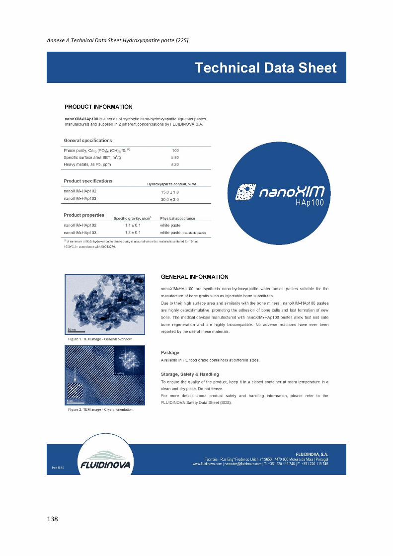
138

Annexe A Technical Data Sheet Hydroxyapatite paste [225].

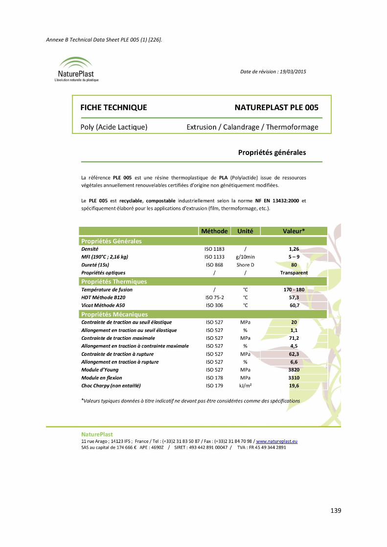
139

Annexe B Technical Data Sheet PLE 005 (1) [226].

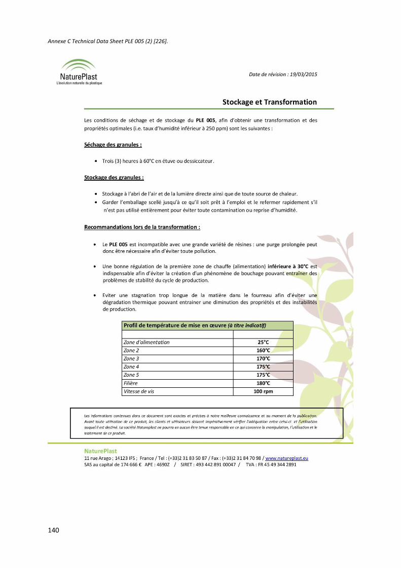
140

Annexe C Technical Data Sheet PLE 005 (2) [226].

Auteursrechtelijke overeenkomst

Ik/wij verlenen het wereldwijde auteursrecht voor de ingediende eindverhandeling:Optimisation and characterisation of nano-hydroxyapatite/polylactide composites using Fused Deposition Modelling technology

Richting: master in de industriële wetenschappen: verpakkingstechnologieJaar: 2017

in alle mogelijke mediaformaten, - bestaande en in de toekomst te ontwikkelen - , aan de Universiteit Hasselt.

Niet tegenstaand deze toekenning van het auteursrecht aan de Universiteit Hasselt behoud ik als auteur het recht om de eindverhandeling, - in zijn geheel of gedeeltelijk -, vrij te reproduceren, (her)publiceren of distribueren zonder de toelating te moeten verkrijgen van de Universiteit Hasselt.

Ik bevestig dat de eindverhandeling mijn origineel werk is, en dat ik het recht heb om de rechten te verlenen die in deze overeenkomst worden beschreven. Ik verklaar tevens dat de eindverhandeling, naar mijn weten, het auteursrecht van anderen niet overtreedt.

Ik verklaar tevens dat ik voor het materiaal in de eindverhandeling dat beschermd wordt door het auteursrecht, de nodige toelatingen heb verkregen zodat ik deze ook aan de Universiteit Hasselt kan overdragen en dat dit duidelijk in de tekst en inhoud van de eindverhandeling werd genotificeerd.

Universiteit Hasselt zal mij als auteur(s) van de eindverhandeling identificeren en zal geen wijzigingen aanbrengen aan de eindverhandeling, uitgezonderd deze toegelaten door deze overeenkomst.

Voor akkoord,

Oris, Erwin

Datum: 6/06/2017

2016•2017 FACULTEIT INDUSTRIËLE … · 2016•2017 Faculteit Industriële...

Documents

Transcript of 2016•2017 FACULTEIT INDUSTRIËLE … · 2016•2017 Faculteit Industriële...