TyD'ÖZ^fedisclaimer notice this document is the best quality available. copy furnished contained a...
90
'S* m . -.v : .::, i I ' -, ' • '-x \ K/7>ir4 f.n.imn ffis/ix sasH/c PAT* UMMTMY t ocma MI TyD'ÖZ^fe nua Timm Amiowons erneu wt$u*it$». o.e. htiMt V£IA umfomtt hf irnmo miAocH mojeers Ateocr Unk* MMMMTAf Ommtk O/fki Am Orttr lk.HI4 ^TELECYNE QEOTGCH R«produc*d by NATIONAL TECHNICAL INFORMATION SERVICE lpir,uf,.ld V. 71ISt cMifM uoomomi MtPM¥iD fO* PltiUC miASi: OlSrHIBUT/O* UMUHim.
Transcript of TyD'ÖZ^fedisclaimer notice this document is the best quality available. copy furnished contained a...

: ■/ .-.^Vä..
*v^ 'S*
■. ■ m
■ .■ ■ -.v :■■.::, i I ' -, ■■'
• '-x \
K/7>ir4
f.n.imn ffis/ix
sasH/c PAT* UMMTMY
t ocma MI
TyD'ÖZ^fe nua Timm Amiowons erneu wt$u*it$». o.e.
htiMt V£IA umfomtt
hf irnmo miAocH mojeers Ateocr Unk* MMMMTAf Ommtk O/fki
Am Orttr lk.HI4
^TELECYNE QEOTGCH R«produc*d by
NATIONAL TECHNICAL INFORMATION SERVICE
lpir,uf,.ld V. 71ISt
cMifM uoomomi
MtPM¥iD fO* PltiUC miASi: OlSrHIBUT/O* UMUHim.

DISCLAIMER NOTICE
THIS DOCUMENT IS THE BEST
QUALITY AVAILABLE.
COPY FURNISHED CONTAINED
A SIGNIFICANT NUMBER OF
PAGES WHICH DO NOT
REPRODUCE LEGIBLY.

Hiitkit I*» MtiKtii Rnnttli Pnjttti Mgntf Mr tkt Ait Fere» TnlMiul Aßßlitttim Ctnttr mill, In nißMtitli lor M§rmui$» eoiiumiä Inni» wkiik AM kim tufflM if tlktr er§§m»ti»iis »r tntrwUn. ma MM teumtiu htntjM ft Itlu nvitin tt mif to iMtutUf. tlu ¥i»w$ uä tMehaüM ßnuiHtä §n ttttt »I tkt lulktrs and $knU mr kt mtirpnirt «t nktturilf rtpnttmini tkt tllititl ßtlititi, titktr ttßrttttä tr implM. tl ikt Hvtnctä Rttttrek Prtjtclt A§tttr, tkt Mir ftret Ttcktietl Mßßlitttittt Cttttr, or tkt U S OMtrtmtnt.

GENERALIZED LINEAR FILTERING OF
SEISMIC ARRAY DATA
SEISMIC DATA LABORATORY REPORT NO. 269
AFTAC Project No.:
Project Title:
ARPA Order No.:
ARPA Program Code No.:
VELA T/2706
Seismic Data Laboratory
1714
2F-10
Ivame of Contractor: TELEDYNE GEOTECII
Contract No.:
Date of Contract:
Amount of Contract:
Contract Expiration Date;
Project Manager:
FJ3657-72-C-0009
01 July 1971
$ 1,290,000
30 June 1972
Royal A. llartenberger (703) 836-7647
P. 0. Box 334, Alexandria, Virginia
APPMVID FOR PUBLIC RELEASE; DISTRIBUTION UNLIMITED.
UNCLASSIFIED
TliU-DYNi: GüOTüCII ALÜXANDRIA, VIRGINIA
GENIiRALIZliD LINHAR l-ILTHRINC OF SEISMIC ARRAY DATA
111111 " H'llll III I || i i jL.j
T AuTMAIffJ AMI BU ISI jgsr
Lintz, P.R.; sax, R.L.; and Blandford, R.R.
NVPORTMTg
8 October 1971 ■ • COM _v
F33657-70-C-0941 * »aejacT MO.
VliLA T/0706 «. ARPA Order No. 6 24 < ARPA Program Code No. 01-10
IB « V» IL*»ILITV/LtMIT*TtOll WOTICH
MPPtona FOU PUBLIC RIUASI; oismium* umimtuo )• IU*
■ 1 «■STItACT
ADVANCIil) Ri;Si;AIU:iI PROJI:(TS ACINCY NUCLEAR MONITORING RESEARCH OFFIC*! IVASMINGTON^ I). C.
'« KEY mono*
Array I' r o c e s s 1 n g ogarithmic Dcconvolution (icneralined Linear l-'iltcrlng
llomomorphic IM I tering
UNCLASSII-IEn Security CUtiificaliofi

4»nmcf
nt »htory •t itwrallMi lUw nitcriM COfptwhti«* 1^*6, Stftfl it wliti to U« pwfclt«! «f «vtrailM t«»« cra»»r«r fuactioai fett»««» • ttitwie »cure» »U »•itmc rtcoHiM ilatl»»« •• • eoMlMHtl*»»««^ »rny.
To provlrf« i{f«ili«iie 4*1« f«r • t«»t of tkf froctttor, • «Koplt sooreo tlgaal la J»afiti Urooffc aiaa «lifrtrtat raailoo F«rt«*rliatioa» of a *olocltr.<itM* airoctora yitUiai Mine dirraraot ayaUaUe »aitoogMO«. I»« aoeltar t»pto»io»t fl.016 fMOtr M4 nnumy *«J ao Aailrtaaoff lalaa^a tvtot Cll iovtobar lf**l ^ft alao |.ro€c»»ti »»tot »latloa» froo lib» ioa|-iaafo-iai»ou-iloa»or»»#Rt oot. Woat of tlit fttar- komlOM art ra«N»*#<l fr«» ma »yotiaiic witmgnm fcy gaoaralttttf lio.ar filtmof THa oa^lotioa Mi ilia t*ria- qaaU »«laoograo* art e^llflN >»f t»»l» praett«.
fft«t tartMaah« ^ftara to liatt looftr not ttn»» rtojia- lug aft^ir gaooralUttf llMOff filltflog ao4 ifct «««Itar ttt^i* tWf mmf *i»ilar Hitfoft tut *rri*al of th« tt^lh M«»*>*

wm
TABLE OF CONTENTS
Page No,
ABSTRACT
INTRODUCTION 1
Sei/iBic signal aodels 1
Hue probability density of the random transfer functions under the hypothesis of :cro additive noise 2
The opimua processor 5
RESULTS 7
Siaulated receiver site effects 7
Observed data 9
REFEREKCHS 12
— ^—^«^^ .

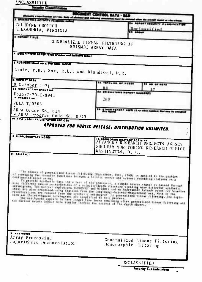
LIST OF FIGURES
l-igurc Title
Transformation of a normal probability density into an almost uniform probability density.
The best fit to a normal probability density of Klappenbcrger's (1907J data. (After Klappenberger, 1967).
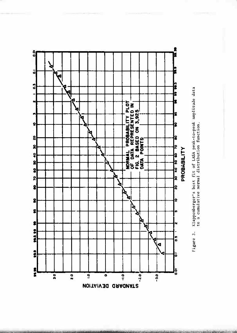
Klappenbcrger's best fit of USA peak-to-pcak amplitude data to a cumulative normal distribution function.
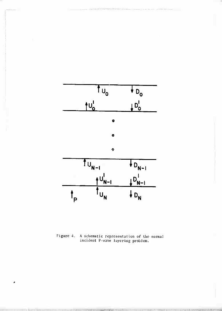
A sdiemutic representation of the normal incident P-wave layering
problem.
Analog computer simulation of the transmission problem. Note the similarity of this problem to the parametric amplifier problem. Also note that S-waves could be handled by designing another ladder network with different delays and reflection coefficients, and interconnecting the nodes of both networks with the proper conversion factors.
A two-stage generalized-linear filter for the estimation of a signal convolved with equal variance, log-normally distributed, uncorrelated transfer functions.
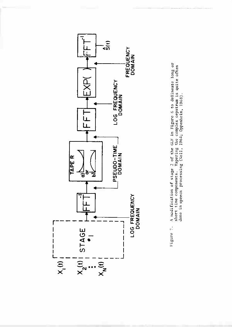
A modification of St#ge 2 of the GLF in Figure 6 to delineate long or short time components. Tapering the complex cepstrum is quite often done in speach processing (Noll, 1964; Oppenheim, 1968).
Synthetic seismogram 1 (a) Reflection coefficients vs. depth (b) Seismogram vs. depth (c) Velocity vs. depth.
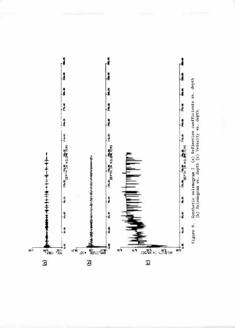
Synthetic seismogram 2 (a) Reflection coefficients vs. depth (b) Seismogram vs. depth (c) Velocity vs. depth.
Synthetic seismogram 3 (a) Reflection coefficients vs. depth (b) Seismogram vs. depth (c) Velocity vs. depth.
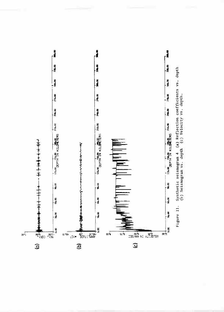
Synthetic seismogram 4 (a) Reflection coefficients vs. depth (b) Seismogram vs. depth (c) Velocity vs. depth.
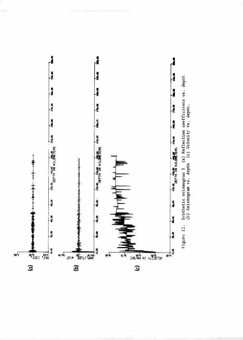
Synthetic seismogram 5 (a) Reflection coefficients vs. depth (b) Seismogram vs. depth (c) Velocity vs. depth.
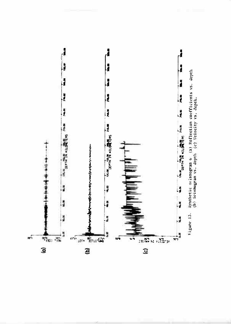
Synthetic seismogram 6 (a) Reflection coefficients vs. depth (bj Seismogram vs. depth (c) Velocity vs. depth.
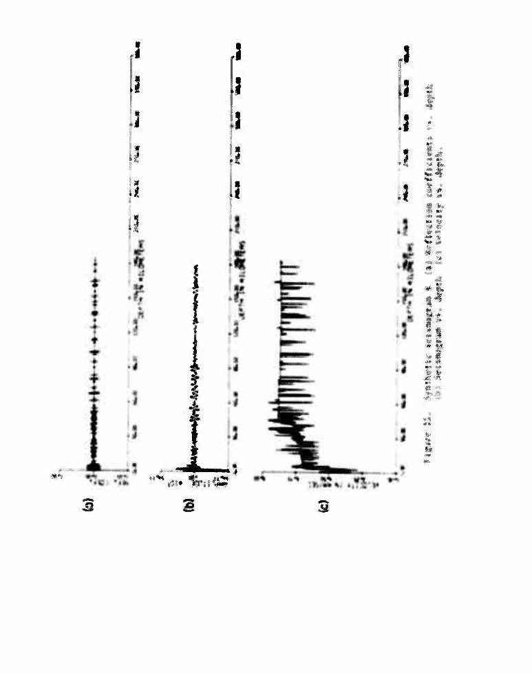
Synthetic seismogram 7 (a) Reflection coefficients vs. depth (bj Seismogram vs. deptli (c) Velocity vs. depth.
Figure No,
1
10
11
12
13
14
■""""■^----■•■^ ..,—J.L'.»»- ■ - -'-
^.■..^..■.■■.....■...^^.^^^.^.^^.^^.^.^...^

15
16
17
18
19
LIST OF FIGURES (Cont'd.)
_. _., Fleurc No. Figurt T.tle *
Synthetic scismogram 8 (a) Reflection coefficients vs. depth (b) Seisroogram vs. depth (c) Velocity vs. depth.
Synthetic seismogram 9 (a) Reflection coefficients vs. depth (b) Seisjnogram vs. depth (c) Velocity vs. depth.
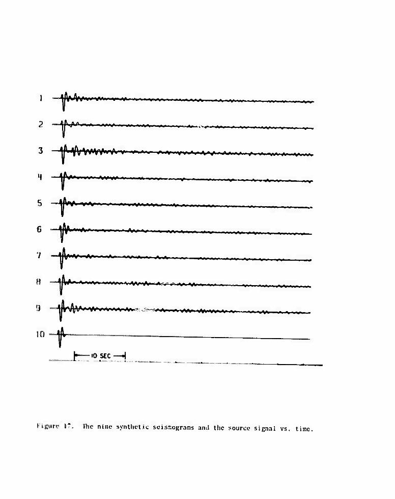
The nine synthetic scisraograms and the source signal vs. time.
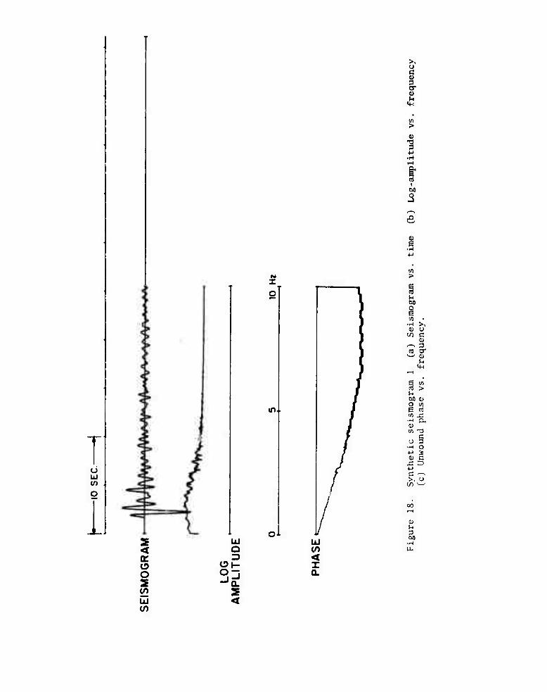
Synthetic seismogram 1 (a) Seismogram vs. time (b) Log-amplitude vs. frequency (c) Unwound phase vs. frequency
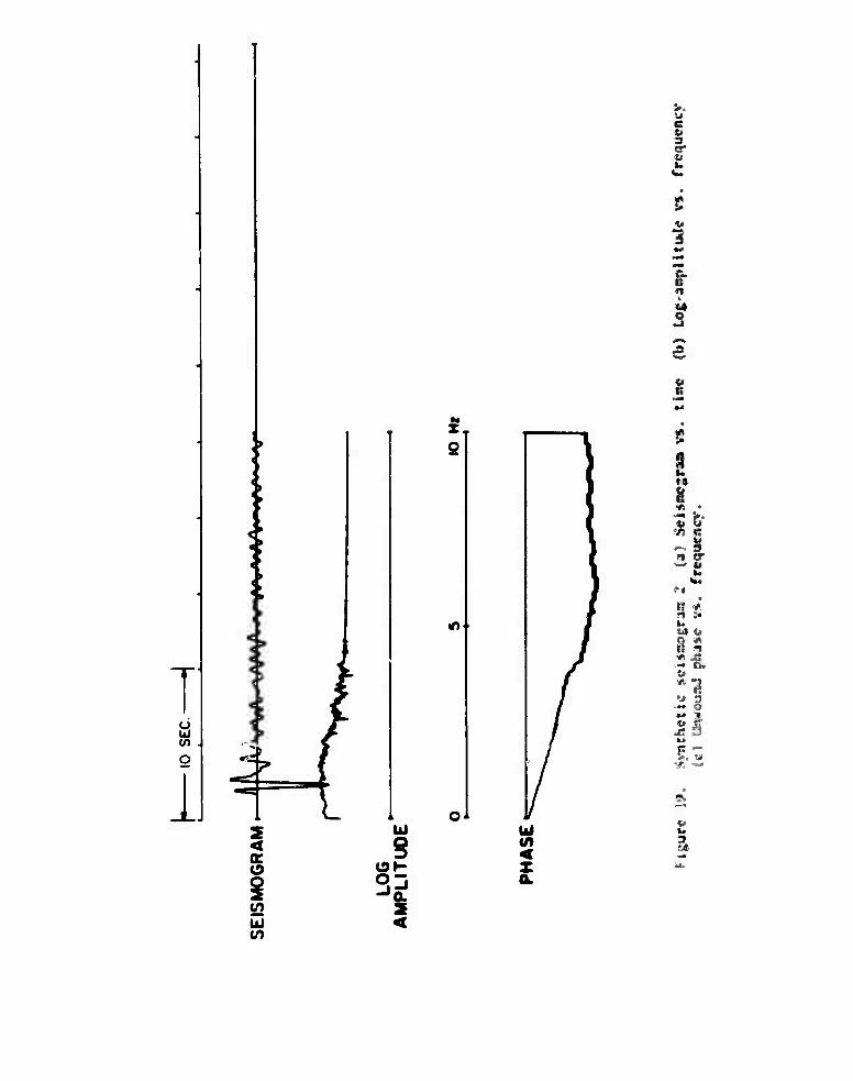
Synthetic seismogram 2 (a) Seismogram vs. time (b) Log-amplitude vs. frequency (c) Unwound phase vs. frequency.
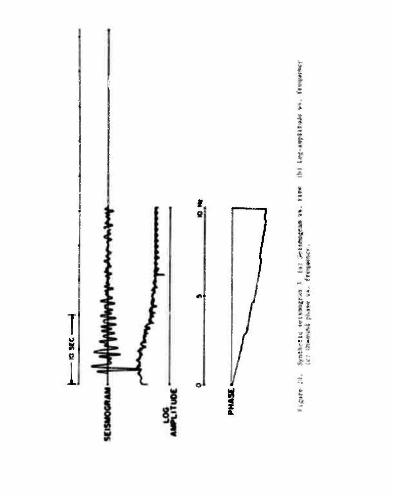
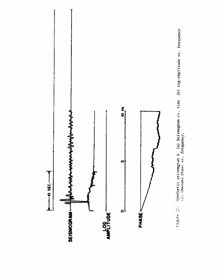
Synthetic seismogram 3 (a) Seismogram vs. time (b) Log-amplitude vs. frequency (c) Unwound phase vs. frequency.
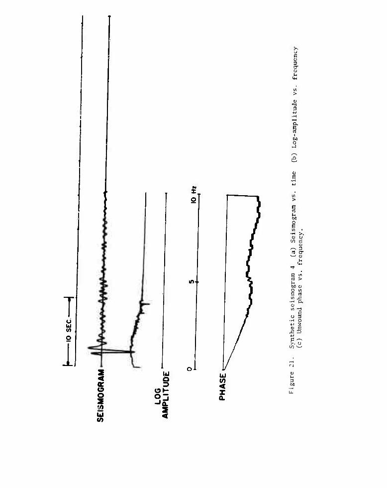
Synthetic seismogram 4 (a) Seismogram vs. time (b) Log-amplitude vs. frequency (c) Unwound phase vs. fi<?quency.
Synthetic s-eismogram 5 (a) Seismogram vs. time (b) Log-amplitude vs. frequency (c) Unwound phase vs. frequency.
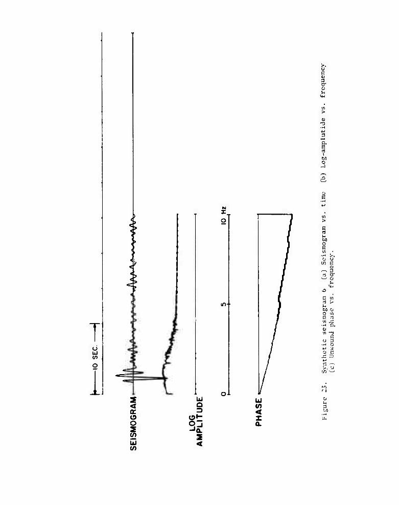
Synthetic sciamogram 6 (a) Soismügram vs. time (b) Log-amplitude vs. frequency (c) Unwound phase vs. frequency.
Synthetic seismogram 7 (a) Seismogram vs, time (b) Log-amplitude vs. frequency (c) Unwound phase vs. frequency.
Synthetic seismogram 8 (a) Seismogram vs. time (b) Log-amplitude vs. frequency (c) Unwound phase vs. frequency.
Synthetic seismogram 9 (a) Seismogram vs. time (b) Log-amplitude vs. frequency (c) Unwound phase vs. frequency.
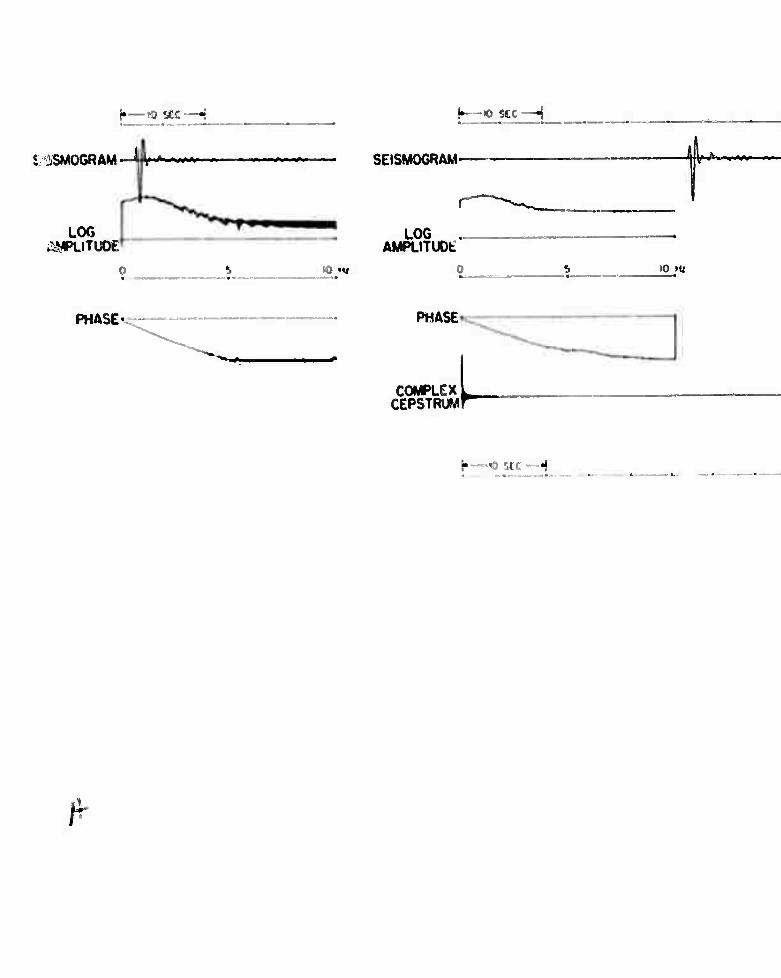
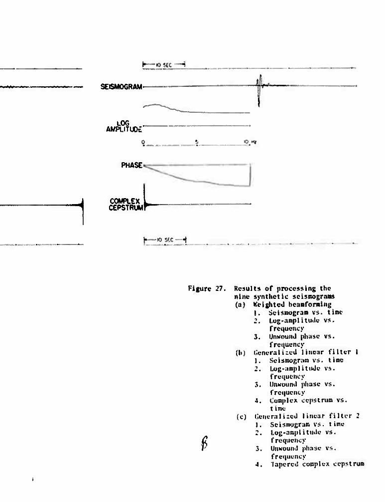
Results of processing the nine synthetic seismograms (a) Weighted beamforming
1. Seismogram vs. time 2. Log-amplitude vs. frequency 3. Unwound phase vs. frequency
(b) Generalized linear filter 1 1. Seismogram vs. time 2. Log-amplitude vs. frequency 3. Unwound phase vs. frequency 4. Complex cepstrum vs. time
(c) Generalized linear filter 2 1. ' eismogram vs. time 2. Log-amplitude vs. frequency 3. Unwound phase vs. frequency 4. Tapered complex cepstrum
21
22
23
24
25
26
27
-...-■
.^.^^...^..^. ^--■■^^■■-"■••■-^^ ■ ■■■■■ ..^^-^.•■■■^.^^^^..^..i.^l-ti^l^toU^.»^ .r ■ ..,J,...„^,..v.....,.1..J.....;...!..^..^:...,_....^..^1^-.^..^^^. ;...,-- ■ ■
"50
LIST OF FIGURES (Cont'd.)
"«"• Tit,e Figur« SO,
Location of events and stations. 28
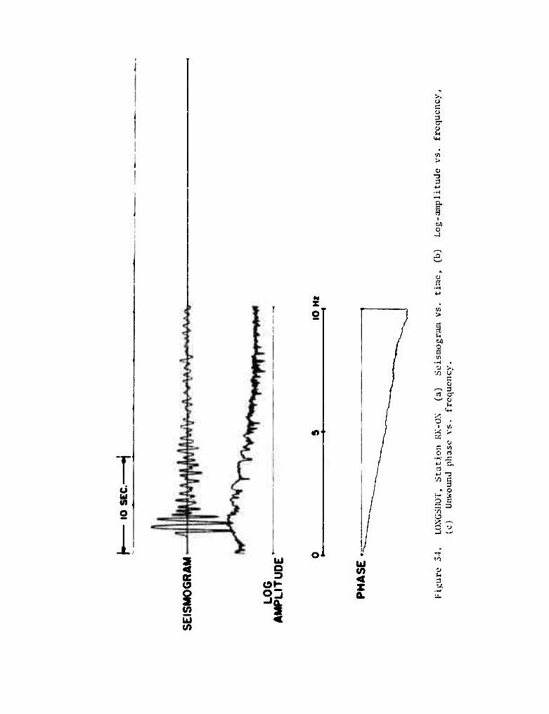
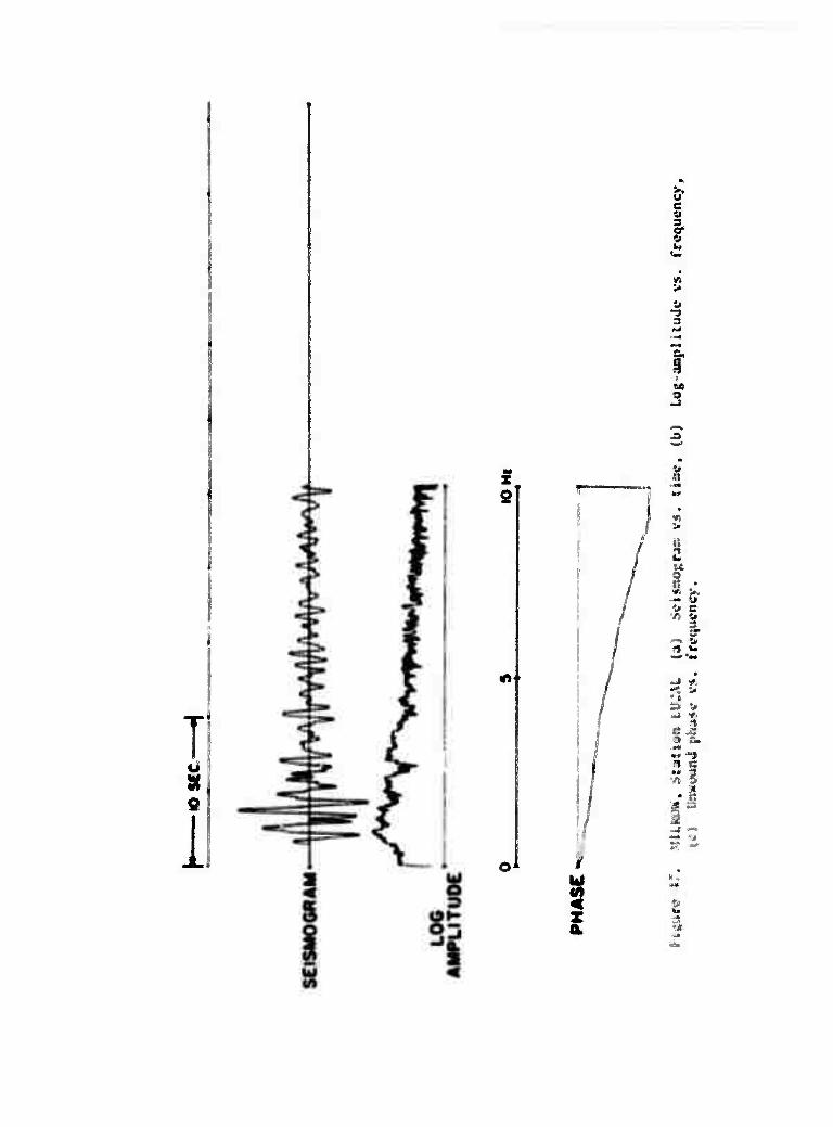
LONGSIÜT. Station KN-UT (a) Seisaograa vs. tlw. (b) Lof-aflpUtude vs. frequency, tc) Unwound phase vs. frequency. 29
LÜNGSÜJT, Station LC-NM (aj Seisoogra« vs. tine, (b) Los-oMlitudc vs. frequency, (c) Unwound phase vs. frequency.
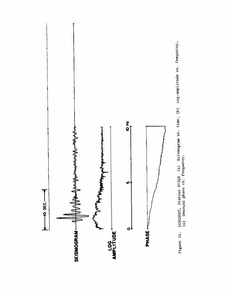
LONGSHOT, Station SV3QB (a) SeiSDOgran vs. tioe. (b) Log-amplitude vs. frequency, (c) Unwound phase vs. frequency. 31
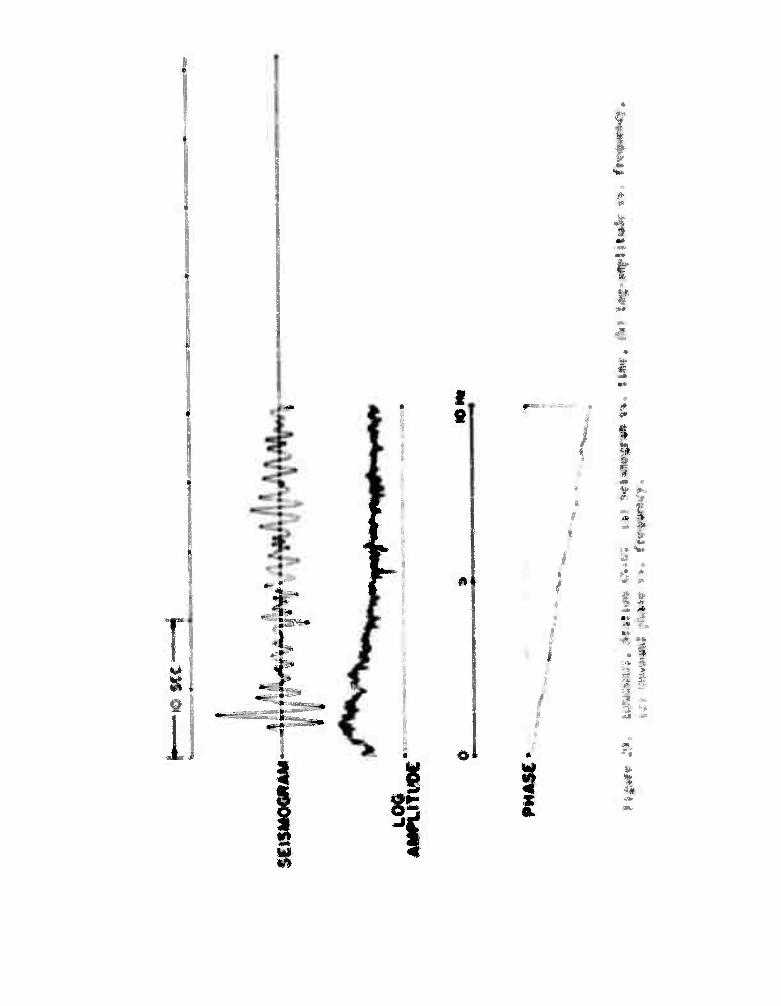
LONGSHOT, Station HL2IÜ (a) Seisroograra vs. time, (b) Log-amplitude vs. Pirequency, (c) Unwound phase vs. frequency. 32
LONGSUOT, Station UG-SÜ (a) Seismogram vs. time, (b) Log-amplitude vs. frequency, (c) Unwound phase vs. frequency. 33
LONGSHOT, Station RK-ON (a) Seismogram vs. time, (b) Log-amplitude vs. frequency, (c) Unwound phase vs. frequency. 34
LONGSUOT, Station SJ-TX fa) Seismogram vs. time, (b) Log-amplitude vs. frequency, (c) Unwound phase vs. frequency. 35
LONGSUOT. Station TF-CL (a) Seismogram vs. time, (b) Log-amplitude vs. frequency, (c) Unwound phase vs. frequency. 36
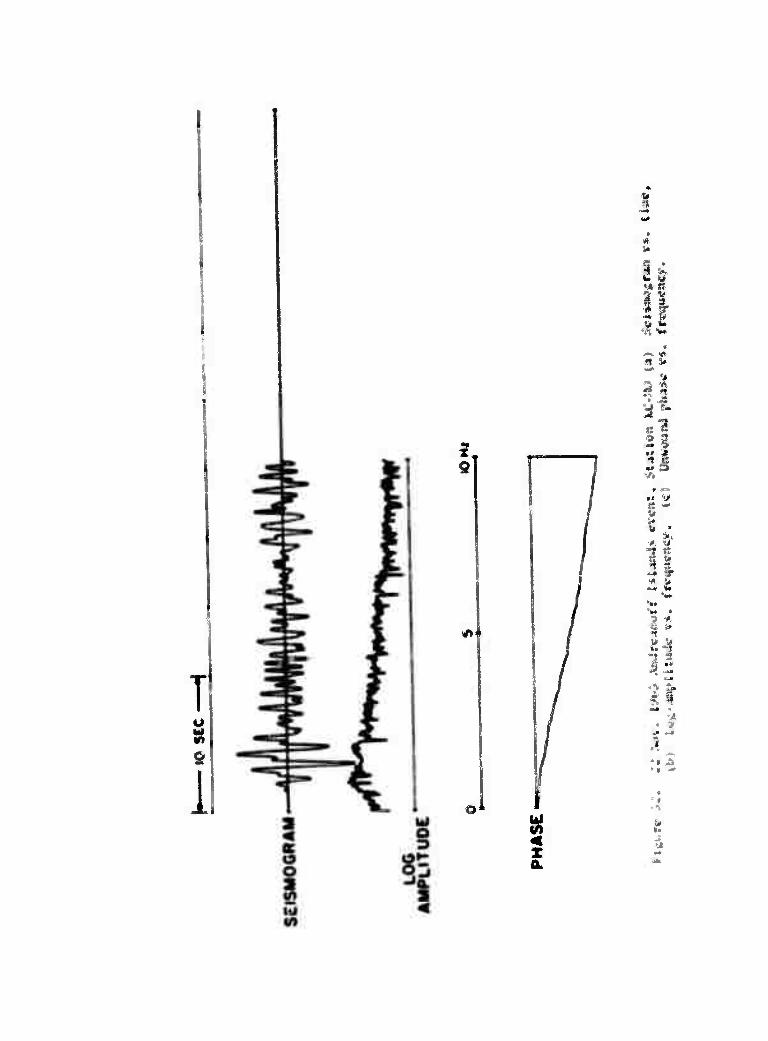
LONGSUOT, Station KC-MO (a) Seismogram vs. time, (b) Log-amplitude vs. frequency, (c) Unwound phase vs. frequency. 37
LONGSUOT, Station YR-CL (a) Seismogram vs. time, fb) Log-amplitude vs. frequency, (c) Unwound phase vs. frequency. 38
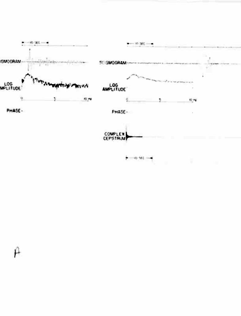
LONGSUOT processing results (a) Beamforming
1. Seismogram vs. time 2. Log-amplitude vs. frequency 3. Unwound phase vs. frequency
(b) Generalized linear filter 1 1. Seismogram vs. time 2. Log-amplitude vs. frequency 3. Unwound phase vs. frequency
(c) Generalized linear filter 2 1. Seismogram vs. time 2. Log-amplitude vs. frequency 3. Unwound phase vs. frequency.
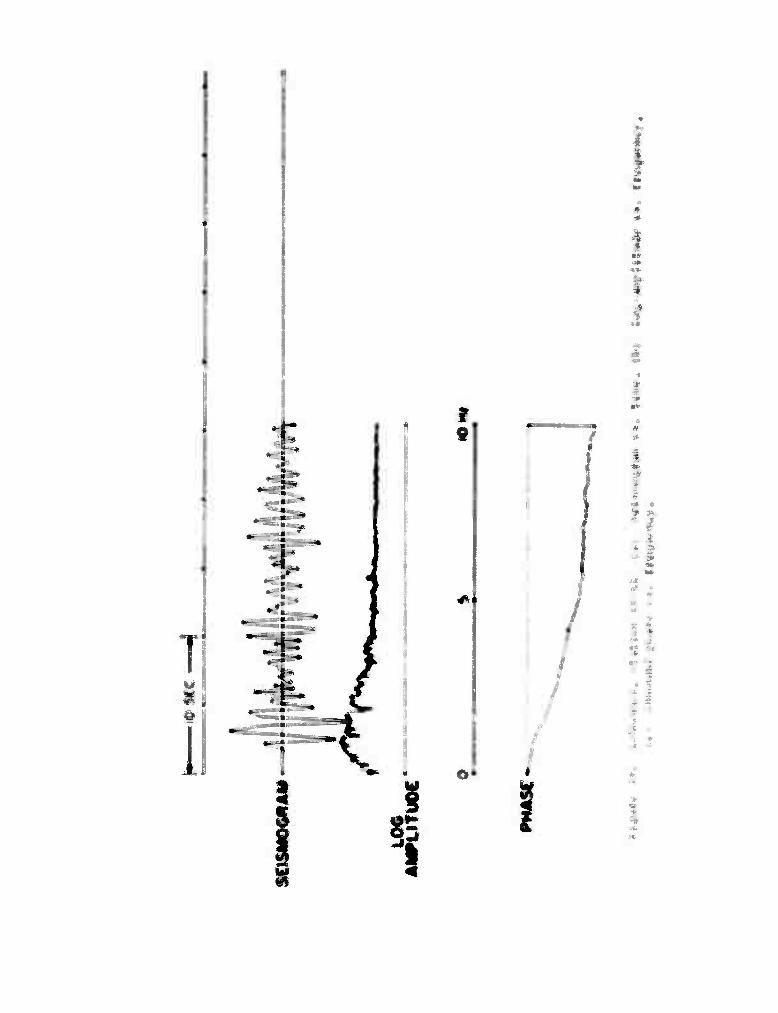
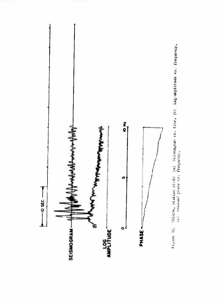
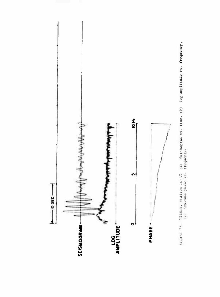
MILROW, Station WQ-1L (a) Seismogram vs. time, (b) Log-amplitude vs. frequency, (c) Unwound phase vs. frequency.
39
40
^^^^..^ ■■ -.^ ^^*^^^-~— .^^,^...^^.^^.^,...„.^.^..-..;....... ^..■^......

Utr OF riOBES UmV4 t
Hfiir« litlt ftiBft ^
MILMKt SuilM «f-l® (tl Siis^vfr«» trt. Hi». (i| t«« ««»III*!» vs. fwqMwcy« (c} Itawoml ^a*» «■» frtifmufccy. H
«•■ rr«<pMficy( (c) ümwa^ij j*.»»* T*. tft^Mmt ».
HtUOW« Station CR2?it Ca| **i»fl»|»i« ,-♦„ «IM« |%| V*$ UQU***** v». frequcncr, C«J W»»«»«»«! pk*** w rf«4N««<T II
»tiLMM. Station LC-NM (a) Solfnogran r» tin«. 1%; Ut Mtfltinit vs. fratutncx, (c)/ itantouad |Aaso vs. Irtquencr* n
MlUttW. Station KX-UI (a} Ukungrm vs. tiM. <b) l«f.aap}iii»t« vt. fr^imcy, (c| ttaMoand pHmut w. frn|0an«^. li
MILMJW. Station AS-PA (a) Svumgrm vv. tin», (fc) Ug.aiiyliiait vs. frequency« (c) Unwound phase v». frequency. r-
•m.ituji. Station I.U.UL (a) Sei»nogran w. tin«, lb» C^*aflplttttJ« vs. frequency, (c) Unwound phase vs. frvqueney. r
MILKOH, Station I'J-PA (a) Setsaosraa vs. tise. (b} Ug-anplitial« vs. frequency, (c) Unwound phase »». frequency. I*
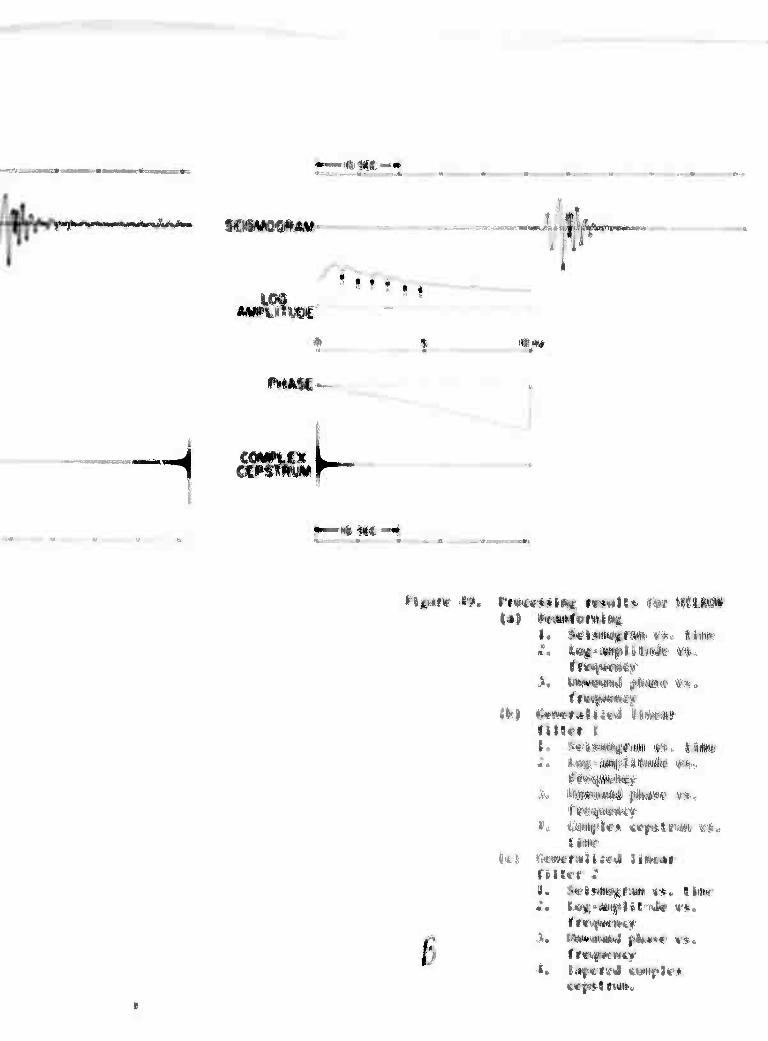
Processing results for MiUtOK (a) Bconformng
1. Seisnograa vs. tine 2. Log-aaplitude vs. frequency 3. Unwound phase vs. frequency
(b) Generaiized linear filter ! 1. Scismogran vs. tine 2. Log-amplitude vs. frequency 3. Unwound phase vs. frequency 4. Complex ccpstnun vs, tise
(c) Generalized linear filter 2 1. Scismogram vs. time 2. Log-amplitude vs. frequency 3. Unwound phsne vs. frequency 4. Tapered complex cepstrum. 49
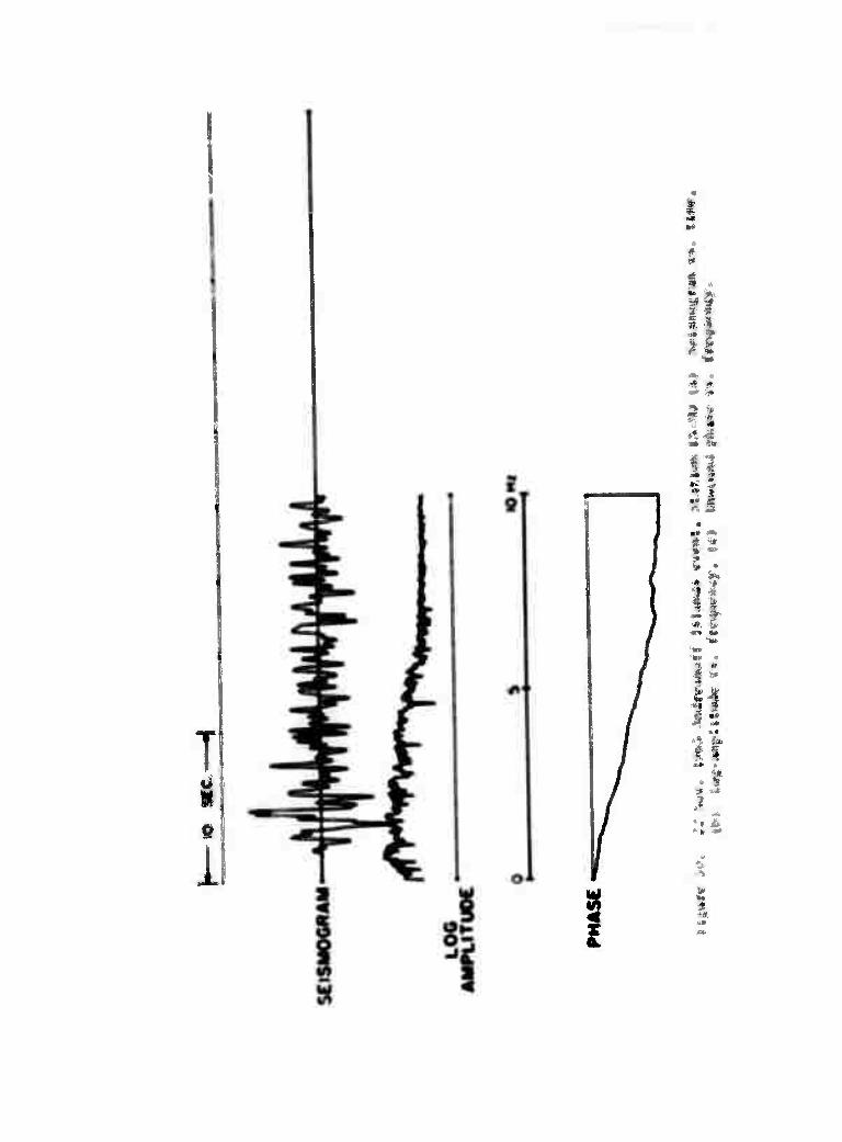
22 Nov. 1965 Andreanoff Islands event. Station LN-MO (a) Scismogram vs. time, (b) Log-amplitude vs. frequency, (c) Unwound phase vs. frequency. SO
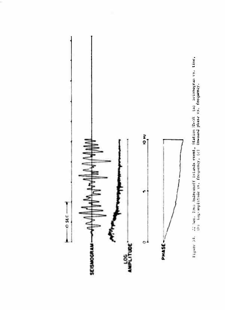
22 Nov. 1965 Andreanoff Islands event, Station IIV-M\ (a) Scismogram vs. time, (b) Log-amplitude vs. frequency, (c) Unwound phase vs. frequency. SI
■ —•'- ■

ii'ni.i "iinn i
uit m tftm» tcnt*<i.i
»i#*f«f i»llt
21 ÜMT. ffli4» iWhMHfi ItlMli 9 la) Stitft»«»«* •'» IIW. lb) IH'iiiifii «§.- #«-*<«^'^'
U 9m» mi mtnmmU Uimi* «-««*%. M«IIM «%•«» 1*1 i«l«Mr*(i *'» II«». «%| |««>Mlf||«««r «t »titwiwy. (ft lllMNIhl I|ä.*%* *•»
21 »üfc- nv* %***«>***»*t t*tm»* mm*, Umum m**& 1«« l*i*.w»^t.n M It««. (Hi) Ifli'Mpillwi? Wt fcupwyi
22 .%*•. Iffci HJnaoifl UlitiKt» ««Mt, ÜMIM i,»» 4* ♦».«..«* it» %■». Hit», Ül !«§ Mflliitfl» «'* M^f*»««».
«UJhaf* %•
i;
il
M
;.; i.*-4 sufefc *ni.m>m*tt I«iMi» •««*!. »IAIIM »H^«^
22 Stov« mi liiwiMff l*laMi«» «*«**, %I««I«^ «% *:» lai StiimnHtf. inn»« n» iiit'Mfi»i««lt »*>•. ftvovüftt«^.
rif**»-»»!^ finwlift fitr 22 %m*c im* mtimmll l«r«fNN ttm* till MNHMOTWIHS
I. StlMMNM «** !•«»
n» 2. HfMfilliiilf) v** tf*■*'!****
«cMff»ii£«i ikMaf ruifi i
HI
1. SftlMwt'«* «'« li« 2« l<iii*«ifliit*«t »*,. ^rvpMwr
4. CHf It* etpiifia ««. IHM»
2. Ug *i^»lil«»«f m» Itvym***
4. fippf«! «Npl** MpilfW«

«Uli« till«
5
^M
INTRODUCTION
Sctawic signal «odels
One difficulty encountered in beaming a short-period
worldwide or ccntinental-sized seismic array is that the
signal coherency falls off markedly with distance*
(liartenberger, 1967; Klappenberger, 1967; Capon et al,
1967).
A possible model of the seismogram recorded at the
Jth instrument an array under excitation of a signal plus
uncorrelated additive noise is
Yj(t) - S(t)*hj(t) * njTt) (1)
where the • indicates convolution.
The Fourier transform at (1) yields
YjCf) » SCOiyf) * Njd") (2)
The H,(f) may be thought of as a source-receiver travel-path
transfer function for *he jth receiver.
'Amplitude anomalies may run as high as eight-to-one for
LASA (Klappenborger, 1967; Mack, 1969), whereas time
anomalies may run as high as 1.5 sec at LASA (Chiburis,
1966).
1-
The probability density of the random transfer functions
under the hypothesis of zero additive noise
If we make the assumption of large signai-lo-addilive
noise ratio, equation (2) becomes
YjCf) = lijCf) S(f) (3)
If we further assume that H (f) may be written as a
product of a large number of small disturbances, then
M Y-jCf) = ^H I Amj(f) | exp [i*mj(f)J S(f) (4)
where m is the index of each small disturbance and M is the
total number of disturbances. Taking the logarithm of both
sides of equation (4), gives
log YjCf) = log|S(f)| + £ loglVitnl m=l J
h^i Kj(f)±27r%^]j (5)
+ i
where Mm.(f) is an integer which reflects the uncertainty in
the correct Riemann sheet at each frequency. We see that the
logarithm of the complex Fourier spectrum has converted our
multiplicative variables into a new set of additive variables.
If Am. (f) and the *m;j (f) can be described by a probability
density function, then we may invoke the weak law of large
numbers and state that our new random variable log Y.(f)
■ ...■ii.tr.-^Us.-.iiiiL.-i'i
is asymptotically normally distributed over the ensemble
with the expected value of the real part equal t«
log|SCf)| * log|u(f)|
where M(f) is the geometric mean of the random transfer
functions. The expected value of the imaginary part of log
Y.(f) is equal to
*s (f) ♦ MO
where ^(f) is the phase of the irean of the random transfer
functions. The maximum likelihood estimate of log|y(f)| is
given by
iSg|7(f)T«jT t L loßiAmi(f) j=l m=l ^
(6a)
The maximum likelihood estimate of $ (f) is given by
N M
^^j?! m?i [^^+%^] (6b)
The probability density function which describes the
complex random variable y. is a log-normal density function
(AJtci;inson and Brown, 1963). Note that if the signal
3-
■ ■ ■■ ■■'..■■■

spectrum is white, then the estimates at different values
of frequency are normally distributed and we have a
stationary bivariate log-normal variable. If the signal
spectrum is non-white we have a non-frequency-stationary
bivariate log-normal variable.
The theory of logarithmic deconvolution has been
developed by Oppenheim (1966) and Schäfer (1967, 1969) as
a specific case of Oppenheim's generalized linear filtering
theory. For random transfer functions, the real difficulty
with this method is the choice of the proper Riemann number
N^f) where N. (f) = £ M (f) for each recording site. If the ni= 1
phase changes rapidly with frequency, i.e., $({) has a large
variance, we may find ourselves faced with an almost uniform
distribution (over the ensemble of stations) for our estimate
of the ensemble average of 4,(f) due to the discontinuous
Riemann transformation. This problem is illustrated in Figure
1 for a zero mean distribution. Our solution is to set the
phase equal to zero zero at zero frequency for each recording
site and then unwind the phase. Schäfer (1969) has discussed
techniques for unwinding the phase.
There is experimental evidence that the A.(f) are log-
normally distributed. Klappenberger (1967) has shown that
earthquakes have log-normally distributed peak-to-peak ampli-
tudes at LASA and Freedman (1967) has shown the same distri-
bution for earthquakes at worldwide recording sites. Figure 2
is the histogram of Klappenberger's data. Figure 3 is
Klappenberger's best straight line fit to his data plotted
on log-normal probability paper. If the data are log-normal,
the cumulative frequency distribution should approximate a
straight line. The hypothesis that the data are log-normal
cannot be rejected at the 95% confidence level.
Further indication of the log-normality of the station
spectra may be obtained by passing a synthetic signal
through ensembles of plane parallel-layered media with
random reflection coefficients.
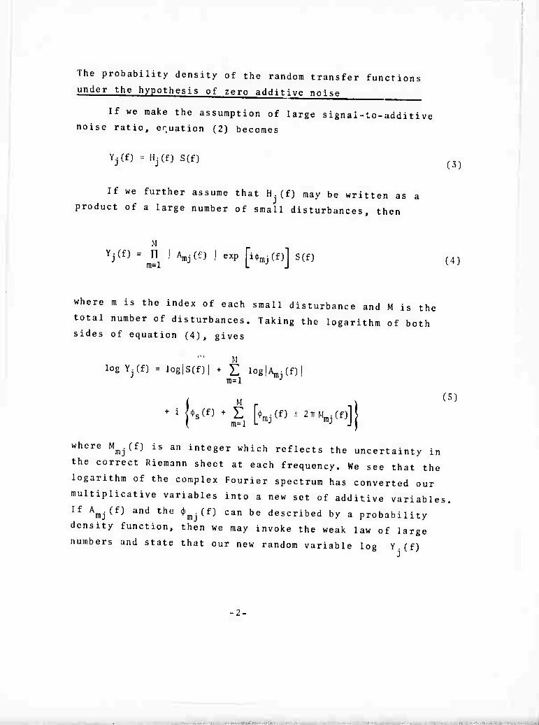
Figure 4 illustrates the problem of a seismic wave
impinging upon a set of plain, parallel layered media. A
subroutine given by Claerbout. (1968) was programmed to
yield the transmission seismogram of an arbitrary wavelet
impinging upon the bottom layer. Figure 5 is the analog
computer simulation of the transmission and reflection
problem. Electrical engineers might recognize the circuit
as a "ladder network" or as a parametric amplifier.
The optimum processor
Under the assumption of white, uncorrelated, zero-mean,
equal variance, log-transfer functions and zero additive noise
it can be demonstrated from maximization of the log-1 ike 1ihood
function that the likelihood estimator for the logarithm of
the signal in the frequency domain is just the arithmetic
average of the individual station log-spectra.
log S(f) = i £ log Y.(f) (7) j = l
or S(f) = exp [log S(f)l (8)
•5-
. .■■, ■
so that sen = N
II YjCf)
l/r (9)
Equation (9) is just the geometric mean of our individual
station amplitude spectn. Figure 6 is a block diagram of
the processor for this case. Figure 7 is a modification of
the processor to filter out undesirable time components.

Mum
fyatliciic ttfiiKMifr«»» »tr« gtii«ratt4 if ftttfiutt • ftit««l of U» fmftm f |l| • t •»f («fttl •!■ w^l !»'<« • •i«cl of Uf*r» •im r«*4«« r«fl«€iiM c#«rri«it«i«. IM
«tlociiy «• a rwMcii«» «f 4«fii <«rr«*|W(t4i t« « mM»m of Ut Micl» lit«« m fifwr« 74 «f %»i ttp«ri %9. !*% fßUwtr a«! *i«««ttitr4 |(f?#i wiiii #«§11 |»»ri«ffli«i!•«* l« i%9 Tvlocur ♦♦ « f«t«£iii«ft «t «l»fi». i« »rji»r I« f«! rtaioaakly t«4i|»iit«i«4 «««««<»«»*•« H ««• «t<t«*«rf i» i»c«rf«rait 1*1« iar«r* n*m4m^ #«4 ci«ct»««t, iffttj AII#
19»*} IMI« ik» 4M><I»I# ligar»» • ikrawga la are plai* af Cal, tkt rartaciia« «»«Ifui<r«ii«, |k)t ikt ttifiiatraiw aaJ, u», ika talacliy a« a f«ia«ii«a «I Jafifc, far alaa raaliaa* llaat «f aar raa4e* pracata, Umt* ««laal iraval-tma layar* aara ial»at ihw «f««iat »t «aafla fNiiaia mm iht Haaar at«"»*» aeala i» aal liaa«r a«i la a faa^naa af laa talaaltf« fie (»llawiaa ftiwr«* «eta «ll aarai«li«#«i la bat» ifca tana |MF«I
valaa» ^tlata aaly lb» *b«p» af lb» «»itaagf««» »«4 »ptcira adt af caacara. fb» firai aia» iraia* af figara 17 ar» * f»lai af lb» aia» «yaibaiit »»Ma^graa* a» a faacilaa af im», Ih« i»«ia ;r««» i« ta» «igaal a»l#ft ira««ai«»iaa ibraagb «af «t ta» *i*r fi»*4#* l«f»r**ia€lft*
tlg«»<r»« i» «M»'«i* ;* **« ia« f>(p{t «f t«l, lb» t»i«iia« gran »»rta* lia«, r*i. lb» laganib» «f lb» »afitiwj» »»raw» fr»4|a»a€r aag, lt|, li» fbaa« «at»at frft^aaacf«
ligwr» i? i» ib» r»««ti af ib» tat«« fira€e»»art»
lb» ibf»» tnt«! »*i#f * ara la» r»$«ii *r «»fgbtaJ
»* *

boa* summing. Trace
/ N /N v al is the weighted beam sum ( Z- Wj X^ (t)/2Z w^ ) J where
\i=l /i=i 1/ M. ■ I/o. and where a. is the sample standard deviation.
Trace a2 is the log amplitude of the weighted beam sum
versus frequency. Trace a3 is the phase of the weighted
beam sum versus frequency. Trace bl is the geometric mean;
trace b2 is the averaged log-amplitudes versus frequency;
and trace b3 is the average phases. Trace b4 is the complex
ccpstrum (Schafer, 13&9). Trace b4 appears to be anti-
symmetric about the midpoint because the phase (trace b3)
is much larger than the log amplitude (trace b4). The unwound
phase is the imaginary part of the log-spectra and is anti-
symmetric about its midpoint (10 Hz), and the log amplitude
is the real part of the log spectra and is symmetric about
its aitttpoint (10 Hz). Since the numbers for the unwound
phase are much larger than the numbers for the log-amplitude,
the complex cepstrum appears to be antisymmetric.
The traces under c have been processed by tapering in
the pseudo-time domain. Trace c2 is the smoothed averaged
log-amplitudes, and trace c3 is the average unwound phase.
Trace c4 ks the first half of the tapered complex cepstrum.
It would appear that the generalized filters have done a
hotter job of estimating the signal than has the weighted
beamed sum. The log amplitudes of the geometric beams and
the phases of the geometric beams also show less variance
than do the iog-amplitude and phase of the weighted beam
sum. Notice, howevefy the small precursor introduced by the
generalised fillters.
-8-

Observed data
Three events were processed on a continental sized array
of LRSM (Long-Range-Seismic-Measurement) stations distributed
throughout the continental United States and Canada. Two
events (LONG SHOT and MILROW) were underground nuclear explo-
sions which were detonated on Amchitka Island in the Aleutian
Island Arc, The other event was an Andreanoff earthquake
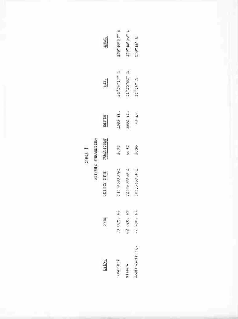
(22 November 1965) in the same island arc. Figure 28 is a
map of the three events and the recording stations. Table I
gives the seismic parameters of interest for the three events.
Table II gives the locations of the recording stations used
in this study. The processing results for LONG SHOT are
given in Figure 29 through Figure 37. The formats are the
same as for Figures 18 through 27. Figures 29 through 37 are
for stations KN-UT, LC-NM, SV3QB, HL2ID, RK-ON, SJ-TX, TF-CL,
KC-MO, and YR-CL, respectively. Notice the large variations
in signal waveform from station-to-station in all traces.
In Figure 39, note the small precursor introduced by the
processor since we did not demand minimum phase as one of
the attributes of our processor. The main signal of our
processor (trace 39bl) seems to "ring" more than the signal
form the weighted beam (trace 39al), yet the coda dies out
more rapidly for the first generalized linear filter compared
to the weighted beam. The variance of trace b2 and trace b3
is seen to much less than the variance of trace a2 and a3.
The spectral null at 1.8 Hz in the LONG SHOT log- i ^e
amplitude spectra (traces a2, b2, and c2) has been inter-
preted (Cohen, 1969) as interference between the direct P
wave and pP, the reflection from the free surface.
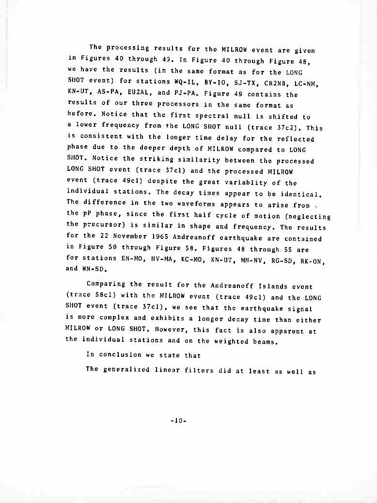
The processing results for the MILROW event are given
in Figures 40 through 49. In Figure 40 through Figure 48,
we have the results (in the same format as for the LONG
SHOT event) for stations WQ-IL, BY-IO, SJ-TX, CR2NB, LC-NM,
KN-UT, AS-PA, EU2AL, and PJ-PA. Figure 49 contains the
results of our three processors in the same format as
before. Notice that the first spectral null is shifted to
a lower frequency from the LONG SHOT null (trace 37c2). This
is consistent with the longer time delay for the reflected
phase due to the deeper depth of MILROW compared to LONG
SHOT. Notice the striking similarity between the processed
LONG SHOT event (trace 37cl) and the processed MILROW
event (trace 49cl) despite the great variablity of the
individual stations. The decay times appear to be identical.
The difference in the two waveforms appears to arise from .
the pP phase, since the first half cycle of motion (neglecting
the precursor) is similar in shape and frequency. The results
for the 22 November 1965 Andreanoff earthquake are contained
in Figure 50 through Figure 58. Figures 48 through 55 are
for stations EN-MO, HV-MA, KC-MO, KN-UT, MN-NV, RG-SD. RK-ON,
and WN-SD.
Comparing the result for the Andreanoff Islands event
(trace 58cl) with the MILROW event (trace 49cl) and the LONG
SHOT event (trace 37cl), we see that the earthquake signal
is more complex and exhibits a longer decay time than either
MILROW or LONG SHOT. However, this fact is also apparent at
the individual stations and on the weighted beams.
In conclusion we state that
The generalized linear filters did at least as well as
10-

the weighted beam sum in the time domain in estimating our
synthetic signal. No significant signal distortion in the
first motion was present in our estinute.
The generalized linear filter traces for the explo-
sions were similar despite substantial variations in the
records for the same event at different stations. The
explosion tracus were simpler than the earthquake trace,
but this was also true at the individual stations.
The codas are smaller for the output from the
generalized filters than at the individual stations or on
the weighted beam sums. The log-amplitude and phase spectra
of the generalized linear filter output exhibited less
variance from their mean compared to either individual
station spectra or the weighted beam spectra. This might
be expected since the geometric beam is the minimum vari-
ance estimator for uncorrelated equal variance random trans- fer functions.
The results suggest that continental beamforming or
indeed even world-wide beamforming is possible for the
initial P-wavc using the theory of generalized linear
filtering, and that complexity measurements and analysis
of source dynamics might better be performed on the
generalized beam.
-11

III. RÜFliRt-NCÜS
Aitduson. J.. and Brown. J.A.C., The Log-normal Distribution; Cambridge University Press, 2nd Printing, 1963.
Aki, K., 1968, Seismological evidences for the existence of soft thin layers in the upper mantle under Japan. Jour. Geo. Res, vol. 73. pp. 585-994.
Capon J.C.. Greenfield, R.J., Kolker, R.J.. and Lacoss, R.T., 1968, bliort-Penod signal processing results for the large aperture seismic
array," Geophysics, vol. 33, no. 3, pp. 452-472.
Chiburis. li.F., 1966, "LASA Travel-time anomalies for various epicentral regions," Seismic Data Laboratory Report No. 159.
Claerbout, Jon F.. 1968, "Synthesis of a layered medium from its acoustic transmission response," Geophysics, Vol. 33, No. 2 pp. 264-269.
Cohen, T.J,, 1969, Determination of source depth by spectral, pseudo- autocovariance, and cepstral analysis: Seismic Data Laboratory Report No. 229, Teledyne Geotech, Alexandria, Virginia.
Freedman, Helen, W., 1967, "Estimating Earthquake Magnitude." Bull. Seis Soc Am. 57. No. 4, pp. 747-760.
Glover. P., and Alexander, S.S., 1970. "A comparison of the Lake Superior and Nevada Test Site Source Regions," Seismic Data Laboratory Report No. 243. r
llartenberger, R.A.. 1967, "The effect of the number and spacing of elements on the efficiency of LASA beams," Seismic Data Laboratory Report No. 205.
Haskell, N.A., 1953, "The Dispersion of Surface Waves on Multilayered Media " Bull. Seis. Soc. Am., Vol. 43, p. 17-34
Klappenberger, F.A.. 1967. "Distribution of Short-Period P-Phase Amplitudes over LASA. Seismic Data Laboratory Report No. 195.
Landers, T.. and Claerbout, Jon F., 1969. "Effects of thin soft layers on Body Waves." Bull. Seis. Soc. Amer.. Vol 59. No. 5. pp. 2071-2078 October, 1969"~
Mack, Harry, 1969, "Nature of Short-period l'-wave variations at LASA; Jour Geo. Res., 74, No. 12, pp. 3161-3170.
Noll, A.M., 1904, "Short-time spectrum and "ccpstrum" techniques for vocaJ- pitch detection," Journal Acc-ist. Soc. Am., Vol. 36. No. 2. pp. 296-502.
12-

Oppcnh«!«, A.V., 1966, "Xoallimr filuria« of OmvH*i rii**l*r QmnttU ProgrMs Report W». io. «««««rcli i^-stnorr »f Il*cir«»ic4. *.t„i
, • i969» "Gsotraa:«^ Uatar Filunngr fJMAtvr i »f btciut ProceMing of ütgn^u. Cold «ml lu^r. H&r-mit.ito*
Schafer, R.W.. 19Ö7. Echo ramvel by t«A«ralueil Imeer ft Hen«.«, i** MW* Kcconi Boston, 1967.
-—, • 19(,9• Ed»0 rcaovel by discrete general i ted It near filler IM TCCJI. Report No. 466, Research Lab. of Uemom«, M.I.T.
13-
• • • S 3 3 > JS 5f
t i - • • •
• « •
9 •»
a
I 3 '■.' •4 «
1 2
■
-. •• -: a ■» • • ■
a 5 i ■ i M «• 3 i : «• «ft •I *l
a ■«
•3 ^ 'a • • •
^ ^ 5 ^ '^ ::
:l it ::
■'■
1
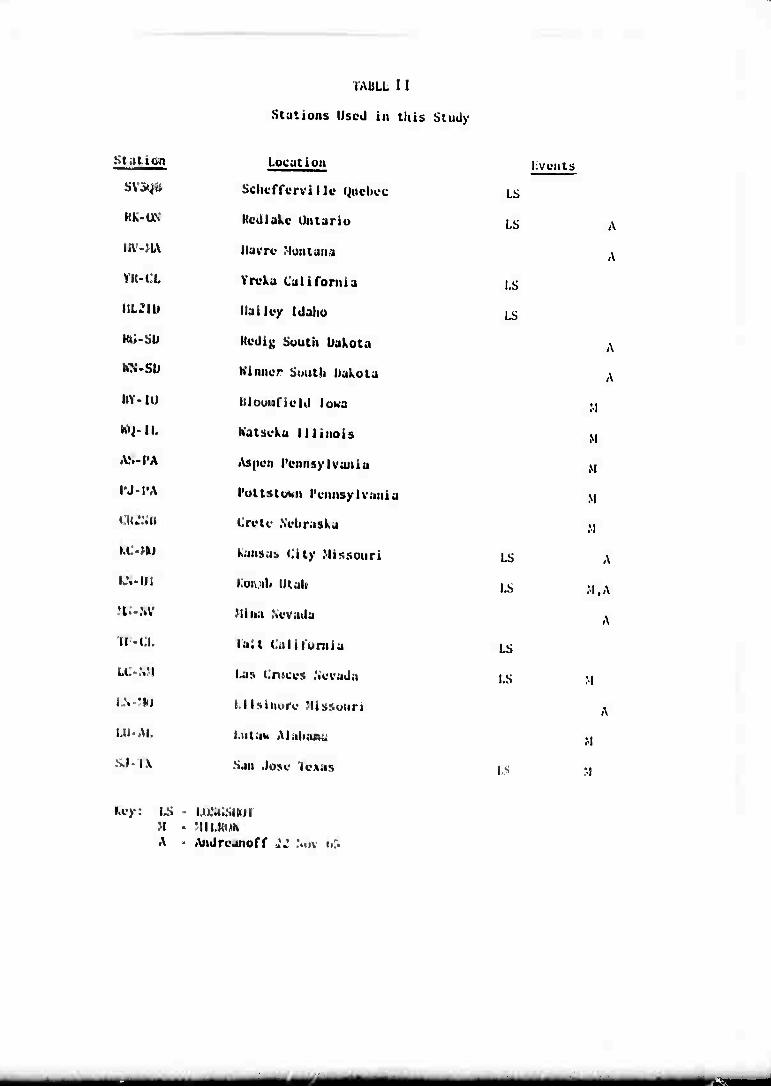
TAÜLL 11
Stations Used in this Study
st .»t ion Location liven ts
svsqs Sehofforvltlo Quebec LS
RK-ON Kcdlokc Ontario LS A
IIV-Jl\ Havre Montana A
¥K-CL Vreka California LS
KUIU tlailey Idaho LS
HÜ-SU Kedig South Dakota A KN-SÜ Winner South Dakota A
mr- iu liiounrield Iowa M
Itt^-lL Katseka Illinois M
A.S-I»A Aspen Pennsylvania M
IM-PA PottStCWI Pennsylvania M
CR^ill Crete Nebraska M
KC-NO Kansas City Missouri LS A » • i', Koiuib Utalt LS M.A
Jt-.W Mi n.i Nevada A
TF-a raft California LS
LC-.\M Las Cneces Nevada LS M
L\->IO ill»inure Missouri A
UI-AL iaitaw AKiboflw M
SJ-TX San Jose Texas IS ■!
key: LS - LuNCSItiH M - mmm A - Andreanoff 22 Nov uU
^^^^^--^^m^m—mtmmetmm—^—m

<Mf)
'3 -TT—'
i(!L^(f)
<f> if) IS WHAT WE MEASURE OUR PROBLEM IS TO RECOVER ^ (f)
Figure 1. Tran»foraatton of .1 numil proJi,»!»! lily «l^nsily into 1«» aloo^t Mi forts proÜMbii lily i.-..,'.
mm —mm

Ä
ft
is-
i ADNIAOJlii
-
ö ö
V o
\
^ O
• \ .
•> * *
o \
IS
a
o
*
K 5 tu "z UJO IS a-o liiUJ KM
*
o
< 1 ifl-
1- 2
8
« < —
ii.2S_
OlkO
i n
1 1
is s 3 o
*
n \ i*
8 o
s
n
1 m
\ •
V s
• V
h 1 • H
% • s «1
2
t ?L
"" ö
o s
s * 3 i 0 t 3 ( 9 « 3 < 3 ( ? o
>-
!J S '4 CD O (T Q.
3
^ • rt c o o C1.-H
0 u 4-1 C 1 ,= r) 4) C O. O
öl 3
O i/l ■ H
• H IM --1
rt ^ g 1/1 H i) O
^3 C
M.5 (U 4-> M rt
4) 3
C 3 4) U B, CU rt rt rt o
4)
s,
NOIiVIASa aUVQNVIS
, m Ji itÄiWif *>5AiJJiiii t-i/it™ ii tJ*.iL;.vh..:,/'Jiü-il
.
T^,
tu;
T
1
TU
t.
N-l
tu N
T N-l
l^NH ^H
iD N
Figure 4. A schematic representation of the normal incident P-wave layering problem.
.■.■. .■.,*..:>. ■.::■..■■;.^!:-.-:.i-:^, -.y / ..^.~.: ::^,-y..^:t:.\.v..~-^-!-^''.L!;^,\.-:-. *...^.-. ■■:....■ ■ .■.■.■- .-■._., i.i.',. ■■,..:.■;■„..■■,.; ...■.■■;,..,... -...:.. .■■.,,. ■...,-. i^^^A^.j^^.li^^^U.^iii.iur^r.ui

Figure 5, Analog computer simulation of the transmission problem. Note the similarity of this problem to the parametric amplifier problem. Also note that S-waves could be handled by designing another ladder network with different delays and reflection coefficients, and interconnecting the nodes of botli networks with the proper conversion factors

i ^mmmm^m>
i
E „s
V
1
T
s
Ik
§
S Of «
1 V T
ft s
• • •
I IA.
II II 11
1 9 m
: JE
11 A4
a» C
1 *.
! •* «
t--f •Jl
d
«^ 1 'K ♦-
Li. <w > o zz UJ-
4 • 3< 'I2! 2 yo FQ it ^- _ -^
CL X
>- u z LÜ ÜJ
2z P o- . UJ<
?2 h- LL. o LL.
_i
4 1—
UJ
"VI "71 2 Q: ^ 7 i=2
1 ^—
UJ ot 0. ^ V Q2 < yL \ ^2 K • o03 UlO
< 1
~\- >- o
Li_ z 111
Li_
REQ
UI
VIA
IN
A* 1
r 1 ^-o LU | o O — -1 < ♦ !
h- 1 c/) 1
i > ^*mm. _ . I. .^ ^_ _ __..J
O C o
C ^ o o
0)
« 3 aj er c
<u -3
I/) •
oo
3 CTl ^1 -I
1/1 " o cu e (DUO U Xi 3 X fi tO O <D
• H rH &, U. O, &,
E O c o
• H U ■• t
•J X en
<u to «
♦J .H —I
, ^ 0
O PUW rt
CO .
(/I
o
M C
• H to ui «J u o ^1 a
o n o a, (A
"+-1 4-1 C •H TH
"3 4-1 O ^ Ü S O C
X O
3 OO
(VJ • • •
X

OO'l M'O
8z
OL
8
OOT) OO'I- •J303 'day
^
ai'Ui og* •(.•it.- 001 —r-
i OS"»!
D3S/KW M X
8
r«
8 JC
•Ö 4-> P. ti
■a
8 .
-1 (A >
8 c •
-g •H *J U (X
■H (1) «^ -3 UJ
8 0) . O «1
i u > C X O 4-1
•H .H Q *-> o A u o m» 0) -1 «
c 4) 8ie 0£ r-N
1 JZ JC 4-1
g S -3
o > 8 B ^
trt E
in bo O
u E 8 •H Ifl
d 4-J -H 41 <u
J= w ♦J
5.2 8 in w -d
00
8
■H
U.
Ä. 8 ■ 1
i^?013A 00 0
^
a:
oo't oo'o otn- •J303 'm
4
LfK 00' Ltlt- tor» gnnindwd
DO'S
1
«1
8 t Xi
+J a. a)
8 -a
i 1« > ifl
8 t c
•H x: U +J
•H a, tW 4)
8 n-i «a
i a» o • O (fl
> c 8 o >,
•H +J d <-• 'H r« u u
Ü o in r-( r-< (T <+-l 0)
8^ OS
r^ U _J rt '—' X <—/
8z 4->
^ n tx
IU H- § -a 0-
8B
(4 •
o > ri E „
(U M Ifl M
8 O o E
^ •H Ifl 4J ■* (U 4) Ä t/) *J
8 c --> XXI to -—'
ai 8 s4 u
M
ä • H H.
8 tS
33S/WX N: Xi:3013A
,3 .Q
. ■ .

■
i%
8z
a. UJ a
8
-d
00'1 i
00'0 •J303
BO'I- •J3y
1.9'Sh 00* 1.9'Ih iOi« 3anindWH
8 i
8 X
4 4-1
0) ^3
8 -1 >
<n <-> C . s i) Ä
J •H *J u a,
rv .H 4) M-l TJ (4-1 U .
8 O VI
-? u >
c >, O .M
•H -H
8 4-> U u o
d 4) r-( ' n rt 4)
<+H > £
8^ U
^ v ' _J £ •c ♦J
fo a 8z 4>
^x B T3 rt
a. fe vi S o >
8 6 in E
D u in M
O o B
8 •H U1 4-> 'H
^ i) 0) jr co ♦J
8 to C-
il o ■-I
8 <u ^ N
g. •H u.
8 se«! oo'o
33s/ww Ni ui:on3A
o
8
in x
1 *- Q. UJ a
OD' 00*0 OD1!- •MD2 'Jiy
at- ■^
£
8z _J
a.
8° =51-
hs5
8 hi*
in
8^ i% «
00'«
a, o
>
c • •H +J u a. '♦-i -a
c >. O +J
•H -H ♦J o u o 0) rH
«« > 0)
U
Rr ^t P,
€. fl) E -3
*- a. W M i/i
8U O >
d t/l E •rt W i) U IA M
0 U E
8 ■H U1
ä <-> -H (U (U Ä w 4-1 c ^
8 XJ3 (/) -—'
1 f—♦ i—t
8 i«
s,
:3g/wy N; I;:30"13A
>S ^i
-i
s
r-
OO'I
£
1 Sz
8- Ui Q
S
8
■I
I ■i
■ i 8
00*0 OOM- •d3D3 'jg«
(its
n D. 0) -a
8 , ■«
in > 71 «->
8 C • ft) ,£
•K •rf »J U (X
•H O «4-1 -3 iu
8 8) •
i O irt U >
C >, O «J
• H -H 8 4J O d o o et (U -H
^ o Iti «« > K 0)
at; Di i~> u
1—\ *—'
^ jj •^J
JC 4-1 8z in B.
o rt
0-
o > 8 B ^
O V. t« M
O u e 8 •H 1/1
i ♦J 'H <U V
SX Ti 4J
8 g.S" to ^
d ri '-*
8 rf
s,
tOl« ^i
T
D3S/H« NI uT^ll 13A
,3 ^
i
ee'i
I
i
■ i
J
tt'i» njiidNi
« J „e
►' r.. i>
8 1 • > n
J c <
i M e. — o «*. «g
1 v.
w< O (ft •J> >
c >. 1 Q **
•*• •*« i M U •■R u o o ~
If C5 . «r «4
« u «J n s -«■^
Hz •-* L^ o a.
a -a a. n
t8 u -Ä
^ ^8 ^ &
s - M
o b 1 Ä M W
8 P ~ ] Ä-e
•r. B *-« 4 •w c
3
-r- +4 W* U"« N*» Vt SB*)
*S 3

■ i
i
i
i
ffi
as*!
3
J
I
•«fco« "•».ot. %■.:«
3 s
J I
I
I «I SS
I
v
lü -
-1
5
3
3
t
I
,1
I
5
m
i
i
?
J
I
II 12
II *
I •
MM
i
3

.1 I I
I
I
I l A Mi
«I i it - I l I
ir ■ _ * •»,.
if JI
.j 0
rr.*** ..'^•i' *'
—i^ww ■■■■ mßm
l • w^r^^M--» '^ ■>■■ ■ ».%• ■ ■■ ■■■■..»—..«..^.w— -. . . JL,
2 <|*<A.ft.%^ ...^ ■■«■.■■ » ^M^..,.. . ^.... _
3 ^MfvV^W»1^ '■ ■-" ■,-i« r , ,,, A ^
H 4/W .»' *.M^ ^ . - -
5 " ir*^ ^^^^ " " ' m" ■**■** ■ V • i -r --ur,
7 ^lU»^.^^-- A. *■> ■ . >,.
9 •-°4jw\)\A#'WV>tf^>^%^^^ e^ .. ^
10 -A- . .
6 '"1W *"* ' - v- - ii i J **0*)0ti*m *m *mm
■■■ ■ ii^^«^
iO S£C
figure |7, flfic nine synthetic scismogrnnis ami the source signal vs. time.
T o UJ
o
11
X O
in.
<
o o
UJ
UJ o
<
c V 3 a- o
>
3
&
60 o
0) E
IM >
o B !/) •
•H >, 0) u w c ^ 3
!TJ cr «-^ 0)
u
3 > M
O t/i E rt
•H O, (U in "3
C U 3
•H o ♦-> 2 UJ c
W
3
V
•3
I «
T' (/>
i
«n
ui o
o-,
I s^
M
MM "B,
I
T i
i
i 9
o
m
!
M
"
»
Li C «J 3 tr
>
•a
&
BO o
o
T </)
I
m-.
O 3
Ol O
e irt
<-J
Ul >
% b 0 E 10 •
■ fH X o u
t/) c aj ,—, 3
a ty *~^ <u ^ It-!
*T
B U1 n) > h DC o O to E rt to Ä
rH tx Ü Id "3
C u 3
• f-t O *■> J 11 c jr 3 ♦J
F /—« .-'. ■J w
r i
<u u 3 to
CO

r Lü
1
in-'
UJ
Lü O
OH
-IQ.
<
O-L
o a 3 er
>
3 +J
M 0
E •H *J
Ifl >
fo o e m •
.M ^. (U u
u^ c ü *—> 3 rt er ^—' UJ h
tw 10
E i/i rt > M M o o 1/1 (3 rt i/l lf*
• ^ (X UJ ifl "3
C U 3
• H O <-> -i o C X D
LO
r i r 1
o ■-
u u-,
z
>■ u c o 3 cr (U
«4-1
5
i M O _)
o E
in >
T u
IM/
11
in--
UJ O
<
oi
o e i/i •
•H >. O U [^ c
ft) —, 3 rt cr ^-^ o
(- u-.
G iyi r3 >
CO ft) O '/) E rt
•rt a. ft) •/) -3
u 3 •rt o ♦J i o c ^: r: »J c — >. 'J ui •--
11
3

u c o 3 cr o
> o
-3 3
e « to o
Tl u Ui IA
o
II
I. O
in
O*
E
tj o B tn •
••» >. •n c ^^
c A u M (I
SI. U S
A : I*
'I
2 < DC
UI
§ g o o*~ J o on 2 !5
ji <
i.
T ü
S
1
9
*>
■a
I
o
x u c 4) 3 tr 4) •H
> 4)
■§ u
• H —1
n 1 M 0
o G
>
I o s — >, y c
ci <-% a o tr w o
la
a»
is M
.^; n u: •-* c a « n o§ — o
£^ r
•-.

2
rf)
c
1
s -.
i ■-2
L
la
i ■
10 m h—io scc-H
i iSMOGRAM ■ IV«*-^^
LOG AMPLITUDE
o
SEISMOGRAM-
••/
LOG AMPLITUDE
Mift » «jn«»^
>0 Hl
PHASE- PHASE
COMPLEX CEPSTRUM l
K—o scc-H • •
. h—öSK-H - i . ii
L06 . AMPUTUOc
PHASE
,,■ ....
J COMPLEX L "i CEPSTRUMf
"O s«—4
Figure 27. Result» of processing the nine synthetic seisnogrom (a) Keighted beaaforming
1. Seisnogran vs. tine 2. Log-nmpiitudc V».
frequency 3. Unwound phase vs.
frequency (b) Gonoralized linear filter 1
1. Scisnogran vs. tine 2. Log-anplitudc vs.
frequency 3. Unwound phase vs.
frequency 4. Conplcx cepstrun vs.
tine (c) Generalized linear filter 2
1. Seisnogran vs. time 2. Log-anplitudc vs.
/? frequency P 3. Unwound phase VS.
frequency 4. Tapered conplex cepstrun

vet.* - im*om S*tmt M—*******
ION* SHOT
*tv
Figure 28. Uwatitm of «v««il» J«»I »trtlt«M.
T 9
i
►•jr
i 9
A
oi
■
I
Ml
i !
I
!
i

ei • n
o je ß c
T
1
5, o
tf>
s • 3
lA O > »
C
u o o a »-• w .«< • c* >.
—« 3 n tr ^» o u
IM
S • • /. •J > •3
g C "3 3 3
••• w .. -. < (1 — X
'»Ig 3
« V o t. S3
A *
o 3
>
3
i
O .-J
T <n
1
x o'
m
o-i 2 Id < o c 3 o OH
35 2 </) S Ul < tf)
o E
>
u 0(1 0 e •H • w >,
c Ü
<-> 3 rt cr M
U-i
cy • ii in > >
U C in O rt
■H X ♦J CU rt tyi c
3 • O
H S o c S 3 V5
M 3
•H U.
T
I
S
o
2 Ul < o
3
i 32 Ü m CO
o*
•
3
•a I
':,'
;
•

T
ii
i ■»-
im
I T m a
i a
^
i ü *
am «#
^
1
T «i
i
z o
KV
o*
o c 3 tr a
U-t
ISI
> u 3
i BO O
e
>
u o
•/I
o »-> 3
w o It
1/3 -3 C 3 O
O '->
OH 2 3 M

o c 3
to >
"3 3 ♦J •H —4
I CO o
T ü UJ (n O
II to LJ
o B
• H ♦J
N
» I * . (/i
» g r / > / 1 i1 ^
CO o
fc E i/l
■V / ■-• • / o >■ { m o / c / <y
I / ^3 / rt cr / ^ <J 1 M / <*- ) x / f- • \ 1 Ifl
o >
on
SJ
ase
v / -H J= < ^ a
/ « / »J "3 / '71 C
3 - O
/ ^ » 1 o e / = = / "9 / 'J
^: —N
1 3-
1 o UJ UJ
o
ASI
ure
OH I « 3, 3
a. a U.

\
5 l
T Ü ui
s
ii
9
on
■
■

B
1 O
:
j
mm
1
I
a IH
t *
T ^ 9
1 ^
r 9
i ■
- i
•■
■
".•
- *
»• I
s
«A»« A^^*'>^^ .j^, IUOC
COMPtCX u ► ««f •
p
...... ■.•■.■■ :... ...:..;,-- . ,. ,.■ ... ;■ :: . ■■.,:. .....
mil ii i wmammto |*~(€ ^"-H
ll^i#m * i i lip !■■ -aWM»» ■ •■ ■ SC«$MDCftAM !!, •
. T
10 Hf
KMiVvl-
COMPLEX CCPStRUM I-
I*—w«t—4
Figure S9. ra'.i.Miiii processing rcstslts (it) Hvoaforaing
I. Sclsnogran vs. lim- 2* l.(ii£>aA|«UtuJlc vs.
frequently i, IMMOUIIII piia^e vs.
trvquvnty 0») (ovncrallUeU linear filter 1
I. äei^gaugftwi vs. tine 2« S^g^aa^ilitude vs.
fre«{uei)!cy $, inwmtud phase vs.
frequency (C) ('»eneral 1 zed linear filter 2
1. Scisnugrasa vs. tine J. l.og'itßplitu«le vs.
frequency ">. Urntoun«! phase vs.
frequency. ß

T u ui «A
O
II
z o
<n
v
f
1
-.4
3
'A >i
.-t -t, r. JC
-a«
4 e
s O 3 < >
o OH X •
§ S2 fl. -
M i 8} *
1
T Ui (A
1.
in
o'
""* >
> •» 1 • •
f >
-

I st;
ll
*-
©A
^
]!
»
i
«• ^ r
:;
•

w ». 9
I
!
-.
:
«
*
i:
M
T
s Ul < o at 3 o O»- 5 Oj 1 a m 9 v)
9
€%
1
I
:
■
i^1
V2
* .» *
•; ^
;

,•
t
T O i »i
1.
9
M

T
i.
1
t
*»
i
I 1
I
T fil
i:
i
S
A-
8
•A
t
Si
•»
s J 5 Bi
.1
*
iti

g
T i
i
X 9
*
Ol
S
I
■
M
Ü ...
21 i ft
i J
M ||
I

ta—««c—^ «&*^**mMtmmmammBtmmmmm
HWWlfciAi /^^
A.wir'.:-JOü
■MM« * n!lMn«r«a|!
V-y ! _
PHAK - PMASC
«SMAJM« L
^
a
I
in ■ « s
! T »
' " ' . .
MtflilUBi1
PWMt«.
J I ■ ■
V ^i
filial i I» '»«i^i«ä*|,r(iiiii m, k\
ttat
fill«» i
1^ I. IHIwiHyMiiJ |4»*«4F w».
'•-
T
11
i i
a
n is
*
!

i
* 0
I ä g
1
n ■* -•
i
I
■
T1
1
9
rf»
o*
z Ik
—>-■
i|
!§ Ml
I
11 I r -• .a
-.
B

I ■ -
•4
T 9
i
9
o*
»
il II •• B
5 2 6
•
1
■
-
I
I
i
Tl Ü
i
s
:
Mf
-»»
i
H *
1
ii r -. •
■

!
I
T i:
ll
9
<*"
o*
«I 3i «9 • - -
!
-
i S
r -
I

I
r u
B
L <

T r ,
U Q
i c
-
* *
av I
•«
jl

t*-***-^
SC&MOC**» Ji iO«C-4
^^4 urn! prrp
•«AS?««,? ^"iNSfHn^,
wVfVS^^/vtWMlr ^ ^
LOG
? ■u
PMASC PNASC-
:c5!?A!il
Nw——^i^ «n*»* •— * JIV»*«
■ ,»n
• «■
• K :«
/f

■VXV^r^ SCKSMOONAM r 1 I!
AMJUTUCC
Pw^SC
j^td
•i aSHMuMr
•MiHBaatfhMaB>M*HaBMMHäaaMMMHMaMn>A Sizl
lifurv Sit. rrmc««!^ rrMilt» for .*.* tar. I9uj
I. s*l*«wKtfaw «it. tin« I« liug'MiftlllHile v«.
ttvtfmmtf
nrtfMMy
niur I
frtnfwvncy
tofMMy
Hi»
P rtltvr ; 1. S«l««oftjMi v«. litte !• l«K;^4ilt|*llli«k> .».
J. lilWMWM»!! fit*»« VS.
1. iij^-twa <L«i^plc» cvfittna».


![Банк ИнтезаCERTIFICATION REGARDING CORRESPONDENT ACCOUNTS FOR FOREIGN BANKS [OMB Control Number 1505-0184] The information contained in this Certification is sought pursuant](https://static.fdocuments.nl/doc/165x107/5fa8857dfc7596483577ec4b/-certification-regarding-correspondent-accounts-for-foreign.jpg)