Thelen, A. E., Nixon, C. A., Chanover, N. J., Cordiner, M. A., Molter,E. M., Teanby, N. A., Irwin, P. G. J., Serigano, J., & Charnley, S. B.(2019). Abundance measurements of Titan's stratospheric HCN,HC3N, C3H4, and CH3CN from ALMA observations. Icarus, 319, 417-432. https://doi.org/10.1016/j.icarus.2018.09.023

Peer reviewed version

Link to published version (if available):10.1016/j.icarus.2018.09.023

Link to publication record in Explore Bristol ResearchPDF-document

This is the accepted author manuscript (AAM). The final published version (version of record) is available onlinevia Elsevier at DOI: 10.1016/j.icarus.2018.09.023. Please refer to any applicable terms of use of the publisher.

University of Bristol - Explore Bristol ResearchGeneral rights

This document is made available in accordance with publisher policies. Please cite only thepublished version using the reference above. Full terms of use are available:http://www.bristol.ac.uk/red/research-policy/pure/user-guides/ebr-terms/

Abundance Measurements of Titan’s Stratospheric HCN,HC3N, C3H4, and CH3CN from ALMA Observations

Authors: Alexander E. Thelena1, C. A. Nixonb, N. J. Chanovera, M. A. Cordinerb,c, E. M. Molterd,N. A. Teanbye, P. G. J. Irwinf , J. Seriganog, S. B. Charnleyb

aNew Mexico State University, bNASA Goddard Space Flight Center, cCatholic University of America, dUniversity

of California, Berkeley, eUniversity of Bristol, fUniversity of Oxford, gJohns Hopkins University

Abstract

Previous investigations have employed more than 100 close observations of Titan by theCassini orbiter to elucidate connections between the production and distribution of Titan’svast, organic-rich chemical inventory and its atmospheric dynamics. However, as Titan tran-sitions into northern summer, the lack of incoming data from the Cassini orbiter presents apotential barrier to the continued study of seasonal changes in Titan’s atmosphere. In ourprevious work (Thelen, A. E. et al. [2018]. Icarus 307, 380–390), we demonstrated that theAtacama Large Millimeter/submillimeter Array (ALMA) is well suited for measurements of Ti-tan’s atmosphere in the stratosphere and lower mesosphere (∼ 100 − 500 km) through the useof spatially resolved (beam sizes <1′′) flux calibration observations of Titan. Here, we derivevertical abundance profiles of four of Titan’s trace atmospheric species from the same 3 inde-pendent spatial regions across Titan’s disk during the same epoch (2012 to 2015): HCN, HC3N,C3H4, and CH3CN. We find that Titan’s minor constituents exhibit large latitudinal variations,with enhanced abundances at high latitudes compared to equatorial measurements; this includesCH3CN, which eluded previous detection by Cassini in the stratosphere, and thus spatially re-solved abundance measurements were unattainable. Even over the short 3-year period, verticalprofiles and integrated emission maps of these molecules allow us to observe temporal changesin Titan’s atmospheric circulation during northern spring. Our derived abundance profiles arecomparable to contemporary measurements from Cassini infrared observations, and we find ad-ditional evidence for subsidence of enriched air onto Titan’s south pole during this time period.Continued observations of Titan with ALMA beyond the summer solstice will enable furtherstudy of how Titan’s atmospheric composition and dynamics respond to seasonal changes.

Keywords: Titan, atmosphere; Atmospheres, composition; Atmospheres, dynamics;Radio Observations; Radiative Transfer;

1Corresponding author. (A. E. Thelen) Email address: athelen@nmsu.edu. Postal Address: Department of As-tronomy, New Mexico State University, PO BOX 30001, MSC 4500, Las Cruces, NM 88003-8001. Telephone: (831)-332-1899.

1

1 Introduction

Saturn’s largest moon, Titan, is host to a dense, dynamic atmosphere rich with trace organic1

molecules produced through N2 and CH4 generated photochemistry. Many hydrocarbon (CXHY )2

and nitrile (CXHY [CN]Z) species have been detected throughout Titan’s atmosphere, often showing3

vertical gradients from their primary formation site in the upper atmosphere (upwards of 700 km)4

through N2/CH4 dissociation and ionospheric interactions, to condensation near the tropopause at5

altitudes below 80 km (see review by Horst, 2017).6

Decades after the initial discovery of Titan’s atmosphere through the spectroscopic detection of7

CH4 (Kuiper, 1944), additional trace hydrocarbons C2H2, C2H4, and C2H6 were detected through8

ground-based observations in the IR (Gillett et al., 1973; Gillett, 1975). N2 and Titan’s most9

abundant nitriles – HCN (hydrogen cyanide), HC3N (cyanoacetylene), and C2N2 – were discovered10

through Voyager 1 Ultraviolet Spectrometer (UVS) and Infrared Spectrometer (IRIS) observations11

during the spacecraft’s flyby of Titan in 1980 (Broadfoot et al., 1981; Hanel et al., 1981; Kunde12

et al., 1981), in addition to more complex hydrocarbons such as C3H8 and C3H4 (or CH3CCH,13

methylacetylene; Maguire et al., 1981). Many of these trace constituents were found to be enhanced14

at mid to high northern latitudes (>50◦N, then in winter) compared to the equator and southern15

latitudes. In particular, the nitriles were enhanced by up to an order of magnitude near the north16

pole. This enrichment was initially attributed to the shielding of the winter pole from UV radiation17

due to Titan’s obliquity of ∼ 26◦, mitigating the rapid depletion of nitriles and some hydrocarbons18

in the stratosphere, and potential seasonal effects (Yung, 1987; Coustenis and Bezard, 1995).19

Upon the arrival of the Cassini orbiter to the Saturnian system in 2004 (nearly one Titanian20

year after the Voyager 1 flyby), more in-depth observations of Titan’s atmospheric composition and21

dynamics were possible through the close monitoring of the moon over 127 targeted flybys, often22

within 1000 km of the moon’s surface and well within its ionosphere, and the deployment of the23

Huygens probe to Titan’s surface in 2005. A campaign of studies investigating Titan’s atmosphere24

revealed further complex chemistry, a wealth of unidentified heavy positive and negative ions in the25

upper atmosphere, additional hydrocarbons and nitriles, and confirmation that the distributions of26

Titan’s complex chemical species are connected to its atmospheric dynamics (see reviews in Bezard27

et al., 2014; Vuitton et al., 2014). The enhancement of many trace chemicals above Titan’s north28

pole was again observed during northern winter, followed by a change from south-to-north circulation29

to a two cell pattern with upwelling onto both poles, and finally into a completely reversed, north-to-30

south circulation cell in 2011 (Flasar et al., 2005; Teanby et al., 2008; Teanby et al., 2010a; Teanby31

et al., 2012; Vinatier et al., 2015; Coustenis et al., 2016).32

The results of Voyager 1 studies of Titan prompted the use of mm/sub-mm ground-based obser-33

vations (Paubert et al., 1984), leading to the confirmation of the existence of HCN, HC3N (Paubert34

et al., 1987; Bezard et al., 1992), and the detection of CH3CN (methyl cyanide) (Bezard et al., 1993)35

with the IRAM 30-m telescope; the latter molecule appeared to be of comparable abundance to36

Titan’s other nitriles through laboratory experiments (Raulin et al., 1982), but eluded detection in37

the IR during the Voyager and Cassini eras. The vertical profiles of these molecules have since been38

studied from the ground with IRAM (Marten et al., 2002), the Submillimeter Array (SMA; Gurwell,39

2004), and most recently, the Atacama Large Millimeter/submillimeter Array (ALMA; Cordiner et40

al., 2014; Molter et al., 2016), which is also capable of detecting C3H4, HNC, C2H3CN, C2H5CN, and41

potentially other trace nitriles (Teanby et al., 2018; Cordiner et al., 2015; Palmer et al., 2017; Lai42

et al., 2017). While early mm/sub-mm studies of Titan have resulted in disk-averaged measurements43

of these minor constituents, ALMA currently provides the capabilities to study the spatial variation44

of many species through resolved observations of Titan, which is ∼ 1′′ on the sky (including its45

extended atmosphere) compared to the maximum resolution obtainable with ALMA of few–10s of46

2

mas. The frequent observations of Titan for ALMA flux calibration measurements facilitates the47

continuation of Cassini’s legacy, allowing for studies of Titan’s climate and atmospheric chemistry48

beyond the northern summer solstice.49

Thelen et al. (2018) – hereafter referred to as ‘Paper I’ – showed that ALMA flux calibration50

observations of Titan enable the measurement of spatial variations in stratospheric temperature.51

While the viewing geometry and spatial resolution of early flux calibration data only permitted large52

latitudinal averages on three separate regions on Titan, the temperature measurements discussed in53

Paper I were in agreement with those found by the Cassini Composite Infrared Spectrometer (CIRS);54

however, the spatial and (in particular) temporal variations in temperature profiles were minor in55

these large ‘beam-footprints’ compared to those seen with the exceptional latitudinal resolution56

of Cassini (Achterberg et al., 2011; Vinatier et al., 2015; Coustenis et al., 2016). Here, we seek57

to use the methodology established in Paper I to further probe Titan’s atmospheric composition58

and dynamics through the stratospheric measurements of HCN, HC3N, CH3CN, and C3H4. We59

present the first spatially-resolved abundance measurements of these species from ground-based radio60

observations, utilizing data from 2012 to 2015 as Titan transitioned into northern summer. We discuss61

the comparisons of these measurements to those from contemporary Cassini/CIRS observations and62

photochemical models, and demonstrate the potential for further studies of spatial and temporal63

variations in Titan’s trace atmospheric species after the end of the Cassini mission using ALMA.64

2 Observations65

We utilize flux calibration data of Titan from the ALMA science archive2, and follow the procedures66

in Paper I to reduce and calibrate datasets. This includes the modification of data reduction scripts67

provided by the Joint ALMA observatory to avoid the flagging (removal) of strong atmospheric lines68

from Titan’s atmosphere, general imaging procedures, and the extraction of disk-averaged spectra.69

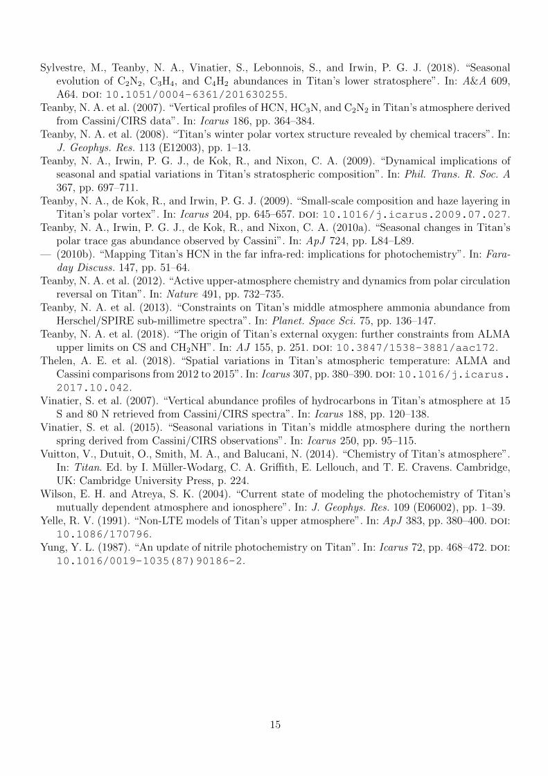
The observational parameters for these data are detailed in Table 1. Datasets were chosen based on70

spatial resolution and observation date, with preference given to the highest resolution data observed71

closest to the data analyzed in Thelen et al. (2018) used to obtain temperature measurements in72

Titan’s stratosphere. The list of detected and modeled transitions for each species is listed in Table73

2.74

We modeled disk-averaged spectra for all datasets listed in Table 1, and spectra from three inde-75

pendent spatial regions for the nitrile species from either 2012 or 2013, and for all species in 201476

and 2015. While spectra representing Titan’s northern and southern hemispheres were extracted for77

C3H4 in 2013, the signal-to-noise ratio was insufficient to yield meaningful abundance retrievals. As78

in Paper I, spatially resolved spectra were extracted from regions where ALMA ‘beam-footprints’79

do not overlap to obtain independent measurements of three spatial regions. These regions were80

chosen to match those in Paper I as closely as possible – with mean latitudes at or within 3◦ of 48◦81

N, 21◦ N, and 16◦ S (hereon referred to as ‘North’, ‘Center’, and ‘South’) – so that we may ensure82

corresponding temperature measurements are appropriate for chemical abundance retrievals. These83

regions are held constant with Titan’s changing tilt from 2012 to 2015. As we do not expect to see84

longitudinal changes in chemical abundance, we extracted spectra representing Titan’s low northern85

latitudes (Center) in some higher resolution data in 2014 and 2015 from Titan’s limb, as opposed to86

Titan’s central disk where emission from atmospheric species is reduced leading to insufficient fluxes.87

Integrated flux (moment 0) maps are shown for HC3N and CH3CN in Fig. 1 for 2013, 2014, and88

2015, demonstrating the spatial variation of these molecules in Titan’s stratosphere.89

2https://almascience.nrao.edu/alma-data/archive

3

3 Spectral Modeling and Retrieval Methodology90

Models of Titan’s atmospheric structure and the subsequent generation of synthetic spectra were91

carried out in a similar fashion to Paper I. Molecular line data were obtained from the HITRAN92

20163 and CDMS4 catalogues (Gordon et al., 2017; Muller et al., 2005). We employed the Non-93

Linear Optimal Estimator for Multivariate Spectra Analysis (NEMESIS) radiative transfer code in94

line-by-line mode (Irwin et al., 2008) to retrieve vertical abundance profiles from 0–1200 km for each95

gas species independently. As in Paper I (and detailed in Teanby et al., 2013), many field-of-view96

averaging points (37-44) are required to model disk-averaged data, with higher concentrations of97

emission angles on Titan’s limb. For spatially resolved spectra, field-of-view points were weighted98

to model emission from each ALMA beam-footprint. Spectra were multiplied by a small scaling99

factor found by modeling nearby regions of continuum emission to account for small offsets due to100

flux calibration or model inaccuracies. Using accurate troposphere temperatures from Cassini radio101

science measurements (Schinder et al., 2012, following the procedures detailed in Paper I) reduced102

these scaling factors to below 5% of the continuum flux, within the expected calibration uncertainty103

level (see ALMA Memo #5945). ALMA data and the resulting best fit spectra for each molecule in104

each year are shown in Fig. 2–5.105

While chemical abundance contributes to the radiance of molecular line cores in Titan’s upper106

atmosphere (∼800 km), we only discuss the retrieval results for the upper troposphere–stratosphere107

(50–550 km) here, where our previous ALMA retrievals of temperature are valid (Paper I) and the108

rotational emission lines are not subject to non-LTE and thermal broadening effects (Yelle, 1991;109

Cordiner et al., 2014); additionally, the few data points that make up the line centers in these110

data contribute little to the χ2 minimization of data and model discrepancies, and the retrieved111

abundance profiles often return to the a priori profile values in the upper atmosphere as in previous112

studies of ALMA data using NEMESIS (Serigano et al., 2016; Molter et al., 2016; Thelen et al.,113

2018). Contribution functions generated for disk-averaged spectra of each molecule are shown in114

Fig. 6, showing significant contribution between ∼100–300 km (10–0.1 mbar) for each molecule, and115

secondary peaks in the upper atmosphere.116

For all gases in this study, multiple a priori abundance profiles were tested to determine uniqueness117

amongst retrieved measurements (see example in Section 3.1). Similar to the previous temperature118

retrievals in Paper I, we have elected to use data besides those obtained by Cassini/CIRS data to119

generate a priori profiles (i.e. profiles with more simple vertical structure) where possible, to facilitate120

the use of ALMA for future Titan measurements after the end of the Cassini era. These often include121

previous disk-averaged observations of Titan in the sub-mm or results from photochemical models.122

A priori vertical profiles were taken with 100% errors at all altitudes and correlation lengths were set123

to 1.5 scale heights (as in Teanby et al., 2007) for all species but the HCN isotopologues (set to 3.0,124

as in Molter et al., 2016) to provide sufficient vertical smoothing, and to account for uncertainties125

due to minor variations in temperature, line broadening parameters, and ALMA flux calibrations.126

The specific parameters, a priori profiles, and retrieval methodology pertaining to each gas species127

are discussed in the following subsections.128

To ensure the accurate retrieval of continuous chemical abundance profiles, we modeled emission129

lines without any contamination from other species where possible, and held atmospheric tempera-130

tures constant. Both spatially resolved and disk-averaged temperature profiles from Paper I were used131

to model 2012, 2014, and 2015 spectra, providing measurements from similar latitude regions within132

∼2 months of the datasets analyzed here (Table 1); temperature variations in Titan’s stratosphere133

3http://hitran.org/4https://www.astro.uni-koeln.de/cdms/catalog5https://science.nrao.edu/facilities/alma/aboutALMA/Technology/ALMA Memo Series/alma594/memo594.pdf

4

are negligible on these timescales (Flasar et al., 1981), particularly for measurements comprised134

of multiple latitudes such as those analyzed here (see Paper I). For 2013 data, we elected to use135

more contemporary temperature profiles obtained during the T89 and T91 Cassini flybys (during136

February 17 and May 23, respectively) obtained with the CIRS instrument (courtesy R. Achterberg,137

private communication; see also Achterberg et al., 2011; Achterberg et al., 2014). All temperature138

profiles used in this study are are shown in Fig. 7. As emission lines in Titan’s atmosphere may139

be significantly affected by temperature variations, we tested the discrepancies found in Paper I140

between retrieved ALMA and Cassini/CIRS temperature profiles (∼0–5 K for spatial regions) on141

HCN isotope lines; we find that variations of temperature on order 5 K or less resulted in abundance142

variations <20%, and were well within the retrieval errors.143

3.1 HC3N and C3H4144

For both molecules, we assumed a Lorentzian broadening HWHM (Γ) value = 0.1 cm−1 bar−1 and145

temperature dependence (α) = 0.75 as in previous studies (Vinatier et al., 2007; Cordiner et al., 2014;146

Lai et al., 2017) and recommended by HITRAN. The strongest 4-5 C3H4 transitions were modeled147

each year, as weaker lines did not significantly contribute to the retrieved vertical abundance profiles.148

For the 2015 dataset, 2 interloping C2H5CN lines were modeled among the C3H4 bandhead, except149

in the Center spectrum, where these lines did not significantly impact the χ2 value.150

The initial HC3N abundance profiles used as a priori inputs came from previous disk-averaged151

measurements of Titan in the sub-mm by Cordiner et al. (2014) and Marten et al. (2002). A152

comparison of these profiles to fractional scale height and continuous abundance retrievals is shown153

in Fig. 8. While adequate fits of disk-averaged lines at low S/N can be accomplished using fractional154

scale height (‘gradient’) profiles as in Cordiner et al. (2014), we find that spectral fits are improved155

by using continuous abundance retrievals (Fig. 8A); for all chemical species, spatial spectra are fit156

better by continuous retrievals due to broadened line wings (compare, e.g., HC3N spectra in Fig. 4).157

Additionally, the gradients present in some continuous vertical profiles are important for the study158

of temporal and dynamical variations. For a variety of a priori profiles (Fig. 8B) or perturbations159

thereof, continuous retrievals converged on similar vertical profiles (Fig. 8C) for all gases modeled160

in this study.161

Models of C3H4 were initialized using ‘step models’ of abundance, as in Cordiner et al. (2014;162

2015), with a VMR = 1×10−8 at 100 km as found by Nixon et al. (2013), or by using photochemical163

model results from Loison et al. (2015). In 2015, additional lines of C2H5CN were modeled using the164

gradient model from Cordiner et al. (2015), comparable to that found in other ALMA studies (Palmer165

et al., 2017; Lai et al., 2017; Teanby et al., 2018). Spatial abundance variations of C2H5CN are not166

determined here due to the lines’ proximity to those of C3H4 and their relatively weak strength.167

3.2 HCN168

Due to the strong self-absorption present in spectra of HCN from spatially resolved datasets of Titan169

and the calibration uncertainties for species with extensive line wings in ALMA data (as with CO,170

detailed in Paper I), we chose to model the HCN isotopologues H13CN and HC15N as proxies for171

HCN abundance. Molter et al. (2016) showed a retrieved vertical abundance profile of HCN could172

be scaled to fit lines of isotopologues and used to determine isotope ratios for disk-averaged spectra.173

Here, we reversed this process by fitting H13CN and HC15N lines using the HCN profile found by174

Molter et al. (2016), and applied a constant scaling factor (12C/13C = 89.8, 14N/15N = 72.2) to175

determine the HCN abundances. As in that study, we model H13CN and HC15N lines with Γ = 0.13,176

α = 0.75. We set condensation to begin at altitudes below ∼ 80 km as in Marten et al. (2002),177

5

which was derived from the vapor saturation law in Lellouch et al. (1994) and is consistent with the178

calculations based on Cassini/Huygens observations in Titan’s lower stratosphere by Lavvas et al.179

(2011); below this altitude, the abundance profile no longer effects the line shape. The HCN isotope180

lines lie on the wings of the CO (J=3–2) and CO (J=6–5) transitions, so those lines were included181

in the model using the parameters given in Paper I.182

While the C and N ratios found for Titan through HCN measurements have a range of values183

(see Molter et al., 2016 and references therein), we find that applying these ratios to line data and184

scaling the retrieved profiles to convert to HCN abundances have vanishingly small effects for the185

range of published isotope ratios. For the 2014 measurements, we were able to model both species in186

disk-averaged and spatially resolved spectra, and found the (scaled) retrieved profiles were in good187

agreement (see Section 4).188

3.3 CH3CN189

For computational efficiency and to preserve the native resolution of ALMA data (i.e. without190

additional channel averaging to meet the array limitations of NEMESIS), we only retrieved abundance191

profiles using the strongest CH3CN lines in each band. Studies of CH3CN in Titan’s atmosphere192

have been limited due to its lack of observable transitions in the IR accessible by Cassini. Therefore193

we tested three different a priori profiles and variations of those by an order of magnitude in each194

direction: the combination of disk-averaged measurements from Marten et al. (2002) to 500 km, and195

the model results from Loison et al. (2015) up to 1200 km; the model by Dobrijevic and Loison196

(2018), which tests a new nitrogen isotope fractionation scheme from Loison et al., 2015; a test197

gradient profile (Profile 1 from Fig. 8). A priori profiles and retrieval results are shown in Fig. 9A198

and B, respectively, for the 2014 disk-averaged spectrum of CH3CN (Fig. 4). All retrievals shown in199

Fig. 9B provided an adequate fit to the data. We find that the retrievals converge around 150 km200

(∼ 2 mbar) and above, where ALMA is sensitive to CH3CN emission (Fig. 6E).201

We adopted the N2-broadening parameters detailed by Dudaryonok et al. (2015), where available.202

As these differ from the parameters used by Marten et al. (2002), we ran a large number of forward203

models of the 2014 (J=16–15) transitions to test the effect of the Lorentzian broadening and tem-204

perature dependence coefficients. Though we obtained some variation in χ2 values for the parameter205

space [Γ=0.1–0.16, α=0.5–0.8] for CH3CN forward models, the effects of these parameters on re-206

trieved abundances were small and well within the retrieval errors for a model using the Dudaryonok207

et al. (2015) parameters.208

4 Results and Discussion209

In Fig. 10, we present the mean disk-averaged results for each molecule; the average of the scaled210

HC15N and H13CN profiles is used to represent HCN here. As with the temperature profiles found211

in Paper I, abundance retrievals from disk-averaged measurements do not show significant variation212

from year to year, and all fall within the retrieval errors of the mean profile. In Fig. 11–13, we present213

the retrieved abundance profiles from spatially resolved spectra in Fig. 2–5. HCN profiles from 2012214

and HC3N, CH3CN profiles from 2013 are shown together in Fig. 11. Scaled HCN profiles from both215

H13CN and HC15N retrievals from 2014 are shown in Fig. 12. With the exception of a small portion216

of the Center retrievals between 0.1–1 mbar, and >10 mbar (where the HCN isotopologues quickly217

lose sensitivity – Fig. 6A,B), these profiles all agree and display similar vertical variations (e.g. a218

slight inversion in north and south retrievals at pressures <0.1 mbar).219

6

4.1 Comparison to Previous Studies220

In Fig. 14 we compare the mean disk-averaged profiles (Fig. 10) to those from previous disk-averaged221

sub-mm measurements of Titan and photochemical model results.222

The disk-averaged HCN profile (a mean of both H13CN and HC15N profiles for all years) agrees well223

with previous sub-mm observations by Molter et al. (2016) with ALMA throughout the atmosphere,224

and with those of Marten et al. (2002) and Gurwell (2004) in the lower atmosphere. Our profile225

is also comparable to the photochemical models of Krasnopolsky (2014) and Dobrijevic and Loison226

(2018) in the stratosphere and above.227

Our mean retrieved HC3N profile shows a highly variable slope – particularly the lower atmo-228

sphere enhancement near 1 mbar – compared to both previous sub-mm observations (Marten et al.,229

2002; Cordiner et al., 2014) and photochemical models (Dobrijevic and Loison, 2018), though the230

abundance at all altitudes is significantly less than predicted by Krasnopolsky (2014). We find strato-231

spheric abundances closest to the fractional scale height model adopted by Cordiner et al. (2014)232

and the models of Dobrijevic and Loison (2018). These differences may be explained by the use233

of continuous abundance retrievals for disk-averaged measurements, which tended towards a mean234

profile of the three spatial regions; HC3N shows significant enhancement between 100–200 km in the235

higher northern and low southern latitudes (Fig. 11–13), which may be reflected in the disk-averaged236

measurements.237

The mean C3H4 profile is consistent with previous CIRS measurements (Nixon et al., 2013), con-238

temporary ALMA observations (Teanby et al., 2018), and photochemical models (Krasnopolsky,239

2014; Loison et al., 2015) below 400 km, where ALMA is most sensitive to C3H4 emission (Fig. 6D).240

Above 200 km, we find that our CH3CN profile is consistent with previous sub-mm observations by241

Marten et al. (2002) and the photochemical model of Dobrijevic and Loison (2018), though generally242

less than that of Krasnopolsky (2014). We find CH3CN to be a factor of ∼ 5 less than the upper243

limit found by Nixon et al. (2010) at 25◦S in Cassini/CIRS measurements at 0.27 mbar. Near 1244

mbar, our retrieval results and the other profiles shown in Fig. 14 diverge, which may be indicative245

of another loss mechanism for CH3CN in Titan’s lower stratosphere that has not been accounted for246

by photochemical models. At higher pressures (particularly >10 mbar, or <100 km) our retrievals247

adhere more strongly to the input vertical profiles (Fig. 9), inhibiting us from accurately determining248

the nature of CH3CN’s lower atmosphere gradient.249

Our retrievals are compared to contemporary Cassini/CIRS limb (Vinatier et al., 2015) and nadir250

(Coustenis et al., 2016) measurements in Fig. 15. We measure lower abundances than those found by251

Coustenis et al. (2016) from 50◦N and S nadir observations at the peak of their contribution functions252

at 7 (HCN) or 10 (HC3N and C3H4) mbar; however, these nadir measurements are assuming constant253

vertical profiles above condensation altitudes, where our continuous retrievals often manifest as steep254

gradients in the lower atmosphere. Our results agree better at altitudes above those sounded by255

2012 and 2013 CIRS nadir observations, particularly at the altitudes of the secondary peaks in the256

contribution functions of HCN and HC3N near 0.1–0.5 mbar seen in 2014.257

We find our 2012 HCN profiles (derived from HC15N) to be comparable to the CIRS limb mea-258

surements by Vinatier et al. (2015) in all regions, with the exception of the south at pressures <0.01259

mbar; here, the large latitudinal average of our ALMA beam-footprint measurements may be less260

directly comparable to CIRS, which is more sensitive to variations in the upper atmosphere. Due to261

the Cassini orbiter’s high latitude resolution and preferable viewing geometry, abundance enhance-262

ments as a result of subsidence onto the south pole, or the increased formation/decreased destruction263

of these molecules in southern winter, are more readily apparent. Further, sub-mm observations lose264

sensitivity in the upper atmosphere (>800 km) for all molecules observed here (Fig. 6). For example,265

while the northern CIRS profile falls within our retrieval errors, we do not observe the same vertical266

7

structure in the upper atmosphere showing a depletion of HCN at pressures <0.02 mbar, as our267

retrieved profile tends to adhere more strongly to the a priori values in the upper atmosphere.268

Similar discrepancies are observed for HC3N, where we find a more shallow gradient at low northern269

(Center) and southern (South) latitudes at high altitudes compared to the 2012 CIRS retrievals. We270

might expect that the relatively large ALMA beams may more easily obfuscate spatial variations in271

shorter lived trace species, such as HC3N and C3H4, which are more susceptible to short term change272

in atmospheric circulation or increased production as the moon transitions into southern winter. As273

HC3N seems to be a good tracer of atmosphere dynamics in Titan’s stratosphere (Fig. 1), continued274

ALMA monitoring of this molecule, particularly with higher spatial resolution, may help elucidate275

changes in shorter lived nitriles and circulation in the stratosphere.276

Due to the lack of earlier spatially resolved C3H4 observations, we compare our 2014 retrievals to277

those of Vinatier et al. (2015) from 2012. Unlike in HCN and HC3N, the ALMA- and CIRS-derived278

southern profiles here are in good agreement, as are the measurements from low northern latitudes279

(Center). The lower altitude enhancement at mid-northern latitudes (North) rises by ∼30 km (from280

170–200 km), and increases in magnitude by a factor of 2.8. This may not be unreasonable, as281

Vinatier et al. (2015) and Coustenis et al. (2016) both observe a general increase in C3H4 abundance282

at mid-northern latitudes into northern spring, and the now reversed pole-to-pole circulation cell may283

shift a lower atmosphere reservoir of C3H4 to higher altitudes. As with the other gases, the abundance284

measurements derived from ALMA observations comprise multiple latitude decades, making direct285

comparisons to CIRS limb observations difficult; however, we find that our results are generally286

compatible with those from Cassini, previous ground-based observations, and photochemical model287

results, particularly near 1–10 mbar, where our retrievals are most sensitive.288

4.2 Spatial and Temporal Variations289

While abundance comparisons to Cassini are generally in agreement, the HCN and HC3N results290

show that our ALMA-derived retrievals are missing the variability in vertical gradients and oscil-291

lations seen at high latitudes on Titan due to the spatial averaging of the relatively large ALMA292

beams, the inherent vertical resolution constraints of ground-based (nadir) observations, and the293

decreased sensitivity to altitudes >300 km. However, our results still display large spatial variations294

in northern and southern latitudes compared to the low northern (Center) latitudes in both retrieved295

vertical profiles (Fig. 11–13) and intensity maps (Fig. 1). When plotting profiles from each spatial296

region over time (Fig. 16), we can also see temporal trends arise as a result of Titan’s atmospheric297

dynamics, even at altitudes where ALMA is less sensitive.298

The HCN isotopes that we model here lie on the broadened wings of CO emission lines, making299

integrated flux maps difficult to interpret. In the retrieval results, we observe a significant enhance-300

ment in the north during 2015 near 0.1 mbar, which is ∼16 times greater than the abundance at301

lower northern latitudes (Center) and a factor of 7 greater than the south. A similar increase of302

HCN in mid-northern latitudes at similar altitudes was observed in Cassini/CIRS limb data be-303

tween 2011–2012 as the result of the of the weakening northern polar vortex and the advection of304

accumulated enriched gas to lower latitudes (Vinatier et al., 2015); the upper atmosphere (<0.01305

mbar) in these observations was also observed to be depleted in HCN, further reinforcing the notion306

of a recent upwelling from the recent north-to-south circulation cell. This trend is also present in307

our observations in 2014 and 2015, indicating we may be probing portions of the upper atmosphere308

at higher northern latitudes that are now depleted in HCN due to the rise of lower stratospheric air309

in the ascending branch. Further, the retrieval results show a consistent enhancement of HCN in the310

upper atmosphere (>300 km) of the low-southern latitudes over time (Fig. 16, top row), resulting311

in abundances >6 times those of the Center and a factor of 5 greater than the North. While our312

8

abundance retrievals are less sensitive to emission at these altitudes, the trend in these profiles seems313

significant; this trend is also observable at low northern latitudes (Center) at the highest portion of314

our retrievals (>400 km). Both of these increases are indicative of the circulation of the large con-315

centration of HCN formed at the north pole during northern winter to the south (now winter) pole,316

and lower latitudes. The effects of this new circulation are present in contemporary Cassini/CIRS317

measurements at high southern latitudes (Vinatier et al., 2015; Coustenis et al., 2016; Sylvestre et al.,318

2018), where subsidence onto the southern pole greatly increased the abundance of all species. In319

particular, species with long chemical lifetimes compared to dynamical timescales in Titan’s strato-320

sphere (such as HCN; see e.g. Loison et al., 2015) provide good tracers of Titan’s global circulation321

(Vinatier et al., 2015).322

Retrievals of HC3N for each year show significant enhancements in the lower atmosphere in both323

the North and South profiles, and are the largest spatial enhancements that we measure here. While324

the North and South enhancements are reduced in 2014 – with 34 and 13 times the Center abundance,325

respectively – they increase from a factor of 50 and 34 to 75 and 61 compared to the center from326

2013 to 2015; these factors are larger than enhancements exhibited by the other nitriles and C3H4 by327

an order of magnitude in the lower stratosphere, but comparable to the large enrichment seen during328

the northern winter by Cassini (Teanby et al., 2010b). These peaks most likely influence the large329

enhancement seen in the disk-averaged profile from each year (Fig. 10). A northern stratospheric330

enhancement of HC3N may be the result of advection between the polar vortex and lower latitudes,331

but a ‘tongue’ of enriched gas was not observed for HC3N during northern winter, as was seen for332

HCN (Teanby et al., 2008). A rapidly appearing tongue in the south soon after the circulation333

reversal in 2011 also seems unlikely (but motivates an analysis of the wind speeds during this epoch).334

Further, lower atmosphere enhancements in abundance are observed by photochemical models due335

to the influence of galactic cosmic ray (GCR) induced chemistry; yet, the Center retrievals lack an336

enhanced peak in the lower stratosphere, which would most likely manifest regardless of latitude. This337

trend also does not fully agree with the integrated intensity maps (Fig. 1), where the enhancements338

are only a factor of 2–3 compared to the central flux, with a prominent decrease in the north from339

2014 to 2015. The shift between a northern and southern enhancement of HC3N between 2014 and340

2015 is consistent across ALMA observations of Titan (Cordiner et al., 2017). The discrepancy341

between retrieval results and image maps may arise from the high opacity of the HC3N line core in342

the sub-mm, possibly inhibiting us from obtaining meaningful comparisons in the lower atmosphere343

from integrated emission maps (Cordiner et al., 2018). Finally, these spatial enhancements occur344

at different altitudes – near 150 km in the south and 200 km in the north – and the peak of both345

regions decreases by about 20 km from 2013 to 2015. The shift of these peaks with altitude and346

time may be a result of a decrease in stratospheric temperatures, causing the condensation altitude347

of HC3N to change; this was observed in Cassini/CIRS spectra at the south pole (Jennings et al.,348

2012; Coustenis et al., 2016). While ALMA temperature measurements at these same spatial regions349

between 100–200 km reveal cooler temperatures at northern latitudes compared to those from the350

subsolar point, the temperatures at low southern latitudes are comparable to those of the center (see351

Paper I, Fig. 9).352

HC3N emission maps show significant spatial changes from 2013 to 2015, where we observe quickly353

increasing southern flux and decreasing flux in the north, but these large changes aren’t immediately354

obvious in the retrieval results. We do observe a general increase in southern abundances over time355

above and below the abundance peak at ∼ 150 km, and a similar decrease in the north (Fig. 16,356

second row); we also observe a reduction in abundance from Center retrievals >1 mbar from 2014357

to 2015. Thus, we can trace most of the variability in the integrated flux maps to changes in the358

deeper atmosphere, and altitudes above the potentially enriched reservoir of HC3N near 1 mbar.359

The retrieved profiles consistently show higher abundance in the upper atmosphere at low southern360

9

latitudes by a factor of 2–4 compared to the North, but the profiles do not show any significant361

trends over time.362

Our HC3N North and South retrievals (and thus, the disk-averaged results) may be adversely363

effected by high opacity and large latitudinal averages at low altitudes. As found by Cordiner et al.364

(2018), these effects may result in abundance underestimates at the pole for higher spatial resolution365

observations, but HC3N still provides a valuable tracer of meridional mixing of nitrile reservoirs366

from Titan’s poles. If the enhancements we present here are real, the cause of a lower stratospheric367

reservoir of HC3N at mid to low latitudes is not fully understood; this motivates a more in depth368

study of HC3N emission over time across Titan’s limb, where more accurate abundances may be369

derived at latitudes below the poles.370

As with the nitriles, we observe an enhancement of C3H4 at mid-northern latitudes with factors of371

5–6 greater than the Center retrievals in 2014 and 2015. Similar to HCN and HC3N, we find that the372

Center C3H4 abundance decreases with time at altitudes <300 km – particularly from 2014 to 2015373

(Fig. 16, third row). We also observe a simultaneous increase in the southern abundances of C3H4374

by a factor of 2 compared to the Center profiles, and a general increase in the upper atmosphere of375

both North and South retrievals. Both of these trends are indicative of the redistribution of enriched376

gas from high northern latitudes to the south with the reversal of Titan’s circulation cell, though we377

do not observe the increase in upper atmosphere gradient observed with CIRS (Vinatier et al., 2015);378

this latter effect may be missing from our C3H4 results due to the lack of sensitivity above ∼400379

km (Fig. 6D). While both HC3N and C3H4 did not show a significant lower atmosphere tongue of380

enriched gas leaking from the polar vortex in Cassini/CIRS observations, C3H4 did extend further381

past the vortex boundary than HC3N by 10 − 15◦ (Teanby et al., 2009). We also find that C3H4 is382

more enhanced at the Center compared to HC3N, as measured during northern winter.383

CH3CN shows enhancements in the north in both retrievals (Fig. 16, bottom row) and maps (Fig.384

1). In the latter, we see the emission peaks confined to 45–60◦N and higher, consistent with some gas385

advection beyond the northern polar vortex barrier observed with Cassini (Teanby et al., 2008). We386

find a slight increase in lower atmosphere abundances in the North over time, increasing by a factor387

of 3–6.5 compared to the Center near 1 mbar; this enhancement rises about 30 km from 2013 to388

2015. The decrease in northern emission seen in the integrated flux maps may be an artifact caused389

by the increasing spatial resolution over time, but we do observe a decrease in northern abundance390

retrievals near 0.01 mbar (400 km) by a factor of ∼3 from 2013 to 2015, where the contribution391

function for CH3CN has a secondary peak (Fig. 6E). This change is minor compared to the retrieval392

errors (i.e. <2σ), but could be the result of upwelling of depleted air from the lower atmosphere that393

we see with HCN and as observed by CIRS (Vinatier et al., 2015). The enhancement of CH3CN in394

the northern lower atmosphere is indicative of a winter enrichment of this molecule, which may be395

advected to the lower latitudes after northern winter. CH3CN has a relatively long chemical lifetime396

throughout Titan’s atmosphere (as compared to the dynamical lifetime), with a similar lifetime to397

HCN in the stratosphere (Wilson and Atreya, 2004; Loison et al., 2015). However, we don’t find398

large variations in southern abundances at higher altitudes over time, or a large difference between399

North and South abundances in the upper stratosphere as is observed for HCN here. As with the400

other nitriles, observations of these changes at the southern pole are inhibited by our viewing angle401

from Earth, though the emission maps may provide evidence for circulation from the north pole to402

the south over time.403

Vertical oscillations appear in CH3CN retrievals to a larger extent than the other molecules, par-404

ticularly in 2014. Oscillations in previous Cassini measurements of nitriles have been documented,405

particularly for mid to high northern latitudes, and are thought to be the result of small scale406

dynamical mixing between gas-depleted lower latitudes and the enriched polar vortex (Teanby et407

al., 2009). While our CH3CN retrievals exhibit larger vertical oscillations with increasing northern408

10

latitudes (Fig. 16), we do not see a similar pattern in the other nitriles or C3H4, as were seen in409

Cassini/CIRS results (Teanby et al., 2009; Vinatier et al., 2015). The lack of contemporary, spatially410

resolved abundance measurements for CH3CN in Titan’s stratosphere, combined with the averaging411

of our measurements across multiple latitudes (with potentially significant dynamics and meridional412

mixing) makes these vertical oscillations difficult to interpret.413

5 Conclusions414

Building on the previous results in Paper I, we present vertical abundance profiles of HCN, HC3N,415

C3H4, and CH3CN obtained through the analysis of rotational transitions in spatially resolved (beam416

sizes ∼ 0.2 − 0.5′′) ALMA flux calibration data from 2012 to 2015. The comparison of three regions417

on Titan’s disk (centered at ∼48◦N, 21◦N, and 16◦S) reveal distinct spatial variations and insight418

into Titan’s atmospheric dynamics. In contrast with the temperature profiles presented in Paper419

I, the abundance profiles of these molecules show temporal changes over the 3 years of observation420

from 2012 to 2015. The combination of the spatial and temporal variations we observe informs our421

understanding of Titan’s atmospheric circulation into northern spring and summer. Our findings are422

summarized as follows:423

– All four molecules display enhancements in the North (and often the South) compared to424

Center, ranging from factors of ∼6 in C3H4 and CH3CN to 15 and 75 in HCN and HC3N,425

respectively. Southern enhancements are more noticeable in the upper atmosphere, particularly426

for HCN and HC3N, yet do not exhibit the steep vertical gradients seen by Cassini/CIRS427

(Teanby et al., 2012; Vinatier et al., 2015; Coustenis et al., 2016).428

– We find large enhancements of HC3N between 150–200 km in all North and South retrievals.429

This is indicative of a relatively new lower atmosphere HC3N reservoir, but may also be the430

result of opacity effects of sub-mm HC3N lines (Cordiner et al., 2018). Nevertheless, the431

combination of retrieval results and integrated flux maps show a rapid reduction of HC3N at432

Titan’s north pole and a simultaneous increase in the south between 2013 and 2015.433

– We observe many temporal trends in abundance retrievals that reveal the continued effects of434

Titan’s large north-to-south circulation cell:435

i. The increase of southern HCN, HC3N, C3H4, and potentially CH3CN at higher altitudes,436

and similar trends (with reduced magnitude) at low-northern latitudes (Center).437

ii. A slight increase in the abundances of mid northern latitudes over time in HCN, C3H4,438

CH3CN, with a change in upper atmosphere gradients in the longer lived chemical species439

(HCN and CH3CN).440

iii. An increase in abundance for all molecules at pressures >1 mbar at southern latitudes,441

except CH3CN, which does not effectively sound higher pressures.442

iv. A reduction in abundance for all molecules in Center profiles at pressures >0.1 mbar.443

These trends show evidence for subsidence at the southern pole, the decrease of a ‘tongue’ at444

low northern latitudes (where enriched air was advected from the northern polar vortex during445

winter), and lofted air replete with longer lived chemical species from Titan’s lower stratosphere446

to higher altitudes.447

11

– The polar enhancements and vertical gradients observed are generally less significant than those448

observed with the Cassini orbiter, indicating that the effects of atmospheric chemistry and449

dynamics are muted when observed in large latitudinal averages (as seen with the temperatures450

reported in Paper I).451

We validated our results using contemporaneous Cassini/CIRS data, and through comparisons of452

mean profiles from 2012 to 2015 to previous disk-averaged ground-based observations and photochem-453

ical model results. We find that our retrieved profiles are comparable to contemporary studies with454

the exception of HC3N, which is optically thick at the poles where the molecule has been observed455

to be greatly enhanced. However, the large temporal variations and fine vertical structure observed456

with the Cassini orbiter are obscured by the latitudinal averaged measurements derived from spectra457

representing relatively large ALMA beam-footprints, particularly at higher altitudes where sub-mm458

measurements are not as sensitive, as observed with the previous atmospheric temperature retrievals459

(Paper I). Thus, this work serves as a proof of concept for future measurements of Titan’s chemical460

abundances throughout the stratosphere that will allow us to continue monitoring Titan’s varied461

atmospheric dynamics into the post-Cassini era.462

6 Acknowledgments463

This research was supported by NASA’s Office of Education and the NASA Minority University464

Research and Education Project ASTAR/JGFP Grant #NNX15AU59H. Additional funding was465

provided by the NRAO Student Observing Support award #SOSPA3-012. C.A.N was supported466

in this work by the NASA Solar System Observations Program and the NASA Astrobiology Insti-467

tute. M.A.C received funding from the National Science Foundation under Grant No. AST-1616306.468

N.A.T and P.G.J.I were supported by the UK Science and Technology Facilities Council. S.B.C was469

funded by an award from the NASA Science Innovation Fund. This paper makes use of the follow-470

ing ALMA data: ADS/JAO.ALMA#2011.0.00724.S, 2011.0.00820.S, 2012.1.00377.S, 2012.1.00225.S,471

2012.1.00453.S, 2013.1.00220.S, and 2013.1.00111.S. ALMA is a partnership of ESO (representing its472

member states), NSF (USA) and NINS (Japan), together with NRC (Canada) and NSC and ASIAA473

(Taiwan) and KASI (Republic of Korea), in cooperation with the Republic of Chile. The Joint474

ALMA Observatory is operated by ESO, AUI/NRAO and NAOJ. The National Radio Astronomy475

Observatory is a facility of the National Science Foundation operated under cooperative agreement476

by Associated Universities, Inc.477

The authors would like to thank Richard Achterberg for his insightful comments on Titan’s strato-478

spheric temperatures and his contribution of Cassini/CIRS temperature profiles for this work and479

Paper I.480

References

Achterberg, R. K., Gierasch, P. J., Conrath, B. J., Flasar, F. M., and Nixon, C. A. (2011). “Tem-poral variations of Titan’s middle-atmosphere temperatures from 2004 to 2009 observed byCassini/CIRS”. In: Icarus 211, pp. 686–698.

Achterberg, R. K., Gierasch, P. J., Conrath, B. J., Flasar, F. M., Jennings, D. E., and Nixon, C. A.(2014). “Post-equinox variations of Titan’s mid-stratospheric temperatures from Cassini/CIRSobservations”. In: DPS Meeting #46.

12

Bezard, B., Marten, A., and Paubert, G. (1992). “First Ground-based Detection of Cyanoacetyleneon Titan”. In: AAS/Division for Planetary Sciences Meeting Abstracts #24. Vol. 24. Bulletin ofthe American Astronomical Society, p. 953.

— (1993). “Detection of Acetonitrile on Titan”. In: AAS/Division for Planetary Sciences MeetingAbstracts #25. Vol. 25. Bulletin of the American Astronomical Society, p. 1100.

Bezard, B., Yelle, R., and Nixon, C. A. (2014). “The Composition of Titan’s atmosphere”. In: Ti-tan. Ed. by I. Muller-Wodarg, C. A. Griffith, E. Lellouch, and T. E. Cravens. Cambridge, UK:Cambridge University Press, p. 158.

Broadfoot, A. L. et al. (1981). “Extreme ultraviolet observations from Voyager 1 encounter withSaturn”. In: Science 212, pp. 206–211. doi: 10.1126/science.212.4491.206.

Cordiner, M. A. et al. (2014). “ALMA measurements of the HNC and HC3N distributions in Titan’satmosphere”. In: ApJ 795, pp. L30–L35.

Cordiner, M. A. et al. (2015). “Ethyl cyanide on Titan: spectroscopic detection and mapping usingALMA”. In: ApJ 800, pp. L14–L19.

Cordiner, M. A. et al. (2017). “ALMA observations of Titan’s atmospheric chemistry and seasonalvariation”. In: IAU Symposium: Astrochemistry VII - Through the Cosmos from Galaxies toPlanets. Vol. 332. Cambridge University Press (In Press).

Cordiner, M. A., Nixon, C. A., Charnley, S. B., Teanby, N. A., Kisiel, Z., and Vuitton, V. (2018).“Interferometric imaging of Titan’s HC3N, H13CCCN and HCCC15N”. In: ApJ 859, p. L15. doi:10.3847/2041-8213/aac38d.

Coustenis, A. and Bezard, B. (1995). “Titan’s atmosphere from Voyager infrared observations. 4:Latitudinal variations of temperature and composition”. In: Icarus 115, pp. 126–140. doi: 10.1006/icar.1995.1084.

Coustenis, A. et al. (2016). “Titan’s temporal evolution in stratospheric trace gases near the poles”.In: Icarus 270, pp. 409–420.

Dobrijevic, M. and Loison, J. C. (2018). “The photochemical fractionation of nitrogen isotopologuesin Titan’s atmosphere”. In: Icarus 307, pp. 371–379. doi: 10.1016/j.icarus.2017.10.027.

Dudaryonok, A. S., Lavrentieva, N. N., and Buldyreva, J. V. (2015). “N2-broadening coefficientsof CH3CN rovibrational lines and their temperature dependence for the Earth and Titan atmo-spheres”. In: Icarus 256, pp. 30–36. doi: 10.1016/j.icarus.2015.04.025.

Flasar, F. M., Samuelson, R. E., and Conrath, B. J. (1981). “Titan’s atmosphere: temperature anddynamics”. In: Nature 292, pp. 293–298.

Flasar, F. M. et al. (2005). “Titan’s atmospheric temperatures, winds, and composition”. In: Science308, pp. 975–978.

Gillett, F. C. (1975). “Further observations of the 8-13 micron spectrum of Titan”. In: ApJL 201,pp. L41–L43. doi: 10.1086/181937.

Gillett, F. C., Forrest, W. J., and Merrill, K. M. (1973). “8-13 Micron Observations of Titan”. In:ApJL 184, p. L93. doi: 10.1086/181296.

Gordon, I. E. et al. (2017). “The HITRAN2016 molecular spectroscopic database”. In: J. Quant.Spec. Radiat. Transf. 203, pp. 3–69. doi: 10.1016/j.jqsrt.2017.06.038.

Gurwell, M. (2004). “Submillimeter observations of Titan: global measures of stratospheric temper-ature, CO, HCN, HC3N, and the isotopic ratios of 12C/13C and 14N/15N”. In: ApJ 616, pp. L7–L10.

Hanel, R. et al. (1981). “Infrared observations of the Saturnian system from Voyager 1”. In: Science212, pp. 192–200. doi: 10.1126/science.212.4491.192.

Horst, S. M. (2017). “Titan’s atmosphere and climate”. In: Journal of Geophysical Research (Planets)122, pp. 432–482. doi: 10.1002/2016JE005240.

13

Irwin, P. G. J. et al. (2008). “The NEMESIS planetary atmosphere radiative transfer and retrievaltool”. In: J. Quant. Spec. Radiat. Transf. 109, pp. 1136–1150.

Jennings, D. E. et al. (2012). “Seasonal Disappearance of Far-infrared Haze in Titan’s Stratosphere”.In: ApJ 754, p. L3. doi: 10.1088/2041-8205/754/1/L3.

Krasnopolsky, V. A. (2014). “Chemical composition of Titan’s atmosphere and ionosphere: observa-tions and the photochemical model”. In: Icarus 236, pp. 83–91.

Kuiper, G. P. (1944). “Titan: a Satellite with an Atmosphere.” In: ApJ 100, p. 378. doi: 10.1086/144679.

Kunde, V. G., Aikin, A. C., Hanel, R. A., Jennings, D. E., Maguire, W. C., and Samuelson, R.E. (1981). “C4H2, HC3N and C2N2 in Titan’s atmosphere”. In: Nature 292, pp. 686–688. doi:10.1038/292686a0.

Lai, J. C.-Y. et al. (2017). “Mapping Vinyl Cyanide and Other Nitriles in Titan’s Atmosphere UsingALMA”. In: AJ 154, p. 206. doi: 10.3847/1538-3881/aa8eef.

Lavvas, P., Griffith, C. A., and Yelle, R. V. (2011). “Condensation in Titan’s atmosphere at theHuygens landing site”. In: Icarus 215, pp. 732–750. doi: 10.1016/j.icarus.2011.06.040.

Lellouch, E., Romani, P. N., and Rosenqvist, J. (1994). “The vertical Distribution and Origin of HCNin Neptune’s Atmosphere”. In: Icarus 108, pp. 112–136. doi: 10.1006/icar.1994.1045.

Loison, J. C. et al. (2015). “The neutral photochemistry of nitriles, amines and imines in the atmo-sphere of Titan”. In: Icarus 247, pp. 218–247.

Maguire, W. C., Hanel, R. A., Jennings, D. E., Kunde, V. G., and Samuelson, R. E. (1981). “C3H8and C3H4 in Titan’s atmosphere”. In: Nature 292, pp. 683–686. doi: 10.1038/292683a0.

Marten, A., Hidayat, T., Biraud, Y., and Moreno, R. (2002). “New millimeter heterodyne observationsof Titan: vertical distributions of nitriles HCN, HC3N, CH3CN, and the isotopic ratio 15N/14Nin its atmosphere”. In: Icarus 158, pp. 532–544.

Molter, E. M. et al. (2016). “ALMA observations of HCN and its isotopologues on Titan”. In: AJ152 (42), pp. 1–7.

Muller, H. S. P., Schloder, F., Stutzki, J., and Winnewisser, G. (2005). “The Cologne Database forMolecular Spectroscopy, CDMS: a useful tool for astronomers and spectroscopists”. In: Journalof Molecular Structure 742, pp. 215–227. doi: 10.1016/j.molstruc.2005.01.027.

Nixon, C. A. et al. (2010). “Upper limits for undetected trace species in the stratosphere of Titan”.In: Faraday Discuss. 147, pp. 65–81.

Nixon, C. A. et al. (2013). “Detection of propene in Titan’s stratosphere”. In: ApJ 776, pp. L14–L19.Palmer, Maureen Y. et al. (2017). “ALMA detection and astrobiological potential of vinyl cyanide

on Titan”. In: Sci. Adv. 3.7. doi: 10.1126/sciadv.1700022.Paubert, G., Gautier, D., and Courtin, R. (1984). “The millimeter spectrum of Titan - Detectability

of HCN, HC3N, and CH3CN and the CO abundance”. In: Icarus 60, pp. 599–612. doi: 10.1016/0019-1035(84)90167-2.

Paubert, G., Marten, A., Rosolen, C., Gautier, D., and Courtin, R. (1987). “First radiodetection ofHCN on Titan.” In: Bulletin of the American Astronomical Society. Vol. 19, p. 633.

Raulin, F., Mourey, D., and Toupance, G. (1982). “Organic syntheses from CH4-N2 atmospheres:Implications for Titan”. In: Origins of Life 12, pp. 267–279. doi: 10.1007/BF00926897.

Schinder, P. J. et al. (2012). “The structure of Titan’s atmosphere from Cassini radio occultations:occultations from the Prime and Equinox missions”. In: Icarus 221, pp. 1020–1031.

Serigano, J., Nixon, C. A., Cordiner, M. A., Irwin, P. G. J., Teanby, N. A., Charnley, S. B., andLindberg, J. E. (2016). “Isotopic ratios of carbon and oxygen in Titan’s CO using ALMA”. In:ApJ 821, pp. L8–L13.

14

Sylvestre, M., Teanby, N. A., Vinatier, S., Lebonnois, S., and Irwin, P. G. J. (2018). “Seasonalevolution of C2N2, C3H4, and C4H2 abundances in Titan’s lower stratosphere”. In: A&A 609,A64. doi: 10.1051/0004-6361/201630255.

Teanby, N. A. et al. (2007). “Vertical profiles of HCN, HC3N, and C2N2 in Titan’s atmosphere derivedfrom Cassini/CIRS data”. In: Icarus 186, pp. 364–384.

Teanby, N. A. et al. (2008). “Titan’s winter polar vortex structure revealed by chemical tracers”. In:J. Geophys. Res. 113 (E12003), pp. 1–13.

Teanby, N. A., Irwin, P. G. J., de Kok, R., and Nixon, C. A. (2009). “Dynamical implications ofseasonal and spatial variations in Titan’s stratospheric composition”. In: Phil. Trans. R. Soc. A367, pp. 697–711.

Teanby, N. A., de Kok, R., and Irwin, P. G. J. (2009). “Small-scale composition and haze layering inTitan’s polar vortex”. In: Icarus 204, pp. 645–657. doi: 10.1016/j.icarus.2009.07.027.

Teanby, N. A., Irwin, P. G. J., de Kok, R., and Nixon, C. A. (2010a). “Seasonal changes in Titan’spolar trace gas abundance observed by Cassini”. In: ApJ 724, pp. L84–L89.

— (2010b). “Mapping Titan’s HCN in the far infra-red: implications for photochemistry”. In: Fara-day Discuss. 147, pp. 51–64.

Teanby, N. A. et al. (2012). “Active upper-atmosphere chemistry and dynamics from polar circulationreversal on Titan”. In: Nature 491, pp. 732–735.

Teanby, N. A. et al. (2013). “Constraints on Titan’s middle atmosphere ammonia abundance fromHerschel/SPIRE sub-millimetre spectra”. In: Planet. Space Sci. 75, pp. 136–147.

Teanby, N. A. et al. (2018). “The origin of Titan’s external oxygen: further constraints from ALMAupper limits on CS and CH2NH”. In: AJ 155, p. 251. doi: 10.3847/1538-3881/aac172.

Thelen, A. E. et al. (2018). “Spatial variations in Titan’s atmospheric temperature: ALMA andCassini comparisons from 2012 to 2015”. In: Icarus 307, pp. 380–390. doi: 10.1016/j.icarus.2017.10.042.

Vinatier, S. et al. (2007). “Vertical abundance profiles of hydrocarbons in Titan’s atmosphere at 15S and 80 N retrieved from Cassini/CIRS spectra”. In: Icarus 188, pp. 120–138.

Vinatier, S. et al. (2015). “Seasonal variations in Titan’s middle atmosphere during the northernspring derived from Cassini/CIRS observations”. In: Icarus 250, pp. 95–115.

Vuitton, V., Dutuit, O., Smith, M. A., and Balucani, N. (2014). “Chemistry of Titan’s atmosphere”.In: Titan. Ed. by I. Muller-Wodarg, C. A. Griffith, E. Lellouch, and T. E. Cravens. Cambridge,UK: Cambridge University Press, p. 224.

Wilson, E. H. and Atreya, S. K. (2004). “Current state of modeling the photochemistry of Titan’smutually dependent atmosphere and ionosphere”. In: J. Geophys. Res. 109 (E06002), pp. 1–39.

Yelle, R. V. (1991). “Non-LTE models of Titan’s upper atmosphere”. In: ApJ 383, pp. 380–400. doi:10.1086/170796.

Yung, Y. L. (1987). “An update of nitrile photochemistry on Titan”. In: Icarus 72, pp. 468–472. doi:10.1016/0019-1035(87)90186-2.

15

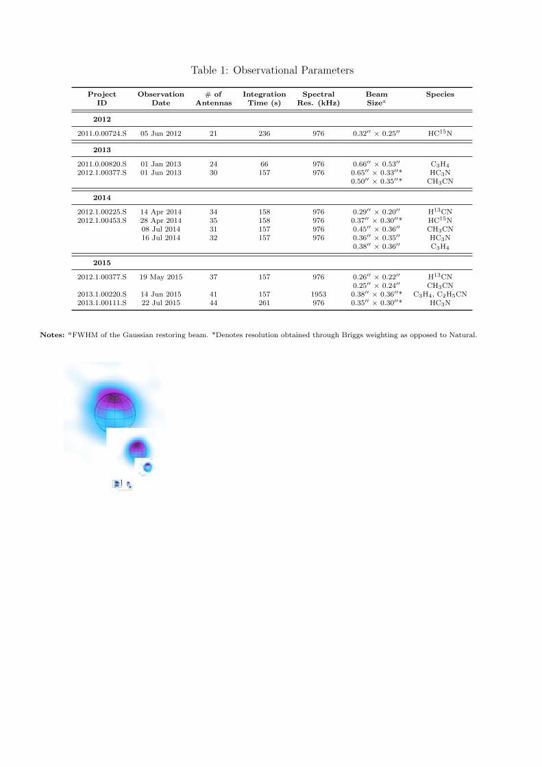
Table 1: Observational Parameters

Project Observation # of Integration Spectral Beam SpeciesID Date Antennas Time (s) Res. (kHz) Sizea

2012

2011.0.00724.S 05 Jun 2012 21 236 976 0.32′′ × 0.25′′ HC15N

2013

2011.0.00820.S 01 Jan 2013 24 66 976 0.66′′ × 0.53′′ C3H4

2012.1.00377.S 01 Jun 2013 30 157 976 0.65′′ × 0.33′′* HC3N0.50′′ × 0.35′′* CH3CN

2014

2012.1.00225.S 14 Apr 2014 34 158 976 0.29′′ × 0.20′′ H13CN2012.1.00453.S 28 Apr 2014 35 158 976 0.37′′ × 0.30′′* HC15N

08 Jul 2014 31 157 976 0.45′′ × 0.36′′ CH3CN16 Jul 2014 32 157 976 0.36′′ × 0.35′′ HC3N

0.38′′ × 0.36′′ C3H4

2015

2012.1.00377.S 19 May 2015 37 157 976 0.26′′ × 0.22′′ H13CN0.25′′ × 0.24′′ CH3CN

2013.1.00220.S 14 Jun 2015 41 157 1953 0.38′′ × 0.36′′* C3H4, C2H5CN2013.1.00111.S 22 Jul 2015 44 261 976 0.35′′ × 0.30′′* HC3N

Notes: aFWHM of the Gaussian restoring beam. *Denotes resolution obtained through Briggs weighting as opposed to Natural.

6000 4000 2000 0 2000 4000 6000Distance (km)

6000

4000

2000

0

2000

4000

6000

Dist

ance

(km

)

(A) CH3CN J = 19 18

Jun 01 20130

5

10

15

20

25

30

35

40

Flux

(Jy

kms

1 bm

1 )

6000 4000 2000 0 2000 4000 6000Distance (km)

6000

4000

2000

0

2000

4000

6000

Dist

ance

(km

)

(B) CH3CN J = 16 15

Jul 08 20140

5

10

15

20

25

Flux

(Jy

kms

1 bm

1 )

6000 4000 2000 0 2000 4000 6000Distance (km)

6000

4000

2000

0

2000

4000

6000

Dist

ance

(km

)

(C) CH3CN J = 37 36

May 19 20150.0

2.5

5.0

7.5

10.0

12.5

15.0

17.5

20.0

Flux

(Jy

kms

1 bm

1 )

6000 4000 2000 0 2000 4000 6000Distance (km)

6000

4000

2000

0

2000

4000

6000

Dist

ance

(km

)

(E) HC3N J = 35 34

Jul 16 20140.0

0.5

1.0

1.5

2.0

2.5

3.0

3.5

Flux

(Jy

kms

1 bm

1 )

6000 4000 2000 0 2000 4000 6000Distance (km)

6000

4000

2000

0

2000

4000

6000

Dist

ance

(km

)

(F) HC3N J = 24 23

Jul 22 20150.0

0.5

1.0

1.5

2.0

2.5

3.0Fl

ux (J

y km

s1 b

m1 )

Figure 1: Maps of integrated flux for CH3CN (A–C) and HC3N (D–F) lines from 2013, 2014, and2015. Contours are in intervals of Fm/5 (where Fm is the maximum flux of each image cube).The solid gray circle denotes Titan’s surface, with lines for latitude (solid) and longitude (dashed)in 22.5◦ and 30◦ increments, respectively. Hashed ellipses represent the FWHM of the Gaussianrestoring beam for each ALMA observation (see Table 1).

16

Table 2: Spectral Transitions

Species Transition Rest Freq.(J ′′

K′′a,c− J ′

K′a,c

) (GHz)

2012

HC15N 8–7 688.273

2013

C3H4 153–143 256.293C3H4 152–142 256.317C3H4 151–141 256.332C3H4 150–140 256.337

HC3N 40–39 363.785

CH3CN 196–186 349.212CH3CN 195–185 349.286CH3CN 194–184 349.346CH3CN 193–183 349.393CH3CN 192–182 349.426CH3CN 191–181 349.446CH3CN 190–180 349.453

2014

H13CN 8–7 690.552

HC15N 4–3 344.200

CH3CN 164–154 294.212CH3CN 163–153 294.251CH3CN 162–152 294.280CH3CN 161–151 294.297CH3CN 160–150 294.302

HC3N 35–34 318.341

C3H4 184–174 307.489C3H4 183–173 307.530C3H4 182–172 307.560C3H4 181–171 307.577C3H4 180–170 307.583

2015

H13CN 8–7 690.552

CH3CN 373–363 679.831CH3CN 372–362 679.895CH3CN 371–361 679.934CH3CN 370–360 679.947

C3H4 203–193 341.682C3H4 202–192 341.715C3H4 201–191 341.735C3H4 200–190 341.741

C2H5CN 401,40–391,39 341.704C2H5CN 400,40–390,39 341.711

HC3N 24–23 218.325

17

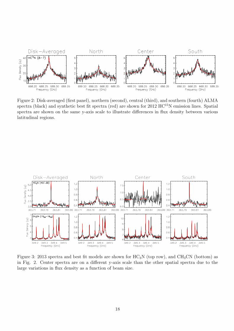
Figure 2: Disk-averaged (first panel), northern (second), central (third), and southern (fourth) ALMAspectra (black) and synthetic best fit spectra (red) are shown for 2012 HC15N emission lines. Spatialspectra are shown on the same y-axis scale to illustrate differences in flux density between variouslatitudinal regions.

Figure 3: 2013 spectra and best fit models are shown for HC3N (top row), and CH3CN (bottom) asin Fig. 2. Center spectra are on a different y-axis scale than the other spatial spectra due to thelarge variations in flux density as a function of beam size.

18

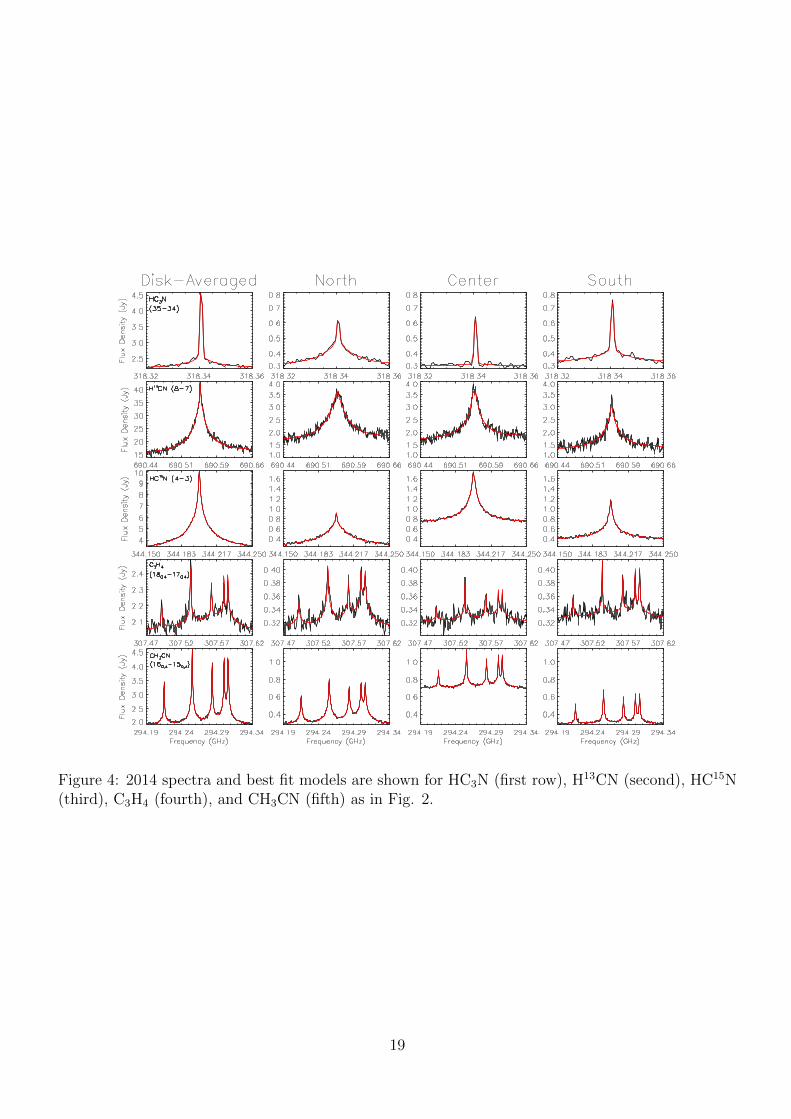
Figure 4: 2014 spectra and best fit models are shown for HC3N (first row), H13CN (second), HC15N(third), C3H4 (fourth), and CH3CN (fifth) as in Fig. 2.

19

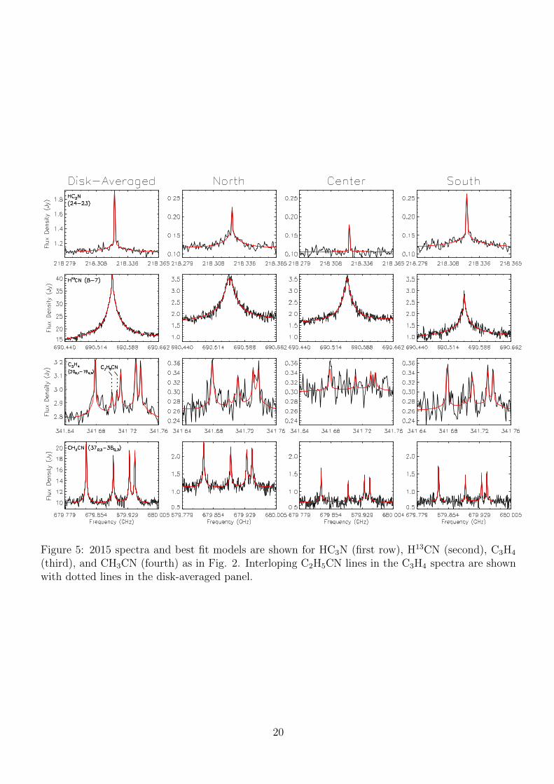
Figure 5: 2015 spectra and best fit models are shown for HC3N (first row), H13CN (second), C3H4

(third), and CH3CN (fourth) as in Fig. 2. Interloping C2H5CN lines in the C3H4 spectra are shownwith dotted lines in the disk-averaged panel.

20

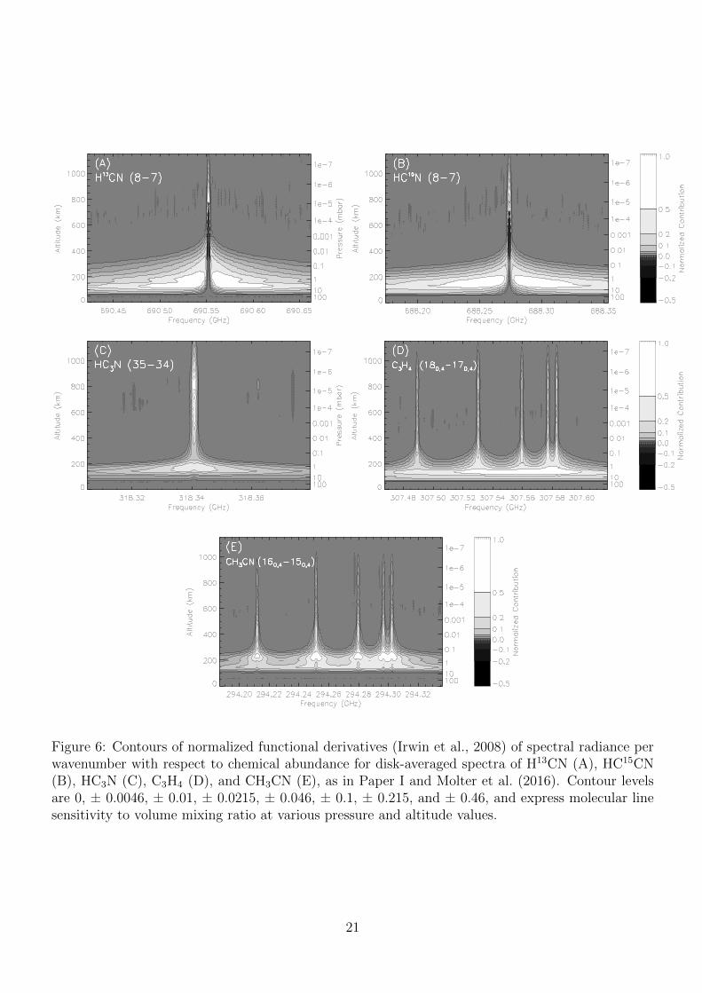
Figure 6: Contours of normalized functional derivatives (Irwin et al., 2008) of spectral radiance perwavenumber with respect to chemical abundance for disk-averaged spectra of H13CN (A), HC15CN(B), HC3N (C), C3H4 (D), and CH3CN (E), as in Paper I and Molter et al. (2016). Contour levelsare 0, ± 0.0046, ± 0.01, ± 0.0215, ± 0.046, ± 0.1, ± 0.215, and ± 0.46, and express molecular linesensitivity to volume mixing ratio at various pressure and altitude values.

21

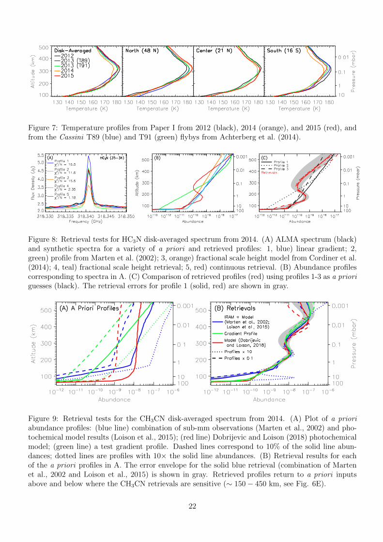
Figure 7: Temperature profiles from Paper I from 2012 (black), 2014 (orange), and 2015 (red), andfrom the Cassini T89 (blue) and T91 (green) flybys from Achterberg et al. (2014).

Figure 8: Retrieval tests for HC3N disk-averaged spectrum from 2014. (A) ALMA spectrum (black)and synthetic spectra for a variety of a priori and retrieved profiles: 1, blue) linear gradient; 2,green) profile from Marten et al. (2002); 3, orange) fractional scale height model from Cordiner et al.(2014); 4, teal) fractional scale height retrieval; 5, red) continuous retrieval. (B) Abundance profilescorresponding to spectra in A. (C) Comparison of retrieved profiles (red) using profiles 1-3 as a prioriguesses (black). The retrieval errors for profile 1 (solid, red) are shown in gray.

Figure 9: Retrieval tests for the CH3CN disk-averaged spectrum from 2014. (A) Plot of a prioriabundance profiles: (blue line) combination of sub-mm observations (Marten et al., 2002) and pho-tochemical model results (Loison et al., 2015); (red line) Dobrijevic and Loison (2018) photochemicalmodel; (green line) a test gradient profile. Dashed lines correspond to 10% of the solid line abun-dances; dotted lines are profiles with 10× the solid line abundances. (B) Retrieval results for eachof the a priori profiles in A. The error envelope for the solid blue retrieval (combination of Martenet al., 2002 and Loison et al., 2015) is shown in gray. Retrieved profiles return to a priori inputsabove and below where the CH3CN retrievals are sensitive (∼ 150 − 450 km, see Fig. 6E).

22

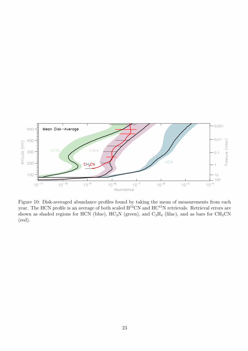
Figure 10: Disk-averaged abundance profiles found by taking the mean of measurements from eachyear. The HCN profile is an average of both scaled H13CN and HC15N retrievals. Retrieval errors areshown as shaded regions for HCN (blue), HC3N (green), and C3H4 (lilac), and as bars for CH3CN(red).

23

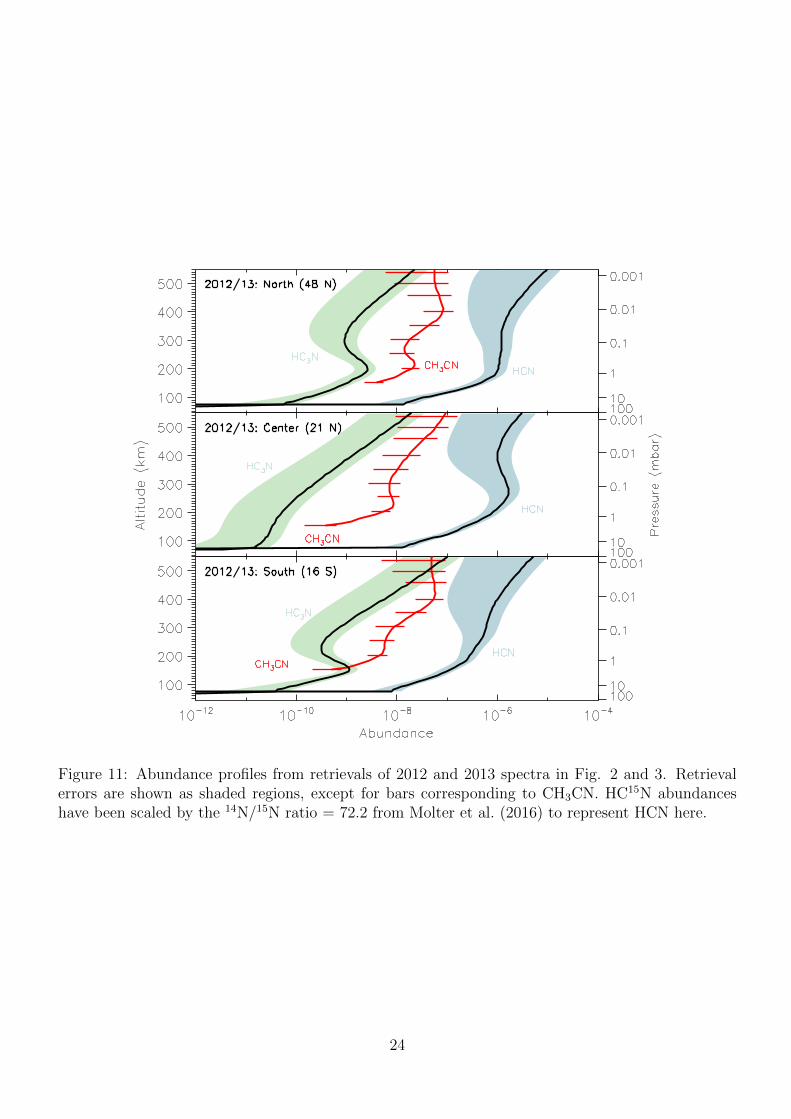
Figure 11: Abundance profiles from retrievals of 2012 and 2013 spectra in Fig. 2 and 3. Retrievalerrors are shown as shaded regions, except for bars corresponding to CH3CN. HC15N abundanceshave been scaled by the 14N/15N ratio = 72.2 from Molter et al. (2016) to represent HCN here.

24

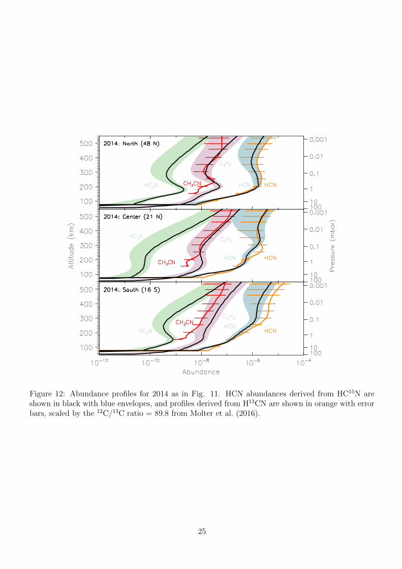
Figure 12: Abundance profiles for 2014 as in Fig. 11. HCN abundances derived from HC15N areshown in black with blue envelopes, and profiles derived from H13CN are shown in orange with errorbars, scaled by the 12C/13C ratio = 89.8 from Molter et al. (2016).

25

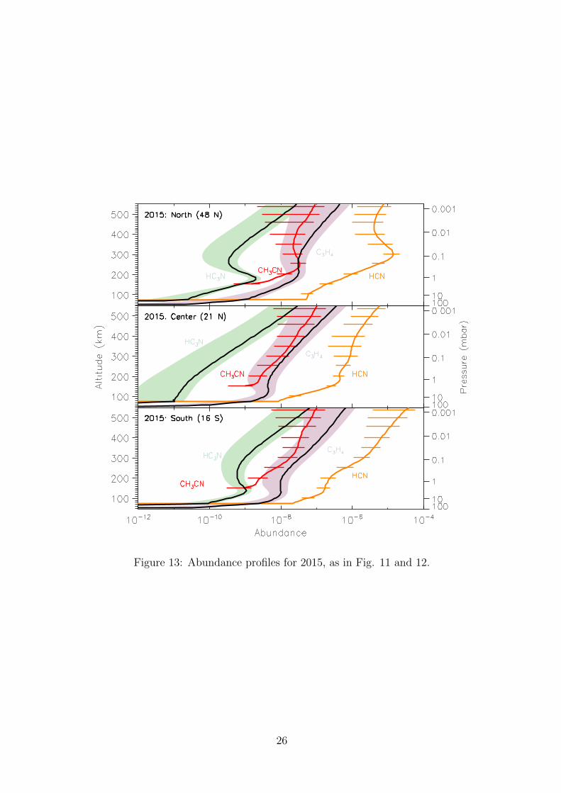
Figure 13: Abundance profiles for 2015, as in Fig. 11 and 12.

26

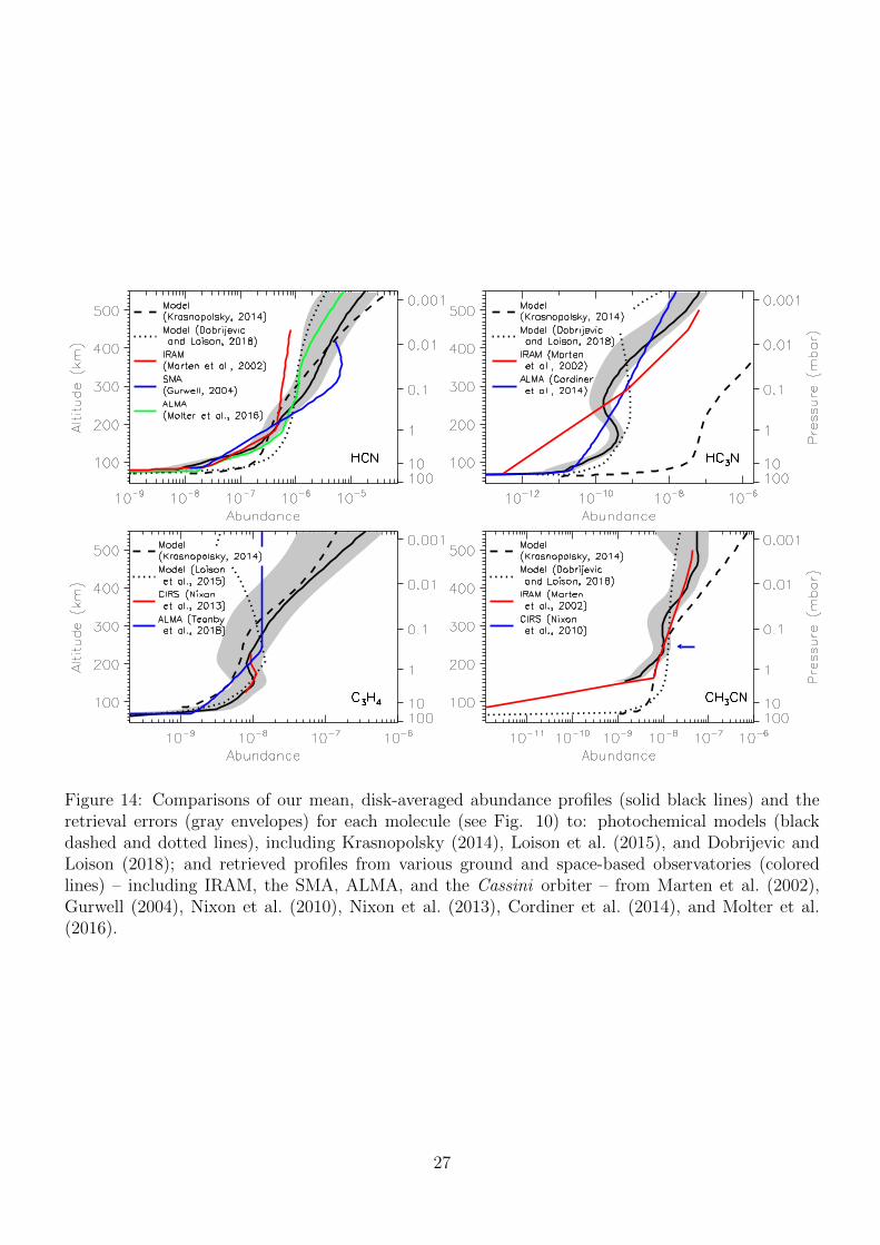
Figure 14: Comparisons of our mean, disk-averaged abundance profiles (solid black lines) and theretrieval errors (gray envelopes) for each molecule (see Fig. 10) to: photochemical models (blackdashed and dotted lines), including Krasnopolsky (2014), Loison et al. (2015), and Dobrijevic andLoison (2018); and retrieved profiles from various ground and space-based observatories (coloredlines) – including IRAM, the SMA, ALMA, and the Cassini orbiter – from Marten et al. (2002),Gurwell (2004), Nixon et al. (2010), Nixon et al. (2013), Cordiner et al. (2014), and Molter et al.(2016).

27

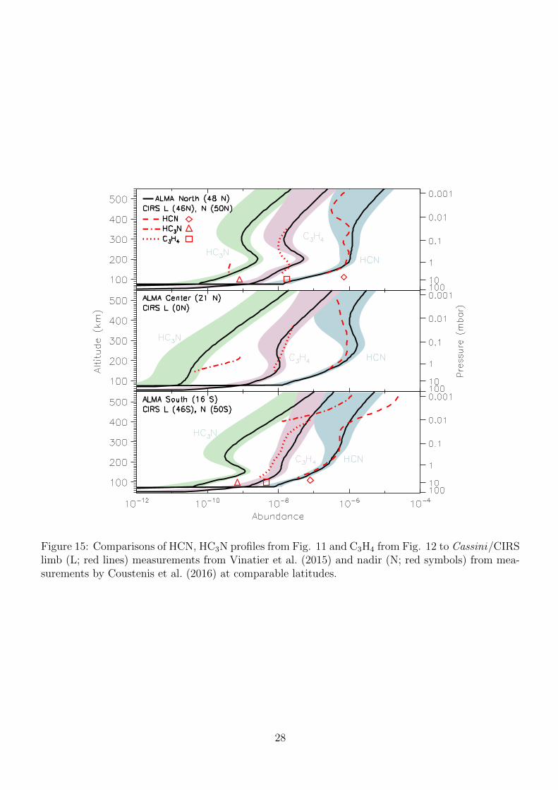
Figure 15: Comparisons of HCN, HC3N profiles from Fig. 11 and C3H4 from Fig. 12 to Cassini/CIRSlimb (L; red lines) measurements from Vinatier et al. (2015) and nadir (N; red symbols) from mea-surements by Coustenis et al. (2016) at comparable latitudes.

28

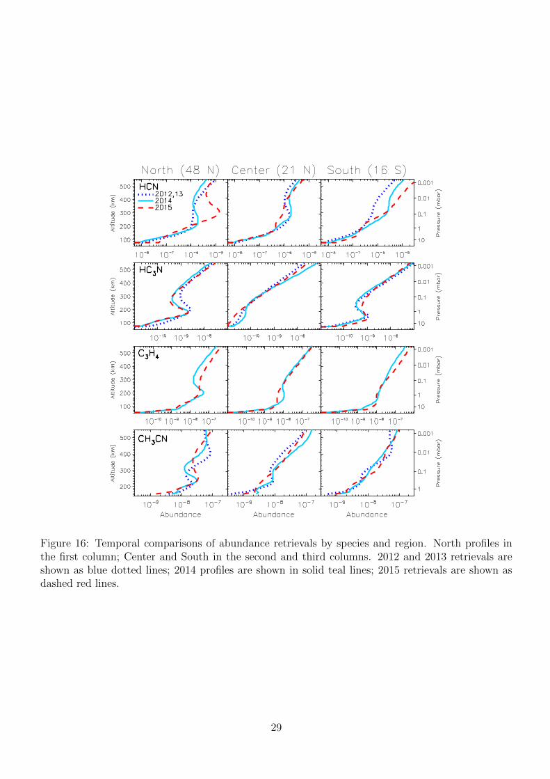
Figure 16: Temporal comparisons of abundance retrievals by species and region. North profiles inthe first column; Center and South in the second and third columns. 2012 and 2013 retrievals areshown as blue dotted lines; 2014 profiles are shown in solid teal lines; 2015 retrievals are shown asdashed red lines.

29