Tanagra Data Mining Ricco Rakotomalala

25 juin 2016 Page 1/17

1 Topic

Image classification using Knime.

The aim of image mining is to extract valuable knowledge from image data. In the context of

supervised image classification, we want to assign automatically a label to image from their visual

content. The whole process is identical to the standard data mining process. We learn a classifier

from a set of classified images. Then, we can apply the classifier to a new image in order to predict

its class membership. The particularity is that we must extract a vector of numerical features from

the image before to launch the machine learning algorithm, and before to apply the classifier in the

deployment phase.

The subject is not really new. But its democratization is more recent. I see two main reasons. First,

the abundance of images with the web data makes necessary this skill to statisticians and data

miner. We note for instance that image processing is increasingly present in the challenges. Second,

there are more and more easy to use tools for data miner. They greatly facilitate our task. Formerly,

a good dose of computer programming ability was needed for handling this type of data. Today,

efficient tools allow us to perform the analysis without being a specialist of image processing. Some

packages are also available for high level programming languages such as Python (e.g. scikit-image).

I took advantage to these properties in recent years for my teachings. The power of the tools allows

me to go to the essentials without having to spend hours to explain in detail the structures of low

level of images. Even if these knowledges may be important when it becomes necessary to finely

adjust the parameters of our analysis.

"Knime Image Processing" module is quite symbolic of this evolution. It is not even necessary to

learn programming language. We can complete an analysis without writing a single line of source

code. The most important is to have a global vision of the basic outline of the study. We simply

define the sequence of treatments in order to obtain results that are relevant. The entire process can

be summed up in several key stages. We must load our collection of images. We may transform the

image characteristics to improve its properties. We extract the descriptors (“features”) to build the

data table (attribute-value table), on which we can apply the machine learning algorithms. To make

the parallel with text mining, another typical domain of unstructured data processing, the main

steps are: load the collection of texts, perform various clean-ups (e.g. remove stop words, remove

punctuations, etc.), extract the dictionary of terms (features), construct the term-document matrix,

on which we can launch the data mining algorithms. We note that the analogy is relevant. The skills

developed in one of the domains is transposable to the other. Merely, the nature of data - and thus

the tools used to handle them - is modified.

Tanagra Data Mining Ricco Rakotomalala

25 juin 2016 Page 2/17

We deal with an image classification task in this tutorial. The goal is to detect automatically the

images which contain a car. The main result is that, even if I have a basic knowledge about the

image processing, I can lead the analysis with a facility which is symptomatic of the usability of

Knime in this context.

2 ‘’Car Detection’’ dataset

The “UIUC Image Database for Car Detection” contains images of side views of cars for use in

evaluation object detection algorithms. The images with cars are positive instances. The others are

the negative instances. The images are all grey-scale and are available in raw PGM format. The

initial package contains: (E1) 1050 training images; (E2.a) 170 single-scale test images i.e. the images

are of different sizes themselves but contain cars of approximately the same scale as in the training

images; (E2.b) 108 multi-scale test images i.e. the images are of different sizes and contain cars of

various scales.

Handling the test samples (E2) requires additional processing (e.g. identifying the position of the car

in the image, put the car on the same scale as the learning sample, or use insensitive to scale

descriptors, etc.) that go beyond the framework of a basic tutorial. So I decided to partition

randomly (E1) to build and evaluate predictive models that we will develop.

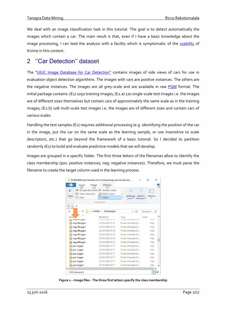
Images are grouped in a specific folder. The first three letters of the filenames allow to identify the

class membership (pos: positive instances; neg: negative instances). Therefore, we must parse the

filename to create the target column used in the learning process.

Figure 1 – Image files - The three first letters specify the class membership

Tanagra Data Mining Ricco Rakotomalala

25 juin 2016 Page 3/17

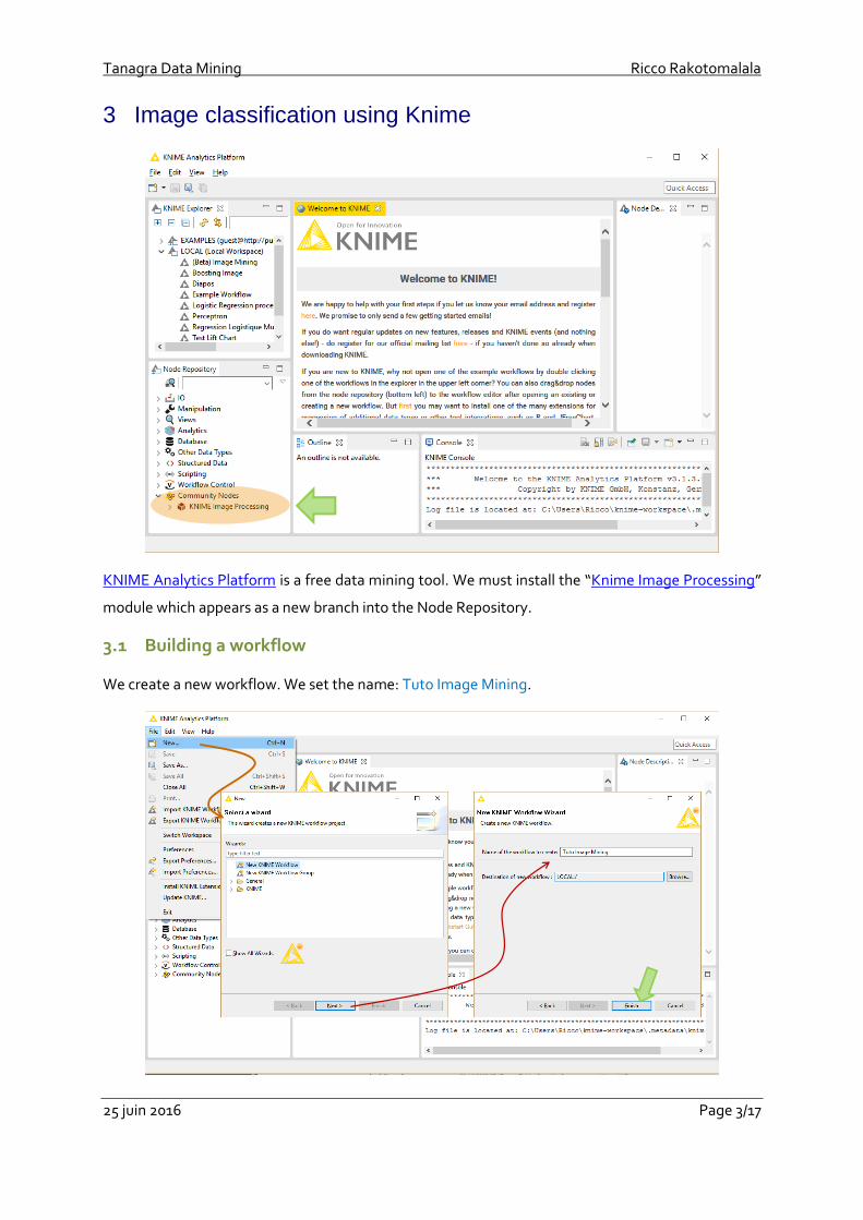
3 Image classification using Knime

KNIME Analytics Platform is a free data mining tool. We must install the “Knime Image Processing”

module which appears as a new branch into the Node Repository.

3.1 Building a workflow

We create a new workflow. We set the name: Tuto Image Mining.

Tanagra Data Mining Ricco Rakotomalala

25 juin 2016 Page 4/17

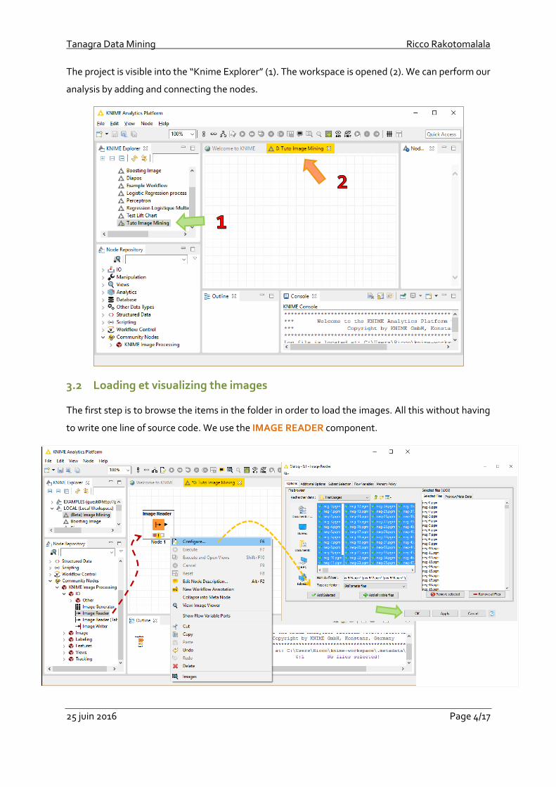
The project is visible into the “Knime Explorer” (1). The workspace is opened (2). We can perform our

analysis by adding and connecting the nodes.

3.2 Loading et visualizing the images

The first step is to browse the items in the folder in order to load the images. All this without having

to write one line of source code. We use the IMAGE READER component.

Tanagra Data Mining Ricco Rakotomalala

25 juin 2016 Page 5/17

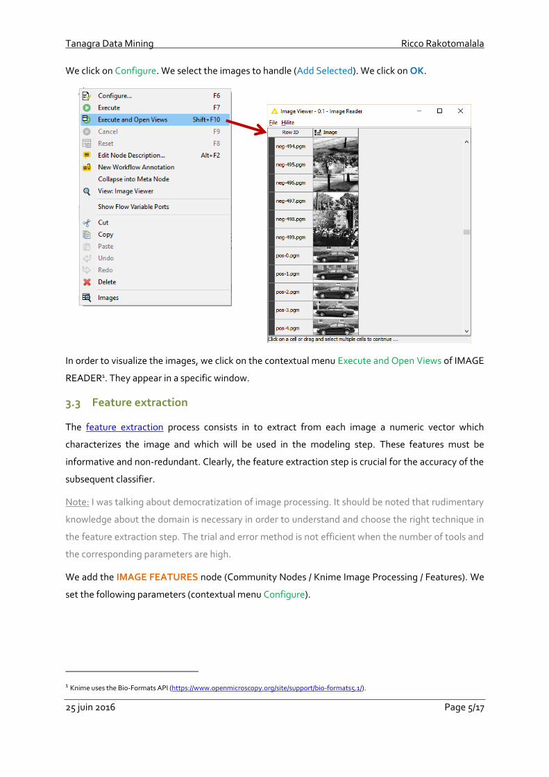
We click on Configure. We select the images to handle (Add Selected). We click on OK.

In order to visualize the images, we click on the contextual menu Execute and Open Views of IMAGE

READER1. They appear in a specific window.

3.3 Feature extraction

The feature extraction process consists in to extract from each image a numeric vector which

characterizes the image and which will be used in the modeling step. These features must be

informative and non-redundant. Clearly, the feature extraction step is crucial for the accuracy of the

subsequent classifier.

Note: I was talking about democratization of image processing. It should be noted that rudimentary

knowledge about the domain is necessary in order to understand and choose the right technique in

the feature extraction step. The trial and error method is not efficient when the number of tools and

the corresponding parameters are high.

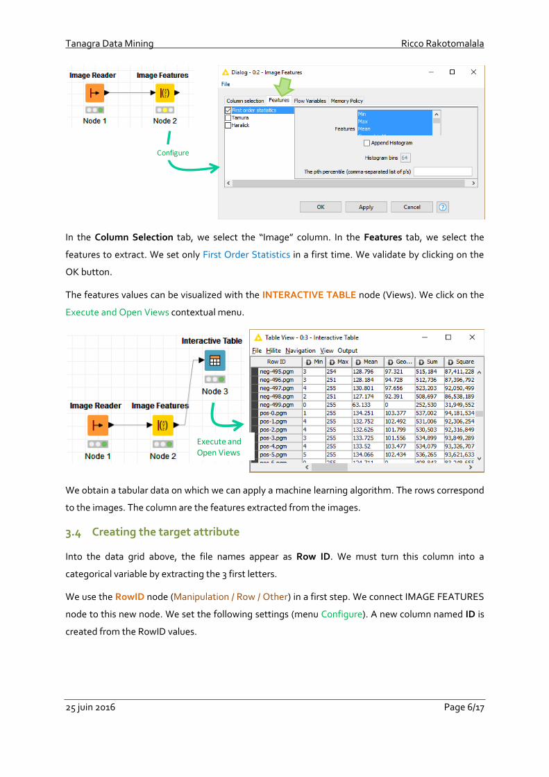
We add the IMAGE FEATURES node (Community Nodes / Knime Image Processing / Features). We

set the following parameters (contextual menu Configure).

1 Knime uses the Bio-Formats API (https://www.openmicroscopy.org/site/support/bio-formats5.1/).

Tanagra Data Mining Ricco Rakotomalala

25 juin 2016 Page 6/17

In the Column Selection tab, we select the “Image” column. In the Features tab, we select the

features to extract. We set only First Order Statistics in a first time. We validate by clicking on the

OK button.

The features values can be visualized with the INTERACTIVE TABLE node (Views). We click on the

Execute and Open Views contextual menu.

We obtain a tabular data on which we can apply a machine learning algorithm. The rows correspond

to the images. The column are the features extracted from the images.

3.4 Creating the target attribute

Into the data grid above, the file names appear as Row ID. We must turn this column into a

categorical variable by extracting the 3 first letters.

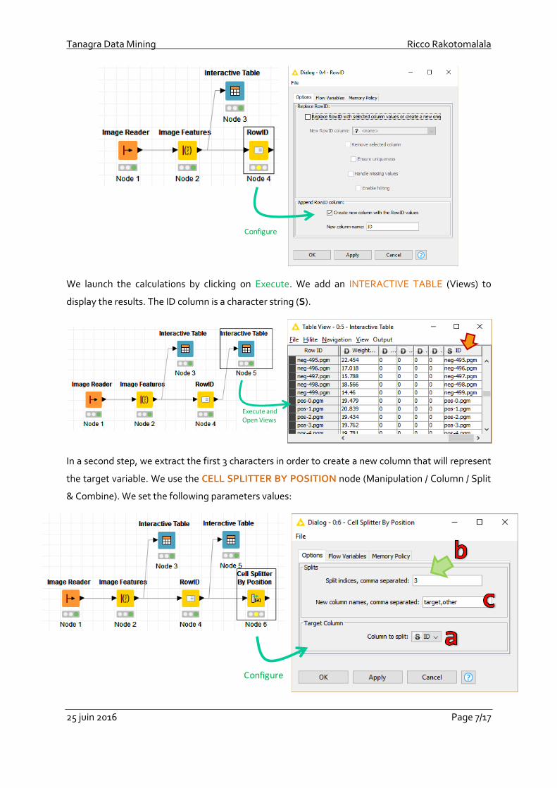
We use the RowID node (Manipulation / Row / Other) in a first step. We connect IMAGE FEATURES

node to this new node. We set the following settings (menu Configure). A new column named ID is

created from the RowID values.

Configure

Execute and Open Views

Tanagra Data Mining Ricco Rakotomalala

25 juin 2016 Page 7/17

We launch the calculations by clicking on Execute. We add an INTERACTIVE TABLE (Views) to

display the results. The ID column is a character string (S).

In a second step, we extract the first 3 characters in order to create a new column that will represent

the target variable. We use the CELL SPLITTER BY POSITION node (Manipulation / Column / Split

& Combine). We set the following parameters values:

Configure

Execute and Open Views

Configure

Tanagra Data Mining Ricco Rakotomalala

25 juin 2016 Page 8/17

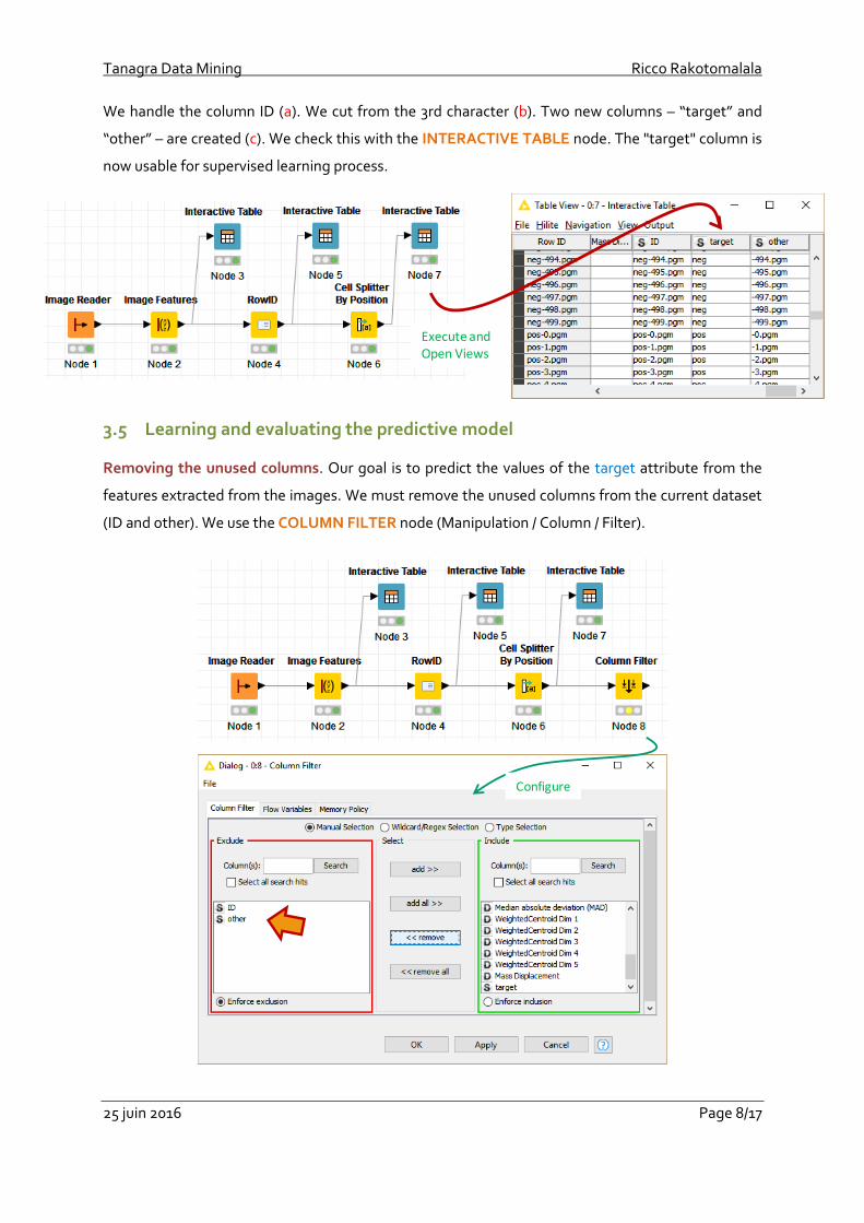
We handle the column ID (a). We cut from the 3rd character (b). Two new columns – “target” and

“other” – are created (c). We check this with the INTERACTIVE TABLE node. The "target" column is

now usable for supervised learning process.

3.5 Learning and evaluating the predictive model

Removing the unused columns. Our goal is to predict the values of the target attribute from the

features extracted from the images. We must remove the unused columns from the current dataset

(ID and other). We use the COLUMN FILTER node (Manipulation / Column / Filter).

Execute and Open Views

Configure

Tanagra Data Mining Ricco Rakotomalala

25 juin 2016 Page 9/17

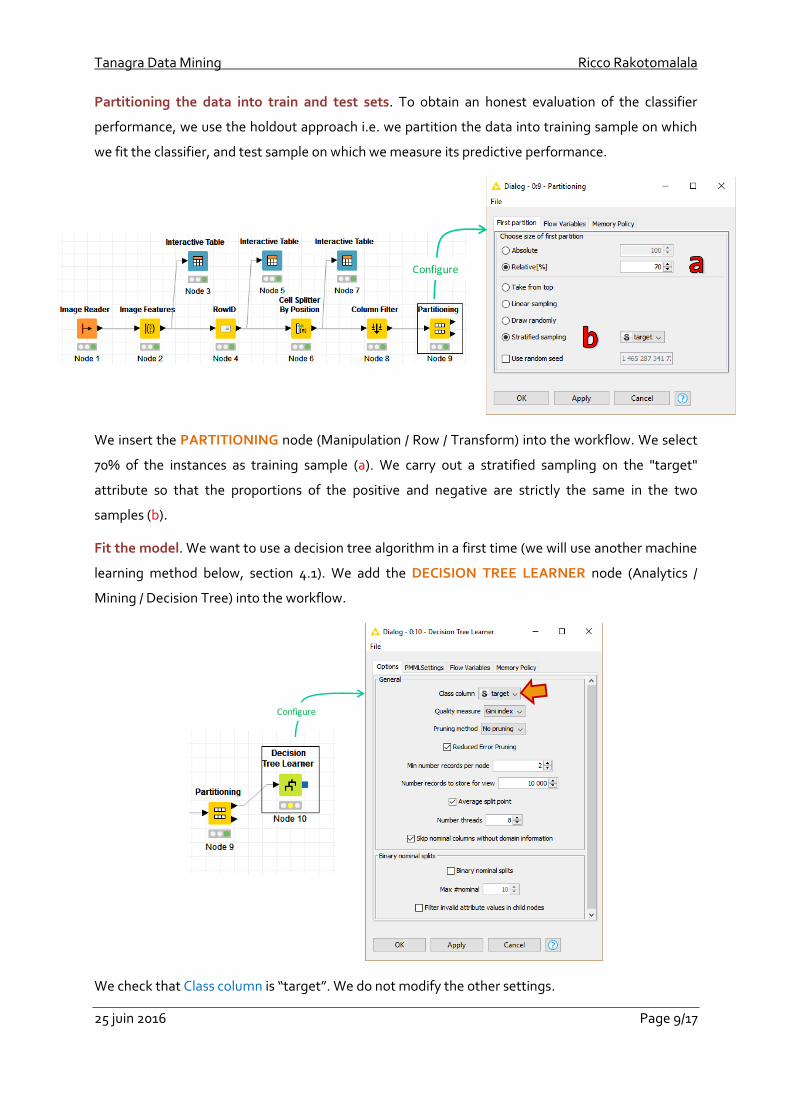
Partitioning the data into train and test sets. To obtain an honest evaluation of the classifier

performance, we use the holdout approach i.e. we partition the data into training sample on which

we fit the classifier, and test sample on which we measure its predictive performance.

We insert the PARTITIONING node (Manipulation / Row / Transform) into the workflow. We select

70% of the instances as training sample (a). We carry out a stratified sampling on the "target"

attribute so that the proportions of the positive and negative are strictly the same in the two

samples (b).

Fit the model. We want to use a decision tree algorithm in a first time (we will use another machine

learning method below, section 4.1). We add the DECISION TREE LEARNER node (Analytics /

Mining / Decision Tree) into the workflow.

We check that Class column is “target”. We do not modify the other settings.

Configure

Configure

Tanagra Data Mining Ricco Rakotomalala

25 juin 2016 Page 10/17

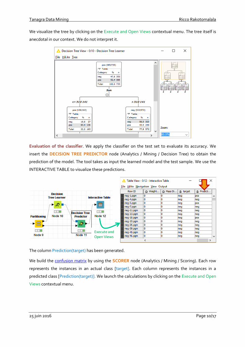
We visualize the tree by clicking on the Execute and Open Views contextual menu. The tree itself is

anecdotal in our context. We do not interpret it.

Evaluation of the classifier. We apply the classifier on the test set to evaluate its accuracy. We

insert the DECISION TREE PREDICTOR node (Analytics / Mining / Decision Tree) to obtain the

prediction of the model. The tool takes as input the learned model and the test sample. We use the

INTERACTIVE TABLE to visualize these predictions.

The column Prediction(target) has been generated.

We build the confusion matrix by using the SCORER node (Analytics / Mining / Scoring). Each row

represents the instances in an actual class [target]. Each column represents the instances in a

predicted class [Prediction(target)]. We launch the calculations by clicking on the Execute and Open

Views contextual menu.

Execute and Open Views

Tanagra Data Mining Ricco Rakotomalala

25 juin 2016 Page 11/17

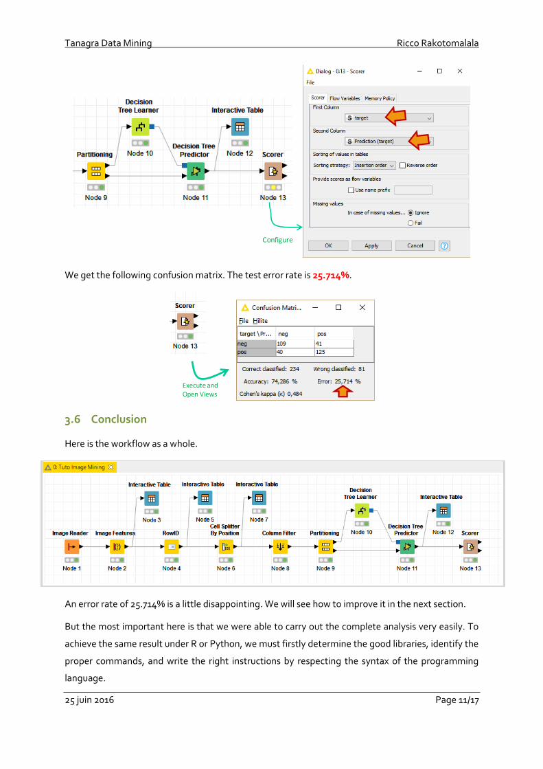
We get the following confusion matrix. The test error rate is 25.714%.

3.6 Conclusion

Here is the workflow as a whole.

An error rate of 25.714% is a little disappointing. We will see how to improve it in the next section.

But the most important here is that we were able to carry out the complete analysis very easily. To

achieve the same result under R or Python, we must firstly determine the good libraries, identify the

proper commands, and write the right instructions by respecting the syntax of the programming

language.

Configure

Execute and Open Views

Tanagra Data Mining Ricco Rakotomalala

25 juin 2016 Page 12/17

4 Improvement opportunities

The basic outline seems right. But the results are disappointing. In this section, we explore some

simple sources of improvement.

4.1 Machine learning algorithm

The easiest way is to try out other machine learning algorithms. To compare them in our image

classification context, we measure the test error rate.

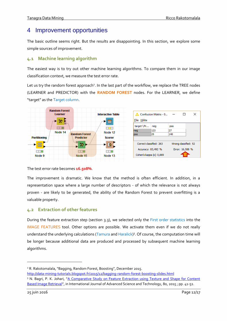
Let us try the random forest approach2. In the last part of the workflow, we replace the TREE nodes

(LEARNER and PREDICTOR) with the RANDOM FOREST nodes. For the LEARNER, we define

“target” as the Target column.

The test error rate becomes 16.508%.

The improvement is dramatic. We know that the method is often efficient. In addition, in a

representation space where a large number of descriptors - of which the relevance is not always

proven - are likely to be generated, the ability of the Random Forest to prevent overfitting is a

valuable property.

4.2 Extraction of other features

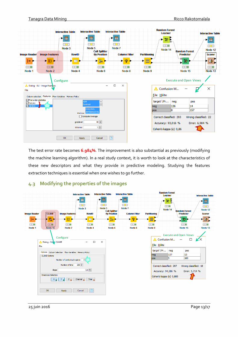
During the feature extraction step (section 3.3), we selected only the First order statistics into the

IMAGE FEATURES tool. Other options are possible. We activate them even if we do not really

understand the underlying calculations (Tamura and Haralick)3. Of course, the computation time will

be longer because additional data are produced and processed by subsequent machine learning

algorithms.

2 R. Rakotomalala, “Bagging, Random Forest, Boosting”, December 2015.

http://data-mining-tutorials.blogspot.fr/2015/12/bagging-random-forest-boosting-slides.html 3 N. Bagri, P. K. Johari, “A Comparative Study on Feature Extraction using Texture and Shape for Content

Based Image Retrieval”, in International Journal of Advanced Science and Technology, 80, 2015 ; pp. 41-52.

Tanagra Data Mining Ricco Rakotomalala

25 juin 2016 Page 13/17

The test error rate becomes 6.984%. The improvement is also substantial as previously (modifying

the machine learning algorithm). In a real study context, it is worth to look at the characteristics of

these new descriptors and what they provide in predictive modeling. Studying the features

extraction techniques is essential when one wishes to go further.

4.3 Modifying the properties of the images

Configure Execute and Open Views

ConfigureExecute and Open Views

Tanagra Data Mining Ricco Rakotomalala

25 juin 2016 Page 14/17

But we can still go more upstream and look at the properties of images themselves. Various image

processing operators allow to enhance the characteristics of the images (filtering noise, modifying

the contrast, transforming the images into binary scale, etc.).

Here also, advanced skills are required if you wish to choose the right tools and finely adjust their

settings. For our dataset, we want to adjust the contrasts with the CLAHE node (Community Nodes /

Knime Image Processing / Image / Process) (see the workflow above).

The test error rate becomes 5.714%. The improvement is minor here. We note above all that this

kind of operation can influence the efficiency of the process.

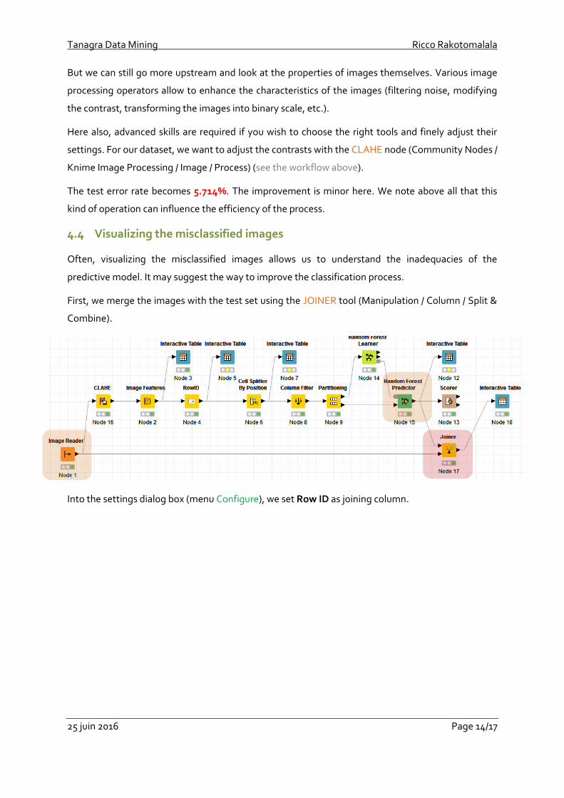
4.4 Visualizing the misclassified images

Often, visualizing the misclassified images allows us to understand the inadequacies of the

predictive model. It may suggest the way to improve the classification process.

First, we merge the images with the test set using the JOINER tool (Manipulation / Column / Split &

Combine).

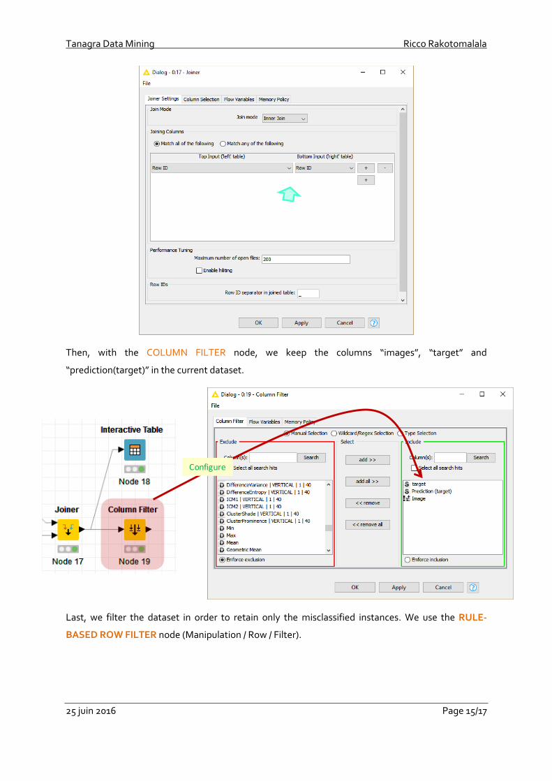
Into the settings dialog box (menu Configure), we set Row ID as joining column.

Tanagra Data Mining Ricco Rakotomalala

25 juin 2016 Page 15/17

Then, with the COLUMN FILTER node, we keep the columns “images”, “target” and

“prediction(target)” in the current dataset.

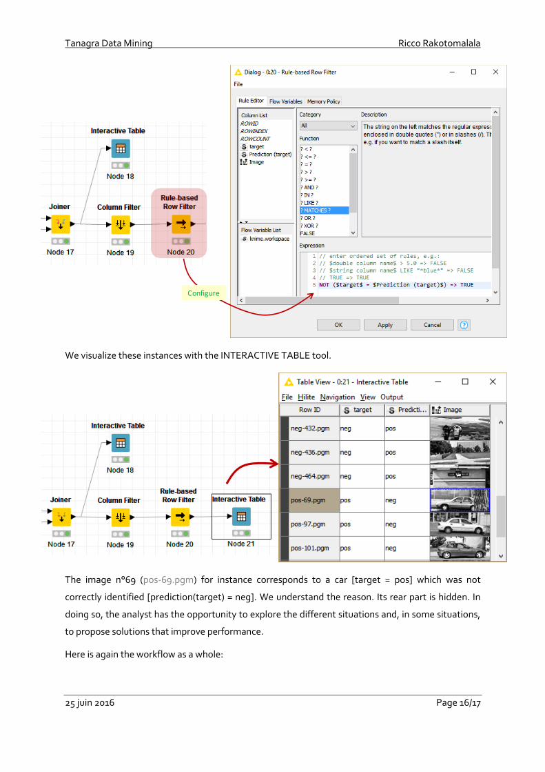
Last, we filter the dataset in order to retain only the misclassified instances. We use the RULE-

BASED ROW FILTER node (Manipulation / Row / Filter).

Configure

Tanagra Data Mining Ricco Rakotomalala

25 juin 2016 Page 16/17

We visualize these instances with the INTERACTIVE TABLE tool.

The image n°69 (pos-69.pgm) for instance corresponds to a car [target = pos] which was not

correctly identified [prediction(target) = neg]. We understand the reason. Its rear part is hidden. In

doing so, the analyst has the opportunity to explore the different situations and, in some situations,

to propose solutions that improve performance.

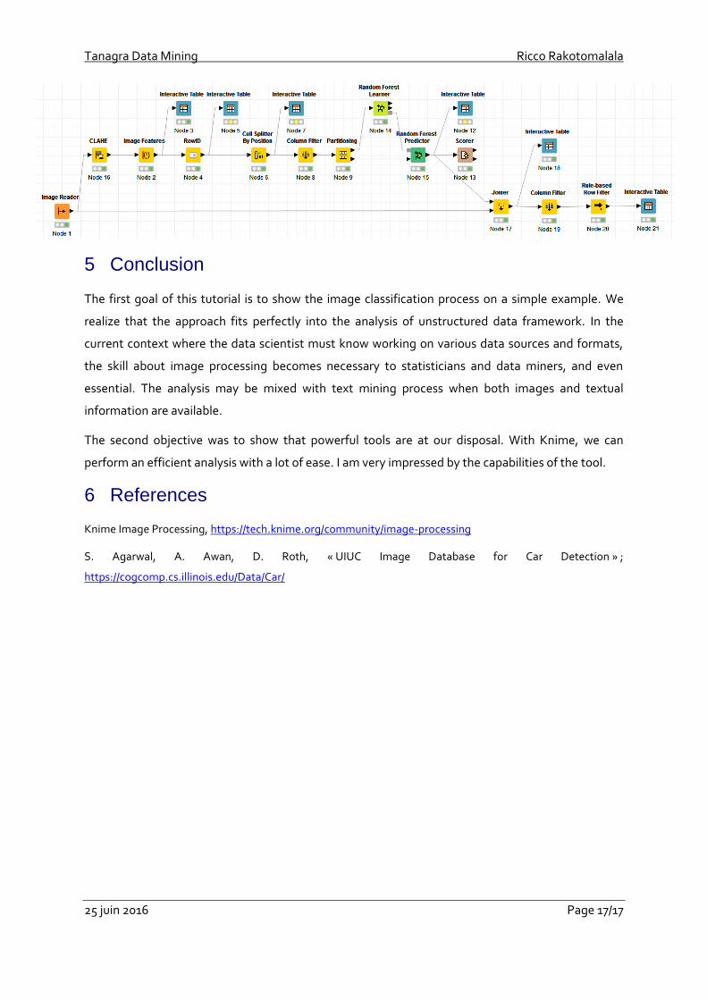
Here is again the workflow as a whole:

Configure

Tanagra Data Mining Ricco Rakotomalala

25 juin 2016 Page 17/17

5 Conclusion

The first goal of this tutorial is to show the image classification process on a simple example. We

realize that the approach fits perfectly into the analysis of unstructured data framework. In the

current context where the data scientist must know working on various data sources and formats,

the skill about image processing becomes necessary to statisticians and data miners, and even

essential. The analysis may be mixed with text mining process when both images and textual

information are available.

The second objective was to show that powerful tools are at our disposal. With Knime, we can

perform an efficient analysis with a lot of ease. I am very impressed by the capabilities of the tool.

6 References

Knime Image Processing, https://tech.knime.org/community/image-processing

S. Agarwal, A. Awan, D. Roth, « UIUC Image Database for Car Detection » ;

https://cogcomp.cs.illinois.edu/Data/Car/