Université Lumière Lyon 2eric.univ-lyon2.fr/~ricco/cours/slides/en/classif_centres_mobiles.pdf ·...

Ricco Rakotomalala

Tutoriels Tanagra - http://tutoriels-data-mining.blogspot.fr/ 1

Ricco RAKOTOMALALA

Université Lumière Lyon 2

http://tutoriels-data-mining.blogspot.fr/

Ricco Rakotomalala


Outline

1. Cluster analysis

2. K-Means algorithm

3. K-Means for categorical data

4. Fuzzy C-Means

5. Clustering of variables

6. Conclusion

7. References


Ricco Rakotomalala


Clustering, unsupervised learning


Ricco Rakotomalala


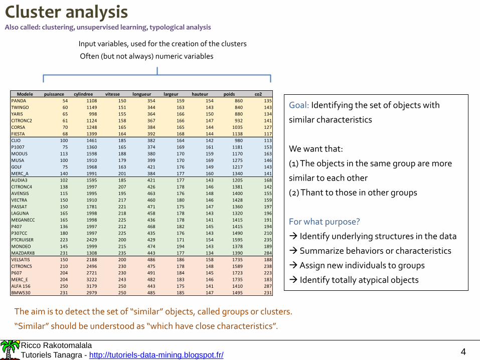
Cluster analysisAlso called: clustering, unsupervised learning, typological analysis

Goal: Identifying the set of objects with

similar characteristics

We want that:

(1) The objects in the same group are more

similar to each other

(2) Thant to those in other groups

For what purpose?

Identify underlying structures in the data

Summarize behaviors or characteristics

Assign new individuals to groups

Identify totally atypical objects

The aim is to detect the set of “similar” objects, called groups or clusters.

“Similar” should be understood as “which have close characteristics”.

Input variables, used for the creation of the clusters

Often (but not always) numeric variables

Modele puissance cylindree vitesse longueur largeur hauteur poids co2

PANDA 54 1108 150 354 159 154 860 135

TWINGO 60 1149 151 344 163 143 840 143

YARIS 65 998 155 364 166 150 880 134

CITRONC2 61 1124 158 367 166 147 932 141

CORSA 70 1248 165 384 165 144 1035 127

FIESTA 68 1399 164 392 168 144 1138 117

CLIO 100 1461 185 382 164 142 980 113

P1007 75 1360 165 374 169 161 1181 153

MODUS 113 1598 188 380 170 159 1170 163

MUSA 100 1910 179 399 170 169 1275 146

GOLF 75 1968 163 421 176 149 1217 143

MERC_A 140 1991 201 384 177 160 1340 141

AUDIA3 102 1595 185 421 177 143 1205 168

CITRONC4 138 1997 207 426 178 146 1381 142

AVENSIS 115 1995 195 463 176 148 1400 155

VECTRA 150 1910 217 460 180 146 1428 159

PASSAT 150 1781 221 471 175 147 1360 197

LAGUNA 165 1998 218 458 178 143 1320 196

MEGANECC 165 1998 225 436 178 141 1415 191

P407 136 1997 212 468 182 145 1415 194

P307CC 180 1997 225 435 176 143 1490 210

PTCRUISER 223 2429 200 429 171 154 1595 235

MONDEO 145 1999 215 474 194 143 1378 189

MAZDARX8 231 1308 235 443 177 134 1390 284

VELSATIS 150 2188 200 486 186 158 1735 188

CITRONC5 210 2496 230 475 178 148 1589 238

P607 204 2721 230 491 184 145 1723 223

MERC_E 204 3222 243 482 183 146 1735 183

ALFA 156 250 3179 250 443 175 141 1410 287

BMW530 231 2979 250 485 185 147 1495 231


Ricco Rakotomalala


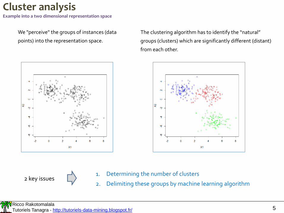
Cluster analysisExample into a two dimensional representation space

We "perceive" the groups of instances (data

points) into the representation space.

The clustering algorithm has to identify the “natural”

groups (clusters) which are significantly different (distant)

from each other.

2 key issues1. Determining the number of clusters

2. Delimiting these groups by machine learning algorithm


Ricco Rakotomalala


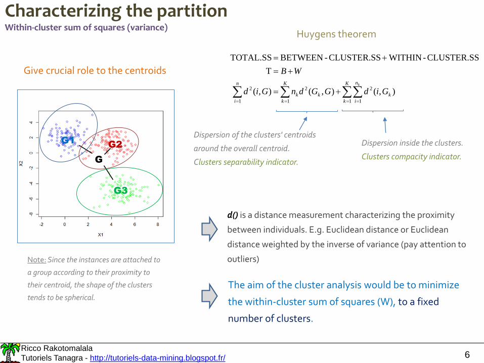
Characterizing the partitionWithin-cluster sum of squares (variance)

K

k

n

i

k

K

k

kk

n

i

k

GidGGdnGid

WB

1 1

2

1

2

1

2 ),(),(),(

T

CLUSTER.SS-WITHINCLUSTER.SS-BETWEEN TOTAL.SS

The aim of the cluster analysis would be to minimize

the within-cluster sum of squares (W), to a fixed

number of clusters.

Huygens theorem

Dispersion of the clusters' centroids

around the overall centroid.

Clusters separability indicator.

Dispersion inside the clusters.

Clusters compacity indicator.

Note: Since the instances are attached to

a group according to their proximity to

their centroid, the shape of the clusters

tends to be spherical.

Give crucial role to the centroids

d() is a distance measurement characterizing the proximity

between individuals. E.g. Euclidean distance or Euclidean

distance weighted by the inverse of variance (pay attention to

outliers)

G

G3

G1 G2


Ricco Rakotomalala


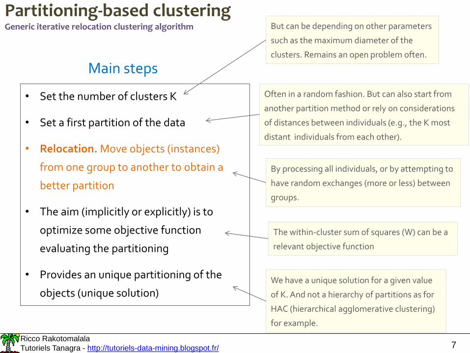
Partitioning-based clusteringGeneric iterative relocation clustering algorithm

Main steps

• Set the number of clusters K

• Set a first partition of the data

• Relocation. Move objects (instances)

from one group to another to obtain a

better partition

• The aim (implicitly or explicitly) is to

optimize some objective function

evaluating the partitioning

• Provides an unique partitioning of the

objects (unique solution)

But can be depending on other parameters

such as the maximum diameter of the

clusters. Remains an open problem often.

Often in a random fashion. But can also start from

another partition method or rely on considerations

of distances between individuals (e.g., the K most

distant individuals from each other).

By processing all individuals, or by attempting to

have random exchanges (more or less) between

groups.

The within-cluster sum of squares (W) can be a

relevant objective function

We have a unique solution for a given value

of K. And not a hierarchy of partitions as for

HAC (hierarchical agglomerative clustering)

for example.


Ricco Rakotomalala


Each group is represented by its centroid


Ricco Rakotomalala


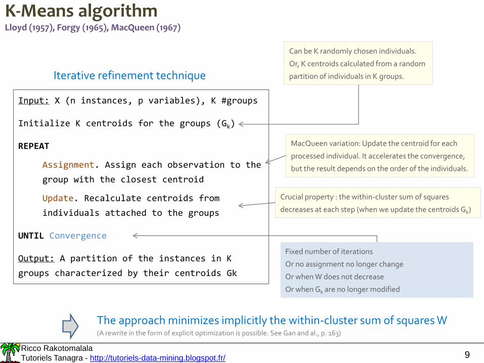
K-Means algorithmLloyd (1957), Forgy (1965), MacQueen (1967)

Input: X (n instances, p variables), K #groups

Initialize K centroids for the groups (Gk)

REPEAT

Assignment. Assign each observation to the

group with the closest centroid

Update. Recalculate centroids from

individuals attached to the groups

UNTIL Convergence

Output: A partition of the instances in K

groups characterized by their centroids Gk

Iterative refinement technique

Can be K randomly chosen individuals.

Or, K centroids calculated from a random

partition of individuals in K groups.

MacQueen variation: Update the centroid for each

processed individual. It accelerates the convergence,

but the result depends on the order of the individuals.

Crucial property : the within-cluster sum of squares

decreases at each step (when we update the centroids Gk)

Fixed number of iterations

Or no assignment no longer change

Or when W does not decrease

Or when Gk are no longer modified

The approach minimizes implicitly the within-cluster sum of squares W(A rewrite in the form of explicit optimization is possible. See Gan and al., p. 163)


Ricco Rakotomalala


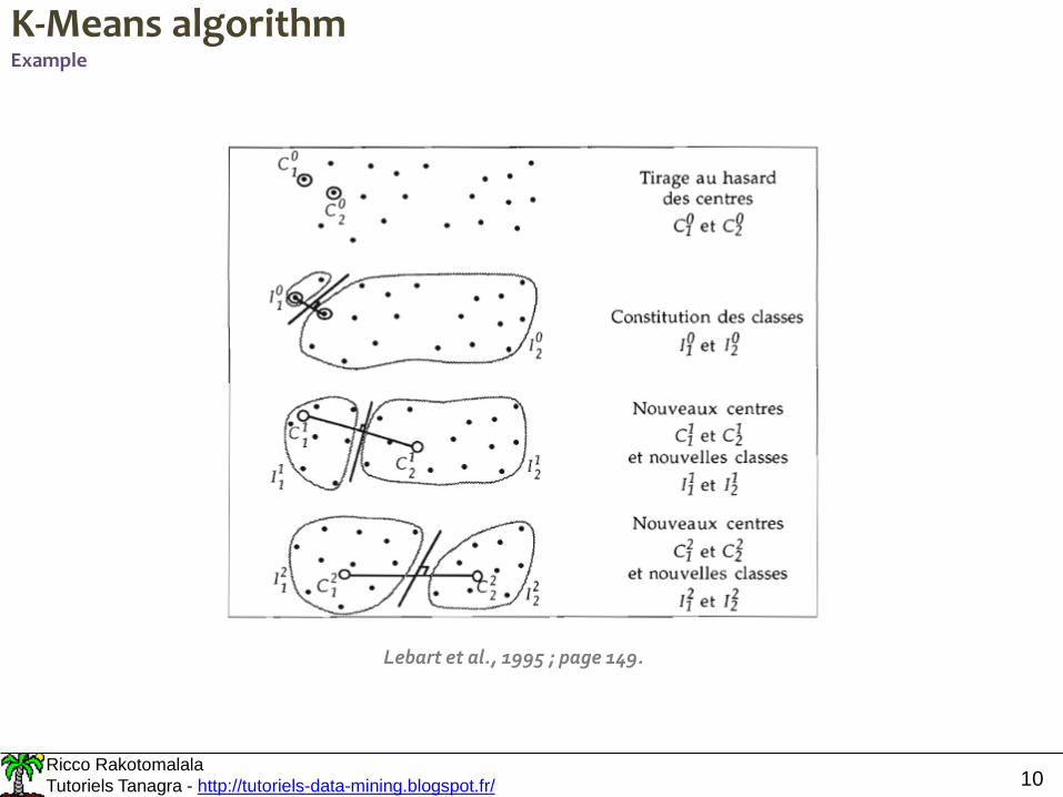
K-Means algorithmExample

Lebart et al., 1995 ; page 149.


Ricco Rakotomalala


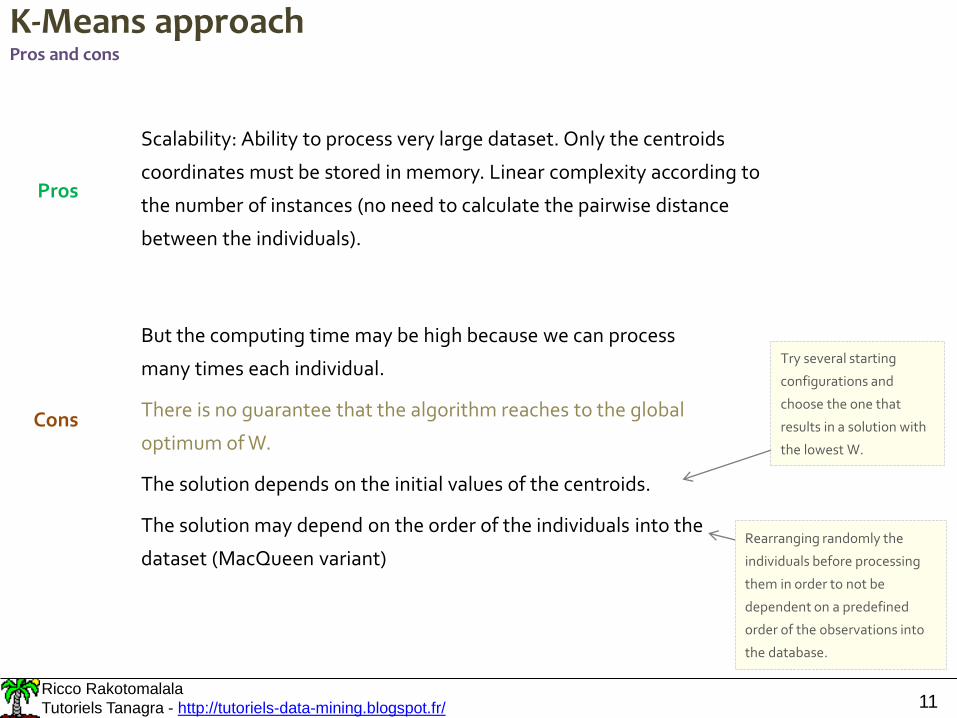
K-Means approachPros and cons

Scalability: Ability to process very large dataset. Only the centroids

coordinates must be stored in memory. Linear complexity according to

the number of instances (no need to calculate the pairwise distance

between the individuals).

Pros

Cons

But the computing time may be high because we can process

many times each individual.

There is no guarantee that the algorithm reaches to the global

optimum of W.

The solution depends on the initial values of the centroids.

The solution may depend on the order of the individuals into the

dataset (MacQueen variant)

Try several starting

configurations and

choose the one that

results in a solution with

the lowest W.

Rearranging randomly the

individuals before processing

them in order to not be

dependent on a predefined

order of the observations into

the database.


Ricco Rakotomalala


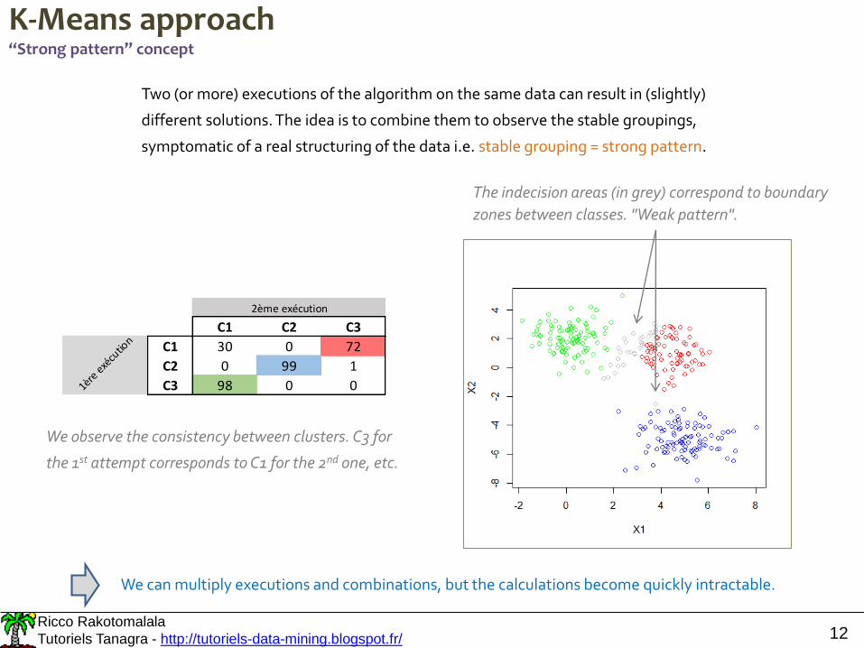
K-Means approach“Strong pattern” concept

Two (or more) executions of the algorithm on the same data can result in (slightly)

different solutions. The idea is to combine them to observe the stable groupings,

symptomatic of a real structuring of the data i.e. stable grouping = strong pattern.

We observe the consistency between clusters. C3 for

the 1st attempt corresponds to C1 for the 2nd one, etc.

The indecision areas (in grey) correspond to boundary

zones between classes. "Weak pattern".

We can multiply executions and combinations, but the calculations become quickly intractable.

C1 C2 C3

2ème exécution

C1 30 0 72

C2 0 99 1

C3 98 0 01ère e

xécu

tion


Ricco Rakotomalala


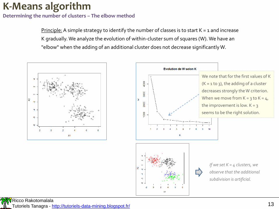
K-Means algorithmDetermining the number of clusters – The elbow method

Principle: A simple strategy to identify the number of classes is to start K = 1 and increase

K gradually. We analyze the evolution of within-cluster sum of squares (W). We have an

"elbow" when the adding of an additional cluster does not decrease significantly W.

We note that for the first values of K

(K = 1 to 3), the adding of a cluster

decreases strongly the W criterion.

When we move from K = 3 to K = 4,

the improvement is low. K = 3

seems to be the right solution.

If we set K = 4 clusters, we

observe that the additional

subdivision is artificial.


Ricco Rakotomalala


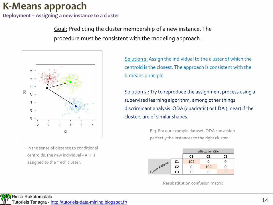
K-Means approachDeployment – Assigning a new instance to a cluster

Goal: Predicting the cluster membership of a new instance. The

procedure must be consistent with the modeling approach.

In the sense of distance to conditional

centroids, the new individual « » is

assigned to the “red” cluster.

Solution 1: Assign the individual to the cluster of which the

centroid is the closest. The approach is consistent with the

k-means principle.

Solution 2 : Try to reproduce the assignment process using a

supervised learning algorithm, among other things

discriminant analysis. QDA (quadratic) or LDA (linear) if the

clusters are of similar shapes.

C1 C2 C3

Affectation QDA

C1 102 0 0

C2 0 100 0

C3 0 0 98Classes K-Means

E.g. For our example dataset, QDA can assign

perfectly the instances to the right cluster.

Resubstitution confusion matrix


Ricco Rakotomalala


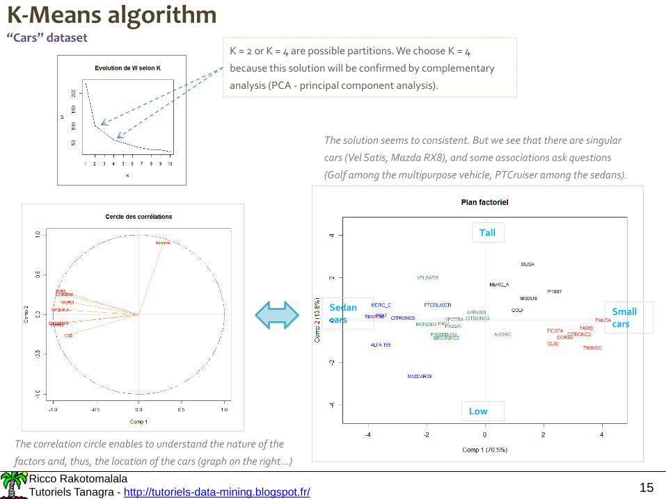
K-Means algorithm“Cars” dataset

K = 2 or K = 4 are possible partitions. We choose K = 4

because this solution will be confirmed by complementary

analysis (PCA - principal component analysis).

Small cars

Sedan cars

Tall

Low

The solution seems to consistent. But we see that there are singular

cars (Vel Satis, Mazda RX8), and some associations ask questions

(Golf among the multipurpose vehicle, PTCruiser among the sedans).

The correlation circle enables to understand the nature of the

factors and, thus, the location of the cars (graph on the right…)


Ricco Rakotomalala


Strategy for the handling of categorical variables


Ricco Rakotomalala


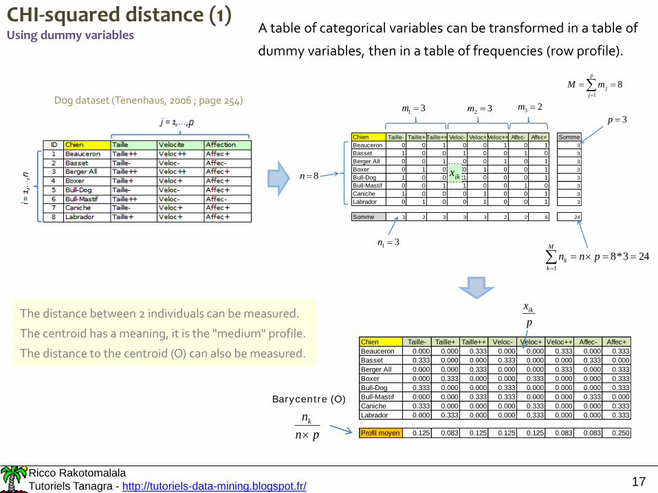
CHI-squared distance (1)Using dummy variables

A table of categorical variables can be transformed in a table of

dummy variables, then in a table of frequencies (row profile).

Chien Taille- Taille+ Taille++ Veloc- Veloc+ Veloc++ Affec- Affec+ Somme

Beauceron 0 0 1 0 0 1 0 1 3

Basset 1 0 0 1 0 0 1 0 3

Berger All 0 0 1 0 0 1 0 1 3

Boxer 0 1 0 0 1 0 0 1 3

Bull-Dog 1 0 0 1 0 0 0 1 3

Bull-Mastif 0 0 1 1 0 0 1 0 3

Caniche 1 0 0 0 1 0 0 1 3

Labrador 0 1 0 0 1 0 0 1 3

Somme 3 2 3 3 3 2 2 6 24

ikx

31 m 32 m 23 m

p

j

jmM1

8

3p

31 n

M

k

k pnn1

243*8

8n

Chien Taille- Taille+ Taille++ Veloc- Veloc+ Veloc++ Affec- Affec+

Beauceron 0.000 0.000 0.333 0.000 0.000 0.333 0.000 0.333

Basset 0.333 0.000 0.000 0.333 0.000 0.000 0.333 0.000

Berger All 0.000 0.000 0.333 0.000 0.000 0.333 0.000 0.333

Boxer 0.000 0.333 0.000 0.000 0.333 0.000 0.000 0.333

Bull-Dog 0.333 0.000 0.000 0.333 0.000 0.000 0.000 0.333

Bull-Mastif 0.000 0.000 0.333 0.333 0.000 0.000 0.333 0.000

Caniche 0.333 0.000 0.000 0.000 0.333 0.000 0.000 0.333

Labrador 0.000 0.333 0.000 0.000 0.333 0.000 0.000 0.333

Profil moyen 0.125 0.083 0.125 0.125 0.125 0.083 0.083 0.250pn

nk

Barycentre (O)

p

xikThe distance between 2 individuals can be measured.

The centroid has a meaning, it is the "medium" profile.

The distance to the centroid (O) can also be measured.

Dog dataset (Tenenhaus, 2006 ; page 254)


Ricco Rakotomalala


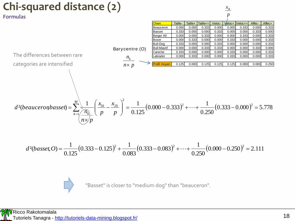
Chi-squared distance (2)Formulas

M

k

kk

k p

x

p

x

pn

nbassetbeaucerond

1

22

2

21 778.5000.0333.0250.0

1333.0000.0

125.0

11),²(

The differences between rare

categories are intensified

Chien Taille- Taille+ Taille++ Veloc- Veloc+ Veloc++ Affec- Affec+

Beauceron 0.000 0.000 0.333 0.000 0.000 0.333 0.000 0.333

Basset 0.333 0.000 0.000 0.333 0.000 0.000 0.333 0.000

Berger All 0.000 0.000 0.333 0.000 0.000 0.333 0.000 0.333

Boxer 0.000 0.333 0.000 0.000 0.333 0.000 0.000 0.333

Bull-Dog 0.333 0.000 0.000 0.333 0.000 0.000 0.000 0.333

Bull-Mastif 0.000 0.000 0.333 0.333 0.000 0.000 0.333 0.000

Caniche 0.333 0.000 0.000 0.000 0.333 0.000 0.000 0.333

Labrador 0.000 0.333 0.000 0.000 0.333 0.000 0.000 0.333

Profil moyen 0.125 0.083 0.125 0.125 0.125 0.083 0.083 0.250pn

nk

Barycentre (O)

p

xik

111.2250.0000.0250.0

1083.0333.0

083.0

1125.0333.0

125.0

1),²(

222 Obassetd

"Basset" is closer to "medium dog" than "beauceron".


Ricco Rakotomalala


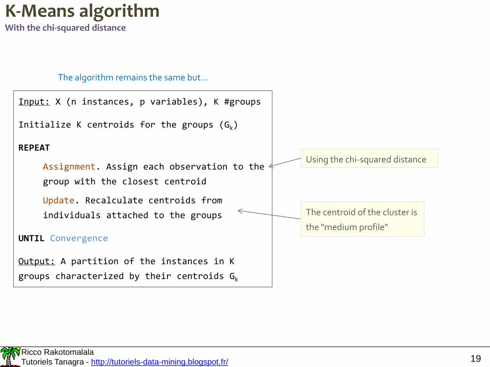
K-Means algorithmWith the chi-squared distance

The algorithm remains the same but...

Using the chi-squared distance

The centroid of the cluster is

the "medium profile"

Input: X (n instances, p variables), K #groups

Initialize K centroids for the groups (Gk)

REPEAT

Assignment. Assign each observation to the


Update. Recalculate centroids from

individuals attached to the groups

UNTIL Convergence

Output: A partition of the instances in K

groups characterized by their centroids Gk


Ricco Rakotomalala


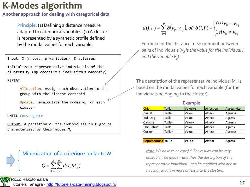
K-Modes algorithmAnother approach for dealing with categorical data

Principle: (1) Defining a distance measure

adapted to categorical variables. (2) A cluster

is represented by a synthetic profile defined

by the modal values for each variable.

jiij

jiijp

j

jiijvvsi

vvsiiioùvviid

'

'

1

'1

0)',(,,)',(

Note: We have to be careful. The results can be very

unstable. The mode – and thus the description of the

representative individual – can be modified with one or

two individuals in more or less into the clusters.

Input: X (n obs., p variables), K #classes

Initialize K representative individuals of the

clusters Mk (by choosing K individuals randomly)

REPEAT

Allocation. Assign each observation to the


Update. Recalculate the modes Mk for each

cluster

UNTIL Convergence

Output: A partition of the individuals in K groups

characterized by their modes Mk

Formula for the distance measurement between

pairs of individuals (vij is the value for the individual i

and the variable Vj )

The description of the representative individual Mk is

based on the modal values for each variable (for the

individuals belonging to the cluster).

Chien Taille Velocite Affection Agressivite

Basset Taille- Veloc- Affec- Agress+

Bull-Dog Taille- Veloc- Affec+ Agress-

Caniche Taille- Veloc+ Affec+ Agress-

Chihuahua Taille- Veloc- Affec+ Agress-

Cocker Taille+ Veloc- Affec+ Agress+

Représentant Taille- Veloc- Affec+ Agress-

Minimization of a criterion similar to W

K

k

n

i

k

k

MidQ1 1

),(

Example


Ricco Rakotomalala


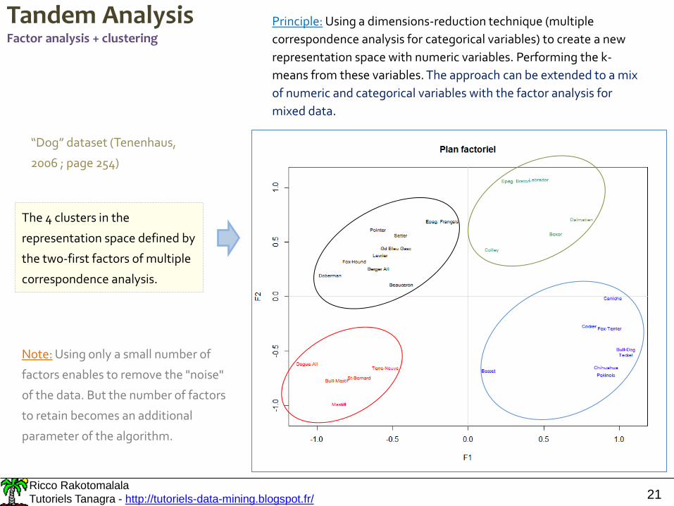
Tandem AnalysisFactor analysis + clustering

Principle: Using a dimensions-reduction technique (multiple

correspondence analysis for categorical variables) to create a new

representation space with numeric variables. Performing the k-

means from these variables. The approach can be extended to a mix

of numeric and categorical variables with the factor analysis for

mixed data.

“Dog” dataset (Tenenhaus,

2006 ; page 254)

Note: Using only a small number of

factors enables to remove the "noise"

of the data. But the number of factors

to retain becomes an additional

parameter of the algorithm.

The 4 clusters in the

representation space defined by

the two-first factors of multiple

correspondence analysis.


Ricco Rakotomalala


Instead of each data point belongs to an unique cluster (crisp

or hard clustering), it can potentially belongs to multiple

clusters to varying degrees (fuzzy or soft clustering)


Ricco Rakotomalala


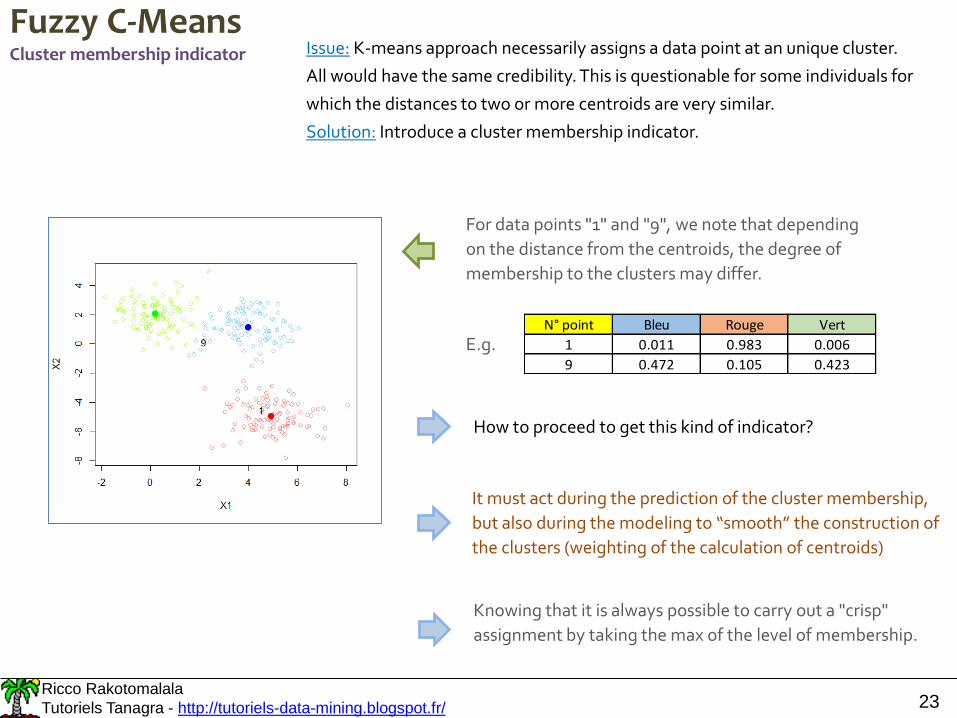
For data points "1" and "9", we note that depending

on the distance from the centroids, the degree of

membership to the clusters may differ.

Fuzzy C-MeansCluster membership indicator Issue: K-means approach necessarily assigns a data point at an unique cluster.

All would have the same credibility. This is questionable for some individuals for

which the distances to two or more centroids are very similar.

Solution: Introduce a cluster membership indicator.

E.g.N° point Bleu Rouge Vert

1 0.011 0.983 0.006

9 0.472 0.105 0.423

How to proceed to get this kind of indicator?

It must act during the prediction of the cluster membership,

but also during the modeling to “smooth” the construction of

the clusters (weighting of the calculation of centroids)

Knowing that it is always possible to carry out a "crisp"

assignment by taking the max of the level of membership.


Ricco Rakotomalala


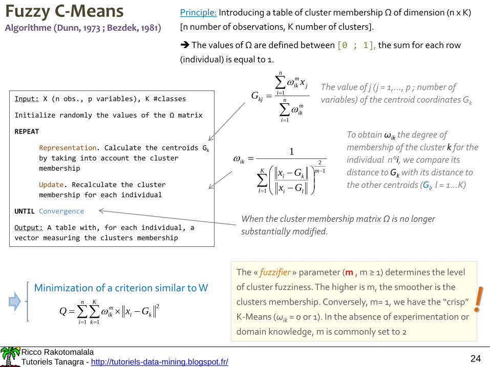
Fuzzy C-MeansAlgorithme (Dunn, 1973 ; Bezdek, 1981)


Initialize randomly the values of the Ω matrix

REPEAT

Representation. Calculate the centroids Gkby taking into account the cluster

membership

Update. Recalculate the cluster

membership for each individual

UNTIL Convergence

Output: A table with, for each individual, a

vector measuring the clusters membership

Principle: Introducing a table of cluster membership Ω of dimension (n x K)

[n number of observations, K number of clusters].

The values of Ω are defined between [0 ; 1], the sum for each row

(individual) is equal to 1.

n

i

m

ik

n

i

j

m

ik

kj

x

G

1

1

The value of j (j = 1,…, p ; number of

variables) of the centroid coordinates Gk

K

l

m

li

ki

ik

Gx

Gx

1

1

2

1

Minimization of a criterion similar to W

n

i

K

k

ki

m

ik GxQ1 1

2

To obtain ωik the degree of

membership of the cluster k for the

individual n°i, we compare its

distance to Gk with its distance to

the other centroids (Gl, l = 1…K)

When the cluster membership matrix Ω is no longer

substantially modified.

The « fuzzifier » parameter (m , m ≥ 1) determines the level

of cluster fuzziness. The higher is m, the smoother is the

clusters membership. Conversely, m= 1, we have the “crisp”

K-Means (ωik = 0 or 1). In the absence of experimentation or

domain knowledge, m is commonly set to 2

!


Ricco Rakotomalala


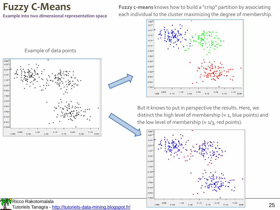
Fuzzy C-MeansExample into two dimensional representation space

Example of data points

Fuzzy c-means knows how to build a "crisp" partition by associating

each individual to the cluster maximizing the degree of membership.

But it knows to put in perspective the results. Here, we

distinct the high level of membership ( 1, blue points) and

the low level of membership ( 1/3, red points).


Ricco Rakotomalala


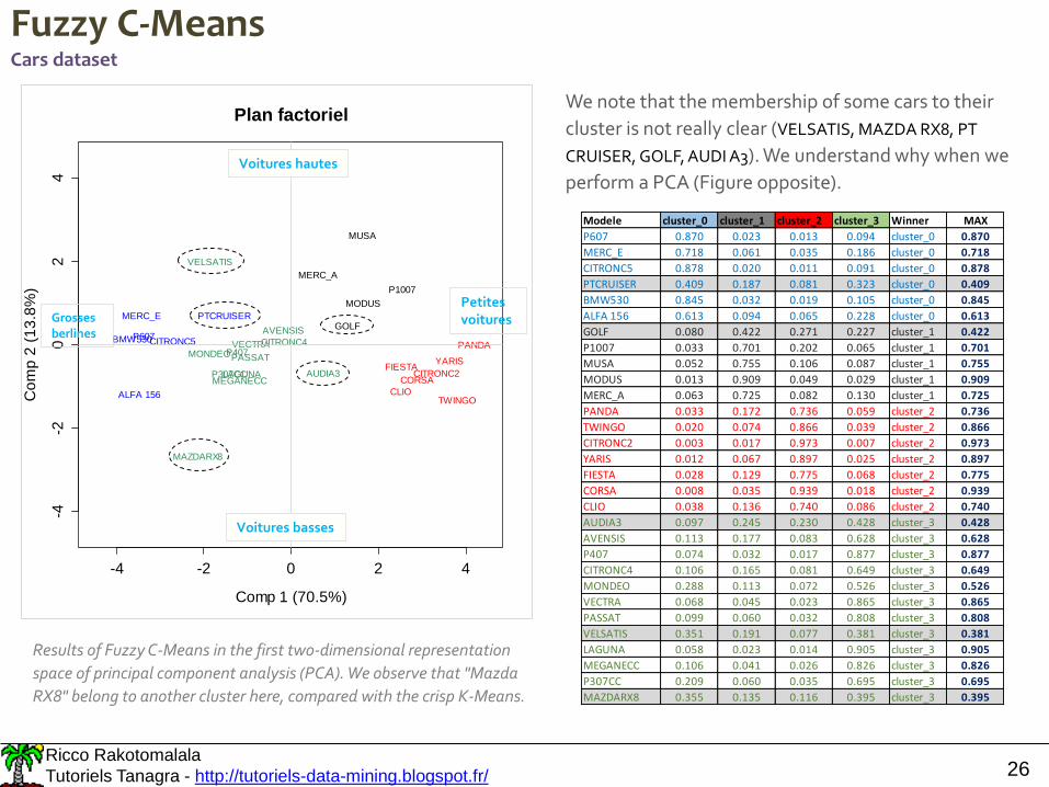
Fuzzy C-MeansCars dataset

Results of Fuzzy C-Means in the first two-dimensional representation

space of principal component analysis (PCA). We observe that "Mazda

RX8" belong to another cluster here, compared with the crisp K-Means.

We note that the membership of some cars to their

cluster is not really clear (VELSATIS, MAZDA RX8, PT

CRUISER, GOLF, AUDI A3). We understand why when we

perform a PCA (Figure opposite).

-4 -2 0 2 4

-4-2

02

4

Plan factoriel

Comp 1 (70.5%)

Co

mp

2 (

13

.8%

)

PANDA

TWINGO

CITRONC2

YARISFIESTA

CORSA

GOLF

P1007

MUSA

CLIO

AUDIA3

MODUS

AVENSIS

P407CITRONC4

MERC_A

MONDEOVECTRA

PASSAT

VELSATIS

LAGUNAMEGANECCP307CC

P607

MERC_E

CITRONC5

PTCRUISER

MAZDARX8

BMW530

ALFA 156

Petites voituresGrosses

berlines

Voitures hautes

Voitures basses

Modele cluster_0 cluster_1 cluster_2 cluster_3 Winner MAX

P607 0.870 0.023 0.013 0.094 cluster_0 0.870

MERC_E 0.718 0.061 0.035 0.186 cluster_0 0.718

CITRONC5 0.878 0.020 0.011 0.091 cluster_0 0.878

PTCRUISER 0.409 0.187 0.081 0.323 cluster_0 0.409

BMW530 0.845 0.032 0.019 0.105 cluster_0 0.845

ALFA 156 0.613 0.094 0.065 0.228 cluster_0 0.613

GOLF 0.080 0.422 0.271 0.227 cluster_1 0.422

P1007 0.033 0.701 0.202 0.065 cluster_1 0.701

MUSA 0.052 0.755 0.106 0.087 cluster_1 0.755

MODUS 0.013 0.909 0.049 0.029 cluster_1 0.909

MERC_A 0.063 0.725 0.082 0.130 cluster_1 0.725

PANDA 0.033 0.172 0.736 0.059 cluster_2 0.736

TWINGO 0.020 0.074 0.866 0.039 cluster_2 0.866

CITRONC2 0.003 0.017 0.973 0.007 cluster_2 0.973

YARIS 0.012 0.067 0.897 0.025 cluster_2 0.897

FIESTA 0.028 0.129 0.775 0.068 cluster_2 0.775

CORSA 0.008 0.035 0.939 0.018 cluster_2 0.939

CLIO 0.038 0.136 0.740 0.086 cluster_2 0.740

AUDIA3 0.097 0.245 0.230 0.428 cluster_3 0.428

AVENSIS 0.113 0.177 0.083 0.628 cluster_3 0.628

P407 0.074 0.032 0.017 0.877 cluster_3 0.877

CITRONC4 0.106 0.165 0.081 0.649 cluster_3 0.649

MONDEO 0.288 0.113 0.072 0.526 cluster_3 0.526

VECTRA 0.068 0.045 0.023 0.865 cluster_3 0.865

PASSAT 0.099 0.060 0.032 0.808 cluster_3 0.808

VELSATIS 0.351 0.191 0.077 0.381 cluster_3 0.381

LAGUNA 0.058 0.023 0.014 0.905 cluster_3 0.905

MEGANECC 0.106 0.041 0.026 0.826 cluster_3 0.826

P307CC 0.209 0.060 0.035 0.695 cluster_3 0.695

MAZDARX8 0.355 0.135 0.116 0.395 cluster_3 0.395


Ricco Rakotomalala


Detecting subsets (clusters) of correlated variables


Ricco Rakotomalala


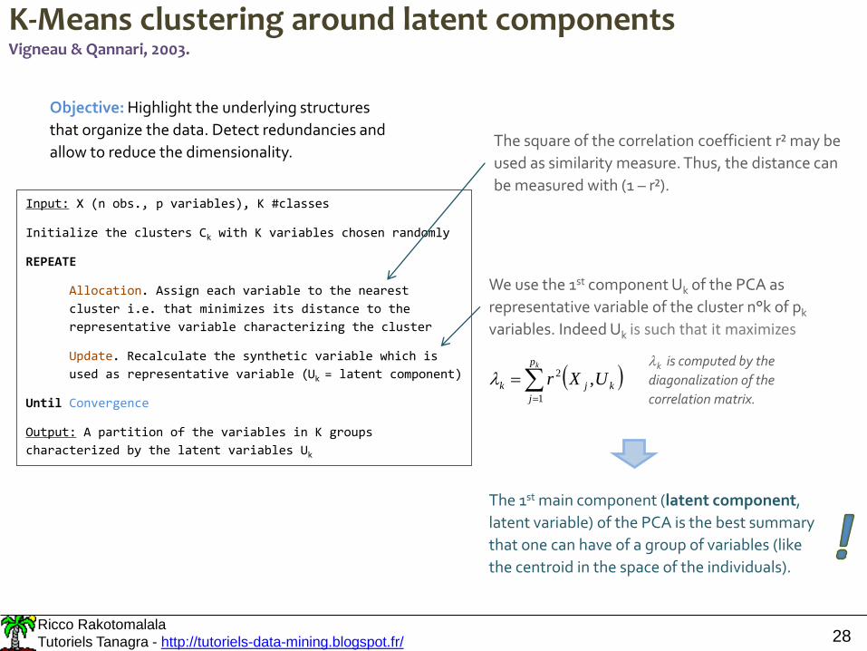
K-Means clustering around latent componentsVigneau & Qannari, 2003.


Initialize the clusters Ck with K variables chosen randomly

REPEATE

Allocation. Assign each variable to the nearest

cluster i.e. that minimizes its distance to the

representative variable characterizing the cluster

Update. Recalculate the synthetic variable which is

used as representative variable (Uk = latent component)

Until Convergence

Output: A partition of the variables in K groups

characterized by the latent variables Uk

Objective: Highlight the underlying structures

that organize the data. Detect redundancies and

allow to reduce the dimensionality.The square of the correlation coefficient r² may be

used as similarity measure. Thus, the distance can

be measured with (1 – r²).

We use the 1st component Uk of the PCA as

representative variable of the cluster n°k of pk

variables. Indeed Uk is such that it maximizes

kp

j

kjk UXr1

2 ,k is computed by the

diagonalization of the

correlation matrix.

The 1st main component (latent component,

latent variable) of the PCA is the best summary

that one can have of a group of variables (like

the centroid in the space of the individuals).


Ricco Rakotomalala


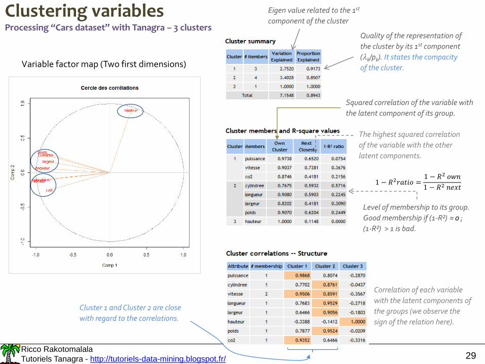
Clustering variablesProcessing “Cars dataset” with Tanagra – 3 clusters

Variable factor map (Two first dimensions)

Eigen value related to the 1st

component of the cluster

Quality of the representation of

the cluster by its 1st component

(k/pk). It states the compacity

of the cluster.

Squared correlation of the variable with

the latent component of its group.

The highest squared correlation

of the variable with the other

latent components.

Level of membership to its group.

Good membership if (1-R²) 0 ;

(1-R²) > 1 is bad.

1 − 𝑅2𝑟𝑎𝑡𝑖𝑜 =1 − 𝑅2 𝑜𝑤𝑛

1 − 𝑅2 𝑛𝑒𝑥𝑡

Correlation of each variable

with the latent components of

the groups (we observe the

sign of the relation here).

Cluster 1 and Cluster 2 are close

with regard to the correlations.


Ricco Rakotomalala


Conclusion

• Partitioning clustering methods are often simple and efficient. K-Means is

one the most popular approach.

• They can process large datasets but they may be slow because many

accesses to the data are needed.

• K-Means approach produce clusters with particular shapes. They are

spherical and have approximately the same size.

• The approach may be generalized to databases with categorical and mixed

(categorical and numeric) variables.

• The approach may be generalized to clustering of variables.

• The choice of K remains an open issue.

• Summarizing the cluster with only the centroid is not always relevant (see

EM algorithm, K-Medoids, etc.).


Ricco Rakotomalala


References

Some books, including state-of-the-art French books

Chandon J.L., Pinson S., « Analyse typologique – Théorie et applications », Masson, 1981.

Diday E., Lemaire J., Pouget J., Testu F., « Eléments d’analyse de données », Dunod, 1982.

Gan G., Ma C., Wu J., « Data Clustering – Theory, Algorithms and Applications », SIAM, 2007.

L. Lebart, A. Morineau, M. Piron, « Statistique exploratoire multidimensionnelle », Dunod, 2000.

Tutorials and other references

“Hierarchical agglomerative clustering”, June 2017.

“Clustering variables”, September 2014.

“Cluster analysis for mixed data”, February 2014.

“Two-step clustering for handling large databases”, June 2009.

“K-Means – Comparison of free tools”, June 2009.


http://data-mining-tutorials.blogspot.fr/2017/06/hierarchical-agglomerative-clustering.html

http://data-mining-tutorials.blogspot.fr/2014/09/clustering-variables-slides.html

http://data-mining-tutorials.blogspot.fr/2014/02/cluster-analysis-for-mixed-data.html

http://data-mining-tutorials.blogspot.fr/2009/06/two-step-clustering-for-handling-large.html

http://data-mining-tutorials.blogspot.fr/2009/06/k-means-comparison-of-free-tools.html

Université Lumière Lyon 2eric.univ-lyon2.fr/~ricco/cours/slides/en/classif_centres_mobiles.pdf ·...

Documents

Transcript of Université Lumière Lyon 2eric.univ-lyon2.fr/~ricco/cours/slides/en/classif_centres_mobiles.pdf ·...