
Solving Di cult Game Positions - Maastricht University · Winands and Jos Uiterwijk, and my...
144
Solving Difficult Game Positions
Transcript of Solving Di cult Game Positions - Maastricht University · Winands and Jos Uiterwijk, and my...
Solving Difficult Game Positions

Solving Difficult Game Positions
PROEFSCHRIFT
ter verkrijging van de graad van doctoraan de Universiteit Maastricht,
op gezag van de Rector Magnificus,Prof. mr. G.P.M.F. Mols,
volgens het besluit van het College van Decanen,in het openbaar te verdedigen
op woensdag 15 december 2010 om 14.00 uur
door
Jahn-Takeshi Saito
Promotor: Prof. dr. G. WeissCopromotor: Dr. M.H.M. Winands
Dr. ir. J.W.H.M. Uiterwijk
Leden van de beoordelingscommissie:Prof. dr. ir. R.L.M. Peeters (voorzitter)Prof. dr. T. Cazenave (Universite Paris-Dauphine)Prof. dr. M. Gyssens (Universiteit Hasselt / Universiteit Maastricht)Prof. dr. ir. J.C. ScholtesProf. dr. C. Witteveen (Technische Universiteit Delft)
The research has been funded by the Netherlands Organisation for Scientific Research
(NWO), in the framework of the project Go for Go, grant number 612.066.409.
Dissertation Series No. 2010-49
The research reported in this thesis has been carried out under the auspices of SIKS,
the Dutch Research School for Information and Knowledge Systems.
ISBN: 978-90-8559-164-1
c© 2010 J.-T. Saito
All rights reserved. No part of this publication may be reproduced, stored in a retrieval
system, or transmitted, in any form or by any means, electronically, mechanically, photo-
copying, recording or otherwise, without prior permission of the author.
Preface
After receiving my Master’s degree in Computational Linguistics and Artificial Intel-ligence in Osnabruck, I faced the pleasant choice between becoming a Ph.D. studentin Osnabruck or Maastricht. The first option would have led me further into thefield of Computational Linguistics. However, I decided for the second option, crossedthe border to the Netherlands, and continued my work on Computer Go that hadbeen the topic of my Master’s thesis. It was a choice that I have never regretted.While I had sensed the gravity of my choice, I could not possibly have foreseen allactual consequences. One consequence was that I entered the research of solvingdifficult game positions. Another consequence was the production of this volume.Yet another consequence was my encounter with many persons whom I would liketo acknowledge here.
Of course, this thesis would not have been possible without the help of a largegroup of people. I would first and foremost like to thank my daily advisors, MarkWinands and Jos Uiterwijk, and my supervisor Gerhard Weiss. I am grateful toMark for his firm guidance on scientific questions and for motivating me whenevernecessary. To Jos I owe gratitude for his patient devotion to detail that so oftenreminded me to work with greater care and less haste. I am indebted to Gerhard fortaking over the responsibility of supervising me and for giving me valuable advicefrom a point of view wider than that of games and search.
Furthermore, I would like to thank all people with whom I collaborated over theyears. I am grateful to Jaap van den Herik of whose inspiring drive for perfection,professional attitude, and superb editing skills I was allowed to profit in particularduring my first three years in Maastricht and still continue to profit today. I oweparticular gratitude to two people who might be caught by surprise: Bruno Bouzyand Helmar Gust. Their support during my Master’s studies led my way to theNetherlands. Similarly, I am grateful to Erik van der Werf who initiated the projectthat I later worked on and who additionally gave me valuable support on manyoccasions. I am indebted to Dr. Yngvi Bjornsson for his collaboration and Prof.Hiroyuki Iida for comments on proof-number search.
I will never forget my roommates in my years in the “women’s prison” of Min-derbroedersberg 6a: Laurens van der Maaten, Maarten Schadd, Guillaume Chaslot,Andra Waagmeester, Pim Nijssen, and David Lupien St-Pierre. Thank you for eas-ing the burden of labor with occasional moments of recreation, and for your adviceon matters scientific and beyond. I would like to thank Sander Spek and Laurensvan der Maaten who shared with me not only an appreciation for decent coffee but
vi
also valuable experience that influenced this thesis. I am indebted for inspiring dis-cussions to my colleagues past and present: Sander Bakkes, Niek Bergboer, Guidode Croon, Jeroen Donkers, Steven de Jong, Michael Kaisers, Joyca Lacroix, NyreeLemmens, Georgi Nalbantov, Marc Ponsen, Evgueni Smirnov, Pieter Spronck, BenTorben-Nielsen, Philippe Uyttendaele, Stijn Vanderlooy and Jean Derks.
The one special person I cannot possibly thank enough for enduring my stressduring producing this thesis also happens to be the person I love, Silja. Danke furDeine unverzichtbare Hilfe.
This work has been supported by FHS’s system administrators Peter Geurtz andTon Derix and secretaries Joke Hellemons, Tons van den Bosch, Karin Braeken andMarijke Verheij.
Countless more people should be thanked here, like the people from BiGCaTBioinformatics Department of Maastricht University. I would just like to thank allof my friends, family, and colleagues for the support they have given me during thework on this thesis.
Jahn-Takeshi SaitoMaastricht, August 2010
Acknowledgments
The research has been carried out under the auspices of the Dutch Research Schoolfor Information and Knowledge Systems (SIKS). I gratefully acknowledge the finan-cial support by the Netherlands Organisation for Scientific Research (NWO).
Table of Contents
Preface v
Table of Contents vii
List of Abbreviations xi
List of Figures xii
List of Tables xiii
1 Introduction 11.1 Games and AI . . . . . . . . . . . . . . . . . . . . . . . . . . . . . . 11.2 Solving Games and Game Positions . . . . . . . . . . . . . . . . . . . 21.3 Problem Statement and Research Questions . . . . . . . . . . . . . . 41.4 Outline of the Thesis . . . . . . . . . . . . . . . . . . . . . . . . . . . 5
2 Basics of Game-Tree Search for Solvers 72.1 Game-Tree Search . . . . . . . . . . . . . . . . . . . . . . . . . . . . 8
2.1.1 Game Tree . . . . . . . . . . . . . . . . . . . . . . . . . . . . 82.1.2 Search Tree . . . . . . . . . . . . . . . . . . . . . . . . . . . . 82.1.3 Transposition Tables and the GHI Problem . . . . . . . . . . 9
2.2 Proof-Number Algorithms . . . . . . . . . . . . . . . . . . . . . . . . 102.2.1 Proof-Number Search . . . . . . . . . . . . . . . . . . . . . . 102.2.2 Variants of PNS . . . . . . . . . . . . . . . . . . . . . . . . . 132.2.3 Performance of Proof-Number Algorithms . . . . . . . . . . . 162.2.4 Enhancements for Proof-Number Algorithms . . . . . . . . . 17
2.3 Monte-Carlo Techniques for Search . . . . . . . . . . . . . . . . . . . 192.3.1 Monte-Carlo Evaluation . . . . . . . . . . . . . . . . . . . . . 202.3.2 Monte-Carlo Tree Search . . . . . . . . . . . . . . . . . . . . 22
2.4 Chapter Summary . . . . . . . . . . . . . . . . . . . . . . . . . . . . 25
3 Monte-Carlo Proof-Number Search 273.1 Monte-Carlo Proof-Number Search . . . . . . . . . . . . . . . . . . . 28
3.1.1 Algorithm . . . . . . . . . . . . . . . . . . . . . . . . . . . . . 283.1.2 Controlling Parameters . . . . . . . . . . . . . . . . . . . . . 29
viii Table of Contents
3.2 Experiment 1: Tuning the Parameters of MC-PNS . . . . . . . . . . 303.2.1 Life-and-Death Problems . . . . . . . . . . . . . . . . . . . . 303.2.2 Test Set . . . . . . . . . . . . . . . . . . . . . . . . . . . . . . 313.2.3 Algorithm and Implementation . . . . . . . . . . . . . . . . . 323.2.4 Test Procedure . . . . . . . . . . . . . . . . . . . . . . . . . . 32
3.3 Results of Experiment 1 . . . . . . . . . . . . . . . . . . . . . . . . . 333.4 Discussion of Experiment 1 . . . . . . . . . . . . . . . . . . . . . . . 353.5 Patterns for PNS . . . . . . . . . . . . . . . . . . . . . . . . . . . . . 37
3.5.1 Patterns in Computer Go . . . . . . . . . . . . . . . . . . . . 373.5.2 Two Pattern-Based Heuristics . . . . . . . . . . . . . . . . . . 37
3.6 Experiment 2: Initialization by Patterns or by Monte-Carlo Evaluation 383.7 Results of Experiment 2 . . . . . . . . . . . . . . . . . . . . . . . . . 383.8 Discussion of Experiment 2 . . . . . . . . . . . . . . . . . . . . . . . 393.9 Chapter Conclusion and Future Research . . . . . . . . . . . . . . . 40
3.9.1 Chapter Conclusion . . . . . . . . . . . . . . . . . . . . . . . 403.9.2 Future Research . . . . . . . . . . . . . . . . . . . . . . . . . 40
4 Monte-Carlo Tree Search Solver 434.1 Monte-Carlo Tree Search Solver . . . . . . . . . . . . . . . . . . . . . 44
4.1.1 Backpropagation . . . . . . . . . . . . . . . . . . . . . . . . . 454.1.2 Selection . . . . . . . . . . . . . . . . . . . . . . . . . . . . . 454.1.3 Pseudocode for MCTS-Solver . . . . . . . . . . . . . . . . . . 46
4.2 Monte-Carlo LOA . . . . . . . . . . . . . . . . . . . . . . . . . . . . 474.2.1 Selection Strategies . . . . . . . . . . . . . . . . . . . . . . . . 474.2.2 Simulation Strategy . . . . . . . . . . . . . . . . . . . . . . . 504.2.3 Parallelization . . . . . . . . . . . . . . . . . . . . . . . . . . 50
4.3 Experiments . . . . . . . . . . . . . . . . . . . . . . . . . . . . . . . . 514.3.1 Experimental Setup . . . . . . . . . . . . . . . . . . . . . . . 514.3.2 Selection Strategies . . . . . . . . . . . . . . . . . . . . . . . . 524.3.3 Comparing Different Solvers . . . . . . . . . . . . . . . . . . . 544.3.4 Testing Parallelized Monte-Carlo Tree Search Solver . . . . . 55
4.4 Chapter Conclusion and Future Research . . . . . . . . . . . . . . . 564.4.1 Chapter Conclusion . . . . . . . . . . . . . . . . . . . . . . . 564.4.2 Future Research . . . . . . . . . . . . . . . . . . . . . . . . . 57
5 Parallel Proof-Number Search 595.1 Parallelization of PNS . . . . . . . . . . . . . . . . . . . . . . . . . . 60
5.1.1 Terminology . . . . . . . . . . . . . . . . . . . . . . . . . . . 605.1.2 ParaPDS and the Master-Servant Design . . . . . . . . . . . 605.1.3 Randomized Parallelization . . . . . . . . . . . . . . . . . . . 61
5.2 RP–PNS . . . . . . . . . . . . . . . . . . . . . . . . . . . . . . . . . . 625.2.1 Detailed Description of Randomized Parallelization for PNS . 625.2.2 Implementation . . . . . . . . . . . . . . . . . . . . . . . . . . 64
5.3 Experiments . . . . . . . . . . . . . . . . . . . . . . . . . . . . . . . . 645.3.1 Setup . . . . . . . . . . . . . . . . . . . . . . . . . . . . . . . 655.3.2 Results . . . . . . . . . . . . . . . . . . . . . . . . . . . . . . 65
Table of Contents ix
5.3.3 Discussion . . . . . . . . . . . . . . . . . . . . . . . . . . . . . 665.4 Chapter Conclusion and Future Research . . . . . . . . . . . . . . . 67
5.4.1 Chapter Conclusion . . . . . . . . . . . . . . . . . . . . . . . 675.4.2 Future Research . . . . . . . . . . . . . . . . . . . . . . . . . 68
6 Paranoid Proof-Number Search 696.1 Search Algorithms for Multi-Player Games . . . . . . . . . . . . . . . 70
6.1.1 The Maxn Algorithm . . . . . . . . . . . . . . . . . . . . . . 706.1.2 Equilibrium Points . . . . . . . . . . . . . . . . . . . . . . . . 716.1.3 Paranoid Search . . . . . . . . . . . . . . . . . . . . . . . . . 72
6.2 Paranoid Proof-Number Search . . . . . . . . . . . . . . . . . . . . . 736.3 Finding the Optimal Score . . . . . . . . . . . . . . . . . . . . . . . . 746.4 The Game of Rolit . . . . . . . . . . . . . . . . . . . . . . . . . . . . 75
6.4.1 Predecessors and Related Games . . . . . . . . . . . . . . . . 756.4.2 Rules of Rolit . . . . . . . . . . . . . . . . . . . . . . . . . . . 766.4.3 Search Space of Rolit . . . . . . . . . . . . . . . . . . . . . . 776.4.4 A Monte-Carlo Player for Rolit . . . . . . . . . . . . . . . . . 78
6.5 Experimental Setup . . . . . . . . . . . . . . . . . . . . . . . . . . . 796.5.1 Initialization . . . . . . . . . . . . . . . . . . . . . . . . . . . 796.5.2 Knowledge Representation and Hardware . . . . . . . . . . . 79
6.6 Results . . . . . . . . . . . . . . . . . . . . . . . . . . . . . . . . . . . 806.6.1 Game Results . . . . . . . . . . . . . . . . . . . . . . . . . . . 806.6.2 Search Trees . . . . . . . . . . . . . . . . . . . . . . . . . . . 816.6.3 PPNS vs. Paranoid Search . . . . . . . . . . . . . . . . . . . 82
6.7 Chapter Conclusion and Future Research . . . . . . . . . . . . . . . 836.7.1 Chapter Conclusion . . . . . . . . . . . . . . . . . . . . . . . 836.7.2 Future Research . . . . . . . . . . . . . . . . . . . . . . . . . 83
7 Conclusions and Future Research 857.1 Conclusions on the Research Questions . . . . . . . . . . . . . . . . . 85
7.1.1 Monte-Carlo Evaluation . . . . . . . . . . . . . . . . . . . . . 857.1.2 Monte-Carlo Tree Search Solver . . . . . . . . . . . . . . . . . 867.1.3 Parallel Proof-Number Search . . . . . . . . . . . . . . . . . . 867.1.4 Paranoid Proof-Number Search . . . . . . . . . . . . . . . . . 87
7.2 Conclusions on the Problem Statement . . . . . . . . . . . . . . . . . 877.3 Recommendations for Future Research . . . . . . . . . . . . . . . . . 88
References 91
Appendix 105
A Rules of Go and LOA 105A.1 Go Rules . . . . . . . . . . . . . . . . . . . . . . . . . . . . . . . . . 105A.2 LOA Rules . . . . . . . . . . . . . . . . . . . . . . . . . . . . . . . . 106
Index 109

x Table of Contents
Summary 113
Samenvatting 117
Curriculum Vitae 121
SIKS Dissertation Series 123

List of Abbreviations
dn Disproof numberdf-pn Depth-first Proof-Number SearchLOA Lines of ActionMCE Monte-Carlo EvaluationMC-PNS Monte-Carlo Proof-Number SearchMCTS Monte-Carlo Tree Searchpn Proof numberParaPDS Parallel Proof-and-Disproof-Number SearchPDS Proof-and-Disproof-Number SearchPDS–PN Two-level Proof-and-Disproof-Number SearchPNS Proof-Number SearchPN∗ Iterative-deepening depth-first Proof-Number SearchPN2 Two-level Proof-Number SearchPN1 First-level search of PN2
PN2 Second-level search of PN2
RP–PNS Randomized-Parallel Proof-Number SearchRP–PN2 Two-level Randomized-Parallel Proof-Number Search
List of Figures
2.1 Example of a PNS tree. . . . . . . . . . . . . . . . . . . . . . . . . . 122.2 The four stages of MCTS. . . . . . . . . . . . . . . . . . . . . . . . . 23
3.1 Schematic representation of a search tree generated by MC-PNS. . . 303.2 Example of a life-and-death problem. . . . . . . . . . . . . . . . . . . 313.3 Time consumption of various configurations of MC-PNS. . . . . . . . 343.4 Space consumption of various configurations of MC-PNS. . . . . . . 36
4.1 LOA position with White to move. . . . . . . . . . . . . . . . . . . . 454.2 Search trees showing a weakness of Monte-Carlo evaluation. . . . . . 46
5.1 Example of a PNS tree. . . . . . . . . . . . . . . . . . . . . . . . . . 63
6.1 Example of a three-player three-ply maxn tree. . . . . . . . . . . . . 716.2 Example of a three-player three-ply paranoid tree. . . . . . . . . . . 726.3 Example of a three-player three-ply PPNS tree. . . . . . . . . . . . . 746.4 Game boards of 8× 8 Reversi and 8× 8 Rolit. . . . . . . . . . . . . 75
A.1 Two illustrations for the rules of Go (adopted from Chaslot, 2010). . 106A.2 Three illustrations for the rules of LOA (adopted from Winands,
2004). . . . . . . . . . . . . . . . . . . . . . . . . . . . . . . . . . . . 107
List of Tables
3.1 Time and node consumption of various configurations of MC-PNS rel-ative to PNS. . . . . . . . . . . . . . . . . . . . . . . . . . . . . . . . 33
3.2 Time and space ranking of the four compared PNS variations averagedover 30 test problems. . . . . . . . . . . . . . . . . . . . . . . . . . . 39
4.1 Comparing different selection strategies on 488 test positions with alimit of 5,000,000 nodes. . . . . . . . . . . . . . . . . . . . . . . . . 53
4.2 Comparing the different Progressive-Bias variants on 224 test posi-tions with a limit of 5,000,000 nodes. . . . . . . . . . . . . . . . . . 53
4.3 Comparing PB-L1 and PB-L2 on 286 test positions with a limit of5,000,000 nodes. . . . . . . . . . . . . . . . . . . . . . . . . . . . . . 54
4.4 Comparing MCTS-Solver, αβ, and PN2 on 488 test positions with alimit of 5,000,000 nodes. . . . . . . . . . . . . . . . . . . . . . . . . 54
4.5 Comparing MCTS-Solver and PN2 on 304 test positions. . . . . . . . 554.6 Experimental results for MCTS-Solver with root parallelization on
319 test positions. . . . . . . . . . . . . . . . . . . . . . . . . . . . . 554.7 Experimental results for MCTS-Solver with tree parallelization. . . 56
5.1 Experimental results for RP–PNS and RP–PN2 on S143. . . . . . . . 66
6.1 Search spaces of 6× 6 and 8× 8 Reversi variants. . . . . . . . . . . . 776.2 Percentages of games won of one million Monte-Carlo games in 4× 4,
6× 6, and 8× 8 Rolit with 2, 3, and 4 players. . . . . . . . . . . . . 786.3 Average branching factors of Rolit. . . . . . . . . . . . . . . . . . . . 796.4 Proven optimal scores for all players on 4× 4, 6× 6, and 8× 8 Rolit
for 2, 3, and 4 players under the paranoid condition. . . . . . . . . . 806.5 Nodes evaluated in 4× 4, 6× 6, and 8× 8 Rolit for 2, 3, and 4 players
under the paranoid condition. . . . . . . . . . . . . . . . . . . . . . . 816.6 Comparison of search-tree sizes on 4 × 4, 6 × 6, and 8 × 8 Rolit for
paranoid search and PPNS. . . . . . . . . . . . . . . . . . . . . . . . 82

Chapter 1
Introduction
This thesis is in the field of games and Artificial Intelligence (AI). It has long beenclaimed, that games are an indicator of or even a precondition to culture (Huizinga,1955). Humans participate in games not only to satisfy their desire for entertain-ment but also because they seek an intellectual challenge. One obvious challengein games is defeating the opponent(s). The AI equivalent to this challenge is thedesigning of strong game-playing programs. Another challenge in games is findingthe result of a game position, for instance whether a Chess position is a win or aloss. The AI equivalent to this challenge is the designing of algorithms that solvepositions. While game-playing programs have become much stronger over the years,solving games still remains a difficult task today and has therefore been receivingattention continuously. Throughout the thesis, we are interested in this difficult taskof solving game positions. The following chapters present algorithms that are basedon recent research in the field of search algorithms. In particular, the thesis extendsrecent developments in Monte-Carlo search for the task of solving. Moreover, openquestions of Proof-Number Search for solving are addressed. To that end, the heredescribed research contributes and tests new search algorithms.
This chapter introduces the basic notion of solving and gives the problem state-ment and four research questions guiding our research. Section 1.1 summarizes therelevance of games for AI. Section 1.2 discusses the concept of solving games andgame positions. Section 1.3 formulates the problem statement and gives four re-search questions. Section 1.4 completes the introduction by presenting the structureof this thesis and the relationship between chapters and research questions.
1.1 Games and AI
Since the early days of AI, games have served as a testing ground for measuringthe progress of the field. Two founding fathers of the discipline, Shannon (1950)and Turing (1953), were among the first to describe Chess-playing programs. Eversince, progress has been steady. Programs have improved and nowadays play a broadrange of games stronger than humans. An event illustrating the progress of playingstrength is the defeat of the human World Champion Gary Kasparov by the Chess
2 Introduction
program Deep Blue. On May 11, 1997 Deep Blue won a six-game match by twowins to one with three draws. This outcome was recognized as a historic victory forAI (DeCoste, 1998).
The number of games in which humans can easily defeat the best game-playingprogram is declining. An example of this trend is computer Go. The game of Gohad been one of the remaining challenges in which the human player had still beenclearly superior to the programs. However, the recent past has witnessed the riseof the Monte-Carlo Tree Search framework (Coulom, 2007a; Kocsis and Szepesvari,2006). It has helped closing the competitive gap between man and machine (Chaslot,2008).
Allis, Van den Herik, and Herschberg (1991) suggest categorizing games based onthe strength of available programs. The five suggested categories are: (1) amateur-level games, (2) grand-master-level games, (3) champion-level games, (4) over- cham-pion games, and (5) solved games. The categories (1) to (4) relate the strength ofthe programs to the strength of human players. For instance, an amateur-level gameis a game in which the strongest available program plays at human amateur level.Category (5), solved games, is not defined in relation to human strength. A game issolved if its game-theoretic value has been calculated (e.g., win for the first player)assuming both players play optimally.
The advance of AI research has resulted in a growing number of over-championgames including the above-mentioned Chess. Although many games have beensolved, solving games has remained challenging (Van den Herik, Uiterwijk, and VanRijswijck, 2002). For some games researchers therefore solved smaller versions, e.g.,5× 5 Go (Van der Werf, Van den Herik, and Uiterwijk, 2003), 6× 6 Lines of Action(LOA) (Winands, 2008), and 8× 8 Hex (Henderson, Arneson, and Hayward, 2009).Even solving mate positions in games such as Chess or Shogi still poses a hardproblem today. This thesis deals with search techniques for addressing this problem.
1.2 Solving Games and Game Positions
Solving is finding the game-theoretic value of a given game position. Some games,such as Hex (Nash, 1952) and Nim (Bouton, 1902), can be solved by a theoreticproof. Many other games cannot be solved in this way. Solving the latter gamesrequires search. Search for solving is described in detail in Chapter 2. We call analgorithm describing how to find a game-theoretic value of a game position a solvingalgorithm. A solver is an implementation of a solving algorithm.
Different degrees of solving have been distinguished by Paul Colley and DonaldMichie (Allis, 1994). The degrees form a hierarchy in which the minimal solution iscalled ultra weak and the maximal solution is called strong. The hierarchy of solvinggames is as follows (Allis, 1994).
Ultra-weakly solved. For the initial position(s), the game-theoretic value hasbeen determined. Crucially, the proof is not necessarily constructive, i.e., itdoes not have to provide a strategy of optimal play. A famous example of anultra-weakly solved game is Hex (Nash, 1952).
1.2 — Solving Games and Game Positions 3
Weakly solved. For the initial position(s), a strategy has been determined to ob-tain at least the game-theoretic value of the game for both players under rea-sonable resources. Examples of weakly solved games include Qubic (Patashnik,1980), Go-Moku (Allis, Huntjes, and Van den Herik, 1996), Nine-Men’s Morris(Gasser, 1996), various k -in-a-row games (Uiterwijk and Van den Herik, 2000),Domineering (Breuker, Uiterwijk, and Van den Herik, 2000), Renju (Wagnerand Virag, 2001), 5 × 5 Go (Van der Werf et al., 2003), Checkers (Schaef-fer et al., 2007), and Fanorona (Schadd et al., 2008).
Strongly solved. For all legal positions, a strategy has been determined to obtainthe game-theoretic value of the position, for both players, under reasonableresources. Examples of recently strongly solved games include Kalah (Irving,Donkers, and Uiterwijk, 2000), Awari (Romein and Bal, 2003), and ConnectFour (Tromp, 2008).
When solving an arbitrary game position (as opposed to only regarding initialpositions), the three degrees of solving can be adopted trivially as follows. A non-initial position can be thought of as the initial position of a derived game. All rulesof the derived game except those determining the start position are the same as inthe original game. We call a position weakly solved if the derived game is solvedweakly. Under this notion, a solving algorithm is a method for solving games orgame positions weakly.
Solvers for positions of two-player games with perfect information such as Go(Wolf, 1994; Kishimoto and Muller, 2005a; Wolf and Shen, 2007), and Shogi (Tak-izawa and Grimbergen, 2000; Nagai, 2002) have been available for a long time. Theearliest solvers were mate solvers for Chess. Two of the earliest solvers deserve men-tioning here. In 1912, the Spanish engineer Torres y Quevedo presented an electro-mechanic automaton called El Ajedrecista (“the Chess player”) which was ableto solve one kind of King-Rook-King endgames (Bell, 1978) with the constraint ofoccasional mechanical failure. About 40 years later, in 1951, Prinz programmed theManchester-Mark I in order to solve mate-in-two endgame problems.
Already in 1985, Grottling (1985) compared the performance of several matesolvers on Chess problems. As pointed out by Lindner (1985), the Chess problemis characterized by the following three attributes: (1) it has a solution (normally acheckmate), (2) the solution is reachable in a fixed number of moves, and (3) thefirst move is required to be unique. A mate-in-n problem is furthermore constraintby the fact that no refutation is possible which prolongs the game beyond n moves.
Besides two-player games with perfect information, several researchers providedsolving algorithms for two-player games with imperfect information. Sakuta and Iida(2000) solved positions for the imperfect-information game of Screen Shogi. Simi-larly, Ferguson (1992) was able to solve the KBNK ending in the game of Kriegspiel.Bolognesi and Ciancarini (2003) successfully solved more demanding endgames ofKriegspiel by considering extensive search spaces given by meta-positions, i.e., col-lections of possible positions deducible from observations with limited information.
The solving algorithms we are studying in this thesis are search algorithms. Theycan be distinguished into forward search and backward search (Schaeffer et al., 2007).Forward search expands a search tree or search graph from a given position and
4 Introduction
gradually searches deeper until all subtrees are solved. Backward search starts byconsidering the game-theoretic values for all terminal positions. Then, the values forall positions directly preceding terminal positions are calculated. Next, the valuesfor the preceding positions are calculated and so on. This information is stored asan endgame database. In this way, the search tree is built bottom up until thegame-theoretic value of the initial position has been found. The most commonbackward-search technique for creating an endgame database is retrograde analysis(Strohlein, 1970). While some games like Go are not suitable for endgame databasesdue to the overwhelming number of terminal positions, other games such as Chess(Thompson, 1986; Nalimov, Haworth, and Heinz, 2000) are more suitable becausetheir state space is converging (Allis, 1994). For such games, including Checkers(Schaeffer et al., 2007) and Fanorona (Schadd et al., 2008), it is possible to combineforward and backward search by expanding a search tree up to a certain depth atwhich an endgame database provides the game-theoretic value.
Forward search commonly applies heuristic knowledge to solve a game, but it isalso possible to combine search and analytical proofs. An analytical proof providesperfect knowledge which the search algorithm can exploit for solving. In this way,Bullock (2002) solved Domineering on large board sizes up to 10× 10 by supplyingperfect knowledge in an evaluation function. Similarly, Allis (1988) provided a rule-based approach to solving Connect Four. Hayward, Bjornsson, and Johanson (2005)solved 7× 7 Hex with perfect knowledge of virtual connections. More recently, Wuand Huang (2006) and Chiang, Wu, and Lin (2010) solved k -in-a-row games bycombining analytical proofs with search algorithms.
1.3 Problem Statement and Research Questions
The previous section reflected on solving games and game positions by computerprograms. This is exactly the topic of the thesis. The game positions studied inthis thesis generalize from the narrow definition of mate-in-n for Chess problems.Throughout this thesis and if not stated otherwise explicitly, the games consideredare deterministic turn-taking adversarial games with perfect information. We con-sider any position of a game for solving. In most cases, we do not know a gameposition’s outcome (win or loss) or the exact depth of the solution. Moreover, thesolution is not required to have a unique best move.
While much effort has been put into αβ search (Knuth and Moore, 1975), thisthesis investigates solving games with Monte-Carlo search techniques (Abramson,1990; Brugmann, 1993; Bouzy and Helmstetter, 2003; Coulom, 2007a; Kocsis andSzepesvari, 2006) and Proof-Number Search (Allis, Van der Meulen, and Van denHerik, 1994). In particular, we test new forward-search algorithms on the games ofGo, LOA, and Rolit. The following problem statement (PS) guides our research.
PS How can we improve forward search for solving game positions?
We give four research questions to address the problem statement. The context ofthe four research questions is the current research in game-tree search in general andtwo current aspects in particular, namely: (i) the recent progress in Monte-Carlo
1.4 — Outline of the Thesis 5
search techniques for game-playing programs, and (ii) open questions in applyingProof-Number Search variants to solving difficult game positions. The four researchquestions deal with (1) Monte-Carlo evaluation, (2) Monte-Carlo Tree Search, (3)parallelized search, and (4) search for multi-player games.
RQ 1 How can we use Monte-Carlo evaluation to improve Proof-Number Search forsolving game positions?
The recent past in the game-tree search domain has witnessed graspable advancesby applying Monte-Carlo evaluation (Abramson, 1990; Brugmann, 1993; Bouzy andHelmstetter, 2003). RQ 1 inquires in how far Proof-Number Search can exploit thisdevelopment.
RQ 2 How can the Monte-Carlo Tree Search framework contribute to solving gamepositions?
Based on Monte-Carlo evaluation, Monte-Carlo Tree Search (MCTS) (Kocsis andSzepesvari, 2006; Coulom, 2007a) has seen many successes in the past few years. RQ2 asks how these successes can be exploited for solving. In particular, the questioncalls for investigating how game-theoretic values can be propagated in the searchtree of MCTS.
RQ 3 How can Proof-Number Search be parallelized?
So far, only a small amount of research treated the issue of parallelizing Proof-Number Search (Kishimoto and Kotani, 1999; Kaneko, 2010). To answer RQ 3, wepropose a way to parallelize Proof-Number Search by randomization.
RQ 4 How can Proof-Number Search be applied to multi-player games?
Most solving algorithms are designed to solve two-player games. RQ 4 addressesa generalization of solving beyond the two-player limit (Luckhardt and Irani, 1986;Korf, 1991; Sturtevant and Korf, 2000). The thesis proposes to extend Proof-NumberSearch for multiple players. In doing so, we address the problem of defining whatsolving means in the context of games with more than two players.
1.4 Outline of the Thesis
This thesis is organized in seven chapters. Chapter 1 gives a general introductionto the topic of this thesis, solving games, and presents the problem statement andfour research questions that guide the research. Chapter 2 establishes the termi-nology used throughout the remainder of the thesis and surveys existing searchalgorithms. In particular, it explains Monte-Carlo search techniques and variants ofProof-Number Search in detail.
Each of Chapters 3, 4, 5, and 6 answers one of the four research questions andthereby addresses the problem statement of this thesis. Chapter 3 describes howMonte-Carlo evaluation can be combined with Proof-Number Search to form an
6 Introduction
algorithm called MC-PNS. We test MC-PNS on Go problems. The chapter providesan answer to RQ 1. Chapter 4 answers RQ 2 by showing how Monte-Carlo TreeSearch can be transformed into a solving algorithm called MCTS Solver. The solveris tested on LOA positions. Chapter 5 addresses RQ 3 and describes a parallelizationof PNS which is based on randomization. The resulting parallel algorithm is calledRP–PNS. RP–PNS and its two-level variant RP–PN2 are tested on LOA positions.Chapter 6 focuses on solving multi-player games and therefore supplies an answerto RQ 4. We propose an adaptation of PNS for multi-player games. The resultingalgorithm, Paranoid Proof-Number Search, is tested on the game of Rolit, a multi-player version of Othello (Reversi).
Chapter 7 concludes the thesis by reviewing the results of the preceding chaptersand relating them to the problem statement and the four research questions, andgives recommendations for future research. The appendix contains the rules for thegames of Go and LOA.
Chapter 2
Basics of Game-Tree Searchfor Solvers
This chapter is partially based on the following two publications.1
1. J-T. Saito, G.M.J.B. Chaslot, J.W.H.M. Uiterwijk, and H.J. van den Herik. Monte-Carlo Proof-Number Search. In H.J. van den Herik, P. Ciancarini, and H.H.L.M.Donkers, editors, Computers and Games - 5th International Conference (CG ‘06),volume 4630 of Lecture Notes in Computer Science, pp. 50–61. Springer, Berlin,Germany, 2007.
2. J-T. Saito, M.H.M. Winands, J.W.H.M. Uiterwijk, and H.J. van den Herik. Group-ing Nodes for Monte-Carlo Tree Search. In M.M. Dastani and E. de Jong, ed-itors, Proceedings of the 19th Belgian-Dutch Conference on Artificial Intelligence(BNAIC ‘07), pp. 276–283. Utrecht University Press, Utrecht University, Utrecht,The Netherlands, 2007.
The solving algorithms presented in the later chapters require a basic under-standing of standard search techniques. The aim of this chapter is to provide anoverview of search techniques related and relevant to solving. To this end, we intro-duce basic concepts and give notational conventions applied throughout the thesis.We then devote particular detail to two topics: (1) proof-number algorithms (Allis,1994; Van den Herik and Winands, 2008), and (2) Monte-Carlo techniques (Abram-son, 1990; Kocsis and Szepesvari, 2006; Coulom, 2007a). Proof-number algorithmsare stressed because they are well-studied standard techniques for solving. The rea-son for paying particular attention to Monte-Carlo techniques is that they can alsobe used for solving positions (cf. Zhang and Chen, 2008; Winands, Bjornsson, andSaito, 2008).
This chapter is organized as follows. Section 2.1 introduces the basic conceptsof game-tree search as well as the notational conventions required for describing
1 The author is grateful to Springer-Verlag and Utrecht University Press for the permission toreuse relevant parts of the articles.
8 Basics of Game-Tree Search for Solvers
solving techniques. Section 2.2 introduces the family of proof-number algorithms.Section 2.3 gives an overview of Monte-Carlo techniques relevant for Monte-Carlo-based solvers which are described in detail in Chapter 4. Section 2.4 concludes thechapter by relating the search techniques introduced in this chapter to the techniquespresented in the following chapters.
2.1 Game-Tree Search
This section describes game-tree search. Subsection 2.1.1 introduces basic con-cepts of game-tree search. Subsection 2.1.2 describes the search tree and threecommon search methods. Subsection 2.1.3 explains transposition tables and theGraph-History-Interaction problem; the latter is relevant to Section 2.2.
2.1.1 Game Tree
A game tree is an explicit representation of the state space for turn-based games.The nodes of the tree represent positions, the edges represent moves. The noderepresenting the initial position is the root. A node is terminal if its correspondingposition is an end position according to the rules of the game. Terminal nodes have agame-theoretic value according to the rules of the games, e.g., win or loss. A node’simmediate successor is called a child. Analogously, a node’s immediate predecessor iscalled its parent. Any node may have zero or more children. The root has no parent.All other nodes have exactly one parent. An internal node is a node that has a child.A node is fully expanded by generating all of its children. A node without childrenis called a leaf. A successor of a node P is recursively defined as either (1) a child ofP, or (2) a child of a successor of P. Analogously, a node P is called predecessor ofanother node S if S is a successor of P. A path to L is the set of all predecessors ofL.
A game tree is generated by first fully expanding the root and then repeatedlyexpanding all non-terminal nodes until all leaves are terminal. The game-theoreticvalue of the game is the value of the initial position under optimal play by bothplayers. The game-theoretic value can be found by observing the game tree.
The depth of the root is zero. For non-root nodes the depth is the one-incrementof the depth of the parent.
2.1.2 Search Tree
Often a game tree is too large to be fully expanded in practice. Instead, a searchtree can be considered. The search tree is part of the game tree. It can be used forfinding a solution for two purposes. The first purpose is finding the game-theoreticvalue of the initial position. The second purpose is finding the best move givenconstraints on time or space.
A search tree is developed starting from the root according to a search method.Search methods are often guided by an evaluation function. Evaluation functionsestimate the game-theoretic value of a game position (Pearl, 1984) by assigning aheuristic value to a game position.
2.1 — Game-Tree Search 9
We distinguish three kinds of search methods: (1) breadth-first search, (2) depth-first search, and (3) best-first search. We shall briefly describe each of them.
Breadth-first search first expands the root node. Next, it expands all non-terminal leaves at depth 1. Then all non-terminal leaves at the next depth areexpanded. This process is repeated incrementally until a solution is found. Thus,siblings are expanded before children. Breadth-first search always finds a solutionwith the shortest path, if there is any, but typically requires too much memory inpractice.
Depth-first search first expands the root. Next, one of its children is selectedfor expansion. If the selected node is not terminal, the node is expanded. Thenagain one of the newborn children is selected for expansion and so forth. If a childis a terminal, one of its siblings is chosen for further investigation. If all childrenhave been investigated, one of the parent’s siblings is chosen and so forth. In thismanner, children are expanded before siblings. Depth-first search requires relativelylittle memory. In practice it is able to find solutions quickly when an evaluationfunction is used. A disadvantage is that the search method often spends much timein subtrees not contributing to finding a solution. αβ search (Knuth and Moore,1975) is an instance of depth-first search that uses an evaluation function in theleaves.
Best-first search aims at combining the advantages of breadth-first and depth-firstsearch. Best-first search iterates a loop that consists of two steps: (1) a heuristicis employed to find the most-promising node which is a leaf in the tree; (2) themost-promising leaf is expanded. The loop is repeated until a solution is found. Adisadvantage of best-first search is that it stores the whole search tree in memory.Examples of best-first search are Proof-Number Search (Allis et al., 1994) and MCTS(Kocsis and Szepesvari, 2006; Coulom, 2007a).
2.1.3 Transposition Tables and the GHI Problem
Search trees may grow large in practical applications. To reduce the size of a searchtree, transposition tables are used to store the results of a searched position (Green-blatt, Eastlake, and Croker, 1967; Breuker, 1998). Transposition tables exploit thefact that nodes representing the same game positions may occur multiple times inthe same search tree. More precisely, a transposition table is a table that maps agame position to some data relevant for that position. Transposition tables mayencounter difficulties in games that allow reaching the same position by differentpaths.
As pointed out by Breuker (1998) two difficulties can arise because of the differentpaths. (1) A position may actually be illegal. For instance, in Go a move may violatea repetition rule when reached via a certain path but not when reached via anotherpath. This is called the move-generation problem. (2) A position may be assigneda wrong game-theoretic value. For instance, in Chess a position may be a draw bythe three-fold repetition rule. This is called the evaluation problem. Both problemsare collectively referred to as the Graph-History-Interaction problem (GHI problem,Palay, 1983; Campbell, 1985).
10 Basics of Game-Tree Search for Solvers
2.2 Proof-Number Algorithms
As noted above, depth-first search and best-first search are more relevant to practicalapplications than breadth-first search. Arguably the strongest contribution thatdepth-first search made to solving is by αβ. Many games were (partially) solvedby iterative-deepening αβ. Among them are Checkers (Schaeffer et al., 2007) andsmall Go boards (Van der Werf et al., 2003; Van der Werf and Winands, 2009). Twoinstances of best-first search that are particularly relevant for solving are Proof-Number Algorithms and Monte-Carlo Tree Search. Proof-Number Algorithms arepresented in this section and Monte-Carlo Tree Search in Section 2.3.
Since the invention of Proof-Number Search (PNS) (Allis et al., 1994) in the 1990sa family of PNS variants evolved. These variants have been successfully applied to avariety of domains including Othello (Nagai, 2002), Shogi (Seo, Iida, and Uiterwijk,2001; Nagai, 2002), Tsume-Go (Kishimoto and Muller, 2003), and LOA (Winands,Uiterwijk, and Van den Herik, 2004). We call the family of algorithms that arevariants of PNS, proof-number algorithms. All of them have two things in common:(1) they are solving algorithms for binary goals (proving, e.g., win or no win), and(2) they rely on the concept of proof number.
This section gives a detailed account of proof-number algorithms. Subsection2.2.1 describes the basic PNS algorithm. Subsection 2.2.2 discusses five proof-numberalgorithms. Subsection 2.2.3 explains how the performance of different proof-numberalgorithms compares and Subsection 2.2.4 introduces three enhancements.
2.2.1 Proof-Number Search
Proof-Number Search (PNS) by Allis et al. (1994) is the most basic proof-number al-gorithm. All other variants of proof-number algorithms are descendants of PNS. Thissubsection describes the PNS algorithm. We do so in four parts: (A) Conspiracy-Numbers Search, (B) basic idea of PNS, (C) proof and disproof numbers, and (D)the PNS algorithm.
A. Forerunner: Conspiracy-Number Search
McAllester (1985; 1988) presented Conspiracy-Number Search which is a conceptualforerunner of PNS. Conspiracy numbers were introduced for minimax search (VonNeumann and Morgenstern, 1944) and indicate how likely it is that the root takes ona certain value v. This likelihood is expressed by the conspiracy number which is theminimum number of leaves (conspirators) that must change their value to cause theroot to change its value to v. The idea was later improved by Schaeffer (1989; 1990).
Two types of numbers, ↑CN and ↓CN , are used in order to calculate the conspir-acy numbers for each non-terminal node N. The minimum number of conspirators toincrease N’s value to v is ↑CN . If N’s value is greater than or equal to v, then ↑CN is0. ↓CN is the minimum number of conspirators required to decrease the value ofN to v. If N’s value is smaller than or equal to v, then ↓CN is 0. For calculating↑CN and ↓CN at the root, ↑CN and ↓CN values are calculated recursively for allnodes in the tree starting at the leaves. Different updating rules apply for ↑CN and
2.2 — Proof-Number Algorithms 11
↓CN depending on whether N is the maximizing player’s node or the minimizingplayer’s node.
Conspiracy numbers are similar to proof numbers with respect to two aspects:(1) two numbers at each node represent information on the expected game-theoreticvalue of the position, and (2) the numbers are calculated bottom up by backpropa-gation from the leaves to the root.
B. Basic Idea of PNS
PNS is a best-first search algorithm. Its heuristic determines the most-promising leafby selecting the most-proving node (cf. Subsection 2.1.2). The most-proving node isfound by exploiting two characteristics of the search tree: (1) its shape (determinedby the branching factors of internal nodes), and (2) the game-theoretic values of theleaves (which are known if a leaf is terminal). Since no other information is used byit, PNS is uninformed search, i.e., the search does not require to use any knowledgebeyond the rules of the game.
C. Proof and Disproof Numbers
As already mentioned, PNS employs ideas similar to Conspiracy Number Search.In order to find the most-proving node, PNS maintains two numbers for each nodeN. (1) The proof number, pn or pn(N), represents the number of leaf nodes that atleast have to be proven in order to prove the goal. Analogously, (2) the disproofnumber, dn or dn(N), represents the number of leaf nodes that at least have to bedisproven to disprove the goal. The values of pn and dn can be calculated for eachnode in the tree as follows.
We start by describing how the values are initialized for leaf nodes. When a goalis proven, no further expansion is required for proving it and no further expansioncan disprove it anymore. The corresponding holds for a disproven node. Adheringto this observation, for any terminal node T, pn and dn are set as follows. If thegoal is proven at T, then pn(T) = 0 and dn(T) =∞. If the goal is disproven at T,then pn(T) =∞ and dn(T) = 0.
For any non-terminal leaf L, it is not yet possible to say what its game-theoreticvalue is. Thus the values for L are set according to an initialization rule. Themost simple initialization rule directly follows the definition of pn and dn. It setspn(L) = dn(L) = 1.
The values for each internal node I are calculated from the set of its children,children(I). The backpropagation rules take into account whether I is an OR nodeor an AND node.
Backpropagation rule for OR nodes:
pn(I) = minS∈children(I)
pn(S) , (2.1)
dn(I) =∑
S∈children(I)
dn(S) . (2.2)
12 Basics of Game-Tree Search for Solvers
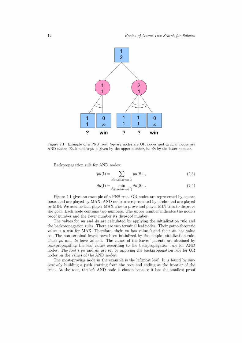
Figure 2.1: Example of a PNS tree. Square nodes are OR nodes and circular nodes areAND nodes. Each node’s pn is given by the upper number, its dn by the lower number.
Backpropagation rule for AND nodes:
pn(I) =∑
S∈children(I)
pn(S) , (2.3)
dn(I) = minS∈children(I)
dn(S) . (2.4)
Figure 2.1 gives an example of a PNS tree. OR nodes are represented by squareboxes and are played by MAX, AND nodes are represented by circles and are playedby MIN. We assume that player MAX tries to prove and player MIN tries to disprovethe goal. Each node contains two numbers. The upper number indicates the node’sproof number and the lower number its disproof number.
The values for pn and dn are calculated by applying the initialization rule andthe backpropagation rules. There are two terminal leaf nodes. Their game-theoreticvalue is a win for MAX. Therefore, their pn has value 0 and their dn has value∞. The non-terminal leaves have been initialized by the simple initialization rule.Their pn and dn have value 1. The values of the leaves’ parents are obtained bybackpropagating the leaf values according to the backpropagation rule for ANDnodes. The root’s pn and dn are set by applying the backpropagation rule for ORnodes on the values of the AND nodes.
The most-proving node in the example is the leftmost leaf. It is found by suc-cessively building a path starting from the root and ending at the frontier of thetree. At the root, the left AND node is chosen because it has the smallest proof
2.2 — Proof-Number Algorithms 13
number. At the selected AND node, the child with minimal dn is selected. This isthe leftmost leaf.
D. The PNS Algorithm
At the start of PNS, pn and dn of the root are both set to 1. As long as neitherpn nor dn of the root has value 0, there are still expansions required and thus thesearch is continued by performing a best-first search iteration.
At each iteration, the pn and dn are kept up to date and consistent for all nodesin the tree. Each iteration consists of four phases as follows.
(1) Selection. The values of pn and dn guide the search towards the most-provingleaf node. This is achieved by the following rule: in OR nodes, the child withminimal pn is selected; in AND nodes the child with minimal dn is selected.
(2) Expansion. The most-promising leaf is expanded.
(3) Evaluation. The new leaves are evaluated. Their pn and dn are set using thegame-theoretic values and the initialization rule as described above.
(4) Backpropagation. The values of pn and dn are updated such that the parents’pn and dn are consistent with their children’s values. The updating is repeatedsuccessively for all predecessors of the expanded leaf.
2.2.2 Variants of PNS
In many practical applications, PNS runs out of space quickly because it stores thewhole search tree in memory. We refer to this phenomenon as the memory problemof PNS. Several variants of PNS have been designed to address the issue. Thissubsection gives an overview of five of such proof-number algorithms: PN2, PN∗,PDS, df-pn, and PDS–PN.
A. PN2
Allis (1994) introduced PN2, a proof-number algorithm that addresses the memoryproblem of PNS by discarding subtrees that have been searched. Whenever nec-essary, the previously discarded subtrees are re-searched. To achieve this strategy,PNS is performed at two levels, called PN1 and PN2.
At the first level, PN1, a normal PNS search is conducted. However, PN2 proce-durally deviates from normal PNS when a leaf L is expanded. There, PNS is usedas initialization procedure. Instead of a simple initialization for non-terminal leaves,a second-level PNS, called PN2, is launched. The root of the PN2 tree is the leafL and the size of the tree is limited to a certain maximum number of nodes. Thesecond-level search terminates if either the maximum number of nodes is exceededor a (dis)proof has been found. When PN2 terminates, the children of L with theirpn and dn are kept as new leaves of the PN1. All successors below the children of Lare removed from memory.
14 Basics of Game-Tree Search for Solvers
As a consequence of using PN2, leaves of the PN1 tree contain more informationthan leaves of regular PNS. Memory is saved because useless PN2 trees are removed.The memory advantage of PN2 comes at a cost in terms of speed because the bestPN2 trees have to be re-searched.
Different approaches for setting the maximum number of nodes in the PN2 treeexist. We note that this maximum is crucial because it determines the trade-offbetween the memory consumption and speed of PN2. The main idea is to expressthe maximum as a function f(x) of the size of the PN1 tree given by the number xof its nodes. In his experiments on Chess positions, Breuker (1998) suggests to setf(x) to be a logistic-growth function
f(x) =1
1 + ea−x
b
. (2.5)
The parameters a and b are strictly positive and require tuning for optimalperformance (cf. Breuker, 1998). Furthermore, the size of PN2 is also limited bythe amount of memory physically available. If N is the physical limit of nodes thatmemory can hold, the maximum size of PN2 is
min(x× f(x), N − x) . (2.6)
B. PN*
As we have seen, PN2 addresses the memory problem of PNS by introducing twolevels of search and discarding most of the second-level results. This approach maybe described as wasteful because important information has to be re-generated everytime a previously discarded subtree is re-searched.
A different approach to addressing the memory problem consists of applyingiterative deepening. The first algorithm to follow this approach was PN∗ by Seo et al.(2001). PN∗ uses a threshold on the proof numbers to perform iterative deepening.The search is initialized with a threshold of 2 on the root’s pn. If no proof can befound the threshold is gradually increased until a proof can be found for the giventhreshold.
Essentially, PN∗ performs multiple-iterative deepening by iteratively deepeningat all AND nodes. Every node has a threshold on the proof number. The valuesfor these thresholds are increased at the AND nodes recursively if no proof can befound within a certain threshold. We note that the disproof numbers are not usedfor this iterative deepening.
A transposition table is used to reduce the overhead of re-searching nodes.Seo et al. (2001) report that their game engine based on PN∗ solved more Shogiproblems from a collection of 295 problems than any other compared solver. By itsiterative-deepening PN∗ essentially is a depth-first search, enabling PN∗ to find verydeep solutions, e.g., for the notoriously hard Microcosmos problem with a solutionsequence of 1,525 steps.
PN∗ is able to cope with harsh memory constraints better than PN2. But as aconsequence of disregarding the disproof numbers for move selection, PN∗ is weakat disproving subtrees.
2.2 — Proof-Number Algorithms 15
C. PDS
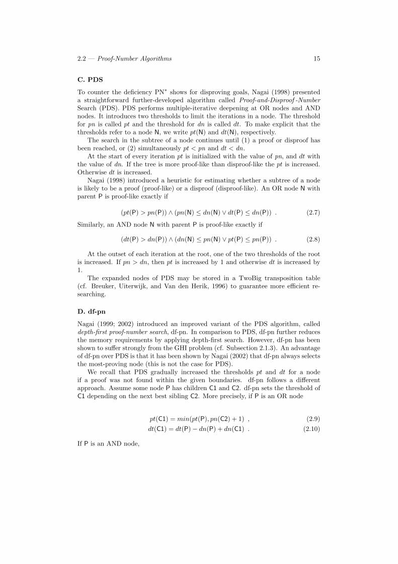
To counter the deficiency PN∗ shows for disproving goals, Nagai (1998) presenteda straightforward further-developed algorithm called Proof-and-Disproof -NumberSearch (PDS). PDS performs multiple-iterative deepening at OR nodes and ANDnodes. It introduces two thresholds to limit the iterations in a node. The thresholdfor pn is called pt and the threshold for dn is called dt. To make explicit that thethresholds refer to a node N, we write pt(N) and dt(N), respectively.
The search in the subtree of a node continues until (1) a proof or disproof hasbeen reached, or (2) simultaneously pt < pn and dt < dn.
At the start of every iteration pt is initialized with the value of pn, and dt withthe value of dn. If the tree is more proof-like than disproof-like the pt is increased.Otherwise dt is increased.
Nagai (1998) introduced a heuristic for estimating whether a subtree of a nodeis likely to be a proof (proof-like) or a disproof (disproof-like). An OR node N withparent P is proof-like exactly if
(pt(P) > pn(P)) ∧ (pn(N) ≤ dn(N) ∨ dt(P) ≤ dn(P)) . (2.7)
Similarly, an AND node N with parent P is proof-like exactly if
(dt(P) > dn(P)) ∧ (dn(N) ≤ pn(N) ∨ pt(P) ≤ pn(P)) . (2.8)
At the outset of each iteration at the root, one of the two thresholds of the rootis increased. If pn > dn, then pt is increased by 1 and otherwise dt is increased by1.
The expanded nodes of PDS may be stored in a TwoBig transposition table(cf. Breuker, Uiterwijk, and Van den Herik, 1996) to guarantee more efficient re-searching.
D. df-pn
Nagai (1999; 2002) introduced an improved variant of the PDS algorithm, calleddepth-first proof-number search, df-pn. In comparison to PDS, df-pn further reducesthe memory requirements by applying depth-first search. However, df-pn has beenshown to suffer strongly from the GHI problem (cf. Subsection 2.1.3). An advantageof df-pn over PDS is that it has been shown by Nagai (2002) that df-pn always selectsthe most-proving node (this is not the case for PDS).
We recall that PDS gradually increased the thresholds pt and dt for a nodeif a proof was not found within the given boundaries. df-pn follows a differentapproach. Assume some node P has children C1 and C2. df-pn sets the threshold ofC1 depending on the next best sibling C2. More precisely, if P is an OR node
pt(C1) = min(pt(P), pn(C2) + 1) , (2.9)
dt(C1) = dt(P)− dn(P) + dn(C1) . (2.10)
If P is an AND node,
16 Basics of Game-Tree Search for Solvers
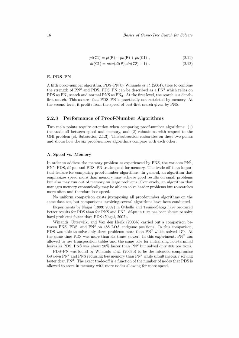
pt(C1) = pt(P)− pn(P) + pn(C1) , (2.11)
dt(C1) = min(dt(P), dn(C2) + 1) . (2.12)
E. PDS–PN
A fifth proof-number algorithm, PDS–PN by Winands et al. (2004), tries to combinethe strength of PN2 and PDS. PDS–PN can be described as a PN2 which relies onPDS as PN1 search and normal PNS as PN2. At the first level, the search is a depth-first search. This assures that PDS–PN is practically not restricted by memory. Atthe second level, it profits from the speed of best-first search given by PNS.
2.2.3 Performance of Proof-Number Algorithms
Two main points require attention when comparing proof-number algorithms: (1)the trade-off between speed and memory, and (2) robustness with respect to theGHI problem (cf. Subsection 2.1.3). This subsection elaborates on these two pointsand shows how the six proof-number algorithms compare with each other.
A. Speed vs. Memory
In order to address the memory problem as experienced by PNS, the variants PN2,PN∗, PDS, df-pn, and PDS–PN trade speed for memory. The trade-off is an impor-tant feature for comparing proof-number algorithms. In general, an algorithm thatemphasizes speed more than memory may achieve good results on small problemsbut also may run out of memory on large problems. Conversely, an algorithm thatmanages memory economically may be able to solve harder problems but re-searchesmore often and therefore lose speed.
No uniform comparison exists juxtaposing all proof-number algorithms on thesame data set, but comparisons involving several algorithms have been conducted.
Experiments by Nagai (1999; 2002) in Othello and Tsume-Shogi have producedbetter results for PDS than for PNS and PN∗. df-pn in turn has been shown to solvehard problems faster than PDS (Nagai, 2002).
Winands, Uiterwijk, and Van den Herik (2003b) carried out a comparison be-tween PNS, PDS, and PN2 on 488 LOA endgame positions. In this comparison,PDS was able to solve only three problems more than PN2 which solved 470. Atthe same time PDS was more than six times slower. In this experiment, PN2 wasallowed to use transposition tables and the same rule for initializing non-terminalleaves as PDS. PNS was about 20% faster than PN2 but solved only 356 positions.
PDS–PN was found by Winands et al. (2003b) to be the intended compromisebetween PN2 and PNS requiring less memory than PN2 while simultaneously solvingfaster than PN2. The exact trade-off is a function of the number of nodes that PDS isallowed to store in memory with more nodes allowing for more speed.
2.2 — Proof-Number Algorithms 17
B. Robustness to the GHI Problem
All proof-number algorithms that perform iterative deepening depend heavily on theuse of transposition tables. This makes them susceptible to the GHI problem (cf.Subsection 2.1.3). Both PDS and particularly df-pn were found to be vulnerable inpractice (Kishimoto and Muller, 2003).
2.2.4 Enhancements for Proof-Number Algorithms
So far, we have seen which proof-number algorithms exist and what points are impor-tant when comparing the performance of such algorithms. This subsection presentsthree kinds of enhancement that have been proposed for proof-number algorithms:(A) improved initialization of proof and disproof numbers, (B) the 1 + ε trick, and(C) solutions to the GHI problem.
A. Initialization of Proof and Disproof Numbers
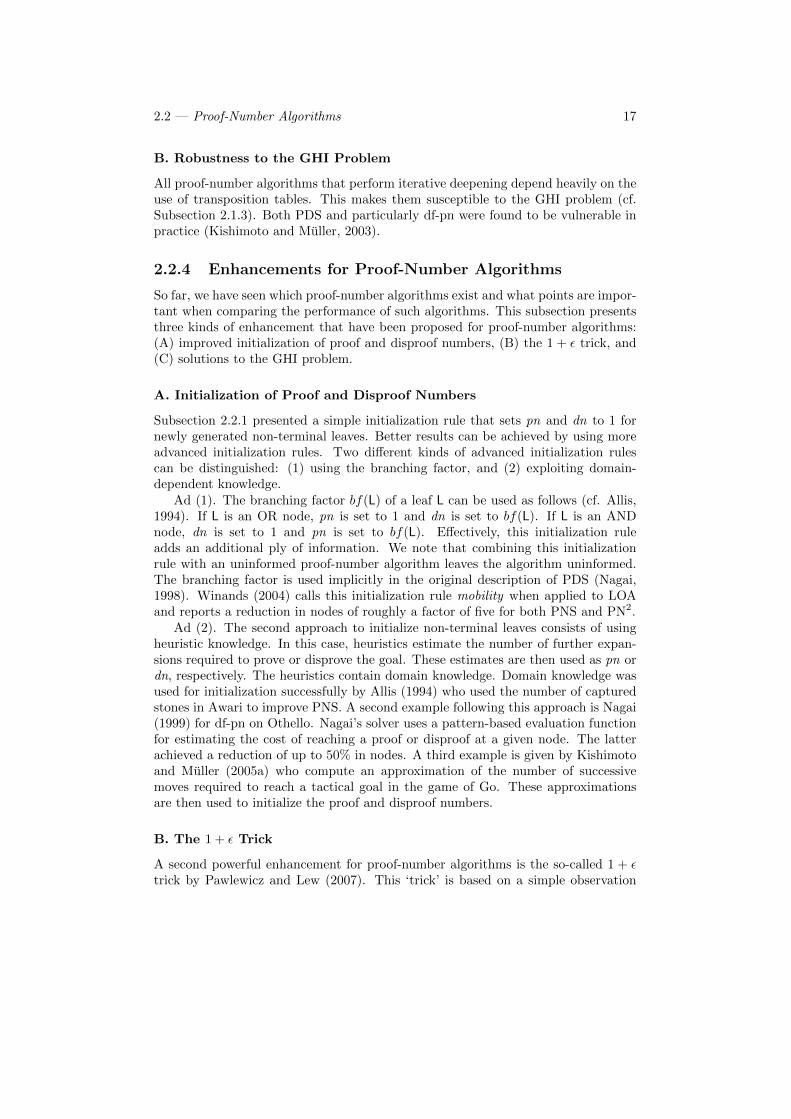
Subsection 2.2.1 presented a simple initialization rule that sets pn and dn to 1 fornewly generated non-terminal leaves. Better results can be achieved by using moreadvanced initialization rules. Two different kinds of advanced initialization rulescan be distinguished: (1) using the branching factor, and (2) exploiting domain-dependent knowledge.
Ad (1). The branching factor bf(L) of a leaf L can be used as follows (cf. Allis,1994). If L is an OR node, pn is set to 1 and dn is set to bf(L). If L is an ANDnode, dn is set to 1 and pn is set to bf(L). Effectively, this initialization ruleadds an additional ply of information. We note that combining this initializationrule with an uninformed proof-number algorithm leaves the algorithm uninformed.The branching factor is used implicitly in the original description of PDS (Nagai,1998). Winands (2004) calls this initialization rule mobility when applied to LOAand reports a reduction in nodes of roughly a factor of five for both PNS and PN2.
Ad (2). The second approach to initialize non-terminal leaves consists of usingheuristic knowledge. In this case, heuristics estimate the number of further expan-sions required to prove or disprove the goal. These estimates are then used as pn ordn, respectively. The heuristics contain domain knowledge. Domain knowledge wasused for initialization successfully by Allis (1994) who used the number of capturedstones in Awari to improve PNS. A second example following this approach is Nagai(1999) for df-pn on Othello. Nagai’s solver uses a pattern-based evaluation functionfor estimating the cost of reaching a proof or disproof at a given node. The latterachieved a reduction of up to 50% in nodes. A third example is given by Kishimotoand Muller (2005a) who compute an approximation of the number of successivemoves required to reach a tactical goal in the game of Go. These approximationsare then used to initialize the proof and disproof numbers.
B. The 1 + ε Trick
A second powerful enhancement for proof-number algorithms is the so-called 1 + εtrick by Pawlewicz and Lew (2007). This ‘trick’ is based on a simple observation
18 Basics of Game-Tree Search for Solvers
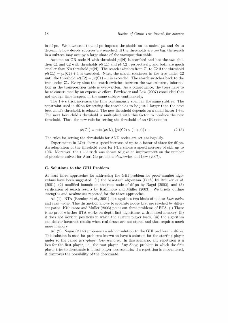
in df-pn. We have seen that df-pn imposes thresholds on its nodes’ pn and dn todetermine how deeply subtrees are searched. If the thresholds are too big, the searchin a subtree may occupy a large share of the transposition table.
Assume an OR node N with threshold pt(N) is searched and has the two chil-dren C1 and C2 with thresholds pt(C1) and pt(C2), respectively, and both are muchsmaller than N’s threshold pt(N). The search switches from C1 to C2 if the thresholdpt(C1) = pt(C2) + 1 is exceeded. Next, the search continues in the tree under C2until the threshold pt(C2) = pt(C1) + 1 is exceeded. The search switches back to thetree under C1. Every time the search switches between the two subtrees, informa-tion in the transposition table is overwritten. As a consequence, the trees have tobe re-constructed by an expensive effort. Pawlewicz and Lew (2007) concluded thatnot enough time is spent in the same subtree continuously.
The 1 + ε trick increases the time continuously spent in the same subtree. Theconstraint used in df-pn for setting the thresholds to be just 1 larger than the nextbest child’s threshold, is relaxed. The new threshold depends on a small factor 1+ ε.The next best child’s threshold is multiplied with this factor to produce the newthreshold. Thus, the new rule for setting the threshold of an OR node is:
pt(C1) = min(pt(N), dpt(C2)× (1 + ε)e) . (2.13)
The rules for setting the thresholds for AND nodes are set analogously.
Experiments in LOA show a speed increase of up to a factor of three for df-pn.An adaptation of the threshold rules for PDS shows a speed increase of still up to10%. Moreover, the 1 + ε trick was shown to give an improvement on the numberof problems solved for Atari Go problems Pawlewicz and Lew (2007).
C. Solutions to the GHI Problem
At least three approaches for addressing the GHI problem for proof-number algo-rithms have been suggested: (1) the base-twin algorithm (BTA) by Breuker et al.(2001), (2) modified bounds on the root node of df-pn by Nagai (2002), and (3)verification of search results by Kishimoto and Muller (2003). We briefly outlinestrengths and weaknesses reported for the three approaches.
Ad (1). BTA (Breuker et al., 2001) distinguishes two kinds of nodes: base nodesand twin nodes. This distinction allows to separate nodes that are reached by differ-ent paths. Kishimoto and Muller (2003) point out three problems of BTA. (i) Thereis no proof whether BTA works on depth-first algorithms with limited memory, (ii)it does not work in positions in which the current player loses, (iii) the algorithmcan deliver incorrect results when real draws are not stored and thus requires muchmore memory.
Ad (2). Nagai (2002) proposes an ad-hoc solution to the GHI problem in df-pn.This solution is used for problems known to have a solution for the starting playerunder so the called first-player loss scenario. In this scenario, any repetition is aloss for the first player, i.e., the root player. Any Shogi problem in which the firstplayer tries to checkmate is a first-player loss scenario: if a repetition is encountered,it disproves the possibility of the checkmate.
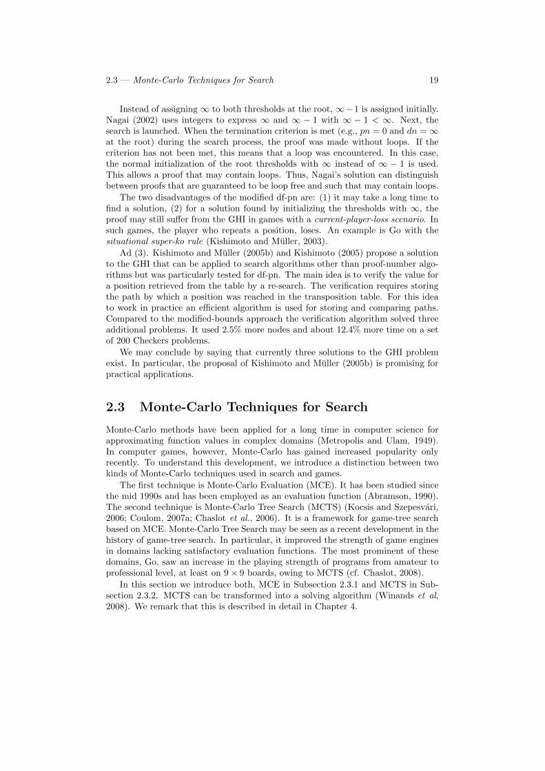
2.3 — Monte-Carlo Techniques for Search 19
Instead of assigning∞ to both thresholds at the root, ∞−1 is assigned initially.Nagai (2002) uses integers to express ∞ and ∞ − 1 with ∞ − 1 < ∞. Next, thesearch is launched. When the termination criterion is met (e.g., pn = 0 and dn =∞at the root) during the search process, the proof was made without loops. If thecriterion has not been met, this means that a loop was encountered. In this case,the normal initialization of the root thresholds with ∞ instead of ∞ − 1 is used.This allows a proof that may contain loops. Thus, Nagai’s solution can distinguishbetween proofs that are guaranteed to be loop free and such that may contain loops.
The two disadvantages of the modified df-pn are: (1) it may take a long time tofind a solution, (2) for a solution found by initializing the thresholds with ∞, theproof may still suffer from the GHI in games with a current-player-loss scenario. Insuch games, the player who repeats a position, loses. An example is Go with thesituational super-ko rule (Kishimoto and Muller, 2003).
Ad (3). Kishimoto and Muller (2005b) and Kishimoto (2005) propose a solutionto the GHI that can be applied to search algorithms other than proof-number algo-rithms but was particularly tested for df-pn. The main idea is to verify the value fora position retrieved from the table by a re-search. The verification requires storingthe path by which a position was reached in the transposition table. For this ideato work in practice an efficient algorithm is used for storing and comparing paths.Compared to the modified-bounds approach the verification algorithm solved threeadditional problems. It used 2.5% more nodes and about 12.4% more time on a setof 200 Checkers problems.
We may conclude by saying that currently three solutions to the GHI problemexist. In particular, the proposal of Kishimoto and Muller (2005b) is promising forpractical applications.
2.3 Monte-Carlo Techniques for Search
Monte-Carlo methods have been applied for a long time in computer science forapproximating function values in complex domains (Metropolis and Ulam, 1949).In computer games, however, Monte-Carlo has gained increased popularity onlyrecently. To understand this development, we introduce a distinction between twokinds of Monte-Carlo techniques used in search and games.
The first technique is Monte-Carlo Evaluation (MCE). It has been studied sincethe mid 1990s and has been employed as an evaluation function (Abramson, 1990).The second technique is Monte-Carlo Tree Search (MCTS) (Kocsis and Szepesvari,2006; Coulom, 2007a; Chaslot et al., 2006). It is a framework for game-tree searchbased on MCE. Monte-Carlo Tree Search may be seen as a recent development in thehistory of game-tree search. In particular, it improved the strength of game enginesin domains lacking satisfactory evaluation functions. The most prominent of thesedomains, Go, saw an increase in the playing strength of programs from amateur toprofessional level, at least on 9× 9 boards, owing to MCTS (cf. Chaslot, 2008).
In this section we introduce both, MCE in Subsection 2.3.1 and MCTS in Sub-section 2.3.2. MCTS can be transformed into a solving algorithm (Winands et al,2008). We remark that this is described in detail in Chapter 4.
20 Basics of Game-Tree Search for Solvers
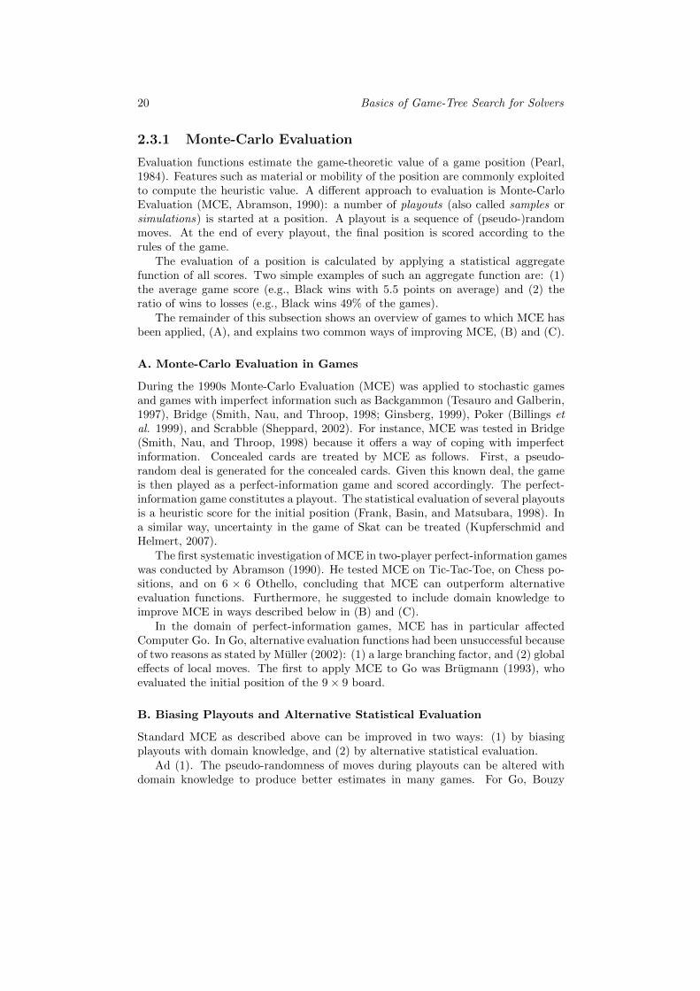
2.3.1 Monte-Carlo Evaluation
Evaluation functions estimate the game-theoretic value of a game position (Pearl,1984). Features such as material or mobility of the position are commonly exploitedto compute the heuristic value. A different approach to evaluation is Monte-CarloEvaluation (MCE, Abramson, 1990): a number of playouts (also called samples orsimulations) is started at a position. A playout is a sequence of (pseudo-)randommoves. At the end of every playout, the final position is scored according to therules of the game.
The evaluation of a position is calculated by applying a statistical aggregatefunction of all scores. Two simple examples of such an aggregate function are: (1)the average game score (e.g., Black wins with 5.5 points on average) and (2) theratio of wins to losses (e.g., Black wins 49% of the games).
The remainder of this subsection shows an overview of games to which MCE hasbeen applied, (A), and explains two common ways of improving MCE, (B) and (C).
A. Monte-Carlo Evaluation in Games
During the 1990s Monte-Carlo Evaluation (MCE) was applied to stochastic gamesand games with imperfect information such as Backgammon (Tesauro and Galberin,1997), Bridge (Smith, Nau, and Throop, 1998; Ginsberg, 1999), Poker (Billings etal. 1999), and Scrabble (Sheppard, 2002). For instance, MCE was tested in Bridge(Smith, Nau, and Throop, 1998) because it offers a way of coping with imperfectinformation. Concealed cards are treated by MCE as follows. First, a pseudo-random deal is generated for the concealed cards. Given this known deal, the gameis then played as a perfect-information game and scored accordingly. The perfect-information game constitutes a playout. The statistical evaluation of several playoutsis a heuristic score for the initial position (Frank, Basin, and Matsubara, 1998). Ina similar way, uncertainty in the game of Skat can be treated (Kupferschmid andHelmert, 2007).
The first systematic investigation of MCE in two-player perfect-information gameswas conducted by Abramson (1990). He tested MCE on Tic-Tac-Toe, on Chess po-sitions, and on 6 × 6 Othello, concluding that MCE can outperform alternativeevaluation functions. Furthermore, he suggested to include domain knowledge toimprove MCE in ways described below in (B) and (C).
In the domain of perfect-information games, MCE has in particular affectedComputer Go. In Go, alternative evaluation functions had been unsuccessful becauseof two reasons as stated by Muller (2002): (1) a large branching factor, and (2) globaleffects of local moves. The first to apply MCE to Go was Brugmann (1993), whoevaluated the initial position of the 9× 9 board.
B. Biasing Playouts and Alternative Statistical Evaluation
Standard MCE as described above can be improved in two ways: (1) by biasingplayouts with domain knowledge, and (2) by alternative statistical evaluation.
Ad (1). The pseudo-randomness of moves during playouts can be altered withdomain knowledge to produce better estimates in many games. For Go, Bouzy
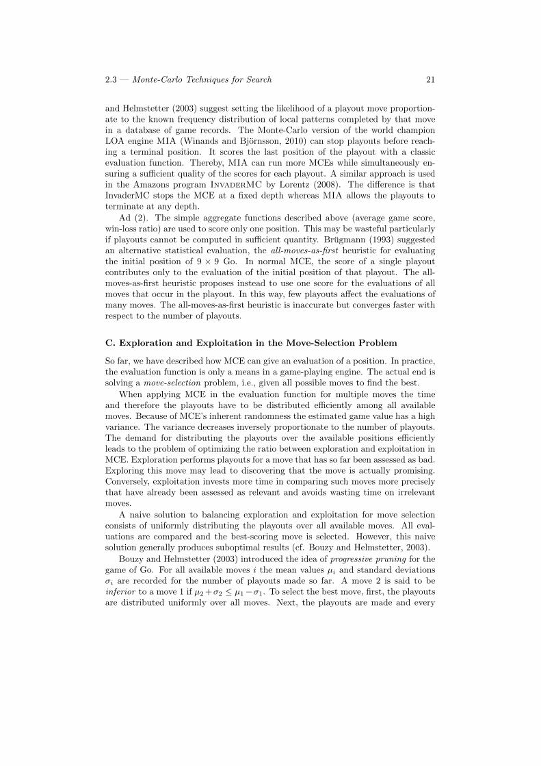
2.3 — Monte-Carlo Techniques for Search 21
and Helmstetter (2003) suggest setting the likelihood of a playout move proportion-ate to the known frequency distribution of local patterns completed by that movein a database of game records. The Monte-Carlo version of the world championLOA engine MIA (Winands and Bjornsson, 2010) can stop playouts before reach-ing a terminal position. It scores the last position of the playout with a classicevaluation function. Thereby, MIA can run more MCEs while simultaneously en-suring a sufficient quality of the scores for each playout. A similar approach is usedin the Amazons program InvaderMC by Lorentz (2008). The difference is thatInvaderMC stops the MCE at a fixed depth whereas MIA allows the playouts toterminate at any depth.
Ad (2). The simple aggregate functions described above (average game score,win-loss ratio) are used to score only one position. This may be wasteful particularlyif playouts cannot be computed in sufficient quantity. Brugmann (1993) suggestedan alternative statistical evaluation, the all-moves-as-first heuristic for evaluatingthe initial position of 9 × 9 Go. In normal MCE, the score of a single playoutcontributes only to the evaluation of the initial position of that playout. The all-moves-as-first heuristic proposes instead to use one score for the evaluations of allmoves that occur in the playout. In this way, few playouts affect the evaluations ofmany moves. The all-moves-as-first heuristic is inaccurate but converges faster withrespect to the number of playouts.
C. Exploration and Exploitation in the Move-Selection Problem
So far, we have described how MCE can give an evaluation of a position. In practice,the evaluation function is only a means in a game-playing engine. The actual end issolving a move-selection problem, i.e., given all possible moves to find the best.
When applying MCE in the evaluation function for multiple moves the timeand therefore the playouts have to be distributed efficiently among all availablemoves. Because of MCE’s inherent randomness the estimated game value has a highvariance. The variance decreases inversely proportionate to the number of playouts.The demand for distributing the playouts over the available positions efficientlyleads to the problem of optimizing the ratio between exploration and exploitation inMCE. Exploration performs playouts for a move that has so far been assessed as bad.Exploring this move may lead to discovering that the move is actually promising.Conversely, exploitation invests more time in comparing such moves more preciselythat have already been assessed as relevant and avoids wasting time on irrelevantmoves.
A naive solution to balancing exploration and exploitation for move selectionconsists of uniformly distributing the playouts over all available moves. All eval-uations are compared and the best-scoring move is selected. However, this naivesolution generally produces suboptimal results (cf. Bouzy and Helmstetter, 2003).
Bouzy and Helmstetter (2003) introduced the idea of progressive pruning for thegame of Go. For all available moves i the mean values µi and standard deviationsσi are recorded for the number of playouts made so far. A move 2 is said to beinferior to a move 1 if µ2 +σ2 ≤ µ1−σ1. To select the best move, first, the playoutsare distributed uniformly over all moves. Next, the playouts are made and every
22 Basics of Game-Tree Search for Solvers
move is evaluated. Then, all moves inferior to some other move are eliminated. Theprocedure is iterated with the remaining moves. In this manner, promising movesare sampled more frequently than initially less promising candidates.
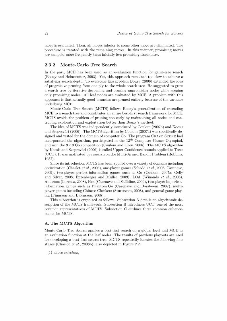
2.3.2 Monte-Carlo Tree Search
In the past, MCE has been used as an evaluation function for game-tree search(Bouzy and Helmstetter, 2003). Yet, this approach remained too slow to achieve asatisfying search depth. To overcome this problem Bouzy (2006) extended the ideaof progressive pruning from one ply to the whole search tree. He suggested to growa search tree by iterative deepening and pruning unpromising nodes while keepingonly promising nodes. All leaf nodes are evaluated by MCE. A problem with thisapproach is that actually good branches are pruned entirely because of the varianceunderlying MCE.
Monte-Carlo Tree Search (MCTS) follows Bouzy’s generalization of extendingMCE to a search tree and constitutes an entire best-first search framework for MCE.MCTS avoids the problem of pruning too early by maintaining all nodes and con-trolling exploration and exploitation better than Bouzy’s method.
The idea of MCTS was independently introduced by Coulom (2007a) and Kocsisand Szepesvari (2006). The MCTS algorithm by Coulom (2007a) was specifically de-signed and tested for the domain of computer Go. The program Crazy Stone hadincorporated the algorithm, participated in the 12th Computer Games Olympiad,and won the 9×9 Go competition (Coulom and Chen, 2006). The MCTS algorithmby Kocsis and Szepesvari (2006) is called Upper Confidence bounds applied to Trees(UCT). It was motivated by research on the Multi-Armed Bandit Problem (Robbins,1952).
Since its introduction MCTS has been applied over a variety of domains includingoptimization (Chaslot et al., 2006), one-player games (Schadd et al., 2008; Cazenave,2009), two-player perfect-information games such as Go (Coulom, 2007a; Gellyand Silver, 2008; Enzenberger and Muller, 2009), LOA (Winands et al., 2008),Amazons (Lorentz, 2008), Hex (Cazenave and Saffidine, 2009), two-player imperfect-information games such as Phantom Go (Cazenave and Borsboom, 2007), multi-player games including Chinese Checkers (Sturtevant, 2008), and general game play-ing (Finnsson and Bjornsson, 2008).
This subsection is organized as follows. Subsection A details an algorithmic de-scription of the MCTS framework. Subsection B introduces UCT, one of the mostcommon representatives of MCTS. Subsection C outlines three common enhance-ments for MCTS.
A. The MCTS Algorithm
Monte-Carlo Tree Search applies a best-first search on a global level and MCE asan evaluation function at the leaf nodes. The results of previous playouts are usedfor developing a best-first search tree. MCTS repeatedly iterates the following fourstages (Chaslot et al., 2008b), also depicted in Figure 2.2:
(1) move selection,
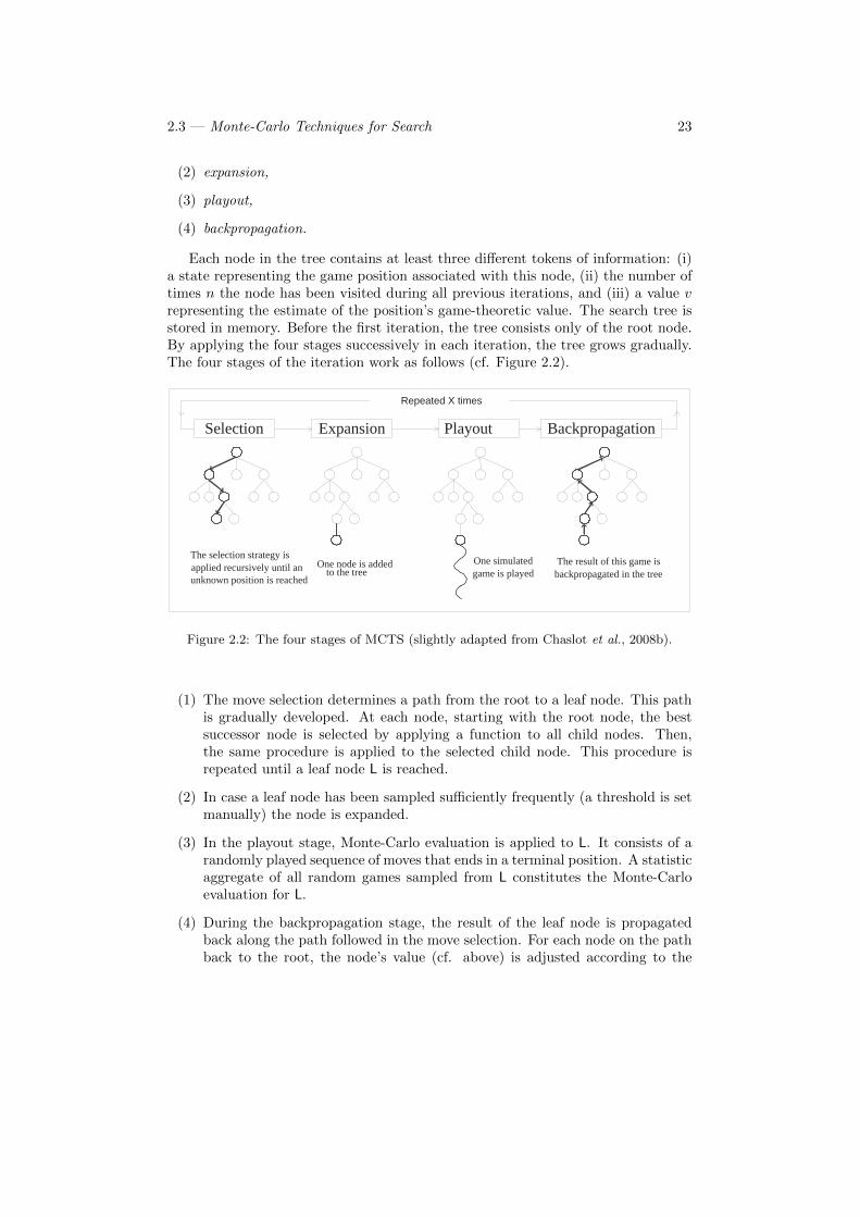
2.3 — Monte-Carlo Techniques for Search 23
(2) expansion,
(3) playout,
(4) backpropagation.
Each node in the tree contains at least three different tokens of information: (i)a state representing the game position associated with this node, (ii) the number oftimes n the node has been visited during all previous iterations, and (iii) a value vrepresenting the estimate of the position’s game-theoretic value. The search tree isstored in memory. Before the first iteration, the tree consists only of the root node.By applying the four stages successively in each iteration, the tree grows gradually.The four stages of the iteration work as follows (cf. Figure 2.2).
Figure 1: (a) The initial position. (b) An example of possible moves. (c) Aterminal position.
Selection Expension Playout Backpropagation
The selection strategy is applied recursively until a
position not part of the tree
is reached One node is added to the tree
The result of this game is backpropagated in the tree
One simulated game is played
Selection Expansion Playout Backpropagation
The selection strategy is applied recursively until an unknown position is reached
One node is added to the tree
The result of this game is backpropagated in the tree
One simulated game is played
Repeated X times
Figure 2: White to move.
1
Figure 2.2: The four stages of MCTS (slightly adapted from Chaslot et al., 2008b).
(1) The move selection determines a path from the root to a leaf node. This pathis gradually developed. At each node, starting with the root node, the bestsuccessor node is selected by applying a function to all child nodes. Then,the same procedure is applied to the selected child node. This procedure isrepeated until a leaf node L is reached.
(2) In case a leaf node has been sampled sufficiently frequently (a threshold is setmanually) the node is expanded.
(3) In the playout stage, Monte-Carlo evaluation is applied to L. It consists of arandomly played sequence of moves that ends in a terminal position. A statisticaggregate of all random games sampled from L constitutes the Monte-Carloevaluation for L.
(4) During the backpropagation stage, the result of the leaf node is propagatedback along the path followed in the move selection. For each node on the pathback to the root, the node’s value (cf. above) is adjusted according to the
24 Basics of Game-Tree Search for Solvers
update function.2 After the root node has been updated, this stage and theiteration are completed. As a consequence of altering the values of the nodeson the path, the move selection of the next iteration is influenced.
The various MCTS algorithms proposed in the literature differ with regard totheir move selection and schemes used for expansions. Next, a specific move selectioncalled UCT is briefly described.
B. UCT
The most influential representative of MCTS has so far been Upper Confidencebounds applied to Trees (UCT). In UCT, Kocsis and Szepesvari (2006) apply solu-tions for the Multi-Armed Bandit Problem (MAB) (Robbins, 1952) to tree search.This problem is structurally similar to move selection and the task of efficiently dis-tributing actions over several slot machines to maximize the expected return. Thedistributions underlying the returns are unknown and have to be approximated.Auer, Cesa-Bianchi, and Fischer (2002) suggested to use a formula called UpperConfidence Bounds (UCB) to cope with the MAB. This UCB formula is the basisfor UCT. The move selection of UCT is as follows. Given a node with children,the move-selection function of UCT chooses the child which maximizes the followingformula:
Let I be the set of nodes immediately reachable from the current node p. Theselection strategy selects the k-th child of the node p that satisfies Formula 2.14:
k ∈ argmaxi∈I(vi +
√C × lnnp
ni
), (2.14)
where vi is the value of the node i, ni is the visit count of i, and np is the visitcount of node p. The coefficient C determines the balance between exploitation andrequires tuning experimentally. The update function used in UCT sets the value niof a node to the average of all the children’s values.
C. MCTS Enhancements
In this subsection we describe three common enhancements to MCTS: (1) RAVE,(2) integrating domain knowledge in MCTS, and (3) parallelization.
Ad (1). Gelly and Silver (2008) suggested Rapid Action Value Estimation (RAVE)which is closely related to the all-moves-as-first heuristic by Brugmann (1993) (cf.Subsection 2.3.1.B). RAVE achieves an advantage by using all-moves-as-first val-ues to bias the UCT value of a move. Compared to UCT values (Formula 2.14),all-moves-as-first values have smaller variance and converge faster. Therefore theall-moves-as-first values are used to bias the move selection only in the beginning.When sufficiently many playouts have been sampled and the UCT values are ex-pected to be sufficiently precise, the effect of the RAVE value diminishes. The speedof fading out is subject to parameter tuning. Gelly and Silver (2008) have shownthat RAVE can improve the playing strength of a Go engine substantially.
2Coulom (2007a) refers to the update function as backpropagation operator.
2.4 — Chapter Summary 25
Ad (2). We have seen that domain knowledge may improve the quality of play-outs in MCE (cf. Subsection 2.3.1.B). Domain knowledge can also be applied out-side of the playout stage in MCTS. There are at least three approaches of achievingthis. The first approach modifies the move selection. Gelly and Silver (2008) andChaslot et al. (2008b) suggest adding a summand to the right-hand side of the origi-nal UCT formula (Formula 2.14). The additional summand represents a value basedon small patterns and thus representing domain knowledge. A second approach isprogressive unpruning (Chaslot et al., 2008b) which first reduces and then increasesthe branching factor of an MCTS node based on domain knowledge. A similar ap-proach is referred to as progressive widening by Coulom (2007b). A third approachconsists of using move categories based on domain knowledge in order to group moves(Saito et al., 2007b).
Ad (3). MCE and MCTS are suitable for parallelization because the playoutscan be computed as independent parallel tasks. A difficulty lies in parallelizing theoperations on the MCTS tree. Several methods have been suggested for paralleliza-tion. Building up on Cazenave and Jouandeau (2007) who had suggested threesimple ways of parallelizing UCT, (Chaslot et al., 2008a) compared the followingfour methods for parallelization: (i) leaf parallelization executes multiple MCEs atthe same leaf in parallel; (ii) root parallelization runs multiple independent instancesof MCTS and merges the results of the root into one value when the search termi-nates; (iii) tree parallelization with global mutex maintains one lock on the wholesearch tree such that each of several threads locks the whole tree when updatingdata; (iv) tree parallelization with local mutexes allows each thread accessing dif-ferent parts of the subtree. Based on experiments for 9 × 9 Go, it was found thatthe simple root parallelization produced the best results (Cazenave and Jouandeau,2007; Chaslot, Winands, and Van den Herik, 2008a). More recently, Enzenbergerand Muller (2010) documented the parallelization of Fuego, the 2009 ComputerOlympiad’s gold medalist program in the 9 × 9 Go competition. It uses a lock-lessimplementation of the local mutex parallelization. This implementation producesinaccurate updates at minor rates. Although playouts are discarded because of theimprecision, the locking scales well for up to seven processors.
2.4 Chapter Summary
In this chapter we introduced basic definitions for describing game-tree search andfundamental concepts including three search methods. The elementary concepts thenserved to outline six proof-number algorithms and two Monte-Carlo techniques. Thefollowing chapters will introduce novel algorithms based on the algorithms that havebeen presented here.
In Chapter 3 we show how MCE can be combined with Proof-Number Searchfor solving Go problems. Chapter 4 describes an approach that utilizes MCTS forsolving and also introduces a parallel version of this approach.

26 Basics of Game-Tree Search for Solvers
Chapter 3
Monte-Carlo Proof-NumberSearch
This chapter is based on the following publications.1
1. J-T. Saito, G.M.J.B. Chaslot, J.W.H.M. Uiterwijk, and H.J. van den Herik. Monte-Carlo Proof-Number Search. In H.J. van den Herik, P. Ciancarini, and H.H.L.M.Donkers, editors, Computers and Games - 5th International Conference (CG ‘06),volume 4630 of Lecture Notes in Computer Science, pp. 50–61. Springer, Berlin,Germany, 2007.
2. J-T. Saito, G.M.J.B. Chaslot, J.W.H.M. Uiterwijk, and H.J. van den Herik. PatternKnowledge for Proof-Number Search in Computer Go. In P.Y. Schobbens, W. Van-hoof, and G. Schwanen, editors, Proceedings of the 18th BeNeLux Conference onArtificial Intelligence (BNAIC‘06), pp. 275–281, 2006.
3. J-T. Saito, G.M.J.B. Chaslot, J.W.H.M. Uiterwijk, H.J. van den Herik, and M.H.M.Winands. Developments in Monte-Carlo Proof-Number Search. In H. Matsubara,T. Ito, and T. Nakamura, editors, Proceedings of the 11th Game Programming Work-shop, pp. 27–31. Information Processing Society of Japan, Tokyo, Japan, 2006.
The overview on solving algorithms given in Chapter 2 divides Monte-Carlomethods for game-tree search in two kinds: (1) Monte-Carlo evaluation, and (2)Monte-Carlo Tree Search. So far, little attention has been paid to the potentiallybeneficial effect of applying Monte-Carlo methods to solvers such as Proof-NumberSearch (PNS) (Allis et al., 1994). In this chapter, we answer the first research ques-tion, RQ 1, by investigating how Monte-Carlo evaluation can be used for solvinggame positions. We propose integrating Monte-Carlo evaluation with Proof-NumberSearch to form a new solving algorithm. We call the new algorithm Monte-CarloProof-Number Search (MC-PNS).
1 The author is grateful to Springer-Verlag and the Information Processing Society of Japan forthe permission to reuse relevant parts of the articles.
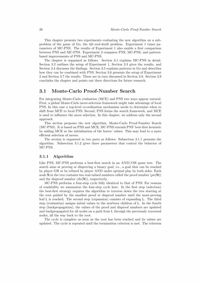
28 Monte-Carlo Proof-Number Search
This chapter presents two experiments evaluating the new algorithm on a sub-problem of the game of Go, the life-and-death problem. Experiment 1 tunes pa-rameters of MC-PNS. The results of Experiment 1 also enable a first comparisonbetween PNS and MC-PNS. Experiment 2 compares PNS, MC-PNS, and pattern-based improvements of PNS and MC-PNS.
The chapter is organized as follows. Section 3.1 explains MC-PNS in detail.Section 3.2 outlines the setup of Experiment 1, Section 3.3 gives the results, andSection 3.4 discusses the findings. Section 3.5 explains patterns in Go and describeshow they can be combined with PNS. Section 3.6 presents the setup of Experiment2 and Section 3.7 the results. These are in turn discussed in Section 3.8. Section 3.9concludes the chapter and points out three directions for future research.
3.1 Monte-Carlo Proof-Number Search
For integrating Monte-Carlo evaluation (MCE) and PNS two ways appear natural.First, a global Monte-Carlo move-selection framework might take advantage of localPNS. In this case a top-level co-ordination mechanism needs to determine when toshift from MCE to local PNS. Second, PNS forms the search framework, and MCEis used to influence the move selection. In this chapter, we address only the secondapproach.
This section proposes the new algorithm, Monte-Carlo Proof-Number Search(MC-PNS). It is based on PNS and MCE. MC-PNS extends PNS’ best-first heuristicby adding MCE at the initialization of the leaves’ values. This may lead to a moreefficient selection of moves.
The section is organized in two parts as follows: Subsection 3.1.1 presents thealgorithm. Subsection 3.1.2 gives three parameters that control the behavior ofMC-PNS.
3.1.1 Algorithm
Like PNS, MC-PNS performs a best-first search in an AND/OR game tree. Thesearch aims at proving or disproving a binary goal, i.e., a goal that can be reachedby player OR or be refuted by player AND under optimal play by both sides. Eachnode N in the tree contains two real-valued numbers called the proof number (pn(N))and the disproof number (dn(N)), respectively.
MC-PNS performs a four-step cycle fully identical to that of PNS. For reasonsof readability we summarize the four-step cycle here. In the first step (selection)the best-first strategy requires the algorithm to traverse down the tree starting atthe root guided by the smallest proof or disproof number until the most-provingleaf L is reached. The second step (expansion) consists of expanding L. The thirdstep (evaluation) assigns initial values to the newborn children of L. In the fourthstep (backpropagation), the values of the proof and disproof numbers are updatedand backpropagated for all nodes on a path from L through the previously traversednodes, all the way back to the root.
The cycle is complete as soon as the root has been reached and its values areupdated. The cycle is repeated until the termination criterion is met. The criterion
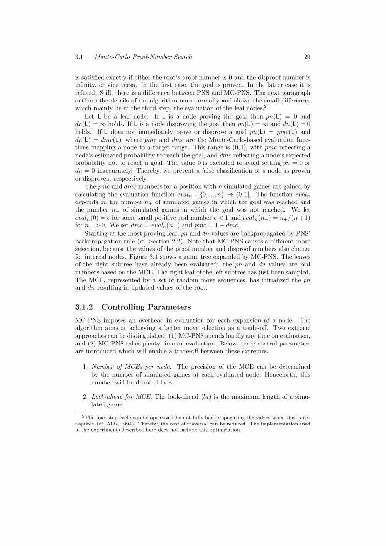
3.1 — Monte-Carlo Proof-Number Search 29
is satisfied exactly if either the root’s proof number is 0 and the disproof number isinfinity, or vice versa. In the first case, the goal is proven. In the latter case it isrefuted. Still, there is a difference between PNS and MC-PNS. The next paragraphoutlines the details of the algorithm more formally and shows the small differenceswhich mainly lie in the third step, the evaluation of the leaf nodes.2
Let L be a leaf node. If L is a node proving the goal then pn(L) = 0 anddn(L) =∞ holds. If L is a node disproving the goal then pn(L) =∞ and dn(L) = 0holds. If L does not immediately prove or disprove a goal pn(L) = pmc(L) anddn(L) = dmc(L), where pmc and dmc are the Monte-Carlo-based evaluation func-tions mapping a node to a target range. This range is (0, 1], with pmc reflecting anode’s estimated probability to reach the goal, and dmc reflecting a node’s expectedprobability not to reach a goal. The value 0 is excluded to avoid setting pn = 0 ordn = 0 inaccurately. Thereby, we prevent a false classification of a node as provenor disproven, respectively.
The pmc and dmc numbers for a position with n simulated games are gained bycalculating the evaluation function evaln : {0, ..., n} → (0, 1]. The function evalndepends on the number n+ of simulated games in which the goal was reached andthe number n− of simulated games in which the goal was not reached. We letevaln(0) = ε for some small positive real number ε < 1 and evaln(n+) = n+/(n+ 1)for n+ > 0. We set dmc = evaln(n+) and pmc = 1− dmc.
Starting at the most-proving leaf, pn and dn values are backpropagated by PNS’backpropagation rule (cf. Section 2.2). Note that MC-PNS causes a different moveselection, because the values of the proof number and disproof numbers also changefor internal nodes. Figure 3.1 shows a game tree expanded by MC-PNS. The leavesof the right subtree have already been evaluated: the pn and dn values are realnumbers based on the MCE. The right leaf of the left subtree has just been sampled.The MCE, represented by a set of random move sequences, has initialized the pnand dn resulting in updated values of the root.
3.1.2 Controlling Parameters
MC-PNS imposes an overhead in evaluation for each expansion of a node. Thealgorithm aims at achieving a better move selection as a trade-off. Two extremeapproaches can be distinguished: (1) MC-PNS spends hardly any time on evaluation,and (2) MC-PNS takes plenty time on evaluation. Below, three control parametersare introduced which will enable a trade-off between these extremes.
1. Number of MCEs per node. The precision of the MCE can be determinedby the number of simulated games at each evaluated node. Henceforth, thisnumber will be denoted by n.
2. Look-ahead for MCE. The look-ahead (la) is the maximum length of a simu-lated game.
2The four-step cycle can be optimized by not fully backpropagating the values when this is notrequired (cf. Allis, 1994). Thereby, the cost of traversal can be reduced. The implementation usedin the experiments described here does not include this optimization.
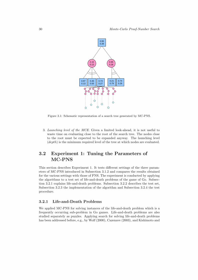
30 Monte-Carlo Proof-Number Search
0.950.39
0.950.26
2.150.13
0.740.26
0.210.79
0.970.13
0.730.27
0.450.55
Figure 3.1: Schematic representation of a search tree generated by MC-PNS.
3. Launching level of the MCE. Given a limited look-ahead, it is not useful towaste time on evaluating close to the root of the search tree. The nodes closeto the root must be expected to be expanded anyway. The launching level(depth) is the minimum required level of the tree at which nodes are evaluated.
3.2 Experiment 1: Tuning the Parameters ofMC-PNS
This section describes Experiment 1. It tests different settings of the three param-eters of MC-PNS introduced in Subsection 3.1.2 and compares the results obtainedfor the various settings with those of PNS. The experiment is conducted by applyingthe algorithms to a test set of life-and-death problems of the game of Go. Subsec-tion 3.2.1 explains life-and-death problems. Subsection 3.2.2 describes the test set,Subsection 3.2.3 the implementation of the algorithm and Subsection 3.2.4 the testprocedure.
3.2.1 Life-and-Death Problems
We applied MC-PNS for solving instances of the life-and-death problem which is afrequently occurring sub-problem in Go games. Life-and-death problems are alsostudied separately as puzzles. Applying search for solving life-and-death problemshas been addressed before, e.g., by Wolf (2000), Cazenave (2003), and Kishimoto and
3.2 — Experiment 1: Tuning the Parameters of MC-PNS 31
Figure 3.2: Example of a life-and-death problem.
Muller (2005a). The general life-and-death problem consists of a locally boundedgame position with a target group of stones. Black moves first and has to determinethe group’s status as either alive, dead, ko, or seki. For the current investigation,however, the problem is reduced to a binary classification of the target group toeither alive or dead.
In order to fit the algorithm to the Go domain, the goal to prove, i.e., the statusof a group of stones as either alive or dead, is checked by a simple status-detectionfunction. This function is called by each simulated move to determine whether toplay further or to stop. Each simulated game halts after either the goal has beenmet or a certain pre-set depth has been reached.
Figure 3.2 depicts a life-and-death problem from the test set used in Experi-ments 1 and 2. Player Black is to move and tries to capture the white group. Theintersections marked by circles are taken into consideration as starting moves.
3.2.2 Test Set
The test set consists of 30 life-and-death problems. The problems are of beginnerand intermediate level (10 Kyu to 1 Dan) and taken from a set publicly availableat GoBase.3 All test problems are a win for Black. The test cases were annotatedwith marks for playable intersections and marks for the groups subject to the life-and-death classification. The number of intersections I becoming playable duringsearch is determined by the initial empty intersections and by intersections which areinitially occupied but become playable because the occupying stones are captured.For the test cases this indicator I of search space varied from 8 to 20. The factorialof I gives a rough lower bound for the number of nodes in the fully expanded searchtree. Thereby, it provides an estimate for the size of the search space.
3Gobase, www.gobase.org.
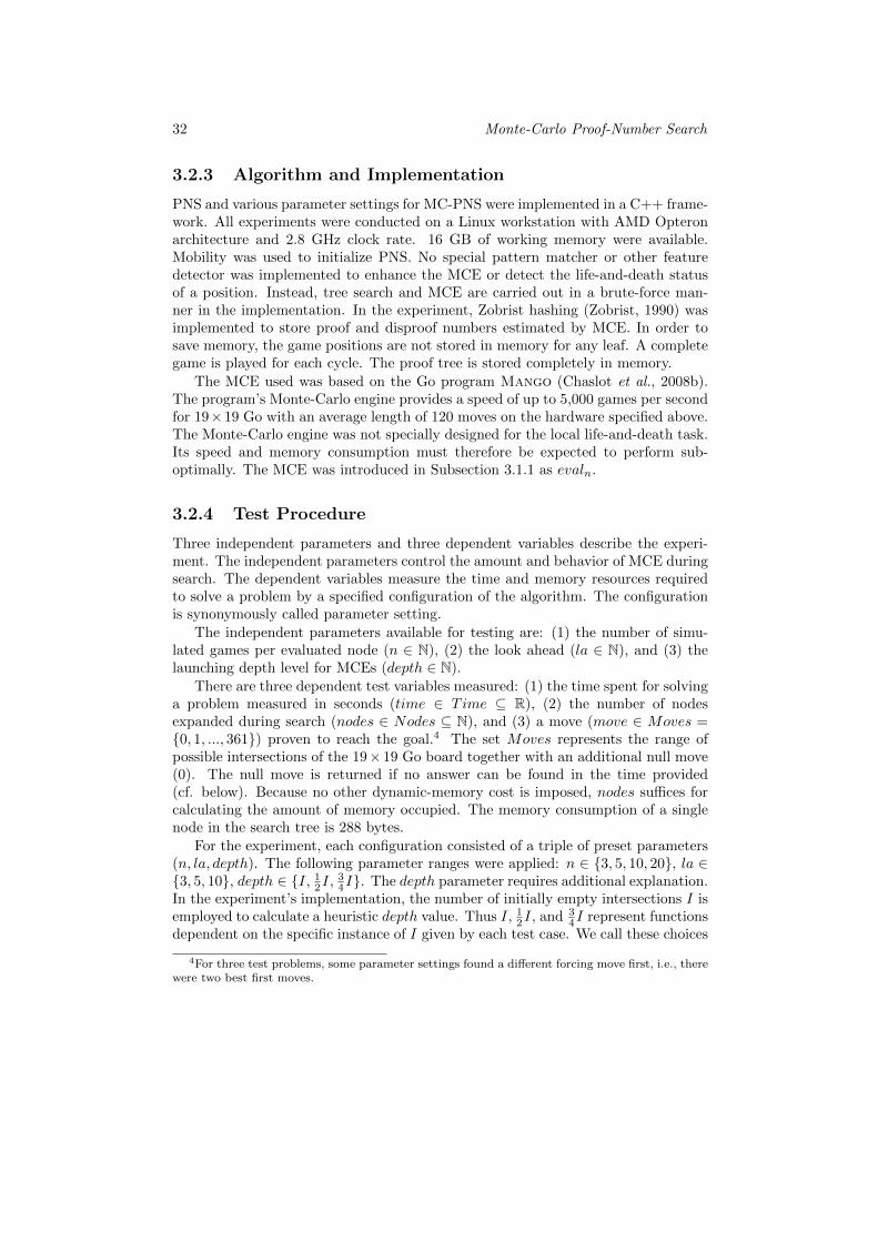
32 Monte-Carlo Proof-Number Search
3.2.3 Algorithm and Implementation
PNS and various parameter settings for MC-PNS were implemented in a C++ frame-work. All experiments were conducted on a Linux workstation with AMD Opteronarchitecture and 2.8 GHz clock rate. 16 GB of working memory were available.Mobility was used to initialize PNS. No special pattern matcher or other featuredetector was implemented to enhance the MCE or detect the life-and-death statusof a position. Instead, tree search and MCE are carried out in a brute-force man-ner in the implementation. In the experiment, Zobrist hashing (Zobrist, 1990) wasimplemented to store proof and disproof numbers estimated by MCE. In order tosave memory, the game positions are not stored in memory for any leaf. A completegame is played for each cycle. The proof tree is stored completely in memory.
The MCE used was based on the Go program Mango (Chaslot et al., 2008b).The program’s Monte-Carlo engine provides a speed of up to 5,000 games per secondfor 19×19 Go with an average length of 120 moves on the hardware specified above.The Monte-Carlo engine was not specially designed for the local life-and-death task.Its speed and memory consumption must therefore be expected to perform sub-optimally. The MCE was introduced in Subsection 3.1.1 as evaln.
3.2.4 Test Procedure
Three independent parameters and three dependent variables describe the experi-ment. The independent parameters control the amount and behavior of MCE duringsearch. The dependent variables measure the time and memory resources requiredto solve a problem by a specified configuration of the algorithm. The configurationis synonymously called parameter setting.
The independent parameters available for testing are: (1) the number of simu-lated games per evaluated node (n ∈ N), (2) the look ahead (la ∈ N), and (3) thelaunching depth level for MCEs (depth ∈ N).
There are three dependent test variables measured: (1) the time spent for solvinga problem measured in seconds (time ∈ Time ⊆ R), (2) the number of nodesexpanded during search (nodes ∈ Nodes ⊆ N), and (3) a move (move ∈ Moves ={0, 1, ..., 361}) proven to reach the goal.4 The set Moves represents the range ofpossible intersections of the 19× 19 Go board together with an additional null move(0). The null move is returned if no answer can be found in the time provided(cf. below). Because no other dynamic-memory cost is imposed, nodes suffices forcalculating the amount of memory occupied. The memory consumption of a singlenode in the search tree is 288 bytes.
For the experiment, each configuration consisted of a triple of preset parameters(n, la, depth). The following parameter ranges were applied: n ∈ {3, 5, 10, 20}, la ∈{3, 5, 10}, depth ∈ {I, 12I, 34I}. The depth parameter requires additional explanation.In the experiment’s implementation, the number of initially empty intersections I isemployed to calculate a heuristic depth value. Thus I, 12I, and 3
4I represent functionsdependent on the specific instance of I given by each test case. We call these choices
4For three test problems, some parameter settings found a different forcing move first, i.e., therewere two best first moves.
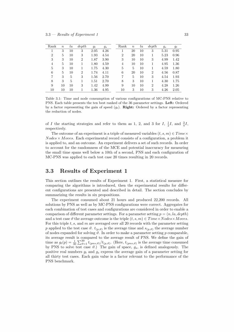
3.3 — Results of Experiment 1 33
Rank n la depth gt gs1 3 10 3 2.05 4.262 5 10 3 1.93 4.543 3 10 2 1.87 3.904 5 10 1 1.80 4.595 3 10 1 1.75 4.306 5 10 2 1.74 4.117 3 5 3 1.56 2.708 3 5 1 1.51 2.709 10 10 3 1.42 4.9910 10 10 1 1.36 4.95
Rank n la depth gs gt1 20 10 3 5.31 0.952 20 10 1 5.23 0.963 10 10 3 4.99 1.424 10 10 1 4.95 1.365 5 10 1 4.59 1.806 20 10 2 4.56 0.877 5 10 3 4.54 1.938 3 10 1 4.30 1.759 10 10 2 4.28 1.2610 3 10 3 4.26 2.05
Table 3.1: Time and node consumption of various configurations of MC-PNS relative toPNS. Each table presents the ten best ranked of the 36 parameter settings. Left: Orderedby a factor representing the gain of speed (gt). Right: Ordered by a factor representingthe reduction of nodes.
of I the starting strategies and refer to them as 1, 2, and 3 for I, 12I, and 3
4I,respectively.
The outcome of an experiment is a triple of measured variables (t, s,m) ∈ Time×Nodes×Moves. Each experimental record consists of a configuration, a problem itis applied to, and an outcome. An experiment delivers a set of such records. In orderto account for the randomness of the MCE and potential inaccuracy for measuringthe small time spans well below a 10th of a second, PNS and each configuration ofMC-PNS was applied to each test case 20 times resulting in 20 records.
3.3 Results of Experiment 1
This section outlines the results of Experiment 1. First, a statistical measure forcomparing the algorithms is introduced, then the experimental results for differ-ent configurations are presented and described in detail. The section concludes bysummarizing the results in six propositions.
The experiment consumed about 21 hours and produced 22,200 records. Allsolutions by PNS as well as by MC-PNS configurations were correct. Aggregates foreach combination of test cases and configurations are considered in order to enable acomparison of different parameter settings. For a parameter setting p = (n, la, depth)and a test case ϑ the average outcome is the triple (t, s,m) ∈ Time×Nodes×Moves.For this triple t, s, and m are averaged over all 20 records with the parameter settingp applied to the test case ϑ. t(p,ϑ) is the average time and s(p,ϑ) the average numberof nodes expanded for solving ϑ. In order to make a parameter setting p comparable,its average result is compared to the average result of PNS. We define the gain oftime as gt(p) = 1
30
∑30ϑ=1 t(pns,ϑ)/t(p,ϑ). (Here, t(pns,ϑ) is the average time consumed
by PNS to solve test case ϑ.) The gain of space, gs, is defined analogously. Thepositive real numbers gt and gs express the average gain of a parameter setting forall thirty test cases. Each gain value is a factor relevant to the performance of thePNS benchmark.
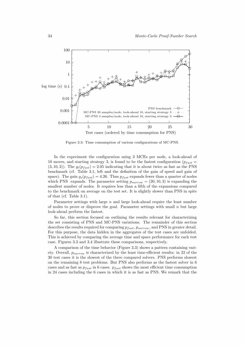
34 Monte-Carlo Proof-Number Search
0.0001
0.001
0.01
0.1
1
10
100
5 10 15 20 25 30
log time (s)
Test cases (ordered by time consumption for PNS)
PNS benchmark
33
333
33333
33
3333
3333333
333
33
33
3MC-PNS 20 samples/node, look-ahead 10, starting strategy 3
++
++
++ +
++
+ + ++
++
+
++ +
+ + ++ + + +
++ +
+
+MC-PNS 3 samples/node, look-ahead 10, starting strategy 3
2 2
2 2 22 2
2
22 2 2
2 2 2 2
2
2 22 2 2
2 2 2 2
22 2
2
2
Figure 3.3: Time consumption of various configurations of MC-PNS.
In the experiment the configuration using 3 MCEs per node, a look-ahead of10 moves, and starting strategy 3, is found to be the fastest configuration (pfast =(3, 10, 3)). The gt(pfast) = 2.05 indicating that it is about twice as fast as the PNSbenchmark (cf. Table 3.1, left and the definition of the gain of speed and gain ofspace). The gain gs(pfast) = 4.26. Thus pfast expands fewer than a quarter of nodeswhich PNS expands. The parameter setting pnarrow = (20, 10, 3) is expanding thesmallest number of nodes. It requires less than a fifth of the expansions comparedto the benchmark on average on the test set. It is slightly slower than PNS in spiteof that (cf. Table 3.1).
Parameter settings with large n and large look-ahead require the least numberof nodes to prove or disprove the goal. Parameter settings with small n but largelook-ahead perform the fastest.
So far, this section focused on outlining the results relevant for characterizingthe set consisting of PNS and MC-PNS variations. The remainder of this sectiondescribes the results required for comparing pfast, pnarrow, and PNS in greater detail.For this purpose, the data hidden in the aggregates of the test cases are unfolded.This is achieved by comparing the average time and space performance for each testcase. Figures 3.3 and 3.4 illustrate these comparisons, respectively.
A comparison of the time behavior (Figure 3.3) shows a pattern containing vari-ety. Overall, pnarrow is characterized by the least time-efficient results: in 22 of the30 test cases it is the slowest of the three compared solvers. PNS performs sloweston the remaining 8 test problems. But PNS also performs as the fastest solver in 6cases and as fast as pfast in 6 cases. pfast shows the most efficient time consumptionin 24 cases including the 6 cases in which it is as fast as PNS. We remark that the
3.4 — Discussion of Experiment 1 35
two leftmost points which are plotted to require 0.0001 seconds actually have value 0because they were measured beyond the precision of the time measurement function.It is reasonable to assume that the values should be ca. 0.001 seconds.
A comparison of the space behavior (Figure 3.4) shows that PNS requires thehighest number of node expansions to prove or disprove a goal, irrespective of thetest case. Its memory requirements are roughly the same as those of pfast andpnarrow except for two test cases. PNS requires much more space than the twoMC-PNS variations on virtually all other test cases. pfast and pnarrow show a similarbehavior in memory consumption with pnarrow performing slightly more efficient.
The results show that the performance depends on the complexity inherent to thetested problem. PNS finds its proofs faster than the other solvers on simple problems,i.e., problems requiring fewer than 5,000 nodes to be solved. It outperforms itscompetitors only once in the 20 more complex tasks while achieving this five timesin the 10 least complex problems. The two MC-PNS variations perform comparablyfaster on the 20 most complex tasks. The experimental outcome shows that the speedadvantage of pfast relative to PNS grows with the complexity of the tested problem.
The main results of this section can be summarized in six propositions.
1. (3,10,3) is the fastest parameter configuration. On average it performs twotimes faster than PNS on the test set and expands fewer than a quarter ofthe nodes.
2. The configuration (20,10,3) is the MC-PNS configuration with the least nodeexpansions on average. It expands only a fifth of the number of nodes expandedby PNS.
3. pfast and pnarrow consistently expand considerably fewer nodes than PNS.
4. pfast performs consistently faster than PNS.
5. The advantage of time performance of pfast relative to PNS even grows withthe complexity of the problem.
6. PNS performs better than pfast on problems with small complexity.
3.4 Discussion of Experiment 1
On average pfast solves problems twice as fast as PNS. This is coherent with a generaltendency observed. As outlined above, settings with small n (i.e., few simulatedgames) and large la (i.e., far look-ahead) are generally the fastest. The speed ofa MC-PNS depends mainly on two items: (1) the number of nodes it expands,and (2) the CPU time needed to evaluate a node. These two items are mutuallydependent. The number of expansions decreases with the intensity of the evaluationbecause the heuristic is more reliable and the search investigates fewer nodes. Thisis reflected by the experimental finding that nodes with thorough evaluation (largen and large la) reach their goals with few expansions (cf. Table 3.1). But moreintensive evaluations require more time. Therefore, an optimization problem has to
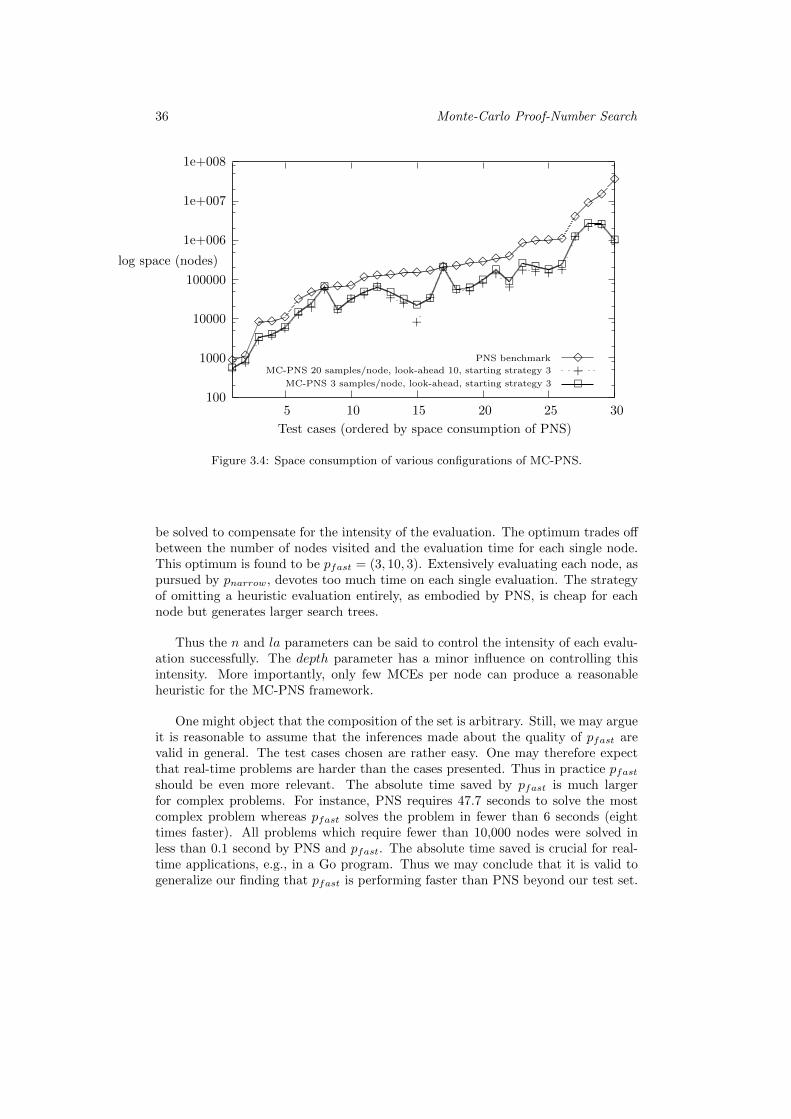
36 Monte-Carlo Proof-Number Search
100
1000
10000
100000
1e+006
1e+007
1e+008
5 10 15 20 25 30
log space (nodes)
Test cases (ordered by space consumption of PNS)
PNS benchmark33
333
33333
3333333333333333
33
3
3
3MC-PNS 20 samples/node, look-ahead 10, starting strategy 3+
+
+ ++
++
+
++ +
++ +
+
+
+
+ ++
++
+ + + +
++ +
+
+MC-PNS 3 samples/node, look-ahead, starting strategy 3
22
2 22
22
2
222 2 2
22
2
2
2 222
2
2 2 2 2
22 2
2
2
Figure 3.4: Space consumption of various configurations of MC-PNS.
be solved to compensate for the intensity of the evaluation. The optimum trades offbetween the number of nodes visited and the evaluation time for each single node.This optimum is found to be pfast = (3, 10, 3). Extensively evaluating each node, aspursued by pnarrow, devotes too much time on each single evaluation. The strategyof omitting a heuristic evaluation entirely, as embodied by PNS, is cheap for eachnode but generates larger search trees.
Thus the n and la parameters can be said to control the intensity of each evalu-ation successfully. The depth parameter has a minor influence on controlling thisintensity. More importantly, only few MCEs per node can produce a reasonableheuristic for the MC-PNS framework.
One might object that the composition of the set is arbitrary. Still, we may argueit is reasonable to assume that the inferences made about the quality of pfast arevalid in general. The test cases chosen are rather easy. One may therefore expectthat real-time problems are harder than the cases presented. Thus in practice pfastshould be even more relevant. The absolute time saved by pfast is much largerfor complex problems. For instance, PNS requires 47.7 seconds to solve the mostcomplex problem whereas pfast solves the problem in fewer than 6 seconds (eighttimes faster). All problems which require fewer than 10,000 nodes were solved inless than 0.1 second by PNS and pfast. The absolute time saved is crucial for real-time applications, e.g., in a Go program. Thus we may conclude that it is valid togeneralize our finding that pfast is performing faster than PNS beyond our test set.
3.5 — Patterns for PNS 37
3.5 Patterns for PNS
As an alternative to MCE, we could use Go patterns to initialize proof and disproofnumbers in the evaluation step of PNS (cf. Subsection 3.1.1). Moreover, we coulduse patterns to improve the MCE of MC-PNS. This section describes patterns incomputer Go and in particular 3× 3 patterns (Subsection 3.5.1). They are used inExperiment 2 as a heuristic for initializing the values of leaves in PNS and also foraltering the probability distribution of MCE in MC-PNS (Subsection 3.5.2).
3.5.1 Patterns in Computer Go
Patterns are a standard means for representing knowledge in computer Go (e.g.,Bouzy and Cazenave, 2001; Bouzy and Chaslot, 2006). A pattern in computer Go is aconfiguration of intersections. High-level representations contain features additionalto the coloring of the intersections. Two examples are: (1) tactical information onconnectivity and (2) life-and-death status. The size of a pattern varies considerablydepending on the application’s purpose. Large-scaled patterns are employed foropenings, while tactical analysis is often guided by small patterns. Patterns canbe created manually or auto-generated (Graepel et al., 2001; Van der Werf, 2004;Bouzy and Chaslot, 2006).
The patterns applied in Experiment 2 are auto-generated 3×3 patterns. They aresmall, but offer the advantage of low pattern-matching cost. This characteristic is aprecondition to any application in the Monte-Carlo framework as given by MC-PNS.The patterns should match each move in each simulated game. The patterns aregenerated by statistical ranking in self-play as described by Bouzy and Chaslot(2006). Each of the 6,561 patterns describes the desirability of the move in thecenter expressed by an integer value. The patterns do not account for informationon the edge of the Go board. They were generated for a MCE Go engine for thewhole game and are not specifically tailored to life-and-death problems.
3.5.2 Two Pattern-Based Heuristics
The patterns are the ingredients for two heuristic variations of PNS. We refer tothem as (1) PNSp and (2) MC-PNSp. As a consequence, we compare four solvingalgorithms in total: (i) PNS, (ii) PNSp, (iii) MC-PNS, and (iv) MC-PNSp.
Ad (1). PNSp applies the patterns to a node X by assigning the suggested patternvalue of the last played intersection to pn(X) and dn(X). The desirability dependson the neighbors surrounding the intersection last played. The intersection’s patternvalue v ranges between 0 and 340. The values of pn and dn are set as pn(X) = 1
v+1and dn(X) = v
340 . Local knowledge on the desirability of the move last played isthus taken into account.
Ad (2). MC-PNSp is a variation of MC-PNS. The patterns are employed to alterthe probability distribution of the moves selected for the random sequence. PureMC-PNS plays randomly distributed legal moves in each random sequence implyinga uniform distribution of the probability for selecting a move. In MC-PNSp thisuniform distribution is altered by the pattern values. Whenever a move is played
38 Monte-Carlo Proof-Number Search
in a random sequence, the pattern values of the intersections next to that moveare updated. These neighbors’ new pattern values are set according to a matchingpattern. The probability to play at a neighbor is proportional to its pattern value.Thus, moves evaluated well by the patterns are more likely to be played than movesless promisingly assessed.
The intuition underlying both heuristics is that main lines of play should be con-sidered first. These lines are given preference by the pattern evaluation. Comparingthe two heuristics, we may predict that MC-PNSp requires considerably more timefor pattern matching because patterns are matched for each move in each randomsequence. PNSp matches the patterns only once at each new node evaluation.
3.6 Experiment 2: Initialization by Patterns or byMonte-Carlo Evaluation
The four variations of the PNS algorithm outlined in the previous section (Section3.5) are tested in Experiment 2: (1) PNS (without heuristics), (2) PNSp (PNS withpattern heuristic), (3) MC-PNS, and (4) MC-PNSp (MC-PNS with pattern heuris-tic). Each variation was tested on the test set of 30 life-and-death problems describedin Subsection 3.2.2. The time spent and the number of nodes expanded for solvingeach test position were measured for each variation. The number of nodes is anindication of efficiency. Simultaneously, the memory consumption is measured bythe same number of nodes. In order to account for the randomness of the MCEsand potential inaccuracy for measuring the small time spans well below a 10th ofa second, each configuration was applied to each test case 20 times. The same testproblems and machinery described for Experiment 1 are used.
3.7 Results of Experiment 2
The experiment required about six hours to complete. All variations solved allproblems correctly. The variations that solved the test cases in decreasing order ofaverage speed were as follows: first MC-PNS, second MC-PNSp, third PNS, andfourth PNSp which required most time to solve the problems. PNSp was 3% slowerthan PNS, while MC-PNS was ca. two times faster than PNS. With respect to nodesexpanded on average, MC-PNS and MC-PNSp performed equal and better than theother variants; PNSp performed third best and PNS performed least. The effect ofthe patterns was small: PNSp expanded about only 6% fewer nodes than PNS intotal, while MC-PNS expanded about 75% fewer nodes than PNS. MC-PNSp wasabout as slow as PNS but used as little space as MC-PNS.
In order to avoid a strong influence of a few large test positions, we suggestan additional metric for comparing the results. For each test case, a ranking canbe established for each variation. Each variation then ranks either first, second,third, or fourth in terms of speed performance. Similarly there is a rank for spaceconsumption. The average ranking is introduced to compare the performance of thevariations on all tests. The average rankings for finding a solution are shown inTable 3.2.
3.8 — Discussion of Experiment 2 39
Algorithm Time rank Space rankMC-PNS 1.6 1.6MC-PNSp 2.6 1.6PNS 2.7 3.6PNSp 3.0 3.1
Table 3.2: Time and space ranking of the four compared PNS variations averaged over 30test problems.
The average ranking by time consumption leads to roughly the same order asthe ranking by space consumption, with one significant exception: PNS solves theproblems faster than PNSp on average (in 17 out of 30 cases), but PNS consumesmore space than PNSp (in two thirds of the cases). However, it should be remarkedthat there are two large outliers in the experimental data.
The results can be structured by noting the explicit occurrence of two features:(1) the Monte-Carlo feature and (2) the pattern feature. The Monte-Carlo featureis present in MC-PNS and MC-PNSp; the pattern feature is present in PNSp andMC-PNSp.
The speed of MC-PNS variations was about twice as high as for PNS on average.Patterns slowed down the speed for finding a solution in both PNS and MC-PNS,whenever they were applied. This tendency was particularly noticeable in MC-PNSp.The variations relying on patterns expanded on average about 6% fewer nodes foreach solution but the variation between the feature groups was larger than withineach feature group. Analogously, the variation of time consumption is smaller be-tween the feature groups than within. The internal variation of time consumption islarger within the Monte-Carlo-feature group than within the pattern-feature group.The reverse holds for space consumption.
3.8 Discussion of Experiment 2
The findings of the previous section can be summarized in three observations. (1)The Monte-Carlo evaluation leads to a better speed improvement than evaluationby patterns. (2) The patterns slow down the speed of the solver and particularlyhinder it in case of MC-PNSp. (3) There is a positive effect of the pattern heuristic,evident in the better space ranking of PNSp compared to that of PNS.
These three observations can be explained as follows. (1) The patterns’ positiveeffect is outweighed by the cost of matching they impose. (2) While the advantagecan be seen in reduced space consumption, this effect is too weak to result in timesavings. (3) The outliers can be explained by the nature of pattern knowledge. Pat-terns are static and generalize from common cases. They are therefore potentiallyweak at handling exceptions. The effect is particularly strong because the patternsare not specialized on life-and-death problems (cf. Subsection 3.5.1). So, the com-bination of patterns and MCE in the manner proposed does not seem promising.However, overall the results, though not practically applicable in the current state,
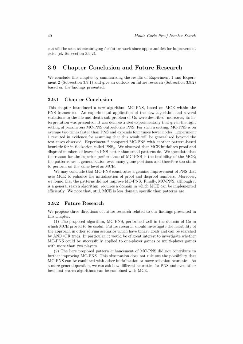
40 Monte-Carlo Proof-Number Search
can still be seen as encouraging for future work since opportunities for improvementexist (cf. Subsection 3.9.2).
3.9 Chapter Conclusion and Future Research
We conclude this chapter by summarizing the results of Experiment 1 and Experi-ment 2 (Subsection 3.9.1) and give an outlook on future research (Subsection 3.9.2)based on the findings presented.
3.9.1 Chapter Conclusion
This chapter introduced a new algorithm, MC-PNS, based on MCE within thePNS framework. An experimental application of the new algorithm and severalvariations to the life-and-death sub-problem of Go were described; moreover, its in-terpretation was presented. It was demonstrated experimentally that given the rightsetting of parameters MC-PNS outperforms PNS. For such a setting, MC-PNS is onaverage two times faster than PNS and expands four times fewer nodes. Experiment1 resulted in evidence for assuming that this result will be generalized beyond thetest cases observed. Experiment 2 compared MC-PNS with another pattern-basedheuristic for initialization called PNSp. We observed that MCE initializes proof anddisproof numbers of leaves in PNS better than small patterns do. We speculate thatthe reason for the superior performance of MC-PNS is the flexibility of the MCE;the patterns are a generalization over many game positions and therefore too staticto perform on the same level as MCE.
We may conclude that MC-PNS constitutes a genuine improvement of PNS thatuses MCE to enhance the initialization of proof and disproof numbers. Moreover,we found that the patterns did not improve MC-PNS. Finally, MC-PNS, although itis a general search algorithm, requires a domain in which MCE can be implementedefficiently. We note that, still, MCE is less domain specific than patterns are.
3.9.2 Future Research
We propose three directions of future research related to our findings presented inthis chapter.
(1) The proposed algorithm, MC-PNS, performed well in the domain of Go inwhich MCE proved to be useful. Future research should investigate the feasibility ofthe approach in other solving scenarios which have binary goals and can be searchedby AND/OR trees. In particular, it would be of great interest to investigate whetherMC-PNS could be successfully applied to one-player games or multi-player gameswith more than two players.
(2) The here proposed pattern enhancement of MC-PNS did not contribute tofurther improving MC-PNS. This observation does not rule out the possibility thatMC-PNS can be combined with other initialization or move-selection heuristics. Asa more general question, we can ask how different heuristics for PNS and even otherbest-first search algorithms can be combined with MCE.

3.9 — Chapter Conclusion and Future Research 41
(3) One reason pointed out for the relatively weak performance of the patterns liesin the kind of patterns used in Experiment 2. As remarked earlier, the patterns wereoriginally designed for improving the playing strength of a Monte-Carlo program forthe whole game of Go. More specific patterns for life-and-death problems couldpotentially provide better results. For instance, the patterns could be larger andthus take into account more context.

42 Monte-Carlo Proof-Number Search
Chapter 4
Monte-Carlo Tree SearchSolver
Sections 4.1 and 4.2 of this chapter are based on the following publication.1
• M.H.M. Winands, Y. Bjornsson, and J-T. Saito. Monte-Carlo Tree Search Solver.In H.J. van den Herik, X. Xu, Z. Ma, and M.H.M. Winands, editors, Proceedings ofComputers and Games 2008 Conference (CG‘08), volume 5131 of Lecture Notes inComputer Science, pp. 25-36. Springer, Berlin, Germany, 2008.
In Chapter 2 we distinguished between two Monte-Carlo methods: (1) Monte-CarloEvaluation (MCE) (Abramson, 1990), and (2) Monte-Carlo Tree Search (MCTS)(Kocsis and Szepesvari, 2006; Coulom, 2007a). Chapter 3 proposed an approach forusing MCE for solving game positions. In this chapter we investigate, in how farMCTS can be used for solving.
In the course of the last few years, MCTS has advanced the field of computer Gosubstantially. Moreover, it is used for other games such as Phantom Go (Cazenaveand Borsboom, 2007) and Clobber (Kocsis, Szepesvari, and Willemson, 2006), andeven for games for which reasonable evaluation functions have been known, e.g.,Amazons (Lorentz, 2008; Kloetzer, Muller, and Bouzy, 2008), LOA (Winands andBjornsson, 2010), and Hex (Cazenave and Saffidine, 2009). Although MCTS is ableto find the best move, it is not able to prove the game-theoretic value of (parts of)the search tree. A search method that is not able to prove or estimate quickly thegame-theoretic value of a node may run into problems. This is especially true forsudden-death games, such as Chess, that may abruptly end by the creation of one ofa prespecified set of patterns (Allis, 1994) (e.g., checkmate in Chess). In this case αβsearch or Proof-Number Search (PNS) (Allis et al., 1994) is traditionally preferredto MCTS.
This chapter answers the second research question, RQ 2: How can the Monte-Carlo Tree Search framework contribute to solving game positions? To that end, we
1The author is grateful to Springer-Verlag for the permission of reusing relevant parts of thearticle in the thesis.
44 Monte-Carlo Tree Search Solver
introduce a new MCTS variant called MCTS-Solver that has been designed to provethe game-theoretic value of a node in a search tree. This is an important step towardsapplying MCTS-based approaches effectively in sudden-death-like games (includingChess). We use the game Lines of Action (LOA) as a testbed. It is an ideal candidatebecause its intricacies are less complicated than those of Chess. Therefore, we canfocus on the sudden-death property. In this chapter we assess MCTS-Solver on atest set of LOA positions. First, we test the influence of the selection strategy onMCTS-Solver. Second, we compare MCTS-Solver with αβ and PN2. Third, rootparallelization and tree parallelization are evaluated for MCTS-Solver. We notethat we investigate the solving strength of MCTS-Solver; its improvement in playingstrength was already investigated by Winands et al. (2008). Experimental resultsindicated that MCTS-Solver defeated the original MCTS program by a winning scoreof 65%.
The chapter is organized as follows. In Section 4.1 we introduce MCTS-Solver. InSection 4.2 we discuss its application to LOA. We empirically evaluate the method inSection 4.3. Finally, Section 4.4 gives conclusions and an outlook on future research.
4.1 Monte-Carlo Tree Search Solver
Although MCTS is unable to prove the game-theoretic value, in the long run MCTSequipped with the UCT formula is able to converge to the game-theoretic value. Forexample, in endgame positions of fixed-termination games like Go and Amazons,MCTS is able to find the optimal move relatively fast (Zhang and Chen, 2007;Kloetzer et al., 2008). However, in a sudden-death game like LOA, where the mainline towards the winning position is narrow, MCTS may often lead to an erroneousoutcome because the nodes’ values in the tree do not converge fast enough to theirgame-theoretic value. For example, if we let MCTS analyze the LOA position inFigure 4.1 for 5 seconds, it selects c7xc4 as the best move, winning 67.2% of thesimulations. However, this move is a forced 8-ply loss, while f8-f7 (scoring 48.2%) isa 7-ply win.2 Only when we let MCTS search for 60 seconds, it selects the optimalmove. For a reference, we remark that it takes αβ in this position less than a secondto select the best move and prove the win.
We designed a new variant called MCTS-Solver which is able to prove the game-theoretic value of a position. Of the four stages of MCTS (described in Chapter 2)two are changed for MCTS-Solver. The simulation and expansion stages remain thesame. The backpropagation and the selection are modified for MCTS-Solver. Thechanges are discussed in Subsections 4.1.1 and 4.1.2, respectively. The pseudocodeof MCTS-Solver is given in Subsection 4.1.3.
2The rules of LOA can be found in Appendix A.
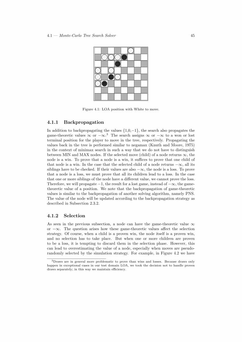
4.1 — Monte-Carlo Tree Search Solver 45
1
Figure 4.1: LOA position with White to move.
4.1.1 Backpropagation
In addition to backpropagating the values {1,0,−1}, the search also propagates thegame-theoretic values ∞ or −∞.3 The search assigns ∞ or −∞ to a won or lostterminal position for the player to move in the tree, respectively. Propagating thevalues back in the tree is performed similar to negamax (Knuth and Moore, 1975)in the context of minimax search in such a way that we do not have to distinguishbetween MIN and MAX nodes. If the selected move (child) of a node returns∞, thenode is a win. To prove that a node is a win, it suffices to prove that one child ofthat node is a win. In the case that the selected child of a node returns −∞, all itssiblings have to be checked. If their values are also −∞, the node is a loss. To provethat a node is a loss, we must prove that all its children lead to a loss. In the casethat one or more siblings of the node have a different value, we cannot prove the loss.Therefore, we will propagate −1, the result for a lost game, instead of −∞, the game-theoretic value of a position. We note that the backpropagation of game-theoreticvalues is similar to the backpropagation of another solving algorithm, namely PNS.The value of the node will be updated according to the backpropagation strategy asdescribed in Subsection 2.3.2.
4.1.2 Selection
As seen in the previous subsection, a node can have the game-theoretic value ∞or −∞. The question arises how these game-theoretic values affect the selectionstrategy. Of course, when a child is a proven win, the node itself is a proven win,and no selection has to take place. But when one or more children are provento be a loss, it is tempting to discard them in the selection phase. However, thiscan lead to overestimating the value of a node, especially when moves are pseudo-randomly selected by the simulation strategy. For example, in Figure 4.2 we have
3Draws are in general more problematic to prove than wins and losses. Because draws onlyhappen in exceptional cases in our test domain LOA, we took the decision not to handle provendraws separately; in this way we maintain efficiency.
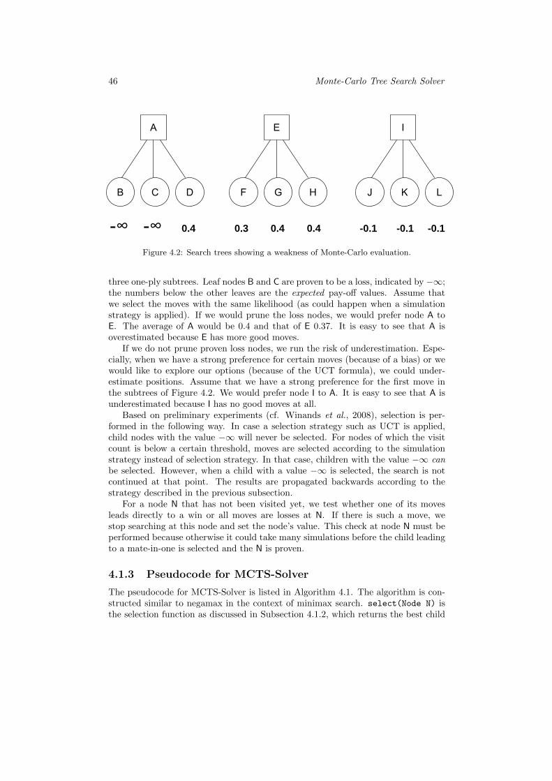
46 Monte-Carlo Tree Search Solver
A
B C D
E
F G H
I
J K L
-∞ -∞ 0.4 0.3 0.4 0.4 -0.1 -0.1 -0.1
Figure 4.2: Search trees showing a weakness of Monte-Carlo evaluation.
three one-ply subtrees. Leaf nodes B and C are proven to be a loss, indicated by −∞;the numbers below the other leaves are the expected pay-off values. Assume thatwe select the moves with the same likelihood (as could happen when a simulationstrategy is applied). If we would prune the loss nodes, we would prefer node A toE. The average of A would be 0.4 and that of E 0.37. It is easy to see that A isoverestimated because E has more good moves.
If we do not prune proven loss nodes, we run the risk of underestimation. Espe-cially, when we have a strong preference for certain moves (because of a bias) or wewould like to explore our options (because of the UCT formula), we could under-estimate positions. Assume that we have a strong preference for the first move inthe subtrees of Figure 4.2. We would prefer node I to A. It is easy to see that A isunderestimated because I has no good moves at all.
Based on preliminary experiments (cf. Winands et al., 2008), selection is per-formed in the following way. In case a selection strategy such as UCT is applied,child nodes with the value −∞ will never be selected. For nodes of which the visitcount is below a certain threshold, moves are selected according to the simulationstrategy instead of selection strategy. In that case, children with the value −∞ canbe selected. However, when a child with a value −∞ is selected, the search is notcontinued at that point. The results are propagated backwards according to thestrategy described in the previous subsection.
For a node N that has not been visited yet, we test whether one of its movesleads directly to a win or all moves are losses at N. If there is such a move, westop searching at this node and set the node’s value. This check at node N must beperformed because otherwise it could take many simulations before the child leadingto a mate-in-one is selected and the N is proven.
4.1.3 Pseudocode for MCTS-Solver
The pseudocode for MCTS-Solver is listed in Algorithm 4.1. The algorithm is con-structed similar to negamax in the context of minimax search. select(Node N) isthe selection function as discussed in Subsection 4.1.2, which returns the best child
4.2 — Monte-Carlo LOA 47
of the node N . The procedure add_to_tree(Node N) adds one more node to thetree; play_out(Node N) is the function which plays a simulated game from the nodeN , and returns the result R ∈ {1, 0,−1} of this game; compute_average(IntegerR) is the procedure that updates the value of the node depending on the result R ofthe last simulated game; get_children(Node N) generates the children of node N .
4.2 Monte-Carlo LOA
In this section we discuss how we applied MCTS-Solver to LOA. First, we proposepossible selection strategies for MCTS-Solver in Subsection 4.2.1. We explain thesimulation strategy in Subsection 4.2.1. Finally, we discuss how we parallelized thesearch in Subsection 4.2.3.
4.2.1 Selection Strategies
We use the UCT (Upper Confidence bounds applied to Trees) strategy (Kocsis andSzepesvari, 2006). UCT is easy to implement and used in many Monte-Carlo Goprograms. UCT can be enhanced with Progressive Bias (PB) (Chaslot et al., 2008b).PB is a technique to embed domain-knowledge bias into the UCT formula. It wassuccessfully applied in the Go program Mango (Chaslot et al., 2008b). UCT withPB works as follows. Let I be the set of nodes immediately reachable from thecurrent node p. The selection strategy selects the child k of the node p that satisfiesFormula 4.1:
k ∈ argmaxi∈I(vi +
√C × lnnp
ni+W × Pmcni + 1
), (4.1)
where vi is the value of the node i, ni is the visit count of i, and np is the visitcount of p. C is a coefficient which must be tuned experimentally. W×Pmc
ni+1 is the PBpart of the formula. W is a constant which must be set manually (here W = 50).Pmc is the transition probability of a move category mc (Tsuruoka, Yokoyama, andChikayama, 2002).
For each move category (e.g., capture, blocking) the probability that a movebelonging to that category will be played is determined. The probability is calledthe transition probability. This statistic is obtained off-line from game records ofmatches played by expert players. The transition probability for a move categorymc is calculated as follows:
Pmc =nplayed(mc)
navailable(mc), (4.2)
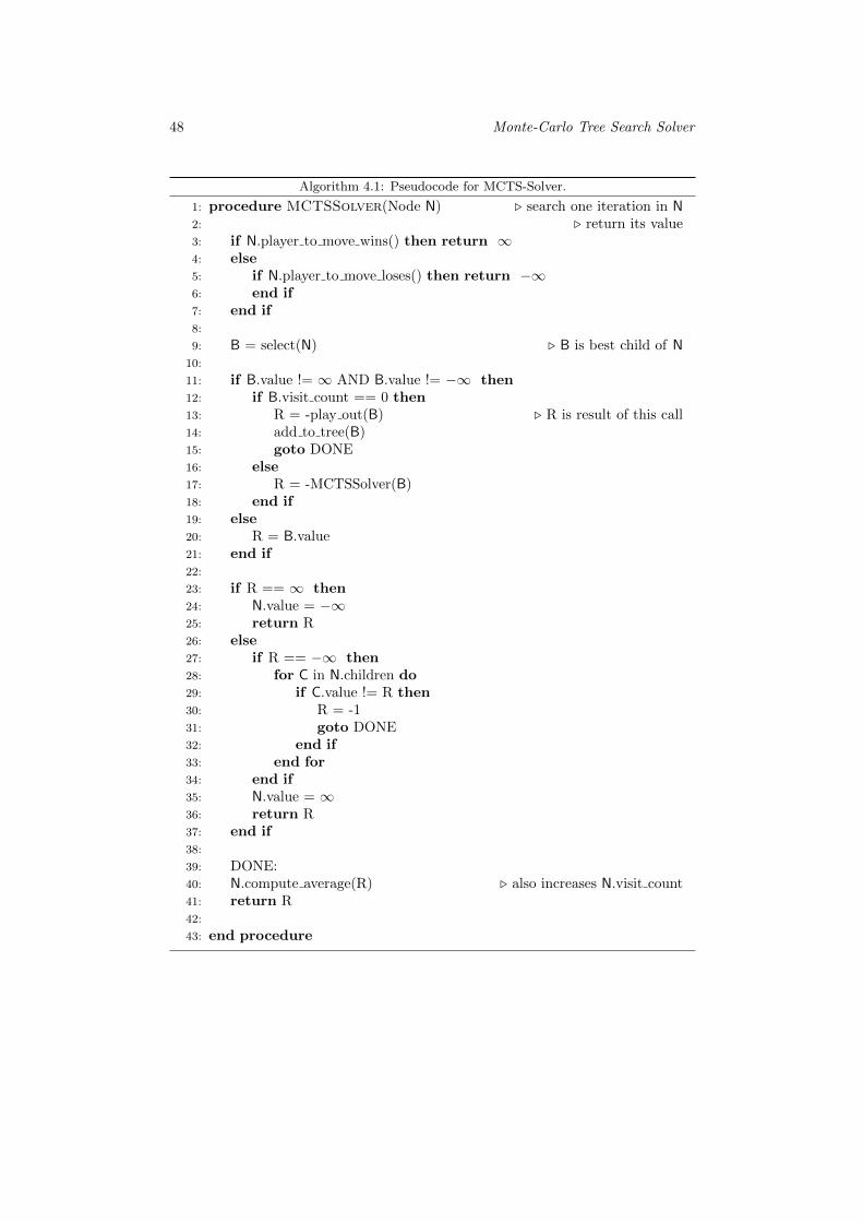
48 Monte-Carlo Tree Search Solver
Algorithm 4.1: Pseudocode for MCTS-Solver.
50 CHAPTER 4. MONTE-CARLO TREE SEARCH SOLVER
Algorithm 4.1 Pseudo code for MCTS-Solver.
1: procedure MCTSSolver(Node N) . search one iteration in N2: . return its value3: if N.player to move wins() then return ∞4: else5: if N.player to move loses() then return −∞6: end if7: end if8:
9: B = select(N) . B is best child of N10:
11: if B.value != ∞ AND B.value != −∞ then12: if B.visit count == 0 then13: R = -play out(B) . R is result of this call14: add to tree(B)15: goto DONE16: else17: R = -MCTSSolver(B)18: end if19: else20: R = B.value21: end if22:
23: if R == ∞ then24: N.value = −∞25: return R26: else27: if R == −∞ then28: for C in N.children do29: if C.value != R then30: R = -131: goto DONE32: end if33: end for34: end if35: N.value = ∞36: return R37: end if38:
39: DONE:40: N.compute average(R) . also increases N.visit count41: return R42:
43: end procedure
4.2 — Monte-Carlo LOA 49
where nplayed(mc) is the number of game positions in which a move belonging tocategory mc was played, and navailable(mc) is the number of positions in which movesbelonging to category mc were available.
The move categories of the MC-LOA program are similar to the ones used in theRealization-Probability Search of the program MIA (Winands and Bjornsson, 2008).They are applied in the following way. First, we classify moves as captures or non-captures. Next, moves are further sub-classified based on the origin and destinationsquares. The board is divided into five different regions: the corners, the 8× 8 outerrim (except corners), the 6× 6 inner rim, the 4× 4 inner rim, and the central 2× 2board. Finally, moves are further classified based on the number of squares traveledaway from or towards the center-of-mass.
The influence of PB has to be important when a few games have been played buthas to decrease fast (when more games have been played) to ensure that the strategyconverges to the UCT selection strategy. Standard, this is done through dividingthe PB component by the number of games played through that node (i.e., ni). Adisadvantage is that by dividing by ni the decrease rate of PB is independent of theactual value of a child (i.e., vi). Nodes that do not perform well should not be biasedthat long, whereas nodes that continue to have a high score should continue to bebiased. Instead of dividing the PB component by the number of games played, itmay be divided by the number of losses li (Nijssen and Winands, 2010) in Formula4.3.
k ∈ argmaxi∈I(vi +
√C × lnnp
ni+W × Pmcli + 1
), (4.3)
Moreover, favoring nodes with a high value could be taken a step further byreplacing every ni with li which would produce Formula 4.4.
k ∈ argmaxi∈I(vi +
√C × lnnp
li+W × Pmcli + 1
), (4.4)
All three PB variants are available in the MCTS program. In Section 4.3, we willdetermine which PB variant works the best for solving positions. Regarding playingstrength, applying the standard PB enables that the MC-LOA program wins almost75% of the games against the standard UCT. The two enhanced variants only gavea slight additional improvement.
Finally, we remark that the selection strategy is applied only at nodes with avisit count higher than a certain threshold T (here 5) (Coulom, 2007a). If the nodehas been visited fewer times than this threshold, the next move is selected accordingto the simulation strategy discussed in the next subsection.
50 Monte-Carlo Tree Search Solver
4.2.2 Simulation Strategy
In the Monte-Carlo LOA program, the move categories together with their transitionprobabilities, as discussed in Subsection 4.2.1, are used to select the moves pseudo-randomly during the MCE. The simulation strategy draws the moves randomly basedon their transition probabilities in the first part of a simulation, but selects thembased on their evaluation score in the second part of a simulation (cf. Winands andBjornsson, 2010).
A simulation requires that the number of moves per game is limited. Whenconsidering the game of LOA, the simulated game is stopped after 200 moves andscored as a draw. The game is also stopped when heuristic knowledge indicates thatthe game is probably over. In general, once a LOA position gets very lopsided, anevaluation function can return a quite trustworthy score, more so than even elaboratesimulation strategies. The game can thus be safely terminated both earlier and witha more accurate score than if continuing the simulation (which might fail to deliverthe win). We use the MIA 4.5 evaluation function (Winands and Van den Herik,2006) for this purpose. When the evaluation function gives a value that exceeds acertain threshold (i.e., 700 points), the game is scored as a win. If the evaluationfunction gives a value that is below a certain threshold (i.e., −700 points), the gameis scored as a loss. For efficiency reasons the evaluation function is called only every3 plies, starting at the second ply (thus at 2, 5, 8, 11 etc.).
4.2.3 Parallelization
The MC-LOA program employs two parallelization methods, (1) root parallelizationand (2) tree parallelization. They are explained below.
Root Parallelization
“Single-run” parallelization (Cazenave and Jouandeau, 2007), also called root paral-lelization (Chaslot et al., 2008a) consists of building multiple MCTS trees in parallel,with one thread per tree. These threads do not share information with each other.When the available time is up, all the root children of the separate MCTS treesare merged with their corresponding clones. For each group of clones, the scores ofall games played are added. Based on this grand total, the best move is selected.This parallelization method only requires a minimal amount of communication be-tween threads, so the parallelization is easy to implement even on a cluster. For asmall number of threads, root parallelization performs remarkably well in compari-son to other parallelization methods (Cazenave and Jouandeau, 2007; Chaslot et al.,2008a). Root parallelization improved the playing strength of the MC-LOA programconsiderably (Winands and Bjornsson, 2010).
Tree Parallelization
Tree parallelization (Cazenave and Jouandeau, 2007; Chaslot et al., 2008a) uses oneshared tree from which several simultaneous games are played. Each thread canmodify the information contained in the tree; therefore, care needs to be taken to
4.3 — Experiments 51
prevent that threads corrupt the values of the nodes by simultaneously operatingon the same data. A lock is used when a leaf is expanded to prevent corruptionof data. Inspired by the suggestion of Enzenberger and Muller (2010), no locks areused when two threads access the same internal node. At the moment that twothreads try to update a node at the same time, one of the updates may be lost. Inour implementation, a special check takes care that the game-theoretic value of aproven node is never overwritten.
If several threads start from the root at the same time, it is possible that theytraverse the tree for a large part along the same path. Simulated games might startfrom leaves close to each other. It may even occur that simulated games begin fromthe same leaf node. Because a search tree typically has millions of nodes, it maybe redundant to explore a rather small part of the tree several times. Instead ofselecting the child solely on its UCT score, we added a small random factor to theUCT formulas. Shoham and Toledo (2002) call this the randomization of the moveselection. Randomization of the move selection has been shown to be beneficialfor parallelizing best-first search in the past (cf. Shoham and Toledo, 2002; Saito,Winands, and Van den Herik, 2010, and Chapter 5 of this thesis). Adding a randomfactor to Formula 4.4 produces Formula 4.5.
k ∈ argmaxi∈I(vi +
√C × lnnp
li+W × Pmcli + 1
+ k × ε)
, (4.5)
where ε is a random variable, ε ∈ [0, 1] and k a constant. This constant is here setto 0.02, to ensure that playing strength is at least the same as when applying rootparallelization.
4.3 Experiments
In this section we evaluate the tactical performance of MCTS-Solver by testing iton LOA endgame positions. First, we explain briefly the experimental setup inSubsection 4.3.1. Next, we test the influence of the selection strategy on MCTS-Solver in Subsection 4.3.2. Subsequently, we compare MCTS-Solver with αβ andPN2 search in Subsection 4.3.3. Finally, root parallelization and tree parallelizationare evaluated for MCTS-Solver in 4.3.4.
4.3.1 Experimental Setup
We tested MCTS-Solver on 488 endgame positions of Lines of Action (LOA).4 Thistest set and subsets thereof have been used frequently in the past (Pawlewicz andLew, 2007; Sakuta et al., 2003; Winands et al., 2003b). We note that the rulesof LOA can be found in the Appendix A. All experiments are carried out on aLinux server with eight 2.66 GHz Xeon cores and 8 GB of RAM. In this section
4The test set is available at www.personeel.unimaas.nl/m-winands/loa/tscg2002a.zip.
52 Monte-Carlo Tree Search Solver
MCTS-Solver is compared with αβ and PN2 search. The details of αβ and PN2 arediscussed below. All search algorithms have been implemented in Java.
αβ Search
The αβ search performs a depth-first iterative-deepening in the PVS / NegaScoutframework (Marsland, 1983; Reinefeld, 1983). The evaluation function of MIA 4.5is used (Winands and Van den Herik, 2006) to assess the values of leaf nodes. ATwoDeep transposition table (Breuker et al., 1996) is applied to prune a subtree orto narrow the αβ window. At all interior nodes that are more than 2 plies awayfrom the leaves, it generates all moves to perform Enhanced Transposition Cutoffs(ETC) (Schaeffer and Plaat, 1996). For move ordering, the move stored in thetransposition table (if applicable) is always tried first, followed by two killer moves(Akl and Newborn, 1977). These are the last two moves that were best or at leastcaused a cutoff at the given depth. Thereafter follow: (1) capture moves going tothe inner area (the central 4× 4 board) and (2) capture moves going to the middlearea (the 6 × 6 rim). All the remaining moves are ordered decreasingly accordingto the relative history heuristic (Winands et al., 2006). At the leaf nodes of theregular search, a quiescence search is performed to get more accurate evaluations(cf. Schrufer, 1989).
PN2 Search
The PN2 search used, was previously employed to solve 6×6 LOA (cf. Winands,2008). In this implementation, the proof number and disproof number are initializedto values 1 and n, respectively, for an OR node (and the reverse for an AND node),where n is the number of legal moves. In LOA, n is equivalent to the mobility of themoving player. It is also an important feature in the evaluation function (Winands,Van den Herik, and Uiterwijk, 2003a). It is known that mobility speeds up PN witha factor of 5 to 6 (Winands, 2004).
As a reminder, we note that PN2 consists of two levels of PN search. The firstlevel consists of a PN search (PN1) which calls a PN search at the second level (PN2)for an evaluation of the most-proving node of the PN1 tree. This PN2 search is boundby a maximum number of nodes N to be stored in memory. In this implementation,N is equal to the size of the PN1 tree (Allis, 1994). The PN2 search is stopped whenthe number of nodes stored in memory exceeds N or the subtree is (dis)proven. Aftercompletion of the PN2 search, the children of the root of the PN2 tree are preserved,but subtrees are removed from memory.
4.3.2 Selection Strategies
In the first experiment we test the effect of enhancing MCTS-Solver with ProgressiveBias (PB) on a set of 488 forced-win LOA positions. We compare the standard UCTselection strategy with the three PB variants, here called Classic PB, PB-L1, andPB-L2 (i.e., Formulas 4.1, 4.3 and 4.4, respectively). We will look how much effort(in nodes and CPU time) it takes to solve endgame positions. For MCTS-Solver, allchildren at a leaf node, evaluated for the termination condition during the search
4.3 — Experiments 53
(cf. Subsection 4.1.2), are counted. The maximum number of nodes searched is5,000,000. The limit ensures that MCTS-Solver does not use more than 30 secondsfor trying to solve a position.
The results are given in Table 4.1. The first column gives the names of thealgorithms, the second the number of positions solved, and the third and fourth thenumber of nodes searched and the time it took, respectively. In the second columnwe see that 174 positions are solved by UCT, 245 by Classic PB, 306 by PB-L1, and319 by PB-L2. In the third and fourth column the number of nodes and the timeconsumed are given for the subset of 154 positions which all algorithms are able tosolve. We see that the PB variants not only solve more problems, but also that theyexplore considerably smaller trees than the UCT variant. For the best PB variant,PB-L2, positions were solved tree times faster in nodes and time than UCT. We mayconclude that PB not only improves the playing performance but also the solvingperformance.
# positions solved 154 positionsAlgorithm (out of 488) Total nodes Total time (ms.)
UCT 174 148,278,311 514,933Classic PB 245 103,369,811 381,944
PB-L1 306 57,010,037 212,437PB-L2 319 45,444,437 171,246
Table 4.1: Comparing different selection strategies on 488 test positions with a limit of5,000,000 nodes.
For better insight into how much faster the enhanced PB variants, PB-L1 andPB-L2, are than the Classic PB in CPU time, a second comparison was performed.In Table 4.2 we compare Classic PB, PB-L1, and PB-L2 on the subset of 224 testpositions which the three algorithms were able to solve. The table reveals that thePB-L1 and PB-L2 are 1.5 to 2 times faster than Classic-PB in CPU time. Takinginto account the number of losses instead of the number of visits in the PB formulaimproves the solving strength of MCTS-Solver.
Algorithm Total nodes Total time (ms.)Classic PB 217,975,808 799,893PB-L1 138,742,124 497,161PB-L2 124,635,541 448,170
Table 4.2: Comparing the different Progressive-Bias variants on 224 test positions with alimit of 5,000,000 nodes.
Finally, to assess which of the enhanced PB variants, PB-L1 and PB-L2, is thebest, we performed a third comparison. In Table 4.3 we compare PB-L1 and PB-L2on a subset of 286 test positions which both algorithms were able to solve. We cansee that PB-L2 is 10 to 15% faster in nodes and CPU time than PB-L1. For theremaining experiments of this chapter we will use the PB-L2 enhancement.
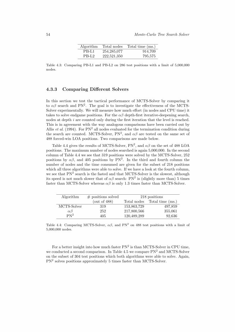
54 Monte-Carlo Tree Search Solver
Algorithm Total nodes Total time (ms.)PB-L1 254,285,077 914,709PB-L2 222,521,350 795,575
Table 4.3: Comparing PB-L1 and PB-L2 on 286 test positions with a limit of 5,000,000nodes.
4.3.3 Comparing Different Solvers
In this section we test the tactical performance of MCTS-Solver by comparing itto αβ search and PN2. The goal is to investigate the effectiveness of the MCTS-Solver experimentally. We will measure how much effort (in nodes and CPU time) ittakes to solve endgame positions. For the αβ depth-first iterative-deepening search,nodes at depth i are counted only during the first iteration that the level is reached.This is in agreement with the way analogous comparisons have been carried out byAllis et al. (1994). For PN2 all nodes evaluated for the termination condition duringthe search are counted. MCTS-Solver, PN2, and αβ are tested on the same set of488 forced-win LOA positions. Two comparisons are made below.
Table 4.4 gives the results of MCTS-Solver, PN2, and αβ on the set of 488 LOApositions. The maximum number of nodes searched is again 5,000,000. In the secondcolumn of Table 4.4 we see that 319 positions were solved by the MCTS-Solver, 252positions by αβ, and 405 positions by PN2. In the third and fourth column thenumber of nodes and the time consumed are given for the subset of 218 positionswhich all three algorithms were able to solve. If we have a look at the fourth column,we see that PN2 search is the fasted and that MCTS-Solver is the slowest, althoughits speed is not much slower that of αβ search: PN2 is (slightly more than) 5 timesfaster than MCTS-Solver whereas αβ is only 1.3 times faster than MCTS-Solver.
Algorithm # positions solved 218 positions(out of 488) Total nodes Total time (ms.)
MCTS-Solver 319 153,863,729 497,859αβ 252 217,800,566 355,061
PN2 405 120,489,289 92,636
Table 4.4: Comparing MCTS-Solver, αβ, and PN2 on 488 test positions with a limit of5,000,000 nodes.
For a better insight into how much faster PN2 is than MCTS-Solver in CPU time,we conducted a second comparison. In Table 4.5 we compare PN2 and MCTS-Solveron the subset of 304 test positions which both algorithms were able to solve. Again,PN2 solves positions approximately 5 times faster than MCTS-Solver.
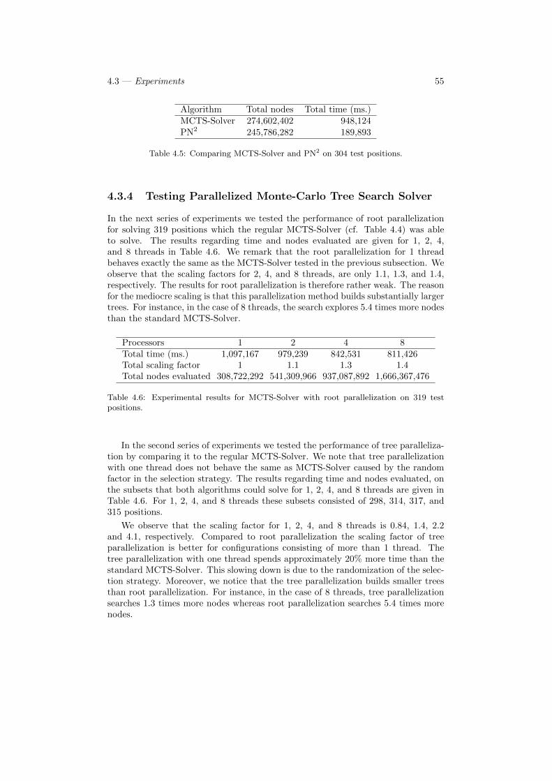
4.3 — Experiments 55
Algorithm Total nodes Total time (ms.)MCTS-Solver 274,602,402 948,124PN2 245,786,282 189,893
Table 4.5: Comparing MCTS-Solver and PN2 on 304 test positions.
4.3.4 Testing Parallelized Monte-Carlo Tree Search Solver
In the next series of experiments we tested the performance of root parallelizationfor solving 319 positions which the regular MCTS-Solver (cf. Table 4.4) was ableto solve. The results regarding time and nodes evaluated are given for 1, 2, 4,and 8 threads in Table 4.6. We remark that the root parallelization for 1 threadbehaves exactly the same as the MCTS-Solver tested in the previous subsection. Weobserve that the scaling factors for 2, 4, and 8 threads, are only 1.1, 1.3, and 1.4,respectively. The results for root parallelization is therefore rather weak. The reasonfor the mediocre scaling is that this parallelization method builds substantially largertrees. For instance, in the case of 8 threads, the search explores 5.4 times more nodesthan the standard MCTS-Solver.
Processors 1 2 4 8Total time (ms.) 1,097,167 979,239 842,531 811,426Total scaling factor 1 1.1 1.3 1.4Total nodes evaluated 308,722,292 541,309,966 937,087,892 1,666,367,476
Table 4.6: Experimental results for MCTS-Solver with root parallelization on 319 testpositions.
In the second series of experiments we tested the performance of tree paralleliza-tion by comparing it to the regular MCTS-Solver. We note that tree parallelizationwith one thread does not behave the same as MCTS-Solver caused by the randomfactor in the selection strategy. The results regarding time and nodes evaluated, onthe subsets that both algorithms could solve for 1, 2, 4, and 8 threads are given inTable 4.6. For 1, 2, 4, and 8 threads these subsets consisted of 298, 314, 317, and315 positions.
We observe that the scaling factor for 1, 2, 4, and 8 threads is 0.84, 1.4, 2.2and 4.1, respectively. Compared to root parallelization the scaling factor of treeparallelization is better for configurations consisting of more than 1 thread. Thetree parallelization with one thread spends approximately 20% more time than thestandard MCTS-Solver. This slowing down is due to the randomization of the selec-tion strategy. Moreover, we notice that the tree parallelization builds smaller treesthan root parallelization. For instance, in the case of 8 threads, tree parallelizationsearches 1.3 times more nodes whereas root parallelization searches 5.4 times morenodes.
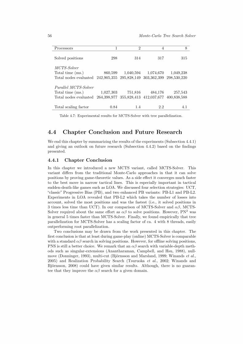
56 Monte-Carlo Tree Search Solver
Processors 1 2 4 8
Solved positions 298 314 317 315
MCTS-SolverTotal time (ms.) 860,599 1,040,594 1,074,670 1,049,238Total nodes evaluated 242,905,355 295,828,149 303,362,399 298,530,220
Parallel MCTS-SolverTotal time (ms.) 1,027,303 751,816 484,176 257,543Total nodes evaluated 264,398,977 355,828,413 412,037,677 400,838,588
Total scaling factor 0.84 1.4 2.2 4.1
Table 4.7: Experimental results for MCTS-Solver with tree parallelization.
4.4 Chapter Conclusion and Future Research
We end this chapter by summarizing the results of the experiments (Subsection 4.4.1)and giving an outlook on future research (Subsection 4.4.2) based on the findingspresented.
4.4.1 Chapter Conclusion
In this chapter we introduced a new MCTS variant, called MCTS-Solver. Thisvariant differs from the traditional Monte-Carlo approaches in that it can solvepositions by proving game-theoretic values. As a side effect it converges much fasterto the best move in narrow tactical lines. This is especially important in tacticalsudden-death-like games such as LOA. We discussed four selection strategies: UCT,“classic” Progressive Bias (PB), and two enhanced PB variants: PB-L1 and PB-L2.Experiments in LOA revealed that PB-L2 which takes the number of losses intoaccount, solved the most positions and was the fastest (i.e., it solved positions in3 times less time than UCT). In our comparison of MCTS-Solver and αβ, MCTS-Solver required about the same effort as αβ to solve positions. However, PN2 wasin general 5 times faster than MCTS-Solver. Finally, we found empirically that treeparallelization for MCTS-Solver has a scaling factor of ca. 4 with 8 threads, easilyoutperforming root parallelization.
Two conclusions may be drawn from the work presented in this chapter. Thefirst conclusion is that at least during game-play (online) MCTS-Solver is comparablewith a standard αβ search in solving positions. However, for offline solving positions,PNS is still a better choice. We remark that an αβ search with variable-depth meth-ods such as singular-extensions (Anantharaman, Campbell, and Hsu, 1988), null-move (Donninger, 1993), multi-cut (Bjornsson and Marsland, 1999; Winands et al.,2005) and Realization Probability Search (Tsuruoka et al., 2002; Winands andBjornsson, 2008) could have given similar results. Although, there is no guaran-tee that they improve the αβ search for a given domain.
4.4 — Chapter Conclusion and Future Research 57
The second conclusion we may draw is that the strength of MCTS-Solver isdependent on enhancements such as PB. Just as for αβ, search enhancements (cf.Marsland, 1986) are crucial for the performance.
4.4.2 Future Research
For search methods based on MCE, to be able to handle proven outcomes is anessential step. With continuing improvements it is not unlikely that in the not sodistant future enhanced MCE-based approaches may even become an alternativeto PNS. As future research, experiments are envisaged in other games to test theperformance of MCTS-Solver. One possible next step would be to test the method inGo, a domain in which MCTS is already widely used. What makes this a somewhatmore difficult task is that additional work is required in enabling perfect endgameknowledge – such as Benson’s Algorithm (Benson, 1988; Van der Werf et al., 2003)– in MCTS.

58 Monte-Carlo Tree Search Solver
Chapter 5
Parallel Proof-NumberSearch
This chapter is based on the following publications.1
1. J-T. Saito, M.H.M. Winands and H.J. van den Herik. Randomized Parallel Proof-Number Search. In T. Calders, K. Tuyls, and M. Pechenizkiy, editors, Proceedingsof the 21st BeNeLux Conference on Artificial Intelligence (BNAIC‘09), pp. 365–366,TU/e Eindhoven, Eindhoven, The Netherlands, 2009.
2. J-T. Saito, M.H.M. Winands and H.J. van den Herik. Randomized Parallel Proof-Number Search. In H.J. van den Herik and P. Spronck, editors, Proceedings of the13th Advances in Computer Games Conference (ACG‘09), volume 6048 of LectureNotes in Computer Science, pp. 75-87. Springer, Berlin, Germany, 2010.
A variety of parallel αβ algorithms have been proposed in the past (cf. Brock-ington, 1996), but so far little research has been conducted on parallelizing PNS.With multi-core processors becoming established as standard equipment, paralleliz-ing PNS has become an important topic. Pioneering research has been conductedby Kishimoto and Kotani (1999), who parallelized the depth-first PNS variant PDS.His algorithm, called ParaPDS, is designed for distributed memory systems.
This chapter addresses RQ 3: How can Proof-Number Search be parallelized? Weparallelize PNS and PN2 for shared-memory systems. The parallelization is basedon randomizing the move selection of multiple threads, which operate on the samesearch tree. The new method is called Randomized Parallel Proof-Number Search(RP–PNS). Its PN2 version is called RP–PN2. We evaluate the new parallelizationon a set of LOA problems.
The chapter is organized in four sections. Section 5.1 describes the parallelizationof search algorithms in general in as far as it is relevant for this work. Moreover,the only other existing parallelization of PNS, ParaPDS, is explained. Section 5.2introduces our new parallelization of PNS and PN2, i.e., RP–PNS and RP–PN2. In
1The author is grateful to Springer-Verlag for the permission to reuse relevant parts of the articlein the thesis.
60 Parallel Proof-Number Search
Section 5.3 RP–PNS and RP–PN2 are tested on a set of LOA endgame positions.Section 5.4 concludes this chapter and gives directions for future work.
5.1 Parallelization of PNS
This section introduces some basic concepts for describing the behavior of par-allel search algorithms (Subsection 5.1.1), outlines ParaPDS, a parallelization ofPDS (Subsection 5.1.2), and explains parallel randomized search (Subsection 5.1.3).
5.1.1 Terminology
Parallelization aims at reducing the time that a sequential algorithm requires forterminating successfully. The speedup is achieved by distributing computations tomultiple threads executed in parallel.
Parallelization gains from dividing computation by multiple resources but si-multaneously it may impose a computational cost. According to Brockington andSchaeffer (1997) three kinds of overhead may occur when parallelizing a search al-gorithm: (1) search overhead, resulting from extra search not performed by the se-quential algorithm; (2) synchronization overhead, created at synchronization pointswhen one thread is idle waiting for another thread; (3) communication overhead,created by exchanging information between threads.
Search overhead is straightforward and can be measured by the number of addi-tional nodes searched. Synchronization and communication overhead depend on thekind of information sharing used. There are two kinds of information sharing: (i)message passing and (ii) shared memory. Message passing simply consists of pass-ing information between memory units exclusively accessed by a particular thread.Under shared memory all threads can access a common part of memory. With theadvent of multi-core CPUs memory sharing has become common place.
An important property governing the behavior of parallel algorithms is scaling.It describes the efficiency of parallelization with respect to the number of threads asa fractional relation t1/tT between the time t1 for terminating successfully with onethread and the time tT for terminating successfully with T threads.
5.1.2 ParaPDS and the Master-Servant Design
The only existing parallelization of PNS described in the literature has so far beenParaPDS by Kishimoto and Kotani (1999).2 This pioneering work of parallel PNSachieved a speedup of 3.6 on 16 processors on a distributed memory machine. Wenote that Kishimoto and Kotani referred to processes instead and whereas we referto threads in our shared memory setting. ParaPDS relies on a master-servant design.
2Conceptually related to PNS is Conspiracy-Number Search (CNS) by McAllester (1988).Lorenz (2001) proposes to parallelize a variant of CNS (PCCNS). PCCNS uses a master-servantmodel (“Employer-Worker Relationship”).We note that just before the printing of this thesis, a parallel version of df-pn on shared mem-ory systems has been proposed by Kaneko (2010). It was tested on Shogi problems on which itproduced a scaling factor of 3.6 with 8 threads.
5.1 — Parallelization of PNS 61
One master process is coordinating the work of several servant processes. The mastermanages a search tree up to a fixed depth d. The master traverses through the treein a depth-first manner typical for PDS. On reaching depth d it assigns the work ofsearching further to an idle servant. The search results of the servant process arebacked up by the master.
The overhead created by ParaPDS is mainly a search overhead. There are tworeasons for this overhead: (1) lack of a shared-memory transposition table, and(2) the particular master-servant design. Regarding reason (1), ParaPDS is asyn-chronous, i.e., no data is passed between the processes except at the initializationand the return of a servant process. ParaPDS thereby avoids message passing. Thealgorithm is designed for distributed-memory machines common at the time Para-PDS was invented (i.e., 1999). Transposition tables are important to PDS, as thisvariation of PNS performs iterative deepening. An implication of using distributed-memory machines is that ParaPDS cannot profit from a shared transposition tableand loses time on re-searching nodes. Regarding reason (2), the master-servant de-sign can lead to situations in which multiple servant processes are idle because themaster process is too busy updating the results of another process or finding thenext candidate to pass to a servant process.
One may speculate that the lack of a shared-memory transposition table in Para-PDS could nowadays be amended to a certain degree, at the expense of a synchro-nization overhead, by the availability of shared-memory machines. However, thesecond reason for ParaPDS’ overhead due to the master-servant design still remains.
5.1.3 Randomized Parallelization
An alternative to the master-servant design of ParaPDS for parallelizing tree searchis randomized parallelization. Shoham and Toledo (2002) proposed a method forparallelizing any kind of best-first search on AND/OR trees. The method relieson a heuristic which may seem counterintuitive at first. Instead of selecting thechild with the best heuristic evaluation, a probability distribution of the childrendetermines which node is selected. Shoham and Toledo call this a randomizationof the move selection. Randomized Parallel Proof-Number Search (RP–PNS) asproposed in this chapter adheres to the principle of randomized parallelization. Thespecific probability distribution is obviously based on the selection heuristic. Wenote that we successfully applied this randomization technique to MCTS-Solver (cf.Chapter 4).
The master-servant design of ParaPDS and randomized parallelization may becompared as follows. ParaPDS maintains a privileged master thread: only the mas-ter thread operates on the top-level tree. The master thread selects the subtreein which the servant threads search. It also coordinates the results of the servantprocesses. Each servant thread maintains a separate transposition table in memory.In randomized parallelization there is no master thread. Each thread is guided byits own probabilities for selecting the branch to explore. There is no communicationoverhead but instead there is synchronization overhead. All threads can operate onthe same tree which is held in shared memory.
62 Parallel Proof-Number Search
5.2 RP–PNS
This section introduces RP–PNS. Subsection 5.2.1 explains the basic functioningof RP–PNS and describes how it differs from ParaPDS. Subsection 5.2.2 explainsdetails of the implementation of RP–PNS.
5.2.1 Detailed Description of Randomized Parallelization forPNS
There are two kinds of threads in RP–PNS: (1) principal-variation (PV) threads,and (2) alternative threads. RP–PNS maintains one PV thread; all other threadsoperating on the search tree are alternative threads. Both kinds of threads apply abest-first selection heuristic in which the most-proving node is calculated. In the PVthread, the most-proving node is always selected. In alternative threads a probabilitydetermines if the most-proving node or one of its siblings is selected.
The PV thread always applies the same selection strategy as sequential PNS.At a node N in the PV thread the most-proving child is selected. Its value is themost-proving number which corresponds exactly to the proof or disproof numberof most-proving child. More precisely, if N is an OR node, the successor with thesmallest proof number is always selected; if N is an AND node, the successor withthe smallest disproof number is always selected. The PV thread therefore operateson the PV, i.e., the path from root to leaf following the heuristic for finding themost-proving node. We call this selection strategy PV selection strategy and a childon the PV, a PV node.
The alternative threads select a node according to a modified selection strategy.Instead of always selecting the most-proving node, there is a chance of selecting asuboptimal sibling. A probability distribution in the heuristic creates the desiredeffect: the expanded nodes are always close to the PV since nodes expanded inalternative threads would likely be on the PV at a later cycle. The alternativethreads anticipate a possible future PV. The probability of a suboptimal node to beselected for an alternative thread depends on the degree by which it deviates fromthe PV. In the selection step, alternative threads consider a subset of best childreninstead of always picking the single best child. All children in this subset have thesame probability to be selected.
More precisely, the probability of an alternative thread to select a child of a nodeN can be calculated as follows. If N is an OR node, we define φD(N) to be the numberof N’s children C for which pn(C) ≤ pn(N) +D. Analogously, if N is an AND node,we define δD(N) to be the number of N’s children C for which dn(C) ≤ dn(N) + D.The probability p(N,C) to select a certain child C of N is then given by Formula 5.1:
p(N,C) =
(φD(N))−1 : N is an OR node and pn(C) ≤ pn(N) +D(δD(N))−1 : N is an AND node and dn(C) ≤ dn(N) +D
0 : otherwise(5.1)
The parameter D in Formula 5.1 is a natural number and regulates the degreeto which the alternative threads differ from the PV. Setting D = 0 will result in the
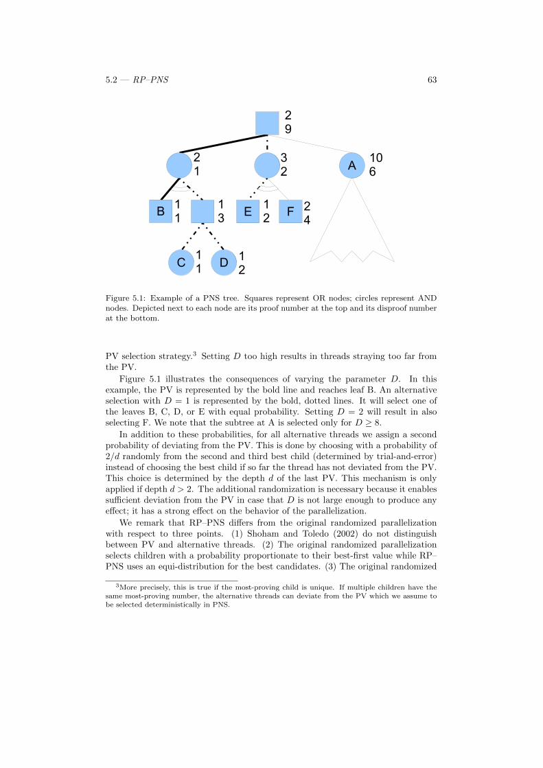
5.2 — RP–PNS 63
11
12
13
11
21
12
24
32
29
B E F
C D
A 106
Figure 5.1: Example of a PNS tree. Squares represent OR nodes; circles represent ANDnodes. Depicted next to each node are its proof number at the top and its disproof numberat the bottom.
PV selection strategy.3 Setting D too high results in threads straying too far fromthe PV.
Figure 5.1 illustrates the consequences of varying the parameter D. In thisexample, the PV is represented by the bold line and reaches leaf B. An alternativeselection with D = 1 is represented by the bold, dotted lines. It will select one ofthe leaves B, C, D, or E with equal probability. Setting D = 2 will result in alsoselecting F. We note that the subtree at A is selected only for D ≥ 8.
In addition to these probabilities, for all alternative threads we assign a secondprobability of deviating from the PV. This is done by choosing with a probability of2/d randomly from the second and third best child (determined by trial-and-error)instead of choosing the best child if so far the thread has not deviated from the PV.This choice is determined by the depth d of the last PV. This mechanism is onlyapplied if depth d > 2. The additional randomization is necessary because it enablessufficient deviation from the PV in case that D is not large enough to produce anyeffect; it has a strong effect on the behavior of the parallelization.
We remark that RP–PNS differs from the original randomized parallelizationwith respect to three points. (1) Shoham and Toledo (2002) do not distinguishbetween PV and alternative threads. (2) The original randomized parallelizationselects children with a probability proportionate to their best-first value while RP–PNS uses an equi-distribution for the best candidates. (3) The original randomized
3More precisely, this is true if the most-proving child is unique. If multiple children have thesame most-proving number, the alternative threads can deviate from the PV which we assume tobe selected deterministically in PNS.
64 Parallel Proof-Number Search
parallelization does not rely on a second probability. The differences in points 2and 3 are based on the desire to produce more deviations from the PV in order toavoid that too many threads congest the same subtree. The selection in RP–PNS issimilar to Buro’s selection of a move from an opening book (Buro, 1999).
In RP–PNS multiple threads operate on the same tree. To facilitate the parallelaccess some complications in the implementation require our attention. The nextsubsection gives details of the actual implementation of RP–PNS.
5.2.2 Implementation
As pointed out in the previous subsection, all threads in RP–PNS operate on thesame search tree held in shared memory. In order to prevent errors in the search tree,RP–PNS has to synchronize the threads. This is achieved in the implementation bya locking policy. Each tree node has a lock. It guarantees that only one threadat a time operates on the same node while avoiding deadlocks. The locking policyconsists of two parts: (1) when a thread selects a node, it has to lock it; (2) whena thread updates a node N it has to lock N and its parent. The new values for Nare computed. After N has been updated, it is released and the updating continueswith the parent.
Each node N maintains a set of flags, one for each thread, to facilitate the deletionof subtrees. Each flag indicates whether the corresponding thread is in the subtreebelow N. A thread can delete the subtree of N only if no other thread has set itsflag in N.
If a transposition table is used to store proof and disproof numbers, each tableentry needs an additional lock. The number of locks for the transposition tablecould be reduced by sharing locks for multiple entries. Similar policies have beenused in parallel Monte-Carlo Tree Search by (Chaslot et al., 2008a) (to which themaster-servant design has also been applied, cf. Cazenave and Jouandeau, 2007 and2008). Synchronization imposes a cost on RP–PNS in terms of memory and timeconsumption. The memory consumption increases due to the additional locks (pernode, 16 bytes for a spin lock and flags, cf. Chaslot et al., 2008a) in each node.
The overhead is partially a synchronization overhead and partially a search over-head. The synchronization overhead occurs whenever a thread has to wait for an-other thread due to the locking policy or due to the transposition-table locking. Thesearch overhead is created by any path that would not have been selected by thesequential PNS and that at the same time does not contribute to find the proof. Thefollowing section describes experiments that also test the overhead of RP–PNS.
5.3 Experiments
This section presents experiments and results for RP–PNS and RP–PN2. Subsection5.3.1 outlines the experimental setup, Subsection 5.3.2 shows the results obtained,and Subsection 5.3.3 discusses the findings.
5.3 — Experiments 65
5.3.1 Setup
We implemented RP–PNS as described in the previous section and tested it oncomplex endgame positions of Lines of Action (LOA).4 We chose LOA because itis an established domain for applying PNS. The test set consisting of 286 problemshas been applied before frequently (Winands et al., 2003b; Pawlewicz and Lew,2007; Van den Herik and Winands, 2008).
The experiment tests two parallelization methods: RP–PNS and RP–PN2 for 1,2, 4, and 8 threads. The combination of an algorithm with a specific number ofthreads is called a configuration and denoted by indexing the number of threads,e.g., RP–PNS8 is RP–PNS using eight threads. We remark that PNS = RP–PNS1
and PN2 = RP–PN21.
The implementation of RP–PN2 uses RP–PNS for PN1 and PNS for PN2. Thesize of PN2 was limited to Sε/T , where S is the size of the PN1 tree, T is the numberof threads used, and ε is a parameter. We set ε such that it is a compromise betweenmemory consumption and speed suitable for the test set. The compromise is fasterthan using the full S as suggested by Allis (1994). Using S for the limit slows downRP–PN2 disproportionally when many threads are used because the PN1 tree growsfaster in RP–PN2 than in the sequential PN2. Moreover, the size of PN2 growsrapidly resulting in slowing down RP–PN2. An advantage of using the above limitcompared to the method of Breuker (1998) is that the former is robust to varyingproblem sizes. The values for the parameters of RP–PNS were set to D = 5 andε = 0.75 based on trial-and-error.
The experiments were carried out on a Linux server with eight 2.66 GHz Xeoncores and 8 GB of RAM. The program was implemented in C++.
5.3.2 Results
Two series of experiments were conducted. The first series tests the efficiency ofRP–PNS; the second tests the efficiency of RP–PN2.
For comparing the efficiency of different configurations, we selected a subsetconsisting of the 143 problems for which PNS was able to find a solution in less than30 seconds. This selection enabled us to acquire the experimental results for the seriesof experiments for RP–PN2 in a reasonable time. We call the set of 143 problemsthe comparison set, S143. PNS required an average of 4.28 million evaluated nodesfor solving a problem of S143 with a standard deviation of 2.9 million nodes.
In the first series of experiments we tested the performance of RP–PNS for solvingthe positions of S143. The results regarding time, nodes evaluated, and nodes inmemory for 1, 2, 4, and 8 threads are given in the upper part of Table 5.1. We observethat the scaling factors for 2, 4, and 8 threads are 1.6, 2.5, and 3.5, respectively.Based on the results we compute that the search overhead expressed by the number ofnodes evaluated is only ca. 33% for 8 threads. This means that the synchronizationoverhead is responsible for the largest part of the total overhead. Finally, we seethat RP–PNS8 uses 50% more memory than PNS.
4The test set is available at http://www.personeel.unimaas.nl/m-winands/loa/endpos.html, “Setof 286 hard positions”.
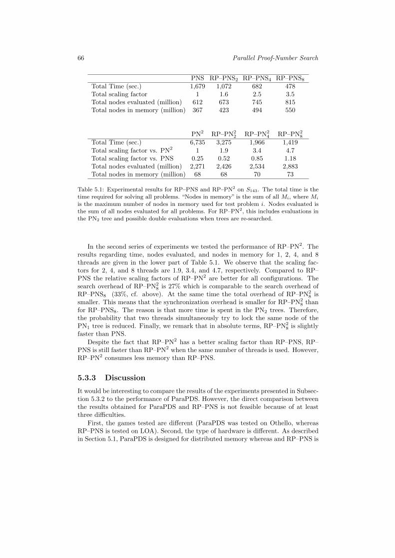
66 Parallel Proof-Number Search
PNS RP–PNS2 RP–PNS4 RP–PNS8
Total Time (sec.) 1,679 1,072 682 478Total scaling factor 1 1.6 2.5 3.5Total nodes evaluated (million) 612 673 745 815Total nodes in memory (million) 367 423 494 550
PN2 RP–PN22 RP–PN2
4 RP–PN28
Total Time (sec.) 6,735 3,275 1,966 1,419Total scaling factor vs. PN2 1 1.9 3.4 4.7Total scaling factor vs. PNS 0.25 0.52 0.85 1.18Total nodes evaluated (million) 2,271 2,426 2,534 2,883Total nodes in memory (million) 68 68 70 73
Table 5.1: Experimental results for RP–PNS and RP–PN2 on S143. The total time is thetime required for solving all problems. “Nodes in memory” is the sum of all Mi, where Mi
is the maximum number of nodes in memory used for test problem i. Nodes evaluated isthe sum of all nodes evaluated for all problems. For RP–PN2, this includes evaluations inthe PN2 tree and possible double evaluations when trees are re-searched.
In the second series of experiments we tested the performance of RP–PN2. Theresults regarding time, nodes evaluated, and nodes in memory for 1, 2, 4, and 8threads are given in the lower part of Table 5.1. We observe that the scaling fac-tors for 2, 4, and 8 threads are 1.9, 3.4, and 4.7, respectively. Compared to RP–PNS the relative scaling factors of RP–PN2 are better for all configurations. Thesearch overhead of RP–PN2
8 is 27% which is comparable to the search overhead ofRP–PNS8 (33%, cf. above). At the same time the total overhead of RP–PN2
8 issmaller. This means that the synchronization overhead is smaller for RP–PN2
8 thanfor RP–PNS8. The reason is that more time is spent in the PN2 trees. Therefore,the probability that two threads simultaneously try to lock the same node of thePN1 tree is reduced. Finally, we remark that in absolute terms, RP–PN2
8 is slightlyfaster than PNS.
Despite the fact that RP–PN2 has a better scaling factor than RP–PNS, RP–PNS is still faster than RP–PN2 when the same number of threads is used. However,RP–PN2 consumes less memory than RP–PNS.
5.3.3 Discussion
It would be interesting to compare the results of the experiments presented in Subsec-tion 5.3.2 to the performance of ParaPDS. However, the direct comparison betweenthe results obtained for ParaPDS and RP–PNS is not feasible because of at leastthree difficulties.
First, the games tested are different (ParaPDS was tested on Othello, whereasRP–PNS is tested on LOA). Second, the type of hardware is different. As describedin Section 5.1, ParaPDS is designed for distributed memory whereas and RP–PNS is
5.4 — Chapter Conclusion and Future Research 67
designed for shared memory. Third, ParaPDS is a depth-first search variant ofPNS whereas RP–PNS is not. ParaPDS is slowed down because of the transpositiontables in distributed memory.
ParaPDS and RP–PN2 both re-search in order to save memory. When compar-ing the experimental results for these two algorithms they appear to scale up in thesame order of magnitude at a superficial glance. On closer inspection, a direct com-parison of the numbers would be unfair. ParaPDS and RP–PN2 parallelize differentsequential algorithms. Furthermore, RP–PN2 parallelizes transposition tables whileour implementation of RP–PNS does not. Moreover, it can be expected that sequen-tial PN2 profits more from transposition tables than RP–PN2 because the parallelversion would suffer from additional communication and synchronization overhead.
In RP–PN2 the size of the PN2 tree determines how much the algorithm tradesspeed for memory. If the PN2 tree is too large, the penalty for searching an unim-portant subtree will be too large as well. In our implementation, we chose rathersmall PN2 trees because the randomization is imprecise. Moreover, the PN2 treesare bigger when fewer threads are used. This explains why RP–PN2 (with a scalingfactor of 4.7) scales better than RP–PNS (with a scaling factor of 3.5). A secondfactor contributing to the better scaling is the reduced synchronization overheadcompared to RP–PNS. This effect is produced by the smaller relative number ofwaiting threads.
We may speculate that RP–PNS and RP–PN2 could greatly profit from a moreprecise criterion for deviating from the PV. To that end, it is desirable to finda quick algorithm for finding the k -most-proving nodes in a proof-number searchtree. Thereby, the search could process the true best variations instead of pseudo-randomly chosen variants close to the PV.
5.4 Chapter Conclusion and Future Research
We end this chapter by summarizing the results of the experiments (Subsection 5.4.1)and giving an outlook on future research (Subsection 5.4.2) based on the findingspresented.
5.4.1 Chapter Conclusion
In this chapter, we introduced a new parallel Proof-Number Search algorithm forshared memory, called RP–PNS. The parallelization is achieved by threads that se-lect moves close to the principal variation based on a probability distribution. Fur-thermore, we adapted RP–PNS for PN2, resulting in an algorithm called RP–PN2.
The scaling factor for RP–PN2 (4.7) is even better than that of RP–PNS (3.5)but this is mainly because the size of the PN2 tree depends on the number of threadsused. Based on these results we may conclude that RP–PNS and RP–PN2 are viablefor parallelizing PNS and PN2, respectively. Strong comparative conclusions cannotbe made for ParaPDS and RP–PNS.
68 Parallel Proof-Number Search
5.4.2 Future Research
Future research will address the following four directions. (1) A combined paral-lelization at PN1 and PN2 trees of RP–PN2 will be tested on a shared-memorysystem with more cores. (2) A better distribution for guiding the move selection,possibly by including more information in the nodes, will be tested to reduce thesearch overhead. For instance, the probability of selecting a child could variablydepend on characteristics of the previous PV. (3) The concept of the k -most-provingnodes of a proof-number search tree and an algorithm for finding these nodes effi-ciently on a parallelized tree will be investigated. (4) The speedup of reducing thenumber of node locks by pooling will be investigated. In pooling multiple nodesshare the same lock and thereby reduce the number of locks used.
Chapter 6
Paranoid Proof-NumberSearch
This chapter is based on the following publication.1
• J-T. Saito and M.H.M. Winands Paranoid Proof-Number Search. In G.N. Yan-nakakis and J. Togelius, editors, Proceedings of the IEEE Conference on Computa-tional Intelligence and Games (CIG‘10), pp. 203–210, IEEE Press, 2010.
Solving algorithms have been specifically designed to tackle two-player games (cf.Van den Herik et al., 2002; Heule and Rothkrantz, 2007). The previous chapterselaborated on algorithms for solving these games. This chapter extends the scope tomulti-player games (i.e., games with more than two players). So far, the notion ofsolving in multi-player games has attracted little if any attention by the game-and-search community. By addressing this topic, we supply an answer to RQ 4: Howcan solvers be applied to multi-player games?
The standard search algorithms for multi-player games are maxn (Luckhardtand Irani, 1986) and paranoid search (Sturtevant and Korf, 2000). These searchalgorithms were designed to provide playing strength for programs but not to solvegames. Proof-Number Search (PNS) (Allis et al., 1994), however, was designedfor solving as we have seen in Chapter 2. The notion of solving in multi-playergames differs from that in two-player games. Therefore, we suggest a definition forsolving a game under the paranoid condition (Sturtevant and Korf, 2000). Underthis condition, a player assumes that all opponents form a coalition against him.Furthermore, we propose to modify PNS for solving under the paranoid condition,and call the resulting algorithm Paranoid Proof-Number Search (PPNS). We applyPPNS to small-board variants of the multi-player game of Rolit to find the optimalscores that a player can achieve.
This chapter is organized as follows. Section 6.1 explains two search algorithmsfor multi-player games, maxn and paranoid search, and introduces concepts fordescribing search in multi-player game trees. Based on these concepts, Section 6.2
1The author is grateful to IEEE for the permission to reuse relevant parts of the article in thethesis.
70 Paranoid Proof-Number Search
gives a definition for solving a position in a multi-player game and proposes thePPNS algorithm. Section 6.3 discusses how PPNS can be used to find an optimalscore. The game of Rolit, its rules and properties are outlined in Section 6.4. Section6.5 describes the experimental setup for applying PPNS to solve variants of Rolit.The results of the experiments are presented and discussed in Section 6.6. Section6.7 concludes the chapter and gives an outlook on future research.
6.1 Search Algorithms for Multi-Player Games
This section discusses two well understood search algorithms for multi-player turn-taking games, maxn (Luckhardt and Irani, 1986) and paranoid search (Sturtevantand Korf, 2000), and provides concepts for characterizing them. The section isorganized in three subsections as follows.
Subsection 6.1.1 describes maxn, a straightforward generalization of minimaxsearch suitable for multi-player games. The limitations of maxn relate to its way ofcoping with so-called equilibrium points. These are the subject of Subsection 6.1.2.Subsection 6.1.3 outlines Paranoid search which forms the basis for PPNS describedin Section 6.2.
6.1.1 The Maxn Algorithm
The maxn algorithm (Luckhardt and Irani, 1986) is a generalization of minimaxsearch to games with more than two players. It assumes that players 1, ..., n par-ticipate in a turn-taking game. Each node N in the maxn tree has an n-tuple~N = (v1, v2, ..., vn) called the maxn value of N. ~N[i] = vi represents the value ofthe game at node N for Player i. Furthermore, if Player i is to move at node N weoccasionally say that ~N[i] is the value of N (omitting that we mean “for Player i”).
If N is a leaf, the value ~N[i] is the value of Player i computed by the evaluationfunction. If N is an internal node with m children C1,...,Cm and player i to move,then N’s tuple is calculated from the children’s tuples recursively as ~N = ~Cj where~Cj is the child with the largest value for Player i among all children.
Figure 6.1 depicts a three-ply maxn tree. Player 1 moves at the root and theleaves, Player 2 at the first ply, and Player 3 at the second ply. The tuple at nodeD is based on D’s children. In this case, F offers the largest value, for Player 3, i.e.,3. (It is just the same as its sibling G’s value). All values (the whole tuple) of F aretaken over to D. Similarly, at node B, Player 2 chooses its children. Node D offersthe largest value for Player 2, namely 6. The root A takes over the tuple from nodeB because Player 1 prefers value 3 above 1.
The αβ algorithm (Knuth and Moore, 1975) is successful in two-player gamesbecause it allows pruning. In combination with move ordering αβ has proven to bea powerful tool that leads the way to success in many games, most notably in Chess(Hsu, 2002). Unfortunately, when generalizing from minimax to maxn, in spite ofthe existence of certain pruning techniques such as shallow pruning (Luckhardt andIrani, 1986), the potential of pruning is reduced considerably (Sturtevant and Korf,2000). Korf (1991) showed that shallow pruning guarantees the correct solution
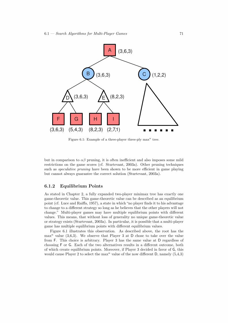
6.1 — Search Algorithms for Multi-Player Games 71
B
A
E(3,6,3)
HG
(3,6,3)
I
C
(5,4,3) (8,2,3) (2,7,1)
D
F
(3,6,3)
(3,6,3)
(1,2,2)
(8,2,3)
Figure 6.1: Example of a three-player three-ply maxn tree.
but in comparison to αβ pruning, it is often inefficient and also imposes some mildrestrictions on the game scores (cf. Sturtevant, 2003a). Other pruning techniquessuch as speculative pruning have been shown to be more efficient in game playingbut cannot always guarantee the correct solution (Sturtevant, 2003a).
6.1.2 Equilibrium Points
As stated in Chapter 2, a fully expanded two-player minimax tree has exactly onegame-theoretic value. This game-theoretic value can be described as an equilibriumpoint (cf. Luce and Raiffa, 1957), a state in which“no player finds it to his advantageto change to a different strategy so long as he believes that the other players will notchange.” Multi-player games may have multiple equilibrium points with differentvalues. This means, that without loss of generality no unique game-theoretic valueor strategy exists (Sturtevant, 2003a). In particular, it is possible that a multi-playergame has multiple equilibrium points with different equilibrium values.
Figure 6.1 illustrates this observation. As described above, the root has themaxn value (3,6,3). We observe that Player 3 at D chose to take over the valuefrom F. This choice is arbitrary. Player 3 has the same value at D regardless ofchoosing F or G. Each of the two alternatives results in a different outcome, bothof which create equilibrium points. Moreover, if Player 3 decided in favor of G, thiswould cause Player 2 to select the maxn value of the now different D, namely (5,4,3)
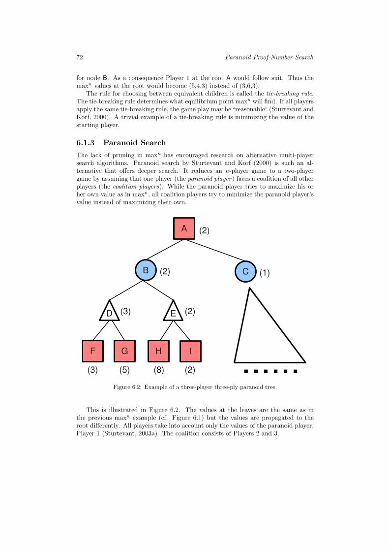
72 Paranoid Proof-Number Search
for node B. As a consequence Player 1 at the root A would follow suit. Thus themaxn values at the root would become (5,4,3) instead of (3,6,3).
The rule for choosing between equivalent children is called the tie-breaking rule.The tie-breaking rule determines what equilibrium point maxn will find. If all playersapply the same tie-breaking rule, the game play may be“reasonable”(Sturtevant andKorf, 2000). A trivial example of a tie-breaking rule is minimizing the value of thestarting player.
6.1.3 Paranoid Search
The lack of pruning in maxn has encouraged research on alternative multi-playersearch algorithms. Paranoid search by Sturtevant and Korf (2000) is such an al-ternative that offers deeper search. It reduces an n-player game to a two-playergame by assuming that one player (the paranoid player) faces a coalition of all otherplayers (the coalition players). While the paranoid player tries to maximize his orher own value as in maxn, all coalition players try to minimize the paranoid player’svalue instead of maximizing their own.
B
A
E(3)
HG
(3)
I
C
(5) (8) (2)
D
F
(1)
(2)
(2)
(2)
Figure 6.2: Example of a three-player three-ply paranoid tree.
This is illustrated in Figure 6.2. The values at the leaves are the same as inthe previous maxn example (cf. Figure 6.1) but the values are propagated to theroot differently. All players take into account only the values of the paranoid player,Player 1 (Sturtevant, 2003a). The coalition consists of Players 2 and 3.
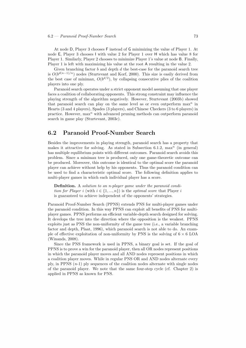
6.2 — Paranoid Proof-Number Search 73
At node D, Player 3 chooses F instead of G minimizing the value of Player 1. Atnode E, Player 3 chooses I with value 2 for Player 1 over H which has value 8 forPlayer 1. Similarly, Player 2 chooses to minimize Player 1’s value at node B. Finally,Player 1 is left with maximizing his value at the root A resulting in the value 2.
Given branching factor b and depth d the best-case for the paranoid search treeis O(bd(n−1)/n) nodes (Sturtevant and Korf, 2000). This size is easily derived fromthe best case of minimax, O(bd/2), by collapsing consecutive plies of the coalitionplayers into one ply.
Paranoid search operates under a strict opponent model assuming that one playerfaces a coalition of collaborating opponents. This strong constraint may influence theplaying strength of the algorithm negatively. However, Sturtevant (2003b) showedthat paranoid search can play on the same level as or even outperform maxn inHearts (3 and 4 players), Spades (3 players), and Chinese Checkers (3 to 6 players) inpractice. However, maxn with advanced pruning methods can outperform paranoidsearch in game play (Sturtevant, 2003c).
6.2 Paranoid Proof-Number Search
Besides the improvements in playing strength, paranoid search has a property thatmakes it attractive for solving. As stated in Subsection 6.1.2, maxn (in general)has multiple equilibrium points with different outcomes. Paranoid search avoids thisproblem. Since a minimax tree is produced, only one game-theoretic outcome canbe produced. Moreover, this outcome is identical to the optimal score the paranoidplayer can achieve without help by his opponents. Thus the paranoid condition canbe used to find a characteristic optimal score. The following definition applies tomulti-player games in which each individual player has a score.
Definition. A solution to an n-player game under the paranoid condi-tion for Player i (with i ∈ {1, ..., n}) is the optimal score that Player iis guaranteed to achieve independent of the opponents’ strategies.
Paranoid Proof-Number Search (PPNS) extends PNS for multi-player games underthe paranoid condition. In this way PPNS can exploit all benefits of PNS for multi-player games. PPNS performs an efficient variable-depth search designed for solving.It develops the tree into the direction where the opposition is the weakest. PPNSexploits just as PNS the non-uniformity of the game tree (i.e., a variable branchingfactor and depth, Plaat, 1996), which paranoid search is not able to do. An exam-ple of effective exploitation of non-uniformity by PNS is the solving of 6 × 6 LOA(Winands, 2008).
Since the PNS framework is used in PPNS, a binary goal is set. If the goal ofPPNS is to prove a win for the paranoid player, then all OR nodes represent positionsin which the paranoid player moves and all AND nodes represent positions in whicha coalition player moves. While in regular PNS OR and AND nodes alternate everyply, in PPNS (n-1) ply sequences of the coalition nodes alternate with single nodesof the paranoid player. We note that the same four-step cycle (cf. Chapter 2) isapplied in PPNS as known for PNS.
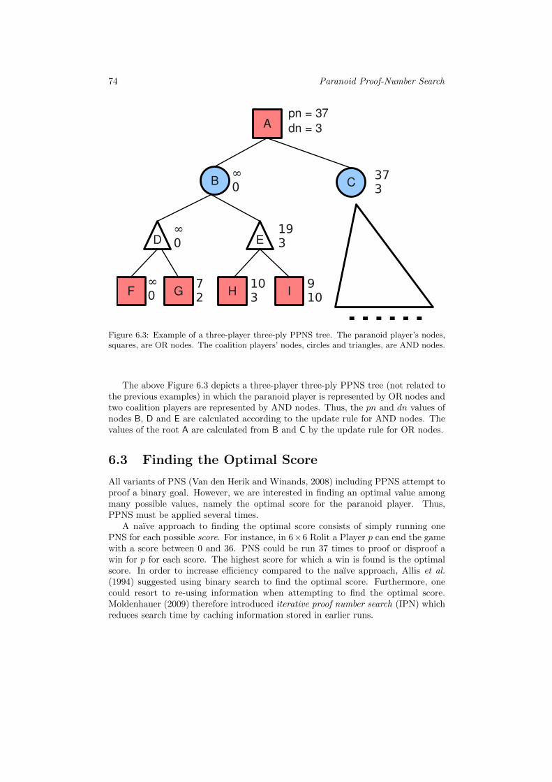
74 Paranoid Proof-Number Search
B
A
E
HG I
C
D
F
pn = 37 dn = 3
�
��
�
��
�
�
��
��
�
�
�
�
���
�
Figure 6.3: Example of a three-player three-ply PPNS tree. The paranoid player’s nodes,squares, are OR nodes. The coalition players’ nodes, circles and triangles, are AND nodes.
The above Figure 6.3 depicts a three-player three-ply PPNS tree (not related tothe previous examples) in which the paranoid player is represented by OR nodes andtwo coalition players are represented by AND nodes. Thus, the pn and dn values ofnodes B, D and E are calculated according to the update rule for AND nodes. Thevalues of the root A are calculated from B and C by the update rule for OR nodes.
6.3 Finding the Optimal Score
All variants of PNS (Van den Herik and Winands, 2008) including PPNS attempt toproof a binary goal. However, we are interested in finding an optimal value amongmany possible values, namely the optimal score for the paranoid player. Thus,PPNS must be applied several times.
A naıve approach to finding the optimal score consists of simply running onePNS for each possible score. For instance, in 6×6 Rolit a Player p can end the gamewith a score between 0 and 36. PNS could be run 37 times to proof or disproof awin for p for each score. The highest score for which a win is found is the optimalscore. In order to increase efficiency compared to the naıve approach, Allis et al.(1994) suggested using binary search to find the optimal score. Furthermore, onecould resort to re-using information when attempting to find the optimal score.Moldenhauer (2009) therefore introduced iterative proof number search (IPN) whichreduces search time by caching information stored in earlier runs.
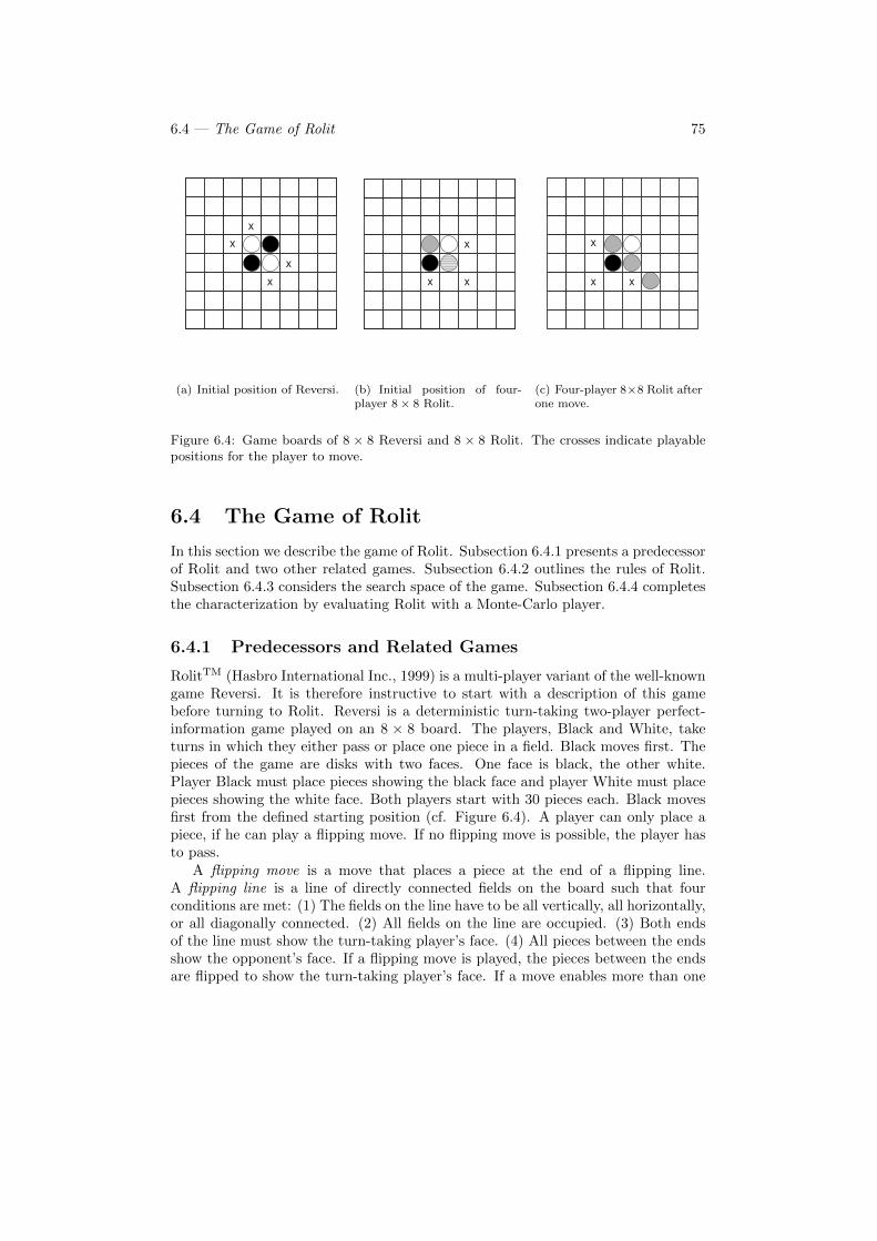
6.4 — The Game of Rolit 75
xx
xx
(a) Initial position of Reversi.
x x
x
(b) Initial position of four-player 8 × 8 Rolit.
xxx
x
(c) Four-player 8×8 Rolit afterone move.
Figure 6.4: Game boards of 8 × 8 Reversi and 8 × 8 Rolit. The crosses indicate playablepositions for the player to move.
6.4 The Game of Rolit
In this section we describe the game of Rolit. Subsection 6.4.1 presents a predecessorof Rolit and two other related games. Subsection 6.4.2 outlines the rules of Rolit.Subsection 6.4.3 considers the search space of the game. Subsection 6.4.4 completesthe characterization by evaluating Rolit with a Monte-Carlo player.
6.4.1 Predecessors and Related Games
RolitTM (Hasbro International Inc., 1999) is a multi-player variant of the well-knowngame Reversi. It is therefore instructive to start with a description of this gamebefore turning to Rolit. Reversi is a deterministic turn-taking two-player perfect-information game played on an 8 × 8 board. The players, Black and White, taketurns in which they either pass or place one piece in a field. Black moves first. Thepieces of the game are disks with two faces. One face is black, the other white.Player Black must place pieces showing the black face and player White must placepieces showing the white face. Both players start with 30 pieces each. Black movesfirst from the defined starting position (cf. Figure 6.4). A player can only place apiece, if he can play a flipping move. If no flipping move is possible, the player hasto pass.
A flipping move is a move that places a piece at the end of a flipping line.A flipping line is a line of directly connected fields on the board such that fourconditions are met: (1) The fields on the line have to be all vertically, all horizontally,or all diagonally connected. (2) All fields on the line are occupied. (3) Both endsof the line must show the turn-taking player’s face. (4) All pieces between the endsshow the opponent’s face. If a flipping move is played, the pieces between the endsare flipped to show the turn-taking player’s face. If a move enables more than one
76 Paranoid Proof-Number Search
flipping line, all affected opponent’s pieces have to be flipped.
The game ends if either (a) one player runs out of his or her 30 pieces, or (b) bothplayers pass consecutively. When the game has ended, Black’s score is the numberof pieces showing the black face, and White’s score is the number of pieces showingthe white face. The player with the higher score wins. If both players have the samescore the game is a draw. We note that pieces which have been played remain onthe board until the end of the game.
In the Reversi variant called Othello, there is no limit to the players’ number ofpieces. Thus the game ends in either of two cases: (a) the board is filled, or (b) bothplayers pass consecutively (i.e., no player can make a flipping move).
Fujii et al. (2006) proposed 4-player Reversi Yonin (Yonin). With the exceptionof Rolit, it is the only multi-player variant of Reversi. This variant is played byexactly four players. Two of them, Players A and C, place pieces showing theblack face and the other two, Players B and D, place pieces with the white faceup. The players take turns in the order A, B, C, D and the board is separatedinto quarters. Each player owns exactly one quarter. Players of the same color ownquarters diagonally opposing each other. The game is played and scored like Reversi,but there are two deviations. First, a player may not place a piece in the diagonallyopposing quarter. Thus the branching factor for the 8 × 8 board is reduced fromca. 8.5 to ca. 6.3 (Fujii et al., 2006). Second, in the end, a Player p’s score isdetermined by counting the usual way but only in the quarter owned by P. (Wenote that 4-player Reversi Yonin can also be played in teams of two players each. Inthat case, the teams are A and C versus B and D). Fujii et al. (2006) studied theproperties of 6× 6 and 8× 8 Yonin empirically by applying Monte-Carlo evaluation.
6.4.2 Rules of Rolit
Rolit is a straightforward multi-player generalization of Reversi. Instead of diskswith two faces, balls with four different-colored quarter spheres are placed. Corre-spondingly, up to four players can play Rolit, each placing his characteristic colorfacing up. The four players are Red, Green, Yellow, and Blue.
Red always moves first. Depending on how many players participate (two, three,or four), the following orders are applied for turn-taking;
2 players: (1) Red, (2) Green;
3 players: (1) Red, (2) Yellow, (3) Green;
4 players: (1) Red, (2) Yellow, (3) Green, (4) Blue.
Irrespective of the number of players participating, Rolit is always played withthe same starting position shown in the center diagram of Figure 6.4.
In Rolit, one player’s color can be completely eliminated from the board by theopponent’s flipping moves. In order to allow a player who has no piece left onthe board to come back into the game, the rules are changed compared to Reversi.Reversi’s passing rule is replaced by Rolit’s free-choice rule: a player who cannot
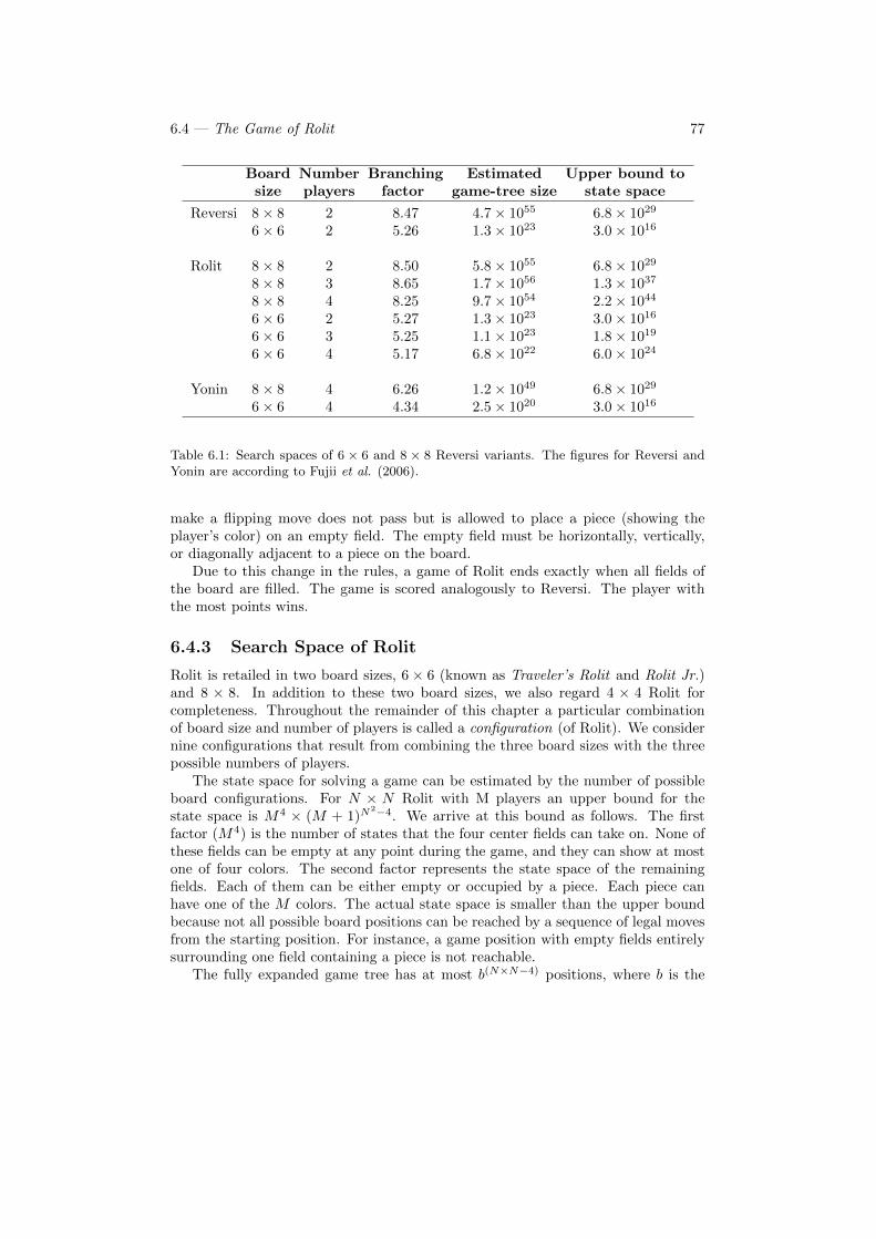
6.4 — The Game of Rolit 77
Board Number Branching Estimated Upper bound tosize players factor game-tree size state space
Reversi 8× 8 2 8.47 4.7× 1055 6.8× 1029
6× 6 2 5.26 1.3× 10²³ 3.0× 10¹⁶
Rolit 8× 8 2 8.50 5.8× 1055 6.8× 1029
8× 8 3 8.65 1.7× 1056 1.3× 1037
8× 8 4 8.25 9.7× 1054 2.2× 1044
6× 6 2 5.27 1.3× 10²³ 3.0× 10¹⁶
6× 6 3 5.25 1.1× 10²³ 1.8× 10¹⁹
6× 6 4 5.17 6.8× 10²² 6.0× 1024
Yonin 8× 8 4 6.26 1.2× 1049 6.8× 1029
6× 6 4 4.34 2.5× 10²⁰ 3.0× 10¹⁶
Table 6.1: Search spaces of 6 × 6 and 8 × 8 Reversi variants. The figures for Reversi andYonin are according to Fujii et al. (2006).
make a flipping move does not pass but is allowed to place a piece (showing theplayer’s color) on an empty field. The empty field must be horizontally, vertically,or diagonally adjacent to a piece on the board.
Due to this change in the rules, a game of Rolit ends exactly when all fields ofthe board are filled. The game is scored analogously to Reversi. The player withthe most points wins.
6.4.3 Search Space of Rolit
Rolit is retailed in two board sizes, 6 × 6 (known as Traveler’s Rolit and Rolit Jr.)and 8 × 8. In addition to these two board sizes, we also regard 4 × 4 Rolit forcompleteness. Throughout the remainder of this chapter a particular combinationof board size and number of players is called a configuration (of Rolit). We considernine configurations that result from combining the three board sizes with the threepossible numbers of players.
The state space for solving a game can be estimated by the number of possibleboard configurations. For N × N Rolit with M players an upper bound for thestate space is M4 × (M + 1)N
2−4. We arrive at this bound as follows. The firstfactor (M4) is the number of states that the four center fields can take on. None ofthese fields can be empty at any point during the game, and they can show at mostone of four colors. The second factor represents the state space of the remainingfields. Each of them can be either empty or occupied by a piece. Each piece canhave one of the M colors. The actual state space is smaller than the upper boundbecause not all possible board positions can be reached by a sequence of legal movesfrom the starting position. For instance, a game position with empty fields entirelysurrounding one field containing a piece is not reachable.
The fully expanded game tree has at most b(N×N−4) positions, where b is the
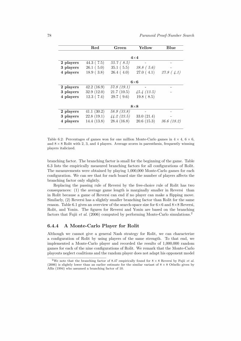
78 Paranoid Proof-Number Search
Red Green Yellow Blue
4×42 players 44.3 ( 7.5) 55.7 ( 8.5) - -3 players 26.1 ( 5.0) 35.1 ( 5.5) 38.8 ( 5.6) -4 players 18.9 ( 3.8) 26.4 ( 4.0) 27.0 ( 4.1) 27.8 ( 4.1)
6×62 players 42.2 (16.9) 57.8 (19.1) - -3 players 32.9 (12.0) 21.7 (10.5) 45.4 (13.5) -4 players 12.3 ( 7.4) 29.7 ( 9.6) 19.8 ( 8.5)
8×82 players 41.1 (30.2) 58.9 (33.8) - -3 players 22.8 (19.1) 44.2 (23.5) 33.0 (21.4) -4 players 14.4 (13.8) 28.4 (16.8) 20.6 (15.3) 36.6 (18.2)
Table 6.2: Percentages of games won for one million Monte-Carlo games in 4 × 4, 6 × 6,and 8 × 8 Rolit with 2, 3, and 4 players. Average scores in parenthesis, frequently winningplayers italicized.
branching factor. The branching factor is small for the beginning of the game. Table6.3 lists the empirically measured branching factors for all configurations of Rolit.The measurements were obtained by playing 1,000,000 Monte-Carlo games for eachconfiguration. We can see that for each board size the number of players affects thebranching factor only slightly.
Replacing the passing rule of Reversi by the free-choice rule of Rolit has twoconsequences: (1) the average game length is marginally smaller in Reversi thanin Rolit because a game of Reversi can end if no player can make a flipping move.Similarly, (2) Reversi has a slightly smaller branching factor than Rolit for the samereason. Table 6.1 gives an overview of the search-space size for 6×6 and 8×8 Reversi,Rolit, and Yonin. The figures for Reversi and Yonin are based on the branchingfactors that Fujii et al. (2006) computed by performing Monte-Carlo simulations.2
6.4.4 A Monte-Carlo Player for Rolit
Although we cannot give a general Nash strategy for Rolit, we can characterizea configuration of Rolit by using players of the same strength. To that end, weimplemented a Monte-Carlo player and recorded the results of 1,000,000 randomgames for each of the nine configurations of Rolit. We remark that the Monte-Carloplayouts neglect coalitions and the random player does not adapt his opponent model
2We note that the branching factor of 8.47 empirically found for 8 × 8 Reversi by Fujii et al.(2006) is slightly lower than an earlier estimate for the similar variant of 8 × 8 Othello given byAllis (1994) who assumed a branching factor of 10.
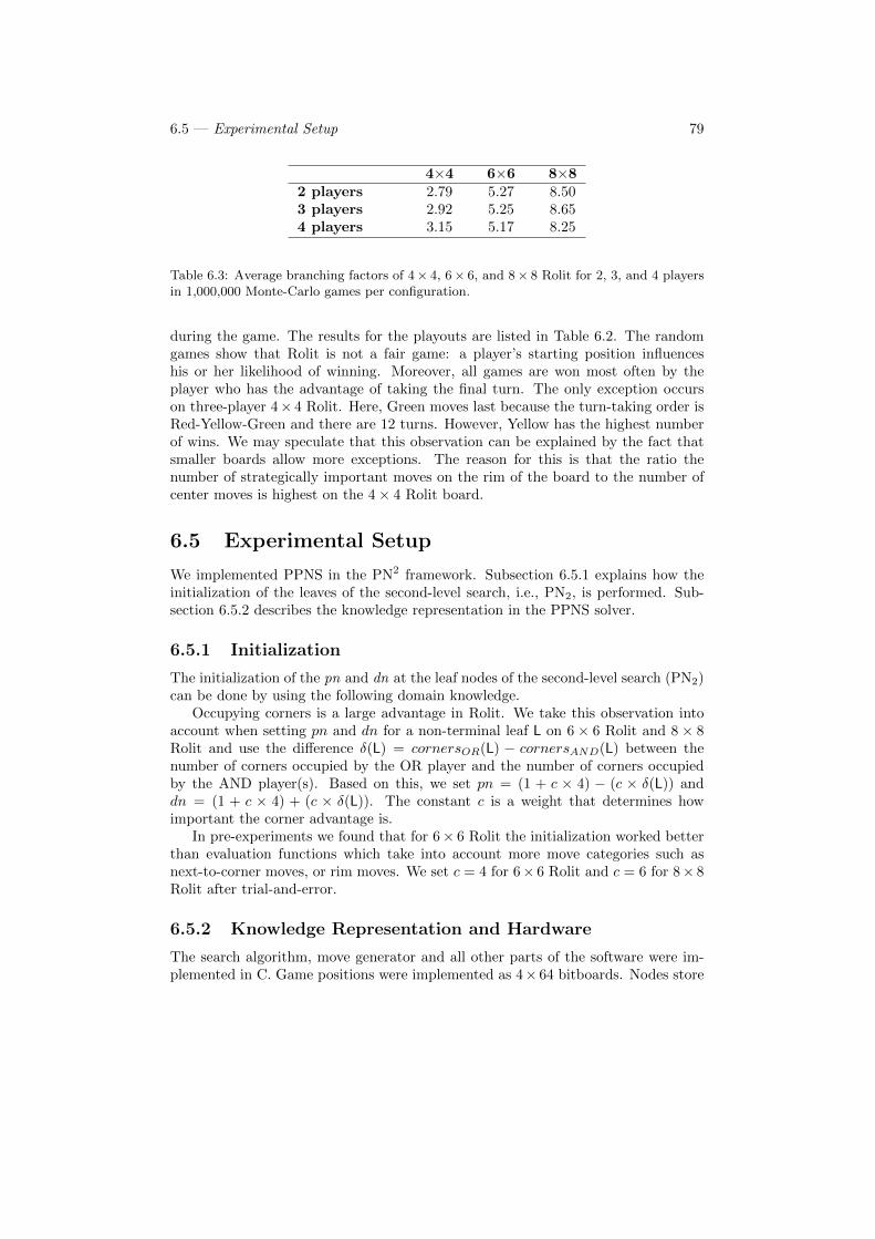
6.5 — Experimental Setup 79
4×4 6×6 8×82 players 2.79 5.27 8.503 players 2.92 5.25 8.654 players 3.15 5.17 8.25
Table 6.3: Average branching factors of 4× 4, 6× 6, and 8× 8 Rolit for 2, 3, and 4 playersin 1,000,000 Monte-Carlo games per configuration.
during the game. The results for the playouts are listed in Table 6.2. The randomgames show that Rolit is not a fair game: a player’s starting position influenceshis or her likelihood of winning. Moreover, all games are won most often by theplayer who has the advantage of taking the final turn. The only exception occurson three-player 4× 4 Rolit. Here, Green moves last because the turn-taking order isRed-Yellow-Green and there are 12 turns. However, Yellow has the highest numberof wins. We may speculate that this observation can be explained by the fact thatsmaller boards allow more exceptions. The reason for this is that the ratio thenumber of strategically important moves on the rim of the board to the number ofcenter moves is highest on the 4× 4 Rolit board.
6.5 Experimental Setup
We implemented PPNS in the PN2 framework. Subsection 6.5.1 explains how theinitialization of the leaves of the second-level search, i.e., PN2, is performed. Sub-section 6.5.2 describes the knowledge representation in the PPNS solver.
6.5.1 Initialization
The initialization of the pn and dn at the leaf nodes of the second-level search (PN2)can be done by using the following domain knowledge.
Occupying corners is a large advantage in Rolit. We take this observation intoaccount when setting pn and dn for a non-terminal leaf L on 6 × 6 Rolit and 8 × 8Rolit and use the difference δ(L) = cornersOR(L) − cornersAND(L) between thenumber of corners occupied by the OR player and the number of corners occupiedby the AND player(s). Based on this, we set pn = (1 + c × 4) − (c × δ(L)) anddn = (1 + c × 4) + (c × δ(L)). The constant c is a weight that determines howimportant the corner advantage is.
In pre-experiments we found that for 6× 6 Rolit the initialization worked betterthan evaluation functions which take into account more move categories such asnext-to-corner moves, or rim moves. We set c = 4 for 6× 6 Rolit and c = 6 for 8× 8Rolit after trial-and-error.
6.5.2 Knowledge Representation and Hardware
The search algorithm, move generator and all other parts of the software were im-plemented in C. Game positions were implemented as 4× 64 bitboards. Nodes store
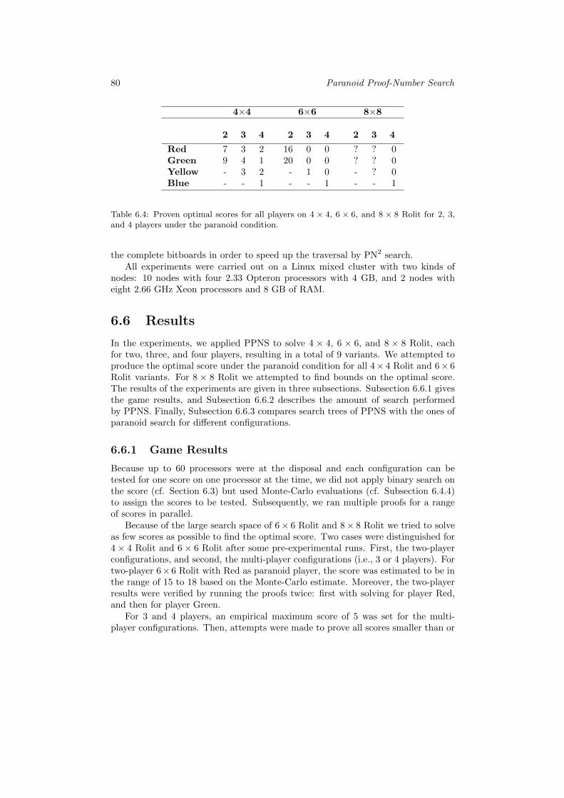
80 Paranoid Proof-Number Search
4×4 6×6 8×8
2 3 4 2 3 4 2 3 4
Red 7 3 2 16 0 0 ? ? 0Green 9 4 1 20 0 0 ? ? 0Yellow - 3 2 - 1 0 - ? 0Blue - - 1 - - 1 - - 1
Table 6.4: Proven optimal scores for all players on 4 × 4, 6 × 6, and 8 × 8 Rolit for 2, 3,and 4 players under the paranoid condition.
the complete bitboards in order to speed up the traversal by PN2 search.All experiments were carried out on a Linux mixed cluster with two kinds of
nodes: 10 nodes with four 2.33 Opteron processors with 4 GB, and 2 nodes witheight 2.66 GHz Xeon processors and 8 GB of RAM.
6.6 Results
In the experiments, we applied PPNS to solve 4 × 4, 6 × 6, and 8 × 8 Rolit, eachfor two, three, and four players, resulting in a total of 9 variants. We attempted toproduce the optimal score under the paranoid condition for all 4× 4 Rolit and 6× 6Rolit variants. For 8 × 8 Rolit we attempted to find bounds on the optimal score.The results of the experiments are given in three subsections. Subsection 6.6.1 givesthe game results, and Subsection 6.6.2 describes the amount of search performedby PPNS. Finally, Subsection 6.6.3 compares search trees of PPNS with the ones ofparanoid search for different configurations.
6.6.1 Game Results
Because up to 60 processors were at the disposal and each configuration can betested for one score on one processor at the time, we did not apply binary search onthe score (cf. Section 6.3) but used Monte-Carlo evaluations (cf. Subsection 6.4.4)to assign the scores to be tested. Subsequently, we ran multiple proofs for a rangeof scores in parallel.
Because of the large search space of 6× 6 Rolit and 8× 8 Rolit we tried to solveas few scores as possible to find the optimal score. Two cases were distinguished for4× 4 Rolit and 6× 6 Rolit after some pre-experimental runs. First, the two-playerconfigurations, and second, the multi-player configurations (i.e., 3 or 4 players). Fortwo-player 6× 6 Rolit with Red as paranoid player, the score was estimated to be inthe range of 15 to 18 based on the Monte-Carlo estimate. Moreover, the two-playerresults were verified by running the proofs twice: first with solving for player Red,and then for player Green.
For 3 and 4 players, an empirical maximum score of 5 was set for the multi-player configurations. Then, attempts were made to prove all scores smaller than or
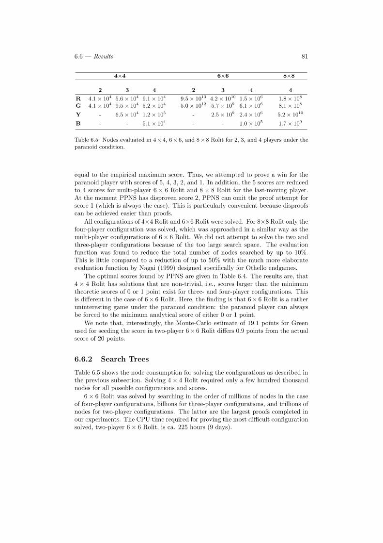
6.6 — Results 81
4×4 6×6 8×8
2 3 4 2 3 4 4
R 4.1 × 10⁴ 5.6 × 10⁴ 9.1 × 10⁴ 9.5 × 10¹³ 4.2 × 10¹⁰ 1.5 × 10⁶ 1.8 × 10⁸
G 4.1 × 10⁴ 9.5 × 10⁴ 5.2 × 10⁴ 5.0 × 10¹² 5.7 × 10⁹ 6.1 × 10⁶ 8.1 × 10⁸
Y - 6.5 × 10⁴ 1.2 × 10⁵ - 2.5 × 10⁹ 2.4 × 10⁶ 5.2 × 10¹⁰
B - - 5.1 × 10⁴ - - 1.0 × 10⁵ 1.7 × 10⁹
Table 6.5: Nodes evaluated in 4× 4, 6× 6, and 8× 8 Rolit for 2, 3, and 4 players under theparanoid condition.
equal to the empirical maximum score. Thus, we attempted to prove a win for theparanoid player with scores of 5, 4, 3, 2, and 1. In addition, the 5 scores are reducedto 4 scores for multi-player 6 × 6 Rolit and 8 × 8 Rolit for the last-moving player.At the moment PPNS has disproven score 2, PPNS can omit the proof attempt forscore 1 (which is always the case). This is particularly convenient because disproofscan be achieved easier than proofs.
All configurations of 4×4 Rolit and 6×6 Rolit were solved. For 8×8 Rolit only thefour-player configuration was solved, which was approached in a similar way as themulti-player configurations of 6× 6 Rolit. We did not attempt to solve the two andthree-player configurations because of the too large search space. The evaluationfunction was found to reduce the total number of nodes searched by up to 10%.This is little compared to a reduction of up to 50% with the much more elaborateevaluation function by Nagai (1999) designed specifically for Othello endgames.
The optimal scores found by PPNS are given in Table 6.4. The results are, that4 × 4 Rolit has solutions that are non-trivial, i.e., scores larger than the minimumtheoretic scores of 0 or 1 point exist for three- and four-player configurations. Thisis different in the case of 6× 6 Rolit. Here, the finding is that 6× 6 Rolit is a ratheruninteresting game under the paranoid condition: the paranoid player can alwaysbe forced to the minimum analytical score of either 0 or 1 point.
We note that, interestingly, the Monte-Carlo estimate of 19.1 points for Greenused for seeding the score in two-player 6× 6 Rolit differs 0.9 points from the actualscore of 20 points.
6.6.2 Search Trees
Table 6.5 shows the node consumption for solving the configurations as described inthe previous subsection. Solving 4× 4 Rolit required only a few hundred thousandnodes for all possible configurations and scores.
6× 6 Rolit was solved by searching in the order of millions of nodes in the caseof four-player configurations, billions for three-player configurations, and trillions ofnodes for two-player configurations. The latter are the largest proofs completed inour experiments. The CPU time required for proving the most difficult configurationsolved, two-player 6× 6 Rolit, is ca. 225 hours (9 days).
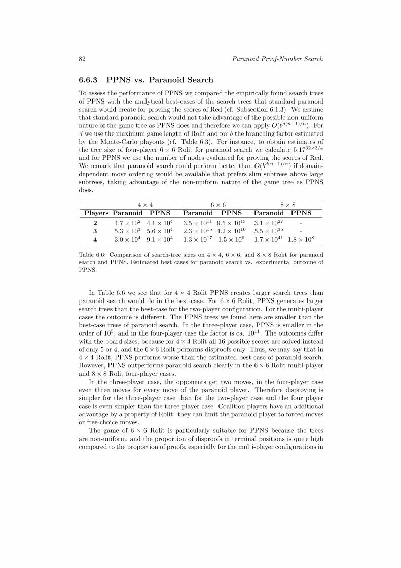
82 Paranoid Proof-Number Search
6.6.3 PPNS vs. Paranoid Search
To assess the performance of PPNS we compared the empirically found search treesof PPNS with the analytical best-cases of the search trees that standard paranoidsearch would create for proving the scores of Red (cf. Subsection 6.1.3). We assumethat standard paranoid search would not take advantage of the possible non-uniformnature of the game tree as PPNS does and therefore we can apply O(bd(n−1)/n). Ford we use the maximum game length of Rolit and for b the branching factor estimatedby the Monte-Carlo playouts (cf. Table 6.3). For instance, to obtain estimates ofthe tree size of four-player 6 × 6 Rolit for paranoid search we calculate 5.1732×3/4
and for PPNS we use the number of nodes evaluated for proving the scores of Red.We remark that paranoid search could perform better than O(bd(n−1)/n) if domain-dependent move ordering would be available that prefers slim subtrees above largesubtrees, taking advantage of the non-uniform nature of the game tree as PPNSdoes.
4× 4 6× 6 8× 8Players Paranoid PPNS Paranoid PPNS Paranoid PPNS
2 4.7× 10² 4.1× 10⁴ 3.5× 10¹¹ 9.5× 10¹³ 3.1× 1027 -3 5.3× 10³ 5.6× 10⁴ 2.3× 10¹⁵ 4.2× 10¹⁰ 5.5× 1035 -4 3.0× 10⁴ 9.1× 10⁴ 1.3× 10¹⁷ 1.5× 10⁶ 1.7× 1041 1.8× 10⁸
Table 6.6: Comparison of search-tree sizes on 4 × 4, 6 × 6, and 8 × 8 Rolit for paranoidsearch and PPNS. Estimated best cases for paranoid search vs. experimental outcome ofPPNS.
In Table 6.6 we see that for 4 × 4 Rolit PPNS creates larger search trees thanparanoid search would do in the best-case. For 6 × 6 Rolit, PPNS generates largersearch trees than the best-case for the two-player configuration. For the multi-playercases the outcome is different. The PPNS trees we found here are smaller than thebest-case trees of paranoid search. In the three-player case, PPNS is smaller in theorder of 105, and in the four-player case the factor is ca. 1011. The outcomes differwith the board sizes, because for 4× 4 Rolit all 16 possible scores are solved insteadof only 5 or 4, and the 6×6 Rolit performs disproofs only. Thus, we may say that in4× 4 Rolit, PPNS performs worse than the estimated best-case of paranoid search.However, PPNS outperforms paranoid search clearly in the 6× 6 Rolit multi-playerand 8× 8 Rolit four-player cases.
In the three-player case, the opponents get two moves, in the four-player caseeven three moves for every move of the paranoid player. Therefore disproving issimpler for the three-player case than for the two-player case and the four playercase is even simpler than the three-player case. Coalition players have an additionaladvantage by a property of Rolit: they can limit the paranoid player to forced movesor free-choice moves.
The game of 6 × 6 Rolit is particularly suitable for PPNS because the treesare non-uniform, and the proportion of disproofs in terminal positions is quite highcompared to the proportion of proofs, especially for the multi-player configurations in
6.7 — Chapter Conclusion and Future Research 83
which only disproofs can be made. Here, PPNS profits from disproving the paranoidplayer at every OR node by a single disproof for each of its three-level subtrees ofAND nodes. Moreover, the prior Monte-Carlo estimates reduce the considered 37scores for solving to only 5. In addition to that, the most difficult proof, i.e., the proofof the analytical minimum for the player moving last in multi-player configurationscould be omitted (because it could be inferred) reducing the scores to be proved to4. We may therefore state that Rolit can be regarded as a benign game for solvingunder the paranoid condition.
6.7 Chapter Conclusion and Future Research
We end this chapter by summarizing the results of experiments (Subsection 6.7.1)and giving an outlook on future research (Subsection 6.7.2) based on the findingspresented.
6.7.1 Chapter Conclusion
In this chapter, we introduced the notion of solving multi-player games under theparanoid condition and the PPNS algorithm for solving multi-player games underthe paranoid condition. We described the multi-player variant of Reversi, Rolit,and applied PPNS to solve 4 × 4 and 6 × 6 Rolit for three and for four players aswell as 8 × 8 Rolit for four players. The outcome is that in 4 × 4 Rolit under theparanoid condition some players can achieve more than the minimum score whilein 6 × 6 and 8 × 8 Rolit (for four players) no player can achieve more than theminimum score. Moreover, we observed that for 6 × 6 Rolit and four-player 8 × 8Rolit PPNS performed better than we would expect from standard paranoid search.We may conclude that PPNS was able to exploit the non-uniformity of the gametree in multi-player games.
6.7.2 Future Research
Based on our results for 6 × 6 Rolit we may speculate that the result for solvingthree-player 8×8 Rolit will be analogous to the results for 6×6 Rolit, i.e., no playercan achieve a score higher than 0 (or 1 for the player moving last). Moreover, thetask of finding games that are more interesting than Rolit, i.e., more like in 4 × 4Rolit than in 6 × 6 Rolit, remains. Such games may also be more interesting forhuman players. We might speculate that non-square versions of Rolit might exhibitsuch properties.
The challenge of solving three-player 8 × 8 Rolit remains for the future. Paral-lelization of PPNS and a better evaluation function may at best give bounds on theoptimal scores for 8× 8 Rolit under the paranoid condition.

84 Paranoid Proof-Number Search
Chapter 7
Conclusions and FutureResearch
In this thesis we investigated solving algorithms for games and game positions. Inspite of AI programs becoming stronger at playing games, the task of solving gamesstill remains difficult. Our research utilizes the current developments in the rapidlydeveloping field of Monte-Carlo methods for game-tree search and the continuouslyevolving field of Proof-Number Search to develop new solving algorithms. The re-search was guided by the problem statement formulated in Section 1.3 which alsoprovided four research questions addressing the problem statement. In this chap-ter we formulate conclusions and recommendations for future research based on ourwork.
Section 7.1 revisits the four research questions one by one and consequentiallyformulates an answer to the problem statement in Section 7.2. Finally, Section 7.3suggest directions for future research.
7.1 Conclusions on the Research Questions
The four research questions stated in Chapter 1 concern four topics central to solvinggame positions with forward search. More precisely, the four questions deal withthe following topics that are part of the recent progress in game-tree search: (1)search with Monte-Carlo evaluation, (2) Monte-Carlo Tree Search, (3) parallelizedsearch, and (4) search for multi-player games. The four questions are revisited inthe following subsections.
7.1.1 Monte-Carlo Evaluation
Our research question RQ 1 addressed in Chapter 3 was as follows.
RQ 1 How can we use Monte-Carlo evaluation to improve Proof-Number Search forsolving game positions?
86 Conclusions and Future Research
Chapter 3 introduced a new algorithm, MC-PNS, based on Monte-Carlo evalu-ation (MCE) within the Proof-Number Search (PNS) framework. An application ofthe new algorithm and several of its variants to the life-and-death sub-problem ofGo were described. It was demonstrated experimentally that given the right settingof parameters MC-PNS outperforms simple PNS. For such a setting, MC-PNS is onaverage two times faster than PNS and expands four times fewer nodes. We fur-thermore compared MC-PNS with a pattern-based heuristic for initialization, calledPNSp, and observed that MCE initializes proof and disproof numbers of leaves inPNS better than small patterns. We concluded that the reason for the superior per-formance of MC-PNS is the flexibility of the MCE. In conclusion, we answer RQ 1by stating that MC-PNS constitutes a genuine improvement of PNS that uses MCEto enhance the initialization of proof and disproof numbers.
7.1.2 Monte-Carlo Tree Search Solver
The research question addressed by Chapter 4 was as follows.
RQ 2 How can the Monte-Carlo Tree Search framework contribute to solving gamepositions?
In Chapter 4 we introduced a new Monte-Carlo Tree Search (MCTS) variant,called MCTS-Solver. It adapts the recently developed MCTS framework for solvinggame positions. MCTS-Solver differs from the traditional MCTS approach in thatit can solve positions by proving game-theoretic values. As a result it convergesmuch faster to the best move in narrow tactical lines. We discussed four selectionstrategies: UCT, “classic” Progressive Bias (PB), and two enhanced PB variants:PB-L1 and PB-L2. Experiments in LOA revealed that PB-L2, which takes thenumber of losses into account, solved the most positions and was the fastest: itsolved positions in three times less time than UCT. When comparing MCTS-Solverto αβ search, MCTS-Solver required about the same effort as αβ to solve positions.However, PN2 was in general 5 times faster than MCTS-Solver. Finally, we foundempirically that tree parallelization for MCTS-Solver has a scaling factor of 4 with8 threads, easily outperforming root parallelization. Thus we may say, that at leastduring game-play (online) MCTS-Solver is comparable with a standard αβ searchin solving positions. However, for off-line solving positions, PNS is still a betterchoice. Finally, we concluded that the strength of MCTS-Solver is dependent onenhancements such as PB. Just as for αβ, search enhancements are crucial for theperformance. Chapter 4 answers RQ 2 question by introducing MCTS-Solver andapplying it to solving game positions.
7.1.3 Parallel Proof-Number Search
The research question addressed by Chapter 5 was as follows.
RQ 3 How can Proof-Number Search be parallelized?
Chapter 5 introduced a parallel Proof-Number Search algorithm for shared mem-ory, called RP–PNS. The parallelization is achieved by threads that select moves
7.2 — Conclusions on the Problem Statement 87
close to the principal variation based on a probability distribution. Furthermore,we adapted RP–PNS for PN2, resulting in an algorithm called RP–PN2. The algo-rithms were tested on LOA positions. For eight threads, the scaling factor foundfor RP–PN2 (4.7) was even better than that of RP–PNS (3.5) but this was mainlybecause the size of the second-level (i.e., PN2) tree depends on the number of threadsused. Based on these results we may conclude that RP–PNS and RP–PN2 are viablefor parallelizing PNS and PN2, respectively. The chapter answers RQ 5 by propos-ing RP–PNS and RP–PN2 which parallelize Proof-Number Search, and describesthe performance of the parallel algorithms.
7.1.4 Paranoid Proof-Number Search
The research question addressed in Chapter 6 was as follows.
RQ 4 How can Proof-Number Search be applied to multi-player games?
The starting point of Chapter 4 was the observation that many two-player gameshave been solved but so far little if any research has been devoted to solving multi-player games. We identified as a reason for this observation that multi-player gamesgenerally do not have a unique game-theoretic value or best strategy because theirsearch trees have multiple equilibrium points. Therefore, the straightforward wayof solving a game by finding the outcome under optimal play (that is applied intwo-player games) cannot be applied to multi-player games directly. We thereforeproposed solving multi-player games under the paranoid condition. This is equivalentto finding the optimal score that a player can achieve independently of the otherplayers’ strategies. We then proposed Paranoid Proof-Number Search (PPNS) forsolving multi-player games under the paranoid condition. In doing so, we made aconstructive contribution to the originally still open question formulated in RQ 4.
Furthermore, we described the multi-player variant of Reversi, Rolit, and appliedPPNS to solve various multi-player versions of 4× 4 and 6× 6 Rolit, and four-player8× 8 Rolit. The outcome was that in 4× 4 Rolit under the paranoid condition someplayers can achieve more than the minimum score while in 6× 6 Rolit and in four-player 8×8 Rolit no player can achieve more than the minimum score. Moreover, weobserved that for 6×6 Rolit and four-player 8×8 Rolit PPNS performed better thanwe would expect from standard paranoid search. We may conclude that PPNS isable to exploit the non-uniformity of the game tree in multi-player games.
Our answer to RQ 4 is that multi-player games can be solved by finding the bestscore under the paranoid condition and provided PPNS for finding this score.
7.2 Conclusions on the Problem Statement
Our problem statement was as follows.
PS How can we improve forward search for solving game positions?
Taking the answers to the research questions above into account we see that thereare several new ways of utilizing the recently so successful Monte-Carlo methods for
88 Conclusions and Future Research
solving game positions, and of tackling open questions related to Proof-NumberSearch for solving game positions. We introduced algorithms that demonstrated(1) how Monte-Carlo evaluation can be used for solving (MC-PNS), (2) how Monte-Carlo Tree Search can be adapted for solving (MCTS-Solver), (3) how Proof-NumberSearch and its two-level variant PN2 can be parallelized (RP–PNS, RP–PN2), and(4) how Proof-Number Search can be used for solving multi-player games (PPNS).
7.3 Recommendations for Future Research
We complete this chapter by listing recommendations for future research groupedby the four algorithms suggested in this thesis.
1. MC-PNS. The proposed algorithm, MC-PNS, performed well in the domainof Go in which MCE proved to be useful. Future research should investigatethe feasibility of the approach in other solving scenarios which have binarygoals and can be searched by AND/OR trees. In particular, it would be ofgreat interest to investigate whether MC-PNS could be successfully applied toone-player games or multi-player games.
2. MCTS-Solver. With continuing improvements it is not unlikely that en-hanced Monte-Carlo-based approaches may even become an alternative toPNS. As future research, experiments are envisaged in other games to test theperformance of MCTS-Solver. One possible next step is testing the method inGo, a domain in which MCTS is already widely used. What makes this a some-what more difficult task is that additional work is required in enabling perfectendgame knowledge – such as Benson’s Algorithm (Benson, 1988; Van derWerf et al., 2003) – in MCTS.
3. Parallel Proof-Number Search. Randomized Parallel PNS could still beimproved in several ways. First, a combined parallelization at PN1 and PN2
trees of RP–PN2 will be tested on a shared-memory system with more cores.Second, a better distribution for guiding the move selection, possibly by in-cluding more information in the nodes, will be tested to reduce the searchoverhead. Third, the speedup of reducing the number of node locks by poolingwill be investigated. Fourth, the concept of the k -most-proving nodes of aproof-number search tree and an algorithm for finding these nodes efficientlyfor a parallelized tree could be investigated and then applied to parallelizingwith a master-servant framework for PNS.
4. Paranoid Proof-Number Search. The challenge of solving three-player8 × 8 Rolit remains for the future. Parallelization and integration of a bet-ter evaluation function will give bounds on the scores for three-player 8 × 8Rolit under the paranoid condition. Moreover, Paranoid PNS could be appliedfor solving other more interesting games under the paranoid condition. Para-noid PNS gives an answer to how game positions can be solved in multi-playergames.

7.3 — Recommendations for Future Research 89
This thesis has contributed to the challenge of solving game positions by im-proving Monte-Carlo methods for search and proof-number algorithms. While weprovided PPNS in order to address the class of deterministic multi-player games withperfect information, solving deterministic multi-player games with imperfect infor-mation is still a challenge. We speculate that devising a combination of methodsproposed and investigated in this thesis such as parallelization with PPNS, or Para-noid PNS for solving multi-player games under the paranoid condition, with methodsused for solving two-player games with imperfect information, such as metapositions(cf. Sakuta, 2001; Favini and Ciancarini, 2007), may help to further advance algo-rithms for solving difficult game positions.

90 Conclusions and Future Research
References
Abramson, B. (1990). Expected-outcome: A general model of static evaluation.IEEE transactions on PAMI, Vol. 12, No. 2, pp. 182–193. [4, 5, 7, 19, 20, 43]
Akl, S.G. and Newborn, M.M. (1977). The Principal Continuation and the KillerHeuristic. 1977 ACM Annual Conference Proceedings, pp. 466–473, ACM Press,New York, NY, USA.[52]
Allis, L.V. (1988). A Knowledge-Based Approach of Connect Four: The Gameis Over, White to Move Wins. M.Sc. thesis, Vrije Universiteit Amsterdam,Amsterdam, The Netherlands. Report No. IR-163. [4]
Allis, L.V. (1994). Searching for Solutions in Games and Artificial Intelligence. Ph.D.thesis, University of Limburg, The Netherlands. [2, 4, 7, 13, 17, 29, 43, 52, 65,78]
Allis, L.V., Herik, H.J. van den, and Herschberg, I.S. (1991). Which Games WillSurvive? Heuristic Programming in Artificial Intelligence 2: the Second Com-puter Olympiad (eds. D.N.L. Levy and D.F. Beal), pp. 232–243. Ellis Horwood,Chichester, England. [2]
Allis, L.V., Meulen, M. van der, and Herik, H.J. van den (1994). Proof-NumberSearch. Artificial Intelligence, Vol. 66, No. 1, pp. 91–124. [4, 9, 10, 27, 43, 54,69, 74]
Allis, L.V., Huntjes, M.P.H., and Herik, H.J. van den (1996). Go-Moku Solved byNew Search Techniques. Computational Intelligence, Vol. 12, No. 1, pp. 7–24.[3]
Anantharaman, T.S., Campbell, M., and Hsu, F.-h. (1988). Singular Extensions:Adding Selectivity to Brute-Force Searching. ICCA Journal, Vol. 11, No. 4, pp.135–143. Also published (1990) in Artificial Intelligence, Vol. 43, No. 1, pp.99–109. [56]
Auer, P., Cesa-Bianchi, N., and Fischer, P. (2002). Finite-time Analysis of theMultiarmed Bandit Problem. Machine Learning, Vol. 47, Nos. 2–3, pp. 235–256. [24]
Bell, A.G. (1978). The Machine Plays Chess? Pergamon Press, Oxford, UK.[3]
92 References
Benson, D.B. (1988). Life in the Game of Go. Computer Games (ed. D.N.L. Levy),Vol. 2, pp. 203–213. Springer-Verlag, New York, NY, USA.[57, 88]
Billings, D., Castillo, L.P., Schaeffer, J., and Szafron, D. (1999). Using ProbabilisticKnowledge and Simulation to Play Poker. AAAI/IAAI, pp. 697–703, AAAIPress / MIT Press, Pasadena, CA, USA.[20]
Bjornsson, Y. and Marsland, T.A. (1999). Multi-Cut Pruning in Alpha-Beta Search.Computers and Games (CG‘98) (eds. H.J. van den Herik and H. Iida), Vol.1558 of Lecture Notes in Computer Science, pp. 15–24, Springer-Verlag, Berlin,Germany. [56]
Bolognesi, A. and Ciancarini, P. (2003). Searching over Metapositions in Kriegspiel.Advances in Computer Games 10 (ACG‘03): Many Games, Many Chal-lenges (eds. H.J. van den Herik, H. Iida, and E.A. Heinz), pp. 325–341, KluwerAcademic Publishers, Boston, MA, USA.[3]
Bouton, C.L. (1902). Nim, a game with a complete mathematical theory. Annals ofMathematics, Vol. 3, pp. 35–39. [2]
Bouzy, B. (2006). Associating Shallow and Selective Global Tree Search with MonteCarlo for 9 × 9 Go. Proceedings of the 4th Computers and Games Conference(CG‘04) (eds. H.J. van den Herik, Y. Bjornsson, and N.S. Netanyahu), Vol.3846 of Lecture Notes in Computer Science, pp. 67–80, Springer, Heidelberg,Germany. [22]
Bouzy, B. and Cazenave, T. (2001). Computer Go: An AI oriented Survey. ArtificialIntelligence, Vol. 132, No. 1, pp. 39–103. [37]
Bouzy, B. and Chaslot, G.M.J.B. (2006). Monte-Carlo Go Reinforcement LearningExperiments. IEEE Symposium on Computational Intelligence and Games (eds.S.J. Louis and G. Kendall), pp. 187–194, Willey - IEEE Press, Malden, MA,USA.[37]
Bouzy, B. and Helmstetter, B. (2003). Monte Carlo Developments. Advances in Com-puter Games 10 (ACG‘03): Many Games, Many Challenges (eds. H.J. van denHerik, H. Iida, and E.A. Heinz), pp. 159–174, Kluwer Academic Publishers,Boston, MA, USA.[4, 5, 20, 21, 22]
Breuker, D.M. (1998). Memory versus search. Ph.D. thesis, Maastricht University,The Netherlands. [9, 14, 65]
Breuker, D.M., Uiterwijk, J.W.H.M., and Herik, H.J. van den (1996). Replacementschemes and two-level tables. ICCA Journal, Vol. 19, No. 3, pp. 175–180. [15,52]
Breuker, D.M., Uiterwijk, J.W.H.M., and Herik, H.J. van den (2000). Solving 8× 8Domineering. Theoretical Computer Science, Vol. 230, Nos. 1–2, pp. 195–206.[3]
References 93
Breuker, D.M., Herik, H.J. van den, Uiterwijk, J.W.H.M., and Allis, L.V. (2001).A Solution to the GHI Problem for Best-First Search. Theoretical ComputerScience, Vol. 252, Nos. 1–2, pp. 121–149. [18]
Brockington, M.G. (1996). A taxonomy of parallel game-tree search algorithms.ICCA Journal, Vol. 19, No. 3, pp. 162–174. [59]
Brockington, M.G. and Schaeffer, J. (1997). APHID Game-Tree Search. Advancesin Computer Chess 8 (eds. H.J. van den Herik and J.W.H.M. Uiterwijk), pp.69–92, Universiteit Maastricht. [60]
Brugmann, B. (1993). Monte Carlo Go. Technical report, Physics Department,Syracuse University, Syracuse, NY, USA.[4, 5, 20, 21, 24]
Bullock, N. (2002). Domineering: Solving Large Combinatorial Search Spaces. ICGAJournal, Vol. 25, No. 2, pp. 67–84. [4]
Buro, M. (1999). Toward Opening Book Learning. ICCA Journal, Vol. 22, No. 2,pp. 98–102. [64]
Campbell, M.S. (1985). The graph-history interaction: On ignoring position history.Proceedings of the 1985 ACM annual conference on the range of computing:mid-80’s perspective, pp. 278–280, ACM, New York, NY, USA.[9]
Cazenave, T. (2003). Metarules to Improve Tactical Go Knowledge. InformationSciences, Vol. 154, Nos. 3–4, pp. 173–188. [30]
Cazenave, T. (2009). Nested Monte-Carlo Search. Proceedings of the 21st Interna-tional Joint Conference on Artificial Intelligence (IJCAI‘09) (ed. C. Boutilier),pp. 456–461, AAAI Press, Pasadena, CA, USA.[22]
Cazenave, T. and Borsboom, J. (2007). Golois Wins Phantom Go Tournament.ICGA Journal, Vol. 30, No. 3, pp. 165–166. [22, 43]
Cazenave, T. and Jouandeau, N. (2007). On the Parallelization of UCT. ComputerGames Workshop (CGW‘07) (eds. H.J. van den Herik, J.W.H.M. Uiterwijk,M.H.M. Winands, and M.P.D. Schadd), Vol. 07-06 of MICC Technical ReportSeries, pp. 93–101, Maastricht University, Maastricht, The Netherlands.[25, 50,64]
Cazenave, T. and Jouandeau, N. (2008). A Parallel Monte-Carlo Tree Search Algo-rithm. Proceedings of the 6th Computers and Games Conference (CG‘08) (eds.H.J. van den Herik, X. Xu, Z. Ma, and M.H.M. Winands), Vol. 5131 of LectureNotes in Computer Science, pp. 72–80, Springer, Heidelberg, Germany. [64]
Cazenave, T. and Saffidine, A. (2009). Utilisation de la recherche arborescenteMonte-Carlo au Hex. Revue d’Intelligence Artificielle, Vol. 23, Nos. 2–3, pp.183–202. (in French). [22, 43]
Chaslot, G.M.J.B. (2008). IA-Go Challenge: MoGo vs. Catalin Taranu. ICGAJournal, Vol. 31, No. 2, p. 126. [2, 19]
94 References
Chaslot, G.M.J.B. (2010). Monte-Carlo Tree Search. Ph.D. thesis, Maastricht Uni-versity, The Netherlands. [105]
Chaslot, G.M.J.B., Jong, S. de, Saito, J-T., and Uiterwijk, J.W.H.M. (2006).Monte-Carlo Tree Search in Production Management Problems. Proceedingsof the 18th BeNeLux Artificial Intelligence Conference (BNAIC‘06) (eds. P.Y.Schobbens, W. Vanhoof, and G. Schwanen), pp. 91–98, Twente University Press,Enschede, The Netherlands. [19, 22]
Chaslot, G.M.J.B., Winands, M.H.M., and Herik, H.J. van den (2008a). ParallelMonte-Carlo Tree Search. Proceedings of the 6th Conference on Computers andGames (CG‘08) (eds. H.J. van den Herik, X. Xu, Z. Ma, and M.H.M. Winands),Vol. 5131 of Lecture Notes in Computer Science, pp. 60–71, Springer, Berlin,Germany. [25, 50, 64]
Chaslot, G.M.J.B., Winands, M.H.M., Uiterwijk, J.W.H.M., Herik, H.J. van den,and Bouzy, B. (2008b). Progressive Strategies for Monte-Carlo Tree Search.New Mathematics and Natural Computation, Vol. 4, No. 3, pp. 343–357. [22,25, 32, 47]
Chiang, S.-H., Wu, I-C., and Lin, P.-H. (2010). On Drawn K-In-A-Row Games. Pro-ceedings of the 13th Advances in Computers Games Conference (ACG‘09) (eds.H.J. van den Herik and P. Spronck), Vol. 6048 of Lecture in Computer Science,pp. 158–169, Springer-Verlag, Heidelberg, Germany. [4]
Coulom, R. (2007a). Efficient Selectivity and Backup Operators in Monte-Carlo TreeSearch. Proceedings of the 5th Computers and Games Conference (CG‘06) (eds.H.J. van den Herik, P. Ciancarini, and H.H.L.M. Donkers), Vol. 4630 of Lecturein Computer Science, pp. 72–83, Springer, Heidelberg, Germany. [2, 4, 5, 7, 9,19, 22, 24, 43, 49]
Coulom, R. (2007b). Computing “Elo Ratings” of Move Patterns in the Game ofGo. ICGA Journal, Vol. 30, No. 4, pp. 199–208. [25]
Coulom, R. and Chen, K.-H. (2006). Crazy Stone Wins 9×9 Go Tournament. ICGAJournal, Vol. 29, No. 3, p. 96. [22]
Davies, J. (1977). The Rules and Elements of Go. Ishi Press, Tokyo, Japan. [105]
DeCoste, D. (1998). The Significance of Kasparov versus Deep Blue and the Futureof Computer Chess. ICCA Journal, Vol. 21, No. 1, pp. 33–43. [2]
Donninger, C. (1993). Null Move and Deep Search: Selective-Search Heuristics forObtuse Chess Programs. ICCA Journal, Vol. 16, No. 3, pp. 137–143. [56]
Enzenberger, M. and Muller, M. (2009). Fuego - an open-source framework for boardgames and Go engine based on Monte-Carlo tree search. Technical Report 08,Dept. of Computing Science, University of Alberta, Edmonton, Canada. [22]
References 95
Enzenberger, M. and Muller, M. (2010). A lock-free multithreaded Monte-Carlotree search algorithm. Proceedings of the 13th Advances in Computers GamesConference (ACG‘09) (eds. H.J. van den Herik and P. Spronck), Vol. 6048 ofLecture in Computer Science, pp. 14–20, Springer, Berlin, Germany. [25, 51]
Favini, G.P. and Ciancarini, P. (2007). Representing Kriegspiel states with metaposi-tions. Proceedings of the 20th International Joint Conference on AI (IJCAI‘07),pp. 2450–2455, Morgan Kaufmann, San Francisco, CA, USA.[89]
Ferguson, T.S. (1992). Mate with bishop and knight in Kriegspiel. TheoreticalComputer Science, Vol. 96, No. 2, pp. 389–403. [3]
Finnsson, H. and Bjornsson, Y. (2008). Simulation-based approach to general gameplaying. Proceedings of the 23rd AAAI Conference on Artificial Intelligence(AAAI‘08) (eds. D. Fox and C.P. Gomes), pp. 259–264, AAAI Press, MenloPark, CA, USA.[22]
Frank, I., Basin, D.A., and Matsubara, H. (1998). Finding Optimal Strategies forImperfect Information Games. Proceedings of the 15th National Conference onArtificial Intelligence (AAAI‘98) (eds. D. Allison and T. Balch), pp. 500–507,AAAI Press, Menlo Park, CA, USA.[20]
Fujii, M., Kita, H., Murata, T., Hashimoto, J., and Iida, H. (2006). Four-personReversi Yonin. Game Informatics GI-15, Vol. 2006, No. 23, pp. 73–80. (inJapanese). [76, 78]
Gasser, R. (1996). Solving Nine Men’s Morris. Computational Intelligence, Vol. 12,pp. 24–41. [3]
Gelly, S. and Silver, D. (2008). Achieving master level play in 9×9 computer Go. Pro-ceedings of the 23rd AAAI Conference on Artificial Intelligence (AAAI‘08) (eds.D. Fox and C.P. Gomes), pp. 1537–1540, AAAI Press, Menlo Park, CA, USA.[22, 24, 25]
Ginsberg, M.L. (1999). GIB: Steps Toward an Expert-Level Bridge-Playing Program.Proceedings of the 16th Joint Conference on Artificial Intelligence (IJCAI‘99),pp. 584–593. [20]
Graepel, T., Goutrie, M., Kruger, M., and Herbrich, R. (2001). Learning on graphsin the game of Go. Proceedings of the 11th International Conference on ArtificialNeural Networks (ICANN‘01) (eds. G. Dorffner, H. Bischof, and K. Hornik), Vol.2130 of Lecture Notes in Computer Science, pp. 347–352, Springer, Heidelberg,Germany. [37]
Greenblatt, R., Eastlake, D., and Croker, S. (1967). The Greenblatt Chess program.Proceedings of the Fall Joint Computer Conference, pp. 801–810. Reprinted(1988) in Computer Chess Compendium (ed. D.N.L. Levy), pp. 56-66. Batsford,London, UK.[9]
Grottling, G. (1985). Problem-solving ability tested. ICCA Journal, Vol. 8, No. 2,pp. 107–110. [3]
96 References
Hasbro International Inc. (1999). Rolit. Hasbro International Inc., Pawtucket, R.I.,USA.[75]
Hayward, R., Bjornsson, Y., and Johanson, M. (2005). Solving 7×7 Hex with domi-nation, fill-in, and virtual connections. Theoretical Computer Science, Vol. 349,No. 2, pp. 123–139. [4]
Henderson, P., Arneson, B., and Hayward, R.B. (2009). Solving 8 × 8 Hex. Pro-ceedings of the 21st International Joint Conference on Artificial Intelligence(IJCAI‘09) (ed. C. Boutilier), pp. 505–510, AAAI Press, Pasadena, CA, USA.[2]
Herik, H.J. van den and Winands, M.H.M. (2008). Proof-Number search and its vari-ants. Oppositional Concepts in Computational Intelligence (eds. H.R. Tizhooshand M. Ventresca), Vol. 155 of Studies in Computational Intelligence, pp. 91–118. Springer, Heidelberg, Germany. [7, 65, 74]
Herik, H.J. van den, Uiterwijk, J.W.H.M., and Rijswijck, J. van (2002). Gamessolved: Now and in the future. Artificial Intelligence, Vol. 134, Nos. 1–2, pp.277–311. [2, 69]
Heule, M.J.H. and Rothkrantz, L.J.M. (2007). Solving Games - Dependence ofApplicable Solving Procedures. Science of Computer Programming, Vol. 67,No. 1, pp. 105–124. [69]
Hsu, F.-h. (2002). Behind Deep Blue: Building the Computer that Defeated theWorld Chess Champion. Princeton University Press, Princeton, NJ, USA.[70]
Huizinga, J. (1955). Homo ludens; A study of the play-element in culture. BeaconPress, Boston, MA, USA.[1]
Irving, G., Donkers, H.H.L.M., and Uiterwijk, J.W.H.M. (2000). Solving Kalah.ICGA Journal, Vol. 23, No. 3, pp. 139–148. [3]
Kaneko, T. (2010). Parallel Depth First Proof Number Search. Proceedings of theTwenty-Fourth AAAI Conference on Artificial Intelligence, (AAAI‘10) (eds. M.Fox and D. Poole), pp. 95–100, AAAI Press, Menlo Park, CA, USA.[5, 60]
Kishimoto, A. (2005). Correct and efficient search algorithms in the presence ofrepetitions. Ph.D. thesis, University of Alberta, Canada. [19]
Kishimoto, A. and Kotani, Y. (1999). Parallel AND/OR tree search based on proofand disproof numbers. Proceedings of the 5th Game Programming Workshop,Vol. 99(14) of IPSJ Symposium Series, pp. 24–30, Hakone, Japan. [5, 59, 60]
Kishimoto, A. and Muller, M. (2003). DF-PN in Go: Application to the one-eyeproblem. Advances in Computer Games 10 (ACG‘03): Many Games, ManyChallenges (eds. H.J. van den Herik, H. Iida, and E.A. Heinz), pp. 125–141,Kluwer Academic Publishers, Boston, MA, USA.[10, 17, 18, 19]
References 97
Kishimoto, A. and Muller, M. (2005a). Search versus knowledge for solving lifeand death problems in Go. Proceedings of the 20th National Conference onArtificial Intelligence (AAAI‘05) (eds. M.M. Veloso and S. Kambhampati), pp.1374–1379, AAAI Press / MIT Press, Menlo Park, CA, USA.[3, 17, 30]
Kishimoto, A. and Muller, M. (2005b). A Solution to the GHI problem for depth-firstproof-number search. Information Sciences, Vol. 175, pp. 296–314. [19]
Kloetzer, J., Muller, M., and Bouzy, B. (2008). A Comparative Study of Solversin Amazons Endgames. 2008 IEEE Symposium on Computational Intelligenceand Games (CIG‘08) (eds. P. Hingston and L. Barone), pp. 378–384. [43, 44]
Knuth, D.E. and Moore, R.W. (1975). An analysis of alpha-beta pruning. ArtificialIntelligence, Vol. 6, No. 4, pp. 293–326. [4, 9, 45, 70]
Kocsis, L. and Szepesvari, C. (2006). Bandit Based Monte-Carlo Planning. Proceed-ings of the 17th European Conference on Machine Learning (ECML‘06) (eds.J. Furnkranz, T. Scheffer, and M. Spiliopoulou), Vol. 4212 of Lecture Notes inComputer Science, pp. 282–293, Springer, Heidelberg, Germany. [2, 4, 5, 7, 9,19, 22, 24, 43, 47]
Kocsis, L., Szepesvari, C., and Willemson, J. (2006). Improved Monte-Carlo Search.http://zaphod.aml.sztaki.hu/papers/cg06-ext.pdf. [43]
Korf, R.E. (1991). Multi-Player Alpha-Beta Pruning. Artificial Intelligence, Vol. 48,No. 1, pp. 99–111. [5, 70]
Kupferschmid, S. and Helmert, M. (2007). A Skat player based on Monte-Carlo Sim-ulation. Proceedings of the 5th Computers and Games Conference (CG‘06) (eds.H.J. van den Herik, P. Ciancarini, and H.H.L.M. Donkers), Vol. 4630 of LectureNotes in Computer Science, pp. 135–147, Springer, Berlin, Germany. [20]
Lindner, L. (1985). A critique of Problem-Solving Ability. ICCA Journal, Vol. 8,No. 3, pp. 182–185. [3]
Lorentz, R.J. (2008). Amazons Discover Monte-Carlo. Proceedings of the 6th Com-puters and Games Conference (CG‘08) (eds. H.J. van den Herik, X. Xu, Z. Ma,and M.H.M. Winands), Vol. 5131 of Lecture Notes in Computer Science, pp.13–24, Springer, Berlin, Germany. [21, 22, 43]
Lorenz, U. (2001). Parallel Controlled Conspiracy Number Search. Euro-Par (eds.M. Monien and R. Feldmann), Vol. 2400 of Lecture Notes in Computer Science,pp. 420–430, Springer, Heidelberg, Germany. [60]
Luce, R. and Raiffa, H. (1957). Games and decisions. John Wiley & Sons, NewYork, NY, USA.[71]
Luckhardt, C. and Irani, K.B. (1986). An Algorithmic Solution of N-Person Games.Proceedings of the 5th National Conference on Artificial Intelligence (AAAI‘86),pp. 158–162, Morgan Kaufmann, San Francisco, CA, USA.[5, 69, 70]
98 References
Marsland, T.A. (1983). Relative Efficiency of Alpha-Beta Implementations. Proceed-ings of the 8th International Joint Conference on Artificial Intelligence (IJCAI-83), pp. 763–766, Karlsruhe, Germany. [52]
Marsland, T.A. (1986). A Review of Game-Tree Pruning. ICCA Journal, Vol. 9,No. 1, pp. 3–19. [57]
McAllester, D.A. (1985). A New Procedure for Growing Min-Max Trees. Technicalreport, Artificial Intelligence Laboratory, MIT, Cambridge, MA, USA.[10]
McAllester, D.A. (1988). Conspiracy numbers for min-max search. Artificial Intel-ligence, Vol. 35, No. 3, pp. 287–310. [10, 60]
Metropolis, N. and Ulam, S. (1949). The Monte Carlo Method. Journal of theAmerican Statistical Association, Vol. 44, No. 247, pp. 335–341. [19]
Moldenhauer, C. (2009). Game tree search algorithms for the game of Cops andRobber. M.Sc. thesis, School of Computing Science, University of Alberta,Alberta, Canada. [74]
Muller, M. (2002). Computer Go. Artificial Intelligence, Vol. 134, Nos. 1–2, pp.145–179. [20]
Nagai, A. (1998). A new depth-first search algorithm for AND/OR trees. Proceed-ings of the Complex Games Lab Workshop (eds. H. Matsubara, Y. Kotani, T.Takizawa, and A. Yoshikawa), pp. 40–45, ETL, Tsuruoka, Japan. [15, 17]
Nagai, A. (1999). Application of df-pn+ to Othello endgames. Proceedings of the5th Game Programming Workshop, Vol. 99(14) of IPSJ Symposium Series, pp.16–23. [15, 16, 17, 81]
Nagai, A. (2002). Df-pn algorithm for searching AND/OR trees and its applications.Ph.D. thesis, University of Tokyo, Japan. [3, 10, 15, 16, 18, 19]
Nalimov, E.V., Haworth, G.McC., and Heinz, E.A. (2000). Space-Efficient Indexingof Chess Endgame Tables. ICGA Journal, Vol. 23, No. 3, pp. 148–162. [4]
Nash, J. (1952). Some games and machines for playing them. Technical ReportD-1164, Rand Corp. [2]
Neumann, J. von and Morgenstern, O. (1944). Theory of Games and EconomicBehavior. Princeton University Press, Princeton, NJ, USA.[10]
Nijssen, J.A.M. and Winands, M.H.M. (2010). Enhancements for Multi-PlayerMonte-Carlo Tree Search. Computers and Games (CG‘10) (eds. H.J. van denHerik, H. Iida, and A. Plaat), (in print). [49]
Palay, A.J. (1983). Searching with probabilities. Ph.D. thesis, Carnagie MellonUniversity, PA, USA.[9]
Patashnik, O. (1980). Qubic: 4×4×4 Tic-Tac-Toe. Mathematics Magazine, Vol. 53,No. 4, pp. 202–216. [3]
References 99
Pawlewicz, J. and Lew, L. (2007). Improving depth-first pn-search: 1+ε trick.Proceedings of the 5th Computers and Games Conference (CG‘06) (eds. H.J.van den Herik, P. Ciancarini, and H.H.L.M. Donkers), Vol. 4630 of LectureNotes in Computer Science, pp. 160–170, Computers and Games, Springer,Heidelberg, Germany. [17, 18, 51, 65]
Pearl, J. (1984). Heuristics: Intelligent Search Strategies for Computer ProblemSolving. Addison-Wesley Longman, Boston, MA, USA.[8, 20]
Plaat, A. (1996). Research Re: Search & Re-search. Ph.D. thesis, Erasmus Univer-siteit Rotterdam, Rotterdam, The Netherlands. [73]
Reinefeld, A. (1983). An Improvement to the Scout Search Tree Algorithm. ICCAJournal, Vol. 6, No. 4, pp. 4–14. [52]
Robbins, H. (1952). Some Aspects of the Sequential Design of Experiments. Bulletinof the American Mathematical Society, Vol. 58, No. 5, pp. 527–535. [22, 24]
Romein, J.W. and Bal, H.E. (2003). Solving Awari with parallel retrograde analysis.IEEE Computer, Vol. 36, No. 10, pp. 26–33. [3]
Saito, J.-T. and Winands, M.H.M. (2010). Paranoid Proof-Number Search.In Proceedings of the Computational Intelligence and Games Conference(CIG‘10) (eds. G.N. Yannakakis and J. Togelius), pp. 203–210, IEEE Press.[69]
Saito, J-T., Chaslot, G.M.J.B., Uiterwijk, J.W.H.M., and Herik, H.J. van den(2006a). Pattern Knowledge for Proof-Number Search in Computer Go.Proceedings of the 18th BeNeLux Conference on Artificial Intelligence(BNAIC‘06) (eds. P.Y. Schobbens, W. Vanhoof, and G. Schwanen), pp. 275–281, University of Twente Press, Enschede, The Netherlands. [27]
Saito, J-T., Chaslot, G.M.J.B., Uiterwijk, J.W.H.M., Herik, H.J. van den, andWinands, M.H.M. (2006b). Developments in Monte-Carlo Proof-NumberSearch. Proceedings of the 11th Game Programming Workshop (eds. H. Mat-subara, T. Ito, and T. Nakamura), pp. 27–31, Information Processing Societyof Japan, Tokyo, Japan. [27]
Saito, J-T., Chaslot, G.M.J.B., Uiterwijk, J.W.H.M., and Herik, H.J. van den(2007a). Monte-Carlo Proof-Number Search. Proceedings of the 5th Com-puters and Games Conference (CG‘06) (eds. H.J. van den Herik, P. Ciancarini,and H.H.L.M. Donkers), Vol. 4630 of Lecture Notes in Computer Science, pp.50–61, Springer, Berlin, Germany. [7, 27]
Saito, J-T., Winands, M.H.M., Uiterwijk, J.W.H.M., and Herik, H.J. van den(2007b). Grouping nodes for Monte-Carlo Tree Search (BNAIC‘07). Proceed-ings of the 19th Belgian-Dutch Conference on Artificial Intelligence (eds. M.M.Dastani and E. de Jong), pp. 276–283, Utrecht University, Utrecht, The Nether-lands. [25, 7]
100 References
Saito, J-T., Winands, M.H.M., and Herik, H.J. van den (2009). Randomized ParallelProof-Number Search. Proceedings of the 21st BeNeLux Conference on ArtificialIntelligence (BNAIC‘09) (eds. T. Calders, K. Tuyls, and M. Pechenizkiy), pp.365–366, TU/e Eindhoven, Eindhoven, The Netherlands. [59]
Saito, J-T., Winands, M.H.M., and Herik, H.J. van den (2010). Randomized ParallelProof-Number Search. Proceedings of the 13th Advances in Computers GamesConference (ACG‘09) (eds. H.J. van den Herik and P. Spronck), Vol. 6048 ofLecture Notes in Computer Science, pp. 75–87, Springer-Verlag, Heidelberg,Germany. [51, 59]
Sakuta, M. (2001). Deterministic Solving of Problems with Uncertainty. Ph.D.thesis, Shizuoka University, Hamamatsu, Japan. [89]
Sakuta, M. and Iida, H. (2000). Solving Kriegspiel-like Problems: Exploiting aTransposition Table. ICGA Journal, Vol. 23, No. 4, pp. 218–229. [3]
Sakuta, M., Hashimoto, T., Nagashima, J., Uiterwijk, J.W.H.M., and Iida, H.(2003). Application of the Killer-tree Heuristic and the Lamba-Search Methodto Lines of Action. Information Sciences, Vol. 154, Nos. 3–4, pp. 141–155. [51]
Schadd, M.P.D., Winands, M.H.M., Uiterwijk, J.W.H.M., Herik, H.J. van den, andBergsma, M.H.J. (2008). Best Play in Fanorona leads to draw. New Mathe-matics and Natural Computation, Vol. 4, No. 3, pp. 369–387. [3, 4, 22]
Schaeffer, J. (1989). Conspiracy Numbers. Advances in Computer Chess 5 (ed. D.F.Beal), pp. 199–217, Elsevier, Maryland Heights, MO, USA.[10]
Schaeffer, J. (1990). Conspiracy Numbers. Artificial Intelligence, Vol. 43, No. 1, pp.67–84. [10]
Schaeffer, J. and Plaat, A. (1996). New Advances in Alpha-Beta Searching. Pro-ceedings of the 1996 ACM 24th Annual Conference on Computer Science, pp.124–130. ACM Press, New York, NY, USA.[52]
Schaeffer, J., Burch, N., Bjornsson, Y., Kishimoto, A., Muller, M., Lake, R., Lu, P.,and Sutphen, S. (2007). Checkers is solved. Science, Vol. 317, No. 5844, pp.1518–1522. [3, 4, 10]
Schrufer, G. (1989). A Strategic Quiescence Search. ICCA Journal, Vol. 12, No. 1,pp. 3–9. [52]
Seo, M., Iida, H., and Uiterwijk, J.W.H.M. (2001). The PN∗-Search algorithm:application to Tsume Shogi. Artificial Intelligence, Vol. 129, Nos. 1–2, pp. 253–277. [10, 14]
Shannon, C.E. (1950). Programming a Computer for Playing Chess. PhilosophicalMagazine, Vol. 41, No. 7, pp. 256–275. [1]
Sheppard, B. (2002). Towards Perfect Play of Scrabble. Ph.D. thesis, MaastrichtUniversity, Maastricht, The Netherlands. [20]
References 101
Shoham, Y. and Toledo, S. (2002). Parallel randomized best-first minimax search.Artificial Intelligence, Vol. 137, Nos. 1–2, pp. 165–196. [51, 61, 63]
Smith, S.J.J., Nau, D., and Throop, T.A. (1998). Computer Bridge: A Big Win forAI Planning. AI Magazine, Vol. 19, No. 2, pp. 93–106. [20]
Strohlein, T. (1970). Untersuchungen uber kombinatorische Spiele. Ph.D. thesis,Technische Hochschule Munchen, Munchen, Germany. (in German). [4]
Sturtevant, N.R. (2003a). Multiplayer games: Algorithms and approaches. Ph.D.thesis, University of California, Los Angeles, CA, USA.[71, 72]
Sturtevant, N.R. (2003b). A Comparison of Algorithms for Multi-player Games.Proceedings of the 3rd Computers and Games Conference 2002 (CG‘02) (eds. J.Schaeffer, M. Muller, and Y. Bjornsson), Vol. 2883 of Lecture Notes in ComputerScience, pp. 108–122, Springer, Heidelberg, Germany. [73]
Sturtevant, N.R. (2003c). Last-Branch and Speculative Pruning Algorithms forMaxn. Proceedings of the Eighteenth International Joint Conference on Ar-tificial Intelligence (IJCAI‘03) (eds. G. Gottlob and T. Walsh), pp. 669–678,Morgan Kaufmann, San Francisco, CA, USA.[73]
Sturtevant, N.R. (2008). An Analysis of UCT in Multi-player Games. Proceedingsof the 6th Computers and Games Conference (CG‘08) (eds. H.J. van den Herik,X. Xu, Z. Ma, and M.H.M. Winands), Vol. 5131 of Lecture Notes in ComputerScience, pp. 37–49, Springer, Heidelberg, Germany. [22]
Sturtevant, N.R. and Korf, R.E. (2000). On Pruning Techniques for Multi-PlayerGames. Proceedings of the 20th National Conference on Artificial Intelligence(AAAI‘00) (eds. H.A. Kautz and B. Porter), pp. 201–207, MIT Press, Cam-bridge, MA, USA.[5, 69, 70, 72, 73]
Takizawa, T. and Grimbergen, R. (2000). Review: Computer Shogi through 2000.Proceedings of the 2nd Computers and Games Conference (CG‘00) (eds. H.J.van den Herik and H. Iida), Vol. 2063 of Lecture Notes in Computer Science,pp. 431–442, Springer, Heidelberg, Germany. [3]
Tesauro, G. and Galperin, G.R. (1997). On-line policy improvement using Monte-Carlo search. Advances in Neural Information Processing Systems, Vol. 9, pp.1068–1074. [20]
Thompson, K. (1986). Retrograde Analysis of Certain Endgames. ICCA Journal,Vol. 9, No. 3, pp. 131–139. [4]
Tromp, J. (2008). Solving Connect-4 on Medium Board Sizes. ICGA Journal, Vol. 31,No. 2, pp. 110–112. [3]
Tsuruoka, Y., Yokoyama, D., and Chikayama, T. (2002). Game-tree Search Al-gorithm based on Realization Probability. ICGA Journal, Vol. 25, No. 3, pp.132–144. [47, 56]
102 References
Turing, A.M. (1953). Chess. Faster than thought: A symposium of digital computingmachines (ed. B.W. Bowden). Pitman Publishing, London, England. [1]
Uiterwijk, J.W.H.M. and Herik, H.J. van den (2000). The Advantage of the Initia-tive. Information Sciences, Vol. 122, No. 1, pp. 43–58. [3]
Wagner, J. and Virag, I. (2001). Solving Renju. ICGA Journal, Vol. 24, No. 1, pp.30–34. [3]
Werf, E.C.D. van der (2004). AI techniques for the game of Go. Ph.D. thesis,Maastricht University, The Netherlands. [37, 105]
Werf, E.C.D. van der and Winands, M.H.M. (2009). Solving Go for RectangularBoards. ICGA Journal, Vol. 32, No. 2, pp. 77–88. [10]
Werf, E.C.D. van der, Herik, H.J. van den, and Uiterwijk, J.W.H.M. (2003). SolvingGo on Small Boards. ICGA Journal, Vol. 26, No. 2, pp. 92–107. [2, 3, 10, 57,88]
Winands, M.H.M. (2004). Informed search in complex games. Ph.D. thesis, Maas-tricht University, The Netherlands. [17, 52, 106]
Winands, M.H.M. (2008). 6× 6 LOA is Solved. ICGA Journal, Vol. 31, No. 3, pp.234–238. [2, 52, 73]
Winands, M.H.M. and Bjornsson, Y. (2008). Enhanced Realization ProbabilitySearch. New Mathematics and Natural Computation, Vol. 4, No. 3, pp. 329–342. [49, 56]
Winands, M.H.M. and Bjornsson, Y. (2010). Evaluation Function Based Monte-Carlo LOA. Proceedings of the 13th Advances in Computers Games Conference(ACG‘09) (eds. H.J. van den Herik and P. Spronck), Vol. 6048 of Lecture Notesin Computer Science, pp. 33–44, Springer, Heidelberg, Germany. [21, 43, 50]
Winands, M.H.M. and Herik, H.J. van den (2006). MIA: A World Champion LOAProgram. The 11th Game Programming Workshop in Japan (GPW 2006), pp.84–91. [50, 52]
Winands, M.H.M., Herik, H.J. van den, and Uiterwijk, J.W.H.M. (2003a). AnEvaluation Function for Lines of Action. Advances in Computer Games 10(ACG‘03): Many Games, Many Challenges (eds. H.J. van den Herik, H. Iida,and E.A. Heinz), pp. 249–260, Kluwer Academic Publishers, Boston, MA, USA.[52]
Winands, M.H.M., Uiterwijk, J.W.H.M., and Herik, H.J. van den (2003b). PDS-PN: A new proof-number search algorithm: Application to Lines of Action.Proceedings of the 3rd Computers and Games Conference 2002 (CG‘02) (eds. J.Schaeffer, M. Muller, and Y. Bjornsson), Vol. 2883 of Lecture Notes in ComputerScience, pp. 170–185, Springer, Heidelberg, Germany. [16, 51, 65]
References 103
Winands, M.H.M., Uiterwijk, J.W.H.M., and Herik, H.J. van den (2004). An effec-tive two-level Proof-Number Search algorithm. Theoretical Computer Science,Vol. 313, No. 3, pp. 511–525. [10, 16]
Winands, M.H.M., Herik, H.J. van den, Uiterwijk, J.W.H.M., and Werf, E.C.D.van der (2005). Enhanced Forward Pruning. Information Sciences, Vol. 175,No. 4, pp. 315–329. [56]
Winands, M.H.M., Werf, E.C.D. van der, Herik, H.J. van den, and Uiterwijk,J.W.H.M. (2006). The Relative History Heuristic. Computers and Games (eds.H.J. van den Herik, Y. Bjornsson, and N.S. Netanyahu), Vol. 3846 of LectureNotes in Computer Science (LNCS), pp. 262–272, Springer-Verlag, Berlin, Ger-many. [52]
Winands, M.H.M., Bjornsson, Y., and Saito, J-T. (2008). Monte-Carlo Tree SearchSolver. Proceedings of the 6th Computers and Games Conference (CG‘08) (eds.H.J. van den Herik, X. Xu, Z. Ma, and M.H.M. Winands), Vol. 5131 of LectureNotes in Computer Science, pp. 25–36, Springer, Berlin, Germany. [7, 22, 43,44, 46]
Wolf, T. (1994). The program GoTools and its computer-generated Tsume Godatabase. Proceedings of the 1st Game Programming Workshop (ed. H. Mat-subara), pp. 84–96, Information Processing Society of Japan, Tokyo, Japan.[3]
Wolf, T. (2000). Forward pruning and other heuristic search techniques in TsumeGo. Information Sciences, Vol. 122, No. 1, pp. 59–76. [30]
Wolf, T. and Shen, L. (2007). Checking Life-and-Death problems in Go I: theprogram ScanLD. ICGA Journal, Vol. 30, No. 2, pp. 67–74. [3]
Wu, I-C. and Huang, D.-Y. (2006). A New Family of k-in-a-Row Games. Proceedingsof the 11th Advances in Computer Games Conference (eds. H.J. van den Herik,S. Hsu, T. Hsu, and H.H.L.M. Donkers), Vol. 4250 of Lecture Notes in ComputerScience, pp. 180–194, Springer. [4]
Zhang, P. and Chen, K.-H. (2007). Monte-Carlo Go Tactic Search. Proceedings ofthe 10th Joint Conference on Information Sciences (JCIS 2007) (eds. P. Wangand others), pp. 662–670, World Scientific Publishing Co. Pte. Ltd. [44]
Zhang, P. and Chen, K.-H. (2008). Monte Carlo Go capturing tactic search. NewMathematics and Natural Computation, Vol. 4, No. 3, pp. 359–367. [7]
Zobrist, A.L. (1990). A new hashing method with application for game playing.ICCA Journal, Vol. 13, No. 2, pp. 69–73. [32]

104 References
Appendix A
Rules of Go and LOA
This Appendix gives the rules for the games of Go and LOA on which some of thealgorithms presented in this thesis have been tested.
A.1 Go Rules
It is beyond the scope of the thesis to explain all rules in detail. For a more elaborateintroduction we refer to Van der Werf (2004). A basic set of rules, adapted fromDavies (1977), is given below. Figure A.1 is adopted from Chaslot (2010).
1. The square grid board is empty at the outset of the game. Usually the gridcontains 19× 19 intersections, though 9× 9 is used as well.
2. There are two players, called Black and White.
3. Black makes the first move, alternating with White (cf. Figure A.1(a)).
4. A move consists of placing one stone of one’s own color on an empty intersectionon the board.
5. A player may pass his turn at any time.
6. A stone or a set of stones of one color that are orthogonally connected bygrid lines is captured and removed from the board when all the intersectionsdirectly adjacent to it are occupied by the opponent (cf. Figure A.1(b)).
7. No stone may be played to repeat a former board position.
8. Two consecutive passes end the game.
9. A player’s territory consists of all the board points he has either occupied orsurrounded.
10. The player with more territory wins.
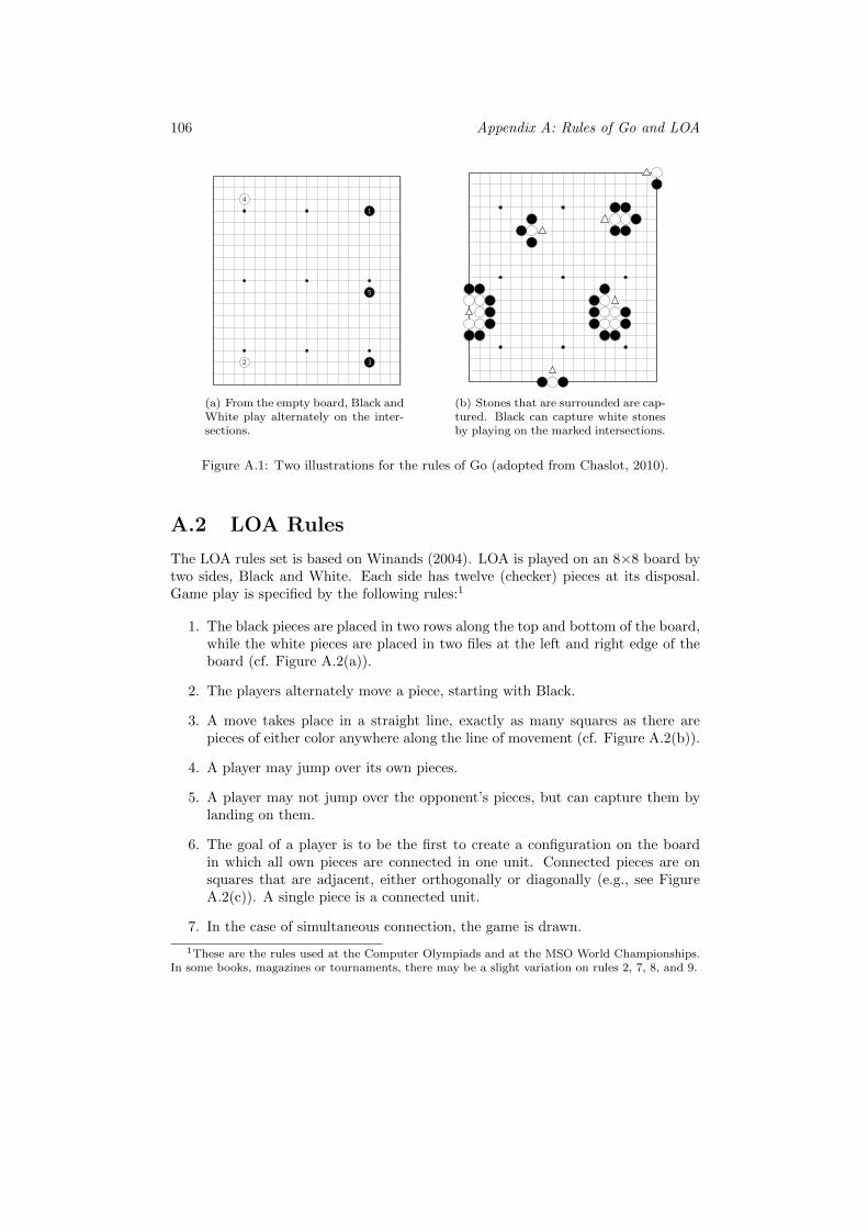
106 Appendix A: Rules of Go and LOA
1
2 3
4
5
1
(a) From the empty board, Black andWhite play alternately on the inter-sections.
1
(b) Stones that are surrounded are cap-tured. Black can capture white stonesby playing on the marked intersections.
Figure A.1: Two illustrations for the rules of Go (adopted from Chaslot, 2010).
A.2 LOA Rules
The LOA rules set is based on Winands (2004). LOA is played on an 8×8 board bytwo sides, Black and White. Each side has twelve (checker) pieces at its disposal.Game play is specified by the following rules:1
1. The black pieces are placed in two rows along the top and bottom of the board,while the white pieces are placed in two files at the left and right edge of theboard (cf. Figure A.2(a)).
2. The players alternately move a piece, starting with Black.
3. A move takes place in a straight line, exactly as many squares as there arepieces of either color anywhere along the line of movement (cf. Figure A.2(b)).
4. A player may jump over its own pieces.
5. A player may not jump over the opponent’s pieces, but can capture them bylanding on them.
6. The goal of a player is to be the first to create a configuration on the boardin which all own pieces are connected in one unit. Connected pieces are onsquares that are adjacent, either orthogonally or diagonally (e.g., see FigureA.2(c)). A single piece is a connected unit.
7. In the case of simultaneous connection, the game is drawn.
1These are the rules used at the Computer Olympiads and at the MSO World Championships.In some books, magazines or tournaments, there may be a slight variation on rules 2, 7, 8, and 9.
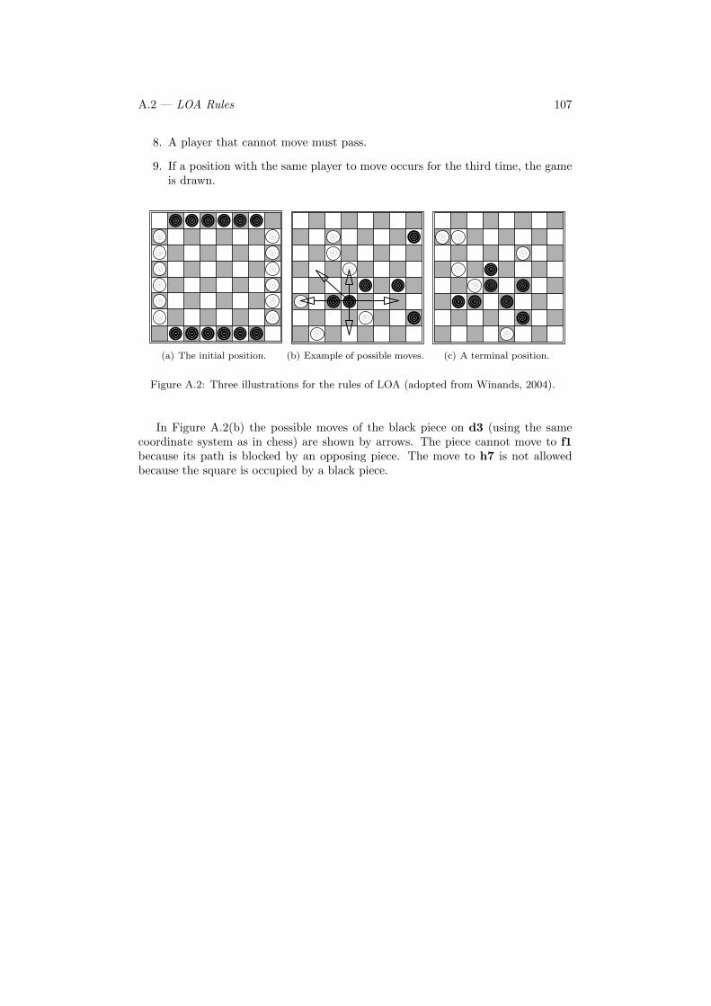
A.2 — LOA Rules 107
8. A player that cannot move must pass.
9. If a position with the same player to move occurs for the third time, the gameis drawn.
A.2 — LOA Rules 105
Figure A.2: (a) The initial position. (b) Example of possible moves. (c) A terminal position.Adapted from Chaslot (2010).
8. A player that cannot move must pass.
9. If a position with the same player to move occurs for the third time, the gameis drawn.
In Figure A.2(b) the possible moves of the black piece on d3 (using the samecoordinate system as in chess) are shown by arrows. The piece cannot move to f1because its path is blocked by an opposing piece. The move to h7 is not allowedbecause the square is occupied by a black piece.
(a) The initial position.
A.2 — LOA Rules 105
Figure A.2: (a) The initial position. (b) Example of possible moves. (c) A terminal position.Adapted from Chaslot (2010).
8. A player that cannot move must pass.
9. If a position with the same player to move occurs for the third time, the gameis drawn.
In Figure A.2(b) the possible moves of the black piece on d3 (using the samecoordinate system as in chess) are shown by arrows. The piece cannot move to f1because its path is blocked by an opposing piece. The move to h7 is not allowedbecause the square is occupied by a black piece.
(b) Example of possible moves.
A.2 — LOA Rules 105
Figure A.2: (a) The initial position. (b) Example of possible moves. (c) A terminal position.Adapted from Chaslot (2010).
8. A player that cannot move must pass.
9. If a position with the same player to move occurs for the third time, the gameis drawn.
In Figure A.2(b) the possible moves of the black piece on d3 (using the samecoordinate system as in chess) are shown by arrows. The piece cannot move to f1because its path is blocked by an opposing piece. The move to h7 is not allowedbecause the square is occupied by a black piece.
(c) A terminal position.
Figure A.2: Three illustrations for the rules of LOA (adopted from Winands, 2004).
In Figure A.2(b) the possible moves of the black piece on d3 (using the samecoordinate system as in chess) are shown by arrows. The piece cannot move to f1because its path is blocked by an opposing piece. The move to h7 is not allowedbecause the square is occupied by a black piece.

108 Appendix A: Rules of Go and LOA
Index
1 + ε trick, 17αβ search, 4, 9, 10, 43, 51, 54, 70, 86
all-moves-as-first heuristic, 21, 24Amazons, 21, 22, 43, 44AND node, 12, 73Artificial Intelligence, 1, 2, 85asynchronous, 61Awari, 3
Backgammon, 20backpropagation, 23
in MCTS-Solver, 45rules, 11, 29
base-twin algorithm, 18Benson’s algorithm, 88best-first search, 9–11, 28, 61bias, 20binary goal, 10branching factor
of Reversi variants, 78breadth-first search, 9Bridge, 20BTA, see base-twin algorithm
Checkers, 3, 4, 10, 19Chess, 1–4, 14, 20child
definition, 8Chinese Checkers, 73Clobber, 43coalition player, 72, 74Connect Four, 3, 4Conspiracy-Number Search, 10, 60Crazy Stone, 22
deadlocks, 64
Deep Blue, 2depth of a game tree, 8depth-first proof-number search, 15–
17, 19parallel, 60
depth-first search, 9df-pn, see depth-first proof-number searchdisproof number, 79
definition, 11disproof-like, 15dn, see disproof numberDomineering, 3
endgame, 3position, 51
endgame positions, 51Enhanced Transposition Cutoffs, 52equilibrium point, 70–73evaluation function, 4, 8, 20, 22, 79,
81, 83evaluation problem, 9expansion, 23
definition, 8exploration and exploitation, 21
Fanorona, 3flipping move, 75forward search, 4, 87
gamegame tree, 8sudden-death, 43
game-theoretic value, 2, 5, 8, 11, 20,44, 71
general game playing, 22GHI, see Graph-History-Interaction prob-
lem
110 INDEX
Go, 3, 4, 10, 19, 20, 22, 30, 37, 44, 57,86, 88
rules, 105Go-Moku, 3GoBase, 31Graph-History-Interaction problem, 8,
9, 15–18
Hearts, 73Hex, 2, 4, 22
imperfect-information game, 3, 22initialization
for Rolit, 79initialization rule, 11, 17InvaderMC, 21iterative deepening, 10
k -in-a-row, 3, 4Kalah, 3knowledge representation, 79Kriegspiel, 3
life-and-death problem, 30Lines of Action, 4, 10, 21, 22, 44, 51,
54, 59, 65, 86, 87rules, 106
LOA, see Lines of Actionlocking policy, 64
Manchester-Mark I, 3Mango, 32master-servant design, 60, 88mate position, 2maxn, 70MC-PNS, see Monte-Carlo Proof-Number
SearchMCE, see Monte-Carlo evaluationMCTS, see Monte-Carlo Tree SearchMCTS-Solver, 44, 46, 51, 54, 56, 61,
86, 88memory
distributed, 61shared, 61, 86
metapositions, 89MIA, 21, 49Monte-Carlo
evaluation, 5, 19–22, 25, 28, 32,39, 43, 50, 80, 86
method, 85player in Rolit, 75simulation for Reversi variants, 78technique, 7, 19
Monte-Carlo Proof-Number Search, 27,38, 86, 88
Monte-Carlo Tree Search, 5, 9, 10, 19,22, 25, 43, 86
algorithm, 22four stages of, 23parallel, 64
most-proving node, 11, 62move category, 47move selection, 21–23, 68
for MCTS-Solver, 45Multi-Armed Bandit problem, 22multi-player game, 5, 22, 69, 83, 85,
88
Nash strategy, 78NegaScout, 52Nim, 2Nine-Men’s Morris, 3node
internal, definition , 8k -most-proving, 67, 88most-proving, 29OR node, 12
non-uniformity, 87
one-player game, 22optimal play, 8optimal score, 73, 74OR node, 73Othello, 6, 10, 16, 20, 76overhead
communication overhead, 60search overhead, 60, 61, 65, 66,
68synchronization overhead, 60, 65,
66
parallel search, 88randomized, 63
parallelization, 24, 25, 60, 85
INDEX 111
of MCTS-Solver, 55root parallelization, 50tree parallelization, 50, 55
paranoid condition, 69, 83, 87paranoid player, 72–74Paranoid Proof-Number Search, 73, 79,
82, 83, 87paranoid search, 70, 72, 73, 82ParaPDS, 59–62, 66, 67parent
definition, 8patterns, 39
auto-generated, 37in Go, 37
PDS, 16, 61PDS–PN, 16perfect knowledge, 4perfect-information game, 3, 20, 22Phantom Go, 22, 43playout, 23pn, see proof numberPN2, 44, 51PN1, 13PN2, 13PN2, 13, 14, 16, 52, 54, 59, 87, 88PN∗, 14–16Poker, 20pooling, 68PPNS, see Paranoid Proof-Number Searchprincipal variation, 62, 63, 68, 87problem statement, 4, 87Progressive Bias, 47, 52proof
analytical, 4proof like, 15proof number, 79
definition, 10, 11Proof-and-Disproof-Number Search, see
PDSproof-number algorithm, 7, 10, 89
definition, 10enhancement, 17
Proof-Number Search, 5, 9, 10, 16, 28,43, 59, 69, 73, 85–87
definition, 13second-level, 13
pruningαβ, 71maxn, 73shallow, 70
pseudo randomness, 20, 45, 50, 67PV thread, 62
Qubic, 3
randomization, 5, 51, 55Randomized Parallel Proof-Number Search,
59, 61, 62, 64, 66, 67, 86–88RAVE, 24Realization-Probability Search, 49Renju, 3Reversi, 6, 75, 76, 78, 83, 87Rolit, 4, 69, 75, 76, 83, 87
Traveler’s Rolit, 77root
definition, 8root parallelization, 55
RP–PNS, see Rndomized Parallel Proof-Number Search59
RP–PN2, 59, 67, 87, 88
scaling factor, 60, 66Scrabble, 20Screen Shogi, 3search
game-tree search, 8parallel search, 60quiescence search, 52search technique, 7search tree, 8second-level search, 79
selection strategy, 47, 52Shogi, 2, 3, 10, 60simulation strategy, 50Skat, 20solution under paranoid condition, def-
inition, 73solver, 2, 79
mate solver, 3solving, 7, 69
definition of, 2degrees of solving, 2game positions, 85, 86
112 INDEX
multi-player games, 88, 89solving algorithm, 2, 10solving game positions, 1, 3solving games, 2strongly, 3ultra-weakly, 2under paranoid condition, 69, 87weakly, 3
Spades, 73
terminaldefinition, 8
threadalternative, 62PV, 62
Tic-Tac-Toe, 20tie-breaking rule, 72transition probability, 47transposition table, 9, 61, 64tree
AND/OR, 61Tsume-Go, 10Tsume-Shogi, 16two-player game, 3, 5, 22, 69, 87
UCB, see Upper Confidence BoundsUCT, see Upper Confidence bounds
applied to TreesUpper Confidence Bounds, 24Upper Confidence bounds applied to
Trees, 22, 24, 25, 44, 47, 86
Yonin, 76
Zobrist hashing, 32
Summary
Humans enjoy playing games not only to satisfy their desire for entertainment butalso because they seek an intellectual challenge. One obvious challenge in games isdefeating an opponent. The AI equivalent to this challenge is the design of stronggame-playing programs. Another challenge in games is finding the result of a gameposition, for instance whether a Chess position is a win or a loss. The AI equivalentto this challenge is the design of algorithms that solve positions. While game-playingprograms have become much stronger over the years, solving games still remains adifficult task today and has therefore been receiving attention continuously.
The topic of the thesis is the difficult task of solving game positions. Our re-search utilizes current developments in the rapidly developing field of Monte-Carlomethods for game-tree search and the continuously evolving field of Proof-NumberSearch to develop new solving algorithms. To that end, the here described researchcontributes and tests new forward-search algorithms, i.e., algorithms that explore asearch space by starting from a game position and developing a search tree from topto bottom. The new algorithms are empirically evaluated on three games, (1) Go,(2) Lines of Action (LOA), and (3) Rolit.
Chapter 1 provides an introduction. It describes the place of games in the domainof AI and provides the notion of solving games and solving game positions. Thechapter introduces the problem statement:
PS How can we improve forward search for solving game positions?
Moreover, Chapter 1 provides four research questions that address four aspectsof the problem statement that are central to solving game positions with forwardsearch. The four questions deal with the following topics, which are part of therecent progress in the research on game-tree search: (1) search with Monte-Carloevaluation, (2) Monte-Carlo Tree Search, (3) parallelized search, and (4) search formulti-player games.
The aim of Chapter 2 is to provide an overview of search techniques related andrelevant to the solving algorithms presented in later chapters. It introduces basicconcepts and gives notational conventions. It devotes particular detail to two topics:proof-number algorithms and Monte-Carlo techniques. Proof-number algorithms arestressed because they are well-studied standard techniques for solving. The reasonfor paying particular attention to Monte-Carlo techniques is that they have recently
114 Summary
contributed substantially to the field of games and AI.
Chapter 3 introduces a new algorithm, MC-PNS, that combines Monte-Carloevaluation (MCE) with Proof-Number Search (PNS). Thereby the first researchquestion is addressed.
RQ 1 How can we use Monte-Carlo evaluation to improve Proof-Number Search forsolving game positions?
An application of the new algorithm and several of its variants to the life-and-death sub-problem of Go is described. It is demonstrated experimentally thatgiven the right setting of parameters MC-PNS outperforms simple PNS. Moreover,MC-PNS is compared with a pattern-based heuristic for initialization leaf nodes inthe search tree of PNS. The result is that MC-PNS outperforms the purely pattern-based initialization. We conclude that the reason for the superior performance ofMC-PNS is the flexibility of the MCE.
Chapter 4 introduces a novel Monte-Carlo Tree Search (MCTS) variant, calledMCTS-Solver, addressing the second research question.
RQ 2 How can the Monte-Carlo Tree Search framework contribute to solving gamepositions?
The chapter adapts the recently developed MCTS framework for solving gamepositions. MCTS-Solver differs from traditional MCTS in that it can solve positionsby propagating game-theoretic values. As a result it converges faster to the bestmove in narrow tactical lines. Experiments in the game of Lines of Action (LOA)show that MCTS-Solver with a particular selection strategy solves LOA positionsthree times faster than MCTS-Solver using the standard selection strategy UCT.When comparing MCTS-Solver to αβ search, MCTS-Solver requires about the sameeffort as αβ to solve positions. Moreover, we observe that PN2 (a two-level Proof-Number Search algorithm) is still five times faster than MCTS-Solver. Additionally,we show that tree parallelization for MCTS-Solver has a scaling factor of 4 with 8threads, easily outperforming root parallelization. We conclude that at least duringgame-play (online) MCTS-Solver is comparable with a standard αβ search in solvingpositions. However, for off-line solving positions, PNS is still a better choice.
Chapter 5 introduces a parallel Proof-Number Search algorithm for shared mem-ory, called RP–PNS. Thereby, we answer the third research question.
RQ 3 How can Proof-Number Search be parallelized?
The parallelization is achieved by threads that select moves close to the principalvariation based on a probability distribution. Furthermore, we adapted RP–PNS forPN2, resulting in an algorithm called RP–PN2. The algorithms are evaluated onLOA positions. For eight threads, the scaling factor found for RP–PN2 (4.7) iseven better than that of RP–PNS (3.5) but mainly achieved because the size of thesecond-level (i.e., PN2) tree depends on the number of threads used. Based on these
Summary 115
results the chapter concludes that RP–PNS and RP–PN2 are viable for parallelizingPNS and PN2, respectively.
Chapter 6 focuses on solving multi-player games. The chapter gives an answerto the fourth research question.
RQ 4 How can Proof-Number Search be applied to multi-player games?
The starting point of Chapter 6 is the observation that many two-player gameshave been solved but virtually no research has been devoted to solving multi-playergames. We identify as a reason for this observation that multi-player games generallydo not have a unique game-theoretic value or strategy because their search trees havemultiple equilibrium points. Therefore, the straightforward way of solving a gameby finding the outcome under optimal play (that is applied in two-player games)cannot be applied to multi-player games directly. We therefore propose solvingmulti-player games under the paranoid condition. This is equivalent to finding theoptimal score that a player can achieve independently of the other players’ strategies.We then propose Paranoid Proof-Number Search (PPNS) for solving multi-playergames under the paranoid condition.
The chapter describes the multi-player variant of the game of Reversi, Rolit, anddiscusses how to apply PPNS to solve various multi-player variants of 4 × 4 and6×6 Rolit, and four-player 8×8 Rolit. The outcome is that in 4×4 Rolit under theparanoid condition some players can achieve more than the minimum score whilein 6 × 6 Rolit and in four-player 8 × 8 Rolit no player can achieve more than theminimum score. However, we observe that for 6×6 Rolit and four-player 8×8 RolitPPNS performs better than we would expect from standard paranoid search. Thechapter concludes by stating that PPNS is able to exploit the non-uniformity of thegame tree in multi-player games.
Chapter 7 concludes the thesis and gives an outlook to open questions and di-rections for future research. While the thesis provides PPNS addressing the classof deterministic multi-player games with perfect information, we end by pointingout that solving deterministic multi-player games with imperfect information stillremains a challenge and we briefly speculate how this problem can be tackled.

Samenvatting
Mensen genieten van abstracte spelen niet alleen om hun verlangen naar amuse-ment te bevredigen maar ook omdat ze een intellectuele uitdaging zoeken. Eenvoor de hand liggende uitdaging in spelen is het verslaan van de tegenstander. Decorresponderende AI uitdaging is het ontwerpen van sterke spelprogramma’s. Eenandere uitdaging in spelen is het vinden van het resultaat van een spelpositie, bijvoor-beeld of een schaakstelling een winst of verlies is. De corresponderende AI uitdagingis het ontwerpen van algoritmen die posities oplossen. Terwijl spelprogramma’s doorde jaren heen veel sterker geworden zijn, blijft het oplossen van spelen nog steedseen moeilijke taak en heeft daarom voortdurend aandacht gekregen.
Het onderwerp van dit proefschrift is de moeilijke taak van het oplossen vanspelposities. Ons onderzoek maakt gebruik van actuele ontwikkelingen in het zichsnel ontwikkelende veld van Monte-Carlo methoden voor spelboom zoekprocessen enhet continu ontwikkelende veld van Proof-Number Search om nieuwe algoritmen teontwikkelen die oplossen. Het hier beschreven onderzoek draagt bij en test nieuwevoorwaarts zoekalgoritmen, dat wil zeggen, algoritmen die een zoekruimte verkennendoor vanuit een positie een zoekboom te ontwikkelen. De nieuwe algoritmen wordenempirisch geevalueerd in drie spelen, (1) Go, (2) Lines of Action (LOA), en (3) Rolit.
Hoofdstuk 1 geeft een inleiding. Het beschrijft de plaats van spelen in het AIdomein en geeft de begrippen van het oplossen van spelen en het oplossen van spel-posities. Het hoofdstuk introduceert de volgende probleemstelling:
PS Hoe kunnen we beter voorwaarts zoeken bij het oplossen van spelposities?
Om de probleemstelling te beantwoorden hebben we vier onderzoeksvragen ge-formuleerd over onderwerpen op het gebied van het oplossen van spelposities doormiddel van voorwaarts zoeken. Ze gaan over (1) het zoeken met Monte-Carlo eva-luaties, (2) Monte-Carlo Tree Search, (3) geparallelliseerde zoekprocessen, en (4)zoekprocessen voor meerdere spelers.
Hoofdstuk 2 geeft een overzicht van zoektechnieken die gerelateerd en relevantzijn voor de zoekalgoritmen die in de latere hoofdstukken worden gegeven. Hethoofdstuk introduceert basisbegrippen en geeft conventies voor notatie. Er wordtdieper in gegaan op twee onderwerpen: Proof-Number algoritmen en Monte-Carlotechnieken. Proof-Number algoritmen worden benadrukt omdat ze goed bestudeerdestandaard technieken zijn voor oplossen van spelposities. De reden voor de aandacht
118 Samenvatting
voor Monte-Carlo technieken is dat ze een aanzienlijk bijdrage hebben geleverd inhet gebied van spelen en AI.
Hoofdstuk 3 introduceert een nieuw algoritme, MC-PNS, dat Monte-Carlo eva-luaties (MCE) combineert met Proof-Number Search (PNS). Dit leidt tot de eersteonderzoeksvraag.
RQ 1 Hoe kunnen we Monte-Carlo evaluaties gebruiken om Proof-Number Searchte verbeteren voor het oplossen van spelposities?
Een toepassing van het nieuwe algoritme op het leven-en-dood subprobleem inhet spel Go wordt beschreven. Er wordt experimenteel aangetoond dat met dejuiste parameterinstellingen MC-PNS de standaard PNS overtreft. Tevens wordtMC-PNS vergeleken met een op patronen gebaseerde heuristiek om de bladerenvan de PNS zoekboom te initialiseren. Het resultaat is dat MC-PNS de patroon-gebaseerde initialisatie overtreft. We concluderen dat de reden voor de betere pres-taties van MC-PNS is gelegen in de flexibiliteit van de toegepaste MCE.
Hoofdstuk 4 introduceert een nieuw Monte-Carlo Tree Search (MCTS) variant,genaamd MCTS-Solver. Dit heeft ons gebracht tot de tweede onderzoeksvraag.
RQ 2 Hoe kan het Monte-Carlo Tree Search raamwerk bijdragen aan het oplossenvan spelposities?
Het hoofdstuk past het MCTS raamwerk aan voor het oplossen van spelposities.De variant MCTS-Solver verschilt van de standaard MCTS aanpak door het feitdat het posities kan oplossen door middel van het propageren van speltheoretischewaarden. Als gevolg daarvan convergeert het sneller naar de beste zet in tactischeposities. Experimenten in het spel Lines of Action (LOA) laten zien dat MCTS-solver met een specifieke selectie strategie LOA posities drie keer sneller oplost danMCTS-Solver met behulp van de standaard selectie strategie UCT. Vergelijken weMCTS-Solver met een standaard αβ zoekproces, dan lost MCTS-Solver LOA posi-ties op met ongeveer dezelfde inspanning als αβ. Bovendien stellen we vast dat PN2
(een Proof-Nunber Search algoritme bestaande uit twee niveaus) nog steeds vijf keersneller is dan MCTS-Solver. Daarnaast tonen we aan dat boomparallellisatie voorMCTS-Solver schaalt met een factor 4 voor 8 processorkernen. Wortelparallellisatiewordt hier eenvoudig overtroffen. We concluderen dat gedurende het spel (online)MCTS-Solver vergelijkbaar is met een standaard αβ zoekproces voor het oplossenvan posities. Echter, voor het oplossen van posities offline is PNS nog steeds eenbetere keuze.
Hoofdstuk 5 introduceert een parallel Proof-Number Search algoritme voor ge-deeld geheugen, genaamd RP–PNS. Daarmee beantwoorden we de derde onderzoeks-vraag.
RQ 3 Hoe kunnen we Proof-Number Search parallelliseren?
Samenvatting 119
De parallellisatie wordt bereikt door middels een kansverdeling zetten te selec-teren in de buurt van de hoofdvariant. Verder hebben we RP–PNS aangepast voorPN2, resulterend in RP–PN2. De algoritmen worden getest op LOA posities. Voor 8processorkernen is de gevonden schaalfactor voor RP–PN2 (4.7) zelfs beter dan dievan RP–PNS (3.5). De reden hiervoor is dat de grootte van de zoekboom op hettweede niveau (dat wil zeggen, PN2) afhangt van het aantal gebruikte processorker-nen. Op basis van deze resultaten concluderen we dat RP–PNS en RP–PN2 geschiktetechnieken zijn om respectievelijk PNS en PN2 te paralleliseren.
Hoofdstuk 6 richt zich op het oplossen van speldomeinen met meerdere spelers.Het hoofdstuk geeft een antwoord op de vierde onderzoeksvraag.
RQ 4 Hoe kunnen we Proof-Number Search toepassen voor speldomeinen metmeerdere spelers?
Het uitgangspunt van dit hoofdstuk is de constatering dat veel tweespeler spelenzijn opgelost, maar vrijwel geen onderzoek is besteed aan het oplossen van spelenmet meerdere spelers. De laatstgenoemde spelen hebben in het algemeen geen uniekespeltheoretische waarde of strategie omdat hun zoekbomen meerdere evenwichtspun-ten kunnen hebben. Daarom kan de aanpak voor het oplossen van een tweespelerspel niet worden toegepast op een meerspeler spel. Wij stellen voor dit soort spelenop te lossen onder de paranoıde conditie. Dit is gelijk aan het vinden van de opti-male score die een speler zelfstandig kan bereiken onafhankelijk van de strategieenvan zijn opponenten. We introduceren Paranoid Proof-Number Search (PPNS) voorhet oplossen van meerspeler spelen onder de paranoıde conditie.
Dit hoofdstuk beschrijft de meerspeler variant van het spel Reversi, Rolit, en be-spreekt hoe PPNS toe te passen om diverse meerspeler varianten van 4× 4 en 6× 6Rolit, en vierspeler 8×8 Rolit op te lossen. Het resultaat is dat voor 4×4 Rolit onderde paranoıde conditie sommige spelers meer dan de minimale score kunnen behalen,terwijl voor 6×6 Rolit en vierspeler 8×8 Rolit geen enkele speler meer kan bereikendan de minimale score. Wij constateren dat voor 6×6 Rolit en vierspeler 8×8 RolitPPNS beter presteert dan het beste geval voor Paranoid Search. Het hoofdstuksluit af door te stellen dat PPNS in staat is om het non-uniforme karakter van despelboom in meerspeler spelen uit te buiten.
Hoofdstuk 7 sluit het proefschrift af en geeft een vooruitblik op open vragen enrichtingen van toekomstig onderzoek. Hoewel in het proefschrift het PPNS algoritmeis voorgesteld om deterministische meerspeler spelen met perfecte informatie op telossen, eindigen we door erop te wijzen dat het oplossen van deterministische meer-speler spelen met imperfecte informatie nog steeds een uitdaging is. We speculerenin het kort hoe dit probleem aangepakt kan worden.

Curriculum Vitae
Jahn-Takeshi Saito was born in Dusseldorf, Germany, on November 6, 1976. Heattended school in Germany and Japan and graduated from Max-Plank-Gymnasiumin Bielefeld, Germany in 1996. After 13 months of compulsory community service atMara Epilepsy Center Bethel in Bielefeld, he went on to study Artificial Intelligenceand Computational Linguistics at Osnabruck University with minors in mathematicsand computer science. During his studies he joined the students’ Go club. In 2001, hestudied mathematics at Trinity College Dublin, Ireland, and did an internship at theKnowledge Engineering group at IBM’s Tokyo Research Laboratory (which turnedout to be located outside of Tokyo prefecture). In 2002, he joined the students’parliament and students’ self-governing body (AStA), started working as a part-timeprogrammer for KIWI GmbH in parallel to pursuing his studies, and decided that thegame of Go would be a suitable subject for a Master thesis. In 2004, he graduatedon Computer Go. In 2005, he started his Ph.D. project at the Games and AI Group,Department of Knowledge Engineering, Maastricht University. There, he acquiredan inside perspective of academia. He worked on search algorithms for board gameson the Go for Go project funded by the Netherlands Organisation for ScientificResearch. Gradually, his research interest evolved towards solving game positions,Proof-Number Search and Monte-Carlo methods. Besides performing research, Jahnwas involved in lecturing and helped organizing the 2006 Computers and Gamesconference in Turin, Italy. In early 2010, Jahn joined the team of the BioinformaticsDepartment, BiGCaT, Maastricht University where he has been working on systemsbiology databases.

SIKS Dissertation Series
1998
1 Johan van den Akker (CWI) DEGAS - AnActive, Temporal Database of AutonomousObjects
2 Floris Wiesman (UM) Information Retrievalby Graphically Browsing Meta-Information
3 Ans Steuten (TUD) A Contribution to theLinguistic Analysis of Business Conversa-tions within the Language/Action Perspec-tive
4 Dennis Breuker (UM) Memory versus Searchin Games
5 Eduard W. Oskamp (RUL) Computeronders-teuning bij Straftoemeting
1999
1 Mark Sloof (VU) Physiology of QualityChange Modelling; Automated Modelling ofQuality Change of Agricultural Products
2 Rob Potharst (EUR) Classification using De-cision Trees and Neural Nets
3 Don Beal (UM) The Nature of MinimaxSearch
4 Jacques Penders (UM) The Practical Art ofMoving Physical Objects
5 Aldo de Moor (KUB) Empowering Commu-nities: A Method for the Legitimate User-Driven Specification of Network InformationSystems
6 Niek J.E. Wijngaards (VU) Re-Design ofCompositional Systems
7 David Spelt (UT) Verification Support forObject Database Design
8 Jacques H.J. Lenting (UM) Informed Gam-bling: Conception and Analysis of a Multi-Agent Mechanism for Discrete Reallocation
2000
1 Frank Niessink (VU) Perspectives on Improv-ing Software Maintenance
2 Koen Holtman (TU/e) Prototyping of CMSStorage Management
3 Carolien M.T. Metselaar (UvA) Sociaal-organisatorische Gevolgen van Kennistech-nologie; een Procesbenadering en Actorper-spectief
4 Geert de Haan (VU) ETAG, A Formal Modelof Competence Knowledge for User InterfaceDesign
5 Ruud van der Pol (UM) Knowledge-BasedQuery Formulation in Information Retrieval
6 Rogier van Eijk (UU) Programming Lan-guages for Agent Communication
7 Niels Peek (UU) Decision-Theoretic Planningof Clinical Patient Management
8 Veerle Coupe (EUR) Sensitivity Analyis ofDecision-Theoretic Networks
9 Florian Waas (CWI) Principles of Probabilis-tic Query Optimization
10 Niels Nes (CWI) Image Database Manage-ment System Design Considerations, Algo-rithms and Architecture
Abbreviations. SIKS – Dutch Research School for Information and Knowledge Systems; CWI– Centrum voor Wiskunde en Informatica, Amsterdam; EUR – Erasmus Universiteit, Rotterdam;KUB – Katholieke Universiteit Brabant, Tilburg; KUN – Katholieke Universiteit Nijmegen; OU –Open Universiteit Nederland; RUG – Rijksuniversiteit Groningen; RUL – Rijksuniversiteit Leiden;RUN – Radboud Universiteit Nijmegen; TUD – Technische Universiteit Delft; TU/e – TechnischeUniversiteit Eindhoven; UL – Universiteit Leiden; UM – Universiteit Maastricht; UT – UniversiteitTwente; UU – Universiteit Utrecht; UvA – Universiteit van Amsterdam; UvT – Universiteit vanTilburg; VU – Vrije Universiteit, Amsterdam.
124 SIKS Dissertation Series
11 Jonas Karlsson (CWI) Scalable DistributedData Structures for Database Management
2001
1 Silja Renooij (UU) Qualitative Approaches toQuantifying Probabilistic Networks
2 Koen Hindriks (UU) Agent ProgrammingLanguages: Programming with Mental Mod-els
3 Maarten van Someren (UvA) Learning asProblem Solving
4 Evgueni Smirnov (UM) Conjunctive and Dis-junctive Version Spaces with Instance-BasedBoundary Sets
5 Jacco van Ossenbruggen (VU) ProcessingStructured Hypermedia: A Matter of Style
6 Martijn van Welie (VU) Task-Based User In-terface Design
7 Bastiaan Schonhage (VU) Diva: Architec-tural Perspectives on Information Visualiza-tion
8 Pascal van Eck (VU) A Compositional Se-mantic Structure for Multi-Agent SystemsDynamics
9 Pieter Jan ’t Hoen (RUL) Towards Dis-tributed Development of Large Object-Oriented Models, Views of Packages asClasses
10 Maarten Sierhuis (UvA) Modeling and Simu-lating Work Practice BRAHMS: a MultiagentModeling and Simulation Language for WorkPractice Analysis and Design
11 Tom M. van Engers (VU) Knowledge Man-agement: The Role of Mental Models in Busi-ness Systems Design
2002
1 Nico Lassing (VU) Architecture-Level Modifi-ability Analysis
2 Roelof van Zwol (UT) Modelling and Search-ing Web-based Document Collections
3 Henk Ernst Blok (UT) Database Optimiza-tion Aspects for Information Retrieval
4 Juan Roberto Castelo Valdueza (UU) TheDiscrete Acyclic Digraph Markov Model inData Mining
5 Radu Serban (VU) The Private CyberspaceModeling Electronic Environments Inhabitedby Privacy-Concerned Agents
6 Laurens Mommers (UL) Applied Legal Epis-temology; Building a Knowledge-based Ontol-ogy of the Legal Domain
7 Peter Boncz (CWI) Monet: A Next-Generation DBMS Kernel For Query-Intensive Applications
8 Jaap Gordijn (VU) Value Based Require-ments Engineering: Exploring Innovative E-Commerce Ideas
9 Willem-Jan van den Heuvel (KUB) Integrat-ing Modern Business Applications with Ob-jectified Legacy Systems
10 Brian Sheppard (UM) Towards Perfect Playof Scrabble
11 Wouter C.A. Wijngaards (VU) Agent BasedModelling of Dynamics: Biological and Or-ganisational Applications
12 Albrecht Schmidt (UvA) Processing XML inDatabase Systems
13 Hongjing Wu (TU/e) A Reference Architec-ture for Adaptive Hypermedia Applications
14 Wieke de Vries (UU) Agent Interaction: Ab-stract Approaches to Modelling, Program-ming and Verifying Multi-Agent Systems
15 Rik Eshuis (UT) Semantics and Verifica-tion of UML Activity Diagrams for WorkflowModelling
16 Pieter van Langen (VU) The Anatomy of De-sign: Foundations, Models and Applications
17 Stefan Manegold (UvA) Understanding,Modeling, and Improving Main-MemoryDatabase Performance
2003
1 Heiner Stuckenschmidt (VU) Ontology-BasedInformation Sharing in Weakly StructuredEnvironments
2 Jan Broersen (VU) Modal Action Logics forReasoning About Reactive Systems
3 Martijn Schuemie (TUD) Human-ComputerInteraction and Presence in Virtual RealityExposure Therapy
4 Milan Petkovic (UT) Content-Based VideoRetrieval Supported by Database Technology
5 Jos Lehmann (UvA) Causation in ArtificialIntelligence and Law – A Modelling Approach
6 Boris van Schooten (UT) Development andSpecification of Virtual Environments
7 Machiel Jansen (UvA) Formal Explorationsof Knowledge Intensive Tasks
8 Yong-Ping Ran (UM) Repair-Based Schedul-ing
9 Rens Kortmann (UM) The Resolution of Vi-sually Guided Behaviour
SIKS Dissertation Series 125
10 Andreas Lincke (UT) Electronic Business Ne-gotiation: Some Experimental Studies onthe Interaction between Medium, InnovationContext and Cult
11 Simon Keizer (UT) Reasoning under Uncer-tainty in Natural Language Dialogue usingBayesian Networks
12 Roeland Ordelman (UT) Dutch Speech Recog-nition in Multimedia Information Retrieval
13 Jeroen Donkers (UM) Nosce Hostem –Searching with Opponent Models
14 Stijn Hoppenbrouwers (KUN) Freezing Lan-guage: Conceptualisation Processes acrossICT-Supported Organisations
15 Mathijs de Weerdt (TUD) Plan Merging inMulti-Agent Systems
16 Menzo Windhouwer (CWI) Feature Gram-mar Systems - Incremental Maintenance ofIndexes to Digital Media Warehouse
17 David Jansen (UT) Extensions of Statechartswith Probability, Time, and Stochastic Tim-ing
18 Levente Kocsis (UM) Learning Search Deci-sions
2004
1 Virginia Dignum (UU) A Model for Or-ganizational Interaction: Based on Agents,Founded in Logic
2 Lai Xu (UvT) Monitoring Multi-party Con-tracts for E-business
3 Perry Groot (VU) A Theoretical and Empir-ical Analysis of Approximation in SymbolicProblem Solving
4 Chris van Aart (UvA) Organizational Princi-ples for Multi-Agent Architectures
5 Viara Popova (EUR) Knowledge Discoveryand Monotonicity
6 Bart-Jan Hommes (TUD) The Evaluation ofBusiness Process Modeling Techniques
7 Elise Boltjes (UM) VoorbeeldIG Onderwijs;Voorbeeldgestuurd Onderwijs, een Opstapnaar Abstract Denken, vooral voor Meisjes
8 Joop Verbeek (UM) Politie en de NieuweInternationale Informatiemarkt, Grensre-gionale Politiele Gegevensuitwisseling enDigitale Expertise
9 Martin Caminada (VU) For the Sake of theArgument; Explorations into Argument-basedReasoning
10 Suzanne Kabel (UvA) Knowledge-rich Index-ing of Learning-objects
11 Michel Klein (VU) Change Management forDistributed Ontologies
12 The Duy Bui (UT) Creating Emotions andFacial Expressions for Embodied Agents
13 Wojciech Jamroga (UT) Using Multiple Mod-els of Reality: On Agents who Know how toPlay
14 Paul Harrenstein (UU) Logic in Conflict.Logical Explorations in Strategic Equilibrium
15 Arno Knobbe (UU) Multi-Relational DataMining
16 Federico Divina (VU) Hybrid Genetic Rela-tional Search for Inductive Learning
17 Mark Winands (UM) Informed Search inComplex Games
18 Vania Bessa Machado (UvA) Supporting theConstruction of Qualitative Knowledge Mod-els
19 Thijs Westerveld (UT) Using generative prob-abilistic models for multimedia retrieval
20 Madelon Evers (Nyenrode) Learning fromDesign: facilitating multidisciplinary designteams
2005
1 Floor Verdenius (UvA) Methodological As-pects of Designing Induction-Based Applica-tions
2 Erik van der Werf (UM) AI techniques for thegame of Go
3 Franc Grootjen (RUN) A Pragmatic Ap-proach to the Conceptualisation of Language
4 Nirvana Meratnia (UT) Towards DatabaseSupport for Moving Object data
5 Gabriel Infante-Lopez (UvA) Two-LevelProbabilistic Grammars for Natural Lan-guage Parsing
6 Pieter Spronck (UM) Adaptive Game AI
7 Flavius Frasincar (TU/e) Hypermedia Pre-sentation Generation for Semantic Web In-formation Systems
8 Richard Vdovjak (TU/e) A Model-driven Ap-proach for Building Distributed Ontology-based Web Applications
9 Jeen Broekstra (VU) Storage, Querying andInferencing for Semantic Web Languages
10 Anders Bouwer (UvA) Explaining Behaviour:Using Qualitative Simulation in InteractiveLearning Environments
126 SIKS Dissertation Series
11 Elth Ogston (VU) Agent Based Matchmakingand Clustering - A Decentralized Approach toSearch
12 Csaba Boer (EUR) Distributed Simulation inIndustry
13 Fred Hamburg (UL) Een Computer-model voor het Ondersteunen van Eu-thanasiebeslissingen
14 Borys Omelayenko (VU) Web-Service config-uration on the Semantic Web; Exploring howsemantics meets pragmatics
15 Tibor Bosse (VU) Analysis of the Dynamicsof Cognitive Processes
16 Joris Graaumans (UU) Usability of XMLQuery Languages
17 Boris Shishkov (TUD) Software SpecificationBased on Re-usable Business Components
18 Danielle Sent (UU) Test-selection strategiesfor probabilistic networks
19 Michel van Dartel (UM) Situated Represen-tation
20 Cristina Coteanu (UL) Cyber Consumer Law,State of the Art and Perspectives
21 Wijnand Derks (UT) Improving Concurrencyand Recovery in Database Systems by Ex-ploiting Application Semantics
2006
1 Samuil Angelov (TU/e) Foundations of B2BElectronic Contracting
2 Cristina Chisalita (VU) Contextual issues inthe design and use of information technologyin organizations
3 Noor Christoph (UvA) The role of metacog-nitive skills in learning to solve problems
4 Marta Sabou (VU) Building Web Service On-tologies
5 Cees Pierik (UU) Validation Techniques forObject-Oriented Proof Outlines
6 Ziv Baida (VU) Software-aided ServiceBundling - Intelligent Methods & Tools forGraphical Service Modeling
7 Marko Smiljanic (UT) XML schema match-ing – balancing efficiency and effectiveness bymeans of clustering
8 Eelco Herder (UT) Forward, Back and HomeAgain - Analyzing User Behavior on the Web
9 Mohamed Wahdan (UM) Automatic Formu-lation of the Auditor’s Opinion
10 Ronny Siebes (VU) Semantic Routing inPeer-to-Peer Systems
11 Joeri van Ruth (UT) Flattening Queries overNested Data Types
12 Bert Bongers (VU) Interactivation - Towardsan e-cology of people, our technological envi-ronment, and the arts
13 Henk-Jan Lebbink (UU) Dialogue and De-cision Games for Information ExchangingAgents
14 Johan Hoorn (VU) Software Requirements:Update, Upgrade, Redesign - towards a The-ory of Requirements Change
15 Rainer Malik (UU) CONAN: Text Mining inthe Biomedical Domain
16 Carsten Riggelsen (UU) ApproximationMethods for Efficient Learning of BayesianNetworks
17 Stacey Nagata (UU) User Assistance forMultitasking with Interruptions on a MobileDevice
18 Valentin Zhizhkun (UvA) Graph transforma-tion for Natural Language Processing
19 Birna van Riemsdijk (UU) Cognitive AgentProgramming: A Semantic Approach
20 Marina Velikova (UvT) Monotone models forprediction in data mining
21 Bas van Gils (RUN) Aptness on the Web
22 Paul de Vrieze (RUN) Fundaments of Adap-tive Personalisation
23 Ion Juvina (UU) Development of CognitiveModel for Navigating on the Web
24 Laura Hollink (VU) Semantic Annotation forRetrieval of Visual Resources
25 Madalina Drugan (UU) Conditional log-likelihood MDL and Evolutionary MCMC
26 Vojkan Mihajlovic (UT) Score Region Alge-bra: A Flexible Framework for Structured In-formation Retrieval
27 Stefano Bocconi (CWI) Vox Populi: gener-ating video documentaries from semanticallyannotated media repositories
28 Borkur Sigurbjornsson (UvA) Focused Infor-mation Access using XML Element Retrieval
2007
1 Kees Leune (UvT) Access Control andService-Oriented Architectures
2 Wouter Teepe (RUG) Reconciling Informa-tion Exchange and Confidentiality: A FormalApproach
3 Peter Mika (VU) Social Networks and the Se-mantic Web
SIKS Dissertation Series 127
4 Jurriaan van Diggelen (UU) Achieving Se-mantic Interoperability in Multi-agent Sys-tems: a dialogue-based approach
5 Bart Schermer (UL) Software Agents,Surveillance, and the Right to Privacy: aLegislative Framework for Agent-enabledSurveillance
6 Gilad Mishne (UvA) Applied Text Analyticsfor Blogs
7 Natasa Jovanovic’ (UT) To Whom It MayConcern - Addressee Identification in Face-to-Face Meetings
8 Mark Hoogendoorn (VU) Modeling of Changein Multi-Agent Organizations
9 David Mobach (VU) Agent-Based MediatedService Negotiation
10 Huib Aldewereld (UU) Autonomy vs. Con-formity: an Institutional Perspective onNorms and Protocols
11 Natalia Stash (TU/e) Incorporating Cogni-tive/Learning Styles in a General-PurposeAdaptive Hypermedia System
12 Marcel van Gerven (RUN) Bayesian Net-works for Clinical Decision Support: ARational Approach to Dynamic Decision-Making under Uncertainty
13 Rutger Rienks (UT) Meetings in Smart Envi-ronments; Implications of Progressing Tech-nology
14 Niek Bergboer (UM) Context-Based ImageAnalysis
15 Joyca Lacroix (UM) NIM: a Situated Com-putational Memory Model
16 Davide Grossi (UU) Designing InvisibleHandcuffs. Formal investigations in Institu-tions and Organizations for Multi-agent Sys-tems
17 Theodore Charitos (UU) Reasoning with Dy-namic Networks in Practice
18 Bart Orriens (UvT) On the development andmanagement of adaptive business collabora-tions
19 David Levy (UM) Intimate relationships withartificial partners
20 Slinger Jansen (UU) Customer ConfigurationUpdating in a Software Supply Network
21 Karianne Vermaas (UU) Fast diffusion andbroadening use: A research on residentialadoption and usage of broadband internet inthe Netherlands between 2001 and 2005
22 Zlatko Zlatev (UT) Goal-oriented design ofvalue and process models from patterns
23 Peter Barna (TU/e) Specification of Applica-tion Logic in Web Information Systems
24 Georgina Ramırez Camps (CWI) StructuralFeatures in XML Retrieval
25 Joost Schalken (VU) Empirical Investigationsin Software Process Improvement
2008
1 Katalin Boer-Sorban (EUR) Agent-BasedSimulation of Financial Markets: A modu-lar, continuous-time approach
2 Alexei Sharpanskykh (VU) On Computer-Aided Methods for Modeling and Analysis ofOrganizations
3 Vera Hollink (UvA) Optimizing hierarchicalmenus: a usage-based approach
4 Ander de Keijzer (UT) Management of Un-certain Data - towards unattended integra-tion
5 Bela Mutschler (UT) Modeling and simulat-ing causal dependencies on process-aware in-formation systems from a cost perspective
6 Arjen Hommersom (RUN) On the Applica-tion of Formal Methods to Clinical Guide-lines, an Artificial Intelligence Perspective
7 Peter van Rosmalen (OU) Supporting the tu-tor in the design and support of adaptive e-learning
8 Janneke Bolt (UU) Bayesian Networks: As-pects of Approximate Inference
9 Christof van Nimwegen (UU) The paradox ofthe guided user: assistance can be counter-effective
10 Wauter Bosma (UT) Discourse orientedSummarization
11 Vera Kartseva (VU) Designing Controls forNetwork Organizations: a Value-Based Ap-proach
12 Jozsef Farkas (RUN) A Semiotically OrientedCognitive Model of Knowledge Representa-tion
13 Caterina Carraciolo (UvA) Topic Driven Ac-cess to Scientific Handbooks
14 Arthur van Bunningen (UT) Context-AwareQuerying; Better Answers with Less Effort
15 Martijn van Otterlo (UT) The Logic of Adap-tive Behavior: Knowledge Representationand Algorithms for the Markov Decision Pro-cess Framework in First-Order Domains
16 Henriette van Vugt (VU) Embodied Agentsfrom a User’s Perspective
128 SIKS Dissertation Series
17 Martin Op’t Land (TUD) Applying Architec-ture and Ontology to the Splitting and Allyingof Enterprises
18 Guido de Croon (UM) Adaptive Active Vi-sion
19 Henning Rode (UT) From document to en-tity retrieval: improving precision and per-formance of focused text search
20 Rex Arendsen (UvA) Geen bericht, goedbericht. Een onderzoek naar de effecten vande introductie van elektronisch berichtenver-keer met de overheid op de administratievelasten van bedrijven
21 Krisztian Balog (UvA) People search in theenterprise
22 Henk Koning (UU) Communication of IT-architecture
23 Stefan Visscher (UU) Bayesian networkmodels for the management of ventilator-associated pneumonia
24 Zharko Aleksovski (VU) Using backgroundknowledge in ontology matching
25 Geert Jonker (UU) Efficient and Equitableexchange in air traffic management plan re-pair using spender-signed currency
26 Marijn Huijbregts (UT) Segmentation, di-arization and speech transcription: surprisedata unraveled
27 Hubert Vogten (OU) Design and implemen-tation strategies for IMS learning design
28 Ildiko Flesh (RUN) On the use of indepen-dence relations in Bayesian networks
29 Dennis Reidsma (UT) Annotations and sub-jective machines- Of annotators, embodiedagents, users, and other humans
30 Wouter van Atteveldt (VU) Semantic net-work analysis: techniques for extracting, rep-resenting and querying media content
31 Loes Braun (UM) Pro-active medical infor-mation retrieval
32 Trung B. Hui (UT) Toward affective dia-logue management using partially observablemarkov decision processes
33 Frank Terpstra (UvA) Scientific workflow de-sign; theoretical and practical issues
34 Jeroen de Knijf (UU) Studies in FrequentTree Mining
35 Benjamin Torben-Nielsen (UvT) Dendriticmorphology: function shapes structure
2009
1 Rasa Jurgelenaite (RUN) Symmetric CausalIndependence Models
2 Willem Robert van Hage (VU) EvaluatingOntology-Alignment Techniques
3 Hans Stol (UvT) A Framework for Evidence-based Policy Making Using IT
4 Josephine Nabukenya (RUN) Improving theQuality of Organisational Policy Making us-ing Collaboration Engineering
5 Sietse Overbeek (RUN) Bridging Supply andDemand for Knowledge Intensive Tasks -Based on Knowledge, Cognition, and Qual-ity
6 Muhammad Subianto (UU) UnderstandingClassification
7 Ronald Poppe (UT) Discriminative Vision-Based Recovery and Recognition of HumanMotion
8 Volker Nannen (VU) Evolutionary Agent-Based Policy Analysis in Dynamic Environ-ments
9 Benjamin Kanagwa (RUN) Design, Discov-ery and Construction of Service-oriented Sys-tems
10 Jan Wielemaker (UvA) Logic programmingfor knowledge-intensive interactive applica-tions
11 Alexander Boer (UvA) Legal Theory, Sourcesof Law & the Semantic Web
12 Peter Massuthe (TU/e, Humboldt-Universtatzu Berlin) Operating Guidelines for Services
13 Steven de Jong (UM) Fairness in Multi-AgentSystems
14 Maksym Korotkiy (VU) From ontology-enabled services to service-enabled ontologies(making ontologies work in e-science withONTO-SOA)
15 Rinke Hoekstra (UvA) Ontology Representa-tion - Design Patterns and Ontologies thatMake Sense
16 Fritz Reul (UvT) New Architectures in Com-puter Chess
17 Laurens van der Maaten (UvT) Feature Ex-traction from Visual Data
18 Fabian Groffen (CWI) Armada, An EvolvingDatabase System
19 Valentin Robu (CWI) Modeling Preferences,Strategic Reasoning and Collaboration inAgent-Mediated Electronic Markets
SIKS Dissertation Series 129
20 Bob van der Vecht (UU) Adjustable Au-tonomy: Controling Influences on DecisionMaking
21 Stijn Vanderlooy (UM) Ranking and ReliableClassification
22 Pavel Serdyukov (UT) Search For Expertise:Going beyond direct evidence
23 Peter Hofgesang (VU) Modelling Web Usagein a Changing Environment
24 Annerieke Heuvelink (VU) Cognitive Modelsfor Training Simulations
25 Alex van Ballegooij (CWI) RAM: ArrayDatabase Management through RelationalMapping
26 Fernando Koch (UU) An Agent-Based Modelfor the Development of Intelligent MobileServices
27 Christian Glahn (OU) Contextual Supportof social Engagement and Reflection on theWeb
28 Sander Evers (UT) Sensor Data Managementwith Probabilistic Models
29 Stanislav Pokraev (UT) Model-Driven Se-mantic Integration of Service-Oriented Appli-cations
30 Marcin Zukowski (CWI) Balancing vectorizedquery execution with bandwidth-optimizedstorage
31 Sofiya Katrenko (UvA) A Closer Look atLearning Relations from Text
32 Rik Farenhorst and Remco de Boer (VU)Architectural Knowledge Management: Sup-porting Architects and Auditors
33 Khiet Truong (UT) How Does Real Affect Af-fect Affect Recognition In Speech?
34 Inge van de Weerd (UU) Advancing in Soft-ware Product Management: An IncrementalMethod Engineering Approach
35 Wouter Koelewijn (UL) Privacy en Poli-tiegegevens; Over geautomatiseerde nor-matieve informatie-uitwisseling
36 Marco Kalz (OU) Placement Support forLearners in Learning Networks
37 Hendrik Drachsler (OU) Navigation Supportfor Learners in Informal Learning Networks
38 Riina Vuorikari (OU) Tags and Self-Organisation: A Metadata Ecology forLearning Resources in a Multilingual Con-text
39 Christian Stahl (TU/e, Humboldt-Universtatzu Berlin) Service Substitution – A Behav-ioral Approach Based on Petri Nets
40 Stephan Raaijmakers (UvT) MultinomialLanguage Learning: Investigations into theGeometry of Language
41 Igor Berezhnyy (UvT) Digital Analysis ofPaintings
42 Toine Bogers (UvT) Recommender Systemsfor Social Bookmarking
43 Virginia Nunes Leal Franqueira (UT) FindingMulti-step Attacks in Computer Networks us-ing Heuristic Search and Mobile Ambients
44 Roberto Santana Tapia (UT) AssessingBusiness-IT Alignment in Networked Orga-nizations
45 Jilles Vreeken (UU) Making Pattern MiningUseful
46 Loredana Afanasiev (UvA) Querying XML:Benchmarks and Recursion
2010
1 Matthijs van Leeuwen (UU) Patterns thatMatter
2 Ingo Wassink (UT) Work flows in Life Sci-ence
3 Joost Geurts (CWI) A Document Engineer-ing Model and Processing Framework forMultimedia documents
4 Olga Kulyk (UT) Do You Know What IKnow? Situational Awareness of Co-locatedTeams in Multidisplay Environments
5 Claudia Hauff (UT) Predicting the Effective-ness of Queries and Retrieval Systems
6 Sander Bakkes (UvT) Rapid Adaptation ofVideo Game AI
7 Wim Fikkert (UT) Gesture interaction at aDistance
8 Krzysztof Siewicz (UL) Towards an ImprovedRegulatory Framework of Free Software. Pro-tecting user freedoms in a world of softwarecommunities and eGovernments
9 Hugo Kielman (UL) Politiele gegevensverw-erking en Privacy, Naar een effectieve waar-borging
10 Rebecca Ong (UL) Mobile Communicationand Protection of Children
11 Adriaan Ter Mors (TUD) The world accord-ing to MARP: Multi-Agent Route Planning
12 Susan van den Braak (UU) Sensemaking soft-ware for crime analysis
13 Gianluigi Folino (RUN) High PerformanceData Mining using Bio-inspired techniques
130 SIKS Dissertation Series
14 Sander van Splunter (VU) Automated WebService Reconfiguration
15 Lianne Bodenstaff (UT) Managing De-pendency Relations in Inter-OrganizationalModels
16 Sicco Verwer (TUD) Efficient Identificationof Timed Automata, theory and practice
17 Spyros Kotoulas (VU) Scalable Discovery ofNetworked Resources: Algorithms, Infras-tructure, Applications
18 Charlotte Gerritsen (VU) Caught in the Act:Investigating Crime by Agent-Based Simula-tion
19 Henriette Cramer (UvA) People’s Responsesto Autonomous and Adaptive Systems
20 Ivo Swartjes (UT) Whose Story Is It Any-way? How Improv Informs Agency and Au-thorship of Emergent Narrative
21 Harold van Heerde (UT) Privacy-aware datamanagement by means of data degradation
22 Michiel Hildebrand (CWI) End-user Supportfor Access to Heterogeneous Linked Data
23 Bas Steunebrink (UU) The Logical Structureof Emotions
24 Dmytro Tykhonov (TUD) Designing Genericand Efficient Negotiation Strategies
25 Zulfiqar Ali Memon (VU) Modelling Human-Awareness for Ambient Agents: A HumanMindreading Perspective
26 Ying Zhang (CWI) XRPC: Efficient Dis-tributed Query Processing on HeterogeneousXQuery Engines
27 Marten Voulon (UL) Automatisch con-tracteren
28 Arne Koopman (UU) Characteristic Rela-tional Patterns
29 Stratos Idreos (CWI) Database Cracking: To-wards Auto-tuning Database Kernels
30 Marieke van Erp (UvT) Accessing NaturalHistory - Discoveries in data cleaning, struc-turing, and retrieval
31 Victor de Boer (UvA) Ontology Enrichmentfrom Heterogeneous Sources on the Web
32 Marcel Hiel (UvT) An Adaptive Service Ori-ented Architecture: Automatically solving In-teroperability Problems
33 Robin Aly (UT) Modeling RepresentationUncertainty in Concept-Based MultimediaRetrieval
34 Teduh Dirgahayu (UT) Interaction Design inService Compositions
35 Dolf Trieschnigg (UT) Proof of Concept:Concept-based Biomedical Information Re-trieval
36 Jose Janssen (OU) Paving the Way for Life-long Learning; Facilitating competence devel-opment through a learning path specification
37 Niels Lohmann (TU/e) Correctness of ser-vices and their composition
38 Dirk Fahland (TU/e) From Scenarios to com-ponents
39 Ghazanfar Farooq Siddiqui (VU) Integrativemodeling of emotions in virtual agents
40 Mark van Assem (VU) Converting and Inte-grating Vocabularies for the Semantic Web
41 Guillaume Chaslot (UM) Monte-Carlo TreeSearch
42 Sybren de Kinderen (VU) Needs-driven ser-vice bundling in a multi-supplier setting - thecomputational e3-service approach
43 Peter van Kranenburg (UU) A Computa-tional Approach to Content-Based Retrievalof Folk Song Melodies
44 Pieter Bellekens (TU/e) An Approach to-wards Context-sensitive and User-adaptedAccess to Heterogeneous Data Sources, Illus-trated in the Television Domain
45 Vasilios Andrikopoulo (UvT) A theory andmodel for the evolution of software services
46 Vincent Pijpers (VU) e3alignment: Ex-ploring Inter-Organizational Business-ICTAlignment
47 Chen Li (UT) Mining Process Model Vari-ants: Challenges, Techniques, Examples
48 Milan Lovric (EUR) Behavioral Finance andAgent-Based Artificial Markets
49 Jahn-Takeshi Saito (UM) Solving difficultgame positions