Simulation Relations for Fault-Tolerance
39
Under consideration for publication in Formal Aspects of Computing Simulation Relations for Fault-Tolerance Ramiro Demasi 1 , Pablo F. Castro 2 , Thomas S.E. Maibaum 3 , and Nazareno Aguirre 2 1 Fondazione Bruno Kessler, Trento, Italy e-mail: [email protected] 2 Departamento de Computaci´ on, FCEFQyN, Universidad Nacional de R´ ıo Cuarto, R´ ıo Cuarto, C´ ordoba, Argentina Consejo Nacional de Investigaciones Cient´ ıficas y T´ ecnicas (CONICET), Argentina e-mail: {pcastro,naguirre}@dc.exa.unrc.edu.ar 3 Department of Computing and Software, McMaster University, Hamilton, Ontario, Canada, e-mail: [email protected] Abstract. We present a formal characterization of fault-tolerant behaviors of computing systems via simulation relations. This formalization makes use of variations of standard simulation relations in order to compare the executions of a system that exhibits faults with executions where no faults occur; intuitively, the latter can be understood as a specification of the system and the former as a fault-tolerant implementation. By employing variations of standard simulation algorithms, our characterization enables us to algorithmically check fault-tolerance in polynomial time, i.e., to verify that a system behaves in an acceptable way even subject to the occurrence of faults. Furthermore, the use of simulation relations in this setting allows us to distinguish between the different levels of fault-tolerance exhibited by systems during their execution. We prove that each kind of simulation relation preserves a corresponding class of temporal properties expressed in CTL; more precisely, masking fault-tolerance preserves liveness and safety properties, nonmasking fault- tolerance preserves liveness properties, while failsafe fault-tolerance guarantees the preservation of safety properties. We illustrate the suitability of this formal framework through its application to standard examples of fault-tolerance. Keywords: Formal Specification, Simulation Relations, Fault-Tolerance, Program Verification 1. Introduction The increasing demand for highly dependable and constantly available systems has focused attention on pro- viding strong guarantees for software robustness, understood as the ability of software to continue behaving in an acceptable way despite erroneous behavior during its execution or the existence of an uncooperative environment; this is particularly true for critical systems. Some examples of such critical systems include software for medical devices and software controllers in the avionics and automotive industries. In this con- text, a problem that requires attention is that of reasoning about faults, that is, those unexpected events that Correspondence and offprint requests to: Pablo F. Castro, Universidad Nacional de R´ ıo Cuarto, Ruta Nac. No. 36 Km. 601, R´ ıo Cuarto (5800), C´ordoba, Argentina. e-mail: [email protected]
Transcript of Simulation Relations for Fault-Tolerance
Under consideration for publication in Formal Aspects of Computing
Simulation Relations forFault-ToleranceRamiro Demasi1, Pablo F. Castro2, Thomas S.E. Maibaum3, and Nazareno Aguirre2
1 Fondazione Bruno Kessler, Trento, Italy
e-mail: [email protected] Departamento de Computacion, FCEFQyN, Universidad Nacional de Rıo Cuarto, Rıo Cuarto, Cordoba, Argentina
Consejo Nacional de Investigaciones Cientıficas y Tecnicas (CONICET), Argentina
e-mail: {pcastro,naguirre}@dc.exa.unrc.edu.ar3 Department of Computing and Software, McMaster University, Hamilton, Ontario, Canada,
e-mail: [email protected]
Abstract.We present a formal characterization of fault-tolerant behaviors of computing systems via simulation
relations. This formalization makes use of variations of standard simulation relations in order to comparethe executions of a system that exhibits faults with executions where no faults occur; intuitively, the lattercan be understood as a specification of the system and the former as a fault-tolerant implementation. Byemploying variations of standard simulation algorithms, our characterization enables us to algorithmicallycheck fault-tolerance in polynomial time, i.e., to verify that a system behaves in an acceptable way evensubject to the occurrence of faults. Furthermore, the use of simulation relations in this setting allows us todistinguish between the different levels of fault-tolerance exhibited by systems during their execution. Weprove that each kind of simulation relation preserves a corresponding class of temporal properties expressedin CTL; more precisely, masking fault-tolerance preserves liveness and safety properties, nonmasking fault-tolerance preserves liveness properties, while failsafe fault-tolerance guarantees the preservation of safetyproperties. We illustrate the suitability of this formal framework through its application to standard examplesof fault-tolerance.
Keywords: Formal Specification, Simulation Relations, Fault-Tolerance, Program Verification
1. Introduction
The increasing demand for highly dependable and constantly available systems has focused attention on pro-viding strong guarantees for software robustness, understood as the ability of software to continue behavingin an acceptable way despite erroneous behavior during its execution or the existence of an uncooperativeenvironment; this is particularly true for critical systems. Some examples of such critical systems includesoftware for medical devices and software controllers in the avionics and automotive industries. In this con-text, a problem that requires attention is that of reasoning about faults, that is, those unexpected events that
Correspondence and offprint requests to: Pablo F. Castro, Universidad Nacional de Rıo Cuarto, Ruta Nac. No. 36 Km. 601,Rıo Cuarto (5800), Cordoba, Argentina. e-mail: [email protected]
2 R. Demasi et al.
could affect a system and may corrupt or degrade its performance. A related problem is that of expressingthe properties of systems in the presence of such faults and providing rigorous, or mathematical, proofs ofthe truth of these properties.
The field of fault-tolerance is concerned with providing techniques that can be used to increase therobustness characteristics of software, or computer systems in general. This includes specific mechanisms forachieving fault-tolerance, as well as for appropriately modeling fault-tolerant systems, and expressing andreasoning about fault-tolerant behaviors. Some examples of traditional techniques employed to deal with theoccurrence of faults are: component replication, N-version programming, exception mechanisms, transactions,etc. All of these techniques can add confidence to critical systems about their capability for dealing withfaults; standard references to the field of fault-tolerance are [Avi95, LA90, PS05, SS98, TP00].
Several approaches have been proposed to deal with fault-tolerance in formal settings, with the mainaim of mathematically proving that a given system effectively tolerates faults. For example, in [Cri85],an approach to design and verify programs that tolerate faults, where faults are formalized as operationsperformed at random time intervals, is proposed. Another example of a formal approach to fault-tolerance isthat presented in [AG93, AK98a, AK98b], where Unity programs are complemented with fault steps, and thelogic underlying Unity is used to prove properties of programs. More recently, formal approaches involvingmodel checking, applied to fault-tolerance, have been proposed (e.g., see [BFG02, SECH98, YTK01]). Inthese approaches, temporal logics are employed to capture fault-tolerance properties of reactive systems,and then model checking algorithms are used to automatically verify that these properties hold for a givensystem. Since model checking provides fully automated analysis (for finite systems), and counterexamples aregenerated when a property does not hold (which is extremely helpful in finding the source of the problem inthe system), model checking-based approaches to fault-tolerance provide significant benefits over other semi-automated or manual formal approaches. However, the languages employed for the description of systemsand system properties in model checking do not provide a built-in way of distinguishing between normal andabnormal behaviors. Thus, when capturing fault-tolerant systems, and expressing fault-tolerance properties,the specifier needs to encode in some suitable way the faults and their consequences. This makes formulaslonger and more difficult to understand, which has an obvious negative impact on the analysis, since theperformance of model checking algorithms depends on the length of the formula being analyzed and thecounterexamples generated may be harder to follow. It also has an impact on comprehension: the complexityof formulae increases and the understanding of the intention is more difficult to discern.
In this paper, we propose an alternative formal approach for dealing with the analysis of fault-tolerance,which allows for a fully automated analysis, and appropriately distinguishes faulty behaviors from normalones. This approach provides a formalism for modeling fault-tolerant systems that features a built-in notion ofabnormal transition, to capture faults. In this setting, fault-tolerance is characterized by defining simulationrelations, between the desired “fault-free” or “ideal” program, and that which tolerates or deals in some wayor another with faults. Since, as it is well known, a system may tolerate faults exhibiting different degrees ofso called fault-tolerance, different simulation relations are provided for different kinds of fault-tolerance. Moreprecisely, the kinds of fault-tolerance that we capture in our setting are masking, nonmasking and failsafeas defined in [Gar99]. Masking fault-tolerance corresponds to the case in which the system may completelytolerate the faults, not allowing these to have any observable consequences for the users; nonmasking fault-tolerance corresponds to the case in which, after a fault occurs, the system may undergo some process toeventually take the system back to a “good” behavior, but the occurrence of faulty behavior is observableby users; finally, failsafe fault-tolerance corresponds to the case in which the system may react to a fault byswitching to a behavior that is safe, but in which the system is restricted in its capacity, again a situationobservable by a user. Since in this approach fault-tolerance is captured via simulation relations, one is ableto check that a system tolerates faults to some degree (masking, nonmasking, failsafe), without the needfor user intervention, by employing variations of standard simulation algorithms, which are known to beefficient. In this paper, we follow the main ideas put forward in [Gar99], where the author characterizes eachlevel of fault tolerance according to the class of properties preserved by the system. More precisely, maskingfault-tolerance is defined as the preservation of liveness and safety properties under the occurrence of faults,while nonmasking fault-tolerance is said to occur when the program guarantees the liveness properties of thespecification, even when exhibiting faults; and finally, failsafe fault-tolerance is defined as the preservationof safety properties in faulty scenarios. We show that our definition of masking/nonmasking/failsafe fault-tolerance by means of simulation relations satisfies the definition of masking/nonmasking/failsafe fault-tolerance given by Gartner in the aforementioned paper, by proving that each class of simulation relationspreserves the corresponding set of temporal properties (see Theorems 3.3, 3.5 and 3.9, below).
Simulation Relations for Fault-Tolerance 3
We have presented the basic ideas in [DCMA13a]; in this paper we revisit the relations defined in thatpaper and investigate the properties of the simulation relations defined; we demonstrate that these relationsguarantee the preservation of important properties of programs when some basic assumptions, such as fair-ness, about the way in which faults occur are made. As discussed above, this shows that our characterizationof (masking, nonmasking and failsafe) fault-tolerance fulfills the basic definitions given in [Gar99], this is acontribution of this paper. Furthermore, we present the algorithms for computing these simulation relationsand we prove that these algorithms are correct and have polynomial runtime in the worst case. Le us remarkthat in this paper we present the theoretical foundations of our framework, we leave as future work theconstruction of software tools implementing these ideas.
The paper is structured as follows. In Section 2 we introduce the basic concepts needed to understandthe rest of the paper. Section 3 presents the definitions of the simulation relations proposed to capture thefault-tolerant behavior, then some basic properties of these relations are proven. The algorithms for checkingthe existence of these simulation relations are introduced in Section 4, and their complexity is discussed. InSection 5, we introduce four examples to illustrate the applicability of these concepts in practice. Relatedwork is discussed in Section 6. Finally, we discuss some further work and conclusions in Section 7.
2. Background
Let us introduce some concepts that will be necessary throughout the paper. For the sake of brevity, weassume some basic knowledge about model checking; the interested reader may consult [BK08]. We modelfault-tolerant systems by means of colored Kripke structures, as introduced in [CKAA11]. Given a set ofpropositional letters AP = {p, q, s, . . . }, a colored Kripke structure is a 5-tuple 〈S, I,R, L,N〉, where S isa (non-empty) finite set of states, I ⊆ S is a (non-empty) set of initial states, R ⊆ S × S is a transitionrelation, L : S → ℘(AP ) is a labeling function indicating which propositions are true in each state, andN ⊆ S is a set of normal, or “green” states. Without loss of generality, we assume that R is left-total, thatis: for every s ∈ S, there is a s′ ∈ S such that s R s′. The complement of N is the set of “red”, abnormal orfaulty, states. Arcs leading to abnormal states (i.e., states not in N ) can be thought of as faulty transitions,or simply faults.
Note that, in this paper, we focus on finite state systems, that is, we consider that our systems can bedescribed by a finite set of states; as argued in [Cla99], many classes of interesting systems can be captured inthis way, and this restriction provides the main benefit of enabling automatic verification of systems; indeedthis is one of the main assumptions when performing model checking, a successful technique that has beenemployed to verify important case studies. Infinite state systems can be dealt with using diverse techniques(e.g., abstraction); we do not investigate this here, referring the interested reader to [Cla99, BK08].
As is usual in the definition of temporal operators, we employ the notion of trace. Given a colored Kripkestructure M = 〈S, I,R, L,N〉, a trace is a maximal sequence of states, whose consecutive pairs are in R.That is, a sequence:
s0s1s2s3 . . .
is said to be a trace of M when si ∈ S and siRsi+1 for every i. When a trace of M starts in an initialstate, it is called an execution of M , and the set of executions of a structure M is denoted by T R(M).Normal executions are those transiting only through green states; the set of normal executions is denotedby NT (M).
Given a trace σ = s0s1s2s3 . . . , the ith state of σ is denoted by σ[i], the final segment of σ startingin position i is denoted by σ[i..]; and the subsegment si . . . sj (with 0 ≤ i ≤ j) is denoted by σ[i..j].Moreover, we distinguish among the different kinds of outgoing transitions from a state. We denote by 99Kthe restriction of R to faulty transitions, and → the restriction of R to non-faulty transitions. We definePostN (s) = {s′ ∈ S | s → s′} as the set of successors of s reachable via non-faulty (or good) transitions;similarly, PostF (s) = {s′ ∈ S | s 99K s′} represents the set of successors of s reachable via faulty arcs, andPost(s) = PostN (s) ∪ PostF (s). Analogously, we define PreN (s′) and PreF (s′) as the set of predecessorsof s′ via normal and faulty transitions, respectively; and similarly for Pre(s). We also define the set ofpredecessors over a set S as Pre(S) =
⋃s∈S Pre(s). In the same manner, for the set of predecessors over a
set S via normal transitions as PreN (S) =⋃
s∈S PreN (s). Moreover, Post∗(s) denotes the states which arereachable from s. As explained above, we assume that every state has a successor, thus: ∀s ∈ S : Post(s) 6= ∅[BK08], note that this simplifies the semantics of the logic, since under this assumption all the executions
4 R. Demasi et al.
are infinite sequences, the case of a state without successor can be modeled using a trap state (as explainedin [BK08]). We also assume that, in every colored Kripke structure, for every normal (green) state thereexists at least one successor state that is also normal (green); formally: ∀s ∈ N : PostN (s) 6= ∅, and that atleast one initial state is green (i.e. N ∩ I 6= ∅). This guarantees that every system has at least one normalexecution, i.e., NT (M) 6= ∅, for any M . We denote by ⇒∗ the transitive closure of 99K ∪ →.
In order to state properties of systems, we use Computation Tree Logic [EC80, EH86] (or CTL), awell-known branching time temporal logic. We briefly introduce this logic below; the interested reader isreferred to [BK08]. The syntax of CTL is defined as follows. Let AP = {p0, p1, . . . } be an enumerable set ofpropositions. The sets Φ and Ψ of state formulas and path formulas, respectively, are mutually recursivelydefined as follows:
Φ ::= > | pi | ¬Φ | Φ→ Φ | A(Ψ) | E(Ψ)Ψ ::= XΦ | Φ U Φ | ΦW Φ
Intuitively, these operators have the following interpretation: A (for all paths or computations), E (forsome paths or computations), Xφ (in the next moment in time φ is true), φ U ψ (ψ is true at some momentin the future, and until ψ becomes true, φ is true) and φ W ψ (either ψ becomes true in the future and φholds until ψ holds, or φ is always true).
Moreover, A(φ U ψ) (on all future paths, φ is true until ψ becomes true), EXφ (on some future pathφ is true at the next moment), are examples of combinations of path quantifiers and temporal operators.Other boolean connectives (here, state operators), such as ∧, ∨, etc., are defined as usual. Also, traditionaltemporal operators Gφ (always in the future φ is true ) and Fφ (eventually φ is true) can be expressed, asG(φ) ≡ φ W ⊥ (here ⊥ is the constant false), and F(φ) ≡ > U φ. When useful, we use these temporaloperators that improve the readability of formulas. Furthermore, it can be proved that any CTL formula canbe expressed by using the operators E U , EG and EX; this fact will be useful when performing inductiveproofs on CTL formulas.
Now, we formally state the semantics of the logic. The standard boolean operators have the usual se-mantics. We first define the relation � for state formulas as follows:
• M, s � A(ψ)⇔ for every σ ∈ T R(M), we have that σ � ψ,
• M, s � E(ψ)⇔ for some σ ∈ T R(M), we have that σ � ψ,
The relation � for executions is defined by:
• M,σ � ψ U ψ′ ⇔ ∃i ≥ 0 : M,σ[i] � ψ′ and ∀j : 0 ≤ j < i : M,σ[j] � ψ.
• M,σ � ψ W ψ′ ⇔ either ∃i ≥ 0 : M,σ[i] � ψ′ and ∀j : 0 ≤ j < i : M,σ[j] � ψ, or ∀i ≥ 0 : M,σ[i] � ψ,
• M,σ � Xψ ⇔M,σ[1] � ψ.
We denote by M � ϕ the fact that M, s � ϕ holds for every initial state s of M , and by � ϕ the fact thatM � ϕ holds for every colored Kripke structure M . CTL-X is the fragment of CTL without the next operator(X), let us note that most of the temporal formulas in this text belong to this sub logic. A CTL formula isin Positive Normal Form (or PNF) [BK08] if the negation operator is only applied to proposition letters. Astandard result is that any CTL formula can be written in PNF, this is achieved by applying the dualities ofthe temporal operators, the interested reader is referred to [BK08] for the details.
We should note some points about our model of computation. Several works [AG93, AAE04, Dij76, Gar99]describe programs in a guarded command style. A guarded command is composed of a boolean conditionover the actual state of the system and an assignment, written as Guard → Command. These syntacticalconstructions are called actions, and a program consists of a collection of actions. Moreover, some actionsare used to represent faults (as done in [AG93, AAE04, Gar99]). Furthermore, distributed systems canbe devised, where we may have several programs interacting concurrently by means of shared memory orchannels of communications; the interested reader is referred to [Abr10, BK88, CM89, Lam94] for a detailedintroduction to this style of programming. The important point here is that we can map these programs tocolored Kripke structures (as explained, for instance, in [BK08]), mapping variable valuations to states andactions to transitions; here green transitions represent non-faulty actions and red ones capture faulty actions.An example of this is shown in Figure 2. This is a simple example called Never 7, introduced in [Bra06] andalso used in [Bon08]. The program has eight states and the system specification requires that state 7 is notreached in the future, and the invariant predicate of the program is the set {0, 1, 2}. The behavior of thissmall system can be expressed by the program shown in Figure 1.

Simulation Relations for Fault-Tolerance 5
Normal Actions:(state = 0)→ (state := 1)(state = 1)→ (state := 2)(state = 2)→ (state := 0)
Faulty Actions:(state = 3)→ (state := 4)(state = 6)→ (state := 7)(state = 1)→ (state := 3)(state = 1)→ (state := 6)(state = 4)→ (state := 5)(state = 5)→ (state := 7)(state = 7)→ (state := 7)
Fig. 1. A simple program “Never 7”.
0 1 2 3 4 5 6 7
Fig. 2. Never 7 program.
For the sake of simplicity, we assume that we only have boolean variables in our programs; it is straight-forward to extend this programming language with other programming types. Note that, in the kinds ofprograms described below, we may have two actions enabled at the same time; if this happens infinitelyoften during the execution of a system, we may have scenarios where some actions are neglected infinitelyoften. To avoid such scenarios, we must introduce the notion of fair executions. In order to express thisfairness assumption, we follow the ideas introduced in [ABK04], where Kripke structures are augmentedwith fairness conditions. The authors consider a transition fairness defined as follow: “A path π is fair withrespect to the transition fairness condition iff all the transitions that are enabled along π infinitely often arealso taken along π infinitely often”.
Definition 2.1 (Set of Fair Executions). Given a colored Kripke structure M = 〈S, I,R, L,N〉, we de-fine the set of fair executions of M as follows:
FT (M) = {σ | σ ∈ T R(M) and ∀w, t ∈ S : ∀i : ∃j > i : (t ∈ Post(σ[j]) ∧ σ[j] = w)
⇒ ∀i : ∃j > i : σ[j] = t∧ σ[j− 1] = w}
We say that a transition w → t is enabled in position i in σ, if σ[i] = w. Definition 2.1 says that actions thatare enabled infinitely often are executed infinitely often. In practice, fair programs can be implemented byusing schedulers, and it is a standard assumption in concurrency. It is worth noting that in our definition offair executions we also consider faulty actions, that is, the faulty actions that are enabled infinitely often inan execution, will occur infinitely often. We can also introduce fair normative executions which do not takeinto account faults, as follows:
Definition 2.2 (Set of Fair Normative Executions). Given a colored Kripke structureM = 〈S, I,R, L,N〉,we define the set of fair normative executions of M as follows:
FNT (M) = {σ | σ ∈ T R(M) and ∀w, t ∈ S : ∀i : ∃j > i : (t ∈ PostN (σ[j]) ∧ σ[j] = w)
⇒ ∀i : ∃j > i : σ[j] = t∧ σ[j− 1] = w}
When useful, we denote the set of fair (resp. fair normative) executions starting in state s by FT (M)(s)(resp. FNT (M)(s)). It is worth remarking that our definition of fair (normative) executions is the same as
6 R. Demasi et al.
that given in [ABK04] when the sets of (normative) states is considered as the fairness condition (a set thatindicate those states that must be taken into account during the execution.)
The following properties will be useful in the next sections and can be proven by resorting to the propertiesof fair executions given in [ABK04].
Property 2.1. Given a colored Kripke structure M = 〈S, I,R, L,N〉 we have FT (M)(s) 6= ∅, for any s ∈ S.
Proof. The proof lies in the observation that M can be considered as a fair structure (as defined in [ABK04])with α = S (the fairness condition). Let s ∈ S be any state, by Lemma 2 given in [ABK04] (page 7) we havethat any finite path s0s1 . . . sk can be extended to a fair path, since s is a finite path of length 1 it can beextended to a fair path and so FT (M)(s) 6= ∅.
A similar property is true for normative fairness.
Property 2.2. Given a colored Kripke structure M = 〈〈S, I,R, L,N〉 we have FNT (M)(s) 6= ∅, for anys ∈ N .
Proof. The proof is similar to above. Let M ′ be the structure obtained by removing all the states notbelonging to N from M (and the corresponding arcs), and s ∈ N note that FNT (M) = FNT (M ′), nowwe can consider M ′ as a fair structure with α = N and so any finite path can be extended to a fair path(Lemma 2 in [ABK04]), and since s is a finite path we have FNT (M ′)(s) 6= ∅ and then FNT (M)(s) 6= ∅.
Note that the restriction to fair executions is reasonable when one inspects the way in which faults aredistributed in practice. If a fault has a positive probability of occurring (if it has probability 0, it can bedeleted from the model), then during an infinite execution it will occur infinitely often. However, in thecase that one wants to restrict the number of occurrences of any fault, the program and the specification ofthe faults can be modified straightforwardly to do so. The restriction of � to fair (normative) executions isdenoted by �f (�nf ).
A brief discussion about safety and liveness properties is necessary to cope with the rest of the paper.We define CTL safety formulas as those that only contain A (or E) and W temporal operators, ∨ and∧ operators and propositional variables or their negation. These subset of formulas are described by thefollowing BNF:
Φsafe ::= A(∗pi W ∗qi) | E(∗pi W ∗qi) | Φsafe ∧ Φsafe | Φsafe ∨ Φsafe
and ∗pi is pi or ¬pi. These formulas define (a subset of) safety properties as introduced for branching timein [MT01], where branching time properties are captured as sets of trees. Let us note that, in particular,these formulas define stuttering insensitive safety properties, as defined originally by Lamport in [Lam85].We show that failsafe simulation (see Section 3) preserves CTL safety properties. An interesting subsetof safety formulas are invariants which are safety formulas of the form AGϕ (being ϕ a formula withouttemporal operators). Roughly speaking, invariants capture state properties that hold in every instant duringthe execution of the system.
On the other hand, we will also define existential eventuality formulas as those that only contain the EFtemporal operator, ∨ and ∧ boolean operators, and propositional variables or their negation. These subsetof formulas are described by the following BNF:
Φlive ::= EF(∗pi) | Φlive ∧ Φlive | Φlive ∨ Φlive
Note that these formulas define (a subset of) liveness properties (as formally defined in [MT01]). In Section 3,we show that non masking simulation preserves existential eventuality formulas; and, furthermore, we showthat, if the number of faults observed in the execution of a program is finite, then we can eventually establishany property of the specification, that is, EFϕ becomes true, where ϕ is a property of the specification; thisagrees with the standard definition of nonmasking in the related literature [AG93, AAE04, Gar99].
3. Simulations and Fault-Tolerance
In this section we present a number of simulation relations that allow us to capture various levels of fault-tolerance that are common in practice, namely masking, nonmasking, and failsafe. In order to define these
Simulation Relations for Fault-Tolerance 7
relations, we follow the basic definitions regarding simulation and bisimulation relations given, for instance,in [BK08]. It is worth remarking that the relations presented below, though having similar characteristicsto standard simulation and bisimulation relations, are different to these kinds of relations, for instance,masking/nonmasking/failsafe relations are not (necessarily) symmetric, a standard property of bisimulationrelations; but they become symmetric when the fault-tolerant version of the system does not exhibit faultybehavior, in contrast to simulation relations which are not symmetric. We discuss this below.
We assume that the system properties we are interested on can be captured by means of a set of safetyand liveness properties (as defined in Section 2). Basically, in order to check fault-tolerance, we consider twocolored Kripke structures for a system, the first one acting as a specification of the intended behavior andthe second as the fault-tolerant implementation. A system will be fault-tolerant if it is able to preserve, tosome degree, the safety and liveness properties corresponding to its specification, even in the presence offaults. Our main goal is to capture, via appropriate simulation relations between the system specificationand the fault-tolerant implementation, different kinds of fault-tolerance, with different levels of propertypreservation.
In the following definitions, given a colored Kripke structure with a labeling L, we consider the notionof a sub-labeling: we say that L0 is a sub-labeling of L (denoted by L0 ⊆ L), if L0(s) = L(s) ∩ AP ′, for allstates s and some AP ′ ⊆ AP . We also say that L0 is obtained by restricting AP to AP ′. The concept ofsub-labeling allows us to focus on certain properties of models.
3.1. Masking Fault-Tolerance
Recall that a program is said to be masking tolerant when it continues satisfying its specification even underthe occurrence of faults [Gar99]. A minor observation about this definition is useful. Usually, when verifyinga component, a piece of software or a module, one is interested in the behavior that is observable through itsinterface (as understood usually in software engineering [GJM03]); thus, when defining masking tolerance werestrict ourselves to the interface (that is, the visible part) of the component, captured formally by meansof the notion of sub-labeling. Let us introduce the notion of masking tolerance simulation.
Definition 3.1. (Masking fault-tolerance) Given two colored Kripke structures M = 〈S, I,R, L,N〉 andM ′ = 〈S′, I ′, R′, L′,N ′〉, we say that a relationship M ⊆ S × S′ is masking fault-tolerant for sub-labelingsL0 ⊆ L and L′0 ⊆ L′ iff:
(A) ∀s1 ∈ I : (∃s2 ∈ I ′ : s1 M s2) and ∀s2 ∈ I ′ : (∃s1 ∈ I : s1 M s2).
(B) for all s1 M s2 the following holds:
(1) L0(s1) = L′0(s2);
(2) if s′1 ∈ PostN (s1), then there exists s′2 ∈ Post(s2) with s′1 M s′2;
(3) if s′2 ∈ PostN (s2), then there exists s′1 ∈ PostN (s1) with s′1 M s′2;
(4) if s′2 ∈ PostF (s2), then either there exists s′1 ∈ PostN (s1) with s′1 M s′2 or s1 M s′2.
When sub-labelings L0 and L′0 are obtained by restricting L and L′ to a vocabulary AP ′ we just say thatM is defined over AP ′.
We say that state s2 is masking fault-tolerant for s1 when s1 M s2. Intuitively, the intention in thedefinition is that, starting in s2, faults can be masked in such a way that the behavior exhibited is the sameas that observed when starting from s1 and executing transitions without faults. Let us explain the abovedefinition. First, note that conditions A, B.1, B.2 and B.3 imply that we have a bisimulation when M andM ′ do not exhibit faulty behavior. Condition B.2 says that the normal execution of M can be masked by anexecution of M ′; note that here we include the possibility of masking normative behavior of the specificationwith faulty behavior of the implementation; roughly speaking, the main idea here is that the implementationmay use some technique (such as redundancy) to mask faults, in such a way that they are not visible tothe user. On the other hand, condition B.3 says that the implementation does not add normal (non-faulty)behavior, while condition B.4 states that every outgoing faulty transition from s2 either must be matchedto an outgoing normal transition from s1, or s′2 is masking tolerant for s1; this expresses the idea that faultytransitions from the second structure mimic a normal behavior of the first structure. Finally, it is worth
8 R. Demasi et al.
remarking that the condition symmetric to (B.4) is not required, since we are only interested in the maskingproperties of M ′.
Using the notion of masking simulations we can define a relation ≺Masking between colored Kripkestructures.
Definition 3.2. Given two colored Kripke structures M = 〈S, I,R, L,N〉 and M ′ = 〈S′, I ′, R′, L′,N ′〉:
M ≺Masking M′ ⇔ there is a masking simulation M ⊆ S × S′
If M ≺Masking M′ we say that M ′ is a masking fault-tolerant implementation of M .
Notice that, if there exists a self-loop at state s′2, then we can stay forever satisfying s1 Ms′2. In this case,fairness is an important assumption which allows us to ensure system progress. Another important remarkis that an execution could be fair, but after a while all its transitions become faulty; in this case we say thatthe execution diverges by faults. To deal with these executions, we will require that from every state it hasto be possible to reach another state where non-faulty transitions are enabled, that is, we always have thepossibility in the future of executing a correct action.
Definition 3.3 (Fault divergence). We say that a model M does not diverge by faults when forevery s ∈ S there exists s′ ∈ S such that s ⇒∗ s′ and PostN (s′) 6= ∅. In this case we say that M is a NDF(non-divergent by faults) structure.
That is, a model diverges by faults when it can reach a state where all the actions that can be executedin the future are faulty. The assumption that a model does not diverge by faults is natural in fault-tolerance,where assumptions about the way that faults occur are needed to prove properties about systems. In thecase of masking tolerance, which is one of the most benign forms of fault-tolerance, the hypothesis thatnormal actions are not always neglected by the model being analyzed is required, in particular, to ensure thepreservation of liveness properties. Note that this condition can be checked with a depth-first search over themodel. Other authors, for instance [AG93, AK98a, AK98b], require that only a finite number of faults shouldoccur in any execution of the system in order to provide masking tolerance; note that this requirement isstronger than the absence of fault divergence.
Example 3.1. Let us consider a memory cell that stores a bit of information and supports reading andwriting operations. A state in this system maintains the current value of the memory cell (m = i, for i = 0, 1),writing allows one to change this value, and reading returns the stored value. Obviously, in this system theresult of a reading depends on the value stored in the cell. Thus, a property that one might associate withthis model is that the value read from the cell coincides with that of the last writing performed in thesystem. A potential fault in this scenario occurs when a cell unexpectedly loses its charge, and its storedvalue turns into another one (e.g., it changes from 1 to 0 due to charge loss). A typical technique to dealwith this situation is redundancy : use three memory bits instead of one. Writing operations are performedsimultaneously on the three bits. Reading, on the other hand, returns the value that is repeated at leasttwice in the memory bits; this is known as voting, and the value read is written back to the three bits.
We take the following approach to model this system: each state is described by variables m and w, whichrecord the value stored in the system (taking voting into account) and the last writing operation performed,respectively. First, note that variable w is only used to enable the verification of properties of the model,thus this variable will not be present in any implementation of the memory.
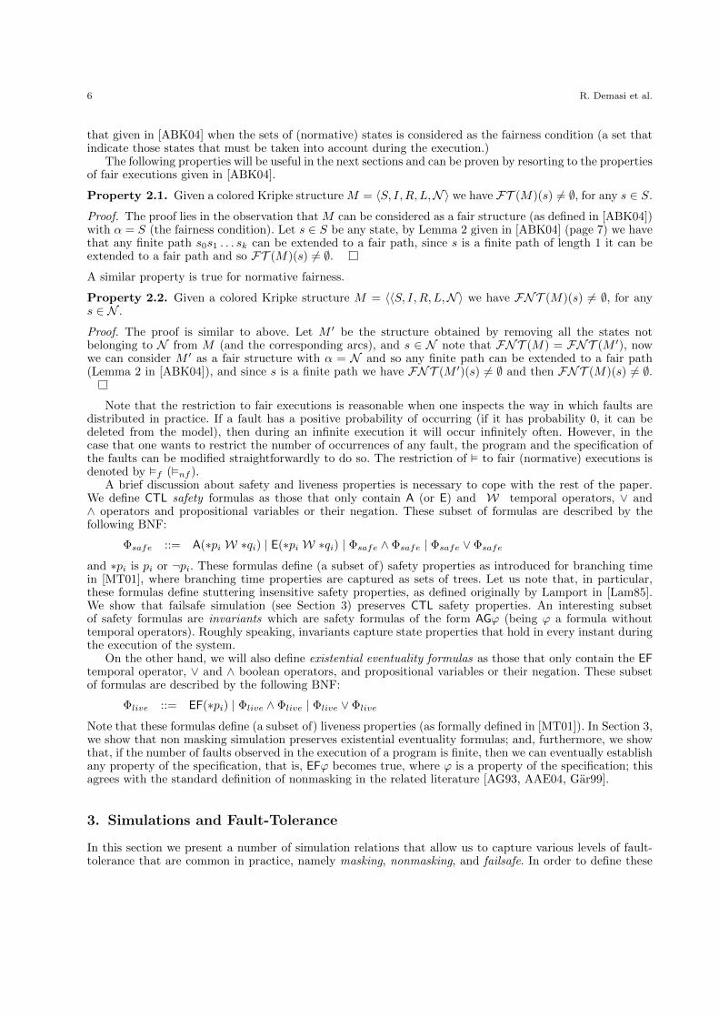
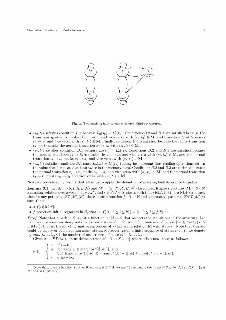
The state also maintains the values of the three bits that constitute the system, captured by booleanvariables c0, c1 and c2. For instance, in Figure 3, state s0 contains the information 11/111, representing thestate: w = 1, m = 1, c0 = 1, c1 = 1, and c2 = 1.
Consider the colored Kripke structures M (left) and M ′ (right) depicted in Figure 3. M only containsnormal transitions describing the expected ideal behavior (without taking into account faults). M ′ includesa model of a fault: a bit may suffer a discharge and then it changes its value from 1 to 0.
We can show that in this simple case there exists a relation of masking fault-tolerance between M andM ′ with the sub-labelings L0 and L′0 obtained by restricting L and L′ to variables m and w, respectively.The relation
M = {〈s0, t0〉, 〈s1, t1〉, 〈s0, t2〉}
is masking fault-tolerant for 〈M,M ′〉 and the sub-labelings L0 and L′0, obtained by restricting L and L′ tovariables m and w, respectively. Notice that each pair of M satisfies each condition of Definition 3.1:
Simulation Relations for Fault-Tolerance 9
s0
11/111
s1
00/000
t0
11/111
t1
00/000
t2
11/101
Fig. 3. Two masking fault-tolerance colored Kripke structures.
• 〈s0, t0〉 satisfies condition B.1 because L0(s0) = L′0(t0). Conditions B.2 and B.3 are satisfied because thetransition s0 → s0 is masked by t0 → t0 and vice versa with 〈s0, t0〉 ∈M, and transition t0 → t1 maskss0 → s1 and vice versa with 〈s1, t1〉 ∈M. Finally, condition B.4 is satisfied because the faulty transitiont0 99K t2 masks the normal transition s0 → s0 with 〈s0, t2〉 ∈M.
• 〈s1, t1〉 satisfies condition B.1 because L0(s1) = L′0(t1). Conditions B.2 and B.3 are satisfied becausethe normal transition t1 → t0 is masked by s1 → s0 and vice versa with 〈s0, t0〉 ∈ M, and the normaltransition t1 → t1 masks s1 → s1 and vice versa with 〈s1, t1〉 ∈M.
• 〈s0, t2〉 satisfies condition B.1 since L0(s0) = L′0(t2) (taking into account that reading operations returnthe value that is repeated at least twice in the memory bits). Conditions B.2 and B.3 are satisfied becausethe normal transition t2 → t0 masks s0 → s0 and vice versa with 〈s0, t0〉 ∈M, and the normal transitiont2 → t1 masks s0 → s1 and vice versa with 〈s1, t1〉 ∈M.
Now, we provide some results that allow us to apply the definition of masking fault-tolerance to paths.
Lemma 3.1. Let M = 〈S, I,R, L,N〉 and M ′ = 〈S′, I ′, R′, L′,N ′〉 be colored Kripke structures, M ⊆ S×S′a masking relation over a vocabulary AP ′, and s ∈ S, s′ ∈ S′ states such that sMs′. If M ′ is a NDF structure,then for any path σ′ ∈ FT (M ′)(s′), there exists a function f : N→ N and a normative path σ ∈ FNT (M)(s)such that:
• σ[f(i)] M σ′[i],
• f preserves initial segments in N, that is, f({i | 0 ≤ i ≤ k}) = {i | 0 ≤ i ≤ f(k)}1.
Proof. Note that a path in S is just a function σ : N→ S that respects the transitions in the structure. Letus introduce some auxiliary notions. Given a state s′ in S′, we define match(s, s′) = {w | w ∈ PostN (s) ∧w M s′}, that is, the set of normative successors of s that are in relation M with state s′. Note that this setcould be empty or could contain many states. Moreover, given a finite sequence of states t0 . . . tn we denoteby num(t0 . . . tn, si) the number of occurrences of state si in t0 . . . tn.
Given σ′ ∈ FT (M ′), let us define a trace σ∗ : N→ S ∪ {∗} where ∗ is a new state, as follows:
σ∗[i] =
s if i = 0,w for some w ∈ match(σ∗JiK, σ′[i]) and∀w′ ∈ match(σ∗JiK, σ′[i]) : num(σ∗[0, i− 1], w) ≤ num(σ∗[0, i− 1], w′),
∗ otherwise,
1Note that, given a function f : A→ B and subset S ⊆ A, we use f(S) to denote the image of S under f , i.e.: f(S) = {y ∈B | ∃x ∈ S : f(x) = y}.
10 R. Demasi et al.
where σ∗JiK = σ∗[last(i, σ∗)], and last(i, σ∗) = max{j | 0 ≤ j < i : σ∗(j) 6= ∗}, that is, the last position inσ∗ that is less than i and contains an element different from ∗.
Intuitively, each state in σ∗ different from ∗ simulates a state in S′, while ∗ states denote stuttering steps.Moreover, note in the definition of σ∗ when choosing some wM σ′[i]; we select the state with the minimumnumber of occurrences in σ∗[0..i− 1]. This ensures the fairness of the execution, since no state w satisfyingthat condition will be neglected forever.
An interesting property about σ∗ is the following:
∀i ≥ 0 : ∃j > i : σ∗[j] 6= ∗ (1)
That is, σ∗ does no contain the infinite string: ∗ ∗ ∗ ∗ . . . . Another interesting property of σ∗ is the following:
∀i : σ∗Ji+ 1K M σ′[i] (2)
A detailed proof of both properties can be found in the appendix.Now, we define function f as follows:
f(i)def= #{k | σ∗[k] 6= ∗ ∧ 0 < k ≤ i}
That is, f(i) counts the number of positions less than or equal to i (starting from 1) in which σ∗ does notcontain a ∗. Note that f is surjective: given any n ∈ N, consider the n-th occurrence of some s 6= ∗ in σ∗ (by(1) there is such an occurrence), let be k the index of such an occurrence, then f(k) = n.
σ is obtained by removing all the ∗’s from σ∗. To do this we use an auxiliary function g(i), defined asfollows:
∀i ≥ 0 : g(i)def= min{k | f(k) = i}
This is well defined since f is surjective. Some interesting properties of these functions are the following:
∀i ≥ 0 : g(i) = last(g(i+ 1), σ∗) (3)
and
∀i ≥ 0 : σ∗[g(f(i))] = σ∗Ji+ 1K (4)
A detailed proof of these properties is shown in the Appendix. Now, we define the normative trace σ asfollows:
∀i ≥ 0 : σ[i] = σ∗[g(i)] (5)
That is, for computing σ[i] we take σ∗ and find the position of the ith symbol in σ∗ different from ∗.Using these definitions we can prove that σ[f(i)] M σ′[i] as follows:
σ[f(i)] = σ∗[g(f(i))] (def. of σ)
= σ∗Ji+ 1K (property above)
M σ[i] (property above)
It remains to prove that σ ∈ FNT (M). First, let us prove that σ ∈ NT (M); that is, for every i,σ[i + 1] ∈ PostN (σ[i]). By definition of σ, this is equivalent to: σ∗[g(i + 1)] ∈ PostN (σ∗[g(i)]), but by (3)this is the same as: σ∗[g(i + 1)] ∈ PostN (last[g(i + 1)], σ∗) and that holds by the definitions of match andσ∗.
Now, we prove that σ is a fair execution. The proof is by contradiction, suppose that for some w and twe have that:
∀i : ∃j > i : σ[j] = w ∧ t ∈ PostN (w) ∧ ∃i ≥ 0 : ∀j > i : σ[j] = w ⇒ σ[j + 1] 6= t, (6)
and let be j1 < j2 < j3 . . . the positions that σ[jk] = w. Since f is surjective, we have i1, i2, . . . suchthat f(ik) = jk, for every k, and since σ[f(ik)] M σ′[ik] (as proven above), we have that σ[jk] M σ′[ik].Furthermore, t ∈ PostN (σ[jk]) for every jk. Since condition B.2 we have a set {t′k | k ≥ 0} such thatt′k ∈ PostN (σ′[ik]) and tM t′k. Note that the number of states in S′ is finite, so we must have some state (sayt′) that occurs infinitely often in {t′k | k ≥ 0}. Also, σ′ is a fair execution, then we must have σ′[ik + 1] = t′
for an infinite number of ik’s (by the fair successor property), that is, t ∈ match(σ[jk], σ′[ik]), which, by(3) and definition of σ, implies that t ∈ match(σ∗[last(jk + 1, σ∗)], σ′[ik]). Now, by the assumption above,
Simulation Relations for Fault-Tolerance 11
we have some i such that ∀j > i : σ[j] = w ⇒ σ[j + 1] 6= t, but note that for a j enough large this leadsto a contradiction. Since in the definition of σ∗ when choosing σ∗[jk + 1] (for jk > j) we choose the statein match(σ∗[last(jk + 2, σ∗)], σ′[ik]) occurring the minimum number of times in σ∗[0..jk], since t has beenneglected since position i, it must be the state in match(σ∗[last(jk +1, σ∗)], σ′[ik]) that occurs the minimumnumber of times in the fragment σ∗[0..jk], and so it will occur at position jk + 1 in σ∗, contradicting (6).
Finally, we prove that f preserves initial segments. That is, for any initial segment {x | 0 ≤ x ≤ i} in N,f({x | 0 ≤ x ≤ i}) = {y | 0 ≤ y ≤ f(i)}. First, note that f is monotone (a detailed proof is given in theAppendix) and f(0) = 0. Take k ∈ f({x | 0 ≤ x ≤ i}), then k = f(j) for some j ≤ i, and by monotonicitywe have, f(j) ≤ f(i) and so k ∈ {y | 0 ≤ y ≤ f(i)}. Now, take k′ ∈ {y | 0 ≤ y ≤ f(i)}, that is, k′ ≤ f(i).By surjectivity of f , we have f(k) = k′ for some k, and k ≤ i (otherwise we have a contradiction), and thenk′ ∈ f({x | 0 ≤ x ≤ i}). Thus both sets are equal.
Note that, if we only consider normative executions starting in s1 and s2 with s1 M s2, by conditions (B.3)and (B.4) of Definition 3.1 we have that, for each normative path starting in s2, there exists a correspondingpath from s1, where its states are similar by a masking relation. This is proven in the following lemma.
Lemma 3.2. Let M = 〈S, I,R, L,N〉 and M ′ = 〈S′, I ′, R′, L′,N ′〉 be colored Kripke structures, M ⊆ S×S′a masking relation over a vocabulary AP ′, and s ∈ S, s′ ∈ S′ states such that s M s′. Then there exist afunction f : FNT (M)(s)→ FT (M ′)(s′) such that:
• ∀σ ∈ FNT (M)(s) : ∀i ≥ 0 : σ[i] M f(σ)[i],
Proof. Given σ ∈ FNT (M)(s) s.t. σ = ss1s2 . . . , then note that we have sM s′ and by (B.2), if si M s′i andsi+1 ∈ PostN (si), then there exists s′i+1 ∈ Post(s′i) such that si+1 M s′i+1. Thus, we can define inductivelya sequence f(σ) = s′s′1s
′2 . . . that satisfies σ[j] M f(σ)[j] for every j. To ensure the fairness of such a
construction, when choosing the successor of a given f(σ)[i] where σ[i] M f(σ)[i], we select the successort ∈ Post(f(σ)[i]) such that σ[i+1]M t that appears the minimum number of times in f(σ)[0..i], which existsby condition (B.2). The result follows.
Now, we can prove that, in the case of masking simulation, the liveness and safety properties of thenormal behavior of the specification are preserved by the implementation. However, note that not all thetemporal properties are preserved; formulas with occurrences of the next operator may not be preserved bythe implementation. Roughly speaking, this is because condition (B.4) allows implementations to advancein time while staying in the same state on the specification side.
Theorem 3.3. Let M = 〈S, I,R, L,N〉 and M ′ = 〈S′, I ′, R′, L′,N ′〉 be colored Kripke structures, M ⊆S×S′ a masking relation over a vocabulary AP ′, and states s1 ∈ S, s2 ∈ S′ be states such that sMs′. Then:
M, s �nf ϕ⇔M ′, s′ �f ϕ,
where ϕ is a CTL-X formula where all the propositional variables of ϕ are in AP ′.
Proof. We proceed by induction over the structure of the formula ϕ.
• Base Case: ϕ = pi. From s M s′ it follows by condition (B.1) for masking fault-tolerance that s and s′
have the same propositional valuation. Thus, M, s �nf pi ⇔M ′, s′ �f pi.• Inductive Case: we prove the property for operators ∧,¬,EU , EG since the other ones can be expressed
by means of them.
Case 1: For ϕ = ψ∧ψ′ and ϕ = ¬ψ the result follows by a direct application of the inductive hypothesis.
Case 2: ϕ = E(ψ1 U ψ2). Let us prove the right implication, suppose that M, s �nf (E(ψ1 U ψ2)), thenfor some path σ ∈ FNT (M) with σ[0] = s we have that:
∃i ≥ 0 : M,σ[i] �nf (ψ2) and ∀0 ≤ j < i : M,σ[j] �nf ψ1
Then by Lemma 3.2 we have a path f(σ) ∈ FT (M ′) with f(σ)[0] = s′ s.t. ∀i ≥ 0 : σ[i] M f(σ)[i]; thisimplies by induction that:
∃i ≥ 0 : M ′, f(σ)[i] �f ψ2 and ∀0 ≤ j < i : M,f(σ)[j] �f ψ1
Then, M ′, s′ �f E(ψ1 U ψ2).For the other direction, we proceed as follows. Assume M ′, s′ �f E(ψ1 U ψ2), this means that
12 R. Demasi et al.
there is some σ′ ∈ FT (s′) such that ∃i ≥ 0 : M ′, s′ �f ψ2 and ∀j : 0 ≤ j < i : M ′, σ′ �f ψ1. Now,by Lemma 3.1, we have a σ ∈ FNT (s) and a function f such that σ[f(i)] M σ′[i], by induction thisimplies that M,σ[f(i)] � ψ2 and also M,σ[f(j)] � ψ1 for 0 ≤ j < i, but since f preserves initialsegments of N we have that {f(0), f(1), . . . , f(i)} = {j | 0 ≤ j < f(i)} and then M,σ[j] �nf ψ1 for0 ≤ j < f(i) which is implies that: M,σ[0] �nf E(ψ1 U ψ2).
Case 3: ϕ = EGψ. Let us prove the right implication. Suppose M, s �nf EGψ, this means that there issome σ ∈ FNT (s) ∀i ≥ 0 : M,σ[i] �nf ψ. By Lemma 3.2 we have some σ′ ∈ FT (M ′)(s′) such thatσ[i] M σ′[i], and so by induction the result follows.
For the other direction assume now that M ′, s′ �f EGψ, this means that ∀i ≥ 0 : M ′, σ′[i] �f ψ,by Lemma 3.1 we have a trace σ ∈ FNT (s) and a function f such that σ[f(i)] M σ[i], by inductionwe have that M,σ[f(i)] � ψ, but since f is surjective this implies that M,σ[i] �nf ψ for every i, thusM, s �nf EGψ.
Summing up, in the case of masking simulation, the basic temporal properties of systems without faults,such as invariants or liveness formulas, are preserved by masking tolerant implementations.
3.2. Nonmasking Fault-Tolerance
We now focus on nonmasking fault-tolerance. This kind of tolerance is more permissive than masking fault-tolerance; recall that it allows for the existence of some states that do not mask faults. Intuitively, thistype of fault-tolerance allows the system to violate its specification while it is recovering from a fault andeventually returning to a normal behavior. The technical definition of nonmasking [Gar99] states that theliveness properties of the nonfaulty part of the system have to be preserved, whereas the safety propertiesobserved in the correct behavior of the system may not be fully preserved. Furthermore, sometimes a strongerdefinition of nonmasking is adopted in which the safety properties may be violated but they should beeventually reinstated [AAE04, Gar99], which can be captured in CTL with formulas AFϕ or EFϕ (being ϕthe safety and liveness properties to be preserved) here we will be interested in the latter kinds of formulas,which intuitively state that the system has a way of recovering from faults, stronger versions of the notionof nonmasking given above can be considered (guaranteeing that all the execution recover from faults), butthey are much more complex to capture (and to algorithmically verify) since quantification over paths isneeded for formally defining them.
Our characterization of nonmasking fault-tolerance is as follows.
Definition 3.4. (Nonmasking fault-tolerance) Given two colored Kripke structures M = 〈S, I,R, L,N〉 andM ′ = 〈S′, I ′, R′, L′,N ′〉, we say that a relation N ⊆ S × S′ is nonmasking for sub-labelings L0 ⊆ L andL′0 ⊆ L′, iff:
(A) ∀s1 ∈ I : (∃s2 ∈ I ′ : s1 N s2) and ∀s2 ∈ I ′ : (∃s1 ∈ I : s1 N s2).
(B) for all s1 N s2 the following holds:
(1) L0(s1) = L′0(s2);
(2) if s′1 ∈ PostN (s1), then there exists s′2 ∈ Post(s2) with s′1 N s′2;
(3) if s′2 ∈ PostN (s2), then there exists s′1 ∈ PostN (s1) with s′1 N s′2;
(4) if s′2 ∈ PostF (s2), then there exists a s′1 ∈ PostN (s1) and a s′′2 ∈ Post∗(s′2) such that s′1 N s′′2 .
As before, when sub-labelings L0 and L′0 are obtained by restricting L0 and L′0 to a vocabulary AP ′ we justsay that N is defined over AP ′.
Let us briefly explain this definition. Conditions A, B.1, B.2 and B.3 are the same as the conditions ofDefinition 3.1. Condition B.4 asserts that, if s1 N s2 and every “faulty” successor state (say s′2) of s2 is notin a nonmasking relation with any normal successor of s1, then any faulty path fragment starting at s′2 canbe extended to reach a s′′2 such that s′1 N s′′2 for some normal successor s′1 of s1; that is, the system canrecover from faults.
We define the relation ≺Nonmask between colored Kripke structures.

Simulation Relations for Fault-Tolerance 13
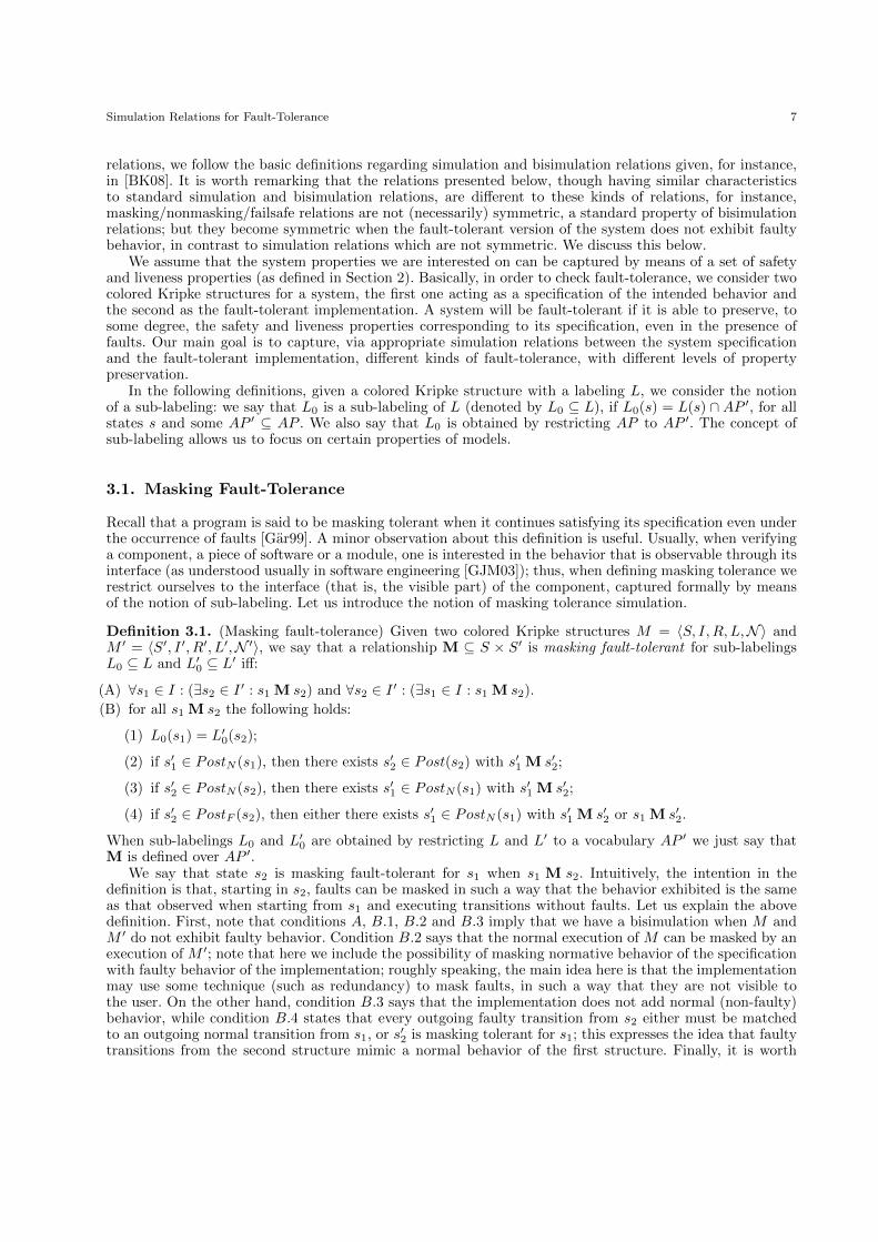
s0
11/111
s1
00/000
t0
11/111
t1
00/000
t2
11/101
t3
10/100
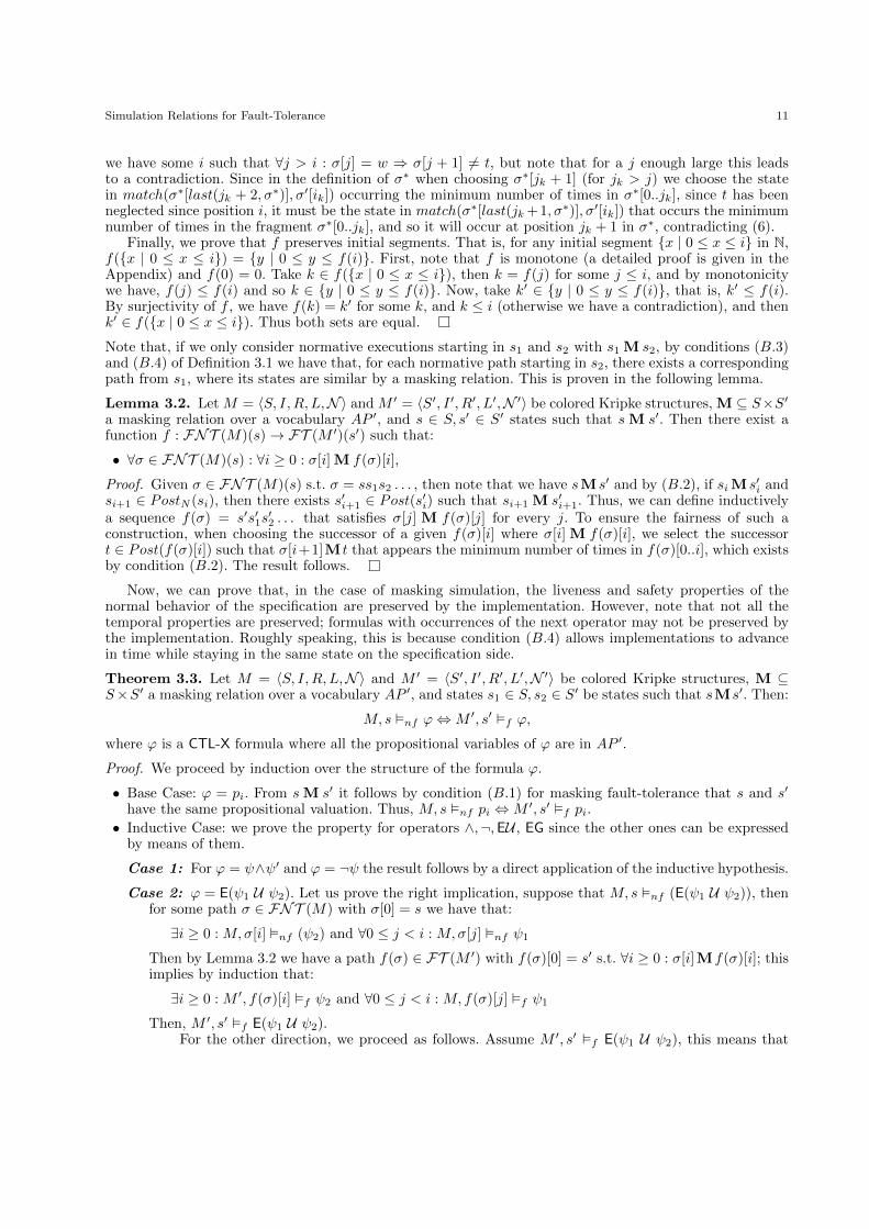
Fig. 4. Two nonmasking fault-tolerance colored Kripke structures.
Definition 3.5. Given two colored Kripke structures M = 〈S, I,R, L,N〉 and M ′ = 〈S′, I ′, R′, L′,N ′〉:
M ≺Nonmask M′ ⇔ there is a nonmasking simulation N ⊆ S × S′
If M ≺Nonmask M′ we say that M ′ is a nonmasking fault-tolerant implementation of M .
At first sight, nonmasking fault-tolerance seems similar to the notion of weak bisimulation used in processalgebra [Mil89], where silent steps are taken into account. Notice, however, that, as opposed to weak bisimu-lation where silent steps produce only non-observable (i.e., internal) changes, faults may produce observablechanges in a nonmasking fault-tolerance relation. Let us present an example of nonmasking tolerance.
Example 3.2. For the memory cell introduced in Example 3.1, consider now the colored Kripke structuresM (left) and M ′ (right) depicted in Figure 4. Now we consider that two faults may occur: up to two bitsmay lose their charge before any normal transition is taken. The relation N = {〈s0, t0〉, 〈s1, t1〉, 〈s0, t2〉}is nonmasking tolerant for 〈M,M ′〉 and the sub-labelings L0 and L′0, obtained by restricting L and L′ tovariables m and w, respectively.
As discussed above, in nonmasking fault-tolerance, one is interested in preserving the liveness propertiesof the non-faulty part of the system; for instance, the requests need to be granted, or the program shouldexhibit some advance towards a given goal, even during a faulty scenario. Note that, in this case, safetyconditions do not need to be preserved. We prove that liveness properties defined by means of eventualityCTL formulas are preserved by nonmasking simulation. First, we prove a lemma about normative and faultyexecutions of two systems related by a nonmasking relation.
Lemma 3.4. GivenM = 〈S, I,R, L,N〉 andM ′ = 〈S′, I ′, R′, L′,N ′〉, N ⊆ S×S′ a nonmasking relation overa vocabulary AP ′, and states s ∈ S, s′ ∈ S′ with sN s′. If there is a σ ∈ FNT (M)(s), such that M,σ � F∗p,for some p in AP ′ (where ∗ is ¬ or blank), then there is a σ′ ∈ FT (M ′)(s′) such that M ′, σ′ � F∗p.
Proof. Given σ ∈ FNT (M)(s), we can define an execution σ′ ∈ FT (M ′) by induction. We define σ′[0] = s′,and σ′[i+ 1] = w, for some w ∈ Post(σ′[i]) such that σ[i+ 1] Nw, which exists by condition B.2. To ensurethe fairness of σ when choosing w we select that state that occurs the minimum number of times in σ[0..i−1],that is, no such a w will be neglected forever.
Now, since M,σ � F ∗ p, we have some k ≥ 0 such that M,σ[k] � ∗p, and then by condition B.1 ofDefinition 3.4 and taking into account that σ[k] N σ′[k] , we have that M,σ′[k] � ∗p. Thus, M,σ′ � F ∗ p.
Now, we can prove that, in the presence of fairness, existential eventuality formulas are preserved by non-masking implementations:
Theorem 3.5. Let M = 〈S, I,R, L,N〉 and M ′ = 〈S′, I ′, R′, L′,N ′〉 be colored Kripke structures, N ⊆S × S′ a nonmasking relation over a vocabulary AP ′, and states s ∈ S, s′ ∈ S′ with sN s′. Then
M, s �nf ϕ⇒M ′, s′ �f ϕ,
where ϕ is an existential eventuality CTL formula and all the propositional variables of ϕ are in AP ′.
Proof. The proof is by induction on ϕ. For the base case, we have :
14 R. Demasi et al.
• If ϕ = EFp, suppose M, s �nf ϕ, that is, there is an execution σ ∈ FNT (M) such that M,σ[i] � p, forsome i, thus by Lemma 3.4, we have a σ′ ∈ FT (M ′) such that M ′, σ′[k] � p for some k.
The inductive cases (that is, ψ1 ∨ ψ2 and ψ1 ∧ ψ2) are direct using the inductive hypothesis.
Note that this theorem guarantees that implementations preserve the existential liveness properties of speci-fications. Furthermore, notice that the other direction of this property is not necessarily true. This is mainlybecause nonmasking implementations may eventually make true some properties, during its faulty behavior,which do not hold in the non-faulty program.
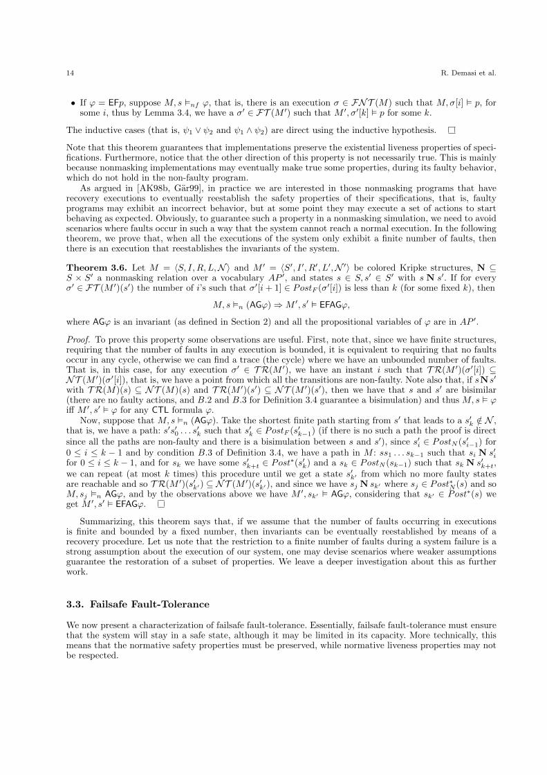
As argued in [AK98b, Gar99], in practice we are interested in those nonmasking programs that haverecovery executions to eventually reestablish the safety properties of their specifications, that is, faultyprograms may exhibit an incorrect behavior, but at some point they may execute a set of actions to startbehaving as expected. Obviously, to guarantee such a property in a nonmasking simulation, we need to avoidscenarios where faults occur in such a way that the system cannot reach a normal execution. In the followingtheorem, we prove that, when all the executions of the system only exhibit a finite number of faults, thenthere is an execution that reestablishes the invariants of the system.
Theorem 3.6. Let M = 〈S, I,R, L,N〉 and M ′ = 〈S′, I ′, R′, L′,N ′〉 be colored Kripke structures, N ⊆S × S′ a nonmasking relation over a vocabulary AP ′, and states s ∈ S, s′ ∈ S′ with s N s′. If for everyσ′ ∈ FT (M ′)(s′) the number of i’s such that σ′[i+ 1] ∈ PostF (σ′[i]) is less than k (for some fixed k), then
M, s �n (AGϕ)⇒M ′, s′ � EFAGϕ,
where AGϕ is an invariant (as defined in Section 2) and all the propositional variables of ϕ are in AP ′.
Proof. To prove this property some observations are useful. First, note that, since we have finite structures,requiring that the number of faults in any execution is bounded, it is equivalent to requiring that no faultsoccur in any cycle, otherwise we can find a trace (the cycle) where we have an unbounded number of faults.That is, in this case, for any execution σ′ ∈ T R(M ′), we have an instant i such that T R(M ′)(σ′[i]) ⊆NT (M ′)(σ′[i]), that is, we have a point from which all the transitions are non-faulty. Note also that, if sNs′
with T R(M)(s) ⊆ NT (M)(s) and T R(M ′)(s′) ⊆ NT (M ′)(s′), then we have that s and s′ are bisimilar(there are no faulty actions, and B.2 and B.3 for Definition 3.4 guarantee a bisimulation) and thus M, s � ϕiff M ′, s′ � ϕ for any CTL formula ϕ.
Now, suppose that M, s �n (AGϕ). Take the shortest finite path starting from s′ that leads to a s′k /∈ N ,that is, we have a path: s′s′0 . . . s
′k such that s′k ∈ PostF (s′k−1) (if there is no such a path the proof is direct
since all the paths are non-faulty and there is a bisimulation between s and s′), since s′i ∈ PostN (s′i−1) for0 ≤ i ≤ k − 1 and by condition B.3 of Definition 3.4, we have a path in M : ss1 . . . sk−1 such that si N s′ifor 0 ≤ i ≤ k − 1, and for sk we have some s′k+t ∈ Post∗(s′k) and a sk ∈ PostN (sk−1) such that sk N s′k+t,we can repeat (at most k times) this procedure until we get a state s′k′ from which no more faulty statesare reachable and so T R(M ′)(s′k′) ⊆ NT (M ′)(s′k′), and since we have sj N sk′ where sj ∈ Post∗N (s) and soM, sj �n AGϕ, and by the observations above we have M ′, sk′ � AGϕ, considering that sk′ ∈ Post∗(s) weget M ′, s′ � EFAGϕ.
Summarizing, this theorem says that, if we assume that the number of faults occurring in executionsis finite and bounded by a fixed number, then invariants can be eventually reestablished by means of arecovery procedure. Let us note that the restriction to a finite number of faults during a system failure is astrong assumption about the execution of our system, one may devise scenarios where weaker assumptionsguarantee the restoration of a subset of properties. We leave a deeper investigation about this as furtherwork.
3.3. Failsafe Fault-Tolerance
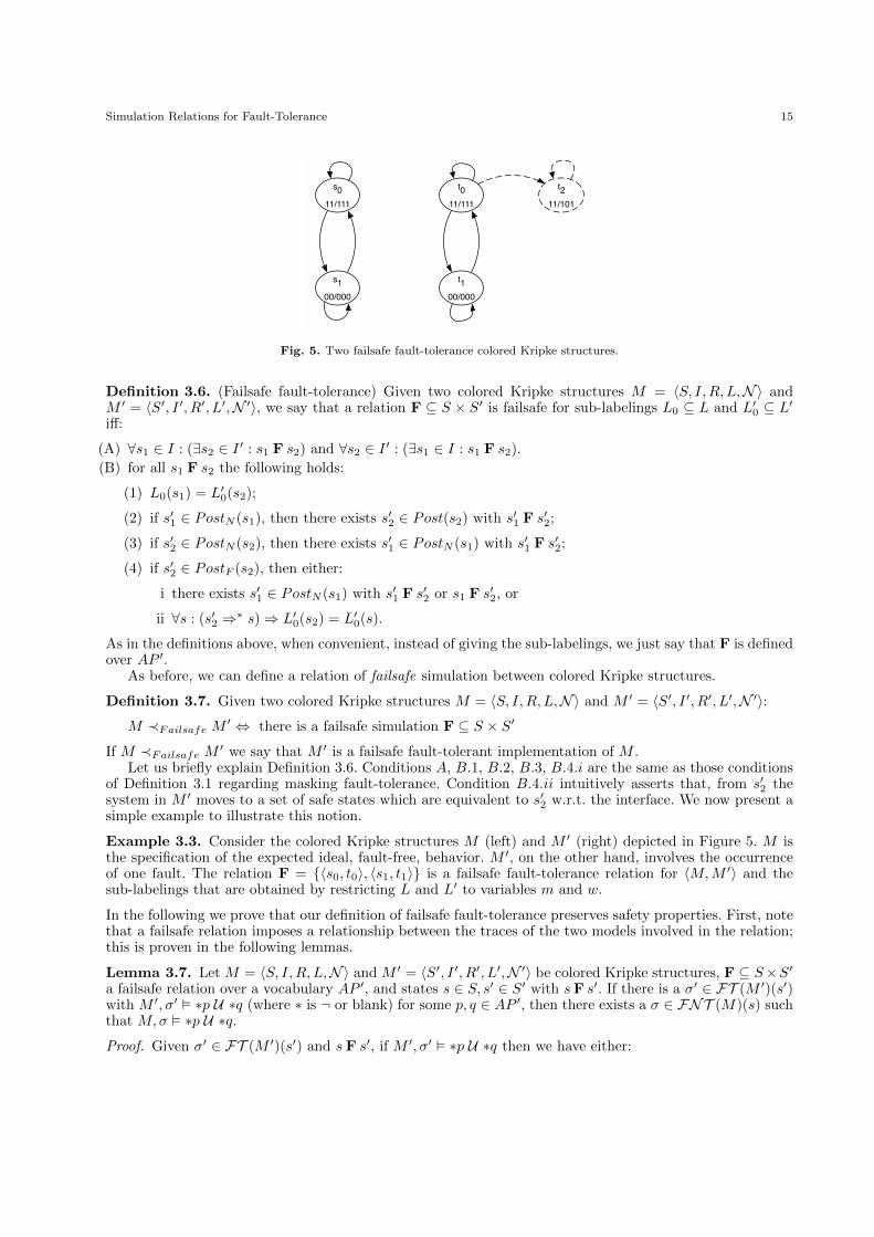
We now present a characterization of failsafe fault-tolerance. Essentially, failsafe fault-tolerance must ensurethat the system will stay in a safe state, although it may be limited in its capacity. More technically, thismeans that the normative safety properties must be preserved, while normative liveness properties may notbe respected.
Simulation Relations for Fault-Tolerance 15
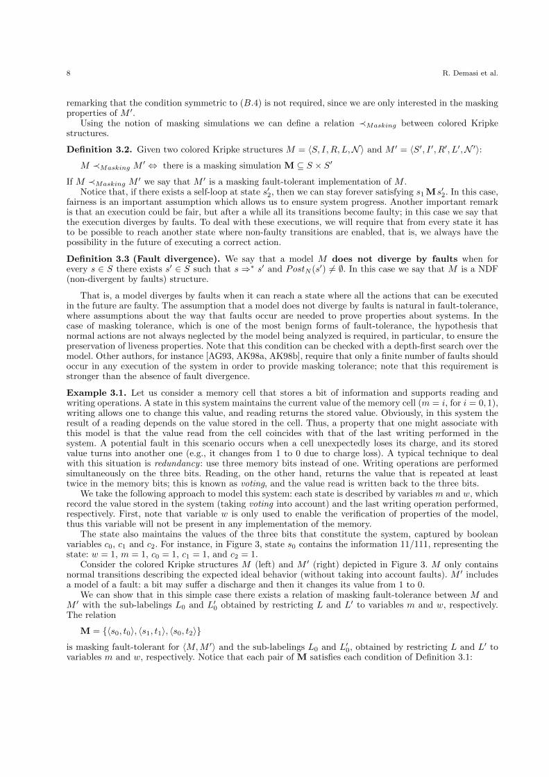
s0
11/111
s1
00/000
t0
11/111
t1
00/000
t2
11/101
Fig. 5. Two failsafe fault-tolerance colored Kripke structures.
Definition 3.6. (Failsafe fault-tolerance) Given two colored Kripke structures M = 〈S, I,R, L,N〉 andM ′ = 〈S′, I ′, R′, L′,N ′〉, we say that a relation F ⊆ S × S′ is failsafe for sub-labelings L0 ⊆ L and L′0 ⊆ L′
iff:
(A) ∀s1 ∈ I : (∃s2 ∈ I ′ : s1 F s2) and ∀s2 ∈ I ′ : (∃s1 ∈ I : s1 F s2).
(B) for all s1 F s2 the following holds:
(1) L0(s1) = L′0(s2);
(2) if s′1 ∈ PostN (s1), then there exists s′2 ∈ Post(s2) with s′1 F s′2;
(3) if s′2 ∈ PostN (s2), then there exists s′1 ∈ PostN (s1) with s′1 F s′2;
(4) if s′2 ∈ PostF (s2), then either:
i there exists s′1 ∈ PostN (s1) with s′1 F s′2 or s1 F s′2, or
ii ∀s : (s′2 ⇒∗ s)⇒ L′0(s2) = L′0(s).
As in the definitions above, when convenient, instead of giving the sub-labelings, we just say that F is definedover AP ′.
As before, we can define a relation of failsafe simulation between colored Kripke structures.
Definition 3.7. Given two colored Kripke structures M = 〈S, I,R, L,N〉 and M ′ = 〈S′, I ′, R′, L′,N ′〉:
M ≺Failsafe M′ ⇔ there is a failsafe simulation F ⊆ S × S′
If M ≺Failsafe M′ we say that M ′ is a failsafe fault-tolerant implementation of M .
Let us briefly explain Definition 3.6. Conditions A, B.1, B.2, B.3, B.4.i are the same as those conditionsof Definition 3.1 regarding masking fault-tolerance. Condition B.4.ii intuitively asserts that, from s′2 thesystem in M ′ moves to a set of safe states which are equivalent to s′2 w.r.t. the interface. We now present asimple example to illustrate this notion.
Example 3.3. Consider the colored Kripke structures M (left) and M ′ (right) depicted in Figure 5. M isthe specification of the expected ideal, fault-free, behavior. M ′, on the other hand, involves the occurrenceof one fault. The relation F = {〈s0, t0〉, 〈s1, t1〉} is a failsafe fault-tolerance relation for 〈M,M ′〉 and thesub-labelings that are obtained by restricting L and L′ to variables m and w.
In the following we prove that our definition of failsafe fault-tolerance preserves safety properties. First, notethat a failsafe relation imposes a relationship between the traces of the two models involved in the relation;this is proven in the following lemmas.
Lemma 3.7. Let M = 〈S, I,R, L,N〉 and M ′ = 〈S′, I ′, R′, L′,N ′〉 be colored Kripke structures, F ⊆ S×S′a failsafe relation over a vocabulary AP ′, and states s ∈ S, s′ ∈ S′ with sF s′. If there is a σ′ ∈ FT (M ′)(s′)with M ′, σ′ � ∗p U ∗q (where ∗ is ¬ or blank) for some p, q ∈ AP ′, then there exists a σ ∈ FNT (M)(s) suchthat M,σ � ∗p U ∗q.
Proof. Given σ′ ∈ FT (M ′)(s′) and s F s′, if M ′, σ′ � ∗p U ∗q then we have either:
16 R. Demasi et al.
(a) M ′, s′ � ∗q or
(b) there is a k > 0 such that M ′, σ′[k] � ∗q and M ′, σ′[j] � ∗p for every j < k.
In the first case, since sF s′ and condition B.1 of Definition 3.4 we obtain M, s � ∗q and so M,σ � ∗p U ∗ q,for any σ ∈ FNT (M)(s), and by Property 2.1, FNT (M)(s) 6= ∅ and then we have a σ ∈ FNT (M)(s)satisfying M,σ � ∗p U ∗ q.
On the other hand, if (b) holds, then let us define a finite path s, s1, s2, . . . , sk′ in M such that M, sk′ � ∗qand M, si � ∗p for 0 ≤ i < k′. First, note that M ′, s′ 2 ∗q and M ′, σ′[k] � ∗q, since s′ ⇒∗ σ′[k] we havethat condition B.4.ii does not hold in any path starting from s′; taking into account that sF s′ we define asequence w = w0, w1, w2, . . . , wk of states in S as follows:
wi =
{s if i = 0,w if there is w ∈ Post(wi−1) with w F s′i,wi−1 otherwise.
Note that for the segment obtained: w0, w1, . . . , wk we have wiFsi; also note that in w we may have somerepeated states, then let w′ = w′0, w
′1, . . . , w
′k′ (with k′ ≤ k) the finite path obtained by removing from w all
the repeated states that do not have self-loops in M . For this sequence of states w′, we have M,w′k′ � ∗q(since w′k′ F wk) and M,w′i � ∗p (since w′i F s′j for some i < k′ and j < k), and also w′i+1 ∈ PostN (w′i),because repeated states were removed. Now, by Property 2.2, we have some σ0 ∈ FNT (M)(wk′), and thenwe can form the path: σ = w′:σ0 (w′ concatenated σ0), also note that σ ∈ FNT (M)(s) (it is fair since σ0is fair). Furthermore, we have M,σ � ∗p U ∗q, this finishes the proof.
Lemma 3.8. Let M = 〈S, I,R, L,N〉 and M ′ = 〈S′, I ′, R′, L′,N ′〉 be colored Kripke structures, F ⊆ S×S′a failsafe relation over a vocabulary AP ′, and states s ∈ S, s′ ∈ S′ with sF s′. If there is a σ ∈ FNT (M)(s)with M,σ � ∗pW ∗q (where ∗ is ¬ or blank) for some p, q ∈ AP ′, then there exists a σ′ ∈ FT (M ′)(s′) suchthat M ′, σ′ � ∗pW ∗q.
Proof. Given σ ∈ FNT (M)(s) such that M,σ � ∗p W ∗q and let σ = s0s1, . . . , by definition of � we haveeither:
(a) ∃j ≥ 0 : M,σ[j] � ∗q and ∀0 ≤ i < j : M,σ[i] � ∗p, or
(b) ∀j ≥ 0 : M,σ[j] � ∗p.
by B.2 of Definition 3.6 we can define inductively an execution σ′ in FT (M ′)(s′), say σ′ = s′0s′1 . . . , such
that: si F s′i, by Definition 3.6 this implies that L0(si) = L′0(s′i) for every i. That is if (a) holds, then wehave: ∃j ≥ 0 : M ′, σ′[j] � ∗q and ∀0 ≤ i < j : M ′, σ′[i] � ∗p; and if (b) holds we have: ∀j ≥ 0 : M ′, σ′[j] � ∗p;thus in any case we get: M ′, σ′ � ∗pW ∗q.
Let us now prove that failsafe implementations preserve safety properties.
Theorem 3.9. Let M = 〈S, I,R, L,N〉 and M ′ = 〈S′, I ′, R′, L′,N ′〉 be colored Kripke structures, F ⊆S × S′ a failsafe relation over a vocabulary AP ′, and states s1 ∈ S, s2 ∈ S′ with s1 F s2. Then:
M, s1 �nf ϕ⇒M ′, s2 �f ϕ
where ϕ is a CTL safety property and all the propositional variables of ϕ are in AP ′.
Proof. We proceed by induction on ϕ. The base case is as follows:
• If ϕ = A(∗p W ∗q), then suppose M, s �nf A(∗p W ∗q) and not M ′, s′ �f A(∗p W ∗q). Thus, we havea σ′ ∈ FT (M ′)(s′) such that M ′, σ′ � (∗p ∧ ¬∗q) U (¬∗p ∧ ¬∗q), consider fresh variables s and t suchthat s ≡ ∗p ∧ ¬∗q and t ≡ ¬∗p ∧ ¬∗q, that is we have M ′, σ′ � s U t. By Lemma 3.7 we get that forsome σ ∈ FNT (M)(s) we have that M,σ �nf s U t and so M,σ �nf (∗p ∧ ¬∗q) U (¬∗p ∧ ¬∗q), whichcontradicts our initial assumption.
• If ϕ = E(∗p W ∗q), then we have some path σ ∈ FNT (M)(s1) such that M,σ � ∗p W ∗q, then byLemma 3.8 we have a σ′ ∈ FT (M ′)(s2) such that M ′, σ′ � ∗pW ∗q and so M ′, s2 � E(∗pW ∗q).
The inductive cases are direct by using the inductive hypothesis.
That is, if we have a failsafe relation between s1 and s2 and for every state in normal paths starting in s1,
Simulation Relations for Fault-Tolerance 17
and a safety property ϕ holds in the absence of faults, then ϕ is always true even in the presence of faultsin paths starting in s2.
3.4. Some Properties
The following lemma presents some properties of the fault-tolerance relations defined above.
Lemma 3.10. Let @∈ {≺Masking,≺Nonmask,≺Failsafe}, then the following properties hold.
• @ is transitive,
• If M and M ′ does not have faults, then: M @M ′ ⇒M ′ @M ,
• @ is not necessarily reflexive.
Proof. We prove the properties for any masking relation ≺Masking. The proofs for the other relations aresimilar.
• Transitivity Suppose that M1 ≺Masking M2 and M2 ≺Masking M3, for colored Kripke structures M1 =〈S1, I1, R1, L1,N1〉, M2 = 〈S2, I2, R2, L2,N2〉, and M3 = 〈S3, I3, R3, L3,N3〉, and sub-labellings L′1 ⊆L1, L
′2 ⊆ L2, and L′3 ⊆ L3 with L′1 = L′2 = L′3. By definition of ≺Masking this means that we have
relations: M1,2 ⊆ S1 × S2 and M2,3 ⊆ S2 × S3 such that the relation M1,3 = M1,2 ◦M2,3, defined asusual, is masking fault-tolerant for 〈M1,M3〉. This can be proven by checking the conditions of Definition3.1:
(A) Consider the initial state s1 of M1. Since M1,2 is masking fault-tolerant, there is an initial state s2of M2 with 〈s1, s2〉 ∈M1,2. As M2,3 is masking fault-tolerant, there is an initial state s3 of M3 with〈s2, s3〉 ∈M2,3. Thus, 〈s1, s3〉 ∈M1,3. In the same way, we can check that for any initial state s3 ofM3, there is an initial state s1 of M1 with 〈s1, s3〉 ∈M1,3.
(B.1) By definition of M1,3, there is a state s2 in M2 with 〈s1, s2〉 ∈M1,2 and 〈s2, s3〉 ∈M2,3. Then,L′1(s1) = L′2(s2) = L′3(s3).
(B.2) Assume 〈s1, s3〉 ∈ M1,3. As 〈s1, s2〉 ∈ M1,2 (for some s2 by definition of ◦), it follows that, ifs′1 ∈ PostN (s1), then 〈s′1, s′2〉 ∈M1,2 for some s′2 ∈ PostN (s2). Since 〈s2, s3〉 ∈M2,3 (by definition of◦), we have 〈s′2, s′3〉 ∈M2,3 for some s′3 ∈ PostN (s3). Hence, 〈s′1, s′3〉 ∈M1,3
(B.3) Similar to the proof for (B.2).
(B.4) Assume 〈s1, s3〉 ∈ M1,3, that is, for some s2 we have s1 M1,2 s2 and s2 M2,3 s3. Now, if s′3 ∈PostF (s3), then by condition B.4 we have a s′2 ∈ PostN (s2) such that s′2 M2,3 s
′3 or s2 M2,3 s
′3; in
the latter case, by definition of ◦ we have that s1 M1,3 s′3 and then condition B.4 holds. In the former
case, since s′2 ∈ PostN (s2) and s1 M1,2 s2 by condition B.3 we have a s′1 ∈ PostN (s1) such thats′1 M1,2 s
′2 and then by ◦ we get s′1 M1,3 s
′3.
Symmetry: In this case the proof is direct since conditions A,B.1, B.2 and B.3 imply that there is abisimulation between M and M ′.
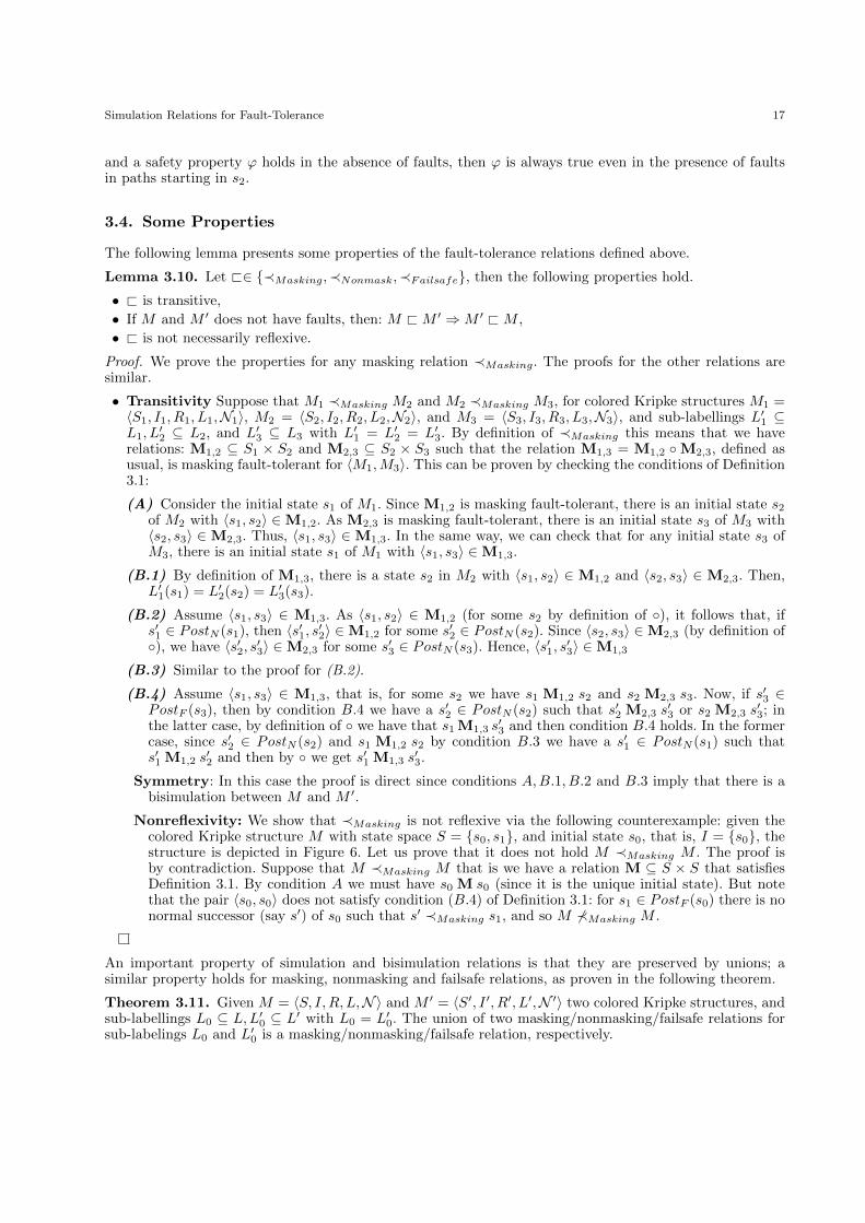
Nonreflexivity: We show that ≺Masking is not reflexive via the following counterexample: given thecolored Kripke structure M with state space S = {s0, s1}, and initial state s0, that is, I = {s0}, thestructure is depicted in Figure 6. Let us prove that it does not hold M ≺Masking M . The proof isby contradiction. Suppose that M ≺Masking M that is we have a relation M ⊆ S × S that satisfiesDefinition 3.1. By condition A we must have s0 M s0 (since it is the unique initial state). But notethat the pair 〈s0, s0〉 does not satisfy condition (B.4) of Definition 3.1: for s1 ∈ PostF (s0) there is nonormal successor (say s′) of s0 such that s′ ≺Masking s1, and so M ⊀Masking M .
An important property of simulation and bisimulation relations is that they are preserved by unions; asimilar property holds for masking, nonmasking and failsafe relations, as proven in the following theorem.
Theorem 3.11. Given M = 〈S, I,R, L,N〉 and M ′ = 〈S′, I ′, R′, L′,N ′〉 two colored Kripke structures, andsub-labellings L0 ⊆ L,L′0 ⊆ L′ with L0 = L′0. The union of two masking/nonmasking/failsafe relations forsub-labelings L0 and L′0 is a masking/nonmasking/failsafe relation, respectively.
18 R. Demasi et al.
s0
p
s1
r
Fig. 6. Counterexample for reflexivity.
s0
p
s1
p
t0
p
t1
p
t2
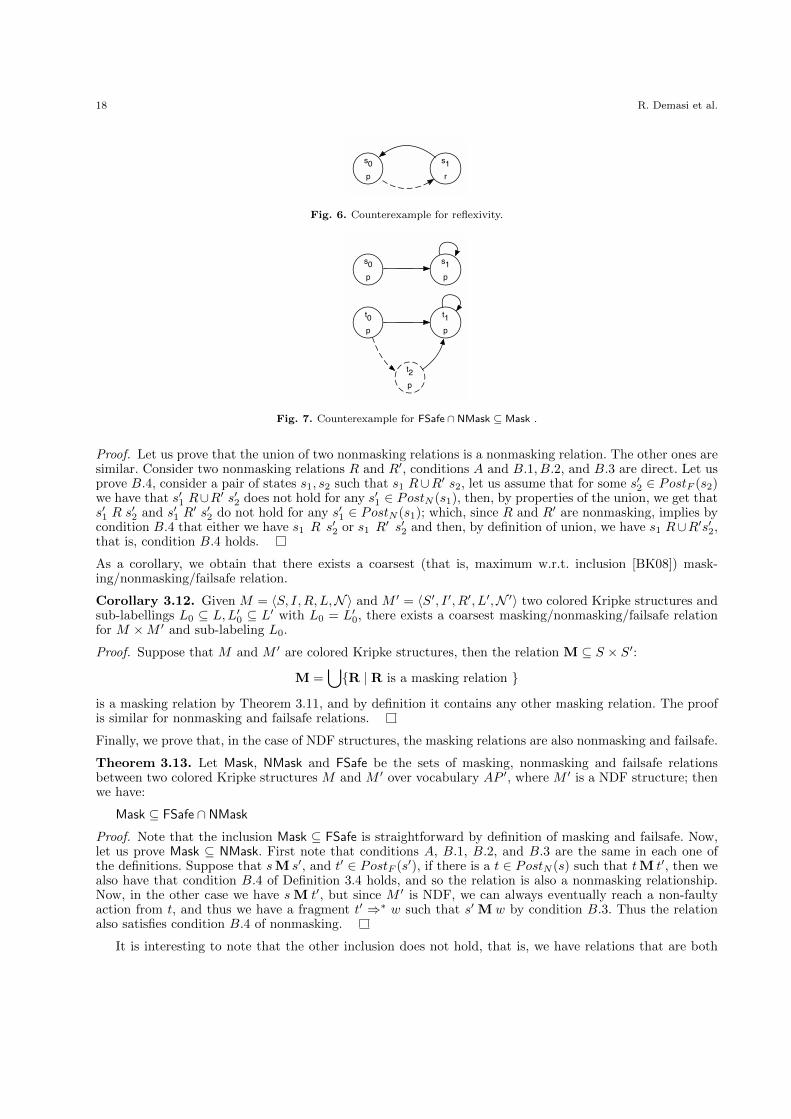
p
Fig. 7. Counterexample for FSafe ∩ NMask ⊆ Mask .
Proof. Let us prove that the union of two nonmasking relations is a nonmasking relation. The other ones aresimilar. Consider two nonmasking relations R and R′, conditions A and B.1, B.2, and B.3 are direct. Let usprove B.4, consider a pair of states s1, s2 such that s1 R∪R′ s2, let us assume that for some s′2 ∈ PostF (s2)we have that s′1 R∪R′ s′2 does not hold for any s′1 ∈ PostN (s1), then, by properties of the union, we get thats′1 R s′2 and s′1 R
′ s′2 do not hold for any s′1 ∈ PostN (s1); which, since R and R′ are nonmasking, implies bycondition B.4 that either we have s1 R s′2 or s1 R
′ s′2 and then, by definition of union, we have s1 R∪R′s′2,that is, condition B.4 holds.
As a corollary, we obtain that there exists a coarsest (that is, maximum w.r.t. inclusion [BK08]) mask-ing/nonmasking/failsafe relation.
Corollary 3.12. Given M = 〈S, I,R, L,N〉 and M ′ = 〈S′, I ′, R′, L′,N ′〉 two colored Kripke structures andsub-labellings L0 ⊆ L,L′0 ⊆ L′ with L0 = L′0, there exists a coarsest masking/nonmasking/failsafe relationfor M ×M ′ and sub-labeling L0.
Proof. Suppose that M and M ′ are colored Kripke structures, then the relation M ⊆ S × S′:
M =⋃{R | R is a masking relation }
is a masking relation by Theorem 3.11, and by definition it contains any other masking relation. The proofis similar for nonmasking and failsafe relations.
Finally, we prove that, in the case of NDF structures, the masking relations are also nonmasking and failsafe.
Theorem 3.13. Let Mask, NMask and FSafe be the sets of masking, nonmasking and failsafe relationsbetween two colored Kripke structures M and M ′ over vocabulary AP ′, where M ′ is a NDF structure; thenwe have:
Mask ⊆ FSafe ∩ NMask
Proof. Note that the inclusion Mask ⊆ FSafe is straightforward by definition of masking and failsafe. Now,let us prove Mask ⊆ NMask. First note that conditions A, B.1, B.2, and B.3 are the same in each one ofthe definitions. Suppose that sM s′, and t′ ∈ PostF (s′), if there is a t ∈ PostN (s) such that tM t′, then wealso have that condition B.4 of Definition 3.4 holds, and so the relation is also a nonmasking relationship.Now, in the other case we have s M t′, but since M ′ is NDF, we can always eventually reach a non-faultyaction from t, and thus we have a fragment t′ ⇒∗ w such that s′ M w by condition B.3. Thus the relationalso satisfies condition B.4 of nonmasking.
It is interesting to note that the other inclusion does not hold, that is, we have relations that are both

Simulation Relations for Fault-Tolerance 19
failsafe and nonmasking but which are not masking fault tolerant. A simple example is given in Figure 7.Consider the relation R = {〈s0, t0〉, 〈s1, t1〉}, it is a failsafe and also a nonmasking fault-tolerant relation forthe two structures shown in the figure, and the sub-labeling obtained by restricting the original labelings tothe letter p. It is not a masking fault-tolerant relation because condition B.4 of Definition 3.1 does not hold.However, any relation that is nonmasking and failsafe can be extended to a masking relation. Note in thefigure above if we add to R the pair 〈s0, t2〉, then the resulting relation is masking.
Theorem 3.14. Let Mask, NMask and FSafe be the sets of masking, nonmasking and failsafe relationsbetween two colored Kripke structures M and M ′ over vocabulary AP ′, where M ′ is a NDF structure; thenwe have:
∀R ∈ NMask ∩ FSafe : ∃R+ ∈ Mask : R ⊂ R+
Proof. We define R+. Let M1 = 〈S1, I1, R1, L1,N1〉 and M2 = 〈S2, I2, R2, L2,N2〉 be Kripke structures,where R ⊆ S1×S2 is defined over a vocabulary AP ′. Let {w1, . . . , wk} ⊆ S2 be the set of states such that forany wi in this set there are s1 ∈ S2, s2 ∈ S2 with s1 R s2, and wi ∈ PostF (s2) and there is no s′1 ∈ PostN (s1)with s′1 R wi. Note that, if this set is empty, R is masking. Since R is nonmasking we know that there is as′′2 such that s′′2 ∈ Post∗(wi) and s′1 R s′′2 (for some s′1 ∈ PostN (s1)), then we define the set:
{〈s′1, si2〉 | si2 ∈ Post∗(wi)}We call this set C(wi). Note that all the elements in this set have the same labeling wrt AP ′ which coincideswith that of s′1 by definition of failsafe. We define:
R+ = R ∪⋃wi
C(wi)
Let us see that this relation is masking. Suppose that s1 R+ s2. If s1 R s2, then we know that itemsA,B.1, B.2, B.3 of Definition 3.1 hold. Let us prove B.4 holds. By definition of R+ we know that for anys′2 ∈ PostF (s2) there is a s′1 such that s′1 R
+ s′2, that satisfies condition A (by properties of failsafe) andthen it satisfies B.1, B.2, B.3, B.4.
For the case that s1 R+ s2 but not s1 R s2 we know that they have the same labeling by definition of
R+, and as before the rest of the items of the definition of masking hold by the properties of nonmaskingand failsafe.
Summing up, if we have an implementation that is both failsafe and nonmasking, we know that we can obtaina relation that “proves” that this implementation is also masking, thus in practice masking is equivalent tothe intersection of nonmasking and failsafe.
4. Checking Fault-Tolerance Properties
Simulation and bisimulation relations are amenable to polynomial computational treatment. In [BK08,HHK95], algorithms for calculating several simulation and bisimulation relations are described and provedto be of polynomial complexity with respect to the number of states and transitions of the correspondingmodels. We have adapted these algorithms to our setting, thus obtaining polynomial procedures to computemasking, nonmasking and failsafe fault-tolerance. Such algorithms can be used to verify whether M @ M ′,with @∈ {≺Mask,≺Nonmask,≺Failsafe}.
The goal of this section is to present the algorithms for computing masking, nonmasking, and failsaferelations. In general, these algorithms take as input a colored Kripke structure M = 〈S, I,R, L,N〉 anda sub-labeling L0 ⊆ L and produce as output either the required fault-tolerance relation M, N, or F incase that it exists or an empty relation, otherwise. Clearly, these algorithms yield at the same time anautomatic approach to check whether the fault-tolerant implementation is masking, nonmasking, or failsafefault-tolerant with respect to the system specification. For this case, the input M is the result of combiningtwo colored Kripke structures M1 = 〈S1, I1, R1, L1,N1〉 and M2 = 〈S2, I2, R2, L2,N2〉 over AP via disjointunion, i.e., M1 ⊕M2. The former represents the system specification which exhibits the normal behaviorof the system and the latter the fault-tolerant implementation which is the extended version of the systemspecification augmented with faults. In other words, we can check whether the extended version of thenominal model with faults accomplishes the desired level of fault-tolerance.

20 R. Demasi et al.
The general scheme for computing the masking, nonmasking, or failsafe fault-tolerant relation for acolored Kripke structure M = 〈S, I,R, L,N〉 and a sub-labeling L0 ⊆ L is sketched in Algorithm 1. Wedevelop this main algorithm in the following three steps:
• Step 1: computation of condition B.2 (same algorithm for all levels of fault-tolerance).
• Step 2: computation of condition B.3 and B.4 for the corresponding level of fault-tolerance (masking,nonmasking, or failsafe).
• Step 3: merge of the results obtained in step 1 and step 2 to return the corresponding fault-tolerantrelation M, N, or F.
Algorithm 1 Computation of a fault-tolerant relation
Input: Colored Kripke structure M = 〈S, I,R, L,N〉, a sub-labeling L0 ⊆ L, and a required level of fault-tolerance R ∈ {masking, nonmasking, failsafe}
Output: Fault-tolerant relation (M, N, or F)1: SimB2 := ComputeB2(M,L0)2: switch R :3: case masking4: SimB3B4 := ComputeMaskB3B4(M,L0)5: case nonmasking6: SimB3B4 := ComputeNonMaskB3B4(M,L0)7: case failsafe8: SimB3B4 := ComputeFailsafeB3B4(M,L0)9: end switch
10: FTSimRel := MergeSimRel(SimB2, SimB3B4)11: return FTSimRel
In the first step of Algorithm 1, we compute a relation SimB2 that satisfies condition B.2 of Defini-tion 3.1, 3.4 and 3.6. This is performed by procedure ComputeB2 on line 1. Notice that this conditionis the same for the three levels of fault-tolerance. In the second step, we compute the corresponding rela-tion SimB3B4 that satisfies condition B.3 and B.4 for the required level of fault-tolerance (lines 2 − 9).We have developed one algorithm for each case, namely ComputeMaskB3B4, ComputeNonMaskB3B4,and ComputeFailsafeB3B4. In the last step, we combine the results obtained from the previous steps(MergeSimRel on line 10) to return the corresponding fault-tolerant relation.
In the following subsections we explain all the details for each procedure used in the main algorithm.
4.1. Computing Masking Fault-Tolerance
In this subsection we present the algorithms for computing the masking fault-tolerant relation M for acolored Kripke Structure M = 〈S, I,R, L,N〉 and a sub-labeling L0 ⊆ L, where M ⊆ S × S. We startdescribing Algorithm 2 (ComputeB2) that computes condition B.2 of Definition 3.1.
First, let us note that Algorithm 2 is also used in the algorithms for computing nonmasking and failsaferelations, since the definitions of these relations also require condition B.2. This algorithm is an adaptationfrom a standard procedure for computing simulation relations introduced in [HHK95]. Let us now describethe general idea of Algorithm 2. It takes as input a colored Kripke structure M = 〈S, I,R, L,N〉 and asub-labeling L0 ⊆ L and computes a SimB2 relation, where the states in SimB2 satisfy condition B.2 ofDefinition 3.1, 3.4, and 3.6. In the first loop, for each s1 ∈ N , the set SimB2(s1) contains the states that arecandidates for masking s1. Initially, SimB2(s1) consists of all normal and faulty states with the same labelsas s1 and RemoveR(s1) contains all states which do not have a normal or faulty successor state maskings1. Moreover, these states cannot mask any of the predecessors of s1: note that Post(s2) ∩ SimB2(s1) 6= ∅iff s2 ∈ Pre(SimB2(s1)). That is, we first obtain all the predecessors of those states that simulate s1(Pre(SimB2(s1))), then we perform the difference between S and this set of predecessors. As a result weobtain a set of states where each state in it does not have a successor that simulates s1 and thus thesestates cannot simulate any of the predecessors of s1. The termination condition of the loop of lines 5-18 isRemoveR(s′1) = ∅ for all s′1 ∈ N , in which case there are no states that need to be removed from the sets of
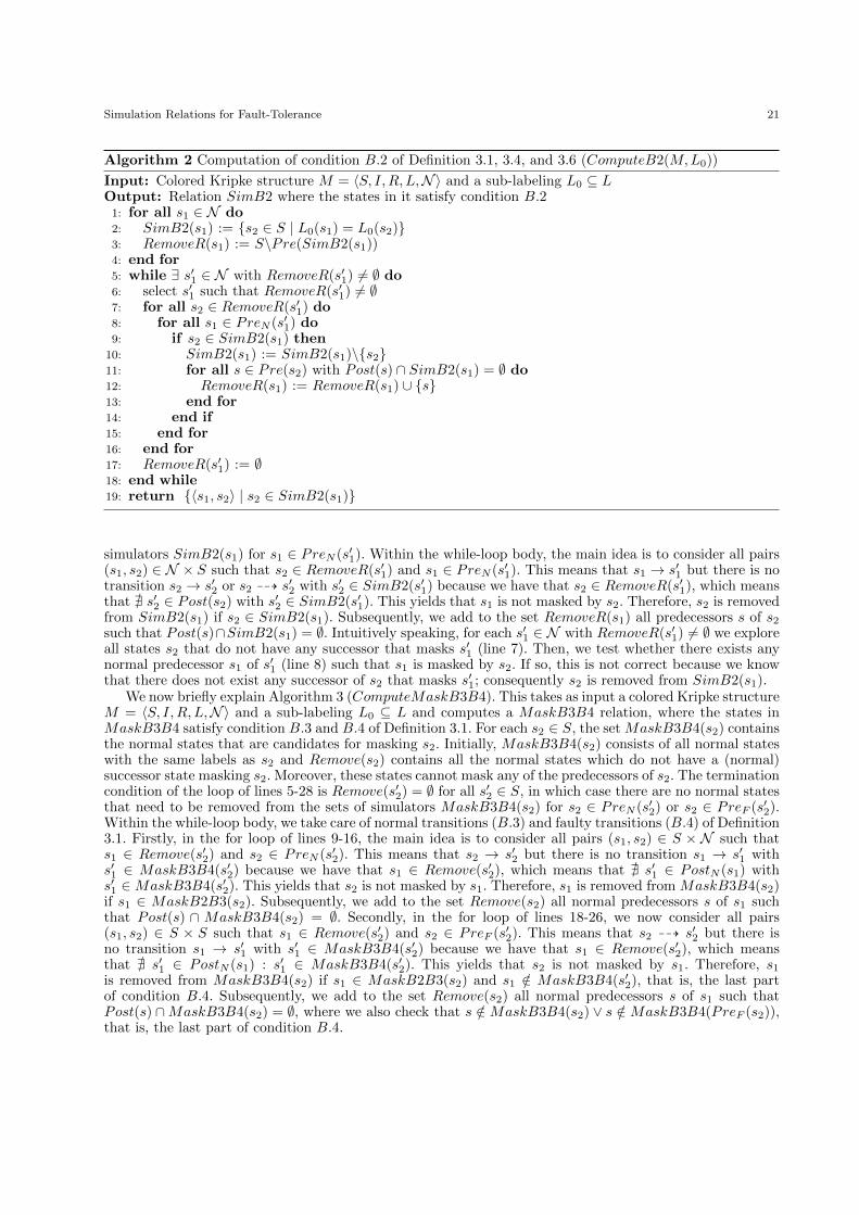
Simulation Relations for Fault-Tolerance 21
Algorithm 2 Computation of condition B.2 of Definition 3.1, 3.4, and 3.6 (ComputeB2(M,L0))
Input: Colored Kripke structure M = 〈S, I,R, L,N〉 and a sub-labeling L0 ⊆ LOutput: Relation SimB2 where the states in it satisfy condition B.2
1: for all s1 ∈ N do2: SimB2(s1) := {s2 ∈ S | L0(s1) = L0(s2)}3: RemoveR(s1) := S\Pre(SimB2(s1))4: end for5: while ∃ s′1 ∈ N with RemoveR(s′1) 6= ∅ do6: select s′1 such that RemoveR(s′1) 6= ∅7: for all s2 ∈ RemoveR(s′1) do8: for all s1 ∈ PreN (s′1) do9: if s2 ∈ SimB2(s1) then
10: SimB2(s1) := SimB2(s1)\{s2}11: for all s ∈ Pre(s2) with Post(s) ∩ SimB2(s1) = ∅ do12: RemoveR(s1) := RemoveR(s1) ∪ {s}13: end for14: end if15: end for16: end for17: RemoveR(s′1) := ∅18: end while19: return {〈s1, s2〉 | s2 ∈ SimB2(s1)}
simulators SimB2(s1) for s1 ∈ PreN (s′1). Within the while-loop body, the main idea is to consider all pairs(s1, s2) ∈ N × S such that s2 ∈ RemoveR(s′1) and s1 ∈ PreN (s′1). This means that s1 → s′1 but there is notransition s2 → s′2 or s2 99K s′2 with s′2 ∈ SimB2(s′1) because we have that s2 ∈ RemoveR(s′1), which meansthat @ s′2 ∈ Post(s2) with s′2 ∈ SimB2(s′1). This yields that s1 is not masked by s2. Therefore, s2 is removedfrom SimB2(s1) if s2 ∈ SimB2(s1). Subsequently, we add to the set RemoveR(s1) all predecessors s of s2such that Post(s)∩SimB2(s1) = ∅. Intuitively speaking, for each s′1 ∈ N with RemoveR(s′1) 6= ∅ we exploreall states s2 that do not have any successor that masks s′1 (line 7). Then, we test whether there exists anynormal predecessor s1 of s′1 (line 8) such that s1 is masked by s2. If so, this is not correct because we knowthat there does not exist any successor of s2 that masks s′1; consequently s2 is removed from SimB2(s1).
We now briefly explain Algorithm 3 (ComputeMaskB3B4). This takes as input a colored Kripke structureM = 〈S, I,R, L,N〉 and a sub-labeling L0 ⊆ L and computes a MaskB3B4 relation, where the states inMaskB3B4 satisfy condition B.3 and B.4 of Definition 3.1. For each s2 ∈ S, the set MaskB3B4(s2) containsthe normal states that are candidates for masking s2. Initially, MaskB3B4(s2) consists of all normal stateswith the same labels as s2 and Remove(s2) contains all the normal states which do not have a (normal)successor state masking s2. Moreover, these states cannot mask any of the predecessors of s2. The terminationcondition of the loop of lines 5-28 is Remove(s′2) = ∅ for all s′2 ∈ S, in which case there are no normal statesthat need to be removed from the sets of simulators MaskB3B4(s2) for s2 ∈ PreN (s′2) or s2 ∈ PreF (s′2).Within the while-loop body, we take care of normal transitions (B.3) and faulty transitions (B.4) of Definition3.1. Firstly, in the for loop of lines 9-16, the main idea is to consider all pairs (s1, s2) ∈ S × N such thats1 ∈ Remove(s′2) and s2 ∈ PreN (s′2). This means that s2 → s′2 but there is no transition s1 → s′1 withs′1 ∈ MaskB3B4(s′2) because we have that s1 ∈ Remove(s′2), which means that @ s′1 ∈ PostN (s1) withs′1 ∈MaskB3B4(s′2). This yields that s2 is not masked by s1. Therefore, s1 is removed from MaskB3B4(s2)if s1 ∈ MaskB2B3(s2). Subsequently, we add to the set Remove(s2) all normal predecessors s of s1 suchthat Post(s) ∩ MaskB3B4(s2) = ∅. Secondly, in the for loop of lines 18-26, we now consider all pairs(s1, s2) ∈ S × S such that s1 ∈ Remove(s′2) and s2 ∈ PreF (s′2). This means that s2 99K s′2 but there isno transition s1 → s′1 with s′1 ∈ MaskB3B4(s′2) because we have that s1 ∈ Remove(s′2), which meansthat @ s′1 ∈ PostN (s1) : s′1 ∈ MaskB3B4(s′2). This yields that s2 is not masked by s1. Therefore, s1is removed from MaskB3B4(s2) if s1 ∈ MaskB2B3(s2) and s1 /∈ MaskB3B4(s′2), that is, the last partof condition B.4. Subsequently, we add to the set Remove(s2) all normal predecessors s of s1 such thatPost(s) ∩MaskB3B4(s2) = ∅, where we also check that s /∈MaskB3B4(s2) ∨ s /∈MaskB3B4(PreF (s2)),that is, the last part of condition B.4.
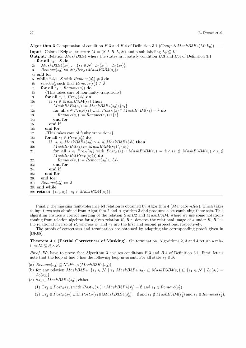
22 R. Demasi et al.
Algorithm 3 Computation of condition B.3 and B.4 of Definition 3.1 (ComputeMaskB3B4(M,L0))
Input: Colored Kripke structure M = 〈S, I,R, L,N〉 and a sub-labeling L0 ⊆ LOutput: Relation MaskB3B4 where the states in it satisfy condition B.3 and B.4 of Definition 3.1
1: for all s2 ∈ S do2: MaskB3B4(s2) := {s1 ∈ N | L0(s1) = L0(s2)}3: Remove(s2) := N\PreN (MaskB3B4(s2))4: end for5: while ∃s′2 ∈ S with Remove(s′2) 6= ∅ do6: select s′2 such that Remove(s′2) 6= ∅7: for all s1 ∈ Remove(s′2) do8: {This takes care of non-faulty transitions}9: for all s2 ∈ PreN (s′2) do
10: if s1 ∈MaskB3B4(s2) then11: MaskB3B4(s2) := MaskB3B4(s2)\{s1}12: for all s ∈ PreN (s1) with PostN (s) ∩MaskB3B4(s2) = ∅ do13: Remove(s2) := Remove(s2) ∪ {s}14: end for15: end if16: end for17: {This takes care of faulty transitions}18: for all s2 ∈ PreF (s′2) do19: if s1 ∈MaskB3B4(s2) ∧ s1 /∈MaskB3B4(s′2) then20: MaskB3B4(s2) := MaskB3B4(s2) \ {s1}21: for all s ∈ PreN (s1) with PostN (s) ∩ MaskB3B4(s2) = ∅ ∧ (s /∈ MaskB3B4(s2) ∨ s /∈
MaskB3B4(PreF (s2))) do22: Remove(s2) := Remove(s2) ∪ {s}23: end for24: end if25: end for26: end for27: Remove(s′2) := ∅28: end while29: return {〈s1, s2〉 | s1 ∈MaskB3B4(s2)}
Finally, the masking fault-tolerance M relation is obtained by Algorithm 4 (MergeSimRel), which takesas input two sets obtained from Algorithm 2 and Algorithm 3 and produces a set combining these sets. Thisalgorithm ensures a correct merging of the relation SimB2 and MaskB3B4, where we use some notationscoming from relation algebra: for a given relation R, R[s] denotes the relational image of s under R, R∼ isthe relational inverse of R, whereas π1 and π2 are the first and second projections, respectively.
The proofs of correctness and termination are obtained by adapting the corresponding proofs given in[BK08].
Theorem 4.1 (Partial Correctness of Masking). On termination, Algorithms 2, 3 and 4 return a rela-tion M ⊆ S × S.
Proof. We have to prove that Algorithm 3 ensures conditions B.3 and B.4 of Definition 3.1. First, let usnote that the loop of line 5 has the following loop invariant. For all state s2 ∈ S:
(a) Remove(s2) ⊆ N\PreN (MaskB3B4(s2))
(b) for any relation MaskB3B4: {s1 ∈ N | s1 MaskB3B4 s2} ⊆ MaskB3B4(s2) ⊆ {s1 ∈ N | L0(s1) =L0(s2)}
(c) ∀s1 ∈MaskB3B4(s2), either:
(1) ∃s′2 ∈ PostN (s2) with PostN (s1) ∩MaskB3B4(s′2) = ∅ and s1 ∈ Remove(s′2),
(2) ∃s′2 ∈ PostF (s2) with PostN (s1)∩MaskB3B4(s′2) = ∅ and s1 /∈MaskB3B4(s′2) and s1 ∈ Remove(s′2),
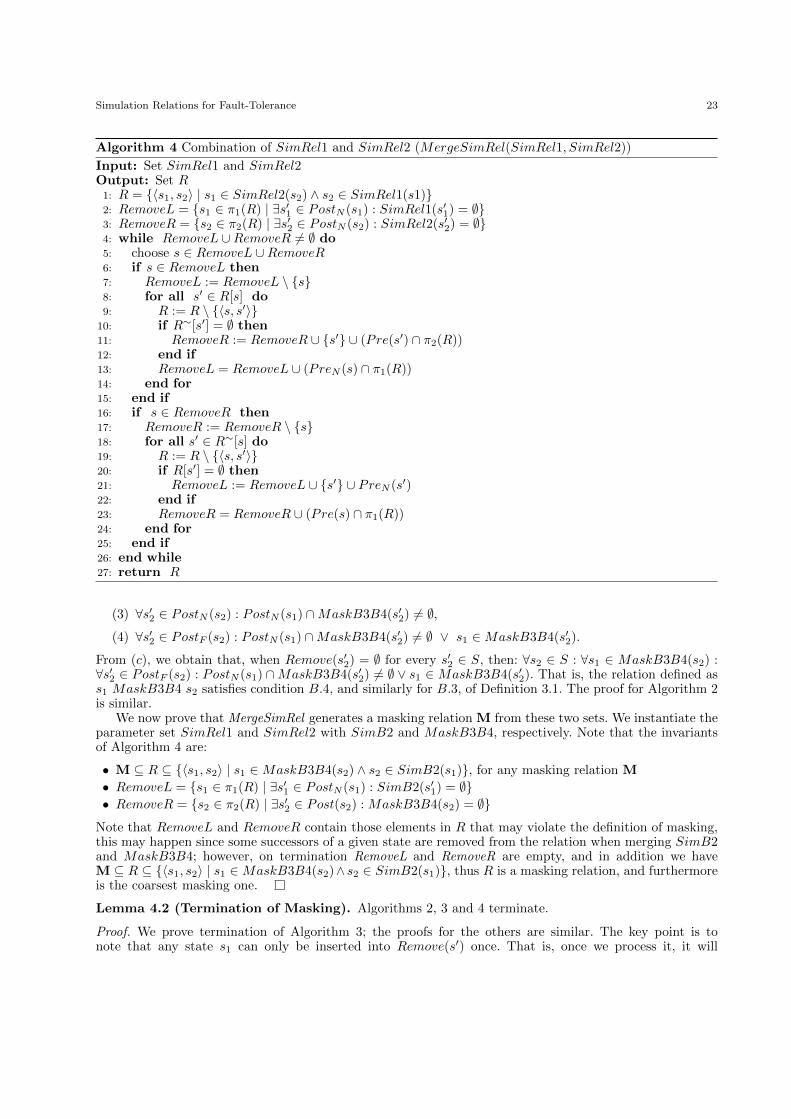
Simulation Relations for Fault-Tolerance 23
Algorithm 4 Combination of SimRel1 and SimRel2 (MergeSimRel(SimRel1, SimRel2))
Input: Set SimRel1 and SimRel2Output: Set R
1: R = {〈s1, s2〉 | s1 ∈ SimRel2(s2) ∧ s2 ∈ SimRel1(s1)}2: RemoveL = {s1 ∈ π1(R) | ∃s′1 ∈ PostN (s1) : SimRel1(s′1) = ∅}3: RemoveR = {s2 ∈ π2(R) | ∃s′2 ∈ PostN (s2) : SimRel2(s′2) = ∅}4: while RemoveL ∪RemoveR 6= ∅ do5: choose s ∈ RemoveL ∪RemoveR6: if s ∈ RemoveL then7: RemoveL := RemoveL \ {s}8: for all s′ ∈ R[s] do9: R := R \ {〈s, s′〉}
10: if R∼[s′] = ∅ then11: RemoveR := RemoveR ∪ {s′} ∪ (Pre(s′) ∩ π2(R))12: end if13: RemoveL = RemoveL ∪ (PreN (s) ∩ π1(R))14: end for15: end if16: if s ∈ RemoveR then17: RemoveR := RemoveR \ {s}18: for all s′ ∈ R∼[s] do19: R := R \ {〈s, s′〉}20: if R[s′] = ∅ then21: RemoveL := RemoveL ∪ {s′} ∪ PreN (s′)22: end if23: RemoveR = RemoveR ∪ (Pre(s) ∩ π1(R))24: end for25: end if26: end while27: return R
(3) ∀s′2 ∈ PostN (s2) : PostN (s1) ∩MaskB3B4(s′2) 6= ∅,
(4) ∀s′2 ∈ PostF (s2) : PostN (s1) ∩MaskB3B4(s′2) 6= ∅ ∨ s1 ∈MaskB3B4(s′2).
From (c), we obtain that, when Remove(s′2) = ∅ for every s′2 ∈ S, then: ∀s2 ∈ S : ∀s1 ∈ MaskB3B4(s2) :∀s′2 ∈ PostF (s2) : PostN (s1) ∩MaskB3B4(s′2) 6= ∅ ∨ s1 ∈ MaskB3B4(s′2). That is, the relation defined ass1 MaskB3B4 s2 satisfies condition B.4, and similarly for B.3, of Definition 3.1. The proof for Algorithm 2is similar.
We now prove that MergeSimRel generates a masking relation M from these two sets. We instantiate theparameter set SimRel1 and SimRel2 with SimB2 and MaskB3B4, respectively. Note that the invariantsof Algorithm 4 are:
• M ⊆ R ⊆ {〈s1, s2〉 | s1 ∈MaskB3B4(s2) ∧ s2 ∈ SimB2(s1)}, for any masking relation M
• RemoveL = {s1 ∈ π1(R) | ∃s′1 ∈ PostN (s1) : SimB2(s′1) = ∅}• RemoveR = {s2 ∈ π2(R) | ∃s′2 ∈ Post(s2) : MaskB3B4(s2) = ∅}
Note that RemoveL and RemoveR contain those elements in R that may violate the definition of masking,this may happen since some successors of a given state are removed from the relation when merging SimB2and MaskB3B4; however, on termination RemoveL and RemoveR are empty, and in addition we haveM ⊆ R ⊆ {〈s1, s2〉 | s1 ∈MaskB3B4(s2)∧ s2 ∈ SimB2(s1)}, thus R is a masking relation, and furthermoreis the coarsest masking one.
Lemma 4.2 (Termination of Masking). Algorithms 2, 3 and 4 terminate.
Proof. We prove termination of Algorithm 3; the proofs for the others are similar. The key point is tonote that any state s1 can only be inserted into Remove(s′) once. That is, once we process it, it will
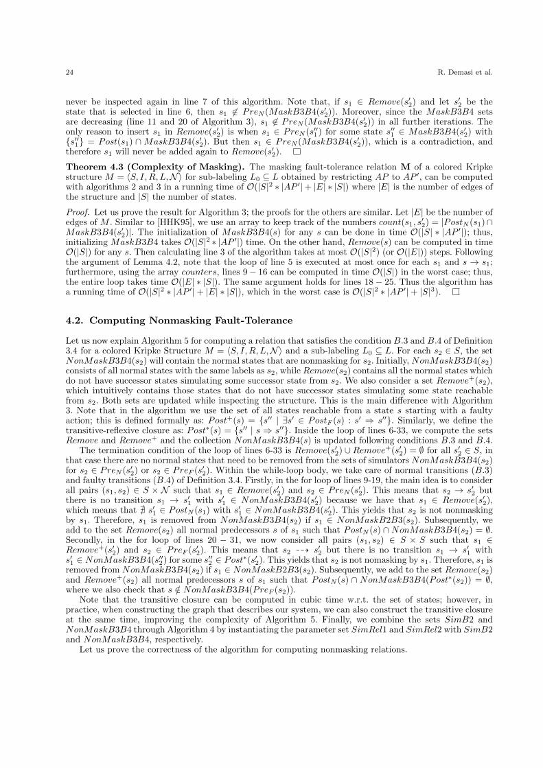
24 R. Demasi et al.
never be inspected again in line 7 of this algorithm. Note that, if s1 ∈ Remove(s′2) and let s′2 be thestate that is selected in line 6, then s1 6∈ PreN (MaskB3B4(s′2)). Moreover, since the MaskB3B4 setsare decreasing (line 11 and 20 of Algorithm 3), s1 6∈ PreN (MaskB3B4(s′2)) in all further iterations. Theonly reason to insert s1 in Remove(s′2) is when s1 ∈ PreN (s′′1) for some state s′′1 ∈ MaskB3B4(s′2) with{s′′1} = Post(s1) ∩MaskB3B4(s′2). But then s1 ∈ PreN (MaskB3B4(s′2)), which is a contradiction, andtherefore s1 will never be added again to Remove(s′2).
Theorem 4.3 (Complexity of Masking). The masking fault-tolerance relation M of a colored Kripkestructure M = 〈S, I,R, L,N〉 for sub-labeling L0 ⊆ L obtained by restricting AP to AP ′, can be computedwith algorithms 2 and 3 in a running time of O(|S|2 ∗ |AP ′|+ |E| ∗ |S|) where |E| is the number of edges ofthe structure and |S| the number of states.
Proof. Let us prove the result for Algorithm 3; the proofs for the others are similar. Let |E| be the number ofedges of M . Similar to [HHK95], we use an array to keep track of the numbers count(s1, s
′2) = |PostN (s1)∩
MaskB3B4(s′2)|. The initialization of MaskB3B4(s) for any s can be done in time O(|S| ∗ |AP ′|); thus,initializing MaskB3B4 takes O(|S|2 ∗ |AP ′|) time. On the other hand, Remove(s) can be computed in timeO(|S|) for any s. Then calculating line 3 of the algorithm takes at most O(|S|2) (or O(|E|)) steps. Followingthe argument of Lemma 4.2, note that the loop of line 5 is executed at most once for each s1 and s → s1;furthermore, using the array counters, lines 9− 16 can be computed in time O(|S|) in the worst case; thus,the entire loop takes time O(|E| ∗ |S|). The same argument holds for lines 18− 25. Thus the algorithm hasa running time of O(|S|2 ∗ |AP ′|+ |E| ∗ |S|), which in the worst case is O(|S|2 ∗ |AP ′|+ |S|3).
4.2. Computing Nonmasking Fault-Tolerance
Let us now explain Algorithm 5 for computing a relation that satisfies the condition B.3 and B.4 of Definition3.4 for a colored Kripke Structure M = 〈S, I,R, L,N〉 and a sub-labeling L0 ⊆ L. For each s2 ∈ S, the setNonMaskB3B4(s2) will contain the normal states that are nonmasking for s2. Initially, NonMaskB3B4(s2)consists of all normal states with the same labels as s2, while Remove(s2) contains all the normal states whichdo not have successor states simulating some successor state from s2. We also consider a set Remove+(s2),which intuitively contains those states that do not have successor states simulating some state reachablefrom s2. Both sets are updated while inspecting the structure. This is the main difference with Algorithm3. Note that in the algorithm we use the set of all states reachable from a state s starting with a faultyaction; this is defined formally as: Post+(s) = {s′′ | ∃s′ ∈ PostF (s) : s′ ⇒ s′′}. Similarly, we define thetransitive-reflexive closure as: Post∗(s) = {s′′ | s ⇒ s′′}. Inside the loop of lines 6-33, we compute the setsRemove and Remove+ and the collection NonMaskB3B4(s) is updated following conditions B.3 and B.4.
The termination condition of the loop of lines 6-33 is Remove(s′2) ∪ Remove+(s′2) = ∅ for all s′2 ∈ S, inthat case there are no normal states that need to be removed from the sets of simulators NonMaskB3B4(s2)for s2 ∈ PreN (s′2) or s2 ∈ PreF (s′2). Within the while-loop body, we take care of normal transitions (B.3)and faulty transitions (B.4) of Definition 3.4. Firstly, in the for loop of lines 9-19, the main idea is to considerall pairs (s1, s2) ∈ S × N such that s1 ∈ Remove(s′2) and s2 ∈ PreN (s′2). This means that s2 → s′2 butthere is no transition s1 → s′1 with s′1 ∈ NonMaskB3B4(s′2) because we have that s1 ∈ Remove(s′2),which means that @ s′1 ∈ PostN (s1) with s′1 ∈ NonMaskB3B4(s′2). This yields that s2 is not nonmaskingby s1. Therefore, s1 is removed from NonMaskB3B4(s2) if s1 ∈ NonMaskB2B3(s2). Subsequently, weadd to the set Remove(s2) all normal predecessors s of s1 such that PostN (s) ∩ NonMaskB3B4(s2) = ∅.Secondly, in the for loop of lines 20 − 31, we now consider all pairs (s1, s2) ∈ S × S such that s1 ∈Remove+(s′2) and s2 ∈ PreF (s′2). This means that s2 99K s′2 but there is no transition s1 → s′1 withs′1 ∈ NonMaskB3B4(s′′2) for some s′′2 ∈ Post∗(s′2). This yields that s2 is not nomasking by s1. Therefore, s1 isremoved from NonMaskB3B4(s2) if s1 ∈ NonMaskB2B3(s2). Subsequently, we add to the set Remove(s2)and Remove+(s2) all normal predecessors s of s1 such that PostN (s) ∩ NonMaskB3B4(Post∗(s2)) = ∅,where we also check that s /∈ NonMaskB3B4(PreF (s2)).
Note that the transitive closure can be computed in cubic time w.r.t. the set of states; however, inpractice, when constructing the graph that describes our system, we can also construct the transitive closureat the same time, improving the complexity of Algorithm 5. Finally, we combine the sets SimB2 andNonMaskB3B4 through Algorithm 4 by instantiating the parameter set SimRel1 and SimRel2 with SimB2and NonMaskB3B4, respectively.
Let us prove the correctness of the algorithm for computing nonmasking relations.
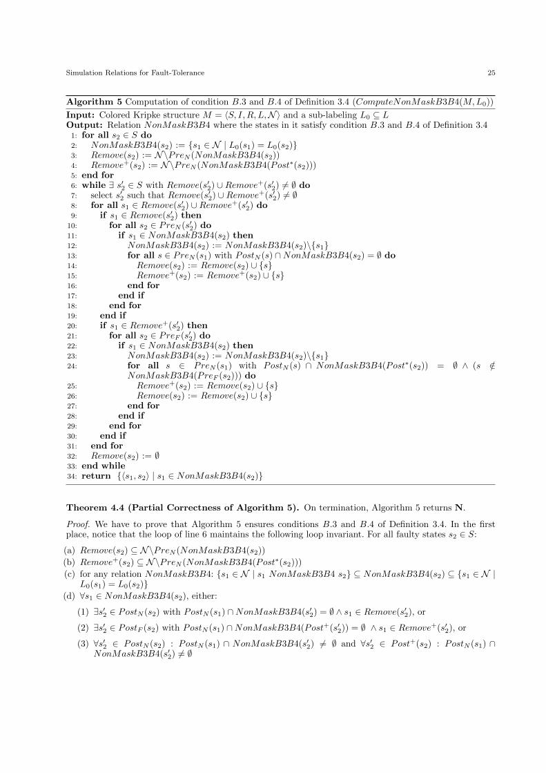
Simulation Relations for Fault-Tolerance 25
Algorithm 5 Computation of condition B.3 and B.4 of Definition 3.4 (ComputeNonMaskB3B4(M,L0))
Input: Colored Kripke structure M = 〈S, I,R, L,N〉 and a sub-labeling L0 ⊆ LOutput: Relation NonMaskB3B4 where the states in it satisfy condition B.3 and B.4 of Definition 3.4
1: for all s2 ∈ S do2: NonMaskB3B4(s2) := {s1 ∈ N | L0(s1) = L0(s2)}3: Remove(s2) := N\PreN (NonMaskB3B4(s2))4: Remove+(s2) := N\PreN (NonMaskB3B4(Post∗(s2)))5: end for6: while ∃ s′2 ∈ S with Remove(s′2) ∪Remove+(s′2) 6= ∅ do7: select s′2 such that Remove(s′2) ∪Remove+(s′2) 6= ∅8: for all s1 ∈ Remove(s′2) ∪Remove+(s′2) do9: if s1 ∈ Remove(s′2) then
10: for all s2 ∈ PreN (s′2) do11: if s1 ∈ NonMaskB3B4(s2) then12: NonMaskB3B4(s2) := NonMaskB3B4(s2)\{s1}13: for all s ∈ PreN (s1) with PostN (s) ∩NonMaskB3B4(s2) = ∅ do14: Remove(s2) := Remove(s2) ∪ {s}15: Remove+(s2) := Remove+(s2) ∪ {s}16: end for17: end if18: end for19: end if20: if s1 ∈ Remove+(s′2) then21: for all s2 ∈ PreF (s′2) do22: if s1 ∈ NonMaskB3B4(s2) then23: NonMaskB3B4(s2) := NonMaskB3B4(s2)\{s1}24: for all s ∈ PreN (s1) with PostN (s) ∩ NonMaskB3B4(Post∗(s2)) = ∅ ∧ (s /∈
NonMaskB3B4(PreF (s2))) do25: Remove+(s2) := Remove(s2) ∪ {s}26: Remove(s2) := Remove(s2) ∪ {s}27: end for28: end if29: end for30: end if31: end for32: Remove(s2) := ∅33: end while34: return {〈s1, s2〉 | s1 ∈ NonMaskB3B4(s2)}
Theorem 4.4 (Partial Correctness of Algorithm 5). On termination, Algorithm 5 returns N.
Proof. We have to prove that Algorithm 5 ensures conditions B.3 and B.4 of Definition 3.4. In the firstplace, notice that the loop of line 6 maintains the following loop invariant. For all faulty states s2 ∈ S:
(a) Remove(s2) ⊆ N\PreN (NonMaskB3B4(s2))
(b) Remove+(s2) ⊆ N\PreN (NonMaskB3B4(Post∗(s2)))
(c) for any relation NonMaskB3B4: {s1 ∈ N | s1 NonMaskB3B4 s2} ⊆ NonMaskB3B4(s2) ⊆ {s1 ∈ N |L0(s1) = L0(s2)}
(d) ∀s1 ∈ NonMaskB3B4(s2), either:
(1) ∃s′2 ∈ PostN (s2) with PostN (s1) ∩NonMaskB3B4(s′2) = ∅ ∧ s1 ∈ Remove(s′2), or
(2) ∃s′2 ∈ PostF (s2) with PostN (s1) ∩NonMaskB3B4(Post+(s′2)) = ∅ ∧ s1 ∈ Remove+(s′2), or
(3) ∀s′2 ∈ PostN (s2) : PostN (s1) ∩ NonMaskB3B4(s′2) 6= ∅ and ∀s′2 ∈ Post+(s2) : PostN (s1) ∩NonMaskB3B4(s′2) 6= ∅
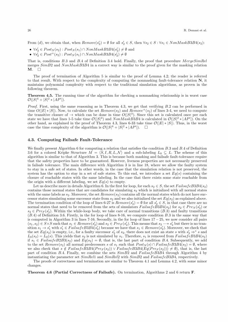
26 R. Demasi et al.
From (d), we obtain that, when Remove(s′2) = ∅ for all s′2 ∈ S, then ∀s2 ∈ S : ∀s1 ∈ NonMaskB3B4(s2):
• ∀s′2 ∈ PostN (s2) : PostN (s1) ∩NonMaskB3B4(s′2) 6= ∅ and
• ∀s′2 ∈ Post+(s2) : PostN (s1) ∩NonMaskB3B4(s′2) 6= ∅
That is, conditions B.3 and B.4 of Definition 3.4 hold. Finally, the proof that procedure MergeSimRelmerges SimB2 and NonMaskB3B4 in a correct way is similar to the proof given for the masking relationM.
The proof of termination of Algorithm 5 is similar to the proof of Lemma 4.2; the reader is referredto that result. With respect to the complexity of computing the nonmasking fault-tolerance relation N, itmaintains polynomial complexity with respect to the traditional simulation algorithms, as proven in thefollowing theorem.
Theorem 4.5. The running time of the algorithm for checking a nonmasking relationship is in worst caseO(|S|4 + |S|2 ∗ |AP ′|).
Proof. First, using the same reasoning as in Theorem 4.3, we get that verifying B.2 can be performed intime O(|E| ∗ |S|). Now, to calculate the set Remove(s2) and Remove+(s2) of lines 3-4, we need to computethe transitive closure of → which can be done in time O(|S|3). Since this set is calculated once per eachstate we have that lines 1-5 take time O(|S|4) and NonMaskB3B4 is calculated in O(|S|2 ∗ |AP ′|). On theother hand, as explained in the proof of Theorem 4.3, lines 6-33 take time O(|E| ∗ |S|). Thus, in the worstcase the time complexity of the algorithm is O(|S|4 + |S|2 ∗ |AP ′|).
4.3. Computing Failsafe Fault-Tolerance
We finally present Algorithm 6 for computing a relation that satisfies the condition B.3 and B.4 of Definition3.6 for a colored Kripke Structure M = 〈S, I,R, L,N〉 and a sub-labeling L0 ⊆ L. The scheme of thisalgorithm is similar to that of Algorithm 3. This is because both masking and failsafe fault-tolerance requirethat the safety properties have to be guaranteed. However, liveness properties are not necessarily preservedin failsafe tolerance. The main difference with Algorithm 3 is in line 18, where we allow the faulty systemto stay in a safe set of states. In other words, in the case that the simulation relation is not preserved, thesystem has the option to stay in a set of safe states. To this end, we introduce a set Eq(s) containing theclosure of reachable states with the same labeling. In the case that there exists some state reachable fromthe origin with a different labeling, we set Eq(s) to empty.
Let us describe more in details Algorithm 6. In the first for loop, for each s2 ∈ S, the set FailsafeB3B4(s2)contains those normal states that are candidates for simulating s2 which is initialized with all normal stateswith the same labels as s2. Moreover, the setRemove(s2) contains all the normal states which do not have suc-cessor states simulating some successor state from s2 and we also initialized the set Eq(s2) as explained above.The termination condition of the loop of lines 6-27 is Remove(s′2) = ∅ for all s′2 ∈ S, in that case there are nonormal states that need to be removed from the sets of simulators FailsafeB3B4(s2) for s2 ∈ PreN (s′2) ors2 ∈ PreF (s′2). Within the while-loop body, we take care of normal transitions (B.3) and faulty transitions(B.4) of Definition 3.6. Firstly, in the for loop of lines 8-16, we compute condition B.3 in the same way thatis computed in Algorithm 3 in lines 7-16. Secondly, in the for loop of lines 17− 25, we now consider all pairs(s1, s2) ∈ S×S such that s1 ∈ Remove(s′2) and s2 ∈ PreF (s′2). This means that s2 99K s′2 but there is no tran-sition s1 → s′1 with s′1 ∈ FailsafeB3B4(s′2) because we have that s1 ∈ Remove(s′2). Moreover, we check thatthe set Eq(s2) is empty, i.e., for a faulty successor s′2 of s2, there does not exist an state s with s′2 ⇒∗ s andL0(s2) = L0(s). This yields that s2 is not simulated by s1. Therefore, s1 is removed from FailsafeB3B4(s2)if s1 ∈ FailsafeB2B3(s2) and Eq(s2) = ∅, that is, the last part of condition B.4. Subsequently, we addto the set Remove(s2) all normal predecessors s of s1 such that PostN (s) ∩ FailsafeB3B4(s2) = ∅, wherewe also check that s /∈ FailsafeB3B4(PreF (s2)) ∨ FailsafeB3B4(Eq(PreF (s2))) 6= ∅), that is, the lastpart of condition B.4. Finally, we combine the sets SimB2 and FailsafeB3B4 through Algorithm 4 byinstantiating the parameter set SimRel1 and SimRel2 with SimB2 and FailsafeB3B4, respectively.
The proofs of correctness and termination are similar to Theorem 4.1 and Lemma 4.2, with some minorchanges.
Theorem 4.6 (Partial Correctness of Failsafe). On termination, Algorithms 2 and 6 return F.
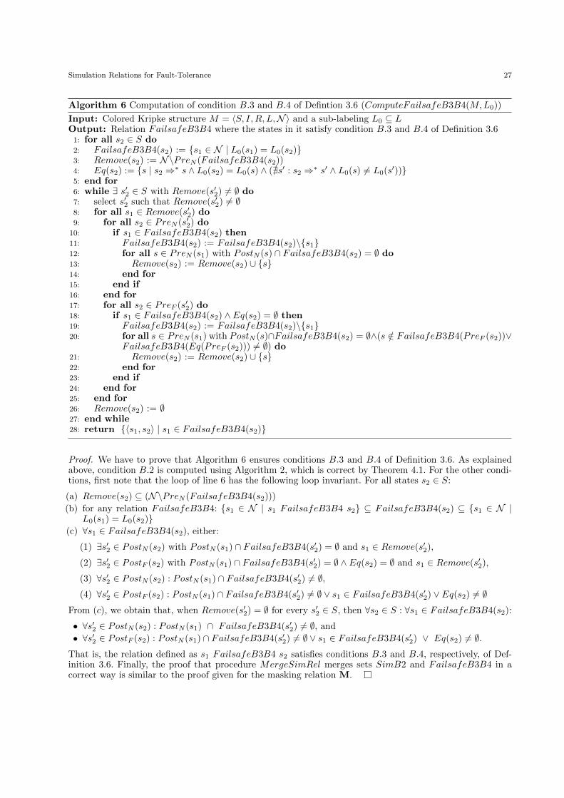
Simulation Relations for Fault-Tolerance 27
Algorithm 6 Computation of condition B.3 and B.4 of Defintion 3.6 (ComputeFailsafeB3B4(M,L0))
Input: Colored Kripke structure M = 〈S, I,R, L,N〉 and a sub-labeling L0 ⊆ LOutput: Relation FailsafeB3B4 where the states in it satisfy condition B.3 and B.4 of Definition 3.6
1: for all s2 ∈ S do2: FailsafeB3B4(s2) := {s1 ∈ N | L0(s1) = L0(s2)}3: Remove(s2) := N\PreN (FailsafeB3B4(s2))4: Eq(s2) := {s | s2 ⇒∗ s ∧ L0(s2) = L0(s) ∧ (@s′ : s2 ⇒∗ s′ ∧ L0(s) 6= L0(s′))}5: end for6: while ∃ s′2 ∈ S with Remove(s′2) 6= ∅ do7: select s′2 such that Remove(s′2) 6= ∅8: for all s1 ∈ Remove(s′2) do9: for all s2 ∈ PreN (s′2) do
10: if s1 ∈ FailsafeB3B4(s2) then11: FailsafeB3B4(s2) := FailsafeB3B4(s2)\{s1}12: for all s ∈ PreN (s1) with PostN (s) ∩ FailsafeB3B4(s2) = ∅ do13: Remove(s2) := Remove(s2) ∪ {s}14: end for15: end if16: end for17: for all s2 ∈ PreF (s′2) do18: if s1 ∈ FailsafeB3B4(s2) ∧ Eq(s2) = ∅ then19: FailsafeB3B4(s2) := FailsafeB3B4(s2)\{s1}20: for all s ∈ PreN (s1) with PostN (s)∩FailsafeB3B4(s2) = ∅∧(s /∈ FailsafeB3B4(PreF (s2))∨
FailsafeB3B4(Eq(PreF (s2))) 6= ∅) do21: Remove(s2) := Remove(s2) ∪ {s}22: end for23: end if24: end for25: end for26: Remove(s2) := ∅27: end while28: return {〈s1, s2〉 | s1 ∈ FailsafeB3B4(s2)}
Proof. We have to prove that Algorithm 6 ensures conditions B.3 and B.4 of Definition 3.6. As explainedabove, condition B.2 is computed using Algorithm 2, which is correct by Theorem 4.1. For the other condi-tions, first note that the loop of line 6 has the following loop invariant. For all states s2 ∈ S:
(a) Remove(s2) ⊆ (N\PreN (FailsafeB3B4(s2)))
(b) for any relation FailsafeB3B4: {s1 ∈ N | s1 FailsafeB3B4 s2} ⊆ FailsafeB3B4(s2) ⊆ {s1 ∈ N |L0(s1) = L0(s2)}
(c) ∀s1 ∈ FailsafeB3B4(s2), either:
(1) ∃s′2 ∈ PostN (s2) with PostN (s1) ∩ FailsafeB3B4(s′2) = ∅ and s1 ∈ Remove(s′2),
(2) ∃s′2 ∈ PostF (s2) with PostN (s1) ∩ FailsafeB3B4(s′2) = ∅ ∧ Eq(s2) = ∅ and s1 ∈ Remove(s′2),
(3) ∀s′2 ∈ PostN (s2) : PostN (s1) ∩ FailsafeB3B4(s′2) 6= ∅,(4) ∀s′2 ∈ PostF (s2) : PostN (s1) ∩ FailsafeB3B4(s′2) 6= ∅ ∨ s1 ∈ FailsafeB3B4(s′2) ∨ Eq(s2) 6= ∅
From (c), we obtain that, when Remove(s′2) = ∅ for every s′2 ∈ S, then ∀s2 ∈ S : ∀s1 ∈ FailsafeB3B4(s2):
• ∀s′2 ∈ PostN (s2) : PostN (s1) ∩ FailsafeB3B4(s′2) 6= ∅, and
• ∀s′2 ∈ PostF (s2) : PostN (s1) ∩ FailsafeB3B4(s′2) 6= ∅ ∨ s1 ∈ FailsafeB3B4(s′2) ∨ Eq(s2) 6= ∅.That is, the relation defined as s1 FailsafeB3B4 s2 satisfies conditions B.3 and B.4, respectively, of Def-inition 3.6. Finally, the proof that procedure MergeSimRel merges sets SimB2 and FailsafeB3B4 in acorrect way is similar to the proof given for the masking relation M.
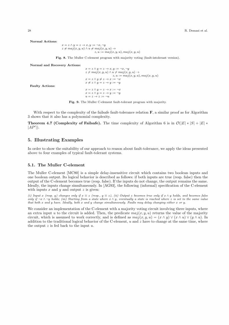
28 R. Demasi et al.
Normal Actions:x = z ∧ y = z → x, y := ¬x,¬yz 6= maj(x, y, u) ∧ u 6= maj(x, y, u)→
z, u := maj(x, y, u),maj(x, y, u)
Fig. 8. The Muller C-element program with majority voting (fault-intolerant version).
Normal and Recovery Actions:x = z ∧ y = z → x, y := ¬x,¬yz 6= maj(x, y, u) ∧ u 6= maj(x, y, u)→
z, u := maj(x, y, u),maj(x, y, u)x = z ∧ y 6= z → x := ¬xx 6= z ∧ y = z → y := ¬y
Faulty Actions:x = z ∧ y = z → x := ¬xx = z ∧ y = z → y := ¬yu = z → z := ¬u
Fig. 9. The Muller C-element fault-tolerant program with majority.
With respect to the complexity of the failsafe fault-tolerance relation F, a similar proof as for Algorithm3 shows that it also has a polynomial complexity.
Theorem 4.7 (Complexity of Failsafe). The time complexity of Algorithm 6 is in O(|E| ∗ |S| + |E| ∗|AP ′|).
5. Illustrating Examples
In order to show the suitability of our approach to reason about fault-tolerance, we apply the ideas presentedabove to four examples of typical fault-tolerant systems.
5.1. The Muller C-element
The Muller C-element [MC80] is a simple delay-insensitive circuit which contains two boolean inputs andone boolean output. Its logical behavior is described as follows: if both inputs are true (resp. false) then theoutput of the C-element becomes true (resp. false). If the inputs do not change, the output remains the same.Ideally, the inputs change simultaneously. In [AG93], the following (informal) specification of the C-elementwith inputs x and y and output z is given:
(i) Input x (resp. y) changes only if x ≡ z (resp., y ≡ z), (ii) Output z becomes true only if x ∧ y holds, and becomes falseonly if ¬x ∧ ¬y holds; (iii) Starting from a state where x ∧ y, eventually a state is reached where z is set to the same valuethat both x and y have. Ideally, both x and y change simultaneously. Faults may delay changing either x or y.
We consider an implementation of the C-element with a majority voting circuit involving three inputs, wherean extra input u to the circuit is added. Then, the predicate maj(x, y, u) returns the value of the majoritycircuit, which is assumed to work correctly, and is defined as maj(x, y, u) = (x ∧ y) ∨ (x ∧ u) ∨ (y ∧ u). Inaddition to the traditional logical behavior of the C-element, u and z have to change at the same time, wherethe output z is fed back to the input u.
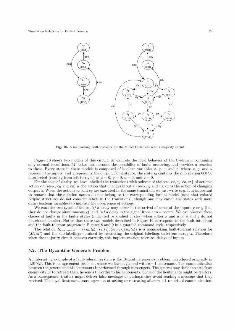
Simulation Relations for Fault-Tolerance 29
s2
110/0
s0
000/0
s1
111/1
s3
001/1
czu
cxy
cxy
czu
t2
110/0
t0
000/0
t1
111/1
t3
001/1
czu
cxy
cxy
czu
t4
011/1
t5
101/1
t8
011/0
t6
001/0
t7
101/0
t9
111/0
cx cy
cy cx
czcz
czcz
cy cx
cxycx cy
Fig. 10. A nonmasking fault-tolerance for the Muller C-element with a majority circuit.
Figure 10 shows two models of this circuit. M exhibits the ideal behavior of the C-element containingonly normal transitions. M ′ takes into account the possibility of faults occurring, and provides a reactionto these. Every state in these models is composed of boolean variables x, y, u, and z, where x, y, and urepresent the inputs, and z represents the output. For instance, the state s0 contains the information 000 \ 0interpreted (reading from left to right) as x = 0, y = 0, u = 0, and z = 0.
For the sake of clarity, we have labelled the transitions with subsets of the set {cx, cy, cu, cz} of actions;action cx (resp., cy and cu) is the action that changes input x (resp., y and u); cz is the action of changingoutput z. When the actions cx and cy are executed in the same transition, we just write cxy. It is importantto remark that these action names do not belong to the corresponding formal model (note that coloredKripke structures do not consider labels in the transitions), though one may enrich the states with moredata (boolean variables) to indicate the occurrence of actions.
We consider two types of faults: (i) a delay may occur in the arrival of some of the inputs x or y (i.e.,they do not change simultaneously), and (ii) a delay in the signal from z to u occurs. We can observe theseclasses of faults in the faulty states (indicated by dashed circles) when either x and y or u and z do notmatch one another. Notice that these two models described in Figure 10 correspond to the fault-intolerantand the fault-tolerant program in Figures 8 and 9 in a guarded command style, respectively.
The relation Rc−element = {〈s0, t0〉, 〈s1, t1〉, 〈s2, t2〉, 〈s3, t3〉} is a nonmasking fault-tolerant relation for〈M,M ′〉 and the sub-labelings obtained by restricting the original labelings to letters u, x, y, z. Therefore,when the majority circuit behaves correctly, this implementation tolerates delays of inputs.
5.2. The Byzantine Generals Problem
An interesting example of a fault-tolerant system is the Byzantine generals problem, introduced originally in[LSP82]. This is an agreement problem, where we have a general with n− 1 lieutenants. The communicationbetween the general and his lieutenants is performed through messengers. The general may decide to attack anenemy city or to retreat; then, he sends the order to his lieutenants. Some of the lieutenants might be traitors.As a consequence, traitors might deliver false messages or perhaps they avoid sending a message that theyreceived. The loyal lieutenants must agree on attacking or retreating after m+ 1 rounds of communication,

30 R. Demasi et al.
s0
r0
s1
P1
r1
s2
P2
r2L0.sendA(L1,2,3) tt L1.fwd(L0, A, L2,3)
L2.fwd(L0, A, L1,3)
L3.fwd(L0, A, L1,2)
tt
restart
t0
r0
t1
P1
r1
t3
P3
r1
L0.sendA(L1,2,3) tt
L1.fwd(L0, A, L2,3)
L2.fwd(L0, A, L1,3)
L3.fwd(L0, A, L1,2)
tt
restart
t2
P2
r2
t4
P4
r2
L1.betray
restart
L2.fwd(L0, A, L1,3)
L3.fwd(L0, A, L1,2)
tt
P1: L1.A0 ⋀ L2.A0 ⋀ L3.A0
P3: L1.A0 ⋀ L2.A0 ⋀ L3.A0 ⋀ L1.traitor
P2: L1.A0,2,3 ⋀ L1.d ⋀ L2.A0,1,3 ⋀ L2.d ⋀ L3.A0,1,2 ⋀ L3.d
P4: L1.A0,2,3 ⋀ L1.traitor ⋀ L1.d ⋀ L2.A0,3 ⋀ L2.d ⋀ L3.A0,2 ⋀ L3.d
Fig. 11. A masking fault-tolerance relation for the Byzantine generals problem.
where m is the maximum numbers of traitors. The algorithm can ensure correct operation only if fewerthan one third of the lieutenants are traitors. We assume the following: L0 is the general, the messages aredelivered correctly and all the lieutenants can communicate directly with each other; in this scenario theycan recognize who is sending a message. Faults can convert loyal lieutenants into traitors. Finally, traitorscannot forge messages on behalf of loyal lieutenants.
In Figure 11 two models of this problem are described. M exhibits the ideal behavior of the Byzantineagreement for a general (L0) and three loyal lieutenants (L1, L2, and L3). On the other hand, M ′ expressesthe same behavior that M does, but considering the presence of lieutenant L1 as a traitor. We specify thisproblem following the ideas introduced in [CM09]. We have the following predicates: Li.Al1,...,ln (this predicateindicates that Li has received a message from lieutenants l1, . . . , ln saying that he must attack). We have aviolation predicate Li.traitor for each lieutenant (this predicate is true when Li is a traitor) and Li.d (thispredicate is true when Li has decided to attack), rj (this predicate is true when we are in round j). Eachstate has the predicates (P1, P2, P3, or P4) which hold in it and the relevant information about the currentround. Each transition is labeled with some of the following actions: Li.sendA(Ll1,...,ln) (lieutenant Li sends tolieutenants l1, . . . , ln the message of attack), Li.fwd(Lk,A, Ll1,...,ln) (the lieutenant Li forwards to lieutenantsl1, . . . , ln the message of attack that he received from Lk), Li.betray (lieutenant Li becomes a traitor). Weconsider a clock that allows lieutenants to synchronize; the action tt increments the clock by one unit oftime. The specification uses m + 1 rounds of messages, which are coordinated by means of the clock, wherem is the number of traitors for which the specification ensures that the loyal lieutenants will agree on adecision. In this case the relation
Rbyzantines = {〈s0, t0〉, 〈s1, t1〉, 〈s2, t2〉, 〈s1, t3〉, 〈s2, t4〉}
is a masking fault-tolerant relation for 〈M,M ′〉 where the sub-labelings are obtained by restricting the
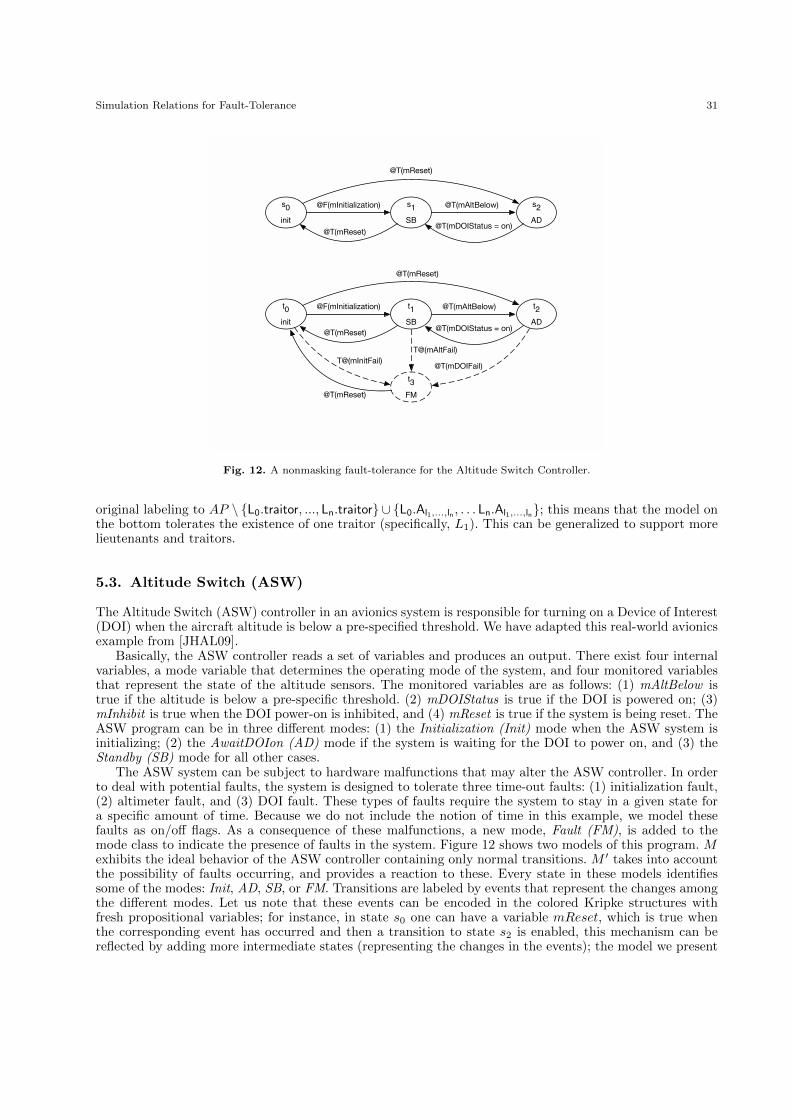
Simulation Relations for Fault-Tolerance 31
s0
init
s1
SB
s2
AD
@T(mReset)
@F(mInitialization) @T(mAltBelow)
@T(mReset)@T(mDOIStatus = on)
t0
init
t1
SB
t2
AD
t3
FM
T@(mAltFail)
@T(mDOIFail)T@(mInitFail)
@T(mReset)
@T(mAltBelow)@F(mInitialization)
@T(mReset)@T(mDOIStatus = on)
@T(mReset)
Fig. 12. A nonmasking fault-tolerance for the Altitude Switch Controller.
original labeling to AP \ {L0.traitor, ..., Ln.traitor} ∪ {L0.Al1,...,ln , . . . Ln.Al1,...,ln}; this means that the model onthe bottom tolerates the existence of one traitor (specifically, L1). This can be generalized to support morelieutenants and traitors.
5.3. Altitude Switch (ASW)
The Altitude Switch (ASW) controller in an avionics system is responsible for turning on a Device of Interest(DOI) when the aircraft altitude is below a pre-specified threshold. We have adapted this real-world avionicsexample from [JHAL09].
Basically, the ASW controller reads a set of variables and produces an output. There exist four internalvariables, a mode variable that determines the operating mode of the system, and four monitored variablesthat represent the state of the altitude sensors. The monitored variables are as follows: (1) mAltBelow istrue if the altitude is below a pre-specific threshold. (2) mDOIStatus is true if the DOI is powered on; (3)mInhibit is true when the DOI power-on is inhibited, and (4) mReset is true if the system is being reset. TheASW program can be in three different modes: (1) the Initialization (Init) mode when the ASW system isinitializing; (2) the AwaitDOIon (AD) mode if the system is waiting for the DOI to power on, and (3) theStandby (SB) mode for all other cases.
The ASW system can be subject to hardware malfunctions that may alter the ASW controller. In orderto deal with potential faults, the system is designed to tolerate three time-out faults: (1) initialization fault,(2) altimeter fault, and (3) DOI fault. These types of faults require the system to stay in a given state fora specific amount of time. Because we do not include the notion of time in this example, we model thesefaults as on/off flags. As a consequence of these malfunctions, a new mode, Fault (FM), is added to themode class to indicate the presence of faults in the system. Figure 12 shows two models of this program. Mexhibits the ideal behavior of the ASW controller containing only normal transitions. M ′ takes into accountthe possibility of faults occurring, and provides a reaction to these. Every state in these models identifiessome of the modes: Init, AD, SB, or FM. Transitions are labeled by events that represent the changes amongthe different modes. Let us note that these events can be encoded in the colored Kripke structures withfresh propositional variables; for instance, in state s0 one can have a variable mReset, which is true whenthe corresponding event has occurred and then a transition to state s2 is enabled, this mechanism can bereflected by adding more intermediate states (representing the changes in the events); the model we present
32 R. Demasi et al.
in Figure 12 is a simplified one (one can think of it as an abstract description of the corresponding model);however, it illustrates how the notion of nonmasking applies to this scenario.
We use the following notation to represent events: @T(c), where c represents the condition value in thebefore state. Once the event @F(mInitialization) occurs, which means that the initialization is complete, thesystem moves from Init to SB. It returns to Init when the pilot pushes the reset button (@T(mReset) occurs).Moreover, the system moves from SB to AD through the action altBelow when the aircraft descends belowthe threshold altitude (@T(mAltBelow)), but requiring as precondition that powering on is not inhibited,and the DOI is not powered on. Once the DOI signals that it is powered on T(mDOIStatus = on), thesystem goes from AD to SB. Furthermore, the system returns from AD to Init when the pilot pushes thereset button (@T(mReset) occurs). All these events correspond to the ideal behavior of the ASW program.On the other hand, we add other monitoring variables mInitFail, mAltFail, and mDOIFail to model theoccurrences of faults, perturbing the normal behavior of the system. Consequently, when the system detectsany of these faults, it goes into the faulty mode (FM ). Finally, the problem specification requires that theprogram does not change its mode from Standby (SB) to AwaitDOI (AD) if the altitude sensors failed,i.e., when @T(mAltFail) occurs. Moreover, from the faulty state FM, the program can only go into theInitialization mode. In fact, the program can recover from the faulty state if the system has been reset bythe pilot (@T(mReset) occurs).
As a result, the relation Rasw−controller = {〈s0, t0〉, 〈s1, t1〉, 〈s2, t2〉, 〈s0, t3〉} is a nonmasking fault-tolerantrelation for 〈M,M ′〉. We obtain a similar result compared to [JHAL09], where the authors use the termeventual masking (“the system enters a fault handling state but eventually recovers to normal behavior”)for this kind of fault-tolerance behavior. We remark that the specification on this example has been slightlysimplified from the original one described in [JHAL09]. For example, the logic in the events that causetransitions in our models is much simpler compared to the ones in [JHAL09].
5.4. A Simple Train System
We now consider a simple train system. Train systems control the movement of trains through a network ofrail segments. Fault-tolerance is a key aspect of these systems: a fault in the system may cause a train collisionand the loss of human life. These kinds of systems are the object of active research in the fault-tolerancecommunity (see [AB08, Abr06, GH90]).
The general version of our system consists of n trains and m rail segments. Rail segments are connectedto other rail segments, where in each of these connections the rails are equipped with a signal which indicatesif the segment is occupied or not. The signals can be green (when the segment is free) or red (when anothertrain is in the segment). We have the following predicates. For each 0 ≤ i ≤ n and 0 ≤ j ≤ m, we have apredicate ti.rj which indicates that train i is in the segment j; the predicate rj .green (rj .red) expresses thatthe signal of segment j is green (red), respectively. Moreover, ti.stop denotes that train ti is stopped andriRrj means that segments i and j are connected. We have the following actions: ti.move(j): train ti movesto segment j, ti.stops: train ti stops, ri.ggreen: the signal of ri is set to green, and ri.gred: the signal of riis set to red.
The specification requires that, if there is a train in a segment, then the signal for this segment mustbe red. On the contrary, if there is no train in the segment, then the signal for the segment must be green.Moreover, when a train detects that another train is already in the same segment, a fault has occurred,and it ought to stop to avoid train collisions. Besides, when a train is in a segment where all the connectedsegments have their signals set to red, the train will stop. Finally, an ideal safety property of this system isthat there are not two trains in the same segment; that is, this property must hold in the specification whenno faults are observed.
This system is implemented by a sensor in each segment which detects the existence of two trains.Furthermore, the movement of trains between rail segments is controlled by a pair of sensors called BlockInstruments in railways. Essentially, these devices have the task of activating the green or red signal. Thebasis of operation of the system is very simple, but what is more significant is the inherent fail-safety builtinto it. In case a fault occurs, the interlocking relay logic turns the signal to red.
In order to provide a better understanding of this example and the particular situation for failsafe fault-tolerance, let us consider trains ti with 0 ≤ i ≤ 2 and rail segments rj with 0 ≤ j ≤ 4, where they areconnected as follow: r0Rr1, r1Rr2, r2Rr3, r2Rr4, and r3Rr4. In Figure 13 two models of this problem aredescribed. M exhibits the ideal behavior of the simple train system for three trains on five rail segments. On
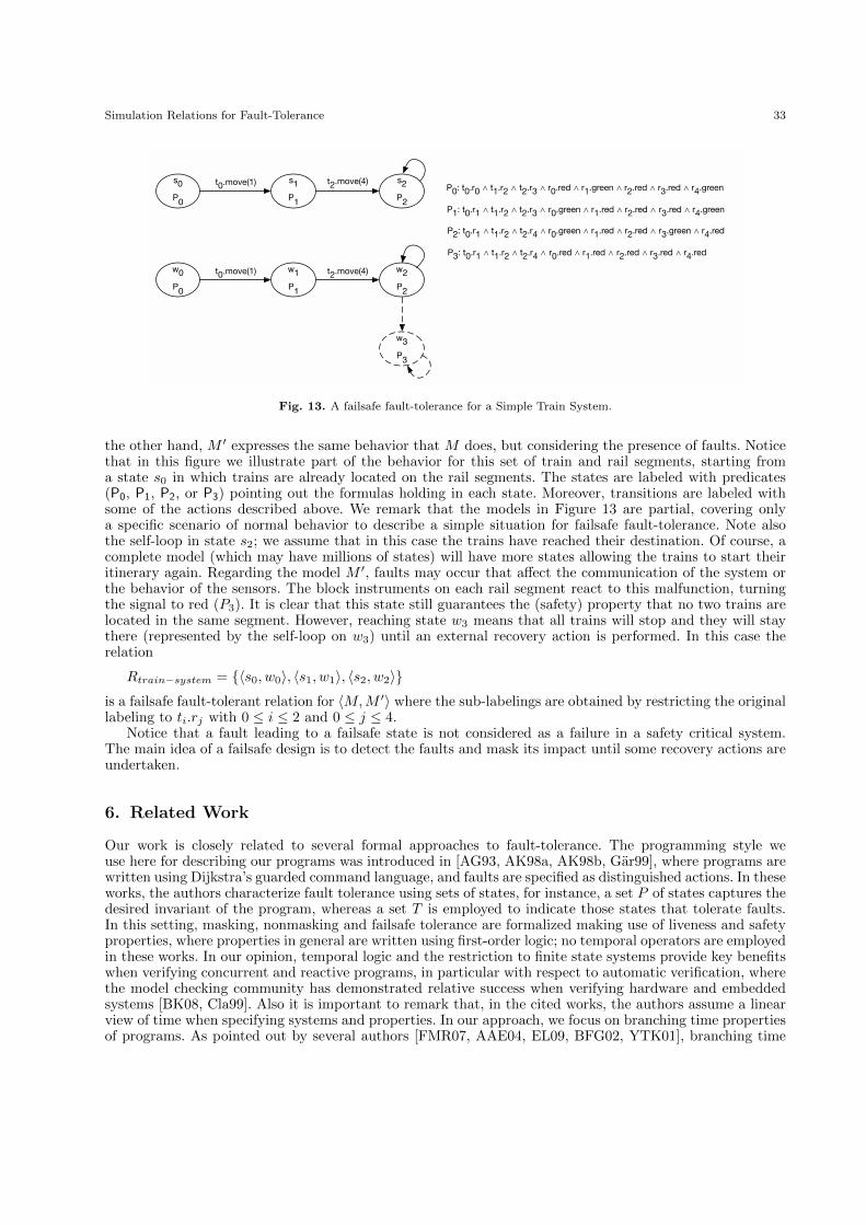
Simulation Relations for Fault-Tolerance 33
s0
P0
s1
P1
s2
P2
t0.move(1) t2.move(4)
w0
P0
w1
P1
w2
P2
t0.move(1) t2.move(4)
w3
P3
P0: t0.r0 ⋀ t1.r2 ⋀ t2.r3 ⋀ r0.red ⋀ r1.green ⋀ r2.red ⋀ r3.red ⋀ r4.green
P1: t0.r1 ⋀ t1.r2 ⋀ t2.r3 ⋀ r0.green ⋀ r1.red ⋀ r2.red ⋀ r3.red ⋀ r4.green
P2: t0.r1 ⋀ t1.r2 ⋀ t2.r4 ⋀ r0.green ⋀ r1.red ⋀ r2.red ⋀ r3.green ⋀ r4.red
P3: t0.r1 ⋀ t1.r2 ⋀ t2.r4 ⋀ r0.red ⋀ r1.red ⋀ r2.red ⋀ r3.red ⋀ r4.red
Fig. 13. A failsafe fault-tolerance for a Simple Train System.
the other hand, M ′ expresses the same behavior that M does, but considering the presence of faults. Noticethat in this figure we illustrate part of the behavior for this set of train and rail segments, starting froma state s0 in which trains are already located on the rail segments. The states are labeled with predicates(P0, P1, P2, or P3) pointing out the formulas holding in each state. Moreover, transitions are labeled withsome of the actions described above. We remark that the models in Figure 13 are partial, covering onlya specific scenario of normal behavior to describe a simple situation for failsafe fault-tolerance. Note alsothe self-loop in state s2; we assume that in this case the trains have reached their destination. Of course, acomplete model (which may have millions of states) will have more states allowing the trains to start theiritinerary again. Regarding the model M ′, faults may occur that affect the communication of the system orthe behavior of the sensors. The block instruments on each rail segment react to this malfunction, turningthe signal to red (P3). It is clear that this state still guarantees the (safety) property that no two trains arelocated in the same segment. However, reaching state w3 means that all trains will stop and they will staythere (represented by the self-loop on w3) until an external recovery action is performed. In this case therelation
Rtrain−system = {〈s0, w0〉, 〈s1, w1〉, 〈s2, w2〉}is a failsafe fault-tolerant relation for 〈M,M ′〉 where the sub-labelings are obtained by restricting the originallabeling to ti.rj with 0 ≤ i ≤ 2 and 0 ≤ j ≤ 4.
Notice that a fault leading to a failsafe state is not considered as a failure in a safety critical system.The main idea of a failsafe design is to detect the faults and mask its impact until some recovery actions areundertaken.
6. Related Work
Our work is closely related to several formal approaches to fault-tolerance. The programming style weuse here for describing our programs was introduced in [AG93, AK98a, AK98b, Gar99], where programs arewritten using Dijkstra’s guarded command language, and faults are specified as distinguished actions. In theseworks, the authors characterize fault tolerance using sets of states, for instance, a set P of states captures thedesired invariant of the program, whereas a set T is employed to indicate those states that tolerate faults.In this setting, masking, nonmasking and failsafe tolerance are formalized making use of liveness and safetyproperties, where properties in general are written using first-order logic; no temporal operators are employedin these works. In our opinion, temporal logic and the restriction to finite state systems provide key benefitswhen verifying concurrent and reactive programs, in particular with respect to automatic verification, wherethe model checking community has demonstrated relative success when verifying hardware and embeddedsystems [BK08, Cla99]. Also it is important to remark that, in the cited works, the authors assume a linearview of time when specifying systems and properties. In our approach, we focus on branching time propertiesof programs. As pointed out by several authors [FMR07, AAE04, EL09, BFG02, YTK01], branching time
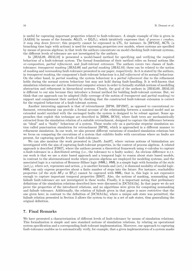
34 R. Demasi et al.
is useful for capturing important properties related to fault-tolerance. A simple example of this is given in[AAE04] by means of the formula: AG(Di ⇒ EGDi), which intuitively expresses that: if process i crashes,it may stay down forever ; this property cannot be expressed in LTL, for instance. In [BFG02], ACTL (abranching time logic with actions) is used for expressing properties over models, where systems are specifiedby means of process algebras; in that work the authors concentrate on model checking fault-tolerant systems,the different levels of tolerance are not investigated by the authors.
In [JHAL09, JHAL10] is presented a model-based method for specifying and verifying the requiredbehaviour of a fault-tolerant system. The formal foundations of their method relies on formal notions likeor-composition, partial refinement, and fault-tolerant extension. The authors covers two classes of fault-tolerance: transparent masking [JHAL09] and partial masking [JHAL10]; these can be related to the notionof masking and nonmasking fault-tolerance presented in our paper, respectively. As it is stated by the authors,in transparent masking, the component’s fault-tolerant behaviour is a full refinement of its normal behaviour.On the other hand, in partial masking, the system behaviour is a partial refinement due to the refinementholds during the normal system behaviour but may not hold during fault-handling. It is well-known thatsimulation relations are used in theoretical computer science in order to formally stablish notions of modellingabstraction and refinement in hierarchical systems. Clearly, the goal of the authors in [JHAL09, JHAL10]is different to our aim because they introduce a formal method for building fault-tolerant systems. But, wethink that our approach can be adapted (fully coverage of the notion of transparent and partial masking) tosupport and complement their method by checking that the constructed fault-tolerant extension is correctfor the required behaviour of a fault-tolerant system.
Another interesting approach is that of retrenchment [BP98, BPJS07], as opposed to conventional re-finement, retrenchment can provide a formal account of the relationship between a nominal model and anextended model enriched with the envisaged faults the system is designed to be robust against. Some ap-proaches that exploit this technique are described in [BB06, BC04], where fault trees are mechanisticallyextracted from the simulation relation of a suitable retrenchment, designed to capture the difference betweenan “ideal” and a “faulty” behaviour of a system. These works rely on a particular stepwise simulation no-tion called punctuation simulation for retrenchment [BP99], which is approached in a different manner torefinement simulation. In our work, we also present different variations of standard simulation relations butwe focus on comparing the executions of a system that exhibits faults with executions where no faults arepresent, for capturing specific levels of fault-tolerance.
We can also mention the work presented in [Jan95, Jan97], where various notions of bisimulation areinvestigated with the aim of capturing fault-tolerant properties, in the context of process algebras. A relatedapproach is described [FH07], where the authors present a theoretical framework using π-calculus to capturen-fault-tolerance in a distributed setting (i.e., the tolerance to n faulty nodes). An obvious difference w.r.t.our work is that we use a state based approach and a temporal logic to reason about state based models,in contrast to the aforementioned works where process algebras are employed for modeling systems, and theassociated logic is a variation of Hennesy-Milner logic (HML). HML is a simple logic with formulas of the style〈acti〉ϕ, where acti represents and action, ϕ is another formula and 〈acti〉 is diamond modality of modal logic.HML can only express properties about a finite number of steps into the future. For instance, reachabilityproperties (of the style AFϕ or EFϕ) cannot be captured with HML; that is, this logic is not expressiveenough to capture important temporal properties [BS07]. Also, the notions of masking, nonmasking andfailsafe fault-tolerance are not investigated in these works. Finally, it is important noting that preliminarydefinitions of the simulation relations described here were discussed in [DCMA13a]. In that paper we do notprove the properties of the introduced relations, and no algorithms were given for computing nonmaskingand failsafe tolerance. Additionally, the relation of failsafe given in that paper is more restrictive that theone given here; in contrast to the definition of [DCMA13a], where a unique safe state was permitted, thefailsafe relation presented in Section 3 allows the system to stay in a set of safe states, thus generalizing theoriginal definition.
7. Final Remarks
We have presented a characterization of different levels of fault-tolerance by means of simulation relations.This formalization is simple and uses standard notions of simulation relations, by relating an operationalsystem specification and a corresponding fault-tolerant implementation. Moreover, our approach to capturingfault-tolerance enables us to automatically verify, for example, that a given implementation of a system masks
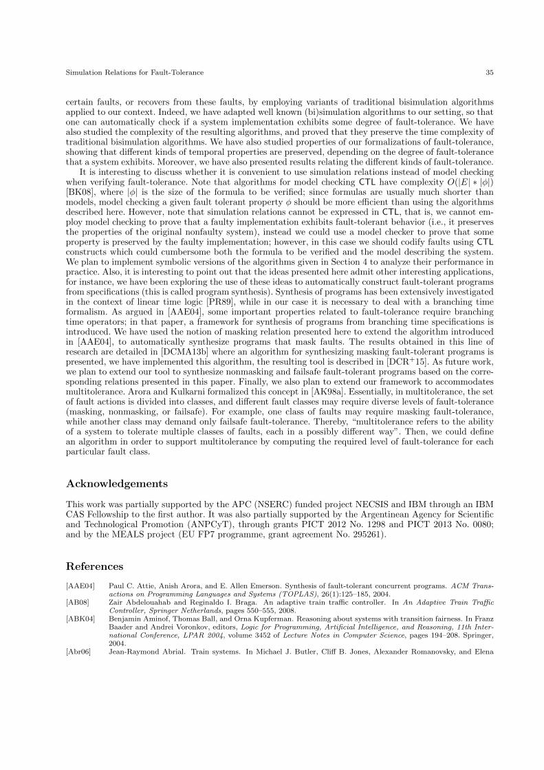
Simulation Relations for Fault-Tolerance 35
certain faults, or recovers from these faults, by employing variants of traditional bisimulation algorithmsapplied to our context. Indeed, we have adapted well known (bi)simulation algorithms to our setting, so thatone can automatically check if a system implementation exhibits some degree of fault-tolerance. We havealso studied the complexity of the resulting algorithms, and proved that they preserve the time complexity oftraditional bisimulation algorithms. We have also studied properties of our formalizations of fault-tolerance,showing that different kinds of temporal properties are preserved, depending on the degree of fault-tolerancethat a system exhibits. Moreover, we have also presented results relating the different kinds of fault-tolerance.
It is interesting to discuss whether it is convenient to use simulation relations instead of model checkingwhen verifying fault-tolerance. Note that algorithms for model checking CTL have complexity O(|E| ∗ |φ|)[BK08], where |φ| is the size of the formula to be verified; since formulas are usually much shorter thanmodels, model checking a given fault tolerant property φ should be more efficient than using the algorithmsdescribed here. However, note that simulation relations cannot be expressed in CTL, that is, we cannot em-ploy model checking to prove that a faulty implementation exhibits fault-tolerant behavior (i.e., it preservesthe properties of the original nonfaulty system), instead we could use a model checker to prove that someproperty is preserved by the faulty implementation; however, in this case we should codify faults using CTLconstructs which could cumbersome both the formula to be verified and the model describing the system.We plan to implement symbolic versions of the algorithms given in Section 4 to analyze their performance inpractice. Also, it is interesting to point out that the ideas presented here admit other interesting applications,for instance, we have been exploring the use of these ideas to automatically construct fault-tolerant programsfrom specifications (this is called program synthesis). Synthesis of programs has been extensively investigatedin the context of linear time logic [PR89], while in our case it is necessary to deal with a branching timeformalism. As argued in [AAE04], some important properties related to fault-tolerance require branchingtime operators; in that paper, a framework for synthesis of programs from branching time specifications isintroduced. We have used the notion of masking relation presented here to extend the algorithm introducedin [AAE04], to automatically synthesize programs that mask faults. The results obtained in this line ofresearch are detailed in [DCMA13b] where an algorithm for synthesizing masking fault-tolerant programs ispresented, we have implemented this algorithm, the resulting tool is described in [DCR+15]. As future work,we plan to extend our tool to synthesize nonmasking and failsafe fault-tolerant programs based on the corre-sponding relations presented in this paper. Finally, we also plan to extend our framework to accommodatesmultitolerance. Arora and Kulkarni formalized this concept in [AK98a]. Essentially, in multitolerance, the setof fault actions is divided into classes, and different fault classes may require diverse levels of fault-tolerance(masking, nonmasking, or failsafe). For example, one class of faults may require masking fault-tolerance,while another class may demand only failsafe fault-tolerance. Thereby, “multitolerance refers to the abilityof a system to tolerate multiple classes of faults, each in a possibly different way”. Then, we could definean algorithm in order to support multitolerance by computing the required level of fault-tolerance for eachparticular fault class.
Acknowledgements
This work was partially supported by the APC (NSERC) funded project NECSIS and IBM through an IBMCAS Fellowship to the first author. It was also partially supported by the Argentinean Agency for Scientificand Technological Promotion (ANPCyT), through grants PICT 2012 No. 1298 and PICT 2013 No. 0080;and by the MEALS project (EU FP7 programme, grant agreement No. 295261).
References
[AAE04] Paul C. Attie, Anish Arora, and E. Allen Emerson. Synthesis of fault-tolerant concurrent programs. ACM Trans-actions on Programming Languages and Systems (TOPLAS), 26(1):125–185, 2004.
[AB08] Zair Abdelouahab and Reginaldo I. Braga. An adaptive train traffic controller. In An Adaptive Train TrafficController, Springer Netherlands, pages 550–555, 2008.
[ABK04] Benjamin Aminof, Thomas Ball, and Orna Kupferman. Reasoning about systems with transition fairness. In FranzBaader and Andrei Voronkov, editors, Logic for Programming, Artificial Intelligence, and Reasoning, 11th Inter-national Conference, LPAR 2004, volume 3452 of Lecture Notes in Computer Science, pages 194–208. Springer,2004.
[Abr06] Jean-Raymond Abrial. Train systems. In Michael J. Butler, Cliff B. Jones, Alexander Romanovsky, and Elena
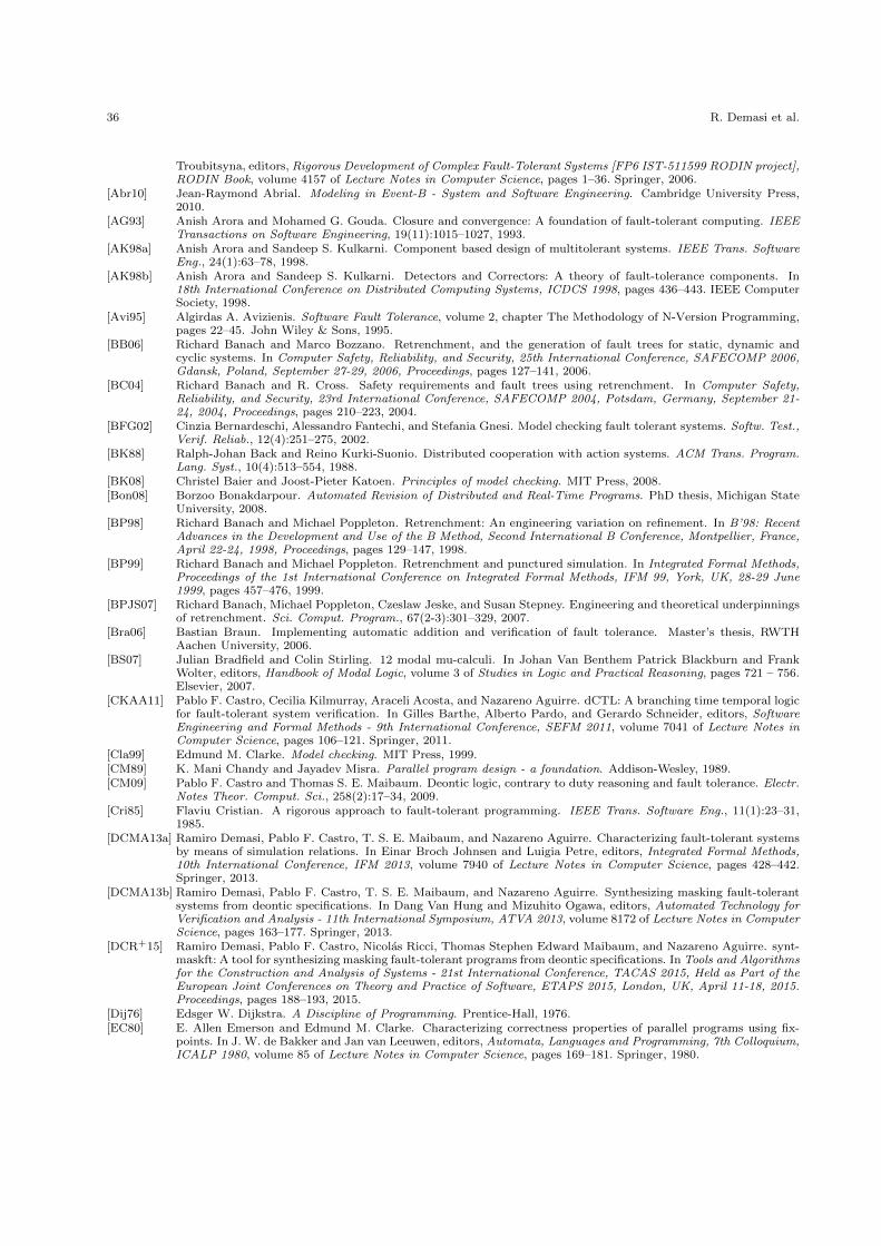
36 R. Demasi et al.
Troubitsyna, editors, Rigorous Development of Complex Fault-Tolerant Systems [FP6 IST-511599 RODIN project],RODIN Book, volume 4157 of Lecture Notes in Computer Science, pages 1–36. Springer, 2006.
[Abr10] Jean-Raymond Abrial. Modeling in Event-B - System and Software Engineering. Cambridge University Press,2010.
[AG93] Anish Arora and Mohamed G. Gouda. Closure and convergence: A foundation of fault-tolerant computing. IEEETransactions on Software Engineering, 19(11):1015–1027, 1993.
[AK98a] Anish Arora and Sandeep S. Kulkarni. Component based design of multitolerant systems. IEEE Trans. SoftwareEng., 24(1):63–78, 1998.
[AK98b] Anish Arora and Sandeep S. Kulkarni. Detectors and Correctors: A theory of fault-tolerance components. In18th International Conference on Distributed Computing Systems, ICDCS 1998, pages 436–443. IEEE ComputerSociety, 1998.
[Avi95] Algirdas A. Avizienis. Software Fault Tolerance, volume 2, chapter The Methodology of N-Version Programming,pages 22–45. John Wiley & Sons, 1995.
[BB06] Richard Banach and Marco Bozzano. Retrenchment, and the generation of fault trees for static, dynamic andcyclic systems. In Computer Safety, Reliability, and Security, 25th International Conference, SAFECOMP 2006,Gdansk, Poland, September 27-29, 2006, Proceedings, pages 127–141, 2006.
[BC04] Richard Banach and R. Cross. Safety requirements and fault trees using retrenchment. In Computer Safety,Reliability, and Security, 23rd International Conference, SAFECOMP 2004, Potsdam, Germany, September 21-24, 2004, Proceedings, pages 210–223, 2004.
[BFG02] Cinzia Bernardeschi, Alessandro Fantechi, and Stefania Gnesi. Model checking fault tolerant systems. Softw. Test.,Verif. Reliab., 12(4):251–275, 2002.
[BK88] Ralph-Johan Back and Reino Kurki-Suonio. Distributed cooperation with action systems. ACM Trans. Program.Lang. Syst., 10(4):513–554, 1988.
[BK08] Christel Baier and Joost-Pieter Katoen. Principles of model checking. MIT Press, 2008.[Bon08] Borzoo Bonakdarpour. Automated Revision of Distributed and Real-Time Programs. PhD thesis, Michigan State
University, 2008.[BP98] Richard Banach and Michael Poppleton. Retrenchment: An engineering variation on refinement. In B’98: Recent
Advances in the Development and Use of the B Method, Second International B Conference, Montpellier, France,April 22-24, 1998, Proceedings, pages 129–147, 1998.
[BP99] Richard Banach and Michael Poppleton. Retrenchment and punctured simulation. In Integrated Formal Methods,Proceedings of the 1st International Conference on Integrated Formal Methods, IFM 99, York, UK, 28-29 June1999, pages 457–476, 1999.
[BPJS07] Richard Banach, Michael Poppleton, Czeslaw Jeske, and Susan Stepney. Engineering and theoretical underpinningsof retrenchment. Sci. Comput. Program., 67(2-3):301–329, 2007.
[Bra06] Bastian Braun. Implementing automatic addition and verification of fault tolerance. Master’s thesis, RWTHAachen University, 2006.
[BS07] Julian Bradfield and Colin Stirling. 12 modal mu-calculi. In Johan Van Benthem Patrick Blackburn and FrankWolter, editors, Handbook of Modal Logic, volume 3 of Studies in Logic and Practical Reasoning, pages 721 – 756.Elsevier, 2007.
[CKAA11] Pablo F. Castro, Cecilia Kilmurray, Araceli Acosta, and Nazareno Aguirre. dCTL: A branching time temporal logicfor fault-tolerant system verification. In Gilles Barthe, Alberto Pardo, and Gerardo Schneider, editors, SoftwareEngineering and Formal Methods - 9th International Conference, SEFM 2011, volume 7041 of Lecture Notes inComputer Science, pages 106–121. Springer, 2011.
[Cla99] Edmund M. Clarke. Model checking. MIT Press, 1999.[CM89] K. Mani Chandy and Jayadev Misra. Parallel program design - a foundation. Addison-Wesley, 1989.[CM09] Pablo F. Castro and Thomas S. E. Maibaum. Deontic logic, contrary to duty reasoning and fault tolerance. Electr.
Notes Theor. Comput. Sci., 258(2):17–34, 2009.[Cri85] Flaviu Cristian. A rigorous approach to fault-tolerant programming. IEEE Trans. Software Eng., 11(1):23–31,
1985.[DCMA13a] Ramiro Demasi, Pablo F. Castro, T. S. E. Maibaum, and Nazareno Aguirre. Characterizing fault-tolerant systems
by means of simulation relations. In Einar Broch Johnsen and Luigia Petre, editors, Integrated Formal Methods,10th International Conference, IFM 2013, volume 7940 of Lecture Notes in Computer Science, pages 428–442.Springer, 2013.
[DCMA13b] Ramiro Demasi, Pablo F. Castro, T. S. E. Maibaum, and Nazareno Aguirre. Synthesizing masking fault-tolerantsystems from deontic specifications. In Dang Van Hung and Mizuhito Ogawa, editors, Automated Technology forVerification and Analysis - 11th International Symposium, ATVA 2013, volume 8172 of Lecture Notes in ComputerScience, pages 163–177. Springer, 2013.
[DCR+15] Ramiro Demasi, Pablo F. Castro, Nicolas Ricci, Thomas Stephen Edward Maibaum, and Nazareno Aguirre. synt-maskft: A tool for synthesizing masking fault-tolerant programs from deontic specifications. In Tools and Algorithmsfor the Construction and Analysis of Systems - 21st International Conference, TACAS 2015, Held as Part of theEuropean Joint Conferences on Theory and Practice of Software, ETAPS 2015, London, UK, April 11-18, 2015.Proceedings, pages 188–193, 2015.
[Dij76] Edsger W. Dijkstra. A Discipline of Programming. Prentice-Hall, 1976.[EC80] E. Allen Emerson and Edmund M. Clarke. Characterizing correctness properties of parallel programs using fix-
points. In J. W. de Bakker and Jan van Leeuwen, editors, Automata, Languages and Programming, 7th Colloquium,ICALP 1980, volume 85 of Lecture Notes in Computer Science, pages 169–181. Springer, 1980.
Simulation Relations for Fault-Tolerance 37
[EH86] E. Allen Emerson and Joseph Y. Halpern. “sometimes” and “not never” revisited: on branching versus linear timetemporal logic. J. ACM, 33(1):151–178, 1986.
[EL09] Jonathan Ezekiel and Alessio Lomuscio. Combining fault injection and model checking to verify fault tolerancein multi-agent systems. In Carles Sierra, Cristiano Castelfranchi, Keith S. Decker, and Jaime Simao Sichman,editors, 8th International Joint Conference on Autonomous Agents and Multiagent Systems, AAMAS 2009, pages113–120. IFAAMAS, 2009.
[FH07] Adrian Francalanza and Matthew Hennessy. A theory for observational fault tolerance. J. Log. Algebr. Program.,73(1-2):22–50, 2007.
[FMR07] Tim French, John Christopher McCabe-Dansted, and Mark Reynolds. A temporal logic of robustness. In Fron-tiers of Combining Systems, 6th International Symposium, FroCoS 2007, Liverpool, UK, September 10-12, 2007,Proceedings, pages 193–205, 2007.
[Gar99] Felix C. Gartner. Fundamentals of fault-tolerant distributed computing in asynchronous environments. ACMComputing Surveys, 31, 1999.
[GH90] Gerard D. Guiho and Claude Hennebert. SACEM software validation (experience report). In Francois-RegisValette, Peter A. Freeman, and Marie-Claude Gaudel, editors, Proceedings of the 12th International Conferenceon Software Engineering, ICSE 1990, pages 186–191. IEEE Computer Society, 1990.
[GJM03] Carlo Ghezzi, Mehdi Jazayeri, and Dino Mandrioli. Fundamentals of software engineering (2. ed.). Prentice Hall,2003.
[HHK95] Monika Rauch Henzinger, Thomas A. Henzinger, and Peter W. Kopke. Computing simulations on finite andinfinite graphs. In 36th Annual Symposium on Foundations of Computer Science, FOCS 1995, pages 453–462.IEEE Computer Society, 1995.
[Jan95] Tomasz Janowski. Bisimulation and Fault-Tolerance. PhD thesis, University of Warwick, United Kingdom, 1995.[Jan97] Tomasz Janowski. On bisimulation, fault-monotonicity and provable fault-tolerance. In Michael Johnson, editor,
Algebraic Methodology and Software Technology, 6th International Conference, AMAST 1997, volume 1349 ofLecture Notes in Computer Science, pages 292–306. Springer, 1997.
[JHAL09] Ralph D. Jeffords, Constance L. Heitmeyer, Myla Archer, and Elizabeth I. Leonard. A formal method for developingprovably correct fault-tolerant systems using partial refinement and composition. In Ana Cavalcanti and DennisDams, editors, Formal Methods, Second World Congress, FM 2009, volume 5850 of Lecture Notes in ComputerScience, pages 173–189. Springer, 2009.
[JHAL10] Ralph D. Jeffords, Constance L. Heitmeyer, Myla Archer, and Elizabeth I. Leonard. Model-based constructionand verification of critical systems using composition and partial refinement. Formal Methods in System Design,37(2-3):265–294, 2010.
[LA90] Peter A. Lee and Thomas Anderson. Fault Tolerance: Principles and Practice. Springer-Verlag New York, Inc.,Secaucus, NJ, USA, 2nd edition, 1990.
[Lam85] Leslie Lamport. Solved problems, unsolved problems and non-problems in concurrency. Operating Systems Review,19(4):34–44, 1985.
[Lam94] Leslie Lamport. The temporal logic of actions. ACM Trans. Program. Lang. Syst., 16(3):872–923, 1994.[LSP82] Leslie Lamport, Robert E. Shostak, and Marshall C. Pease. The Byzantine generals problem. ACM Trans. Program.
Lang. Syst., 4(3):382–401, 1982.[MC80] Carver Mead and Lynn Conway. Introduction to VLSI systems. Addison-Wesley, 1980.[Mil89] Robin Milner. Communication and concurrency. PHI Series in computer science. Prentice Hall, 1989.[MT01] Panagiotis Manolios and Richard J. Trefler. Safety and liveness in branching time. In 16th Annual IEEE Symposium
on Logic in Computer Science, Boston, Massachusetts, USA, June 16-19, 2001, Proceedings, pages 366–374, 2001.[PR89] Amir Pnueli and Roni Rosner. On the synthesis of a reactive module. In Sixteenth Annual ACM Symposium on
Principles of Programming Languages, POPL 1989, pages 179–190. ACM Press, 1989.[PS05] Ignatius S. W. B. Prasetya and S. Doaitse Swierstra. Formal design of self-stabilizing programs. J. High Speed
Networks, 14(1):59–83, 2005.[SECH98] Francis Schneider, Steve M. Easterbrook, John R. Callahan, and Gerard J. Holzmann. Validating requirements
for fault tolerant systems using model checking. In 3rd International Conference on Requirements Engineering,ICRE 1998, pages 4–13. IEEE Computer Society, 1998.
[SS98] Daniel P. Siewiorek and Robert S. Swarz. Reliable Computer Systems (3rd Ed.): Design and Evaluation. A. K.Peters, Ltd., Natick, MA, USA, 1998.
[TP00] Wilfredo Torres-Pomales. Software fault tolerance: A tutorial. Technical report, NASA Technical MemorandumTM-2000-210616, 2000.
[YTK01] Tomoyuki Yokogawa, Tatsuhiro Tsuchiya, and Tsuchiya Kikuno. Automatic verification of fault tolerance usingmodel checking. In 8th Pacific Rim International Symposium on Dependable Computing, PRDC 2001, pages95–102. IEEE Computer Society, 2001.
38 R. Demasi et al.
A. Proofs of Properties
In this section we prove some properties introduced in Section 3.
Proof of Property: ∀i : σ∗Ji+ 1K M σ′[i]The proof is by induction on i. For the base case i = 0, σ∗J1K = σ∗[0] = sM s′ = σ′[0]. For the inductive
case we have to prove that σ∗Ji+2KMσ′[i+1]. By definition of last, if σ∗[i+1] 6= ∗, then σ∗Ji+2K = σ∗[i+1].Furthermore, by definition of σ∗, σ∗[i+ 1] = w for some w ∈ match(σJi+ 1K, σ′[i+ 1]), thus by definition ofmatch(), we have σ∗[i+ 1] M σ′[i+ 1], and since σJi+ 2K = σ∗[i+ 1], we get σ∗Ji+ 2K M σ′[i+ 1].
Let us prove the case σ∗[i+1] = ∗. In this case, by definition of σ∗Ji+2K, we get σ∗Ji+2K = σ∗Ji+1K, and byinduction we get: σ∗Ji+1KMσ′[i]. By definition of σ∗ we have σ∗[i+1] = ∗ since @w ∈ match(σJi+1K, σ′[i+1]),but taking into account that σ′[i + 1] ∈ Post(σ′[i]) and σ∗Ji + 1K M σ′[i], by B.4 we must have thatσ∗Ji+ 1K M σ′[i+ 1] that is (recalling that σ∗Ji+ 2K = σ∗Ji+ 1K) we get σ∗Ji+ 2K M σ′[i+ 1].
Proof of Property: ∀i ≥ 0 : ∃j > i : σ∗[j] 6= ∗ (Used in Lemma 3.1)The proof is by contradiction. Suppose that ∃i ≥ 0 such that ∀j > i : σ∗[j] = ∗, let k be the least of
such i’s, that is, σ∗[k] 6= ∗ and ∀j > k : σ∗[j] = ∗. This means that σ∗[last(k + h, σ∗)] = σ∗JkK for all h ≥ 0.Furthermore, since σ′ is fair and a NDF structure we have a j > k such that σ′[j + 1] ∈ PostN (σ′[j]). Now,note that we have σ∗Jj+1KMσ′[j] (by the property above) and since σ∗[k+h] = ∗ (for every h ≥ 0) we musthave @w ∈ match(σ∗Jk + hK, σ′[k + h]), that is for k + h = j + 1, we have @w ∈ match(σ∗Jj + 1K, σ′[j + 1]).By definition of match, this implies that: @w ∈ PostN (σ∗Jj + 1K) : w M σ′[j + 1], which contradicts B.2.This finishes the proof.
Now we prove some useful properties about function g as defined in Lemma 3.1 that will be useful toprove the properties used in the proof of Lemma 3.1.
Property A.1. f is monotone.
Proof. Assume n ≤ m, that is, m = n+ h, then:
f(n) = #{k | σ∗[k] 6= ∗ ∧ 0 < k ≤ n} (Def. of f)
≤ #{k | σ∗[k] 6= ∗ ∧ 0 < k ≤ n+ h} (monotonicity of #)
= f(n+ h) (Def. f)
= f(m) (assumption)
Proof of Property: ∀i : g(i) = last(g(i+ 1), σ∗)
Proof. The proof is by using the definition of last:
last(g(i+ 1), σ∗) = max{k | 0 ≤ k < g(i+ 1) : σ∗[k] 6= ∗} (Def. of g)
= max{k | 0 ≤ k ≤ g(i) ∨ g(i) < k < g(i+ 1) : σ∗[k] 6= ∗} (properties of ≤)
= max{k | 0 ≤ k ≤ g(i) : σ∗[k] 6= ∗} (Def. of g)
= g(i) (Def. of max)
Proof of Property: ∀i : σ∗[g(f(i))] = σ∗Ji+ 1K.
Proof. First, let us prove that:
#{k | σ∗[k] 6= ∗ ∧ 0 ≤ k ≤ k′} = #{k | σ∗[k] 6= ∗ ∧ 0 ≤ k ≤ last(i+ 1, σ∗)} ⇒ k′ ≥ last(i+ 1, σ∗)
the proof is by contradiction, assume the antecedent holds and k′ < last(i+ 1, σ∗). That is: last(i+ 1, σ∗) =k′ + h for some h, but then:
#{k | σ∗[k] 6= ∗ ∧ 0 ≤ k ≤ k′} = #{k | σ∗[k] 6= ∗ ∧ 0 ≤ k ≤ last(i+ 1, σ∗)} (assumption)
= #{k | σ∗[k] 6= ∗ ∧ 0 ≤ k ≤ k′ ∨ k′ < k ≤ last(i+ 1, σ∗)} (properties of ≤)
= #{k | σ∗[k] 6= ∗ ∧ 0 ≤ k ≤ k′}+ {k′ < k ≤ last(i+ 1, σ∗) ∧ σ∗[k] 6= ∗} (properties of #)
Simulation Relations for Fault-Tolerance 39
thus {k′ < k ≤ last(i+ 1, σ∗[k]) ∧ σ∗[k] 6= ∗} = 0, and then, σ∗[last(i+ 1, σ∗)] = ∗ which is a contradictionby definition of last. Now, we can prove the property:
σ∗[g(f(i))] = σ∗[min{k | f(k) = f(i)}] (Def. of g)
= σ∗[min{k | #{k | σ∗[k] 6= ∗ ∧ 0 ≤ k ≤ k′} = #{k | σ∗[k] 6= ∗ ∧ 0 ≤ k ≤ i}}] (Def. of f)
= σ∗[min{k | #{k | σ∗[k] 6= ∗ ∧ 0 ≤ k ≤ k′} = #{k | σ∗[k] 6= ∗ ∧ 0 ≤ k ≤ last(i+ 1, σ∗)}}] (Def. of last)
= σ∗[last(i+ 1, σ∗)] (property above)
= σ∗Ji+ 1K (Def. of σ∗Ji+ 1K)