QR Complexity
25
Chapter 3 The QR Algorithm The QR algorithm computes a Schur decomposition of a matrix. It is certainly one of the most important algorithm in eigenvalue computations. However, it is applied to dense (or: full ) matrices only. The QR algorithm consists of two separate stages. First, by means of a similarity transformation, the original matrix is transformed in a finite number of steps to Hessenberg form or – in the Hermitian/symmetric case – to real tridiagonal form. This first stage of the algorithm prepares its second stage, the actual QR iterations that are applied to the Hessenberg or tridiagonal matrix. The overall complexity (number of floating points) of the algorithm is O(n 3 ), which we will see is not entirely trivial to obtain. The major limitation of the QR algorithm is that already the first stage generates usually complete fill-in in general sparse matrices. It can therefore not be applied to large sparse matrices, simply because of excessive memory requirements. On the other hand, the QR algorithm computes all eigenvalues (and eventually eigenvectors) which is rarely desired in sparse matrix computations anyway. The treatment of the QR algorithm in these lecture notes on large scale eigenvalue computation is justified in two respects. First, there are of course large or even huge dense eigenvalue problems. Second, the QR algorithm is employed in most other algorithms to solve ‘internal’ small auxiliary eigenvalue problems. 3.1 The basic QR algorithm In 1958 Rutishauser [6] of ETH Zurich experimented with a similar algorithm that we are going to present, but based on the LR factorization, i.e., based on Gaussian elimination without pivoting. That algorithm was not successful as the LR factorization (nowadays called LU factorization) is not stable without pivoting. Francis [3, 4] noticed that the QR factorization would be the preferred choice and devised the QR algorithm with many of the bells and whistles used nowadays. Before presenting the complete picture, we start with a basic iteration, given in Algo- rithm 3.1, discuss its properties and improve on it step by step until we arrive at Francis’ algorithm. We notice first that (3.1) A k = R k Q k = Q ∗ k A k−1 Q k , and hence A k and A k−1 are unitarily similar. The matrix sequence {A k } converges (un- der certain assumptions) towards an upper triangular matrix [7]. Let us assume that the 51
-
Upload
arvind-adimoolam -
Category
Documents
-
view
223 -
download
2
Transcript of QR Complexity
Chapter 3
The QR Algorithm
The QR algorithm computes a Schur decomposition of a matrix. It is certainly one ofthe most important algorithm in eigenvalue computations. However, it is applied to dense
(or: full) matrices only.
The QR algorithm consists of two separate stages. First, by means of a similaritytransformation, the original matrix is transformed in a finite number of steps to Hessenbergform or – in the Hermitian/symmetric case – to real tridiagonal form. This first stage ofthe algorithm prepares its second stage, the actual QR iterations that are applied to theHessenberg or tridiagonal matrix. The overall complexity (number of floating points) ofthe algorithm is O(n3), which we will see is not entirely trivial to obtain.
The major limitation of the QR algorithm is that already the first stage generatesusually complete fill-in in general sparse matrices. It can therefore not be applied to largesparse matrices, simply because of excessive memory requirements. On the other hand,the QR algorithm computes all eigenvalues (and eventually eigenvectors) which is rarelydesired in sparse matrix computations anyway.
The treatment of the QR algorithm in these lecture notes on large scale eigenvaluecomputation is justified in two respects. First, there are of course large or even huge dense
eigenvalue problems. Second, the QR algorithm is employed in most other algorithms tosolve ‘internal’ small auxiliary eigenvalue problems.
3.1 The basic QR algorithm
In 1958 Rutishauser [6] of ETH Zurich experimented with a similar algorithm that we aregoing to present, but based on the LR factorization, i.e., based on Gaussian eliminationwithout pivoting. That algorithm was not successful as the LR factorization (nowadayscalled LU factorization) is not stable without pivoting. Francis [3, 4] noticed that the QRfactorization would be the preferred choice and devised the QR algorithm with many ofthe bells and whistles used nowadays.
Before presenting the complete picture, we start with a basic iteration, given in Algo-rithm 3.1, discuss its properties and improve on it step by step until we arrive at Francis’algorithm.
We notice first that
(3.1) Ak = RkQk = Q∗
kAk−1Qk,
and hence Ak and Ak−1 are unitarily similar. The matrix sequence {Ak} converges (un-der certain assumptions) towards an upper triangular matrix [7]. Let us assume that the
51
52 CHAPTER 3. THE QR ALGORITHM
Algorithm 3.1 Basic QR algorithm
1: Let A ∈ Cn×n. This algorithm computes an upper triangular matrix T and a unitary
matrix U such that A = UTU∗ is the Schur decomposition of A.2: Set A0 := A and U0 = I.3: for k = 1, 2, . . . do4: Ak−1 =: QkRk; /* QR factorization */5: Ak := RkQk;6: Uk := Uk−1Qk; /* Update transformation matrix */7: end for8: Set T := A∞ and U := U∞.
eigenvalues are mutually different in magnitude and we can therefore number the eigen-values such that |λ1| > |λ2| > · · · > |λn|. Then – as we will show in Chapter 6 – theelements of Ak below the diagonal converge to zero like
(3.2) |a(k)ij | = O(|λi/λj |
k), i > j.
From (3.1) we see that
(3.3) Ak = Q∗
kAk−1Qk = Q∗
kQ∗
k−1Ak−2Qk−1Qk = · · · = Q∗
k · · ·Q∗
1A0 Q1 · · ·Qk︸ ︷︷ ︸
Uk
.
With the same assumption on the eigenvalues, Ak tends to an upper triangular matrixand Uk converges to the matrix of Schur vectors.
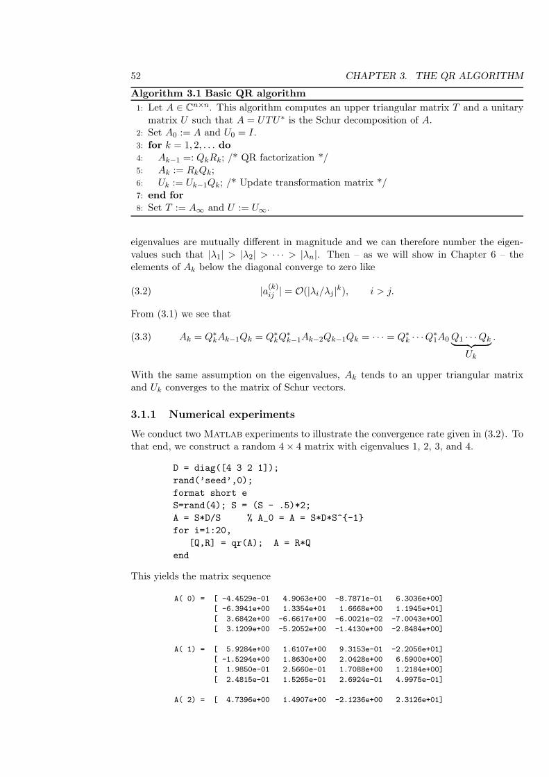
3.1.1 Numerical experiments
We conduct two Matlab experiments to illustrate the convergence rate given in (3.2). Tothat end, we construct a random 4× 4 matrix with eigenvalues 1, 2, 3, and 4.
D = diag([4 3 2 1]);
rand(’seed’,0);
format short e
S=rand(4); S = (S - .5)*2;
A = S*D/S % A_0 = A = S*D*S^{-1}
for i=1:20,
[Q,R] = qr(A); A = R*Q
end
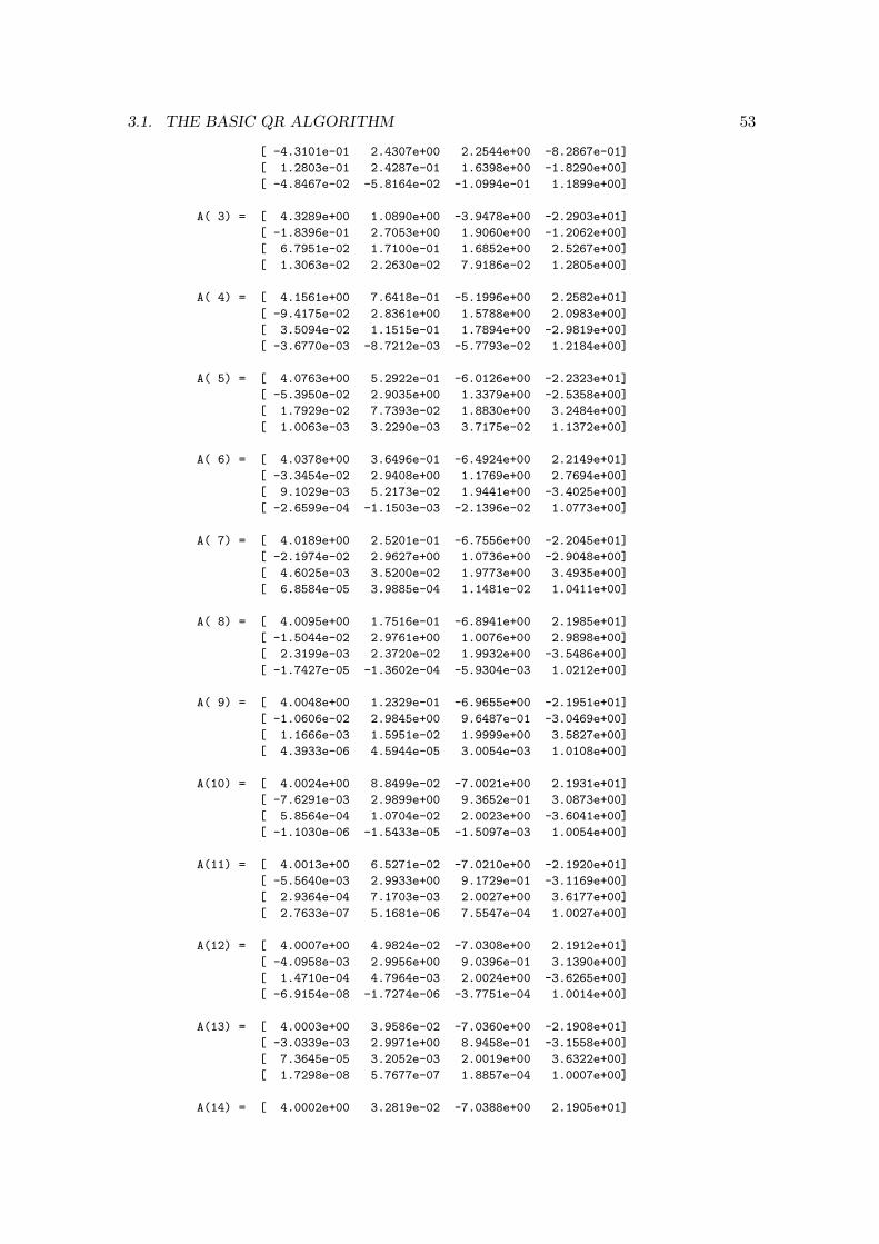
This yields the matrix sequence
A( 0) = [ -4.4529e-01 4.9063e+00 -8.7871e-01 6.3036e+00]
[ -6.3941e+00 1.3354e+01 1.6668e+00 1.1945e+01]
[ 3.6842e+00 -6.6617e+00 -6.0021e-02 -7.0043e+00]
[ 3.1209e+00 -5.2052e+00 -1.4130e+00 -2.8484e+00]
A( 1) = [ 5.9284e+00 1.6107e+00 9.3153e-01 -2.2056e+01]
[ -1.5294e+00 1.8630e+00 2.0428e+00 6.5900e+00]
[ 1.9850e-01 2.5660e-01 1.7088e+00 1.2184e+00]
[ 2.4815e-01 1.5265e-01 2.6924e-01 4.9975e-01]
A( 2) = [ 4.7396e+00 1.4907e+00 -2.1236e+00 2.3126e+01]
3.1. THE BASIC QR ALGORITHM 53
[ -4.3101e-01 2.4307e+00 2.2544e+00 -8.2867e-01]
[ 1.2803e-01 2.4287e-01 1.6398e+00 -1.8290e+00]
[ -4.8467e-02 -5.8164e-02 -1.0994e-01 1.1899e+00]
A( 3) = [ 4.3289e+00 1.0890e+00 -3.9478e+00 -2.2903e+01]
[ -1.8396e-01 2.7053e+00 1.9060e+00 -1.2062e+00]
[ 6.7951e-02 1.7100e-01 1.6852e+00 2.5267e+00]
[ 1.3063e-02 2.2630e-02 7.9186e-02 1.2805e+00]
A( 4) = [ 4.1561e+00 7.6418e-01 -5.1996e+00 2.2582e+01]
[ -9.4175e-02 2.8361e+00 1.5788e+00 2.0983e+00]
[ 3.5094e-02 1.1515e-01 1.7894e+00 -2.9819e+00]
[ -3.6770e-03 -8.7212e-03 -5.7793e-02 1.2184e+00]
A( 5) = [ 4.0763e+00 5.2922e-01 -6.0126e+00 -2.2323e+01]
[ -5.3950e-02 2.9035e+00 1.3379e+00 -2.5358e+00]
[ 1.7929e-02 7.7393e-02 1.8830e+00 3.2484e+00]
[ 1.0063e-03 3.2290e-03 3.7175e-02 1.1372e+00]
A( 6) = [ 4.0378e+00 3.6496e-01 -6.4924e+00 2.2149e+01]
[ -3.3454e-02 2.9408e+00 1.1769e+00 2.7694e+00]
[ 9.1029e-03 5.2173e-02 1.9441e+00 -3.4025e+00]
[ -2.6599e-04 -1.1503e-03 -2.1396e-02 1.0773e+00]
A( 7) = [ 4.0189e+00 2.5201e-01 -6.7556e+00 -2.2045e+01]
[ -2.1974e-02 2.9627e+00 1.0736e+00 -2.9048e+00]
[ 4.6025e-03 3.5200e-02 1.9773e+00 3.4935e+00]
[ 6.8584e-05 3.9885e-04 1.1481e-02 1.0411e+00]
A( 8) = [ 4.0095e+00 1.7516e-01 -6.8941e+00 2.1985e+01]
[ -1.5044e-02 2.9761e+00 1.0076e+00 2.9898e+00]
[ 2.3199e-03 2.3720e-02 1.9932e+00 -3.5486e+00]
[ -1.7427e-05 -1.3602e-04 -5.9304e-03 1.0212e+00]
A( 9) = [ 4.0048e+00 1.2329e-01 -6.9655e+00 -2.1951e+01]
[ -1.0606e-02 2.9845e+00 9.6487e-01 -3.0469e+00]
[ 1.1666e-03 1.5951e-02 1.9999e+00 3.5827e+00]
[ 4.3933e-06 4.5944e-05 3.0054e-03 1.0108e+00]
A(10) = [ 4.0024e+00 8.8499e-02 -7.0021e+00 2.1931e+01]
[ -7.6291e-03 2.9899e+00 9.3652e-01 3.0873e+00]
[ 5.8564e-04 1.0704e-02 2.0023e+00 -3.6041e+00]
[ -1.1030e-06 -1.5433e-05 -1.5097e-03 1.0054e+00]
A(11) = [ 4.0013e+00 6.5271e-02 -7.0210e+00 -2.1920e+01]
[ -5.5640e-03 2.9933e+00 9.1729e-01 -3.1169e+00]
[ 2.9364e-04 7.1703e-03 2.0027e+00 3.6177e+00]
[ 2.7633e-07 5.1681e-06 7.5547e-04 1.0027e+00]
A(12) = [ 4.0007e+00 4.9824e-02 -7.0308e+00 2.1912e+01]
[ -4.0958e-03 2.9956e+00 9.0396e-01 3.1390e+00]
[ 1.4710e-04 4.7964e-03 2.0024e+00 -3.6265e+00]
[ -6.9154e-08 -1.7274e-06 -3.7751e-04 1.0014e+00]
A(13) = [ 4.0003e+00 3.9586e-02 -7.0360e+00 -2.1908e+01]
[ -3.0339e-03 2.9971e+00 8.9458e-01 -3.1558e+00]
[ 7.3645e-05 3.2052e-03 2.0019e+00 3.6322e+00]
[ 1.7298e-08 5.7677e-07 1.8857e-04 1.0007e+00]
A(14) = [ 4.0002e+00 3.2819e-02 -7.0388e+00 2.1905e+01]
54 CHAPTER 3. THE QR ALGORITHM
[ -2.2566e-03 2.9981e+00 8.8788e-01 3.1686e+00]
[ 3.6855e-05 2.1402e-03 2.0014e+00 -3.6359e+00]
[ -4.3255e-09 -1.9245e-07 -9.4197e-05 1.0003e+00]
A(15) = [ 4.0001e+00 2.8358e-02 -7.0404e+00 -2.1902e+01]
[ -1.6832e-03 2.9987e+00 8.8305e-01 -3.1784e+00]
[ 1.8438e-05 1.4284e-03 2.0010e+00 3.6383e+00]
[ 1.0815e-09 6.4192e-08 4.7062e-05 1.0002e+00]
A(16) = [ 4.0001e+00 2.5426e-02 -7.0413e+00 2.1901e+01]
[ -1.2577e-03 2.9991e+00 8.7953e-01 3.1859e+00]
[ 9.2228e-06 9.5295e-04 2.0007e+00 -3.6399e+00]
[ -2.7039e-10 -2.1406e-08 -2.3517e-05 1.0001e+00]
A(17) = [ 4.0000e+00 2.3503e-02 -7.0418e+00 -2.1900e+01]
[ -9.4099e-04 2.9994e+00 8.7697e-01 -3.1917e+00]
[ 4.6126e-06 6.3562e-04 2.0005e+00 3.6409e+00]
[ 6.7600e-11 7.1371e-09 1.1754e-05 1.0000e+00]
A(18) = [ 4.0000e+00 2.2246e-02 -7.0422e+00 2.1899e+01]
[ -7.0459e-04 2.9996e+00 8.7508e-01 3.1960e+00]
[ 2.3067e-06 4.2388e-04 2.0003e+00 -3.6416e+00]
[ -1.6900e-11 -2.3794e-09 -5.8750e-06 1.0000e+00]
A(19) = [ 4.0000e+00 2.1427e-02 -7.0424e+00 -2.1898e+01]
[ -5.2787e-04 2.9997e+00 8.7369e-01 -3.1994e+00]
[ 1.1535e-06 2.8265e-04 2.0002e+00 3.6421e+00]
[ 4.2251e-12 7.9321e-10 2.9369e-06 1.0000e+00]
A(20) = [ 4.0000e+00 2.0896e-02 -7.0425e+00 2.1898e+01]
[ -3.9562e-04 2.9998e+00 8.7266e-01 3.2019e+00]
[ 5.7679e-07 1.8846e-04 2.0002e+00 -3.6424e+00]
[ -1.0563e-12 -2.6442e-10 -1.4682e-06 1.0000e+00]
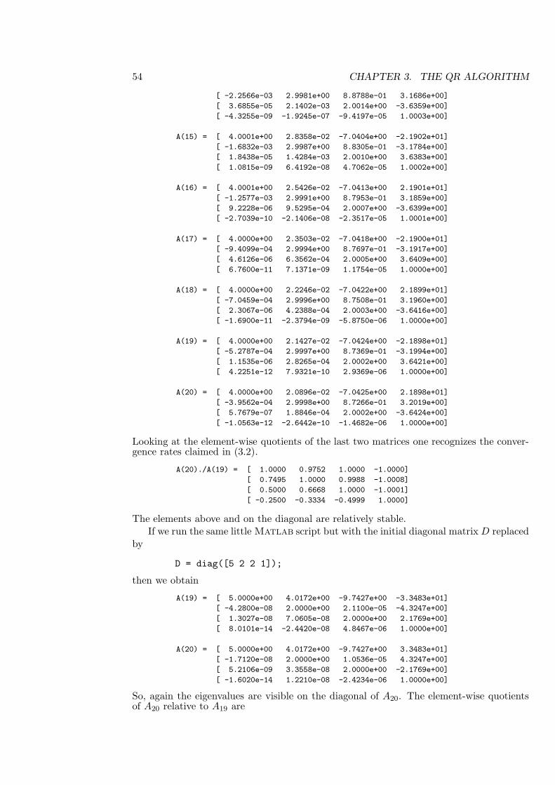
Looking at the element-wise quotients of the last two matrices one recognizes the conver-gence rates claimed in (3.2).
A(20)./A(19) = [ 1.0000 0.9752 1.0000 -1.0000]
[ 0.7495 1.0000 0.9988 -1.0008]
[ 0.5000 0.6668 1.0000 -1.0001]
[ -0.2500 -0.3334 -0.4999 1.0000]
The elements above and on the diagonal are relatively stable.If we run the same little Matlab script but with the initial diagonal matrix D replaced
by
D = diag([5 2 2 1]);
then we obtain
A(19) = [ 5.0000e+00 4.0172e+00 -9.7427e+00 -3.3483e+01]
[ -4.2800e-08 2.0000e+00 2.1100e-05 -4.3247e+00]
[ 1.3027e-08 7.0605e-08 2.0000e+00 2.1769e+00]
[ 8.0101e-14 -2.4420e-08 4.8467e-06 1.0000e+00]
A(20) = [ 5.0000e+00 4.0172e+00 -9.7427e+00 3.3483e+01]
[ -1.7120e-08 2.0000e+00 1.0536e-05 4.3247e+00]
[ 5.2106e-09 3.3558e-08 2.0000e+00 -2.1769e+00]
[ -1.6020e-14 1.2210e-08 -2.4234e-06 1.0000e+00]
So, again the eigenvalues are visible on the diagonal of A20. The element-wise quotientsof A20 relative to A19 are
3.2. THE HESSENBERG QR ALGORITHM 55
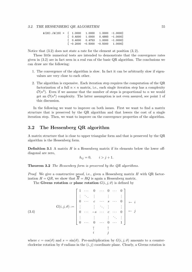
A(20)./A(19) = [ 1.0000 1.0000 1.0000 -1.0000]
[ 0.4000 1.0000 0.4993 -1.0000]
[ 0.4000 0.4753 1.0000 -1.0000]
[ -0.2000 -0.5000 -0.5000 1.0000]
Notice that (3.2) does not state a rate for the element at position (3, 2).These little numerical tests are intended to demonstrate that the convergence rates
given in (3.2) are in fact seen in a real run of the basic QR algorithm. The conclusions wecan draw are the following:
1. The convergence of the algorithm is slow. In fact it can be arbitrarily slow if eigen-values are very close to each other.
2. The algorithm is expensive. Each iteration step requires the computation of the QRfactorization of a full n× n matrix, i.e., each single iteration step has a complexityO(n3). Even if we assume that the number of steps is proportional to n we wouldget an O(n4) complexity. The latter assumption is not even assured, see point 1 ofthis discussion.
In the following we want to improve on both issues. First we want to find a matrixstructure that is preserved by the QR algorithm and that lowers the cost of a singleiteration step. Then, we want to improve on the convergence properties of the algorithm.
3.2 The Hessenberg QR algorithm
A matrix structure that is close to upper triangular form and that is preserved by the QRalgorithm is the Hessenberg form.
Definition 3.1 A matrix H is a Hessenberg matrix if its elements below the lower off-diagonal are zero,
hij = 0, i > j + 1.
Theorem 3.2 The Hessenberg form is preserved by the QR algorithms.
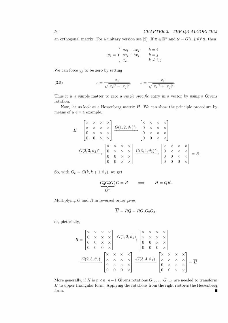
Proof. We give a constructive proof, i.e., given a Hessenberg matrix H with QR factor-ization H = QR, we show that H = RQ is again a Hessenberg matrix.
The Givens rotation or plane rotation G(i, j, ϑ) is defined by
(3.4)
G(i, j, ϑ) :=
1 · · · 0 · · · 0 · · · 0...
. . ....
......
0 · · · c · · · s · · · 0...
.... . .
......
0 · · · −s · · · c · · · 0...
......
. . ....
0 · · · 0 · · · 0 · · · 1
← i
← j
↑ ↑i j
where c = cos(ϑ) and s = sin(ϑ). Pre-multiplication by G(i, j, ϑ) amounts to a counter-clockwise rotation by ϑ radians in the (i, j) coordinate plane. Clearly, a Givens rotation is
56 CHAPTER 3. THE QR ALGORITHM
an orthogonal matrix. For a unitary version see [2]. If x ∈ Rn and y = G(i, j, ϑ)∗x, then
yk =
cxi − sxj, k = isxi + cxj , k = jxk, k 6= i, j
We can force yj to be zero by setting
(3.5) c =xi
√
|xi|2 + |xj |2, s =
−xj√
|xi|2 + |xj|2.
Thus it is a simple matter to zero a single specific entry in a vector by using a Givensrotation.
Now, let us look at a Hessenberg matrix H. We can show the principle procedure bymeans of a 4× 4 example.
H =
× × × ×× × × ×0 × × ×0 0 × ×
G(1, 2, ϑ1)∗·
−−−−−−−−−→
× × × ×0 × × ×0 × × ×0 0 × ×
G(2, 3, ϑ2)∗·
−−−−−−−−−→
× × × ×0 × × ×0 0 × ×0 0 × ×
G(3, 4, ϑ3)∗·
−−−−−−−−−→
× × × ×0 × × ×0 0 × ×0 0 0 ×
= R
So, with Gk = G(k, k + 1, ϑk), we get
G∗
3G∗
2G∗
1︸ ︷︷ ︸
Q∗
G = R ⇐⇒ H = QR.
Multiplying Q and R in reversed order gives
H = RQ = RG1G2G3,
or, pictorially,
R =
× × × ×0 × × ×0 0 × ×0 0 0 ×
·G(1, 2, ϑ1)−−−−−−−−→
× × × ×× × × ×0 0 × ×0 0 0 ×
·G(2, 3, ϑ2)−−−−−−−−→
× × × ×× × × ×0 × × ×0 0 0 ×
·G(3, 4, ϑ1)−−−−−−−−→
× × × ×× × × ×0 × × ×0 0 × ×
= H
More generally, if H is n×n, n−1 Givens rotations G1, . . . , Gn−1 are needed to transformH to upper triangular form. Applying the rotations from the right restores the Hessenbergform.
3.2. THE HESSENBERG QR ALGORITHM 57
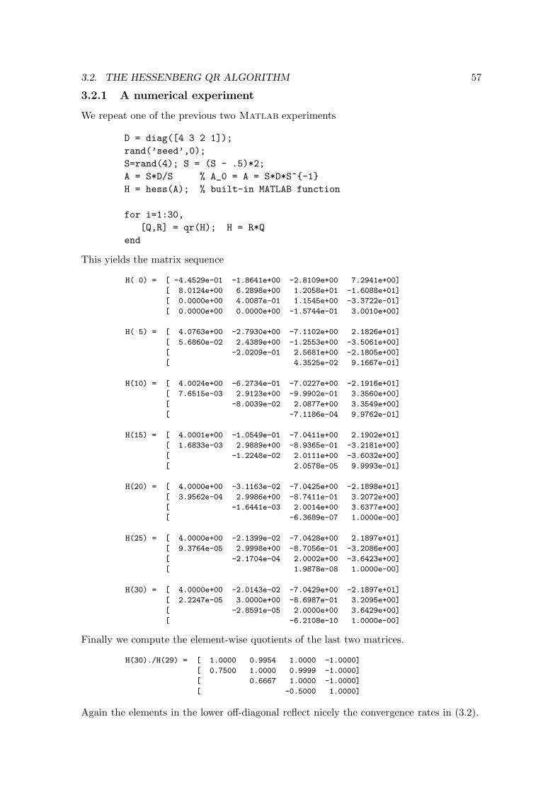
3.2.1 A numerical experiment
We repeat one of the previous two Matlab experiments
D = diag([4 3 2 1]);
rand(’seed’,0);
S=rand(4); S = (S - .5)*2;
A = S*D/S % A_0 = A = S*D*S^{-1}
H = hess(A); % built-in MATLAB function
for i=1:30,
[Q,R] = qr(H); H = R*Q
end
This yields the matrix sequence
H( 0) = [ -4.4529e-01 -1.8641e+00 -2.8109e+00 7.2941e+00]
[ 8.0124e+00 6.2898e+00 1.2058e+01 -1.6088e+01]
[ 0.0000e+00 4.0087e-01 1.1545e+00 -3.3722e-01]
[ 0.0000e+00 0.0000e+00 -1.5744e-01 3.0010e+00]
H( 5) = [ 4.0763e+00 -2.7930e+00 -7.1102e+00 2.1826e+01]
[ 5.6860e-02 2.4389e+00 -1.2553e+00 -3.5061e+00]
[ -2.0209e-01 2.5681e+00 -2.1805e+00]
[ 4.3525e-02 9.1667e-01]
H(10) = [ 4.0024e+00 -6.2734e-01 -7.0227e+00 -2.1916e+01]
[ 7.6515e-03 2.9123e+00 -9.9902e-01 3.3560e+00]
[ -8.0039e-02 2.0877e+00 3.3549e+00]
[ -7.1186e-04 9.9762e-01]
H(15) = [ 4.0001e+00 -1.0549e-01 -7.0411e+00 2.1902e+01]
[ 1.6833e-03 2.9889e+00 -8.9365e-01 -3.2181e+00]
[ -1.2248e-02 2.0111e+00 -3.6032e+00]
[ 2.0578e-05 9.9993e-01]
H(20) = [ 4.0000e+00 -3.1163e-02 -7.0425e+00 -2.1898e+01]
[ 3.9562e-04 2.9986e+00 -8.7411e-01 3.2072e+00]
[ -1.6441e-03 2.0014e+00 3.6377e+00]
[ -6.3689e-07 1.0000e-00]
H(25) = [ 4.0000e+00 -2.1399e-02 -7.0428e+00 2.1897e+01]
[ 9.3764e-05 2.9998e+00 -8.7056e-01 -3.2086e+00]
[ -2.1704e-04 2.0002e+00 -3.6423e+00]
[ 1.9878e-08 1.0000e-00]
H(30) = [ 4.0000e+00 -2.0143e-02 -7.0429e+00 -2.1897e+01]
[ 2.2247e-05 3.0000e+00 -8.6987e-01 3.2095e+00]
[ -2.8591e-05 2.0000e+00 3.6429e+00]
[ -6.2108e-10 1.0000e-00]
Finally we compute the element-wise quotients of the last two matrices.
H(30)./H(29) = [ 1.0000 0.9954 1.0000 -1.0000]
[ 0.7500 1.0000 0.9999 -1.0000]
[ 0.6667 1.0000 -1.0000]
[ -0.5000 1.0000]
Again the elements in the lower off-diagonal reflect nicely the convergence rates in (3.2).
58 CHAPTER 3. THE QR ALGORITHM
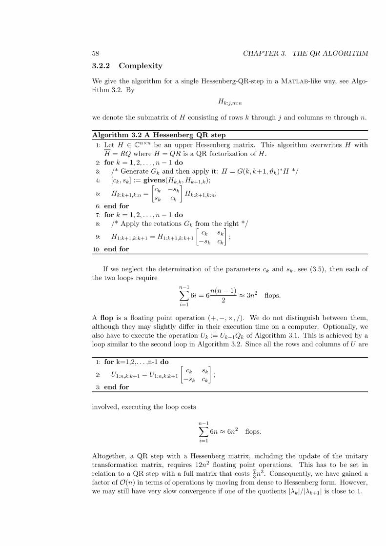
3.2.2 Complexity
We give the algorithm for a single Hessenberg-QR-step in a Matlab-like way, see Algo-rithm 3.2. By
Hk:j,m:n
we denote the submatrix of H consisting of rows k through j and columns m through n.
Algorithm 3.2 A Hessenberg QR step
1: Let H ∈ Cn×n be an upper Hessenberg matrix. This algorithm overwrites H with
H = RQ where H = QR is a QR factorization of H.2: for k = 1, 2, . . . , n− 1 do3: /* Generate Gk and then apply it: H = G(k, k+1, ϑk)∗H */4: [ck, sk] := givens(Hk,k,Hk+1,k);
5: Hk:k+1,k:n =
[ck −sk
sk ck
]
Hk:k+1,k:n;
6: end for7: for k = 1, 2, . . . , n− 1 do8: /* Apply the rotations Gk from the right */
9: H1:k+1,k:k+1 = H1:k+1,k:k+1
[ck sk
−sk ck
]
;
10: end for
If we neglect the determination of the parameters ck and sk, see (3.5), then each ofthe two loops require
n−1∑
i=1
6i = 6n(n − 1)
2≈ 3n2 flops.
A flop is a floating point operation (+,−,×, /). We do not distinguish between them,although they may slightly differ in their execution time on a computer. Optionally, wealso have to execute the operation Uk := Uk−1Qk of Algorithm 3.1. This is achieved by aloop similar to the second loop in Algorithm 3.2. Since all the rows and columns of U are
1: for k=1,2,. . . ,n-1 do
2: U1:n,k:k+1 = U1:n,k:k+1
[ck sk
−sk ck
]
;
3: end for
involved, executing the loop costs
n−1∑
i=1
6n ≈ 6n2 flops.
Altogether, a QR step with a Hessenberg matrix, including the update of the unitarytransformation matrix, requires 12n2 floating point operations. This has to be set inrelation to a QR step with a full matrix that costs 7
3n3. Consequently, we have gained afactor of O(n) in terms of operations by moving from dense to Hessenberg form. However,we may still have very slow convergence if one of the quotients |λk|/|λk+1| is close to 1.
3.3. THE HOUSEHOLDER REDUCTION TO HESSENBERG FORM 59
3.3 The Householder reduction to Hessenberg form
In the previous section we discovered that it is a good idea to perform the QR algorithmwith Hessenberg matrices instead of full matrices. But we have not discussed how wetransform a full matrix (by means of similarity transformations) into Hessenberg form.We catch up on this issue in this section.
3.3.1 Householder reflectors
Givens rotations are designed to zero a single element in a vector. Householder reflectorsare more efficient if a number of elements of a vector are to be zeroed at once. Here, wefollow the presentation given in [5].
Definition 3.3 A matrix of the form
P = I − 2uu∗, ‖u‖ = 1,
is called a Householder reflector.
It is easy to verify that Householder reflectors are Hermitian and that P 2 = I. From thiswe deduce that P is unitary. It is clear that we only have to store the Householdervector u to be able to multiply a vector (or a matrix) with P ,
(3.6) Px = x− u(2u∗x).
This multiplication only costs 4n flops where n is the length of the vectors.A task that we repeatedly want to carry out with Householder reflectors is to transform
a vector x on a multiple of e1,
Px = x− u(2u∗x) = αe1.
Since P is unitary, we must have α = ρ‖x‖, where ρ ∈ C has absolute value one. Therefore,
u =x− ρ‖x‖e1
‖x− ρ‖x‖e1‖=
1
‖x− ρ‖x‖e1‖
x1 − ρ‖x‖x2...
xn
We can freely choose ρ provided that |ρ| = 1. Let x1 = |x1|eiφ. To avoid numerical
cancellation we set ρ = −eiφ.In the real case, one commonly sets ρ = −sign(x1). If x1 = 0 we can set ρ in any way.
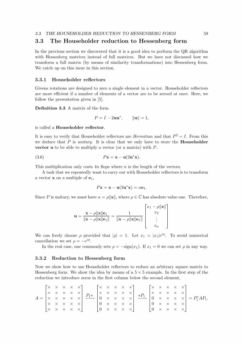
3.3.2 Reduction to Hessenberg form
Now we show how to use Householder reflectors to reduce an arbitrary square matrix toHessenberg form. We show the idea by means of a 5× 5 example. In the first step of thereduction we introduce zeros in the first column below the second element,
A =
× × × × ×× × × × ×× × × × ×× × × × ×× × × × ×
P1∗−−−→
× × × × ×× × × × ×0 × × × ×0 × × × ×0 × × × ×
∗P1−−−→
× × × × ×× × × × ×0 × × × ×0 × × × ×0 × × × ×
= P ∗
1 AP1.
60 CHAPTER 3. THE QR ALGORITHM
Notice that P1 = P ∗
1 since it is a Householder reflector! It has the structure
P1 =
1 0 0 0 00 × × × ×0 × × × ×0 × × × ×0 × × × ×
=
[1 0T
0 I4 − 2u1u∗
1
]
.
The Householder vector u1 is determined such that
(I − 2u1u∗
1)
a21
a31
a41
a51
=
α000
with u1 =
u1
u2
u3
u4
.
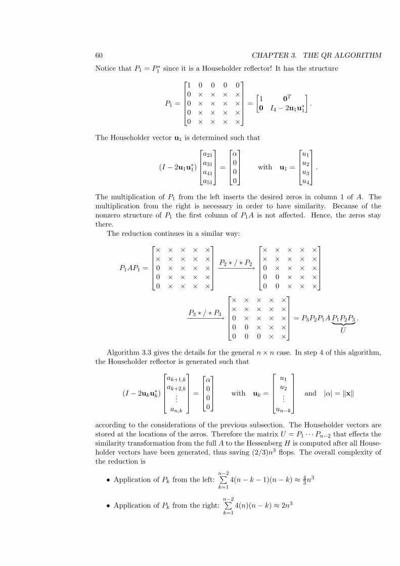
The multiplication of P1 from the left inserts the desired zeros in column 1 of A. Themultiplication from the right is necessary in order to have similarity. Because of thenonzero structure of P1 the first column of P1A is not affected. Hence, the zeros staythere.
The reduction continues in a similar way:
P1AP1 =
× × × × ×× × × × ×0 × × × ×0 × × × ×0 × × × ×
P2 ∗ / ∗ P2−−−−−−−−→
× × × × ×× × × × ×0 × × × ×0 0 × × ×0 0 × × ×
P3 ∗ / ∗ P3−−−−−−−−→
× × × × ×× × × × ×0 × × × ×0 0 × × ×0 0 0 × ×
= P3P2P1AP1P2P3︸ ︷︷ ︸
U
.
Algorithm 3.3 gives the details for the general n× n case. In step 4 of this algorithm,the Householder reflector is generated such that
(I − 2uku∗
k)
ak+1,k
ak+2,k
...an,k
=
α000
with uk =
u1
u2...
un−k
and |α| = ‖x‖
according to the considerations of the previous subsection. The Householder vectors arestored at the locations of the zeros. Therefore the matrix U = P1 · · ·Pn−2 that effects thesimilarity transformation from the full A to the Hessenberg H is computed after all House-holder vectors have been generated, thus saving (2/3)n3 flops. The overall complexity ofthe reduction is
• Application of Pk from the left:n−2∑
k=1
4(n− k − 1)(n− k) ≈ 43n3
• Application of Pk from the right:n−2∑
k=1
4(n)(n− k) ≈ 2n3
3.4. IMPROVING THE CONVERGENCE OF THE QR ALGORITHM 61
Algorithm 3.3 Reduction to Hessenberg form
1: This algorithm reduces a matrix A ∈ Cn×n to Hessenberg form H by a sequence of
Householder reflections. H overwrites A.2: for k = 1 to n−2 do3: Generate the Householder reflector Pk;4: /* Apply Pk = Ik ⊕ (In−k − 2ukuk
∗) from the left to A */5: Ak+1:n,k:n := Ak+1:n,k:n − 2uk(uk
∗Ak+1:n,k:n);6: /* Apply Pk from the right, A := APk */7: A1:n,k+1:n := A1:n,k+1:n − 2(A1:n,k+1:nuk)uk
∗;8: end for9: if eigenvectors are desired form U = P1 · · ·Pn−2 then
10: U := In;11: for k = n−2 downto 1 do12: /* Update U := PkU */13: Uk+1:n,k+1:n := Uk+1:n,k+1:n − 2uk(uk
∗Uk+1:n,k+1:n);14: end for15: end if
• Form U = P1 · · ·Pn−2:n−2∑
k=1
4(n − k)(n − k) ≈ 43n3
Thus, the reduction to Hessenberg form costs 103 n3 flops without forming the transforma-
tion matrix and 143 n3 including forming this matrix.
3.4 Improving the convergence of the QR algorithm
We have seen how the QR algorithm for computing the Schur form of a matrix A can beexecuted more economically if the matrix A is first transformed to Hessenberg form. Nowwe want to show how the convergence of the Hessenberg QR algorithm can be improveddramatically by introducing (spectral) shifts into the algorithm.
Lemma 3.4 Let H be an irreducible Hessenberg matrix, i.e., hi+1,i 6= 0 for all i =1, . . . , n − 1. Let H = QR be the QR factorization of H. Then for the diagonal elements
of R we have
|rkk| > 0 for all k < n.
Thus, if H is singular then rnn = 0.
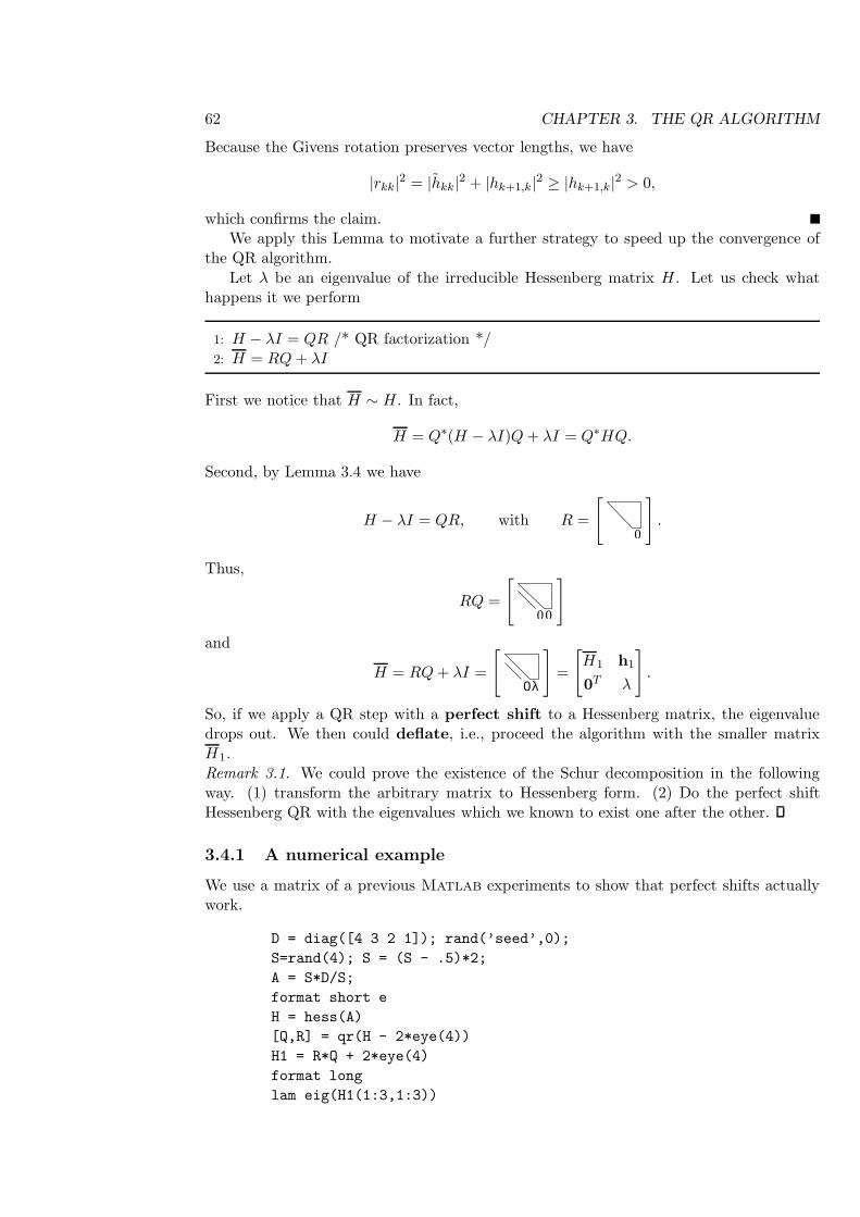
Proof. Let us look at the k-th step of the Hessenberg QR factorization. For illustration,let us consider the case k = 3 in a 5× 5 example, where the matrix has the structure
+ + + + +0 + + + +0 0 + + +0 0 × × ×0 0 0 × ×
.
The plus-signs indicate elements that have been modified. In step 3, the (nonzero) elementh43 will be zeroed by a Givens rotation G(3, 4, ϕ) that is determined such that
[cos(ϕ) − sin(ϕ)sin(ϕ) cos(ϕ)
] [h̃kk
hk+1,k
]
=
[rkk
0
]
.
62 CHAPTER 3. THE QR ALGORITHM
Because the Givens rotation preserves vector lengths, we have
|rkk|2 = |h̃kk|
2 + |hk+1,k|2 ≥ |hk+1,k|
2 > 0,
which confirms the claim.We apply this Lemma to motivate a further strategy to speed up the convergence of
the QR algorithm.
Let λ be an eigenvalue of the irreducible Hessenberg matrix H. Let us check whathappens it we perform
1: H − λI = QR /* QR factorization */2: H = RQ + λI
First we notice that H ∼ H. In fact,
H = Q∗(H − λI)Q + λI = Q∗HQ.
Second, by Lemma 3.4 we have
H − λI = QR, with R =
[
0
]
.
Thus,
RQ =
[
00
]
and
H = RQ + λI =
[
λ0
]
=
[
H1 h1
0T λ
]
.
So, if we apply a QR step with a perfect shift to a Hessenberg matrix, the eigenvaluedrops out. We then could deflate, i.e., proceed the algorithm with the smaller matrixH1.
Remark 3.1. We could prove the existence of the Schur decomposition in the followingway. (1) transform the arbitrary matrix to Hessenberg form. (2) Do the perfect shiftHessenberg QR with the eigenvalues which we known to exist one after the other.
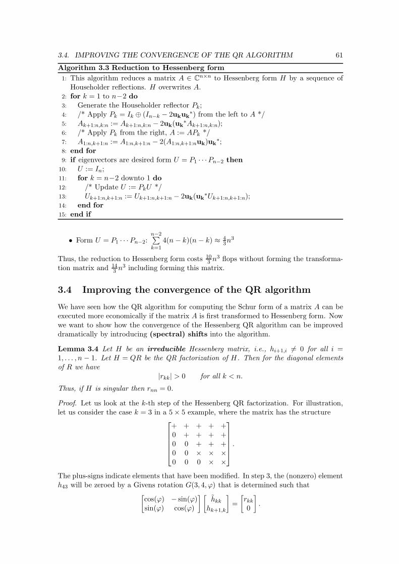
3.4.1 A numerical example
We use a matrix of a previous Matlab experiments to show that perfect shifts actuallywork.
D = diag([4 3 2 1]); rand(’seed’,0);
S=rand(4); S = (S - .5)*2;
A = S*D/S;
format short e
H = hess(A)
[Q,R] = qr(H - 2*eye(4))
H1 = R*Q + 2*eye(4)
format long
lam eig(H1(1:3,1:3))
3.4. IMPROVING THE CONVERGENCE OF THE QR ALGORITHM 63
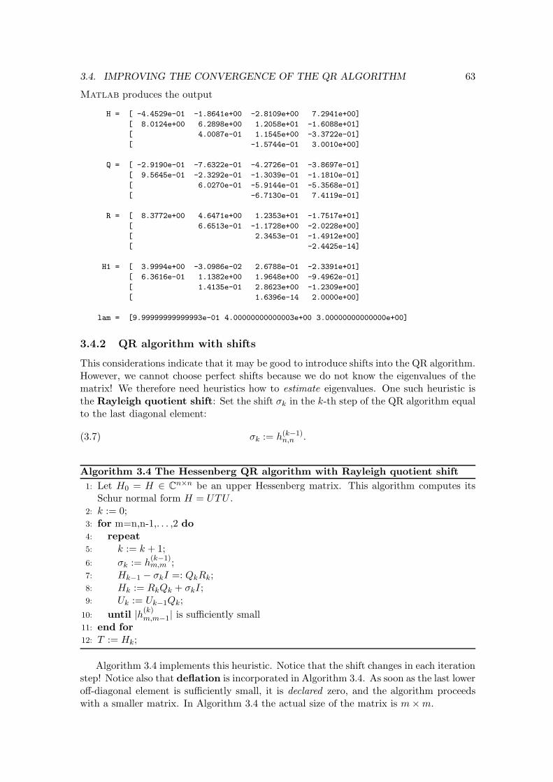
Matlab produces the output
H = [ -4.4529e-01 -1.8641e+00 -2.8109e+00 7.2941e+00]
[ 8.0124e+00 6.2898e+00 1.2058e+01 -1.6088e+01]
[ 4.0087e-01 1.1545e+00 -3.3722e-01]
[ -1.5744e-01 3.0010e+00]
Q = [ -2.9190e-01 -7.6322e-01 -4.2726e-01 -3.8697e-01]
[ 9.5645e-01 -2.3292e-01 -1.3039e-01 -1.1810e-01]
[ 6.0270e-01 -5.9144e-01 -5.3568e-01]
[ -6.7130e-01 7.4119e-01]
R = [ 8.3772e+00 4.6471e+00 1.2353e+01 -1.7517e+01]
[ 6.6513e-01 -1.1728e+00 -2.0228e+00]
[ 2.3453e-01 -1.4912e+00]
[ -2.4425e-14]
H1 = [ 3.9994e+00 -3.0986e-02 2.6788e-01 -2.3391e+01]
[ 6.3616e-01 1.1382e+00 1.9648e+00 -9.4962e-01]
[ 1.4135e-01 2.8623e+00 -1.2309e+00]
[ 1.6396e-14 2.0000e+00]
lam = [9.99999999999993e-01 4.00000000000003e+00 3.00000000000000e+00]
3.4.2 QR algorithm with shifts
This considerations indicate that it may be good to introduce shifts into the QR algorithm.However, we cannot choose perfect shifts because we do not know the eigenvalues of thematrix! We therefore need heuristics how to estimate eigenvalues. One such heuristic isthe Rayleigh quotient shift: Set the shift σk in the k-th step of the QR algorithm equalto the last diagonal element:
(3.7) σk := h(k−1)n,n .
Algorithm 3.4 The Hessenberg QR algorithm with Rayleigh quotient shift
1: Let H0 = H ∈ Cn×n be an upper Hessenberg matrix. This algorithm computes its
Schur normal form H = UTU .2: k := 0;3: for m=n,n-1,. . . ,2 do4: repeat5: k := k + 1;
6: σk := h(k−1)m,m ;
7: Hk−1 − σkI =: QkRk;8: Hk := RkQk + σkI;9: Uk := Uk−1Qk;
10: until |h(k)m,m−1| is sufficiently small
11: end for12: T := Hk;
Algorithm 3.4 implements this heuristic. Notice that the shift changes in each iterationstep! Notice also that deflation is incorporated in Algorithm 3.4. As soon as the last loweroff-diagonal element is sufficiently small, it is declared zero, and the algorithm proceedswith a smaller matrix. In Algorithm 3.4 the actual size of the matrix is m×m.
64 CHAPTER 3. THE QR ALGORITHM
Lemma 3.4 guarantees that a zero is produced at position (n, n− 1) in the Hessenbergmatrix. What happens, if hn,n is a good approximation to an eigenvalue of H? Let usassume that we have an irreducible Hessenberg matrix
× × × × ×× × × × ×0 × × × ×0 0 × × ×0 0 0 ε hn,n
,
where ε is a small quantity. If we perform a shifted Hessenberg QR step, we first have tofactor H − hn,nI, QR = H − hn,nI. After n− 2 steps of this factorization the R-factor isalmost upper triangular,
+ + + + +0 + + + +0 0 + + +0 0 0 α β0 0 0 ε 0
.
From (3.5) we see that the last Givens rotation has the nontrivial elements
cn−1 =α
√
|α|2 + |ε|2, sn−1 =
−ε√
|α|2 + |ε|2.
Applying the Givens rotations from the right one sees that the last lower off-diagonalelement of H = RQ + hn,nI becomes
(3.8) h̄n,n−1 =ε2β
α2 + ε2.
So, we have quadratic convergence unless α is also tiny.
A second even more often used shift strategy is the Wilkinson shift:
(3.9) σk := eigenvalue of
[
h(k−1)n−1,n−1 h
(k−1)n−1,n
h(k−1)n,n−1 h
(k−1)n,n
]
that is closer to h(k−1)n,n .
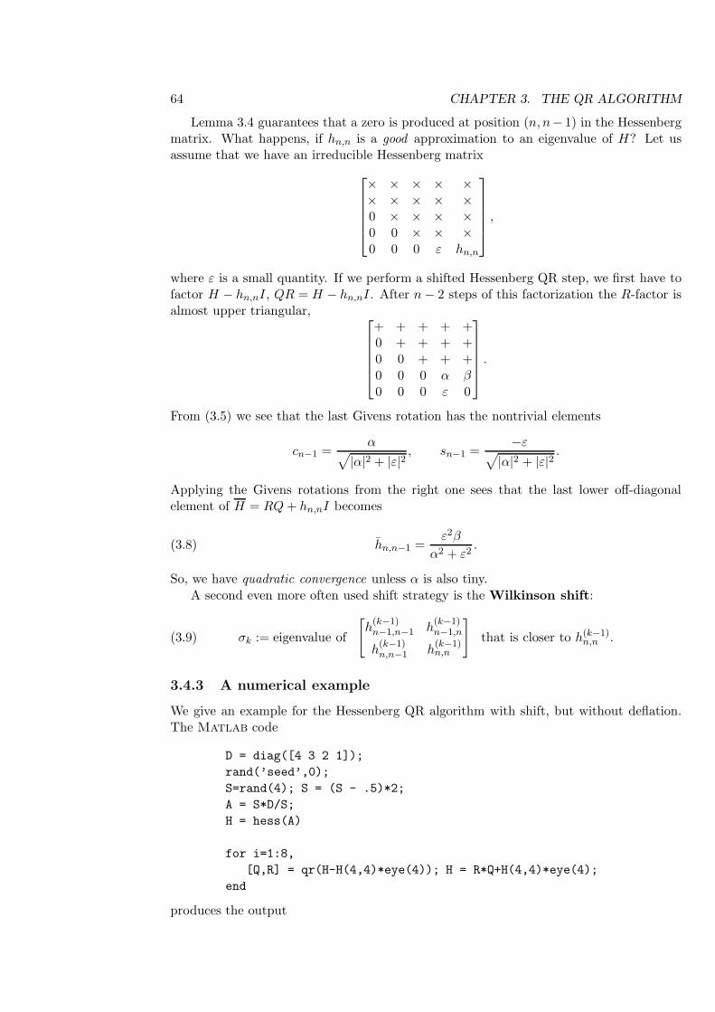
3.4.3 A numerical example
We give an example for the Hessenberg QR algorithm with shift, but without deflation.The Matlab code
D = diag([4 3 2 1]);
rand(’seed’,0);
S=rand(4); S = (S - .5)*2;
A = S*D/S;
H = hess(A)
for i=1:8,
[Q,R] = qr(H-H(4,4)*eye(4)); H = R*Q+H(4,4)*eye(4);
end
produces the output
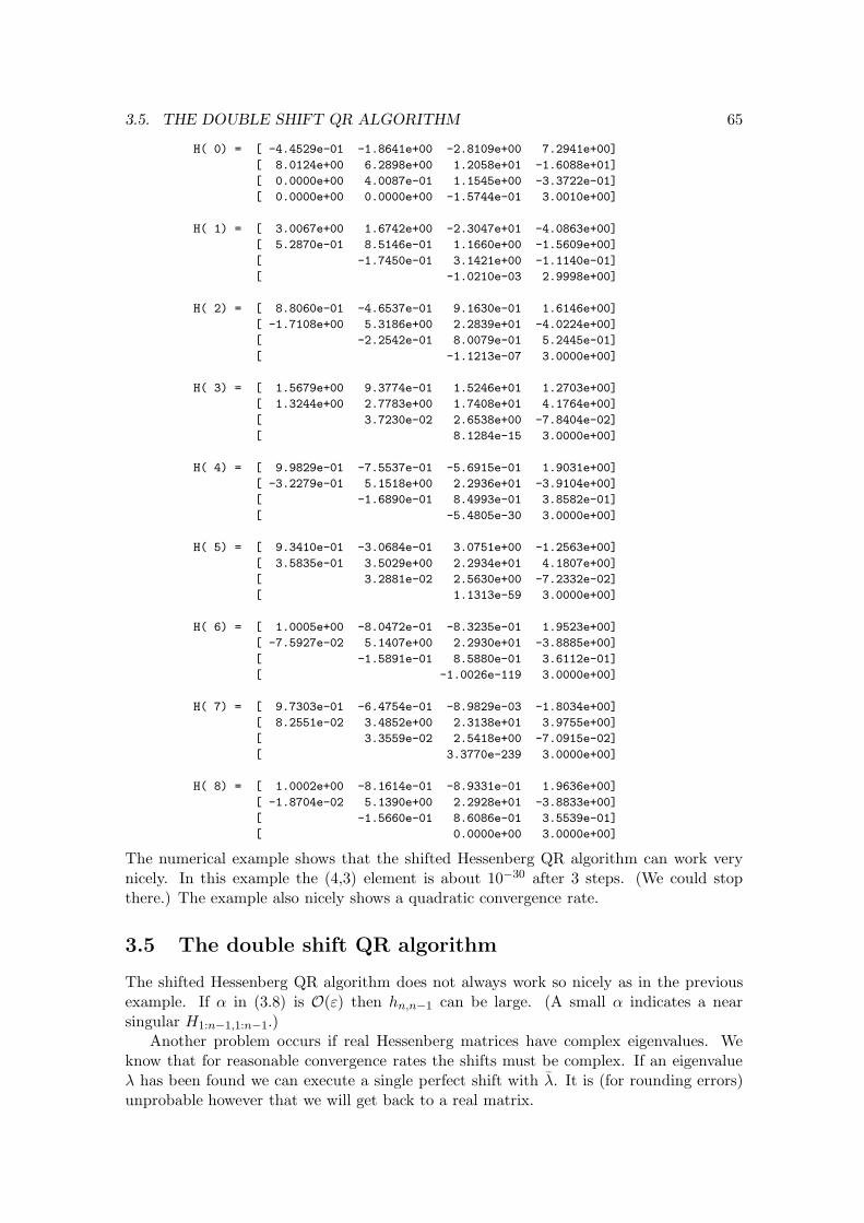
3.5. THE DOUBLE SHIFT QR ALGORITHM 65
H( 0) = [ -4.4529e-01 -1.8641e+00 -2.8109e+00 7.2941e+00]
[ 8.0124e+00 6.2898e+00 1.2058e+01 -1.6088e+01]
[ 0.0000e+00 4.0087e-01 1.1545e+00 -3.3722e-01]
[ 0.0000e+00 0.0000e+00 -1.5744e-01 3.0010e+00]
H( 1) = [ 3.0067e+00 1.6742e+00 -2.3047e+01 -4.0863e+00]
[ 5.2870e-01 8.5146e-01 1.1660e+00 -1.5609e+00]
[ -1.7450e-01 3.1421e+00 -1.1140e-01]
[ -1.0210e-03 2.9998e+00]
H( 2) = [ 8.8060e-01 -4.6537e-01 9.1630e-01 1.6146e+00]
[ -1.7108e+00 5.3186e+00 2.2839e+01 -4.0224e+00]
[ -2.2542e-01 8.0079e-01 5.2445e-01]
[ -1.1213e-07 3.0000e+00]
H( 3) = [ 1.5679e+00 9.3774e-01 1.5246e+01 1.2703e+00]
[ 1.3244e+00 2.7783e+00 1.7408e+01 4.1764e+00]
[ 3.7230e-02 2.6538e+00 -7.8404e-02]
[ 8.1284e-15 3.0000e+00]
H( 4) = [ 9.9829e-01 -7.5537e-01 -5.6915e-01 1.9031e+00]
[ -3.2279e-01 5.1518e+00 2.2936e+01 -3.9104e+00]
[ -1.6890e-01 8.4993e-01 3.8582e-01]
[ -5.4805e-30 3.0000e+00]
H( 5) = [ 9.3410e-01 -3.0684e-01 3.0751e+00 -1.2563e+00]
[ 3.5835e-01 3.5029e+00 2.2934e+01 4.1807e+00]
[ 3.2881e-02 2.5630e+00 -7.2332e-02]
[ 1.1313e-59 3.0000e+00]
H( 6) = [ 1.0005e+00 -8.0472e-01 -8.3235e-01 1.9523e+00]
[ -7.5927e-02 5.1407e+00 2.2930e+01 -3.8885e+00]
[ -1.5891e-01 8.5880e-01 3.6112e-01]
[ -1.0026e-119 3.0000e+00]
H( 7) = [ 9.7303e-01 -6.4754e-01 -8.9829e-03 -1.8034e+00]
[ 8.2551e-02 3.4852e+00 2.3138e+01 3.9755e+00]
[ 3.3559e-02 2.5418e+00 -7.0915e-02]
[ 3.3770e-239 3.0000e+00]
H( 8) = [ 1.0002e+00 -8.1614e-01 -8.9331e-01 1.9636e+00]
[ -1.8704e-02 5.1390e+00 2.2928e+01 -3.8833e+00]
[ -1.5660e-01 8.6086e-01 3.5539e-01]
[ 0.0000e+00 3.0000e+00]
The numerical example shows that the shifted Hessenberg QR algorithm can work verynicely. In this example the (4,3) element is about 10−30 after 3 steps. (We could stopthere.) The example also nicely shows a quadratic convergence rate.
3.5 The double shift QR algorithm
The shifted Hessenberg QR algorithm does not always work so nicely as in the previousexample. If α in (3.8) is O(ε) then hn,n−1 can be large. (A small α indicates a nearsingular H1:n−1,1:n−1.)
Another problem occurs if real Hessenberg matrices have complex eigenvalues. Weknow that for reasonable convergence rates the shifts must be complex. If an eigenvalueλ has been found we can execute a single perfect shift with λ̄. It is (for rounding errors)unprobable however that we will get back to a real matrix.
66 CHAPTER 3. THE QR ALGORITHM
Since the eigenvalues come in complex conjugate pairs it is natural to search for a pairof eigenvalues right-away. This is done by collapsing two shifted QR steps in one doublestep with the two shifts being complex conjugates of each other.
Let σ1 and σ2 be two eigenvalues of the real matrix
G =
[
h(k−1)n−1,n−1 h
(k−1)n−1,n
h(k−1)n,n−1 h
(k−1)n,n
]
∈ R2×2.
If σ1 ∈ C then σ2 = σ̄1. Let us perform two QR steps using σ1 and σ2 as shifts:
(3.10)
H − σ1I = Q1R1,
H1 = R1Q1 + σ1I,
H1 − σ2I = Q2R2,
H2 = R2Q2 + σ2I.
Here, for convenience, we wrote H, H1, and H2 for Hk−1, Hk, and Hk+1, respectively.From the second and third equation in (3.10) we get
R1Q1 + (σ1 − σ2)I = Q2R2.
Multiplying this with Q1 from the left and with R1 from the right we get
Q1R1Q1R1 + (σ1 − σ2)Q1R1 = Q1R1(Q1R1 + (σ1 − σ2)I)
= (H − σ1I)(H − σ2I) = Q1Q2R2R1.
Because σ2 = σ̄1 we have
M := (H − σ1I)(H − σ2I) = H2 − 2Re(σ)H + |σ|2I = Q1Q2R2R1,
whence (Q1Q2)(R2R1) is the QR factorization of a real matrix. Therefore, we can chooseQ1 and Q2 such that Z := Q1Q2 is real orthogonal. By consequence,
H2 = (Q1Q2)∗H(Q1Q2) = ZT HZ
is real.
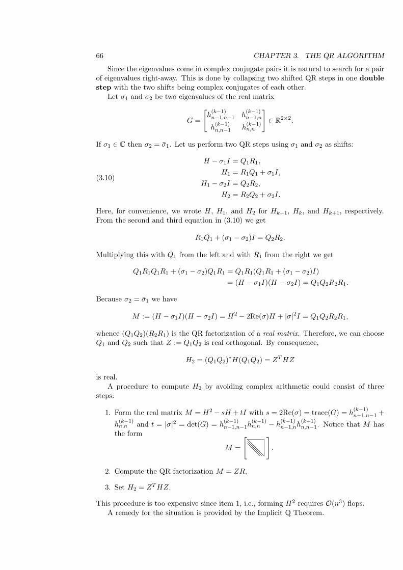
A procedure to compute H2 by avoiding complex arithmetic could consist of threesteps:
1. Form the real matrix M = H2 − sH + tI with s = 2Re(σ) = trace(G) = h(k−1)n−1,n−1 +
h(k−1)n,n and t = |σ|2 = det(G) = h
(k−1)n−1,n−1h
(k−1)n,n − h
(k−1)n−1,nh
(k−1)n,n−1. Notice that M has
the form
M =
[ ]
.
2. Compute the QR factorization M = ZR,
3. Set H2 = ZT HZ.
This procedure is too expensive since item 1, i.e., forming H2 requires O(n3) flops.
A remedy for the situation is provided by the Implicit Q Theorem.
3.5. THE DOUBLE SHIFT QR ALGORITHM 67
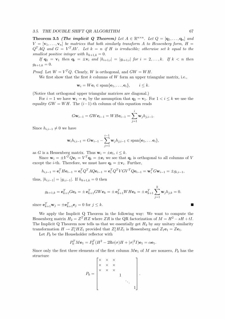
Theorem 3.5 (The implicit Q Theorem) Let A ∈ Rn×n. Let Q = [q1, . . . ,qn] and
V = [v1, . . . ,vn] be matrices that both similarly transform A to Hessenberg form, H =QT AQ and G = V T AV . Let k = n if H is irreducible; otherwise set k equal to the
smallest positive integer with hk+1,k = 0.If q1 = v1 then qi = ±vi and |hi+1,i| = |gi+1,i| for i = 2, . . . , k. If k < n then
gk+1,k = 0.
Proof. Let W = V T Q. Clearly, W is orthogonal, and GW = WH.We first show that the first k columns of W form an upper triangular matrix, i.e.,
wi = Wei ∈ span{e1, . . . , ei}, i ≤ k.
(Notice that orthogonal upper triangular matrices are diagonal.)For i = 1 we have w1 = e1 by the assumption that q1 = v1. For 1 < i ≤ k we use the
equality GW = WH. The (i−1)-th column of this equation reads
Gwi−1 = GWei−1 = WHei−1 =
i∑
j=1
wjhj,i−1.
Since hi,i−1 6= 0 we have
wihi,i−1 = Gwi−1 −
i−1∑
j=1
wjhj,i−1 ∈ span{e1, . . . ei},
as G is a Hessenberg matrix. Thus wi = ±ei, i ≤ k.Since wi = ±V T Qei = V Tqi = ±ei we see that qi is orthogonal to all columns of V
except the i-th. Therefore, we must have qi = ±vi. Further,
hi,i−1 = eTi Hei−1 = eT
i QT AQei−1 = eTi QT V GV T Qei−1 = wT
i Gwi−1 = ±gi,i−1,
thus, |hi,i−1| = |gi,i−1|. If hk+1,k = 0 then
gk+1,k = eTk+1Gek = ± eT
k+1GWek = ± eTk+1WHek = ± eT
k+1
k∑
j=1
wjhj,k = 0.
since eTk+1wj = ±eT
k+1ej = 0 for j ≤ k.
We apply the Implicit Q Theorem in the following way: We want to compute theHessenberg matrix H2 = ZT HZ where ZR is the QR factorization of M = H2− sH + tI.The Implicit Q Theorem now tells us that we essentially get H2 by any unitary similaritytransformation H → Z∗
1HZ1 provided that Z∗
1HZ1 is Hessenberg and Z1e1 = Ze1.Let P0 be the Householder reflector with
P T0 Me1 = P T
0 (H2 − 2Re(σ)H + |σ|2I)e1 = αe1.
Since only the first three elements of the first column Me1 of M are nonzero, P0 has thestructure
P0 =
× × ×× × ×× × ×
1. . .
1
.
68 CHAPTER 3. THE QR ALGORITHM
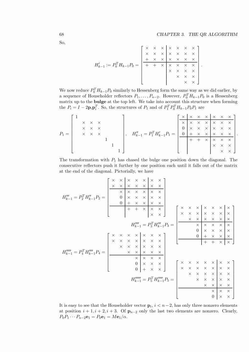
So,
H ′
k−1 := P T0 Hk−1P0 =
× × × × × × ×× × × × × × ×+ × × × × × ×
+ + × × × × ×× × × ×× × ×× ×
.
We now reduce P T0 Hk−1P0 similarly to Hessenberg form the same way as we did earlier, by
a sequence of Householder reflectors P1, . . . , Pn−2. However, P T0 Hk−1P0 is a Hessenberg
matrix up to the bulge at the top left. We take into account this structure when formingthe Pi = I − 2pip
Ti . So, the structures of P1 and of P T
1 P T0 Hk−1P0P1 are
P1 =
1× × ×× × ×× × ×
11
1
, H ′′
k−1 = P T1 H ′
k−1P1 =
× × × × × × ×
× × × × × × ×0 × × × × × ×0 + × × × × ×
+ + × × × ×× × ×× ×
.
The transformation with P1 has chased the bulge one position down the diagonal. Theconsecutive reflectors push it further by one position each until it falls out of the matrixat the end of the diagonal. Pictorially, we have
H ′′′
k−1 = P T2 H ′′
k−1P2 =
× × × × × × ×× × × × × × ×
× × × × × ×0 × × × × ×0 + × × × ×
+ + × × ×× ×
H ′′′′
k−1 = P T3 H ′′′
k−1P3 =
× × × × × × ×× × × × × × ×× × × × × ×
× × × × ×0 × × × ×0 + × × ×
+ + × ×
H ′′′′′
k−1 = P T4 H ′′′′
k−1P4 =
× × × × × × ×× × × × × × ×× × × × × ×× × × × ×
× × × ×0 × × ×0 + × ×
H ′′′′′′
k−1 = P T5 H ′′′′′
k−1P5 =
× × × × × × ×× × × × × × ×× × × × × ×× × × × ×× × × ×
× × ×0 × ×
It is easy to see that the Householder vector pi, i < n−2, has only three nonzero elementsat position i + 1, i + 2, i + 3. Of pn−2 only the last two elements are nonzero. Clearly,P0P1 · · ·Pn−2e1 = P0e1 = Me1/α.
3.5. THE DOUBLE SHIFT QR ALGORITHM 69
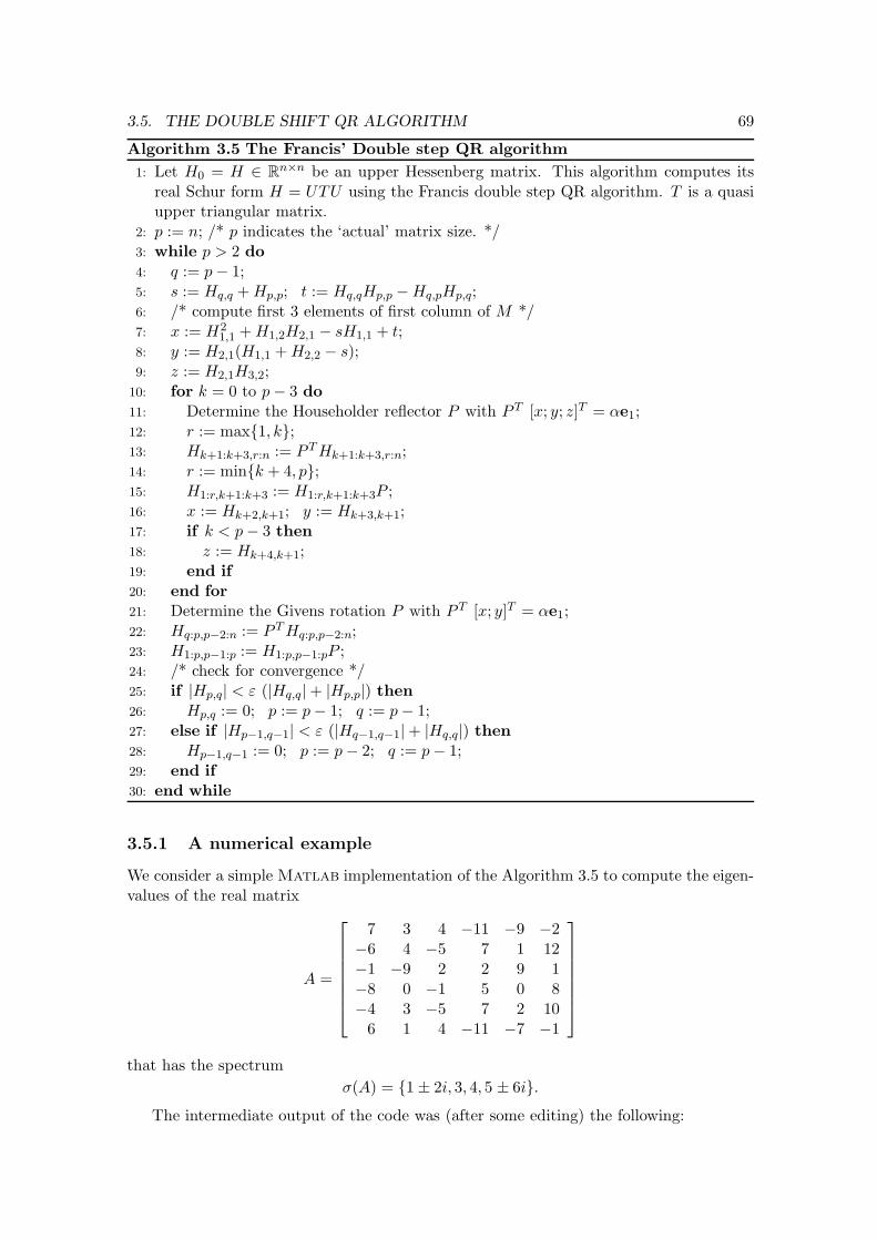
Algorithm 3.5 The Francis’ Double step QR algorithm
1: Let H0 = H ∈ Rn×n be an upper Hessenberg matrix. This algorithm computes its
real Schur form H = UTU using the Francis double step QR algorithm. T is a quasiupper triangular matrix.
2: p := n; /* p indicates the ‘actual’ matrix size. */3: while p > 2 do4: q := p− 1;5: s := Hq,q + Hp,p; t := Hq,qHp,p −Hq,pHp,q;6: /* compute first 3 elements of first column of M */7: x := H2
1,1 + H1,2H2,1 − sH1,1 + t;8: y := H2,1(H1,1 + H2,2 − s);9: z := H2,1H3,2;
10: for k = 0 to p− 3 do11: Determine the Householder reflector P with P T [x; y; z]T = αe1;12: r := max{1, k};13: Hk+1:k+3,r:n := P T Hk+1:k+3,r:n;14: r := min{k + 4, p};15: H1:r,k+1:k+3 := H1:r,k+1:k+3P ;16: x := Hk+2,k+1; y := Hk+3,k+1;17: if k < p− 3 then18: z := Hk+4,k+1;19: end if20: end for21: Determine the Givens rotation P with P T [x; y]T = αe1;22: Hq:p,p−2:n := P T Hq:p,p−2:n;23: H1:p,p−1:p := H1:p,p−1:pP ;24: /* check for convergence */25: if |Hp,q| < ε (|Hq,q|+ |Hp,p|) then26: Hp,q := 0; p := p− 1; q := p− 1;27: else if |Hp−1,q−1| < ε (|Hq−1,q−1|+ |Hq,q|) then28: Hp−1,q−1 := 0; p := p− 2; q := p− 1;29: end if30: end while
3.5.1 A numerical example
We consider a simple Matlab implementation of the Algorithm 3.5 to compute the eigen-values of the real matrix
A =
7 3 4 −11 −9 −2−6 4 −5 7 1 12−1 −9 2 2 9 1−8 0 −1 5 0 8−4 3 −5 7 2 10
6 1 4 −11 −7 −1
that has the spectrum
σ(A) = {1± 2i, 3, 4, 5 ± 6i}.
The intermediate output of the code was (after some editing) the following:
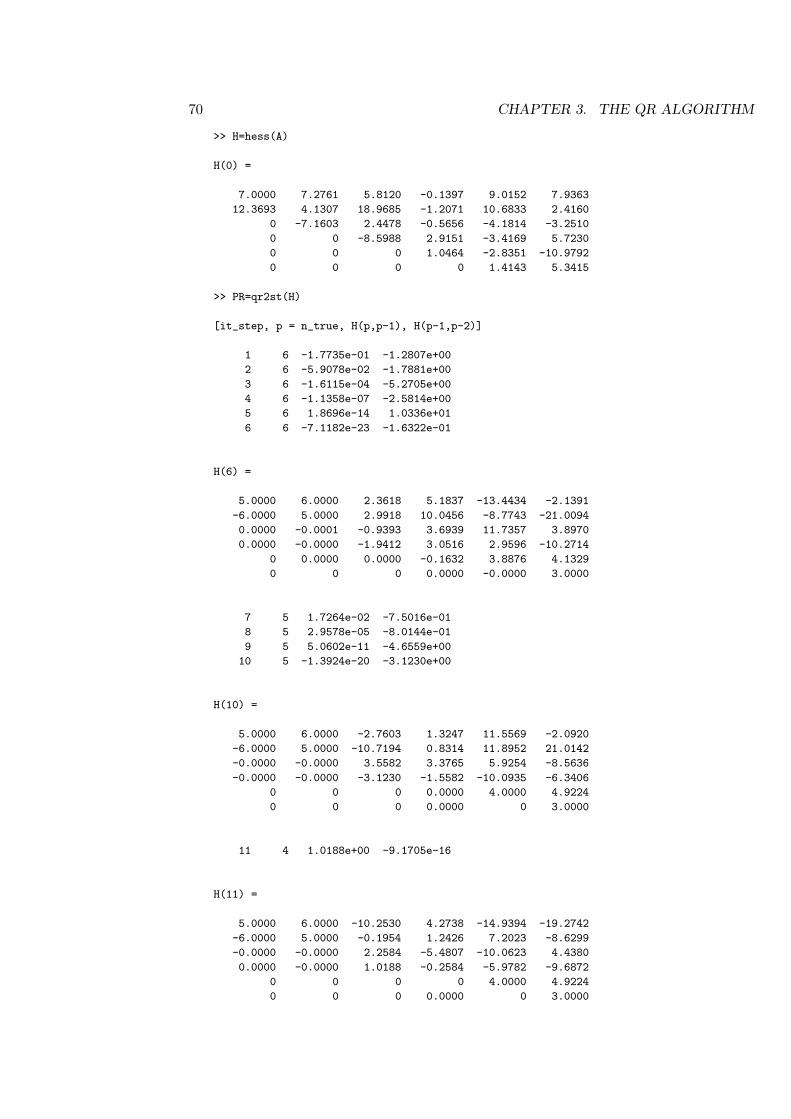
70 CHAPTER 3. THE QR ALGORITHM
>> H=hess(A)
H(0) =
7.0000 7.2761 5.8120 -0.1397 9.0152 7.9363
12.3693 4.1307 18.9685 -1.2071 10.6833 2.4160
0 -7.1603 2.4478 -0.5656 -4.1814 -3.2510
0 0 -8.5988 2.9151 -3.4169 5.7230
0 0 0 1.0464 -2.8351 -10.9792
0 0 0 0 1.4143 5.3415
>> PR=qr2st(H)
[it_step, p = n_true, H(p,p-1), H(p-1,p-2)]
1 6 -1.7735e-01 -1.2807e+00
2 6 -5.9078e-02 -1.7881e+00
3 6 -1.6115e-04 -5.2705e+00
4 6 -1.1358e-07 -2.5814e+00
5 6 1.8696e-14 1.0336e+01
6 6 -7.1182e-23 -1.6322e-01
H(6) =
5.0000 6.0000 2.3618 5.1837 -13.4434 -2.1391
-6.0000 5.0000 2.9918 10.0456 -8.7743 -21.0094
0.0000 -0.0001 -0.9393 3.6939 11.7357 3.8970
0.0000 -0.0000 -1.9412 3.0516 2.9596 -10.2714
0 0.0000 0.0000 -0.1632 3.8876 4.1329
0 0 0 0.0000 -0.0000 3.0000
7 5 1.7264e-02 -7.5016e-01
8 5 2.9578e-05 -8.0144e-01
9 5 5.0602e-11 -4.6559e+00
10 5 -1.3924e-20 -3.1230e+00
H(10) =
5.0000 6.0000 -2.7603 1.3247 11.5569 -2.0920
-6.0000 5.0000 -10.7194 0.8314 11.8952 21.0142
-0.0000 -0.0000 3.5582 3.3765 5.9254 -8.5636
-0.0000 -0.0000 -3.1230 -1.5582 -10.0935 -6.3406
0 0 0 0.0000 4.0000 4.9224
0 0 0 0.0000 0 3.0000
11 4 1.0188e+00 -9.1705e-16
H(11) =
5.0000 6.0000 -10.2530 4.2738 -14.9394 -19.2742
-6.0000 5.0000 -0.1954 1.2426 7.2023 -8.6299
-0.0000 -0.0000 2.2584 -5.4807 -10.0623 4.4380
0.0000 -0.0000 1.0188 -0.2584 -5.9782 -9.6872
0 0 0 0 4.0000 4.9224
0 0 0 0.0000 0 3.0000
3.6. THE SYMMETRIC TRIDIAGONAL QR ALGORITHM 71
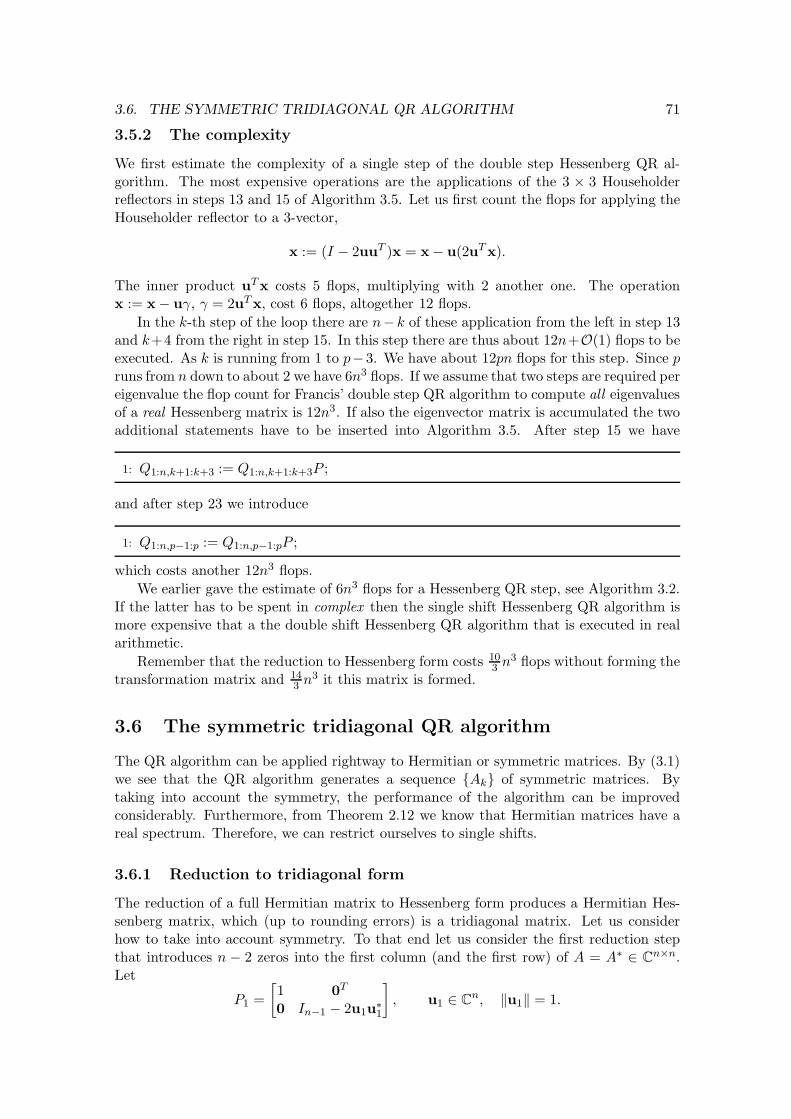
3.5.2 The complexity
We first estimate the complexity of a single step of the double step Hessenberg QR al-gorithm. The most expensive operations are the applications of the 3 × 3 Householderreflectors in steps 13 and 15 of Algorithm 3.5. Let us first count the flops for applying theHouseholder reflector to a 3-vector,
x := (I − 2uuT )x = x− u(2uT x).
The inner product uTx costs 5 flops, multiplying with 2 another one. The operationx := x− uγ, γ = 2uT x, cost 6 flops, altogether 12 flops.
In the k-th step of the loop there are n− k of these application from the left in step 13and k+4 from the right in step 15. In this step there are thus about 12n+O(1) flops to beexecuted. As k is running from 1 to p−3. We have about 12pn flops for this step. Since pruns from n down to about 2 we have 6n3 flops. If we assume that two steps are required pereigenvalue the flop count for Francis’ double step QR algorithm to compute all eigenvaluesof a real Hessenberg matrix is 12n3. If also the eigenvector matrix is accumulated the twoadditional statements have to be inserted into Algorithm 3.5. After step 15 we have
1: Q1:n,k+1:k+3 := Q1:n,k+1:k+3P ;
and after step 23 we introduce
1: Q1:n,p−1:p := Q1:n,p−1:pP ;
which costs another 12n3 flops.
We earlier gave the estimate of 6n3 flops for a Hessenberg QR step, see Algorithm 3.2.If the latter has to be spent in complex then the single shift Hessenberg QR algorithm ismore expensive that a the double shift Hessenberg QR algorithm that is executed in realarithmetic.
Remember that the reduction to Hessenberg form costs 103 n3 flops without forming the
transformation matrix and 143 n3 it this matrix is formed.
3.6 The symmetric tridiagonal QR algorithm
The QR algorithm can be applied rightway to Hermitian or symmetric matrices. By (3.1)we see that the QR algorithm generates a sequence {Ak} of symmetric matrices. Bytaking into account the symmetry, the performance of the algorithm can be improvedconsiderably. Furthermore, from Theorem 2.12 we know that Hermitian matrices have areal spectrum. Therefore, we can restrict ourselves to single shifts.
3.6.1 Reduction to tridiagonal form
The reduction of a full Hermitian matrix to Hessenberg form produces a Hermitian Hes-senberg matrix, which (up to rounding errors) is a tridiagonal matrix. Let us considerhow to take into account symmetry. To that end let us consider the first reduction stepthat introduces n − 2 zeros into the first column (and the first row) of A = A∗ ∈ C
n×n.Let
P1 =
[1 0T
0 In−1 − 2u1u∗
1
]
, u1 ∈ Cn, ‖u1‖ = 1.
72 CHAPTER 3. THE QR ALGORITHM
Then,
A1 := P ∗
1 AP1 = (I − 2u1u∗
1)A(I − 2u1u∗
1)
= A− u1(2u∗
1A− 2(u∗
1Au1)u∗
1)− (2Au1 − 2u1(u∗
1Au1))︸ ︷︷ ︸
v1
u∗
1
= A− v1u∗
1 − v1u∗
1.
In the k-th step of the reduction we similarly have
Ak = P ∗
k Ak−1Pk = Ak−1 − vk−1u∗
k−1 − vk−1u∗
k−1,
where the last n− k elements of uk−1 and vk−1 are nonzero. Forming
vk−1 = 2Ak−1uk−1 − 2uk−1(u∗
k−1Ak−1uk−1)
costs 2(n − k)2 + O(n − k) flops. This complexity results from Ak−1uk−1. The rank-2update of Ak−1,
Ak = Ak−1 − vk−1u∗
k−1 − vk−1u∗
k−1,
requires another 2(n−k)2+O(n−k) flops, taking into account symmetry. By consequence,the transformation to tridiagonal form can be accomplished in
n−1∑
k=1
(4(n − k)2 +O(n− k)
)=
4
3n3 +O(n2)
floating point operations.
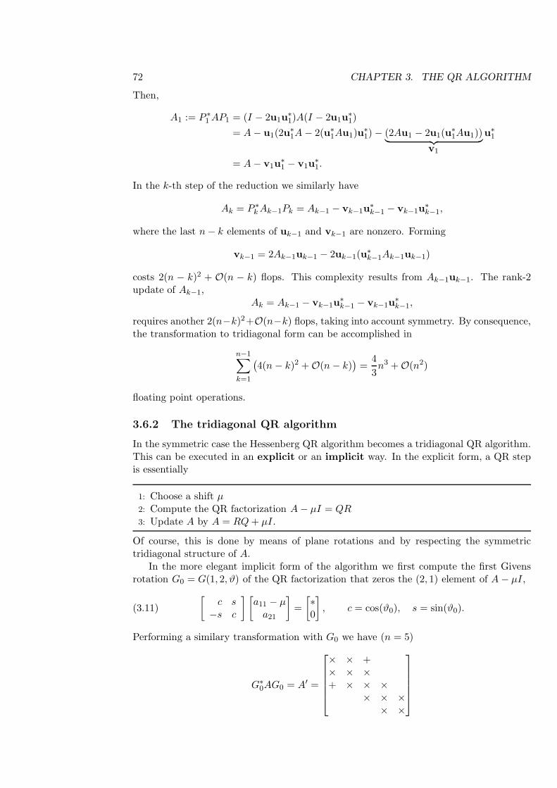
3.6.2 The tridiagonal QR algorithm
In the symmetric case the Hessenberg QR algorithm becomes a tridiagonal QR algorithm.This can be executed in an explicit or an implicit way. In the explicit form, a QR stepis essentially
1: Choose a shift µ2: Compute the QR factorization A− µI = QR3: Update A by A = RQ + µI.
Of course, this is done by means of plane rotations and by respecting the symmetrictridiagonal structure of A.
In the more elegant implicit form of the algorithm we first compute the first Givensrotation G0 = G(1, 2, ϑ) of the QR factorization that zeros the (2, 1) element of A− µI,
(3.11)
[c s−s c
] [a11 − µ
a21
]
=
[∗0
]
, c = cos(ϑ0), s = sin(ϑ0).
Performing a similary transformation with G0 we have (n = 5)
G∗
0AG0 = A′ =
× × +× × ×+ × × ×
× × ×× ×
3.6. THE SYMMETRIC TRIDIAGONAL QR ALGORITHM 73
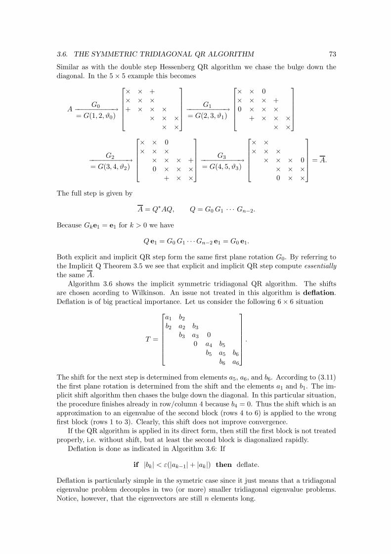
Similar as with the double step Hessenberg QR algorithm we chase the bulge down thediagonal. In the 5× 5 example this becomes
AG0−−−−−−−−−−→
= G(1, 2, ϑ0)
× × +× × ×+ × × ×
× × ×× ×
G1−−−−−−−−−−→= G(2, 3, ϑ1)
× × 0× × × +0 × × ×
+ × × ×× ×
G2−−−−−−−−−−→= G(3, 4, ϑ2)
× × 0× × ×× × × +0 × × ×
+ × ×
G3−−−−−−−−−−→= G(4, 5, ϑ3)
× ×× × ×× × × 0× × ×0 × ×
= A.
The full step is given by
A = Q∗AQ, Q = G0 G1 · · · Gn−2.
Because Gke1 = e1 for k > 0 we have
Q e1 = G0 G1 · · ·Gn−2 e1 = G0 e1.
Both explicit and implicit QR step form the same first plane rotation G0. By referring tothe Implicit Q Theorem 3.5 we see that explicit and implicit QR step compute essentially
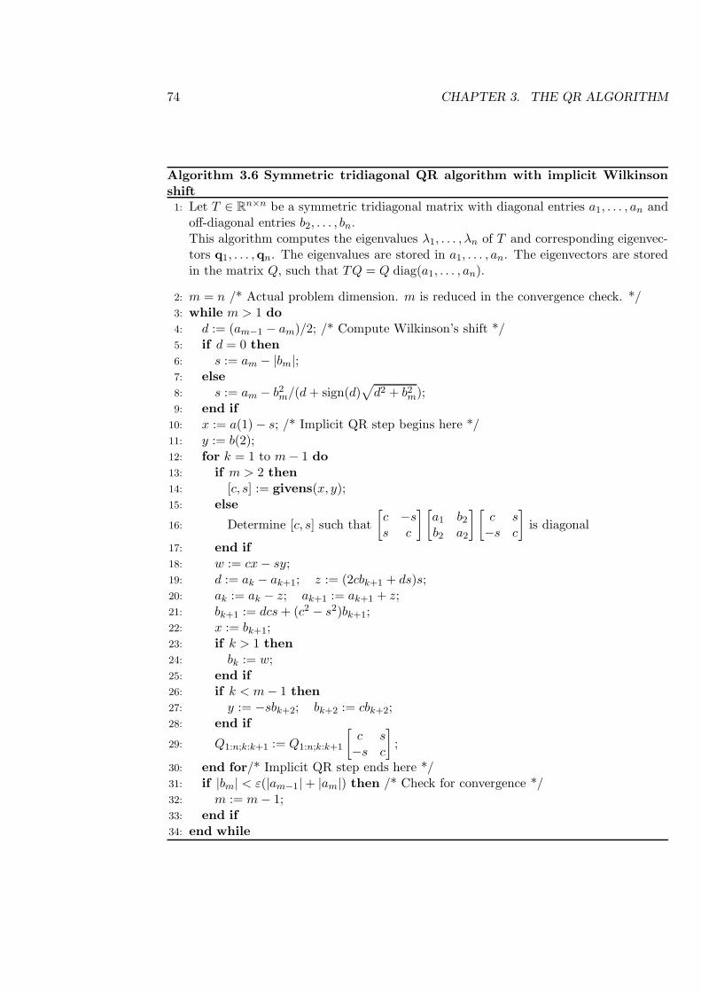
the same A.Algorithm 3.6 shows the implicit symmetric tridiagonal QR algorithm. The shifts
are chosen acording to Wilkinson. An issue not treated in this algorithm is deflation.Deflation is of big practical importance. Let us consider the following 6× 6 situation
T =
a1 b2
b2 a2 b3
b3 a3 00 a4 b5
b5 a5 b6
b6 a6
.
The shift for the next step is determined from elements a5, a6, and b6. According to (3.11)the first plane rotation is determined from the shift and the elements a1 and b1. The im-plicit shift algorithm then chases the bulge down the diagonal. In this particular situation,the procedure finishes already in row/column 4 because b4 = 0. Thus the shift which is anapproximation to an eigenvalue of the second block (rows 4 to 6) is applied to the wrongfirst block (rows 1 to 3). Clearly, this shift does not improve convergence.
If the QR algorithm is applied in its direct form, then still the first block is not treatedproperly, i.e. without shift, but at least the second block is diagonalized rapidly.
Deflation is done as indicated in Algorithm 3.6: If
if |bk| < ε(|ak−1|+ |ak|) then deflate.
Deflation is particularly simple in the symetric case since it just means that a tridiagonaleigenvalue problem decouples in two (or more) smaller tridiagonal eigenvalue problems.Notice, however, that the eigenvectors are still n elements long.
74 CHAPTER 3. THE QR ALGORITHM
Algorithm 3.6 Symmetric tridiagonal QR algorithm with implicit Wilkinsonshift1: Let T ∈ R
n×n be a symmetric tridiagonal matrix with diagonal entries a1, . . . , an andoff-diagonal entries b2, . . . , bn.This algorithm computes the eigenvalues λ1, . . . , λn of T and corresponding eigenvec-tors q1, . . . ,qn. The eigenvalues are stored in a1, . . . , an. The eigenvectors are storedin the matrix Q, such that TQ = Q diag(a1, . . . , an).
2: m = n /* Actual problem dimension. m is reduced in the convergence check. */3: while m > 1 do4: d := (am−1 − am)/2; /* Compute Wilkinson’s shift */5: if d = 0 then6: s := am − |bm|;7: else8: s := am − b2
m/(d + sign(d)√
d2 + b2m);
9: end if10: x := a(1)− s; /* Implicit QR step begins here */11: y := b(2);12: for k = 1 to m− 1 do13: if m > 2 then14: [c, s] := givens(x, y);15: else
16: Determine [c, s] such that
[c −ss c
] [a1 b2
b2 a2
] [c s−s c
]
is diagonal
17: end if18: w := cx− sy;19: d := ak − ak+1; z := (2cbk+1 + ds)s;20: ak := ak − z; ak+1 := ak+1 + z;21: bk+1 := dcs + (c2 − s2)bk+1;22: x := bk+1;23: if k > 1 then24: bk := w;25: end if26: if k < m− 1 then27: y := −sbk+2; bk+2 := cbk+2;28: end if
29: Q1:n;k:k+1 := Q1:n;k:k+1
[c s−s c
]
;
30: end for/* Implicit QR step ends here */31: if |bm| < ε(|am−1|+ |am|) then /* Check for convergence */32: m := m− 1;33: end if34: end while
3.7. SUMMARY 75
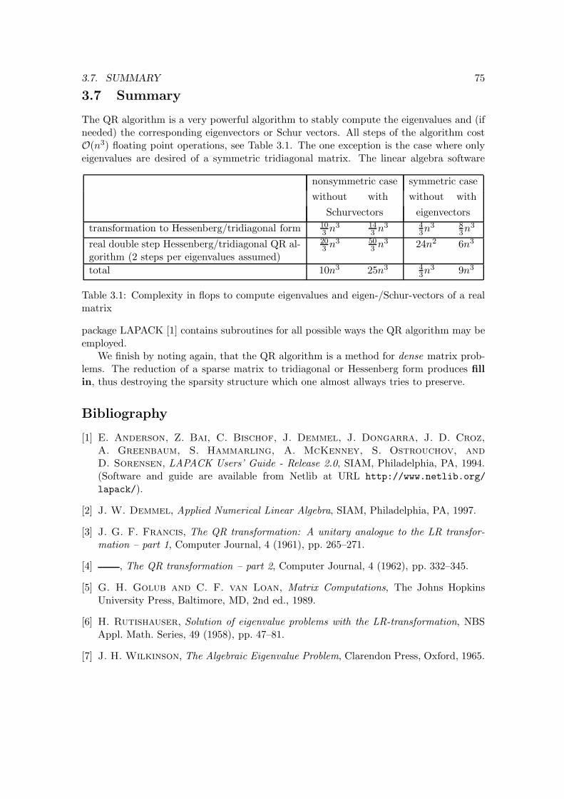
3.7 Summary
The QR algorithm is a very powerful algorithm to stably compute the eigenvalues and (ifneeded) the corresponding eigenvectors or Schur vectors. All steps of the algorithm costO(n3) floating point operations, see Table 3.1. The one exception is the case where onlyeigenvalues are desired of a symmetric tridiagonal matrix. The linear algebra software
nonsymmetric case symmetric case
without with without with
Schurvectors eigenvectors
transformation to Hessenberg/tridiagonal form 103 n3 14
3 n3 43n3 8
3n3
real double step Hessenberg/tridiagonal QR al-gorithm (2 steps per eigenvalues assumed)
203 n3 50
3 n3 24n2 6n3
total 10n3 25n3 43n3 9n3
Table 3.1: Complexity in flops to compute eigenvalues and eigen-/Schur-vectors of a realmatrix
package LAPACK [1] contains subroutines for all possible ways the QR algorithm may beemployed.
We finish by noting again, that the QR algorithm is a method for dense matrix prob-lems. The reduction of a sparse matrix to tridiagonal or Hessenberg form produces fillin, thus destroying the sparsity structure which one almost allways tries to preserve.
Bibliography
[1] E. Anderson, Z. Bai, C. Bischof, J. Demmel, J. Dongarra, J. D. Croz,
A. Greenbaum, S. Hammarling, A. McKenney, S. Ostrouchov, and
D. Sorensen, LAPACK Users’ Guide - Release 2.0, SIAM, Philadelphia, PA, 1994.(Software and guide are available from Netlib at URL http://www.netlib.org/
lapack/).
[2] J. W. Demmel, Applied Numerical Linear Algebra, SIAM, Philadelphia, PA, 1997.
[3] J. G. F. Francis, The QR transformation: A unitary analogue to the LR transfor-
mation – part 1, Computer Journal, 4 (1961), pp. 265–271.
[4] , The QR transformation – part 2, Computer Journal, 4 (1962), pp. 332–345.
[5] G. H. Golub and C. F. van Loan, Matrix Computations, The Johns HopkinsUniversity Press, Baltimore, MD, 2nd ed., 1989.
[6] H. Rutishauser, Solution of eigenvalue problems with the LR-transformation, NBSAppl. Math. Series, 49 (1958), pp. 47–81.
[7] J. H. Wilkinson, The Algebraic Eigenvalue Problem, Clarendon Press, Oxford, 1965.