![arXiv:2008.09150v1 [cs.CL] 20 Aug 2020](https://static.fdocuments.nl/doc/165x107/61fcb62fe2d18d7f487cd21b/arxiv200809150v1-cscl-20-aug-2020.jpg)
Proefschrift - arXiv
264
arXiv:0707.2482v1 [cs.IT] 17 Jul 2007 Multiple-Description Lattice Vector Quantization Proefschrift ter verkrijging van de graad van doctor aan de Technische Universiteit Delft, op gezag van de Rector Magnificus prof.dr.ir. J. T. Fokkema, voorzitter van het College voor Promoties, in het openbaar te verdedigen op maandag 18 juni 2007 om 12:30 uur door Jan ØSTERGAARD Civilingeniør van Aalborg Universitet, Denemarken geboren te Frederikshavn.
Transcript of Proefschrift - arXiv
arX
iv:0
707.
2482
v1 [
cs.IT
] 17
Jul
200
7
Multiple-Description
Lattice Vector Quantization
Proefschrift
ter verkrijging van de graad van doctoraan de Technische Universiteit Delft,
op gezag van de Rector Magnificus prof.dr.ir. J. T. Fokkema,voorzitter van het College voor Promoties,
in het openbaar te verdedigen op maandag 18 juni 2007 om 12:30uurdoor Jan ØSTERGAARD
Civilingeniør van Aalborg Universitet, Denemarkengeboren te Frederikshavn.
Dit proefschrift is goedgekeurd door de promotor:Prof.dr.ir. R. L. Lagendijk
Toegevoegd promotor:Dr.ir. R. Heusdens
Samenstelling promotiecommissie:
Rector Magnificus, voorzitterProf.dr.ir. R. L. Lagendijk, Technische Universiteit Delft, promotorDr.ir. R. Heusdens, Technische Universiteit Delft, toegevoegd
promotorProf.dr. J. M. Aarts, Technische Universiteit DelftProf.dr.ir. P. Van Mieghem, Technische Universiteit DelftProf.dr. V. K. Goyal, Massachusetts Institute of Technology,
Cambridge, United StatesProf.dr. B. Kleijn, KTH School of Electrical Engineering,
Stockholm, SwedenProf.dr. E. J. Delp, Purdue University, Indiana,
United States
The production of this thesis has been financially supportedby STW.
ISBN-13: 978-90-9021979-0
Copyright c© 2007 by J. Østergaard
All rights reserved. No part of this thesis may be reproducedor transmitted in any formor by any means, electronic, mechanical, photocopying, anyinformation storage orretrieval system, or otherwise, without written permission from the copyright owner.

Multiple-Description
Lattice Vector Quantization


Preface
The research for this thesis was conducted within the STW project DET.5851,Adapti-ve Sound Coding (ASC). One of the main objectives of the ASC project was to de-velop a universal audio codec capable of adapting to time-varying characteristics ofthe input signal, user preferences, and application-imposed constraints or time-varyingnetwork-imposed constraints such as bit rate, quality, latency, bandwidth, and bit-errorrate (or packet-loss rate).
This research was carried out during the period February 2003 – February 2007in the Information and Communication Theory group at Delft University of Tech-nology, Delft, The Netherlands. During the period June 2006– September 2006 theresearch was conducted in the department of Electrical Engineering-Systems at TelAviv University, Tel Aviv, Israel.
I would like to take this opportunity to thank my supervisor Richard Heusdensand cosupervisor Jesper Jensen, without whose support, encouragement, and splendidsupervision this thesis would not have been possible.
I owe a lot to my office mates Omar Niamut and Pim Korten. Omar, your knowled-ge of audio coding is impressive. On top of that you are also a gifted musician. A trulymarvelous cocktail. Pim, you have an extensive mathematical knowledge, which onecan only envy. I thank you for the many insightful and delightful discussions we havehad over the years.
I am grateful to Ram Zamir for hosting my stay at Tel Aviv University. I hadsuch a great time and sincerely appreciate the warm welcoming that I received fromyou, your family and the students at the university. It goes without saying that I willdefinitely be visiting Tel Aviv again.
I would also like to thank Inald Lagendijk for accepting being my Promotor andof course cheers go out to the former and current audio cluster fellows; ChristofferRødbro, Ivo Shterev, Ivo Batina, Richard Hendriks, and Jan Erkelens for the manyinsightful discussions we have had. In addition I would liketo acknowledge all mem-
i

bers of the ICT group especially Anja van den Berg, Carmen Lai, Bartek Gedrojc andAna-Ioana Deac. Finally, the financial support by STW is gratefully acknowledged.
J. Østergaard, Delft, January 2007.

Summary
Internet services such as voice over Internet protocol (VoIP) and audio/video stream-ing (e.g. video on demand and video conferencing) are becoming more and morepopular with the recent spread of broadband networks. Thesekind of “real-time” ser-vices often demand low delay, high bandwidth and low packet-loss rates in order todeliver tolerable quality for the end users. However, the heterogeneous communica-tion infrastructure of today’s packet-switched networks does not provide a guaranteedperformance in terms of bandwidth or delay and therefore thedesired quality of ser-vice is generally not achieved.
To achieve a certain degree of robustness on errorprone channels one can make useof multiple-description (MD) coding, which is a disciplinethat recently has received alot of attention. The MD problem is basically a joint source-channel coding problem.It is about (lossy) encoding of information for transmission over an unreliableK-channel communication system. The channels may break down resulting in erasuresand a loss of information at the receiving side. Which of the2K−1 non-trivial subsetsof theK channels that are working is assumed known at the receiving side but not atthe encoder. The problem is then to design an MD scheme which,for given channelrates (or a given sum rate), minimizes the distortions due toreconstruction of thesource using information from any subsets of the channels.
While this thesis focuses mainly on the information theoretic aspects of MD cod-ing, we will also show how the proposed MD coding scheme can beused to constructa perceptually robust audio coder suitable for audio streaming on packet-switchednetworks.
We attack the MD problem from a source coding point of view andconsider thegeneral case involvingK descriptions. We make extensive use of lattice vector quanti-zation (LVQ) theory, which turns out to be instrumental in the sense that the proposedMD-LVQ scheme serves as a bridge between theory and practice. In asymptotic casesof high resolution and large lattice vector quantizer dimension, we show that the best
iii
known information theoretic rate-distortion MD bounds canbe achieved, whereas innon-asymptotic cases of finite-dimensional lattice vectorquantizers (but still underhigh resolution assumptions) we construct practical MD-LVQ schemes, which arecomparable and often superior to existing state-of-the-art schemes.
In the two-channel symmetric case it has previously been established that the sidedescriptions of an MD-LVQ scheme admit side distortions, which (at high resolutionconditions) are identical to that ofL-dimensional quantizers having spherical Voronoicells. In this case we say that the side quantizers achieve theL-sphere bound. Such aresult has not been established for the two-channel asymmetric case before. However,the proposed MD-LVQ scheme is able to achieve theL-sphere bound for two descrip-tions, at high resolution conditions, in both the symmetricand asymmetric cases.
The proposed MD-LVQ scheme appears to be among the first schemes in the liter-ature that achieves the largest known high-resolution three-channel MD region in thequadratic Gaussian case. While optimality is only proven for K ≤ 3 descriptions weconjecture it to be optimal for anyK descriptions.
We present closed-form expressions for the rate and distortion performance forgeneral smooth stationary sources and squared error distortion criterion and at highresolution conditions (also for finite-dimensional lattice vector quantizers). It is shownthat the side distortions in the three-channel case is expressed through the dimension-less normalized second moment of anL-sphere independent of the type of lattice usedfor the side quantizers. This is in line with previous results for the two-descriptioncase.
The rate loss when using finite-dimensional lattice vector quantizers is lattice in-dependent and given by the rate loss of anL-sphere and an additional term describingthe ratio of two dimensionless expansion factors. The overall rate loss is shown to besuperior to existing three-channel schemes.
Contents
Preface i
Summary iii
1 Introduction 11.1 Motivation . . . . . . . . . . . . . . . . . . . . . . . . . . . . . . . . 11.2 Introduction to MD Lattice Vector Quantization . . . . . . .. . . . . 2
1.2.1 Two Descriptions . . . . . . . . . . . . . . . . . . . . . . . . 21.2.2 Many Descriptions . . . . . . . . . . . . . . . . . . . . . . . 31.2.3 Scalar vs. Vector Quantization . . . . . . . . . . . . . . . . . 4
1.3 Contributions . . . . . . . . . . . . . . . . . . . . . . . . . . . . . . 41.4 Structure of Thesis . . . . . . . . . . . . . . . . . . . . . . . . . . . 61.5 List of Papers . . . . . . . . . . . . . . . . . . . . . . . . . . . . . . 7
2 Lattice Theory 92.1 Lattices . . . . . . . . . . . . . . . . . . . . . . . . . . . . . . . . . 10
2.1.1 Sublattices . . . . . . . . . . . . . . . . . . . . . . . . . . . 112.2 J -Lattice . . . . . . . . . . . . . . . . . . . . . . . . . . . . . . . . 12
2.2.1 J -Sublattice . . . . . . . . . . . . . . . . . . . . . . . . . . 132.2.2 Quotient Modules . . . . . . . . . . . . . . . . . . . . . . . 152.2.3 Group Actions on Quotient Modules . . . . . . . . . . . . . . 16
2.3 Construction of Lattices . . . . . . . . . . . . . . . . . . . . . . . . . 162.3.1 Admissible Index Values . . . . . . . . . . . . . . . . . . . . 172.3.2 Sublattices . . . . . . . . . . . . . . . . . . . . . . . . . . . 19
3 Single-Description Rate-Distortion Theory 253.1 Rate-Distortion Function . . . . . . . . . . . . . . . . . . . . . . . . 253.2 Quantization Theory . . . . . . . . . . . . . . . . . . . . . . . . . . 28
v
3.3 Lattice Vector Quantization . . . . . . . . . . . . . . . . . . . . . . .303.3.1 LVQ Rate-Distortion Theory . . . . . . . . . . . . . . . . . . 31
3.4 Entropy Coding . . . . . . . . . . . . . . . . . . . . . . . . . . . . . 34
4 Multiple-Description Rate-Distortion Theory 374.1 Information Theoretic MD Bounds . . . . . . . . . . . . . . . . . . . 37
4.1.1 Two-Channel Rate-Distortion Results . . . . . . . . . . . . .394.1.2 K-Channel Rate-Distortion Results . . . . . . . . . . . . . . 474.1.3 Quadratic GaussianK-Channel Rate-Distortion Region . . . 51
4.2 Multiple-Description Quantization . . . . . . . . . . . . . . . .. . . 564.2.1 Scalar Two-Channel Quantization with Index Assignments . . 574.2.2 Lattice Vector Quantization for Multiple Descriptions . . . . . 60
5 K-Channel Symmetric Lattice Vector Quantization 655.1 Preliminaries . . . . . . . . . . . . . . . . . . . . . . . . . . . . . . 66
5.1.1 Index Assignments . . . . . . . . . . . . . . . . . . . . . . . 665.2 Rate and Distortion Results . . . . . . . . . . . . . . . . . . . . . . . 675.3 Construction of Labeling Function . . . . . . . . . . . . . . . . . .. 71
5.3.1 Expected Distortion . . . . . . . . . . . . . . . . . . . . . . 715.3.2 Cost Functional . . . . . . . . . . . . . . . . . . . . . . . . . 725.3.3 Minimizing Cost Functional . . . . . . . . . . . . . . . . . . 73
5.4 High-Resolution Analysis . . . . . . . . . . . . . . . . . . . . . . . . 785.4.1 Total Expected Distortion . . . . . . . . . . . . . . . . . . . 795.4.2 Optimalν,N andK . . . . . . . . . . . . . . . . . . . . . . 81
5.5 Construction of Practical Quantizers . . . . . . . . . . . . . . .. . . 825.5.1 Index Values . . . . . . . . . . . . . . . . . . . . . . . . . . 825.5.2 ConstructingK-tuples . . . . . . . . . . . . . . . . . . . . . 835.5.3 AssigningK-Tuples to Central Lattice Points . . . . . . . . . 845.5.4 Example of an Assignment . . . . . . . . . . . . . . . . . . . 85
5.6 Numerical Results . . . . . . . . . . . . . . . . . . . . . . . . . . . . 865.6.1 Performance of Individual Descriptions . . . . . . . . . . .. 875.6.2 Distortion as a Function of Packet-Loss Probability .. . . . . 89
5.7 Conclusion . . . . . . . . . . . . . . . . . . . . . . . . . . . . . . . 90
6 K-Channel Asymmetric Lattice Vector Quantization 936.1 Preliminaries . . . . . . . . . . . . . . . . . . . . . . . . . . . . . . 94
6.1.1 Index Assignments . . . . . . . . . . . . . . . . . . . . . . . 946.1.2 Rate and Distortion Results . . . . . . . . . . . . . . . . . . 95
6.2 Construction of Labeling Function . . . . . . . . . . . . . . . . . .. 966.2.1 Expected Distortion . . . . . . . . . . . . . . . . . . . . . . 966.2.2 Cost Functional . . . . . . . . . . . . . . . . . . . . . . . . . 976.2.3 Minimizing Cost Functional . . . . . . . . . . . . . . . . . . 98
6.2.4 Comparison to Existing Asymmetric Index Assignments. . . 1006.3 High-Resolution Analysis . . . . . . . . . . . . . . . . . . . . . . . . 101
6.3.1 Total Expected Distortion . . . . . . . . . . . . . . . . . . . 1026.4 Optimal Entropy-Constrained Quantizers . . . . . . . . . . . .. . . 104
6.4.1 Entropy Constraints Per Description . . . . . . . . . . . . . .1046.4.2 Total Entropy Constraint . . . . . . . . . . . . . . . . . . . . 1056.4.3 Example With Total Entropy Constraint . . . . . . . . . . . . 107
6.5 Distortion of Subsets of Descriptions . . . . . . . . . . . . . . .. . . 1086.5.1 Asymmetric Assignment Example . . . . . . . . . . . . . . . 109
6.6 Numerical Results . . . . . . . . . . . . . . . . . . . . . . . . . . . . 1116.6.1 Assessing Two-Channel Performance . . . . . . . . . . . . . 1116.6.2 Three Channel Performance . . . . . . . . . . . . . . . . . . 112
6.7 Conclusion . . . . . . . . . . . . . . . . . . . . . . . . . . . . . . . 112
7 Comparison to Existing High-Resolution MD Results 1157.1 Two-Channel Performance . . . . . . . . . . . . . . . . . . . . . . . 115
7.1.1 Symmetric Case . . . . . . . . . . . . . . . . . . . . . . . . 1157.1.2 Asymmetric Case . . . . . . . . . . . . . . . . . . . . . . . . 116
7.2 Achieving Rate-Distortion Region of(3, 1) SCECs . . . . . . . . . . 1177.3 Achieving Rate-Distortion Region of(3, 2) SCECs . . . . . . . . . . 118
7.3.1 Random Binning on Side Codebooks of MD-LVQ Schemes . 1197.3.2 Symmetric Case . . . . . . . . . . . . . . . . . . . . . . . . 1227.3.3 Asymmetric Case . . . . . . . . . . . . . . . . . . . . . . . . 123
7.4 Comparison toK-Channel Schemes . . . . . . . . . . . . . . . . . . 1247.4.1 Rate Loss of MD-LVQ . . . . . . . . . . . . . . . . . . . . . 125
7.5 Conclusion . . . . . . . . . . . . . . . . . . . . . . . . . . . . . . . 126
8 Network Audio Coding 1298.1 Transform Coding . . . . . . . . . . . . . . . . . . . . . . . . . . . . 130
8.1.1 Modified Discrete Cosine Transform . . . . . . . . . . . . . . 1308.1.2 Perceptual Weighting Function . . . . . . . . . . . . . . . . . 1308.1.3 Distortion Measure . . . . . . . . . . . . . . . . . . . . . . . 1318.1.4 Transforming Perceptual Distortion Measure toℓ2 . . . . . . 1318.1.5 Optimal Bit Distribution . . . . . . . . . . . . . . . . . . . . 133
8.2 Robust Transform Coding . . . . . . . . . . . . . . . . . . . . . . . . 1368.2.1 Encoder . . . . . . . . . . . . . . . . . . . . . . . . . . . . . 1368.2.2 Decoder . . . . . . . . . . . . . . . . . . . . . . . . . . . . . 139
8.3 Results . . . . . . . . . . . . . . . . . . . . . . . . . . . . . . . . . . 1398.3.1 Expected Distortion Results . . . . . . . . . . . . . . . . . . 1398.3.2 Scalable Coding Results . . . . . . . . . . . . . . . . . . . . 144
8.4 Conclusion . . . . . . . . . . . . . . . . . . . . . . . . . . . . . . . 146

9 Conclusions and Discussion 1479.1 Summary of Results . . . . . . . . . . . . . . . . . . . . . . . . . . . 1479.2 Future Research Directions . . . . . . . . . . . . . . . . . . . . . . . 148
A Quaternions 151
B Modules 153B.1 General Definitions . . . . . . . . . . . . . . . . . . . . . . . . . . . 153B.2 Submodule Related Definitions . . . . . . . . . . . . . . . . . . . . . 155B.3 Quadratic Forms . . . . . . . . . . . . . . . . . . . . . . . . . . . . 156
C Lattice Definitions 159C.1 General Definitions . . . . . . . . . . . . . . . . . . . . . . . . . . . 159C.2 Norm Related Definitions . . . . . . . . . . . . . . . . . . . . . . . . 161C.3 Sublattice Related Definitions . . . . . . . . . . . . . . . . . . . . .162
D Root Lattices 165D.1 Z1 . . . . . . . . . . . . . . . . . . . . . . . . . . . . . . . . . . . . 165D.2 Z2 . . . . . . . . . . . . . . . . . . . . . . . . . . . . . . . . . . . . 166D.3 A2 . . . . . . . . . . . . . . . . . . . . . . . . . . . . . . . . . . . . 167D.4 Z4 . . . . . . . . . . . . . . . . . . . . . . . . . . . . . . . . . . . . 168D.5 D4 . . . . . . . . . . . . . . . . . . . . . . . . . . . . . . . . . . . . 169
E Proofs for Chapter 2 173
F Estimating ψL 175F.1 Algorithm . . . . . . . . . . . . . . . . . . . . . . . . . . . . . . . . 175
G Assignment Example 177
H Proofs for Chapter 5 181H.1 Proof of Theorem 5.3.1 . . . . . . . . . . . . . . . . . . . . . . . . . 181H.2 Proof of Theorem 5.3.2 . . . . . . . . . . . . . . . . . . . . . . . . . 184H.3 Proof of Theorem 5.3.3 . . . . . . . . . . . . . . . . . . . . . . . . . 190H.4 Proof of Proposition 5.4.1 . . . . . . . . . . . . . . . . . . . . . . . . 191H.5 Proof of Proposition 5.4.2 . . . . . . . . . . . . . . . . . . . . . . . . 194
I Proofs for Chapter 6 197I.1 Proof of Theorem 6.2.1 . . . . . . . . . . . . . . . . . . . . . . . . . 197I.2 Proof of Proposition 6.3.1 . . . . . . . . . . . . . . . . . . . . . . . . 202I.3 Proof of Proposition 6.3.2 . . . . . . . . . . . . . . . . . . . . . . . . 203I.4 Proof of Lemmas . . . . . . . . . . . . . . . . . . . . . . . . . . . . 205I.5 Proof of Theorem 6.5.1 . . . . . . . . . . . . . . . . . . . . . . . . . 206
J Proofs for Chapter 7 213J.1 Proofs of Lemmas . . . . . . . . . . . . . . . . . . . . . . . . . . . . 213J.2 Proof of Theorem 7.3.1 . . . . . . . . . . . . . . . . . . . . . . . . . 215
K Results of Listening Test 219
Samenvatting 223
Curriculum Vitae 225
Glossary of Symbols and Terms 227
Bibliography 231
Index 245

Chapter1Introduction
1.1 Motivation
Internet services such as voice over Internet protocol (VoIP) and audio/video stream-ing (e.g. video on demand and video conferencing) are becoming more and morepopular with the recent spread of broadband networks. Thesekinds of “real-time”services often demand low delay, high bandwidth and low packet-loss rates in order todeliver tolerable quality for the end users. However, the heterogeneous communica-tion infrastructure of today’s packet-switched networks does not provide a guaranteedperformance in terms of bandwidth or delay and therefore thedesired quality of ser-vice is (at least in the authors experience) generally not achieved.
Clearly, many consumers enjoy the Internet telephony services provided for freethrough e.g. SkypeTM. This trend seems to be steadily growing, and more and morepeople are replacing their traditional landline phones with VoIP compatible systems.On the wireless side it is likely that cell phones soon are to be replaced by VoIPcompatible wireless (mobile) phones. A driving impetus is consumer demand forcheaper calls, which sometimes may compromise quality.
The structure of packet-switched networks makes it possible to exploit diversityin order to achieve robustness towards delay and packet losses and thereby improvethe quality of existing VoIP services. For example, at the cost of increased bandwidth(or bit rate), every packet may be duplicated and transmitted over two different paths(or channels) throughout the network. If one of the channelsfails, there will be noreduction in quality at the receiving side. Thus, we have a great degree of robustness.On the other hand, if none of the channels fail so that both packets are received, therewill be no improvement in quality over that of using a single packet. Hence, robustnessvia diversity comes with a price.
However, if we can tolerate a small quality degradation on reception of a single
1
2 (Chapter 1) Introduction
packet, we can reduce the bit rates of the individual packets, while still maintainingthe good quality on reception of both packets by making sure that the two packetsimprove upon each other. This idea of trading off bit rate vs.quality between a numberof packets (or descriptions) is usually referred to as the multiple-description (MD)problem and is the topic of this thesis.
While this thesis focuses mainly on the information theoretic aspects of MD cod-ing, we will also show how the proposed MD coding scheme can beused to constructa perceptually robust audio coder suitable for audio streaming on packet-switchednetworks. To the best of the author’s knowledge the use of MD coding in currentstate-of-the-art VoIP systems or audio streaming applications is virtually non-existent.We expect, however, that future schemes will employ MD coding to achieve a certaindegree of robustness towards packet losses. The research presented in this thesis is astep in that direction.
1.2 Introduction to MD Lattice Vector Quantization
The MD problem is basically a joint source-channel coding problem. It is about(lossy) encoding of information for transmission over an unreliableK-channel com-munication system. The channels may break down resulting inerasures and a loss ofinformation at the receiving side. Which of the2K − 1 non-trivial subsets of theKchannels that are working is assumed known at the receiving side but not at the en-coder. The problem is then to design an MD scheme which, for given channel rates (ora given sum rate), minimizes the distortions on the receiverside due to reconstructionof the source using information from any subsets of the channels.
1.2.1 Two Descriptions
The traditional case involves two descriptions as shown in Fig. 1.1. The total bit rateRT , also known as the sum rate, is split between the two descriptions, i.e.RT =
R0 + R1, and the distortion observed at the receiver depends on which descriptionsarrive. If both descriptions are received, the resulting distortion(Dc) is smaller thanif only a single description is received (D0 or D1). It may be noticed from Fig. 1.1that Decoder 0 and Decoder 1 are located on the sides of Decoder c and it is thereforecustomary to refer to Decoder 0 and Decoder 1 as the side decoders and Decodercas the central decoder. In a similar manner we often refer toDi, i = 0, 1, as theside distortions andDc as the central distortion. The situation whereD0 = D1 andR0 = R1 is called symmetric MD coding and is a special case of asymmetric MDcoding, where we allow unequal side rates and unequal side distortions.
One of the fundamental problems of MD coding is that if two descriptions bothrepresent the source well, then, intuitively, they must be very similar to the source andtherefore also similar to each other. Thus, their joint description is not much better

Section 1.2 Introduction to MD Lattice Vector Quantization 3
Source Encoder
Decoder 0
Decoder c
Decoder 1
PSfrag replacements
D0
D1
Dc
R0
R0
R1
R1
Description 0
Description 1
Figure 1.1: The traditional two-channel MD system.
than a single one of them. Informally, we may therefore say that the MD problemis about how good one can make the simultaneous representations of the individualdescriptions as well as their joint description.
The two-description MD problem was formalized and presented by Wyner,Witsenhausen, Wolf and Ziv at an information theory workshop in September1979 [50].1 Formally, the traditional two-description MD problem askswhat is thelargest possible set of distortions(D0, D1, Dc) given the bit rate constraints(R0, R1)
or alternatively the largest set of bit rates(R0, R1) given the distortion constraints(D0, D1, Dc)? Both these questions were partially answered by El Gamal and Coverwho presented an achievable rate-distortion region [42], which Ozarow [107] provedwas tight in the case of a memoryless Gaussian source and the squared error distortionmeasure. Currently, this is the only case where the solutionto the MD problem iscompletely known.
1.2.2 Many Descriptions
Recently, the information theoretic aspects of the generalcase ofK > 2 descriptionshave received a lot of attention [111, 114, 141, 142, 146]. This case is the naturalextension of the two-description case. Given the rate tuple(R0, . . . , RK−1), we seekthe largest set of simultaneously achievable distortions over all subsets of descriptions.The generalK-channel MD problem will be treated in greater detail in Chapter 4.
With this thesis we show that, at least for the case of audio streaming for lossypacket-switched networks, there seems to be a lot to be gained by using more thantwo descriptions. It is likely that this result carries overto VoIP and video streamingapplications.
1At that time the problem was already known to several people including Gersho, Ozarow, Jayant,Miller, and Boyle who all made contributions towards its solution, see [50] for more information.

4 (Chapter 1) Introduction
1.2.3 Scalar vs. Vector Quantization
In the single-description (SD) case it is known that the scalar rate loss (i.e. the bitrate increase due to using a scalar quantizer instead of an optimal infinite-dimensionalvector quantizer) is approximately0.2546 bit/dim. [47]. For many applications thisrate loss is discouraging small and it is tempting to quote Uri Erez:2
“The problem of vector quantization is that scalar quantization works so well.”
However, in the MD case, the sum (or accumulative) rate loss over many descrip-tions can be severe. For example, in the two-description case, it is known that thescalar rate loss is about twice that of the SD scalar rate loss[136]. Therefore, whenconstructing MD schemes for many descriptions, it is important that the rate loss iskept small. To achieve this, we show in this thesis, that one can, for example, uselattice vector quantizers combined with an index-assignment algorithm.
1.3 Contributions
The MD problem is a joint source-channel coding problem. However, in this work wemainly attack the MD problem from a source coding point of view, where we considerthe general case involvingK descriptions. We make extensive use of lattice vectorquantization (LVQ) theory, which turns out to be instrumental in the sense that theproposed MD-LVQ scheme serves as a bridge between theory andpractice. In asymp-totic cases of high resolution and large lattice vector quantizer dimension, we showthat the best known information theoretic rate-distortionMD bounds can be achieved,whereas in non-asymptotic cases of finite-dimensional lattice vector quantizers (butstill under high resolution assumptions) we construct practical MD-LVQ schemes,which are comparable and often superior to existing state-of-the-art schemes.
The main contributions of this thesis are the following:
1. L-sphere bound for two descriptions
In the two-channel symmetric case it has previously been established that theside descriptions of an MD-LVQ scheme admit side distortions, which (at highresolution conditions) are identical to that ofL-dimensional quantizers havingspherical Voronoi cells [120, 139]. In this case we say that the side quantiz-ers achieve theL-sphere bound. Such a result has not been established for thetwo-channel asymmetric case before. However, the proposedMD-LVQ schemeis able to achieve theL-sphere bound for two descriptions, at high resolutionconditions, in both the symmetric and asymmetric cases.
2Said during a break at the International Symposium on Information Theory in Seattle, July 2006.
Section 1.3 Contributions 5
2. MD high-resolution region for three descriptions
The proposed MD-LVQ scheme appears to be among the first schemes in theliterature that achieves the largest known high-resolution three-channel MD re-gion in the quadratic Gaussian case.3 We prove optimality forK ≤ 3 de-scriptions, but conjecture optimality for anyK descriptions.
3. Exact rate-distortion results for L-dimensional LVQ
We present closed-form expressions for the rate and distortion performancewhen usingL-dimensional lattice vector quantizers. These results arevalidfor smooth stationary sources and squared-error distortion criterion and at highresolution conditions.
4. Rate loss for finite-dimensional LVQ
The rate loss of the proposed MD-LVQ scheme when using finite-dimensionallattice vector quantizers is lattice independent and givenby the rate loss of anL-sphere and an additional term describing the ratio of two dimensionless ex-pansion factors. The overall rate loss is shown to be superior to existing three-channel schemes, a result that appears to hold for any numberof descriptions.
5. K-channel asymmetric MD-LVQ
In the asymmetric two-description case it has previously been shown that by in-troducing weights, the distortion profile of the system can range from successiverefinement to complete symmetric MD coding [27, 28]. We show asimilar re-sult for the general case ofK descriptions. Furthermore, for any set of weights,we find the optimal number of descriptions and show that the redundancy inthe scheme is independent of the target rate, source distribution and choice oflattices for the side quantizers. Finally, we show how to optimally distributea given bit budget among the descriptions, which is a topic that has not beenaddressed in previous asymmetric designs.
6. Lattice construction using algebraicJ -modules
For the two-description case it has previously been shown that algebraic toolscan be exploited to simplify the construction of MD-LVQ schemes [27,28,120,139]. We extend these results toK-channel MD-LVQ and show that algebraicJ -modules provide simple solutions to the problem of constructing the latticesused in MD-LVQ.
3A conference version of the proposed symmetricK-channel MD-LVQ scheme appeared in [104] andthe full version in [105]. The asymmetricK-channel MD-LVQ scheme appeared in [99]. Independently,Chen et al. [16–18] presented a different design ofK-channel asymmetric MD coding.

6 (Chapter 1) Introduction
7. K-channel MD-LVQ based audio coding
We present a perceptually robust audio coder based on the modified discretecosine transform andK-channel MD-LVQ. This appears to be the first schemeto consider more than two descriptions for audio coding. Furthermore, we showthat using more than two descriptions is advantageous in packet-switched net-work environments with excessive packet losses.
1.4 Structure of Thesis
The main contributions of this thesis are presented in Chapters 5–8 and the corre-sponding appendices, i.e. Appendices E–K.
The general structure of the thesis is as follows:
Chapter 2 The theory of LVQ is a fundamental part of this thesis and in this chapterwe describe in detail the construction of lattices and show how they can be usedas vector quantizers. A majority of the material in this chapter is known, butthe use ofJ -modules for constructing product lattices based on more than twosublattices is new.
Chapter 3 We consider the MD problem from a source-coding perspectiveand in thischapter we cover aspects of SD rate-distortion theory, which are also relevantfor the MD case.
Chapter 4 In this chapter we present and discuss the existing MD rate-distortion re-sults, which are needed in order to better understand (and tobe able to compareto) the new MD results to be presented in the forthcoming chapters.
Chapter 5 Here we present the proposed entropy-constrainedK-channel symmetricMD-LVQ scheme. We derive closed-form expressions for the rate and distortionperformance of MD-LVQ at high resolution and find the optimallattice parame-ters, which minimize the expected distortion given the packet-loss probabilities.We further show how to construct practical MD-LVQ schemes and evaluatetheir numerical performance. This work was presented in part in [104,105].
Chapter 6 We extend the results of the previous chapter to the asymmetric case.In addition we present closed-form expressions for the distortion due toreconstructing using arbitrary subsets of descriptions. We also describe howto distribute a fixed target bit rate across the descriptionsso that the expecteddistortion is minimized. This work was presented in part in [98,99].
Chapter 7 In this chapter we compare the rate-distortion performanceof the pro-posed MD-LVQ scheme to that of existing state-of-the-art MDschemes aswell as to known information theoretic high-resolutionK-channel MD rate-distortion bounds. This work was presented in part in [98,102].

Section 1.5 List of Papers 7
Chapter 8 In this chapter we propose to combine the modified discrete cosine trans-form with MD-LVQ in order to construct a perceptually robustaudio coder. Partof the research presented in this chapter represents joint work with O. Niamut.This work was presented in part in [106].
Chapter 9 A summary of results and future research directions are given here.
Appendices The appendices contain supporting material including proofs of lemmas,propositions, and theorems.
1.5 List of Papers
The following papers have been published by the author of this thesis during his Ph.D.studies or are currently under peer review.
1. J. Østergaard and R. Zamir, “Multiple-Description Coding by Dithered DeltaSigma Quantization”, IEEE Proc. Data Compression Conference (DCC), pp.63 – 72. March 2007. (Reference [127]).
2. J. Østergaard, R. Heusdens, and J. Jensen, “Source-Channel Erasure CodesWith Lattice Codebooks for Multiple Description Coding”, IEEE Int. Sym-posium on Information Theory (ISIT), pp. 2324 – 2328, July 2006. (Refer-ence [102]).
3. J. Østergaard, R. Heusdens and J. Jensen “n-Channel Asymmetric Entropy-Constrained Multiple-Description Lattice Vector Quantization”, Submitted toIEEE Trans. Information Theory, June 2006. (Reference [98]).
4. J. Østergaard, J. Jensen and R. Heusdens,“n-Channel Entropy-ConstrainedMultiple-Description Lattice Vector Quantization”, IEEETrans. InformationTheory, vol. 52, no. 5, pp. 1956 – 1973, May 2006. (Reference [105]).
5. J. Østergaard, O. A. Niamut, J. Jensen and R. Heusdens, “Perceptual Au-dio Coding usingn-Channel Lattice Vector Quantization”, Proc. IEEE Int.Conference on Audio, Speech and Signal Processing (ICASSP), vol. V, pp.197 – 200, May 2006. (Reference [106]).
6. J. Østergaard, R. Heusdens, and J. Jensen, “On the Rate Loss in PerceptualAudio Coding”, IEEE Benelux/DSP Valley Signal Processing Symposium, pp.27 – 30, March 2006. (Reference [101]).
7. J. Østergaard, R. Heusdens, J. Jensen, "n-Channel Asymmetric Multiple-Description Lattice Vector Quantization", IEEE Int. Symposium on InformationTheory (ISIT), pp. 1793 – 1797. September 2005. (Reference [99]).
8 (Chapter 1) Introduction
8. J. Østergaard, R. Heusdens, J. Jensen, "On the Bit Distribution in AsymmetricMultiple-Description Coding", 26th Symposium on Information Theory in theBenelux, pp. 81 – 88, May 2005. (Reference [100]).
9. J. Østergaard, J. Jensen and R. Heusdens, "n-Channel Symmetric Multiple-Description Lattice Vector Quantization", IEEE Proc. DataCompression Con-ference (DCC), pp. 378 – 387, March 2005. (Reference [104]).
10. J. Østergaard, J. Jensen and R. Heusdens, "Entropy Constrained Multiple De-scription Lattice Vector Quantization", Proc. IEEE Int. Conference on Audio,Speech and Signal Processing (ICASSP), vol. 4, pp. 601 – 604,May 2004.(Reference [103]).
Chapter2
Lattice Theory
In this chapter we introduce the concept of a lattice and showthat it can be used asa vector quantizer. We form subsets (called sublattices) ofthis lattice, and show thatthese sublattices can also be used as quantizers. In fact, inlater chapters, we will usea lattice as a central quantizer and the sublattices will be used as side quantizers forMD-LVQ. We defer the discussion on rate-distortion properties of the lattice vectorquantizer to Chapters 3 and 4.
We begin by describing a lattice in simple terms and show how it can be usedas a vector quantizer. This is done in Section 2.1 and more details can be found inAppendix C. Then in Section 2.2 we show that lattice theory isintimately connected toalgebra and it is therefore possible to use existing algebraic tools to solve lattice relatedproblems. For example it is well known that lattices form groups under ordinary vectoraddition and it is therefore possible to link fundamental group theory to lattices. InSection 2.3 we then use these algebraic tools to construct lattices and sublattices. Itmight be a good idea here to consult Appendix A for the definition of Quaternions andAppendix B for a brief introduction to module theory.
We would like to point out that Section 2.1 contains most of the essential latticetheory needed to understand the concept of MD-LVQ. Sections2.2 and 2.3 are sup-plementary to Section 2.1. In these sections we construct lattices and sublattices inan algebraic fashion by using the machinery of module theory. This turns out to be avery convenient approach, since it allows simple constructions of lattices. This theoryis therefore also very helpful for the practical implementation of MD-LVQ schemes.In addition, we would like to emphasize that by use of module theory we are ableto prove the existence of lattices which admit the required sublattices and productlattices. In Chapters 5–7 we will implicitly assume that alllattices, sublattices, andproduct lattices are constructed as specified in this chapter.
9
10 (Chapter 2) Lattice Theory
2.1 Lattices
An L-dimensional lattice is a discrete set of equidistantly spaced points in theL-dimensional Euclidean vector spaceRL. For example, the set of integersZ forms alattice inR and the Cartesian productZ× Z forms a lattice inR2. More formally, wehave the following definition.
Definition 2.1.1 ([22]). A lattice Λ ⊂ RL consists of all possible integral linearcombinations of a set of basis vectors, that is
Λ =
λ ∈ RL : λ =
L∑
i=1
ξiζi, ∀ξi ∈ Z
, (2.1)
whereζi ∈ RL are the basis vectors also known as generator vectors of the lattice.
The generator vectorsζi, i = 1, . . . , L, (or more correctly their transposes) formthe rows of the generator matrixM . Usually there exists several generator matriceswhich all lead to the same lattice. In Appendix D we present some possible generatormatrices for the lattices considered in this thesis.
Definition 2.1.2. Given a discrete set of pointsS ⊂ RL, the nearest neighbor regionof s ∈ S is called a Voronoi cell, Voronoi region or Dirichlet region, and is defined by
V (s) , x ∈ RL : ‖x− s‖2 ≤ ‖x− s′‖2, ∀ s′ ∈ S, (2.2)
where‖x‖ denotes the usual norm inRL, i.e.‖x‖2 = xTx.
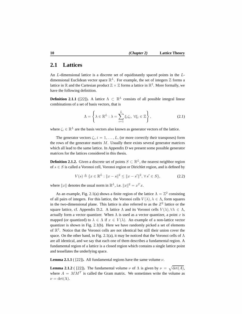
As an example, Fig. 2.1(a) shows a finite region of the latticeΛ = Z2 consistingof all pairs of integers. For this lattice, the Voronoi cellsV (λ), λ ∈ Λ, form squaresin the two-dimensional plane. This lattice is also referredto as theZ2 lattice or thesquare lattice, cf. Appendix D.2. A latticeΛ and its Voronoi cellsV (λ), ∀λ ∈ Λ,actually form a vector quantizer. WhenΛ is used as a vector quantizer, a pointx ismapped (or quantized) toλ ∈ Λ if x ∈ V (λ). An example of a non-lattice vectorquantizer is shown in Fig. 2.1(b). Here we have randomly picked a set of elementsof R2. Notice that the Voronoi cells are not identical but still their union cover thespace. On the other hand, in Fig. 2.1(a), it may be noticed that the Voronoi cells ofΛare all identical, and we say that each one of them describes afundamental region. Afundamental region of a lattice is a closed region which contains a single lattice pointand tessellates the underlying space.
Lemma 2.1.1( [22]). All fundamental regions have the same volumeν.
Lemma 2.1.2( [22]). The fundamental volumeν of Λ is given byν =√
det(A),whereA = MMT is called the Gram matrix. We sometimes write the volume asν = det(Λ).

Section 2.1 Lattices 11
−2 −1 0 1 2
−2.5
−2
−1.5
−1
−0.5
0
0.5
1
1.5
2
2.5
(a) Λ = Z2
−2 −1 0 1 2
−2.5
−2
−1.5
−1
−0.5
0
0.5
1
1.5
2
2.5
(b) Random point set
Figure 2.1: (a) finite region of the latticeΛ = Z2. (b) randomly selected points ofR2. The
solid lines describe the boundaries of the Voronoi cells of the points.
Let us defineV0 , V (0), i.e. the Voronoi cell around the lattice point located atthe origin. This region is called a fundamental region of thelattice since it specifiesthe complete lattice through translations. We then have thefollowing definition.
Definition 2.1.3 ( [22]). The dimensionless normalized second moment of inertiaG(Λ) of a latticeΛ is defined by
G(Λ) ,1
Lν1+2/L
∫
V0
‖x‖2dx, (2.3)
whereν is the volume ofV0.
Applying any scaling or orthogonal transform, e.g. rotation or reflection onΛ willnot changeG(Λ), which makes it a good figure of merit when comparing differentlattices (quantizers). Furthermore,G(Λ) depends only upon the shape ofV0, and ingeneral, the more sphere-like shape, the smaller normalized second moment [22].
2.1.1 Sublattices
If Λ is a lattice then a sublatticeΛ′ ⊆ Λ is a subset of the elements ofΛ that is itselfa lattice. For example ifΛ = Z then the set of all even integers is a sublattice ofΛ.Geometrically speaking, a sublatticeΛ′ ⊂ Λ is obtained by scaling and rotating (andpossibly reflecting) the latticeΛ so that all points ofΛ′ coincide with points ofΛ. AsublatticeΛ′ ⊂ Λ obtained in this manner is referred to as a geometrically-similarsublattice ofΛ. Fig. 2.2 shows an example of a latticeΛ ⊂ R2 and a geometrically-similar sublatticeΛ′ ⊂ Λ. In this caseΛ is the hexagonal lattice which is described in
12 (Chapter 2) Lattice Theory
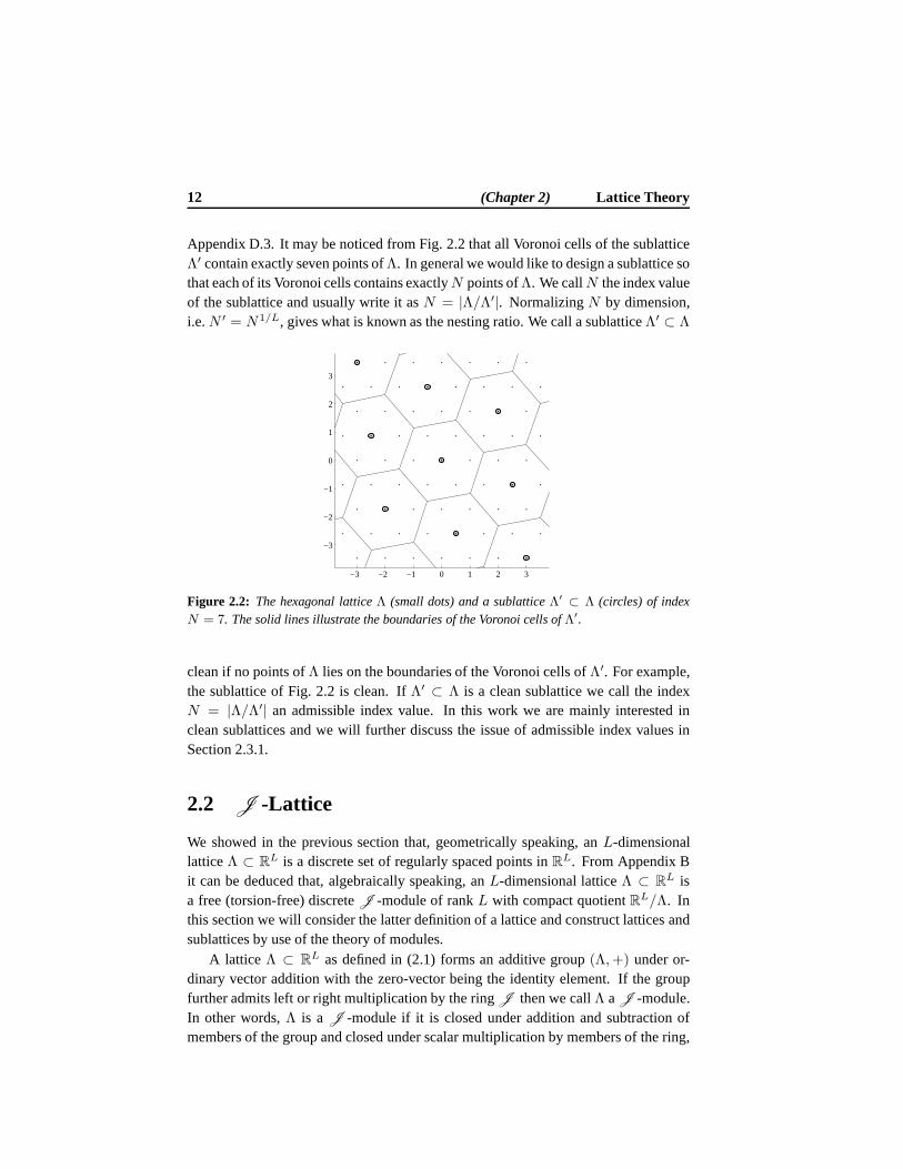
Appendix D.3. It may be noticed from Fig. 2.2 that all Voronoicells of the sublatticeΛ′ contain exactly seven points ofΛ. In general we would like to design a sublattice sothat each of its Voronoi cells contains exactlyN points ofΛ. We callN the index valueof the sublattice and usually write it asN = |Λ/Λ′|. NormalizingN by dimension,i.e.N ′ = N1/L, gives what is known as the nesting ratio. We call a sublatticeΛ′ ⊂ Λ
−3 −2 −1 0 1 2 3
−3
−2
−1
0
1
2
3
Figure 2.2: The hexagonal latticeΛ (small dots) and a sublatticeΛ′ ⊂ Λ (circles) of indexN = 7. The solid lines illustrate the boundaries of the Voronoi cells of Λ′.
clean if no points ofΛ lies on the boundaries of the Voronoi cells ofΛ′. For example,the sublattice of Fig. 2.2 is clean. IfΛ′ ⊂ Λ is a clean sublattice we call the indexN = |Λ/Λ′| an admissible index value. In this work we are mainly interested inclean sublattices and we will further discuss the issue of admissible index values inSection 2.3.1.
2.2 J -Lattice
We showed in the previous section that, geometrically speaking, anL-dimensionallatticeΛ ⊂ RL is a discrete set of regularly spaced points inRL. From Appendix Bit can be deduced that, algebraically speaking, anL-dimensional latticeΛ ⊂ RL isa free (torsion-free) discreteJ -module of rankL with compact quotientRL/Λ. Inthis section we will consider the latter definition of a lattice and construct lattices andsublattices by use of the theory of modules.
A lattice Λ ⊂ RL as defined in (2.1) forms an additive group(Λ,+) under or-dinary vector addition with the zero-vector being the identity element. If the groupfurther admits left or right multiplication by the ringJ then we callΛ aJ -module.In other words,Λ is a J -module if it is closed under addition and subtraction ofmembers of the group and closed under scalar multiplicationby members of the ring,

Section 2.2 J -Lattice 13
see Appendix B for details. SinceΛ is also a lattice we sometimes prefer the nameJ -lattice overJ -module.
Let ζi, i = 1, . . . , L be a set of linearly independent vectors inRL and letJ ⊂ Rbe a ring. Then a leftJ -latticeΛ generated byζi, i = 1, . . . , L consists of all linearcombinations
ξ1ζ1 + · · ·+ ξLζL, (2.4)
whereξi ∈ J , i = 1, . . . , L [22]. A right J -lattice is defined similarly with themultiplication ofζi on the right byξi instead.
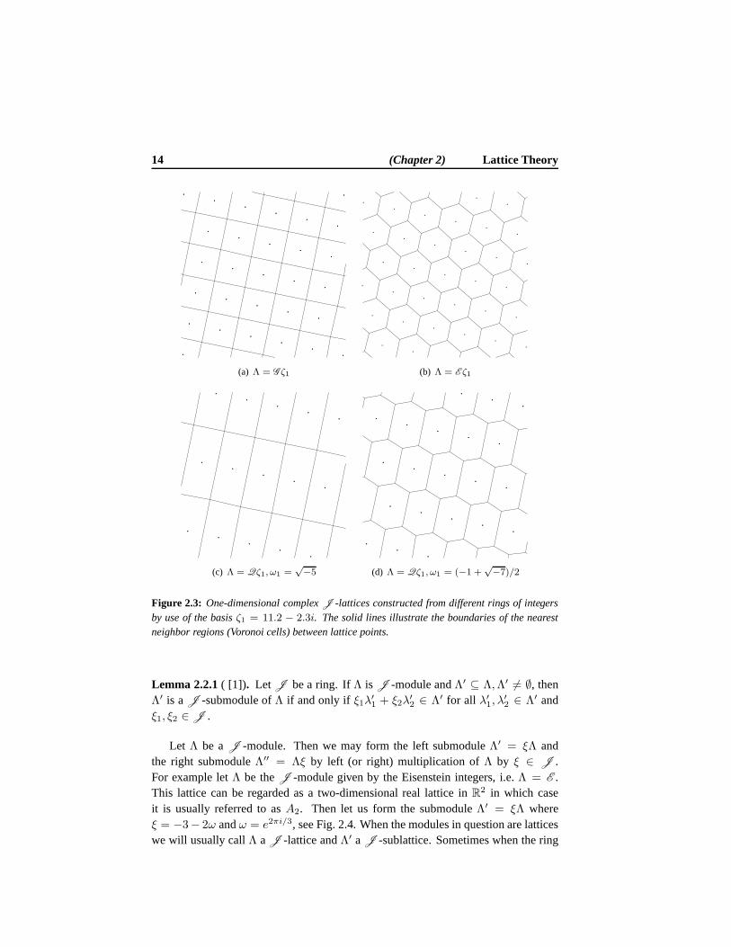
We have so far assumed that the underlying field is the Cartesian product of thereals, i.e.RL. However, there are other fields which when combined with well definedrings of integers will lead toJ -lattices that are good for quantization. Let the field bethe complex fieldC and let the ring of integers be the Gaussian integersG , where [22]
G = ξ1 + iξ2 : ξ1, ξ2 ∈ Z, i =√−1. (2.5)
Then we may form a one-dimensional complex lattice (to whichthere always existsan isomorphism that will bring it toR2) by choosing any non-zero element (a basis)ζ1 ∈ C and insert in (2.4), cf. Fig. 2.3(a) where we have made the arbitrary choice ofζ1 = 11.2− 2.3i. The lattice described by the set of Gaussian integers is isomorphicto the square latticeZ2 = Z2. The operationG ζ1 then simply rotate and scale theZ2 lattice. To better illustrate the shape of theJ -lattice we have in Fig. 2.3(a) alsoshown the boundaries (solid lines) of the nearest neighbor regions (also called Voronoicells) between the lattice points. Fig. 2.3(b) shows an example where the basisζ1 =
11.2− 2.3i has been multiplied by the Eisenstein integersE , where [22]
E = ξ1 + ωξ2 : ξ1, ξ2 ∈ Z, ω = e2πi/3. (2.6)
The ring of algebraic integersQ is defined by [22]
Q = ξ1 + ω1ξ2 : ξ1, ξ2 ∈ Z, (2.7)
whereω1 is, for example, one of
√−2,
√−5,
−1 +√−7
2,−1 +
√−11
2. (2.8)
Figs. 2.3(c) and 2.3(d) show examples whereJ is the ring of algebraic integers andwhereω1 =
√−5 andω1 = (−1+
√−7)/2, respectively. In both cases we have used
the basisζ1 = 11.2− 2.3i.
2.2.1 J -Sublattice
If Λ′ is a submodule of aJ -moduleΛ thenΛ′ is simply a sublattice of the latticeΛ.More formally we have the following lemma.
14 (Chapter 2) Lattice Theory
(a) Λ = G ζ1 (b) Λ = E ζ1
(c) Λ = Qζ1, ω1 =√−5 (d) Λ = Qζ1, ω1 = (−1 +
√−7)/2
Figure 2.3: One-dimensional complexJ -lattices constructed from different rings of integersby use of the basisζ1 = 11.2 − 2.3i. The solid lines illustrate the boundaries of the nearestneighbor regions (Voronoi cells) between lattice points.
Lemma 2.2.1( [1]). Let J be a ring. IfΛ is J -module andΛ′ ⊆ Λ,Λ′ 6= ∅, thenΛ′ is aJ -submodule ofΛ if and only if ξ1λ′1 + ξ2λ
′2 ∈ Λ′ for all λ′1, λ
′2 ∈ Λ′ and
ξ1, ξ2 ∈ J .
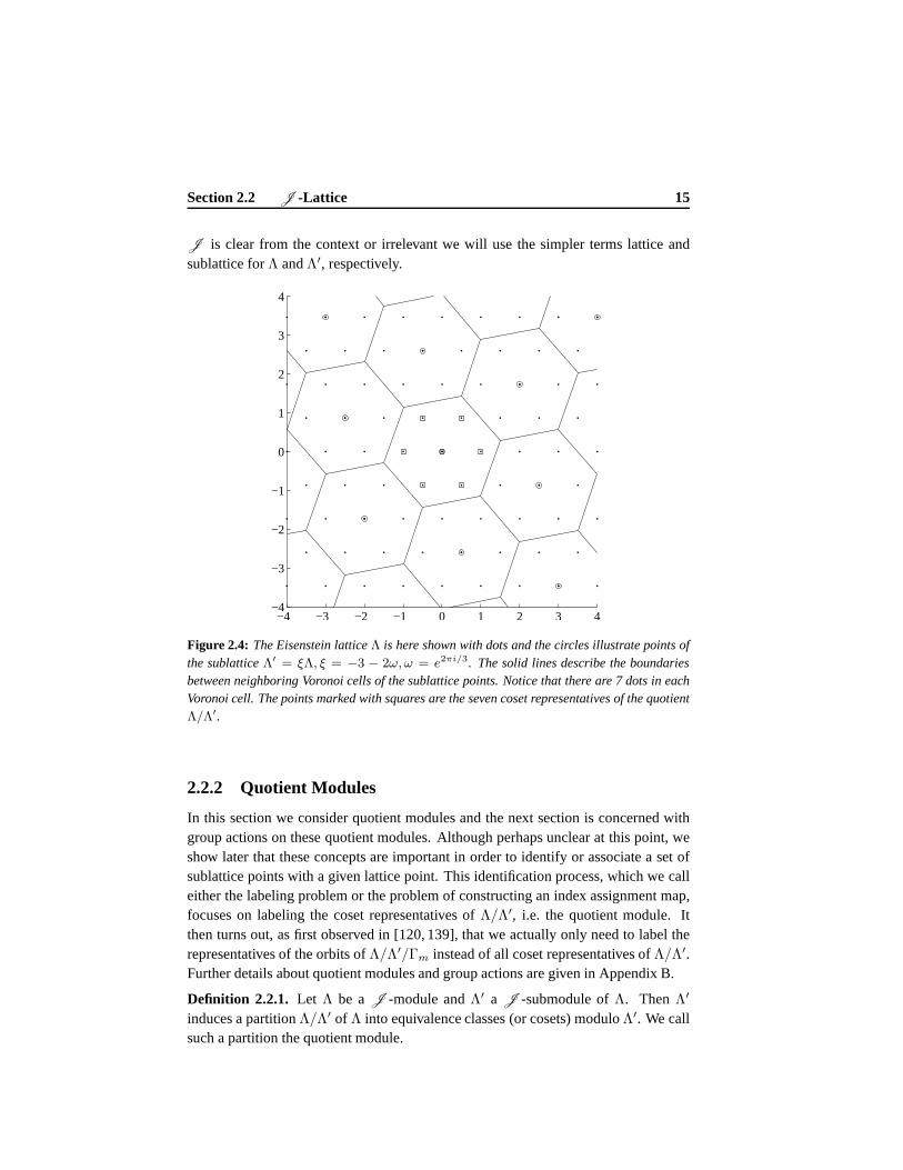
Let Λ be aJ -module. Then we may form the left submoduleΛ′ = ξΛ andthe right submoduleΛ′′ = Λξ by left (or right) multiplication ofΛ by ξ ∈ J .For example letΛ be theJ -module given by the Eisenstein integers, i.e.Λ = E .This lattice can be regarded as a two-dimensional real lattice in R2 in which caseit is usually referred to asA2. Then let us form the submoduleΛ′ = ξΛ whereξ = −3− 2ω andω = e2πi/3, see Fig. 2.4. When the modules in question are latticeswe will usually callΛ a J -lattice andΛ′ a J -sublattice. Sometimes when the ring
Section 2.2 J -Lattice 15
J is clear from the context or irrelevant we will use the simpler terms lattice andsublattice forΛ andΛ′, respectively.
−4 −3 −2 −1 0 1 2 3 4−4
−3
−2
−1
0
1
2
3
4
Figure 2.4: The Eisenstein latticeΛ is here shown with dots and the circles illustrate points ofthe sublatticeΛ′ = ξΛ, ξ = −3 − 2ω, ω = e2πi/3. The solid lines describe the boundariesbetween neighboring Voronoi cells of the sublattice points. Notice that there are 7 dots in eachVoronoi cell. The points marked with squares are the seven coset representatives of the quotientΛ/Λ′.
2.2.2 Quotient Modules
In this section we consider quotient modules and the next section is concerned withgroup actions on these quotient modules. Although perhaps unclear at this point, weshow later that these concepts are important in order to identify or associate a set ofsublattice points with a given lattice point. This identification process, which we calleither the labeling problem or the problem of constructing an index assignment map,focuses on labeling the coset representatives ofΛ/Λ′, i.e. the quotient module. Itthen turns out, as first observed in [120, 139], that we actually only need to label therepresentatives of the orbits ofΛ/Λ′/Γm instead of all coset representatives ofΛ/Λ′.Further details about quotient modules and group actions are given in Appendix B.
Definition 2.2.1. Let Λ be aJ -module andΛ′ a J -submodule ofΛ. ThenΛ′
induces a partitionΛ/Λ′ of Λ into equivalence classes (or cosets) moduloΛ′. We callsuch a partition the quotient module.
16 (Chapter 2) Lattice Theory
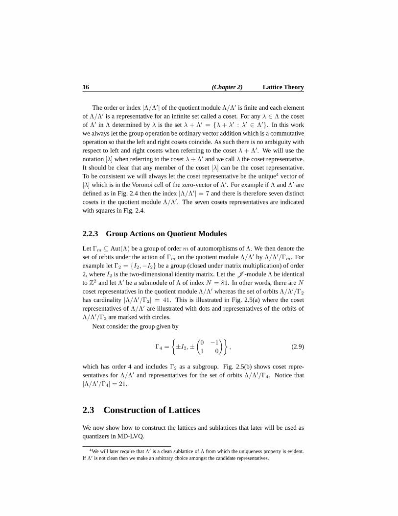
The order or index|Λ/Λ′| of the quotient moduleΛ/Λ′ is finite and each elementof Λ/Λ′ is a representative for an infinite set called a coset. For anyλ ∈ Λ the cosetof Λ′ in Λ determined byλ is the setλ + Λ′ = λ + λ′ : λ′ ∈ Λ′. In this workwe always let the group operation be ordinary vector addition which is a commutativeoperation so that the left and right cosets coincide. As suchthere is no ambiguity withrespect to left and right cosets when referring to the cosetλ + Λ′. We will use thenotation[λ] when referring to the cosetλ+ Λ′ and we callλ the coset representative.It should be clear that any member of the coset[λ] can be the coset representative.To be consistent we will always let the coset representativebe the unique4 vector of[λ] which is in the Voronoi cell of the zero-vector ofΛ′. For example ifΛ andΛ′ aredefined as in Fig. 2.4 then the index|Λ/Λ′| = 7 and there is therefore seven distinctcosets in the quotient moduleΛ/Λ′. The seven cosets representatives are indicatedwith squares in Fig. 2.4.
2.2.3 Group Actions on Quotient Modules
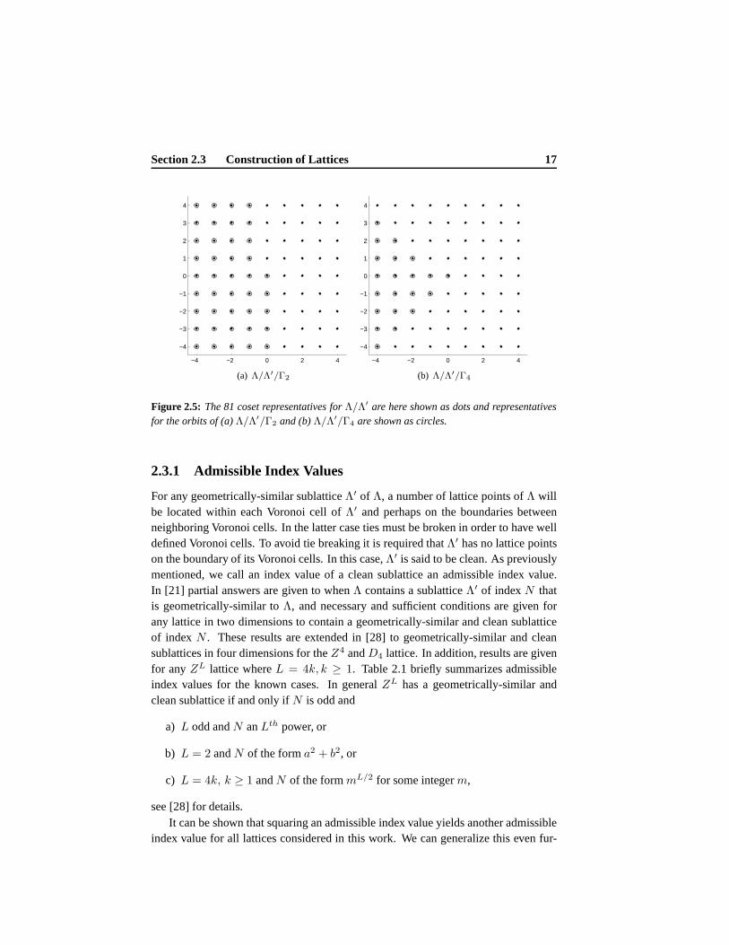
Let Γm ⊆ Aut(Λ) be a group of orderm of automorphisms ofΛ. We then denote theset of orbits under the action ofΓm on the quotient moduleΛ/Λ′ by Λ/Λ′/Γm. Forexample letΓ2 = I2,−I2 be a group (closed under matrix multiplication) of order2, whereI2 is the two-dimensional identity matrix. Let theJ -moduleΛ be identicalto Z2 and letΛ′ be a submodule ofΛ of indexN = 81. In other words, there areNcoset representatives in the quotient moduleΛ/Λ′ whereas the set of orbitsΛ/Λ′/Γ2
has cardinality|Λ/Λ′/Γ2| = 41. This is illustrated in Fig. 2.5(a) where the cosetrepresentatives ofΛ/Λ′ are illustrated with dots and representatives of the orbitsofΛ/Λ′/Γ2 are marked with circles.
Next consider the group given by
Γ4 =
±I2,±(0 −1
1 0
)
, (2.9)
which has order 4 and includesΓ2 as a subgroup. Fig. 2.5(b) shows coset repre-sentatives forΛ/Λ′ and representatives for the set of orbitsΛ/Λ′/Γ4. Notice that|Λ/Λ′/Γ4| = 21.
2.3 Construction of Lattices
We now show how to construct the lattices and sublattices that later will be used asquantizers in MD-LVQ.
4We will later require thatΛ′ is a clean sublattice ofΛ from which the uniqueness property is evident.If Λ′ is not clean then we make an arbitrary choice amongst the candidate representatives.
Section 2.3 Construction of Lattices 17
−4 −2 0 2 4
−4
−3
−2
−1
0
1
2
3
4
(a) Λ/Λ′/Γ2
−4 −2 0 2 4
−4
−3
−2
−1
0
1
2
3
4
(b) Λ/Λ′/Γ4
Figure 2.5: The 81 coset representatives forΛ/Λ′ are here shown as dots and representativesfor the orbits of (a)Λ/Λ′/Γ2 and (b)Λ/Λ′/Γ4 are shown as circles.
2.3.1 Admissible Index Values
For any geometrically-similar sublatticeΛ′ of Λ, a number of lattice points ofΛ willbe located within each Voronoi cell ofΛ′ and perhaps on the boundaries betweenneighboring Voronoi cells. In the latter case ties must be broken in order to have welldefined Voronoi cells. To avoid tie breaking it is required thatΛ′ has no lattice pointson the boundary of its Voronoi cells. In this case,Λ′ is said to be clean. As previouslymentioned, we call an index value of a clean sublattice an admissible index value.In [21] partial answers are given to whenΛ contains a sublatticeΛ′ of indexN thatis geometrically-similar toΛ, and necessary and sufficient conditions are given forany lattice in two dimensions to contain a geometrically-similar and clean sublatticeof indexN . These results are extended in [28] to geometrically-similar and cleansublattices in four dimensions for theZ4 andD4 lattice. In addition, results are givenfor anyZL lattice whereL = 4k, k ≥ 1. Table 2.1 briefly summarizes admissibleindex values for the known cases. In generalZL has a geometrically-similar andclean sublattice if and only ifN is odd and
a) L odd andN anLth power, or
b) L = 2 andN of the forma2 + b2, or
c) L = 4k, k ≥ 1 andN of the formmL/2 for some integerm,
see [28] for details.It can be shown that squaring an admissible index value yields another admissible
index value for all lattices considered in this work. We can generalize this even fur-
18 (Chapter 2) Lattice Theory
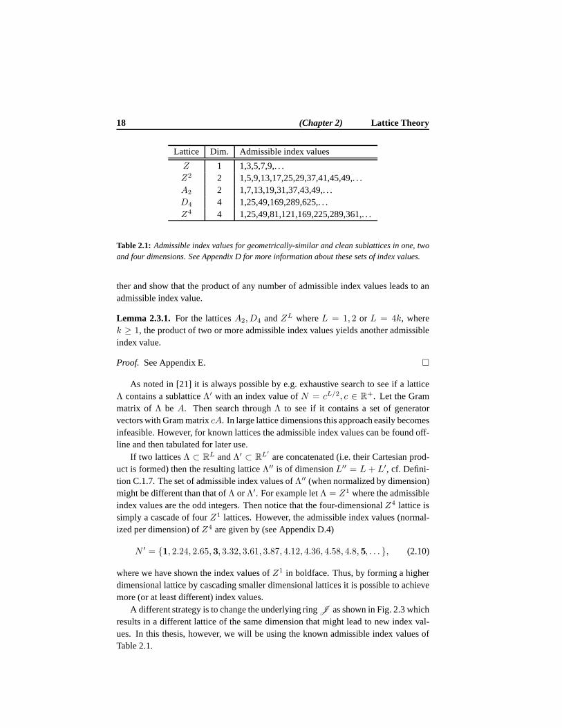
Lattice Dim. Admissible index values
Z 1 1,3,5,7,9,. . .Z2 2 1,5,9,13,17,25,29,37,41,45,49,. . .A2 2 1,7,13,19,31,37,43,49,. . .D4 4 1,25,49,169,289,625,. . .Z4 4 1,25,49,81,121,169,225,289,361,. . .
Table 2.1: Admissible index values for geometrically-similar and clean sublattices in one, twoand four dimensions. See Appendix D for more information about these sets of index values.
ther and show that the product of any number of admissible index values leads to anadmissible index value.
Lemma 2.3.1. For the latticesA2, D4 andZL whereL = 1, 2 or L = 4k, wherek ≥ 1, the product of two or more admissible index values yields another admissibleindex value.
Proof. See Appendix E.
As noted in [21] it is always possible by e.g. exhaustive search to see if a latticeΛ contains a sublatticeΛ′ with an index value ofN = cL/2, c ∈ R+. Let the Grammatrix of Λ beA. Then search throughΛ to see if it contains a set of generatorvectors with Gram matrixcA. In large lattice dimensions this approach easily becomesinfeasible. However, for known lattices the admissible index values can be found off-line and then tabulated for later use.
If two latticesΛ ⊂ RL andΛ′ ⊂ RL′
are concatenated (i.e. their Cartesian prod-uct is formed) then the resulting latticeΛ′′ is of dimensionL′′ = L + L′, cf. Defini-tion C.1.7. The set of admissible index values ofΛ′′ (when normalized by dimension)might be different than that ofΛ orΛ′. For example letΛ = Z1 where the admissibleindex values are the odd integers. Then notice that the four-dimensionalZ4 lattice issimply a cascade of fourZ1 lattices. However, the admissible index values (normal-ized per dimension) ofZ4 are given by (see Appendix D.4)
N ′ = 1, 2.24, 2.65,3, 3.32, 3.61, 3.87, 4.12, 4.36, 4.58, 4.8,5, . . . , (2.10)
where we have shown the index values ofZ1 in boldface. Thus, by forming a higherdimensional lattice by cascading smaller dimensional lattices it is possible to achievemore (or at least different) index values.
A different strategy is to change the underlying ringJ as shown in Fig. 2.3 whichresults in a different lattice of the same dimension that might lead to new index val-ues. In this thesis, however, we will be using the known admissible index values ofTable 2.1.

Section 2.3 Construction of Lattices 19
2.3.2 Sublattices
In this section we construct sublattices and primarily focus on a special type of sub-lattices called product lattices. In [28] the following definition of a product lattice waspresented.
Definition 2.3.1 ( [28]). Let J be an arbitrary ring, letΛ = J and form the twosublatticesΛ0 = ξ0Λ andΛ1 = Λξ1, ξi ∈ Λ, i = 0, 1. Then the latticeΛπ = ξ0Λξ1is called a product lattice and it satisfiesΛπ ⊆ Λi, i = 0, 1.
In this work, however, we will make use of a more general notion of a product latticewhich includes Definition 2.3.1 as a special case.
Definition 2.3.2. A product latticeΛπ is any sublattice satisfyingΛπ ⊆ Λi whereΛi = ξiΛ orΛi = Λξi, i = 0, . . . ,K − 1.
The construction of product lattices based on two sublattices as described inDefinition 2.3.1 was treated in detail in [28]. In this section we extend the existingresults of [28] and construct product lattices based on morethan two sublattices forL = 1, 2 and4 dimensions for the root latticesZ1, Z2, A2, Z
4 andD4, which aredescribed in Appendix D. Along the same lines as in [28] we construct sublatticesand product lattices by use of the ordinary rational integersZ as well as the GaussianintegersG , Eisenstein integersE , Lipschitz integral QuaternionsH0 and the Hurwitzintegral QuaternionsH1, whereG andE are given by (2.5) and (2.6), respectively,and [22]
H0 = ξ1 + iξ2 + jξ3 + kξ4 : ξ1, ξ2, ξ3, ξ4 ∈ Z, (2.11)
H1 = ξ1 + iξ2 + jξ3 + kξ4 : ξ1, ξ2, ξ3, ξ4 all in Z or all in Z+ 1/2, (2.12)
wherei, j andk are unit Quaternions, see Appendix A for more information. Forexample a sublatticeΛ1 of Λ = Z is easily constructed, simply by multiplying allpointsλ ∈ Λ by ξ whereξ ∈ Z\0.5 This gives a geometrically-similar sublatticeΛ1 = ξZ of index |ξ|. This way of constructing sublattices may be generalized byconsidering different rings of integers. For example, for the square latticeΛ = G
whose points lie in the complex plane, a geometrically-similar sublattice of index 2may be obtained by multiplying all elements ofΛ by the Gaussian integerξ = 1 + i.
Sublattices and product lattices ofZ1, Z2 andA2
The construction of product lattices based on the sublatticesZ1, Z2 andA2 is astraight forward generalization of the approach taken in [28]. Let the latticeΛ beany one ofZ1 = Z, Z2 = G orA2 = E and let the geometrically-similar sublatticesΛi be given byξiΛ whereξi is an element of the rational integersZ, the GaussianintegersG or the Eisenstein integersE , respectively.
5SinceΛ is a torsion freeJ -module the submoduleΛ′ = ξΛ is a non-trivial cyclic submodule when-ever0 6= ξ ∈ Λ.
20 (Chapter 2) Lattice Theory
Lemma 2.3.2.Λπ = ξ0ξ1 · · · ξK−1Λ is a product lattice.
Proof. See Appendix E.
Also, as remarked in [28], since the three rings considered are unique factorizationrings, the notion of least common multiple (lcm) is well defined. Let us defineξ∩ ,
lcm(ξ0, . . . , ξK−1) so thatξi|ξ∩, i.e.ξi dividesξ∩. This leads to the following lemma.
Lemma 2.3.3.Λ′π = ξ∩Λ is a product lattice.
Proof. See Appendix E.
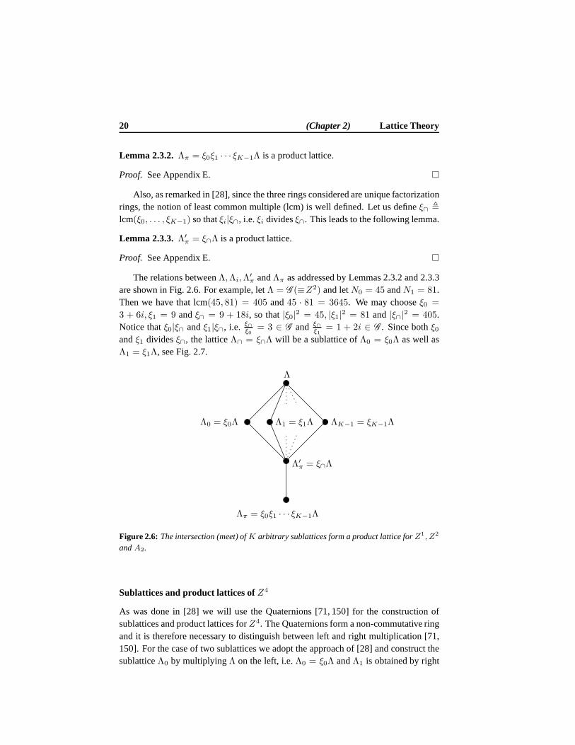
The relations betweenΛ,Λi,Λ′π andΛπ as addressed by Lemmas 2.3.2 and 2.3.3
are shown in Fig. 2.6. For example, letΛ = G (≡Z2) and letN0 = 45 andN1 = 81.Then we have that lcm(45, 81) = 405 and45 · 81 = 3645. We may chooseξ0 =
3 + 6i, ξ1 = 9 andξ∩ = 9 + 18i, so that|ξ0|2 = 45, |ξ1|2 = 81 and|ξ∩|2 = 405.Notice thatξ0|ξ∩ andξ1|ξ∩, i.e. ξ∩
ξ0= 3 ∈ G and ξ∩
ξ1= 1 + 2i ∈ G . Since bothξ0
andξ1 dividesξ∩, the latticeΛ∩ = ξ∩Λ will be a sublattice ofΛ0 = ξ0Λ as well asΛ1 = ξ1Λ, see Fig. 2.7.
PSfrag replacements
Λ
Λ0 = ξ0Λ Λ1 = ξ1Λ ΛK−1 = ξK−1Λ
Λ′π = ξ∩Λ
Λπ = ξ0ξ1 · · · ξK−1Λ
Figure 2.6: The intersection (meet) ofK arbitrary sublattices form a product lattice forZ1, Z2
andA2.
Sublattices and product lattices ofZ4
As was done in [28] we will use the Quaternions [71, 150] for the construction ofsublattices and product lattices forZ4. The Quaternions form a non-commutative ringand it is therefore necessary to distinguish between left and right multiplication [71,150]. For the case of two sublattices we adopt the approach of[28] and construct thesublatticeΛ0 by multiplyingΛ on the left, i.e.Λ0 = ξ0Λ andΛ1 is obtained by right
Section 2.3 Construction of Lattices 21
−20 −15 −10 −5 0 5 10 15 20−20
−15
−10
−5
0
5
10
15
20
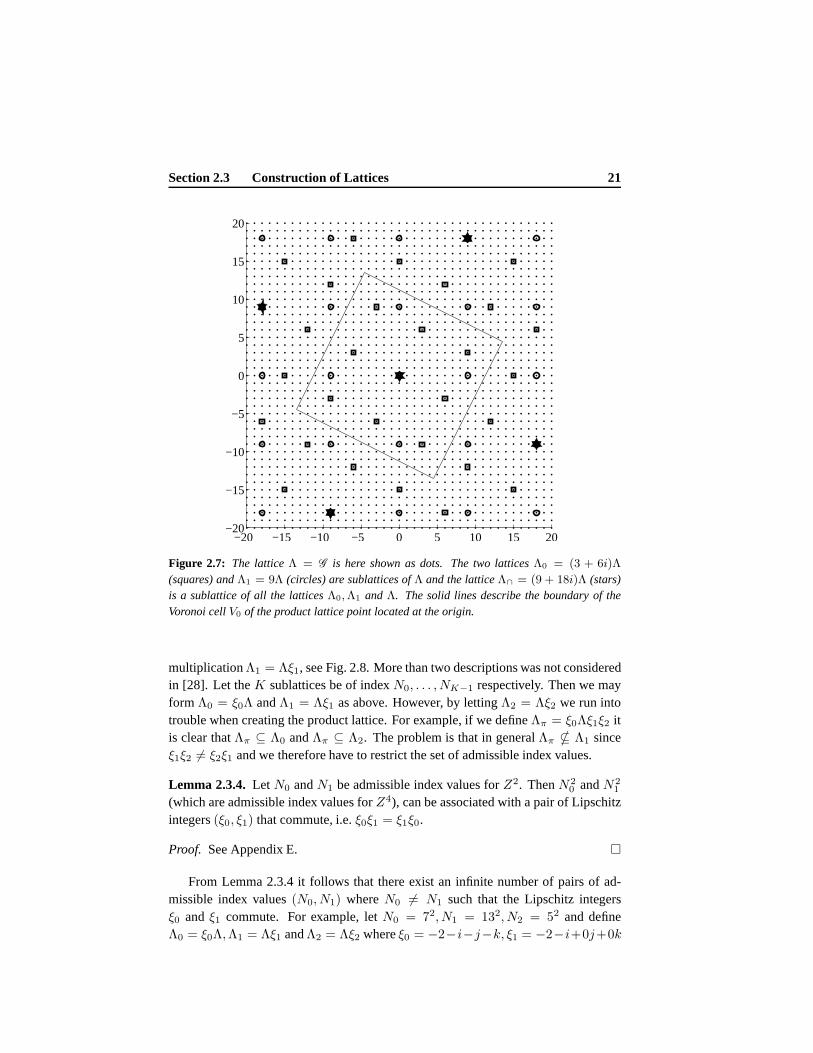
Figure 2.7: The latticeΛ = G is here shown as dots. The two latticesΛ0 = (3 + 6i)Λ
(squares) andΛ1 = 9Λ (circles) are sublattices ofΛ and the latticeΛ∩ = (9 + 18i)Λ (stars)is a sublattice of all the latticesΛ0,Λ1 andΛ. The solid lines describe the boundary of theVoronoi cellV0 of the product lattice point located at the origin.
multiplicationΛ1 = Λξ1, see Fig. 2.8. More than two descriptions was not consideredin [28]. Let theK sublattices be of indexN0, . . . , NK−1 respectively. Then we mayform Λ0 = ξ0Λ andΛ1 = Λξ1 as above. However, by lettingΛ2 = Λξ2 we run intotrouble when creating the product lattice. For example, if we defineΛπ = ξ0Λξ1ξ2 itis clear thatΛπ ⊆ Λ0 andΛπ ⊆ Λ2. The problem is that in generalΛπ * Λ1 sinceξ1ξ2 6= ξ2ξ1 and we therefore have to restrict the set of admissible indexvalues.
Lemma 2.3.4. LetN0 andN1 be admissible index values forZ2. ThenN20 andN2
1
(which are admissible index values forZ4), can be associated with a pair of Lipschitzintegers(ξ0, ξ1) that commute, i.e.ξ0ξ1 = ξ1ξ0.
Proof. See Appendix E.
From Lemma 2.3.4 it follows that there exist an infinite number of pairs of ad-missible index values(N0, N1) whereN0 6= N1 such that the Lipschitz integersξ0 andξ1 commute. For example, letN0 = 72, N1 = 132, N2 = 52 and defineΛ0 = ξ0Λ,Λ1 = Λξ1 andΛ2 = Λξ2 whereξ0 = −2−i−j−k, ξ1 = −2−i+0j+0k
22 (Chapter 2) Lattice Theory
PSfrag replacements
Λ
Λ0 = ξ0Λ Λ1 = Λξ1
Λπ = ξ0Λξ1
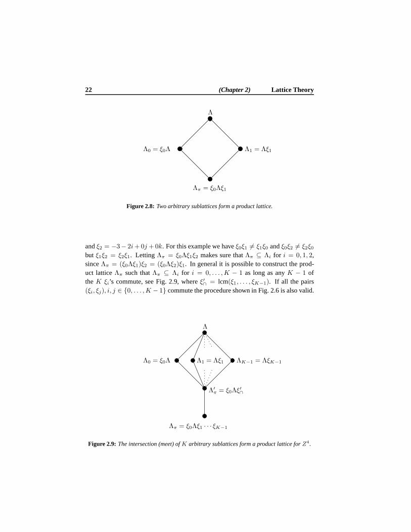
Figure 2.8: Two arbitrary sublattices form a product lattice.
andξ2 = −3− 2i+0j +0k. For this example we haveξ0ξ1 6= ξ1ξ0 andξ0ξ2 6= ξ2ξ0but ξ1ξ2 = ξ2ξ1. LettingΛπ = ξ0Λξ1ξ2 makes sure thatΛπ ⊆ Λi for i = 0, 1, 2,sinceΛπ = (ξ0Λξ1)ξ2 = (ξ0Λξ2)ξ1. In general it is possible to construct the prod-uct latticeΛπ such thatΛπ ⊆ Λi for i = 0, . . . ,K − 1 as long as anyK − 1 oftheK ξi’s commute, see Fig. 2.9, whereξ′∩ = lcm(ξ1, . . . , ξK−1). If all the pairs(ξi, ξj), i, j ∈ 0, . . . ,K − 1 commute the procedure shown in Fig. 2.6 is also valid.
PSfrag replacements
Λ
Λ0 = ξ0Λ Λ1 = Λξ1 ΛK−1 = ΛξK−1
Λ′π = ξ0Λξ
′∩
Λπ = ξ0Λξ1 · · · ξK−1
Figure 2.9: The intersection (meet) ofK arbitrary sublattices form a product lattice forZ4.
Section 2.3 Construction of Lattices 23
Sublattices and product lattices ofD4
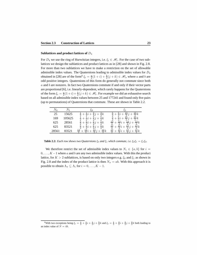
ForD4 we use the ring of Hurwitzian integers, i.e.ξi ∈ H1. For the case of two sub-lattices we design the sublattices and product lattices as in [28] and shown in Fig. 2.8.For more than two sublattices we have to make a restriction onthe set of allowableadmissible index values. The Quaternions leading to admissible index values forD4
obtained in [28] are of the form6 ξi = a2 (1 + i) + b
2 (j + k) ∈ H1, wherea andb areodd positive integers. Quaternions of this form do generally not commute since botha andb are nonzero. In fact two Quaternions commute if and only if their vector partsare proportional [6], i.e. linearly-dependent, which rarely happens for the Quaternionsof the formξi = a
2 (1+ i)+b2 (j+k) ∈ H1. For example we did an exhaustive search
based on all admissible index values between 25 and 177241 and found only five pairs(up to permutations) of Quaternions that commute. These areshown in Table 2.2.
N0 N1 ξ0 ξ125 15625 1
2 + 12 i+
32j +
32k
52 + 5
2 i+152 j +
152 k
169 105625 12 + 1
2 i+52j +
52k
52 + 5
2 i+252 j +
252 k
625 28561 52 + 5
2 i+52j +
52k
132 + 13
2 i+132 j +
132 k
625 83521 52 + 5
2 i+52j +
52k
172 + 17
2 i+172 j +
172 k
28561 83521 132 + 13
2 i+132 j +
132 k
172 + 17
2 i+172 j +
172 k
Table 2.2: Each row shows two Quaternionsξ0 andξ1 which commute, i.e.ξ0ξ1 = ξ1ξ0.
We therefore restrict the set of admissible index values toNi ∈ a, b for i =
0, . . . ,K−1 wherea andb are any two admissible index values. With this the productlattice, forK > 2 sublattices, is based on only two integers e.g.ξ0 andξ1 as shown inFig. 2.8 and the index of the product lattice is thenNπ = ab. With this approach it ispossible to obtainΛπ ⊆ Λi for i = 0, . . . ,K − 1.
6With two exceptions beingξi = 12+ 1
2i + 1
2j + 5
2k andξi = 1
2+ 3
2i + 3
2j + 3
2k both leading to
an index value ofN = 49.

Chapter3Single-Description Rate-Distortion
Theory
Source coding with a fidelity criterion, also called rate-distortion theory (or lossysource coding), was introduced by Shannon in his two landmark papers from1948 [121] and 1959 [122] and has ever since received a lot of attention. For anintroduction to rate-distortion theory we refer the readerto the survey papers by Ki-effer [74] and Berger and Gibson [9] and the text books by Berger [8], Ciszár andKörner [26] and Cover and Thomas [24].
3.1 Rate-Distortion Function
A fundamental problem of rate-distortion theory is that of describing the rateRrequired to encode a sourceX at a prescribed distortion (fidelity) levelD. LetXL = Xi, i = 1, . . . , L be a sequence of random variables (or letters) of a station-ary7 random processX . LetX be the reproduction ofX and letx andx be realizationsofX andX , respectively. The alphabetsX andX of X andX , respectively, can becontinuous or discrete and in the latter case we distinguishbetween discrete alphabetsof finite or countably infinite cardinality. When it is clear from context we will oftenignore the superscriptL which indicates the dimension of the variable or alphabet sothatx ∈ X ⊂ RL denotes anL-dimensional vector or element of the alphabetX
which is a subset ofRL.
Definition 3.1.1. A fidelity criterion for the sourceX is a family ρ(L)(X, X), L ∈N of distortion measures of whichρ(L) computes the distortion when representing
7Throughout this work we will assume all stochastic processes to be discrete-time zero-mean weak-sense stationary processes (unless otherwise stated).
25
26 (Chapter 3) Single-Description Rate-Distortion Theory
X by X. If ρ(L)(X, X) , 1L
∑Li=1 ρ(Xi, Xi) thenρ is said to be a single-letter
fidelity criterion and we will then use the notationρ(X, X). Distortion measures ofthe formρ(X−X) are called difference distortion measures. For exampleρ(X, X) =1L‖X−X‖2 is a difference distortion measure (usually referred to as the squared-errordistortion measure).
In this work we will be mainly interested in the squared-error single-letter fidelitycriterion which is defined by
ρ(X, X) ,1
L
L∑
i=1
(Xi − Xi)2. (3.1)
With this, formally stated, Shannon’s rate-distortion functionR(D) (expressed inbit/dim.) for stationary sources with memory and single-letter fidelity criterion,ρ, isdefined as [8]
R(D) , limL→∞
RL(D), (3.2)
where theLth order rate-distortion function is given by
RL(D) = inf 1LI(X ; X) : Eρ(X, X) ≤ D, (3.3)
whereI(X ; X) denotes the mutual information8 betweenX andX, E denotes thestatistical expectation operator and the infimum is over allconditional distributionsfX|X(x|x) for which the joint distributionsfX,X(x, x) = fX(x)fX|X(x|x) satisfythe expected distortion constraint given by
∫
X
∫
X
fX(x)fX|X(x|x)ρ(x, x)dxdx ≤ D. (3.4)
TheLth order rate-distortion functionRL(D) can be seen as the rate-distortion func-tion of anL-dimensional i.i.d. vector sourceX producing vectors with the distributionof X [82].
Let h(X) denote the differential entropy (or continuous entropy) ofX which isgiven by [24]
h(X) = −∫
X
fX(x) log2(fX(x)) dx
and let the differential entropy rateh(X) be defined byh(X) , limL→∞1Lh(X)
where for independently and identically distributed (i.i.d.) scalar processesh(X) =
8The mutual information between to continuous-alphabet sourcesX andX with a joint pdffX,X andmarginalsfX andf
X, respectively, is defined as [24]
I(X; X) =
∫
X
∫
X
fX,X(x, x) log2
(fX,X(x, x)
fX(x)f
X(x)
)
dxdx.
Section 3.1 Rate-Distortion Function 27
1Lh(X). With a slight abuse of notation we will also use the notationh(X) to indicatethe dimension normalized differential entropy of an i.i.d.vector source. Ifρ is a dif-ference distortion measure, then (3.2) and (3.3) can be lower bounded by the Shannonlower bound [8]. Specifically, ifEρ is the mean squared error (MSE) fidelity criterion,then [8,82]
R(D) ≥ h(X)− 1
2log2(2πeD), (3.5)
where equality holds at almost all distortion levelsD for a (stationary) Gaussiansource [8].9 In addition it has been shown that (3.5) becomes asymptotically tightat high resolution, i.e. asD → 0, for sources with finite differential entropies andfinite second moments for general difference distortion measures, cf. [82].
Recall that the differential entropy of a jointly Gaussian vector is given by [24]
h(X) =1
2log2((2πe)
L|Φ|), (3.6)
where|Φ| is the determinant ofΦ = EXXT , i.e. the covariance matrix ofX . Itfollows from (3.5) that the rate-distortion function of a memoryless scalar Gaussianprocess of varianceσ2
X is given by
R(D) =1
2log2
(σ2X
D
)
, (3.7)
wheneverD ≤ σ2X andR(D) = 0 for D > σ2
X sinceR(D) is everywhere non-negative.
The inverse ofR(D) is called the distortion-rate functionD(R) and it basicallysays that if a source sequence is encoded at a rateR the distortion is at leastD(R).From (3.7) we see that the distortion-rate function of the memoryless Gaussian processis given by
D(R) = σ2X2−2R, (3.8)
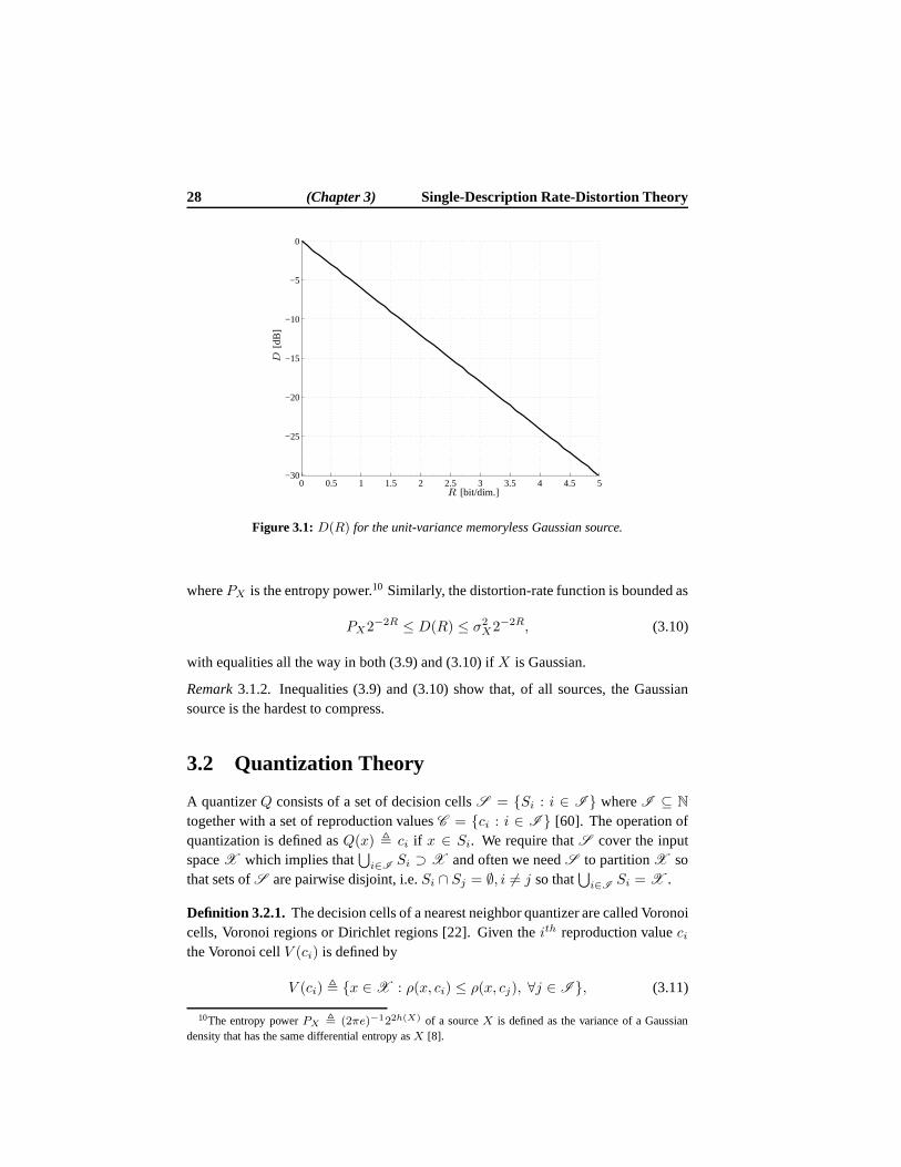
which is shown in Fig. 3.1 for the case ofσ2X = 1.
Remark3.1.1. From (3.8) and also from Fig. 3.1 it may be seen that each extrabitreduces the distortion by a factor of four — a phenomena oftenreferred to as the “6dB per bit rule” [60]. In fact, the “6 dB per bit rule” is approximately true not just forthe Gaussian source but for arbitrary sources.
The rate-distortion function of a memoryless scalar sourceand squared-error dis-tortion measure may be upper and lower bounded by use of the entropy-power in-equality, that is [8]
1
2log2
(σ2X
D
)
≥ R(D) ≥ 1
2log2
(PX
D
)
, (3.9)
9Eq. (3.5) is tight for allD ≤ essinf SX , whereSX is the power spectrum of a stationary GaussianprocessX [8].
28 (Chapter 3) Single-Description Rate-Distortion Theory
0 0.5 1 1.5 2 2.5 3 3.5 4 4.5 5−30
−25
−20
−15
−10
−5
0
PSfrag replacements
D[d
B]
R [bit/dim.]
Figure 3.1:D(R) for the unit-variance memoryless Gaussian source.
wherePX is the entropy power.10 Similarly, the distortion-rate function is bounded as
PX2−2R ≤ D(R) ≤ σ2X2−2R, (3.10)
with equalities all the way in both (3.9) and (3.10) ifX is Gaussian.
Remark3.1.2. Inequalities (3.9) and (3.10) show that, of all sources, theGaussiansource is the hardest to compress.
3.2 Quantization Theory
A quantizerQ consists of a set of decision cellsS = Si : i ∈ I whereI ⊆ Ntogether with a set of reproduction valuesC = ci : i ∈ I [60]. The operation ofquantization is defined asQ(x) , ci if x ∈ Si. We require thatS cover the inputspaceX which implies that
⋃
i∈ISi ⊃ X and often we needS to partitionX so
that sets ofS are pairwise disjoint, i.e.Si ∩ Sj = ∅, i 6= j so that⋃
i∈ISi = X .
Definition 3.2.1. The decision cells of a nearest neighbor quantizer are called Voronoicells, Voronoi regions or Dirichlet regions [22]. Given theith reproduction valuecithe Voronoi cellV (ci) is defined by
V (ci) , x ∈ X : ρ(x, ci) ≤ ρ(x, cj), ∀j ∈ I , (3.11)
10The entropy powerPX , (2πe)−122h(X) of a sourceX is defined as the variance of a Gaussiandensity that has the same differential entropy asX [8].

Section 3.2 Quantization Theory 29
where ties (if any) can be arbitrarily broken.11
It follows that the expected distortion of a quantizer is given by
DQ =∑
i∈I
∫
x∈Si
fX(x)ρ(x, ci) dx. (3.12)
Let us for the moment assume thatX = RL andC = X ⊂ RL. Then, forthe squared error distortion measure, the Voronoi cells of an L-dimensional nearestneighbor quantizer (vector quantizer) are defined as
V (xi) , x ∈ RL : ‖x− xi‖2 ≤ ‖x− xj‖2, ∀xj ∈ X , xi ∈ X , (3.13)
where‖ · ‖ denotes theℓ2-norm, i.e.‖x‖2 =∑L
n=1 x2n.
Vector quantizers are often classified as either entropy-constrained quantizers orresolution-constrained quantizers or as a mixed class where for example the outputof a resolution-constrained quantizer is further entropy coded.12 When designing anentropy-constrained quantizer one seeks to form the Voronoi regionsV (xi), xi ∈ X ,and the reproduction alphabetX such that the distortionDQ is minimized subject toan entropy constraintR on the discrete entropyH(X). Recall that the discrete entropyof a random variable is given by [24]
H(X) = −∑
i∈I
P (xi) log2(P (xi)), (3.14)
whereP denotes probability andP (xi) = P (x ∈ V (xi)). On the other hand, inresolution-constrained quantization the distortion is minimized subject to a constrainton the cardinality of the reproduction alphabet. In this case the elements ofX arecoded with a fixed rate ofR = log2(|X |)/L. For large vector dimensions, i.e. whenL ≫ 1, it is very likely that randomly chosen source vectors belong to a typical setA (L) in which the elements are approximately uniformly distributed [24]. As a con-sequence, in this situation there is not much difference between entropy-constrainedand resolution-constrained quantization.
There exists several iterative algorithms for designing vector quantizers. Oneof the earliest such algorithms is the Lloyd algorithm whichis used to constructresolution-constrained scalar quantizers [87], see also [88]. The Lloyd algorithm isbasically a cyclic minimizer that alternates between two phases:
1. Given a codebookC = X find the optimal partition of the input space, i.e.form the Voronoi cellsV (xi), ∀xi ∈ X .
11Two neighboringL-dimensional Voronoi cells for continuous-alphabet sources share a commonL′-dimensional face whereL′ ≤ L− 1. For discrete-alphabet sources it is also possible that a point is equallyspaced between two or more centroids of the codebook, in which case tie breaking is necessary in order tomake sure that the point is not assigned to more than one Voronoi cell.
12Entropy-constrained quantizers (resp. resolution-constrained quantizers) are also called variable-ratequantizers (resp. fixed-rate quantizers).
30 (Chapter 3) Single-Description Rate-Distortion Theory
2. Given the partition, form an optimal codebook, i.e. letxi ∈ X be the centroidof the setx ∈ V (xi).
If an analytical description of the pdf is unavailable it is possible to estimate the pdfby use of empirical observations [45]. Furthermore, Lloyd’s algorithm has been ex-tended to the vector case [45, 81] but has not been explicitlyextended to the case ofentropy-constrained vector quantization. Towards that end Chou et al. [19] presentedan iterative algorithm based on a Lagrangian formulation ofthe optimization problem.In general these empirically designed quantizers are only locally optimal and unlesssome structure is enforced on the codebooks, the search complexity easily becomesoverwhelming (the computational complexity of an unconstrained quantizer increasesexponentially with dimension) [45]. There exists a great deal of different design al-gorithms and we refer the reader to the text books [22, 45, 57]as well as the in-deptharticle by Gray and Neuhoff [60] for more information about the theory and practiceof vector quantization.
3.3 Lattice Vector Quantization
In this work we will focus on structured vector quantizationand more specifically onlattice vector quantization (LVQ) [22,46,57]. A family of highly structured quantizersis the tesselating quantizers which includes lattice vector quantizers as a sub family.In a tesselating quantizer all decision cells are translated and possibly rotated andreflected versions of a prototype cell, sayV0. In a lattice vector quantizer all Voronoicells are translations ofV0 which is then taken to beV0 , V (0), i.e. the Voronoi cell ofthe reproduction point located at the origin (the zero vector) so thatV (xi) = V0+xi.13
In a high-resolution lattice vector quantizer the reproduction alphabetX is usuallygiven by anL-dimensional latticeΛ ⊂ RL, see Appendices C and D for more detailsabout lattices.
In order to describe the performance of a lattice vector quantizer it is convenient tomake use of high resolution (or high rate) assumptions whichfor a stationary sourcecan be summarized as follows [45,57]:
1. The rate or entropy of the codebook is large, which means that the variance ofthe quantization error is small compared to the variance of the source. Thus, thepdf of the source can be considered constant within a Voronoicell, i.e.fX(x) ≈fX(xi) if x ∈ V (xi). Hence, the geometric centroids of the Voronoi cells areapproximately the midpoints of the cells
2. The quantization noise process tends to be uncorrelated even when the sourceis correlated
13Notice that not all tesselating quantizers are lattice quantizers. For example, a tesselating quantizerhaving triangular shaped decision cells is not a lattice vector quantizer.
Section 3.3 Lattice Vector Quantization 31
3. The quantization error is approximately uncorrelated with the source
Notice that 1) is always true if the source distribution is uniform. Furthermore, allthe above assumptions have been justified rigorously in the limit as the variance ofthe quantization error tends to zero for the case of smooth sources (i.e. continuous-alphabet sources having finite differential entropies) [86, 145, 161]. If subtractivedither is used, as is the case of entropy-constrained dithered (lattice) quantization(ECDQ), the above assumptions are valid at any resolution and furthermore the quan-tization errors are independent of the source [159,160,165]. A nice property of ECDQis that the additive noise model is accurate at any resolution, so that the quantizationoperation can be modeled as an additive noise process [160].The dither signal of anECDQ is an i.i.d. random14 process which is uniformly distributed over a Voronoi cellof the quantizer so that for a scalar quantizer the distribution of the quantization errorsis uniform. Asymptotically, as the dimension of the ECDQ grows unboundedly, anyfinite-dimensional marginal of the noise process becomes jointly Gaussian distributedand the noise process becomes Gaussian distributed in the divergence15 sense [161].These properties of the noise process are also valid for entropy-constrained LVQ(without dither) under high resolution assumptions [161].It is interesting to see that atvery low resolution, i.e. as the variance of the quantization error tends to the varianceof the source, the performance of an entropy-constrained scalar quantizer is asymptot-ically as good as any vector quantizer [91].
3.3.1 LVQ Rate-Distortion Theory
LetH denote the discrete entropyH(X ) of the codebook of an entropy-constrainedvector quantizer and let the dimension-normalized MSE distortion measureDL bedefined as
DL ,1
LE‖X − X‖2. (3.15)
Then by extending previous results of Bennett [7] for high resolution scalar quantiza-tion to the vector case it was shown by Zador [156] that ifX has a probability densitythen16
limH→∞
DL22H/L = aL2
2h(X)/L, (3.16)
whereh(X) is the differential entropy ofX andaL is a constant that depends only onL. In the scalar case whereL = 1 it was shown by Gish and Pierce [47] thata1 = 1/12
14The dither signal is assumed known at the decoder so it is in fact a pseudo-random process.15The information divergence (also called Kullback-Leiblerdistance or relative entropy) between two
pdfsfX andgX is defined as [24]
D(f‖g) =∫
X
fX(x) log2(fX (x)/g
X(x)) dx.
16Later on the precise requirements on the source for (3.16) tobe valid was formalized by Linder andZeger [86].
32 (Chapter 3) Single-Description Rate-Distortion Theory
and that the quantizer that achieves this value is the unbounded uniform scalar (lattice)quantizer. For the case of1 < L < ∞ the value ofaL is unknown [86].17 It wasconjectured by Gersho in 1979 [44] that if the source distribution is uniform overa bounded convex set inRL then the optimal quantizer will have a partition whoseregions are all congruent to some polytope. Today, more than25 years after, thisconjecture remains open. But if indeed it is true then, at high resolution, the optimalentropy-constrained quantizer is a tessellating quantizer independent of the sourcedistribution (as long as it is smooth).
The distortion at high resolution of an entropy-constrained lattice vector quantizeris given by [44,86]
DL ≈ G(Λ)ν2/L, (3.17)
whereν (the volume of a fundamental region of the lattice) is given by
ν2/L = 22(h(X)−H)/L. (3.18)
Thus, if we assume that Gersho’s conjecture is true and furthermore assume that alattice vector quantizer is optimal then (3.17) implies that aL = G(Λ). By inserting(3.18) in (3.17) the discrete entropy (again at high resolution) is found to be given by
H(X ) ≈ h(X)− L
2log2
(DL
G(Λ)
)
[bit] . (3.19)
The Shannon lower bound is the most widely used tool to relatethe performanceof lattice quantizers to the rate-distortion function of a source. For example, at highresolution, the Shannon lower bound is tight for all smooth sources, thus
R(D) ≈ h(X)− 1
2log2(2πeD) [bit/dim.], (3.20)
so that the asymptotic rate-redundancyRred of a lattice vector quantizer over the rate-distortion function of a smooth source under the MSE distortion measure is18
Rred =1
2log2(2πeG(Λ)) [bit/dim.] (3.21)
From (3.17) it may be noticed that the distortion of a latticevector quantizer issource independent and in fact, for fixedν, the distortion only depends uponG(Λ).Furthermore,G(Λ) is scale and rotation invariant and depends only upon the shape ofthe fundamental regionV0 of the latticeΛ [22]. In general the more sphere-like shapeof V0 the smallerG(Λ) [22]. It follows thatG(Λ) is lower bounded byG(SL) thedimensionless normalized second moment of anL-sphere where [22]
G(SL) =1
(L+ 2)πΓ
(L
2+ 1
)2/L
, (3.22)
17For the case of resolution-constrained quantization botha1 anda2 are known [58].18Rred is in fact the divergence of the quantization noise from Gaussianity in high resolution lattice vector
quantization.
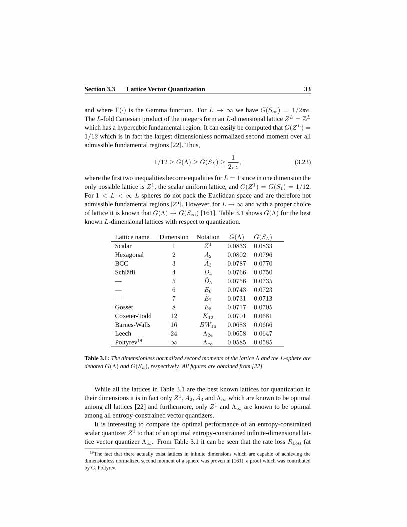
Section 3.3 Lattice Vector Quantization 33
and whereΓ(·) is the Gamma function. ForL → ∞ we haveG(S∞) = 1/2πe.TheL-fold Cartesian product of the integers form anL-dimensional latticeZL = ZL
which has a hypercubic fundamental region. It can easily be computed thatG(ZL) =
1/12 which is in fact the largest dimensionless normalized second moment over alladmissible fundamental regions [22]. Thus,
1/12 ≥ G(Λ) ≥ G(SL) ≥1
2πe, (3.23)
where the first two inequalities become equalities forL = 1 since in one dimension theonly possible lattice isZ1, the scalar uniform lattice, andG(Z1) = G(S1) = 1/12.For 1 < L < ∞ L-spheres do not pack the Euclidean space and are therefore notadmissible fundamental regions [22]. However, forL→ ∞ and with a proper choiceof lattice it is known thatG(Λ) → G(S∞) [161]. Table 3.1 showsG(Λ) for the bestknownL-dimensional lattices with respect to quantization.
Lattice name Dimension Notation G(Λ) G(SL)
Scalar 1 Z1 0.0833 0.0833
Hexagonal 2 A2 0.0802 0.0796
BCC 3 A3 0.0787 0.0770
Schläfli 4 D4 0.0766 0.0750
— 5 D5 0.0756 0.0735
— 6 E6 0.0743 0.0723
— 7 E7 0.0731 0.0713Gosset 8 E8 0.0717 0.0705
Coxeter-Todd 12 K12 0.0701 0.0681
Barnes-Walls 16 BW16 0.0683 0.0666
Leech 24 Λ24 0.0658 0.0647
Poltyrev19 ∞ Λ∞ 0.0585 0.0585
Table 3.1: The dimensionless normalized second moments of the latticeΛ and theL-sphere aredenotedG(Λ) andG(SL), respectively. All figures are obtained from [22].
While all the lattices in Table 3.1 are the best known lattices for quantization intheir dimensions it is in fact onlyZ1, A2, A3 andΛ∞ which are known to be optimalamong all lattices [22] and furthermore, onlyZ1 andΛ∞ are known to be optimalamong all entropy-constrained vector quantizers.
It is interesting to compare the optimal performance of an entropy-constrainedscalar quantizerZ1 to that of an optimal entropy-constrained infinite-dimensional lat-tice vector quantizerΛ∞. From Table 3.1 it can be seen that the rate lossRLoss (at
19The fact that there actually exist lattices in infinite dimensions which are capable of achieving thedimensionless normalized second moment of a sphere was proven in [161], a proof which was contributedby G. Poltyrev.
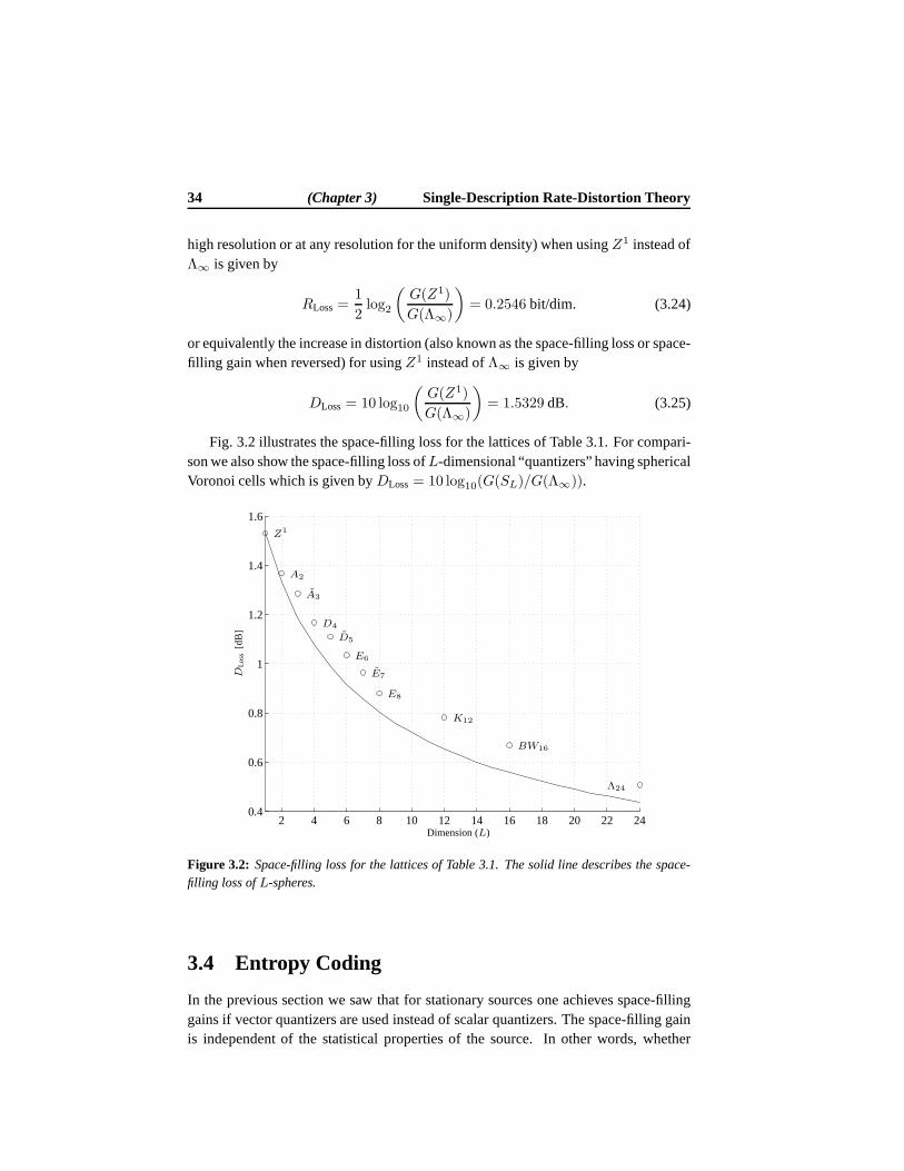
34 (Chapter 3) Single-Description Rate-Distortion Theory
high resolution or at any resolution for the uniform density) when usingZ1 instead ofΛ∞ is given by
RLoss=1
2log2
(G(Z1)
G(Λ∞)
)
= 0.2546 bit/dim. (3.24)
or equivalently the increase in distortion (also known as the space-filling loss or space-filling gain when reversed) for usingZ1 instead ofΛ∞ is given by
DLoss= 10 log10
(G(Z1)
G(Λ∞)
)
= 1.5329 dB. (3.25)
Fig. 3.2 illustrates the space-filling loss for the latticesof Table 3.1. For compari-son we also show the space-filling loss ofL-dimensional “quantizers” having sphericalVoronoi cells which is given byDLoss= 10 log10(G(SL)/G(Λ∞)).
2 4 6 8 10 12 14 16 18 20 22 240.4
0.6
0.8
1
1.2
1.4
1.6
PSfrag replacements
DLo
ss[d
B]
Dimension (L)
Z1
A2
A3
D4
D5
E6
E7
E8
K12
BW16
Λ24
Figure 3.2: Space-filling loss for the lattices of Table 3.1. The solid line describes the space-filling loss ofL-spheres.
3.4 Entropy Coding
In the previous section we saw that for stationary sources one achieves space-fillinggains if vector quantizers are used instead of scalar quantizers. The space-filling gainis independent of the statistical properties of the source.In other words, whether
Section 3.4 Entropy Coding 35
the source is i.i.d. or has memory the space-filling gain remains the same. However,for this to be true, we implicitly assume that any statistical redundancy (correlation)which might be present in the quantized signal is removed by a(lossless) entropycoder. Recall that the discrete entropyH(X ) of the quantizer is given by (3.19) andthatP (xi) denotes the probability of the symbolxi wherexi ∈ X . Assume now thata codeword (of the entropy coder) of lengthli is assigned to the symbolxi. Then theaverage codeword lengths is given by
s =∑
i∈I
P (xi)li. (3.26)
The idea of an entropy coder is to assign short codewords to very probable symbolsand long codewords to less probable symbols in order to drives towards its minimum.Since we require the (entropy) code to be lossless it means that the code should be auniquely decodable code. Due to a result of Shannon we can lower bounds by thefollowing theorem.
Theorem 3.4.1. [121] The average codeword lengths of a uniquely decodable binarycode satisfies
s ≥ H(X ). (3.27)
In the same paper Shannon also gave an upper bound ons, i.e. s < H(X ) + 1
and he furthermore showed that if a sequence of, says, symbols is jointly coded thenthe average number of bits per symbol satisfy
H(X ) ≤ s < H(X ) +1
s, (3.28)
which shows that the entropyH(X ) can be approximated arbitrarily closely by enco-ding sufficiently long sequences [121].
In (3.26) we have|I | = |X | and we thereby implicitly restrictX to be a dis-crete alphabet be it finite or countably finite, but we do in fact not always requirethat |X | < ∞. For example it is known that an entropy-constrained vectorquan-tizer (ECVQ) may be recast in a Lagrangian sense [19,59,63] and that a Lagrangian-optimal20 ECVQ always exists under general conditions on the source and distortionmeasure [63]. Furthermore, György et al. [64] showed that, for the squared error dis-tortion measure, a Lagrangian-optimal ECVQ has only a finitenumber of codewordsif the tail of the source distribution is lighter than the tail of the Gaussian distribution(of equal variance), while if the tail is heavier than that ofthe Gaussian distribution theLagrangian-optimal ECVQ has an infinite number of codewords[64]. If the sourcedistribution is Gaussian then the finiteness of the codebookdepends upon the rate of
20The operational distortion-rate function is the infimum of the set of distortion-rate functions that can beobtained by use of any vector quantizer which satisfies the given entropy constraints. A Lagrangian-optimalECVQ achieves points on the lower convex hull of the operational distortion-rate function and in generalany point can be achieved by use of time-sharing [63].

36 (Chapter 3) Single-Description Rate-Distortion Theory
the codebook. In addition they also showed that for source distributions with boundedsupport the Lagrangian-optimal ECVQ has a finite number of codewords.21 22
In this work we will not delve into the theory of entropy coding but merely as-sume that there exist entropy coders which are complex enough so that (at least intheory) the discrete entropies of the quantizers can be reached. For more informationabout entropy coding we refer the reader to Chapter 9 of the text book by Gersho andGray [45] as well as the references cited in this section.
21These quantizers are not unique. For example it was shown by Gray et al. [58] that for the uniformdensity on the unit cube there exists Lagrangian-optimal ECVQs with codebooks of infinite cardinality.
22In Chapter 7 we will show that, in certain important cases, the cardinality of lattice codebooks is finite.

Chapter4Multiple-Description
Rate-Distortion Theory
The MD problem is concerned with lossy encoding of information for transmissionover an unreliableK-channel communication system. The channels may break downresulting in erasures and a potential loss of information atthe receiving side. Which ofthe2K − 1 non-trivial subsets of theK channels that are working is assumed knownat the receiving side but not at the encoder. The problem is then to design an MDsystem which, for given channel rates or a given sum rate, minimizes the distortionsdue to reconstruction of the source using information from any subsets of the channels.The compound channel (or composite channel) containing theK subchannels is oftendescribed as a packet-switched network where individual packets are either receivederrorless or not at all. In such situations the entire systemis identified as a multiple-description system havingK descriptions.
The classical case involves two descriptions as shown in Fig. 4.1. The total rateRT , also known as the sum rate, is split between the two descriptions, i.e.RT =
R0 + R1, and the distortion observed at the receiver depends on which descriptionsarrive. If both descriptions are received, the distortion(Dc) is lower than if onlya single description is received (D0 or D1). The generalK-channel MD probleminvolvesK descriptions and is depicted in Fig. 4.2.
4.1 Information Theoretic MD Bounds
From an information theoretic perspective the MD problem ispartly about describingthe achievable MD rate-distortion region and partly about designing good practicalcodes whose performance is (in some sense) near optimum. Before presenting theknown information theoretic bounds we need the following definitions.
37
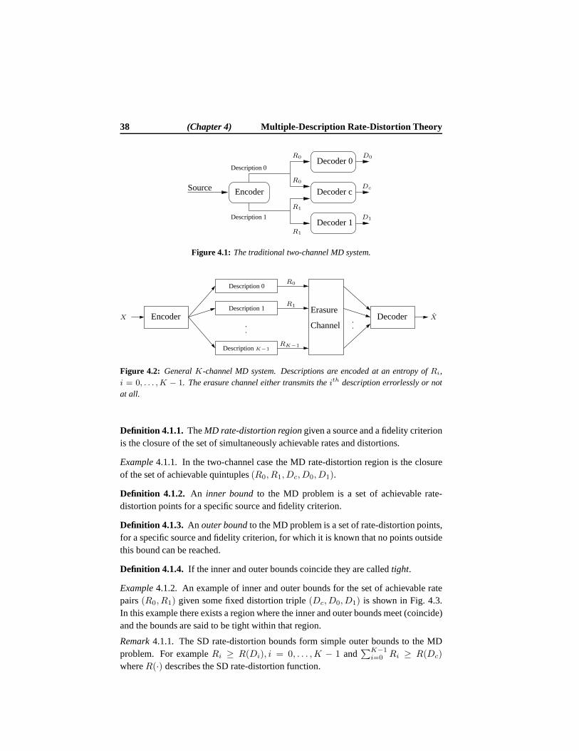
38 (Chapter 4) Multiple-Description Rate-Distortion Theory
Source Encoder
Decoder 0
Decoder c
Decoder 1
PSfrag replacements
D0
D1
Dc
R0
R0
R1
R1
Description 0
Description 1
Figure 4.1: The traditional two-channel MD system.
EncoderChannel
DecoderErasure
PSfrag replacements
X X
R0
R1
RK−1
Description 0
Description 1
DescriptionK−1
Figure 4.2: GeneralK-channel MD system. Descriptions are encoded at an entropy of Ri,i = 0, . . . ,K − 1. The erasure channel either transmits theith description errorlessly or notat all.
Definition 4.1.1. TheMD rate-distortion regiongiven a source and a fidelity criterionis the closure of the set of simultaneously achievable ratesand distortions.
Example4.1.1. In the two-channel case the MD rate-distortion region is theclosureof the set of achievable quintuples(R0, R1, Dc, D0, D1).
Definition 4.1.2. An inner boundto the MD problem is a set of achievable rate-distortion points for a specific source and fidelity criterion.
Definition 4.1.3. An outer boundto the MD problem is a set of rate-distortion points,for a specific source and fidelity criterion, for which it is known that no points outsidethis bound can be reached.
Definition 4.1.4. If the inner and outer bounds coincide they are calledtight.
Example4.1.2. An example of inner and outer bounds for the set of achievableratepairs(R0, R1) given some fixed distortion triple(Dc, D0, D1) is shown in Fig. 4.3.In this example there exists a region where the inner and outer bounds meet (coincide)and the bounds are said to be tight within that region.
Remark4.1.1. The SD rate-distortion bounds form simple outer bounds to the MDproblem. For exampleRi ≥ R(Di), i = 0, . . . ,K − 1 and
∑K−1i=0 Ri ≥ R(Dc)
whereR(·) describes the SD rate-distortion function.
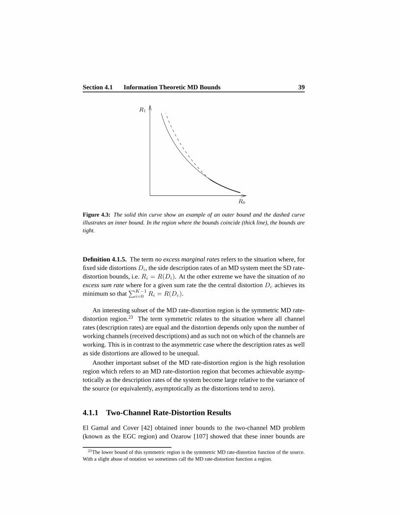
Section 4.1 Information Theoretic MD Bounds 39
PSfrag replacements
R0
R1
Figure 4.3: The solid thin curve show an example of an outer bound and the dashed curveillustrates an inner bound. In the region where the bounds coincide (thick line), the bounds aretight.
Definition 4.1.5. The termno excess marginal ratesrefers to the situation where, forfixed side distortionsDi, the side description rates of an MD system meet the SD rate-distortion bounds, i.e.Ri = R(Di). At the other extreme we have the situation ofnoexcess sum ratewhere for a given sum rate the the central distortionDc achieves itsminimum so that
∑K−1i=0 Ri = R(Dc).
An interesting subset of the MD rate-distortion region is the symmetric MD rate-distortion region.23 The term symmetric relates to the situation where all channelrates (description rates) are equal and the distortion depends only upon the number ofworking channels (received descriptions) and as such not onwhich of the channels areworking. This is in contrast to the asymmetric case where thedescription rates as wellas side distortions are allowed to be unequal.
Another important subset of the MD rate-distortion region is the high resolutionregion which refers to an MD rate-distortion region that becomes achievable asymp-totically as the description rates of the system become large relative to the variance ofthe source (or equivalently, asymptotically as the distortions tend to zero).
4.1.1 Two-Channel Rate-Distortion Results
El Gamal and Cover [42] obtained inner bounds to the two-channel MD problem(known as the EGC region) and Ozarow [107] showed that these inner bounds are
23The lower bound of this symmetric region is the symmetric MD rate-distortion function of the source.With a slight abuse of notation we sometimes call the MD rate-distortion function a region.

40 (Chapter 4) Multiple-Description Rate-Distortion Theory
tight for the memoryless Gaussian source under the squared-error fidelity criterion.24
Ahlswede [2] and Zhang and Berger [163] showed that the EGC region is also tight forgeneral sources and distortion measures in the no excess sumrate case. However, inthe excess sum rate case it was shown by Zhang and Berger [163]that the EGC regionis not always tight for the binary memoryless source under the Hamming distortionmeasure. Outer bounds for the binary symmetric source and Hamming distortion havealso been obtained by Wolf, Wyner and Ziv [153], Witsenhausen [152] and Zhang andBerger [164]. Zamir [157,158] obtained inner and outer bounds for smooth stationarysources and the squared-error fidelity criterion and further showed that the bounds be-come tight at high resolution. High resolution bounds for smooth sources and locallyquadratic distortion measures have been obtained by Linderet al. [84]. Outer boundsfor arbitrary memoryless sources and squared-error distortion measure were obtainedby Feng and Effros [35] and Lastras-Montano and Castelli [79].
To summarize, the achievable MD rate-distortion region is only completely knownfor the case of two channels, squared-error fidelity criterion and the memoryless Gaus-sian source [42, 107]. This region consists of the convex hull of the set of achievablequintuples(R0, R1, D0, D1, Dc) where the rates satisfy [18,107]
R0 ≥ R(D0) =1
2log2
(σ2X
D0
)
(4.1)
R1 ≥ R(D1) =1
2log2
(σ2X
D1
)
(4.2)
R0 +R1 ≥ R(Dc) +1
2log2 δ(D0, D1, Dc) (4.3)
=1
2log2
(σ2X
Dc
)
+1
2log2 δ(D0, D1, Dc), (4.4)
whereσ2X denotes the source variance andδ(·) is given by [18]
δ(D0, D1, Dc) =
1, Dc < D0 +D1 − σ2X
σ2XDc
D0D1, Dc >
(1D0
+ 1D1
− 1σ2X
)−1
(σ2X−Dc)
2
(σ2X−Dc)2−
(√(σ2
X−D0)(σ2X−D1)−
√(D0−Dc)(D1−Dc)
)2 , o.w.,
(4.5)
and the distortions satisfy [107]
D0 ≥ σ2X2−2R0 (4.6)
D1 ≥ σ2X2−2R1 (4.7)
Dc ≥σ2X2−2(R0+R1)
1−(√
Π−√)2 , (4.8)
24It is customary in the literature to refer to the case of a memoryless Gaussian source and squared-errorfidelity criterion as the quadratic Gaussian case.

Section 4.1 Information Theoretic MD Bounds 41
whereΠ = (1 − D0/σ2X)(1 − D1/σ
2X) and = (D0D1/σ
4X) − 2−2(R0+R1). In
general it is only possible to simultaneously achieve equality in two of the three rateinequalities given by (4.1) – (4.3). However, in the high side distortion case, i.e. whenδ(·) = 1, it is in fact possible to have equality in all three [42].
Fig. 4.4 shows the central distortion (4.8) as a function of the side distortion (4.6)in a symmetric setup whereD0 = D1 andR0 = R1 = 1 bit/dim. for the unit-varianceGaussian source. Notice that at one extreme we have optimal side distortion, i.e.D0 = D(R0) = −6.02 dB, which is on the single-channel rate-distortion function ofa unit-variance Gaussian source at 1 bit/dim. At the other extreme we have optimalcentral distortion, i.e.Dc = D(2R0) = −12.04 dB, which is on the single-channelrate-distortion function of the Gaussian source at 2 bit/dim. Thus, in this example,the single-channel rate-distortion bounds become effective for the two-channel MDproblem only at two extreme points.
−6 −5.5 −5 −4.5 −4 −3.5 −3
−12
−11.5
−11
−10.5
−10
−9.5
−9
−8.5
Side distortion [dB]
Cen
tral
dis
tort
ion
[dB
]
PSfrag replacements
R1
Figure 4.4: Central distortion(Dc) as a function of side distortion(D0 = D1) in a symmetricsetup whereR0 = R1 = 1 bit/dim. for the unit-variance Gaussian source and MSE.
The rate region comprising the set of achievable rate pairs(R0, R1) which satisfy(4.1), (4.2) and (4.3) is illustrated in Fig. 4.5. In this example we assume a unit-variance Gaussian source and choose distortionsD0 = 1
2 , D1 = 14 andDc = 1
13.9 .Notice thatR0 andR1 are lower bounded by0.5 and1 bit/dim., respectively, and thesum rate is lower bounded byR0 +R1 ≥ 2 bit/dim.
Ozarow’s Double-Branch Test Channel
Ozarow [107] showed that the double-branch test channel depicted in Fig. 4.6 achievesthe complete two-channel MD rate-distortion region in the quadratic Gaussian case.This channel has two additive noise branchesY0 = X+N0 andY1 = X+N1, where
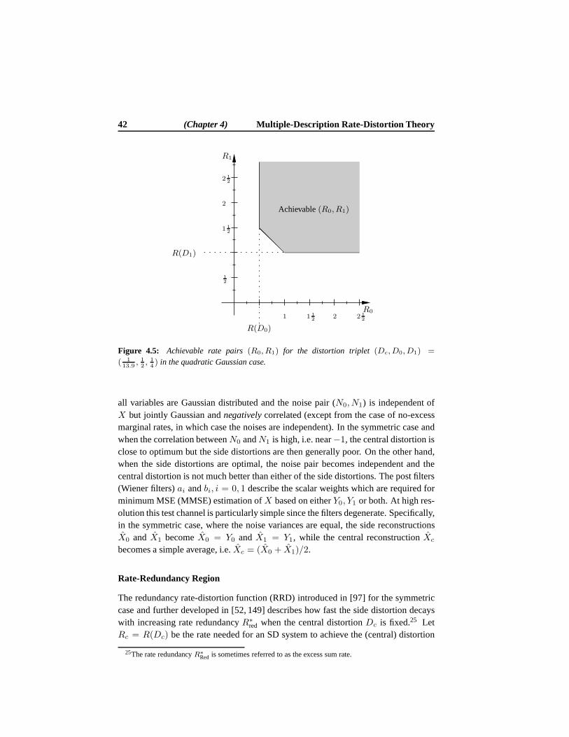
42 (Chapter 4) Multiple-Description Rate-Distortion Theory
PSfrag replacements
12
1 1 12
1 12
2
2
2 12
2 12
R0
R1
R(D0)
R(D1)
Achievable(R0, R1)
Figure 4.5: Achievable rate pairs(R0, R1) for the distortion triplet (Dc, D0, D1) =
( 113.9
, 12, 14) in the quadratic Gaussian case.
all variables are Gaussian distributed and the noise pair (N0, N1) is independent ofX but jointly Gaussian andnegativelycorrelated (except from the case of no-excessmarginal rates, in which case the noises are independent). In the symmetric case andwhen the correlation betweenN0 andN1 is high, i.e. near−1, the central distortion isclose to optimum but the side distortions are then generallypoor. On the other hand,when the side distortions are optimal, the noise pair becomes independent and thecentral distortion is not much better than either of the sidedistortions. The post filters(Wiener filters)ai andbi, i = 0, 1 describe the scalar weights which are required forminimum MSE (MMSE) estimation ofX based on eitherY0, Y1 or both. At high res-olution this test channel is particularly simple since the filters degenerate. Specifically,in the symmetric case, where the noise variances are equal, the side reconstructionsX0 and X1 becomeX0 = Y0 and X1 = Y1, while the central reconstructionXc
becomes a simple average, i.e.Xc = (X0 + X1)/2.
Rate-Redundancy Region
The redundancy rate-distortion function (RRD) introducedin [97] for the symmetriccase and further developed in [52, 149] describes how fast the side distortion decayswith increasing rate redundancyR∗
red when the central distortionDc is fixed.25 LetRc = R(Dc) be the rate needed for an SD system to achieve the (central) distortion
25The rate redundancyR∗
Red is sometimes referred to as the excess sum rate.

Section 4.1 Information Theoretic MD Bounds 43
+
+
+
PSfrag replacements
N1
N0
X
X1
X0
Xc
a1
a0
b1
b0
Figure 4.6: The MD optimum test channel of Ozarow [107]. At high resolution the filters
degenerate so in the symmetric case we haveai = 1 and bi = 1/2, i = 1, 2 so thatX0 =
Y0, X1 = Y1 andXc = 12(X0 + X1).
Dc. Then consider a symmetric setup whereD0 = D1 andR0 = R1 and defineR∗
red , 2R0 − Rc, i.e.R∗red describes the additional rate needed for an MD system
over that of an SD system to achieve the central distortionDc. In order to reducethe side distortionD0 while keepingDc fixed it is necessary to introduce redundancysuch that2R0 ≥ Rc. For a givenRc (or equivalently a givenDc) and a givenR∗
red theside distortion for the unit-variance Gaussian source is lower bounded by [52]
D0 ≥
12 (1 + 2−2Rc − (1− 2−2Rc)
√1− 2−2R∗
red), R∗red ≤ R∗
red
2−(Rc+R∗red), R∗
red > R∗red
(4.9)
whereR∗red = Rc − 1 + log2(1 + 2−2Rc). If R∗
red = 0 we have optimum centraldistortion, i.e. no excess sum rate, but the side distortions will then generally be high.As we increase the rate while keeping the central distortionfixed we are able to lowerthe side distortions. Fig. 4.7 shows the side distortionD0 = D1 as a function ofthe rate redundancyR∗
red when the central distortion is fixed atDc = 2−2Rc , Rc ∈0.5, 1, 1.5, 2, 2.5. It is interesting to observe that whenDc is optimal, i.e. whenR∗
red = 0, then the gap fromD1 to D(R0) increases with increasingRc. To seethis, notice that whenR∗
red = 0 it follows from the first bound of (4.9) thatD0 ≥(1 + 2−2Rc)/2. The second bound of (4.9) is actually the SD rate-distortion bound,i.e.2−(Rc+R∗
red) = 2−2R0 , and the gap between these two bounds is shown in Table 4.1.
Two-Channel High-Resolution Results
Based on the results for the Gaussian source of Ozarow [107] it was shown byVaishampayan et al. [136, 137] that at high resolution and for the symmetric case,
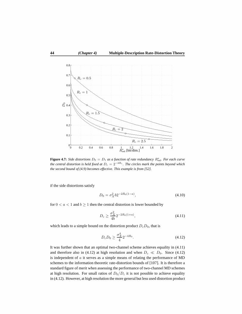
44 (Chapter 4) Multiple-Description Rate-Distortion Theory
0 0.2 0.4 0.6 0.8 1 1.2 1.4 1.6 1.8 20
0.1
0.2
0.3
0.4
0.5
0.6
0.7
0.8
PSfrag replacements
Rc = 0.5
Rc = 1
Rc = 1.5
Rc = 2
Rc = 2.5
D0
R∗
red [bit/dim.]
Figure 4.7: Side distortionsD0 = D1 as a function of rate redundancyR∗
red. For each curvethe central distortion is held fixed atDc = 2−2Rc . The circles mark the points beyond whichthe second bound of (4.9) becomes effective. This example isfrom [52].
if the side distortions satisfy
D0 = σ2Xb2
−2R0(1−a), (4.10)
for 0 < a < 1 andb ≥ 1 then the central distortion is lower bounded by
Dc ≥σ2X
4b2−2R0(1+a), (4.11)
which leads to a simple bound on the distortion productDcD0, that is
DcD0 ≥ σ4X
42−4R0 . (4.12)
It was further shown that an optimal two-channel scheme achieves equality in (4.11)and therefore also in (4.12) at high resolution and whenDc ≪ D0. Since (4.12)is independent ofa it serves as a simple means of relating the performance of MDschemes to the information theoretic rate-distortion bounds of [107]. It is therefore astandard figure of merit when assessing the performance of two-channel MD schemesat high resolution. For small ratios ofD0/Dc it is not possible to achieve equalityin (4.12). However, at high resolution the more general but less used distortion product
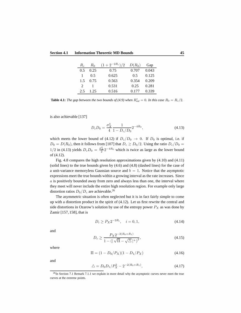
Section 4.1 Information Theoretic MD Bounds 45
Rc R0 (1 + 2−2Rc)/2 D(R0) Gap0.5 0.25 0.75 0.707 0.0431 0.5 0.625 0.5 0.125
1.5 0.75 0.563 0.354 0.2092 1 0.531 0.25 0.281
2.5 1.25 0.516 0.177 0.339
Table 4.1: The gap between the two bounds of (4.9) whenR∗
red = 0. In this caseR0 = Rc/2.
is also achievable [137]
DcD0 =σ4X
4
1
1−Dc/D02−4R0 , (4.13)
which meets the lower bound of (4.12) ifDc/D0 → 0. If D0 is optimal, i.e. ifD0 = D(R0), then it follows from [107] thatDc ≥ D0/2. Using the ratioDc/D0 =
1/2 in (4.13) yieldsDcD0 =σ4X
2 2−4R0 which is twice as large as the lower boundof (4.12).
Fig. 4.8 compares the high resolution approximations givenby (4.10) and (4.11)(solid lines) to the true bounds given by (4.6) and (4.8) (dashed lines) for the case ofa unit-variance memoryless Gaussian source andb = 1. Notice that the asymptoticexpressions meet the true bounds within a growing interval as the rate increases. Sincea is positively bounded away from zero and always less than one, the interval wherethey meet will never include the entire high resolution region. For example only largedistortion ratiosD0/Dc are achievable.26
The asymmetric situation is often neglected but it is in factfairly simple to comeup with a distortion product in the spirit of (4.12). Let us first rewrite the central andside distortions in Ozarow’s solution by use of the entropy powerPX as was done byZamir [157,158], that is
Di ≥ PX2−2Ri , i = 0, 1, (4.14)
and
Dc ≥PX2−2(R0+R1)
1− (|√Π−√|+)2
, (4.15)
whereΠ = (1−D0/PX)(1 −D1/PX) (4.16)
and = D0D1/P
2X − 2−2(R0+R1), (4.17)
26In Section 7.1 Remark 7.1.1 we explain in more detail why the asymptotic curves never meet the truecurves at the extreme points.
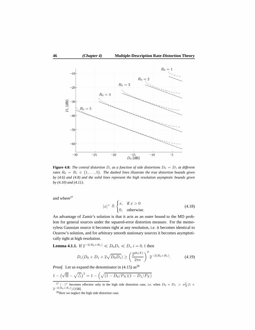
46 (Chapter 4) Multiple-Description Rate-Distortion Theory
−30 −25 −20 −15 −10 −5
−60
−50
−40
−30
−20
−10
PSfrag replacements
Dc
[dB
]
D0 [dB]
R0 = 1
R0 = 2
R0 = 3
R0 = 4
R0 = 5
Figure 4.8: The central distortionDc as a function of side distortionsD0 = D1 at differentratesR0 = R1 ∈ 1, . . . , 5. The dashed lines illustrate the true distortion bounds givenby (4.6) and (4.8) and the solid lines represent the high resolution asymptotic bounds givenby (4.10) and (4.11).
and where27
|x|+ ,
x, if x > 0
0, otherwise.(4.18)
An advantage of Zamir’s solution is that it acts as an outer bound to the MD prob-lem for general sources under the squared-error distortionmeasure. For the memo-ryless Gaussian source it becomes tight at any resolution, i.e. it becomes identical toOzarow’s solution, and for arbitrary smooth stationary sources it becomes asymptoti-cally tight at high resolution.
Lemma 4.1.1. If 2−2(R0+R1) ≪ D0D1 ≪ Di, i = 0, 1 then
Dc(D0 +D1 + 2√
D0D1) ≥(22h(X)
2πe
)2
2−2(R0+R1). (4.19)
Proof. Let us expand the denominator in (4.15) as28
1−(√
Π−√
)2
= 1−(√
(1 −D0/PX)(1 −D1/PX)
27 | · |+ becomes effective only in the high side distortion case, i.e. whenD0 + D1 > σ2X(1 +
2−2(R0+R1)) [158].28Here we neglect the high side distortion case.
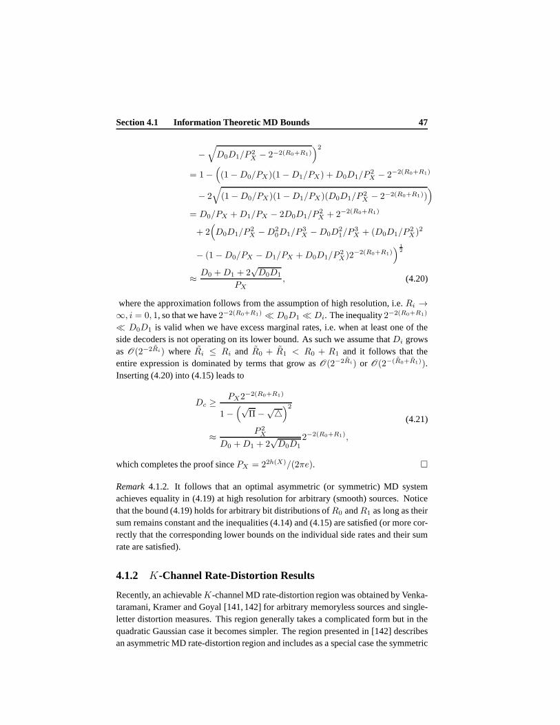
Section 4.1 Information Theoretic MD Bounds 47
−√
D0D1/P 2X − 2−2(R0+R1)
)2
= 1−(
(1−D0/PX)(1 −D1/PX) +D0D1/P2X − 2−2(R0+R1)
− 2√
(1−D0/PX)(1 −D1/PX)(D0D1/P 2X − 2−2(R0+R1))
)
= D0/PX +D1/PX − 2D0D1/P2X + 2−2(R0+R1)
+ 2(
D0D1/P2X −D2
0D1/P3X −D0D
21/P
3X + (D0D1/P
2X)2
− (1−D0/PX −D1/PX +D0D1/P2X)2−2(R0+R1)
) 12
≈ D0 +D1 + 2√D0D1
PX, (4.20)
where the approximation follows from the assumption of highresolution, i.e.Ri →∞, i = 0, 1, so that we have2−2(R0+R1) ≪ D0D1 ≪ Di. The inequality2−2(R0+R1)
≪ D0D1 is valid when we have excess marginal rates, i.e. when at least one of theside decoders is not operating on its lower bound. As such we assume thatDi growsas O(2−2Ri) whereRi ≤ Ri and R0 + R1 < R0 + R1 and it follows that theentire expression is dominated by terms that grow asO(2−2Ri) or O(2−(R0+R1)).Inserting (4.20) into (4.15) leads to
Dc ≥PX2−2(R0+R1)
1−(√
Π−√)2
≈ P 2X
D0 +D1 + 2√D0D1
2−2(R0+R1),
(4.21)
which completes the proof sincePX = 22h(X)/(2πe).
Remark4.1.2. It follows that an optimal asymmetric (or symmetric) MD systemachieves equality in (4.19) at high resolution for arbitrary (smooth) sources. Noticethat the bound (4.19) holds for arbitrary bit distributionsofR0 andR1 as long as theirsum remains constant and the inequalities (4.14) and (4.15)are satisfied (or more cor-rectly that the corresponding lower bounds on the individual side rates and their sumrate are satisfied).
4.1.2 K-Channel Rate-Distortion Results
Recently, an achievableK-channel MD rate-distortion region was obtained by Venka-taramani, Kramer and Goyal [141, 142] for arbitrary memoryless sources and single-letter distortion measures. This region generally takes a complicated form but in thequadratic Gaussian case it becomes simpler. The region presented in [142] describesan asymmetric MD rate-distortion region and includes as a special case the symmetric

48 (Chapter 4) Multiple-Description Rate-Distortion Theory
MD rate-distortion region. The construction of this regionrelies upon forming lay-ers of conditional random codebooks. It was, however, observed by Pradhan, Puriand Ramchandran in a series of papers [109–114] that by exploiting recent results ondistributed source coding it is possible to replace the conditional codebooks with uni-versal codebooks whereby the codebook rate can be reduced through random binning.While Pradhan et al. limited their interests to the symmetric case it can be shown thattheir results carry over to the asymmetric case as well. Thishas recently been doneby Wang and Viswanath [146] who further extended the resultsto the case of vectorGaussian sources and covariance distortion measure constraints.
The largest known achievable rate-distortion region for theK-channel MD prob-lem is that of Pradhan et al. [111,114].29 Common for all the achievable rate-distortionregions is that they represent inner bounds and it is currently not known whether theycan be further improved. However, for the quadratic Gaussian case it was conjecturedin [114] that their bound is in fact tight. That conjecture remains open.
The key ideas behind the achievable region obtained by Pradhan et al. are wellexplained in [111, 114] and we will here repeat some of their insights and resultsbefore presenting the largest knownK-channel achievable rate-distortion region.
Consider a packet-erasure channel with parametersK andk, i.e. at leastk out ofK descriptions are received. For the moment being, we assumek = 1. GenerateK independent random codebooks, sayC0, . . . ,CK−1 each of rateR. The sourceis now separately and independently quantized using each ofthe codebooks. Theindex of the nearest codeword in theith codebook is transmitted on theith channel.A code constructed in this way was dubbed a source-channel erasure code in [111]which we, for notational convenience, abridge to(K, k) SCEC. Notice that sinceeach of the individual codebooks are optimal for the source then if only a single indexis received the source is reconstructed with a distortion that is on the distortion-ratefunctionD(R) of the source. However, if more than one index is received, the qualityof the reconstructed signal can be strictly improved due to multiple versions of thequantized source. The above scheme is generalized to(K, k) SCEC fork > 1 bymaking use of random binning. This is possible since the quantized variables areassumed (symmetrically) correlated so that general results of distributed source codingare applicable. Specifically, due to celebrated results of Slepian and Wolf [124] andWyner and Ziv [154], if it is assumed that somek out of the set ofK correlatedvariables are received then (by e.g. use of random binning) it is possible to encode ata rate close to the joint entropy of anyk variables, in a distributed fashion, so that theencoder does not need to know whichk variables that are received. It is usually thennot possible to decode on reception of fewer thank variables.
Before presenting the main theorem of [111] which describesthe achievable rate-distortion regions of(K, k) SCECs in the general case of1 ≤ k ≤ K, we need somedefinitions.
29Outer bounds for theK-channel quadratic Gaussian problem were presented in [142].

Section 4.1 Information Theoretic MD Bounds 49
Definition 4.1.6. D(K,k) denotes the distortion when receivingk out ofK descrip-tions.
Definition 4.1.7. A tuple(R,D(K,k), D(K,k+1), . . . , D(K,K)) is said to be achievableif for arbitraryδ > 0, there exists, for sufficiently large block lengthL, a(K, k) SCECwith parameters(L,Θ,∆k,∆k+1, . . . ,∆K) with
Θ ≤ 2L(R+δ) and∆h ≤ D(K,h) + δ, h = k, k + 1, . . . ,K. (4.22)
Let Ik = I : I ⊆ 0, . . . ,K − 1, |I| ≥ k. A (K, k) SCEC with parameters(L,Θ,∆k,∆k+1, . . . ,∆K) is defined by a set ofK encoding functions [111]
Fi : X → 1, 2, . . . ,Θ, i = 0, . . . ,K − 1, (4.23)
and a set of|Ik| decoding functions
GI :⊗
I
1, 2, . . . ,Θ → X , ∀I ∈ Ik (4.24)
where⊗
denotes the Cartesian product and for allh ∈ k, k+1, . . . ,K andX ∈ X
we have
∆h = Eρ(X,GI(Fi1(X), . . . , Fih(X)))
I = i1, . . . , ih, ∀I ∈ Ik, |I| = h.(4.25)
Theorem 4.1.1( [111], Th. 1). For a probability distribution30
p(x, y0, . . . , yK−1) = q(x)p(y0, . . . , yK−1|x) (4.26)
defined overX⊕
Y K whereY is some finite alphabet,p(y0, . . . , yK−1|x) is sym-metric, and a set of decoding functions∀I ∈ Ik, gI : Y |I| → X , if
Eρ(X, gI(YI)) ≤ D(K,|I|), ∀I ∈ Ik (4.27)
and
R >1
kH(Y0, . . . , Yk−1)−
1
KH(Y0, . . . , YK−1|X) (4.28)
then(R,D(K,k), D(K,k+1), . . . , D(K,K)) is an achievable rate-distortion tuple.
In [114] an achievable rate-distortion region for theK-channel MD problem waspresented. The region was obtained by constructing a numberof layers within eachdescription where the set of alljth layers across theK descriptions corresponds toa (K, j) SCEC. Assume that it is desired to achieve some distortion triplet (D(3,1),
D(3,2), D(3,3)) for a three-channel system. Then first a (3,1) SCEC is constructedusing a rate ofR(0) bit/dim. per description. We use the superscript to distinguish
30To avoid clutter we omit the subscripts on the probability distributions in this section.

50 (Chapter 4) Multiple-Description Rate-Distortion Theory
between the rateR0 of encoder 0 in an asymmetric setup and the rateR(0) of layer 0in a symmetric setup. The rateR(0) is chosen such thatD(3,1) can be achieved withthe reception of any single description. If two descriptions are received the distortionis further decreased. However ifD(3,2) is not achieved on the reception of any twodescriptions, then a (3,2) SCEC is constructed at a rateR(1) bit/dim. per description.The rateR(1) is chosen such thatD(3,2) can be achieved on the reception of any twodescriptions. IfD(3,3) is not achieved on the reception of all three descriptions, arefinement layer is constructed at a rate ofR(2) bit/dim. per description, see Fig. 4.9.Each description contains three layers, e.g. descriptioni consists of a concatenationof L0i, L1i andL2i. It is important to see that the first layer, i.e. the (3,1) SCEC isconstructed exactly as described by Theorem 4.1.1. The second layer, i.e. the (3,2)SCEC differs from the construction in that of the binning rate. Since, on receptionof any two descriptions (say description 0 and 1), we have notonly the two secondlayers (L10 andL11) but also two base layers (L00 andL01). This makes it possible todecrease the binning rateR(1) by exploiting correlation across descriptions as well asacross layers. The final layer can be a simple refinement layerwhere bits are evenlysplit among the three descriptions or for example a (3,3) SCEC. The rate of eachdescription is then given byR = R(0) +R(1) +R(2) and the total rate is3R.
PSfrag replacements
R(0) R(1) R(2)
L00
L01
L02
L10
L11
L12
L20
L21
L22
Description 0
Description 1
Description 2
(3, 1) SCEC (3, 2) SCEC (3, 3) SCEC
︸ ︷︷ ︸︸ ︷︷ ︸︸ ︷︷ ︸
Figure 4.9: Concatenation of (3,1), (3,2) and (3,3) SCECs to achieve thedistortion triplet(D(3,1), D(3,2), D(3,3)). Each description contains three layers and the rate of eachdescriptionisR = R(0) +R(1) +R(2).
We are now in a position to introduce the main theorem of [114]which describesan achievable rate-distortion region for the concatenations of(K, k) SCECs. LetYijbe a random variable in theith layer andjth description and letIK−1
0 = 0, . . . ,K−1. For i ∈ IK−2
0 , letYiIK−10
= (Yi0, Yi1, . . . , YiK−1) representK random variables
in the ith layer taking values in alphabetYi. Let YK−1 be the last layer refinementvariable taking values in the alphabetYK−1 and
YIK−20 IK−1
0= (Y0IK−1
0, Y1IK−1
0, . . . , Y(K−2)IK−1
0). (4.29)
A joint distribution p(yIK−20 IK−1
0, yK−1|x) is called symmetric if for all1 ≤ ri ≤
Section 4.1 Information Theoretic MD Bounds 51
K wherei ∈ IK−20 , the following is true: the joint distribution ofYK−1 and all
(r0 + r1 + · · ·+ rK−2) random variables where anyri are chosen from theith layer,conditioned onx, is the same.
Theorem 4.1.2( [114], Th. 2). For any probability distribution
p(x, yIK−20 IK−1
0, yK−1) = p(x)p(yIK−2
0 IK−10
, yK−1|x) (4.30)
wherep(yIK−20 IK−1
0, yK−1|x) is symmetric, defined overX × Y K
0 × Y K1 × · · · ×
Y KK−2 × YK−1, and a set of decoding functions given by31
gI : Y|I|0 × · · · × Y
|I||I|−1 → X ∀I ⊂ IK−1
0
gIK−10
: Y K0 × Y K
1 × · · · × Y KK−2 × YK−1 → X
(4.31)
the convex closure of(R,D(K,1), D(K,2), . . . , D(K,K)) is achievable where
EρI(X, gI(YI|I|−10 I
)) ≤ D(K,|I|) ∀I ⊂ IK−10 , (4.32)
EρIK−10
(X, gIK−10
(YIK−20 IK−1
0, YK−1)) ≤ D(K,K), (4.33)
and
R ≥ H(Y00) +K−1∑
k=2
1
kH(Yk−1Ik−1
0|YIk−2
0 Ik−10
)
+1
KH(YK−1|YIK−2
0 IK−10
)− 1
KH(YIK−2
0 IK−10
, YK−1|X).
(4.34)
The main difference between Theorem 4.1.1 and Theorem 4.1.2is that the lattertheorem considers the completeK-tuple of distortions(D(K,1), D(K,2), . . . , D(K,K))
whereas the former theorem considers the(K − k + 1)-tuple of distortions(D(K,k),
D(K,k+1), . . . , D(K,K)). Hence, an SCEC based on the construction presentedin [111] is specifically tailored to networks where it is known that at leastk chan-nels outK channels are always working. With the construction presented in [114] itis possible to concatenate several SCECs and obtain a code that works for networkswhere the number of working channels is not known a priori.
4.1.3 Quadratic GaussianK-Channel Rate-Distortion Region
We will now describe the achievableK-channel rate-distortion region for the quadraticGaussian case. This appears to be the only case where explicit (and relatively simple)closed-form expressions for rate and distortion have been found.
31 Y ji denotes thej times Cartesian product of the alphabetYi.
52 (Chapter 4) Multiple-Description Rate-Distortion Theory
Consider a unit-variance Gaussian sourceX and define the random variablesYi, i = 0, . . . ,K − 1, given by
Yi = X +Qi, (4.35)
where theQi’s are identically distributed jointly Gaussian random variables (indepen-dent ofX) with varianceσ2
q and covariance matrixQ given by
Q = σ2q
1 ρq ρq · · · ρqρq 1 ρq · · · ρqρq ρq 1 · · · ρq...
......
. . ....
ρq ρq ρq · · · 1
, (4.36)
where, forK > 1, it is required that the correlation coefficient satisfies−1/(K−1) <
ρq ≤ 1 to ensure thatQ is positive semidefinite [142]. In the case of Ozarow’s doublebranch test channel forK = 2 descriptions, we only need to consider non positiveρq ’s. This is, in fact, also the case forK > 2 descriptions [142].
It is easy to show that the MMSE when estimatingX from any set ofm Yi’s isgiven by [111,142]
D(K,m) =σ2q (1 + (m− 1)ρq)
m+ σ2q(1 + (m− 1)ρq)
. (4.37)
We now focus on the(K, k) SCEC as presented in Theorem 4.1.1. The rate of eachdescription is given by [111]
R =1
2log2
(
k + σ2q (1 + (k − 1)ρq)
σ2q (1− ρq)
)1/k (1− ρq
1 + (K − 1)ρq
)1/K
. (4.38)
The quantization error varianceσ2q can now be obtained from (4.38)
σ2q = k
(
(1− ρq)22kR
(1 + (K − 1)ρq
1− ρq
)k/K
− (1 + (k − 1)ρq)
)−1
. (4.39)
We will follow [111] and look at the performance of a(K, k) SCEC in three dif-ferent situations distinguished by the amount of correlationρq introduced in the quan-tization noise.
Independent quantization noise:ρq = 0
The quantization noise is i.i.d., i.e.ρq = 0, henceQ is diagonal. Assuming that thequantization noise is normalized such thatσ2
q = k/(22kR − 1), we get the followingexpressions for the distortion
D(K,k+r) =σ2q
σ2q + (k + r)
=k
22kR(k + r)− rfor 0 ≤ r ≤ K − k, (4.40)
Section 4.1 Information Theoretic MD Bounds 53
andD(K,m) = 1 for 0 ≤ m < k. (4.41)
The distortion when receivingk descriptions is optimal, i.e.D(K,k) = 2−2kR.
Correlated quantization noise:ρq = ρ∗q
The amount of correlationρ∗q needed in order to be on the distortion-rate function onthe reception ofk = K descriptions is given by
ρ∗q = − 22KR − 1
(K − 1)22KR + 1≈ − 1
K − 1. (4.42)
This leads to the following performance
D(K,r) = 1− r
K(1− 2−2KR) for 0 ≤ r ≤ K. (4.43)
Notice that the distortion when receivingK descriptions is optimal, i.e.D(K,K) =
2−2KR.
Correlated quantization noise:ρ∗q < ρq < 0
Here a varying degree of correlation is introduced and the performance is given by
D(K,r) =σ2q (1 + (r − 1)ρq)
σ2q(1 + (r − 1)ρq) + r
for k ≤ r ≤ K, (4.44)
andD(K,m) = 1 for 0 ≤ m < k. (4.45)
Fig. 4.10 shows the three-channel distortionD(3,3) as a function of the two-channel distortionD(3,2) when varyingρq and keeping the rate constant by useof (4.39). In this example we use a(3, 2) SCEC withR = 1 bit/dim. At one endwe haveD(3,2) = −12.0412 dB which is on the distortion-rate function of the sourceand at the other end we haveD(3,3) = −18.0618 dB which is also on the distortion-rate function.
In Fig. 4.11 we show the simultaneously achievable one-channel D(3,1), two-channelD(3,2) and three-channelD(3,3) distortions for the unit-variance memorylessGaussian source at 1 bit/dim. when using a(3, 1)SCEC. It is interesting to observe thatwhile it is possible to achieve optimum one-channel distortion (ρq = 0 ⇒ D(3,1) ≈−6 dB) and optimum three-channel distortion (ρq → −1/2 ⇒ D(3,3) ≈ −18 dB) itis not possible to drive the two-channel distortion towardsits optimum (∀ρq, D(3,2) <
−12 dB). In other words, a(3, 1) SCEC can achieve optimal one-channel and three-channel performance and a(3, 2) SCEC can achieve optimal two-channel and three-channel performance.
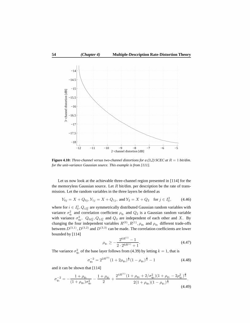
54 (Chapter 4) Multiple-Description Rate-Distortion Theory
−12 −11 −10 −9 −8 −7 −6 −5
−18
−17.5
−17
−16.5
−16
−15.5
−15
−14.5
−14
2−channel distortion [dB]
3−ch
anne
l dis
tort
ion
[dB
]
Figure 4.10: Three-channel versus two-channel distortions for a (3,2) SCEC atR = 1 bit/dim.for the unit-variance Gaussian source. This example is from[111].
Let us now look at the achievable three-channel region presented in [114] for thethe memoryless Gaussian source. LetR bit/dim. per description be the rate of trans-mission. Let the random variables in the three layers be defined as
Y0j = X +Q0j, Y1j = X +Q1j , andY2 = X +Q2 for j ∈ I20 , (4.46)
where fori ∈ I10 , QiI20
are symmetrically distributed Gaussian random variables withvarianceσ2
qi and correlation coefficientρqi andQ2 is a Gaussian random variablewith varianceσ2
q2 . Q0I20, Q1I2
0andQ2 are independent of each other andX . By
changing the four independent variablesR(0), R(1), ρq0 andρq1 different trade-offsbetweenD(3,1), D(3,2) andD(3,3) can be made. The correlation coefficients are lowerbounded by [114]
ρqi ≥ − 26R(i) − 1
2 · 26R(i) + 1. (4.47)
The varianceσ2q0 of the base layer follows from (4.39) by lettingk = 1, that is
σ−2q0 = 22R
(0)
(1 + 2ρq0)13 (1− ρq0)
23 − 1 (4.48)
and it can be shown that [114]
σ−2q1 = − 1 + ρq1
(1 + ρq0)σ2q0
− 1 + ρq12
+24R
(1)
(1 + ρq0 + 2/σ2q0)(1 + ρq1 − 2ρ2q1)
23
2(1 + ρq0)(1 − ρq1)13
.
(4.49)

Section 4.1 Information Theoretic MD Bounds 55
−0.45 −0.4 −0.35 −0.3 −0.25 −0.2 −0.15 −0.1 −0.05 0−18
−16
−14
−12
−10
−8
−6
−4
−2M
SE
[dB
]
PSfrag replacements
D(3,1)
D(3,2)
D(3,3)
ρq
Figure 4.11: The simultaneously achievable one-channel, two-channel and three-channel dis-tortions for the unit-variance Gaussian source at 1 bit/dim. for a (3,1) SCEC.
Let MSE2 denote the distortion given by any two base-layer random variables, andMSE3 denote the distortion given by all the random variables in the base and thesecond layer. Hence, MSE2 denotes the MMSE obtained in estimating the sourceX
using either (Y00, Y01), (Y00, Y02) or (Y01, Y02). Similarly MSE3 denotes the MMSEin estimatingX from (Y00, Y01, Y02, Y10, Y11, Y12). From (4.37) it follows that
MSE2 =σ2q0(1 + ρq0)
σ2q0(1 + ρq0) + 2
, (4.50)
and it can also be shown that [114]
MSE3 =σ2q0σ
2q1(1 + 2ρq0 + 2ρq1 + 4ρq0ρq1)
3σ2q0(1 + 2ρq0) + 3σ2
q1(1 + 2ρq1) + σ2q0σ
2q1(1 + 2ρq0 + 2ρq1 + 4ρq0ρq1)
,
(4.51)
and
σ2q2 =
MSE3
26(R−R(0)−R(1)) − 1. (4.52)
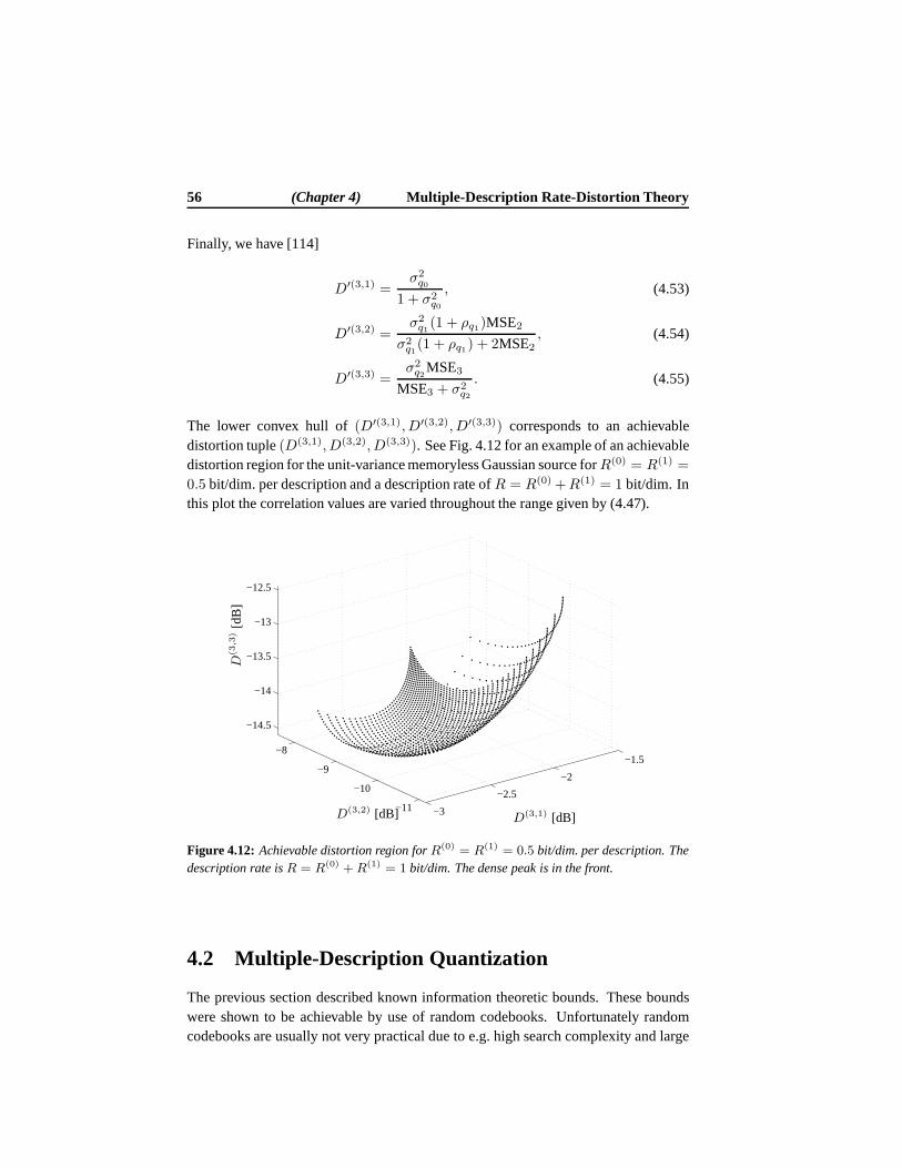
56 (Chapter 4) Multiple-Description Rate-Distortion Theory
Finally, we have [114]
D′(3,1) =σ2q0
1 + σ2q0
, (4.53)
D′(3,2) =σ2q1 (1 + ρq1)MSE2
σ2q1(1 + ρq1) + 2MSE2
, (4.54)
D′(3,3) =σ2q2MSE3
MSE3 + σ2q2
. (4.55)
The lower convex hull of(D′(3,1), D′(3,2), D′(3,3)) corresponds to an achievabledistortion tuple(D(3,1), D(3,2), D(3,3)). See Fig. 4.12 for an example of an achievabledistortion region for the unit-variance memoryless Gaussian source forR(0) = R(1) =
0.5 bit/dim. per description and a description rate ofR = R(0) +R(1) = 1 bit/dim. Inthis plot the correlation values are varied throughout the range given by (4.47).
−3
−2.5
−2
−1.5
−11
−10
−9
−8
−14.5
−14
−13.5
−13
−12.5
PSfrag replacements
D(3,1) [dB]D(3,2) [dB]
D(3
,3)
[dB
]
Figure 4.12: Achievable distortion region forR(0) = R(1) = 0.5 bit/dim. per description. Thedescription rate isR = R(0) +R(1) = 1 bit/dim. The dense peak is in the front.
4.2 Multiple-Description Quantization
The previous section described known information theoretic bounds. These boundswere shown to be achievable by use of random codebooks. Unfortunately randomcodebooks are usually not very practical due to e.g. high search complexity and large
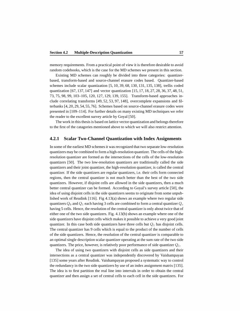
Section 4.2 Multiple-Description Quantization 57
memory requirements. From a practical point of view it is therefore desirable to avoidrandom codebooks, which is the case for the MD schemes we present in this section.
Existing MD schemes can roughly be divided into three categories: quantizer-based, transform-based and source-channel erasure codes based. Quantizer-basedschemes include scalar quantization [5, 10, 39, 68, 130, 131, 135, 138], trellis codedquantization [67, 137, 147] and vector quantization [15, 17, 18, 27, 28, 36, 37, 48, 51,73, 75, 98, 99, 103–105, 120, 127, 129, 139, 155]. Transform-based approaches in-clude correlating transforms [49, 52, 53, 97, 148], overcomplete expansions and fil-terbanks [4, 20, 29, 54, 55, 76]. Schemes based on source-channel erasure codes werepresented in [109–114]. For further details on many existing MD techniques we referthe reader to the excellent survey article by Goyal [50].
The work in this thesis is based on lattice vector quantization and belongs thereforeto the first of the catagories mentioned above to which we willalso restrict attention.
4.2.1 Scalar Two-Channel Quantization with Index Assignments
In some of the earliest MD schemes it was recognized that two separate low-resolutionquantizers may be combined to form a high-resolution quantizer. The cells of the high-resolution quantizer are formed as the intersections of thecells of the low-resolutionquantizers [50]. The two low-resolution quantizers are traditionally called the sidequantizers and their joint quantizer, the high-resolutionquantizer, is called the centralquantizer. If the side quantizers are regular quantizers, i.e. their cells form connectedregions, then the central quantizer is not much better than the best of the two sidequantizers. However, if disjoint cells are allowed in the side quantizers, then a muchbetter central quantizer can be formed. According to Goyal’s survey article [50], theidea of using disjoint cells in the side quantizers seems to originate from some unpub-lished work of Reudink [116]. Fig 4.13(a) shows an example where two regular sidequantizersQ0 andQ1 each having 3 cells are combined to form a central quantizerQc
having 5 cells. Hence, the resolution of the central quantizer is only about twice that ofeither one of the two side quantizers. Fig. 4.13(b) shows an example where one of theside quantizers have disjoint cells which makes it possibleto achieve a very good jointquantizer. In this case both side quantizers have three cells butQ1 has disjoint cells.The central quantizer has 9 cells which is equal to the product of the number of cellsof the side quantizers. Hence, the resolution of the centralquantizer is comparable toan optimal single description scalar quantizer operating at the sum rate of the two sidequantizers. The price, however, is relatively poor performance of side quantizerQ1.
The idea of using two quantizers with disjoint cells as side quantizers and theirintersections as a central quantizer was independently discovered by Vaishampayan[135] some years after Reudink. Vaishampayan proposed a systematic way to controlthe redundancy in the two side quantizers by use of an index assignment matrix [135].The idea is to first partition the real line into intervals in order to obtain the centralquantizer and then assign a set of central cells to each cell in the side quantizers. For
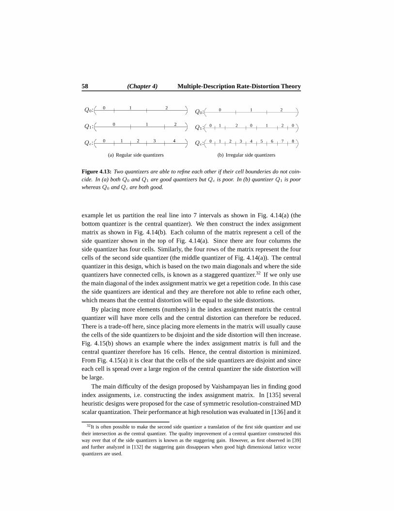
58 (Chapter 4) Multiple-Description Rate-Distortion Theory
0 1 2
0 1 2
40 1 2 3
PSfrag replacementsQ0:
Q1:
Qc:
(a) Regular side quantizers
0 1 2
0 1 2 0 1 2 0
0 1 2 3 4 5 6 7 8
PSfrag replacementsQ0:
Q1:
Qc:
(b) Irregular side quantizers
Figure 4.13: Two quantizers are able to refine each other if their cell bounderies do not coin-cide. In (a) bothQ0 andQ1 are good quantizers butQc is poor. In (b) quantizerQ1 is poorwhereasQ0 andQc are both good.
example let us partition the real line into 7 intervals as shown in Fig. 4.14(a) (thebottom quantizer is the central quantizer). We then construct the index assignmentmatrix as shown in Fig. 4.14(b). Each column of the matrix represent a cell of theside quantizer shown in the top of Fig. 4.14(a). Since there are four columns theside quantizer has four cells. Similarly, the four rows of the matrix represent the fourcells of the second side quantizer (the middle quantizer of Fig. 4.14(a)). The centralquantizer in this design, which is based on the two main diagonals and where the sidequantizers have connected cells, is known as a staggered quantizer.32 If we only usethe main diagonal of the index assignment matrix we get a repetition code. In this casethe side quantizers are identical and they are therefore notable to refine each other,which means that the central distortion will be equal to the side distortions.
By placing more elements (numbers) in the index assignment matrix the centralquantizer will have more cells and the central distortion can therefore be reduced.There is a trade-off here, since placing more elements in thematrix will usually causethe cells of the side quantizers to be disjoint and the side distortion will then increase.Fig. 4.15(b) shows an example where the index assignment matrix is full and thecentral quantizer therefore has 16 cells. Hence, the central distortion is minimized.From Fig. 4.15(a) it is clear that the cells of the side quantizers are disjoint and sinceeach cell is spread over a large region of the central quantizer the side distortion willbe large.
The main difficulty of the design proposed by Vaishampayan lies in finding goodindex assignments, i.e. constructing the index assignmentmatrix. In [135] severalheuristic designs were proposed for the case of symmetric resolution-constrained MDscalar quantization. Their performance at high resolutionwas evaluated in [136] and it
32It is often possible to make the second side quantizer a translation of the first side quantizer and usetheir intersection as the central quantizer. The quality improvement of a central quantizer constructed thisway over that of the side quantizers is known as the staggering gain. However, as first observed in [39]and further analyzed in [132] the staggering gain dissappears when good high dimensional lattice vectorquantizers are used.

Section 4.2 Multiple-Description Quantization 59
Columns
Rows
PSfrag replacements
0
0
0
1
1
1
2
2
2
3
3
3 4 5 6
7
8
9
10
11
12
13
14
15
(a) Side and central quantizers
PSfrag replacements
0 1
2 3
4 5
6
7
8
9
10
11
12
13
14
15
(b) Index assignment matrix
Figure 4.14: (a) The two side quantizers each having four cells are offsetfrom each other.Their intersection forms the central quantizer having 7 cells. (b) shows the correspondingindex assignment matrix for the quantizers. The columns of the matrix form a side quantizerand the rows also form a side quantizer.
PSfrag replacements
00
0 00
0
11 11
1 111
1
2222
2 222
2
3 3
33 3
3 4 5 6 7 8 9 10 11 12 13 14 15
(a) Side and central quantizers
PSfrag replacements
0 1
2
3
4
5 6
7
8
9 10
11
12
13
14 15
(b) Index assignment matrix
Figure 4.15: (a) The two side quantizers each having four cells are not identical. Their intersec-tion forms the central quantizer having 16 cells. (b) shows the corresponding index assignmentmatrix for the quantizers. The columns of the matrix form a side quantizer and the rows alsoform a side quantizer.

60 (Chapter 4) Multiple-Description Rate-Distortion Theory
was shown that in the quadratic Gaussian case, the distortion productDcD0 was 8.69dB away from the optimal high resolution distortion product(4.12). Vaishampayanand Domaszewicz [138] then proposed an entropy-constrained MD scalar quantizerwhere the index-assignment matrix was optimized using a generalized Lloyd algo-rithm. The distortion product of this design was shown to be only 3.06 dB away fromthe theoretical optimum [136]. Recall that the space-filling loss of an SD scalar quan-tizer is 1.53 dB so that, quite surprisingly, the gap to the optimal distortion product ofa two-description scalar quantizer is twice the scalar space-filling loss. The design ofgood index assignments for the scalar case is further considered in [10].
It is known that the entropy-constrained scalar uniform quantizer is optimal in theSD case, see Chapter 3. This result, however, does not carry over to the MD case.Goyal et al. [51, 73] were the first to recognize that by slightly modifying the centralquantizer in a way so that it no longer forms a lattice, it is possible to reduce thedistortion product not only in the scalar case but also in thetwo-dimensional case.This phenomenon was further investigated by Tian et al. [129–131] who showed thatthe scalar distortion product can be further improved by 0.4dB by modifying thecentral quantizer.
4.2.2 Lattice Vector Quantization for Multiple Descriptions
Recently, Servetto, Vaishampayan and Sloane [120, 139] presented a clever construc-tion based on lattices, which at high resolution and asymptotically in vector dimensionis able to achieve the symmetric two-channel MD rate-distortion region. The designof [120,139] is again based on index assignments which are non-linear mappings thatlead to a curious result. LetRs = R0 = R1 denote the rate of each of the sidequantizers and let0 < a < 1. Then, at high resolution, the central distortionDc
satisfies [139]
limR→∞
Dc22Rs(1+a) =
1
4G(Λ)22h(X), (4.56)
whereas the side distortionsD0 = D1 satisfy
limR→∞
D022Rs(1−a) = G(SL)2
2h(X), (4.57)
whereG(Λ) andG(SL) are the dimensionless normalized second moments of thecentral latticeΛ and anL-sphere, respectively. Thus, remarkably, the performanceof the side quantizers is identical to that of quantizers having spherical Voronoi cells;note that in the SD case this is not possible for1 < L <∞.
The design presented in [120, 139] is based on a central lattice Λ and a singlesublatticeΛs of indexN = |Λ/Λs|. Each central lattice pointλ ∈ Λ is mapped toa pair of sublattice points(λ0, λ1) ∈ Λs × Λs using an index assignment function.A pair of sublattice points is called an edge. The edges are constructed by pairingclosely spaced (in the Euclidean sense) sublattice points.By exploiting the direction

Section 4.2 Multiple-Description Quantization 61
of an edge (i.e. the pair(λ0, λ1) is distinguishable from(λ1, λ0)) it is possible to usean edge twice. In order to construct the edges as well as the assignment of edges tocentral lattice points, geometric properties of the lattices are exploited. Specifically,the edges(λ0, λ1) and(λ1, λ0) are mapped to the central lattice pointsλ ∈ Λ andλ′ ∈ Λ which satisfyλ+λ′ = λ0+λ1 and furthermore, the distance from the midpointof an edge and the associated central lattice point should beas small as possible (whenaveraged over all edges and the corresponding assigned central lattice points). Only asmall number of edges and assignments needs to be found, whereafter the symmetryof the lattices can be exploited in order to cover the entire lattice. Examples of edgeconstructions and assignments are presented in [120,139].
The asymmetric case was considered by Diggavi, Sloane and Vaishampayan [27,28] who constructed a two-channel scheme also based on indexassignments andwhich, at high resolution and asymptotically in vector dimension, is able to reachthe entire two-channel MD rate-distortion region. Specifically, at high resolution, thecentral distortion satisfies [28]
Dc = G(Λ)22(h(X)−Rc), (4.58)
whereRc is the rate of the central quantizer and the side distortionssatisfy
D0 =γ21
(γ0 + γ1)2G(Λs)2
2h(X)2−2(R0+R1−Rc), (4.59)
and
D1 =γ20
(γ0 + γ1)2G(Λs)2
2h(X)2−2(R0+R1−Rc), (4.60)
whereG(Λs) is the dimensionless normalized second moment of a sublattice Λs,which is geometrically-similar to both side latticesΛi, i = 0, 1, andγ0, γ1 ∈ R+
are weights which are introduced to control the asymmetry inthe side distortions.
Notice that in the distortion-balanced case we haveγ0 = γ1 so that γ20
(γ0+γ1)2= 1
4
and if γ0 = 0 or γ1 = 0 then the design degenerates to a successive refinementscheme [28, 32]. It is worth emphasizing that the side quantizers in the asymmetricdesign do generally not achieve the sphere bound in finite dimensions as was the caseof the symmetric design.
The design presented in [27, 28] is based on a central latticeΛ, two sublatticesΛ0 ⊂ Λ andΛ1 ⊂ Λ of indexN0 = |Λ/Λ0| andN1 = |Λ/Λ1|, respectively, and aproduct latticeΛπ ⊂ Λi, i = 0, 1, of indexNπ = N0N1. The Voronoi cellVπ(λπ)of the product lattice pointλπ ∈ Λπ containsN1 sublattice points ofΛ0 andN0
sublattice points ofΛ1, see Fig. 4.16 for an example whereN0 = 5 andN1 = 9. Inthis example, only the 45 central lattice points located withinVπ(0) need to have edgesassigned. The remaining assignments are done simply by shifting these assignmentsby λπ ∈ Λπ. In other words, if the edge(λ0, λ1) is assigned toλ then the edge(λ0 + λπ, λ1 + λπ) is assigned toλ + λπ. We say that the assignments are shiftinvariant with respect to the product lattice.
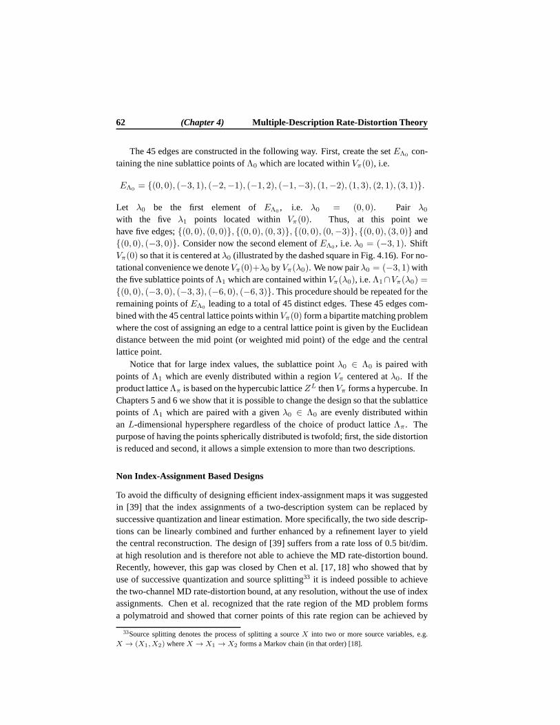
62 (Chapter 4) Multiple-Description Rate-Distortion Theory
The 45 edges are constructed in the following way. First, create the setEΛ0 con-taining the nine sublattice points ofΛ0 which are located withinVπ(0), i.e.
EΛ0 = (0, 0), (−3, 1), (−2,−1), (−1, 2), (−1,−3), (1,−2), (1, 3), (2, 1), (3, 1).
Let λ0 be the first element ofEΛ0 , i.e. λ0 = (0, 0). Pair λ0with the five λ1 points located within Vπ(0). Thus, at this point wehave five edges;(0, 0), (0, 0), (0, 0), (0, 3), (0, 0), (0,−3), (0, 0), (3, 0) and(0, 0), (−3, 0). Consider now the second element ofEΛ0 , i.e.λ0 = (−3, 1). ShiftVπ(0) so that it is centered atλ0 (illustrated by the dashed square in Fig. 4.16). For no-tational convenience we denoteVπ(0)+λ0 byVπ(λ0). We now pairλ0 = (−3, 1)withthe five sublattice points ofΛ1 which are contained withinVπ(λ0), i.e.Λ1∩Vπ(λ0) =(0, 0), (−3, 0), (−3, 3), (−6, 0), (−6, 3). This procedure should be repeated for theremaining points ofEΛ0 leading to a total of 45 distinct edges. These 45 edges com-bined with the 45 central lattice points withinVπ(0) form a bipartite matching problemwhere the cost of assigning an edge to a central lattice pointis given by the Euclideandistance between the mid point (or weighted mid point) of theedge and the centrallattice point.
Notice that for large index values, the sublattice pointλ0 ∈ Λ0 is paired withpoints ofΛ1 which are evenly distributed within a regionVπ centered atλ0. If theproduct latticeΛπ is based on the hypercubic latticeZL thenVπ forms a hypercube. InChapters 5 and 6 we show that it is possible to change the design so that the sublatticepoints ofΛ1 which are paired with a givenλ0 ∈ Λ0 are evenly distributed withinanL-dimensional hypersphere regardless of the choice of product latticeΛπ. Thepurpose of having the points spherically distributed is twofold; first, the side distortionis reduced and second, it allows a simple extension to more than two descriptions.
Non Index-Assignment Based Designs
To avoid the difficulty of designing efficient index-assignment maps it was suggestedin [39] that the index assignments of a two-description system can be replaced bysuccessive quantization and linear estimation. More specifically, the two side descrip-tions can be linearly combined and further enhanced by a refinement layer to yieldthe central reconstruction. The design of [39] suffers froma rate loss of 0.5 bit/dim.at high resolution and is therefore not able to achieve the MDrate-distortion bound.Recently, however, this gap was closed by Chen et al. [17, 18]who showed that byuse of successive quantization and source splitting33 it is indeed possible to achievethe two-channel MD rate-distortion bound, at any resolution, without the use of indexassignments. Chen et al. recognized that the rate region of the MD problem formsa polymatroid and showed that corner points of this rate region can be achieved by
33Source splitting denotes the process of splitting a sourceX into two or more source variables, e.g.X → (X1,X2) whereX → X1 → X2 forms a Markov chain (in that order) [18].
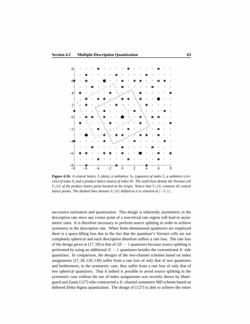
Section 4.2 Multiple-Description Quantization 63
−8 −6 −4 −2 0 2 4 6 8−8
−6
−4
−2
0
2
4
6
8
Figure 4.16: A central latticeΛ (dots), a sublatticeΛ0 (squares) of index 5, a sublattice (cir-cles) of index 9, and a product lattice (stars) of index 45. The solid lines denote the Voronoi cellVπ(0) of the product lattice point located at the origin. Notice that Vπ(0) contains 45 centrallattice points. The dashed lines denotesVπ(0) shifted so it is centered at(−3, 1).
successive estimation and quantization. This design is inherently asymmetric in thedescription rate since any corner point of a non-trivial rate region will lead to asym-metric rates. It is therefore necessary to perform source splitting in order to achievesymmetry in the description rate. When finite-dimensional quantizers are employedthere is a space-filling loss due to the fact that the quantizer’s Voronoi cells are notcompletely spherical and each description therefore suffers a rate loss. The rate lossof the design given in [17,18] is that of2K − 1 quantizers because source splitting isperformed by using an additionalK − 1 quantizers besides the conventionalK sidequantizers. In comparison, the designs of the two-channel schemes based on indexassignments [27, 28, 120, 139] suffer from a rate loss of onlythat of two quantizersand furthermore, in the symmetric case, they suffer from a rate loss of only that oftwo spherical quantizers. That it indeed is possible to avoid source splitting in thesymmetric case without the use of index assignments was recently shown by Øster-gaard and Zamir [127] who constructed aK-channel symmetric MD scheme based ondithered Delta-Sigma quantization. The design of [127] is able to achieve the entire

64 (Chapter 4) Multiple-Description Rate-Distortion Theory
symmetric two-channel MD rate-distortion region at any resolution and the rate losswhen finite-dimensional quantizers are used is that of two lattice quantizers. Hence, inthe two-channel case the rate loss when using index assignments is less than or equalto that of the designs which are not using index assignments [17,18,127].
Chapter5
K-Channel Symmetric Lattice
Vector Quantization
In this chapter we consider a special case of the generalK-channel symmetric MDproblem where only a single parameter controls the redundancy tradeoffs between thecentral and the side distortions. With a single controllingparameter it is possible todescribe the entire symmetric rate-distortion region for two descriptions and at highresolution, as shown in [120, 139], but it is not enough to describe the symmetricachievableK-channel rate-distortion region. As such the proposed scheme offers apartial solution to the problem of designing balanced MD-LVQ systems. In Chapter 7we include more controlling parameters in the design and show that the three-channelMD region given by Theorem 4.1.1 can be reached at high resolution.
We derive analytical expressions for the central and side quantizers which, underhigh-resolution assumptions, minimize the expected distortion at the receiving sidesubject to entropy constraints on the side descriptions forgiven packet-loss proba-bilities. The central and side quantizers we use are latticevector quantizers. Thecentral distortion depends upon the lattice type in question whereas the side distor-tions only depend on the scaling of the lattices but are independent of the specifictypes of lattices. In the case of three descriptions we show that the side distortions canbe expressed through the dimensionless normalized second moment of a sphere aswas the case for the two descriptions system presented in [120,139]. Furthermore, weconjecture that this is true in the general case of an arbitrary number of descriptions.
In the presented approach the expected distortion observedat the receiving sidedepends only upon the number of received descriptions, hence the descriptions aremutually refinable and reception of anyκ out of K descriptions yields equivalentexpected distortion. This is different from successive refinement schemes [32] wherethe individual descriptions often must be received in a prescribed order to be able to
65
66 (Chapter 5) K-Channel Symmetric Lattice Vector Quantization
refine each other, i.e. description numberl will not do any good unless descriptions0, . . . , l−1 have already been received. We construct a scheme which for given packet-loss probabilities and a maximum bit budget (target entropy) determines the optimalnumber of descriptions and specifies the corresponding quantizers that minimize theexpected distortion.
5.1 Preliminaries
We consider a central quantizer andK ≥ 2 side quantizers. The central quantizer is(based on) a latticeΛc ⊂ RL with a fundamental region of volumeν = det(Λc). Theside quantizers are based on a geometrically-similar and clean sublatticeΛs ⊆ Λc ofindexN = |Λc/Λs| and fundamental regions of volumeνs = νN . The trivial caseK = 1 leads to a single-description system, where we would simplyuse one centralquantizer and no side quantizers.
We will consider the balanced situation, where the entropyR is the same foreach description. Furthermore, we consider the case where the contributionDi, i =
0, . . . ,K − 1 of each description to the total distortion is the same. Our design makessure34 that the distortion observed at the receiving side depends only on the number ofdescriptions received; hence reception of anyκ out ofK descriptions yields equivalentexpected distortion.
5.1.1 Index Assignments
A source vectorx is quantized to a reconstruction pointλc in the central latticeΛc.Hereafter follows index assignments (mappings), which uniquely mapλc to one vector(reconstruction point) in each of the side quantizers. Thismapping is done througha labeling functionα, and we denote the individual component functions ofα by αi,wherei = 0, . . . ,K − 1. In other words, the injective mapα that mapsΛc intoΛs × · · · × Λs, is given by
α(λc) = (α0(λc), α1(λc), . . . , αK−1(λc)) (5.1)
= (λ0, λ1, . . . , λK−1), (5.2)
whereαi(λc) = λi ∈ Λs andi = 0, . . . ,K−1. EachK-tuple(λ0, . . . , λK−1) is usedonly once when labeling points inΛc in order to make sure thatλc can be recoveredunambiguously when allK descriptions are received. At this point we also define theinverse component map,α−1
i , which gives the set of distinct central lattice points aspecific sublattice point is mapped to. This is given by
α−1i (λi) = λc ∈ Λc : αi(λc) = λi, λi ∈ Λs, (5.3)
34We prove this symmetry property for the asymptotic case ofN → ∞ andνs → 0. For finiteN wecannot guarantee the existence of an exact symmetric solution. However, by use of time-sharing arguments,it is always possible to achieve symmetry.
Section 5.2 Rate and Distortion Results 67
where |α−1i (λi)| ≈ N , since there areN times as many central lattice points as
sublattice points within a bounded region ofRL.Since lattices are infinite arrays of points, we construct a shift invariant labeling
function, so we only need to label a finite number of points as is done in [28, 139].Following the approach outlined in Chapter 2 we construct a product latticeΛπ whichhasN2 central lattice points andN sublattice points in each of its Voronoi cells.The Voronoi cellsVπ of the product latticeΛπ are all similar so by concentrating onlabeling only central lattice points within one Voronoi cell of the product lattice, therest of the central lattice points may be labeled simply by translating this Voronoi cellthroughoutRL. Other choices of product lattices are possible, but this choice hasa particular simple construction. With this choice of product lattice, we only labelcentral lattice points withinVπ(0), which is the Voronoi cell ofΛπ around the origin.With this we get
α(λc + λπ) = α(λc) + λπ, (5.4)
for all λπ ∈ Λπ and allλc ∈ Λc.
5.2 Rate and Distortion Results
Central Distortion
Let us consider a scalar process that generates i.i.d. random variables with probabilitydensity function (pdf)f . LetX ∈ RL be a random vector made by blocking outputsof the scalar process into vectors of lengthL, and letx ∈ RL denote a realization ofX . TheL-fold pdf ofX is denotedfX and given by35
fX(x) =
L−1∏
j=0
f(xj). (5.5)
The expected distortion (per dimension)Dc occuring when all packets are received iscalled the central distortion and is defined as
Dc ,1
L
∑
λc∈Λc
∫
Vc(λc)
‖x− λc‖2fX(x)dx, (5.6)
whereVc(λc) is the Voronoi cell of a single reconstruction pointλc ∈ Λc. Usingstandard high resolution assumptions, cf. Chapter 3, we mayassume that each Voronoicell is sufficiently small andfX(x) is smooth and hence approximately constant withineach cell. In this caseλc is approximately the centroid (conditional mean) of thecorresponding cell, that is
λc ≈∫
Vc(λc)xfX(x)dx
∫
Vc(λc)fX(x)dx
. (5.7)
35It is worth pointing out that we actually only require the individual vectors to be i.i.d. and as suchcorrelation within vectors is allowed.
68 (Chapter 5) K-Channel Symmetric Lattice Vector Quantization
Since the pdf is approximately constant within a small region we also have that
fX(x) ≈ fX(λc), ∀x ∈ Vc(λc), (5.8)
and we can therefore express the probability,P , of a cell as
P (Vc(λc)) =
∫
Vc(λc)
fX(x)dx ≈ fX(λc)
∫
Vc(λc)
dx = νfX(λc), (5.9)
whereν is the volume of a Voronoi cell. With this, we get
fX(λc) ≈P (Vc(λc))
ν. (5.10)
Inserting (5.10) into (5.6) gives
Dc ≈1
L
∑
λc∈Λc
P (Vc(λc))
∫
Vc(λc)
‖x− λc‖2ν
dx, (5.11)
whereΛc is a lattice so all Voronoi cells are congruent and the integral is similar forall λc’s. Hence, without loss of generality, we letλc = 0 and simplify (5.11) as
Dc ≈1
L
∫
Vc(0)
‖x‖2ν
dx, (5.12)
where we used the fact that∑
λc∈ΛcP (Vc(λc)) = 1. We can express the average
central distortion (5.12) in terms of the dimensionless normalized second moment ofinertiaG(Λc) by
Dc ≈ G(Λc)ν2/L. (5.13)
Side Distortions
The side distortion for theith description, i.e. the distortion when reconstructing usingonly theith description, is given by [139]
Di =1
L
∑
λc∈Λc
∫
Vc(λc)
‖x− αi(λc)‖2fX(x)dx, i = 0, . . . ,K − 1,
=1
L
∑
λc∈Λc
∫
Vc(λc)
‖x− λc + λc − αi(λc)‖2fX(x)dx
=1
L
∑
λc∈Λc
∫
Vc(λc)
‖x− λc‖2fX(x)dx +1
L
∑
λc∈Λc
∫
Vc(λc)
‖λc − αi(λc)‖2fX(x)dx
+2
L
∑
λc∈Λc
∫
Vc(λc)
〈x− λc, λc − αi(λc)〉fX(x)dx
≈ Dc +1
L
∑
λc∈Λc
‖λc − αi(λc)‖2P (λc)
Section 5.2 Rate and Distortion Results 69
+2
L
∑
λc∈Λc
⟨∫
Vc(λc)
xfX(x)dx −∫
Vc(λc)
λcfX(x)dx, λc − αi(λc)
⟩
= Dc +1
L
∑
λc∈Λc
‖λc − αi(λc)‖2P (λc), (5.14)
whereP (λc) is the probability thatX will be mapped toλc, i.e.Q(X) = λc, and thelast equality follows since by use of (5.7) we have that
∫
Vc(λc)
xfX(x)dx −∫
Vc(λc)
λcfX(x)dx = 0. (5.15)
We notice from (5.14) that independent of which labeling function we use, the distor-tion introduced by the central quantizer is orthogonal (under high-resolution assump-tions) to the distortion introduced by the side quantizers.
Exploiting the shift-invariance property of the labeling function (5.4) makes itpossible to simplify (5.14) as
Di ≈ Dc +1
L
∑
λπ∈Λπ
P (λπ)
N2
∑
λc∈Vπ(0)
‖λc − αi(λc)‖2
= Dc +1
N2
1
L
∑
λc∈Vπ(0)
‖λc − αi(λc)‖2, i = 0, . . . ,K − 1,
(5.16)
where we assume the regionVπ(0) is sufficiently small soP (λc) ≈ P (λπ)/N2, for
λc ∈ Vπ(λπ). Notice that we assumeP (λπ) to be constant only within each regionVπ(λπ), hence it may take on different values for eachλπ ∈ Λπ.
Central Rate
Let Rc = H(Q(X))/L denote the minimum entropy (per dimension) needed for asingle-description system to achieve an expected distortion ofDc, the central distor-tion of the multiple-description system as given by (5.13).
The single-description rateRc is given by
Rc = − 1
L
∑
λc∈Λc
∫
Vc(λc)
fX(x)dx log2
(∫
Vc(λc)
fX(x)dx
)
. (5.17)
Using that each quantizer cell has identical volumeν and assuming thatfX(x) is
70 (Chapter 5) K-Channel Symmetric Lattice Vector Quantization
approximately constant within Voronoi cells of the centrallatticeΛc, it follows that
Rc ≈ − 1
L
∑
λc∈Λc
∫
Vc(λc)
fX(x)dx log2 (fX(λc)ν)
= − 1
L
∑
λc∈Λc
∫
Vc(λc)
fX(x)dx log2 (fX(λc))
− 1
L
∑
λc∈Λc
∫
Vc(λc)
fX(x)dx log2(ν)
= − 1
L
∑
λc∈Λc
∫
Vc(λc)
fX(x)dx log2 (fX(λc))−1
Llog2(ν)
= h(X)− 1
Llog2(ν).
(5.18)
Side Rates
LetRi = H(αi(Q(X)))/L denote the entropy (per dimension) of theith description,wherei = 0, . . . ,K− 1. Notice that in the symmetric situation we haveRs = Ri, i ∈0, . . . ,K − 1.
The side descriptions are based on a coarser lattice obtained by scaling (and possi-bly rotating) the Voronoi cells of the central lattice by a factor ofN . Assuming the pdfofX is roughly constant within a sublattice cell, the entropy oftheith side descriptionis given by
Ri =− 1
L
∑
λi∈Λs
∑
λc∈α−1i (λi)
∫
Vc(λc)
fX(x)dx log2
∑
λc∈α−1i (λi)
∫
Vc(λc)
fX(x)dx
=− 1
L
∑
λi∈Λs
∑
λc∈α−1i (λi)
∫
Vc(λc)
fX(x)dx log2 (νfX(λi)N)
=− 1
L
∑
λi∈Λs
∑
λc∈α−1i (λi)
∫
Vc(λc)
fX(x)dx log2 (fX(λi))
− 1
L
∑
λi∈Λs
∑
λc∈α−1i (λi)
∫
Vc(λc)
fX(x)dx log2(νN)
=h(X)− 1
Llog2(Nν).
(5.19)
The entropy of the side descriptions is related to the entropy of the single-descriptionsystem by
Ri = Rc −1
Llog2(N). (5.20)
Section 5.3 Construction of Labeling Function 71
5.3 Construction of Labeling Function
The index assignment is done by a labeling functionα, that maps central lattice pointsto sublattice points. An optimal index assignment minimizes a cost functional when0 < κ < K descriptions are received. In addition, the index assignment should be in-vertible so the central quantizer can be used when all descriptions are received. Beforedefining the labeling function we have to define the cost functional to be minimized.To do so, we first describe how to approximate the source sequence when receivingonly κ descriptions and how to determine the expected distortion in that case. Thenwe define the cost functional to be minimized by the labeling functionα and describehow to minimize it.
5.3.1 Expected Distortion
At the receiving side,X ∈ RL is reconstructed to a quality that is determined onlyby the number of received descriptions. If no descriptions are received we reconstructusing the expected value,EX , and if allK descriptions are received we reconstructusing the inverse mapα−1(λ0, . . . , λK−1), hence obtaining the quality of the centralquantizer.
In this work we use a simple reconstruction rule which applies for arbitrarysources.36 When receiving1 ≤ κ < K descriptions we reconstruct using the av-erage of theκ descriptions. We show later (Theorem 5.3.1) that using the averageof received descriptions as reconstruction rule makes it possible to split the distortiondue to reception of any number of descriptions into a sum of squared norms betweenpairs of lattice points. Moreover, this lead to the fact thatthe side quantizers’ per-formances approach those of quantizers having spherical Voronoi cells. There are ingeneral several ways of receivingκ out of K descriptions. LetL (K,κ) denote anindex set consisting of all possibleκ combinations out of0, . . . ,K − 1. Hence|L (K,κ)| =
(Kκ
). We denote an element ofL (K,κ) by l = l0, . . . , lκ−1 ∈ L (K,κ).
Upon reception of anyκ descriptions we reconstructX using
X =1
κ
κ−1∑
j=0
λlj . (5.21)
Our objective is to minimize some cost functional subject toentropy constraintson the description rates. We can, for example, choose to minimize the distortionwhen receiving any two out of three descriptions. Another choice is to minimizethe weighted distortion over all possible description losses. In the following we willassume that the cost functional to be minimized is the expected weighted distortion
36We show in Chapter 7 that this simple reconstruction rule is,at high resolution, optimal in the quadraticGaussian case, i.e. we show that the largest known three-channel MD region can be achieved in that case.This is in line with Ozarow’s double-branch test-channel, where the optimum post filters are trivial at highresolution.

72 (Chapter 5) K-Channel Symmetric Lattice Vector Quantization
over all description losses and we further assume that the weights are given by thepacket-loss probabilities. We discuss the case where the weights are allowed to bechosen almost arbitrarily in Chapter 6.
Assuming the packet-loss probabilities, sayp, are independent and are the same forall descriptions, we may use (5.16) and write the expected distortion when receivingκ outK descriptions as
D(K,κ)a ≈ (1− p)κpK−κ×
(K
κ
)
Dc +1
N2
1
L
∑
l∈L (K,κ)
∑
λc∈Vπ(0)
∥∥∥∥∥∥
λc −1
κ
κ−1∑
j=0
λlj
∥∥∥∥∥∥
2
,
(5.22)
whereλlj = αlj (λc) and the two casesκ ∈ 0,K, which do not involve the index-
assignment map, are given byD(K,0)a ≈ pKE‖X‖2/L andD(K,K)
a ≈ (1− p)KDc.
5.3.2 Cost Functional
From (5.22) we see that the distortion expression may be split into two terms, onedescribing the distortion occurring when the central quantizer is used on the source,and one that describes the distortion due to the index assignment. An optimal indexassignment jointly minimizes the second term in (5.22) overall 1 ≤ κ ≤ K − 1 pos-sible descriptions. The cost functionalJ (K) to be minimized by the index assignmentalgorithm is then given by
J (K) =K−1∑
κ=1
J (K,κ), (5.23)
where
J (K,κ) =(1− p)κpK−κ
LN2
∑
l∈L (K,κ)
∑
λc∈Vπ(0)
∥∥∥∥∥∥
λc −1
κ
κ−1∑
j=0
λlj
∥∥∥∥∥∥
2
. (5.24)
The cost functional should be minimized subject to an entropy constraint on the sidedescriptions. We remark here that the side entropies dependsolely onν andN and assuch not on the particular choice ofK-tuples. In other words, for fixedN andν theindex assignment problem is solved if (5.23) is minimized. The problem of choosingν andN such that the entropy constraint is satisfied is independentof the assignmentproblem and deferred to Section 5.4.2.
The following theorem makes it possible to rewrite the cost functional in a waythat brings more insight into whichK-tuples to use.37
37Notice that Theorem 5.3.1 is very general. We do not even require Λc orΛs to be lattices, in fact, theycan be arbitrary sets of points.
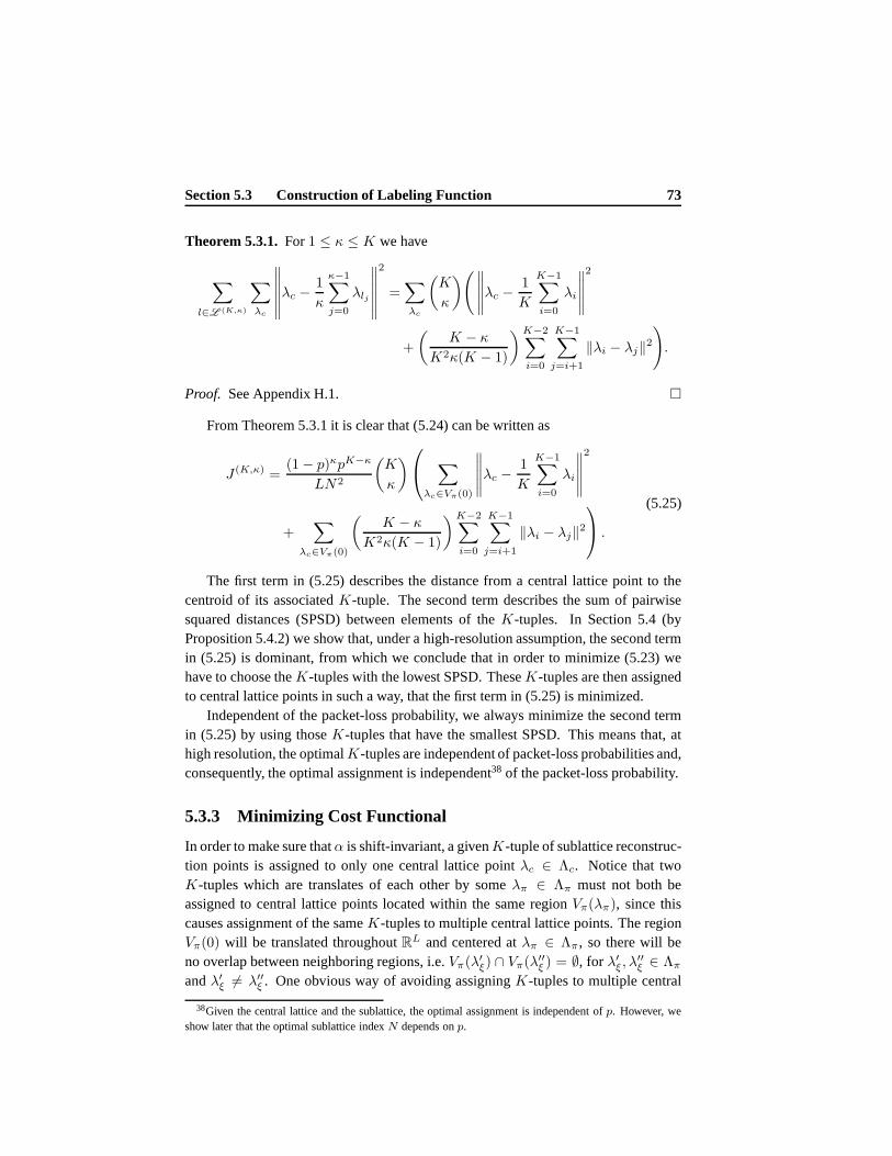
Section 5.3 Construction of Labeling Function 73
Theorem 5.3.1.For1 ≤ κ ≤ K we have
∑
l∈L (K,κ)
∑
λc
∥∥∥∥∥∥
λc −1
κ
κ−1∑
j=0
λlj
∥∥∥∥∥∥
2
=∑
λc
(K
κ
)(∥∥∥∥∥λc −
1
K
K−1∑
i=0
λi
∥∥∥∥∥
2
+
(K − κ
K2κ(K − 1)
)K−2∑
i=0
K−1∑
j=i+1
‖λi − λj‖2)
.
Proof. See Appendix H.1.
From Theorem 5.3.1 it is clear that (5.24) can be written as
J (K,κ) =(1− p)κpK−κ
LN2
(K
κ
)
∑
λc∈Vπ(0)
∥∥∥∥∥λc −
1
K
K−1∑
i=0
λi
∥∥∥∥∥
2
+∑
λc∈Vπ(0)
(K − κ
K2κ(K − 1)
)K−2∑
i=0
K−1∑
j=i+1
‖λi − λj‖2
.
(5.25)
The first term in (5.25) describes the distance from a centrallattice point to thecentroid of its associatedK-tuple. The second term describes the sum of pairwisesquared distances (SPSD) between elements of theK-tuples. In Section 5.4 (byProposition 5.4.2) we show that, under a high-resolution assumption, the second termin (5.25) is dominant, from which we conclude that in order tominimize (5.23) wehave to choose theK-tuples with the lowest SPSD. TheseK-tuples are then assignedto central lattice points in such a way, that the first term in (5.25) is minimized.
Independent of the packet-loss probability, we always minimize the second termin (5.25) by using thoseK-tuples that have the smallest SPSD. This means that, athigh resolution, the optimalK-tuples are independent of packet-loss probabilities and,consequently, the optimal assignment is independent38 of the packet-loss probability.
5.3.3 Minimizing Cost Functional
In order to make sure thatα is shift-invariant, a givenK-tuple of sublattice reconstruc-tion points is assigned to only one central lattice pointλc ∈ Λc. Notice that twoK-tuples which are translates of each other by someλπ ∈ Λπ must not both beassigned to central lattice points located within the same regionVπ(λπ), since thiscauses assignment of the sameK-tuples to multiple central lattice points. The regionVπ(0) will be translated throughoutRL and centered atλπ ∈ Λπ, so there will beno overlap between neighboring regions, i.e.Vπ(λ
′ξ) ∩ Vπ(λ′′ξ ) = ∅, for λ′ξ, λ
′′ξ ∈ Λπ
andλ′ξ 6= λ′′ξ . One obvious way of avoiding assigningK-tuples to multiple central
38Given the central lattice and the sublattice, the optimal assignment is independent ofp. However, weshow later that the optimal sublattice indexN depends onp.
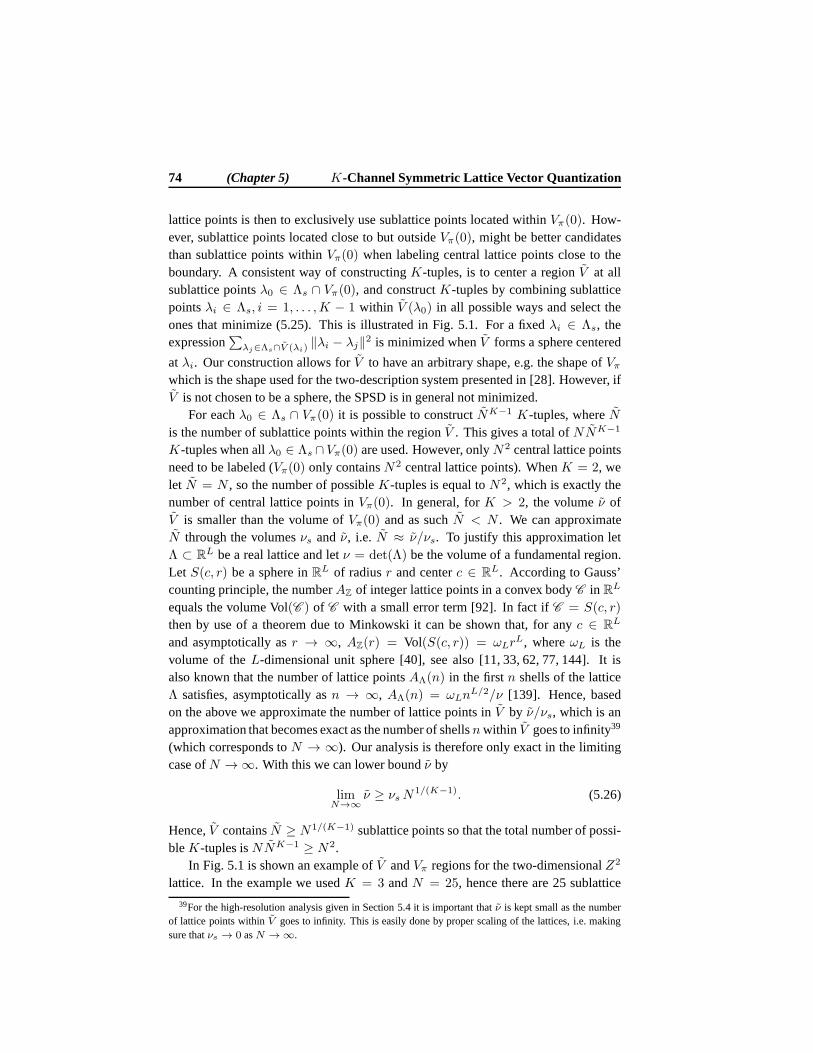
74 (Chapter 5) K-Channel Symmetric Lattice Vector Quantization
lattice points is then to exclusively use sublattice pointslocated withinVπ(0). How-ever, sublattice points located close to but outsideVπ(0), might be better candidatesthan sublattice points withinVπ(0) when labeling central lattice points close to theboundary. A consistent way of constructingK-tuples, is to center a regionV at allsublattice pointsλ0 ∈ Λs ∩ Vπ(0), and constructK-tuples by combining sublatticepointsλi ∈ Λs, i = 1, . . . ,K − 1 within V (λ0) in all possible ways and select theones that minimize (5.25). This is illustrated in Fig. 5.1. For a fixedλi ∈ Λs, theexpression
∑
λj∈Λs∩V (λi)‖λi − λj‖2 is minimized whenV forms a sphere centered
at λi. Our construction allows forV to have an arbitrary shape, e.g. the shape ofVπwhich is the shape used for the two-description system presented in [28]. However, ifV is not chosen to be a sphere, the SPSD is in general not minimized.
For eachλ0 ∈ Λs ∩ Vπ(0) it is possible to constructNK−1 K-tuples, whereNis the number of sublattice points within the regionV . This gives a total ofNNK−1
K-tuples when allλ0 ∈ Λs ∩ Vπ(0) are used. However, onlyN2 central lattice pointsneed to be labeled (Vπ(0) only containsN2 central lattice points). WhenK = 2, welet N = N , so the number of possibleK-tuples is equal toN2, which is exactly thenumber of central lattice points inVπ(0). In general, forK > 2, the volumeν ofV is smaller than the volume ofVπ(0) and as suchN < N . We can approximateN through the volumesνs and ν, i.e. N ≈ ν/νs. To justify this approximation letΛ ⊂ RL be a real lattice and letν = det(Λ) be the volume of a fundamental region.Let S(c, r) be a sphere inRL of radiusr and centerc ∈ RL. According to Gauss’counting principle, the numberAZ of integer lattice points in a convex bodyC in RL
equals the volume Vol(C ) of C with a small error term [92]. In fact ifC = S(c, r)
then by use of a theorem due to Minkowski it can be shown that, for anyc ∈ RL
and asymptotically asr → ∞, AZ(r) = Vol(S(c, r)) = ωLrL, whereωL is the
volume of theL-dimensional unit sphere [40], see also [11, 33, 62, 77, 144]. It isalso known that the number of lattice pointsAΛ(n) in the firstn shells of the latticeΛ satisfies, asymptotically asn → ∞, AΛ(n) = ωLn
L/2/ν [139]. Hence, basedon the above we approximate the number of lattice points inV by ν/νs, which is anapproximation that becomes exact as the number of shellsnwithin V goes to infinity39
(which corresponds toN → ∞). Our analysis is therefore only exact in the limitingcase ofN → ∞. With this we can lower boundν by
limN→∞
ν ≥ νsN1/(K−1). (5.26)
Hence,V containsN ≥ N1/(K−1) sublattice points so that the total number of possi-bleK-tuples isNNK−1 ≥ N2.
In Fig. 5.1 is shown an example ofV andVπ regions for the two-dimensionalZ2
lattice. In the example we usedK = 3 andN = 25, hence there are 25 sublattice
39For the high-resolution analysis given in Section 5.4 it is important thatν is kept small as the numberof lattice points withinV goes to infinity. This is easily done by proper scaling of the lattices, i.e. makingsure thatνs → 0 asN → ∞.

Section 5.3 Construction of Labeling Function 75
points withinVπ. There areN = N1/(K−1) = 5 sublattice points inV which isexactly the minimum number of points required, according to(5.26).
PSfrag replacements
∈ Λs
∈ Λπ
V
Vπ
Vπ(0)
K = 3
N = 25
N = 5
Figure 5.1: The regionV (big circles) is here shown centered at two different sublattice pointswithin Vπ(0). Small dots represents sublattice points ofΛs and large dots represents productlattice pointsλπ ∈ Λπ . Central lattice points are not shown here.Vπ (shown as squares)contains 25 sublattice points centered at product lattice points. In this exampleV contains 5sublattice points.
With equality in (5.26) we obtain a region that contains the exact number of sub-lattice points required to constructN tuples for each of theN λ0 points inVπ(0).According to (5.25), a central lattice point should be assigned thatK-tuple where aweighted average of any subset of the elements of theK-tuple is as close as possible tothe central lattice point. The optimal assignment ofK-tuples to central lattice pointscan be formulated and solved as a linear assignment problem [151].
Shift-Invariance by use of Cosets
By centeringV around eachλ0 ∈ Λs ∩ Vπ(0), we make sure that the mapα isshift-invariant. However, this also means that allK-tuples have their first coordinate(i.e.λ0) insideVπ(0). To be optimal this restriction must be removed which is easilydone by considering all cosets of eachK-tuple. The coset of a fixedK-tuple, sayt = (λ0, λ1, . . . , λK−1) whereλ0 ∈ Λs ∩ Vπ(0) and (λ1, . . . , λK−1) ∈ ΛK−1
s ,is given byCoset(t) = t + λπ : ∀λπ ∈ Λπ . K-tuples in a coset are distinctmoduloΛπ and by making sure that only one member from each coset is used, theshift-invariance property is preserved. In general it is sufficient to consider only thoseλπ product lattice points that are close toVπ(0), e.g. those points whose Voronoi celltouchesVπ(0). The number of such points is given by the kissing-numberK(Λπ) of
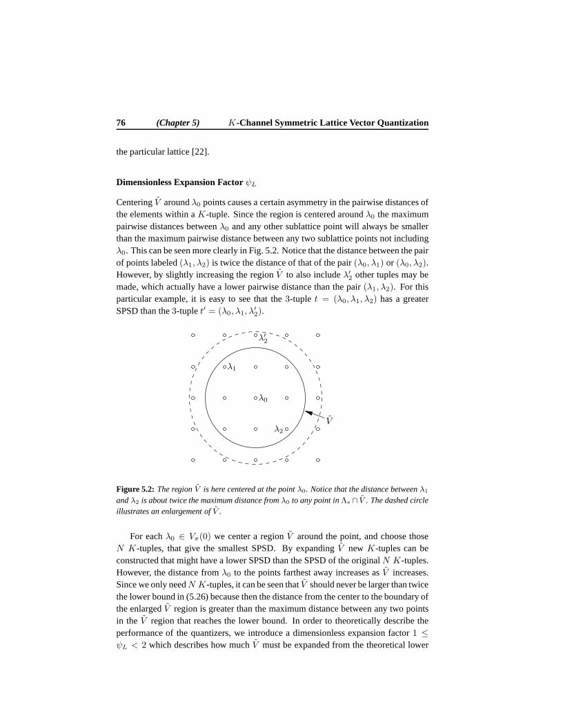
76 (Chapter 5) K-Channel Symmetric Lattice Vector Quantization
the particular lattice [22].
Dimensionless Expansion FactorψL
CenteringV aroundλ0 points causes a certain asymmetry in the pairwise distancesofthe elements within aK-tuple. Since the region is centered aroundλ0 the maximumpairwise distances betweenλ0 and any other sublattice point will always be smallerthan the maximum pairwise distance between any two sublattice points not includingλ0. This can be seen more clearly in Fig. 5.2. Notice that the distance between the pairof points labeled(λ1, λ2) is twice the distance of that of the pair(λ0, λ1) or (λ0, λ2).However, by slightly increasing the regionV to also includeλ′2 other tuples may bemade, which actually have a lower pairwise distance than thepair (λ1, λ2). For thisparticular example, it is easy to see that the3-tuple t = (λ0, λ1, λ2) has a greaterSPSD than the3-tuplet′ = (λ0, λ1, λ
′2).
PSfrag replacements
λ0
λ1
λ2
λ′1
λ′2
V
K = 3
N = 81
N = 9
Figure 5.2: The regionV is here centered at the pointλ0. Notice that the distance betweenλ1
andλ2 is about twice the maximum distance fromλ0 to any point inΛs ∩ V . The dashed circleillustrates an enlargement ofV .
For eachλ0 ∈ Vπ(0) we center a regionV around the point, and choose thoseN K-tuples, that give the smallest SPSD. By expandingV newK-tuples can beconstructed that might have a lower SPSD than the SPSD of the originalN K-tuples.However, the distance fromλ0 to the points farthest away increases asV increases.Since we only needN K-tuples, it can be seen thatV should never be larger than twicethe lower bound in (5.26) because then the distance from the center to the boundary ofthe enlargedV region is greater than the maximum distance between any two pointsin the V region that reaches the lower bound. In order to theoretically describe theperformance of the quantizers, we introduce a dimensionless expansion factor1 ≤ψL < 2 which describes how muchV must be expanded from the theoretical lower
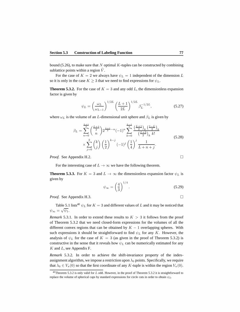
Section 5.3 Construction of Labeling Function 77
bound (5.26), to make sure thatN optimalK-tuples can be constructed by combiningsublattice points within a regionV .
For the case ofK = 2 we always haveψL = 1 independent of the dimensionLso it is only in the caseK ≥ 3 that we need to find expressions forψL.
Theorem 5.3.2.For the case ofK = 3 and any oddL, the dimensionless expansionfactor is given by
ψL =
(ωL
ωL−1
)1/2L (L+ 1
2L
)1/2L
β−1/2LL , (5.27)
whereωL is the volume of anL-dimensional unit sphere andβL is given by
βL =
L+12∑
n=0
(L+12
n
)
2L+12 −n(−1)n
L−12∑
k=0
(L+12
)
k
(1−L2
)
k(L+32
)
kk!
×k∑
j=0
(k
j
)(1
2
)k−j
(−1)j(1
4
)j1
L+ n+ j.
(5.28)
Proof. See Appendix H.2.
For the interesting case ofL→ ∞ we have the following theorem.
Theorem 5.3.3. ForK = 3 andL → ∞ the dimensionless expansion factorψL isgiven by
ψ∞ =
(4
3
)1/4
. (5.29)
Proof. See Appendix H.3.
Table 5.1 lists40 ψL forK = 3 and different values ofL and it may be noticed thatψ∞ =
√ψ1.
Remark5.3.1. In order to extend these results toK > 3 it follows from the proofof Theorem 5.3.2 that we need closed-form expressions for the volumes of all thedifferent convex regions that can be obtained byK − 1 overlapping spheres. Withsuch expressions it should be straightforward to findψL for anyK. However, theanalysis ofψL for the case ofK = 3 (as given in the proof of Theorem 5.3.2) isconstructive in the sense that it reveals howψL can be numerically estimated for anyK andL, see Appendix F.
Remark 5.3.2. In order to achieve the shift-invariance property of the index-assignment algorithm, we impose a restriction uponλ0 points. Specifically, we requirethatλ0 ∈ Vπ(0) so that the first coordinate of anyK-tuple is within the regionVπ(0).
40Theorem 5.3.2 is only valid forL odd. However, in the proof of Theorem 5.3.2 it is straightforward toreplace the volume of spherical caps by standard expressions for circle cuts in order to obtainψ2.

78 (Chapter 5) K-Channel Symmetric Lattice Vector Quantization
L ψL
1 1.1547005 · · ·2 1.1480804 · · ·3 1.1346009 · · ·5 1.1240543 · · ·7 1.1172933 · · ·9 1.1124896 · · ·11 1.1088540 · · ·13 1.1059819 · · ·
L ψL
15 1.1036412 · · ·17 1.1016878 · · ·19 1.1000271 · · ·21 1.0985938 · · ·51 1.0883640 · · ·71 1.0855988 · · ·101 1.0831849 · · ·∞ 1.0745699 . . .
Table 5.1:ψL values obtained by use of Theorems 5.3.2 and 5.3.3 forK = 3.
To avoid excludingK-tuples that have their first coordinate outsideVπ(0) we formcosets of eachK-tuple and allow only one member from each coset to be assigned toa central lattice point withinVπ(0). This restriction, which is only put onλ0 ∈ Λs,might cause a bias towardsλ0 points. However, it is easy to show that, asymptoticallyasN → ∞, any such bias can be removed. For the case ofK = 2 we can use sim-ilar arguments as used in [28], and forK > 2, as shown in Chapter 6, the numberof K-tuples affected by this restriction is small compared to the number ofK-tuplesnot affected. So for example this means that we can enforce similar restrictions on allsublattice points, which, asymptotically asN → ∞, will only reduce the number ofK-tuples by a neglectable amount. And as such, any possible bias towards the set ofpointsλ0 ∈ Λs is removed.
As mentioned above, theK-tuples need to be assigned to central lattice pointswithin Vπ(0). This is a standard linear assignment problem where a cost measureis minimized. However, solutions to linear assignment problems are generally notunique. Therefore, there might exist several labelings, which all yield the same cost,but exhibit a different amount of asymmetry. Theoretically, exact symmetry may thenbe obtained by e.g. time sharing through a suitable mixing oflabelings. In practice,however, any scheme would use a finiteN (and finite rates). In addition, for manyapplications, time sharing is inconvenient. In these non-asymptotic cases we cannotguarantee exact symmetry. To this end, we have provided a fewexamples that as-sess the distortions obtained from practical experiments,see Section 5.6 (Tables 5.3and 5.4).
5.4 High-Resolution Analysis
In this section we derive high-resolution approximations for the expected distortion.For this high-resolution analysis we letN → ∞ andνs → 0. Thus, the indexN ofthe sublattices increases, but the actual volumes of the Voronoi cells shrink.
Section 5.4 High-Resolution Analysis 79
5.4.1 Total Expected Distortion
We wish to obtain an analytical expression for the expected distortion given by (5.22).In order to achieve this we first relate the sum of distances between pairs of sublatticepoints toG(SL), the dimensionless normalized second moment of anL-sphere. Thisis done by Proposition 5.4.1.
Proposition 5.4.1. ForK = 2 and asymptotically asN → ∞ andνs → 0, as wellas forK = 3 and asymptotically asN,L → ∞ andνs → 0, we have for any pair(λi, λj), i, j = 0, . . . ,K − 1, i 6= j,
1
L
∑
λc∈Vπ(0)
‖αi(λc)− αj(λc)‖2 = G(SL)ψ2LN
2N2K/L(K−1)ν2/L.
Proof. See Appendix H.4.
Conjecture 5.4.1.Proposition 5.4.1 is true also forK > 3 asymptotically asN,L→∞ andνs → 0.
Remark5.4.1. Arguments supporting conjecture 5.4.1 are given in Appendix H.4.
Remark5.4.2. In Appendix H.4 we also present an exact expression for Proposition5.4.1 forK = 3 and finiteL.
Recall that we previously showed that by use of Theorem 5.3.1it is possible tosplit (5.22) into two terms; one that describes the distancefrom a central lattice point tothe centroid of its associatedK-tuple and another which describes the sum of pairwisesquared distances (SPSD) between elements of theK-tuples. To determine which ofthe two terms that are dominating we present the following proposition:
Proposition 5.4.2. ForN → ∞ and2 ≤ K <∞ we have
∑
λc∈Vπ(0)
∥∥∥λc − 1
K
∑K−1i=0 λi
∥∥∥
2
∑
λc∈Vπ(0)
∑K−2i=0
∑K−1j=i+1 ‖λi − λj‖2
→ 0. (5.30)
Proof. See Appendix H.5.
The expected distortion (5.22) can by use of Theorem 5.3.1 bewritten as
D(K,κ)a ≈ (1− p)κpK−κ×
(K
κ
)
Dc +1
L
1
N2
∑
l∈L (K,κ)
∑
λc∈Vπ(0)
∥∥∥∥∥∥
λc −1
κ
κ−1∑
j=0
λlj
∥∥∥∥∥∥
2
= (1− p)κpK−κ
(K
κ
)
×(
Dc +1
L
1
N2
∑
λc∈Vπ(0)
∥∥∥∥∥λc −
1
K
K−1∑
i=0
λi
∥∥∥∥∥
2
+
(K − κ
K2κ(K − 1)
)K−2∑
i=0
K−1∑
j=i+1
‖λi − λj‖2
)
.
(5.31)
80 (Chapter 5) K-Channel Symmetric Lattice Vector Quantization
By use of Proposition 5.4.1 (as an approximation that becomes exact forL→ ∞),Proposition 5.4.2 and Eq. (5.13) it follows that (5.31) can be written as
D(K,κ)a ≈ (1− p)κpK−κ
(K
κ
)
×
Dc +1
L
1
N2
∑
λc∈Vπ(0)
(K − κ
K2κ(K − 1)
)K−2∑
i=0
K−1∑
j=i+1
‖λi − λj‖2
(5.32)
≈ (1− p)κpK−κ
(K
κ
)
×(
G(Λc)ν2/L +
(K − κ
2Kκ
)
G(SL)ψ2LN
2K/L(K−1)ν2/L)
. (5.33)
The second term in (5.33), that is
(K − κ
2Kκ
)
G(SL)ψ2LN
2K/L(K−1)ν2/L (5.34)
is the dominating term forκ < K andN → ∞ and describes the side distortion dueto reception of anyκ < K descriptions. Observe that this term is only dependent uponκ through the coefficientK−κ
2Kκ .
The total expected distortionD(K)a is obtained from (5.33) by summing overκ
including the cases whereκ = 0 andκ = K, which leads to
D(K)a ≈ K1G(Λc)ν
2/L + K2G(SL)ψ2LN
2K/L(K−1)ν2/L + pKE‖X‖2/L, (5.35)
whereK1 is given by
K1 =
K∑
κ=1
(K
κ
)
pK−κ(1 − p)κ
= 1− pK ,
(5.36)
andK2 is given by
K2 =
K∑
κ=1
(K
κ
)
pK−κ(1− p)κK − κ
2κK. (5.37)
Using (5.18) and (5.19) we can writeν andN as a function of differential entropyand side entropies, that is
ν2/L = 22(h(X)−Rc), (5.38)
and
N2K/L(K−1) = 22K
K−1 (Rc−Rs), (5.39)
Section 5.4 High-Resolution Analysis 81
whereRs = Ri, i = 0, . . . ,K − 1 denotes the side description rate. Inserting (5.38)and (5.39) in (5.35) makes it possible to write the expected distortion as a function ofentropies
D(K)a ≈ K1G(Λc)2
2(h(X)−Rc)
+ K2ψ2LG(SL)2
2(h(X)−Rc)22K
K−1 (Rc−Rs) + pKE‖X‖2/L,(5.40)
where we see that the distortion due to the side quantizers depends only upon thescaling (and dimension) of the sublattice but not upon whichsublattice is used. Thus,the side distortions can be expressed through the dimensionless normalized secondmoment of a sphere.
5.4.2 Optimalν,N andK
We now derive expressions for the optimalν, N andK. Using these values we areable to construct the latticesΛc andΛs. The optimal index assignment is hereafterfound by using the approach outlined in Section 5.3. These lattices combined withtheir index assignment completely specify an optimal entropy-constrained MD-LVQsystem.
In order for the entropies of the side descriptions to be equal to the target entropyRT /K, we rewrite (5.19) and get
Nν = 2L(h(X)−RT /K) , τ, (5.41)
whereτ is constant. The expected distortionD(K)a (5.40) may now be expressed as a
function ofν,
D(K)a = K1G(Λc)ν
2/L
+ K2ψ2LG(SL)ν
2/Lν−2K
L(K−1) τ2K
L(K−1) + pKE‖X‖2/L.(5.42)
Differentiating w.r.t.ν and equating to zero gives,
0 =∂D
(K)a
∂ν
=2
LK1G(Λc)
ν2/L
ν+
(2
L− 2
L
K
K − 1
)
K2ψ2LG(SL)
ν2/L
νν−
2KL(K−1) τ
2KL(K−1) ,
(5.43)
from which we obtain the optimal value ofν
ν = τ
(
1
K − 1
K2
K1
G(SL)
G(Λc)ψ2L
)L(K−1)2K
. (5.44)
82 (Chapter 5) K-Channel Symmetric Lattice Vector Quantization
The optimalN follows easily by use of (5.41)
N =
(
(K − 1)K1
K2
G(Λc)
G(SL)
1
ψ2L
)L(K−1)2K
. (5.45)
Eq. (5.45) shows that the optimal redundancyN is, for fixedK, independent of thesublattice as well as the target entropy.
For a fixedK the optimalν andN are given by (5.44) and (5.45), respectively,and the optimalK can then easily be found by evaluating (5.35) for various values ofK, and choosing the one that yields the lowest expected distortion. The optimalK isthen given by
Kopt = arg minK
D(K)a , K = 1, . . . ,Kmax, (5.46)
whereKmax is a suitable chosen positive integer. In practiceK will always be finiteand furthermore limited to a narrow range of integers, whichmakes the complexity ofthe minimization approach, given by (5.46), negligible.
5.5 Construction of Practical Quantizers
5.5.1 Index Values
Eqs. (5.44) and (5.45) suggest that we are able to continuously trade off central versusside-distortions by adjustingN andν according to the packet-loss probability. Thisis, however, not the case, since certain constraints must beimposed onN . First ofall, sinceN denotes the number of central lattice points within each Voronoi cell ofthe sublattice, it must be integer and positive. Second, we require the sublattice tobe geometrically similar to the central lattice. Finally, we require the sublattice tobe a clean sublattice, so that no central lattice points are located on boundaries ofVoronoi cells of the sublattice. This restricts the amount of admissible index valuesfor a particular lattice to a discrete set, cf. Section 2.3.1.
Fig. 5.3 shows the theoretically optimal index values (i.e.ignoring the fact thatNbelongs to a discrete set) for theA2 quantizer, given by (5.45) forψL = 1, 1.1481
and1.1762 corresponding toK = 2, 3 and4, respectively.41 Also shown are thetheoretical optimal index values when restricted to admissible index values. Noticethat the optimal index valueN increases for increasing number of descriptions. Thisis to be expected since a higher index value leads to less redundancy; this redun-dancy reduction, however, is balanced out by the redundancyincrease resulting fromthe added number of descriptions. In [103] we observed that for a two-descriptionsystem, usually only very few index values would be used (assuming a certain min-imum packet-loss probability). Specifically, for the two-dimensionalA2 quantizer,
41The valueψL = 1.1762 for K = 4 is estimated numerically by using the method outlined in Ap-pendix F.
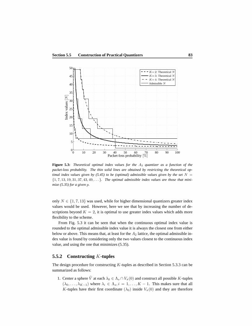
Section 5.5 Construction of Practical Quantizers 83
0 10 20 30 40 50 60 70 80 90 1000
5
10
15
20
25
30
35
40
45
50
PSfrag replacements
Inde
xva
lues[N
]
Packet-loss probability[%]
K=2: TheoreticalNK=3: TheoreticalNK=4: TheoreticalNAdmissibleN
Figure 5.3: Theoretical optimal index values for theA2 quantizer as a function of thepacket-loss probability. The thin solid lines are obtainedby restricting the theoretical op-timal index values given by (5.45) to be (optimal) admissible values given by the setN =
1, 7, 13, 19, 31, 37, 43, 49, . . . . The optimal admissible index values are those that mini-mize (5.35) for a givenp.
onlyN ∈ 1, 7, 13 was used, while for higher dimensional quantizers greater indexvalues would be used. However, here we see that by increasingthe number of de-scriptions beyondK = 2, it is optimal to use greater index values which adds moreflexibility to the scheme.
From Fig. 5.3 it can be seen that when the continuous optimal index value isrounded to the optimal admissible index value it is always the closest one from eitherbelow or above. This means that, at least for theA2 lattice, the optimal admissible in-dex value is found by considering only the two values closestto the continuous indexvalue, and using the one that minimizes (5.35).
5.5.2 ConstructingK-tuples
The design procedure for constructingK-tuples as described in Section 5.3.3 can besummarized as follows:
1. Center a sphereV at eachλ0 ∈ Λs ∩ Vπ(0) and construct all possibleK-tuples(λ0, . . . , λK−1) whereλi ∈ Λs, i = 1, . . . ,K − 1. This makes sure that allK-tuples have their first coordinate(λ0) insideVπ(0) and they are therefore
84 (Chapter 5) K-Channel Symmetric Lattice Vector Quantization
shift invariant. We will only useK-tuples whose elements satisfy‖λi − λj‖ ≤r, ∀i, j ∈ 0, . . . ,K − 1, wherer is the radius ofV . MakeV large enough sothat at leastN distinctK-tuples are found for eachλ0.
2. Construct cosets of eachK-tuple.
3. TheN2 central lattice points inΛc∩Vπ(0) must now be matched to distinctK-tuples. This is a standard linear assignment problem where only one memberfrom each coset is (allowed to be) matched to a central lattice point inVπ(0).
The restriction‖λi − λj‖ ≤ r from step 1) which is used to avoid bias towards anyof the sublattices, reduces the number ofK-tuples that can be constructed within thesphereV . To be able to formN K-tuples it is therefore necessary to use a sphereV
with a volume larger than the lower bound (5.26). This enlargement is exactly givenbyψL. As such, for eachλ0, we form (at least)N K-tuples and theseK-tuples are theones having minimum norm. We show later (see Lemma 6.2.3 and its proof) that weactually form all suchK-tuples of minimal norm which implies that no otherK-tuplescan improve the SPSD.
5.5.3 AssigningK-Tuples to Central Lattice Points
In order to assign the set ofK-tuples to theN2 central lattice points we solve a linearassignment problem. However, for largeN , the problem becomes difficult to solve inpractice. To solve a linear assignment problem or more specifically a bipartite match-ing problem, one can make use of the Hungarian method [78], which has complexityof cubic order. Hence, if the Hungarian method is used to solve the assignment prob-lem the complexity is of orderO(N6). We would like point out that lettingNπ = N2
is a convenient choice, which is valid for any lattice. However, it is possible to letNπ = Nξ, where bothN andξ are admissible index values. In this caseNπ is alsoguaranteed to be an admissible index value by Lemma 2.3.1. Ifξ = 1 thenNπ = N ,which is a special case whereVπ(0) contains a single sublattice pointλ0 of Λs.42 WithNπ = Nξ, the complexity is reduced toO(N3).
Vaishampayan et al. observed in [120,139] that the number ofcentral lattice pointsto be labeled can be reduced by exploiting symmetries in the lattices. For example,one can form the quotientJ -moduleΛ/Λπ and only label representatives of theorbits ofΛ/Λπ/Γ, whereΓ is a group of automorphisms, cf. Chapter 2. While onlytwo descriptions were considered in [139] it is straight-forward to show that their ideaalso works in our design for an arbitrary number of descriptions. This is because
42Practical experiments have shown that having too few sublattice points inVπ(0) leads to a poor indexassignment. Theoretically, we do not exclude the possibility thatNπ = N , since we only require thatVcontains a large number of sublattice points but such a contraint is not imposed onVπ(0). However, in thefollowing chapter, where we consider the asymmetric case (so there are several index values), the specialcase is not allowed.
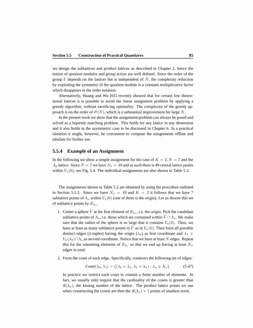
Section 5.5 Construction of Practical Quantizers 85
we design the sublattices and product lattices as describedin Chapter 2, hence thenotion of quotient modules and group action are well defined.Since the order of thegroupΓ depends on the lattices but is independent ofN , the complexity reductionby exploiting the symmetry of the quotient module is a constant multiplicative factorwhich disappears in the order notation.
Alternatively, Huang and Wu [65] recently showed that for certain low dimen-sional lattices it is possible to avoid the linear assignment problem by applying agreedy algorithm, without sacrificing optimality. The complexity of the greedy ap-proach is on the order ofO(N), which is a substantial improvement for largeN .
In the present work we show that the assignment problem can always be posed andsolved as a bipartite matching problem. This holds for any lattice in any dimensionand it also holds in the asymmetric case to be discussed in Chapter 6. In a practicalsituation it might, however, be convenient to compute the assignments offline andtabulate for further use.
5.5.4 Example of an Assignment
In the following we show a simple assignment for the case ofK = 2, N = 7 and theA2 lattice. SinceN = 7 we haveNπ = 49 and as such there is 49 central lattice pointswithin Vπ(0), see Fig. 5.4. The individual assignments are also shown in Table 5.2.
The assignments shown in Table 5.2 are obtained by using the procedure outlinedin Section 5.5.2. Since we haveNπ = 49 andK = 2 it follows that we have 7sublattice points ofΛs within Vπ(0) (one of them is the origin). Let us denote this setof sublattice points byEΛs
.
1. Center a sphereV at the first element ofEλs, i.e. the origin. Pick the candidate
sublattice points ofΛs, i.e. those which are contained withinV ∩Λs. We makesure that the radius of the sphere is so large that it containsVπ(0). Thus, wehave at least as many sublattice points inV as inVπ(0). Then form all possibledistinct edges (2-tuples) having the origin (λ0) as first coordinate andλ1 ∈Vπ(λ0)∩Λs as second coordinate. Notice that we have at leastN edges. Repeatthis for the remaining elements ofEΛs
so that we end up having at leastNπ
edges in total.
2. Form the coset of each edge. Specifically, construct the following set of edges:
Coset(λ0, λ1) = (λ0 + λπ , λ1 + λπ) : λπ ∈ Λπ. (5.47)
In practice we restrict each coset to contain a finite number of elements. Infact, we usually only require that the cardinality of the cosets is greater thanK(Λs), the kissing number of the lattice. The product lattice points we usewhen constructing the cosets are then theK(Λs) + 1 points of smallest norm.
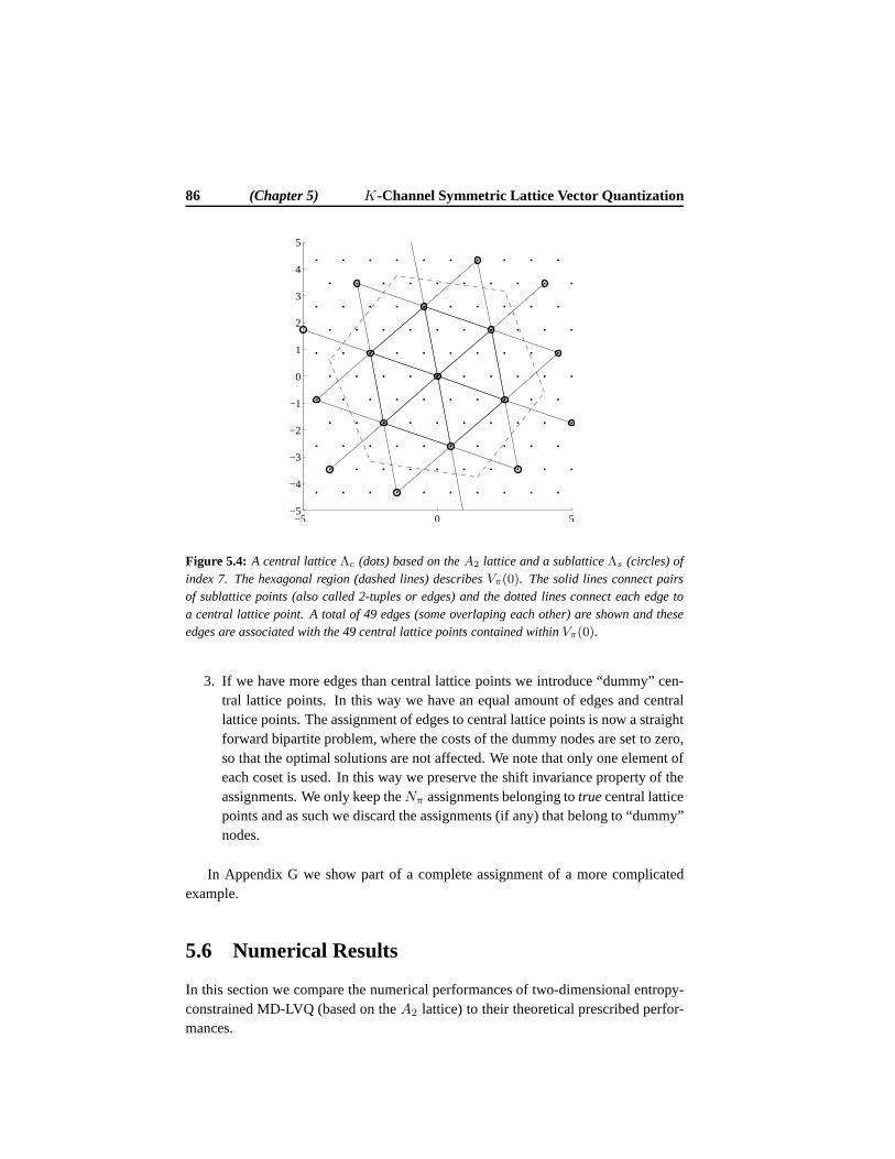
86 (Chapter 5) K-Channel Symmetric Lattice Vector Quantization
−5 0 5−5
−4
−3
−2
−1
0
1
2
3
4
5
Figure 5.4: A central latticeΛc (dots) based on theA2 lattice and a sublatticeΛs (circles) ofindex 7. The hexagonal region (dashed lines) describesVπ(0). The solid lines connect pairsof sublattice points (also called 2-tuples or edges) and thedotted lines connect each edge toa central lattice point. A total of 49 edges (some overlapingeach other) are shown and theseedges are associated with the 49 central lattice points contained withinVπ(0).
3. If we have more edges than central lattice points we introduce “dummy” cen-tral lattice points. In this way we have an equal amount of edges and centrallattice points. The assignment of edges to central lattice points is now a straightforward bipartite problem, where the costs of the dummy nodes are set to zero,so that the optimal solutions are not affected. We note that only one element ofeach coset is used. In this way we preserve the shift invariance property of theassignments. We only keep theNπ assignments belonging totruecentral latticepoints and as such we discard the assignments (if any) that belong to “dummy”nodes.
In Appendix G we show part of a complete assignment of a more complicatedexample.
5.6 Numerical Results
In this section we compare the numerical performances of two-dimensional entropy-constrained MD-LVQ (based on theA2 lattice) to their theoretical prescribed perfor-mances.
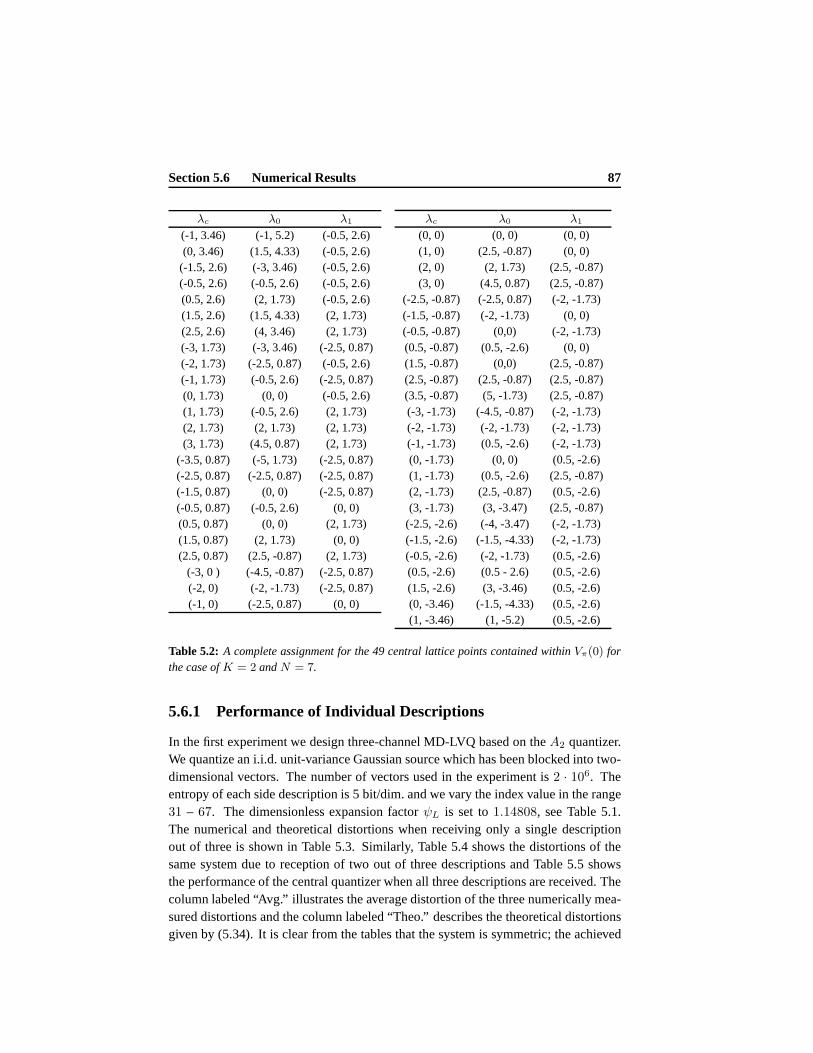
Section 5.6 Numerical Results 87
λc λ0 λ1
(-1, 3.46) (-1, 5.2) (-0.5, 2.6)(0, 3.46) (1.5, 4.33) (-0.5, 2.6)
(-1.5, 2.6) (-3, 3.46) (-0.5, 2.6)(-0.5, 2.6) (-0.5, 2.6) (-0.5, 2.6)(0.5, 2.6) (2, 1.73) (-0.5, 2.6)(1.5, 2.6) (1.5, 4.33) (2, 1.73)(2.5, 2.6) (4, 3.46) (2, 1.73)(-3, 1.73) (-3, 3.46) (-2.5, 0.87)(-2, 1.73) (-2.5, 0.87) (-0.5, 2.6)(-1, 1.73) (-0.5, 2.6) (-2.5, 0.87)(0, 1.73) (0, 0) (-0.5, 2.6)(1, 1.73) (-0.5, 2.6) (2, 1.73)(2, 1.73) (2, 1.73) (2, 1.73)(3, 1.73) (4.5, 0.87) (2, 1.73)
(-3.5, 0.87) (-5, 1.73) (-2.5, 0.87)(-2.5, 0.87) (-2.5, 0.87) (-2.5, 0.87)(-1.5, 0.87) (0, 0) (-2.5, 0.87)(-0.5, 0.87) (-0.5, 2.6) (0, 0)(0.5, 0.87) (0, 0) (2, 1.73)(1.5, 0.87) (2, 1.73) (0, 0)(2.5, 0.87) (2.5, -0.87) (2, 1.73)
(-3, 0 ) (-4.5, -0.87) (-2.5, 0.87)(-2, 0) (-2, -1.73) (-2.5, 0.87)(-1, 0) (-2.5, 0.87) (0, 0)
λc λ0 λ1
(0, 0) (0, 0) (0, 0)(1, 0) (2.5, -0.87) (0, 0)(2, 0) (2, 1.73) (2.5, -0.87)(3, 0) (4.5, 0.87) (2.5, -0.87)
(-2.5, -0.87) (-2.5, 0.87) (-2, -1.73)(-1.5, -0.87) (-2, -1.73) (0, 0)(-0.5, -0.87) (0,0) (-2, -1.73)(0.5, -0.87) (0.5, -2.6) (0, 0)(1.5, -0.87) (0,0) (2.5, -0.87)(2.5, -0.87) (2.5, -0.87) (2.5, -0.87)(3.5, -0.87) (5, -1.73) (2.5, -0.87)(-3, -1.73) (-4.5, -0.87) (-2, -1.73)(-2, -1.73) (-2, -1.73) (-2, -1.73)(-1, -1.73) (0.5, -2.6) (-2, -1.73)(0, -1.73) (0, 0) (0.5, -2.6)(1, -1.73) (0.5, -2.6) (2.5, -0.87)(2, -1.73) (2.5, -0.87) (0.5, -2.6)(3, -1.73) (3, -3.47) (2.5, -0.87)
(-2.5, -2.6) (-4, -3.47) (-2, -1.73)(-1.5, -2.6) (-1.5, -4.33) (-2, -1.73)(-0.5, -2.6) (-2, -1.73) (0.5, -2.6)(0.5, -2.6) (0.5 - 2.6) (0.5, -2.6)(1.5, -2.6) (3, -3.46) (0.5, -2.6)(0, -3.46) (-1.5, -4.33) (0.5, -2.6)(1, -3.46) (1, -5.2) (0.5, -2.6)
Table 5.2: A complete assignment for the 49 central lattice points contained withinVπ(0) forthe case ofK = 2 andN = 7.
5.6.1 Performance of Individual Descriptions
In the first experiment we design three-channel MD-LVQ basedon theA2 quantizer.We quantize an i.i.d. unit-variance Gaussian source which has been blocked into two-dimensional vectors. The number of vectors used in the experiment is2 · 106. Theentropy of each side description is 5 bit/dim. and we vary theindex value in the range31 – 67. The dimensionless expansion factorψL is set to1.14808, see Table 5.1.The numerical and theoretical distortions when receiving only a single descriptionout of three is shown in Table 5.3. Similarly, Table 5.4 showsthe distortions of thesame system due to reception of two out of three descriptionsand Table 5.5 showsthe performance of the central quantizer when all three descriptions are received. Thecolumn labeled “Avg.” illustrates the average distortion of the three numerically mea-sured distortions and the column labeled “Theo.” describesthe theoretical distortionsgiven by (5.34). It is clear from the tables that the system issymmetric; the achieved

88 (Chapter 5) K-Channel Symmetric Lattice Vector Quantization
distortion depends on the number of received descriptions but is essentially indepen-dent of which descriptions are used for reconstruction. The numericallymeasureddiscrete entropies of the side descriptions are shown in Table 5.6.
N λ0 λ1 λ2 Avg. Theo.
31 −25.6918 −25.6875 −25.6395 −25.6729 −24.8853
37 −24.5835 −24.5324 −24.5404 −24.5521 −24.5011
43 −24.5772 −24.5972 −24.5196 −24.5647 −24.1748
49 −24.2007 −24.2837 −24.2713 −24.2519 −23.8911
61 −23.8616 −23.9011 −23.8643 −23.8757 −23.4155
67 −23.7368 −23.7362 −23.7655 −23.7462 −23.2118
Table 5.3: Distortion (in dB) due to reception of a single description out of three.
N 12(λ0 + λ1)
12(λ0 + λ2)
12(λ1 + λ2) Avg. Theo.
31 −30.7792 −30.7090 −30.7123 −30.7335 −30.9059
37 −29.8648 −29.8430 −29.9472 −29.8850 −30.5217
43 −29.9087 −29.8749 −29.9641 −29.9159 −30.1954
49 −29.6290 −29.5577 −29.6662 −29.6176 −29.9117
61 −29.3076 −29.2185 −29.3715 −29.2992 −29.4361
67 −29.1752 −29.2128 −29.2151 −29.2010 −29.2324
Table 5.4: Distortion (in dB) due to reception of two descriptions out of three.
N λc Theo.
31 −43.6509 −43.6508
37 −44.4199 −44.4192
43 −45.0705 −45.0719
49 −45.6401 −45.6391
61 −46.5879 −46.5905
67 −46.9992 −46.9979
Table 5.5: Distortion (in dB) due to reception of all three descriptions.
The distortions shown in Tables 5.3 to 5.5 correspond to the case where we varythe index valueN throughout the range67 ≥ N ≥ 31 for three-channel MD-LVQoperating atRs = 5 bit/dim. per description. To achieve similar performance witha (3,1) SCEC we need to vary the correlationρq within the interval−0.49 ≤ ρq ≤−0.45, as shown in Fig. 5.5.
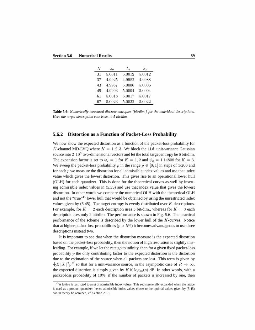
Section 5.6 Numerical Results 89
N λ0 λ1 λ2
31 5.0011 5.0012 5.0012
37 4.9925 4.9982 4.9988
43 4.9967 5.0006 5.0006
49 4.9993 5.0004 5.0004
61 5.0018 5.0017 5.0017
67 5.0023 5.0022 5.0022
Table 5.6: Numerically measured discrete entropies [bit/dim.] for the individual descriptions.Here the target description rate is set to 5 bit/dim.
5.6.2 Distortion as a Function of Packet-Loss Probability
We now show the expected distortion as a function of the packet-loss probability forK-channel MD-LVQ whereK = 1, 2, 3. We block the i.i.d. unit-variance Gaussiansource into2·106 two-dimensional vectors and let the total target entropy be6 bit/dim.The expansion factor is set toψ2 = 1 for K = 1, 2 andψ2 = 1.14808 for K = 3.We sweep the packet-loss probabilityp in the rangep ∈ [0; 1] in steps of 1/200 andfor eachp we measure the distortion for all admissible index values and use that indexvalue which gives the lowest distortion. This gives rise to an operational lower hull(OLH) for each quantizer. This is done for the theoretical curves as well by insert-ing admissible index values in (5.35) and use that index value that gives the lowestdistortion. In other words we compare the numerical OLH withthe theoretical OLHand not the “true”43 lower hull that would be obtained by using the unrestricted indexvalues given by (5.45). The target entropy is evenly distributed overK descriptions.For example, forK = 2 each description uses 3 bit/dim., whereas forK = 3 eachdescription uses only 2 bit/dim. The performance is shown inFig. 5.6. The practicalperformance of the scheme is described by the lower hull of theK-curves. Noticethat at higher packet-loss probabilities (p > 5%) it becomes advantageous to use threedescriptions instead two.
It is important to see that when the distortion measure is theexpected distortionbased on the packet-loss probability, then the notion of high resolution is slightly mis-leading. For example, if we let the rate go to infinity, then for a given fixed packet-lossprobabilityp the only contributing factor to the expected distortion is the distortiondue to the estimation of the source when all packets are lost.This term is given by1LE‖X‖2pK so that for a unit-variance source, in the asymptotic case ofR → ∞,the expected distortion is simply given byK10 log10(p) dB. In other words, with apacket-loss probability of 10%, if the number of packets is increased by one, then
43A lattice is restricted to a set of admissible index values. This set is generally expanded when the latticeis used as a product quantizer, hence admissible index values closer to the optimal values given by (5.45)can in theory be obtained, cf. Section 2.3.1.

90 (Chapter 5) K-Channel Symmetric Lattice Vector Quantization
−0.49 −0.485 −0.48 −0.475 −0.47 −0.465 −0.46 −0.455 −0.45
−46
−44
−42
−40
−38
−36
−34
−32
−30
−28
−26M
SE
[dB
]
PSfrag replacements
D(3,1)
D(3,2)
D(3,3)
ρq
Figure 5.5: The simultaneously achievable one-channel, two-channel and three-channel dis-tortions for the unit-variance Gaussian source at 5 bit/dim. for −0.49 < ρq < −0.45 for a(3, 1) SCEC.
the corresponding decrease in distortion is exactly 10 dB. We have illustrated this inFig. 5.7 forK = 1, . . . , 5.
5.7 Conclusion
We derived closed-form expressions for the central and sidequantizers which, at high-resolution conditions, minimize the expected distortion of a symmetricK-channelMD-LVQ scheme subject to entropy constraints on the side descriptions for givenpacket-loss probabilities. The expected distortion observed at the receiving side de-pends only upon the number of received descriptions but is independent of whichdescriptions are received. We focused on a special case of the symmetric MD prob-lem where only a single parameter (i.e.N ) controls the redundancy tradeoffs betweenthe central and the side distortions. We showed that the optimal amount of redundancyis in independent of the source distribution, the target rate and the type of lattices usedfor the side quantizers.
The practical design allows an arbitrary number of descriptions and the optimalnumber of descriptions depends (among other factors) upon the packet-loss probabil-ity. The theoretical rate-distortion results were proven for the case ofK ≤ 3 descrip-tions and conjectured to be true in the general case of arbitraryK descriptions.
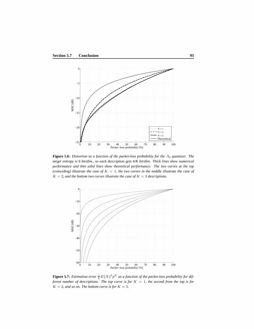
Section 5.7 Conclusion 91
0 10 20 30 40 50 60 70 80 90 100−25
−20
−15
−10
−5
0
Packet−loss probability [%]
MS
E [d
B]
Theoretical
PSfrag replacements K=1
K=2
K=3
Figure 5.6: Distortion as a function of the packet-loss probability fortheA2 quantizer. Thetarget entropy is 6 bit/dim., so each description gets 6/K bit/dim. Thick lines show numericalperformance and thin solid lines show theoretical performance. The two curves at the top(coinciding) illustrate the case ofK = 1, the two curves in the middle illustrate the case ofK = 2, and the bottom two curves illustrate the case ofK = 3 descriptions.
0 10 20 30 40 50 60 70 80 90 100−60
−50
−40
−30
−20
−10
0
Packet−loss probability [%]
MS
E [d
B]
Figure 5.7: Estimation error 1LE‖X‖2pK as a function of the packet-loss probability for dif-
ferent number of descriptions. The top curve is forK = 1, the second from the top is forK = 2, and so on. The bottom curve is forK = 5.

Chapter6
K-Channel Asymmetric Lattice
Vector Quantization
In this chapter we will focus on asymmetric MD-LVQ forK ≥ 2 descriptions, seeFig. 6.1. Asymmetric schemes offer additional flexibility over the symmetric schemes,since the bit distribution is also a design parameter and different weights are intro-duced in order to control the distortions. In fact, symmetric MD-LVQ is a special caseof asymmetric MD-LVQ.
In [27, 28] asymmetric two-channel MD-LVQ systems are derived subject to en-tropy constraints on the individual side entropies. However, since these schemes aresubject to individual side entropy constraints and not subject to a single constrainton the sum of the side entropies, the problem of how to distribute a total bit budgetamong the two descriptions is not addressed. In this chapterwe derive MD quantizerparameters subject to individual side entropy constraintsand/or subject to a total en-tropy constraint on the sum of the side entropies. We then show that the optimal bitdistribution among the descriptions is not unique but is in fact characterized by a setof solutions, which all lead to minimal expected distortion.
For the case ofK = 2 our design admits side distortions which are superior to theside distortions of [27,28] while achieving identical central distortion. Specifically, weshow that the side distortions of our design can be expressedthrough the dimension-less normalized second momentG(SL) of anL-sphere whereas the side distortions ofprevious asymmetric designs [27,28] depend on the dimensionless normalized secondmomentG(Λ) of theL-dimensional lattices. More accurately, the difference insidedistortions between the two schemes is given by the difference betweenG(SL) andG(Λ). Notice thatG(SL) ≤ G(Λ) with equality forL = 1 and forL → ∞ by aproper choice of lattice [161], cf. Section 3.3.1. We also show that, for the case ofK = 3 and asymptotically in lattice vector dimension, the side distortions can again
93
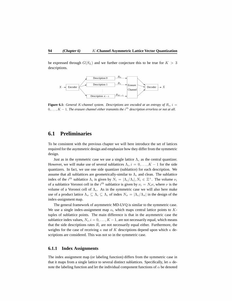
94 (Chapter 6) K-Channel Asymmetric Lattice Vector Quantization
be expressed throughG(SL) and we further conjecture this to be true forK > 3
descriptions.
ChannelDecoder
ErasureEncoder
PSfrag replacements
X X
R0
R1
RK−1
Description 0
Description 1
DescriptionK−1
Figure 6.1: GeneralK-channel system. Descriptions are encoded at an entropy ofRi, i =0, . . . ,K − 1. The erasure channel either transmits theith description errorless or not at all.
6.1 Preliminaries
To be consistent with the previous chapter we will here introduce the set of latticesrequired for the asymmetric design and emphasize how they differ from the symmetricdesign.
Just as in the symmetric case we use a single latticeΛc as the central quantizer.However, we will make use of several sublatticesΛi, i = 0, . . . ,K − 1 for the sidequantizers. In fact, we use one side quantizer (sublattice)for each description. Weassume that all sublattices are geometrically-similar toΛc and clean. The sublatticeindex of theith sublatticeΛi is given byNi = |Λc/Λi|, Ni ∈ Z+. The volumeνiof a sublattice Voronoi cell in theith sublattice is given byνi = Niν, whereν is thevolume of a Voronoi cell ofΛc. As in the symmetric case we will also here makeuse of a product latticeΛπ ⊆ Λi ⊆ Λc of indexNπ = |Λc/Λπ| in the design of theindex-assignment map.
The general framework of asymmetric MD-LVQ is similar to thesymmetric case.We use a single index-assignment mapα, which maps central lattice points toK-tuples of sublattice points. The main difference is that in the asymmetric case thesublattice index values,Ni, i = 0, . . . ,K − 1, are not necessarily equal, which meansthat the side descriptions ratesRi are not necessarily equal either. Furthermore, theweights for the case of receivingκ out ofK descriptions depend upon whichκ de-scriptions are considered. This was not so in the symmetric case.
6.1.1 Index Assignments
The index assignment map (or labeling function) differs from the symmetric case inthat it maps from a single lattice to several distinct sublattices. Specifically, letα de-note the labeling function and let the individual componentfunctions ofα be denoted
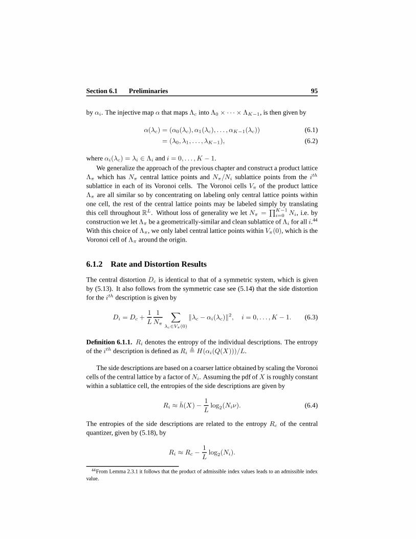
Section 6.1 Preliminaries 95
byαi. The injective mapα that mapsΛc intoΛ0 × · · · × ΛK−1, is then given by
α(λc) = (α0(λc), α1(λc), . . . , αK−1(λc)) (6.1)
= (λ0, λ1, . . . , λK−1), (6.2)
whereαi(λc) = λi ∈ Λi andi = 0, . . . ,K − 1.
We generalize the approach of the previous chapter and construct a product latticeΛπ which hasNπ central lattice points andNπ/Ni sublattice points from theith
sublattice in each of its Voronoi cells. The Voronoi cellsVπ of the product latticeΛπ are all similar so by concentrating on labeling only centrallattice points withinone cell, the rest of the central lattice points may be labeled simply by translatingthis cell throughoutRL. Without loss of generality we letNπ =
∏K−1i=0 Ni, i.e. by
construction we letΛπ be a geometrically-similar and clean sublattice ofΛi for all i.44
With this choice ofΛπ, we only label central lattice points withinVπ(0), which is theVoronoi cell ofΛπ around the origin.
6.1.2 Rate and Distortion Results
The central distortionDc is identical to that of a symmetric system, which is givenby (5.13). It also follows from the symmetric case see (5.14)that the side distortionfor theith description is given by
Di = Dc +1
L
1
Nπ
∑
λc∈Vπ(0)
‖λc − αi(λc)‖2, i = 0, . . . ,K − 1. (6.3)
Definition 6.1.1. Ri denotes the entropy of the individual descriptions. The entropyof theith description is defined asRi , H(αi(Q(X)))/L.
The side descriptions are based on a coarser lattice obtained by scaling the Voronoicells of the central lattice by a factor ofNi. Assuming the pdf ofX is roughly constantwithin a sublattice cell, the entropies of the side descriptions are given by
Ri ≈ h(X)− 1
Llog2(Niν). (6.4)
The entropies of the side descriptions are related to the entropy Rc of the centralquantizer, given by (5.18), by
Ri ≈ Rc −1
Llog2(Ni).
44From Lemma 2.3.1 it follows that the product of admissible index values leads to an admissible indexvalue.

96 (Chapter 6) K-Channel Asymmetric Lattice Vector Quantization
6.2 Construction of Labeling Function
In this section we construct the index-assignment mapα, which takes a single vectorλc and maps it to a set ofK vectorsλi, i = 0, . . . ,K − 1, whereλi ∈ Λi. Themapping is invertible so that we haveλc = α−1(λ0, . . . , λK−1).
In asymmetric MD-LVQ weights are introduced in order to control the amount ofasymmetry between the side distortions. We will in the following assume that theseweights are based on the packet-loss probabilities of the individual descriptions. How-ever, it should be clear that the weights are not limited to represent packet-loss prob-abilities but can in fact be almost arbitrarily chosen. We will consider the case wherethe index-assignment map is constructed such that the expected distortion, given bythe sum of the distortions due to all possible description losses weighted by their cor-responding loss probabilities, is minimized.
In addition to knowing the weighted distortion over all description losses it is alsointeresting to know the distortion of any subset of theK descriptions. This issue isconsidered in Section 6.5.
6.2.1 Expected Distortion
At the receiving side,X ∈ RL is reconstructed to a quality that is determined bythe received descriptions. If no descriptions are receivedwe reconstruct using theexpected value,EX , and if allK descriptions are received we reconstruct using theinverse mapα−1(λ0, . . . , λK−1), hence obtaining the quality of the central quantizer.In all other cases, we reconstruct to the average of the received descriptions as wasdone in the symmetric case.
There are in general several ways of receivingκ out ofK descriptions. LetL (K,κ)
denote an index set consisting of all possibleκ combinations out of0, . . . ,K−1 sothat |L (K,κ)| =
(Kκ
). We denote an element ofL (K,κ) by l = l0, . . . , lκ−1. The
complementlc of l denotes theK − κ indices not inl, i.e. lc = 0, . . . ,K − 1\l.We will use the notationL (K,κ)
i to indicate the set of alll ∈ L (K,κ) that contains
the indexi, i.e., L(K,κ)i = l : l ∈ L (K,κ) and i ∈ l and similarlyL
(K,κ)i,j =
l : l ∈ L (K,κ) and i, j ∈ l. Furthermore, letpi be the packet-loss probabilityfor the ith description and letµi = 1 − pi be the probability that theith descriptionis received. Finally, letp(l) =
∏
i∈l µi
∏
j∈lc pj , p(L(K,κ)) =
∑
l∈L (K,κ) p(l),
p(L(K,κ)i ) =
∑
l∈L(K,κ)i
p(l) andp(L (K,κ)i,j ) =
∑
l∈L(K,κ)i,j
p(l). For example, for
K = 3 andκ = 2 we haveL (3,2) = 0, 1, 0, 2, 1, 2 and hencep(L (3,2)) =
µ0µ1p2 + µ0µ2p1 + µ1µ2p0. In a similar manner forK = 6 andκ = 3 we have
L(6,3)1,2 = 0, 1, 2, 1, 2, 3, 1, 2, 4, 1, 2, 5,
and
p(L(6,2)1,2 ) = µ0µ1µ2p3p4p5 + µ1µ2µ3p0p4p5 + µ1µ2µ4p0p3p5 + µ1µ2µ5p0p3p4.
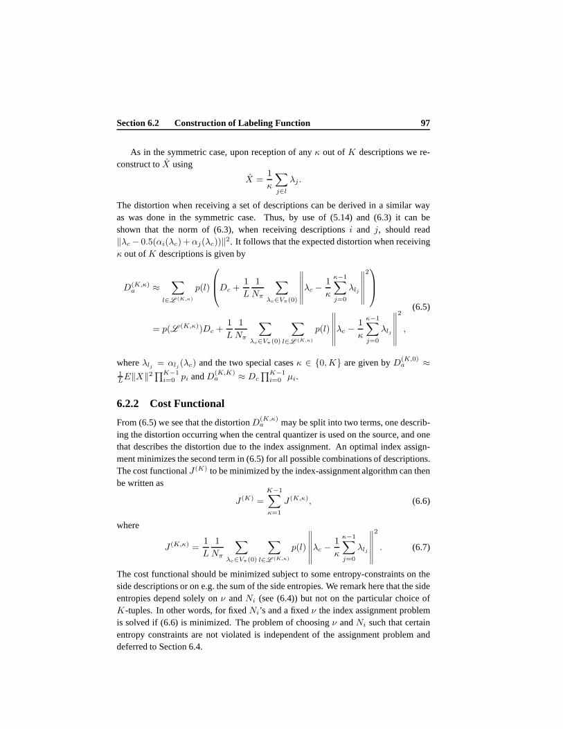
Section 6.2 Construction of Labeling Function 97
As in the symmetric case, upon reception of anyκ out ofK descriptions we re-construct toX using
X =1
κ
∑
j∈l
λj .
The distortion when receiving a set of descriptions can be derived in a similar wayas was done in the symmetric case. Thus, by use of (5.14) and (6.3) it can beshown that the norm of (6.3), when receiving descriptionsi and j, should read‖λc − 0.5(αi(λc) +αj(λc))‖2. It follows that the expected distortion when receivingκ out ofK descriptions is given by
D(K,κ)a ≈
∑
l∈L (K,κ)
p(l)
Dc +
1
L
1
Nπ
∑
λc∈Vπ(0)
∥∥∥∥∥∥
λc −1
κ
κ−1∑
j=0
λlj
∥∥∥∥∥∥
2
= p(L (K,κ))Dc +1
L
1
Nπ
∑
λc∈Vπ(0)
∑
l∈L (K,κ)
p(l)
∥∥∥∥∥∥
λc −1
κ
κ−1∑
j=0
λlj
∥∥∥∥∥∥
2
,
(6.5)
whereλlj = αlj (λc) and the two special casesκ ∈ 0,K are given byD(K,0)a ≈
1LE‖X‖2∏K−1
i=0 pi andD(K,K)a ≈ Dc
∏K−1i=0 µi.
6.2.2 Cost Functional
From (6.5) we see that the distortionD(K,κ)a may be split into two terms, one describ-
ing the distortion occurring when the central quantizer is used on the source, and onethat describes the distortion due to the index assignment. An optimal index assign-ment minimizes the second term in (6.5) for all possible combinations of descriptions.The cost functionalJ (K) to be minimized by the index-assignment algorithm can thenbe written as
J (K) =
K−1∑
κ=1
J (K,κ), (6.6)
where
J (K,κ) =1
L
1
Nπ
∑
λc∈Vπ(0)
∑
l∈L (K,κ)
p(l)
∥∥∥∥∥∥
λc −1
κ
κ−1∑
j=0
λlj
∥∥∥∥∥∥
2
. (6.7)
The cost functional should be minimized subject to some entropy-constraints on theside descriptions or on e.g. the sum of the side entropies. Weremark here that the sideentropies depend solely onν andNi (see (6.4)) but not on the particular choice ofK-tuples. In other words, for fixedNi’s and a fixedν the index assignment problemis solved if (6.6) is minimized. The problem of choosingν andNi such that certainentropy constraints are not violated is independent of the assignment problem anddeferred to Section 6.4.
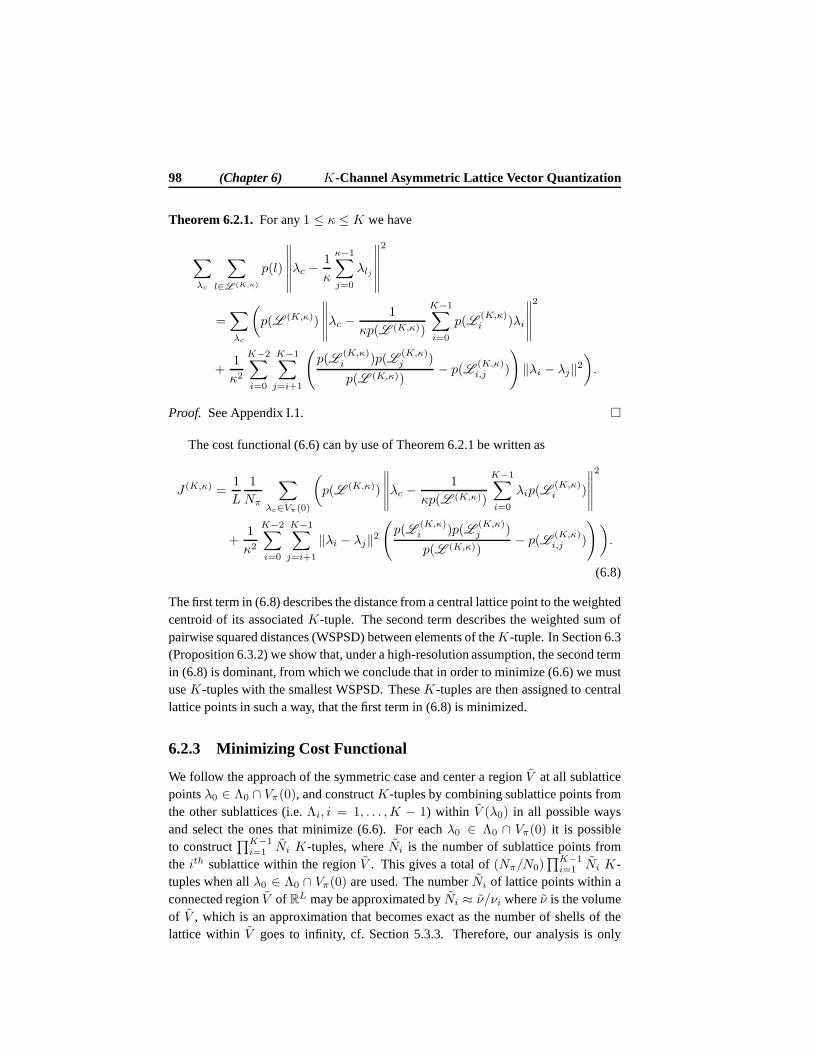
98 (Chapter 6) K-Channel Asymmetric Lattice Vector Quantization
Theorem 6.2.1.For any1 ≤ κ ≤ K we have
∑
λc
∑
l∈L (K,κ)
p(l)
∥∥∥∥∥∥
λc −1
κ
κ−1∑
j=0
λlj
∥∥∥∥∥∥
2
=∑
λc
(
p(L (K,κ))
∥∥∥∥∥λc −
1
κp(L (K,κ))
K−1∑
i=0
p(L(K,κ)i )λi
∥∥∥∥∥
2
+1
κ2
K−2∑
i=0
K−1∑
j=i+1
(
p(L(K,κ)i )p(L
(K,κ)j )
p(L (K,κ))− p(L
(K,κ)i,j )
)
‖λi − λj‖2)
.
Proof. See Appendix I.1.
The cost functional (6.6) can by use of Theorem 6.2.1 be written as
J (K,κ) =1
L
1
Nπ
∑
λc∈Vπ(0)
(
p(L (K,κ))
∥∥∥∥∥λc −
1
κp(L (K,κ))
K−1∑
i=0
λip(L(K,κ)i )
∥∥∥∥∥
2
+1
κ2
K−2∑
i=0
K−1∑
j=i+1
‖λi − λj‖2(
p(L(K,κ)i )p(L
(K,κ)j )
p(L (K,κ))− p(L
(K,κ)i,j )
))
.
(6.8)
The first term in (6.8) describes the distance from a central lattice point to the weightedcentroid of its associatedK-tuple. The second term describes the weighted sum ofpairwise squared distances (WSPSD) between elements of theK-tuple. In Section 6.3(Proposition 6.3.2) we show that, under a high-resolution assumption, the second termin (6.8) is dominant, from which we conclude that in order to minimize (6.6) we mustuseK-tuples with the smallest WSPSD. TheseK-tuples are then assigned to centrallattice points in such a way, that the first term in (6.8) is minimized.
6.2.3 Minimizing Cost Functional
We follow the approach of the symmetric case and center a region V at all sublatticepointsλ0 ∈ Λ0 ∩ Vπ(0), and constructK-tuples by combining sublattice points fromthe other sublattices (i.e.Λi, i = 1, . . . ,K − 1) within V (λ0) in all possible waysand select the ones that minimize (6.6). For eachλ0 ∈ Λ0 ∩ Vπ(0) it is possibleto construct
∏K−1i=1 Ni K-tuples, whereNi is the number of sublattice points from
the ith sublattice within the regionV . This gives a total of(Nπ/N0)∏K−1
i=1 Ni K-tuples when allλ0 ∈ Λ0 ∩ Vπ(0) are used. The numberNi of lattice points within aconnected regionV of RL may be approximated byNi ≈ ν/νi whereν is the volumeof V , which is an approximation that becomes exact as the number of shells of thelattice within V goes to infinity, cf. Section 5.3.3. Therefore, our analysisis only
Section 6.2 Construction of Labeling Function 99
exact in the asymptotic case ofNi → ∞ andνi → 0. SinceNi ≈ ν/νNi and weneedN0 K-tuples for eachλ0 ∈ Vπ(0) we see that
N0 =
K−1∏
i=1
Ni ≈νK−1
νK−1
K−1∏
i=1
N−1i ,
so in order to obtain at leastN0 K-tuples, the volume ofV must satisfy
limNi→∞,∀i
ν ≥ ν
K−1∏
i=0
N1/(K−1)i . (6.9)
For the symmetric case, i.e.N = Ni, i = 0, . . . ,K − 1, we haveν ≥ νNK/(K−1),which is in agreement with the results obtained in Chapter 5.
Before we outline the design procedure for constructing an optimal index assign-ment we remark that in order to minimize the WSPSD between a fixedλi and the setof pointsλj ∈ Λj ∩ V it is required thatV forms a sphere centered atλi. Thedesign procedure can be outlined as follows:
1. Center a sphereV at eachλ0 ∈ Λ0 ∩ Vπ(0) and construct all possibleK-tuples(λ0, λ1, . . . , λK−1) whereλi ∈ Λi ∩ V (λ0) andi = 1, . . . ,K − 1. Thisensures that allK-tuples have their first coordinate (λ0) insideVπ(0) and theyare therefore shift-invariant. We will only useK-tuples whose elements satisfy‖λi − λj‖ ≤ r, ∀i, j ∈ 0, . . .K − 1, wherer is the radius ofV . MakeV largeenough so at leastN0 distinctK-tuples are found for eachλ0.
2. Construct cosets of eachK-tuple.
3. TheNπ central lattice points inΛc∩Vπ(0) must now be matched to distinctK-tuples. As in the symmetric case, this is a standard linear assignment problem[151] where only one member from each coset is (allowed to be)matched to acentral lattice point inVπ(0).
The restriction‖λi − λj‖ ≤ r from step 1), which is used to avoid bias towardsany of the sublattices, reduces the number of distinctK-tuples that can be constructedwithin the regionV . To be able to formN0 K-tuples it is therefore necessary to use aregionV with a volume larger than the lower bound in (6.9). In order totheoreticallydescribe the performance of the quantizers we need to know the optimalν, i.e. thesmallest volume which (asymptotically for largeNi) leads to exactlyN0 K-tuples.In Section 5.3.3 a dimensionless expansion factorψL which only depends onK andL was introduced.ψL was used to describe how muchV had to be expanded fromthe theoretical lower bound (6.9), to make sure thatN0 optimalK-tuples could beconstructed by combining sublattice points within a regionV .
Lemma 6.2.1. The dimensionless expansion factorψL for the asymmetric case isidentical to the one for the symmetric case.
100 (Chapter 6) K-Channel Asymmetric Lattice Vector Quantization
Proof. Follows by replacing the constantνs by νi in the proof of Theorem 5.3.2.
Adopting this approach leads to
ν = ψLLν
K−1∏
i=0
N1/(K−1)i .
Remark6.2.1. It might appear that the shift invariance restriction enforced by usingonly one member from each coset will unfairly penalizeΛ0. However, the next twolemmas prove that, asymptotically asNi → ∞, there is no bias towards any of thesublattices. We will consider here the case ofK > 2 (for K = 2 we can use similararguments as given in [28]).
Lemma 6.2.2. ForK > 2 the number ofK-tuples that is affected by the coset re-striction is (asymptotically asNi → ∞, ∀i) neglectable compared to the number ofK-tuples which are not affected.
Proof. See Appendix I.4.
Lemma 6.2.3. The set ofNπ K-tuples that is constructed by centeringV at eachλ0 ∈ Vπ(0) ∩ Λ0 is asymptotically identical to the set constructed by centering V ateachλi ∈ Vπ(0) ∩ Λi, for anyi ∈ 1, . . . ,K − 1.
Proof. See Appendix I.4.
Remark6.2.2. TheK-tuples need to be assigned to central lattice points withinVπ(0).This is a standard linear assignment problem where a cost measure is minimized.However, solutions to linear assignment problems are generally not unique. Therefore,there might exist several labelings, which all yield the same cost, but exhibit a differentamount of asymmetry. To achieve the specified distortions itmay then be necessaryto e.g. use time sharing through a suitable mixing of labelings.
6.2.4 Comparison to Existing Asymmetric Index Assignments
In this section we have presented a new design for asymmetricMD-LVQ based on theasymmetric design of Diggavi et al. [28]. The main difference between the existingdesign of Diggavi et al. and the proposed design is that of theshape of the regionwithin which sublattice points are distributed. More specifically, in the design ofDiggavi et al., a given sublattice pointλ0 ∈ Λ0 is paired with a set of sublatticepoints ofΛ1 which are all evenly distributed within a Voronoi cell ofΛπ, the productlattice. However, in the proposed design, a sublattice point λ0 ∈ Λ0 is paired with aset of sublattice points ofΛ1 which are all evenly distributed within anL-dimensionalhypersphere.
Let us emphasize some of the advantages as well as weaknessesof the proposeddesign.
Section 6.3 High-Resolution Analysis 101
• Advantages
1. The side distortion is reduced (compared to the previous design) whenfinite dimensional lattice vector quantizers are used (whenthe dimensionis strictly greater than one). To see this, notice that the side distortion isa function of the dimensionless normalized second moment ofthe regionover which the sublattice points are distributed. ForL = 1 as well asL → ∞ spheres pack space and it is possible to have spherical Voronoicells ofΛπ by a proper choice of product lattice.
2. To simplify the design it is often convenient to base the product latticeupon the simple hypercubicZL lattice. In this case, the side distortionof the design of Diggavi et al. is independent of the vector dimensionof the lattices, whereas with the proposed design the distortion steadilydecreases as the dimension increases. The reduction in sidedistortion isupper bounded by approximately 1.53 dB per description.
3. The proposed design scales easily to more than two descriptions. It is notclear how to obtain more than two descriptions with the previous designs.
• Weaknesses
1. The design of Diggavi et al. exploits several geometric properties of theunderlying lattices to ensure that any single sublattice point of Λ0 is pairedwith exactlyN0 sublattice points ofΛ1. On the other hand, the proposeddesign guarantees such a symmetry property only in asymptotic cases.Thus, in practice, if such a symmetry property is desired, one might needto search within a set of candidate solutions.
6.3 High-Resolution Analysis
In this section we derive high-resolution approximations for the expected distortion.In line with the high-resolution analysis presented in Chapter 5 we letNi → ∞ andνi → 0, i.e. for each sublattice the index increase, while the volume of their Voronoicell shrink.
102 (Chapter 6) K-Channel Asymmetric Lattice Vector Quantization
6.3.1 Total Expected Distortion
Using Theorem 6.2.1, the expected distortion (6.5) whenκ out ofK descriptions arereceived can be written as
D(K,κ)a ≈ p(L (K,κ))Dc +
1
L
1
Nπ
∑
λc∈Vπ(0)
∑
l∈L (K,κ)
p(l)
∥∥∥∥∥∥
λc −1
κ
κ−1∑
j=0
λlj
∥∥∥∥∥∥
2
= p(L (K,κ))Dc
+1
L
1
Nπ
∑
λc∈Vπ(0)
(
p(L (K,κ))
∥∥∥∥∥λc −
1
κp(L (K,κ))
K−1∑
i=0
p(L(K,κ)i )λi
∥∥∥∥∥
2
+1
κ2
K−2∑
i=0
K−1∑
j=i+1
(
p(L(K,κ)i )p(L
(K,κ)j )
p(L (K,κ))− p(L
(K,κ)i,j )
)
‖λi − λj‖2)
.
(6.10)
Proposition 6.3.1. ForK = 2 and asymptotically asNi → ∞, νi → 0 as well asfor K = 3 and asymptotically asNi, L → ∞ andνi → 0, we have for any pair ofsublattices,(Λi,Λj), i, j = 0, . . . ,K − 1, i 6= j,
1
L
∑
λc∈Vπ(0)
‖αi(λc)− αj(λc)‖2 = ψ2Lν
2/LG(SL)Nπ
K−1∏
m=0
N2/L(K−1)m .
Proof. See Appendix I.2.
Conjecture 6.3.1. Proposition 6.3.1 is true for anyK asymptotically asL,Ni → ∞andνi → 0, ∀i.
Proposition 6.3.2. ForNi → ∞ we have
∑
λc∈Vπ(0)
∥∥∥∥∥λc −
1
κp(L )
K−1∑
i=0
p(L(K,κ)i )λi
∥∥∥∥∥
2
∑
λc∈Vπ(0)
K−2∑
i=0
K−1∑
j=i+1
(
p(L(K,κ)i )p(L
(K,κ)j )
p(L (K,κ))− p(L
(K,κ)i,j )
)
‖λi − λj‖2→ 0.
Proof. See Appendix I.3.
By use of Propositions 6.3.1 and 6.3.2 and (5.13) it follows that (6.10) can be
Section 6.3 High-Resolution Analysis 103
written as
D(K,κ)a ≈ p(L (K,κ))Dc
+1
L
1
Nπ
∑
λc∈Vπ(0)
1
κ2
K−2∑
i=0
K−1∑
j=i+1
(
p(L(K,κ)i )p(L
(K,κ)j )
p(L (K,κ))− p(L
(K,κ)i,j )
)
‖λi − λj‖2
≈ G(Λc)ν2/Lp(L (K,κ)) + ψ2
Lν2/LG(SL)β
(K,κ)K−1∏
m=0
N2/L(K−1)m ,
whereβ(K,κ) depends on the packet-loss probabilities and is given by
β(K,κ) =1
κ2
K−2∑
i=0
K−1∑
j=i+1
(
p(L(K,κ)i )p(L
(K,κ)j )
p(L (K,κ))− p(L
(K,κ)i,j )
)
.
The total expected distortionD(K)a is obtained by summing overκ including the cases
whereκ = 0 andκ = K,
D(K)a ≈ G(Λc)ν
2/Lp(L (K)) + ψ2Lν
2/LG(SL)
K−1∏
m=0
N2/L(K−1)m β(K)
+1
LE‖X‖2
K−1∏
i=0
pi,
(6.11)
where
p(L (K)) =
K∑
κ=1
p(L (K,κ))
and
β(K) =
K∑
κ=1
β(K,κ).
Using (5.18) and (6.4) we can writeν andNi as a function of differential entropyand side entropies, that is
ν2/L = 22(h(X)−Rc),
andK−1∏
i=0
N2/L(K−1)i = 2
2KK−1 (Rc− 1
K
∑K−1i=0 Ri).
Inserting these results in (6.11) leads to
D(K)a ≈ G(Λc)2
2(h(X)−Rc)p(L (K))
+ ψ2LG(SL)2
2(h(X)−Rc)22K
K−1 (Rc− 1K
∑K−1i=0 Ri)β(K) +
1
LE‖X‖2
K−1∏
i=0
pi,
(6.12)
where we see that the distortion due to the side quantizers isindependent of the typeof sublattices.
104 (Chapter 6) K-Channel Asymmetric Lattice Vector Quantization
6.4 Optimal Entropy-Constrained Quantizers
In this section we first derive closed-form expressions for the optimal scaling factorsν andNi subject to entropy constraints on theK side descriptions. With these scalingfactors we are able to construct a central lattice andK sublattices. The index assign-ments are then found using the approach outlined in Section 6.2. The central latticeand theK side lattices combined with their index assignment map completely specifyan optimal scheme for asymmetric entropy-constrained MD-LVQ. We then considerthe situation where the total bit budget is constrained, i.e. we find the optimal scalingfactors subject to entropy constraints on the sum of the sideentropies
∑
iRi ≤ R∗,whereR∗ is the target entropy. We also find the optimal bit distribution among theKdescriptions.
6.4.1 Entropy Constraints Per Description
We assumeK descriptions are to be used. Packet-loss probabilitiespi, i = 0, . . . ,K−1, are given as well as entropy-constraints on the side descriptions, i.e.Ri ≤ R∗
i ,whereR∗
i are known target entropies. To be optimal, the entropies of the side descrip-tions must be equal to the target entropies, hence by use of (6.4) we must have that
Ri = h(X)− 1
Llog2(Niν) = R∗
i ,
from which we getNiν = 2L(h(X)−R∗
i ) = τi, (6.13)
whereτi are constants. It follows thatNi = τi/ν and since∏K−1
i=0 N2/L(K−1)i =
ν−2K/L(K−1)∏K−1
i=0 τ2/L(K−1)i we can express (6.11) as a function ofν, i.e.
D(K)a ≈ G(Λc)ν
2/Lp(L (K))
+ ψ2Lν
2/LG(SL)ν−2K/L(K−1)τ2/L(K−1)β(K) +
1
LE‖X‖2
K−1∏
i=0
pi
= G(Λc)ν2/Lp(L (K)) + ψ2
LG(SL)ν−2/L(K−1)τ2/L(K−1)β(K)
+1
LE‖X‖2
K−1∏
i=0
pi,
whereτ =∏K−1
i=0 τi.Differentiating w.r.t.ν and equating to zero gives,
∂D(K)a
∂ν=
2
LG(Λc)ν
2/L−1p(L (K))
− 2
L(K − 1)ψ2LG(SL)ν
−2/L(K−1)−1τ2/L(K−1)β(K) = 0,
Section 6.4 Optimal Entropy-Constrained Quantizers 105
from which we obtain the optimal value ofν
ν = τ1/K
(
ψ2L
1
K − 1
G(SL)
G(Λc)
β(K)
p(L (K))
)L(K−1)2K
= 2L(h(X)− 1K
∑
i R∗i )
(
ψ2L
1
K − 1
G(SL)
G(Λc)
β(K)
p(L (K))
)L(K−1)2K
.
(6.14)
The optimalNi’s follow easily by use of (6.13):
Ni =τiν
= τiτ−1/K
(1
ψ2L
(K − 1)G(Λc)
G(SL)
p(L (K))
β(K)
)L(K−1)2K
. (6.15)
Eq. (6.15) shows that the optimal redundanciesNi’s are, for fixedK, independent ofthe sublattices. Moreover, sinceτiτ−1/K = 2−L(R∗
i− 1K
∑
jR∗
j ) the source-dependentterm h(X) is eliminated and it follows that the redundanciesNi are independent ofthe source but also of actual values of target entropies (Ni depends only upon thedifference between the average target entropy andR∗
i ).
6.4.2 Total Entropy Constraint
First we observe from (6.12) that the expected distortion depends upon thesumofthe side entropies and not the individual side entropies. Inorder to be optimal it isnecessary to achieve equality in the entropy constraint, i.e.R∗ =
∑
iRi. From (6.4)we have
R∗ =
K−1∑
i=0
Ri = Kh(X)− 1
L
K−1∑
i=0
log2(Niν).
This equation can be rewritten as
K−1∏
i=0
(Niν) = 2L(Kh(X)−R∗) = τ∗, (6.16)
whereτ∗ is constant for fixed target entropy and differential entropies. Writing (6.16)as
K−1∏
i=0
N2/L(K−1)i = ν−2K/L(K−1)τ
2/L(K−1)∗ ,
and inserting in (6.11) leads to
D(K)a ≈ G(Λc)ν
2/Lp(L (K)) + ψ2Lν
−2/L(K−1)τ2/L(K−1)∗ G(SL)β
(K)
+1
LE‖X‖2
K−1∏
i=0
pi.
106 (Chapter 6) K-Channel Asymmetric Lattice Vector Quantization
Differentiating w.r.t.ν and equating to zero gives
∂D(K)a
∂ν=
2
LG(Λc)ν
2/L−1p(L (K))
− 2
L(K − 1)ψ2LG(SL)ν
−2/L(K−1)−1τ2/L(K−1)∗ β(K) = 0,
from which we obtain the optimal value ofν, that is
ν = 2L(h(X)− 1K
R∗)
(
ψ2L
1
K − 1
G(SL)
G(Λc)
β(K)
p(L (K))
)L(K−1)2K
. (6.17)
We note that this expression is identical to (6.14). The results of this section show thatthe optimalν is the same whether we optimize subject to entropy constraints on theindividual side entropies or on the sum of the side entropiesas long as the total bitbudget is the same.
At this point we still need to find expressions for the optimalRi (or equivalentlyoptimalNi givenν). LetRi = aiR
∗, where∑
i ai = 1, ai ≥ 0, henceR∗ =∑
iRi.From (6.4) we have
Ri = h(X)− 1
Llog2(Niν) = aiR
∗,
which can be rewritten as
Ni = ν−12L(h(X)−aiR∗).
Inserting (6.17) leads to an expression for the optimal index valueNi, that is
Ni = 2LK
(1−ai)R∗
(
ψ−2L (K − 1)
G(Λc)
G(SL)
p(L (K))
β(K)
)L(K−1)2K
. (6.18)
It follows from (5.18) and (6.4) thatRc ≥ aiR∗ so thatai ≤ Rc/R
∗. In addition,since the rates must be positive, we obtain the following inequalities:
0 < aiR∗ ≤ Rc, i = 0, . . . ,K − 1. (6.19)
Thus, when we only have a constraintR∗ on the sum of the side entropies, theindividual side entropiesRi = aiR
∗ can be arbitrarily chosen (without loss of perfor-mance) as long as they satisfy (6.19) and
∑
i ai = 1. We remark thatRi is boundedaway from zero by a positive constant, cf. (4.1) and (4.2). For example, for the two-channel case we haveR0 = a0R
∗ andR1 = a1R∗ = (1 − a0)R
∗, so thatRc ≥(1− a0)R
∗ which implies thatR∗ −Rc ≤ R0 ≤ Rc.45
This result leads to an interesting observation. Given a single entropy constraint onthe sum of the side entropies, the optimal bit distribution among the two descriptions
45Recall thatRc is fixed, since it depends onν which is given by (6.17).

Section 6.4 Optimal Entropy-Constrained Quantizers 107
is not unique but contains in fact a set of solutions (i.e. a set of quantizers) whichall lead to minimal expected distortion.46 This allows for additional constraints tobe imposed on the quantizers without sacrificing optimalitywith respect to minimalexpected distortion. For example, in some mobile wireless environments, it might bebeneficial to use those quantizers from the set of optimal quantizers that require theleast amount of power.
6.4.3 Example With Total Entropy Constraint
Let us show by an example some interesting aspects resultingfrom the fact that weobtain a set of candidate solutions, which all minimize the expected distortion. For ex-ample, consider IP-telephony applications, which with therecent spread of broadbandnetworks are being used extensively throughout the world today. More specifically,let us consider a packet-switched network where a user has access to two differentchannels both based on the unreliable user datagram protocol [133]. Channel 0 is anon priority-based channel whereas channel 1 is a priority-based channel or they areboth priority-based channels but of different priorities.Equivalently this network canbe thought of as a packet-switched network where the individual packets are givenpriorities; low or high priority. In any case, we assume thatonly a single packet istransmitted on each channel for each time instance (this canbe justified with e.g. tightdelay constraints). The priority-based channel favor packets with higher priority andthe packet-loss probabilityp1 on channel 1 is therefore lower than that of channel0, i.e.p1 < p0. Assume the Internet telephony service provider (ITSP) in questioncharges a fixed amount of say $1 ($2) per bit transmitted via channel 0 (channel 1).If we then use say 6 bits on channel 1 the quality is better thanif we use the 6 bitson channel 0. It is therefore tempting to transmit all the bits through channel 1 (orequivalently send both packets with high priority) since itoffers better quality thanchannel 0. However, our results reveal that it is often beneficial to make use of bothchannels (or equivalently send two packets simultaneouslyof low and high priority).The importance of exploiting two channels is illustrated inTable 6.1 for the examplesgiven above for a total bit budget of 6 bits and packet-loss probabilitiesp0 = 5% andp1 = 2%. Notice the peculiarity that since the total bit budget is limited to 6 bits theneven if the user is willing to pay more than $8 the performancewould be no betterthan what can be achieved when paying exactly $8. The last column of Table 6.1describes the expected distortion occurring when quantizing a unit-variance Gaussiansource which has been scalar quantized at a total entropy of 6bit/dim. The packet-lossprobabilities arep0 = 0.05 andp1 = 0.02. The quantization error (hence not taking
46In retrospect, this is not a surprising result since, for thetwo-description case, we already saw that fora fixed distortion tuple(Dc, D0, D1) the lower bound of the rate region is piece-wise linear, cf. Fig. 4.5.Furthermore, when the sum rate is minimum, this line segmenthas a 45 degree (negative) slope. Hence,any choice of rate pairs on this line segment satisfies the sumrate. The new observation here, however, isthat now we have a practical scheme, which for any number of descriptions, also satisfies this property.
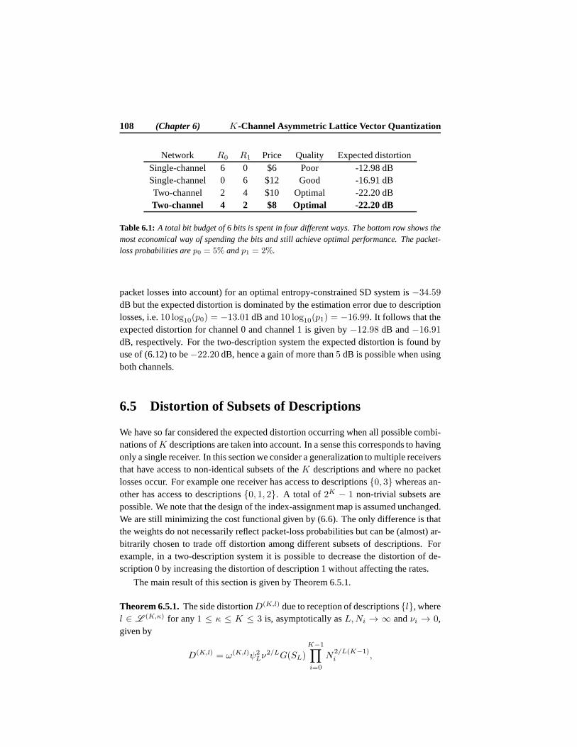
108 (Chapter 6) K-Channel Asymmetric Lattice Vector Quantization
Network R0 R1 Price Quality Expected distortionSingle-channel 6 0 $6 Poor -12.98 dBSingle-channel 0 6 $12 Good -16.91 dBTwo-channel 2 4 $10 Optimal -22.20 dBTwo-channel 4 2 $8 Optimal -22.20 dB
Table 6.1: A total bit budget of 6 bits is spent in four different ways. The bottom row shows themost economical way of spending the bits and still achieve optimal performance. The packet-loss probabilities arep0 = 5% andp1 = 2%.
packet losses into account) for an optimal entropy-constrained SD system is−34.59
dB but the expected distortion is dominated by the estimation error due to descriptionlosses, i.e.10 log10(p0) = −13.01 dB and10 log10(p1) = −16.99. It follows that theexpected distortion for channel 0 and channel 1 is given by−12.98 dB and−16.91
dB, respectively. For the two-description system the expected distortion is found byuse of (6.12) to be−22.20 dB, hence a gain of more than5 dB is possible when usingboth channels.
6.5 Distortion of Subsets of Descriptions
We have so far considered the expected distortion occurringwhen all possible combi-nations ofK descriptions are taken into account. In a sense this corresponds to havingonly a single receiver. In this section we consider a generalization to multiple receiversthat have access to non-identical subsets of theK descriptions and where no packetlosses occur. For example one receiver has access to descriptions0, 3 whereas an-other has access to descriptions0, 1, 2. A total of 2K − 1 non-trivial subsets arepossible. We note that the design of the index-assignment map is assumed unchanged.We are still minimizing the cost functional given by (6.6). The only difference is thatthe weights do not necessarily reflect packet-loss probabilities but can be (almost) ar-bitrarily chosen to trade off distortion among different subsets of descriptions. Forexample, in a two-description system it is possible to decrease the distortion of de-scription 0 by increasing the distortion of description 1 without affecting the rates.
The main result of this section is given by Theorem 6.5.1.
Theorem 6.5.1.The side distortionD(K,l) due to reception of descriptionsl, wherel ∈ L (K,κ) for any1 ≤ κ ≤ K ≤ 3 is, asymptotically asL,Ni → ∞ andνi → 0,given by
D(K,l) = ω(K,l)ψ2Lν
2/LG(SL)K−1∏
i=0
N2/L(K−1)i ,
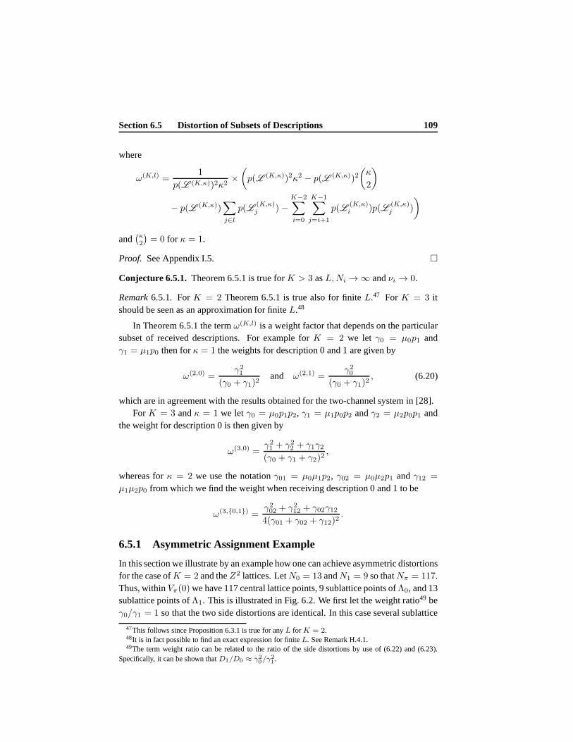
Section 6.5 Distortion of Subsets of Descriptions 109
where
ω(K,l) =1
p(L (K,κ))2κ2×(
p(L (K,κ))2κ2 − p(L (K,κ))2(κ
2
)
− p(L (K,κ))∑
j∈l
p(L(K,κ)j )−
K−2∑
i=0
K−1∑
j=i+1
p(L(K,κ)i )p(L
(K,κ)j )
)
and(κ2
)= 0 for κ = 1.
Proof. See Appendix I.5.
Conjecture 6.5.1. Theorem 6.5.1 is true forK > 3 asL,Ni → ∞ andνi → 0.
Remark6.5.1. ForK = 2 Theorem 6.5.1 is true also for finiteL.47 ForK = 3 itshould be seen as an approximation for finiteL.48
In Theorem 6.5.1 the termω(K,l) is a weight factor that depends on the particularsubset of received descriptions. For example forK = 2 we let γ0 = µ0p1 andγ1 = µ1p0 then forκ = 1 the weights for description 0 and 1 are given by
ω(2,0) =γ21
(γ0 + γ1)2and ω(2,1) =
γ20(γ0 + γ1)2
, (6.20)
which are in agreement with the results obtained for the two-channel system in [28].ForK = 3 andκ = 1 we letγ0 = µ0p1p2, γ1 = µ1p0p2 andγ2 = µ2p0p1 and
the weight for description 0 is then given by
ω(3,0) =γ21 + γ22 + γ1γ2(γ0 + γ1 + γ2)2
,
whereas forκ = 2 we use the notationγ01 = µ0µ1p2, γ02 = µ0µ2p1 andγ12 =
µ1µ2p0 from which we find the weight when receiving description 0 and1 to be
ω(3,0,1) =γ202 + γ212 + γ02γ124(γ01 + γ02 + γ12)2
.
6.5.1 Asymmetric Assignment Example
In this section we illustrate by an example how one can achieve asymmetric distortionsfor the case ofK = 2 and theZ2 lattices. LetN0 = 13 andN1 = 9 so thatNπ = 117.Thus, withinVπ(0) we have 117 central lattice points, 9 sublattice points ofΛ0, and 13sublattice points ofΛ1. This is illustrated in Fig. 6.2. We first let the weight ratio49 beγ0/γ1 = 1 so that the two side distortions are identical. In this case several sublattice
47This follows since Proposition 6.3.1 is true for anyL for K = 2.48It is in fact possible to find an exact expression for finiteL. See Remark H.4.1.49The term weight ratio can be related to the ratio of the side distortions by use of (6.22) and (6.23).
Specifically, it can be shown thatD1/D0 ≈ γ20/γ21 .

110 (Chapter 6) K-Channel Asymmetric Lattice Vector Quantization
points ofΛ0 located outsideVπ(0) will be used when labeling central lattice pointsinsideVπ(0). The solid lines in Fig. 6.2 illustrate the 117 edges that areassigned tothe 117 central lattice points.
If we let the weight ratio beγ0/γ1 = 4 we favorΛ0 overΛ1. In this case the edgeassignments are chosen such that for a given edge, the sublattice point belonging toΛ0 is closer to the central lattice point than the sublattice point belonging toΛ1. Thisis illustrated in Fig. 6.3. Notice that in this case the sublattice points ofΛ0 used forthe edges that labels central lattice points withinVπ(0) are all located withinVπ(0).Furthermore, in order to construct the required 117 edges, sublattice points ofΛ1 atgreater distance fromVπ(0) need to be used.
In practice, large index values are required in order to achieve large weight ratiosγ0/γ1 or γ1/γ0. Notice that we can achieve asymmetric side distortions even in thecase where the sublattices are identical (so thatN0 = N1 and the rates are thereforeidentical) simply by lettingγ0 6= γ1. Moreover, we can achieve symmetric side distor-tions by lettingγ0 = γ1 even whenN0 6= N1 (i.e.R0 6= R1). In the case where eitherγ0 = 0 andγ1 6= 0 or γ1 = 0 andγ0 6= 0 the scheme degenerates to a successiverefinement scheme, where the side distortion correspondingto the zero weight cannotbe controlled. In practice this happens if eitherγ0 ≫ γ1 or γ1 ≫ γ0.
−10 −5 0 5 10−10
−8
−6
−4
−2
0
2
4
6
8
10
Figure 6.2: A central lattice based onZ2 (dots) and two geometrically-similar sublattices ofindex 13 (circles) and 9 (squares), respectively. The dashed square illustrates the boundary ofVπ(0). The solid lines illustrate the 117 edges (where some are overlapping). The weight ratiois here set toγ0/γ1 = 1.
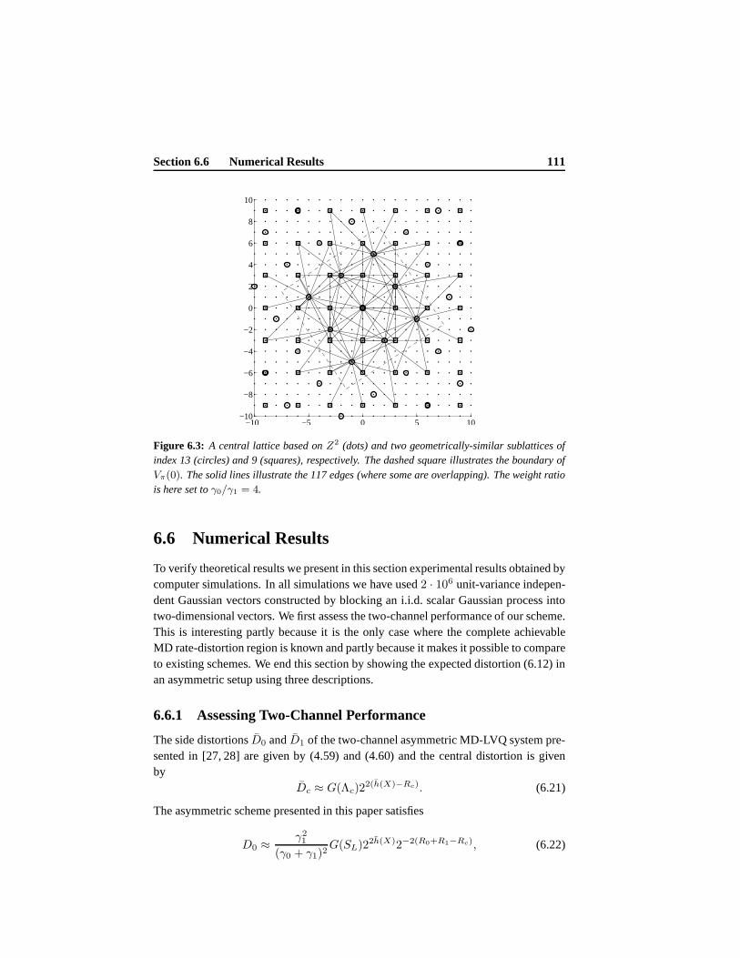
Section 6.6 Numerical Results 111
−10 −5 0 5 10−10
−8
−6
−4
−2
0
2
4
6
8
10
Figure 6.3: A central lattice based onZ2 (dots) and two geometrically-similar sublattices ofindex 13 (circles) and 9 (squares), respectively. The dashed square illustrates the boundary ofVπ(0). The solid lines illustrate the 117 edges (where some are overlapping). The weight ratiois here set toγ0/γ1 = 4.
6.6 Numerical Results
To verify theoretical results we present in this section experimental results obtained bycomputer simulations. In all simulations we have used2 · 106 unit-variance indepen-dent Gaussian vectors constructed by blocking an i.i.d. scalar Gaussian process intotwo-dimensional vectors. We first assess the two-channel performance of our scheme.This is interesting partly because it is the only case where the complete achievableMD rate-distortion region is known and partly because it makes it possible to compareto existing schemes. We end this section by showing the expected distortion (6.12) inan asymmetric setup using three descriptions.
6.6.1 Assessing Two-Channel Performance
The side distortionsD0 andD1 of the two-channel asymmetric MD-LVQ system pre-sented in [27, 28] are given by (4.59) and (4.60) and the central distortion is givenby
Dc ≈ G(Λc)22(h(X)−Rc). (6.21)
The asymmetric scheme presented in this paper satisfies
D0 ≈ γ21(γ0 + γ1)2
G(SL)22h(X)2−2(R0+R1−Rc), (6.22)
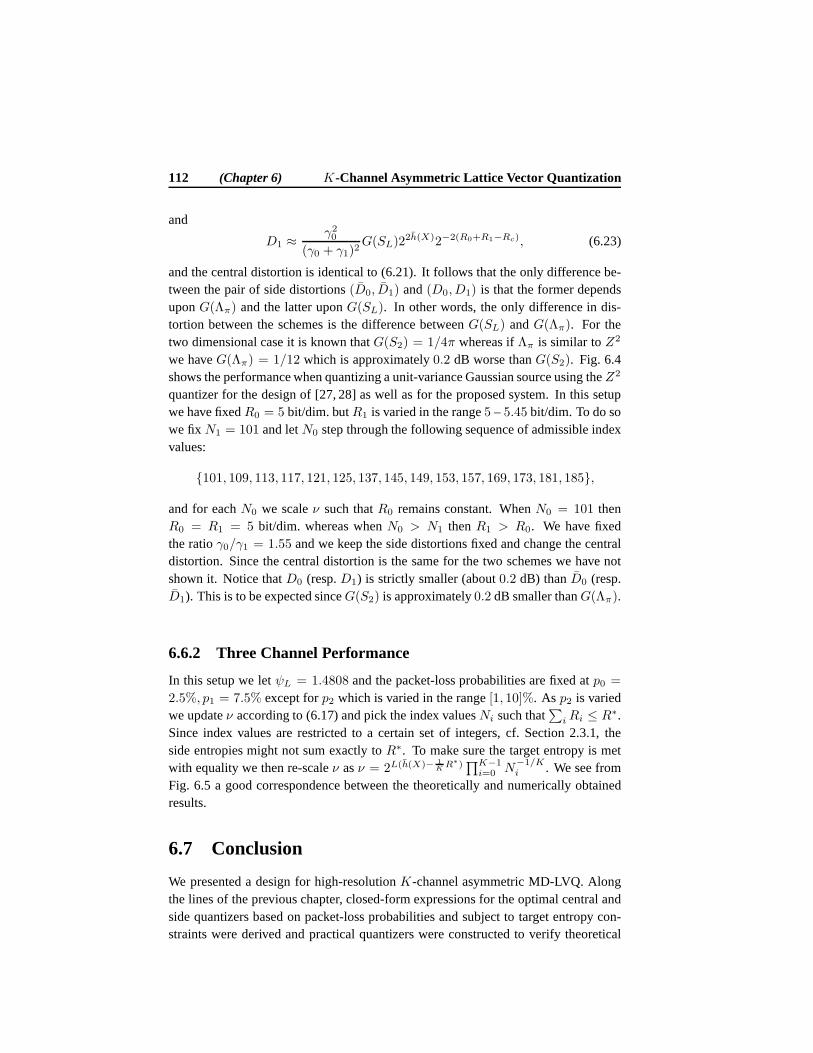
112 (Chapter 6) K-Channel Asymmetric Lattice Vector Quantization
and
D1 ≈ γ20(γ0 + γ1)2
G(SL)22h(X)2−2(R0+R1−Rc), (6.23)
and the central distortion is identical to (6.21). It follows that the only difference be-tween the pair of side distortions(D0, D1) and(D0, D1) is that the former dependsuponG(Λπ) and the latter uponG(SL). In other words, the only difference in dis-tortion between the schemes is the difference betweenG(SL) andG(Λπ). For thetwo dimensional case it is known thatG(S2) = 1/4π whereas ifΛπ is similar toZ2
we haveG(Λπ) = 1/12 which is approximately0.2 dB worse thanG(S2). Fig. 6.4shows the performance when quantizing a unit-variance Gaussian source using theZ2
quantizer for the design of [27, 28] as well as for the proposed system. In this setupwe have fixedR0 = 5 bit/dim. butR1 is varied in the range5 – 5.45 bit/dim. To do sowe fixN1 = 101 and letN0 step through the following sequence of admissible indexvalues:
101, 109, 113, 117, 121, 125, 137, 145, 149, 153, 157, 169, 173, 181, 185,
and for eachN0 we scaleν such thatR0 remains constant. WhenN0 = 101 thenR0 = R1 = 5 bit/dim. whereas whenN0 > N1 thenR1 > R0. We have fixedthe ratioγ0/γ1 = 1.55 and we keep the side distortions fixed and change the centraldistortion. Since the central distortion is the same for thetwo schemes we have notshown it. Notice thatD0 (resp.D1) is strictly smaller (about0.2 dB) thanD0 (resp.D1). This is to be expected sinceG(S2) is approximately0.2 dB smaller thanG(Λπ).
6.6.2 Three Channel Performance
In this setup we letψL = 1.4808 and the packet-loss probabilities are fixed atp0 =
2.5%, p1 = 7.5% except forp2 which is varied in the range[1, 10]%. As p2 is variedwe updateν according to (6.17) and pick the index valuesNi such that
∑
iRi ≤ R∗.Since index values are restricted to a certain set of integers, cf. Section 2.3.1, theside entropies might not sum exactly toR∗. To make sure the target entropy is metwith equality we then re-scaleν asν = 2L(h(X)− 1
KR∗)∏K−1
i=0 N−1/Ki . We see from
Fig. 6.5 a good correspondence between the theoretically and numerically obtainedresults.
6.7 Conclusion
We presented a design for high-resolutionK-channel asymmetric MD-LVQ. Alongthe lines of the previous chapter, closed-form expressionsfor the optimal central andside quantizers based on packet-loss probabilities and subject to target entropy con-straints were derived and practical quantizers were constructed to verify theoretical

Section 6.7 Conclusion 113
5 5.05 5.1 5.15 5.2 5.25 5.3 5.35 5.4−16
−15.5
−15
−14.5
−14
−13.5
−13
−12.5M
SE
[dB
]
PSfrag replacements
Theo:D0
Theo:D1
Num: D0
Num: D1
Theo:D0
Theo:D1
R1 [bit/dim.]
Figure 6.4: The side distortions are here kept fixed as the rate is increased. Notice that the nu-merically obtained side distortionsD0 andD1 (crosses) are strictly smaller than the theoreticalD0 andD1 (thin lines).
results. For the two-channel case we compared the proposed MD-LVQ scheme to astate-of-the-art two-channel asymmetric scheme and showed that the performance ofthe central quantizer was equivalent to that of the state-of-the-art scheme whereas theside quantizers were strictly superior in finite dimensionsgreater than one. The prob-lem of distributing bits among theK descriptions was analyzed and it was shown thatthe optimal solution was not unique. In fact, it turned out that bits could be almostarbitrarily distributed among theK descriptions without loss of performance. As wasthe case for the symmetric design, the practical design of asymmetric MD-LVQ allowsan arbitrary number of descriptions but the theoretical rate-distortion results were onlyproven for the case ofK ≤ 3 descriptions and conjectured to be true in the generalcase of arbitraryK descriptions.
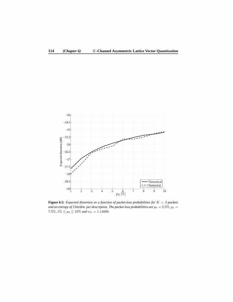
114 (Chapter 6) K-Channel Asymmetric Lattice Vector Quantization
1 2 3 4 5 6 7 8 9 10−29
−28.5
−28
−27.5
−27
−26.5
−26
−25.5
−25
−24.5
−24
Exp
ecte
d di
stor
tion
[dB
]
TheoreticalNumerical
PSfrag replacements
p3 [%]
Figure 6.5: Expected distortion as a function of packet-loss probabilities forK = 3 packetsand an entropy of 3 bit/dim. per description. The packet-loss probabilities arep0 = 2.5%, p1 =
7.5%, 1% ≤ p2 ≤ 10% andψL = 1.14808.

Chapter7Comparison to Existing
High-Resolution MD Results
In this chapter we compare the rate-distortion performanceof the proposed MD-LVQscheme to that of existing state-of-the-art schemes as wellas to known informationtheoretic high-resolutionK-channel MD rate-distortion bounds.
7.1 Two-Channel Performance
We will first consider the symmetric case and show that, whilethe proposed design isdifferent than the design of Vaishampayan et al. [139], the two-channel performanceis, in fact, identical to the results of [139]. Then we consider the asymmetric case andshow that the asymmetric distortion product given by Lemma 4.1.1 is achievable.
7.1.1 Symmetric Case
LetK = 2 so thatψ2L = 1. From Theorem 6.5.1 (see also (5.34)) we see that the side
distortion (i.e. fork = 1) for the symmetric case, i.e.D0 = D1 andRs = Ri, i = 0, 1,is given by (asymptotically asN → ∞ andνs → 0)
D0 =1
4G(SL)N
4/Lν2/L. (7.1)
In order to trade off the side rate for the central rate we use an idea of [139] and let2−2aRs = 4N−2/L where0 < a < 1, which implies that
N = 2L(aRs+1). (7.2)
115
116 (Chapter 7) Comparison to Existing High-Resolution MD Results
Let us insert (7.2) into (5.19) in order to expressν as a function ofRs anda,
ν = 2L(h(X)−aRs−Rs−1). (7.3)
From (6.21) we know that the two-channel central distortionDc is given byDc =
G(Λc)ν2/L which by use of (7.3) can be rewritten as
Dc = G(Λc)22(h(X)−aRs−Rs−1), (7.4)
which leads to
limRs→∞
Dc22Rs(1+a) =
1
4G(Λc)2
2h(X). (7.5)
By inserting (7.2) and (7.3) in (7.1) we find
D0 =1
4G(SL)2
4(aRs+1)+2(h(X)−aRs−Rs−1), (7.6)
which leads tolim
Rs→∞D02
2Rs(1−a) = G(SL)22h(X). (7.7)
Comparing (7.5) and (7.7) with those of Vaishampayan (4.56)and (4.57) reveals thatthe performance of the proposed two-channel design achievethe same performanceas the two-channel design of Vaishampayan et al. [139]. Furthermore, letb = 1 andL→ ∞ and notice that in the memoryless Gaussian caseG(S∞)22h(X) = σ2
X so that,by comparing (7.5) and (7.7) with (4.11) and (4.10), we see that the high-resolutiontwo-channel symmetric rate-distortion function of Ozarowcan be achieved.
Remark7.1.1. It is important to see thata in (7.5) and (7.7) is bounded away fromzero and one. In the extreme case wherea = 0 the ratio of side distortion overcentral distortion is small andN cannot be made arbitrarily large as is required forthe asymptotic expressions to be valid. On the other hand, when a = 1 we can nolonger force the cells of the side quantizers to be small compared to the variance ofthe source and the high resolution assumptions are therefore not satisfied. This is alsotrue for the general case ofK > 2 descriptions.
Remark7.1.2. We would like to point out an error in [102] where we overlooked therequirement thata < 1. In [102] we showed that the high resolution performanceof (3, 2) SCECs can be achieved by use of lattice codebooks and index assigments(which is true) but we also wrongly claimed that in the extreme case wherea = 1,lattice codebooks achieve rate-distortion points that cannot be achieved by randomcodebooks, obviously, this cannot be true since, fora = 1, the high resolution assump-tions are not satisfied (Remark 7.1.1).
7.1.2 Asymmetric Case
We already showed in Section 6.6 that the performance of the asymmetric two-channelscheme by Diggavi et al. [27,28] can be achieved. In fact, in finite dimensions greater

Section 7.2 Achieving Rate-Distortion Region of(3, 1) SCECs 117
than one, the performance of the proposed scheme was strictly superior to that ofDiggavi et al. Furthermore, it is easy to show that the high resolution asymmetricdistortion product presented by Lemma 4.1.1 can be achieved. To see this note that byuse of (6.22), (6.23) and (6.21) we get
Dc(D0 +D1 + 2√
D0D1) = G(Λc)22(h(X)−Rc) (7.8)
×(
γ20 + γ21(γ0 + γ1)2
G(SL)22h(X)2−2(R0+R1−Rc)
+ 2
√
γ20γ21
(γ0 + γ1)4G(SL)224h(X)2−4(R0+R1−Rc)
)
= G(Λc)G(SL)24h(X)2−2(R0+R1),
which, asymptotically asL→ ∞, leads to Lemma 4.1.1.
7.2 Achieving Rate-Distortion Region of(3, 1) SCECs
We will now consider the symmetric three-channel case and show that the rate-distortion performance of(3, 1) SCECs can be achieved at high resolution.
We are interested in the three-channel case, i.e.K = 3, and in the limit ofL→ ∞so that
G(SL) →1
2πe(7.9)
and
ψ2∞ =
√
4
3. (7.10)
Furthermore, without any loss of generality, we assume thatthe source has unit vari-ance. Thus, from (5.34) we see that
D(3,1) =1
3ψ2∞N
′2−2Rs , (7.11)
sinceRc = Rs + log2(N′),
D(3,2) =1
12ψ2∞N
′2−2Rs , (7.12)
and the central distortionDc = D(3,3) given by (6.21) can be written as
D(3,3) =
(1
N ′
)2
2−2Rs . (7.13)
The following lemma shows that symmetric three-channel MD-LVQ can achievethe rate-distortion region of(3, 1) SCECs at high resolution.
118 (Chapter 7) Comparison to Existing High-Resolution MD Results
Lemma 7.2.1. At high resolution, the one, two and three-channel distortions of(3, 1)SCECs are identical to (7.11) – (7.13) in the quadratic Gaussian case.
Proof. See Appendix J.1.
Remark7.2.1. The notion of a large sublattice indexN in K-channel MD-LVQ cor-responds to a large (negative) codebook correlationρq for (K, 1) SCECs and in thelimit of N → ∞ we actually haveρq → −1/(K − 1). Thus, forK = 3 we haveρq → −1/2 asN → ∞.
7.3 Achieving Rate-Distortion Region of(3, 2) SCECs
We will now show that the rate-distortion performance of(3, 2) SCECs can beachieved by extending the proposed design of three-channelMD-LVQ to include ran-dom binning on the side codebooks. Specifically, we show thatthe achievable two-channel versus three-channel distortion region of(3, 2) SCECs for the memorylessGaussian source and MSE can be achieved under high-resolution assumptions. Sincethe performance of a(3, 3) SCEC is identical to that of a single description scheme, itis clear that we can also achieve such performance simply by lettingK = 1 and onlyuse the central quantizer. Explicit bounds forK > 3 descriptions were not derivedin [111, 114] but we expect that these (non-derived) bounds are also achievable withthe proposedK-channel MD-LVQ scheme.
We will begin by considering the general situation where we allow finite dimensio-nal lattice vector quantizers and asymmetric rates and distortions. Then, at the end ofthe section, we focus on the symmetric case and infinite-dimensional lattice vectorquantizers in order to compare the performance to the existing bounds.
Recall that the proposed design ofK-channel MD-LVQ is able to vary the redun-dancy by changing the number of descriptionsK as well as the index valuesNi. Inaddition, it is possible to trade off distortion among subsets of descriptions, withoutaffecting the rates, simply by varying the weights. Increasing Ni and at the sametime decreasingν so thatνi = Niν remains constant does not affect the rateRi.However, the distortion due to theith description is affected (unless counteracted bythe weights). For example in the symmetric setup whereN = Ni for all i and theweights are also balanced, the side distortion due to reception of only a subset ofdescriptions is increased asN is increased andνN is kept constant. However, in thiscase, the central distortion due to reception of all descriptions is decreased. In otherwords, in the symmetric case, for a givenK, the degree of redundancy is controled bythe single parameterN .

Section 7.3 Achieving Rate-Distortion Region of(3, 2) SCECs 119
7.3.1 Random Binning on Side Codebooks of MD-LVQ Schemes
In order to achieve the performance of general(K, k) SCECs we need to introducemore controlling parameters into the design ofK-channel MD-LVQ. To do so wefollow an idea of Pradhan et al. [111] and exploit recent results on distributed sourcecoding. More specifically, we apply random binning on the side codebooks of theK-channel MD-LVQ scheme. This corresponds in some sense to replacing the randomcodebooks of(K, k) SCECs with structured lattice codebooks except that we alsohave a central quantizer and an index assignment map to consider.
Random binning is usually applied on (in principle infinite-dimensional) randomcodebooks. The idea is to exploit the fact that for a given codevector, sayλ0, ofcodebookC0, only a small set of the codevectors in codebookC1 is jointly typicalwith λ0. Then by randomly distributing the codevectors ofC1 overM1 bins, it isunlikely that two or more codevectors, which are all jointlytypical with λ0, end upin the same bin (at least this is true ifM1 is large enough). Thus, if the binning rateRb,1 = log2(M1) is less than the codebook rateR1 then it is possible to reduce thedescription rate by sending the bin indices instead of the codevector indices.
The rate and distortion performance of lattice vector quantizers are often describedusing high-resolution assumptions, i.e. the rate of the quantizer is sufficiently high andthe source pdf sufficiently smooth, so that the pdf can be considered constant withinVoronoi regions of the code vectors. Under these assumptions the theoretical perfor-mance of lattice vector quantizers can be derived for arbitrary vector dimension. Thisis in contrast to the asymptotics used when deriving theoretical expressions for the per-formance of random codebooks. For random codebooks the theoretical performanceis usually derived based on asymptotically high vector dimension but arbitrary rates.The theory behind random binning relies upon asymptotically high vector dimensionand as such when using random binning inK-channel MD-LVQ we make use of bothasymptotics, i.e. high vector dimension and high rates. It is also worth mentioningthat we consider memoryless sources with infinite alphabetssuch as e.g. the Gaussiansource, whereas the analysis of SCECs relies upon strong typicality and as such onlydiscrete alphabet memoryless sources are valid.50
In lattice codebooks, the code vectors are generally not jointly typical and theconcept of random binning is therefore not directly applicable. It is, however, possibleto simulate joint typicality by for example some distance metric, so that code vectorsclose together (in e.g. Euclidean sense) are said to be “jointly typical”. The indexassignments of MD-LVQ is another example of how to simulate joint typicality. Weuse the term admissibleK-tuple for any set ofK code vectors(λ0, . . . , λK−1) whichis obtained by applying the index-assignment map on a code vectorλc, i.e.α(λc) =(λ0, . . . , λK−1) for all λc ∈ Λc. So for lattice code vectors we exploit that only asubset of allK-tuples are admissibleK-tuples which, in some sense, corresponds to
50However, in [111] the authors remark that the analysis of SCECs can be generalized to continuous-alphabet memoryless sources by using the techniques of [41,Ch.7].

120 (Chapter 7) Comparison to Existing High-Resolution MD Results
the fact that only a subset of allK-tuples of random code vectors are jointly typical.LetJ ⊆ 0, . . . ,K−1 denote an index set, where|J | = k. A k-tuple is a set ofk
elementsλj, j ∈ J whereλj ∈ Λj . Thek-tuple given byλj = αj(λc), j ∈ J
for anyλc ∈ Λc is said to be an admissiblek-tuple. Each latticeΛi contains an infinitenumber of lattice points (or reproduction vectors) but we show by Lemma 7.3.1 thatonly finite sets of these points are needed for the codebooks of the side quantizers andwe denote these sets byCi ⊂ Λi, where|Ci| <∞. The set
λ2|λ1, λ0 =
λ2 ∈ Λ2 : λ2 = α2(λc) and(α1(λc), α0(λc)) = (λ1, λ0), ∀λc ∈ Λc,(7.14)
denotes the set ofλ2’s which are in admissiblek-tuples that also contain the specificelementsλ0 andλ1.
Since we consider the asymmetric case some ambiguity is present in the termD(K,k), because it is not specified whichk out of theK descriptions that are to beconsidered. To overcome this technicality we introduce thenotationD(K,J), J ∈ K ,whereK denotes the set of combinations of descriptions for which the distortion isspecified. For example, if we are only interested in the distortion when receiving de-scriptions0, 1, 0, 2 or 0, 1, 2 out of all subset of0, 1, 2, thenK = 0, 1,0, 2, 0, 1, 2 and nothing is guaranteed upon reception of either a single descrip-tion or the pair of descriptions1, 2.
We will now outline the construction of(K,K ) MD-LVQ. It can be seen that theconstruction of(K,K ) MD-LVQ resembles the construction of(K, k) SCECs givenin [111].
Construction of lattice codebooks Construct aK-channel MD-LVQ system withone central quantizer andK side quantizers of rateRi. Let Cc be the codebook ofthe central quantizer and letλc(jc) ∈ Cc denote thejthc element ofCc. Similarly,let Ci wherei = 0, . . .K − 1 denote the codebook of theith side quantizer and letλi(ji) ∈ Ci denote thejthi codeword ofCi. Finally, letα be the index-assignmentfunction that maps central lattice points to sublattice points.
Random binning Perform random binning on each of the side codebooksCi toreduce the side description rate fromRi to Rb,i bit/dim., where we assumeRi >
Rb,i. Let ξi = 2L(Ri−Rb,i+γi) whereγi > 0. Assignξi codewords to each of the2LRb,i bins of each codebook. The codewords for a given bin of codebook C0 isfound by randomly extractingξ0 codewords fromC0 uniformly, independently andwith replacement. This procedure is then repeated for all the remaining codebooksCi, i = 1, . . . ,K − 1.
Encoding Given a source wordX ∈ RL, find the closest elementλc ∈ Cc and useα to obtain the correspondingK-tuple, i.e.α(λc) = (λ0(j0), . . . , λK−1(jK−1)). If
Section 7.3 Achieving Rate-Distortion Region of(3, 2) SCECs 121
the codewordλi /∈ Ci then setji equal to a fixed special symbol51, sayji = ϑ. Fori = 0, . . . ,K − 1 define the functionfi(λi(ji)) which indicates the index of a bincontaining the codewordλi(ji). If λi(ji) is found in more than one bin, setfi(λi(ji))equal to the least index of these bins. Ifλi(ji) is not in any bin, setfi(λi(ji)) = ϑ.The bin indexfi(λi(ji)) is sent over channeli.
Decoding The decoder receives somem bin indices and searches through the corre-sponding bins to identify a unique admissiblem-tuple.
Remark7.3.1. For (K,K ) MD-LVQ the notion of large block length, i.e.L → ∞,is introduced in order to make sure that standard binning arguments can be applied.However, it should be clear that the quantizer dimension is allowed to be finite. Iffinite quantizer dimension is used it must be understood that(finite length) codewordsfrom consecutive blocks are concatenated to form anL-sequence of codewords. Thedimension of theL-sequence becomes arbitrarily large asL → ∞, but the quantizerdimension remains fixed. As such this will not affect the binning rate but the distortiontupleD(K,J)J∈K is affected in an obvious way.
Theorem 7.3.1. Let X ∈ RL be a source vector constructed by blocking an ar-bitrary i.i.d. source with finite differential entropy intosequences of lengthL. LetJ ⊆ 0, . . . ,K − 1 and letλJ denote the set of codewords indexed byJ . The setof decoding functions is denotedgJ :
⊗
j∈J Λj → RL. Then, under high-resolutionassumptions, if
E[ρ(X, gJ(λJ ))] ≤ D(K,J), ∀J ∈ K ,
whereρ(·, ·) is the squared-error distortion measure and for allS ⊆ J∑
i∈S
Rb,i >∑
i∈S
γi +1
Llog2(|λS |λJ−S|), (7.15)
the rate-distortion tuple(Rb,0, . . . , Rb,(K−1), D(K,J)J∈K ) is achievable.
Proof. See Appendix J.2.
We have the following corollary for the symmetric case:
Corollary 7.3.1 (Symmetric case). Let X ∈ RL be a source vector constructed byblocking an arbitrary i.i.d. source with finite differential entropy into sequences oflengthL. For anyJ ⊆ 0, . . . ,K − 1 let λJ denote the set of received codewordsand letgJ :
⊗
j∈J Λj → RL be the set of decoding functions. Then, under high-resolution assumptions, if
E[ρ(X, gJ(λJ ))] ≤ D(K,|J|), ∀J ⊆ 0, . . . ,K − 1, |J | ≥ k,
whereρ(·, ·) is the squared-error distortion measure and for allS ⊆ J
51The rate increase caused by the introduction of the additional symbolϑ is vanishing small for largeL.
122 (Chapter 7) Comparison to Existing High-Resolution MD Results
Rb > γ +1
|S|L log2(|λS |λJ−S|), (7.16)
the tuple(Rb, D(K,k), D(K,k+1), . . . , D(K,K)) is achievable.
Proof. Follows immediately from Theorem 7.3.1.
7.3.2 Symmetric Case
To actually apply Theorem 7.3.1 we need to find a set of binningratesRb,i, i =0, . . . ,K − 1, such that (7.15) is satisfied for all subsetsS of J and for all elementsJ of K . Let us consider the symmetric case whereK = 3 and design a(3, 2)MD-LVQ system. We then haveJ = i0, i1 and it suffices to check the two caseswhereS = i0 andS = i0, i1. Without loss of generality we assume thati0 =
0 and i1 = 1. The number of distinctλ1’s that is paired with a givenλ0 can beapproximated52 by (ψL
√N ′)L, whereN ′ = N1/L is the dimension normalized index
value describing the index (redundancy) per dimension. LetS = 0, 1 and noticethat |λS| ≤ |λ1|λ0| · |C0|. Then, asymptotically, asN → ∞, it follows that|λ1|λ0| = (ψL
√N ′)L. Let us now bound the codebook cardinality.
Lemma 7.3.1. |Ci| = 2LRi. Furthermore, the entropy of the quantizer indices isupper bounded byRi.53
Proof. See Appendix J.1.
We are now able to findRb by considering the two cases|S| = 1, 2. For |S| = 1
we have from (7.16) that
Rb,I > γ + log2(ψL
√N ′), (7.17)
whereas for|S| = 2
Rb,II >1
2Rs + γ +
1
2log2(ψL
√N ′). (7.18)
The dominantRb is then given byRb = max(Rb,I , Rb,II). Since (7.17) and (7.18)depends uponN ′ the dominating binning rate depends uponN ′. To resolve this prob-lem, we form the inequalityRb,II ≥ Rb,I and find thatN ′ ≤ 22Rs/ψ2
L. So forN ′ ≤ 22Rs/ψ2
L we haveRb = Rb,II . It is interesting to see that when insertingN ′ = 22Rs/ψ2
L in (7.17) we getRb,I = γ + Rs. Coincidently,Rb,I becomes effec-tive when the binning rateRb is equal to the codebook rateRs, which violates theassumption thatRb > Rs.
It is clear that if we setRb equal to the lower bound in (7.18) we get
Rb =1
2Rs +
1
4log2(N
′) +1
2log2(ψL),
52Recall that this approximation becomes exact asN → ∞.53For largeL there is really no loss by assuming that2LRi is an integer.
Section 7.3 Achieving Rate-Distortion Region of(3, 2) SCECs 123
from which we can expressN ′ andRs as functions of each other andRb, that is
N ′ = 24Rb−2Rsψ−2L , (7.19)
and
Rs = 2Rb − log2(ψL)−1
2log2(N
′). (7.20)
It follows that when varying the redundancy per dimensionN ′, the binning rateRb
can be kept constant by adjustingRs according to (7.20).In order to compare these results to the existing bounds we let L → ∞ so that by
inserting (7.20) in (5.34) we get
D(3,2) =1
12ψ2∞N
′2−2Rs
=1
12ψ4∞(N ′)22−4Rb .
(7.21)
The central distortion (Dc = D(3,3)) in MD-LVQ is given by
D(3,3) = 2−2Rc , (7.22)
whereRc = Rs + log2(N′) which leads to
Rc = 2Rb − log2(ψ∞) +1
2log2(N
′). (7.23)
Inserting (7.23) into (7.22) leads to
D(3,3) =ψ2∞N ′ 2
−4Rb . (7.24)
Lemma 7.3.2. At high resolution, the two and three-channel distortions of (3, 2)
SCECs are identical to (7.21) and (7.24) in the quadratic Gaussian case.
Proof. See Appendix J.1.
7.3.3 Asymmetric Case
For the asymmetric case,K = 3 and whereK = 0, 1, 0, 2, 1, 2, 0, 1, 2,i.e. reconstruction is possible when any two or more descriptions are received, it canbe shown (similar to the symmetric case) that the binning rateRb,i is lower boundedbyRb,i = max(Rb,iI , Rb,iII ) where
Rb,iI = log2(ψL) +1
2log2(N
′π)− log2(N
′i) (7.25)
and
Rb,iII =1
2log2(ψL) +
1
4log2(N
′π)−
1
2log2(N
′i) +
1
2Ri, (7.26)
124 (Chapter 7) Comparison to Existing High-Resolution MD Results
whereN ′π = N ′
0N′1N
′2.
To see this note that ifλi andλj both are in the same admissibleK-tuple, thenλimust be within a sphereV centered atλj . The volume ofV is ν, which implies thatthe maximum number of distinctλi points withinV is approximatelyν/νi. In otherwords,
|λi|λj| ≈ ν/νi
= (ψL
√
N ′0N
′1N
′2/Ni)
L,(7.27)
where the approximation becomes exact for large index values. With this it is easy tosee that
Rb,i >1
Llog2(|λi|λj|)
≈ log2(ψL) +1
2log2(N
′0N
′1N
′2)− log2(Ni),
(7.28)
which is identical to (7.25). From Theorem 7.3.1 we can also see that the pair-wisesum rate must satisfy
Rb,i +Rb,j >1
Llog2(|Ci||λj |λi|)
≈ Ri + log2(ψL) +1
2log2(N
′0N
′1N
′2)− log2(Nj),
(7.29)
which can equivalently be expressed asRb,i + Rb,j >1L log2(|Cj ||λi|λj|) from
which the individual rate requirements can be found to be given by (7.26).
7.4 Comparison toK-Channel Schemes
In the asymptotic case of large lattice vector quantizer dimension and under high res-olution conditions, we showed in the previous sections thatexisting MD bounds canbe achieved. However, it is also of interest to consider the rate-distortion performancethat can be expected in practical situations. Towards that end we presented some nu-merical results obtained through computer simulations in Sections 5.6 and 6.6.
In this section we will compare the theoretical performanceof the proposed MD-LVQ scheme to existing state-of-the-artK-channel MD schemes [18, 127]. Whilethe schemes [18, 127] (as well as the proposed scheme) can be shown to be optimal,under certain asymptotic conditions, they are not without their disadvantages whenused in practical situations. We will, however, refrain from comparing implementationspecific factors such as computational complexity as well asscalability in dimension,description rate and number of descriptions. Such comparisons, although relevant, areoften highly application specific.
The above mentioned schemes are all based on LVQ and it is therefore possible tocompare their theoretical rate-distortion performance when finite-dimensional lattice
Section 7.4 Comparison toK-Channel Schemes 125
vector quantizers are used. Recall from Section 4.2.2 that the scheme of Chen etal. [18] has a rate loss of(2K − 1) L-dimensional lattice vector quantizers.54 Thescheme of Østergaard and Zamir [127] was, for the case ofK = 2, shown to havea rate loss of only twoL-dimensional lattice vector quantizers. While this designwas shown to permit an arbitrary number of descriptions, therate loss forK > 2
descriptions was not assessed. The rate loss of the proposedscheme, on the other hand,has a somewhat peculiar form. In the case of two descriptions, the rate loss is givenby that of twoL-dimensional quantizers having spherical Voronoi cells.55 However,in the case ofK > 2 descriptions, there is an additional term which influences the rateloss.
7.4.1 Rate Loss of MD-LVQ
To be able to assess the rate loss of MD-LVQ when using finite-dimensional quantizersand more than two descriptions, we letRf denote the description rate (where thesubscriptf indicates that finite-dimensional quantizers are used). Then the distortionwhen receiving a single description out ofK = 3 can be found by use of (5.34) to begiven by
D(3,1) =1
3G(SL)(2πe)ψ
2LN
′2−2Rf . (7.30)
Equalizing (7.11) and (7.30) reveals that the rate loss (Rf −Rs), forK = 3, is givenby (at high resolution)
Rf −Rs =1
2log2(G(SL)(2πe)) + log2(ψL/ψ∞). (7.31)
SinceψL ≤ ψ1 = ψ2∞ (at least forK = 3) we can upper bound the second term
of (7.31) by
log2(ψL/ψ∞) ≤ log2(ψ∞) = 0.1038 bit/dim. (7.32)
Fig. 7.1 showslog2(ψL/ψ∞) for 1 ≤ L ≤ 101 for K = 3 using the values ofψL
from Table 5.1.
Remark7.4.1. ForK = 2 we haveψL = 1, ∀L, and (7.31) is true. Furthermore, if theK-channel MD-LVQ scheme is optimal also forK > 3, as we previously conjectured,then (7.31) is true for anyK ≥ 2 (at high resolution).
It is interesting to observe that both terms in (7.31) are independent of the partic-ular type of lattice being used. For example, if the product latticeΛ = Z∞ is usedfor the side quantizers, then the rate loss vanishes (it becomes identical to zero) even
54In the asymmetric case where corner points of the rate regionare desired, the rate loss of [18] is onlythat ofK lattice vector quantizers. However, in the symmetric case,source splitting is necessary and thereis an additional rate loss.
55This is true in the symmetric case as well as in the asymmetriccase.

126 (Chapter 7) Comparison to Existing High-Resolution MD Results
thoughG(Λ) = 1/12.56 This is not the case with the other two schemes mentionedabove, i.e. [18, 127]. Fig. 7.2 shows the rate loss of the different schemes forK = 3
descriptions. The lattices used are those of Table 3.1. Since we do not haveψL valuesfor all evenL we have in Fig. 7.2 simply used the average of the two neighboringvalues, that is
ψL =
ψL−1 + ψL+1
2, L even
ψL, L odd.(7.33)
10 20 30 40 50 60 70 80 90 100
0.02
0.03
0.04
0.05
0.06
0.07
0.08
0.09
0.1
Bit/
dim
.
PSfrag replacements
L
Figure 7.1: The rate loss due to the termlog2(ψL/ψ∞) is here expressed in bit/dim. as afunction of the dimensionL.
7.5 Conclusion
In the previous two chapters we initially used a single index-assignment map to controlthe redundancy between descriptions. In this chapter we then showed that by use ofrandom binning on the side codebooks in addition to the index-assignment map itwas possible to introduce more rate-distortion controlling parameters into the design.While the use of random binning is standard procedure in distributed source codingand has previously been applied to MD schemes based on randomcodebooks as well,
56Recall that the central distortion depends upon the type of lattice being used. However, at high reso-lution conditions, the index value is large (i.e.N → ∞) and as such the central distortion is very smallcompared to the side distortion and can therefore be neglected.
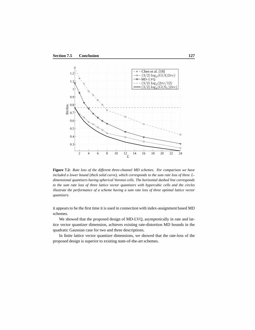
Section 7.5 Conclusion 127
2 4 6 8 10 12 14 16 18 20 22 24
0.3
0.4
0.5
0.6
0.7
0.8
0.9
1
1.1
1.2
Bit/
dim
.
MD−LVQ
PSfrag replacements
Chen et al. [18](3/2) log2(G(Λ)2πe)
(3/2) log2(2πe/12)(3/2) log2(G(SL)2πe)
L
Figure 7.2: Rate loss of the different three-channel MD schemes. For comparison we haveincluded a lower bound (thick solid curve), which corresponds to the sum rate loss of threeL-dimensional quantizers having spherical Voronoi cells. The horizontal dashed line correspondsto the sum rate loss of three lattice vector quantizers with hypercubic cells and the circlesillustrate the performance of a scheme having a sum rate lossof three optimal lattice vectorquantizers.
it appears to be the first time it is used in connection with index-assignment based MDschemes.
We showed that the proposed design of MD-LVQ, asymptotically in rate and lat-tice vector quantizer dimension, achieves existing rate-distortion MD bounds in thequadratic Gaussian case for two and three descriptions.
In finite lattice vector quantizer dimensions, we showed that the rate-loss of theproposed design is superior to existing state-of-the-art schemes.


Chapter8Network Audio Coding
In this chapter we apply the developed MD coding scheme to thepractical problemof network audio coding. Specifically, we consider the problem of reliable distribu-tion of audio over packet-switched networks such as the Internet or general ad hocnetworks.57 Thus, in order to combat (excessive) audio packet losses we choose totransmit multiple audio packets.
Many state-of-the-art audio coding schemes perform time-frequency analysis ofthe source signal, which makes it possible to exploit perceptual models in both thetime and the frequency domain in order to discard perceptually-irrelevant informa-tion. This is done in e.g. MPEG-1 (MP3) [93], MPEG-2 advancedaudio coding(AAC) [94], Lucent PAC [123] and Ogg Vorbis [134]. The time-frequency analy-sis is often done by a transform coder which is applied to blocks of the input signal.A common approach is to use the modified discrete cosine transform (MDCT) [90]as was done in e.g. MPEG-2 AAC [94], Lucent PAC [123] and Ogg Vorbis [134]. Inthis chapter we combine the MDCT withK-channel MD-LVQ in order to obtain aperceptual transform coder, which is robust to packet losses.
MD coding of audio has to the best of the author’s knowledge sofar only beenconsidered for two descriptions [3, 119]. However, here we propose a scheme that isable to use an arbitrary number of descriptions without violating the target entropy.We show how to distribute the bit budget among the MDCT coefficients and presentclosed-form expressions for the rate and distortion performance of theK-channelMD-LVQ system which minimize the expected distortion basedon the packet-lossprobabilities. Theoretical results are verified with numerical computer simulationsand it is shown that in environments with excessive packet losses it is advantageousto use more than two descriptions. We verify the findings thatmore than two descrip-tions are needed by subjective listening tests, which further proves that acceptable
57Part of the research presented in this chapter represents joint work with O. Niamut.
129
130 (Chapter 8) Network Audio Coding
audio quality can be obtained even when the packet-loss rateis as high as 30%.
8.1 Transform Coding
In this section we describe the MDCT and we define a perceptualdistortion measurein the MDCT domain.
8.1.1 Modified Discrete Cosine Transform
The MDCT is a modulated lapped transform [90] which is applied on overlappingblocks of the input signal. A window of2M time-domain samples is transformed intoM MDCT coefficients, whereafter the window is shiftedM samples for the nextMMDCT coefficients to be calculated.
Given a blocks ∈ R2M , the set ofM MDCT coefficients is given by [90]
xk =1√2M
2M−1∑
n=0
hnsn cos
((2n+M + 1)(2k + 1)π
4M
)
, k = 0, . . . ,M − 1,
(8.1)wherexk, hn ∈ R andh is an appropriate analysis window, e.g. the symmetric sinewindow [90]
hn = sin
((
n+1
2
)(π
2M
))
, n = 0, . . . , 2M − 1. (8.2)
The inverse MDCT is given by [90]58
sn = hn1√2M
M−1∑
k=0
xk cos
((2n+M + 1)(2k + 1)π
4M
)
, n = 0, . . . , 2M − 1.
(8.3)
8.1.2 Perceptual Weighting Function
On each block a psycho-acoustic analysis is performed whichleads to a masking curvethat describes thresholds in the frequency domain below which distortions are inaudi-ble. In our work the masking curve is based on a2nM -point DFT wheren ∈ N andthe computation of the masking curve is described in detail in [140]. Let us denotethe masking curve byΣ. We then define a perceptual weightµ as the inverse of themasking thresholdΣ evaluated at the center frequencies of the MDCT basis functions,that is
µk = Σ−12nk+1, k = 0, . . . ,M − 1. (8.4)
58Notice that the MDCT is not an invertible transform on a block-by-block basis since2M samplesare transformed into onlyM samples. We therefore use the tilde notation to indicate that, at this point,the reconstructed samplessn are not identical to the original samplessn. In order to achieve perfectreconstruction we need to perform overlap-add of consecutive reconstructed blocks [90].
Section 8.1 Transform Coding 131
We requireµ to be a multiplicative weight but otherwise arbitrary. We will notgo into more details aboutµ except mentioning that we assume it can be efficientlyencoded at e.g.4 kpbs as was done in [96].
8.1.3 Distortion Measure
Let X ∈ RM denote a random vector process59 and letx ∈ RM be a realization ofX . By Xk andxk we denote thekth components ofX andx, respectively, and wewill useXk to denote the alphabet ofXk. The pdf ofX is denotedfX with marginalsfXk
.We define a perceptual distortion measure in the MDCT domain betweenx and a
quantized versionx of x to be the single-letter distortion measure given by60
ρ(x, x) ,1
M
M−1∑
k=0
µk|xk − xk|2, (8.5)
whereµk is given by (8.4). The expected perceptual distortion follows from (8.5)simply by taking the expectation overx, that is
D(x, x) =1
M
M−1∑
k=0
∫
Xk
µk|xk − xk|2fXk(xk)dxk, (8.6)
where we remark thatµ depends ons throughx.
8.1.4 Transforming Perceptual Distortion Measure toℓ2
For the traditional MSE distortion measure which is also known as theℓ2 distortionmeasure, it is known that, under high-resolution assumptions, a lattice vector quan-tizer is good (even optimal asL → ∞) for smooth sources, see Chapter 3. TheMSE distortion measure is used mainly due its mathematical tractability. However,in applications involving a human observer it has been notedthat distortion measureswhich include some aspects of human auditory perception generally perform betterthan the MSE. A great number of perceptual distortion measures are non-differencedistortion measures and unfortunately even for simple sources their correspondingrate-distortion functions are not known. For example, the perceptual distortion mea-sure given by (8.6) is an input-weighted MSE (becauseµ is a function ofs), hence itis a non-difference distortion measure.
In certain cases it is possible to derive the rate-distortion functions for generalsources under non-difference distortion measures. For example, for the Gaussian pro-cess with a weighted squared error criterion, where the weights are restricted to be lin-ear time-invariant operators, the complete rate-distortion function was found in [118].
59In fact it is the output of the MDCT of a random vector processS ∈ R2M .
60Strictly speaking this is not a single-letter distortion measure since the perceptual weight depends uponthe entire vector.
132 (Chapter 8) Network Audio Coding
Other examples include the special case of locally quadratic distortion measures forfixed rate vector quantizers and under high-resolution assumptions [43], results whichare extended to variable-rate vector quantizers in [80, 83]. With regards to the MDproblem, [84] presents a high-resolution rate-distortionregion for smooth sources andlocally quadratic distortion measures for the case of two descriptions. The case ofvector sources and more than two descriptions remains unsolved.
Remark8.1.1. In the SD case it has been shown that it is sometimes possible to apply afunction (called a multidimensional compressor) on the source signal in order to trans-form it into a domain where a lattice vector quantizer is good. This approach was firstconsidered by Bennett in [7] for the case of a scalar compressor followed by uniformscalar quantization. The general case of a multidimensional compressor followed bylattice vector quantization was considered in [85]. In general anL-dimensional sourcevectorX is “compressed” by an invertible mappingF .61 HereafterF (X) is quantizedby a lattice vector quantizer. To obtain the reconstructed signal X, the inverse map-pingF−1 (the expander) is applied, that is
X → F (·) → Q(·) → F−1(·) → X, (8.7)
whereQ denotes a lattice vector quantizer. It was shown in [85] thatan optimal com-pressorF is independent of the source distribution and only depends upon the distor-tion measure. However, it was also shown that an optimal compressor does not alwaysexists.62 In the MD case, results on optimal compressors are very limited. However,it was suggested in [84], that a compressor obtained in a similar way as for the SDcase, might perform well also in the two-description case for smooth scalar processes.Unfortunately, we have been unsuccessful in finding an analytical expression for sucha vector compressor for our distortion measure (8.5).
In this chapter we will assume that the decoder has access to the perceptual weightµ, which makes it possible to exploitµ also at the encoder when quantizing the MDCTcoefficients. This has been done before by e.g. Edler et al. [31]. In addition, in theperceptual MD low delay audio coder presented in [119] a postfilter, which resemblesthe auditory masking curve, was transmitted as side information. The input signalwas first pre filtered by a perceptual filter which transforms the input signal into aperceptual domain that approximates anℓ2 domain. A lattice vector quantizer is usedin this domain and at the decoder the signal is reconstructedby applying the post filter.
We adopt the approach of normalizing the input signal by the perceptual weight.First we show that, under a mild assumption on the masking curve, this proceduretransforms the perceptual distortion measure into anℓ2 distortion measure. From (8.6)
61The invertible mappingF is for historically reasons called a compressor and said to compress thesignal. However,F is allowed to be any invertible mapping (also an expander) but we will use the termcompressor to be consistent with earlier literature.
62In the scalar case an optimal compressor always exists for a wide range of distortion measures.
Section 8.1 Transform Coding 133
we have that
D(x, x) =1
M
M−1∑
k=0
∫
Xk
µk|xk − xk|2fXk(xk)dxk (8.8)
(a)=
1
M
M−1∑
k=0
∑
j
∫
Xk∩V ′j
µk|xk − xk|2fXk(xk)dxk
=1
M
M−1∑
k=0
∑
j
∫
Xk∩V ′j
|yk − yk|2fXk(xk)dxk, (8.9)
whereyk = xkõk, yk = xk
õk and(a) follows by breaking up the integral into
disjoint partial integrals over each Voronoi cellV ′j of the quantizer. In order to perform
the necessary variable substitution in the integral given by (8.9) we write
dykdxk
= xkd
dxk(õk) +
õk. (8.10)
At this point we enforce the following condition on the masking curve. Within eachquantization cell, the first derivative of the masking curvewith respect to the sourcesignal is assumed approximately zero so that from (8.10)dxk ≈
√
1/µkdyk.63 Inser-ting this in (8.9) leads to
D(x, x) ≈ 1
M
M−1∑
k=0
∑
j
∫
Yk∩Vj
|yk − yk|2fXk(xk)
√
1/µkdyk
=1
M
M−1∑
k=0
∑
j
∫
Yk∩Vj
|yk − yk|2fYk(yk)dyk,
=1
ME
M−1∑
k=0
|yk − yk|2,
(8.11)
since it can be shown thatfYk(yk) = fXk
(xk)√
1/µk cf. [126, p.100]. In other words,simply by normalizing the input signalx by the root of the input-dependent weightµ,the perceptual distortion measure forx is transformed into anℓ2 distortion measurefor y. Therefore, when quantizingy, the distortion is approximately the same whenmeasuring theℓ2-distortion i.e.E‖y − y‖2/M or transformingy and y back intoxandx, respectively, and measuring the perceptual distortion given by (8.6).
8.1.5 Optimal Bit Distribution
Each blocks leads toM MDCT coefficients, which we first normalize byõ and then
vector quantize usingK-channel MD-LVQ. Since, the number of coefficients in the
63To justify this assumption notice that we can approximate the masking curve by piece-wise flat regions(since the masking curve also needs to be coded), which meansthat small deviations of the source will notaffect the masking curve.
134 (Chapter 8) Network Audio Coding
MDCT is quite large, e.g.M = 1024 in our case, it is necessary to split the sequenceof M coefficients into smaller vectors to make the quantization problem practicallyfeasible. Any small number of coefficients can be combined and jointly quantized.For example, if the set ofM coefficients is split intoM ′ bands (vectors) of lengthLk
wherek = 0, . . . ,M ′ − 1 it can be deduced from (5.40) that the total distortion isgiven by64
Da =1
M ′
M ′−1∑
k=0
K1,kG(Λk)22(h(Yk)−Rck
)
+ K2,kψ2LkG(Sk)2
2(h(Yk)−Rck)2
2KkKk−1 (Rck
−Rk) +pKk
LkE‖Yk‖2,
(8.12)
where we allow the quantizersΛk and the number of packetsKk to vary among theM ′ bands as well as from block to block. For a given target entropy R∗ we need tofind the individual entropiesRk for theM ′ bands, such that
∑Rk = R∗/K and in
addition we need to find the entropiesRck of the central quantizers. For simplicitywe assume in the following that theM ′ bands are of equal dimensionL′, that similarcentral latticesΛc are used, and that the number of packetsK is fixed for allk.
We now use the fact that (5.44) and (5.45) hold for any bit distribution, hence wemay insert (5.44) and (5.45) into (8.12) which leads to individual distortions given by
Dk = K1G(Λc)22(h(Yk)−Rk)
(
1
K − 1
K2
K1
G(SL′)
G(Λc)ψ2L′
)K−1K
+ K2G(SL′)22(h(Yk)−Rk)
(
(K − 1)K1
K2
G(Λc)
G(SL′)
)(
1
K − 1
K2
K1
G(SL′)
G(Λc)ψ2L′
)K−1K
+pK
L′ E‖Yk‖2
= a022(h(Yk)−Rk) +
pK
L′ E‖Yk‖2,(8.13)
wherea0 is independent ofk and given by
a0 = K1G(Λc)
(
1
K − 1
K2
K1
G(SL′)
G(Λc)ψ2L′
)K−1K
. (8.14)
64The distortion over individual normalized MDCT coefficients is additive in the MDCT domain (recallthat we are using a single-letter distortion measure). However, adding the entropies of a set of MDCT coeffi-cients is suboptimal unless the coefficients are independent. Futhermore, the individual MDCT coefficientswill generally be correlated over consecutive blocks. For example, overlapping blocks of an i.i.d. processyields a Markov process. For simplicity, we do not exploit any correlation across blocks nor between thevectors of MDCT coeffficients (but only within the vectors).

Section 8.1 Transform Coding 135
In order to find the optimal bit distribution among theM ′ bands subject to the entropyconstraint
∑M ′−1k=0 Rk = R∗/K we take the common approach of turning the con-
strained optimization problem into an unconstrained problem by introducing a Lagran-gian cost functional of the form
J =
M ′−1∑
k=0
Dk + λ
M ′−1∑
k=0
Rk. (8.15)
Differentiating (8.15) w.r.t.Rk leads to
∂J
∂Rk= −2 ln(2)a02
2(h(Yk)−Rk) + λ. (8.16)
After equating (8.16) to zero and solving forRk we get
Rk = −1
2log2
(λ
2 ln(2)a0
)
+ h(Yk). (8.17)
In order to eliminateλ we invoke the sum-rate constraint∑M ′−1
k=0 Rk = R∗/K andget
M−1∑
k=0
Rk = −M′
2log2
(λ
2 ln(2)a0
)
+M ′−1∑
k=0
h(Yk) = R∗/K, (8.18)
from which we obtain
λ = 2 ln(2)a02− 2
M′ (R∗/K−∑M′−1
k=0 h(Yk)). (8.19)
We can now eliminateλ by inserting (8.19) into (8.17), that is
Rk =R∗/K −∑M ′−1
k=0 h(Yk)
M ′ + h(Yk). (8.20)
With the simple Lagrangian approach taken here there is no guarantee that theentropiesRk given by (8.20) are all non-negative. It might be possible toextendthe Lagrangian cost functional (8.15) byM ′ additional Lagrangian weights (alsocalled “complementary slackness” variables [128]) in order to obtainM ′ inequalityconstraints making sure thatRk ≥ 0 in addition to the single equality constraint∑Rk = R∗/K. While the resulting problem can be solved using numerical techni-
ques, it does not appear to lead to a closed-form expression for the individual entropiesRk. It is not possible either to simply set negative entropies equal to zero since this willmost likely violate the constraint
∑Rk = R∗/K. Instead we propose a sequential
procedure where we begin by considering allM ′ bands and then one-by-one eliminatebands having negative entropies. We assign entropies to each band using (8.20) andthen find the one having the largest negative entropy and exclude that one from theoptimization process. This procedure continues until all entropies are positive or zeroas shown in Table 8.1.
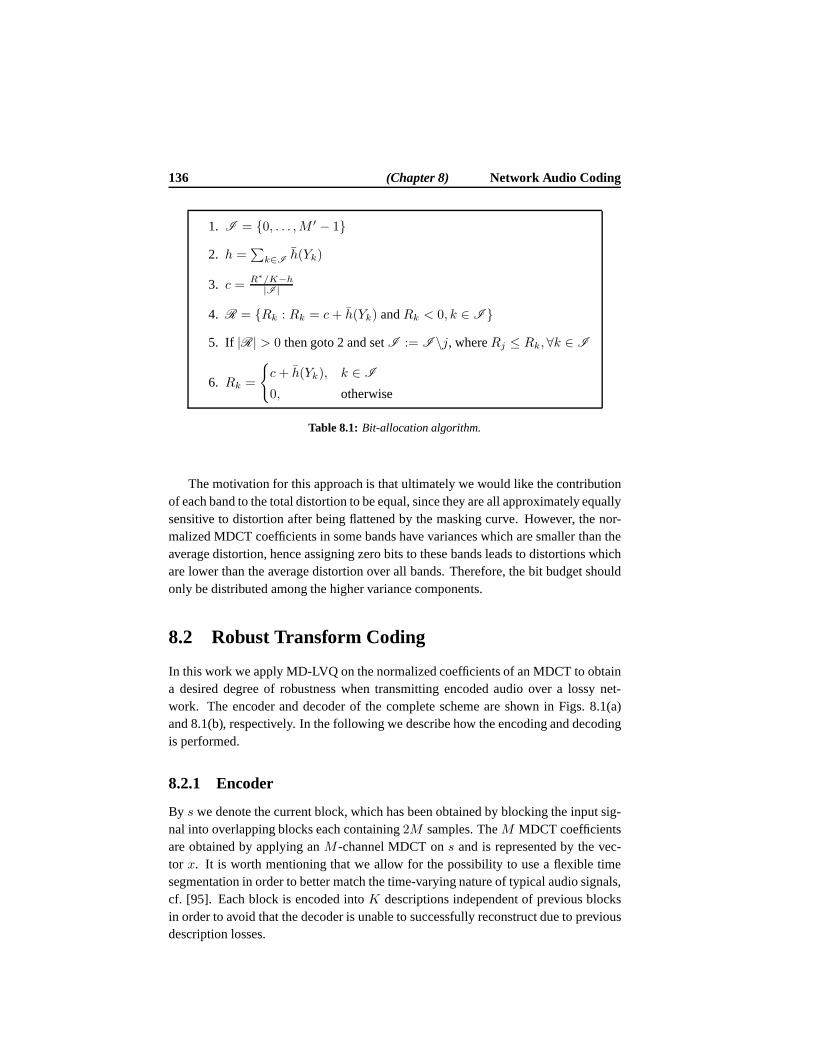
136 (Chapter 8) Network Audio Coding
1. I = 0, . . . ,M ′ − 1
2. h =∑
k∈Ih(Yk)
3. c = R∗/K−h|I |
4. R = Rk : Rk = c+ h(Yk) andRk < 0, k ∈ I
5. If |R| > 0 then goto 2 and setI := I \j, whereRj ≤ Rk, ∀k ∈ I
6. Rk =
c+ h(Yk), k ∈ I
0, otherwise
Table 8.1: Bit-allocation algorithm.
The motivation for this approach is that ultimately we wouldlike the contributionof each band to the total distortion to be equal, since they are all approximately equallysensitive to distortion after being flattened by the maskingcurve. However, the nor-malized MDCT coefficients in some bands have variances whichare smaller than theaverage distortion, hence assigning zero bits to these bands leads to distortions whichare lower than the average distortion over all bands. Therefore, the bit budget shouldonly be distributed among the higher variance components.
8.2 Robust Transform Coding
In this work we apply MD-LVQ on the normalized coefficients ofan MDCT to obtaina desired degree of robustness when transmitting encoded audio over a lossy net-work. The encoder and decoder of the complete scheme are shown in Figs. 8.1(a)and 8.1(b), respectively. In the following we describe how the encoding and decodingis performed.
8.2.1 Encoder
By s we denote the current block, which has been obtained by blocking the input sig-nal into overlapping blocks each containing2M samples. TheM MDCT coefficientsare obtained by applying anM -channel MDCT ons and is represented by the vec-tor x. It is worth mentioning that we allow for the possibility to use a flexible timesegmentation in order to better match the time-varying nature of typical audio signals,cf. [95]. Each block is encoded intoK descriptions independent of previous blocksin order to avoid that the decoder is unable to successfully reconstruct due to previousdescription losses.
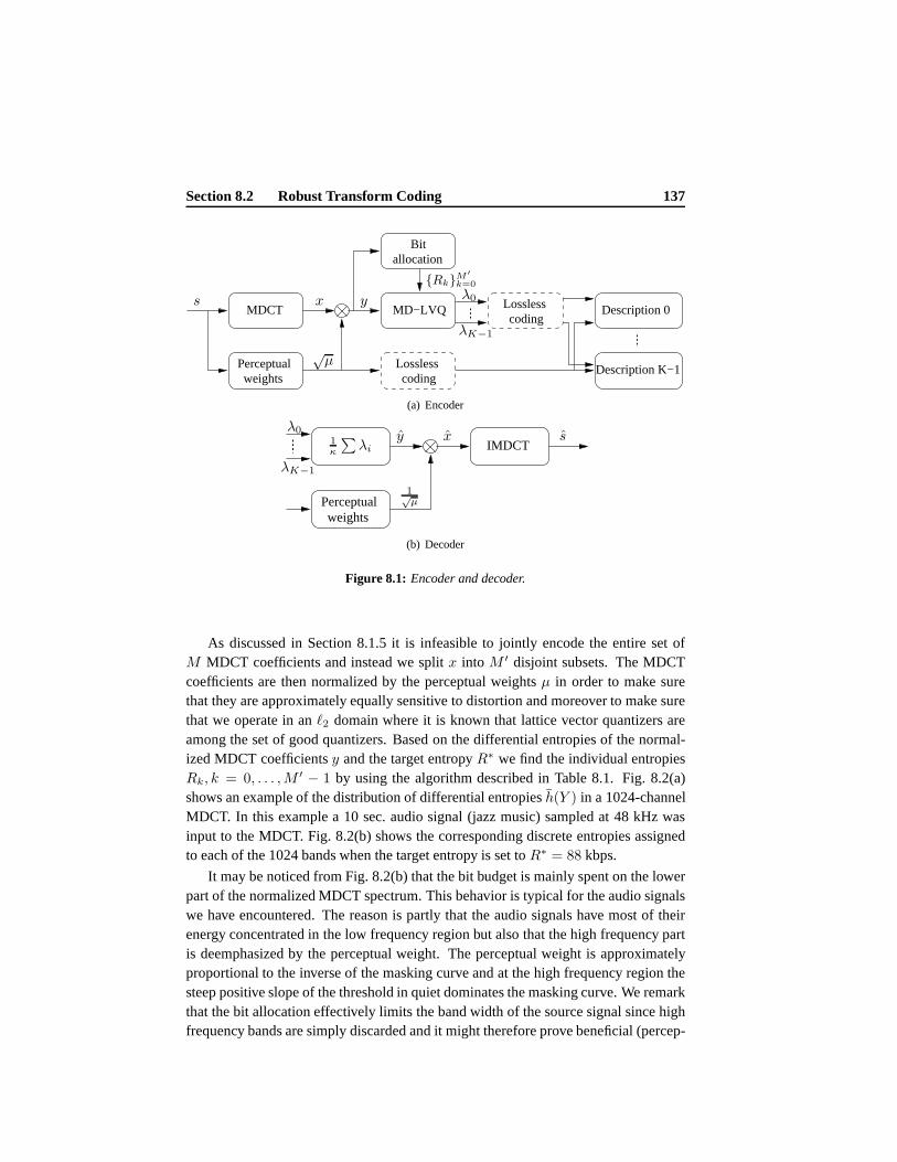
Section 8.2 Robust Transform Coding 137
MDCT MD−LVQ
weightsPerceptual Description K−1
Description 0Losslesscoding
allocationBit
Losslesscoding
PSfrag replacements
s x y
õ
λ0
λK−1
RkM′
k=0
(a) Encoder
Perceptualweights
IMDCT
PSfrag replacements
s
xyõ
λ0λK−1
RkM′
k=0
sxy
1õ
λ0
λK−1
1κ
∑λi
(b) Decoder
Figure 8.1: Encoder and decoder.
As discussed in Section 8.1.5 it is infeasible to jointly encode the entire set ofM MDCT coefficients and instead we splitx into M ′ disjoint subsets. The MDCTcoefficients are then normalized by the perceptual weightsµ in order to make surethat they are approximately equally sensitive to distortion and moreover to make surethat we operate in anℓ2 domain where it is known that lattice vector quantizers areamong the set of good quantizers. Based on the differential entropies of the normal-ized MDCT coefficientsy and the target entropyR∗ we find the individual entropiesRk, k = 0, . . . ,M ′ − 1 by using the algorithm described in Table 8.1. Fig. 8.2(a)shows an example of the distribution of differential entropiesh(Y ) in a 1024-channelMDCT. In this example a 10 sec. audio signal (jazz music) sampled at 48 kHz wasinput to the MDCT. Fig. 8.2(b) shows the corresponding discrete entropies assignedto each of the 1024 bands when the target entropy is set toR∗ = 88 kbps.
It may be noticed from Fig. 8.2(b) that the bit budget is mainly spent on the lowerpart of the normalized MDCT spectrum. This behavior is typical for the audio signalswe have encountered. The reason is partly that the audio signals have most of theirenergy concentrated in the low frequency region but also that the high frequency partis deemphasized by the perceptual weight. The perceptual weight is approximatelyproportional to the inverse of the masking curve and at the high frequency region thesteep positive slope of the threshold in quiet dominates themasking curve. We remarkthat the bit allocation effectively limits the band width ofthe source signal since highfrequency bands are simply discarded and it might thereforeprove beneficial (percep-
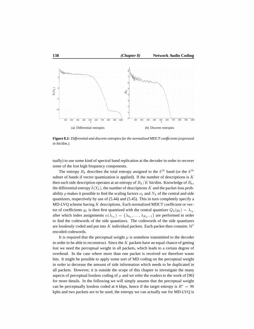
138 (Chapter 8) Network Audio Coding
100 200 300 400 500 600 700 800 900 1000
−10
−5
0
5
k
PSfrag replacements
h(Y
k)
Rk
(a) Differential entropies
100 200 300 400 500 600 700 800 900 10000
1
2
3
4
5
6
7
8
k
PSfrag replacements
h(Yk)
Rk
(b) Discrete entropies
Figure 8.2: Differential and discrete entropies for the normalized MDCT coefficients (expressedin bit/dim.).
tually) to use some kind of spectral band replication at the decoder in order to recoversome of the lost high frequency components.
The entropyRk describes the total entropy assigned to thekth band (or thekth
subset of bands if vector quantization is applied). If the number of descriptions isKthen each side description operates at an entropy ofRk/K bit/dim. Knowledge ofRk,the differential entropyh(Yk), the number of descriptionsK and the packet-loss prob-ability pmakes it possible to find the scaling factorsνk andNk of the central and sidequantizers, respectively by use of (5.44) and (5.45). This in turn completely specify aMD-LVQ scheme havingK descriptions. Each normalized MDCT coefficient or vec-tor of coefficientsyk is then first quantized with the central quantizerQk(yk) = λckafter which index assignmentsα(λck ) = λ0k , . . . , λKk−1 are performed in orderto find the codewords of the side quantizers. The codewords ofthe side quantizersare losslessly coded and put intoK individual packets. Each packet then containsM ′
encoded codewords.It is required that the perceptual weightµ is somehow transmitted to the decoder
in order to be able to reconstruct. Since theK packets have an equal chance of gettinglost we need the perceptual weight in all packets, which leads to a certain degree ofoverhead. In the case where more than one packet is received we therefore wastebits. It might be possible to apply some sort of MD coding on the perceptual weightin order to decrease the amount of side information which needs to be duplicated inall packets. However, it is outside the scope of this chapterto investigate the manyaspects of perceptual lossless coding ofµ and we refer the readers to the work of [96]for more details. In the following we will simply assume thatthe perceptual weightcan be perceptually lossless coded at 4 kbps, hence if the target entropy isR∗ = 96
kpbs and two packets are to be used, the entropy we can actually use for MD-LVQ is

Section 8.3 Results 139
then only88 kbps, since8 kbps (4 kbps in each packet) are used for the weight. Ifa greater number of packets is desired the overhead for transmitting µ increases evenfurther.
8.2.2 Decoder
At the receiving side an estimatey of the normalized MDCT spectrum is first obtainedby simply taking the average of the received descriptions, i.e. yk = 1
κ′
∑
i∈l′ λik ,wherel′ denotes the indices of the received descriptions andκ′ = |l′|. This estimate isthen denormalized in order to obtainx, i.e. xk = yk/
õk. Finally the inverse MDCT
(including overlap-add) is applied in order to obtain an approximations of the timedomain signals. The decoding procedure is shown in Fig. 8.1(b).
8.3 Results
In this section we compare numerical simulations with theoretical results and in addi-tion we show the results of a subjective listening test. We first show results related tothe expected distortion based on the packet-loss probabilities and then we show resultsfor the case of scalable coding. In both cases we assume a symmetric setup.
8.3.1 Expected Distortion Results
For the objective test we use four short audio clips of different genres (classical jazzmusic, German male speech, pop music, rock music) each having a duration between10 and 15 sec. and a sampling frequency of48 kHz. We refer to these fragmentsas “jazz”, “speech” , “pop” and “rock”. We set the target entropy to 96 kbps (aswas done in [119]) which corresponds to2 bit/dim. since the sampling frequency is48 kHz. We do not encode the perceptual weight but simply assumethat it can betransmitted to the receiver at an entropy of4 kbps. Since the weight must be includedin all of theK descriptions we deduct4K kbps from the total entropy, hence theeffective target entropyR∗
e is given byR∗e = R∗ − 4K so that a single description
system hasR∗e = 92 kbps whereas a four description system hasR∗
e = 80 kbps (i.e.20 kbps for each side description). For simplicity we furthermore assume that thesources are stationary processes so that we can measure the statistics for each vectorof MDCT coefficients upfront. However, since audio signals in general have timevarying statistics we expect that it will be possible to reduce the bit rate by properadaptation to the source. Since for this particular test we are merely interested inthe performance of the proposed audio coder with a varying number of descriptionswe will not address the issue of efficient entropy coding but simply assume that thequantized variables can be losslessly coded arbitrarily close to their discrete entropies.
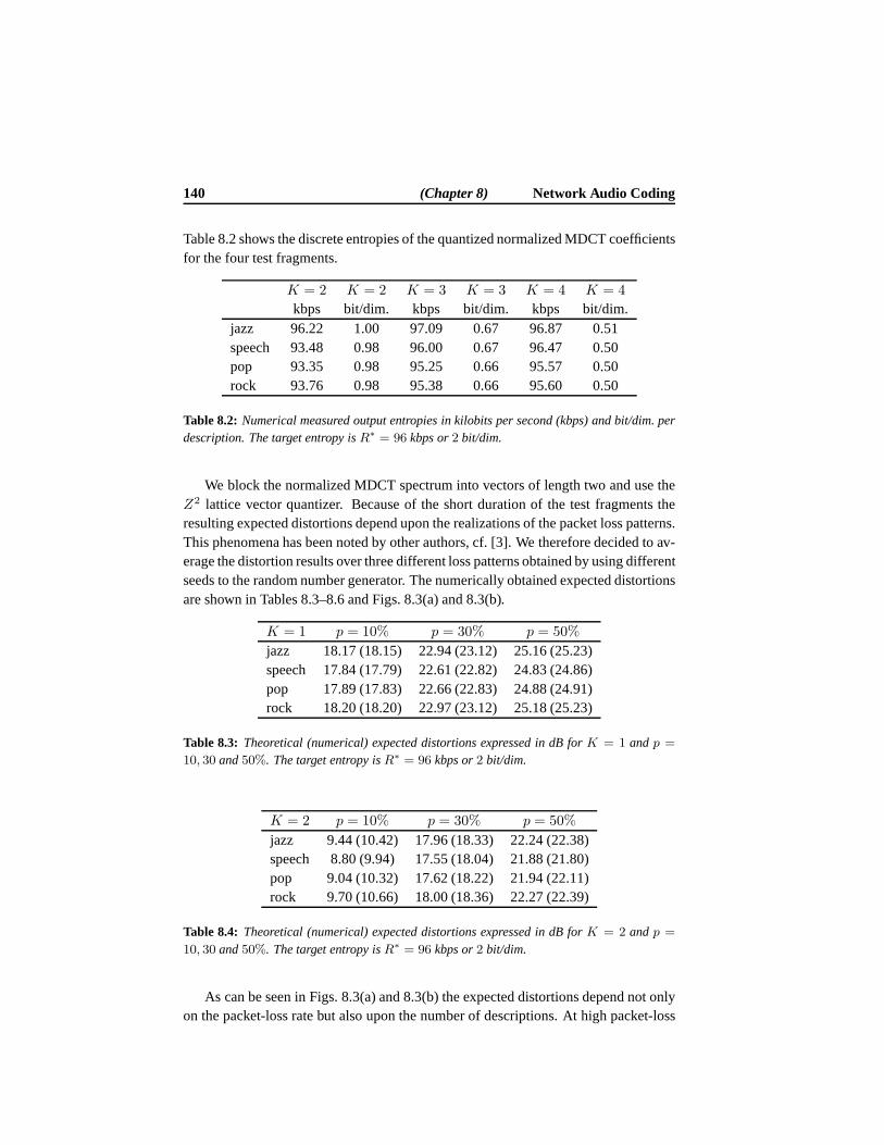
140 (Chapter 8) Network Audio Coding
Table 8.2 shows the discrete entropies of the quantized normalized MDCT coefficientsfor the four test fragments.
K = 2 K = 2 K = 3 K = 3 K = 4 K = 4
kbps bit/dim. kbps bit/dim. kbps bit/dim.jazz 96.22 1.00 97.09 0.67 96.87 0.51speech 93.48 0.98 96.00 0.67 96.47 0.50pop 93.35 0.98 95.25 0.66 95.57 0.50rock 93.76 0.98 95.38 0.66 95.60 0.50
Table 8.2: Numerical measured output entropies in kilobits per second(kbps) and bit/dim. perdescription. The target entropy isR∗ = 96 kbps or2 bit/dim.
We block the normalized MDCT spectrum into vectors of lengthtwo and use theZ2 lattice vector quantizer. Because of the short duration of the test fragments theresulting expected distortions depend upon the realizations of the packet loss patterns.This phenomena has been noted by other authors, cf. [3]. We therefore decided to av-erage the distortion results over three different loss patterns obtained by using differentseeds to the random number generator. The numerically obtained expected distortionsare shown in Tables 8.3–8.6 and Figs. 8.3(a) and 8.3(b).
K = 1 p = 10% p = 30% p = 50%
jazz 18.17 (18.15) 22.94 (23.12) 25.16 (25.23)speech 17.84 (17.79) 22.61 (22.82) 24.83 (24.86)pop 17.89 (17.83) 22.66 (22.83) 24.88 (24.91)rock 18.20 (18.20) 22.97 (23.12) 25.18 (25.23)
Table 8.3: Theoretical (numerical) expected distortions expressed in dB forK = 1 andp =
10, 30 and50%. The target entropy isR∗ = 96 kbps or2 bit/dim.
K = 2 p = 10% p = 30% p = 50%
jazz 9.44 (10.42) 17.96 (18.33) 22.24 (22.38)speech 8.80 (9.94) 17.55 (18.04) 21.88 (21.80)pop 9.04 (10.32) 17.62 (18.22) 21.94 (22.11)rock 9.70 (10.66) 18.00 (18.36) 22.27 (22.39)
Table 8.4: Theoretical (numerical) expected distortions expressed in dB forK = 2 andp =
10, 30 and50%. The target entropy isR∗ = 96 kbps or2 bit/dim.
As can be seen in Figs. 8.3(a) and 8.3(b) the expected distortions depend not onlyon the packet-loss rate but also upon the number of descriptions. At high packet-loss
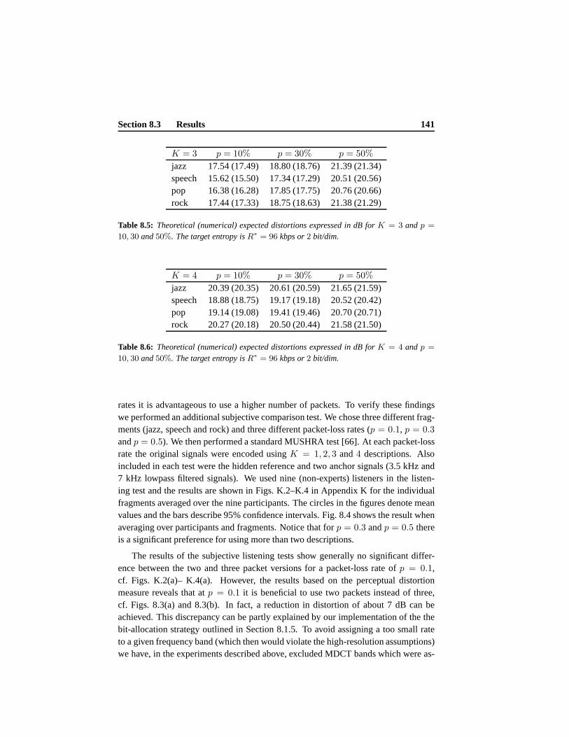
Section 8.3 Results 141
K = 3 p = 10% p = 30% p = 50%
jazz 17.54 (17.49) 18.80 (18.76) 21.39 (21.34)speech 15.62 (15.50) 17.34 (17.29) 20.51 (20.56)pop 16.38 (16.28) 17.85 (17.75) 20.76 (20.66)rock 17.44 (17.33) 18.75 (18.63) 21.38 (21.29)
Table 8.5: Theoretical (numerical) expected distortions expressed in dB forK = 3 andp =
10, 30 and50%. The target entropy isR∗ = 96 kbps or2 bit/dim.
K = 4 p = 10% p = 30% p = 50%
jazz 20.39 (20.35) 20.61 (20.59) 21.65 (21.59)speech 18.88 (18.75) 19.17 (19.18) 20.52 (20.42)pop 19.14 (19.08) 19.41 (19.46) 20.70 (20.71)rock 20.27 (20.18) 20.50 (20.44) 21.58 (21.50)
Table 8.6: Theoretical (numerical) expected distortions expressed in dB forK = 4 andp =
10, 30 and50%. The target entropy isR∗ = 96 kbps or2 bit/dim.
rates it is advantageous to use a higher number of packets. Toverify these findingswe performed an additional subjective comparison test. We chose three different frag-ments (jazz, speech and rock) and three different packet-loss rates (p = 0.1, p = 0.3
andp = 0.5). We then performed a standard MUSHRA test [66]. At each packet-lossrate the original signals were encoded usingK = 1, 2, 3 and4 descriptions. Alsoincluded in each test were the hidden reference and two anchor signals (3.5 kHz and7 kHz lowpass filtered signals). We used nine (non-experts) listeners in the listen-ing test and the results are shown in Figs. K.2–K.4 in Appendix K for the individualfragments averaged over the nine participants. The circlesin the figures denote meanvalues and the bars describe 95% confidence intervals. Fig. 8.4 shows the result whenaveraging over participants and fragments. Notice that forp = 0.3 andp = 0.5 thereis a significant preference for using more than two descriptions.
The results of the subjective listening tests show generally no significant differ-ence between the two and three packet versions for a packet-loss rate ofp = 0.1,cf. Figs. K.2(a)– K.4(a). However, the results based on the perceptual distortionmeasure reveals that atp = 0.1 it is beneficial to use two packets instead of three,cf. Figs. 8.3(a) and 8.3(b). In fact, a reduction in distortion of about 7 dB can beachieved. This discrepancy can be partly explained by our implementation of the thebit-allocation strategy outlined in Section 8.1.5. To avoid assigning a too small rateto a given frequency band (which then would violate the high-resolution assumptions)we have, in the experiments described above, excluded MDCT bands which were as-
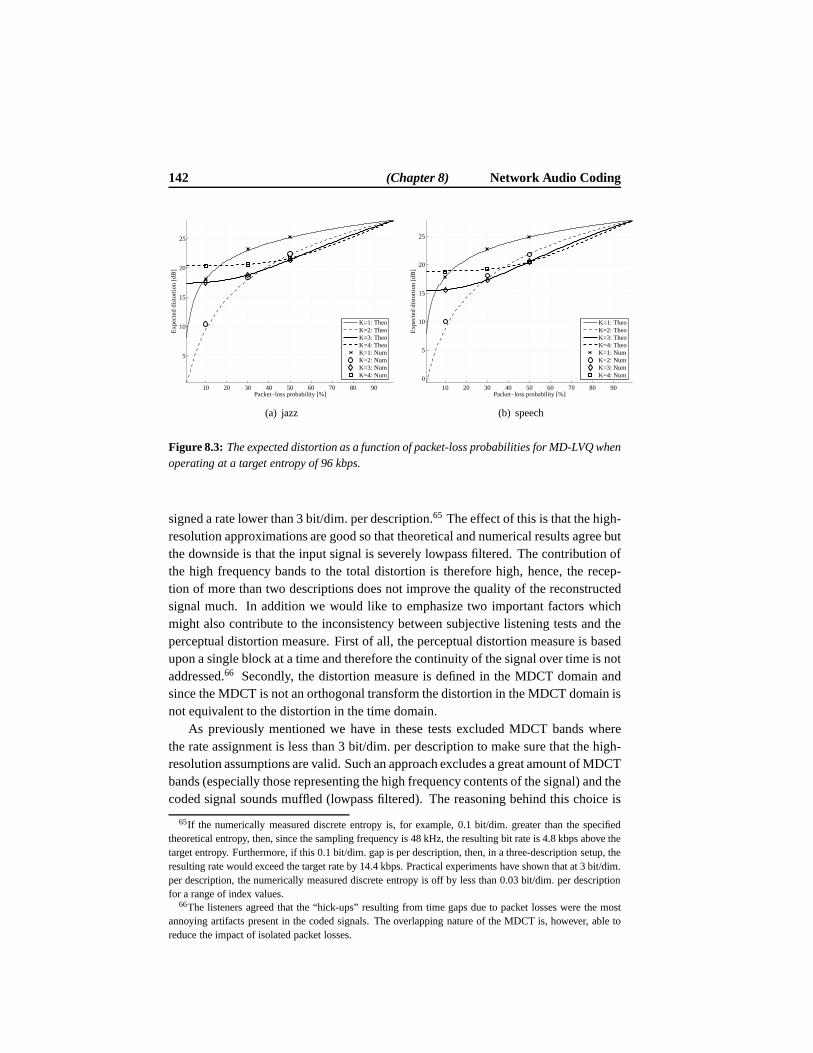
142 (Chapter 8) Network Audio Coding
10 20 30 40 50 60 70 80 90
5
10
15
20
25
Packet−loss probability [%]
Exp
ecte
d di
stor
tion
[dB
]
K=1: TheoK=2: TheoK=3: TheoK=4: TheoK=1: NumK=2: NumK=3: NumK=4: Num
(a) jazz
10 20 30 40 50 60 70 80 90
0
5
10
15
20
25
Packet−loss probability [%]
Exp
ecte
d di
stor
tion
[dB
]
K=1: TheoK=2: TheoK=3: TheoK=4: TheoK=1: NumK=2: NumK=3: NumK=4: Num
(b) speech
Figure 8.3: The expected distortion as a function of packet-loss probabilities for MD-LVQ whenoperating at a target entropy of 96 kbps.
signed a rate lower than 3 bit/dim. per description.65 The effect of this is that the high-resolution approximations are good so that theoretical andnumerical results agree butthe downside is that the input signal is severely lowpass filtered. The contribution ofthe high frequency bands to the total distortion is therefore high, hence, the recep-tion of more than two descriptions does not improve the quality of the reconstructedsignal much. In addition we would like to emphasize two important factors whichmight also contribute to the inconsistency between subjective listening tests and theperceptual distortion measure. First of all, the perceptual distortion measure is basedupon a single block at a time and therefore the continuity of the signal over time is notaddressed.66 Secondly, the distortion measure is defined in the MDCT domain andsince the MDCT is not an orthogonal transform the distortionin the MDCT domain isnot equivalent to the distortion in the time domain.
As previously mentioned we have in these tests excluded MDCTbands wherethe rate assignment is less than 3 bit/dim. per description to make sure that the high-resolution assumptions are valid. Such an approach excludes a great amount of MDCTbands (especially those representing the high frequency contents of the signal) and thecoded signal sounds muffled (lowpass filtered). The reasoning behind this choice is
65If the numerically measured discrete entropy is, for example, 0.1 bit/dim. greater than the specifiedtheoretical entropy, then, since the sampling frequency is48 kHz, the resulting bit rate is 4.8 kbps above thetarget entropy. Furthermore, if this 0.1 bit/dim. gap is perdescription, then, in a three-description setup, theresulting rate would exceed the target rate by 14.4 kbps. Practical experiments have shown that at 3 bit/dim.per description, the numerically measured discrete entropy is off by less than 0.03 bit/dim. per descriptionfor a range of index values.
66The listeners agreed that the “hick-ups” resulting from time gaps due to packet losses were the mostannoying artifacts present in the coded signals. The overlapping nature of the MDCT is, however, able toreduce the impact of isolated packet losses.
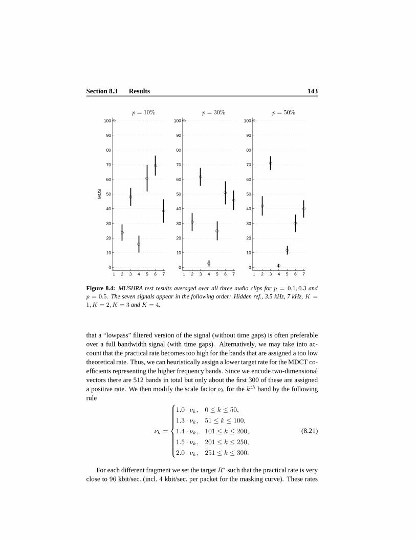
Section 8.3 Results 143
1 2 3 4 5 6 7
0
10
20
30
40
50
60
70
80
90
100
MO
S
1 2 3 4 5 6 7
0
10
20
30
40
50
60
70
80
90
100
1 2 3 4 5 6 7
0
10
20
30
40
50
60
70
80
90
100
PSfrag replacements
p = 10% p = 30% p = 50%
Figure 8.4: MUSHRA test results averaged over all three audio clips forp = 0.1, 0.3 andp = 0.5. The seven signals appear in the following order: Hidden ref., 3.5 kHz, 7 kHz,K =
1,K = 2, K = 3 andK = 4.
that a “lowpass” filtered version of the signal (without timegaps) is often preferableover a full bandwidth signal (with time gaps). Alternatively, we may take into ac-count that the practical rate becomes too high for the bands that are assigned a too lowtheoretical rate. Thus, we can heuristically assign a lowertarget rate for the MDCT co-efficients representing the higher frequency bands. Since we encode two-dimensionalvectors there are 512 bands in total but only about the first 300 of these are assigneda positive rate. We then modify the scale factorνk for thekth band by the followingrule
νk =
1.0 · νk, 0 ≤ k ≤ 50,
1.3 · νk, 51 ≤ k ≤ 100,
1.4 · νk, 101 ≤ k ≤ 200,
1.5 · νk, 201 ≤ k ≤ 250,
2.0 · νk, 251 ≤ k ≤ 300.
(8.21)
For each different fragment we set the targetR∗ such that the practical rate is veryclose to96 kbit/sec. (incl.4 kbit/sec. per packet for the masking curve). These rates
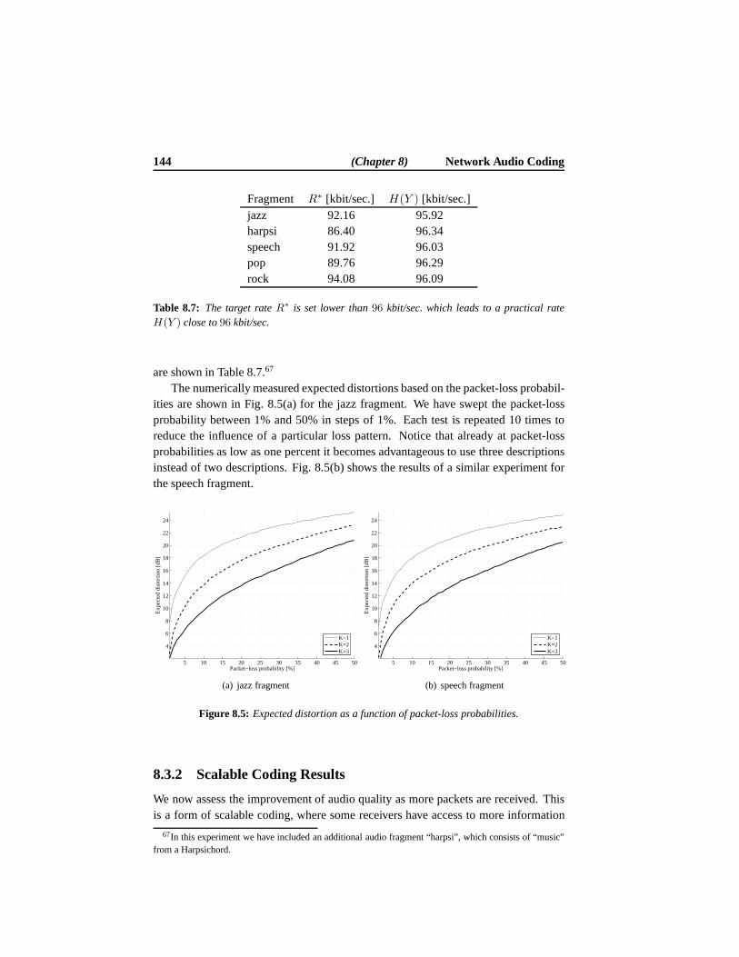
144 (Chapter 8) Network Audio Coding
Fragment R∗ [kbit/sec.] H(Y ) [kbit/sec.]jazz 92.16 95.92harpsi 86.40 96.34speech 91.92 96.03pop 89.76 96.29rock 94.08 96.09
Table 8.7: The target rateR∗ is set lower than96 kbit/sec. which leads to a practical rateH(Y ) close to96 kbit/sec.
are shown in Table 8.7.67
The numerically measured expected distortions based on thepacket-loss probabil-ities are shown in Fig. 8.5(a) for the jazz fragment. We have swept the packet-lossprobability between 1% and 50% in steps of 1%. Each test is repeated 10 times toreduce the influence of a particular loss pattern. Notice that already at packet-lossprobabilities as low as one percent it becomes advantageousto use three descriptionsinstead of two descriptions. Fig. 8.5(b) shows the results of a similar experiment forthe speech fragment.
5 10 15 20 25 30 35 40 45 50
4
6
8
10
12
14
16
18
20
22
24
Packet−loss probability [%]
Exp
ecte
d di
stor
tion
[dB
]
K=1K=2K=3
(a) jazz fragment
5 10 15 20 25 30 35 40 45 50
4
6
8
10
12
14
16
18
20
22
24
Packet−loss probability [%]
Exp
ecte
d di
stor
tion
[dB
]
K=1K=2K=3
(b) speech fragment
Figure 8.5: Expected distortion as a function of packet-loss probabilities.
8.3.2 Scalable Coding Results
We now assess the improvement of audio quality as more packets are received. Thisis a form of scalable coding, where some receivers have access to more information
67In this experiment we have included an additional audio fragment “harpsi”, which consists of “music”from a Harpsichord.
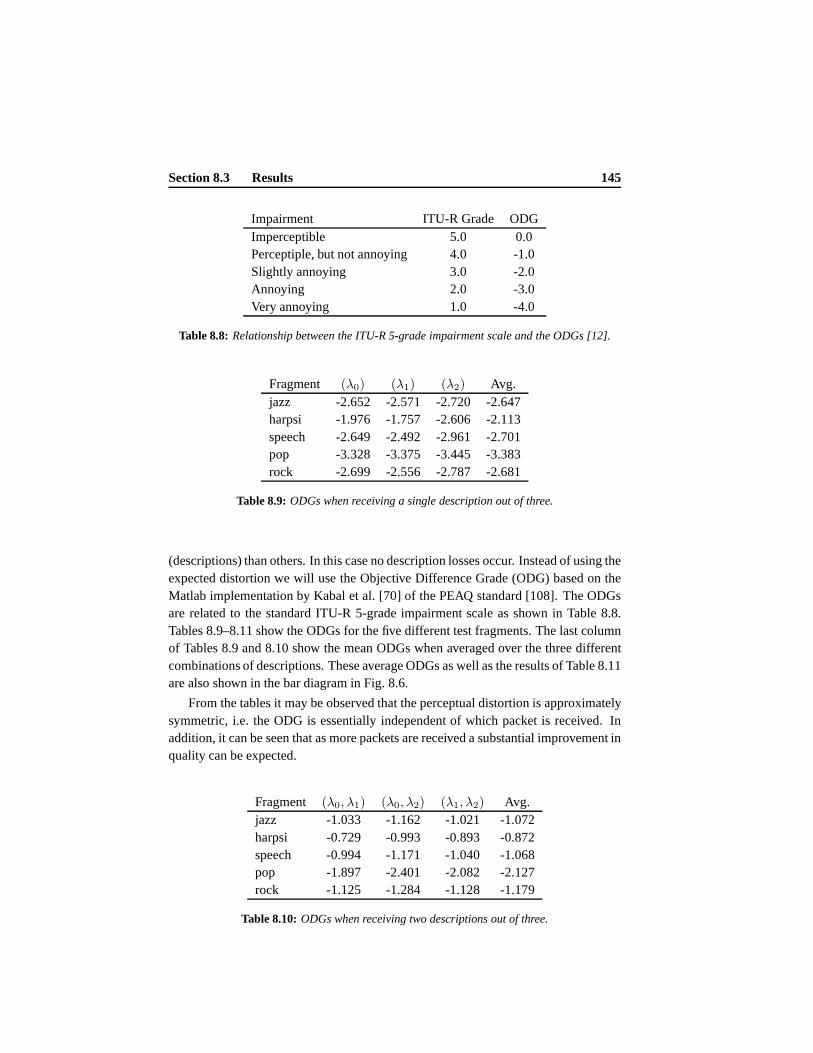
Section 8.3 Results 145
Impairment ITU-R Grade ODGImperceptible 5.0 0.0Perceptiple, but not annoying 4.0 -1.0Slightly annoying 3.0 -2.0Annoying 2.0 -3.0Very annoying 1.0 -4.0
Table 8.8: Relationship between the ITU-R 5-grade impairment scale and the ODGs [12].
Fragment (λ0) (λ1) (λ2) Avg.jazz -2.652 -2.571 -2.720 -2.647harpsi -1.976 -1.757 -2.606 -2.113speech -2.649 -2.492 -2.961 -2.701pop -3.328 -3.375 -3.445 -3.383rock -2.699 -2.556 -2.787 -2.681
Table 8.9: ODGs when receiving a single description out of three.
(descriptions) than others. In this case no description losses occur. Instead of using theexpected distortion we will use the Objective Difference Grade (ODG) based on theMatlab implementation by Kabal et al. [70] of the PEAQ standard [108]. The ODGsare related to the standard ITU-R 5-grade impairment scale as shown in Table 8.8.Tables 8.9–8.11 show the ODGs for the five different test fragments. The last columnof Tables 8.9 and 8.10 show the mean ODGs when averaged over the three differentcombinations of descriptions. These average ODGs as well asthe results of Table 8.11are also shown in the bar diagram in Fig. 8.6.
From the tables it may be observed that the perceptual distortion is approximatelysymmetric, i.e. the ODG is essentially independent of whichpacket is received. Inaddition, it can be seen that as more packets are received a substantial improvement inquality can be expected.
Fragment (λ0, λ1) (λ0, λ2) (λ1, λ2) Avg.jazz -1.033 -1.162 -1.021 -1.072harpsi -0.729 -0.993 -0.893 -0.872speech -0.994 -1.171 -1.040 -1.068pop -1.897 -2.401 -2.082 -2.127rock -1.125 -1.284 -1.128 -1.179
Table 8.10:ODGs when receiving two descriptions out of three.
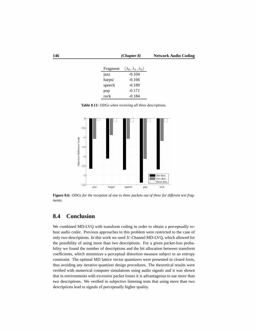
146 (Chapter 8) Network Audio Coding
Fragment (λ0, λ1, λ2)
jazz -0.104harpsi -0.166speech -0.189pop -0.171rock -0.184
Table 8.11:ODGs when receiving all three descriptions.
jazz harpsi speech pop rock−3.5
−3
−2.5
−2
−1.5
−1
−0.5
0
Obj
ectiv
e D
iffer
ence
Gra
de
One desc.Two desc.Three desc.
Figure 8.6: ODGs for the reception of one to three packets out of three fordifferent test frag-ments.
8.4 Conclusion
We combined MD-LVQ with transform coding in order to obtain aperceptually ro-bust audio coder. Previous approaches to this problem were restricted to the case ofonly two descriptions. In this work we usedK-Channel MD-LVQ, which allowed forthe possibility of using more than two descriptions. For a given packet-loss proba-bility we found the number of descriptions and the bit allocation between transformcoefficients, which minimizes a perceptual distortion measure subject to an entropyconstraint. The optimal MD lattice vector quantizers were presented in closed form,thus avoiding any iterative quantizer design procedures. The theoretical results wereverified with numerical computer simulations using audio signals and it was shownthat in environments with excessive packet losses it is advantageous to use more thantwo descriptions. We verified in subjective listening teststhat using more than twodescriptions lead to signals of perceptually higher quality.

Chapter9Conclusions and Discussion
9.1 Summary of Results
We presented an index-assignment based design ofK-channel MD-LVQ. Whereprevious designs have been limited to two descriptions we considered the generalcase ofK descriptions. Exact rate-distortion results were derivedfor the case ofK ≤ 3 descriptions and high resolution conditions for smooth stationary sourcesand the squared error distortion measure. In the asymptoticcase of large lattice vectorquantizer dimension and high resolution conditions, it wasshown that existing rate-distortion MD bounds can be achieved in the quadratic Gaussian case. These resultswere conjectured to hold also forK > 3 descriptions.
In the two-description asymmetric case it was shown that theperformance was su-perior to existing state-of-the-art asymmetric schemes infinite lattice vector quantizerdimensions greater than one. In one and infinite dimensions as well as in the symmet-ric case (for all dimensions), the performance is identicalto existing state-of-the-artschemes.
In the three-description symmetric and asymmetric cases for finite lattice vectorquantizer dimensions, the rate loss of the proposed design is superior to that of existingschemes.
The optimal amount of redundancy in the system was shown to beindependentof the source distribution, target rate and type of latticesused for the side quantizers.Basically, the channel conditions (expressed through a setof packet-loss probabilities)describe the required amount of redundancy in the system. Thus, for given channelconditions, the optimal index-assignment map can be found and adapting to time-varying source distributions or bit rate requirements amounts to a simple scaling ofthe central and side lattice vector quantizers.
We proposed an entropy-constrained design where either theside description rates
147

148 (Chapter 9) Conclusions and Discussion
or their sum rate are subject to entropy contraints. In the case of a single sum rateentropy contraint, we showed that the optimal bit allocation across descriptions is notunique, but in fact consists of a set of solutions, which all lead to minimal expecteddistortion.
On the practical side it was shown that the optimalK-channel MD lattice vectorquantizers can be found in closed-form, hence avoiding any iterative (e.g. generalizedLloyd-like) design algorithms. Furthermore, we combined MD-LVQ with transformcoding in order to obtain a perceptually robust audio coder.Previous approaches tothis problem were restricted to the case of only two descriptions. For a given packet-loss probability we found the number of descriptions and thebit allocation betweentransform coefficients, which minimizes a perceptual distortion measure subject toan entropy constraint. The theoretical results were verified with numerical computersimulations using audio signals and it was shown that in environments with excessivepacket losses it is advantageous to use more than two descriptions. We verified insubjective listening tests that using more than two descriptions leads to signals ofperceptually higher quality.
9.2 Future Research Directions
In this thesis we considered index-assignment based MD schemes at high resolutionconditions, which provide a partial solution to theK-channel MD problem. However,more work is needed before the general MD problem is solved. Besides the informa-tion theoretic open problems discussed in Chapter 4 there are many unsolved problemsrelated to MD-LVQ. Below we list a few of these.
• Proving the conjectures of this thesis, i.e. proving the rate-distortion results forK > 3 descriptions.
• Extending the results to general resolution. To the best of the authors knowl-edge, the only case where exact rate-distortion expressions (in non high-resolution cases) have been presented for index-assignment based MD schemes,is the two-channel scalar scheme by Frank-Dayan and Zamir [39].
• It is an open problem of how to construct practical MD-LVQ schemes thatcomes arbitrarily close to the known MD bounds. Such schemesrequire high-dimensional lattice vector quantizers and large index values. However, solvingthe linear assignment problem can become computationally infeasible for largeindex values. For the symmetric case and certain low dimensional lattices, someprogress have been made in reducing this complexity by the design of Huangand Wu [65]. A construction for high-dimensional nested lattice codes was re-cently presented by Zamir et al. [162]. No index-assignmentmethods have,however, been presented for the nested lattice code design and the problem istherefore not solved.
Section 9.2 Future Research Directions 149
• Constructing functional MD schemes for existing applications in real environ-ments and assessing their performance. For example for real-time application,even if the packet-loss rate of a network is very low, the delay might occa-sionally be high, which then means that (at least for real-time applications) adelayed packet is considered lost (at least for the current frame) and the use ofMD coding might become beneficial.

AppendixAQuaternions
We will here briefly define the Quaternions and describe a few important propertiesthat we will use in this work. For a comprehensive treatment of the Quaternions werefer the reader to [23,71,150].
The Quaternions, which were discovered in the middle of the19th century byHamilton [71], is in some sense a generalization of the complex numbers. Just as1and i denote unit vectors of the complex spaceC we define1, i, j andk to be unitvectors in Quaternion spaceH. The set of numbers defined asa + bi + cj + dk :
a, b, c, d ∈ R are then called Quaternion numbers or simply Quaternions. Additionof two Quaternionsq = a+ bi+ cj + dk andq′ = a′ + b′i+ c′j + d′k is defined as
q + q′ = (a+ a′) + (b+ b′)i+ (c+ c′)j + (d+ d′)k, (A.1)
and multiplication follows by first defining a multiplication rule for pairs of Quater-nion units, that is
i2 = j2 = k2 = −1,
ij = k, ji = −k,jk = i, kj = −1,
ki = j, ik = −j,
(A.2)
which leads to
qq′ = (aa′ − bb′ − cc′ − dd′) + (ab′ + ba′ + cd′ − dc′)i
+ (ac′ + ca′ + db′ − bd′)j + (ad′ + da′ + bc′ − cb′)k.(A.3)
Definition A.1.1. The skew fieldH of Quaternions is defined as the setz =
a + bi + cj + dk : a, b, c, d ∈ R combined with two maps (addition and multi-plication) given by (A.1) and (A.3), respectively, that satisfies field properties exceptthat multiplication is non commutative.
151
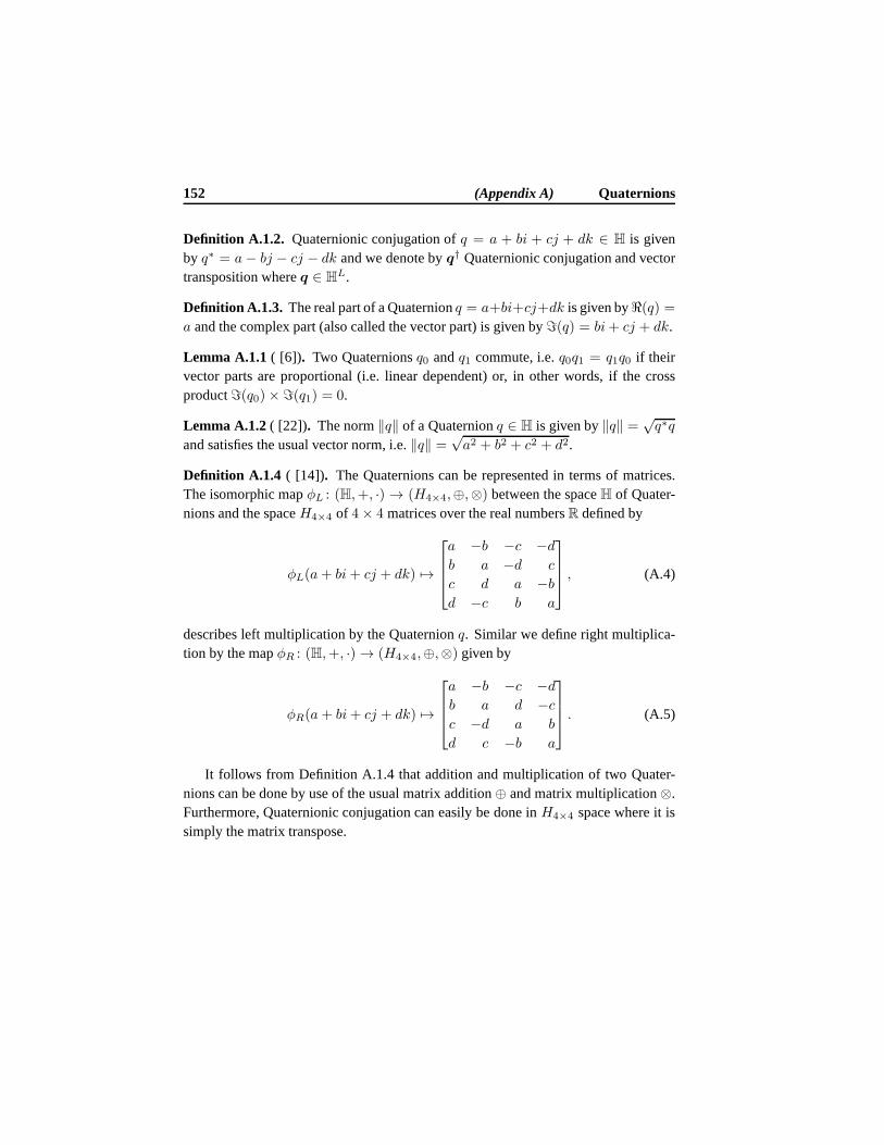
152 (Appendix A) Quaternions
Definition A.1.2. Quaternionic conjugation ofq = a + bi + cj + dk ∈ H is givenby q∗ = a− bj − cj − dk and we denote byq† Quaternionic conjugation and vectortransposition whereq ∈ HL.
Definition A.1.3. The real part of a Quaternionq = a+bi+cj+dk is given byℜ(q) =a and the complex part (also called the vector part) is given byℑ(q) = bi+ cj + dk.
Lemma A.1.1 ( [6]). Two Quaternionsq0 andq1 commute, i.e.q0q1 = q1q0 if theirvector parts are proportional (i.e. linear dependent) or, in other words, if the crossproductℑ(q0)×ℑ(q1) = 0.
Lemma A.1.2( [22]). The norm‖q‖ of a Quaternionq ∈ H is given by‖q‖ =√q∗q
and satisfies the usual vector norm, i.e.‖q‖ =√a2 + b2 + c2 + d2.
Definition A.1.4 ( [14]). The Quaternions can be represented in terms of matrices.The isomorphic mapφL : (H,+, ·) → (H4×4,⊕,⊗) between the spaceH of Quater-nions and the spaceH4×4 of 4× 4 matrices over the real numbersR defined by
φL(a+ bi+ cj + dk) 7→
a −b −c −db a −d c
c d a −bd −c b a
, (A.4)
describes left multiplication by the Quaternionq. Similar we define right multiplica-tion by the mapφR : (H,+, ·) → (H4×4,⊕,⊗) given by
φR(a+ bi+ cj + dk) 7→
a −b −c −db a d −cc −d a b
d c −b a
. (A.5)
It follows from Definition A.1.4 that addition and multiplication of two Quater-nions can be done by use of the usual matrix addition⊕ and matrix multiplication⊗.Furthermore, Quaternionic conjugation can easily be done inH4×4 space where it issimply the matrix transpose.
AppendixBModules
In this appendix we give a brief introduction to the theory ofalgebraic modules. Formore information we refer the reader to the following textbooks [1,22,61,72].
B.1 General Definitions
Definition B.1.1. Let J be a ring which is not necessarily commutative with respectto multiplication. Then an Abelian (commutative) groupS is called a leftJ -moduleor a left module overJ with respect to a mapping (scalar multiplication on the leftwhich is simply denoted by juxtaposition)J × S → S such that for alla, b ∈ J
andg, h ∈ S,
1) a(g + h) = ag + ah,
2) (a+ b)g = ag + bg,
3) (ab)g = a(bg).
Remark B.1.1. For simplicity we have used the same notations for addi-tion/multiplication in the group as well as in the ring.
RemarkB.1.2. A right module is defined in a similar way but with multiplication onthe right. In fact if the ringJ is commutative then every leftJ -module is also aright J -module [61].
Definition B.1.2. If J has identity1 and if 1a = a for all a ∈ S, thenS is called aunitary or unitalJ -module.
RemarkB.1.3. In this work all modules have an identity.
153
154 (Appendix B) Modules
Definition B.1.3 ( [72]). A subsetS′ = m1, . . . ,mn ⊂ S of the J -moduleSis linearly independent overJ if, for xi ∈ J , x1m1 + · · · + xnmn = 0 only ifx1 = · · · = xn = 0. If in additionS′ generatesS thenS′ is a basis forS.
ExampleB.1.1. The setS = 2, 3 is finite and generatesZ, considered as aZ-module over itself [72]. However,S is not a linearly independent set. Further, neitherelement ofS can be omitted to give a generating set with one member. Hence, S isnot a basis ofZ.
Definition B.1.4 ( [72]). A J -module that has a basis is called a freeJ -module.
Definition B.1.5 ( [72]). The number of elements in a basis of aJ -moduleS iscalled the rank or dimension ofS.
RemarkB.1.4. Not all modules have a basis [72]. LetZm = Z/mZ be the residuering of integers, i.e.Zm = [0], . . . , [m − 1], where[s] = [r] in Zm impliess ≡ r
(mod m). Notice thatZm contains no linear independent subsets, sincemx = 0 foranyx ∈ Z, henceZm has no basis and is therefore not a free module.
Definition B.1.6 ( [1]). Let J be a ring and letS, S′ be leftJ -modules. A functionf : S → S′ is aJ -module homomorphism if
1. f(m1 +m2) = f(m1) + f(m2) for all m1,m2 ∈ S, and
2. f(am) = af(m) for all a ∈ J andm ∈ S.
Definition B.1.7 ( [1]). The set of allJ -module homomorphisms fromS to S′ isdenoted Hom(S, S′). If S = S′ then we write End(S) where elements of End(S) arecalled endomorphisms. Iff ∈ End(S) is invertible, then it is called an automorphism.The group of all automorphisms is denoted Aut(S).
Definition B.1.8 ( [72]). Let J be a ring andS aJ -module. Then an annihilator ofan elementg ∈ S is the set
Ann(g) = h ∈ J : hg = 0. (B.1)
An elementg ∈ S is said to be a torsion element ofS if Ann(g) 6= 0, that is, there issome non-zero elementa ∈ J with ag = 0.
Definition B.1.9 ( [72]). A J -moduleS is said to be torsion-free if the only torsionelement inS is 0.
Definition B.1.10. Let S′ be a finite group and letS be a leftJ -module. The orbitunder the action ofm ∈ S is obtained by left multiplication, i.e.S′m = gm : g ∈S′.
Section B.2 Submodule Related Definitions 155
B.2 Submodule Related Definitions
Definition B.2.1. Let S be aJ -module andS′ a nonempty subset ofS. ThenS′ iscalled a submodule ofS if S′ is a subgroup ofS and for allg ∈ S, h ∈ S′, we havegh ∈ S′.
Definition B.2.2 ( [61]). A cyclic submodule is a submodule which is generated bya single element. For example in a leftJ -moduleS, a cyclic submodule can begenerated bym ∈ S in the following waysJm = xm : x ∈ J ormJ = mx :
x ∈ J .
Definition B.2.3 ( [61]). In general the submoduleS′ of theJ -moduleS generatedby a finite subsetm1, . . . ,mn ⊂ S is the set
Jm1 + · · ·+ Jmn = x1m1 + · · ·+ xnmn : x1, . . . , xi ∈ J (B.2)
of all linear combinations ofm1, . . . ,mn. Such submodules are called finitely gener-ated. IfS′ = S thenm1, . . . ,mn is a set of generators forS.
Lemma B.2.1( [72]). Let S andS′ be submodules of aJ -moduleS. Then theirsum
S + S′ = l+ n : l ∈ S, n ∈ S′, (B.3)
is also a submodule. Moreover,S + S′ = S ⇐⇒ S′ ⊆ S.
Lemma B.2.2( [72]). Let S andS′ be submodules of aJ -moduleS. Then theirintersection
S ∩ S′ = x : x ∈ S andx ∈ S′, (B.4)
is also a submodule. Moreover,S ∩ S′ = S ⇐⇒ S ⊆ S′.
RemarkB.2.1. Submodules of a vector space are its subspaces.
Proposition B.2.1( [72]). LetS′ be a submodule of theJ -moduleS. Letm,n ∈ S
and define a relation onS by the rule thatm ≡ n ⇐⇒ m− n ∈ S′. The equivalenceclass of an elementm ∈ S is given by the set
[m] = m+ S′ = m+ l : l ∈ S′. (B.5)
The quotient module (or factor module)S/S′ is defined to be the set of all such equiv-alence classes, with addition given by
[m] + [n] = [m+ n], [m], [n] ∈ S/S′, (B.6)
and multiplication byr ∈ J is given by
r[m] = [rm], [m] ∈ S/S′. (B.7)
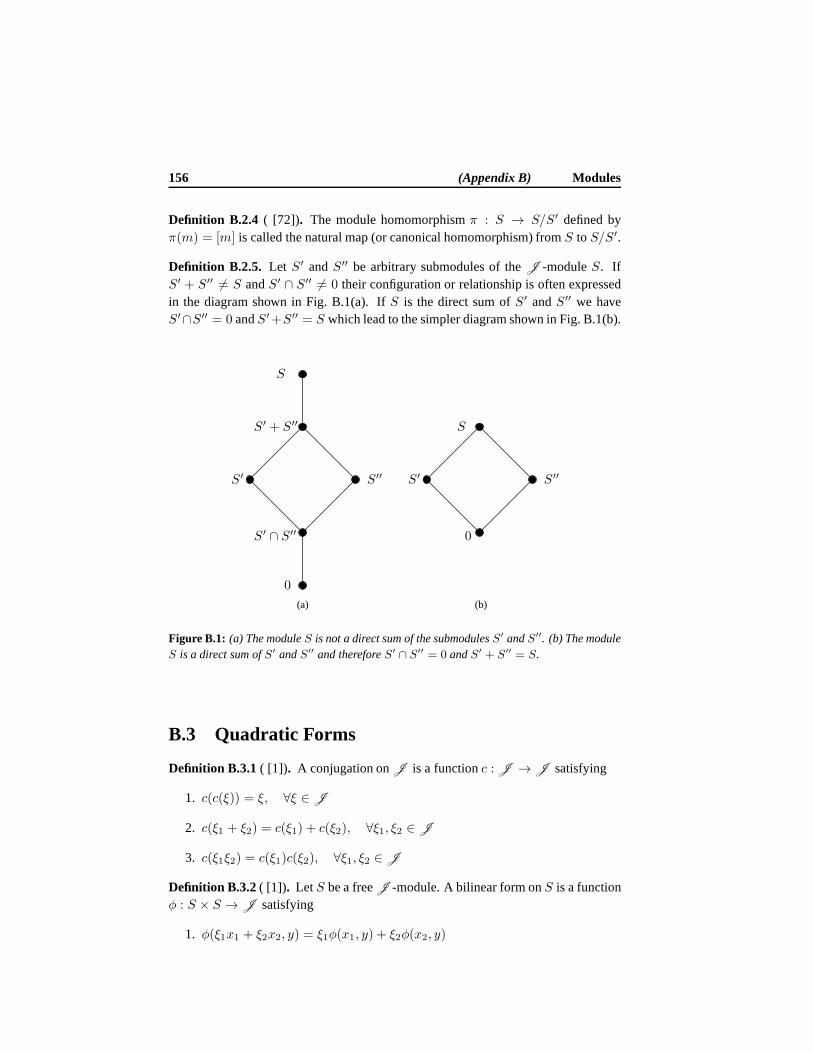
156 (Appendix B) Modules
Definition B.2.4 ( [72]). The module homomorphismπ : S → S/S′ defined byπ(m) = [m] is called the natural map (or canonical homomorphism) fromS to S/S′.
Definition B.2.5. Let S′ andS′′ be arbitrary submodules of theJ -moduleS. IfS′ + S′′ 6= S andS′ ∩ S′′ 6= 0 their configuration or relationship is often expressedin the diagram shown in Fig. B.1(a). IfS is the direct sum ofS′ andS′′ we haveS′∩S′′ = 0 andS′+S′′ = S which lead to the simpler diagram shown in Fig. B.1(b).
PSfrag replacementsS′ S′′
S
S′ ∩ S′′
S′ + S′′
0
(a)
PSfrag replacements
S′ S′′
S
S′ ∩ S′′
S′ + S′′
0
(b)
Figure B.1: (a) The moduleS is not a direct sum of the submodulesS′ andS′′. (b) The moduleS is a direct sum ofS′ andS′′ and thereforeS′ ∩ S′′ = 0 andS′ + S′′ = S.
B.3 Quadratic Forms
Definition B.3.1 ( [1]). A conjugation onJ is a functionc : J → J satisfying
1. c(c(ξ)) = ξ, ∀ξ ∈ J
2. c(ξ1 + ξ2) = c(ξ1) + c(ξ2), ∀ξ1, ξ2 ∈ J
3. c(ξ1ξ2) = c(ξ1)c(ξ2), ∀ξ1, ξ2 ∈ J
Definition B.3.2( [1]). LetS be a freeJ -module. A bilinear form onS is a functionφ : S × S → J satisfying
1. φ(ξ1x1 + ξ2x2, y) = ξ1φ(x1, y) + ξ2φ(x2, y)

Section B.3 Quadratic Forms 157
2. φ(x, ξ1y1 + ξ2y2) = ξ1φ(x, y1) + ξ2φ(x, y2)
for all x1, x2, y1, y2 ∈ S andξ1, ξ2 ∈ J .
Definition B.3.3 ( [1]). Let S be a freeJ -module. A sesquilinear form onS is afunctionφ : S × S → J satisfying
1. φ(ξ1x1 + ξ2x2, y) = ξ1φ(x1, y) + ξ2φ(x2, y)
2. φ(x, ξ1y1 + ξ2y2) = c(ξ1)φ(x, y1) + c(ξ2)φ(x, y2)
for all x1, x2, y1, y2 ∈ S andξ1, ξ2 ∈ J for a non-trivial conjugationξ 7→ c(ξ) onJ .
Definition B.3.4( [22]). LetΛ be aJ -lattice inRL having basis vectorsζ1, . . . , ζL ∈RL whose transposes form the rows of the generator matrixM . Then any lattice pointλ ∈ Λ may be written on generic form asλ = ξTM whereξ = (ξ1, . . . , ξL)
T andwhereξi ∈ J . Let us define the following function ofλ (i.e. a squared norm)
τ(λ) =
L∑
i=1
L∑
j=1
(ξiζi)T ξjζj
= ξTMMT ξ.
(B.8)
The functionτ in (B.8) is referred to as the quadratic form associated withthe lat-tice Λ. If Λ has full rank, thenMMT is a positive definite matrix and the associ-ated quadratic form is called a positive definite form. If we extendτ to τ(λ1, λ2) =ξT1 MMT ξ2 we obtain the bilinear form of Definition B.3.2 and if the underlying fieldis non real we get the sesquilinear form of Definition B.3.3 where the conjugationfunctionc depends on the field.
RemarkB.3.1. In this work we will not make explicitely use of quadratic forms. In-stead we equip the underlying field with an inner product〈·, ·〉 which satisfies Defi-nition B.3.2 and is therefore a bilinear form.
ExampleB.3.1. Let Λ ⊂ RL, i.e.Λ is a lattice embedded in the fieldRL. Then wecan define the usual vector norm‖λ‖2 , 〈λ, λ〉, whereλ ∈ Λ. Notice that here theconjugation is simply the identity. See Appendix C for more examples.

AppendixCLattice Definitions
In this appendix we present a number of lattice-related definitions and propertieswhich are used throughout the thesis.
Let V be a vector space over the fieldK and letV be equipped with an innerproduct〈·, ·〉. If KL = RL thenV is the traditional vector space over the Cartesianproduct of the reals.68 As such,(V, 〈·, ·〉) is an inner-product space. An inner-productspace induces a norm‖ · ‖ defined as‖ · ‖2 , 〈·, ·〉. If KL = RL we use theℓ2-norm defined as‖x‖2 , xTx whereas ifKL = CL we have‖x‖2 , xHx whereH denotes Hermitian transposition (i.e. the conjugate transpose). IfKL = HL then‖x‖2 , x†x where† denotes Quaternionic conjugation and transposition. For moreinformation about inner-product spaces we refer the readerto the widely used textbookby Luenberger [89].
C.1 General Definitions
Definition C.1.1 ( [22]). A lattice Λ ⊂ KL consists of all possible integral linearcombinations of a set of basis vectors, or, more formally
Λ =
λ ∈ KL : λ =L∑
i=1
ξiζi, ∀ξi ∈ J
, (C.1)
whereζi ∈ KL are the basis vectors also known as generator vectors of the lattice andJ ⊂ K is a well defined ring of integers.
RemarkC.1.1. It should be noted that it is often convenient to useL′ > L basisvectors to form anL-dimensional lattice embedded inKL′
.68Recall that, in a vector space overR
L, addition and subtraction is with respect to vectors ofRL whereas
multiplication is defined as multiplications of vectors inRL with scalar elements ofR. Thus, a vector spaceis aJ -module whereJ is a field, i.e. a ring where all elements (except 0) have inverses.
159
160 (Appendix C) Lattice Definitions
Definition C.1.2. LetM be a generator matrix of the latticeΛ. Then the rows ofMare given by the tranposes of the column vectorsζTi , i = 1, . . . , L, where we actuallydo not require thatM is square.
Definition C.1.3. The square matrixA =MMT is called the Gram matrix.
Definition C.1.4. A fundamental region of a lattice is a closed region which containsa single lattice points and tessellate the underlying space.
Lemma C.1.1( [22]). All fundamental regions have the same volume.
Lemma C.1.2( [22]). The fundamental volumeν of Λ is given byν =√
det(A),sometimes written asν = det(Λ). If M is a square generator matrix thenν =
| det(M)|.
Definition C.1.5 ( [25]). An L-dimensional polytope is a finite convex region inKL
enclosed by a finite number of hyperplanes.
Definition C.1.6 ( [30]). The quotientKL/Λ is theL-dimensional torus obtained bycombining opposite faces of the fundamental parallelotopea1ζ1 + . . . + aLζL|0 ≤ai ≤ 1.
Definition C.1.7. The Cartesian product⊗ of two latticesΛ1 andΛ2 is obtained bypairing all points inΛ1 with every point inΛ2, i.e.
Λ1 ⊗ Λ2 = (λ1, λ2)|λ1 ∈ Λ1, λ2 ∈ Λ2. (C.2)
It follows that the dimension ofΛ = Λ1 ⊗ Λ2 is equal to the sum of the dimensionsof the two latticesΛ1 andΛ2.
Definition C.1.8 ( [22]). The automorphism group Aut(Λ) of a latticeΛ is the set ofdistance-preserving transformations (or isometries) of the space that fix the origin andtakes the lattice to itself.
Theorem C.1.1( [22]). For a lattice in ordinary Euclidean spaceRL, Aut(Λ) is finiteand the transformations in Aut(Λ) may be represented by orthogonal matrices. LetΛ
have generator matrixM . Then an orthogonal matrixB is in Aut(Λ) if and only ifthere is an integral matrixU with determinant±1 such that
UM =MB. (C.3)
This impliesU =MBMTA−1, whereA−1 is the Gram matrix ofΛ.
RemarkC.1.2. Aut(Λ = ZL) consists of all sign changes of theL coordinates(= 2L)
and all permutations(= L!). Hence,|Aut(ZL)| = 2LL! [22].
Section C.2 Norm Related Definitions 161
Definition C.1.9 ( [22]). The dual latticeΛ of the latticeΛ is given by
Λ = x ∈ RL|xTλ ∈ Z for all λ ∈ Λ. (C.4)
Alternatively, ifM is a square generator matrix ofΛ thenΛ can be constructed by useof the generator matrixM = (M−1)T .
Theorem C.1.2( [30]). If Λ ⊂ RL is a discrete subgroup with compact quotientRL/Λ thenΛ is a lattice.
Definition C.1.10( [22]). The coefficientsBi of the Theta seriesΘΛ(z) ,∑
iBiqi
of a latticeΛ describe the number of points at squared distancei from an arbitrarypoint in space (which is usually taken to be the origin). The indeterminateq is some-times set toq = exp(iπz), wherez ∈ C andℑ(z) > 0.
C.2 Norm Related Definitions
Definition C.2.1 ( [22]). Let Λ ⊂ KL be a lattice. The nearest neighbor region ofλ ∈ Λ is defined as
V (λ) , x ∈ KL : ‖x− λ‖2 ≤ ‖x− λ′‖2, ∀λ′ ∈ Λ. (C.5)
Definition C.2.2. The nearest neighbor regions of a lattice are also called Voronoicells, Voronoi regions or Dirichlet regions. In this work wewill use the name Voronoicells.
Definition C.2.3. Voronoi cells of a lattice are congruent polytopes, hence they aresimilar in size and shape and may be seen as translated versions of a fundamentalregion, e.g.V0 = V (0), i.e. the Voronoi cell around the origin.
Definition C.2.4 ( [22]). The dimensionless normalized second moment of inertiaG(Λ) of a latticeΛ is defined by
G(Λ) ,1
Lν1+2/L
∫
V0
‖x‖2dx. (C.6)
RemarkC.2.1. Applying any scaling or orthogonal transform, e.g. rotation or reflec-tion onΛ will not changeG(Λ), which makes it a good figure of merit when compar-ing different lattices (quantizers). In other words,G(Λ) depends only upon the shapeof the fundamental region, and in general, the more sphere-like shape, the smallernormalized second-moment [22].
Definition C.2.5 ( [38]). The minimum squared distanced2min(Λ) between latticepoints is the minimum non-zero norm of any lattice pointλ ∈ Λ, i.e.
d2min(Λ) , minλ∈Λλ6=0
‖λ‖2. (C.7)
162 (Appendix C) Lattice Definitions
Definition C.2.6( [38]). The packing radiusρp(Λ) of the latticeΛ ⊂ RL is the radiusof the greatestL-dimensional sphere that can be inscribed withinV0. We then have
ρp(Λ) , dmin(Λ)/2. (C.8)
Definition C.2.7( [38]). The covering radiusρc(Λ) of the latticeΛ ⊂ RL is the radiusof the leastL-dimensional sphere that containsV0, i.e.
ρc(Λ) , maxx∈V0
‖x‖. (C.9)
Definition C.2.8 ( [38]). The kissing69 numberK(Λ) is the number of nearest neigh-bors to any lattice point, which is also equal to the number oflattice points of squarednormd2min(Λ), i.e.
K(Λ) , |λ ∈ Λ : ‖λ‖2 = d2min(Λ)|. (C.10)
Definition C.2.9. The space-filling loss of a latticeΛ with dimensionless normalizedsecond momentG(Λ) is given by
DLoss= 10 log10 (2πeG(Λ))dB. (C.11)
C.3 Sublattice Related Definitions
Definition C.3.1. A sublatticeΛ′ ⊆ Λ is a subset of the elements ofΛ that is itself alattice.
Definition C.3.2 ( [28]). A sublatticeΛ′ ⊂ Λ is called clean if no point ofΛ lies onthe boundary of the Voronoi cells ofΛ′.
Definition C.3.3. If Λ′ is a sublattice ofΛ thenN = |Λ/Λ′| denotes the index ororder of the quotientΛ/Λ′.
Definition C.3.4. If Λ′ is a clean sublattice ofΛ then the index valueN = |Λ/Λ′| iscalled an admissible index value.
Definition C.3.5. The Lth root of the indexN is called the nesting ratioN ′, i.e.N ′ = N1/L.
Definition C.3.6 ( [28]). Let Λ be anL dimensional lattice with square generatormatrixM . A sublatticeΛ′ ⊆ Λ is geometrically strictly similar toΛ if and only if thefollowing holds
1. There is an invertibleL× L matrixU1 with integer entries
69The terminology kissing number was introduced by N. J. A. Sloane who drew an analogy to billiards,where two balls are said to kiss if they touch each other, see for example the interview with N. J. A. Sloaneby R. Calderbank, which can be found online at http://www.research.att.com/˜njas/doc/interview.html.
Section C.3 Sublattice Related Definitions 163
2. a non-zero scalarc1 ∈ R
3. an orthogonalL× L matrixK1 with determinant 1,
such that a generator matrixM1 for Λ1 can be written as
M1 = U1M = c1MK1. (C.12)
If (C.12) holds then the indexN1 of Λ′ is equal to
N1 = |Λ/Λ′| = det(Λ′)
det(Λ)=
∣∣∣∣
det(M1)
det(M)
∣∣∣∣= det(U1) = cL1 . (C.13)
Furthermore,Λ′ has Gram matrix
A1 =M1MT1 = U1MMTUT
1 = U1AUT1 = c21A, (C.14)
whereA =MMT is a Gram matrix forΛ.
Definition C.3.7. If in Definition C.3.6 the determinant ofK1 is allowed to be±1,i.e.K1 can be either a rotation or a reflection operator, then the sublatticeΛ′ is said tobe geometrically similar toΛ.


AppendixDRoot Lattices
This appendix describes some properties of the root70 lattices considered in this thesis.
D.1 Z1
The scalar uniform lattice also calledZ1 partitions the real line into intervals of equallengths. Table D.1 outlines important constants related totheZ1 lattice.
Description Notation Value
Dimension L 1Fundamental volume ν 1
Packing radius ρp 1/2
Covering radius ρc 1/2
Space-filling loss Dloss 1.5329 dBSpace-filling gain overZ1 Dgain 0 dBKissing-number K 2Minimal squared distance d2min 1Dimensionless normalizedsecond moment
G(Λ) 1/12
Table D.1: Relevant constants for theZ1 lattice.
The set of admissible index values forZ1 is the set of all odd integers [28] and thecoefficients of the Theta series are given byB0 = 1 andBi = 2, i > 0.
70The term root lattice refers to a lattice which can be generated by the roots of specific reflectiongroups [22, 34].
165
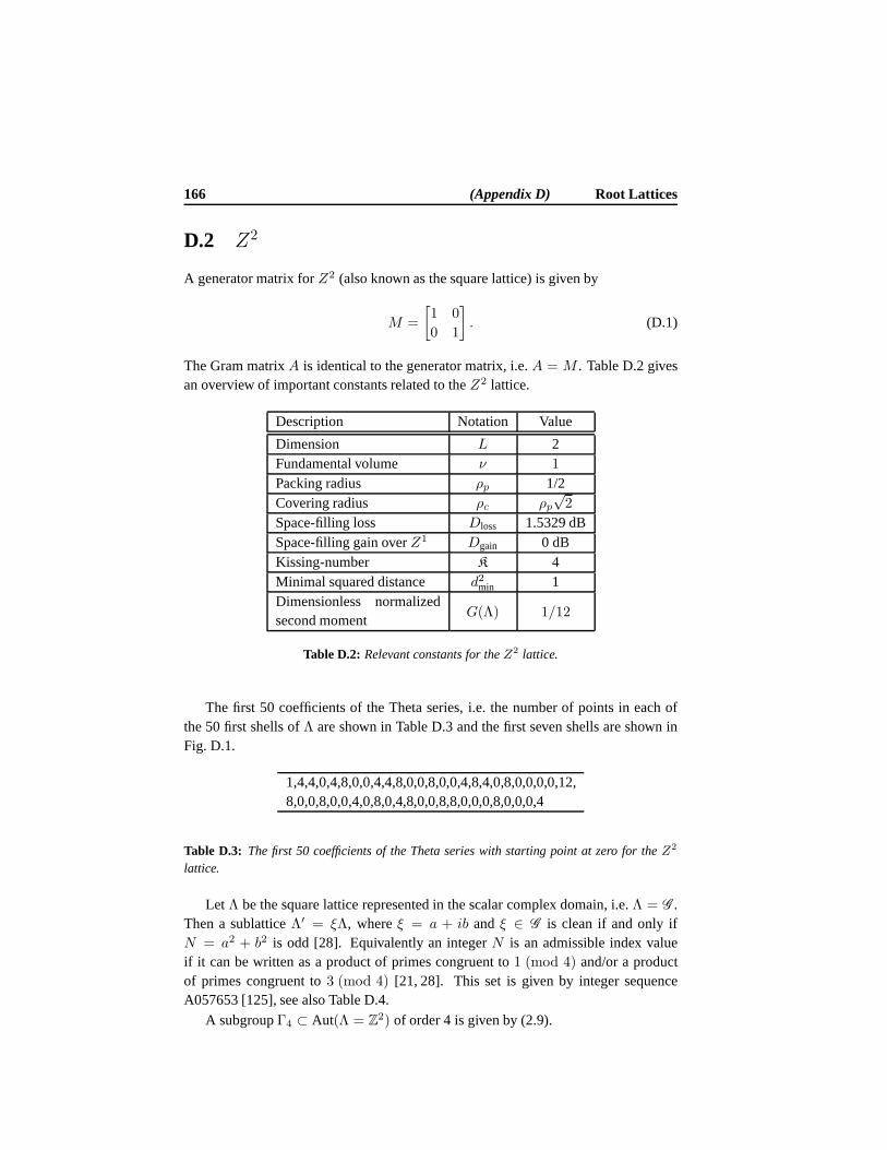
166 (Appendix D) Root Lattices
D.2 Z2
A generator matrix forZ2 (also known as the square lattice) is given by
M =
[1 0
0 1
]
. (D.1)
The Gram matrixA is identical to the generator matrix, i.e.A = M . Table D.2 givesan overview of important constants related to theZ2 lattice.
Description Notation Value
Dimension L 2Fundamental volume ν 1
Packing radius ρp 1/2Covering radius ρc ρp
√2
Space-filling loss Dloss 1.5329 dBSpace-filling gain overZ1 Dgain 0 dBKissing-number K 4Minimal squared distance d2min 1Dimensionless normalizedsecond moment
G(Λ) 1/12
Table D.2: Relevant constants for theZ2 lattice.
The first 50 coefficients of the Theta series, i.e. the number of points in each ofthe 50 first shells ofΛ are shown in Table D.3 and the first seven shells are shown inFig. D.1.
1,4,4,0,4,8,0,0,4,4,8,0,0,8,0,0,4,8,4,0,8,0,0,0,0,12,8,0,0,8,0,0,4,0,8,0,4,8,0,0,8,8,0,0,0,8,0,0,0,4
Table D.3: The first 50 coefficients of the Theta series with starting point at zero for theZ2
lattice.
Let Λ be the square lattice represented in the scalar complex domain, i.e.Λ = G .Then a sublatticeΛ′ = ξΛ, whereξ = a + ib andξ ∈ G is clean if and only ifN = a2 + b2 is odd [28]. Equivalently an integerN is an admissible index valueif it can be written as a product of primes congruent to1 (mod 4) and/or a productof primes congruent to3 (mod 4) [21, 28]. This set is given by integer sequenceA057653 [125], see also Table D.4.
A subgroupΓ4 ⊂ Aut(Λ = Z2) of order 4 is given by (2.9).
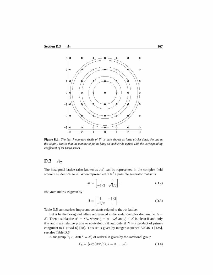
Section D.3 A2 167
−3 −2 −1 0 1 2 3
−3
−2
−1
0
1
2
3
Figure D.1: The first 7 non-zero shells ofZ2 is here shown as large circles (incl. the one atthe origin). Notice that the number of points lying on each circle agrees with the correspondingcoefficient of its Theta series.
D.3 A2
The hexagonal lattice (also known asA2) can be represented in the complex fieldwhere it is identical toE . When represented inR2 a possible generator matrix is
M =
[1 0
−1/2√3/2
]
. (D.2)
Its Gram matrix is given by
A =
[1 −1/2
−1/2 1
]
. (D.3)
Table D.5 summarizes important constants related to theA2 lattice.Let Λ be the hexagonal lattice represented in the scalar complex domain, i.e.Λ =
E . Then a sublatticeΛ′ = ξΛ, whereξ = a + ωb andξ ∈ E is clean if and onlyif a andb are relative prime or equivalently if and only ifN is a product of primescongruent to1 (mod 6) [28]. This set is given by integer sequence A004611 [125],see also Table D.6.
A subgroupΓ6 ⊂ Aut(Λ = E ) of order 6 is given by the rotational group
Γ6 = exp(ikπ/6), k = 0, . . . , 5. (D.4)

168 (Appendix D) Root Lattices
1,5,9,13,17,25,29,37,41,45,49,53,61,65,73,81,85,89,97,101,109,113,117,121,125,137,145,149,153,157,169,173,181,185,197,205,221,225,229,233,241,245,257,261,265,269,277,281,289,293,305,313,317,325333,337,. . .
Table D.4: Admissible index values forZ2.
Description Notation Value
Dimension L 2Fundamental volume ν
√3/2
Packing radius ρp 1/2Covering radius ρc 2ρp
√3
Space-filling loss Dloss 1.3658 dBSpace-filling gain overZ1 Dgain 0.1671 dBKissing-number K 6Minimal squared distance d2min 1Dimensionless normalizedsecond moment
G(Λ) 5/(36√3)
Table D.5: Relevant constants for theA2 lattice.
The first 50 coefficients of the Theta series forA2 are shown in Table D.7 andFig. D.2
D.4 Z4
The hypercubic latticeZ4 is generated by
M =
1 0 0 0
0 1 0 0
0 0 1 0
0 0 0 1
. (D.5)
The Gram matrixA is identical to the generator matrix, i.e.A = M . Table D.8 givesan overview of important constants related to theZ4 lattice.
Z4 has a geometrically-similar and clean sublattice of indexN if and only ifN isodd and of the forma2 for some integera [28]. The set of admissible index values isgiven by integer sequence A016754 [125], see also Table D.9.
The first 50 coefficients of the Theta series forZ4 are given in Table D.10.
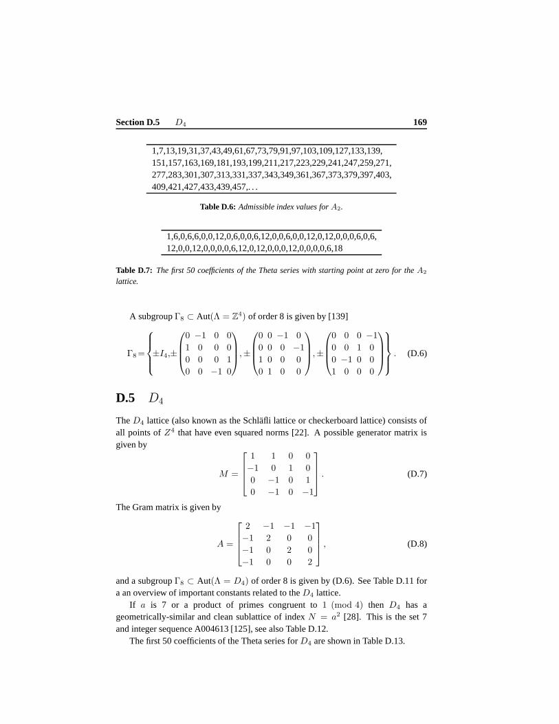
Section D.5 D4 169
1,7,13,19,31,37,43,49,61,67,73,79,91,97,103,109,127,133,139,151,157,163,169,181,193,199,211,217,223,229,241,247,259,271,277,283,301,307,313,331,337,343,349,361,367,373,379,397,403,409,421,427,433,439,457,. . .
Table D.6: Admissible index values forA2.
1,6,0,6,6,0,0,12,0,6,0,0,6,12,0,0,6,0,0,12,0,12,0,0,0,6,0,6,12,0,0,12,0,0,0,0,6,12,0,12,0,0,0,12,0,0,0,0,6,18
Table D.7: The first 50 coefficients of the Theta series with starting point at zero for theA2
lattice.
A subgroupΓ8 ⊂ Aut(Λ = Z4) of order 8 is given by [139]
Γ8=
±I4,±
0 −1 0 0
1 0 0 0
0 0 0 1
0 0 −1 0
,±
0 0 −1 0
0 0 0 −1
1 0 0 0
0 1 0 0
,±
0 0 0 −1
0 0 1 0
0 −1 0 0
1 0 0 0
. (D.6)
D.5 D4
TheD4 lattice (also known as the Schläfli lattice or checkerboard lattice) consists ofall points ofZ4 that have even squared norms [22]. A possible generator matrix isgiven by
M =
1 1 0 0
−1 0 1 0
0 −1 0 1
0 −1 0 −1
. (D.7)
The Gram matrix is given by
A =
2 −1 −1 −1
−1 2 0 0
−1 0 2 0
−1 0 0 2
, (D.8)
and a subgroupΓ8 ⊂ Aut(Λ = D4) of order 8 is given by (D.6). See Table D.11 fora an overview of important constants related to theD4 lattice.
If a is 7 or a product of primes congruent to1 (mod 4) then D4 has ageometrically-similar and clean sublattice of indexN = a2 [28]. This is the set 7and integer sequence A004613 [125], see also Table D.12.
The first 50 coefficients of the Theta series forD4 are shown in Table D.13.

170 (Appendix D) Root Lattices
−3 −2 −1 0 1 2 3
−3
−2
−1
0
1
2
3
Figure D.2: The first 6 non-zero shells ofA2 is here shown as large circles (incl. the one atthe origin). Notice that the number of points lying on each circle agrees with the correspondingcoefficient of the Theta series.
Description Notation Value
Dimension L 4Fundamental volume ν 1
Packing radius ρp 1/2Covering radius ρc 1Space-filling loss Dloss 1.5329 dBSpace-filling gain overZ1 Dgain 0 dBKissing-number K 8Minimal squared distance d2min 1Dimensionless normalizedsecond moment
G(Λ) 1/12
Table D.8: Relevant constants for theZ4 lattice.

Section D.5 D4 171
1,9,25,49,81,121,169,225,289,361,441,529,625,729,841,961,1089,1225,1369,1521,1681,1849,2025,2209,2401,2601,2809,3025,3249,3481,3721,3969,4225,4489,4761,5041,5329,5625,5929,6241,6561,. . .
Table D.9: Admissible index values forZ4.
1,8,24,32,24,48,96,64,24,104,144,96,96,112,192,192,24,144,312,160,144, 256,288,192,96,248,336,320,192,240,576,256,24,384,432,384,312,304,480,448,144,336,768,352,288,624,576,384,96,456
Table D.10: The first 50 coefficients of the Theta series with starting point at zero for theZ4
lattice.
Description Notation Value
Dimension L 4Fundamental volume ν 2
Packing radius ρp 1/√2
Covering radius ρc ρp√2
Space-filling loss Dloss 1.1672 dBSpace-filling gain overZ1 Dgain 0.3657 dBKissing-number K 24Minimal squared distance d2min 2Dimensionless normalizedsecond moment
G(Λ) 0.076603
Table D.11: Relevant constants for theD4 lattice.
1,5,7,13,17,25,29,37,41,53,61,65,73,85,89,97,101,109,113,125,137,145,149,157,169,173,181,185,193,197,205,221,229,233,241,257,265,269,277,281,289,293,305,313,317,325,337,349,353,365,373,377,389,397,401,409,421,. . .
Table D.12: Admissible index values forD4.

172 (Appendix D) Root Lattices
1,0,24,0,24,0,96,0,24,0,144,0,96,0,192,0,24,0,312,0,144,0,288,0,96,0,336,0,192,0,576,0,24,0,432,0,312,0,480,0,144,0,768,0,288,0,576,0,96,0
Table D.13: The first 50 coefficients of the Theta series with starting point at zero for theD4
lattice.
AppendixEProofs for Chapter 2
Proof of Lemma 2.3.1.Most of the work towards proving the lemma has already beendone in [21] and [28] and we only need some simple extensions of their results. ForZ1 the proof is trivial, since any odd integer is an admissible index value [28] andthe product of odd integers yields odd integers. Now leta, b ∈ Z+ be odd integersthat can be written as the product of primes from a certain sets. It is clear that theproductab is also odd an can be written as the product of primes ofs. ForZ2 aninteger is an admissible index value if it can be written as a product of a set of primeswhich are congruent to1 (mod 4) and/or congruent to3 (mod 4) [21,28]. ForA2 aninteger is an admissible index value if and only if it is a product of primes which arecongruent to1 (mod 6) [21, 28] and ifm is a product of primes which are congruentto 1 (mod 4) thenm2 is an an admissible integer forD4 [28].71 It follows that thelemma holds for the lattices mentioned above. Finally, forZL andL = 4k, wherek ≥ 1, an integer is an admissible index value if it is odd and can bewritten on theformmL/2 for some integerm [28]. Let a = mL/2 andb = (m′)L/2 we then havethat ab = mL/2(m′)L/2 = (m′′)L/2, wherem′′ = mm′ is odd and therefore anadmissible index value forZL.
Proof of Lemma 2.3.2.The cyclic submoduleΛ0 = ξ0Λ is closed under multiplica-tion by elements ofΛ so for anyξ′ = ξ1ξ2 · · · ξK−1 ∈ Λ and anyλ0 ∈ Λ0 it istrue thatξ′λ0 ∈ Λ0 which further implies thatΛπ ⊆ Λ0 sinceξ′λ0 ∈ Λπ. More-over, multiplication is commutative inZ,G andE so the order of the set of elementsξ0, . . . , ξK−1 when formingΛπ is irrelevant. Thus,Λπ ⊆ Λi and it is therefore aproduct lattice.
Proof of Lemma 2.3.3.Since the rings considered are unique factorization rings there
71We have excluded the index value obtained form = 7, since this particular index value cannot bewritten as a product of primes mod 4 but is a special case foundin [28].
173

174 (Appendix E) Proofs for Chapter 2
must be an elementξ′ ∈ Λ such thatξ0ξ′ = ξ∩, whereξ′ is unique up to multiplica-tion by units of the respective rings. However, a unitu ∈ Λ belongs to Aut(Λ) andmultiplication byu is therefore an isometric operation which takes a lattice toitself.It follows thatξ0ξ′ ∈ Λ0 for anyξ0 ∈ Λ0 which implies thatΛ′
π ⊆ Λ0 = ξ0Λ. Onceagain we invoke the fact thatZ,G andE are multiplicative commutative rings fromwhich it is clear thatΛ′
π ⊆ Λi = ξiΛ, i = 0, . . . ,K − 1.
Proof of Lemma 2.3.4.Follows trivially from the fact that Gaussian integers commuteand Lipschitz integers include Gaussian integers as a special case where thejth andkth elements are both zero.
AppendixFEstimating ψL
In this appendix we present a method to numerically estimateψL for anyL andK.
F.1 Algorithm
In Chapter 5 we presented closed-form expressions forψL for the case ofK = 3 andL = 2 or odd as well as for the asymptotic case ofL → ∞. In order to extend theseresults toK > 3 it follows from the proof of Theorem 5.3.2 that we need closed-formexpressions for the volumes of all the different convex regions that can be obtained byK−1 overlapping spheres. With such expressions it should be straightforward to findψL for anyK. However, we will take a different approach here.
Let ν be the volume of the sphereV , which contains the exact number of sublatticepoints required to constructN distinctK-tuples, where the elements of eachK-tuplesatisfy‖λi−λj‖ ≤ r, wherer is the radius ofV . Notice thatV is the expanded sphere.Thus, the volumeν of V is ψL
L times larger than the lower bound of (5.26). Now letν′ = ν/ψL
L denote the volume of a sphere that achieves the lower bound (5.26) so thatN = (ν′/νs)K−1 (at least this is true for largeN ). But this implies that asymptoticallyas the number of lattice points inV goes to infinity we have
N =
(ν/ψL
L
νs
)K−1
, (F.1)
which leads to
ψL =
(ωLr
L
νsN1/K−1
)1/L
, (F.2)
where, without loss of generality, we can assume thatνs = 1 (simply a matter ofscaling). For a givenr in (F.2) we can numerically estimateN , which then leads toan estimate ofψL. To numerically estimateN it follows that we need to find the set
175
176 (Appendix F) Estimating ψL
of lattice points within a sphereV of radiusr. For each of these lattice points wecenter another sphere of radiusr and find the set of lattice points which are within theintersection of the two spheres. This procedure continuesK − 1 times. In the end wefindN by adding the number of lattice points within each intersection, i.e.
N =∑
Λ1
∑
Λ2
· · ·∑
ΛK−2
|Λs ∩ V (λK−2) ∩ · · · ∩ V (λ0)|, (F.3)
where
Λ1 = λ1 : λ1 ∈ Λs ∩ V (λ0),Λ2 = λ2 : λ2 ∈ Λs ∩ V (λ1) ∩ V (λ0),
...
ΛK−2 = λK−2 : λK−2 ∈ Λs ∩ V (λK−3) ∩ · · · ∩ V (λ0).
(F.4)
As r gets large the estimate gets better. For example forK = 4,Λ = Z2 andr = 10, 20, 50 and 70 then using the algorithm outlined above we findψ2 ≈1.1672, 1.1736, 1.1757 and1.1762, respectively.
AppendixGAssignment Example
In this appendix we give an example of part of a complete assignment. We letΛ = Z2,K = 2 andN = 101 and construct 2-tuples as outlined in Sections 5.3.3and 5.5.2. These 2-tuples are then assigned to central lattice points inVπ(0). SinceN = 101 then (at least theoretically) each sublattice points will be used 101 times.Furthermore, for a given sublattice point, sayλ0 ∈ Λs, theN associated sublat-tice points, i.e. the set of sublattice points representingthe second coordinate of the2-tuples havingλ0 as first coordinate, will be approximately spherically distributedaroundλ0 (sinceV forms a sphere). Fig. G.1(a) shows the set ofN sublattice pointsgiven by
λ1 ∈ Λs : λ1 = α1(λc) andα0(λc) = (1,−10), λc ∈ Λc, (G.1)
which represent the set of second coordinates of theN 2-tuples all havingλ0 =
(1,−10) as first coordinate. Each 2-tuple is assigned to a central lattice point. Thisassignment is illustrated in Fig. G.1(b). Here a dashed lineconnects a given 2-tuple(represented by its second coordinateλ1) with a central lattice point. TheseN assign-ments are also shown in Table G.1.
177

178 (Appendix G) Assignment Example
−50 0 50
−60
−50
−40
−30
−20
−10
0
10
20
30
40
(a)
−50 0 50−60
−50
−40
−30
−20
−10
0
10
20
30
40
(b)
Figure G.1: The square marks the sublattice pointλ0 = (1,−10) and the small circles illus-trate the 101 sublattice points which are associated withλ0. (a) The large circle emphasize thatthe sublattice points are approximately spherically distributed aroundλ0. (b) The assignmentsare illustrated with dashed lines and the small dots represent central lattice points.

179
λc ∈ Λ α1(λc) ∈ Λs λc ∈ Λ α1(λc) ∈ Λs λc ∈ Λ α1(λc) ∈ Λs
(-27,-6) (-50,-5) (21,-8) (41,-6) (-3,-32) (-5,-51)(-27,-4) (-51,5) (20,2) (39,14) (-10,-32) (-25,-53)(-26,-14) (-49,-15) (17,-5) (30,3) (6,-31) (15,-49)(-25,-16) (-48,-25) (16,-9) (31,-7) (5,-31) (5,-50)(-23,-20) (-47,-35) (15,1) (29,13) (20,-30) (35,-47)(-23,4) (-42,16) (14,11) (27,33) (15,-30) (25,-48)(-23,7) (-43,26) (14,7) (28,23) (22,-29) (45,-46)(-22,-3) (-41,6) (14,-12) (32,-17) (-14,-29) (-26,-43)(-21,-16) (-38,-24) (11,-8) (21,-8) (-16,-29) (-36,-44)(-20,-7) (-40,-4) (10,6) (18,22) (16,-26) (34,-37)(-19,-12) (-39,-14) (10,-1) (19,12) (5,-26) (4,-40)(-16,4) (-32,17) (10,-4) (20,2) (-3,-26) (-6,-41)(-16,11) (-33,27) (5,-4) (10,1) (24,-25) (44,-36)(-15,-7) (-30,-3) (3,-1) (9,11) (-9,-25) (-16,-42)(-15,-2) (-31,7) (5,18) (6,41) (13,-24) (24,-38)(-14,-12) (-29,-13) (7,18) (16,42) (8,-24) (14,-39)(-13,4) (-22,18) (-5,17) (-14,39) (-13,-24) (-27,-33)(-13,8) (-23,28) (-3,17) (-4,40) (-17,-24) (-37,-34)(-10,-1) (-21,8) (-13,16) (-24,38) (7,-19) (13,-29)(-9,-9) (-19,-12) (5,13) (7,31) (-5,-19) (-7,-31)(-8,-4) (-20,-2) (-5,12) (-13,29) (-8,-19) (-17,-32)(-8,6) (-12,19) (-2,12) (-3,30) (-15,-19) (-28,-23)(-5,0) (-11,9) (9,11) (17,32) (17,-18) (33,-27)(28,-4) (50,5) (-2,7) (-2,20) (3,-18) (3,-30)(28,-6) (51,-5) (5,6) (8,21) (11,-17) (23,-28)(28,-19) (53,-25) (1,2) (-1,10) (2,-16) (2,-20)(25,3) (49,15) (-6,-37) (-14,-62) (-8,-16) (-18,-22)(24,-11) (52,-15) (14,-36) (26,-58) (14,-14) (22,-18)(24,-14) (42,-16) (7,-36) (16,-59) (-4,-14) (-8,-21)(22,6) (38,24) (3,-36) (6,-60) (8,-13) (12,-19)(22,-18) (43,-26) (-4,-34) (-4,-61) (-4,-11) (-9,-11)(21,13) (37,34) (-9,-33) (-15,-52) (6,-9) (11,-9)(21,-3) (40,4) (-17,-33) (-35,-54) (-1,-8) (1,-10)(-4,-6) (-10,-1) (-2,-3) (0,0)
Table G.1: The assignments of theN = 101 2-tuples which all haveλ0 = (1,−10) as firstcoordinate, i.e.α0(λc) = (1,−10).

AppendixHProofs for Chapter 5
For notational convenience we will in this appendix use the shorter notationL insteadof L (K,κ).
H.1 Proof of Theorem 5.3.1
In order to prove Theorem 5.3.1, we need the following results.
Lemma H.1.1. For1 ≤ κ ≤ K we have
∑
l∈L
⟨
λc,
κ−1∑
j=0
λlj
⟩
=κ
K
(K
κ
)⟨
λc,
K−1∑
i=0
λi
⟩
.
Proof. Expanding the sum on the left-hand-side leads to(Kκ
)κ different terms of the
form 〈λc, λi〉, wherei ∈ 0, . . . ,K − 1. There areK distinctλi’s so the number oftimes eachλi occur is
(Kκ
)κ/K.
Lemma H.1.2. For1 ≤ κ ≤ K we have
∑
l∈L
∥∥∥∥∥∥
κ−1∑
j=0
λlj
∥∥∥∥∥∥
2
=κ
K
(K
κ
)K−1∑
i=0
‖λi‖2 +2κ(κ− 1)
K(K − 1)
(K
κ
)K−2∑
i=0
K−1∑
j=i+1
〈λi, λj〉.
Proof. There are(Kκ
)distinct ways of addingκ out ofK elements. Squaring a sum
of κ elements leads toκ squared elements and2(κ2
)cross products (product of two
different elements). This gives a total of(Kκ
)κ squared elements, and2
(Kκ
)(κ2
)cross
products. Now since there areK distinct elements, the number of times each squaredelement occurs is given by
#‖λi‖2 =
(K
k
)κ
K. (H.1)
181

182 (Appendix H) Proofs for Chapter 5
There are(K2
)distinct cross products, so the number of times each cross product
occurs is given by
#〈λi,λj〉 =
(K
κ
)2(κ2
)
(K2
) =2κ(κ− 1)
K(K − 1)
(K
κ
)
. (H.2)
Lemma H.1.3. ForK ≥ 1 we have
(K − 1)
K−1∑
i=0
‖λi‖2 − 2
K−2∑
i=0
K−1∑
j=i+1
〈λi, λj〉 =K−2∑
i=0
K−1∑
j=i+1
‖λi − λj‖2. (H.3)
Proof. Expanding the right-hand-side of (H.3) yields
K−2∑
i=0
K−1∑
j=i+1
‖λi − λj‖2 =
K−2∑
i=0
K−1∑
j=i+1
(‖λi‖2 + ‖λj‖2 − 2〈λi, λj〉
). (H.4)
We also have
K−2∑
i=0
K−1∑
j=i+1
(‖λi‖2 + ‖λj‖2
)=
K−2∑
i=0
(K − 1− i)‖λi‖2 +K−2∑
i=0
K−1∑
j=i+1
‖λj‖2
=
K−2∑
i=0
(K − 1− i)‖λi‖2 +K−1∑
j=1
j‖λj‖2
=
K−1∑
i=0
(K − 1− i)‖λi‖2 +K−1∑
j=0
j‖λj‖2
=
K−1∑
i=0
(K − 1)‖λi‖2 −K−1∑
i=0
i‖λi‖2 +K−1∑
j=0
j‖λj‖2
= (K − 1)
K−1∑
i=0
‖λi‖2,
(H.5)
which completes the proof.
We are now in a position to prove the following result.
Proposition H.1.1. For1 ≤ κ ≤ K we have
∑
l∈L
∥∥∥∥∥∥
λc −1
κ
κ−1∑
j=0
λlj
∥∥∥∥∥∥
2
=
(K
κ
)(∥∥∥∥∥λc −
1
K
K−1∑
i=0
λi
∥∥∥∥∥
2
+
(K − κ
K2κ(K − 1)
)K−2∑
i=0
K−1∑
j=i+1
‖λi − λj‖2)
.
Section H.1 Proof of Theorem 5.3.1 183
Proof. We have
∥∥∥∥∥∥
λc −1
κ
κ−1∑
j=0
λlj
∥∥∥∥∥∥
2
= ‖λc‖2 − 2
⟨
λc,1
κ
κ−1∑
j=0
λlj
⟩
+1
κ2
∥∥∥∥∥∥
κ−1∑
j=0
λlj
∥∥∥∥∥∥
2
.
Hence, by use of Lemmas H.1.1 and H.1.2, we have that
∑
l∈L
∥∥∥∥∥∥
λc −1
κ
κ−1∑
j=0
λlj
∥∥∥∥∥∥
2
=
(K
κ
)(
‖λc‖2 −2
K
⟨
λc,K−1∑
i=0
λi
⟩
+1
Kκ
K−1∑
i=0
‖λi‖2
+2(κ− 1)
K(K − 1)κ
K−2∑
i=0
K−1∑
j=i+1
〈λi, λj〉)
=
(K
κ
)(∥∥∥∥∥λc −
1
K
K−1∑
i=0
λi
∥∥∥∥∥
2
− 1
K2
∥∥∥∥∥
K−1∑
i=0
λi
∥∥∥∥∥
2
+1
Kκ
K−1∑
i=0
‖λi‖2 +2(κ− 1)
K(K − 1)κ
K−2∑
i=0
K−1∑
j=i+1
〈λi, λj〉)
=
(K
κ
)(∥∥∥∥∥λc −
1
K
K−1∑
i=0
λi
∥∥∥∥∥
2
+
(1
Kκ− 1
K2
)K−1∑
i=0
‖λi‖2
+
(2(κ− 1)
K(K − 1)κ− 2
K2
)K−2∑
i=0
K−1∑
j=i+1
〈λi, λj〉)
=
(K
κ
)(∥∥∥∥∥λc −
1
K
K−1∑
i=0
λi
∥∥∥∥∥
2
+
(K − κ
K2κ
)K−1∑
i=0
‖λi‖2
−(
K − κ
K2κ(K − 1)
)
2K−2∑
i=0
K−1∑
j=i+1
〈λi, λj〉)
so that, by Lemma H.1.3, we finally have that
=
(K
κ
)(∥∥∥∥∥λc −
1
K
K−1∑
i=0
λi
∥∥∥∥∥
2
+
(K − κ
K2κ(K − 1)
)K−2∑
i=0
K−1∑
j=i+1
‖λi − λj‖2)
,
which completes the proof.
184 (Appendix H) Proofs for Chapter 5
Theorem 5.3.1.For 1 ≤ κ ≤ K we have
∑
λc
∑
l∈L
∥∥∥∥∥∥
λc −1
κ
κ−1∑
j=0
λlj
∥∥∥∥∥∥
2
=∑
λc
(K
κ
)(∥∥∥∥∥λc −
1
K
K−1∑
i=0
λi
∥∥∥∥∥
2
+
(K − κ
K2κ(K − 1)
)K−2∑
i=0
K−1∑
j=i+1
‖λi − λj‖2)
.
Proof. Follows trivially from Proposition H.1.1.
H.2 Proof of Theorem 5.3.2
Theorem 5.3.2.For the case ofK = 3 and any oddL, the dimensionless expansionfactor is given by
ψL =
(ωL
ωL−1
)1/2L (L+ 1
2L
)1/2L
β−1/2LL , (H.6)
whereβL is given by
βL =
L+12∑
n=0
(L+12
n
)
2L+12 −n(−1)n
L−12∑
k=0
(L+12
)
k
(1−L2
)
k(L+32
)
kk!
×k∑
j=0
(k
j
)(1
2
)k−j
(−1)j(1
4
)j1
L+ n+ j.
(H.7)
Proof. In the following we consider the case ofK = 3. For a specificλ0 ∈ Λs
we need to constructN 3-tuples all havingλ0 as the first coordinate. To do this wefirst center a sphereV of radiusr at λ0, see Fig. 5.2. For largeN and smallνsthis sphere contains approximatelyν/νs lattice points fromΛs. Hence, it is possibleto construct(ν/νs)2 distinct 3-tuples using lattice points insideV . However, themaximum distance betweenλ1 andλ2 points is greater than the maximum distancebetweenλ0 andλ1 points and also betweenλ0 andλ2 points. To avoid this biastowardsλ0 points we only use 3-tuples that satisfy‖λi − λj‖ ≤ r for i, j = 0, 1, 2.However, with this restriction we can no longer formN 3-tuples. In order to make surethat exactlyN 3-tuples can be made we expandV by the factorψL. It is well knownthat the number of lattice points at exactly squared distance l from c, for anyc ∈ RL isgiven by the coefficients of the Theta series of the latticeΛ [22]. Theta series dependon the lattices and also onc [22]. Instead of working directly with Theta series wewill, in order to be lattice and displacement independent, consider theL-dimensionalhollow sphereC obtained asC = S(c,m) − S(c,m − 1) and shown in Fig. H.1(a).
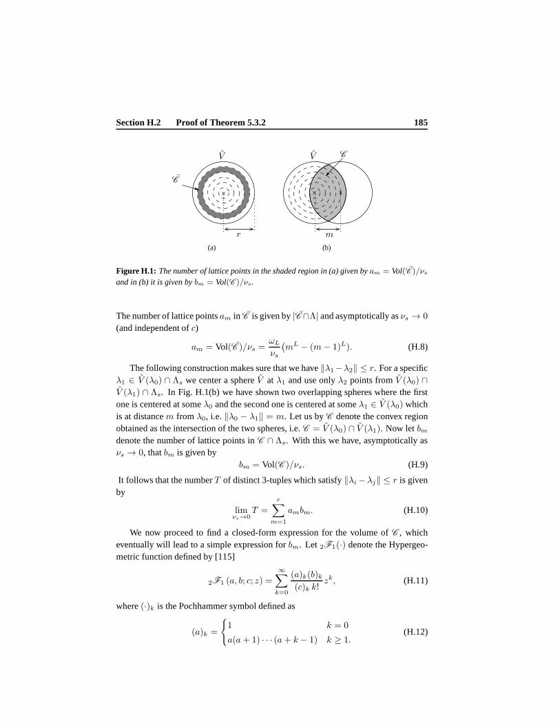
Section H.2 Proof of Theorem 5.3.2 185
PSfrag replacements V
mC
C
rλ0
(a)
PSfrag replacements V
m
C
C
rλ0
(b)
Figure H.1: The number of lattice points in the shaded region in (a) givenbyam = Vol(C )/νsand in (b) it is given bybm = Vol(C )/νs.
The number of lattice pointsam in C is given by|C ∩Λ| and asymptotically asνs → 0
(and independent ofc)
am = Vol(C )/νs =ωL
νs
(mL − (m− 1)L). (H.8)
The following construction makes sure that we have‖λ1−λ2‖ ≤ r. For a specificλ1 ∈ V (λ0) ∩ Λs we center a sphereV at λ1 and use onlyλ2 points fromV (λ0) ∩V (λ1) ∩ Λs. In Fig. H.1(b) we have shown two overlapping spheres where the firstone is centered at someλ0 and the second one is centered at someλ1 ∈ V (λ0) whichis at distancem from λ0, i.e.‖λ0 − λ1‖ = m. Let us byC denote the convex regionobtained as the intersection of the two spheres, i.e.C = V (λ0) ∩ V (λ1). Now letbmdenote the number of lattice points inC ∩ Λs. With this we have, asymptotically asνs → 0, thatbm is given by
bm = Vol(C )/νs. (H.9)
It follows that the numberT of distinct 3-tuples which satisfy‖λi −λj‖ ≤ r is givenby
limνs→0
T =r∑
m=1
ambm. (H.10)
We now proceed to find a closed-form expression for the volumeof C , whicheventually will lead to a simple expression forbm. Let 2F1(·) denote the Hypergeo-metric function defined by [115]
2F1 (a, b; c; z) =
∞∑
k=0
(a)k(b)k(c)k k!
zk, (H.11)
where(·)k is the Pochhammer symbol defined as
(a)k =
1 k = 0
a(a+ 1) · · · (a+ k − 1) k ≥ 1.(H.12)
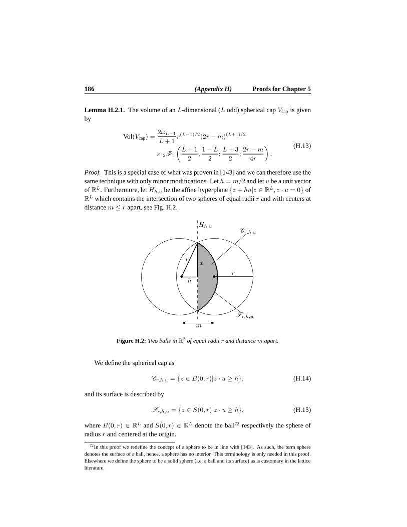
186 (Appendix H) Proofs for Chapter 5
Lemma H.2.1. The volume of anL-dimensional (L odd) spherical capVcap is givenby
Vol(Vcap) =2ωL−1
L+ 1r(L−1)/2(2r −m)(L+1)/2
× 2F1
(L+ 1
2,1− L
2;L+ 3
2;2r −m
4r
)
,(H.13)
Proof. This is a special case of what was proven in [143] and we can therefore use thesame technique with only minor modifications. Leth = m/2 and letu be a unit vectorof RL. Furthermore, letHh,u be the affine hyperplanez + hu|z ∈ RL, z · u = 0 ofRL which contains the intersection of two spheres of equal radii r and with centers atdistancem ≤ r apart, see Fig. H.2.
PSfrag replacements
Hh,uCr,h,u
Sr,h,u
r
r
h
m
x
Figure H.2: Two balls inR2 of equal radiir and distancem apart.
We define the spherical cap as
Cr,h,u = z ∈ B(0, r)|z · u ≥ h, (H.14)
and its surface is described by
Sr,h,u = z ∈ S(0, r)|z · u ≥ h, (H.15)
whereB(0, r) ∈ RL andS(0, r) ∈ RL denote the ball72 respectively the sphere ofradiusr and centered at the origin.
72In this proof we redefine the concept of a sphere to be in line with [143]. As such, the term spheredenotes the surface of a ball, hence, a sphere has no interior. This terminology is only needed in this proof.Elsewhere we define the sphere to be a solid sphere (i.e. a balland its surface) as is customary in the latticeliterature.
Section H.2 Proof of Theorem 5.3.2 187
The sphereHh,u ∩ Sr,h,u has radiusx =√r2 − h2 and it is clear thath =√
r2 − x2. Moreover, any point ofSr,h,u which is at distance73 t from Hh,u is atdistance(x2 − t2 − 2th)1/2 from the real lineRu (i.e. the span ofu). Hence, thevolume Vol(Cr,h,u) of Cr,h,u is given by
Vol(Cr,h,u) =
∫ r−h
0
ωL−1(x2 − t2 − 2th)(L−1)/2 dt
= ωL−1
∫ r−h
0
((r − h− t)(r + h+ t))(L−1)/2
dt
= ωL−1
∫ α
0
(α− t)γ(t− β)γ dt,
(H.16)
whereα = r − h, β = −r − h andγ = (L− 1)/2. The last integral in (H.16) can beshown to be equal to [69, Eq. 3.196.1]
∫ α
0
(α − t)γ(t− β)γ dt =αγ+1(−β)γγ + 1
2F1
(
1,−γ; γ + 2;α
β
)
, (H.17)
which by use of (H.35) can be written as
αγ+1(−β)γγ + 1
2F1
(
1,−γ; γ + 2;α
β
)
=
(
1− α
β
)γαγ+1(−β)γγ + 1
2F1
(
γ + 1,−γ; γ + 2;α
α− β
)
.
(H.18)
The volume Vol(Cr,h,u) follows by inserting (H.18) in (H.16), that is
Vol(Cr,h,u) = ωL−1
(
1− α
β
)γαγ+1(−β)γγ + 1
2F1
(
γ + 1,−γ; γ + 2;α
α− β
)
=ωL−1
L+ 1r(L−1)/2(2r −m)(L+1)/2
× 2F1
(
L/2 + 1/2, 1/2− L/2;L/2 + 3/2;2r −m
4r
)
,
(H.19)
which completes the proof.
The regionC consists of two equally sized spherical caps. Inserting (H.8)
73By distance we mean the length of the shortest straight line that can be drawn betweenHh,u andSr,h,u. It is clear that this line is perpendicular toHh,u.
188 (Appendix H) Proofs for Chapter 5
and (H.9) into (H.10) leads to74 (asymptotically asνs → 0)
T =
r∑
m=1
ambm
=2ωLωL−1
ν2s (L+ 1)
r∑
m=1
(mL − (m− 1)L)r(L−1)/2
× (2r −m)(L+1)/22F1
(L+ 1
2,1− L
2;L+ 3
2;2r −m
4r
)
(a)=
2ωLωL−1
ν2s (L+ 1)r
L−12
L+12∑
n=0
(L+12
n
)
(2r)L+1
2 −n(−1)n
×L−1
2∑
k=0
(L+12
)
k
(1−L2
)
k(L+32
)
kk!
k∑
j=0
(k
j
)(1
2
)k−j
(−1)j(
1
4r
)j
×r∑
m=1
(mL − (m− 1)L)mnmj
(b)=
2ωLωL−1
ν2s (L+ 1)r
L−12
L+12∑
n=0
(L+12
n
)
(2r)L+1
2 −n(−1)n
×L−1
2∑
k=0
(L+12
)
k
(1−L2
)
k(L+32
)
kk!
k∑
j=0
(k
j
)(1
2
)k−j
(−1)j(
1
4r
)j
×(
Lr∑
m=1
mL−1+n+j + O(mL−2+n+j)
)
.
(c)=
2ωLωL−1
ν2s (L+ 1)r
L−12
L+12∑
n=0
(L+12
n
)
(2r)L+1
2 −n(−1)n
×L−1
2∑
k=0
(L+12
)
k
(1−L2
)
k(L+32
)
kk!
k∑
j=0
(k
j
)(1
2
)k−j
(−1)j(
1
4r
)j
×(
L
L+ n+ jrL+n+j + O
(rL−1+n+j
))
,
(H.20)
where(a) follows by use of the binomial series expansion [56, p.162],i.e.(x+ y)k =∑k
n=0
(kn
)xk−nyn, which in our case leads to
(2r −m)L+12 =
L+12∑
n=0
(L+12
n
)
(2r)L+1
2 −n(−1)nmn (H.21)
74In this asymptotic analysis we assume that allλ1 points within a givenC is at exact same distancefrom the center ofV (i.e. fromλ0). The error due to this assumption is neglectable, since anyconstantoffset fromm will appear insideO(·).
Section H.2 Proof of Theorem 5.3.2 189
and(2r −m
4r
)k
=
k∑
j=0
(k
j
)(1
2
)k−j
(−1)j(m
4r
)j
. (H.22)
(b) is obtained by once again applying the binomial series expansion, that is
(m− 1)L = mL − LmL−1 + O(mL−2), (H.23)
and(c) follows from the fact that∑r
m=1mL = 1
L+1rL+1 + O(rL).
Next we letr → ∞ so that the number ofhollow spheres insideV goes to infin-ity.75 From (H.20) we see that, asymptotically asνs → 0 andr → ∞, we have
T = 2ωLωL−1
ν2s
L
L+ 1βLr
2L, (H.25)
whereβL is constant for fixedL and given by (H.7).We are now in a position to find an expression forψL. Let ν be equal to the lower
bound (5.26), i.e.ν = νs√N and letr be the radius of the sphere having volumeν.
ThenψL is given by the ratio ofr andr, i.e.ψL = r/r, wherer is the radius ofV .Using this in (H.25) leads to
r =
(Tνs(L + 1)
2ωLωL−1LβL
)1/2L
. (H.26)
Since the radiusr of anL-dimensional sphere of volumeν is given by
r =
(ν
ωL
)1/L
, (H.27)
we can findψL by dividing (H.26) by (H.27), that is
ψL =r
r=
(Tν2s (L+ 1)
2ωLωL−1LβL
)1/2L(ν
ωL
)−1/L
. (H.28)
Since we need to obtainN 3-tuples we letT = N so that withν =√Nνs we can
rewrite (H.28) as
ψL =
(ωL
ωL−1
)1/2L (L+ 1
2L
)1/2L
β−1/2LL . (H.29)
This completes the proof.
75We would like to emphasize that this is equivalent to keepingr fixed, sayr = 1, and then let thenumber ofhollow spheres insideV go to infinity. To see this letM → ∞ and then rewrite (H.8) as
am/M = Vol(C )/νs =ωL
νs
((m
M
)L−(m− 1
M
)L)
, 1 ≤ m ≤ M. (H.24)
A similar change applies to (H.9). Hence, the asymptotic expression forT is also valid within a localizedregion ofRL which is a useful property we exploit when proving Proposition 5.4.1.
190 (Appendix H) Proofs for Chapter 5
H.3 Proof of Theorem 5.3.3
Lemma H.3.1. ForL→ ∞ we have(
ωL
ωL−1
)1/2L
= 1. (H.30)
Proof. The volumeωL of an L-dimensional unit hypersphere is given byωL =
πL/2/(L/2)! so we have that
limL→∞
(πL/2
(L/2)!
(L/2− 1/2)!
πL/2−1/2
)1/2L
= limL→∞
π1/4L(O(L−1)
)1/2L
= 1.
(H.31)
Lemma H.3.2. ForL→ ∞ we have
1
β1/2LL
=
(4
3
)1/4
. (H.32)
Proof. The inner sum in (5.28) may be well approximated by using that1L+c ≈ 1
L forL≫ c, which leads to
k∑
j=0
(k
j
)(1
2
)k−j
(−1)j(1
4
)j1
L+ n+ j
≈k∑
j=0
(k
j
)(1
2
)k−j
(−1)j(1
4
)j1
L
=1
L
(1
4
)k
.
(H.33)
We also have thatL−1
2∑
k=0
(L+12
)
k
(1−L2
)
k(L+32
)
kk!
(1
4
)k
=2F1
(L+ 1
2,1− L
2;L+ 3
2;1
4
)
(a)= (1 − 1/4)(−1+L)/2
2F1
(
1,1− L
2;L+ 3
2;−1
3
)
= (3/4)(−1+L)/2
L/2−1/2∑
k=0
k!
k!
(1/2− L/2)k(3/2 + L/2)k
(−1/3)k
= (3/4)(−1+L)/2
×L/2−1/2∑
k=0
((−L/2)k
(L/2)k + O(Lk−1)+ O(L−1)
)
(−1/3)k

Section H.4 Proof of Proposition 5.4.1 191
≈ (3/4)(−1+L)/2
L/2−1/2∑
k=0
(1/3)k, (H.34)
where(a) follows from the following hypergeometric transformation[115]
2F1 (a, b; c; z) = (1− z)−b2F1 (c− a, b; c; ξ) , (H.35)
whereξ = zz−1 . Finally, it is true that
L/2+1/2∑
n=0
(L/2 + 1/2
n
)
2L/2+1/2−n(−1)n = 1. (H.36)
Inserting (H.33), (H.34) and (H.36) into (H.7) leads to
βL ≈ (3/4)(−1+L)/2 1
L
L/2−1/2∑
k=0
(1/3)k, (H.37)
where since∑∞
k=0(1/3)k = 3/2, we get
limL→∞
1
β1/2LL
= limL→∞
(4/3)1/4(4/3)−1/4LL1/2L(2/3)1/2L
= (4/3)1/4,
(H.38)
which proves the Lemma.
We are now in a position to prove the following theorem.Theorem 5.3.3.For K = 3 andL → ∞ the dimensionless expansion factorψL isgiven by
ψ∞ =
(4
3
)1/4
. (H.39)
Proof. The proof follows trivially by use of Lemma H.3.1 and Lemma H.3.2 in (H.29).
H.4 Proof of Proposition 5.4.1
LetTi = λi : λi = αi(λc), λc ∈ Vπ(0), i.e. the set ofN2 sublattice pointsλi ∈ Λs
associated with theN2 central lattice points withinVπ(0). Furthermore, letT ′i ⊆ Ti
be the set of unique elements ofTi, where|T ′i | ≈ N . Finally, let
Tj(λi) = λj : λj = αj(λc) andλi = αi(λc), λc ∈ Vπ(0), (H.40)
and letT ′j(λi) ⊆ Tj(λi) be the set of unique elements. That is,Tj(λi) contains all the
elementsλj ∈ Λs which are in theK-tuples that also contains a specificλi. We will

192 (Appendix H) Proofs for Chapter 5
also make use of the notation#λjto indicate the number of occurrences of a specific
λj in Tj(λi).For the pair(i, j) we have
∑
λc∈Vπ(0)
‖αi(λc)− αj(λc)‖2 =∑
λi∈T ′i
∑
λj∈Tj(λi)
‖λi − λj‖2.
Givenλi ∈ T ′i , we have
∑
λj∈Tj(λi)
‖λi − λj‖2νs =∑
λj∈T ′j(λi)
#λj‖λi − λj‖2νs
(a)≈ N
N
∑
λj∈T ′j(λi)
‖λi − λj‖2νs
≈ N
N
∫
V (λi)
‖λi − x‖2 dx
≈ N
Nν1+2/LLG(SL)
(b)= Nνsν
2/LLG(SL),
(H.41)
where(a) follows by assuming (see the discussion below for the case ofK = 3)that#λj
= N/N for all λj ∈ Tj(λi) and(b) follows sinceν = Nνs. Hence, withν = Nνs = ψN1/(K−1)νs andνs = Nν, we have
1
L
∑
λj∈Tj(λi)
‖λi − λj‖2νs ≈ Nνsψ2Lν
2/LN2/LN2/L(K−1)G(SL)
= νsψ2LN
1+2K/L(K−1)ν2/LG(SL),
which is independent ofλi, so that
1
L
∑
λi∈T ′i
∑
λj∈Tj(λi)
‖λi − λj‖2 ≈N
L
∑
λj∈Tj(λi)
‖λi − λj‖2
≈ ψ2LN
2+2K/L(K−1)ν2/LG(SL).
In (H.41) we used the approximation#λj≈ N/N without any explanation. For
the case ofK = 2 and asN → ∞ we have thatT ′i = Ti andN = N , hence the
approximation becomes exact, i.e.#λj= 1. This proves the Proposition forK = 2.
We will now consider the case ofK = 3 and show that asymptotically, asL → ∞,the following approximation becomes exact.
1
L
∑
λj∈Tj(λi)
‖λi − λj‖2 ≈ Nν2/LG(SL). (H.42)
Section H.4 Proof of Proposition 5.4.1 193
To prove this we use the same procedure as when deriving closed-form expressionsfor ψL leads to the following asymptotic expression
∑
λj∈Tj(λi)
‖λi − λj‖2 =
r∑
m=1
ambmm2, (H.43)
where we without loss of generality assumed thatλi = 0 and used the fact that wecan replace‖λj‖2 by m2 for theλj points which are at distancem from λi = 0. Itfollows that we have
1
L
∑
λj∈Tj(λi)
‖λi − λj‖2 = 2ωLωL−1
ν2s
1
L+ 1β′Lr
2L+2, (H.44)
where
β′L =
L+12∑
n=0
(L+12
n
)
2L+12 −n(−1)n
L−12∑
k=0
(L+12
)
k
(1−L2
)
k(L+32
)
kk!
×k∑
j=0
(k
j
)(1
2
)k−j
(−1)j(1
4
)j1
L+ n+ j + 2.
(H.45)
Sinceν = ωLrL = ψL
L
√Nνs we can rewrite (H.44) as
∑
λj∈Tj(λi)
‖λi − λj‖2 = 2ωLωL−1
ν2s
1
L+ 1β′Lν
2+2/L 1
ω2+2/LL
= 2ωL−1
ω1+2/LL
1
L+ 1β′Lν
2/Lψ2LL N
(a)= 2
ωL−1
ω1+2/LL
1
L+ 1β′Lν
2/LN
(ωL
ωL−1
)(L+ 1
2L
)1
βL
=1
ω2/LL
1
Lν2/LN
β′L
βL,
(H.46)
where(a) follows by inserting (H.29). Dividing (H.46) by (H.42) leads to
1
ω2/LL
1
L
1
G(SL)
β′L
βL=L+ 2
L
β′L
βL. (H.47)
Hence, asymptotically asL→ ∞ we have that
limL→∞
L+ 2
L
β′L
βL= 1, (H.48)
which proves the Proposition.
RemarkH.4.1. Proposition 5.4.1 considered the asymptotic case ofL → ∞. Exactdistortion expressions for the case ofK = 3 and finiteL follow by replacing (H.41)with (H.43).

194 (Appendix H) Proofs for Chapter 5
RemarkH.4.2. ForK > 3 it is very likely that similar equations can be found forψL which can then be used to verify the goodness of the approximations for anyK.Moreover, in Appendix H.5 we show that the rate of growth of (H.41) is unaffectedif we replace#λj
by eitherminλj#λj
or maxλj#λj
which means that the errorby using the approximationN/N instead of the true#λj
is constant (i.e. it does notdepend onN ) for fixedK andL. It remains to be shown whether this error term tendsto zero asL→ ∞ forK > 3. However, based on the discussion above we conjecturethat Proposition 5.4.1 is true for anyK asymptotically asN,L → ∞ andνs → 0.In other words, the side distortion of aK-channel MD-LVQ system can be expressedthrough the normalized second moment of a sphere as the dimension goes to infinity.
H.5 Proof of Proposition 5.4.2
Before proving Proposition 5.4.2 we need to lower and upper bound#λj(see Ap-
pendix H.4 for an introduction to this notation). As previously mentioned theλjpoints which are close (in Euclidean sense) toλi occur more frequently thanλj pointsfarther away. To see this observe that the construction ofK-tuples can be seen asan iterative procedure that first picks aλ0 ∈ Λs ∩ Vπ(0) and then anyλ1 ∈ Λs ispicked such that‖λ0 − λ1‖ ≤ r, henceλ1 ∈ Λs ∩ V (λ0). The set ofλK−1 pointsthat can be picked for a particular(K − 1)-tuple e.g.(λ0, . . . , λK−2) is then given byλK−1 : λK−1 ∈ Λs∩ V (λK−2)∩· · · ∩ V (λ0). It is clear that‖λi−λj‖ ≤ r where(λi, λj) = (αi(λc), αj(λc)), ∀λc ∈ Λc and anyi, j ∈ 0, . . . ,K − 1.
Let Tmin(λi, λj) denote the minimum number of times the pair(λi, λj) is used.The minimumTmin of Tmin(λi, λj) over all pairs(λi, λj) lower boundsN/N . Wewill now show thatTmin is always bounded away from zero. To see this notice that theminimum overlap between two spheres of radiusr centered atλ0 andλ1, respectively,is obtained whenλ0 andλ1 are are maximally separated, i.e. when‖λ0 − λ1‖ =
r. This is shown by the shaded area in Fig. H.3 forL = 2. For three spheres theminimum overlap is again obtained when all pairwise distances are maximized, i.e.when‖λi − λj‖ = r for i, j ∈ 0, 1, 2 and i 6= j. It is clear that the volume ofthe intersection of three spheres is less than that of two spheres, hence the minimumnumber ofλ2 points is greater than the minimum number ofλ3 points. However,by construction it follows that when centeringK spheres at the set of pointss =
λ0, . . . , λK−1 = α0(λc), . . . , αK−1(λc) each of the points ins will be in theintersection∩s of theK spheres. Since the intersection of an arbitrary collectionofconvex sets leads to a convex set [117], the convex hullC (s) of s will also be in∩s.Furthermore, for the example in Fig. H.3, it can be seen thatC (s) (indicated by theequilateral triangle) will not get smaller forK ≥ 3 and this is true in general sincepoints are never removed froms asK grows. ForL = 3 the regular tetrahedron [25]consisting of four points with a pairwise distance ofr describes a regular convexpolytope which lies in∩s. In general the regularL-simplex [25] lies in∩s and the

Section H.5 Proof of Proposition 5.4.2 195
PSfrag replacements
λ0 λ1
λ2C (s)
Figure H.3: Three spheres of equal radius are here centered at the set of points s =
λ0, λ1, λ2. The shaded area describes the intersection of two spheres.The equilateral trian-gle describes the convex hullC (s) of s.
volume Vol(L) of a regularL-simplex with side lengthr is given by [13]
Vol(L) =rL
L!
√
L+ 1
2L= cLr
L, (H.49)
wherecL depends only onL. It follows that the minimum number ofK-tuples thatcontains a specific(λi, λj) pair is lower bounded by Vol(L)K−2/νK−2
s . Since thevolumeν of V is given byν = ωLr
L we get
(Vol(L)νs
)K−2
=
(cLωL
)K−2(ν
νs
)K−2
. (H.50)
Also, by construction we have thatN ≤ (ν/νs)K−1 and thatN = ν/νs so an upper
bound onN/N is given by
N
N≤(ν
νs
)K−2
, (H.51)
which differs from the lower bound in (H.50) by a multiplicative constant.We are now in a position to prove Proposition 5.4.2.
Proposition 5.4.2ForN → ∞ and2 ≤ K <∞ we have
∑
λc∈Vπ(0)
∥∥∥λc − 1
K
∑K−1i=0 λi
∥∥∥
2
∑
λc∈Vπ(0)
∑K−2i=0
∑K−1j=i+1 ‖λi − λj‖2
→ 0. (H.52)
Proof. The numerator describes the distance from a central latticepoint to the meanvector of its associatedK-tuple. This distance is upper bounded by the coveringradius of the sublatticeΛs. The rate of growth of the covering radius is proportional
196 (Appendix H) Proofs for Chapter 5
to ν1/Ls = (Nν)1/L, hence
∑
λc∈Vπ(0)
∥∥∥∥∥λc −
1
K
K−1∑
i=0
λi
∥∥∥∥∥
2
= O(
N2N2/Lν2/L)
. (H.53)
Since the approximationN/N used in Proposition 5.4.1 is sandwiched between thelower and upper bounds (i.e. Eqs. (H.50) and (H.51)) we can write
∑
λc∈Vπ(0)
K−2∑
i=0
K−1∑
j=i+1
‖αi(λc)− αj(λc)‖2
=
K−2∑
i=0
K−1∑
j=i+1
∑
λc∈Vπ(0)
‖αi(λc)− αj(λc)‖2
≈ L
2K(K − 1)G(SL)ψ
2LN
2N2K/L(K−1)ν2/L,
(H.54)
so that, sinceλi = αi(λc),
∑
λc∈Vπ(0)
K−2∑
i=0
K−1∑
j=i+1
‖λi − λj‖2 = O(
N2N2K/L(K−1)ν2/L)
. (H.55)
Comparing (H.53) to (H.55) we see that (H.52) grows asO(N−K/(K−1)
)→ 0 for
N → ∞ andK <∞.
Appendix IProofs for Chapter 6
For notational convenience we will in this appendix use the shorter notationsL ,Li
andLi,j instead ofL (K,κ),L(K,κ)i andL
(K,κ)i,j .
I.1 Proof of Theorem 6.2.1
To prove Theorem 6.2.1 we need the following results.
Lemma I.1.1. For1 ≤ κ ≤ K and anyi ∈ 0, . . . ,K − 1 we have
K−1∑
j=0j 6=i
p(Lj) = κp(L )− p(Li).
Proof. Since|Lj | =(K−1κ−1
)the sum
∑K−1j=0 p(Lj) containsK
(K−1κ−1
)terms. How-
ever, the number of distinct terms is|L | =(Kκ
)and each individual term occursκ
times in the sum, since
K(K−1κ−1
)
(Kκ
) = κ.
Subtracting the terms forj = i proves the lemma.
Lemma I.1.2. For1 ≤ κ ≤ K and anyi, j ∈ 0, . . . ,K − 1 we have
K−1∑
j=0
p(Li,j) = κp(Li).
197
198 (Appendix I) Proofs for Chapter 6
Proof. It is true thatLi,i = Li and since|Li| =(K−1κ−1
)and |Li,j | =
(K−2κ−2
)the
sum∑K−1
j=0 p(Li,j) contains(K − 1)(K−2κ−2
)+(K−1κ−1
)terms. However, the number of
distinctl ∈ Li terms is|Li| =(K−1κ−1
)and each term occursκ times in the sum, since
(K − 1)(K−2κ−2
)+(K−1κ−1
)
(K−1κ−1
) = κ.
Lemma I.1.3. For1 ≤ κ ≤ K we have
∑
l∈L
p(L )
⟨
λc,1
κ
∑
i∈l
λi
⟩
=
⟨
λc,1
κ
K−1∑
i=0
λip(Li)
⟩
.
Proof. We have that
∑
l∈L
p(L )
⟨
λc,1
κ
∑
i∈l
λi
⟩
=
⟨
λc,1
κ
∑
l∈L
p(l)∑
i∈l
λi
⟩
=
⟨
λc,1
κ
K−1∑
i=0
λip(Li)
⟩
,
where the last equality follows sinceLi denotes the set of alll-terms that contains theindexi.
Lemma I.1.4. For1 ≤ κ ≤ K we have
K−2∑
i=0
K−1∑
j=i+1
p(Li)p(Lj)‖λi − λj‖2 =K−1∑
i=0
p(Li) (κp(L )− p(Li)) ‖λi‖2
− 2
K−2∑
i=0
K−1∑
j=i+1
p(Li)p(Lj)〈λi, λj〉.
Proof. We have that
K−2∑
i=0
K−1∑
j=i+1
p(Li)p(Lj)‖λi − λj‖2 =K−2∑
i=0
K−1∑
j=i+1
p(Li)p(Lj)(‖λi‖2 + ‖λj‖2)
− 2
K−2∑
i=0
K−1∑
j=i+1
p(Li)p(Lj)〈λi, λj〉.
Furthermore, it follows that
K−2∑
i=0
K−1∑
j=i+1
p(Li)p(Lj)(‖λi‖2 + ‖λj‖2)
Section I.1 Proof of Theorem 6.2.1 199
=
K−2∑
i=0
p(Li)‖λi‖2K−1∑
j=i+1
p(Lj) +
K−1∑
j=1
p(Lj)‖λj‖2j−1∑
i=0
p(Li)
=
K−1∑
i=0
p(Li)‖λi‖2K−1∑
j=i+1
p(Lj)
︸ ︷︷ ︸
0 for i=K−1
+
K−1∑
j=0
p(Lj)‖λj‖2j−1∑
i=0
p(Li)
︸ ︷︷ ︸
0 for j=0
=
K−1∑
i=0
p(Li)‖λi‖2
i−1∑
j=0
p(Lj) +
K−1∑
j=i+1
p(Lj)
=
K−1∑
i=0
p(Li)‖λi‖2K−1∑
j=0j 6=i
p(Lj)
=
K−1∑
i=0
p(Li)‖λi‖2 (κp(L )− p(Li)) ,
where the last equality follows by use of Lemma I.1.1.
Lemma I.1.5. For1 ≤ κ ≤ K we have
K−2∑
i=0
K−1∑
j=i+1
p(Li,j)‖λi − λj‖2 = (κ− 1)
K−1∑
i=0
p(Li)‖λi‖2
− 2K−2∑
i=0
K−1∑
j=i+1
p(Li,j)〈λi, λj〉.
Proof. We have that
K−2∑
i=0
K−1∑
j=i+1
p(Li,j)‖λi − λj‖2 =
K−2∑
i=0
K−1∑
j=i+1
p(Li,j)(‖λi‖2
+ ‖λj‖2)− 2
K−2∑
i=0
K−1∑
j=i+1
p(Li,j)〈λi, λj〉.
Furthermore, it follows that
K−2∑
i=0
K−1∑
j=i+1
p(Li,j)(‖λi‖2 + ‖λj‖2)
=
K−2∑
i=0
K−1∑
j=i+1
p(Li,j)‖λi‖2 +K−2∑
i=0
K−1∑
j=i+1
p(Li,j)‖λj‖2
=
K−2∑
i=0
‖λi‖2K−1∑
j=i+1
p(Li,j) +
K−1∑
j=1
j−1∑
i=0
p(Li,j)‖λj‖2
200 (Appendix I) Proofs for Chapter 6
=
K−1∑
i=0
‖λi‖2K−1∑
j=i+1
p(Li,j)
︸ ︷︷ ︸
0 for i=K−1
+
K−1∑
j=0
‖λj‖2j−1∑
i=0
p(Li,j)
︸ ︷︷ ︸
0 for j=0
=
K−1∑
i=0
‖λi‖2
i−1∑
j=0
p(Li,j) +
K−1∑
j=i+1
p(Li,j)
=
K−1∑
i=0
‖λi‖2
K−1∑
j=0
p(Li,j)− p(Li)
(a)=
K−1∑
i=0
‖λi‖2 (κp(Li)− p(Li))
= (κ− 1)
K−1∑
i=0
‖λi‖2p(Li),
where(a) follows by use of Lemma I.1.2.
Lemma I.1.6. For1 ≤ κ ≤ K we have
∑
l∈L
p(l)
∥∥∥∥∥
∑
i∈l
λi
∥∥∥∥∥
2
= κK−1∑
i=0
p(Li)‖λi‖2 −K−2∑
i=0
K−1∑
j=i+1
p(Li,j)‖λi − λj‖2.
Proof. The set of all elementsl of L that contains the indexi is denoted byLi.Similarly the set of all elements that contains the indicesi andj is denoted byLi,j .From this we see that
∑
l∈L
p(l)
∥∥∥∥∥
∑
i∈l
λi
∥∥∥∥∥
2
=∑
l∈L
p(l)
∑
i∈l
‖λi‖2 + 2
κ−2∑
i=0
κ−1∑
j=i+1
〈λli , λlj 〉
=
K−1∑
i=0
p(Li)‖λi‖2 + 2
K−2∑
i=0
K−1∑
j=i+1
p(Li,j)〈λi, λj〉.
By use of Lemma I.1.5 it follows that
∑
l∈L
p(l)
∥∥∥∥∥
∑
i∈l
λi
∥∥∥∥∥
2
=K−1∑
i=0
p(Li)‖λi‖2 + (κ− 1)K−1∑
i=0
p(Li)‖λi‖2
−K−2∑
i=0
K−1∑
j=i+1
p(Li,j)‖λi − λj‖2
= κ
K−1∑
i=0
p(Li)‖λi‖2 −K−2∑
i=0
K−1∑
j=i+1
p(Li,j)‖λi − λj‖2

Section I.1 Proof of Theorem 6.2.1 201
We are now in a position to prove the following result.
Proposition I.1.1. For1 ≤ κ ≤ K we have
∑
l∈L
p(l)
∥∥∥∥∥λc −
1
κ
∑
i∈l
λi
∥∥∥∥∥
2
= p(L )
∥∥∥∥∥λc −
1
κp(L )
K−1∑
i=0
p(Li)λi
∥∥∥∥∥
2
+1
κ2
K−2∑
i=0
K−1∑
j=i+1
(p(Li)p(Lj)
p(L )− p(Li,j)
)
‖λi − λj‖2.
(I.1)
Proof. Expansion of the norm on the left-hand-side in (I.1) leads to
∑
l∈L
p(l)
∥∥∥∥λc −
1
κ
∑
i∈l
λi
∥∥∥∥
2
=∑
l∈L
p(l)
‖λc‖2 − 2
⟨
λc,1
κ
∑
i∈l
λi
⟩
+1
κ2
∥∥∥∥∥
∑
i∈l
λi
∥∥∥∥∥
2
(a)= p(L )‖λc‖2 − 2
⟨
λc,1
κ
K−1∑
i=0
p(Li)λi
⟩
+1
κ2
∑
l∈L
p(l)
∥∥∥∥∥
∑
i∈l
λi
∥∥∥∥∥
2
= p(L )
∥∥∥∥∥λc −
1
κp(L )
K−1∑
i=0
p(Li)λi
∥∥∥∥∥
2
− 1
κ2p(L )
∥∥∥∥∥
K−1∑
i=0
p(Li)λi
∥∥∥∥∥
2
+1
κ2
∑
l∈L
p(l)
∥∥∥∥∥
∑
i∈l
λi
∥∥∥∥∥
2
= p(L )
∥∥∥∥∥λc −
1
κp(L )
K−1∑
i=0
p(Li)λi
∥∥∥∥∥
2
+1
κ2
∑
l∈L
p(l)
∥∥∥∥∥
∑
i∈l
λi
∥∥∥∥∥
2
− 1
κ2p(L )
K−1∑
i=0
p(Li)2‖λi‖2 + 2
K−2∑
i=0
K−1∑
j=i+1
p(Li)p(Lj)〈λi, λj〉
(b)= p(L )
∥∥∥∥∥λc −
1
κp(L )
K−1∑
i=0
p(Li)λi
∥∥∥∥∥
2
+1
κ
K−1∑
i=0
p(Li)‖λi‖2
− 1
κ2
K−2∑
i=0
K−1∑
j=i+1
p(Li,j)‖λi − λj‖2 −1
κ2p(L )
K−1∑
i=0
p(Li)2‖λi‖2
+1
κ2p(L )
(K−2∑
i=0
K−1∑
j=i+1
p(Li)p(Lj)‖λi − λj‖2
−K−1∑
i=0
p(Li)(κp(L )− p(Li))‖λi‖2)
= p(L )
∥∥∥∥∥λc −
1
κp(L )
K−1∑
i=0
p(Li)λi
∥∥∥∥∥
2
202 (Appendix I) Proofs for Chapter 6
+1
κ2
K−2∑
i=0
K−1∑
j=i+1
(p(Li)p(Lj)
p(L )− p(Li,j)
)
‖λi − λj‖2,
where(a) follows by use of Lemma I.1.3 and(b) by use of Lemmas I.1.4 and I.1.6.
Theorem I.1.1. For1 ≤ κ ≤ K we have
∑
λc
∑
l∈L
p(l)
∥∥∥∥∥λc −
1
κ
∑
i∈l
λi
∥∥∥∥∥
2
=∑
λc
(
p(L )
∥∥∥∥∥λc −
1
κp(L )
K−1∑
i=0
p(Li)λi
∥∥∥∥∥
2
+1
κ2
K−2∑
i=0
K−1∑
j=i+1
(p(Li)p(Lj)
p(L )− p(Li,j)
)
‖λi − λj‖2)
.
(I.2)
Proof. Follows trivially from Proposition I.1.1.
I.2 Proof of Proposition 6.3.1
Proposition 6.3.1ForK = 2 and asymptotically asNi → ∞, νi → 0 as well asfor K = 3 and asymptotically asNi, L → ∞ andνi → 0, we have for any pair ofsublattices,(Λi,Λj), i, j = 0, . . . ,K − 1, i 6= j,
1
L
∑
λc∈Vπ(0)
‖αi(λc)− αj(λc)‖2 = ψ2Lν
2/LG(SL)Nπ
K−1∏
m=0
N2/L(K−1)m .
Proof. Let Ti = λi : λi = αi(λc), λc ∈ Vπ(0), i.e. the set ofNπ sublattice pointsλi ∈ Λi associated with theNπ central lattice points withinVπ(0). Furthermore,let T ′
i ⊆ Ti be the set of unique elements ofTi. Since (for largeNi) all the latticepoints ofΛi which are contained withinVπ(0) are used in someK-tuples, it followsthat |T ′
i | ≈ ν/νi = Nπ/Ni. Finally, let Tj(λi) = λj : λj = αj(λc) andλi =
αi(λc), λc ∈ Vπ(0) and letT ′j(λi) ⊆ Tj(λi) be the set of unique elements. That
is, Tj(λi) contains all the elementsλj ∈ Λj which are in theK-tuples that alsocontains a specificλi ∈ Λi. We will also make use of the notation#λj
to indicate thenumber of occurrences of a specificλj in Tj(λi). For example forK = 2 we have#λj
= 1, ∀λj whereas forK > 2 we have#λj≥ 1. We will show later that using
the approximation#λj≈ Ni/Nj is asymptotically good forK = 3, L → ∞ and
Nn → ∞, ∀n. Furthermore, we conjecture this to be the case forK > 3 as well.For sublatticeΛi andΛj we have
∑
λc∈Vπ(0)
‖αi(λc)− αj(λc)‖2 =∑
λi∈T ′i
∑
λj∈Tj(λi)
‖λi − λj‖2.
Section I.3 Proof of Proposition 6.3.2 203
Givenλi ∈ T ′i , we have
∑
λj∈Tj(λi)
‖λi − λj‖2νj =∑
λj∈T ′j(λi)
#λj‖λi − λj‖2νj
≈ Ni
Nj
∑
λj∈T ′j(λi)
‖λi − λj‖2νj
≈ Ni
Nj
∫
V (λi)
‖λi − x‖2 dx
=Ni
Nj
ν1+2/LLG(SL)
= Niνj ν2/LLG(SL)
(I.3)
sinceNj = ν/νj. Hence, withν = ψLLν∏K−1
m=0N1/(K−1)m , we have
1
L
∑
λj∈Tj(λi)
‖λi − λj‖2νj ≈ Niνjψ2Lν
2/LG(SL)
K−1∏
m=0
N2/L(K−1)m ,
which is independent ofλi, so that
1
L
∑
λi∈T ′i
∑
λj∈Tj(λi)
‖λi − λj‖2 ≈ 1
L
Nπ
Ni
∑
λj∈Tj(λi)
‖λi − λj‖2
≈ ψ2Lν
2/LG(SL)Nπ
K−1∏
m=0
N2/L(K−1)m ,
which completes the first part of the proof. We still need to show that forK = 3
andL → ∞ as well asNm → ∞, ∀m the approximation#λj≈ Ni/Nj is good.
That this is so can be deduced from the proof of Proposition 5.4.1 (the last part whereK = 3) by using the fact thatν = ψL
Lν∏N
1/(K−1)m in order to prove that
1
L
∑
λj∈Tj(λi)
‖λi − λj‖2 = Niν2/LG(SL), (I.4)
which shows that (I.3) is asymptotically true forK = 3, L→ ∞ andNn → ∞, ∀n.
I.3 Proof of Proposition 6.3.2
Proposition 6.3.2ForNi → ∞ we have
∑
λc∈Vπ(0)
∥∥∥λc − 1
κp(L )
∑K−1i=0 p(Li)λi
∥∥∥
2
∑
λc∈Vπ(0)
∑K−2i=0
∑K−1j=i+1
(p(Li)p(Lj)
p(L ) − p(Li,j))
‖λi − λj‖2→ 0. (I.5)
204 (Appendix I) Proofs for Chapter 6
Proof. The numerator describes the distance from a central latticepoint to theweighted centroid of its associatedK-tuple. Let us chooseΛ0 such thatN0 ≤ Ni, ∀i.Then, since by construction there is no bias towards any of the sublattices, theweighted centroids will be evenly distributed aroundλ0 points. Hence, the distancefrom central lattice points to the centroids can be upper bounded by the covering ra-dius ofΛ0. This is a conservative76 upper bound but will suffice for the proof. Therate of growth of the covering radius is proportional toν1/L0 = (N0ν)
1/L, hence
∑
λc∈Vπ(0)
∥∥∥∥∥λc −
1
κp(L )
K−1∑
i=0
p(Li)λi
∥∥∥∥∥
2
= O(
NπN2/L0 ν2/L
)
. (I.6)
By use of Proposition 6.3.1 we have77
1
L
∑
λc∈Vπ(0)
K−2∑
i=0
K−1∑
j=i+1
(p(Li)p(Lj)
p(L )− p(Li,j)
)
‖αi(λc)− αj(λc)‖2
=1
L
K−2∑
i=0
K−1∑
j=i+1
(p(Li)p(Lj)
p(L )− p(Li,j)
)∑
λc∈Vπ(0)
‖αi(λc)− αj(λc)‖2
≈ ψ2Lν
2/LG(SL)Nπ
K−1∏
m=0
N2/L(K−1)m
K−2∑
i=0
K−1∑
j=i+1
(p(Li)p(Lj)
p(L )− p(Li,j)
)
,
so that, sinceλi = αi(λc), we get by use of Proposition 6.3.178
∑
λc∈Vπ(0)
K−2∑
i=0
K−1∑
j=i+1
(p(Li)p(Lj)
p(L )− p(Li,j)
)
‖λi − λj‖2
= Ω
(
Nπν2/L
K−1∏
m=0
N2/L(K−1)m
)
.
(I.7)
Comparing (I.6) to (I.7) we see that (I.5) grows asΘ(
N2/L0 /N
2/L(K−1)π
)
→ 0 for
Ni → ∞.
76The number of distinct centroids per unit volume is larger than the number of points ofΛ0 per unitvolume.
77The approximation of#λjin Proposition 6.3.1 does not influence this analysis. To seethis we refer
the reader to Appendix H.5.78In this case we actually lower bound the expression and as such the order operatorO is in factΩ. Recall
that we say thatf(n) = O(g(n)) if 0 < f(n) ≤ c1g(n) andf(n) = Ω(g(n)) if f(n) ≥ c0g(n), forc0, c1 > 0 and some largen. Furthermore,f(n) = Θ(g(n)) if c0g(n) ≤ f(n) ≤ c1g(n), cf. [56].
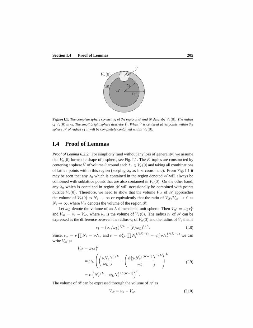
Section I.4 Proof of Lemmas 205
PSfrag replacementsVπ(0)
V
r0
r1
AB
Figure I.1: The complete sphere consisting of the regionsA andB describeVπ(0). The radiusof Vπ(0) is r0. The small bright sphere describeV . WhenV is centered atλ0 points within thesphereA of radiusr1 it will be completely contained withinVπ(0).
I.4 Proof of Lemmas
Proof of Lemma 6.2.2.For simplicity (and without any loss of generality) we assumethatVπ(0) forms the shape of a sphere, see Fig. I.1. TheK-tuples are constructed bycentering a sphereV of volumeν around eachλ0 ∈ Vπ(0) and taking all combinationsof lattice points within this region (keepingλ0 as first coordinate). From Fig. I.1 itmay be seen that anyλ0 which is contained in the region denotedA will always becombined with sublattice points that are also contained inVπ(0). On the other hand,any λ0 which is contained in regionB will occasionally be combined with pointsoutsideVπ(0). Therefore, we need to show that the volumeVA of A approachesthe volume ofVπ(0) asNi → ∞ or equivalently that the ratio ofVB/VA → 0 asNi → ∞, whereVB denotes the volume of the regionB.
Let ωL denote the volume of anL-dimensional unit sphere. ThenVA = ωLrL1
andVB = νπ − VA , whereνπ is the volume ofVπ(0). The radiusr1 of A can beexpressed as the difference between the radiusr0 of Vπ(0) and the radius ofV , that is
r1 = (νπ/ωL)1/L − (ν/ωL)
1/L. (I.8)
Since,νπ = ν∏Ni = νNπ and ν = ψL
Lν∏N
1/(K−1)i = ψL
LνN1/(K−1)π we can
write VA as
VA = ωLrL1
= ωL
(νNπ
ωL
)1/L
−(
ψLLνN
1/(K−1)π
ωL
)1/L
L
= ν(
N1/Lπ − ψLN
1/L(K−1)π
)L
.
(I.9)
The volume ofB can be expressed through the volume ofA as
VB = νπ − VA , (I.10)
206 (Appendix I) Proofs for Chapter 6
so that their ratio is given by
VB
VA
=Nπ
(
N1/Lπ −N
1/L(K−1)π
)L− 1. (I.11)
Clearly, forK > 2 we have
limNπ→∞
Nπ(
N1/Lπ −N
1/L(K−1)π
)L= 1, (I.12)
which proves the claim.
Proof of Lemma 6.2.3.We only need to prove Lemma 6.2.3 forΛ0 andΛ1. Then bysymmetry it must hold for any pair. LetSλ0 denote the set ofK-tuples constructedby centeringV at someλ0 ∈ Vπ(0) ∩ Λ0. Hence,s ∈ Sλ0 hasλ0 as first coordinateand the distance between any two elements ofs is less thanr, the radius ofV . Wewill assume79 thatSλ0 6= ∅, ∀λ0.
Similarly, define the setSλ1 6= ∅ by centeringV at someλ1 ∈ Vπ(0) ∩ Λ1.Assume80 all elements of theK-tuples are inVπ(0). Then it must hold that for anys ∈Sλ1 we haves ∈ ⋃λ0∈Vπ∩Λ0
Sλ0 . But it is also true that for anys′ ∈ Sλ0 we haves′ ∈ ⋃λ1∈Vπ∩Λ1
Sλ1 . Hence, we deduce that⋃
λ0∈Vπ∩Λ0Sλ0 ≡ ⋃
λ1∈Vπ∩Λ1Sλ1 .
Furthermore,|Vπ(0) ∩ Λ0| = Nπ/N0, |Sλ0 | = N0, ∀λ0 ∈ Vπ(0) ∩ Λ0 andSλ′0∩
Sλ′′0= ∅, λ′0 6= λ′′0 , which implies that|⋃λ0∈Vπ∩Λ0
Sλ0 | = Nπ.
I.5 Proof of Theorem 6.5.1
Before proving Theorem 6.5.1 we need the following results.
Lemma I.5.1. For1 ≤ κ ≤ K and anyl ∈ L we have
∥∥∥∥∥∥
∑
j∈l
λj
∥∥∥∥∥∥
2
= κ∑
j∈l
‖λj‖2 −κ−2∑
i=0
κ−1∑
j=i+1
‖λlj − λli‖2.
79This is always the case ifr ≥ maxi r(Λi) wherer(Λi) is the covering radius of theith sublattice.The covering radius depends on the lattice and is maximized if Λi is geometrically similar toZL, in whichcase we have [22]
r(Λi) =1
2
√2ν1/LN
1/Li .
Sincer = ψLν1/LN
1/L(K−1)π /ω
1/LL it follows that in order to make sure thatSλ0
6= ∅ the indexvalues must satisfy
Ni ≤ (√2ψL)
LωLN1/(K−1)π , i = 0, . . . ,K − 1. (*)
Throughout this work we therefore require (and implicitly assume) that (*) is satisfied.80This is asymptotically true according to Lemma 6.2.2 since we at this point do not consider the cosets of
theK-tuples. Furthermore, the cosets are invariant to which lattice is used for the construction ofK-tuplesas long as all elements of theK-tuples are withinVπ(0).
Section I.5 Proof of Theorem 6.5.1 207
Proof. We can write
∥∥∥∥∥∥
∑
j∈l
λj
∥∥∥∥∥∥
2
=∑
j∈l
‖λj‖2 + 2κ−2∑
i=0
κ−1∑
j=i+1
〈λlj , λli〉,
which by use of Lemma H.1.3 leads to
∥∥∥∥∥∥
∑
j∈l
λj
∥∥∥∥∥∥
2
=∑
j∈l
‖λj‖2 + (κ− 1)∑
j∈l
‖λj‖2 −κ−2∑
i=0
κ−1∑
j=i+1
‖λlj − λli‖2
= κ∑
j∈l
‖λj‖2 −κ−2∑
i=0
κ−1∑
j=i+1
‖λlj − λli‖2.
Lemma I.5.2. For1 ≤ κ ≤ K and anyl ∈ L we have
2
⟨∑
j∈l
λj ,
K−1∑
i=0
p(Li)λi
⟩
= p(L )κ∑
j∈l
‖λj‖2
+ κ
K−1∑
i=0
p(Li)‖λi‖2 −∑
j∈l
K−1∑
i=0
p(Li)‖λj − λi‖2.
Proof.
2
⟨∑
j∈l
λj ,
K−1∑
i=0
p(Li)λi
⟩
= 2∑
j∈l
K−1∑
i=0
p(Li)〈λj , λi〉
= −∑
j∈l
K−1∑
i=0
p(Li)‖λj − λi‖2
+∑
j∈l
K−1∑
i=0
p(Li)(‖λj‖2 + ‖λi‖2
)
where by use of Lemma I.1.1 we obtain
2
⟨∑
j∈l
λj ,
K−1∑
i=0
p(Li)λi
⟩
= −∑
j∈l
K−1∑
i=0
p(Li)‖λj − λi‖2
+ κp(L )∑
j∈l
‖λj‖2 + κ
K−1∑
i=0
p(Li)‖λi‖2.
208 (Appendix I) Proofs for Chapter 6
Proposition I.5.1. For0 < κ ≤ K ≤ 3,Ni → ∞, νi → 0 and anyl ∈ L we have
1
L
∑
λc∈Vπ(0)
∥∥∥∥∥∥
1
κ
∑
j∈l
λj −1
κp(L )
K−1∑
i=0
p(Li)λi
∥∥∥∥∥∥
2
= ω(K,l)ψ2Lν
2/LG(SL)Nπ
K−1∏
m=0
N2/L(K−1)m ,
where
ω(K,l) =1
p(L )2κ2
(
p(L )2κ2 − p(L )2(κ
2
)
− p(L )∑
j∈l
p(Lj)
−K−2∑
i=0
K−1∑
j=i+1
p(Li)p(Lj)
)
,
where(κ2
)= 0 for κ = 1.
Proof. We have that
∥∥∥∥
1
κ
∑
j∈l
λj −1
κp(L )
K−1∑
i=0
p(Li)λi
∥∥∥∥
2
=1
p(L )2κ2
(
p(L )2
∥∥∥∥∥∥
∑
j∈l
λj
∥∥∥∥∥∥
2
+
∥∥∥∥∥
K−1∑
i=0
p(Li)λi
∥∥∥∥∥
2
− 2p(L )
⟨∑
j∈l
λj ,
K−1∑
i=0
p(Li)λi
⟩)
,
which by use of Lemmas I.5.1 and I.5.2 leads to
∥∥∥∥
1
κ
∑
j∈l
λj −1
p(L )κ
K−1∑
i=0
p(Li)λi
∥∥∥∥
2
=1
p(L )2κ2
(
p(L )2κ∑
j∈l
‖λj‖2 − p(L )2κ−2∑
i=0
κ−1∑
j=i+1
‖λli − λlj‖2
+ p(L )κ
K−1∑
i=0
p(Li)‖λi‖2 −K−2∑
i=0
K−1∑
j=i+1
p(Li)p(Lj)‖λi − λj‖2
− p(L )2κ∑
j∈l
‖λj‖2 − p(L )κ
K−1∑
i=0
p(Li)‖λi‖2
+ p(L )∑
j∈l
K−1∑
i=0
p(Li)‖λj − λi‖2)

Section I.5 Proof of Theorem 6.5.1 209
=1
p(L )2κ2
(
p(L )∑
j∈l
K−1∑
i=0
p(Li)‖λj − λi‖2
− p(L )2κ−2∑
i=0
κ−1∑
j=i+1
‖λli − λlj‖2
−K−2∑
i=0
K−1∑
j=i+1
p(Li)p(Lj)‖λi − λj‖2)
. (I.13)
It follows from Proposition 6.3.1, (I.13) and Lemma I.1.1 that we can write
1
L
∑
λc∈Vπ(0)
∥∥∥∥
1
κ
∑
j∈l
λj −1
p(L )κ
K−1∑
i=0
p(Li)λi
∥∥∥∥
2
≈ 1
p(L )2κ2
(
p(L )∑
j∈l
K−1∑
i=0i6=j
p(Li)− p(L )2κ−2∑
i=0
κ−1∑
j=i+1
−K−2∑
i=0
K−1∑
j=i+1
p(Li)p(Lj)
)
× ψ2Lν
2/LG(SL)Nπ
K−1∏
m=0
N2/L(K−1)m
=1
p(L )2κ2
(
p(L )2κ2 − p(L )∑
j∈l
p(Lj)− p(L )2(κ
2
)
−K−2∑
i=0
K−1∑
j=i+1
p(Li)p(Lj)
)
ψ2Lν
2/LG(SL)Nπ
K−1∏
m=0
N2/L(K−1)m .
This completes the proof.
Proposition I.5.2. For any1 ≤ κ ≤ K andl ∈ L we have
∑
λc∈Vπ(0)
∥∥∥∥∥∥
1
κ
∑
j∈l
λj −1
p(L )κ
K−1∑
i=0
p(Li)λi
∥∥∥∥∥∥
= O
(
ν1/LNπ
K−1∏
m=0
N1/L(K−1)m
)
Proof. Recall that the sublattice pointsλi andλj satisfy‖λi − λj‖ ≤ r, wherer =
(ν/ωL)1/L is the radius ofV . Hence, without loss of generality, we letλj = r and
λi = 0, which leads to
∑
λc∈Vπ(0)
∥∥∥∥∥∥
1
κ
∑
j∈l
λj −1
p(L )κ
K−1∑
i=0
p(Li)λi
∥∥∥∥∥∥
≤ rNπ
= O
(
ν1/LNπ
K−1∏
m=0
N1/L(K−1)m
)
,
sinceν = ψLLν∏K−1
m=0N1/(K−1)m .
210 (Appendix I) Proofs for Chapter 6
Proposition I.5.3. For1 ≤ κ ≤ K ≤ 3, l ∈ L ,Ni → ∞ andνi → 0 we have
∑
λc∈Vπ(0)
∥∥∥∥∥∥
1
κ
∑
j∈l
λj − λc
∥∥∥∥∥∥
2
=∑
λc∈Vπ(0)
∥∥∥∥∥∥
1
κ
∑
j∈l
λj −1
p(L )κ
K−1∑
i=0
p(Li)λi
∥∥∥∥∥∥
2
.
Proof. Let λ = 1p(L )κ
∑K−1i=0 p(Li)λi andλ′ = 1
κ
∑
j∈l λj . We now follow [28, Eqs.(67) – (72)] and obtain the following inequalities:
‖λ′ − λc‖2 = ‖λ′ − λ+ λ− λc‖2
= ‖λ′ − λ‖2 + ‖λ− λc‖2 + 2〈(λ′ − λ), (λ − λc)〉,from which we can establish the inequality
‖λ′ − λ‖2 + ‖λ− λc‖2 − 2|〈(λ′ − λ), (λ− λc)〉| ≤ ‖λ′ − λc‖2
≤ ‖λ′ − λ‖2 + ‖λ− λc‖2 + 2|〈(λ′ − λ), (λ − λc)〉|.Using the Cauchy-Schwartz inequality we get
‖λ′ − λ‖2 + ‖λ− λc‖2 − 2‖(λ′ − λ)‖‖(λ− λc)‖ ≤ ‖λ′ − λc‖2
≤ ‖λ′ − λ‖2 + ‖λ− λc‖2 + 2‖(λ′ − λ)‖‖(λ− λc)‖.which can be rewritten as
‖λ′ − λ‖2(
1− ‖λ− λc‖‖λ′ − λ‖
)2
≤ ‖λ′ − λc‖2
≤ ‖λ′ − λ‖2(
1 +‖λ− λc‖‖λ′ − λ‖
)2
Summing overλc ∈ Vπ(0) and observing that‖λ− λc‖2 ≥ 0, we get∑
λc∈Vπ(0)
(‖λ′ − λ‖2 − 2‖λ′ − λ‖‖λ− λc‖
)≤
∑
λc∈Vπ(0)
‖λc − λ′‖2
≤∑
λc∈Vπ(0)
(‖λ′ − λ‖2 + ‖λ− λc‖2 + 2‖λ′ − λ‖‖λ− λc‖
),
which can be rewritten as
∑
λc∈Vπ(0)
‖λ′ − λ‖2
(
1− 2
∑
λc∈Vπ(0)‖λ′ − λ‖‖λ− λc‖
∑
λc∈Vπ(0)‖λ′ − λ‖2
)
(I.14)
≤∑
λc∈Vπ(0)
‖λc − λ′‖2 (I.15)
≤
∑
λc∈Vπ(0)
‖λ′ − λ‖2
×(
1 +
∑
λc∈Vπ(0)‖λ− λc‖2
∑
λc∈Vπ(0)‖λ′ − λ‖2 + 2
∑
λc∈Vπ(0)‖λ′ − λ‖‖λ− λc‖
∑
λc∈Vπ(0)‖λ′ − λ‖2
)
. (I.16)
Section I.5 Proof of Theorem 6.5.1 211
By use of (I.6) and Proposition I.5.2 it is possible to upper bound the numerator of thefraction in (I.14) by
∑
λc∈Vπ(0)
‖λ′ − λ‖‖λ− λc‖ = O
(
(Nkν)1/LNπν
1/LK−1∏
m=0
N1/L(K−1)m
)
,
since the covering radius of thekth sublattice is proportional to(Nkν)1/L, whereNk
is the minimum ofNi, i = 0, . . . ,K − 1.By use of Proposition I.5.1 it is easily seen that the denominator in (I.14) grows as
∑
λc∈Vπ(0)
‖λ′ − λ‖2 = O
(
ν2/LNπ
K−1∏
m=0
N2/L(K−1)m
)
,
hence the fraction in (I.14) go to zero forNi → ∞. By a similar analysis it is easilyseen that the fractions in (I.16) also go to zero asNi → ∞.
Based on the asymptotic behavior of the fractions in (I.14) and (I.16) we see that(asymptotically asNi → ∞)
∑
λc∈Vπ(0)
‖λ′ − λ‖2 ≤∑
λc∈Vπ(0)
‖λc − λ′‖2 ≤∑
λc∈Vπ(0)
‖λ′ − λ‖2,
hence∑
λc∈Vπ(0)
‖λc − λ′‖2 ≈∑
λc∈Vπ(0)
‖λ′ − λ‖2,
which completes the proof.
We are now in a position to prove Theorem 6.5.1.Theorem 6.5.1The side distortionD(K,l) due to reception of descriptionsl, wherel ∈ L for any1 ≤ κ ≤ K ≤ 3 is, asymptotically asL,Ni → ∞ andνi → 0, givenby
D(K,l) = ω(K,l)ψ2Lν
2/LG(SL)
K−1∏
i=0
N2/L(K−1)i ,
where
ω(K,l) =1
p(L )2κ2
(
p(L )2κ2 − p(L )2(κ
2
)
− p(L )∑
j∈l
p(Lj)
−K−2∑
i=0
K−1∑
j=i+1
p(Li)p(Lj)
)
,
where(κ2
)= 0 for κ = 1.
212 (Appendix I) Proofs for Chapter 6
Proof. By use of (5.16) we can write the distortion as
D(K,l) =1
LE
∥∥∥∥∥∥
1
κ
∑
j∈l
λj −X
∥∥∥∥∥∥
2
≈ Dc +1
L
1
Nπ
∑
λc∈Vπ(0)
∥∥∥∥∥∥
1
κ
∑
j∈l
λj − λc
∥∥∥∥∥∥
2
≈ 1
L
1
Nπ
∑
λc∈Vπ(0)
∥∥∥∥∥∥
1
κ
∑
j∈l
λj − λc
∥∥∥∥∥∥
2
,
(I.17)
where the second approximation follows from that fact that asNi → ∞, the distortiondue to the index assignment is dominating. Furthermore, by use of Propositions I.5.3and I.5.1 in (I.17) we are able to write
D(K,l) ≈ 1
L
1
Nπ
∑
λc∈Vπ(0)
∥∥∥∥∥∥
1
κ
∑
j∈l
λj −1
p(L )κ
K−1∑
i=0
p(Li)λi
∥∥∥∥∥∥
2
≈ ω(K,l)ψ2Lν
2/LG(SL)K−1∏
m=0
N2/L(K−1)m ,
which completes the proof.
AppendixJProofs for Chapter 7
This appendix contains proofs of the Lemmas and Theorems presented in Chapter 7.
J.1 Proofs of Lemmas
Proof of Lemma 7.2.1.ForK = 3, k = 1 andRs → ∞ we see from (4.39) that
σ2q =
(
(1− ρq)22Rs
(1 + 2ρq1− ρq
)1/3
− 1
)−1
≈ (1 − ρq)−2/3(1 + 2ρq)
−1/32−2Rs ,
(J.1)
where the approximation follows from the high resolution assumption which impliesthat 22Rs ≫ 1. With this, we can write the optimal single-channel distortion of a(3, 1) SCEC, which is given by (4.37), as
D(3,1) =σ2q
σ2q + 1
≈ σ2q ,
(J.2)
where the approximation follows sinceσ2q ≪ 1. We now equalize the single-channel
distortion of three-channel MD-LVQ (or (3,1) MD-LVQ) and (3,1) SCECs (i.e. we set(7.11) equal to (J.2)) so that we can expressρq as a function ofN ′. This leads to
1 + 2ρq =
(3
ψ2∞N
′
)3
(1 − ρq)−2. (J.3)
Using (4.37) we rewrite the two-channel distortion of (3,1)SCECs as
D(3,2) =σ2q (1 + ρq)
σ2q (1 + ρq) + 2
213
214 (Appendix J) Proofs for Chapter 7
(a)≈ 1
2σ2q (1 + ρq)
(b)=
1 + ρq6
ψ2∞N
′2−2Rs
(c)≈ 1
12ψ2∞N
′2−2Rs (J.4)
where (a) is true at high resolution sinceσ2q ≪ 1, (b) follows by replacingσ2
q
with (J.1) and inserting (J.3) and(c) is valid for largeN ′ sinceN ′ ≫ 1 implies thatρq ≈ −1/2. Similarly, by using (J.3) in (4.37) the optimal three-channel distortioncan be written as
D(3,3) =σ2q (1 + 2ρq)
σ2q(1 + 2ρq) + 3
≈ 1
3σ2q (1 + 2ρq)
= 3ψ−4∞ (1 − ρq)
−2
(1
N ′
)2
2−2Rs
≈(
1
N ′
)2
2−2Rs ,
(J.5)
where the first approximation is valid whenσ2q ≪ 1 and the second follows since
ρq ≈ −1/2. Comparing (J.4) and (J.5) to (7.12) and (7.13) shows that three-channelMD-LVQ reach the achievable rate-distortion region of a(3, 1) SCEC in the quadraticGaussian case at high resolution.
Proof of Lemma 7.3.1.LetA(L)ǫ denote the set of epsilon-typical sequences [24] and
note thatA(L)ǫ must have bounded support since, for anyL, fX(x0, . . . , xL−1) >
2−L(h(X)+ǫ) for x ∈ A(L)ǫ and∫
A(L)ǫ
fX(x0, . . . , xL−1)dx ≤ 1.
Let the side quantizers of an MD-LVQ system be SD entropy-constrained lattice vec-tor quantizers. An SD lattice vector quantizer designed foran output entropy of, sayRi, for theL-dimensional uniform source with bounded support (in fact matched tothe support ofA(L)
ǫ ) has a finite number of codewords given by2LRi. The distortionperformance of a lattice vector quantizer is, under high-resolution assumptions, inde-pendent of the source pdf [22, 86]. Therefore, using this quantizer forA(L)
ǫ insteadof a truly uniformly distributed source will not affect the distortion performance butit might affect the rate. However, since the bounded uniformdistribution is entropymaximizing it follows thatRi upper bounds the rate of the quantizer.
Proof of Lemma 7.3.2.The two-channel distortion of a(3, 2) SCEC is given by
D(3,2) ≈ 1
2σ2q (1 + ρq), (J.6)
Section J.2 Proof of Theorem 7.3.1 215
where from (4.39) we see that
σ2q = 2(1− ρq)
−1/3(1 + 2ρq)−2/32−4Rb . (J.7)
Inserting (J.7) into (J.6) and setting the result equal to (7.21), i.e. we normalize suchthat the two-channel distortion of (3,2) SCECs is equal to that of (3,2) MD-LVQ. Thisleads to
(1 + ρq)(1 − ρq)−1/3(1 + 2ρq)
−2/3 =1
12ψ4∞(N ′)2, (J.8)
from which we find that
(1 + 2ρq)1/3 =
(1
12ψ4∞(N ′)2
)−1/2
(1 + ρq)1/2(1− ρq)
−1/6. (J.9)
It follows that we can writeD(3,3) as
D(3,3) =1
3σ2q(1 + 2ρq)
=2
3(1− ρq)
−1/3(1 + 2ρq)1/32−4Rb
=2
3(1− ρq)
−1/3√12(1 + ρq)
1/2(1− ρq)−1/6ψ−2
∞ (N ′)−12−4Rb
≈ ψ2∞N ′ 2
−4Rb , (J.10)
where the approximation follows by insertingρ ≈ −1/2. The proof is now completesince (J.10) is identical to (7.24).
J.2 Proof of Theorem 7.3.1
Since(3, 2) MD-LVQ is closely related to(3, 2) SCECs we can to some extent usethe proof techniques of [111]. However, there are some important differences. Wecannot rely on random coding arguments since we are not usingrandom codebooks.For example where [111] exploit properties of the entropy ofsubsets, we need toshow that certain properties hold for all subsets and not just on average. Furthermore,we consider the asymmetric case where the individual codebook ratesRi and binningratesRb,i are allowed to be unequal whereas in [111] the symmetric casewas conside-red, i.e. only a single codebook rateRs and a single binning rateRb was taken intoaccount.
Theorem 7.3.1Let X ∈ RL be a source vector constructed by blocking an ar-bitrary i.i.d. source with finite differential entropy intosequences of lengthL. LetJ ⊆ 0, . . . ,K − 1 and letλJ denote the set of codewords indexed byJ . The setof decoding functions is denotedgJ :
⊗
j∈J Λj → RL. Then, under high-resolutionassumptions, if
E[ρ(X, gJ(λJ ))] ≤ D(K,J), ∀J ∈ K ,
216 (Appendix J) Proofs for Chapter 7
whereρ(·, ·) is the squared-error distortion measure and for allS ⊆ J
∑
i∈S
Rb,i >∑
i∈S
γi +1
Llog2(|λS |λJ−S|), (J.11)
the rate-distortion tuple(Rb,0, . . . , Rb,(K−1), D(K,J)J∈K ) is achievable.
Proof of Theorem 7.3.1.Define the following error events.
1. E0 : X does not belong toA(L)ǫ (X).
2. E1 : There exists no indices(j0, . . . , jK−1) such that(λ0(j0), . . . , λK−1(jK−1)) =
α(λc) for λc = Q(X).
3. E2 : Not all channel indices are valid.
4. E3 : For somek received bin indices there exists another admissiblek-tuple inthe same bins.
As usual we haveE =⋃K−1
i=0 Ei and the probability of error is bounded from aboveby the union bound, i.e.P (E ) ≤∑K−1
i=0 P (Ei).BoundingP (E0): Applying standard arguments for typical sequences it can be
shown thatP (E0) → 0 for L sufficiently large [24]. We may now assume the eventE c0 , i.e. all source vectors belong to the set of typical sequences and hence they are
approximately uniformly distributed.BoundingP (E1): The source vectorX is encoded by the central quantizer using
a nearest neighbor rule. Since any source vector will have a closest element (whichmight not be unique) inCc and by construction allλc ∈ Cc have an associatedK-tupleof sublattice points, it follows thatP (E1) = 0 for all L.
BoundingP (E2): We only have to prove this for one of the channels. Then bysymmetry it holds for all of them. Furthermore, since the intersection of a finite num-ber of sets of probability 1 is 1 it follows that with probability 1 a codewordλi givenλc can be found in some bin. In the following we assumeK < ∞. Let λc be thecodeword associated withX (i.e.X is quantized toλc), whereX ∈ A
(L)ǫ (X). Let
A denote the event thatλ0(j0) exists in the codebookC0, i.e. the event[λ0(j0) ∈C0, λ0(j0) = α0(λc)]. We then have that
P (f0(λ0(j0)) 6= ϑ) = P (f0(λ0(j0)) 6= ϑ|Ac)P (Ac)
+ P (f0(λ0(j0)) 6= ϑ|A)P (A),
where the first term on the right hand side is zero if we make sure that allλc’s areassigned a (unique)K-tuple. Therefore, we only have to look at the second term aswas the case in [111]. We must show thatG = P [f0(λ0(j0)) 6= ϑ|A] → 1, i.e.
1−G = P [λ0j 6= λ0(j0), 0 ≤ j ≤M0 − 1|A], (J.12)
Section J.2 Proof of Theorem 7.3.1 217
whereM0 = ξ02LRb,0 = 2L(R0+γ0) is the total number of codewords selected for all
bins fromC0 andλ0j indicates thejth such selected codeword. Since the codewordsλ0j are chosen independently (uniformly) and with replacementthey all have the sameprobability of being equal toλ0(j0), so we letj = 0 and rewrite (J.12) as
1−G = [P (λ00 6= λ0(j0)|A)]M0 .
The size ofC0 is |C0| and all codewords ofC0 are equally probable so
1−G =
(
1− 1
|C0|
)M0
. (J.13)
Taking logs and invoking the log-inequality81, Eq. (J.13) can be rewritten as
log(1 −G) ≤ −M0
|C0|= −2L(R0+γ0)
|C0|,
which goes to−∞ for L → ∞ if R0 + γ0 >1L log2(|C0|). By use of Lemma 7.3.1
we have|C0| = 2LR0 so that1−G→ 0 for L→ ∞ if γ0 > 0.BoundingP (E3): Assume we receivek bin indices from the encoder. We then
need to show that there is a unique set of codewords (one from each bin) which forman admissiblek-tuple. LetJ = i0, . . . , ik−1. Along the lines of [111] we define thefollowing error event for anyS ⊆ J :
E ′S : ∃j′i 6= ji, ∀i ∈ S, fS(λS(j
′S)) = fS(λS(jS)),
(λS(j′S), λJ−S(jJ−S)) = αJ(λc), λc ∈ Cc,
i.e. that there exist more than one admissiblek-tuple in the givenk bins. The eventE3 can be expressed asE3 =
⋃
S⊆J E ′S . The probability of the error eventE ′
S can beupper bounded by
P (E ′S) ≤
∏
i∈S
(ξi − 1)P [(λ∗S , λJ−S(jJ−S)) = αJ (λc)],
for someλc, whereλ∗i is a randomly chosen vector fromCi for i ∈ S. LetλS |λJ−Sdenote the set of admissiblek-tuples that containsλJ−S so that
P [(λ∗S , λJ−S(jJ−S)) = αJ (λc)] <|λS |λJ−S|∏
i∈S |Ci|.
We are then able to boundP (E ′s) by
P (E ′S) <
∏
i∈S
ξi|λS |λJ−S|∏
i∈S |Ci|
=∏
i∈S
2L(γi−Rb,i)|λS |λJ−S|,
81The log-inequality is given bylog(z) ≤ z − 1, z > 0, wherelog denotes the natural logarithm.
218 (Appendix J) Proofs for Chapter 7
which goes to zero if
∑
i∈S
Rb,i >∑
i∈S
γi +1
Llog2(|λS |λJ−S|). (J.14)
Finally, the expected distortion is bounded byP (E c)DJ + P (E )dmax, ∀J ∈ K
whereP (E ) → 0 for L → ∞ and assuming that the distortion measure is bounded,i.e.dmax <∞, proves the theorem.82
82We here make the assumption, as appears to be customary, thatthe distortion measure is bounded alsofor sources with unbounded support.
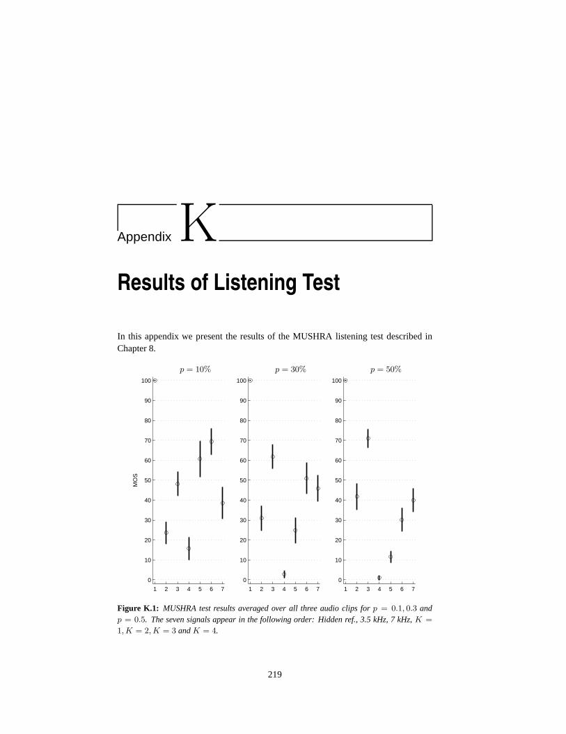
AppendixKResults of Listening Test
In this appendix we present the results of the MUSHRA listening test described inChapter 8.
1 2 3 4 5 6 7
0
10
20
30
40
50
60
70
80
90
100
MO
S
1 2 3 4 5 6 7
0
10
20
30
40
50
60
70
80
90
100
1 2 3 4 5 6 7
0
10
20
30
40
50
60
70
80
90
100
PSfrag replacements
p = 10% p = 30% p = 50%
Figure K.1: MUSHRA test results averaged over all three audio clips forp = 0.1, 0.3 andp = 0.5. The seven signals appear in the following order: Hidden ref., 3.5 kHz, 7 kHz,K =
1,K = 2, K = 3 andK = 4.
219

220 (Appendix K) Results of Listening Test
Orig 3.5kHz 7kHz K=1 K=2 K=3 K=40
10
20
30
40
50
60
70
80
90
100
MO
S
(a) p = 0.1
Orig 3.5kHz 7kHz K=1 K=2 K=3 K=40
10
20
30
40
50
60
70
80
90
100
MO
S
(b) p = 0.3
Orig 3.5kHz 7kHz K=1 K=2 K=3 K=40
10
20
30
40
50
60
70
80
90
100
MO
S
(c) p = 0.5
Figure K.2: MUSHRA test results for the jazz fragment andp = 0.1, 0.3 andp = 0.5.
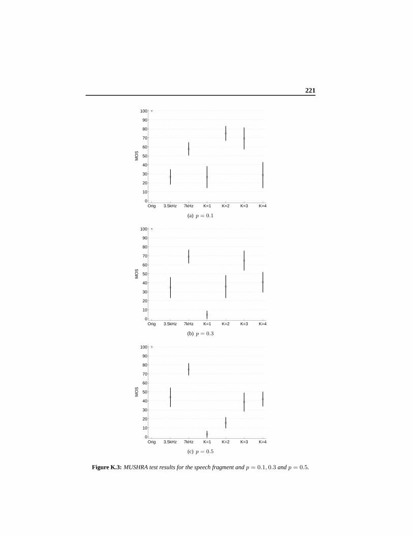
221
Orig 3.5kHz 7kHz K=1 K=2 K=3 K=40
10
20
30
40
50
60
70
80
90
100
MO
S
(a) p = 0.1
Orig 3.5kHz 7kHz K=1 K=2 K=3 K=40
10
20
30
40
50
60
70
80
90
100
MO
S
(b) p = 0.3
Orig 3.5kHz 7kHz K=1 K=2 K=3 K=40
10
20
30
40
50
60
70
80
90
100
MO
S
(c) p = 0.5
Figure K.3: MUSHRA test results for the speech fragment andp = 0.1, 0.3 andp = 0.5.

222 (Appendix K) Results of Listening Test
Orig 3.5kHz 7kHz K=1 K=2 K=3 K=40
10
20
30
40
50
60
70
80
90
100
MO
S
(a) p = 0.1
Orig 3.5kHz 7kHz K=1 K=2 K=3 K=40
10
20
30
40
50
60
70
80
90
100
MO
S
(b) p = 0.3
Orig 3.5kHz 7kHz K=1 K=2 K=3 K=40
10
20
30
40
50
60
70
80
90
100
MO
S
(c) p = 0.5
Figure K.4: MUSHRA test results for the rock fragment andp = 0.1, 0.3 andp = 0.5.
Samenvatting
Internetdiensten zoals het voice over Internet-protocol (VoIP) en audio/video stream-ing (b.v. video op verzoek en video vergaderen) worden steeds populairder door derecente groei van breedbandnetwerken. Dit soort "real-time" diensten vereisen vaakeen lage verzendtijd, een hoge bandbreedte en een lage pakket-verlies kans om ac-ceptabele kwaliteit voor de eindgebruikers te leveren. De heterogene communicatieinfrastructuur van de huidige pakketgeschakelde netwerken verschaffen echter geengegarandeerde prestaties met betrekking tot bandbreedte of verzendtijd en daaromwordt de gewenste kwaliteit over het algemeen niet bereikt.
Om een bepaalde mate van robuustheid te bereiken op kanalen waarop foutenkunnen voorkomen, kan multiple-description (MD) coding toegepast worden. Dit iseen methode waar de laatste tijd erg veel aandacht aan is besteed. Het MD probleemis in wezen een gecombineerd bron-kanaal coderingsprobleem dat gaat over (het metverlies) coderen van informatie voor transmissie over een onbetrouwbaarK-kanalencommunicatie systeem. De kanalen kunnen falen, met als resultaat het verlies vaneen pakket en daardoor een verlies van informatie aan de ontvangende kant. Welkevan de2K − 1 niet-triviale deelverzamelingen van deK kanalen falen, wordt bekendverondersteld aan de ontvangende kant, maar niet bij de encoder. Het probleem isdan een MD schema te ontwerpen dat, voor gegeven kanaal rate (of een gegeven somrate), de distorsies minimaliseert die een gevolg zijn van reconstruering van de bron,gebruik makend van informatie van willekeurige deelverzamelingen van de kanalen.
Hoewel wij ons in dit proefschrift hoofdzakelijk richten opde informatie theo-retische aspecten van MD codering, zullen we voor de volledigheid ook laten zienhoe het voorgestelde MD coderingsschema kan worden gebruikt om een perceptueelrobuuste audio coder te construeren, die geschikt is voor b.v. audio-streaming oppakketgeschakelde netwerken.
We richten ons op het MD probleem vanuit een bron-codering standpunt en bek-ijken het algemene geval vanK pakketten. We maken uitgebreid gebruik van lattice
223
224 Samenvatting
vector kwantisatie (LVQ) theorie, hetgeen een goed instrument blijkt, in de zin dathet voorgestelde MD-LVQ schema als brug tussen theorie en praktijk dient. Voorasymptotische gevallen van hoge resolutie en grote latticevector kwantisator dimen-sie, tonen wij aan dat de beste bekende informatie theoretische rate-distorsie MD gren-zen kunnen worden bereikt, terwijl we, in niet asymptotische gevallen van eindig-dimensionale lattice vector kwantisators (maar nog onder hoge resolutie veronder-stelling), praktische MD-LVQ schemas construeren, die vergelijkbaar met en vaaksuperieur zijn aan bestaande state-of-the-art schemas.
In het twee-kanaal symmetrische geval is eerder aangetoonddat de zij-representa-ties van een MD-LVQ schema zij-distorsies toelaten, die (bij hoge resolutie voorwaar-den) identiek zijn aan die vanL-dimensionale kwantisators met bolvormige Voronoicellen. In dit geval zeggen wij dat de zij-kwantisators deL-bol grens bereikt. Eendergelijk resultaat is niet eerder aangetoond voor het twee-kanaal asymmetrischegeval. Het voorgestelde MD-LVQ schema is echter in staat deL-bol grens te bereiken,bij hoge resolutie voorwaarden, voor zowel het symmetrische geval als het asym-metrische geval.
Het voorgestelde MD-LVQ schema schijnt een van de eerste schemas in de litera-tuur te zijn die het grootst bekende hoge resolutie drie-kanaal MD gebied in hetkwadratische Gaussische geval bereikt. Hoewel de optimaliteit alleen voorK ≤ 3
wordt bewezen, nemen we aan dat het optimaal is voor willekeurigeK representaties.We laten gesloten-vorm uitdrukkingen zien voor de rate en distorsie prestaties voor
algemene gladde stationaire bronnen en een kwadratische-fout distorsie criterium envoor hoge resolutie voorwaarden (ook voor eindig-dimensionale lattice vector kwanti-sators). Er wordt aangetoond dat de zij-distorsies in het drie-kanaal geval kan wordenuitgedrukt in het dimensieloze, genormaliseerde, tweede moment van eenL-bol, onaf-hankelijk van het type lattice dat wordt gebruikt voor de zij-kwantisators. Dit komtovereen met eerdere resultaten voor het geval van twee representaties.
Het rate verlies wanneer eindig-dimensionale lattice vector kwantisators gebruiktworden is onafhankelijk van het lattice en wordt gegeven door het rate verlies van eenL-bol en een bijkomende term die de ratio van twee dimensieloze expansie factorenbeschrijft. Er wordt aangetoond dat het totale rate verliessuperieur is aan bestaandedrie-kanaal schemas. Dit resultaat lijkt te gelden voor elkaantal representaties.

Curriculum Vitae
Jan Østergaard was born in Frederikshavn, Denmark, in 1974.He obtained his highschool diploma at Frederikshavns Tekniske Skole (HTX) in Frederikshavn in 1994.In 1999 he received the M.Sc. degree in Electrical Engineering at Aalborg University,Denmark. From 1999 to 2002 he worked as a researcher in the area of signal analysisand classification at ETI A/S in Aalborg, Denmark. From 2002 to 2003 he worked as aresearcher at ETI US in Virginia, United States. In February2003, he started as a Ph.D.student in the Information and Communication Theory group at Delft University ofTechnology, Delft, The Netherlands. During the period June2006 – September 2006he was a visiting researcher in the department of ElectricalEngineering-Systems atTel Aviv University, Tel Aviv, Israel.
225


Glossary of Symbols and Terms
Symbol DescriptionRL L-dimensional Euclidean space (real field)CL L-dimensional complex fieldZL L-dimensional set of all rational integersG Gaussian integersQ Algebraic integersE Eisenstein integers
H0 Lipschitz integersH1 Hurwitzian integersxH Hermitian transposition (conjugate transposition)x† Quaternionic transposition (Quaternionic conjugate transposition)J J -module (J -lattice)‖X‖ Vector norm with respect to underlying field
〈X,X〉 Inner product
Table K.1: Algebra-related symbols.
227

228 Glossary of Symbols and Terms
Symbol DescriptionX Scalar random process orL-dimensional random vector(X ∈ RL)
x L-dimensional vector (realization ofX)fX Distribution ofXX Reconstruction ofXX Alphabet ofX (usuallyX = RL)X Alphabet ofX (usuallyX ⊂ RL)ρ Fidelity criterion (usually squared-error)
R(D) Rate-distortion functionD(R) Distortion-rate functionI(·; ·) Mutual informationh(·) Differential entropyh(·) Differential entropy rateH(·) Discrete entropyE Statistical expectation operatorRSLB Shannon lower boundRLoss Rate lossR∗
red Rate redundancyDLoss Space-filling lossσ2X Variance ofXPX Entropy powerQ(X) Quantization ofX
Table K.2: Source-coding related symbols.

Glossary of Symbols and Terms 229
Symbol DescriptionΛc Central lattice (central quantizer)Λs SublatticeΛs ⊆ Λc (side quantizer in symmetric case)Λi SublatticeΛi ⊆ Λc (side quantizer in asymmetric case)Λπ Product latticeΛπ ⊂ Λi orΛπ ⊂ Λs
Λc/Λπ Quotient latticeVc Voronoi cell ofΛc
V Voronoi cell ofΛs orΛi
ν Volume of Voronoi cell ofΛc
νs Volume of Voronoi cell ofΛs
νi Volume of Voronoi cell ofΛi
νπ Volume of Voronoi cell ofΛπ
N Index value of sublatticeΛs (N = |Λc/Λs|)Ni Index value of sublatticeΛs (Ni = |Λc/Λi|)Nπ Index value of product latticeΛπ (Nπ = |Λc/Λπ|)N ′ Nesting ratio ofΛs (index per dimension)G(Λ) Dimensionless normalized second moment ofΛ
G(SL) Dimensionless normalized second moment ofL-sphereζi Basis vector (lattice generator vector)M Lattice generator matrixA Gram matrixΓm Multiplicative group of automorphisms of orderm
Λc/Λπ/Γm Set of orbit representativesZ1 Scalar lattice (uniform lattice)Z2 Square latticeZL Hypercubic latticeA2 Hexagonal two-dimensional latticeD4 Four dimensional (checker board) latticeξΛc Sublattice ofΛc (cyclic right submodule)Λcξ Sublattice ofΛc (cyclic left submodule)K(Λ) Kissing number ofΛ
Table K.3: Lattice-related symbols.
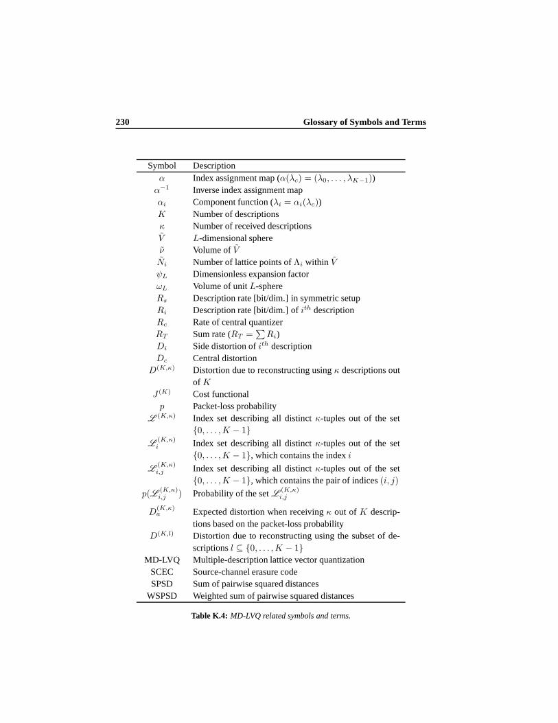
230 Glossary of Symbols and Terms
Symbol Descriptionα Index assignment map (α(λc) = (λ0, . . . , λK−1))α−1 Inverse index assignment mapαi Component function (λi = αi(λc))K Number of descriptionsκ Number of received descriptionsV L-dimensional sphereν Volume ofVNi Number of lattice points ofΛi within VψL Dimensionless expansion factorωL Volume of unitL-sphereRs Description rate [bit/dim.] in symmetric setupRi Description rate [bit/dim.] ofith descriptionRc Rate of central quantizerRT Sum rate (RT =
∑Ri)
Di Side distortion ofith descriptionDc Central distortion
D(K,κ) Distortion due to reconstructing usingκ descriptions outof K
J (K) Cost functionalp Packet-loss probability
L (K,κ) Index set describing all distinctκ-tuples out of the set0, . . . ,K − 1
L(K,κ)i Index set describing all distinctκ-tuples out of the set
0, . . . ,K − 1, which contains the indexi
L(K,κ)i,j Index set describing all distinctκ-tuples out of the set
0, . . . ,K − 1, which contains the pair of indices(i, j)
p(L(K,κ)i,j ) Probability of the setL (K,κ)
i,j
D(K,κ)a Expected distortion when receivingκ out ofK descrip-
tions based on the packet-loss probabilityD(K,l) Distortion due to reconstructing using the subset of de-
scriptionsl ⊆ 0, . . . ,K − 1MD-LVQ Multiple-description lattice vector quantization
SCEC Source-channel erasure codeSPSD Sum of pairwise squared distances
WSPSD Weighted sum of pairwise squared distances
Table K.4: MD-LVQ related symbols and terms.
Bibliography
[1] W. A. Adkins and S. H. Weintraub.Algebra an Approach via Module Theory.Springer-Verlag, 1992.
[2] R. Ahlswede. The rate-distortion region for multiple-descriptions without ex-cess rate.IEEE Trans. Inf. Theory, IT-31:721 – 726, November 1985.
[3] R. Arean, J. Kovacevic, and V. K. Goyal. Multiple description perceptual au-dio coding with correlating transform.IEEE Trans. Speech Audio Processing,8(2):140 – 145, March 2000.
[4] R. Balan, I. Daubechies, and V. Vaishampayan. The analysis and design of win-dowed fourier frame based multiple description source coding schemes.IEEETrans. Inf. Theory, 46(7):2491 – 2536, November 2000.
[5] J.-C. Batllo and V. A. Vaishampayan. Asymptotic performance of multipledescription transform codes.IEEE Trans. Inf. Theory, 43(2):703 – 707, March1997.
[6] W. E. Baylis and G. Jones. The Pauli algebra approach to special relativity. J.Phys. A: Math. Gen., 22:1 – 15, January 1989.
[7] W. R. Bennett. Spectra of quantized signals.Bell System Technical Journal,27:446 – 472, July 1948.
[8] T. Berger. Rate distortion theory, a mathematical basis for data compression.Prentice-Hall, 1971.
[9] T. Berger and J. D. Gibson. Lossy source coding.IEEE Trans. Inf. Theory,44(6):2693 – 2723, October 1998.
231
232 Bibliography
[10] T. Y. Berger-Wolf and E. M. Reingold. Index assignment for multichannelcommunication under failure.IEEE Trans. Inf. Theory, 48(10):2656 – 2668,October 2002.
[11] J. Bokowski and A. M. Odlyzko. Lattice points and the volume/area ratio ofconvex bodies.Geometriae Dedicata, 2:249 – 254, 1973.
[12] M. Bosi and R. E. Goldberg.Introduction to digital audio coding and stan-dards. Kluwer Academic Publishers, 2003.
[13] R. H. Buchholz. Perfect pyramids.Bulletin Australian Mathematical Society,45(3), 1992.
[14] A R. Calderbank, S. Das, N. Al-Dhahir, and S N. Diggavi. Construction andanalysis of a new quaternionic space-time code for4 transmit antennas.Com-munications in Information and Systems, 2005.
[15] J. Cardinal. Entropy-constrained index assignments for multiple descriptionquantizers.IEEE Trans. Signal Proc., 52(1):265 – 270, January 2004.
[16] J. Chen, C. Tian, T. Berger, and S. Hemami. Achieving themultiple descrip-tion rate-distortion region with lattice quantization. InProc. Conf. InformationSciences and Systems, 2005.
[17] J. Chen, C. Tian, T. Berger, and S. S. Hemami. A new class of universal multipledescription lattice quantizers. InProc. IEEE Int. Symp. Information Theory,pages 1803 – 1807, Adelaide, Australia, September 2005.
[18] J. Chen, C. Tian, T. Berger, and S. S. Hemami. Multiple descriptionquantization via Gram-Schmidt orthogonalization.IEEE Trans. Inf. Theory,52(12):5197 – 5217, December 2006.
[19] P. A. Chou, T. Lookabaugh, and R. M. Gray. Entropy-constrained vector quan-tization. IEEE Trans. Acoust., Speech, and Signal Proc., 37(1):31 – 42, January1989.
[20] P. A. Chou, S. Mehrotra, and A. Wang. Multiple description decoding of over-complete expansions using projections onto convex sets. InProc. Data Com-pression Conf., pages 72 – 81, March 1999.
[21] J. H. Conway, E. M. Rains, and N. J. A. Sloane. On the existence of similarsublattices.Canadian Jnl. Math., 51:1300 – 1306, 1999.
[22] J. H. Conway and N. J. A. Sloane.Sphere packings, Lattices and Groups.Springer, 3rd edition, 1999.
Bibliography 233
[23] J. H. Conway and D. A. Smith.On Quaternions and Octonions. AK Peters,2003.
[24] T. M. Cover and J. A. Thomas.Elements of information theory. Wiley, 1991.
[25] H. S. M. Coxeter.Regular polytopes. Dover, 1973.
[26] I. Csiszár and J. Körner.Information Theory: Coding Theorems for DiscreteMemoryless Systems. Academic Press, New York, 1981.
[27] S. N. Diggavi, N. J. A. Sloane, and V. A. Vaishampayan. Design of asymmetricmultiple description lattice vector quantizers. InProc. Data Compression Conf.,pages 490 – 499, March 2000.
[28] S. N. Diggavi, N. J. A. Sloane, and V. A. Vaishampayan. Asymmetric multipledescription lattice vector quantizers.IEEE Trans. Inf. Theory, 48(1):174 – 191,January 2002.
[29] P. L. Dragotti, J. Kovacevic, and V. K. Goyal. Quantized oversampled filterbanks with erasures. InProc. Data Compression Conf., pages 173 – 182, March2001.
[30] W. Ebeling.Lattices and Codes. Friedr. Vieweg & Sohn, 1994.
[31] B. Edler and G. Schuller. Audio coding using a psychoacoustic pre- and post-filter. In Proc. IEEE Int. Conf. Acoustics, Speech, and Signal Processing, vol-ume II, pages 881 – 884, 2000.
[32] W. H. R. Equitz and T. M. Cover. Successive refinement of information.IEEETrans. Inf. Theory, 37(2):269 – 275, March 1991.
[33] P. Erdös, P. M. Gruber, and J. Hammer.Lattice points, volume 39 ofPitmanMonographs and Surveys in Pure and Applied Mathematics. John Wiley &Sons, New York, 1989.
[34] T. Ericson and V. Zinoviev.Codes on Euclidean Spheres. North-Holland, May2001.
[35] H. Feng and M. Effros. On the rate loss of multiple description source codes.IEEE Trans. Inf. Theory, 51(2):671 – 683, February 2005.
[36] M. Fleming and M. Effros. Generalized multiple description vector quantiza-tion. In Proc. Data Compression Conf., March 1999.
[37] M. Fleming, Q. Zhao, and M. Effros. Network vector quantization.IEEE Trans.Inf. Theory, 50(8):1584 – 1604, August 2004.
234 Bibliography
[38] G. David Forney. On the duality of coding and quantization. In R. Calderbank,G. D. Forney Jr., and N. Moayeri, editors,DIMACS, volume 14 ofSeries in Dis-crete Mathematics and Theoretical Computer Science, pages 1 – 14. AmericanMathematical Society, 1993.
[39] Y. Frank-Dayan and R. Zamir. Dithered lattice-based quantizers for multipledescriptions.IEEE Trans. Inf. Theory, 48(1):192 – 204, January 2002.
[40] F. Fricker.Einführung in die gitterpunktlehre. Birkhäuser, 1982.
[41] R. G. Gallager.Information Theory and Reliable Communication. New-York:Wiley, 1968.
[42] A. A. El Gamal and T. M. Cover. Achievable rates for multiple descriptions.IEEE Trans. Inf. Theory, IT-28(6):851 – 857, November 1982.
[43] W. R. Gardner and B. D. Rao. Theoretical analysis of the high-rate vectorquantization of LPC parameters.IEEE Trans. Speech Audio Processing, pages367 – 381, September 1995.
[44] A. Gersho. Asymptotically optimal block quantization. IEEE Trans. Inf. The-ory, IT-25:373 – 380, July 1979.
[45] A. Gersho and R. M. Gray.Vector Quantization and Signal Compression.Kluwer Academic Publishers, 1992.
[46] J. D. Gibson and K. Sayood. Lattice quantization.Advances in Electronics andElectron Physics, 72:259 – 330, 1988.
[47] H. Gish and J. Pierce. Asymptotically efficient quantizing. IEEE Trans. Inf.Theory, 14(5):676 – 683, September 1968.
[48] N. Görtz and P. Leelapornchai. Optimization of the index assignments for mul-tiple description vector quantizers.IEEE Trans. Commun., 51(3):336 – 340,March 2003.
[49] V. Goyal, J. Kovacevic, and J. Kelner. Quantized frame expansions with era-sures.Journal of Appl. and Comput. Harmonic Analysis, 10(3):203–233, May2001.
[50] V. K. Goyal. Multiple description coding: Compressionmeets the network.IEEE Signal Processing Mag., 18(5):74 – 93, September 2001.
[51] V. K. Goyal, J. A. Kelner, and J. Kovacevic. Multiple description vector quan-tization with a coarse lattice.IEEE Trans. Inf. Theory, 48(3):781 – 788, March2002.
Bibliography 235
[52] V. K. Goyal and J. Kovacevic. Generalized multiple descriptions coding withcorrelating transforms.IEEE Trans. Inf. Theory, 47(6):2199 – 2224, September2001.
[53] V. K. Goyal, J. Kovacevic, and M. Vetterli. Multiple description transformcoding: Robustness to erasures using tight frame expansions. In Proc. IEEEInt. Symp. Information Theory, page 408, August 1998.
[54] V. K. Goyal, J. Kovacevic, and M. Vetterli. Quantized frame expansions assource channel codes for erasure channels. InProc. Data Compression Conf.,pages 326 – 335, March 1999.
[55] V. K. Goyal, M. Vetterli, and N. T. Thao. Quantized overcomplete expansionsin RN : analysis, synthesis, and algorithms.IEEE Trans. Inf. Theory, 44(1):16– 31, January 1998.
[56] R. L. Graham, D. E. Knuth, and O. Patashnik.Concrete mathematics. Addison-Wesley, 2nd edition, 1994.
[57] R. M. Gray.Source Coding Theory. Kluwer Academic Publishers, 1990.
[58] R. M. Gray and T. Linder. Results and conjectures on highrate quantization.In Proc. Data Compression Conf., pages 3 – 12, March 2004.
[59] R. M. Gray, T. Linder, and J. Li. A Lagrangian formulation of zador’s entropy-constrained quantization theorem.IEEE Trans. Inf. Theory, 48(3):695 – 707,March 2002.
[60] R. M. Gray and D. Neuhoff. Quantization.IEEE Trans. Inf. Theory, 44(6):2325– 2383, 1998.
[61] Pierre Grillet.Algebra. John Wiley & Sons, 1999.
[62] P. M. Gruber and C. G. Lekkerkerker.Geometry of numbers. North-Holland,2nd edition, 1987.
[63] A. György and T. Linder. A note on the existence of optimal entropy-constrained vector quantizers. InProc. IEEE Int. Symp. Information Theory,page 37, June 2002.
[64] A. György, T. Linder, P. A. Chou, and B. J. Betts. Do optimal entropy-constrained quantizers have a finite or infinite number of codewords? IEEETrans. Inf. Theory, 49(11):3031 – 3037, November 2003.
[65] X. Huang and X. Wu. Optimal index assignment for multiple description latticevector quantization. InProc. Data Compression Conf., Snowbird, Utah, March2006.
236 Bibliography
[66] Radiocommunication Sector BS.1534-1 International Telecommunica-tions Union. Method for the subjective assessment of intermediate qualitylevel coding systems (MUSHRA), January 2003.
[67] H. Jafarkhani and V. Tarokh. Multiple description trellis-coded quantization.IEEE Trans. Commun., 47(6):799 – 803, June 1999.
[68] N. S. Jayant. Subsampling of a DPCM speech channel to provide two self-contained, half-rate channels.Bell Syst. Tech. Jour., 60:501 – 509, April 1981.
[69] Alan Jeffrey and Daniel Zwillinger, editors.Table of integrals, series, andproducts. Academic Press, 6th edition, July 2000.
[70] P. Kabel. An examination and interpretation of ITU-R BS.1387: Perceptualevaluation of audio quality. TSP Lab Technical Report, Dept. Electrical &Computer Engineering, McGill University, May 2002.
[71] I. L. Kantor and A.S. Solodovnikov.Hypercomplex numbers; an elementaryintroduction to algebras. Springer-verlag, 1989.
[72] M. E. Keating.A first course in module theory. Imperial College Press, 1998.
[73] J. A. Kelner, V. K. Goyal, and J. Kovacevic. Multiple description lattice vectorquantization: Variations and extensions. InProc. Data Compression Conf.,pages 480 – 489, March 2000.
[74] J. C. Kieffer. A survey of the theory of source coding with a fidelity criterion.IEEE Trans. Inf. Theory, 39(5):1473 – 1490, September 1993.
[75] P. Koulgi, S. L. Regunathan, and K. Rose. Multiple description quantization bydeterministic annealing.IEEE Trans. Inf. Theory, 49(8):2067 – 2075, August2003.
[76] J. Kovacevic, P. L. Dragotti, and V. K. Goyal. Filter bank frame expansionswith erasures.IEEE Trans. Inf. Theory, 48(6):1439 – 1450, June 2002.
[77] E. Krätzel.Lattice points. Kluwer Academic Publisher, 1988.
[78] H. W. Kuhn. The Hungarian method for the assignment problem. In NavalResearch Logistics Quaterly, volume 2, pages 83 – 97, 1955.
[79] L. A. Lastras-Montano and V. Castelli. Near sufficiency of random coding fortwo descriptions.IEEE Trans. Inf. Theory, 52(2):681 – 695, February 2006.
[80] J. Li, N. Chaddha, and R. M. Gray. Asymptotic performance of vector quantiz-ers with a perceptual distortion measure.IEEE Trans. Inf. Theory, 45(4):1082– 1091, May 1999.
Bibliography 237
[81] Y. Linde, A. Buzo, and R. M. Gray. An algorithm for vectorquantizer design.IEEE Trans. Commun., 28(1):84 – 95, January 1980.
[82] T. Linder and R. Zamir. On the asymptotic tightness of the Shannon lowerbound.IEEE Trans. Inf. Theory, 40(6):2026 – 2031, November 1994.
[83] T. Linder and R. Zamir. High-resolution source coding for non-differencedistortion measures: the rate-distortion function.IEEE Trans. Inf. Theory,45(2):533 – 547, march 1999.
[84] T. Linder, R. Zamir, and K. Zeger. The multiple description rate region for highresolution source coding. InProc. Data Compression Conf., pages 149 – 158,March 1998.
[85] T. Linder, R. Zamir, and K. Zeger. High-resolution source coding for non-difference distortion measures: multidimensional companding. IEEE Trans.Inf. Theory, 45(2):548 – 561, march 1999.
[86] T. Linder and K. Zeger. Asymptotic entropy-constrained performance of tesse-lating and universal randomized lattice quantization.IEEE Trans. Inf. Theory,40(2):575 – 579, March 1994.
[87] S. P. Lloyd. Least squares quantization in PCM. Unpublished Bell Laboratoriestechnical note, 1957.
[88] S. P. Lloyd. Least squares quantization in PCM.IEEE Trans. Inf. Theory,IT-28(2):127 – 135, March 1982.
[89] D. G. Luenberger.Optimization by vector space methods. John Wiley andSons, Inc., 1 edition, 1997.
[90] H. S. Malvar.Signal processing with lapped transforms. Artech House, 1992.
[91] D. Marco and D. L. Neuhoff. Low-resolution scalar quantization for Gaussiansources and squared error.IEEE Trans. Inf. Theory, 52(4):1689 – 1697, April2006.
[92] J. E. Mazo and A. M. Odlyzko. Lattice points in high-dimensional spheres.Monatsh. Math., 110:47 – 61, 1990.
[93] International Standard ISO/IEC 11172-3 (MPEG). Information technology -coding of moving pictures and associated audio for digital storage media at upto about 1.5 mbit/s. part 3: Audio, 1993.
[94] International Standard ISO/IEC 13818-7 (MPEG). Information technology -generic coding of moving pictures and associated audio, part 7: Advanced au-dio coding, 1997.

238 Bibliography
[95] O. A. Niamut. Rate-distortion optimal time-frequency decompositions forMDCT-based audio coding. PhD thesis, Delft University of Technology,November 2006.
[96] O. Niemeyer and B. Edler. Efficient coding of excitationpatterns combinedwith a transform audio coder. InProc. of the 118th AES Conv., Barcelona,Spain, May 2005.
[97] M. T. Orchard, Y. Wang, V. Vaishampayan, and A. R. Reibman. Redundancyrate-distortion analysis of multiple description coding using pairwise correlat-ing transforms. InProc. IEEE Conf. on Image Proc., volume 1, pages 608 –611, 1997.
[98] J. Østergaard, R. Heusdens, and J. Jensen.n-channel asymmetric entropy-constrained multiple-description lattice vector quantization. IEEE Trans. Inf.Theory, 2005. Submitted.
[99] J. Østergaard, R. Heusdens, and J. Jensen.n-channel asymmetric multiple-description lattice vector quantization. InProc. IEEE Int. Symp. InformationTheory, pages 1793 – 1797, September 2005.
[100] J. Østergaard, R. Heusdens, and J. Jensen. On the bit distribution in asymmetricmultiple-description coding. In26th Symposium on Information Theory in theBenelux, pages 81 – 88, May 2005.
[101] J. Østergaard, R. Heusdens, and J. Jensen. On the rate loss in perceptual audiocoding. InProc. of IEEE BENELUX/DSP Valley Signal Processing Symposium,pages 27 – 30, Antwerpen, Belgium, 2006.
[102] J. Østergaard, R. Heusdens, and J. Jensen. Source-channel erasure codes withlattice codebooks for multiple description coding. InProc. IEEE Int. Symp.Information Theory, pages 2324 – 2328, July 2006.
[103] J. Østergaard, J. Jensen, and R. Heusdens. Entropy constrained multiple de-scription lattice vector quantization. InProc. IEEE Int. Conf. Acoustics, Speech,and Signal Processing, volume 4, pages 601 – 604, May 2004.
[104] J. Østergaard, J. Jensen, and R. Heusdens.n-channel symmetric multiple-description lattice vector quantization. InProc. Data Compression Conf., pages378 – 387, March 2005.
[105] J. Østergaard, J. Jensen, and R. Heusdens.n-channel entropy-constrainedmultiple-description lattice vector quantization.IEEE Trans. Inf. Theory,52(5):1956 – 1973, May 2006.
Bibliography 239
[106] J. Østergaard, O. A. Niamut, J. Jensen, and R. Heusdens. Perceptual audiocoding usingn-channel lattice vector quantization. InProc. IEEE Int. Conf.Acoustics, Speech, and Signal Processing, volume 5, pages 197 – 200, May2006.
[107] L. Ozarow. On a source-coding problem with two channels and three receivers.Bell System Technical Journal, 59:1909 – 1921, December 1980.
[108] Method for the objective measurements of perceived audio quality. ITU-R BS.1387, 1998.
[109] S. S. Pradhan, R. Puri, and K. Ramchandran. MDS source-channel erasurecodes. InProc. IEEE Int. Symp. Information Theory, June 2001. Special sessionon new results.
[110] S. S. Pradhan, R. Puri, and K. Ramchandran.(n, k) source-channel erasurecodes: Can parity bits also refine quality? InConference on Information Sci-ences and Systems, March 2001.
[111] S. S. Pradhan, R. Puri, and K. Ramchandran.n-channel symmetric multipledescriptions–part I:(n, k) source-channel erasure codes.IEEE Trans. Inf. The-ory, 50(1):47 – 61, January 2004.
[112] R. Puri, S. S. Pradhan, and K. Ramchandran.n-channel multiple descriptions:Theory and constructions. InProc. Data Compression Conf., pages 262 – 271,March 2002.
[113] R. Puri, S. S. Pradhan, and K. Ramchandran.n-channel symmetric multipledescriptions: New rate regions. InProc. IEEE Int. Symp. Information Theory,page 93, June 2002.
[114] R. Puri, S. S. Pradhan, and K. Ramchandran.n-channel symmetric multipledescriptions- part II: An achievable rate-distortion region. IEEE Trans. Inf.Theory, 51(4):1377 – 1392, April 2005.
[115] E. D. Rainville.Special functions. The Macmillan company, 1960.
[116] D. O. Reudink. The channel splitting problem with interpolative coders. Tech-nical Report TM80-134-1, Bell Labs, October 1980.
[117] R. T. Rockafellar.Convex analysis. Princeton University Press, 1970.
[118] D. J. Sakrison. The rate distortion function of a Gaussian process with aweighted square error criterion.IEEE Trans. Inf. Theory, IT-14:506 – 508,May 1968.
240 Bibliography
[119] G. Schuller, J. Kovacevic, F. Masson, and V. K. Goyal. Robust low-delay au-dio coding using multiple descriptions.IEEE Trans. Speech Audio Processing,13(5), September 2005.
[120] S. D. Servetto, V. A. Vaishampayan, and N. J. A. Sloane.Multiple descriptionlattice vector quantization. InProc. Data Compression Conf., pages 13 – 22,March 1999.
[121] C. E. Shannon. A mathematical theory of communication. Bell Syst. Tech.Journal, 27:379 – 423; 623 – 656, July and October 1948.
[122] C. E. Shannon. Coding theorems for a discrete source with a fidelity criterion.In IRE Conv. Rec., volume 7, pages 142 – 163, 1959.
[123] D. Sinha, J. D. Johnston, S. Dorward, and S. Quackenbush. The perceptualaudio coder (PAC). InThe digital signal processing handbook. New York:IEEE Press, 1998.
[124] D. Slepian and J. K. Wolf. Noiseless coding of correlated information sources.IEEE Trans. Inf. Theory, IT-19:471 – 480, 1973.
[125] N. J. A. Sloane. On-line encyclopedia of integer sequences. Published elec-tronically at http://www.research.att.com/˜njas/sequences, 2006.
[126] H. Stark and J. W. Woods.Probability, random processes, and estimation the-ory for engineers. Prentice-Hall, 1986.
[127] J. Østergaard and R. Zamir. Multiple-description coding by dithered delta-sigma quantization. InProc. Data Compression Conf., pages 63 – 72, March2007.
[128] R. K. Sundaram.A first course in optimization theory. Cambridge universitypress, 1999.
[129] C. Tian and S. S. Hemami. Optimality and suboptimalityof multiple-description vector quantization with a lattice codebook.IEEE Trans. Inf. The-ory, 50(10):2458 – 2470, October 2004.
[130] C. Tian and S. S. Hemami. Sequential design of multipledescription scalarquantizers. InProc. Data Compression Conf., pages 32 – 41, March 2004.
[131] C. Tian and S. S. Hemami. Universal multiple description scalar quantization:analysis and design.IEEE Trans. Inf. Theory, 50(9):2089 – 2102, September2004.
[132] C. Tian and S. S. Hemami. Staggered lattices in multiple description quantiza-tion. In Proc. Data Compression Conf., pages 398 – 407, March 2005.
Bibliography 241
[133] User datagram protocol: RFC-768. http://www.rfc-editor.org.
[134] Ogg Vorbis open-source audio codec. Published electronically at:http://www.vorbis.com.
[135] V. A. Vaishampayan. Design of multiple description scalar quantizers.IEEETrans. Inf. Theory, 39(3):821 – 834, May 1993.
[136] V. A. Vaishampayan and J.-C. Batllo. Asymptotic analysis of multiple descrip-tion quantizers.IEEE Trans. Inf. Theory, 44(1):278 – 284, January 1998.
[137] V. A. Vaishampayan, J.-C. Batllo, and A.R. Calderbank. On reducing gran-ular distortion in multiple description quantization. InProc. IEEE Int. Symp.Information Theory, page 98, August 1998.
[138] V. A. Vaishampayan and J. Domaszewicz. Design of entropy-constrainedmultiple-description scalar quantizers.IEEE Trans. Inf. Theory, 40(1):245 –250, January 1994.
[139] V. A. Vaishampayan, N. J. A. Sloane, and S. D. Servetto.Multiple-descriptionvector quantization with lattice codebooks: Design and analysis. IEEE Trans.Inf. Theory, 47(5):1718 – 1734, July 2001.
[140] S. van de Par, A. Kohlrausch, G. Charestan, and R. Heusdens. A new psychoa-coustical masking model for audio coding applications. InProc. of the 2002 Int.Conf. on Acoustics, Speech and Signal Processing, pages 1805–1808, Orlando,USA, May 2002.
[141] R. Venkataramani, G. Kramer, and V. K. Goyal. Bounds onthe achievableregion for certain multiple description coding problems. In Proc. IEEE Int.Symp. Information Theory, page 148, June 2001.
[142] R. Venkataramani, G. Kramer, and V. K. Goyal. Multipledescription codingwith many channels.IEEE Trans. Inf. Theory, 49(9):2106 – 2114, September2003.
[143] J. L. Verger-Gaugry. Covering a ball with smaller equal balls inRn. Discreteand Computational Geometry, 33:143 – 155, 2005.
[144] I. M. Vinograd. On the number of integer points in a sphere. Izv. Akad. NaukSSSR Ser. Math., 27, 1963.
[145] H. Viswanathan and R. Zamir. On the whiteness of high-resolution quantizationerrors.IEEE Trans. Inf. Theory, 47(5):2029 – 2038, July 2001.
[146] H. Wang and P. Viswanath. Vector gaussian multiple description with individualand central receivers. InProc. IEEE Int. Symp. Information Theory, 2006.
242 Bibliography
[147] X. Wang and M. T. Orchard. Multiple description codingusing trellis codedquantization. InIEEE Int. Conf. Image Processing, volume 1, pages 391 – 394,September 2000.
[148] Y. Wang, M. T. Orchard, and A. R. Reibman. Multiple description image codingfor noisy channels by pairing transform coefficients. InProc. IEEE WorkshopMultimedia Signal Processing, pages 419 – 424, 1997.
[149] Y. Wang, A. R. Reibman, M. T. Orchard, and H. Jafarkhani. An improvement tomultiple description transform coding.IEEE Trans. Signal Proc., 50(11):2843– 2854, November 2002.
[150] J. P. Ward. Quaternions and Cayley numbers; algebra and applications.Kluwer, 1997.
[151] D. B. West.Introduction to graph theory. Prentice Hall, 2001.
[152] H. Witsenhausen. On source networks with minimal breakdown degradation.Bell System Technical Journal, 59(6):1083 – 1087, July-August 1980.
[153] J. Wolf, A. Wyner, and J. Ziv. Source coding for multiple descriptions.BellSystem Technical Journal, 59(8):1417 – 1426, October 1980.
[154] A. Wyner and J. Ziv. The rate-distortion function for source coding with sideinformation at the receiver.IEEE Trans. Inf. Theory, 22:1 – 11, January 1976.
[155] P. Yahampath. On index assignment and the design of multiple descriptionquantizers. InProc. IEEE Int. Conf. Acoustics, Speech, and Signal Processing,May 2004.
[156] P. L. Zador. Asymptotic quantization error of continuous signals and their quan-tization dimension.IEEE Trans. Inf. Theory, IT-28(2), 1982.
[157] R. Zamir. Gaussian codes and shannon bounds for multiple descriptions.IEEETrans. Inf. Theory, 45(7):2629 – 2636, November 1999.
[158] R. Zamir. Shannon type bounds for multiple descriptions of a stationary source.Journal of Combinatorics, Information and System Sciences, pages 1 – 15, De-cember 2000.
[159] R. Zamir and M. Feder. On universal quantization by randomized uni-form/lattice quantizer.IEEE Trans. Inf. Theory, 38(2):428 – 436, March 1992.
[160] R. Zamir and M. Feder. Information rates of pre/post-filtered dithered quantiz-ers. IEEE Trans. Inf. Theory, 42(5):1340 – 1353, September 1996.
[161] R. Zamir and M. Feder. On lattice quantization noise.IEEE Trans. Inf. Theory,42(4):1152 – 1159, July 1996.
Bibliography 243
[162] R. Zamir, S. Shamai, and U. Erez. Nested linear/lattice codes for structuredmultiterminal binning.IEEE Trans. Inf. Theory, Special A.D. Wyner issue:1250– 1276, June 2002.
[163] Z. Zhang and T. Berger. New results in binary multiple descriptions. IEEETrans. Inf. Theory, 33(4):502 – 521, July 1987.
[164] Z. Zhang and T. Berger. Multiple description source coding with no excessmarginal rate.IEEE Trans. Inf. Theory, 41(2):349 – 357, March 1995.
[165] J. Ziv. On universal quantization.IEEE Trans. Inf. Theory, IT-31:344 – 347,May 1985.


Index
SymbolsψL . . . . . . . . . . . . . . . . 76, 77, 99, 184, 1916 dB per bit rule . . . . . . . . . . . . . . . . . . . . 27
AAAC . . . . . . . . . . . . . . . . . . . . .seeMPEG-2admissible index value . . . . . . . .seeindex
(admissible)affine hyperplane . . . . . . . . . . . . . . . . . . 186alphabet . . . . . . . . . . . . . . . . . . . . . . . . 25, 49
continuous . . . . . . . . . 25, 26, 29, 119countably finite . . . . . . . . . . . . . 25, 35countably infinite . . . . . . . . . . . . . . 25discrete . . . . . . . . . . . . . . . . 25, 29, 35reproduction . . . . . . . . . . . . . . . . . . . 30
anchor signals . . . . . . . . . . . . . . . . . . . . . 141annihilator . . . . . . . . . . . . . . . . . . . . . . . . 154audio coding . . . . . . . . . . . . . . . 6, 129, 146automorphism . . . . . . . . . . . . . . . . 154, 160
group . . . . . . . . . . . . . . . . . . . . 16, 160
Bball . . . . . . . . . . . . . . . . . . . . . . . . . . . . . . 186Barnes-Walls lattice. . . . . . . . . . . . . . . . .33bilinear form . . . . . . . . . . . . . . . . . 156, 157binomial series expansion . . . . . . . . . . 188bipartite matching problem . . . . . . . . . . 84
bit-allocation algorithm . . . . . . . . . . . . 136bounded support . . . . . . . . . . . . . . . 36, 214
CCartesian product . . . . . . . . . . . . 33, 49, 51central distortion . . . . . . . . . . . . . . 2, 42, 93central quantizer . . . . . . . . . 57, 58, 66, 69centroid . . . . . . . . . . . . . . . . . . . . . . . . 30, 67
geometric . . . . . . . . . . . . . . . . . . . . . 30checkerboard lattice . . . . . . . . . . . . . . . 169clean sublattice . . . . . . . . . . . . . . . . 12, 162closure . . . . . . . . . . . . . . . . . . . . . . . . . . . . 38complementary slackness variables . . 135compressor . . . . . . . . . . . . . . . . . . . . . . . 132conjugation
function . . . . . . . . . . . . . . . . . 156, 157Hermitian . . . . . . . . . . . . . . . . . . . . 159Quaternionic . . . . . . . . . . . . . 152, 159
continuous entropy . . . . . . . . .seeentropy(differential)
convex closure . . . . . . . . . .seeconvex hullconvex hull . . . . . . . . . .35, 40, 51, 56, 195correlation coefficient . . . . . . . . . . . .52, 54coset . . . . . . . . . . . . . . . . .16, 75, 78, 84, 99
representative . . . . . . . . . . . . . . . . . . 15cost functional . . . . . . . . . . 71, 72, 97, 135covariance matrix . . . . . . . . . . . . . . . . . . .27
245

246 Index
covering radius . . . . .seelattice (coveringradius)
Coxeter-Todd lattice . . . . . . . . . . . . . . . . 33cyclic
minimizer . . . . . . . . . . . . . . . . . . . . . 29submodule . . . . . . . . . . . . . . . . 19, 155
DDelta-Sigma quantization . . . . . . . . . . . .64description rate . . . . . . . . . . . . . . . 2, 47, 70determinant of a lattice . . . . . . . . . 10, 160dimensionless normalized second mo-
ment . . .seesecond moment ofinertia
direct sum . . . . . . . . . . . . . . . . . . . . . . . . 156Dirichlet regions . . . . . . .seeVoronoi celldistortion measure
covariance constraints . . . . . . . . . . 48difference . . . . . . . . . . . . . . . . . . 26, 27fidelity criterion . . . . . . . . . . . . . . . .25Hamming . . . . . . . . . . . . . . . . . . . . . 40locally quadratic . . . . . . . . . . .40, 132non difference . . . . . . . . . . . . . . . . 131perceptual . . . . . . . . . . . . . . . 130–132single letter . . . . . . . . . . . . . . . . 26, 47squared error26, 27, 29, 40, 46, 131,
132distortion product . . . . . . . . . . . . 44, 45, 60distortion-rate function . . . . . . . . . . . . . . 27distribution
conditional . . . . . . . . . . . . . . . . . . . . 26Gaussian . . . . . . . . . . . . . . . . . . .28, 35heavy tail . . . . . . . . . . . . . . . . . . . . . 35joint . . . . . . . . . . . . . . . . . . . . . . . . . . 26light tail . . . . . . . . . . . . . . . . . . . . . . . 35symmetric . . . . . . . . . . . . . . 48, 49, 54uniform . . . . . . . . . . . . . . . . 29, 31, 32
dual lattice . . . . . . . . . . . . . . . . . . . . . . . . 161
EECDQ . . . . . . . . . . . . . . . . . . . . . . . . . . . . . 31endomorphism . . . . . . . . . . . . . . . . . . . . 154
entropycoding . . . . . . . . . . . . . . . . . . . . . 29, 35differential . . . . . . . . . . . . . . . . . . . . 26discrete . . . . . . . . . . . . . . . . . . . . . . . 29of Gaussian vector . . . . . . . . . . . . . 27power . . . . . . . . . . . . . . . . . . . . . 28, 45rate . . . . . . . . . . . . . . . . . . . . . . . . . . . 26relative . . . . . . .seeKullback-Leibler
distanceentropy-constrained quantization . . . . . 29equivalence class . . . . . . . . . . . . .seecoseterasure channel . . . . . . . . . . . . . . . . . 38, 48expansion factor . . . . . . . . . . . . . . . .seeψL
Ffactor module . . . . .seemodule (quotient)fundamental
region . . . . . . . . . . . . . . . . . . . . . . . 160volume . . . . . . . . . . . . . . . . . . . . . . 160
GGamma function. . . . . . . . . . . . . . . . . . . .33Gaussian process . . . . . . . . . . . . . . . . . . . 27generator
matrix . . . . . . . . . . . . . . . . . . . . . . . . 10vector . . . . . . . . . . . . . . . . . . . . . 10, 18
geometricallysimilar . . . . . . . . . . . . . . . . . . . . . . . 163strictly similar . . . . . . . . . . . . . . . . 162
Gersho’s conjecture . . . . . . . . . . . . . . . . . 32Gosset lattice. . . . . . . . . . . . . . . . . . . . . . .33Gram matrix . . . . . . . . . . . . . . . . . . . . 10, 18group . . . . . . . . . . . . . . . . . . . . . . . . . . . 9, 12
Abelian . . .seegroup (commutative)action . . . . . . . . . . . . . . . . . . . . . . . . . 15commutative . . . . . . . . . . . . . . . . . 153of automorphisms . . . . . . . . . . . . . 154orbits . . . . . . . . . . . . . . . . . . . . . . . . 154reflection . . . . . . . . . . . . . . . . . . . . .165rotational . . . . . . . . . . . . . . . . . . . . 167sub . . . . . . . . . . . . . . . . . . . . . . .16, 155
Index 247
Hhexagonal lattice . . . . . . . .seelattice (A2)high rate . .seehigh resolution conditionshigh resolution conditions . . . . . . . . . . . 30homomorphism . . . . . . . . . . . . . . . . . . . 154Hungarian method . . . . . . . . . . . . . . . . . . 84hypercubic lattice . . . . . . .seelattice (Z4)hypergeometric function . . . . . . . . . . . 185
Iimpairment scale . . . . . . . . . . . . . . . . . . 145index
admissible . . . . . . . . . . . . . . . . 17, 162nesting ratio . . . . . . . . . . . . . . 12, 162
index-assignmentgreedy . . . . . . . . . . . . . . . . . . . . . . . . 85labeling function . . . . . . . . . . . 71, 94map . . . . . . . . . . . . . . . . . . . . . . . . . . 66matrix . . . . . . . . . . . . . . . . . . . . . . . . 60
inequalityCauchy-Schwartz . . . . . . . . . . . . . 210entropy-power . . . . . . . . . . . . . . . . . 27log . . . . . . . . . . . . . . . . . . . . . . . . . . 217
infimum . . . . . . . . . . . . . . . . . . . . . . . . 26, 35information divergence . . . . . . . . . . . . .see
Kullback-Leibler distanceinner bound . . . . . . . . . . . . . . . . . . . . . . . . 39inner product . .seenorm (inner product)input weighted . . .seedistortion measure
(non difference)integer
algebraic . . . . . . . . . . . . . . . . . . . . . . 13Eisenstein . . . . . . . . . . . . . . . . . . . . . 13Gaussian . . . . . . . . . . . . . . . . . . . . . . 13Hurwitzian . . . . . . . . . . . . . . . . . 19, 23Lipschitz . . . . . . . . . . . . . . . . . . 19, 21rational . . . . . . . . . . . . . . . . . . . . . . . 19residue ring . . . . . . . . . . . . . . . . . . 154
integral matrix . . . . . . . . . . . . . . . . . . . . 160isometry . . . . . . . . . . . . . .seeisomorphismisomorphism . . . . . . . . . . . . . . . . . . . . . . . 13
Jjoint source-channel coding . . . . . . . . . . . 2
KK-tuple . . . . . . . . . . . . . . . . . . . . . . . . . . . 66kissing-number . . 75, 162, 165, 166, 168,
170, 171Kullback-Leibler distance . . . . . . . . . . . 31
Llabeling function . .seeindex-assignment
(map)Lagrangian multipliers. . .seeLagrangian
weightsLagrangian optimal quantizer . . . . . . . . 35Lagrangian weights . . . . . . . . . . . . . . . . 135lattice . . . . . . . . . . . . . . . . . . . . . . . . . . . . . 10
A2 . . . . . . . . . . . . . . . . . . . . . . . . . . 167D4 . . . . . . . . . . . . . . . . . . . . . . . . . . 169Z1 . . . . . . . . . . . . . . . . . . . . . . . . . . 165Z2 . . . . . . . . . . . . . . . . . . . . . . . . . . 166Z4 . . . . . . . . . . . . . . . . . . . . . . . . . . 168covering radius . . . . . . . . . . .162, 195minimum squared distance . . . . . 161packing radius . . . . . . . . . . . . . . . . 162product lattice . . . . . . . . . . 19, 20, 23shell . . . . . . . . . . . . . . . . . . . . . . .74, 98sublattice . . . . . . . . . . . . . . . . 9, 11, 13
least common multiple . . . . . . . . . . . . . . 20Leech lattice . . . . . . . . . . . . . . . . . . . . . . . 33linear assignment . . . . . . . . . . . . . . . . . . . 84Lipschitz integer . .seeinteger (Lipschitz)listening test . . . . . . . . . . . . . . . . . .139, 141Lloyd algorithm . . . . . . . . . . . . . . . . . . . . 29
Mmarginal
excess rate . . . . . . . . . . . . . . . . . . . . 47Gaussian distributed . . . . . . . . . . . . 31no-excess rate . . . . . . . . . . . . . . 39, 42
Markov chain . . . . . . . . . . . . . . . . . . . . . . 62Markov process . . . . . . . . . . . . . . . . . . . 134
248 Index
masking curve . . . . . . . . . . . . . . . . 130, 136MDCT . . . . .seemodified discrete cosine
transformmeet . . . . . . . . . . . . . . . . . . . . . . . . . . . 20, 22memoryless process . . . .seememoryless
sourcememoryless source . . . . . . . . . . . . . . . . . 27minimum MSE estimation . . . . . . . 42, 52modified discrete cosine transform . .129,
130module . . . . . . . . . . . . . . . . . . . . . . . . . . 9, 12
action . . . . . . . . . . . . . . . . . . . . . . . .154algebraic . . . . . . . . . . . . . . . . . . . . . 153cyclic . . . . . .seecyclic (submodule)left . . . . . . . . . . . . . . . . . . . . . . . . . . 153quotient . . . . . . . . . . . . . . . 15, 16, 155right . . . . . . . . . . . . . . . . . . . . . . . . . 153sub . . . . . . . . . . . . . . . . . . . . . . . . . . . 13unital . . . . . . . . . . . . . . . . . . . . . . . . 153unitary . . . . . . . . . . . . . . . . . . . . . . . 153
modulolattice . . . . . . . . . . . . . . . . . . . . . . . . . 15
MP3 . . . . . . . . . . . . . . . . . . . . . . . . . . . . . 129MPEG-2. . . . . . . . . . . . . . . . . . . . . . . . . .129MSE 27,seedistortion measure (squared
error)MUSHRA test . . . . . . . . . . . . . . . . . . . . 141mutual information . . . . . . . . . . . . . . . . . 26
Nnearest neighbor
quantizer . . . . . . . . . . . . . . . . . . 28, 29region . . . . . . . . . . . . . . . . . . . . 10, 161
nesting ratio . . . .seeindex (nesting ratio)non-commutative ring . . . . . . . . . . . . . . . 20norm
inner product . . . . . . . . . . . . . .10, 159Quaternion . . . . . . . . . . . . . . . . . . . 152
Oobjective difference grade . . . . . . . . . . 145Ogg Vorbis . . . . . . . . . . . . . . . . . . . . . . . 129
operational lower hull . . . . . . . . . . . . . . . 89operational rate-distortion function . . . 35orbits . . . . . . . . . . . . . . . . . . . . . . 15, 16, 154outer bound . . . . . . . . . . . . . . . . . . . . . . . . 38overcomplete expansion . . . . . . . . . . . . . 57
PPAC. . . . . . . . . . . . . . . . . . . . . . . . . . . . . .129packet-loss probability . . . . . . . . . . . . . . 72packet-switched network . . . . . . . . . 6, 129packing radiusseelattice (packing radius)pdf . . . . .seeprobability density functionPEAQ . . . . . . . . . . . . . . . . . . . . . . . . . . . . 145Pochhammer symbol . . . . . . . . . . . . . . 185Poltyrev lattice . . . . . . . . . . . . . . . . . . . . . 33polymatroid . . . . . . . . . . . . . . . . . . . . . . . . 63polytope . . . . . . . . . . . . . . . . . . . . . . . . . . 160
congruent . . . . . . . . . . . . . . . . . 32, 161post filter . . . . . . . . . . . . . . . . . . . . . . 42, 132probability density function . . . 30, 31, 67product latticeseelattice (product lattice)pseudo-random process . . . . . . . . . . . . . 31psycho-acoustic analysis . . . . . . . . . . . 130
Qquadratic
form . . . . . . . . . . . . . . . . . . . . . . . . . 157Gaussian 5, 40, 41, 47, 51, 118, 123
quantization theory . . . . . . . . . . . . . . . . . 28Quaternions . . . . . . . . . . . . . . . . . . . . . . .151quintuple . . . . . . . . . . . . . . . . . . . . . . . . . . 38quotient
compact . . . . . . . . . . . . . .12, 160, 161lattice . . . . . . . . . . . . . . . . . . . . . . . .162module. . . . . . . . . . . . . . . . . . . . . . . .84
Rradius ofL-sphere . . . . . . . . . . . . . . . . . 189random
binning . . . . . . . . . . . . . 118–120, 126codebook . . . . . . . . . . . . . . . . . . . . 119
rate loss
Index 249
MD . . . . . . . . . . . . . . . . . . . 62, 63, 125MD-LVQ . . . . . . . . . . . . . . . . . . . . 125SD . . . . . . . . . . . . . . . . . . . . . . . . . . . 33
rate redundancyMD. . . . . . . . . . . . . . . . . . . . . . . . . . . 42SD . . . . . . . . . . . . . . . . . . . . . . . . . . . 32
rate-distortionbounds . . . . . . . . . . . . . . . . . . . . . . . . 38function . . . . . . . . . . . . . . . . . . . . . . . 39MD region . . . . . . . . . . . . . . . . . . . . 38region. . . . . . . . . . . . . . . . . . . . . . . . .39theory . . . . . . . . . . . . . . . . . . . . . . . . .25
reflection . . . . . . . . . . . . . . . . . . . . .161, 163relative entropy . . . .seeKullback-Leibler
distancerepetition code . . . . . . . . . . . . . . . . . . . . . 58resolution-constrained quantization . . . 29rotation
transform . . . . . . . . . . . . . . . . 161, 163
Sscalable coding . . . . . . . . . . . . . . . . . . . . 144scalar
process. . . . . . . . . . . . . . . . . . . . . . . .26quantization . . . . . . . . . . . . . . . . 57, 60
scalar lattice . . . . . . . . . . . .seelattice (Z1)SCEC . .seesource-channel erasure codeSchläfli lattice . . . . . . . . . . . . . . . . . 33, 169second-moment of inertia . . . . . . . . . . 162
of anL-sphere . . . . . . . . . . . . . . . . . 32of a lattice . . . . . . . . . . . . . . . . 33, 161
sesquilinear form . . . . . . . . . . . . . . . . . . 157Shannon lower bound . . . . . . . . . . . .27, 32shift invariance . . . . . . . . . . . . . 67, 84, 100side distortion . . . . . 2, 39, 80, 81, 93, 108
high . . . . . . . . . . . . . . . . . . . . . . . . . . 41side quantizer . . . . . . . . . . . . . 4, 57, 65, 66side rate . . . . . . . . . . . .seedescription ratesimplex
regular . . . . . . . . . . . . . . . . . . . . . . . 194skew field . . . . . . . . . . . . . . . . . . . . . . . . .151Slepian-Wolf coding . . . . . . . . . . . . . . . . 48
smooth source . . . . . . . . . . . . . . . . . . 31, 32source coding . . . . . . . . . . . . . . . . . . . . . . 25
lossy . . . . . . . . . . . . . . . . . . . . . . . . . . 25source splitting . . . . . . . . . . . . . 62, 63, 125source-channel erasure code . 48, 57, 116space-filling gain . . .seespace-filling lossspace-filling loss . . . . . . . . . . . .34, 60, 162spectral band replication . . . . . . . . . . . 138sphere
bound . . . . . . . . . . . . . . . . . . . . . . . . . 61second-moment . . . . . . . . . . . . . . . . 32volume . . . . . . . . . . . . . . . . . . . . . . 190
spherical cap . . . . . . . . . . . . . . . . . . . . . . 186SPSD . . . . . .seesum of pairwise squared
distancessquare lattice . . . . . . . . . . .seelattice (Z2)staggering gain . . . . . . . . . . . . . . . . . . . . . 58stationary process. . . . . . . . . . . . . . . . . . .25subgroup . 166, 167, 169,seegroup (sub)sublattice . . . . . . . 66, 74,seelattice (sub)subtractive dither . . . . . . . . . . . . . . . . . . . 31successive refinement . . . . . . . . . 5, 61, 65sum of pairwise squared distances 73, 74,
76, 79, 84sum rate. . . . . .37, 41, 107, 124, 127, 148
excess . . . . . . . . . . . . . . . . . . . . . . . . 40no excess . . . . . . . . . . . . . . . 39, 42, 43
Ttarget entropy . . . . . . . . . . . .seetarget ratetarget rate . . . . . . . .5, 81, 82, 89, 104, 105tessellating
quantizer . . . . . . . . . . . . . . . . . . . . . . 10region . . . . . . . . . . . . . . . . . . . . . . . 160
test channel . . . . . . . . . . . . . . . . . 41, 42, 52tetrahedron . . . . . . . . . . . . . . . . . . . . . . . 194theta series . . . . . 161, 165, 166, 168, 169threshold in quiet . . . . . . . . . . . . . . . . . . 137tight bound . . . . . . . . . . . . . . . . . . . . . . . . 38time sharing . . . . . . . . . . . . 35, 66, 78, 100time-frequency analysis . . . . . . . . . . . . 129torsion . . . . . . . . . . . . . . . . . . . . . . . . . . . 154
250 Index
free . . . . . . . . . . . . . . . . . . . 12, 19, 154torus . . . . . . . . . . . . . . . . . . . . . . . . . . . . . 160trellis coded quantization . . . . . . . . . . . . 57typical
jointly . . . . . . . . . . . . . . . . . . . . . . . 119set . . . . . . . . . . . . . . . . . . . . . . . . . . . . 29strongly . . . . . . . . . . . . . . . . . . . . . . 119
Uunique factorization ring . . . . . . . . . . . . 20
VVoice over IP . . . . . . . . . . . . . . . . . . . . . . . . 1volume
regular simplex . . . . . . . . . . . . . . . 195spherical cap . . . . . . . . . . . . . . . . . 186unit-sphere . . . . . . . . . . . . . . . . . . . 190
Voronoi cell . . . . . . . . . . . 67, 68, 161, 162spherical . . . . . . . . . . . . . . . 60, 63, 71
Wweight ratio . . . . . . . . . . . . . . . . . . 109, 110weighted sum of pairwise squared dis-
tances. . . . . . . . . . . . . . . . . . . .98,99
WSPSD . . .seeweighted sum of pairwisesquared distances
Wyner-Ziv coding . . . . . . . . . . . . . . . . . . 48

![arXiv:2011.03395v2 [cs.LG] 24 Nov 2020](https://static.fdocuments.nl/doc/165x107/61cb75f2e49e730eca229624/arxiv201103395v2-cslg-24-nov-2020.jpg)

![arXiv:2108.05028v2 [cs.CV] 23 Sep 2021](https://static.fdocuments.nl/doc/165x107/6207eaf1e5248f5b80789422/arxiv210805028v2-cscv-23-sep-2021.jpg)
![arXiv:2102.10240v2 [cs.LG] 28 Feb 2021](https://static.fdocuments.nl/doc/165x107/620743cab3f32c352d2a6f75/arxiv210210240v2-cslg-28-feb-2021.jpg)

![arXiv:1605.03092v1 [physics.flu-dyn] 10 May 2016](https://static.fdocuments.nl/doc/165x107/62021446ac5c64589c2741fc/arxiv160503092v1-10-may-2016.jpg)

![arXiv:2110.00976v1 [cs.CL] 3 Oct 2021](https://static.fdocuments.nl/doc/165x107/618128f0c6657810fd459d58/arxiv211000976v1-cscl-3-oct-2021.jpg)
![arXiv:1104.1905v2 [cs.MA] 12 Aug 2011](https://static.fdocuments.nl/doc/165x107/61e4edf35af159063323d858/arxiv11041905v2-csma-12-aug-2011.jpg)

![arXiv:1212.2865v2 [cs.IT] 18 Dec 2012](https://static.fdocuments.nl/doc/165x107/61e1c47a0cf8ff11dd71d367/arxiv12122865v2-csit-18-dec-2012.jpg)

![arXiv:2010.03923v2 [cs.MS] 11 Oct 2020](https://static.fdocuments.nl/doc/165x107/6240a17de7a6ce0b477bd33e/arxiv201003923v2-csms-11-oct-2020.jpg)

![arXiv:2108.13418v1 [astro-ph.IM] 30 Aug 2021](https://static.fdocuments.nl/doc/165x107/62abbf549eeafa0f4f109d56/arxiv210813418v1-astro-phim-30-aug-2021.jpg)
![arXiv:2102.06779v3 [cs.LG] 26 Feb 2021](https://static.fdocuments.nl/doc/165x107/6169dd6d11a7b741a34c3934/arxiv210206779v3-cslg-26-feb-2021.jpg)
![arXiv:1908.00080v3 [cs.LG] 21 Sep 2020](https://static.fdocuments.nl/doc/165x107/621685614e46432aea29b82e/arxiv190800080v3-cslg-21-sep-2020.jpg)
![arXiv:2108.12971v1 [cs.CL] 30 Aug 2021](https://static.fdocuments.nl/doc/165x107/6169b54c11a7b741a34a7b37/arxiv210812971v1-cscl-30-aug-2021.jpg)