![Further Studies of BURSTS and Spallation in High-Energy ... · this work [1] [2] that in highenergy heavy ion reactions above a threshold of - Ecm/u ~150 MeV two dominant reaction](https://static.fdocuments.nl/doc/165x107/5e41f7dd38737e65897c3ce7/further-studies-of-bursts-and-spallation-in-high-energy-this-work-1-2-that.jpg)
Numerical Combustion Modeling For Complex Reaction Systems · 2007-03-06 · Numerical Combustion...
235
Numerical Combustion Modeling for Complex Reaction Systems PROEFSCHRIFT ter verkrijging van de graad van doctor aan de Technische Universiteit Eindhoven, op gezag van de Rector Magnificus, prof.dr.ir. C.J. van Duijn, voor een commissie aangewezen door het College voor Promoties in het openbaar te verdedigen op dinsdag 13 februari 2007 om 14.00 uur door Alexey Evlampiev geboren te Moskou, Rusland
Transcript of Numerical Combustion Modeling For Complex Reaction Systems · 2007-03-06 · Numerical Combustion...
Numerical Combustion Modeling
for Complex Reaction Systems
PROEFSCHRIFT
ter verkrijging van de graad van doctor aan de Technische Universiteit Eindhoven, op gezag van de
Rector Magnificus, prof.dr.ir. C.J. van Duijn, voor een commissie aangewezen door het College voor
Promoties in het openbaar te verdedigen op dinsdag 13 februari 2007 om 14.00 uur
door
Alexey Evlampiev
geboren te Moskou, Rusland
Dit proefschrift is goedgekeurd door de promotoren: prof. dr. ir. R.S.G. Baert en prof. dr. L.P.H. de Goey Copromotor: dr. ir. L.M.T. Somers A catalogue record is available from the Library Eindhoven University of Technology ISBN-10: 90-386-2719-X ISBN-13: 978-90-386-2719-9
This research was supported by the Dutch Technology Foundation STW (project EWE.5125)
Acknowledgements
In the creating process of this thesis I received the help of many people. I would like to thank Rik Baert, Philip de Goey and Bart Somers for the freedom they gave me in doing my research. Furthermore I would like to thank my colleagues from Eindhoven. Special thanks go to my parents, brother, family and friends who supported me all those years. Nora without you my thesis would not have appeared. There are a few people that I would like to thank personally: Vincent Huijnen You were my roommate for three years. Thank you for your patience while hearing my talks. Thanks also for all the discussions and help in establishing 3D flow field simulations. Viktor Kornilov Thank you Viktor for all you did. With you I practically discussed 100% of my work. I very much appreciate your interest and support up to the last moment. Bernard Geurts Thank you very much for the critical notes you gave. They helped me to improve the thesis. Henning Richter and Alexander Konnov The correspondence we had during my PhD project stimulated me to continue my work when things were going difficult. Thank you both for that. Thanks a lot to the people who helped me gaining my knowledge during my studying and work in Moscow: Alexander Konstantinovich Parfionov† Alexander Vasilievich Lubimov Sergey Mihailovich Frolov Valentin Yakovlevich Basevich Vladimir Segizmundovich Posvianskiy A.A. Beliaev

Contents
1 Introduction.................................................................................................. 1 1.1 Background........................................................................................................... 1 1.2 The state of art with Diesel combustion modeling........................................ 2
1.2.1 Turbulent reactive flow modeling..................................................................... 3 1.2.2 Fuel Injection and Sprays Formation Modeling............................................. 4 1.2.3 Modeling of Auto-ignition, Combustion and Emission ............................... 5 1.2.4 Modeling of High-Pressure Effects.................................................................. 6
1.3 Focus of this thesis.............................................................................................. 6 1.3.1 High-pressures effects ........................................................................................ 7 1.3.2 Auto-ignition ........................................................................................................ 7 1.3.3 Soot formation ..................................................................................................... 8
1.4 Challenges ............................................................................................................. 9 1.4.1 Introducing combustion sub-models ............................................................... 9 1.4.2 Ensuring Computational efficiency................................................................ 11 1.4.3 Introducing efficient methods for data interpreting and processing........ 12
1.5 Approach ............................................................................................................ 13 1.6 Outline of this thesis ......................................................................................... 15
2 Processing and analysis of chemical and thermo-physical data ............... 17 2.1 Introduction........................................................................................................ 17
2.1.1 Complex chemistry............................................................................................ 19 2.1.2 Critical properties .............................................................................................. 22 2.1.3 Thermodynamics ............................................................................................... 25 2.1.4 Molecular Transport Properties ...................................................................... 28 2.1.5 Outline................................................................................................................. 35
2.2 TROT: A C++ program for interpreting and analysis of chemical and thermo-physical data .......................................................................................................... 36
2.2.1 Interpreter ........................................................................................................... 38 2.2.2 Linker................................................................................................................... 39 2.2.3 Structure of input .............................................................................................. 41
2.3 C-MECH: An inline source code format for reaction mechanisms ......... 43 2.4 Some typical results ........................................................................................... 45
2.4.1 Molecular transport coefficients ..................................................................... 45 2.4.2 Complex chemistry............................................................................................ 53
2.5 Summary ............................................................................................................. 56
3 Modeling homogeneous reactions at supercritical high-pressure conditions .......................................................................................................... 59
3.1 Introduction........................................................................................................ 59 3.2 Modeling Homogeneous Reaction Processes............................................... 61
iv
3.2.1 Problem formulation......................................................................................... 62 3.2.2 Method of solution............................................................................................ 65 3.2.3 Reaction mechanism ......................................................................................... 66 3.2.4 Approach ............................................................................................................ 70
3.3 Results ................................................................................................................. 74 3.3.1 Auto-ignition ...................................................................................................... 74 3.3.2 NO-formation.................................................................................................... 77
3.4 Discussion........................................................................................................... 82 3.5 Conclusions ........................................................................................................ 85
4 Modeling of One-Dimensional Diffusion Flamelets with Complex Chemistry........................................................................................................... 87
4.1 Introduction........................................................................................................ 87 4.1.1 Flamelet modeling ............................................................................................. 87 4.1.2 Laminar counterflow diffusion flame ............................................................ 89
4.2 Numerical approach.......................................................................................... 92 4.2.1 Finite differences representation..................................................................... 93 4.2.2 Method of Solution ........................................................................................... 95 4.2.3 Modified Differential and Finite Difference Operators ............................. 97 4.2.4 Implementation................................................................................................100
4.3 Validation of the CFDF-program.................................................................103 4.3.1 Steady non-reactive mixing layer...................................................................103 4.3.2 Modeling partially premixed n-heptane flames ..........................................106 4.3.3 Non-premixed dimethyl-carbonate flame ...................................................112
4.4 Modeling high-pressure effects .....................................................................115 4.4.1 The non-ideal gas model ................................................................................116 4.4.2 Two test cases ..................................................................................................117 4.4.3 Results and discussion ....................................................................................119
4.5 Conclusions ......................................................................................................123
5 Detailed Modeling of Soot Formation ......................................................125 5.1 Introduction......................................................................................................125
5.1.1 The problem of soot pollution......................................................................125 5.1.2 Phenomenology of soot formation ..............................................................127 5.1.3 Numerical models............................................................................................130
5.2 The effect of the mixing rate on PAH/Soot formation in steady diffusion flamelets 134
5.2.1 Background.......................................................................................................135 5.2.2 The applied sectional model ..........................................................................139 5.2.3 Studying approach ...........................................................................................145
5.3 Results and Discussion ...................................................................................147 5.3.1 Structure of sooting flamelets........................................................................147 5.3.2 Effects of the mixing rate...............................................................................150 5.3.3 Particle size distribution function .................................................................158
v
5.4 Conclusions ......................................................................................................160
6 Steady turbulent jet diffusion flames ........................................................163 6.1 Introduction......................................................................................................163 6.2 Turbulent combustion model........................................................................164
6.2.1 Steady laminar flamelet assumption .............................................................165 6.2.2 Statistical description of turbulent diffusion flame....................................166
6.3 Numerical implementation ............................................................................172 6.3.1 KIVA-3V simulator for turbulent reactive flows.......................................172 6.3.2 Mixture fraction variable ................................................................................173
6.4 Sandia flame D.................................................................................................174 6.4.1 Experimental setup of Sandia Flame D.......................................................175 6.4.2 Numerical setup...............................................................................................175 6.4.3 Results and discussion ....................................................................................177
6.5 PAH/soot modeling in ethylene/air flame.................................................184 6.5.1 Experimental setup of Turbulent Non-premixed Ethylene/Air Jet Flame. 184 6.5.2 Numerical setup...............................................................................................184 6.5.3 Results and discussion ....................................................................................184
6.6 Conclusions ......................................................................................................190
7 Conclusions and recommendations..........................................................193
A Output format of the TROT processor.....................................................197
B Modified Gauss Algorithm for Block Tri-diagonal Matrices .................. 203
C Steady Laminar Flamelet Libraries.......................................................... 207
References........................................................................................................ 209
Abstract ............................................................................................................ 223
Samenvatting ................................................................................................... 225
Curriculum Vitae ............................................................................................. 227

Chapter 1
1 Introduction
1.1 Background The internal combustion engine has been with us for over a century. For a long time the development of this power source focused on increasing its reliability and performance. Over the last decades however, the main driver for further engine development has been the reduction of its emission of noise and of pollutants (while maintaining of course reliability and performance). This has resulted in the introduction of catalytic aftertreatment systems but also of new variable fuelling technology, variable valve timing technology, variable turbocharging systems and – recently - even systems that allow varying engine compression ratio. This has given the engine much more flexibility such that, in combination with electronic control, it has been able to meet the increasingly stringent emission legislation imposed by governments. At the same time this increased flexibility has made the engine design and calibration process much more difficult. To avoid a corresponding increase in development time, engine manufacturers are continuously looking for ways to improve this development process. It is expected that, in the future, detailed multi-dimensional numerical simulations of the engine combustion process will play an increasingly important role in engine development: • they give information that would otherwise be available only when applying very
complex laser diagnostics to a dedicated research engine that was modified for optical access,
• they can give this information at an early stage, when the engine is still on the drawing board, thus avoiding – to some extent – the number of prototype parts,
• they can be used to calibrate simpler low-dimensional models that in turn can be used for defining control algorithms.
Introduction 2
With recent progress in the areas of numerical methods, mesh flexibility and flow visualization, computational fluid dynamics (CFD) has become one of the most powerful and efficient tools for obtaining and analyzing of detailed three-dimensional flow data for internal combustion (IC) engines. However, the development of adequate and accurate CFD methodology and efficient computer codes for engine simulation is still a challenging task. The most important reason for this is that the IC-process consists of a high number of very complex and interacting phenomena. In the case of Diesel engine combustion, the key processes that need accurate modeling are: • non-stationary turbulent flow • injection, atomization, dispersion and evaporation of liquid fuel • fuel auto-ignition and combustion • formation of harmful pollutants such as nitrogen oxides (NOx) and particulates. Therefore, the first requirement of a CFD code is that it should model these processes with sufficient accuracy. A second requirement is that it should do this for the complex, time-varying geometries typical of modern internal engines. Finally, all this should be possible with acceptable investments in computing power and within reasonably short computational times. In the following section the state of art will be reviewed. The given materials are based on and also adopted from a number of extended reviews dedicated to engine CFD-modeling. Since this thesis is part of a larger project aimed at improved numerical modeling of combustion and emissions formation [1] in modern heavy-duty truck Diesel engines, the focus of this section and the rest of this thesis is also Diesel engine modeling.
1.2 The state of art with Diesel combustion modeling
The internal combustion engine represents one of the most challenging fluid mechanics problems to be modeled because the flow is compressible with large density variations, turbulent, unsteady, cyclic, and non-stationary, both spatially and temporally [2]. The combustion characteristics are greatly influenced by the details of the fuel preparation process and by the distribution of fuel in the engine which is, in turn, controlled by the in-cylinder fluid mechanics. Liquid fuel injection introduces the complexity of describing the physics of vaporizing two-phase flows that vary spatially and temporally from very dense to fairly dilute. Pollutant emissions are controlled by details of the turbulent fuel-air mixing and combustion processes, and a
The state of art with Diesel combustion modeling 3
detailed understanding of these processes is required to improve performance and reduce emissions while not compromising fuel economy. In spite of the detailed nature of even the most comprehensive of diesel engine codes, they will not be entirely predictive for the foreseeable future due to the wide range of length and timescales needed to describe engine fluid mechanics. Current storage and run times capabilities of computers limit simulations to some millions of grid points [2]. For geometries of practical interest, this often prevents the spatial resolution of many important processes like local auto-ignition or rolling up of flame surfaces. The required computer capabilities will be difficult to realize in the next decade, even with the most optimistic projections about computer power increases. A detailed review on the numerical aspects of engine modeling can be found in [3]. Diesel combustion presents especially difficult and complex modeling challenges. For example, sub-models are required for turbulence, spray injection, atomization, breakup, coalescence, vaporization, ignition, premixed combustion, diffusion combustion, wall heat transfer, and emissions (soot and NOx). All of these sub-models must work together in turbulent flow fields. Until now this complexity has prevented widespread application of these models.
1.2.1 Turbulent reactive flow modeling The fluid mechanical properties of the combustion system must be well known to describe the mixing between reactants and all transfer phenomena occurring in turbulent flames (heat transfer, molecular diffusion, convection, turbulent transport, etc.). In the case of combustion taking place in IC-engines, the turbulent flow field is characterized by a wide range of time and length scales that cannot be resolved numerically. In practice, engine simulations aim to predict only the statistically averaged flow field, so local fluctuations and turbulent structures are integrated in the averaged quantities and do not have to be described in detail. The corresponding procedure is called Reynolds Averaged Navier-Stokes (RANS) modeling. The RANS-transformation of the general flow equations yields unclosed quantities, representative of the turbulent fluctuations, that must be modeled [4]. The Reynolds averaging technique therefore leads to the need for closing models. Most engineering and academic engine codes employ some version of the well-known k ε− model. This RANS approach is presently the only one really suited for the simulation of practical configurations, but its accuracy is limited and while it has been used to identify trends, its predictive capabilities are limited. The one practical alternative to the k ε− model is Large Eddy Simulation (LES). In LES, the largest structures of the flow field are explicitly computed whereas the effects of small-scale structures are modeled. For certain applications, especially for intrinsically time-varying problems like an engine, it is expected that LES will replace the k ε− approach. LES simulations are thus, by construction, more expensive than RANS calculations but are already widely used for non-reacting flow simulations. For turbulent combustion they are still at an early stage of development.
Introduction 4
Compared to RANS, LES requires a lower level of empirical input but provides more complete information on in-cylinder flow structure. LES offers a more realistic representation of the in-cylinder turbulent flow compared to RANS. In many cases of practical CFD modeling transition from RANS to LES is highly desirable. Initially LES will be used to address fundamental aspects of in-cylinder turbulent flow structure, but eventually it is likely to become the engineering turbulence model of choice. At this point it is also worthwhile mentioning DNS. Both RANS and LES approaches require modeling the effects of turbulent structures. The direct numerical simulation (DNS) solving all the physical spatial and time-scales (without any model for turbulence) offers an excellent complement to experiments in order to assess the importance of various physical mechanisms, to obtain complementary information and therefore to improve turbulent combustion modeling [4]. It has been widely used for premixed [5, 6] as well as non-premixed [7, 8] combustion. Many authors have employed DNS as a "numerical experiment" where unwanted physical effects can be excluded by design.
1.2.2 Fuel Injection and Sprays Formation Modeling Spray modeling is another key component of CFD-models for Diesel engine calculation. This is because of the controlling role of fuel injection on combustion and emission formation in these engines. Two main mathematical frameworks have been used to describe sprays: one is the Continuum Eulerian (CE) approach [9, 10]; and the other is the Discrete Lagrangian (DL) approach [11-13]. Both approaches present certain difficulties when applied to Diesel sprays. A comprehensive overview of these difficulties can be found in [14]. As shown in the same review, models of different levels of capability are now available for nearly all fuel injection processes (at least for Diesel engines), including: • pump/line/nozzle simulation; • flow in the nozzle including cavitation [15-17]; • atomisation [15] [18-20]; • spray motion and evaporation [14, 21] • wall impingement [22, 23] and film formation and evaporation [24-26] In general, however, it has proven to be necessary to empirically "tune" coefficients or other inputs to the models by reference to experimental data to obtain satisfactory quantitative predictions, particularly when dealing with new designs or substantially different operating conditions [3]. This is undoubtedly due in part to weaknesses in some of the simulation components, with cavitations and atomization modeling being the prime suspects. It should also be noted that although judgments of spray modeling accuracy are usually made by reference to quantities such as penetration and (less frequently) droplet sizes and velocities, the real quantities of interest are the distributions of
The state of art with Diesel combustion modeling 5
mixture concentration and temperature, because these are the main determining factors on ignition and combustion: however they are difficult to measure, especially within the spray.
1.2.3 Modeling of Auto-ignition, Combustion and Emission It is well recognized that phenomena like auto-ignition, combustion and emission are kinetically controlled. Improved predictions of the environmental impact of combustion processes are only possible with accurate chemical kinetics modelling. In the light of the continuous and impressive developments in computer power and speeds, chemical reaction engineering and detailed kinetic modeling in particular are becoming more and more current and important. The number of species and reactions is increasing as well as the detail and accuracy of the predictions. However, the development of reliable and robust reaction mechanisms, especially for the combustion of complex fuels, is still a challenging problem [27]. The current state of modeling oxidation chemistry aspects of auto-ignition, combustion and emission formation in IC-engines can be described by considering separately the aspects of fuel composition modeling and that of handling complex chemistry.
Fuel composition modeling Most of the hydrocarbon fuels involved in practical combustion devices such as internal combustion engines are complex mixtures of large hydrocarbon molecules. Commercial gasoline, for instance, consists of several chemical species and chemical additives that enhance performance and reduce emissions. Practical diesel fuels consist of a great number of paraffinic, naphtenic and aromatic compounds, and their combustion is too complex to be modeled using a comprehensive chemical mechanism [28]. Practical numerical simulations are at present only feasible for so-called surrogate fuels. These are blends (i.e. mixtures) of a small number of hydrocarbon components that – supposedly – behave in the same way as the real fuel. For example, in [29, 30] diesel fuel is replaced by a 70/30% (vol.) of n-heptane, C7H16, and toluene, C7H8. Although describing engine combustion with a surrogate fuel reduces the problem complexity, it still requires the corresponding reaction model to be available. At present, comprehensive mechanisms describing fuel auto-ignition and combustion are available for a limited number of large hydrocarbons only. Corresponding sources can be found in [31-37].
Handling complex chemistry Simulating turbulent reactive flows with complex chemistry requires solving a dedicated equation for each chemical species involved. The resulting highly nonlinear system of equations exhibits extreme sensitivity to small variations in initial and boundary conditions. This usually creates a need of using computationally expensive numerical approaches, e.g., the implicit methods. Consequently many of the widely
Introduction 6
used CFD-simulators apply drastically reduced reaction mechanisms, or do not account for auto-ignition and chemistry/turbulence interaction at all. Despite the resulting low computational costs, this approach does not guarantee robust predictions of the processes taking place in IC-engines. It can be argued, that there exist some generic models that capture well phenomena such as NTC-behavior or soot formation/oxidation and these are already used in 3D diesel simulations. For example, the so-called Shell Model, has been used for the longest time in order to predict auto-ignition in premixed mixtures [38]. However, for true predictive response and increased accuracy at the ppm level, a more detailed description (and handling) of combustion chemistry is needed.
1.2.4 Modeling of High-Pressure Effects In the majority of combustion processes, pressure levels are near atmospheric or in the order of 10 bar at the most. This is different with internal combustion engines. In Diesel engines, fuel injection and combustion take place at pressures varying from 20 to 300 bar. At these conditions gas-phase thermodynamic and transport properties become pressure-dependent [39] and therefore, applicability of the ideal gas assumption is questionable. Nevertheless, at present, there is little knowledge on the effect of neglecting these high pressure effects. For most CFD-packages modeling Diesel combustion the ideal gas law is the default equation of state. This approach has been questioned, however, in a few recent scientific reports (see [40-42] and [43]). Another phenomenon where pressure has a strong effect is that of fuel droplet vaporization. It is known that the common assumptions of gas phase quasi-steadiness, ideal gas behavior, and insolubility of ambient gas in the liquid phase that are employed in subcritical models, become less valid as the ambient pressure increases [44-48]. Spray models currently in use normally do not include any special treatment of critical or supercritical droplet vaporization conditions even though supercritical vaporization and combustion are likely to occur. A number of comprehensive reviews can be found in [49-52]. Before continuing it is worthwhile to point out that this section was only aimed at highlighting the complexity and the formidable task of Diesel engine combustion modeling. For a detailed, more extensive overview of the different models, the reader is referred to [3, 14, 53].
1.3 Focus of this thesis Due to the high complexity of the Diesel engine, it is not possible to study all aspects of the corresponding CFD-simulation. Fortunately, many excellent research groups are active in this field. Most of them have focused on improving the modeling of non-stationary turbulent flow and two-phase spray dynamics. The part of thermo-chemical modeling has thus far been receiving less attention.
Focus of this thesis 7
Theoretical and numerical aspects of combustion are the key areas of research in the Combustion Technology Group of Technische Universiteit Eindhoven. The general goal of the present study is to contribute in the area of Diesel engine modeling with, as decided in [1] the special aim to improve the modeling of the thermo-chemistry of realistic fuels. In particular, this thesis aims at: • assessing the significance of high-pressure effects • modeling auto-ignition for realistic fuels with complex chemistry • modeling PAH/Soot formation for realistic fuels with complex chemistry Some specific problems coupled with these aspects are briefly described in the following.
1.3.1 High-pressures effects The importance of taking pressure effects into account when calculating fuel droplet evaporation has been demonstrated elsewhere [45, 50, 49]. In this thesis it is the intention to assess the applicability of the ideal gas assumption to thermo-chemical and molecular transport processes taking place at Diesel-like conditions. The general questions to be answered are :
1) What is the quantitative consequence of using the ideal gas model for Diesel-like pressures? 2) Which impact will it have for reactions at homogeneous conditions? 3) What is the impact for flames?
1.3.2 Auto-ignition An important and specific challenge with Diesel combustion modeling is the need to predict with sufficient accuracy the auto-ignition process. The importance of detailed chemistry for modeling auto-ignition phenomena is widely recognized and is described for example in [54]. A specific feature of the oxidation process leading up to auto-ignition with higher hydrocarbons is the so called "negative temperature coefficient" (NTC) behaviour. At very low temperatures, the ignition delay usually decreases as temperature increases. However, for many fuels (like higher hydrocarbons), at a certain temperature the ignition delay changes its behavior and becomes longer with a further temperature increase. Then, at even higher temperature the ignition delay decreases again as temperature increases. In order to capture all the subtle details of the fuel (low temperature) oxidation process, mechanisms of significant size are required. Potentially these mechanisms involve thousands of species and tens of thousands of reactions. One of the key complications is that different temperature regimes are known to activate different
Introduction 8
reaction pathways [55]. With respect to the area of the present study, two specific goals have been defined:
1) Methods have to be defined for handling complex models for auto-ignition 2) These tools will be applied to study the effects of high pressures on the auto-ignition of
practical fuels
1.3.3 Soot formation In recent years the study of all aspects of diesel particulate emission has become an important research topic. In fact, not only the number and mass densities of these particles is considered of importance but also the details of the particle size distribution, since recent research has suggested that knowledge on the particle surface and its morphology is required to understand health effects [56]. These diesel particles in turn originate from the soot particles formed in the course of the combustion process. Therefore, in modeling the formation of soot in flames, one is interested in the spatial and temporal evolution of the size distribution of the soot particles. Hence the problem of solving the population balance of soot particles has to be studied [57]. For this purpose the mechanisms of particle formation, growth and oxidation has to be modeled and the corresponding population balance equation has to be solved. Several approaches have been developed for solving this problem [58]. Frenklach et al. applied the method of moments [59, 60]. This method is based on the fact that the solution of the population balance equation is equivalent to the solution of an infinite set of equations for the moments of the size distribution. In practical CFD-simulations only a few first moments are modeled. In this case the method of moments is computationally very efficient and it provides integral quantities such as mean number density and volume fraction, quantities that can be determined using several measuring techniques. With this approach, the information of the exact shape of the size distribution is, however, lost and approximations (interpolation schemes) have to be made to close the system of equations for the moments that are introduced by coagulation and surface reactions [58]. Numerical methods that approximate the size distribution rather than its moments include the discrete sectional [61, 62], stochastic [58, 63, 64] and Galerkin methods [65]. Up to now, only the sectional method and the Galerkin method have been applied to model the soot particle size distribution function (PSDF). Recently, Richter et al. [66] proposed a highly detailed description of PAH/Soot formation based on the sectional method. The mechanism consists of 295 species, 1102 conventional gas phase, and 5552 reactions describing particle growth. Due to the model complexity, the mechanism is difficult to extract in the sense of interpreting and processing. Additionally, due to the vast amount of model data, its use in numerical simulations is extremely demanding.
Focus of this thesis 9
In Diesel engine soot formation takes place under the conditions of turbulent mixing. It is known, that the soot formation is strongly correlated with the flow field [67-69]. Particularly, the impact of the flow field on the soot particle size distribution function was experimentally investigated by Vandsburger et al. [69] by considering ethylene/air flames in a counterflow geometry. The authors note that both the mean soot quantities and the particle size distribution functions are strongly affected by the flow conditions. To reproduce these trends numerically a complex chemical model of soot formation is absolutely required. In this study the detailed mechanism of Richter et al. [66] is selected for modeling the PAH/Soot formation in non-premixed flames. The specific goals to be achieved are:
1) Setting up methods for handling the sectional model of PAH/Soot formation [66] 2) Applying these models to study the effects of flow field on the PAH/Soot particle size
distribution function
1.4 Challenges In order to achieve the goals presented in the preceding section, a number of additional challenges have to be met. These are described below.
1.4.1 Introducing combustion sub-models Chemical reactions taking place in turbulent flow are strongly influenced by the flow conditions. At present, the direct numerical modeling (DNS) technique allows to calculate the interplay between turbulence and chemistry in small-scale systems, but the resolution requirements for such simulations make them inappropriate for real-world (i.e. engine) applications. Consequently the interaction between the turbulence and the chemical kinetics must be modeled. Different kinds of zero-dimensional (0D) and one-dimensional (1D) combustion sub-models have been formulated for this purpose [4]. Amongst these sub-models, different variations of the eddy dissipation concept (EDC) and laminar FLAMELET-like models are the most used at present. A brief description of EDC and FLAMELET concepts is given below.
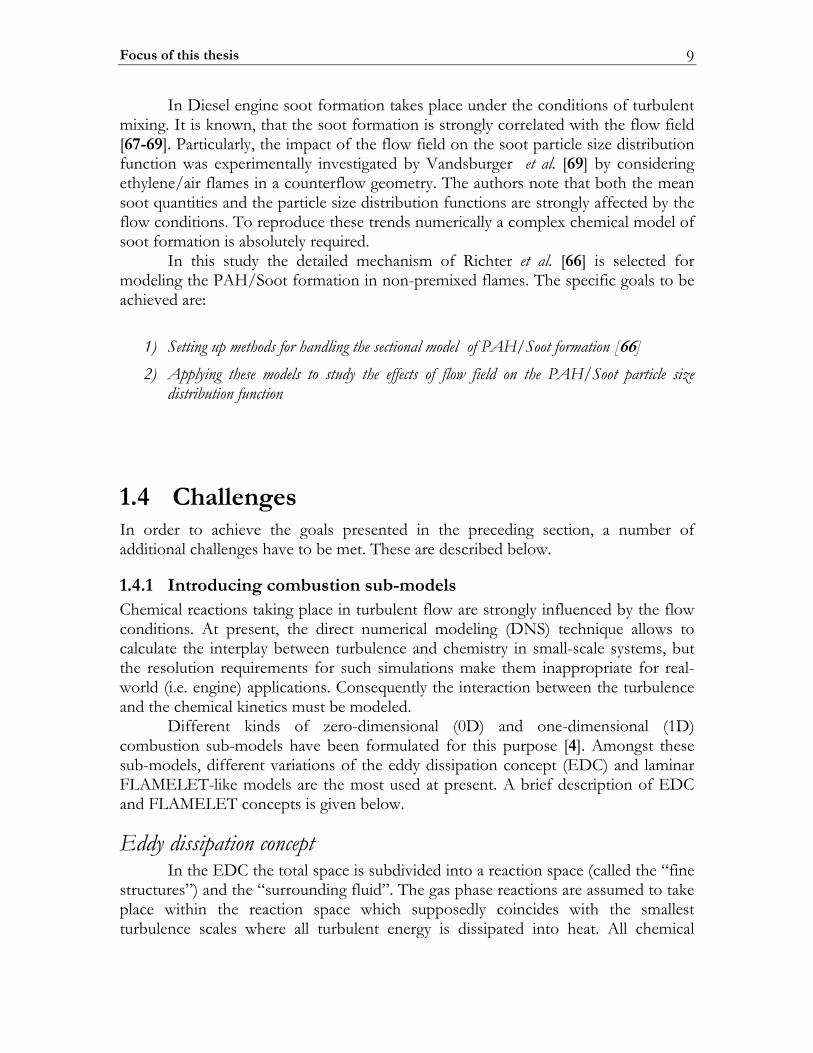
Eddy dissipation concept In the EDC the total space is subdivided into a reaction space (called the “fine structures”) and the “surrounding fluid”. The gas phase reactions are assumed to take place within the reaction space which supposedly coincides with the smallest turbulence scales where all turbulent energy is dissipated into heat. All chemical
Introduction 10
processes in the surrounding fluid are neglected. In order to treat the reactions within the fine structures, the volume fraction of the reaction space *γ and the mass transfer rate *M between the fine structures and the surrounding fluid need to be determined. Both quantities are derived from the turbulence characteristics of the flow field. A detailed description of the EDC implementation can be found in [70]. By treating the reacting fine structures locally as a well stirred reactor (0D problem) which transfers mass and energy only to the surrounding fluid (see Figure 1), every chemical kinetic mechanism can be linked with the EDC combustion model.
reaction space
“fine structures”M* M*
heat loss
reactants products
surrounding gas Figure 1 Illustration for the Well Stirred Reactor Model in the Eddy Dissipation Concept
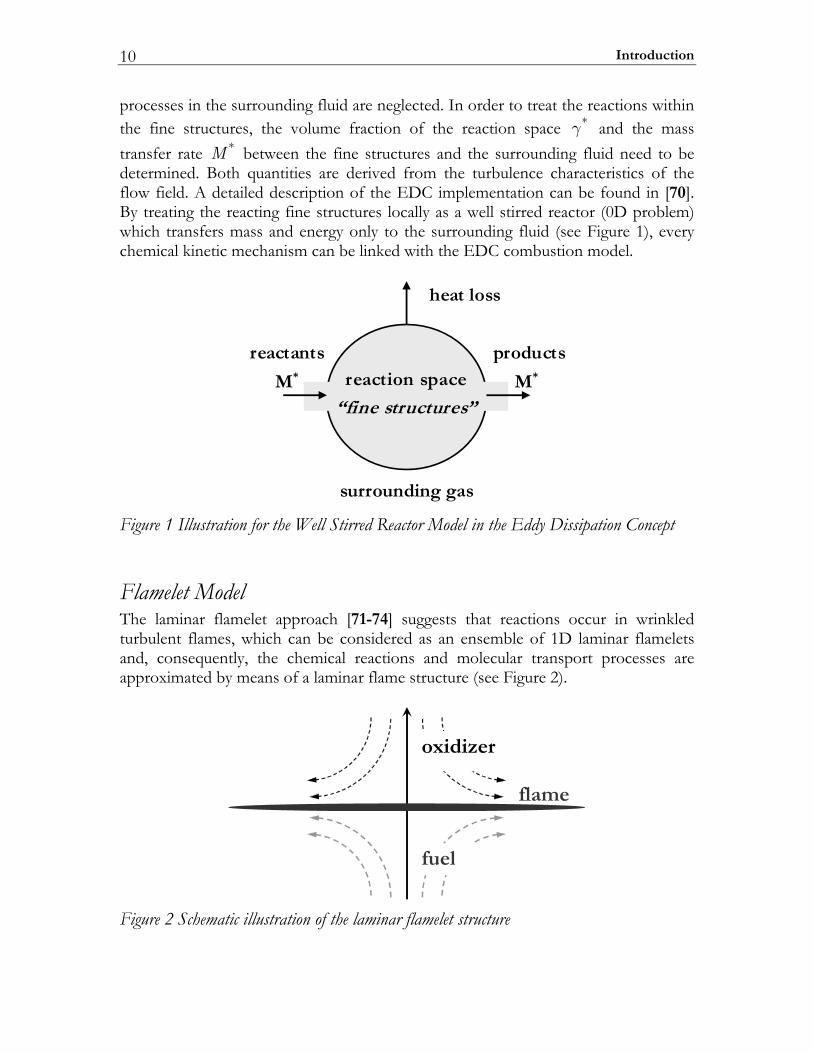
Flamelet Model The laminar flamelet approach [71-74] suggests that reactions occur in wrinkled turbulent flames, which can be considered as an ensemble of 1D laminar flamelets and, consequently, the chemical reactions and molecular transport processes are approximated by means of a laminar flame structure (see Figure 2).
oxidizer
fuel
flame
Figure 2 Schematic illustration of the laminar flamelet structure
Challenges 11
The link between the 1D laminar flamelets and the actual turbulent flame is formed by determining the spatial location of the flame together with local mixing conditions. These can be found in terms of a conserved scalar Z (so called "mixture fraction") defined by the transport equation:
0k Zk k k
Z Z Zv Dt x x x
ρ ρ ρ∂ ∂ ∂ ⎛ ∂ ⎞⎟⎜+ − =⎟⎜ ⎟⎝ ⎠∂ ∂ ∂ ∂ (1.1)
with the boundary conditions 1Z = in the pure fuel stream and 0Z = in pure oxidizer stream one can show that the gradient of Z is perpendicular to the flame sheet. The diffusion coefficient ZD in Equation (1.1) is usually defined such that the Lewis-number ZLe (the ratio between coefficients of thermal conductivity and self-diffusivity) is equal to one. Considering a locally defined coordinate system, where one coordinate 1x is Z and thereby perpendicular to the flame sheet and the other two 2x , 3x lie within the flame sheet, the conservation equations for the species and temperature can be transformed. After a scaling analysis of the terms of the resulting equations and the neglect of the terms, which are small to leading order, the equations appear in one-dimensional form [72]. With contemporary CPU power in combination with state-of-the-art solvers, arbitrary chemical models can be used in this approach as well.
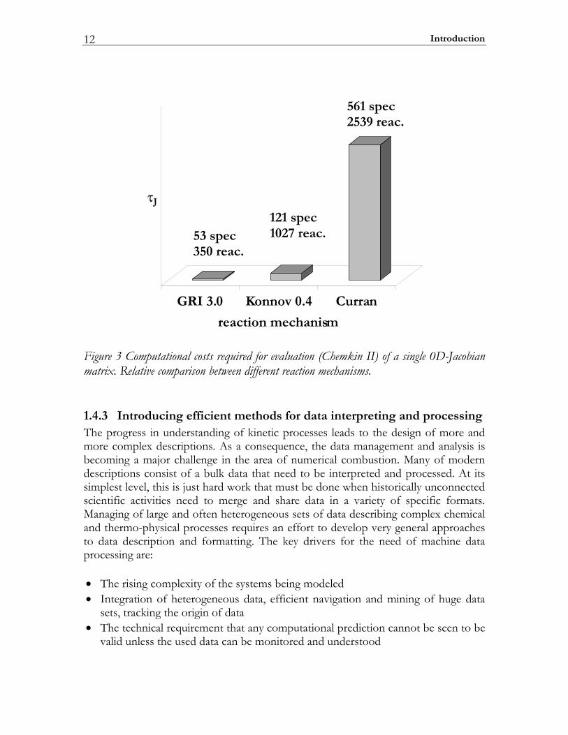
1.4.2 Ensuring Computational efficiency Setting up and solving the 0D and 1D combustion sub-models for a realistic fuel is a complex problem by itself that involves taking into account many chemical species and reactions. Furthermore, it is computationally demanding. This is caused by two major factors. The first one is the fact that a balance equation has to be solved for each chemical species involved. About 80–90% of the total computing time is usually spent in the subroutines determining these physical properties, in particular to compute chemical source terms and diffusion velocities [75]. The second factor is the high computational cost of evaluation and factoring of the problem Jacobian matrix. The Jacobian matrix plays an important role in solving so-called stiff equation systems such as the governing equations of the 0D and 1D problems described here. As an example, the dependence of the computational costs per 0D-Jacobian on the mechanism size (number of species and reactions) is illustrated in Figure 3. The results for the shown comparison were obtained with the CHEMKIN-II package [76]. Numerical evaluation of the 0D-Jacobian for the Konnov [77] and for the Curran [31] reaction mechanisms are respectively found to be about 7 and 130 times more expensive than when using the GRI-3 model [78]. This demonstrates the highly non-linear correlation between the computational costs and the reaction mechanism complexity of the reaction model. Obviously, in order to use complex reaction models in practical Diesel simulations there is a need for a strong computational speedup.
Introduction 12
J
GRI 3.0 Konnov 0.4 Curran
reaction mechanism
121 spec1027 reac.
561 spec2539 reac.
53 spec350 reac.
Figure 3 Computational costs required for evaluation (Chemkin II) of a single 0D-Jacobian matrix. Relative comparison between different reaction mechanisms.
1.4.3 Introducing efficient methods for data interpreting and processing The progress in understanding of kinetic processes leads to the design of more and more complex descriptions. As a consequence, the data management and analysis is becoming a major challenge in the area of numerical combustion. Many of modern descriptions consist of a bulk data that need to be interpreted and processed. At its simplest level, this is just hard work that must be done when historically unconnected scientific activities need to merge and share data in a variety of specific formats. Managing of large and often heterogeneous sets of data describing complex chemical and thermo-physical processes requires an effort to develop very general approaches to data description and formatting. The key drivers for the need of machine data processing are: • The rising complexity of the systems being modeled • Integration of heterogeneous data, efficient navigation and mining of huge data
sets, tracking the origin of data • The technical requirement that any computational prediction cannot be seen to be
valid unless the used data can be monitored and understood
Approach 13
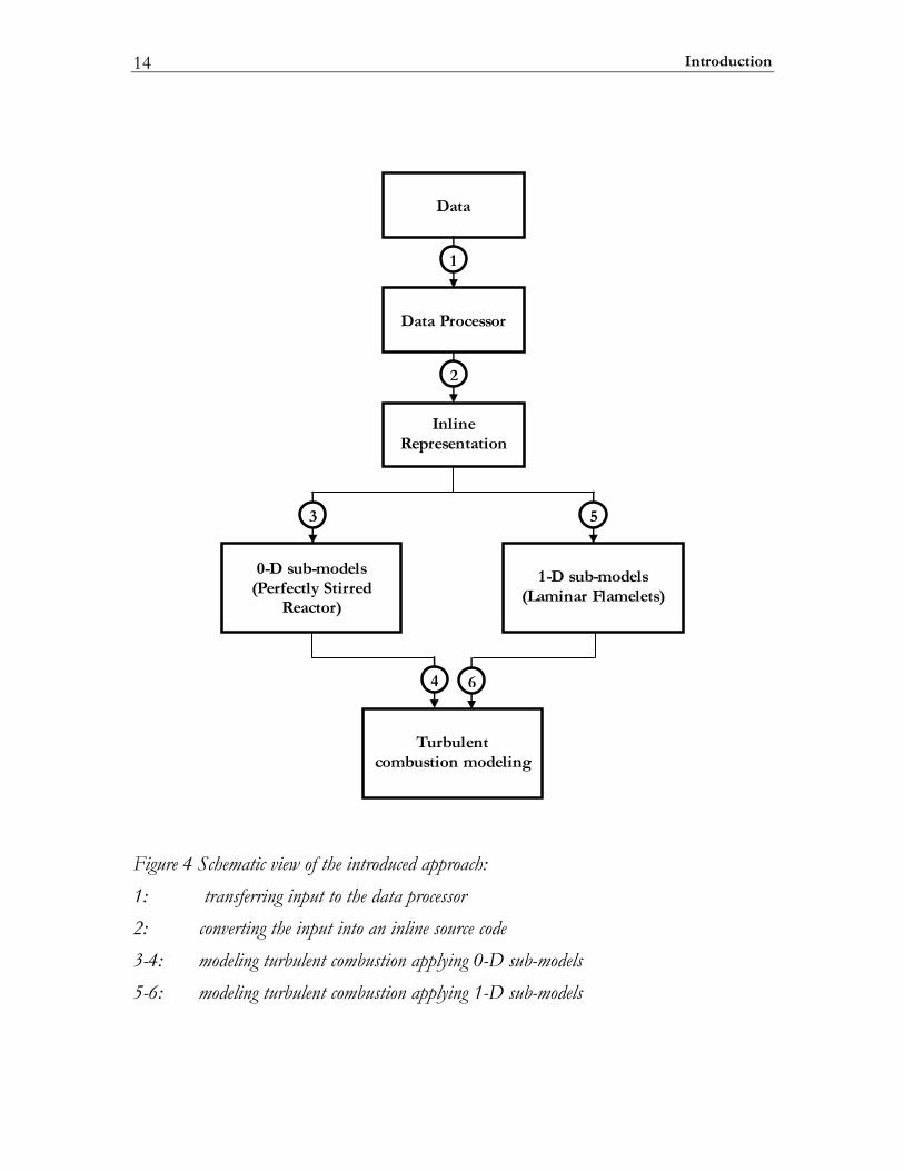
1.5 Approach At this moment, 0D and 1D combustion sub-models are viewed as the most generic way of applying complex chemical and thermo-physical descriptions to turbulent combustion modeling. A variety of numerical methods for solving these 0D and 1D problems have been presented in the literature. In principle, each of these methods can be directly imposed to IC-modeling as soon as the problem parameters (chemical reaction, thermodynamic and molecular transport data) are processed and adapted for use. Hence, the major challenges are considered to be machine interpreting, analysis and processing of heterogeneous data sets describing complex reacting systems. Within these, the interpreting step is absolutely required, since at present the descriptions are mostly available in symbolic formats rather than in the form of electronic metadata. The step of the machine analysis is employed to control the validity and compatibility of the problem parameters. It is quite obvious, that with increase of the data amounts involved, the risk of potentially invalid or incompatible parameters is increasing. This is even more the case if there is a practical need to use sets of combined data like mixed reaction mechanisms or thermodynamic databases. Finally, the processing step is necessary to adapt the interpreted and validated problem parameters for subsequent use in CFD-simulations or for an extra processing step aiming to achieve a higher computational performance. In the present approach the extra processing step is employed for transferring chemical and thermo-physical descriptions into the machine inline source codes that are subroutine libraries for CFD-solvers. A schematic view of the proposed approach is shown in Figure 4. A set of chemical and thermo-physical data describing a complex chemical reaction system and given in a symbolic format is considered as the starting point of the application process. First, the data sets are transferred to the data processor. Here the problem description is interpreted, analyzed and processed preparing a link-database. Second, the link-database is converted into inline subroutines for the required computational speedup. Finally, 0D (perfectly stirred reactor) and 1D (laminar diffusion flamelet) simulators incorporate the complex chemical/thermo-physical model into CFD-simulations as shown in branches 3-4 and 5-6 respectively (see Figure 4)
Introduction 14
Data Processor
InlineRepresentation
0-D sub-models(Perfectly Stirred
Reactor)
1-D sub-models(Laminar Flamelets)
Turbulentcombustion modeling
Data
1
2
3 5
4 6
Figure 4 Schematic view of the introduced approach: 1: transferring input to the data processor 2: converting the input into an inline source code 3-4: modeling turbulent combustion applying 0-D sub-models 5-6: modeling turbulent combustion applying 1-D sub-models
Outline of this thesis 15
1.6 Outline of this thesis This thesis consists of seven chapters and three appendices. The first chapter is this introduction and the last chapter summarizes conclusions and perspectives. The appendices present results and derivations which are used throughout the different chapters. The core of this thesis is divided into five chapters. Chapter 2 describes the design and development of a program (called TROT) for interpreting and analyzing chemical and thermo-physical data. The chapter first introduces the theoretical basis that is employed in the program and also describes the applied data format. Second a brief description of the TROT-processor and the CMECH- inline source code format are presented. In chapter 3 a study on the applicability of the ideal gas assumption for modeling high-pressure compression-reaction processes is presented. Here results from homogeneous auto-ignition and NO-formation calculations applying the ideal gas respectively real gas models are compared. Chapter 4 presents the computational algorithms used for resolving the structure of 1D (laminar) diffusion flamelets. This algorithm is validated by comparison with published computational and experimental profiles of a counterflow diffusion flame. The potential impact of gas non-ideality on the flamelet structure is considered for a n-heptane/air diffusion flame at elevated pressures. Chapter 5 is dedicated to detailed modeling of PAH/Soot formation. The chapter first introduces some basic knowledge on the process and the most frequently used numerical approaches. Second, results on PAH/Soot formation in ethylene/air and benzene/air counterflow diffusion flames are presented. The effect of strain rate on PAH/Soot is considered in terms of major characteristics like mass- and number-density as well as in terms of particle size distribution function. In chapter 6 the application of the steady laminar flamelet sub-model to turbulent diffusion jet-flames is presented. Here a partially premixed methane/air flame and a sooting non-premixed ethylene/air flames are considered. The results are compared to available experimental data.

Chapter 2
2 Processing and analysis of chemical and thermo-physical data
In this chapter the technique applied for handling data-intensive computational models is introduced. The problem of data management and the problem of computational performance are described in the introduction (2.1). Section (2.2) introduces the TROT program developed for interpreting and processing of complex model parameters. Section (2.3) presents the C-MECH format designed for reaction mechanisms and supplemental data that provides the required computational speedup. Some typical results are illustrated in section (2.4), where computational predictions on the molecular transport coefficients and the auto-ignition delay of n-heptane/air mixtures are presented. Finally, an outline of this chapter is given in section (2.5).
2.1 Introduction Setting up a detailed 3-D numerical model of a combustion process involves a series of activities: • it involves defining the equations that describe the fluid dynamics of the reacting
gases, • in addition the chemistry of the reacting gas needs to be described. This requires
identifying the set of chemical processes involved and the reaction kinetics of these processes,
• finally also the thermodynamic and transport properties of the reacting gas mixture needs to be defined.
The latter involves identifying an accurate equation of state describing the relation between pressure, temperature and volume; it also involves identifying accurate correlations for thermodynamic properties enthalpy and entropy (in principle as a
Processing and analysis of chemical and thermo-physical data 18
function of both pressure and temperature); finally accurate correlations are needed for the relevant transport properties (viscosity, diffusivity, conductivity) as a function of pressure and temperature. In view of the above, robust modeling of complex gas mixture in a wide range of operating conditions requires accurate description of mixture chemistry, thermodynamics and molecular transport phenomena. Normally these descriptions involve a variety of data of different nature. Until recently data management and analysis issues have not posed limitations on performing computations of combustion processes. However, as reacting flow simulations are rapidly increasing in chemical complexity this situation is changing. Of course, practical CFD-simulations can be done only when a comprehensive and accurate set of parameters describing the reacting mixture and its chemistry is available. At the present state of information technologies this would not create a problem if the model parameters were available in the form of an electronic database. However, it is historically conditioned that most reaction mechanisms and databases of thermo-physical properties are available in a variety of symbolic formats (text formats). Processing of symbolic information is far more sophisticated/difficult than that of an equivalent digital data set. Another difficulty associated with applying complex descriptions in practical CFD-simulations is the problem of computational performance. It is well known that modeling combustion chemistry cannot be done applying classical explicit algorithms [79]. Instead, the use of computationally demanding implicit methods is necessary. Applying these methods to simulate a homogeneous reaction process can already be unacceptably expensive. Therefore, two key topics that have to be considered when setting up a CFD-code for performing Diesel engine combustion modeling are:
I. The data needed for describing combustion (chemistry, thermodynamics and molecular transport) are heterogeneous in nature and are usually available in a symbolic/textual format;
II. The complexity of the newest chemistry models leads to unacceptably high computational costs, even for the simplest formulations such as 0D and 1D problems.
In the past, any CFD package was characterized by its own (dedicated) data format, fitting into its particular code-architecture. However, in recent years there has been an evolution towards using a more generic data format that can be shared by different CFD-packages. One such format is that of the so called CHEMKIN software package. CHEMKIN has evolved over the last 30 years [80, 76, 81] and is now widely distributed and used by researchers around the world. The formats designed for CHEMKIN incorporate complex gas-phase chemical reaction mechanisms into numerical simulations and represent a widely accepted standard. In fact the majority of the new extended chemistry models are introduced in these formats and a variety of its extensions.
Introduction 19
Therefore, in this thesis, the standards of CHEMKIN input are considered as a basis of the data format. A brief description of the complex chemical reaction models, thermodynamic functions and molecular transport properties including the corresponding formats are presented in sections (2.1.1), (2.1.2) and (2.1.3). The required extensions accounting for non-ideal gas effects and also a capability to handle the increasing complexity of chemical models are introduced in section (2.1.4).
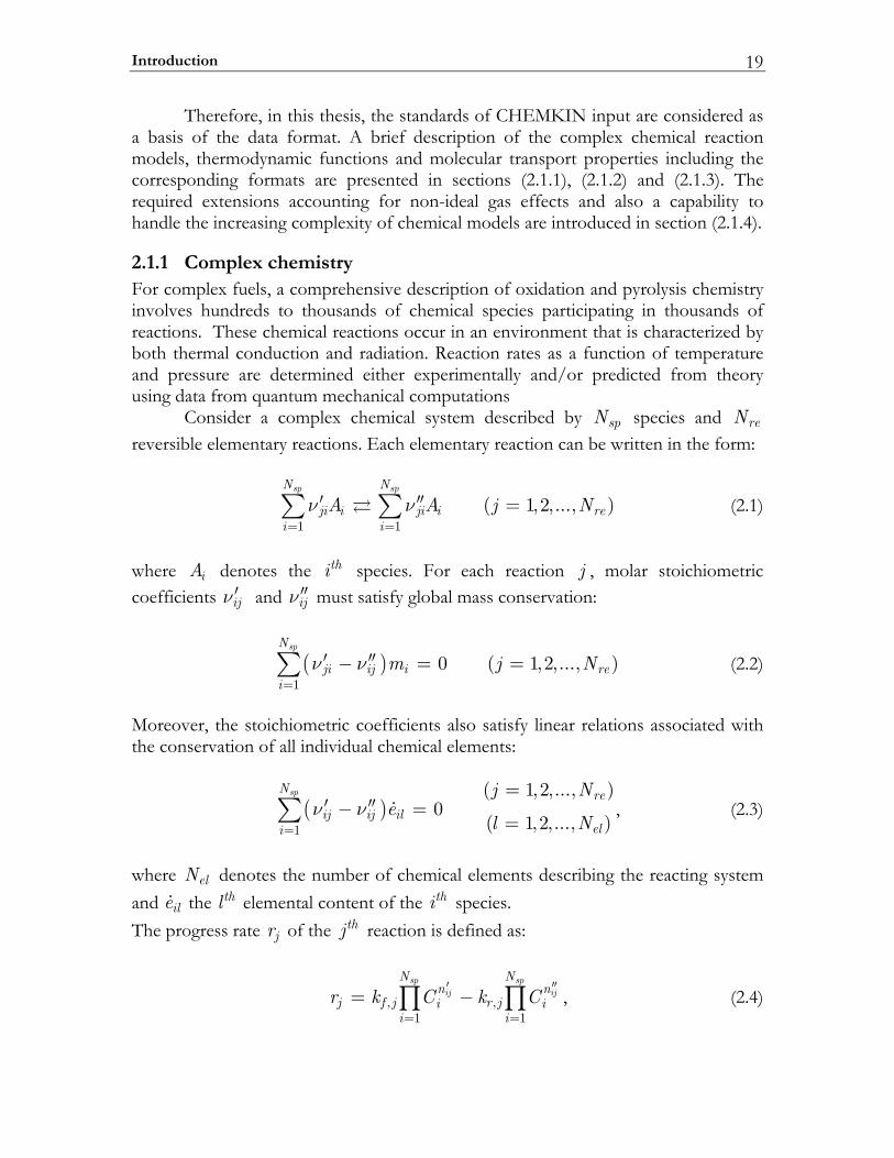
2.1.1 Complex chemistry For complex fuels, a comprehensive description of oxidation and pyrolysis chemistry involves hundreds to thousands of chemical species participating in thousands of reactions. These chemical reactions occur in an environment that is characterized by both thermal conduction and radiation. Reaction rates as a function of temperature and pressure are determined either experimentally and/or predicted from theory using data from quantum mechanical computations Consider a complex chemical system described by spN species and reN reversible elementary reactions. Each elementary reaction can be written in the form:
1 1
( 1,2,..., )sp spN N
ji i ji i rei i
A A j Nν ν= =
′ ′′ =∑ ∑ (2.1)
where iA denotes the thi species. For each reaction j , molar stoichiometric coefficients ijν ′ and ijν ′′ must satisfy global mass conservation:
( )1
0 ( 1,2,..., )spN
ji ij i rei
m j Nν ν=
′ ′′− = =∑ (2.2)
Moreover, the stoichiometric coefficients also satisfy linear relations associated with the conservation of all individual chemical elements:
( )1
( 1,2,..., )0
( 1,2,..., )
spN reij ij il
eli
j Ne
l Nν ν
=
=′ ′′− =
=∑ , (2.3)
where elN denotes the number of chemical elements describing the reacting system and ile the thl elemental content of the thi species. The progress rate jr of the thj reaction is defined as:
, ,1 1
sp spij ij
N Nn n
j f j r ji ii i
r k C k C′ ′′
= == −∏ ∏ , (2.4)
Processing and analysis of chemical and thermo-physical data 20
where iC denotes the molar concentration of the species i , ,f jk and ,r jk the forward and reverse constants and exponents ijn ′ and ijn ′′ are equal to coefficients
ijν ′ and ijν ′′ respectively, if the thj reaction describes a true molecular process1. Usually, the forward constants ,f jk are functions of temperature T and species concentrations iC . The particular expressions for forward constant ,f jk are different for different chemical models. However, chemical models mostly used in combustion share the same description of elementary chemical reactions, based on an Arrhenius law, leading to a rate coefficient expressed as:
, exp( )j jf j j
Ek AT
RTβ= − (2.5)
with jA the pre-exponential factor, jβ the temperature exponent and jE the activation energy. The forward and reverse constants of the reaction are linked by the equilibrium constant ,e jK :
,fj
e jrj
kK
k= (2.6)
that is expressed by:
( ) ( )1
0 0exp
Nsp
kj kjk j jatm
ejS HPK
RT R RT
ν ν=
′ ′′−∑ ⎡ ⎤∆ ∆⎢ ⎥= −⎢ ⎥⎣ ⎦ (2.7)
The parameters 0
jS∆ and 0jH∆ correspond, respectively, to the ideal gas entropy
and enthalpy changes during the transition from reactants to products for the thj reaction. These quantities are obtained from tabulations based on experimental
measurements and/or theory. The mass reaction rate of species k is the sum of all contributions from the elementary reactions:
( )1
Nre
k kj kj jj
rω ν ν=
′ ′′= −∑ . (2.8)
For numerical simulations of reacting flows, the chemical scheme has to be given. This means that the knowledge of all species and reactions must be determined before the computation can be carried out.
1 With respect to this one should also mention that the format described above is also often used to describe so-called global reactions. For these the exponents ijn ′ and ijn ′′ do not necessarily equal the
stoichiometric coefficients ijν ′ and ijν ′′ .
Introduction 21
ELEMH O N AR
END
SPECH2 OH H2O HO2 HO2 AR CO2C2H6 C2H5 C7H14 CO
END
REACTIONS CAL/MOL
H2+OH=H2O+H &1.000E+08 1.6 3300.0
H+O2(+M)=HO2(+M) &1.480E+12 0.6 0.0LOW /3.50E+16 -0.41 -1116.0/TROE /0.5 100000 10/AR/0.0/ H2O/10.6/ H2/1.5/ CO2/2.4/
C2H6(+M)=C2H5+H(+M) &8.850E+20 -1.228 102210.0LOW /6.90E+42 -6.431 107175.0/SRI /47.61 16182.0 3371.0/
C7H14+HO2+7O2=>7CO+7H2O+HO2 &3.162E+13 0.00 10000FORD / O2 0.0 /
END
input file:chemicalelements
chemicalspecies
reaction (1)
reaction (2)
reaction (3)
reaction (4)
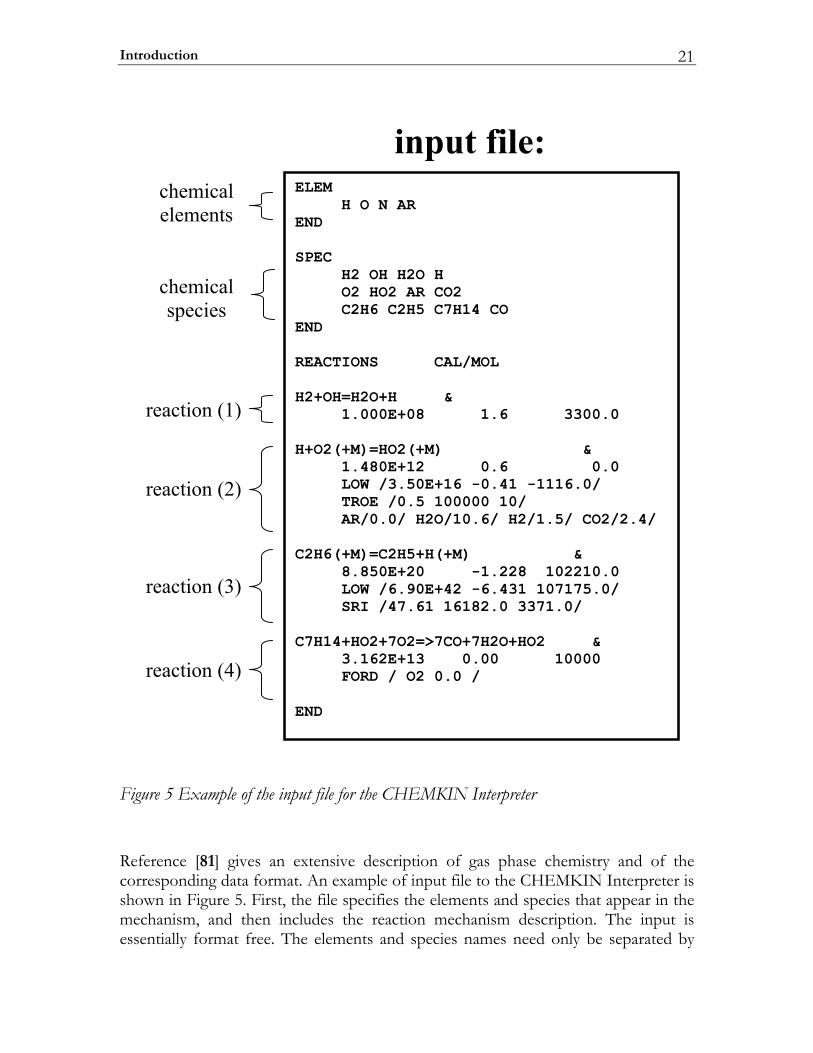
Figure 5 Example of the input file for the CHEMKIN Interpreter Reference [81] gives an extensive description of gas phase chemistry and of the corresponding data format. An example of input file to the CHEMKIN Interpreter is shown in Figure 5. First, the file specifies the elements and species that appear in the mechanism, and then includes the reaction mechanism description. The input is essentially format free. The elements and species names need only be separated by

Processing and analysis of chemical and thermo-physical data 22
blank spaces. The character string that describes the reaction appears on the left and is followed by the three Arrhenius coefficients (pre-exponential factor, temperature exponent, and activation energy). Enhanced third body efficiencies for selected species are specified in the line following that for a reaction which contains an arbitrary third body, M. A variety of extra features (e.g. deviations from the Arrhenius law or specific units of involved parameters) can be specified in the blocks of auxiliary information following the corresponding reaction equation. At present about 20 keys for auxiliary information are introduced in the CHEMKIN standard [81]. The fact that this format expresses reaction mechanisms in classical chemical equations is an obvious advantage. Nevertheless, this format becomes an obstacle for practical use in numerical modeling, where the form of electronic databases is preferable.
2.1.2 Critical properties In practical CFD-modeling, the ideal gas law is the default assumption, although more accurate correlations are available. In general, making the choice when to reject the ideal gas law in favor of the more complex but more accurate method is difficult. In order to guarantee sufficient flexibility of the CFD-modeling the option for such a choice must be enabled. One of the most common ways to involve the real gas description is based on the law of Corresponding State. The law of Corresponding States expresses the generalization that all properties that are determined by molecular interactions are correlated with critical properties in the same way for all chemical compounds. In fact the relation of pressure P to volume V at constant temperature T is different for different chemical substances. However, this relation becomes nearly universal for the reduced volumetric properties
r r rc c c
P V TP V TP V T
= = = , (2.9)
where cP , cV and cT are the corresponding critical values. At present this law provides the most general basis for the development of correlations accounting for the gas non-ideality. Particularly, development of real gas equations of state (EOS) is one of common applications of the law of Corresponding States. The generalized form of an EOS can be written as
PVZRT
= , (2.10)
where Z is the compressibility factor characterizing the gas non-ideality (for ideal gases 1Z = ). The law of Corresponding States suggests a correlation of / cZ Z as a
Introduction 23
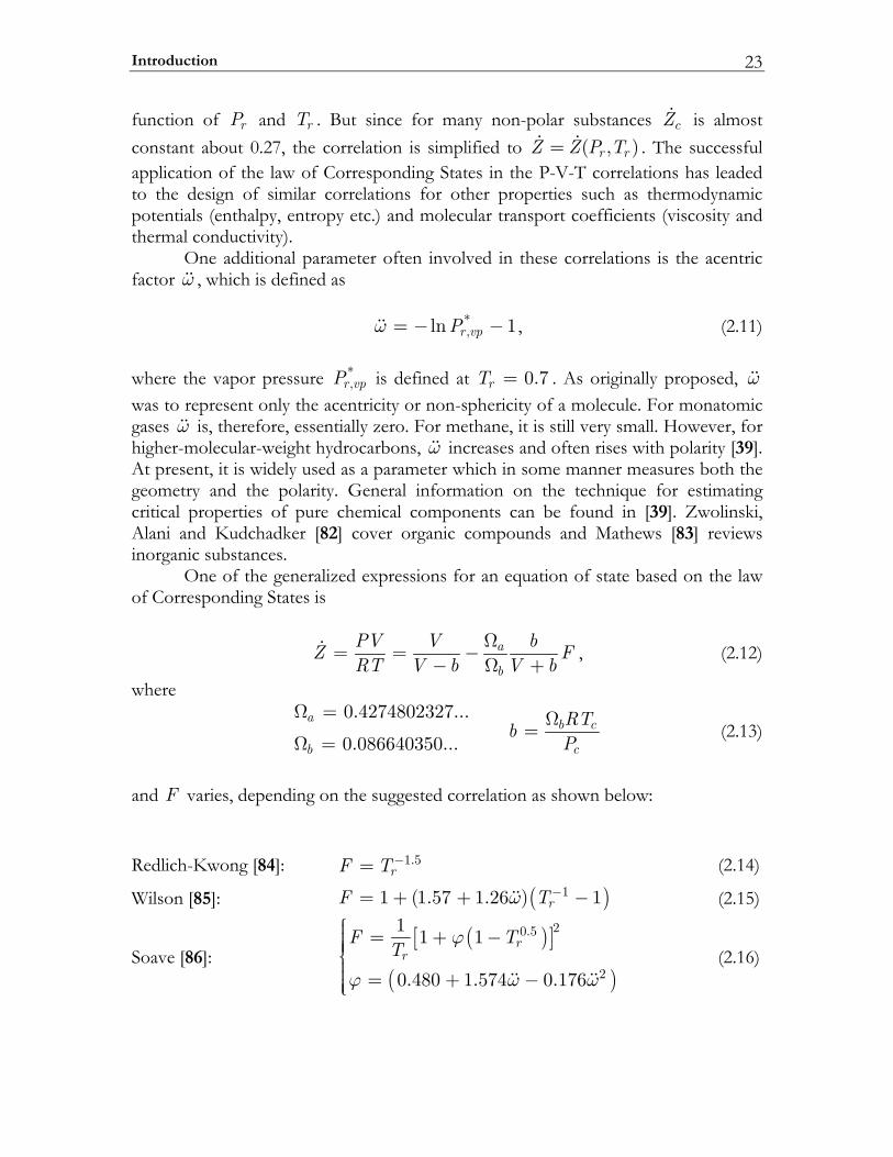
function of rP and rT . But since for many non-polar substances cZ is almost constant about 0.27, the correlation is simplified to Z = ( , )r rZ P T . The successful application of the law of Corresponding States in the P-V-T correlations has leaded to the design of similar correlations for other properties such as thermodynamic potentials (enthalpy, entropy etc.) and molecular transport coefficients (viscosity and thermal conductivity). One additional parameter often involved in these correlations is the acentric factor ω , which is defined as *
,ln 1r vpPω = − − , (2.11) where the vapor pressure *
,r vpP is defined at 0.7rT = . As originally proposed, ω was to represent only the acentricity or non-sphericity of a molecule. For monatomic gases ω is, therefore, essentially zero. For methane, it is still very small. However, for higher-molecular-weight hydrocarbons, ω increases and often rises with polarity [39]. At present, it is widely used as a parameter which in some manner measures both the geometry and the polarity. General information on the technique for estimating critical properties of pure chemical components can be found in [39]. Zwolinski, Alani and Kudchadker [82] cover organic compounds and Mathews [83] reviews inorganic substances. One of the generalized expressions for an equation of state based on the law of Corresponding States is
a
b
PV V bZ FRT V b V b
Ω= = −− Ω +
, (2.12)
where
0.4274802327...
0.086640350...a b c
cb
RTbP
Ω = Ω=Ω =
(2.13)
and F varies, depending on the suggested correlation as shown below: Redlich-Kwong [84]: 1.5
rF T−= (2.14)
Wilson [85]: ( )11 (1.57 1.26 ) 1rF Tω −= + + − (2.15)
Soave [86]: ( )[ ]
( )
20.5
2
1 1 1
0.480 1.574 0.176
rr
F TT
ϕ
ϕ ω ω
⎧⎪ = + −⎪⎪⎪⎨⎪⎪ = + −⎪⎪⎩
(2.16)
Processing and analysis of chemical and thermo-physical data 24
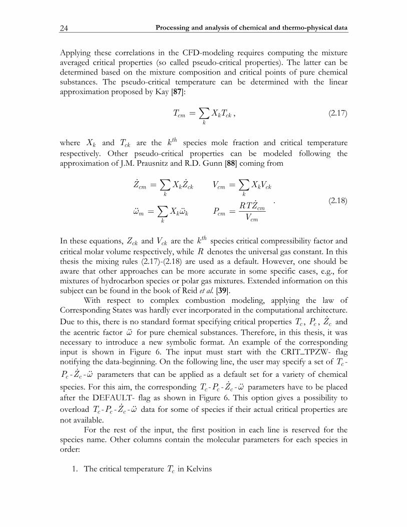
Applying these correlations in the CFD-modeling requires computing the mixture averaged critical properties (so called pseudo-critical properties). The latter can be determined based on the mixture composition and critical points of pure chemical substances. The pseudo-critical temperature can be determined with the linear approximation proposed by Kay [87]: cm k ck
kT X T=∑ , (2.17)
where kX and ckT are the thk species mole fraction and critical temperature respectively. Other pseudo-critical properties can be modeled following the approximation of J.M. Prausnitz and R.D. Gunn [88] coming from
cm k ck cm k ckk k
cmm k k cm
cmk
Z X Z V X V
RTZX PV
ω ω
= =
= =
∑ ∑
∑. (2.18)
In these equations, ckZ and ckV are the thk species critical compressibility factor and critical molar volume respectively, while R denotes the universal gas constant. In this thesis the mixing rules (2.17)-(2.18) are used as a default. However, one should be aware that other approaches can be more accurate in some specific cases, e.g., for mixtures of hydrocarbon species or polar gas mixtures. Extended information on this subject can be found in the book of Reid et al. [39]. With respect to complex combustion modeling, applying the law of Corresponding States was hardly ever incorporated in the computational architecture. Due to this, there is no standard format specifying critical properties cT , cP , cZ and the acentric factor ω for pure chemical substances. Therefore, in this thesis, it was necessary to introduce a new symbolic format. An example of the corresponding input is shown in Figure 6. The input must start with the CRIT_TPZW- flag notifying the data-beginning. On the following line, the user may specify a set of cT -
cP - cZ -ω parameters that can be applied as a default set for a variety of chemical species. For this aim, the corresponding cT - cP - cZ -ω parameters have to be placed after the DEFAULT- flag as shown in Figure 6. This option gives a possibility to overload cT - cP - cZ -ω data for some of species if their actual critical properties are not available. For the rest of the input, the first position in each line is reserved for the species name. Other columns contain the molecular parameters for each species in order:
1. The critical temperature cT in Kelvins
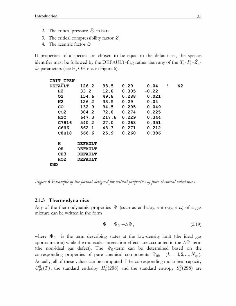
Introduction 25
2. The critical pressure cP in bars 3. The critical compressibility factor cZ 4. The acentric factor ω
If properties of a species are chosen to be equal to the default set, the species identifier mast be followed by the DEFAULT-flag rather than any of the cT - cP - cZ -ω parameters (see H, OH etc. in Figure 6).
CRIT_TPZWDEFAULT 126.2 33.5 0.29 0.04 ! N2 H2 33.2 12.8 0.305 -0.22
O2 154.6 49.8 0.288 0.021N2 126.2 33.5 0.29 0.04CO 132.9 34.5 0.295 0.049CO2 304.2 72.8 0.274 0.225H2O 647.3 217.6 0.229 0.344C7H16 540.2 27.0 0.263 0.351C6H6 562.1 48.3 0.271 0.212C8H18 566.6 25.9 0.260 0.386
H DEFAULT OH DEFAULT CH3 DEFAULT HO2 DEFAULTEND
Figure 6 Example of the format designed for critical properties of pure chemical substances.
2.1.3 Thermodynamics Any of the thermodynamic properties Ψ (such as enthalpy, entropy, etc.) of a gas mixture can be written in the form 0Ψ = Ψ + Ψ , (2.19) where 0Ψ is the term describing states at the low-density limit (the ideal gas approximation) while the molecular interaction effects are accounted in the Ψ -term (the non-ideal gas defect). The 0Ψ -term can be determined based on the corresponding properties of pure chemical components 0kΨ ( 1,2,..., spk N= ). Actually, all of these values can be computed if the corresponding molar heat capacity
0 ( )pkC T , the standard enthalpy 0(298)kH and the standard entropy 0(298)kS are
Processing and analysis of chemical and thermo-physical data 26
available. Normally, the non-dimensional heat capacities (determined experimentally or theoretically) are approximated with the temperature polynomials given by
0
( 1)
1
Npk n
nkn
Ca T
R−
==∑ (2.20)
Other ideal gas thermodynamic properties are given in terms of integrals of the 0
pkC -function. First, the molar enthalpy is defined by
0 0 0
298
(298 )T
k k pkK
H H K C dT= + ∫ (2.21)
so that
0 ( 1)
1,
1
N nN kk nk
n
aH a TRT n T
−+
== +∑ , (2.22)
where the parameter 1,N ka + , represents the standard heat of formation at 298 K. The molar entropy is given by
0
0 0
298
(298 )T
pkk k
K
CS S K dT
T= + ∫ (2.23)
so that
0 ( 1)
1 2,2
ln( )( 1)
N nk nk
k N kn
S a Ta T aR n
−
+=
= + +−∑ , (2.24)
where the parameter 2,N ka + , represents the standard entropy of formation at 298 K. Since the common input (CHEMKIN format) is designed to work with thermodynamic data in the form used in the NASA chemical equilibrium code [89], the approximation 0 ( )pkC T is considered for two temperature ranges and seven coefficients ka are needed for each of these ranges. These polynomial approximations take the following form:
0
2 3 41 2 3 4 5
pkk k k k k
Ca a T a T a T a T
R= + + + + , (2.25)
where the temperature is in Kelvin. Figure 7 shows some examples of thermodynamic property input for atomic and molecular oxygen. The first line of the input gives the basic information such as the species identifier (O and O2), the elemental composition, the flag indicating the phase state and boundaries of two
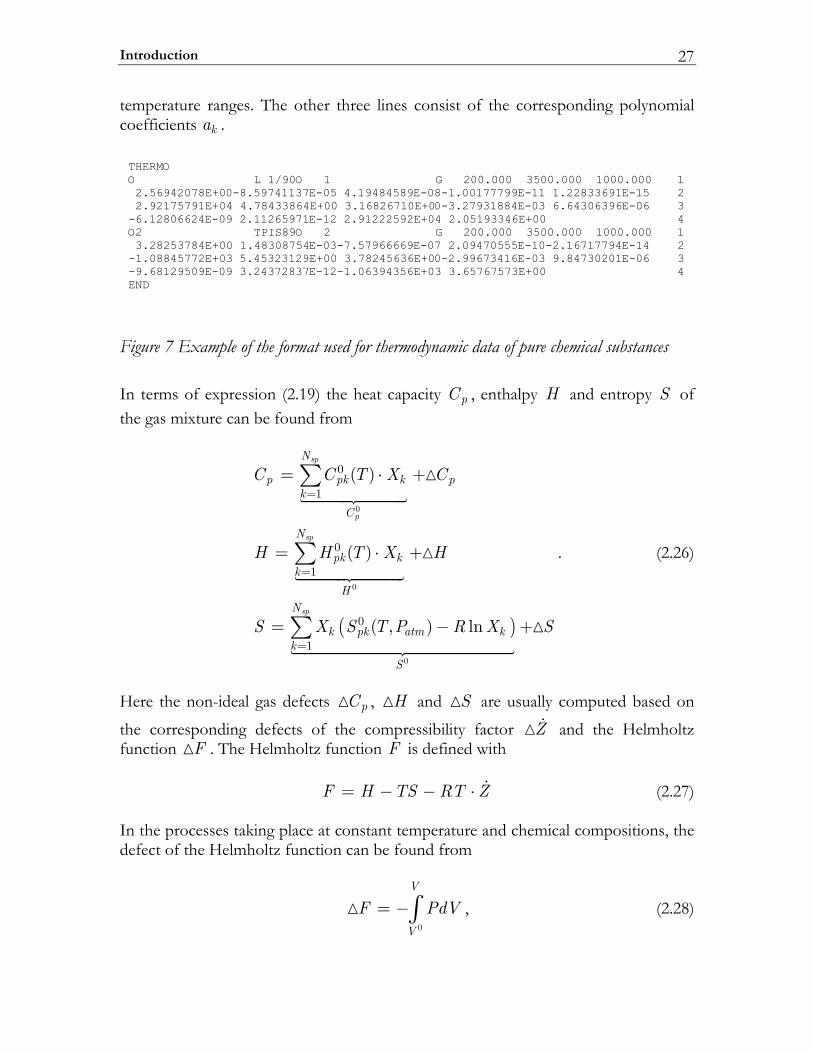
Introduction 27
temperature ranges. The other three lines consist of the corresponding polynomial coefficients ka . THERMOO L 1/90O 1 G 200.000 3500.000 1000.000 1 2.56942078E+00-8.59741137E-05 4.19484589E-08-1.00177799E-11 1.22833691E-15 2 2.92175791E+04 4.78433864E+00 3.16826710E+00-3.27931884E-03 6.64306396E-06 3-6.12806624E-09 2.11265971E-12 2.91222592E+04 2.05193346E+00 4O2 TPIS89O 2 G 200.000 3500.000 1000.000 1 3.28253784E+00 1.48308754E-03-7.57966669E-07 2.09470555E-10-2.16717794E-14 2-1.08845772E+03 5.45323129E+00 3.78245636E+00-2.99673416E-03 9.84730201E-06 3-9.68129509E-09 3.24372837E-12-1.06394356E+03 3.65767573E+00 4END
Figure 7 Example of the format used for thermodynamic data of pure chemical substances In terms of expression (2.19) the heat capacity pC , enthalpy H and entropy S of the gas mixture can be found from
( )
0
0
0
0
1
0
1
0
1
( )
( )
( , ) ln
sp
p
sp
sp
N
p pk k pk
C
N
pk kk
HN
k pk atm kk
S
C C T X C
H H T X H
S X S T P R X S
=
=
=
= ⋅ +
= ⋅ +
= − +
∑
∑
∑
. (2.26)
Here the non-ideal gas defects pC , H and S are usually computed based on the corresponding defects of the compressibility factor Z and the Helmholtz function F . The Helmholtz function F is defined with F H TS RT Z= − − ⋅ (2.27) In the processes taking place at constant temperature and chemical compositions, the defect of the Helmholtz function can be found from
0
V
V
F PdV= −∫ , (2.28)
Processing and analysis of chemical and thermo-physical data 28
where 0V is the reference molar volume corresponding to the ideal gas conditions. Since at the ideal gas states 1Z = , the corresponding Z -defect can be written as
1Z Z= − . Finally, if F is determined, the non-ideal gas defects pC , H and S are computed with
( )
( )( )
1
pP
V
HCT
H F T S RT Z
FST
∂=∂
= ∆ + + −
∂= −∂
. (2.29)
At this point we considered chemical kinetic and thermodynamic data required for modeling complex reaction systems. In general, a consistent set of these data is sufficient for simulating of any 0D thermo-chemical phenomena. However, detailed modeling of 1D-processes normally requires taking into account phenomena of molecular transport. The latter can be described based on the molecular transport coefficients of pure chemical substances and gas mixtures. In the following some classical expressions and semi-empirical correlations for computing these properties as well as the involved parameters are described.
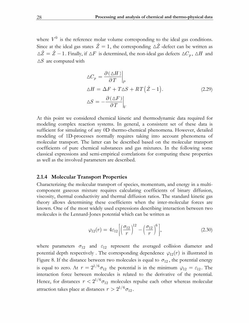
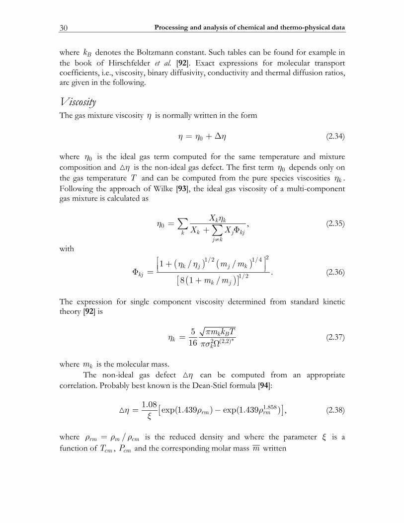
2.1.4 Molecular Transport Properties Characterizing the molecular transport of species, momentum, and energy in a multi-component gaseous mixture requires calculating coefficients of binary diffusion, viscosity, thermal conductivity and thermal diffusion ratios. The standard kinetic gas theory allows determining these coefficients when the inter-molecular forces are known. One of the most widely used expressions describing interaction between two molecules is the Lennard-Jones potential which can be written as
( ) ( )12 612 12
12 12( ) 4rr rσ σϕ ε ⎡ ⎤= −⎢ ⎥⎢ ⎥⎣ ⎦
, (2.30)
where parameters 12σ and 12ε represent the averaged collision diameter and potential depth respectively . The corresponding dependence 12( )rϕ is illustrated in Figure 8. If the distance between two molecules is equal to 12σ , the potential energy is equal to zero. At 1/6
122r σ= the potential is in the minimum 12 12ϕ ε= . The interaction force between molecules is related to the derivative of the potential. Hence, for distances 1/6
122r σ< molecules repulse each other whereas molecular attraction takes place at distances 1/6
122r σ> .
Introduction 29
12 r
1/6122
12
12
Figure 8 Lennard-Jones potential For polar molecules such as H2O, CH3OH etc, the Stockmayer potential is preferable. This equation adds a dipole interaction term to the Lennard-Jones equation. The resulting expression then becomes
( ) ( ) ( )212 6 3
12 12 12 1212 12 3
12 12
1( ) 44
r fr r rσ σ µ σϕ ε
ε σ⎡ ⎤⎢ ⎥= − −⎢ ⎥⎣ ⎦
, (2.31)
where f is a parameter accounting for the dipoles orientation and where 12µ represents the dipole moment. In addition to these, some more advanced models involve other quantities such as polarizability α and the rotational relaxation collision number Zrot. Relevant information can be found in, e.g. [90]. The standard kinetic theory expresses molecular transport coefficients in terms of potential parameters (the above mentioned) and of so-called collision integrals *Ω [91, 92]. Quantities *Ω account for molecular interactions that are more complex compared to the simplest model of solid spheres (there * 1Ω = ). Actual values of *Ω can be computed from temperature and from the quantities ε and µ . Typically the required collision integrals are tabulated versus the reduced temperature
* Bk TT ε= (2.32)
and the reduced dipole moment coming from
2
*3
12µδεσ
= , (2.33)
Processing and analysis of chemical and thermo-physical data 30
where Bk denotes the Boltzmann constant. Such tables can be found for example in the book of Hirschfelder et al. [92]. Exact expressions for molecular transport coefficients, i.e., viscosity, binary diffusivity, conductivity and thermal diffusion ratios, are given in the following.
Viscosity The gas mixture viscosity η is normally written in the form 0η η η= +∆ (2.34) where 0η is the ideal gas term computed for the same temperature and mixture composition and η is the non-ideal gas defect. The first term 0η depends only on the gas temperature T and can be computed from the pure species viscosities kη . Following the approach of Wilke [93], the ideal gas viscosity of a multi-component gas mixture is calculated as
0k k
k j kjkj k
XX X
ηη
≠
=+ Φ∑ ∑ , (2.35)
with
( ) ( )( )[ ]
21/2 1/4
1/2
1 / /
8 1 /
k j j kkj
k j
m m
m m
η η⎡ ⎤+⎢ ⎥⎣ ⎦Φ =+
. (2.36)
The expression for single component viscosity determined from standard kinetic theory [92] is
2 (2,2)*516
k Bk
k
m k Tπηπσ
=Ω
(2.37)
where km is the molecular mass. The non-ideal gas defect η can be computed from an appropriate correlation. Probably best known is the Dean-Stiel formula [94]:
[ ]1.8581.08 exp(1.439 ) exp(1.439 )rm rmη ρ ρξ
= − , (2.38)
where /rm m cmρ ρ ρ= is the reduced density and where the parameter ξ is a function of cmT , cmP and the corresponding molar mass m written
Introduction 31
1/6
2/3cm
cm
TmP
ξ = . (2.39)
Binary diffusion coefficients Most experimental data on the diffusion phenomena at high-pressures relate to the self-diffusion coefficients [39]. Consequently, corresponding high pressure correlations for binary diffusion coefficients jkD are not yet available. An ideal gas expression for 0
ijD [92] is
( )30
2 (1,1)*2 /3
16B jk
jkjk
k T mD
Pππσ
=Ω
(2.40)
where jkm is the reduced molecular mass for the ( , )j k species pair
j kjk
j k
m mm
m m=
+, (2.41)
jkσ is the reduced collision diameter and P is the pressure in atmospheres. The
reduced temperature *jkT required to compute the collision integral (1,1)*Ω may
depend on the dipole moment ijµ and polarizabilities jα and kα . In computing the reduced quantities, two characteristic cases are considered, depending on whether the collision partners are polar or non-polar [90]. For the case that the partners are either both polar or both non-polar the following expressions apply:
( )
2j k
jk j k jk jk j kσ σ
ε ε ε σ µ µ µ+
= ⋅ = = ⋅ (2.42)
For the case of a polar molecule interacting with a non-polar molecule apply
1
2 6( )
02
n pnp n p np np
σ σε ξ ε ε σ ξ µ
−+= ⋅ = = (2.43)
where
* *114
pn p
n
εξ α µ
ε= + (2.44)
In the above equations *
nα is the reduced polarizability for the non-polar molecule and *
pµ is the reduced dipole moment for the polar molecule coming from
Processing and analysis of chemical and thermo-physical data 32
* *3 3
pnn p
n p p
µαα µσ ε σ
= = (2.45)
Pure Species Thermal Conductivities The thermal conductivity of gas mixtures is written as 0λ λ λ= + , (2.46) where 0λ is the pressure independent (ideal gas) term computed for the same gas temperature and mixture composition and λ is the term accounting for the pressure effects (non-ideal gas). The first term is a function of thermal conductivities of pure chemical substances kλ . The ideal gas thermal conductivity coefficients of the multi-component mixture can be computed with the Mason-Saxena approximation [95]:
0 *k k
k j kjkj k
XX k X
λλ
≠
=+ ⋅ Φ∑ ∑
, (2.47)
where kjΦ are determined with (2.36) and *k is a constant value. As suggested by Mason and Saxena and as usual in combustion modeling * 1.065k = is applied. However, alternative values of this parameter ( * 1k = or * 0.85k = ) can also be found in the literature [39]. The pure species thermal conductivities are composed of translational, rotational, and vibrational contributions as proposed by Warnatz [96] ( )k
k trans v trans rot v rot vib v vibkf C f C f C
mηλ = + + , (2.48)
where
( )
..
.
.
.
5 212
21
v rottrans
v trans
kkrot
k
kkvib
k
C AfC B
D AfB
Df
πρη π
ρη
⎛ ⎞⎟⎜= − ⎟⎜ ⎟⎟⎜⎝ ⎠
= +
=
(2.49)
Introduction 33
and
..
5 2 52 3
v rotkk kkrot
k k
CD DA B ZR
ρ ρη π η
= − = + + (2.50)
The molar heat capacity vC relationships are different depending on the molecular structure. For molecules consisting of more than one atom
. . .3 3 32 2v trans v rot v vib vC R C R C C R= = = − . (2.51)
The translational part of vC is always the same, and therefore in the case of single atoms there are no internal contributions to vC , and hence,
32
kk trans
kf R
mηλ = ⋅ (2.52)
where 5/2transf = . The “self-diffusion” coefficient comes from the following expression:
( )30
2 (1,1)*3 4 /16
B kkk
jk
k T mDPππσ
=Ω
(2.53)
The rotational relaxation collision number .rotZ is a parameter that is assumed to be available at 298K. It has a temperature dependence given in an expression by Parker [97] and Brau and Jonkman [98]
. .(298 )( ) (298 )
( )rot rotF KZ T Z KF T
= , (2.54)
where
1/2 3/23/2 2
3/2( ) 1 22 4B B B
F Tk T k T k T
π ε π ε επ⎛ ⎞⎛ ⎞ ⎛ ⎞⎟⎜⎟ ⎟⎜ ⎜= + + + +⎟⎟ ⎟⎜⎜ ⎜⎟ ⎟⎟⎜⎝ ⎠ ⎝ ⎠⎝ ⎠
(2.55)
One of the best known correlations representing the pressure dependent part λ∆ is the approximation proposed by Stiel and Thodos in [99]:
Processing and analysis of chemical and thermo-physical data 34
[ ]
[ ]
8
5
8
5
8*
5
14.0 10 exp(0.535 ) 1 0.5
13.1 10 exp(0.67 ) 1.069 0.5 2.0
2.976 10 exp(1.115 ) 2.805 2.0 2.8
rm rmcm
rm rmcm
rm rmcm
Z
Z
Z
ρ ρ
λ ρ ρ
ρ ρ
−
−
−
⎧ ⋅⎪⎪ − ⇔ <⎪⎪ Γ ⋅⎪⎪⎪ ⋅⎪⎪= − ⇔ < <⎨⎪ Γ ⋅⎪⎪⎪ ⋅⎪ ⎡ ⎤⎪ − ⇔ < <⎪ ⎣ ⎦⎪ Γ ⋅⎪⎩
where Γ is given by
1/6
2/3cm
cm
T mP
Γ = (2.56)
and m denotes the mixture averaged molar mass.
Thermal Diffusion Ratios The molecular transfer of mass caused by the temperature gradient is referred to as thermal diffusion. The thermal diffusion causes a system to reach steady state with non-zero gradients of temperature and concentrations. This molecular transport can be described by introducing thermal diffusion ratios kΘ defined for each species k [90]. A thermal diffusion ratio kΘ can be defined such that the thermal diffusion velocity dkw is given by
k kdk
k
Dw TX TΘ= ∇ (2.57)
The thermal diffusion ratio [100, 101] is given by k jk
j kθ
≠Θ =∑ , (2.58)
where jkθ are thermal diffusion ratios in binary isotropic gas mixtures. Following [91], quantities jkθ can be computed with
( )( )( )
* *
* * *
2 5 6 5152 16 12 55
kj
kj kj j kjk k j
j kkj kj kj
A C m mX X
m mA A Bτ
θ+ − −
=+− +
(2.59)
and
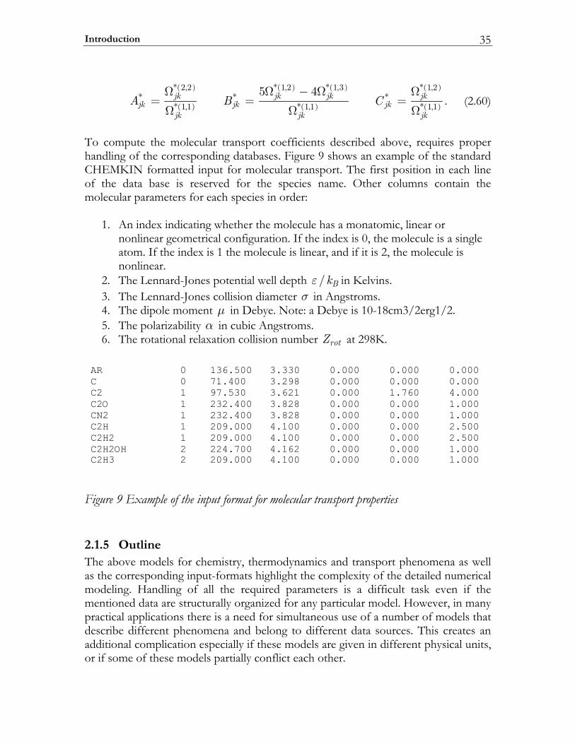
Introduction 35
( )
( )
( ) ( )
( )
( )
( )
* 2,2 * 1,2 * 1,3 * 1,2* * *
* 1,1 * 1,1 * 1,1
5 4jk jk jk jkjk jk jk
jk jk jkA B C
Ω Ω − Ω Ω= = =
Ω Ω Ω. (2.60)
To compute the molecular transport coefficients described above, requires proper handling of the corresponding databases. Figure 9 shows an example of the standard CHEMKIN formatted input for molecular transport. The first position in each line of the data base is reserved for the species name. Other columns contain the molecular parameters for each species in order:
1. An index indicating whether the molecule has a monatomic, linear or nonlinear geometrical configuration. If the index is 0, the molecule is a single atom. If the index is 1 the molecule is linear, and if it is 2, the molecule is nonlinear.
2. The Lennard-Jones potential well depth / Bkε in Kelvins. 3. The Lennard-Jones collision diameter σ in Angstroms. 4. The dipole moment µ in Debye. Note: a Debye is 10-18cm3/2erg1/2. 5. The polarizability α in cubic Angstroms. 6. The rotational relaxation collision number rotZ at 298K.
AR 0 136.500 3.330 0.000 0.000 0.000C 0 71.400 3.298 0.000 0.000 0.000C2 1 97.530 3.621 0.000 1.760 4.000C2O 1 232.400 3.828 0.000 0.000 1.000CN2 1 232.400 3.828 0.000 0.000 1.000C2H 1 209.000 4.100 0.000 0.000 2.500C2H2 1 209.000 4.100 0.000 0.000 2.500C2H2OH 2 224.700 4.162 0.000 0.000 1.000C2H3 2 209.000 4.100 0.000 0.000 1.000
Figure 9 Example of the input format for molecular transport properties
2.1.5 Outline The above models for chemistry, thermodynamics and transport phenomena as well as the corresponding input-formats highlight the complexity of the detailed numerical modeling. Handling of all the required parameters is a difficult task even if the mentioned data are structurally organized for any particular model. However, in many practical applications there is a need for simultaneous use of a number of models that describe different phenomena and belong to different data sources. This creates an additional complication especially if these models are given in different physical units, or if some of these models partially conflict each other.
Processing and analysis of chemical and thermo-physical data 36
Obviously, handling of all the required data cannot be done manually. Instead, developing a dedicated machine algorithm (data-processor) is highly desirable. The major requirements of such a processor are that it should be able to: • interpret symbolic information given in an arbitrary number of input-files • convert of the input data into user-prescribed units • link the inputs and create the output adapted for use in CFD-modeling • verify the resulting data set and report the results of this verification The following section describes the major features of a newly designed and developed data processor (called TROT) that meets with these requirements.
2.2 TROT: A C++ program for interpreting and analysis of chemical and thermo-physical data
TROT is a C++ program designed and developed for processing and analyzing of chemical and thermo-physical data. The working cycle of the TROT processor is shown schematically in Figure 10. The TROT-input consists of data sets describing: gas-phase chemical reactions, molecular transport, ideal gas thermodynamics and real gas properties (critical properties). The data processing and analysis starts in the program module called Interpreter. Here the “grammar” of the text-formatted inputs is parsed and input data are converted into an internal machine representation. Further, the continuation is delegated to the second module called Linker. This module verifies the data compatibility and if successful creates the TROT-output file "scheme.dat" that contains all model parameters being linked and translated into the user-specified physical units. The output data in the "scheme.dat" file are given in a text-format adapted for an easy machine scan and use in CFD-modeling (see appendix A). The advanced features of the TROT-processor are its flexible handling of: • global and complex models of gas-phase chemistry; • non-ideal gas descriptions; • large variety of physical units; • validation of input parameters. The following paragraphs describe these features in more detail and consider the performance of the Interpreter and the Linker model respectively.
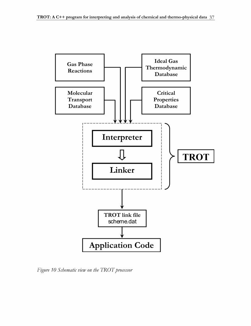
TROT: A C++ program for interpreting and analysis of chemical and thermo-physical data 37
Gas PhaseReactions
Ideal GasThermodynamic
Database
MolecularTransportDatabase
Interpreter
Linker
TROT
TROT link filescheme.dat
Application Code
CriticalPropertiesDatabase
Figure 10 Schematic view on the TROT processor
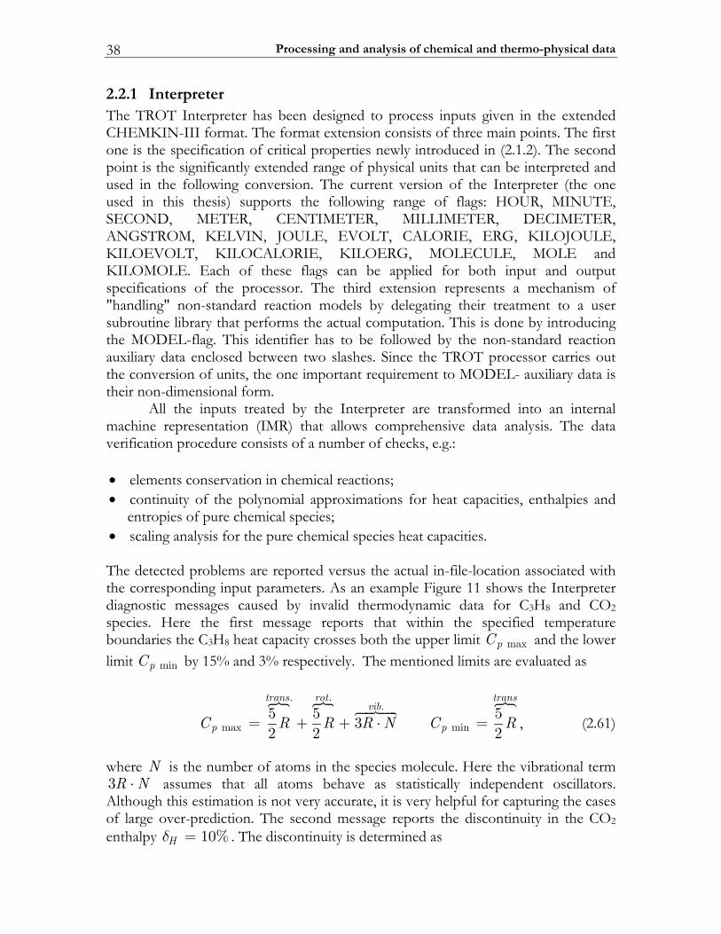
Processing and analysis of chemical and thermo-physical data 38
2.2.1 Interpreter The TROT Interpreter has been designed to process inputs given in the extended CHEMKIN-III format. The format extension consists of three main points. The first one is the specification of critical properties newly introduced in (2.1.2). The second point is the significantly extended range of physical units that can be interpreted and used in the following conversion. The current version of the Interpreter (the one used in this thesis) supports the following range of flags: HOUR, MINUTE, SECOND, METER, CENTIMETER, MILLIMETER, DECIMETER, ANGSTROM, KELVIN, JOULE, EVOLT, CALORIE, ERG, KILOJOULE, KILOEVOLT, KILOCALORIE, KILOERG, MOLECULE, MOLE and KILOMOLE. Each of these flags can be applied for both input and output specifications of the processor. The third extension represents a mechanism of "handling" non-standard reaction models by delegating their treatment to a user subroutine library that performs the actual computation. This is done by introducing the MODEL-flag. This identifier has to be followed by the non-standard reaction auxiliary data enclosed between two slashes. Since the TROT processor carries out the conversion of units, the one important requirement to MODEL- auxiliary data is their non-dimensional form. All the inputs treated by the Interpreter are transformed into an internal machine representation (IMR) that allows comprehensive data analysis. The data verification procedure consists of a number of checks, e.g.: • elements conservation in chemical reactions; • continuity of the polynomial approximations for heat capacities, enthalpies and
entropies of pure chemical species; • scaling analysis for the pure chemical species heat capacities. The detected problems are reported versus the actual in-file-location associated with the corresponding input parameters. As an example Figure 11 shows the Interpreter diagnostic messages caused by invalid thermodynamic data for C3H8 and CO2 species. Here the first message reports that within the specified temperature boundaries the C3H8 heat capacity crosses both the upper limit maxpC and the lower limit minpC by 15% and 3% respectively. The mentioned limits are evaluated as
. ..
max min5 5 532 2 2
trans rot transvib
p pC R R R N C R= + + ⋅ = , (2.61)
where N is the number of atoms in the species molecule. Here the vibrational term 3R N⋅ assumes that all atoms behave as statistically independent oscillators. Although this estimation is not very accurate, it is very helpful for capturing the cases of large over-prediction. The second message reports the discontinuity in the CO2 enthalpy 10%Hδ = . The discontinuity is determined as
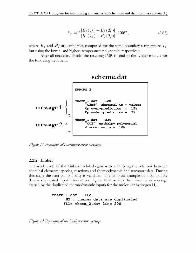
TROT: A C++ program for interpreting and analysis of chemical and thermo-physical data 39
( ) ( )( ) ( )
1 2
1 22 100%b b
Hb b
H T H TH T H T
δ −= ⋅+
, (2.62)
where 1H and 2H are enthalpies computed for the same boundary temperature bT , but using the lower- and higher- temperature polynomial respectively. After all necessary checks the resulting IMR is send to the Linker module for the following treatment.
ERRORS 2
therm_1.dat 120“C3H8”: abnormal Cp – valuesCp over-prediction = 15%Cp under-prediction = 3%
therm_1.dat 530“CO2”: enthalpy polynomialdiscontinuity = 10%
scheme.dat
message 1
message 2
Figure 11 Example of Interpreter error messages
2.2.2 Linker The work cycle of the Linker-module begins with identifying the relations between chemical elements, species, reactions and thermodynamic and transport data. During this stage the data compatibility is validated. The simplest example of incompatible data is duplicated input information. Figure 12 illustrates the Linker error message caused by the duplicated thermodynamic inputs for the molecular hydrogen H2.
therm_1.dat 112"H2": thermo data are duplicatedfile therm_2.dat line 200
Figure 12 Example of the Linker error message
Processing and analysis of chemical and thermo-physical data 40
The analysis of the data compatibility is followed by the computation and polynomial fit of the molecular transport coefficients. The required values of collision integrals
( , )*k lΩ are computed based on the parameters of the Lennard-Jones and Stockmayer molecular potentials. Particularly, collision integrals ( )* 1,1
jkΩ and ( )* 2,2jkΩ that
determine coefficients of binary diffusivity and coefficients of viscosity and thermal conductivity are computed based on the approximations suggested by Brokaw [102]:
( ) ( )*
* 1,1 * 1,1*
0.19jk jk T
δ′Ω = Ω + (2.63)
and
( ) ( )*
* 2,2 * 2,2*
0.2jk jk T
δ′Ω = Ω + , (2.64)
where ( )* 1,1
jk′Ω and ( )* 2,2jk′Ω are the corresponding Lennard-Jones collision integrals,
*δ is the reduced dipole moment and *T is the reduced temperature (see section (2.1.4)). Since thermal diffusion ratios cannot be predicted well even with the detailed kinetic theory, these quantities have been computed based on the Lennard-Jones molecular potential only. For computational purposes the tabulated values of Lennard-Jones collision integrals [92] have been approximated by the polynomial expansion
( ) ( )7
** ,
0
1 lniik lia T
== ⋅
′Ω ∑ . (2.65)
The ia parameters of the approximation (2.65) determined for the ( ),k l -pairs of ( )1,1 , ( )1,2 , ( )1, 3 and ( )2,2 are shown in Table 1 Pre-computed transport coefficients are approximated with temperature polynomials ( )A T . For each transport coefficient ϕ the order of the polynomial approximation Aϕ is determined from the requirement
maxAϕ
ϕϕ
δϕ−
< . (2.66)
The default TROT setting for the approximation is max 3%ϕδ = . This value is well within the accuracy due to the theory itself (e.g., for the binary diffusivities the errors can reach a level of about 15% [39]). The diffusion coefficient fits are computed at the atmospheric pressure. Following CHEMKIN-standards a polynomial fit of the
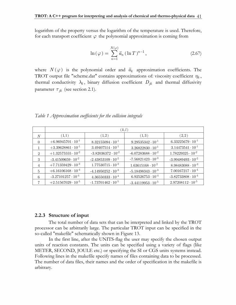
TROT: A C++ program for interpreting and analysis of chemical and thermo-physical data 41
logarithm of the property versus the logarithm of the temperature is used. Therefore, for each transport coefficient ϕ the polynomial approximation is coming from
( ) ( )( )
1
1ln ln
Nn
nna T
ϕϕ −
== ∑ , (2.67)
where ( )N ϕ is the polynomial order and ka approximation coefficients. The TROT output file "scheme.dat" contains approximations of: viscosity coefficient kη , thermal conductivity kλ , binary diffusion coefficient jkD and thermal diffusivity parameter jkτ (see section 2.1).
Table 1 Approximation coefficients for the collision integrals
( ),k l N ( )1,1 ( )1,2 ( )1, 3 ( )2,2 0 -1+6.96945701 10⋅ -1 8.32155094 10⋅ -1 9.29535342 10⋅ -1 6.33225679 10⋅ 1 -1+3.39628861 10⋅ -1 3.49407514 10⋅ -1 3.26822830 10⋅ -1 3.14473541 10⋅ 2 -2+1.32575555 10⋅ -2 -3.82036372 10⋅ -2-6.07283688 10⋅ -21.78229325 10⋅ 3 -2-3.41509659 10⋅ -2-2.43853109 10⋅ -3-7.56821423 10⋅ -2-3.99489493 10⋅ 4 -3+7.71359429 10⋅ -2 1.77530715 10⋅ -21.63615168 10⋅ -3 8.98483088 10⋅ 5 -4+6.16106168 10⋅ -3-4.14950252 10⋅ -3-5.18498343 10⋅ -4 7.00167217 10⋅ 6 -4-3.27101257 10⋅ -4 4.36550333 10⋅ -4 6.92526753 10⋅ -4-3.82733808 10⋅ 7 -5+2.51567029 10⋅ -5-1.73701462 10⋅ -5-3.44119953 10⋅ -52.97208112 10⋅
2.2.3 Structure of input The total number of data sets that can be interpreted and linked by the TROT processor can be arbitrarily large. The particular TROT input can be specified in the so-called "makefile" schematically shown in Figure 13. In the first line, after the UNITS-flag the user may specify the chosen output units of reaction constants. The units can be specified using a variety of flags (like METER, SECOND, JOULE etc.) or specifying the SI or CGS units systems instead. Following lines in the makefile specify names of files containing data to be processed. The number of data files, their names and the order of specification in the makefile is arbitrary.
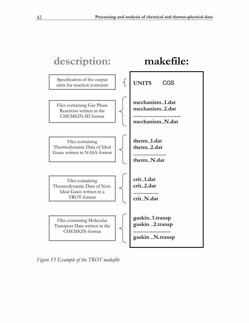
Processing and analysis of chemical and thermo-physical data 42
UNITS CGS
mechanism_1.datmechanism_2.dat................................mechanism_N.dat
therm_1.dattherm_2.dat......................therm_N.dat
crit_1.datcrit_2.dat.................crit_N.dat
gaskin_1.transpgaskin _2.transp.........................gaskin _N.transp
Specification of the outputunits for reaction constants
Files containing Gas PhaseReactions written in theCHEMKIN-III format
Files containingThermodynamic Data of IdealGases written in NASA-format
Files containingThermodynamic Data of Non-
Ideal Gases written in aTROT-format
Files containing MolecularTransport Data written in the
CHEMKIN-format
makefile:description:
Figure 13 Example of the TROT makefile
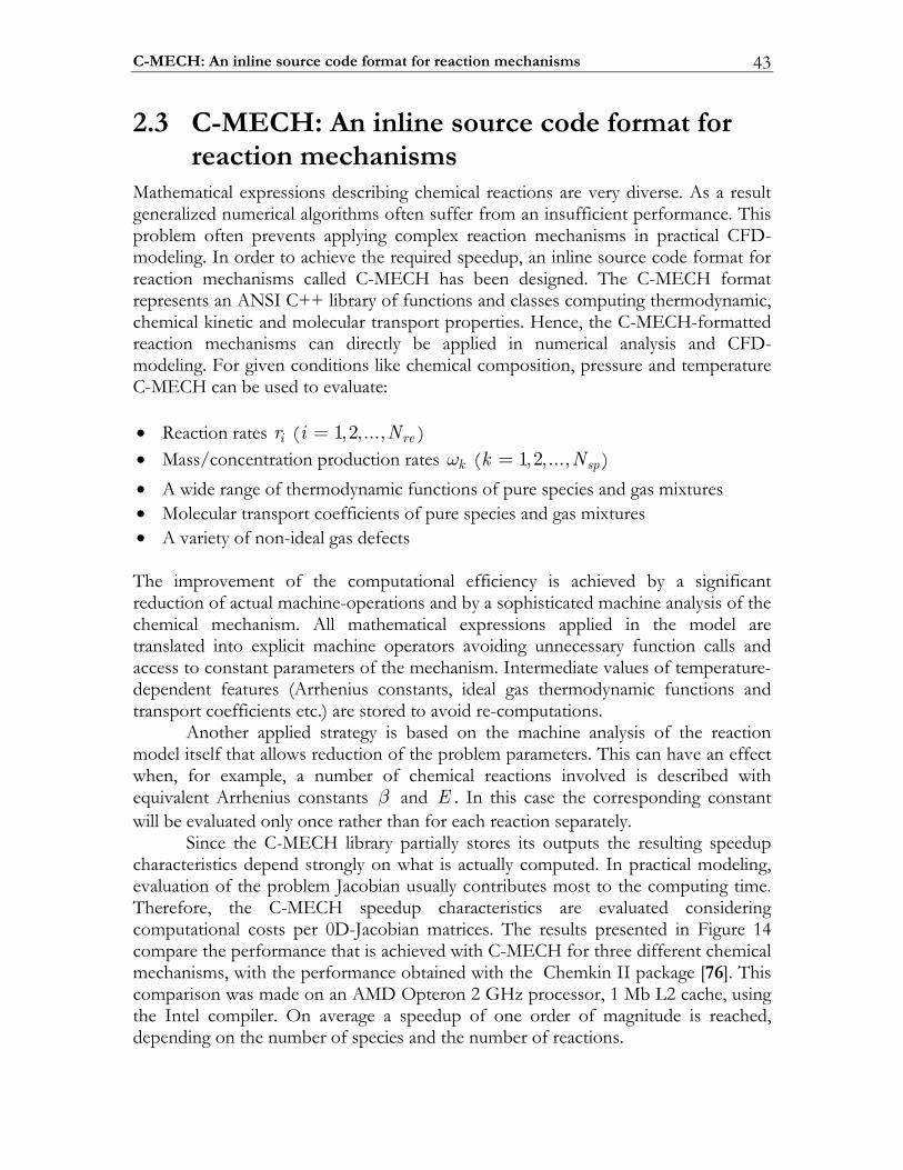
C-MECH: An inline source code format for reaction mechanisms 43
2.3 C-MECH: An inline source code format for reaction mechanisms
Mathematical expressions describing chemical reactions are very diverse. As a result generalized numerical algorithms often suffer from an insufficient performance. This problem often prevents applying complex reaction mechanisms in practical CFD-modeling. In order to achieve the required speedup, an inline source code format for reaction mechanisms called C-MECH has been designed. The C-MECH format represents an ANSI C++ library of functions and classes computing thermodynamic, chemical kinetic and molecular transport properties. Hence, the C-MECH-formatted reaction mechanisms can directly be applied in numerical analysis and CFD-modeling. For given conditions like chemical composition, pressure and temperature C-MECH can be used to evaluate: • Reaction rates ir ( 1,2,..., rei N= ) • Mass/concentration production rates kω ( 1,2,..., spk N= ) • A wide range of thermodynamic functions of pure species and gas mixtures • Molecular transport coefficients of pure species and gas mixtures • A variety of non-ideal gas defects The improvement of the computational efficiency is achieved by a significant reduction of actual machine-operations and by a sophisticated machine analysis of the chemical mechanism. All mathematical expressions applied in the model are translated into explicit machine operators avoiding unnecessary function calls and access to constant parameters of the mechanism. Intermediate values of temperature-dependent features (Arrhenius constants, ideal gas thermodynamic functions and transport coefficients etc.) are stored to avoid re-computations. Another applied strategy is based on the machine analysis of the reaction model itself that allows reduction of the problem parameters. This can have an effect when, for example, a number of chemical reactions involved is described with equivalent Arrhenius constants β and E . In this case the corresponding constant will be evaluated only once rather than for each reaction separately. Since the C-MECH library partially stores its outputs the resulting speedup characteristics depend strongly on what is actually computed. In practical modeling, evaluation of the problem Jacobian usually contributes most to the computing time. Therefore, the C-MECH speedup characteristics are evaluated considering computational costs per 0D-Jacobian matrices. The results presented in Figure 14 compare the performance that is achieved with C-MECH for three different chemical mechanisms, with the performance obtained with the Chemkin II package [76]. This comparison was made on an AMD Opteron 2 GHz processor, 1 Mb L2 cache, using the Intel compiler. On average a speedup of one order of magnitude is reached, depending on the number of species and the number of reactions.
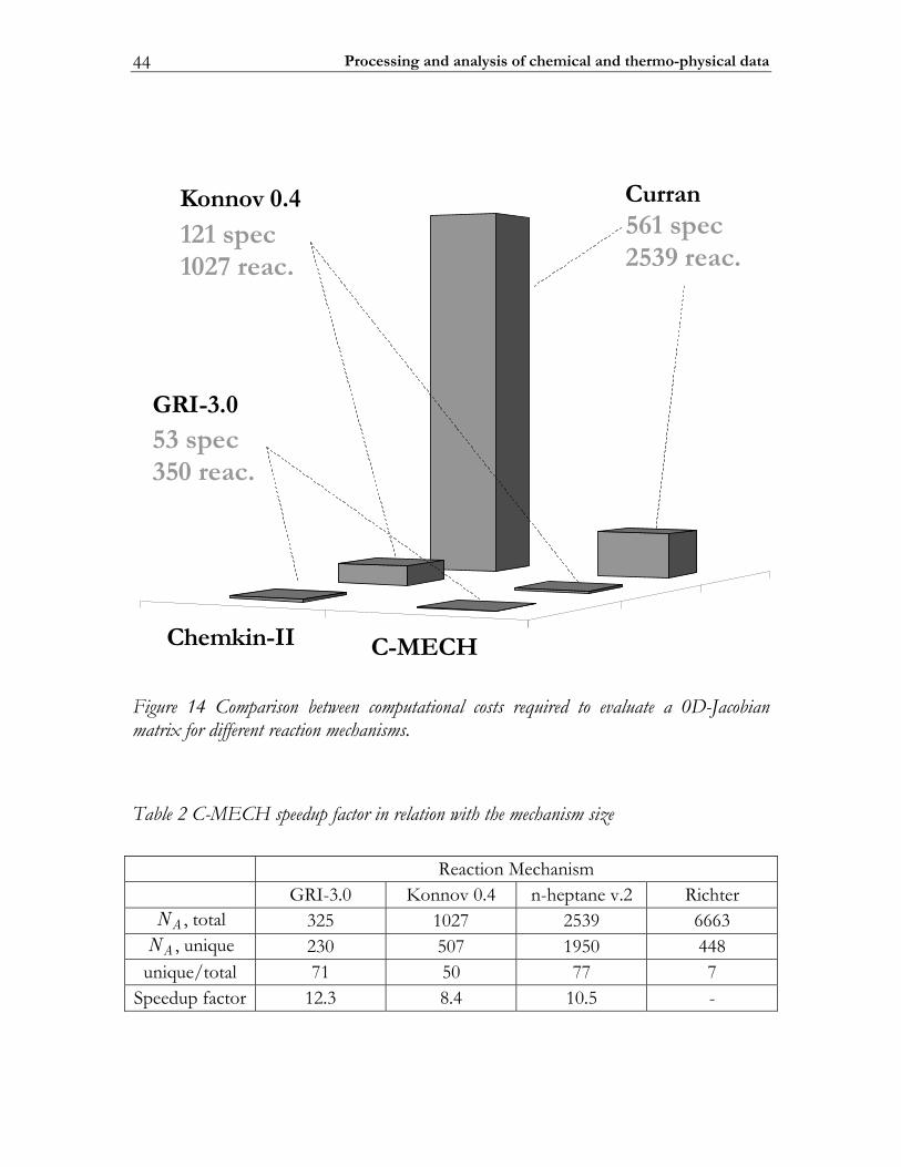
Processing and analysis of chemical and thermo-physical data 44
II-nikmehC HCEM-C GRI-3.0KONNOV-4.0
CURRAN
ceps35.caer053
0.3-IRG
ceps121.caer7201
4.0vonnoKceps165
.caer9352
narruC
Figure 14 Comparison between computational costs required to evaluate a 0D-Jacobian matrix for different reaction mechanisms.
Table 2 C-MECH speedup factor in relation with the mechanism size
Reaction Mechanism GRI-3.0 Konnov 0.4 n-heptane v.2 Richter
AN , total 325 1027 2539 6663 AN , unique 230 507 1950 448
unique/total 71 50 77 7 Speedup factor 12.3 8.4 10.5 -
C-MECH: An inline source code format for reaction mechanisms 45
The mechanism properties and actual speedup are summarized in Table 2. Here the AN -total is the number of Arrhenius constants found in the mechanism and the AN -
unique is the number of Arrhenius constants having no duplicates. As the mechanism of Richter et al. [103] cannot be interpreted by any another generic chemical kinetics package, the resulting speedup is not reported.
2.4 Some typical results
2.4.1 Molecular transport coefficients In the following examples, the molecular transport coefficients computed employing the TROT-link file are compared to the experimental data from [104]. The link file has been generated by processing of the GRI-3.0 reaction mechanism [78] and the critical properties adopted from [39]. Coefficients of pure substances and gas mixtures are computed based on expressions presented before in this chapter.
Viscosity Comparison between experimental and computational viscosities of pure CO, CO2 and H2O species at different pressures and temperatures is shown in Figure 15. Note that in the case when the gas consists of a single chemical substance, use of the linear mixing rules is equivalent to the direct application of the corresponding critical properties. The results obtained for all three species demonstrate that viscosities predicted for atmospheric pressure are in excellent agreement with the experimental data. At elevated pressures, the discrepancy between the experiment and theory depends on the chemical substance. With respect to the CO-species, the computed viscosity is in very good agreement with the experiment. For pressures from 1atm and up to 300atm, the errors are not higher than just a few percent. At higher pressures up to 800atm, the errors reach a level of about 10%. Considering the viscosity coefficient of CO2, the computational inaccuracy depends a lot on gas temperature and pressure. At temperature lower than 800K, the inaccuracy can reach a value of 60% when pressure varies between 300 and 600 atm. However, at higher temperatures that are more relevant to combustion conditions, the discrepancy is not high. Here, for pressures up to 300atm, the discrepancies are not higher than a few persent. With pressure increase up to 600atm the discrepancy level increases to approximately 10%. The worst disagreement with the experiment is found for the viscosity of water vapor. At temperatures lower than approximately 800K, the errors are maximal and vary form 10 to 60 percent, depending on the pressure.
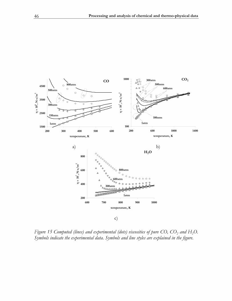
Processing and analysis of chemical and thermo-physical data 46
0051
0052
0053
0054
006005004003002
K,erutarepmet
η×
108 ,N
⋅s/
m2
mta008
mta005
mta003
mta051
mta1
OC
001
0001
00410001006002
K,erutarepmet
η×
107 ,N
⋅s/
m2
mta1
mta001
mta003mta005
mta006
OC 2
a) b)
002
004
006
008
0001009008007006
K,erutarepmet
η×
107 ,N
⋅s/
m2
mta003
mta006
mta008
mta1
H2O
c)
Figure 15 Computed (lines) and experimental (dots) viscosities of pure CO, CO2 and H2O. Symbols indicate the experimental data. Symbols and line styles are explained in the figure.
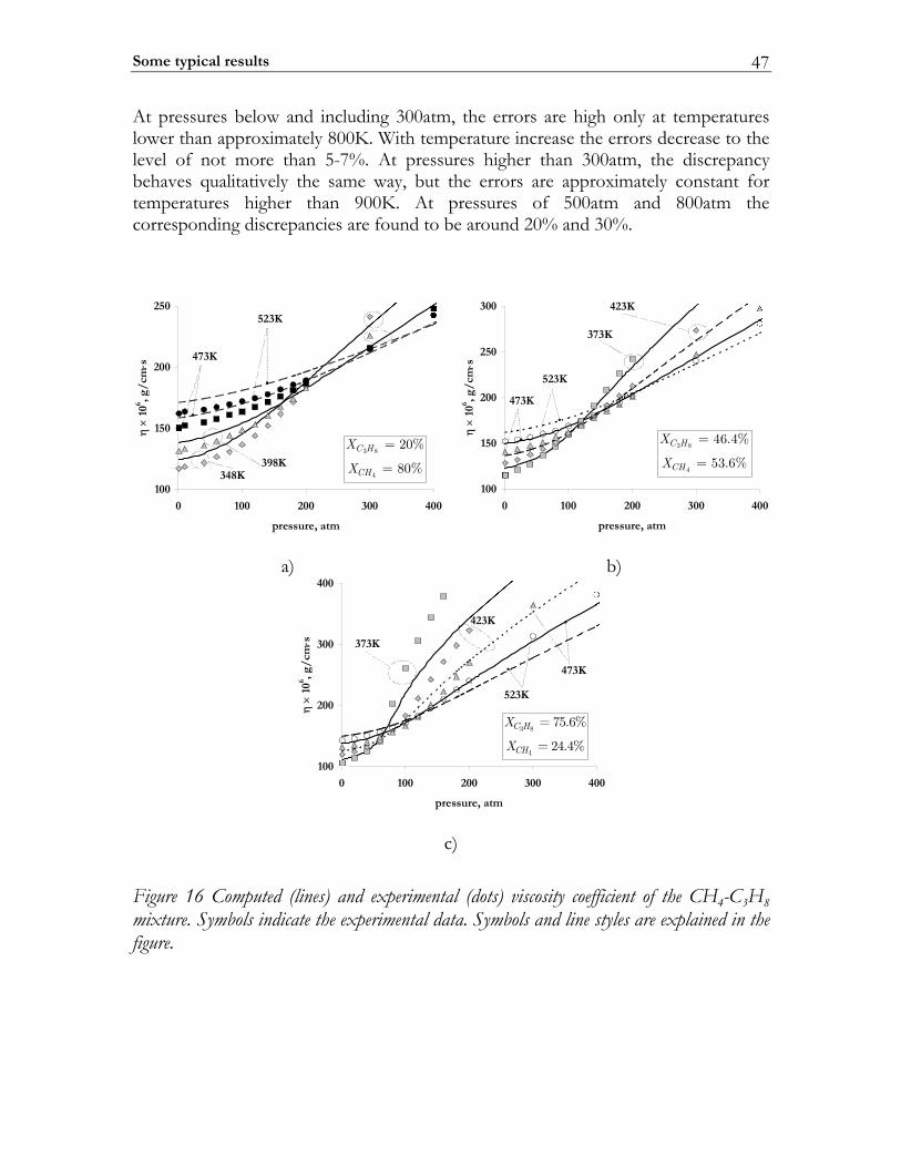
Some typical results 47
At pressures below and including 300atm, the errors are high only at temperatures lower than approximately 800K. With temperature increase the errors decrease to the level of not more than 5-7%. At pressures higher than 300atm, the discrepancy behaves qualitatively the same way, but the errors are approximately constant for temperatures higher than 900K. At pressures of 500atm and 800atm the corresponding discrepancies are found to be around 20% and 30%.
001
051
002
052
0040030020010
mta,erusserp
η×
106 ,g
/cm
⋅s
K843K893
K374
K325
83
4
%02
%08HC
HC
X
X001
051
002
052
003
0040030020010
mta,erusserp
η×
106 ,g
/cm
⋅s
K373
K324
K325
K374
83
4
%4.64
%6.35HC
HC
X
X
a) b)
001
002
003
004
0040030020010
mta,erusserp
η×
106 ,g
/cm
⋅s K373
K374
K324
K325
83
4
%6.57
%4.42HC
HC
X
X
c)
Figure 16 Computed (lines) and experimental (dots) viscosity coefficient of the CH4-C3H8 mixture. Symbols indicate the experimental data. Symbols and line styles are explained in the figure.
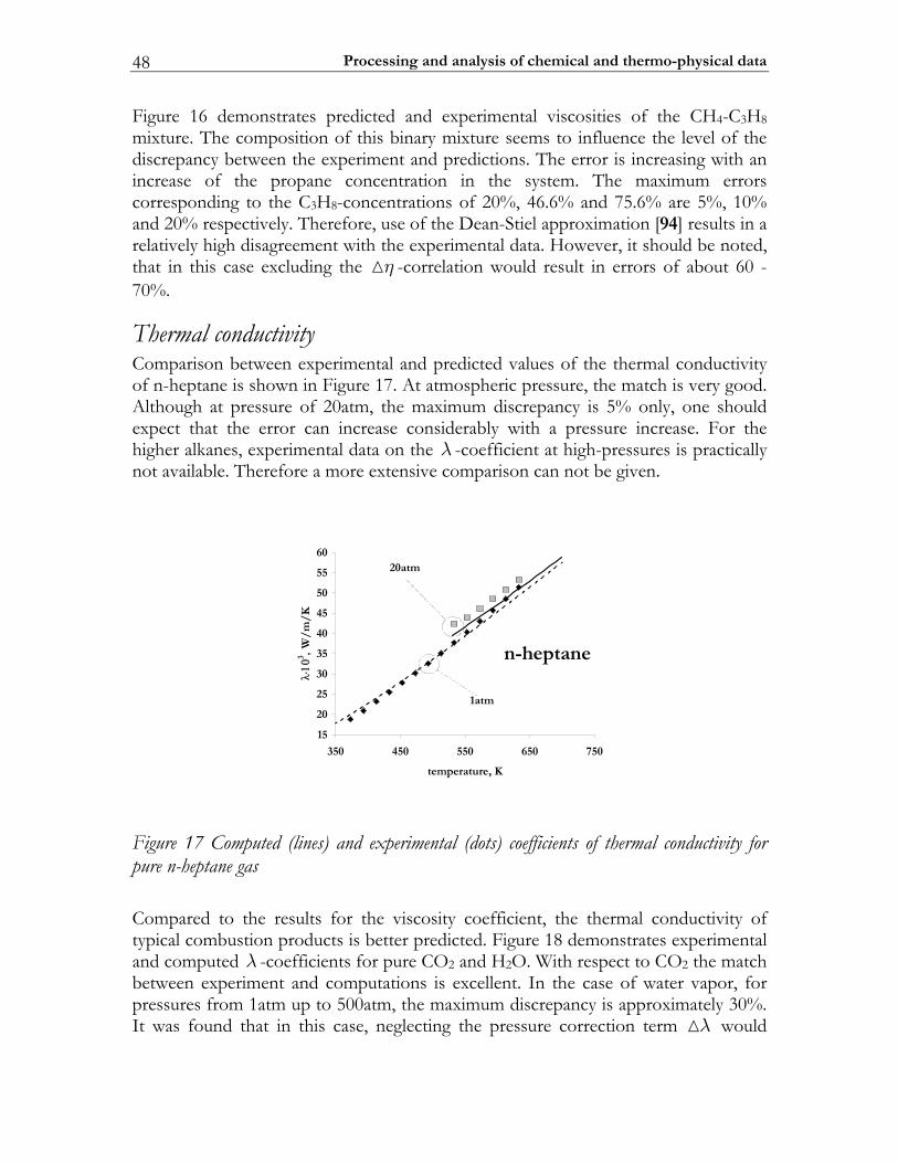
Processing and analysis of chemical and thermo-physical data 48
Figure 16 demonstrates predicted and experimental viscosities of the CH4-C3H8 mixture. The composition of this binary mixture seems to influence the level of the discrepancy between the experiment and predictions. The error is increasing with an increase of the propane concentration in the system. The maximum errors corresponding to the C3H8-concentrations of 20%, 46.6% and 75.6% are 5%, 10% and 20% respectively. Therefore, use of the Dean-Stiel approximation [94] results in a relatively high disagreement with the experimental data. However, it should be noted, that in this case excluding the η -correlation would result in errors of about 60 - 70%.
Thermal conductivity Comparison between experimental and predicted values of the thermal conductivity of n-heptane is shown in Figure 17. At atmospheric pressure, the match is very good. Although at pressure of 20atm, the maximum discrepancy is 5% only, one should expect that the error can increase considerably with a pressure increase. For the higher alkanes, experimental data on the λ -coefficient at high-pressures is practically not available. Therefore a more extensive comparison can not be given.
51
02
52
03
53
04
54
05
55
06
057056055054053
K,erutarepmet
λ⋅10
3 ,W/
m/
K
mta1
mta02
enatpeh-n
Figure 17 Computed (lines) and experimental (dots) coefficients of thermal conductivity for pure n-heptane gas Compared to the results for the viscosity coefficient, the thermal conductivity of typical combustion products is better predicted. Figure 18 demonstrates experimental and computed λ -coefficients for pure CO2 and H2O. With respect to CO2 the match between experiment and computations is excellent. In the case of water vapor, for pressures from 1atm up to 500atm, the maximum discrepancy is approximately 30%. It was found that in this case, neglecting the pressure correction term λ would
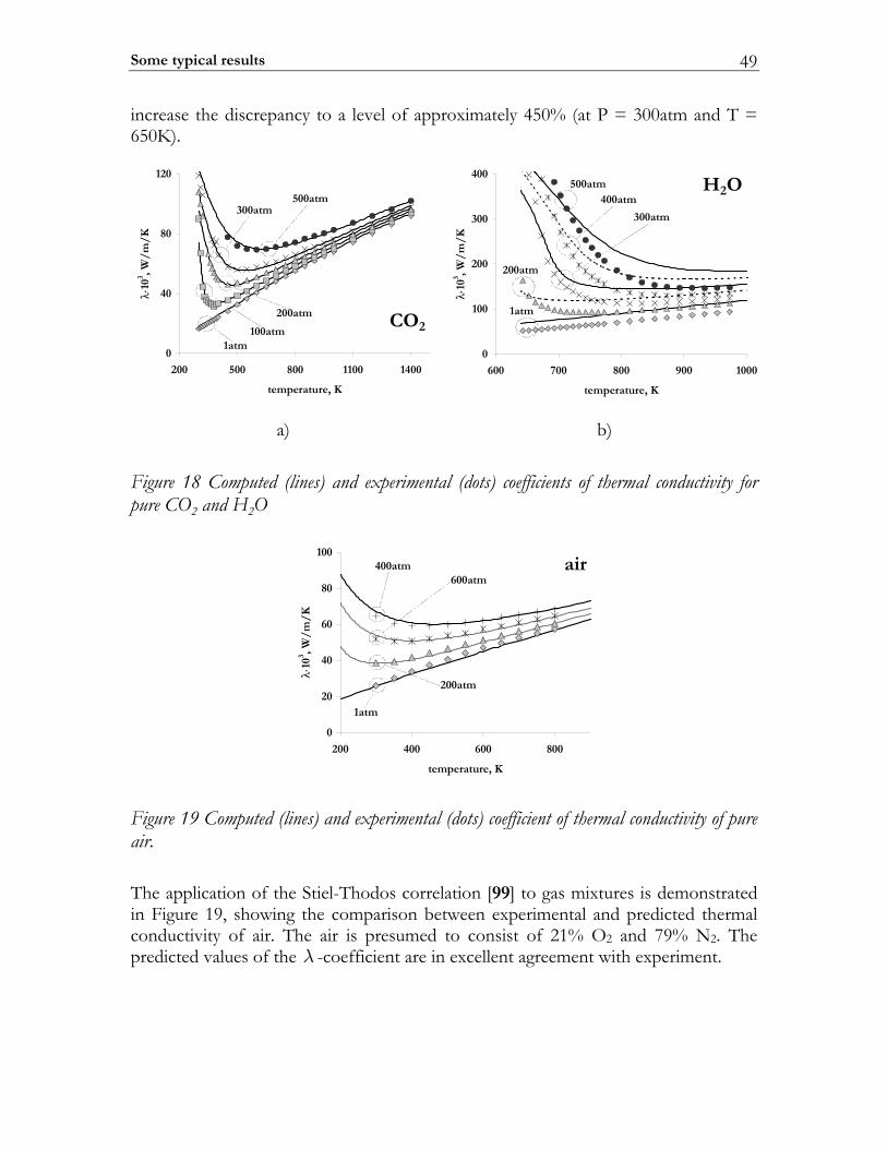
Some typical results 49
increase the discrepancy to a level of approximately 450% (at P = 300atm and T = 650K).
0
04
08
021
00410011008005002
K,erutarepmet
λ⋅10
3 ,W/m
/K
mta1
mta002
mta003mta005
mta001OC 2
0
001
002
003
004
0001009008007006
K,erutarepmet
λ⋅10
3 ,W/
m/
K
mta1
mta002
mta003
mta005mta004
H2O
a) b)
Figure 18 Computed (lines) and experimental (dots) coefficients of thermal conductivity for pure CO2 and H2O
0
02
04
06
08
001
008006004002
K,erutarepmet
λ⋅10
3 ,W/
m/
K
mta002
mta006
mta1
mta004 ria
Figure 19 Computed (lines) and experimental (dots) coefficient of thermal conductivity of pure air. The application of the Stiel-Thodos correlation [99] to gas mixtures is demonstrated in Figure 19, showing the comparison between experimental and predicted thermal conductivity of air. The air is presumed to consist of 21% O2 and 79% N2. The predicted values of the λ -coefficient are in excellent agreement with experiment.
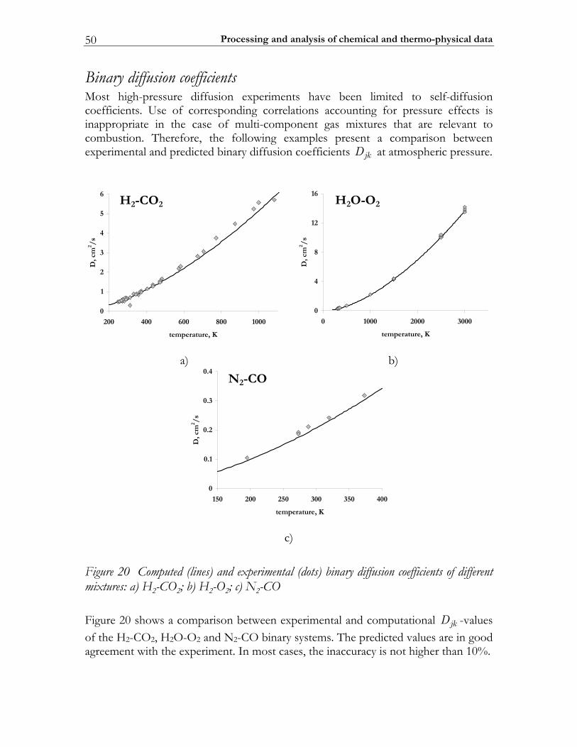
Processing and analysis of chemical and thermo-physical data 50
Binary diffusion coefficients Most high-pressure diffusion experiments have been limited to self-diffusion coefficients. Use of corresponding correlations accounting for pressure effects is inappropriate in the case of multi-component gas mixtures that are relevant to combustion. Therefore, the following examples present a comparison between experimental and predicted binary diffusion coefficients jkD at atmospheric pressure.
0
1
2
3
4
5
6
0001008006004002
K,erutarepmet
D,c
m2 /
s
H2 OC- 2
0
4
8
21
61
0003000200010
K,erutarepmet
D,c
m2 /
s
H2 O-O 2
a) b)
0
1.0
2.0
3.0
4.0
004053003052002051
K,erutarepmet
D,c
m2 /
s
N2 OC-
c)
Figure 20 Computed (lines) and experimental (dots) binary diffusion coefficients of different mixtures: a) H2-CO2; b) H2-O2; c) N2-CO Figure 20 shows a comparison between experimental and computational jkD -values of the H2-CO2, H2O-O2 and N2-CO binary systems. The predicted values are in good agreement with the experiment. In most cases, the inaccuracy is not higher than 10%.
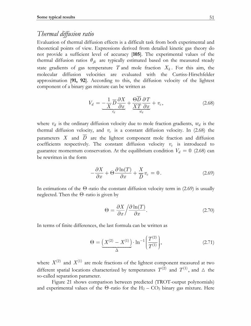
Some typical results 51
Thermal diffusion ratio Evaluation of thermal diffusion effects is a difficult task from both experimental and theoretical points of view. Expressions derived from detailed kinetic gas theory do not provide a sufficient level of accuracy [105]. The experimental values of the thermal diffusion ratios jkθ are typically estimated based on the measured steady state gradients of gas temperature T and mole fraction kX . For this aim, the molecular diffusion velocities are evaluated with the Curtiss-Hirschfelder approximation [91, 92]. According to this, the diffusion velocity of the lightest component of a binary gas mixture can be written as
1
d d
d c
v w
X D TV D vX x XT x
∂ Θ ∂= − + +∂ ∂
, (2.68)
where dv is the ordinary diffusion velocity due to mole fraction gradients, dw is the thermal diffusion velocity, and cv is a constant diffusion velocity. In (2.68) the parameters X and D are the lightest component mole fraction and diffusion coefficients respectively. The constant diffusion velocity cv is introduced to guarantee momentum conservation. At the equilibrium condition 0dV = (2.68) can be rewritten in the form
ln( ) 0cX T X vx x D
∂ ∂− +Θ + =∂ ∂
. (2.69)
In estimations of the Θ -ratio the constant diffusion velocity term in (2.69) is usually neglected. Then the Θ -ratio is given by
ln( )X Tx x
∂ ∂Θ = ∂ ∂ . (2.70)
In terms of finite differences, the last formula can be written as
( )(2)
(2) (1) 1(1)ln TX XT
−
∆
⎛ ⎞⎟⎜Θ = − ⋅ ⎟⎜ ⎟⎟⎜⎝ ⎠, (2.71)
where (2)X and (1)X are mole fractions of the lightest component measured at two different spatial locations characterized by temperatures (2)T and (1)T , and the so-called separation parameter. Figure 21 shows comparison between predicted (TROT-output polynomials) and experimental values of the Θ -ratio for the H2 – CO2 binary gas mixture. Here
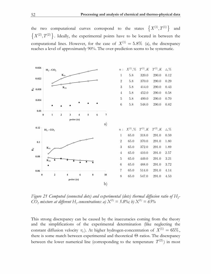
Processing and analysis of chemical and thermo-physical data 52
the two computational curves correspond to the states (1) (1),X T and
(2) (2),X T . Ideally, the experimental points have to be located in between the
computational lines. However, for the case of (1) 5.8%X = (a), the discrepancy reaches a level of approximately 90%. The over-prediction seems to be systematic.
10.0
410.0
810.0
220.0
620.0
76543210
)n(tniop
KT
H2 OC- 2
K 1T
K 2T
(1) (1) (1): ,% , , ,%
1 5.8 320.0 290.0 0.12
2 5.8 370.0 290.0 0.29
3 5.8 414.0 290.0 0.43
4 5.8 452.0 290.0 0.58
5 5.8 499.0 290.0 0.70
6 5.8 548.0 290.0 0.82
n X T K T K
a)
60.0
80.0
1.0
21.0
0186420
)n(tniop
KT
H2 OC- 2
K 1T
K 2T
(1) (1) (2): ,% , , ,%
1 65.0 318.0 291.0 0.59
2 65.0 370.0 291.0 1.80
3 65.0 372.0 291.0 1.89
4 65.0 410.0 291.0 2.57
5 65.0 449.0 291.0 3.21
6 65.0 488.0 291.0 3.72
7 65.0 514.0 291.0 4.14
8 65.0 547.0 291.0 4.53
n X T K T K
b)
Figure 21 Computed (connected dots) and experimental (dots) thermal diffusion ratio of H2-CO2 mixture at different H2 concentrations: a) X(1) = 5.8%; b) X(1) = 65% This strong discrepancy can be caused by the inaccuracies coming from the theory and the simplifications of the experimental determination (like neglecting the constant diffusion velocity cv ). At higher hydrogen-concentration of (1) 65%X = , there is some match between experimental and theoretical Θ -ratios. The discrepancy between the lower numerical line (corresponding to the temperature (2)T ) in most
Some typical results 53
cases is less than 5%. The higher numerical line over-predicts the Θ -ratio of about 50% in maximum. The theoretical over prediction of Θ -ratios is not necessarily always the case. As an example of this, Figure 22 demonstrates comparison between experimental data and computational predictions for H2 – C2H4 binary gas mixture. In this case, the computational Θ -ratio is under-predicted on about 90%.
0
10.0
20.0
30.0
40.0
86420
)n(tniop
KT
H2 C- 2H4
K 1T
K 2T
(1) (1) (2): ,% , , ,%
1 17.0 288.0 183.0 1.35
2 17.0 288.0 187.0 1.23
3 17.0 288.0 199.0 1.08
4 17.0 288.0 208.0 0.99
5 17.0 288.0 215.0 0.90
6 17.0 288.0 228.0 0.68
7 17.0 288.0 239.0 0.54
n X T K T K
Figure 22 Computed (connected dotes) and experimental (dots) thermal diffusion ration of H2-C2H4 mixture The thermal diffusion is a second order effect that can be of importance only if there is a large difference between molecular masses of chemical species present in mixture. Therefore, in modeling combustion of relatively light fuels (e.g. methane, ethane, natural gas etc.), this effect is often neglected without much consequences. With respect to heavy hydrocarbon fuels, one should be noted that the difference in molecular masses of species involved can be significant. In this case taking into account the phenomenon of thermal diffusion is desirable. Therefore in the modeling presented in this thesis, this effect is included by a default. At the same time, it is understood that the insufficient accuracy of the predictions of the corresponding transport coefficients represent an extra issue for the future analysis.
2.4.2 Complex chemistry Parsing and processing of reaction mechanisms are the most intensive data transformation activities. During this stage, the machine first translates symbolic information into a digital analog while distinguishing chemical models and converting physical units. Secondly, the mechanisms are linked with other data (elements, species, thermodynamics etc.). Due to the complexity of these processes, selecting a single reaction step of the mechanism for a check would not be sufficient. Therefore,
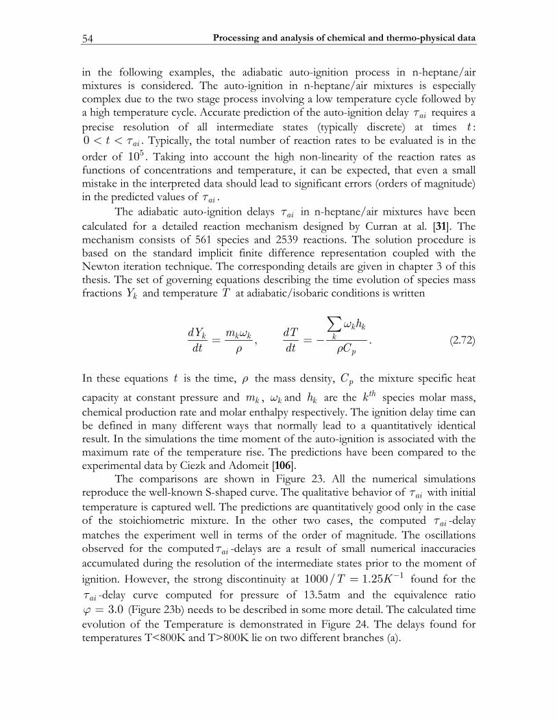
Processing and analysis of chemical and thermo-physical data 54
in the following examples, the adiabatic auto-ignition process in n-heptane/air mixtures is considered. The auto-ignition in n-heptane/air mixtures is especially complex due to the two stage process involving a low temperature cycle followed by a high temperature cycle. Accurate prediction of the auto-ignition delay aiτ requires a precise resolution of all intermediate states (typically discrete) at times t : 0 ait τ< < . Typically, the total number of reaction rates to be evaluated is in the order of 510 . Taking into account the high non-linearity of the reaction rates as functions of concentrations and temperature, it can be expected, that even a small mistake in the interpreted data should lead to significant errors (orders of magnitude) in the predicted values of aiτ . The adiabatic auto-ignition delays aiτ in n-heptane/air mixtures have been calculated for a detailed reaction mechanism designed by Curran at al. [31]. The mechanism consists of 561 species and 2539 reactions. The solution procedure is based on the standard implicit finite difference representation coupled with the Newton iteration technique. The corresponding details are given in chapter 3 of this thesis. The set of governing equations describing the time evolution of species mass fractions kY and temperature T at adiabatic/isobaric conditions is written
,k k
k k k k
p
hdY m dTdt dt C
ωωρ ρ
= = −∑
. (2.72)
In these equations t is the time, ρ the mass density, pC the mixture specific heat capacity at constant pressure and km , kω and kh are the thk species molar mass, chemical production rate and molar enthalpy respectively. The ignition delay time can be defined in many different ways that normally lead to a quantitatively identical result. In the simulations the time moment of the auto-ignition is associated with the maximum rate of the temperature rise. The predictions have been compared to the experimental data by Ciezk and Adomeit [106]. The comparisons are shown in Figure 23. All the numerical simulations reproduce the well-known S-shaped curve. The qualitative behavior of aiτ with initial temperature is captured well. The predictions are quantitatively good only in the case of the stoichiometric mixture. In the other two cases, the computed aiτ -delay matches the experiment well in terms of the order of magnitude. The oscillations observed for the computed aiτ -delays are a result of small numerical inaccuracies accumulated during the resolution of the intermediate states prior to the moment of ignition. However, the strong discontinuity at 11000/ 1.25T K−= found for the aiτ -delay curve computed for pressure of 13.5atm and the equivalence ratio
3.0ϕ = (Figure 23b) needs to be described in some more detail. The calculated time evolution of the Temperature is demonstrated in Figure 24. The delays found for temperatures T<800K and T>800K lie on two different branches (a).
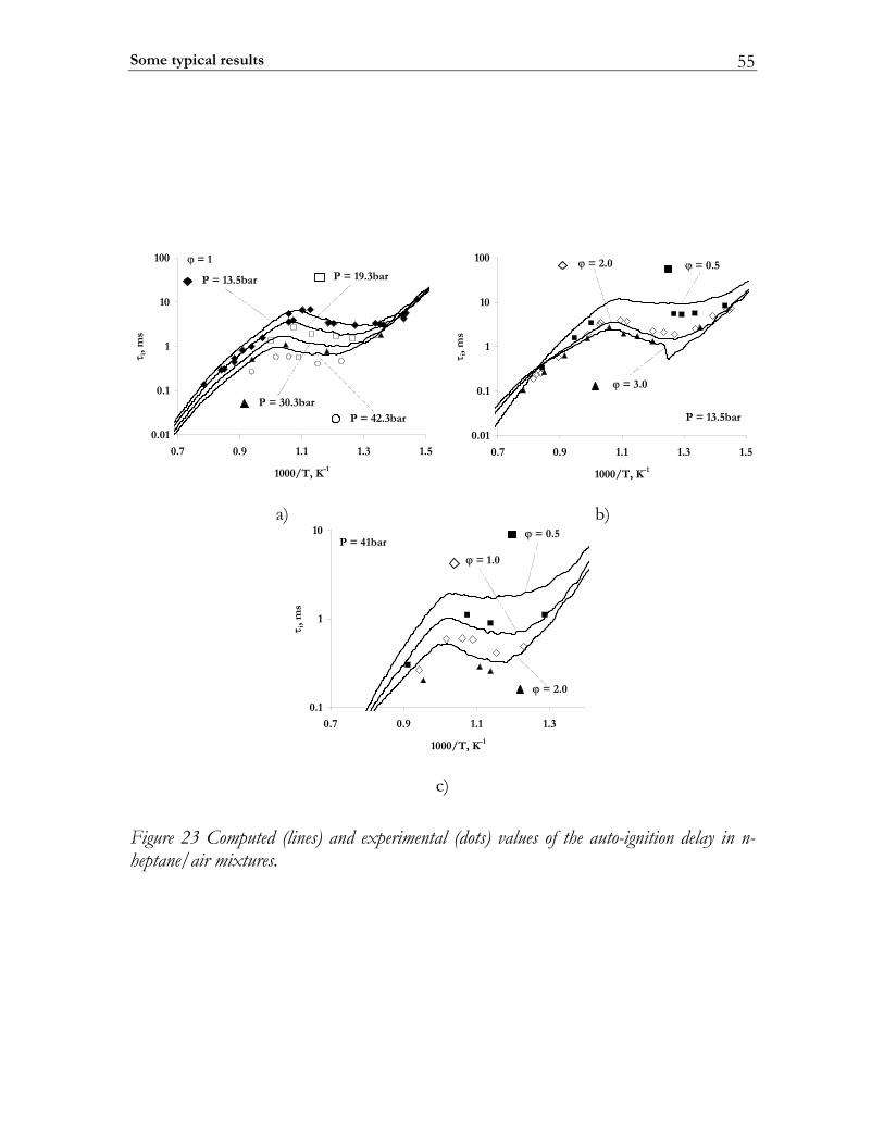
Some typical results 55
10.0
1.0
1
01
001
5.13.11.19.07.0
K,T/0001 1-
τ i,m
s
rab5.31=P rab3.91=P
rab3.03=Prab3.24=P
ϕ 1=
10.0
1.0
1
01
001
5.13.11.19.07.0
K,T/0001 1-τ i
,ms
ϕ 5.0=ϕ 0.2=
ϕ 0.3=
rab5.31=P
a) b)
1.0
1
01
3.11.19.07.0
K,T/0001 1-
τ i,m
s
rab14=Pϕ 5.0=
ϕ 0.1=
ϕ 0.2=
c)
Figure 23 Computed (lines) and experimental (dots) values of the auto-ignition delay in n-heptane/air mixtures.
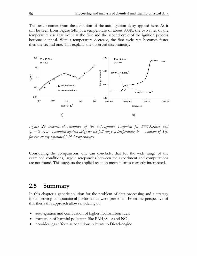
Processing and analysis of chemical and thermo-physical data 56
This result comes from the definition of the auto-ignition delay applied here. As it can be seen from Figure 24b, at a temperature of about 800K, the two rates of the temperature rise that occur at the first and the second cycle of the ignition process become identical. With a temperature decrease, the first cycle rate becomes faster then the second one. This explains the observed discontinuity.
10.0
1.0
1
01
001
5.13.11.19.07.0
K,T/0001 1-
τ i,m
s
tnemirepxe-
rab5.31=Pϕ 0.3=
+ snoitatupmoc-
006
0001
0041
0081
30-E6.130-E1.140-E0.640-E0.1
ces,emit
tem
per
atu
re, K K42.1=T/0001 1-
K52.1=T/0001 1-
rab5.31=Pϕ 0.3=
a) b)
Figure 24 Numerical resolution of the auto-ignition computed for P=13.5atm and 3.0ϕ = : a- computed ignition delay for the full range of temperature, b- solution of T(t)
for two closely separated initial temperatures Considering the comparisons, one can conclude, that for the wide range of the examined conditions, large discrepancies between the experiment and computations are not found. This suggests the applied reaction mechanism is correctly interpreted.
2.5 Summary In this chapter a generic solution for the problem of data processing and a strategy for improving computational performance were presented. From the perspective of this thesis this approach allows modeling of • auto-ignition and combustion of higher hydrocarbon fuels • formation of harmful pollutants like PAH/Soot and NOx • non-ideal gas effects at conditions relevant to Diesel-engine

Summary 57
With respect to the non-ideal gas thermodynamics, it is worthwhile to point out that this approach is also well-suited for future modeling of high pressure multi-component droplet vaporization and for modeling of other high pressure phenomena, e.g., for thermodynamic modeling of detonation. The technique introduced for improving the computational performance consists of two strategies. The first one is converting the chemical/physical model into inline source code that significantly reduces the number of machine operations required to evaluate properties of interest. The second one is the optimization of data by automated analysis of the models architecture. This strategy allows skipping a number of unwanted re-computations that are often the case in CFD-simulations. The achieved speedup factor is about one order of magnitude. Combining this methodology with other computational techniques is expected to result in a further speedup that can bring detailed modeling of complex combustion processes to an even higher level of practical applicability. A description of some of these techniques can be found in [107]for repro-modeling, [108] for in-situ adaptive tabulation (ISAT), [109] for the piecewise reusable implementation of solution mapping (PRISM) and [110] for artificial neural-networks (ANN). Finally, some typical computational results and their comparison to experimental data were demonstrated for molecular transport coefficients and the auto-ignition delay of n-heptane/air mixtures. On one hand, these comparisons demonstrate the robustness of the developed tools. On the other hand they give an important indication on the accuracies that can be expected when applying models of extended complexity to practical simulations. The shown comparisons demonstrate a remarkable improvement of predicted transport properties at elevated pressures when taking into account the effects of non-ideal gas. With respect to the thermal conditions relevant to Diesel engine, the applied correlations yield a reasonable accuracy. It is important to mention, that in principle, a better accuracy can be achieved by making a choice for other correlations that fit better for each particular problem.

Chapter 3
3 Modeling homogeneous reactions at supercritical high-pressure conditions
In this chapter the applicability of the ideal gas assumption in modeling homogeneous auto-ignition and NO-formation processes at supercritical high-pressure conditions is explored. In the first section the problem is introduced. The set of equations describing homogeneous reactions in a rapid compression machine is presented in section (3.2). The thermal conditions are chosen such that they resemble a heavy-duty diesel engine. The ideal gas predictions are compared to a reference simulation based on a non-ideal gas model. Results on the modeling of auto-ignition of a stoichiometric n-heptane/air mixture are presented in section (3.3). The effect of the ideal gas assumption is analyzed on two test cases described with different initial temperatures. The results on the modeling of NO-formation are given in section (3.4) as well. Discussion and conclusions are presented in sections (3.4) and (3.5) respectively.
3.1 Introduction In recent years, the charge pressure of the turbocharged Direct Injection Heavy-Duty diesel engine has been rising continuously. The motivation for this trend has been primarily the resulting increase in engine torque density (or so-called bmep) giving the engine better performance. At the same time the increasing charge density reduces the negative impact of friction losses on fuel consumption. Finally, increasingly stringent emission legislation has lead to the need to run these engines with increasing amounts of exhaust gas recirculation. To maintain torque density with such exhaust gas recirculation again implies higher charge densities. Currently, HD diesel engine designs are being investigated that aim at full-load intake charge pressures above 4 bar (absolute pressure), e.g., by implementing two-stage turbo-charging technology. In these engines, in-cylinder pressures and temperatures at the end of the compression stroke will reach values of 160 bar and
Modeling homogeneous reactions at supercritical high-pressure conditions 60
850 K. Of course higher pressures (up to 240 bar and – for race truck engines and marine diesel applications – even as high as 300 bar) will be achieved as combustion progresses. Although it is obvious that the common assumption of ideal gas behavior that is employed in current CFD codes becomes less valid as the ambient pressure increases [45, 39], a direct comparison of numerical predictions using different equations of state (EOS) has not been reported in the literature before. Most numerical investigations where non-ideal gas models were applied have been dedicated to droplet vaporization and combustion at Diesel like pressures. Under these conditions, fuel vapor non-ideality will have an impact not only on the volumetric properties like density and temperature, but also on molecular transport coefficients [39, 44-48]. These efforts were usually motivated with the understanding that the droplet lifetime is a critical parameter of importance in the design of Diesel engine: a slower droplet vaporization can lead to liquid fuel penetrating further into the combustion chamber; too large liquid fuel penetration can result in cylinder wall-wetting and ultimately in excessive emissions of unburned hydrocarbons. An extended review on the supercritical droplet vaporization and combustion studies can be found in [49]. When considering combustion, it can be expected that temperature errors resulting from use of the ideal gas law will accumulate during a mechanical process like gas compression/expansion, and that in turn would lead to errors when calculating important temperature-sensitive phenomena like auto-ignition and NO-formation. However, with respect to homogeneous reaction processes, a quantitative validation of the applicability of the ideal gas law can hardly be found in the literature. To our knowledge, the single attempt in this direction was presented by Zevenhoven in [40], where thermal NO formation was estimated with temperatures computed with different equations of state based on pressure and volume histories taken from an engine cycle of a large diesel engine. These computations indicated that the use of the ideal gas law leads to an over-estimation of the computed temperature compared to the experimentally determined (volume averaged) value while the use of real gas models lead to under-estimated temperatures. Based on the Zeldovich chemical reaction mechanism for nitrogen oxidation, the release of NO was computed for a number of equations of state. Results presented in [40] are summarized in Table 3. The first row shows the maximum of the volume averaged temperature during the engine cycle and the second row represents the corresponding relative NO densities. From this table it follows that the use of the ideal gas assumption leads to a NO deviation of about 200% from the measured one. The non-ideal gas EOS gives temperatures that are very close to the measured ones and therefore yield good predictions of the NO release.
Introduction 61
Table 3 Maximum temperature experimentally determined and predicted with different equations of state, and the effect on calculated NOx formation via the Zeldovich mechanism.
experiment ideal gas van der Waals Berthelot Beattie –
Bridgeman
max,T K 1676 1722 1675 1660 1660
,%NOδ 100* (reference) 298 101 69 70
maxT -Temperature maximum NOδ -Relative NO emission
* -Not measured NO emission, but calculated via the Zeldovich mechanism using experimental temperature data With Zevenhoven [40], the gas temperature was directly evaluated from the equation of state as
P vTZ R
⋅=⋅
, (3.1)
where P is the gas pressure, v the molar volume, R the universal gas constant and Z the compressibility factor. However, in CFD simulations the temperature is typically determined solving the energy conservation equation, where the EOS is indirectly involved by modeling the mechanical work terms and the non-ideal gas defect of the internal energy. Furthermore with CFD often only pressure or volume variation is an input, and the other parameter has to be determined using the equation of state. Therefore, the equation of state can be applied in different ways depending on the particular problem. This means that the inaccuracy of the ideal gas law in modeling high-pressure processes depends on the method of its application. In this chapter we investigate several modeling approaches with respect to the application of the ideal gas assumption. The study focuses on homogeneous auto-ignition and NO-emission, both key processes in Diesel engine design.
3.2 Modeling Homogeneous Reaction Processes In this section the problem of homogeneous compression-reaction processes and the applied numerical algorithm are described. The subject is divided in four parts. The first part (3.2.1) introduces the formulation together with a generalized system of governing equations. The method of solution is described in the second part (3.2.2).
Modeling homogeneous reactions at supercritical high-pressure conditions 62
The applied reaction model and validation of the computational method are presented in the third part (3.2.3). Finally, the fourth part (3.2.4) presents the approach.
3.2.1 Problem formulation We consider an adiabatic compression-reaction (ACR) process taking place in a homogeneous gas mixture. As described in the following, for every ACR-process four different problem formulations can be identified. They are denoted here as REF, IV, IP and IPV. The ultimate goal of this chapter is to clarify the qualitative and quantitative differences between the computational results obtained with these four problem formulations. The exact description of REF, IV, IP and IPV formulations is presented below.
REF-formulation The reacting mixture is considered as a non-ideal gas described with the Redlich-Kwong equation of state [84]. The volume history of an ACR-process is prescribed. The time history of pressure, temperature and gas composition is determined by solving corresponding equations for the thermodynamic state, here the Redlich-Kwong equation, conservation of energy and species. The results of the REF-computations are considered as the most reliable with respect to the high-pressure ACR phenomena and therefore, are used as reference data for all other formulations.
IV-formulation The reacting mixture is considered as an ideal gas. The volume history of the ACR-process (pre-computed REF-process) is the applied closing condition. The time history of pressure, temperature and gas composition is determined applying the ideal gas law, in conjunction with energy and species conservation. The IV-simulation is relevant to the CFD modeling for internal combustion engines, where the volume history is typically defined in terms of the engine crank angle.
IP-formulation The reacting mixture is considered as an ideal gas. The pressure history of the pre-computed REF-process is the applied closing condition. The time history of volume, temperature and gas composition is determined by applying the ideal gas law, in conjunction with energy and species conservation. The IP-setup is relevant to the approach used normally for open reactor modelling with that difference, that the gas pressure is a function of time.
IPV-formulation The reacting mixture is considered as an ideal gas. Both volume and pressure histories of the pre-computed REF-process are applied to close the system. The time history of the gas composition is determined by solving the species conservation equations, while the gas temperature is directly defined from the ideal gas law. Note that computational predictions based on the IPV - formulation reproduce adiabatic conditions only when the ideal gas law is fully adequate. The IPV-setup is not
Modeling Homogeneous Reaction Processes 63
common for numerical modeling, since the combination of prescribed pressure and volume histories is quite unusual. However, the estimations of the NO-concentration reported in [40] are performed based on the IPV-formulation. It is important to stress that all four formulations should yield completely identical predictions if the reacting system behaves like an ideal gas at the given thermal conditions. Otherwise, the differences between the corresponding predictions indicate the level of the gas non-ideality. On the other hand, considering these differences can clarify which problem formulation based on the ideal gas law (IV, IP or IPV) is the most successful for modeling high-pressure ACR-processes. With respect to the above described formulations we introduce the time-dependent vector of unknowns written as , , , , 1,2,...,k Q spT Y P V k Nω= = , (3.2) where T is the gas temperature, kY the mass fraction of the thk species, spN the total number of species, P the ambient pressure, V the chamber volume and Qω the specific rate of the external energy supply which is zero if the process is adiabatic (this can not be the case in the IPV-modeling). The set of equations describing the processes in the homogeneous charge is given in the following.
Governing equations The time evolution of the chemical composition is coming from the chemical kinetics equation written as
k k kdY mdt
ωρ
= , (3.3)
where km and kω are the thk species molar mass and chemical production rate respectively, t is the time and ρ the mass density. The energy conservation equation is written in the form of
1k kQk
v v v vIII IVI II
udT P dV ddt C V C dt m C dt C
ωωξ
ρ ρ= − − − +⋅ ⋅
∑, (3.4)
where ku is the thk species molar energy, vC the mixture specific heat capacity at constant volume, m the mixture molar mass, ξ the non-ideal gas defect of the mixture molar energy. In the last equation, the I -term represents a change of temperature due to chemical reactions, the II -term describes the temperature change caused by mechanical work, the III - and IV -terms account for the gas non-ideality
Modeling homogeneous reactions at supercritical high-pressure conditions 64
and non-adiabatic conditions respectively. According to the previously described problem formulations, the deviation of the molar internal energy from its ideal gas value is
( )1 23 ln2
0 , ,
a v b REFvT b
IV IP IPVξ
+⎧⎪− ⇔⎪⎪= ⎨⎪⎪ ⇔⎪⎩
. (3.5)
In this formula, v is the mixture molar volume and parameters a and b are computed from
2 2.5; 0.4274802327
; 0.08664035
a cma
cm
b cmb
cm
R TaPRTbP
Ω= Ω =
Ω= Ω =, (3.6)
where cmP and cmT are the mixtures pseudo-critical pressure and temperature respectively (see chapter 2). Here the mixture pseudo-critical temperature is evaluated following the approximation of Kay [87] and Prausnitz and Gunn [88] (see chapter 2). Since critical points for chemical radicals have no physical basis they were approximated by the values of molecular nitrogen. This will not have a significant effect since the concentrations of the radicals are low. The systems volumetric parameters and the chemical composition are coupled with an equation of state written in the form
( )
, ,
RT a REFv b Tv v bPRT IV IP IPVv
⎧⎪ − ⇔⎪⎪ − +⎪= ⎨⎪⎪ ⇔⎪⎪⎩
. (3.7)
Finally the system of equations is closed with two equations that define the process conditions written as
1
2
0
0
Φ =
Φ =. (3.8)
Here the relation 1Φ represent the prescribed volume or pressure history and comes from
Modeling Homogeneous Reaction Processes 65
1
( ) , ,
( )V
P
V h t REF IV IPV
P h t IP
⎧ − ⇔⎪⎪Φ = ⎨⎪ − ⇔⎪⎩. (3.9)
The relation 2Φ is written in the form
2
, ,
( )Q
P
REF IP IV
P h t IPV
ω ⇔⎧⎪⎪Φ = ⎨⎪ − ⇔⎪⎩, (3.10)
which represents the adiabatic requirement 0Qω = for formulations REF, IP and IV and is the pressure-history ( )Ph t for the IPV-formulation (then the value of Qω is determined from equation (3.4)).
3.2.2 Method of solution To be solved numerically the system of governing equations (3.3)-(3.10) was transformed using finite differencing techniques. The idea is to identify a discrete solution of the governing equations for the sequence of time moments 1 20 ...t t τΤ = = < < < , (3.11) where τ denotes the time of the process duration. For the continuous mapping 1( ) :y t t R→ , we define ( ) ( )n
ny y t= . Using this discretization, the time derivatives in equations (3.3)-(3.10) are approximated with
1
1n
n n
n nt t
dy y ydt t t
+
+=
−≅−
. (3.12)
All other terms of the equations system were expressed as functions of the vector (3.2) defined at the time moment 1nt + . For example the kinetic equation
k k kdY mdt
ωρ=
is then transformed into
( ) ( ) ( )1 1
1 1
k k k kn n n
n n n
Y Y mt t
ωρ
+ +
+ +
−=
−. (3.13)
Modeling homogeneous reactions at supercritical high-pressure conditions 66
The resulting non-linear system of algebraic equation was solved with the standard method of Newton iterations. The reaction source terms and thermodynamic properties were computed using the C-MECH library (see chapter 2) constructed for the particular reaction mechanism described in the next sub-section.
3.2.3 Reaction mechanism The chemical reaction mechanism selected for this chapter is a combination of a reduced chemical kinetic model for Homogeneous Charge Compression Ignition (HCCI) combustion of primary reference fuels in a rapid compression machine [111] with the GRI detailed mechanism including the NOx chemistry [78]. The two-stage ignition of n-heptane which involves low and high temperature cycles followed by a branched chain explosion is described with the reduced kinetic model [111]. The reaction is initiated by the abstraction of an H-atom from the n-heptane molecule (QH) by O2 to form the alkyl radical Q and HO2: 2 2QH O Q HO+ ⇔ + (3.14) At low temperatures, the initiated process consists of a number of steps which can be summarized into the global equation 2 2QH+2O H O+OQOOH⇒ . (3.15) During the low temperature cycle, the temperature rises rapidly until the competing reaction: 2 2Q+O Olefin HO⇔ + (3.16) becomes faster than process (3.15). This is followed by the reaction: 2 2 2 2 2HO +HO H O +O⇒ (3.17) Then, the temperature continues to rise slowly until the reaction 2 2H O (M) OH+OH+(M)+ ⇒ (3.18) becomes important and a thermal explosion is initiated. The much less exothermic high-temperature cycle is expressed with 2 2 2QH+O Olefin+H O⇒ (3.19) In [111] the oxidation of the intermediate products like OQO and Olefin is described with a set of global chemical reactions. The block of chemical equations describing the n-heptane ignition is given in detail in Table 4.
Modeling Homogeneous Reaction Processes 67
Table 4 The reaction mechanism describing low anf high temperature cycles of n-heptane oxidation (Tanaka et al, 2003).
REACTIONS ( exp( / )nk A T E RT= ⋅ − ) A n E
1 :R 7 16 2 7 15 2
12
C H +O C H +HO
/1.00 10 0.0 0.0/REV
⇔
⋅ 161.00 10⋅ 0.0 46000.0
2 :R 7 15 2 7 15
13
C H +O C H OO
REV/2.51 10 0.0 27400.0/
⇔
⋅ 121.00 10⋅ 0.0 0.0
3 :R 7 15 7 14
11
C H OO C H OOH
REV/1.00 10 0.0 11000.0/
⇔
⋅ 111.51 10⋅ 0.0 19000.0
4R 7 14 2 7 14
13
C H OOH+O OOC H OOH
/2.51 10 0.0 27400.0/REV
⇔
⋅ 113.16 10⋅ 0.0 0.0
5 :R 7 14 7 13OOC H OOH OC H OOH+OH⇒ 108.91 10⋅ 0.0 17000.0
6 :R 7 16 7 15 2C H +OH C H +H O⇒ 131.00 10⋅ 0.0 3000.0
7 :R 7 13 7 13OCC H OOH OC H O+OH⇒ 153.98 10⋅ 0.0 43000.0
8 :R 7 15 2 7 14 2
11
C H +O C H +HO
REV/3.16 10 0.0 19500.0/
⇔
⋅ 113.16 10⋅ 0.0 6000.0
9 :R 7 13 2 7 12 2
11
OC H O+O OC H O+HO
/3.16 10 0.0 19500.0/REV
⇔
⋅ 113.16 10⋅ 0.0 6000.0
10 :R 7 12 2 2 7 10 2 2 2
2
OC H O+HO +O OC H O+H O +HO
/ 0.0/FORD O
⇒133.16 10⋅ 0.0 10000.0
11 :R 7 10 2 2 2 2
2
OC H O+HO +5O 7CO+5H O+HO
FORD/O 0.0/
⇒ 133.16 10⋅ 0.0 10000.0
12 :R 7 14 2 2 2
2
C H +HO +7O 7CO+7H O+HO2
FORD/O 0.0/
⇒ 133.16 10⋅ 0.0 10000.0
Modeling homogeneous reactions at supercritical high-pressure conditions 68
The remaining chemical equations including the block describing NO-formation are adopted from the GRI model [78]. The critical volumetric properties of stable species are adopted from [39]. The resulting mechanism was composed and interpreted with the TROT-pre-processor program (see chapter 2). The total mechanism consists of 73 species and 350 reactions.
Validation The mechanism was validated by modeling the auto-ignition in homogeneous n-heptane/air mixtures. The auto-ignition delay was computed based on the IP- problem formulation with the closing condition 1 0P PΦ = − , (3.20) where 0P is the constant ambient pressure. The obtained numerical predictions have been compared to the experimental data of Ciezki and Adomeit [106], where n-heptane/air mixtures were investigated in a high pressure shock tube where pressures and temperatures behind the reflected shock-waves varied between 3.2 and 42 bar, respectively between 660 and 1350K and this for equivalence ratio’s between 0.5 and 3.0. This range of conditions covers a region pertinent to internal combustion engines. In the numerical simulations a homogeneous gas mixture was subject to these same initial conditions. Figure 25 shows the experimental [106] and calculated ignition delay times plotted versus the inverse of the initial temperature. In the simulations the moment of auto-ignition is associated with the maximum rate of temperature rise. In the high-temperature region the experimental and computed ignition delay-time are approximately straight lines in the Arrhenius plot. Here the computed curves show both qualitatively and quantitatively good agreement with the experimental lines. For pressures around 13.5bar the dependencies become strongly non-linear in the temperature range between 700 and 950K. In this intermediate temperature region a decrease in ignition delay time is observed with decreasing temperatures. This leads to the known S-shape curve with a maximum and minimum. Between both extremes the dependence shows a negative temperature coefficient (NTC zone). The position of this transition region shifts to higher temperatures with increasing pressure. In the low-temperature region (below approximately 700K) the dependence of the ignition delay time on temperature can again be expressed by a linear dependence in the Arrhenius plot (i.e., log( )τ vs. 1/T ). Except for the low-temperature zone the computed auto-ignition delay is systematically smaller than the experimental values for all the pressures. However, the qualitative behavior of the experimental and computed Arrhenius plots, including the location of the NTC zones, correspond very well.
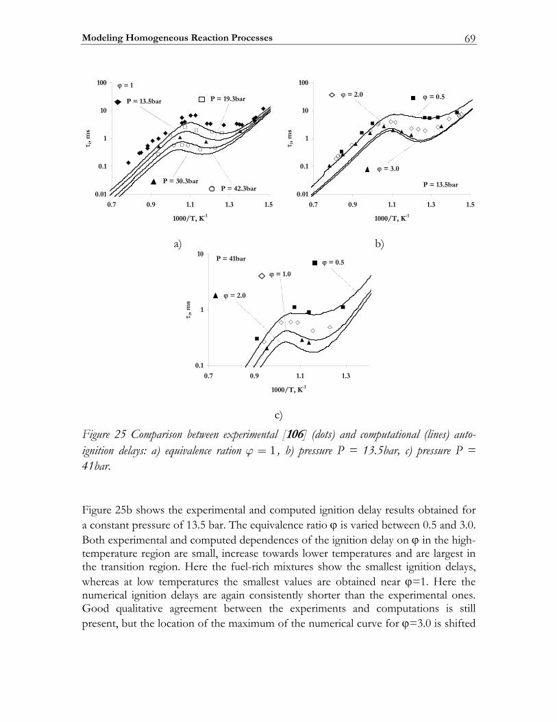
Modeling Homogeneous Reaction Processes 69
10.0
1.0
1
01
001
5.13.11.19.07.0
K,T/0001 1-
τ i,m
s
rab5.31=P rab3.91=P
rab3.03=Prab3.24=P
ϕ 1=
10.0
1.0
1
01
001
5.13.11.19.07.0
K,T/0001 1-
τ i,m
s
ϕ 5.0=ϕ 0.2=
ϕ 0.3=
rab5.31=P
a)
b)
1.0
1
01
3.11.19.07.0
K,T/0001 1-
τ i,m
s
rab14=P ϕ 5.0=
ϕ 0.1=
ϕ 0.2=
c)
Figure 25 Comparison between experimental [106] (dots) and computational (lines) auto-ignition delays: a) equivalence ration 1ϕ = , b) pressure P = 13.5bar, c) pressure P = 41bar. Figure 25b shows the experimental and computed ignition delay results obtained for a constant pressure of 13.5 bar. The equivalence ratio ϕ is varied between 0.5 and 3.0. Both experimental and computed dependences of the ignition delay on ϕ in the high-temperature region are small, increase towards lower temperatures and are largest in the transition region. Here the fuel-rich mixtures show the smallest ignition delays, whereas at low temperatures the smallest values are obtained near ϕ=1. Here the numerical ignition delays are again consistently shorter than the experimental ones. Good qualitative agreement between the experiments and computations is still present, but the location of the maximum of the numerical curve for ϕ=3.0 is shifted
Modeling homogeneous reactions at supercritical high-pressure conditions 70
towards lower temperatures compared to the experimental data. Similar observations were also found for the case of 41 bar (see Figure 25c). All the computed graphs demonstrate the well-known negative temperature coefficient region and show qualitatively good agreement with experimental values. Both measured and computed dependencies show that with increasing pressure and increasing equivalence ratio the negative temperature coefficient region shifts to higher temperatures and lower ignition delays. Although at high temperatures computed delays are systematically lower than experimental, the adequate behavior of the modelled processes shows the applicability of this computational procedure and chemical model. Considering the comparison between the computational and experimental results, it can be concluded, that the temperature-dependence of the auto-ignition delay is captured well. Therefore, the composed reaction mechanism is applicable for the present study. It is worthwhile to note, that the results obtained with this combined mechanism are compatible with those obtained with the detailed model by Curran at al. [31] in chapter 2. Although the detailed mechanism gives better predictions for the cases of stoichiometric mixture and different mixtures at pressure of 13.5bar, it is less accurate for the pressure of 41bar.
3.2.4 Approach We consider the REF- numerical predictions as the most reliable description of the high-pressure processes. These are referred to as the reference case. Results coming from other approaches that employ the ideal gas law are always compared to these reference data. Our approach consists of two steps:
1) A high-pressure process of interest is modeled applying the Redlich-Kwong equation of state (REF-formulation) yielding reference time-histories of pressure, volume, temperature and chemical composition.
2) The process of interest is modeled with the Ideal Gas assumption. IV, IP and IPV - simulations are performed using the corresponding reference histories (i.e. V, P and PV respectively) as conditions imposed to the reacting gas.
The REF-modeling Figure 26 shows an example of the REF- adiabatic compression-reaction processes computed for an n-heptane/air mixture with an equivalence ratio 2ϕ = and the prescribed volume history given by
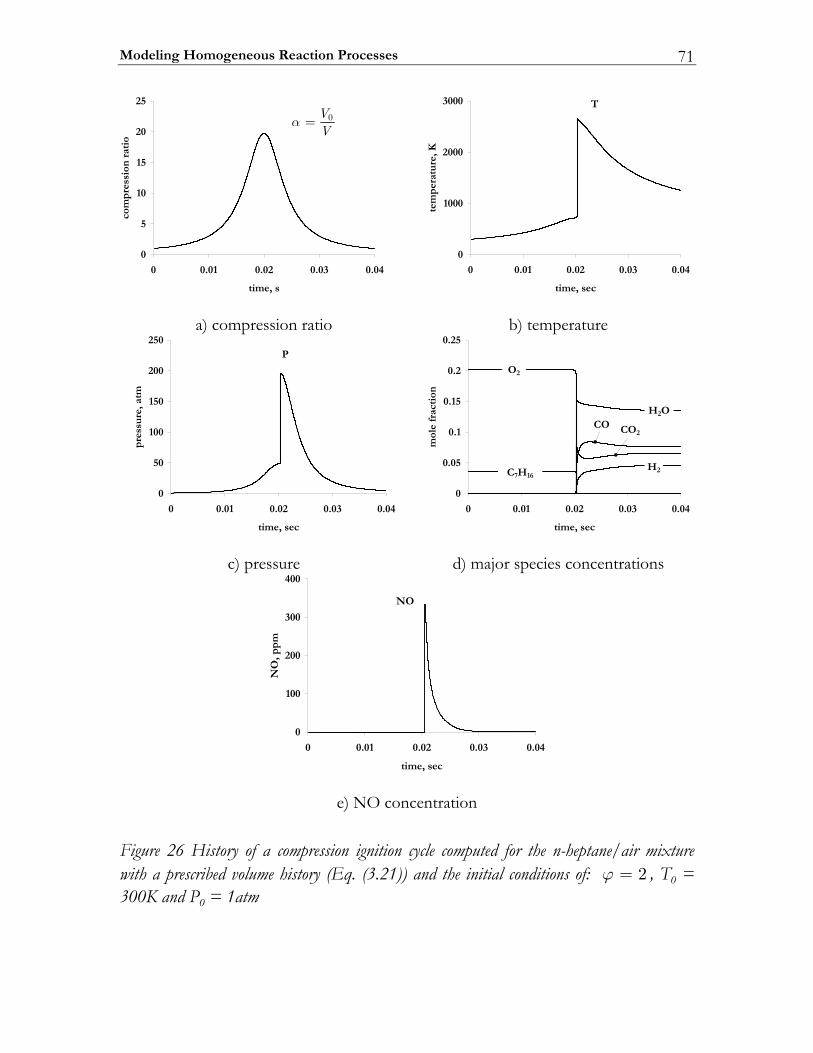
Modeling Homogeneous Reaction Processes 71
0
5
10
15
20
25
0 0.01 0.02 0.03 0.04
time, s
com
pre
ssio
n r
atio
0VV
=
0
0001
0002
0003
40.030.020.010.00
ces,emit
tem
per
atu
re, K
T
a) compression ratio
b) temperature
0
05
001
051
002
052
40.030.020.010.00
ces,emit
pre
ssu
re, a
tm
P
0
50.0
1.0
51.0
2.0
52.0
40.030.020.010.00
ces,emit
mol
e fr
acti
on
C7H 61
O2
H2O
H2
OC OC 2
c) pressure
d) major species concentrations
0
001
002
003
004
40.030.020.010.00
ces,emit
NO
,pp
m
ON
e) NO concentration
Figure 26 History of a compression ignition cycle computed for the n-heptane/air mixture with a prescribed volume history (Eq. (3.21)) and the initial conditions of: 2ϕ = , T0 = 300K and P0 = 1atm
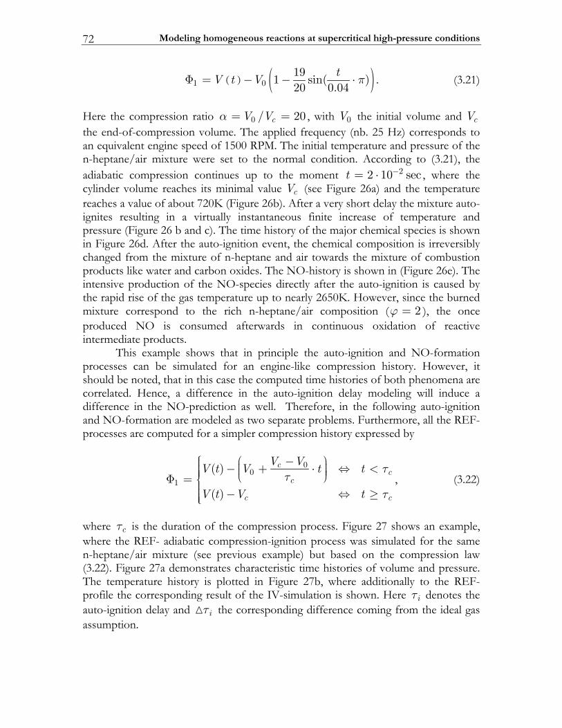
Modeling homogeneous reactions at supercritical high-pressure conditions 72
( ) ( )1 0191 sin( )20 0.04
tV t V πΦ = − − ⋅ . (3.21)
Here the compression ratio 0 / 20cV Vα = = , with 0V the initial volume and cV the end-of-compression volume. The applied frequency (nb. 25 Hz) corresponds to an equivalent engine speed of 1500 RPM. The initial temperature and pressure of the n-heptane/air mixture were set to the normal condition. According to (3.21), the adiabatic compression continues up to the moment 22 10 sect −= ⋅ , where the cylinder volume reaches its minimal value cV (see Figure 26a) and the temperature reaches a value of about 720K (Figure 26b). After a very short delay the mixture auto-ignites resulting in a virtually instantaneous finite increase of temperature and pressure (Figure 26 b and c). The time history of the major chemical species is shown in Figure 26d. After the auto-ignition event, the chemical composition is irreversibly changed from the mixture of n-heptane and air towards the mixture of combustion products like water and carbon oxides. The NO-history is shown in (Figure 26e). The intensive production of the NO-species directly after the auto-ignition is caused by the rapid rise of the gas temperature up to nearly 2650K. However, since the burned mixture correspond to the rich n-heptane/air composition ( 2ϕ = ), the once produced NO is consumed afterwards in continuous oxidation of reactive intermediate products. This example shows that in principle the auto-ignition and NO-formation processes can be simulated for an engine-like compression history. However, it should be noted, that in this case the computed time histories of both phenomena are correlated. Hence, a difference in the auto-ignition delay modeling will induce a difference in the NO-prediction as well. Therefore, in the following auto-ignition and NO-formation are modeled as two separate problems. Furthermore, all the REF-processes are computed for a simpler compression history expressed by
0
01
( )
( )
cc
c
c c
V VV t V t t
V t V t
ττ
τ
⎧ ⎛ − ⎞⎪ ⎟⎜⎪ − + ⋅ ⇔ <⎟⎜ ⎟⎪⎪ ⎝ ⎠Φ = ⎨⎪⎪ − ⇔ ≥⎪⎪⎩
, (3.22)
where cτ is the duration of the compression process. Figure 27 shows an example, where the REF- adiabatic compression-ignition process was simulated for the same n-heptane/air mixture (see previous example) but based on the compression law (3.22). Figure 27a demonstrates characteristic time histories of volume and pressure. The temperature history is plotted in Figure 27b, where additionally to the REF-profile the corresponding result of the IV-simulation is shown. Here iτ denotes the auto-ignition delay and iτ the corresponding difference coming from the ideal gas assumption.
Modeling Homogeneous Reaction Processes 73
0
0.2
0.4
0.6
0.8
1
1.2
0 0.01 0.02 0.03 0.04
time, sec
volu
me,
pre
ssu
re0
VvV=
max
PpP
=
a) volume and pressure histories
0
005
0001
0051
0002
0052
0003
30.0520.020.0510.0
ces,emit
tem
per
atu
re,K
ssecorpecnerefer)ledomsaglaer(
noitciderp-VI)ledomsaglaedi(
iτ
cτ iτ
b) temperature history
Figure 27 History of compression-ignition process: a) real gas histories of volume and pressure b) real gas and ideal gas histories of temperature
It is important to note, that with respect to the IP and IPV-formulations for an auto-ignition problem, applying the complete pressure history obtained in the REF-modeling of the pressure is physically non-adequate. This can lead to the situation that the explosion-like rise of the pressure of the auto-ignition REF simulation is applied as the closure condition to a by far not igniting gas mixture simulated with the IP or IPV problem formulation. Therefore, in the case of IP and IPV modeling,
Modeling homogeneous reactions at supercritical high-pressure conditions 74
we close the system of governing equations with the REF-history of the pressure only for time moments ct τ< . For ct τ≥ the closing conditions are
1
2
( ) ( )c
Q
V t V τ
ω
Φ = −
Φ =. (3.23)
With this, we focus on the final state of the compression process. Since applying different problem formulations can result in different values of the adiabatic compression temperature at ct τ= , this will have an influence on the auto-ignition and NO-formation predictions. In the following sections results on the auto-ignition delay and thermal NO-production are presented. The results are given in terms of the relative error between the ideal gas predictions of the quantity If (IV, IP and IPV modeling) and its corresponding value obtained with the Redlich-Kwong equation of state Rf (REF-model):
100%I Rf
R
f ff
ε −= ⋅ . (3.24)
3.3 Results In this section results on the homogeneous auto-ignition and NO-formation modeling are presented.
3.3.1 Auto-ignition This section considers the auto-ignition of a stoichiometric n-heptane/air mixture in an adiabatic compression-ignition process. Initial conditions (an absolute pressure of 3.5bar and a temperature of 300K and 400K) were chosen such that they resemble the initial state (before the compression) in a modern HD engine.
REF-modeling The conditions just prior to the auto-ignition event were generated by a rapid adiabatic compression of the mixture with an initial pressure of 3.5bar and temperatures of 300K and 400K. The REF-simulations were performed for a variety of compression ratios 0 /V Vα = . The applied compression law is given by (3.22) with 20c msτ = . The adiabatic compression state at ct τ= and the resulting auto-ignition delays are shown in Figure 28. Concerning diesel engine modeling the compressed states of practical interest are characterized by a temperature range between 700K and 1000K (between 1000 / 1.4K T ≈ and 1000 / 1K T = ).
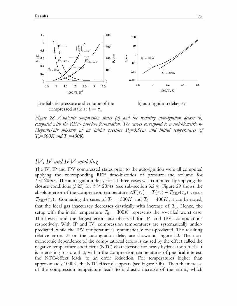
Results 75
0
0.2
0.4
0.6
0.8
1
1.2
0.5 1 1.5 2 2.5 3 3.5
1000/T, K-1
a
0
100
200
300
400
P, a
tm
0 300T KP =
0 400T KP =
0/
VV
00 400T K
VV =
00 300T K
VV =
0.001
0.01
0.1
1
10
100
0.8 1 1.2 1.4 1.6
1000/T, K-1
i, m
s
0 300T K=
0 400T K=
a) adiabatic pressure and volume of the
compressed state at ct τ=
b) auto-ignition delay iτ
Figure 28 Adiabatic compression states (a) and the resulting auto-ignition delays (b) computed with the REF- problem formulation. The curves correspond to a stoichiometric n-Heptane/air mixture at an initial pressure P0=3.5bar and initial temperatures of T0=300K and T0=400K.
IV, IP and IPV-modeling The IV, IP and IPV compressed states prior to the auto-ignition were all computed applying the corresponding REF time-histories of pressure and volume for
20t ms< . The auto-ignition delay for all three cases was computed by applying the closure conditions (3.23) for 20t ms≥ (see sub-section 3.2.4). Figure 29 shows the absolute error of the compression temperature ( ) ( ) ( )c c REF cT T Tτ τ τ= − versus
( )REF cT τ . Comparing the cases of 0 300T K= and 0 400T K= , it can be noted, that the ideal gas inaccuracy decreases drastically with increase of 0T . Hence, the setup with the initial temperature 0 300T K= represents the so-called worst case. The lowest and the largest errors are observed for IP- and IPV- computations respectively. With IP and IV, compression temperatures are systematically under-predicted, while the IPV temperature is systematically over-predicted. The resulting relative errors ε on the auto-ignition delay are shown in Figure 30. The non-monotonic dependence of the computational errors is caused by the effect called the negative temperature coefficient (NTC) characteristic for heavy hydrocarbon fuels. It is interesting to note that, within the compression temperatures of practical interest, the NTC–effect leads to an error reduction. For temperatures higher than approximately 1000K, the NTC-effect disappears (see Figure 30b). Then the increase of the compression temperature leads to a drastic increase of the errors, which
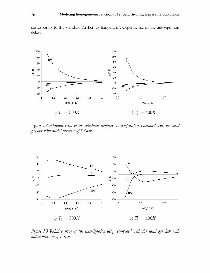
Modeling homogeneous reactions at supercritical high-pressure conditions 76
corresponds to the standard Arrhenius temperature-dependence of the auto-ignition delay.
04-
02-
0
02
04
06
08
001
28.16.14.12.11
K,T/0001 1-
∆T,K
VPI
VIPI
04-
02-
0
02
04
06
08
001
021
7.12.17.0
K,T/0001 1-
∆T
,K
VPI
PI VI
a) 0 300T K=
b) 0 400T K=
Figure 29 Absolute error of the adiabatic compression temperature computed with the ideal gas law with initial pressure of 3.5bar
06-
04-
02-
0
02
04
06
28.16.14.12.11
K,T/0001 1-
ε,%
VPI
PI
I
07-
05-
03-
01-
01
03
05
7.12.17.0
K,T/0001 1-
ε,%
VPI
PI
VI
a) 0 300T K=
b) 0 400T K=
Figure 30 Relative error of the auto-ignition delay computed with the ideal gas law with initial pressure of 3.5bar
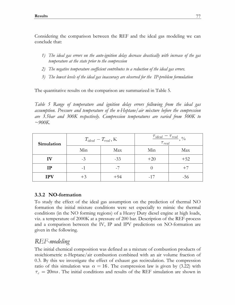
Results 77
Considering the comparison between the REF and the ideal gas modeling we can conclude that:
1) The ideal gas errors on the auto-ignition delay decrease drastically with increase of the gas temperature at the state prior to the compression
2) The negative temperature coefficient contributes to a reduction of the ideal gas errors. 3) The lowest levels of the ideal gas inaccuracy are observed for the IP-problem formulation
The quantitative results on the comparison are summarized in Table 5.
Table 5 Range of temperature and ignition delay errors following from the ideal gas assumption. Pressure and temperature of the n-Heptane/air mixture before the compression are 3.5bar and 300K respectively. Compression temperatures are varied from 500K to ~900K.
ideal realT T− , K ideal real
real
τ ττ− , %
Simulation Min Max Min Max
IV -3 -33 +20 +52
IP -1 -7 0 +7
IPV +3 +94 -17 -56
3.3.2 NO-formation To study the effect of the ideal gas assumption on the prediction of thermal NO formation the initial mixture conditions were set especially to mimic the thermal conditions (in the NO forming regions) of a Heavy Duty diesel engine at high loads, viz. a temperature of 2000K at a pressure of 200 bar. Description of the REF-process and a comparison between the IV, IP and IPV predictions on NO-formation are given in the following.
REF-modeling The initial chemical composition was defined as a mixture of combustion products of stoichiometric n-Heptane/air combustion combined with an air volume fraction of 0.3. By this we investigate the effect of exhaust gas recirculation. The compression ratio of this simulation was 16α = . The compression law is given by (3.22) with
20c msτ = . The initial conditions and results of the REF simulation are shown in
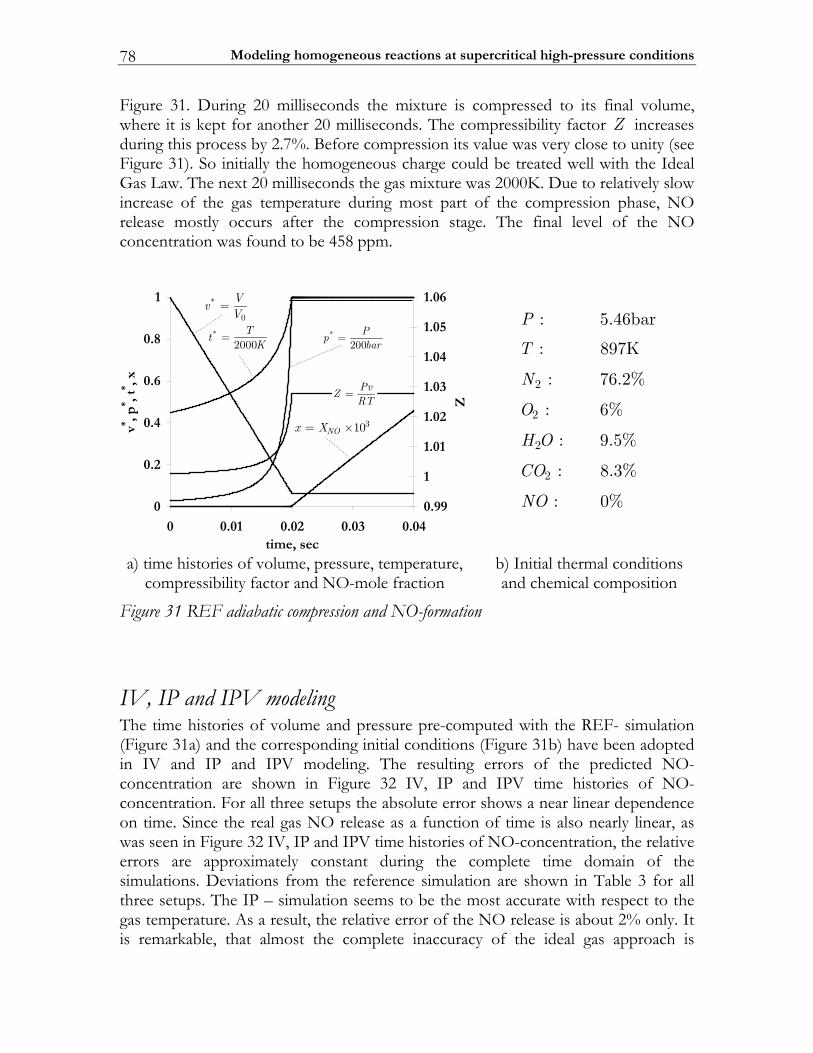
Modeling homogeneous reactions at supercritical high-pressure conditions 78
Figure 31. During 20 milliseconds the mixture is compressed to its final volume, where it is kept for another 20 milliseconds. The compressibility factor Z increases during this process by 2.7%. Before compression its value was very close to unity (see Figure 31). So initially the homogeneous charge could be treated well with the Ideal Gas Law. The next 20 milliseconds the gas mixture was 2000K. Due to relatively slow increase of the gas temperature during most part of the compression phase, NO release mostly occurs after the compression stage. The final level of the NO concentration was found to be 458 ppm.
0
0.2
0.4
0.6
0.8
1
0 0.01 0.02 0.03 0.04time, sec
v* ,p* ,t
* , x
0.99
1
1.01
1.02
1.03
1.04
1.05
1.06
Z
310NOx X= ×
*
0
VvV=
*2000TtK
= *200Ppbar
=
PvZRT
=
2
2
2
2
: 5.46bar
: 897K
: 76.2%
: 6%
: 9.5%
: 8.3%
: 0%
P
T
N
O
H O
CO
NO
a) time histories of volume, pressure, temperature, compressibility factor and NO-mole fraction
b) Initial thermal conditions and chemical composition
Figure 31 REF adiabatic compression and NO-formation
IV, IP and IPV modeling The time histories of volume and pressure pre-computed with the REF- simulation (Figure 31a) and the corresponding initial conditions (Figure 31b) have been adopted in IV and IP and IPV modeling. The resulting errors of the predicted NO-concentration are shown in Figure 32 IV, IP and IPV time histories of NO-concentration. For all three setups the absolute error shows a near linear dependence on time. Since the real gas NO release as a function of time is also nearly linear, as was seen in Figure 32 IV, IP and IPV time histories of NO-concentration, the relative errors are approximately constant during the complete time domain of the simulations. Deviations from the reference simulation are shown in Table 3 for all three setups. The IP – simulation seems to be the most accurate with respect to the gas temperature. As a result, the relative error of the NO release is about 2% only. It is remarkable, that almost the complete inaccuracy of the ideal gas approach is
Results 79
accumulated in the computed value of the mixture volume ( 3%Vε = − ). This is directly related to the compressibility (Z) history. However, the chemical reaction rate is not exponentially dependent on the deviation of the mixture volume. This explains the high accuracy of the IP setup with respect to the thermal NO formation process. The defect of the predictions of the IV - simulations is more complicated, due to the fact that the resulting difference is accumulated in both gas pressure and temperature. At the end of compression the pressure is 7bar less and temperature is 16K less than the reference value. This gives an underestimation of the NO level at the end of the process of about 22%. The IPV - simulation demonstrates the largest deviation from the reference temperature. Its level reaches a value of about 55K. The thermal NO release is therefore overestimated by a factor of 2.27 (127% error) compared to the reference simulation.
-200
0
200
400
600
800
0.02 0.025 0.03 0.035 0.04
time, sec
NO
, pp
m
IPV
IV
IP
Figure 32 IV, IP and IPV time histories of NO-concentration
Table 6 Error levels found for the simulations with the ideal gas.
Simulation ,T K ,%Tε ,P atm ,%Pε ,%Vε ,%NOε
IV -16 -0.8 -7 -3.5 … -22
IP -2 -0.1 … … -3 -2
IPV +55 2.7 … … … +127 In order to evaluate the sensitivity of the results, similar comparisons between the REF and the ideal gas simulations were performed for different global parameters, viz. the final temperature, the final pressure and compression ratio. To study the effects of compression pressure, simulations were performed that varied between 100bar to 300bar to cover a region typical for internal
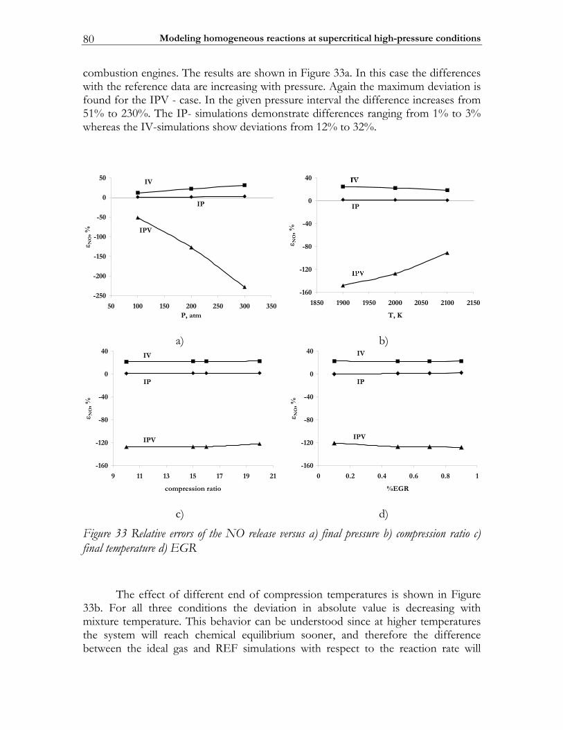
Modeling homogeneous reactions at supercritical high-pressure conditions 80
combustion engines. The results are shown in Figure 33a. In this case the differences with the reference data are increasing with pressure. Again the maximum deviation is found for the IPV - case. In the given pressure interval the difference increases from 51% to 230%. The IP- simulations demonstrate differences ranging from 1% to 3% whereas the IV-simulations show deviations from 12% to 32%.
052-
002-
051-
001-
05-
0
05
05300305200205100105mta,P
ε NO
,% VPI
VI
PI
061-
021-
08-
04-
0
04
0512001205020002059100910581
K,T
ε NO
,%
I
PI
PI
a)
b)
061-
021-
08-
04-
0
04
1291715131119
oitarnoisserpmoc
ε NO
,%
VI
PI
VPI
061-
021-
08-
04-
0
04
18.06.04.02.00
RGE%
ε NO
,%
VI
PI
VPI
c)
d)
Figure 33 Relative errors of the NO release versus a) final pressure b) compression ratio c) final temperature d) EGR The effect of different end of compression temperatures is shown in Figure 33b. For all three conditions the deviation in absolute value is decreasing with mixture temperature. This behavior can be understood since at higher temperatures the system will reach chemical equilibrium sooner, and therefore the difference between the ideal gas and REF simulations with respect to the reaction rate will
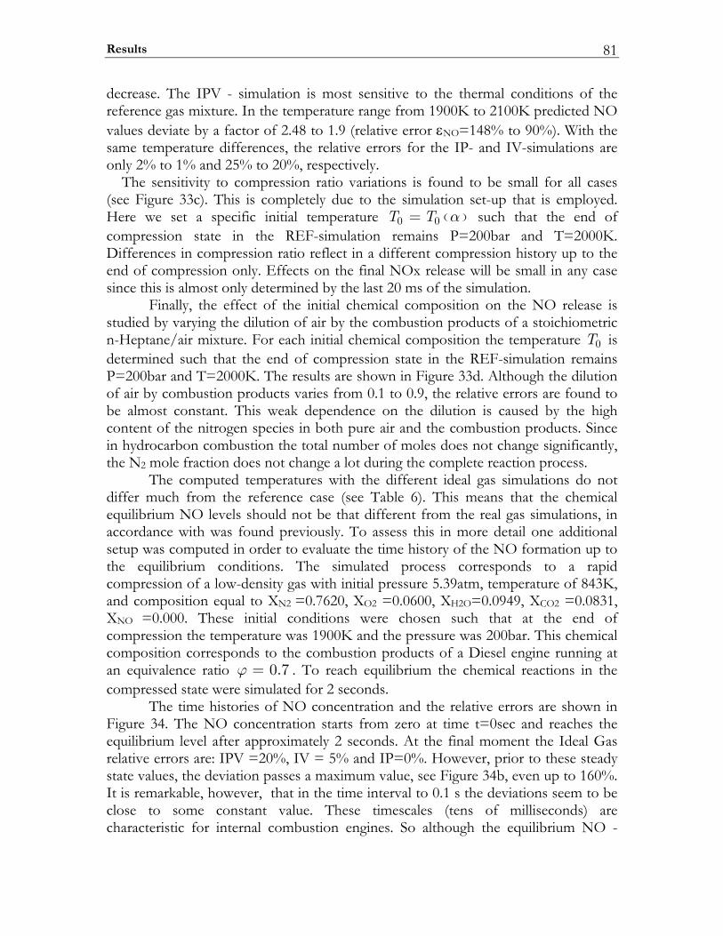
Results 81
decrease. The IPV - simulation is most sensitive to the thermal conditions of the reference gas mixture. In the temperature range from 1900K to 2100K predicted NO values deviate by a factor of 2.48 to 1.9 (relative error εNO=148% to 90%). With the same temperature differences, the relative errors for the IP- and IV-simulations are only 2% to 1% and 25% to 20%, respectively. The sensitivity to compression ratio variations is found to be small for all cases (see Figure 33c). This is completely due to the simulation set-up that is employed. Here we set a specific initial temperature ( )0 0T T α= such that the end of compression state in the REF-simulation remains P=200bar and T=2000K. Differences in compression ratio reflect in a different compression history up to the end of compression only. Effects on the final NOx release will be small in any case since this is almost only determined by the last 20 ms of the simulation. Finally, the effect of the initial chemical composition on the NO release is studied by varying the dilution of air by the combustion products of a stoichiometric n-Heptane/air mixture. For each initial chemical composition the temperature 0T is determined such that the end of compression state in the REF-simulation remains P=200bar and T=2000K. The results are shown in Figure 33d. Although the dilution of air by combustion products varies from 0.1 to 0.9, the relative errors are found to be almost constant. This weak dependence on the dilution is caused by the high content of the nitrogen species in both pure air and the combustion products. Since in hydrocarbon combustion the total number of moles does not change significantly, the N2 mole fraction does not change a lot during the complete reaction process. The computed temperatures with the different ideal gas simulations do not differ much from the reference case (see Table 6). This means that the chemical equilibrium NO levels should not be that different from the real gas simulations, in accordance with was found previously. To assess this in more detail one additional setup was computed in order to evaluate the time history of the NO formation up to the equilibrium conditions. The simulated process corresponds to a rapid compression of a low-density gas with initial pressure 5.39atm, temperature of 843K, and composition equal to XN2 =0.7620, XO2 =0.0600, XH2O=0.0949, XCO2 =0.0831, XNO =0.000. These initial conditions were chosen such that at the end of compression the temperature was 1900K and the pressure was 200bar. This chemical composition corresponds to the combustion products of a Diesel engine running at an equivalence ratio 0.7ϕ = . To reach equilibrium the chemical reactions in the compressed state were simulated for 2 seconds. The time histories of NO concentration and the relative errors are shown in Figure 34. The NO concentration starts from zero at time t=0sec and reaches the equilibrium level after approximately 2 seconds. At the final moment the Ideal Gas relative errors are: IPV =20%, IV = 5% and IP=0%. However, prior to these steady state values, the deviation passes a maximum value, see Figure 34b, even up to 160%. It is remarkable, however, that in the time interval to 0.1 s the deviations seem to be close to some constant value. These timescales (tens of milliseconds) are characteristic for internal combustion engines. So although the equilibrium NO -
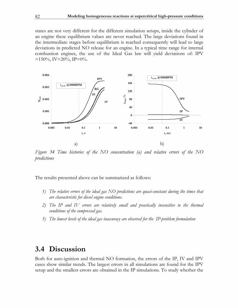
Modeling homogeneous reactions at supercritical high-pressure conditions 82
states are not very different for the different simulation setups, inside the cylinder of an engine these equilibrium values are never reached. The large deviations found in the intermediate stages before equilibrium is reached consequently will lead to large deviations in predicted NO release for an engine. In a typical time range for internal combustion engines, the use of the Ideal Gas law will yield deviations of: IPV =150%, IV=20%, IP=0%.
000.0
100.0
200.0
300.0
400.0
0111.010.0100.0
s,t
XN
O
VPI
VI
PI
GRt elcyc MPR0001@
04-
0
04
08
021
061
002
0111.010.0100.0
ces,t
ε NO
,% VPI
VI
PI
t elcyc MPR0001@
a)
b)
Figure 34 Time histories of the NO concentration (a) and relative errors of the NO predictions The results presented above can be summarized as follows:
1) The relative errors of the ideal gas NO predictions are quasi-constant during the times that are characteristic for diesel engine conditions.
2) The IP and IV errors are relatively small and practically insensitive to the thermal conditions of the compressed gas.
3) The lowest levels of the ideal gas inaccuracy are observed for the IP-problem formulation
3.4 Discussion Both for auto-ignition and thermal NO formation, the errors of the IP, IV and IPV cases show similar trends. The largest errors in all simulations are found for the IPV setup and the smallest errors are obtained in the IP simulations. To study whether the
Discussion 83
observed quality ranking |εIPVNO,τ|> |εIVNO,τ| >|εIPNO,τ| can be explained a simplified form of the REF equation of state, i.e., the Redlich-Kwong EOS [84]:
( )
RT aPV b TV V b= −
− + (3.25)
is employed. The first term in (3.25) represents the part of the gas pressure caused by thermal and finite molecular size factors. The second term is due to molecular attraction forces. This term plays an important role only by determining the gas-liquid phase transition. Since the considered states are supercritical, the second term can be neglected here. This is correct when the thermal part of the internal energy is much larger than the part caused by the molecular attractions. Then the reduced Redlich-Kwong formula (in fact the Clausius law) is given by
RTPV b=
− (3.26)
The most remarkable feature of this expression in our case is that it does not modify the internal energy, since the parameter a is not present. Using the energy conservation law 0dE PdV+ = (3.27) the "real" gas adiabatic lines can be formulated in terms of temperature vs volume,
( )1
00
vCR
VT TV b
≈−
(3.28)
and temperature vs. pressure:
1
00
pCR
PT TP
⎛ ⎞⎟⎜≈ ⎟⎜ ⎟⎝ ⎠ (3.29)
Here pC and vC are ideal gas constant non-dimensional heat capacities at constant pressure and constant volume, respectively. In equation (3.28) the b -parameter in the numerator was neglected since the initial gas state is much closer to an ideal gas state and therefore 0V b>> .
IV-simulation The ideal gas adiabatic temperature computed from the prescribed volume is given by the well-known expression
Modeling homogeneous reactions at supercritical high-pressure conditions 84
( )1
00
vCI
VT TV
≈ (3.30)
Thus the ratio of /I RT T is given by
( )1
1 vCI
R
T bT V= − (3.31)
which for a two atomic gas can be approximated as
( )0.31I
R
T bT V
≈ − . (3.32)
Hence, the IV-adiabatic temperature is always lower than the REF-prediction.
IP-simulation For the estimation of the ratio /I RT T for the case where the pressure history is prescribed we have to use (3.29) for RT . Since TI is given by the same formula we find that (with this approximation) the ratio is one and both temperatures are equal. According to this
I R RIRT RT VVP P Z
= = = (3.33)
This means that in the IP-simulations the difference between the ideal gas and real gas simulation is completely captured by a change of volume (see Table 6). Of course in reality, the simplified equation (3.26) is an – be it good – approximation; because of this there will still be a small difference in T-estimate between RES and IP (see Table 5 and Table 6). Since chemical reaction rates are proportional to the concentration to some low power (~2) but are depending exponentially on the temperature, the IP-simulations will yield the best results. Therefore, the use of a measured pressure history is preferable to the use of known volume history in conjunction with the use of the ideal gas law.
IPV-simulation For the case where both volume and pressure history are used the ratio /I RT T directly follows from the ideal gas equation of state and equation (3.26):
Discussion 85
( ) 11I
R
T bT V
−= − . (3.34)
From this it can be predicted that in the IPV - simulations the ideal gas temperature is always larger than the real gas temperature. This is consistent with the observations found earlier using the full Redlich-Kwong EOS. Obviously, the ideal and real gas temperatures are correlated according to
I I R RI RPV P VT Z TR R
= = = ⋅ (3.35)
The non-ideality of the gas is completely reflected in the prediction of the temperature. Due to this fact, the use of prescribed volume and pressure history will give the largest error in the predicted temperature. This explains the observations.
3.5 Conclusions High-pressure homogeneous auto-ignition and NO formation processes were modeled in a rapid compression machine using the real and the ideal gas equations of state. Results of the Redlich-Kwong EOS simulations were used as reference data to analyze errors following from the ideal gas assumption. The results show that for the case where both the volume V and the pressure P are prescribed (IPV-modeling) significant errors are introduced. Compared to the other two approaches where either P (IP-modeling) or V (IV-modeling) is prescribed the IPV-modeling leads to the highest errors in the predicted gas temperature and consequently to the highest errors in predicted auto-ignition delay and NO-release. The IPV-results obtained in modeling NO-formation show remarkable over-predictions when compared to the reference data (REF-formulation). This is in agreement with the trend predicted by Zevenhoven [40] for the same setup. It is furthermore worthwhile to point out that calculating T, and the apparent heat release, from a (P,V)-curve is a key element in combustion analysis with internal combustion engines Prescription of the volume V history results in a practically acceptable accuracy. Errors observed for the adiabatic compression temperature are well comparable to these induced by common uncertainties of initial conditions and/or a non-precise knowledge of the actual heat exchange taking place in the chamber of IC-engines. The resulting errors of up to 50% for the auto-ignition delays are caused by the exponential temperature dependence of the chemical reaction. Since the modeled thermal conditions were chosen to represent the worst case for the models comparison, a lower level of errors is expected when applying the ideal gas law in practical CFD-modeling. Additionally, from the simulations it was found that the
Modeling homogeneous reactions at supercritical high-pressure conditions 86
relative error for NO release was constant for timescales occurring in engines. Therefore if necessary for engine simulations, this effect could be captured by a single correction factor. The last case where the pressure P is prescribed does not show any significant difference compared to the full reference simulation. For high-pressure problems this is the most accurate way if one restricts oneself to an ideal gas description of the state equation. In the performed IP-modelling, the calculated (and therefore not imposed) gas volume V accumulates the complete error caused by the gas non-ideality. This results to almost correct temperature T and therefore, gives the most accurate reaction rate values compared to the IV and IPV methods. The above shows that inaccuracy of the ideal gas assumption is determined not only by the P-V-T conditions but also by the problem formulation itself. For each modeling case when applying this assumption, the potential errors have to be estimated in an appropriate way. One important reason for this is that predictions coming from different formulations can be completely opposite. This was illustrated, e.g., on modeling NO-formation, where applying the IPV-formulation lead to remarkable over-predictions of the NO-concentration while applying the IV-formulation lead to an under-prediction but with a much smaller difference.
Chapter 4
4 Modeling of One-Dimensional Diffusion Flamelets with Complex Chemistry
In this chapter laminar counterflow diffusion flames described with detailed chemistry are treated. A fully implicit numerical approach dealing with specific problems coupled with the use of second order schemes is presented. The algorithm is verified on a partially premixed n-heptane flames and a non-premixed dimethyl-carbonate flame at atmospheric pressure. Furthermore, the algorithm has been used to study effects of high pressures on the combustion in laminar flamelet structures.
4.1 Introduction
4.1.1 Flamelet modeling Laminar one-dimensional flames play a fundamental role in the flamelet combustion model. The laminar flamelet concept views the turbulent flame as an ensemble of thin, laminar, locally one-dimensional flame structures embedded within the turbulent flow-field [112, 113, 72, 71]. The main advantage of the flamelet concept is that non-equilibrium effects can be incorporated, while the detailed chemistry calculations do not need to be coupled with the turbulent flame calculation. The flame properties like the gas composition kY , chemical production rates kω can be obtained from the steady one-dimensional flamelets. The pre-computed flamelet structures are typically tabulated as functions of prescribed parameters. With respect to non-premixed combustion these parameters are the so-called mixture fraction Z and the scalar dissipation rate χ representing the mixing-coordinate and the mixing-rate between the chemical reactants. From the perspective of Diesel engine modeling the flamelet approach is promising because the phenomena of interest, like auto-ignition and PAH/Soot formation, can be captured in a very natural and generic way. Another obvious advantage is that complex thermodynamic and molecular transport descriptions are
Modeling of One-Dimensional Diffusion Flamelets with Complex Chemistry 88
also accounted for when resolving the 1D flamelet structures and need not be included in the 3D-flow solver. In fact the resulting properties are accessed by the 3D-flow simulator as a function of Z and χ . Therefore the (flamelet) approach requires a simultaneous (together with a CFD-solver) or pre-computation of the flamelet structure resolved on a 1D-mesh. Although, there are no principle problems associated with modeling 1D reacting flows, describing these flows with arbitrary complex chemistry leads to a certain complication. The main source of this is that in general, especially for automotive fuels, a very large number of chemical species is involved. The resulting intensive usage of computer memory prevents establishing a sufficient mesh resolution even for a 1D problem. As an example, consider the n-heptane detailed reaction mechanism designed by Curran et al. [31]. This mechanism consists of 561spN = chemical species. The required memory CPUM can be estimated from ( )2
CPU sp p J TM N N N N≈ ⋅ ⋅ + ⋅ , (4.1) where spN is the number of chemical species, pN the number of mesh points, JN
the number of 2spN -memory blocks in each row of the Jacobian matrix, TN the
number of 2spN -memory blocks for binary molecular transport coefficients per a
mesh point and ∆ the amount of memory used for a real type (e.g., 8 bytes for the case of a double precision real). When applying the ultimately preferable implicit methods, each row of the Jacobian matrix consists of 3JN = memory blocks with an approximate size of 2
spN . If the physical model accounts for preferential diffusion effects the TN -number of corresponding 2
spN -blocks is one or two depending on the model (with/without thermal diffusion) and the way of memory usage2. Finally, if the 1D mesh consists of few hundred nodes, the needed CPU memory CPUM is of several gigabytes. This memory requirement is comparable or even larger than the corresponding memory allocation for the 3D-flow simulation. Taking into account practical limitations of CPU memory, the approximation achievable on 1D mesh can be insufficient. In principle, this problem can be solved by applying numerical approaches of higher order of accuracy (e.g., second or third order). However, these introduce a new problem associated with a higher numerical instability (see, e.g., [79] and [114]). The main objective of this chapter is the development of a second order numerical method for modeling 1D laminar diffusion flamelets described with complex chemical and thermo-physical models. One additional point that will be
2 2
spN -blocks are only necessary if the symmetry properties of diffusion coefficients are not
exploited. If memory alignment is optimized further actually 2 /2spN memory locations are necessary.
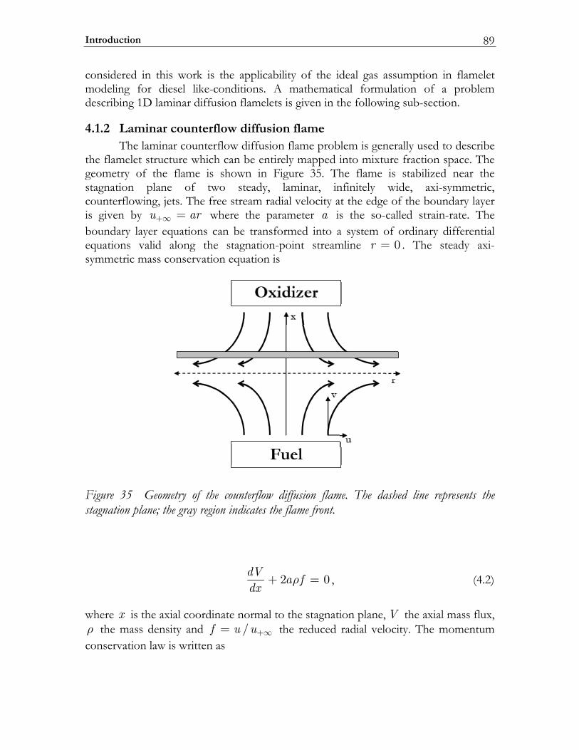
Introduction 89
considered in this work is the applicability of the ideal gas assumption in flamelet modeling for diesel like-conditions. A mathematical formulation of a problem describing 1D laminar diffusion flamelets is given in the following sub-section.
4.1.2 Laminar counterflow diffusion flame The laminar counterflow diffusion flame problem is generally used to describe the flamelet structure which can be entirely mapped into mixture fraction space. The geometry of the flame is shown in Figure 35. The flame is stabilized near the stagnation plane of two steady, laminar, infinitely wide, axi-symmetric, counterflowing, jets. The free stream radial velocity at the edge of the boundary layer is given by u ar+∞ = where the parameter a is the so-called strain-rate. The boundary layer equations can be transformed into a system of ordinary differential equations valid along the stagnation-point streamline 0r = . The steady axi-symmetric mass conservation equation is
Figure 35 Geometry of the counterflow diffusion flame. The dashed line represents the stagnation plane; the gray region indicates the flame front.
2 0dV a fdx
ρ+ = , (4.2)
where x is the axial coordinate normal to the stagnation plane, V the axial mass flux, ρ the mass density and /f u u+∞= the reduced radial velocity. The momentum conservation law is written as
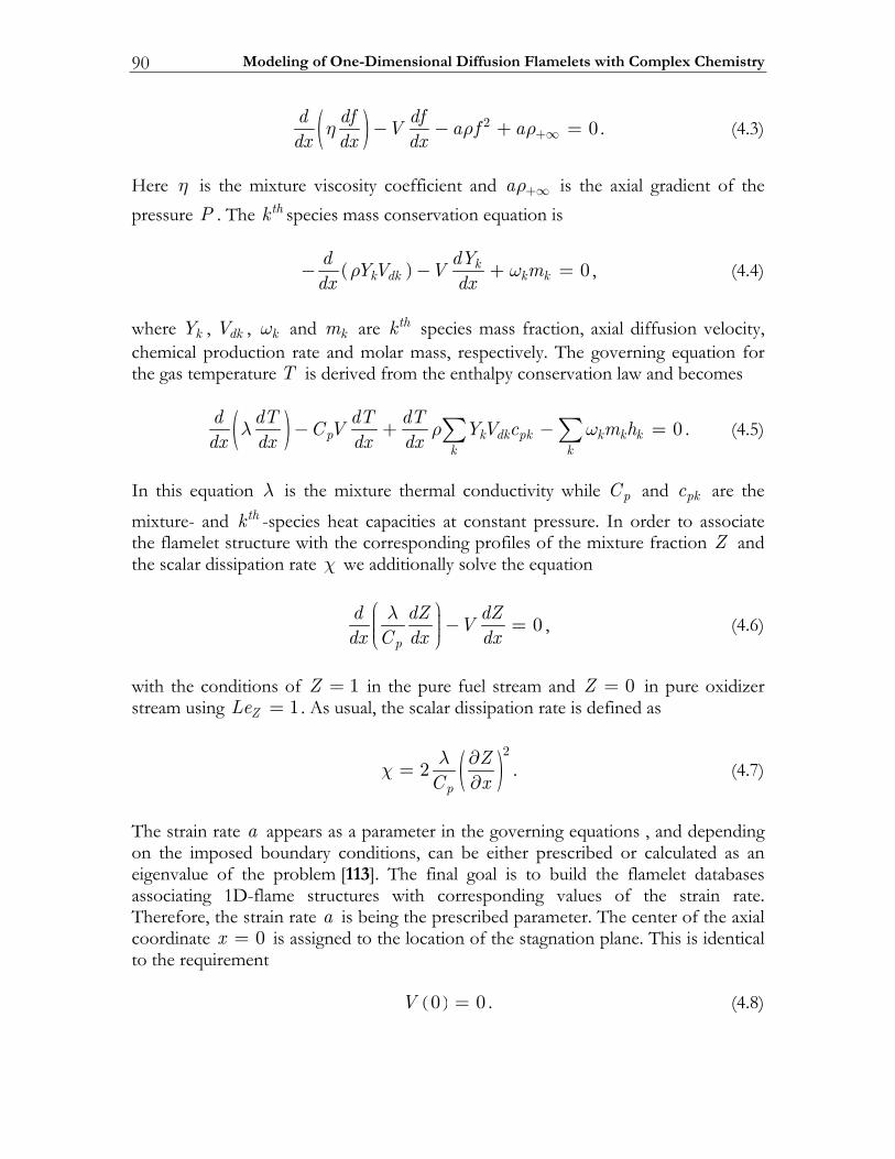
Modeling of One-Dimensional Diffusion Flamelets with Complex Chemistry 90
( ) 2 0d df dfV a f adx dx dx
η ρ ρ+∞− − + = . (4.3)
Here η is the mixture viscosity coefficient and aρ+∞ is the axial gradient of the pressure P . The thk species mass conservation equation is
( ) 0kk dk k k
d dYYV V mdx dx
ρ ω− − + = , (4.4)
where kY , dkV , kω and km are thk species mass fraction, axial diffusion velocity, chemical production rate and molar mass, respectively. The governing equation for the gas temperature T is derived from the enthalpy conservation law and becomes
( ) 0p k dk pk k k kk k
d dT dT dTC V YV c m hdx dx dx dx
λ ρ ω− + − =∑ ∑ . (4.5)
In this equation λ is the mixture thermal conductivity while pC and pkc are the mixture- and thk -species heat capacities at constant pressure. In order to associate the flamelet structure with the corresponding profiles of the mixture fraction Z and the scalar dissipation rate χ we additionally solve the equation
0p
d dZ dZVdx C dx dx
λ⎛ ⎞⎟⎜ − =⎟⎜ ⎟⎜⎝ ⎠, (4.6)
with the conditions of 1Z = in the pure fuel stream and 0Z = in pure oxidizer stream using 1ZLe = . As usual, the scalar dissipation rate is defined as
( )22p
ZC xλχ ∂=
∂. (4.7)
The strain rate a appears as a parameter in the governing equations , and depending on the imposed boundary conditions, can be either prescribed or calculated as an eigenvalue of the problem [113]. The final goal is to build the flamelet databases associating 1D-flame structures with corresponding values of the strain rate. Therefore, the strain rate a is being the prescribed parameter. The center of the axial coordinate 0x = is assigned to the location of the stagnation plane. This is identical to the requirement ( )0 0V = . (4.8)
Introduction 91
Finally, boundary conditions for fuel (x = −∞ ) and oxidizer (x = +∞ ) sides of the domain are written as
x = −∞ x = +∞
1Z = ,f ρ
ρ−∞+∞=
( ) ( ), , ,k kY T Y T −∞=
( )2dV a fdx
ρ −∞= −
0Z = 1f =
( ) ( ), , ,k kY T Y T +∞=
( )2dV a fdx
ρ +∞= −
(4.9)
To determine the gas density and the molecular transport coefficients involved in the system of equations (4.2) - (4.7), either the ideal gas assumption is used or a more sophisticated thermodynamic model is employed. With respect to the Diesel engine modeling, it can be noted that the ideal gas law seems to be a reasonable but not a completely obvious choice. The main concern comes from the fact that thermodynamic states of unburned fuel with a combination of high-pressure and low temperature can occur during the combustion process. This is illustrated in Figure 36 comparing the adiabatic compression temperatures computed for pure air and pure n-heptane gases at different pressures.
005
009
0031
0071
0012
002051001050
mta,P
T,K
ria
enatpeh-n
Figure 36 Computational adiabatic temperatures of n-heptane and air versus pressure.
The temperatures are evaluated solving the entropy conservation equation indicating the adiabatic compression:
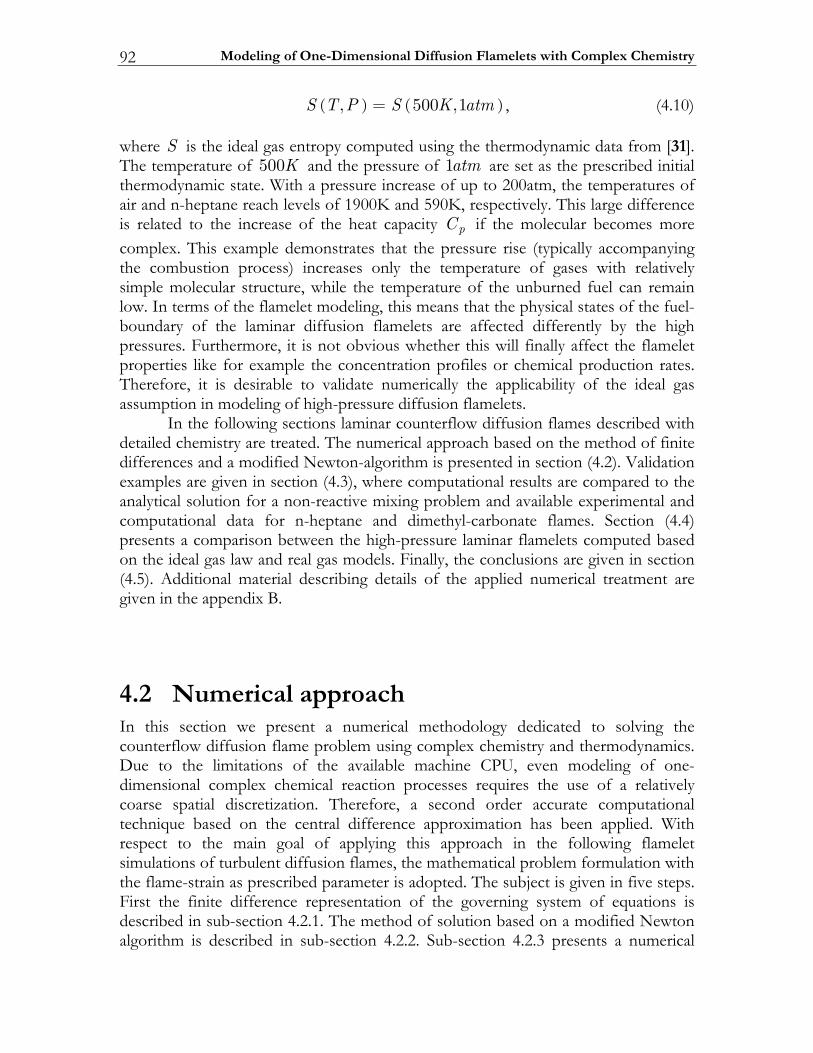
Modeling of One-Dimensional Diffusion Flamelets with Complex Chemistry 92
( ) ( ), 500 ,1S T P S K atm= , (4.10) where S is the ideal gas entropy computed using the thermodynamic data from [31]. The temperature of 500K and the pressure of 1atm are set as the prescribed initial thermodynamic state. With a pressure increase of up to 200atm, the temperatures of air and n-heptane reach levels of 1900K and 590K, respectively. This large difference is related to the increase of the heat capacity pC if the molecular becomes more complex. This example demonstrates that the pressure rise (typically accompanying the combustion process) increases only the temperature of gases with relatively simple molecular structure, while the temperature of the unburned fuel can remain low. In terms of the flamelet modeling, this means that the physical states of the fuel-boundary of the laminar diffusion flamelets are affected differently by the high pressures. Furthermore, it is not obvious whether this will finally affect the flamelet properties like for example the concentration profiles or chemical production rates. Therefore, it is desirable to validate numerically the applicability of the ideal gas assumption in modeling of high-pressure diffusion flamelets. In the following sections laminar counterflow diffusion flames described with detailed chemistry are treated. The numerical approach based on the method of finite differences and a modified Newton-algorithm is presented in section (4.2). Validation examples are given in section (4.3), where computational results are compared to the analytical solution for a non-reactive mixing problem and available experimental and computational data for n-heptane and dimethyl-carbonate flames. Section (4.4) presents a comparison between the high-pressure laminar flamelets computed based on the ideal gas law and real gas models. Finally, the conclusions are given in section (4.5). Additional material describing details of the applied numerical treatment are given in the appendix B.
4.2 Numerical approach In this section we present a numerical methodology dedicated to solving the counterflow diffusion flame problem using complex chemistry and thermodynamics. Due to the limitations of the available machine CPU, even modeling of one-dimensional complex chemical reaction processes requires the use of a relatively coarse spatial discretization. Therefore, a second order accurate computational technique based on the central difference approximation has been applied. With respect to the main goal of applying this approach in the following flamelet simulations of turbulent diffusion flames, the mathematical problem formulation with the flame-strain as prescribed parameter is adopted. The subject is given in five steps. First the finite difference representation of the governing system of equations is described in sub-section 4.2.1. The method of solution based on a modified Newton algorithm is described in sub-section 4.2.2. Sub-section 4.2.3 presents a numerical
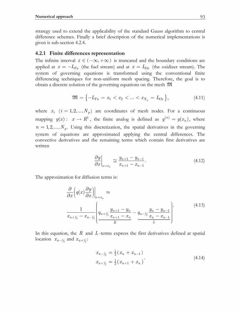
Numerical approach 93
strategy used to extend the applicability of the standard Gauss algorithm to central difference schemes. Finally a brief description of the numerical implementations is given is sub-section 4.2.4.
4.2.1 Finite differences representation The infinite interval ( ),x ∈ −∞ +∞ is truncated and the boundary conditions are applied at Fux L= − (the fuel stream) and at Oxx L= (the oxidizer stream). The system of governing equations is transformed using the conventional finite differencing techniques for non-uniform mesh spacing. Therefore, the goal is to obtain a discrete solution of the governing equations on the mesh M 1 2 ...
pFu N OxL x x x L= − = < < < =M , (4.11) where ix ( 1,2,..., pi N= ) are coordinates of mesh nodes. For a continuous mapping 1( ) :y x x R→ , the finite analog is defined as ( ) ( )n
ny y x= , where 1,2,..., pn N= . Using this discretization, the spatial derivatives in the governing
system of equations are approximated applying the central differences. The convective derivatives and the remaining terms which contain first derivatives are written
1 1
1 1n
n n
n nx x
y y yx x x
+ −
+ −=
∂ −≅∂ −
. (4.12)
The approximation for diffusion terms is:
( )
1 12 2
1 12 2
1 1
1 1
( )
1
nx x
n n n nn n
n n n n n nLR
yq xx x
y y y yq qx x x x x x
=
+ −+ −
+ − + −
∂ ∂ ≈∂ ∂
⎛ ⎞⎟⎜ ⎟⎜ − − ⎟⎜ ⎟−⎜ ⎟⎜ ⎟− − −⎜ ⎟⎜ ⎟⎝ ⎠
. (4.13)
In this equation, the R and L -terms express the first derivatives defined at spatial location 1
2nx − and 12nx + :
( )
( )
12
12
112
112
n n n
n n n
x x x
x x x
− −
+ +
= +
= +. (4.14)
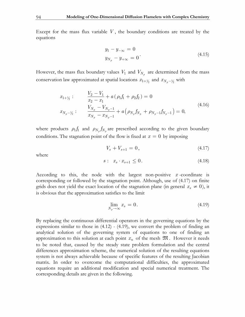
Modeling of One-Dimensional Diffusion Flamelets with Complex Chemistry 94
Except for the mass flux variable V , the boundary conditions are treated by the equations
1 0
0pN
y y
y y−∞
+∞
− =
− = . (4.15)
However, the mass flux boundary values 1V and
pNV are determined from the mass conservation law approximated at spatial locations 1
21x + and 12pNx − with
( )
( )
12
12
2 11 1 1 2 2
2 1
11 1
1
: 0
: 0,p pp p p p p
p p
N NN N N N N
N N
V Vx a f fx xV V
x a f fx x
ρ ρ
ρ ρ
+
−− − −
−
− + + =−−
+ + =−
(4.16)
where products 1 1fρ and
p pN Nfρ are prescribed according to the given boundary conditions. The stagnation point of the flow is fixed at 0x = by imposing 1 0s sV V ++ = , (4.17) where 1: 0s ss x x +⋅ ≤ . (4.18) According to this, the node with the largest non-positive x -coordinate is corresponding or followed by the stagnation point. Although, use of (4.17) on finite grids does not yield the exact location of the stagnation plane (in general 0sx ≠ ), it is obvious that the approximation satisfies to the limit lim 0
psNx
→∞= . (4.19)
By replacing the continuous differential operators in the governing equations by the expressions similar to those in (4.12) - (4.19), we convert the problem of finding an analytical solution of the governing system of equations to one of finding an approximation to this solution at each point nx of the mesh M . However it needs to be noted that, caused by the steady state problem formulation and the central differences approximation scheme, the numerical solution of the resulting equations system is not always achievable because of specific features of the resulting Jacobian matrix. In order to overcome the computational difficulties, the approximated equations require an additional modification and special numerical treatment. The corresponding details are given in the following.
Numerical approach 95
4.2.2 Method of Solution The goal is to find the solution * of the non-linear system of difference equations ( ) 0=F (4.20) In this notation, F is an p vN N× vector, where vN denotes the number of the governing equations. For an initial solution estimation 0 which is sufficiently close to * , the system of non-linear equations (4.20) can be solved applying a modified Newton's method, which we write in the form ( )( ) ( )1s s s s sJ γ+− − = F . (4.21) Here s denotes the ths solution iterate, sγ the ths damping parameter ( )0 1γ< ≤ , and ( ) ( )/s sJ F= ∂ ∂ the 2 2
p vN N× Jacobian matrix. In the applied implementation at each iteration a system of linear equations is solved for corrections to the previous solution vector. Since computational costs of forming and factoring the Jacobian matrix is a significant part of the cost of the total calculation, we consider applying a modified version of Newton's method in which the Jacobian is re-evaluated only periodically. The modified algorithm is
( )( ) ( )1
0,1,2,...
0i s s s s
sJ
i sγ+
=− − =
≤ ≤F , (4.22)
where i is the index of the iteration at which the Jacobian is re-evaluated. The criterion determining the iteration number r requiring the re-evaluation of J can be expressed with r i Jt α τ− ≥ ⋅ , (4.23) where r it − is the computational time difference between the current moment rt (corresponding to the beginning of the thr iteration) and the moment t: s=i , Jτ is the computational time required for the matrix forming and factoring and α an optimization parameter of order of unity. The details on the treatment of the linear equations system are given in the following.
Linearization procedure Considering the approximation (4.12)-(4.19), the F -vector can be expressed with
Modeling of One-Dimensional Diffusion Flamelets with Complex Chemistry 96
( )( )
( ) ( 1) ( ) ( 1)
2, 3,..., 1
, , 1,2,...,
1,2,...,
pn n n n
vi j j j
v
n N
y y y i N
j N
ϕ − +
= −
= =
=
F , (4.24)
where ( )n
iϕ is the thi difference operator written for the thn spatial point and ( )njy
the thj variable defined with ( ) ( )nj njy y x= . The corresponding expressions written
for the mesh boundary nodes 1n = and pn N= are
( )( )
(1) (1) (2)
( ) ( 1) ( )
1 : ,1,2,...,
: ,p p p
i j jvN N N
p i j j
n y yj N
n N y y
ϕ
ϕ −
= ==
= =
F
F (4.25)
Therefore, for the mesh internal points 1 pn N< < , the elements of the Jacobian matrix depend on the index k representing the thn node itself (k n= ) and two coterminous nodes 1k n= − and 1k n= + :
( )
( , )( )
1,...
1 1
1,...
1,...
p
ndefn k iij k
vj
v
n N
n k nJ
i Nyj N
ϕ
=
− ≤ ≤ +∂==∂=
. (4.26)
Since the k -index is limited by only three possible numbers 1n − , n and 1n + , it is convenient to view the ( , )n kJ− Jacobian blocks as structures composed from three characteristic v vN N× sub-matrixes ( )
,ni jA , ( )
,ni jB and ( )
,ni jC defined as
( ) ( , 1)
( ) ( , )
( ) ( , 1)
1,...,
1,...,
1,...,
defn n nij ij
pdefn n n
vij ij
defn n n vij ij
A J n N
B J i N
j NC J
−
+
=− =
=− =
==−
. (4.27)
This leads to the block-tri-diagonal structure of the linear equations system written as
Numerical approach 97
( ) ( ) ( )
( ) ( )
(1)(1) (1)
(2)(2) (2) (2)
1 1 1( 1)
( )
v v vv
v vv
ij ij
ij ij ij
N N NNij ij ij
N Nij ij N
yB C
yA B C
A B C yA B
y
− − −−
∆⎡ ⎤⎡ ⎤ ⎡ ⎤⎢ ⎥ ⎢ ⎥⎢ ⎥⎣ ⎦ ⎣ ⎦⎢ ⎥ ∆⎡ ⎤ ⎡ ⎤ ⎡ ⎤⎢ ⎥⎢ ⎥ ⎢ ⎥ ⎢ ⎥⎣ ⎦ ⎣ ⎦ ⎣ ⎦⎢ ⎥⎢ ⎥⎢ ⎥⎢ ⎥⎢ ⎥⎢ ⎥×⎢ ⎥⎢ ⎥⎢ ⎥⎢ ⎥⎢ ⎥⎡ ⎤ ⎡ ⎤ ⎡ ⎤⎢ ⎥⎣ ⎦ ⎣ ⎦ ⎣ ⎦ ∆⎢ ⎥⎢ ⎥⎡ ⎤ ⎡ ⎤⎢ ⎥⎣ ⎦ ⎣ ⎦⎣ ⎦ ∆
(1)
(2)
( 1)
( )
v
v
N
N
ϕ
ϕ
ϕ
ϕ
−
⎧ ⎫ ⎧ ⎫⎪ ⎪ ⎪ ⎪⎪ ⎪ ⎪ ⎪⎪ ⎪ ⎪ ⎪⎪ ⎪ ⎪ ⎪⎪ ⎪ ⎪ ⎪⎪ ⎪ ⎪ ⎪⎪ ⎪ ⎪ ⎪⎪ ⎪ ⎪ ⎪⎪ ⎪ ⎪ ⎪⎪ ⎪ ⎪ ⎪⎪ ⎪ ⎪ ⎪⎪ ⎪ ⎪ ⎪⎪ ⎪ ⎪ ⎪⎪ ⎪ ⎪ ⎪⎪ ⎪ ⎪ ⎪⎪ ⎪ ⎪ ⎪⎪ ⎪ ⎪ ⎪=⎨ ⎬ ⎨ ⎬⎪ ⎪ ⎪ ⎪⎪ ⎪ ⎪ ⎪⎪ ⎪ ⎪ ⎪⎪ ⎪ ⎪ ⎪⎪ ⎪ ⎪ ⎪⎪ ⎪ ⎪ ⎪⎪ ⎪ ⎪ ⎪⎪ ⎪ ⎪ ⎪⎪ ⎪ ⎪ ⎪⎪ ⎪ ⎪ ⎪⎪ ⎪ ⎪ ⎪⎪ ⎪ ⎪ ⎪⎪ ⎪ ⎪ ⎪⎪ ⎪ ⎪ ⎪⎪ ⎪ ⎪ ⎪⎪ ⎪ ⎪ ⎪⎪ ⎪ ⎪ ⎪⎩ ⎭ ⎩ ⎭
This tri-diagonal linear system can, in principle, be solved by a variety of methods. One of the common approaches is to apply a Gauss-like algorithm. Details on the version of the algorithm applied for the present problem are given in appendix B. In general, the numerical method presented above is suitable to solve the governing system of equations. However, it is important to note that the use of the central differences requires additional techniques to make the algorithm stable. The nature and solution of this problem are given in the following sub-section.
4.2.3 Modified Differential and Finite Difference Operators Although, the central difference scheme leads to second order accuracy, its use limits the number of cases for which the linearized equations can be solved with the Gauss algorithm. The standard Gauss-transformation of the block tri diagonal matrix ( ) ( ) ( ), ,n n nij ij ijA B C can be expressed with
( ) ( ) ( ) ( ) ( ) ( ), , , ,Gaussn n n n n n
ij ij ij ij ij ijA B C S M R⎯⎯⎯⎯→ , (4.28) where ( )n
ijS is the zero-matrix, and ( )nijM an upper triangle matrix. The structure of
the ( )nijR -matrix depends on the particular conditions. The procedure (4.28) is
successful only when all the diagonal elements of the ( )nijM -matrix are not zeros.
Considering the convection-diffusion operator at the mesh nodes 1n = (left boundary) and 2n = , the comparison between decompositions (4.28) for the central and the upwind difference schemes is shown schematically in Figure 37. The absence of the diagonal element (2)B in the central difference scheme (a) automatically leads to zero diagonal elements (2)M and therefore to an ill conditioned block-matrix ( ) ( ) ( ), ,n n nS M R . This problem does not exist for the upwind scheme (Figure 37b)
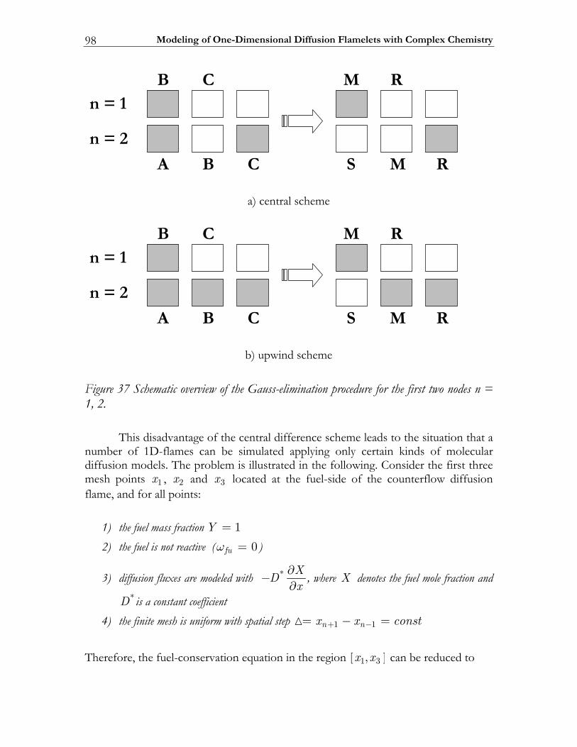
Modeling of One-Dimensional Diffusion Flamelets with Complex Chemistry 98
B C Mn = 1
R
n = 2
A B C S M R
a) central scheme
B C Mn = 1
R
n = 2
A B C S M R
b) upwind scheme
Figure 37 Schematic overview of the Gauss-elimination procedure for the first two nodes n = 1, 2. This disadvantage of the central difference scheme leads to the situation that a number of 1D-flames can be simulated applying only certain kinds of molecular diffusion models. The problem is illustrated in the following. Consider the first three mesh points 1x , 2x and 3x located at the fuel-side of the counterflow diffusion flame, and for all points:
1) the fuel mass fraction 1Y = 2) the fuel is not reactive ( 0fuω = )
3) diffusion fluxes are modeled with * XDx
∂−∂
, where X denotes the fuel mole fraction and *D is a constant coefficient
4) the finite mesh is uniform with spatial step 1 1n nx x const+ −= − =
Therefore, the fuel-conservation equation in the region [ ]1 3,x x can be reduced to
Numerical approach 99
( )* 0d dX dYD Vdx dx dx
− = . (4.29)
The corresponding central difference approximation written for the node 2n = is
( )(3) (2) (1) (3) (1)
(2) * (2)2
20fu
X X X Y YD Vϕ− + −= − + =
∆, (4.30)
and therefore ( )(2) (2) (2) ( ) ( ), , 1,2, 3n n
fu fu V Y X nϕ ϕ= = . (4.31) The partial derivatives of this equation can be found from
(2) (2) (2) ( )
( ) ( ) ( ) ( )
jfu fu fuj j j j
X Y
XY Y X Yϕ ϕ ϕ
∆
⎛ ⎞ ⎛ ⎞∂ ∂ ∂ ∂⎟ ⎟⎜ ⎜⎟ ⎟⎜ ⎜= + ⋅⎟ ⎟⎜ ⎜⎟ ⎟⎟ ⎟⎜ ⎜∂ ∂ ∂ ∂⎝ ⎠ ⎝ ⎠. (4.32)
Here the ∆ -partial derivative can be found from
( )1fu
m Xm
∆ = − , (4.33)
and since 1X = the second term on the right hand side of (4.32) is zero. Finally, the elements of the (2) (2) (2), ,ij ij ijA B C -blocks formed from (4.30) are
( ) ( )
(2)(2) (2)
(2)(1) (3)
(2) (2)(2) (2) (2)
, , ,3 1 3 1
; 0;
fufu fu
fu fu fu fu fu fu
YY Y
V VA B Cx x x x
ϕϕ ϕ
∂∂ ∂
∂∂ ∂
= − = = +− −
, (4.34)
so that the diagonal element (2)
,fu fuB has a zero-value. This example shows that the diffusion terms do not always contribute to the diagonal elements of the Jacobian. Here the model with diffusion fluxes proportional to the mole fraction gradients leads to an ill-conditioned problem. To extend the approach to arbitrary diffusion models, the species conservation equation has been modified. The new form of this equation is written
Modeling of One-Dimensional Diffusion Flamelets with Complex Chemistry 100
( ) 0k lk dk k k
l
d dY dYYV V V mdx dx dx
β
ρ ω− − + + =∑ , (4.35)
where β is an artificial convective term. Note, that the presence of the β -term does not contribute to the computational results since for each spatial point 1kY =∑ , and hence 0β = . The advantage of this modification comes from the possibility to approximate the β -term using an upwind difference scheme:
( 1) ( )
( ) ( )
1
n nn n l l
n nl
Y YVx x
β+
+
−≅−∑ , (4.36)
which guarantees non-zero elements on the main diagonal of the Jacobian matrix. For example the resulting elements of the (2) (2) (2), ,ij ij ijA B C -block now are
( ) ( )
(2) (2) (2)
(1) (2) (3)
(2) (2) (2)(2) (2) (2)
, , ,3 1 3 2 3 1
; ;
fu fu fu
fu fu fu fu fu fu
Y Y Y
V V VA B Cx x x x x x
ϕ ϕ ϕ∂ ∂ ∂∂ ∂ ∂
= − = = +− − −
, (4.37)
and therefore a Gauss-like algorithm can be used for solving the system of linearized equations. Note that the modified algorithm is appropriate for arbitrary diffusion models and at the same time the second order accuracy associated with the central differencing technique is preserved.
4.2.4 Implementation The numerical methodology described in sub-sections 4.2.1-4.2.3 is implemented in the CFDF-program written in the C++ computer language. The required thermodynamic and physical/chemical kinetic gas properties are computed with the C-MECH user library (see chapter 2). The scheme of the CFDF-computational algorithm is shown in Figure 38. The start of the algorithm requires an initial flame profile 0Z . Then the linearization procedure(4.24)-(4.27) is performed with the numerical evaluation of the problem Jacobian. The resulting linear three-diagonal block system of equations is solved with the modified Gauss algorithm (see Appendix B). The next estimation 1s+Z for the vector of unknowns, is determined applying the damping technique, which limits the vector increment Z based on the requirements
( )
( )max
maxk k
T T
Y Y
≤
≤. (4.38)
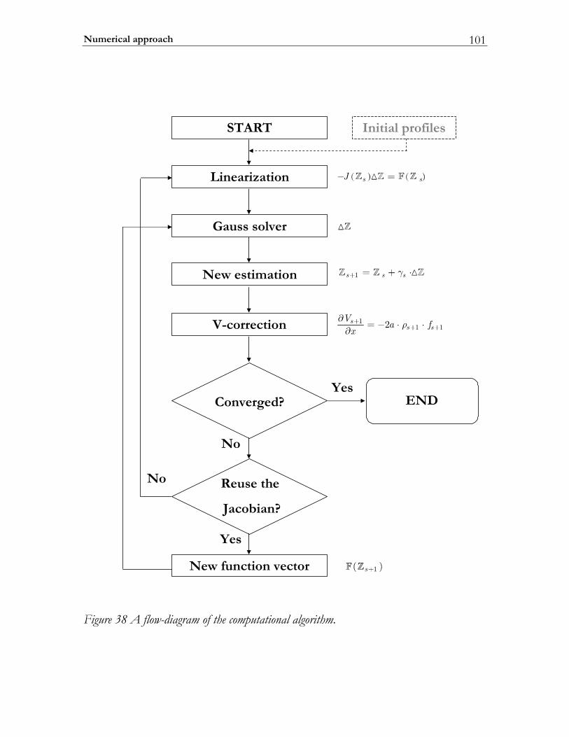
Numerical approach 101
START Initial profiles
Linearization s sJ
1s s s
11 12s
s sV
a fx
Gauss solver
New estimation
V-correction
Converged?
Reuse the
Jacobian?
New function vector
Yes
ENDYes
No
No
1s
Figure 38 A flow-diagram of the computational algorithm.
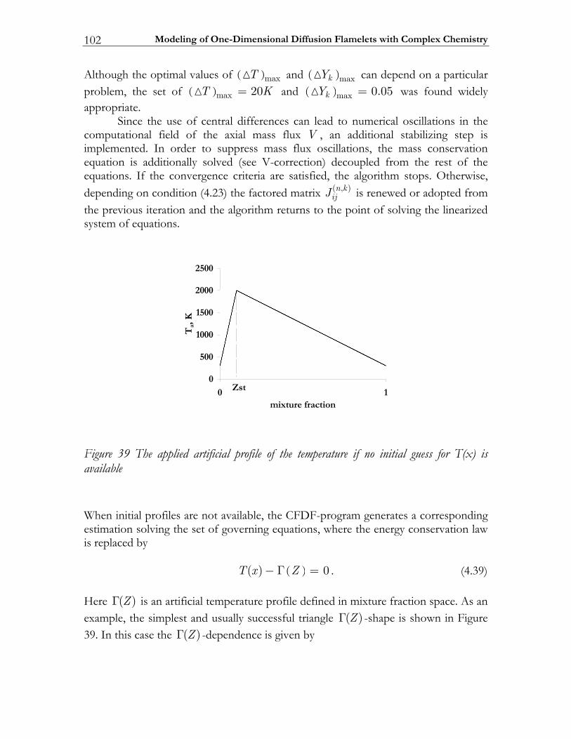
Modeling of One-Dimensional Diffusion Flamelets with Complex Chemistry 102
Although the optimal values of ( )maxT and ( )maxkY can depend on a particular problem, the set of ( )max 20T K= and ( )max 0.05kY = was found widely appropriate. Since the use of central differences can lead to numerical oscillations in the computational field of the axial mass flux V , an additional stabilizing step is implemented. In order to suppress mass flux oscillations, the mass conservation equation is additionally solved (see V-correction) decoupled from the rest of the equations. If the convergence criteria are satisfied, the algorithm stops. Otherwise, depending on condition (4.23) the factored matrix ( , )n k
ijJ is renewed or adopted from the previous iteration and the algorithm returns to the point of solving the linearized system of equations.
0
005
0001
0051
0002
0052
10noitcarferutxim
Ta,
K
tsZ
Figure 39 The applied artificial profile of the temperature if no initial guess for T(x) is available When initial profiles are not available, the CFDF-program generates a corresponding estimation solving the set of governing equations, where the energy conservation law is replaced by ( )( ) 0T x Z− Γ = . (4.39) Here ( )ZΓ is an artificial temperature profile defined in mixture fraction space. As an example, the simplest and usually successful triangle ( )ZΓ -shape is shown in Figure 39. In this case the ( )ZΓ -dependence is given by
Numerical approach 103
( )
( )
1
st oxox st
st
fu stst st st
st
T TT Z if Z ZZ
Z T TT Z Z if Z Z
Z
−⎧⎪ + ⋅ ≤⎪⎪⎪⎪Γ = ⎨ −⎪⎪ + − ⋅ ≥⎪⎪ −⎪⎩
, (4.40)
where stZ is the stoichiometric mixture fraction and oxT , fuT and stT are temperatures of pure oxidizer, pure fuel and the stoichiometric mixture, respectively. .
4.3 Validation of the CFDF-program In this section the numerical algorithm solving the laminar counterflow diffusion flame problem is validated. The numerical predictions are compared with the analytical solution of a non-reactive mixing problem (sub-section 4.3.1) and available experimental and computational data on n-heptane (sub-section 4.3.2) and dimethyl-carbonate (sub-section 4.3.3) counterflow diffusion flames.
4.3.1 Steady non-reactive mixing layer In this test case, we consider a fuel/oxidizer non-reactive mixing layer established in the counterflow geometry at pressure 1P atm= and temperature * 300T K= for both jets. The molecular diffusion fluxes kΦ are described with the Fick's law written as
kk k
YDx
ρ ∂Φ = −∂
, (4.41)
where ρ is the mass density of the gas mixture, D the thk species self-diffusion coefficient and kY the thk species mass fraction. For simplicity, the fuel and oxidizer molecular properties are chosen to be identical and adopted from those of molecular nitrogen. Therefore, the corresponding molar masses m and the self-diffusion coefficients D are:
-2
-5 2
2.8 10 ( / )
2.22 10 ( / ).
m kg mol
D m s
≈ ⋅
≈ ⋅ (4.42)
For these conditions, an analytical solution of the problem can be found. The mass flux ( )V x , reduced radial velocity ( )f x and temperature ( )T x are given by
Modeling of One-Dimensional Diffusion Flamelets with Complex Chemistry 104
*
( ) 2
( ) 1
( ) ,
V x a x
f x
T x T
ρ= −
=
=
(4.43)
where according to the applied conditions the mass density 31.14kg/mρ ≈ . The chemical composition of the fuel/oxidizer binary gas mixture can be determined fully with the fuel mass fraction Y , since the corresponding oxidizer mass fraction is equal to 1 Y− . Taking into account that ρ and D are constants and using ( )V x from (4.43), the fuel mass conservation law can be written as
2
2 2 0Y YD axxx
∂ ∂+ =∂∂
. (4.44)
This equation first leads to the solution for the first derivative /Y x∂ ∂ :
( )2expY a xx D
∂ = −∂
. (4.45)
Then, integrating (4.45) yields the analytical solution:
( ) ( )2expx
aY x Y A x dxD−∞
−∞
= + ⋅ −∫ , (4.46)
where 1Y−∞ = is the fuel mass fraction at x = −∞ and A- the constant parameter determined from the boundary conditions:
( )2exp
Y YAa x dxD
+∞ −∞+∞
−∞
−=−∫
, (4.47)
with 0Y+∞ = . Finally, the analytical expression for the fuel mass fraction is
( )
( )
2
2
exp( ) 1
exp
xa x dxD
Y xa x dxD
−∞+∞
−∞
−= −
−
∫
∫. (4.48)
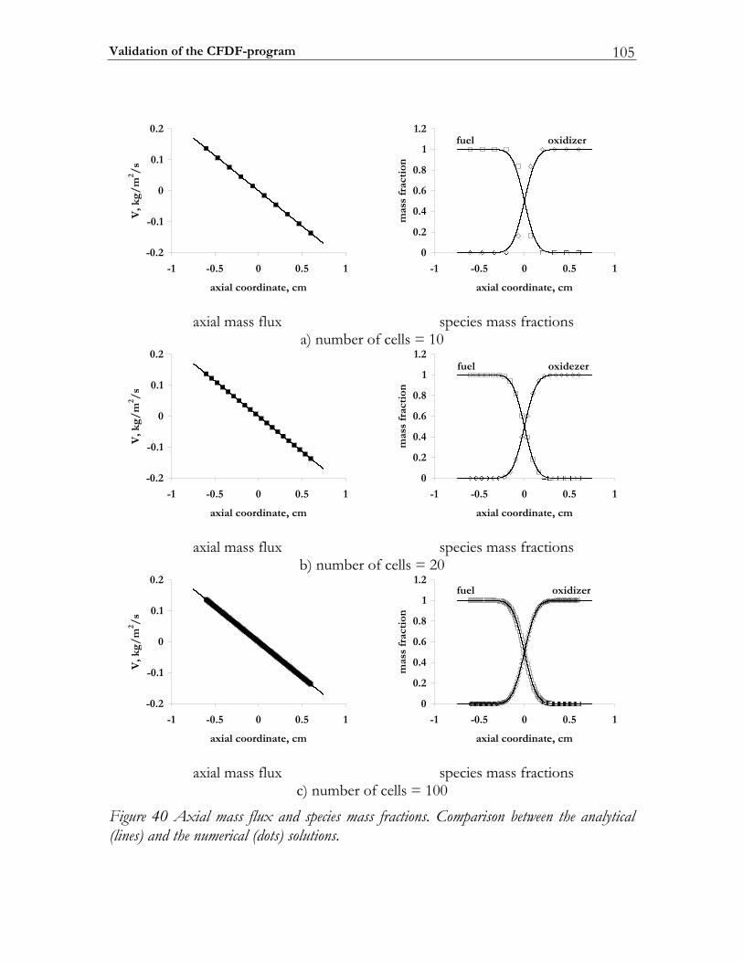
Validation of the CFDF-program 105
2.0-
1.0-
0
1.0
2.0
15.005.0-1-
mc,etanidrooclaixa
V, k
g/m
2 /s
0
2.0
4.0
6.0
8.0
1
2.1
15.005.0-1-
mc,etanidrooclaixa
mas
s fr
acti
on
rezidixoleuf
axial mass flux
species mass fractions a) number of cells = 10
2.0-
1.0-
0
1.0
2.0
15.005.0-1-
mc,etanidrooclaixa
V, k
g/m
2 /s
0
2.0
4.0
6.0
8.0
1
2.1
15.005.0-1-
mc,etanidrooclaixa
mas
s fr
acti
on
rezedixoleuf
axial mass flux
species mass fractions b) number of cells = 20
2.0-
1.0-
0
1.0
2.0
15.005.0-1-
mc,etanidrooclaixa
V, k
g/m
2 /s
0
2.0
4.0
6.0
8.0
1
2.1
15.005.0-1-
mc,etanidrooclaixa
mas
s fr
acti
on
rezidixoleuf
axial mass flux
species mass fractions c) number of cells = 100
Figure 40 Axial mass flux and species mass fractions. Comparison between the analytical (lines) and the numerical (dots) solutions.
Modeling of One-Dimensional Diffusion Flamelets with Complex Chemistry 106
Predictions of the corresponding numerical solutions obtained with the CFDF-program on the uniform mesh 1 20.6 ... 0.6
pNcm x x x cm= − = < < < = +M (4.49) with a variable number of points pN have been compared to the analytical profiles
(4.43) and (4.48) for the strain rate parameter 110a s−= . The numerically obtained ( )f x and ( )T x are constant values matching the conditions (4.43) independent from
the mesh resolution. Comparisons for the mass flux and both the fuel and the oxidizer mass fractions are shown in Figure 40 for three spatial resolutions: a)
10pN = ; b) 20pN = and c) 100pN = . Although, some discrepancy for the species mass fractions is observed at the lowest resolution ( 10pN = ), in general the numerical predictions are in excellent agreement with the analytical curves. For both meshes of 20pN = and 100pN = the numerical and theoretical profiles are identical.
4.3.2 Modeling partially premixed n-heptane flames In this sub-section we present results on the numerical modeling of two partially premixed n-heptane counterflow diffusion flames.
Experimental setup The experimental conditions of two flames (flame A and flame B) given in Table 7 are adopted from the recently published work of Paolo Berta et al. [115], where these flame were studied both experimentally and numerically. The axial-velocity boundary conditions given in Table 7 are evaluated based on the global strain rate parameter
1100ga s−= defined in [115] as
2 1 fu fuoxg
oxfu
vvaL v
ρρ
⎛ ⎞⎟⎜= + ⎟⎜ ⎟⎟⎜⎝ ⎠with 2 2
fu fu ox oxv vρ ρ= (4.50)
where the fu and ox subscripts denote the fuel and the oxidizer properties, respectively.
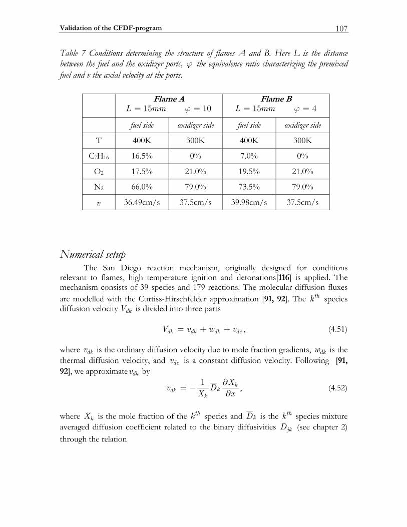
Validation of the CFDF-program 107
Table 7 Conditions determining the structure of flames A and B. Here L is the distance between the fuel and the oxidizer ports, ϕ the equivalence ratio characterizing the premixed fuel and v the axial velocity at the ports.
Flame A
15 10L mm ϕ= = Flame B
15 4L mm ϕ= =
fuel side oxidizer side fuel side oxidizer side
T 400K 300K 400K 300K
C7H16 16.5% 0% 7.0% 0%
O2 17.5% 21.0% 19.5% 21.0%
N2 66.0% 79.0% 73.5% 79.0%
v 36.49cm/s 37.5cm/s 39.98cm/s 37.5cm/s
Numerical setup The San Diego reaction mechanism, originally designed for conditions relevant to flames, high temperature ignition and detonations[116] is applied. The mechanism consists of 39 species and 179 reactions. The molecular diffusion fluxes are modelled with the Curtiss-Hirschfelder approximation [91, 92]. The thk species diffusion velocity dkV is divided into three parts dk dk dk dcV v w v= + + , (4.51) where dkv is the ordinary diffusion velocity due to mole fraction gradients, dkw is the thermal diffusion velocity, and dcv is a constant diffusion velocity. Following [91, 92], we approximate dkv by
1 kkdk
k
Xv DX x
∂= −∂
, (4.52)
where kX is the mole fraction of the thk species and kD is the thk species mixture averaged diffusion coefficient related to the binary diffusivities jkD (see chapter 2) through the relation
Modeling of One-Dimensional Diffusion Flamelets with Complex Chemistry 108
( )1/k
kj jk
j k
YDX D
≠
−= ∑ . (4.53)
The thermal diffusion velocity dkw is given by
k kdk
k
D TwX T xΘ ∂=
∂ (4.54)
with
j kk kj j k
j kj k
m mX X
m mτ
≠
−Θ = ⋅
+∑ , (4.55)
where kjτ is a function of temperature determined for each pair of components j and k (see chapter 2). Finally, the constant diffusion velocity dcv is introduced to satisfy the condition 0dk
kYV =∑ , (4.56)
which must hold if momentum is to be conserved. Upon making use of (4.51) and (4.56) we have ( )dc k dk dk
kv Y v w= − +∑ . (4.57)
The viscosity and thermal conductivity coefficients of the multi-component gas mixture were computed with the approximations proposed by Wilke [93] and Mason-Saxena [95] (see chapter 2), respectively. The involved molecular transport coefficients kjD , kjτ (see formula (4.55)), kη and kλ were pre-computed and approximated with temperature-polynomials using the TROT-package described in chapter 2. The thermal radiation effects were not taking into account. The A- and B-flame structures have been computed on the uniform mesh 1 2 ...
pfu N oxL x x x L= − = < < < = +−M , with the number of spatial points equal to 2000pN = .
Results Since the mathematical formulation is given in terms of the strain rate a , it does not prescribe the velocity boundary conditions as given in Table 7. In order to overcome
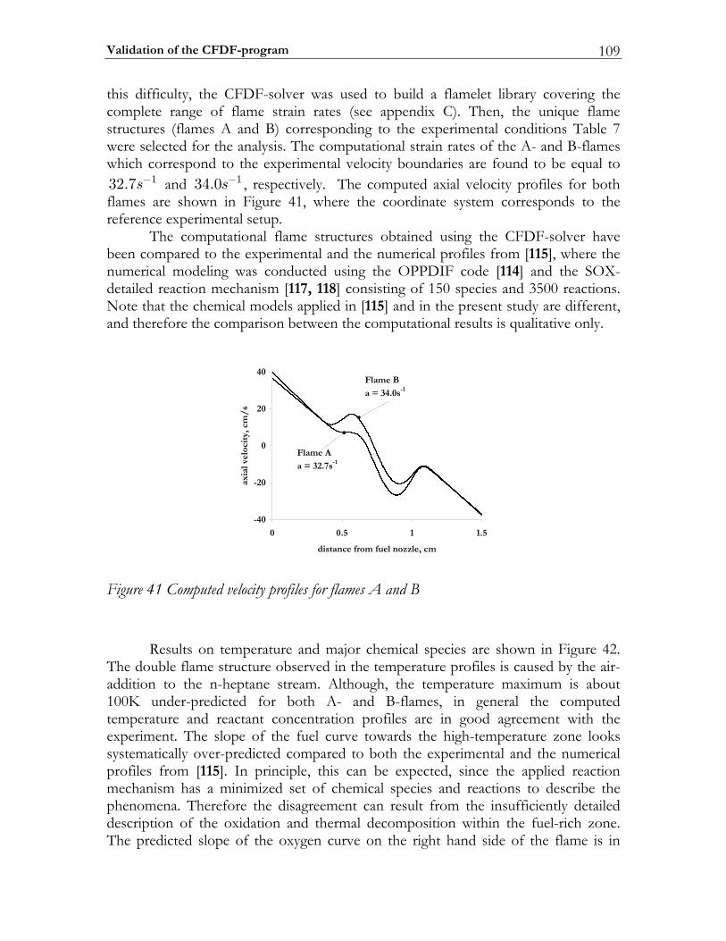
Validation of the CFDF-program 109
this difficulty, the CFDF-solver was used to build a flamelet library covering the complete range of flame strain rates (see appendix C). Then, the unique flame structures (flames A and B) corresponding to the experimental conditions Table 7 were selected for the analysis. The computational strain rates of the A- and B-flames which correspond to the experimental velocity boundaries are found to be equal to
132.7s− and 134.0s− , respectively. The computed axial velocity profiles for both flames are shown in Figure 41, where the coordinate system corresponds to the reference experimental setup. The computational flame structures obtained using the CFDF-solver have been compared to the experimental and the numerical profiles from [115], where the numerical modeling was conducted using the OPPDIF code [114] and the SOX-detailed reaction mechanism [117, 118] consisting of 150 species and 3500 reactions. Note that the chemical models applied in [115] and in the present study are different, and therefore the comparison between the computational results is qualitative only.
04-
02-
0
02
04
5.115.00
mc,elzzonleufmorfecnatsid
axia
l vel
ocit
y,cm
/s
BemalF
s0.43=a 1-
AemalF
s7.23=a 1-
Figure 41 Computed velocity profiles for flames A and B Results on temperature and major chemical species are shown in Figure 42. The double flame structure observed in the temperature profiles is caused by the air-addition to the n-heptane stream. Although, the temperature maximum is about 100K under-predicted for both A- and B-flames, in general the computed temperature and reactant concentration profiles are in good agreement with the experiment. The slope of the fuel curve towards the high-temperature zone looks systematically over-predicted compared to both the experimental and the numerical profiles from [115]. In principle, this can be expected, since the applied reaction mechanism has a minimized set of chemical species and reactions to describe the phenomena. Therefore the disagreement can result from the insufficiently detailed description of the oxidation and thermal decomposition within the fuel-rich zone. The predicted slope of the oxygen curve on the right hand side of the flame is in
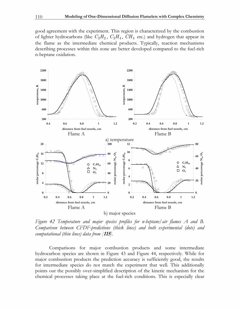
Modeling of One-Dimensional Diffusion Flamelets with Complex Chemistry 110
good agreement with the experiment. This region is characterized by the combustion of lighter hydrocarbons (like 2 2C H , 2 4C H , 4CH etc.) and hydrogen that appear in the flame as the intermediate chemical products. Typically, reaction mechanisms describing processes within this zone are better developed compared to the fuel-rich n-heptane oxidation.
002
006
0001
0041
0081
0022
2.118.06.04.0
mc,elzzonleufmorfecnatsid
tem
per
atu
re,K
002
006
0001
0041
0081
0022
2.118.06.04.02.0
mc,elzzonleufmorfecnatsid
tem
per
atu
re,K
Flame A Flame B a) temperature
0
4
8
21
61
02
2.118.06.04.02.0
mc,elzzonleufmorfecnatsid
mol
ar p
erce
nta
geC
7H16
0
02
04
06
08
001
mol
ar p
erce
ntag
eN
2, O
2
C7H 61
N2
O2
0
2
4
6
8
01
21
2.118.06.04.02.0
mc,elzzonleufmorfecnatsid
mol
ar p
erce
nta
geC
7H16
0
02
04
06
08
mol
ar p
erce
ntag
eN
2, O
2
C7H 61
N2
O2
Flame A Flame B b) major species
Figure 42 Temperature and major species profiles for n-heptane/air flames A and B. Comparison between CFDF-predictions (thick lines) and both experimental (dots) and computational (thin lines) data from [115]. Comparisons for major combustion products and some intermediate hydrocarbon species are shown in Figure 43 and Figure 44, respectively. While for major combustion products the prediction accuracy is sufficiently good, the results for intermediate species do not match the experiment that well. This additionally points out the possibly over-simplified description of the kinetic mechanism for the chemical processes taking place at the fuel-rich conditions. This is especially clear
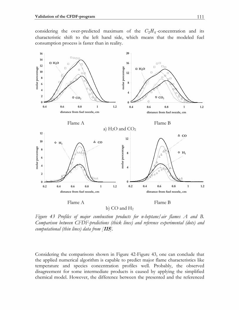
Validation of the CFDF-program 111
considering the over-predicted maximum of the 2 4C H -concentration and its characteristic shift to the left hand side, which means that the modeled fuel consumption process is faster than in reality.
0
2
4
6
8
01
21
41
61
2.118.06.04.0
mc,elzzonleufmorfecnatsid
mol
ar p
erce
ntag
e
H2O
OC 2
0
4
8
21
61
02
2.118.06.04.0
mc,elzzonleufmorfecnatsid
mol
ar p
erce
ntag
e
H2O
OC 2
Flame A
Flame B
a) H2O and CO2
0
2
4
6
8
01
21
2.118.06.04.02.0
mc,elzzonleufmorfecnatsid
mol
ar p
erce
nta
ge
OCH2
0
4
8
21
2.118.06.04.02.0
mc,elzzonleufmorfecnatsid
mol
ar p
erce
ntag
e
OC
H2
Flame A
Flame B
b) CO and H2
Figure 43 Profiles of major combustion products for n-heptane/air flames A and B. Comparison between CFDF-predictions (thick lines) and reference experimental (dots) and computational (thin lines) data from [115]. Considering the comparisons shown in Figure 42-Figure 43, one can conclude that the applied numerical algorithm is capable to predict major flame characteristics like temperature and species concentration profiles well. Probably, the observed disagreement for some intermediate products is caused by applying the simplified chemical model. However, the difference between the presented and the referenced
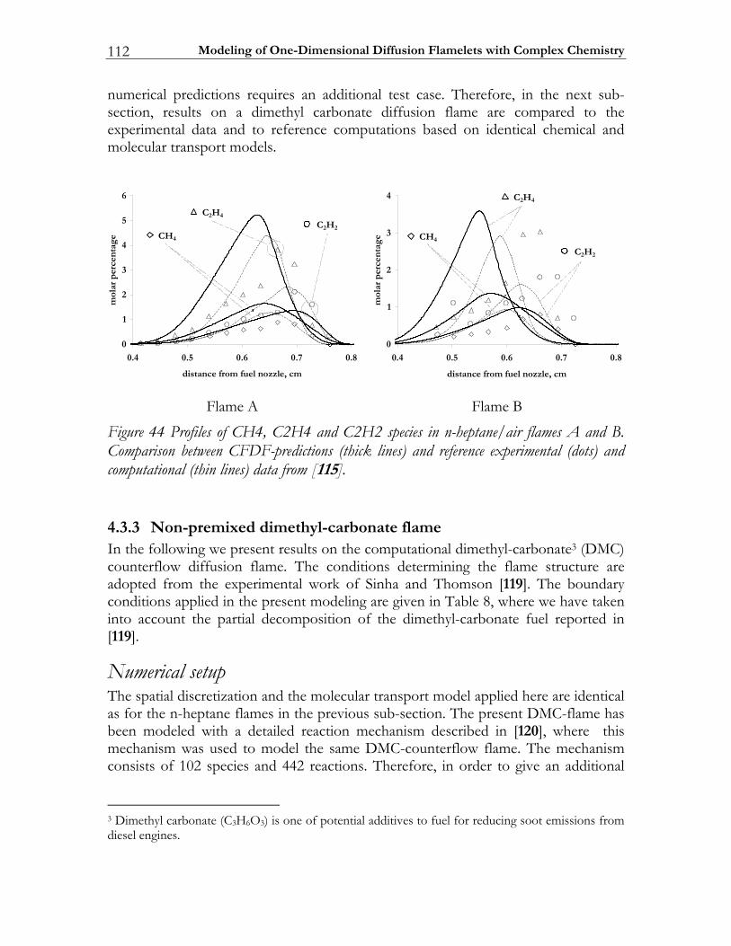
Modeling of One-Dimensional Diffusion Flamelets with Complex Chemistry 112
numerical predictions requires an additional test case. Therefore, in the next sub-section, results on a dimethyl carbonate diffusion flame are compared to the experimental data and to reference computations based on identical chemical and molecular transport models.
0
1
2
3
4
5
6
8.07.06.05.04.0
mc,elzzonleufmorfecnatsid
mol
ar p
erce
ntag
e
C2H4
HC 4
C2H2
0
1
2
3
4
8.07.06.05.04.0
mc,elzzonleufmorfecnatsidm
olar
per
cen
tage
C2H4
HC 4
C2H2
Flame A
Flame B
Figure 44 Profiles of CH4, C2H4 and C2H2 species in n-heptane/air flames A and B. Comparison between CFDF-predictions (thick lines) and reference experimental (dots) and computational (thin lines) data from [115].
4.3.3 Non-premixed dimethyl-carbonate flame In the following we present results on the computational dimethyl-carbonate3 (DMC) counterflow diffusion flame. The conditions determining the flame structure are adopted from the experimental work of Sinha and Thomson [119]. The boundary conditions applied in the present modeling are given in Table 8, where we have taken into account the partial decomposition of the dimethyl-carbonate fuel reported in [119].
Numerical setup The spatial discretization and the molecular transport model applied here are identical as for the n-heptane flames in the previous sub-section. The present DMC-flame has been modeled with a detailed reaction mechanism described in [120], where this mechanism was used to model the same DMC-counterflow flame. The mechanism consists of 102 species and 442 reactions. Therefore, in order to give an additional
3 Dimethyl carbonate (C3H6O3) is one of potential additives to fuel for reducing soot emissions from diesel engines.
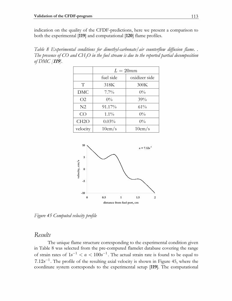
Validation of the CFDF-program 113
indication on the quality of the CFDF-predictions, here we present a comparison to both the experimental [119] and computational [120] flame profiles.
Table 8 Experimental conditions for dimethyl-carbonate/air counterflow diffusion flame. . The presence of CO and CH2O in the fuel stream is due to the reported partial decomposition of DMC [119].
20L mm= fuel side oxidizer side
T 318K 300K DMC 7.7% 0% O2 0% 39% N2 91.17% 61% CO 1.1% 0%
CH2O 0.03% 0% velocity 10cm/s 10cm/s
01-
5-
0
5
01
25.115.00
mc,tropleufmorfecnatsid
velo
city
, cm
/s
s21.7=a 1-
Figure 45 Computed velocity profile
Results The unique flame structure corresponding to the experimental condition given in Table 8 was selected from the pre-computed flamelet database covering the range of strain rates of 1 11 100s a s− −< < . The actual strain rate is found to be equal to
17.12s− . The profile of the resulting axial velocity is shown in Figure 45, where the coordinate system corresponds to the experimental setup [119]. The computational
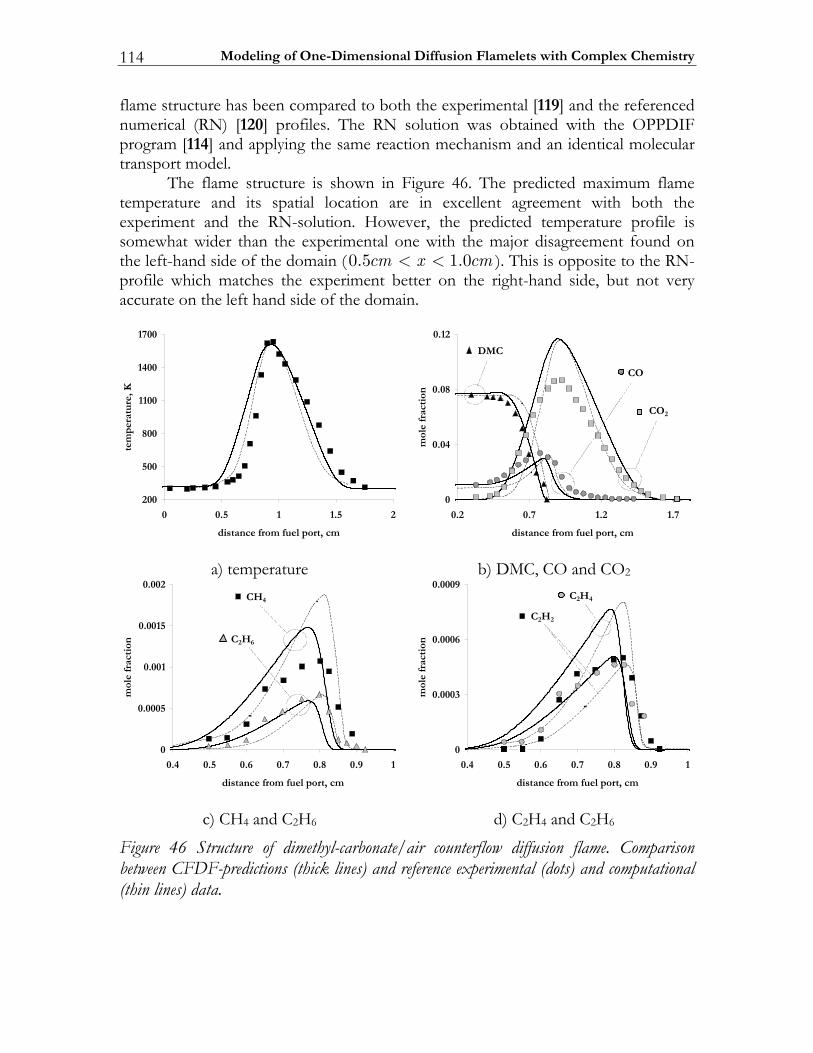
Modeling of One-Dimensional Diffusion Flamelets with Complex Chemistry 114
flame structure has been compared to both the experimental [119] and the referenced numerical (RN) [120] profiles. The RN solution was obtained with the OPPDIF program [114] and applying the same reaction mechanism and an identical molecular transport model. The flame structure is shown in Figure 46. The predicted maximum flame temperature and its spatial location are in excellent agreement with both the experiment and the RN-solution. However, the predicted temperature profile is somewhat wider than the experimental one with the major disagreement found on the left-hand side of the domain (0.5 1.0cm x cm< < ). This is opposite to the RN-profile which matches the experiment better on the right-hand side, but not very accurate on the left hand side of the domain.
002
005
008
0011
0041
0071
25.115.00
mc,tropleufmorfecnatsid
tem
per
atu
re,K
0
40.0
80.0
21.0
7.12.17.02.0
mc,tropleufmorfecnatsid
mol
e fr
acti
on
CMD
OC
OC 2
a) temperature
b) DMC, CO and CO2
0
5000.0
100.0
5100.0
200.0
19.08.07.06.05.04.0
mc,tropleufmorfecnatsid
mol
e fr
acti
on
HC 4
C2H6
0
3000.0
6000.0
9000.0
19.08.07.06.05.04.0
mc,tropleufmorfecnatsid
mol
e fr
acti
on
C2H4
C2H2
c) CH4 and C2H6
d) C2H4 and C2H6
Figure 46 Structure of dimethyl-carbonate/air counterflow diffusion flame. Comparison between CFDF-predictions (thick lines) and reference experimental (dots) and computational (thin lines) data.
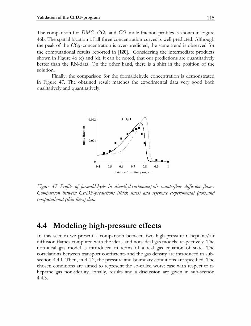
Validation of the CFDF-program 115
The comparison for DMC , 2CO and CO mole fraction profiles is shown in Figure 46b. The spatial location of all three concentration curves is well predicted. Although the peak of the 2CO -concentration is over-predicted, the same trend is observed for the computational results reported in [120]. Considering the intermediate products shown in Figure 46 (c) and (d), it can be noted, that our predictions are quantitatively better than the RN-data. On the other hand, there is a shift in the position of the solution. Finally, the comparison for the formaldehyde concentration is demonstrated in Figure 47. The obtained result matches the experimental data very good both qualitatively and quantitatively.
0
100.0
200.0
19.08.07.06.05.04.0
mc,tropleufmorfecnatsid
mol
e fr
acti
on
HC 2O
Figure 47 Profile of formaldehyde in dimethyl-carbonate/air counterflow diffusion flame. Comparison between CFDF-predictions (thick lines) and reference experimental (dots)and computational (thin lines) data.
4.4 Modeling high-pressure effects In this section we present a comparison between two high-pressure n-heptane/air diffusion flames computed with the ideal- and non-ideal gas models, respectively. The non-ideal gas model is introduced in terms of a real gas equation of state. The correlations between transport coefficients and the gas density are introduced in sub-section 4.4.1. Then, in 4.4.2, the pressure and boundary conditions are specified. The chosen conditions are aimed to represent the so-called worst case with respect to n-heptane gas non-ideality. Finally, results and a discussion are given in sub-section 4.4.3.
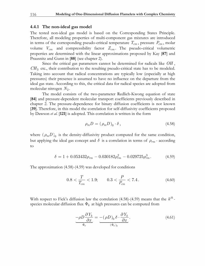
Modeling of One-Dimensional Diffusion Flamelets with Complex Chemistry 116
4.4.1 The non-ideal gas model The tested non-ideal gas model is based on the Corresponding States Principle. Therefore, all modeling properties of multi-component gas mixtures are introduced in terms of the corresponding pseudo-critical temperature cmT , pressure cmP , molar volume cmV and compressibility factor cmZ . The pseudo-critical volumetric properties are determined with the linear approximations proposed by Kay [87] and Prausnitz and Gunn in [88] (see chapter 2). Since the critical gas parameters cannot be determined for radicals like OH ,
3CH etc., their contribution to the resulting pseudo-critical state has to be modeled. Taking into account that radical concentrations are typically low (especially at high pressures) their presence is assumed to have no influence on the departure from the ideal gas state. According to this, the critical data for radical species are adopted from molecular nitrogen 2N . The model consists of the two-parameter Redlich-Kwong equation of state [84] and pressure-dependent molecular transport coefficients previously described in chapter 2. The pressure-dependence for binary diffusion coefficients is not known [39]. Therefore, in this model the correlation for self-diffusivity coefficients proposed by Dawson et al. [121] is adopted. This correlation is written in the form ( )0m mD Dρ ρ δ= ⋅ , (4.58) where ( )0mDρ is the density-diffusivity product computed for the same condition, but applying the ideal gas concept and δ is a correlation in terms of rmρ - according to 2 31 0.053432 0.030182 0.029725rm rm rmδ ρ ρ ρ= + − − . (4.59) The approximation (4.58)-(4.59) was developed for conditions
0.8 1.9; 0.3 7.4cm cm
T PT P< < < < . (4.60)
With respect to Fick’s diffusion law the correlation (4.58)-(4.59) means that the thk -species molecular diffusion flux kΦ at high pressures can be computed from
( )
( )0
0
k k
k kY YD Dx x
ρ ρ δΦ Φ
∂ ∂− = − ⋅∂ ∂
. (4.61)
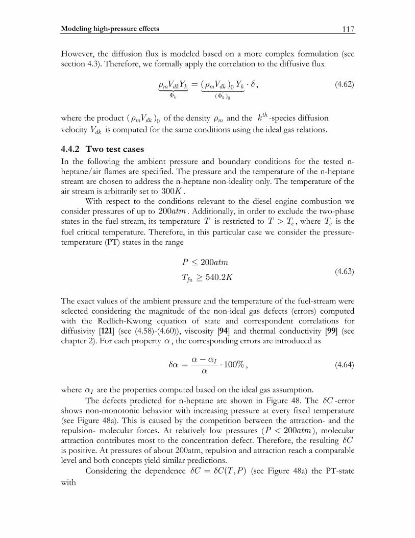
Modeling high-pressure effects 117
However, the diffusion flux is modeled based on a more complex formulation (see section 4.3). Therefore, we formally apply the correlation to the diffusive flux ( )
( )0
0k k
m dk k m dk kV Y V Yρ ρ δΦ Φ
= ⋅ , (4.62)
where the product ( )0m dkVρ of the density mρ and the thk -species diffusion velocity dkV is computed for the same conditions using the ideal gas relations.
4.4.2 Two test cases In the following the ambient pressure and boundary conditions for the tested n-heptane/air flames are specified. The pressure and the temperature of the n-heptane stream are chosen to address the n-heptane non-ideality only. The temperature of the air stream is arbitrarily set to 300K . With respect to the conditions relevant to the diesel engine combustion we consider pressures of up to 200atm . Additionally, in order to exclude the two-phase states in the fuel-stream, its temperature T is restricted to cT T> , where cT is the fuel critical temperature. Therefore, in this particular case we consider the pressure-temperature (PT) states in the range
200
540.2fu
P atm
T K
≤
≥ (4.63)
The exact values of the ambient pressure and the temperature of the fuel-stream were selected considering the magnitude of the non-ideal gas defects (errors) computed with the Redlich-Kwong equation of state and correspondent correlations for diffusivity [121] (see (4.58)-(4.60)), viscosity [94] and thermal conductivity [99] (see chapter 2). For each property α , the corresponding errors are introduced as 100%Iα αδα α
−= ⋅ , (4.64)
where Iα are the properties computed based on the ideal gas assumption. The defects predicted for n-heptane are shown in Figure 48. The Cδ -error shows non-monotonic behavior with increasing pressure at every fixed temperature (see Figure 48a). This is caused by the competition between the attraction- and the repulsion- molecular forces. At relatively low pressures ( 200P atm< ), molecular attraction contributes most to the concentration defect. Therefore, the resulting Cδ is positive. At pressures of about 200atm, repulsion and attraction reach a comparable level and both concepts yield similar predictions. Considering the dependence ( , )C C T Pδ δ= (see Figure 48a) the PT-state with
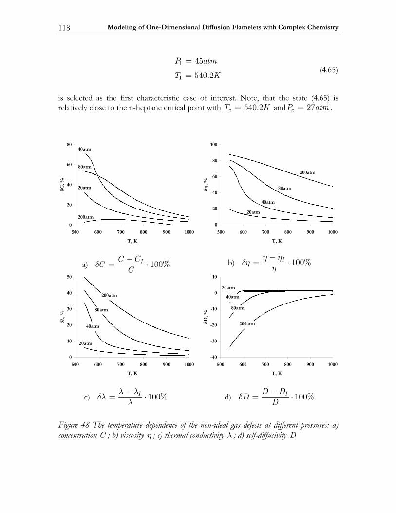
Modeling of One-Dimensional Diffusion Flamelets with Complex Chemistry 118
1
1
45
540.2
P atm
T K
=
= (4.65)
is selected as the first characteristic case of interest. Note, that the state (4.65) is relatively close to the n-heptane critical point with 540.2cT K= and 27cP atm= .
0
02
04
06
08
0001009008007006005
K,T
δC,%
mta02
mta04
mta08
mta002
0
02
04
06
08
001
0001009008007006005
K,T
δη,%
mta02
mta04
mta08
mta002
a) 100%IC CCC
δ −= ⋅
b) 100%Iη ηδη η
−= ⋅
0
01
02
03
04
05
0001009008007006005
K,T
δλ,%
mta02
mta04
mta08
mta002
04-
03-
02-
01-
0
01
0001009008007006005
K,T
δD,%
mta02
mta04
mta08
mta002
c) 100%Iλ λδλ λ−= ⋅
d) 100%ID DDD
δ −= ⋅
Figure 48 The temperature dependence of the non-ideal gas defects at different pressures: a) concentration C ; b) viscosity η ; c) thermal conductivity λ ; d) self-diffusivity D
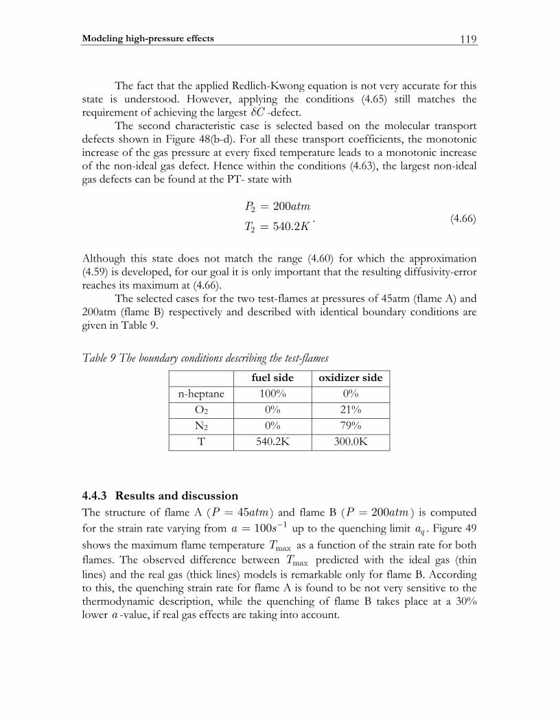
Modeling high-pressure effects 119
The fact that the applied Redlich-Kwong equation is not very accurate for this state is understood. However, applying the conditions (4.65) still matches the requirement of achieving the largest Cδ -defect. The second characteristic case is selected based on the molecular transport defects shown in Figure 48(b-d). For all these transport coefficients, the monotonic increase of the gas pressure at every fixed temperature leads to a monotonic increase of the non-ideal gas defect. Hence within the conditions (4.63), the largest non-ideal gas defects can be found at the PT- state with
2
2
200
540.2
P atm
T K
=
=. (4.66)
Although this state does not match the range (4.60) for which the approximation (4.59) is developed, for our goal it is only important that the resulting diffusivity-error reaches its maximum at (4.66). The selected cases for the two test-flames at pressures of 45atm (flame A) and 200atm (flame B) respectively and described with identical boundary conditions are given in Table 9.
Table 9 The boundary conditions describing the test-flames fuel side oxidizer side
n-heptane 100% 0% O2 0% 21% N2 0% 79% T 540.2K 300.0K
4.4.3 Results and discussion The structure of flame A ( 45P atm= ) and flame B ( 200P atm= ) is computed for the strain rate varying from 1100a s−= up to the quenching limit qa . Figure 49 shows the maximum flame temperature maxT as a function of the strain rate for both flames. The observed difference between maxT predicted with the ideal gas (thin lines) and the real gas (thick lines) models is remarkable only for flame B. According to this, the quenching strain rate for flame A is found to be not very sensitive to the thermodynamic description, while the quenching of flame B takes place at a 30% lower a -value, if real gas effects are taking into account.
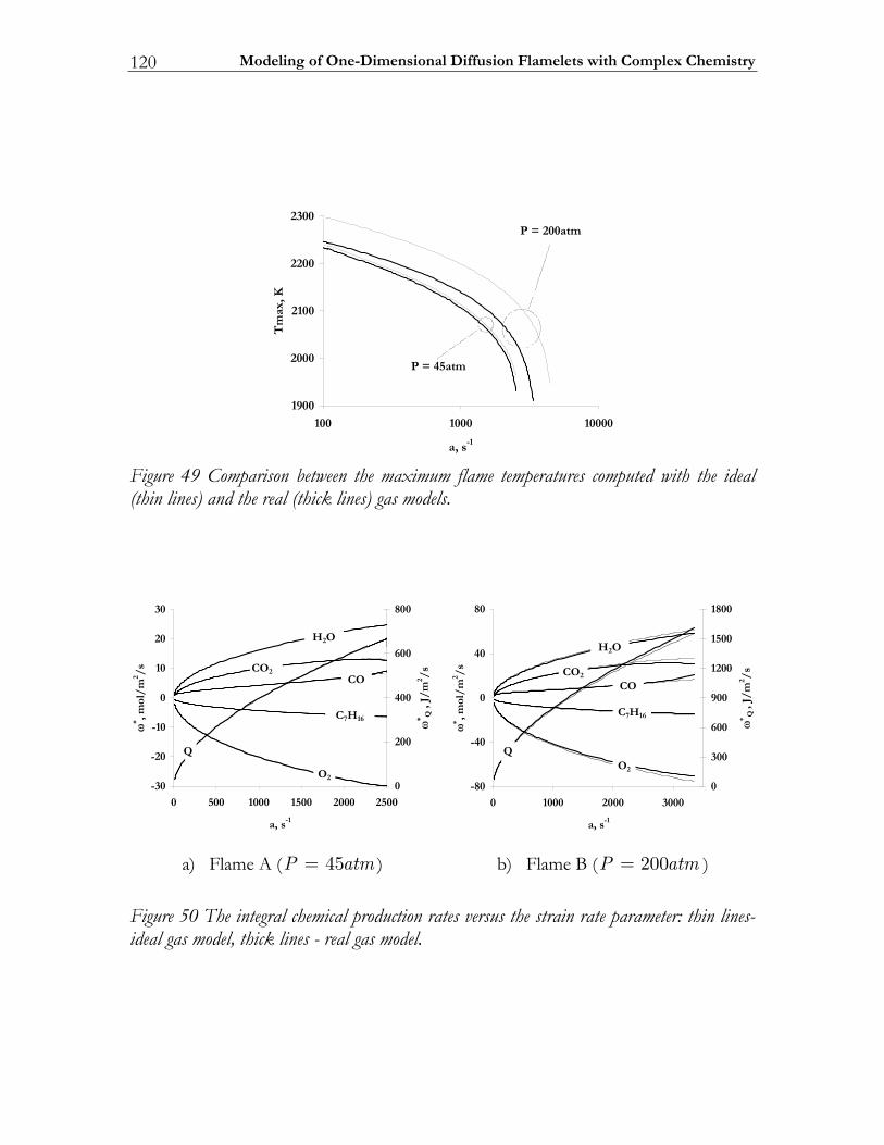
Modeling of One-Dimensional Diffusion Flamelets with Complex Chemistry 120
0091
0002
0012
0022
0032
000010001001
s,a 1-
Tm
ax, K
mta54=P
mta002=P
Figure 49 Comparison between the maximum flame temperatures computed with the ideal (thin lines) and the real (thick lines) gas models.
03-
02-
01-
0
01
02
03
00520002005100010050
s,a 1-
ω* ,m
ol/
m2 /
s
0
002
004
006
008
ω* Q
,J/
m2 /
s
Q
C7H 61
O2
OCOC 2
H2O
08-
04-
0
04
08
0003000200010
s,a 1-
ω∗ ,m
ol/
m2 /
s
0
003
006
009
0021
0051
0081
ω∗ Q
,J/m
2 /s
QO2
C7H 61
OCOC 2
H2O
a) Flame A ( 45P atm= )
b) Flame B ( 200P atm= )
Figure 50 The integral chemical production rates versus the strain rate parameter: thin lines-ideal gas model, thick lines - real gas model.
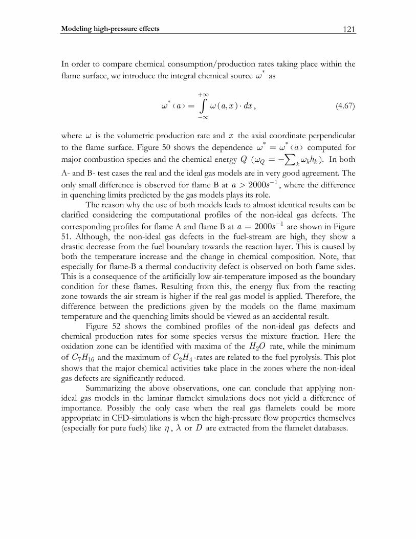
Modeling high-pressure effects 121
In order to compare chemical consumption/production rates taking place within the flame surface, we introduce the integral chemical source *ω as
( ) ( )* ,a a x dxω ω+∞
−∞
= ⋅∫ , (4.67)
where ω is the volumetric production rate and x the axial coordinate perpendicular to the flame surface. Figure 50 shows the dependence ( )* * aω ω= computed for major combustion species and the chemical energy Q ( Q k kk
hω ω= −∑ ). In both A- and B- test cases the real and the ideal gas models are in very good agreement. The only small difference is observed for flame B at 12000a s−> , where the difference in quenching limits predicted by the gas models plays its role. The reason why the use of both models leads to almost identical results can be clarified considering the computational profiles of the non-ideal gas defects. The corresponding profiles for flame A and flame B at 12000a s−= are shown in Figure 51. Although, the non-ideal gas defects in the fuel-stream are high, they show a drastic decrease from the fuel boundary towards the reaction layer. This is caused by both the temperature increase and the change in chemical composition. Note, that especially for flame-B a thermal conductivity defect is observed on both flame sides. This is a consequence of the artificially low air-temperature imposed as the boundary condition for these flames. Resulting from this, the energy flux from the reacting zone towards the air stream is higher if the real gas model is applied. Therefore, the difference between the predictions given by the models on the flame maximum temperature and the quenching limits should be viewed as an accidental result. Figure 52 shows the combined profiles of the non-ideal gas defects and chemical production rates for some species versus the mixture fraction. Here the oxidation zone can be identified with maxima of the 2H O rate, while the minimum of 7 16C H and the maximum of 2 4C H -rates are related to the fuel pyrolysis. This plot shows that the major chemical activities take place in the zones where the non-ideal gas defects are significantly reduced. Summarizing the above observations, one can conclude that applying non-ideal gas models in the laminar flamelet simulations does not yield a difference of importance. Possibly the only case when the real gas flamelets could be more appropriate in CFD-simulations is when the high-pressure flow properties themselves (especially for pure fuels) like η , λ or D are extracted from the flamelet databases.
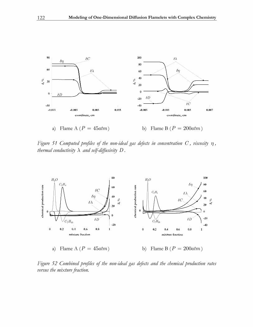
Modeling of One-Dimensional Diffusion Flamelets with Complex Chemistry 122
-30
0
30
60
90
-0.015 -0.005 0.005 0.015
coordinate, cm
,%
D
C
-40
-20
0
20
40
60
80
100
-0.005 -0.001 0.003 0.007
coordinate, cm
,%
D
C
a) Flame A ( 45P atm= )
b) Flame B ( 200P atm= )
Figure 51 Computed profiles of the non-ideal gas defects in concentration C , viscosity η , thermal conductivity λ and self-diffusivity D .
0 0.2 0.4 0.6 0.8 1
mixture fraction
chem
ical
pro
du
ctio
n r
ate
-20
0
20
40
60
80
,%
0
2 4C H
7 16C H
2H O
D
C
0 0.2 0.4 0.6 0.8 1
mixture fraction
chem
ical
pro
du
ctio
n r
ate
-40
-20
0
20
40
60
80
100
,%0
2 4C H
7 16C H
2H O
C
D
a) Flame A ( 45P atm= )
b) Flame B ( 200P atm= )
Figure 52 Combined profiles of the non-ideal gas defects and the chemical production rates versus the mixture fraction.
Conclusions 123
4.5 Conclusions A numerical approach for modeling laminar counterflow diffusion flames with complex chemistry is presented. The approach is based on the second-order accurate finite difference scheme. The developed methodology was validated comparing numerical predictions with corresponding analytical solutions for a simplified non-reactive mixing problem and available experimental and computational data on partially premixed n-heptane flames and a non-premixed dimethyl-carbonate flame. The comparison proved both quantitative and qualitative adequateness of the computational method. The approach gives reliable predictions on the structure of flames described with complex chemistry and therefore, can be adopted for flamelet modeling of turbulent diffusion flames in subsequent chapters. The computational approach was used in modeling high-pressure counterflow diffusion flames. The applicability of the ideal gas law to diesel-combustion modeling was verified by comparing the structures of n-heptane/air flamelets computed with ideal gas and real gas models. The comparisons were conducted for two characteristic cases having the highest non-ideality. The results demonstrate that even for these extreme conditions, applying a real gas model does not lead to a difference in the flamelet structure compared to the predictions obtained with the ideal gas assumption. In the following chapters the presented computational methodology is applied to detailed modeling of soot formation. The influence of the strain rate on the soot particles size distribution is studied in the next chapter. Application of the methodology to turbulent combustion modeling is presented in chapter 6.

Chapter 5
5 Detailed Modeling of Soot Formation
In this chapter the results on the detailed modeling of the PAH/Soot formation in stretched diffusion flamelets are presented. The focus of the study is the PAH/Soot-sensitivity to the strain rate parameter which represents the mixing dynamics. Effects on the total PAH/Soot amount and on the particle size distribution function are both considered. The chapter is divided into four parts. The problem of soot formation in general, the process phenomenology and classical numerical methods are described in the introduction (section 5.1). The following section (5.2) is dedicated to the effects of mixing dynamics. Here a brief overview of reported experimental observations, the applied model of PAH/Soot formation and the approach are described. Numerical results and conclusions are presented in sections (5.3) and (5.4) respectively.
5.1 Introduction
5.1.1 The problem of soot pollution Combustion of fuel in Diesel engines results in the formation of a complex mixture of gaseous components (hydrocarbons, CO, CO2) and particulate matter (PM). About 95% of Diesel PM is soot consisting of elemental and organic carbon [122]. The organic carbon is a class of carbon-particles additionally containing hydrogen, oxygen, nitrogen, sulfur as well as other elements in small quantities. Typical soot emitted from long-residence time turbulent non-premixed fames of toluene, benzene, acetylene, propylene, and propane flames burning in air, shows the following elemental mole ratio ranges: C:H of 8.3-18.3 , C:O of 58-109 , and C:N of 292-976 [123]. The soot density is less than that of carbon black and usually in the range of
31700-1800 kg/m , depending on the porosity of the soot [124]. Soot emission depends on many factors. Within these factors the fuel characteristics play a very important role. Different kinds of hydrocarbon fuels start producing soot at different specific C/O-ratios. For instance benzene-oxygen flames start to form carbon at
Detailed Modeling of Soot Formation 126
C/O 0.75≈ while for acetylene flames the threshold is at C/O 0.95≈ . The benzene flames produce about 100 times more polycyclic aromatic compounds compared to the aliphatic fuels for the same C/O ratio [125]. Another important factor is the operating condition. Unlike spark-ignition combustion, Diesel combustion is a fairly non-homogenous process. Carbonaceous particle formation takes place primarily during the phase of diffusion-combustion, and is highest during conditions of high fuel air ratios (fuel-rich mixtures). However, most of the carbonaceous matter formed in Diesel engine (80% to 98%) is oxidized during combustion, most likely by OH-radicals [126, 127]. PM is formed by a number of physical processes like nucleation, coagulation, condensation, and adsorption. The core particles in the Diesel exhaust (DE) are formed by nucleation and coagulation. Actually, Diesel PM consists of fine particles (fine particles have a diameter <2.5 mµ ), including a subgroup with a large number of ultra-fine particles (ultra-fine particles have a diameter <0.1 mµ ) [122]. A basic understanding of Diesel combustion processes can assist in gaining a better insight the complex factors that influence the formation of PM and other DE emissions. Soot is a major DE pollutant. It contains trace elements that have hazardous effects on human health. The particles themselves also are an issue. Fine particles, defined by a diameter equal to or below 2.5 mµ , are thought to pose a particularly great risk to health because they are more likely to be toxic than larger particles and can penetrate more deeply into the lungs [128, 129]. Many PAHs present in combustion products have been found to be mutagenic or tumorigenic [130-134]. A molecular biological pathway linking one of them, benzo[a]-pyrene, to human lung cancer has been established recently [135]. Reducing PM emissions (as well as emission of nitrogen oxides, NOx ) to the levels required by stringent new regulations poses a significant challenge for engine manufacturers. In addition to the emissions challenge, soot formation in Diesel engines can also influence engine performance and have feedback effects on in-cylinder combustion and emission formation processes. Examples include radiative heat transfer from soot to in-cylinder engine walls, which accounts for a significant portion of the heat loss in a Diesel engine [136], and a lowering of flame temperature by radiation heat transfer from soot, which will in turn affect NOx formation [137]. The total soot amount is usually characterized by the soot volume fraction defined as s
vs
f ρσ= , (5.1)
where sρ is the soot mass density in the gas phase and 31800 /s kg mσ ≈ the mass density of the condensed soot matter. The basic phenomenology of the soot formation in homogeneous mixtures and under dynamic mixing conditions is presented in the following two sub-sections. The most part of the presented material is adopted from the extensive review of Richter and Howard [128].
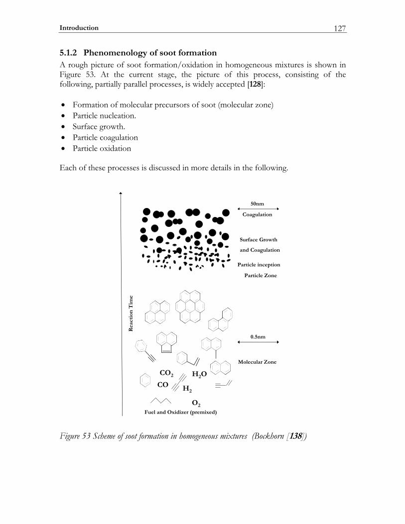
Introduction 127
5.1.2 Phenomenology of soot formation A rough picture of soot formation/oxidation in homogeneous mixtures is shown in Figure 53. At the current stage, the picture of this process, consisting of the following, partially parallel processes, is widely accepted [128]: • Formation of molecular precursors of soot (molecular zone) • Particle nucleation. • Surface growth. • Particle coagulation • Particle oxidation Each of these processes is discussed in more details in the following.
O2
H2O
H2
CO2
CO
Fuel and Oxidizer (premixed)
Molecular Zone
0.5nm
Rea
ctio
n T
ime
Particle inception
Particle Zone
50nm
Surface Growth
and Coagulation
Coagulation
Figure 53 Scheme of soot formation in homogeneous mixtures (Bockhorn [138])
Detailed Modeling of Soot Formation 128
Formation of molecular precursors of soot The molecular precursors of soot particles are considered to be heavy PAHs of molecular weight 500-1000amu [128]. The growth process from small molecules (such as benzene) to larger and larger PAH appears to involve both the addition of
2C and 3C or other small units. Specifically, acetylene has received much attention, with respect to PAH radicals, and reactions between the growing aromatic species, such as PAH–PAH radical recombination and addition reactions. The relative contribution of the different types of growth reactions depends on the fuel [128]. In the case of aromatic fuels, active reactants for aromatics formation are formed in relatively large concentrations in the breakdown of the fuel. In the case of aliphatic fuels (such as acetylene, ethylene or methane), the first aromatic ring must be formed from fuel decomposition products by a sequence of elementary reactions in which the active ring formation reactants are in lower concentrations than in the aromatics flames. This picture is consistent with a trend of increasing ease of soot formation from paraffin to mono- and di-olefins, benzenes and naphthalenes [139-142]. At present the general understanding of soot formation is based on the so-called “Hydrocarbon Polymerization Theory” which has been suggested by Gaydon [143]. According to Gaydon: “In the presence of an excess of fuel molecules, free radicals initiate chain polymerisation processes which lead to the formation of higher hydrocarbons which decompose thermally to solid carbon and hydrogen. In the presence of sufficient oxygen the radicals are removed by reaction with this and do not cause so much polymerisation.”
Soot particle inception Soot particle inception acts as the link between the main gas-phase combustion zone chemistry and soot particle dynamics, and it determines the number of nascent soot particles in flames. In this process mass is converted from molecular to particulate systems. This means that heavy PAH molecules form soot particles with a molecular mass of approximately 2000amu and an effective diameter of about 1.5nm. Chemical details of the formation of initial soot particles are relatively poorly understood. The main reason for this is caused by experimental difficulties. Using gas chromatography, an efficient identification of species produced at different stages of the growth process is limited to molecular masses less than about 300amu . However, the observation and counting of soot particles by high resolution electron microscopy has been limited to particle diameters larger than about 1.5nm. There are three major proposals regarding the inception pathway, which differ mainly in the key gaseous precursors that are assumed: polyacetylenes, ionic species, or polycyclic aromatic hydrocarbons (PAHs). The PAH hypothesis is the most generally accepted based on conclusions from numerous experimental and modeling studies. The PAH pathway involves the formation and growth of aromatic species. The starting point is the formation of the first aromatic ring (benzene) from small
Introduction 129
aliphatic components. These small aliphatic components are the “building blocks” of soot formation; they can be even-carbon-atom species such as acetylene ( 2 2C H ), or odd-carbon-atom species such as the propargyl radical ( 3 3C H ), or both. Following the formation of first ring aromatics, they grow to form large PAHs through the so-called “H-abstraction- 2 2C H -addition” (HACA) mechanism. HACA involves the abstraction of a hydrogen atom from the reacting aromatic molecules by a gaseous hydrogen atom, followed by the addition of a gaseous acetylene molecule to the radical site so formed. Some of the large PAH's have stable structures at high temperature. These species are called “islands of stability” that allow more and more building blocks to be added via HACA. At a certain size, some PAH species begin to stick to each other during collision, while individual PAHs keep increasing in size at the same time via HACA. This combined growth by molecular chemical reactions and physical collisions leads to the appearance of solid particles. Parallel to aromatics growth is aromatics oxidation. The primary mechanism seems to be the oxidation of aromatics by oxygen molecules. The oxidation by hydroxyl radical is unimportant at this early stage of soot formation. However, the role of 2O in PAHs oxidation is twofold. On one hand, it suppresses carbon mass from further growth by oxidation. On the other hand, it promotes soot formation by building up the radical pool, especially H atoms for HACA. Soot appearance in the flame is determined by the competition between soot formation and oxidation even at this early stage of the process.
Soot Surface Growth After the formation of the initial soot particles their mass is increased via the addition of gas phase species such as acetylene and PAH, including PAH radicals [128]. These reactions are believed to involve radical sites on the soot particles in the case of stable reactants such as acetylene and stable PAH. This process of course does not affect the number of soot particles. The relative contributions of acetylene and PAH is the subject of current discussions in the combustion community. Surface growth inherently involves heterogeneous reactions and that complicates the modeling of soot formation.
Soot Particle Coagulation Sticking collisions between particles during the mass growth process significantly increases particles size and decreases particle number without changing the total mass of soot present. The continuation of substantial molecular addition of gas phase species after the early formation of composite particles via sticking particle–particle collisions partly hides the identity of primary particulate units in electron microscopy images of soot particles. Particle coagulation usually is classified into two distinct processes: coalescent collision and agglomeration. In coalescent collision, two particles come together and merge to form a single larger particle, while in agglomeration, two particles stick to each other to form a chain-like structure but the identity of individual particles is maintained. The two processes may not be separated
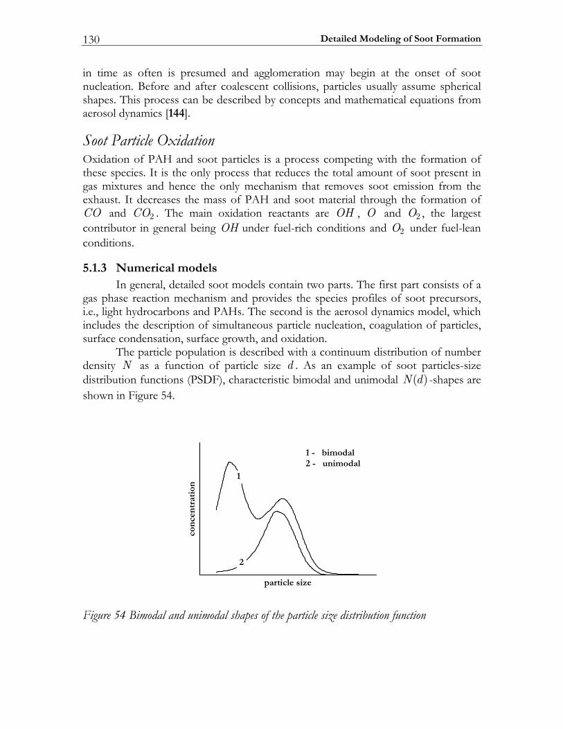
Detailed Modeling of Soot Formation 130
in time as often is presumed and agglomeration may begin at the onset of soot nucleation. Before and after coalescent collisions, particles usually assume spherical shapes. This process can be described by concepts and mathematical equations from aerosol dynamics [144].
Soot Particle Oxidation Oxidation of PAH and soot particles is a process competing with the formation of these species. It is the only process that reduces the total amount of soot present in gas mixtures and hence the only mechanism that removes soot emission from the exhaust. It decreases the mass of PAH and soot material through the formation of CO and 2CO . The main oxidation reactants are OH , O and 2O , the largest contributor in general being OH under fuel-rich conditions and 2O under fuel-lean conditions.
5.1.3 Numerical models In general, detailed soot models contain two parts. The first part consists of a gas phase reaction mechanism and provides the species profiles of soot precursors, i.e., light hydrocarbons and PAHs. The second is the aerosol dynamics model, which includes the description of simultaneous particle nucleation, coagulation of particles, surface condensation, surface growth, and oxidation. The particle population is described with a continuum distribution of number density N as a function of particle size d . As an example of soot particles-size distribution functions (PSDF), characteristic bimodal and unimodal ( )N d -shapes are shown in Figure 54.
eziselcitrap
con
cen
trat
ion
1
2
ladomib-1ladominu-2
Figure 54 Bimodal and unimodal shapes of the particle size distribution function
Introduction 131
The evolution of the PSDF is described by the following system of equations:
1
, ,1 1
12
1,2,...
i i
i
G Gi
ij i j j i j i j i j i i
j jG
dN N N N N R Wdt
i
β β
+ −
− ∞
− −= =
= − + +
= ∞
∑ ∑ . (5.2)
where i and j are indices describing certain particle sizes, N is the number density, G is the rate of coagulation, β is the coagulation kernel,R the rate of particle inception and W is the rate of surface reactions. In these equations, the G -source is explicitly expressed in terms of the Smoluchowski coagulation model. The G -source is a sum of two sub-sources depending on the β -coagulation kernel coefficients which are primarily a function of the particle diffusivity and collision cross-section. The first terms G+ represent the formation of size i particles due to collisions of smaller particles. The term G− represents the reduction of particles of size i due to their collisions with other sized particles to form larger particles. The numerical solution of equation (5.2) is a very challenging problem. The two most important reasons for that are the large size of the system of governing equations and the nonlinearity of the coagulation operator G . Reactions taking place on the particles surface and the process of particle inception can also cause severe numerical challenges. There are several models describing the dynamics of the PSDF: the sectional model [145, 146], the method of moments [59, 60, 147], the stochastic [58, 148], and the Galerkin [149] model. With respect to CFD combustion modeling, the method of moments and the sectional approach have been used the most. Comparing these two, the sectional approach, in which the size distribution is segmented into a number of bins, is the most general but also the most computationally demanding method. In the following both methods are discussed in some more detail.
Method of Moments The soot particle size distribution function (PSDF) can be considered as a discrete distribution where particles of the thi size are described with the volume iv and the mass im according to: 1 1i iv i v m i m= ⋅ = ⋅ , (5.3) Here 1v and 1m are volume and mass of the smallest particle representing the soot condensed phase. Then the thr moment of the PSDF is defined as
Detailed Modeling of Soot Formation 132
1
rr i i
iM m N
∞
==∑ . (5.4)
According to this, the first two moments 0M and 1M represent the total number density and the total mass density respectively. The complete set of moments rM ( 0,1,2...,r = ∞ ) defines the PSDF univocally. Therefore, the time evolution of the PSDF can be determined solving corresponding equations for the PSDF-moments. These equations can be obtained based on the master equation (5.2) and applying the definition (5.4). Considering only the coagulation processes (operator G in equation (5.2)) the time evolution of the PSDF is determined from
( )
0,
1 1
1
2,
1 11
1 1 1
12
0
1 !2 ! !
2, 3,...
i j i ji j
i j i ji jr
r k r ki j ij i j
k i j
dM N Ndt
dMdtdM ij N Ndt
dM r m m N Ndt k r k
r
β
β
β
∞ ∞
= =
∞ ∞
= =− ∞ ∞
−
= = =
= −
=
=
⎛ ⎞⎟⎜ ⎟= ⎜ ⎟⎜ ⎟− ⎜⎝ ⎠=
∑∑
∑∑
∑ ∑∑
(5.5)
Although the size of the resulting system of equations (5.5) is infinite, in many practical applications (when the shape of the PSDF is known or presumed), the properties of importance are determined by the first few moments [147]. Therefore, solving an infinite number of differential equations for the moments of the PSDF can be replaced by considering only a small number of equations for the lowest-order moments. In this case the method of moments (MOM) is computationally the most efficient approach to obtain a numerical approximation to the moments of a population balance [150]. For this reason this method is often used when simulating problems where transport of particles in a flow with complex geometry is essential. Despite all the computational advantages there are some shortcomings associated with the method of moments [150]. The most significant one is the non-uniqueness of the reconstruction of the particle size distribution function, i.e., the PSDF itself is not available. As a result, oxidation reactions that take place on the particles surface can only be incorporated with additional model assumptions. Usually, a lognormal (unimodal) PSDF is used for practical soot modeling. However, recent experimental data from premixed and diffusion flames reveal a bimodal size distribution of particulates formed by combustion. The first peak of the distribution corresponding to high-molecular-mass soot precursors is at about 2nm and the second peak at 20–50 nm due to primary soot particles [151, 148, 152].
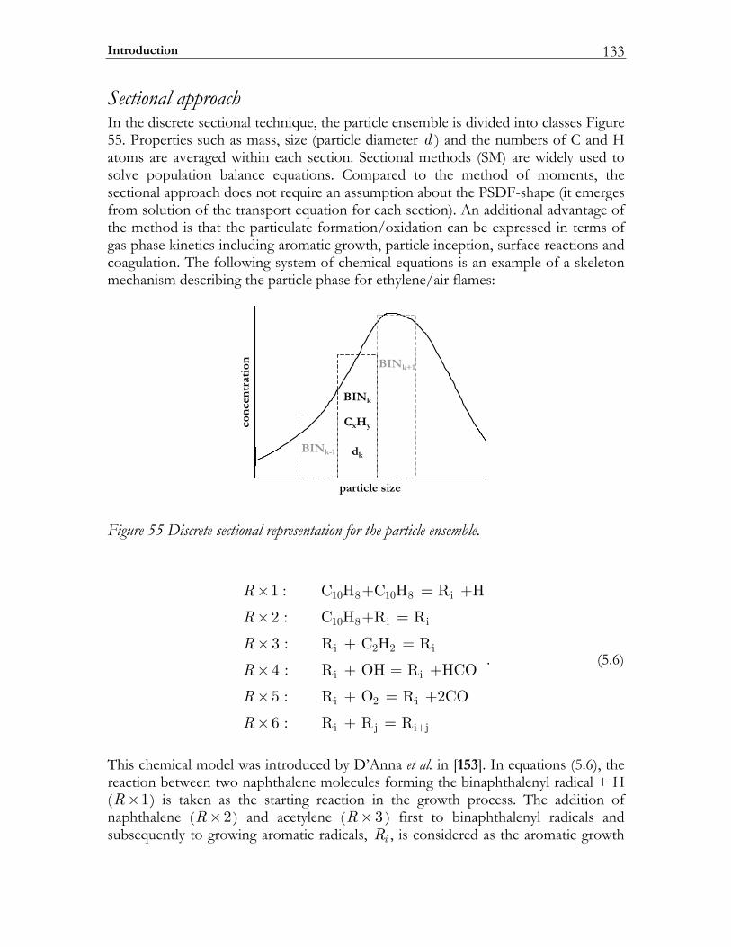
Introduction 133
Sectional approach In the discrete sectional technique, the particle ensemble is divided into classes Figure 55. Properties such as mass, size (particle diameter d ) and the numbers of C and H atoms are averaged within each section. Sectional methods (SM) are widely used to solve population balance equations. Compared to the method of moments, the sectional approach does not require an assumption about the PSDF-shape (it emerges from solution of the transport equation for each section). An additional advantage of the method is that the particulate formation/oxidation can be expressed in terms of gas phase kinetics including aromatic growth, particle inception, surface reactions and coagulation. The following system of chemical equations is an example of a skeleton mechanism describing the particle phase for ethylene/air flames:
eziselcitrap
con
cen
trat
ion
NIB k
CxHy
dkNIB 1-k
NIB 1+k
Figure 55 Discrete sectional representation for the particle ensemble.
10 8 10 8 i
10 8 i i
i 2 2 i
i i
i 2 i
i j i+j
1 : C H +C H = R +H
2 : C H +R = R
3 : R + C H = R
4 : R + OH = R +HCO
5 : R + O = R +2CO
6 : R + R = R
R
R
R
R
R
R
×
×
×
×
×
×
. (5.6)
This chemical model was introduced by D’Anna et al. in [153]. In equations (5.6), the reaction between two naphthalene molecules forming the binaphthalenyl radical + H ( 1R× ) is taken as the starting reaction in the growth process. The addition of naphthalene ( 2R× ) and acetylene ( 3R× ) first to binaphthalenyl radicals and subsequently to growing aromatic radicals, iR , is considered as the aromatic growth
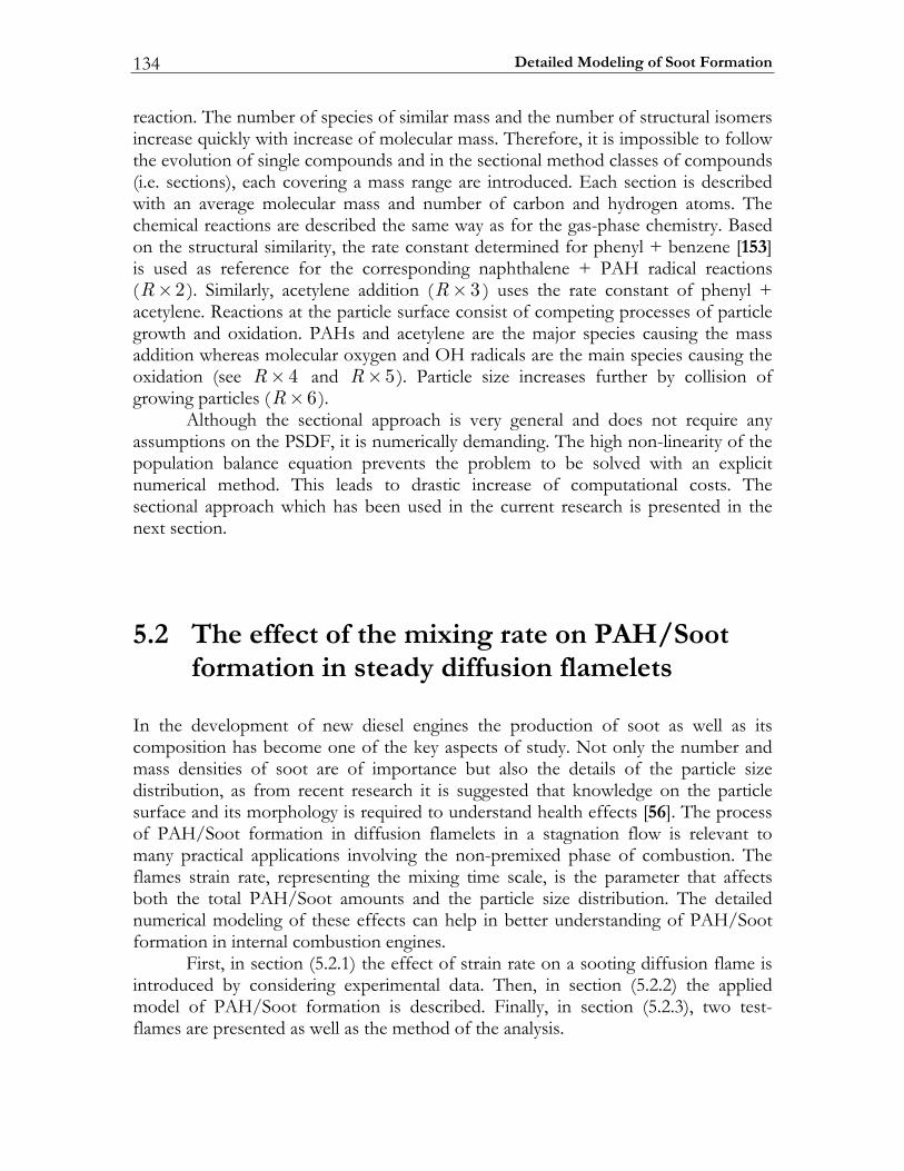
Detailed Modeling of Soot Formation 134
reaction. The number of species of similar mass and the number of structural isomers increase quickly with increase of molecular mass. Therefore, it is impossible to follow the evolution of single compounds and in the sectional method classes of compounds (i.e. sections), each covering a mass range are introduced. Each section is described with an average molecular mass and number of carbon and hydrogen atoms. The chemical reactions are described the same way as for the gas-phase chemistry. Based on the structural similarity, the rate constant determined for phenyl + benzene [153] is used as reference for the corresponding naphthalene + PAH radical reactions ( 2R× ). Similarly, acetylene addition ( 3R× ) uses the rate constant of phenyl + acetylene. Reactions at the particle surface consist of competing processes of particle growth and oxidation. PAHs and acetylene are the major species causing the mass addition whereas molecular oxygen and OH radicals are the main species causing the oxidation (see 4R× and 5R× ). Particle size increases further by collision of growing particles ( 6R× ). Although the sectional approach is very general and does not require any assumptions on the PSDF, it is numerically demanding. The high non-linearity of the population balance equation prevents the problem to be solved with an explicit numerical method. This leads to drastic increase of computational costs. The sectional approach which has been used in the current research is presented in the next section.
5.2 The effect of the mixing rate on PAH/Soot formation in steady diffusion flamelets
In the development of new diesel engines the production of soot as well as its composition has become one of the key aspects of study. Not only the number and mass densities of soot are of importance but also the details of the particle size distribution, as from recent research it is suggested that knowledge on the particle surface and its morphology is required to understand health effects [56]. The process of PAH/Soot formation in diffusion flamelets in a stagnation flow is relevant to many practical applications involving the non-premixed phase of combustion. The flames strain rate, representing the mixing time scale, is the parameter that affects both the total PAH/Soot amounts and the particle size distribution. The detailed numerical modeling of these effects can help in better understanding of PAH/Soot formation in internal combustion engines. First, in section (5.2.1) the effect of strain rate on a sooting diffusion flame is introduced by considering experimental data. Then, in section (5.2.2) the applied model of PAH/Soot formation is described. Finally, in section (5.2.3), two test-flames are presented as well as the method of the analysis.
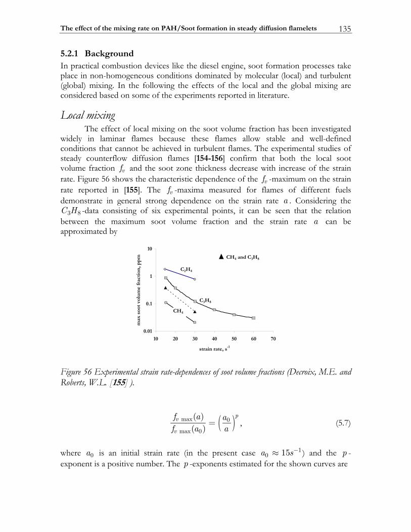
The effect of the mixing rate on PAH/Soot formation in steady diffusion flamelets 135
5.2.1 Background In practical combustion devices like the diesel engine, soot formation processes take place in non-homogeneous conditions dominated by molecular (local) and turbulent (global) mixing. In the following the effects of the local and the global mixing are considered based on some of the experiments reported in literature.
Local mixing The effect of local mixing on the soot volume fraction has been investigated widely in laminar flames because these flames allow stable and well-defined conditions that cannot be achieved in turbulent flames. The experimental studies of steady counterflow diffusion flames [154-156] confirm that both the local soot volume fraction vf and the soot zone thickness decrease with increase of the strain rate. Figure 56 shows the characteristic dependence of the vf -maximum on the strain rate reported in [155]. The vf -maxima measured for flames of different fuels demonstrate in general strong dependence on the strain rate a . Considering the
3 8C H -data consisting of six experimental points, it can be seen that the relation between the maximum soot volume fraction and the strain rate a can be approximated by
10.0
1.0
1
01
07060504030201
s,etarniarts 1-
max
soot
vol
um
e fr
acti
on, p
pm
C2H4
C3H8
HC 4
HC 4 Cdna 3H8
Figure 56 Experimental strain rate-dependences of soot volume fractions (Decroix, M.E. and Roberts, W.L. [155] ).
( )max 0
max 0
( )( )
pv
v
f a af a a
= , (5.7)
where 0a is an initial strain rate (in the present case 1
0 15a s−≈ ) and the p -exponent is a positive number. The p -exponents estimated for the shown curves are
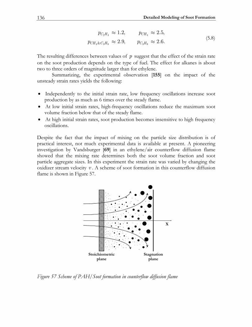
Detailed Modeling of Soot Formation 136
2 4 4
4 3 8 3 8&
1.2, 2.5,
2.9, 2.6.C H CH
CH C H C H
p p
p p
≈ ≈
≈ ≈ (5.8)
The resulting differences between values of p suggest that the effect of the strain rate on the soot production depends on the type of fuel. The effect for alkanes is about two to three orders of magnitude larger than for ethylene. Summarizing, the experimental observation [155] on the impact of the unsteady strain rates yields the following: • Independently to the initial strain rate, low frequency oscillations increase soot
production by as much as 6 times over the steady flame. • At low initial strain rates, high-frequency oscillations reduce the maximum soot
volume fraction below that of the steady flame. • At high initial strain rates, soot production becomes insensitive to high frequency
oscillations. Despite the fact that the impact of mixing on the particle size distribution is of practical interest, not much experimental data is available at present. A pioneering investigation by Vandsburger [69] in an ethylene/air counterflow diffusion flame showed that the mixing rate determines both the soot volume fraction and soot particle aggregate sizes. In this experiment the strain rate was varied by changing the oxidizer stream velocity v . A scheme of soot formation in this counterflow diffusion flame is shown in Figure 57.
X
cirtemoihciotSenalp
noitangatSenalp
Figure 57 Scheme of PAH/Soot formation in counterflow diffusion flame
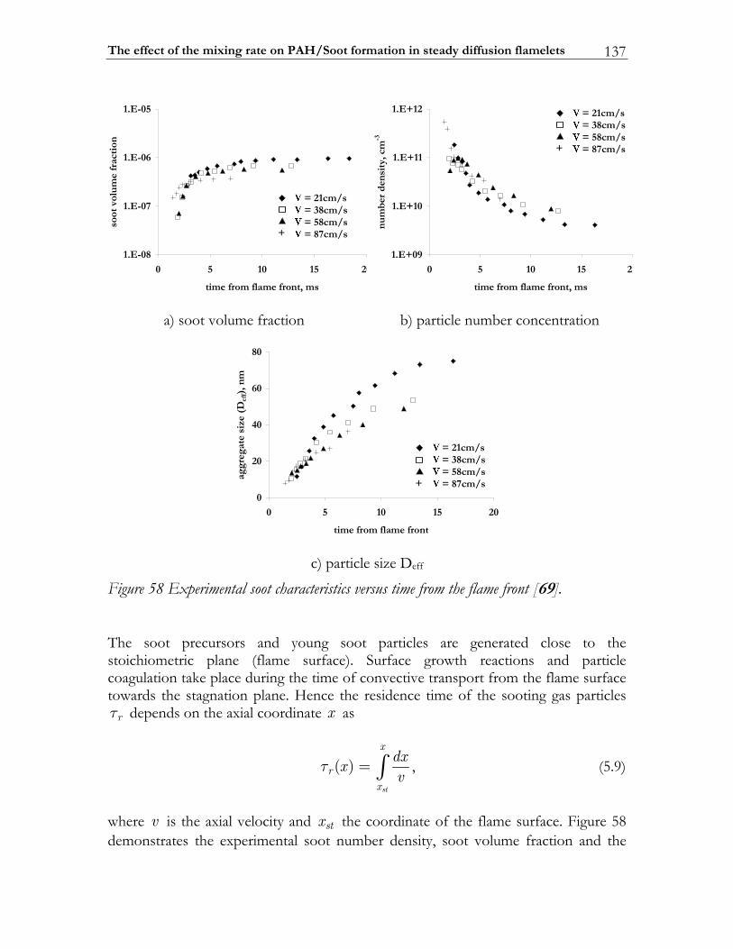
The effect of the mixing rate on PAH/Soot formation in steady diffusion flamelets 137
80-E.1
70-E.1
60-E.1
50-E.1
02510150
sm,tnorfemalfmorfemit
soot
volu
me
frac
tion
+
s/mc12=s/mc83=s/mc85=s/mc78=
90+E.1
01+E.1
11+E.1
21+E.1
02510150
sm,tnorfemalfmorfemit
nu
mb
erd
ensi
ty,c
m-3
+
s/mc12=s/mc83=s/mc85=s/mc78=
a) soot volume fraction b) particle number concentration
0
02
04
06
08
02510150
tnorfemalfmorfemit
aggr
egat
esi
ze(D
eff)
,nm
+
s/mc12=s/mc83=s/mc85=s/mc78=
c) particle size Deff
Figure 58 Experimental soot characteristics versus time from the flame front [69].
The soot precursors and young soot particles are generated close to the stoichiometric plane (flame surface). Surface growth reactions and particle coagulation take place during the time of convective transport from the flame surface towards the stagnation plane. Hence the residence time of the sooting gas particles rτ depends on the axial coordinate x as
( )st
x
rx
dxxv
τ = ∫ , (5.9)
where v is the axial velocity and stx the coordinate of the flame surface. Figure 58 demonstrates the experimental soot number density, soot volume fraction and the
Detailed Modeling of Soot Formation 138
corresponding particle aggregate size versus the residence time rτ as it was reported in [69]. The soot volume fraction (Figure 58a) increases as one proceeds from the zone where soot particles first appear close to the stagnation point. The profiles show the typical strong initial increase in the soot volume fraction due to surface growth reactions and a leveling off close to the stagnation point. Particle number density profiles are shown in Figure 58b. The number density decreases from the flame zone to the stagnation point due to coagulation. With increasing oxidizer velocity the final number of particles increases slightly due to the reduced time for coagulation. The measured particle sizes range from around 10nm close to the flame front up to around 70nm near the stagnation plane. Figure 58c shows that the maximum particle size decreases with increasing the oxidizer approach velocity (increasing strain rate). The particle size at each location is a function of both the coagulation and surface growth until that point. The authors from [69] note that the number of young particles is not affected in the examined velocity gradients. The observed trends can be summarized as: • The soot loading decreases with increasing strain rate (oxidizer stream velocity). • The maximum particle size decreases with increasing strain rate. • The number of young soot particles is not affected in the examined strain rates
range.
Global mixing The effect of mixing is usually quantified by the local flame strain rate. In turbulent sooting flames, however, measurement of strain rate is predominantly limited to global, or characteristic, rather than local values due to the difficulties of undertaking such measurements in unsteady flames. Investigations performed by Kent and Bastin [157] in a simple turbulent jet flame showed that the average soot volume fraction decreases with increasing characteristic strain rate. In addition, the rate of this decrease is higher at high mixing rates than at low mixing rates. Later measurements by Qamar [67] reveal that there is an inverse relationship between global mixing rates and the total volume of soot. His observations are broadly consistent with previous measurements of the effect of local strain rate on soot in laminar flames and with the deduction of Bockhorn et al. [158] that soot formation and oxidation occur in laminar-like flame filaments. From the modeling point of view, the difference between effects of global and local mixing is terminological only if the combustion process occurs in the so-called flamelet regime. According to the flamelet concept [159, 160], the turbulent flame surface can be viewed as an ensemble of locally one-dimensional laminar flames. In this case, the detailed modeling of soot formation in one-dimensional laminar flame structures under different strain rates covers both subjects of local and global mixing.
The effect of the mixing rate on PAH/Soot formation in steady diffusion flamelets 139
5.2.2 The applied sectional model
Discrete sectional representation In order to model soot formation the discrete sectional technique is adopted in this thesis. In this method, the particle ensemble is divided into classes (BINs). Each BIN of the discrete distribution represents a class of particles characterized with nearly the same properties such as mass and C/H-ratio. Within the sectional approach, the steady 1D-spatial distribution of the ths class of particles is described with the same equations as the gas phase compounds:
( ) ss s s s
d dYYV v mdx dx
ρ ρ ω+ = . (5.10)
Here the left hand size is the sum of diffusion and convection terms respectively, and the source term on the right hand side represents mass production rate. The BINs diffusion fluxes are modeled with the Hirschfelder–Curtiss (or zero-order) approximation [92] that is identical to the gas compounds. The corresponding binary diffusion coefficients are determined based on the Lennard-Jones potential describing molecular interactions. The chemical model for determining reaction source terms in the species-mass conservation equations is described in the following.
Chemical model The reaction source terms of both the gas phase and the particulate matter have been computed with a detailed kinetic model describing formation and consumption of PAH and soot in fuel-rich hydrocarbon combustion [103]. In this model, using a sectional approach described in some details in [103], large PAH and carbonaceous particles with diameters of up to 70nm are defined as classes (BINs) covering prescribed mass ranges. Numbers of carbon and hydrogen atoms corresponding to their average masses are assigned to each BIN, accounting for a decrease in H/C ratios with increasing particle size. The model has been applied to several premixed flames of benzene/oxygen/argon [103] and recently to ethylbenzene and ethyl-alcohol flames in [161]. So far no tests have been performed for non-premixed flames. Formation of PAH and soot is described in the form of usual gas phase kinetics with conservation of mass and elemental balances of all individual reactions. The molecules with number of carbon and hydrogen atoms sufficiently large to correspond to soot particles of increasing size are handled with the TROT-interpreter (see chapter 2). The reaction mechanism consists of 295 species, 1102 conventional gas phase reactions and 5552 reactions describing particle growth. This mechanism, including the corresponding thermodynamic and transport property data, is available on-line [66]. With respect to the aerosol species (particulate matter), forward and reverse reactions are independently described or reverse reactions are neglected. The number of species of similar mass and the number of structural isomers increases
Detailed Modeling of Soot Formation 140
quickly with molecular mass. Therefore, classes (BINs) of very large PAH and of particles covering certain mass ranges have been defined. The average molecular mass and the number of carbon and hydrogen atoms are assigned to each BIN. The resulting characteristics of the BINs [103] are given in Table 10.
Table 10. Definition of classes of molecules (BINs) describing large PAH/Soot particles
BIN Mass (amu) x yC H ( )d nm /H C 1 201–400 C24H12 0.85 0.500 2 401–800 C48H24 1.07 0.500 3 801–1600 C96H48 1.34 0.500 4 1601–3200 C193H84 1.69 0.435 5 3201–6400 C388H144 2.13 0.371 6 6401–12,800 C778H264 2.68 0.339 7 12,801–25,600 C1560H480 3.37 0.308 8 25,601–51,200 C3124H912 4.24 0.292 9 51,201–102,400 C6256H1728 5.35 0.276 10 102,401–204,800 C12528H3264 6.73 0.261 11 204,801–409,600 C25088H6144 8.48 0.245 12 409,601–819,200 C50240H11520 10.69 0.229 13 819,201–1,638,400 C100608H21504 13.46 0.214 14 1,638,401–3,276,800 C201472H39936 16.96 0.198 15 3,276,801–6,553,600 C403456H73728 21.36 0.183 16 6,553,601–13,107,200 C807936H135168 26.91 0.167 17 13,107,201–26,214,400 C1617920H245760 33.91 0.152 18 26,214,401–52,428,800 C3239936H442368 42.72 0.137 19 52,428,801–104,857,600 C6483968H835584 53.83 0.129 20 104,857,601–209,715,200 C12972032H1622016 67.82 0.125
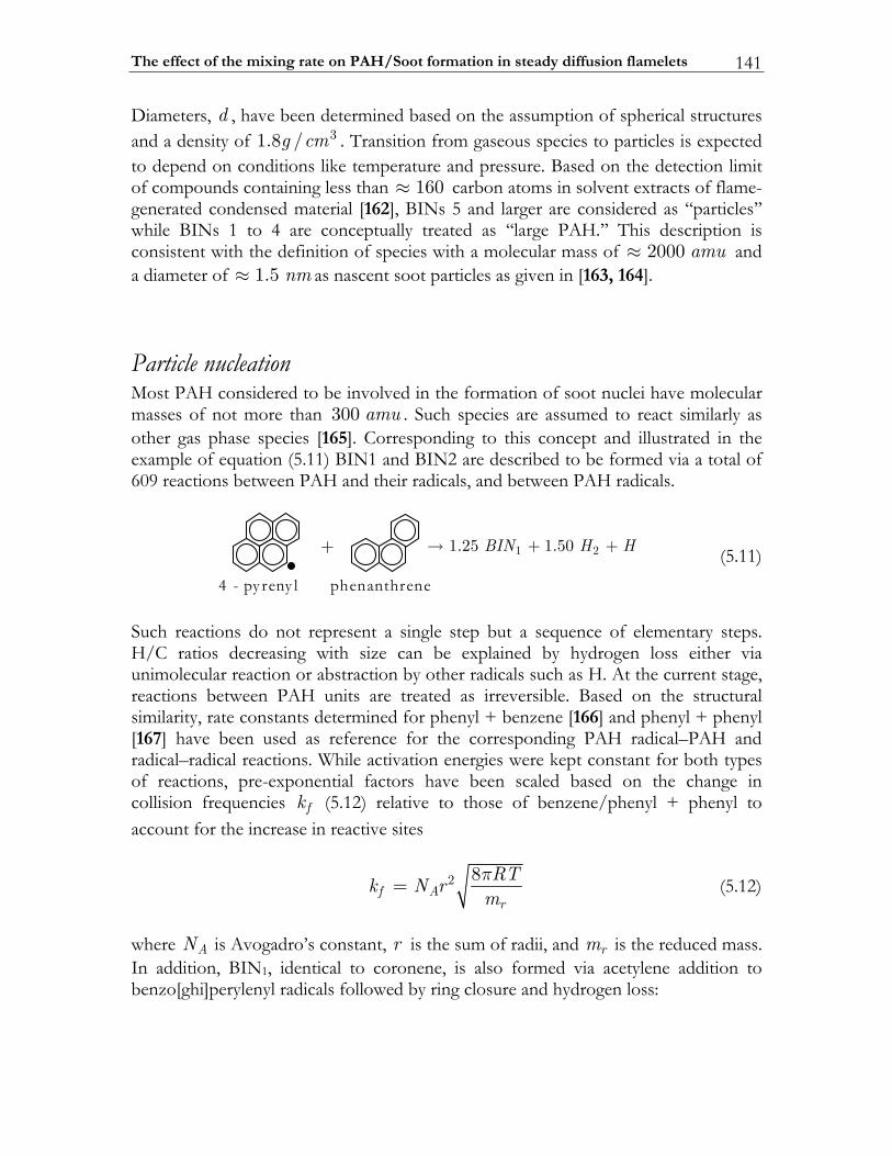
The effect of the mixing rate on PAH/Soot formation in steady diffusion flamelets 141
Diameters, d , have been determined based on the assumption of spherical structures and a density of 31.8 /g cm . Transition from gaseous species to particles is expected to depend on conditions like temperature and pressure. Based on the detection limit of compounds containing less than 160≈ carbon atoms in solvent extracts of flame-generated condensed material [162], BINs 5 and larger are considered as ‘‘particles’’ while BINs 1 to 4 are conceptually treated as ‘‘large PAH.’’ This description is consistent with the definition of species with a molecular mass of 2000 amu≈ and a diameter of 1.5 nm≈ as nascent soot particles as given in [163, 164].
Particle nucleation Most PAH considered to be involved in the formation of soot nuclei have molecular masses of not more than 300 amu . Such species are assumed to react similarly as other gas phase species [165]. Corresponding to this concept and illustrated in the example of equation (5.11) BIN1 and BIN2 are described to be formed via a total of 609 reactions between PAH and their radicals, and between PAH radicals.
1 21.25 1.50BIN H H→ + +
4 - py reny l phenanthrene
+
(5.11)
Such reactions do not represent a single step but a sequence of elementary steps. H/C ratios decreasing with size can be explained by hydrogen loss either via unimolecular reaction or abstraction by other radicals such as H. At the current stage, reactions between PAH units are treated as irreversible. Based on the structural similarity, rate constants determined for phenyl + benzene [166] and phenyl + phenyl [167] have been used as reference for the corresponding PAH radical–PAH and radical–radical reactions. While activation energies were kept constant for both types of reactions, pre-exponential factors have been scaled based on the change in collision frequencies fk (5.12) relative to those of benzene/phenyl + phenyl to account for the increase in reactive sites
2 8f A
r
RTk N rmπ= (5.12)
where AN is Avogadro’s constant, r is the sum of radii, and rm is the reduced mass. In addition, BIN1, identical to coronene, is also formed via acetylene addition to benzo[ghi]perylenyl radicals followed by ring closure and hydrogen loss:
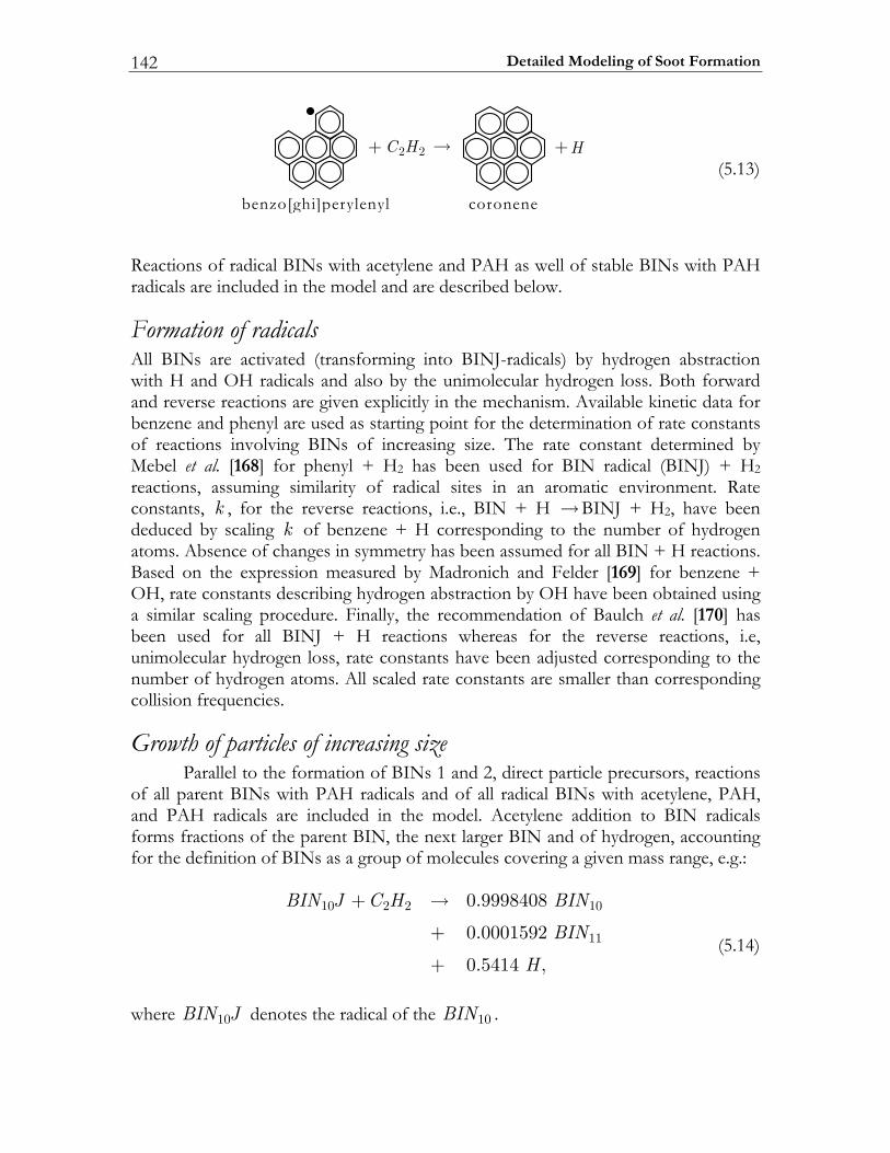
Detailed Modeling of Soot Formation 142
+ 2 2C H → +H
benzo[ghi]perylenyl coronene
(5.13)
Reactions of radical BINs with acetylene and PAH as well of stable BINs with PAH radicals are included in the model and are described below.
Formation of radicals All BINs are activated (transforming into BINJ-radicals) by hydrogen abstraction with H and OH radicals and also by the unimolecular hydrogen loss. Both forward and reverse reactions are given explicitly in the mechanism. Available kinetic data for benzene and phenyl are used as starting point for the determination of rate constants of reactions involving BINs of increasing size. The rate constant determined by Mebel et al. [168] for phenyl + H2 has been used for BIN radical (BINJ) + H2 reactions, assuming similarity of radical sites in an aromatic environment. Rate constants, k , for the reverse reactions, i.e., BIN + H →BINJ + H2, have been deduced by scaling k of benzene + H corresponding to the number of hydrogen atoms. Absence of changes in symmetry has been assumed for all BIN + H reactions. Based on the expression measured by Madronich and Felder [169] for benzene + OH, rate constants describing hydrogen abstraction by OH have been obtained using a similar scaling procedure. Finally, the recommendation of Baulch et al. [170] has been used for all BINJ + H reactions whereas for the reverse reactions, i.e, unimolecular hydrogen loss, rate constants have been adjusted corresponding to the number of hydrogen atoms. All scaled rate constants are smaller than corresponding collision frequencies.
Growth of particles of increasing size Parallel to the formation of BINs 1 and 2, direct particle precursors, reactions of all parent BINs with PAH radicals and of all radical BINs with acetylene, PAH, and PAH radicals are included in the model. Acetylene addition to BIN radicals forms fractions of the parent BIN, the next larger BIN and of hydrogen, accounting for the definition of BINs as a group of molecules covering a given mass range, e.g.:
10 2 2 10
11
0.9998408
0.0001592
0.5414 ,
BIN J C H BIN
BIN
H
+ →
+
+ (5.14)
where 10BIN J denotes the radical of the 10BIN .
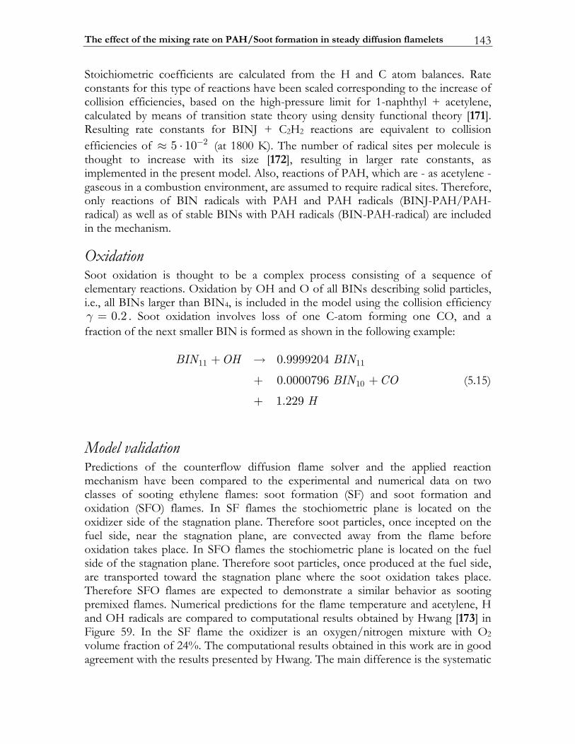
The effect of the mixing rate on PAH/Soot formation in steady diffusion flamelets 143
Stoichiometric coefficients are calculated from the H and C atom balances. Rate constants for this type of reactions have been scaled corresponding to the increase of collision efficiencies, based on the high-pressure limit for 1-naphthyl + acetylene, calculated by means of transition state theory using density functional theory [171]. Resulting rate constants for BINJ + C2H2 reactions are equivalent to collision efficiencies of 25 10−≈ ⋅ (at 1800 K). The number of radical sites per molecule is thought to increase with its size [172], resulting in larger rate constants, as implemented in the present model. Also, reactions of PAH, which are - as acetylene - gaseous in a combustion environment, are assumed to require radical sites. Therefore, only reactions of BIN radicals with PAH and PAH radicals (BINJ-PAH/PAH-radical) as well as of stable BINs with PAH radicals (BIN-PAH-radical) are included in the mechanism.
Oxidation Soot oxidation is thought to be a complex process consisting of a sequence of elementary reactions. Oxidation by OH and O of all BINs describing solid particles, i.e., all BINs larger than BIN4, is included in the model using the collision efficiency
0.2γ = . Soot oxidation involves loss of one C-atom forming one CO, and a fraction of the next smaller BIN is formed as shown in the following example:
11 11
10
0.9999204
0.0000796
1.229
BIN OH BIN
BIN CO
H
+ →
+ +
+
(5.15)
Model validation Predictions of the counterflow diffusion flame solver and the applied reaction mechanism have been compared to the experimental and numerical data on two classes of sooting ethylene flames: soot formation (SF) and soot formation and oxidation (SFO) flames. In SF flames the stochiometric plane is located on the oxidizer side of the stagnation plane. Therefore soot particles, once incepted on the fuel side, near the stagnation plane, are convected away from the flame before oxidation takes place. In SFO flames the stochiometric plane is located on the fuel side of the stagnation plane. Therefore soot particles, once produced at the fuel side, are transported toward the stagnation plane where the soot oxidation takes place. Therefore SFO flames are expected to demonstrate a similar behavior as sooting premixed flames. Numerical predictions for the flame temperature and acetylene, H and OH radicals are compared to computational results obtained by Hwang [173] in Figure 59. In the SF flame the oxidizer is an oxygen/nitrogen mixture with O2 volume fraction of 24%. The computational results obtained in this work are in good agreement with the results presented by Hwang. The main difference is the systematic
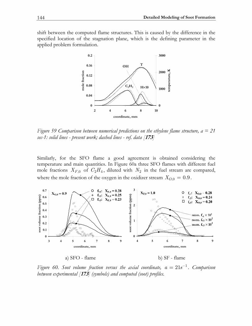
Detailed Modeling of Soot Formation 144
shift between the computed flame structures. This is caused by the difference in the specified location of the stagnation plane, which is the defining parameter in the applied problem formulation.
0
40.0
80.0
21.0
61.0
2.0
018642
mm,etanidrooc
mol
efr
acti
on
0
0001
0002
0003
tem
per
atu
re,K
T
C2H2 H× 01
HO
Figure 59 Comparison between numerical predictions on the ethylene flame structure, a = 21 sec-1: solid lines - present work; dashed lines - ref. data [173] Similarly, for the SFO flame a good agreement is obtained considering the temperature and main quantities. In Figure 60a three SFO flames with different fuel mole fractions ,0FX of 2 4C H , diluted with 2N in the fuel stream are compared, where the mole fraction of the oxygen in the oxidizer stream ,0 0.9OX = .
a) SFO - flame b) SF - flame
Figure 60. Soot volume fraction versus the axial coordinate, 121a s−= . Comparison between experimental [173] (symbols) and computed (soot) profiles.
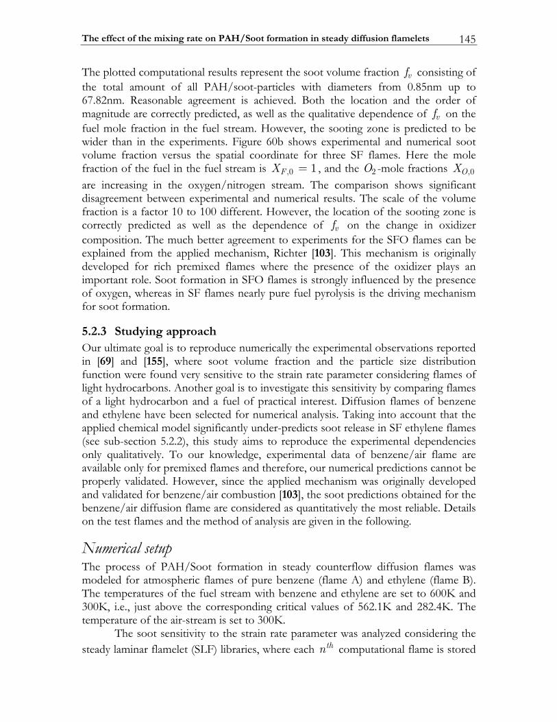
The effect of the mixing rate on PAH/Soot formation in steady diffusion flamelets 145
The plotted computational results represent the soot volume fraction vf consisting of the total amount of all PAH/soot-particles with diameters from 0.85nm up to 67.82nm. Reasonable agreement is achieved. Both the location and the order of magnitude are correctly predicted, as well as the qualitative dependence of vf on the fuel mole fraction in the fuel stream. However, the sooting zone is predicted to be wider than in the experiments. Figure 60b shows experimental and numerical soot volume fraction versus the spatial coordinate for three SF flames. Here the mole fraction of the fuel in the fuel stream is ,0 1FX = , and the 2O -mole fractions ,0OX are increasing in the oxygen/nitrogen stream. The comparison shows significant disagreement between experimental and numerical results. The scale of the volume fraction is a factor 10 to 100 different. However, the location of the sooting zone is correctly predicted as well as the dependence of vf on the change in oxidizer composition. The much better agreement to experiments for the SFO flames can be explained from the applied mechanism, Richter [103]. This mechanism is originally developed for rich premixed flames where the presence of the oxidizer plays an important role. Soot formation in SFO flames is strongly influenced by the presence of oxygen, whereas in SF flames nearly pure fuel pyrolysis is the driving mechanism for soot formation.
5.2.3 Studying approach Our ultimate goal is to reproduce numerically the experimental observations reported in [69] and [155], where soot volume fraction and the particle size distribution function were found very sensitive to the strain rate parameter considering flames of light hydrocarbons. Another goal is to investigate this sensitivity by comparing flames of a light hydrocarbon and a fuel of practical interest. Diffusion flames of benzene and ethylene have been selected for numerical analysis. Taking into account that the applied chemical model significantly under-predicts soot release in SF ethylene flames (see sub-section 5.2.2), this study aims to reproduce the experimental dependencies only qualitatively. To our knowledge, experimental data of benzene/air flame are available only for premixed flames and therefore, our numerical predictions cannot be properly validated. However, since the applied mechanism was originally developed and validated for benzene/air combustion [103], the soot predictions obtained for the benzene/air diffusion flame are considered as quantitatively the most reliable. Details on the test flames and the method of analysis are given in the following.
Numerical setup The process of PAH/Soot formation in steady counterflow diffusion flames was modeled for atmospheric flames of pure benzene (flame A) and ethylene (flame B). The temperatures of the fuel stream with benzene and ethylene are set to 600K and 300K, i.e., just above the corresponding critical values of 562.1K and 282.4K. The temperature of the air-stream is set to 300K. The soot sensitivity to the strain rate parameter was analyzed considering the steady laminar flamelet (SLF) libraries, where each thn computational flame is stored
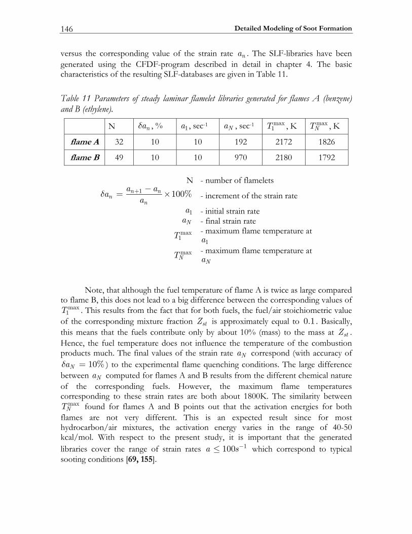
Detailed Modeling of Soot Formation 146
versus the corresponding value of the strain rate na . The SLF-libraries have been generated using the CFDF-program described in detail in chapter 4. The basic characteristics of the resulting SLF-databases are given in Table 11.
Table 11 Parameters of steady laminar flamelet libraries generated for flames A (benzene) and B (ethylene).
N naδ , % 1a , sec-1 Na , sec-1 max1T , K max
NT , K
flame A 32 10 10 192 2172 1826
flame B 49 10 10 970 2180 1792
N - number of flamelets 1 100%n n
nn
a aaa
δ + −= × - increment of the strain rate
1a - initial strain rate Na - final strain rate
max1T
- maximum flame temperature at 1a
maxNT
- maximum flame temperature at Na
Note, that although the fuel temperature of flame A is twice as large compared to flame B, this does not lead to a big difference between the corresponding values of
max1T . This results from the fact that for both fuels, the fuel/air stoichiometric value
of the corresponding mixture fraction stZ is approximately equal to 0.1 . Basically, this means that the fuels contribute only by about 10% (mass) to the mass at stZ . Hence, the fuel temperature does not influence the temperature of the combustion products much. The final values of the strain rate Na correspond (with accuracy of
10%Naδ = ) to the experimental flame quenching conditions. The large difference between Na computed for flames A and B results from the different chemical nature of the corresponding fuels. However, the maximum flame temperatures corresponding to these strain rates are both about 1800K. The similarity between
maxNT found for flames A and B points out that the activation energies for both
flames are not very different. This is an expected result since for most hydrocarbon/air mixtures, the activation energy varies in the range of 40-50 kcal/mol. With respect to the present study, it is important that the generated libraries cover the range of strain rates 1100a s−≤ which correspond to typical sooting conditions [69, 155].
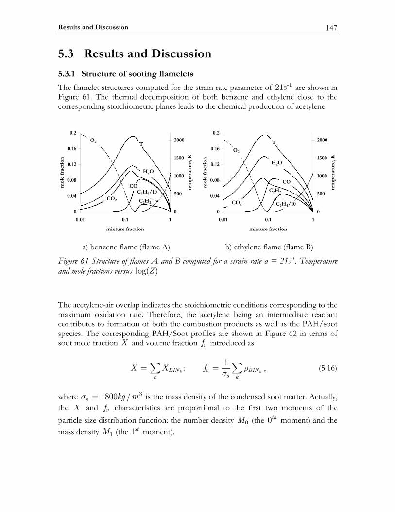
Results and Discussion 147
5.3 Results and Discussion
5.3.1 Structure of sooting flamelets
The flamelet structures computed for the strain rate parameter of -121s are shown in Figure 61. The thermal decomposition of both benzene and ethylene close to the corresponding stoichiometric planes leads to the chemical production of acetylene.
0
40.0
80.0
21.0
61.0
2.0
11.010.0
noitcarferutxim
mol
e fr
acti
on
0
005
0001
0051
0002
tem
per
atu
re, K
O2 T
H2O
OC
C2H2OC 2
C6H6 01/
0
40.0
80.0
21.0
61.0
2.0
11.010.0
noitcarferutxim
mol
e fr
acti
on0
005
0001
0051
0002
tem
per
atu
re, K
O2
T
H2O
OC
C2H4 01/
C2H2
OC 2
a) benzene flame (flame A) b) ethylene flame (flame B)
Figure 61 Structure of flames A and B computed for a strain rate a = 21s-1. Temperature and mole fractions versus log( )Z
The acetylene-air overlap indicates the stoichiometric conditions corresponding to the maximum oxidation rate. Therefore, the acetylene being an intermediate reactant contributes to formation of both the combustion products as well as the PAH/soot species. The corresponding PAH/Soot profiles are shown in Figure 62 in terms of soot mole fraction X and volume fraction vf introduced as
1;k kBIN v BIN
sk kX X f ρσ= =∑ ∑ , (5.16)
where 31800 /s kg mσ = is the mass density of the condensed soot matter. Actually, the X and vf characteristics are proportional to the first two moments of the particle size distribution function: the number density 0M (the 0th moment) and the mass density 1M (the 1st moment).
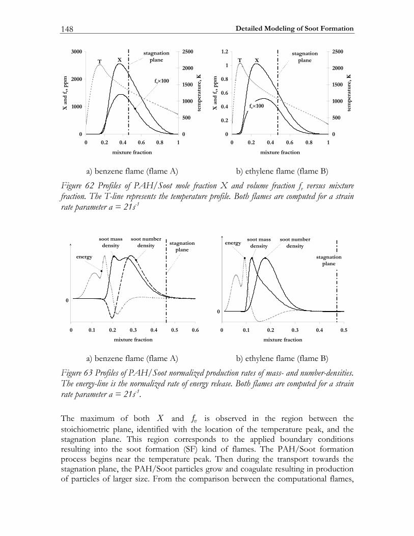
Detailed Modeling of Soot Formation 148
0
0001
0002
0003
18.06.04.02.00
noitcarferutxim
X a
nd
fv,
ppm
0
005
0001
0051
0002
0052
tem
per
atu
re, K
noitangatsenalpT X
fv× 001
0
2.0
4.0
6.0
8.0
1
2.1
18.06.04.02.00
noitcarferutxim
X a
nd
fv,
ppm
0
005
0001
0051
0002
0052
tem
per
atu
re, K
noitangatsenalpXT
fv× 001
a) benzene flame (flame A) b) ethylene flame (flame B)
Figure 62 Profiles of PAH/Soot mole fraction X and volume fraction fv versus mixture fraction. The T-line represents the temperature profile. Both flames are computed for a strain rate parameter a = 21s-1
6.05.04.03.02.01.00
noitcarferutxim
0
ygrene
ssamtoosytisned noitangats
enalp
rebmuntoosytisned
5.04.03.02.01.00
noitcarferutxim
0
ygrenessamtoos
ytisned
noitangatsenalp
rebmuntoosytisned
a) benzene flame (flame A) b) ethylene flame (flame B)
Figure 63 Profiles of PAH/Soot normalized production rates of mass- and number-densities. The energy-line is the normalized rate of energy release. Both flames are computed for a strain rate parameter a = 21s-1. The maximum of both X and vf is observed in the region between the stoichiometric plane, identified with the location of the temperature peak, and the stagnation plane. This region corresponds to the applied boundary conditions resulting into the soot formation (SF) kind of flames. The PAH/Soot formation process begins near the temperature peak. Then during the transport towards the stagnation plane, the PAH/Soot particles grow and coagulate resulting in production of particles of larger size. From the comparison between the computational flames,
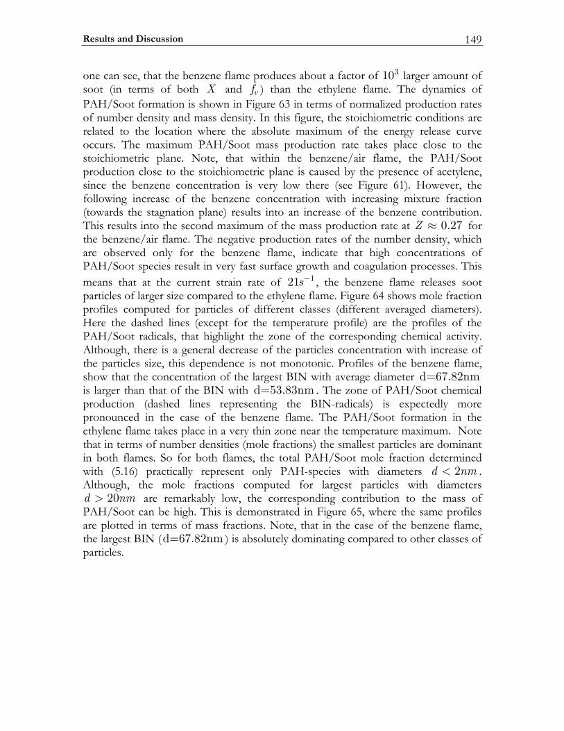
Results and Discussion 149
one can see, that the benzene flame produces about a factor of 310 larger amount of soot (in terms of both X and vf ) than the ethylene flame. The dynamics of PAH/Soot formation is shown in Figure 63 in terms of normalized production rates of number density and mass density. In this figure, the stoichiometric conditions are related to the location where the absolute maximum of the energy release curve occurs. The maximum PAH/Soot mass production rate takes place close to the stoichiometric plane. Note, that within the benzene/air flame, the PAH/Soot production close to the stoichiometric plane is caused by the presence of acetylene, since the benzene concentration is very low there (see Figure 61). However, the following increase of the benzene concentration with increasing mixture fraction (towards the stagnation plane) results into an increase of the benzene contribution. This results into the second maximum of the mass production rate at 0.27Z ≈ for the benzene/air flame. The negative production rates of the number density, which are observed only for the benzene flame, indicate that high concentrations of PAH/Soot species result in very fast surface growth and coagulation processes. This means that at the current strain rate of 121s− , the benzene flame releases soot particles of larger size compared to the ethylene flame. Figure 64 shows mole fraction profiles computed for particles of different classes (different averaged diameters). Here the dashed lines (except for the temperature profile) are the profiles of the PAH/Soot radicals, that highlight the zone of the corresponding chemical activity. Although, there is a general decrease of the particles concentration with increase of the particles size, this dependence is not monotonic. Profiles of the benzene flame, show that the concentration of the largest BIN with average diameter d=67.82nm is larger than that of the BIN with d=53.83nm . The zone of PAH/Soot chemical production (dashed lines representing the BIN-radicals) is expectedly more pronounced in the case of the benzene flame. The PAH/Soot formation in the ethylene flame takes place in a very thin zone near the temperature maximum. Note that in terms of number densities (mole fractions) the smallest particles are dominant in both flames. So for both flames, the total PAH/Soot mole fraction determined with (5.16) practically represent only PAH-species with diameters 2d nm< . Although, the mole fractions computed for largest particles with diameters
20d nm> are remarkably low, the corresponding contribution to the mass of PAH/Soot can be high. This is demonstrated in Figure 65, where the same profiles are plotted in terms of mass fractions. Note, that in the case of the benzene flame, the largest BIN (d=67.82nm ) is absolutely dominating compared to other classes of particles.
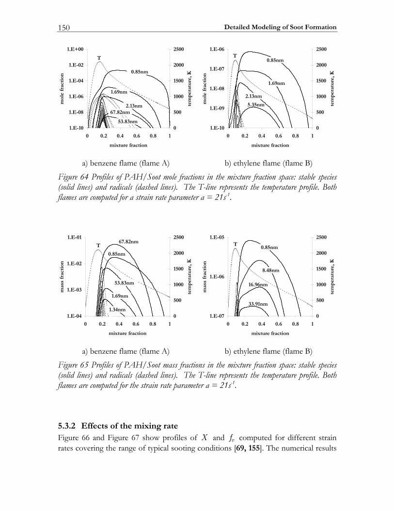
Detailed Modeling of Soot Formation 150
01-E.1
80-E.1
60-E.1
40-E.1
20-E.1
00+E.1
18.06.04.02.00
noitcarferutxim
mol
e fr
acti
on
0
005
0001
0051
0002
0052
tem
per
atu
re, K
T
mn58.0
mn96.1
mn31.2mn28.76
mn38.3501-E.1
90-E.1
80-E.1
70-E.1
60-E.1
18.06.04.02.00
noitcarferutxim
mol
e fr
acti
on
0
005
0001
0051
0002
0052
tem
per
atu
re, K
Tmn58.0
mn96.1
mn31.2
mn53.5
a) benzene flame (flame A) b) ethylene flame (flame B)
Figure 64 Profiles of PAH/Soot mole fractions in the mixture fraction space: stable species (solid lines) and radicals (dashed lines). The T-line represents the temperature profile. Both flames are computed for a strain rate parameter a = 21s-1.
40-E.1
30-E.1
20-E.1
10-E.1
18.06.04.02.00
noitcarferutxim
mas
s fr
acti
on
0
005
0001
0051
0002
0052
tem
per
atu
re, K
T
mn58.0
mn96.1
mn43.1
mn28.76
mn38.35
70-E.1
60-E.1
50-E.1
18.06.04.02.00
noitcarferutxim
mas
s fr
acti
on
0
005
0001
0051
0002
0052
tem
per
atu
re, K
Tmn58.0
mn84.8
mn69.61
mn19.33
a) benzene flame (flame A) b) ethylene flame (flame B)
Figure 65 Profiles of PAH/Soot mass fractions in the mixture fraction space: stable species (solid lines) and radicals (dashed lines). The T-line represents the temperature profile. Both flames are computed for the strain rate parameter a = 21s-1.
5.3.2 Effects of the mixing rate Figure 66 and Figure 67 show profiles of X and vf computed for different strain rates covering the range of typical sooting conditions [69, 155]. The numerical results
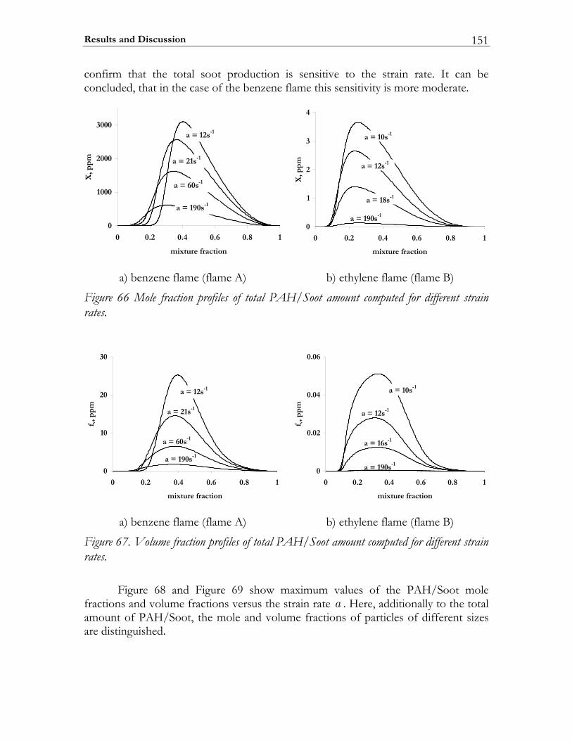
Results and Discussion 151
confirm that the total soot production is sensitive to the strain rate. It can be concluded, that in the case of the benzene flame this sensitivity is more moderate.
0
0001
0002
0003
18.06.04.02.00
noitcarferutxim
X, p
pm
s21=a 1-
s12=a 1-
s06=a 1-
s091=a 1-
0
1
2
3
4
18.06.04.02.00
noitcarferutxim
X, p
pm
s01=a 1-
s21=a 1-
s81=a 1-
s091=a 1-
a) benzene flame (flame A) b) ethylene flame (flame B)
Figure 66 Mole fraction profiles of total PAH/Soot amount computed for different strain rates.
0
01
02
03
18.06.04.02.00
noitcarferutxim
f v,p
pm
s21=a 1-
s12=a 1-
s06=a 1-
s091=a 1-
0
20.0
40.0
60.0
18.06.04.02.00
noitcarferutxim
f v,p
pm
s01=a 1-
s21=a 1-
s61=a 1-
s091=a 1-
a) benzene flame (flame A) b) ethylene flame (flame B)
Figure 67. Volume fraction profiles of total PAH/Soot amount computed for different strain rates. Figure 68 and Figure 69 show maximum values of the PAH/Soot mole fractions and volume fractions versus the strain rate a . Here, additionally to the total amount of PAH/Soot, the mole and volume fractions of particles of different sizes are distinguished.
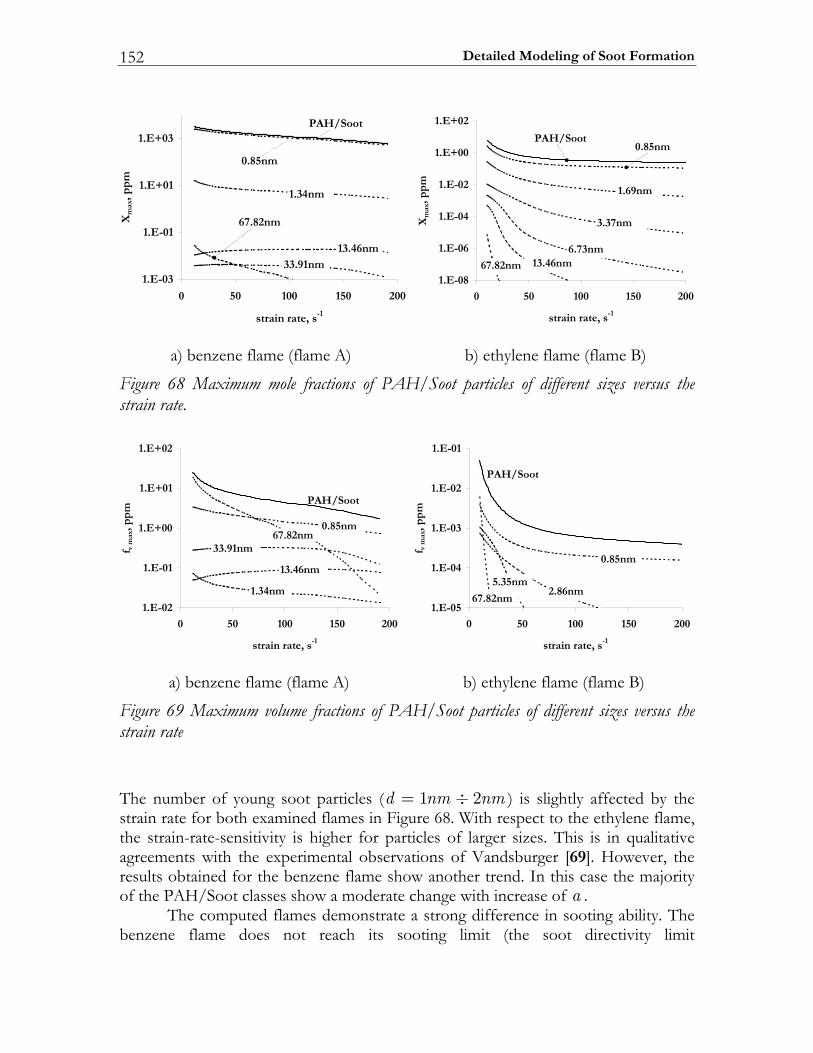
Detailed Modeling of Soot Formation 152
30-E.1
10-E.1
10+E.1
30+E.1
002051001050
s,etarniarts 1-
Xm
ax,p
pm
tooS/HAP
mn58.0
mn19.33mn64.31
mn43.1
mn28.76
80-E.1
60-E.1
40-E.1
20-E.1
00+E.1
20+E.1
002051001050
s,etarniarts 1-
Xm
ax,p
pm
tooS/HAP
mn96.1
mn73.3
mn37.6mn64.31mn28.76
mn58.0
a) benzene flame (flame A) b) ethylene flame (flame B)
Figure 68 Maximum mole fractions of PAH/Soot particles of different sizes versus the strain rate.
20-E.1
10-E.1
00+E.1
10+E.1
20+E.1
002051001050
s,etarniarts 1-
f v m
ax,p
pm
tooS/HAP
mn58.0mn28.76
mn19.33
mn64.31
mn43.1
50-E.1
40-E.1
30-E.1
20-E.1
10-E.1
002051001050
s,etarniarts 1-
f v m
ax,p
pm
tooS/HAP
mn58.0
mn68.2mn53.5
mn28.76
a) benzene flame (flame A) b) ethylene flame (flame B)
Figure 69 Maximum volume fractions of PAH/Soot particles of different sizes versus the strain rate The number of young soot particles ( 1 2d nm nm= ÷ ) is slightly affected by the strain rate for both examined flames in Figure 68. With respect to the ethylene flame, the strain-rate-sensitivity is higher for particles of larger sizes. This is in qualitative agreements with the experimental observations of Vandsburger [69]. However, the results obtained for the benzene flame show another trend. In this case the majority of the PAH/Soot classes show a moderate change with increase of a . The computed flames demonstrate a strong difference in sooting ability. The benzene flame does not reach its sooting limit (the soot directivity limit
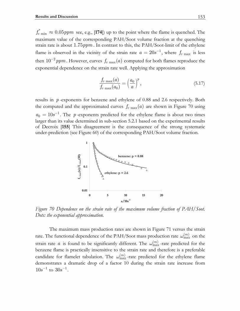
Results and Discussion 153
*min 0.05vf ppm≈ see, e.g., [174]) up to the point where the flame is quenched. The
maximum value of the corresponding PAH/Soot volume fraction at the quenching strain rate is about 1.75ppm . In contrast to this, the PAH/Soot-limit of the ethylene flame is observed in the vicinity of the strain rate 120a s−= , where maxvf is less then 210 ppm− . However, curves max( )vf a computed for both flames reproduce the exponential dependence on the strain rate well. Applying the approximation
( )max 0
max 0
( )( )
pv
v
f a af a a
= , (5.17)
results in p -exponents for benzene and ethylene of 0.88 and 2.6 respectively. Both the computed and the approximated curves max( )vf a are shown in Figure 70 using
10 10a s−= . The p -exponents predicted for the ethylene flame is about two times
larger than its value determined in sub-section 5.2.1 based on the experimental results of Decroix [155] This disagreement is the consequence of the strong systematic under-prediction (see Figure 60) of the corresponding PAH/Soot volume fraction.
10.0
1.0
1
02510150
s01/a 1-
f vm
ax(a
)/f v
max
(10) 88.0=p:enezneb
6.2=p:enelyhte
Figure 70 Dependence on the strain rate of the maximum volume fraction of PAH/Soot. Dots: the exponential approximation. The maximum mass production rates are shown in Figure 71 versus the strain rate. The functional dependence of the PAH/Soot mass production rate ( )
maxmω on the
strain rate a is found to be significantly different. The ( )maxmω -rate predicted for the
benzene flame is practically insensitive to the strain rate and therefore is a preferable candidate for flamelet tabulation. The ( )
maxmω -rate predicted for the ethylene flame
demonstrates a dramatic drop of a factor 10 during the strain rate increase from 110s− to 130s− .
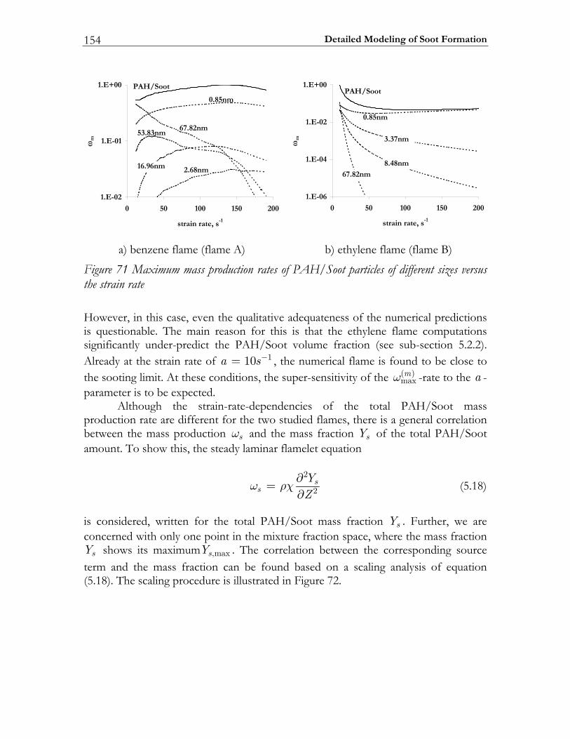
Detailed Modeling of Soot Formation 154
20-E.1
10-E.1
00+E.1
002051001050
s,etarniarts 1-
ωm
mn86.2mn69.61
tooS/HAP
mn58.0
mn28.76mn38.35
60-E.1
40-E.1
20-E.1
00+E.1
002051001050
s,etarniarts 1-
ωm
tooS/HAP
mn58.0
mn28.76
mn73.3
mn84.8
a) benzene flame (flame A) b) ethylene flame (flame B)
Figure 71 Maximum mass production rates of PAH/Soot particles of different sizes versus the strain rate However, in this case, even the qualitative adequateness of the numerical predictions is questionable. The main reason for this is that the ethylene flame computations significantly under-predict the PAH/Soot volume fraction (see sub-section 5.2.2). Already at the strain rate of 110a s−= , the numerical flame is found to be close to the sooting limit. At these conditions, the super-sensitivity of the ( )
maxmω -rate to the a -
parameter is to be expected. Although the strain-rate-dependencies of the total PAH/Soot mass production rate are different for the two studied flames, there is a general correlation between the mass production sω and the mass fraction sY of the total PAH/Soot amount. To show this, the steady laminar flamelet equation
2
2s
sYZ
ω ρχ ∂=∂
(5.18)
is considered, written for the total PAH/Soot mass fraction sY . Further, we are concerned with only one point in the mixture fraction space, where the mass fraction sY shows its maximum ,maxsY . The correlation between the corresponding source
term and the mass fraction can be found based on a scaling analysis of equation (5.18). The scaling procedure is illustrated in Figure 72.
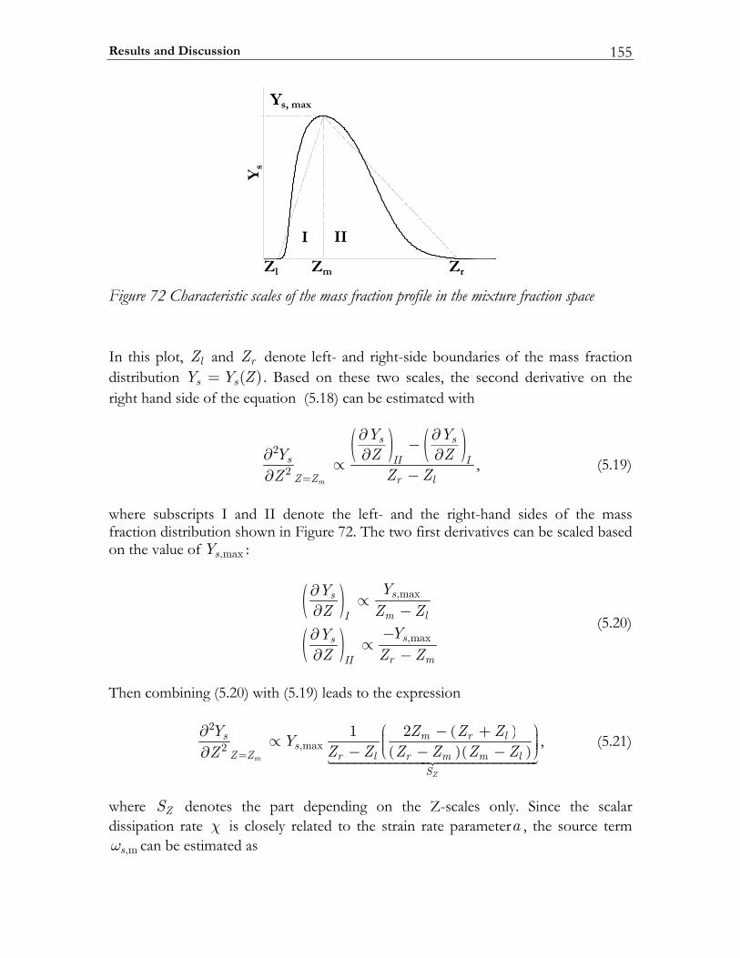
Results and Discussion 155
Ys
xam,s
Zm ZrZl
I II
Figure 72 Characteristic scales of the mass fraction profile in the mixture fraction space In this plot, lZ and rZ denote left- and right-side boundaries of the mass fraction distribution ( )s sY Y Z= . Based on these two scales, the second derivative on the right hand side of the equation (5.18) can be estimated with
( ) ( )2
2m
s s
s II I
Z Z r l
Y YY Z Z
Z ZZ =
∂ ∂−∂ ∂ ∂∝−∂
, (5.19)
where subscripts I and II denote the left- and the right-hand sides of the mass fraction distribution shown in Figure 72. The two first derivatives can be scaled based on the value of ,maxsY :
( )( )
,max
,max
ss
m lI
ss
r mII
YYZ Z Z
YYZ Z Z
∂ ∝∂ −
−∂ ∝∂ −
(5.20)
Then combining (5.20) with (5.19) leads to the expression
( )( )( )
2
,max21 2
m
Z
s m r ls
Z Z r l r m m lS
Y Z Z ZYZ Z Z Z Z ZZ =
∂ ⎛ − + ⎞⎟⎜∝ ⎟⎜ ⎟⎝ ⎠− − −∂, (5.21)
where ZS denotes the part depending on the Z-scales only. Since the scalar dissipation rate χ is closely related to the strain rate parametera , the source term
,msω can be estimated as
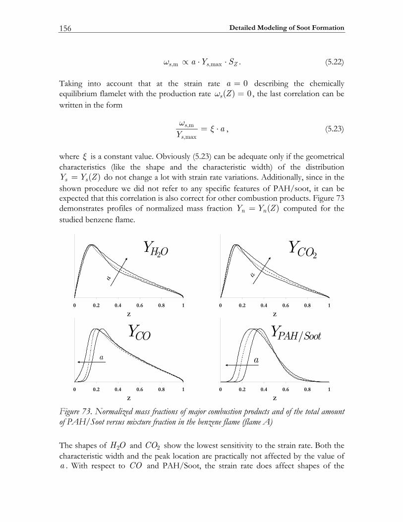
Detailed Modeling of Soot Formation 156
,m ,maxs s Za Y Sω ∝ ⋅ ⋅ . (5.22) Taking into account that at the strain rate 0a = describing the chemically equilibrium flamelet with the production rate ( ) 0s Zω = , the last correlation can be written in the form
,m
,max
s
sa
Yω
ξ= ⋅ , (5.23)
where ξ is a constant value. Obviously (5.23) can be adequate only if the geometrical characteristics (like the shape and the characteristic width) of the distribution
( )s sY Y Z= do not change a lot with strain rate variations. Additionally, since in the shown procedure we did not refer to any specific features of PAH/soot, it can be expected that this correlation is also correct for other combustion products. Figure 73 demonstrates profiles of normalized mass fraction ( )n nY Y Z= computed for the studied benzene flame.
18.06.04.02.00
Z
2OHY
18.06.04.02.00
Z
2OCY
18.06.04.02.00
Z
OCYa
18.06.04.02.00
Z
/ tooSHAPY
a
Figure 73. Normalized mass fractions of major combustion products and of the total amount of PAH/Soot versus mixture fraction in the benzene flame (flame A) The shapes of 2H O and 2CO show the lowest sensitivity to the strain rate. Both the characteristic width and the peak location are practically not affected by the value of a . With respect to CO and PAH/Soot, the strain rate does affect shapes of the
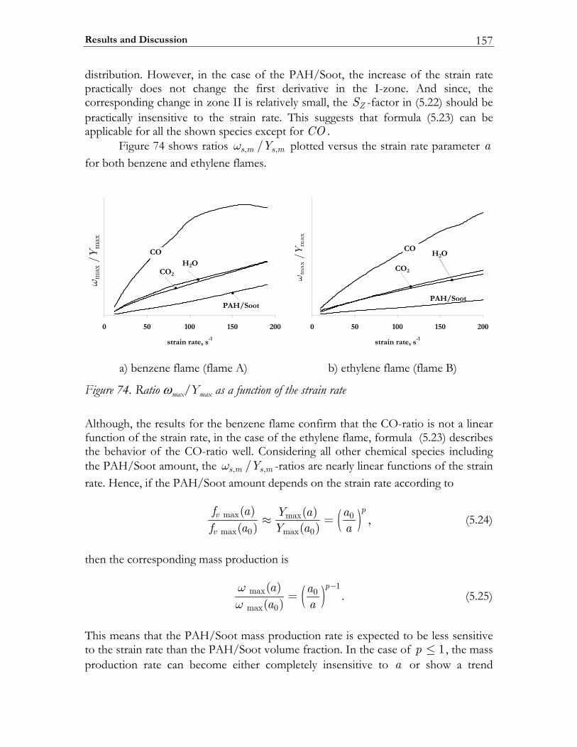
Results and Discussion 157
distribution. However, in the case of the PAH/Soot, the increase of the strain rate practically does not change the first derivative in the I-zone. And since, the corresponding change in zone II is relatively small, the ZS -factor in (5.22) should be practically insensitive to the strain rate. This suggests that formula (5.23) can be applicable for all the shown species except for CO . Figure 74 shows ratios , ,/s m s mYω plotted versus the strain rate parameter a for both benzene and ethylene flames.
0 50 100 150 200
strain rate, s-1
?m
axm
ax/Y
CO
PAH/Soot
CO2
H2O
0 50 100 150 200
strain rate, s-1
?m
axm
ax/Y
CO
PAH/Soot
CO2
H2O
a) benzene flame (flame A) b) ethylene flame (flame B)
Figure 74. Ratio ωmax/Ymax as a function of the strain rate Although, the results for the benzene flame confirm that the CO-ratio is not a linear function of the strain rate, in the case of the ethylene flame, formula (5.23) describes the behavior of the CO-ratio well. Considering all other chemical species including the PAH/Soot amount, the , ,/s m s mYω -ratios are nearly linear functions of the strain rate. Hence, if the PAH/Soot amount depends on the strain rate according to
( )max max 0
max 0 max 0
( ) ( )( ) ( )
pv
v
f a Y a af a Y a a
≈ = , (5.24)
then the corresponding mass production is
( ) 1max 0
max 0
( )( )
pa aa a
ωω
−= . (5.25)
This means that the PAH/Soot mass production rate is expected to be less sensitive to the strain rate than the PAH/Soot volume fraction. In the case of 1p ≤ , the mass production rate can become either completely insensitive to a or show a trend
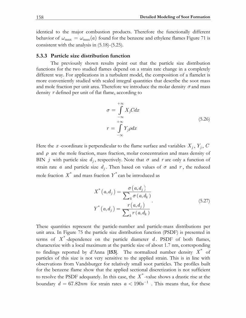
Detailed Modeling of Soot Formation 158
identical to the major combustion products. Therefore the functionally different behavior of max max( )aω ω= found for the benzene and ethylene flames Figure 71 is consistent with the analysis in (5.18)-(5.25).
5.3.3 Particle size distribution function The previously shown results point out that the particle size distribution functions for the two studied flames depend on a strain rate change in a completely different way. For applications in a turbulent model, the composition of a flamelet is more conveniently studied with scaled integral quantities that describe the soot mass and mole fraction per unit area. Therefore we introduce the molar density σ and mass density r defined per unit of flat flame, according to
j
j
X Cdx
r Y dx
σ
ρ
+∞
−∞+∞
−∞
=
=
∫
∫ (5.26)
Here the x -coordinate is perpendicular to the flame surface and variables jX , jY , C and ρ are the mole fraction, mass fraction, molar concentration and mass density of BIN j with particle size jd , respectively. Note that σ and r are only a function of strain rate a and particle size jd . Then based on values of σ and r , the reduced
mole fraction *X and mass fraction *Y can be introduced as
( ) ( )( )
( ) ( )( )
*
*
,,
,
,,
,
jj
kk
jj
kk
a dX a d
a d
r a dY a d
r a d
σσ
=
=
∑
∑
. (5.27)
These quantities represent the particle-number and particle-mass distributions per unit area. In Figure 75 the particle size distribution function (PSDF) is presented in terms of *X -dependence on the particle diameter d . PSDF of both flames, characterize with a local maximum at the particle size of about 1.7 nm, corresponding to findings reported by d’Anna [153]. The normalized number density *X of particles of this size is not very sensitive to the applied strain. This is in line with observations from Vandsburger for relatively small soot particles. The profiles built for the benzene flame show that the applied sectional discretization is not sufficient to resolve the PSDF adequately. In this case, the *X -value shows a drastic rise at the boundary 67.82d nm= for strain rates 1190a s−< . This means that, for these
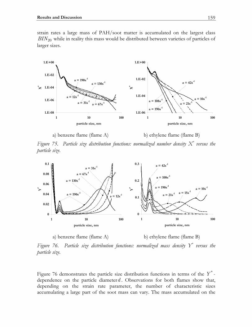
Results and Discussion 159
strain rates a large mass of PAH/soot matter is accumulated on the largest class 20BIN while in reality this mass would be distributed between varieties of particles of
larger sizes.
80-E.1
60-E.1
40-E.1
20-E.1
00+E.1
001011
mn,eziselcitrap
X*
s21=a 1-
s13=a 1-s76=a 1-
s031=a 1-s091=a 1-
60-E.1
40-E.1
20-E.1
00+E.1
001011
mn,eziselcitrap
X*
s01=a 1-
s24=a 1-
s12=a 1-s801=a 1-
s091=a 1-
a) benzene flame (flame A) b) ethylene flame (flame B)
Figure 75. Particle size distribution functions: normalized number density X* versus the particle size.
0
20.0
40.0
60.0
80.0
1.0
001011
mn,eziselcitrap
Y*
s21=a 1-
s13=a 1-
s76=a 1-
s031=a 1-
s091=a 1-
0
1.0
2.0
3.0
001011
mn,eziselcitrap
Y* s01=a 1-
s51=a 1-
s12=a 1-
s24=a 1-
s801=a 1-
s091=a 1-
a) benzene flame (flame A) b) ethylene flame (flame B)
Figure 76. Particle size distribution functions: normalized mass density Y* versus the particle size. Figure 76 demonstrates the particle size distribution functions in terms of the *Y -dependence on the particle diameterd . Observations for both flames show that, depending on the strain rate parameter, the number of characteristic sizes accumulating a large part of the soot mass can vary. The mass accumulated on the
Detailed Modeling of Soot Formation 160
largest particle increases with decreasing strain rate. Here reactions of particles growth and coagulation processes have enough time to form particles of larger sizes. At strain rates -1a 130s≥ for the benzene flame and -1a 21s≤ for the ethylene flame, the PSDF are described with bimodal shapes. This is in correspondence to results from D’Alessio [151] where a similar bimodal particle distribution was found experimentally. Note that this is essentially different from a log-normal distribution that is presumed in many studies experimental as well as numerical.
5.4 Conclusions A detailed mechanism for PAH/soot formation based on the sectional approach is applied to the modeling of benzene/air and ethylene/air diffusion flames. Comparison of the numerical predictions on the soot volume fraction in the ethylene/air laminar counterflow diffusion flame to corresponding experimental data shows that the applied mechanism gives quantitatively correct predictions for soot formation/oxidation flames and a disagreement of one to two orders of magnitude for soot formation flames. The reason is that the applied mechanism was developed for rich premixed flames where fuel is significantly diluted. Therefore, as for IC-engines most practical applications are Soot Formation flames, additional research is necessary to optimize the parameters in the chemical mechanism. With respect to the ethylene combustion, the mechanism which was recently proposed by D’Anna [153] is expected to give better results for non-premixed flames. The analysis of the benzene and ethylene SLF libraries confirms the general experimental observations that soot mass and number densities (first two moments of the PSDF) depend strongly on the mixing characteristics within a flame. At the same time, this numerical result suggests that the chemical production rates of the two first PSDF-moments can be a moderate function of the strain rate depending on the flame sooting characteristics. In that case, and if the turbulent combustion occurs on in the Laminar Flamelet regime, the SLF-assumption is appropriate for simulations focused on the first two moments of the soot PSDF. However, the combustion process typical for Diesel-like engines can be characterized by a transient process that passes through a number of characteristic states, e.g., a combination of a rich pre-mixed front feeding a fully non-premixed part [175], ending late in the cycle as a reactive charge at nearly homogeneous conditions. In this case, with respect to the detailed modeling of the soot PSDF, the choice on the turbulence-soot interaction model has a crucial role independent from the flame specifics. An adequate modeling of these processes could be achieved using the Representative Interactive Flamelet (RIF) framework [176, 177]. An important result from this work is that for low strain rates a bimodal distribution function for the volume fraction is reproduced, which is in correspondence with experimental observations from D’Alessio. This questions the
Conclusions 161
assumption of a lognormal distribution, which is generally used in the method of moments. The general observations of this study can be summarized as follows • The soot release decreases with increasing strain rate. • The maximum particle size decreases with increasing strain rate. • The strain rate affects the number of young soot particles ( 1 2d nm= − ) only
slightly. • Mainly bimodal particle size distribution functions are observed for both
examined flames.

Chapter 6
6 Steady turbulent jet diffusion flames In this chapter the application of detailed reaction mechanisms to turbulent combustion modeling is explored. First, a combustion model based on the laminar flamelet concept is presented in terms of exact equations. Second, the RANS-averaging approach and computational strategy within the KIVA-3V code are described. The numerical simulations are performed for two different test cases. The first case is a piloted methane/air turbulent jet flame (Sandia Flame D). The extensive experimental data describing this flame has been considered for validation purposes. The second case is a sooting turbulent ethylene/air jet flame. The modeled soot field is compared to experimental data.
6.1 Introduction With respect to diesel combustion simulations, when applying detailed reaction models one aims to predict phenomena like auto-ignition and pollutant formation for given physical conditions (characteristics of the fuel injection, actual geometry, etc). The dynamics of these phenomena is strongly related to the chemical nature of the reacting system and the flow field impact (see chapter 5). Modeling of the interaction between the flow field and complex chemical reactions in two- and three-dimensional geometries is a challenging problem. Directly solving the 2D/3D Navier-Stokes equations for reacting flows is computationally demanding even for laminar flow problems. Instead of that, detailed chemical descriptions are usually applied being incorporated into combustion sub-models based on different kinds of 0D- and 1D-formulations [75]. A description of some of these formulations applied to complex chemical systems was given in previous chapters of this thesis. The present chapter focuses on practical application of detailed reaction mechanisms to turbulent combustion modeling.
Steady turbulent jet diffusion flames 164
The steady turbulent non-premixed jet-flames of gas-fuels/air combustion are chosen as test case. Compared to an actual diesel-engine model, this case is characterized with the following important advantages: • The jet-flames are described with a very simple geometry. The wall-flow
interaction does not have to be modeled. • As the injecting fuel is gas rather than liquid, a number of complications coupled
with vaporization dynamics and closure for corresponding source terms is avoided.
• The steady flow characteristics can be analyzed in a comprehensive way. • A number of experimental investigations on turbulent jet-flames were reported in
the past [178-183]. This allows validation of the corresponding numerical models. Two different experimental flames are selected for numerical simulation. The first one is a partially premixed piloted methane/air flame (Sandia-flame D). The corresponding experimental setup is especially designed to validate computational models and the experimental data of the main flow characteristics are available. The second case is a sooting non-premixed ethylene/air flame. In section (6.2), the applied model of combustion and the RANS-averaging approach are introduced. The computational strategy and implementation in the Kiva-3V code are described in section (6.3). The computational results on two test flames and conclusions are given in sections (6.4-6.6).
6.2 Turbulent combustion model To model turbulent flames with detailed chemistry one cannot, at least for most practical situations, rely on solving the full set of equations, i.e., Navier Stokes coupled with all balance equations for all chemical species involved. The shear number of equations and the necessity to resolve the smallest scales in time and space do not allow for that. Even if the chemistry is reduced to a very simple and limited model still the turbulent flow field has to be modeled using a statistical RANS- or the more promising LES-approach [184, 185]. The approach taken to model the turbulence here is explained in sub-section 6.2.2. The specific issues associated with applying detailed chemical models in turbulent flames are dealt with by the flamelet concept. With this approach a wide variety of detailed chemical mechanisms can be used. Yet its computational demands are tractable. In the following sub-section the steady flamelet concept will be explained in more detail.
Turbulent combustion model 165
6.2.1 Steady laminar flamelet assumption In general, the starting point of the laminar flamelet concept is that a turbulent diffusion flame is described as a geometrical surface. Hence, the flame is considered to be thin compared to all flow length-scales. The specific assumption of the familiar steady laminar flamelet model is that for each element of the flame surface a local balance between chemical reactions and mixing rates takes place as if it was modeled as a steady 1D counter flow diffusion flame. Therefore, all thermo-chemical characteristics (temperature, species concentrations, reaction rates, etc.) are determined with the flame internal coordinate Z (mixture fraction) and the flame strain rate a caused by local flow conditions. With the steady laminar flamelet concept, the set of equations describing turbulent diffusion flames reads: continuity
0k
k
vt xρ ρ∂ ∂+ =
∂ ∂ (6.1)
momentum conservation
1,2, 3
i i k iki
k i k
v v v p Ft x x x
i
ρ ρ τ∂ ∂ ∂ ∂+ = − + +∂ ∂ ∂ ∂=
(6.2)
the ideal gas equation of state
k
kk
Yp RTm
ρ= ⋅ ⋅∑ (6.3)
transport of the mixture fraction
k
k k k
Z Zv ZDt x x xρ ρ ρ∂ ∂ ∂ ⎛ ∂ ⎞⎟⎜+ = ⎟⎜ ⎟⎝ ⎠∂ ∂ ∂ ∂
(6.4)
and flamelet correlations
( )
( )
, ,
,k k
T T Z
Y Y Z
χ
χ
=
= (6.5)
Steady turbulent jet diffusion flames 166
In (6.2) ikτ and iF denote the stress tensor and the force acting on the fluid, respectively. The flamelet correlations (6.5) are normally pre-computed using the desired chemical model4.
6.2.2 Statistical description of turbulent diffusion flame Although the set of governing equations is significantly reduced with the SLF assumption, its direct numerical solution (DNS) for the case of turbulent combustion remains to be a very difficult problem, since still a large spectrum of time and length scales has to be resolved. Therefore, the classical problem re-definition in terms of statistical flow modeling is applied. The basic idea of the statistical description is that each instantaneous flow characteristic ϕ is decomposed into the mean part ϕ and the fluctuating part ϕ′ : ϕ ϕ ϕ′= + . (6.6) The corresponding ensemble averaging procedure is expressed with relations
( ) ( )
( )1
1, lim ,
, 0
e
e
n
k i kn e i
k
x t x tn
x t
ϕ ϕ
ϕ
→∞ ==
′ =
∑ (6.7)
where ( ),i kx tϕ is the ith sample of the ϕ -quantity and en the total number of samples. To obtain the transport equations for the mean flow characteristics ϕ the instantaneous flow equations have to be averaged. This averaging procedure is called Reynolds Averaged Navier-Stokes (RANS) modeling. In terms of the ensemble-averaged flow description the mass conservation equation now reads
( ) ( )0
kk
k k
vvt x x
ρρ ρ ′ ′∂∂ ∂+ + =∂ ∂ ∂
. (6.8)
In this equation the kvρ′ ′ correlation is unclosed and has to be modeled. In incompressible flows, constρ = , this is normally not an issue. However in combustion systems large density variations occur and a model for this correlation has to be formulated. This problem can be avoided if a different type of averaging is introduced, the so-called density weighting procedure [186]. A density averaged (Favre averaged) flow characteristic ϕ is defined as 4 For each given value of the strain rate a the solution of the counterflow diffusion flame problem determines a unique distribution ( , )Z aχ χ= . Hence, the correlation (6.5) can also be written in
the form of *( , )T T Z a= and *( , )k kY Y Z a= .
Turbulent combustion model 167
ρϕϕρ
= . (6.9)
With this the ϕ -instantaneous value can be decomposed into the mean part ϕ and the fluctuating part ϕ′′ : ϕ ϕ ϕ′′= + , (6.10) where the fluctuating term is such that
( )
0ρ ϕ ϕϕρ−′′ = = . (6.11)
Following this definition, the Favre-averaging procedure can be expressed with
( ) ( ) ( )1
1 1, lim , ,e
e
n
k i k kn e ix t x t x t
nϕ ϕ ρρ →∞ =
= ⋅∑ (6.12)
where
( ) ( )1
1, lim ,e
e
n
k kn e ix t x t
nρ ρ
→∞ == ∑ (6.13)
The main advantage of this procedure is that the density weighted features in products with the mean density include correlations ρ ϕ′ ′ as follows ρϕ ρ ϕ ρ ϕ′ ′= ⋅ + . (6.14) With this, the classical RANS equations are formally extended to model reacting flows characterizing by density variations. For instance now mass conservation yields
0k
k
vt xρ ρ∂ ∂+ =
∂ ∂, (6.15)
which is identical to the instantaneous version but now holding for the definition of the averaged velocity kv . In the flamelet combustion model the instantaneous gas temperature and chemical composition are determined with the instantaneous values of mixture fraction and scalar dissipation rate. However, applying the RANS-averaging procedure to the governing equations the unknowns are redefined from
Steady turbulent jet diffusion flames 168
instantaneous to statistically mean features. This step obviously leads to information-loss and prevents a direct coupling between flow field and steady flamelet structures. On the other hand, since each flamelet feature ϕ is defined on the ,Z χ -domain, its statistically-averaged value at a spatial location kx and time moment t can be found from ( ) ( )* * * * * *, , ; ,k
Z
Z P Z x t dZ dχ
ϕ ϕ χ χ χ= ⋅∫ ∫ , (6.16)
where ( )* *, ; ,kP Z x tχ the corresponding probability density function (PDF). This PDF-function quantifies the probability to find Z and χ parameters within the range * * * */2, /2Z Z χ χ±∆ ±∆ for the given location kx and time t . Therefore, in order to model turbulent flames in terms of Favre-averaged characteristics, knowledge of the P PDF-function (mass-weighted PDF) is required. The P -function is such that
( )
( ) ( ) ( )
( ) ( ) ( )( ) ( )
1* * * *
0 01
* * * * * *
0 01
2* * * * * * 2
0 0
, ; , 1,
, ; , , , ,
, ; , , , , .
k
k k
k k k
P Z x t dZ d
P Z x t Z dZ d x t
P Z x t Z x t dZ d x t
χ χ
χ ϕ χ χ ϕ
χ ϕ χ ϕ χ ϕ
∞
∞
∞
=
=
′′− =
∫ ∫
∫ ∫
∫ ∫
(6.17)
In general, to build the PDF-function requires solving the corresponding balance equation. These PDF transport equations can be deduced from [187, 188] and have to be solved in conjunction with the turbulent flow field [189, 190]. However, in most practical simulations presumed PDF-shapes are used since this technique requires knowledge of a few statistical quantities (for example mean and variance) only. In the present study a few widely used assumptions are applied to model the shape of the PDF-function. The first one, is that the mixture fraction Z and the scalar dissipation rate χ are uncorrelated leading to ( ) ( ) ( )* * * *, ; , ; , ; ,k Z k kP Z x t P Z x t P x tχχ χ= ⋅ . (6.18) The second assumption is that the ZP -part of the joint PDF (6.18) is presumed to have the β -function shape:
Turbulent combustion model 169
( )
( )
11
111
0
1
1Z
Z ZP
Z Z dZ
βα
βα
−−
−−
−=
−∫, (6.19)
where α and β are parameters that are defined by the first two statistical moments of the mixture fraction variable: mean mixture fraction Z and its variance 2Z ′′ . An explicit formula for the α and β can be deduced by the important requirement that the PDF function should reproduce these moments:
( )
( ) ( )
* * *
22 * * *
; ,
; ,
Z
Z
Z Z P Z x t dZ
Z Z Z P Z x t dZ
β
β
=
′′ = −
∫
∫, (6.20)
With some rigorous algebra [191], this leads to explicit formulas for the parameters α and β :
( )
( ) ( )2
2
1
11
Z ZZ
ZZ Z
ZZ
α
β
⎡ ⎤−⎢ ⎥= ⎢ ⎥′′⎣ ⎦⎡ ⎤−⎢ ⎥= − ⎢ ⎥′′⎣ ⎦
. (6.21)
Due to the large variety of possible β -shapes this presumed PDF is able to reproduce averaged flame features adequately. Figure 77 shows the shape of the PDFβ − for a fixed value of the mean mixture fraction Z (MMF) and different
values of its root mean square 2Zσ ′′= (RMS). Increasing the value of σ leads to continuous transformation from the Gaussian shape (lines 1, 2 and 3) to the function reaching infinity at 0Z = and/or
1Z = (lines 4 and 5). Figures (a) and (b) illustrate this transformation for the cases of 0.5Z = and 0.1Z = , respectively. If at any spatial location the β -function assumes a Gaussian shape, this implies that an observation of unburnt reactants at this location is statistically very rare or even not possible at all. If the β -function reaches infinity on one or both of the two borders of the Z -domain, the observation of combustion products is a rare event. Mostly unburned reagents will be observed then. So the β -function seems a viable choice to represent the physical situations that occur in turbulent combustion. However, due to its versatility, the numerical integration of the β -function is a very difficult problem. The main complication is
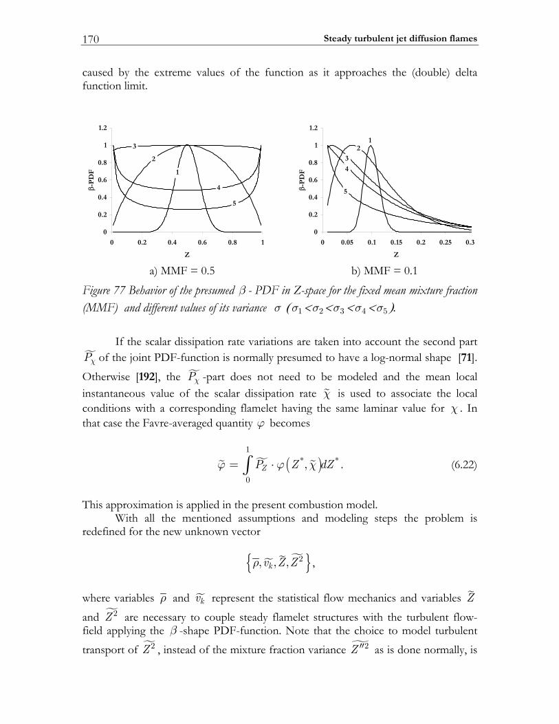
Steady turbulent jet diffusion flames 170
caused by the extreme values of the function as it approaches the (double) delta function limit.
0
0.2
0.4
0.6
0.8
1
1.2
0 0.2 0.4 0.6 0.8 1
Z
-PD
F 1
2
3
4
5
0
0.2
0.4
0.6
0.8
1
1.2
0 0.05 0.1 0.15 0.2 0.25 0.3
Z
-PD
F
12
3
4
5
a) MMF = 0.5 b) MMF = 0.1
Figure 77 Behavior of the presumed β - PDF in Z-space for the fixed mean mixture fraction (MMF) and different values of its variance σ ( 1σ < 2σ < 3σ < 4σ < 5σ ). If the scalar dissipation rate variations are taken into account the second part Pχ of the joint PDF-function is normally presumed to have a log-normal shape [71]. Otherwise [192], the Pχ -part does not need to be modeled and the mean local instantaneous value of the scalar dissipation rate χ is used to associate the local conditions with a corresponding flamelet having the same laminar value for χ . In that case the Favre-averaged quantity ϕ becomes
( )1
* *
0
,ZP Z dZϕ ϕ χ= ⋅∫ . (6.22)
This approximation is applied in the present combustion model. With all the mentioned assumptions and modeling steps the problem is redefined for the new unknown vector 2, , ,kv Z Zρ ,
where variables ρ and kv represent the statistical flow mechanics and variables Z and 2Z are necessary to couple steady flamelet structures with the turbulent flow-field applying the β -shape PDF-function. Note that the choice to model turbulent transport of 2Z , instead of the mixture fraction variance 2Z ′′ as is done normally, is
Turbulent combustion model 171
just a numerical convenience. The variance follows directly from the computed Z and 2Z by its definition: 22 2Z Z Z′′ = − . (6.23) Finally, the problem redefinition into the statistical flow description leads to the new system of transport equations
0k
k
vt xρ ρ∂ ∂+ =
∂ ∂ (6.24)
i i k i k iki
k k i k
v v v v v p gt x x x xρ ρ ρ τ ρ
′′ ′′∂ ∂ ∂ ∂ ∂+ = − − + +∂ ∂ ∂ ∂ ∂
(6.25)
k k
k k k k
Z v Z Z v ZDt x x x xρ ρ ρρ
′′ ′′∂ ∂ ∂ ⎛ ∂ ⎞ ∂⎟⎜+ = −⎟⎜ ⎟⎝ ⎠∂ ∂ ∂ ∂ ∂ (6.26)
[ ]22 2 2kk
tk k k k
v ZZ v Z ZDt x x x x
ρρ ρ ρ ρχ′′⎛ ⎞ ′′∂∂ ∂ ∂ ∂ ⎟⎜ ⎟+ = − −⎜ ⎟⎜ ⎟∂ ∂ ∂ ∂ ∂⎟⎜⎝ ⎠
(6.27)
Resulting from the averaging process, Favre-averaged products of fluctuating variables appear as new unknowns. Additional modeling is required to close this set of equations. Probably, the most simple closure approach usually used in practical combustion simulations is the Eddy Viscosity Model (EVM). In the EVM approach the unclosed RANS-terms are modeled as diffusion-like turbulent transport processes. For example the so-called Reynolds stresses i kv vρ ′′ ′′ in the momentum equation (6.25) are expressed as
jii j t
j i
vvv vx x
ρ µ⎛ ⎞∂∂ ⎟⎜′′ ′′ = + ⎟⎜ ⎟⎜∂ ∂⎝ ⎠
, (6.28)
where tµ is the turbulent viscosity coefficients. Similarly the unclosed terms in the scalar transport equations are expressed as
( )t
kkct
vxS ϕ
µ ϕρ ϕ ∂′′ ′′ =∂
, (6.29)
where ( )ctSϕ is the turbulent Schmidt number for the variable ϕ . Hence, in the EVM
the closure problem is delegated to the modeling of turbulent transport coefficients. Some details on the applied closure technique are given in the following section.
Steady turbulent jet diffusion flames 172
6.3 Numerical implementation Ultimately, we want to apply large detailed chemical reaction mechanisms to assess pollutant formation (mainly xNO and Soot) in HD diesel engines. To do so a computer program should be used that is capable of handling the specific requirements: moving geometries (valves/piston) and injection of liquid fuels. A wide-spread program in the engine research community is Kiva3V [193-199, 160, 200, 201], also due to the fact that it is open software. In the next sub-section the implementation of the RANS model in Kiva3V is discussed. Kiva3V is not designed to incorporate detailed chemical mechanisms. Therefore, in 6.3.2 the extension of the original combustion model to the flamelet approach is discussed.
6.3.1 KIVA-3V simulator for turbulent reactive flows. In order to simulate the turbulent jet diffusion flames, the Steady Laminar Flamelet (SLF) model has been implemented in the KIVA-3V flow field simulator [202]. The Kiva-3V code is an advanced computer program for the numerical calculation of transient, three-dimensional chemically reacting fluid flows including high-density liquid sprays. It was primarily developed for simulating flows in reciprocating internal-combustion engines. The Favre averaging procedure described earlier is applied in Kiva3V. To close the Reynolds stress tensor and scalar turbulent correlations the Eddy Viscosity Model (EVM) is applied in conjunction with the standard k ε− model to determine the turbulent viscosity coefficients. Based on the classical dimensional analysis, the turbulent viscosity coefficient is
2
tkC fµ µµε
= , (6.30)
where k and ε are turbulent kinetic energy and its dissipation rate coming from
2
12 k k
l
k
k v v
ux
ε ν
′′ ′′=
′′⎛ ⎞∂ ⎟⎜= ⎟⎜ ⎟⎜∂⎝ ⎠
, (6.31)
and Cµ and fµ are an empirical constant and an empirical damping function respectively. Turbulent transport equations for Favre-averaged variables k and ε are now written as:
k tk
k k kk
k v k k Pt x x xρ ρ µµ ρε
σ⎡ ⎤⎛ ⎞∂ ∂ ∂ ∂⎟⎜⎢ ⎥+ = + + −⎟⎜ ⎟⎜∂ ∂ ∂ ∂⎢ ⎥⎝ ⎠⎣ ⎦
(6.32)
Numerical implementation 173
2
1 1 2 2k t
kk k k
v c f P c ft x x x k kε ε
ε
ρε ρ ε µ ε ε εµσ
∂ ∂ ∂ ⎡⎛ ⎞ ∂ ⎤⎟⎜+ = + + −⎢ ⎥⎟⎜ ⎟⎝ ⎠∂ ∂ ∂ ∂⎢ ⎥⎣ ⎦ (6.33)
where kσ , εσ , 1εσ and 2εσ are empirical constants of the turbulence model; 1f and 2f are empirical functions and kP is the production of the turbulent kinetic energy.
The governing equations are discretized using the finite volume method. A detailed description of the numerical algorithm can be found in [202].
6.3.2 Mixture fraction variable
The extension of the KIVA-3V with the mixture fraction variables (Z and 2Z ) has been performed by introduction of two extra chemically inert species f and g to the list of species that describe the original problem. These two artificial components have been modeled as dilutions present in physically small amounts. Hence this will have no explicit influence on physics and chemistry of the original system. These extra quantities are defined as
2
f Z
g Z
α
α
= ⋅
= ⋅, (6.34)
where parameter α denotes a small scaling parameter. Introducing the turbulent transport operator L as
( ) kt
k k k
vL Dt x x xρϕ ρ ϕ ϕϕ ρ∂ ∂ ∂ ⎛ ∂ ⎞⎟⎜= + − ⎟⎜ ⎟⎝ ⎠∂ ∂ ∂ ∂
, (6.35)
differential equations for Z and 2Z can be written as
( )
( )2 2
v
v
L Z S
L Z ZS ρχ
=
= ⋅ −, (6.36)
where vS is the time-averaged mixture fraction production rate caused by the evaporating liquid fuel. Since the turbulent transport operator is linear ( )( ) ( )L Lα ϕ α ϕ⋅ = ⋅ , transport equations for Favre-averaged f and g fields are
Steady turbulent jet diffusion flames 174
( )( ) 2
v
v
L f S
L g f S
α
α ρχ
= ⋅
= ⋅ ⋅ − ⋅ (6.37)
The practical advantage of this implementation is that the original numerical algorithm solving the species transport can be directly applied to these extra-variables without any modifications. Both extra variables act as passive scalars not influencing the original calculation procedure. Note, that the liquid fuel evaporation term is in general not equal to zero if modern DI are modeled. This gives an additional closure problem for the 2 vf S⋅ ⋅ term [51]. However, for both reference flames used in this study, the fuel inflow does not contain a liquid phase and therefore, the f and g Favre-averaged fields reduce to
0k
tk k k
kt
k k k
f v f fDt x x xg v g gD at x x x
ρ ρ ρ
ρ ρ ρ ρχ
⎛ ⎞∂ ∂ ∂ ∂ ⎟⎜+ − =⎟⎜ ⎟⎜∂ ∂ ∂ ∂⎝ ⎠∂ ∂ ∂ ⎛ ∂ ⎞⎟⎜+ − = − ⋅⎟⎜ ⎟⎝ ⎠∂ ∂ ∂ ∂
. (6.38)
Since this work is focused on detailed chemical descriptions rather than turbulent flow modeling, the Favre-averaged scalar dissipation rate χ is evaluated with the simplest linear relaxation model leading to
2Zkεχ ′′= . (6.39)
A better description for turbulent mixing can be achieved solving the balance equation for the scalar dissipation rate [203]. In the next two sub-sections the Kiva-3V code will be tested on its ability to simulate turbulent flames. To test the flamelet code Sandia-flame D is chosen (section 6.4). Finally, to show the performance on the Soot model in a turbulent setting a sooting ethylene/air turbulent jet flame is modeled (section 6.5).
6.4 Sandia flame D In this section results on numerical simulations of the Sandia Flame D [181, 204-206] are presented. This flame has been chosen as one of the well known test cases for turbulent combustion modeling. A detailed set of experimental data exists on the important flow and scalar quantities. This flame is frequently used as a reference to
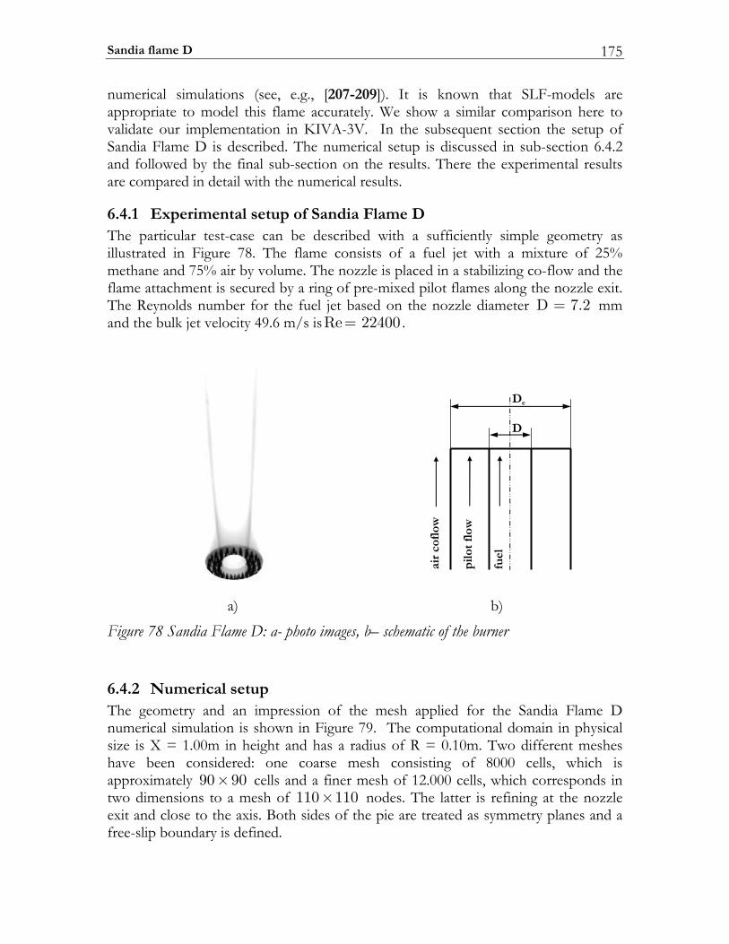
Sandia flame D 175
numerical simulations (see, e.g., [207-209]). It is known that SLF-models are appropriate to model this flame accurately. We show a similar comparison here to validate our implementation in KIVA-3V. In the subsequent section the setup of Sandia Flame D is described. The numerical setup is discussed in sub-section 6.4.2 and followed by the final sub-section on the results. There the experimental results are compared in detail with the numerical results.
6.4.1 Experimental setup of Sandia Flame D The particular test-case can be described with a sufficiently simple geometry as illustrated in Figure 78. The flame consists of a fuel jet with a mixture of 25% methane and 75% air by volume. The nozzle is placed in a stabilizing co-flow and the flame attachment is secured by a ring of pre-mixed pilot flames along the nozzle exit. The Reynolds number for the fuel jet based on the nozzle diameter D = 7.2 mm and the bulk jet velocity 49.6 m/s isRe= 22400 .
fuel
pilo
tfl
ow
air
cofl
owD
De
a) b)
Figure 78 Sandia Flame D: a- photo images, b– schematic of the burner
6.4.2 Numerical setup The geometry and an impression of the mesh applied for the Sandia Flame D numerical simulation is shown in Figure 79. The computational domain in physical size is X = 1.00m in height and has a radius of R = 0.10m. Two different meshes have been considered: one coarse mesh consisting of 8000 cells, which is approximately 90 90× cells and a finer mesh of 12.000 cells, which corresponds in two dimensions to a mesh of 110 110× nodes. The latter is refining at the nozzle exit and close to the axis. Both sides of the pie are treated as symmetry planes and a free-slip boundary is defined.
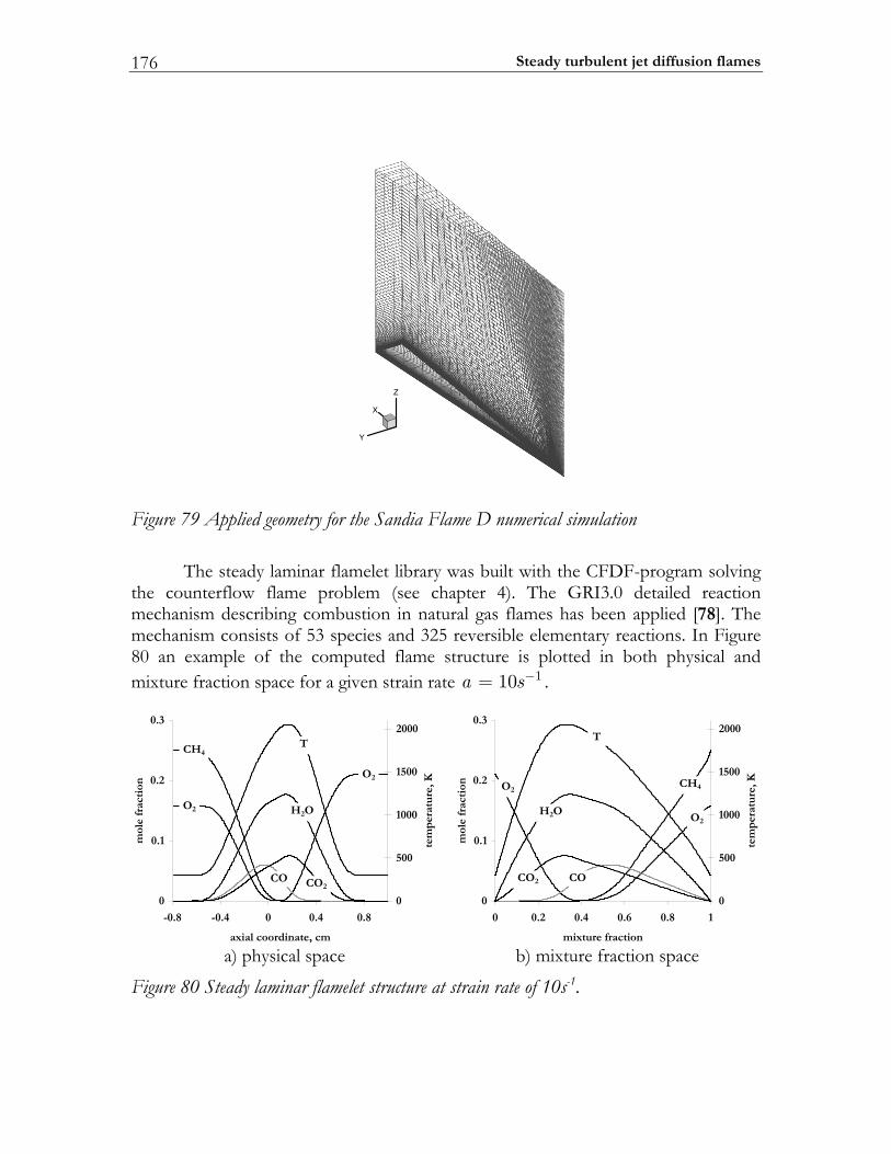
Steady turbulent jet diffusion flames 176
X
Y
Z
Figure 79 Applied geometry for the Sandia Flame D numerical simulation The steady laminar flamelet library was built with the CFDF-program solving the counterflow flame problem (see chapter 4). The GRI3.0 detailed reaction mechanism describing combustion in natural gas flames has been applied [78]. The mechanism consists of 53 species and 325 reversible elementary reactions. In Figure 80 an example of the computed flame structure is plotted in both physical and mixture fraction space for a given strain rate 110a s−= .
0
1.0
2.0
3.0
8.04.004.0-8.0-
mc,etanidrooclaixa
mol
efr
acti
on
0
005
0001
0051
0002
tem
per
atu
re,K
T
O2
O2
HC 4
H2O
OC 2OC
0
1.0
2.0
3.0
18.06.04.02.00
noitcarferutxim
mol
efr
acti
on
0
005
0001
0051
0002
tem
per
atu
re,K
T
O2
O2
HC 4
H2O
OC 2 OC
a) physical space b) mixture fraction space
Figure 80 Steady laminar flamelet structure at strain rate of 10s-1.
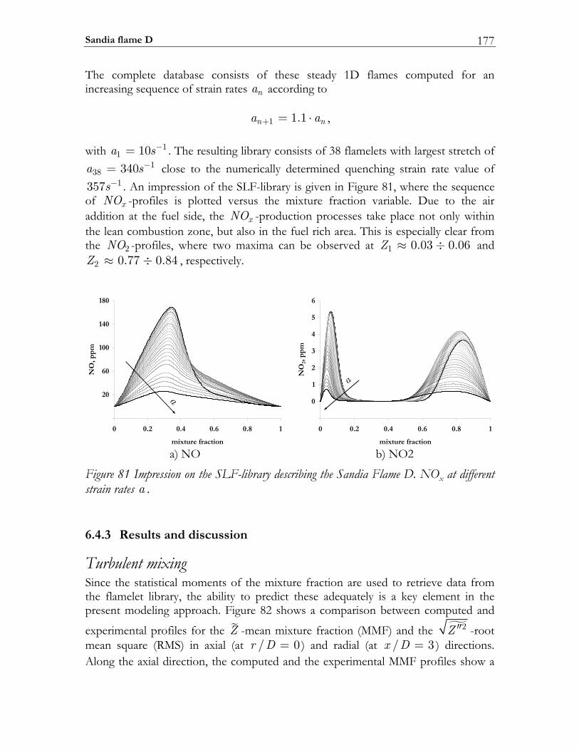
Sandia flame D 177
The complete database consists of these steady 1D flames computed for an increasing sequence of strain rates na according to 1 1.1n na a+ = ⋅ , with 1
1 10a s−= . The resulting library consists of 38 flamelets with largest stretch of 1
38 340a s−= close to the numerically determined quenching strain rate value of 1357s− . An impression of the SLF-library is given in Figure 81, where the sequence
of xNO -profiles is plotted versus the mixture fraction variable. Due to the air addition at the fuel side, the xNO -production processes take place not only within the lean combustion zone, but also in the fuel rich area. This is especially clear from the 2NO -profiles, where two maxima can be observed at 1 0.03 0.06Z ≈ ÷ and
2 0.77 0.84Z ≈ ÷ , respectively.
-20
20
60
100
140
180
0 0.2 0.4 0.6 0.8 1
mixture fraction
NO
, pp
m
a-1
0
1
2
3
4
5
6
0 0.2 0.4 0.6 0.8 1
mixture fraction
NO
2, p
pm
a
a) NO b) NO2
Figure 81 Impression on the SLF-library describing the Sandia Flame D. NOx at different strain rates a .
6.4.3 Results and discussion
Turbulent mixing Since the statistical moments of the mixture fraction are used to retrieve data from the flamelet library, the ability to predict these adequately is a key element in the present modeling approach. Figure 82 shows a comparison between computed and
experimental profiles for the Z -mean mixture fraction (MMF) and the 2Z ′′ -root mean square (RMS) in axial (at / 0r D = ) and radial (at / 3x D = ) directions. Along the axial direction, the computed and the experimental MMF profiles show a
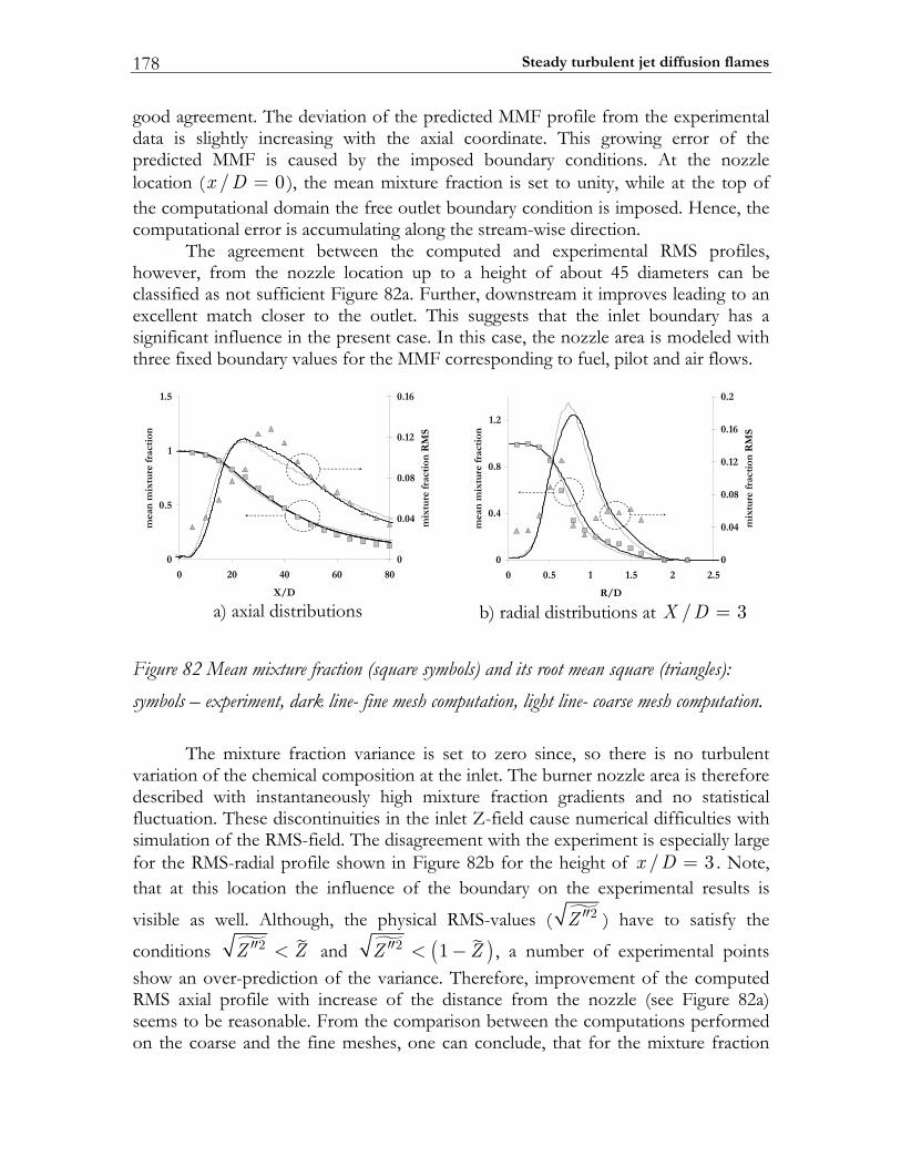
Steady turbulent jet diffusion flames 178
good agreement. The deviation of the predicted MMF profile from the experimental data is slightly increasing with the axial coordinate. This growing error of the predicted MMF is caused by the imposed boundary conditions. At the nozzle location ( / 0x D = ), the mean mixture fraction is set to unity, while at the top of the computational domain the free outlet boundary condition is imposed. Hence, the computational error is accumulating along the stream-wise direction. The agreement between the computed and experimental RMS profiles, however, from the nozzle location up to a height of about 45 diameters can be classified as not sufficient Figure 82a. Further, downstream it improves leading to an excellent match closer to the outlet. This suggests that the inlet boundary has a significant influence in the present case. In this case, the nozzle area is modeled with three fixed boundary values for the MMF corresponding to fuel, pilot and air flows.
0
5.0
1
5.1
080604020
D/X
mea
nm
ixtu
re f
ract
ion
0
40.0
80.0
21.0
61.0
mix
ture
fra
ctio
nR
MS
0
4.0
8.0
2.1
5.225.115.00
D/R
mea
nm
ixtu
re f
ract
ion
0
40.0
80.0
21.0
61.0
2.0
mix
ture
fra
ctio
nR
MS
a) axial distributions b) radial distributions at / 3X D =
Figure 82 Mean mixture fraction (square symbols) and its root mean square (triangles): symbols – experiment, dark line- fine mesh computation, light line- coarse mesh computation. The mixture fraction variance is set to zero since, so there is no turbulent variation of the chemical composition at the inlet. The burner nozzle area is therefore described with instantaneously high mixture fraction gradients and no statistical fluctuation. These discontinuities in the inlet Z-field cause numerical difficulties with simulation of the RMS-field. The disagreement with the experiment is especially large for the RMS-radial profile shown in Figure 82b for the height of / 3x D = . Note, that at this location the influence of the boundary on the experimental results is
visible as well. Although, the physical RMS-values ( 2Z ′′ ) have to satisfy the
conditions 2Z Z′′ < and ( )2 1Z Z′′ < − , a number of experimental points show an over-prediction of the variance. Therefore, improvement of the computed RMS axial profile with increase of the distance from the nozzle (see Figure 82a) seems to be reasonable. From the comparison between the computations performed on the coarse and the fine meshes, one can conclude, that for the mixture fraction
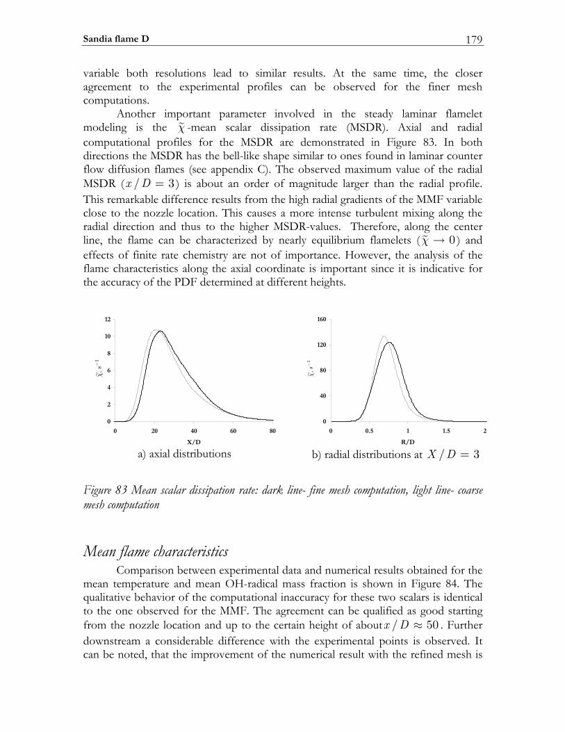
Sandia flame D 179
variable both resolutions lead to similar results. At the same time, the closer agreement to the experimental profiles can be observed for the finer mesh computations. Another important parameter involved in the steady laminar flamelet modeling is the χ -mean scalar dissipation rate (MSDR). Axial and radial computational profiles for the MSDR are demonstrated in Figure 83. In both directions the MSDR has the bell-like shape similar to ones found in laminar counter flow diffusion flames (see appendix C). The observed maximum value of the radial MSDR ( / 3x D = ) is about an order of magnitude larger than the radial profile. This remarkable difference results from the high radial gradients of the MMF variable close to the nozzle location. This causes a more intense turbulent mixing along the radial direction and thus to the higher MSDR-values. Therefore, along the center line, the flame can be characterized by nearly equilibrium flamelets ( 0χ → ) and effects of finite rate chemistry are not of importance. However, the analysis of the flame characteristics along the axial coordinate is important since it is indicative for the accuracy of the PDF determined at different heights.
0
2
4
6
8
10
12
0 20 40 60 80
X/D
h1
,s
0
40
80
120
160
0 0.5 1 1.5 2
R/D
h1
,s
a) axial distributions b) radial distributions at / 3X D =
Figure 83 Mean scalar dissipation rate: dark line- fine mesh computation, light line- coarse mesh computation
Mean flame characteristics Comparison between experimental data and numerical results obtained for the mean temperature and mean OH-radical mass fraction is shown in Figure 84. The qualitative behavior of the computational inaccuracy for these two scalars is identical to the one observed for the MMF. The agreement can be qualified as good starting from the nozzle location and up to the certain height of about / 50x D ≈ . Further downstream a considerable difference with the experimental points is observed. It can be noted, that the improvement of the numerical result with the refined mesh is
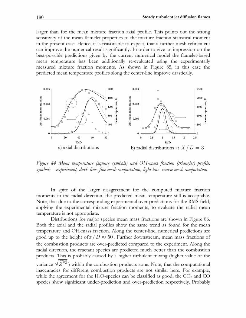
Steady turbulent jet diffusion flames 180
larger than for the mean mixture fraction axial profile. This points out the strong sensitivity of the mean flamelet properties to the mixture fraction statistical moment in the present case. Hence, it is reasonable to expect, that a further mesh refinement can improve the numerical result significantly. In order to give an impression on the best-possible predictions given by the current numerical model the flamelet-based mean temperature has been additionally re-evaluated using the experimentally measured mixture fraction moments. As shown in Figure 85, in this case the predicted mean temperature profiles along the center-line improve drastically.
0
0.001
0.002
0.003
0 20 40 60 80
X/D
OH
-mea
n m
ass
frac
tion
0
400
800
1200
1600
2000
mea
n te
mp
erat
ure
,K
0
0.001
0.002
0.003
0 0.5 1 1.5 2 2.5
R/D
OH
-mea
n m
ass
frac
tion
0
500
1000
1500
2000
2500
mea
n te
mp
erat
ure
,K
a) axial distributions b) radial distributions at / 3X D =
Figure 84 Mean temperature (square symbols) and OH-mass fraction (triangles) profile: symbols – experiment, dark line- fine mesh computation, light line- coarse mesh computation. In spite of the larger disagreement for the computed mixture fraction moments in the radial direction, the predicted mean temperature still is acceptable. Note, that due to the corresponding experimental over-predictions for the RMS-field, applying the experimental mixture fraction moments, to evaluate the radial mean temperature is not appropriate. Distributions for major species mean mass fractions are shown in Figure 86. Both the axial and the radial profiles show the same trend as found for the mean temperature and OH-mass fraction. Along the center-line, numerical predictions are good up to the height of / 50x D ≈ . Further downstream, mean mass fractions of the combustion products are over-predicted compared to the experiment. Along the radial direction, the reactant species are predicted much better than the combustion products. This is probably caused by a higher turbulent mixing (higher value of the
variance 2Z ′′ ) within the combustion products zone. Note, that the computational inaccuracies for different combustion products are not similar here. For example, while the agreement for the H2O-species can be classified as good, the CO2 and CO species show significant under-prediction and over-prediction respectively. Probably
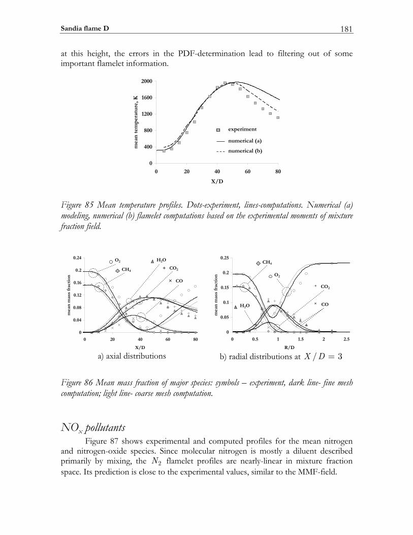
Sandia flame D 181
at this height, the errors in the PDF-determination lead to filtering out of some important flamelet information.
0
400
800
1200
1600
2000
0 20 40 60 80
X/D
mea
n t
emp
erat
ure
,Kexperiment
numerical (a)
numerical (b)
Figure 85 Mean temperature profiles. Dots-experiment, lines-computations. Numerical (a) modeling, numerical (b) flamelet computations based on the experimental moments of mixture fraction field.
0
0.04
0.08
0.12
0.16
0.2
0.24
0 20 40 60 80
X/D
mea
n m
ass
frac
tion
O2
CH4
CO×
H2O
CO2+
0
0.05
0.1
0.15
0.2
0.25
0 0.5 1 1.5 2 2.5
R/D
mea
n m
ass
frac
tion
CH4
CO×
CO2+
O2
H2O
a) axial distributions b) radial distributions at / 3X D =
Figure 86 Mean mass fraction of major species: symbols – experiment, dark line- fine mesh computation; light line- coarse mesh computation.
NOx pollutants Figure 87 shows experimental and computed profiles for the mean nitrogen and nitrogen-oxide species. Since molecular nitrogen is mostly a diluent described primarily by mixing, the 2N flamelet profiles are nearly-linear in mixture fraction space. Its prediction is close to the experimental values, similar to the MMF-field.
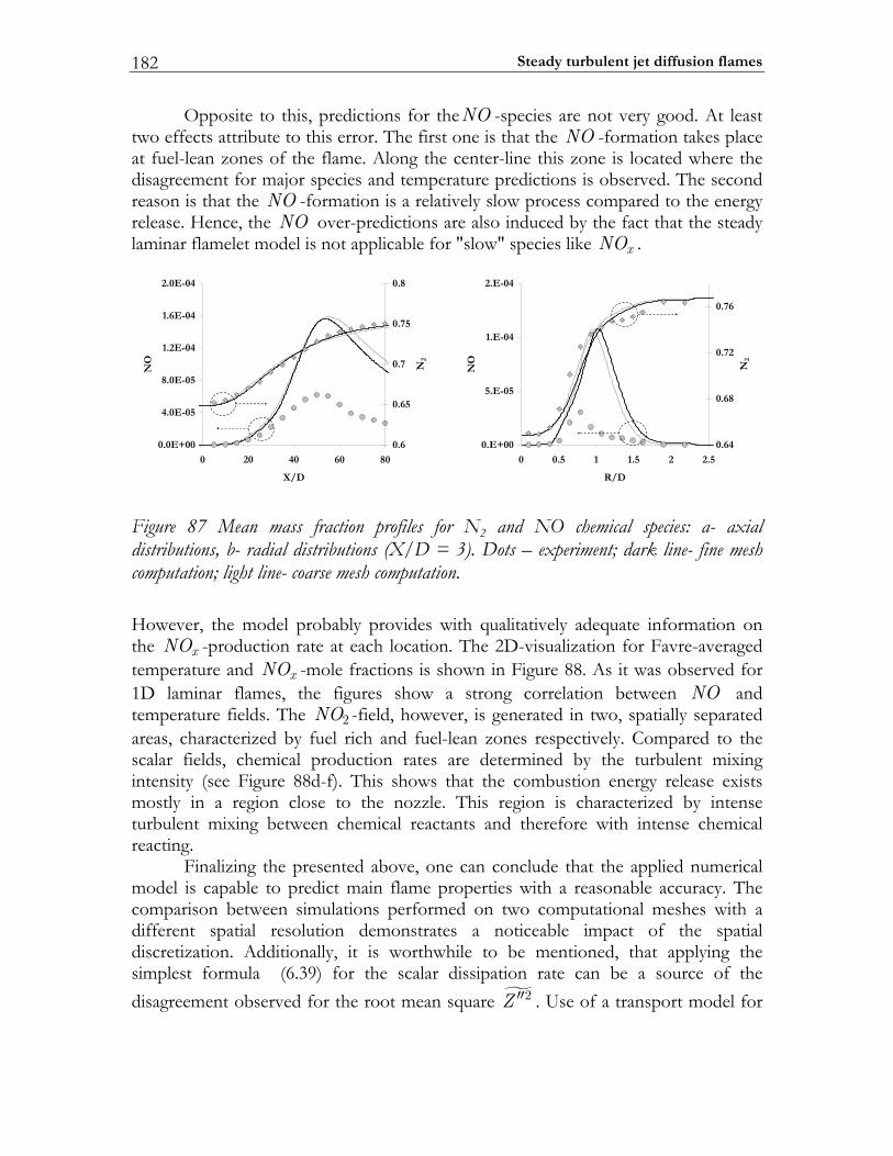
Steady turbulent jet diffusion flames 182
Opposite to this, predictions for theNO -species are not very good. At least two effects attribute to this error. The first one is that the NO -formation takes place at fuel-lean zones of the flame. Along the center-line this zone is located where the disagreement for major species and temperature predictions is observed. The second reason is that the NO -formation is a relatively slow process compared to the energy release. Hence, the NO over-predictions are also induced by the fact that the steady laminar flamelet model is not applicable for "slow" species like xNO .
00+E0.0
50-E0.4
50-E0.8
40-E2.1
40-E6.1
40-E0.2
080604020
D/X
NO
6.0
56.0
7.0
57.0
8.0
N2
00+E.0
50-E.5
40-E.1
40-E.2
5.225.115.00
D/RN
O
46.0
86.0
27.0
67.0
N2
Figure 87 Mean mass fraction profiles for N2 and NO chemical species: a- axial distributions, b- radial distributions (X/D = 3). Dots – experiment; dark line- fine mesh computation; light line- coarse mesh computation. However, the model probably provides with qualitatively adequate information on the xNO -production rate at each location. The 2D-visualization for Favre-averaged temperature and xNO -mole fractions is shown in Figure 88. As it was observed for 1D laminar flames, the figures show a strong correlation between NO and temperature fields. The 2NO -field, however, is generated in two, spatially separated areas, characterized by fuel rich and fuel-lean zones respectively. Compared to the scalar fields, chemical production rates are determined by the turbulent mixing intensity (see Figure 88d-f). This shows that the combustion energy release exists mostly in a region close to the nozzle. This region is characterized by intense turbulent mixing between chemical reactants and therefore with intense chemical reacting. Finalizing the presented above, one can conclude that the applied numerical model is capable to predict main flame properties with a reasonable accuracy. The comparison between simulations performed on two computational meshes with a different spatial resolution demonstrates a noticeable impact of the spatial discretization. Additionally, it is worthwhile to be mentioned, that applying the simplest formula (6.39) for the scalar dissipation rate can be a source of the disagreement observed for the root mean square 2Z ′′ . Use of a transport model for
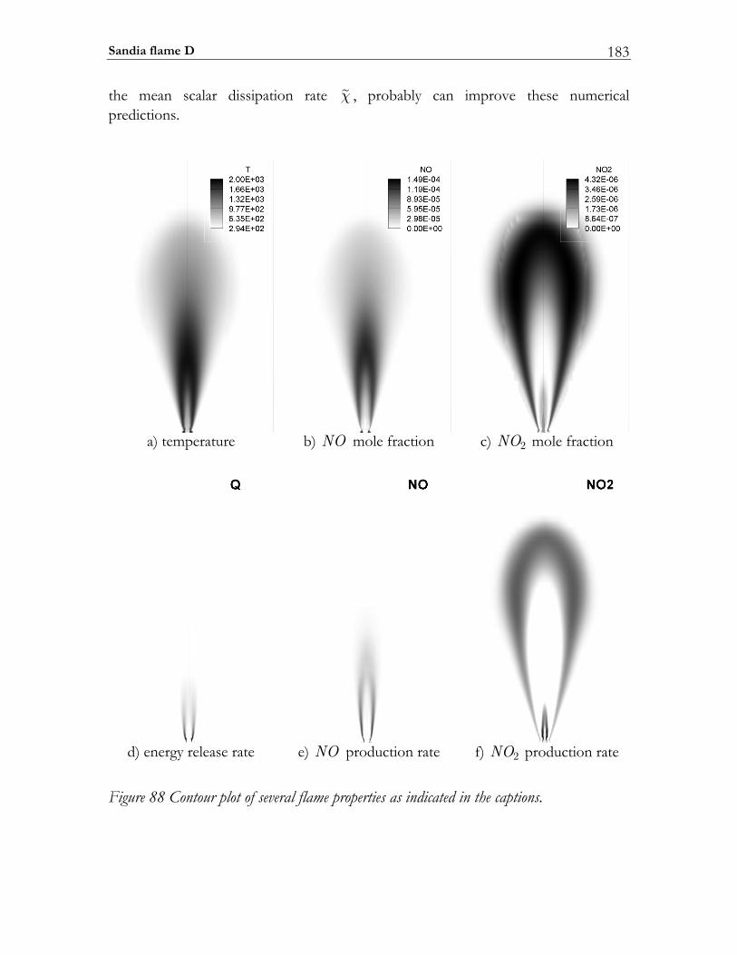
Sandia flame D 183
the mean scalar dissipation rate χ , probably can improve these numerical predictions.
a) temperature b) NO mole fraction c) 2NO mole fraction
d) energy release rate e) NO production rate f) 2NO production rate
Figure 88 Contour plot of several flame properties as indicated in the captions.
Steady turbulent jet diffusion flames 184
6.5 PAH/soot modeling in ethylene/air flame In this section results for a sooting turbulent non-premixed ethylene/air jet flame [182] are presented. This flame has been chosen since it is provided with the soot volume fraction field as well as with the mean mixture fraction (MMF) and mean temperature quantities. In the subsequent section the setup of the Ethylene/Air Jet Flame is described. The experimental and numerical results are compared and analyzed.
6.5.1 Experimental setup of Turbulent Non-premixed Ethylene/Air Jet Flame.
This flame is a rim-stabilized turbulent non-premixed ethylene jet flame [182]. The ethylene issues into stagnant air through a pipe with a diameter of 3.1mm at a speed of 24.5m/s at room temperature and atmospheric pressure. The Reynolds number was about Re 8600= . The visible flame height was about 0.65m. The soot volume fraction profiles along axial and radial directions were measured by a laser-extinction technique along with mixture fraction by microprobe sampling and mass spectrometric analysis. The temperature was determined by thin-wire thermocouples. The axial locations for the radial profile are 160, 250 and 350mm above the exit of the jet.
6.5.2 Numerical setup The geometry applied for this case is identical to the one used in the previous section 6.4. The computational domain in physical size is X = 0.75m in height and with a radius of R = 0.30m. The applied mesh consists of 100 70× cells. In order to model chemical processes of soot formation and oxidation a detailed reaction mechanism [103] based on the sectional approach has been applied. The correspondent SLF database described in chapter 5 has been adopted.
6.5.3 Results and discussion
Mean mixture fraction and temperature Figure 89 presents a comparison of predicted and measured mean mixture fraction (MMF) and mean temperature along the axial direction. Predictions for the mean mixture fraction are obviously not sufficiently accurate. Close to the nozzle there is a fast non-physical mixing leading to a large MMF-gradient initially. The modeling yields MMF-under-prediction starting from the bottom and up to approximately 100mm. Further downstream a relative short region of agreement is observed, however starting from the height of about 150mm the modeled MMF-level is over-predicted. At these distances the modeled mean mixture fraction demonstrates quasi-stationary behavior at nearly-stoichiometric mixing conditions. Opposite to this, the
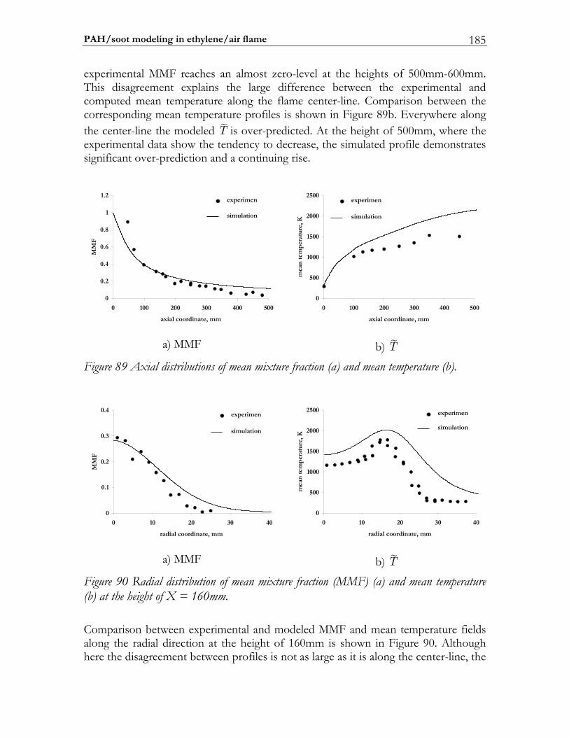
PAH/soot modeling in ethylene/air flame 185
experimental MMF reaches an almost zero-level at the heights of 500mm-600mm. This disagreement explains the large difference between the experimental and computed mean temperature along the flame center-line. Comparison between the corresponding mean temperature profiles is shown in Figure 89b. Everywhere along the center-line the modeled T is over-predicted. At the height of 500mm, where the experimental data show the tendency to decrease, the simulated profile demonstrates significant over-prediction and a continuing rise.
0
2.0
4.0
6.0
8.0
1
2.1
0050040030020010
mm,etanidrooclaixa
MM
F
nemirepxe
noitalumis
0
005
0001
0051
0002
0052
0050040030020010
mm,etanidrooclaixa
mea
nte
mp
erat
ure,
K
nemirepxe
noitalumis
a) MMF b) T
Figure 89 Axial distributions of mean mixture fraction (a) and mean temperature (b).
0
1.0
2.0
3.0
4.0
040302010
mm,etanidrooclaidar
MM
F
nemirepxe
noitalumis
0
005
0001
0051
0002
0052
040302010
mm,etanidrooclaidar
mea
nte
mp
erat
ure,
K
nemirepxe
noitalumis
a) MMF b) T
Figure 90 Radial distribution of mean mixture fraction (MMF) (a) and mean temperature (b) at the height of X = 160mm. Comparison between experimental and modeled MMF and mean temperature fields along the radial direction at the height of 160mm is shown in Figure 90. Although here the disagreement between profiles is not as large as it is along the center-line, the
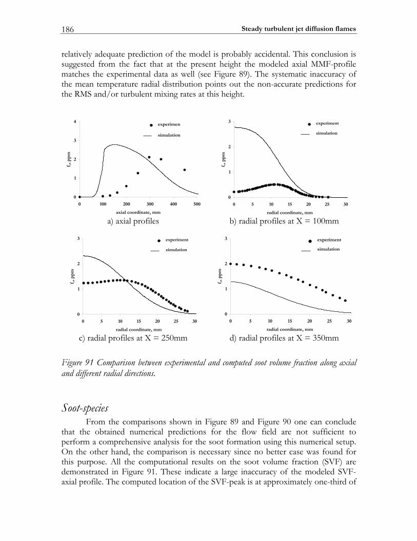
Steady turbulent jet diffusion flames 186
relatively adequate prediction of the model is probably accidental. This conclusion is suggested from the fact that at the present height the modeled axial MMF-profile matches the experimental data as well (see Figure 89). The systematic inaccuracy of the mean temperature radial distribution points out the non-accurate predictions for the RMS and/or turbulent mixing rates at this height.
0
1
2
3
4
0 100 200 300 400 500
axial coordinate, mm
f v, p
pm
experimen
simulation
0
1
2
3
0 5 10 15 20 25 30
radial coordinate, mm
f v, p
pm
experiment
simulation
a) axial profiles b) radial profiles at X = 100mm
0
1
2
3
0 5 10 15 20 25 30
radial coordinate, mm
f v, p
pm
experiment
simulation
0
1
2
3
0 5 10 15 20 25 30
radial coordinate, mm
f v, p
pm
experiment
simulation
c) radial profiles at X = 250mm d) radial profiles at X = 350mm
Figure 91 Comparison between experimental and computed soot volume fraction along axial and different radial directions.
Soot-species From the comparisons shown in Figure 89 and Figure 90 one can conclude that the obtained numerical predictions for the flow field are not sufficient to perform a comprehensive analysis for the soot formation using this numerical setup. On the other hand, the comparison is necessary since no better case was found for this purpose. All the computational results on the soot volume fraction (SVF) are demonstrated in Figure 91. These indicate a large inaccuracy of the modeled SVF-axial profile. The computed location of the SVF-peak is at approximately one-third of
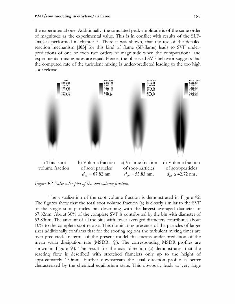
PAH/soot modeling in ethylene/air flame 187
the experimental one. Additionally, the simulated peak amplitude is of the same order of magnitude as the experimental value. This is in conflict with results of the SLF-analysis performed in chapter 5. There it was shown, that the use of the detailed reaction mechanism [103] for this kind of flame (SF-flame) leads to SVF under-predictions of one or even two orders of magnitude when the computational and experimental mixing rates are equal. Hence, the observed SVF-behavior suggests that the computed rate of the turbulent mixing is under-predicted leading to the too high soot release.
a) Total soot
volume fraction b) Volume fraction
of soot particles 67.82 nmeffd =
c) Volume fraction of soot-particles
53.83 nmeffd = .
d) Volume fraction of soot-particles
42.72 nmeffd ≤ .
Figure 92 False color plot of the soot volume fraction. The visualization of the soot volume fraction is demonstrated in Figure 92. The figures show that the total soot volume fraction (a) is closely similar to the SVF of the single soot particles bin describing with the largest averaged diameter of 67.82nm. About 30% of the complete SVF is contributed by the bin with diameter of 53.83nm. The amount of all the bins with lower averaged diameters contributes about 10% to the complete soot release. This dominating presence of the particles of larger sizes additionally confirms that for the sooting regions the turbulent mixing times are over-predicted. In terms of the present model this means under-prediction of the mean scalar dissipation rate (MSDR, χ ). The corresponding MSDR profiles are shown in Figure 93. The result for the axial direction (a) demonstrates, that the reacting flow is described with stretched flamelets only up to the height of approximately 150mm. Further downstream the axial direction profile is better characterized by the chemical equilibrium state. This obviously leads to very large
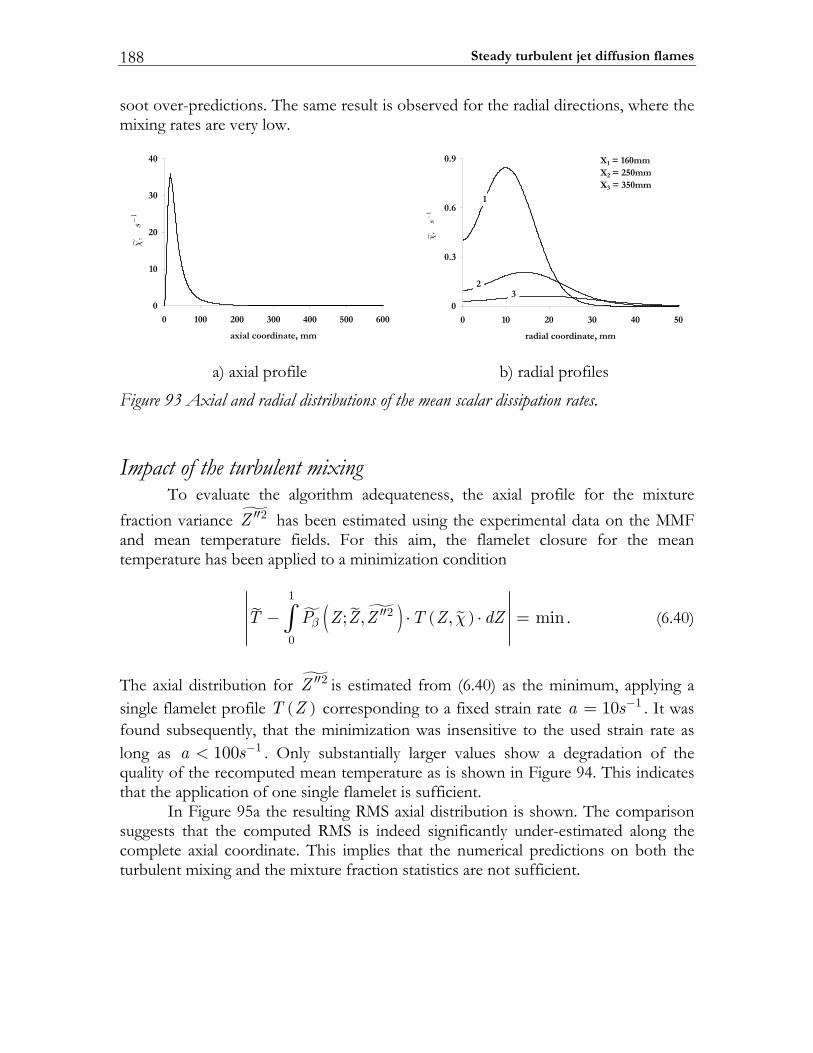
Steady turbulent jet diffusion flames 188
soot over-predictions. The same result is observed for the radial directions, where the mixing rates are very low.
0
10
20
30
40
0 100 200 300 400 500 600
axial coordinate, mm
1,s
0
0.3
0.6
0.9
0 10 20 30 40 50
radial coordinate, mm
X1 = 160mmX2 = 250mmX3 = 350mm
1
23
1,s
a) axial profile b) radial profiles
Figure 93 Axial and radial distributions of the mean scalar dissipation rates.
Impact of the turbulent mixing To evaluate the algorithm adequateness, the axial profile for the mixture fraction variance 2Z ′′ has been estimated using the experimental data on the MMF and mean temperature fields. For this aim, the flamelet closure for the mean temperature has been applied to a minimization condition
( ) ( )1
2
0
; , , minT P Z Z Z T Z dZβ χ′′− ⋅ ⋅ =∫ . (6.40)
The axial distribution for 2Z ′′ is estimated from (6.40) as the minimum, applying a single flamelet profile ( )T Z corresponding to a fixed strain rate 110a s−= . It was found subsequently, that the minimization was insensitive to the used strain rate as long as 1100a s−< . Only substantially larger values show a degradation of the quality of the recomputed mean temperature as is shown in Figure 94. This indicates that the application of one single flamelet is sufficient. In Figure 95a the resulting RMS axial distribution is shown. The comparison suggests that the computed RMS is indeed significantly under-estimated along the complete axial coordinate. This implies that the numerical predictions on both the turbulent mixing and the mixture fraction statistics are not sufficient.
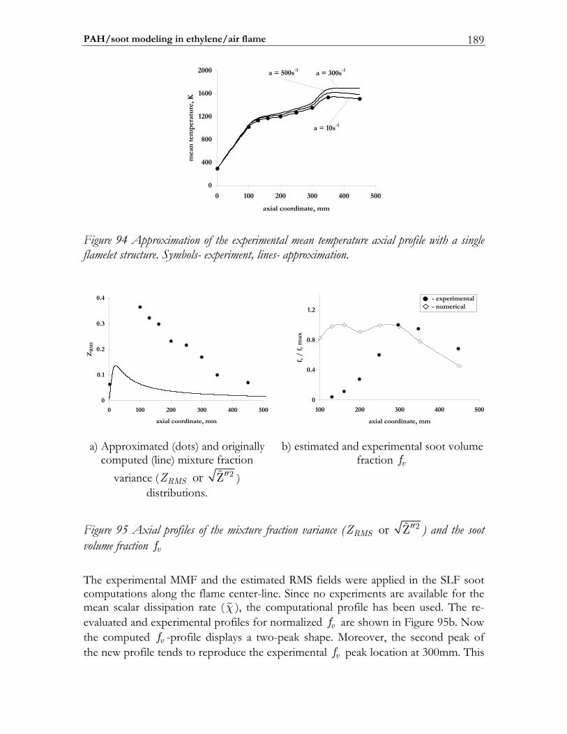
PAH/soot modeling in ethylene/air flame 189
0
400
800
1200
1600
2000
0 100 200 300 400 500
axial coordinate, mm
mea
n t
emp
erat
ure
,K
a = 500s-1 a = 300s-1
a = 10s-1
Figure 94 Approximation of the experimental mean temperature axial profile with a single flamelet structure. Symbols- experiment, lines- approximation.
0
0.1
0.2
0.3
0.4
0 100 200 300 400 500
axial coordinate, mm
ZR
MS
0
0.4
0.8
1.2
100 200 300 400 500
axial coordinate, mm
f v /
f v m
ax - experimental - numerical
a) Approximated (dots) and originally
computed (line) mixture fraction variance ( 2 or ZRMSZ ′′ )
distributions.
b) estimated and experimental soot volume fraction vf
Figure 95 Axial profiles of the mixture fraction variance ( 2 or ZRMSZ ′′ ) and the soot volume fraction vf The experimental MMF and the estimated RMS fields were applied in the SLF soot computations along the flame center-line. Since no experiments are available for the mean scalar dissipation rate (χ ), the computational profile has been used. The re-evaluated and experimental profiles for normalized vf are shown in Figure 95b. Now the computed vf -profile displays a two-peak shape. Moreover, the second peak of the new profile tends to reproduce the experimental vf peak location at 300mm. This
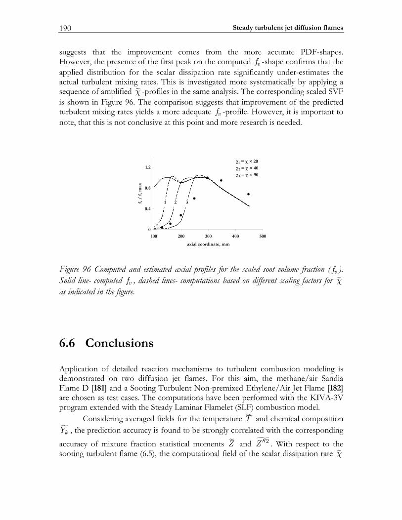
Steady turbulent jet diffusion flames 190
suggests that the improvement comes from the more accurate PDF-shapes. However, the presence of the first peak on the computed vf -shape confirms that the applied distribution for the scalar dissipation rate significantly under-estimates the actual turbulent mixing rates. This is investigated more systematically by applying a sequence of amplified χ -profiles in the same analysis. The corresponding scaled SVF is shown in Figure 96. The comparison suggests that improvement of the predicted turbulent mixing rates yields a more adequate vf -profile. However, it is important to note, that this is not conclusive at this point and more research is needed.
0
0.4
0.8
1.2
100 200 300 400 500
axial coordinate, mm
f v /
f v m
ax
1 2 3
1 = × 20
2 = × 40
3 = × 90
Figure 96 Computed and estimated axial profiles for the scaled soot volume fraction ( vf ). Solid line- computed vf , dashed lines- computations based on different scaling factors for χ as indicated in the figure.
6.6 Conclusions Application of detailed reaction mechanisms to turbulent combustion modeling is demonstrated on two diffusion jet flames. For this aim, the methane/air Sandia Flame D [181] and a Sooting Turbulent Non-premixed Ethylene/Air Jet Flame [182] are chosen as test cases. The computations have been performed with the KIVA-3V program extended with the Steady Laminar Flamelet (SLF) combustion model. Considering averaged fields for the temperature T and chemical composition kY , the prediction accuracy is found to be strongly correlated with the corresponding
accuracy of mixture fraction statistical moments Z and 2Z ′′ . With respect to the sooting turbulent flame (6.5), the computational field of the scalar dissipation rate χ
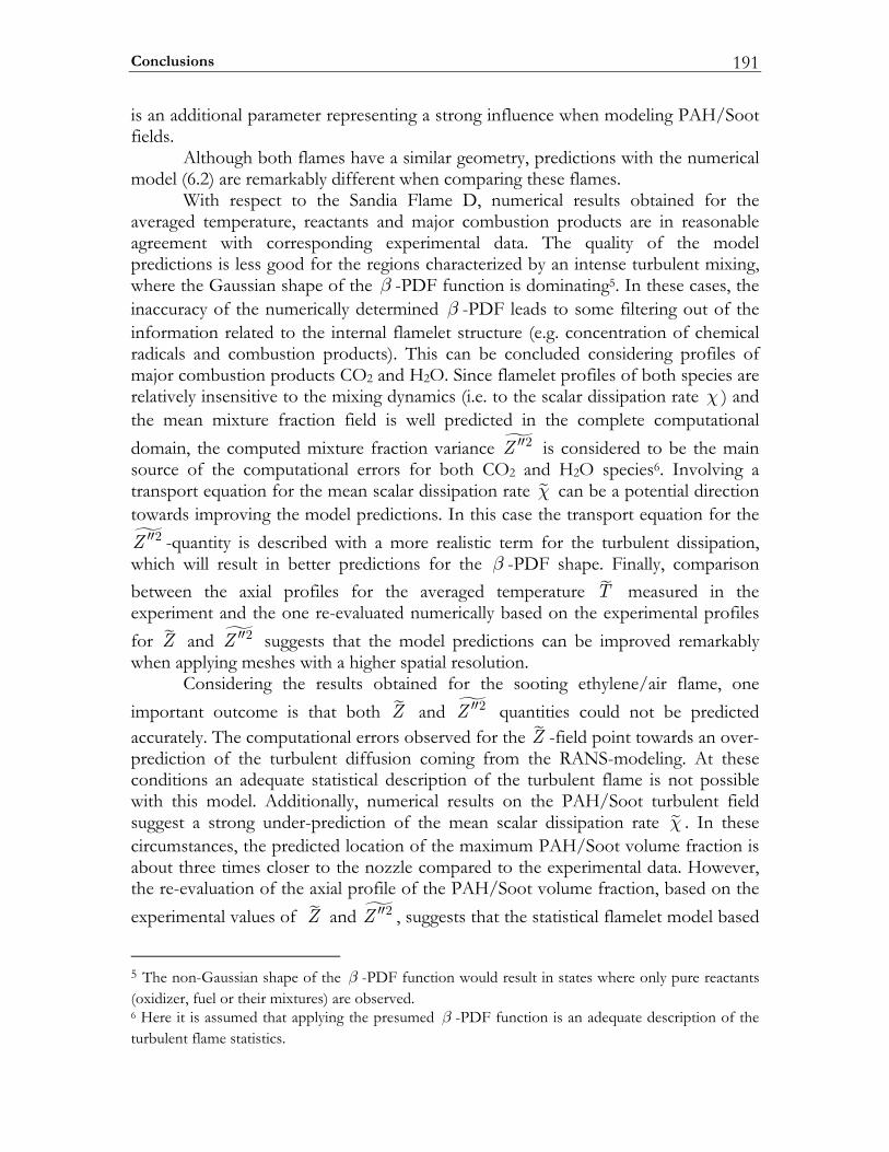
Conclusions 191
is an additional parameter representing a strong influence when modeling PAH/Soot fields. Although both flames have a similar geometry, predictions with the numerical model (6.2) are remarkably different when comparing these flames. With respect to the Sandia Flame D, numerical results obtained for the averaged temperature, reactants and major combustion products are in reasonable agreement with corresponding experimental data. The quality of the model predictions is less good for the regions characterized by an intense turbulent mixing, where the Gaussian shape of the β -PDF function is dominating5. In these cases, the inaccuracy of the numerically determined β -PDF leads to some filtering out of the information related to the internal flamelet structure (e.g. concentration of chemical radicals and combustion products). This can be concluded considering profiles of major combustion products CO2 and H2O. Since flamelet profiles of both species are relatively insensitive to the mixing dynamics (i.e. to the scalar dissipation rate χ ) and the mean mixture fraction field is well predicted in the complete computational domain, the computed mixture fraction variance 2Z ′′ is considered to be the main source of the computational errors for both CO2 and H2O species6. Involving a transport equation for the mean scalar dissipation rate χ can be a potential direction towards improving the model predictions. In this case the transport equation for the
2Z ′′ -quantity is described with a more realistic term for the turbulent dissipation, which will result in better predictions for the β -PDF shape. Finally, comparison between the axial profiles for the averaged temperature T measured in the experiment and the one re-evaluated numerically based on the experimental profiles for Z and 2Z ′′ suggests that the model predictions can be improved remarkably when applying meshes with a higher spatial resolution. Considering the results obtained for the sooting ethylene/air flame, one important outcome is that both Z and 2Z ′′ quantities could not be predicted accurately. The computational errors observed for the Z -field point towards an over-prediction of the turbulent diffusion coming from the RANS-modeling. At these conditions an adequate statistical description of the turbulent flame is not possible with this model. Additionally, numerical results on the PAH/Soot turbulent field suggest a strong under-prediction of the mean scalar dissipation rate χ . In these circumstances, the predicted location of the maximum PAH/Soot volume fraction is about three times closer to the nozzle compared to the experimental data. However, the re-evaluation of the axial profile of the PAH/Soot volume fraction, based on the experimental values of Z and 2Z ′′ , suggests that the statistical flamelet model based
5 The non-Gaussian shape of the β -PDF function would result in states where only pure reactants (oxidizer, fuel or their mixtures) are observed. 6 Here it is assumed that applying the presumed β -PDF function is an adequate description of the turbulent flame statistics.
Steady turbulent jet diffusion flames 192
on the presumed β -PDF is capable of reproducing the correct PAH/Soot profile if Z , 2Z ′′ and χ quantities are well predicted by the CFD-simulation. On the other hand, it is important to mention, that capturing other details like particles size distribution function (for each spatial location) requires applying a combustion model taking into account time-dependent effects (see e.g. Representative Interactive Flamelet [176] or Eddy Dissipation Concept [30]). The presented qualitative comparison between numerical predictions for the two selected turbulent jet-flames demonstrates the impact of the turbulence model. Both flames are establishes in the simplest geometry and were computed using the same CFD-simulator and the same kind of the spatial mesh. Despite this, the quality of computational predictions is drastically different. The obtained results suggest that when applying comprehensive reaction mechanisms in practical simulations of IC-engines an adequate prediction of the turbulent mixing processes is an additional issue of importance. The last can be ensured during the stage prior to the complex modeling or can be achieved employing more advanced turbulence models like e.g. the Large Eddy Simulation approach.
Chapter 7
7 Conclusions and recommendations In this thesis a generic approach for handling complex thermo-physical and chemical reaction models for practical combustion simulations is introduced. This approach considers a variety of 0D and 1D combustion sub-models as a common basis for applying complex reaction mechanisms in industrial simulations (e.g. Diesel engine modeling). The approach has been applied for modeling of high-pressure effects on combustion at Diesel-like conditions, for modeling of the effects of mixing dynamics on the soot formation in laminar diffusion flamelets and for modeling of turbulent diffusion jet-flames. The quantitative consequence of applying the ideal gas assumption for modeling the gas-phase combustion at elevated pressures was considered for two different aspects. The first one is related to the impact of this assumption on modeling compression/expansion processes in homogeneous gas mixtures. In this case, the temperature errors resulting from applying the ideal gas law lead to errors when calculating important temperature-sensitive phenomena like auto-ignition and NO-formation. The second aspect is related to the impact of the non-ideality on computed laminar flamelet structures. Now the effect is due to the differences between the gas volumetric concentrations and molecular transport properties when either the ideal gas or the real gas models are used. The impact of the mixing dynamics on the PAH/Soot formation processes in laminar diffusion flamelets was studied by modeling counterflow diffusion flames. In order to model formation of PAH/Soot particles of different sizes a detailed reaction mechanism based on the sectional approach was applied. An application of the developed approach is demonstrated by simulations of methane and ethylene turbulent diffusion jet flames. The most important aspects and results of each of these studies are summarized below together with some recommendation for future research. In Chapter 2 a generic approach for the problem of data processing and a strategy for improving computational performance were presented. With respect to the focus of this thesis, the application of these techniques leads to the two main results. The first one is the possibility of using arbitrarily complex thermo-physical/chemical models in practical CFD-simulations. This includes a wide range of
Conclusions and recommendations 194
non-ideal gas descriptions based on the law of Corresponding States. The second outcome is the significant computational speedup achieved by the representation of the actual thermo-physical and chemical parameters in the form of a computer code C-MECH adapted for high-performance computing. In the future research, the TROT data processor can be used for modeling of high pressure multi-component droplet vaporization and for modeling of many other high pressure phenomena, e.g. for thermodynamic modeling of detonation. A better computational performance can even be achieved by applying an adaptive tabulation technique to the temperature-dependent properties of reaction models. In Chapter 3 the applicability of the ideal gas assumption for modeling high-pressure compression-reaction processes was studied. The results from homogeneous auto-ignition and NO-formation simulations applying the ideal gas and real gas models were compared. The comparison has shown that inaccuracy of the ideal gas assumption is determined not only by the P-V-T conditions but also by the problem formulation itself. In future research, when applying the ideal gas model, the potential errors have to be estimated in an appropriate way. With respect to IC-engine modeling, the obtained results confirm that the ideal gas law is well-applicable for the range of practical interest. Chapter 4 presented the computational algorithms used for resolving the structure of 1D (laminar) diffusion flamelets described with complex chemistry. The impact of gas non-ideality on the flamelet structure was evaluated by comparisons between flames computed using ideal gas and real gas models. The computations were performed for the so-called "worst" case of the fuel-component non-ideality. The obtained results have shown that the real gas defects which can be high near the fuel-boundary are rapidly decreasing towards the stoichiometric surface. The predicted combustion characteristics of the flamelets at high-pressure were found to be insensitive to the thermodynamic model. For the practical CFD-modeling of high-pressure combustion this result suggests that for a flamelet model to determine the chemical composition (or reaction rates) it is appropriate to apply the ideal gas assumption. The application of a non-ideal gas model would be necessary only if the flamelet computation is additionally used to determine the molecular transport properties. Note that this last situation can occur in the CFD-modeling based on the Large Eddy Simulation approach. Chapter 5 was dedicated to detailed modeling of PAH/Soot formation. The results on PAH/Soot formation in ethylene/air and benzene/air counterflow diffusion flames were presented. The effect of strain rate on PAH/Soot was considered in terms of major characteristics like the mass- and number-density as well as in terms of particle size distribution function. The analysis of the benzene and ethylene flames confirms the general experimental observations that soot mass and number densities (first two moments of the PSDF) depend strongly on the mixing characteristics within a flame. An important result from this work is that for low strain rates a bimodal distribution function for the volume fraction is reproduced, which is in correspondence with experimental observations by D’Alessio. This questions the assumption of a lognormal distribution, which is generally used in the
195
method of moments. In future research, the current implementation of the sectional approach (based on the C-MECH source code) can be used to model the time-dependent effects on PAH/Soot formation in turbulent combustion. Adequate modeling of these processes could be achieved using 0D- (e.g. Eddy Dissipation Concept) or 1D- (e.g. Representative Interactive Flamelet) type of combustion sub-models. In Chapter 6 the application of detailed reaction mechanisms based on the steady laminar flamelet (1D) model to turbulent diffusion jet-flames was presented. A partially premixed methane/air flame (Sandia Flame D) and a sooting non-premixed ethylene/air flames were considered. The results were compared to available experimental data. Although both flames have a similar geometry, predictions with the numerical model were found to be remarkably different when comparing these flames. With respect to the Sandia Flame D, numerical results obtained for the averaged temperature, reactants and major combustion products are in reasonable agreement with corresponding experimental data. Considering the results obtained for the sooting ethylene/air flame, one important outcome was that the two main statistical moments of the mixture fraction variable could not be predicted accurately. In these circumstances, the predicted location of the maximum PAH/Soot volume fraction is about three times closer to the nozzle than the experimentally found location. However, the re-evaluation of the axial profile of the PAH/Soot volume fraction, based on the experimental values of the mixture fraction, suggests that the statistical flamelet model based on the presumed beta-PDF is capable of reproducing the correct PAH/Soot profile if the mixing characteristics are well predicted by the CFD-simulation. In future research, capturing other details like the particles size distribution function (for each spatial location) requires applying a combustion model taking into account time-dependent effects. The obtained results point out that when applying comprehensive reaction mechanisms in practical simulations of IC-engines an adequate prediction of the turbulent mixing processes is an important/crucial issue. The last can be ensured during the stage prior to simulations using the complete model by adjusting the model parameters (e.g. in RANS simulations) or by employing more advanced turbulence models like e.g. the Large Eddy Simulation approach.

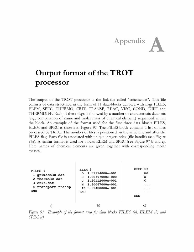
Appendix A
A Output format of the TROT processor
The output of the TROT processor is the link-file called "scheme.dat". This file consists of data structured in the form of 11 data-blocks denoted with flags FILES, ELEM, SPEC, THERMO, CRIT, TRANSP, REAC, VISC, COND, DIFF and THERMDIFF. Each of these flags is followed by a number of characteristic data-sets (e.g., combination of name and molar mass of chemical element) sequenced within the block. An example of the format used for the first three data blocks FILES, ELEM and SPEC is shown in Figure 97. The FILES-block contains a list of files processed by TROT. The number of files is positioned on the same line and after the FILES-flag. Each file is associated with unique integer index (file handle) (see Figure 97a). A similar format is used for blocks ELEM and SPEC (see Figure 97 b and c). Here names of chemical elements are given together with corresponding molar masses.
FILES 41 grimech30.dat2 thermo30.dat3 crit.dat4 transport.transp
END
SPEC 53H2HO.........
END
a) b) c)
Figure 97 Example of the format used for data blocks FILES (a), ELEM (b) and SPEC (c)
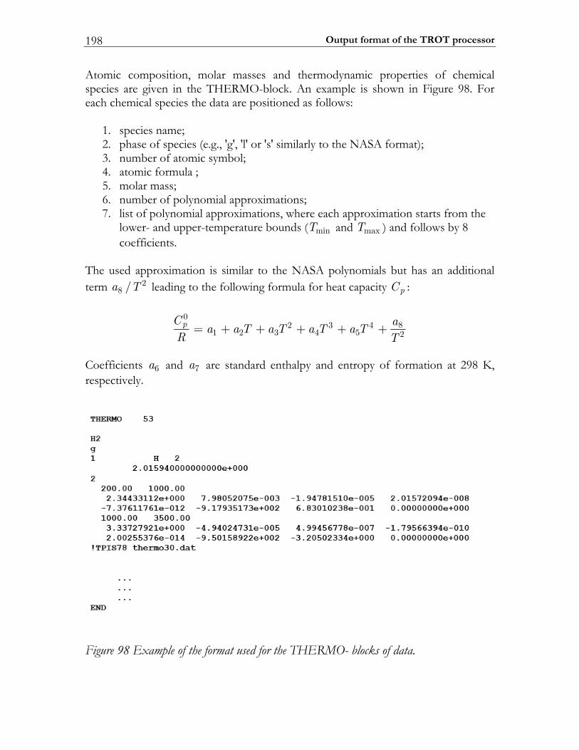
Output format of the TROT processor 198
Atomic composition, molar masses and thermodynamic properties of chemical species are given in the THERMO-block. An example is shown in Figure 98. For each chemical species the data are positioned as follows:
1. species name; 2. phase of species (e.g., 'g', 'l' or 's' similarly to the NASA format); 3. number of atomic symbol; 4. atomic formula ; 5. molar mass; 6. number of polynomial approximations; 7. list of polynomial approximations, where each approximation starts from the
lower- and upper-temperature bounds ( minT and maxT ) and follows by 8 coefficients.
The used approximation is similar to the NASA polynomials but has an additional term 2
8 /a T leading to the following formula for heat capacity pC :
0
82 3 41 2 3 4 5 2
pC aa a T a T a T a TR T= + + + + +
Coefficients 6a and 7a are standard enthalpy and entropy of formation at 298 K, respectively.
Figure 98 Example of the format used for the THERMO- blocks of data.
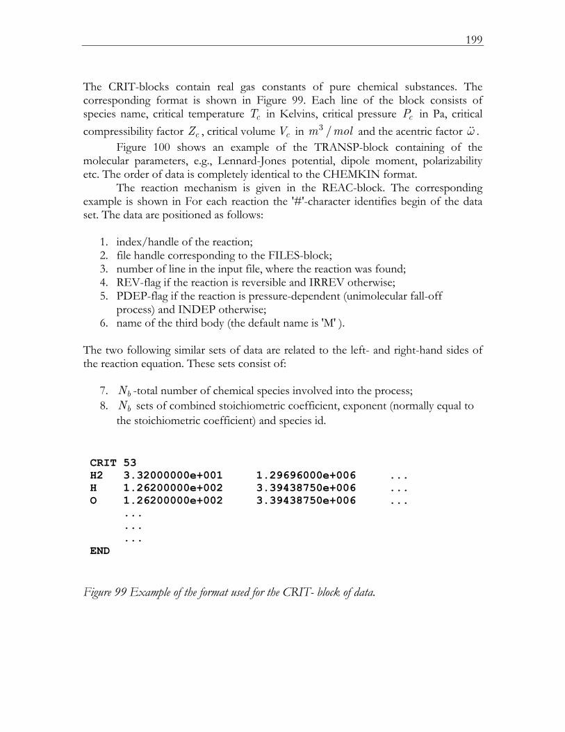
199
The CRIT-blocks contain real gas constants of pure chemical substances. The corresponding format is shown in Figure 99. Each line of the block consists of species name, critical temperature cT in Kelvins, critical pressure cP in Pa, critical compressibility factor cZ , critical volume cV in 3 /m mol and the acentric factor ω . Figure 100 shows an example of the TRANSP-block containing of the molecular parameters, e.g., Lennard-Jones potential, dipole moment, polarizability etc. The order of data is completely identical to the CHEMKIN format. The reaction mechanism is given in the REAC-block. The corresponding example is shown in For each reaction the '#'-character identifies begin of the data set. The data are positioned as follows:
1. index/handle of the reaction; 2. file handle corresponding to the FILES-block; 3. number of line in the input file, where the reaction was found; 4. REV-flag if the reaction is reversible and IRREV otherwise; 5. PDEP-flag if the reaction is pressure-dependent (unimolecular fall-off
process) and INDEP otherwise; 6. name of the third body (the default name is 'M' ).
The two following similar sets of data are related to the left- and right-hand sides of the reaction equation. These sets consist of:
7. bN -total number of chemical species involved into the process; 8. bN sets of combined stoichiometric coefficient, exponent (normally equal to
the stoichiometric coefficient) and species id.
CRIT 53H2 3.32000000e+001 1.29696000e+006 ...H 1.26200000e+002 3.39438750e+006 ...O 1.26200000e+002 3.39438750e+006 ...
...
...
...END
Figure 99 Example of the format used for the CRIT- block of data.
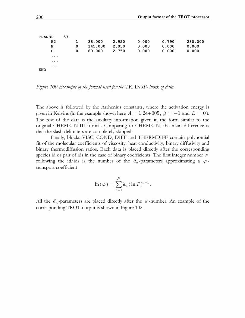
Output format of the TROT processor 200
TRANSP 53H2 1 38.000 2.920 0.000 0.790 280.000H 0 145.000 2.050 0.000 0.000 0.000O 0 80.000 2.750 0.000 0.000 0.000.........
END
Figure 100 Example of the format used for the TRANSP- block of data. The above is followed by the Arrhenius constants, where the activation energy is given in Kelvins (in the example shown here 1.2e+005A = , 1β = − and 0E = ). The rest of the data is the auxiliary information given in the form similar to the original CHEMKIN-III format. Comparing to CHEMKIN, the main difference is that the slash-delimiters are completely skipped. Finally, blocks VISC, COND, DIFF and THERMDIFF contain polynomial fit of the molecular coefficients of viscosity, heat conductivity, binary diffusivity and binary thermodiffusion ratios. Each data is placed directly after the corresponding species id or pair of ids in the case of binary coefficients. The first integer number N following the id/ids is the number of the na -parameters approximating a ϕ -transport coefficient
( ) ( ) 1
1ln ln
Nn
nna Tϕ −
==∑ .
All the na -parameters are placed directly after the N -number. An example of the corresponding TROT-output is shown in Figure 102.
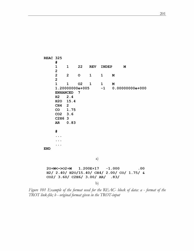
201
REAC 325#1 1 22 REV INDEP M22 2 O 1 1 M21 1 O2 1 1 M1.20000000e+005 -1 0.00000000e+000ENHANCED 7H2 2.4H2O 15.4CH4 2CO 1.75CO2 3.6C2H6 3AR 0.83
#.........
END
a)
b)
Figure 101 Example of the format used for the REAC- block of data: a - format of the TROT link-file; b - original format given in the TROT-input
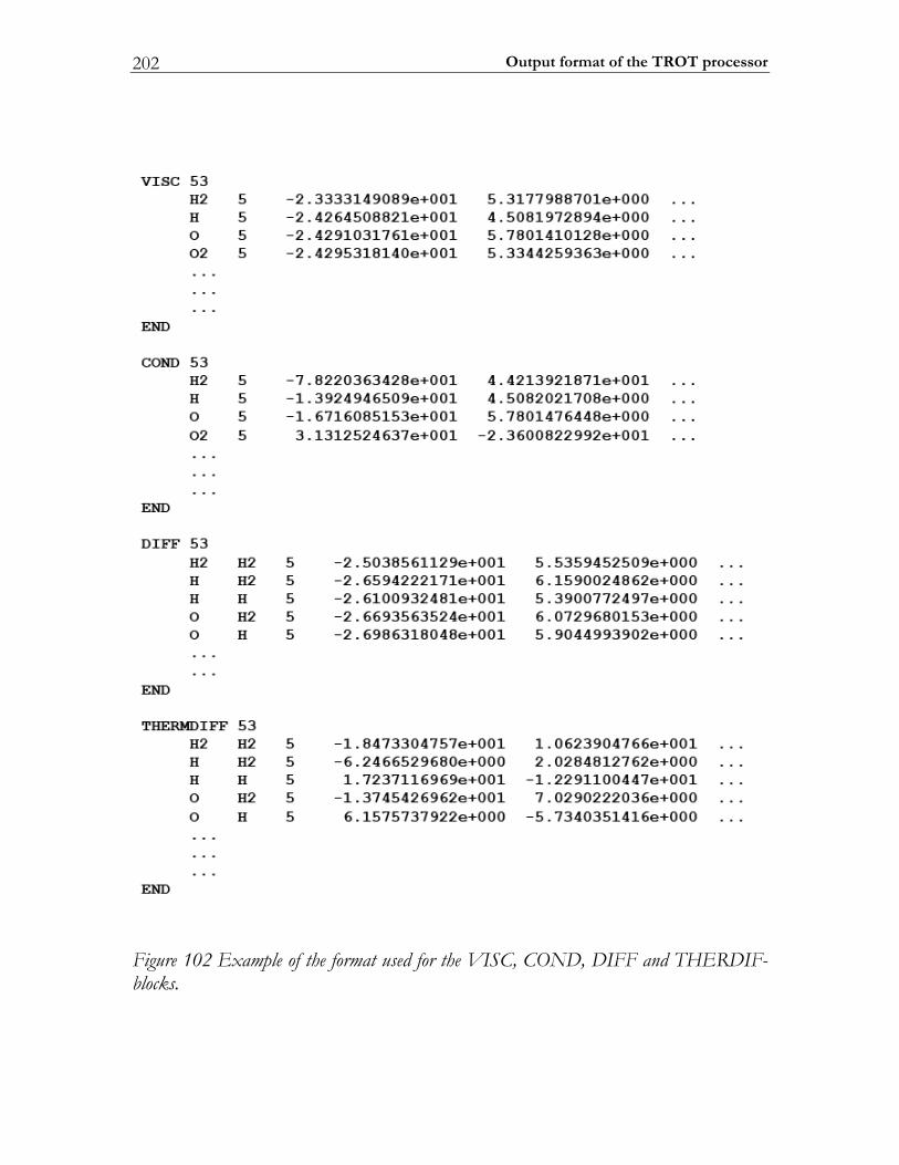
Output format of the TROT processor 202
Figure 102 Example of the format used for the VISC, COND, DIFF and THERDIF- blocks.
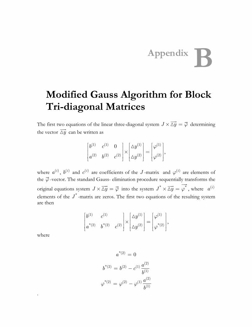
Appendix B
B Modified Gauss Algorithm for Block Tri-diagonal Matrices
The first two equations of the linear three-diagonal system J y ϕ× = determining the vector y can be written as
(1) (1) (1) (1)
(2) (2) (2) (2) (2)
0b c y
a b c y
ϕ
ϕ
⎡ ⎤ ⎡ ⎤ ⎡ ⎤⎢ ⎥ ⎢ ⎥ ⎢ ⎥× =⎢ ⎥ ⎢ ⎥ ⎢ ⎥⎢ ⎥ ⎢ ⎥ ⎢ ⎥⎣ ⎦ ⎣ ⎦ ⎣ ⎦
,
where ( )ia , ( )ib and ( )ic are coefficients of the J -matrix and ( )iϕ are elements of the ϕ -vector. The standard Gauss- elimination procedure sequentially transforms the
original equations system J y ϕ× = into the system * *J y ϕ× = , where ( )ia elements of the *J -matrix are zeros. The first two equations of the resulting system are then
(1) (1) (1) (1)
*(2) *(2) (2) (2) *(2)
b c y
a b c y
ϕ
ϕ
⎡ ⎤ ⎡ ⎤ ⎡ ⎤⎢ ⎥ ⎢ ⎥ ⎢ ⎥× =⎢ ⎥ ⎢ ⎥ ⎢ ⎥⎢ ⎥ ⎢ ⎥ ⎢ ⎥⎣ ⎦ ⎣ ⎦ ⎣ ⎦
,
where
*(2)
(2)*(2) (2) (1)
(1)
(2)*(2) (2) (1)
(1)
0a
ab b cbab
ϕ ϕ ϕ
=
= −
= −
.
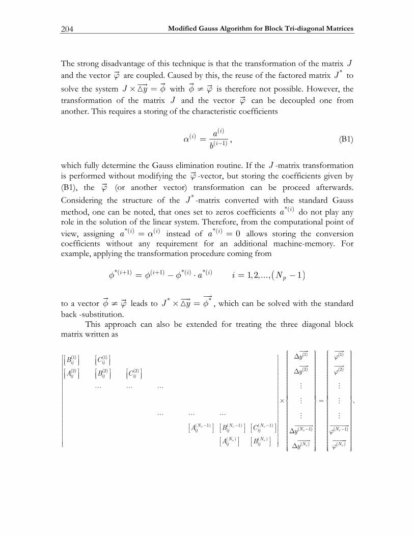
Modified Gauss Algorithm for Block Tri-diagonal Matrices 204
The strong disadvantage of this technique is that the transformation of the matrix J and the vector ϕ are coupled. Caused by this, the reuse of the factored matrix *J to solve the system J y φ× = with φ ϕ≠ is therefore not possible. However, the transformation of the matrix J and the vector ϕ can be decoupled one from another. This requires a storing of the characteristic coefficients
( )
( )( 1)
ii
iab
α −= , (B1)
which fully determine the Gauss elimination routine. If the J -matrix transformation is performed without modifying the ϕ -vector, but storing the coefficients given by (B1), the ϕ (or another vector) transformation can be proceed afterwards. Considering the structure of the *J -matrix converted with the standard Gauss method, one can be noted, that ones set to zeros coefficients *( )ia do not play any role in the solution of the linear system. Therefore, from the computational point of view, assigning *( ) ( )i ia α= instead of *( ) 0ia = allows storing the conversion coefficients without any requirement for an additional machine-memory. For example, applying the transformation procedure coming from ( )*( 1) ( 1) *( ) *( ) 1,2,..., 1i i i i
pa i Nφ φ φ+ += − ⋅ = −
to a vector φ ϕ≠ leads to * *J y φ× = , which can be solved with the standard back -substitution. This approach can also be extended for treating the three diagonal block matrix written as
( ) ( ) ( )
( ) ( )
(1)(1) (1)
(2)(2) (2) (2)
1 1 1( 1)
( )
v v vv
v vv
ij ij
ij ij ij
N N NNij ij ij
N Nij ij N
yB C
yA B C
A B C yA B
y
− − −−
∆⎡ ⎤⎡ ⎤ ⎡ ⎤⎢ ⎥ ⎢ ⎥⎢ ⎥⎣ ⎦ ⎣ ⎦⎢ ⎥ ∆⎡ ⎤ ⎡ ⎤ ⎡ ⎤⎢ ⎥⎢ ⎥ ⎢ ⎥ ⎢ ⎥⎣ ⎦ ⎣ ⎦ ⎣ ⎦⎢ ⎥⎢ ⎥⎢ ⎥⎢ ⎥⎢ ⎥⎢ ⎥×⎢ ⎥⎢ ⎥⎢ ⎥⎢ ⎥⎢ ⎥⎡ ⎤ ⎡ ⎤ ⎡ ⎤⎢ ⎥⎣ ⎦ ⎣ ⎦ ⎣ ⎦ ∆⎢ ⎥⎢ ⎥⎡ ⎤ ⎡ ⎤⎢ ⎥⎣ ⎦ ⎣ ⎦⎣ ⎦ ∆
(1)
(2)
( 1)
( )
,
v
v
N
N
ϕ
ϕ
ϕ
ϕ
−
⎧ ⎫ ⎧ ⎫⎪ ⎪ ⎪ ⎪⎪ ⎪ ⎪ ⎪⎪ ⎪ ⎪ ⎪⎪ ⎪ ⎪ ⎪⎪ ⎪ ⎪ ⎪⎪ ⎪ ⎪ ⎪⎪ ⎪ ⎪ ⎪⎪ ⎪ ⎪ ⎪⎪ ⎪ ⎪ ⎪⎪ ⎪ ⎪ ⎪⎪ ⎪ ⎪ ⎪⎪ ⎪ ⎪ ⎪⎪ ⎪ ⎪ ⎪⎪ ⎪ ⎪ ⎪⎪ ⎪ ⎪ ⎪⎪ ⎪ ⎪ ⎪⎪ ⎪ ⎪ ⎪=⎨ ⎬ ⎨ ⎬⎪ ⎪ ⎪ ⎪⎪ ⎪ ⎪ ⎪⎪ ⎪ ⎪ ⎪⎪ ⎪ ⎪ ⎪⎪ ⎪ ⎪ ⎪⎪ ⎪ ⎪ ⎪⎪ ⎪ ⎪ ⎪⎪ ⎪ ⎪ ⎪⎪ ⎪ ⎪ ⎪⎪ ⎪ ⎪ ⎪⎪ ⎪ ⎪ ⎪⎪ ⎪ ⎪ ⎪⎪ ⎪ ⎪ ⎪⎪ ⎪ ⎪ ⎪⎪ ⎪ ⎪ ⎪⎪ ⎪ ⎪ ⎪⎪ ⎪ ⎪ ⎪⎩ ⎭ ⎩ ⎭
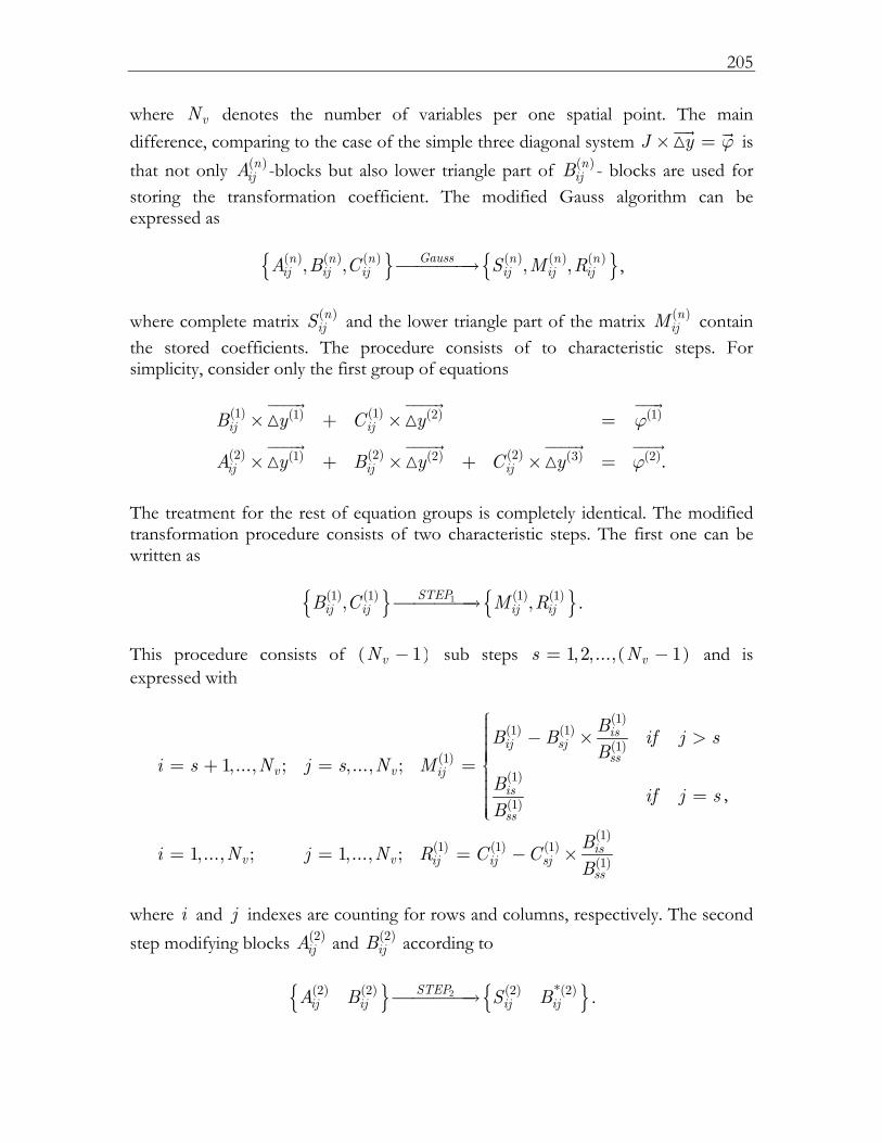
205
where vN denotes the number of variables per one spatial point. The main difference, comparing to the case of the simple three diagonal system J y ϕ× = is that not only ( )n
ijA -blocks but also lower triangle part of ( )nijB - blocks are used for
storing the transformation coefficient. The modified Gauss algorithm can be expressed as
( ) ( ) ( ) ( ) ( ) ( ), , , ,Gaussn n n n n nij ij ij ij ij ijA B C S M R⎯⎯⎯⎯→ ,
where complete matrix ( )n
ijS and the lower triangle part of the matrix ( )nijM contain
the stored coefficients. The procedure consists of to characteristic steps. For simplicity, consider only the first group of equations
(1) (1)(1) (2) (1)
(2) (2) (2)(1) (2) (3) (2).
ij ij
ij ij ij
B y C y
A y B y C y
ϕ
ϕ
× + × =
× + × + × =
The treatment for the rest of equation groups is completely identical. The modified transformation procedure consists of two characteristic steps. The first one can be written as 1(1) (1) (1) (1), ,STEP
ij ij ij ijB C M R⎯⎯⎯⎯→ . This procedure consists of ( )1vN − sub steps ( )1,2,..., 1vs N= − and is expressed with
(1)(1) (1)
(1)(1)
(1)
(1)
(1)(1) (1) (1)
(1)
1,..., ; ,..., ;
1,..., ; 1,..., ;
isij sj
ssv v ij
is
ss
isv v ij ij sj
ss
BB B if j sB
i s N j s N MB if j sB
Bi N j N R C CB
⎧⎪⎪ − × >⎪⎪⎪⎪= + = = ⎨⎪⎪⎪ =⎪⎪⎪⎩
= = = − ×
,
where i and j indexes are counting for rows and columns, respectively. The second step modifying blocks (2)
ijA and (2)ijB according to
2(2) (2) (2) *(2)STEP
ij ij ij ijA B S B⎯⎯⎯⎯→ .
Modified Gauss Algorithm for Block Tri-diagonal Matrices 206
This transformation consists of vN sub steps 1,2,..., vs N= and comes from
(2)(2) (1)
(1)(2)
(2)
(1)
(2)*(2) (2) (1)
(1)
1,..., ,...,
1,..., 1,...,
isij sj
ssv v ij
is
ss
isv v ij ij ij
ss
AA M if j sM
i N j s N SA if j sM
Ai N j N B B RM
⎧⎪⎪ − × >⎪⎪⎪⎪= = = ⎨⎪⎪⎪ =⎪⎪⎪⎩
= = = − ×
.
The transformed three-diagonal block matrix can be reused solving the equations for
different vectors ( )iφ . This requires the prior vectors transformation consisting of two steps. The first one is coming from *(1) (1) (1)(1)
si i isMϕ ϕ ϕ= − × , where indexes ( )1,2,..., 1vs N= − and 1,..., vi s N= + count the sub-steps and the vector elements respectively. Then the second step is *(2) (2) (2)(1)
si i isSϕ ϕ ϕ= − × , with 1,2,..., vs N= and 1,..., vi N= . Finally, the solution of the linear system of equations is
( )( )
( ) ( )
1( )( )
, 1 ,...,1
, 1 ,...,1
vNn nn
s sj jp p j sn
s nv v ss
D M yn N Ny
s N N M= +
− ⋅= −=
= −
∑,
where D -vector computes as
( ) ( ) ( ) ( 1)n n n nD R yϕ += − ×
Appendix C
C Steady Laminar Flamelet Libraries
Throughout this thesis the CFDF-program for solving the counterflow diffusion flame problem (see chapter 4) has been used to build steady laminar flamelet (SLF) libraries. By definition, the SLF-libraries is a series of flamelet structures resolved for different values of the strain rate na from a monotonic sequence Α : 1 2 ... qa a aΑ = < < < , where qa is the so-called quenching limit. The used correlation between two strain rates na and 1na − is coming from ( )11 1 10n na a −
−= ⋅ + . This means that each thn strain rate is 10% larger than the previous one ( 1na − ). As an example Figure 103 show characteristic changes of the flame properties with the increasing strain rate. Since the scalar dissipation rate χ is usually a preferable parameter for the flamelet tabulation, profiles of χ are a default output in each SLF-library.
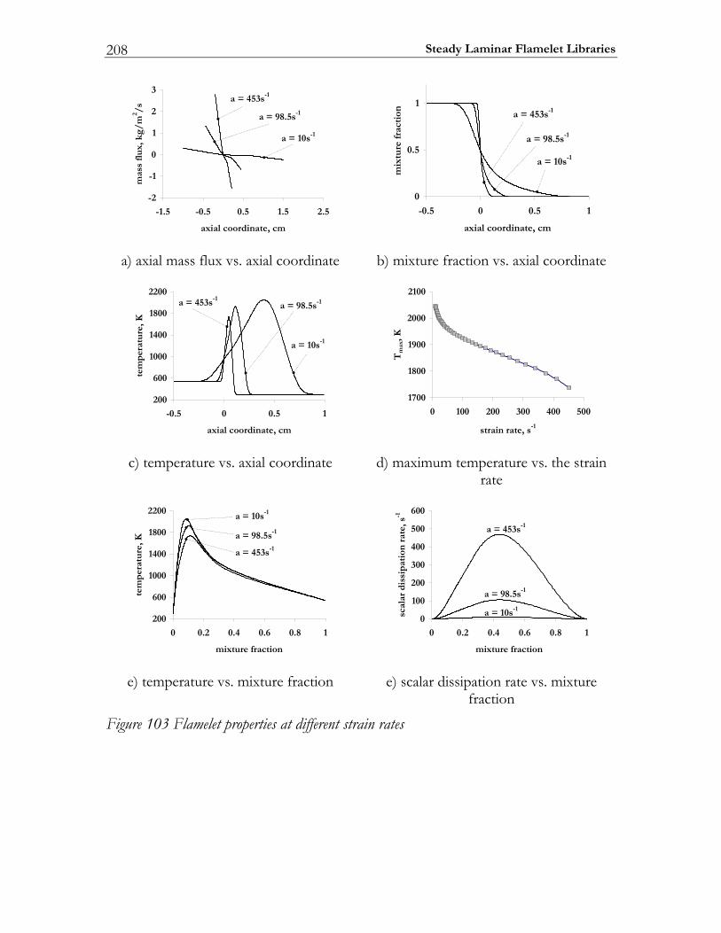
Steady Laminar Flamelet Libraries 208
2-
1-
0
1
2
3
5.25.15.05.0-5.1-
mc,etanidrooclaixa
mas
sfl
ux,
kg/
m2 /
s
s354=a 1-
s5.89=a 1-
s01=a 1-
0
5.0
1
15.005.0-
mc,etanidrooclaixa
mix
ture
frac
tion
s01=a 1-
s5.89=a 1-
s354=a 1-
a) axial mass flux vs. axial coordinate
b) mixture fraction vs. axial coordinate
002
006
0001
0041
0081
0022
15.005.0-
mc,etanidrooclaixa
tem
per
atu
re,K
s01=a 1-
s5.89=a 1-s354=a 1-
0071
0081
0091
0002
0012
0050040030020010
s,etarniarts 1-
Tm
ax,K
c) temperature vs. axial coordinate
d) maximum temperature vs. the strain
rate
002
006
0001
0041
0081
0022
18.06.04.02.00
noitcarferutxim
tem
per
atu
re,K
s01=a 1-
s5.89=a 1-
s354=a 1-
0
001
002
003
004
005
006
18.06.04.02.00
noitcarferutxim
scal
ard
issi
pat
ion
rate
,s-1
s01=a 1-
s5.89=a 1-
s354=a 1-
e) temperature vs. mixture fraction
e) scalar dissipation rate vs. mixture fraction
Figure 103 Flamelet properties at different strain rates
References
1. R. S. G. Baert and J. J. ter Meulen, "Direct injection diesel engine combustion
modeling," description of research project EWE.5125 funded by STW, Eindhoven, 1999.
2. R. D. Reitz and C. J. Rutland, Development and testing of diesel engine cfd models, Prog Energy Combust Sci 21 (1995), 173-196.
3. A. D. Gosman, State of the art of multi-dimensional modeling of engine reacting flows, Oil & Gas Science and Technology - Rev. de l'IFP 54 (1999), no. 2, 149-159.
4. D. Veynante and L. Vervisch, Turbulent combustion modeling., Prog Energy Combust Sci 28 (2002), no. 3, 193–266.
5. T. Poinsot, S. Candel and A. Trouve´, Applications of direct numerical simulation to premixed turbulent combustion., Prog Energy Combust Sci 21 (1996), 531–576.
6. T. Poinsot, Using direct numerical simulations to understand premixed turbulent combustion., Prog Energy Combust Sci 26 (1996), 219-232.
7. L. Vervisch and T. Poinsot, Direct numerical simulation of non premixed turbulent flames., Ann. Rev. Fluid Mech. 30 (1998), 655-692.
8. L. Vervisch, Using numerics to help understand nonpremixed turbulent flames., Proc. Combust. Inst. 28 (2000), 11-24.
9. F. H. Harlow and A. A. Amsden, Numerical calculation of multiphase fluid flow, Journal of Computational Physics 17 (1975), 19-52.
10. F. V. Bracco, Application of steady state spray equations to combustion modeling, AIAA J. 12 (1976), 1534-1540.
11. C. T. Crowe, A computational model for the gas-droplet flow field in the vicinity of an atomiser, 11th JANAF Symposium, No 74-23, The Combustion Institute, 1974, p.
12. C. T. Crowe, H. P. Sharma and D. E. Stock, The particle-source-in-cell (psi-cell) model for gas/droplet flows, ASME Journal of Fluids Engineering 99 (1977), 325-332.
13. J. K. Dukowicz, Particle-fluid numerical model for liquid sprays, Journal of Computational Physics 35 (1980), 229-253.
14. A. D. Gosman and D. Clerides, Diesel spray modeling: A review, ILASS-Europe Annual Meeting, 1997, p.
15. S. C. Kong, P. K. Senecal and R. D. Reitz, Developments in spray modeling in diesel and direct-injection gasoline engines, Oil & Gas Science and Technology - Rev. IFP 54 (1999), no. 2, 197-204.
16. D. P. Schmidt, C. J. Rutland and M. L. Corradini, A numerical study of cavitating flow through various nozzle shapes, SAE Paper No 971597 (1997).
References 210
17. A. K. M. Von Dirke, J. Ostertag M. Mennicken, C. Badock, Simulation of cavitating flows in diesel injectors, Oil & Gas Science and Technology - Rev. IFP 54 (1999), no. 2, 223-226.
18. K. Y. Huh and A. D. Gosman, A phenomenological model of diesel spray atomisation, Internation Conference on Multiphase Flows, 1991, p. 515--518.
19. C. Arcoumanis, M. Gavaises, J. M. Nouri, E. Abdul-Wahab and R. W. Horrocks, Analysis of the flow in the nozzle of a vertical multi-hole diesel engine injector., SAE Paper No 980811 (1998).
20. N. Naitoh, Cyto-fluid dynamic theory of atomization processes, Oil & Gas Science and Technology - Rev. IFP 54 (1999), no. 2, 205 - 210.
21. R. D. Reitz, Modeling atomisation processes in high-pressure vaporising sprays, Atomisation and Spray Technology 3 (1987), 309-337.
22. C. Bai and A. D. Gosman, Development of methodology for spray impingement simulation, SAE Paper No 950283 (1995).
23. M. Nagaoka, H. Kawazoe and N. Nomura, Modeling fuel spray impingement on a hot wall for gasoline engines, SAE Paper No 9405254 (1994).
24. C. Bai and A. D. Gosman, Mathematical modeling of wall films formed by impinging sprays., SAE Paper No 960626 (1996).
25. D. W. Stanton and C. J. Rutland, Modeling fuel film formation and wall interaction in diesel engines., SAE Paper No 960628 (1996).
26. C. Habchi, H. Foucart and T. Baritaud, Influence of wall temperature on mixture preparation in di gasoline engines., Oil & Gas Science and Technology - Rev. IFP 54 (1999), no. 2, 211-222.
27. E. Ranzi, M. Dente, A. Goldaniga, G. Bozzano and T. Faravelli, Lumping procedures in detailed kinetic modeling of gasification, pyrolysis, partial oxidation and combustion of hydrocarbon mixtures, Prog Energy Combust Sci 27 (2000), 99–139.
28. V. I. Golovitchev and N. Nordin, Detailed chemsitry spray combustion model for the kiva code, International Multidimensional Engine Modeling User's Group Meeting at the SAE Congress, MI, 2001, p.
29. J. Gustavsson and V. I. Golovitchev, Spray combustion simulation based on detailed chemistry approach for diesel fuel surrogate model, SAE Paper 2003-0137 (2003).
30. V. I. Golovitchev, K. Atarashiya, K. Tanaka and S. Yamada, Towards universal edc-based combustion model for compression ignited engine simulations, SAE paper 2003-01-1849 (2003).
31. H. J. Curran, P. Gaffuri, W. J. Pitz and C. K. Westbrook, A comprehensive modeling study of n-heptane oxidation, Combustion and Flame 114 (1998), no. 149-177.
32. H. J. Curran, W. J. Pitz, C. K. Westbrook, C. V. Callahan and F. L. Dryer, Oxidation of automotive primary reference fuels at elevated pressures., Proc. Combust. Inst. 27 (1998), 379-387.
33. H. J. Curran, C. Wu, N. M. Marinov, W. J. Pitz, C. K. Westbrook and A. Burcat, The ideal gas thermodynamics of diesel fuel ingredients: I. Naphthalene derivatives and their radicals, Journal of Physical and Chemical Reference Data 29 (2000), 463-517.
211
34. H. J. Curran, P. Gaffuri, W. J. Pitz and C. K. Westbrook, A comprehensive modeling study of iso-octane oxidation, Combustion and Flame 129 (2002), 253-280.
35. C. K. Westbrook, W. J. Pitz, H. C. Curran, J. Boercker and E. Kunrath, A detailed chemical kinetic modeling study of the shock tube ignition of isomers of heptane, International Journal of Chemical Kinetics 33 (2001), 868-877.
36. C. K. Westbrook and F. L. Dryer, Simplified reaction mechanisms for the oxidation of hydrocarbon fuels in flames, Combustion Science and Technology 27 (1981), 31-43.
37. C. K. Westbrook, Chemical kinetics of hydrocarbon ignition in practical combustion systems, Proc. Combust. Inst. 28 (2000), 1563-1577.
38. M. P. Halstead, L. J. Kirsch and C. P. Quinn, The autoignition of hydrocarbon fuels at high temperatures and pressures—fitting of a mathematical model, Combustion and Flame 30 (1977), 45-60.
39. R. C. Reid, J. M. Prausnitz and B. E. Poling,McGraw-Hill (Ed.), The properties of gases and liquids, New York, 1987.
40. R. Zevenhoven, Non-ideal gases in diesel engine processes, First Biennial Meeting and General Section of The Scandinavian-Nordic Section of the Combustion Institute, Chalmers Univ. of Technol., 2001, p. 103.
41. H. Lou and R. S. Miller, On ternary species mixing and combustion in isotropic turbulence at supercritical pressure, Physics of Fluids 16 (2004), no. 5, 1423-1438.
42. S. Palle, C. Nolan and R. S. Miller, On molecular transport effects in real gas laminar diffusion flames at large pressure, Physics of Fluids 17 (2005), 103601.
43. M. El-Gamal, E. Gutheil and J. Warnatz, The structure of laminar premixed h2/air-flames at elevated pressures, Zeitschrift für Physikalische Chemie 214 (2000), no. 4, 419-435.
44. D. B. Spalding, Theory of particle combustion at high pressures, ARS J. 29 (1959), 828-835.
45. F. A. Williams, On the assumptions underlying droplet vaporization and combustion theories, J. Chem. Phys. 33 (1960), 133-144.
46. P. R. Wieber, Calculated temperature histories of vaporizing droplets to the critical point, AIAA J. 1 (1963), 2764-2770.
47. T. A. Brzustowski, Chemical and physical limits on vapor-phase diffusion flames of droplets, Can. J. Cham. Eng. 43 (1965), 30-35.
48. D. E. Rosner, On liquid droplet combustion at high pressures, AIAA J. 5 (1967), 163-166.
49. S. D. Givler and J. Abraham, Supercritical droplet vaporization and combustion studies, Prog Energy Combust Sci 22 (1996), 1-28.
50. P. Lafon and M. Habiballah, Numerical analysis of droplet vaporization and burning under high-pressure conditions, Prog. Astro. Aero. 152 (1993), 263-279.
51. J. Réveillon and L. Vervisch, Spray vaporization in nonpremixed turbulent combustion modelling: A single droplet model, Combustion and Flame 121 (2000), 75-90.
52. G. Zhu, R. D. Reitz and S. K. Aggarwal, Gas-phase unsteadiness and its influence on droplet vaporization in sub- and super-critical environments, International Journal of Heat and Mass Transfer 44 (2001), no. 16, 3081-3093.
References 212
53. D. C. Haworth, A review of turbulent combustion modeling for multidimensional in-cylinder cfd, SAE No 2005-01-0993 (2005).
54. T. M. Sloane and P. D. Ronney, A comparison of ignition phenomena modelled with detailed and simplified kinetics, Combustion Science and Technology 88 (1993), 1-13.
55. I. P. Androulakis, New approaches for representing, analyzing and visualizing complex kinetic mechanisms, European Symposium on Computer Aided Process Engineering, Elsevier Science B.V., 2005, p.
56. H. Moshammer and N. M., The active surface of suspended particles as a predictor of lung function and pulmonary symptoms in austrian school children., Atmospheric Environment 37 (2003), 1737-1744.
57. R. Doraiswami,(Ed.), Theory and applications to particulate systems in engineering, Academic Press, San Diego, 2000.
58. A. Balthasar and M. Kraft, A stochastic approach to calculate the particle size distribution function of soot particles in laminar premixed flames., Combustion and Flame 133 (2003), 289–298.
59. M. Frenklach and S. J. Harris, Aerosol dynamics modeling using the method of moments., Colloid and Interface Sci., 118 (1987), 252-261.
60. M. Frenklach and H. Wang,H. Bockhorn (Ed.), Detailed mechanism and modleing of soot particle formation., Springer-Verlag, Heidelberg, 1994.
61. J. D. Landgrebe and S. E. Pratsinis, A discrete-sectional model for powder production by gas-phase chemical reaction and aerosol coagulation in the free molecular regime, J. Colloid Interface Sci. 139 (1990), 63-86.
62. M. J. Hounslow, A discretized population balance for continuous systems at steady state, AIChE J. 36 (1990), no. 1, 106-116.
63. D. T. Gillespie, An exact method for numerically simulating the stochastic coalescence process in a cloud, J. Atmospheric Sci. 32 (1975), no. 10, 1977–1989.
64. M. Smith and T. Matsoukas, Constant-number monte carlo simulation of population balances, Chem. Eng. Sci. 53 (1998), no. 9, 1777–1786.
65. M. Wulkow, The simulation of molecular weight distributions in polyreaction kinetics by discrete galerkin methods, Macromolecular Theory Simulations 5 (1996), no. 393–416.
66. Mit detailed modeling of pah and soot formation in a laminar premixed benzene/oxygen/argon low-pressure flame, Available from: http://web.mit.edu/anish/www/MITcomb.html
67. N. H. Qamar, G. J. Nathan, Z. T. Alwahabi and K. D. King, The effect of global mixing on soot volume fraction: Measurements in simple jet, precessing jet, and bluff body flames, Proceedings of the Combustion Institute 30 (2005), no. 1, 1493-1500.
68. M. E. Decroix, W. L. Roberts and A. Evlampiev, "Experimental strain rate-dependences of soot volume fractions (decroix, m.E. And roberts, w.L.2000 ). ," 2006.
69. U. Vandsburger, I. M. Kennedy and I. Glassman, Sooting counter-flow diffusion flames with varying velocity gradients, Proc. Combust. Institute 20 (1984), 1105–1112.
213
70. B. F. Magnussen and B. H. Hjertager, On mathematical modelling of turbulent combustion with special emphasis on soot formation and combustion, 16th Symposium (International) on Combustion, Combustion Institute, 1976, p. 719-729.
71. N. Peters, Laminar flamelet concepts in turbulent combustion., Twenty-First Symposium (International) on Combustion., The Combustion Institute, 1987, p. 1231-1250.
72. N. Peters, Laminar diffusion flamelet models in non premixed combustion. , Prog. Energy Combust. Sci. 10 (1984), 319-339.
73. J. H. M. ten Thije Boonkkamp and L. P. H. de Goey, A flamelet model for premixed stretched flames, Combustion Science and Technology 149 (2000), 183-200.
74. L. P. H. de Goey, T. Plessing, R. T. E. Hermanns and N. Peters, Analysis of the flame thickness of turbulent flamelets in the thin reaction zones regime, Proc. Combust. Inst. 30 (2005), no. 859-866.
75. R. Hilbert, F. Tap, H. El-Rabii and D. Thevenin, Impact of detailed chemistry and transport models on turbulent combustion simulations., Progress in Energy and Combustion Science 30 (2004), 61-117.
76. R. J. Kee, F. M. Rupley and J. A. Miller, "Chemkin-ii: A fortran chemical kinetics package for the analysis of gas-phase chemical kinetics," Sandia National Laboratories Report, 1990.
77. A. Konnov, Detailed reaction mechanism for small hydrocarbons combustion. Release 0.4, http://homepages.vub.ac.be/~akonnov/science/mechanism/version0_4.html
78. G. P. Smith, D. M. Golden, M. Frenklach, N. W. Moriarty, B. Eiteneer, M. Goldenberg, C. T. Bowman, R. Hanson, S. Song, W. C. Gardiner, V. Lissianski and Z. Qin, Gri-mech, http://www.me.berkeley.edu/gri_mech
79. E. S. Oran and J. P. Boris,(Ed.), Numerical simulation of reactive flow, Elsevier, 1987.
80. R. J. Kee, J. A. Miller and T. H. Jefferson, "Chemkin: A general-purpose, problem-independent, transportable, fortran chemical kinetics code package," Sandia National Laboratories Report, 1980.
81. R. J. Kee, F. M. Rupley, E. Meeks and J. A. Miller, "Chemkin-iii: A fortran chemical kinetics package for the analysis of gas-phase chemical and plasma kinetics," Sandia National Laboratories Report, 1996.
82. B. J. Zwolinski, A. P. Kudchadker and G. H. Alani, The critical constants of organic substances, Chem. Rev. 68 (1968), 659.
83. J. F. Mathews, The critical constants of inorganic substances, Chem. Rev. 72 (1972), 71.
84. O. Redlich and J. N. S. Kwong, On the thermodynamics of solutions. V. An equation of state. Fugacities of gaseous solutions, Chem. Rev. 44 (1949), 233-244.
85. G. M. Wilson, Calculation of enthalpy data from a modified redlich-kwong equation of state, Adv. Cryog. Eng. 11 (1966), 392-400.
References 214
86. G. Soave, Equilibrium constants for a modified redlich-kwong equation of state, Chem. Eng. Sci. 27 (1972), 1197-1203.
87. W. E. Kay, Density of hydrocarbon gases and vapors at high temperature and pressure, J. Ind. Eng. Chem. 28 (1936), 1014.
88. J. M. Prausnitz and R. D. Gunn, Volumetric properties of. Nonpolar gaseous mixtures, AIChE J. 4 (1958), 494-430.
89. S. Gordon and B. J. McBride, "Computer program for calculation of complex chemical equilibrium compositions, rocket performance, incident and reflected shocks and chapman-jouguet detonations," 1971.
90. R. J. Kee, G. Dixon-Lewis, J. Warnatz, M. E. Coltrin and J. A. Miller, "A fortran computer code package for the evaluation of gas-phase multicomponent transport properties.," Report SAND86-8246, Sandia National Laboratories, 1986.
91. C. F. Curtiss and J. O. Hirschfelder, Transport properties of multicomponent gas mixtures, J. Chem. Phys. 17 (1949), no. 6, 550–555.
92. J. O. Hirschfelder, C. F. Curtiss and R. B. Bird,(Ed.), Molecular theory of gases and liquids., Wiley, New York, 1954.
93. C. R. Wilke, A viscosity equation for gas mixtures, J. Chem. Phys. 18 (1950), 517-522.
94. D. E. Dean and L. I. Stiel, The viscosity of nonpolar gas mixtures at moderate and high pressures, AIChE J. 11 (1965), 526.
95. E. A. Mason and S. C. Saxena, Approximation formula for the thermal conductivity of gas mixtures, Physics of Fluids 1 (1958), no. 5, 361-369.
96. J. Warnatz, "Influence of transport models and boundary conditions on flame structure," Numerical methods in flame propagation, N. Peters and J. Warnatz (Editors), Vieweg Verlag, Braunschweig/Wiesbaden, 1982, pp. 87-111.
97. J. G. Parker, Rotational and vibrational relaxation in diatomic gases, Physics of Fluids 2 (1959), no. 4, 449-462.
98. C. A. Brau and R. H. Jonkman, Classical theory of rotational relaxation in diatomic gases, Journal of Chemical Physics 52 (1970), no. 2, 474– 484.
99. L. I. Stiel and G. Thodos, The thermal conductivity of nonpolar substances in the dense gaseous and liquid regions, AIChE J. 10 (1964), 266.
100. R. Clark Jones, On the theory of the thermal diffusion coefficient for isotopes, Phys. Rev. 58 (1940), 111-122.
101. S. Chapman and T. G. Cowling,(Ed.), The mathematical theory of non-uniform gases, Cambridge University Press, Cambridge, 1970.
102. R. S. Brokaw, Predicting transport properties of dilute gases, Ind. Eng. Chem. Process Des. Dev. 8 (1969), 240-253.
103. H. Richter, S. Granata, W. H. Green and J. B. Howard, Detailed modeling of pah and soot formation in a laminar premixed benzene/oxygen/argon low-pressure flame., Combustion Institute, 2005, p. 1397–1405.
104. N. B. Vargaftik,(Ed.), Tables on the thermophysical properties of liquids and gases, Hemisphere, Washington, 1975.
215
105. S. C. Saxena and B. P. Mathur, Thermal diffusion in binary gas mixtures and intermolecular forces, Reviews of Modern Physics 31 (1965), no. 2, 316-325.
106. H. K. Ciezki and G. Adomeit, Shock-tube investigation of self-ignition of n-heptane-air mixtures under engine relevant conditions, Combustion and Flame 93 (1993), 421-433.
107. T. Turányi, Parameterization of reaction mechanisms using orthonormal polynomials, Computers Chem. 18 (1994), 45-54.
108. S. B. Pope, Computationally efficient implementation of combustion chemistry using in situ adaptive tabulation, Combustion Theory and Modelling 1 (1997), no. 1, 41-63.
109. J. B. Bell, N. J. Brown, M. S. Day, M. Frenklach, J. F. Grcar, R. M. Propp and S. R. Tonse, Scaling and efficiency of prism in adaptive simulations of turbulent premixed flames, Proc. Combust. Inst. 28 (2000), 107-113.
110. J. Y. Chen, J. A. Blasco, N. Fueyo and C. Dopazo, An economical strategy for storage of chemical kinetics: Fitting in situ adaptive tabulation with artifical neural netwoks., Proc. Combust. Inst. 28 (2000), 115-121.
111. S. Tanaka, F. Ayala and J. C. Keck, A reduced chemical kinetic model for hcci combustion of primary reference fuels in a rapid compression machine, Combustion and Flame 133 (2003), 467–481.
112. N. Peters, Local quenching due to flame stretch and non-premixed turbulent combustion, Combustion Science and Technology 30 (1983), 1-17.
113. K. N. Bray and N. Peters,P. A. L. a. F. A. Williams (Ed.), Laminar flamelets in turbulent flames, Academic Press, 1994.
114. A. E. Lutz, R. J. Kee, J. F. Grcar and F. M. Rupley, "Oppdif: A fortran program for computing opposed-flow diffusion flames," SAND96-8243, Thermal & Plasma Processes Department Sandia National Laboratories, 1997.
115. P. Berta, I. K. Puri and S. K. Aggarwal, Structure of partially premixed n-heptane–air counterflow flames, Proceedings of the Combustion Institute 30 (2005), 447–453.
116. http://maeweb.ucsd.edu/~combustion/cermech 117. A. Goldaniga, T. Faravelli and E. Ranzi, The kinetic modeling of soot precursors in a
butadiene flame, Combustion and Flame 122 (2000), no. 3, 350-358. 118. P. Berta, A. Mukhopadhyay, I. K. Puri, S. Granata, T. Faravelli and E. Ranzi,
Numerical investigation of soot and nox formation in partially premixed heptane–air flames, XXIV Event of the Italian Section of The Combustion Institute, 2001, p.
119. A. Sinha and M. J. Thomson, The chemical structures of opposed flow diffusion flames of c3 oxygenated hydrocarbons (isopropanol, dimethoxy methane, and dimethyl carbonate) and their mixtures, Combustion and Flame 136 (2004), 548–556.
120. P. A. Glaude, W. J. Pitz and M. J. Thomson, Chemical kinetic modeling of dimethyl carbonate in an opposed-flow diffusion flame, Proceedings of the Combustion Institute 30 (2005), 1111–1118.
121. R. Dawson, F. Khoury and R. Kobayashi, Self-diffusion measurements in methane by pulsed nuclear magnetic resonance, AIChE J. 16 (1970), 725.
References 216
122. U. S. E. P. A. (EPA), "Health assessment document for diesel engine exhaust.," National Center for Environmental Assessment, Washington, 2002.
123. G. M. Faeth and U. O. Koylu, Soot morphology and optical properties in nonpremixed turbulent flame environment, Combustion Science and Technology 108 (1995), 207-229.
124. M. Y. Choi, G. W. Mulholland, A. Hamins and T. Kashiwagi, Comparisons of the soot volume fraction using gravimetric and light extinction techniques., Combustion and Flame 102 (1995), 161-169.
125. K. H. Homann and H. G. Wagner, Some new aspects of the mechanism of carbon formation in premixed flames., Eleventh Symposium (International) on Combustion, The Combustion Institute, Pittsburgh, 1967, p. 371-379.
126. D. E. Foster and D. R. Tree, "Optical measurements of soot particle size, number density and temperature in a direct injection diesel engine as a function of speed and load.," SAE Technical Paper, 1994.
127. D. B. Kittelson, M. L. Pipho and J. L. Ambs, "Particle concentrations in a diesel cylinder: Comparison of theory and experiment.," SAE Technical Paper, 1986.
128. H. Richter and J. B. Howard, Formation of polycyclic aromatic hydrocarbons and their growth to soot-a review of chemical reaction pathways, Progress in Energy and Combustion Science 26 (2000), 565–608.
129. F. J. Miller, D. E. Gardner, J. A. Graham, L. J. R.E., W. E. Wilson and J. D. Bachmann, Size considerations for establishing a standard for inhalable particles., J Air Pollut Control Assoc 29 (1979), 610-615.
130. D. A. Kaden, R. A. Hites and W. G. Thilly, Mutagenicity of soot and associated polycyclic aromatic hydrocarbons to salmonella typhimurium, Cancer Res 39 (1979), 4152-4159.
131. A. W. Wood, W. Levin, R. L. Chang, M. T. Huang, D. E. Ryan, P. E. Thomas, R. E. Lehr, S. Kumar, M. Koreeda, H. Akagi, Y. Ittah, P. Dansette, H. Yagi, D. M. Jerina and A. H. Conney, Mutagenicity and tumor-initiating activity of cyclopenta[c,d]pyrene and structurally related compounds., Cancer Res 40 (1980), 642–649.
132. P. P. Fu, F. A. Beland and S. K. Yang, Cyclopenta-polycyclic aromatic hydrocarbons: Potential carcinogens and mutagens., Carcinogenesis 1 (1980), 725–727.
133. W. F. Busby, E. K. Stevens, E. R. Kellenbach, J. Cornelisse and J. Lugtenburg, Dose–response relationships of the tumorigenicity of cyclopenta[c,d]pyrene, benzo[a]pyrene and 6 nitrochrysene in a newborn mouse lung adenoma bioassay., Carcinogenesis 9 (1988), 741–746.
134. A. L. Lafleur, J. P. Longwell, L. Shirname´-More´, P. A. Monchamp, W. A. Peters and E. F. Plummer, Chemical characterization and bacterial mutagenicity testing of ethylene combustion products from a jet-stirred/plug-flow reactor, Energy &Fuels 4 (1990), 307-319.
135. M. F. Denissenko, A. Pao, M.-S. Tang and G. P. Pfeifer, Preferential formation of benzo[a]pyrene adducts at lung cancer mutational hotspots in p53., Science 274 (1996), 430–432.
217
136. P. Flynn, M. Mizusawa, O. A. Uyehara and P. S. Myers, An experimental determination of the instantaneous potential radiant heat transfer within an operating diesel engine, SAE Trans. 81 (1972), 95–126.
137. B. J. Alder, L. K. Tseng, N. M. Laurendeau and J. P. Go, Effects of partial premixing on nox emission indices of soot-containing flames, Combustion Science and Technology 152 (2000), 167–178.
138. H. Bockhorn (Ed.), Soot formation in combustion--mechanisms and models., Springer-Verlag, 1994.
139. A. E. Clarke, T. C. Hunter and F. H. Garner, The tendency to smoke of organic substances on burning., J Inst Petrol 32 (1946), no. Part I, 627-642.
140. K. P. Schug, Y. Manheimer-Timnat, P. Yaccarino and I. Glassman, Sooting behaviour of gaseous hydrocarbon diffusion flames and the influence of additives., Combustion Science and Technology 22 (1980), 235–250.
141. B. Haynes, S, and H. G. Wagner, Soot formation., Prog Energy Combust Sci 7 (1981), 229–273.
142. H. B. Palmer and C. F. Cullis,W. PL (Ed.), The formation of carbon from gases., vol. 1, Marcel Dekker, New York, 1965.
143. A. G. Gaydon,Chapman and Hall (Ed.), Spectroscopy and combustion theory., London, 1948.
144. S. K. Friedlander,(Ed.), Smoke, dust, and haze: Fundamentals of aerosol behavior., Oxford University Press, New York, 2000.
145. C. J. Pope and J. B. Howard, Simultaneous particle and molecule modeling (spamm): An approach for combining sectional aerosol equations and elementary gas-phase reactions., Aerosol Sci. Technol. 27 (1997), 73-94.
146. R. J. Hall, M. D. Smooke and M. B. Colket,F. L. Dryer and R. F. Sawyer (Ed.), Physical and chemical aspects of combustion: A tribute to irvine glassman, Gordon & Breach, 1997.
147. M. Frenklach, Method of moments with interpolative closure., Chem. Engineering Sci. 57 (2002), 2229-2239.
148. B. Zhao, Z. Yang, M. V. Johnston, H. Wang, A. S. Wexler, M. Balthasar and M. Kraft, Measurement and numerical simulation of soot particle size distribution functions in a laminar premixed ethylene-oxygen-argon flame., Combustion and Flame 133 (2003), 173–188.
149. J. Appel, H. Bockhorn and M. Wulkow, A detailed numerical study of the evolution of soot particle size distributions in laminar premixed flames., Chemosphere 42 (2001), 635–645.
150. M. Kraft, "Modelling of particulate processes," Technical Report 30, c4e-Preprint Series, Cambridge, 2005.
151. A. D’Alessio, A. C. Barone, R. Cau, A. D’Anna and P. Minutolo, Surface deposition and coagulation efficiency of combustion generated nanoparticles in the size range from 1 to 10 nm, Proceedings of the Combustion Institute 30 (2005), no. 2, 2595-2603.
References 218
152. H.-H. Grotheer, H. Pokorny, K.-L. Barth, M. Thierley and M. Aigner, Mass spectrometry up to 1 million mass units for the simultaneous detection of primary soot and of soot precursors (nanoparticles) in flames, Chemosphere 57 (2004), no. 10, 1335-1342.
153. A. D’Anna and J. H. Kent, Modeling of particulate carbon and species formation in coflowing diffusion flames of ethylene, Combustion and Flame 144 (2006), 249–260.
154. A. Beltrame, P. Porshnev, W. Merchan-Merchan, A. Saveliev, A. Fridman, L. A. Kennedy, O. Petrova, S. Zhdanouk, F. Amouri and O. Charon, Sootnext term and no formation in methane–oxygen enriched diffusion flames, Combustion and Flame 124 (2001), no. 1-2, 295-310.
155. M. E. Decroix and W. L. Roberts, Transient flow field effects on soot volume fraction in diffusion flames, Combustion Science and Technology 160 (2000), no. 1-6, 165-189
156. H. Wang, D. X. Du, C. J. Sung and C. K. Law, Experiments and numerical simulation on soot formation in opposed jet ethylene diffustion flames., Proc. Combust. Institute 26 (1996), 2359-2368.
157. J. H. Kent and S. J. Bastin, Parametric effects on sooting in turbulent acetylene diffusion flames, Combustion and Flame 56 (1984), no. 1, 29-42.
158. H. Bockhorn, H. Geitlinger, B. Jungfleish, T. Lehre, A. Schon, T. Streibel and R. Suntz, 2002 progress in characterization of soot formation by optical methods, Phys. Chem. Chem. Phys. 4 (2002), 3780–3793.
159. E. Riesmeir, S. Honnet and N. Peters, Flamelet modeling of pollutant formation in a gas turbine combustion chamber using detailed chemistry for a kerosene model fuel, J Eng Gas Turbine Power 126 (2004), 899–905.
160. C. Hasse and N. Peters, A two mixture fraction flamelet model applied to split injections in a di diesel engine, Combustion Institute 2005, p. 2755-2762.
161. A. Ergut, S. Granata, J. Jordan, J. Carlson, J. B. Howard, H. Richter and Y. A. Levendisa, Pah formation in one-dimensional premixed fuel-rich atmospheric pressure ethylbenzene and ethyl alcohol flames, Combustion and Flame 144 (2006), no. 4, 757-772.
162. A. L. Lafleur, K. Taghizadeh, J. B. Howard, J. F. Anacleto and M. A. Quilliam, Characterization of flame-generated c10 to c160 polycyclic aromatic hydrocarbons by atmospheric-pressure chemical ionization mass spectrometry with liquid introduction via nebulizer interface., J. Am. Soc. Mass Spectrom. (1996), 276–286.
163. S. J. Harris and A. M. Weiner, A picture of soot particle inception, Proc. Combust. Inst. 22 (1988), 333–342.
164. J. T. McKinnon and J. B. Howard, The roles of pah and acetylene in soot nucleation and growth, Twenty-Fourth Symposium (International) on Combustion, The Combustion Institute, 1992, p. 965-971.
165. A. D'Anna, A. Violi, A. D'Alessio and A. F. Sarofim, A reaction pathway for nanoparticle formation in rich premixed flames., Combustion and Flame 127 (2001), 1995–2003.
166. J. Park, S. Burova, A. S. Rodgers and M. C. Lin, Experimental and theoretical studies of the c6h5 + c6h6 reaction, J. Phys. Chem. 103 (1999), no. 45, 9036–9041.
219
167. J. Park and M. C. Lin, Kinetics for the recombination of phenyl radicals, J. Phys. Chem. 101 (1997), 14-18.
168. A. M. Mebel, M. C. Lin, T. Yu and K. Morokuma, Theoretical study of potential energy surface and thermal rate constants for the c6h5+h-2 and c6h6+h reactions, J. Phys. Chem. 101 (1997), no. (17), 3189–3196.
169. S. Madronich and W. Felder, Kinetics and the mechanism of the reaction of oh with c6h6 over 790-1410 k, J. Phys. Chem. 89 (1985), 3556-3561.
170. D. L. Baulch, C. J. Cobos, R. A. Cox, C. Esser, P. Frank, T. Just, J. A. Kerr, M. J. Pilling, J. Troe, R. W. Walker and J. Warnatz, Evaluated kinetic data for combustion modeling, J. Phys. Chem. Ref. Data 21 (1992), 411–429.
171. H. Richter, O. A. Mazyar, R. Sumathi, W. H. Green, J. B. Howard and J. W. Bozzelli, Detailed kinetic study of the growth of small polycyclic aromatic hydrocarbons. 1. 1-naphthyl plus ethyne J. Phys. Chem. 105 (2001), 1561 - 1573.
172. J. B. Howard, Carbon addition and oxidation reactions in heterogeneous combustion and soot formation, 23rd Symp. (Int.) on Combustion, Combustion Inst., 1991, p. 1107–1127.
173. J. Y. Hwang and S. H. Chung, Growth of soot particles in counterflow diffusion flames of ethylene, Combustion and Flame 125 (2001), 752-762.
174. C. S. McEnally, A. M. Schaffer, M. B. Long, L. D. Pfefferle, M. D. Smooke, M. B. Colket and R. J. Hall, Computational and experimental study of soot formation in a coflow, laminar ethylene diffusion flame, Proc. Combust. Inst. 27 (1998), 1497–1505.
175. J. E. Dec, A conceptual model of di diesel combustion based on laser-sheet imaging, SAE Technical Paper No 970873 (1997).
176. H. Barths, C. Antoni and N. Peters, Three-dimensional simulation of pollutant formation in a di diesel engine using multiple interactive flamelets, SAE Paper (982459) (1998).
177. H. Pitsch, H. Barths and N. Peters, Three-dimensional modeling of nox and soot formation in di-diesel engines using detailed chemistry based on the interactive flamelet approach, SAE Paper (962057) (1996).
178. J. Hult, U. Meier, W. Meier, A. Harvey and C.F. Kaminski, Experimental analysis of local flame extinction in a turbulent jet diffusion flame by high repetition 2-d laser techniques and multi-scalar measurements, Proceedings of the Combustion Institute 30 (2005), 701-709.
179. J. M. Donbar, J. F. Driscoll and C. D. Carter, Strain rates measured along the wrinkled flame contour within turbulent non-premixed jet flames, Combustion and Flame 125 (2001), no. 4, 1239-1257.
180. A. Cessou, C. Maurey and D. Stepowski, Parametric and statistical investigation of the behavior of a lifted flame over a turbulent free-jet structure, Combustion and Flame 137 (2004), no. 4, 458-477.
181. R. Barlow, www.ca.sandia.gov/TNF 182. K. J. Young and J. B. Moss, Modelling sooting turbulent jet flames using an extended
flamelet technique, Combustion Science and Technology 105 (1995), no. 1-3, 33-53.
References 220
183. D. Han and M. G. Mungala, Simultaneous measurements of velocity and ch distributions. Part 1: Jet flames in co-flow, Combustion and Flame 132 (2003), no. 3, 565-590.
184. J. Ferziger,O. Metais and J. Ferziger (Ed.), Large eddy simulation: An introduction and perspective., Berlin, 1997.
185. M. R. H. Sheikhia, T. G. Drozdaa, P. Givia, F. A. Jaberib and S. B. Popec, Large eddy simulation of a turbulent nonpremixed piloted methane jet flame (sandia flame d). Combustion Institute, 2005, p. 549–556.
186. A. Favre, Statistical equations of turbulent gases., Problems of Hydrodynamics and Continuum Mechanics, SIAM, p. 231-266.
187. S. B. Pope, Lagrangian pdf methods for turbulent flows, Annu. Rev. Fluid Mech 26 (1994), 23-63.
188. C. Dopazo,P. A. Libby and F. A. Williams (Ed.), Recent development in pdf methods, 1993.
189. R. P. Lindstedt and H. C. Ozarovsky, Joint scalar transported pdf modeling of nonpiloted turbulent diffusion flames, Combustion and Flame 143 (2005), no. 4, 471-490
190. H. Möbus, P. Gerlingerb and B. D., Scalar and joint scalar-velocity-frequency monte carlo pdf simulation of supersonic combustion., Combustion and Flame 132 (2003), no. 1-2, 3-24.
191. M. Abramowitz and I. A. Stegun,Dover (Ed.), Handbook of mathematical functions., NY, USA, 1970.
192. R. W. Bilger, S. B. Pope, K. N. C. Bray and J. F. Driscoll, "Paradigms in turbulent combustion research," Combustion Institute, 2004.
193. V. Esfahaniana, A. Javaheria and M. Ghaffarpour, Thermal analysis of an si engine piston using different combustion boundary condition treatments, Applied Thermal Engineering 26 (2005), no. 2-3, 277-287.
194. S. L. Yang, Y. K. Siow, C. Y. Teo and K. Hanjalic, A kiva code with reynolds-stress model for engine flow simulation, Energy 30 (2005), no. 2-4, 427-445.
195. Y. Z. Zhang, E. H. Kung and D. C. Haworth, A pdf method for multidimensional modeling of hcci engine combustion: Effects of turbulence/chemistry interactions on ignition timing and emissions, Combustion Institute 2005, p. 2763-2771.
196. K. Jin, O. Takashi, D. Yasuhiro, K. Ryouji and S. Takeshi, Combustion and exhaust gas emission characteristics of a diesel engine dual- fueled with natural gas., JSAE Review 21 (2000), no. 4, 489-496.
197. L. Seang-Wock, T. Daisuke, K. Jin and D. Yasuhiro, Two-dimensional laser induced fluorescence measurement of spray and oh radicals of lpg in constant volume chamber., JSAE Review 23 (2002), no. 2, 195-203.
198. C. Olivier, P. d. C. António and J. Stéphane, Detailed chemistry-based auto-ignition model including low temperature phenomena applied to 3-d engine calculations, Combustion Institute 2005, p. 2649-2656.
199. F. Tao, V. I. Golovitchev and J. Chomiak, A phenomenological model for the prediction of soot formation in diesel spray combustion., Combustion and Flame 136 (2004), no. 3, 270-282.
221
200. S. C. Lia, F. A. Williams and K. Gebertb, A simplified, fundamentally based method for calculating nox emissions in lean premixed combustors, Combustion and Flame 119 (1999), no. 3, 367-373.
201. D. Zhang and S. H. Frankel, A numerical study of natural gas combustion in a lean burn engine., Fuel 77 (1998), no. 12, 1339-1347.
202. A. A. Amsden, P. J. O'Rourke and T. D. Butler, "Kiva-ii: A computer program for chemically reactive flows with sprays.," Technical Report, L. A. N. Laboratory (Editor), 1989.
203. W. P. Jones,P. A. Libby and F. A. Williams (Ed.), Turbulence modeling and numerical solution methods for variable density and combustion flows., Academic Press, London, 1994.
204. R. S. Barlow and J. H. Frank, Effects of turbulence on species mass fractions in methane/air jet flames, Proc. Combust. Inst. 27 (1998), 1087-1095.
205. Schneider Ch., A. Dreizler and J. Janicka, Flow field measurements of stable and locally extinguishing hydrocarbon-fuelled jet flames, Combustion and Flame 135 (2003), 185-190.
206. R. S. Barlow, J. H. Frank, A. N. Karpetis and J. Y. Chen, Piloted methane/air jet flames: Transport effects and aspects of scalar structure, Combustion and Flame 143 (2005), no. 4, 433-449.
207. H. Pitsch and S. H., Large-eddy simulation of a turbulent piloted methane/air diffusion flame (sandia flame d), Physics of Fluids 12 (2000), no. 10, 2541-2554.
208. H. Wang and Y. Chen, Steady flamelet modelling of a turbulent non-premixed flame considering scalar dissipation rate fluctuations, Fluid Dynamics Research 37 (2005), no. 3, 133-153.
209. R. Mustata, L. Valino, C. Jiménez, W. P. Jones and S. Bondi, A probability density function eulerian monte carlo field method for large eddy simulations: Application to a turbulent piloted methane/air diffusion flame (sandia d), Combustion and Flame 145 (2006), no. 1-2, 88-104.

Abstract
Most practical combustion applications use a fuel that consists of a mixture of a variety of large hydrocarbon molecules. This introduces extra complexity to processes such as fuel oxidation and pyrolysis and the accompanying formation of PAH/Soot and NOx-pollutants. Increasingly stringent demands on thermal efficiency and pollutant emissions of practical combustion devices require accurate and comprehensive prediction of these complex phenomena. With respect to internal combustion engines such as Diesel and spark-ignition engine, the problem becomes even more complex since for these applications, combustion takes place at elevated pressures and in a non-stationary flow field. In order to match the requirements mentioned above, computational tools should be developed that apply sufficiently detailed thermo-chemical and fluid dynamics descriptions. In particular, it is essential that these tools are able to handle: large number of chemical reactions and species, realistic thermodynamic models for molecular transport and gas-volumetric properties and also the interplay between chemistry and turbulent flow field. In this thesis a generic approach for handling complex thermo-physical and chemical reaction models for practical combustion simulations is introduced. A variety of 0D and 1D combustion sub-models are considered since they form an established common basis for applying complex reaction mechanisms in industrial simulations (e.g. Diesel engine modeling). The central point of the approach is the automated processing and analysis of large data sets describing complex chemical reaction systems. The computational strategy developed for handling descriptions of complex reaction systems is introduced in chapter 2. The algorithms that have been developed and implemented allow for a practical application of chemical kinetic models of extended complexity in conjunction with non-ideal gas models. Some typical results for predicted real gas transport- (e.g. diffusivity, conductivity) and chemical properties (auto-ignition) are presented and compared with available experimental data. The results demonstrate their ability to handle complex reaction models and to capture effects of elevated pressure on gas properties for pure chemical substances and their mixtures. At the same time these comparisons give an important indication on the accuracies that can be expected when applying these models to practical simulations. The algorithms introduced in chapter 2 are used throughout the complete thesis. The applicability of the ideal gas assumption for modeling high-pressure compression-reaction processes was studied in chapter 3 based on a 0D numerical setup. The results from homogeneous auto-ignition and NO-formation simulations applying the ideal gas and real gas models were compared. These comparisons have shown that the inaccuracy of the ideal gas assumption is determined not only by the P-V-T conditions but also by the problem formulation itself. Therefore, for each case where the ideal gas law is applied in modeling high-pressure compression-reaction
Abstract 224
processes, the analysis shows that the potential errors have to be estimated in an appropriate way. Chapter 4 presents a computational algorithm for resolving the structure of 1D (laminar) diffusion flamelets of fuels with complex chemistry. The algorithm has been used to evaluate the impact of gas non-ideality on the flamelet. The computations were performed for the so-called "worst" case of the fuel-component non-ideality. The comparison demonstrates that even for these extreme conditions, applying a real gas model does not lead to a difference in the flamelet structure compared to the predictions obtained with the ideal gas assumption. With respect to the practical CFD-modeling of high-pressure combustion, this result suggests that for a flamelet model to determine the chemical composition (or reaction rates) it is appropriate to apply the ideal gas assumption. The application of a non-ideal gas model would be necessary only if the flamelet computation is additionally used to determine the molecular transport properties. The last situation can occur in the CFD-modeling based on the Large Eddy Simulation approach. Chapter 5 is dedicated to detailed modeling of PAH/Soot formation in laminar diffusion flamelets. Results on PAH/Soot formation in ethylene/air and benzene/air counterflow diffusion flames are presented. The effect of strain rate on PAH/Soot is considered in terms of major characteristics like the mass- and number-density as well as in terms of particle size distribution function (PSDF). The obtained computational results confirm the general experimental observations that soot mass and number densities (first two moments of the PSDF) depend strongly on the mixing characteristics within a flame. The computed particle size distribution function reveals both unimodal and bimodal shapes depending on the imposed strain rate. This questions the assumption of a lognormal distribution, which is often used in the method of moments. An application of detailed reaction mechanisms based on the steady laminar flamelet (1D) model to turbulent diffusion jet-flames is presented in chapter 6. A partially premixed methane/air flame (Sandia Flame D) and a sooting non-premixed ethylene/air flames have been modeled. The results are compared to available experimental data. Although the simulated flames have a similar geometry, the quality of the computational predictions is found to be very different for these flames. This result points out that when applying comprehensive reaction mechanisms in practical simulations of IC-engines an adequate prediction of the turbulent mixing processes is a crucial issue.
Samenvatting
In veel praktische verbrandingsystemen bestaat de brandstof uit grote koolwaterstof moleculen. Vergeleken met processen gebaseerd op kleinere koolwaterstoffen, zoals aardgas en butaan, introduceren deze extra complexiteit in de voor de toepassing relevante processen als brandstof oxidatie, pyrolyse en de vorming van schadelijke stoffen NOx en PAK’s/roet. Echter, de almaar toenemende eisen aan verbrandingstoestellen verlangen een omvattende en accurate beschrijving van dit soort fenomenen. Met betrekking to verbrandingsmotoren, zowel diesel als benzine, wordt dit zomogelijk nog complexer omdat de verbranding en emissievorming zich afspeelt onder hoge druk in een tijdsafhankelijk stromingsveld. Om de huidige eisen uit de moderne industrie te verwezenlijken zullen rekenmodellen op een voldoende gedetailleerd thermo-chemische en stromingsdynamische beschrijving gebaseerd moeten zijn. In het bijzonder is het essentieel dat het model kan omgaan met: groot aantal chemische reacties en stofjes, realistische thermodynamische modellen voor transport- en gaseigenschappen en de wisselwerking tussen chemie en turbulentie. In dit proefschrift wordt een generieke aanpak gepresenteerd voor de behandeling van complexe thermo-chemische reactie modellen. Hoewel de toepasbaarheid van dit soort mechanismen meestal beperkt is tot 0D en soms 1D reagerende systemen is het belang voor praktische, complexe 3D evident. Als submodellen vormen deze eenvoudige systemen een gemeenschappelijke basis voor de toepassing van gedetailleerde chemische mechanismen in industriële berekeningen (e.g. Diesel motor simulaties). Echter, juist de complexiteit van de chemische schema’s dwingt tot een geautomatiseerde interpretatie met daaraan gekoppeld een diepgaande analyse van de thermodynamische en moleculaire transport data die onlosmakelijk hieraan verbonden zijn. In hoofdstuk 2 wordt een de strategie beschreven die ontwikkeld is voor de analyse en interpretatie van grote reactie systemen (e.g. > 1000 stofjes). De ontwikkelde algoritmes zijn toegespitst op de toepassing van dit soort modellen in praktische situaties. Hierbij is extra functionaliteit aan het standaard formaat toegevoegd om zogenaamde reëel gas effecten te in de beschouwing te betrekken. De algoritmes zijn getoetst aan een uitgebreide vergelijking van relevante grootheden (e.g. de toestandsvergelijking, diffusie/geleidingscoëfficiënten) met beschikbare experimenten uit de literatuur. Hierbij is expliciet de drukafhankelijkheid getoetst voor pure componenten en mengsels van deze. De resultaten geven tevens een indruk van de nauwkeurigheid die te verwachten valt in praktische applicaties. In hoofdstukken 3 en 4 is de ontwikkelde systematiek getoetst aan 0D en 1D reagerende systemen. In hoofdstuk 3 wordt de toepasbaarheid van de ideale gaswet
Samenvatting 226
bestudeerd op een zogenaamde ‘rapid compression machine’, een ruimtelijk homogeen systeem dat een gecontroleerde compressie doorloopt waarna zelfontsteking volgt. Het effect van de toestandsvergelijking op belangrijke Diesel-motor parameters, ontstekingsuitstel en NOx vorming, zijn hier beschreven en vergeleken met beschikbare experimenten. De resultaten laten zien dat de nauwkeurigheid mede bepaald wordt door hoe de ideale gas wet toegepast wordt in de bepaling van de thermodynamische toestand. In hoofdstuk 4 wordt ingegaan op het effect van niet-ideale gassen op 1D diffusie vlammen. Dit soort elementaire vlamstructuren, zogenaamde ‘flamelets’, worden veelvuldig toegepast in berekeningen van grote turbulente systemen (industriële branders, motoren, gasturbines). Naast de toestandsvergelijking is hier ook het effect van reëel gas modellen op transport grootheden en dus vlamstructuur bestudeerd. Het blijkt dat zelfs in een worstcase situatie er geen belangrijk verschil optreedt in vlamstructuur tussen de berekeningen met beide toestandsvergelijkingen. Voor de toepassing van het flamelet concept in de simulatie van hoge druk processen is het dan ook gerechtvaardigd om de ideale gaswet te gebruiken. Slechts in het geval dat ook transport grootheden uit de flamelet database bepaald worden zullen reëel gas modellen gebruikt moeten worden. Juist deze situatie kan zich voordoen in de meer en meer toegepaste Large-Eddy aanpak. Hoofdstuk 5 is gewijd aan de gedetailleerde beschrijving van PAK/roet vorming in dezelfde elementaire vlamstructuren, de 1D diffusievlam. Resultaten van roetende ethyleen/lucht en benzeen/lucht vlammen worden gepresenteerd. Het effect van de extern opgelegde stromingsvervorming is (i.e. ‘strain’) is gekarakteriseerd aan de hand van hoofdgrootheden als massa- en molfractie (i.e. ‘number-density’ and ‘mass-density’) maar ook de deeltjesgrootte verdeling (i.e. Particle Size Distribution, PSD) van het roet. De berekeningen bevestigen de algemene experimentele observaties dat de ‘number-density’ en ‘mass-density’ sterk afhangen van de mengkarakteristieken in de vlam. Daarbij laat de deeltjesgrootte verdeling zowel uni-modale als bi-modale verdelingen zien. Dit trekt de gebruikelijke aanname van een log-normale verdeling, zoals toegepast in de zogenaamde moment-methode (‘Method of Moments’) aanpak, in twijfel. Een toepassing van de flamelet aanpak op twee turbulente reagerende jet-diffusie vlammen is gepresenteerd in hoofdstuk 6. Een referentie vlam, de gedeeltelijk voorgemengd methaan/lucht vlam (Sandia Flame D) en een roetende niet-voorgemengde ethyleen/lucht vlam. De resultaten zijn vergeleken met beschikbare experimenten. Hoewel de geometrie van beide vlammen vergelijkbaar is, is de kwaliteit van de voorspellingen sterk verschillend. Dit wijst op het feit dat de toepassing van zeer uitgebreide reactiemechanismen in verbrandingsmotoren eigenlijk slechts verdedigbaar is als het turbulente meng proces adequaat beschreven wordt.
Curriculum Vitae
March 15th 1975 : Born in Moscow , USSR March 1999 : Moscow State Engineering Physics Institute
(Technical University), Department of Chemical Physics. Graduate and postgraduate student.
August 1999 - May 2002 : Moscow N.N. Semionov Institute of Chemical
Physics, Department of Kinetics and Catalysis. Postgraduate student and engineer.
June 2002 - July 2006 PhD student,
Technische Universiteit Eindhoven, Faculty of Mechanical Engineering, Combustion Technology Group