HDL-64E S2 and S2 › cam › special › Velodyne › common › pdf...F i r mw ar e Vers i o n 4 ....
43
U S E R ’ S M A N U A L A N D P R O G R A M M I N G G U I D E F i r m w a r e Ve r s i o n 4 . 0 7 HDL-64E S2 and S2.1 High Definition LiDAR ™ Sensor
Transcript of HDL-64E S2 and S2 › cam › special › Velodyne › common › pdf...F i r mw ar e Vers i o n 4 ....

U S E R ’ S M A N U A L A N D
P R O G R A M M I N G G U I D E
F i r m w a r e Ve r s i o n 4 . 0 7
HDL-64E S2 and S2.1
High Definition LiDAR™ Sensor
i S A F E T Y N O T I C E S
1 I N T R O D U C T I O N
In The Box
2 P R I N C I P L E S O F O P E R A T I O N
3 I N S T A L L A T I O N O V E R V I E W
3 FrontlBack Mounting
4 Side Mounting
5 Top Mounting
6 Wiring
6 U S A G E
6 Use the Included Point-cloud Viewer
6 Develop Your Own Application-specific Point-cloud Viewer
7 db.xml Calibration Parameters
8 Change Run-Time Parameters
1O Control Spin Rate
— Change Spin Rate in Flash Memory — Change Spin Rate in RAM Only
1O Limit Horizontal FOV data Collected
11 Define Sensor Memory IP Source and Destination Addresses
11 Upload Calibration Data
11 External GPS Time Synchronization
— GPS Receiver Option 1: Velodyne Supplied GPS Receiver
— GPS Receiver Option 2: Customer Supplied GPS Receiver
13 Packet Format and Status Byte for GPS Time Stamping
13 Time Stamping Accuracy Rules
13 Laser Firing Sequence and Timing
14 F I R M W A R E U P D A T E
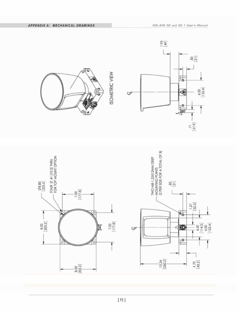
15 A P P E N D I X A : Mechanical Drawings
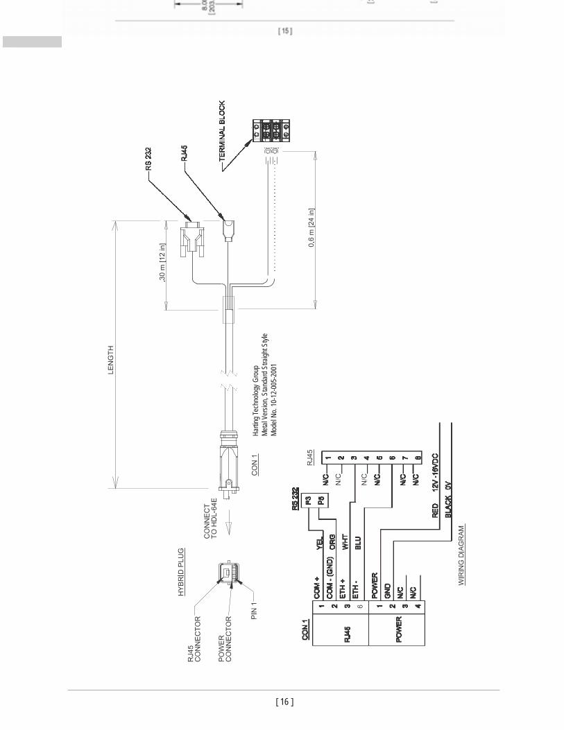
16 A P P E N D I X B : Wiring Diagram 17 A P P E N D I X C : Digital Sensor Recorder (DSR)
17 Install
17 Calibrate
17 Live Playback
18 Record Data
18 Playback of Recorded Files
19 DSR Key Controls
19 DSR Mouse Controls 2O A P P E N D I X D : Matlab Sample Code
22 Reading Calibration and Sensor Parameter Data 23 A P P E N D I X E : Data Packet Format
27 Last Six Bytes Examples 3O A P P E N D I X F : Dual Two Point Calibration Methodology 34 A P P E N D I X G : Ethernet Transmit Timing Table 36 A P P E N D I X H : Laser and Detector Arrangement 37 A P P E N D I X I : Angular Resolution 38 T R O U B L E S H O O T I N G
38 S E R V I C E A N D M A I N T E N A N C E
39 S P E C I F I C A T I O N S
C A U T I O N — S A F E T Y NOTIC E
[ i ]
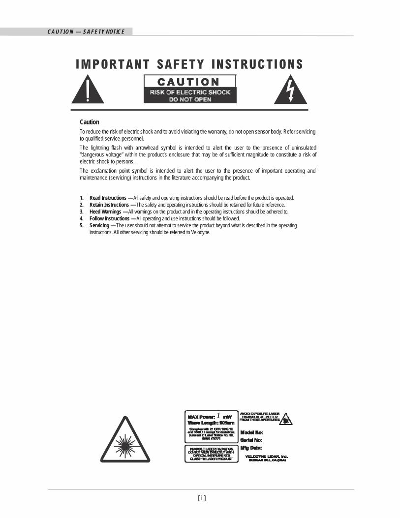
Caution To reduce the risk of electric shock and to avoid violating the warranty, do not open sensor body. Refer servicing to qualified service personnel.
The lightning flash with arrowhead symbol is intended to alert the user to the presence of uninsulated “dangerous voltage” within the product’s enclosure that may be of sufficient magnitude to constitute a risk of electric shock to persons.
The exclamation point symbol is intended to alert the user to the presence of important operating and maintenance (servicing) instructions in the literature accompanying the product.
1. Read Instructions — All safety and operating instructions should be read before the product is operated. 2. Retain Instructions — The safety and operating instructions should be retained for future reference. 3. Heed Warnings — All warnings on the product and in the operating instructions should be adhered to. 4. Follow Instructions — All operating and use instructions should be followed. 5. Servicing — The user should not attempt to service the product beyond what is described in the operating
instructions. All other servicing should be referred to Velodyne.
1
I N T R O D U C T I O N HDL-64E S2 and S2.1 User’s Manual
[ 1 ]
Congratulations on your purchase of a Velodyne HDL-64E S2 or S2.1 High Definition LiDAR Sensor. These sensors represent a
breakthrough in sensing technology by providing more information about the surrounding environment than previously possible.
The HDL-64E S2 or S2.1 High Definition LiDAR sensors are referred to as the sensor throughout this manual.
This manual and programming guide covers:
• Installation and wiring
• HDL-64-ADAPT (GPS Adaptor Box)
• The data packet format
• The serial interface
• Software updates
• GPS installation notes
• Viewing the data
• Programming information
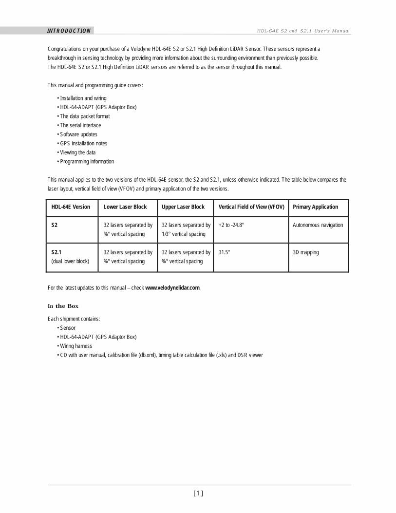
This manual applies to the two versions of the HDL-64E sensor, the S2 and S2.1, unless otherwise indicated. The table below compares the
laser layout, vertical field of view (VFOV) and primary application of the two versions.
HDL-64E Version
Lower Laser Block
Upper Laser Block
Vertical Field of View (VFOV)
Primary Application
S2
32 lasers separated by
%° vertical spacing
32 lasers separated by
1/3° vertical spacing
+2 to -24.8°
Autonomous navigation
S2.1
(dual lower block)
32 lasers separated by
%° vertical spacing
32 lasers separated by
%° vertical spacing
31.5°
3D mapping
For the latest updates to this manual — check www.velodynelidar.com.
In the Box
Each shipment contains:
• Sensor
• HDL-64-ADAPT (GPS Adaptor Box)
• Wiring harness
• CD with user manual, calibration file (db.xml), timing table calculation file (.xls) and DSR viewer
P R I N C I P L E S O F O P E R AT I O N HDL-64E S2 and S2.1 User’
[ 2 ]
s ManuaI
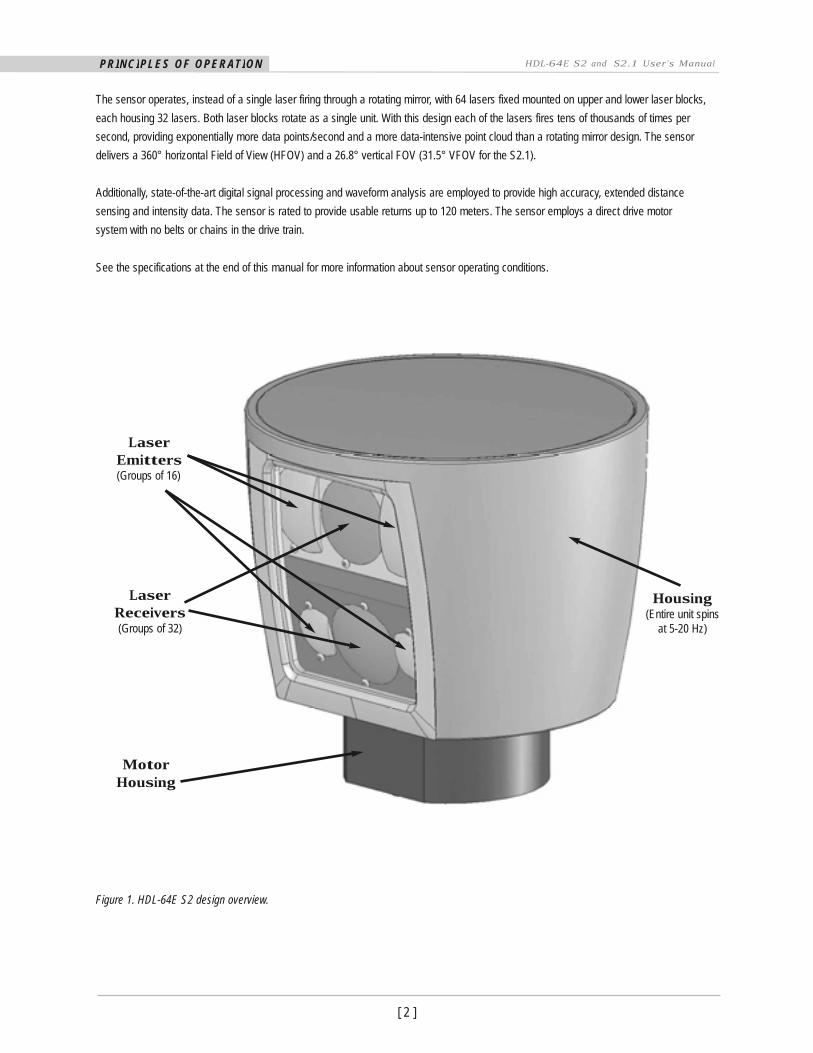
The sensor operates, instead of a single laser firing through a rotating mirror, with 64 lasers fixed mounted on upper and lower laser blocks,
each housing 32 lasers. Both laser blocks rotate as a single unit. With this design each of the lasers fires tens of thousands of times per
second, providing exponentially more data points/second and a more data-intensive point cloud than a rotating mirror design. The sensor
delivers a 360° horizontal Field of View (HFOV) and a 26.8° vertical FOV (31.5° VFOV for the S2.1).
Additionally, state-of-the-art digital signal processing and waveform analysis are employed to provide high accuracy, extended distance
sensing and intensity data. The sensor is rated to provide usable returns up to 120 meters. The sensor employs a direct drive motor
system with no belts or chains in the drive train.
See the specifications at the end of this manual for more information about sensor operating conditions.
Laser Emitters (Groups of 16)
Laser Receivers (Groups of 32)
Motor Housing
Housing (Entire unit spins
at 5-20 Hz)
Figure 1. HDL-64E S2 design overview.
[ 3 ]
I N S TA L L AT I O N O V E R V I E W HDL-64E S2 and S2.1 User’s Manual
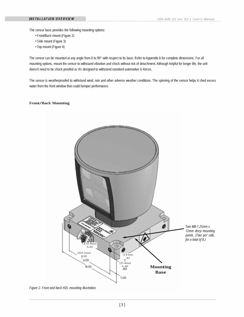
The sensor base provides the following mounting options:
• Front/Back mount (Figure 2)
• Side mount (Figure 3)
• Top mount (Figure 4)
The sensor can be mounted at any angle from 0 to 90° with respect to its base. Refer to Appendix A for complete dimensions. For all
mounting options, mount the sensor to withstand vibration and shock without risk of detachment. Although helpful for longer life, the unit
doesn’t need to be shock proofed as it’s designed to withstand standard automotive G-forces.
The sensor is weatherproofed to withstand wind, rain and other adverse weather conditions. The spinning of the sensor helps it shed excess
water from the front window that could hamper performance.
Front/Back Mounting
[152.4mm] 6.00
Two M8-1.25mm x 12mm deep mounting points. (Two per side, for a total of 8.)
[203.2mm]
8.00 [21mm]
.83
[25.4mm] 1.00
Mounting
Base
Figure 2. Front and back HDL mounting illustration.
I N S
[ 4 ]
TA L L AT I O N O V E R V I E W HDL-64E S2 and S2.1 User’s Manual
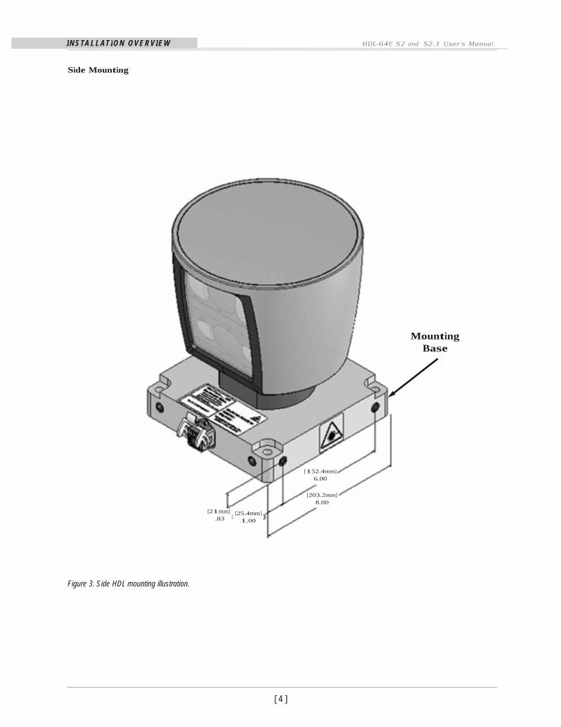
Side Mounting
Mounting Base
[152.4mm] 6.00
[21mm] .83
[25.4mm]
1.00
[203.2mm] 8.00
Figure 3. Side HDL mounting illustration.
I N S TA L L AT I O N O V E R V I E W HDL-64E
[ 5 ]
S2 and S2.1 User’s Manual
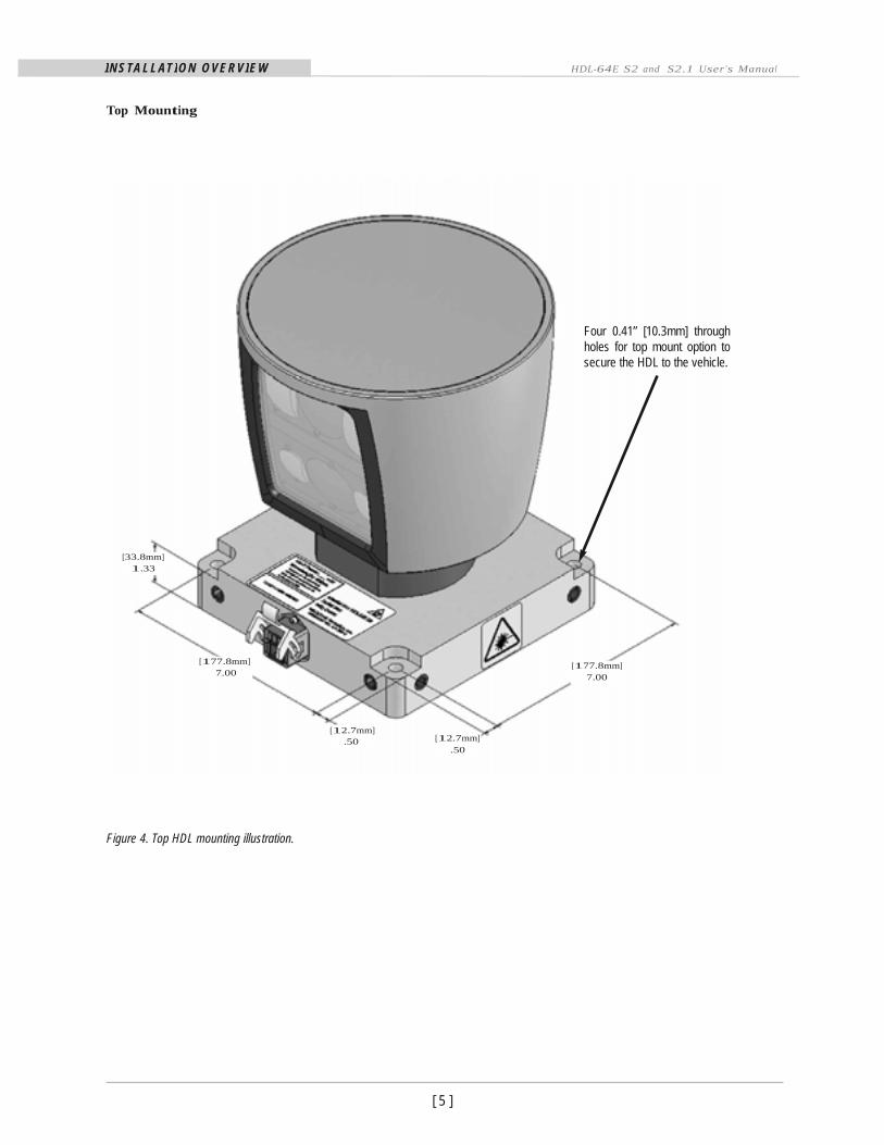
Top Mounting
Four 0.41” [10.3mm] through holes for top mount option to secure the HDL to the vehicle.
[33.8mm] 1.33
[177.8mm] 7.00
[177.8mm]
7.00
[12.7mm] .50 [12.7mm]
.50
Figure 4. Top HDL mounting illustration.
I N S
[ 6 ]
TA L L AT I O N O V E R V I E W HDL-64E S2 and S2.1 User’s Manual
Wiring
The sensor comes with a pre-wired connector, wired with power, DB9 serial and standard RJ45 Ethernet connectors. The connector wires are
approximately 10’ [3 meters] in length.
Power. Connect the red and black wires to vehicle power. Be sure red is positive polarity. THE SENSOR IS RATED ONLY FOR 12 - 16
VOLTS. Any voltage applied over 16 volts could damage the sensor. The sensor draws 4-6 AMPS during normal usage.
The sensor doesn’t have a power switch. It spins whenever power is applied.
Lockout Circuit. The sensor has a lockout circuit that prevents its lasers from firing until it achieves approximately 300 RPMs.
Ethernet. This standard Ethernet connector is designed to connect to a standard PC.
The sensor is only compatible with network cards that have either MDI or AUTO MDIX capability.
Serial Interface RS-232 DB9. This standard connector allows for a firmware update to be applied to the sensor. Velodyne may release
firmware updates from time to time. It also accepts commands to change the RPM of the unit, control HFOV, change the unit’s IP address,
and other functions described later in this manual.
Wiring Diagram. If you need to wire your own connector for your installation, refer to the wiring diagram in Appendix B.
U S A G E
The sensor needs no configuration, calibration, or other setup to begin producing usable data. Once the unit is mounted and wired, supplying
it power causes it to start scanning and producing data packets.
Use the Included Point-cloud Viewer
The quickest way to view the data collected as an image is to use the included Digital Sensor Recorder (DSR). DSR is Velodyne’s point-cloud
processing data viewer software. DSR reads in the packets from the sensor over Ethernet, performs the necessary calculations to determine
point locations and then plots the points in 3D on your PC monitor. You can observe both distance and intensity data through DSR. If you
have never used the sensor before, this is the recommended starting point. For more on installing and using DSR, see Appendix C.
Develop Your Own Application-specific Point-cloud Viewer
Many users elect to develop their own application-specific point cloud tracking and plotting and/or storage scheme, which requires these
fundamental steps:
1. Establish communication with the sensor.
2. Create a calibration table either from the calibration data included in-stream from the sensor or from the included db.xml data file.
3. Parse the packets for rotation, block, distance and intensity data
4. Apply the calibration factors to the data.
5. Plot or store the data as needed.
[ 7 ]
U S A G E HDL-64E S2 and S2.1 User’s Manual
The following provides more detail on each of the above steps.
1. Establish communication with the sensor.
The sensor broadcasts UDP packets. By using a network monitoring tool, such as Wireshark, you can capture and observe the
packets as they are generated by the sensor. See Appendix E for the UDP packet format. The default source IP address for the
sensor is 192.168.3.043, and the destination IP address is 192.168.3.255. To change these IP addresses, see page 11.
2. Create an internal calibration table either from the calibration data included in-stream from the sensor or from the included
db.xml data file.
This table must be built and stored internal to the point-cloud processing software. The easiest and most reliable way to build the
calibration table is by reading the calibration data directly from the UDP data packets. A MatLab example of reading and building
such a table can be found in Appendix D and on the CD included with the sensor named CALTABLEBUILD.m.
Alternatively, the calibration data can be found in the included db.xml file found on the CD included with the sensor. A description of the
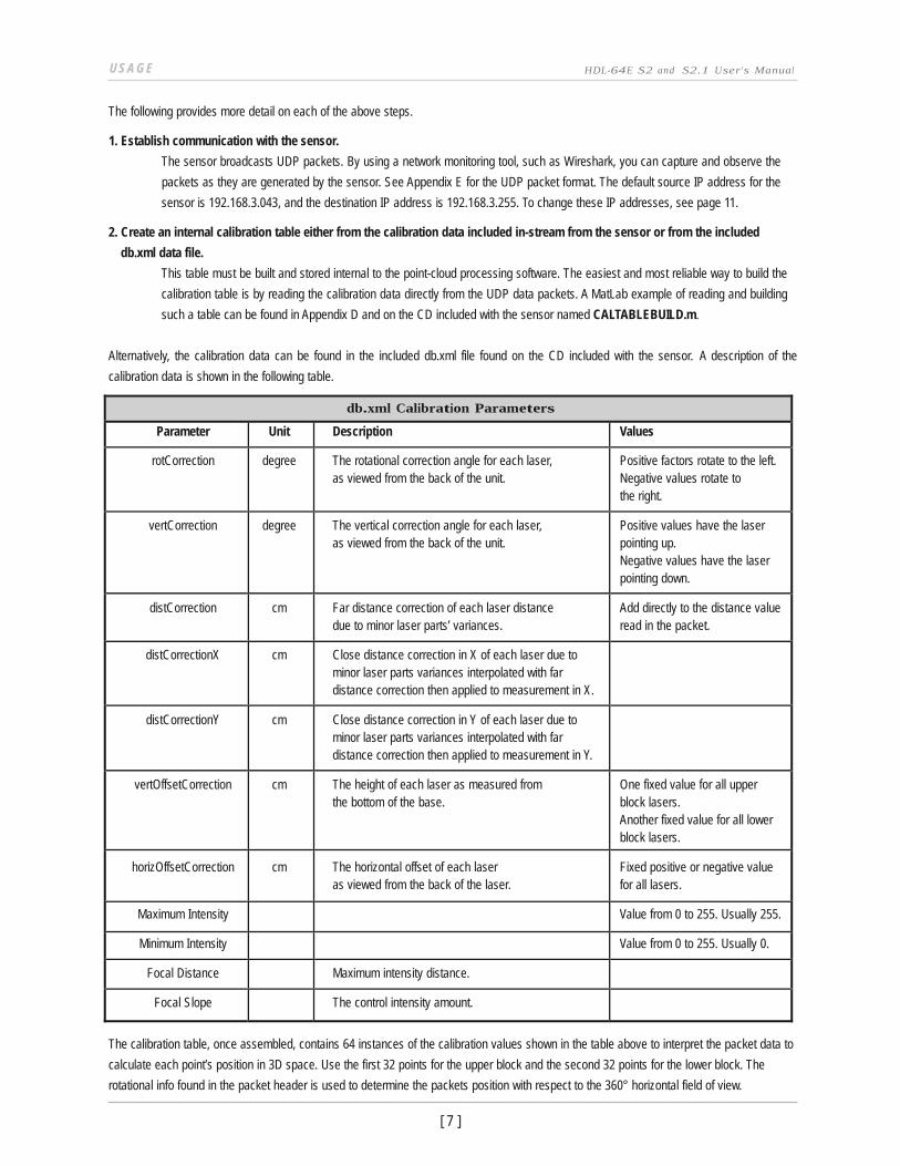
calibration data is shown in the following table.
db.xml Calibration Parameters Parameter Unit Description Values
rotCorrection degree The rotational correction angle for each laser, as viewed from the back of the unit.
Positive factors rotate to the left. Negative values rotate to the right.
vertCorrection degree The vertical correction angle for each laser, as viewed from the back of the unit.
Positive values have the laser pointing up. Negative values have the laser pointing down.
distCorrection cm Far distance correction of each laser distance due to minor laser parts’ variances.
Add directly to the distance value read in the packet.
distCorrectionX cm Close distance correction in X of each laser due to minor laser parts variances interpolated with far distance correction then applied to measurement in X.
distCorrectionY cm Close distance correction in Y of each laser due to minor laser parts variances interpolated with far distance correction then applied to measurement in Y.
vertOffsetCorrection cm The height of each laser as measured from the bottom of the base.
One fixed value for all upper block lasers. Another fixed value for all lower block lasers.
horizOffsetCorrection
cm
The horizontal offset of each laser as viewed from the back of the laser.
Fixed positive or negative value for all lasers.
Maximum Intensity Value from 0 to 255. Usually 255.
Minimum Intensity Value from 0 to 255. Usually 0.
Focal Distance Maximum intensity distance.
Focal Slope The control intensity amount.
The calibration table, once assembled, contains 64 instances of the calibration values shown in the table above to interpret the packet data to
calculate each point’s position in 3D space. Use the first 32 points for the upper block and the second 32 points for the lower block. The
rotational info found in the packet header is used to determine the packets position with respect to the 360° horizontal field of view.
[ 8 ]
U S A G E HDL-64E S2 and S2.1 User’s Manual
3. Parse the packets for rotation, block, distance and intensity data. Each sensor’s LIFO data packet has a 1206 byte payload consisting
of 12 blocks of 100 byte firing data followed by 6 bytes of calibration and other information pertaining to the sensor.
Each 100 byte record contains a block identifier, then a rotational value followed by 32 3-byte combinations that report on each laser fired
for the block. Two bytes report distance to the nearest 0.2 cm, and the remaining byte reports intensity on a scale of 0 -255. 12 100 byte
records exist, therefore, 6 records exist for each block in each packet. For more on packet construction, see Appendix E.
4. Apply the calibration factors to the data. Each of the sensor’s lasers is fixed with respect to vertical angle and offset to the rotational
index data provided in each packet. For each data point issued by the sensor, rotational and horizontal correction factors must be applied to
determine the point’s location in 3D space referred to by the return. Intensity and distance offsets must also be applied. Each sensor comes
from Velodyne’s factory calibrated using a dual-point calibration methodology, explained further in Appendix F.
The minimum return distance for the sensor is approximately 3 feet (0.9 meters). Ignore returns closer than this.
A file on the CD called “HDL Source Example” shows the calculations using the above correction factors. This DSR uses this code to
determine 3D locations of sensor data points.
5. Plot or store the data as needed. For DSR, the point-cloud data, once determined, is plotted onscreen. The source to do this can be
found on the CD and is entitled “HDL Plotting Example.” DSR uses OpenGL to do its plotting.
You may also want to store the data. If so, it may be useful to timestamp the data so it can be referenced and coordinated with other sensor
data later. The sensor has the capability to synchronize its data with GPS precision time. For more in this capability, see page 11.
Change Run-Time Parameters
The sensor has several run-time parameters that can be changed using the RS-232 serial port. For all commands, use the following
serial parameters:
• Baud 9600
• Parity: None
• Data bits: 8
• Stop bits: 1
All serial commands, except one version of the spin rate command, store data in the sensor’s flash memory. Data stored in flash memory
through serial commands is retained during firmware updates or power cycles.
The sensor has no echo back feature, so no serial data is returned from the sensor. Commands can be sent using a terminal program or by
using batch files (e.g. .bat). A sample .bat file is shown below.
Sample Batch File (.bat)
MODE COM3: 9600,N,8,1 COPY SERCMD.txt COM3 Pause
Sample SERCMD.txt file
This command sets the spin rate to 300 RPM and stores the new value in the unit’s flash memory.
#HDLRPM0300$
[ 9 ]
U S A G E HDL-64E S2 and S2.1 User’s Manual
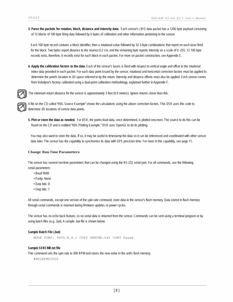
Available commands
The following run-time commands are available with the sensor:
Command Description Parameters
#HDLRPMnnnn$ Set spin rate from 300 to 1200 RPM
n flash memory (default is 600 RPM) nnnn is an integer between 0300 and 1200
#HDLRPNnnnn$ Set spin rate from 300 to 1200 RPM
in RAM (default is 600 RPM) nnnn is an integer between 0300 and 1200
#HDLIPAssssssssssssdddddddddddd$ Change source and/or destination
IP address • ssssssssssss is the source 12-digit IP address
• dddddddddddd is the destination 12-digit
IP address
#HDLFOVsssnnn$ Change horizontal Field of View (HFOV) • sss = starting angle in degrees; sss is an integer
between 000 and 360
• nnn = ending angle in degrees; nnn is an
integer between 000 and 360
You can also upload calibration data from db.xml into flash memory and use GPS time synchronization.
.
U S A G E
[ 10 ]
HDL-64E S2 and S2.1 User’s Manual
Control Spin Rate
Change Spin Rate in Flash Memory
The sensor can spin at rates ranging from 300 RPM (5 Hz) to 1200 RPM (20 Hz). The default is 600 RPM (10 Hz). Changing the spin rate
does not change the data rate — the unit sends out the same number of packets (at a rate of ~1.3 million data points per second) regardless
of its spin rate. The horizontal image resolution increases or decreases depending on rotation speed.
See the Angular Resolution section found in Appendix I for the angular resolution values for various spin rates.
To control the sensor’s spin rate, issue a serial command of the case sensitive format #HDLRPMnnnn$ where nnnn is an integer between
0300 and 1200. The sensor immediately adopts the new spin rate. You don’t need to power cycle the unit, and the new RPM is retained
with future power cycles.
Change Spin Rate in RAM Only
If repeated and rapid updates to the RPM are needed, such as for synchronizing multiple sensors controlled by a closed loop application,
you can adjust the sensors’ spin rates without storing the new RPM in flash memory (this preserves flash memory over time).
To control the sensor’s spin rate in RAM only, issue a serial command of the case sensitive format #HDLRPNnnnn$ where nnnn is an
integer between 0300 and 1200. The sensor immediately adopts the new spin rate. You shouldn’t power cycle the sensor as the new RPM
is lost with future power cycles, which returns to the last known RPM.
Limit Horizontal FOV Data Collected
The sensor defaults to a 360° surrounding view of its environment. It may be desirable to reduce this horizontal Field of View (HFOV) and,
hence, the data created.
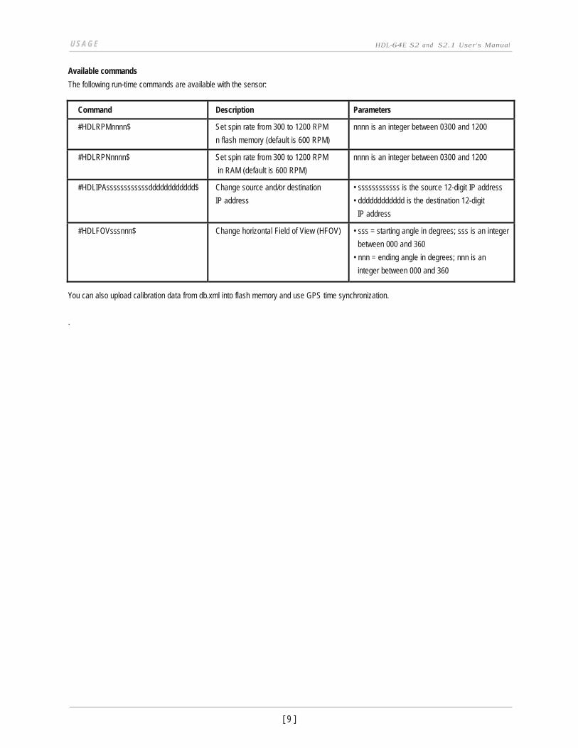
To limit the horizontal FOV, issue a serial command of the case sensitive format #HDLFOVsssnnn$ where:
• sss = starting angle in degrees; sss is an integer between 000 and 360
• nnn = ending angle in degrees; nnn is an integer between 000 and 360
The HDL unit immediately adopts the new HFOV angles without power cycling and will retain the new HFOV settings upon power cycle.
Examples
Regardless of the FOV setting, the lasers will always fire at the full 360° HFOV. Limiting the HFOV only limits data transmission to the HFOV
of interest.
The following diagram shows the HFOV from the top view of the sensor.
Case 1: FOV 0° to 360°
FOV command: #HDLFOV000360$
Case 2: FOV 0° to 90°
FOV command: #HDLFOV000090$
Case 3: FOV -90° to 90°
FOV command: #HDLFOV270090$
Top view of Sensor
[ 11 ]
U S A G E HDL-64E S2 and S2.1 User’s Manual
Define Sensor Memory IP Source and Destination Addresses
The HDL-64E comes with the following default IP addresses:
• Source: 192.168.3.043
• Destination: 192.168.3.255
To change either of the above IP addresses, issue a serial command of the case sensitive format #HDLIPAssssssssssssdddddddddddd$
where,
• ssssssssssss is the source 12-digit IP address
• dddddddddddd is the destination 12-digit IP address
Use all 12 digits to set an IP address. Use 0 (zeros) where a digit would be absent. For example, 192168003043 is the correct syntax for IP
address 192.168.3.43.
The unit must be power cycled to adopt the new IP addresses.
Upload Calibration Data
Sensors use the db.xml file exclusively for calibration data. The calibration data found in db.xml can be uploaded and saved to the unit’s
flash memory by following the steps outlined below.
1. Locate the files HDLCAL.bat, loadcal.exe, and db.xml on the CD and copy them to the same directory on your PC
connected to the sensor.
2. Edit HDLCAL.bat to ensure the copy command lists the right COM port for RS-232 communication with the sensor.
3. Run HDLCAL.bat and ensure successful completion.
4. The sensor received and saved the calibration data.
To verify successful load of the calibration data, ensure the date and time of the upload have been updated. Refer to Appendix E for where in
the data packets this data can be located.
External GPS Time Synchronization
The sensor can synchronize its data with precision GPS-supplied time pulses so you can ascertain the exact firing time of each laser in any
particular packet. The firing time of the first laser in a particular packet is reported in the form of microseconds since the top of the hour, and
from that time each subsequent laser’s firing time can be derived via the table published in Appendix H and included on the CD.
Calculating the exact firing time requires a GPS receiver generating a sync pulse and the $GPRMC NMEA record over a dedicated RS-232
serial port. The output from the GPS receiver is connected to an external GPS adaptor box supplied by Velodyne that conditions the signal
and passes it to the sensor. The GPS receiver can either be supplied by Velodyne or the customer can adapt their GPS receiver to provide
the required sync pulse and NMEA record.
GPS Receiver Option 1: Velodyne Supplied GPS Receiver
Velodyne provides an optional pre-programmed GPS receiver (HDL-64-GPS) This receiver is pre-wired with an RS-232 connector that
plugs into the GPS adapter box. To obtain a pre-programmed GPS receiver, contact Velodyne sales or service.
GPS Receiver Option 2: Customer Supplied GPS Receiver
You can supply and configure your own GPS device. If using your own GPS device:
• Issue a once-a-second synchronization pulse, typically output over a dedicated wire.
• Configure an available RS-232 serial port to issue a once-a-second $GPRMC NMEA record. No other output can be accepted
from the GPS device.
• Issue the sync pulse and NMEA record sequentially.
• The sync pulse length is not critical (typical lengths are between 20ms and 200ms)
• Start the $GPRMC record between 50ms and 500ms after the end of the sync pulse.
• Configure the $GPRMC record either in the hhmmss or hhmmss.s format.
U S A G E HDL-64E S2 and S2.1 User
’s Manual
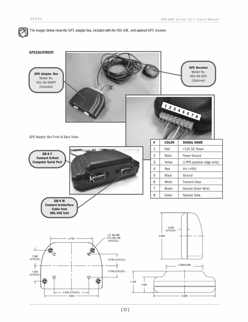
The images below show the GPS adaptor box, included with the HDL-64E, and optional GPS receiver.
G P S E QU I P M E N T
GPS Adaptor Box Model No.
HDL-64-ADAPT (Included)
GPS Receiver Model No.
HDL-64-GPS (Optional)
GPS Adaptor Box Front & Back View
DB-9 F Connect to Host
Computer Serial Port
DB-9 M Connect to Interface
Cable from HDL-64E Unit
# COLOR SIGNAL NAME
1 Red +12V DC Power
2 Black Power Ground
3 Yellow 1 PPS (positive edge only)
4 Red Vin (+5V)
5 Black Ground
6 White Transmit Data
7 Brown Ground (Drain Wire)
8 Green Receive Data
[ 12 ]
U S A G E HDL-64E S2 and S2.1 User’s Manual
[ 13 ]
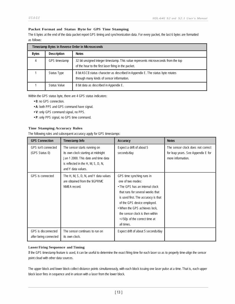
Packet Format and Status Byte for GPS Time Stamping
The 6 bytes at the end of the data packet report GPS timing and synchronization data. For every packet, the last 6 bytes are formatted
as follows:
Timestamp Bytes in Reverse Order in Microseconds
Bytes Description Notes
4 GPS timestamp 32 bit unsigned integer timestamp. This value represents microseconds from the top
of the hour to the first laser firing in the packet.
1 Status Type 8 bit ASCII status character as described in Appendix E. The status byte rotates
through many kinds of sensor information.
1 Status Value 8 bit data as described in Appendix E.
Within the GPS status byte, there are 4 GPS status indicators:
• 0: no GPS connection.
• A: both PPS and GPS command have signal.
• V: only GPS command signal, no PPS.
• P: only PPS signal, no GPS time command.
Time Stamping Accuracy Rules
The following rules and subsequent accuracy apply for GPS timestamps:
GPS Connection Timestamp Info Accuracy Notes
GPS isn’t connected
(GPS Status 0) The sensor starts running on
its own clock starting at midnight
Jan 1 2000. This date and time data
is reflected in the H, M, S, D, N,
and Y data values.
Expect a drift of about 5
seconds/day The sensor clock does not correct
for leap years. See Appendix E for
more information.
GPS is connected The H, M, S, D, N, and Y data values
are obtained from the $GPRMC
NMEA record.
GPS time synching runs in
one of two modes:
• The GPS has an internal clock
that runs for several weeks that
is used first. The accuracy is that
of the GPS device employed.
• When the GPS achieves lock,
the sensor clock is then within
+/-50js of the correct time at
all times.
GPS is disconnected
after being connected The sensor continues to run on
its own clock. Expect drift of about 5 seconds/day
Laser Firing Sequence and Timing
If the GPS timestamp feature is used, it can be useful to determine the exact firing time for each laser so as to properly time-align the sensor
point cloud with other data sources.
The upper block and lower block collect distance points simultaneously, with each block issuing one laser pulse at a time. That is, each upper
block laser fires in sequence and in unison with a laser from the lower block.
U S A G E HDL-64E S2 and S2.1 User’s Manual
Lasers are numbered sequentially starting with 0 for the first lower block laser to 31 for the last lower block laser; and 32 for the first upper block laser
to 63 for the last upper block laser. For example, laser 32 fires simultaneously with laser 0, laser 33 fires with laser 1, and so on.
The sensor has an equal number of upper and lower block returns. Hence, when interpreting the delay table, each sequential pair of data blocks
represents the upper and lower block respectively. Each upper and lower block data pair in the Ethernet packet has the same delay value.
The first firing of a laser pair occurs 419.3 ps after the issuance of the fire command. Six firings of each block takes 139 ps and then the collected
data is transmitted. It takes 100 ps to transmit the entire 1248 byte Ethernet packet. This is equal to 12.48 Bytes/ps and
0.080128 ps/Byte. See Appendix E for more information.
A timing table, shown in Appendix G, shows how much time elapses between the actual capturing of a distance point and when that point is output
from the device. By registering the event of the Ethernet data capture, you can calculate back in time the exact time at which any particular distance
point was captured.
F I R M WA R E U P D AT E
From time to time Velodyne issues firmware updates. To update the sensor’s firmware:
1. Obtain the update file from Velodyne.
2. Connect the wiring harness RS-232 cable to a standard Windows compatible PC or laptop serial port.
3. Power up the sensor.
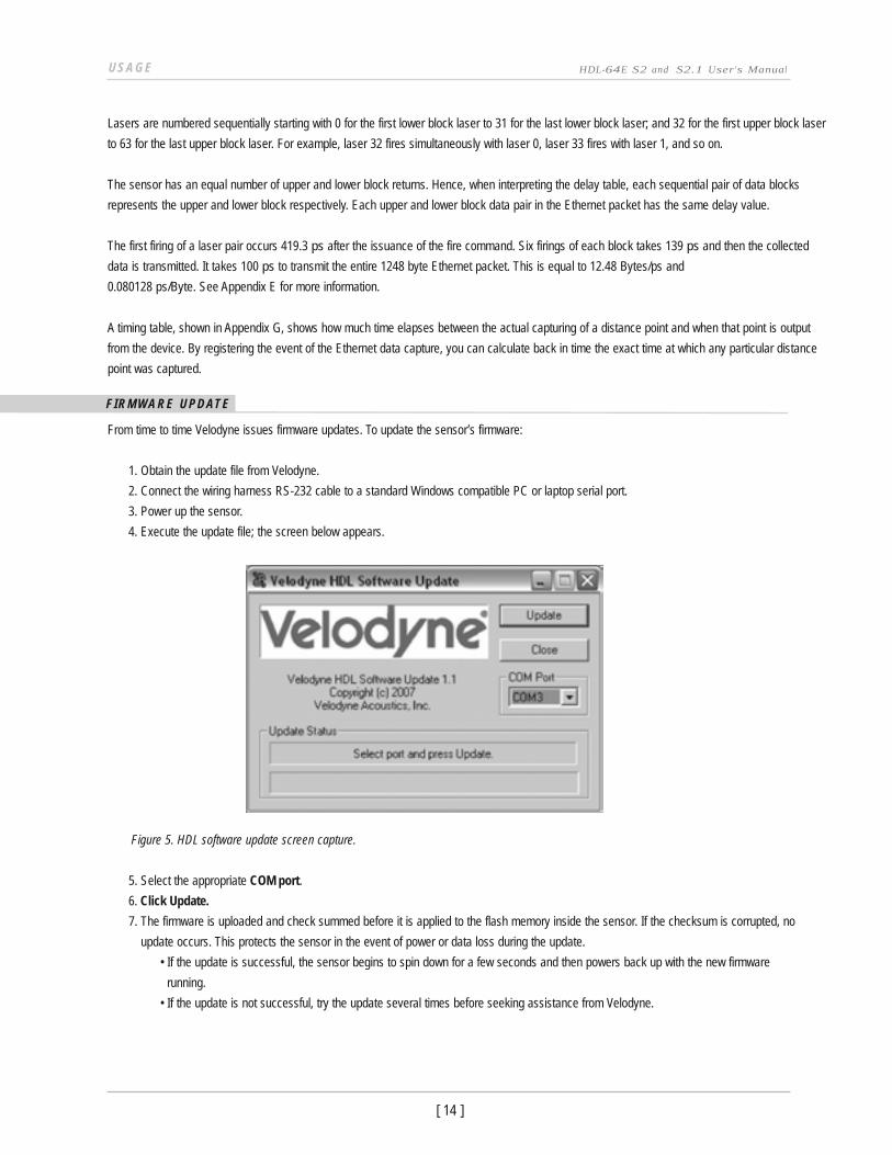
4. Execute the update file; the screen below appears.
Figure 5. HDL software update screen capture.
5. Select the appropriate COM port.
6. Click Update.
7. The firmware is uploaded and check summed before it is applied to the flash memory inside the sensor. If the checksum is corrupted, no
update occurs. This protects the sensor in the event of power or data loss during the update.
• If the update is successful, the sensor begins to spin down for a few seconds and then powers back up with the new firmware
running.
• If the update is not successful, try the update several times before seeking assistance from Velodyne.
[ 14 ]
U S A G E HDL-64E S2 and S2.1 User’s Manual
[ 15 ]
A P P E N D I X B : W I R I N G D I A G R A M HDL-64E S2 and S2.1 User’s ManuaI
Har
ting
Tech
nolo
gy G
roup
M
etal
Ver
sion
, Sta
ndar
d St
raig
ht S
tyle
M
odel
No.
10-
12-0
05-2
001
[ 16 ]
A P P E N D
[ 17 ]
I X C : D I G I TA L S E N S O R R E C O R DER (DSR) HDL-64E S2 and S2.I User’s Manual
Digital Sensor Recorder (DSR) Digital Sensor Recorder (DSR)
DSR is a 3D point-cloud visualization software program designed for use with the sensor. This software is an “out of the box” tool for the
rendering and recording of point cloud data from the HDL unit.
DSR is a 3D point-cloud visualization software program designed for use with the sensor. This software is an “out of the box” tool for the
rendering and recording of point cloud data from the HDL unit.
You can develop visualization software using the DSR as a reference platform. A code snippet is provided on the CD to aid in understanding
the methods at which DSR parses the data points generated by the HDL sensor. See page 20 for more information.
You can develop visualization software using the DSR as a reference platform. A code snippet is provided on the CD to aid in understanding
the methods at which DSR parses the data points generated by the HDL sensor. See page 20 for more information.
Install Install
To install the DSR on your computer: To install the DSR on your computer:
1. Locate the DSR executable program on the provided CD. 1. Locate the DSR executable program on the provided CD.
2. Double-click this DSR executable file to begin the installation onto a computer connected to the sensor. We recommend that you use
the default settings during the installation.
2. Double-click this DSR executable file to begin the installation onto a computer connected to the sensor. We recommend that you use
the default settings during the installation.
3. Copy the db.xml file supplied with the sensor into the same directory as the DSR executable (defaults to c:\program files\ Digital 3. Copy the db.xml file supplied with the sensor into the same directory as the DSR executable (defaults to c:\program files\ Digital
Sensor Recorder). You may want to rename the existing default db.xml that comes with the DSR install. Sensor Recorder). You may want to rename the existing default db.xml that comes with the DSR install.
Failure to use the calibration db.xml file supplied with your sensor will result in an inaccurate point cloud rendering in DSR.
Calibrate
The db.xml file provided with the sensor contains correction factors for the proper alignment of the point cloud information gathered for each
laser. When implemented properly, the image viewable from the DSR is calibrated to provide an accurate visual representation of the
environment in which the sensor is being used. Also use these calibration factors and equations in any program using the data generated by
the unit.
Live Playback
For live playback:
1. Secure and power up the sensor so that it is spinning.
2. Connect the RJ45 Ethernet connector to your host computer’s network connection. You may wish to use auto DNS settings for your
computers network configuration.
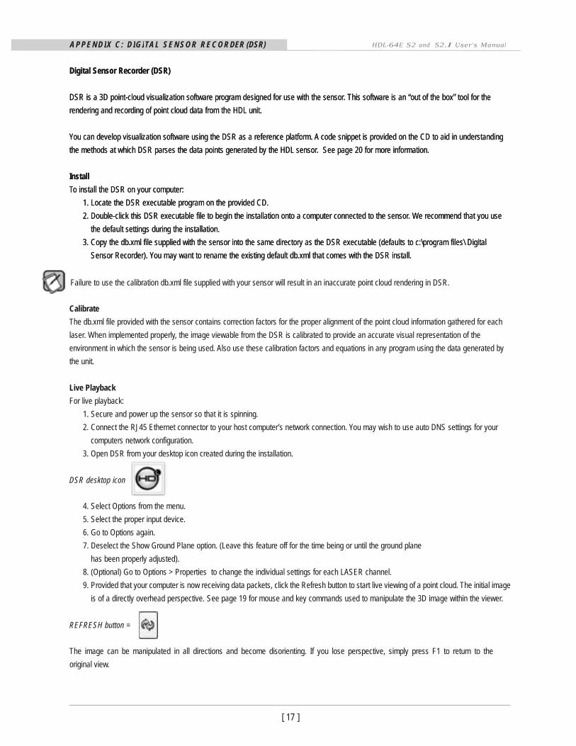
3. Open DSR from your desktop icon created during the installation.
= DSR desktop icon
4. Select Options from the menu.
5. Select the proper input device.
6. Go to Options again.
7. Deselect the Show Ground Plane option. (Leave this feature off for the time being or until the ground plane
has been properly adjusted).
8. (Optional) Go to Options > Properties to change the individual settings for each LASER channel.
9. Provided that your computer is now receiving data packets, click the Refresh button to start live viewing of a point cloud. The initial image
is of a directly overhead perspective. See page 19 for mouse and key commands used to manipulate the 3D image within the viewer.
REFRESH button =
The image can be manipulated in all directions and become disorienting. If you lose perspective, simply press F1 to return to the
original view.
A P P E N D
[ 18 ]
I X C : D I G I TA L S E N S O R R E C O R DER (DSR) HDL-64E S2 and S2.I User’s Manual
Record Data
1. Confirm the input of streaming data through the live playback feature.
2. Click the Record button.
RECORD button =
5. Enter the name and location for the pcap file to be created.
6. Recording begins immediately once the file information has been entered.
7. Click Record again to discontinue the capture.
8. String multiple recordings together on the same file by performing the Record function repeatedly. A new file name isn’t
requested until after the session has been aborted.
An Ethernet capture utility, such as Wireshark, can also be used as a pcap capture utility.
Playback of Recorded Files
1. Use the File > Open command to open a previously captured pcap file for playback. The DSR playback controls are similar
to any DVD/VCR control features.
2. Press the Play button to render the file. The Play button toggles to a Pause button when in playback mode.
PLAY button = PAUSE button =
Use the Forward and Reverse buttons to change the direction of playback..
FORWARD button = REVERSE button =
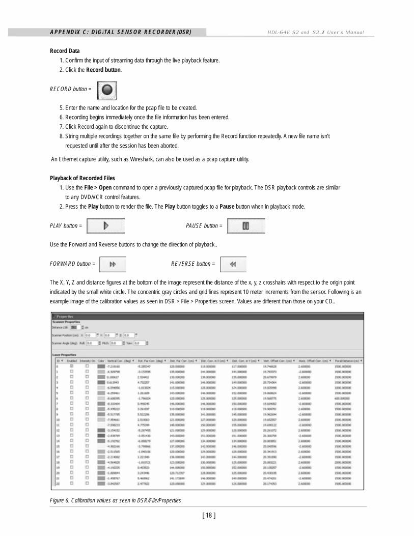
The X, Y, Z and distance figures at the bottom of the image represent the distance of the x, y, z crosshairs with respect to the origin point
indicated by the small white circle. The concentric gray circles and grid lines represent 10 meter increments from the sensor. Following is an
example image of the calibration values as seen in DSR > File > Properties screen. Values are different than those on your CD..
Figure 6. Calibration values as seen in DSR/File/Properties
A P P E N D
[ 19 ]
I X C : D I G I TA L S E N S O R R E C O R DER (DSR) HDL-64E S2 and S2.I User’s Manual
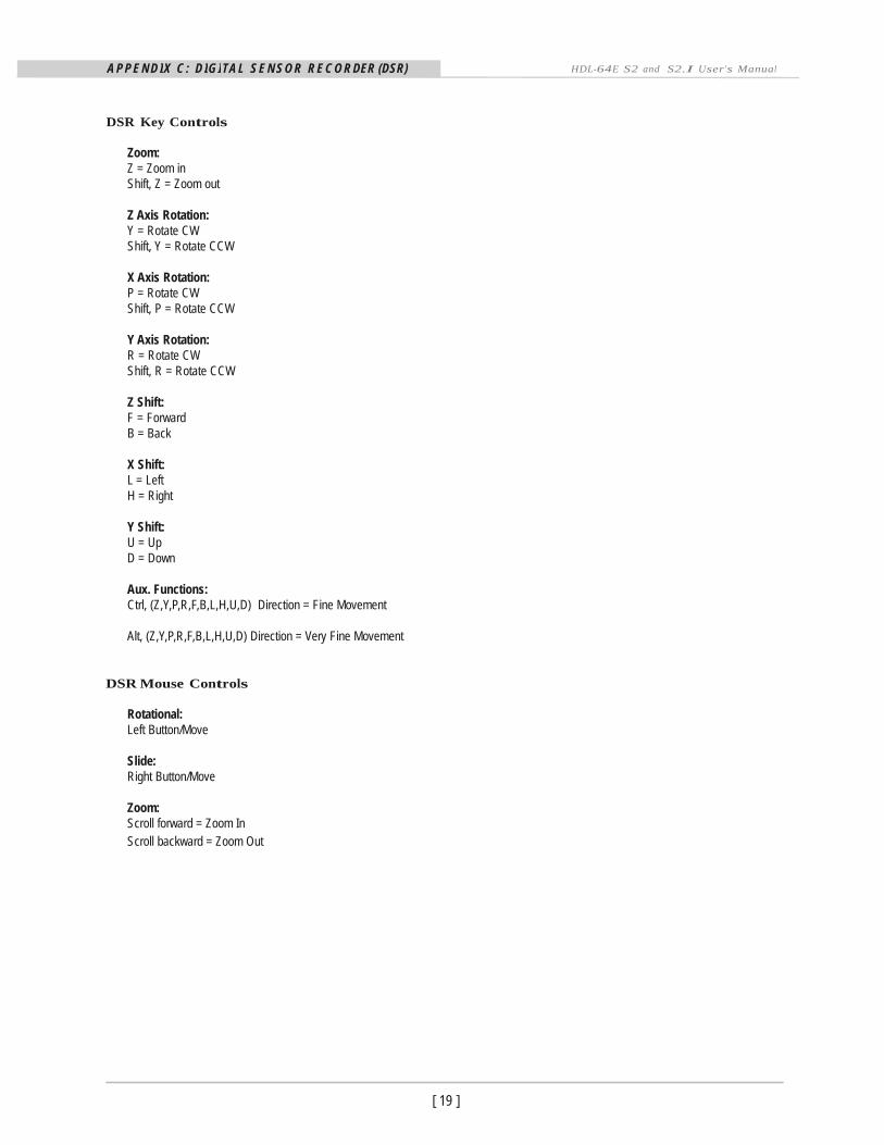
DSR Key Controls
Zoom: Z = Zoom in Shift, Z = Zoom out
Z Axis Rotation: Y = Rotate CW Shift, Y = Rotate CCW
X Axis Rotation: P = Rotate CW Shift, P = Rotate CCW
Y Axis Rotation: R = Rotate CW Shift, R = Rotate CCW
Z Shift: F = Forward B = Back
X Shift: L = Left H = Right
Y Shift: U = Up D = Down
Aux. Functions: Ctrl, (Z,Y,P,R,F,B,L,H,U,D) Direction = Fine Movement
Alt, (Z,Y,P,R,F,B,L,H,U,D) Direction = Very Fine Movement
DSR Mouse Controls
Rotational: Left Button/Move
Slide: Right Button/Move
Zoom: Scroll forward = Zoom In Scroll backward = Zoom Out
A P P E N D I X D : M AT L A B S A M P L E C O D E HDL-64E S2 and S2.I User’s Manual
[ 20 ]
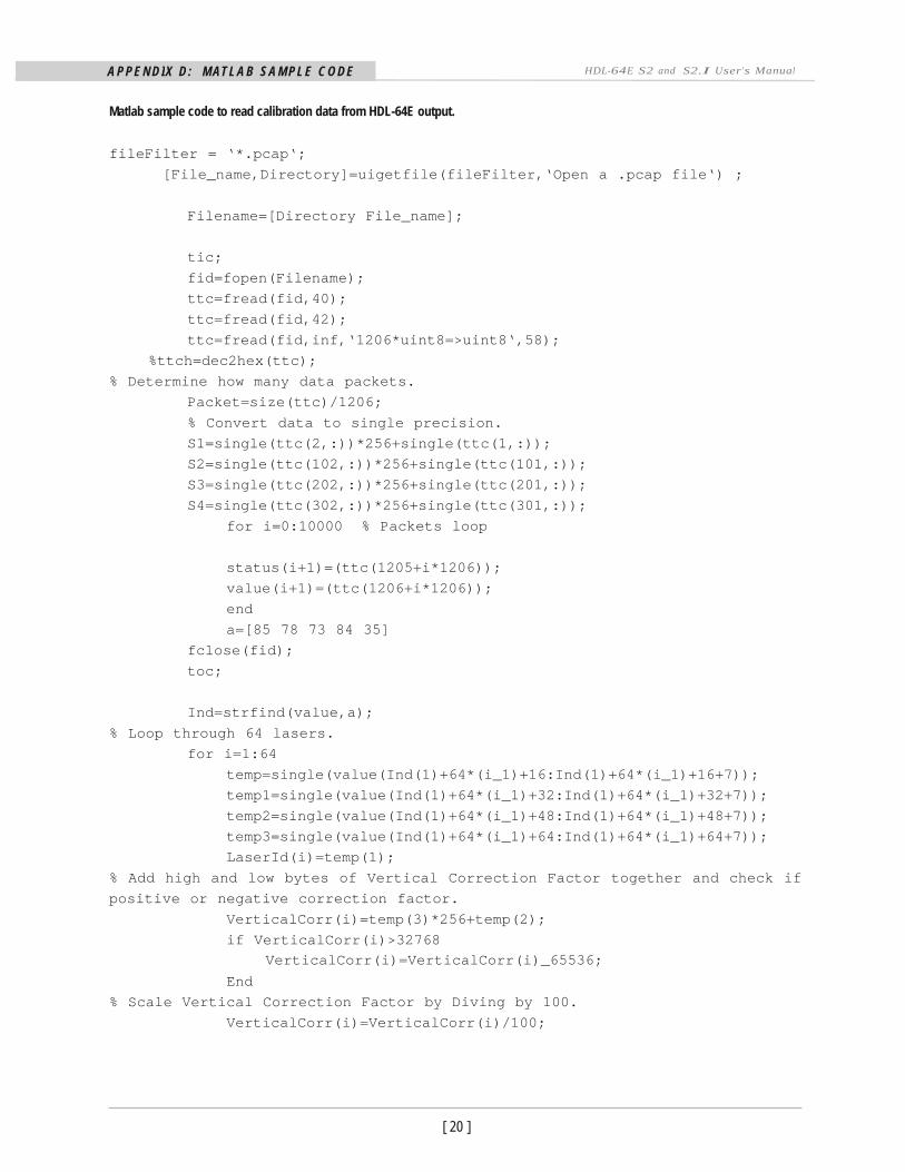
Matlab sample code to read calibration data from HDL-64E output.
fileFilter = ‘*.pcap‘;
[File_name,Directory]=uigetfile(fileFilter,‘Open a .pcap file‘) ;
Filename=[Directory File_name];
tic;
fid=fopen(Filename);
ttc=fread(fid,40);
ttc=fread(fid,42); ttc=fread(fid,inf,‘1206*uint8=>uint8‘,58);
%ttch=dec2hex(ttc); % Determine how many data packets.
Packet=size(ttc)/1206; % Convert data to single precision.
S1=single(ttc(2,:))*256+single(ttc(1,:));
S2=single(ttc(102,:))*256+single(ttc(101,:));
S3=single(ttc(202,:))*256+single(ttc(201,:));
S4=single(ttc(302,:))*256+single(ttc(301,:)); for i=0:10000 % Packets loop
status(i+1)=(ttc(1205+i*1206));
value(i+1)=(ttc(1206+i*1206));
end a=[85 78 73 84 35]
fclose(fid); toc;
Ind=strfind(value,a);
% Loop through 64 lasers.
for i=1:64 temp=single(value(Ind(1)+64*(i_1)+16:Ind(1)+64*(i_1)+16+7));
temp1=single(value(Ind(1)+64*(i_1)+32:Ind(1)+64*(i_1)+32+7));
temp2=single(value(Ind(1)+64*(i_1)+48:Ind(1)+64*(i_1)+48+7));
temp3=single(value(Ind(1)+64*(i_1)+64:Ind(1)+64*(i_1)+64+7));
LaserId(i)=temp(1); % Add high and low bytes of Vertical Correction Factor together and check if
positive or negative correction factor. VerticalCorr(i)=temp(3)*256+temp(2); if VerticalCorr(i)>32768
VerticalCorr(i)=VerticalCorr(i)_65536; End
% Scale Vertical Correction Factor by Diving by 100. VerticalCorr(i)=VerticalCorr(i)/100;
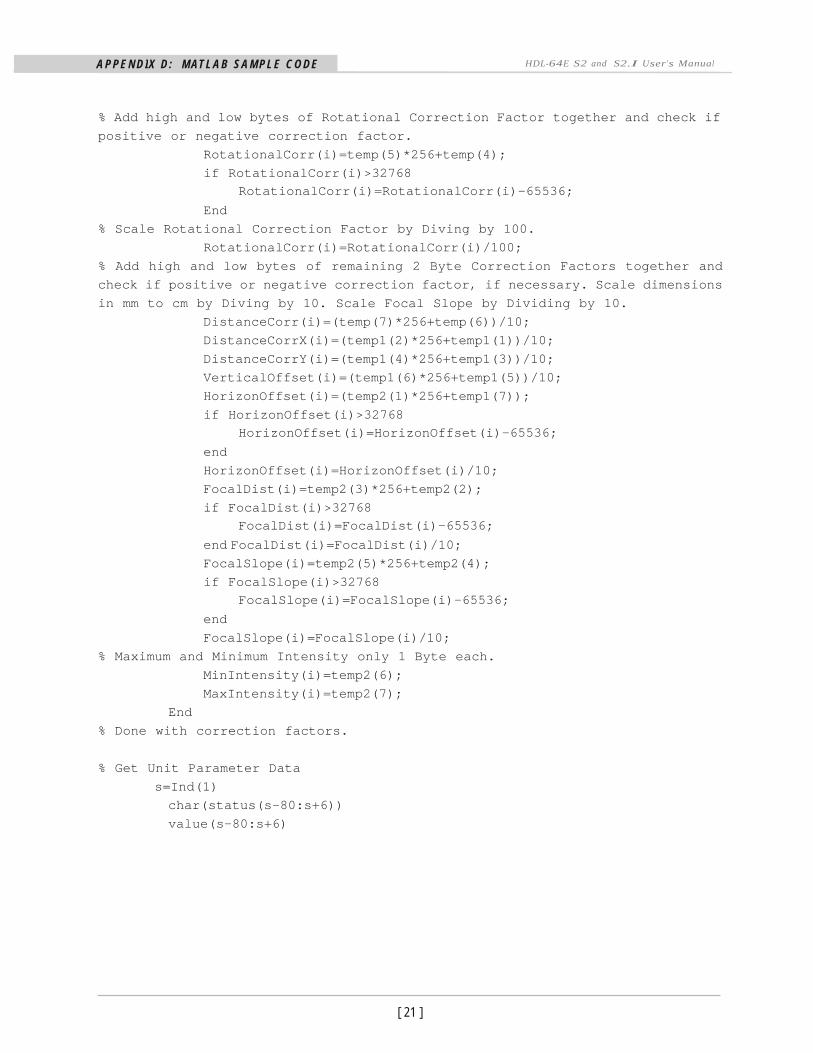
A P P E N D I X D : M AT L A B S A M P L E C O D E HDL-64E S2 and S2.I User’s Manual % Add high and low bytes of Rotational Correction Factor together and check if
positive or negative correction factor. RotationalCorr(i)=temp(5)*256+temp(4); if RotationalCorr(i)>32768
RotationalCorr(i)=RotationalCorr(i)—65536; End
% Scale Rotational Correction Factor by Diving by 100. RotationalCorr(i)=RotationalCorr(i)/100;
% Add high and low bytes of remaining 2 Byte Correction Factors together and
check if positive or negative correction factor, if necessary. Scale dimensions
in mm to cm by Diving by 10. Scale Focal Slope by Dividing by 10. DistanceCorr(i)=(temp(7)*256+temp(6))/10;
DistanceCorrX(i)=(temp1(2)*256+temp1(1))/10;
DistanceCorrY(i)=(temp1(4)*256+temp1(3))/10;
VerticalOffset(i)=(temp1(6)*256+temp1(5))/10;
HorizonOffset(i)=(temp2(1)*256+temp1(7)); if HorizonOffset(i)>32768
HorizonOffset(i)=HorizonOffset(i)—65536; end
HorizonOffset(i)=HorizonOffset(i)/10;
FocalDist(i)=temp2(3)*256+temp2(2); if FocalDist(i)>32768
FocalDist(i)=FocalDist(i)—65536; end FocalDist(i)=FocalDist(i)/10;
FocalSlope(i)=temp2(5)*256+temp2(4);
if FocalSlope(i)>32768 FocalSlope(i)=FocalSlope(i)—65536;
end FocalSlope(i)=FocalSlope(i)/10;
% Maximum and Minimum Intensity only 1 Byte each. MinIntensity(i)=temp2(6);
MaxIntensity(i)=temp2(7); End
% Done with correction factors.
% Get Unit Parameter Data
s=Ind(1) char(status(s—80:s+6)) value(s—80:s+6)
[ 21 ]
A P P E N D I X D : M AT L A B S A M P L E C O D E HDL-64E S2 and S2.I User’s Manual
[ 22 ]
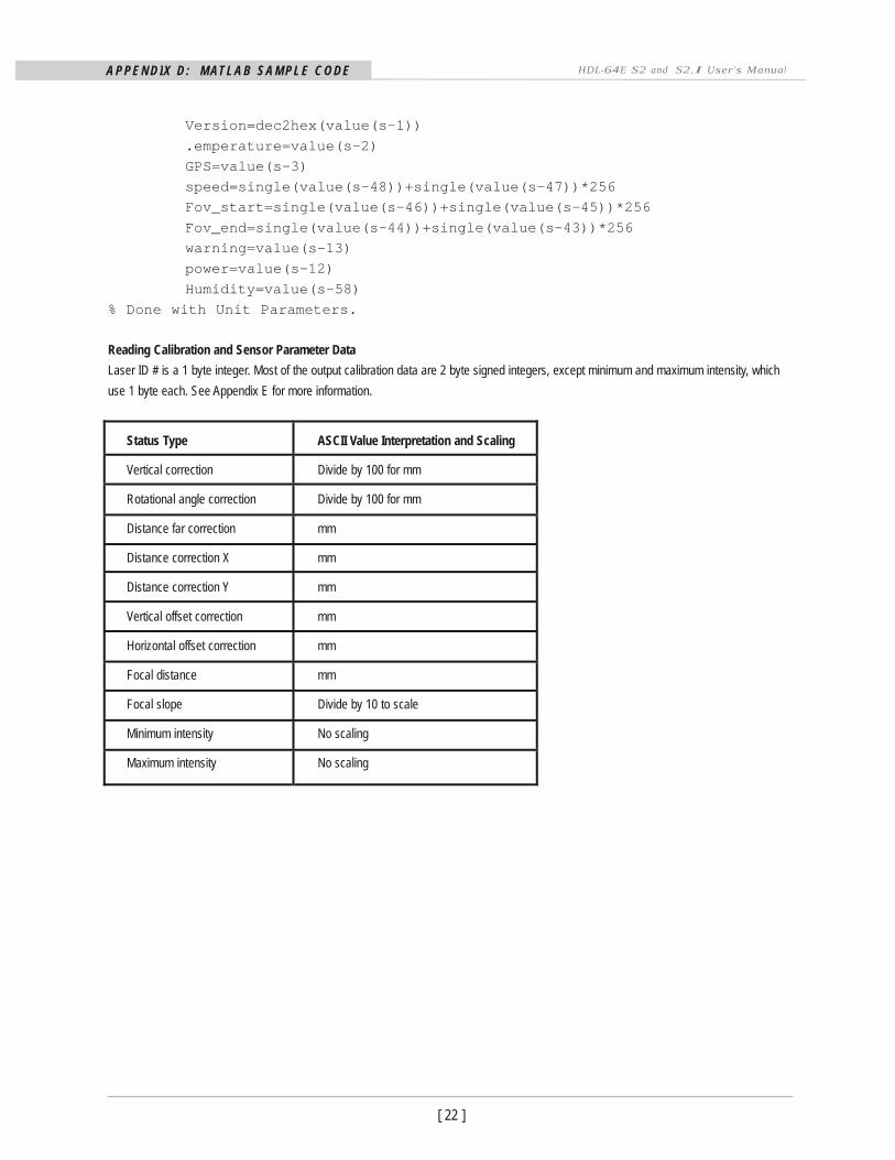
Version=dec2hex(value(s-1)) .emperature=value(s-2)
GPS=value(s-3) speed=single(value(s-48))+single(value(s-47))*256 Fov_start=single(value(s-46))+single(value(s-45))*256 Fov_end=single(value(s-44))+single(value(s-43))*256
warning=value(s-13) power=value(s-12)
Humidity=value(s-58) % Done with Unit Parameters.
Reading Calibration and Sensor Parameter Data
Laser ID # is a 1 byte integer. Most of the output calibration data are 2 byte signed integers, except minimum and maximum intensity, which
use 1 byte each. See Appendix E for more information.
Status Type
ASCII Value Interpretation and Scaling
Vertical correction Divide by 100 for mm
Rotational angle correction Divide by 100 for mm
Distance far correction mm
Distance correction X mm
Distance correction Y mm
Vertical offset correction mm
Horizontal offset correction mm
Focal distance mm
Focal slope Divide by 10 to scale
Minimum intensity No scaling
Maximum intensity No scaling
[ 23 ]
A P P E N D I X E : D ATA PA C K E T F O R M AT HDL-64E S2 and S2.1 User’s Manual
Data Packet Format
The sensor outputs UDP Ethernet packets. Each packet contains a header, a data payload of firing data and status data. Data packets are
assembled with the collection of all firing data for six upper block sequences and six lower block sequences. The upper block laser distance
and intensity data is collected first followed by the lower block laser data. The data packet is then combined with status and header data
in a UDP packet transmitted over Ethernet. The firing data is assembled into the packets in the firing order, with multi-byte values transmitted
least significant byte first.
The status data always contains a GPS 4 byte timestamp representing microseconds from the top of the hour. In addition, the status
data contains one type of data. The other status data rotates through a sequence of different pieces of information. See datagram on
the next page.
A P P E N D
[ 24 ]
I X E : D ATA PA C K E T F O R M AT HDL-64E S2 and S2.1 User’s Manual
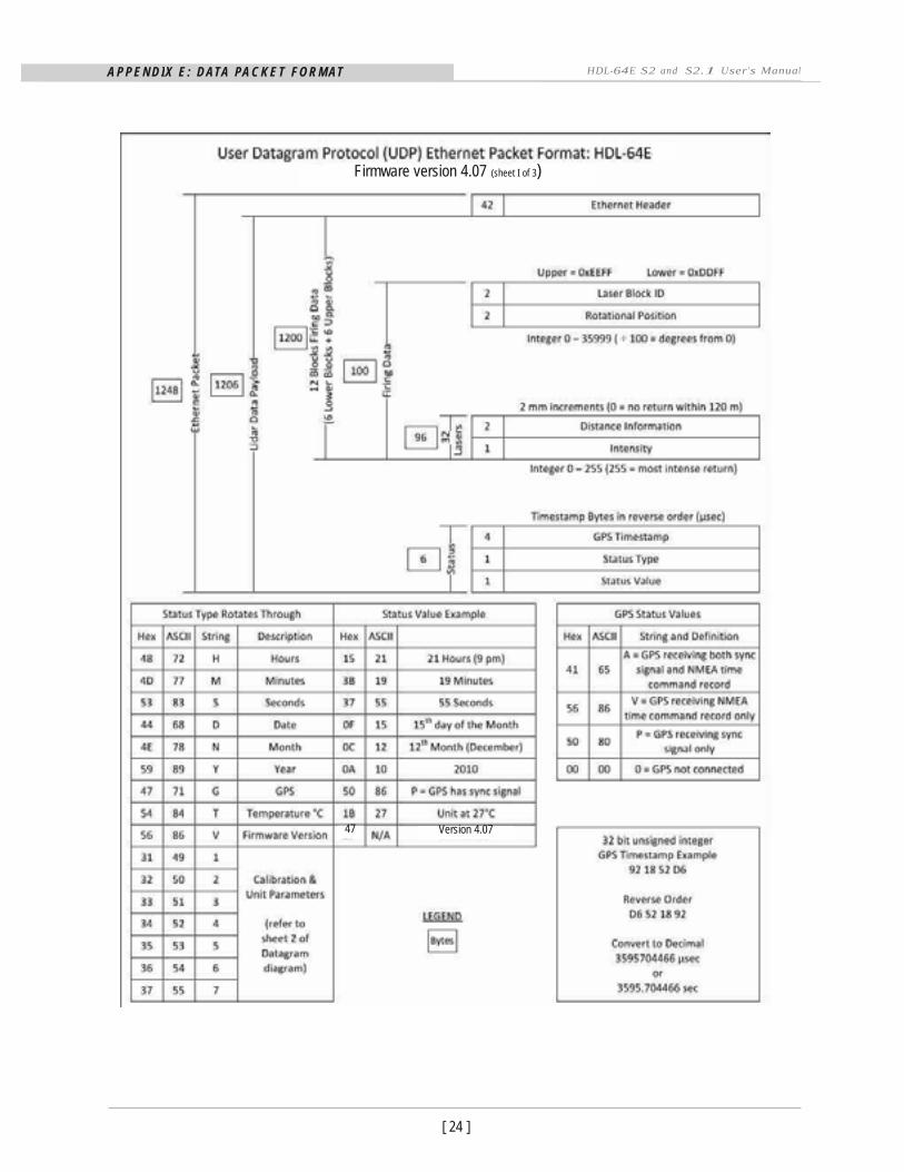
Firmware version 4.07 (sheet I of 3)
47 Version 4.07
[ 25 ]
A P P E N D I X E : D ATA PA C K E T F O R M AT HDL-64E S2 and S2.1 User’s Manual
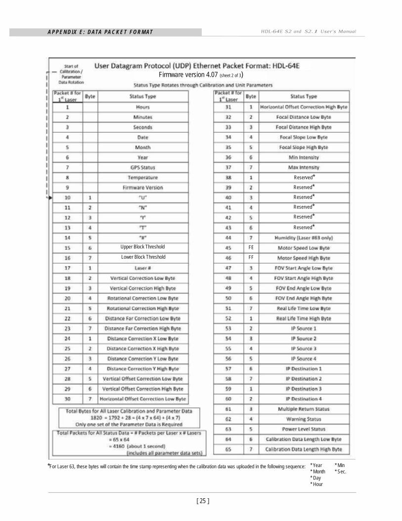
Firmware version 4.07 (sheet 2 of 3)
Reserved*
Reserved*
Reserved*
Reserved*
Reserved*
Reserved*
Upper Block Threshold FE
Lower Block Threshold FF
*For Laser 63, these bytes will contain the time stamp representing when the calibration data was uploaded in the following sequence: * Year * Month * Day * Hour
* Min * Sec.
[ 26 ]
A P P E N D I X E : D ATA PA C K E T F O R M AT HDL-64E S2 and S2.1 User’s Manual
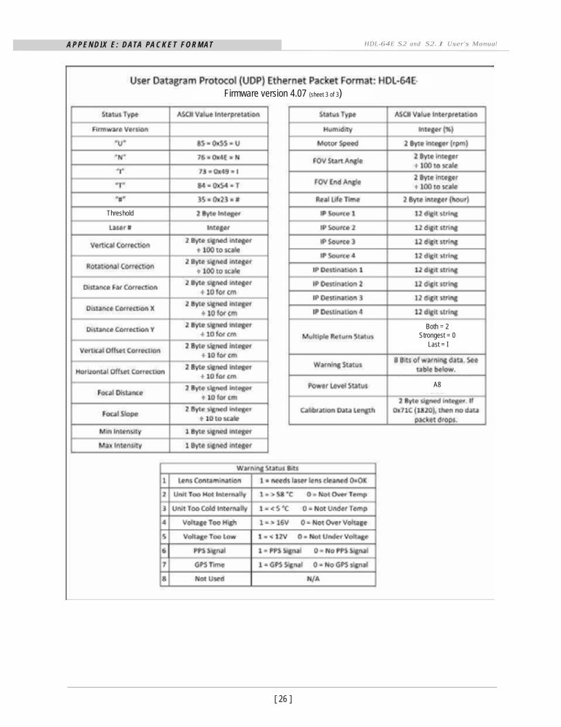
Firmware version 4.07 (sheet 3 of 3)
Threshold
Both = 2 Strongest = 0
Last = I
A8
[ 27 ]
A P P E N D I X E : D ATA PA C K E T F O R M AT HDL-64E S2 and S2.1 User’s Manual
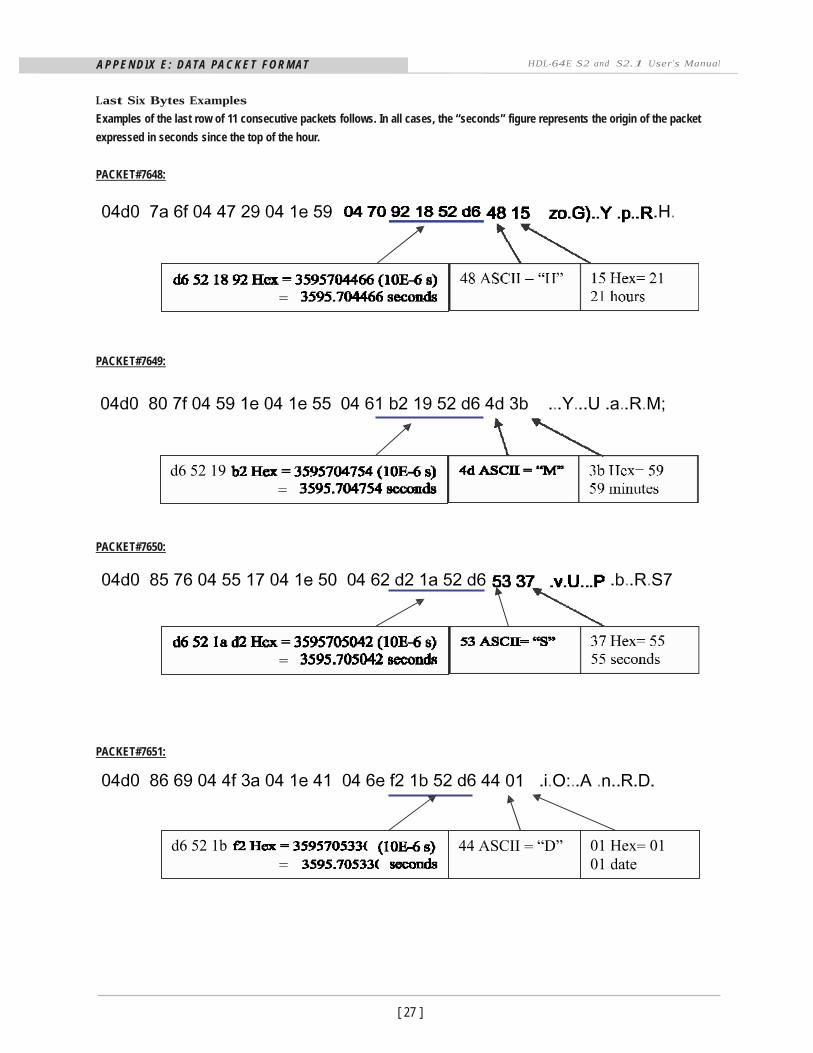
Last Six Bytes Examples
Examples of the last row of 11 consecutive packets follows. In all cases, the “seconds” figure represents the origin of the packet
expressed in seconds since the top of the hour.
PACKET #7648:
PACKET #7649:
PACKET #7650:
PACKET #7651:
[ 28 ]
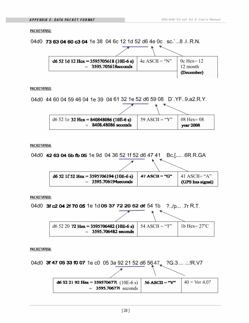
A P P E N D I X E : D ATA PA C K E T F O R M AT HDL-64E S2 and S2.1 User’s Manual
PACKET #7652:
PACKET #7653:
PACKET #7654:
PACKET #7655:
PACKET #7656:
47
40 = Ver 4.07
A P P E N D I X E : D ATA PA C K E T F O R M AT
[ 29 ]
HDL-64E S2 and S2.1 User’s Manual
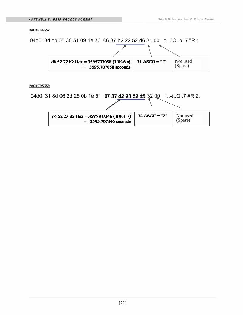
PACKET #7657:
Not used (Spare)
PACKET #7658:
Not used (Spare)
APPENDIX F: DUAL TWO POINT CALIBRATION METHODOLOGY HDL-64E S2 and S2.I User’s Manual
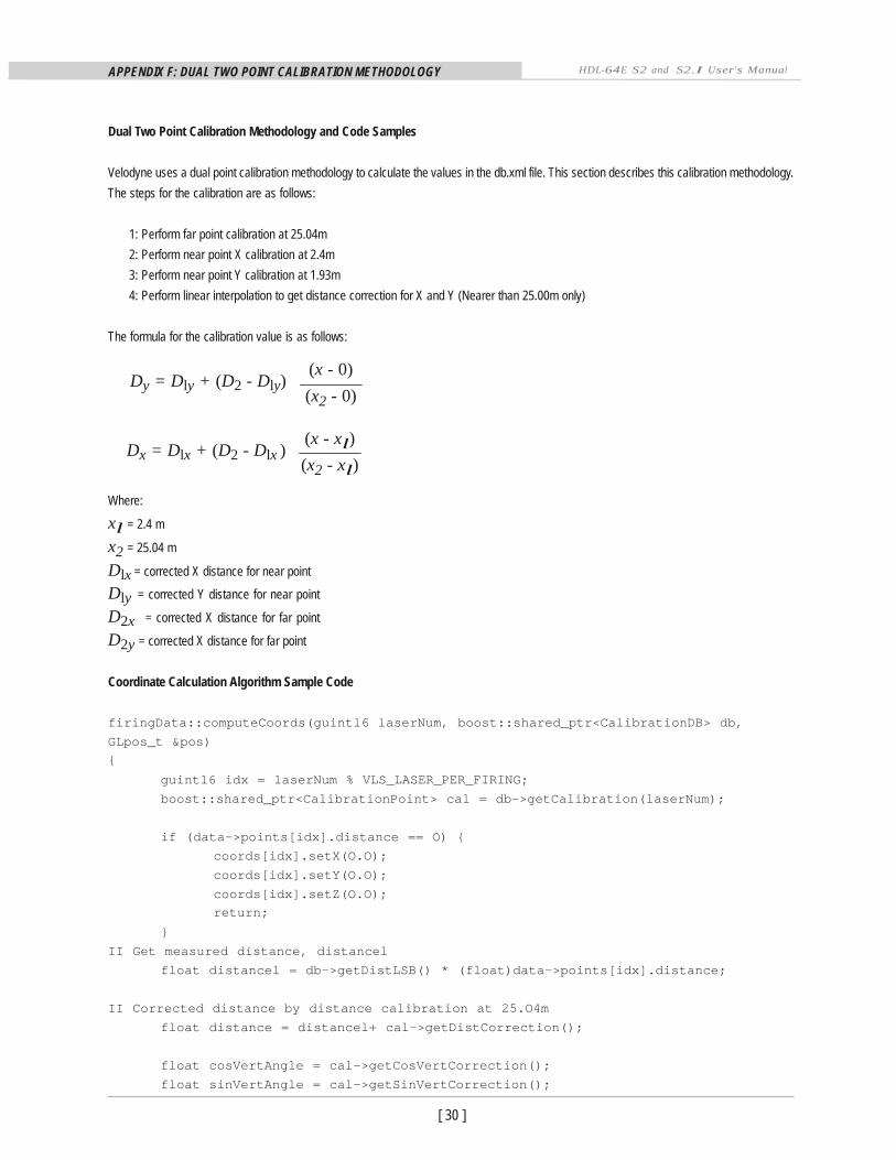
Dual Two Point Calibration Methodology and Code Samples
Velodyne uses a dual point calibration methodology to calculate the values in the db.xml file. This section describes this calibration methodology.
The steps for the calibration are as follows:
1: Perform far point calibration at 25.04m
2: Perform near point X calibration at 2.4m
3: Perform near point Y calibration at 1.93m
4: Perform linear interpolation to get distance correction for X and Y (Nearer than 25.00m only)
The formula for the calibration value is as follows:
(x - 0) Dy = Dly + (D2 - Dly)
Dx = Dlx + (D2 - Dlx )
(x2 - 0) (x - xl)
(x2 - xl)
Where:
xl = 2.4 m
x2 = 25.04 m
Dlx = corrected X distance for near point
Dly = corrected Y distance for near point
D2x = corrected X distance for far point
D2y = corrected X distance for far point
Coordinate Calculation Algorithm Sample Code
firingData::computeCoords(guintl6 laserNum, boost::shared_ptr<CalibrationDB> db,
GLpos_t &pos) {
guintl6 idx = laserNum % VLS_LASER_PER_FIRING;
boost::shared_ptr<CalibrationPoint> cal = db->getCalibration(laserNum);
if (data->points[idx].distance == O) {
coords[idx].setX(O.O);
coords[idx].setY(O.O);
coords[idx].setZ(O.O); return;
}
II Get measured distance, distancel
float distancel = db->getDistLSB() * (float)data->points[idx].distance;
II Corrected distance by distance calibration at 25.O4m
float distance = distancel+ cal->getDistCorrection();
float cosVertAngle = cal->getCosVertCorrection();
float sinVertAngle = cal->getSinVertCorrection();
[ 30 ]
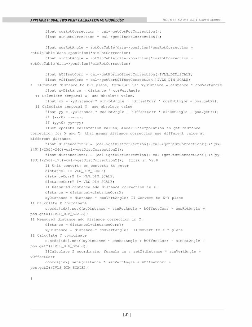
APPENDIX F: DUAL TWO POINT CALIBRATION METHODOLOGY HDL-64E S2 and S2.I User’s Manual
float cosRotCorrection = cal->getCosRotCorrection();
float sinRotCorrection = cal->getSinRotCorrection();
float cosRotAngle = rotCosTable[data->position]*cosRotCorrection +
rotSinTable[data->position]*sinRotCorrection;
float sinRotAngle = rotSinTable[data->position]*cosRotCorrection -
rotCosTable[data->position]*sinRotCorrection;
float hOffsetCorr = cal->getHorizOffsetCorrection()IVLS_DIM_SCALE;
float vOffsetCorr = cal->getVertOffsetCorrection()IVLS_DIM_SCALE;
; IIConvert distance to X-Y plane, formular is: xyDistance = distance * cosVertAngle
float xyDistance = distance * cosVertAngle
II Calculate temporal X, use absolute value.
float xx = xyDistance * sinRotAngle - hOffsetCorr * cosRotAngle + pos.getX();
II Calculate temporal Y, use absolute value
float yy = xyDistance * cosRotAngle + hOffsetCorr * sinRotAngle + pos.getY();
if (xx<0) xx=-xx;
if (yy<0) yy=-yy;
IIGet 2points calibration values,Linear interpolation to get distance
correction for X and Y, that means distance correction use different value at
different distance
float distanceCorrX = (cal->getDistCorrection()-cal->getDistCorrectionX())*(xx-
240)I(2504-240)+cal->getDistCorrectionX();
float distanceCorrY = (cal->getDistCorrection()-cal->getDistCorrectionY())*(yy-
l93)I(2504-l93)+cal->getDistCorrectionY(); IIfix in V2.0
II Unit convert: cm converts to meter
distancel I= VLS_DIM_SCALE;
distanceCorrX I= VLS_DIM_SCALE;
distanceCorrY I= VLS_DIM_SCALE;
II Measured distance add distance correction in X.
distance = distancel+distanceCorrX;
xyDistance = distance * cosVertAngle; II Convert to X-Y plane
II Calculate X coordinate
coords[idx].setX(xyDistance * sinRotAngle - hOffsetCorr * cosRotAngle +
pos.getX()IVLS_DIM_SCALE);
II Measured distance add distance correction in Y.
distance = distancel+distanceCorrY;
xyDistance = distance * cosVertAngle; IIConvert to X-Y plane
II Calculate Y coordinate
coords[idx].setY(xyDistance * cosRotAngle + hOffsetCorr * sinRotAngle +
pos.getY()IVLS_DIM_SCALE);
IICalculate Z coordinate, formula is : setZ(distance * sinVertAngle +
vOffsetCorr
coords[idx].setZ(distance * sinVertAngle + vOffsetCorr +
pos.getZ()IVLS_DIM_SCALE);
}
[ 31 ]
APPENDIX F: DUAL TWO POINT CALIBRATION METHODOLOGY HDL-64E S2 and S2.I User’s Manual
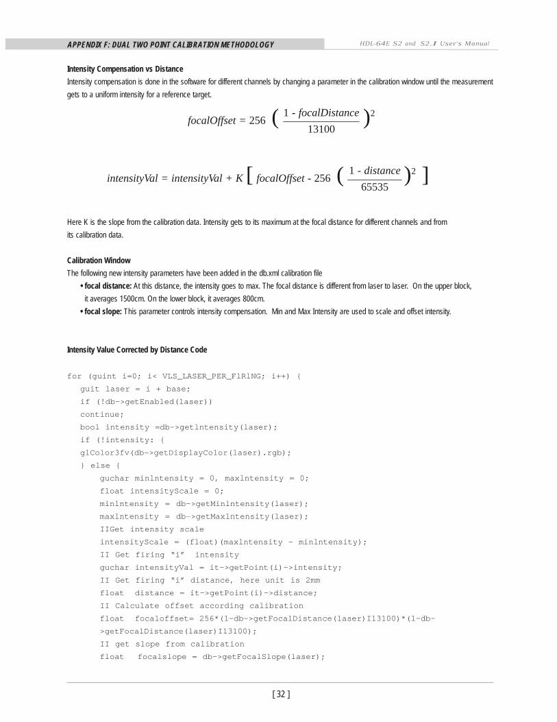
Intensity Compensation vs Distance
Intensity compensation is done in the software for different channels by changing a parameter in the calibration window until the measurement
gets to a uniform intensity for a reference target.
focalOffset = 256 ( 1 - focalDistance )2
13100
intensityVal = intensityVal + K [ focalOffset - 256 ( 1 - distance )2 ] 65535
Here K is the slope from the calibration data. Intensity gets to its maximum at the focal distance for different channels and from
its calibration data.
Calibration Window
The following new intensity parameters have been added in the db.xml calibration file
• focal distance: At this distance, the intensity goes to max. The focal distance is different from laser to laser. On the upper block,
it averages 1500cm. On the lower block, it averages 800cm.
• focal slope: This parameter controls intensity compensation. Min and Max Intensity are used to scale and offset intensity.
Intensity Value Corrected by Distance Code for (guint i=0; i< VLS_LASER_PER_FlRlNG; i++) {
guit laser = i + base;
if (!db->getEnabled(laser))
continue;
bool intensity =db->getlntensity(laser);
if (!intensity: {
glColor3fv(db->getDisplayColor(laser).rgb);
} else {
guchar minlntensity = 0, maxlntensity = 0;
float intensityScale = 0;
minlntensity = db->getMinlntensity(laser);
maxlntensity = db->getMaxlntensity(laser);
IIGet intensity scale
intensityScale = (float)(maxlntensity - minlntensity);
II Get firing “i” intensity
guchar intensityVal = it->getPoint(i)->intensity;
II Get firing “i” distance, here unit is 2mm
float distance = it->getPoint(i)->distance;
II Calculate offset according calibration
float focaloffset= 256*(1-db->getFocalDistance(laser)I13100)*(1-db-
>getFocalDistance(laser)I13100);
II get slope from calibration
float focalslope = db->getFocalSlope(laser);
[ 32 ]
APPENDIX F: DUAL TWO POINT CALIBRATION METHODOLOGY HDL-64E S2 and S2.I User’s Manual
[ 33 ]
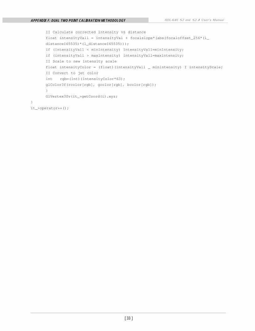
II Calculate corrected intensity vs distance
float intensityVall = intensityVal + focalslope*(abs(focaloffset_256*(l_
distanceI65535)*(l_distanceI65535)));
if (intensityVall < minlntensity) intensityVall=minlntensity;
if (intensityVall > maxlntensity) intensityVall=maxlntensity;
II Scale to new intensity scale
float intensityColor = (float)(intensityVall _ minlntensity) I intensityScale;
II Convert to jet color
int rgb=(int)(intensityColor*63);
glColor3f(rcolor[rgb], gcolor[rgb], bcolor[rgb]);
}
GlVertex3fv(it_>getCoord(i).xyz;
}
it_>operator++();
[ 34 ]
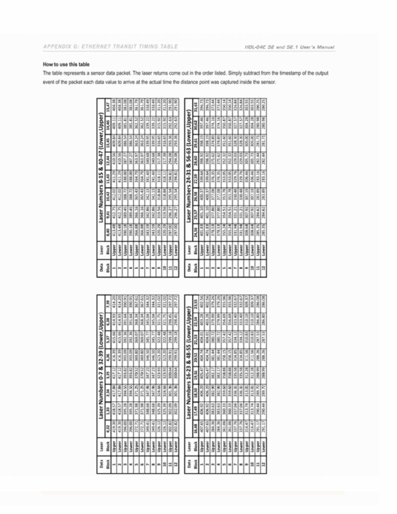
APPENDIX G: ETHERNET TRANSIT TIMING TABLE HDL-64E S2 and S2.I User’s Manual
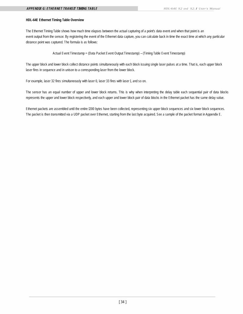
HDL-64E Ethernet Timing Table Overview
The Ethernet Timing Table shows how much time elapses between the actual capturing of a point’s data event and when that point is an
event output from the sensor. By registering the event of the Ethernet data capture, you can calculate back in time the exact time at which any particular
distance point was captured. The formula is as follows:
Actual Event Timestamp = (Data Packet Event Output Timestamp) — (Timing Table Event Timestamp)
The upper block and lower block collect distance points simultaneously with each block issuing single laser pulses at a time. That is, each upper block
laser fires in sequence and in unison to a corresponding laser from the lower block.
For example, laser 32 fires simultaneously with laser 0, laser 33 fires with laser I, and so on.
The sensor has an equal number of upper and lower block returns. This is why when interpreting the delay table each sequential pair of data blocks
represents the upper and lower block respectively, and each upper and lower block pair of data blocks in the Ethernet packet has the same delay value.
Ethernet packets are assembled until the entire I200 bytes have been collected, representing six upper block sequences and six lower block sequences.
The packet is then transmitted via a UDP packet over Ethernet, starting from the last byte acquired. See a sample of the packet format in Appendix E.
[ 35 ]
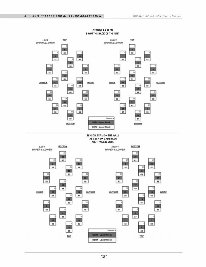
A P P E N D I X H : L A S E R A N D D E T E C T O R A R R A N G E M E N T HDL-64 E S2 and S2.I User’s Manual
SENSOR AS SEEN FROM THE BACK OF THE UNIT
SENSOR BEAM ON THE WALL AS SEEN ON CAMERA IN
NIGHT VISION MODE
[ 36 ]
[ 37 ]
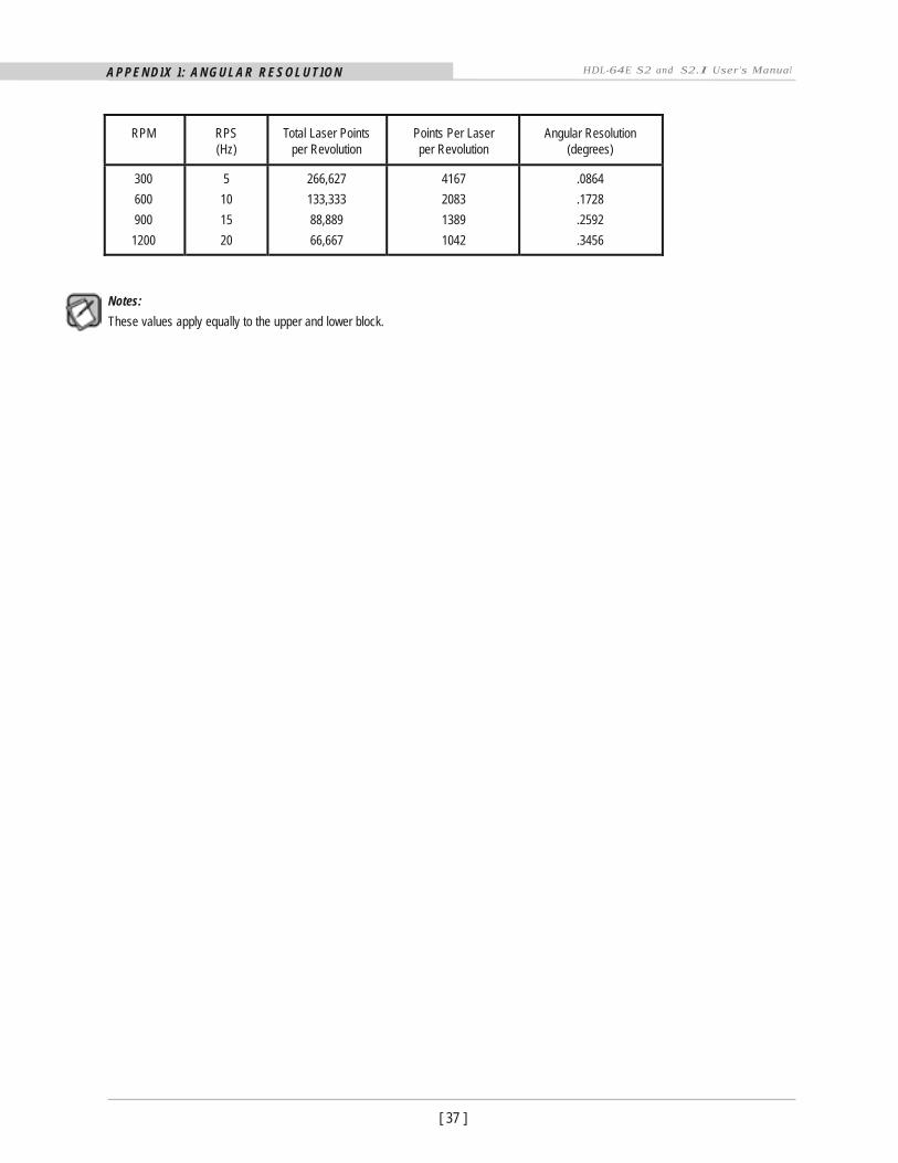
A P P E N D I X I : A N G U L A R R E S O L U T I O N HDL-64E S2 and S2.I User’s Manual
RPM
RPS (Hz)
Total Laser Points per Revolution
Points Per Laser per Revolution
Angular Resolution (degrees)
300
600
900
1200
5
10
15
20
266,627
133,333
88,889
66,667
4167
2083
1389
1042
.0864
.1728
.2592
.3456
Notes:
These values apply equally to the upper and lower block.
T R O U B L E S H O O T
[ 38 ]
I N G HDL-64E S2 and S2.I User’s Manual
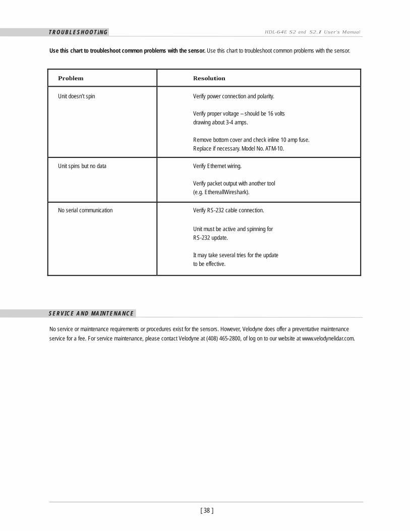
Use this chart to troubleshoot common problems with the sensor. Use this chart to troubleshoot common problems with the sensor.
Problem
Resolution
Unit doesn’t spin
Verify power connection and polarity.
Verify proper voltage — should be 16 volts
drawing about 3-4 amps.
Remove bottom cover and check inline 10 amp fuse.
Replace if necessary. Model No. ATM-10.
Unit spins but no data
Verify Ethernet wiring.
Verify packet output with another tool
(e.g. EthereallWireshark).
No serial communication
Verify RS-232 cable connection.
Unit must be active and spinning for
RS-232 update.
It may take several tries for the update
to be effective.
S E R V I C E A N D M A I N T E N A N C E
No service or maintenance requirements or procedures exist for the sensors. However, Velodyne does offer a preventative maintenance
service for a fee. For service maintenance, please contact Velodyne at (408) 465-2800, of log on to our website at www.velodynelidar.com.
[ 39 ]
S P E C I F I C AT I O N S HDL-64E S2 and S2.I User’s Manual
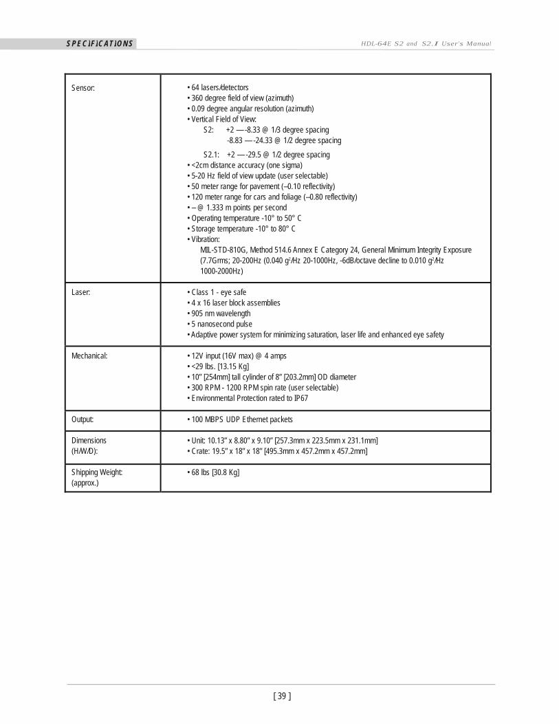
Sensor:
• 64 lasers/detectors • 360 degree field of view (azimuth) • 0.09 degree angular resolution (azimuth) • Vertical Field of View:
S2: +2 — -8.33 @ 1/3 degree spacing -8.83 — -24.33 @ 1/2 degree spacing
S2.1: +2 — -29.5 @ 1/2 degree spacing • <2cm distance accuracy (one sigma) • 5-20 Hz field of view update (user selectable) • 50 meter range for pavement (—0.10 reflectivity) • 120 meter range for cars and foliage (—0.80 reflectivity) • — @ 1.333 m points per second • Operating temperature -10° to 50° C • Storage temperature -10° to 80° C • Vibration:
MIL-STD-810G, Method 514.6 Annex E Category 24, General Minimum Integrity Exposure (7.7Grms; 20-200Hz (0.040 g2/Hz 20-1000Hz, -6dB/octave decline to 0.010 g2/Hz 1000-2000Hz)
Laser: • Class 1 - eye safe • 4 x 16 laser block assemblies • 905 nm wavelength • 5 nanosecond pulse • Adaptive power system for minimizing saturation, laser life and enhanced eye safety
Mechanical: • 12V input (16V max) @ 4 amps • <29 lbs. [13.15 Kg] • 10” [254mm] tall cylinder of 8” [203.2mm] OD diameter • 300 RPM - 1200 RPM spin rate (user selectable) • Environmental Protection rated to IP67
Output: • 100 MBPS UDP Ethernet packets
Dimensions (H/W/D):
• Unit: 10.13” x 8.80” x 9.10” [257.3mm x 223.5mm x 231.1mm] • Crate: 19.5” x 18” x 18” [495.3mm x 457.2mm x 457.2mm]
Shipping Weight: (approx.)
• 68 lbs [30.8 Kg]
Velodyne LiDAR, Inc. 345 Digital Drive
Morgan Hill, CA 95037
408.465.2800 voice
408.779.9227 fax
408.779.9208 service fax
www.velodynelidar.com
Service Email: [email protected]
Product Email: [email protected]
Technical Email: [email protected]
Sales Email: [email protected]
All Velodyne products are made in the U.S.A.
Specifications subject to change without notice
Other trademarks or registered trademarks are property of their respective owner.
63HDL64E S2 Rev F DEC11