AD0A167 317 DISTRIBUTED COMPUTING FOR SIGNRL PROCESSING: MODELING 1.12OF ASYNCHRONOUS PAR.. (U) PURDUE UNIV LAFAYETTE INSCHOOL OF ELECTRICRL ENGINEERING G LIN ET RL. AO G4

UNCLASSIFIED TR-EE-84-29 RRO-18790. £7-EL-RPP-F F/G 912hh/hshshshhsIsI lllfff|lffl f| l llEhlhEElh|hEEEI

I hhhE|hlfllfl ||,Sffllffllflflflf lllI ..hhmhmhmhmh.

II.LP NA -.

II '** -u 118 U2-miT

11111125 .h14 6

MICR ACP' CHART

.............. 71Ph.D. Thesis by: Gie-Hing Lin*,gq.jjL

.............. Faculty Advisor: Philip H. SwainAPPENDIX F for

......... 7.. Distributed Computing for Signal......... ..... Processing: Modeling of Asynchronous

Parallel Computation; Final Report.............. .for U.S. Army Research Office.............. Contract No. DAAG29-82-K-Ol0l.............. *Chapter 3 supported by this contract

Studies in

Gie-Ming Lin

Philip H. Swain

T-EE 84-29August 1984

>-- DTICC1.( ELECTEf

LU ~ APR 29 05

School of Electrical EngineeringPurdue UniversityWest Lafayette, Indiana 47907Approved for public release, distribution unlimnited C..

P.Pi*...I..I.P 86 4 2

7- , . . . . -; 7.

UnclassifiedUNITY CLASSIFICATION OF THIS PAGE (When Doeta Fnsred)_

REPORT DOCUMENTATION PAGE READ INSTRUCTIONSREPORTDOCUMETATIONBEFORE COMPLETING FORM .-

I. REPORT NUMBER 2. GOVT ACCESSION NO. 3. RECIPIENT'S CATALOG NUMBER %..

4. TITLE (end Subtitle) S. TYPE OF REPORT 4 PERIOD COVERED -

Studies in Parallel Image Processing Technical Report

6. PERFORMING O4G. REPORT NUMBER *,p •

TR-EE 84-29."7. AUTHOR(*) 9. CONTRACT OR GRANT NUMBER(e)

Contract nos.

Gie-Ming Lin, Philip H. Swain F30602-83-K-0119,DAAG29-82-K-0101

9 PERFORMING ORGANIZATION NAME AND ADDRESS 10. PROGRAM ELEMENT. PROJECT. TASKAREA 6 WORK UNIT NUMBERS

School of Electrical EngineeringPurdue UniversityWest Lafayette, IN 47907 -

II. CONTROLLING OFFICE NAME AND ADDRESS 12. REPORT DATE

Rome Air Development Center, USAF; August 1984

Army Research Office. 13. NUMBER OF PAGES163

14. MONITORING AGENCY NAME I ADDRESS(II dtlierent tram Controllind Office) IS. SECURITY CLASS. (of (hie repotl)

Unclassified

IS.. DECL ASS! PIC ATION/DOWNGRAOINGSCHEDULE

16. DISTRIBUTION STATEMENT (of thle Report)

Appr ,ved for public release; distribution unlimited W

17. DISTRIBUTION STATEMENT (of the lbetret enltered in Block 20, It different from Report)

N/A

18 SUPPLEMENTARY NOTES

19 KEY WORDS (Continue on reveree side If necessary end Identify by block number) 7

image processing, parallel processing, pattern classification, remote

sensing.

20 ABSTRACT (Continue on reveree side If necessary and Identify by block number)

The supervised relaxation operator combines the information from

muiltiple ancillary data sources with the information from multispectral

remote sensing image data and spatial context. Iterative calculations... :inte-grate information from the various sources, reaching a balance in

consistency between these sources of information. The supervised relax-

ation operator is shown to produce substantial improvements in classifi-

cation accuracy comEared to the accuracy produced by the conventionalDD i 1473 EDITION OF 1 NOV SS IS OBSOLETE Unclassified

. SECURITY CLASSIFICATION OF THIS PAGE (When Dote Entered)

• "... - .-. .--.,....".. -.- '. v .. '.. .... ...... .. . . . . . . ... .... ..-... ....... ., ;... -'. -;.-- - a' :

. . ..**'

UnclassifiedSECURITY CLASSIFICATION OF THIS PAGE(Wma Data Znterd) *

maximum likelihood classifier using spectral data only. The convergenceproperty of the supervised relaxation algorithm is also described. PIM

Improvement in classification accuracy by means of supervised relaxation .comes at a high price in terms of computation. In order to overcome thecomputation-intensive problem, a distributed/parallel implementation isadopted to take advantage of a high degree of inherent parallelism inthe algorithm. *o accomplish this, first, a graphical modeling and analysismethod is dec ied for algorithms implemented using the SIMD mode of parallel-ism. Second, th comparison of execution times between SIMD and MIMDmodes is discusse , based on the analysis of implicit and explicit operationsembedded in an alg ithm. From the comparison it is shown that somealgorithms are suitAble for MIMD mode of parallelism; some are more suitedto SIMD. Third, several performance measures for SIMD, functions of problem

size and system size, are discussed. Finally, two multistage interconnectionnetworks to support the distributed/parallel system are overviewed. Basedon these considerations, an optimal system configuration in terms of .

execution time and system cost is proposed.

-.7... .. -.

?;_" I..

STUDIES IN PARALLEL IMAGE PRHOCESSINCG

Gie-Minig Lin

Philip 11. Swain

Purdue 1.Tniversit~y

School of Eilectrittl Enrgineering =

w'est i-arayette, IN .17007

USAAccesion ForNTIS CRAWlDTIC TAB 03Ui.announced 0

TU?-EE[, 81-29 .J.stification.........

............... .Di4 butioal

August. 1081-Availability Codes

Avaii an'd orDist special

This research was supported by the United States Air Force Command, RomeAir Development Center, under contract no. F30602-83-K-0119, and by theU.S. Army Research Office, Department or the Army, under contract no.DAAG29-82-K-OlOI. Approved for public release, distribution unlimited.

TABLE OF CONTENTS

Page

CHIAPTER 1 INTOITl('ON ................................................... I

CI-LXPTER 2 SUPEI)IlSlI-I? RELAXATlION OPER1?ATOR...................1

2.1 Derivation or the Superv-ised Relaxation Algorithm ..................... 4

2.1.1 Probabilistic Relaxation Operator.............:...................... 42.1.2 Compatibility Coefficients as C'onditional Probabilities ......... 92.1.3 Problem ............................................................... 12.1.4 Approach: Supervised Relaxation Labeling ...................... 13

2.2 Method of the Integration of Image D~ata from Multiple AncillaryData Sources.................................................................. 20

2.3 Convergence Property........................................................ 22

2.3.1 Introduction............................. ............................. 22.3.2 Consistency ............................................................ 2-12.3.3 Geometrical Structure of Assignment Space....................... 292.3.4 Maximizing Average Local Consistency............................ 322.3.5 Relax ation Operator.................................................. 382.3.6 Supervised Relaxation Operator..................................... 41

2.4 Simulation and Experimental Results ...................................... 1432.4.1 Results from the Maximum Likelihood Classifi ca tion

Algorithm .............................................................. 452.4.2 Results from the Relaxat-ion Operator ............................. 452.4.3 Results from the Supervised Relaxation Operator with One

Ancillary Information Source ........................................ 472.4.4 Results from the Supervised Relaxation Operator with Two

Ancillary Information Sources........................................ 49

2.5 Summary and Conclusions................................................... 53

9%

4%

CIIAI"CEI 3 PARAIE PROCESSING ........... . ..... ................... 5

3.1 Modeling Image Classificat ion b~y Means of S-Nets .................613.1.1 S-Net Structure: Overview ...............I...............62

3.1.2 M easures of Parallelism .................................66

3.1.3 Stonie's Vecto~r Sumn Ux ample...........................................67

3.1A. Modeling Complex Applications wvithi S-Nets ...................... 723.1.5 Modeling Maximum Likelihood Classification with S-Nets .... 733.1.6 Modeling a Pipeline linplement at ioen or Max imum Likelihood

Classification .......................................................... 853.2 S EID vs. MIMD .............................................................. 91

3.2.1 The Flow Chart. and th!e Algorithms of the Supervised

Relaxation Operator ................................................... 9023.2.2 Detailed Description of the Algorithm in Block C................. 963.2.3 Implicit Operatio~ns in the Algorithmn.............................. 97 .-

3.2.4 Comparison Between SINII) and MIMD............................. 1043.3 Alternative Performance Criteria............................................. 110

3.3.1 A Clustering Algorithm ................................................ 1133.3.2 Farallel Implvimentition................................................ 1143.3.3 Pertorrman e Analysis................................................... 120w

3.4 Parallel Architectutre ............................ .............................. 1303.1 1 Hybridl Network................ . ....................................... 1323A4.2 Partitioning thie Cuibe Network into 2 NMIM~s and I SIID ....1353.A.3 Partitioning the ADM Network into 2 IMDs and I SIMD ....137

3.5 Summary andl Conclusions .................................................... 142

(ILXPTER I CONCLUSIONS ANI) SUGGESTIONS .......................... 147

LIS'T OF REFI'MENCES ............................................................ 151

APPULNIIX ............................................................................ 154

r-..,. :,

HI.''- .".

(1IlA"'El? I - INT RO)1 U('TION

The conventional classification of multispectral image data collected by

remote sensing devices such as the multispectral scanners aboard the Landsat

or Skylab sateilites has usually been performed such that each pixel is classified

by using spectral information independent of the neighboring pixels. There is

no provision for using the spatial information inherent in the data. In many

cases there are available other sources of data which an analyst can use as well

as spatial information to establish a context for deciding what a particular

pixel in the imagery might be. By utilizing this contextual information, it may

be possible to achieve an improvement in classification accuracy. For example, .

in the case of forestry, various tree species are known to exhibit growth

patterns dependent upon topographic position. When this fact is used along .-

with spectral and spatial information, a classification with enhanced accuracy -

can be obtained [1,2].

The supervised relaxation operator which combines information from

spectral, spatial, and ancillary data to classify multispectral image data is part

of the subject of this report. lRelaxation operations are a class of iterative,

parallel techniques for using contextual information to reduce local ambiguities

[3]. Such techniques have been found to be useful in many applications such as

edge reinforcement [4], image noise reduction [5], histogram modification, ..

thinning, angle detection, templiate matching, and region labelling [6]. Its

. , o, .. .%.. . , . . . . . . ..% . . . . .. ,.,. . . ..-. -°.. %.% % ., o

.. , .,. ,. . . . . . . . . .o . ., .. . . . . ...". . . . . . . . . . ... . ,' ." °.•.,= "% • . ,-, °° •. " . - .. . ." ° " .

'.,'-.:,,' -........ ..

4,...4' -. 7 7-7

2 . - -

convergence, the derivation of co)mpatibility coeflicients, and the theoretical

foundations of relaxation labeling processes have been described in [7,8,9,10,111.

A modification to existing probabilistic relaxation processes to allow the

information contained in the initial labels to exert an influence on the direction

of relaxation throughout the process has been described in I12). This modified

relaxation method, called supervise(d relaxation labeling, has been extended to

incorporate one ancillary information source into the results of an existing

classification [21. In this thesis, a method for integrating image data from

multiple ancillary data sources is described in Chapter 2. Based on the

approach in 1131, the convergence property of the supervised relaxation

operator is presented. The supervised relaxation operator is generalized and

demonstrated experimentally to combine information from spatial and multiple

ancillary data sources with the spectral information for the classification of

mull ispectral imagery with multiple classes.

Due to the high computational complexity of such operations and the

availability of low cost microprocessors, architectures involving multiple

processors are very attractive. Several parallel organizations have been

proposed, principally SIMI) and MIMI) architectures. In Chapter 3 of this

report we focus our attention on performance measures for parallel processors

and interconnection networks for mulliprocessor systems. Section 3.1 will

present the application of S-Nets 1-.,151 to modeling the maximum likelihood

algorithm in SIMI) and pipeline implementations. Several alternative

performance mea.sures for the parallelism inherent in the algorithm are also

described. The algorithm vc('11mt ion ililnes d(riv.d l)ased on the analysis of

Implicit and vexplicit operatlis in t he algorithmn for SIMI) and \11\11) modes ofparallelism are comlpared and disc rsed in -Secj.tion :12. In Sect ion 3.3. the

-.. -

3

determination of the optimal number of processing elements in terms of

execution time and system cost for a given image size based on the measures of

evaluating the performance of an algorithm is discussed. Finally, Section 3.4 "

describes how two multistage networks I16,17,18, iI, the cube network and

ADM network, can be configured to support an implement at ion which utilizes %_ -

both SIMD and MINI) processing components.

N O.'S.-':-'..

* .~.. .'.. . * ...--..-.. . .

* -~ -- . ... . . ..... S - . *S- *a .. ~-. .~ ' ~. ;~A,2 .. ~ a~d~..S.-~ S~ * ~*.*S..f~* ~ ..------.-.-- ~ .- *o.

% .0

CHAPTER 2 -SUlPIRVISEl) I? IAXATION OPIHATINR

In this chapter, Sect ion 2.1I c( nItnains a st ep-bly-Aep1 dec ript iofl of thiie

supervised relaxation operator. In Sect ion 2.2, a method for the integration of

image data from multiple auxiliary data, sources will be given. Section 2.3

discusses the convergence property or the supervised relaxation algorithin.

Finally, Section 2.4 presents experimental results on a 182-by-182 pixel ---

Landsat image.

2.1 Derivation of the SuPervised Relaxation Algorithm

In this section, the derivation of the supervised relaxation operator from

the original relaxation operator 131 is described step by step, and an heuristic

interpretation of the supervised relaxation operator is given.

2.1.1 Probabilistic II elax at ion Operator

Most classifiers used with remiote sensing data are pixel-specific. Each

pix el is classified by using spectral information independent, of the classification

of the neighboring pixels. No spatial or contextual information is usedI.

Relax at ion labeling pr~ocesses are a class of Ite(rat ive, patrallel te(chntiques

for using contextuial in fo rmat ion to( d iainbigmiiate proba bilist ic Ia helings of

objects [31 . They make use of tw W( Iw1ereiit sources of in formatimont, a Ipriori

neighborhood modlels and initial observations, which interact to produice the

2.N

% V,

final labelings. The relaxation proc..sCs iII ,,ve a set of objects, A {

a,, a,. an , afnd the relationship of each object to its neighbors. Attached to '

each of the objects is a set of labels, A {XI X. Xm, where each label

indicates a possible interpretative assertion about, that object; for example, theSobjects might be image p lXIs and the labels Inight be spectral class names.

The relxation algorithm allempts 1( use constraiat or compatibility

relationships defined over pairs of labels, possible interpretations, attached to

current and neighboring objects in order to eliminate inconsistent combinations

of labels. ("Current" refers to an object. which, at the moment, is the focus of

at tention.

A measure of likelihood or confidence is associated with each of the

possible labels attached to objects. This measure is denoted by Pi(X). These

likelihoods satisfy the condition

-i(X) 1, for all ait A, 0 < P(X) < 1.>X (A

In this probabilistic model, the likelihoods estimated for an object's labels

are updated on the basis of the likelil (ods distributed among the labels of theneighboring ljects. These likelihoods interact through a set of compatibility

coefficients that are defined for each pair of labels on current, and neighboring

objects. The compatibility coeflicients are determined a priori based on some

foreknowledge of or on a "typical" model for the image to be classified. More

speci-ally, for a given object ai, the likelihood lii(X) of a given label X should '

increa.e if the neigh boring objects' lbels w iti high likelihoods are highly

)compatibl h wiIi X- at ai. ('onversel . ',(X) sh(|ld decrease if neighboring high-

likelihood labels are incompatible witli X at ai. On the other hand, neighboring

labels with low likelihoods should have little influence on Pi(X) regardless of

-i k. .

............................................. . . . .**.*

their compatibility with it. Let X' be a label for a neighboring object and X for

the current object. These characteristics can be summarized in tabular form as

follows:

('ompatibility of X' with X %

High Low --

Likelihood of X' High + -

Low 0 0 - -

where + means that Pi(X) should increase, - means that it, should decrease,

and 0 means that it should remain relatively unchanged. The coefficient ;.

'lii(X,X') is a measure of the compatibility between label X on current object ai

and label X on neighboring object. ai. These compatibility coefficients are

defined over the range 1-i, 1]. The aim is that the -)s should behave as

follows:

-'(X,X' ) > 0, if X on ai frequently co-occurs with X on a".

1, if X on ai always co-occurs with X' on aj. Pam

< 0, if X on ai rarely co-oceurs with X on aj.

I-".: -".2

-I. if X on ai never co-occurs with X' on a1. MI.

o, ir x ,m ai o'iirs iiilwcn enitv o f ( ' on

With these ('oml)atiilities, the ('ontextial k;owledge is incorporated into the

probabilistic relaxation operator.

The initial la)l likelilhtIds are provided from a (lnssificatiion of

rmmiltispmctral l,andsat da:t0. A mlti,-Ipec.tral w'nincr (M1SS) gaivhers r:nliance

7. .m

data in various sections of the ehictroiiagnetic spectrum (wavelength bands).

For example, the Landsat MSS has four wavelength bands in the visible and

near infrared spectrum. Such remotely sensed data have been collected and

stored in digital format.

The first step in multispectral classification begins with the selection of an

MSS data set which has suflicient qualit.y so that the classes of interest on the

land covered can be identified with tie desired accuracy. After choosing the

best available data set for analysis, the study area within the data is located

and the reference data (such as aerial photography, maps, etc.) are correlated

with the nultispectral scanner data. These reference data provide the key to

relating successfully the spectral responses in the data to the cover types on the

ground.

The second step is the selection of the training samples. A common

procedure for selecting the training areas is to use the available reference data

to identify areas that contain the information classes of interest. The images of

these areas are then identified in the multispectral scanner data. These

training samples are used to (lcternife parameters fr tlie pattern recognition

Agoril his, effectively raitiii'" li, (omiloI,,r to rcogniz, the (lasses or

interest. L,ater when the clas.ificntti(in operation is carried out byv the )attern

recognition algorithi, each data po int to be classified is compared with the

training samples for each class, and tHie pixel is assigned to the class it

reseijibles Illost closely. MW

'he third step is to use these 1r:iinig .1:1niples to define trainiuug 'l:isses.

"i'hv tr:ainuing, 'lsses are (ften chi r:ict,(izn'( i n r (i Of Ili e rniie(i v(,( rs and

co ariance Imatifrices by Owhe chisferinig algorilhn. ( lustering in.)% be u.ed to

identify natiral spectral groupings of pixels in the training samples. These

.N6.

natural groupings, called "spectral classes," are used as candidate training

classes. To be sure or the reliability in identifying the information class of each

cluster class obtained, all available reference data are used. This step is the

most important in ensuring that the classifier is correctly trained.

The final step is classification using a maximum likelihood classification

algorithm. The set of discriminan t functions for the max inIumII likelihood

classification rule, usually specified in terms of mean vectors and covariance

matrices of classes, is derived from the statistical decision theory so as to

minimize the probability of making an erroneous classification. When tlie data

values of a pi)xel are substituted into all of the functions, the pixel is assigned

to the class which produrces the la rgest va lue.

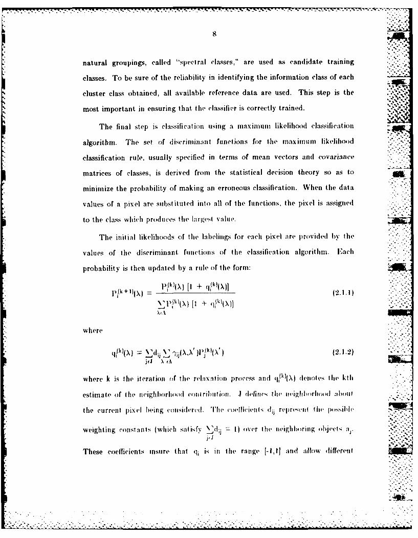
The initial likelihoods or the labelngs for each pixel are provided by the

values of the discriminant fuinctions of the classification algorithmr. Each

probability is then updated by a rule of the form:

p(k)(x) [I + (0l1(qX]

p.(k+i 1)(X)(..1

XA

where

qj(k)(X) d 1 '~(X'j)k( )(2.1.2)j(J X c

where k is the it erat ion of the relax ation process anid q(i d(X)(enot es the kt h

estimate of the neighborho(O coni ribtit ion. .1de tines- the ueighborihood ailni

the current pixel being conisiviered. Thev (oeihicievits dij reprewnit t lie possAil

weighting consi ants (which satisfy \'9li =I) ove(r the neighboring object,; aj. -

j, j

These coefficients insure that (Ii is in thie range (-1,11 anid allow different

o°. 0Dw

neighbors in J to have different degrees of influence in the neighborhood

contribution. Indeed, if ) is high, and 'ijX,X') is very positive or very

negative, theli the label X' at aj makes a substantial positive or negative '

contribution to qik'(kX); while if l'k)(X') is low, X at aj makes relatively little

contribution to qi(k)(x) regardless (,f the value of -jHX,X' ). Therefore, a very

positive or very negative contribution to qi(k) contributes an increase or

decrease to i(k)(X) since ])i(k1(X) is obtained by multiplying P)(") by (1 + qI(k)),

whereas a sinall contribul ion to (i(k) con rilbiiI es little change to I .(k + I) . Ilere,

the d(inOIh tor i() Jl, Ia JJ 12.1.1) guarantees flint all the P's sum to 1

Moreover, they remain nonnegative, since qjk) is in the range 1-1,11 provided

that _ d(i = I, so I + q.ik) is nonnegative.

This rule is used t,, update 11he likelihood of each label on each object in

parallel, and is lien iteral ed uil no rurtlher cli:igs (Wcir. \t. this point, we .. .

say that Ihe final lalwling reach a balance in consistenc\ between spectral and

spat ial (or contextual) data sm urces of information.

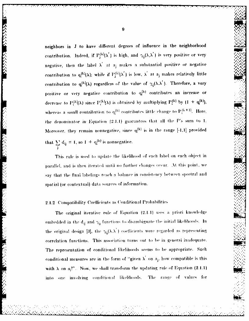
2.1.2 (ompatibilitv Coellicients as (onditional Probabilities

The original iterative rule of Iquation (2.1.1) uses a priori knowledge

eltbedded ill the dij and -).j fi ctlim I(ti d iumhiguate Ih, initial likelihood . In

the original designi [3], the mi( X.X )coellicients were regarded as representin'

correlation functions. This associatiom Iirns ou t to be ili general inadequate.

The represent ation of conditional likelihoods seems to he appropriate. Such

conditional measures are in the form of "given X on a,, how co"patible is this

with X on a?" . Now, we shall Iransforrm the updating rule oif lquiiation (2.1.1)

into ,iP inv~'ling cVoinli ,i:l likelilOods. The range of values for

. .-

.. "i .- ' i':.,'. -, . - ,... ... . .- .. --.. . . •. .. .. '.-. . - . , . • .- . .. , . .. . . -. . ,

_ 10 '

compatibilities, [-1,1], must be sealed into [0,11. The simplest transformation

is:

Pj'(X X') -.- Y,-.+1(2.13)

where Pij(X X') is to be read as the conditional probability that ai has label Xgiven i has '. ' ".s ...77.

given aj has X a is a suitable constant. Substituting Ilqat ion (2.1..3) into

Equation (2.1.1) giv.s:

j(I)(X)j I + \"di ,, 'l x ') - n # !x /:- -''..

Pi(k + )(X) =

(k)(X){ I + d~i jaP~1 (Xj ) - ]Pik)(X' )}

i x -'. ..- ',

P)(k)(X){ I + ( -- )i(X'x i x .,

PI)(k(X 8 { +(~ ljd;(1 j 'l';j~(X X' )I.).." " """' "

id)

j ): :.-.

j )kl' ' }.

Pi(X{ (ii ]lij X )I'j(/X' )~ ....".

=j x.

p'(k)( ,x)Q(k)(x): (2.1.1

wherel

:'.' -. - . - - ' , . . . .': . . .L .i .; ,; --. .' . . . ... . * * p % *,", .-. .. -. ,- . . . ....-''."- - , -- , .• " 5.'. 2i .

4~~ It P5 .

|, .....

Qifk)(,kj = k.i V P.(X~k j ' )l'l)( X') ( 2.1.5)

)NeA

This is an, analogous or,,, ,,f th,, ,,idati,,g r,,l, ,f El,,iat ion (2.1.1 )with L

complIat ibility c()eflicien1 s rFyI) f ,j y( ) ,(0n(1it (ifln:il li k li lt i 1(1 whiich sat is fy ' 1-

2.1.3 Problem

The problem we want to deal with here is how to incorporate information

from multip, le ancillary data soires inlt I!li rsults ,:r an existing classification

of remotely sensed data. ('onventio mal classiiation of over hp.vl'r in rinotely."-)t-('I.

sensed data, based only upon spectral informalion, might inOt he enough. In

many cases, there are other sources of practical data available which can be

used along with the spectral information to improve the classification. For .

example, various tree species are known to exhibit growth patterns dependent

upon topographic position, as shown in Fig. 2.!.1, so that tree species or other

forest classifications cold be iml)roved by conmIliniig spectral data with

elevation, slope, and other lopographically rvlated inf,,rm lin. As shown in

Fig. 2.1.1, the current pixel with remotely sensed dath [x, x2 X3, x 41 gathered

from four wavelength bands from visible and nvar infrared spectrum has other

ancillary (lata y1, Y2, Y3 obtaineld from information of elevation, slope and

aspect. The infornmtion from ancillary (lata soirees i :ssIiiied to be available

in tlie form (of a set or Iik eli lho,d.s. Th,e )r(cvdures ,,ropl)osed )elow are post- .

classification techniques, in that lh influence of the available ancillary data

can be imposed on an existing, spectrally determined, class;ification result.

. .7

12

Xi Spectral Datacollected from

iX2 four wavelengthY2 bands

3tX4 Elevation

Tyl Slope

Y2 Aspect

Registered Data Planes

Fig. 2. 1. 1. U~se of Ancillary Data [2]

* .. S

13

2.1.4 Approach: Supervised l elaxation Labeling

A method of supervised relaxation labeling 112,21 has been proposed for

incorporating one source of ancillary in formation into a classification in a1'..- a

quantitatlie manner. This mehod was previously applied only to a two-class

(spruce-fir vs. others) problem. The sulwrvised relaxation labeling (an develop

consistency between spect ral, spatinl. and iUlliple anciilary (ata sources of

information for problems with nitiltiple classes. The classification used for this

purpose was produced from nmltispectral Skylab imagery. For example,

(list rilution of the classes of Iree species with respect to the elevation in oneSpeili" area is shown in Fog. ". I",%r simplicity, tile area is assumed to be

labeled into Ihiree classes, Spruce Fir, )ouglas A White F"ir, and Ponderosa

Pine. But the method can be applied in a similar way to problems involving

more classes. In this area, there are also data describing the elevation, slope,

and aspect preferences of the various tree species, along with digitized terrain

maps of (hevation, slope, and aslpect. For the present study, elevation was

chosen as the most important ancillary data variable for improving -'

classification accuracy over an existing classification obtained from spectral

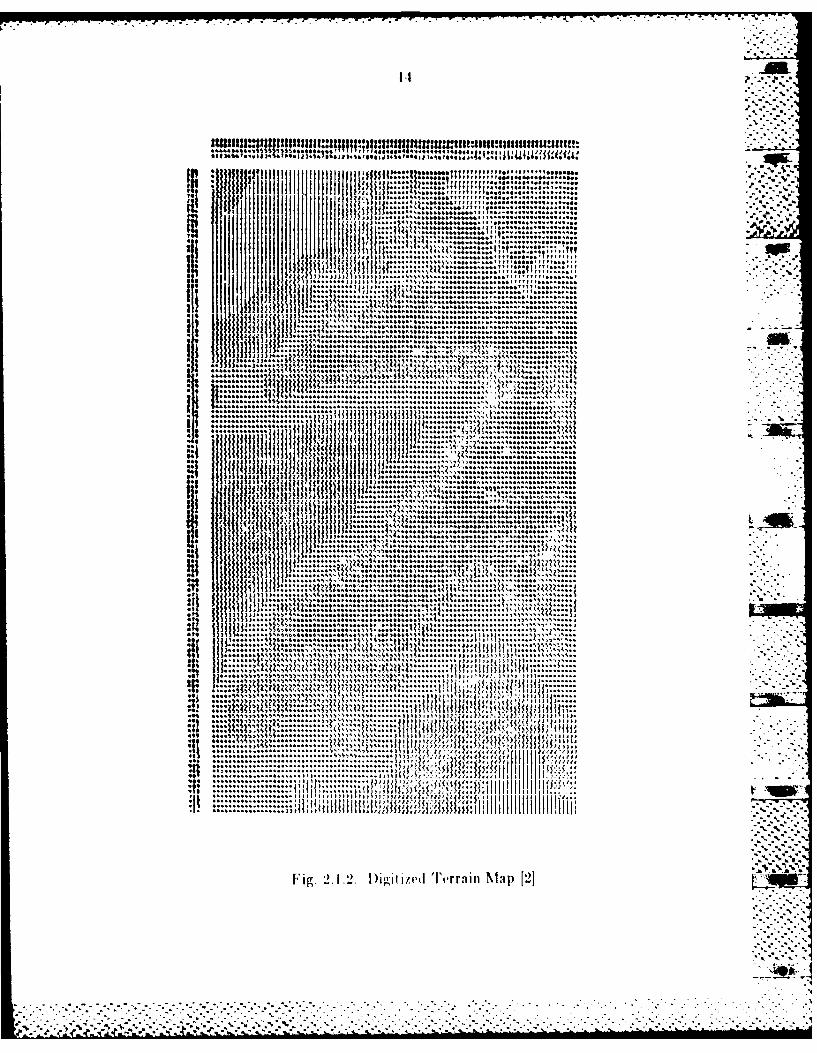
data alone. An elevation map of the area is shown in Fig. 2.1.2 [21 and the

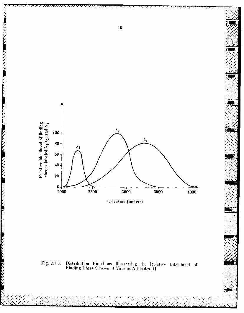
(listrilbutions of three classes (assume their labels are X, X2, and 3a) with

respect to elevation are shown in Fig. 2.1.3. Given the elevation of the current

pixel knfown from Fig 2.1-2 Ile prhlba)litly of finding ('lasses labeled XI, X,

and X3 (an be seen in Fig. 2. 1.3. ILeI the likelihoods he x, y, and z. Then a set

of relativ" likelihoods (corresponding to each pixel in an image) for each of the

labels for the current pixel ai Is :I- follows:

wit.-

. .* . °%.i

1.1

• ]l l alJI llllll~ lf!...t ......, ............................. P.ik -

:n.3.

•~ ~~ ~ v , .. .... ...I,,;....................::1,;...

*IIII Jll i I l it l lil, '1hu:l I s . . . .. ..........

Sii I 111 ..... ............ . .

............ .........................

................... .......

. ......... ...........

... . ............................

. ........... .. ... . ......IM 13, . .... i n ............. ... ...........

Mj . 44, .. . .........

.................... .....

............

lllll lhlllhh ++ .. ..... ....... + ................................... ......

. . ........ . . . .

..I.... h .N.............1............. ........i. .......... ...... .. .. .

S.....

11,3. * ***I... X ..........i...

"..........

..................................... _

||........ +3+++++................................ . ... , .... + .....

I-...........

i........

...................... ,...33+.. 3+. 33Is.............. S.......... lhi~ lll~ l ..... <n.......... !is .. ..V S 55 55 , ........ .ll . .. . . .. . . .. . .

S. , .... ..........

.00 ... "%:"S,. .

il .......................................

lll$++++l+li++U 3l1,l 3.....+ + .................. ..... t+lhl'Ii Ii ltl~hlhl q. ...... , ....................... >,=S. . ...... ....... . ..........................llh 'V*+}lll......+s ............... .+.s,....... ++ .... '

.............

.2............... ,, . ........I II|+ , ..... ..................... t....... .... ......- "• , llh.... , ................... , .............. ...... 4...Il.. ,

, I ) .... , +................... ... .................. 4........., -. . .1hh ....5'* .................... , .........................

I1*,,,.. ...... % .*. , 4... ... 4...,4+, ... ,, ,, %.............,+ ,... ,,S,.,%....+) ...... ,, ......... ...4 *t4.**~ .*b .4..... s,,, ........4,)... ..... .... 4j. . -"5 ;"

** J ~ . 4.. 4A.. ..... ++ +..... ..............4t* *%*h&4.43 ... ,....... '''+

9,3. i... .... 1.... . ..........444444S444444i44 -.... ,133,,l. 4%4..... " "''oeooo+4 %+ N+m + •+ 4 4 oo ~ 1+ + • + +m+++e

• 3, ....l+,k}},+,,•+, ....... },,+ 33.33......... ,!l+]l]:g+ + . 33i+$j 3::l,..

... . * .. ........ tH... .. ... . II , , ,4 . .. *4* + ........... .... 44 44..... 333 1lt i.+L +++ +++ u+ ++ e ... ..,*99 ...... 4 ................ 3)' 3U? ° I++ '°" . ++ + + ..... ..

. .............. ........ ,...... t+*,+,:+<,+ 3..,3,, lll .... - .4oo9. . . .oo .+ooo~m. 3 .. • .... +.) 133,''<i ( +4+ .+i| I|i lT#".To9 . ...... . ..................3I < I,, I IIIII

° ° t °° + ° ° t ° ° + + 4 ° •.33 33 3 3 l +i+t3J3Z134 ? ''') ' ? #? , t+ 1ttf 1 .1...1

3,,........... . ...... + I .. 3L, . .. .33I3 3333 I I ' 4

&Io+oO~o..•i I 'I ig I)J .2. J; Ji l ip2 z ,'d Te r in4+ Ma [2

. .•.. . .. ...

•.-.. .S..

g ~ ~ ~ ~ ~ ~ ~ ~ - 7 7 u u *pi. . . ... -

Cd 100-so-.

3X

7: -a 60-

S40-

20-

0-2000 2500 3000 3500 4000

Elevation (meters)

Fig. 2.1 .3. Dist ribut ion I''mct ions Illuzst rating t he I? 'a t ivv Likelihood ofFind ing Th ref C lasses Ai Variotis Alt it udes [1I

16 AML

3600, -IZOOO CSUBALPINE

ENGELMANNSPRUCE

3300 . ,11000

3000 WHT 10000

PINEf WIT DOUGLASPE ASPEN /FIR

Ir2700 9 - 000

w

2 2400 - 8oo00

a'JPONDEROSA,

I SOO§

2100 7E00

PACINO SOUNIPER

'>.,SUIO OINIBTO ONONORH

FREQUENCY OF 0CCUANE 4~FACING SLOPEAS A FUNCTION OF ELEVATION ,~

Fig. 2.1.4. Forest Species Distribtion als a 11111(1 h)II of Illev aitI and1( Aspetin the San Ju an MounIt ains 11)

71% -

%1JJ.2*...

6.9,. .

9 ,.

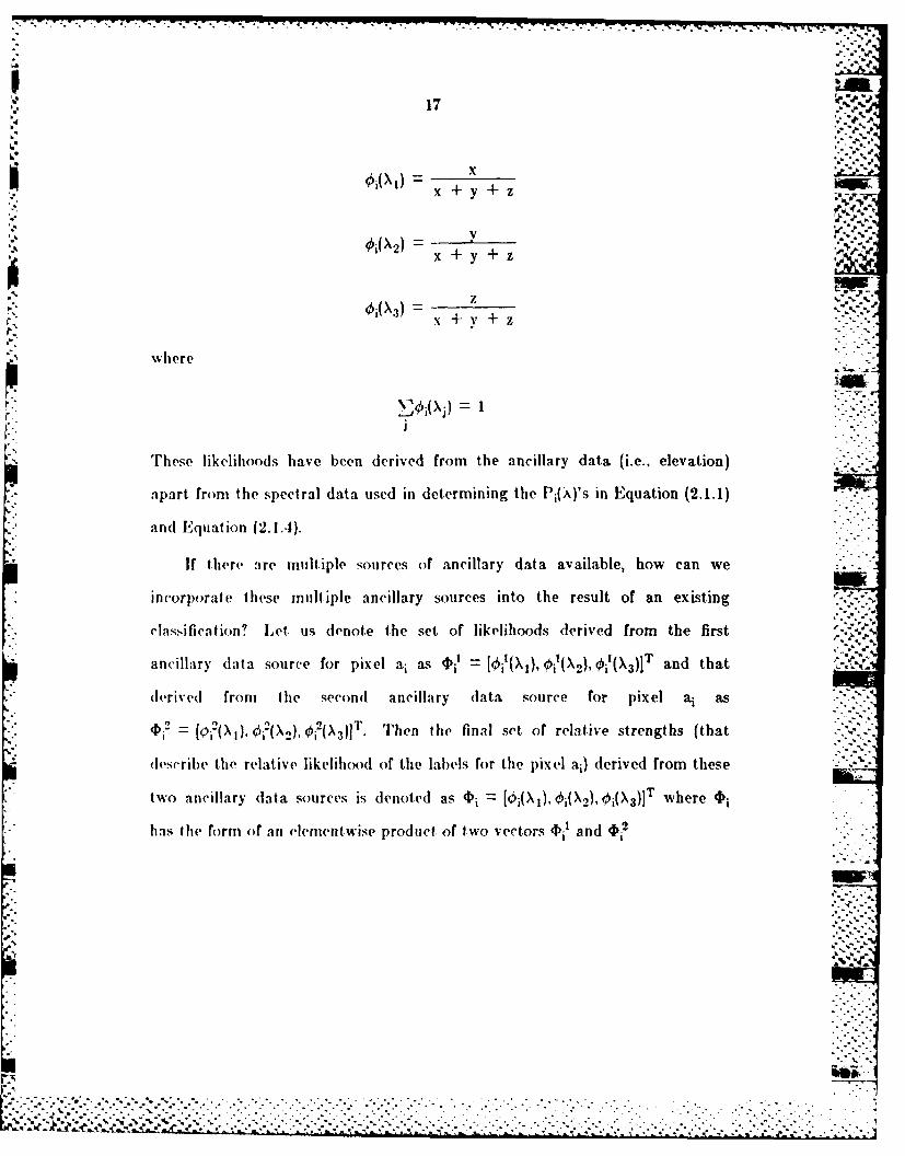
, x + y + z --- i

OA3)-:,':4:

x + y + z

apa t fi(X ) -

c s f a o L t u-

where T t. 'a-

These likelihoods have been derived from the ancillary data (i.e.. elevation)• ~ ~~apart fro)m the spectral data used in determining the Pi(X)'s in Equation (2.1.1) 2--.-

i ~ ~~and Equation (2.I..,l)."," .

If there are multiple sources of ancillhry data available, how can we ,

incorporate these multiple ancillary sources into the result of an existing".-' -.,-:

classification? let us denote he set of likelihoods derived from the first -'..-

ancillary (data source for pixel ai as =i : [i(X), ),i1lX2 ), $i1(X3)]r and that ""

• "" d(,erivedl from the second ancillary data source for pixel ai as "."....'

= i -[O2i). l'0l2}, 0i(X 3 )JT• Then the final set, of relative strengths (that ,'...

describe the relative likelihood of the labels for the pixel ai) derived from these -""

two ancillary data sources is denoted as 4i = )IT(X1), i{X2), i(X3)]" where *i.has the form of an clementwise product, of two vectors 4%i and ii?

. .. ..

.99 ..9* .: ? -29 ." ,

.-b"'

"_,:.:_,- . 'k'', .' .'., ','"'" ," ."'';,"'' ."'' .'" " .","."-, ..- , .",'","-, .".". .' ,"" '.. - ... ,.. ".. . .,"". .".. .

~( X3) )02(X\ 1) + 0,I(X) t ?(X,,) +O1 1X3 )0i2(X 3) ,%~.

OP I)

0i(X3( -1 )!X~ ~(Xk 2 . +Oil'\ I)j13)

33

+ oi 13X1 21

The final set of relative st religils Iias been normnaIized to make thev S1111 of all

the terms equal 1. Of ()Iourse, thlis approach.I can be gew',ralizvd to deall %%t0h

prob~lems with multiple-class. mnu It ipc-an ci 1k ry dat a soulrces. Therefore, t he

modified sup~ervised relax at ion procedure is adlopted1 to incorporate thle Oi(X\'

and thus allows multiple sources of ancillary data to bias the out come of the

set of likelihoods for each pixel i thie imiage at each iteration. If tHe cu rrent

favored la bel on the pixel is a so stron glN su plirt ed bN the a neli arv dI:iti a [a.

expressedl by, oiXI ..... its, ............ is streng~ tened prior to ino~IliiI( to ii

next iteration. Conversely, if thec cuIrrenit favo redl label is in t sI ro nigh

supported by the a ncillary data I a. the its prob~abi lity vIs weakened lbef( )N

proceeding. F"ront the formi of 4)i it is easy to realize the reason why an

elenien twise produact rule is chosen to comniie the sets of l ik eli hoods d1eriv ed

from mult iple ancillar% sources. N ainiv, any Label (or class namnie) wit Ii a vvi 'N

small valuev of prolbility d(erived from aumcillary data source %kill force th it

label to liab ()only verN limited ellects on thev next es4tite for thev curreiit lpix

aeven thoiigh othevr aincillary sources hiave evidence to suipport this label. It

furt her preveniits the a(Iddit ive aceUiulat ion of thev smnall responses from

I~~ . -...

ancillary data sources due to some inaccurate estimations. The strategy of

modified supervised relaxation labeling ('an be imlpliniented quantitatively by

defining

I + *i[No,(X) 1 , (A (2. I.)

N is the total number of possible la bel (i.e., cla.sses)

3 is a weighting constant. to he determined

Through the parameter 3, 11lie present. method allows the relative influence of

spectral and ancillary data sources to be A'a red . large 3 reflects a high

degree of Ci,nfidene it, the accur:au ,,f acilla rv (Lit:a s mrc.s . At ti k +1 Ih _

iteration, Equation (2.1.6) is used to ni(dif' the Libel weiglhts according to

I(k + Ow + (2.1.7) -

-" I{+ ! l,, ) ! _

where the dlenlominiator PIS iioniiil/iiiii r;l(tnr. IF 0. tlme" L.(X) an

1)k+i)X) - - ilk+ 1(X), whi.h mine:i is I he a m'illarv data have no inllien e at

all. If the ancillary (lata sour'es h:ave proided no information ((or no

preference for any label for th,, pixe'l aj), then 65(X) - N for XA. Tl is leads

to lI(k+ )lX) + L l ( X) i.e.. the an cillary data sources have no iifluence on

the progress of the relaxalIi, ii.

Sul bst it ittiug l'qI t llim i (2 1 1) Fit , i , ii (2.1.7). it bvnr' ie.- . . -.

l'i ~)1( I())+ I(X l)"l

4X IA

where

• ", .-.-'.... . . . . . . . . . . . . . . . . . . . . . . . ......... ' ". .. . .: :-....i :. .." ~~~. .. ..-. ' ~.L.I'L .+' .L +" . t...".. ... . .. +_""'l-.. .. .. . . . . . .44....

1- . .. .. v.

20

N

QA~1 X j~(k()*t(X ) (2. 1 q)

Q i( k)( X) is the original ne igh blorho od~( con tri b1t ion o f l Ejlat ion (2 ,11 .5) a ugm e ntedWT

The mnodified supervised relaxation labeling starts with 100t)(X), X (A

where P. t( t \ ) is the In itijal probability. In principlIe, these likelihoods are

available in the penuilimante step of the maxiiii likelihood Casf(I o

obtained using spectral (Iat a on ly (i.e., j ust prior to the pixel being Ia beled -

according to the largest of t hose li keli hoods).

The required context conditional likelihoods Pij(X I X Ys are co)mput ed from

the original classification. A more precise means for obtaining the

compatibilities would be to estimate them from some other source of dlata K

known to be correct.

Thie finial la beling achieved will repiresen t a Ilan ice in co Isi~t en cv botweeni

the spectral in format ion implicit in the( Initial likelihoods PitO)( X). VA, ancillairy

information emb~edded in the Oi(X)Vs. and spat i context (dat a Incorporat ed III

the set of 1) (X X,) s.

2.2 Method0( of the hit era t ion of I~in mg )at a from

MulItiple AncillIa ry D a ta Sources . 7

In Section 2.1.4, an elemnentwise product of two vectors (Pi and (Vi2 which

are derived from two ancillary data sources for a pixel ai is used to produce the

final set of relative strengths. This section will provide a justification for using

the elementwise product of vectors to integrate ancillary information from -

muIt iple sources.

-41

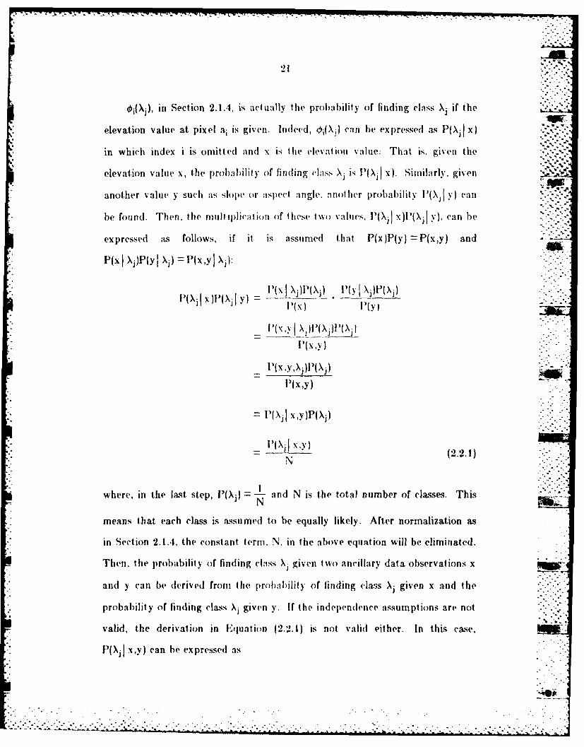
"OPY, in Section 2.1.4, is actually the probability of finding class Xj if theelevation value at pixel ai is given. Ideed, Oj(Xj)can be expressed as P( x .

in which index i is omitted and x is the elevation value: That is, given theelevation value x, the probability of finding class Xj Is fXjj x). Similarly, given

another value y such as slope or asj)(Wt angle. another l)robal)ility I'(Xjl y) call

be found. Then, the mulliplica Iio, of these t%%() values, I'(Xj] x)l'(Xjl y), can be

expressed as follows, if it. is assumed that P(x)P(y) P(x,y) and

P(xI Xj)P(yI X1) ZP(x,Y Xj):

I(Xi )P(XIjY) (x Xj)l,(Xj) _ l iv I )j l'(Xj x )Pl~J y) = I'(x) " I(y

.. l'~I(x,y) ..

P(x,y)

IXj x,v)P(Xj)

I)X~J xy) (2.2.1)

N

where, in the last step, P(Xi) = - and N is the total number of classes. This

means that each class is assumed to be equally likely. After normalization as

in Section 2.1.4, the constant term, N, in the above equation will be eliminated.

Then, the probability of finding class Xj given two ancillary data observations x

andl y canl be (derived froni tfie p)roba:bility of finrding class Xj given x and the

probability of finding class X v giwen . If the independence assumptions are not

valid, the derivation in Equation (2.2.1) is not valid either. In this case,

"(Xij x,y) can be expressed as

• . , .

' -A',

l~(X1 x~) l(X.y X)f()(..)IP(x 'V)

T1he joint (list ribuit ions, I (X ,vj X ) in iNs be est iated first through the training

samnples, and t hen the probability, V ( X x,y), (-.,il be calcla~lfted.

Given m~ore than two independent ancillary data sources, the probability

of finding class Xi can be dlerived in exactly the same way as in l~quat jon (2.2.1I)

ex cept that the constant t erm will lbe dlifferent . Again, the const ant t erm will

be elitnina ted after ia rnuiliza ti n. tw

2.3 Convergence Property

Section 2.3.6 will discuss the convergence property of the supervised

relaxation operator. The preceding material will describe some theoretical

background. most closely following [131, step by step in order to reach the final

conclusion in the last Sect ion 2.3.6.

2.3.1 Introduction

In a relaxation operator, there are:

(1) a set of objects;

(2) a set of labels for each object;

(3) a neighbor relation over the objects; and

(4) a constraint relation over labels at pairs of neighboring objects

We shall denote the objects by the variable i, i rA, which can take on integerv.l n

values between I and n (the number of objects), the set of labels attached to

node 1 by Ai, and the individual la bel (elenen ts of A)b h aibeX

.. e--d-

- - - - - --- - - - - -Y - -- 7 , 7--.

24 3L ______ '

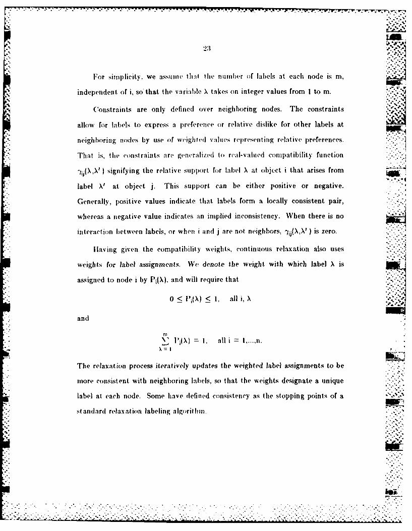
For simplicity, we assume that the number of labels at each node is m, 2independent of i, so that the variale X takes on integer values from I to m. "-''

,-.% 5.ti

Constraints are only defined over neighboring nodes. The constraints

allow for labels to express a preference or relative dislike for other labels at

neighboring noodes by use of weighted values representing relative preferences.

That is, the constraints are genralize(d to real-valued compatibility function

- j(X,X' ) signifying the relative support. for label X at object i that arises from

label V at object j. This support can be either positive or negative.

Generally, positive values indicate that labels form a locally consistent pair,

whereas a negative value indicates an implied inconsistency. When there is no

interaction between labels, or when i and j are not, neighbors, myij(X,X' ) is zero.

laving given the compatibility weights, continuous relaxation also uses

weights for label assignments. We denote the weight with which label X is

assigned to node i by PiAX), and will require that

0O<Pi(X)< I, all1, X

andr.n

\ J l'(X) , all i I. n.x=l , .

The relaxation process iteratively updates the weighted label assignments to be

more consistent with neighboring labels, so that the weights designate a unique

label at, each node. Some have defined consistency as the stopping points of a

standard relaxation labeling algorithm.

E . .

2-1

2.3.2 Consistency

An unambiguous labeling assigitiment, is a, mappinig from the set of objects -

into the set of all labels, so thait each ob~ject. is associated with exactly one

label.

fobject i maps to label XPA(X) = o if object i does not map to X

Note that for each object i, 2-

VJPX)1

The variables Pi(I), .,Pi(m) can be viewed as composing an rn-vector Is

and the concatenation of the vectors 1 g.. P~n b iwda omn

an assignment vector N~R"lm. The space of unambiguous labelings is defined

by

K* {P Rnn,: P- ( 1 P . .

Pi(X) =0orl1, all i,X;

A weigh ted labeling assignin en t ca ii be dfi ii ed by~ replacinig the c( ndlit(ioit

Pi(X) =0 or I by the cond~ition 0 < lP1(X) <I for all i and X. The space of

weighted laling assignments is defined by

~ U ~~V* W~!'-~ -r ."rz'qv 7

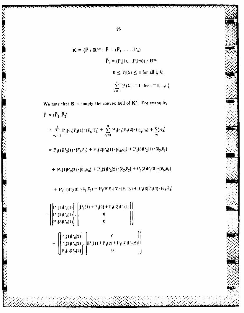
* 25

03~~* n. 1 (

K=i =IRm P (I ,...,Pj~) '

m~

We notei that' K is' s l th covxhl fK.Freape

3I 3

(FIFj)+ 1()P 0 () 1 forP" all , X

I3 +X P, (o) +iP,,(3).1n1)]

+ 1P1(2)'.)P2 (1 1~) +Pj(2 + 3),e 3 )2

e 1 1 e1 ~I e

26 tI

P1 (I)P,(3) 0 -..

+ P1(2)P2(3)j0P1 (3)P2(3) (P 1( 1) + 1) 1(2) + P 1(3)) P,(3)

p 1 ( 1) 12)(1)

-P 1 (2) P,,(2)

P1 (3) P2 (3)

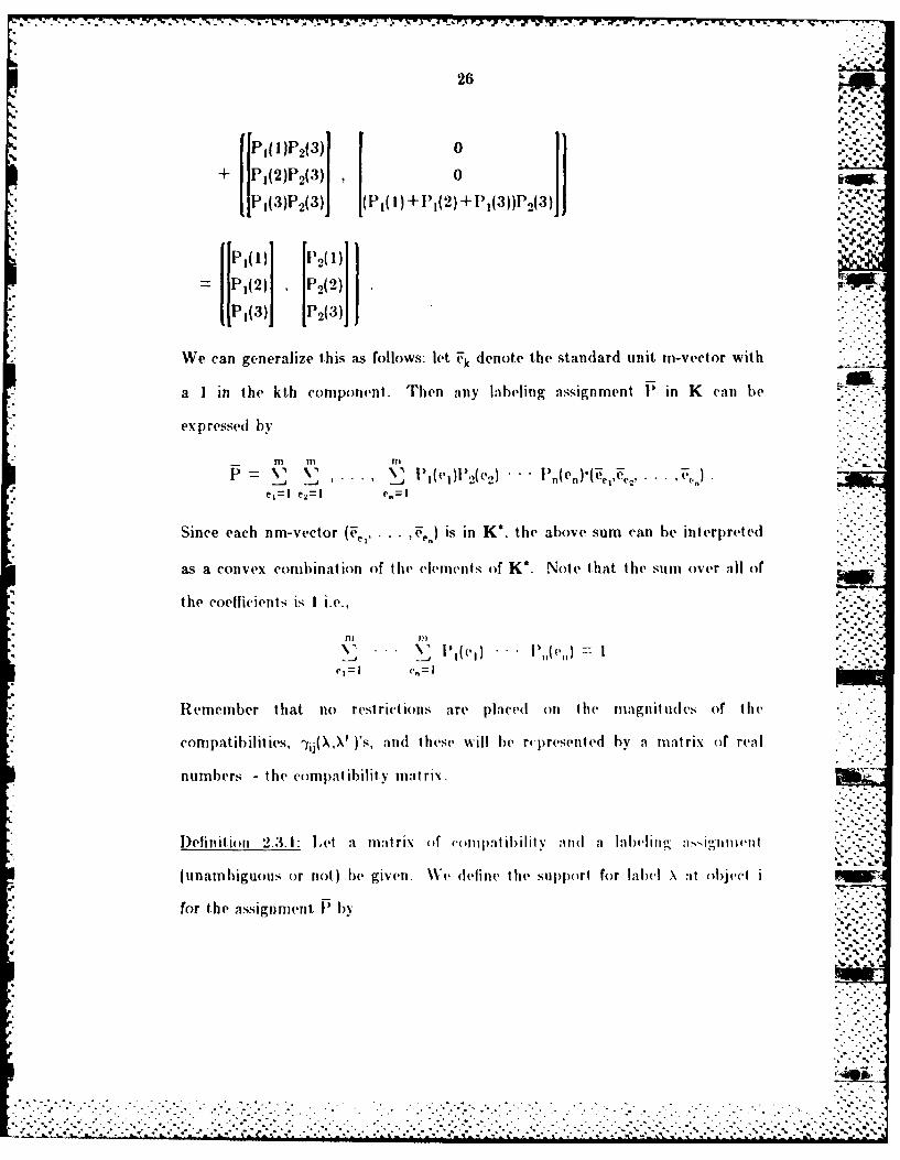
We can generalize this as follows: let ek denote the standard unit in-vector with

a I in the kthb component. Then any labeling assignment F in K canti be

expressedI by

e1=I e.,=I Cn~

Since each nm-vector ' .. n) is in K*, the above sum can be inlterpreted

as a convex combination of thle elements of K*. Note~ that the stim over all of

the coelicients is i.e.,

Remember that no rest rictions are placed onl the nuagiti es or tit(

compatibilit ies, '(X.')'s, andl these will Ibe r, presented by a ma.t rix of real

numbers - the c~ompat ibility v at rix

Definition 2.3.1: Let a, nmatrix tf colliplat lilt v :11(d a lbeling" a.igiiti1eiit -

unambiguous or not ) be given. ~efiebne the sutppo~rt for label X at object I

for the asignnt1'b aaa.a

27

n ms lX) =s lX;I") V V" \" jX'' PI '

More generally, the support values Sj(X) combine to give a support vector -

that is a function of , i.e. S S(P).

)efinition 2.3.2 (Define _(onstrqcv for u na yrnbjigoils labelings):

Let P K* be III unamlbigutius Iabeling. Sulppose that X, .. , are the

labels which are assigned to objects ).,n by the labeling P). That is,

P =xe, ,e). The unambiguous labeling P is consistent (in K*)

providing.

S,(X 1 : P) > (X: P), I < X < -.

S; X,,: 1') _> S,,X ), I < X < in

At a consistent unambiguous lal)(ling, the support, at each ol)ject. for the -

assigned label is the maximun) support at that object. The condition for

consistency in K* can be restated as follows:

for all unambiguous labelings V ( K'.

l)elinitio n 2.3 3 {('ornsisten,.' for wialit e l Ie gling.-in en

Let NK be a weighted labeling assignment. The J) is consistent (in K)

.)providing

=' P~~. . .. _, ,_. , . r... . . . 5","," .',. _ . *_. " .5.. . ."

, . . -. 5,. ... . .. . , ' ,5.% % .'. . .. . - ' ' ,

28 -

m m

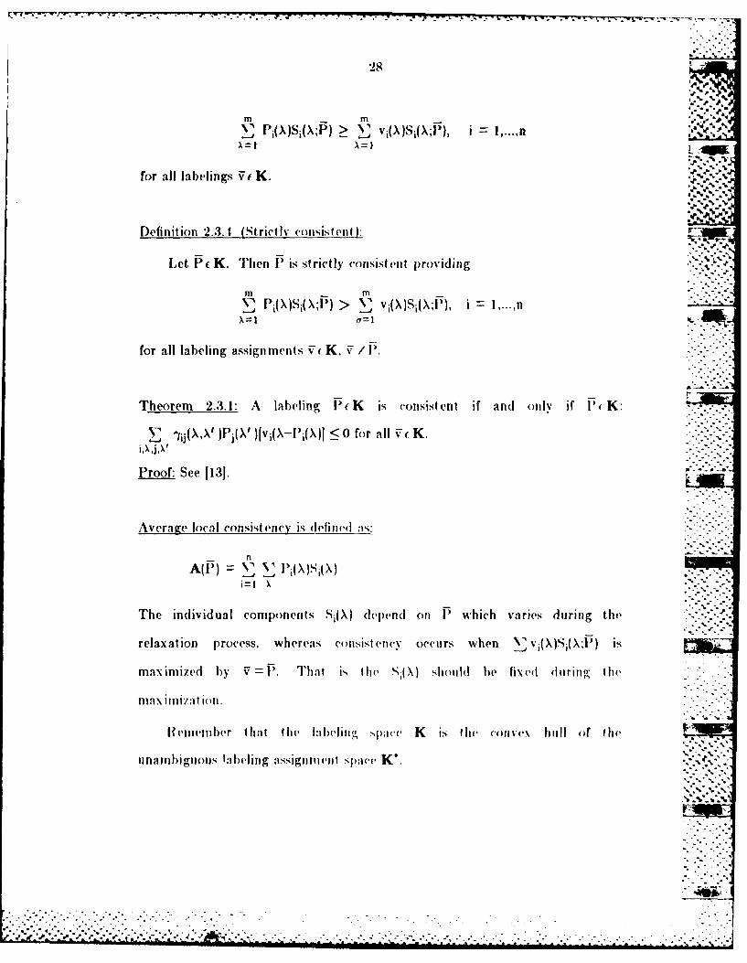
for all labefings V( K. *

Definition 2..3.4 (Strict lv consistent I:

Let P( K. Then F is strictly consistenut providing %%

for all labeling assignments v K, 7I

Theorem 2.3.1: A labeling F(K is consistent if andl only if P( K

~ y~XX')Pj(X' )[vj(X-Pj(X)I 0 fr~ all V( K.

Proof: See 113J.

Average local consist ency is (lefiine( ls:

The ind~ividual components Si(X) depend on F which vairies, (luring the

relaxation process, whereas consistency occurs when \'v(X)S'j(X;P) Is-

maximized by 1,11 k. Th1t is-he(X) ShoulId be fixed duiring- the -

ma IruI,[ at ion.

Iemevinber that the Ia belim ng pacve K Is the( can iti1111 of' t lie

unambiguous U bding assignmnilt space K*.

* ~294,.

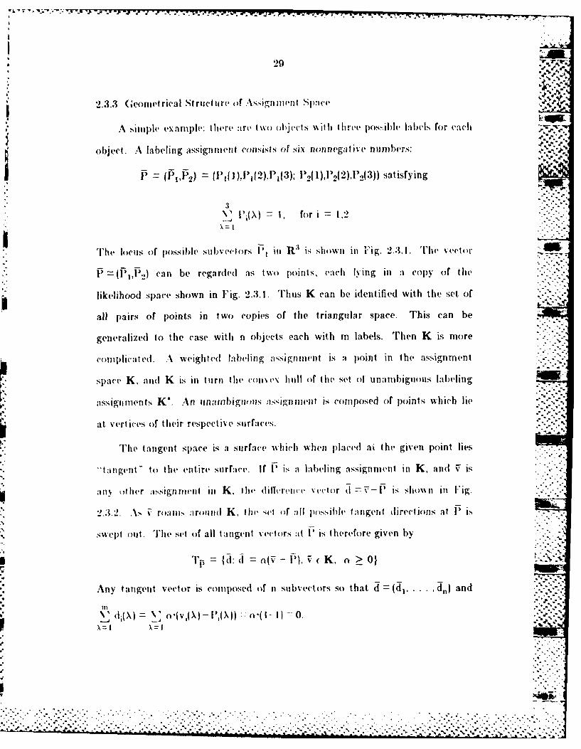
2.3.3 (eomet rical St ru't ire of \sticriimvl S e. .

A .,imple exali)Il: there arC tw() (jects uilh three l)0s;ih1 Iabels for each Mr-

object. A labeling assignment consists (if six nonnega iv, numbers:

I 1 ,t12) = (P ),I2),1'1(3); P2 11),P 2(2),P 2(3))satisfying

\ IAiX) I, for i L.2

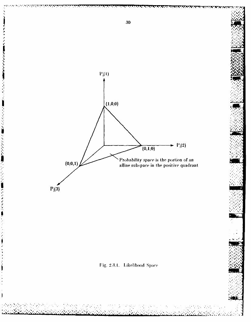
The locus of poss'hl sUbveclors 11 itllR1 is shown in Fig. 2.3.1. 'I'he vector

P=(P1 ,lP) can be regarded as two points, each lying in a copy of tile

likelihood space shown in Fig. 2.3.1. Thus K can be identified with the set of

all pairs of points in two copies of the triangular space. This can be

generalized to the case with n objects each with m labels. Then K is more

complicated. .A weighted labeling :vsignmnvnt is a point in the assignment

space K, and K is in turn the (oil\ hull of the set ol unambiguous labeling

assignments K*. An tiainibigimts nssignient is composed of points which lie %

at vertices of their respective surfaces.

The tangent, space is a surface whitch when l)la('d ai the given point lies

'tangent" to the entire surfaee. If P is a labeling assignment in K, and V is

an} olhcr ; signiviit ill K, te dileretce vector d= v-i- is shown in l'ig.

2.3.2. V , , ro:,t :,roi(l K, the ;,I of All possible ,mngert direciors at ) i.

% swepi oult. The set of all I a igent vectors at I is therefore given by

Tr, d:d (k(V-1) n> K, n > 0} '.

Any tangent vector is composed of n subvectors so that. d = (dl . . . . . d) and

X=l X=t

. .................................. ... . ._ . -,_ -.: --. .-. :..::- :... . .- "".-". .. "". ."."."..'.'... . ..-.- '. .,. .'.-'."," .. ". ,,"" " "".,.'''', -'''.. .""" ,"

0.7~% T-7-7.4-1

30

(1,0,0)

Pj(2)

U Probability space is the portion of anafline subspace in (lie positive quadrant

Pj(3)

Fig. 2.3. 1. Likelihood Spee

31

(1,0,0)~

d~

4* 4 . S

(0,1,01

(0,0,1)

Pj(3)

I-'Ig 2.32. Talgelt SIMP lo

32

The set of tangent vectors at the interior point P consists of an entire

subspace, which is given by

rnr

(P interior to K)

Observe that Tp and K are parallel flat surfaces.

When P lies on a boundary of K, the tangent set is a proper subset of the

above space Tp where P. is any intorior point.. That is, when the assignment

Phas some zero components, the set of vectors of the form ~-)Is

restricted to -

m

TP = d =(d 1, ... An): di RI, N' d (X) =0,

and d,(X) 0 It Pj(X) 0

2.3.4 Maximizing Average Local Consistency

From Theorem 2.3.1, maximizing A(P) corresponds to finding a consistent

labeling. The increase in A(P) due to a small step of length (t in the direction

Ui is approximately the directional dlerivative:

A(P + af) - A())~ K A (F + t a U) gra d A a( doi

where 11ul 1. The greatest increase in A(P) ca.n lbe expected if a step is taken

in the t anlgent direct ion ff wh)ichi max imiizes the direct ion al dery at iVV.

However, if the (directional derivative is negative or zero for all nonzero tangent

direct ions, then A( P) is a local maximum andl no step should be In ken. To find .';-.

[;" ~33"--"

a direction of steepest ascent. grad A(I)'ii should be maximized among the set

or t ang(eut vectors. Ihowever, it sutfies to considr only those tangent vectors

w'I ) EwI'den no i 1 I together with U 0.wit h Iti,'lidean norm 1f :l .ith. : " ,..

Thus the direction of steepest ascent can be found by solving the

following.

Problem 1: Find ffTp fl' l()) such that fCj> "j for all Tpfl [,O),

where(j-.gradA(P). Ihere (0= . _ R''m: 1 5".'.-

When the maximum u-q=O, we will agree that U=0 is the best solution to

problem 1. Conceptually, starting at. an initial labeling P, we compute

q- grad A(P), and solve problem 1. If the resulting u is nonzero, we take a

small step in 1he (lirection i, an(d repeat the process. The algorithm terminates

when d 0. _____

When P is the interior of the assignment space K, solving problem I

corresponds to projecting j onto the tangent space Tp, and then normalizing.

Lenmi1: I lf 1) lies in the interior of K, then the following algorithm solves

proldn e =|

(2) set \ %,(X) % l(X) ( , al i, X.

(3) Set (u1(Xj Wi(X\)/1Wjj aVV I.

1V \,

." .,.-)2J

~~~~~~~~~~~.....................................................-'- ."-',., . .-. .. ":'.'.-- _ _ - .,_"..-

3.1

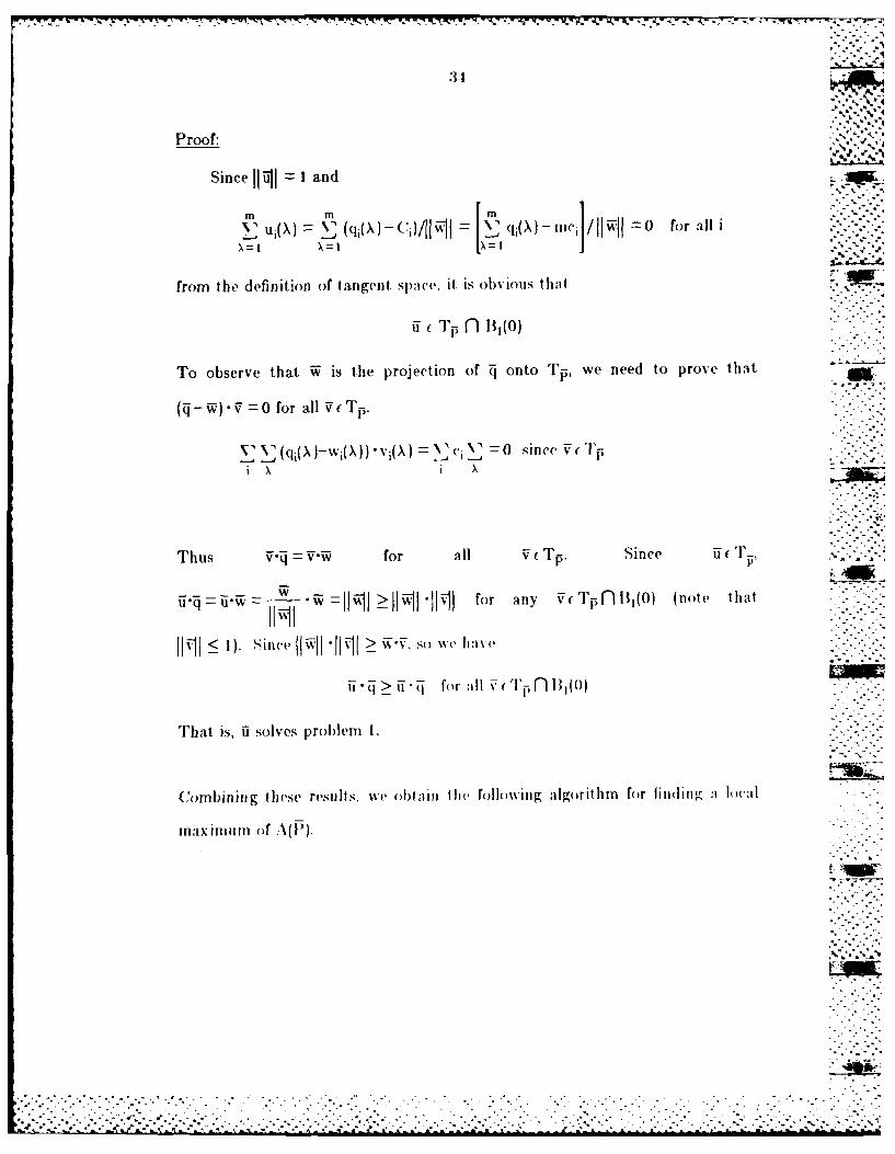
Proof:Sincel--ll =1 and ,

I+x 1 - 0 for all I

from the definition of tangent. space, it is obvious that l

U (T., n fi~o)

To observe that W is the projection of q onto Tp, we need to prove that

(Z-W) Z1V 0 for all V(Tp.

.. _ (qi(X)-wi(X))"vi(X) c\' =0 since V(1'rp

I X .-. o _ . °

T hus V ' = v for all V t T p. Since T Vv--

Ul w WO for any v( Trnifl(o) (note that

I1'-1! < ). St"<& I! *l"1 -1 > " " .) we ,:, ..v

ii > i4 for all 1 f l l (O)

That is, fi solves problem I.

Cormbining these results, w, o)1 ai Hie following nIlgrithin for Iindling : hw-al

max iir ()m f A(P~)).

-IRV P01,

35- . % o

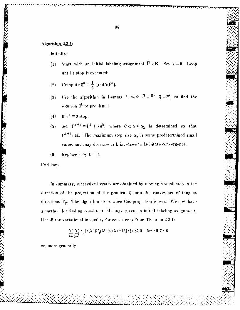
Algorithm 2.3.1:

Initialize:

(1) Start, with an initial labeling assignment F"(K. Set k =0. Loop

until a stop is executed:

12) Compute qk = gradA(k).

2

(3)1 Use the algorithin in Lemma 1, with P--P', q_-k, to find the

solution Ik to prol)len I

(4) if ilk 0 stop.

(5) Set pk +- pk+ kk, where 0 < h 5k is determined so that

Pk+n ItK. The maximum step size ak is some predetermined small

value, and may decrease as k increases to facilitate convergence.

(() Repla(ce k by k + 1.

End lo:p.

In summary, successive iterates are obtained by moving a small step in the

direction of the projection of th( gradient 51 onto the convex set of tangent

(irections 1"0 'l'h mlgorithm stops when this projection is zero. l now have ..

a method for finding (consii vnt l ,clihl , %i('n an iiti1 It l,,I n"

I?(,call the varintion:i ineql ality fo r (.,nsisliency from Iheorem 2.3.1 :

4 -(dXN , )l'(X' )(vl(X)-l-1(X)) < 0 for all V Ki, m j,X' W

or, niore gneraly

. . . . .%

S-.-.-,., .-.

:-'- -',.. " .G '' .".- . " - .,- '. -. .' '" . ',.: .* "" . "- , . "."' ---.. .- • '.-,. '.. . ... ,'," -', . . "". " ,' . -" ' . ' -. ,.'"",. '

36

,%1%--. % ,. ,

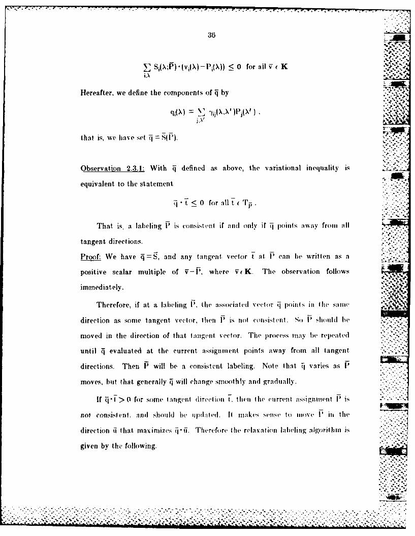
N' Si(;P) - ( v i(X)-P i(X)) <0 for all V K

Hereafter, we define the components of q by

(li(X) : X -Yif ,')lj(X ) ,',ov I.

that is, we have set Tj S(F).

Observation 2.3.1: With defined as above, the variational inequality is

equivalent to the statement

-t< 0 for allt Tp:

That is, a labeling l5 is consistent ir ai(d only if (C points way fromn all

tangent directions.

Proof: We have =S, and any tangent vector t at, P can be wrillen as a

positive scalar multiple of V-P, where VrK. The observation follows

immediately.

Therefore, if at a labeling P, the associated 'e('lor 51 points in ( he sav n

direction as some tangent vector, then P is not consistenlt. So I) should he -.

moved in the direction of that taIngent sector. The process may be repeated

until evaluated at the current. assignment points away from all tangent-

directions. Then P will be a consistent labeling. Note that Tj varies as P

moves, but that generally ij will change smoothly andl gradually.

If j t> 0 for some lanigent (lire(,t ioll , then the current assignmen rP is

not COnSistent, Afl(l Shon 1(1 be iij)(,it ed. It miakes ,seiise to io Ve F iii the

direction ii that maximizes (l'i. Therefore hlie rela atim labeling algorithm is

given by the following.

.- -..- .- - ........-.---- .... ..-.. -. '- ... . ..- . .."-. -. '..-'..-,. -.-". ....- .- ,-:'.. "

37

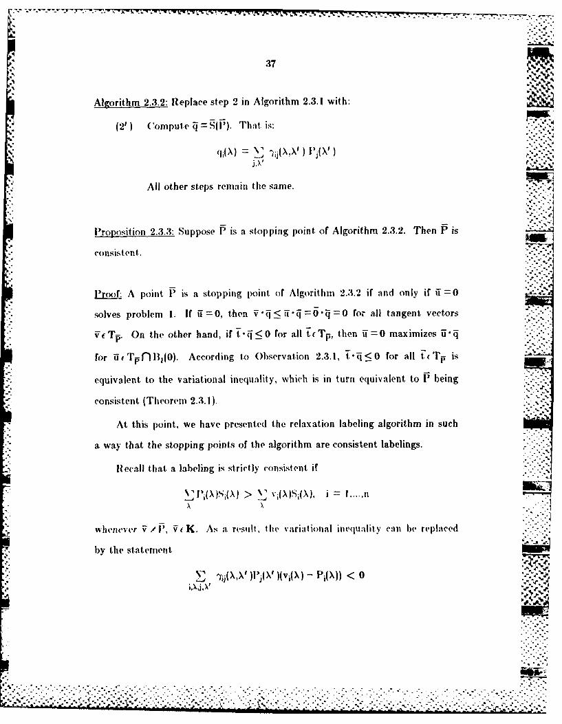
Alizorithm 2.3-2: Replace step 2 in Algorithm 2.3.1 with:___

(2' )Comput e Tj SillP). Thait- is: *

All other steps remain the same.

Proposition 2.3.3: Suppose P is a stopping point of Algorithm 2.3.2. Then Pis

consistent.

Proof: A point Pis a stoppinig point. of Algorithmr 2.3.2 if and only if i = 0

solves problem I. If U =0, then VTl:5if 40 4=O fo. all tangent vectors

VcTF On the other hand, if t 4!50 for all t(cTp, then W 0 maximizes ii-j

for -5 ( Tpflh1(0). According to Observation 2.3.1, t. !50 for all tcTp is

equivalent to the variational inequality, which is in turn equivalent to Pbeing

consistent (Theorem 2.3.1)..

At this point, we have presented the relaxation labeling algorithm in such

a way that the stopping points of the algorithm are consistent labelings.

Recall that a labeling is strictly consistent if

whenever V / ',i(~K. As a. result, t he variational inequality cam le replaced *--

% lby the statemnent

-Y,,(X,X' )P,(X' )(vA) - PADX) < 0

for all VK,V/

for a strictly consistent labeling. In part icutlar, 4j* U < 0 for all nonzero tangent .

directions Ui at a strictly consistent labeling P. We claim Chat. P( K (i e., t hat

P is an unambiguous labeling). Su ppose, for cont radlict ion, t hat 0) < I ,)< I

for some (in. Xn). Then for sonme otlier X,', 0 < l~( ,~)< 1. W~e consider I%%o

tangent directions,

and "2 "1

That is, i has a 1 in the ( in,Xn) posit ion anol a -1 in t he ( iX 0 ) lposit ion, and~ Ui2

is the other way around. These are vahdid tangent dlirect ions according to thme

formulation of TP. However, 4j i-4 ib so they cannot. bothI be iiegat lye.

Hence, we have shown that a strictly consistent. labeling P must be

unambiguous. Thus if ~jpoints away from the surface K at a vertex (i.e., an

unambiguous consistent, labeling), then 51 will point generally towardl the vertex

at nearby assignmnints in K. Ac cordingly. if is near the uniambiguous

consistent labeling, moving P) in a tangent dlirect ion 4i that points in the same

direction as ~,should cause P~ to converge to the vertex.

2.3.5 Relaxation Operator

Algorithin 2.3.2 updates weighted labeling assignments by computing an.

intermediate vector ij, where

j 1P' )%'

and then updating P in the direction defined by the projection of 4 onto Tp.

39

As we shall show, the original updating formula 111 has the intermediate vector

~defined by

* q1(X) d•jjd , ) N- l°

In Algorithm 2.3.2, we set qi(X) Si(X). IHere the support vector .~is a function

S(P"), where Si(X) is computed from a nonlinear function of current assignment

values in P.Presumably, Si(X) depends on the components of P~ for objects j

near object i, and is relatively independent of the %-allies of l for objects

(list anlt fromn T herefore, I Ii diffteren t olbj ('t j nieair oblject i is allei ii

inflIuence oil the supp~lort, fut ion I(1-q( X ) whtichi dleends onl the a Ine of weight ing

constant dj andl has no influence onl qi(X) at all if dij is zero.

The principle difference lies in the manner in which I is projected onto a

tangent vector, In Algorithm 2.3.2, the tangent direction was obtained by

maximizing 5 - i among 5i ( T, fl 1i(o).

owe or the standard relaxation formulas was suggested by Rosenfeld et al.

3i1 and is given by

iP(X) I + qi(X).

SPi(e)[1 + qi(e)J

(it is assumed, when using this formula, that the -1j(X,X ) values are sufficiently

small so that., one (can b e sure that Ije(X)h <tp.) There is another similar

formula, actually derived from this one by transforming compatibility

coefficient Pyu(XX' Sto conditional probability P on(X V ). Therefore the proof of

convergence for one is automatically valid for the other.

-". .%

ditai frl i. T eeoe-h ifrn betj n a lj(t ii ic il:"'''"

7-1I

40

To consider the l)ehavior of thiis standard '( rim l:,, first :issl i n thai t is

near the center of the assignment space, so that very approxiniatelv

P i(X)=I/m_ for all i, X. The updating can then be regarded as consistingof o."....

two steps. First, the vector P5 is changed into an intermediate I". where

P i(X) = P1(X) [I + q1(X)] P l'(X) + q1(X)/mn. -i ,

Next, Pis normalized uising a sca lar conist ant for eaIch object P. When P is

near the center or K, this rescaling process shifts P in a direction essentially

perpendicular to K. That is, P is reset to approximately the projection of P-

onto K. Denoting the orthogonal projection operator by Ok, we have

P-P' -Ok( ) ,O k + j/mj

by virtue of the continuity of O k . Further, assuming that P is in the interior

of K, and ? is sufficiently small, then

Ok(P + q/m) =P OT

where OT is the orthogonal projection onto the linear subspace Tp. However,

the solution U to problem I is obtained by normalizing OT(q). Combining, we

have that

for some scalar a. Thus, P is reset to a vector which is approximately the

updated vector that one would obtain by Algorithm 2.3.2.

When P is close to an edge or corner, the situation is somewhat more

complicated. The first step in standard updating (i.e.,

P1 i(\)P =Pi(X)[I + qi(X)] =Pi(X) + lPi(X)qi(X)) can be viewed as an initial

operation changing j, since the components of c eorresponding to small

. . •..

. .... **..... . . . . .... ...... .............. . .

components of P7 have minimal effect (i.e., the motions in directions .

perpendicular to the nearby edges are scaled down). The normalization step is

the same as before. Therefore, the formula results in attenuation of motion

perpendicular to an edge. Further, a zero component can never become *.,

lnonzero even if the evidence supports the value.

2.3.6 Supervised Relaxation Operator

Now we are prepared to establish the convergence property of the

supervised relaxation operator.

The original relaxation operator 13] indicates that Pi(X) is updated by

Pi(X)[l + qi(X)l in which qi(X) is the neighborhood function. Actually,

Pi(X) [1 + q,(X)J = Pi(X) + Pi(X)qi(X). These m likelihoods, Pi(X), X =

form a rn-vector, Pi, for the current object i. Similarly, Pi(X)qi(X), X =

form another m-vector, Piqi. The formula, Pi(X)qi(X), implies that the

neighborhood contribution to the class X at current object i should remain

relatively unchanged if the class X at current object i has likelihood close to 1;

otherwise it should decrease. The likelihood space of Pi and the vector Piqi are

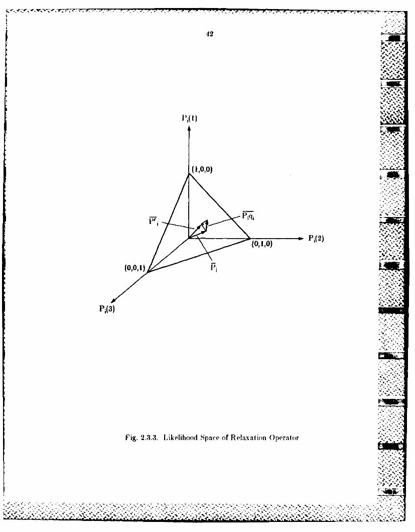
shown in Fig. 2.3.3, in which 'iqi influences the movement direction of Pi.

After normalization, the summation of the components in the newly updated

vector P i' is equal to I. That means the vector P + Piqi is resealed to make

the ncw vector Pi' still in the likelihood space.

In the supervised relaxation algorithm, before t'i, defined later, influences

the movement direction of Pi, the Pi(X) is influenced by Qi(X) using the formula

-. I'i(X)Qi(X) in which Qi(X) is also a neighborhood contribution but the

compatability coeflicient " i(XX') is expressed in terms of the conditional

.. ,--

42

(1,0,0)

*.j%. -

IPI

Pj(2)(0,-s0)

(0,0,1) .

P5! 4.

Fig. 2.3.3. Likelihood Space of Relaxation Operator . ~

43 .

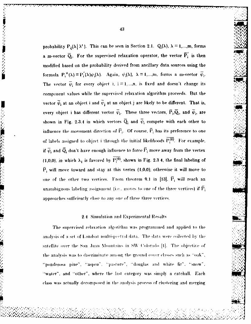
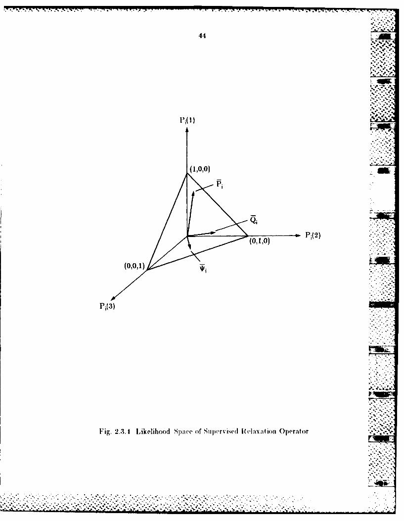
probability Pii(Xj X'). This can be seen in Section 2.1. Qi(X), X = 1,...,m, forms

a m-vector Qi. For the supervised relaxation operator, the vector Pi is then

modified based on the probability derived from ancillary data sources using the

formula Pi+(X)= P(X)g, (X). Again, 0i(X), X =,....m, forms a ni-vector i•

The vector V% for every object i, i = I.n, is fixed and doesn't change its

component values while the supervised relaxation algorithm proceeds. But the

vector at an object i and vi at an object j are likely to be different. That is,

every object i has different vector t/'i- These three vectors, Pi,Qi, and i, are

shown in Fig. 2.3.4 in which vectors Qi and t! compete with each other to

influence the movement direction of 1Pi. Of course, Pi has its preference to one

of labels assigned to object i through the initial likelihoods Pito)• For example,

if Oi and Qi don't have enough influence to force Pi move away from the vectex

(1,0,0), in which XI is favored by Pio), shown in Fig. 2.3 4, the final labeling of __

Pi will move toward and stay at this vertex (1,0,0); otherwise it will move to

one of the other two vertices. "romt theorem 9.1 in 1131, Pi will reach an

unambiguous labeling assigimient (i.e.. inoves to one ( f the three vertices) if Pi

approaches sulficient ly close to a:ny one of these three vertices.

2.4 Simulation and I'xperimental leslts

The stipervised relaxation :0go rit bi was programmted and applied to the

a:llvsis of a set of Lndsat miil, ,'tr:1 data. The dmLt were v(lle<'ted by the

sat ellite over the San .11n .Moiiit iii in S\ ('oloradoh [I]. The objective of

the analysis was to discrininate amn, the ground cover cl:,ases s1ch as "'oak

ponderosa pine, "aspen , past ire, "hu glas and white fir",. "snow", -

"water", and "other", where the last category was simply a catchall. Each

class was actually decomposed in the a:lysis n proess of clustering and merging

. . . . . . . . . . . .-. •.-' .....- ,-. .-

44

Pj( I

(1,0,0)-

Pi

Pj(2)

Pj(3)

Fig. 2.3.A Likelihood Space of Sii jrvised RI lax ation Operator

45

4-4

into a union of subclasses, each having a dlata distribution describable as

* approximately multivariate normal.

2..1 Results from the Maximum Likelihood Classification Algorithm

To provide a baseline for comiparison, the (data fim the first and the

secondl channels, whliich were In t he rnnge of v'isibleC wavelengths, were first

analyzed using the max imum likelihood classificationt algorithm. The a priori

likelihoods of the classes were approximated as being equal, and 2122 test

samples, independent of the training samples, were used to evaluate the results.

lDue to different, numbers of test. samnples in each class beingr used in the

evaluat ion of the algorihm per-f rmance, the measure called average

perfornmnce by class is used to avoid anty bias toward any class whieh has the

largest number of test samples. As shown in Table 2.4.1, the average

performance by class of this conventional maximum likelihood classifier was

38.5 percent correct.

9.4.2 Results from the R elax at ion Operator

To implement the relaxation analysis, the most formidable job is

estimating both the initial likelihoods lP(), XeA and the conditional

likelihoods Pip(I X). The initial likelihoods are availahle in the penultimate

stvp of the mnax imunh likelihood classification using 2-channel spectral data only

i.e., just prior to the pixel being Ia lbeledl accordig to the largest, of these ____

likelihoods). The required -oiit ext conditional likelihoods ~ ,)were

estimated fr(mi the final classifi cat ion resulIts p~r( td II(( roiti the max imunmii

likelihood classificat ion algorithm by coi ain g joint andl indliv idual occurrences

of the classes. However, rather than computing four (lifferent sets of these

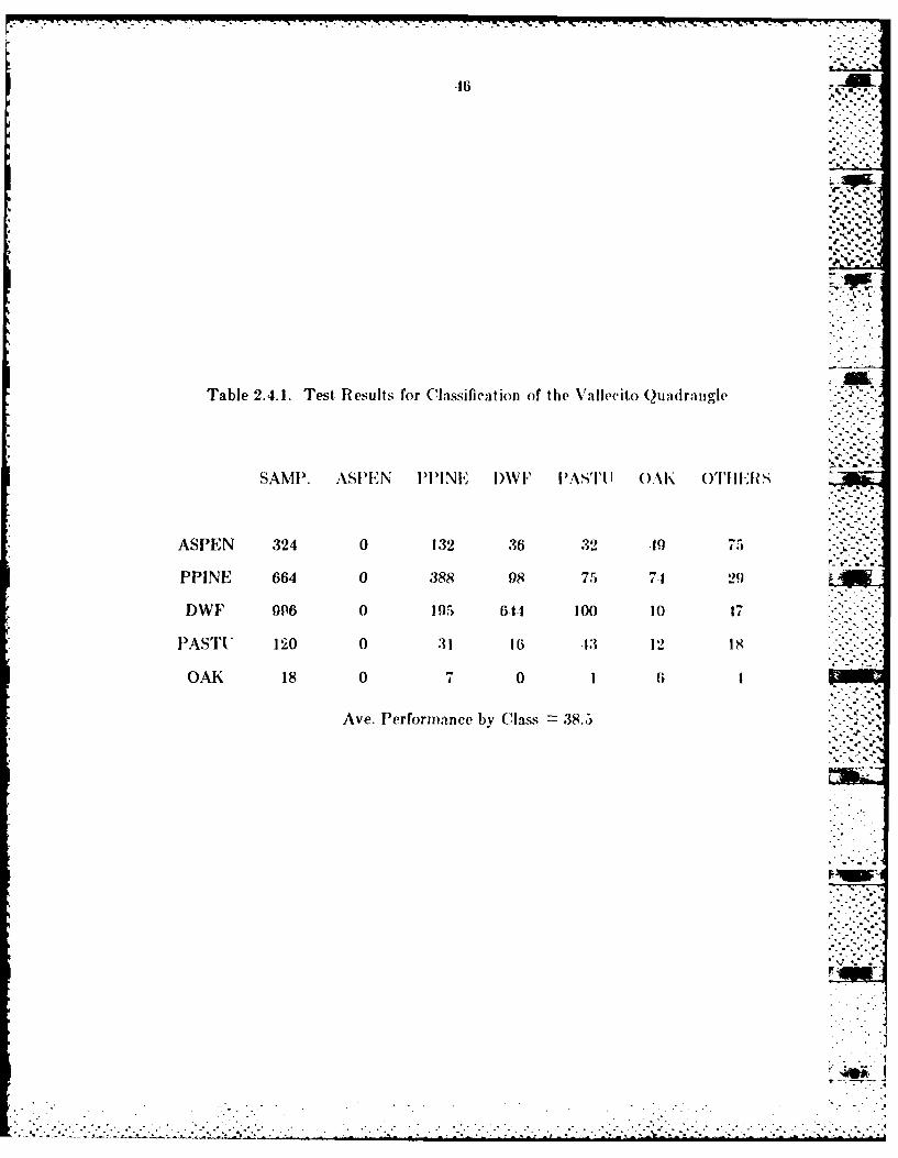
Table 2.4.1. Test Results for Classification of tIhe Vallecito Qu-mriigle

SAMP. ASPEN PPlINE I)W1F PASTI1 J (OAk OIiIIi

ASPEN 324 0 132 36 32 -19 7

PPINE 664 0 388 98 75 7129

DWF 996 0 105 6.1. 10O 1O 17

PASTU 12 0 0 16 Iii13 12 Is

OAK 18 0 7 0 1 6 1

Ave. Performance by (lass 38.5

17

corresponding to each differtnW neighibor type (left, right, above, and below), a

single set was calculated by counting joint occurrences in both directions both

vertically and horizontally.

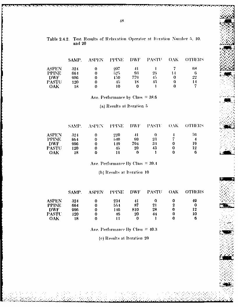
The same test samples were used to evaluate the r.'sults. The results of

this relaxation oper;)tor at iterali(n numbler 5, 10, and( 20 are shown in Table.J

2.4.2. Tefinal result wais slightly better thantemx.niilklho

classification. The average performance by class was .10.3 percent correct.

2.A.3 Results from the Supervised Relaxation Operator with One Ancillary

Information Source

Due to the n mavaila hility of multiple ancillary information sources and

the desire to demoinstrate the feasibililty of the algorithm, channel 3 data was

used as ancillary data in the ( experiment. The supervised relaxation operator is

now shown, by example, to be a useful tool for incorporating information from :*"-"

one ancillary data source, channel 3 data, into an existing classification --

produced from the maximum likelihood algorithm using 2-channel spectral

data. (hannel 3 is an infrared spwetral hand 1. The uean and standard

deviation of each class hav ing a data dist ribut ion describable as approximately

normal were estimated for channel 3 using clustering and merge-statistics .7

algorithm. From these data, sets of 0i(X) for each pixel in the image were

generated and incorporated in the supervised relaxation algorithm. The same

initial likeliloods and (onlitional likelihoods were again used. Several

relax at in tests were lerl'rmed using differing degrees of supervision, i.e.,

variou.s weighling constants given to Ihe influence of the ancillary data via the

parameter ,1. The value of /3 which produced the best results was chosen.

*..............

." . . -. " . . .*" " .;- . . ;.'-.-i- .. . . -. . . '. ."-.- - ". -. -". -... . -' .- .. .-*.*. .**** ***

.18

Table 2.4.2. Test Results of Relaxation Operator at Iteration Number 5, 10.and 20

SAMP. ASPEN IIIIINE I)W" I AS'I'1' OA O I I I I -S, "' t ',. '.-.. . --

ASPEN 324 0 207 .11 I 7 68PPINE 661 0 525 9.3 26 111 IDWF 096 0 150 770 .15 0 22

PASTU 120 0 .15 18 .13 0 !1OAK 18 0 10 0 I 0

Ave. Performance by Class 38.6

(a) Results at Iteration 5

SANI. ASPN IINI I)\V i' I)A,'I' ().\!K ('1'11i1 is

ASPEN 324 0 220 .11 0 .1 52PPINE 664 0 5g0 90 23 7 4DWF 906 0 149 79.1 31 0 19

PASTU 120 0 45 20 43 0 12 .

OAK 18 0 11 0 1 0 6

Ave. lerformance By Class 39.4

(b) Results at It eration 10

SAMP. ASPEN PPINEI DWF PASTU OAK OTHERS

ASPEN 324 0 234 41 0 0 49PPINE 664 0 55.1 87 21 2 0DWF 996 0 116 810 28 0 12

PASTU 120 0 46 20 44 0 10OAK 18 0 11 0 1 0 6

Ave. Performance By Class =10.3

(c) Results at Iteration 20

.:.. ..4..

49

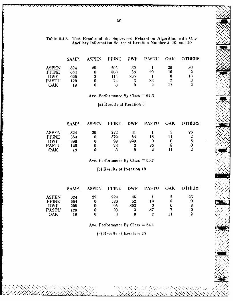
Again the same test samples were used l() evnluate the results. As shown in

Table 2.4.3, the average performance by class was better than the ordinary

relaxation analysis. The final result is 6.1. percent correct. In addition, a,

closer look at, the class-by-class results reveals that the performance for each ,' -,

class was better than those attained using the relaxation operator without,

ancillary information.

2.4.4 Results from the Supervised Relaxation Operator with Two Ancillary AW

Information Sources

In this section, the supervised relaxation algorithm is shown to be an

effective technique for incorporating information from two ancillary data

sources, channel 3 data and elevation data, into an existing classification to see

any improvement in classification accuracy over that obtained with only one

ancillary source. Figure 2.1.4 shows the distribution of tree species as a

function of elevation for an area northeast of the Vallecito Reservoir in the

Colorado Rockies. Fig. 2.1.2 shows a digitized terrain -map for the area covered • ..

by the multispectral scanner data described earlier. From these data, the

second set of Oi(X) for each pixel in the image was gererated and used along

with those generated from the first. set of 0j(X) in the supervised relaxation

algorithm. The same initial likelihoods, conditional likelihoods, and test

samples were used. The weight constant producing the best results was chosen.

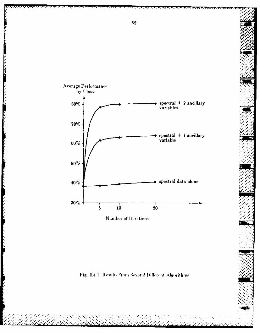
As shown in Table 2.4.4, the average performance by class using two ancillary

data sources of information gave the best result, 80.8 percent accuracy. The

results from the maximum likelihood algorithm,,, the relaxation algorithm and

the supervised relaxation algorithm are compared an(d drawn in Fig. 2.4.1.

From this figure, it is clear that the more information we use, the more

LIN t h. ". -V

50

Table 2.4.3. Test Results of the Supervised IHelaxation Algorithm n ith One

Ancillary Information Source at Iteration Number 5, 10, and 20

SAMP. ASPEN 1)1)1NE DWF PASTU OAK OTHERS ,-*. -

ASPEN 324 29 20t, 39 I 20 30PPINE 664 0 568 58 20 16 2DWF 996 3 II 865 1 0 13

PASTU 120 0 2. 3 83 7 3OAK 18 0 3 0 2 11 2

Ave. Performance By Class 62.3

(a) Results at Iteration 5

SAMP. ASPEN PI'INE I)WF PASTU OAK OTHERS

ASPEN 324 29 222 41 1 5 26 ...

PPINE 664 0 579 54 18 11 2DWF 996 0 98 890 0 0 8

PASTU 120 0 23 3 86 8 0OAK 18 0 3 0 2 11 2

Ave. Performance By Class = 63.7

(b) Results at Iteration 10

SAMP. ASPEN PlI'NE DWF PASTU OAK OTHERS

ASPEN 324 29 224 45 1 2 23PPINE 664 0 586 52 18 8 0DWF 996 0 95 893 0 0 8

PASTU 120 0 23 3 87 7 0OAK 18 0 3 0 2 11 2

Ave. Performance By Class 64.1

(c) Results at Iteration 20

. . . . . . . . . . .... . . . . . . . . . . . . .

- .---.---..-- * ~ * ~ ~*~ *~A *A ~ . -. - -° -h a., .°+,.aS "'+°°+o

51

Table 2.4.4. Test Results of the Supervised Relaxation Algorithm with TwoAncillary Information Sources at Iteration Number 5, 10, and 20

SAMP. ASPEN PPINE DWF PASTU OAK OTHERS

ASPEN 324 276 11 22 0 0 15PPINE 664 0 462 73 8 19 2DWF 996 44 52 899 0 0 1

PASTU 120 0 19 3 87 11 0OAK 18 0 4 0 2 11 1

Ave. iPerformance By Class = 78.8

(a) Results at Iteration 5

SAMP. ASP.EN PPINE DWF PASTU OAK OTHERS

ASPEN 324 292 6 18 0 0 0PPINE 664 0 567 77 8 12 0

DWF 996 -11 45 909 0 0 1PASTiU 120 0 19 3 87 11 0

OAK 18 0 4 0 2 1I 1

Ave. Performance By Class = 80.1

(b) Results at Iteration 10

SAMPi. ASPIN I'INE DWF PASTU OAK OTHERS

ASPEN 32.1 206 6 18 0 0 4PI5NE 6i.I 0 568 78 8 10 0DWF 996 35 .12 918 0 0 1

PASTI' 120 0 18 3 87 12 0OAK 18 0 4 0 2 11 1

Ave. Performance By Class = 80.5

(c) iesiltd al Iteration 20:: .:

:: . : : .%:- _.. ..-. ... ......... - ,-., ..: -..,. .,. .. .......- .: .....,.,. .,.... .-.. .. ..--. ..... .. . .... . . . . .. . .. . .. . .

52 '.

on '

Average Performanceby C lass

80%- spectral + 2 ancillaryvariables

70%-

spectral + 1 ancillary60% variable

50%

40% spectral data alone

30%

5 10 20

Number of Iterations

Fig. 2..1 Results from~ DP~rllif~rent A\lgorithmtis

. . . . . . . S . . . . . . .' . .5 . . .

I., .,I ,

53

accuracy in classification can be achieved. The probabilistic relaxation

methods provides an effective approach for integrating information from diverse

sources of image data.

For the present study, there is no specifie way to determine the value of

weighting constant J1 in Equation (2.1.61. In any specific image to be classified,

the significance of the ancillary data will depend on its rel'vance and accuracy.

Consequently, the optimum degree of supervision must be estimated using

training data just as training data are used in establishing classifier parameters.

The algorithm is ternina(ed after the fixed points have been reached, that

is, when the likelihoods a:Psignvd to each class at. every pixel do not change X'=-

when the algorithin mo ves froi current ii era ion to next, iteration. For the

current, study, after 20 iterations the algorithm had reached the fixed points.

The final labeling represents a balance in consistcncy between spectral .".-

information in the initial likelihoods Pi(°)(X), spatial context data incorporated

in Pij(XI V ), ani ancillary information embedded in the p,(X).

2.5 Summary and Conclusions

The relaxation operator has been adopted as a mnechanisi for

incorporating contextual information into an existing classification result.

ased on the formula derived in Equation (2.1.4), the supervised relaxation

operator carriers on further and incorporates inrormation from mulliple

ancillary data sources into the results of an existing classification, i.e., to

integrate informalion from the various sources, reaching a balance in

consistency between spectral, spatial, and ancillary data sources of information.

""-' " " ....... '-" ":':".............. .. = ..... ..... ,. ""''-'"-'"=.=•' ",'=,-:,[,', ''.'..:''.'."

*~ ~~~ ' CC . .

In Section 2.1, the supervised relaxation algorithm was derived fronm the

standard relaxation formula to incorporate ancillary information by adjusting

the neighborhood contribution to containt thle inf0luences froin bothI local conteox t

and ancillary infornmat ion. 'FThis intet is t hat thle niov ing dIirect ion of t he initial

likelihoods is influenced no%% by hot h local conltext andl~ anDcilla1ry in roriali on as

shown in Fig. 2.3.4. The p~roof that Algorithm 2.3.2 stops at consistent

labelings can be used for the supervised relaxation algorithm by genteralizintg

the support (or neighborhood function) not only from local contextual

informrationt lbt also froml :t t othier Initformtat ionr, whili is 1I1-c(fl I to Improve

the classification accuracy, siclt as anitclary initformtatt ionl desc ribed III Sect it u

2.4. Thus, the final labeling results from convergence or e'vidlence, reaching

consistent labelings, i.e., integrates information from the various sources,

achieving a ground cover classification which is both accuirate and consistent. in

the face of inconsistencies which may exist among the (data components.

Sect ion 2.4 showed ex perimnt fal results of the supvrv i' (t relat\ at jol

algorithm. With the contextual:i informtat ion uncorporat ed in the relax ation

algorithm. the performance was slightly better than t hat obtained from thIe

maximum likelihood classifier. B~y incorporating one anicillary Informtat ion

source, channel 3 data, using supervised relaxation algorithm, the performtance

was much better than previously obt ained. for the area classifiedI, thtere were-

dat a ava ili ble (describing the c'levalot I pttrreferentces of4 thbe varn il; t ret' species,

along with a digit izedl elevat ion inti . IBy incorporating Il i dv at iln (la an

channel 3 data in the supervised relaxation algort itm, sigiicantlyV better

performance was obtained. These results demonstrate that the supervised

relaxation algorithin is a useful technique for incorporating both contextual..

information and multiple ancillary information sotureVS into tan existing '

classification.

It will often be the case that one has only a classification map to work

with rather than sets of likelihoods generated by a classification algorithm.

Under this circumstance, arbitrary "probability" values consistent with the -

classificat fort can be assigned to classes at every object as the initial likelihoods.

Of course, the label for a )articular object indicated by the classifier as most

likely must be assigned the largest, probability value. But for the present

study, the initial likelihoods, lP1(°)(X), X A, were available in the penultimate

step of the maximum likelihood classification using spectral data only.

Therefore, classification results with higher accuracy may )e expected since

pixels or objects with only marginal likelihoods from the maximum likelihood . -

classifier may have their classes or labels changed early in the process rather

than having them fixed erroneously as a result of the initial likelihoods

assigned. As seen from the classification results, the distributions of various

classes tend to be more homogeneous than that before relaxation. This is the ".-:.-

characteristic of the relaxation operator showing that the spatial context

infrrirn tion has been used.

At the moment, there is no s)ecili(c way to dternine the value of

weighting constant /i, in Equalion (2.1.6), through which the supervised

relaxation algorithm allows the relative influence of spectral and ancillary data

sources to be varied. In any particular image to be classified, the significance

of the ancillary data will depend on both its relevance and accuracy.

(onsequently, the optliillin degree of supervision, i.e., weighting to be given to

,. -'- ,:i3_Z ... --...- .-. " .-. .- . ..- ' -.-. ' ..- ., .

56' 7'

the influence of the ancillary data via the parameter /1, must be estimated

using training data just as training data are used in establishing classifier

parameters. Obviously, this involves additional analysis cost.

The contributions from the four nearest. neighbors have been used in the 4'.

supervised relaxation algorithm for the present study to incorporate the

contextual information into an existing classification. For the simulation

presented in Section 2.4, equal weighting constants, dii, have been assigned to

the four nearest neighbors; i.e., these four neighboring pixels have equal degree

of influence in the neighborhood contribution. If the weighting constant, dij,

can be dynamically adjusted to allow different neighbors to have different

degrees of influence on the current pixel classification, the classification

accuracy expected may be better than that with fixed weighting constants.

Clearly, there is a tradeoff between the better classification accuracy and the

cost involved in dynamically adjusting weighting constants.

In the integration of multiple ancillary data sources, the elementwise

product of sets of likelihoods derived from distinctive ancillary data sources is

used. This means that each distinctive ancillary data source is given equal

degree of confidence. In a more complicated case such as one ancillary data

source being more reliable than the other, it nay be desirable to assign two

different weighting constants to the different data sources.

To use the supervised relaxation as a post classification technique. the set

of context conditional likelihoods I % xj X' ) must he (let'rtinIe. The rveu ire,

context conditional likelihoods, Xij( X ), cain be est ii ated from Ihe results of

the maximum likelihood classifier if no other spatial model known to be correct

for the image tnder consideration is available. Obviously the resu lts will suffer

some inaccuracy because the -oni:::it ional likelihoods are est iat ml from the

a.. 57 a

results which are not perfectly correct. For the simulation results presented

here, the contextual conditional likelihoods were estimated from another source

of data known to be correct. When the number of possible classes involved is

large, the number of Pij(XJ X') values is also large. Based on the work in 120],

it. is suggested that highly accurate compatibilities are not required. Therefore,

reasonable values can be estimated from the results of the maximum likelihood

classifier or from some foreknowledge of the spatial characteristics of the image

data if the initial likelihoods in the penultimate step of the classification

algorithm are not available.

..'. :

a." .- '

.-. °

.,. .... -

. . .. . . . . . . . . .-.. . . . . . . . . .

.".

. .• .-..', % ... ,.-.

58

CIAPTER 3 - PARALLEL PROCESSING

This chapter will describe how an optimal system configuration can be

determined based on the perforrllarce criteria and parallel architecture

described in this chapter. An IMN! (Snl- is dins e M, lt iple- Pat i-

stream) machine, as shown in Fig. 3.1, conisist s or a control unit, N processors,

N memory modules, and an interconnection network. A processor and a.

memory module forms a processing element (PE). The control unit broadcasts

instructions to all active PEs and all active PEs execute the same inst ruct ion,

in lock-step, on the data it) their own memories. The interconnection net work

provides a communic ation facility for the PEs. An MIMI) (Multiple-

Ins truction-st ream, Multiple-IData-strearn) machine, as shown in Fig. 3.2.,

consists of a coordinator, N PEs, and an interconnection network. Every PE

fetches instructions from its own memory ,in(1 executes them on the (lat inI its

own memory. Every PE, executes the in~struc(tions Independently and

asynchronously. The interconnect ion network prov ides aoI111nui c:l ionl

medium for the PEs. The coordinator orehest rates the activ-ities, of the iPiS.

Secticn 3.1 will present the application of S-Nets 11.1,151 to describing a n

SIMvD and pipeline implementation of maximum likelihood classification. and(

several performance measures to evaluate the inherent parallelism in this

algorithm %%Ill be discussed iii thiiis section. inI Sect ion .3.2, for the al gorit hr in

b~lock C shown in Fig. 3.2.1 fite al gorit hin ex ('(ili on t ilnes ba;sed on the

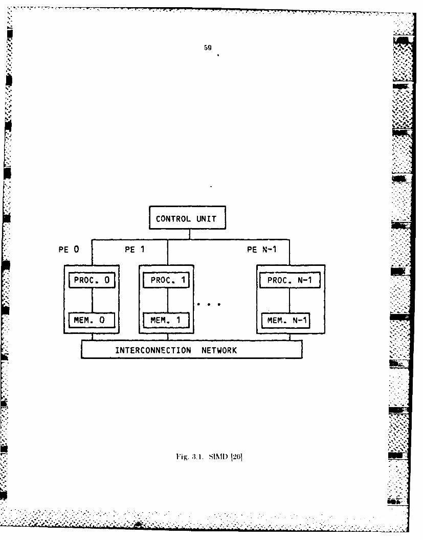
59

PE j PEl1 PE N-i1

IRs0 PROC. 1 PROC. N-

FEM. 0 MEM. 1 MM

I INTERCONNECTION NETWORK

Fig. 3. 1. SIMI) 12651

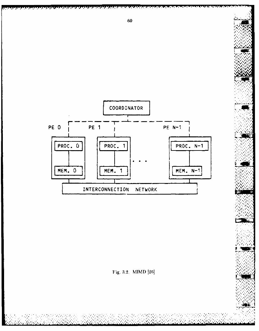
60

COORDIAO

PEO0 PEl1 PE N-1

PROC. 0 PROC. 1 PROC. N-i

EM~~~ ~ E:: 0 S.1LE.N1

INTERCONNECTION NETWORK

F~ig. 3.2. MIMI) 126]

......

61

counting of explicit and implicil operations iin both SIMI) and MIID mode of

parallelism will be compared and discussed. In Section 3.3, several performance ,.

measures different from those in Section 3.1 for SIMD will be discussed. Most

important is the determination of the optimal number of processing elements

for a given image size I)y considering the tradeoff between the cost of execution

time and processing eleenws. Section 3.4 will describe how two multistage

networks 116,17,18,191, cube network and A)Nf network, can be configured to

support simultaneously both MIMI) and SIMD modes of parallelism.

3.1 Modeling Image Classification by Means of S-Net.s

Synchronous Nets 1i14,15], hereafter S-Nets, are an extension of Petri nets

and were developed especially for the description of SIMD processes. This

section presents the application of S-Nets to describiog maximum likelihood

classification, which is commonly used for classifying remote sensing image

data. This application is fairly typical of image processing operations which

are not window-type operations, i.e., they depend on the data at a single pixel

rather than a neighborhood. In general, the higher the dimensionality of the

remote sensing (multispectral) data and the more classes represented in the

iimage, tie greater the potential benefits to be derived from SIMI)'

implementation of the process. This section begins with an introductory

overview of S-Nets.

4-2

-aa- ...... .. '.... . ......-.- ... .. .. . . . . . . . . . . . ... -.. . . . . .. . .. . .

., .-- .-- .

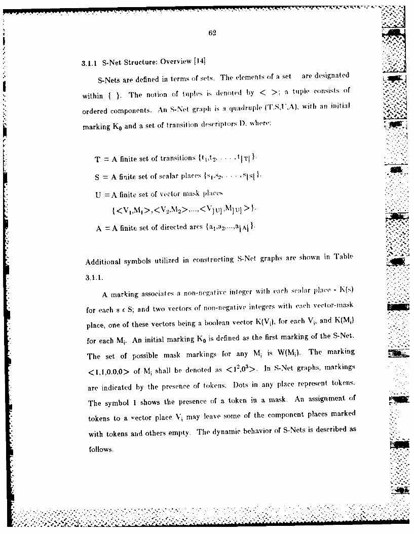
j 62

S-Nets are defined in terms of sets. The elements of a set, are designated

within { }. The notion of tuples is (lenoted by < >; a. tiple consists of

ordered components. An S-Net gralh is a quadruple (I',.IS',A,) with an init ia

marking Ko and a set of transition descriptors I), where:

T A finite set of transitions {t 1,t . t I TI }

S = A finite set of scalar places {ss,.••,ss ....

U A finite set of vec.tor mask places

<VjMI > <V,'M'> ,..., <%'I qI I > %--;" ;

A =A finite set of directed arcs {al,a,...,aJAI -

Additional symbols utilized in constructing S-Net graphs are shown in Table -am;

3.1.1. "'

A marking associates a non-nega tive' integer with each scalar place - K(s)

for each s ( S; and two vectors of non-negative integers with each vector-mask

place, one of these vectors being a boolean vector K(Vi), for each Vi, and K(M i)

for each Mi. An initial marking K0 is defined as the first marking of the S-Net.

The set of possible mask markings for any Mi is W(Mi). The marking

<1,1,0,0,0> of Mi shall be denoted as <12,03>. In S-Net graphs, markings

are indicated by the presence of tokens. Dots in any place represent tokens.

The symbol 1 shows the presence of a token in a mask. An assignment of

tokens to a ',ector place Vi may leave some of the component places marked

with tokens and others empty. The dynamic behavior of S-Nets is described as

follows.

.................... •.... .. ..

", *.. . .s. . - . ' - - "- * '. . " . . . " . " * • , . .. . - . - ' , - .- . ' ' " " . - . - .. -.- ' .. *, - . ' *

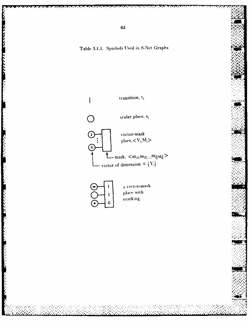
-J . . .j . . .M

63

Table 3.1.1. Symbols Used in S-Net Graphs

I transition, ti

Qscalar place, si

v'ec tor- mask

L..mask, <mi.Mi2 ,. MilMi>

vector of dimension Xi

~ a vector-mask

* j~lJC~'With

nuarking

7-7: *.

-7*

64

b,%

A scalar place is holding if it has at least one token in it.. A vector-mask

place <Vi,Mi> is holding if at, least, one K(mi) = 1, j l,2,...,I Il . and the

corresponding vii ( V i has a non-zero niarking. A transition t is cnlblcd if all

scalar places of transition t are holding and all vector-mask places of Iransition -

t are holding. When a transition t is enabled, it.s firing function is defined at, a

given marking K n of the S-Net, and the firing yields Kn+ I, a new marking. A

transition type specifies the firing capabilities of the transition - either simple

or mask firing - designated SFT and MFT respectively. A transition descriptor

D[t] for a transition t with vector-mask output places

<Vi,M1>, <VMj>, . , <V,,M,> is specified as Dit = [type;K(Mi)cW(Mi), K(Mi),WIMi), K(M,)cW(Mr)I.ii]i :: :

A simpie firing associated with an enabled transition t is such that:

(a) For every scalar input place s, K+I(s) Kn(S)-1.

(b) For every scalar output place s, K, + I(s) = Kn(s) + 1.

(c) For every vector-mask input place <V,Mij>, then for vij(Vi,

j1,2,...,l Vii , Kn+I(vij) = Kn(vii)-I for those j for which mij(M i has a non-zero

marking; and for miiMi, Kn+u(mii) Kn(mij) for all j.

(d) For every vector-mask output place <Vi,Mi, then for vjj(Vi,

j=1,2,...,I V, Kn+i(vij) = Kn(vii)+l for those j for which mii M i has a non-

zero marking; and for mijMiN, Kn+ 1(niin) K(n(mij) for all j.

As seen from the firing rules, SFTs do not alter their input or output masks.

A mask firing is associated with an enabled transition t that has at least

one <V.,Mi> output place, and is such that:

% ...-. ..-.. .- :.|

...... ..... .....--....--.... ..... ......-..-.

* . . .. ... .. • ,- . .- . . - ., ....... .. . . . -. ."• -- ,-.-_-- - -.- - - "" .°" % " " " .'

- ° -

-, .:

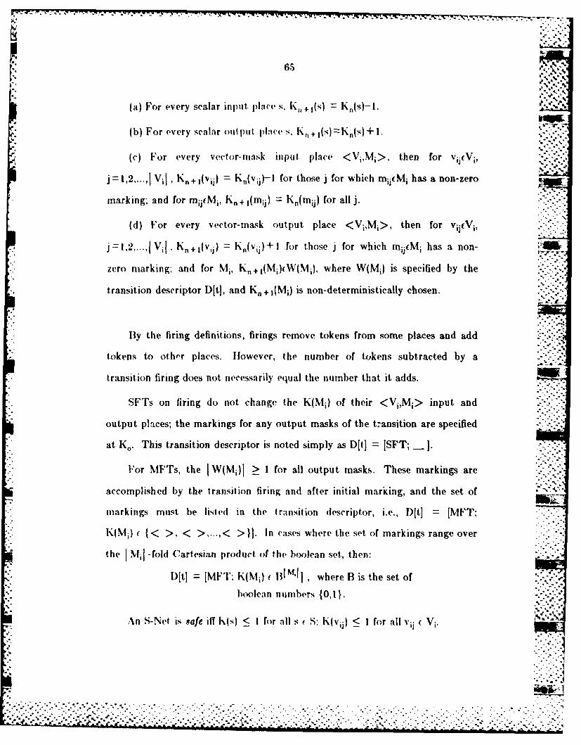
(a) For every scalar input. place s, K,,+ (s) Kn(s)-I.

(b) For every scalar out put Place s, K ilsl=Kn(s)+

(c) For every vector-mask input. place <Vi,Mi>, then for vii(Vi,'

jzl,2.... Vi K, Ka+ 1(v ) = Kn(vJ)-I for those j for which mii, g i has a non-zero _ .

marking; and for mi(M i, K + (mii) Kn(mij) for all j.

(d) For every vector-mask output place <Vi,Mi>, then for vij(Vi,

j.i,2,...,I VJ . Kn+l(vi) = Kn(vii)+ I for those j for which mijcM i has a non-

zero marking- and for Mi, Kn+,(Mi)(W(Mi), where W(M) is specified by the

transition descriptor DitJ, and Kn + 1(Mi) is non-deterministically chosen.

By the firing definitions, firings remove tokens from some places and addtokens to othor places. Ilowever, the number of tokens subtracted by a

transition firing does not necessarily equal the number that it adds.

SFTs on firing do not change the K(Mi) of their <Vi,Mi> input and -

output places; the markings for any output masks of the transition are specified

at KO. This transition descriptor is noted simply as DIti = ISFT; ].

For MFTs, the I W(Mi)I > I for all output masks. These markings are

accomplished by the transition firing and after initial marking, and the set of '

markings must be listed in the transition descriptor, i.e., Djtj = [MFT;

K(M1 ) I {< >, < >....,< >}]. in cases where the set of markings range over

the N4l -fold Cartesian product of the boolean set., then:

DIt] = [MFT; K(IM) ( BIM' 1 where B is the set of

boolean numbers (0,1 }.

An S-Net is safe iff Ix(s) < 1 for all s S; K(vij) < I for all vi ( Vi.

.-. .. .- .- -...= - .> , - " - -. < . . --. . -... , . .-.............. ...- , -. -- - - =

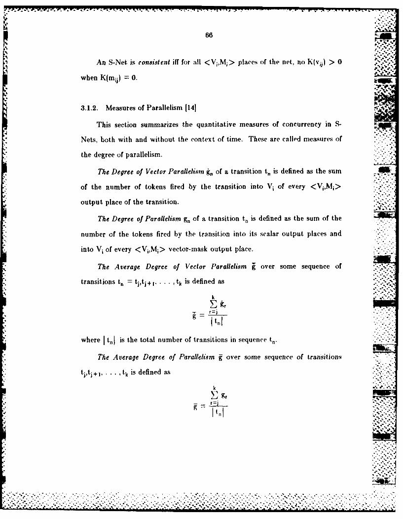
*~~~~P d (4-4 . ..

An S-Net is consistent iff for all <Vj,M,> places of the net, no K(v;1 ) > 0 e

when K(mj) = 0.

3.1.2. Measures of Parallelism 1141

This section summarizes the quantitative measures of concurrency in S-

Nets, both with and without the context of time. These are called measures of

the degree of parallelism.

The Degree of Vector Parallelism kn of a transition tn is defined as the sum

of the number of tokens fired by the transition into Vi of every <Vi,Mi>

output place of the transition.

The Degree of Parallelism gn of a transition tn is defined as the sum of the

number of the tokens fired by the transition into its scalar output places and

into Vi of every <Vi,Mi> vector-mask output place.

The Average Degree of Vector Parallelism g over some sequence of

transitions t. t1 ,ti +I. ,t is defined as

where t,,l is the total number of transitions iii sequence tn.

The Average Degree of Parallelism over some sequence of transitions

*it + I tk is defined as

k

grU7,

9..-'

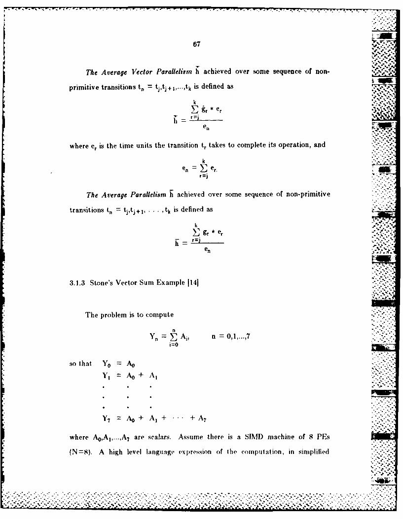
67

The Average Vector Parallelism h achieved over some sequence of non-

primitive transitions t,, =t 1,ti+1,...,tk is deieda

k*r er %

1=r=i

where er is the time units the transition tr takes to complete its operation, and 4

ke e.

The Average Parallelism h achieved over some sequence of non-primitive

transitions t jtj +I,* ,tk isdefined as

k

3.1.3 Stone's Vector Sum Example 114J

The problem is to compute

i0O

so that Y0 = A0 O

Y,=AO + A,

Y7 AO + A, + +A

where A0,A,,...,A 7 are scalars. Assuime there is a SIMID machine of 8 PEs

(N=S). A high level langivage expression of the computation, in simplified

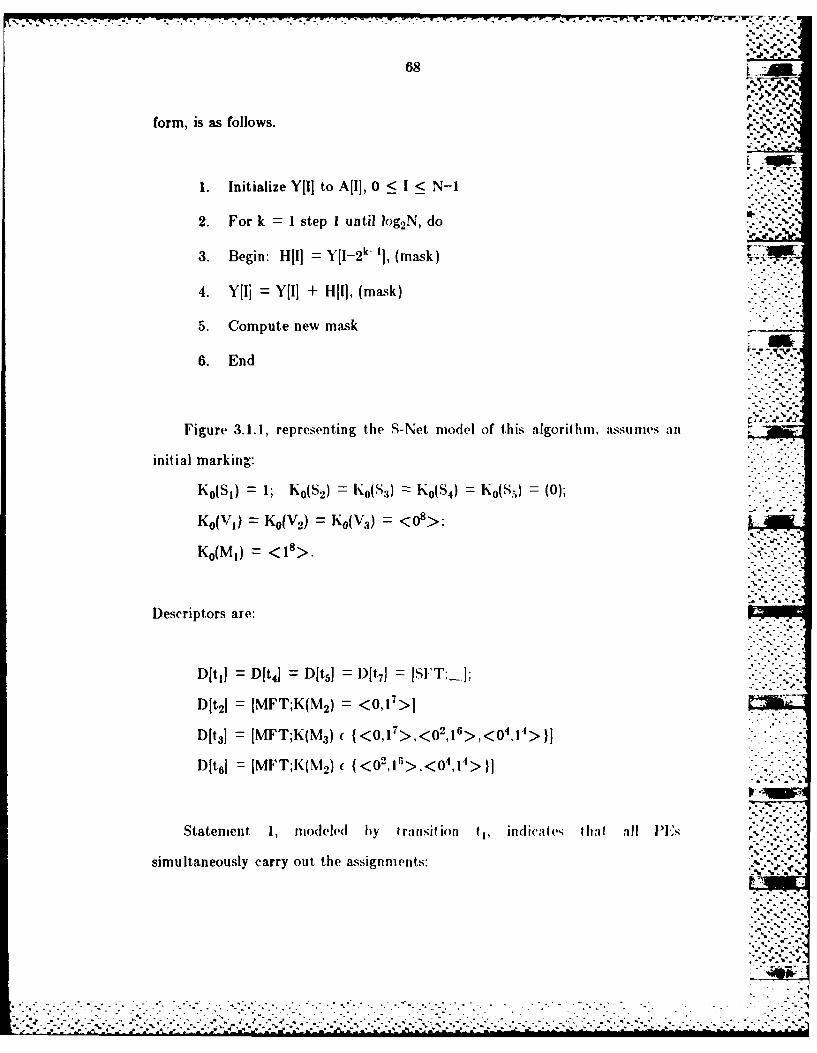
68 *~*=

form, is as follows.

1. Initialize Y[I] to A[11, 0 < I < N-i

2. For k I step I until log 2N, do

3. Begin: H[I] Yt-2k ] (mask)

4. Y[Ij =Y[j + 1111], (mask)

5. Compute new mask

6. End

Figure 3.1.1, representing the S-Net model of this algorithm, issunives.111

initial marking:

K0(S1) =1; K0 (S2) K 0 ) KO(S 4) K0 (Ss~) =(0);

K0 (V1 ) =K 0(V2) =K 0(V3) 0>

K0 (M I) x

Descriptors are:

Djt1J DIQ] Dit 5I Djt 7J [SFT;...;

D[t31 [MFT;K(M3) <01

D~t6] = [NFT;K(M2) { ,><02,1 >,<04,14> }

Statement 1, modleled by 1 rim isit ion ti i' mdicates 111 l Is~-

simultaneously carry out the assignrnients:

ZZ1

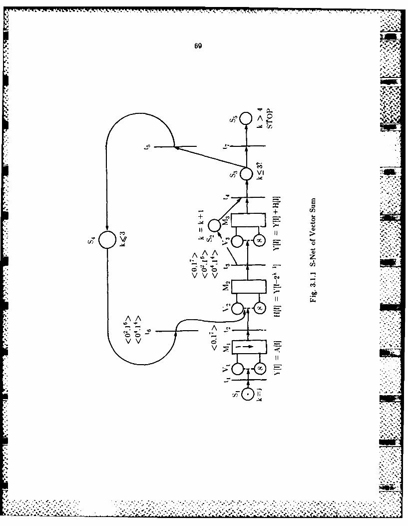
669

C- I Is

- C

A A

v* v

17U

. . . . . . . . - - . - * Va r-. -P V- i

70

Y(O) = A(O), Y(I) = A(I),..., Y(7) A(7).

Since each PE has both Y(l) and A(I), these operations can lake place "ill

parallel."

Statement 3, modeled by t2, requires that data are transferred between

participating PEs. For the firing of t,, 11(1) holds Y(O), 11(2) holds Y(I).. and

H(7) holds Y(6). PE0 does not participate, since K(M) <0,17>.

Statement 4, modeled by t3, has all participating PIs adding

simultaneously. If MFT t.3 first, fires K(MN1 3) <0,17>, then, for the first

iteration of the loop, PE 0 does not participate. The first holding of <\ 3 ,N 3>

models sums: Y(I) has Y(0) + Y(I); Y(2) has Y(I) + Y(2), etc.

A branci is modeled by the t5 and t7 transition which have scalar input ' .. '

place s3 in common, modeling the result of a test of the iteration counter.

The firing of t2 models the first. iteration (k =1), the first, firing of t6 models

the second iteration (k=2), and the second firing of t,6 models the third-

iteration (k=3). After the third iteration, transition t7 will fire and the

computation halts, as all eight sums reside in the appropriate Y( ) variables.

Despite the availability of 8 PEs, the degree of parallelism achieved over

the computational flow is not 8. Over the firing sequence described and listed

in Table 3.1.2, and are calcu lated as follows:

- 51/13 3.02; 4 = 12/13 3.23.

The maximum parallelism achieved at this level of modeling is reduced by the

nature of the algorithm and by the scalar processes modeled in the testing of

the loop. The use of the h and h measures are not considered here. In a **.

realistic analysis, some weifiting of the additional time to accomplish mask

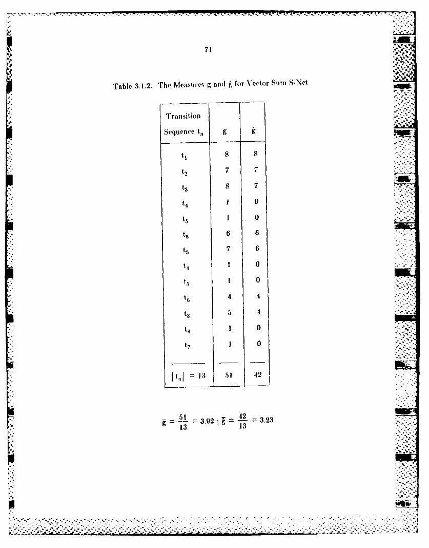
71

Table 3.. The Measures g and fr~ Vector Sum S-Net

Sequence t, g

8 7

t4 10

1 0

t37 6

0

4 4

t3 4

t4 0

t7 0

_ _ 51g- -39 L 3.23

13 13

1.7 ~

72 --

firing would be appropriate, as for transitions t,, t'3, and tr.

3.1.4. Modeling Complex Applications with S-Nets [141.

S-Nets have been developedl to p)rovidIe a tool t~o ex press :tlgorithii

implementation on SIMD and MSINII) architectures. The imp~lementations are

modeled by using safe and consistent S-Nets. In modeling revilistiC

applications, the first obvious complication in S-Net graphs is that of length,

i.e., the length of the transition sequence will not fit, within some desired 6

reference frame. Connectors, such as shown here

may be used to show where an arc breaks and reconnects, much in the manner --

that connectors are used in flow charts. The connector can be inserted between

a transition and the following place, or between a place and the following

transition.

Macro S-Net transitions (macros) are introduced to support hierarchical

modeling and to permit a more abstracted representation of an event which is a

component of a computation. A inacro transiiion t is defined as a transition

which itself is an S-Net graph. It begins with a single vertex t~r and ends with

single ver~.ex tq, where tr and t. themselves can be macro S-Net transit ions. A

label is appended to the transition bar to distinguish macros in the global flow,

shown as

. . " . ..•. .. . . .. . . "..

. . . . . . . .. .-

.. ,. *A €. . . . . . . . . . . . . . . .~"• . . . . . . . . . . . . .. . . . . . .

P.r .. . .7.' :; ;P'Ir-"

73 "N.,

where 11) is any symbol used by the mod.er. *.'*

Figure 3.1.2 illustrates hierarchic:l modeling, defining two macros and .

showing how the substitution of the greater detail can be modeled in the S-Net.p.. #,.

With this definition, the non-primitive transition t n (which is a sequence of

transition, tjt + , . . . , tk) is seen as a type of macro since it represents a

transition sequence beginning with t i and terminating with tk.

3.1.5 Modeling Maximum Likelihood Classification with S-Nets

The purpose of this section is to use S-Nets to model an SIMD

implementation of maximum likelihood classification [211. Assume that there

are N=M PEs available where the image size is M-by-M. The PEs can be

arranged in a row of M elements or in a V/M-by-v'M array. Each PE will be

assigned either one image column or a VA-by-%/M subimage that will be stored

in its memory.

The SIMD implementation of maximum likelihood ciassification has been

described in [22). For each of the m possible classes into which a pixel may be

classified, a discriminant function is computed. Each discriminant value

depends on the pixel vector, the corresponding class mean vector and

covariance matrix, and a constant related to the prior probability of occurrence

of the class. The pixel is assigned to the class yielding the largest discriminant

value.

The essential calculations are as follows. Let

X = 1x~x2 . jT. the n-dimensional pixel vectorX 02- --,

. .. ... . . . . . . . .7

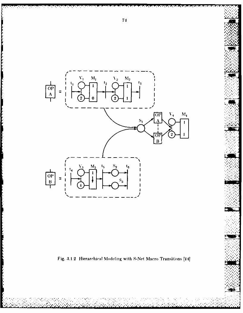
7-1

S, A

%V' -M 3 2 t6

t4

Fig. .3.1.2 Hierarchic,,l Modeling with S-Net, Macro Transitions [I-l1

.1* ~75 ..

*1-J

Ui =u Iu'... I the n-dimensional mean vector for class

1 2 n 1

C2 the n-by-n inverse= , of the covariance

matrix for classent . nn

constant pertaining to class 1ijw

In addition, A(i) will be the discriminant value for class i. Figure 3.1.3 shows

how these values are calculated and a pixel is classified. The following

conditions are assumed:

1. All pixels are to be stored in the PE memories. Each PE is

responsible for M pixels. -

2. Mean vectors (n-dimensional) and inverse czwariance matrices (n-

by-n) of m classes are stored in all PE memories. The m class

constants ci are also stored in all PE memories.

3. Concurrency between the scalar host, And the ar.ray resources canl be

supp~orted by thie hardware. The scalar host, can be regarded as the

control unit and the array resources as the p~rocessors.

The computation proceeds as follows:

i. itilizv the vniiies or.\( I) to eonst ant ci, for I < I < .

2.n (()put e 11 he N a 1liivs of the v(d iscriii n n t f ii n(cI ions for al I I i classes.

Wit.

%,- %

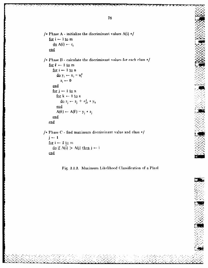
7 . T; W7~ F5 17 -j .. * V

76

/* Phase A - initialize the discriminant values A(i) *

doA(i) -. Ci

end

1* Phase 13 - calculate the discriminant values for each class *

for (9 1 tomi

for 4 - I to n

d i *, - Xi - u

i4- 0

for I to nfor k *-I tonI

yjk kmadA(V) 4-A(V) - *jz

endend

/* Phase C - find maximum discrirniniant value and class *

kiti 2 to m .

do if[A() > A(j) tenj i

end

Fig. 3.1.3. Maximum Likelihood Class ifi cation of a Pixel

77 j

3. Choose the maximum value or the discriminant functions.

4. If there are more data in PEs, then go to step 1.

5. End

The S-Net. modeling this comptitat ion ks shown in Figure 3.1.4. There are

three macros, UNIT A, DIS 13 and MIAX C, definied in Figures 3.5,3.1.6, and

3.1.7. respectively. A brief description of the S-Net is as follows:Am

-The dimensionality of the Vi components, IVl=M, represents the .-

nutmber of PEs available in this SIMD implemeptation.

-The initial marking of the S-Net, is

1(0(S2) K0 (S3) .... K0(S) (0t);

K0 (VI) K0(V2) ... K0(VM) < M>

I(0 (M1 ) KOIM 9 ) .... K(M 6) = I>

-Descriptors are:

Dt1 j Dt,, .... Dt26? [SFT;-I;

D~t27J IN1FT;lK(N 7) BM]

D~t281 'V~291 ... 1D(t331 SF;~

h I ias a token in F"igu re 3. 1A initially, so thie 1 NIT A mnacro transit ion

is enabled and begins execift on when it% first transit ion t.1 fires..

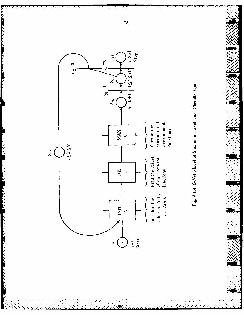
78

A~

E cfr

00

v I)

E! 00

CfC)

~z

030

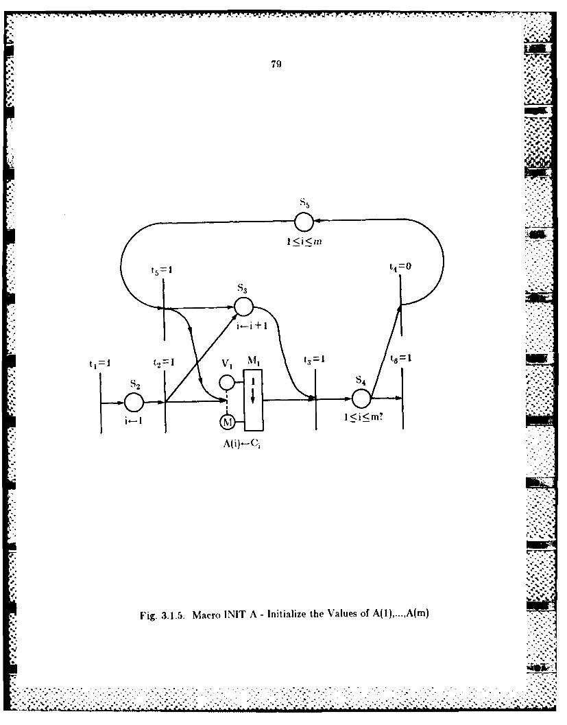
79

.d. u

I <i<rn

tt4 0

S3

-U.2 S4 ~

I <i~m?

.JU.. U .i

Fig 3...M coI IT A -IiilzeteV le.f ~)..A

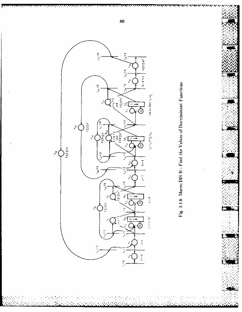
80

- .i

VI-

VIC

bbi

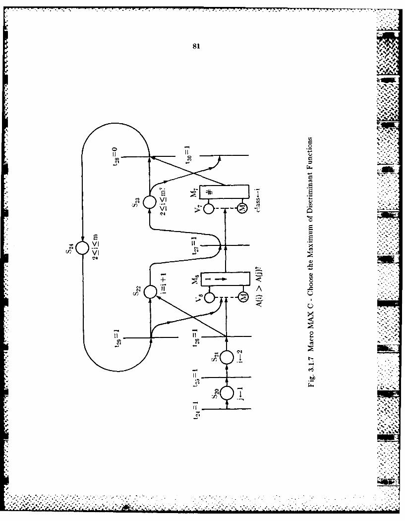
81

VI.

VI,ce4 .

v.4

CIS'

bb-4 .

,clP.%

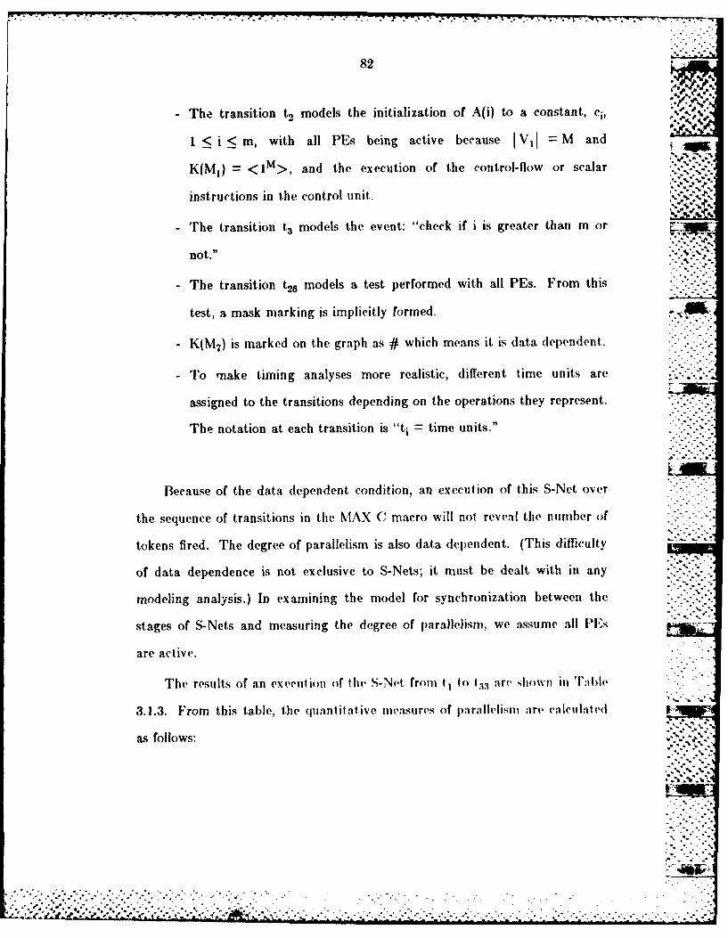
--W ~~:- "- .V-.--r

82

. %.

- The transition t2 models the initialization of A(i) to a constant, ci, %

1 < i < m, with all PEs being active because I VI = M and I l

K(M1 ) = <lM>, and the execution of the control-flow or scalar.'

instructions in the control unit. V,

- The transition t3 models the event: "check if i is greater than m or

not."

- The transition t 26 models a test performed with all PEs. From this

test, a mask marking is implicitly formed. r

- K(M 7) is marked on the graph as # which means it is data dependent.

- To make timing analyses more realistic, different time units are

assigned to the transitions depending on the operations they represent.

The notation at each transition is "ti - time units."

Because of the data dependent condition, an execution of this S-Net over

the sequence of transitions in the MAX C macro will not reveal the number of

tokens fired. The degree of parallelism is also data dependent. (This difficulty

of data dependence is not exclusive to S-Nets; it must be dealt with in any

modeling analysis.) In examining the model for synchronization between the

stages of S-Nets and measuring the degree of parallelism, we assume all P's

are active.

The results of an execution of the S-Net from ti to t33 are Shown in T:ble

3.1.3. From this table, the quantitaltive measures of parallelism are calculated

as follows:

*° . "° o-

83

Table 3.1.3. Timing Analysis of SIMI) S-Net __

no. of time the

transiition firings transition ti

t!takes, e1 k, nje 1j*n 1*e1 inie

tjNi 1 0 1 NI 0 Mt2 M I M I+M M M 2 (1 +M)M

t3mM 1 0 1 mM 0 Mt4 M-IM 0 0 1 0 0 0ts (m-1)M I M 1+M _m-)M (M-1)M 2 (I +M)(m-1)M

t6M 1 0 1 M 0 MtM 1 0 1 M 0 M

ta mM I M I+M mM MW (I +M)mMto nmM I M 1+M anm nMM 2 (I +M)nmMto (n-1)mM 0 0 1 0 0 0ti, (n-1)mM 1 M I +M (n-I)mnM (n- I MM 2 (1+M)(n-l)mM

t2mM 1 0 1 mM 0 Mm1 rM 1 0 1 M M 0 M

t4nmnM 3 M 1+M 3nmM 3nmM2 (I +M)3nmMt 5 (n-1)nmM 0 0 1 0 0 0tie (n-1)nmM 3 M I+ M 3(n-I)nmM 3(n-I)nrnM2 (I +M)31n-I)nmM

t17 nmnM 3 M 1+M 3nmM 3uMM 2 (1+ M)3nmM18 (-1)mM 0 0 1 0 00

t10 (n-1)mnM 1 0 1 (n-I)mM 0 (n-1)mMt mM 1 0 1 mM 0 M

121 MM 1 0 1 mM 0 Mt22 (m-1)M 0 0 1 0 0 0

t3 (m-1)M 1 0 1 (m-1)M 0 (m-1)Mt24 NI 1 0 1 M 0 M

tsM 1 0 1 M 0 NItbM I M I+M M (I2 (+M)M

t27 (M-1)M I M I +M (mn-1)M (m-1)M' (1I+M)(M-1)M129 (m-2)M 0 0 1 0 0 0t29 (rn-2)M I M 1+M (m-2)M (m-2)M2 (I +M)(m-2)M

NIo 1 0 1 M 0 Mt M 1 0 1 M 0 MtN2I-1 0 0 1 0 0 0t31 0 0 1 0 0 0

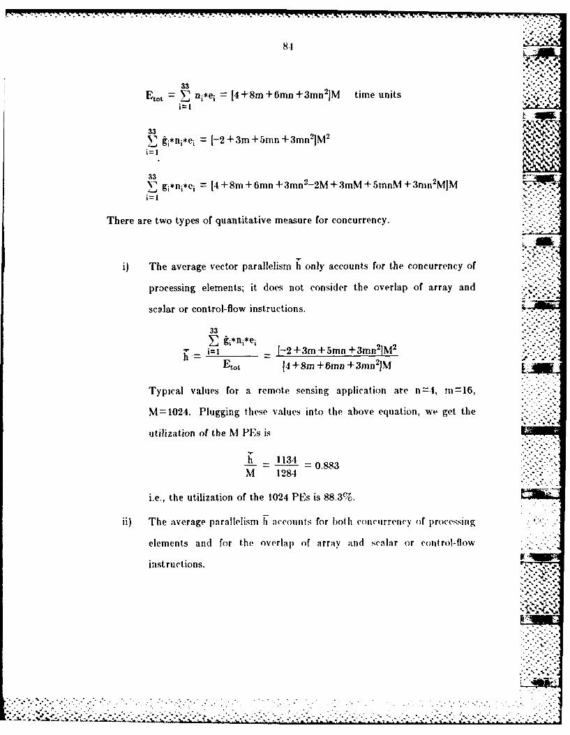
33Etot V I n1*ej 1 [4+8m +6mn+3mn 2 1M time units

N' i:*.*e 1-2 +3m +5mn +3mn1M

33 2 MM AN' gi*ni*ei = 4 +8m + mn +3mnn-2M +3mM ± SmnM +3nn2 MJMWW

There are two types of quantitative measure for concurrency.

i) The average vector parallelism h only accounts for the concurrency of

processing elements; it does not consider the overlap of array and-

scalar or control-flow instructions.

33

~ - 1-2 +3m + mn +3mnM

-to 14 +8m +mn +3mn 2 )M

Typical values for a remnote sensing application are n=4, m=16,

M=1024. Plugging these values into the above equation, we get the

utilization of the M PEs is

h 1134

M 1284-0.8

i.e., the utilization of the 1024 PEs is 88.3%.

ii) The average parallelism hi accomits for bot h con('urreriey of p)rocessing

elements and for the overlap of array and scalar or control-flow

instructions.

'..'-.

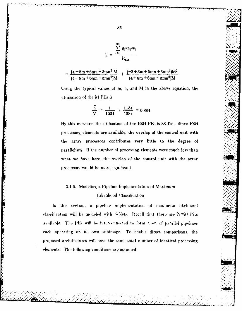
85

- i gg1*n,*e,

14 4+8m +6mn +3mn 2 )M + (-2+3m+5mn+3mn 2 )M2 % 1.

(4+8m+Bmn+3mn 2)M (4+8m+6mn+3mn 2)mr

Using the typical values of m, n, and M in the above equation, the

utilization of the M PEs is

h + 1134 0.884M 1024 12~O84

Biy this measure, the utilization of the 1024 PEs is 88.4%. Since 1024

processing elements are available, the overlap of the control unit with

the array processors contributes very little to the degree of

parallelism. If the number of processing elements were much less than

what we have here, the overlap of the control unit with the array

processors would be more significant.

3.1.6. Modeling a Pipeline Implementation of maximum

Like!ihood Classification

In tis section, :1 pipeline i In plemetat ion of maximium likelihood

classification will he modeled with Ii-Nets. R~ecall t hat there are N=.M PIs

available. Thel( l'Es will be interceoiI(ct ed to form a. set of parallel pip~elines

ealch operating on its own suhimnage. To enable direct comparisons, the

proposed architectures will have the same total number of identical processing

elements. The following conditions are assumned:

1. The n-dimensional mean vector and n-by-n inverse covariance

matrix of class i have been stored in PEi_1 , as have the m class

constants.

2. The parallelism being exploited has each stage concurrently

performing a different step of the task on a different data item

(pixel).

M M3. Assume - is an integer and that there are - pipelines. Each

m m

pipeline will process mM pixels. .

4. In calculating the degree of parallelism, the overhead required for

the pipeline to reach full efficiency will be ignored, i.e., steady state

operation is assumed.

A high level description of this computation at stage i-I is as follows:

1. initialize the value of A(i) to constant '2 '

2. Find the value of tle discriminant. function for class i.

3. Compare the value of the discriminant, function for class i with te

value of tempi-., received from the l)revious stage.

4. Set the value of temp-class i based on the comparison in step 3.

5. Transfer the piXel(hit a, t ('m[ip andl teml)-classi to the next stage.

6. if there is more data, go to step 1.

7. End.

The S-Net of stage i-I of the pipeline is shown in [igure 3. 1.8. A brief

::~~~~~ : -: .- .. . .?.....:.--.:..?.--.:.- !:)::::-.- ""''

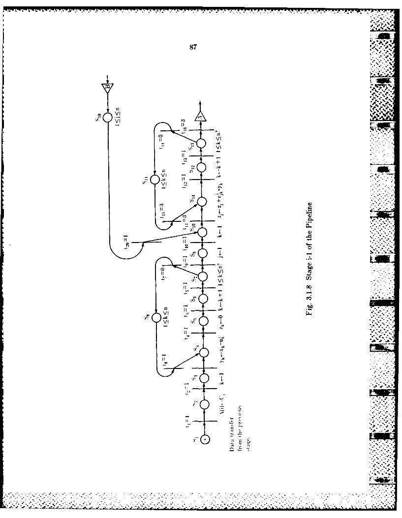
87 16

upla

.. ;*i

II VI

- I- VI

III

v I

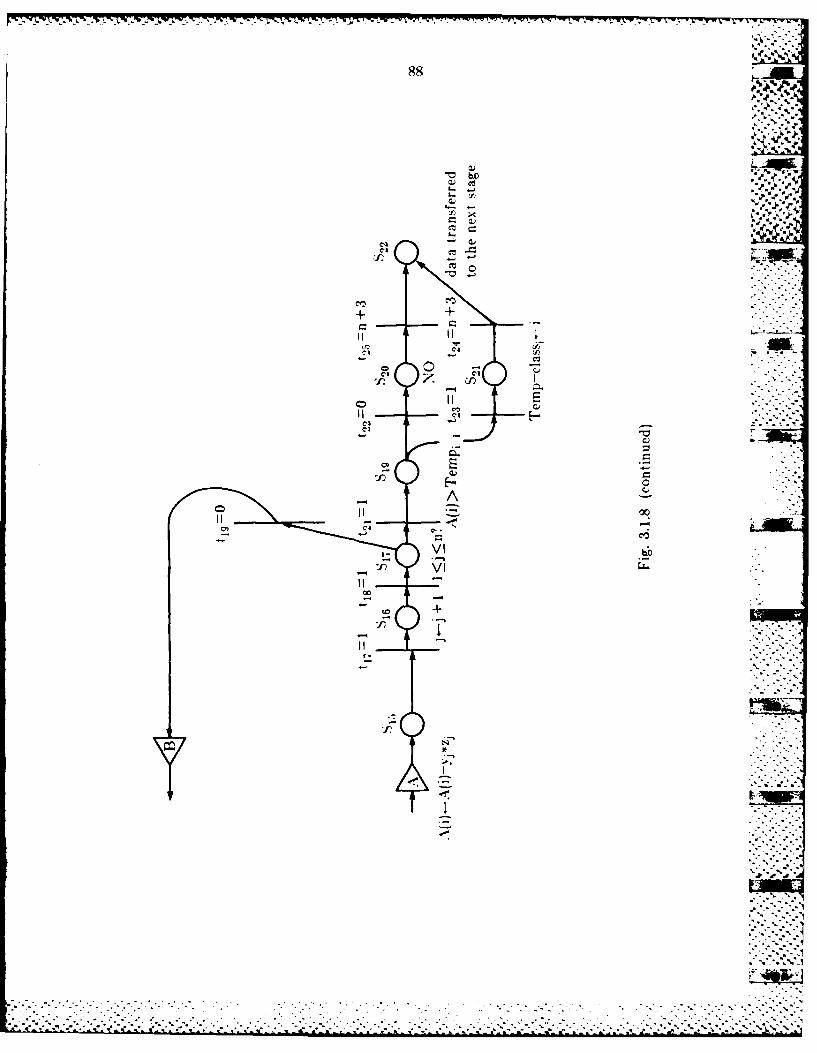
-o

vII

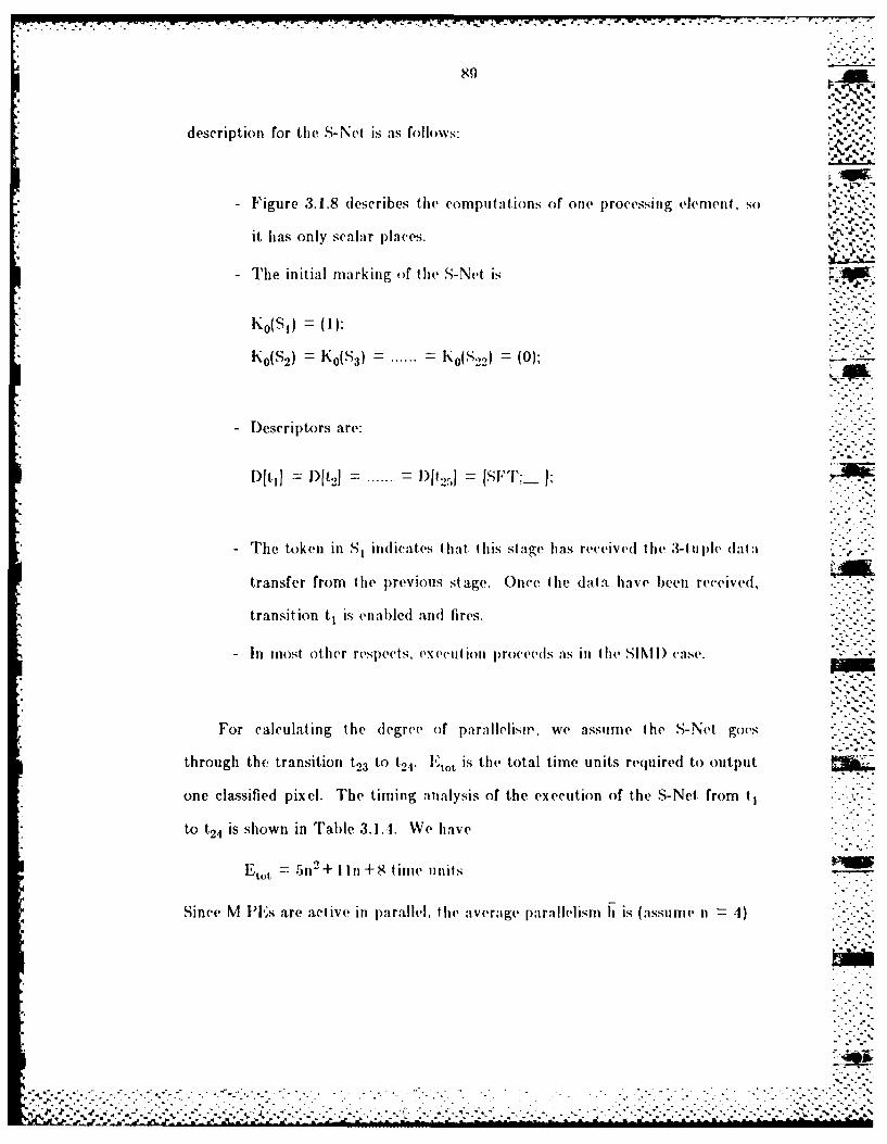
807

description for the S-Net is as follows:

- Figure ,3.1.8 describes the computations of one processing element, so

it has only scalar places. 6

- The initial marking of the S-Net is

K0(SI) = I);

K0(S2) = K S) ...... 10('22) (0);

Descriptors are:

Dftj - D[t . ...... JI)t.j [SFT; ;

- The token in Sn indicates that. this stage has received the 3-tule data -

transfer from the previous stage. Once the data have been received,

transition tj is enal)led and fires.

- In most other respects, execution )roceels as in the SINI) case.

For calculating the degree of parallelism, we assume the S-Net goes

through the transition t23 to t 24. "lo t is the total time units required to output

one classified pixel. The timing analysis of the execution of the S-Net from ti

to t 24 is shown in Table 3.1.1. We have

Etot = 5112+ 1111+8 time units

Since M PEs are active in parallel, the average parallelism h is (assume n ')

•

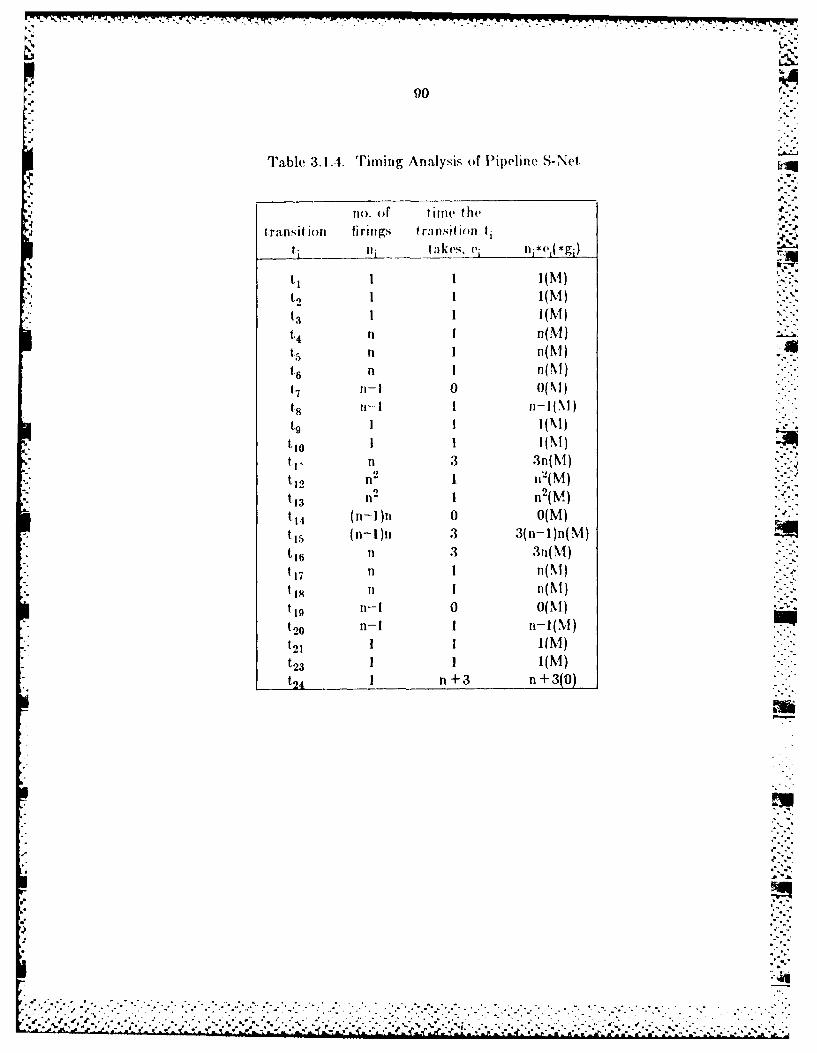
-' ~90 ..

Table 3.1.1. Timing Analysis of Pipeline S-Net

no. of ti imw the

I ransit jon firings transition tiIni takes. ei nit *(P gi)

,% I I 1 1 ( M ) ,<1-+ 1 I(NI) .n I n(M)-".t3

i ~~~t4 n lnM)-".

Cn I n(M)

16 n n(M)i7 n-I 0 0(M)18 ti-I 1 n-J(N._-t9 I I I (\1) -to 8 1 1(M)

ii"ti 3 3n(M ) .'-

tn 1 (M)t1 11 2 1 n2(N )

C14 (n-I)n 0 O(m)

n-In 1n(M)

-: t15 (n n 3 3(11 ln M

t 1 6 l i 3 U ( M ) " [

17 n I n(M)i1 1(M)

". I~.l.o n- I -l M:; ~~~~t21 l)".;;.

]+ ~~~t23 (M -

t2 4 I n+3 n + 3(0)

V..

'"

q..

..-...

AD-A16? 31? DISTRIBUTED CONPUTING FOR SIGNA PROCESSING: MODEING VOF ASYNCHRONOUS PAR.. CU) PURDUE UNIV LAFAY#ETTE INSCHOOL OF ELECTRICAL ENGINEERING 0 LIN ET AL. AUG 64

UNCLSSIFIED TR-EE-4-29 ARO-1979. ±7-EL-APP- F/0 9/2 M

mhhEmhEmEomiImmmmhmhhhhhu

L1.04

IL 6

__, 20

III UI - II1 II i)!

MICRnlCOP' CHART

.- wl

.. . .0 .A . ...* . * ~ ~ * * ..* ~ ... ... •%

* . . . . * * . * * , ,o

...-t

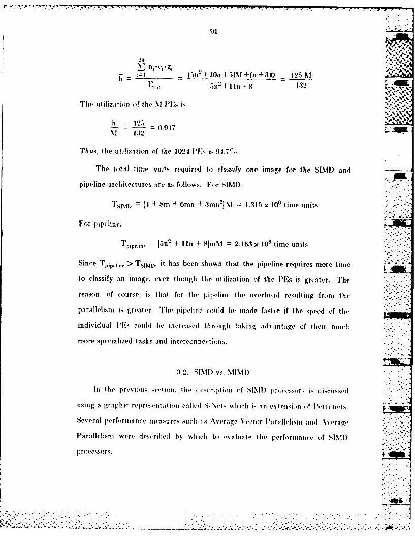
-, - .* -, - *..*..**t V

91 7. .. "-

24 * .

_-= ,=- __ = - n'+10n,+,).%I+ln +3)0 _ 125 M_

Ett5ni+1111+8 132

The tilization orfithe mI n-,,,; is

h_125- = 0. () 7

1 1:32

Thus, the utilization of the 1021 PE's Is 91.7j.

The total lime units required to classify one image for the SIMI) and

pipeline architectures are as follows. For SIMD,

TSIM) = [4 + 8m + 6rnn + 3mn ] N- 1.315 x 106 time units

For pipeline.

![pipeline 15n " + tIn + 81mM = 2.163 x 10 s time units

Since Tpipejine > TSIMD, it has been shown that the pipeline requires more time

to classify an image, even though the utilization of the PEs is greater. The

reason, of course, is that for the pipeline the overhead resulting from til

parallelism is greater. The pipeline could be made faster if ile speed of fihe

individual lPEs could be increased through taking advantlage or their much

more specialized tasks and interconnections.

3.2. SIID vs. NIMNI)'

In the previous section, the (escriplion of SIMI) processors is discussed

using a graphic representatioln called S-Nets which is an exlension of lPetri nets.

Several performa nce measures such is Average Vector P arallelism and Average

Parallelism were described by which to evaluate the performance of SIMI)

processors.

..." . " " . ... .. - . .-.- , , .: : : :: . :,: . , :,,

92

In this s~ection, the comparison between execution times of both SIXMD and

MIMII) processors is dIi~isssed. Wheni a part icutlar algrorithm such as the

max .inumi likel ihood classificat in :t 1g rjt fin or t he clust ering algorit hm is

givenl , is nevessary to ask which~i ioe of paallsm II or NDwl

have less execution timle and better utilization of PE' resources if the number of

processing elements is fixed, It ordler to answer such ques;tions, this section will

analyze expllicit and implicit operat is 1231 embedded in an algorithm and,

based on these operations. dlerive the total execution times for hot h S[I) andm

NiINII) modes of parallelism. In add~it ion. the potential advantages and

(lisadvantages. inherent. in an algorithim, of MUMI) mode of parallelism will be

discussed as compared t~o SIMI) mo(de of parallelism.

3.2.1. The Flow Chtart andl the Algorithms of tlte Supervised Relaxation

Operator

Trhe flow chart of the sup~ervisedl relaxation operator is shown in Fig. 3.2.1.

The algorithms in blocks A, 13, and C can be executed simultaneously because

K the input dlata in these three blocks are Indlependent, of each othter, and the

Algorithms are independent of results produced by each Other. The algorithms

can be imiplemnented either lit SiNIl) mode or in MIMII) niode depending on the

alg( rlihnIt chia ract erist ics. whtich wIll lbe (described lit the folloV\ ing sect ions.

Sinc(e the( algorlihni Iiblock 1) nceds the results fromt blocks A. 13 and] C to

exe(cti te its inst ruct ionis, it is best that blocks A, B an (J C produce thIeir results

alm11ost at the sallte tlie, then block D) only, needls to wait as little time as

po)T ilE to j'rovIeed %i lil its, ('\e tit in of inst rit ihns. Thel( alIgorit hmis in blocks..

A. B . An Ctl are qiite (1I lireit. th'elreft rv their coiplexjt ies Inl t erns of

(X(Ciiiol tme re;ukt tui dihrcitlit order to pro)(lice the re'dllts alitost

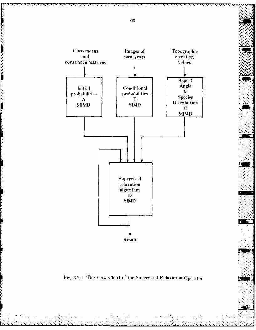
93 ..

covariance matrices values

Aspect

I'n't lal ConditionalAnlprobabilities probabilitiesSpie

A 13NIND SIMI1) Distribution .

Su perv isedrelax ationalgorithm

SII)

Result

Fig. 3.2.1 The Flow (Chart of ( lie Supervised II (lax ati)n Operalor

4p94Lba

simultaneously and provide better utilization of IPEs, it is necessary to assign

different numbers of i's and different, modes of parallelism to the -, ow - .

implementation of these algorithms.

The algorithm in block A is actually the maximum likelihood classification

algorithm except for the multiplication by a priori probability, l>(Xj), for each -. .

class. If we assune that lV(Xi) I/N where N is the riumber of classes, these

two algorithms are exactly the same e('xcept for a constant factor. The

algorithm in block A calculates the initial probability of every class for each

pixel. Since this algorithm involves the multiplication of vector and matrix,

matrix inversion, calculation of a matrix determinant, and an exponential

,perat ion, the execution time of each pixel depends on the multichannel data

v'alues. Elspeciallv for the exponential operation, its execution time is a.

function of argument. value because it is a complex operation. An exponential "

operation is computed as a power series and the convergence of the power

series depends on the argument value. In SIMD mode, the control unit,

broadcasts instructions to all active PEs and all active PEs execute the same

instruction on the data in Iheir own memories. Indeed all steps are

synchlrouized. If this algorithl is imphlmented in SI\I) mode, each PE

executes the instruction on a different data value. As a result, each PE has a

different execution time. Therefore, the PEs with shorter execution times have

to wait. until the PE with longest execution time completes its execution. Then

the control unit can broadcast the next instruction to all PEs. The

disadvantage of using SIMID mode is that the total execution time is equal to

the summation of the maxinmunm exccution times of every .peration because the ','.'

execution time of the operation is data dependent. The advantages of using

SINI) mode is that scalar instructions executed by tie control unit and array

~~~~~.A............... ......... .-.. ..-.-....- •." ..-. . . ." -- -- "....' . ... 2 ' - -', :,_., -_-. *_. ._I,.'...L.- _*.; -. '.. ." .

instructions executed by the PEs call be overlapp)ed.

On the other hand, if the algorithm in block A is implemented in NIIMI)

mode, each PE can execute an instruction fetched from its own inenorv

immediately after compjlet ing d ie prev iouis inst ruct ion. Therefore the tota:l

execuntion time is the stiiiiiat ion of I lie ex(cu1t ion t imies (if e'very ol~crat ion in

the PE. If we assumne that tlie dat a va:lues are randomly. (list rihited

throughout the IPEs, the probability of getting the (dat a with longer (xecut i( )i

time is the same for every PE. Wiit h his p~roperty, thie total execution times o)f

PEs in MIMID mode almost have the same values if the number of pixels in

each PE is large enough.

The algorit bin iii block 1 3 in volves only the accu mu lat ive o perait ions of-

counting boti Iindiv idu al a 11( joint occurrences, and division operat ions. Flie

execution times of these t wo operations are almost (lata indpdee)nlt.

Therefore, no benefit can be drawn from implementing in NID mode. u

Furthermore, the algorithm has window-type operations and needs inter-PE

transfers. SIMD mode can offer synchronized inter-PE transfers. That is, all

active PEs can transfer (data to the neighiboring PEs located in the same

direction relative to the trransferring I"Es. Since operations are simp~le andl

execution times are short, fewer PEs are assigned to block B when compared to

block A in order for block A and B to take same amount of time to execute.

SIMD mode is implemented to take advantage of synchronized inter-PE

transfers and simp~le control system.

The algorit iIm in block C consists of two subalgorit Iimns. One (let ermines

the aspect angle of the pix el. From this aspect, angle, thle other subalgoritlim

calculates the species distrib~ut ion function of the classes which amre possibly to

be assigned to the pixel. The subalgorithm to determine the aspect angle ha-s

J--

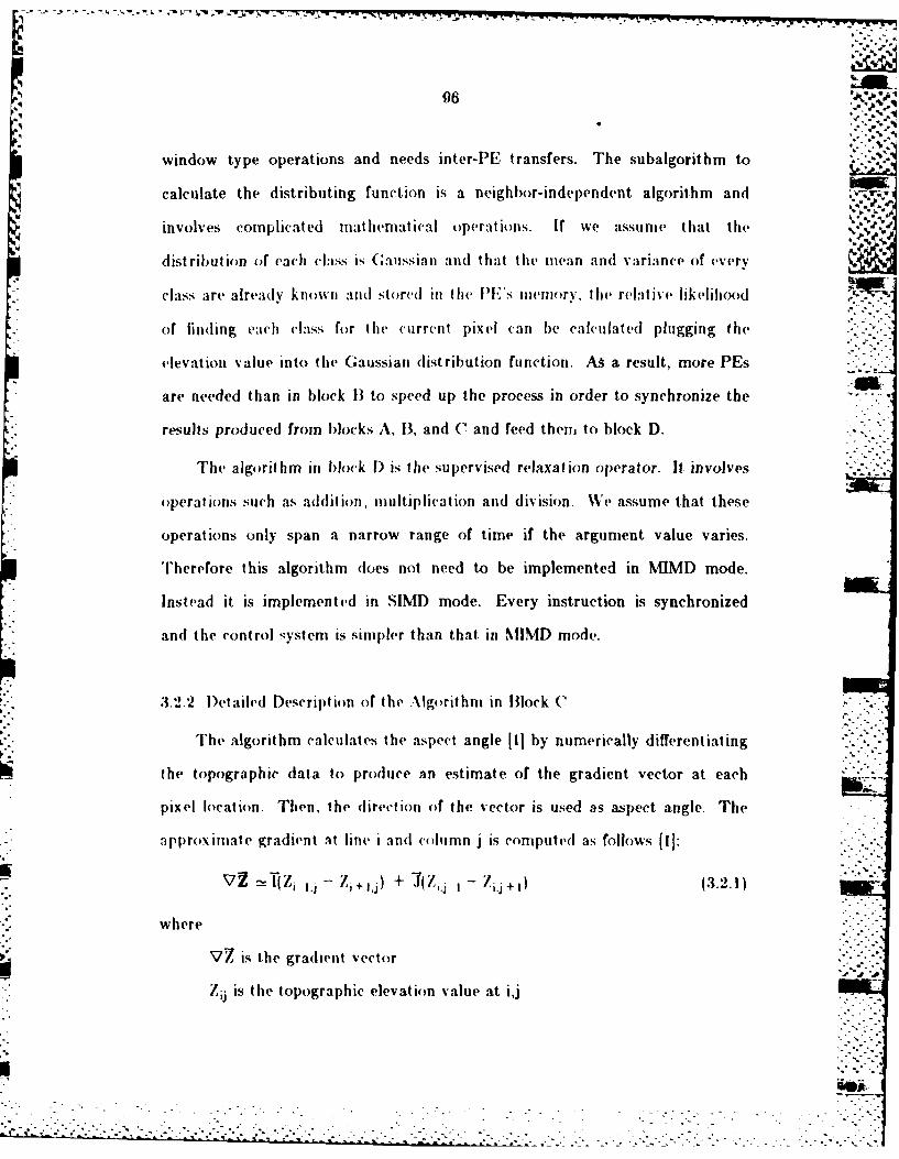
.. .~ .~..~ .- .~ *- .. IN L -rev

06 ....% : : I t

window type operations and needs inter-PE transfers. The subalgorithm to

calculate the distributing function is a neighlbor-independent algorithm and~~~involves complicated mathematical operations. If we assume that the ,:;.

distribution of each class Is (aussia and that it, mean and variance of very

class are already known all(] stored in the PELs Iivmorv, the relativ hikelihood 77

or finding each class for the current pixel can be calculated plugging the

elevation value into the Gaussian distribution function. AA a result, more PEs

are needed than in block B to speed up the process in order to synchronize the

results produced from blocks A, B, and C and feed thenr, to block D.

'he algorithm in b)ock D is the supervised relaxation operator. It involves . -

operations such as addition, multiplication and division. We assume that, these

operations only span a narrow range of time if the argument value varies.

Therefore this algorithm does not need to be implemented in MIMD mode.

Instead it is implemented in SIMD mode. Every instruction is synchronized

and the control system is simpler than that, in MIMD mode.

3.2.2 l)etailed Description of the Algorithm in Block C

The algorithm calculate the aspect angle [I] by numerically differentiating

the topographic data to produce an estimate of the gradient vector at each

pixel location. Then, the direction of the vector is used as aspect angle. The

approx inate gradient at line i and c(lumn j is computed as follows (l:

VZ "T Zi - Zi + ) + (Ztj I - i ) (3.2.1)

where

V7 is the gradient vector

Zji is the topographic elevation value at i,j

. -

. ° .-.

• k % - K % °t-

ij are line and column coordinates

Tand - are line and column unit vectors

The aspect angle is calculated as follows [I]:

(Zi - ij - Zi +n 1).--.--a = tan n+(3.2.2)

iji - I - Zi, +)

where

a is the direction of slope measured clockwise from north.

The subalgorithms for both aspect angle and species distribution are

shown in Fig. 3.2.2. The subalgorithrn for calculating the aspect angle of the

current pixel decides that a pixel faces either south or north. Forest species -...

distribution as a function of elevation and aspect in the San Juan Mountains is

shown in Figure 2.1.4 [1]. In this figure, different aspects have different forest

species distributions. That is the reason why the aspect angle is needed before

calculating the distribution value. Constant C in Fig. 3.2.2 is a threshold to

distinguish angle of south from that of north. In Fig. 3.2.2, the same

subalgorithm is used to calculate the species distribution of south facing and

north facing pixels. But the actual parameters such as m[k] and ojk] which are

the mean and the standard deviation of class k are different for south facing

and north facing pixels. The constant ('1k] in the subalgorithm is a

precalculated value stored in the memory.

3.2.3 Implicit Operations in the Algorithm

Some of the statements in the following two sections are quoted from [23].

The conventional complexity analysis of an algoritli gives no knowle-dge

about how fast an algorithm will execute for a given t:ik of size N. lhevrefore

this kind of analysis gives only the o rder of magnitude (,f thv tiUe that aIlt i

%-.

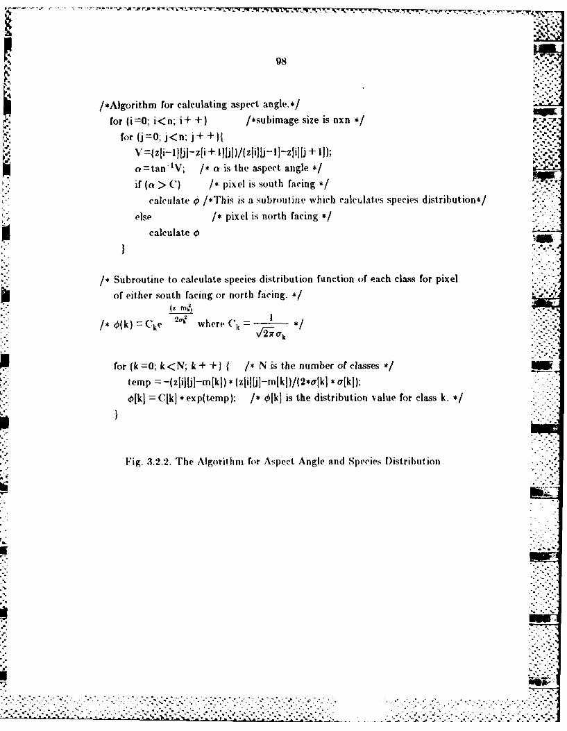
.,8,.... ..

/*Algorithm for calculating aspect angle.*/

for (i=0; i<n; i+ +) /*subimage size is nxn

for (j=O; j<n; j++)jV =(zji-I~Jjj-zji + 1lJlj)/(zjiilj-Ij-zjilJ + 1]1; V-..--a =tan -IV; /* a is the aspect angle *

if (a > C) /* pixel is south facing *,calculate 0 /*This is a subroutine which calculates species distribution*/

else /* pixel is north facing */

calculate 04

/* Subroutine to calculate species distribution function of each class for pixel

of either south facing or north facing. */

/* O(k) Cke where (k -

for (k =0; k<N; k + +) { /* N is the number of classes */

temp = -(zlij[j]-m [k]) * (zli][j]-mlk])/(2*ojk] * ok);

0[k]= CkJ* exp(temp); /* O/k] is the distribution value for class k. */

Fig. 3.2.2. The Algorithm for Aspect Angle and Species Distribution

5w

~~~~~~~~~~~~~~~....... """ "................................... ' . : :-::. . .- ."..:- --

. .. .. . . .... . ... .. . .. .:: X , , -,: , .,a , -.. . . , -. , .. _ .... ; .,.:.: -:._....-.:....'.. .?.'....:

* . . . - .. * i.,2. - -' . .* -.- . - , -. Y - : - -"

'= . . 7 " -F+ -=---

99

algorithm will take for a given size N, such as "order N" or "order N2 .- Several

papers have given the analysis of execution time by counting the number of

explicit operations that an algorithm will perform 124,251. However, there are

many implicit operations neglected in the analysis such as the calculation of

the real address of index variable zli][j], moving operands from memory into

machine registers, and moving results from machine registers back into memory .. *..*

11]. Counting only explicit operations gives only an analysis or explicit

arithmetic operations, and not the implicit operations. Often these implicit

operations can have a significant impact on the execution time of an algorithm-

and therefore should not be ignored.

In Fig. 3.2.2, there are many indexed variables such as z[ilj], iek] and

r[k]. Let us look one example to identify implicit o)erations. [or exantple. in.

order to get the value of mlk] into a machine register, the base a(lress of array

Sin must be found, put into a machine register, added to i, and the resulting

address used to load the value of ni[k]. As another example, loading the value

of z[i][1l into a machine register requires that i be multiplied by the row size of

the z array, added to j, the result added to base address of the z array, and the

resulting address used to ]oad the value oa zilli]f. Alt ernativl,, ,o aoid the, --

multiplication, an indirection lable could bv ,i id. The tcthvlod requires thati I

be added to the base address of the indirect ion table, the result lug address tus.ed

to load the address of the ith row of array z, which is added to j to get the

°U .-Ef, •

t~ ~ ~~~ ~~ ., . . . . . . . .-• J....

100

address of z[i][j]. Finally, this address is used to load the data itself. While

this method saves a multii)lication, it requires an additional memory load and

space for the indirection table.

The notation Mladdress] will be used to denote a memory reference to

address. The implicit operations required to access operands are summarized in

Table 3.2.1.

Before counting, in Section 3.2.4, the total number of implicit and explicit

operations in the program shown in Fig. 3.2.2, several assumptions 1231 are

listed as follows:

1. The class means and standard deviations, m[k] and ojk], k =1,2,...,N,

have been stored in each PE.

2. C[k] = 1/(virk]), k = ,...,N, have been precalculated and stored in

each PE.

3. There are not enough machine registers to hold all data of the

program shown in Fig. 3.3.2.

4. There are enough machine data registers to hold all index variables

currently in use such as i, j, and k in the program.

5. There are enough machine data registers to hold all teml)orarv results

such as V and temp, and repeated expressions such as a[k] and a

compiler is capable of recognizing and exploiting this fact. That is,

the compilr will not generate store and re-load operations in these

situations. .

i. '[here are f,notugh addres registers to hold t he addresses of all .ingle

%arialbles such as V nd n , ad Ihe hase addresmts of array variables

su(h as z, ini, and (.

. . . . . . . . . . . . . .. . . . . . .

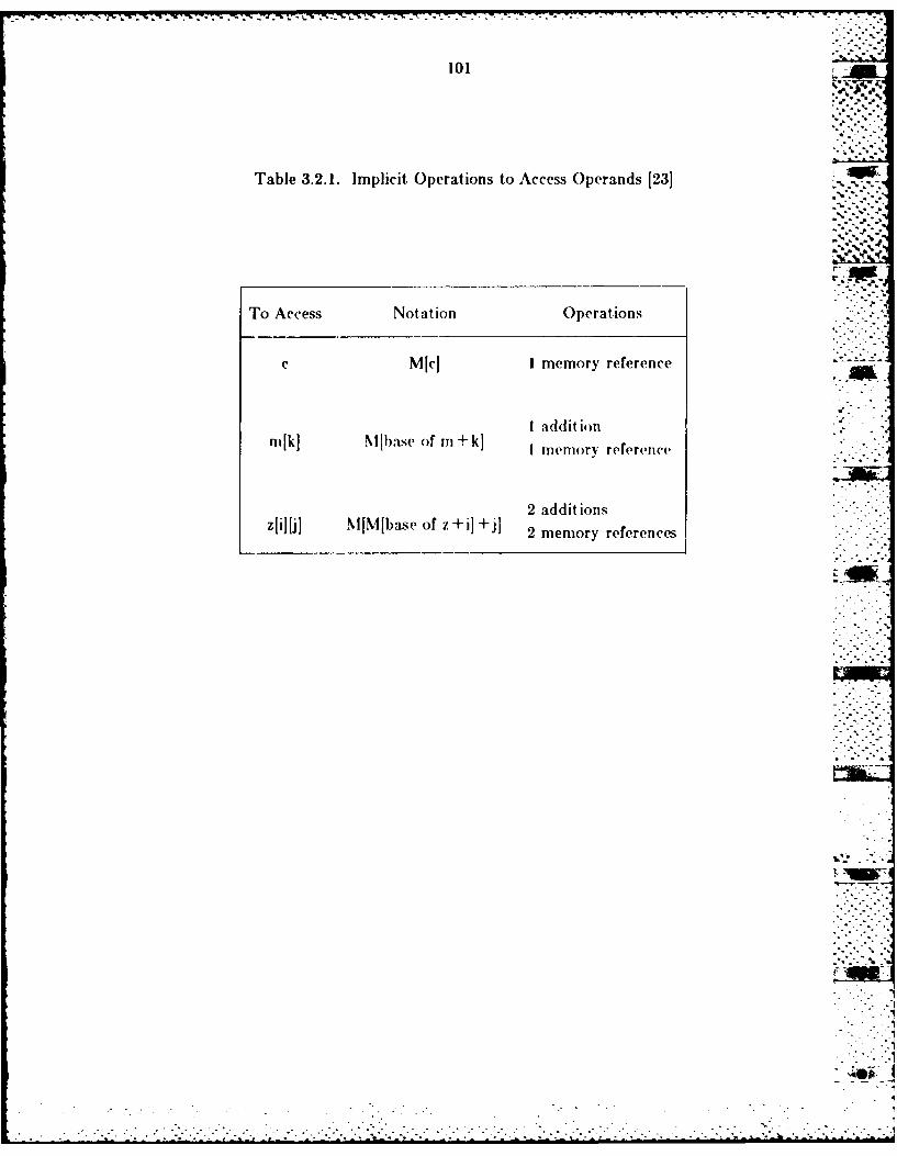
W. R.

101

Table 3.2. 1. Implicit Operations to Access Operands 123]

To Access Notation Operations

c MIC] I memory reference

I addit ionm[k] NI1base of mu + k) emr

2 addit ionszfi[i M[~bse f ~i]i] 2 memory references

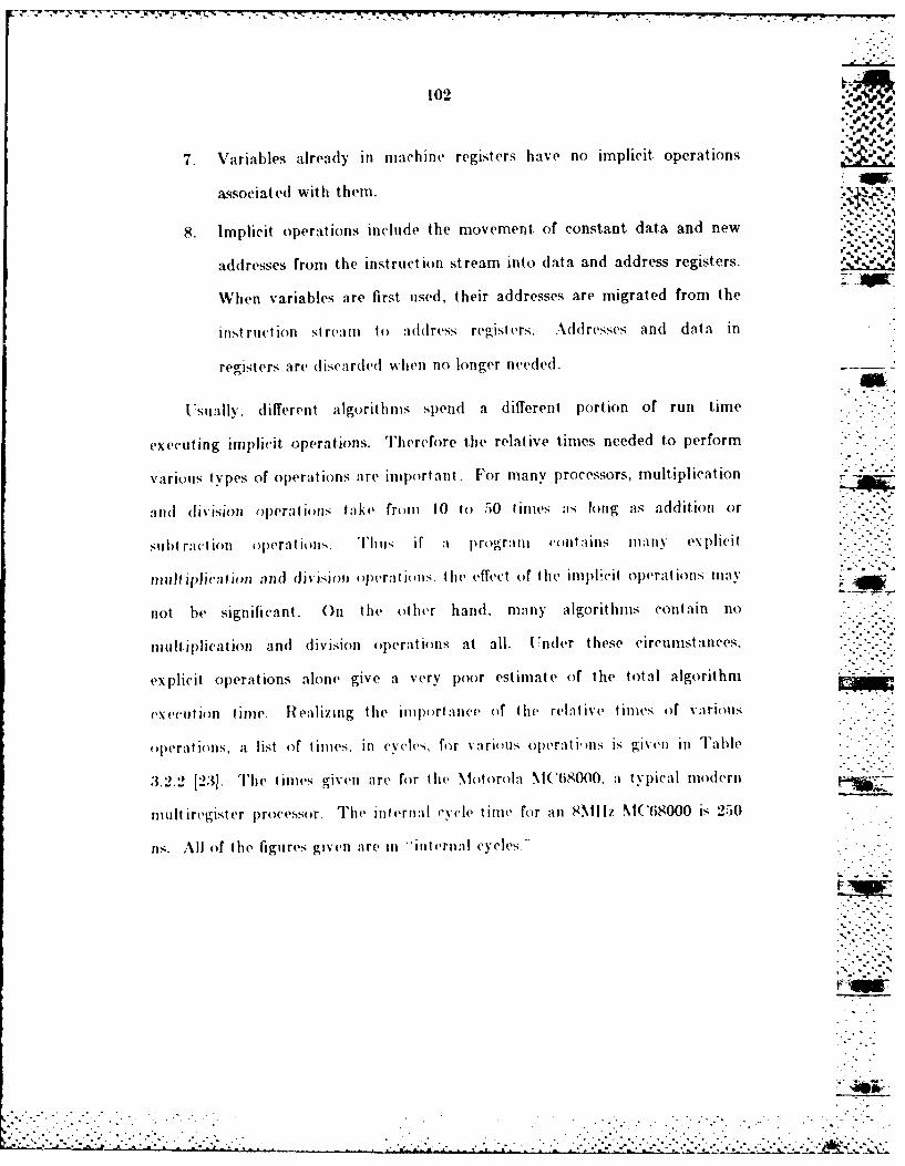
102

7. Variables alreadly in machine registers have no implicit operations

associated with them.

8. Implicit operations include the movement of constant data and new

addresses from the instruction stream into dlata and address registers.

When variables are first used, their addresses are migrated from the

instruct ion st reamI to add(ress registers. Adldresses andl dat a in

registers are discarded wNhen no longer needed.

I 'sually, different algorithms spend a different portion of run time

executing implicit operations. Therefore the relative times needed to perform

various types of operations are important. 1"or many processors, multiplication

an id (iv ision operations. tajke fromn1 10 to 50 times s long is add it ion or

su bt ract ion op1evra t I on i lI is. ifajrogain l lais maiv epii

trill I phen I JI )fld div i..ion opera t i is. the effect of the imp~licit op~erat ions 1113%

not be signifi cant. 0 n the other hand, many, algorithmns Contin 11n

multiplication and division operations at all. Under these circumistances.

explicit operations alone give a very poor estimate of the total algorithm

ex e~l ii n timle. Real izing thle im1port anev of the relatIive tinies or v arious

operat ions, a list of limies, in cycles, for %a rnims olperat i' is is given in Table

:3.2.2 [23]. The limies giv en are for I hv Mo torola NI( t8000. a tyvpical imodern

mult iregister processor. Thel( internal cycle timie for anl 8N11lz NtC68000 is 2-50

ns. All of the figures giv en are Ii 'intIernal cycles.-

103

Table 3.2.2. Cycle linmes of Various Operators 123]

OPERIAND) (CYCIA's SIZI-__

(operands in registers)addition, subtraction, (A,S) 2 word

3 long

boolean, comparison 2 word3 longr

shift 3 +shift count word

multiplication (M) 35 word*wordl =longdivision (D) 75 long/word =word

(address in a register)load, store (R ) 41 wordl

6 long

(immediatre)load immediate address or constant. data. .1 word

6 long

(operand in a registrer) P

test and branch on condition 5

(address in a register)subroutine call 9save/restore n registers on the stack 4+4nsubroutine rAurn

interrupt, 21

.~~~~~~~w . . .. . . . .. . . .

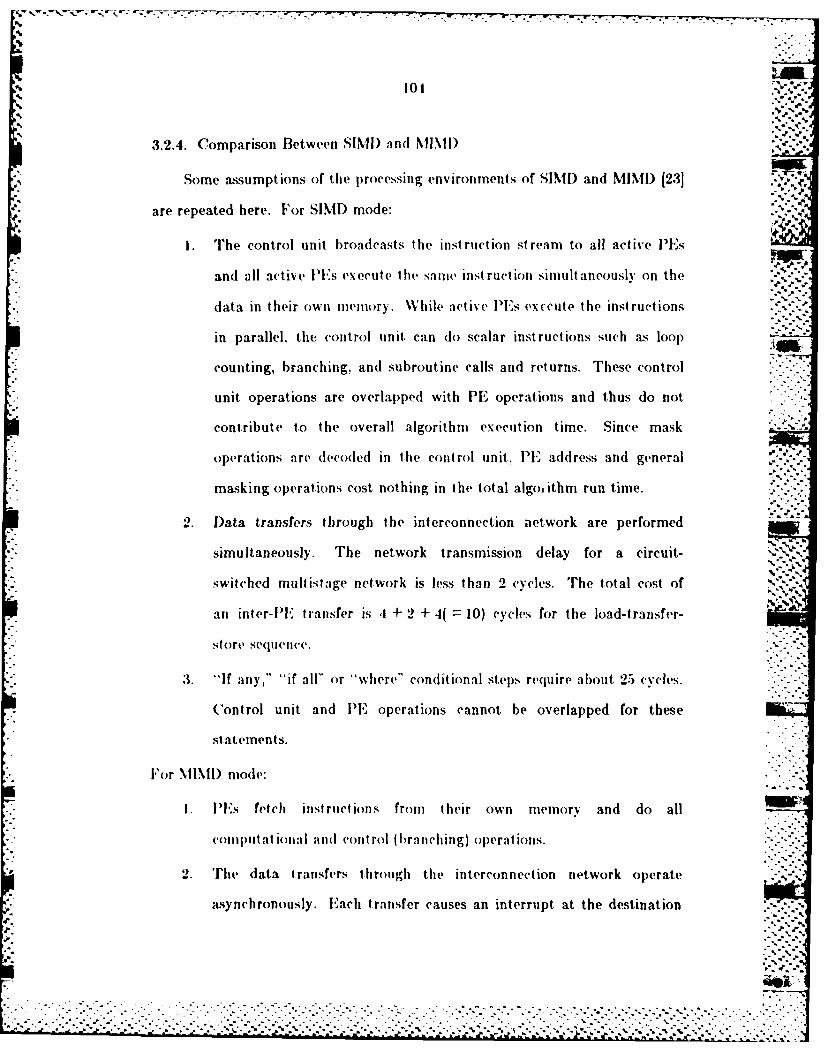
101

3.2.4. Comparison Between SINI) arnd NIJNII)Ve

Some assumptions or the processing environments of SIMID and MIMI) [231

are repeated here. For SIMIL mode:

I . The control unit broadcasts the instruction stream to all active PEs

and all active P~ls execute the same Inst ruct ion sinmult ateoUslY on the

data in their own inenory. W~hile aictive IEs exceute the instructions

in parallel, the control unit. can do scalar instructions such as 1l0o)

counting, branching, and subroutine calls and returns. These control

unit operations are overlapped with PE operations and thus do not

contribute to the overall algorithm execution time. Since mask

operations are dlecodied in tile cont rol unit. PE adldress and general

masking operations cost nothing in the total algoiithm run time.

2. Data tranSfers5 through the interconnection network are performed

simultaneously. The network transmission delay for a circuit-

switched multistage network is less than 2 cycles. The total cost of

an inter-PE' transfer is 4 + 2 + 41( 10) cycles for the load-transfer-

store se(lui(enc(..

:1. "If anty," "if all" or "where" conditional step~s require ab~out. 25 cycles.

Control unit and PE operations cannot be overlapped for these

st atemnents.

For MIMI) modle:

I . Ills fetch instruictionsl from their own memory and do all

coitpu tat n ia anid control ( h rn ciing) operations.

2. The data transfers through the interconnection network operate

asynchronously. E1-ach transfer causes an interrupt, at the destination

4..

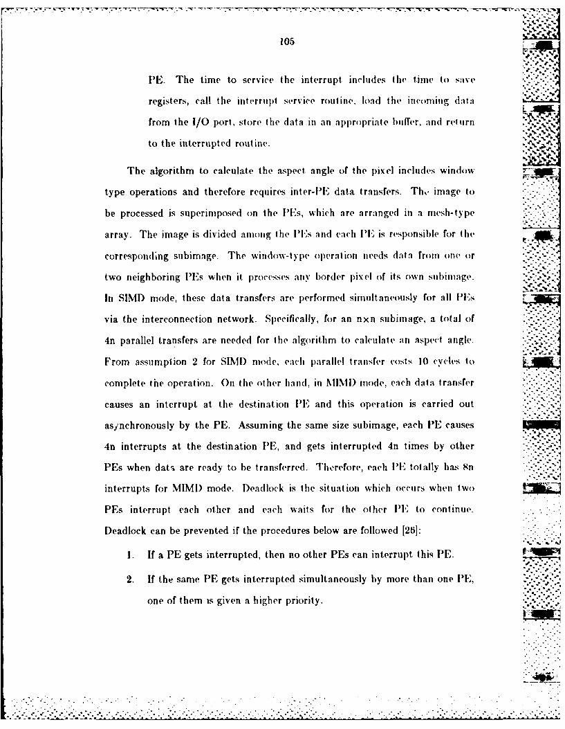
'os

PE. The time to service the interrupt, includes the time to save

registers, call the interrtipt service routine, load the incominig daLta

from the I/0 port, store the data in an appropriate buffer, and return ._%

to the interrupted routine.

The algorithm to calculate the aspect, angle of the pixel includes window

type operations and therefore requires inter-PE data transfers. Th- image to

be processed is superimposed on the P'Es, which are arranged in a mesh-type

array. The image is divided among the lIEs andl each PE is responsible for the

corresponding subimage. The window-type operation needs data from one or

two neighboring lPEs when it. processes any border pixel of its own subinage.

In SIMD mode, these data transfers are performed simultaneously for all P's

via the interconnection network. Specifically, for an nxn subimage, a total of --

4n parallel transfers are needed for the algorithm to calculate an aspect angle.

From assumption 2 for SIMI) mode, each parallel transfer costs 10 cycles to

complete the operation. On the other hand, in MIMI) mode, each data transfer

causes an interrupt at the destination PE and this operation is carried out

asynchronously by the PE. Assuming the same size subimage, each PE causes

4n interrupts at the destination PE, and gets interrupted 4n times by other

PEs when dats are ready to be transferred. Therefore, each PE totally has 8n

interrupts for MIMD mode. Deadlock is the situation which occurs when two

PEs interrupt each other and each waits for the other PI' to continue.

Deadlock can be prevented if the procedures below are followed [26]:

1. If a PE gets interrupted, then no other PEs can interrupt this PE. FAMEW1

2. If the same PE gets interrupted simultaneously by more than one P1,-

one of them is given a higher priority.

V... .. . .. ...

106

3. If F'Ei and IPEj Interrut e:ach other, then e 'h El I has the capalility

to grant one of the interrupts and disable the other. For example, , -.

PEi has the capability to detect that it interrupted IPEj and that Pj"

interrupted PEi. Therefore, if PEi has higher priority, PEj will grant -

PEi's interrupt, request and PEj will withdraw its interrupt to PEi. A

similar situat ion occurs if PEi interrupts PI'Ej and PEi gets interrupted

simulaneously

Since the o ol ii ing operali(ns in SINI) mode are executed by the ('I"

and overlapped with array instructions executed by lPEs, they cost nothing in

the total algorithm run time. On the other hand, loop counting operations in

MIMD mode are executed by the PEs and not overlapped with array

instructions. For example, the "C" program instruction in Fig. 3.2.2

for (i = 0: i < n: i + +)

requires n additions and n + I comparisons. These operations are in the

category of loop counting operations.

There is no memory contention problem in SIMD mode since the elevation

values zjij]j] of the nxn subimage and all the parameters such as m[k] and 0[k] .--

are stored in the corresponding memory of the PEs. PEs only fetch data from

their own memories. however, there are two alternative memory organizations

possible in MINII) mode One is the MIMI) mode with global memory which

stores the parameters such as mnk] and arIk], but the elevation values for the

subimage in each PE are stored in local PE memory. Serious memory

contention will occur when every PE tries to access mk] and o[k] to calculat.e

the frequency responses of all (lasses. The other MIMI) mode uses only local

memory. In this case, all parameters aid data are stored in local meniory. Or

course, it requires more t(tm l memory. All PI's can access the data from their

,r:~~i?:

• "U ' " ." - ' --,: - ' " . .--.'- . ."- ...' ' .-, .. ." : .i 3 " .-" ? -" " : ." "" ' . : .. ." .'

107 k

own memories without memory c(ontcii tion. I lere, we consid(er the MII) me(

with local memory only. -_

The algorithm shown in Fig. 3.2.2 requires (2 + N) subtractions, (I + N) -

divisions, 4N multiplications, I comparison, I conditional step, I arctangent.

and N exponential operations per pixel where N is the number of classes.

These operations are in the category of explicit operations.

Now we are in :a position to enutnerte lhe implicit opernli'ms :issoci: ted

with the program shown in Fig. 3.2.2. It is found that the algorithm requires I

operation to move the constant 2 to a data register, 9 operations to move the

addresses of variables such as V, z, a... etc. to address registers, (.IN + 11)

additions, and (.IN+ 10) memory references per pixel. A memory reference is

either a memory store or a memory load operation.

The number of operations involved in executing the algorithm in ,IMI),

MIMD, and serial modes are listed Table 3.2.3. The operations to move data

and addresses into data and address registers are included in immediate

operations. In SIMD mode, data transfers are via interconnection networks and

not via interrupt operations. Loop counting operations are overlapped with PE

instructions. The same situation doesn't occur in eilther MIMI) or serial

processor n'oales. In .MIMI) mode, data tra r>4,ers are e\ecuted oin dema nd via

interrupt operations but not through parallel tratsfers. In serial processor

mode, the overhead of parallelism, Present in both SIMl and NMID modes,

doesn't ex ist.

In Table 3.2.3, the execution times of most operations are argument-

independent except two: the artgnt : eimnrtxA o, l ' ei lrai mis. In SIMI)

mode, since every instruction is a lockstp operatin. the I'IN with shorter.

instruction execution time has to wait for compleli m of the I ' it h longest

.. J:-:.--:x--.

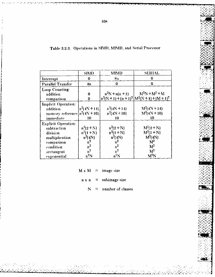
108 .. F .

Table 3.2.3. Operations in SIMI), MIMI), and Serial Processor

?. .' ..- ,

SMINI) NII) SERl. - i

Interrupt 0 811 0

Parallel Transfer 4n 0 0

Loop Counting:addition 0 n2N+n(n +1) M2N +M'+Mcomparison 0 n2(N + 1) +(n + 1)"2 M2(N + 1) +(M + 1)2

Implicit Operation:addition n2(.IN + I.I) n2(4IN + 141)M 2(IN + 14)memory reference n2 (.IN + 10) n2 (4N + 10) M2(4N + 10)

immediate 10 10 10

Explicit Operation:subtraction n12(2 +N) n2(2 + N) M2(2 + N)

division n2(1 +N) n2 (1 +N) M2 (1 +N) "

multiplication n2(4N) n2(4N) M2(4N)comparison n2 n2 M2

Confdition n n" Marctangent nnf'xl)onential n-N n2N M2N

Mx M image size

Sx n = subimage size

N number of classes

., -- .-..

................................... .

1 09. . . . . . . . .. -- ., -'

instruction execution time. Therefore, the total algorithmi run titne is the

summation of the maximum execu tion times of every operation. The I,,k sIep

operation mode will thereby lead to inellicient utilizati )n of I 'IC in SI.lI). on

the other hand, PEs in MIMI) mode can execute the ntex t instructiE)I ..-'.-

immediately after completing the current instruction. Therefore, parallelism in

MIMD mode has the potential to save execution time. The cycle times of

various operations are listed in Table 3.2.2. But there is no data available fron.

which to estimate the range of the execution times of either arctangeni or -

exponential operations. For most I)r,(.(, ()rs, mutilti)lication and ,livisi-_•.

operations take froii 10 Io 50 flines as Ibmg as addition or subi ract i()- ""

operations. Exponential and arctangent operations are coml)lex operations

which involve many multiplication and division operations. Therefore, a

reasonable range of execution times of these two operations are assumed in

order to carry out the comparison of the execution times of SIMI) and MIMI)

modes. Further, it will be assumed that the argument values are randomly

distributed throughout the whole image so that the algorithm run time is " "

approximately equal to the sum of the means of every operation execution time -g :

in each PE.

The plane of execution times for SIMD mode is shown in Fig. 3.2.3 under

the assumption that the range of maximum execution times of both operations

is from 200 to 400 cycles. Other assumptions used to calculate the algorithm

execution time are that an interrupt costs 21 cycles, a parallel transfer 10

cycles, an addition 2 cycles, a comparison 2 cycles, a memory reference .1 cycles,

an immediate operand 4 cycles, a subtraction 2 cycles, a division 75 cycles, a -...

multiplication 35 cycles, a conditional step 25 cycles; the subimage size is

n =32, the number of classes N 5, and the whole image size M 256. The z-

•%i;;-•-.

110

axis is execution time, the x-axis is the range of the execution time of the

arctangent operator, and the y-axis is the range of the execution time of the

exponential ope*rat or. The range (f the iean instruction execulion time is 11-'-I

assumed to b~e from I10 to 360 cycles for both operators. The plane of the

execution time for MIMI) tiode is also shown in Fig. 3.2.3. If the range of the

execution time is different from what. we have assumed here, the results are

expected to ibe simtiar. l'he results shown in Fig. 3.2.3 only indicate the trend

Of the d ilTerence of the vx\'-titio1 titues between SIMD ad MIID modes. This.

figure shows t hat MINI) mode has less execution time than SIII) mode.

Although scalar operations can not, overlap with array operations in MIMD

mode. the execution time saved due to efficient utilization of PEs in MIMD

mode leads to less execution time and better utilization of PEs in MIMD mode.

3.3 Alternative Performance Criteria

Feature enhancement methods, commonly used in producing maps from

imagery data, enhance or cnphasize information-bearing attributes of the data

while, ideally, suppressing other "noise" characteristics. The distinction

between "information" and "noise" is highly application-dependent. For the

purpose of this udy, attention is focused on spectral similarity, an image

attribute which is commonly found to be useful in scene analysis. If theimagery is black-and-white, spectral similarity reduces simply to tonal (gray-

scale) similarity. A clustering algorithm will be described, including a parallel

implementation, which can be used to identify sets of spectrally similar pixels.

The pixels need not be spatially contiguous, but simply have the same "color"

in a generalized sense This algorithm will be used to illustrate alternative

performance criteria for cvaluatin|g parallel (SIMi)) algorith is.

. . . .-. .-

- . . . - A .

7.I - 7 .

CJ,

3.8- SAKS

2.*.

2.1 %

2 i0 3230lns(f xetinlm o SN! n lM)*,210 3-A).

2S* 3-*m-

'320%

V..

to~~ 36u*0 1%" k

.. . .. . . .. . . .. . . .. . . .. .

-*..*.-.-*--.~~~10 2M*..** -"*-- -. *

*~~~~~~~ e 1L.., a. ** .

- . '. ~ . - -. - - .

112

In general, the complexity of SIMI) algorithms is a function of the problem

size ( number of elements in the dat a set to be processed). machine size (number .7

,,f Pis). and the intr(' )tioiiiio net work used to provide communications

among the PL's. For example, an algorithm %..hich uses N PEs to execute some

operation on an M x M image will exhibit different "perfocmance" for different

value- of N. The obvious use of performance measures is for selecting from

alternative SMIi) algorithms. For a given SIMI) machine, different algorithms

for performing a particular task can be compared. The algorithm which

performs best based on the desired measurement criteria can then be chosen. ..-

As another use for performance measures, consider the situation where the

typical values of image size M are known. Then a measure of the way in which

the machine size affects the performance of the application algorithms will be

useful in deciding how many PE's the system should have. Lastly, given a

recontigurable systiem [271. the machine size can be tailored to the problem size

for execution of a given algorithin if there exists performance criteria for -*--"--

comparing different choices of machine size. The goal of this section is to study

the relationships among the various parailel configurations. In order to

demonstrate one way in which the measures can be applied, an SIMD clustering

algorithm is presented. In this example algorithm evaluation, both the image

ize and ith, nmahi ie ,izc are varied, permitting the performance of the

algirit h i to be examined AnId compare(d un(her a art(,Iv of conditions. -

zf - % % 7.... ..-. - -•°

113

3.3.1 A Clustering Algorithm

Given n-dimensional vectors X a [aa,,,. . . allT and

Xb b~~...bn]T the Euclidean distance between the vectors is defined by

D i (ai-bj)2J-

Given a population of ni-d imflfs ona I vectors normally dist ribut ed N(I \

and a second population normally (list rib~uted N( her I -~ are the

population means and N" \_' are the population covariance matrices, the

distance between these populations is defined to be the divergence

+ tr V(i +\-I j)IIH'..TT

The following clustering algorithm is based on the ISODATA algorithm of *

flail and Bahll [28]. It groups vectors in such a. way as to minimize the sum-or-

squared-error (SSE):

where

c =number o, clusters

=i the set of vectors belong to the it h chist er

\1 the mean veetor for the ith (III~t r

Intunitively the vectors are grouped :is tight ly :is possible abo( u tt Ii ci r ri''vcl

cluster means.--

114

Step 1: Select c arbitrary but distinct vectors to serve as initial cluster

centers, Mi, i= ,2,...,c. (The user specifies the value of c.)

Step 2: Assign each vector li the data set to the nearest cluster center, based

on Euclidean distance.

Step 3: ('ompute the mean vectors for the data assigned to each cluster.

Denote means by Mi, i . ,c

Step -I: If the new cluster means Mi are identical with the old cluster centers

.NI, go to Step 5. Otherwise set Mi Mi, i=1,2,...,c and return to

Step 2.

Step 5: ('ompute the intIreluster distances (divergences) and m, ige indistinct,

clusters (having divergences less than a prespecified threshold).

('lustering complete.

The clustering algorithin is (epicte(d in Figure 3.3.1. On every iteration of

st ., 3. and I, the reassigninvnI and nio\vement. of cluister centers (means)

reduces the SSE. Since there is a lower limit on the S.44 (it cannot be made

less than zer(), the algorithun is giiaranteed t) terminate via step 5.

.3.3.2 Parallel ImplementatiOfi

Iigure 3.3.2 (ont ains a i)arallhl ilhmtpleuentl a ion of tihe clustering algorithm-

i a, high-levl programming l:nguge. Th,' inphlew'ualion is of the SMINI) "

hV pv. N is the number of IP'l's aid NI x Ni is the image size. The lE's are

,10)nligiired logically as a vN-by-V'N grid on which the NI-by-N image is

.sUpernm)(,d. so that vac'h !1 hols a -- bv- subimage for

'nw'n'Vence it is a.su med that NI/. - is an integer). e'l'l ocal" assign iment

U-.: -'::: -.. . -..> :: . -• -.: •. . •..: . *.. .

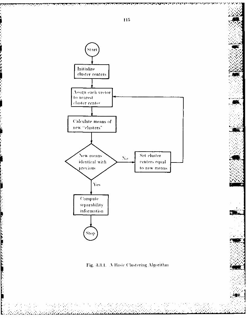
115

Sta'rt

I itialIize -

C'alculate mecans ofnew "clusters"

\(,%kIlle ll., No et custe

idenicalwill cenens qua

previ~~~lls ton w e

y Yes

e,-

Fig. 3.3.1I. A Kisic (lust ering Algoril tim

__t -1 _21 .7 4... .*-Z

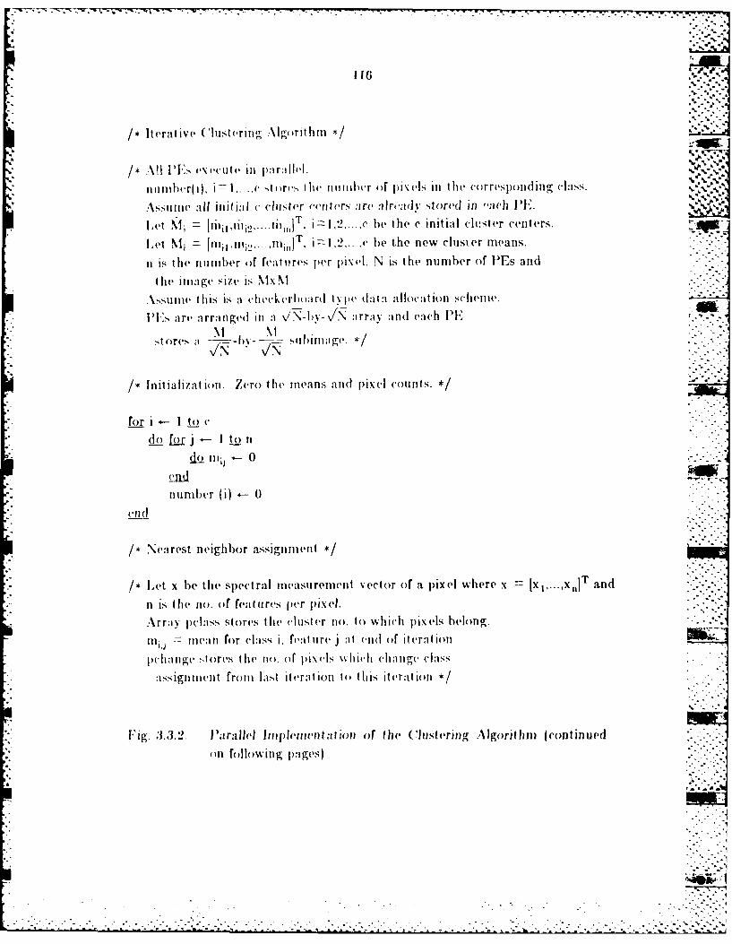
/* Iterative (lustering A\lgorithmit *

nil t1)ecr( i), i -0 () nr-, he cntii i 1cru o r1) 1R es 1it I Ihe co rresp)on Iiig clInss.

.'ssi it all In11itIial c duste c ('eIcrs are a Jo ad x stored in 'ach PE.

L et NI iii m~ 1 I 1,2,.c be the c initial ( s:t er cent ers.

Let MiI mia~2 m.,,,,jT 112--v. be the new clusi or means.

it Is t he riumber ( f featlirvs per pixel, N is the niumber of P~s and

Olhe im1age size is NixNI

P~s are arraniged in :i -,/N-l)V\ N irrai and( each PE'N I \I

st1oresi a )-~ s hrig.

~In itia lizat ion. Zero the means an:d pixel coun ts. *

for 1 1 to cdo for j .I to n

(10 IIIi i- 0

numbher (1) .- 0

/*Nearest neighbor issignmiient./

/* Let x be the spectral mneasiurenment v~ector of a pixel where x [XI,.. ,X n and

it is (te no. orf ea tures pcr pixeli.A\rray pclass stores the (lust er no. to0 whic ix ~els belong.

11ij iieain for (lass i, featiture j at e nd of iteration

p)elahige :lIorvs the no0. (4 p~ixels Mlicjh cliaiige- (las

aissigiiiieit fromi hat it erat ion to this iterat ion

* FVig. :3.3.2, 1ParallelJ Implement at ion of the (Clust ering AlIgorith (incontued

on following p~ages)

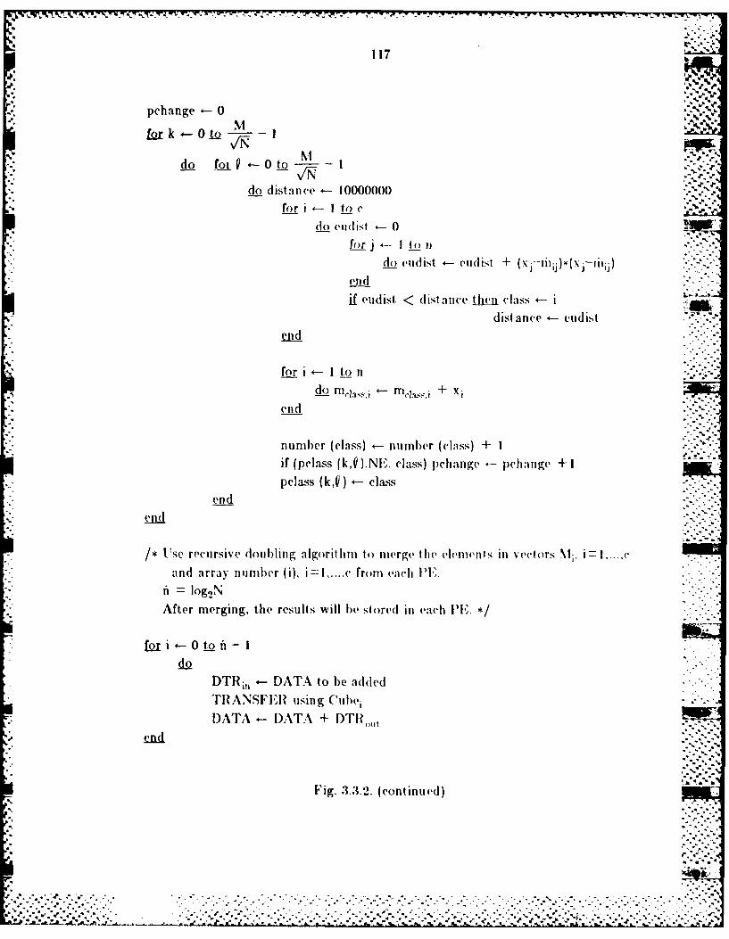
117

* pchange - 0m ..

N-I

do distance 10000000for i 1- to c

(do eIIdist 4-0

fo2r j4-I to 1)

do cud 1st 4- ed 1st + -i~)' x~iiendif eud~iSt < (listanice t him class "is

distance 4-eudist

end

for i ~-I to nI

number (class) .- number (class) + Iif (pclass (k,Q iNE. class) pehange jpchange +11pelass (k,(I) ~-class

endend

/* Use recursive doubling algorith1m to merge the elemevnts in vect ors i. i I--cand array number ( i). I fromn each PEI.n og 2N

After merging, the results will he stored in each PI. *

Lar i -0 to fl - 1do

DTR j, DATA to be add(ed

TRANSFERI using CubviDATA D-IATA + DTI?(...

.5 Fig. 3.3.2. (continued)

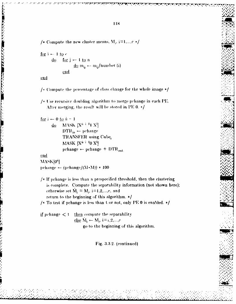
--- w-w-w.-."-,-<.-'

,4. *.

118 r

/* Compute the new cluster means. M,, i= .... c >

(1o f! r j _ - I to"i

do mi -- rri/nurnber (i) *.

end

/ Compute the percentage of class change for the whole image */

/* Ise recursive' doul)ing 'algorithin to merge pchange in each 11I.

After merging, the result will be stored in IP 0. *0/

for i 0 to 1i -1

do NI.Sk [X i nI Xi]l)~in *-- pchange

TIANSFiEiJ using Cube i

MASK [X' '0 X ] "

pchange +- pchange + )' ut -

end(xlASl [0"';

lpch:nge 4- (i,)changv/(Xl-.Nl)) * 100 l' -

/* If phange is less than a lprespecified threshold, then the clustering

is complete. Compute the separability information (not shown here);

otherwise set M1 i = M1 , i=1,2., and

return to the beginning of this algorithm. *//* To test if pchange is less than t or not,, only PE 0 is enabled. */

if pchange < t then compIute the separabilityele M1i M-- Mi,-,...,c

go to the beginning of this algorithm. .

Fig. 3.3.2. (continued) ".

c-7.. . -...

...............

of pixels to cluster centers is performed in parallel, so Ihat each IT" emi tains

the result of a clustering iteration for the subiimage which it h)Is '"I To

compute the new cluster means, these local results are then coml)ined using :-form of ove.lapped recursive doubling. %

The exact data allocation scheme used for this ilgorithin is not critli'al.

The only requirement is that I/N a1 tie image eleeIs be assigned to eaci

For simplicity, we shall assume a scenario witrh monochrome imagery, so A

that the nurmber of features per pixel (n) is I for this algorithm. Then on each

iteration, the distance calculation and determination of cluster membership

requires (3 additions + c subtractions + (c+l) comparisons + c

multiplications) * operations for each lIE. The recursive doubling

N

algorithm to inerge the means M i, and constants number(i), i= l,...,c in each IPE-

requires 2c parallel transfers and add operations at each step. Since there are -.

log 2N steps to merge the data, a total of 2clog2 N parallel transfers and

additions is required. After merging the data, c division operations are needed

to compute the new cluster centers. Using the recursive doubling algorithm to

merge pchange from each PE requires h)g2 N transfers and additions, and,

21og0N masking operations. Computing the percentage of class change requires

(2 multiplications + I division) operations and I mask operation. Finally, to

test if pchange is less than a prespecified threshold t requires 1 comparison:

only PE 0 is enabled at this step.

0.

'A

.....................

. ..................

-. - .,-.,.,. *

, ~.:.. ,

120

3.3.3 Performance Analysis "*

For application of the performance measures to the clustering algorithm,.-

the following are :issulmed:S%."

ta =time for I integer addition operation,

=. time for I integer subtraction operation,

tm time for I masking operation,

tr = time for I integer comparison operation,

t y = time for I integer multiplication operation,

td time for I integer division operation,

tdN) time for I parallel data transfer operation.

For simplicity in the example that follows, it will also be assumed that

ta ts = tc ty/2 : td/2 = 2t, tt(N)/2. The actual relationships among

these operations will be implementation dependent. Time for loading and

storing data items and for program control operations such as testing loop

indices has not been explicitly included in the analysis. The time required for

program control will be assumed negligible in comparison to the other times,

and, in general, the program control operations can be overlapped with the PE

and inter-PE transfer operations. As shown earlier, the analysis could be

modified to account for implicit operations.

"The performance of the clustering algorithm will be evaluated as a

function of N for an M-by-NI image, with NI ranging from 2' = 6.1 to

2 8102. The evaluation is limited to machines having between 26 and 21"

EI's and the un)er of (lusters being 32.

• - -.. . . . .. . . . . . . .. ... . . ...

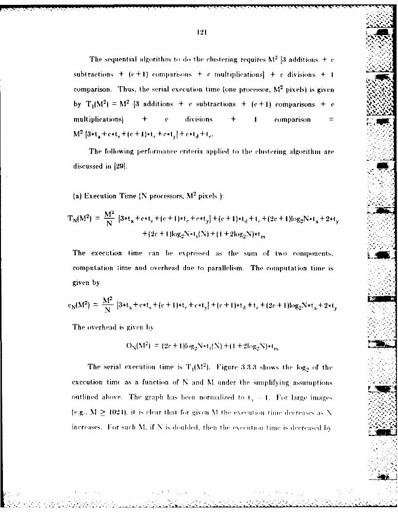
121-. '.'-.

The sequential alg rilini to (lo the clustering requires NI2 [3 additions + c

subtractions + (c+ I ) compari.,is + e ,utt ipliat ions] + c divisions + I

comparison. Thus, the serial execution time (one processor, N2 pixels) is given

by T1 (M2) = N -2 [3 additions + c subtractions + (c+1) comparisons + c = 'N12 V

multiplicationsj + c divisions + I comparison -

N2 [3*t. + c*ts + (c + 1)*t, + c*ty] + ('*td + c.-

The following perform:ince criteria applied to the clustering algorithim are

discussed in [291.

(a) Execution Time (N processors, NI2 pixels ):

TN(M 2 ) AL.[3t+ct2--N I*ta+c*ts+(c+l)*t0,+c*ty[+(c+l)*td+to+( 2 c+l)hg 2N*t+2*ty

+(2c + I)log.N*tt(N) +(1I +21og 2 N)*t ...

The execution time (,ain be expressed a.s the suri of two comiponents,

computation time and overhead due to parallelism. The computation time is

given by

2 2 IN.CN(NIM) -- [3*ta+c*t 9+(c+I)*t +C*tyl+(c+l)*td+t,+(2c+l)tlog 2N*t +2*ty

The overhead is given )y

(N(M 2 ) (2c + I)log2.N*t,(N) +21 2 ,N)*tn .;i

The serial execution time is T \(2). Figure 3.3.3 shows the 1g2 of the

execution tim( as a function of N and N under the simplifying assuiptions

outlined above. The gra ph i s beeIn Tnirnliz d Ii ' tt I " Fr Large ininges -

(e.g., M > 1021). it is cl :ir t h:it rr wiv.. \1 I tie ,\v' li i tinw decri,,va,, : N- -

increases. [Or such MI. if N i dnItlthd, t ho t e ,,,ii t liOwn ke d1,,ooe:l I,' ='e: -'bLI=4

.. N)

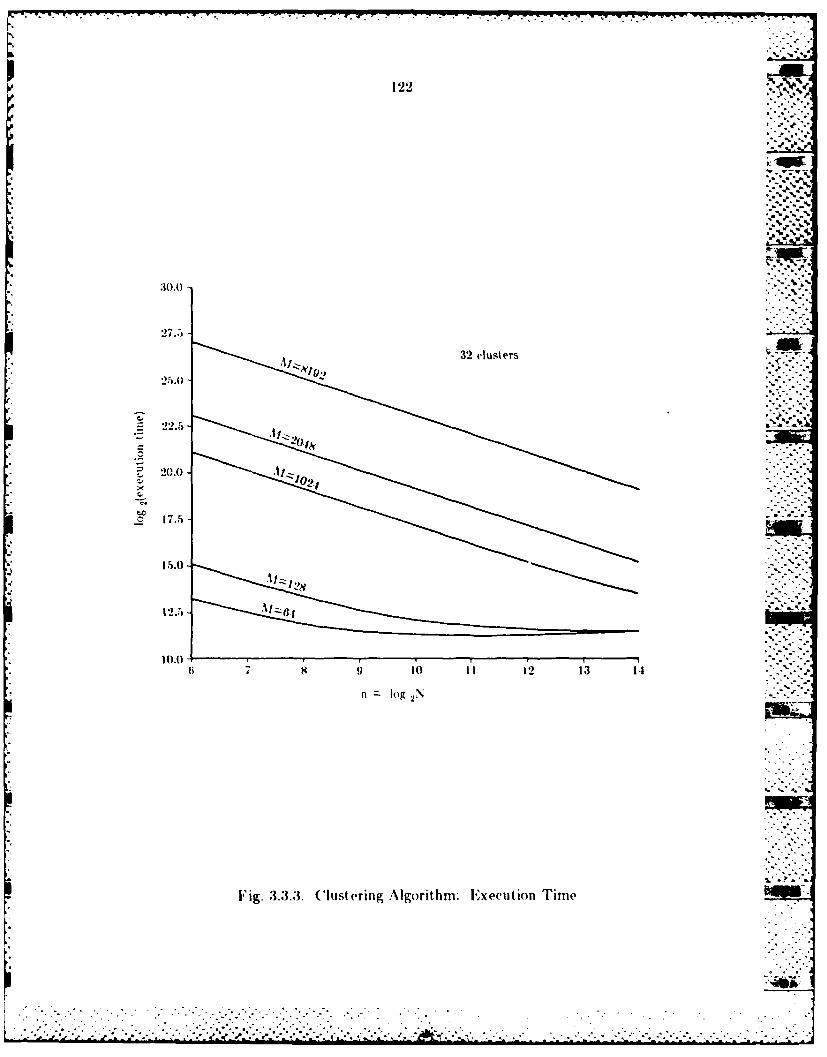
122

30.0~

2 7.r

32 clusters-

25.0-

40.0)

o 17.5-

12.5- Al -6 .

6 !' tO I'I 12 13 1

nl - lg 2N

Fig. 3.3.3. Clustering Algorithm: I-xecution Time

123

approximately a factor of two. For small images, an increase in the number of

PEs has little effect on the execution time. For such NI. the time required for

the recursive doubling algorithm dominates when N is large, and there is little *-

or no advantage to using a large machine. For each NI in the range 61 to 128,

the rate at which TN(%12) dlecreases (dTr( lI~)/(tN) also decrea'ss as N

increases. Therefore, for practical pl)rposes it may be appropriate to consider

dTN(M )/dN as well as TN(M 2).

(b) Speed-Up:

SN(M 2) TI(M2 )/TN(M2)

Figure 3.3.4 shows the log2 of the speed-up as a function of N and NI, under

the simplifying assumptions. For large M, SN(M 2 ) N, i.e., the speed-up is

almost ideal for all N considered. Therefore, using SN(M 2) as the performance

criterion wouid dictate using as many PEs as are available. For small NI,

SN(M 2) << N, and the choice of N ha-s little effect. on the speed-up. For

example, for NI = 6. there is little advantage to using more than 29 = 512

PEs. For small M, there exists a value for N up to which increasing the

number of PEs significantly increases the speed-up, but beyond which there is

little advantage to increasing N. Titus, it appears that using a combination of

speed-up with d(speed-up)/dN (and/or a measure such as utilization or

efficiency - L.ee below) is a more practical criterion than speed-upi alone.

. 1

124

12.5624-'7

H.~a 1250

S.25(9) N0

5.3750

3.9375

6 7 03 10 1'] 12 33 11

In)g 2N

F~ig. 3.3. 1. ( lust eritig AlIgorithmifi: Speed u p

-. -.- ..,.,.....,

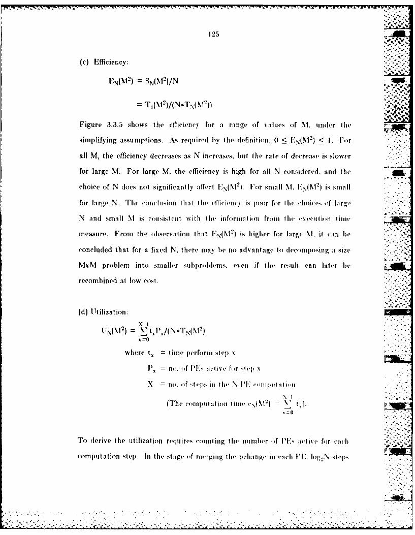
125

(c) Efficiency:

EN(M 2 ) = SN(1 2)/N

= T l2)/iNT(I-2l)'

Figure 3.3.5 shows the eflicietic% for a range of v~iltes of M, underIQ II h

simplifying assumptions. As required by the definition, 0 < E'N(I1- ) < I. For

all M, the efficiency decreases as N increases, but the rate of decrease is slower

for large M. For large M, the efficiency is high for all N considered, and thechoice of N does not significantly iffTect. EN({N). Ior smN I I"( i2 s5 lI

for large N. The conchlsion tl ht the efli' my is por for III(, l oi(c,, of Irg-e

N and small NI is co nsistent. with II the inform:titin from le ,xec'uliin time

measure. From the observation that [IN(NI-) is higher for large M, it can be

concluded that for a fixed N, there may be no advantage to decomposing a size

MxM problem into smaller sul)prol)ems, even if the result can latner be

recombined at low cost.

(d) Utilization:x I :'"

X=it'N(M) = Zt.I1x/(NTN(I) ""-

where tx = time perform step x

= no. of l'l' :stive for step x

S no. of steps it] thv N IlT: vlopill:ti,. .

(The ('oi l)ulalt ion it lite (',\\ 2 ) - 1j .

To derive the utilization requires co unting the number or I'Is active for e:ah

computation step. In the stige f mewrging he pchang, iM ach I 'I'X I'g2N step

............ . .

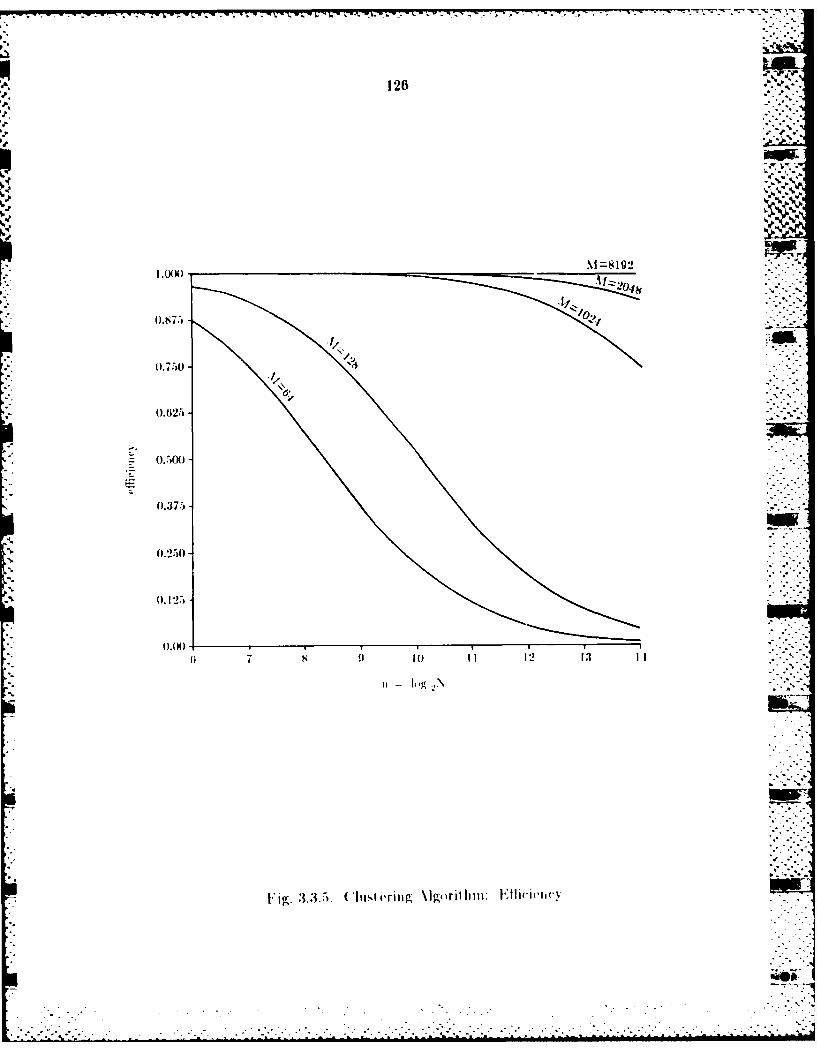
126

M =8192

O.S75

0.750 )

0. 625

0.500

0.37.5

0.250

0. 125

s 0 10 11t 12 13 I

F~ig. 3.3.5. ( lust erilig \lgoriilimii [iliiii,

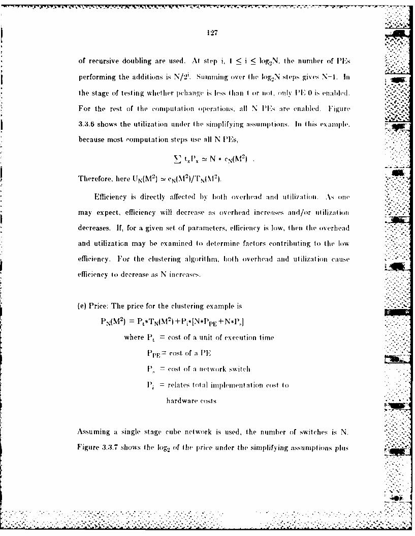
127

of recursive doubling are used. At step i, I o.N, the numb~er of [PEs

performing the additions is N/2'. Stiu ing over th lIog.AN steps givs N-1. In

the stage of testing whet her jwmi eis less t i I or not f)l.nly IT" 0 Is enabled -U.

For the rest or the co0mput ation o perations. all N IP Is are enablled . lFigtire%

3.3.6 shows the ut ilizat ion tinder the sinpilry ing assumip tions. In, this ex amnple.

because most eomputation step~s use all N P~Es,

Vj tX N *CN(N't)

Therefore, here UjN(X1) cN(M )/T'N(N1

Efficiency is directly a ffect ed by bo th overhead andI( uitili z a ii. .\s oii

may expect, efficiency will decrease as overhead increnses and/or utilizat ion

decreases. If, for a given set of parameters, efficiency is low, thenl the o%-erhea-:(l

and utilization may be examined to determine factors contrib~uting to the low

efficiency. For the clustering algorit hmi, both overhead and ut ilizat ion caIuse

efficiency to (lecrea-se as N Increases.

(e) Price: The price for the clustering example is

PN(M 2 Pt*TN(M 2 +Pi*[ N*P'PE+N*)SI

where Pt cost of a unfit of execution time

~PE),- cost Of a.I lE

P., cost or a iiet wo(rk switclh

P. relates total Implement al ion co( st to

hardware costs

Assuming a single stage cube network is used1, trhe number of switches is N.

Figure .3.3.7 shows the log2 of the, price under the simplifying assumpt ions plis

-V.,

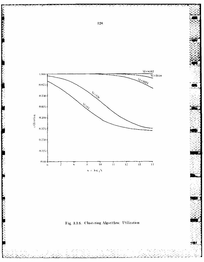
-q ~~128 .. *q

I.M 0% - 01

* 0.500 -

0.3 7

0.2.-)0

73 1( I2 13 1 1

ii- log ,

I'g.3.3.6. ( lust uring Algoritiuii: Ut iliza tion

129

- V.

32.000-

29.375

26.750'

1- I.000 -

16.i225 .06 71 10 11 12 13 I

Fig. .3.3.7. ('lustering Algorithm: ~rie(• .

I -C... .

'.. . - ".: ..... "-.- ... " . A ": .. . .. . -.- CC -" .. " -." .i ... t '- . " . . ,'. , . . -. . .

fheassumptl~fions~fl that P, Pi~ ~1,I nd E 3) ,~ 1.- For small NI, the

curve has a inilnimium III the range 2~< N < 211. Fuirt hermuore, the optimal N

is greal er for large Images 1i bal for sinall Iliia-es. lI'i. occus beaus forlag

un a geI, e((luti Ic m u lm(iltin ues toc eces igniifiva ut I as N increases, whileV.7

Ilhe geni(ralize1 price for the clustering algorithm, under the same

*1.*[N*P'pr+ P]

where k exprse ft(i relative importalnce of execution t ime versus system cost.

I.,gue :.38 sow th gnerlied rie a afunction of N and a for a

1024Ix 12.1 Image . As expected, the optimal value of N shifts to the right as

executionl time becomes more critical than system cost and to the left when

systemn cost (lomin ates (ai < I).

3.41 Parallel Architecture

F'rom fte (discussion of the previous three sections, a multiprocessor system

v Inch can be dynamically reconfigured as one or more independent

IMI)/INI submachines of different sizes is needed to implement the

sulperv ised relax at ion algorithmn. In thi's sect ion,the1 partitioning of the%

ini I ()(41 lection niet%\w rks. cube l nv it Wcrk and1( alinenited dat a man ipulat or

nI\ wcrk . is cc nsidled . Tv picaIN %O.wlen t he niumtber of pro)cessinig elemnents in

I lie niit il sso('5r -svsivnl Iicreast. il dat a comimunicatlions between the l11,

Ibeconil ll1( )i' 1(1 lmore j1ll port 1111. lFsI&cially for mnultiple submnachi nes of

MINIDI anld MIINID molit des. It is rvqu iredl that d ifferent subimach ines can

Siryl l1t 11 Ieouly vxc'X'ccle thlir I15nstrctioncsa in]doc not ilt er-fere wit h each other.

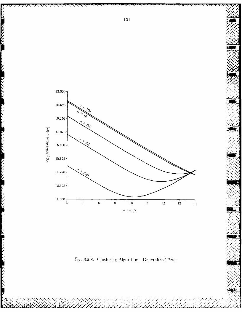
P6?

131

22.000-.

20.625-..

16.500

1 2.50

6 7 10J If 12 1 .

F'ig. 3..9 ( Iiitering- :\ kn rIt h ( ,rerviai ~ed P rice 4

-4

1.32

But, they still can cooperate with each other in the results through the

interconnection network after certain stages of computations. The routing

schemes presented below for both cube network and ADM network and hybrid

tNlpe network are quoted from [16,17,18,1i]. The network adopted is so well

suited to the supervised relaxation algorithm that substantial speedup by the

muilt iprocessor syste CI,, e x pectedl.

3.4.1 Hybrid Network

-.

As shown in Fig. 3.4.1, the hybrid cube network is an integration of two

networks, the unidirectional packet-switched cube network and the bi-

dl irec.tional circuit-sw.it ched cube network. This netw rk is suitable for the

parallelism modes configured as shown in Fig. 3.2.1 because large blocks of

input data can be piipcline( through the lower half network and fast data and

instruction fetches can be provided by the upper half network. The upper half

of the hvbrid cube network is a Ill-to-l'[ configuration in which the cube

net work is wral)pel d ar n !( .,nnected to N Ills. There is a local memory

modtuh associated with eachi I1H. The lower iaIf of tic hvbridl ctibe network is

a lE-to-memory configuration in vMi<ch N F'Es are connected on one side and

N metmory modules are connected on the other side. The memory spaces in the

N memory modules shared by the N PiEs are much larger than the local .. .

inviiiry modu111les inI the N P 's. The in terchia nge boxes at the nt h stage -

(in o1,,,.)N) (-,an be set to connect to the upper half or the lower half of the

hybrid cube network by setting the interchange boxes lo straight or exchange;

they each h:lixe oe inpult port conct,,d to a lEs..

The advantage of the l'-t,-El configmiration is fast local memory

accesses. For SI NII) mo(de, data are stored in the local rnem ry. Therefore.

'..7

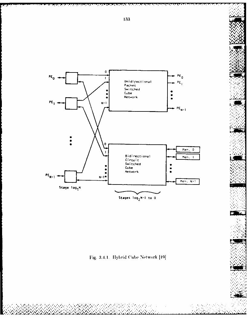
133

PE 0 PE 0Unidirectional P E

PE N-

PEN N-

0~

Fig 31. .I l b Netu w Ntk~I~PE. ,

. . . . . . . . . . . . . . .

. . .. . . . . . . . . . . . .

131,'. o .° , te

this configuration can provide fast instruction and data fetches. For the PF-

to-memory configuration, N PFs share large blocks of data stored in N memory

Modules and can vary the amount o>f memory used by each processing element. "

For the packel-switched cule network, a packet makes its way from stage

to stage relesing links and intercha ge boxes immediately after using them.

It, is good for NJIMI) nm(<h whichi neevis a frequently changing p~ath through the.'' """. .

network when performing window-type operations. Therefore, every PE can

request dala from a neighi)oring PE by sending a message via the

interconnection network and the requested P1E can respond accordingly. As a

result, it (an reduce contention incurred by sen(ling two packets to the same

inlput port or the interchange box or dispat ching two paekets from the same

output port of the interchange box. For the circuit-switched cul)e network, a

complete circuit is established from input port, to output port for one particular

path. It is good for SIMI) mode which can provide parallel data transfers via

the interconnection network and also good for transferring large blocks of data -

from the shared memory modules to IPEs. Therefore, data transfers can be

pipelne(I through the network. Once this path is establislhed, the only delay is .-" -

propagation delay.

The upper half of tlie hylbrid cu be network is an unidirectional network.

Since the inputs and outputs of the network are connected to PEs, the

unid irection:al network is sunflicient. [or the lower half of the hvbrid cube

net W(,rk, siiice large blocks of (tala need to be transferred between PEs and

nieior% msul,,s, a bilirectioial nelwork is necssary to provide Ibis facilit.

.Xctuall. the li)rid cube net\ork coitains N iipnlt )orts, 2N output ..

ports an(d two size N generalized cube networks. It has mi+l stages labeled

fr(un in to 0. litercliange boxes in st age in divide the network into two halves.

* .. .: . . .. .. v. v.:. . . -. -.--... .............. ........ . .............. : :::..-.. .. . . .. . . . .. . . . .. . . .

13,5

That is, the Interchange boxes can be set to connect to either the( upper half or

lower half of the network.

If the cuibe net % I rk is replaced 1)% Ihle A IM) net wo rk, thlenlii he 11briil %

cubeC netw~ork b~ecomies tit(e hbbrId .\l iiet~v(uk. Thle AIM\ mvI(irk I iiiui11,(.

powerful t han the( cube netwo)rk . For Ihli Dil ist age (tib e t wI%%irk. Iire I

only one path between a part iculair netwoirk In put an rd out put. Htit foir t he -

multistage ADI) network, there are mnult iple pathls betwe~(en a given net work

input and output. Thus, the hybrid ADMN network can reroute the packets

through aniot her pathi if lte cuirrent established pathi is broken or Ii s busy -

swit ching elements in It. It cani perfoirmi :itny pernhllt t ion tIim a I muDin Ihis-ag

cube netrwork canti perform. H owever, in add ition to thiese- a;iov iges' for tOli

hybrid MAI network, there are also additional Implement ation co.is and

control complexityv that the hybrid cube network dloes not have.

If the multiprocessor system with the hybrid network is uisedl to implinen

the supervised relaxat ion algorithmn, the data inputs to the stibalgorit hms in

blocks A, It, and C can be stored in the memory modu ile-, first. The( inpt (lit :i

tend to be large. Therefore, the memory modules canti prov-ide large stoirage

space for thenm and data can be ret rieve(] o)il demnd.i~ After using them, results

produced can be transferred back to memory in,,dule' In order to save ineiory. .-

spaces in PI~s for other purp)oses.

.3.1.2 Partitionig thv ('Ibe( Net\%oirk Into 2 \Il\Il~s and I SI\1l

Partitioning and] roti ti ng schenies for tie( cube net wo rk are described in tie(

Appendix.

I : ti

For simuphlicity~, assu me there are N 16 PE)Js. We want t o pa rt ition these

IPLs into) 2 MII) sitbinaeltines anrd I SINI I submachinie for the %1.

implemen at ion of the su per.~ise(I rel \ at ion a 1goritIhrin in thiis mul1 tip rocessor

,. .S' ... -

system. One NIMI) has 8 P's and the other MIMI) has 2 PEs. The SIMID has

.1 PE'Is plus one PE for the control unit. 'hus a total of 15 PE's have been

used. NoN , the remainitg probldem is how to partition the network into 2

MII I)s and )ne SINIl) with the control unit assc siated wi. i it. if the network

can )e partitioned into thliee three independent groups, then the PEs connected m

to this network are automatically partitioned into three corresponding

inde)endent subnmachi nes.

For MIMI) mode with size 8, the addresses of these 8 ports must differ in 3

lit positions. For example, if port addresses from 0 to 7 are assigned to the

MIMI) machine, their addresses will all agree in only the most, significant bit

posit ion. ly setting to straight the interchange boxes i; stage 3 corresponding

to the input port, addresses ranging from 0 to 7, one MIMD with size 8 is

formed. Similarly, for NIIMD mode with size 2, the addresses of these two

must differ inl I bit position. Let. us say that port addresses, 10 and 11, form

one MIMI). Therefo re, two addresses will agree in the upper 3 bit positions.

IBv setfiig I straight lho ilterhange boxes in stages 3 2, and I corresponding

Io I in.e I c,(, irt :tlwro *sp., . one imh'dependen MINI1) wilh size 2 is formed. For

SI\I). if port address 8 is selected as the control unit and port addresses

ranging from 12 to 15 are selected for the processing PEs, then these latter 4

addresses agree in ilhe most significant bit position. By setting to straight the

nt erebaage( x es ti stage :3 corro-,potd ing to p)ort add resses from 12 to 15,

these I addrvsses fo)rm one independent group. ]PE 8 can broadcast

inst ructions to thcs,, I by cal'ulAting the routing tag as follows:

.. ..... . .... . .. ,. .

1.37

It S G )r8 ( 12=1000G (DI100=0100

and

(the notation is defined in the Appenidix ). For PE' 8 by set ting the Int erchatnge

boxes in stage 3, 2, 1, and 0 to st ra igh t, ex chiange, broadcast, antd br )adlast 11i

can broadcast inst ruet ions to I ~Is 12, 1:1, 11I, antd 15. 'Ihle restl It islw.hwn III

F ig. 3.4.2.

3.4.3 Partitioning the AD)M Network into 2 NIIMI~s and I SINII)

Since the determination of rotiting tags can be roi( 11 [16,1 7J, this

section only overviews the advantages of the AJ)M network. Most important is

the description of the p~art it ioninig o)r thev ,wm\ net work into 2 MI MI)s an I11

S I NI I).

The advantages of the AI)NI network as dlescribed before are the lillit iple

paths existing between a network input and output, ali( the additional

permutations, as compared to the cube network, which the AI)NI network can

perform.

The ADM network consists of N iniput ports, N output ports, and

m 10lo2 N stages with N switching elements p~er stage. Stages are numbered

from m- I to 0. Each switching element in stage i performs a straight-

connection and the PM21 (plus-minus 2') interconnection function which is

defined as .

1)\ + j(j) (j + 2') mnod N

MlN i(j) (0 -2') mod N

for 0 <j <N anrid 0 <n< I

Therefore, each node j at stage i of the network has three outpuit lines. But,

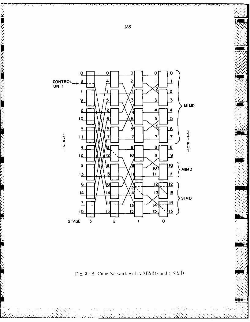
138

0-. 0.0

CONTROL 8421UNIT

MIMD

0

TUTT

- 10 SIMD

SI.

STAGE 3 2 1 0

. .1. 2 0 1ijbv Ncw i 1 2 N1 ) 1 nD S IN 11)

139

there are only two distinct data paths from each no)de ill stage m-I [ 17]. 'I'he.

ADM network is shown in Fig. 3.1.3. The indiid ual switching eleimienlis in

every stage can be controdled idlnldepelently awl r(uti ng tags :are einpl(,. cd th

distribute control of the network aimnong the processors to avoid the I bt(tleneck

created by ihe centralized ('orol unit.

Assume there are N 16 lPEs connected to the AI)N network. ''he.

network can I)e partit ioned I) one SI NI) machine with size 2, one MINi)

machine with size .1, and one MIMI) mnachine with size 2 as shown Ii lFig. 3.1. I.

For the MIMI) machine of size 1, if the port addresses include I, 5, 0, and 13,

set the corresponding switching elements in stages 0 and I to straight. For .

MIMD machine of size 2, if this group includes ports 7 and 15, set. the

corresponding switching elements in stages 0, 1, and 2 to straight. The

principle of partitioning is that the size of each subnetwork must be a power of

2 and the addresses of Ihe input ports in the subnetwork o)f size 2' must agree

in their lower order m-s bit positions. For SIMI) mode, port II acts as the

control unit to broadcast instructions to ports 2 and I. The routing tag

contains two parts: {R,B} = {11001, 10001). In 116,171, calculation of the

routing tags is described. Therefore, PE 11 sets the switching elements insuccessive stages to be -2-, straight, straight. 2'type I)roadcast. Thus, it can

broadcast instructions to l'Is 2 and I. The 2 MII) modes and I SIMI) mode

in the independent subnetworks shown in Fig. 3.1.1 have the complete

interconnection capabilities of the AI)M network.

The important ability of this network is that it can dynamically reroute

the message through alternate available paths to gain fault tolerance as well as '

improved throughput [17].

... . .. .. .. . .- .. .. .. . ... . ,. ..-.. .. .. .. .. . . .- . - .- ..-. - . .. , . - -. -" .. " . ..

- ' ' . . . . .... . . . . . .. . .. . 1

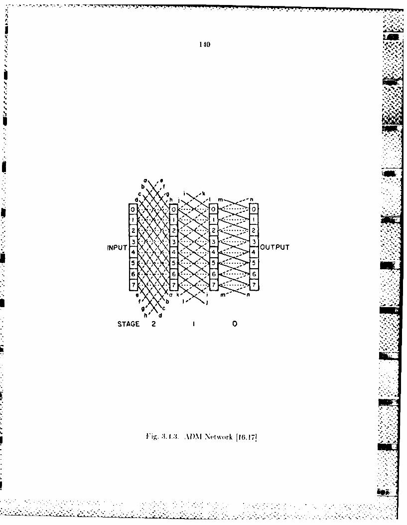
a 0b f

0 0e

o..'Y2 .... -.. H2

IN U - C .

4 ...

STAGE 2 0

3. 1-:3. .\i)\ Net work 116,1l71

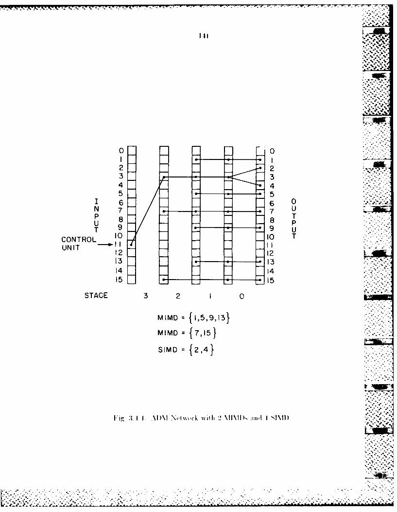
~*% w' .

0 0

2 23 .9 .3

4 45 . 4-5

6 6 0N 7- 47 U

88T 9 U

CONTROL 10 10 T

UNT12 1213 1-~314 1415 1 5

STAGE 3 2 1

MIMD 1, 5, 9,13}

MIMD {7,15}

SIMI) {2,4}

FI 3. 1. 1..-A N. \(rk 11h .\1\1) m d .SMI

1-12

3.5 Summary anld Conclusions

In ecio 31,it was shwn that the maximum parallelism achieve at

this level of modeling is reduced by the nat lre of the algorithm and especially

by the scalar p~rocesses Involved in thle test ing of the loop despite the

availability of 1021 IPls. It also was shown that the average parallelism h

wihich accont s for bot h c oieurrency of p~rocessing elements sand for the overlap

of array and~ scalar or control-flow instrructions, is usually larger than the

averg vto paallls h which only accounts for the concurrency of

processing elements and doesn't consider the overlap or array and scalar or

conY~ rI-fo Iftijtt thle nu tmber of processing elemlents is relatively

smiall, the tv erlap of the control1 unit with the array p~rocessors may be

significant. Otherwise, thie overlap of the control unit with the array processors

contrib)utes very little to the degree of parallelism.

An interesting result of the analyses in this section was that, the total time

required to classify an Im age using a pipeline is greater than that using an

SINI) architecture even though the uitilization of the P~s Is greater for the

ppelile. fltreason Is thlat II he ovcrlievid (I-l o It iriijtiit inrg thie paraillelisi

For the pipeline is, great er. The overliead inc(ludel(s scala r operations executed at

each stage of the pipeline aind dat a tranusfers bet ween stagtes of the pipeline. In

SIMDI mode. IPE a(ddress an id general I ask ing operat ions~ -ost nothIiin g in the

tota:l algorithmn riot tune If we :issniittIhat inising operaitions are decodledl in

the coinrol mll.t This prp'rvit\ i-, Alo iii ,delvd with S-Nets. Thelirefore, the

tr-it~i ort firing 1itne , niot inrr:ised to :wcoiiiiuiti mask iwtirkings thait are

not all I's. D~ata tranisfer t1ime and d~ataiIrif' thrx-igh Ibe interconnect ion

nietw~ork can ailso be itiodeled wit S-Nets. st :is thle &ia ra rtnsfers in vect or

stin vx :t phe. BasedI o thle S- Net l( mde, sysin et tItr(otiglt -,icn 1e increased

by maximizing the hand i measures.

Also in this section, we modeled a. 'omplllex algorithmi (nmximium likelihood

classification) with S-Nets on SIMI) a 11( pipelinie architect ures. So me .-

quantitative mneasu res such as parallelisi m d 1(1eciit i( time were considered P

in conjunction with S-Nets. l)ite to the a%-ailahilit y or qtiant itat ive niea-su res,

we can make direct comparisons between two architectutres b~ased on a given

image size and nu~mber of 1PEs. In general, for image processing operations

which are not window-type operations, the higher the dirnensionality of the -

remote sens in at da mi it(- he ore (lasses re'presenit ed in thle imI. i reIr

the potent i beniefits to be derived from SINIl) implenient at i n rf the process.

Section 3.2 dliscussed the c()Iiirisofl betweeni execut ion t inies or SIMI) 7~

and MIMD processors based on the analysis of explicit, andl implicit operations

embedded in an algorit hmn. In Sect ion .3.2.4 It wavs demionsi rated that11 tOli

MIMI) mode is better than SI4\il) mode for the a goi-nt Iins w~hi chi :irv uro

suit able for jockstep opvraition. Of course. MIMi I fiiodl nied~s a miore

complicated( con trol st raegy :ind( has niore (onuiIlicat('(I ielods Fu)r dat l:i

transfers than SII) miode. [in SIMNII) 1w )de. very step is sv uchr( (ii d a id tOw

control strategy is simpler. InI geneivi, aIgorit Iins whIiichluiv e wiridow-t v e

operations andl do not haive opera tors who se vxcu lt i( l~imes a r(' a rrfunieio-

dependent are suit able for SINI I niodel( because t hey canII t :ik( ad 'ant ae (,f

overlapping of scalair and] arrayN operati( (115, I):irall('l (Litn t risfcr, sx ohir inIi/il,

operation, and simpler control schliis wvithout loo"Iiig 11 lie ('t(r 1t ili,:iI ion (11

PE resouirces. A gorithims wh ich (do not Iiave windol(-ty 1w operaIios i'I; :II a1.%.

op~erators whose ex ecunt iona tiues are a g ue ((pn( 'ire suii it aI) le

NIIMI) mode because t he%- ca:n a vl f(i it i jl erru pt (pera t i( s fo r aisy iiclir~ iii (ls -

(lat a transfers and deadlock p~r'eention schi'lis, acliey(' belttn it williat 1ion of

%~j

144

PE processing power, and minimize execution times. For algorithms which r.l

have window-type operations and are suitable for MIMD mode, data transfers

can be executed in parallel before performing any data computation or can be

executed in a more general fashion though interrupt operations provided that

the complicated control scheme of the system is available. We assume that

asynchronous data transfers through interrupt operations and control schemes

can be supported by the hardware/software.

The supervised relaxation algorithm contains several subalgorithms, some -..--

of which have execution times that are argument-dependent. These

subalgorithnms are suitable for MIMD mode in order to most efficiently utilize

the processing power of PI's and minimize execution times. On the other

hand, sulbalgorithnis with execution times which are nou argument-dependent

are most suitable for SIMD mode in order to take advantage of the simpler

control strategy and lockstep operations. PASM 126,271, a partitionable,

reconfigurable SIMD/MIMD multimicroprocessor system, offers an interesting

environnent in which to implement the supervised relaxation algorithm. It can

be conligured as one SINI) submachine and two MIMD submachines of

L different sIzes for the earlier processing stages and later can be reconfigured as

an SIMI) machine with max imum PEs in order to avoid a bottleneck due to a

particularly complex operation. From Table 3.2.3, it, was seen that the

Speldu]p of b)oth -IMI) and MIMD submachines will be close to (M/n) 2, which is

th, nhluier of ilEs, if the subimage size is large enough so that the overhead

caused by parallelism is not a dominant factor.

in Section 3.3, analysis of a representative algorithm (clustering)

emphasized system performance as a function of problem size and system size.

Although the system performances are for SIMI) mode, it can be generalized to

. . . . . . . . . . . . . . . . . . . . . . . . . . . . . . .. . . . . . .

.-A-.•...................................-.....-..•... -. -. .......... .. ..- i-':

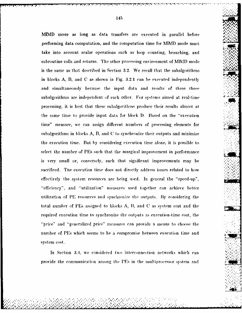
145

MIMD mode as long as data transfers are executed in parallel before

performing data computation, and the computation time for MIMD mode must

take into account scalar operations such as loop counting, branching, and

subroutine calls and returns. The other processing environment of MIMI) mode

is the same as that described in Section 3.2. We recall that the subalgorithms

in blocks A, B, and C as shown in Fig. 3.2.1 can be executed independently

and simultaneously because the input data and results of these three

subalgorithms are independent of each other. For systems aimed at real-time

processing, it is best that. these subalgorithms produce their results almost at

the same tinte to provide input data for block D. Based on the "execution

time" measure, we can assign different numbers of processing elements for

subalgorithms in blocks A, B, and C to synchronize their outputs and minimize

the execution time. But by considering execution time alone, it is possible to

select the number of PEs such that the marginal improvement in performance

is very small or, conversely, such that significant improvements may be

sacrificed. The execution time does not directly address issues related to how

effectively the system resources are being used. In general the "speed-up",

'"efficiency", andi "utilization" measures used together can achieve better

utilization of PE resources and synchroiize the outputs. By considering the

total number of IPEs assigned to blocks A, 1B, and C as system cost and the

required execution time to synchronize the outputs as execution-time cost, the

''price" and "generalized price" measures can )rovide a means to choose the

number of PEs which seems to be a compromise between execution time and

system cost.

In Section 3.1, we considered two interconnection networks which can

provide the communication among the lP's in the mult iprocessor system and

- -.- % ,

146 1J.p~

described how these two networks can be reconfigured as 2 MIIMDs and 1 SINMD

subnetworks to support the system to implement the supervised relaxation WaW.

algorit hmi.

. ' % V s. . S V.-' ~. ~. ~ V c I-. rb~S s.is-. - '/ "-

'47

a a .M' l"%

CHAPTER 4- CONCLUSIONS AND SUGGESTIONS

The supervised relaxation operator was demonstrated successfully as a

mechanism for combining the information from multiple ancillary data sources

with the information from spectral data and spatial context in classifying of

multispectral imagery. In Chapter 2, the method was described and the

convergence of the iterative algorithm was established. The final labeling

results from convergence of evidence, reaching consistent labeling. The key

inputs to the supervised relaxation operator are a quantitative characterization

of initial probabilities computed from the spectral data and conditional

probabilities computed from the contextual information. The initial

probabilities were obtained in the penultimate step of the maximum likelihood -

classification using spectral data; the conditional probabilities were calculated

from another source of data known to be correct. The experimental results

showed that the performance of the method using spatial contextual -..

information was only slightly better than that obtained from the maximum

likelihood classifier; the performance with one ancillary information source was

much better than previously obtained; and the performance measure with two

ancillary information sources was still better. These results demonstrate that

the supervised relaxation algorithm is a useful technique to integrate

information from the various sources and achieve a ground cover classification

....-.......

* * . -.- ~

1 48 ":

%

which is both accurate and consistent in the face of inconsistencies which may

exist among the data components.

In Chapter 3, S-Nets were used to describe the maximum likelihood

algorithm implemented in SIMD and pipeline modes of parallelism. Analysis of

the S-Net models showed that the overhead incurred by the pipeline causes

longer execution time than SIMD mode. PE address and general mask

operations, which for SINID are decoded in the control unit and cost nothing in

the algorithm run time, can also be modeled with S-Nets, as can the data -

transfer time and data transfers through the network.

Some quantitative measures such as average parallelism and execution

time were also developed and used to make direct comparisons between two

architectures. Detailed descriptions and analyses of implicit operations, explicit

operations, loop counting operations, parallel transfers, and interrupt

operations occurring in SIMD and MIMD modes of parallelism were presented

in Section 3.2. Based on these analyses, the comparison of execution times

derived can lead to the right decision concerning which mode of parallelism,

SIMI) or MIND, is best suited to one specific algorithm. In general, algorithms

which have window-type operations and do not have operators whose execution

time are argument-dependent are suitable for SIMD mode because they can

make use of overlap of scalar and array operations, parallel data transfers,

synchronized operation, and simpler control scheme. Algorithms which do nothave window-type operations and have operators whose execution times are

argument-dependent ate best suited to MIMID mode. Even for algorithms .ii

which have window type operations and have operators wbose execution times

are argument-dependent, MIMD mode is still suitable as long as data transfers

can be executed in parallel fashion before performing data computation.

.- -.

149

Section 3.3 described the determination of the optimal number of processing

elements for a given image size based on measures of evaluating the

performance of algorithms for SIMD machines. An important concept is that

the number of PEs can be chosen subject to the relative importance of system

cost and execution time.

Finally, two multistage interconnection networks were described, the cube

network and ADM network, which provide the communication medium for the

multiprocessor system and can be configured to operate as subnetworks

supporting complex tasks.

The neighborhood contributions from the four nearest neighbors have been

used in the current study. For further research, parallel implementations may 7

be developed to utilize neighborhood relations beyond just near neighboring

pixels to combine the contextual information in the algorithm. Equal

weighting corstants, dij , have been assigned to the four nearest neighbors; i.e.,

these four neighboring pixels have equal degree of influence in the

neighborhood contribution. If the weighting constants can be dynamically

adjusted to allow different neighbors to have different degrees of influence on

the current pixel classification, the classification accuracy expected may be

better. Furthermore, in a more complicated cas- in which one ancillary data

source is felt to be more accurate than another, it is possible to assign two

different weighting constants to the ancillary variables in the supervised

relaxation process.

The current modeling based on SIMD and pipeline architectures appears to -

work quite well. A future challenge is to use S-Nets to model control strategies "

or operating systems for various type architectures. Also, further investigations -.

should exploit algorithms on MIMI) architectures and on MSIMD architectures .-..

" o A o

' -VrT 9- 7~UUi

150

in which SIMDs operates asynchronously. If the total elapsed time of the S-

Net the transition sequences and the average parallelism of the S-Net can be

quantitatively determined, together with the description presented in Section

3.2, the results may provide a more reliable way to deci~e which architecture

model is best suited to a particular algorithm.

____________________J_ lipV

LIST.. OF REFRECE

PTWMV*

* -1-7 7 - W .

LIST OF REFERENCES ."

[1] R.M. tloffer and staff, "Computer-aided analysis of SKYLABmultispectral scanner data in mountainous terrain for land use, forestry,water resource, and geologic applications," Tech. Rept. No. 121275,LARS, Purdue University, 1975.

121 J. Richards, D. Landgrebe, and P. Swain, "A means for utilizingancillary information in multispectral classification," Remote Sensing of . -

Environment, Vol. 12, pp. 463-477. 1982. --.

[3] A Rosenfeld, R. lummel and S. Zucker, "Scene labeling by relaxationoperations," IEEE Trans. Syst., Alan, Cybern., Vol. SMC-6, pp. 420-433, -June 1076.

141 B. Schachter, A. Lev, S. Zucker, and A. Rosenfeld, "An application ofrelaxation methods to edge reinforcement," IEEE Trans. Syst., Alan,Cybern., Vol. SMC-7, No. 11, pp. 813-816, Nov. 1977. *1 _

[5] A. Lev, S. Zucker, and A. Rosenfeld, "Iterative enhancement of noisyimages," IEEE Trans. Syst., Alan, and Cybern., Vol. SMC-7, No. 6, pp. .'

435-442, June 1977.

[6] A. Rosenfeld, "Iterative methods in image analysis," Proc. 1978 IEEEConf. Pattern Recognition and Image Processing, pp. 181-187, Jan. 1978. -.

[7] S. Zucker and J. Mohammed, "Analysis of probabilities relaxationlabeling processes," Proc. 1978 IEEhi Conf. Pattern Recognition andImage Processing, pp. 307-312, May 1978.

[8] S. Zucker, E. Krishnamurthy, and R. Haas, "Relaxation processes forscene labeling: convergence, speed, and stability," IEEE Trans. Syst.,Man, Cybern., Vol. SMC-8, No. 1, pp. 41-48, Jan. 1978.

[91 R. Hummel an S. Zucker, "On the foundations of relaxation labelingprocesses, Proc. 1980 IEEE Conf. Pattern Recognition, pp. 50-53, .-

March 1980.

.

~._ 5" '. *

.-. .

[101 S. Peleg and A. Rosenfeld, "Determining compatibility coefficients forcurve enhancement relaxation processes," IEEE Trans. Syst., Mlan,Cybern., Vol. SMC-8, No. 7, pp. 548-555, July 1078.

11) . Yamamnoto, "A method of deriving compatibility coefficients forrelax at ion operators," Computer Graphics and Image Processing, Vol. 10,pp. 256-271, 1979.

112] J. Richards, D. Landgrebe, and P. Swain, "Pixel labeling by supervisedprobabilistic relaxation," IEEE Trans. Pattern Analy. and Machine 7

Intel., Vol. PAMI1-3, No. 2, pp. 188-191, March 1981.

1131 R.A. Huimmel and S.W. Zucker, "On the foundations of relaxationlabeling processes," IEEE Trans. PAM!, Vol. PAMI-5, No. 3, pp. 267-287, May 1083.

[H.] A.J. Krygiel, "Synchronous nets for single instruction stream - multipledata stream computers," D.Sc. dissertation, Sever Institute ofTechnology, Washington University, St. Louis, MO, May 1980.

1151 A. 31. Krygiel, "Synchronous nets for single instruction stream - multipledata stream computers," Proc. 1981 Int'l. Conup. Parallel Processing, xAug. 1981, pp. 266-273.

[16] R.J. McMillen, 11.1. Siegel, "Routing schemes for the augmented data___manipulator network in an MIMI) system," IEEE Trans. Cornpt., Vol.C-31, pp. 1202-121.4, Dec. 1982.

117-1 11.J. Siegel and R..J. McMillen, "Using the augmerited data manipulatornetwork in PASM," Computer, Vol. 14, No. 2, pp. 25-33, Feb. 1981. ..-

[18] HA... Siegel and R.J. Mc~villen, "The multistage2 cube: A versatileinterconnection network," Computer, Vol. 14, No. 12, pp. 65-76, Dec.

10~1 R. N Mcillen andl 11.1. Siegel, "The hybrid cube network," IEEE Proc.of the Distri. Data Acquis., Compu., and Control Slym., pp. 11-22, Dec.

[20] .1. Richards, D. 1Landlgrebe, and P. Swain, "On the accuracy of pixelrelaxation labeling," IEEE Trans. Syst., Alan, and Cybern., Vol. SMC-

* I11. No. -1, pp. 30.3-300, April 1981.

[211 P.11. Swain, "F'undamentals of p~attern recognition in remote sensing," inIermote Sensing: The Quantitative Approach, P. 1-1. Swain and S. M.

N Davis, Eds., MlcGraw-Hlill, New York, 1078.

153 .~ '

'AW

1221 L.J. Siegel, t.J. Siegel, P.. Swain, G.B. Adams II. A.E. Feather, GA."

Lin, and M.R. Warpenburg, "Parallel Image Processing/FeatureExtraction Algorithms and Architecture Emulation: Interim Report forFiscal 1981," TR-EE 81-35, Purdue Univ., School of ElectricalEngineering, Oct. 1981.

[23] J.T. Kuehn, "A more accurate complexity analysis technique," informalcommunications, Sept. 1082......,

[24] L.J. Siegel, I.J. Siegel, and A.E. Feather, "Parallel processingapproaches to image correlation," IEEE Trans. Comput., Vol. C-31, pp.

1251 P.T. Mueller, Jr., L.J. Siegel, and IlI.J. Siegel, "Parallel algorithms forthe two-dimensional FFT," Proc. 5th Int'l. Conf. Pattern Recognition,pp. 497-502, Dec. 1980.

[26] D.L. Tuomenksa, G.B. Adams III, II.J. Siegel, and O.R. Mitchell, "Aparallel algorithm for contour extraction: advantages and architecturalimplications," IEEE Cornput. Soc. Conf. Computer Vision and PatternRecognition, pp. 336-3.14, June 1983.

[27] H.J. Siegel, L.J. Siegel, F.C. Kemmerer, P.T. Mueller, Jr., tt.E. Smalley,Jr., and S.D. Smith, "PASM: A partitionable SIMD/MIMD system forimag.- processing and pattern recognition," IEEE Trans. Comput., Vol.C-30, pp. 03.1-917, Dec. 1981.

[28] R.O. Duda and P.E. Hart, Pattern Classification and Scene Analysis,Wiley, New York, 1973.

[29] L.J. Siegel. Il.J. Siegel, an P.11. Swain, "Performance measures forevaluating algorithms for SINI) machines," IEEE Trans. SoftwareEngineering, Vol. SE-8, pp. 319-331, July 1982.

[301 K.E. Batcher, "MPP - a massively parallel processor," Proc. 1979 Int'lConf Parallel Processing, Aug. 1970, p. 210.

." , - . ..

- ',~rt~r. r., ~ 4- -- u~-~ rc rLw. .- J -v-v w~ r.~-- ~r r -. ~s'r.rs.r. - .- - -- --

.. 44~

A%. b

b .~.

A'4 I~h*

'-.4 .~.

*. *.

4...-.'-

4~.'.~

4. -.4 d.

-: .'v'.1* *?S

r~in7

*44~

.~. -~.4.

i...~

..- *4%~

*: -. ' -..-4.-..

~ -

- - - 4 . . 4 . .

-. 4.- .-. *-'..4 . - ~ .. *.~%'%% .?

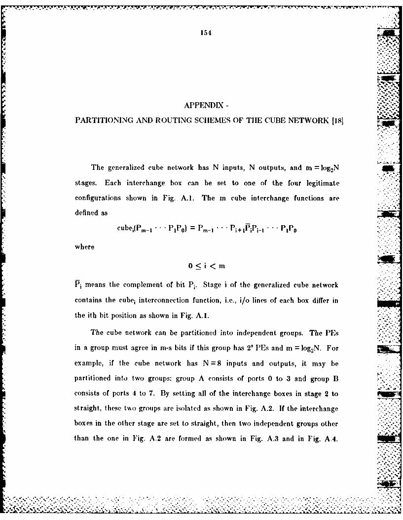
- -' - ., - - . - -,,- -'7. . : , .::- ,J. % f t. , .. , - - .:

.- - , ,; , . . .. _ : . . -v,, i, 'w " - ',.,m~-J " -

154

- ° .°.°q

APPENDIX -

PARTITIONING AND ROUTING SCHEMES OF TIE CUBE NETWORK [18]

The generalized cube network has N inputs, N outputs, and m =log 2N

stages. Each interchange box can be set to one of the four legitimate

configurations shown in Fig. A.I. The m cube interchange functions are

defined as

cubei(Pm- "" PIP0) = P,-1 "" Pi+l~iPi-i ... PP 0 "

where

0 < i < m -..- '

P1 means the complement of bit Pi. Stage i of the generalized cube network

contains the cube i interconnection function, i.e., i/o lines of each box differ in

the ith bit position as shown in Fig. A. .

The cube network can be partitioned into independent groups. The PEs

in a group must agree in m-s bits if this group has 2' PEs and m = log 2N. For

example, if the cube network has N =8 inputs and outputs, it may be

partitioned into two groups: group A consists of ports 0 to 3 and group B

consists of ports 4 to 7. By setting all of the interchange boxes in stage 2 to

straight., these to groups are isolated as shown in Fig. A.2. If the interchange .. :-"

boxes in the other stage are set to straight, then two independent groups other -

than the one in Fig. A.2 are formed as shown in Fig. A.3 and in Fig. A.4.

.. .-..- .-.. .-..

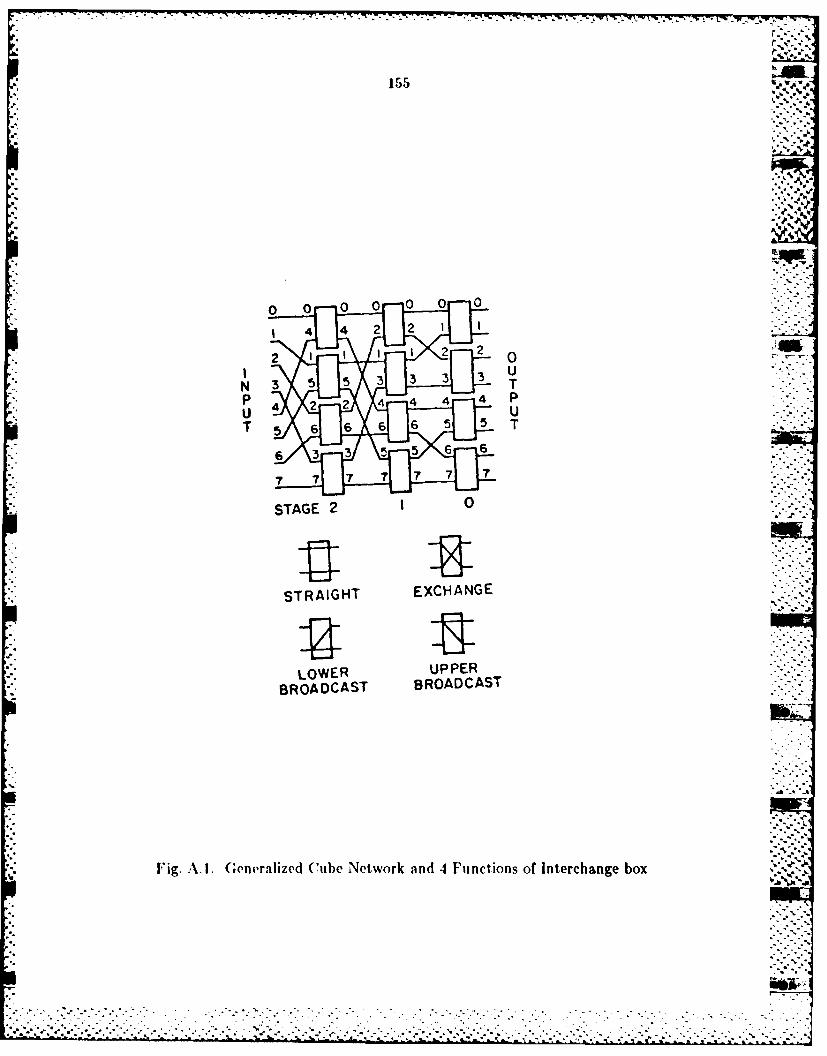
77 ~ ~ ~ TV -717- ."

1556.i

2 0

UU

LOE UPE

BROADCAST6BROADCAT

Fig.~~ 3l Geeaie CueN6okad. uctoso necag o

7 7.7.7

STG 2.

. . . .. . . . . . . . . . . . . T E XCH AN. . .

. . . . . . . . . . . .. . . . . . . ER~.

Fig. A. I. ;ener...............wok..n..4.Fu.ti.ns.of..nerchange bo

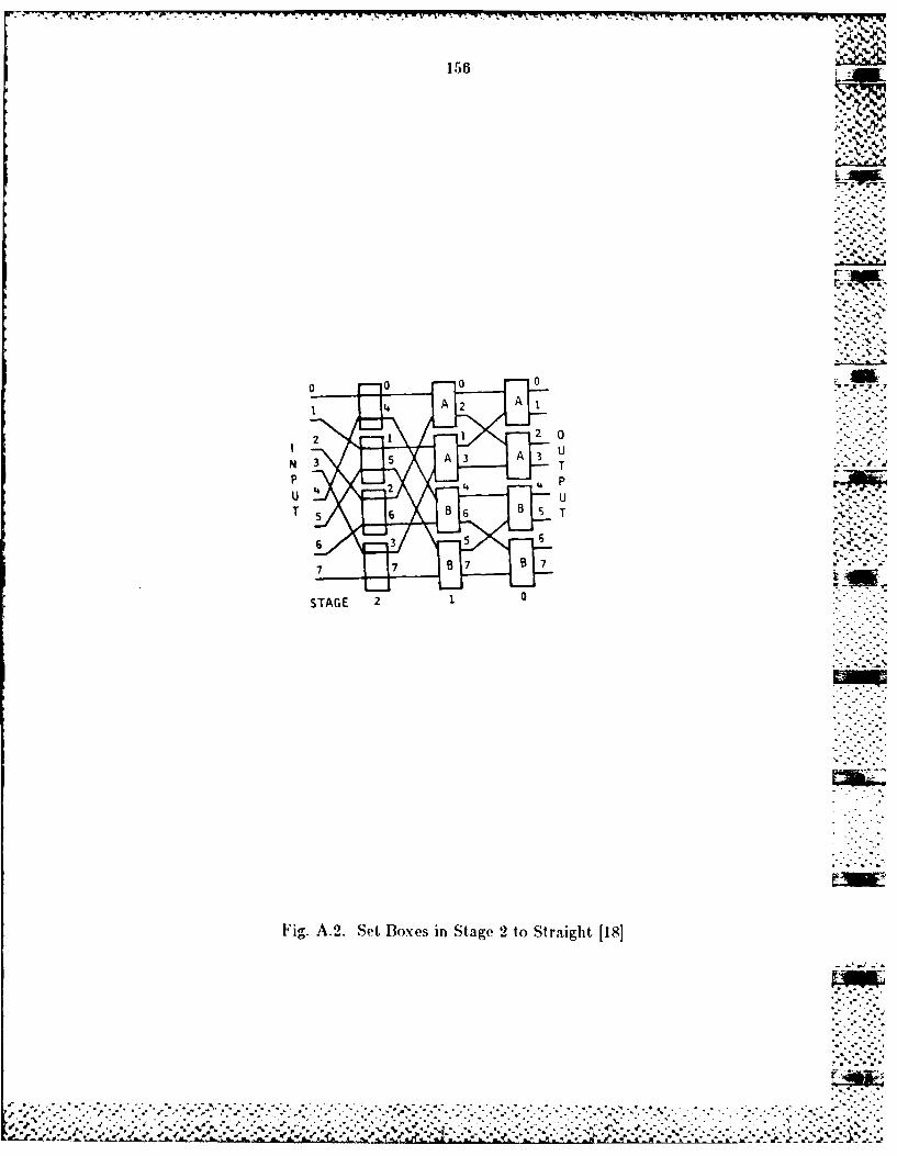
156

, .' ." , .-

N T -f '--"

0 0

...........................-..

4 .A .2

2:::!:::2 .,

N. 3" 5° 3

7-.''.P:

Fig. A.2. Set Boxes in Stage 2 to Straight [18]

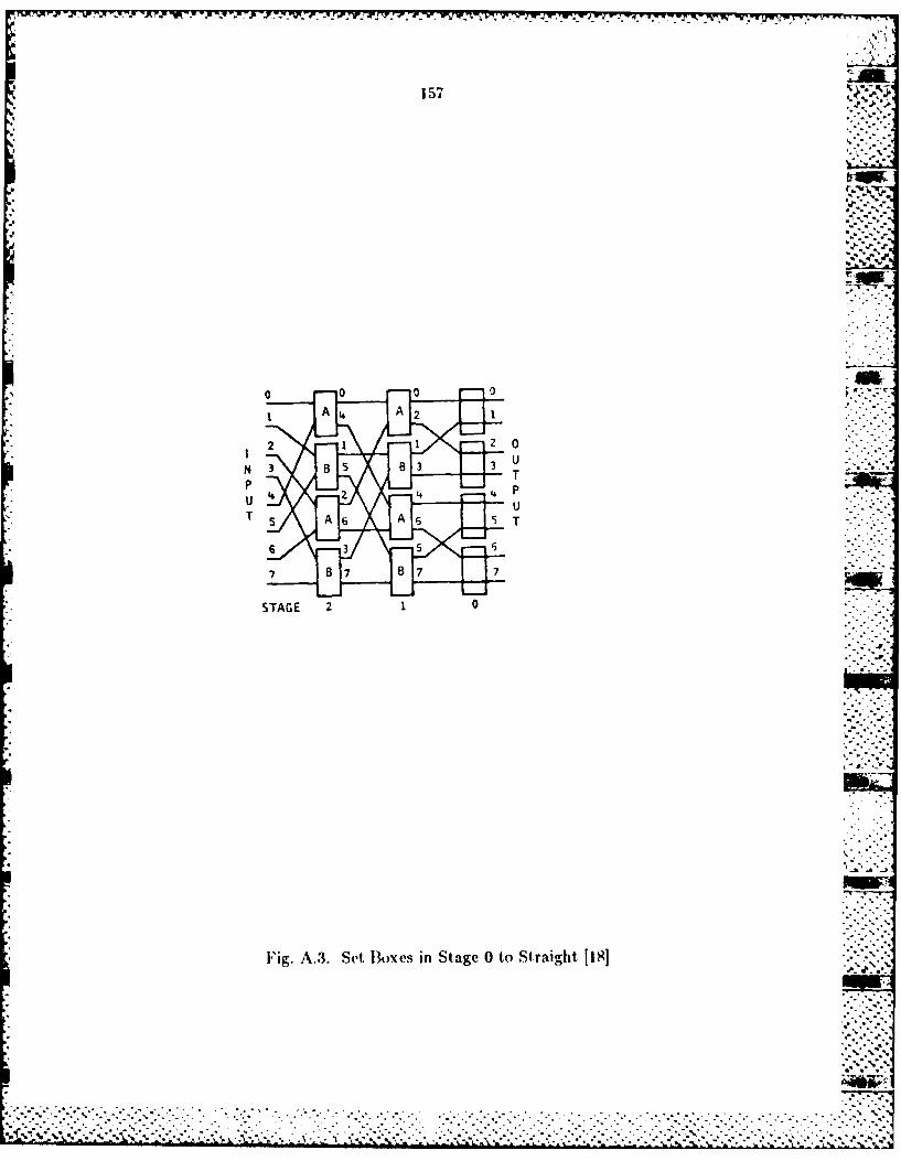
-. ~ ~ ~ ~ ~ ~ ~ ~ ~ ~ ~ ~ ~ ~ ~ ~ I '. r . . pV rq'~'~~' V VdW~V ''-- - ~~

157

2n 0

* u

Fig. A.3. Set Botxes in Stage 0 to Straight [18]

T

p pi

u\ 4 2uC

A C

Fig. AA4 Set B~oxes in Stage I to Straight [181- -

A A A

159

E'ach subnetwork has the properties of a cube network and can be further

subdivided to form smaller independent subnetworks. As shown in Fig. A.5, l

the subnetwork 13 in Fig. A.2 is further divided to form two independent

subtnetwvorks C and I).

Any type of a centralized control unit would create a bottleneck, but if

control is dist ributed among the processors, each is responsible for determining

its own control signals. Therefore, the purpose of using routing tags as headers

()n eIIcssages is to allow network control to be distributed among the processors.

If the processors using the network are configured as an SIMD machine, their

nonl)roa(Icasting communication needs take the form of interconnection

functions. An interconnection function is a specification of the way all of the N

input ports are connected to the N output ports. An interconnection function

is said to be admissible by the network if there are no conflicting requests for

interchange box settings. In establishing an admissible interconnection

funct ion, routing tags are used by all active processors simultaneously. In

MIMI) mode, the routing requests occur at random intervals.

For one-to-one connection, the routing tag, T, is calculated as T S E D

in i'hich S is the inpiit port and D is the output port. The operator G denotes

"exclusive or." For example, if S=5=101 and D=3=011, then

T =S GD = 101 GDo0 = 110. The interchange box in stage i only checks T.

which is the ith bit of routing tag T. If T i = 1, set interchange box to

exchange. If T = 0, set interchange box to straight. Fig. A.6 shows the path

established between input port 5 and output port 3. The incoming tag is also

the same as the return tag. Therefore, it can implement handshaking.

For one-to-many broadcast, the routing tag contains two parts: R contains

routing information and B contains broadcast information. I contains m bits,

................. ' -. a aiiii

d' . . • - • • . ' " • • . i . , .. . . . • . . ". '% " • .• - . ° . " . -.A•-..

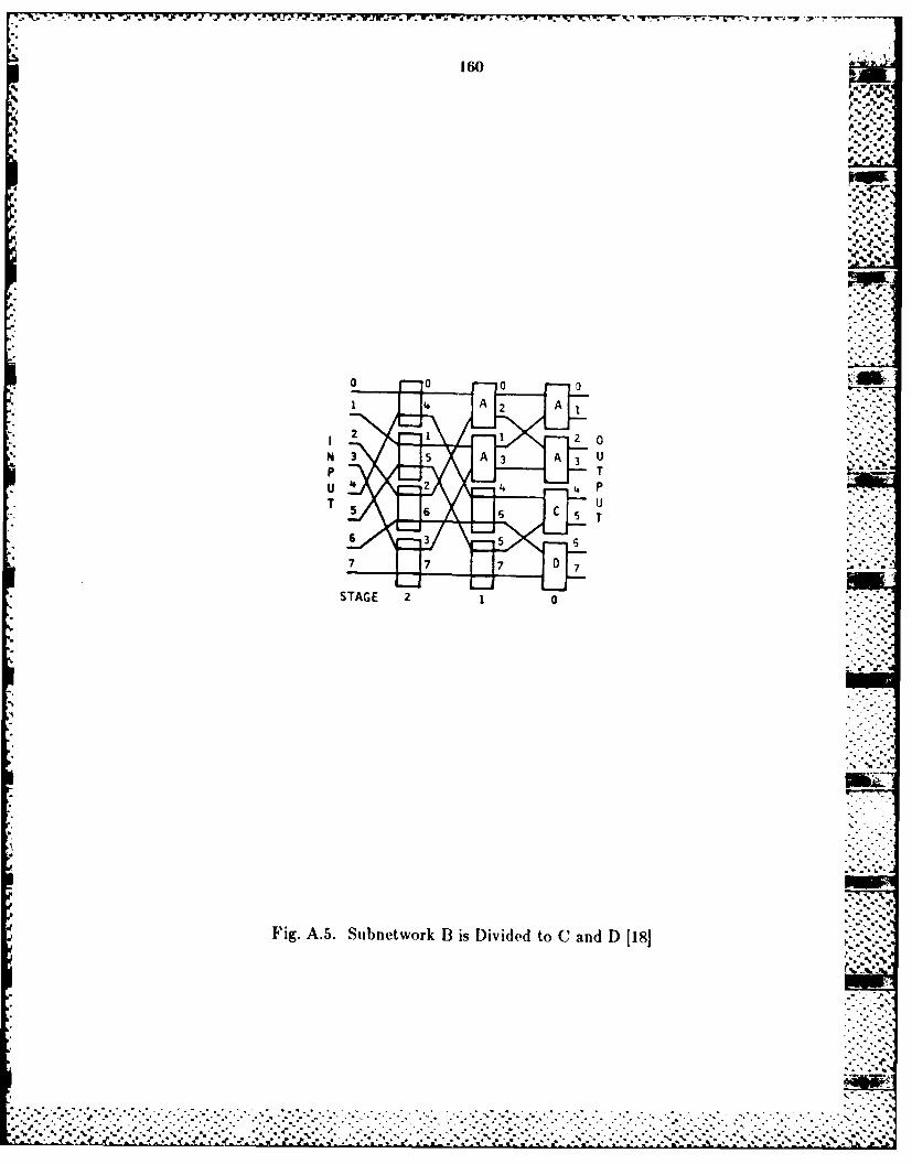
136

I GO

pT

T U

Fig. A.5. Subnetwork 13 is Divided to C and D [8

0U

U

Fig. A.6. Connect Input Port 5 to Output Port 3

.......... 01 (DOI I 10

162

so does B. For b~roadcasting, the destination group must be a group of size

equal to 2J. In this group, there must Ibe at most j bits that disagree among

any pair of the addresses. in(I n-j bit positions in which al11 these addlresses **

must agree. For example, inpult port S =5 =101 broadcasts mnessages to

output ports 2, .3, 6, and 7, in which all addresses agree in the first bit. position

(th e least significant bit is thle 0th lbit). Then,

R =S EDDiS (D,=I101 @00-II where Diis any one of 4 (lest inat ion

addresses and 13 Di D Dk w01 G i ii io10 where Di) and 1)k must have

hamming distance of 2. The interchange boxes in stage i check 13i first. If

=i 1, set interchange box t~o either upper broadcast or lower broadcast. If

Bi =0, then check Ri. If R1 =0, set interchange box to straight, otherwise set

exchange. Fig. A.7 shows input port, S =5, broadcasts messages to output

ports, D = 2, 3,6 and 7.

e- .7 -2

14 163

2TGE 1 0

fl. .7 S= Irada~s esag o =,36,an0

......................... . .

......... ......... .. . . . . . . . .

*~~~ ~~ 4 2. 2.. 4 4...* 4-.... .%*. . .. . . . . . . . . .

* .- *-. -- ~ -

II.A.

A

'.4

p,.

I4-.

4.

I..'.4'

<S

s.f

o~ou

'S

SI.

5'

-S.

* VL.L. .J~ ~ ~.- ~