Anomalous diffusion ofDirac fermions

Proefschrift

ter verkrijging van

de graad van Doctor aan de Universiteit Leiden,op gezag van de Rector Magnificus prof. mr P. F. van der Heijden,

volgens besluit van het College voor Promoties

te verdedigen op woensdag 8 december 2010

te klokke 13.45 uur

door

Christoph Waldemar Grothgeboren te Gdynia, Polen in 1980

Promotiecommissie

Promotor: prof. dr. C. W. J. BeenakkerCo-Promotor: dr. J. Tworzydło (Universiteit van Warschau)

Overige leden: prof. dr. G. T. Barkemaprof. dr. ir. J. W. M. Hilgenkampprof. dr. J. M. van Ruitenbeekdr. X. Waintal (CEA Grenoble)

Casimir PhD Series, Delft-Leiden, 2010-30

ISBN 978-90-8593-090-7

Dit werk maakt deel uit van het onderzoekprogramma van de Stich-ting voor Fundamenteel Onderzoek der Materie (FOM), die deeluit maakt van de Nederlandse Organisatie voor WetenschappelijkOnderzoek (NWO).

This work is part of the research programme of the Foundationfor Fundamental Research on Matter (FOM), which is part of theNetherlands Organisation for Scientific Research (NWO).

The cover shows a snapshot from a simulation of anomalous dif-fusion on a Sierpinski lattice (Chapter 2). The blue and red dotscorrespond, respectively, to occupied and empty sites. Particlesenter the system via the bottom left corner and leave it via thebottom right corner. One can see how obstacles (black triangles)hinder the transport on all length scales.

Contents

1 Introduction 11.1 Normal and anomalous diffusion . . . . . . . . . . . . 1

1.2 Dirac fermions and graphene . . . . . . . . . . . . . 4

1.3 Shot noise of subdiffusion . . . . . . . . . . . . . . . 8

1.4 Discretization of the Dirac equation . . . . . . . . . 10

1.5 Topological insulators . . . . . . . . . . . . . . . . . 15

1.6 Outline of this thesis . . . . . . . . . . . . . . . . . . 18

2 Electronic shot noise in fractal conductors 232.1 Introduction . . . . . . . . . . . . . . . . . . . . . . . 23

2.2 Results and discussion . . . . . . . . . . . . . . . . . 25

2.2.1 Sierpinski lattice . . . . . . . . . . . . . . . . 26

2.2.2 Percolating network . . . . . . . . . . . . . . . 27

2.3 Conclusion . . . . . . . . . . . . . . . . . . . . . . . . 28

Appendix 2.A Calculation of the Fano factor for the tun-nel exclusion process on a two-dimensional network 28

2.A.1 Counting statistics . . . . . . . . . . . . . . . 29

2.A.2 Construction of the counting matrix . . . . . . 31

2.A.3 Extraction of the cumulants . . . . . . . . . . 32

3 Nonalgebraic length dependence of transmission through achain of barriers with a Levy spacing distribution 393.1 Introduction . . . . . . . . . . . . . . . . . . . . . . . 39

3.2 Formulation of the problem . . . . . . . . . . . . . . . 41

3.3 Arbitrary moments . . . . . . . . . . . . . . . . . . . 43

3.4 Scaling with length . . . . . . . . . . . . . . . . . . . 44

3.4.1 Asymptotic expansions . . . . . . . . . . . . 44

3.4.2 Results . . . . . . . . . . . . . . . . . . . . . . 45

v

3.5 Numerical test . . . . . . . . . . . . . . . . . . . . . . 46

3.6 Conclusion and outlook . . . . . . . . . . . . . . . . . 47

4 Finite difference method for transport properties of masslessDirac fermions 514.1 Introduction . . . . . . . . . . . . . . . . . . . . . . . . 51

4.2 Finite difference representation of the transfer matrix 53

4.2.1 Dirac equation . . . . . . . . . . . . . . . . . 53

4.2.2 Discretization . . . . . . . . . . . . . . . . . . 55

4.2.3 Transfer matrix . . . . . . . . . . . . . . . . . 58

4.2.4 Numerical stability . . . . . . . . . . . . . . . 59

4.3 From transfer matrix to scattering matrix and con-ductance . . . . . . . . . . . . . . . . . . . . . . . . . 59

4.3.1 General formulation . . . . . . . . . . . . . . 59

4.3.2 Infinite wave vector limit . . . . . . . . . . . . 61

4.4 Ballistic transport . . . . . . . . . . . . . . . . . . . . 62

4.4.1 Dispersion relation . . . . . . . . . . . . . . . 62

4.4.2 Evanescent modes . . . . . . . . . . . . . . . 64

4.4.3 Conductance . . . . . . . . . . . . . . . . . . 66

4.5 Transport through disorder . . . . . . . . . . . . . . . 67

4.5.1 Scaling of conductance at the Dirac point . . 68

4.5.2 Conductance fluctuations at the Dirac point 70

4.5.3 Transport away from the Dirac point . . . . 72

4.6 Conclusion . . . . . . . . . . . . . . . . . . . . . . . . 74

Appendix 4.A Current conserving discretization of thecurrent operator . . . . . . . . . . . . . . . . . . . . . 76

Appendix 4.B Stable multiplication of transfer matrices 76

Appendix 4.C Crossover from ballistic to diffusive con-duction . . . . . . . . . . . . . . . . . . . . . . . . . . 79

5 Switching of electrical current by spin precession in the firstLandau level of an inverted-gap semiconductor 815.1 Introduction . . . . . . . . . . . . . . . . . . . . . . . . 81

5.2 General theory . . . . . . . . . . . . . . . . . . . . . . 84

5.3 Application to a HgTe quantum well . . . . . . . . . 86

vi

5.4 Conclusion . . . . . . . . . . . . . . . . . . . . . . . . 90

6 Theory of the topological Anderson insulator 936.1 Introduction . . . . . . . . . . . . . . . . . . . . . . . 93

6.2 Model . . . . . . . . . . . . . . . . . . . . . . . . . . . 94

6.3 TAI mechanism . . . . . . . . . . . . . . . . . . . . . 95

6.4 Conclusion . . . . . . . . . . . . . . . . . . . . . . . . . 101

References 103

Summary 115

Samenvatting 119

List of Publications 123

Curriculum Vitæ 125

vii

1 Introduction

1.1 Normal and anomalous diffusion

Diffusion is the spreading of randomly moving particles fromregions with higher concentration to regions with lower concentra-tion. The first class of diffusive processes to have been recognizedhistorically is now known under the name normal diffusion. Itssignature is the linear growth with time of the mean squared dis-placement of a particle from its starting point,⟨

x2⟩ = Dt. (1.1)

On long time scales all normal diffusive processes show the samebehavior and microscopic details of particle dynamics play no roleother than determining the value of the diffusion coefficient D.

The importance and generality of the concept of normal diffu-sion was recognized in the nineteenth century. One of the firstmilestones was the discovery of Brownian motion, the diffusion ofparticles suspended in a fluid, by Scottish botanist Robert Brown in1827 [27]. It was subsequently realized that phenomena seeminglyas different as the spreading of infected mosquitos [107] and theconduction of heat in solids can be described in terms of normaldiffusion.

The driving force for diffusion need not be differences in concen-tration, but can also be a difference in potential energy. Electricalconduction in metals is usually also a normal diffusive process,driven by differences in electrical potential (since differences inelectron concentration would violate charge neutrality) [39].

Though it is a remarkably general concept, normal diffusion failsto describe all diffusive phenomena. Since the 1970s, increasingly

1

processes were found in nature [125] where the mean squareddisplacement of a particle scales as a power of time different fromunity, ⟨

x2⟩ = Dtγ, γ 6= 1. (1.2)

Examples include the foraging patterns of some animals [16], hu-man travel behavior [26], and the spreading of light in a cloudyatmosphere [40]. This kind of diffusion has been termed anomalous,and can occur in two varieties: subdiffusion, where the particlesspread with time arbitrarily slower than normal diffusion (γ < 1),and superdiffusion, where they spread arbitrarily faster (γ > 1, withan upper limit γ = 2 for ballistic motion without any scattering).

Random walks are stochastic processes in which particles movein a sequence of randomly directed steps. The lengths s of thesteps and the duration τ of a step are drawn from a probabilitydistribution P(s, τ). (For simplicity, we assume an isotropic randomwalk, so P is independent of the direction of the step.) For arandom walk to be normal, the variance Var s = 〈s2〉 − 〈s〉2 ofthe step size has to be finite as well as the average duration 〈τ〉.Then, according to the central limit theorem, the mean squaredisplacement after time t will approach a normal distributionwith variance (t/〈τ〉)Var s. This is the reason for the previouslymentioned similarity of all diffusive processes.

If the requirements for a normal random walk are violated,the random walk will be anomalous and the scaling of the meansquared displacement will in general have a power law (1.2) withγ 6= 1. This can occur in several ways (See Ref. [145] for a detailedpresentation).

Superdiffusion happens if the step size distribution P(s) has aheavy tail ∝ 1/s1+α for large s, with 0 < α < 2. If the durationτ = vs is simply proportional to the step size (with constantvelocity v) this leads to superdiffusive behavior with

γ = max(3− α, 2). (1.3)

Such an anomalous random walk is called a Levy walk, afterthe French mathematician Paul Pierre Levy. Alternatively, one

2

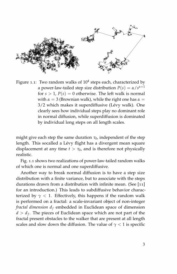
Figure 1.1: Two random walks of 104 steps each, characterized bya power-law-tailed step size distribution P(s) = α/sα+1

for s > 1, P(s) = 0 otherwise. The left walk is normalwith α = 3 (Brownian walk), while the right one has α =

3/2 which makes it superdiffusive (Levy walk). Oneclearly sees how individual steps play no dominant rolein normal diffusion, while superdiffusion is dominatedby individual long steps on all length scales.

might give each step the same duration τ0, independent of the steplength. This socalled a Levy flight has a divergent mean squaredisplacement at any time t > τ0, and is therefore not physicallyrealistic.

Fig. 1.1 shows two realizations of power-law-tailed random walksof which one is normal and one superdiffusive.

Another way to break normal diffusion is to have a step sizedistribution with a finite variance, but to associate with the stepsdurations drawn from a distribution with infinite mean. (See [11]for an introduction.) This leads to subdiffusive behavior charac-terized by γ < 1. Effectively, this happens if the random walkis performed on a fractal: a scale-invariant object of non-integerfractal dimension d f embedded in Euclidean space of dimensiond > d f . The pieces of Euclidean space which are not part of thefractal present obstacles to the walker that are present at all lengthscales and slow down the diffusion. The value of γ < 1 is specific

3

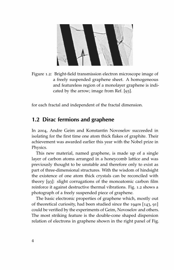
Figure 1.2: Bright-field transmission electron microscope image ofa freely suspended graphene sheet. A homogeneousand featureless region of a monolayer graphene is indi-cated by the arrow; image from Ref. [93].

for each fractal and independent of the fractal dimension.

1.2 Dirac fermions and graphene

In 2004, Andre Geim and Konstantin Novoselov succeeded inisolating for the first time one atom thick flakes of graphite. Theirachievement was awarded earlier this year with the Nobel prize inPhysics.

This new material, named graphene, is made up of a singlelayer of carbon atoms arranged in a honeycomb lattice and waspreviously thought to be unstable and therefore only to exist aspart of three-dimensional structures. With the wisdom of hindsightthe existence of one atom thick crystals can be reconciled withtheory [93]: slight corrugations of the monoatomic carbon filmreinforce it against destructive thermal vibrations. Fig. 1.2 shows aphotograph of a freely suspended piece of graphene.

The basic electronic properties of graphene which, mostly outof theoretical curiosity, had been studied since the 1940s [143, 91]could be verified by the experiments of Geim, Novoselov and others.The most striking feature is the double-cone shaped dispersionrelation of electrons in graphene shown in the right panel of Fig.

4

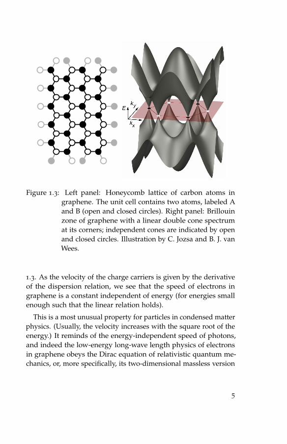
Figure 1.3: Left panel: Honeycomb lattice of carbon atoms ingraphene. The unit cell contains two atoms, labeled Aand B (open and closed circles). Right panel: Brillouinzone of graphene with a linear double cone spectrumat its corners; independent cones are indicated by openand closed circles. Illustration by C. Jozsa and B. J. vanWees.

1.3. As the velocity of the charge carriers is given by the derivativeof the dispersion relation, we see that the speed of electrons ingraphene is a constant independent of energy (for energies smallenough such that the linear relation holds).

This is a most unusual property for particles in condensed matterphysics. (Usually, the velocity increases with the square root of theenergy.) It reminds of the energy-independent speed of photons,and indeed the low-energy long-wave length physics of electronsin graphene obeys the Dirac equation of relativistic quantum me-chanics, or, more specifically, its two-dimensional massless version

5

−ihv(

0 ∂x − i∂y

∂x + i∂y 0

)(ΨAΨB

)= E

(ΨAΨB

). (1.4)

The A and B components of the wave function correspond toexcitations on the two sublattices of the honecomb lattice (see leftpanel of Fig. 1.3) and form a spin-like degree of freedom calledpseudospin. The velocity v is the effective speed of light which ingraphene is about 106 m/s or 1/300 of the true speed of light.

Definition of the vector of Pauli matrices σ = (σx, σy, σz) allowsto express Eq. (1.4) in the compact form

vp · σ ψ = Eψ, (1.5)

with the momentum operator p = −ih(∂x, ∂y) and the spinor ψ =

(ΨA, ΨB). Electrons governed by Dirac equation are called Diracfermions.

The Dirac equation has only a single Dirac cone, while the disper-sion relation of graphene shown in the right panel of Fig. 1.3 hastwo independent cones called valleys. (Adjacent cones are indepen-dent, while next-nearest-neighbors are equivalent upon translationby a reciprocal lattice vector.) The existence of two independentcones is accounted for by the valley degree of freedom and thefull1 low energy physics has to be described by a four componentspinor Ψ = (ΨA, ΨB,−Ψ′B, Ψ′A) satisfying the four-dimensionalDirac equation (

vp · σ 00 vp · σ

)Ψ = EΨ. (1.6)

In the low-energy limit described by the Dirac equation the twovalleys are decoupled, but in real graphene inter-valley scatteringcan occur by potential features which are sharp on the atomic scale.

The Dirac equation gives rise to unusual transport properties.Because the speed of Dirac particles is independent of their energy,

1The true spin degree of freedom of electrons is still missing, but it only weaklycoupled to the dynamics and can be ignored.

6

0

0.5

1

0.01 0.1 1 10 100

K0

(L/W

)〈G〉×

h/4e2

a)

L/a = 40 72Nimp/Ntot= 0.022

0.045�◦

�

���

Anderson

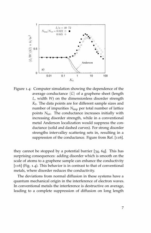
Figure 1.4: Computer simulation showing the dependence of theaverage conductance 〈G〉 of a graphene sheet (lengthL, width W) on the dimensionless disorder strengthK0. The data points are for different sample sizes andnumber of impurities Nimp per total number of latticepoints Ntot. The conductance increases initially withincreasing disorder strength, while in a conventionalmetal Anderson localization would suppress the con-ductance (solid and dashed curves). For strong disorderstrengths intervalley scattering sets in, resulting in asuppression of the conductance. Figure from Ref. [116].

they cannot be stopped by a potential barrier [34, 64]. This hassurprising consequences: adding disorder which is smooth on thescale of atoms to a graphene sample can enhance the conductivity[116] (Fig. 1.4). This behavior is in contrast to that of conventionalmetals, where disorder reduces the conductivity.

The deviations from normal diffusion in these systems have aquantum mechanical origin in the interference of electron waves.In conventional metals the interference is destructive on average,leading to a complete suppression of diffusion on long length

7

scales. This is the celebrated localization effect discovered byPhilip Anderson in 1957 [9]. For Dirac fermions the interferenceis constructive on average, which is at the origin of the enhancedconductivity seen in Fig. 1.4.

1.3 Shot noise of subdiffusion

Conductance, the ratio between applied voltage and the resultingtime-averaged current, is the basic quantity measured in electronictransport experiments. How does the conductance of a diffusived-dimensional system scale with its linear size L? For normaldiffusion, the answer is given by Ohm’s law,

G = σLd−2. (1.7)

The proportionality constant σ is the conductivity.Transport by anomalous diffusion is fundamentally different: the

conductance depends on L with a different power than in Eq. 1.7.As a consequence, the conductivity becomes scale dependent.

In the case of subdiffusion on fractals the conductance scales as(reviewed in Refs. [135, 111])

G ∝ Ld f−2/γ, (1.8)

with γ the exponent that governs the mean-square displacement inEq. (1.2). Note that diffusion on a fractal is not just normal diffusionin a medium with non-integer dimension d f . In that case, onewould expect G to scale as Ld f−2. Because γ is smaller than 1 forsubdiffusion, conduction is suppressed stronger than would beexpected solely on the basis of the fractal dimension.

Given the special scaling of conductance with length for subdif-fusion, one might ask how other transport properties scale. Whilethe time-averaged current determines the conductance, the time-dependent fluctuations determine the shot noise power S. In termsof the charge Q transmitted in a time τ, one has

S = limτ→∞

2⟨δQ2⟩ /τ. (1.9)

8

The shot noise power is proportional to the applied voltage andhence to the mean current

I = limτ→∞〈Q〉 /τ. (1.10)

The ratio F = S/2eI is called the Fano factor. The Fano factoris unity in the case where completely uncorrelated particles aretransmitted. Then, Q is Poisson-distributed which leads to F = 1.A value F > 1 indicates bunching of charge carriers (particlestend to arrive in groups more often than in the uncorrelated case),whereas F < 1 is a signature of anti-bunching (particles arriveless often in groups). Anti-bunching of electrons is a consequenceof the Pauli exclusion principle, which prevents two electrons tooccupy the same quantum mechanical state. For normal diffusionthe Pauli principle produces a Fano factor F = 1/3 [18, 96].

What is the Fano factor for subdiffusion on fractals? Shot noiseon fractals has been studied previously under circumstances thatthe Pauli principle is not operative, because the average occupationof a quantum state is much smaller than unity. (This is called anondegenerate electron gas.) One example is the regime of high-voltage transport modeled by hopping conduction. Then I and Sscale differently with L, so that the Fano factor is scale dependent.(See Fig. 1.5.) The Pauli principle is expected to govern the shotnoise for diffusive conduction in the regime of low voltages andlow temperatures, when the average occupation of a quantum stateis of order unity (a degenerate electron gas).

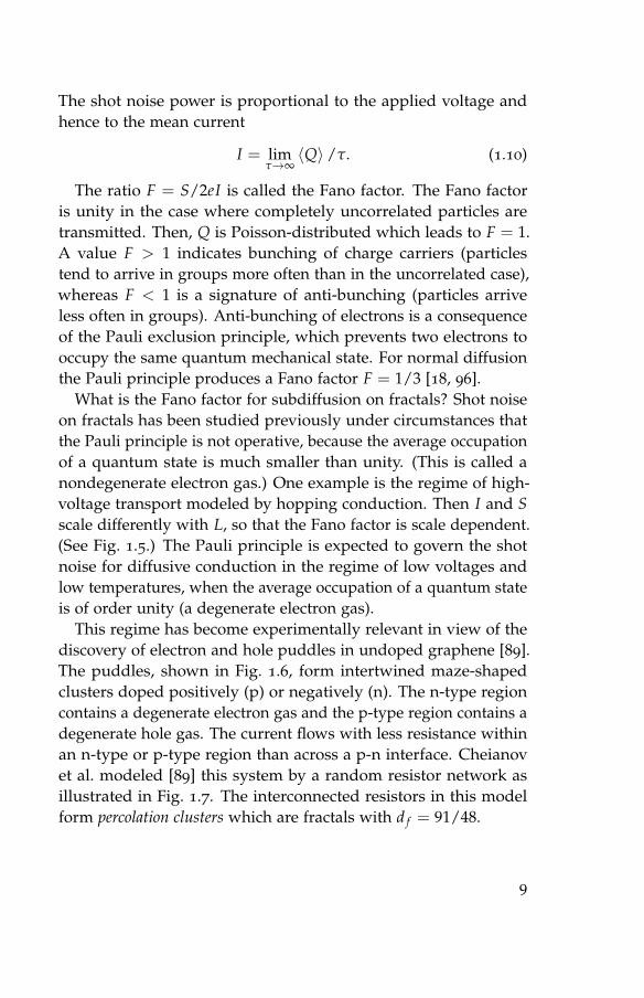
This regime has become experimentally relevant in view of thediscovery of electron and hole puddles in undoped graphene [89].The puddles, shown in Fig. 1.6, form intertwined maze-shapedclusters doped positively (p) or negatively (n). The n-type regioncontains a degenerate electron gas and the p-type region contains adegenerate hole gas. The current flows with less resistance withinan n-type or p-type region than across a p-n interface. Cheianovet al. modeled [89] this system by a random resistor network asillustrated in Fig. 1.7. The interconnected resistors in this modelform percolation clusters which are fractals with d f = 91/48.

9

Figure 1.5: Fano factor as function of sample size from a MonteCarlo simulation of two-dimensional hopping througha disordered conductor. The Fano factor is scale depen-dent because the average current and the noise powerscale with a different power of the sample size. Figurefrom Ref. [68].

Several experiments have studied the Fano factor of graphenerecently. Measurements from two of these experiments, performedby Danneau et al. in Helsinki [37] and by DiCarlo et al. in Harvard[41] are shown in Figs. 1.8 and 1.9, respectively. In the Helsinkiexperiment the Fano factor depends strongly on doping, witha peak value of 1/3, while the Harvard measurements show adoping-independent Fano factor of 1/3. The theory for shot noiseon a fractal developed in this thesis offers a way to reconcile thesetwo conflicting experiments.

1.4 Discretization of the Dirac equation

The standard model for graphene is the tight-binding approxi-mation, in which the hopping of electrons between overlappingorbitals of the atoms constituting the carbon sheet is directly con-

10

Figure 1.6: Experimentally determined color map of the spatialcarrier density variations in a graphene flake. Blueregions correspond to hole doping (p-type) and redregions to electron doping (n-type). The black contourmarks the p-n interface. Figure from Ref. [89].

sidered. This model is widely used to study the properties ofgraphene numerically. It can recover all electronic properties ofthe material, but is viable for small flakes only, as the computationtimes grow quickly with the number of atoms. To allow computermodeling of larger flakes of graphene and to probe the physicsof a single Dirac cone, it would be useful to simulate the Diracequation (1.4) directly, and not only as the low-energy limit ofthe tight-binding model. For this, the Dirac equation needs to bediscretized, i.e. put on a lattice. This can be done in real space or inmomentum space. The momentum space approach was developedin Refs. [13] and [99], while the real-space approach is developedin this thesis.

The discretization of the Dirac equation is notoriously difficult,because of the socalled fermion doubling problem [98]. The moststraightforward way to discretize the Dirac equation in real space isto define the wave function ψ(x, y) on a rectangular grid with lattice

11

Figure 1.7: Random resistor network representation of a graphenesheet with average zero doping. The conductance is gwithin an n-type or p-type region (red or blue lines),and has a smaller value across a p-n interface. (Thesymbol γ used in this figure is unrelated to the random-walk exponent.) Figure from Ref. [35].

constant a and to replace the derivatives with finite differences,

∂xψ→ ψ(x + a, y)− ψ(x− a, y)2a

, (1.11)

∂yψ→ ψ(x, y + a)− ψ(x, y− a)2a

. (1.12)

This discretization fails to describe the physics of a single Diraccone.

To see this, let us look at the dispersion relation of the discretizedequation. For simplicity, we consider only plane waves moving inthe x direction, so that ky = 0. Such plane waves have the generalform

ψ = ψ0 e±ikxx. (1.13)

Inserting this into the Dirac equation (1.4) with the substitutions

12

Figure 1.8: Results from a transport experiment performed by R.Danneau et al. on a graphene sheet. The measurementsare consistent with theoretical predictions for ballistictransport at the Dirac point [141]. Left panel: Resis-tance and conductivity as a function of gate voltage andcharge carrier density. The conductivity at the Diracpoint reaches the expected value 4e2/πh. Right panel:Fano factor as function of charge carrier density. At theDirac point, the value 1/3 is reached with F falling offfor both positive and negative doping. Figures from Ref.[37].

(1.11) and (1.12) gives the dispersion relation

E = ± hva

sin ka, (1.14)

plotted as the solid curve of Fig. 1.10.We see that unphysical low-energy states, forming a second

Dirac cone, have appeared around kxa = ±π, ky = 0. There aretwo additional cones, one around kxa = 0, kya = ±π, and onearound kxa = ±π, kya = ±π, giving four in total in the firstBrillouin zone. These additional states are due to the fact that the

13

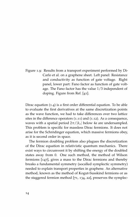
Figure 1.9: Results from a transport experiment performed by Di-Carlo et al. on a graphene sheet. Left panel: Resistanceand conductivity as function of gate voltage. Rightpanel, lower part: Fano factor as function of gate volt-age. The Fano factor has the value 1/3 independent ofdoping. Figure from Ref. [41].

Dirac equation (1.4) is a first order differential equation. To be ableto evaluate the first derivatives at the same discretization pointsas the wave function, we had to take differences over two latticesites in the difference operators (1.11) and (1.12). As a consequence,waves with a spatial period 2π/|kx| below 4a are undersampled.This problem is specific for massless Dirac fermions. It does notarise for the Schrodinger equation, which massive fermions obey,as it is second order in space.

The fermion doubling problem also plagues the discretizationof the Dirac equation in relativistic quantum mechanics. Thereexist ways to circumvent it by shifting the energy of the doubledstates away from 0. One such method, the method of Wilsonfermions [147], gives a mass to the Dirac fermions and therebybreaks a fundamental symmetry (socalled symplectic symmetry)needed to explain transport properties in graphene. An alternativemethod, known as the method of Kogut-Susskind fermions or asthe staggered fermion method [71, 134, 22], preserves the symplec-

14

−2

−1

0

1

2

−π 0 π

Ea/

hv

kxa

Figure 1.10: Solid curve: dispersion relation of the naively dis-cretized Dirac equation showing fermion doubling: asecond Dirac cone appears at kx = ±π. Dashed curve:dispersion relation of the Dirac equation discretizedaccording to the method of staggered fermions. Theenergy of the unphysical states at kx = ±π has beenshifted away to ±∞.

tic symmetry and is therefore the method which we will apply tographene.

The dashed curve of Fig. 1.10 shows the dispersion relation ofthe Dirac equation discretized according to the staggered fermionmethod. The spurious Dirac cone has disappeared.

1.5 Topological insulators

In 1980 Klaus von Klitzing discovered that the conductance ofthin semiconductor layers at low temperatures and large perpen-dicular magnetic fields is quantized in integer multiples of theconductance quantum e2/h [69]. The mechanism for this quantumHall effect is illustrated in the left panel of Fig. 1.11 and can bedescribed as follows: Under the influence of the magnetic field the

15

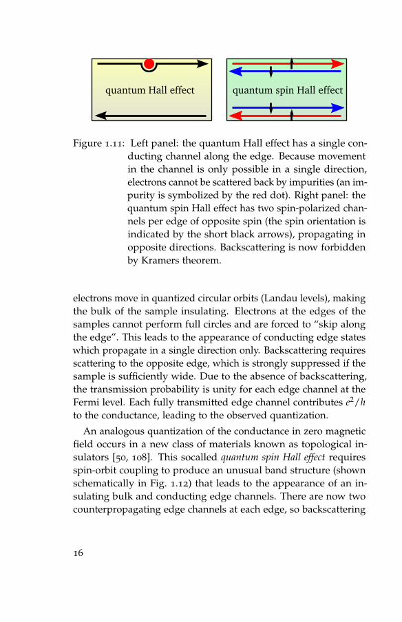
quantum Hall effect quantum spin Hall effect

Figure 1.11: Left panel: the quantum Hall effect has a single con-ducting channel along the edge. Because movementin the channel is only possible in a single direction,electrons cannot be scattered back by impurities (an im-purity is symbolized by the red dot). Right panel: thequantum spin Hall effect has two spin-polarized chan-nels per edge of opposite spin (the spin orientation isindicated by the short black arrows), propagating inopposite directions. Backscattering is now forbiddenby Kramers theorem.

electrons move in quantized circular orbits (Landau levels), makingthe bulk of the sample insulating. Electrons at the edges of thesamples cannot perform full circles and are forced to “skip alongthe edge”. This leads to the appearance of conducting edge stateswhich propagate in a single direction only. Backscattering requiresscattering to the opposite edge, which is strongly suppressed if thesample is sufficiently wide. Due to the absence of backscattering,the transmission probability is unity for each edge channel at theFermi level. Each fully transmitted edge channel contributes e2/hto the conductance, leading to the observed quantization.

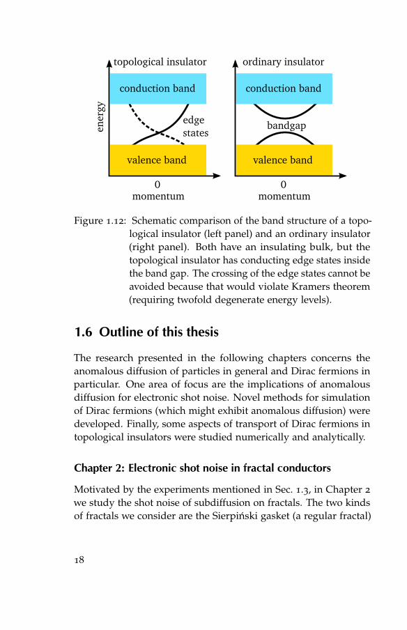
An analogous quantization of the conductance in zero magneticfield occurs in a new class of materials known as topological in-sulators [50, 108]. This socalled quantum spin Hall effect requiresspin-orbit coupling to produce an unusual band structure (shownschematically in Fig. 1.12) that leads to the appearance of an in-sulating bulk and conducting edge channels. There are now twocounterpropagating edge channels at each edge, so backscattering

16

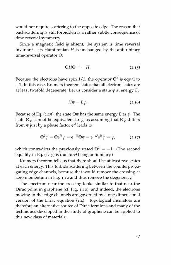
would not require scattering to the opposite edge. The reason thatbackscattering is still forbidden is a rather subtle consequence oftime reversal symmetry.

Since a magnetic field is absent, the system is time reversalinvariant – its Hamiltonian H is unchanged by the anti-unitarytime-reversal operator Θ:

ΘHΘ−1 = H. (1.15)

Because the electrons have spin 1/2, the operator Θ2 is equal to−1. In this case, Kramers theorem states that all electron states areat least twofold degenerate: Let us consider a state ψ at energy E,

Hψ = Eψ. (1.16)

Because of Eq. (1.15), the state Θψ has the same energy E as ψ. Thestate Θψ cannot be equivalent to ψ, as assuming that Θψ differsfrom ψ just by a phase factor eiδ leads to

Θ2ψ = Θeiδψ = e−iδΘψ = e−iδeiδψ = ψ, (1.17)

which contradicts the previously stated Θ2 = −1. (The secondequality in Eq. (1.17) is due to Θ being antiunitary.)

Kramers theorem tells us that there should be at least two statesat each energy. This forbids scattering between the counterpropa-gating edge channels, because that would remove the crossing atzero momentum in Fig. 1.12 and thus remove the degeneracy.

The spectrum near the crossing looks similar to that near theDirac point in graphene (cf. Fig. 1.10), and indeed, the electronsmoving in the edge channels are governed by a one-dimensionalversion of the Dirac equation (1.4). Topological insulators aretherefore an alternative source of Dirac fermions and many of thetechniques developed in the study of graphene can be applied tothis new class of materials.

17

conduction band

valence band

edgestates

bandgap

0

topological insulator

momentum

ener

gy

conduction band

valence band

0

ordinary insulator

momentum

Figure 1.12: Schematic comparison of the band structure of a topo-logical insulator (left panel) and an ordinary insulator(right panel). Both have an insulating bulk, but thetopological insulator has conducting edge states insidethe band gap. The crossing of the edge states cannot beavoided because that would violate Kramers theorem(requiring twofold degenerate energy levels).

1.6 Outline of this thesis

The research presented in the following chapters concerns theanomalous diffusion of particles in general and Dirac fermions inparticular. One area of focus are the implications of anomalousdiffusion for electronic shot noise. Novel methods for simulationof Dirac fermions (which might exhibit anomalous diffusion) weredeveloped. Finally, some aspects of transport of Dirac fermions intopological insulators were studied numerically and analytically.

Chapter 2: Electronic shot noise in fractal conductors

Motivated by the experiments mentioned in Sec. 1.3, in Chapter 2

we study the shot noise of subdiffusion on fractals. The two kindsof fractals we consider are the Sierpinski gasket (a regular fractal)

18

and random planar resistor networks which arise from a model ofgraphene. We determine the scaling with size L of the shot noisepower S due to elastic scattering in a fractal conductor. We finda power-law scaling S ∝ Ld f−2/γ, with an exponent depending onthe fractal dimension d f and the anomalous diffusion exponent2

γ. This is the same scaling as the time-averaged current I, whichimplies that the Fano factor F = S/2eI is scale independent. Weobtain a value F = 1/3 for anomalous diffusion that is the sameas for normal diffusion, even if there is no smallest length scalebelow which the normal diffusion equation holds. The fact that Fremains fixed at 1/3 as one crosses the percolation threshold in arandom-resistor network may explain measurements of a doping-independent Fano factor in a graphene flake [41].

Chapter 3: Nonalgebraic length dependence of transmissionthrough a chain of barriers with a Levy spacing distribution

In Chapter 3 we analyze transport through a linear chain of barrierswith independent spacings s drawn from a heavy-tailed Levy distri-bution. We are motivated by the recent realization of a “Levy glass”[15] (a three-dimensional optical material with a Levy distributionof scattering lengths) of which our system is a one-dimensionalanalogue. The step length distribution of particles in our systemalso has a heavy tail, P(s) ∝ s−1−α for s → ∞, but strong corre-lations exist between subsequent steps because the same spacebetween two barriers will often be traversed back after a particlegets scattered by a barrier. We show that a random walk alongsuch a sparse chain is not a Levy walk because of these correlations.Thus, by working in the lowest possible dimension, we can providea worst-case estimate for the effect of the correlations in higherdimensions.

We calculate all moments of conductance (or transmission), inthe regime of incoherent sequential tunneling through the barriers.

2In Chapter 2 the symbol α is used for a differently defined anomalous diffusionexponent: α = 1/γ− 2.

19

The average transmission from one barrier to a point at a distanceL scales as L−α ln L for 0 < α < 1. The corresponding electronicshot noise has a Fano factor that approaches 1/3 very slowly, with1/ ln L corrections.

Chapter 4: Finite difference method for transport propertiesof massless Dirac fermions

As shown in Sec. 1.4, a straightforward discretization of the mass-less Dirac equation fails because of the fermion doubling problem.In Chapter 4 we adapt a finite difference method of solution, de-veloped in the context of lattice gauge theory, to the calculationof electrical conduction in a graphene sheet or on the surface of atopological insulator. The discretized Dirac equation retains a sin-gle Dirac point (no fermion doubling), avoids intervalley scatteringas well as trigonal warping (a triangular distortion of the conicalband structure that breaks the momentum inversion symmetry),and thus preserves the single-valley time reversal symmetry (=symplectic symmetry) at all length scales and energies. This comesat the expense of a nonlocal finite difference approximation of thedifferential operator. We demonstrate the symplectic symmetryby calculating the scaling of the conductivity with sample size,obtaining the logarithmic increase due to antilocalization. We alsocalculate the sample-to-sample conductance fluctuations as well asthe shot noise power, and compare with analytical predictions.

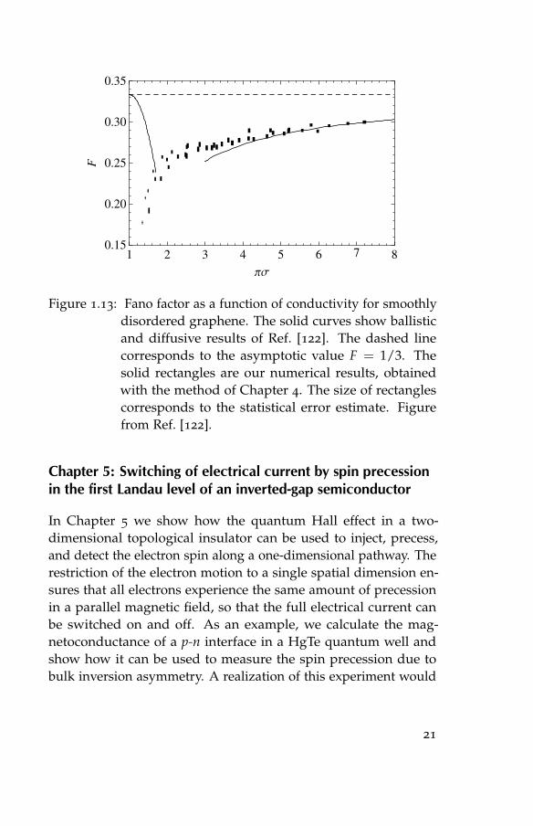
Our numerical results are in good agreement with a recent theoryof transport in smoothly disordered graphene by Schuessler et al.[122]. Fig. 1.13 compares their analytical results (solid curve) withour numerical data (rectangles). The same numerical results wereused to prepare Fig. 4.12.

20

1 2 3 4 5 6 7 80.15

0.20

0.25

0.30

0.35

ΠΣ

F

Figure 1.13: Fano factor as a function of conductivity for smoothlydisordered graphene. The solid curves show ballisticand diffusive results of Ref. [122]. The dashed linecorresponds to the asymptotic value F = 1/3. Thesolid rectangles are our numerical results, obtainedwith the method of Chapter 4. The size of rectanglescorresponds to the statistical error estimate. Figurefrom Ref. [122].

Chapter 5: Switching of electrical current by spin precessionin the first Landau level of an inverted-gap semiconductor

In Chapter 5 we show how the quantum Hall effect in a two-dimensional topological insulator can be used to inject, precess,and detect the electron spin along a one-dimensional pathway. Therestriction of the electron motion to a single spatial dimension en-sures that all electrons experience the same amount of precessionin a parallel magnetic field, so that the full electrical current canbe switched on and off. As an example, we calculate the mag-netoconductance of a p-n interface in a HgTe quantum well andshow how it can be used to measure the spin precession due tobulk inversion asymmetry. A realization of this experiment would

21

provide a unique demonstration of full-current switching by spinprecession.

Chapter 6: Theory of the topological Anderson insulator

In Chapter 6 we present an effective medium theory that explainsthe disorder-induced transition into a phase of quantized conduc-tance, discovered in computer simulations of HgTe quantum wells[81]. Depending on the width of their innermost layer, such quan-tum wells are two-dimensional topological insulators or ordinaryinsulators. Our theory explains how the combination of a randompotential and quadratic corrections ∝ p2σz to the Dirac Hamiltoniancan drive an ordinary band insulator into a topological insulator(having conducting edge states). We calculate the location of thephase boundary at weak disorder and show that it correspondsto the crossing of a band edge rather than a mobility edge. Ourmechanism for the formation of a topological Anderson insulator isgeneric, and would apply as well to three-dimensional semiconduc-tors with strong spin-orbit coupling. It has indeed been adapted tothat case recently [49].

22

2 Electronic shot noise in fractalconductors

2.1 Introduction

Diffusion in a medium with a fractal dimension is characterizedby an anomalous scaling with time t of the root-mean-squareddisplacement ∆. The usual scaling for integer dimensionality d is∆ ∝ t1/2, independent of d. If the dimensionality d f is noninteger,however, an anomalous scaling

∆ ∝ t1/(2+α) (2.1)

with α > 0 may appear. This anomaly was discovered in the early1980’s [144, 7, 21, 46, 109] and has since been studied extensively(see Refs. [53, 57] for reviews). Intuitively, the slowing down ofthe diffusion can be understood as arising from the presence ofobstacles at all length scales – characteristic of a selfsimilar fractalgeometry.

A celebrated application of the theory of fractal diffusion is tothe scaling of electrical conduction in random-resistor networks(reviewed in Refs. [135, 111]). According to Ohm’s law, the con-ductance G should scale with the linear size L of a d-dimensionalnetwork as G ∝ Ld−2. In a fractal dimension the scaling is modifiedto G ∝ Ld f−2−α, depending both on the fractal dimensionality d fand on the anomalous diffusion exponent α. At the percolationthreshold, the known [53] values for d = 2 are d f = 91/48 andα = 0.87, leading to a scaling G ∝ L−0.97. This almost inverse-linearscaling of the conductance of a planar random-resistor network

23

contrasts with the L-independent conductance G ∝ L0 predicted byOhm’s law in two dimensions.

All of this body of knowledge applies to classical resistors, withapplications to disordered semiconductors and granular metals[128, 29]. The quantum Hall effect provides one quantum me-chanical realization of a random-resistor network [140], in a ratherspecial way because time-reversal symmetry is broken by the mag-netic field. Recently [35], Cheianov, Fal’ko, Altshuler, and Aleinerannounced an altogether different quantum realization in zeromagnetic field. Following experimental [89] and theoretical [56]evidence for electron and hole puddles in undoped graphene1,Cheianov et al. modeled this system by a degenerate electron gas2

in a random-resistor network. They analyzed both the high-tempe-rature classical resistance, as well as the low-temperature quantumcorrections, using the anomalous scaling laws in a fractal geometry.

These recent experimental and theoretical developments openup new possibilities to study quantum mechanical aspects of frac-tal diffusion, both with respect to the Pauli exclusion principleand with respect to quantum interference (which are operative indistinct temperature regimes). To access the effect of the Pauli prin-ciple one needs to go beyond the time-averaged current I (studiedby Cheianov et al. [35]), and consider the time-dependent fluctua-tions δI(t) of the current in response to a time-independent appliedvoltage V. These fluctuations exist because of the granularity ofthe electron charge, hence their name “shot noise” (for reviews, see

1Graphene is a single layer of carbon atoms, forming a two-dimensional honey-comb lattice. Electrical conduction is provided by overlapping π-orbitals, withon average one electron per π-orbital in undoped graphene. Electron puddleshave a little more than one electron per π-orbital (n-type doping), while holepuddles have a little less than one electron per π-orbital (p-type doping).

2An electron gas is called “degenerate” if the average occupation number of aquantum state is either close to unity or close to zero. It is called “nondegen-erate” if the average occupation number is much smaller than unity for allstates.

24

Refs. [24, 19]). Shot noise is quantified by the noise power

P = 2∫ ∞

−∞dt 〈δI(0)δI(t)〉 (2.2)

and by the Fano factor F = P/2eI. The Pauli principle enforcesF < 1, meaning that the noise power is smaller than the Poissonvalue 2eI – which is the expected value for independent particles(Poisson statistics).

The investigation of shot noise in a fractal conductor is partic-ularly interesting in view of two different experimental results[41, 37] that have been reported. Both experiments measure theshot noise power in a graphene flake and find F < 1. A calcula-tion [141] of the effect of the Pauli principle on the shot noise ofundoped graphene predicted F = 1/3 in the absence of disorder,with a rapid suppression upon either p-type or n-type doping.This prediction is consistent with the experiment of Danneau etal. [37], but the experiment of DiCarlo et al. [41] gives instead anapproximately doping-independent F near 1/3. Computer simula-tions [118, 80] suggest that disorder in the samples of DiCarlo et al.might cause the difference.

Motivated by this specific example, we study here the fundamen-tal problem of shot noise due to anomalous diffusion in a fractalconductor. While equilibrium thermal noise in a fractal has beenstudied previously [110, 51, 43], it remains unknown how anoma-lous diffusion might affect the nonequilibrium shot noise. Existingstudies [77, 31, 68] of shot noise in a percolating network were inthe regime where inelastic scattering dominates, leading to hoppingconduction, while for diffusive conduction we need predominantlyelastic scattering.

2.2 Results and discussion

We demonstrate that anomalous diffusion affects P and I in such away that the Fano factor (their ratio) becomes scale independent aswell as independent of d f and α. Anomalous diffusion, therefore,

25

produces the same Fano factor F = 1/3 as is known [18, 96] fornormal diffusion. This is a remarkable property of diffusive con-duction, given that hopping conduction in a percolating networkdoes not produce a scale-independent Fano factor [77, 31, 68]. Ourgeneral findings are consistent with the doping independence ofthe Fano factor in disordered graphene observed by DiCarlo et al.[41].

To arrive at these conclusions we work in the experimentallyrelevant regime where the temperature T is sufficiently high thatthe phase coherence length is � L, and sufficiently low that theinelastic length is� L. Quantum interference effects can then beneglected, as well as inelastic scattering events. The Pauli principleremains operative if the thermal energy kT remains well below theFermi energy, so that the electron gas remains degenerate.

We first briefly consider the case that the anomalous diffusion onlong length scales is preceded by normal diffusion on short lengthscales. This would apply, for example, to a percolating cluster ofelectron and hole puddles with a mean free path l which is shortcompared to the typical size a of a puddle. We can then rely on thefact that F = 1/3 for a conductor of any shape, provided that thenormal diffusion equation holds locally [97, 136], to conclude thatthe transition to anomalous diffusion on long length scales mustpreserve the one-third Fano factor.

This simple argument cannot be applied to the more typical classof fractal conductors in which the normal diffusion equation doesnot hold on short length scales. As representative for this class, weconsider fractal lattices of sites connected by tunnel barriers. Thelocal tunneling dynamics then crosses over into global anomalousdiffusion, without an intermediate regime of normal diffusion.

2.2.1 Sierpinski lattice

A classic example is the Sierpinski lattice [130] shown in Fig. 2.1(inset). Each site is connected to four neighbors by bonds thatrepresent the tunnel barriers, with equal tunnel rate Γ through each

26

barrier. The fractal dimension is d f = log2 3 and the anomalousdiffusion exponent is [53] α = log2(5/4). The Pauli exclusionprinciple can be incorporated as in Ref. [84], by demanding thateach site is either empty or occupied by a single electron. Tunnelingis therefore only allowed between an occupied site and an adjacentempty site. A current is passed through the lattice by connectingthe lower left corner to a source (injecting electrons so that the siteremains occupied) and the lower right corner to a drain (extractingelectrons so that the site remains empty). The resulting stochasticsequence of current pulses is the “tunnel exclusion process” of Ref.[112].

The statistics of the current pulses can be obtained exactly (albeitnot in closed form) by solving a master equation [12]. We have cal-culated the first two cumulants by extending to a two-dimensionallattice the one-dimensional calculation of Ref. [112]. To manage theadded complexity of an extra dimension we found it convenientto use the Hamiltonian formulation of Ref. [119]. The hierarchy oflinear equations that we need to solve in order to obtain I and P isderived in the appendix.

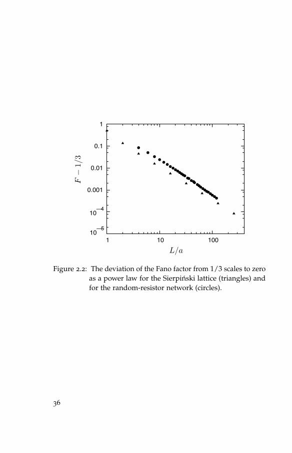
The results in Fig. 2.1 demonstrate, firstly, that the shot noisepower P scales as a function of the size L of the lattice with thesame exponent d f − 2− α = log2(3/5) as the conductance; and,secondly, that the Fano factor F approaches 1/3 for large L. Moreprecisely, see Fig. 2.2, we find that F− 1/3 ∝ L−1.5 scales to zero asa power law, with F− 1/3 < 10−4 for our largest L.

2.2.2 Percolating network

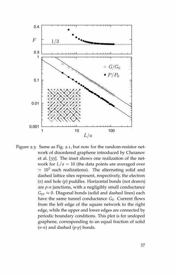
Turning now to the application to graphene mentioned in theintroduction, we have repeated the calculation of shot noise andFano factor for the random-resistor network of electron and holepuddles introduced by Cheianov et al. [35]. The results, shownin Fig. 2.3, demonstrate that the shot noise power P scales withthe same exponent L−0.97 as the conductance G (solid lines inthe lower panel), and that the Fano factor F approaches 1/3 for

27

large networks (upper panel). This is a random, rather than adeterministic fractal, so there remains some statistical scatter in thedata, but the deviation of F from 1/3 for the largest lattices is still< 10−3 (see the circular data points in Fig. 2.2).

2.3 Conclusion

In conclusion, we have found that the universality of the one-thirdFano factor, previously established for normal diffusion [18, 96,97, 136], extends to anomalous diffusion as well. This universalitymight have been expected with respect to the fractal dimensiond f (since the Fano factor is dimension independent), but we hadnot expected universality with respect to the anomalous diffusionexponent α. The experimental implication of the universality is thatthe Fano factor remains fixed at 1/3 as one crosses the percolationthreshold in a random-resistor network – thereby crossing overfrom anomalous diffusion to normal diffusion. This is consistentwith the doping-independent Fano factor measured in a grapheneflake by DiCarlo et al. [41].

Appendix 2.A Calculation of the Fano factor forthe tunnel exclusion process on atwo-dimensional network

Here we present the method we used to calculate the Fano factorfor the tunnel exclusion process in the Sierpinski lattice and in therandom-resistor network. We follow the master equation approachof Refs. [112, 12]. The two-dimensionality of our networks requiresa more elaborate bookkeeping, which we manage by means of theHamiltonian formalism of Ref. [119].

28

2.A.1 Counting statistics

We consider a network of N sites, each of which is either empty orsingly occupied. Two sites are called adjacent if they are directlyconnected by at least one bond. A subset S of the N sites isconnected to the source and a subset D is connected to the drain.Each of the 2N possible states of the network is reached with acertain probability at time t. We store these probabilities in the2N-dimensional vector |P(t)〉. Its time evolution in the tunnelexclusion process is given by the master equation

ddt|P(t)〉 = M |P(t)〉 , (2.3)

where the matrix M contains the tunnel rates. The normalizationcondition can be written as 〈Σ|P〉 = 1, in terms of a vector 〈Σ| thathas all 2N components equal to 1. This vector is a left eigenstate ofM with zero eigenvalue

〈Σ|M = 0, (2.4)

because every column of M must sum to zero in order to conserveprobability. The right eigenstate with zero eigenvalue is the station-ary distribution |P∞〉. All other eigenvalues of M have a real part< 0.

We store in the vector |P(t, Q)〉 the conditional probabilities thata state is reached at time t after precisely Q charges have enteredthe network from the source. Because the source remains occupied,a charge which has entered the network cannot return back tothe source but must eventually leave through the drain. One cantherefore use Q to represent the number of transfered charges. Thetime evolution of |P(t, Q)〉 reads

ddt|P(t, Q)〉 = M0 |P(t, Q)〉+ M1 |P(t, Q− 1)〉 , (2.5)

where M = M0 + M1 has been decomposed into a matrix M0

containing all transitions by which Q does not change and a matrixM1 containing all transitions that increase Q by 1.

29

The probability 〈Σ|P(t, Q)〉 that Q charges have been transferredthrough the network at time t represents the counting statistics. Itdescribes the entire statistics of current fluctuations. The cumulants

Cn =∂nS(t, χ)

∂χn

∣∣∣∣χ=0

(2.6)

are obtained from the cumulant generating function

S(t, χ) = ln

[∑Q〈Σ|P(t, Q)〉 eχQ

]. (2.7)

The average current and Fano factor are given by

I = limt→∞

C1/t, F = limt→∞

C2/C1. (2.8)

The cumulant generating function (2.7) can be expressed interms of a Laplace transformed probability vector |P(t, χ)〉 =

∑Q |P(t, Q〉 eχQ as

S(t, χ) = ln 〈Σ|P(t, χ)〉 . (2.9)

Transformation of Eq. (2.5) gives

ddt|P(t, χ)〉 = M(χ) |P(t, χ)〉 , (2.10)

where we have introduced the counting matrix

M(χ) = M0 + eχ M1. (2.11)

The cumulant generating function follows from

S(t, χ) = ln 〈Σ| etM(χ) |P(0, χ)〉 . (2.12)

The long-time limit of interest for the Fano factor can be im-plemented as follows [12]. Let µ(χ) be the eigenvalue of M(χ)

with the largest real part, and let |P∞(χ)〉 be the corresponding(normalized) right eigenstate,

M(χ) |P∞(χ)〉 = µ(χ) |P∞(χ)〉 , (2.13)

〈Σ|P∞(χ)〉 = 1. (2.14)

30

Since the largest eigenvalue of M(0) is zero, we have

M(0) |P∞(0)〉 = 0⇔ µ(0) = 0. (2.15)

(Note that |P∞(0)〉 is the stationary distribution |P∞〉 introducedearlier.) In the limit t→ ∞ only the largest eigenvalue contributesto the cumulant generating function,

limt→∞

1t

S(t, χ) = limt→∞

1t

ln [etµ(χ) 〈Σ|P∞(χ)〉] = µ(χ). (2.16)

2.A.2 Construction of the counting matrix

The construction of the counting matrix M(χ) is simplified byexpressing it in terms of raising and lowering operators, so that itresembles a Hamiltonian of quantum mechanical spins [119]. First,consider a single site with the basis states |0〉 = (1

0) (vacant) and|1〉 = (0

1) (occupied). We define, respectively, raising and loweringoperators

s+ =

(0 01 0

), s− =

(0 10 0

). (2.17)

We also define the electron number operator n = s+s− and the holenumber operator ν = 11− n (with 11 the 2× 2 unit matrix). Eachsite i has such operators, denoted by s+i , s−i , ni, and νi. The matrixM(χ) can be written in terms of these operators as

M(χ) = ∑〈i,j〉

(s+j s−i − νjni

)+ ∑

i∈S(eχs+i − νi) + ∑

i∈D(s−i − ni), (2.18)

where all tunnel rates have been set equal to unity. The firstsum runs over all ordered pairs 〈i, j〉 of adjacent sites. These areHermitian contributions to the counting matrix. The second sumruns over sites in S connected to the source, and the third sum runsover sites in D connected to the drain. These are non-Hermitiancontributions.

31

It is easy to convince oneself that M(0) is indeed M of Eq. (2.3),since every possible tunneling event corresponds to two terms in Eq.(2.18): one positive non-diagonal term responsible for probabilitygain for the new state and one negative diagonal term responsiblefor probability loss for the old state. In accordance with Eq. (2.11),the full M(χ) differs from M by a factor eχ at the terms associatedwith charges entering the network.

2.A.3 Extraction of the cumulants

In view of Eq. (2.16), the entire counting statistics in the long-timelimit is determined by the largest eigenvalue µ(χ) of the operator(2.18). However, direct calculation of that eigenvalue is feasibleonly for very small networks. Our approach, following Ref. [112],is to derive the first two cumulants by solving a hierarchy of linearequations.

We define

Ti = 〈Σ| ni |P∞(χ)〉 = 1− 〈Σ| νi |P∞(χ)〉 , (2.19)

Uij = Uji = 〈Σ| ninj |P∞(χ)〉 for i 6= j, (2.20)

Uii = 2Ti − 1. (2.21)

The value Ti|χ=0 is the average stationary occupancy of site i. Simi-larly, Uij|χ=0 for i 6= j is the two-point correlator.

We will now express µ(χ) in terms of Ti. We start from thedefinition (2.13). If we act with 〈Σ| on the left-hand-side of Eq.(2.13) we obtain

〈Σ|M(0) + (eχ − 1) ∑i∈S

s+i |P∞(χ)〉

= (eχ − 1) ∑i∈S〈Σ| s+i |P∞(χ)〉

= (eχ − 1) ∑i∈S〈Σ| νi |P∞(χ)〉

= (eχ − 1) ∑i∈S

(1− Ti). (2.22)

32

In the second equality we have used Eq. (2.4) [which holds sinceM ≡ M(0)]. Acting with 〈Σ| on the the right-hand-side of Eq.(2.13) we obtain just µ(χ), in view of Eq. (2.14). Hence we arrive at

µ(χ) = (eχ − 1) ∑i∈S

(1− Ti). (2.23)

From Eq. (2.23) we obtain the average current and Fano factor interms of Ti and the first derivative T′i = dTi/dχ at χ = 0,

I = limt→∞

C1/t = µ′(0) = ∑i∈S

(1− Ti|χ=0), (2.24)

F = limt→∞

C2

C1=

µ′′(0)µ′(0)

= 1− 2 ∑i∈S T′i |χ=0

∑i∈S (1− Ti|χ=0). (2.25)

Average current

To obtain Ti we set up a system of linear equations starting from

µ(χ)Ti = 〈Σ| ni M(χ) |P∞(χ)〉 . (2.26)

Commuting ni to the right, using the commutation relations [ni, s+i ] =s+i and [ni, s−i ] = −s−i , we find

µ(χ)Ti = ∑j(i)

Tj − kiTi + ki,S + (eχ − 1) ∑l∈S

(Ti −Uli). (2.27)

The notation ∑j(i) means that the sum runs over all sites j adjacentto i. The number ki is the total number of bonds connected to sitei; ki,S of these bonds connect site i to the source.

In order to compute Ti|χ=0 we set χ = 0 in Eq. (2.27), use Eq.(2.15) to set the left-hand-side to zero, and solve the resultingsymmetric sparse linear system of equations,

−ki,S = ∑j(i)

Tj − kiTi. (2.28)

This is the first level of the hierarchy. Substitution of the solutioninto Eq. (2.24) gives the average current I.

33

Fano factor

To calculate the Fano factor via Eq. (2.25) we also need T′i |χ=0. Wetake Eq. (2.27), substitute Eq. (2.23) for µ(χ), differentiate and setχ = 0 to arrive at

∑l∈S

(Uli − TlTi)− ki,S = ∑j(i)

T′j − kiT′i . (2.29)

To find Uij|χ=0 we note that

µ(χ)Uij = 〈Σ| ninj M(χ) |P∞(χ)〉 , i 6= j, (2.30)

and commute ni to the right. Setting χ = 0 provides the secondlevel of the hierarchy of linear equations,

0 = ∑l(j),l 6=i

Uil + ∑l(i),l 6=j

Ujl − (ki + k j − 2dij)Uij

+ k j,STi + ki,STj, i 6= j. (2.31)

The number dij is the number of bonds connecting sites i and j ifthey are adjacent, while dij = 0 if they are not adjacent.

34

0.3

0.4

0.001

0.01

0.1

1

1 10 100

Figure 2.1: Lower panel: Electrical conduction through a Sierpinskilattice. This is a deterministic fractal, constructed byrecursively removing a central triangular region froman equilateral triangle. The recursion level r quanti-fies the size L = 2ra of the fractal in units of the el-ementary bond length a (the inset shows the fourthrecursion). The conductance G = I/V (open dots, nor-malized by the tunneling conductance G0 of a singlebond) and shot noise power P (filled dots, normalizedby P0 = 2eVG0) are calculated for a voltage difference Vbetween the lower-left and lower-right corners of the lat-tice. Both quantities scale as Ld f−2−α = Llog2(3/5) (solidlines on the double-logarithmic plot). The Fano factorF = P/2eI = (P/P0)(G0/G) rapidly approaches 1/3,as shown in the upper panel.

35

0.001

0.01

0.1

1

1 10 100

– 5 10

– 4 10

Figure 2.2: The deviation of the Fano factor from 1/3 scales to zeroas a power law for the Sierpinski lattice (triangles) andfor the random-resistor network (circles).

36

0.3

0.4

0.001

0.01

0.1

1

1 10 100

Figure 2.3: Same as Fig. 2.1, but now for the random-resistor net-work of disordered graphene introduced by Cheianovet al. [35]. The inset shows one realization of the net-work for L/a = 10 (the data points are averaged over' 103 such realizations). The alternating solid anddashed lattice sites represent, respectively, the electron(n) and hole (p) puddles. Horizontal bonds (not drawn)are p-n junctions, with a negligibly small conductanceGpn ≈ 0. Diagonal bonds (solid and dashed lines) eachhave the same tunnel conductance G0. Current flowsfrom the left edge of the square network to the rightedge, while the upper and lower edges are connected byperiodic boundary conditions. This plot is for undopedgraphene, corresponding to an equal fraction of solid(n-n) and dashed (p-p) bonds.

37

3 Nonalgebraic length dependenceof transmission through a chainof barriers with a Levy spacingdistribution

3.1 Introduction

Barthelemy, Bertolotti, and Wiersma have reported on the fabri-cation of an unusual random optical medium which they havecalled a Levy glass [15]. It consists of a random packing of glassmicrospheres having a Levy distribution of diameters. The spacebetween the spheres is filled with strongly scattering nanoparti-cles. A photon trajectory therefore consists of ballistic segmentsof length s through spherical regions, connected by isotropic scat-tering events. A Levy distribution is characterized by a slowlydecaying tail, p(s) ∝ 1/s1+α for s → ∞, with 0 < α < 2, such thatthe second moment (and for α < 1 also the first moment) diverges.The transmission of light through the Levy glass was analyzed [15]in terms of a Levy walk [87, 129, 92] for photons.

Because the randomness in the Levy glass is frozen in time(“quenched” disorder), correlations exist between subsequent scat-tering events. Backscattering after a large step is likely to result inanother large step. This is different from a Levy walk, where sub-sequent steps are independently drawn from the Levy distribution(“annealed” disorder). Numerical [76] and analytical [120] theo-ries indicate that the difference between quenched and annealeddisorder can be captured (at least approximately) by a renormal-

39

ization of the Levy walk exponent – from the annealed value α tothe quenched value α′ = α + (2/d)max(0, α− d) in d dimensions.Qualitatively speaking, the correlations in a Levy glass slow downthe diffusion relative to what is expected for a Levy walk, and theeffect is the stronger the lower the dimension.

To analyze the effect of such correlations in a quantitative manner,we consider in this paper the one-dimensional analogue of a Levyglass, which is a linear chain of barriers with independently Levydistributed spacings s. Such a system might be produced artificially,along the lines of Ref. [15], or it might arise naturally in a porousmedium [79] or in a nanowire [72]. Earlier studies of this system1

[52, 36, 14, 25] have compared the dynamical properties with thoseof a Levy walk. In particular, Barkai, Fleurov, and Klafter [14]found a superdiffusive mean-square displacement as a functionof time [〈x2(t)〉 ∝ tγ with γ > 1] – reminiscent of a Levy walk(where γ = 3− α). No precise correspondence to a Levy walk isto be expected in one dimension, because subsequent step lengthsare highly correlated: Backscattering after a step of length s to theright results in the same step length s to the left.

The simplicity of one-dimensional dynamics allows for an ex-act solution of the static transmission statistics, without havingto assume a Levy walk. We present such a calculation here, andfind significant differences with the L−α/2 scaling of the averagetransmission expected [40, 78, 28] for a Levy walk (annealed dis-order) through a system of length L. If the length of the system ismeasured from the first barrier, we find for the case of quencheddisorder an average transmission 〈T〉 ∝ L−α ln L for 0 < α < 1and 〈T〉 ∝ L−1 for α > 1. Note that the nonalgebraic length de-

1The authors of Ref. [14] calculate a lower bound to the mean square displace-ment, with the result 〈x2〉 ≥ tmin(2,3−α) if the initial position of the particle israndomly chosen along the chain (so superdiffusion for any 0 < α < 2). If theparticle starts at a barrier (which corresponds to the situation we consider inthe present work), the result is 〈x2〉 ≥ t2−α (so superdiffusion for 0 < α < 1).Earlier papers [52, 36] gave different results for the mean square displacement,but a direct comparison is problematic because those papers did not noticethe dependence on the starting position.

40

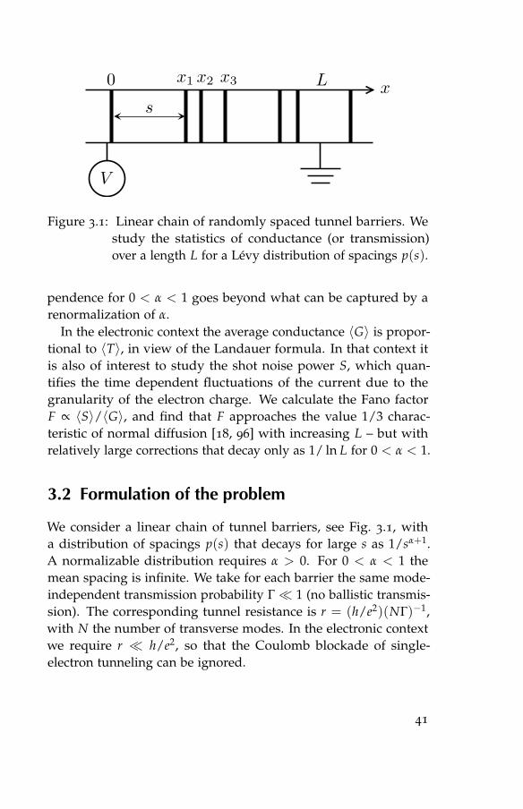
Figure 3.1: Linear chain of randomly spaced tunnel barriers. Westudy the statistics of conductance (or transmission)over a length L for a Levy distribution of spacings p(s).

pendence for 0 < α < 1 goes beyond what can be captured by arenormalization of α.

In the electronic context the average conductance 〈G〉 is propor-tional to 〈T〉, in view of the Landauer formula. In that context itis also of interest to study the shot noise power S, which quan-tifies the time dependent fluctuations of the current due to thegranularity of the electron charge. We calculate the Fano factorF ∝ 〈S〉/〈G〉, and find that F approaches the value 1/3 charac-teristic of normal diffusion [18, 96] with increasing L – but withrelatively large corrections that decay only as 1/ ln L for 0 < α < 1.

3.2 Formulation of the problem

We consider a linear chain of tunnel barriers, see Fig. 3.1, witha distribution of spacings p(s) that decays for large s as 1/sα+1.A normalizable distribution requires α > 0. For 0 < α < 1 themean spacing is infinite. We take for each barrier the same mode-independent transmission probability Γ� 1 (no ballistic transmis-sion). The corresponding tunnel resistance is r = (h/e2)(NΓ)−1,with N the number of transverse modes. In the electronic contextwe require r � h/e2, so that the Coulomb blockade of single-electron tunneling can be ignored.

41

We work in the regime of incoherent sequential tunneling (noresonant tunneling). This regime can be reached for N � 1 as aresult of intermode scattering, or it can be reached even for smallN as a result of a short phase coherence length. For sequentialtunneling the resistance R of n barriers in series is just the seriesresistance nr [corresponding to a transmission probability T =

(nΓ)−1]. We measure this resistance

R(L) = r ∑n

θ(xn)θ(L− xn) (3.1)

between one contact at x = 0 and a second contact at x = L > 0.The numbers xn indicate the coordinates of the tunnel barriers andθ(x) is the step function [θ(x) = 1 if x > 0 and θ(x) = 0 if x < 0].

Without further restrictions the statistics of the conductancewould be dominated by ballistic realizations, that have not a singletunnel barrier in the interval (0, L). The reason, discussed in Ref.[14], is that the average distance between a randomly chosen pointalong the chain and the nearest tunnel barrier diverges for any 0 <

α < 2 (so even if the mean spacing between the barriers is finite). Toeliminate ballistic transmission, we assume that one tunnel barrieris kept fixed at x0 = 0+. (This barrier thus contributes r to theresistance.) If we order the coordinates such that xn < xn+1, wehave

R(L) = r + r∞

∑n=1

θ(xn)θ(L− xn). (3.2)

We seek the scaling with L in the limit L → ∞ of the negativemoments 〈R(L)p〉 (p = −1,−2,−3, . . .) of the resistance. Thisinformation will give us the scaling of the positive moments of theconductance G = R−1 and transmission T = (h/Ne2)R−1. It willalso give us the average of the shot noise power S, which for anarbitrary number of identical tunnel barriers in series is determinedby the formula [61]

S =23

e|V|r−1[(R/r)−1 + 2(R/r)−3], (3.3)

42

where V is the applied voltage. From 〈S〉 and 〈G〉 we obtain theFano factor F, defined by

F =〈S〉

2e|V|〈G〉 . (3.4)

3.3 Arbitrary moments

The general expression for moments of the resistance is

〈R(L)p〉 = rp

⟨(1 +

∞

∑n=1

θ(xn)θ(L− xn)

)p⟩, (3.5)

where the brackets 〈· · · 〉 indicate the average over the spacings,

〈· · · 〉 =∞

∏n=1

∫ ∞

−∞dxn p(xn − xn−1) · · · , (3.6)

with the definitions x0 = 0 and p(s) = 0 for s < 0. We work outthe average,

〈R(L)p〉 = rp∞

∑n=1

np

(n

∏i=1

∫ ∞

−∞dsi p(si)

)

× θ

(n

∑i=1

si − L

)θ

(L−

n−1

∑i=1

si

). (3.7)

It is more convenient to evaluate the derivative with respect to Lof Eq. (3.7), which takes the form of a multiple convolution of thespacing distribution2,

ddL〈Rp〉 = rp(2p − 1)p(L)

+ rp∞

∑n=2

[(n + 1)p − np]∫ ∞

−∞dxn−1 · · ·

∫ ∞

−∞dx1

p(L− xn−1)p(xn−1 − xn−2) · · · p(x2 − x1)p(x1). (3.8)

2We cannot directly take the derivative of Eq. (3.5), because that would lead(for p 6= 1) to an undefined product of θ(L − x) and δ(L − x). No suchcomplication arises if we take the derivative of Eq. (3.7).

43

In terms of the Fourier (or Laplace) transform

f (ξ) =∫ ∞

0ds eiξs p(s), (3.9)

the series (3.8) can be summed up,

ddL〈Rp〉 = rp

2π

∫ ∞+i0+

−∞+i0+dξ e−iξL

∞

∑n=1

[(n + 1)p − np] f (ξ)n

=rp

2π

∫ ∞+i0+

−∞+i0+dξ e−iξL 1− f (ξ)

f (ξ)Li−p[ f (ξ)]. (3.10)

The function Li(x) is the polylogarithm. The imaginary infinitesi-mal i0+ added to ξ regularizes the singularity of the integrand atξ = 0. For negative p this singularity is integrable, and the integral(3.10) may be rewritten as an integral over the positive real axis,

ddL〈Rp〉 = rp

πRe

∫ ∞

0dξ e−iξL 1− f (ξ)

f (ξ)Li−p[ f (ξ)]. (3.11)

3.4 Scaling with length

3.4.1 Asymptotic expansions

In the limit L→ ∞ the integral over ξ in Eq. (3.11) is governed bythe ξ → 0 limit of the Fourier transformed spacing distribution.Because p(s) is normalized to unity one has f (0) = 1, while thelarge-s scaling p(s) ∝ 1/sα+1 implies

limξ→0

f (ξ) ={

1 + cα(s0ξ)α, 0 < α < 1,1 + isξ + cα(s0ξ)α, 1 < α < 2.

(3.12)

The characteristic length s0 > 0, the mean spacing s, as well as thenumerical coefficient cα are determined by the specific form of thespacing distribution.

44

The limiting behavior of the polylogarithm is governed by

Li1(1 + ε) = − ln(−ε), (3.13)

limε→0

Li2(1 + ε) = ζ(2)− ε ln(−ε), (3.14)

limε→0

Lin(1 + ε) = ζ(n) + ζ(n− 1)ε, n = 3, 4, . . . (3.15)

In combination with Eq. (3.12) we find, for 0 < α < 1, the followingexpansions of the integrand in Eq. (3.11):

limξ→0

1− ff

Li−p( f ) = cα(s0ξ)α ln[−cα(s0ξ)α],

if p = −1, (3.16)

limξ→0

1− ff

Li−p( f ) = − ζ(−p)cα(s0ξ)α,

p = −2,−3 . . . (3.17)

For 1 < α < 2 we should replace cα(s0ξ)α by isξ + cα(s0ξ)α.

3.4.2 Results

We substitute the expansions (3.16) and (3.17) into Eq. (3.11), andobtain the large-L scaling of the moments of conductance with thehelp of the following Fourier integrals (L > 0, α > −1):∫ ∞

0dξ e−iξLξα ln ξ = iΓ(1 + α)e−iπα/2L−1−α

× (ln L + iπ/2 + γE − Hα), (3.18)∫ ∞

0dξ e−iξLξα = −iΓ(1 + α)e−iπα/2L−1−α, (3.19)

Re∫ ∞

0dξ e−iξLiξ = 0, (3.20)

Re∫ ∞

0dξ e−iξLiξ ln ξ = − 1

2 πL−2. (3.21)

Here γE is Euler’s constant and Hα is the harmonic number. Theresulting scaling laws are listed in Table 3.1.

Two physical consequences of these scaling laws are:

45

0 < α < 1 1 < α < 2〈R−1〉 ≡ 〈G〉 L−α ln L L−1

〈Rp〉 ≡ 〈G−p〉, p = −2,−3, . . . L−α L−α

Table 3.1: Scaling with L of moments of conductance (or, equiva-lently, transmission).

• The Fano factor (3.4) approaches 1/3 in the limit L → ∞,regardless of the value of α, but for 0 < α < 1 the approachis very slow: F− 1/3 ∝ 1/ ln L. For 1 < α < 2 the approachis faster but still sublinear, F− 1/3 ∝ 1/Lα−1.

• The root-mean-square fluctuations rms G =√〈G2〉 − 〈G〉2

of the conductance become much larger than the averageconductance for large L, scaling as rms G/〈G〉 ∝ Lα/2/ ln Lfor 0 < α < 1 and as rms G/〈G〉 ∝ L1−α/2 for 1 < α < 2.

3.5 Numerical test

To test the scaling derived in the previous sections, in particu-lar to see how rapidly the asymptotic L-dependence is reachedwith increasing L, we have numerically generated a large numberof random chains of tunnel barriers and calculated moments ofconductance and the Fano factor from Eqs. (3.2)–(3.4).

For the spacing distribution in this numerical calculation we tookthe Levy stable distribution3 for α = 1/2,

p1/2(s) = (s0/2π)1/2s−3/2e−s0/2s. (3.22)

Its Fourier transform is

f1/2(ξ) = exp(−√−2is0ξ)⇒ c1/2 = i− 1. (3.23)

3For efficient algorithms to generate random variables with a Levy stable distri-bution, see Refs. [33, 88].

46

Inserting the numerical coefficients, the large-L scaling of con-ductance moments for the distribution (3.22) is

limL→∞〈G〉 = 1

r(2πL/s0)

−1/2[ln(2L/s0) + γE], (3.24)

limL→∞〈Gp〉 = 2ζ(p)

1rp (2πL/s0)

−1/2, p ≥ 2. (3.25)

The resulting scaling of the conductance fluctuations and Fanofactor is(

rms G〈G〉

)2

≡ 〈G2〉

〈G〉2 − 1 ≈ (π2/3)(2πL/s0)1/2

[ln(2L/s0) + γE]2− 1, (3.26)

F ≈ 13+

(4/3)ζ(3)ln(2L/s0) + γE

. (3.27)

In Fig. 3.2 we compare these analytical large-L formulas with thenumerical data. The average conductance converges quite rapidlyto the scaling (3.24), while the convergence for higher moments(which determine the conductance fluctuations and Fano factor)requires somewhat larger systems. We clearly see in Fig. 3.2 therelative growth of the conductance fluctuations with increasingsystem size and the slow decay of the Fano factor towards thediffusive 1/3 limit.

3.6 Conclusion and outlook

In conclusion, we have analyzed the statistics of transmissionthrough a sparse chain of tunnel barriers. The average spacing ofthe barriers diverges for a Levy spacing distribution p(s) ∝ 1/s1+α

with 0 < α < 1. This causes an unusual scaling with system lengthL (measured from the first tunnel barrier) of the moments of trans-mission or conductance, as summarized in Table 3.1. A logarithmiccorrection to the power law scaling appears for the first moment.Higher moments of conductance all scale with the same powerlaw, differing only in the numerical prefactor. As a consequence,

47

sample-to-sample fluctuations of the transmission become largerthan the average with increasing L.

This theoretical study of a one-dimensional “Levy glass” was mo-tivated by an optical experiment on its three-dimensional analogue[15]. The simplicity of a one-dimensional geometry has allowedus to account exactly for the correlations between subsequent steplengths, which distinguish the random walk through the sparsechain of barriers from a Levy walk. We surmise that step lengthcorrelations will play a role in two and three dimensional sparsearrays as well, complicating a direct application of the theory ofLevy walks to the experiment. This is one line of investigation forthe future.

A second line of investigation is the effect of wave interference onthe transmission of electrons or photons through a sparse chain oftunnel barriers. Here we have considered the regime of incoherentsequential transmission, appropriate for a multi-mode chain withmode-mixing or for a single-mode chain with a short coherencelength. The opposite, phase coherent regime was studied in Ref.[25]. In a single-mode and phase coherent chain interference canlead to localization, producing an exponential decay of transmis-sion. An investigation of localization in this system is of particularinterest because the sparse chain belongs to the class of disorderedsystems with long-range disorder, to which the usual scaling theoryof Anderson localization does not apply [115].

A third line of investigation concerns the question “what is theshot noise of anomalous diffusion”? Anomalous diffusion [92]is characterized by a mean square displacement 〈x2〉 ∝ tγ with0 < γ < 1 (subdiffusion) or γ > 1 (superdiffusion). The shot noisefor normal diffusion (γ = 1) has Fano factor 1/3 [18, 96], and Ref.[48] concluded that subdiffusion on a fractal also produces F =

1/3. Here we found a convergence, albeit a logarithmically slowconvergence, to the same 1/3 Fano factor for a particular systemwith superdiffusive dynamics. We conjecture that F = 1/3 in theentire subballistic regime 0 < γ < 2, with deviations appearing inthe ballistic limit γ→ 2 – but we do not have a general theory tosupport this conjecture.

48

0.01

0.1

1

10 100 1000 10000

1

10

0.2

0.3

0.4

0.5

Figure 3.2: Scaling of the average conductance (bottom panel), thevariance of the conductance (middle panel), and theFano factor (top panel), for a chain of tunnel barrierswith spacings distributed according to the α = 1/2Levy stable distribution (3.22). The data points are cal-culated numerically, by averaging over a large numberof random chains of tunnel barriers. The solid curvesare the analytical results (3.24)–(3.27) of the asymptoticanalysis in the L→ ∞ limit.

49

4 Finite difference method fortransport properties of masslessDirac fermions

4.1 Introduction

The discovery of graphene [47] has created a need for efficientnumerical methods to calculate transport properties of masslessDirac fermions. The two-dimensional massless Dirac equation(or Weyl equation) that governs the low-energy and long-wavelength dynamics of conduction electrons in graphene has a timereversal symmetry called symplectic – which is special because itsquares to −1. (The usual time reversal symmetry, which squaresto +1, is called orthogonal.) The symplectic symmetry is at theorigin of some of the unusual transport properties of graphene[86, 104, 117, 20, 42], including the absence of back scattering [10],weak antilocalization [137], enhanced conductance fluctuations[67, 66], and absence of a metal-insulator transition [13, 99].

Numerical methods of solution can be divided into two classes,depending on whether they break or preserve the symplectic sym-metry.

The tight-binding model of graphene, with nearest neighborhopping on a honeycomb lattice, breaks the symplectic symmetryby the two mechanisms of intervalley scattering [137] and trigo-nal warping [90]. Intervalley scattering couples the two flavors ofDirac fermions, corresponding to the two different valleys (at oppo-site corners of the Brillouin zone) in the graphene band structure,thereby changing the symmetry class from symplectic to orthog-

51

onal. Trigonal warping is a triangular distortion of the conicalband structure that breaks the momentum inversion symmetry(+p→ −p), thereby effectively breaking time reversal symmetryin a single valley and changing the symmetry class from symplecticto unitary.

Breaking of the symplectic symmetry eliminates both weak an-tilocalization as well as the enhancement of the conductance fluctu-ations, and drives the system to an insulator with increasing size ordisorder [6, 8]. As observed in computer simulations [116, 80, 148],the breaking of the symplectic symmetry can be pushed to largersystem sizes and larger disorder strengths by reducing the latticeconstant (at fixed correlation length and fixed amplitude of thedisorder potential) – but this severely limits the computationalefficiency.

The Chalker-Coddington network model [32, 54, 75], appliedto graphene in Ref. [133], has a single flavor of Dirac fermions,so there is no intervalley scattering – but it still belongs to thesame class of methods that break the symplectic symmetry of themassless Dirac equation. (The symplectic symmetry is broken onshort length scales by the Aharonov-Bohm phases that appear inthe mapping of the Dirac equation onto the network model.)

Both the network model and the tight-binding model are realspace regularizations of the Dirac equation, with a smallest lengthscale (the lattice constant) to cut off the unbounded spectrum atlarge positive and large negative energies. There exists at presentjust one method to calculate transport properties numerically whilepreserving the symplectic symmetry, developed independently(and implemented differently) in Refs. [13] and [99]. That method(used also in Refs. [118, 100]) is based on a momentum space regu-larization, with a cutoff of the Fourier transformed Dirac equationat some large value of momentum.

It is the purpose of the present paper to develop and implementan alternative method of solution of the Dirac equation, that shareswith the tight-binding and network models the convenience ofa formulation in real space rather than momentum space, butwithout breaking the symplectic symmetry.

52

A celebrated no-go theorem [98] in lattice gauge theory forbidsany regularization of the Dirac equation with local couplings frompreserving symplectic symmetry. (The problematic role of inter-valley scattering appears in that context as the fermion doublingproblem.) Several nonlocal finite difference methods have beenproposed to work around the no-go theorem and we will adaptone of these (developed by Stacey [134] and by Bender, Milton, andSharp [22]) to the study of transport properties.

The adaptation amounts to 1) the inclusion of a spatially depen-dent electrostatic potential (which breaks the chiral symmetry thatplayed a central role in Refs. [134, 22]), and 2) a proper discretiza-tion of the current operator (such that the total current throughany cross section is conserved). We implement the finite differencemethod to solve the scattering problem of Dirac fermions in a disor-dered potential landscape connected to ballistic leads, and compareour numerical results for the scaling and statistics of conductanceand shot noise power with analytical theories [67, 66, 121].

Our numerical method is relevant for electrical conduction ingraphene under the assumption that the impurity potential in thecarbon monolayer is long-ranged (so that intervalley scattering issuppressed) and weak (so that trigonal warping can be neglected).Massless Dirac fermions are also expected to govern the electricalconduction along the surface of a three-dimensional topologicalinsulator [45, 94, 114] (realized in BiSb [55]). In that case thesymplectic symmetry is preserved even for short-range scatterers,and our numerical results should be applicable more generally.

4.2 Finite difference representation of the transfermatrix

4.2.1 Dirac equation

We consider the two-dimensional massless Dirac equation,

HΨ = EΨ, H = −ihv(σx∂x + σy∂y) + U(r), (4.1)

53

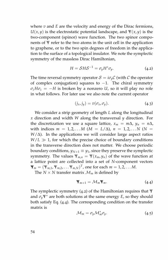
where v and E are the velocity and energy of the Dirac fermions,U(x, y) is the electrostatic potential landscape, and Ψ(x, y) is thetwo-component (spinor) wave function. The two spinor compo-nents of Ψ refer to the two atoms in the unit cell in the applicationto graphene, or to the two spin degrees of freedom in the applica-tion to the surface of a topological insulator. We note the symplecticsymmetry of the massless Dirac Hamiltonian,

H = SHS−1 = σyH∗σy. (4.2)

The time reversal symmetry operator S = iσyC (with C the operatorof complex conjugation) squares to −1. The chiral symmetryσzHσz = −H is broken by a nonzero U, so it will play no rolein what follows. For later use we also note the current operator

(jx, jy) = v(σx, σy). (4.3)

We consider a strip geometry of length L along the longitudinalx direction and width W along the transversal y direction. Forthe discretization we use a square lattice, xm = m∆, yn = n∆,with indices m = 1, 2, . . . M (M = L/∆), n = 1, 2, . . . N (N =

W/∆). In the applications we will consider large aspect ratiosW/L � 1, for which the precise choice of boundary conditionsin the transverse direction does not matter. We choose periodicboundary conditions, yN+1 ≡ y1, since they preserve the symplecticsymmetry. The values Ψm,n = Ψ(xm, yn) of the wave function ata lattice point are collected into a set of N-component vectorsΨm = (Ψm,1, Ψm,2, . . . Ψm,N)

T, one for each m = 1, 2, . . . M.The N × N transfer matrixMm is defined by

Ψm+1 =MmΨm. (4.4)

The symplectic symmetry (4.2) of the Hamiltonian requires that Ψand σyΨ∗ are both solutions at the same energy E, so they shouldboth satisfy Eq. (4.4). The corresponding condition on the transfermatrix is

Mm = σyM∗mσy. (4.5)

54

The transfer matrix should conserve the total current through anycross section of the strip. In terms of the (still to be determined)discretized current operator Jx, this condition reads

〈Ψm+1|Jx|Ψm+1〉 = 〈Ψm|Jx|Ψm〉, (4.6)

which then corresponds to the following condition on the transfermatrix:

M†m JxMm = Jx. (4.7)

Our problem is to discretize the differential operators in theDirac equation (4.1), as well as the current operator (4.3), in such away that the resulting transfer matrix describes a single flavor ofDirac fermions and without violating the two conditions (4.5), (4.7)of symplectic symmetry and current conservation.

4.2.2 Discretization

A local replacement of the differential operators ∂x, ∂y by finitedifferences either violates the Hermiticity of H (thus violatingconservation of current) or breaks the symplectic symmetry (bythe mechanism of fermion doubling). A nonlocal finite differencemethod that preserves the Hermiticity and symplectic symmetryof H was developed by Stacey [134] and by Bender, Milton, andSharp [22]. These authors considered the case U = 0, when bothsymplectic and chiral symmetry are present. We extend theirmethod to a spatially dependent U (thereby breaking the chiralsymmetry), and obtain the discretized transfer matrix and currentoperator.

Since the transfer matrix relates Ψ(x, y) at two different valuesof x, it is convenient to isolate the derivative with respect to x fromthe Dirac equation (4.1). Multiplication of both sides by (i/hv)σx

gives∂xΨ = (−iσz∂y − iσxV)Ψ, (4.8)

with the definition V = (U − E)/hv. We can now make contactwith the discretization in Refs. [134, 22] of the Dirac equation in

55

Figure 4.1: Square lattice (filled circles) on which the wave func-tion Ψ is discretized as Ψm,n. The finite differences areevaluated at the displaced points indicated by crosses.The Dirac equation (4.8) is applied at the empty cir-cles, by taking the mean of the contributions from thetwo adjacent crosses. The resulting finite differenceequation defines a transfer matrix in the x directionthat conserves current and preserves the symplecticsymmetry.

one space and one time dimension, with x playing the role of(imaginary) time and y being the spatial dimension.

The key step by which Refs. [134, 22] avoid fermion doubling isthe evaluation of the finite differences on a lattice that is displacedsymmetrically from the original lattice. The displaced lattice points(xm + ∆/2, yn + ∆/2) are indicated by crosses in Fig. 4.1. On thedisplaced lattice, the differential operators are discretized by

∂xΨ→ 12∆

(Ψm+1,n + Ψm+1,n+1 −Ψm,n −Ψm,n+1), (4.9)

∂yΨ→ 12∆

(Ψm,n+1 + Ψm+1,n+1 −Ψm,n −Ψm+1,n), (4.10)

56

and the potential term is replaced by

VΨ→ 14 Vm,n(Ψm+1,n + Ψm+1,n+1 + Ψm,n + Ψm,n+1), (4.11)

with Vm,n = V(xm + ∆/2, yn + ∆/2). The Dirac equation (4.8) isapplied at the points (xm + ∆/2, yn) (empty circles in Fig. 4.1) byaveraging the terms at the two adjacent points (xm + ∆/2, yn ±∆/2).

The resulting finite difference equation can be written in a com-pact form with the help of the N × N tridiagonal matrices J , K,V (m), defined by the following nonzero elements:

Jn,n = 1, Jn,n+1 = Jn,n−1 = 12 , (4.12)

Kn,n+1 = 12 , Kn,n−1 = − 1

2 , (4.13)

V (m)n,n = 1

2 (Vm,n + Vm,n−1), V (m)n,n+1 = 1

2 Vm,n,

V (m)n,n−1 = 1

2 Vm,n−1. (4.14)

In accordance with the periodic boundary conditions, the indicesn ± 1 should be evaluated modulo N. Notice that J and V (m)

are real symmetric matrices, while K is real antisymmetric. Fur-thermore J and K commute, but neither matrix commutes withV (m).

For later use, we note that J has eigenvalues

jl = 2 cos2(πl/N), l = 1, 2, . . . N, (4.15)

corresponding to the eigenvectors ψ(l) with elements

ψ(l)n = N−1/2 exp(2πiln/N). (4.16)

The eigenvalues of K are

κl = i sin(2πl/N), l = 1, 2, . . . N, (4.17)

for the same eigenvectors ψ(l). From Eq. (4.15) we see that for Neven there is a zero eigenvalue of J (at l = N/2). To avoid thecomplications from a noninvertible J , we restrict ourselves to Nodd (when all eigenvalues of J are nonzero).

57

4.2.3 Transfer matrix

The discretized Dirac equation is expressed in terms of the matrices(4.12)–(4.14) by

12∆J (Ψm+1 −Ψm) =

(− i

2∆σzK−

i4

σxV (m)

)(Ψm + Ψm+1). (4.18)

Rearranging Eq. (4.18) we arrive at Eq. (4.4) with the transfer matrix

Mm =(J + iσzK+ 1

2 i∆σxV (m))−1

(J − iσzK− 1

2 i∆σxV (m))

. (4.19)

Since we take N odd, so that J is invertible, we may equivalentlywrite Eq. (4.19) in the more compact form

Mm =1− iXm

1 + iXm, Xm = J −1(σzK+ 1

2 ∆σxV (m)). (4.20)

As announced, the transfer matrix is nonlocal (in the sense thatmultiplication of Ψm byMm couples all transverse coordinates).

One can readily check that the condition (4.5) of symplectic sym-metry is fullfilled. In App. 4.A we demonstrate that the condition(4.7) of current conservation holds if we define the discretizedcurrent operator Jx in terms of the symmetric matrix J ,

Jx = 12 vσxJ . (4.21)

The absence of fermion doubling is checked in Sec. 4.4.1.The transfer matrix M through the entire strip (from x = 0 to

x = L) is the product of the one-step transfer matricesMm,

M =M

∏m=1Mm, (4.22)

ordered such that Mm+1 is to the left of Mm. The properties ofsymplectic symmetry and current conservation are preserved uponmatrix multiplication.

58

4.2.4 Numerical stability

The repeated multiplication (4.22) of the one-step transfer matrix toarrive at the transfer matrix of the entire strip is unstable because itproduces both exponentially growing and exponentially decayingeigenvalues, and the limited numerical accuracy prevents onefrom retaining both sets of eigenvalues. We resolve this obstacle,following Refs. [13, 133, 138], by converting the transfer matrix intoa unitary matrix, which has only eigenvalues of unit absolute value.The formulas that accomplish this transformation are given in App.4.B.

4.3 From transfer matrix to scattering matrix andconductance

4.3.1 General formulation

The scattering matrix is obtained from the transfer matrix by con-necting the two ends of the strip at x = 0 and x = L to semi-infiniteballistic leads. The N transverse modes in the leads (calculated inSec. 4.4), consist of N0 propagating modes φ±l (labeled + for right-moving and − for left-moving), and N − N0 evanescent modes χ±l(decaying for x → ±∞). The propagating modes are normalizedsuch that each carries unit current.

Consider an incoming wave in mode l0 from the left. At x = 0,the sum of incoming, reflected, and evanescent waves is given by

Φleftl0 = φ+

l0+ ∑

lrl,l0 φ−l + ∑

lαl,l0 χ−l , (4.23)

while the sum of transmitted and evanescent waves at x = L isgiven by

Φrightl0

= ∑l

tl,l0 φ+l + ∑

lα′l,l0 χ+

l . (4.24)

The N0 × N0 reflection matrix r and transmission matrix t are

59

obtained by equating

Φrightl0

=MΦleftl0 , (4.25)

eliminating the coefficients α, α′, and repeating for each of the N0

propagating modes incident from the left. Starting from a modeincident from the right, we similarly obtain the reflection matricesr′ and t′, which together with r and t form a 2N0 × 2N0 unitaryscattering matrix,

S =

(r t′

t r′

). (4.26)

As a consequence of unitarity, the matrix products tt† and t′t′†

have the same set of eigenvalues T1, T2, . . . TN0 , called transmissioneigenvalues.

The number N0 of propagating modes in the leads is an oddinteger, because of our choice of periodic boundary conditions.The symplectic symmetry condition (4.5) then implies that thetransmission eigenvalues Tn consist of one unit eigenvalue and(N0 − 1)/2 degenerate pairs (Kramers degeneracy1).

The conductance G follows from the transmission eigenvaluesvia the Landauer formula,

G = G0 ∑n

Tn. (4.27)

The conductance quantum G0 = 4e2/h in the application to graphene(which has both spin and valley degeneracies), while G0 = e2/hin the application to the surface of a topological insulator. TheKramers degeneracy, which is present in both applications, is ac-counted for in the sum over the transmission eigenvalues.

1Symplectic symmetry also implies that the basis of modes in the leads canbe chosen such that S is antisymmetric (S = −ST). We use a different basis,so our S will be not be antisymmetric. For a direct proof of the Kramersdegeneracy of the transmission eigenvalues from the antisymmetry of thescattering matrix, see J. H. Bardarson, J. Phys. A 41, 405203 (2008).

60

4.3.2 Infinite wave vector limit

Following Ref. [141], we model metal contacts by leads with aninfinitely large Fermi wave vector. In the infinite wave vectorlimit all modes in the leads are propagating, so N0 = N and thescattering matrix has dimension 2N × 2N. The states φ±l (l =

1, 2, . . . N) in this limit are simply the 2N eigenstates of the currentoperator Jx, normalized such that each carries the same current.In terms of the eigenvalues and eigenvectors (4.15), (4.16) of J wehave

φ±l = j−1/2l

(1±1

)ψ(l). (4.28)

Instead of the general Eqs. (4.23) and (4.24) we now have thesimpler equations

Φleftl0 = φ+

l0+ ∑

lrl,l0 φ−l , Φright

l0= ∑

ltl,l0 φ+

l . (4.29)

To obtain from Eq. (4.25) a closed-form expression for S in termsofM, we first perform the similarity transformation

M = RMR−1, R = σHJ 1/2, (4.30)

where σH is the Hadamard matrix,

σH = 2−1/2(

1 11 −1

)= σ−1

H . (4.31)

The notation σHJ 1/2 signifies a direct product, where σH actson the spinor degrees of freedom s = ± and J 1/2 acts on thelattice degrees of freedom n = 1, 2, . . . N. Notice that the matrixR is Hermitian [since J is Hermitian with exclusively positiveeigenvalues, see Eq. (4.15)].

We separate the spinor degrees of freedom ofM into four N×Nblocks,

M =

(M++ M+−

M−+ M−−

), (4.32)

61

such thatMns,ms′ =Mss′nm. The matrix M has a corresponding de-

composition into submatrices Mss′ . As one can verify by substitu-tion into Eq. (4.29) and comparison with Eq. (4.25), the submatricesMss′ are related to the transmission and reflection matrices by

r = −(M−−)−1 M−+, (4.33a)

t = M++ − M+− (M−−)−1 M−+, (4.33b)

t′ =(M−−)−1 , (4.33c)

r′ = M+− (M−−)−1 . (4.33d)

Similar formulas were derived in Ref. [133], but there the trans-formation fromM to S involved only a Hadamard matrix and nomatrix J , because of the different current operator in that model.

4.4 Ballistic transport

For a constant U we have ballistic transport through the strip oflength L and width W. In this section we check that we recoverthe known results [63, 141] for ballistic transport of Dirac fermionsfrom the discretized transfer matrix.

4.4.1 Dispersion relation

For U = U0 = constant the matrix (4.14) of discretized potentialsis given by V (m) = −(ε/∆)J , with ε = (E−U0)∆/hv the dimen-sionless energy (measured relative to the Dirac point at energyU0). Substitution into Eq. (4.20) gives the m-independent ballistictransfer matrixMball,

Mball =1 + i(ε/2)σx − iJ −1Kσz

1− i(ε/2)σx + iJ −1Kσz. (4.34)

This is the one-step transfer matrix. The transfer matrix throughthe entire strip, in this ballistic case, is simplyM = (Mball)

M.

62

In accordance with Eqs. (4.15)–(4.17), the matrix J −1K can bediagonalized (for N odd) by

J −1K = FΛF †, Λnn′ = i tan(πn/N)δnn′ , (4.35a)

Fnn′ = N−1/2 exp(2πinn′/N). (4.35b)

The Fourier transformed transfer matrix FMballF † is diagonal inthe mode index l = 1, 2, . . . N. A 2× 2 matrix structure ml in thespin index remains, given by

ml =1 + i(ε/2)σx + tan(πl/N)σz

1− i(ε/2)σx − tan(πl/N)σz. (4.36)

The eigenvalues and eigenvectors of ml are

mlu±l = e±iku±l , u±l =

(ε/2

i tan(πl/N)± tan(k/2)

), (4.37)

with the dimensionless momentum k given as a function of ε and lby the dispersion relation

tan2(k/2) + tan2(πl/N) = (ε/2)2. (4.38)

In Fig. 4.2 we have plotted the dispersion relation (4.38) for twodifferent modes in the first Brillouin zone −π < k < π. For eachmode index l, there is one wave that propagates to positive x(on the branch with dε/dk > 0) and one wave that propagates tonegative x (on the branch with dε/dk < 0).

As anticipated [134, 22], the discretization of the Dirac equa-tion on the displaced lattice (crosses in Fig. 4.1) has avoided thespurious doubling of the fermion degrees of freedom that wouldhave happened if the finite differences would have been calcu-lated on the original lattice (solid dots in Fig. 4.1). In the low-energy and long-wave-length limit k, ε → 0, the conical disper-sion relation (vpx)2 + (vpy)2 = (E −U0)2 of the Dirac equation(4.1) is recovered. The longitudinal momentum is px = hk/∆,while the transverse momentum is py = (2πh/W)l if l/N → 0 orpy = −(2πh/W)(N − l) if l/N → 1.

63

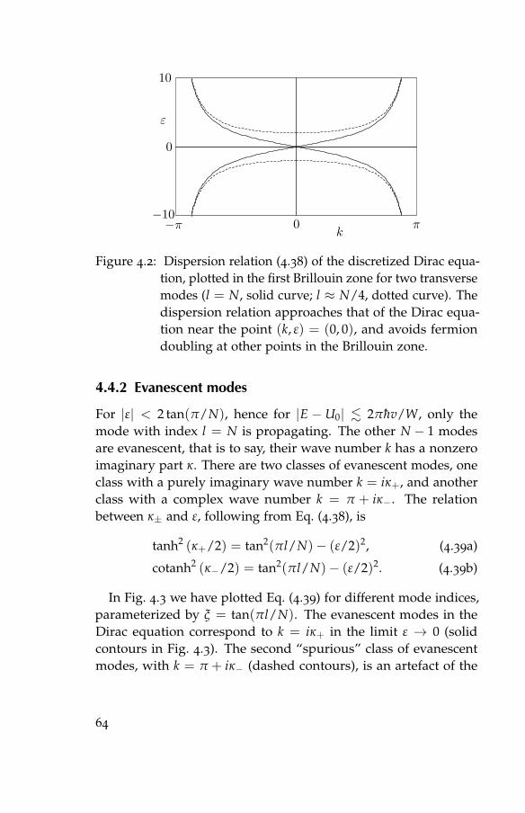
Figure 4.2: Dispersion relation (4.38) of the discretized Dirac equa-tion, plotted in the first Brillouin zone for two transversemodes (l = N, solid curve; l ≈ N/4, dotted curve). Thedispersion relation approaches that of the Dirac equa-tion near the point (k, ε) = (0, 0), and avoids fermiondoubling at other points in the Brillouin zone.

4.4.2 Evanescent modes

For |ε| < 2 tan(π/N), hence for |E − U0| . 2πhv/W, only themode with index l = N is propagating. The other N − 1 modesare evanescent, that is to say, their wave number k has a nonzeroimaginary part κ. There are two classes of evanescent modes, oneclass with a purely imaginary wave number k = iκ+, and anotherclass with a complex wave number k = π + iκ−. The relationbetween κ± and ε, following from Eq. (4.38), is

tanh2 (κ+/2) = tan2(πl/N)− (ε/2)2, (4.39a)

cotanh2 (κ−/2) = tan2(πl/N)− (ε/2)2. (4.39b)

In Fig. 4.3 we have plotted Eq. (4.39) for different mode indices,parameterized by ξ = tan(πl/N). The evanescent modes in theDirac equation correspond to k = iκ+ in the limit ε → 0 (solidcontours in Fig. 4.3). The second “spurious” class of evanescentmodes, with k = π + iκ− (dashed contours), is an artefact of the

64

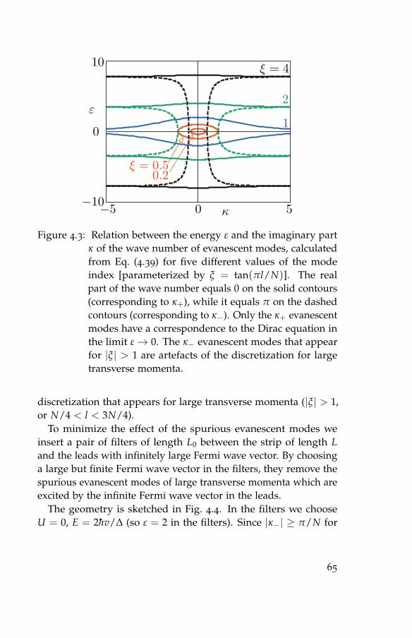
Figure 4.3: Relation between the energy ε and the imaginary partκ of the wave number of evanescent modes, calculatedfrom Eq. (4.39) for five different values of the modeindex [parameterized by ξ = tan(πl/N)]. The realpart of the wave number equals 0 on the solid contours(corresponding to κ+), while it equals π on the dashedcontours (corresponding to κ−). Only the κ+ evanescentmodes have a correspondence to the Dirac equation inthe limit ε→ 0. The κ− evanescent modes that appearfor |ξ| > 1 are artefacts of the discretization for largetransverse momenta.

discretization that appears for large transverse momenta (|ξ| > 1,or N/4 < l < 3N/4).

To minimize the effect of the spurious evanescent modes weinsert a pair of filters of length L0 between the strip of length Land the leads with infinitely large Fermi wave vector. By choosinga large but finite Fermi wave vector in the filters, they remove thespurious evanescent modes of large transverse momenta which areexcited by the infinite Fermi wave vector in the leads.

The geometry is sketched in Fig. 4.4. In the filters we chooseU = 0, E = 2hv/∆ (so ε = 2 in the filters). Since |κ−| ≥ π/N for

65

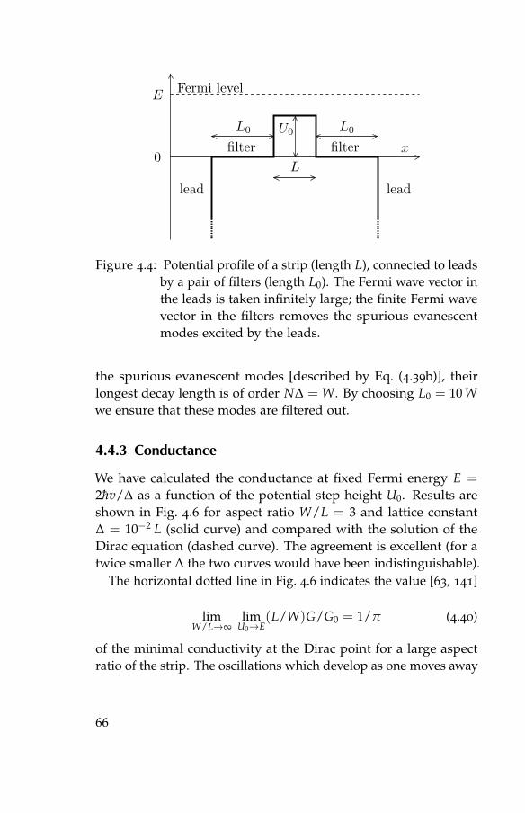
Figure 4.4: Potential profile of a strip (length L), connected to leadsby a pair of filters (length L0). The Fermi wave vector inthe leads is taken infinitely large; the finite Fermi wavevector in the filters removes the spurious evanescentmodes excited by the leads.

the spurious evanescent modes [described by Eq. (4.39b)], theirlongest decay length is of order N∆ = W. By choosing L0 = 10 Wwe ensure that these modes are filtered out.

4.4.3 Conductance

We have calculated the conductance at fixed Fermi energy E =

2hv/∆ as a function of the potential step height U0. Results areshown in Fig. 4.6 for aspect ratio W/L = 3 and lattice constant∆ = 10−2 L (solid curve) and compared with the solution of theDirac equation (dashed curve). The agreement is excellent (for atwice smaller ∆ the two curves would have been indistinguishable).

The horizontal dotted line in Fig. 4.6 indicates the value [63, 141]

limW/L→∞

limU0→E

(L/W)G/G0 = 1/π (4.40)

of the minimal conductivity at the Dirac point for a large aspectratio of the strip. The oscillations which develop as one moves away

66

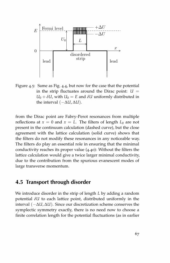
Figure 4.5: Same as Fig. 4.4, but now for the case that the potentialin the strip fluctuates around the Dirac point: U =

U0 + δU, with U0 = E and δU uniformly distributed inthe interval (−∆U, ∆U).

from the Dirac point are Fabry-Perot resonances from multiplereflections at x = 0 and x = L. The filters of length L0 are notpresent in the continuum calculation (dashed curve), but the closeagreement with the lattice calculation (solid curve) shows thatthe filters do not modify these resonances in any noticeable way.The filters do play an essential role in ensuring that the minimalconductivity reaches its proper value (4.40): Without the filters thelattice calculation would give a twice larger minimal conductivity,due to the contribution from the spurious evanescent modes oflarge transverse momentum.

4.5 Transport through disorder

We introduce disorder in the strip of length L by adding a randompotential δU to each lattice point, distributed uniformly in theinterval (−∆U, ∆U). Since our discretization scheme conserves thesymplectic symmetry exactly, there is no need now to choose afinite correlation length for the potential fluctuations (as in earlier

67

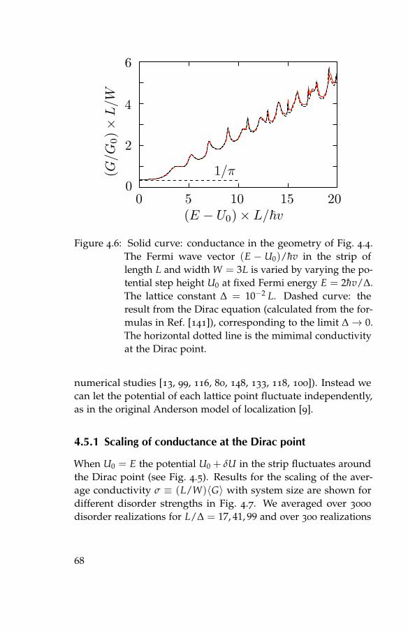
Figure 4.6: Solid curve: conductance in the geometry of Fig. 4.4.The Fermi wave vector (E − U0)/hv in the strip oflength L and width W = 3L is varied by varying the po-tential step height U0 at fixed Fermi energy E = 2hv/∆.The lattice constant ∆ = 10−2 L. Dashed curve: theresult from the Dirac equation (calculated from the for-mulas in Ref. [141]), corresponding to the limit ∆→ 0.The horizontal dotted line is the mimimal conductivityat the Dirac point.

numerical studies [13, 99, 116, 80, 148, 133, 118, 100]). Instead wecan let the potential of each lattice point fluctuate independently,as in the original Anderson model of localization [9].

4.5.1 Scaling of conductance at the Dirac point

When U0 = E the potential U0 + δU in the strip fluctuates aroundthe Dirac point (see Fig. 4.5). Results for the scaling of the aver-age conductivity σ ≡ (L/W)〈G〉 with system size are shown fordifferent disorder strengths in Fig. 4.7. We averaged over 3000

disorder realizations for L/∆ = 17, 41, 99 and over 300 realizations

68

Figure 4.7: Scaling with system size of the average conductivityσ ≡ (L/W)〈G〉 in a disordered strip at the Dirac point(geometry of Fig. 4.5). The length L of the strip is variedat fixed aspect ratio W/L = 3. The data are collectedfor different disorder strengths ∆U (listed in units ofhv/∆).

for L/∆ = 239. The aspect ratio was fixed at W/L = 3.For sufficiently strong disorder strengths ∆U & 3hv/∆ the data

follow the logarithmic scaling [13, 99]

σ/G0 = c ln[L/l∗(∆U)]. (4.41)

There is a consensus in the literature that c = 1/π can be calculatedperturbatively [121] as a weak antilocalization correction. Thequantity l∗ plays the role of a mean free path, dependent on thedisorder strength. We fit this scaling to our data with a commonfitting parameter c (disregarding the data sets with low ∆U asbeing too close to the ballistic limit). The fitting gives l∗ for everydata set with the same ∆U.

The resulting single-parameter scaling is presented in Fig. 4.8(including also the low ∆U sets, for completeness). The data setscollapse onto a single logarithmically increasing conductivity with

69

Figure 4.8: Dependence of the conductivity of Fig. 4.7 on therescaled system length L/l∗(∆U). The two dotted linesare the analytical weak and strong disorder limits.

c ≈ 0.33(1), close to the expected value c = 1/π ≈ 0.318. Toassess the importance of finite-size corrections [131] we include anon-universal lattice-constant dependent term to the logarithmicscaling: σ/G0 = c ln[L/l∗(∆U)] + f (∆U)∆/L. We then find c ≈0.316(5), again close to the expected value [121]. These results forthe absence of localization of Dirac fermions are consistent withearlier numerical calculations [13, 99] using a momentum spaceregularization of the Dirac equation.

4.5.2 Conductance fluctuations at the Dirac point

The sample-to-sample conductance fluctuations at the Dirac pointwere calculated numerically in Ref. [116] using the tight-bindingmodel on a honeycomb lattice. An enhancement of the varianceabove the value for point scatterers was observed, and explainedin Ref. [67] in terms of the absence of intervalley scattering. A

70

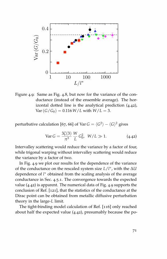
Figure 4.9: Same as Fig. 4.8, but now for the variance of the con-ductance (instead of the ensemble average). The hor-izontal dotted line is the analytical prediction (4.42),Var (G/G0) = 0.116 W/L with W/L = 3.

perturbative calculation [67, 66] of Var G = 〈G2〉 − 〈G〉2 gives

Var G =3ζ(3)

π3WL

G20 , W/L� 1. (4.42)

Intervalley scattering would reduce the variance by a factor of four,while trigonal warping without intervalley scattering would reducethe variance by a factor of two.

In Fig. 4.9 we plot our results for the dependence of the varianceof the conductance on the rescaled system size L/l∗, with the ∆Udependence of l∗ obtained from the scaling analysis of the averageconductance in Sec. 4.5.1. The convergence towards the expectedvalue (4.42) is apparent. The numerical data of Fig. 4.9 supports theconclusion of Ref. [121], that the statistics of the conductance at theDirac point can be obtained from metallic diffusive perturbationtheory in the large-L limit.

The tight-binding model calculation of Ref. [116] only reachedabout half the expected value (4.42), presumably because the po-

71

Figure 4.10: Crossover from ballistic to diffusive conduction awayfrom the Dirac point. The conductivity is plot-ted versus system size, at fixed Fermi wave vector(E −U0)/hv = 0.8 ∆−1 in the strip and fixed aspectratio W/L = 3. The data is for different disorderstrengths ∆U, listed in units of hv/∆. The dottedcurves are a fit to the semiclassical formula (4.43), withthe transport mean free path l0 as a fit parameter.

tential was not quite smooth enough to avoid intervalley scattering.This illustrates the power of the finite difference method used here:We retain single-valley physics even when the correlation length ofthe potential is equal to the lattice constant.

4.5.3 Transport away from the Dirac point

The results of Secs. 4.5.1 and 4.5.2 are for potential fluctuationsaround the Dirac point (U0 = E). In this subsection we considerthe average conductance and the conductance fluctuations awayfrom the Dirac point. We take (E−U0) = 0.8 hv/∆ and vary thesample length L at fixed aspect ratio W/L = 3. The resultingsize dependence of the conductivity is presented in Fig. 4.10, fordifferent disorder strengths ∆U.

72

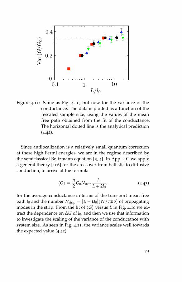
Figure 4.11: Same as Fig. 4.10, but now for the variance of theconductance. The data is plotted as a function of therescaled sample size, using the values of the meanfree path obtained from the fit of the conductance.The horizontal dotted line is the analytical prediction(4.42).

Since antilocalization is a relatively small quantum correctionat these high Fermi energies, we are in the regime described bythe semiclassical Boltzmann equation [3, 4]. In App. 4.C we applya general theory [106] for the crossover from ballistic to diffusiveconduction, to arrive at the formula

〈G〉 = π

2G0Nstrip

l0L + 2l0

, (4.43)

for the average conductance in terms of the transport mean freepath l0 and the number Nstrip = |E−U0|(W/πhv) of propagatingmodes in the strip. From the fit of 〈G〉 versus L in Fig. 4.10 we ex-tract the dependence on ∆U of l0, and then we use that informationto investigate the scaling of the variance of the conductance withsystem size. As seen in Fig. 4.11, the variance scales well towardsthe expected value (4.42).

73

4.6 Conclusion

In conclusion, we have presented in this paper what one might callthe “Anderson model for Dirac fermions”. Just as in the originalAnderson tight-binding model of localization [9], our model is atight-binding model on a lattice with uncorrelated on-site disorder.Unlike the tight-binding model of graphene (with nearest neighborhopping on a honeycomb lattice), our model preserves the symplec-tic symmetry of the Dirac equation – at the expense of a nonlocalfinite difference approximation of the transfer matrix.

Our finite difference method is based on a discretization schemedeveloped in the context of lattice gauge theory [134, 22], withthe purpose of resolving the fermion doubling problem. We haveadapted this scheme to include the chiral symmetry breaking by adisorder potential, and have cast it in a current-conserving transfermatrix form suitable for the calculation of transport properties.

To test the validity and efficiency of the model, we have calcu-lated the average and the variance of the conductance and com-pared with earlier numerical and analytical results. We recoverthe logarithmic increase of the average conductance at the Diracpoint, found in numerical calculations that use a momentum spacerather than a real space discretization of the Dirac equation [13, 99].The coefficient that multiplies the logarithm is close to 1/π, inagreement with analytical expectations [121]. The variance of theconductance is enhanced by the absence of intervalley scattering,and we have been able to confirm the scaling with increasing sys-tem size towards the expected limit [67, 66] – something whichhad not been possible in earlier numerical calculations [116] be-cause intervalley scattering sets in before the large-system limit isreached.

Our calculations support the expectation [121] that the statisticsof the conductance at the Dirac point scales towards that of adiffusive metal in the large-system limit. This would imply thatthe shot noise should scale towards a Fano factor F = 1/3 [18].Earlier numerical studies using the momentum space discretization

74

Figure 4.12: Scaling with system size of the Fano factor (averageshot noise power divided by average current) in a dis-ordered strip at the Dirac point (geometry of Fig. 4.5).The length L of the strip is varied at fixed aspect ratioW/L = 3. The data are collected for different disorderstrengths ∆U (listed in units of hv/∆). The dotted hor-izontal line is the value F = 1/3 for a diffusive metal.The dotted curve is a fit to F = 1/3+ a[b+ ln(L/l∗)]−1,included in order to indicate a possible scaling towardsthe expected value.

[118] found a saturation at the smaller value of F = 0.295. Ourown numerical results, shown in Fig. 4.12, instead suggest a slow,logarithmic, increase towards the expected F = 1/3. More researchon this particular quantity is required for a conclusive answer.

We anticipate that the numerical method developed here willprove useful for the study of graphene with smooth disorder poten-tials (produced for example by remote charge fluctuations), sincesuch potentials produce little intervalley scattering. Intervalley scat-tering is absent by construction in the metallic surface states of topo-logical insulators (such as BiSb [55]). These surface states might be

75

studied by starting from a three-dimensional tight-binding model,but we would expect a two-dimensional formulation as presentedhere to be more efficient.

Appendix 4.A Current conserving discretizationof the current operator

We seek a discretization of the current operator (4.3) that satisfiesthe condition (4.7) of current conservation. Substitution of theexpression (4.20) into the condition (4.7) gives the requirement

J−1x M†

m Jx =M−1m ⇔ J−1

x X†m Jx = Xm. (4.44)

The requirement that Eq. (4.44) holds for any choice of potentialfixes the discretization (4.21) of the current operator [up to a multi-plicative constant, which follows from the continuum limit (4.3)].

This is an appropriate point to note that current conservationcould not have been achieved if the potential would have beendiscretized in a way that would have resulted in a nonsymmetricmatrix Vm. For example, if instead of Eq. (4.11) we would havechosen

VΨ→ 14 (Vm+1,nΨm+1,n + Vm+1,n+1Ψm+1,n+1

+ Vm,nΨm,n + Vm,n+1Ψm,n+1), (4.45)

with Vm,n = V(xm, yn), then the corresponding matrix Vm wouldhave been asymmetric and no choice of Jx could have satisfied Eq.(4.44).

Appendix 4.B Stable multiplication of transfermatrices

To perform the multiplication (4.22) of transfer matrices in a stableway (avoiding exponentially growing and decaying eigenvalues),we use the current conservation relation (4.7) to convert the product

76

into a composition of unitary matrices (involving only eigenvaluesof unit absolute value). The same method was used in Refs. [13,133, 138], but for a different current operator, so the requiredtransformation formulas need to be adapted.

We separate the spinor degrees of freedom s = ± of the transfermatrixMm into four N × N blocks,

Mm =

(M++m M+−

mM−+

m M−−m

). (4.46)

The current conservation relation (4.7) with current operator (4.21)can be written in the canonical form,

M†m

(1 00 −1

)Mm =

(1 00 −1

), (4.47)

in terms of a matrix Mm related toMm by a similarity transforma-tion,

Mm = RMmR−1, R = 2−1/2(J 1/2 J 1/2

J 1/2 −J 1/2

). (4.48)

Eq. (4.47) follows only from Eqs. (4.7) and (4.21) if the matrix Ris Hermitian, which it is since J is Hermitian with only positiveeigenvalues [see Eq. (4.15)].

It now follows directly from Eq. (4.7) that the matrix Um con-structed from Mm by

Mm =

(a bc d

)⇔ Um =

( −d−1c d−1

a− bd−1c bd−1

)(4.49)

is a unitary matrix. Matrix multiplication of Mm’s induces anonlinear composition of Um’s,

M1M2 ⇔ U1 ⊗U2, (4.50)

77

defined by

(A1 B1

C1 D1

)⊗(

A2 B2

C2 D2

)=

(A3 B3

C3 D3

), (4.51a)

A3 = A1 + B1(1− A2D1)−1A2C1, (4.51b)

B3 = B1(1− A2D1)−1B2, (4.51c)

C3 = C2(1− D1A2)−1C1, (4.51d)

D3 = D2 + C2(1− D1A2)−1D1B2. (4.51e)

To evaluate the product (4.22) ofMm’s in a stable way, we firstwrite it in terms of the matrices Mm,

M = R−1

(M

∏m=1Mm

)R. (4.52)

We then transform each transfer matrix Mm into a unitary matrixUm according to Eq. (4.49) and we compose the unitary matricesaccording to Eq. (4.51). Each step in this calculation is numericallystable.

At the end of the calculation, we may in principle transformback from the final unitary matrix U to the transfer matrixM =

R−1MR by means of the inverse of relation (4.49),

U =

(A BC D

)⇔ M =

(C− DB−1A DB−1

−B−1A B−1

). (4.53)

This inverse transformation is itself unstable, but we may avoid itbecause [as we can see by comparing Eqs. (4.49) and (4.53) withEq. (4.33)] the final U is identical to the scattering matrix S betweenleads in the infinite wave vector limit. Hence the conductance canbe directly obtained from U via the Landauer formula (4.27) [withthe Tn’s being the eigenvalues of BB† and CC†].

78

Appendix 4.C Crossover from ballistic to diffusiveconduction

Away from the Dirac point (for Fermi wave vectors kF = |E −U0|/hv in the strip large compared to 1/L) conduction throughthe strip is via propagating rather than evanescent modes. Ifthe number Nstrip = kFW/π of propagating modes is � 1, thesemiclassical Boltzmann equation can be used to calculate theconductance.

As the transport mean free path l0 is reduced by adding disorderto the strip, the conduction crosses over from the ballistic to thediffusive regime. How to describe this crossover is a well-knownproblem in the context of radiative transfer [106]. An exact solutionof the Boltzmann equation does not provide a closed-form expres-sion for the crossover, but the following formula has been found tobe accurate within a few percent:

〈G〉 = CdG0Nstripl0

L + 2ξ. (4.54)

The coefficient Cd depends on the dimensionality d: C3 = 4/3,C2 = π/2, C1 = 2. The length ξ is the socalled extrapolation lengthof radiative transfer theory, equal to l0 times a numerical coefficientthat depends on the reflectivity of the interface at x = 0 and x = L.An infinite potential step in the Dirac equation has ξ = l0, seeRef. [124]. Substitution into Eq. (4.54) then gives the formula (4.43)used in the text.

79

5 Switching of electrical current byspin precession in the firstLandau level of an inverted-gapsemiconductor

5.1 Introduction

A central goal of spin-transport electronics (or spintronics) is theability to switch current between spin-selective electrodes by meansof spin precession [151]. In the original Datta-Das proposal for sucha spin-based transistor [38], the current which is switched carriesboth spin and charge. It has proven difficult to separate the effectsof spin precession from purely orbital effects (deflection of electrontrajectories), so most succesful implementations use a nonlocalgeometry [60] to modulate the spin current at zero charge current[58, 85, 139]. Even in the absence of an orbital effect, the fact thatdifferent electrons (moving along different trajectories) experiencedifferent amounts of spin precession prevents a complete switchingof the current from one electrode to the other.

If the electron motion could somehow be confined to a singlespatial dimension, it would be easier to isolate spin effects fromorbital effects and to ensure that all electron spins precess by thesame amount. Complete switching of the current would then bepossible, limited only by spin relaxation processes. Edge statetransport in the quantum Hall effect is one-dimensional and spinselective (in sufficiently strong perpendicular magnetic fields B⊥),but spin precession plays no role in the traditional experiments

81

Figure 5.1: Top panel: Schematic illustration of the one-dimensional pathway along which the electron spinis injected, precessed, and detected (filled circles: oc-cupied states; open circles: empty states). Bottompanel: Potential profile of the p-n junction, shown forB⊥ > Bc (for B⊥ < Bc the labels E+ and E− should beinterchanged).

on a two-dimensional electron gas [17]. In this paper we showhow the quantum Hall effect in an inverted-gap semiconductoroffers the unique possibility to perform a one-dimensional spinprecession experiment.

The key idea is to combine the spin-selectivity of edge stateswith free precession along a p-n interface. The geometry, shownin Fig. 5.1, has been studied in graphene [146, 2, 105, 142] – butthere spin is only weakly coupled to the orbit and plays a minorrole [62, 1]. The strong spin-orbit coupling in inverted-gap semi-conductors splits the first Landau level into a pair of levels E± ofopposite magnetic moment [74, 123]. One level E+ (say, with spinup) has electron-like character and produces edge states in the

82

conduction band. The other level E− (with spin down) has hole-like character and produces edge states in the valence band. Theedge states from E+ and E− have opposite chirality, meaning thatone circulates clockwise along the edge while the other circulatescounter-clockwise. These spin-selective, chiral edge states providethe spin injection at x = 0 and detection at x = W.

For the spin precession we need to combine states from E+ andE−. This is achieved by means of a gate electrode, which creates asmooth potential step (height U0, width d) centered at y = 0, suchthat the Fermi level lies in the conduction band for y < 0 (n-dopedregion) and in the valence band for y > 0 (p-doped region). Atthe p-n interface states from the first Landau levels E+ and E−overlap at the Fermi energy EF, to form a spin-degenerate one-dimensional state. Spin precession can be realized externally by aparallel magnetic field B‖ (in the x− y plane) or internally by bulkor structure inversion asymmetry [74].

Good overlap at EF of the states from E+ and E− is crucial foreffective spin precession. The requirement is that the spatial sepa-ration δy ' |E+ − E−|d/U0 of the states should be small comparedto the magnetic length lm = (h/eB⊥)1/2 (which sets their spatialextent). This is where the inverted gap comes in, as we now explain.

Inversion of the gap means that the first Landau level in the con-duction band goes down in energy with increasing magnetic field(because it has hole-like character), while the first Landau level inthe valence band goes up in energy (because it has electron-likecharacter). As a consequence, the gap |E+ − E−| has a minimalvalue Ec much less than the cyclotron energy hωc at a crossovermagnetic field Bc. Indeed, Ec = 0 in the absence of inversionasymmetry [74]. Good overlap can therefore be reached in aninverted-gap semiconductor, simply by tuning the magnetic field.In a normal (non-inverted) semiconductor, such as GaAs, the cy-clotron energy difference between E+ and E− effectively preventsthe overlap of Landau levels from conduction and valence bands.

In the following two sections, we first present a general, modelindependent analysis and then specialize to the case of a HgTe

83

quantum well (where we test the analytical theory by computersimulation).

5.2 General theory

We introduce a one-dimensional coordinate s± along the E± edgestates, increasing in the direction of the chirality (see Fig. 5.1). Thewave amplitudes ψ±(s±) of these two states can be combined intothe spinor Ψ = (ψ+, ψ−). Far from the p-n interface, ψ+ and ψ−evolve independently with Hamiltonian

H0 =

(H+ 00 H−

), H± = v±

(−ih

∂

∂s±− p±F

). (5.1)

This is the generic linearized Hamiltonian of a chiral mode, withgroup velocity v± ≡ v(s±) and Fermi momentum p±F ≡ pF(s±).Near the p-n interface the spin-up and spin-down states are coupledby the generic precession Hamiltonian,

Hprec =

(0 M∗

M 0

), (5.2)

with a matrix elementM to be specified later.We seek the transfer matrix T, defined by

Ψ(s f+, s f−) = TΨ(si

+, si−). (5.3)

We take for Ψ a solution of the Schrodinger equation,

(H0 + Hprec)Ψ = 0, (5.4)

at zero excitation energy (appropriate for electrical conductionin linear response). The initial and final points si

± and s f± are

taken away from the p-n interface. The unitary scattering matrix S(relating incident and outgoing current amplitudes) is related to Tby a similarity transformation,

S =

(v f+ 00 v f

−

)1/2

T(

vi+ 00 vi

−

)−1/2

. (5.5)

84

The two-terminal linear-response conductance G of the p-n junctionis given by the Landauer formula,

G =e2

h|S21|2. (5.6)

The transition matrix element M(s+, s−) between ψ+(s+) andψ−(s−) vanishes if the separation |s+ − s−| of the two states islarge compared to the magnetic length lm. We assume that B⊥ issufficiently close to Bc that |s+ − s−| < lm at the p-n interface y = 0,0 < x < W, where we may take M = constant (independent ofx). At the two edges x = 0 and x = W we setM = 0, neglectingthe crossover region within lm of (0, 0) and (W, 0). (The precessionangle there will be small compared to unity for lm � hv±/|M|.)

In this “abrupt approximation” we may identify the initial andfinal coordinates si

± and s f± with the points (0, 0) and (W, 0), at

the two ends of the p-n interface. Integration of the Schrodingerequation (5.4) along the p-n interface gives the transfer matrix, andapplication of Eq. (5.5) then gives the scattering matrix

S = exp[−i

Wh

(p+F M∗/

√v+v−

M/√

v+v− p−F

)]. (5.7)

(We have assumed that v± and p±F , as well asM, do not vary alongthe p-n interface, so we may omit the labels i, f .) One verifies thatS is unitary, as it should be.

Evaluation of the matrix exponent in Eq. (5.7) and substitutioninto Eq. (5.6) gives the conductance,

G =e2

hsin2

( |peff|Wh

)sin2 α. (5.8)

The effective precession momentum

peff =

(ReM

v,

ImMv

,δpF

2

)(5.9)

(with δpF = p+F − p−F and v =√

v+v−) makes an angle α with thez-axis. This is the final result of our general analysis.

85

5.3 Application to a HgTe quantum well

We now turn to a specific inverted-gap semiconductor, a quantumwell consisting of a 7 nm layer of HgTe sandwiched symmetricallybetween Hg0.3Cd0.7Te [73]. The properties of this socalled topologi-cal insulator have been reviewed in [74]. The low-energy excitationsare described by a four-orbital tight-binding Hamiltonian [23, 44],

H = ∑n

c†nEncn − ∑

n,m (nearest neighb.)c†

nTnmcm. (5.10)

Each site n on a square lattice (lattice constant a = 4 nm) has fourstates |s,±〉, |px ± ipy,±〉 – two electron-like s-orbitals and twohole-like p-orbitals of opposite spin σ = ±. Annihilation operatorscn,τσ for these four states (with τ ∈ {s, p}) are collected in a vector

cn = (cn,s+, cn,p+, cn,s−, cn,p−).

States on the same site are coupled by the 4× 4 potential matrixEn and states on adjacent sites by the 4× 4 hopping matrix Tnm.

In zero magnetic field and without inversion asymmetry H de-couples into a spin-up block H+ and a spin-down block H−, de-fined in terms of the 2× 2 matrices

E+n = E−n = diag (εs −Un, εp −Un), (5.11)

T +nm =

(T −nm

)∗=

(tss tspeiθnm

tspe−iθmn −tpp

). (5.12)

Here Un is the electrostatic potential and θnm is the angle betweenthe vector rn − rm and the positive x-axis (so θmn = π − θnm). Theorbital effect of a perpendicular magnetic field B⊥ is introducedinto the hopping matrix elements by means of the Peierls substitu-tion

Tnm 7→ Tnm exp[i(eB⊥/h)(yn − ym)xn].

This breaks the degeneracy of the spin-up and spin-down energylevels, but it does not couple them.

86

Spin-up and spin-down states are coupled by the Zeeman effectfrom a parallel magnetic field (with gyromagnetic factor g‖) and byspin-orbit interaction without inversion symmetry (parameterizedby a vector ∆). In first-order perturbation theory, the correction δEto the on-site potential has the form [74]

δE = (∆ · σ)⊗ τy +12 µBg‖(B‖ · σ)⊗ (τ0 + τz)

+ µBB⊥σz ⊗ (g⊥τ0 + δg⊥τz). (5.13)

The Pauli matrices σ = (σx, σy, σz) act on the spin-up and spin-down blocks, while the Pauli matrices τy, τz and the unit matrix τ0

act on the orbital degree of freedom s, p within each block.The parameters of the tight-binding model for a 7 nm thick

HgTe/Hg0.3Cd0.7Te quantum well (grown in the (001) direction)are as follows [74]: tss = 74.9 meV, tpp = 10.9 meV, tsp = 45.6 meV,εs = 289.5 meV, εp = −33.5 meV, g⊥ = 10.75, δg⊥ = 11.96, g‖ =−20.5, ∆ = (0, 1.6 meV, 0).

The quantum well is symmetric, so only bulk inversion asymme-try contributes to ∆. The p-n junction is defined by the potentialprofile

U(x, y) = 12U0[1 + tanh(4y/d)], 0 < x < W, (5.14)

with U0 = 32 meV, d = 12 nm, and W = 0.8 µm. We fix the Fermilevel at EF = 25 meV, so that it lies in the conduction band fory < 0 and in the valence band for y > 0. (We have checked thatnone of the results are sensitive to the choice of potential profileor parameter values.) The scattering matrix of the p-n junction iscalculated with the recursive Green function technique, using the“knitting” algorithm1 of Ref. [65]. Results for G as a function of B‖are shown in Figs. 5.2 and 5.3.

The dependence of the conductance on the parallel magnetic fieldB‖ shows a striking “bullseye” pattern, which can be understood

1 The computer code for the knitting algorithm was kindly provided to us byDr. Waintal.

87

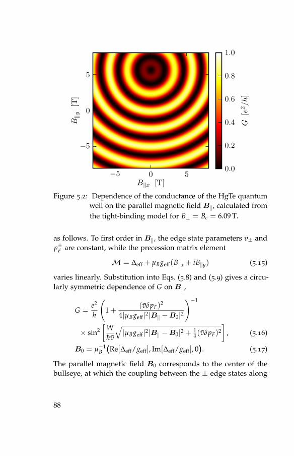
−5 0 5B‖x [T]

−5

0

5B‖y

[T]

0.0

0.2

0.4

0.6

0.8

1.0

G[e

2/h

]

Figure 5.2: Dependence of the conductance of the HgTe quantumwell on the parallel magnetic field B‖, calculated fromthe tight-binding model for B⊥ = Bc = 6.09 T.

as follows. To first order in B‖, the edge state parameters v± andp±F are constant, while the precession matrix element

M = ∆eff + µBgeff(B‖x + iB‖y) (5.15)

varies linearly. Substitution into Eqs. (5.8) and (5.9) gives a circu-larly symmetric dependence of G on B‖,

G =e2

h

(1 +

(vδpF)2

4|µBgeff|2|B‖ −B0|2

)−1

× sin2[

Whv

√|µBgeff|2|B‖ −B0|2 + 1

4 (vδpF)2

], (5.16)

B0 = µ−1B(((Re[∆eff/geff], Im[∆eff/geff], 0

))). (5.17)

The parallel magnetic field B0 corresponds to the center of thebullseye, at which the coupling between the ± edge states along

88

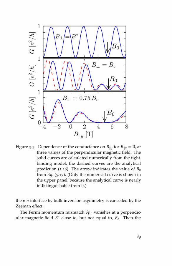
Figure 5.3: Dependence of the conductance on B‖y for B‖x = 0, atthree values of the perpendicular magnetic field. Thesolid curves are calculated numerically from the tight-binding model, the dashed curves are the analyticalprediction (5.16). The arrow indicates the value of B0

from Eq. (5.17). (Only the numerical curve is shown inthe upper panel, because the analytical curve is nearlyindistinguishable from it.)

the p-n interface by bulk inversion asymmetry is cancelled by theZeeman effect.

The Fermi momentum mismatch δpF vanishes at a perpendic-ular magnetic field B∗ close to, but not equal to, Bc. Then the

89

magnetoconductance oscillations are purely sinusoidal,

G =e2

hsin2[(W/hv)µBgeff|B‖ −B0|]. (5.18)

For a quantitative comparison between numerics and analytics,we extract the parameters v± and p±F from the dispersion relation ofthe edge states ψ± along an infinitely long p-n interface (calculatedfor uncoupled blocks H±). The overlap of ψ+ and ψ− determinesthe coefficients

∆eff = (∆x + i∆y)〈ψ−|τy|ψ+〉, (5.19)

geff =12 g‖〈ψ−|τ0 + τz|ψ+〉. (5.20)

For B⊥ = Bc = 6.09 T we find vδpF = 0.86 meV, hv/W =

0.23 meV, ∆eff = −1.59 meV, geff = −4.99. The Fermi momen-tum mismatch δpF vanishes for B⊥ = B∗ = 5.77 T. Substitutionof the parameters into Eq. (5.16) gives the dashed curves in Fig.5.3, in reasonable agreement with the numerical results from thetight-binding model (solid curves). In particular, the value of B0 ex-tracted from the numerics is within a few percent of the analyticalprediction (5.17).

Because of the one-dimensionality of the motion along the p-n interface, electrostatic disorder and thermal averaging have arelatively small perturbing effect on the conductance oscillations.For disorder potentials ∆U and thermal energies kBT up to 10% ofU0 the perturbation is hardly noticeable (a few percent). As shownin Fig. 5.4, the conductance oscillations remain clearly visible evenfor ∆U and kBT comparable to U0. In particular, we have foundthat the center of the bullseye pattern remains within 10% of B0

even for ∆U as large as the p-n step height U0.

5.4 Conclusion

In conclusion, we have proposed a one-dimensional spin precessionexperiment at a p-n junction in an inverted-gap semiconductor. The

90

Figure 5.4: The solid blue curve in both panels is the same asin Fig. 5.3, top panel, calculated for B⊥ = B∗ fromthe tight-binding model at zero temperature withoutany disorder. The dotted black curve in the lowerpanel shows the effect of raising the temperature to30 K ≈ U0/3kB. The dotted red curve and dashed greencurve in the upper panel show the effect of disorderat zero temperature. The on-site disorder potential isdrawn uniformly from the interval (−∆U0, ∆U0), with,respectively, ∆U = U0/4 and ∆U = U0/2.

conductance as a function of parallel magnetic field oscillates in abullseye pattern, centered at a field B0 proportional to the matrixelement ∆eff of the bulk inversion asymmetry. Our numerical andanalytical calculations show conductance oscillations of amplitudenot far below e2/h, robust to disorder and thermal averaging.Realization of the proposed experiment in a HgTe quantum well[74] (or in other inverted-gap semiconductors [82]) would provide a

91

unique demonstration of full-current switching by spin precession.As directions for future research, we envisage potential applica-

tions of this technique as a sensitive measurement of the degreeof bulk inversion asymmetry, or as a probe of the effects of inter-actions on spin precession. It might also be possible to eliminatethe external magnetic field and realize electrical switching of thecurrent in our setup: The role of the perpendicular magnetic fieldin producing spin-selective edge states can be taken over by mag-netic impurities or a ferromagnetic layer [83], while the role of theparallel magnetic field in providing controlled spin precession canbe taken over by gate-controlled structural inversion asymmetry.

92

6 Theory of the topologicalAnderson insulator

6.1 Introduction

Topological insulators continue to surprise with unexpected phys-ical phenomena [30]. A recent surprise was the discovery of thetopological Anderson insulator (TAI) by Li, Chu, Jain, and Shen[81]. In computer simulations of a HgTe quantum well, these au-thors discovered in the phase diagram a transition from an ordinaryinsulating state (exponentially small conductance) to a state witha quantized conductance of G0 = 2e2/h. The name TAI refersto the latter state. The findings of Ref. [81] were confirmed byindependent simulations [59].

The phenomenology of the TAI is similar to that of the quan-tum spin Hall (QSH) effect, which is well understood [62, 23]and observed experimentally in HgTe quantum wells [70, 74, 113].The QSH effect is a band structure effect: It requires a quantumwell with an inverted band gap, modeled by an effective DiracHamiltonian with a negative (socalled “topological”) mass. Thematching of this negative mass inside the system to the usual pos-itive mass outside leaves edge states in the gap. The edge statesare “helical”, in the sense that the direction of propagation is tiedto the electron spin. Opposite edges each contribute e2/h to theconductance. The conductance remains quantized in the presenceof (weak) disorder, because time reversal symmetry forbids scatter-ing between counter-propagating edge states (of opposite helicity)[62, 23, 70, 74, 113].

The crucial difference between the TAI and QSH phases is that

93

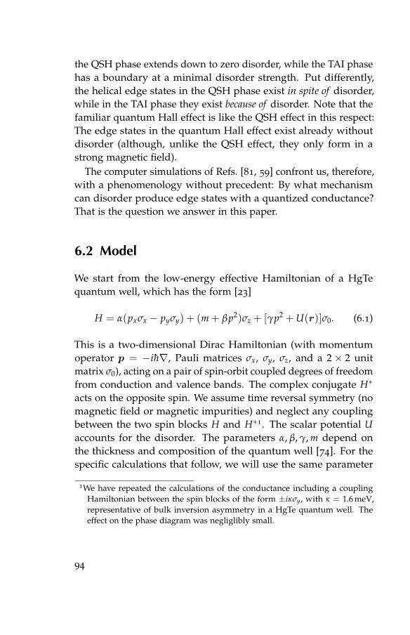
the QSH phase extends down to zero disorder, while the TAI phasehas a boundary at a minimal disorder strength. Put differently,the helical edge states in the QSH phase exist in spite of disorder,while in the TAI phase they exist because of disorder. Note that thefamiliar quantum Hall effect is like the QSH effect in this respect:The edge states in the quantum Hall effect exist already withoutdisorder (although, unlike the QSH effect, they only form in astrong magnetic field).

The computer simulations of Refs. [81, 59] confront us, therefore,with a phenomenology without precedent: By what mechanismcan disorder produce edge states with a quantized conductance?That is the question we answer in this paper.

6.2 Model

We start from the low-energy effective Hamiltonian of a HgTequantum well, which has the form [23]

H = α(pxσx − pyσy) + (m + βp2)σz + [γp2 + U(r)]σ0. (6.1)

This is a two-dimensional Dirac Hamiltonian (with momentumoperator p = −ih∇, Pauli matrices σx, σy, σz, and a 2× 2 unitmatrix σ0), acting on a pair of spin-orbit coupled degrees of freedomfrom conduction and valence bands. The complex conjugate H∗

acts on the opposite spin. We assume time reversal symmetry (nomagnetic field or magnetic impurities) and neglect any couplingbetween the two spin blocks H and H∗1. The scalar potential Uaccounts for the disorder. The parameters α, β, γ, m depend onthe thickness and composition of the quantum well [74]. For thespecific calculations that follow, we will use the same parameter

1We have repeated the calculations of the conductance including a couplingHamiltonian between the spin blocks of the form ±iκσy, with κ = 1.6 meV,representative of bulk inversion asymmetry in a HgTe quantum well. Theeffect on the phase diagram was negliglibly small.

94

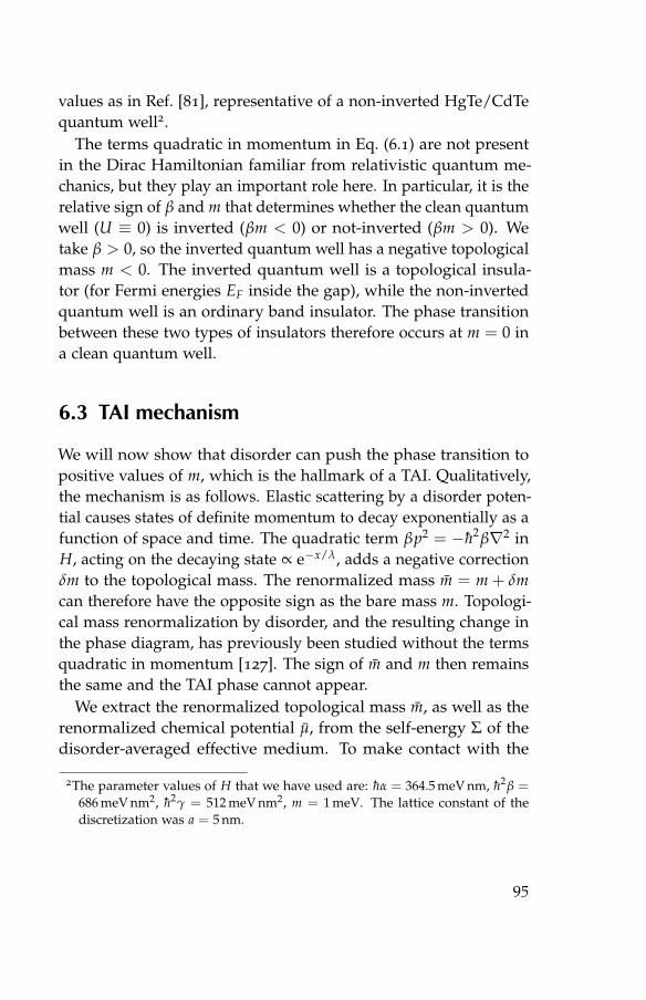
values as in Ref. [81], representative of a non-inverted HgTe/CdTequantum well2.

The terms quadratic in momentum in Eq. (6.1) are not presentin the Dirac Hamiltonian familiar from relativistic quantum me-chanics, but they play an important role here. In particular, it is therelative sign of β and m that determines whether the clean quantumwell (U ≡ 0) is inverted (βm < 0) or not-inverted (βm > 0). Wetake β > 0, so the inverted quantum well has a negative topologicalmass m < 0. The inverted quantum well is a topological insula-tor (for Fermi energies EF inside the gap), while the non-invertedquantum well is an ordinary band insulator. The phase transitionbetween these two types of insulators therefore occurs at m = 0 ina clean quantum well.

6.3 TAI mechanism

We will now show that disorder can push the phase transition topositive values of m, which is the hallmark of a TAI. Qualitatively,the mechanism is as follows. Elastic scattering by a disorder poten-tial causes states of definite momentum to decay exponentially as afunction of space and time. The quadratic term βp2 = −h2β∇2 inH, acting on the decaying state ∝ e−x/λ, adds a negative correctionδm to the topological mass. The renormalized mass m = m + δmcan therefore have the opposite sign as the bare mass m. Topologi-cal mass renormalization by disorder, and the resulting change inthe phase diagram, has previously been studied without the termsquadratic in momentum [127]. The sign of m and m then remainsthe same and the TAI phase cannot appear.

We extract the renormalized topological mass m, as well as therenormalized chemical potential µ, from the self-energy Σ of thedisorder-averaged effective medium. To make contact with the

2The parameter values of H that we have used are: hα = 364.5 meV nm, h2β =686 meV nm2, h2γ = 512 meV nm2, m = 1 meV. The lattice constant of thediscretization was a = 5 nm.

95

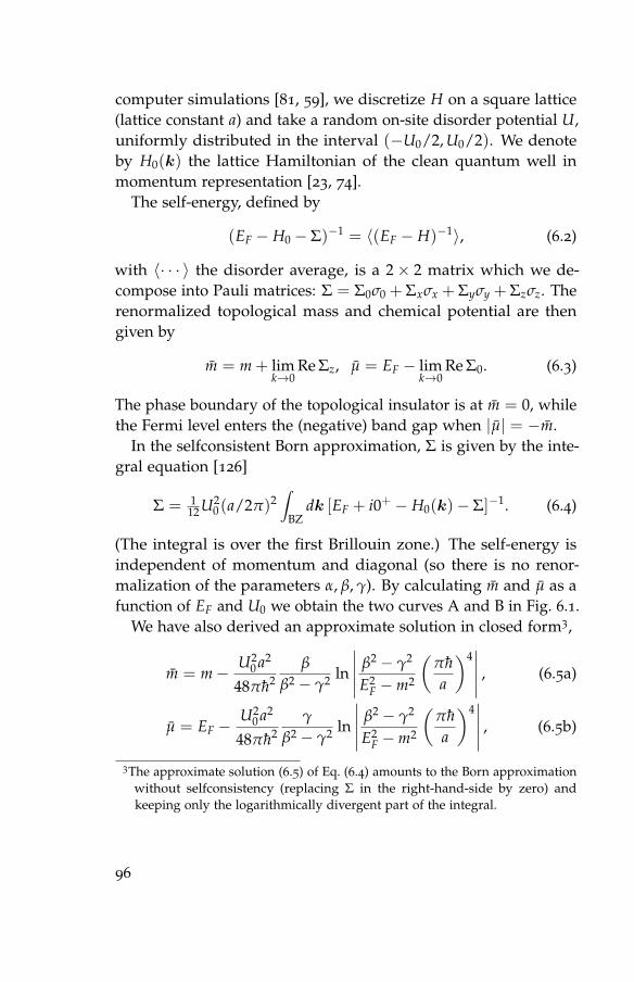
computer simulations [81, 59], we discretize H on a square lattice(lattice constant a) and take a random on-site disorder potential U,uniformly distributed in the interval (−U0/2, U0/2). We denoteby H0(k) the lattice Hamiltonian of the clean quantum well inmomentum representation [23, 74].

The self-energy, defined by

(EF − H0 − Σ)−1 = 〈(EF − H)−1〉, (6.2)

with 〈· · · 〉 the disorder average, is a 2× 2 matrix which we de-compose into Pauli matrices: Σ = Σ0σ0 + Σxσx + Σyσy + Σzσz. Therenormalized topological mass and chemical potential are thengiven by

m = m + limk→0

Re Σz, µ = EF − limk→0

Re Σ0. (6.3)

The phase boundary of the topological insulator is at m = 0, whilethe Fermi level enters the (negative) band gap when |µ| = −m.

In the selfconsistent Born approximation, Σ is given by the inte-gral equation [126]

Σ = 112U2

0(a/2π)2∫

BZdk [EF + i0+ − H0(k)− Σ]−1. (6.4)

(The integral is over the first Brillouin zone.) The self-energy isindependent of momentum and diagonal (so there is no renor-malization of the parameters α, β, γ). By calculating m and µ as afunction of EF and U0 we obtain the two curves A and B in Fig. 6.1.

We have also derived an approximate solution in closed form3,

m = m− U20 a2

48πh2β

β2 − γ2 ln

∣∣∣∣∣ β2 − γ2

E2F −m2

(πha

)4∣∣∣∣∣ , (6.5a)

µ = EF −U2

0 a2

48πh2γ

β2 − γ2 ln

∣∣∣∣∣ β2 − γ2

E2F −m2

(πha

)4∣∣∣∣∣ , (6.5b)

3The approximate solution (6.5) of Eq. (6.4) amounts to the Born approximationwithout selfconsistency (replacing Σ in the right-hand-side by zero) andkeeping only the logarithmically divergent part of the integral.

96

showing that the correction δm = m−m to the topological massby disorder is negative – provided β > γ. For β < γ the clean HgTequantum well would be a semimetal, lacking a gap in the entireBrillouin zone. Neither the TAI phase nor the QSH phase wouldthen appear. In HgTe the parameter β is indeed larger than γ, butnot by much4. Eq. (6.5) implies that the lower branch of curve B(defined by µ = m < 0) is then fixed at EF ≈ m > 0 independentof U0. This explains the puzzling absence of the TAI phase inthe valence band (EF < 0), observed in the computer simulations[81, 59].

To quantitatively test the phase diagram resulting from the effec-tive medium theory, we performed computer simulations similarto those reported in Refs. [81, 59]. The conductance G is calculatedfrom the lattice Hamiltonian [23, 74] in a strip geometry, usingthe method of recursive Green functions. The strip consists of arectangular disordered region (width W, length L), connected tosemi-infinite, heavily doped, clean leads5. Theory and simulationare compared in Figs. 6.1 and 6.2.

Fig. 6.1 shows the phase diagram. The weak-disorder boundaryof the TAI phase observed in the simulations is described quite wellby the selfconsistent Born approximation (curve B) – without anyadjustable parameter. Curve B limits the region where (A) the renor-malized topological mass m is negative and (B) the renormalizedchemical potential µ lies inside the band gap: |µ| < −m. Condition(A) is needed for the existence of edge states with a quantizedconductance. Condition (B) is not needed for an infinite system,because then Anderson localization suppresses conductance viabulk states as well as coupling of edge states at opposite edges.In the relatively small systems accessible by computer simulation,the localization length for weak disorder remains larger than thesystem size (see later). Condition (B) is then needed to eliminate

4See footnote on page 95.5The reason we dope the leads in the computer simulations is to be able to access

the region |EF| < m in the phase diagram, where the band gap in the cleanleads would otherwise prevent conduction through the disordered region.

97

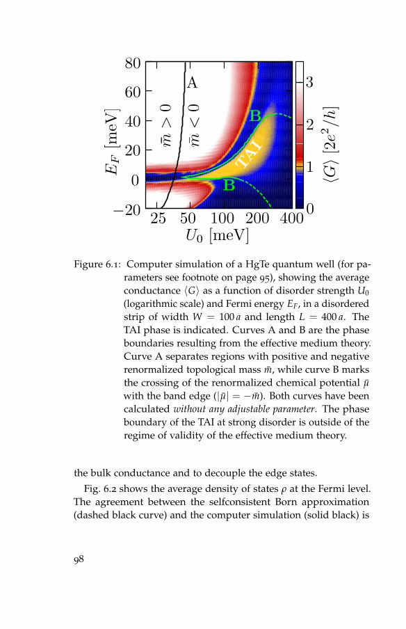
Figure 6.1: Computer simulation of a HgTe quantum well (for pa-rameters see footnote on page 95), showing the averageconductance 〈G〉 as a function of disorder strength U0

(logarithmic scale) and Fermi energy EF, in a disorderedstrip of width W = 100 a and length L = 400 a. TheTAI phase is indicated. Curves A and B are the phaseboundaries resulting from the effective medium theory.Curve A separates regions with positive and negativerenormalized topological mass m, while curve B marksthe crossing of the renormalized chemical potential µ

with the band edge (|µ| = −m). Both curves have beencalculated without any adjustable parameter. The phaseboundary of the TAI at strong disorder is outside of theregime of validity of the effective medium theory.

the bulk conductance and to decouple the edge states.

Fig. 6.2 shows the average density of states ρ at the Fermi level.The agreement between the selfconsistent Born approximation(dashed black curve) and the computer simulation (solid black) is

98

Figure 6.2: Black curves, left axis: Average density of states ρ

as a function of EF for U0 = 100 meV, calculated bycomputer simulation (solid curve, for a disordered100 a × 100 a square with periodic boundary condi-tions) or by effective medium theory (dashed curve).Red curve, right axis: Average conductance 〈G〉, cal-culated by computer simulation in a disordered strip(U0 = 100 meV, W = 100 a, L = 400 a). The TAI phaseof quantized conductance lines up with the band gap.

quite good, in particular considering the fact that this plot is for adisorder strength which is an order of magnitude larger than theband gap. The range of Fermi energies over which the gap extendslines up nicely with the conductance plateau, shown in the samefigure (red curve).

The strong-disorder phase boundary of the TAI cannot be de-scribed by effective medium theory, but it should be similar to theQSH phase boundary. In the QSH effect the strong-disorder transi-

99

Figure 6.3: Red dashed curve: Average conductance 〈G〉 as a func-tion of disorder strength (EF = 25 meV, W = L = 100 a).Black solid curve: Localization length ξ, showing thepeak at the strong-disorder edge of the conductanceplateau – characteristic of a localization transition. Thescaling with system size W of the width δU0 of the peakis shown in the inset (double-logarithmic plot).

tion is in the universality class of the quantum Hall effect [102] –in the absence of coupling between the spin blocks [103, 101]. Toascertain the nature of the strong-disorder transition out of the TAI,we have calculated the critical exponent ν governing the scaling ofthe localization length ξ. For that purpose we roll up the strip intoa cylinder, thereby eliminating the edge states [59]. We determinethe localization length ξ ≡ −2 limL→∞ L〈ln G/G0〉−1 by increasingthe length L of the cylinder at fixed circumference W.

In Fig. 6.3 we show ξ as a function of disorder strength U0 at EF =

100

25 meV, W = 100 a. As mentioned above, ξ becomes much largerthan W upon crossing the weak-disorder boundary of the TAI, sothere is no localization there6. At the strong-disorder boundary,however, the dependence of ξ on U0 shows the characteristic peakof a localization transition [42]. In the inset we plot the scalingwith W of the width δU0 at half maximum of the peak. This yieldsthe critical exponent via δU0 ∝ W−1/ν. We find ν = 2.66± 0.15,consistent with the value ν = 2.59 expected for a phase transitionin the quantum Hall effect universality class [132].

6.4 Conclusion

In conclusion, we have identified the mechanism for the appearanceof a disorder-induced phase of quantized conductance in computersimulations of a HgTe quantum well [81, 59]. The combination ofa random potential and quadratic momentum terms in the DiracHamiltonian can change the sign of the topological mass, therebytransforming a non-inverted quantum well (without edge states inthe band gap) into an inverted quantum well (with edge states).The weak-disorder boundary in the phase diagram of the TAI hasbeen calculated by effective medium theory, in good agreementwith the simulations (curve B in Fig. 6.1).

Contrary to what the name “topological Anderson insulator”might suggest, we have found that the hallmark of the TAI in thesimulations, the weak-disorder transition into a phase of quantizedconductance, is not an Anderson transition at all. Instead, theweak-disorder boundary B marks the crossing of a band edgerather than a mobility edge. A mobility edge (similar to the QSH

6A pronounced conductance dip between the quantized plateau and the high-conductance regime exists for samples with a large aspect ratio L/W, becom-ing broader and broader with increasing L/W. The dip is clearly visible in Fig.6.2 (for L/W = 4) and absent in Fig. 6.3 (for L/W = 1). Our numerical datasuggests that the conductance dip extends over the parameter range whereW < ξ < L, so that conduction is suppressed both through the bulk and alongthe edges.

101

effect [102, 103, 101]) is crossed at strong disorder, as evidenced bythe localization length scaling (Fig. 6.3).

Our findings can be summed up in one sentence: “A topolog-ical insulator wants to be topological”. The mechanism for theconversion of an ordinary insulator into a topological insulatorthat we have discovered is generically applicable to narrow-bandsemiconductors with strong spin-orbit coupling (since these aredescribed by a Dirac equation, which generically has quadraticmomentum terms [150]). There is no restriction to dimensionality.We expect, therefore, a significant extension of the class of knowntopological insulators7 to disordered materials without intrinsicband inversion.

7For introductions to topological insulators, see [149, 30, 95]

102

References

[1] D. A. Abanin, P. A. Lee, and L. S. Levitov, Phys. Rev. Lett. 96,176803 (2006).

[2] D. A. Abanin and L. S. Levitov, Science 317, 641 (2007).

[3] S. Adam, E. H. Hwang, V. Galitski, and S. Das Sarma, Proc.Natl. Acad. Sci. USA 104, 18392 (2007).

[4] S. Adam and S. Das Sarma, Phys. Rev. B 77, 115436 (2008).

[5] A. R. Akhmerov and C. W. J. Beenakker, Phys. Rev. Lett. 98,157003 (2007).

[6] I. L. Aleiner and K. B. Efetov, Phys. Rev. Lett. 97, 236801 (2006).

[7] S. Alexander and R. Orbach, J. Phys. Lett. (Paris) 43, L625

(1982).

[8] A. Altland, Phys. Rev. Lett. 97, 236802 (2006).

[9] P. W. Anderson, Phys. Rev. 109, 1492 (1958).

[10] T. Ando, T. Nakanishi, and R. Saito, J. Phys. Soc. Japan 67,2857 (1998).

[11] Daniel ben-Avraham and Shlomo Havlin, Diffusion and Reac-tions in Fractals and Disordered Systems (Cambridge UniversityPress, 2000).

[12] D. A. Bagrets and Yu. V. Nazarov, Phys. Rev. B 67, 085316

(2003).

103

[13] J. H. Bardarson, J. Tworzydło, P. W. Brouwer, and C. W. J.Beenakker, Phys. Rev. Lett. 99, 106801 (2007).

[14] E. Barkai, V. Fleurov, and J. Klafter, Phys. Rev. E 61 1164 (2000).

[15] P. Barthelemy , J. Bertolotti, and D. S. Wiersma, Nature 453,495 (2008).

[16] F. Bartumeus, M. G. E. Da Luz, G. M. Viswanathan, and J.Catalan, Ecology 86, 3078 (2005).

[17] C. W. J. Beenakker and H. van Houten, Solid State Phys. 44, 1

(1991); arXiv:cond-mat/0412664.

[18] C. W. J. Beenakker and M. Buttiker, Phys. Rev. B 46, 1889

(1992).

[19] C. W. J. Beenakker and C. Schonenberger, Physics Today, May2003, p. 37.

[20] C. W. J. Beenakker, Rev. Mod. Phys. 80, 1337 (2008).

[21] D. Ben-Avraham and S. Havlin, J. Phys. A 15, L691 (1982).

[22] C. M. Bender, K. A. Milton, and D. H. Sharp, Phys. Rev. Lett.51, 1815 (1983).

[23] B. A. Bernevig, T. L. Hughes, and S.-C. Zhang, Science 314,1757 (2006).

[24] Ya. M. Blanter and M. Buttiker, Phys. Rep. 336, 1 (2000).

[25] D. Boose and J. M. Luck, J. Phys. A 40, 14045 (2007).

[26] D. Brockmann, L. Hufnagel, and T. Geisel, Nature 439, 462

(2006).

[27] R. Brown, London and Edinburgh philosophical magazineand journal of science 4, 161 (1828).

104

[28] S. V. Buldyrev, S. Havlin, A. Ya. Kazakov, M. G. E. da Luz, E.P. Raposo, H. E. Stanley, and G. M. Viswanathan, Phys. Rev.E 64, 041108 (2001); S. V. Buldyrev et al., Physica A 302, 148

(2001).

[29] A. Bunde and S. Havlin, editors, Fractals and Disordered Systems(Springer, 1996).

[30] M. Buttiker, Science 325, 278 (2009).

[31] F. E. Camino, V. V. Kuznetsov, E. E. Mendez, M. E. Gershenson,D. Reuter, P. Schafmeister, and A. D. Wieck, Phys. Rev. B 68,073313 (2003).

[32] J. T. Chalker and P. D. Coddingon, J. Phys. C 21, 2665 (1988).

[33] J. M. Chambers, C. L. Mallows, and B. W. Stuck, J. Am. Stat.Ass. 71, 340 (1976).

[34] V. V. Cheianov and V. I. Fal’ko, Phys. Rev. B 74, 041403(R)(2006).

[35] V. V. Cheianov, V. I. Fal’ko, B. L. Altshuler, and I. L. Aleiner,Phys. Rev. Lett. 99, 176801 (2007).

[36] K. W. Cheung, K. W. Yu, and P. M. Hui, Phys. Rev. B 45, 456

(1992).

[37] R. Danneau, F. Wu, M. F. Craciun, S. Russo, M. Y. Tomi, J.Salmilehto, A. F. Morpurgo, and P. J. Hakonen, Phys. Rev. Lett.100, 196802 (2008).

[38] S. Datta and B. Das, Appl. Phys. Lett. 56, 665 (1990).

[39] S. Datta, Electronic transport in mesoscopic systems (CambridgeUniversity Press, 1995).

[40] A. Davis and A. Marshak, in Fractal Frontiers, edited by M. M.Novak and T. G. Dewey (World Scientific, 1997).

105

[41] L. DiCarlo, J. R. Williams, Y. Zhang, D. T. McClure, and C. M.Marcus, Phys. Rev. Lett. 100, 156801 (2008).

[42] F. Evers and A. D. Mirlin, Rev. Mod. Phys. 80, 1355 (2008).

[43] B. Fourcade and A.-M. S. Tremblay, Phys. Rev. B 34, 7802

(1986).

[44] L. Fu and C. L. Kane, Phys. Rev. B 76, 045302 (2007).

[45] L. Fu, C. L. Kane, and E. J. Mele, Phys. Rev. Lett. 98, 106803

(2007).

[46] Y. Gefen, A. Aharony, and S. Alexander, Phys. Rev. Lett. 50, 77

(1983).

[47] A. K. Geim and K. S. Novoselov, Nature Mat. 6, 183 (2007).

[48] C. W. Groth, J. Tworzydło, and C. W. J. Beenakker, Phys. Rev.Lett. 100, 176804 (2008).

[49] H.-M. Guo, G. Rosenberg, G. Refael, M. Franz,arXiv:1006.2777.

[50] M. Z. Hasan and C. L. Kane, arXiv:1002.3895.

[51] A. Hansen and M. Nelkin, Phys. Rev. B 33, 649 (1986).

[52] S. Havlin, A. Bunde, and H. E. Stanley, Phys. Rev. B 34, 445

(1986).

[53] S. Havlin and D. Ben-Avraham, Adv. Phys. 36, 695 (1987).

[54] C.-M. Ho and J. T. Chalker, Phys. Rev. B 54, 8708 (1996).

[55] D. Hsieh, D. Qian, L. Wray, Y. Xia, Y. S. Hor, R. J. Cava, and M.Z. Hasan, Nature 452, 970 (2008).

[56] E. H. Hwang, S. Adam, and S. DasSarma, Phys. Rev. Lett. 98,186806 (2007).

106

[57] M. B. Isichenko, Rev. Mod. Phys. 64, 961 (1992).

[58] F. J. Jedema, H. B. Heersche, A. T. Filip, J. J. A. Baselmans, andB. J. van Wees, Nature 416, 713 (2001).

[59] H. Jiang, L. Wang, Q.-F. Sun, and X. C Xie, Phys. Rev. B 80,165316 (2009).

[60] M. Johnson and R. H. Silsbee, Phys. Rev. Lett. 55, 1790 (1985).

[61] M. J. M. de Jong and C. W. J. Beenakker, Phys. Rev. B 51, 16867

(1995).

[62] C. L. Kane and E. J. Mele, Phys. Rev. Lett. 95, 226801 (2005).

[63] M. I. Katsnelson, Eur. Phys. J. B 51, 157 (2006).

[64] M. I. Katsnelson, K. S. Novoselov and A. K. Geim, NaturePhys. 2, 620 (2006).

[65] K. Kazymyrenko and X. Waintal, Phys. Rev. B 77, 115119

(2008).

[66] K. Kechedzhi, O. Kashuba, and V. I. Fal’ko, Phys. Rev. B 77,193403 (2008).

[67] M. Yu. Kharitonov and K. B. Efetov, Phys. Rev. B 78, 033404

(2008).

[68] Y. A. Kinkhabwala, V. A. Sverdlov, A. N. Korotkov, and K. K.Likharev, J. Phys. Condens. Matter 18, 1999 (2006).

[69] K. v. Klitzing, G. Dorda, M. Pepper, Phys. Rev. Lett. 45, 494

(1980).

[70] M. Konig, S. Wiedmann, C. Brune, A. Roth, H. Buhmann, L.W. Molenkamp, X.-L. Qi, and S.-C. Zhang, Science 318, 766

(2007).

[71] J. Kogut and L. Susskind, Phys. Rev. B 11, 395 (1975).

107

[72] H. Kohno and H. Yoshida, Solid State Comm. 132, 59 (2004).

[73] M. Konig, S. Wiedmann, C. Brune, A. Roth, H. Buhmann,L. Molenkamp, X.-L. Qi, and S.-C. Zhang, Science 318, 766

(2007).

[74] M. Konig, H. Buhmann, L. Molenkamp, T. Hughes, C.-X. Liu,X.-L. Qi, and S.-C. Zhang, J. Phys. Soc. Japan 77, 031007 (2008).

[75] B. Kramer, T. Ohtsuki, and S. Kettemann, Phys. Rep. 417, 211

(2005).

[76] R. Kutner and Ph. Maass, J. Phys. A 31, 2603 (1998).

[77] V. V. Kuznetsov, E. E. Mendez, X. Zuo, G. L. Snider, and E. T.Croke, Phys. Rev. Lett. 85, 397 (2000).

[78] H. Larralde, F. Leyvraz, G. Martinez-Mekler, R. Rechtman,and S. Ruffo, Phys. Rev. E 58, 4254 (1998).

[79] P. Levitz, Europhys. Lett. 39, 6593 (1997).

[80] C. H. Lewenkopf, E. R. Mucciolo, and A. H. Castro Neto, Phys.Rev. B 77, 081410(R) (2008).

[81] J. Li, R.-L. Chu, J. K. Jain, and S.-Q. Shen, Phys. Rev. Lett. 102,136806 (2009); commentary by S. Mitra in Physics, April 6,2009.

[82] C.-X. Liu, T. Hughes, X.-L. Qi, K. Wang, and S.-C. Zhang, Phys.Rev. Lett. 100, 236601 (2008).

[83] C.-X. Liu, X.-L. Qi, X. Dai, Z. Fang, and S.-C. Zhang, Phys.Rev. Lett. 101, 146802 (2008).

[84] R. C. Liu, P. Eastman, and Y. Yamamoto, Solid State Comm.102, 785 (1997).

[85] X. Lou, C. Adelmann, S. A. Crooker, E. S. Garlid, J. Zhang, K.S. Madhukar Reddy, S. D. Flexner, C. J. Palmstrom, and P. A.Crowell, Nature Phys. 3, 197 (2007).

108

[86] A. W. W. Ludwig, M. P. A. Fisher, R. Shankar, and G. Grinstein,Phys. Rev. B 50, 7526 (1994).

[87] B. B. Mandelbrot, The Fractal Geometry of Nature (Freeman,New York, 1983).

[88] R. N. Mantegna, Phys. Rev. E 49, 4677 (1994).

[89] J. Martin, N. Akerman, G. Ulbricht, T. Lohmann, J. H. Smet,K. von Klitzing, and A. Yacoby, Nature Phys. 4, 144 (2008).

[90] E. McCann, K. Kechedzhi, V. I. Fal’ko, H. Suzuura, T. Ando,and B. L. Altshuler, Phys. Rev. Lett. 97, 146805 (2006).

[91] J. W. McClure, Phys. Rev. 104, 666 (1956).

[92] R. Metzler and J. Klafter, Phys. Rep. 339, 1 (2000).

[93] J. C. Meyer, A. K. Geim, M. I. Katsnelson, K. S. Novoselov, T. J.Booth, and S. Roth, Nature 446, 60 (2007).

[94] J. E. Moore and L. Balents, Phys. Rev. B 75, 121306(R) (2007).

[95] J. Moore, Nature Phys. 5, 378 (2009).

[96] K. E. Nagaev, Phys. Lett. A 169, 103 (1992).

[97] Yu. V. Nazarov, Phys. Rev. Lett. 73, 134 (1994).

[98] H. B. Nielsen and M. Ninomiya, Nucl. Phys. B 185, 20 (1981).

[99] K. Nomura, M. Koshino, and S. Ryu, Phys. Rev. Lett. 99,146806 (2007).

[100] K. Nomura, S. Ryu, M. Koshino, C. Mudry, and A. Furusaki,Phys. Rev. Lett. 100, 246806 (2008).

[101] H. Obuse, A. Furusaki, S. Ryu, and C. Mudry, Phys. Rev. B76, 075301 (2007).

[102] M. Onoda and N. Nagaosa, Phys. Rev. Lett. 90, 206601 (2003).

109

[103] M. Onoda, Y. Avishai, and N. Nagaosa, Phys. Rev. Lett. 98,076802 (2007).

[104] P. M. Ostrovsky, I.V. Gornyi, and A. D. Mirlin, Phys. Rev.Lett. 98, 256801 (2007).

[105] B. Ozyilmaz, P. Jarillo-Herrero, D. Efetov, D. A. Abanin, L. S.Levitov, and P. Kim, Phys. Rev. Lett. 99, 166804 (2007).

[106] J. C. J. Paasschens, M. J. M. de Jong, and C. W. J. Beenakker,arXiv:0807.1623.

[107] K. Pearson, A mathematical theory of random migration (Dulauand co., London, 1906).

[108] X.-L. Qi, S.-C. Zhang, arXiv:1008.2026.

[109] R. Rammal and G. Toulouse, J. Phys. Lett. (Paris) 44, L13

(1983).

[110] R. Rammal, J. Phys. Lett. (Paris) 45, L1007 (1984).

[111] S. Redner, arXiv:0710.1105.

[112] P.-E. Roche, B. Derrida, and B. Doucot, Eur. Phys. J. B 43,1434 (2005).

[113] A. Roth, C. Bruene, H. Buhmann, L. W. Molenkamp, J. Ma-ciejko, X.-L. Qi, and S.-C. Zhang, Science 325, 294 (2009).

[114] R. Roy, Phys. Rev. B 79, 195321 (2009).

[115] S. Russ, J. W. Kantelhardt, A. Bunde, and S. Havlin, Phys.Rev. B 64, 134209 (2001).

[116] A. Rycerz, J. Tworzydło, and C. W. J. Beenakker, Europhys.Lett. 79, 57003 (2007).

[117] S. Ryu, C. Mudry, H. Obuse, and A. Furusaki, Phys. Rev. Lett.99, 116601 (2007).

110

[118] P. San-Jose, E. Prada, and D. S. Golubev, Phys. Rev. B 76,195445 (2007).

[119] G. M. Schutz, in Phase Transitions and Critical Phenomena,edited by C. Domb and J. L. Lebowitz (Academic, 2001).

[120] M. Schulz, Phys. Lett. A 298, 105 (2002); M. Schulz and P.Reineker, Chem. Phys. 284, 331 (2002).

[121] A. Schuessler, P. M. Ostrovsky, I. V. Gornyi, and A. D. Mirlin,Phys. Rev. B 79, 075405 (2009).

[122] A. Schuessler, P. M. Ostrovsky, I. V. Gornyi, and A. D. Mirlin,Phys. Rev. B 82, 085419 (2010)

[123] M. J. Schmidt, E. G. Novik, M. Kindermann, and B. Trauzettel,Phys. Rev. B 79, 241306(R) (2009).

[124] R. A. Sepkhanov, A. Ossipov, and C. W. J. Beenakker, Euro-phys. Lett. 85, 14005 (2009).

[125] H. Scher and E. Montroll, Phys. Rev. B 12, 2455, (1975).

[126] P. Sheng, Introduction to Wave Scattering, Localization, andMesoscopic Phenomena (Springer, Berlin, 2006).

[127] R. Shindou and S. Murakami, Phys. Rev. B, 79, 045321 (2009).

[128] B. I. Shklovskii and A. L. Efros, Electronic Properties of DopedSemiconductors (Springer, 1984).

[129] M. Shlesinger, G. Zaslavsky, and U. Frisch, editors, LevyFlights and Related Topics in Physics (Springer, Berlin, 1995).

[130] W. Sierpinski, C. R. Acad. Sci. Paris 160, 302 (1915).

[131] Y. Asada, K. Slevin, and T. Ohtsuki, Phys. Rev. B 70, 035115

(2004).

[132] K. Slevin and T. Ohtsuki, Phys. Rev. B 80, 041304(R) (2009).

111

[133] I. Snyman, J. Tworzydło, and C. W. J. Beenakker, Phys. Rev.B 78, 045118 (2008).

[134] R. Stacey, Phys. Rev. D 26, 468 (1982).

[135] D. Stauffer and A. Aharony, Introduction to Percolation Theory(Taylor and Francis, 1994).

[136] E. V. Sukhorukov and D. Loss, Phys. Rev. Lett. 80, 4959 (1998).

[137] H. Suzuura and T. Ando, Phys. Rev. Lett. 89, 266603 (2002).

[138] H. Tamura and T. Ando, Phys. Rev. B 44, 1792 (1991).

[139] N. Tombros, C. Jozsa, M. Popinciuc, H. T. Jonkman, and B. J.Van Wees, Nature 448, 571 (2007).

[140] S. A. Trugman, Phys. Rev. B 27, 7539 (1983).

[141] J. Tworzydło, B. Trauzettel, M. Titov, A. Rycerz, and C. W. J.Beenakker, Phys. Rev. Lett. 96, 246802 (2006).

[142] J. Tworzydło, I. Snyman, A. R. Akhmerov, and C. W. J.Beenakker, Phys. Rev. B 76, 035411 (2007).

[143] P. R. Wallace, Phys. Rev. 71, 622 (1947).

[144] I. Webman, Phys. Rev. Lett. 47, 1496 (1981).

[145] E. R. Weeks, J. S. Urbach, and H. L. Swinney, Physica D 97,291 (1996).

[146] J. R. Williams, L. DiCarlo, and C. M. Marcus, Science 317,638 (2007).

[147] K. Wilson, in New Phenomena in Subnuclear Physics, edited byA. Zichichi (Plenum, New York, 1977).

[148] Y.-Y. Zhang, J. Hu, B. A. Bernevig, X. R. Wang, X. C Xie, andW. M Liu, Phys. Rev. Lett 102, 106401 (2009).

112

[149] S.-C. Zhang, Physics 1, 6 (2008).

[150] H. Zhang, C.-X. Liu, X.-L. Qi, X. Dai, Z. Fang, and S.-C.Zhang, Nature Phys. 5, 438 (2009).

[151] I. Zutic, J. Fabian, and S. Das Sarma, Rev. Mod. Phys. 76, 323

(2004).

113

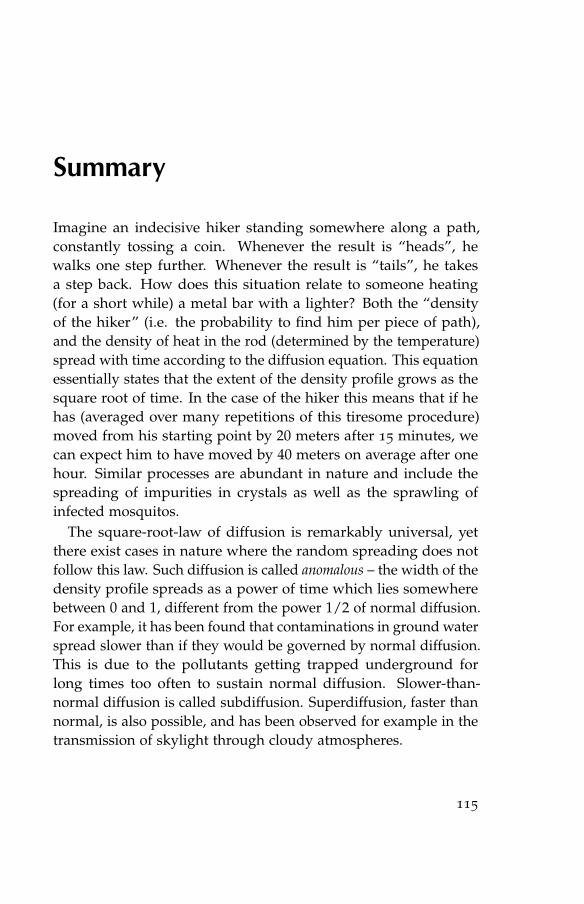
Summary

Imagine an indecisive hiker standing somewhere along a path,constantly tossing a coin. Whenever the result is “heads”, hewalks one step further. Whenever the result is “tails”, he takesa step back. How does this situation relate to someone heating(for a short while) a metal bar with a lighter? Both the “densityof the hiker” (i.e. the probability to find him per piece of path),and the density of heat in the rod (determined by the temperature)spread with time according to the diffusion equation. This equationessentially states that the extent of the density profile grows as thesquare root of time. In the case of the hiker this means that if hehas (averaged over many repetitions of this tiresome procedure)moved from his starting point by 20 meters after 15 minutes, wecan expect him to have moved by 40 meters on average after onehour. Similar processes are abundant in nature and include thespreading of impurities in crystals as well as the sprawling ofinfected mosquitos.

The square-root-law of diffusion is remarkably universal, yetthere exist cases in nature where the random spreading does notfollow this law. Such diffusion is called anomalous – the width of thedensity profile spreads as a power of time which lies somewherebetween 0 and 1, different from the power 1/2 of normal diffusion.For example, it has been found that contaminations in ground waterspread slower than if they would be governed by normal diffusion.This is due to the pollutants getting trapped underground forlong times too often to sustain normal diffusion. Slower-than-normal diffusion is called subdiffusion. Superdiffusion, faster thannormal, is also possible, and has been observed for example in thetransmission of skylight through cloudy atmospheres.

115

Anomalous diffusion can also occur in electrical conductionthrough disordered metals and semiconductors. At low tempera-tures quantum mechanics enters as another mechanism by whichthe diffusion of electrons can become anomalous. It may slowdown to a complete halt due to destructive interference, while ifthe interference is constructive, the opposite effect can happen.

This thesis addresses a variety of systems in which the diffusionis anomalous, mainly motivated by recent experimental develop-ments.

In Chapter 2 we look at the consequences that slower-than-normal diffusion on fractals has for shot noise, the time-dependentfluctuations of the electric current. Fractals are self-similar geo-metric objects characterized by a non-integer dimension. (Cloudpatterns are a familiar example of fractals.) Our study is motivatedby the fractals which form from “puddles” of electrons and holesin graphene, a one-atom thick sheet of carbon.

Faster-than-normal diffusion requires long steps to happen suffi-ciently more often than in the case of normal diffusion. Recently,superdiffusion of photons was reported in a medium consisting ofglass spheres with a large range of diameters. Because the arrange-ment of the spheres is fixed in time, the steps which the photonmakes in the medium are correlated: a long step in one direction islikely to be followed by another long step in the opposite direction.To assess the importance of the correlations we examine in Chapter3 the effects correlations have on superdiffusion in one dimension.Working in one dimension enhances the correlations (thus provid-ing a worst-case estimate) and allows an exact solution in closedform.

Electrons in graphene have the unusual property that they aremassless, and their wave equation is the relativistic Dirac equa-tion, rather than the nonrelativistic Schrodinger equation. (Thesemassless electrons are the Dirac fermions from the title.) Quantuminterference in graphene is constructive rather than destructive onaverage. As a consequence, while increasing the disorder strengthin normal materials makes it more difficult for electrons to travel, in

116

the case of graphene the opposite effect can occur. In Chapter 4 wedevelop and demonstrate the usefulness of a method to simulatethe anomalous diffusion of Dirac fermions in a computer.

The last two chapters of this thesis address other properties ofDirac fermions, not directly related to anomalous diffusion. Theseappear in socalled topological insulators, a novel class of materialswhich are insulating in the bulk but can conduct via metallic edgestates. These edge states are unique because spin-up and spin-down electrons move in opposite directions, regardless of anyobstacles they might find along their way. Chapter 5 proposes andanalyzes a spin precession experiment in topological insulators.In Chapter 6 we present the mechanism for the conversion of anordinary insulator into a topological insulator by disorder. Thisconversion was reported in the literature, on the basis of computersimulations, but had remained unexplained.

117

Samenvatting

Stel je voor, een twijfelende wandelaar ergens op een pad, die steedsmaar weer een munt opgooit. Als het resultaat “kruis” is, doet hijeen stap naar voren. Als het resultaat “munt” is, doet hij een stapnaar achteren. Wat is het verband met het (gedurende korte tijd)opwarmen van een metalen staaf met een aansteker? Zowel de“dichtheid van de wandelaar” (namelijk, de kans om hem in eenbepaald stuk van het pad aan te treffen), alsook de dichtheid vanwarmte in de staaf (bepaald door de temperatuur) breiden zich metde tijd uit volgens een diffusievergelijking. Deze vergelijking zegtin essentie dat de uitgebreidheid van het dichtheidsprofiel groeitmet de wortel uit de tijd. In het geval van de wandelaar betekentdit dat, als hij zich (gemiddeld over vele herhalingen van dezevermoeiende operatie) 20 meter van zijn startpositie heeft verplaatstna 15 minuten, we kunnen verwachten dat hij zich gemiddeld 40meter heeft verplaatst na een uur. Soortgelijke processen komenveel voor in de natuur, van de verspreiding van verontreinigingenin een kristal tot de verspreiding van geınfecteerde muskieten.

De wortel-uit-de-tijd wet van diffusie is opvallend universeel, entoch zijn er gevallen in de natuur waar het toevallig verspreidenvan deze wetmatigheid afwijkt. Zulke diffusie heet anomaal – debreedte van het dichtheidsprofiel breidt zich in de tijd uit met eenmacht die ergens tussen 0 en 1 ligt, verschillend van de macht 1/2van normale diffusie. Bijvoorbeeld, het is bekend dat verontreini-gingen in water zich langzamer verspreiden dan het gevolg zouzijn van normale diffusie. De reden is dat verontreinigingen langetijd onder de grond vast kunnen komen te zitten. Diffusie dielangzamer is dan normaal heet subdiffusie. Superdiffusie, snellerdan normaal, is ook mogelijk, en is bijvoorbeeld waargenomen in

119

de voortplanting van hemellicht door een bewolkte atmosfeer.Anomale diffusie kan ook voorkomen in elektrische geleiding

door wanordelijke metalen en halfgeleiders. Bij lage temperaturendoet de kwantummechanica haar intrede als een ander mechanismewaardoor diffusie van elektronen anomaal kan worden. Het kanvertragen tot een komplete stop ten gevolge van destructieve inter-ferentie, terwijl constructieve interferentie het tegenovergesteldekan bewerkstelligen.

Dit proefschrift behandelt een verscheidenheid van systemenwaarin de diffusie anomaal is, vooral gemotiveerd door recenteexperimentele ontwikkelingen.

In hoofdstuk 2 onderzoeken we de gevolgen die langzamer-dan-normale diffusie op fraktalen heeft voor hagelruis, de tijds-afhankelijke fluctuaties van de elektrische stroom. Fraktalen zijngeometrische objecten die gekarakteriseerd worden door een niet-heeltallige dimensie. (Wolkpatronen zijn een vertrouwd voorbeeldvan fraktalen.) Onze studie is gemotiveerd door de fraktalen diegevormd worden door de gebiedjes van elektronen en gaten ingrafeen, een enkele laag koolstofatomen.

Sneller-dan-normale diffusie vereist lange stappen, met een ho-gere frequentie dan bij normale diffusie. Recent is superdiffusievan fotonen gerapporteerd in een medium bestaande uit glazenbollen met een grote verscheidenheid aan diameters. Omdat deordening van de bollen vast ligt in de tijd, zijn de stappen die eenfoton maakt door het medium gecorreleerd: een lange stap in deene richting wordt waarschijnlijk gevolgd door een lange stap inde omgekeerde richting. Om het belang van de correlaties te on-derzoeken bestuderen we in hoofdstuk 3 het effect van correlatiesop superdiffusie in een dimensie. In een dimensie is het effect vancorrelaties het sterkst (het is dus een “worst-case” geval), en dezedimensie heeft het voordeel dat een exacte oplossing kan wordenopgeschreven.

Elektronen in grafeen hebben de ongebruikelijke eigenschapdat ze massaloos zijn. Hun golfvergelijking is de relativistischeDirac-vergelijking, in plaats van de niet-relativistische Schrodinger-

120

vergelijking. (Deze masssaloze elektronen zijn de Dirac-fermionenuit de titel.) Kwantum-interferentie in grafeen is constructief inplaats van destructief, gemiddeld gesproken. Terwijl toenamevan de wanorde in gewone materialen het moeilijker maakt voorelektronen om zich voort te bewegen, gebeurt in grafeen het te-genovergestelde. In hoofdstuk 4 ontwikkelen en demonstreren weeen methode om de anomale diffusie van Dirac-fermionen op eencomputer te simuleren.

De laatste twee hoofdstukken van dit proefschrift behandelenandere eigenschappen van Dirac-fermionen, niet direct gerelateerdaan anomale diffusie. Deze treden op in zogenaamde topologischeisolatoren, een nieuwe klasse van materialen die isoleren in hetbinnenste maar geleiden via metallische randtoestanden. Dezerandtoestanden zijn uniek omdat spin-op en spin-neer elektronenin tegenovergestelde richtingen bewegen, ongeacht een obstakeldat ze op hun weg zouden kunnen vinden. Hoofdstuk 5 stelteen spin-precessie experiment voor in topologische isolatoren, enanalyseert het. In hoofdstuk 6 presenteren we een mechanismeom een gewone isolator te converteren in een topologische isolatordoor middel van wanorde. Deze conversie was gerapporteerdin de literatuur, op basis van computersimulaties, maar zonderverklaring.

121

List of Publications

• Counting statistics of coherent population trapping in quantumdots, C. W. Groth, B. Michaelis, C. W. J. Beenakker, Phys. Rev.B 74, 125315 (2006).

• Electronic shot noise in fractal conductors, C. W. Groth,J. Tworzydło, C. W. J. Beenakker, Phys. Rev. Lett. 100, 176804

(2008) [Chapter 2].

• Finite difference method for transport properties of massless Diracfermions, J. Tworzydło, C. W. Groth, C. W. J. Beenakker, Phys.Rev. B 78, 235438 (2008) [Chapter 4].

• Nonalgebraic length dependence of transmission through a chainof barriers with a Levy spacing distribution, C. W. J. Beenakker,C. W. Groth, A. R. Akhmerov, Phys. Rev. B 79, 024204 (2009)[Chapter 3].

• Switching of electrical current by spin precession in the first Lan-dau level of an inverted-gap semiconductor, A. R. Akhmerov,C. W. Groth, J. Tworzydło, C. W. J. Beenakker, Phys. Rev. B80, 195320 (2009) [Chapter 5].

• Theory of the topological Anderson insulator, C. W. Groth, M. Wim-mer, A. R. Akhmerov, J. Tworzydło, C. W. J. Beenakker, Phys.Rev. Lett. 103, 196805 (2009) [Chapter 6].

123

Curriculum Vitæ

I was born in Gdynia on the Polish Baltic coast on the 15th ofDecember 1980. In 1990 my family moved to Kulmbach in Germany,where I received the remaining primary and secondary education.During school years I attended the science competition Jugendforscht six times, winning five times on regional level. In 2001 myproject Fluid simulation for computer graphics won the second prizeon national level. After finishing school in the same year, I workedfor ten months in a boarding school for mentally disabled childrenas my compulsory community service.

In 2002 I enrolled at the University of Bayreuth for a GermanDiplom degree in physics. Having passed the intermediate examsafter four semesters, I was granted a scholarship of Cusanuswerk.In 2005 I moved to the Netherlands to continue my studies atLeiden University, and obtained there in 2007 a master’s degreein theoretical physics with a thesis entitled Counting statistics ofcoherent population trapping in quantum dots supervised by prof.C. W. J. Beenakker. After graduation I stayed in the group ofprof. Beenakker employed by Stichting FOM to pursue the researchwhich is documented in this thesis.

During my studies in Germany I taught exercise classes in Quan-tum Mechanics I. In Leiden I taught the exercise classes in Com-putational Physics and Electromagnetism II. I have attended twosummer schools and represented my work at a number of confer-ences.

125

Stellingenbehorende bij het proefschrift

Anomalous diffusion of Dirac fermions

1. Our finding that diffusion and subdiffusion have the sameFano factor can explain the carrier-density independent mea-surements of DiCarlo et al.

L. DiCarlo, J. R. Williams, Y. Zhang,D. T. McClure, and C. M. Marcus,

Phys. Rev. Lett. 100, 156801 (2008);This thesis, Chapter 2.

2. The strong effects of correlations found in a one-dimensionalLevy glass persist in higher dimensions.

This thesis, Chapter 3.

3. A Levy walk with characteristic exponent α has a transmis-sion probability over a length L which decays as L1−α for1 < α < 2 and is length-independent for 0 < α < 1.

4. Inverted-gap semiconductors are ideally suited to realize theDatta-Das transistor.

This thesis, Chapter 5.

5. The name “topological Anderson insulator” is a misnomer.

This thesis, Chapter 6.

6. In chiral p-wave superconductors, the tricritical point at theintersection of the metal-insulator and insulator-insulatorphase boundaries is repulsive.

M. V. Medvedyeva, J. Tworzydło, and C. W. J. Beenakker,Phys. Rev. B 81, 214203 (2010).

7. Inclusion of a vector potential in the discretized single-valleyDirac equation breaks gauge invariance.

8. The fact that modern travel is superdiffusive hinders theconfinement of epidemics.

D. Brockmann, L. Hufnagel, and T. Geisel,Nature 439, 462 (2006).

9. The freedom to modify (and therefore to study, fix, andimprove) the things one owns is increasingly endangered.

Christoph Groth,November 2010