
Analysis of high-pressure safety valves - Technische Universiteit
135
Analysis of high-pressure safety valves PROEFSCHRIFT ter verkrijging van de graad van doctor aan de Technische Universiteit Eindhoven, op gezag van de rector magnificus, prof.dr.ir. C.J. van Duijn, voor een commissie aangewezen door het College voor Promoties in het openbaar te verdedigen op donderdag 22 oktober 2009 om 16.00 uur door Arend Beune geboren te Helmond
Transcript of Analysis of high-pressure safety valves - Technische Universiteit

Analysis of high-pressure safety valves
PROEFSCHRIFT
ter verkrijging van de graad van doctor aan deTechnische Universiteit Eindhoven, op gezag van de
rector magnificus, prof.dr.ir. C.J. van Duijn, voor eencommissie aangewezen door het College voor
Promoties in het openbaar te verdedigenop donderdag 22 oktober 2009 om 16.00 uur
door
Arend Beune
geboren te Helmond
Dit proefschrift is goedgekeurd door de promotoren:
prof.dr.ir. J.J.H. BrouwersenProf.Dipl.-Ing. J. Schmidt
Copromotor:dr. J.G.M. Kuerten
Copyright © 2009 by A. BeuneAll rights reserved. No part of this publication may be reproduced, stored in aretrieval system, or transmitted, in any form, or by any means, electronic, mechanical,photocopying, recording, or otherwise, without the prior permission of the author.
Cover design: Oranje Vormgevers Eindhoven (www.oranjevormgevers.nl).
Printed by the Eindhoven University Press.
A catalogue record is available from the Eindhoven University of Technology Library
ISBN: 978-90-386-2006-0

ACKNOWLEDGEMENTS
The following organizations are acknowledged for their contribution:
BASF SE Ludwigshafen am Rhein in Germany for funding this research.
The department Safety Engineering & Fluid Dynamics for providing know-how andthe department High-pressure Technology for providing the test facility at the high-pressure laboratory in Ludwigshafen.
Contents
Summary 7
1 Introduction 91.1 Background . . . . . . . . . . . . . . . . . . . . . . . . . . . . . . . . . 91.2 Literature overview . . . . . . . . . . . . . . . . . . . . . . . . . . . . . 131.3 Research objectives and outline . . . . . . . . . . . . . . . . . . . . . . 18
2 Valve sizing methods 212.1 Standardized valve sizing method . . . . . . . . . . . . . . . . . . . . . 222.2 Real-gas material definition . . . . . . . . . . . . . . . . . . . . . . . . 242.3 Real-gas property table generation . . . . . . . . . . . . . . . . . . . . 262.4 Applicability to other gases . . . . . . . . . . . . . . . . . . . . . . . . 312.5 Literature review of valve sizing at high pressures . . . . . . . . . . . . 312.6 Alternative valve sizing methods . . . . . . . . . . . . . . . . . . . . . 342.7 Comparison of valve sizing methods . . . . . . . . . . . . . . . . . . . 37
3 Development of numerical tool 393.1 Numerical valve model parameters . . . . . . . . . . . . . . . . . . . . 39
3.1.1 Mathematical models . . . . . . . . . . . . . . . . . . . . . . . 403.1.2 Discretization and solution method . . . . . . . . . . . . . . . . 43
3.2 Validation test cases at low pressure . . . . . . . . . . . . . . . . . . . 453.2.1 1D shock tube . . . . . . . . . . . . . . . . . . . . . . . . . . . 463.2.2 Axisymmetric nozzle . . . . . . . . . . . . . . . . . . . . . . . . 493.2.3 2D supersonic ramp . . . . . . . . . . . . . . . . . . . . . . . . 513.2.4 2D simplified valve model . . . . . . . . . . . . . . . . . . . . . 553.2.5 3D pneumatic valve model . . . . . . . . . . . . . . . . . . . . . 573.2.6 3D safety valve . . . . . . . . . . . . . . . . . . . . . . . . . . . 59
3.3 Validation test case of a high-pressure nozzle . . . . . . . . . . . . . . 62
4 Facility for safety valve tests 654.1 Design considerations and construction . . . . . . . . . . . . . . . . . . 654.2 Measurement variables . . . . . . . . . . . . . . . . . . . . . . . . . . . 67
4.2.1 Valve disk lift . . . . . . . . . . . . . . . . . . . . . . . . . . . . 684.2.2 Valve disk force . . . . . . . . . . . . . . . . . . . . . . . . . . . 70
6 Contents
4.2.3 Temperature . . . . . . . . . . . . . . . . . . . . . . . . . . . . 734.2.4 Pressure . . . . . . . . . . . . . . . . . . . . . . . . . . . . . . . 744.2.5 Liquid mass flow rate . . . . . . . . . . . . . . . . . . . . . . . 754.2.6 Gas mass flow rate . . . . . . . . . . . . . . . . . . . . . . . . . 784.2.7 Discharge coefficient . . . . . . . . . . . . . . . . . . . . . . . . 804.2.8 Data acquisition . . . . . . . . . . . . . . . . . . . . . . . . . . 80
4.3 Examples of valve tests . . . . . . . . . . . . . . . . . . . . . . . . . . 814.3.1 Valve test with water . . . . . . . . . . . . . . . . . . . . . . . 814.3.2 Valve test with nitrogen . . . . . . . . . . . . . . . . . . . . . . 82
5 Comparison of numerical and experimental results 855.1 Liquid valve flow . . . . . . . . . . . . . . . . . . . . . . . . . . . . . . 85
5.1.1 Experimental results . . . . . . . . . . . . . . . . . . . . . . . . 855.1.2 Numerical simulations . . . . . . . . . . . . . . . . . . . . . . . 875.1.3 Comparison and analysis . . . . . . . . . . . . . . . . . . . . . 89
5.2 Gas valve flow . . . . . . . . . . . . . . . . . . . . . . . . . . . . . . . . 935.2.1 Re-evaluation of low-pressure safety valve measurement data . 935.2.2 Numerical simulation of high-pressure valve tests . . . . . . . . 955.2.3 Comparison and analysis of high-pressure valve tests . . . . . . 98
5.3 Safety valve flow with real-gas effects . . . . . . . . . . . . . . . . . . . 108
6 Dynamic flow simulations 1116.1 Numerical approach . . . . . . . . . . . . . . . . . . . . . . . . . . . . 1136.2 Results . . . . . . . . . . . . . . . . . . . . . . . . . . . . . . . . . . . . 116
7 Discussion 121
Bibliography 127
Dankwoord 133
Curriculum vitae 135
Summary
Analysis of high-pressure safety valves
In presently used safety valve sizing standards the gas discharge capacity is based ona nozzle flow derived from ideal gas theory. At high pressures or low temperaturesreal-gas effects can no longer be neglected, so the discharge coefficient corrected forflow losses cannot be assumed constant anymore. Also the force balance and as aconsequence the opening characteristics will be affected.
In former Computational Fluid Dynamics (CFD) studies valve capacities havebeen validated at pressures up to 35 bar without focusing on the opening charac-teristic. In this thesis alternative valve sizing models and a numerical CFD tool aredeveloped to predict the opening characteristics of a safety valve at higher pressures.
To describe gas flows at pressures up to 3600 bar and for practical applicability toother gases the Soave Redlich-Kwong real-gas equation of state is used. For nitrogenconsistent tables of the thermodynamic quantities are generated. Comparison withexperiment yielded inaccuracies below 5% for reduced temperatures larger than 1.5.
The first alternative valve sizing method is the real-average method that averagesbetween the valve inlet and the nozzle throat at the critical pressure ratio. The secondreal-integral method calculates small isentropic state changes from the inlet to the fi-nal critical state. In a comparison the most simple ideal method performs slightlybetter than the real-average method and the dimensionless flow coefficient differs lessthan 3% from the most accurate real-integral valve sizing method.
Benchmark validation test cases from which field data is available are used to in-vestigate the relevance of the physical effects present in a safety valve and to determinethe optimal settings of the CFD code ANSYS CFX. First, 1D Shock tube calcula-tions show that strong shocks cannot be captured without oscillations, but the shockstrength in a safety valve flow is small enough to be accurately computed. Second, anaxisymmetric nozzle (ISO 9300) model is simulated at inlet pressures up to 200 barwith computed mass flow rate deviations less than 0.46%. Third, a supersonic rampflow shows a dependency of the location of the separation and reattachment pointson the turbulence model, where the first-order accurate SST model gives the bestagreement with experiment. Fourth, computations of a simplified 2D valve model byFollmer show that reflecting shocks can be accurately resolved. Fifth, a comparisonof mass flow rates of a pneumatic valve model results in deviations up to 5% whichseems due to a 5% too high stagnation pressure at the disk front. Sixth, the computedsafety valve capacities of TUV Rheinland Aachen overpredict the measured dischargecoefficient by 18%. However, a replication of this experiment at the test facility re-
8 Summary
duces the error to 3%. A clear reason for the large deviation with the reference datacannot be given. Lastly, the computed mass flow rates of a nozzle flow with nitrogenat pressures up to 3500 bar agrees within 5% with experiment.
A high-pressure test facility has been constructed to perform tests of safety valveswith water and nitrogen at operating pressures up to 600 bar at ambient temperature.The valve disk lift and flow force measurement systems are integrated in a modifiedpressurized protection cap so that the opening characteristics are minimally affected.The mass flow rates of both fluids are measured at ambient conditions by means ofa collecting tank with a mass balance for fluids and through subcritical orifices forgases with inaccuracies of the discharge coefficient of 3 and 2.5%.
Reproducible valve tests with water have been carried out at operating pressuresfrom 64 to 450 bar. The discharge coefficient does not depend on the set pressure ofthe safety valve. The dimensionless flow force slightly increases with disk lift. CFDcomputations of selected averaged measurement points with constant disk lift showthat for smaller disk lifts the mass flow rate is overpredicted up to 41%. Extendingthe numerical model with the Rayleigh-Plesset cavitation model reduces the errors ofthe mass flow rates by a factor of two. The reductions in the flow forces range from35 to 7% at lower disk lifts.
Also reproducible valve tests with nitrogen gas at operating pressures from 73 to453 bar have been conducted. The discharge coefficient is also independent of setpressure. In contrast to the water tests, the dimensionless flow force continually de-creases with disk lift. All computed mass flow rates agree within 3.6%. The computedflow forces deviate between 7.8 and 14.7%.
An analysis shows that the effects of condensation, transient effects, variation ofthe computational domain or mechanical wear cannot explain the flow force devia-tion. The reason partially lies in a larger difference between the set pressure and theopening pressure of the test valve. The flow distribution around the valve spindle issensitive to the inlet pressure and rounding of sharp edges due to mechanical wear.The cavity of the valve spindle probably causes valve chatter partially observed in theexperiments and simulations.
In safety valve computations with nitrogen at higher pressures up to 2000 barand temperatures down to 175 K outside the experimentally validated region the dis-charge coefficient of all three valve sizing methods varies less than 6% compared tothe 7 bar reference value at ambient temperature. So the standardized ideal valvesizing method is sufficient for safety valve sizing. The dimensionless force, however,increases with pressure up to 34% so that the valve characteristic is affected.
The influence of valve dynamics on steady-state performance of a safety valve isstudied by extending the CFD tool with deformable numerical grids and the inclusionof Newton’s law applied to the valve disk. The mass flow rate and disk lift are lessaffected, but a fast rise and collapse of the flow force due to redirection of the bulkflow has been observed during opening. Only dynamic simulations can realisticallymodel the opening characteristic, because these force peaks have not been observedin the static approach. Furthermore, the valve geometry can be optimized withoutsharp edges or cavities so that redirection of the flow will result in gradual flow forcechanges. Then, traveling pressure waves will lead to less unstable valve operation.
Chapter 1
Introduction
1.1 Background
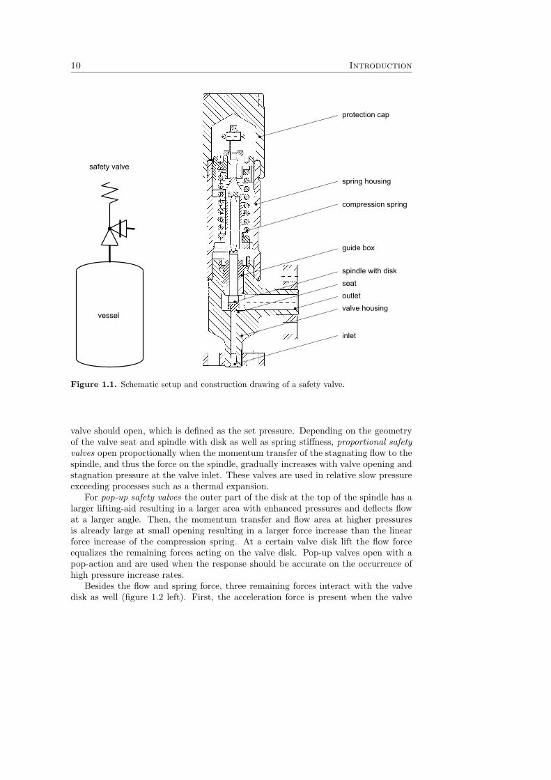
In process industry, a process is continuously further optimized to operate more effi-ciently closer to its mechanical limits such as its maximum allowable operating pres-sure. To ensure safe plant operation, the performance of all levels of safety systemsneeds to be reconsidered. Besides the organizational and process control measuresto maintain safe plant operation, the last stage of protection of a process apparatusagainst excess pressure is often through the use of a mechanical self-actuated device.These devices, a safety relief valve or bursting disc, are mostly installed on top of thepressurized system, like a vessel, to be protected and directly connected to the systemthrough a short pipe (figure 1.1 left).
Excess pressures can result from a failure in the heating system supplying ex-trinsic heat to the contents of a vessel. Further possible causes are a breakdown ofthe cooling system or the presence of a catalyst overdosing in a reactor vessel, whichmay initiate an exothermic chemical reaction. Furthermore, leakages or overpressuresin an apparatus connected to the pressurized system considered can result in excesspressure of the system. If in case of an emergency relief the temperature rise and sothe pressure rise of the system is estimated, the most suitable safety relief device canbe chosen.
When the pressure in the apparatus reaches the set pressure of the safety device,the pressure forces the disk to open and the fluid is discharged into a disposal system,a containment vessel or directly into the atmosphere. In the case of a spring-loadedsafety relief valve a spring forces the disk to close when the pressure decreases belowthe closing pressure of the valve. Then, the plant can be shut down in a controlledway with a minimum loss of product to the environment.
A spring-loaded safety relief valve consists of a compression spring, which pressesthe valve spindle with disk on the valve seat in order to seal the pressurized system incase of operating conditions below the valve set pressure (figure 1.1 right). Prior to thevalve installation the spring is pre-stressed so that the spring force equals the desiredpressure multiplied with the sealing area of the valve seat. At this pressure the safety
10 Introduction
vessel
safety valve
compression spring
spring housing
inlet
outlet
protection cap
seatspindle with disk
guide box
valve housing
Figure 1.1. Schematic setup and construction drawing of a safety valve.
valve should open, which is defined as the set pressure. Depending on the geometryof the valve seat and spindle with disk as well as spring stiffness, proportional safetyvalves open proportionally when the momentum transfer of the stagnating flow to thespindle, and thus the force on the spindle, gradually increases with valve opening andstagnation pressure at the valve inlet. These valves are used in relative slow pressureexceeding processes such as a thermal expansion.
For pop-up safety valves the outer part of the disk at the top of the spindle has alarger lifting-aid resulting in a larger area with enhanced pressures and deflects flowat a larger angle. Then, the momentum transfer and flow area at higher pressuresis already large at small opening resulting in a larger force increase than the linearforce increase of the compression spring. At a certain valve disk lift the flow forceequalizes the remaining forces acting on the valve disk. Pop-up valves open with apop-action and are used when the response should be accurate on the occurrence ofhigh pressure increase rates.
Besides the flow and spring force, three remaining forces interact with the valvedisk as well (figure 1.2 left). First, the acceleration force is present when the valve
1.1 Background 11
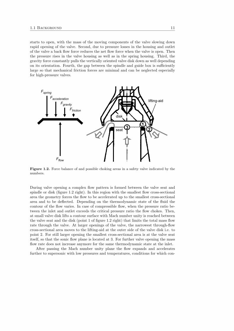
starts to open, with the mass of the moving components of the valve slowing downrapid opening of the valve. Second, due to pressure losses in the housing and outletof the valve a back flow force reduces the net flow force when the valve is open. Thenthe pressure rises in the valve housing as well as in the spring housing. Third, thegravity force constantly pulls the vertically oriented valve disk down as well dependingon its orientation. Fourth, the gap between the spindle and guide box is sufficientlylarge so that mechanical friction forces are minimal and can be neglected especiallyfor high-pressure valves.
Facceleration
Ffriction
Fgravity
Fflow
Fspring
3 21
lifting-aid
disk
seat
Figure 1.2. Force balance of and possible choking areas in a safety valve indicated by thenumbers.
During valve opening a complex flow pattern is formed between the valve seat andspindle or disk (figure 1.2 right). In this region with the smallest flow cross-sectionalarea the geometry forces the flow to be accelerated up to the smallest cross-sectionalarea and to be deflected. Depending on the thermodynamic state of the fluid thecontour of the flow varies. In case of compressible flow, when the pressure ratio be-tween the inlet and outlet exceeds the critical pressure ratio the flow chokes. Then,at small valve disk lifts a contour surface with Mach number unity is reached betweenthe valve seat and the disk (point 1 of figure 1.2 right) that limits the total mass flowrate through the valve. At larger openings of the valve, the narrowest through-flowcross-sectional area moves to the lifting-aid at the outer side of the valve disk i.e. topoint 2. For still larger opening the smallest cross-sectional area is at the valve seatitself, so that the sonic flow plane is located at 3. For further valve opening the massflow rate does not increase anymore for the same thermodynamic state at the inlet.
After passing the Mach number unity plane the flow expands and acceleratesfurther to supersonic with low pressures and temperatures, conditions for which con-
12 Introduction
densation could occur. Also the local pressure at the disk wall is reduced, thus theflow force acting on the disk varies with the position of the effective throat as well.Further downstream a compression shock wave brings the flow to the thermodynamicstate at the valve outlet. The strength of the compression wave depends on the pres-sure ratio. Because of the strong deflection of the internal forced flow underneath thevalve disk, at the edges of the disk and seat, large adverse pressure gradients resultin flow separation areas and areas with recirculating flow. In addition, due to highoperating pressures of safety valves the fluid has to be considered as a real gas.
If the flow Mach number remains much smaller than unity throughout the valve,the flow can be considered incompressible. Then, compressibility effects such as shocksand sonic flow do not occur, but in the same area after the smallest cross-sectionalarea with the largest velocities (equal to the supersonic area for compressible flow)the flow still strongly accelerates with low local pressures as well so that for liquidflows phase transition by means of cavitation can occur. The mass flow rate is limitedby pressure losses occurring in the whole valve housing.
The European standard EN ISO 4126-1 [30] and the derived German regulation AD2000 [1] describe the sizing procedure of safety devices for protection against excesspressure. These standards are valid for safety valve sizing with operating pressuresup to 200 bar. However, many plants throughout the world are operated at pressuresup to 3000 bar for the production of synthesis gas or low-density polyethylene. Inthis pressure range the discharge capacity is not prescribed and currently the valvesizing procedures have to be extrapolated.
The flow capacity calculation of a safety valve is based on isentropic flow through anozzle with a correction factor for flow losses and redirection of the flow, the so-calleddischarge coefficient Kd. For incompressible nozzle flow the mass flow rate calculationis based on the Bernoulli equation with a correction for viscous flow effects and forcompressible flow the equation of state (EoS) for a perfect gas is used. The dischargecoefficient is experimentally determined in valve tests mostly at low pressures withremoved compression spring so that the valve spindle can be fixed at a specified po-sition. There are test rigs available with operating pressures up to 250 bar to testthe function and release capacity of spring-loaded safety relief valves. The test fluidsare sub-cooled water and gaseous air or nitrogen. Discharge coefficients derived fromthese tests are directly used for other liquids and gases as well. As a consequence, inthe standard it is assumed that the experimentally obtained discharge coefficient isconstant for a certain valve type, independent of the set pressure and compressibilityof the fluid. From a physical point of view, at higher pressures the intermolecularinteraction of a gas denoted as real-gas effects cannot be neglected. Therefore, it isexpected that the discharge coefficient will vary with pressure while it will also dependon the gas considered.
Alternative analytical calculation tools are available to calculate the flow con-ditions around the safety valve as part of the piping system (Cremers, 2000 [15]).Especially for piping systems with long entrance and relief lines enhanced pressurelosses occur that affect the proper functioning of the safety valve. In the worst casethe valve starts to vibrate due to oscillating flow so that the maximum disk lift is not
1.2 Literature overview 13
reached at all and the effective discharge capacity is reduced substantially. On thewhole, these methods do not consider the complex flow dynamics in a safety valveand assume that the safety valve will open and relieve as expected with a constant as-sumed discharge coefficient at 10% above the maximum allowable operating pressureof the pressurized system as defined in the valve sizing standards.
1.2 Literature overview
In order to identify safety valve functioning the literature overview starts with safetyvalve flow considerations and the dynamics of safety valves. Then, studies of safetyvalve flows carried out employing Computational Fluid Dynamics (CFD) are given.Next, the focus is on CFD studies of flow phenomena that are related to safety valveflows. Finally, recent references are discussed that consider flow dynamics of valvesusing with CFD.
Dynamics in safety valvesIn many literature sources the dynamic response of safety valves is discussed. To startwith the experimental work of Sallet (1981) [57], the flow inside a typical safety valvewas studied by visualization of the flow in a 2D valve model. Pressure distributionsand discharge capacities were investigated in tests with choked air flow, water andchoked two-phase flow. It can be recognized that the physical effects of flow separa-tion, cavitation, choking and valve disk vibrations are significant flow phenomena thatcomplicate the prediction of the characteristic valve coefficients. Sallet also observedthat vortical flows near the valve disk (periodic flow oscillations due to flow past acavity) cause valve disk vibrations. This effect is larger for incompressible flows. Alsoin a safety valve the interaction between shock waves and flow separation can causeself-sustaining oscillating flow fields.
Follmer (1981) [22] performed experimental research on air flow through a flatvalve choked in the annular gap. By means of a Mach-Zender-Interferometer iso-density fringes of the flow were accurately determined. Assuming isenthalpic flow,the density distribution was converted into a Mach number distribution to obtaininsight into the gas dynamics of choked gas flow. The pressure ratio and the geom-etry of the valve inlet were varied to study the effects of flow separation and shocksresulting in additional pressure losses and periodic oscillations of the supersonic partof the flow. This research forms the basis for a quantitative comparison with resultingcomputational methods.
Singh (1982) [62] studied the dynamics and stability of spring-loaded safety re-lief valves. He developed an analytical coupled thermal-hydraulic and spring-masssystems model. He concluded that the operating stability of a safety valve can beincreased by either lowering an adjustment ring mounted at the valve seat so thatthe discharge angle becomes smaller, or by a softer spring, smaller backpressures, oradding a damping device as well. Also MacLeod (1985) [40] used analytical models toanalyze the dynamic stability of safety valves. The addition of a dampening systembalances between fast valve opening and the avoidance of rapid and extreme alter-nating opening and closing of the safety valve, the so-called valve chatter or flutter.
14 Introduction
Baldwin (1986) [8] introduced design guidelines to avoid flow-induced vibration insafety valves, which is the main cause of relief failure in power plant industry. Thisvibration comprises unstable coupling of vortex shedding at the valve inlet with theside branch acoustic resonance. The design procedure uses a relationship involvingStrouhal number, Mach number and pipe stub dimensions based on dynamic responsedata from safety valves in power plant steam service. It was observed, that the shapeof the trailing edge of a cavity can stabilize the flow in such a way that alternatingflow impingement is avoided. Moisidis (1995) [44] reduced the risk of relief valve fail-ure by improving the design of a Crosby safety valve. By reducing the misalignmentbetween moving parts and eccentric loading, the risk of valve operating failures, suchas popping pressure drift, spurious valve actuations, or leakage is minimized.
In choking flow experiments by Betts (1997) [10] 3D effects on the local pressureratio upstream of the safety valve disk were studied. These effects were more appar-ent at the outer part of the disk due to circulating flow patterns. This asymmetry ofthe flow field around the disk is confirmed by the experiments of pilot-operated reliefvalves of Botros (1998) [12]. He found that the safety valve is subjected to lateralforces, which can lead to rubbing, sticking or in extreme cases adhesive wear, i.e.galling.
Safety valve tests with enhanced backpressures of Francis (1998) [24] showed thatthe movement of the shock wave due to changes in reservoir pressure and backpressureclearly affects the lifting force on the disk and hence its position, especially at lowlifts for which the shock wave can be expected to be relatively close to the seal. Thisindicates again that backpressure effects are important for the 3D flow field in thenarrowest flow cross-section of the safety valve. In addition to the operating stabilitymechanisms of a safety valve configuration, Frommann (2000) [25] investigated theeffect of bends in the inlet line on the reflection of the pressure wave in experimentswith straight vertical inlet lines. There were no significant differences observed andthe mechanism remains the same.
Cremers (2003) [16] experimentally investigated the effect of the inlet and dis-charge pipe dimensions on the dynamical performance of a safety relief valve. For acertain configuration the valve can chatter. Practical technical guidelines and designrules have been created to permit a certain maximum length of the inlet and dis-charge pipes. Also a maximum allowable pressure loss in the pipes during dischargedue to friction in the inlet pipe has been defined. Muschelknautz (2003) [47] evaluatedthe effect of flow reaction forces during discharge of a safety relief valve on a largerscale, which is the foundation of a plant. From numerical calculations and blowdowntests he concluded that a T-piece at the outlet compensates stationary flow reactionforces and the instationary flow forces occur at a too high frequency to affect the plant.
Safety valve studies with CFDIn the above described literature sources the effects of valve flow on the dynamicalperformance of safety valves are generally discussed. The present project, however,does not focus on the chatter phenomenon itself, but on the design of a numerical toolto describe the complex 3D flow in safety salves necessary for proper valve sizing anddesign. It has been chosen to use advanced numerical methods to model these 3D flow
1.2 Literature overview 15
fields. Computational fluid dynamics (CFD) is a numerical approach that providesa qualitative and with extra effort sometimes even a quantitative prediction of 3Dfluid flows by means of solving partial differential equations with the help of numer-ical methods. It gives also insight into flow patterns that are difficult, expensive orimpossible to study with traditional experimental techniques. As in experiments onlya few local or integrated quantities can be measured for a limited range of problemsand operating conditions, CFD predicts all modeled quantities with high resolution inspace and time in the whole actual flow domain for any operating condition whethersafe or unsafe. It is noted that CFD results can never be 100% reliable, because theinput data may involve inaccuracy, the mathematical model of e.g. turbulence maybe inadequate and the computational recourses may limit the computational grid res-olution and therewith the accuracy of the flow problem too much.
In the following academic studies the 3D flow physics in a safety valve is calcu-lated with the help of CFD software. In the thesis of Zahariev (2001) [71] the flowbehavior in safety valves was studied with the commercial CFD software packageCFX TASCflow. The study mainly focused on optimization of the valve disk. Thevalidation of the numerical model was limited to force experiments of a single valveexperiment series of air with fixed disk lifts at an inlet pressure of 20 bar blowingoff at atmospheric conditions. Although the differences between the predicted andmeasured quantities is within 5%, from a single validation it is not possible to eval-uate the performance of the numerical tool. As a result, more validation needs tobe done with the focus on the physical phenomena occurring in high-pressure safetyvalve flows.
In the work of Bredau (2000) [13] air flows in simplified pneumatic valve models upto 7 bar have been visualized in experiments and calculated with the CFD programTASCflow. The calculated flow field showed good agreement with the experimentaldata. The flow could be considered in the smallest flow cross-section as quasi-steady,but at the outlet the fluctuations were larger, so that a steady approximation was nolonger valid. This work shows the ability of CFD modelling to accurately describesafety valve flows, but this applies only to flows at low pressures. Within the sameresearch project in the work of Burk (2006) [14], numerical calculations with CFXbased on additional experimental data of pneumatic valve models showed that for thepractical relevant disk lift range with the smallest flow cross-sectional area smallerthan the seat area, the calculated mass flow rates and the pressure distribution on thevalve disk are in good agreement with experiments. For higher disk lifts the pressureloss in the stagnation area is calculated too small but it still resulted in a smallerdifference of the measured and predicted forces.
In industry, the role of CFD for safety valve design gradually becomes more im-portant. Darby and Molavi (1997) [18] calculated viscous correction factors for high-viscous fluids through safety valves with the help of CFD. In the work of Follmer andSchnettler (2003) [23] it is stated that the flow fields agree with expectations, butquantitative comparisons with experimental data is not given. Furthermore, in recentwork of Moncalvo and Hohne (2008) [45] four mass flow rates of fixed lift safety valveexperiments up to 35 bar have been calculated with ANSYS Flo with deviations upto 11%.

16 Introduction
According to the academic studies modeling safety valve flow should be possiblewith sufficient accuracy, but validation has been considered for low pressures only.The industry, however, has not published accurate validation data yet. The capabil-ity of a numerical tool for the highly complex safety valve flow can be judged onlywhen it is also focused on the individual flow phenomena that occur in safety valveflows.
CFD studies of flow phenomena in high-pressure safety valvesThe flow in a safety valve is basically a nozzle flow that impinges on a plate and isdeflected to a side outlet. Nozzle flows are extensively studied with analytical modelsalso with the inclusion of real-gas effects, see section 2.5. Besides these models, nozzlesare also studied with numerical methods. Kim (2008) [33] investigated flow featuresof high-pressure hydrogen through a choked nozzle using a fully implicit finite volumemethod. Several kinds of EoS were used in order to study the influence of real-gaseffects, with the real-gas EoS Redlich-Kwong (RK) predicting comparatively well.
Johnson (1998) [32] investigated the effectiveness of using CFD for a critical stan-dard ISO 9300 nozzle assuming a perfect gas, assessing the level of agreement betweenexperiments and numerical solutions for four different gas species (Ar, N2, CO2, andH2). The results matched within 0.5% except for CO2 that is 2%. The inclusion ofreal-gas effects would probably improve the results. These previous studies show thatmodeling nozzle flows is possible with CFD with high accuracy, but validation at highpressures cannot be carried out because of lack of experimental data.
Supersonic impinging jets were experimentally and numerically investigated byAlvi (2002) [2]. A stagnation bubble with low-velocity recirculating flow and high-speed radial wall jet were found to be similar in the computations with the ShearStress Transport (SST) turbulence model and the experimental data. It was statedthat the Boussinesq hypothesis is not valid in the impingement area and Reynolds-stress models should improve the results. According to this work the usage of theSST model is promising, but the influence of the turbulence model used for safetyvalve flows should be investigated.
The stagnating flow on the disk forms a boundary layer and becomes supersonicagain followed by a shock inducing flow separation. This interaction in the form ofshock-induced boundary layer separation occurs in supersonic intakes of an aircraftand is extensively experimentally investigated and studied with CFD. In the experi-mental work of Muller (2001) [43] the position and reattachment of a supersonic flowpast a 24◦ ramp was investigated. Also NASA has experimental data available froma supersonic shock/boundary-layer interaction database from Settles (1991) [60] forthe same geometry.
In the studies with CFD, Druguet (2003) [21] investigated the influence of viscousdissipation in shock wave reflections in supersonic steady flows. She found that thechoice of the numerical method has a significant impact on the quality of the predictedshock reflections and the height of the so-called Mach stem.
Knight et al. (2003) [34] compared results of numerical simulations with differ-ent turbulence models and five different configurations with experiment. For thesupersonic flow passing a 3D double fin, two-equation turbulence Reynolds-Averaged
1.2 Literature overview 17
Navier-Stokes (RANS) models sufficiently predict the surface streamline pattern, butaccurately predict the surface pressure only in the initial region of the interaction.
Kral (1998) [36] applied different RANS models to the calculation of complex flowfields over aircraft components. The SST turbulence models performed best for thelift and drag of an airfoil with separation and shock. This model is also capable topredict the flow separation in shock/boundary layer interaction calculations. For non-equilibrium external flows the SST turbulence model is recommended. For internalflows the k − ε models may provide better predictions than the SST model.
Rigas (2005) [54] validated the propagation of shock waves produced by a denseexplosive detonation in a small-scale complex tunnel configuration. The arrival timeand pressure of the explosion front were reasonably predicted and it was concludedthat CFD can be effectively used for problems with sudden and complex flow phe-nomena.
CFD studies of safety valve dynamicsIn recent studies the valve opening characteristics are investigated with CFD. A firstpreliminary study without any verification data is from Domagala (2008) [20], in whichthe CFD program ANSYS CFX was used to prove the principle of fluid-structure in-teraction (FSI) for a pilot-operated relief valve. It was experienced problematic todefine a single deformable grid that can cover the whole operating range. Srikanth(2009) [66] studied subsonic compressible air flow in an electric circuit breaker withANSYS CFX with valve element mesh motion. From the axisymmetrical simulationsthe pressure history was found to be significantly affected by the velocity of the mov-ing contact in the chamber, which can be used for future design studies.
Dynamic simulations with FSI is also applied in practical engineering problems.In coupled FSI simulations of a vacuum relief valve of Reich (2001) [51] a moving bodysimulation was set up to mimic field conditions during opening of the valve. With thisset up the design was improved to avoid the tendency of the valve to flutter underexpected subcritical gas flow conditions. The problem was solved with two grids thatinteract with each other by a overset mesh module. The computed mass flow rate atfull opening deviated 3% from that found in experiment.
Li et al. (2005) [38] used non-linear finite element analysis in combination withCFD to dynamically model the closing characteristics of a subsurface safety valveoperating in productive gas wells. A combination of valve testing and finding thecause for problematic slam-closure loads with the help of FSI has led to a changedvalve design that closes throughout the entire range of flow rates. With this engineer-ing approach the strength of FSI is used to qualitatively analyse the valve functionwithout focussing on local physical effects.
Mahkamov (2006) [41] has developed a CFD model for axisymmetric flow to anal-yse the working process of a Stirling cycle machine. The gas dynamics and heattransfer of the internal gas circuit are calculated on a structured computational grid,where a virtual piston cyclic moves from the smallest volume of the compression spaceto the one of a connected expansion space. With this model the performance is moreaccurately predicted than the traditional approach with analytical models. However,comparison with local measurement data is not pursued.

18 Introduction
The only study in which the problem of reduced grid quality is tackled with mul-tiple grids with high-speed flows is the research from Burk (2006) [14]. He carried outtransient CFD simulations with moving grids with a predefined trajectory of a pneu-matic valve with critical gas flow with ANSYS CFX. Due to large deformations ofthe computational domain intermediate meshes are necessary to keep the mesh qual-ity appropriate. With the help of the programming language Perl simulations withmultiple meshes are automatically controlled. Validations of the numerical modelemploying data from experiment with prescribed valve disk velocity showed that aquasi-stationary approach is sufficient for a pressure ratio down to 1/3. For higherpressures and faster disk movements it is expected that the already observed dynamiceffects become significant.
1.3 Research objectives and outline
From the literature overview it is clear that the physical effects of choking, shocksand flow separation basically occur in safety valves. Preliminary CFD studies alreadyshowed that it is basically possible to predict safety valve capacities. However, thevalidation only occurred at pressures up to 35 bar only with different levels of agree-ment. In order to evaluate the performance of the numerical method, it is desiredto validate the physical phenomena occurring in safety valves separately, so that themathematical models of the numerical method can be evaluated. In the present the-sis these phenomena are investigated with also the application to high-pressure valveflows. Also the opening characteristics have been explored with CFD, in which moststudies lack on sufficient validation.
The objective of this research is to develop a numerical tool of sufficient predictivecapability that allows the calculation of mass flow capacities and opening character-istics of spring-loaded safety valves at operating pressures up to 3600 bar. For themass flow capacity calculation the standardized sizing method based on nozzle flowof a perfect gas needs to be evaluated. Possibly this model has to be extended toaccount for flows at high pressures with real-gas effects. Besides the mass flow ca-pacity, for predicting the opening characteristics CFD is the only way to obtain thecomplex flow phenomena. Therefore, a numerical method needs to be developed thatcovers the physical effects so that the pressure distributions around and flow force onthe valve disk can be predicted accurately. This method needs to be extended withmoving meshes to study and optimize the valve opening characteristic and operatingstability.
As a result, with the use of the numerical tool the number of high-cost valve func-tion tests can be reduced, the reliability of safety valves in existing process systemscan be improved and valve design for future applications can be optimized. The re-search focuses on compressible high-pressure single-phase flow through safety valvesdischarging into the atmosphere.
In the following chapter descriptions of the approach of this research project is out-lined. In chapter 2 the current standardized valve sizing method based on a perfect-gas gas nozzle model will be presented in detail. In order to evaluate this method
1.3 Research objectives and outline 19
for safety valve flows at high pressures a real-gas EoS will be proposed, from whichreal-gas data will be derived. The same data will also be used for CFD computationslater on. Then, two alternative valve sizing methods for real gases will be discussedwith different complexity. Lastly, to evaluate the performance of the existing and thetwo new valve sizing methods with real-gas effects the results of the methods will becompared with each other.
In chapter 3 a numerical method for valve characterization will be developed, thatis based on a finite volume method to solve the time dependent Navier Stokes equa-tions. First, the mathematical models, the discretization and the solution methodwill be given. Then, a suitable CFD software package will be chosen and its modelparameters will be determined in a step-by-step development from 1D inviscid to 3Dreal-gas flows. As part of the development process, validation test cases based onreference data from literature will be defined. The cases are chosen such that theseare a combination of the relevant physical phenomena. Finally, the numerical methodas well as the valve sizing methods will be validated with experimental data of a high-pressure nozzle with inlet pressures up to 3500 bar.
In order to validate the numerical tool at high-pressures, experimental data ofsafety valve flows has to be obtained. Chapter 4 will present the high-pressure testfacility that will be designed and realized to conduct function tests of high-pressuresafety valves with operating pressures up to 600 bar. With this data the valve sizingmodels and the CFD tool for valve characterization can be validated. First, designconsiderations for the construction of the test facility will be provided. Then, the ap-paratus for the quantities to be measured will be given. At the end, two examples ofvalve tests will be shown for which the valve capacity and opening characteristic of asafety valve operating with sub-cooled water and gaseous nitrogen can be determined.
In chapter 5 the experimental results from the high-pressure valve tests will becompared with both the standardized valve sizing methods and with CFD compu-tations of the developed numerical model. First, steady-flow experimental results ofvalve tests for sub-cooled water at two different set pressures will be presented. Then,the setup of the numerical simulations will be given and after that both results willbe compared with each other. In the analysis deviations between the results will bediscussed with the focus on local physical effects. The same comparison and analysiswill be presented for gaseous nitrogen valve flows at two different set pressures. Thischapter concludes with calculations of valve flows outside the experimental validationregion to higher pressures up to 2000 bar to investigate the influence of real-gas effectson the valve characteristic.
In chapter 6 the numerical tool will be extrapolated to transient flow with theinclusion of fluid-structure interaction (FSI). Then the opening characteristics andoperating stability of safety valves will be studied for liquid flow.
In chapter 7 the outcome of this research will be discussed and recommendationsfor application of the valve sizing methods and numerical valve characterization toolwill be given.

20 Introduction
Chapter 2
Valve sizing methods
This chapter focuses on valve models to determine the discharge capacity of safetyvalves, which is required for accurate valve sizing. As stated in the introduction thedischarge coefficient Kd is the correction factor between the mass flow rate of anisentropic flow in a nozzle mnozzle and the actual mass flow rate in a safety valvemexp
Kd = mexp/mnozzle. (2.1)
Ideally, this discharge coefficient should only account for flow losses and redirectionof the flow caused by a non-ideal geometry. In addition, the dimensionless flow coeffi-cient C calculated with the nozzle model should only cover the thermodynamic statechanges as much as possible by [59]
C =mnozzle
A0
√2p0ρ0
, (2.2)
with valve seat area A0, stagnation pressure p0 and density ρ0 or specific volumeυ0 = 1/ρ0. Then the nozzle model depends on the thermodynamic fluid properties,such as set pressure and compressibility. It is hypothesized that depending on theextent that the nozzle flow model covers the thermodynamics of the nozzle flow, thedischarge coefficient will be less sensitive to set pressure and compressibility. In fact,this chapter will analyse different nozzle flow models that deliver a fluid-dynamic flowcoefficient used as a basis for valve sizing methods at high-pressures.
First, in section 2.1, the standardized valve sizing method will be discussed, whichdoes not properly take real-gas effects into account. Then, in sections 2.2 and 2.3 areal-gas EoS will be proposed from which real-gas property data will be derived toaccurately compute flows at high pressures with real-gas effects. Also the possibility touse the real-gas definitions for other gases is discussed in section 2.4. Furthermore, insection 2.5, a literature study focuses on existing approaches of nozzle flows with real-gas effects. Hereafter, in section 2.6, two alternative valve sizing methods that accountfor real-gas effects will be presented. In the last section 2.7, results of the existingand the two new valve sizing methods will be compared with experimental data of ahigh-pressure nozzle with inlet pressures up to 3500 bar, so that the performance ofthe models can be assessed.
22 Valve sizing methods
2.1 Standardized valve sizing method
For sizing of a safety valve, the capacity needs to be known at a certain specified inletpressure. The prediction of the discharge capacity is based on quasi-one-dimensionalreversible and adiabatic, i.e. isentropic, flow through a nozzle with smallest cross-sectional area A0 and an experimentally determined discharge coefficient Kd. Thisdischarge coefficient corrects for flow losses due to friction, deflection and separationof the flow. For nozzle flows this factor is close to unity but for safety valve flows itmostly varies between 0.5 and 0.9. This dependency stems from the area of the valveseat being taken rather than the actual geometrical smallest cross-sectional flow area.The latter could be smaller at lower disk lifts.
The principle of critical or choked gas flow is explained with a flow in a convergent-divergent duct or stream tube with variable cross-section. First the Mach number Mais defined, which is the ratio between the flow velocity u and the speed of sound a
Ma = u/a. (2.3)
The speed of sound is related to the isentropic change of pressure p with respect todensity ρ
a2 =(
∂p
∂ρ
)s
. (2.4)
From the conservation equations for quasi-one dimensional isentropic flow and thedefinition of the speed of sound an area-velocity relation valid for isentropic flow in avariable-area duct is deduced (Anderson, 2003) [3]
1A
dA
dx= (Ma2 − 1)
1u
du
x. (2.5)
This expression shows that a subsonic flow in a convergent duct will always accelerate,while a supersonic flow in the same duct shows the opposite behavior. The relationalso shows that an (isentropic) acceleration from subsonic flow to supersonic flow,passing the sonic condition Ma = 1, is only possible at an extremum of the ductcross-sectional area A. Further analysis shows that this always is a minimum, athroat. Apparently, the mass flow density ρu as a function of flow Mach number Mashows the maximum at Ma = 1, corresponding to a minimum A. This phenomenonis called choking. With the calculation of the gaseous mass flow rate mg at the throatof the convergent-divergent duct with density at the throat ρ∗, cross-section area A0
and sonic velocity u = amg = ρ∗A0a, (2.6)
equation (2.5) prevents increase of the Mach number beyond unity, so that a furtherreduction in pressure at the nozzle exit cannot influence the flow properties at thethroat so that the mass flow rate only depends on the inlet conditions.
According to the European standard EN ISO 4126 [30], the derived German regulationAD 2000 [1] and the American standard API 520 [5] for non-condensing and non-reacting vapors and gases, the dimensionless flow coefficient Cg,id is derived from the
2.1 Standardized valve sizing method 23
perfect gas EoS at stagnation conditions
Cg,id =√
κ0
κ0 − 1η
2κ0
[1− η
κ0−1κ0
]. (2.7)
The variable η is the ratio of the pressure p at the smallest cross-section area andinlet pressure p0
η = p/p0. (2.8)
This standardized calorically perfect gas approximation of the flow coefficient will bereferred to as ideal method in a comparison in section 2.7. For a calorically perfectgas the adiabatic exponent κ0 is defined as the ratio between the specific heats orgiven as a function of the specific gas constant Rs = R/M given by the molar gasconstant R divided by the molar mass M of the gas
κ0 =cp,0
cp,0 −Rs. (2.9)
When the backpressure at the outlet of the valve pb is equal or lower than the pressureat the nozzle throat, the flow is choked at the nozzle throat and the critical pressureratio is fixed. In case of a calorically perfect gas the critical pressure ratio ηcrit equals
ηcrit =(
2κ0 + 1
) κ0κ0−1
. (2.10)
For even lower backpressures or lower pressure ratios no further increase in dischargecapacity can be achieved and shocks occur after the throat until the flow is completelysupersonic until the outlet.
At high pressures (or low temperatures) the gas cannot be considered to behave asa perfect gas anymore, so that the stagnation properties deviate from the caloricallyperfect gas approximation and have to be calculated employing a real-gas EoS. Then,the density is corrected with a compressibility factor Z and the adiabatic exponentκ has to be calculated with a real-gas EoS as well. The derivation of real-gas nozzleflow models will be presented in the next section.
The flow can be considered incompressible when the maximum flow velocity is ap-proximately one order lower than the speed of sound of the fluid. Then the dis-charge capacity is calculated with the Bernoulli equation for incompressible flow witha correction factor for effects of viscosity (wall friction) Kv. The dimensionless flowcoefficient for liquids Cl is
Cl = Kv
√1− η. (2.11)
Since the flow is considered incompressible the backpressure pb always limits thethroughput. The viscosity correction factor Kv for water equals unity. At high-pressures the density is no longer constant but significantly varies with pressure ac-cording to Roberts (2006) [56]
p = pamb + a2(ρ–ρamb), (2.12)
24 Valve sizing methods
where the speed of sound a depends on the bulk modulus K and the pressure pamb
and density ρamb at standard temperature and pressure
a =√
K/ρamb. (2.13)
The resulting density for calculating the mass flow rate in equation (2.2) for liquidsyields
ρ = ρamb
(p− pamb
K+ 1)
. (2.14)
2.2 Real-gas material definition
For the standardized valve sizing method the density ρ and the adiabatic exponent κat the valve inlet need to be accurately known in the region where real-gas effects aresignificant. Also for the alternative sizing methods (section 2.5) and especially for thenumerical tool (chapter 3) more parameters are necessary. This section presents theparameters related to the standardized valve sizing method. The following sectionfocuses on the parameters used in the numerical tool and partially in the alternativesizing methods.
An accurate database for thermodynamic properties of pure gases is tabulated inIUPAC (2008) [31] with pressures up to 10000 bar. In order to calculate real-gas flowsat pressures up to 3600 bar with the CFD code the temperature has to range from100 to 6000 K and the pressure from 0.01 to 10000 bar for numerical stability duringthe iterative solution process. In addition, it is essential that all data points are allthermodynamically consistent with each other so that a unique solution can exist ateach integration point. However, the IUPAC tables only partially cover this regionand with less points than necessary for the CFD code. Moreover, linear interpolationclose to the critical point and extrapolation to low and high temperatures would leadto inconsistencies and failure of the solver of the numerical method. As a result, itis chosen to use an EoS to generate the points in the extreme large pressure andtemperature region with the focus on thermodynamic consistency.
The cubic Redlich-Kwong (RK) EoS relates the pressure to the temperature andspecific volume of a supercritical gas. This equation was extended by Soave for im-proved accuracy for larger and polar molecules. For many gases the coefficients ofthis EoS are well tabulated and with the help of mixing rules this EoS can also beapplied to gas mixtures, which is beneficial for practical applicability of the valvesizing models and the numerical tool.
The Soave Redlich-Kwong (SRK) EoS has not been developed for pressures above1000 bar, so it is chosen to compare the thermodynamic property compressibility fac-tor Z and the specific heat capacity cp with accurate data tables from IUPAC (2008)[31] to ensure accuracy in the wide range of interest. All other properties depend onthese two parameters, which will be explained in the next section. The compressibilityfactor Z equals
Z =pυ
RsT(2.15)
2.2 Real-gas material definition 25
with υ the specific volume per unit of mass equal to 1/ρ. The SRK EoS is defined as
Z =υ
υ − b− aα
RsT (υ + b), (2.16)
where the coefficients a, b and acentric factor ω are functions of the specific gasconstant Rs, pressure p and temperature T , critical pressure pc, critical temperatureTc (Soave, 1972) [64].
a = 0.42747R2
sT2c
pc(2.17)
b = 0.08664RsTc
pc(2.18)
α = [1 + (0.480 + 1.574ω − 0.176ω2)(1− T 0.5r )]2 (2.19)
(2.20)
Soave has introduced a generalized correlation for the acentric factor ω
ω = −1− log10 (pr)Tr=0.7 . (2.21)
The thermodynamic properties of different gases can be compared with each other byexpressing the properties in terms of reduced pressure pr and reduced temperatureTr:
pr =p
pc(2.22)
Tr =T
Tc(2.23)
The adiabatic exponent κ is defined as the ratio of isentropic pressure-density fluctu-ations
κ = −υ
p
(∂p
∂υ
)s
. (2.24)
For real gases according to Rist (1996) [55]
κ =cp
cp[1−Kp]− ZRs[1 + KT ]2, (2.25)
where Kp and KT are derivatives of the compressibility factor Z, which are zero forperfect gases since then Z = 1
Kp =(
p
Z
∂Z
∂p
)T
(2.26)
KT =(
T
Z
∂Z
∂T
)p
. (2.27)
26 Valve sizing methods
2.3 Real-gas property table generation
This section presents the thermodynamic properties necessary for the numerical tooland partially for the alternative valve sizing methods. These properties are derivedfrom the same SRK EoS (2.16) presented in the preceding section. In order to ad-equately compare the results of the valve sizing methods (section 2.7) and a CFDvalidation test case of a high-pressure nozzle flow (section 3.3) with each other, ex-actly the same material properties have to be used. Then, the EoS will not contributeto possible differences between results of the methods.
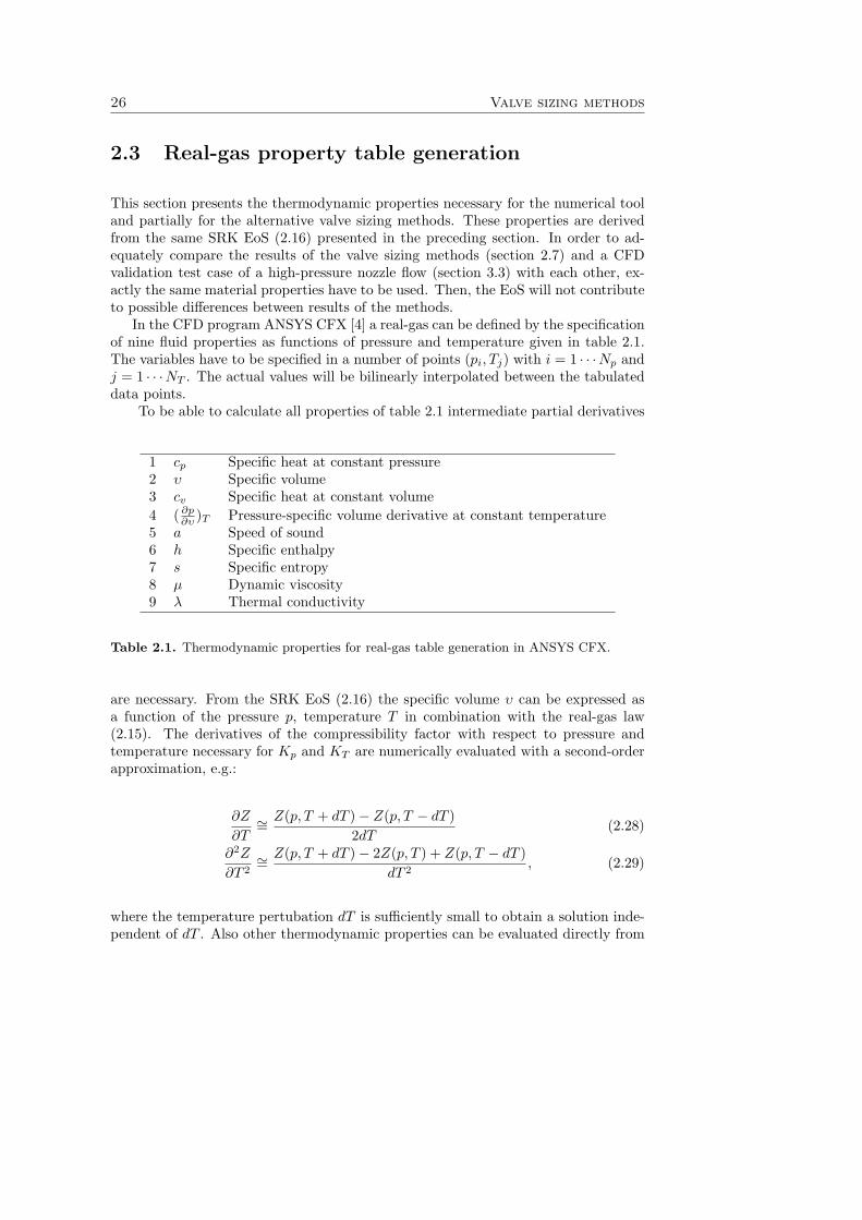
In the CFD program ANSYS CFX [4] a real-gas can be defined by the specificationof nine fluid properties as functions of pressure and temperature given in table 2.1.The variables have to be specified in a number of points (pi, Tj) with i = 1 · · ·Np andj = 1 · · ·NT . The actual values will be bilinearly interpolated between the tabulateddata points.
To be able to calculate all properties of table 2.1 intermediate partial derivatives
1 cp Specific heat at constant pressure2 υ Specific volume3 cv Specific heat at constant volume4 ( ∂p
∂υ )T Pressure-specific volume derivative at constant temperature5 a Speed of sound6 h Specific enthalpy7 s Specific entropy8 μ Dynamic viscosity9 λ Thermal conductivity
Table 2.1. Thermodynamic properties for real-gas table generation in ANSYS CFX.
are necessary. From the SRK EoS (2.16) the specific volume υ can be expressed asa function of the pressure p, temperature T in combination with the real-gas law(2.15). The derivatives of the compressibility factor with respect to pressure andtemperature necessary for Kp and KT are numerically evaluated with a second-orderapproximation, e.g.:
∂Z
∂T∼= Z(p, T + dT )− Z(p, T − dT )
2dT(2.28)
∂2Z
∂T 2∼= Z(p, T + dT )− 2Z(p, T ) + Z(p, T − dT )
dT 2, (2.29)
where the temperature pertubation dT is sufficiently small to obtain a solution inde-pendent of dT . Also other thermodynamic properties can be evaluated directly from
2.3 Real-gas property table generation 27
the EoS:
∂ρ
∂p= − ρ
Z
∂Z
∂p− Z
p(2.30)
∂p
∂υ= − ρ2
∂ρ∂p
(2.31)
∂ρ
∂T= −ρ
p
Z + T ∂Z∂T
T Zp
(2.32)
∂2υ
∂T 2= 2
∂Z
∂T
Rs
p+ Rs
T
p
∂2Z
∂T 2(2.33)
In order to calculate the thermodynamic properties as a function of p and T it ischosen to combine the EoS (2.16) with the specific heat capacity at constant pressurecp as a function of temperature at one value of the pressure pref . This is the minimalset of information wherefrom all thermodynamic states in the whole pressure andtemperature domain can be derived in a thermodynamically consistent way, i.e. byobeying the Maxwell relations. It is convenient to choose pref as low as possible, sothat the fluid is in the gas phase for all values of T at this pressure.
The first law of thermodynamics for the specific enthalpy difference dh (2.41) readsin combination with the general real-gas EoS
dh = cpdT −KT υdp. (2.34)
The specific enthalpy can now be calculated at any combination of p and T from(2.34) with the trapezoidal rule:
h(p, T ) = href +∫ T
Tref
cp(pref , T )dT −∫ p
pref
KT (p, T )υ(p, T )dp, (2.35)
where href = h(pref , Tref ) is a reference value. The specific heat cp can be derivedin a similar way by using the Maxwell relation
∂cp
∂p=
∂
∂T
(υ − T
(∂υ
∂T
)p
). (2.36)
For numerical stability of high-pressure calculations up to 3600 bar with CFD it isnecessary that the pressure of the real-gas property table ranges from 0.01 to 10000bar and the temperature from 100 to 6000 K. However, the IUPAC tables supply datafrom 10 bar onwards with a limited temperature range, so an alternative referencesource has to be used for lower pressures and higher temperatures. For a large numberof species thermochemical data is available (NIST, 2009) [49], where for nitrogen theheat capacity at constant pressure per unit quantity of mass is directly tabulated with0.3 to 0.8% uncertainty at low temperatures up to 2000 K and at a constant referencepressure of 0.01 bar. For higher temperatures from 298 up to 6000 K a polynomialfit from the same database is used
cp = (A + BT + CT 2 + DT 3 + E/T 2)/M (2.37)
28 Valve sizing methods
with temperature T = 10−3T , molar mass M = 28.014 × 10⁻³ kg/mol, coefficientsA = 26.092 J/(mol K), B = 8.218801 J/(mol K2), C = −1.976141 J/(mol K3),D = 0.159274 J/(mol K4) and E = 0.044434 J K/mol valid for a reference pressureof 1 bar. The high-temperature polynomial is slightly shifted to match the tabulateddata at the lower reference pressure of 0.01 bar. Hereafter, three fifth-order polynomialfits with ranges 100-400 K, 400-1010 K and 1010-6000 K are defined to achieve thehighest accuracy for calculation of the internal real-gas property table points (pref , T )with the function
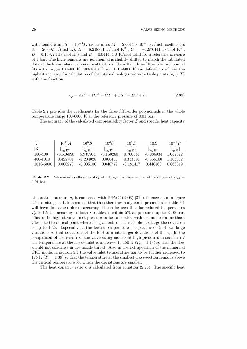
cp = AT 5 + BT 4 + CT 3 + DT 2 + ET + F . (2.38)
Table 2.2 provides the coefficients for the three fifth-order polynomials in the wholetemperature range 100-6000 K at the reference pressure of 0.01 bar.
The accuracy of the calculated compressibility factor Z and specific heat capacity
T 1012A 109B 106C 103D 10E 10−3F[K] [ J
kg K6 ] [ Jkg K5 ] [ J
kg K4 ] [ Jkg K3 ] [ J
kg K2 ] [ Jkg K ]
100-400 -3.516090 5.935904 -3.150280 0.760534 -0.086934 1.042872400-1010 0.422704 -1.204028 0.866450 0.333386 -0.355100 1.1038621010-6000 0.000278 -0.005100 0.040772 -0.181417 0.446863 0.866319
Table 2.2. Polynomial coefficients of cp of nitrogen in three temperature ranges at pref =0.01 bar.
at constant pressure cp is compared with IUPAC (2008) [31] reference data in figure2.1 for nitrogen. It is assumed that the other thermodynamic properties in table 2.1will have the same order of accuracy. It can be seen that for reduced temperaturesTr > 1.5 the accuracy of both variables is within 5% at pressures up to 3600 bar.This is the highest valve inlet pressure to be calculated with the numerical method.Closer to the critical point where the gradients of the variables are large the deviationis up to 10%. Especially at the lowest temperature the parameter Z shows largevariations so that deviations of the EoS turn into larger deviations of the cp. In thecomparison of the results of the valve sizing models at high pressures in section 2.7the temperature at the nozzle inlet is increased to 150 K (Tr = 1.18) so that the flowshould not condense in the nozzle throat. Also in the extrapolation of the numericalCFD model in section 5.3 the valve inlet temperature has to be further increased to175 K (Tr = 1.39) so that the temperature at the smallest cross-section remains abovethe critical temperature for which the deviations are smaller.
The heat capacity ratio κ is calculated from equation (2.25). The specific heat

2.3 Real-gas property table generation 29
10-1 100 101 1020
50
100
150
200
c p[J
/(mol
K)]
10-1 100 101 102-10
-5
0
5
10
pr [-]
e rel[%
]
10-1 100 101 102
100
101
Z[-]
10-1 100 101 102-5
0
5
10
pr [-]
e rel[%
]
T = 135 K (Tr = 1.07)
T = 200 K (Tr = 1.58)T = 300 K (Tr = 2.38)
Figure 2.1. Comparison of calculated compressibility factor Z and specific heat capacityat constant pressure cp with IUPAC data for nitrogen for three values of the reduced tem-perature. The circles in the two upper figures refer to the IUPAC data and in the two lowerfigures refer to the points of comparison.
capacity at constant volume cv and the speed of sound a are derived from
cv = ZRs[1 + KT ]2
κ[1−Kp]2 − [1−Kp](2.39)
a =
√√√√√√(
∂p
∂ρ
)T
+T
ρ2cv
⎛⎜⎝(
∂ρ∂T
)p(
∂ρ∂p
)T
⎞⎟⎠
2
. (2.40)
For higher pressures the specific enthalpy h
dh = cpdT +
[υ − T
(∂υ
∂T
)p
]dp (2.41)
and the specific entropy s
ds = cpdT
T−(
∂υ
∂T
)p
dp. (2.42)
are numerically integrated using the trapezoidal rule.The dynamic viscosity μ(p, T ) in [Pa s] is defined according to the rigid, non-
interacting sphere model (Reid, 1966) [52] with the molar mass M in [kg/mol], the
30 Valve sizing methods
temperature in [K] and the critical volume Vc in [m3/mol].
μ = 10−726.69√
1000MT
σ2(2.43)
σ = 0.809V 1/3c (2.44)
The thermal conductivity λ(p, T ) is defined according to the modified Euken model(Reid, 1966) [52] as
λ = μcv(1.32 + 1.77Rs
cv). (2.45)
The CFD solver ANSYS CFX does not permit the real-gas property data to comeinto the subcooled liquid region, so that the EoS can only be used in the vapor andsupercritical region. This region is bounded by the saturated vapor pressure curve upto the critical point and needs to be specified. For instance, at pressures lower thanthe critical pressure, when during iteration of the numerical method the temperaturestored at a certain grid node would become beyond the saturation temperature at thatpressure, the solution variables of that grid node will be clipped to the values at thatsaturation pressure. Furthermore, at pressures higher than the critical pressure, whenduring iteration the temperature falls below the critical temperature, the solutionvariables stored at the grid nodes of the CFD code will be clipped to values in thereal-gas tables at the critical temperature Tc.
The saturated vapor pressure curve according to Gomez-Thodos (Reid, 1966) [52]crosses the critical point and is given by
psat = 10−5pc exp(β[1
Tmr
− 1] + γ[T 7r − 1]) (2.46)
with the parameters β, m and γ depending on the critical pressure pc, critical tem-perature Tc and boiling temperature Tb of the gas.
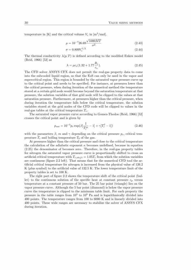
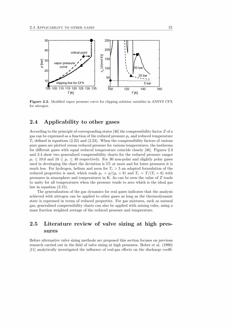
At pressures higher than the critical pressure and close to the critical temperaturethe calculation of the adiabatic exponent κ becomes undefined, because in equation(2.25) the denominator of becomes zero. Therefore, in the real-gas property tablesfor nitrogen the saturated vapor pressure curve is proportionally shifted to cross anartificial critical temperature with Tr,shift = 1.05Tr from which the solution variablesare continuous (figure 2.2 left). That means that for the numerical CFD tool the ar-tificial critical temperature for nitrogen is increased from the physical value of 126.2K (plus symbol) to the artificial value of 132.5 K. The lower temperature limit of theproperty tables is set to 100 K.
The right part of figure 2.2 shows the temperature shift of the critical point (bul-let) to the continuous solution of the specific heat at constant pressure cp versustemperature at a constant pressure of 50 bar. The 25 bar point (triangle) lies on thevapor pressure curve. Although the 5 bar point (diamond) is below the vapor pressurecurve the temperature is clipped to the minimum table limit. For each property thepressure in the table ranges from 103 to 109 Pa and is logarithmically divided into400 points. The temperature ranges from 100 to 6000 K and is linearly divided into400 points. These wide ranges are necessary to stabilize the solver of ANSYS CFXduring iteration.
2.4 Applicability to other gases 31
100 120 140 1600
50
100
150
200
250
T [K]
c p[J
/(mol
K)]
5 bar
25 bar
50 barvapor pressure
curve
critical point
clipping line for CFX
100 105 110 115 120 125 130 135
10
20
30
40
50p
[bar
]
T [K]
Figure 2.2. Modified vapor pressure curve for clipping solution variables in ANSYS CFXfor nitrogen.
2.4 Applicability to other gases
According to the principle of corresponding states [46] the compressibility factor Z of agas can be expressed as a function of the reduced pressure pr and reduced temperatureTr defined in equations (2.22) and (2.23). When the compressibility factors of variouspure gases are plotted versus reduced pressure for various temperatures, the isothermsfor different gases with equal reduced temperature coincide closely [46]. Figures 2.3and 2.4 show two generalized compressibility charts for the reduced pressure rangespr ≤ 10.0 and 10 ≤ pr ≤ 40 respectively. For 30 non-polar and slightly polar gasesused in developing the chart the deviation is 5% at most and for lower pressures it ismuch less. For hydrogen, helium and neon for Tr > 5 an adapted formulation of thereduced properties is used, which reads pr = p/(pc + 8) and Tr = T/(Tc + 8) withpressures in atmosphere and temperatures in K. As can be seen the value of Z tendsto unity for all temperatures when the pressure tends to zero which is the ideal gaslaw in equation (2.15).
The generalization of the gas dynamics for real gases indicates that the analysisachieved with nitrogen can be applied to other gases as long as the thermodynamicstate is expressed in terms of reduced properties. For gas mixtures, such as naturalgas, generalized compressibility charts can also be applied with mixing rules, using amass fraction weighted average of the reduced pressure and temperature.
2.5 Literature review of valve sizing at high pres-sures
Before alternative valve sizing methods are proposed this section focuses on previousresearch carried out in the field of valve sizing at high pressures. Bober et al. (1990)[11] analytically investigated the influence of real-gas effects on the discharge coeffi-

32 Valve sizing methods
Figure 2.3. Generalized compressibility chart for pr ≤ 10.0 (Moran, 2006) [46]. Legend:solid = constant reduced temperature Tr; dashed = constant pseudo-reduced specific volumeυ′
r = υ/(RsTc/pc).
cient of choked nozzles. In their work an analytical method for non-ideal isentropicgas flow through converging-diverging nozzles based on the Redlich-Kwong EoS withthe specific heat as function of temperature and pressure was developed. Chokedmass flow rates between ideal gas and real-gas flow differed up to 19% for methaneat a reduced pressure p0,r = 5 and reduced temperature T0,r = 1.4. It was concludedthat the iteration scheme would be more efficient when the isentropic change betweentwo thermodynamic states would be solved with temperature T and specific volumeυ as the independent variables instead of solving it as function of pressure.
Also Bauerfeind et al. (2003) [9] focused on an analytical method to calculate thelocal course of thermodynamic and fluid dynamic states of a real-gas in an adiabaticnozzle in order to calculate the maximum mass flow rate with variable dissipationeffects. The local dissipation rate along the nozzle was estimated with functions forthe loss coefficient depending on the shape of the nozzle. It was concluded that themass flow rate through a critical nozzle can be calculated accurately enough withthe simple isentropic state change of an ideal gas as presented in section 2.1, whenthe compressibility factor Z and the adiabatic exponent κ are arithmetically averagedbetween the fluid dynamic state at the inlet and the critical state at the nozzle throat.Closer to the critical point of the gas this approach is still accurate because the mod-eling errors compensate each other. The dissipation coefficients reduced from 0.975for stagnation pressures below the critical pressure and to 0.95 for pressures above thecritical point up to 160 bar. This dissipation effect is a relatively small error source in
2.5 Literature review of valve sizing at high pressures 33
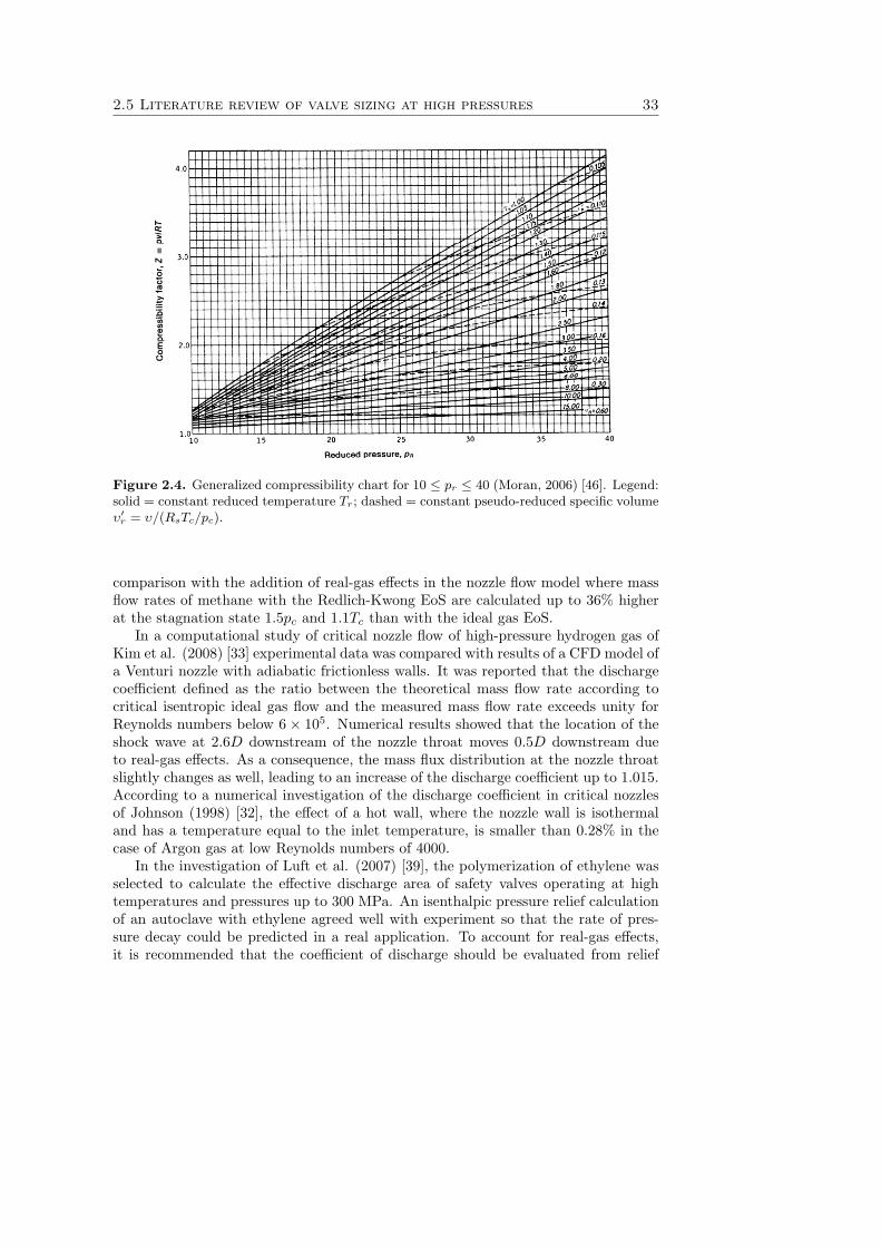
Figure 2.4. Generalized compressibility chart for 10 ≤ pr ≤ 40 (Moran, 2006) [46]. Legend:solid = constant reduced temperature Tr; dashed = constant pseudo-reduced specific volumeυ′
r = υ/(RsTc/pc).
comparison with the addition of real-gas effects in the nozzle flow model where massflow rates of methane with the Redlich-Kwong EoS are calculated up to 36% higherat the stagnation state 1.5pc and 1.1Tc than with the ideal gas EoS.
In a computational study of critical nozzle flow of high-pressure hydrogen gas ofKim et al. (2008) [33] experimental data was compared with results of a CFD model ofa Venturi nozzle with adiabatic frictionless walls. It was reported that the dischargecoefficient defined as the ratio between the theoretical mass flow rate according tocritical isentropic ideal gas flow and the measured mass flow rate exceeds unity forReynolds numbers below 6× 10⁵. Numerical results showed that the location of theshock wave at 2.6D downstream of the nozzle throat moves 0.5D downstream dueto real-gas effects. As a consequence, the mass flux distribution at the nozzle throatslightly changes as well, leading to an increase of the discharge coefficient up to 1.015.According to a numerical investigation of the discharge coefficient in critical nozzlesof Johnson (1998) [32], the effect of a hot wall, where the nozzle wall is isothermaland has a temperature equal to the inlet temperature, is smaller than 0.28% in thecase of Argon gas at low Reynolds numbers of 4000.
In the investigation of Luft et al. (2007) [39], the polymerization of ethylene wasselected to calculate the effective discharge area of safety valves operating at hightemperatures and pressures up to 300 MPa. An isenthalpic pressure relief calculationof an autoclave with ethylene agreed well with experiment so that the rate of pres-sure decay could be predicted in a real application. To account for real-gas effects,it is recommended that the coefficient of discharge should be evaluated from relief
34 Valve sizing methods
measurements under the conditions the valves are operated. However, this is onlypossible for small relief valves at laboratory scale and in particular hardly possible atindustrial scale, so that a numerical tool is necessary for accurate valve sizing.
In contrast to the derivation of the real-gas critical nozzle flow model with dissipa-tion of Bauerfeind it is expected that the pressure losses due to shocks should not betaken into account, since these occur after the choking plane and influence the criticalpressure at the nozzle throat only at lower Reynolds numbers. Furthermore, in caseof small pressure ratios the shock is located far downstream towards the nozzle exit.Then a small variation of the first shock does not influence the mass flux distributionin the nozzle itself. Also, the calculated dissipation coefficients have an averaged valueof 0.96, which is small in comparison with the loss factors as given in the standardISO 9300 [28] at high Reynolds numbers. The dissipation coefficients are up to 0.995where the boundary layers are thin and are calibrated with experiments to achieveerrors below < 0.5% in practice.
From the brief literature overview concerning recent investigations in the field of high-pressure valve sizing two ways for analytical determination of the mass flow rate ofa choked nozzle with real-gas effects can be distinguished. In the first approach,referred to as real-average method, only the stagnation properties of the nozzle inletor an arithmetical average between the inlet and the critical properties at the nozzlethroat are used. This method is used by Bauerfeind et al. (2003) [9] based onrecommendations of the American standard API RP520 (2000) [5] and extensivelydescribed by Rist (1996) [55]. In the second approach, referred to as real-integralmethod, the critical thermodynamic state is calculated iteratively with isentropicthermodynamic state change relations. This method was used by Bober et al. (1990)[11].
From a practical point of view it is desirable to have an accurate nozzle flow modelthat resolves real-gas effects without using iteration schemes. Then the dischargecoefficient accounting for flow losses due to friction, separation and recirculation ofthe flow should depend only weakly on thermodynamic effects, such as real-gas effects,when the nozzle model already accurately captures this. In addition, the dischargecoefficient Kd becomes essentially a geometry factor that is insensitive to the inlettemperature and pressure. The real-gas nozzle flow model delivers the flow coefficientCg to calculate the mass flow rate in the general equation (2.2).
2.6 Alternative valve sizing methods
This section presents two alternative valve sizing methods based on both approaches.In section 2.7 the results of these methods are compared with the standardized valvesizing method. In section 3.3 the performance of the three valve sizing methods andalso CFD results will be compared with experimental data from a high-pressure nozzleflow. It is emphasized that for each valve sizing method the same real-gas definitiondescribed in sections 2.2 and 2.3 are used to minimize influences from inaccuracies ofthe EoS used.
The derivation of both analytical nozzle methods starts with the first law of ther-

2.6 Alternative valve sizing methods 35
modynamics for the specific enthalpy difference dh (2.41) which results in combinationwith the general real-gas EoS in equation (2.34). With the help of the second law ofthermodynamics the specific entropy ds equals (2.42). For an isentropic flow, ds = 0,the enthalpy difference becomes [59]
dhis = ZRscp
1 + KTdT = ZRs
κ[1 + KT ]κ[1−Kp]− 1
dT =ZRs
ΠdT, (2.47)
where
Π =κ[1−Kp]− 1
κ[1 + KT ]. (2.48)
In an adiabatic isentropic nozzle the specific total enthalpy remains constant, so thatthe enthalpy difference can be integrated from the nozzle inlet with velocity zero tothe nozzle throat ∫ throat
0
dh = −u2/2, (2.49)
where u is the velocity in the throat. The locations of both thermodynamic statesin a truncated nozzle are shown in figure 2.5. In reality, viscous effects and heat
h0 hthroat
A0
Figure 2.5. Enthalpy change of a flow in a truncated nozzle.
conduction always result in entropy production. As a consequence, for a convergentadiabatic nozzle flow the enthalpy change with enthalpy production Δh yields [55]
∫ throat
0
dh = −u2/2 + Δh. (2.50)
For a frictionless nozzle flow the mass flow rate mg,nozzle equals
mg,nozzle =A0
υ
√−2∫ throat
0
dh ≡ CgA0
√2p0
υ0(2.51)
with throat area A0, specific volume υ, dimensionless flow coefficient Cg and totalpressure p0 that equals the definition of equation (2.2). An isentropic change of stateof a real-gas without friction reads
Cg =υ0
υ
√− ∫ throat
0dhis
υ0p0. (2.52)
36 Valve sizing methods
First alternative valve sizing method: real-averageIn the first approach, referred to as real-average method, the enthalpy integral issolved by arithmetically averaging all variables between the total state at the inletand the static state at the nozzle throat, where the enthalpy is maximum. Thisapproach has been published in Schmidt et al. (2009) [59].
Cg =υ0
υ
√1
Πm
Zm
Z0
(1− T
T0
)(2.53)
with the mean values according to Rist (1996) [55]
κm = (κ + κ0)/2 (2.54)Zm = (Z + Z0)/2 (2.55)
Kp,m = (Kp + Kp,0)/2 (2.56)KT,m = (KT + KT,0)/2 (2.57)
Πm =κm[1−Kp,m]− 1
κm[1 + KT,m]. (2.58)
The isentropic relations for real gases are
T
T0=(
p
p0
)Πm
(2.59)
υ0
υ=(
p
p0
) 1κm
. (2.60)
With the coefficient ϕ accounting for viscous effects and heat conduction, the dimen-sionless flow coefficient for real gases as function of the pressure ratio η = p/p0 withpressure p at the nozzle throat becomes
Cg = ϕ
√1
Πm
Zm
Z0η
2κm (1− ηΠm). (2.61)
By differentiating this equation with respect to the pressure ratio the maximum valueof Cg is formed for the pressure ratio
ηcrit =[
22 + Πmκm
] 1Πm
. (2.62)
When this critical pressure ratio is smaller than the backpressure ratio ηb = pb/p0
the flow is choked. The critical pressure ratio has to be determined iteratively be-cause it depends on the thermodynamic properties of the critical state as well. Asinitial guess the ideal gas critical ratio can be used, which is equation (2.62) withKp,m = KT,m = 0 so that Πm,ideal = (κ0 − 1)/κ0. When the critical pressure ratiois larger than the backpressure ratio the flow remains subsonic and the dimensionlessflow coefficient can be directly calculated with the actual backpressure ratio.
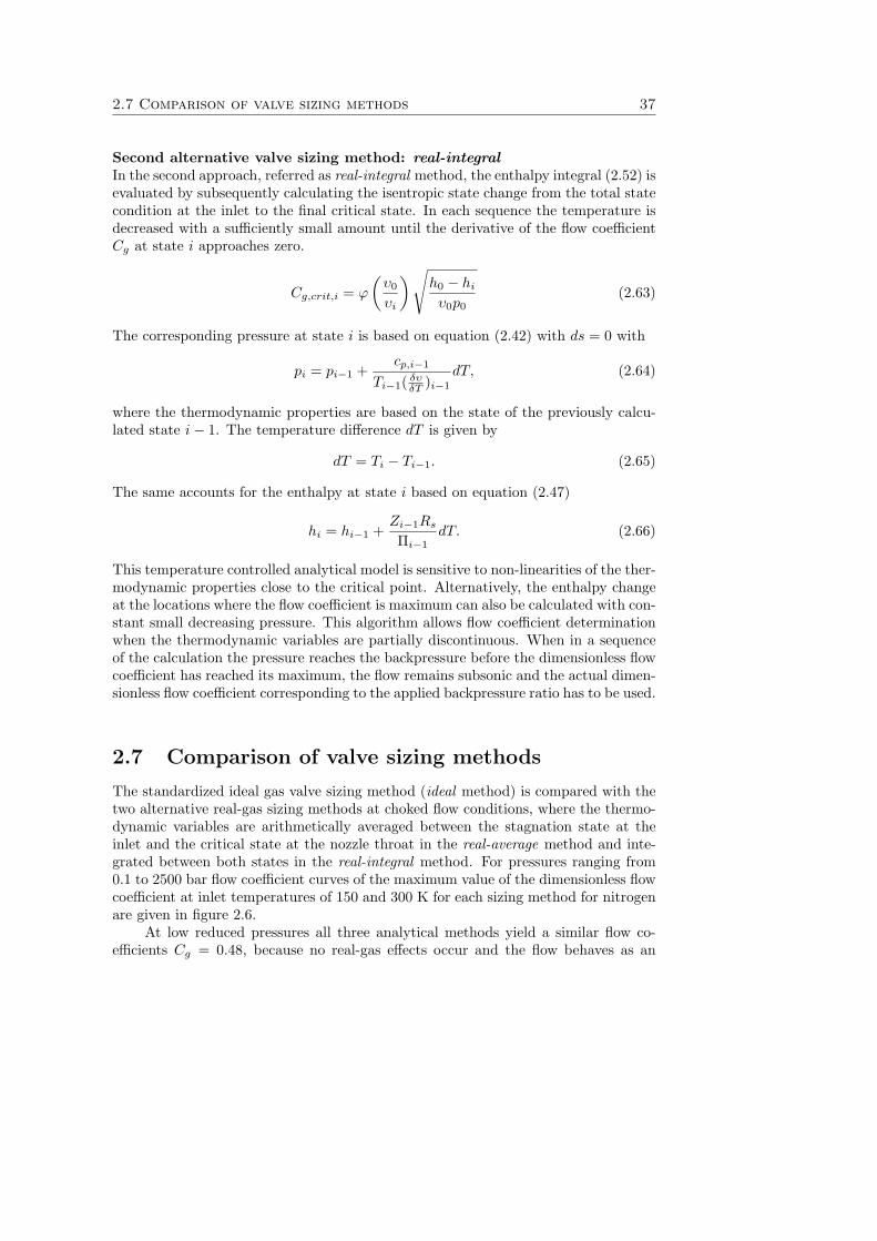
2.7 Comparison of valve sizing methods 37
Second alternative valve sizing method: real-integralIn the second approach, referred as real-integral method, the enthalpy integral (2.52) isevaluated by subsequently calculating the isentropic state change from the total statecondition at the inlet to the final critical state. In each sequence the temperature isdecreased with a sufficiently small amount until the derivative of the flow coefficientCg at state i approaches zero.
Cg,crit,i = ϕ
(υ0
υi
)√h0 − hi
υ0p0(2.63)
The corresponding pressure at state i is based on equation (2.42) with ds = 0 with
pi = pi−1 +cp,i−1
Ti−1( δυδT )i−1
dT, (2.64)
where the thermodynamic properties are based on the state of the previously calcu-lated state i− 1. The temperature difference dT is given by
dT = Ti − Ti−1. (2.65)
The same accounts for the enthalpy at state i based on equation (2.47)
hi = hi−1 +Zi−1Rs
Πi−1dT. (2.66)
This temperature controlled analytical model is sensitive to non-linearities of the ther-modynamic properties close to the critical point. Alternatively, the enthalpy changeat the locations where the flow coefficient is maximum can also be calculated with con-stant small decreasing pressure. This algorithm allows flow coefficient determinationwhen the thermodynamic variables are partially discontinuous. When in a sequenceof the calculation the pressure reaches the backpressure before the dimensionless flowcoefficient has reached its maximum, the flow remains subsonic and the actual dimen-sionless flow coefficient corresponding to the applied backpressure ratio has to be used.
2.7 Comparison of valve sizing methods
The standardized ideal gas valve sizing method (ideal method) is compared with thetwo alternative real-gas sizing methods at choked flow conditions, where the thermo-dynamic variables are arithmetically averaged between the stagnation state at theinlet and the critical state at the nozzle throat in the real-average method and inte-grated between both states in the real-integral method. For pressures ranging from0.1 to 2500 bar flow coefficient curves of the maximum value of the dimensionless flowcoefficient at inlet temperatures of 150 and 300 K for each sizing method for nitrogenare given in figure 2.6.
At low reduced pressures all three analytical methods yield a similar flow co-efficients Cg = 0.48, because no real-gas effects occur and the flow behaves as an
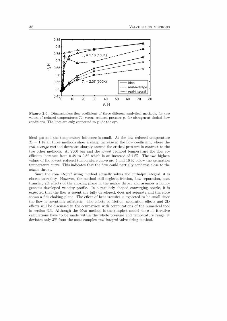
38 Valve sizing methods
Tr = 1.18 (150K)
0 10 20 30 40 50 60 70 800.45
0.5
0.55
0.6
0.65
0.7
0.75
0.8
0.85
pr [-]
C g[-]
idealreal-averagereal-integral
Tr = 2.37 (300K)
Figure 2.6. Dimensionless flow coefficient of three different analytical methods, for twovalues of reduced temperatures Tr, versus reduced pressure pr for nitrogen at choked flowconditions. The lines are only connected to guide the eye.
ideal gas and the temperature influence is small. At the low reduced temperatureTr = 1.18 all three methods show a sharp increase in the flow coefficient, where thereal-average method decreases sharply around the critical pressure in contrast to thetwo other methods. At 2500 bar and the lowest reduced temperature the flow co-efficient increases from 0.48 to 0.82 which is an increase of 71%. The two highestvalues of the lowest reduced temperature curve are 5 and 10 K below the saturationtemperature curve. This indicates that the flow could partially condense close to thenozzle throat.
Since the real-integral sizing method actually solves the enthalpy integral, it isclosest to reality. However, the method still neglects friction, flow separation, heattransfer, 2D effects of the choking plane in the nozzle throat and assumes a homo-geneous developed velocity profile. In a regularly shaped converging nozzle, it isexpected that the flow is essentially fully developed, does not separate and thereforeshows a flat choking plane. The effect of heat transfer is expected to be small sincethe flow is essentially adiabatic. The effects of friction, separation effects and 2Deffects will be discussed in the comparison with computations of the numerical toolin section 3.3. Although the ideal method is the simplest model since no iterativecalculations have to be made within the whole pressure and temperature range, itdeviates only 3% from the most complex real-integral valve sizing method.
Chapter 3
Development of numericaltool
In this chapter the numerical method for valve characterizing is developed with CFD.In section 3.1, the mathematical models, the discretization and the solution methodof the numerical method will be given. Then in section 3.2, a suitable CFD softwarepackage will be chosen and its model parameters will be determined with the help ofvalidation test cases based on low-pressure reference data from literature. In section3.3, the performance of the CFD method as well as the valve sizing methods fromthe preceding chapter will be validated with measurement data from a high-pressurenozzle flow.
3.1 Numerical valve model parameters
Computational fluid dynamics is applied as a numerical tool to describe the flowthrough safety valves. The numerical tool comprises partial differential equations(PDE) representing the physics of the flow, which are solved for small control vol-umes defined by a computational mesh. In the case of fluid flow the PDE systemconsists of the conservation equations for the mass, momentum and energy. BeforeCFD can be applied it is important to know which physical phenomena dominate theflow within a safety valve and with which physical models the Navier-Stokes equationshave to be completed. Then, the computational domain has to be specified so that atthe boundaries the flow variables are prescribed or follow from boundary conditions.The considered valve geometry will be decomposed into small volumes, where the el-ements should be small in flow regions with large gradients of the flow variables. Thecoupled non-linear algebraic equations resulting from discretization of the governingPDE’s must be solved iteratively until a certain convergence criterion is met. Thena solution of the flow problem is achieved that can be analyzed in a post-processor.From the computed flow field the desired information can be extracted, such as inte-gral computed variables that can be compared with experimental data.
40 Development of numerical tool
3.1.1 Mathematical models
To describe the 3D flow phenomena in a safety valve, the conservation laws of mass,momentum and energy are used in a set of equations known as the unsteady Navier-Stokes equations which are solved by a commercial software package ANSYS CFXin their conservation form [4]. The continuity equation with density ρ and velocityvector u is
∂ρ
∂t+∇ · (ρu) = 0. (3.1)
The momentum equations with pressure p, in absence of volumetric forces yields
∂(ρu)∂t
+∇ · (ρuu) = −∇p +∇ · τ (3.2)
with assuming a Newtonian fluid the stress tensor τ related to the strain rate by
τ = μ
(∇u + (∇u)T − 2
3δ∇ · u
). (3.3)
Here Stokes’ hypothesis that τ has a zero trace is used to relate the second viscosity tothe dynamic viscosity. The total energy equation with Fourier’s law of heat conductionis
∂ρh0
∂t− ∂p
∂t+∇ · (ρuh0) = ∇ · (λ∇T ) +∇ · (u · τ), (3.4)
where total enthalpy h0 = h + 12u
2 and the term ∇ · (u · τ) represents the work dueto viscous stresses. The volumetric heat sources are neglected. For low velocities orincompressible flows the density is approximately constant and the continuity equationreduces to
∇ · u = 0. (3.5)
The conservation equations have to be completed with definitions of the fluid proper-ties in the form of a thermal EoS, which describes the relation between the thermo-dynamic parameters pressure, density and temperature of the fluid. Also a caloricEoS expressing the internal energy as a function of two independent thermodynamicparameters and the transport properties dynamic viscosity μ and thermal conductiv-ity λ of the fluid are necessary. Section 2.5 focuses on material properties for highpressures.
The Navier-Stokes equations can be solved directly numerically (DNS) when thenumerical grid is sufficiently fine. Then, all spatial and time scales must be resolved inthe computational mesh from the smallest dissipative scales up to the integral scale as-sociated with the motions containing most of the kinetic energy. However, turbulenceoccurs at much smaller scales than can actually be resolved in practical applications.Also for engineering purposes only the time-averaged flow quantities and not the fluc-tuations are of interest. To obtain an approximate solution, the Reynolds-AveragedNavier-Stokes (RANS) equations are used. In this approach, the flow quantities aredecomposed in a mean (ensemble-average) and a fluctuating part. For example, ateach location x at time t the velocity u(x, t) is decomposed into the time-averaged
3.1 Numerical valve model parameters 41
u value denoted by an overbar and the random fluctuating component of motion u′
denoted by a primeu(x, t) = u(x) + u′(x, t). (3.6)
Substituting this decomposition in the Navier-Stokes equation and time-averaging,results for the averaged equation of momentum
∂ρu∂t
+∇ · (ρuu) = ∇ · (τ − ρu′u′). (3.7)
In the averaged partial differential equations cross-correlations of the turbulent fluc-tuations appear as new terms. These terms are called the Reynolds stresses −ρu′u′and the Reynolds heat flux −ρu′h′ for the averaged energy equation and constitutenine new unknowns, which means that the system is not closed anymore.
A solution is to approximate the Reynolds stress tensor and the turbulent heatflux term with a turbulence model depending on the type of flow. There is a largevariety of models, but all these models have in common that they introduce uncer-tainties. The main difference between these turbulence models is their complexity.In engineering flows, eddy viscosity based models are the simplest level of closurethat does not require geometry or flow regime as input with a reasonable compromisebetween computational effort and physical accuracy. Herein, the Boussinesq approxi-mation assumes that the Reynolds stresses are proportional to the eddy or turbulentviscosity μt and the mean velocity gradients
−ρu′u′ = μt(∇u + (∇u)T )− 23δ(ρk + μt∇ · u), (3.8)
with turbulent kinetic energy k defined as
k =12u′2. (3.9)
The gradient-diffusion hypothesis relates the Reynolds fluxes of a scalar linearly tothe mean scalar gradient
−u′h′0 = −ΓT∇h0, (3.10)
where ΓT is the eddy diffusivity as a function of the turbulent Prandtl number PrT
ΓT =μt
PrT. (3.11)
The turbulent Prandtl number is defined as a function of the mean velocity andtemperature gradients, the turbulent shear stress u′v′ and the turbulent heat fluxv′T ′
PrT = u′v′∂T
∂y
/v′T ′
∂u
∂y, (3.12)
which is a prescribed dimensionless quantity. Two-equation models provide the tur-bulent viscosity μt so that the turbulence is expressed in terms of mean variables.The most popular version of the two-equation model is de k− ε model, where ε is the
42 Development of numerical tool
rate at which turbulent energy is dissipated into smaller eddies (Jones and Launder,1972) [32]
μt = Cμρk2
ε, (3.13)
where Cμ is a dimensionless quantity. The values of k and ε are computed from twopartial differential transport equations for the turbulence kinetic energy and turbu-lence dissipation rate. The k − ε model is less sensitive to the free stream values ofε, but is often inadequate in flows with adverse pressure gradients such as in safetyvalves.
The second most widely used type of turbulence model is the k − ω model ofWilcox (1993) [69], where ω is the frequency of the largest eddies. The k − ω modelassumes that the turbulent viscosity μt is related to the turbulence kinetic energy andturbulent frequency via
μt = ρk
ω. (3.14)
The k − ω model performs well close to walls in boundary layers in strong adversepressure gradients. However, it is sensitive to the free stream value of ω and unlessgreat care is taken to set this value, inaccurate results can be found in both theboundary layer and shear flows.
An interesting option is a combination of the two models, which is called the Base-line (BSL) model (Menter, 1994) [42]. In this model the properties of the k−ω modelclose to the wall and the performance of the k − ε model in the free shear flow areretained by a gradual blending of the two models from the wall to the free stream.The BSL model combines the advantages of the k− ω and k− ε model, but still failsto properly predict the onset and extent of flow separation from smooth surfaces.The main reason is that both models do not account for the transport of turbulentshear stress. This results in an overprediction of the eddy viscosity. A limiter inthe formulation of the eddy viscosity can obtain the proper transport behavior. Thisapproach is known as the shear stress transport (SST) model, proposed by Menter(1994) [42]. This SST model is considered as the best two-equation turbulence modelto predict the turbulent flow effects under the influence of adverse pressure gradients,non-equilibrium boundary layer regions as those found behind shocks, or close to re-gions with flow separation.
Two-equation RANS turbulence models are only valid in developed turbulent bulkflows at high Reynolds numbers. Adjacent to the wall in the boundary layer turbulentfluctuations are suppressed and viscous flow effects become important. Also high flowgradients would require a high grid density to accurately resolve the boundary layer.Commonly used empirical wall functions model the viscous sub-layer and the log-lawzone of the boundary layer so that they overcome the inaccuracy of the turbulencemodel and the necessity of a fine grid at the wall. For smooth walls the laminarviscous sub-layer has the velocity profile
u(y) = yτw
μ(3.15)
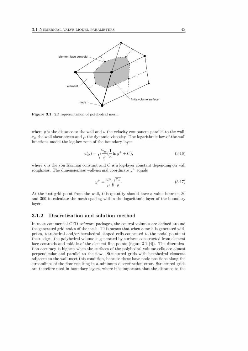
3.1 Numerical valve model parameters 43
element face centroid
element
nodefinite volume surface
Figure 3.1. 2D representation of polyhedral mesh.
where y is the distance to the wall and u the velocity component parallel to the wall,τw the wall shear stress and μ the dynamic viscosity. The logarithmic law-of-the-wallfunctions model the log-law zone of the boundary layer
u(y) =√
τw
ρ(1κ
ln y+ + C), (3.16)
where κ is the von Karman constant and C is a log-layer constant depending on wallroughness. The dimensionless wall-normal coordinate y+ equals
y+ =yρ
μ
√τw
ρ. (3.17)
At the first grid point from the wall, this quantity should have a value between 30and 300 to calculate the mesh spacing within the logarithmic layer of the boundarylayer.
3.1.2 Discretization and solution method
In most commercial CFD software packages, the control volumes are defined aroundthe generated grid nodes of the mesh. This means that when a mesh is generated withprism, tetrahedral and/or hexahedral shaped cells connected to the nodal points attheir edges, the polyhedral volume is generated by surfaces constructed from elementface centroids and middle of the element line points (figure 3.1 [4]). The discretiza-tion accuracy is highest when the surfaces of the polyhedral volume cells are almostperpendicular and parallel to the flow. Structured grids with hexahedral elementsadjacent to the wall meet this condition, because these have node positions along thestreamlines of the flow resulting in a minimum discretization error. Structured gridsare therefore used in boundary layers, where it is important that the distance to the
44 Development of numerical tool
walls, the dimensionless wall-normal coordinate y+ is kept at a constant value to meetthe requirements for near-wall turbulence modeling. For high-pressure compressibleflows the boundary layers are thin so that the height of the first cell at the boundarywall has to be up to 1000 times smaller in comparison with transonic flow at atmo-spheric conditions or incompressible flows.
For complex valve geometries a structured mesh is not possible without dividingthe volume into blocks to generate a block-structured mesh. The cells at the cornersof the block are optimal, but the drawback is that at the edges between two blocks inthe bulk flow the cells become too stretched which can cause numerical instabilities.Unstructured hexahedral grids are the compromise between geometrical flexibility andthe possibility to refine the mesh locally without deteriorating the mesh quality. Afurther advantage of using hexahedral mesh elements is that the memory usage is upto four times smaller and the computational time up to 1.6 times shorter than for atetrahedral mesh with equivalent accuracy according to FEM calculations of Tsuboi(2001) [67].
At the surfaces of a meshed computational domain boundary conditions have to beimposed. Since a safety valve flow involves high velocities the heat exchange with thewalls is negligible so that the wall can be considered as adiabatic. At the enlargedinlet and outlet of a safety valve flow the velocities are low so that the stagnationpressure and temperature are well-defined which can directly be specified at theseboundaries. In case of compressible flows with unknown inlet velocity profile or massflow rate, specified values of the total pressure and total temperature at the subsonicinlet and the static pressure and temperature at the subsonic outlet give the moststable results. It is noted that both boundaries are defined as an opening allowingthe fluid to cross the boundary surface in either direction. Then these boundaries donot block traveling pressure waves in reverse flow direction possibly causing numericalinstabilities. At the inlet also a low turbulence intensity is set and it is recommendedto set it at the outlet to zero gradient.
In the CFD software package ANSYS CFX the numerical discretization is nodebased and it uses shape functions to evaluate the derivatives for the pressure gradientterm and the diffusion terms in the momentum, continuity and turbulence quantititiesequations. The Navier-Stokes equations are discretized in an unstaggered, collocatedway and solved by an algebraic multigrid solver. To avoid pressure-velocity decou-pling, a robust interpolation scheme similar to Rhie-Chow interpolation (1983) [53] isused. CFX solves the conservation equations of mass and momentum in one-systemof linear equations, with all equations being fully coupled (ANSYS, 2006) [4]. Theturbulence equations are pairwise solved as well.
CFX uses advection schemes such as first-order upwind difference and numericaladvection with specified blend factor. This blend factor can be varied between 0 and1 to vary between a first- and second-order differencing scheme to control numericaldiffusion. The high resolution scheme option will be chosen which maintains the blendfactor as close as possible to 1 without violating the boundedness principle that couldresult in non-physical overshoots or undershoots in the solution. Only for the turbu-lence equations the first-order accurate scheme is sufficient. For CFD simulations for
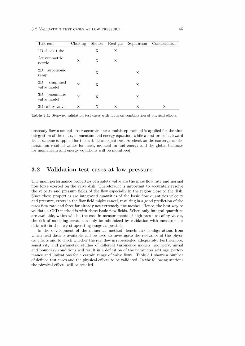
3.2 Validation test cases at low pressure 45
Test case Choking Shocks Real gas Separation Condensation
1D shock tube X X
Axisymmetricnozzle X X X
2D supersonicramp X X
2D simplifiedvalve model X X X
3D pneumaticvalve model X X X
3D safety valve X X X X X
Table 3.1. Stepwise validation test cases with focus on combination of physical effects.
unsteady flow a second-order accurate linear multistep method is applied for the timeintegration of the mass, momentum and energy equation, while a first-order backwardEuler scheme is applied for the turbulence equations. As check on the convergence themaximum residual values for mass, momentum and energy and the global balancesfor momentum and energy equations will be monitored.
3.2 Validation test cases at low pressure
The main performance properties of a safety valve are the mass flow rate and normalflow force exerted on the valve disk. Therefore, it is important to accurately resolvethe velocity and pressure fields of the flow especially in the region close to the disk.Since these properties are integrated quantities of the basic flow quantities velocityand pressure, errors in the flow field might cancel, resulting in a good prediction of themass flow rate and force for already not extremely fine meshes. Hence, the best way tovalidate a CFD method is with these basic flow fields. When only integral quantitiesare available, which will be the case in measurements of high-pressure safety valves,the risk of modeling errors can only be minimized by validation with measurementdata within the largest operating range as possible.
In the development of the numerical method, benchmark configurations fromwhich field data is available will be used to investigate the relevance of the physi-cal effects and to check whether the real flow is represented adequately. Furthermore,sensitivity and parametric studies of different turbulence models, geometry, initialand boundary conditions will result in a definition of the parameter settings, perfor-mance and limitations for a certain range of valve flows. Table 3.1 shows a numberof defined test cases and the physical effects to be validated. In the following sectionsthe physical effects will be studied.
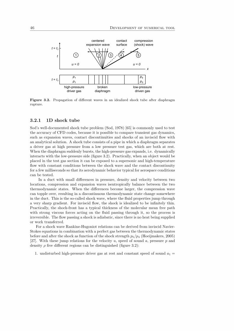
46 Development of numerical tool
contactsurface
t
centeredexpansion wave
compression(shock) wave
x
p1
ρ1
p5
ρ5
0 = u0 = u
t = t1
t = t1
high-pressuredriver gas
low-pressuredriven gas
brokendiaphragm
21 3 4 5
Figure 3.2. Propagation of different waves in an idealized shock tube after diaphragmrupture.
3.2.1 1D shock tube
Sod’s well-documented shock tube problem (Sod, 1978) [65] is commonly used to testthe accuracy of CFD codes, because it is possible to compare transient gas dynamics,such as expansion waves, contact discontinuities and shocks of an inviscid flow withan analytical solution. A shock tube consists of a pipe in which a diaphragm separatesa driver gas at high pressure from a low pressure test gas, which are both at rest.When the diaphragm suddenly bursts, the high-pressure gas expands, i.e. dynamicallyinteracts with the low-pressure side (figure 3.2). Practically, when an object would beplaced in the test gas section it can be exposed to a supersonic and high-temperatureflow with constant conditions between the shock wave and the contact discontinuityfor a few milliseconds so that its aerodynamic behavior typical for aerospace conditionscan be tested.
In a duct with small differences in pressure, density and velocity between twolocations, compression and expansion waves isentropically balance between the twothermodynamic states. When the differences become larger, the compression wavecan topple over, resulting in a discontinuous thermodynamic state change somewherein the duct. This is the so-called shock wave, where the fluid properties jump througha very sharp gradient. For inviscid flow, the shock is idealized to be infinitely thin.Practically, the shock-front has a typical thickness of the molecular mean free pathwith strong viscous forces acting on the fluid passing through it, so the process isirreversible. The flow passing a shock is adiabatic, since there is no heat being suppliedor work transferred.
For a shock wave Rankine-Hugoniot relations can be derived from inviscid Navier-Stokes equations in combination with a perfect gas between the thermodynamic statesbefore and after the shock as function of the shock strength p5/p4 (Hoeijmakers, 2005)[27]. With these jump relations for the velocity u, speed of sound a, pressure p anddensity ρ five different regions can be distinguished (figure 3.2):
1. undisturbed high-pressure driver gas at rest and constant speed of sound a1 =
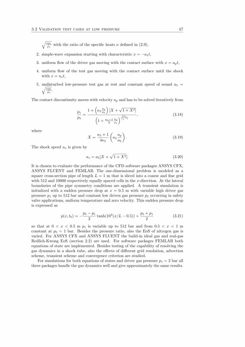
3.2 Validation test cases at low pressure 47
√κp1ρ1
with the ratio of the specific heats κ defined in (2.9),
2. simple-wave expansion starting with characteristic x = −a1t,
3. uniform flow of the driver gas moving with the contact surface with x = upt,
4. uniform flow of the test gas moving with the contact surface until the shockwith x = ust,
5. undisturbed low-pressure test gas at rest and constant speed of sound a5 =√κp5ρ5
.
The contact discontinuity moves with velocity up and has to be solved iteratively from
p1
p5=
1 +(κ5
up
a5
)[X +
√1 + X2](
1 + κ1−12
up
a1
) 2κ1κ1−1
, (3.18)
where
X =κ5 + 14κ5
(κ5
up
a5
). (3.19)
The shock speed us is given by
us = a5[X +√
1 + X2]. (3.20)
It is chosen to evaluate the performance of the CFD software packages ANSYS CFX,ANSYS FLUENT and FEMLAB. The one-dimensional problem is modeled as asquare cross-section pipe of length L = 1 m that is sliced into a coarse and fine gridwith 512 and 10000 respectively equally spaced cells in the x-direction. At the lateralboundaries of the pipe symmetry conditions are applied. A transient simulation isinitialized with a sudden pressure drop at x = 0.5 m with variable high driver gaspressure p1 up to 512 bar and constant low driven gas pressure p5 occurring in safetyvalve applications, uniform temperature and zero velocity. This sudden pressure dropis expressed as
p(x, t0) = −p5 − p1
2tanh(104(x/L− 0.5)) +
p5 + p1
2(3.21)
so that at 0 < x < 0.5 m p1 is variable up to 512 bar and from 0.5 < x < 1 mconstant at p5 = 1 bar. Besides the pressure ratio, also the EoS of nitrogen gas isvaried. For ANSYS CFX and ANSYS FLUENT the build-in ideal gas and real-gasRedlich-Kwong EoS (section 2.2) are used. For software packages FEMLAB bothequations of state are implemented. Besides testing of the capability of resolving thegas dynamics in a shock tube, also the effects of different grid resolution, advectionscheme, transient scheme and convergence criterion are studied.
For simulations for both equations of states and driver gas pressure p1 = 2 bar allthree packages handle the gas dynamics well and give approximately the same results.
48 Development of numerical tool
0 0.5 10
100
200
300ρ
[kg/
m3
]
0 0.5 10
500
1000
u[m
/s]
0 0.5 10
2
4
6x 10 7
x [m]
p[P
a]
0 0.5 10
500
1000
1500
x [m]
T[K
]
exactCFXFLUENT
Figure 3.3. Comparison of results of CFX and FLUENT with exact solution for a perfectgas with driver gas pressure p1 = 512 bar, uniform initial temperature 600 K and t = 3×10⁻⁴
s on coarse grid with 512 cells.
However, at higher driver gas pressures the FEMLAB package fails to converge. Theother two packages converge with pressures up to 512 bar with time steps varyingbetween 10−5 to 10−6 s. The exact solution is only available for a perfect gas andthe results of the coarse grid with 512 cells are shown in figure 3.3 after a simulationtime of 3× 10⁻⁴ s and time step size of 10−6 s.
The performance of both software packages is comparable with only deviationsbetween the analytical and numerical solution in the high-temperature region betweenthe contact surface and the shock wave. These deviations are due to the numericaldiffusion of the coarse grid and the inclusion of a turbulence model for the FLUENTcase. The simulations have shown that CFX is more stable compared to FLUENTsolver this problem with large discontinuities of the solution variables. Simulationswith the real-gas EoS are not presented here, but the convergence rates and calculationtime are similar to the case of ideal gas simulations resulting in similar behavior ofdensity, velocity, pressure and temperature.
Figure 3.4 presents results from simulations with the fine grid of 10000 cells witha nodal distance of 0.1 mm, which is comparable to the grid size in the bulk flowin a safety valve. The discretization order is varied as well. It can be seen that theresults of the simulations on the fine mesh match in the high-temperature region,
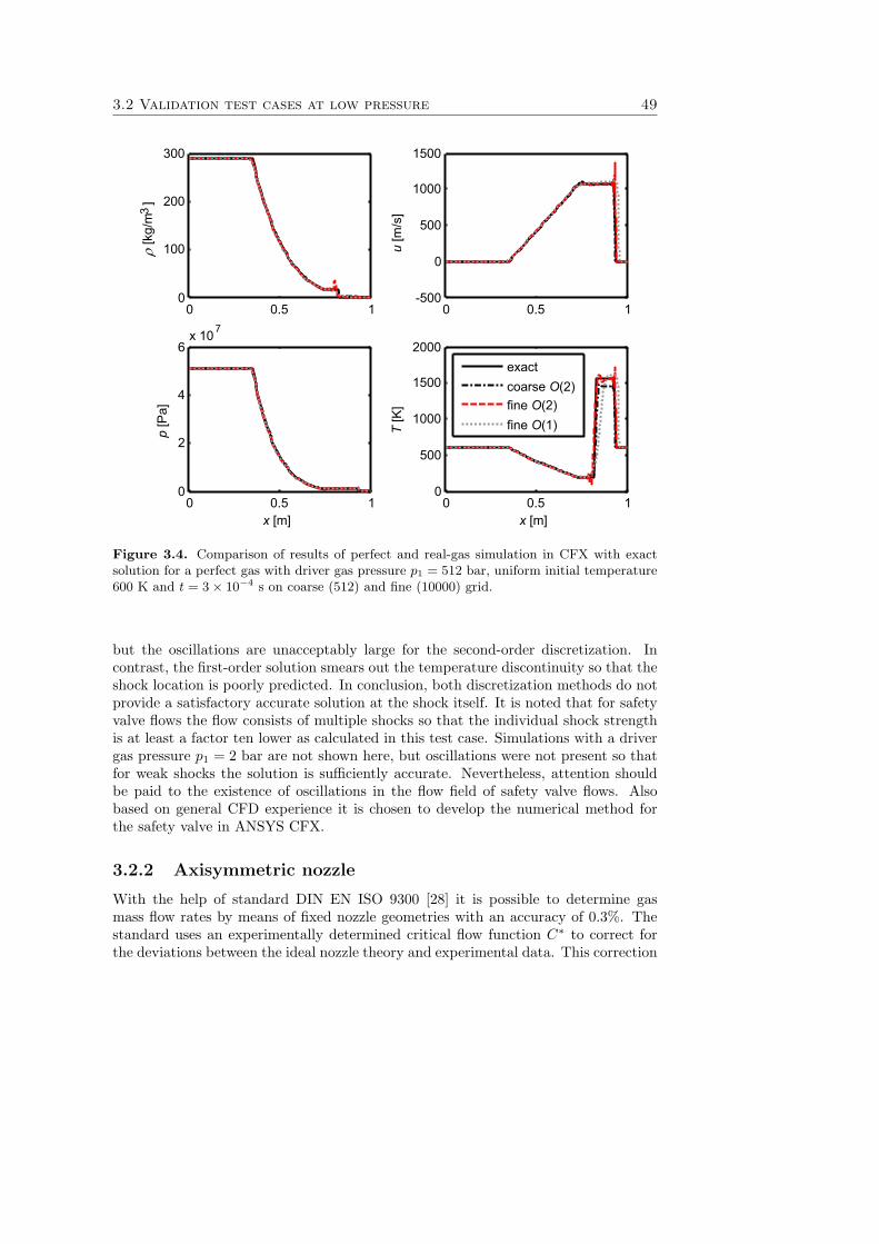
3.2 Validation test cases at low pressure 49
0 0.5 10
100
200
300
0 0.5 1-500
0
500
1000
1500
0 0.5 10
2
4
6x 10 7
x [m]
p[P
a]
0 0.5 10
500
1000
1500
2000
x [m]
T[K
]
exactcoarse O(2)fine O(2)fine O(1)
ρ[k
g/m
3]
u[m
/s]
Figure 3.4. Comparison of results of perfect and real-gas simulation in CFX with exactsolution for a perfect gas with driver gas pressure p1 = 512 bar, uniform initial temperature600 K and t = 3 × 10⁻⁴ s on coarse (512) and fine (10000) grid.
but the oscillations are unacceptably large for the second-order discretization. Incontrast, the first-order solution smears out the temperature discontinuity so that theshock location is poorly predicted. In conclusion, both discretization methods do notprovide a satisfactory accurate solution at the shock itself. It is noted that for safetyvalve flows the flow consists of multiple shocks so that the individual shock strengthis at least a factor ten lower as calculated in this test case. Simulations with a drivergas pressure p1 = 2 bar are not shown here, but oscillations were not present so thatfor weak shocks the solution is sufficiently accurate. Nevertheless, attention shouldbe paid to the existence of oscillations in the flow field of safety valve flows. Alsobased on general CFD experience it is chosen to develop the numerical method forthe safety valve in ANSYS CFX.
3.2.2 Axisymmetric nozzle
With the help of standard DIN EN ISO 9300 [28] it is possible to determine gasmass flow rates by means of fixed nozzle geometries with an accuracy of 0.3%. Thestandard uses an experimentally determined critical flow function C∗ to correct forthe deviations between the ideal nozzle theory and experimental data. This correction
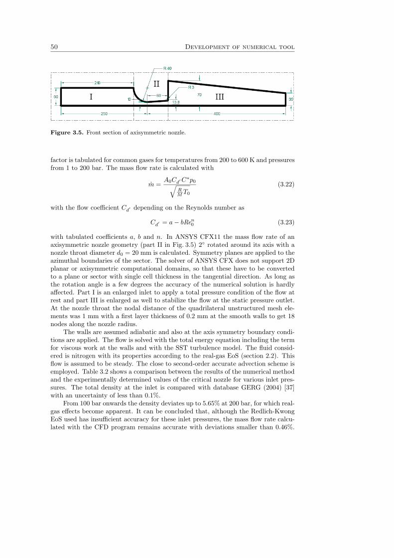
50 Development of numerical tool
Figure 3.5. Front section of axisymmetric nozzle.
factor is tabulated for common gases for temperatures from 200 to 600 K and pressuresfrom 1 to 200 bar. The mass flow rate is calculated with
m =A0Cd′C
∗p0√RM T0
(3.22)
with the flow coefficient Cd′ depending on the Reynolds number as
Cd′ = a− bRen0 (3.23)
with tabulated coefficients a, b and n. In ANSYS CFX11 the mass flow rate of anaxisymmetric nozzle geometry (part II in Fig. 3.5) 2◦ rotated around its axis with anozzle throat diameter d0 = 20 mm is calculated. Symmetry planes are applied to theazimuthal boundaries of the sector. The solver of ANSYS CFX does not support 2Dplanar or axisymmetric computational domains, so that these have to be convertedto a plane or sector with single cell thickness in the tangential direction. As long asthe rotation angle is a few degrees the accuracy of the numerical solution is hardlyaffected. Part I is an enlarged inlet to apply a total pressure condition of the flow atrest and part III is enlarged as well to stabilize the flow at the static pressure outlet.At the nozzle throat the nodal distance of the quadrilateral unstructured mesh ele-ments was 1 mm with a first layer thickness of 0.2 mm at the smooth walls to get 18nodes along the nozzle radius.
The walls are assumed adiabatic and also at the axis symmetry boundary condi-tions are applied. The flow is solved with the total energy equation including the termfor viscous work at the walls and with the SST turbulence model. The fluid consid-ered is nitrogen with its properties according to the real-gas EoS (section 2.2). Thisflow is assumed to be steady. The close to second-order accurate advection scheme isemployed. Table 3.2 shows a comparison between the results of the numerical methodand the experimentally determined values of the critical nozzle for various inlet pres-sures. The total density at the inlet is compared with database GERG (2004) [37]with an uncertainty of less than 0.1%.
From 100 bar onwards the density deviates up to 5.65% at 200 bar, for which real-gas effects become apparent. It can be concluded that, although the Redlich-KwongEoS used has insufficient accuracy for these inlet pressures, the mass flow rate calcu-lated with the CFD program remains accurate with deviations smaller than 0.46%.
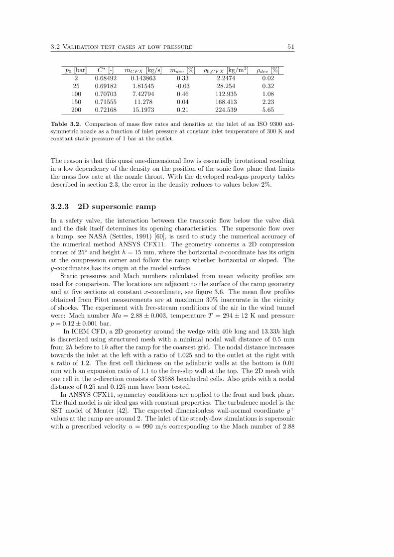
3.2 Validation test cases at low pressure 51
p0 [bar] C∗ [-] mCFX [kg/s] mdev [%] ρ0,CFX [kg/m3] ρdev [%]2 0.68492 0.143863 0.33 2.2474 0.0225 0.69182 1.81545 -0.03 28.254 0.32100 0.70703 7.42794 0.46 112.935 1.08150 0.71555 11.278 0.04 168.413 2.23200 0.72168 15.1973 0.21 224.539 5.65
Table 3.2. Comparison of mass flow rates and densities at the inlet of an ISO 9300 axi-symmetric nozzle as a function of inlet pressure at constant inlet temperature of 300 K andconstant static pressure of 1 bar at the outlet.
The reason is that this quasi one-dimensional flow is essentially irrotational resultingin a low dependency of the density on the position of the sonic flow plane that limitsthe mass flow rate at the nozzle throat. With the developed real-gas property tablesdescribed in section 2.3, the error in the density reduces to values below 2%.
3.2.3 2D supersonic ramp
In a safety valve, the interaction between the transonic flow below the valve diskand the disk itself determines its opening characteristics. The supersonic flow overa bump, see NASA (Settles, 1991) [60], is used to study the numerical accuracy ofthe numerical method ANSYS CFX11. The geometry concerns a 2D compressioncorner of 25◦ and height h = 15 mm, where the horizontal x-coordinate has its originat the compression corner and follow the ramp whether horizontal or sloped. They-coordinates has its origin at the model surface.
Static pressures and Mach numbers calculated from mean velocity profiles areused for comparison. The locations are adjacent to the surface of the ramp geometryand at five sections at constant x-coordinate, see figure 3.6. The mean flow profilesobtained from Pitot measurements are at maximum 30% inaccurate in the vicinityof shocks. The experiment with free-stream conditions of the air in the wind tunnelwere: Mach number Ma = 2.88 ± 0.003, temperature T = 294 ± 12 K and pressurep = 0.12± 0.001 bar.
In ICEM CFD, a 2D geometry around the wedge with 40h long and 13.33h highis discretized using structured mesh with a minimal nodal wall distance of 0.5 mmfrom 2h before to 1h after the ramp for the coarsest grid. The nodal distance increasestowards the inlet at the left with a ratio of 1.025 and to the outlet at the right witha ratio of 1.2. The first cell thickness on the adiabatic walls at the bottom is 0.01mm with an expansion ratio of 1.1 to the free-slip wall at the top. The 2D mesh withone cell in the z-direction consists of 33588 hexahedral cells. Also grids with a nodaldistance of 0.25 and 0.125 mm have been tested.
In ANSYS CFX11, symmetry conditions are applied to the front and back plane.The fluid model is air ideal gas with constant properties. The turbulence model is theSST model of Menter [42]. The expected dimensionless wall-normal coordinate y+
values at the ramp are around 2. The inlet of the steady-flow simulations is supersonicwith a prescribed velocity u = 990 m/s corresponding to the Mach number of 2.88
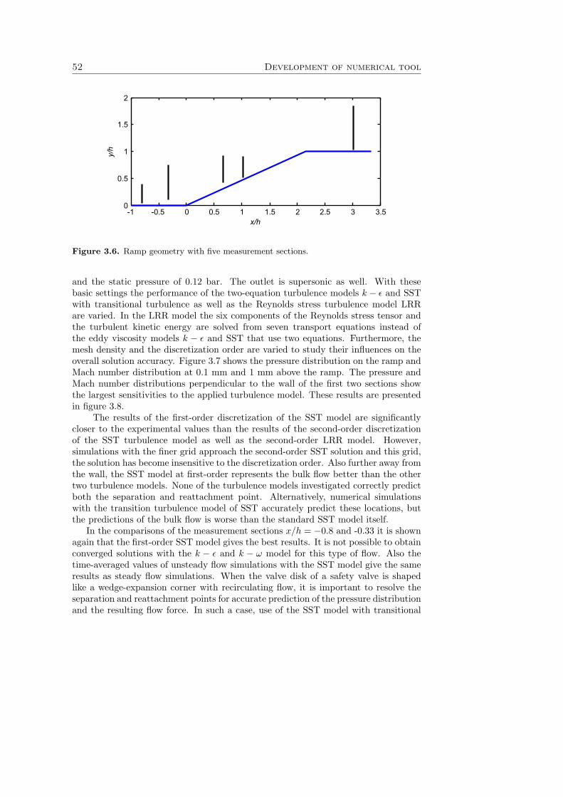
52 Development of numerical tool
-1 -0.5 0 0.5 1 1.5 2 2.5 3 3.50
0.5
1
1.5
2
x/h
y/h
Figure 3.6. Ramp geometry with five measurement sections.
and the static pressure of 0.12 bar. The outlet is supersonic as well. With thesebasic settings the performance of the two-equation turbulence models k − ε and SSTwith transitional turbulence as well as the Reynolds stress turbulence model LRRare varied. In the LRR model the six components of the Reynolds stress tensor andthe turbulent kinetic energy are solved from seven transport equations instead ofthe eddy viscosity models k − ε and SST that use two equations. Furthermore, themesh density and the discretization order are varied to study their influences on theoverall solution accuracy. Figure 3.7 shows the pressure distribution on the ramp andMach number distribution at 0.1 mm and 1 mm above the ramp. The pressure andMach number distributions perpendicular to the wall of the first two sections showthe largest sensitivities to the applied turbulence model. These results are presentedin figure 3.8.
The results of the first-order discretization of the SST model are significantlycloser to the experimental values than the results of the second-order discretizationof the SST turbulence model as well as the second-order LRR model. However,simulations with the finer grid approach the second-order SST solution and this grid,the solution has become insensitive to the discretization order. Also further away fromthe wall, the SST model at first-order represents the bulk flow better than the othertwo turbulence models. None of the turbulence models investigated correctly predictboth the separation and reattachment point. Alternatively, numerical simulationswith the transition turbulence model of SST accurately predict these locations, butthe predictions of the bulk flow is worse than the standard SST model itself.
In the comparisons of the measurement sections x/h = −0.8 and -0.33 it is shownagain that the first-order SST model gives the best results. It is not possible to obtainconverged solutions with the k − ε and k − ω model for this type of flow. Also thetime-averaged values of unsteady flow simulations with the SST model give the sameresults as steady flow simulations. When the valve disk of a safety valve is shapedlike a wedge-expansion corner with recirculating flow, it is important to resolve theseparation and reattachment points for accurate prediction of the pressure distributionand the resulting flow force. In such a case, use of the SST model with transitional
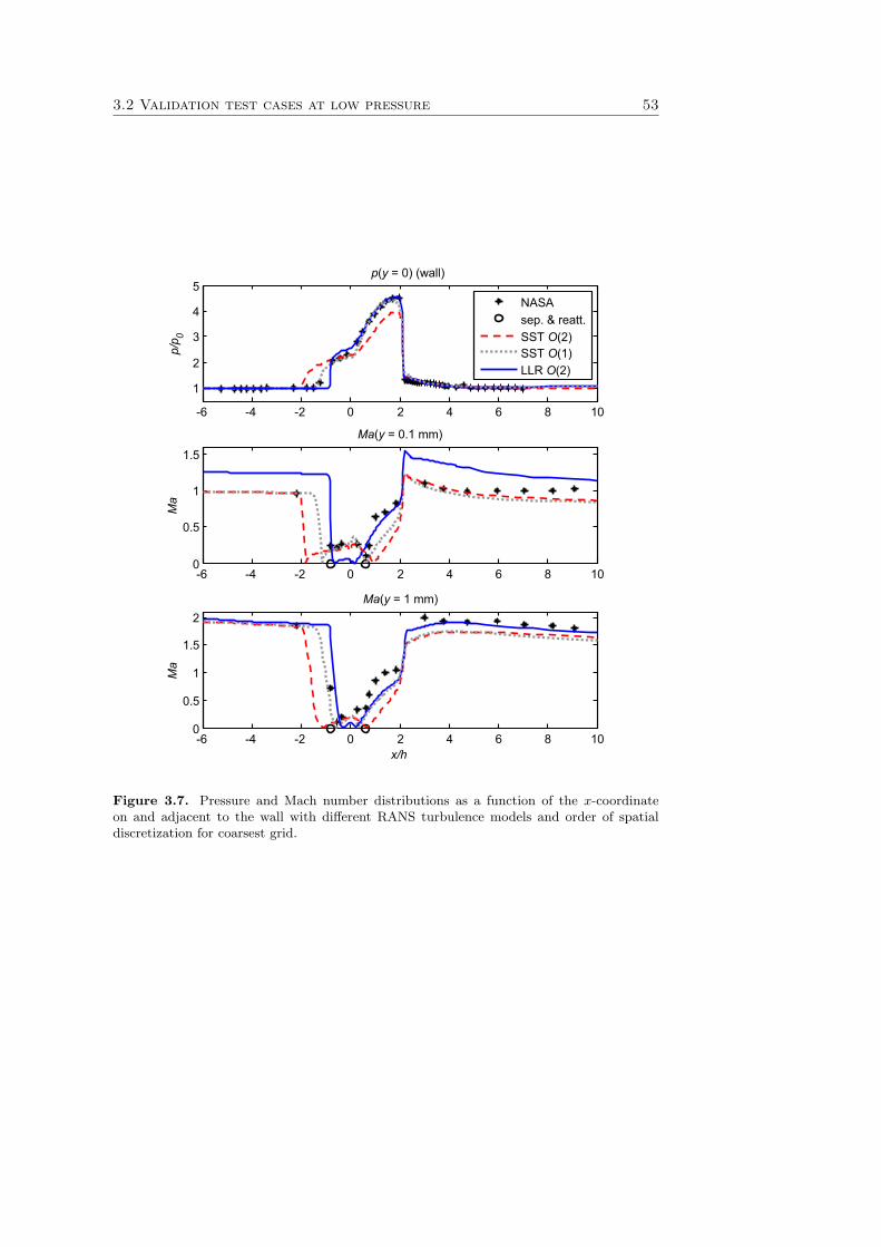
3.2 Validation test cases at low pressure 53
-6 -4 -2 0 2 4 6 8 10
1
2
3
4
5p(y = 0) (wall)
p/p 0
NASAsep. & reatt.SST O(2)SST O(1)LLR O(2)
-6 -4 -2 0 2 4 6 8 100
0.5
1
1.5
Ma(y = 0.1 mm)
Ma
-6 -4 -2 0 2 4 6 8 100
0.5
1
1.5
2Ma(y = 1 mm)
x/h
Ma
Figure 3.7. Pressure and Mach number distributions as a function of the x-coordinateon and adjacent to the wall with different RANS turbulence models and order of spatialdiscretization for coarsest grid.
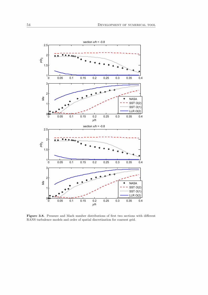
54 Development of numerical tool
0 0.05 0.1 0.15 0.2 0.25 0.3 0.35 0.41
1.5
2
2.5section x/h = -0.8
p/p 0
0 0.05 0.1 0.15 0.2 0.25 0.3 0.35 0.40
1
2
3
Ma
y/h
NASASST O(2)SST O(1)LLR O(2)
0 0.05 0.1 0.15 0.2 0.25 0.3 0.35 0.41
1.5
2
2.5section x/h = -0.8
p/p 0
0 0.05 0.1 0.15 0.2 0.25 0.3 0.35 0.40
1
2
3
Ma
y/h
NASASST O(2)SST O(1)LLR O(2)
Figure 3.8. Pressure and Mach number distributions of first two sections with differentRANS turbulence models and order of spatial discretization for coarsest grid.
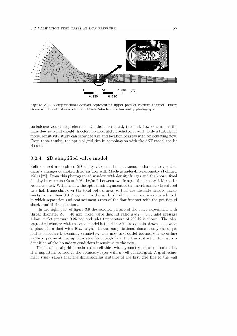
3.2 Validation test cases at low pressure 55
nozzle
Figure 3.9. Computational domain representing upper part of vacuum channel. Insertshows window of valve model with Mach-Zehnder-Interferometry photograph.
turbulence would be preferable. On the other hand, the bulk flow determines themass flow rate and should therefore be accurately predicted as well. Only a turbulencemodel sensitivity study can show the size and location of areas with recirculating flow.From these results, the optimal grid size in combination with the SST model can bechosen.
3.2.4 2D simplified valve model
Follmer used a simplified 2D safety valve model in a vacuum channel to visualizedensity changes of choked dried air flow with Mach-Zehnder-Interferometry (Follmer,1981) [22]. From this photographed window with density fringes and the known fixeddensity increments (dρ = 0.034 kg/m3) between two fringes, the density field can bereconstructed. Without flow the optical misalignment of the interferometer is reducedto a half fringe shift over the total optical area, so that the absolute density uncer-tainty is less than 0.017 kg/m3. In the work of Follmer an experiment is selected,in which separation and reattachment areas of the flow interact with the position ofshocks and their reflections.
In the right part of figure 3.9 the selected picture of the valve experiment withthroat diameter d0 = 40 mm, fixed valve disk lift ratio h/d0 = 0.7, inlet pressure1 bar, outlet pressure 0.25 bar and inlet temperature of 293 K is shown. The pho-tographed window with the valve model is the ellipse in the domain shown. The valveis placed in a duct with 10d0 height. In the computational domain only the upperhalf is considered, assuming symmetry. The inlet and outlet geometry is accordingto the experimental setup truncated far enough from the flow restriction to ensure adefinition of the boundary conditions insensitive to the flow.
The hexahedral grid domain is one cell thick with symmetry planes on both sides.It is important to resolve the boundary layer with a well-defined grid. A grid refine-ment study shows that the dimensionless distance of the first grid line to the wall
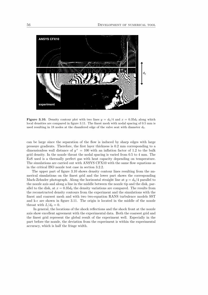
56 Development of numerical tool
ANSYS CFX10
experiment
Y X d0
Figure 3.10. Density contour plot with two lines y = d0/4 and x = 0.35d0 along whichlocal densities are compared in figure 3.11. The finest mesh with nodal spacing of 0.5 mm isused resulting in 18 nodes at the chamfered edge of the valve seat with diameter d0.
can be large since the separation of the flow is induced by sharp edges with largepressure gradients. Therefore, the first layer thickness is 0.2 mm corresponding to adimensionless wall distance of y+ = 100 with an inflation factor of 1.2 to the bulkgrid density. In the nozzle throat the nodal spacing is varied from 0.5 to 4 mm. TheEoS used is a thermally perfect gas with heat capacity depending on temperature.The simulations are carried out with ANSYS CFX10 with the same flow equations asin the critical ISO nozzle test case in section 3.2.2.
The upper part of figure 3.10 shows density contour lines resulting from the nu-merical simulations on the finest grid and the lower part shows the correspondingMach-Zehnder photograph. Along the horizontal straight line at y = d0/4 parallel tothe nozzle axis and along a line in the middle between the nozzle tip and the disk, par-allel to the disk, at x = 0.35d0 the density variations are compared. The results fromthe reconstructed density contours from the experiment and the simulations with thefinest and coarsest mesh and with two two-equation RANS turbulence models SSTand k-ε are shown in figure 3.11. The origin is located in the middle of the nozzlethroat with L/d0 = 0.
In general, the locations of the shock reflections and the shock front at the nozzleaxis show excellent agreement with the experimental data. Both the coarsest grid andthe finest grid represent the global result of the experiment well. Especially in thepart before the nozzle, the deviation from the experiment is within the experimentalaccuracy, which is half the fringe width.
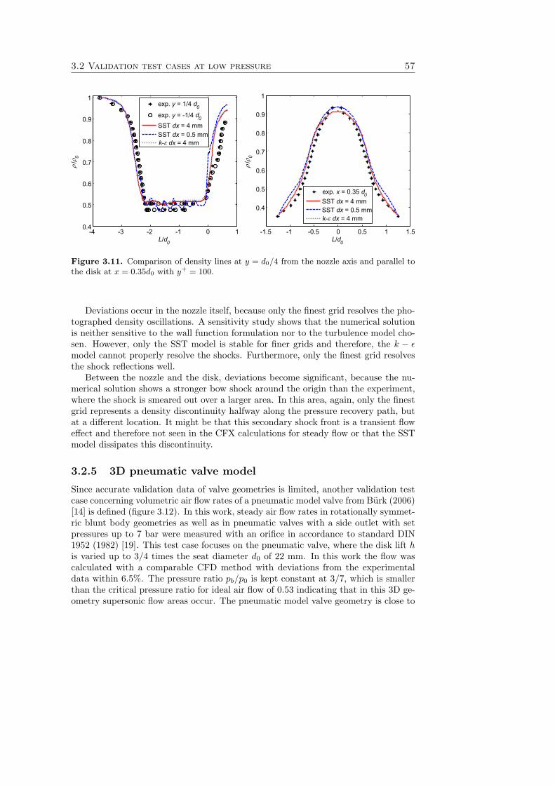
3.2 Validation test cases at low pressure 57
-4 -3 -2 -1 0 10.4
0.5
0.6
0.7
0.8
0.9
1
L/d0
ρ/ρ
0
exp. y = 1/4 d0
exp. y = -1/4 d0SST dx = 4 mmSST dx = 0.5 mmk-ε dx = 4 mm
-1.5 -1 -0.5 0 0.5 1 1.5
0.4
0.5
0.6
0.7
0.8
0.9
1
L/d0ρ
/ρ0
exp. x = 0.35 d0SST dx = 4 mmSST dx = 0.5 mmk-ε dx = 4 mm
Figure 3.11. Comparison of density lines at y = d0/4 from the nozzle axis and parallel tothe disk at x = 0.35d0 with y+ = 100.
Deviations occur in the nozzle itself, because only the finest grid resolves the pho-tographed density oscillations. A sensitivity study shows that the numerical solutionis neither sensitive to the wall function formulation nor to the turbulence model cho-sen. However, only the SST model is stable for finer grids and therefore, the k − εmodel cannot properly resolve the shocks. Furthermore, only the finest grid resolvesthe shock reflections well.
Between the nozzle and the disk, deviations become significant, because the nu-merical solution shows a stronger bow shock around the origin than the experiment,where the shock is smeared out over a larger area. In this area, again, only the finestgrid represents a density discontinuity halfway along the pressure recovery path, butat a different location. It might be that this secondary shock front is a transient floweffect and therefore not seen in the CFX calculations for steady flow or that the SSTmodel dissipates this discontinuity.
3.2.5 3D pneumatic valve model
Since accurate validation data of valve geometries is limited, another validation testcase concerning volumetric air flow rates of a pneumatic model valve from Burk (2006)[14] is defined (figure 3.12). In this work, steady air flow rates in rotationally symmet-ric blunt body geometries as well as in pneumatic valves with a side outlet with setpressures up to 7 bar were measured with an orifice in accordance to standard DIN1952 (1982) [19]. This test case focuses on the pneumatic valve, where the disk lift his varied up to 3/4 times the seat diameter d0 of 22 mm. In this work the flow wascalculated with a comparable CFD method with deviations from the experimentaldata within 6.5%. The pressure ratio pb/p0 is kept constant at 3/7, which is smallerthan the critical pressure ratio for ideal air flow of 0.53 indicating that in this 3D ge-ometry supersonic flow areas occur. The pneumatic model valve geometry is close to

58 Development of numerical tool
Figure 3.12. Computational domain of 3D pneumatic valve model with highlighted flapper.
a safety valve geometry except the inlet length, which is only 2D long with a suddencontraction, instead of over 10D with a conical contraction. Therefore, it is likelythat flow separation at the edge of the sudden contraction plays a more importantrole for the pneumatic model valve. As a consequence, after flow separation at thesudden contraction, the flow will not reattach before the seat and a recirculation arearemains. Also the outlet of the pneumatic valve is small, so that the choking planeat high disk lifts and low pressure ratios will not exist between the valve seat and theflat disk, but at the outlet.
The computational domain is divided into 1.2 million tetrahedral cells with struc-tured boundary layer cells. Also a second computational domain is created for axisym-metric simulations similar to validation test case nozzle DIN EN ISO 9300 describedin section 3.2.2. Simulations for steady flow to compute the normalized volumetricflow rate VN of air are carried out at different valve lifts with constant inlet pressureof 7 bar, outlet pressure 3 bar and 20 ◦C (see figure 3.13). The present numericalsimulations show that the numerical 3D model reproduces the measured normalizedvolume flow rates within 5%. At the smallest and highest disk lifts 3D effects of theflow at the inlet play a less dominant role, because the deviations of the axisymme-tric simulations become smaller. The deviation of the normalized volumetric flow rateVN,dev is largest when the geometric cross-section of the valve seat πd2
0/4 and the areabetween the seat and the disk πd0h are equal when 4h/d0 = 1. The overprediction
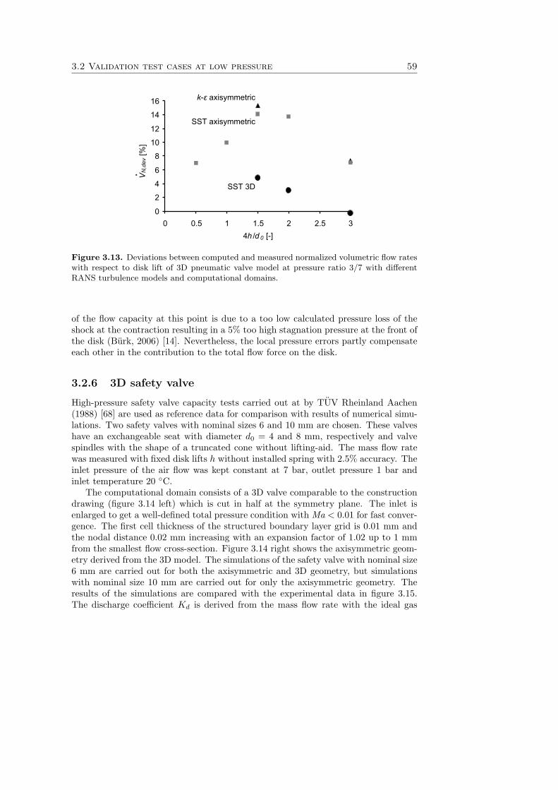
3.2 Validation test cases at low pressure 59
.
k-ε axisymmetric
SST axisymmetric
SST 3D
0
2
4
6
8
10
12
14
16
0 0.5 1 1.5 2 2.5 34h /d 0 [-]
VN
,dev
[%]
Figure 3.13. Deviations between computed and measured normalized volumetric flow rateswith respect to disk lift of 3D pneumatic valve model at pressure ratio 3/7 with differentRANS turbulence models and computational domains.
of the flow capacity at this point is due to a too low calculated pressure loss of theshock at the contraction resulting in a 5% too high stagnation pressure at the front ofthe disk (Burk, 2006) [14]. Nevertheless, the local pressure errors partly compensateeach other in the contribution to the total flow force on the disk.
3.2.6 3D safety valve
High-pressure safety valve capacity tests carried out at by TUV Rheinland Aachen(1988) [68] are used as reference data for comparison with results of numerical simu-lations. Two safety valves with nominal sizes 6 and 10 mm are chosen. These valveshave an exchangeable seat with diameter d0 = 4 and 8 mm, respectively and valvespindles with the shape of a truncated cone without lifting-aid. The mass flow ratewas measured with fixed disk lifts h without installed spring with 2.5% accuracy. Theinlet pressure of the air flow was kept constant at 7 bar, outlet pressure 1 bar andinlet temperature 20 ◦C.
The computational domain consists of a 3D valve comparable to the constructiondrawing (figure 3.14 left) which is cut in half at the symmetry plane. The inlet isenlarged to get a well-defined total pressure condition with Ma < 0.01 for fast conver-gence. The first cell thickness of the structured boundary layer grid is 0.01 mm andthe nodal distance 0.02 mm increasing with an expansion factor of 1.02 up to 1 mmfrom the smallest flow cross-section. Figure 3.14 right shows the axisymmetric geom-etry derived from the 3D model. The simulations of the safety valve with nominal size6 mm are carried out for both the axisymmetric and 3D geometry, but simulationswith nominal size 10 mm are carried out for only the axisymmetric geometry. Theresults of the simulations are compared with the experimental data in figure 3.15.The discharge coefficient Kd is derived from the mass flow rate with the ideal gas
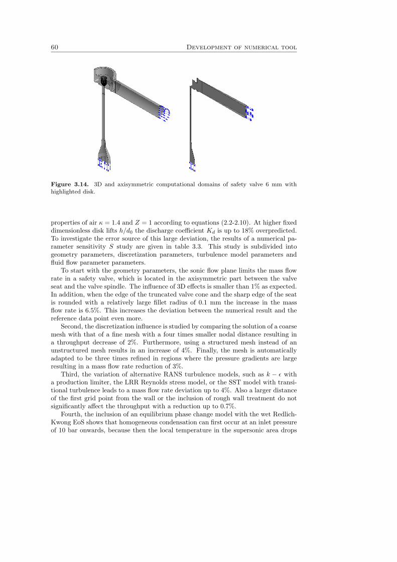
60 Development of numerical tool
Figure 3.14. 3D and axisymmetric computational domains of safety valve 6 mm withhighlighted disk.
properties of air κ = 1.4 and Z = 1 according to equations (2.2-2.10). At higher fixeddimensionless disk lifts h/d0 the discharge coefficient Kd is up to 18% overpredicted.To investigate the error source of this large deviation, the results of a numerical pa-rameter sensitivity S study are given in table 3.3. This study is subdivided intogeometry parameters, discretization parameters, turbulence model parameters andfluid flow parameter parameters.
To start with the geometry parameters, the sonic flow plane limits the mass flowrate in a safety valve, which is located in the axisymmetric part between the valveseat and the valve spindle. The influence of 3D effects is smaller than 1% as expected.In addition, when the edge of the truncated valve cone and the sharp edge of the seatis rounded with a relatively large fillet radius of 0.1 mm the increase in the massflow rate is 6.5%. This increases the deviation between the numerical result and thereference data point even more.
Second, the discretization influence is studied by comparing the solution of a coarsemesh with that of a fine mesh with a four times smaller nodal distance resulting ina throughput decrease of 2%. Furthermore, using a structured mesh instead of anunstructured mesh results in an increase of 4%. Finally, the mesh is automaticallyadapted to be three times refined in regions where the pressure gradients are largeresulting in a mass flow rate reduction of 3%.
Third, the variation of alternative RANS turbulence models, such as k − ε witha production limiter, the LRR Reynolds stress model, or the SST model with transi-tional turbulence leads to a mass flow rate deviation up to 4%. Also a larger distanceof the first grid point from the wall or the inclusion of rough wall treatment do notsignificantly affect the throughput with a reduction up to 0.7%.
Fourth, the inclusion of an equilibrium phase change model with the wet Redlich-Kwong EoS shows that homogeneous condensation can first occur at an inlet pressureof 10 bar onwards, because then the local temperature in the supersonic area drops
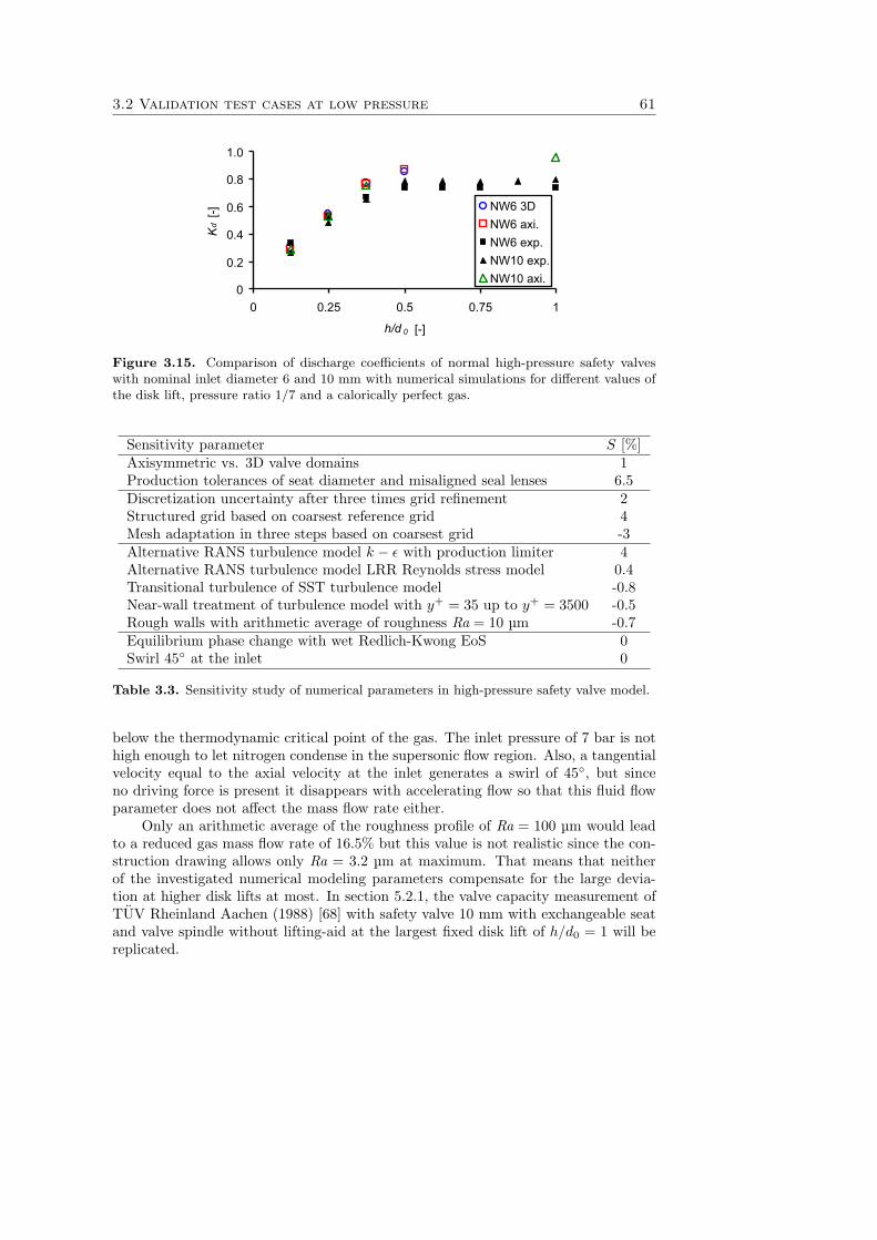
3.2 Validation test cases at low pressure 61
0
0.2
0.4
0.6
0.8
1.0
0 0.25 0.5 0.75 1
h/d 0 [-]
Kd
[-] NW6 3DNW6 axi.NW6 exp.NW10 exp.NW10 axi.
Figure 3.15. Comparison of discharge coefficients of normal high-pressure safety valveswith nominal inlet diameter 6 and 10 mm with numerical simulations for different values ofthe disk lift, pressure ratio 1/7 and a calorically perfect gas.
Sensitivity parameter S [%]Axisymmetric vs. 3D valve domains 1Production tolerances of seat diameter and misaligned seal lenses 6.5Discretization uncertainty after three times grid refinement 2Structured grid based on coarsest reference grid 4Mesh adaptation in three steps based on coarsest grid -3Alternative RANS turbulence model k − ε with production limiter 4Alternative RANS turbulence model LRR Reynolds stress model 0.4Transitional turbulence of SST turbulence model -0.8Near-wall treatment of turbulence model with y+ = 35 up to y+ = 3500 -0.5Rough walls with arithmetic average of roughness Ra = 10 μm -0.7Equilibrium phase change with wet Redlich-Kwong EoS 0Swirl 45◦ at the inlet 0
Table 3.3. Sensitivity study of numerical parameters in high-pressure safety valve model.
below the thermodynamic critical point of the gas. The inlet pressure of 7 bar is nothigh enough to let nitrogen condense in the supersonic flow region. Also, a tangentialvelocity equal to the axial velocity at the inlet generates a swirl of 45◦, but sinceno driving force is present it disappears with accelerating flow so that this fluid flowparameter does not affect the mass flow rate either.
Only an arithmetic average of the roughness profile of Ra = 100 μm would leadto a reduced gas mass flow rate of 16.5% but this value is not realistic since the con-struction drawing allows only Ra = 3.2 μm at maximum. That means that neitherof the investigated numerical modeling parameters compensate for the large devia-tion at higher disk lifts at most. In section 5.2.1, the valve capacity measurement ofTUV Rheinland Aachen (1988) [68] with safety valve 10 mm with exchangeable seatand valve spindle without lifting-aid at the largest fixed disk lift of h/d0 = 1 will bereplicated.
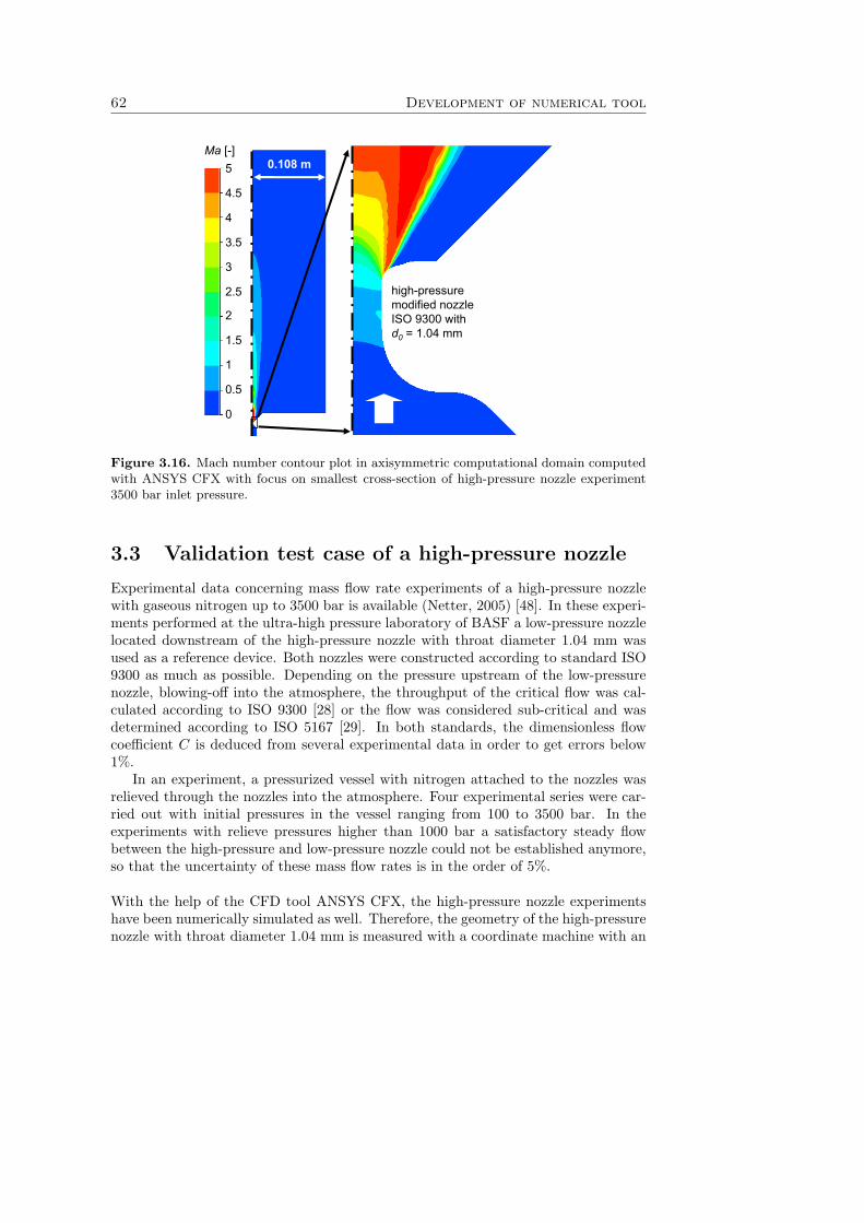
62 Development of numerical tool
0.108 mMa [-]
high-pressuremodified nozzle ISO 9300 withd0 = 1.04 mm
5
4
4.5
3.5
2.5
3
2
1
1.5
0.5
0
Figure 3.16. Mach number contour plot in axisymmetric computational domain computedwith ANSYS CFX with focus on smallest cross-section of high-pressure nozzle experiment3500 bar inlet pressure.
3.3 Validation test case of a high-pressure nozzle
Experimental data concerning mass flow rate experiments of a high-pressure nozzlewith gaseous nitrogen up to 3500 bar is available (Netter, 2005) [48]. In these experi-ments performed at the ultra-high pressure laboratory of BASF a low-pressure nozzlelocated downstream of the high-pressure nozzle with throat diameter 1.04 mm wasused as a reference device. Both nozzles were constructed according to standard ISO9300 as much as possible. Depending on the pressure upstream of the low-pressurenozzle, blowing-off into the atmosphere, the throughput of the critical flow was cal-culated according to ISO 9300 [28] or the flow was considered sub-critical and wasdetermined according to ISO 5167 [29]. In both standards, the dimensionless flowcoefficient C is deduced from several experimental data in order to get errors below1%.
In an experiment, a pressurized vessel with nitrogen attached to the nozzles wasrelieved through the nozzles into the atmosphere. Four experimental series were car-ried out with initial pressures in the vessel ranging from 100 to 3500 bar. In theexperiments with relieve pressures higher than 1000 bar a satisfactory steady flowbetween the high-pressure and low-pressure nozzle could not be established anymore,so that the uncertainty of these mass flow rates is in the order of 5%.
With the help of the CFD tool ANSYS CFX, the high-pressure nozzle experimentshave been numerically simulated as well. Therefore, the geometry of the high-pressurenozzle with throat diameter 1.04 mm is measured with a coordinate machine with an
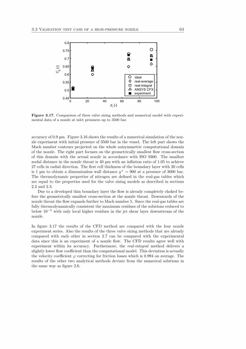
3.3 Validation test case of a high-pressure nozzle 63
0 20 40 60 80 1000.45
0.5
0.55
0.6
0.65
0.7
0.75
0.8
pr [-]
C g[-]
idealreal-averagereal-integralANSYS CFXexperiment
Figure 3.17. Comparison of three valve sizing methods and numerical model with experi-mental data of a nozzle at inlet pressures up to 3500 bar.
accuracy of 0.9 μm. Figure 3.16 shows the results of a numerical simulation of the noz-zle experiment with initial pressure of 3500 bar in the vessel. The left part shows theMach number contours projected on the whole axisymmetric computational domainof the nozzle. The right part focuses on the geometrically smallest flow cross-sectionof this domain with the actual nozzle in accordance with ISO 9300. The smallestnodal distance in the nozzle throat is 40 μm with an inflation ratio of 1.05 to achieve27 cells in radial direction. The first cell thickness of the boundary layer with 20 cellsis 1 μm to obtain a dimensionless wall distance y+ = 900 at a pressure of 3000 bar.The thermodynamic properties of nitrogen are defined in the real-gas tables whichare equal to the properties used for the valve sizing models as described in sections2.2 and 2.3.
Due to a developed thin boundary layer the flow is already completely choked be-fore the geometrically smallest cross-section at the nozzle throat. Downwards of thenozzle throat the flow expands further to Mach number 5. Since the real-gas tables arefully thermodynamically consistent the maximum residues of the solutions reduced tobelow 10−5 with only local higher residues in the jet shear layer downstream of thenozzle.
In figure 3.17 the results of the CFD method are compared with the four nozzleexperiment series. Also the results of the three valve sizing methods that are alreadycompared with each other in section 2.7 can be compared with the experimentaldata since this is an experiment of a nozzle flow. The CFD results agree well withexperiment within its accuracy. Furthermore, the real-integral method delivers aslightly lower flow coefficient than the computational model. This deviation is actuallythe velocity coefficient ϕ correcting for friction losses which is 0.994 on average. Theresults of the other two analytical methods deviate from the numerical solutions inthe same way as figure 2.6.

64 Development of numerical tool
Chapter 4
Facility for safety valve tests
This chapter summarizes the high-pressure test facility to conduct function tests ofhigh-pressure safety valves at operating pressures up to 600 bar to provide measure-ment data for validation of the numerical method. In section 4.1, design considerationsand the construction of the test facility are provided. Then in section 4.2, the appa-ratus for the quantities to be measured are presented. Lastly in section 4.3, in twoexample tests is demonstrated how the valve capacity and opening characteristic of asafety valve operating with sub-cooled water and gaseous nitrogen are determined.
4.1 Design considerations and construction
For validation of the numerical method, valve tests are conducted at well-defined mea-surement conditions for various fluids, pressures, valve types, valve sizes and springs.A test facility is constructed to determine the discharge capacity and opening charac-teristics of high-pressure safety valves for water and nitrogen at operating pressuresup to 600 bar. Also special measurement equipment is designed and calibrated tomeasure local values of pressure and temperature, valve disk lift and the integratedquantities mass flow rate and force on the valve disk. In the test facility the majorvalve characteristics described in the standard EN ISO 4126 [30] are tested. The valvetests are carried out for the following operating conditions for maximum pressure re-lief:
• The valve is installed on a vessel with a minimum pipe length so that the riskof valve disk vibrations, caused by moving pressure waves or excessive pressurelosses at the inlet during valve opening, is minimized.
• The pressure losses in the piping around the valve are small compared to thepressure loss in the valve.
• The vessel is large to have well-defined conditions for accurate measurement ofthe total pressure and temperature and so the mass flow rate.
66 Facility for safety valve tests
• The valves are experimentally investigated with mounted protection cap on thespring housing so that an elevated pressure in the spring housing can build upto act as counter-pressure assisting to close the valve.
The operating characteristics are determined by measurement of:
• total temperature at the valve inlet,
• total pressure at the valve inlet,
• valve disk lift,
• mass flow rate through the safety valve,
• force on the valve disk.
No local temperatures and pressures in the bulk flow are measured, since it is difficultto implement sensors in a high-pressure test rig without disturbing the flow.
All sensors are located at different positions around the test valve and have dif-ferent response times. As a consequence, for accurate valve characterization, the flowconditions at the test valve inlet have to be constant as long as the slowest sensorresponse during blow-off to avoid effects of finite response time of the measurementequipment. The application of a second storage vessel connected by a control valveto the buffer vessel on which the safety valve is mounted allows constant operatingconditions in the following way. Prior to a valve test the storage vessel is pressurizedwith compressed nitrogen at a higher pressure than the operating pressure of the testvalve. During the test the control valve adjusts the flow rate from the storage vesselto the buffer vessel in order to keep the pressure in the buffer vessel constant duringblow-off of the test valve, while the pressure in the storage vessel decreases. The buffervessel is sufficiently large to damp fast pressure changes caused by sudden opening ofthe control valve or the test valve.
The test rig consists of four vessels (see figure 4.1). Vessel B1 is connected tothe compressor, which provides a pressure up to 4000 bar. Safety valve SV1 protectsvessel B1 and safety valve SV2 ensures a safe pressure reduction to 600 bar in thetest facility itself. After the shut-off valve V2 the high-pressure pipe changes from amaximum allowable operating pressure of 3600 bar (PN3600) to piping with a nom-inal pressure PN700 and nominal diameter 24 mm (NW24) connected to the vesselsB2, B3 and B4. Either buffer vessel B3 is in use for valve tests with water or buffervessel B2 for valve tests with nitrogen. In figure 4.1 the connected parts of the testfacility to the buffer vessels that are partly in use for valve tests with either nitrogenor with water are grey colored. During a valve test, high-pressure nitrogen in thestorage vessel B4 expands into buffer vessel B3 filled with water or buffer vessel B2filled with nitrogen and actually pushes the test fluid in the buffer vessel through thevalve located at the opposite side of the feed lines of one of the buffer vessels.
Vessel B3 is tilted 1 m at the side with the water feed valve V7 at the lower inletand air vent or nitrogen release valve V8 at the higher inlet to increase the maximumfilling level of water to 90%. The remaining 10% can be compressed with nitrogenfrom storage vessel B4. Nitrogen release valve V4 is used to relax buffer vessel B2
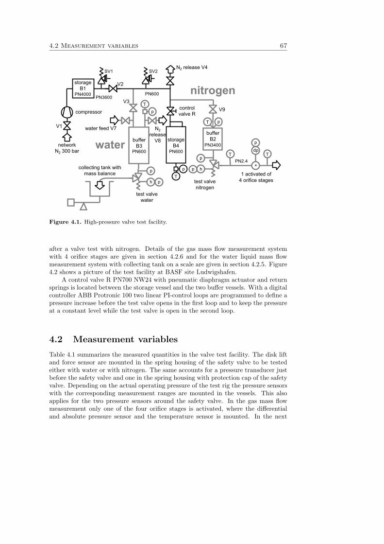
4.2 Measurement variables 67
pT
pT
storageB1
PN4000PN3600
PN600
p
T
controlvalve R
N2 release V4SV1 SV2
storageB4
bufferB2
PN3400PN600
networkN2 300 bar
h
p
1 activated of4 orifice stages
p
N2release
V8
water feed V7
bufferB3
PN600
h
pcollecting tank with
mass balancep
water
nitrogenV3
compressor
test valvenitrogen
test valvewater
V2
V1
V9
p
dpT T
PN2.4
Figure 4.1. High-pressure valve test facility.
after a valve test with nitrogen. Details of the gas mass flow measurement systemwith 4 orifice stages are given in section 4.2.6 and for the water liquid mass flowmeasurement system with collecting tank on a scale are given in section 4.2.5. Figure4.2 shows a picture of the test facility at BASF site Ludwigshafen.
A control valve R PN700 NW24 with pneumatic diaphragm actuator and returnsprings is located between the storage vessel and the two buffer vessels. With a digitalcontroller ABB Protronic 100 two linear PI-control loops are programmed to define apressure increase before the test valve opens in the first loop and to keep the pressureat a constant level while the test valve is open in the second loop.
4.2 Measurement variables
Table 4.1 summarizes the measured quantities in the valve test facility. The disk liftand force sensor are mounted in the spring housing of the safety valve to be testedeither with water or with nitrogen. The same accounts for a pressure transducer justbefore the safety valve and one in the spring housing with protection cap of the safetyvalve. Depending on the actual operating pressure of the test rig the pressure sensorswith the corresponding measurement ranges are mounted in the vessels. This alsoapplies for the two pressure sensors around the safety valve. In the gas mass flowmeasurement only one of the four orifice stages is activated, where the differentialand absolute pressure sensor and the temperature sensor is mounted. In the next
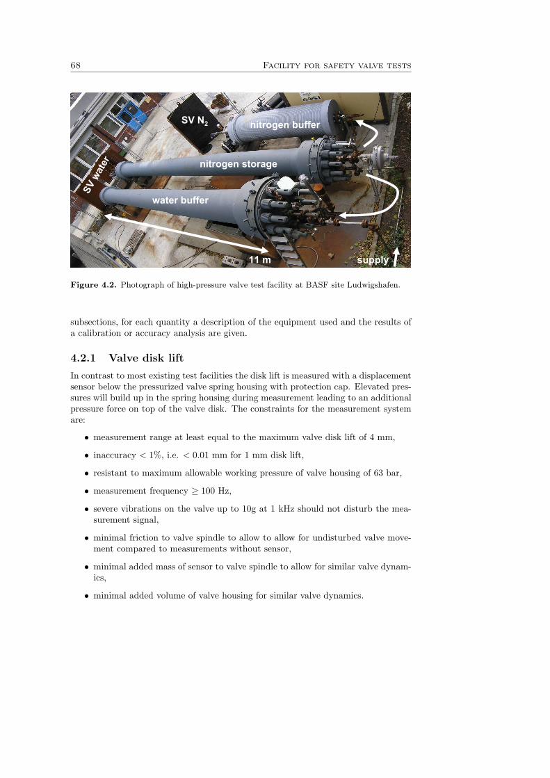
68 Facility for safety valve tests
nitrogen storage
nitrogen buffer
water buffer
supply11 m
SV N2
SVwa
ter
Figure 4.2. Photograph of high-pressure valve test facility at BASF site Ludwigshafen.
subsections, for each quantity a description of the equipment used and the results ofa calibration or accuracy analysis are given.
4.2.1 Valve disk lift
In contrast to most existing test facilities the disk lift is measured with a displacementsensor below the pressurized valve spring housing with protection cap. Elevated pres-sures will build up in the spring housing during measurement leading to an additionalpressure force on top of the valve disk. The constraints for the measurement systemare:
• measurement range at least equal to the maximum valve disk lift of 4 mm,
• inaccuracy < 1%, i.e. < 0.01 mm for 1 mm disk lift,
• resistant to maximum allowable working pressure of valve housing of 63 bar,
• measurement frequency ≥ 100 Hz,
• severe vibrations on the valve up to 10g at 1 kHz should not disturb the mea-surement signal,
• minimal friction to valve spindle to allow to allow for undisturbed valve move-ment compared to measurements without sensor,
• minimal added mass of sensor to valve spindle to allow for similar valve dynam-ics,
• minimal added volume of valve housing for similar valve dynamics.

4.2 Measurement variables 69
Variable # Sensor Range InaccuracyDisk lift 1 Temposonics type R 25 mm 0.0152-0.0323 mm
(spring housing)Disk force 1 HBM U2B 1 kN 12.8-52 N
(spring housing)Temperature 3 thermocouple type K 273-313 K 1 K
(Vessels B2, B3, B4)2 resistance PT100 223-323 K 0.3 K
(pipes with orifice)Pressure 3 WIKA UT-10 20/100/600 bar 0.01/0.05/0.3 bar(gauge) (vessels B2/B3, valve)
1 SETRA GC206 700 bar 0.35 bar(vessel B4)
2 WIKA S-10 16 bar 0.01 bar(vessels B2/B3, valve)
(absolute) 1 Rosemount 3051 CA1 2000 mbar 1 mbar(differential) 2 Rosemount 69/690 mbar 0.15/0.83 mbar
3051 CD1/CD2(pipes with orifice)
Liquid mass 1 mass balance 2000 kg 2-3.5%flow rate Bizerba 4000 VE-LGas mass 4 orifices 0.04-15 kg/s 1.3%flow rate DN50/100/200/400
acc. to EN ISO 5167
Table 4.1. Overview of all sensors and their locations of the high-pressure valve test facility.
The valve spindle is guided within a small gap so that friction between the spindleand the guidance rings is minimized. Consequently, only the two translational andthe two rotational degrees of freedom perpendicular to the spindle axis that tilt thespindle are weakly suppressed. A non-contact displacement sensor at the side of thespindle is only accurate when the small distance between the spindle and the sensoris constant during opening of the valve. Consequently, this measurement principle isunsuitable to measure the movement of the spindle itself accurately. Alternatively, aMTS Temposonics R-serie analogue magnetostrictive non-contacting linear displace-ment sensor in combination with a guiding extension is used. This sensor is commonlyused in hydraulic applications and therefore resistant to severe vibrations and to highpeak pressures up to 750 bar.
In figure 4.3 the setup of the disk lift measurement is shown. The sensor withbar is mounted in an elongated protection cap with pressure sensor tap. Since theminimal available length of the sensor bar is 50 mm the protection cap is elongatedwith the smallest possible diameter so that the total dead volume still equals thevolume of the original protection cap. The top part of the elongated protection cap isthe same for other test valve types and sizes, so that the sensor can be used for other
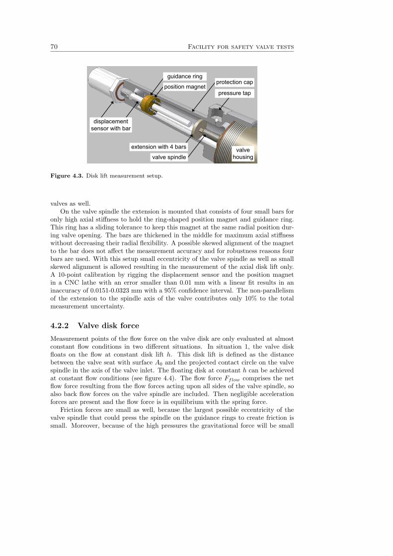
70 Facility for safety valve tests
displacement sensor with bar
position magnet
valve housing
guidance ring
valve spindle
pressure tap
extension with 4 bars
protection cap
Figure 4.3. Disk lift measurement setup.
valves as well.On the valve spindle the extension is mounted that consists of four small bars for
only high axial stiffness to hold the ring-shaped position magnet and guidance ring.This ring has a sliding tolerance to keep this magnet at the same radial position dur-ing valve opening. The bars are thickened in the middle for maximum axial stiffnesswithout decreasing their radial flexibility. A possible skewed alignment of the magnetto the bar does not affect the measurement accuracy and for robustness reasons fourbars are used. With this setup small eccentricity of the valve spindle as well as smallskewed alignment is allowed resulting in the measurement of the axial disk lift only.A 10-point calibration by rigging the displacement sensor and the position magnetin a CNC lathe with an error smaller than 0.01 mm with a linear fit results in aninaccuracy of 0.0151-0.0323 mm with a 95% confidence interval. The non-parallelismof the extension to the spindle axis of the valve contributes only 10% to the totalmeasurement uncertainty.
4.2.2 Valve disk force
Measurement points of the flow force on the valve disk are only evaluated at almostconstant flow conditions in two different situations. In situation 1, the valve diskfloats on the flow at constant disk lift h. This disk lift is defined as the distancebetween the valve seat with surface A0 and the projected contact circle on the valvespindle in the axis of the valve inlet. The floating disk at constant h can be achievedat constant flow conditions (see figure 4.4). The flow force Fflow comprises the netflow force resulting from the flow forces acting upon all sides of the valve spindle, soalso back flow forces on the valve spindle are included. Then negligible accelerationforces are present and the flow force is in equilibrium with the spring force.
Friction forces are small as well, because the largest possible eccentricity of thevalve spindle that could press the spindle on the guidance rings to create friction issmall. Moreover, because of the high pressures the gravitational force will be small
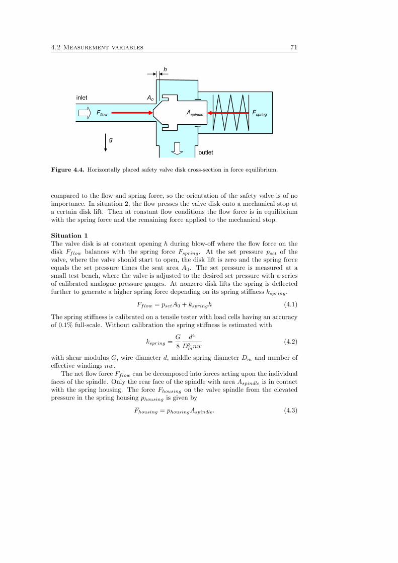
4.2 Measurement variables 71
Fflow
g
Fspring
inlet
outlet
A0
Aspindle
h
Figure 4.4. Horizontally placed safety valve disk cross-section in force equilibrium.
compared to the flow and spring force, so the orientation of the safety valve is of noimportance. In situation 2, the flow presses the valve disk onto a mechanical stop ata certain disk lift. Then at constant flow conditions the flow force is in equilibriumwith the spring force and the remaining force applied to the mechanical stop.
Situation 1The valve disk is at constant opening h during blow-off where the flow force on thedisk Fflow balances with the spring force Fspring. At the set pressure pset of thevalve, where the valve should start to open, the disk lift is zero and the spring forceequals the set pressure times the seat area A0. The set pressure is measured at asmall test bench, where the valve is adjusted to the desired set pressure with a seriesof calibrated analogue pressure gauges. At nonzero disk lifts the spring is deflectedfurther to generate a higher spring force depending on its spring stiffness kspring.
Fflow = psetA0 + kspringh (4.1)
The spring stiffness is calibrated on a tensile tester with load cells having an accuracyof 0.1% full-scale. Without calibration the spring stiffness is estimated with
kspring =G
8d4
D3mnw
(4.2)
with shear modulus G, wire diameter d, middle spring diameter Dm and number ofeffective windings nw.
The net flow force Fflow can be decomposed into forces acting upon the individualfaces of the spindle. Only the rear face of the spindle with area Aspindle is in contactwith the spring housing. The force Fhousing on the valve spindle from the elevatedpressure in the spring housing phousing is given by
Fhousing = phousingAspindle. (4.3)

72 Facility for safety valve tests
Situation 2When the test facility is operated close to its capacity limit it is difficult to control thepressure in the buffer vessel to constant force equilibrium. Therefore, a force sensormeasuring the force Fsensor acts as the mechanical stop at variable maximum disklift and allows still accurate force measurement when the spindle moves to this stop.With this mechanism flow forces in a safety valve are measured outside its equilibriumposition instead when the valve would move up to the maximum position given bythe valve construction itself. When the valve disk reaches the mechanical stop at disklift hstop the resulting flow force extends to
Fflow = psetA0 + kspringhstop + Fsensor. (4.4)
Figure 4.5 shows the construction of the force measurement with mechanical stop,which is used in combination with the previous described valve disk lift setup. The
Figure 4.5. Picture of force sensor on protection cap as it is implemented in the test facility.
valve spindle presses on a round bar, which is held at one side with a tight slidingfitting ring working as a joint. The other side is connected with a knuckle eye tothe force sensor type HBM U2B with measurement range 1 kN that is fixed on theprotection cap. The force sensor consists of 24 strain gauges that linearly change theirresistance to elastic deformation and is resistant to excessive side forces compared toits axial force to be measured with an inaccuracy of 0.1%.
The spindle presses at approximately one-third of the bar, so that the force sensormeasures approximately the same part of the original force. The protection cap canstill be pressurized up to 63 bar because two rubber rings seal the space betweenthe bar and a metal holder which is mounted on the base of the protection cap withsufficient space for elastic deformation of the bar and sensor. To avoid excessive peakforces from damaging the force sensor when the spindle collides with the mechanicalstop, a screw with a rubber plate is mounted on top of the spindle to damp the col-lision forces. This screw is adjusted to the desired maximum allowable disk lift with0.1 mm inaccuracy.
Due to tolerances of the valve seat diameter, eccentricity of the valve spindle, disk
4.2 Measurement variables 73
lift measurement and set pressure determination at the small test rig, the resultingaccuracy of the force measurement without mechanical stop is 3.2%. For the measure-ments with mechanical stop and force sensor, different setup configurations betweenthe use of rubber seal rings and the use of a collision damper between the spindlescrew and the bar are calibrated. During a calibration measurement the completeconfiguration with rubber sealing is subjected to random force changes at differentfrequencies and amplitudes. These force changes are generated by manually movingthe traverse of a tensile tester up and down with variable speeds and positions.
The calibration measurements result in a hysteresis range of 52 N independent ofthe actual force applied. For the configuration without rubber sealing this uncertaintyreduces to 13 N, so the viscoelastic behavior of the rubber sealing causes the largestuncertainty. Nevertheless, the backflow force that would occur in valve experimentswith pressurized protection cap is on average five times higher so that measuring withrubber sealing is preferred. For instance, when the total disk force measured is 2 kN,from which 200 N comes from the force sensor, the total uncertainty is still then only5%.
4.2.3 Temperature
Thermocouples type K measure the total temperature in the storage and the twobuffer vessels. The thermocouples consist of two chromel and alumel wires in a circuitwhere a voltage exists when both connections are subjected to different temperaturesdue to the thermoelectric or Seebeck effect. The sensor bar with variable length ofapproximately 1 m is strengthened with ceramic material in a thin stainless steel pipeof 5 mm diameter and reduced at the sensor tip to 2 mm diameter, so that the sensortip is at least 152.4 mm (ASME, 1998) [6] away from the vessel wall. At the tip theconnections of the sensor wires are welded on the pipe wall for fast response. Thethermocouples are directly connected to the data acquisition system with the electri-cally incorporated cold junction as reference temperature and are calibrated (ASTM,2008) [7] at 0 ◦C and at 30 ◦C so that the resulting precision is ±0.2 K. In practiceand due to temperature drift of the sensors, the resulting uncertainty increases to 1K.
Platinum resistance thermometers PT100 measure gas flows directly downstreamof the safety valve and downstream of the orifices. The resistance equals 100 Ω at 0◦C linearly increasing with temperature. The sensor wire with 1.5 mm diameter isplaced in a stainless steel pipe with Teflon insulation to minimize heat transfer to thewall with the free sensor tip located in the middle of the pipe. The uncertainty af-ter calibration in combination with the temperature transmitter and data acquisitionsystem is 0.15 K.
Transducers in a flow always detect the so-called recovery temperature, close tothe stagnation temperature. When the PT100 sensors are subjected to flow Machnumbers higher than 0.1 the difference between the recovery temperature and tempe-rature of the undisturbed flow becomes significant. Then, the total temperature T0
at the sensor tip significantly differs from the temperature Treal of the fluid far away
74 Facility for safety valve tests
from the transducer. The recovery temperature with recovery factor R is defined as
T0
Treal= 1 + R
γ − 12
Ma2, (4.5)
where the temperatures are in Kelvin. For a wire perpendicular to the flow directionand 0 < Ma < 1, the recovery factor satisfies 0.84 < R < 0.87 (Shapiro, 1954) [61].This leads to a real temperature of approximately 2 K lower than the measured tem-perature at Ma = 0.2. Another measurement error occurs when at low temperatureswater vapor condenses on the sensor resulting in too low temperatures. Experimentshave shown that this effect occurs at the PT100 sensor directly after the test valve.Fortunately, the second sensor far away from the test valve does not suffer from thiseffect, because all condensates have already settled down on the pipe wall upstreamof the sensor.
4.2.4 Pressure
Gauge pressure sensors WIKA UT-10 with adjustable ranges 20-100-600 bar, SETRAGC206 (700 bar) and WIKA S-10 (16 bar) are used to measure the pressure in thevessels, before the safety valve and in the protection cap. For the gas meter equipmentan absolute pressure sensor Rosemount CA1 (2 bar) is used to measure the static pres-sure in the low-pressure pipe and two differential pressure sensors Rosemount CD1(62 mbar) and CD2 (620 mbar) are necessary to cover the whole measurement range.
Basically, a (pressure) transmitter should not be operated below 10% of its span,because then the noise level becomes poor and systematic errors become apparent.For the same reason also the turndown, which is the reduction factor of the maximumspan, is practically limited to five. The measurement frequency of the pressure trans-ducers with their span equal to or higher than 100 bar is 100 Hz so that high-frequentpressure oscillations do not disturb the measurement signal of interest at lower fre-quencies.
In all special high-pressure adapter pieces between the buffer vessel and the testvalve high-pressure taps at the end of the adapter piece are placed with at least 10Dconstant pipe diameter upstream to achieve a sufficient boundary layer thickness foraccurate static pressure measurement within the boundary layer at the pipe wall.The pressure bores are perpendicular to the pipe flow with 1 mm diameter and sharpedges to have a minimal error of smaller than 0.2% when the radii of the edges of thebores are smaller than 0.25D (Nitsche, 1994) [50].
All 10-point calibrations are carried out with a hydro-balance module for pres-sures equal to or higher than 16 bar and high-precision pressure transmitters at lowerpressures with a precision of 0.05%. The resulting measurement uncertainty for atime interval of 3 s taking into account the non-linearities of the measurement systemand the transmitters, the noise on the signal, the calibration inaccuracy and the tem-perature and time dependent drift one year after calibration is smaller than 0.25%for all sensors except for the 700 bar pressure transmitter at the storage vessel whichis smaller than 0.6%.

4.2 Measurement variables 75
grates
water jet fromtest valve
mass balance
collectingcontainer
cylinder withlateral inlet
Figure 4.6. Schematic representation of liquid mass flow rate measurement setup.
4.2.5 Liquid mass flow rate
The liquid mass flow rate can be measured in either the high-pressure part just beforethe safety test valve or in the low-pressure part after the safety test valve at atmo-spheric conditions. A measurement in the high-pressure part of the setup is preferredfor fast response. The conditions for the mass flow measurement system are:
• test fluid water,
• maximum mass flow rate 40 kg/s,
• size of the tank must be large enough for a measurement of at least 40 s,
• insensitivity to valve vibrations,
• not affecting the opening characteristics of the test valve.
At the high-pressure side only an ultrasonic flow meter with its sensors clamped on theoutside of the high-pressure entrance pipe could measure the mass flow rate withoutdisturbing the flow at the valve inlet or inducing additional pressure losses. However,excessive accelerations of the test valve up to 10g at a frequency 1 kHz during pre-liminary high-pressure valve tests resulted in signal failure of the sensor. Therefore,measuring the mass flow rate with a mass balance at the low-pressure side after thesafety valve where the water is collected in a tank is the most preferable option. Thepossibility of transient mass discharge measurement of (multiphase) fluid in a 10 literreactor in combination with force sensors was previously represented in the work ofKoenig (2005) [35].
In figure 4.6 and figure 4.7 the setup of the water mass flow rate measurement isschematically shown. Before the liquid flows into the collecting tank it first passesfive vertically placed grids with grate distances from 2 to 10 mm located in a DN200horizontal cylinder. These grids decelerate the jet flow from the safety valve so thatthe stream divides across the vertical cylinder. Hereafter, a DN1000 vertical cylinder
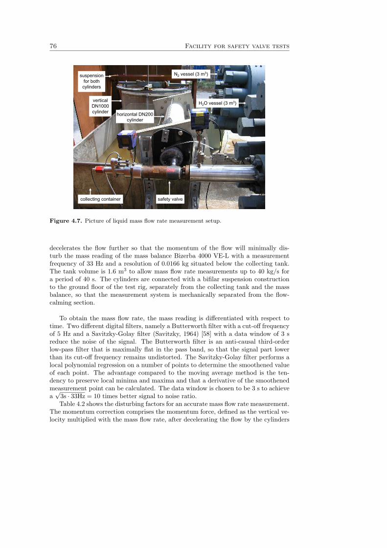
76 Facility for safety valve tests
safety valvecollecting container
horizontal DN200 cylinder
verticalDN1000cylinder
N2 vessel (3 m3)
H2O vessel (3 m3)
suspension for bothcylinders
Figure 4.7. Picture of liquid mass flow rate measurement setup.
decelerates the flow further so that the momentum of the flow will minimally dis-turb the mass reading of the mass balance Bizerba 4000 VE-L with a measurementfrequency of 33 Hz and a resolution of 0.0166 kg situated below the collecting tank.The tank volume is 1.6 m3 to allow mass flow rate measurements up to 40 kg/s fora period of 40 s. The cylinders are connected with a bifilar suspension constructionto the ground floor of the test rig, separately from the collecting tank and the massbalance, so that the measurement system is mechanically separated from the flow-calming section.
To obtain the mass flow rate, the mass reading is differentiated with respect totime. Two different digital filters, namely a Butterworth filter with a cut-off frequencyof 5 Hz and a Savitzky-Golay filter (Savitzky, 1964) [58] with a data window of 3 sreduce the noise of the signal. The Butterworth filter is an anti-causal third-orderlow-pass filter that is maximally flat in the pass band, so that the signal part lowerthan its cut-off frequency remains undistorted. The Savitzky-Golay filter performs alocal polynomial regression on a number of points to determine the smoothened valueof each point. The advantage compared to the moving average method is the ten-dency to preserve local minima and maxima and that a derivative of the smoothenedmeasurement point can be calculated. The data window is chosen to be 3 s to achievea√
3s · 33Hz = 10 times better signal to noise ratio.Table 4.2 shows the disturbing factors for an accurate mass flow rate measurement.
The momentum correction comprises the momentum force, defined as the vertical ve-locity multiplied with the mass flow rate, after decelerating the flow by the cylinders
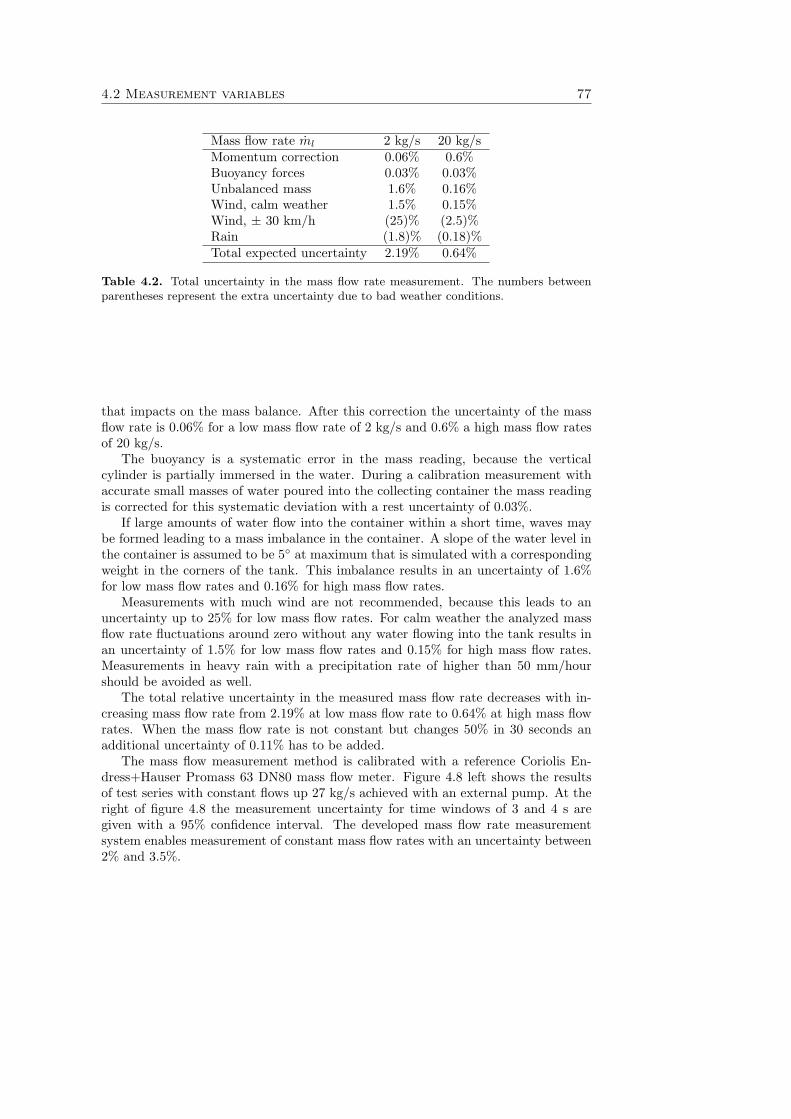
4.2 Measurement variables 77
Mass flow rate ml 2 kg/s 20 kg/sMomentum correction 0.06% 0.6%Buoyancy forces 0.03% 0.03%Unbalanced mass 1.6% 0.16%Wind, calm weather 1.5% 0.15%Wind, ± 30 km/h (25)% (2.5)%Rain (1.8)% (0.18)%Total expected uncertainty 2.19% 0.64%
Table 4.2. Total uncertainty in the mass flow rate measurement. The numbers betweenparentheses represent the extra uncertainty due to bad weather conditions.
that impacts on the mass balance. After this correction the uncertainty of the massflow rate is 0.06% for a low mass flow rate of 2 kg/s and 0.6% a high mass flow ratesof 20 kg/s.
The buoyancy is a systematic error in the mass reading, because the verticalcylinder is partially immersed in the water. During a calibration measurement withaccurate small masses of water poured into the collecting container the mass readingis corrected for this systematic deviation with a rest uncertainty of 0.03%.
If large amounts of water flow into the container within a short time, waves maybe formed leading to a mass imbalance in the container. A slope of the water level inthe container is assumed to be 5◦ at maximum that is simulated with a correspondingweight in the corners of the tank. This imbalance results in an uncertainty of 1.6%for low mass flow rates and 0.16% for high mass flow rates.
Measurements with much wind are not recommended, because this leads to anuncertainty up to 25% for low mass flow rates. For calm weather the analyzed massflow rate fluctuations around zero without any water flowing into the tank results inan uncertainty of 1.5% for low mass flow rates and 0.15% for high mass flow rates.Measurements in heavy rain with a precipitation rate of higher than 50 mm/hourshould be avoided as well.
The total relative uncertainty in the measured mass flow rate decreases with in-creasing mass flow rate from 2.19% at low mass flow rate to 0.64% at high mass flowrates. When the mass flow rate is not constant but changes 50% in 30 seconds anadditional uncertainty of 0.11% has to be added.
The mass flow measurement method is calibrated with a reference Coriolis En-dress+Hauser Promass 63 DN80 mass flow meter. Figure 4.8 left shows the resultsof test series with constant flows up 27 kg/s achieved with an external pump. At theright of figure 4.8 the measurement uncertainty for time windows of 3 and 4 s aregiven with a 95% confidence interval. The developed mass flow rate measurementsystem enables measurement of constant mass flow rates with an uncertainty between2% and 3.5%.
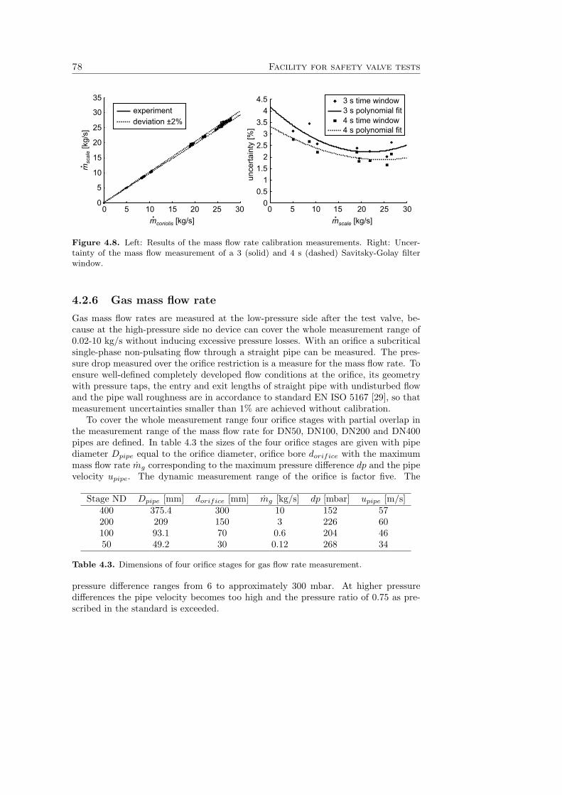
78 Facility for safety valve tests
0 5 10 15 20 25 300
5
10
15
20
25
30
35experimentdeviation ±2%
00.5
11.5
22.5
33.5
44.5
unce
rtain
ty [%
]
0 5 10 20 25 3015mcoriolis [kg/s].
msc
ale
[kg/
s]
.
3 s time window
4 s polynomial fit
mscale [kg/s].
3 s polynomial fit4 s time window
Figure 4.8. Left: Results of the mass flow rate calibration measurements. Right: Uncer-tainty of the mass flow measurement of a 3 (solid) and 4 s (dashed) Savitsky-Golay filterwindow.
4.2.6 Gas mass flow rate
Gas mass flow rates are measured at the low-pressure side after the test valve, be-cause at the high-pressure side no device can cover the whole measurement range of0.02-10 kg/s without inducing excessive pressure losses. With an orifice a subcriticalsingle-phase non-pulsating flow through a straight pipe can be measured. The pres-sure drop measured over the orifice restriction is a measure for the mass flow rate. Toensure well-defined completely developed flow conditions at the orifice, its geometrywith pressure taps, the entry and exit lengths of straight pipe with undisturbed flowand the pipe wall roughness are in accordance to standard EN ISO 5167 [29], so thatmeasurement uncertainties smaller than 1% are achieved without calibration.
To cover the whole measurement range four orifice stages with partial overlap inthe measurement range of the mass flow rate for DN50, DN100, DN200 and DN400pipes are defined. In table 4.3 the sizes of the four orifice stages are given with pipediameter Dpipe equal to the orifice diameter, orifice bore dorifice with the maximummass flow rate mg corresponding to the maximum pressure difference dp and the pipevelocity upipe. The dynamic measurement range of the orifice is factor five. The
Stage ND Dpipe [mm] dorifice [mm] mg [kg/s] dp [mbar] upipe [m/s]400 375.4 300 10 152 57200 209 150 3 226 60100 93.1 70 0.6 204 4650 49.2 30 0.12 268 34
Table 4.3. Dimensions of four orifice stages for gas flow rate measurement.
pressure difference ranges from 6 to approximately 300 mbar. At higher pressuredifferences the pipe velocity becomes too high and the pressure ratio of 0.75 as pre-scribed in the standard is exceeded.
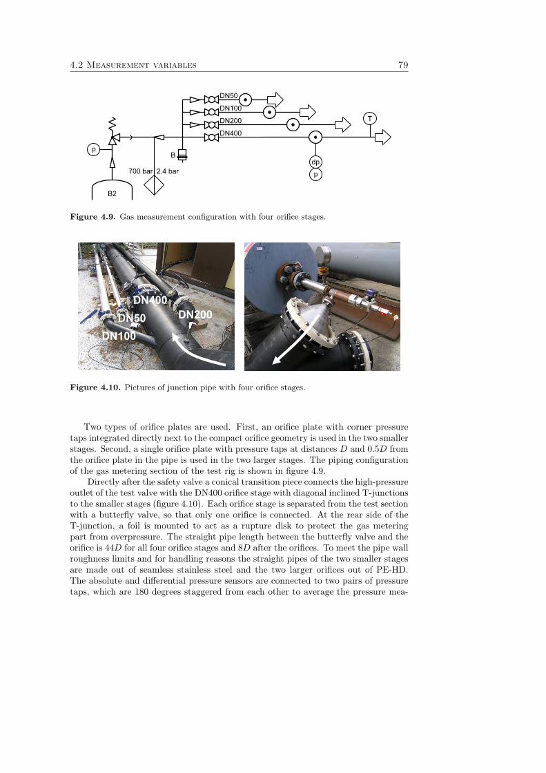
4.2 Measurement variables 79
p
T
B2
B
700 bar 2.4 bar
DN50
DN100
DN200
DN400
dp
p
Figure 4.9. Gas measurement configuration with four orifice stages.
DN400DN50
DN100
DN200
Figure 4.10. Pictures of junction pipe with four orifice stages.
Two types of orifice plates are used. First, an orifice plate with corner pressuretaps integrated directly next to the compact orifice geometry is used in the two smallerstages. Second, a single orifice plate with pressure taps at distances D and 0.5D fromthe orifice plate in the pipe is used in the two larger stages. The piping configurationof the gas metering section of the test rig is shown in figure 4.9.
Directly after the safety valve a conical transition piece connects the high-pressureoutlet of the test valve with the DN400 orifice stage with diagonal inclined T-junctionsto the smaller stages (figure 4.10). Each orifice stage is separated from the test sectionwith a butterfly valve, so that only one orifice is connected. At the rear side of theT-junction, a foil is mounted to act as a rupture disk to protect the gas meteringpart from overpressure. The straight pipe length between the butterfly valve and theorifice is 44D for all four orifice stages and 8D after the orifices. To meet the pipe wallroughness limits and for handling reasons the straight pipes of the two smaller stagesare made out of seamless stainless steel and the two larger orifices out of PE-HD.The absolute and differential pressure sensors are connected to two pairs of pressuretaps, which are 180 degrees staggered from each other to average the pressure mea-
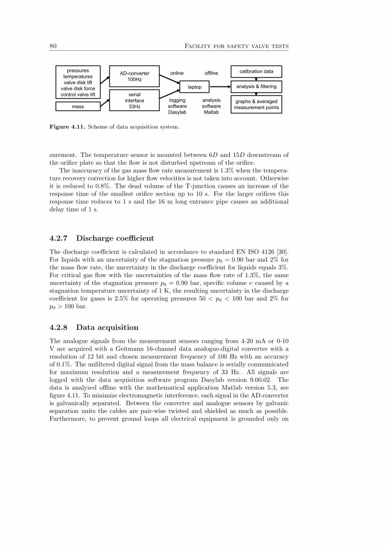
80 Facility for safety valve tests
calibration datapressurestemperaturesvalve disk lift
valve disk forcecontrol valve lift
mass
AD-converter100Hz
serialinterface
33Hz
laptop analysis & filtering
graphs & averagedmeasurement points
online offline
loggingsoftwareDasylab
analysissoftwareMatlab
Figure 4.11. Scheme of data acquisition system.
surement. The temperature sensor is mounted between 6D and 15D downstream ofthe orifice plate so that the flow is not disturbed upstream of the orifice.
The inaccuracy of the gas mass flow rate measurement is 1.3% when the tempera-ture recovery correction for higher flow velocities is not taken into account. Otherwiseit is reduced to 0.8%. The dead volume of the T-junction causes an increase of theresponse time of the smallest orifice section up to 10 s. For the larger orifices thisresponse time reduces to 1 s and the 16 m long entrance pipe causes an additionaldelay time of 1 s.
4.2.7 Discharge coefficient
The discharge coefficient is calculated in accordance to standard EN ISO 4126 [30].For liquids with an uncertainty of the stagnation pressure p0 = 0.90 bar and 2% forthe mass flow rate, the uncertainty in the discharge coefficient for liquids equals 3%.For critical gas flow with the uncertainties of the mass flow rate of 1.3%, the sameuncertainty of the stagnation pressure p0 = 0.90 bar, specific volume υ caused by astagnation temperature uncertainty of 1 K, the resulting uncertainty in the dischargecoefficient for gases is 2.5% for operating pressures 50 < p0 < 100 bar and 2% forp0 > 100 bar.
4.2.8 Data acquisition
The analogue signals from the measurement sensors ranging from 4-20 mA or 0-10V are acquired with a Geitmann 16-channel data analogue-digital converter with aresolution of 12 bit and chosen measurement frequency of 100 Hz with an accuracyof 0.1%. The unfiltered digital signal from the mass balance is serially communicatedfor maximum resolution and a measurement frequency of 33 Hz. All signals arelogged with the data acquisition software program Dasylab version 9.00.02. Thedata is analyzed offline with the mathematical application Matlab version 5.3, seefigure 4.11. To minimize electromagnetic interference, each signal in the AD-converteris galvanically separated. Between the converter and analogue sensors by galvanicseparation units the cables are pair-wise twisted and shielded as much as possible.Furthermore, to prevent ground loops all electrical equipment is grounded only on
4.3 Examples of valve tests 81
the test rig if necessary and connected indirectly to the mains power system with atransformer without grounding.
4.3 Examples of valve tests
Before each series of experiments a safety valve is assembled, set to the desired setpressure and mounted into the test facility. Then, a series of valve relief tests arecarried out in which the safety valve to be tested remains mounted in the test facility.After a few tests the valve is disassembled and the geometries of the valve housingand spindle, and the stiffness of the spring are measured. In addition, all points ofstationary valve operation within each relief test of the same series are collected, fromwhich the opening characteristic is deduced.
In this section for two example tests is demonstrated how the valve capacity andopening characteristic of a safety valve operating with sub-cooled water and gaseousnitrogen are determined.
4.3.1 Valve test with water
Figure 4.12 shows the behavior of all measured quantities of a single safety valve testwith water. Prior to the valve test the storage vessel is pressurized at pstorage = 550bar and the buffer vessel with the safety valve to be tested is at ambient pressure (4.12top left), shown by the two measured pressures by the pressure transducer located inthe buffer vessel pbuffer and just upstream the test valve pvalve. When the pressurelosses are small the pressure just before the safety valve and the one in the buffervessel should always be almost equal, which is the case in this example experiment.The pressure in the spring housing phousing is at atmospheric condition.
The control valve is closed and the data logging is started so that the actual valvetest begins when the automatic pressure control is activated. Then, at t = 7 s thecontrol valve opens (not presented in figures) and the buffer vessel with the test valveis pressurized by high-pressure nitrogen from the storage vessel. At time t = 12.7 sthe safety valve starts to open, because a disk lift larger than the smallest detectabledisk lift of h = 0.012 mm is measured. At this time the valve pressure is determinedat 362 bar, which is defined as the opening pressure. In figure 4.12 top right theaccumulated mass m in the collecting tank and the derived mass flow rate m aregiven. At t = 15 s onwards the mass increases from 235 to 502 kg at the end of thevalve test with a maximum mass flow rate of m = 6 kg/s during 23 s.
Figure 4.12 lower left shows the valve disk lift that reaches the mechanical stophstop = 1.68 mm at t = 16 s. Although the buffer and valve pressure increases further,because it is difficult to control it at a constant pressure of 465 bar, the spindle movesonly little due to the rubber collision damping plate at the spindle top. In figure 4.12lower right the force sensor measures the remaining flow force Fflow − Fspring thatcannot be compensated by the spring force Fspring anymore when the spindle presseson the mechanical stop during the period of 23 s. In the same period with high disklift the pressure in the spring housing increases to 7 bar.
Around t = 22 and 42 s the changes of the pressure, mass flow rate, disk lift and

82 Facility for safety valve tests
0 50 100 1500
100
200
300
400
500
p[b
ar]
pstorage
pbuffer
pvalve
phousing
0 50 100 1500
0.5
1
1.5
h[m
m]
t [s]
0 50 100 150200
400
600
m[k
g]
0 50 100 150
10
m[k
g/s]
0 50 100 1501800
2000
2200
2400
2600
t [s]
F[N
]
Fflow
Fspring
5
0
.
m.
m
Figure 4.12. Example of valve test with water.
disk force are small enough so that the measurement points around these times areaveraged with a measurement interval typically ranging from 1 up to 100 s. Due tothe large time scale of the figure the steady conditions cannot be clearly seen. Att = 72 s the control valve is closed so that the pressure in the buffer vessel decreasesfaster and the pressure in the storage vessel starts to increase slowly due to heatingof the cold nitrogen gas by the thick vessel walls at ambient temperature. At timet = 91 s, the pressure in the buffer vessel decreases faster, because this vessel is alsodepressurized with a vent valve to avoid chatter of the test valve while closing. Dueto damage to the sealing of the valve it does not close entirely to zero disk lift andremains leaking for a longer time that can be seen in still slowly increasing mass inthe collecting tank.
4.3.2 Valve test with nitrogen
Figure 4.13 shows the distribution of all measured quantities of a safety valve ex-periment with gaseous nitrogen. In general the pressure distributions of this valvetest are similar to the distributions of the valve test example with water described in
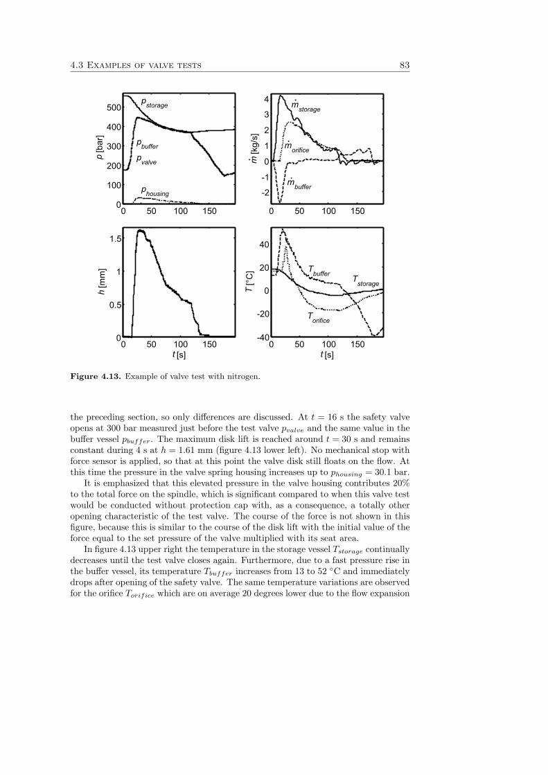
4.3 Examples of valve tests 83
0 50 100 1500
100
200
300
400
500p
[bar
]pstorage
pbuffer
pvalve
phousing
0 50 100 150-40
-20
0
20
40
t [s]
T[°
C]
Tstorage
Tbuffer
Torifice
0 50 100 1500
0.5
1
1.5
h[m
m]
t [s]
0 50 100 150
-2
-1
0
1
2
3
4
m[k
g/s]
mstorage
.
mbuffer.
morifice.
.
Figure 4.13. Example of valve test with nitrogen.
the preceding section, so only differences are discussed. At t = 16 s the safety valveopens at 300 bar measured just before the test valve pvalve and the same value in thebuffer vessel pbuffer. The maximum disk lift is reached around t = 30 s and remainsconstant during 4 s at h = 1.61 mm (figure 4.13 lower left). No mechanical stop withforce sensor is applied, so that at this point the valve disk still floats on the flow. Atthis time the pressure in the valve spring housing increases up to phousing = 30.1 bar.
It is emphasized that this elevated pressure in the valve housing contributes 20%to the total force on the spindle, which is significant compared to when this valve testwould be conducted without protection cap with, as a consequence, a totally otheropening characteristic of the test valve. The course of the force is not shown in thisfigure, because this is similar to the course of the disk lift with the initial value of theforce equal to the set pressure of the valve multiplied with its seat area.
In figure 4.13 upper right the temperature in the storage vessel Tstorage continuallydecreases until the test valve closes again. Furthermore, due to a fast pressure rise inthe buffer vessel, its temperature Tbuffer increases from 13 to 52 ◦C and immediatelydrops after opening of the safety valve. The same temperature variations are observedfor the orifice Torifice which are on average 20 degrees lower due to the flow expansion
84 Facility for safety valve tests
in the safety valve.For valve tests with nitrogen it is also possible to measure the mass flow rates
by calculating the changing mass in the vessels as function of its total pressure andtemperature (figure 4.13 upper right). Unfortunately, due to large temperature varia-tions this experimental method can only be used as indication to check the steadinessof the flow between the storage vessel, buffer vessel and the orifice. Then the flow issteady when the mass flow rate in the buffer vessel mbuffer is zero and the mass flowrate at the orifice morifice approximately equals the mass flow rate from the storagevessel mstorage.
Furthermore, temperature differences of the gas up to 50 K from the initial valueinduce additional errors to the gas mass flow rate measurement. Then the flow be-tween the orifice and the temperature sensor cannot be considered adiabatic any more,because the pipe walls are heating or cooling the flow. In addition, the standard ENISO 5167 [29] assumes that the flow is isothermal, which is justified as long as thepressure losses over the orifice and the resulting temperature differences due to isen-thalpic expansion are low.
In principle, the temperature in the buffer vessel always decreases with decreasingpressure. As a result, it is practically impossible to have both pressure and tempe-rature before the safety valve constant during an experiment. Theoretically constantconditions can only be achieved when the volume of the storage vessel reduces as wellwhile relieving. Nevertheless, it is still possible to generate satisfactory stable oper-ating conditions for evaluation as long as the temperature of the gas in the orificesdiffers less than approximately 20 K from the pipe wall temperature.
Chapter 5
Comparison of numerical andexperimental results
The performance of the numerical method is validated with experimental data de-rived from safety valve tests conducted at the test facility. Section 5.1 focuses onhigh-pressure valve tests with water at operating pressures ranging from 64 to 450bar. Section 5.2 presents a re-evaluation of the TUV measurement with nitrogenas described in section 3.2.6 at an operating pressure of 7 bar. Also experimentaland numerical results from high-pressure safety valve tests with nitrogen at operatingpressures ranging from 73 to 453 bar are presented. Finally, section 5.3 presents calcu-lations of gas flows through high-pressure safety valves outside the validated pressureregion in order to investigate the influence of real-gas effects on the valve charac-teristics in the largest possible pressure and temperature domain of the numericalmethod.
5.1 Liquid valve flow
First the experimental results from the valve tests with water are presented. Then, thenumerical simulation procedure is given. Hereafter, results of numerical simulationsare compared with selected measurement points. In the following analysis, the methodis extended to account for cavitation and validated again.
5.1.1 Experimental results
Safety valve test series at set pressures pset = 50 and 375 bar are chosen for validation.Typical results are presented in figure 5.1. The measurement points are averaged overfive and two valve relief test runs with the same valve at operating pressures between64-79 bar and 434-450 bar, respectively, attached to the buffer vessel of the testfacility. In figure 5.1 upper left the mass flow rate m versus the dimensionless disklift h/d0 is shown. The dashed vertical line represents the nominal disk lift of 1 mm.The mass flow rate increases almost linearly with disk lift. The small scatter in the
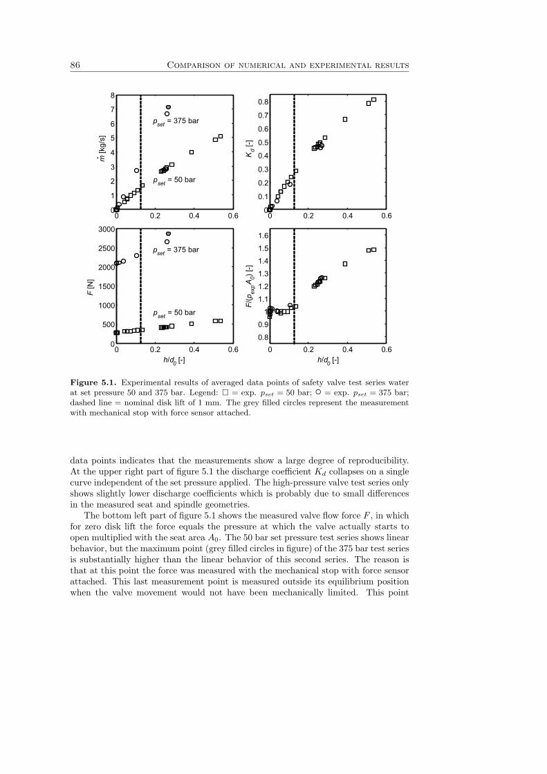
86 Comparison of numerical and experimental results
0 0.2 0.4 0.60
1
2
3
4
5
6
7
8
0 0.2 0.4 0.60
0.1
0.2
0.3
0.4
0.5
0.6
0.7
0.8
0 0.2 0.4 0.60
500
1000
1500
2000
2500
3000
0 0.2 0.4 0.60.8
0.9
1
1.1
1.2
1.3
1.4
1.5
1.6
m[k
g/s]
F[N
]
F/(p
expA 0)
[-]
. Kd
[-]
h/d0 [-] h/d0 [-]
pset = 50 bar
pset = 375 bar
pset = 50 bar
pset = 375 bar
Figure 5.1. Experimental results of averaged data points of safety valve test series waterat set pressure 50 and 375 bar. Legend: � = exp. pset = 50 bar; ◦ = exp. pset = 375 bar;dashed line = nominal disk lift of 1 mm. The grey filled circles represent the measurementwith mechanical stop with force sensor attached.
data points indicates that the measurements show a large degree of reproducibility.At the upper right part of figure 5.1 the discharge coefficient Kd collapses on a singlecurve independent of the set pressure applied. The high-pressure valve test series onlyshows slightly lower discharge coefficients which is probably due to small differencesin the measured seat and spindle geometries.
The bottom left part of figure 5.1 shows the measured valve flow force F , in whichfor zero disk lift the force equals the pressure at which the valve actually starts toopen multiplied with the seat area A0. The 50 bar set pressure test series shows linearbehavior, but the maximum point (grey filled circles in figure) of the 375 bar test seriesis substantially higher than the linear behavior of this second series. The reason isthat at this point the force was measured with the mechanical stop with force sensorattached. This last measurement point is measured outside its equilibrium positionwhen the valve movement would not have been mechanically limited. This point
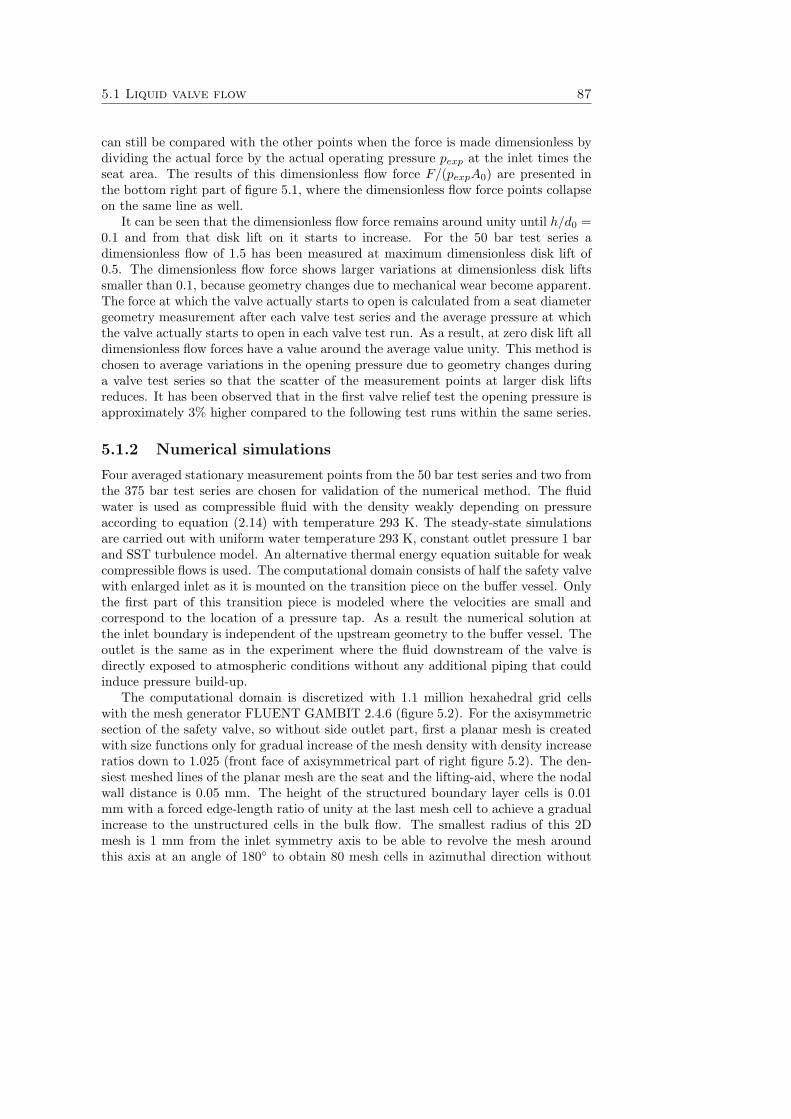
5.1 Liquid valve flow 87
can still be compared with the other points when the force is made dimensionless bydividing the actual force by the actual operating pressure pexp at the inlet times theseat area. The results of this dimensionless flow force F/(pexpA0) are presented inthe bottom right part of figure 5.1, where the dimensionless flow force points collapseon the same line as well.
It can be seen that the dimensionless flow force remains around unity until h/d0 =0.1 and from that disk lift on it starts to increase. For the 50 bar test series adimensionless flow of 1.5 has been measured at maximum dimensionless disk lift of0.5. The dimensionless flow force shows larger variations at dimensionless disk liftssmaller than 0.1, because geometry changes due to mechanical wear become apparent.The force at which the valve actually starts to open is calculated from a seat diametergeometry measurement after each valve test series and the average pressure at whichthe valve actually starts to open in each valve test run. As a result, at zero disk lift alldimensionless flow forces have a value around the average value unity. This method ischosen to average variations in the opening pressure due to geometry changes duringa valve test series so that the scatter of the measurement points at larger disk liftsreduces. It has been observed that in the first valve relief test the opening pressure isapproximately 3% higher compared to the following test runs within the same series.
5.1.2 Numerical simulations
Four averaged stationary measurement points from the 50 bar test series and two fromthe 375 bar test series are chosen for validation of the numerical method. The fluidwater is used as compressible fluid with the density weakly depending on pressureaccording to equation (2.14) with temperature 293 K. The steady-state simulationsare carried out with uniform water temperature 293 K, constant outlet pressure 1 barand SST turbulence model. An alternative thermal energy equation suitable for weakcompressible flows is used. The computational domain consists of half the safety valvewith enlarged inlet as it is mounted on the transition piece on the buffer vessel. Onlythe first part of this transition piece is modeled where the velocities are small andcorrespond to the location of a pressure tap. As a result the numerical solution atthe inlet boundary is independent of the upstream geometry to the buffer vessel. Theoutlet is the same as in the experiment where the fluid downstream of the valve isdirectly exposed to atmospheric conditions without any additional piping that couldinduce pressure build-up.
The computational domain is discretized with 1.1 million hexahedral grid cellswith the mesh generator FLUENT GAMBIT 2.4.6 (figure 5.2). For the axisymmetricsection of the safety valve, so without side outlet part, first a planar mesh is createdwith size functions only for gradual increase of the mesh density with density increaseratios down to 1.025 (front face of axisymmetrical part of right figure 5.2). The den-siest meshed lines of the planar mesh are the seat and the lifting-aid, where the nodalwall distance is 0.05 mm. The height of the structured boundary layer cells is 0.01mm with a forced edge-length ratio of unity at the last mesh cell to achieve a gradualincrease to the unstructured cells in the bulk flow. The smallest radius of this 2Dmesh is 1 mm from the inlet symmetry axis to be able to revolve the mesh aroundthis axis at an angle of 180◦ to obtain 80 mesh cells in azimuthal direction without
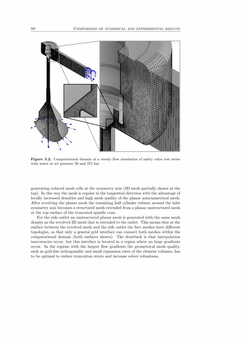
88 Comparison of numerical and experimental results
Figure 5.2. Computational domain of a steady flow simulation of safety valve test serieswith water at set pressure 50 and 375 bar.
generating reduced mesh cells at the symmetry axis (3D mesh partially shown at thetop). In this way the mesh is regular in the tangential direction with the advantage oflocally increased densities and high mesh quality of the planar axisymmetrical mesh.After revolving the planar mesh the remaining half cylinder volume around the inletsymmetry axis becomes a structured mesh extruded from a planar unstructured meshat the top surface of the truncated spindle cone.
For the side outlet an unstructured planar mesh is generated with the same meshdensity as the revolved 3D mesh that is extruded to the outlet. This means that at thesurface between the revolved mesh and the side outlet the face meshes have differenttopologies, so that only a general grid interface can connect both meshes within thecomputational domain (both surfaces shown). The drawback is that interpolationinaccuracies occur, but this interface is located in a region where no large gradientsoccur. In the regions with the largest flow gradients the geometrical mesh quality,such as grid-line orthogonalily and small expansion rates of the element volumes, hasto be optimal to reduce truncation errors and increase solver robustness.
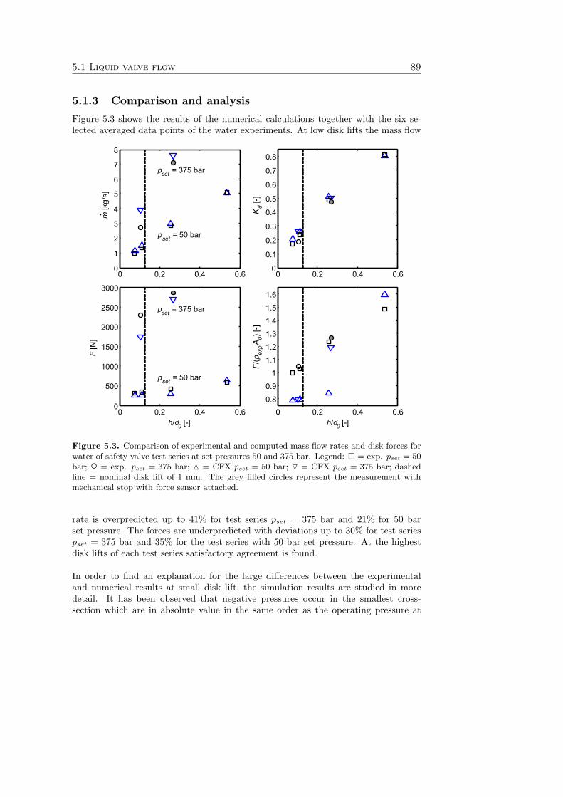
5.1 Liquid valve flow 89
5.1.3 Comparison and analysis
Figure 5.3 shows the results of the numerical calculations together with the six se-lected averaged data points of the water experiments. At low disk lifts the mass flow
0 0.2 0.4 0.60
1
2
3
4
5
6
7
8
0 0.2 0.4 0.60
0.1
0.2
0.3
0.4
0.5
0.6
0.7
0.8
0 0.2 0.4 0.60
500
1000
1500
2000
2500
3000
0 0.2 0.4 0.60.8
0.9
1
1.1
1.2
1.3
1.4
1.5
1.6
m[k
g/s]
F[N
]
F/(p
expA 0)
[-]
. Kd
[-]
h/d0 [-] h/d0 [-]
pset = 50 bar
pset = 375 bar
pset = 50 bar
pset = 375 bar
Figure 5.3. Comparison of experimental and computed mass flow rates and disk forces forwater of safety valve test series at set pressures 50 and 375 bar. Legend: � = exp. pset = 50bar; ◦ = exp. pset = 375 bar; � = CFX pset = 50 bar; � = CFX pset = 375 bar; dashedline = nominal disk lift of 1 mm. The grey filled circles represent the measurement withmechanical stop with force sensor attached.
rate is overpredicted up to 41% for test series pset = 375 bar and 21% for 50 barset pressure. The forces are underpredicted with deviations up to 30% for test seriespset = 375 bar and 35% for the test series with 50 bar set pressure. At the highestdisk lifts of each test series satisfactory agreement is found.
In order to find an explanation for the large differences between the experimentaland numerical results at small disk lift, the simulation results are studied in moredetail. It has been observed that negative pressures occur in the smallest cross-section which are in absolute value in the same order as the operating pressure at
90 Comparison of numerical and experimental results
the inlet. In incompressible flow computations negative pressures are possible in aconverged solution, because an absolute pressure is not defined and all calculatedpressures depend on a chosen reference pressure. In reality, cavitation already occursat absolute pressures in the order of 10 mbar for water, but in the present model thisis not taken into account. In order to investigate its effect on mass flow rate and flowforce, the standard cavitation model of CFX has been applied. Cavitation is a phasechange at almost constant temperature and is due to a local drop in the pressuregenerated by the flow itself. The degree of development is defined by the cavitationnumber σ (Agostino et al., 2007) [17]:
σ =pref − pv
12ρu2
(5.1)
where pref is the reference pressure of the liquid, pv the vapor pressure and u thecharacteristic velocity as part of the denominator representing the dynamic pressure.When the cavitation number decreases the flow tends to cavitate more. The tem-perature of the incompressible flow is assumed constant so that the correspondingvapor pressure for water is constant and equal to pv = 3.169 kPa. The Rayleigh-Plesset equation models the mass transfer between the liquid and the vapor phase bydescribing the growth and collapse of a vapor bubble in a liquid. Then the rate ofvaporization and condensation is controlled by liquid-vapor pressure differences de-rived from a mechanical balance. This model does not take any thermal effects intoaccount. The total interface mass transfer rate per unit volume mlg for vaporizationis defined as (Singhal, 2002) [63]
mlg = F3rgρg
RB
√23|pv − p|
ρlsign(pv − p), (5.2)
where F is an empirical factor with the default value in CFX equal to 50 for vapor-ization, rg the volume fraction of the gas phase and RB = 1 μm the radius of thenucleation sites. When the vapor pressure is higher than the local pressure the fluidvaporizes relatively fast in comparison with the situation that the local pressure islower than the saturation pressure so that eventual vapor in a control volume con-denses. Then in equation (5.2) variable rg needs to be replaced with rnuc(1 − rg)to
mlg = F3rnuc(1− rg)ρg
RB
√23|pv − p|
ρlsign(pv − p), (5.3)
where F is an empirical factor equal to 0.01 for relative slow condensation comparedto vaporization and rnuc = 5 × 10⁻⁴ the empirically determined volume fraction ofthe nucleation sites. This predefined volume fraction is still three orders of magni-tude lower than the computed volume fraction where cavitation actually occurs. Thecavitation model is implemented as a homogeneous multiphase model with assumedno-slip velocity conditions between the two phases. The cavitation appears as a vol-ume source term in the continuity equation that is solved in a separate transportequation set. The vapor phase is modeled as a gas with constant material properties.

5.1 Liquid valve flow 91
The steady flow simulations are initialized with zero velocity and gradually de-creasing pressure field from the inlet to the outlet with a function according to equa-tion (3.21). The simulations with cavitation model are initialized with the solutionfields from the simulations without cavitation model and with zero gas phase at theboundaries. The steady flow simulations do not completely stabilize with sufficientlylow local residues, but the actual mass flow rates and disk forces are averaged at themoments that the differences of the fluctuating mass flow rates between the inlet andoutlet are below 5%.
Figure 5.4 shows the results of the simulations extended with the cavitation modelcompared to the experimentally determined mass flow rates and disk forces. The
0 0.2 0.4 0.60
1
2
3
4
5
6
7
8
0 0.2 0.4 0.60
0.1
0.2
0.3
0.4
0.5
0.6
0.7
0.8
0 0.2 0.4 0.60
500
1000
1500
2000
2500
3000
0 0.2 0.4 0.60.8
0.9
1
1.1
1.2
1.3
1.4
1.5
1.6
m[k
g/s]
F[N
]
F/(p
expA 0)
[-]
. Kd
[-]
h/d0 [-] h/d0 [-]
pset = 50 bar
pset = 375 bar
pset = 50 bar
pset = 375 bar
Figure 5.4. Comparison of experimental and computed mass flow rates and disk forceswith water of safety valve test series at set pressures 50 and 375 bar with cavitation model.Legend: � = exp. pset = 50 bar; ◦ = exp. pset = 375 bar; × = CFX pset = 50 bar; += CFX pset = 375 bar; dashed line = nominal disk lift of 1 mm. The grey filled circlesrepresent the measurement with mechanical stop with force sensor attached.
simulations with cavitation lead to a significantly better agreement with experiment:deviations in the mass flow rate are gradually reduced by a factor of two up to 23%,
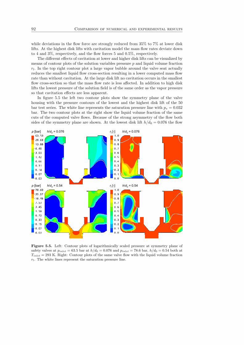
92 Comparison of numerical and experimental results
while deviations in the flow force are strongly reduced from 35% to 7% at lower disklifts. At the highest disk lifts with cavitation model the mass flow rates deviate downto 4 and 3%, respectively, and the flow forces 5 and 0.5%, respectively.
The different effects of cavitation at lower and higher disk lifts can be visualized bymeans of contour plots of the solution variables pressure p and liquid volume fractionrl. In the top right contour plot a large vapor bubble around the valve seat actuallyreduces the smallest liquid flow cross-section resulting in a lower computed mass flowrate than without cavitation. At the large disk lift no cavitation occurs in the smallestflow cross-section so that the mass flow rate is less affected. In addition to high disklifts the lowest pressure of the solution field is of the same order as the vapor pressureso that cavitation effects are less apparent.
In figure 5.5 the left two contour plots show the symmetry plane of the valvehousing with the pressure contours of the lowest and the highest disk lift of the 50bar test series. The white line represents the saturation pressure line with pv = 0.032bar. The two contour plots at the right show the liquid volume fraction of the samecuts of the computed valve flows. Because of the strong asymmetry of the flow bothsides of the symmetry plane are shown. At the lowest disk lift h/d0 = 0.076 the flow
p [bar]
p [bar] h/d0 = 0.54
h/d0 = 0.076 rl [-]
rl [-] h/d0 = 0.54
h/d0 = 0.076
Figure 5.5. Left: Contour plots of logarithmically scaled pressure at symmetry plane ofsafety valves at pinlet = 63.5 bar at h/d0 = 0.076 and pinlet = 78.6 bar, h/d0 = 0.54 both atTinlet = 293 K. Right: Contour plots of the same valve flow with the liquid volume fractionrl. The white lines represent the saturation pressure line.
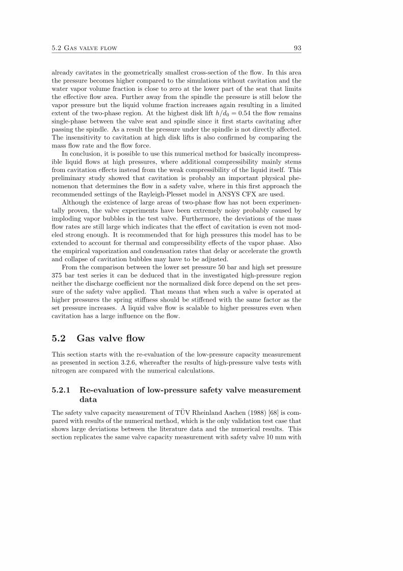
5.2 Gas valve flow 93
already cavitates in the geometrically smallest cross-section of the flow. In this areathe pressure becomes higher compared to the simulations without cavitation and thewater vapor volume fraction is close to zero at the lower part of the seat that limitsthe effective flow area. Further away from the spindle the pressure is still below thevapor pressure but the liquid volume fraction increases again resulting in a limitedextent of the two-phase region. At the highest disk lift h/d0 = 0.54 the flow remainssingle-phase between the valve seat and spindle since it first starts cavitating afterpassing the spindle. As a result the pressure under the spindle is not directly affected.The insensitivity to cavitation at high disk lifts is also confirmed by comparing themass flow rate and the flow force.
In conclusion, it is possible to use this numerical method for basically incompress-ible liquid flows at high pressures, where additional compressibility mainly stemsfrom cavitation effects instead from the weak compressibility of the liquid itself. Thispreliminary study showed that cavitation is probably an important physical phe-nomenon that determines the flow in a safety valve, where in this first approach therecommended settings of the Rayleigh-Plesset model in ANSYS CFX are used.
Although the existence of large areas of two-phase flow has not been experimen-tally proven, the valve experiments have been extremely noisy probably caused byimploding vapor bubbles in the test valve. Furthermore, the deviations of the massflow rates are still large which indicates that the effect of cavitation is even not mod-eled strong enough. It is recommended that for high pressures this model has to beextended to account for thermal and compressibility effects of the vapor phase. Alsothe empirical vaporization and condensation rates that delay or accelerate the growthand collapse of cavitation bubbles may have to be adjusted.
From the comparison between the lower set pressure 50 bar and high set pressure375 bar test series it can be deduced that in the investigated high-pressure regionneither the discharge coefficient nor the normalized disk force depend on the set pres-sure of the safety valve applied. That means that when such a valve is operated athigher pressures the spring stiffness should be stiffened with the same factor as theset pressure increases. A liquid valve flow is scalable to higher pressures even whencavitation has a large influence on the flow.
5.2 Gas valve flow
This section starts with the re-evaluation of the low-pressure capacity measurementas presented in section 3.2.6, whereafter the results of high-pressure valve tests withnitrogen are compared with the numerical calculations.
5.2.1 Re-evaluation of low-pressure safety valve measurementdata
The safety valve capacity measurement of TUV Rheinland Aachen (1988) [68] is com-pared with results of the numerical method, which is the only validation test case thatshows large deviations between the literature data and the numerical results. Thissection replicates the same valve capacity measurement with safety valve 10 mm with
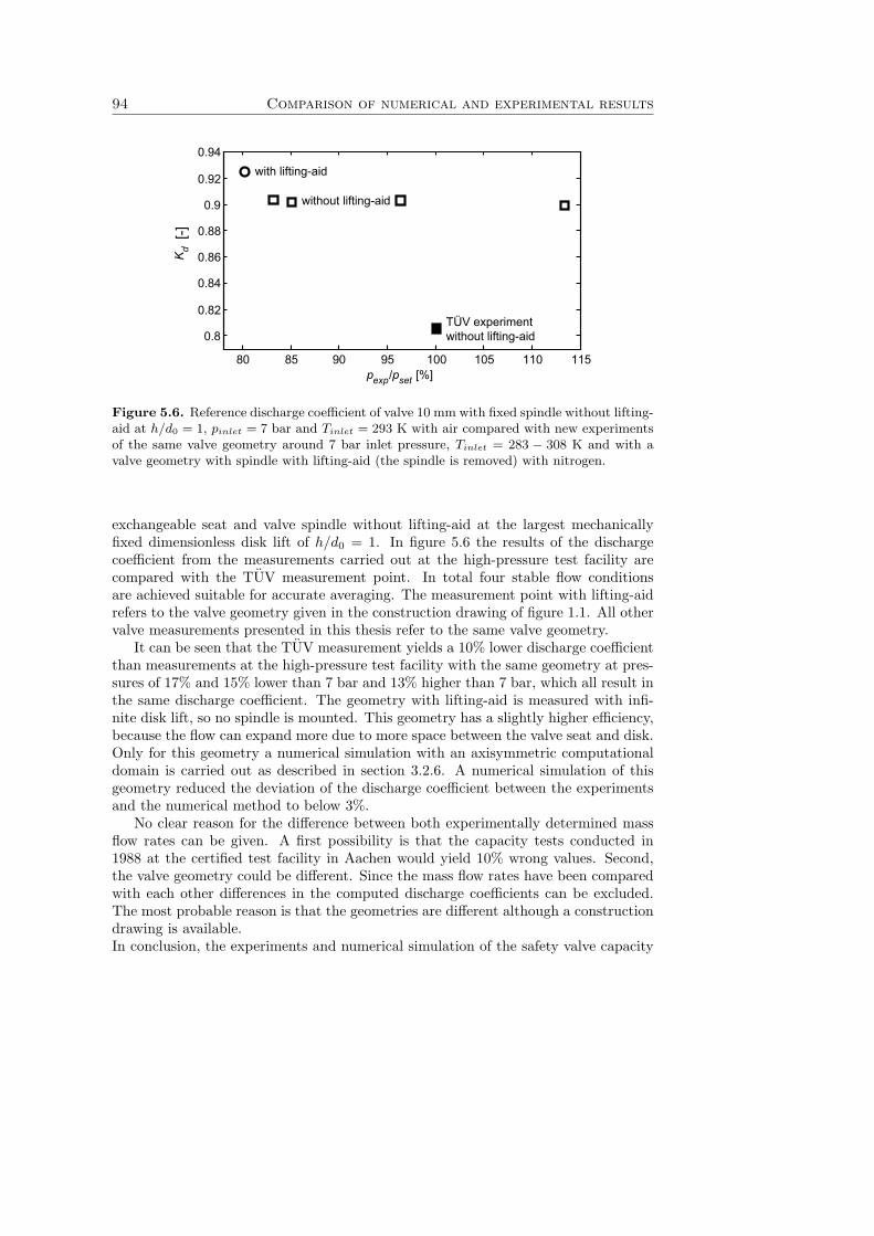
94 Comparison of numerical and experimental results
exp set
80 85 90 95 100 105 110 115
0.8
0.82
0.84
0.86
0.88
0.9
0.92
0.94
p /p [%]
Kd
[-]with lifting-aid
without lifting-aid
TÜV experiment without lifting-aid
Figure 5.6. Reference discharge coefficient of valve 10 mm with fixed spindle without lifting-aid at h/d0 = 1, pinlet = 7 bar and Tinlet = 293 K with air compared with new experimentsof the same valve geometry around 7 bar inlet pressure, Tinlet = 283 − 308 K and with avalve geometry with spindle with lifting-aid (the spindle is removed) with nitrogen.
exchangeable seat and valve spindle without lifting-aid at the largest mechanicallyfixed dimensionless disk lift of h/d0 = 1. In figure 5.6 the results of the dischargecoefficient from the measurements carried out at the high-pressure test facility arecompared with the TUV measurement point. In total four stable flow conditionsare achieved suitable for accurate averaging. The measurement point with lifting-aidrefers to the valve geometry given in the construction drawing of figure 1.1. All othervalve measurements presented in this thesis refer to the same valve geometry.
It can be seen that the TUV measurement yields a 10% lower discharge coefficientthan measurements at the high-pressure test facility with the same geometry at pres-sures of 17% and 15% lower than 7 bar and 13% higher than 7 bar, which all result inthe same discharge coefficient. The geometry with lifting-aid is measured with infi-nite disk lift, so no spindle is mounted. This geometry has a slightly higher efficiency,because the flow can expand more due to more space between the valve seat and disk.Only for this geometry a numerical simulation with an axisymmetric computationaldomain is carried out as described in section 3.2.6. A numerical simulation of thisgeometry reduced the deviation of the discharge coefficient between the experimentsand the numerical method to below 3%.
No clear reason for the difference between both experimentally determined massflow rates can be given. A first possibility is that the capacity tests conducted in1988 at the certified test facility in Aachen would yield 10% wrong values. Second,the valve geometry could be different. Since the mass flow rates have been comparedwith each other differences in the computed discharge coefficients can be excluded.The most probable reason is that the geometries are different although a constructiondrawing is available.In conclusion, the experiments and numerical simulation of the safety valve capacity
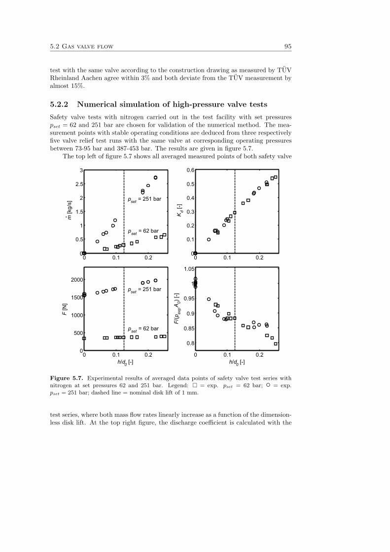
5.2 Gas valve flow 95
test with the same valve according to the construction drawing as measured by TUVRheinland Aachen agree within 3% and both deviate from the TUV measurement byalmost 15%.
5.2.2 Numerical simulation of high-pressure valve tests
Safety valve tests with nitrogen carried out in the test facility with set pressurespset = 62 and 251 bar are chosen for validation of the numerical method. The mea-surement points with stable operating conditions are deduced from three respectivelyfive valve relief test runs with the same valve at corresponding operating pressuresbetween 73-95 bar and 387-453 bar. The results are given in figure 5.7.
The top left of figure 5.7 shows all averaged measured points of both safety valve
m[k
g/s]
F[N
]
F/(p
expA 0)
[-]
. Kd
[-]
h/d0 [-] h/d0 [-]
0 0.1 0.20
0.5
1
1.5
2
2.5
3
0 0.1 0.20
0.1
0.2
0.3
0.4
0.5
0.6
0 0.1 0.20
500
1000
1500
2000
0 0.1 0.2
0.8
0.85
0.9
0.95
1
1.05
pset = 62 bar
pset = 251 bar
pset = 62 bar
pset = 251 bar
Figure 5.7. Experimental results of averaged data points of safety valve test series withnitrogen at set pressures 62 and 251 bar. Legend: � = exp. pset = 62 bar; ◦ = exp.pset = 251 bar; dashed line = nominal disk lift of 1 mm.
test series, where both mass flow rates linearly increase as a function of the dimension-less disk lift. At the top right figure, the discharge coefficient is calculated with the
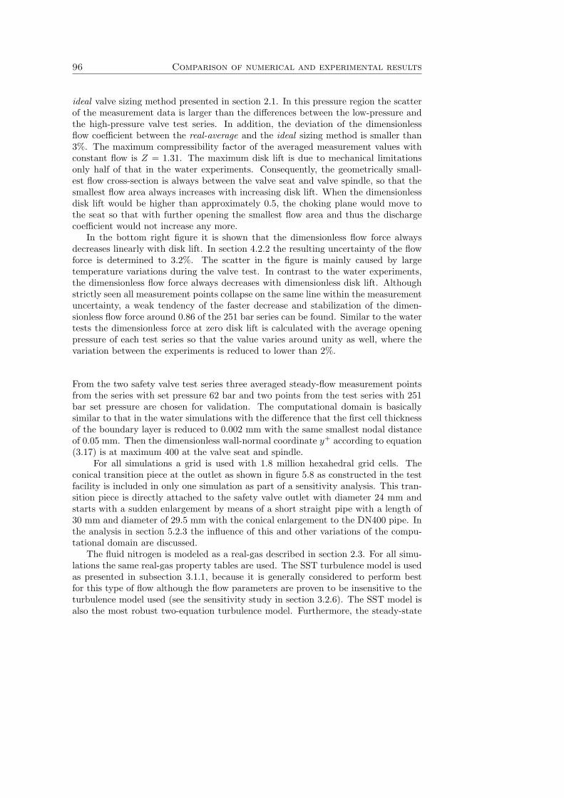
96 Comparison of numerical and experimental results
ideal valve sizing method presented in section 2.1. In this pressure region the scatterof the measurement data is larger than the differences between the low-pressure andthe high-pressure valve test series. In addition, the deviation of the dimensionlessflow coefficient between the real-average and the ideal sizing method is smaller than3%. The maximum compressibility factor of the averaged measurement values withconstant flow is Z = 1.31. The maximum disk lift is due to mechanical limitationsonly half of that in the water experiments. Consequently, the geometrically small-est flow cross-section is always between the valve seat and valve spindle, so that thesmallest flow area always increases with increasing disk lift. When the dimensionlessdisk lift would be higher than approximately 0.5, the choking plane would move tothe seat so that with further opening the smallest flow area and thus the dischargecoefficient would not increase any more.
In the bottom right figure it is shown that the dimensionless flow force alwaysdecreases linearly with disk lift. In section 4.2.2 the resulting uncertainty of the flowforce is determined to 3.2%. The scatter in the figure is mainly caused by largetemperature variations during the valve test. In contrast to the water experiments,the dimensionless flow force always decreases with dimensionless disk lift. Althoughstrictly seen all measurement points collapse on the same line within the measurementuncertainty, a weak tendency of the faster decrease and stabilization of the dimen-sionless flow force around 0.86 of the 251 bar series can be found. Similar to the watertests the dimensionless force at zero disk lift is calculated with the average openingpressure of each test series so that the value varies around unity as well, where thevariation between the experiments is reduced to lower than 2%.
From the two safety valve test series three averaged steady-flow measurement pointsfrom the series with set pressure 62 bar and two points from the test series with 251bar set pressure are chosen for validation. The computational domain is basicallysimilar to that in the water simulations with the difference that the first cell thicknessof the boundary layer is reduced to 0.002 mm with the same smallest nodal distanceof 0.05 mm. Then the dimensionless wall-normal coordinate y+ according to equation(3.17) is at maximum 400 at the valve seat and spindle.
For all simulations a grid is used with 1.8 million hexahedral grid cells. Theconical transition piece at the outlet as shown in figure 5.8 as constructed in the testfacility is included in only one simulation as part of a sensitivity analysis. This tran-sition piece is directly attached to the safety valve outlet with diameter 24 mm andstarts with a sudden enlargement by means of a short straight pipe with a length of30 mm and diameter of 29.5 mm with the conical enlargement to the DN400 pipe. Inthe analysis in section 5.2.3 the influence of this and other variations of the compu-tational domain are discussed.
The fluid nitrogen is modeled as a real-gas described in section 2.3. For all simu-lations the same real-gas property tables are used. The SST turbulence model is usedas presented in subsection 3.1.1, because it is generally considered to perform bestfor this type of flow although the flow parameters are proven to be insensitive to theturbulence model used (see the sensitivity study in section 3.2.6). The SST model isalso the most robust two-equation turbulence model. Furthermore, the steady-state
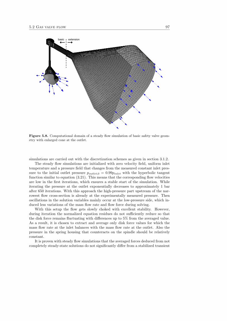
5.2 Gas valve flow 97
basic extension
Figure 5.8. Computational domain of a steady flow simulation of basic safety valve geom-etry with enlarged cone at the outlet.
simulations are carried out with the discretization schemes as given in section 3.1.2.The steady flow simulations are initialized with zero velocity field, uniform inlet
temperature and a pressure field that changes from the measured constant inlet pres-sure to the initial outlet pressure poutlet,0 = 0.99pinlet with the hyperbolic tangentfunction similar to equation (3.21). This means that the corresponding flow velocitiesare low in the first iterations, which ensures a stable start of the simulation. Whileiterating the pressure at the outlet exponentially decreases to approximately 1 barafter 650 iterations. With this approach the high-pressure part upstream of the nar-rowest flow cross-section is already at the experimentally measured pressure. Thenoscillations in the solution variables mainly occur at the low-pressure side, which in-duced less variations of the mass flow rate and flow force during solving.
With this setup the flow gets slowly choked with excellent stability. However,during iteration the normalized equation residues do not sufficiently reduce so thatthe disk force remains fluctuating with differences up to 5% from the averaged value.As a result, it is chosen to extract and average only disk force values for which themass flow rate at the inlet balances with the mass flow rate at the outlet. Also thepressure in the spring housing that counteracts on the spindle should be relativelyconstant.
It is proven with steady flow simulations that the averaged forces deduced from notcompletely steady-state solutions do not significantly differ from a stabilized transient
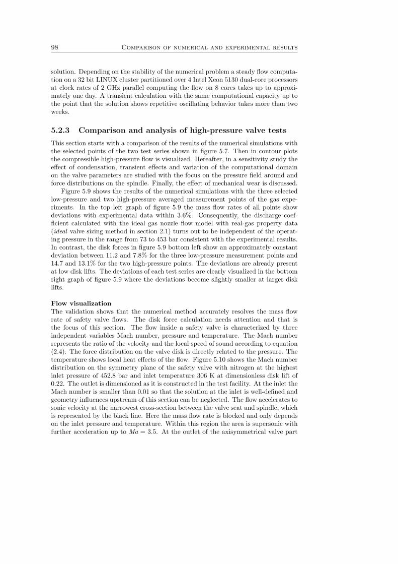
98 Comparison of numerical and experimental results
solution. Depending on the stability of the numerical problem a steady flow computa-tion on a 32 bit LINUX cluster partitioned over 4 Intel Xeon 5130 dual-core processorsat clock rates of 2 GHz parallel computing the flow on 8 cores takes up to approxi-mately one day. A transient calculation with the same computational capacity up tothe point that the solution shows repetitive oscillating behavior takes more than twoweeks.
5.2.3 Comparison and analysis of high-pressure valve tests
This section starts with a comparison of the results of the numerical simulations withthe selected points of the two test series shown in figure 5.7. Then in contour plotsthe compressible high-pressure flow is visualized. Hereafter, in a sensitivity study theeffect of condensation, transient effects and variation of the computational domainon the valve parameters are studied with the focus on the pressure field around andforce distributions on the spindle. Finally, the effect of mechanical wear is discussed.
Figure 5.9 shows the results of the numerical simulations with the three selectedlow-pressure and two high-pressure averaged measurement points of the gas expe-riments. In the top left graph of figure 5.9 the mass flow rates of all points showdeviations with experimental data within 3.6%. Consequently, the discharge coef-ficient calculated with the ideal gas nozzle flow model with real-gas property data(ideal valve sizing method in section 2.1) turns out to be independent of the operat-ing pressure in the range from 73 to 453 bar consistent with the experimental results.In contrast, the disk forces in figure 5.9 bottom left show an approximately constantdeviation between 11.2 and 7.8% for the three low-pressure measurement points and14.7 and 13.1% for the two high-pressure points. The deviations are already presentat low disk lifts. The deviations of each test series are clearly visualized in the bottomright graph of figure 5.9 where the deviations become slightly smaller at larger disklifts.
Flow visualizationThe validation shows that the numerical method accurately resolves the mass flowrate of safety valve flows. The disk force calculation needs attention and that isthe focus of this section. The flow inside a safety valve is characterized by threeindependent variables Mach number, pressure and temperature. The Mach numberrepresents the ratio of the velocity and the local speed of sound according to equation(2.4). The force distribution on the valve disk is directly related to the pressure. Thetemperature shows local heat effects of the flow. Figure 5.10 shows the Mach numberdistribution on the symmetry plane of the safety valve with nitrogen at the highestinlet pressure of 452.8 bar and inlet temperature 306 K at dimensionless disk lift of0.22. The outlet is dimensioned as it is constructed in the test facility. At the inlet theMach number is smaller than 0.01 so that the solution at the inlet is well-defined andgeometry influences upstream of this section can be neglected. The flow accelerates tosonic velocity at the narrowest cross-section between the valve seat and spindle, whichis represented by the black line. Here the mass flow rate is blocked and only dependson the inlet pressure and temperature. Within this region the area is supersonic withfurther acceleration up to Ma = 3.5. At the outlet of the axisymmetrical valve part
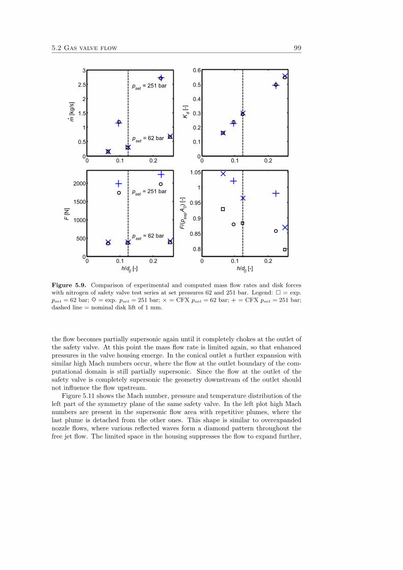
5.2 Gas valve flow 99
m[k
g/s]
F[N
]
F/(p
expA 0)
[-]
. Kd
[-]
h/d0 [-] h/d0 [-]
0 0.1 0.20
0.5
1
1.5
2
2.5
3
0 0.1 0.20
0.1
0.2
0.3
0.4
0.5
0.6
0 0.1 0.20
500
1000
1500
2000
0 0.1 0.2
0.8
0.85
0.9
0.95
1
1.05
pset = 62 bar
pset = 251 bar
pset = 62 bar
pset = 251 bar
Figure 5.9. Comparison of experimental and computed mass flow rates and disk forceswith nitrogen of safety valve test series at set pressures 62 and 251 bar. Legend: � = exp.pset = 62 bar; ◦ = exp. pset = 251 bar; × = CFX pset = 62 bar; + = CFX pset = 251 bar;dashed line = nominal disk lift of 1 mm.
the flow becomes partially supersonic again until it completely chokes at the outlet ofthe safety valve. At this point the mass flow rate is limited again, so that enhancedpressures in the valve housing emerge. In the conical outlet a further expansion withsimilar high Mach numbers occur, where the flow at the outlet boundary of the com-putational domain is still partially supersonic. Since the flow at the outlet of thesafety valve is completely supersonic the geometry downstream of the outlet shouldnot influence the flow upstream.
Figure 5.11 shows the Mach number, pressure and temperature distribution of theleft part of the symmetry plane of the same safety valve. In the left plot high Machnumbers are present in the supersonic flow area with repetitive plumes, where thelast plume is detached from the other ones. This shape is similar to overexpandednozzle flows, where various reflected waves form a diamond pattern throughout thefree jet flow. The limited space in the housing suppresses the flow to expand further,
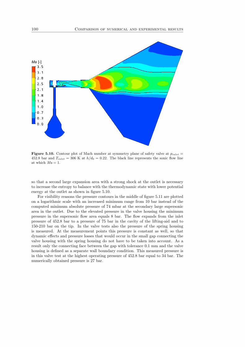
100 Comparison of numerical and experimental results
Ma [-]
Figure 5.10. Contour plot of Mach number at symmetry plane of safety valve at pinlet =452.8 bar and Tinlet = 306 K at h/d0 = 0.22. The black line represents the sonic flow lineat which Ma = 1.
so that a second large expansion area with a strong shock at the outlet is necessaryto increase the entropy to balance with the thermodynamic state with lower potentialenergy at the outlet as shown in figure 5.10.
For visibility reasons the pressure contours in the middle of figure 5.11 are plottedon a logarithmic scale with an increased minimum range from 10 bar instead of thecomputed minimum absolute pressure of 74 mbar at the secondary large supersonicarea in the outlet. Due to the elevated pressure in the valve housing the minimumpressure in the supersonic flow area equals 8 bar. The flow expands from the inletpressure of 452.8 bar to a pressure of 75 bar in the cavity of the lifting-aid and to150-210 bar on the tip. In the valve tests also the pressure of the spring housingis measured. At the measurement points this pressure is constant as well, so thatdynamic effects and pressure losses that would occur in the small gap connecting thevalve housing with the spring housing do not have to be taken into account. As aresult only the connecting face between the gap with tolerance 0.1 mm and the valvehousing is defined as a separate wall boundary condition. This measured pressure isin this valve test at the highest operating pressure of 452.8 bar equal to 34 bar. Thenumerically obtained pressure is 27 bar.
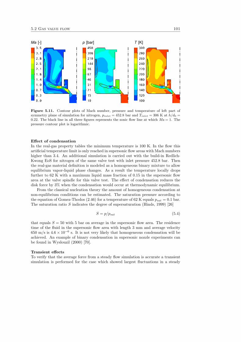
5.2 Gas valve flow 101
Ma [-] T [K]p [bar]
Figure 5.11. Contour plots of Mach number, pressure and temperature of left part ofsymmetry plane of simulation for nitrogen, pinlet = 452.8 bar and Tinlet = 306 K at h/d0 =0.22. The black line in all three figures represents the sonic flow line at which Ma = 1. Thepressure contour plot is logarithmic.
Effect of condensationIn the real-gas property tables the minimum temperature is 100 K. In the flow thisartificial temperature limit is only reached in supersonic flow areas with Mach numbershigher than 3.4. An additional simulation is carried out with the build-in Redlich-Kwong EoS for nitrogen of the same valve test with inlet pressure 452.8 bar. Thenthe real-gas material definition is modeled as a homogeneous binary mixture to allowequilibrium vapor-liquid phase changes. As a result the temperature locally dropsfurther to 62 K with a maximum liquid mass fraction of 0.15 in the supersonic flowarea at the valve spindle for this valve test. The effect of condensation reduces thedisk force by 3% when the condensation would occur at thermodynamic equilibrium.
From the classical nucleation theory the amount of homogeneous condensation atnon-equilibrium conditions can be estimated. The saturation pressure according tothe equation of Gomez-Thodos (2.46) for a temperature of 62 K equals psat = 0.1 bar.The saturation ratio S indicates the degree of supersaturation (Hinds, 1999) [26]
S = p/psat (5.4)
that equals S = 50 with 5 bar on average in the supersonic flow area. The residencetime of the fluid in the supersonic flow area with length 3 mm and average velocity650 m/s is 4.6× 10⁻⁶ s. It is not very likely that homogeneous condensation will beachieved. An example of binary condensation in supersonic nozzle experiments canbe found in Wyslouzil (2000) [70].
Transient effectsTo verify that the average force from a steady flow simulation is accurate a transientsimulation is performed for the case which showed largest fluctuations in a steady
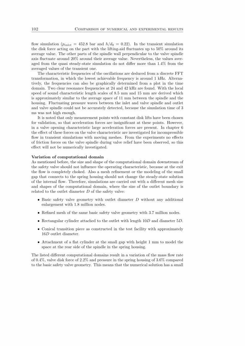
102 Comparison of numerical and experimental results
flow simulation (pinlet = 452.8 bar and h/d0 = 0.22). In the transient simulationthe disk force acting on the part with the lifting-aid fluctuates up to 50% around itsaverage value. The other parts of the spindle wall perpendicular to the valve spindleaxis fluctuate around 20% around their average value. Nevertheless, the values aver-aged from the quasi steady-state simulation do not differ more than 1.4% from theaveraged values of the transient one.
The characteristic frequencies of the oscillations are deduced from a discrete FFTtransformation, in which the lowest achievable frequency is around 1 kHz. Alterna-tively, the frequencies can also be graphically determined from a plot in the timedomain. Two clear resonance frequencies at 24 and 42 kHz are found. With the localspeed of sound characteristic length scales of 8.5 mm and 15 mm are derived whichis approximately similar to the average space of 11 mm between the spindle and thehousing. Fluctuating pressure waves between the inlet and valve spindle and outletand valve spindle could not be accurately detected, because the simulation time of 3ms was not high enough.
It is noted that only measurement points with constant disk lifts have been chosenfor validation, so that acceleration forces are insignificant at these points. However,in a valve opening characteristic large acceleration forces are present. In chapter 6the effect of these forces on the valve characteristic are investigated for incompressibleflow in transient simulations with moving meshes. From the experiments no effectsof friction forces on the valve spindle during valve relief have been observed, so thiseffect will not be numerically investigated.
Variation of computational domainAs mentioned before, the size and shape of the computational domain downstream ofthe safety valve should not influence the operating characteristic, because at the exitthe flow is completely choked. Also a mesh refinement or the modeling of the smallgap that connects to the spring housing should not change the steady-state solutionof the internal flow. Therefore, simulations are carried out with a different mesh sizeand shapes of the computational domain, where the size of the outlet boundary isrelated to the outlet diameter D of the safety valve:
• Basic safety valve geometry with outlet diameter D without any additionalenlargement with 1.8 million nodes.
• Refined mesh of the same basic safety valve geometry with 3.7 million nodes.
• Rectangular cylinder attached to the outlet with length 10D and diameter 5D.
• Conical transition piece as constructed in the test facility with approximately16D outlet diameter.
• Attachment of a flat cylinder at the small gap with height 1 mm to model thespace at the rear side of the spindle in the spring housing.
The listed different computational domains result in a variation of the mass flow rateof 0.4%, valve disk force of 2.2% and pressure in the spring housing of 3.6% comparedto the basic safety valve geometry. This means that the numerical solution has a small
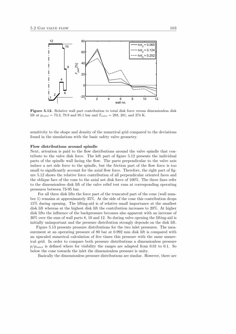
5.2 Gas valve flow 103
1 2 4 6 8 10 12-20
0
20
40
60
80
wall no.
F part
[%]
h/d0 = 0.065
h/d0 = 0.124
h/d0 = 0.252
12
4
6
8
10
12
Figure 5.12. Relative wall part contribution to total disk force versus dimensionless disklift at pinlet = 73.3, 79.9 and 95.1 bar and Tinlet = 293, 281, and 274 K.
sensitivity to the shape and density of the numerical grid compared to the deviationsfound in the simulations with the basic safety valve geometry.
Flow distributions around spindleNext, attention is paid to the flow distributions around the valve spindle that con-tribute to the valve disk force. The left part of figure 5.12 presents the individualparts of the spindle wall facing the flow. The parts perpendicular to the valve axisinduce a net side force to the spindle, but the friction part of the flow force is toosmall to significantly account for the axial flow force. Therefore, the right part of fig-ure 5.12 shows the relative force contribution of all perpendicular oriented faces andthe oblique face of the cone to the axial net disk force of 100%. The three lines referto the dimensionless disk lift of the valve relief test runs at corresponding operatingpressures between 73-95 bar.
For all three disk lifts the force part of the truncated part of the cone (wall num-ber 1) remains at approximately 35%. At the side of the cone this contribution drops15% during opening. The lifting-aid is of relative small importance at the smallestdisk lift whereas at the highest disk lift the contribution increases to 20%. At higherdisk lifts the influence of the backpressure becomes also apparent with an increase of30% over the sum of wall parts 8, 10 and 12. So during valve opening the lifting-aid isinitially unimportant and the pressure distribution strongly depends on the disk lift.
Figure 5.13 presents pressure distributions for the two inlet pressures. The mea-surement at an operating pressure of 80 bar at 0.992 mm disk lift is compared withan upscaled numerical calculation of five times this pressure with the same numer-ical grid. In order to compare both pressure distributions a dimensionless pressurep/pinlet is defined where for visibility the ranges are adapted from 0.01 to 0.1. Sobelow the cone towards the inlet the dimensionless pressure is unity.
Basically the dimensionless pressure distributions are similar. However, there are
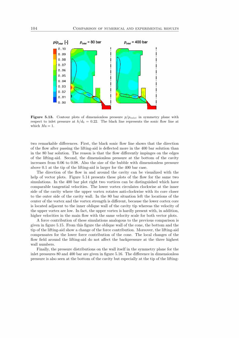
104 Comparison of numerical and experimental results
p/pinlet [-] pinlet = 80 bar pinlet = 400 barp/pinlet [-] pinlet = 80 bar pinlet = 400 bar
Figure 5.13. Contour plots of dimensionless pressure p/pinlet in symmetry plane withrespect to inlet pressure at h/d0 = 0.22. The black line represents the sonic flow line atwhich Ma = 1.
two remarkable differences. First, the black sonic flow line shows that the directionof the flow after passing the lifting-aid is deflected more in the 400 bar solution thanin the 80 bar solution. The reason is that the flow differently impinges on the edgesof the lifting-aid. Second, the dimensionless pressure at the bottom of the cavityincreases from 0.06 to 0.08. Also the size of the bubble with dimensionless pressureabove 0.1 at the tip of the lifting-aid is larger for the 400 bar case.
The direction of the flow in and around the cavity can be visualized with thehelp of vector plots. Figure 5.14 presents these plots of the flow for the same twosimulations. In the 400 bar plot right two vortices can be distinguished which havecomparable tangential velocities. The lower vortex circulates clockwise at the innerside of the cavity where the upper vortex rotates anti-clockwise with its core closerto the outer side of the cavity wall. In the 80 bar situation left the locations of thecenter of the vortex and the vortex strength is different, because the lower cortex coreis located adjacent to the inner oblique wall of the cavity tip whereas the velocity ofthe upper vortex are low. In fact, the upper vortex is hardly present with, in addition,higher velocities in the main flow with the same velocity scale for both vector plots.
A force contribution of these simulations analogous to the previous comparison isgiven in figure 5.15. From this figure the oblique wall of the cone, the bottom and thetip of the lifting-aid show a change of the force contribution. Moreover, the lifting-aidcompensates for the lower force contribution of the cone. The local changes of theflow field around the lifting-aid do not affect the backpressure at the three highestwall numbers.
Finally, the pressure distributions on the wall itself in the symmetry plane for theinlet pressures 80 and 400 bar are given in figure 5.16. The difference in dimensionlesspressure is also seen at the bottom of the cavity but especially at the tip of the lifting-
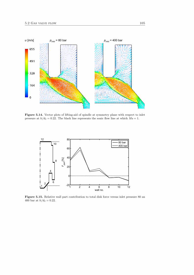
5.2 Gas valve flow 105
u [m/s] pinlet = 80 bar pinlet = 400 bar
Figure 5.14. Vector plots of lifting-aid of spindle at symmetry plane with respect to inletpressure at h/d0 = 0.22. The black line represents the sonic flow line at which Ma = 1.
1 2 4 6 8 10 12-20
0
20
40
60
80
wall no.
F part
[%]
80 bar400 bar
12
4
6
8
10
12
Figure 5.15. Relative wall part contribution to total disk force versus inlet pressure 80 an400 bar at h/d0 = 0.22.
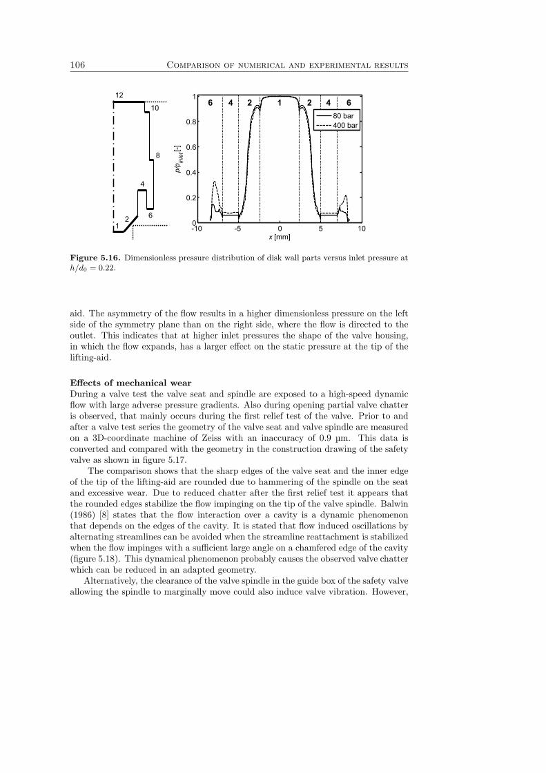
106 Comparison of numerical and experimental results
-10 -5 0 5 100
0.2
0.4
0.6
0.8
1
x [mm]
p/p in
let[-]
80 bar400 bar
1 22 4 646
12
4
6
8
10
12
Figure 5.16. Dimensionless pressure distribution of disk wall parts versus inlet pressure ath/d0 = 0.22.
aid. The asymmetry of the flow results in a higher dimensionless pressure on the leftside of the symmetry plane than on the right side, where the flow is directed to theoutlet. This indicates that at higher inlet pressures the shape of the valve housing,in which the flow expands, has a larger effect on the static pressure at the tip of thelifting-aid.
Effects of mechanical wearDuring a valve test the valve seat and spindle are exposed to a high-speed dynamicflow with large adverse pressure gradients. Also during opening partial valve chatteris observed, that mainly occurs during the first relief test of the valve. Prior to andafter a valve test series the geometry of the valve seat and valve spindle are measuredon a 3D-coordinate machine of Zeiss with an inaccuracy of 0.9 μm. This data isconverted and compared with the geometry in the construction drawing of the safetyvalve as shown in figure 5.17.
The comparison shows that the sharp edges of the valve seat and the inner edgeof the tip of the lifting-aid are rounded due to hammering of the spindle on the seatand excessive wear. Due to reduced chatter after the first relief test it appears thatthe rounded edges stabilize the flow impinging on the tip of the valve spindle. Balwin(1986) [8] states that the flow interaction over a cavity is a dynamic phenomenonthat depends on the edges of the cavity. It is stated that flow induced oscillations byalternating streamlines can be avoided when the streamline reattachment is stabilizedwhen the flow impinges with a sufficient large angle on a chamfered edge of the cavity(figure 5.18). This dynamical phenomenon probably causes the observed valve chatterwhich can be reduced in an adapted geometry.
Alternatively, the clearance of the valve spindle in the guide box of the safety valveallowing the spindle to marginally move could also induce valve vibration. However,
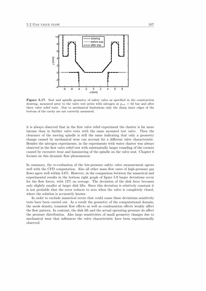
5.2 Gas valve flow 107
x [mm]-8 -6 -4 -2 0 2 4 6 8
-4
-2
0
2
4
6
8
10
y[m
m]
drawingbefore exp.after exp.
Figure 5.17. Seat and spindle geometry of safety valve as specified in the constructiondrawing, measured prior to the valve test series with nitrogen at pset = 62 bar and afterthree valve relief tests. Due to mechanical limitations only the sharp inner edges of thebottom of the cavity are not correctly measured.
it is always observed that in the first valve relief experiment the chatter is far moreintense than in further valve tests with the same mounted test valve. Then theclearance of the moving spindle is still the same indicating that only a geometrychange caused by mechanical wear can account for a different valve characteristic.Besides the nitrogen experiments, in the experiments with water chatter was alwaysobserved in the first valve relief test with substantially larger rounding of the cornerscaused by excessive wear and hammering of the spindle on the valve seat. Chapter 6focuses on this dynamic flow phenomenon.
In summary, the re-evaluation of the low-pressure safety valve measurement agreeswell with the CFD computation. Also all other mass flow rates of high-pressure gasflows agree well within 3.6%. However, in the comparison between the numerical andexperimental results in the bottom right graph of figure 5.9 larger deviations occurfor the flow forces, with 12% on average. The deviation of the disk force becomesonly slightly smaller at larger disk lifts. Since this deviation is relatively constant itis not probable that the error reduces to zero when the valve is completely closed,where the solution is accurately known.
In order to exclude numerical errors that could cause these deviations sensitivitytests have been carried out. As a result the geometry of the computational domain,the mesh density, transient flow effects as well as condensation effects weakly affectthe flow pattern. In contrast, the disk lift and the actual operating pressure do affectthe pressure distribution. Also large sensitivities of small geometry changes due tomechanical wear that influences the valve characteristic have been experimentallyobserved.
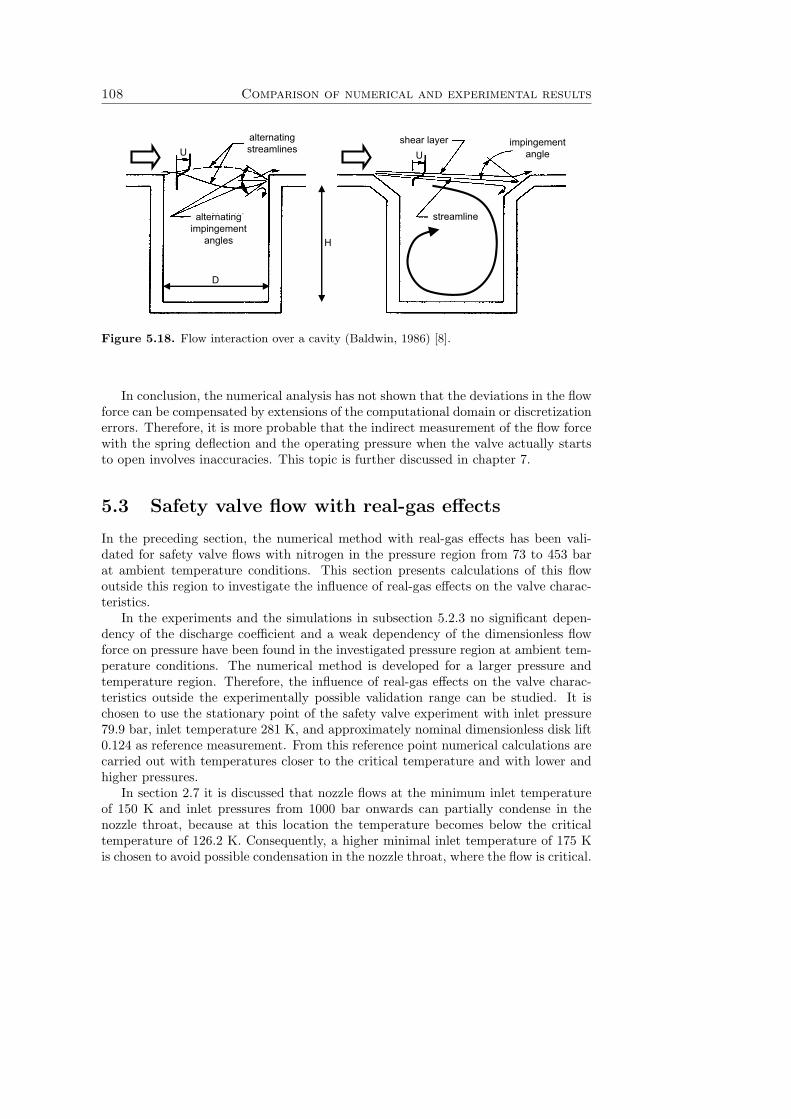
108 Comparison of numerical and experimental results
alternatingimpingement
angles
U Ushear layer impingement
angle
streamline
alternatingstreamlines
H
D
Figure 5.18. Flow interaction over a cavity (Baldwin, 1986) [8].
In conclusion, the numerical analysis has not shown that the deviations in the flowforce can be compensated by extensions of the computational domain or discretizationerrors. Therefore, it is more probable that the indirect measurement of the flow forcewith the spring deflection and the operating pressure when the valve actually startsto open involves inaccuracies. This topic is further discussed in chapter 7.
5.3 Safety valve flow with real-gas effects
In the preceding section, the numerical method with real-gas effects has been vali-dated for safety valve flows with nitrogen in the pressure region from 73 to 453 barat ambient temperature conditions. This section presents calculations of this flowoutside this region to investigate the influence of real-gas effects on the valve charac-teristics.
In the experiments and the simulations in subsection 5.2.3 no significant depen-dency of the discharge coefficient and a weak dependency of the dimensionless flowforce on pressure have been found in the investigated pressure region at ambient tem-perature conditions. The numerical method is developed for a larger pressure andtemperature region. Therefore, the influence of real-gas effects on the valve charac-teristics outside the experimentally possible validation range can be studied. It ischosen to use the stationary point of the safety valve experiment with inlet pressure79.9 bar, inlet temperature 281 K, and approximately nominal dimensionless disk lift0.124 as reference measurement. From this reference point numerical calculations arecarried out with temperatures closer to the critical temperature and with lower andhigher pressures.
In section 2.7 it is discussed that nozzle flows at the minimum inlet temperatureof 150 K and inlet pressures from 1000 bar onwards can partially condense in thenozzle throat, because at this location the temperature becomes below the criticaltemperature of 126.2 K. Consequently, a higher minimal inlet temperature of 175 Kis chosen to avoid possible condensation in the nozzle throat, where the flow is critical.
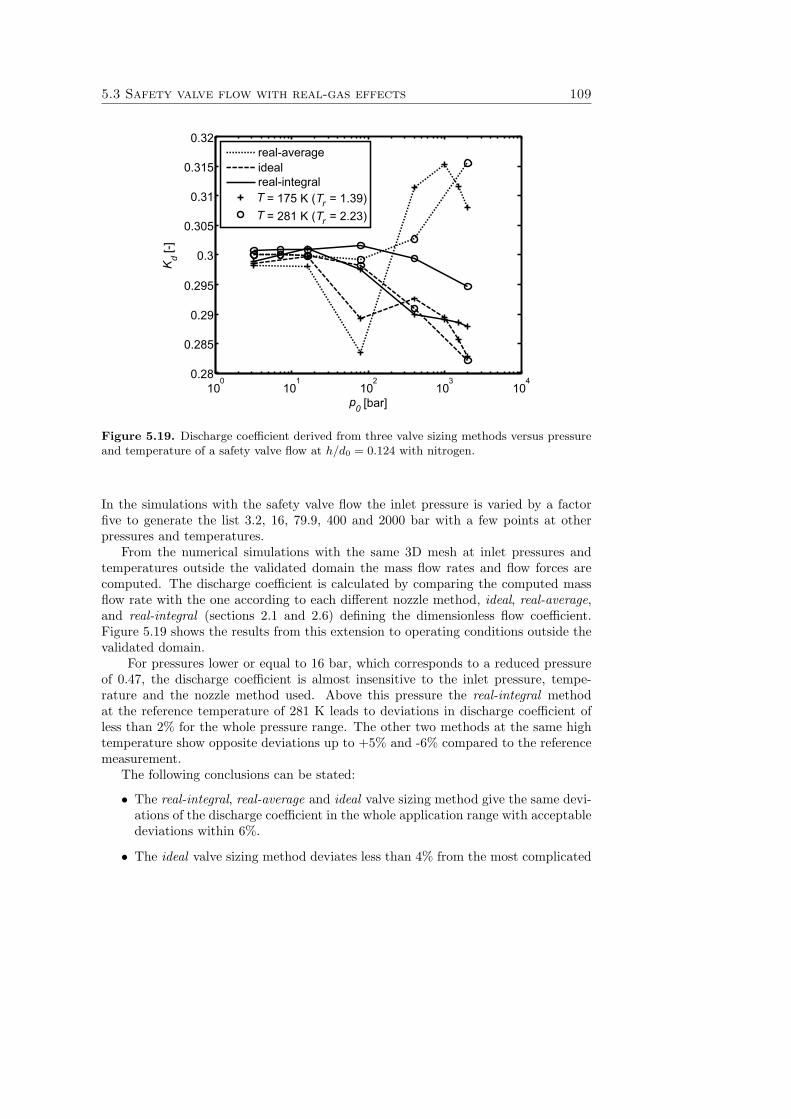
5.3 Safety valve flow with real-gas effects 109
100
101
102
103
104
0.28
0.285
0.29
0.295
0.3
0.305
0.31
0.315
0.32
p0 [bar]
Kd
[-]real-averageidealreal-integralT = 175 K (Tr = 1.39)T = 281 K (Tr = 2.23)
Figure 5.19. Discharge coefficient derived from three valve sizing methods versus pressureand temperature of a safety valve flow at h/d0 = 0.124 with nitrogen.
In the simulations with the safety valve flow the inlet pressure is varied by a factorfive to generate the list 3.2, 16, 79.9, 400 and 2000 bar with a few points at otherpressures and temperatures.
From the numerical simulations with the same 3D mesh at inlet pressures andtemperatures outside the validated domain the mass flow rates and flow forces arecomputed. The discharge coefficient is calculated by comparing the computed massflow rate with the one according to each different nozzle method, ideal, real-average,and real-integral (sections 2.1 and 2.6) defining the dimensionless flow coefficient.Figure 5.19 shows the results from this extension to operating conditions outside thevalidated domain.
For pressures lower or equal to 16 bar, which corresponds to a reduced pressureof 0.47, the discharge coefficient is almost insensitive to the inlet pressure, tempe-rature and the nozzle method used. Above this pressure the real-integral methodat the reference temperature of 281 K leads to deviations in discharge coefficient ofless than 2% for the whole pressure range. The other two methods at the same hightemperature show opposite deviations up to +5% and -6% compared to the referencemeasurement.
The following conclusions can be stated:
• The real-integral, real-average and ideal valve sizing method give the same devi-ations of the discharge coefficient in the whole application range with acceptabledeviations within 6%.
• The ideal valve sizing method deviates less than 4% from the most complicated
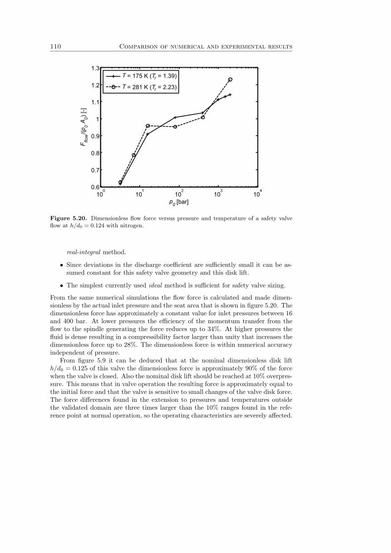
110 Comparison of numerical and experimental results
100
101
102
103
104
0.6
0.7
0.8
0.9
1
1.1
1.2
1.3
p0 [bar]
F flow
/(p0
A 0) [-]
T = 175 K (Tr = 1.39)
T = 281 K (Tr = 2.23)
Figure 5.20. Dimensionless flow force versus pressure and temperature of a safety valveflow at h/d0 = 0.124 with nitrogen.
real-integral method.
• Since deviations in the discharge coefficient are sufficiently small it can be as-sumed constant for this safety valve geometry and this disk lift.
• The simplest currently used ideal method is sufficient for safety valve sizing.
From the same numerical simulations the flow force is calculated and made dimen-sionless by the actual inlet pressure and the seat area that is shown in figure 5.20. Thedimensionless force has approximately a constant value for inlet pressures between 16and 400 bar. At lower pressures the efficiency of the momentum transfer from theflow to the spindle generating the force reduces up to 34%. At higher pressures thefluid is dense resulting in a compressibility factor larger than unity that increases thedimensionless force up to 28%. The dimensionless force is within numerical accuracyindependent of pressure.
From figure 5.9 it can be deduced that at the nominal dimensionless disk lifth/d0 = 0.125 of this valve the dimensionless force is approximately 90% of the forcewhen the valve is closed. Also the nominal disk lift should be reached at 10% overpres-sure. This means that in valve operation the resulting force is approximately equal tothe initial force and that the valve is sensitive to small changes of the valve disk force.The force differences found in the extension to pressures and temperatures outsidethe validated domain are three times larger than the 10% ranges found in the refe-rence point at normal operation, so the operating characteristics are severely affected.
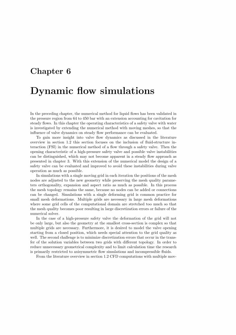
Chapter 6
Dynamic flow simulations
In the preceding chapter, the numerical method for liquid flows has been validated inthe pressure region from 64 to 450 bar with an extension accounting for cavitation forsteady flows. In this chapter the operating characteristics of a safety valve with wateris investigated by extending the numerical method with moving meshes, so that theinfluence of valve dynamics on steady flow performance can be evaluated.
To gain more insight into valve flow dynamics as discussed in the literatureoverview in section 1.2 this section focuses on the inclusion of fluid-structure in-teraction (FSI) in the numerical method of a flow through a safety valve. Then theopening characteristic of a high-pressure safety valve and possible valve instabilitiescan be distinguished, which may not become apparent in a steady flow approach aspresented in chapter 3. With this extension of the numerical model the design of asafety valve can be evaluated and improved to avoid these instabilities during valveoperation as much as possible.
In simulations with a single moving grid in each iteration the positions of the meshnodes are adjusted to the new geometry while preserving the mesh quality parame-ters orthogonality, expansion and aspect ratio as much as possible. In this processthe mesh topology remains the same, because no nodes can be added or connectionscan be changed. Simulations with a single deforming grid is common practice forsmall mesh deformations. Multiple grids are necessary in large mesh deformationswhere some grid cells of the computational domain are stretched too much so thatthe mesh quality becomes poor resulting in large discretization errors or failure of thenumerical solver.
In the case of a high-pressure safety valve the deformation of the grid will notbe only large, but also the geometry at the smallest cross-section is complex so thatmultiple grids are necessary. Furthermore, it is desired to model the valve openingstarting from a closed position, which needs special attention to the grid quality aswell. The second challenge is to minimize discretization errors that occur in the trans-fer of the solution variables between two grids with different topology. In order toreduce unnecessary geometrical complexity and to limit calculation time the researchis primarily restricted to axisymmetric flow simulations and incompressible fluids.
From the literature overview in section 1.2 CFD computations with multiple mov-
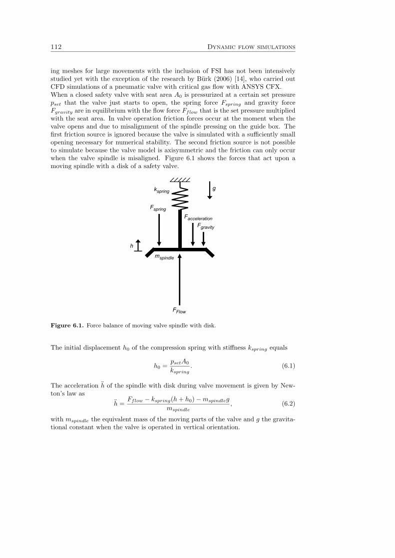
112 Dynamic flow simulations
ing meshes for large movements with the inclusion of FSI has not been intensivelystudied yet with the exception of the research by Burk (2006) [14], who carried outCFD simulations of a pneumatic valve with critical gas flow with ANSYS CFX.When a closed safety valve with seat area A0 is pressurized at a certain set pressurepset that the valve just starts to open, the spring force Fspring and gravity forceFgravity are in equilibrium with the flow force Fflow that is the set pressure multipliedwith the seat area. In valve operation friction forces occur at the moment when thevalve opens and due to misalignment of the spindle pressing on the guide box. Thefirst friction source is ignored because the valve is simulated with a sufficiently smallopening necessary for numerical stability. The second friction source is not possibleto simulate because the valve model is axisymmetric and the friction can only occurwhen the valve spindle is misaligned. Figure 6.1 shows the forces that act upon amoving spindle with a disk of a safety valve.
FaccelerationFgravity
FFlow
Fspring
gkspring
mspindle
h
Figure 6.1. Force balance of moving valve spindle with disk.
The initial displacement h0 of the compression spring with stiffness kspring equals
h0 =psetA0
kspring. (6.1)
The acceleration h of the spindle with disk during valve movement is given by New-ton’s law as
h =Fflow − kspring(h + h0)−mspindleg
mspindle, (6.2)
with mspindle the equivalent mass of the moving parts of the valve and g the gravita-tional constant when the valve is operated in vertical orientation.
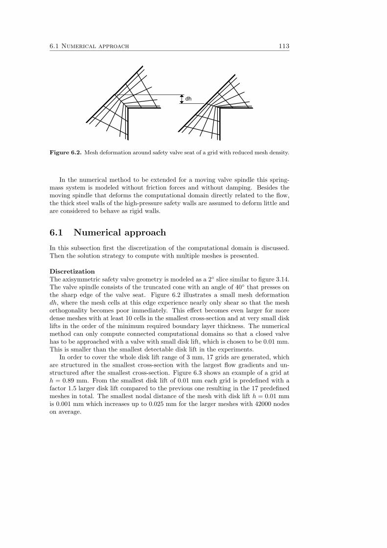
6.1 Numerical approach 113
dh
Figure 6.2. Mesh deformation around safety valve seat of a grid with reduced mesh density.
In the numerical method to be extended for a moving valve spindle this spring-mass system is modeled without friction forces and without damping. Besides themoving spindle that deforms the computational domain directly related to the flow,the thick steel walls of the high-pressure safety walls are assumed to deform little andare considered to behave as rigid walls.
6.1 Numerical approach
In this subsection first the discretization of the computational domain is discussed.Then the solution strategy to compute with multiple meshes is presented.
DiscretizationThe axisymmetric safety valve geometry is modeled as a 2◦ slice similar to figure 3.14.The valve spindle consists of the truncated cone with an angle of 40◦ that presses onthe sharp edge of the valve seat. Figure 6.2 illustrates a small mesh deformationdh, where the mesh cells at this edge experience nearly only shear so that the meshorthogonality becomes poor immediately. This effect becomes even larger for moredense meshes with at least 10 cells in the smallest cross-section and at very small disklifts in the order of the minimum required boundary layer thickness. The numericalmethod can only compute connected computational domains so that a closed valvehas to be approached with a valve with small disk lift, which is chosen to be 0.01 mm.This is smaller than the smallest detectable disk lift in the experiments.
In order to cover the whole disk lift range of 3 mm, 17 grids are generated, whichare structured in the smallest cross-section with the largest flow gradients and un-structured after the smallest cross-section. Figure 6.3 shows an example of a grid ath = 0.89 mm. From the smallest disk lift of 0.01 mm each grid is predefined with afactor 1.5 larger disk lift compared to the previous one resulting in the 17 predefinedmeshes in total. The smallest nodal distance of the mesh with disk lift h = 0.01 mmis 0.001 mm which increases up to 0.025 mm for the larger meshes with 42000 nodeson average.
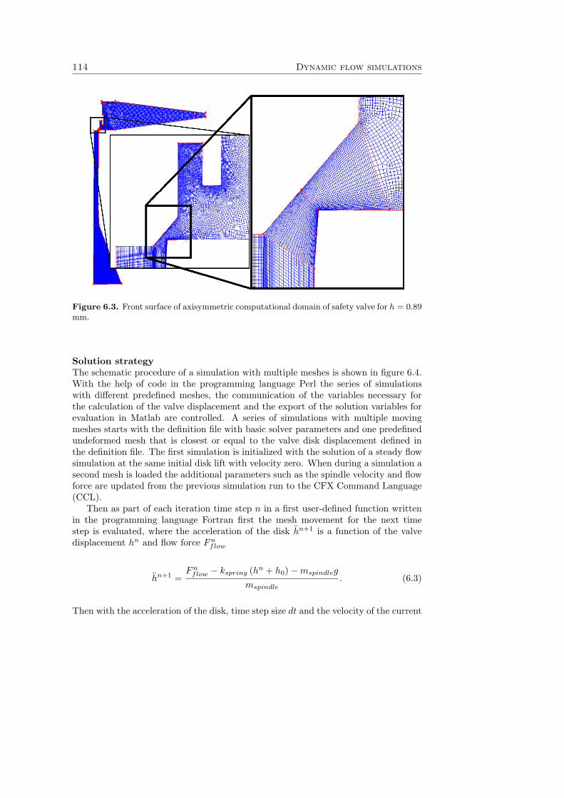
114 Dynamic flow simulations
Figure 6.3. Front surface of axisymmetric computational domain of safety valve for h = 0.89mm.
Solution strategyThe schematic procedure of a simulation with multiple meshes is shown in figure 6.4.With the help of code in the programming language Perl the series of simulationswith different predefined meshes, the communication of the variables necessary forthe calculation of the valve displacement and the export of the solution variables forevaluation in Matlab are controlled. A series of simulations with multiple movingmeshes starts with the definition file with basic solver parameters and one predefinedundeformed mesh that is closest or equal to the valve disk displacement defined inthe definition file. The first simulation is initialized with the solution of a steady flowsimulation at the same initial disk lift with velocity zero. When during a simulation asecond mesh is loaded the additional parameters such as the spindle velocity and flowforce are updated from the previous simulation run to the CFX Command Language(CCL).
Then as part of each iteration time step n in a first user-defined function writtenin the programming language Fortran first the mesh movement for the next timestep is evaluated, where the acceleration of the disk hn+1 is a function of the valvedisplacement hn and flow force Fn
flow
hn+1 =Fn
flow − kspring (hn + h0)−mspindleg
mspindle. (6.3)
Then with the acceleration of the disk, time step size dt and the velocity of the current
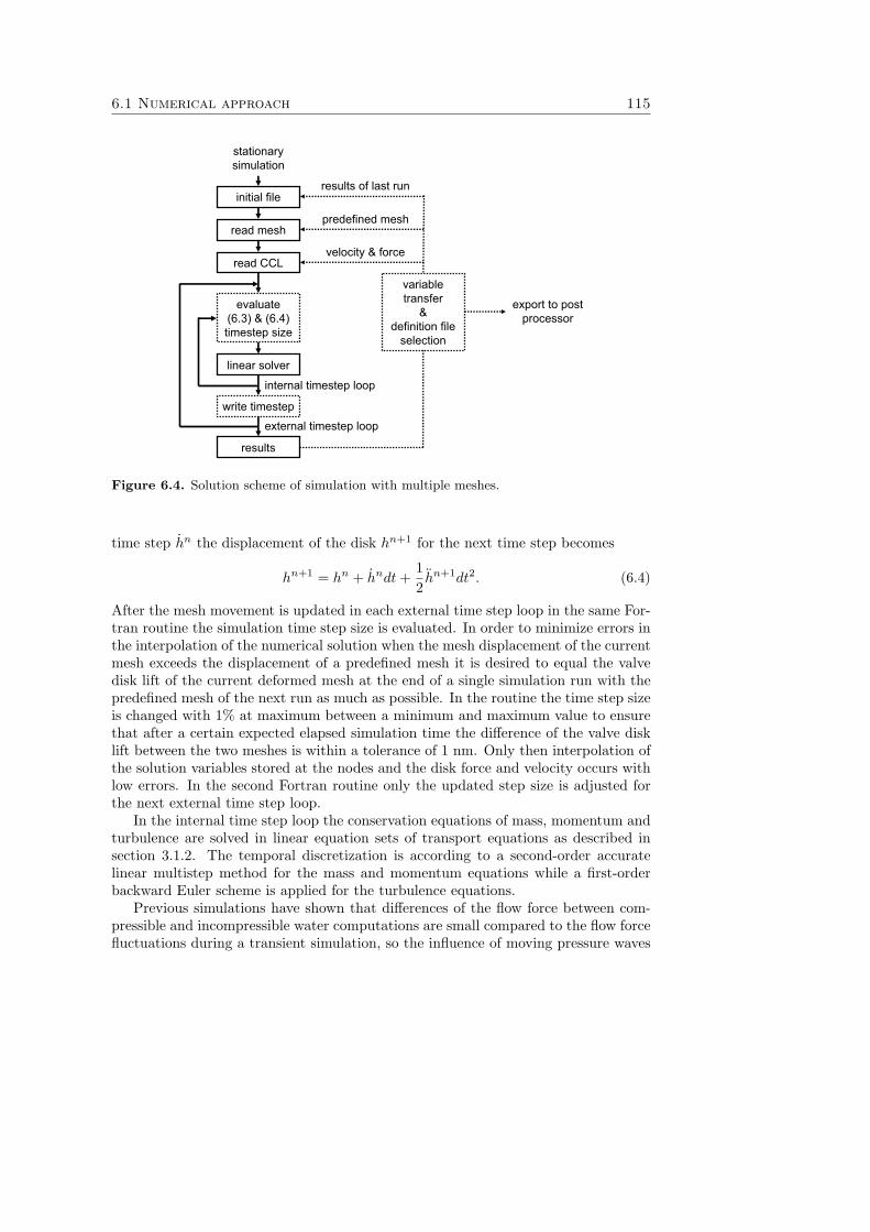
6.1 Numerical approach 115
internal timestep loop
external timestep loop
stationarysimulation
velocity & force
predefined mesh
results of last run
variabletransfer
&definition file
selection
export to post processor
initial file
read mesh
read CCL
evaluate(6.3) & (6.4) timestep size
linear solver
write timestep
results
Figure 6.4. Solution scheme of simulation with multiple meshes.
time step hn the displacement of the disk hn+1 for the next time step becomes
hn+1 = hn + hndt +12hn+1dt2. (6.4)
After the mesh movement is updated in each external time step loop in the same For-tran routine the simulation time step size is evaluated. In order to minimize errors inthe interpolation of the numerical solution when the mesh displacement of the currentmesh exceeds the displacement of a predefined mesh it is desired to equal the valvedisk lift of the current deformed mesh at the end of a single simulation run with thepredefined mesh of the next run as much as possible. In the routine the time step sizeis changed with 1% at maximum between a minimum and maximum value to ensurethat after a certain expected elapsed simulation time the difference of the valve disklift between the two meshes is within a tolerance of 1 nm. Only then interpolation ofthe solution variables stored at the nodes and the disk force and velocity occurs withlow errors. In the second Fortran routine only the updated step size is adjusted forthe next external time step loop.
In the internal time step loop the conservation equations of mass, momentum andturbulence are solved in linear equation sets of transport equations as described insection 3.1.2. The temporal discretization is according to a second-order accuratelinear multistep method for the mass and momentum equations while a first-orderbackward Euler scheme is applied for the turbulence equations.
Previous simulations have shown that differences of the flow force between com-pressible and incompressible water computations are small compared to the flow forcefluctuations during a transient simulation, so the influence of moving pressure waves
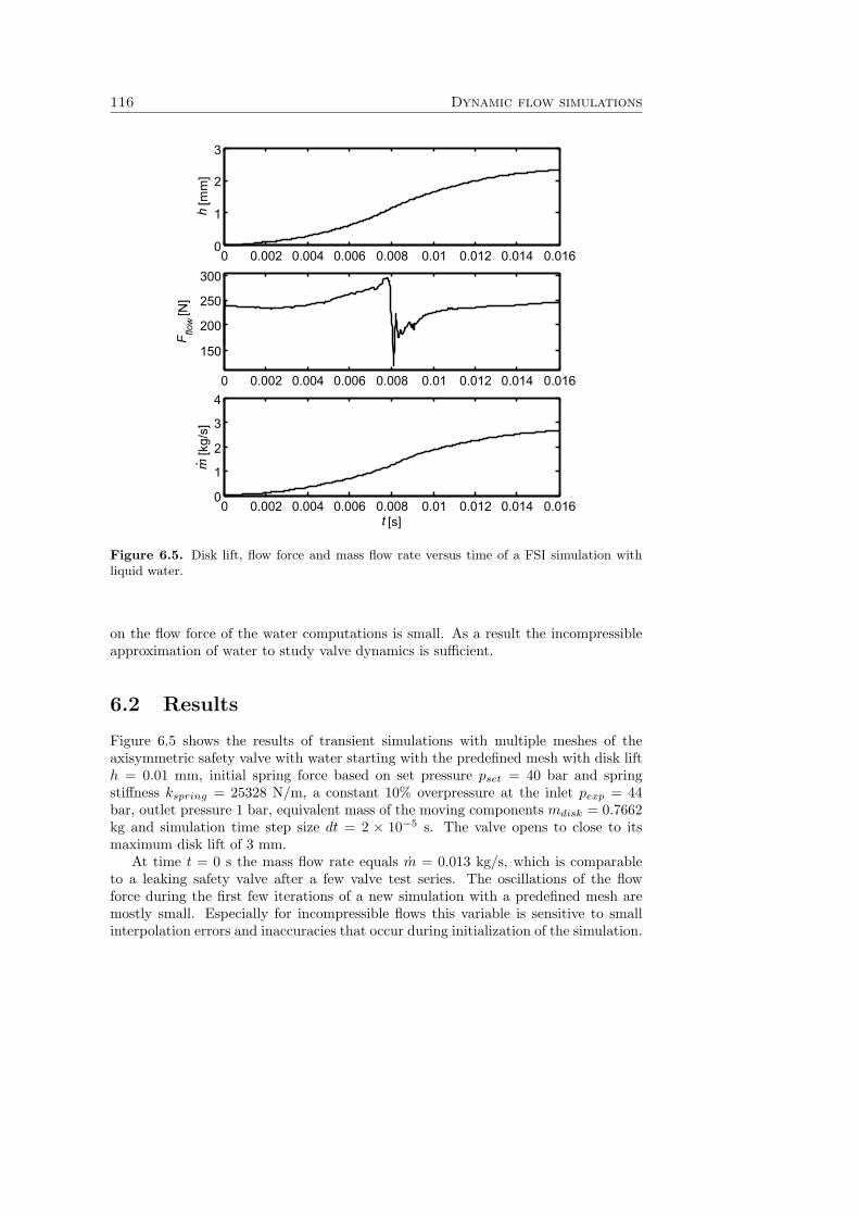
116 Dynamic flow simulations
.
0 0.002 0.004 0.006 0.008 0.01 0.012 0.014 0.0160
1
2
3
h[m
m]
0 0.002 0.004 0.006 0.008 0.01 0.012 0.014 0.016
150
200
250
300
F flow
[N]
0 0.002 0.004 0.006 0.008 0.01 0.012 0.014 0.0160
1
2
3
4
t [s]
m[k
g/s]
Figure 6.5. Disk lift, flow force and mass flow rate versus time of a FSI simulation withliquid water.
on the flow force of the water computations is small. As a result the incompressibleapproximation of water to study valve dynamics is sufficient.
6.2 Results
Figure 6.5 shows the results of transient simulations with multiple meshes of theaxisymmetric safety valve with water starting with the predefined mesh with disk lifth = 0.01 mm, initial spring force based on set pressure pset = 40 bar and springstiffness kspring = 25328 N/m, a constant 10% overpressure at the inlet pexp = 44bar, outlet pressure 1 bar, equivalent mass of the moving components mdisk = 0.7662kg and simulation time step size dt = 2 × 10⁻⁵ s. The valve opens to close to itsmaximum disk lift of 3 mm.
At time t = 0 s the mass flow rate equals m = 0.013 kg/s, which is comparableto a leaking safety valve after a few valve test series. The oscillations of the flowforce during the first few iterations of a new simulation with a predefined mesh aremostly small. Especially for incompressible flows this variable is sensitive to smallinterpolation errors and inaccuracies that occur during initialization of the simulation.
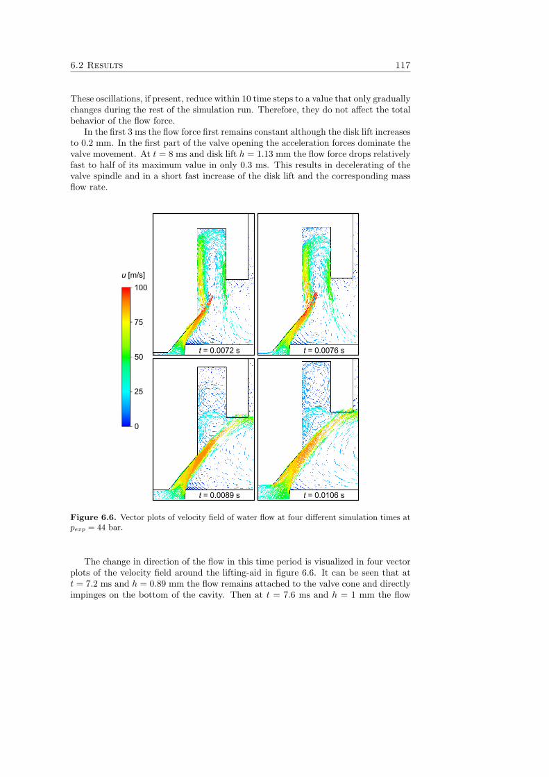
6.2 Results 117
These oscillations, if present, reduce within 10 time steps to a value that only graduallychanges during the rest of the simulation run. Therefore, they do not affect the totalbehavior of the flow force.
In the first 3 ms the flow force first remains constant although the disk lift increasesto 0.2 mm. In the first part of the valve opening the acceleration forces dominate thevalve movement. At t = 8 ms and disk lift h = 1.13 mm the flow force drops relativelyfast to half of its maximum value in only 0.3 ms. This results in decelerating of thevalve spindle and in a short fast increase of the disk lift and the corresponding massflow rate.
0
25
50
75
100u [m/s]
t = 0.0072 s t = 0.0076 s
t = 0.0106 st = 0.0089 s
Figure 6.6. Vector plots of velocity field of water flow at four different simulation times atpexp = 44 bar.
The change in direction of the flow in this time period is visualized in four vectorplots of the velocity field around the lifting-aid in figure 6.6. It can be seen that att = 7.2 ms and h = 0.89 mm the flow remains attached to the valve cone and directlyimpinges on the bottom of the cavity. Then at t = 7.6 ms and h = 1 mm the flow
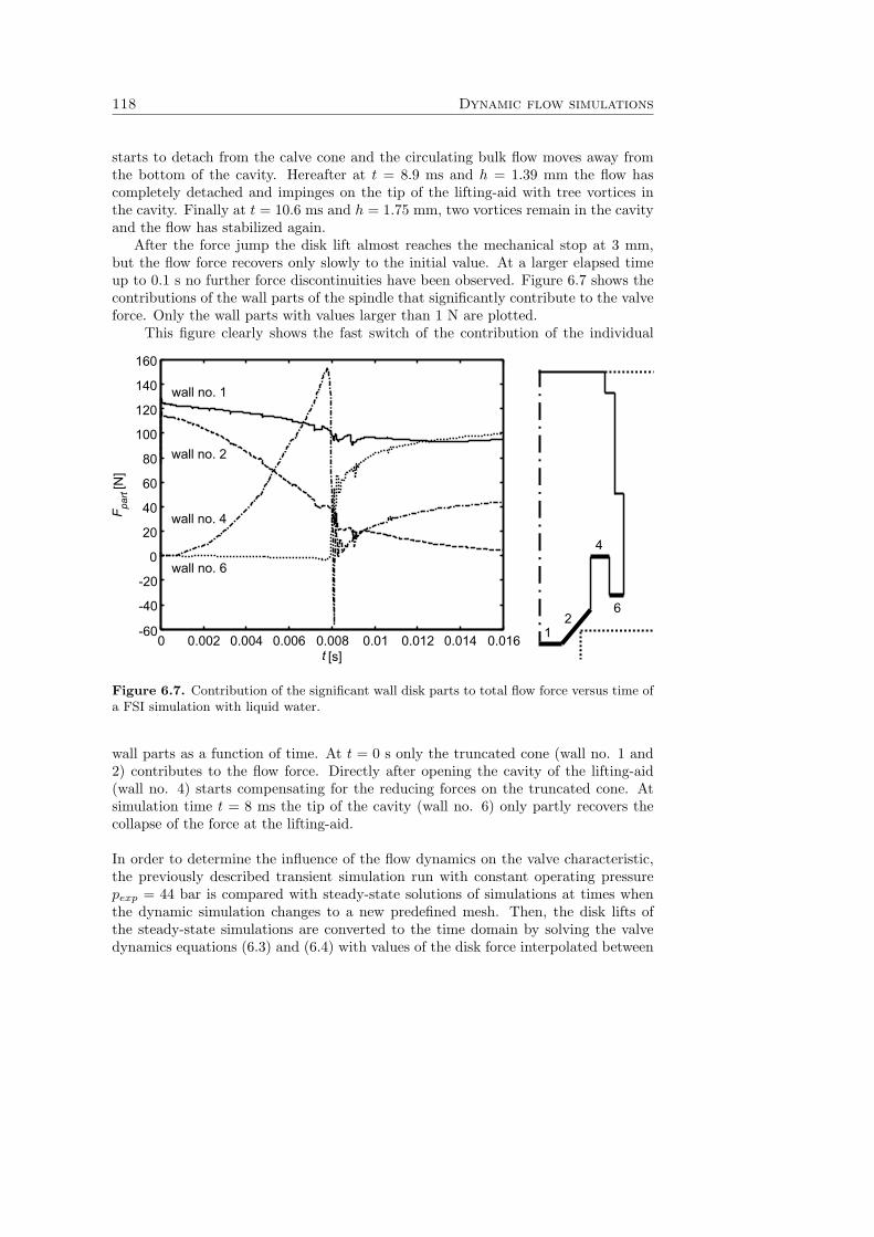
118 Dynamic flow simulations
starts to detach from the calve cone and the circulating bulk flow moves away fromthe bottom of the cavity. Hereafter at t = 8.9 ms and h = 1.39 mm the flow hascompletely detached and impinges on the tip of the lifting-aid with tree vortices inthe cavity. Finally at t = 10.6 ms and h = 1.75 mm, two vortices remain in the cavityand the flow has stabilized again.
After the force jump the disk lift almost reaches the mechanical stop at 3 mm,but the flow force recovers only slowly to the initial value. At a larger elapsed timeup to 0.1 s no further force discontinuities have been observed. Figure 6.7 shows thecontributions of the wall parts of the spindle that significantly contribute to the valveforce. Only the wall parts with values larger than 1 N are plotted.
This figure clearly shows the fast switch of the contribution of the individual
wall no. 1
wall no. 2
wall no. 4
wall no. 6
12
4
6
0 0.002 0.004 0.006 0.008 0.01 0.012 0.014 0.016-60
-40
-20
0
20
40
60
80
100
120
140
160
t [s]
F part
[N]
Figure 6.7. Contribution of the significant wall disk parts to total flow force versus time ofa FSI simulation with liquid water.
wall parts as a function of time. At t = 0 s only the truncated cone (wall no. 1 and2) contributes to the flow force. Directly after opening the cavity of the lifting-aid(wall no. 4) starts compensating for the reducing forces on the truncated cone. Atsimulation time t = 8 ms the tip of the cavity (wall no. 6) only partly recovers thecollapse of the force at the lifting-aid.
In order to determine the influence of the flow dynamics on the valve characteristic,the previously described transient simulation run with constant operating pressurepexp = 44 bar is compared with steady-state solutions of simulations at times whenthe dynamic simulation changes to a new predefined mesh. Then, the disk lifts ofthe steady-state simulations are converted to the time domain by solving the valvedynamics equations (6.3) and (6.4) with values of the disk force interpolated between
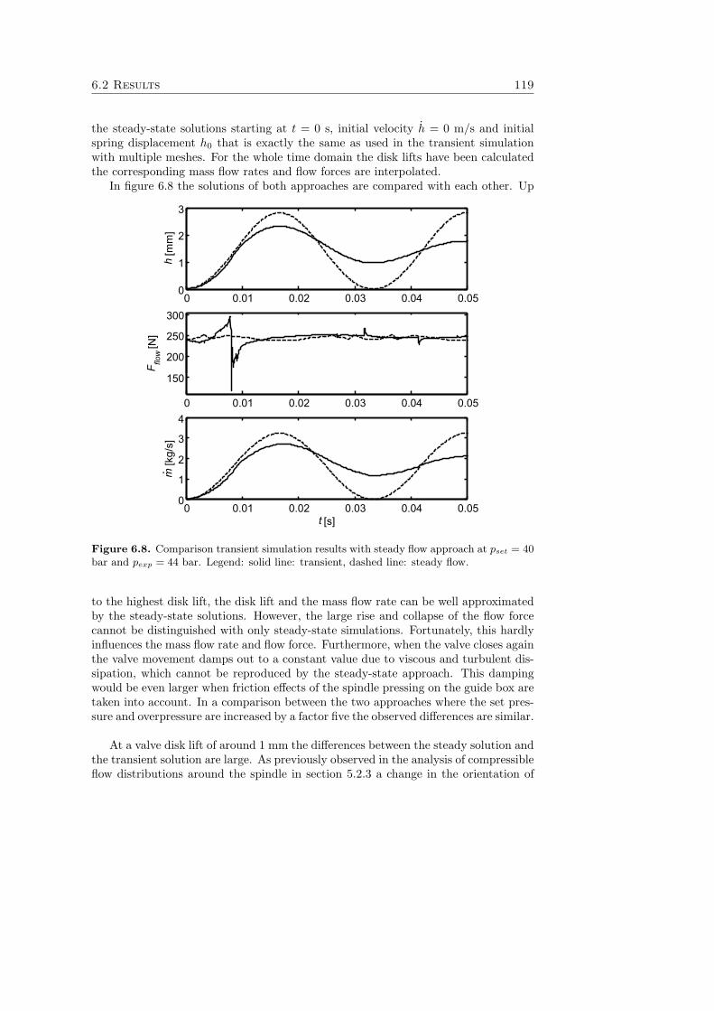
6.2 Results 119
the steady-state solutions starting at t = 0 s, initial velocity h = 0 m/s and initialspring displacement h0 that is exactly the same as used in the transient simulationwith multiple meshes. For the whole time domain the disk lifts have been calculatedthe corresponding mass flow rates and flow forces are interpolated.
In figure 6.8 the solutions of both approaches are compared with each other. Up
.
0 0.01 0.02 0.03 0.04 0.050
1
2
3
h[m
m]
0 0.01 0.02 0.03 0.04 0.05
150
200
250
300
F flow
[N]
0 0.01 0.02 0.03 0.04 0.050
1
2
3
4
t [s]
m[k
g/s]
Figure 6.8. Comparison transient simulation results with steady flow approach at pset = 40bar and pexp = 44 bar. Legend: solid line: transient, dashed line: steady flow.
to the highest disk lift, the disk lift and the mass flow rate can be well approximatedby the steady-state solutions. However, the large rise and collapse of the flow forcecannot be distinguished with only steady-state simulations. Fortunately, this hardlyinfluences the mass flow rate and flow force. Furthermore, when the valve closes againthe valve movement damps out to a constant value due to viscous and turbulent dis-sipation, which cannot be reproduced by the steady-state approach. This dampingwould be even larger when friction effects of the spindle pressing on the guide box aretaken into account. In a comparison between the two approaches where the set pres-sure and overpressure are increased by a factor five the observed differences are similar.
At a valve disk lift of around 1 mm the differences between the steady solution andthe transient solution are large. As previously observed in the analysis of compressibleflow distributions around the spindle in section 5.2.3 a change in the orientation of
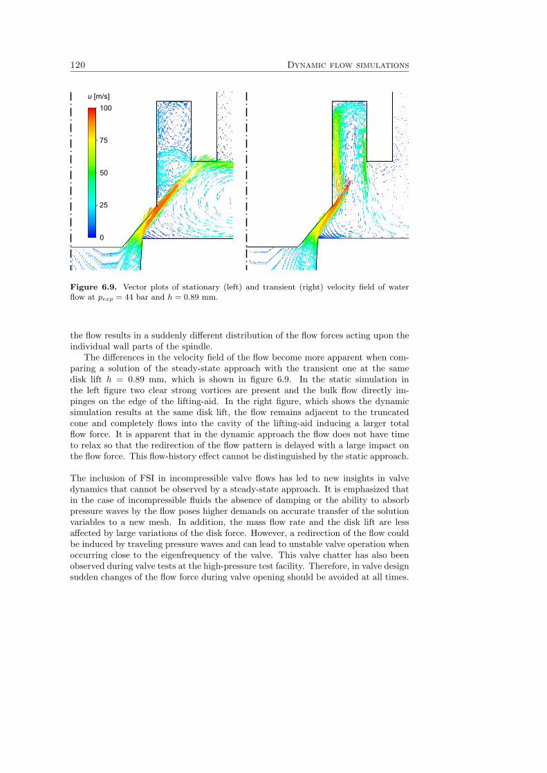
120 Dynamic flow simulations
0
25
50
75
100u [m/s]
Figure 6.9. Vector plots of stationary (left) and transient (right) velocity field of waterflow at pexp = 44 bar and h = 0.89 mm.
the flow results in a suddenly different distribution of the flow forces acting upon theindividual wall parts of the spindle.
The differences in the velocity field of the flow become more apparent when com-paring a solution of the steady-state approach with the transient one at the samedisk lift h = 0.89 mm, which is shown in figure 6.9. In the static simulation inthe left figure two clear strong vortices are present and the bulk flow directly im-pinges on the edge of the lifting-aid. In the right figure, which shows the dynamicsimulation results at the same disk lift, the flow remains adjacent to the truncatedcone and completely flows into the cavity of the lifting-aid inducing a larger totalflow force. It is apparent that in the dynamic approach the flow does not have timeto relax so that the redirection of the flow pattern is delayed with a large impact onthe flow force. This flow-history effect cannot be distinguished by the static approach.
The inclusion of FSI in incompressible valve flows has led to new insights in valvedynamics that cannot be observed by a steady-state approach. It is emphasized thatin the case of incompressible fluids the absence of damping or the ability to absorbpressure waves by the flow poses higher demands on accurate transfer of the solutionvariables to a new mesh. In addition, the mass flow rate and the disk lift are lessaffected by large variations of the disk force. However, a redirection of the flow couldbe induced by traveling pressure waves and can lead to unstable valve operation whenoccurring close to the eigenfrequency of the valve. This valve chatter has also beenobserved during valve tests at the high-pressure test facility. Therefore, in valve designsudden changes of the flow force during valve opening should be avoided at all times.
Chapter 7
Discussion
The objective of this study is to analyze the mass flow capacity and opening charac-teristics of spring-loaded safety valves at operating pressures up to 3600 bar by bothnumerical simulations and high-pressure valve tests.
Valve sizing methodsCurrently, the gas mass flow capacity of a safety valve at any pressure and tempera-ture condition is determined with a standardized valve sizing method. This methodis derived from the ideal gas theory and assumes a constant discharge coefficient thatis experimentally determined at low pressures. In this study the applicability of thisstandardized and two alternative valve sizing methods to real-gas flows has been an-alyzed by means of: CFD computations of nitrogen nozzle and safety valve flow atinlet pressures from 0.1 to 2500 bar and temperatures from 150 to 300 K; experimen-tal data of nitrogen nozzle flow at inlet pressures from 100 to 3500 bar and ambienttemperatures; experimental data from safety valve tests with nitrogen at operatingpressures up to 600 bar and ambient temperatures.
The two introduced alternative valve sizing methods (real-average and real-integral)approximate the thermodynamic state changes between the inlet and the chokingplane of a critical nozzle flow according to the real-gas theory. From the CFD com-putations of nozzle flow with nitrogen it is concluded that although the standardizedideal valve sizing method is the simplest method since no iterative calculations haveto be made and it is based on critical nozzle flow model derived from the ideal gastheory, it deviates only 3% from the most complex real-integral valve sizing method.
Safety valve computations have been carried out at higher inlet pressures up to2000 bar and a lower inlet temperature of 175 K as close as possible to the criticalpoint to remain single phase in the smallest flow cross-section. The discharge coef-ficient reduces by only 2% in combination with the real-integral sizing method anddeviates 6% when the dimensionless flow coefficient is calculated with the ideal orreal-average method. Consequently, for this valve geometry the discharge coefficientcan be assumed constant and the simplest ideal valve sizing method is sufficient. Theaccuracy of the method is also proven by a comparison with experimental data fromnozzle flows at inlet pressures up to 3500 bar.
122 Discussion
In conclusion, the nozzle model of the ideal valve sizing method sufficiently coversthe thermodynamics of the flow, because errors cancel each other, so that the dis-charge coefficient corrected for frictional losses and redirection of the flow only weaklydepends on the thermodynamic state at the inlet of the valve. This means that thecurrent practice of determining the valve discharge capacity by means of valve testsat low inlet pressures between 5 and 7 bar discharging into the atmosphere providessufficient information for valve sizing at other pressure and temperature conditions. Itis noted that this study focused on one valve geometry, but in publication (Schmidt,Peschel and Beune, 2009) [59] computations with another typical high-pressure valvegeometry the discharge coefficient with improved accuracy of the equation of stateused in the CFD tool is expected to vary within 10%.
According to the principle of corresponding states, this analysis can also be quan-titatively applied to other non-polar and weakly polar pure gases or gas mixturesthat can be decomposed with the mixing rules and the used equation of state SoaveRedlich-Kwong. For polar gases or complicated gas mixtures it is recommended touse a suitable equation of state in combination with the CFD tool to determine thedischarge capacity of safety valves when no experimental data is available. For valvesizing by plant designers it is recommended to use the sufficiently accurate stan-dardized ideal valve sizing method with properties for the compressibility factor andadiabatic exponent derived from a sufficiently accurate real-gas equation of state whendeviations from the ideal gas equation of state become significant.
Analysis of experimental and numerical results for steady valve flowValve sizing methods cannot be used to predict the opening characteristics of safetyvalves. Alternatively, a CFD model or valve tests are necessary to account for 3Dflow effects that result in a complex pressure distribution at the valve disk whichdetermines the flow force. The flow force actually determines stable operation of thevalve and is, therefore, for a valve manufacturer more important than the mass flowrate as a design parameter for a satisfactory and stable opening characteristic.
In computations of the CFD tool of the investigated safety valve with nitrogen atnominal disk lift and inlet pressures outside the experimental validation range up to2000 bar the dimensionless flow force continually increases with pressure independentof the inlet temperature within the numerical accuracy. The deviations compared tothe reference experiment at 80 bar are -34% at a lower pressure of 3.2 bar and +28%at a higher pressure of 2000 bar. As a result, when stable valve operation is found inaccordance with the standards at a certain operating pressure, the opening charac-teristic differs from valve operation at another set pressure when the spring stiffnessis adapted with the same factor as the set pressure ratio.
From the high-pressure safety valve tests conducted at the constructed high-pressure facility with operating pressures up to 600 bar, accurate and reproduciblestationary valve flow conditions have been achieved, wherefrom the averaged measure-ment points show remarkable differences between the valve characteristic conductedwith sub-cooled water and gaseous nitrogen both in the pressure range of 64 and 453bar at ambient temperature. In the valve tests with water the dimensionless flowforce based on the actual operating pressure slightly increases to 1.05 at the nominal
123
disk lift of 1 mm while the experiments with nitrogen show a dimensionless flow forcecontinuously decreasing to 0.88 at nominal disk lift.
The mass flow rates have been accurately determined so that it is possible torelate the small scatter in the measured valve characteristic to specific experimentalconditions. In the water tests the dominant experimental uncertainty is a gradualgeometry change due to rounding off the edges of the valve seat and spindle causedby excessive mechanical wear. This results in increased discharge capacities up to10% at the same disk lift for the studied valve type. Also valve chatter in tests afterthe first blow-off test, if present, reduces or is absent in further blow-off tests of thesame valve. In the nitrogen valve tests at high operating pressures large temperaturefluctuations in the buffer vessel and the mass flow measurement system cause inaccu-racies in the discharge coefficient up to 10%. For both fluids the discharge coefficientand the dimensionless flow force are independent of pressure at the valve inlet in therange between 64 and 453 bar and at ambient temperatures.
In the numerical calculation with the CFD tool for water flows it seems necessaryto extend the numerical model with a cavitation model. Simulations with cavitationlead to a significantly better agreement. At low disk lifts and at high pressures thecaviation model needs to be extended to account for thermal and compressibility ef-fects of the vapor phase.
For compressible high-pressure valve flows, the mass flow rates always agree within3.6%. The flow forces show an approximately constant deviation between 7.8% and14.7% between experiment and numerical simulation, which are already present atlow disk lifts. Analysis of the results shows that this deviation cannot be completelyexplained by numerical errors, so it is expected that the indirect flow force mea-surement method with the spring deflection and opening pressure of the test valveis mostly responsible for the deviation. A larger experimental error than previouslyestimated in the accuracy analysis is possible, because the difference between the setpressure and the actual opening pressure of the investigated safety valve is larger thana priori estimated. This results in a larger pressure range where the valve leaks atnon-detectable small disk lift with increasing inlet pressure before the valve actuallyopens and starts relieving large amounts of fluid. Also frictional effects could play alarger role at high pressures than previously estimated.
For more accurate force measurements it is recommended to decrease the stiffnessof the spring as much as possible so that the spring can still be pre-stressed to theforce at the desired set pressure, without pressing the windings on each other so thatfurther compression is mechanically blocked by the spring. Then the valve immedi-ately opens and with the force sensor installed stable valve opening at the mechanicalstop is ensured. Then the difference between the set pressure and the uncertain ope-ning pressure is minimized. It is noted that it is important to damp the collision ofthe spindle on the mechanical stop with rubber to avoid excessive peak forces possiblydamaging the attached force sensor. Alternatively, it would be better not to install aspring at all and measure at fixed disk lifts directly with the force sensor only. Thedrawback is that it is more difficult to achieve stable operating conditions during avalve test, because the valve already relieves fluid when the buffer vessel is pressurized.
124 Discussion
Dynamic CFD modelingIt is possible to study the opening characteristic of a high-pressure safety valve withincompressible flow in the entire disk lift range with the multimesh FSI algorithm. Inthe development of this algorithm it is focused on mesh quality and accurate transferof the solution variables to a new predefined mesh. Especially for incompressible flowit is important to postpone transfer to a new mesh until the disk lift of the deformedmesh differs only 1 nm from the next predefined mesh so that force oscillations, dueto discretization errors are minimized.
In the dynamic simulation of an axisymmetric safety valve with water at a setpressure of 40 bar and at 10% overpressure a large rise and huge collapse of the flowforce with factor two at approximately nominal disk lift have been observed. A cor-responding redirection of the flow hardly affects the mass flow rate and disk lift, butcan lead to unstable valve operation when these changes of the flow pattern occurclose to the eigenfrequency of the moving parts of the valve.
In a comparison between static and dynamic simulations with incompressible flowa collapse of the flow force can only be seen in the steady-state approach when theamount of steady-state simulations is significantly increased so that the discretizationof the coupled valve dynamics is more accurate. That means that flow-history effectsshould be small so that the flow immediately adapts to changed boundary conditions,which is the case for incompressible flows.
For gases flow-history effects are present resulting in a less strict tolerance of thedisk lift difference between two numerical grids, since small interpolation errors arelocally damped. However, at high pressures the flow gradients adjacent to the wallsare large so that this algorithm is still necessary for accurate calculation. For sim-ulations with (real-) gases it is recommended to reduce the smallest nodal distanceof the meshes at lower disk lifts so that converged solutions will be achieved as well.Another future research topic is to model an opening valve with water with a cavita-tion model, so that the effect of cavitation on the valve dynamics can be investigated.
Possibilities with the CFD toolThis CFD tool can be used for accurate prediction of the discharge coefficient whenno measurement data is available or when it is hardly possible to conduct a valve test.It is still unclear whether this tool can quantitatively predict flow forces with similaraccuracy. As a result, evaluating valve design should always occur in combinationwith experimental research.
For safety valve design it is important that the flow force is accurately knownas a function of disk lift and varies without large discontinuities caused by redirec-tions of the flow pattern. In static simulations flow pattern changes can be observed,but flow-history effects can only be distinguished by a dynamic approach. That’swhy in the static approach these redirections of the flow still occur but with smalleramplitudes of the flow force and at slightly different disk lifts than in the dynamicapproach. In incompressible flows flow-history effects are smaller than in compress-ible flows. It is still unclear when dynamic simulations are necessary for differentcompressible fluids at other circumstances. In future research it is recommended toinvestigate multimesh FSI simulations for compressible high-pressure valve flows that
125
comes along with high computational costs and long preparation times compared tothe steady-state approach.
Nevertheless, in a static approach of the CFD tool it is possible to study differentgeometries and see the development of the flow without suddenly emerging separationpoints causing changed locations of recirculation areas. Actually, from a design pointof view it is desired to control these moments to occur outside the mechanically possi-ble disk lift range or at the nominal disk lift in the case of pop-up safety relief valves.Then no unwanted force fluctuations occur during opening and closing of the safetyvalve when it is most sensitive to elevated backpressures and dynamic flow effects.In other words, the flow gradually changes while opening with separation points andrecirculation areas at positions that are insensitive to small changes of the gas or,ideally, to compressibility effects at all. Furthermore, the safety valve can be appliedto both gases and liquids with the largest possible pressure range of a single spring.
A safety valve should open to its nominal disk lift at 10% overpressure maximum.The tolerance of the valve spring stiffness and the safety factor of the reduced dis-charge coefficient used in the standardized valve sizing methods are both 10%. Thatmeans that the flow force should be calculated with an accuracy of the order of 1%.This high accuracy demand cannot be achieved with the CFD tool so that the springstiffness cannot be numerically determined for a safety valve. Therefore, the springcan be dimensioned only in valve experiments and up-scaling to higher pressures thanexperimentally possible should always taken with care.
Nevertheless, the strength of the CFD tool is to optimize valve geometries incombination with sensitivity studies to account for small geometry changes (effect ofmechanical wear and production tolerances) and real-gas effects to find the cause forvalve chatter and to avoid it in improved geometries.
So the CFD tool is suitable to quantitatively predict the mass flow rate, but canonly qualitatively predict and show tendencies of the flow force. This means thatwhen a safety valve will be applied at higher pressures than measurable in a testfacility, it should always be verified that it certainly reaches its nominal disk lift at10% overpressure when mounted at the pressurized system of the plant itself. Nev-ertheless, the simulations of the dimensionless forces at pressures up to 2000 bar ofthis valve type have shown that the momentum transfer of the flow to the valve diskbecomes more efficient resulting in a larger force at nominal disk lift indicating thatthe net force to open the valve increases with pressure. However, frictional effectscan prevent the valve from opening at higher pressures when the overshoot of thenet force is small or cause the dimensionless force to decrease too much directly aftervalve opening.

126 Discussion
Bibliography
[1] AD: 2001, AD 2000 Merkblatt A2 Sicherheitseinrichtungen gegenDruckuberschreitung – Sicherheitsventile. Berlin: Beuth Verlag GmbH.
[2] Alvi, F., J. Ladd, and W. Bower: 2002, ‘Experimental and computational inves-tigation of supersonic impinging jets’. AIAA journal 40(4), 599–609.
[3] Anderson, J.: 2003, Modern compressible flow with historical perspective, 3rdedition. New York: McGraw-Hill.
[4] ANSYS: 2006, ‘Manual ANSYS CFX, Release 11.0’. Canonsburg.
[5] API: 2000, API RP-520:2000 Sizing, selection, and installation of pressure-relieving devices in refineries, Part I sizing and selection. Washington, DC:7th ed., American Petroleum Institute.
[6] ASME: 1998, Performance Test Code PTC19.3:1974 (R1998) Temperature Mea-surement. New York: ASME.
[7] ASTM: 2008, ASTM E220 - 07a Standard Test Method for Calibration of Ther-mocouples By Comparison Techniques. West Conshohocken: ASTM Interna-tional.
[8] Baldwin, R. and H. Simmons: 1986, ‘Flow-Induced Vibration in Safety ReliefValves’. Journal of Pressure Vessel Technology 108, 267–272.
[9] Bauerfeind, K. and L. Friedel: 2003, ‘Berechnung der dissipationsbehafteten kri-tischen Dusenstromung realer Gase’. Forschung im Ingenieurwesen 67(6), 227–235.
[10] Betts, P. and J. Francis: 1997, ‘Pressures beneath the disc of a compensatedpressure relief valve for gas/vapour service’. Proceedings of the Institution ofMechanical Engineers, Part E: Journal of Process Mechanical Engineering 211,285–289.
[11] Bober, W. and W. Chow: 1990, ‘Nonideal isentropic gas flow through converging-diverging nozzles’. ASME, Transactions, Journal of Fluids Engineering 112,455–461.
128 BIBLIOGRAPHY
[12] Botros, K., G. Dunn, and J. Hrycyk: 1998, ‘Riser-Relief Valve Dynamic Interac-tions (Extension to a Previous Model)’. Journal of Pressure Vessel Technology120, 207–212.
[13] Bredau, J.: 2000, ‘Numerische Stromungsberechnung und experimentelleStromungsvisualisierung in der Pneumatik’. Ph.D. thesis, TU Dresden, Ger-many.
[14] Burk, E.: 2006, ‘Numerische Stromungsberechnung erganzt durch experimentelleMethoden zur Untersuchung pneumatischer Stromungen’. Ph.D. thesis, TU Dres-den, Germany.
[15] Cremers, J.: 2000, ‘Auslegungsmethode zur Vermeidung von Schwingungen beifederbelasteten Sicherheitsventilen mit Zu- und Ableitung’. Ph.D. thesis, TUHamburg-Harburg, Germany.
[16] Cremers, J. and L. Friedel: 2003, ‘Design of spring loaded safety valves with inletand discharge pipe against chatter in the case of gas flow’. Chemical Engineering& Technology 26(5), 573–576.
[17] d’Agostino, L. and M. Salvetti: 2007, Fluid Dynamics of Cavitation and Cavi-tating Turbopumps. SpringerWienNewYork.
[18] Darby, R. and K. Molavi: 1997, ‘Viscosity Correction Factor for EmergencyRelief Valves’. Process Safety Progress 16(2), 80–82.
[19] DIN: 1982, DIN 1952:1982, Durchflußmessung mit Blenden, Dusen undVenturirohren in voll durchstromten Rohren mit Kreisquerschnitt (VDI-Durchflußmeßregeln. Berlin:.
[20] Domagala, M.: 2008, ‘CFD Analysis of pilot operating relief valve’. CzasopismoTechniczne, wydawnictwo politechniki Krakowshiej z. 3-M.
[21] Druguet, M. and D. Zeitoun: 2003, ‘Influence of numerical and viscous dissipationon shock wave reflections in supersonic steady flows’. Computers and Fluids32(4), 515–533.
[22] Follmer, B.: 1981, ‘Stromung im Einlauf von Sicherheitsventilen’. Ph.D. thesis,RWTH Aachen, Germany.
[23] Follmer, B. and A. Schnettler: 2003, ‘Challenges in designing API safety reliefvalves’. Valve World 10, 39–43.
[24] Francis, J. and P. Betts: 1998, ‘Backpressure in a high-lift compensated pressurerelief valve subject to single phase compressible flow’. Journal of Loss Preventionin the Process Industries 11(1), 55–66.
[25] Frommann, O.: 2000, ‘Effect of Pressure Waves in the Feed Lines upon thePerformance of Full Lift Safety Valves’. Chemical Engineering & Technology23(9), 765–769.
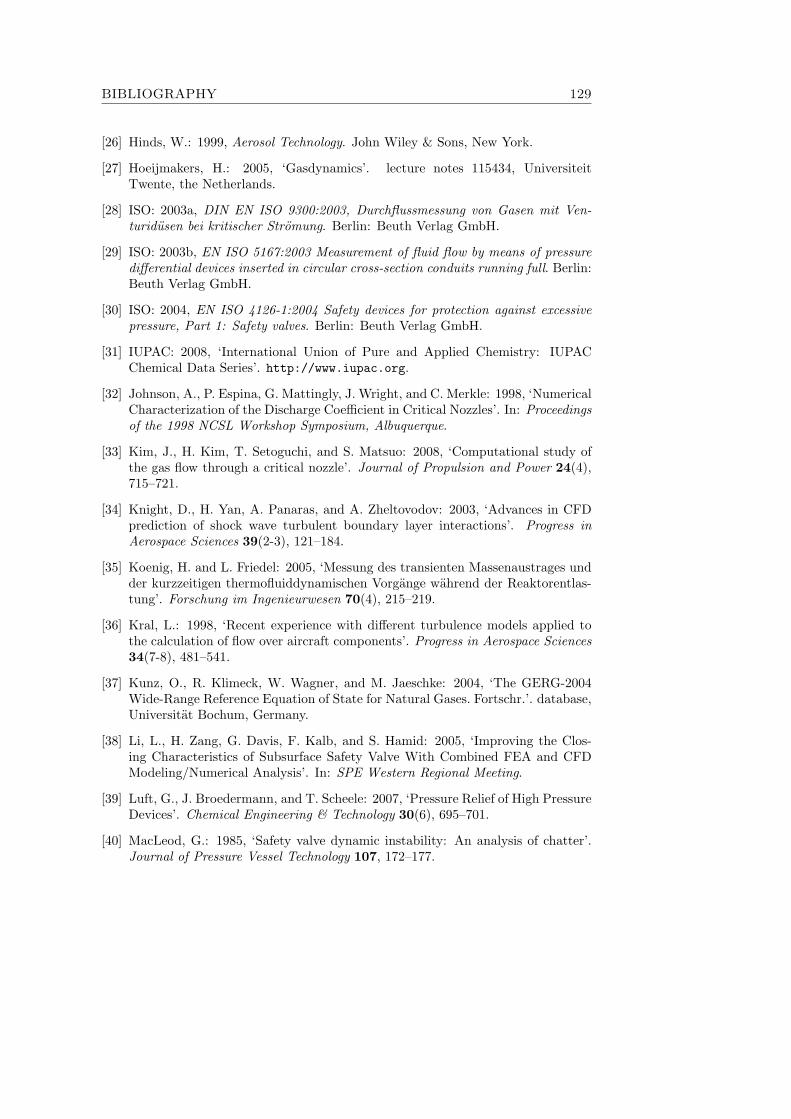
BIBLIOGRAPHY 129
[26] Hinds, W.: 1999, Aerosol Technology. John Wiley & Sons, New York.
[27] Hoeijmakers, H.: 2005, ‘Gasdynamics’. lecture notes 115434, UniversiteitTwente, the Netherlands.
[28] ISO: 2003a, DIN EN ISO 9300:2003, Durchflussmessung von Gasen mit Ven-turidusen bei kritischer Stromung. Berlin: Beuth Verlag GmbH.
[29] ISO: 2003b, EN ISO 5167:2003 Measurement of fluid flow by means of pressuredifferential devices inserted in circular cross-section conduits running full. Berlin:Beuth Verlag GmbH.
[30] ISO: 2004, EN ISO 4126-1:2004 Safety devices for protection against excessivepressure, Part 1: Safety valves. Berlin: Beuth Verlag GmbH.
[31] IUPAC: 2008, ‘International Union of Pure and Applied Chemistry: IUPACChemical Data Series’. http://www.iupac.org.
[32] Johnson, A., P. Espina, G. Mattingly, J. Wright, and C. Merkle: 1998, ‘NumericalCharacterization of the Discharge Coefficient in Critical Nozzles’. In: Proceedingsof the 1998 NCSL Workshop Symposium, Albuquerque.
[33] Kim, J., H. Kim, T. Setoguchi, and S. Matsuo: 2008, ‘Computational study ofthe gas flow through a critical nozzle’. Journal of Propulsion and Power 24(4),715–721.
[34] Knight, D., H. Yan, A. Panaras, and A. Zheltovodov: 2003, ‘Advances in CFDprediction of shock wave turbulent boundary layer interactions’. Progress inAerospace Sciences 39(2-3), 121–184.
[35] Koenig, H. and L. Friedel: 2005, ‘Messung des transienten Massenaustrages undder kurzzeitigen thermofluiddynamischen Vorgange wahrend der Reaktorentlas-tung’. Forschung im Ingenieurwesen 70(4), 215–219.
[36] Kral, L.: 1998, ‘Recent experience with different turbulence models applied tothe calculation of flow over aircraft components’. Progress in Aerospace Sciences34(7-8), 481–541.
[37] Kunz, O., R. Klimeck, W. Wagner, and M. Jaeschke: 2004, ‘The GERG-2004Wide-Range Reference Equation of State for Natural Gases. Fortschr.’. database,Universitat Bochum, Germany.
[38] Li, L., H. Zang, G. Davis, F. Kalb, and S. Hamid: 2005, ‘Improving the Clos-ing Characteristics of Subsurface Safety Valve With Combined FEA and CFDModeling/Numerical Analysis’. In: SPE Western Regional Meeting.
[39] Luft, G., J. Broedermann, and T. Scheele: 2007, ‘Pressure Relief of High PressureDevices’. Chemical Engineering & Technology 30(6), 695–701.
[40] MacLeod, G.: 1985, ‘Safety valve dynamic instability: An analysis of chatter’.Journal of Pressure Vessel Technology 107, 172–177.
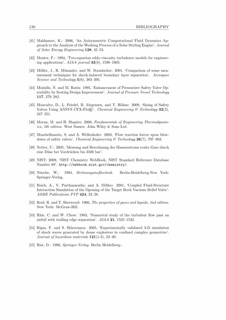
130 BIBLIOGRAPHY
[41] Mahkamov, K.: 2006, ‘An Axisymmetric Computational Fluid Dynamics Ap-proach to the Analysis of the Working Process of a Solar Stirling Engine’. Journalof Solar Energy Engineering 128, 45–53.
[42] Menter, F.: 1994, ‘Two-equation eddy-viscosity turbulence models for engineer-ing applications’. AIAA journal 32(8), 1598–1605.
[43] Muller, J., R. Mummler, and W. Staudacher: 2001, ‘Comparison of some mea-surement techniques for shock-induced boundary layer separation’. AerospaceScience and Technology 5(6), 383–395.
[44] Moisidis, N. and M. Ratiu: 1995, ‘Enhancement of Pressurizer Safety Valve Op-erability by Seating Design Improvement’. Journal of Pressure Vessel Technology117, 279–282.
[45] Moncalvo, D., L. Friedel, B. Jorgensen, and T. Hohne: 2009, ‘Sizing of SafetyValves Using ANSYS CFX-Flo®’. Chemical Engineering & Technology 32(2),247–251.
[46] Moran, M. and H. Shapiro: 2006, Fundamentals of Engineering Thermodynam-ics, 5th edition. West Sussex: John Wiley & Sons Ltd.
[47] Muschelknautz, S. and A. Wellenhofer: 2003, ‘Flow reaction forces upon blow-down of safety valves’. Chemical Engineering & Technology 26(7), 797–803.
[48] Netter, U.: 2005, ‘Messung und Berechnung des Massenstroms realer Gase durcheine Duse bei Vordrucken bis 3500 bar’.
[49] NIST: 2009, ‘NIST Chemistry WebBook, NIST Standard Reference DatabaseNumber 69’. http://webbook.nist.gov/chemistry/.
[50] Nitsche, W.: 1994, Stromungsmeßtechnik. Berlin-Heidelberg-New York:Springer-Verlag.
[51] Reich, A., V. Parthasarathy, and A. DiMeo: 2001, ‘Coupled Fluid-StructureInteraction Simulation of the Opening of the Target Rock Vacuum Relief Valve’.ASME Publications PVP 424, 23–28.
[52] Reid, R. and T. Sherwood: 1966, The properties of gases and liquids, 2nd edition.New York: McGraw-Hill.
[53] Rhie, C. and W. Chow: 1983, ‘Numerical study of the turbulent flow past anairfoil with trailing edge separation’. AIAA 21, 1525–1532.
[54] Rigas, F. and S. Sklavounos: 2005, ‘Experimentally validated 3-D simulationof shock waves generated by dense explosives in confined complex geometries’.Journal of hazardous materials 121(1-3), 23–30.
[55] Rist, D.: 1996, Springer-Verlag. Berlin Heidelberg:.
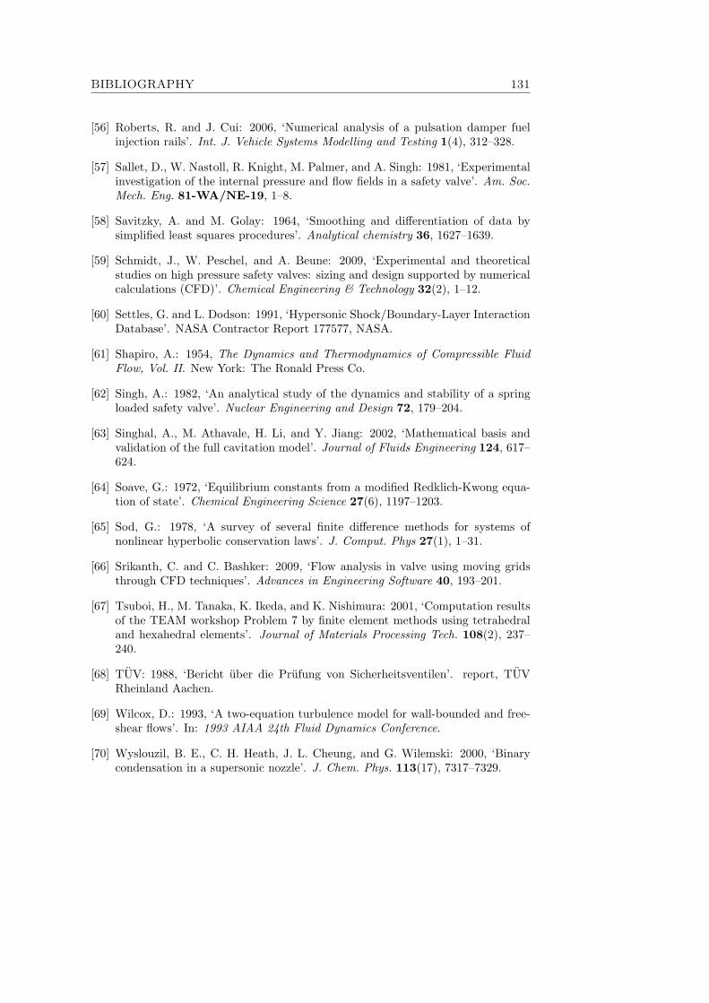
BIBLIOGRAPHY 131
[56] Roberts, R. and J. Cui: 2006, ‘Numerical analysis of a pulsation damper fuelinjection rails’. Int. J. Vehicle Systems Modelling and Testing 1(4), 312–328.
[57] Sallet, D., W. Nastoll, R. Knight, M. Palmer, and A. Singh: 1981, ‘Experimentalinvestigation of the internal pressure and flow fields in a safety valve’. Am. Soc.Mech. Eng. 81-WA/NE-19, 1–8.
[58] Savitzky, A. and M. Golay: 1964, ‘Smoothing and differentiation of data bysimplified least squares procedures’. Analytical chemistry 36, 1627–1639.
[59] Schmidt, J., W. Peschel, and A. Beune: 2009, ‘Experimental and theoreticalstudies on high pressure safety valves: sizing and design supported by numericalcalculations (CFD)’. Chemical Engineering & Technology 32(2), 1–12.
[60] Settles, G. and L. Dodson: 1991, ‘Hypersonic Shock/Boundary-Layer InteractionDatabase’. NASA Contractor Report 177577, NASA.
[61] Shapiro, A.: 1954, The Dynamics and Thermodynamics of Compressible FluidFlow, Vol. II. New York: The Ronald Press Co.
[62] Singh, A.: 1982, ‘An analytical study of the dynamics and stability of a springloaded safety valve’. Nuclear Engineering and Design 72, 179–204.
[63] Singhal, A., M. Athavale, H. Li, and Y. Jiang: 2002, ‘Mathematical basis andvalidation of the full cavitation model’. Journal of Fluids Engineering 124, 617–624.
[64] Soave, G.: 1972, ‘Equilibrium constants from a modified Redklich-Kwong equa-tion of state’. Chemical Engineering Science 27(6), 1197–1203.
[65] Sod, G.: 1978, ‘A survey of several finite difference methods for systems ofnonlinear hyperbolic conservation laws’. J. Comput. Phys 27(1), 1–31.
[66] Srikanth, C. and C. Bashker: 2009, ‘Flow analysis in valve using moving gridsthrough CFD techniques’. Advances in Engineering Software 40, 193–201.
[67] Tsuboi, H., M. Tanaka, K. Ikeda, and K. Nishimura: 2001, ‘Computation resultsof the TEAM workshop Problem 7 by finite element methods using tetrahedraland hexahedral elements’. Journal of Materials Processing Tech. 108(2), 237–240.
[68] TUV: 1988, ‘Bericht uber die Prufung von Sicherheitsventilen’. report, TUVRheinland Aachen.
[69] Wilcox, D.: 1993, ‘A two-equation turbulence model for wall-bounded and free-shear flows’. In: 1993 AIAA 24th Fluid Dynamics Conference.
[70] Wyslouzil, B. E., C. H. Heath, J. L. Cheung, and G. Wilemski: 2000, ‘Binarycondensation in a supersonic nozzle’. J. Chem. Phys. 113(17), 7317–7329.

132 BIBLIOGRAPHY
[71] Zahariev, T.: 2001, ‘Berechnung der Durchstromung und der Kennwerte vonSicherheitsventilen’. Ph.D. thesis, Otto-von Quericke-Universitat Magdeburg,Germany.
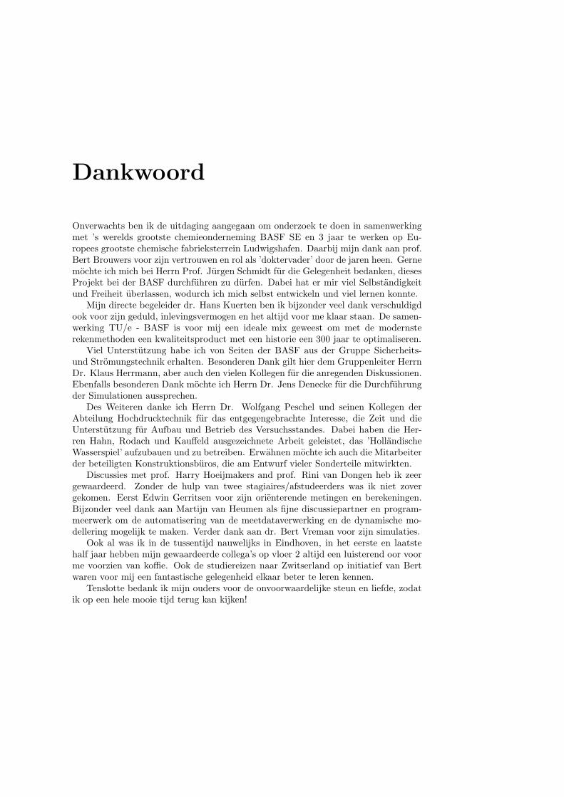
Dankwoord
Onverwachts ben ik de uitdaging aangegaan om onderzoek te doen in samenwerkingmet ’s werelds grootste chemieonderneming BASF SE en 3 jaar te werken op Eu-ropees grootste chemische fabrieksterrein Ludwigshafen. Daarbij mijn dank aan prof.Bert Brouwers voor zijn vertrouwen en rol als ’doktervader’ door de jaren heen. Gernemochte ich mich bei Herrn Prof. Jurgen Schmidt fur die Gelegenheit bedanken, diesesProjekt bei der BASF durchfuhren zu durfen. Dabei hat er mir viel Selbstandigkeitund Freiheit uberlassen, wodurch ich mich selbst entwickeln und viel lernen konnte.
Mijn directe begeleider dr. Hans Kuerten ben ik bijzonder veel dank verschuldigdook voor zijn geduld, inlevingsvermogen en het altijd voor me klaar staan. De samen-werking TU/e - BASF is voor mij een ideale mix geweest om met de modernsterekenmethoden een kwaliteitsproduct met een historie een 300 jaar te optimaliseren.
Viel Unterstutzung habe ich von Seiten der BASF aus der Gruppe Sicherheits-und Stromungstechnik erhalten. Besonderen Dank gilt hier dem Gruppenleiter HerrnDr. Klaus Herrmann, aber auch den vielen Kollegen fur die anregenden Diskussionen.Ebenfalls besonderen Dank mochte ich Herrn Dr. Jens Denecke fur die Durchfuhrungder Simulationen aussprechen.
Des Weiteren danke ich Herrn Dr. Wolfgang Peschel und seinen Kollegen derAbteilung Hochdrucktechnik fur das entgegengebrachte Interesse, die Zeit und dieUnterstutzung fur Aufbau und Betrieb des Versuchsstandes. Dabei haben die Her-ren Hahn, Rodach und Kauffeld ausgezeichnete Arbeit geleistet, das ’HollandischeWasserspiel’ aufzubauen und zu betreiben. Erwahnen mochte ich auch die Mitarbeiterder beteiligten Konstruktionsburos, die am Entwurf vieler Sonderteile mitwirkten.
Discussies met prof. Harry Hoeijmakers and prof. Rini van Dongen heb ik zeergewaardeerd. Zonder de hulp van twee stagiaires/afstudeerders was ik niet zovergekomen. Eerst Edwin Gerritsen voor zijn orienterende metingen en berekeningen.Bijzonder veel dank aan Martijn van Heumen als fijne discussiepartner en program-meerwerk om de automatisering van de meetdataverwerking en de dynamische mo-dellering mogelijk te maken. Verder dank aan dr. Bert Vreman voor zijn simulaties.
Ook al was ik in de tussentijd nauwelijks in Eindhoven, in het eerste en laatstehalf jaar hebben mijn gewaardeerde collega’s op vloer 2 altijd een luisterend oor voorme voorzien van koffie. Ook de studiereizen naar Zwitserland op initiatief van Bertwaren voor mij een fantastische gelegenheid elkaar beter te leren kennen.
Tenslotte bedank ik mijn ouders voor de onvoorwaardelijke steun en liefde, zodatik op een hele mooie tijd terug kan kijken!

134 Dankwoord
Curriculum vitae
Arend Beune was born in Helmond, the Netherlands, on the 23rd of October 1978.From 1991 to 1997 he attended pre-university education (VWO) at Carolus Bor-romeus College in Helmond, the Netherlands. In 1997 he started to study MechanicalEngineering at Eindhoven University of Technology (the Netherlands). In 1999-2000he was one year a board member of the student association of the faculty of Mechan-ical Engineering ’Simon Stevin’.
During his four-month internship at the University of Strathclyde in Glasgow(United Kingdom) in 2004 he was involved in experimental research on the character-istics of bubble formation when emerging from an orifice depending on wettability andReynolds number. Hereafter in 2004-2005 he performed the practical part of his Mas-ter’s thesis at the research institute for Recource Efficient and Sustainable Systems atGraz University of Technology, Austria. During his stay of eight months he analyzedthe devices of a pot furnace biomass combustion setup and implemented improve-ments, which increased its reliability and accuracy. In February 2005 he received hisMSc degree ’with great appreciation’ in Mechanical Engineering at Eindhoven Uni-versity of Technology (TU/e).
Thereafter, he started to work on his PhD project in the Process Technology groupof TU/e in cooperation with and funded by the Safety Engineering & Fluid Dynamicsand High-pressure Technology departments of BASF SE in Ludwigshafen (Germany).The topic of his research is to develop a numerical method to predict the discharge ca-pacity and opening characteristic of high-pressure safety valves up to 3600 bar. Thisis a basis for a new approach to reduce time-consuming and cost-intensive experi-ments and improve their operating reliability. For the experimental validation he hasworked at BASF for three years. There he has built a unique industrial mini-plant tocarry out the high-pressure valve tests at double set pressures compared to existingtest facilities.