Analysis, Control and Design of Walking Robots · ANALYSIS, CONTROL AND DESIGN OF WALKING ROBOTS...
225
Transcript of Analysis, Control and Design of Walking Robots · ANALYSIS, CONTROL AND DESIGN OF WALKING ROBOTS...

Analysis, Control and Design of Walking Robots
Gijs van Oort
Promotiecommissie
Voorzitter/secr. prof. dr. ir. A. J. Mouthaan Universiteit TwentePromotor prof. dr. ir. S. Stramigioli Universiteit TwenteOverige leden prof. dr. A. Ruina Cornell University
dr. ir. M. Wisse Technische Univ. Delftprof. dr. ir. P. P. Jonker Technische Univ. Eindhovenprof. dr. ir. H. F. J. M. Koopman Universiteit Twenteprof. dr. ir. J. van Amerongen Universiteit Twente
Paranimfen Edwin DertienWietse Balkema
The research described in this thesis has been conducted at the Department of ElectricalEngineering, Math, and Computer Science at the University of Twente, and has been fi-nancially supported by the IMPACT institute and the VIACTORS project, supported by theEuropean Commission under the 7th Framework Programme.
The research is part of the research program of the Dutch Institute of Systems and Control(DISC). The author has successfully completed the educational program of the GraduateSchool DISC.
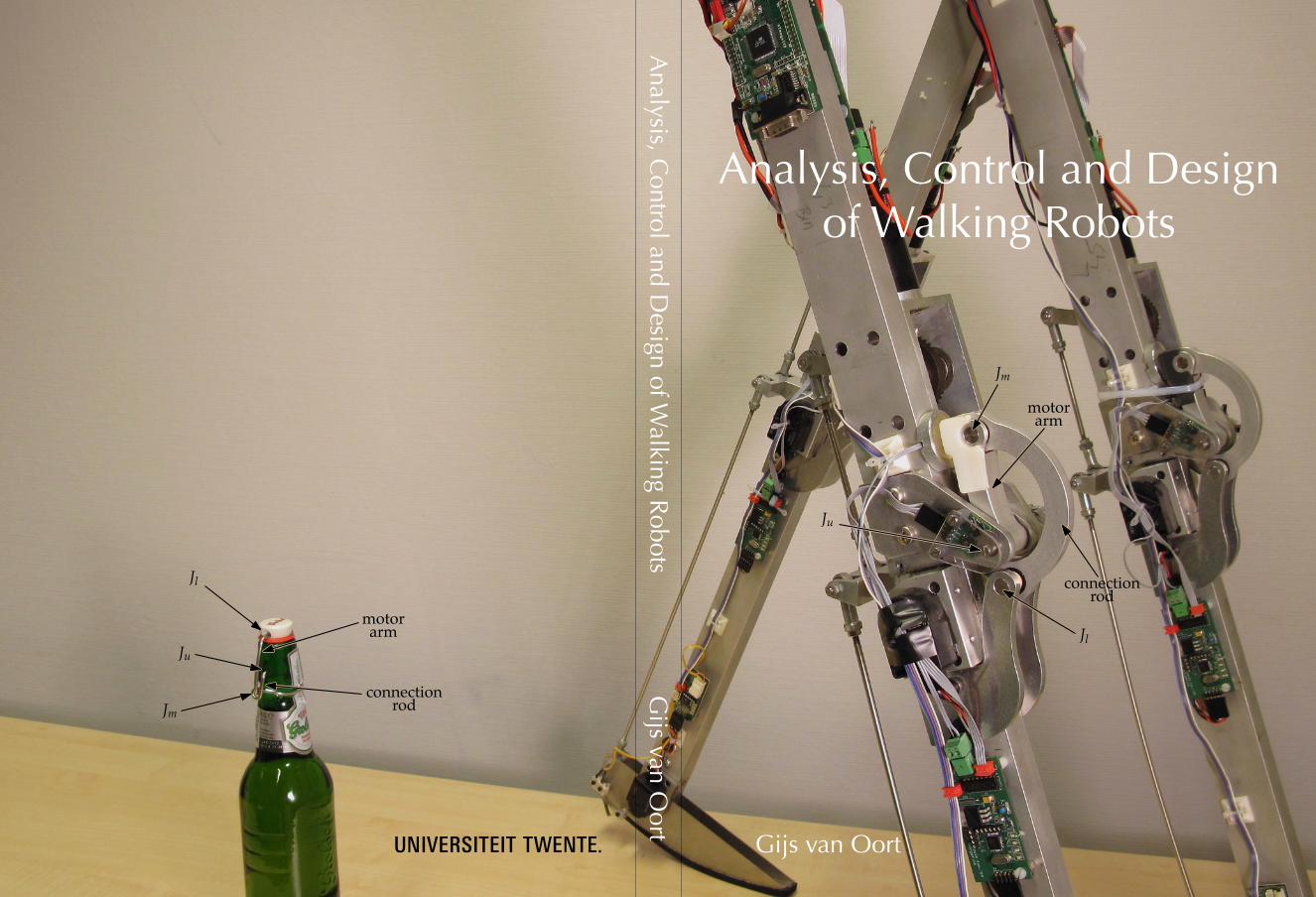
Cover picture: The design of the knee lock for the walking robot Dribbel was inspired bythe mechanism of the swing top bottle (see chapter 9).
ISBN 978-90-365-3264-8DOI 10.3990/1.9789036532648
Copyright c© 2011 by G. van Oort, Enschede, The Netherlands.
No part of this work may be reproduced by print, photocopy, or anyother means without the permission in writing from the publisher. Allpictures in this thesis have been reproduced with permission of therespective copyright holders.
Printed by Wöhrmann Print Service, Zutphen, The Netherlands.
ANALYSIS, CONTROL AND DESIGN
OF WALKING ROBOTS
PROEFSCHRIFT
ter verkrijging van
de graad van doctor aan de Universiteit Twente,
op gezag van de rector magnificus,
prof. dr. H. Brinksma
volgens besluit van het College voor Promoties
in het openbaar te verdedigen
op woensdag 26 oktober 2011 om 14.45 uur
door
Gijs van Oort
geboren op 29 november 1978
te Nijmegen, Nederland

Dit proefschrift is goedgekeurd door
Prof. dr. ir. S. Stramigioli, promotor
ISBN 978-90-365-3264-8
DOI 10.3990/1.9789036532648
Copyright c© 2011 by G. van Oort, Enschede, The Netherlands
Samenvatting
Lopende robots zijn cool. De aanblik van zo’n mooi stukje voortstappend tech-niek spreekt velen tot de verbeelding. Momenteel worden lopende robots danook regelmatig ingezet in de entertainmentindustrie. Behalve leuk kunnen lo-pende robots ook nuttig zijn: in de toekomst kunnen ze bijvoorbeeld taken over-nemen in het huishouden, in kantooromgevingen en in de zorg. Onderzoek naarlopende robots heeft, behalve voor het maken van lopende robots zelf, nog meernut. Zo kunnen verschillende onderzoeksgebieden die betrekking hebben op lo-pende robots (bijvoorbeeld de analyse van multi-body-dynamica en contactmo-dellen), direct toegepast worden op andere vlakken van de robotica zoals hetaansturen van (industriële) robotarmen en het ontwikkelen van grijpers. Ook le-ren we door het onderzoek veel over menselijk lopen; die kennis wordt toegepastbij revalidatie en het maken van protheses en orthoses.
In dit proefschrift worden vijf onderzoeksvragen beantwoord die van belang zijnvoor de ontwikkeling van tweebenige (bipedal) lopende robots. De onderzoeks-vragen zijn gecategoriseerd in drie hoofdonderwerpen: analyse, regeling en aanstu-ring en ontwerp. De onderzoeksvragen worden hieronder besproken. De hoofd-stukken van dit proefschrift zijn ieder gebaseerd op een artikel dat is gepubli-ceerd bij of verzonden naar een conferentie.
DEEL I: Analyse
Hoe kunnen we het gedrag analyseren van een 2D passief-dynamische loperdie over oneffen terrein loopt?Een bekende analyse-tool voor 2D passief-dynamische lopers1 is de post-impactPoincaré-sectie: het ‘vlak’ in de toestandsruimte bestaande uit alle mogelijke toe-standen2 van de loper direct na de voet-impact op vlakke vloer. Dit concept kan
12D loper: een lopertje dat niet naar links en rechts kan omvallen; alleen naar voren en achteren(de bewegingsruimte is gereduceerd tot een tweedimensionaal vlak). Passief-dynamische loper: maaktgebruik van het natuurlijke (passieve) zwaaigedrag van de benen; hierdoor is voor het naar vorenzwaaien van het been geen energie nodig.
2Toestand: de positie en snelheid van alle ledematen van de robot (Engels: state).
i
echter niet gebruikt worden als de loper op oneffen terrein loopt. In dit proef-schrift wordt hiervoor een oplossing geboden in de vorm van een mapping diemet iedere mogelijke post-impact toestand op oneffen terrein een punt op dePoincaré-sectie associeert (hoofdstuk 2).
Kunnen we, door middel van een ‘andere kijk’ op de robot, meer inzicht krij-gen in de dynamica?Om de toestand van een robot numeriek te representeren (zodat ermee gerekendkan worden) maken we vaak gebruik van coördinaten. Er bestaan vele verschil-lende coördinaatrepresentaties (b.v. absolute hoeken, of juist relatieve) van eentoestand; welke representatie het meest geschikt is hangt af van het specifiekeprobleem dat opgelost moet worden. Sommige problemen kunnen ook zonderhet gebruik van coördinaten (geometrisch) worden opgelost.
Voor lopende robots wordt vaak een coördinaatrepresentatie gekozen waarbij detorso het referentielichaam is. In dit proefschrift wordt aangetoond dat dit nietaltijd de meest geschikte keuze is; soms is de standvoet als referentielichaam be-ter. De vergelijkingen die de bewegingen van de robot beschrijven worden daneenvoudiger en door deze te bestuderen kan men beter inzicht krijgen in de ro-botdynamica (hoofdstuk 3).
In dit proefschrift wordt een methode beschreven om, gegeven de grondcontact-wrench (de kracht die de grond uitoefent op de voet van de robot), op een co-ordinaat-vrije manier de positie te bepalen van het Zero-Moment Point3 (ZMP).In plaats van wiskundige vergelijkingen wordt er gebruik gemaakt van geome-trische relaties, wat het inzicht in de materie verhoogt (hoofdstuk 4).
Vaak helpt het om voor de analyse een versimpeld model van de robot te ge-bruiken. In dit proefschrift wordt zo’n model besproken: het locked inertia model.Hierin wordt de robot voorgesteld als zijnde één star lichaam. De wiskundigevergelijkingen van het model zijn veel eenvoudiger dan die van de robot zelfen kunnen gebruikt worden als startpunt voor analyse van de dynamica van derobot (hoofdstuk 5).
DEEL II: Regeling en aansturing
Hoe kunnen we een robot regelen om hem te stabiliseren in de laterale (zij-waartse) richting?In dit proefschrift worden twee regelaars besproken die dit kunnen bewerkstel-ligen. Beide maken gebruik van ‘laterale voetplaatsing’: door de voet iets meernaar links of rechts neer te zetten, kan gezorgd worden dat de robot niet naarlinks of rechts omvalt.
Bij de eerste methode (toegepast op een zeer simpel loper-model) wordt precies
3De positie van dit punt (op de vloer) geeft een indicatie of de standvoet stevig op de grond staat.
ii
halverwege de stap (mid-stance) de zijwaartse snelheid van de heup gemeten envia een lineaire P-regelaar teruggekoppeld naar de zijwaartse positie van de voet.Er wordt numeriek aangetoond dat deze regelaar een stabiel systeem oplevertmet een grote robuustheid tegen verstoringen (hoofdstuk 6).
De tweede methode gebruikt het Extrapolated Center of Mass4 (XCOM) als invoervoor de (lineaire) regelaar. Deze methode is geïmplementeerd in TUlip5. Test-resultaten laten zien dat de robot met de regelaar inderdaad stabiel is in lateralerichting (hoofdstuk 7).
Hoe kunnen we de actuatoren verbeteren om een minimaal energieverbruik teverkrijgen?De actuatoren (‘motoren’) die in de meeste lopende robots zitten zijn niet ergenergiezuinig. In dit proefschrift wordt een concept voor een nieuw type actuatorgeïntroduceerd dat negatieve arbeid mechanisch kan opslaan en later hergebrui-ken. De actuator bestaat uit een DC motor, een rem om de motoras vast te zetten,een spiraalveer en een ‘oneindig variabele transmissie’ (IVT) (hoofdstuk 8).
DEEL III: Ontwerp
Hoe kunnen we het knie- en enkelgewricht van een lopende robot verbeteren?Het kniegewricht van Dribbel6 en het enkelgewricht van TUlip voldeden niet aanonze verwachtingen. Door veel aandacht te besteden aan het formuleren van deprecieze eisen van de gewrichten, kwamen we tot creatieve ontwerpoplossingen.
Het eerste ontwerp is een innovatief knie-blokkeermechanisme, dat ervoor zorgtdat het standbeen van de robot gestrekt blijft. Het is gebaseerd op een ‘vierstan-genmechanisme’ (four-bar linkage) en blokkeert door middel van een mechanischesingulariteit: een bepaalde stand van het mechanisme waarin één bewegingsrich-ting van het mechanisme geblokkeerd wordt. Het geblokkeerd houden van deknie kost geen energie terwijl het deblokkeren zeer gemakkelijk gaat. Het ont-werp is succesvol toegepast in de 2D loper Dribbel (hoofdstuk 9).
Het tweede ontwerp is een twee-graden-van-vrijheid enkelbesturing. In plaatsvan het gebruik van één motor voor het actueren van de x-as en één voor de y-as,zijn beide motoren gemonteerd in een differentieelopstelling. Draaien de motorenbeide in dezelfde richting, dan wordt de x-as geactueerd; draaien ze in tegenge-stelde richting, dan wordt de y-as geactueerd. Voordeel hiervan is dat de krachtvan beide motoren samen gebruikt kan worden voor de enkelafzet tijdens hetlopen, waardoor kleine motoren kunnen volstaan (hoofdstuk 10).
4De positie van dit punt (op de vloer) geeft een indicatie van waar de voet neergezet moet wordenom de robot in één stap tot stilstand te brengen.
5TUlip, een 3D lopende robot, is ontwikkeld in een samenwerkingsproject van de UniversiteitTwente (vakgroep Control Engineering), en de Technische Universiteiten van Delft en Eindhoven.
6Dribbel, een 2D lopende robot, is ontwikkeld op de vakgroep Control Engineering van de Univer-siteit Twente.
iii

iv
Summary
Walking robots are cool. The appearance of such a beautiful piece of technol-ogy that moves around in the way that we humans do, is appealing to many.Consequently, walking robots are regularly being used in the entertainment in-dustry. Apart from being fun, walking robots can also be useful: in the futurethey can for example take over tasks in household, office environments and thehealth care sector. Research on walking robots is, except for making the walkingrobots themselves, of more use. Several research areas related to walking robots(such as analysis of multi-body dynamics and contact models) can be directly ap-plied in other robotics fields such as the control of (industrial) robot arms andthe development of grippers. Also, by researching walking robots, we learn a lotabout human walking; this knowledge is being applied in rehabilitation and thedevelopment of prostheses and orthoses.
In this thesis five research questions are discussed that are related to the develop-ment of two-legged (bipedal) walking robots. The research questions are catego-rized in three main topics: analysis, control and actuation and design. The researchquestions are discussed below. Each chapter of this thesis is based on an articlewhich was published at or submitted to a conference.
PART I: Analysis
How can we analyze the behavior of a 2D passive dynamic walker that is walk-ing on rough terrain?A well-known analysis tool for 2D passive dynamic walkers1 is the post-impactPoincaré section: the ‘plane’ in the state space consisting of all possible states2 ofthe walker directly after foot-impact on a flat floor. This concept however can notbe used if the walker is walking on rough terrain. In this thesis a solution to this
12D walker: a walking system that cannot fall sideways; only forward and backward (the motionspace is reduced to a two-dimensional plane). Passive dynamic walker: utilizes the natural (passive)swinging motion of the legs; because of this no energy is required to swing the leg forward.
2State: the position and velocity of all parts of the body.
v
is given by providing a mapping that associates with each possible post-impactstate on rough terrain a point on the Poincaré section (chapter 2).
By looking at the robot from a different ‘perspective’, can we gain more insightin its dynamics?In order to represent the state of a robot numerically (to be able to do calculationswith it), we often make use of coordinates. There exist many different coordinaterepresentations (e.g., absolute angles, or relative ones) of a state; which of therepresentations is most suitable depends on the exact problem that needs to besolved. Some problems can also be solved without the use of coordinates, i.e., ina geometric manner.
For walking robots usually a coordinate representation is chosen in which thetorso is the reference body. In this thesis it is shown that this is not always the bestchoice; sometimes it is more convenient to take the stance foot as the referencebody. The equations that describe the motions of the robot become simpler andby studying these, one can gain better insight in the robot dynamics (chapter 3).
In this thesis a method is presented for determining the position of the Zero-Moment Point3 (ZMP) in a coordinate-free way, given the ground reaction wrench(the force the ground exerts on the foot of the robot). Instead of using mathemat-ical equations, the method uses geometrical relations, which gives more insightin the material (chapter 4).
It is often helpful to use a simplified model of the robot. In this thesis such amodel is discussed: the locked inertia model. In this model the robot is representedas a single rigid body. The mathematical equations of this model are much sim-pler than those of the robot itself and can be used as a starting point for analysisof the dynamics of the robot (chapter 5).
PART II: Control and actuation
How can we control a walking robot in order to stabilize it in the lateral (side-ways) direction?In this thesis two controllers are discussed that can achieve this. Both controllersmake use of ‘lateral foot placement’: positioning the foot a little to the left or right,which prevents the robot from falling sideways.
In the first method (applied to a very simple walker model), the sideways velocityof the hip is measured, exactly halfway the step (at mid-stance). This velocity isthen, through a linear P-controller, fed back to the lateral position of the foot.It is shown numerically that this controller yields a stable system with a large
3The position of this point (on the floor) gives an indication whether the stance foot is firmlystanding on the ground.
vi

robustness margin (chapter 6).
The second method uses the Extrapolated Center of Mass4 (XCOM) as input of the(linear) controller. This method was implemented in TUlip5. Experimental re-sults show that the robot is indeed stabilized in the lateral direction (chapter 7).
How can we improve the actuators in order to get minimum energy consump-tion?The actuators (‘motors’) commonly used in walking robots are not very energyefficient. In this thesis a concept is introduced for a new type of actuator whichcan store negative work mechanically and re-use it later. The actuator consists ofa DC motor, a clutch to fix the motor axis, a rotational spring and an ‘infinitelyvariable transmission’ (IVT) (chapter 8).
PART III: Design
How can we improve the knee and ankle joints of a walking robot?The knee joint of Dribbel6 and the ankle joint of TUlip did not meet our expecta-tions. By paying much attention to formulating the exact requirements of thesejoints, we came up with creative design solutions.
The first design is an innovative knee locking mechanism, which keeps the stanceleg of the robot stretched. It is based on a four-bar linkage and locks by means ofa mechanical singularity: a certain configuration of the mechanism in which onedirection of motion of the mechanism is locked. Keeping the knee locked doesnot require any energy, and unlocking goes easily. The design was successfullyapplied on the 2D walker Dribbel (chapter 9).
The second design is a two-degrees-of-freedom ankle actuation system. Insteadof using one motor for actuating the x-axis and one for the y-axis, both motors aremounted in a differential setup. When both motors turn in the same direction, thex-axis is actuated; if they turn in opposite direction, the y-axis is actuated. Theadvantage of this is that the force of both motors together can be used for anklepush-off, which allows the use of smaller motors (chapter 10).
4The position of this point (on the floor) gives an indication of where the foot should be placed inorder to bring the robot to a stand-still in one step.
5TUlip, a 3D walking robot, was developed in a collaboration project of University of Twente (theControl Engineering group) and the Technical Universities of Delft and Eindhoven.
6Dribbel, a 2D walking robot, was developed at the Control Engineering group of the University ofTwente.
vii

viii

Contents
Samenvatting i
Summary v
1 Introduction 1
1.1 The field of walking robots . . . . . . . . . . . . . . . . . . . . . . . . 1
1.1.1 Walking robots . . . . . . . . . . . . . . . . . . . . . . . . . . 1
1.1.2 Research on walking robots . . . . . . . . . . . . . . . . . . . 3
1.1.3 Different types of walking . . . . . . . . . . . . . . . . . . . . 5
1.2 The VIACTORS project . . . . . . . . . . . . . . . . . . . . . . . . . . . 13
1.3 Main topics of the thesis . . . . . . . . . . . . . . . . . . . . . . . . . 14
1.3.1 Analysis . . . . . . . . . . . . . . . . . . . . . . . . . . . . . . 14
1.3.2 Control and actuation . . . . . . . . . . . . . . . . . . . . . . 15
1.3.3 Design . . . . . . . . . . . . . . . . . . . . . . . . . . . . . . . 16
1.4 Thesis outline . . . . . . . . . . . . . . . . . . . . . . . . . . . . . . . 17
1.4.1 Research goals . . . . . . . . . . . . . . . . . . . . . . . . . . 17
1.4.2 Contents of each chapter . . . . . . . . . . . . . . . . . . . . . 17
I Analysis 21
2 The Poincaré section and basin of attraction of a 2D passive dynamicwalker on an irregular floor 23
ix
2.1 Introduction . . . . . . . . . . . . . . . . . . . . . . . . . . . . . . . . 24
2.1.1 Test models . . . . . . . . . . . . . . . . . . . . . . . . . . . . 24
2.1.2 Irregular floor . . . . . . . . . . . . . . . . . . . . . . . . . . . 26
2.2 Dynamic equations . . . . . . . . . . . . . . . . . . . . . . . . . . . . 26
2.3 The Poincaré section . . . . . . . . . . . . . . . . . . . . . . . . . . . 28
2.3.1 Poincaré section and irregular terrain . . . . . . . . . . . . . 29
2.3.2 Dimension of the Poincaré section . . . . . . . . . . . . . . . 32
2.4 The basin of attraction . . . . . . . . . . . . . . . . . . . . . . . . . . 34
2.4.1 Definition of the basin of attraction . . . . . . . . . . . . . . . 34
2.4.2 Comparison of basins of attraction . . . . . . . . . . . . . . . 35
2.5 Relation between BOA and disturbances . . . . . . . . . . . . . . . . 36
2.6 Experiments . . . . . . . . . . . . . . . . . . . . . . . . . . . . . . . . 39
2.7 Conclusions and future work . . . . . . . . . . . . . . . . . . . . . . 39
3 Coordinate transformation as a help for analysis, simulation and con-troller design in walking robots 43
3.1 Introduction . . . . . . . . . . . . . . . . . . . . . . . . . . . . . . . . 44
3.2 Coordinate transformation of the robot’s dynamic equations . . . . 45
3.2.1 Dynamic equations of a floating rigid-body system . . . . . 45
3.2.2 The coordinate transformation . . . . . . . . . . . . . . . . . 47
3.2.3 Interpretation of the coordinate transformation . . . . . . . . 49
3.2.4 The double support phase . . . . . . . . . . . . . . . . . . . . 49
3.3 Applications . . . . . . . . . . . . . . . . . . . . . . . . . . . . . . . . 50
3.3.1 Static analysis: joint torques and stability . . . . . . . . . . . 50
3.3.2 Rigid foot contact . . . . . . . . . . . . . . . . . . . . . . . . . 51
3.3.3 Mass matrix and P(I)D control . . . . . . . . . . . . . . . . . 53
3.4 Conclusions and future work . . . . . . . . . . . . . . . . . . . . . . 54
3.A List of mathematical notations and identities . . . . . . . . . . . . . 55
3.B Analytical expression for E . . . . . . . . . . . . . . . . . . . . . . . 55
x
4 Geometric interpretation of the Zero-Moment Point 57
4.1 Introduction . . . . . . . . . . . . . . . . . . . . . . . . . . . . . . . . 58
4.2 The Zero-Moment Point . . . . . . . . . . . . . . . . . . . . . . . . . 59
4.3 Wrench — a 6D force . . . . . . . . . . . . . . . . . . . . . . . . . . . 60
4.4 Decomposition of a wrench . . . . . . . . . . . . . . . . . . . . . . . 64
4.5 Construction of the ZMP using the ground reaction wrench . . . . . 67
4.6 Explicit expression for the ZMP position, given the ground reactionwrench . . . . . . . . . . . . . . . . . . . . . . . . . . . . . . . . . . . 70
4.6.1 Expression for the ZMP . . . . . . . . . . . . . . . . . . . . . . 70
4.6.2 Obtaining the ground reaction wrench . . . . . . . . . . . . . 71
4.7 Conclusions . . . . . . . . . . . . . . . . . . . . . . . . . . . . . . . . 72
4.A A more mathematical proof of theorem 2 . . . . . . . . . . . . . . . 72
5 Compact analysis of 3D bipedal gait using geometric dynamics of sim-plified models 75
5.1 Introduction . . . . . . . . . . . . . . . . . . . . . . . . . . . . . . . . 76
5.2 Dynamics of a Humanoid . . . . . . . . . . . . . . . . . . . . . . . . 77
5.2.1 Locked Inertia . . . . . . . . . . . . . . . . . . . . . . . . . . . 78
5.2.2 Dynamic Equations of a General Mechanism . . . . . . . . . 79
5.3 Impacts . . . . . . . . . . . . . . . . . . . . . . . . . . . . . . . . . . . 80
5.3.1 Single Impacts on a Rigid Mechanism . . . . . . . . . . . . . 80
5.3.2 Impacts in a Locked Mechanism . . . . . . . . . . . . . . . . 81
5.4 Analysis of 3D Walking Cycles . . . . . . . . . . . . . . . . . . . . . 83
5.4.1 High-level Kinematic Description of 3D Gait . . . . . . . . . 83
5.4.2 Kinematics of 3D Rolling . . . . . . . . . . . . . . . . . . . . 85
5.4.3 Dynamics of 3D Rolling . . . . . . . . . . . . . . . . . . . . . 86
5.5 Simulation example . . . . . . . . . . . . . . . . . . . . . . . . . . . . 88
5.6 Conclusions and Future Work . . . . . . . . . . . . . . . . . . . . . . 90
xi
II Control and actuation 91
6 Using time-reversal symmetry for stabilizing a simple 3D walker model 93
6.1 Introduction . . . . . . . . . . . . . . . . . . . . . . . . . . . . . . . . 94
6.2 Model description . . . . . . . . . . . . . . . . . . . . . . . . . . . . . 94
6.2.1 General . . . . . . . . . . . . . . . . . . . . . . . . . . . . . . . 94
6.2.2 Equations of motion . . . . . . . . . . . . . . . . . . . . . . . 95
6.2.3 Impact equations and energy injection . . . . . . . . . . . . . 96
6.2.4 Stride function . . . . . . . . . . . . . . . . . . . . . . . . . . 97
6.3 Analysis of the uncontrolled gait . . . . . . . . . . . . . . . . . . . . 98
6.4 Using time-reversal symmetry for the design of a controller . . . . 99
6.5 Control . . . . . . . . . . . . . . . . . . . . . . . . . . . . . . . . . . . 102
6.6 Simulation results . . . . . . . . . . . . . . . . . . . . . . . . . . . . . 103
6.7 Interpretation as a standard discrete nonlinear controller . . . . . . 106
6.8 Conclusions and future work . . . . . . . . . . . . . . . . . . . . . . 107
7 Dynamic walking stability of the TUlip robot by means of the extrapo-lated center of mass 109
7.1 Introduction and motivation . . . . . . . . . . . . . . . . . . . . . . . 110
7.2 The XCOM and the constant offset controller applied to a linear in-verted pendulum . . . . . . . . . . . . . . . . . . . . . . . . . . . . . 111
7.3 Stability by foot placement applied to TUlip . . . . . . . . . . . . . . 114
7.3.1 State machine of the gait . . . . . . . . . . . . . . . . . . . . . 114
7.3.2 Calculation of the XCOM . . . . . . . . . . . . . . . . . . . . . 115
7.3.3 Foot placement . . . . . . . . . . . . . . . . . . . . . . . . . . 116
7.4 Experimental results . . . . . . . . . . . . . . . . . . . . . . . . . . . 118
7.5 Conclusions . . . . . . . . . . . . . . . . . . . . . . . . . . . . . . . . 122
8 A concept for a new energy efficient actuator 123
8.1 Introduction . . . . . . . . . . . . . . . . . . . . . . . . . . . . . . . . 124
xii
8.2 Reflections on actuators . . . . . . . . . . . . . . . . . . . . . . . . . 124
8.3 The V2E2 actuator . . . . . . . . . . . . . . . . . . . . . . . . . . . . . 128
8.3.1 Using an IVT to modulate actuation torques . . . . . . . . . . 128
8.3.2 Adding a spring . . . . . . . . . . . . . . . . . . . . . . . . . 129
8.3.3 Preventing the singular situation ϕS = 0 . . . . . . . . . . . 129
8.3.4 Static load compensation . . . . . . . . . . . . . . . . . . . . 130
8.3.5 Electrical storage . . . . . . . . . . . . . . . . . . . . . . . . . 131
8.4 The IVT . . . . . . . . . . . . . . . . . . . . . . . . . . . . . . . . . . . 131
8.5 Control . . . . . . . . . . . . . . . . . . . . . . . . . . . . . . . . . . . 133
8.6 Conclusions and discussion . . . . . . . . . . . . . . . . . . . . . . . 135
8.6.1 Proposed system . . . . . . . . . . . . . . . . . . . . . . . . . 135
8.6.2 Consequences for robotics . . . . . . . . . . . . . . . . . . . . 135
8.6.3 Ongoing work . . . . . . . . . . . . . . . . . . . . . . . . . . . 136
8.A Acknowledgments . . . . . . . . . . . . . . . . . . . . . . . . . . . . 136
III Design 137
9 Design and realization of an energy efficient knee-locking mechanismfor a dynamically walking robot 139
9.1 Introduction . . . . . . . . . . . . . . . . . . . . . . . . . . . . . . . . 140
9.2 Design requirements . . . . . . . . . . . . . . . . . . . . . . . . . . . 143
9.3 The new knee locking mechanism: The ‘Beugel’ . . . . . . . . . . . 144
9.3.1 Four-linkages mechanism . . . . . . . . . . . . . . . . . . . . 146
9.3.2 Suction cup . . . . . . . . . . . . . . . . . . . . . . . . . . . . 149
9.3.3 Actuator . . . . . . . . . . . . . . . . . . . . . . . . . . . . . . 150
9.3.4 Mechanical integration . . . . . . . . . . . . . . . . . . . . . . 150
9.3.5 Electronics . . . . . . . . . . . . . . . . . . . . . . . . . . . . . 150
9.3.6 Sensors . . . . . . . . . . . . . . . . . . . . . . . . . . . . . . . 150
9.4 Tests and measurements on Dribbel . . . . . . . . . . . . . . . . . . 152
xiii
9.4.1 Locking strength . . . . . . . . . . . . . . . . . . . . . . . . . 152
9.4.2 Torque of the actuator . . . . . . . . . . . . . . . . . . . . . . 152
9.4.3 Power consumption of the knee mechanisms during nor-mal gait . . . . . . . . . . . . . . . . . . . . . . . . . . . . . . 154
9.4.4 Total power consumption, specific cost of transport . . . . . 154
9.5 How mechanical play is —for once— our friend . . . . . . . . . . . 154
9.6 Conclusions and future work . . . . . . . . . . . . . . . . . . . . . . 157
10 New ankle actuation mechanism for a humanoid robot 159
10.1 Introduction . . . . . . . . . . . . . . . . . . . . . . . . . . . . . . . . 160
10.2 Old ankle design . . . . . . . . . . . . . . . . . . . . . . . . . . . . . 162
10.2.1 Lateral joint (ankle-x) . . . . . . . . . . . . . . . . . . . . . . 162
10.2.2 Sagittal joint (ankle-y) . . . . . . . . . . . . . . . . . . . . . . 163
10.3 Requirements for new design . . . . . . . . . . . . . . . . . . . . . . 163
10.3.1 Acceleration dependency . . . . . . . . . . . . . . . . . . . . 165
10.3.2 Velocity dependency . . . . . . . . . . . . . . . . . . . . . . . 166
10.4 New design . . . . . . . . . . . . . . . . . . . . . . . . . . . . . . . . 167
10.4.1 Series elastics . . . . . . . . . . . . . . . . . . . . . . . . . . . 168
10.4.2 Differential setup . . . . . . . . . . . . . . . . . . . . . . . . . 168
10.4.3 Actuator choice . . . . . . . . . . . . . . . . . . . . . . . . . . 169
10.5 Control . . . . . . . . . . . . . . . . . . . . . . . . . . . . . . . . . . . 170
10.5.1 Linear control of the coupled Series Elastic Actuator . . . . . 170
10.5.2 Nonlinearity . . . . . . . . . . . . . . . . . . . . . . . . . . . . 173
10.5.3 Nonlinearity — releasing the small-angle approximation . . 173
10.5.4 Nonlinearity — off-plane rotation axes . . . . . . . . . . . . 174
10.6 Conclusions . . . . . . . . . . . . . . . . . . . . . . . . . . . . . . . . 178
11 Conclusions 179
11.1 Conclusions . . . . . . . . . . . . . . . . . . . . . . . . . . . . . . . . 179
11.2 Recommendations for future work . . . . . . . . . . . . . . . . . . . 183
xiv

Bibliography 189
Dankwoord 201
About the author 203
xv

xvi
Chapter 1
Introduction
1.1 The field of walking robots
Walking robots are fascinating machines. They beautifully combine advancedtechnology on the one side, and basic human-like behavior on the other. Scientif-ically, walking robots can also be seen as interesting research objects. One of thereasons for that is that many different disciplines are needed in order to be ableto build them and make them walk properly. Walking robots themselves and theresearch conducted on it will be focused upon in more detail below.
1.1.1 Walking robots
There are different types of walking robots. The most appealing are walkingrobots that are roughly shaped like a human: two legs, two arms, a torso anda head. These are called humanoid robots. Robots that have two legs (but are notnecessarily) humanly shaped are called bipedal robots. Opposed to that are multi-legged robots, which are usually inspired by some animal. Some of the smallermulti-legged robots are very capable of negotiating rough terrain such as debrisof collapsed buildings. Therefore, they are sometimes used in search and rescueoperations to find casualties.
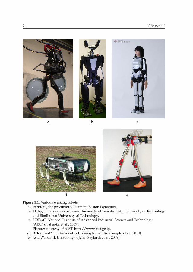
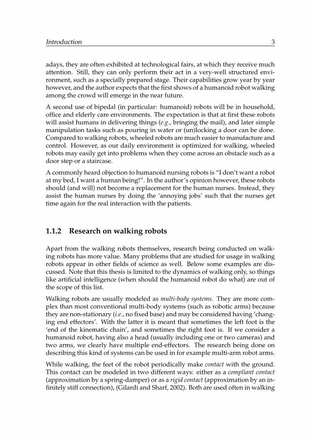
Some of the walking robots that exist today are shown in figure 1.1. It should benoted that only a small part of all existing robot designs are actually commerciallyavailable; most are prototypes from universities or spin-off companies. This the-sis discusses bipedal walking only, therefore, the rest of this section will focus onbipedal robots.
Humanoid robots gradually find their way into the entertainment industry. Now-
1
2 Chapter 1
a b c
d e
Figure 1.1: Various walking robots:a) PetProto, the precursor to Petman, Boston Dynamics,b) TUlip, collaboration between University of Twente, Delft University of Technology
and Eindhoven University of Technology,c) HRP-4C, National Institute of Advanced Industrial Science and Technology
(AIST) (Nakaoka et al., 2009).Picture: courtesy of AIST, http://www.aist.go.jp,
d) RHex, Kod*lab, University of Pennsylvania (Komsuoglu et al., 2010),e) Jena Walker II, University of Jena (Seyfarth et al., 2009).
Introduction 3
adays, they are often exhibited at technological fairs, at which they receive muchattention. Still, they can only perform their act in a very-well structured envi-ronment, such as a specially prepared stage. Their capabilities grow year by yearhowever, and the author expects that the first shows of a humanoid robot walkingamong the crowd will emerge in the near future.
A second use of bipedal (in particular: humanoid) robots will be in household,office and elderly care environments. The expectation is that at first these robotswill assist humans in delivering things (e.g., bringing the mail), and later simplemanipulation tasks such as pouring in water or (un)locking a door can be done.Compared to walking robots, wheeled robots are much easier to manufacture andcontrol. However, as our daily environment is optimized for walking, wheeledrobots may easily get into problems when they come across an obstacle such as adoor step or a staircase.
A commonly heard objection to humanoid nursing robots is “I don’t want a robotat my bed, I want a human being!”. In the author’s opinion however, these robotsshould (and will) not become a replacement for the human nurses. Instead, theyassist the human nurses by doing the ‘annoying jobs’ such that the nurses gettime again for the real interaction with the patients.
1.1.2 Research on walking robots
Apart from the walking robots themselves, research being conducted on walk-ing robots has more value. Many problems that are studied for usage in walkingrobots appear in other fields of science as well. Below some examples are dis-cussed. Note that this thesis is limited to the dynamics of walking only, so thingslike artificial intelligence (when should the humanoid robot do what) are out ofthe scope of this list.
Walking robots are usually modeled as multi-body systems. They are more com-plex than most conventional multi-body systems (such as robotic arms) becausethey are non-stationary (i.e., no fixed base) and may be considered having ‘chang-ing end effectors’. With the latter it is meant that sometimes the left foot is the‘end of the kinematic chain’, and sometimes the right foot is. If we consider ahumanoid robot, having also a head (usually including one or two cameras) andtwo arms, we clearly have multiple end-effectors. The research being done ondescribing this kind of systems can be used in for example multi-arm robot arms.
While walking, the feet of the robot periodically make contact with the ground.This contact can be modeled in two different ways: either as a compliant contact(approximation by a spring-damper) or as a rigid contact (approximation by an in-finitely stiff connection), (Gilardi and Sharf, 2002). Both are used often in walking
4 Chapter 1
robots. Compliant models are easy to implement, but usually make the model‘stiff’ (i.e., very high as well as very low eigenfrequencies within the model),which results in long simulation times. Rigid contact models do not suffer fromthis problem, but are hard to implement. Especially when multiple points are incontact at the same time, it is complex to figure out if contact loss occurs at any ofthe contacts (Ruspini and Khatib, 1997; Duindam, 2006). Other robotic fields inwhich contacts play a role, such as grasping or object stacking, can use the samestrategies for coping with contacts as in walking robots.
The actuation of almost all walking robots that are being built today is done byelectrical motors. Although this type of actuators has reached a high level of ma-turity, it is questionable whether this is, in the long term, the best actuator typefor walking robots. In order to make motors really suitable for walking, a fewproperties have to be ‘faked’ by control (see section 1.3.2). The control methodsdeveloped for this purpose can also be used in other fields of research, in partic-ular in robots that interact with humans. A few experiments are being conductedaround the world on making walking robots with actuators that are not basedon DC motors (Verrelst et al., 2005; Kratz et al., 2007). Once more knowledge isobtained on how to use these actuators in walking robots, the actuators can alsobe implemented in other types of robots.
The same holds for the mechanical design of walking robots. Due to the high de-mands on the mechanics (small and light to fit in the human-like shape, yet strongand accurate to ensure performance), innovative concepts are used in walkingrobot design. These concepts may be useful for other robots in other fields aswell.
Most robotics applications, such as industrial robot arms, use tight trajectory con-trol algorithms, meaning that at each instant in time, the system should be as closeas possible to a desired trajectory. For walking robots the exact trajectory of eachjoint is usually not so important; there are only bounds on the behavior. As anexample, in order to not topple over, the center of pressure of the robot should bewithin the foot area, but where it is exactly does not matter (see chapter 4). Thisfreedom could be exploited in new control algorithms that eventually can also beused in other fields of robotics.
Lastly, research on the dynamics of walking will lead to more insight in how hu-mans walk. By either synthesizing or analyzing the gait of a robot that has moreor less the same shape as a human, we can learn the principles behind walking:how exactly can we cope with disturbances and asymmetries, what if one of thejoints is limited in its agility, etc. Using a simple robot with only a few degrees offreedom and a simple (known) controller, gives us the possibility to isolate andstudy specific effects that influence the gait. The lessons learned can then be usedfor rehabilitation, orthoses and prostheses.
Introduction 5
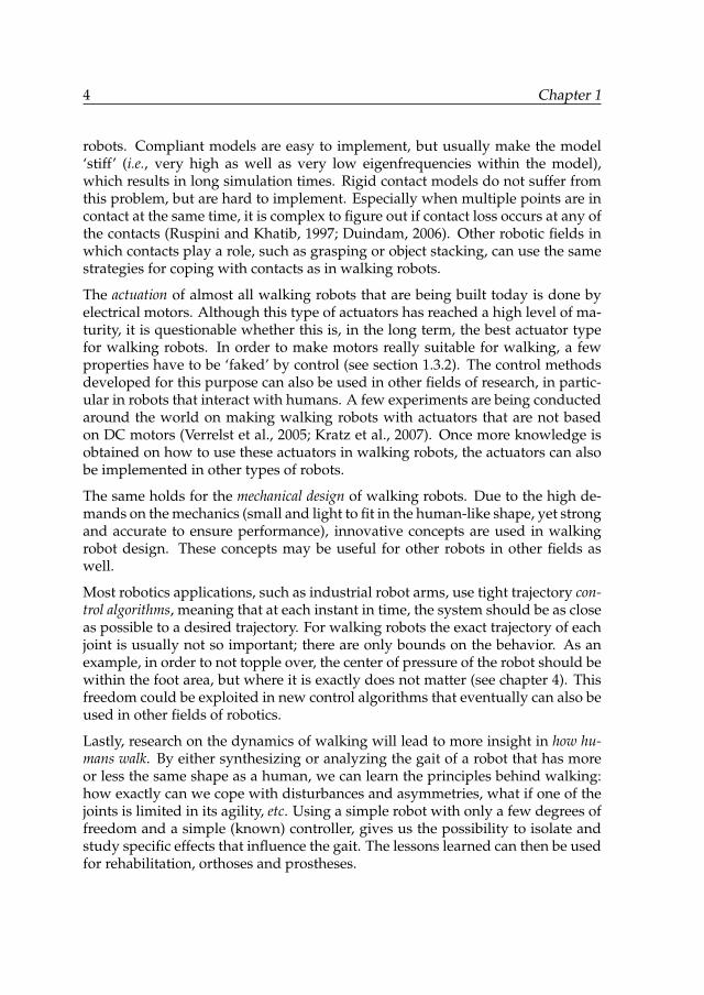
Figure 1.2: ‘Static walking’. As long as the center of mass of the robot is above the sup-porting foot and the movements are so slow that any dynamic effects can be neglected, therobot will not fall.
1.1.3 Different types of walking
Generally, the field of walking robots can be divided into two categories. Giv-ing an adequate name to these categories is hard, and will become harder in thefuture, as both categories tend to integrate more and more (which is a good de-velopment). The two categories, which will be termed Zero-Moment Point walkingand limit cycle walking in this thesis, will be explained below, together with a dis-cussion of the various names that are in use of the categories.
Zero-Moment Point walking
The easiest way to control a walking robot is by making sure that it is always instatic equilibrium. This is the case if
1. the center of mass (COM) of the robot is above the supporting foot, i.e., thevertical projection of the COM onto the ground plane is within the convexhull of the supporting foot (called the support polygon) as in figure 1.2, and
2. the movements of the robot are so slow that any dynamic effects can beneglected.
As soon as the vertical projection of the COM gets outside the support polygon,the foot will start to rotate (topple over) and the entire robot will fall. A goodterm for this type of walking would be static walking.
6 Chapter 1
ades
aτ
agrav
aup
FRI ZMP
ades
τ1
τ2
a bfZMP COP
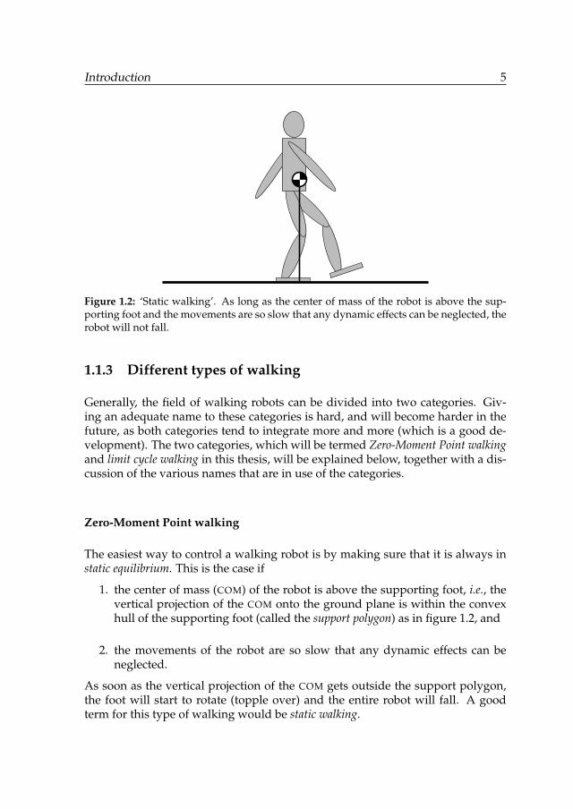
Figure 1.3: A 2D sketch showing the idea of extending static walking to include dynamics.a) A robot and the desired acceleration of the COM. b) All accelerations involved and theprojection of the COM along aτ onto the ground plane (resulting in the FRI or (f)ZMP). Inthis case, the FRI lies outside the convex hull of the support foot so the foot will start torotate about its rear edge. The ZMP or COP cannot leave the support polygon and coincideswith the rear edge of the foot in this case. It is assumed that there is no change in angularmomentum of the system.
The above can be extended by incorporating dynamics, in particular the acceler-ation of the center of mass. Assume that we want to accelerate the COM of a robotwith acceleration ades, as shown in figure 1.3. In order to do that, we need torquesτ on the joints that result in an acceleration aτ , being the combination of:
1. the desired acceleration ades, and
2. an acceleration component aup to counteract the gravitational accelerationagrav.
For the sake of simplicity, we assume that there is no change in angular momen-tum of the system. Now instead of projecting the COM of the robot straight downonto the ground plane, we project it along the vector aτ . The projection pointis known as the Foot Rotation Indicator (FRI), (Goswami, 1999) or (fictitious) Zero-Moment Point1((f)ZMP), (Vukobratovic and Borovac, 2004). Similarly to the staticcase, if this point is outside the support polygon, the foot will start to rotate.Contrary to the static case however, there is no direct link between the FRI beingoutside the support polygon and falling of the robot (Pratt and Tedrake, 2006).
1If the point is within the support polygon, it is called Zero-Moment Point (ZMP). If the point isoutside the support polygon, it is called fictitious Zero-Moment Point (fZMP) and the ZMP is the pointon the support polygon closest to the fZMP.
Introduction 7
gM
m
stanceleg
γ
swingleg
m
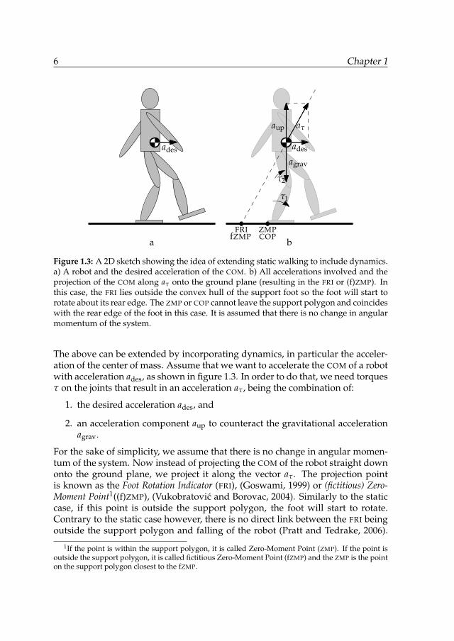
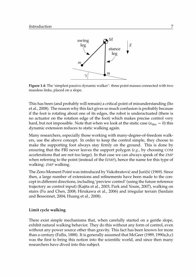
Figure 1.4: The ‘simplest passive dynamic walker’: three point masses connected with twomassless links, placed on a slope.
This has been (and probably will remain) a critical point of misunderstanding (Itoet al., 2008). The reason why this fact gives so much confusion is probably becauseif the foot is rotating about one of its edges, the robot is underactuated (there isno actuator on the rotation edge of the foot) which makes precise control veryhard, but not impossible. Note that when we look at the static case (ades = 0) thisdynamic extension reduces to static walking again.
Many researchers, especially those working with many-degree-of-freedom walk-ers, use the above concept. In order to keep the control simple, they choose tomake the supporting foot always stay firmly on the ground. This is done byensuring that the FRI never leaves the support polygon (e.g., by choosing COMaccelerations that are not too large). In that case we can always speak of the ZMPwhen referring to the point (instead of the fZMP), hence the name for this type ofwalking: ZMP walking.
The Zero-Moment Point was introduced by Vukobratovic and Juricic (1969). Sincethen, a large number of extensions and refinements have been made to the con-cept in different directions, including ‘preview control’ (using the future referencetrajectory as control input) (Kajita et al., 2003; Park and Youm, 2007), walking onstairs (Fu and Chen, 2008; Hirukawa et al., 2006) and irregular terrain (Sardainand Bessonnet, 2004; Huang et al., 2008).
Limit cycle walking
There exist simple mechanisms that, when carefully started on a gentle slope,exhibit natural walking behavior. They do this without any form of control, evenwithout any power source other than gravity. This fact has been known for morethan a century (Fallis, 1888). It is generally assumed that McGeer (1989, 1990a,b,c)was the first to bring this notion into the scientific world, and since then manyresearchers have dived into this subject.
8 Chapter 1
Consider a 2D mechanical structure as shown in figure 1.4: a ‘hip mass’ M, con-nected to two ‘foot masses’ m by rigid links. The structure is put on a gentle slopeγ and gravity g is acting on the system. Collisions between the feet and groundare considered fully inelastic and rigid. Friction is high enough to prevent slip-ping. Each of the legs is either in the role of stance leg or in the role of swing leg.
At the start of each step the rear leg leaves the ground and swings forward as apendulum. If we allow ‘foot scuffing’ (that is, allow the swing foot to temporarilypenetrate the ground while swinging forward), the swing foot will end up in frontof the stance foot, impacting the ground. Due to the rigidity and inelasticity ofthe collision, the rear foot will immediately leave the ground, starting a new step.During each step, the walker converts potential energy (it walks down the slope)to kinetic energy. At the end of the step, during foot impact, some of the kineticenergy of the walker is dissipated. Besides very naturally looking, this type ofwalking is very energy efficient.
There exist hip and foot trajectories such that after one complete step the state ofthe walker is exactly the same as it was before (only translated along the slope),i.e., if we denote the system state at the start of step k as xk, we have xk+1 = xkfor all k. Such a set of hip and foot trajectories is called a limit cycle. For a narrowset of parameters, the limit cycle of the walker is even stable: there is a smallregion around the limit cycle, called the basin of attraction (BOA), such that, whenthe walker is started within the BOA, the walker converges to the limit cycle andshows a stable walking gait. This type of walking is called passive dynamic walking:it utilizes only the passive dynamics of the system. It should be noted that therobustness of these passive dynamic walkers is very poor: if the walker is notstarted very close to the limit cycle, it will fall inevitably.
Many researchers have investigated passive dynamic walkers in different forms:with or without knees, with point feet or arc-shaped feet, with or without torso,2D or 3D etc. (Goswami et al., 1996; Collins et al., 2001; Wisse et al., 2004; Chen,2007; Kuo, 1999).
A natural extension to true passive dynamic walkers would be to add some formof actuation. There are mainly two reasons to do so:
1. to provide the energy needed for walking, such that walking on a horizontalfloor (γ = 0) becomes possible,
2. to provide some means of control to increase robustness or versatility.
A common place for the actuator is between the legs in the hip (Wisse and vanFrankenhuyzen, 2003; Beekman, 2004). This way, the actuator can help the swingleg to swing forward (provide energy for walking) and it can precisely positionthe leg in order to increase robustness (control). Another common place for theactuator is in the ankles (Hobbelen and Wisse, 2008), such that a push-off force
Introduction 9
can be generated. However, the potential of increasing robustness by control ofthe ankle actuator is much less than it is with hip actuation. Dribbel, the firstwalking robot developed at the Control Engineering Group at the University ofTwente, has both hip and ankle actuation (Franken, 2007).
This field of research suffers from an interesting conflict: on the one hand wewant to leave the walker alone in order not to disturb the nice passive dynamicbehavior, on the other hand, we want to actively control it in order to maximizethe robustness of the walker. Moreover, in order to keep the walker energy effi-cient, the controller action should be as low as possible.
Fortunately, the passive dynamics in the system can also help here. When a dis-turbance occurs, mechanical work should be done in order to restore the balance.However, it is not necessary that the actuator itself does all the work. Ideally,the actuator only changes the ‘shape’ of the system by a minimum control action,such that the passive dynamics result in the rebalancing of the system energy.As an example, consider the case where a walker has experienced a disturbancewhich has reduced the kinetic energy of the hip (i.e., it slowed down the forwardmotion of the hip). Now instead of actively accelerating the hip by applying alarge ankle torque, we could control the swing leg position such that a smallerstep is made than normal. This reduces the energy lost at the next foot impact, sothe total energy of the system is restored.
As already stated, the terms for different types of walking have become a littleconfusing. Especially the group of walkers that are based on passive dynamicwalking but do have actuation are referred to by many different terms. Below, afew are listed and the pitfalls are explained.
• As the ‘passive’ in ‘passive dynamic walking’ actually refers to the dynam-ics being passive (not the walker), it can be argued that passive dynamic walk-ing is a good term for the walkers considered, even if they are active. Therisk to confusion however is obvious, and therefore the use of this termshould be avoided.
• Following up on the previous term and its confusion, a term sometimesseen is the paradoxical but correct powered passive dynamic walking (Camp,1997; Mitobe et al., 2010).
• As the walkers considered are not passive anymore, people tend to simplyomit the word ‘passive’, resulting in the term dynamic walking (Kuo, 2007).This term is not incorrect (the walkers are walking in a dynamical fashion),but so are the ZMP-walkers! Therefore, this term does not distinguish be-tween these two types and the use of this term should be avoided.
• The safe way is just describing the field instead of giving a direct name:
10 Chapter 1
walking based on passive dynamic walking (Wisse and van Frankenhuyzen,2003; Collins et al., 2005), or, a little shorter, passivity-based walking (Hasset al., 2006; Wang et al., 2008).
• Probably the best solution — the one that the author favors — is to com-pletely abandon the words passive and dynamic and use the term limit cy-cle walking instead (Hosoda and Narioka, 2007; Hobbelen, 2008). This termexactly indicates the essence of all walkers in the category: the use of thenatural limit cycle.
The walking cycle of a limit cycle walker is dependent on the system dynamicsof the walker. Generally, only one limit cycle (i.e., one combination of step length,step time, ground clearance etc.) comes naturally with a walker. This is a limi-tation, because normally one wants to be able to make a robot exhibit differentgaits (at the very first, it should be able to transition from a ‘standing still gait’ toa walking gait). Similarly to the control case described above, one can extend thecapabilities of a limit cycle walker in two ways: either by making the actuatorsconstantly do work to push the walker into a different ‘artificial’ limit cycle, or byusing the actuator to change the dynamics so that a different natural limit cycleappears. As an example of the latter, consider a passive dynamic walker with avariable stiffness torsional spring between its legs. By having an actuator increasethe stiffness, the natural swing frequency of the swing leg increases, putting thewalker in a different (faster) limit cycle (Kuo, 2002).
Closing the gap
Humans are a good example of the combination of both strategies. Obviously,they have an enormous dexterity, which is due to the fact that they learned to dofull control on all limbs when needed. Also, when walking normally, the energyconsumption of humans is very low, suggesting that in that case extensive use ismade of the passive dynamics.
In order for future humanoid robots to be useful, they need both strategies aswell. They need the versatility from ZMP walkers to be able to start and stopwalking, turn and walk at different velocities, and they need the energy efficiencyof limit cycle walkers (having the naturally looking gait of limit cycle walkers canbe seen as a bonus). It is believed that, to reach the full potential of walking inrobots, both fields should merge into one integrated strategy. First attempts toclosing the gap for walking robots are being made (Hobbelen et al., 2008; Mitobeet al., 2010).
Introduction 11
2D and 3D walkers
In the world of walking robots, a clear distinction is made between two-dimen-sional (2D) and three-dimensional (3D) walkers. With a two-dimensional walker(also called a planar walker) a walker is meant that can move in the sagittal plane(forwards and backwards) but does not have any degrees of freedom to move inthe lateral plane (sideways). The reason to study two-dimensional walkers (bothin theory and in practice) is to split the complex problem of understanding walk-ing into smaller problems: first concentrate only on the fore–aft motion, and onlythen add the sideways motion.
In analysis and control, reducing the number of dimensions from three to tworeduces the complexity of locomotion to much less than 2/3rd of the originalcomplexity. Firstly, restricting to two dimensions reduces the number of direc-tions to which a robot can fall; it cannot fall sideways. Secondly, in the 3D case,the robot can rotate around its vertical axis and there exists complex couplingbetween motions in the sagittal and lateral plane, which does not exist in 2D. Fi-nally, the number of degrees of freedom of a 2D walker is generally much less,which results in equations of motion that are actually manageable.
Building a 2D robot is a different story. As we live in a 3D world, any real robotis essentially a 3D robot. In order to restrict its movements to two dimensions,three methods are available:
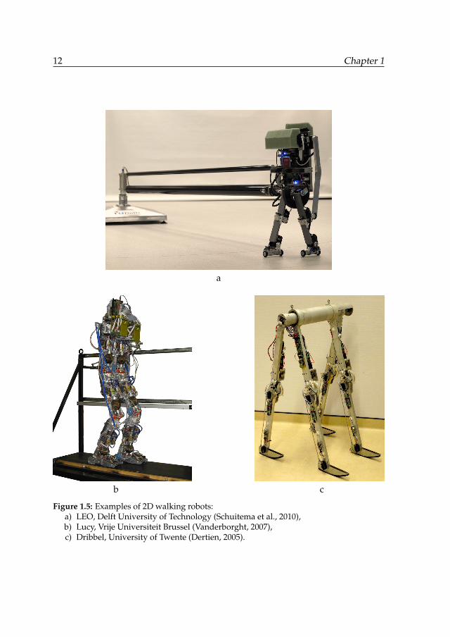
1. mounting a two-legged robot on the end of a boom in such a way that itcan walk on the perimeter of a circle (figure 1.5a). This is a quite simpleconstruction, but takes a lot of lab-space;
2. mounting a two-legged robot on a suspension that inhibits movements insideways direction and rotation around the unwanted axes (figure 1.5b).Care must be taken that the suspension does not influence the dynamics ofthe walker too much. Therefore, it should not be too heavy and have aslittle friction as possible;
3. building a free-walking four-legged robot with all its legs in line. The outerlegs are paired, as are the inner legs (figure 1.5c). The challenge in thistype of design is to make the paired legs identical, such that any sidewaysmotion is really impossible. The big advantage is that the robot is mobile soit can easily be demonstrated anywhere.
12 Chapter 1
a
b c
Figure 1.5: Examples of 2D walking robots:a) LEO, Delft University of Technology (Schuitema et al., 2010),b) Lucy, Vrije Universiteit Brussel (Vanderborght, 2007),c) Dribbel, University of Twente (Dertien, 2005).
Introduction 13
1.2 The VIACTORS project
Most industrial robots are manufactured as rigid as possible: in order to be accu-rate, control should be stiff and the deformation of the links of the robot shouldbe minimal. Consequently, the robots need to be heavy and the actuators needto be extremely powerful in order to achieve the desired accelerations. As longas no humans are close to the robot, nothing is wrong with that, except perhapsthe relatively large energy consumption. However, for robots operating in thevicinity of humans (think of a robotic arm mounted on a wheel chair of disabledperson, or a humanoid robot walking around in the same room as humans), thisis not a good choice. The problem is safety. The stiff controllers make that as soonas a slight deviation is found between the desired end-effector trajectory and theactual one, enormous forces are exerted. Moreover, as the impulse of a part of therobot scales linearly with its mass, a heavy part will have a large impulse whenmoving. Both can be dangerous if the robot accidentally comes in contact with ahuman.
To solve the problem, one could use sensors to detect any accidental contact andthen, by very quick (thus stiff) control, react on the sensory information to min-imize damage. If the system was designed well, this may be a good solution.However, if the sensor or controller fails, the robot is still dangerous.
Another way to cope with the problem is by not making the robot stiff in thefirst place; instead use light constructions (and compensate for deformation bycontrol) and use a special type of actuators that can be adapted to the task athand: strong if they need to but compliant if they can. Such actuators are calledvariable-impedance actuators.
The VIACTORS project, a project supported by the European Commission un-der the 7th Framework Programme, addresses the development and use of safe,energy-efficient, and highly dynamic variable-impedance actuation systems.
One of the ‘work packages’, WP5, focuses on locomotion with variable-impedanceactuation, in particular (Viactors, 2011): analysis, simulation and development oflegged locomotion systems which are, at the same time, robust, in terms of theability of the system to stabilize its motion under substantial disturbances, andenergy efficient, in terms of minimization of the energy consumptions. Focuspoints are:
• Morphological analysis and definition of metrics for “locomotion controlla-bility”;
• Implementation of developed actuators and control in humanoid robots;
• Modeling and simulations of (new actuation for) robust and energy efficient
14 Chapter 1
legged locomotion;
• Experiments of (new actuation for) robust and energy efficient legged loco-motion.
The following partners are in the consortium of VIACTORS: German AerospaceCenter (DLR), University of Pisa, University of Twente, Imperial college Lon-don, Italian Institute of Technology and Free University of Brussels. The author’sPh.D. position at the University of Twente has been financed for 40 % by VIAC-TORS.
1.3 Main topics of the thesis
Building walking robots is a multi-disciplinary job; it requires knowledge fromdifferent research areas to succeed. For this thesis it was chosen to take a lookat various disciplines instead of focusing on one aspect only. The thesis containsthree parts, which are discussed in more detail below.
1.3.1 Analysis
Analysis is the art of studying the behavior of a (complex) system and trying tofind rules that explain the behavior, in order to gain understanding of the system.An important aspect of analysis is the modeling of the system: the process ofmaking a (mathematical) system description in which only the relevant aspectsof the system are included. As an example, for general kinematics and dynam-ics analysis of a walking robot, it is often sufficient to make a rigid body model, inwhich each link of the robot is represented as an infinitely stiff mass and the con-nections between the links are represented as ideal prismatic or revolute joints.For different research questions, different aspects of a robot may be important,therefore different models should be used.
Many ‘tools’ are available for model making and analysis of the model. For verysimple walkers, typically 2D limit cycle walkers with three or less degrees of free-dom, the equations of motion may be simple enough to analyze analytically. Thiscan lead to basic but important conclusions such as the fact that for the ‘simplestwalker model’ the swing foot velocity just before foot impact does not influencethe dynamics for the next step (see chapter 2). For slightly larger models, theequations of motion are already too complex, and one must resort to analyzingnumerical trends or specific properties of the equations of motion, such as thePoincaré section, the step-to-step function and its eigenvalues (Goswami et al.,1996).
Introduction 15
When the walkers become even more complex, typically the ZMP walkers thathave many degrees of freedom, the analysis tools described above do not workanymore (the models are too complex to do such analysis and for ZMP walkersthe limit cycle analysis is irrelevant anyway). In those cases one can resort toanalysis tools like the center of mass (COM), extrapolated center of mass (XCOM)2
(Hof, 2008), center of pressure (COP), Zero-Moment Point (ZMP), locked inertiaand others. These are all concepts that ‘transform’ the full high-dimensional stateof the system to a meaningful two- or three-dimensional point in Euclidean space.
Often it is helpful to ‘look at the walker from a different point of view’. Forexample, when calculating the result of an inelastic collision between two bodies,it makes more sense to look at the impulses of the bodies than at their velocities:the equations become simpler just by taking different look. This can also be donefor walking robots. By using different mathematics (e.g., Screw theory, (Ball, 1900)instead of classical mechanics), analysis of the model can become much simpler.
Because walking robots are very complex systems with highly non-linear behav-ior, proper analysis tools are a necessity for building good robots. Without them,it is simply impossible to figure out whether a robot will be able to walk or not. Inorder to understand increasingly better the walking behavior of walking robots,new analysis tools constantly need to be developed.
1.3.2 Control and actuation
If there are actuators in a walking robot, these actuators should be steered in someway: a controller is needed. The non-linearity of the robots, as well as their verylimited margin of robustness (if any), may put high demands on the controllers.
For ZMP walkers, tight trajectory control is often used. Low-level feed-forwardcontrollers cancel out all internal dynamics and impose the accelerations obtainedfrom the desired trajectories while linear feed-back controllers compensate formodel mismatch and disturbances.
For limit cycle walkers, it is usually tried to make the controllers as simple aspossible, in order not to disturb the passive dynamic behavior too much. Oftenordinary linear feedback controllers are used. By choosing the input and outputof the controller carefully, very nice results can be achieved, even with linearcontrollers (see chapter 6).
The controller inside a walking robot can make or break the robot’s performance.Where a simple controller could barely keep a robot walking, a slight improve-ment (or even proper tuning) may improve the gait a lot. Therefore, research onproper control is vital for walking robots.
2Also known as the Instantaneous Capture Point (Pratt et al., 2006; Koolen, 2011).
16 Chapter 1
An ideal actuator is a lossless converter of energy from one domain (e.g., electrical)into mechanical energy (and vice versa), which does not influence the dynamicsof the joint, other than by the actuation torque. Electrical motors, the most-usedactuators for walking robots, are unfortunately far from ideal. Firstly, because ofthe series resistance in the electrical part of the motor, electrical energy is dissi-pated when a force is generated, even if no mechanical work is done. Secondly,the motor’s moment of inertia and friction (especially the gearbox) heavily influ-ence the dynamics of the joint (i.e., the motor is not backdrivable). Especially forlimit cycle walkers, this is undesired.
Biological muscles are, in some sense, better. Although they are certainly not loss-less (Whipp and Wasserman, 1969), their backdrivability (in uncontracted condi-tion) is much better than DC motors. Furthermore, muscles can exert high peakforces, which allows for quick disturbance rejection. The benefits of muscles areclearly seen in many walking organisms: their locomotion is highly energy effi-cient and robust. It is the author’s strong belief that, until an entirely new class of(muscle-like) actuators is mature enough for usage, we will not be able to buildhumanoid robots that are as versatile and robust against disturbances as humans.
As long as we still have to work with electric motors, there are ways to ‘fake’ ide-ality of some aspects of the actuator. Especially backdrivability (i.e., acting as apure force source) can be mimicked by embedding the motor in a series elastic actu-ator and applying appropriate control (Pratt and Williamson, 1995). This conceptcan be extended to a more versatile type of actuator, as discussed in chapter 8.
1.3.3 Design
Thanks to the recent improvements of materials and manufacturing techniques(3D printing for example) and to the miniaturization of electronics, humanoidrobots start to look better and better. In some cases (e.g., HRP-4C, figure 1.1c)the developers have succeeded to compress all the hardware into the postureof a normal human being. Still, the robots lack functionality that is needed forreally useful behavior. For example, in order to reduce weight, each hand ofHRP-4C is only provided with 2 degrees of freedom (Kaneko et al., 2009). So,future developments in design will be necessary for improving this.
For limit cycle walkers the design criteria are different than for ZMP walkers.As the internal dynamics of the system are important, this has to be taken intoconsideration much more than in ZMP walkers. As an example, for a good gait themass ratio between upper and lower leg should be approximately 10:1 (Frankenet al., 2008), which limits freedom of putting heavy actuators in the lower leg.Creative designs can help in such cases; by combining existing technology ininnovative ways, solutions can be generated for the problems. In this way, cleverdesign can help increasing the potential of limit cycle walkers.
Introduction 17
1.4 Thesis outline
1.4.1 Research goals
In this thesis a number of questions are addressed, all relevant to walking robots:
1. How can we analyze the behavior of a 2D passive dynamic walker that iswalking on rough terrain?
2. By looking at the robot from a different ‘perspective’, can we gain moreinsight in its dynamics?
3. How can we control a walking robot in order to stabilize it in the lateral(sideways) direction?
4. How can we improve the actuators in order to get minimum energy con-sumption?
5. How can we improve the knee and ankle joints of a walking robot?
1.4.2 Contents of each chapter
Each chapter in this thesis is based on a paper which has been published at orsubmitted to a conference (with the exception of chapter 3, which has not beenpublished before). The contents of each chapter is mostly identical to the origi-nal paper, but at some points the chapters in this thesis are more extensive: theycontain content that was originally removed from the paper to get it within theconference’s six-page limit (with the exception of chapter 7, which has under-gone a major revision). Because of the fact that the chapters are based on separatepapers, the contents of the chapters overlaps in some places. Below a short de-scription is given of each chapter, and it is indicated to which research goal thechapter contributes.
PART I: Analysis
Chapter 2 addresses question 1 from the research goals. A standard way of an-alyzing the behavior of a 2D walker is by using the so-called Poincaré map: afunction which, given the walker’s state x+k at the start of step k, returns the newstate x+k+1 at the start of step k + 1. In this chapter it is shown that this methodcan not be used for walkers on an irregular floor. An extension to this theory isproposed that does make it possible. Furthermore, the relation is shown between
18 Chapter 1
different types of disturbances and curves on the Poincaré section, introducing anew way of analyzing the walker’s behavior.
Chapter 3 addresses question 2 from the research goals. The configuration of awalking robot can be described as the pose (position and orientation) of one of therigid bodies (called the ‘reference body’) of the robot plus all internal joint angles.It is customary to take the torso as reference body. In this chapter it is shownthat in some cases it is more convenient to take the stance foot as reference body:the equations become easier. It is also shown how the reference body change (astandard non-linear coordinate transformation) is done on a 3D walking robot.
Chapter 4 addresses question 2 from the research goals. A widely used concept inrobot walking is the Zero-Moment Point (ZMP). The theory about ZMP, includingequations on how to calculate its position, exists already for over 40 years. In thischapter it is explained how the position of the ZMP can be found geometrically(i.e., in a coordinate-free manner) from the ground contact wrench. In order toarrive at this, general theorems are presented on how one can decompose onewrench W into other wrenches W ′1 and W ′2.
Chapter 5 also addresses question 2 from the research goals. It focuses on simpli-fication of the dynamic model of a 3D walker; in particular the approximation ofthe walker by one single rigid body (the locked inertia) rolling over the sole of acurved foot.
PART II: Control and actuation
Chapter 6 addresses question 3 from the research goals. In this chapter a specific3D walker model is used that, in its limit cycle, exhibits time-symmetrical behav-ior (i.e., the trajectories played backwards are identical to the trajectories playedforwards). In the case of a disturbance, the trajectory becomes asymmetric; theamount of asymmetry is used as an input for a (linear) stabilizing foot placementcontroller.
Chapter 7 also addresses question 3 from the research goals. In this chapter it isexplained how the walking robot ‘TUlip’ is controlled by means of the extrapolatedcenter of mass (XCOM). The XCOM is a projection of the robot’s center of mass(COM) onto the ground plane, where the direction of projection is dependent onCOM’s velocity. Experiments on the real robot are presented.
Chapter 8 addresses question 4 from the research goals. In this chapter a new ac-tuation concept is presented, called the very versatile energy efficient actuator, V2E2.An ideal actuator is just an energy converter (e.g., from the electrical to the me-chanical domain). The V2E2 has, on top of that, a mechanical energy storage ele-ment (a spring) and an ‘infinitely variable transmission’ (a continuously variable
Introduction 19
transmission that can have a positive as well as negative transmission ratio). Thepower of the V2E2is its ability to store negative work mechanically and release itwhen positive work is needed.
PART III: Design
Chapter 9 addresses question 5 from the research goals. It describes the designof a new knee locking mechanism for the 2D walking robot Dribbel. The mecha-nism keeps the leg in extended position while it serves as stance leg. It does thisby exploiting a mechanical singularity which, in theory, can withstand arbitrarylarge torques while consuming no energy. Unlocking however only requires aminimum amount of energy. In this chapter the system is described in detail andexperiments are presented that show the benefits of the system.
Chapter 10 also addresses question 5 from the research goals. It describes theanalysis, design and control of a new ankle actuation system for the 3D walkingrobot TUlip. The system consists of two series-elastic actuators (DC-motors withsprings in series) that drive both the x-axis (sideways rotation) and y-axis (for-ward/backward rotation) of the ankle, in a differential set-up. The analysis ofthis non-linear, coupled series elastic system is treated in this chapter, as well assome control issues following from the series elasticity and non-linearity.

20 Chapter 1

Part I
Analysis
21

Chapter 2
The Poincaré section and basin ofattraction of a 2D passive dynamic
walker on an irregular floor
This chapter is based on the following article (van Oort and Stramigioli, 2012):
The Poincaré section and basin of attraction of a2D passive dynamic walker on an irregular floor
Gijs van Oort and Stefano StramigioliSubmitted to IEEE International Conference on
Robotics and Automation (ICRA’12).
Abstract—In analysis of passive dynamic walking, one often makes use of thePoincaré section and basin of attraction. In this chapter we show that thesemethods cannot be used when the walker walks on an irregular floor. As a so-lution we propose three different mappings (called stance foot angle mapping,rotation mapping and integration mapping) and show that integration mappingis optimal for analysis. Furthermore, we introduce a new way to visualize therelation between disturbances of different magnitude and the states on thePoincaré section. This opens a new way of analyzing the walker’s behavior.We show the effectiveness of the proposed methods by means of a simple sim-ulation experiment.
23
24 Chapter 2
2.1 Introduction
For more than two decades already people have researched passive dynamicwalking. A passive dynamic walker is a mechanical system that, when ‘launched’from a gentle slope, can exhibit stable walking behavior (McGeer, 1990b). Thereare no actuators in the system; all energy needed for walking is obtained fromgravity’s potential field. For quite a large range of parameters stable walking canbe achieved, but the robustness of these walkers is very poor (i.e., if the walker isnot started ‘close to the periodic trajectory’, it falls).
For analyzing the behavior of passive dynamic walkers, the notions of Poincarésection, and basin of attraction are often used. Although these have been studiedintensively in the past (by Goswami et al. (1998); Liu et al. (2007); Schwab andWisse (2001) and more), we found that they were often only loosely defined; usu-ally just by a sentence that only intuitively makes sense1.
In this chapter we will define the Poincaré section and the basin of attraction ina more formal manner, and show that this has implications if one wants to usethem on irregular floors. Secondly, we show the relation between points on thebasin of attraction and various disturbances. This helps in understanding howvarious disturbances influence the gait.
This chapter is organized as follows. At the end of this introduction, we intro-duce two walker models that we will use throughout the chapter and spend somewords on irregular floors. In section 2.2 we introduce the equations that describethe behavior of the walkers. Then, in section 2.3 we give a definition of the Poin-caré section. It also contains the main contribution of this chapter: the descriptionof how to deal with irregular floors and the Poincaré section. In section 2.4 wegive a definition of the basin of attraction and discuss the usage of the area ofbasin of attraction as a measure of robustness. Section 2.5 contains the secondcontribution of this chapter, being the relation between points on the basin of at-traction and various disturbances. Finally, in section 2.6 we show by means ofsome experiments the usage of the methods.
2.1.1 Test models
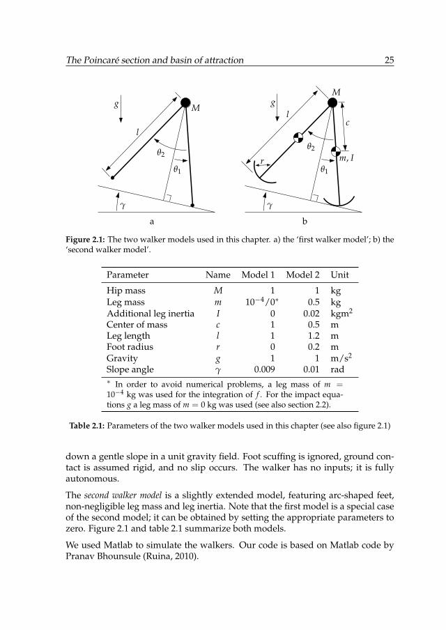
In this chapter, we use two different 2D walker models for our simulations. Theseare described below. The first walker model is the model used by Garcia et al.(1998). It is a compass walker model (no knees) with point feet, a unit point massM at the hip, very small foot mass (m � M), having unit length legs, walking
1A notable exception is the work by Grizzle et al. (2001), which thoroughly defines the Poincarésection. His definition however, is incompatible with irregular floors.
The Poincaré section and basin of attraction 25
θ1
θ2
γ
l
g M
θ1
θ2
γ
lg
M
r m, I
c
a b
Figure 2.1: The two walker models used in this chapter. a) the ‘first walker model’; b) the‘second walker model’.
Parameter Name Model 1 Model 2 Unit
Hip mass M 1 1 kgLeg mass m 10−4/0∗ 0.5 kgAdditional leg inertia I 0 0.02 kgm2
Center of mass c 1 0.5 mLeg length l 1 1.2 mFoot radius r 0 0.2 mGravity g 1 1 m/s2
Slope angle γ 0.009 0.01 rad∗ In order to avoid numerical problems, a leg mass of m =10−4 kg was used for the integration of f . For the impact equa-tions g a leg mass of m = 0 kg was used (see also section 2.2).
Table 2.1: Parameters of the two walker models used in this chapter (see also figure 2.1)
down a gentle slope in a unit gravity field. Foot scuffing is ignored, ground con-tact is assumed rigid, and no slip occurs. The walker has no inputs; it is fullyautonomous.
The second walker model is a slightly extended model, featuring arc-shaped feet,non-negligible leg mass and leg inertia. Note that the first model is a special caseof the second model; it can be obtained by setting the appropriate parameters tozero. Figure 2.1 and table 2.1 summarize both models.
We used Matlab to simulate the walkers. Our code is based on Matlab code byPranav Bhounsule (Ruina, 2010).
26 Chapter 2
−θ1
−θ2
γ
r
hi
l
hi
hi−1
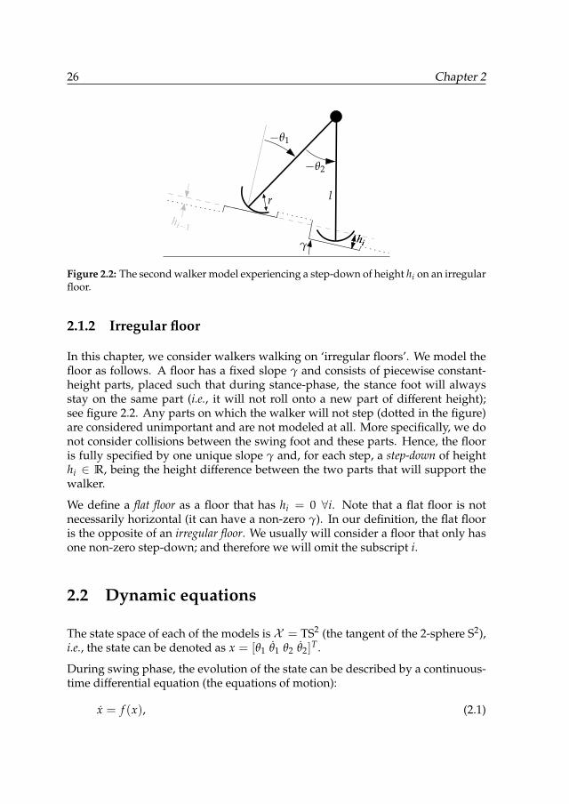
Figure 2.2: The second walker model experiencing a step-down of height hi on an irregularfloor.
2.1.2 Irregular floor
In this chapter, we consider walkers walking on ‘irregular floors’. We model thefloor as follows. A floor has a fixed slope γ and consists of piecewise constant-height parts, placed such that during stance-phase, the stance foot will alwaysstay on the same part (i.e., it will not roll onto a new part of different height);see figure 2.2. Any parts on which the walker will not step (dotted in the figure)are considered unimportant and are not modeled at all. More specifically, we donot consider collisions between the swing foot and these parts. Hence, the flooris fully specified by one unique slope γ and, for each step, a step-down of heighthi ∈ R, being the height difference between the two parts that will support thewalker.
We define a flat floor as a floor that has hi = 0 ∀i. Note that a flat floor is notnecessarily horizontal (it can have a non-zero γ). In our definition, the flat flooris the opposite of an irregular floor. We usually will consider a floor that only hasone non-zero step-down; and therefore we will omit the subscript i.
2.2 Dynamic equations
The state space of each of the models is X = TS2 (the tangent of the 2-sphere S2),i.e., the state can be denoted as x = [θ1 θ1 θ2 θ2]
T .
During swing phase, the evolution of the state can be described by a continuous-time differential equation (the equations of motion):
x = f (x), (2.1)
The Poincaré section and basin of attraction 27
where f is a nonlinear continuous function. The exact equations of motion forthe first model are written out in (Garcia et al., 1998). Note that during normalwalking, θ1 < 0. As soon as the swing foot hits the floor (‘heelstrike’ or ‘impact’),the state is instantaneously reset using the impact equations
x+ = g(x−), (2.2)
where x− and x+ denote the state just before and just after the moment of impactrespectively and g is a continuous function. The impact equations also effectuatethe leg-relabeling. The post-impact velocities θ+1 , θ+2 are linear in θ−1 and θ−2 .
On a flat (i.e., non-irregular) floor, the moment of impact is when x ∈ S0, where
S0 = {x ∈ X | θ2 = 2θ1, both legs on the ground−π < θ2 < 0, stance foot behind swing footθ1 < 0, forward movementθ2 < 2θ1 swing foot goes down}.
(2.3)
In the field of hybrid systems, S0 ⊂ X is called the switching surface, and theimpact equations g are seen as a function g : S0 → X . We define S?• as the imageof g when applied to S•; i.e., by definition X ⊃ S?0 = {g(x−)|x− ∈ S0}. Inthe case of irregular terrain, a step down or obstacles, the switching surface isdifferent. For example, when experiencing a step-down of height h, the momentof impact (and thus the switching surface) for both walker models is
Sh = {x ∈ X | (l − r) cos(θ2 − θ1) = (l − r) cos θ1 + h,−π < θ2 < 0, θ1 < 0,sin(θ2 − θ1)(θ2 − θ1)− sin θ1 θ1 < 0}.
(2.4)
In order for the impact equations g to be valid always, any switching surface S•should be in the domain of g. Therefore we’d rather see g as a function g : X →X , meaning that it can return, for any state x− a post-impact state x+ if the swingfoot would hit an object at that particular x−.
For later reference, we show the impact equations g of the first walker model(contrary to for example the equations by Garcia et al. (1998), this is valid for anyx− ∈ X ):
θ1θ1θ2θ2
+
=
1 0 −1 00 cos θ2 0 00 0 −1 00 cos θ2(1− cos θ2) 0 0
θ1θ1θ2θ2
−
. (2.5)
The impact equations of the second walker model are a much more complexfunction of θ2. Around the limit cycle, having x− ≈ [−0.19 rad,−0.26 rad/s,
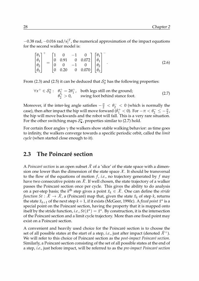
28 Chapter 2
−0.38 rad,−0.016 rad/s]T , the numerical approximation of the impact equationsfor the second walker model is:
θ1θ1θ2θ2
+
=
1 0 −1 00 0.91 0 0.0720 0 −1 00 0.20 0 0.070
θ1θ1θ2θ2
−
. (2.6)
From (2.3) and (2.5) it can be deduced that S?0 has the following properties:
∀x+ ∈ S?0 : θ+2 = 2θ+1 , both legs still on the ground;θ+2 > 0, swing foot behind stance foot.
(2.7)
Moreover, if the inter-leg angle satisfies −π2 < θ−2 < 0 (which is normally the
case), then after impact the hip will move forward (θ+1 < 0). For−π < θ−2 ≤ −π2 ,
the hip will move backwards and the robot will fall. This is a very rare situation.For the other switching maps S?• , properties similar to (2.7) hold.
For certain floor angles γ the walkers show stable walking behavior: as time goesto infinity, the walkers converge towards a specific periodic orbit, called the limitcycle (when started close enough to it).
2.3 The Poincaré section
A Poincaré section is an open subset X of a ‘slice’ of the state space with a dimen-sion one lower than the dimension of the state space X . It should be transversalto the flow of the equations of motion f , i.e., no trajectory generated by f mayhave two consecutive points on X . If well chosen, the state trajectory of a walkerpasses the Poincaré section once per cycle. This gives the ability to do analysison a per-step basis; the kth step gives a point xk ∈ X . One can define the stridefunction St : X → X , a (Poincaré) map that, given the state xk of step k, returnsthe state xk+1 of the next step k+ 1, if it exists (McGeer, 1990c). A fixed point x? is aspecial point on the Poincaré section, having the property that it is mapped ontoitself by the stride function, i.e., St(x?) = x?. By construction, it is the intersectionof the Poincaré section and a limit cycle trajectory. More than one fixed point mayexist on a Poincaré section.
A convenient and heavily used choice for the Poincaré section is to choose theset of all possible states at the start of a step, i.e., just after impact (denoted X+).We will refer to this choice of Poincaré section as the post-impact Poincaré section.Similarly, a Poincaré section consisting of the set of all possible states at the end ofa step, i.e., just before impact, will be referred to as the pre-impact Poincaré section
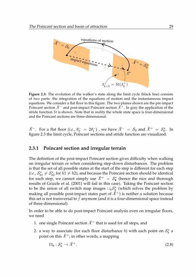
The Poincaré section and basin of attraction 29
equations of motion
x+k+1 = St(x+k )
X += S ?
0
X −= S0
x?
impact equations
Figure 2.3: The evolution of the walker’s state along the limit cycle (black line) consistsof two parts: the integration of the equations of motion and the instantaneous impactequations. We consider a flat floor in this figure. The two planes shown are the pre-impactPoincaré section X− and post-impact Poincaré section X+. In gray the application of thestride function St is shown. Note that in reality the whole state space is four-dimensionaland the Poincaré sections are three-dimensional.
X−. For a flat floor (i.e., θ−2 = 2θ−1 ) , we have X− = S0 and X+ = S?0 . Infigure 2.3 the limit cycle, Poincaré sections and stride function are visualized.
2.3.1 Poincaré section and irregular terrain
The definition of the post-impact Poincaré section gives difficulty when walkingon irregular terrain or when considering step-down disturbances. The problemis that the set of all possible states at the start of the step is different for each step(i.e., S?h1 6= S?h2 for h1 6= h2), and because the Poincaré section should be identicalfor each step, we cannot simply use X+ = S?• (hence the nice and thoroughresults of Grizzle et al. (2001) will fail in this case). Taking the Poincaré sectionto be the union of all switch map images ∪hS?h (which solves the problem bymaking all possible post-impact states part of X+) is neither a solution becausethis set is not transversal to f anymore (and it is a four-dimensional space insteadof three-dimensional).
In order to be able to do post-impact Poincaré analysis even on irregular floors,we need
1. one single Poincaré section X+ that is used for all steps, and
2. a way to associate (for each floor disturbance h) with each point on S?h apoint on this X+; in other words, a mapping
Πh : S?h → X+. (2.8)
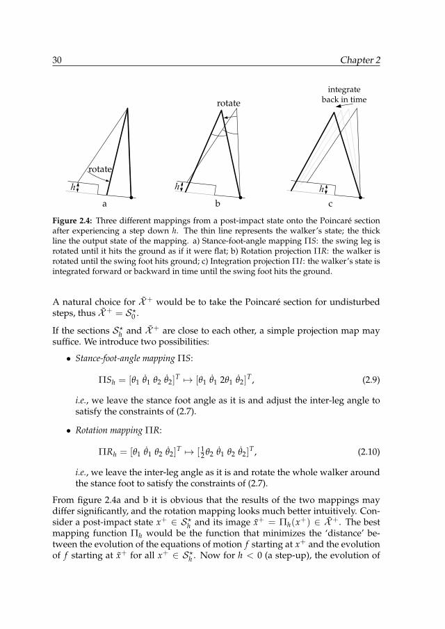
30 Chapter 2
a
h
rotate
rotate
b
h
integrateback in time
c
h
Figure 2.4: Three different mappings from a post-impact state onto the Poincaré sectionafter experiencing a step down h. The thin line represents the walker’s state; the thickline the output state of the mapping. a) Stance-foot-angle mapping ΠS: the swing leg isrotated until it hits the ground as if it were flat; b) Rotation projection ΠR: the walker isrotated until the swing foot hits ground; c) Integration projection ΠI: the walker’s state isintegrated forward or backward in time until the swing foot hits the ground.
A natural choice for X+ would be to take the Poincaré section for undisturbedsteps, thus X+ = S?0 .
If the sections S?h and X+ are close to each other, a simple projection map maysuffice. We introduce two possibilities:
• Stance-foot-angle mapping ΠS:
ΠSh = [θ1 θ1 θ2 θ2]T 7→ [θ1 θ1 2θ1 θ2]
T , (2.9)
i.e., we leave the stance foot angle as it is and adjust the inter-leg angle tosatisfy the constraints of (2.7).
• Rotation mapping ΠR:
ΠRh = [θ1 θ1 θ2 θ2]T 7→ [ 1
2 θ2 θ1 θ2 θ2]T , (2.10)
i.e., we leave the inter-leg angle as it is and rotate the whole walker aroundthe stance foot to satisfy the constraints of (2.7).
From figure 2.4a and b it is obvious that the results of the two mappings maydiffer significantly, and the rotation mapping looks much better intuitively. Con-sider a post-impact state x+ ∈ S?h and its image x+ = Πh(x+) ∈ X+. The bestmapping function Πh would be the function that minimizes the ‘distance’ be-tween the evolution of the equations of motion f starting at x+ and the evolutionof f starting at x+ for all x+ ∈ S?h . Now for h < 0 (a step-up), the evolution of
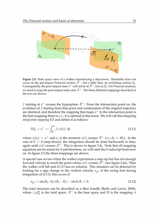
The Poincaré section and basin of attraction 31
X −= S0
Sh
S?hx+
ΠSΠR ΠI
X += S ?
0
Figure 2.5: State space view of a walker experiencing a step-down. Heelstrike does notoccur on the pre-impact Poincaré section X−, but a little later, on switching surface Sh.Consequently, the post-impact state x+ will not be at X+, but at S?h . For Poincaré analysis,we need to map the post-impact state onto X+. The three different mappings described inthe text are shown.
f starting at x+ crosses the hyperplane X+. From the intersection point on, theevolution of f starting from that point and continuation of the original trajectoryare identical, and therefore the mapping that maps x+ to the intersection point isthe best mapping there is, i.e., it is optimal in this sense. We will call this mappingintegration mapping ΠI and define it as follows:
ΠIh = x+ 7→∫ t1
t0f (x(t)) dt (2.11)
where x(t0) = x+ and t1 is the moment x(t) crosses X+ (i.e., θ2 = 2θ1). In thecase of h > 0 (step-down), the integration should be done backwards in time,again until x(t) crosses X+. This is shown in figure 2.4c. Note that all mappingequations are invariant for h and therefore, we will omit the h-subscript from nowon. In figure 2.5 the three mappings are shown.
A special case occurs when the walker experiences a step-up but has not enoughforward velocity to reach the point where x(t) crosses X+ (see figure 2.6a). Thenthe walker will fall and (2.11) has no solution. This situation can be detected bylooking for a sign change in the vertical velocity vy f of the swing foot duringintegration of (2.11); this occurs if
vy f = sin(θ2−θ1)(θ2 − θ1)− sin θ1 θ1 = 0. (2.12)
The total structure can be described as a fiber bundle (Bullo and Lewis, 2004),where ∪hS?h is the total space, X+ is the base space and Π is the mapping π
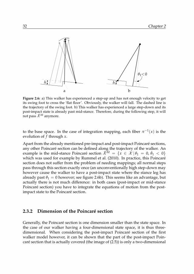
32 Chapter 2
a
h
b
h
θ1<0
Figure 2.6: a) This walker has experienced a step-up and has not enough velocity to getits swing foot to cross the ‘flat floor’. Obviously, the walker will fall. The dashed line isthe trajectory of the swing foot. b) This walker has experienced a large step-down and itspost-impact state is already past mid-stance. Therefore, during the following step, it willnot pass XM anymore.
to the base space. In the case of integration mapping, each fiber π−1(x) is theevolution of f through x.
Apart from the already mentioned pre-impact and post-impact Poincaré sections,any other Poincaré section can be defined along the trajectory of the walker. Anexample is the mid-stance Poincaré section XM = {x ∈ X | θ1 = 0, θ1 < 0}which was used for example by Rummel et al. (2010). In practice, this Poincarésection does not suffer from the problem of needing mappings; all normal stepspass through this section exactly once (an unconventionally high step-down mayhowever cause the walker to have a post-impact state where the stance leg hasalready past θ1 = 0 however; see figure 2.6b). This seems like an advantage, butactually there is not much difference: in both cases (post-impact or mid-stancePoincaré section) you have to integrate the equations of motion from the post-impact state to the Poincaré section.
2.3.2 Dimension of the Poincaré section
Generally, the Poincaré section is one dimension smaller than the state space. Inthe case of our walker having a four-dimensional state space, it is thus three-dimensional. When considering the post-impact Poincaré section of the firstwalker model however, it can be shown that the part of the post-impact Poin-caré section that is actually covered (the image of (2.5)) is only a two-dimensional
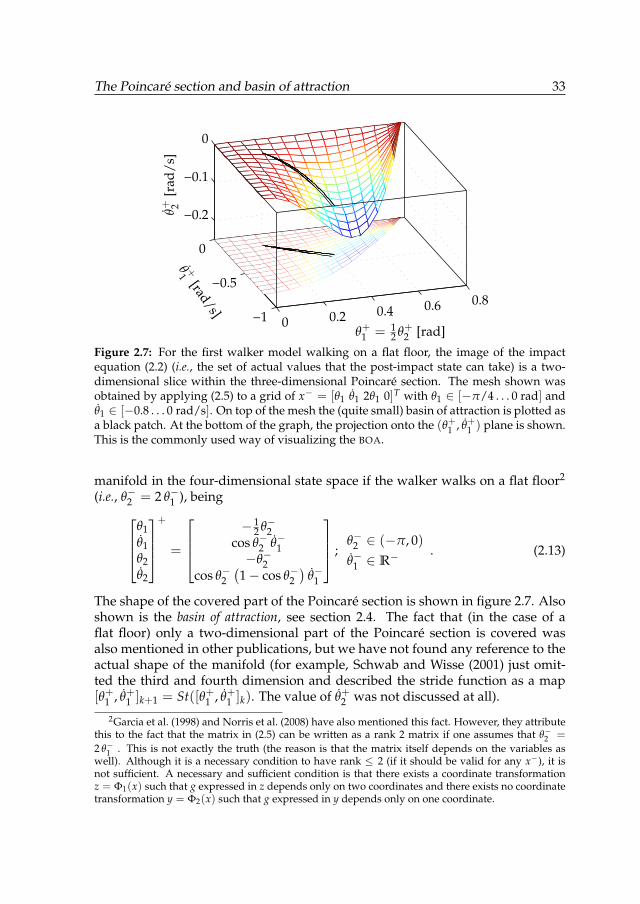
The Poincaré section and basin of attraction 33
00.2
0.40.6
0.8
−1
−0.5
0
−0.2
−0.1
0
θ+1 = 12 θ+2 [rad]
θ +1 [rad/s]
θ+ 2[r
ad/s
]
Figure 2.7: For the first walker model walking on a flat floor, the image of the impactequation (2.2) (i.e., the set of actual values that the post-impact state can take) is a two-dimensional slice within the three-dimensional Poincaré section. The mesh shown wasobtained by applying (2.5) to a grid of x− = [θ1 θ1 2θ1 0]T with θ1 ∈ [−π/4 . . . 0 rad] andθ1 ∈ [−0.8 . . . 0 rad/s]. On top of the mesh the (quite small) basin of attraction is plotted asa black patch. At the bottom of the graph, the projection onto the (θ+1 , θ+1 ) plane is shown.This is the commonly used way of visualizing the BOA.
manifold in the four-dimensional state space if the walker walks on a flat floor2
(i.e., θ−2 = 2 θ−1 ), being
θ1θ1θ2θ2
+
=
− 12 θ−2
cos θ−2 θ−1−θ−2
cos θ−2(1− cos θ−2
)θ−1
;
θ−2 ∈ (−π, 0)θ−1 ∈ R−
. (2.13)
The shape of the covered part of the Poincaré section is shown in figure 2.7. Alsoshown is the basin of attraction, see section 2.4. The fact that (in the case of aflat floor) only a two-dimensional part of the Poincaré section is covered wasalso mentioned in other publications, but we have not found any reference to theactual shape of the manifold (for example, Schwab and Wisse (2001) just omit-ted the third and fourth dimension and described the stride function as a map[θ+1 , θ+1 ]k+1 = St([θ+1 , θ+1 ]k). The value of θ+2 was not discussed at all).
2Garcia et al. (1998) and Norris et al. (2008) have also mentioned this fact. However, they attributethis to the fact that the matrix in (2.5) can be written as a rank 2 matrix if one assumes that θ−2 =
2 θ−1 . This is not exactly the truth (the reason is that the matrix itself depends on the variables aswell). Although it is a necessary condition to have rank ≤ 2 (if it should be valid for any x−), it isnot sufficient. A necessary and sufficient condition is that there exists a coordinate transformationz = Φ1(x) such that g expressed in z depends only on two coordinates and there exists no coordinatetransformation y = Φ2(x) such that g expressed in y depends only on one coordinate.
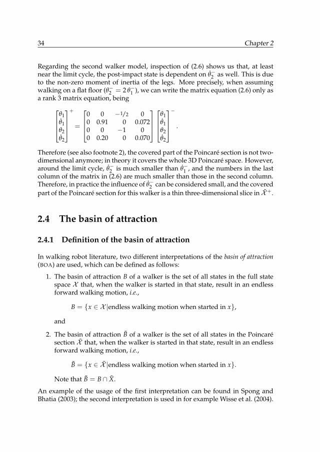
34 Chapter 2
Regarding the second walker model, inspection of (2.6) shows us that, at leastnear the limit cycle, the post-impact state is dependent on θ−2 as well. This is dueto the non-zero moment of inertia of the legs. More precisely, when assumingwalking on a flat floor (θ−2 = 2 θ−1 ), we can write the matrix equation (2.6) only asa rank 3 matrix equation, being
θ1θ1θ2θ2
+
=
0 0 −1/2 00 0.91 0 0.0720 0 −1 00 0.20 0 0.070
θ1θ1θ2θ2
−
.
Therefore (see also footnote 2), the covered part of the Poincaré section is not two-dimensional anymore; in theory it covers the whole 3D Poincaré space. However,around the limit cycle, θ−2 is much smaller than θ−1 , and the numbers in the lastcolumn of the matrix in (2.6) are much smaller than those in the second column.Therefore, in practice the influence of θ−2 can be considered small, and the coveredpart of the Poincaré section for this walker is a thin three-dimensional slice in X+.
2.4 The basin of attraction
2.4.1 Definition of the basin of attraction
In walking robot literature, two different interpretations of the basin of attraction(BOA) are used, which can be defined as follows:
1. The basin of attraction B of a walker is the set of all states in the full statespace X that, when the walker is started in that state, result in an endlessforward walking motion, i.e.,
B = {x ∈ X |endless walking motion when started in x},
and
2. The basin of attraction B of a walker is the set of all states in the Poincarésection X that, when the walker is started in that state, result in an endlessforward walking motion, i.e.,
B = {x ∈ X |endless walking motion when started in x}.
Note that B = B ∩ X.
An example of the usage of the first interpretation can be found in Spong andBhatia (2003); the second interpretation is used in for example Wisse et al. (2004).
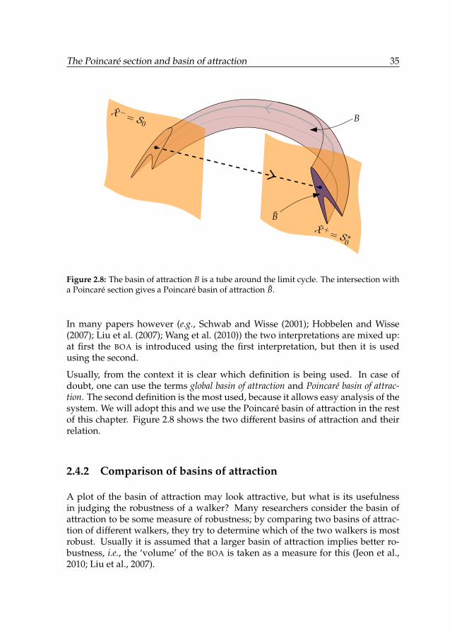
The Poincaré section and basin of attraction 35
X += S ?
0
X −= S0 B
B
Figure 2.8: The basin of attraction B is a tube around the limit cycle. The intersection witha Poincaré section gives a Poincaré basin of attraction B.
In many papers however (e.g., Schwab and Wisse (2001); Hobbelen and Wisse(2007); Liu et al. (2007); Wang et al. (2010)) the two interpretations are mixed up:at first the BOA is introduced using the first interpretation, but then it is usedusing the second.
Usually, from the context it is clear which definition is being used. In case ofdoubt, one can use the terms global basin of attraction and Poincaré basin of attrac-tion. The second definition is the most used, because it allows easy analysis of thesystem. We will adopt this and we use the Poincaré basin of attraction in the restof this chapter. Figure 2.8 shows the two different basins of attraction and theirrelation.
2.4.2 Comparison of basins of attraction
A plot of the basin of attraction may look attractive, but what is its usefulnessin judging the robustness of a walker? Many researchers consider the basin ofattraction to be some measure of robustness; by comparing two basins of attrac-tion of different walkers, they try to determine which of the two walkers is mostrobust. Usually it is assumed that a larger basin of attraction implies better ro-bustness, i.e., the ‘volume’ of the BOA is taken as a measure for this (Jeon et al.,2010; Liu et al., 2007).
36 Chapter 2
In most cases, comparing the basins of attraction of two different walkers is notmeaningful: from the basin of attraction one cannot immediately tell which oneis ‘better’. We can explain this with an easy contradictory example.
Consider two walkers, A and B. Assume that walker B moves twice as fast aswalker A and that the basin of attraction of walker B is the same as that of walkerA but stretched a factor of two in the velocity direction. If we consider the volumeof the BOA’s as a measure of robustness, we may conclude that walker B is twiceas robust as walker A. However, if we would normalize the plots relatively to thefixed point x?, we would conclude that both robots are equally robust. Thus, ourconclusion depends on our choice of representation and not solely on the walkerproperties.
Mathematically speaking, considering the volume of the BOA makes no sense atall. This is because the BOA is a subset of X = TS2, and a thing as a volume isnot defined on TS2. We could abuse the fact that TS2 is locally homeomorphic toR4 to define a volume for a small part of the domain, but then the volume willbe dependent on the homeomorphism used. In the case of our simple walkers(figure 2.7), the unit of the volume (assuming the mis-use of the homeomorphism)is rad3/s2, which is physically not something meaningful. Furthermore, if wewould use different coordinates, the volume measurement would change too. Inother words, the ‘volume’ of the BOA is not an intrinsic property of the walker, itis influenced by the choice of coordinates. Even worse: by sticking strictly to this‘definition’, we would conclude that the first walker is not robust at all becausethe volume of its basin of attraction is zero (a 2D surface in a 3D space has novolume).
In practice however, in some cases it may still be meaningful to compare twodifferent basins of attraction: if two very similar walkers have the same fixedpoint x? and the same coordinates and homeomorphism are used. An example isif we have one robot and test different closed-loop controllers on it. It is requiredthen, however, that all controllers act identically when the walker is in its limitcycle (otherwise, the different set-ups still have different fixed points).
2.5 Relation between BOA and disturbances
The assumption is often made that a larger basin of attraction directly impliesa more robust walker. Intuitively this sounds reasonable: if a larger part of allpossible states is inside the BOA, then the chances are higher that the visited statesare inside. The thing that we are interested in however, is not purely ‘how muchof the states’ is within the BOA, but much more something like ‘how much of theimportant states’ is within the BOA. In other words: it does not help to makethe basin of attraction larger if the majority of the added states is never reached
The Poincaré section and basin of attraction 37
anyway. Therefore, it is interesting to know which part of the Poincaré sectionis covered during normal walking (with disturbances). Below we present a newway of visualizing the relation between the Poincaré BOA and disturbances: acurve on the Poincaré section, associated with the disturbance.
Let us investigate some disturbance (e.g., an impulsive torque around the stanceankle just after the start of the step, or a step-down) with magnitude d ∈ R.When experiencing a disturbance (i.e., d 6= 0), the walker will deviate from itslimit cycle, and thus cross the post-impact Poincaré section at a point x(d) 6= x?.We can draw a curve consisting of all points {x(d)|d ∈ R}. By definition, thiscurve fully lies in the covered part of the Poincaré section and it includes the fixedpoint x? (for d = 0). If and only if the disturbance is such that the walker will notfall, then the point x(d) lies within the basin of attraction. For large disturbances,the walker cannot complete a full step (e.g., for a large step-up the swing foot willnever reach the floor level after foot-scuffing), so not for each d there exists a x(d).
As an example we inspect the following disturbances on the walker:
• An impulsive torque p ∈ R around stance ankle just after the start of thestep; the maximum value P such that the walker survives a constant impul-sive torque of each −P < p < P is said to be a measure of robustness; thelarger P, the more robust the walker against this type of disturbance. Thisdisturbance can also be interpreted as being an impulsive backward pushat the hip just after the start of the step.
• A step-down h ∈ R; The maximum value H such that the walker survivesa step down of each −H < h < H is said to be a measure of robustness; thelarger H, the more robust the walker against this disturbance. In order touse the Poincaré section, we used the integration mapping ΠI.
Figure 2.9 shows the curves of the two types of disturbance on top of the basinof attraction of the second walker model. By using this method, we immediatelysee that when considering these two disturbances, only a small part of the basinof attraction is important for the practical robustness of the walker; the wholelower-right part is never reached by any of the disturbances.
So we learned that if we want to make the walker more robust against these dis-turbances by extending the basin of attraction (e.g., by applying control), then weshould focus on extending the top part.
The relation between basin of attraction and permanent disturbances (such as pa-rameter change, joint friction or a different slope) can not be investigated throughthis method. The reason is that a walker with a permanent disturbance has adifferent limit cycle and a different basin of attraction than the original walker.Therefore, comparison of the disturbance to the original basin of attraction hasno meaning.
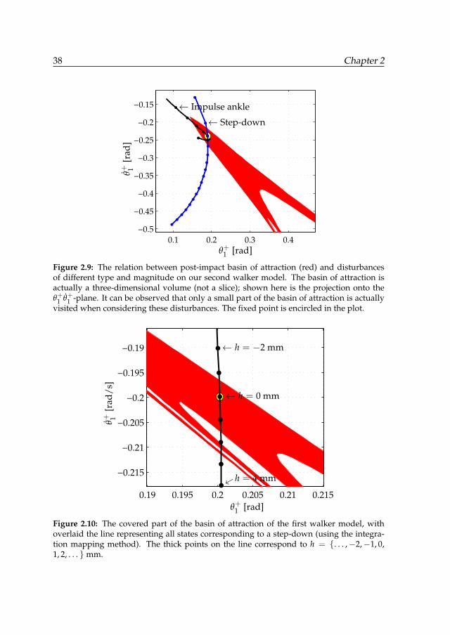
38 Chapter 2
0.1 0.2 0.3 0.4
−0.5
−0.45
−0.4
−0.35
−0.3
−0.25
−0.2
−0.15
← Impulse ankle
← Step-down
θ+1 [rad]
θ+ 1[r
ad]
Figure 2.9: The relation between post-impact basin of attraction (red) and disturbancesof different type and magnitude on our second walker model. The basin of attraction isactually a three-dimensional volume (not a slice); shown here is the projection onto theθ+1 θ+1 -plane. It can be observed that only a small part of the basin of attraction is actuallyvisited when considering these disturbances. The fixed point is encircled in the plot.
0.19 0.195 0.2 0.205 0.21 0.215
−0.215
−0.21
−0.205
−0.2
−0.195
−0.19
← h = −2 mm
← h = 0 mm
←h = 4 mm
θ+1 [rad]
θ+ 1[r
ad/s
]
Figure 2.10: The covered part of the basin of attraction of the first walker model, withoverlaid the line representing all states corresponding to a step-down (using the integra-tion mapping method). The thick points on the line correspond to h = {. . . ,−2,−1, 0,1, 2, . . . }mm.
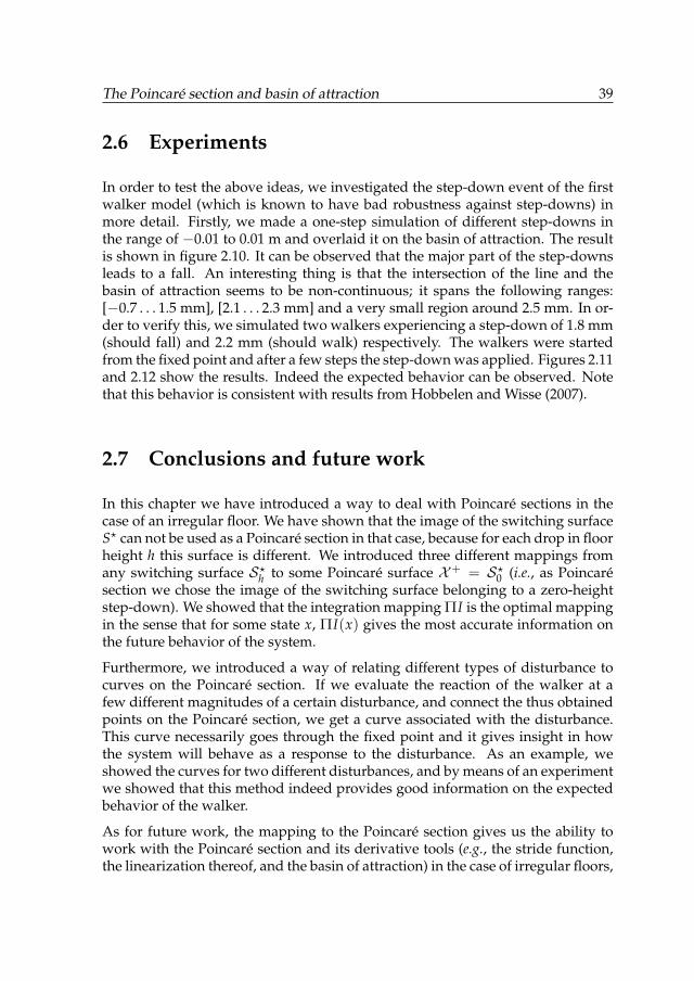
The Poincaré section and basin of attraction 39
2.6 Experiments
In order to test the above ideas, we investigated the step-down event of the firstwalker model (which is known to have bad robustness against step-downs) inmore detail. Firstly, we made a one-step simulation of different step-downs inthe range of −0.01 to 0.01 m and overlaid it on the basin of attraction. The resultis shown in figure 2.10. It can be observed that the major part of the step-downsleads to a fall. An interesting thing is that the intersection of the line and thebasin of attraction seems to be non-continuous; it spans the following ranges:[−0.7 . . . 1.5 mm], [2.1 . . . 2.3 mm] and a very small region around 2.5 mm. In or-der to verify this, we simulated two walkers experiencing a step-down of 1.8 mm(should fall) and 2.2 mm (should walk) respectively. The walkers were startedfrom the fixed point and after a few steps the step-down was applied. Figures 2.11and 2.12 show the results. Indeed the expected behavior can be observed. Notethat this behavior is consistent with results from Hobbelen and Wisse (2007).
2.7 Conclusions and future work
In this chapter we have introduced a way to deal with Poincaré sections in thecase of an irregular floor. We have shown that the image of the switching surfaceS? can not be used as a Poincaré section in that case, because for each drop in floorheight h this surface is different. We introduced three different mappings fromany switching surface S?h to some Poincaré surface X+ = S?0 (i.e., as Poincarésection we chose the image of the switching surface belonging to a zero-heightstep-down). We showed that the integration mapping ΠI is the optimal mappingin the sense that for some state x, ΠI(x) gives the most accurate information onthe future behavior of the system.
Furthermore, we introduced a way of relating different types of disturbance tocurves on the Poincaré section. If we evaluate the reaction of the walker at afew different magnitudes of a certain disturbance, and connect the thus obtainedpoints on the Poincaré section, we get a curve associated with the disturbance.This curve necessarily goes through the fixed point and it gives insight in howthe system will behave as a response to the disturbance. As an example, weshowed the curves for two different disturbances, and by means of an experimentwe showed that this method indeed provides good information on the expectedbehavior of the walker.
As for future work, the mapping to the Poincaré section gives us the ability towork with the Poincaré section and its derivative tools (e.g., the stride function,the linearization thereof, and the basin of attraction) in the case of irregular floors,
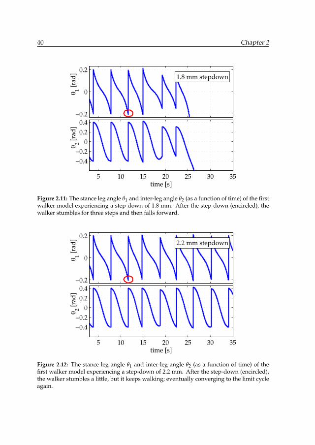
40 Chapter 2
−0.2
0
0.2θ
1 [
rad
]1.8 mm stepdown
5 10 15 20 25 30 35
−0.4
−0.2
0
0.2
0.4
time [s]
θ2 [
rad
]
Figure 2.11: The stance leg angle θ1 and inter-leg angle θ2 (as a function of time) of the firstwalker model experiencing a step-down of 1.8 mm. After the step-down (encircled), thewalker stumbles for three steps and then falls forward.
−0.2
0
0.2
θ1 [
rad
]
2.2 mm stepdown
5 10 15 20 25 30 35
−0.4
−0.2
0
0.2
0.4
time [s]
θ2 [
rad
]
Figure 2.12: The stance leg angle θ1 and inter-leg angle θ2 (as a function of time) of thefirst walker model experiencing a step-down of 2.2 mm. After the step-down (encircled),the walker stumbles a little, but it keeps walking; eventually converging to the limit cycleagain.
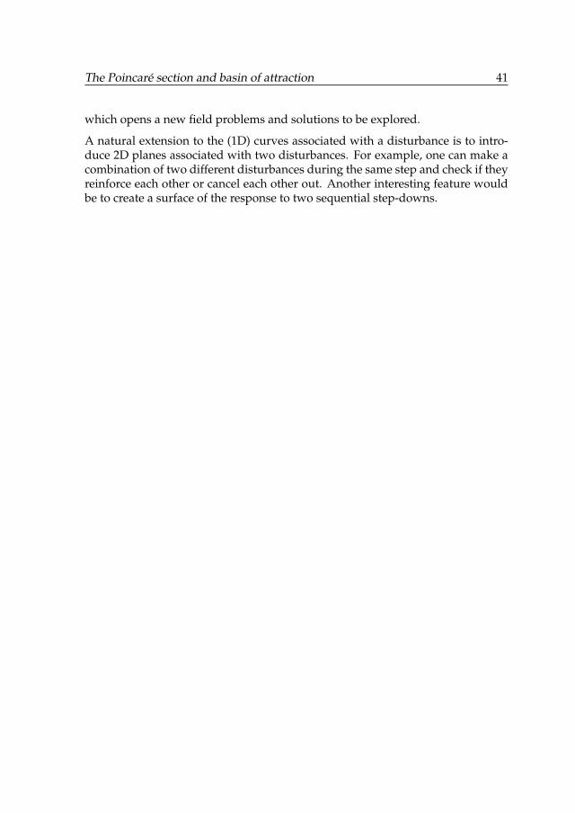
The Poincaré section and basin of attraction 41
which opens a new field problems and solutions to be explored.
A natural extension to the (1D) curves associated with a disturbance is to intro-duce 2D planes associated with two disturbances. For example, one can make acombination of two different disturbances during the same step and check if theyreinforce each other or cancel each other out. Another interesting feature wouldbe to create a surface of the response to two sequential step-downs.

42 Chapter 2
Chapter 3
Coordinate transformation as a helpfor analysis, simulation and
controller design in walking robots
The contents of this chapter has not been published before.
Abstract—In this chapter we show how a change of coordinates—in particu-lar, the choice of the stance foot as reference body—can facilitate both modelanalysis and controller design for humanoid robots. Firstly, it is shown whatthe coordinate transformation looks like, all in directly applicable equations.Then a few examples are given of things that become easier due to the coordi-nate change.
43
44 Chapter 3
3.1 Introduction
In robotics it customary to describe the mechanics of the robot by means of amodel. The model consists of the state (pose and velocity of each part of therobot) and equations of motion that tell how the state evolves in time.
In order to do calculations, the state needs to be expressed in numbers. For mobilerobots, usually the pose and velocity of one body (called the reference body inthis chapter) are taken as numerical entries in the state, as well as the (angular)positions and velocities of all joints. For walking robots the most obvious choiceis to take the torso as reference body. This is often convenient because
1. the notion of ‘position of the robot’ is, intuitively, more related to the posi-tion of the torso than to to any of the other parts, and
2. it is symmetric with respect to left and right steps.
Sometimes however, it is useful to choose a different reference body, for examplethe stance foot. Advantages of this choice of reference body are, amongst others:
1. During normal walking, the stance foot is standing still on the ground. So,the reference body is fixed and its velocity is zero. This makes analysis ofthe system easier.
2. Forces acting on the reference body appear directly in the equations of mo-tion. Choosing the stance foot as a reference body thus implies that groundreaction forces can easily be handled.
3. As will be shown in section 3.3.3, the form of the mass matrix in stance footcoordinates is much more useful than the original mass matrix.
More than in other literature, we explicitly denote how (in which coordinate rep-resentation, with respect to which body etc.) all elements of the equations areexpressed. The reason for that is twofold. Firstly, the whole point of this chapteris in the difference between different representations. Therefore, it is importantthat there can be no confusion about which representation is used. Secondly, byexplicitly denoting these things, it is easier to directly implement the equations,lowering the chance of mistakes.
In this chapter we combine some well-known principles (state representation,non-linear coordinate transformation and analysis tools from walking robots).We will show that, when using coordinate transformations, analysis algorithmson walking robots can become much easier, reducing the chance of errors whenimplementing. This is especially useful for actual realization of analysis algo-rithms in robot prototypes. Usually, in such prototypes, the state of the robot iscalculated in only one representation. The equations in this chapter are ready-to-
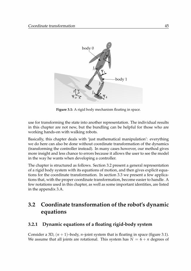
Coordinate transformation 45
J1
J2
J4Ψ4
Ψ1
Ψ0
Ψw x
yz
body 0
body 1
Figure 3.1: A rigid body mechanism floating in space.
use for transforming the state into another representation. The individual resultsin this chapter are not new, but the bundling can be helpful for those who areworking hands-on with walking robots.
Basically, this chapter deals with ‘just mathematical manipulation’: everythingwe do here can also be done without coordinate transformation of the dynamics(transforming the controller instead). In many cases however, our method givesmore insight and less chance to errors because it allows the user to see the modelin the way he wants when developing a controller.
The chapter is structured as follows. Section 3.2 present a general representationof a rigid body system with its equations of motion, and then gives explicit equa-tions for the coordinate transformation. In section 3.3 we present a few applica-tions that, with the proper coordinate transformation, become easier to handle. Afew notations used in this chapter, as well as some important identities, are listedin the appendix 3.A.
3.2 Coordinate transformation of the robot’s dynamicequations
3.2.1 Dynamic equations of a floating rigid-body system
Consider a 3D, (n + 1)–body, n–joint system that is floating in space (figure 3.1).We assume that all joints are rotational. This system has N = 6 + n degrees of
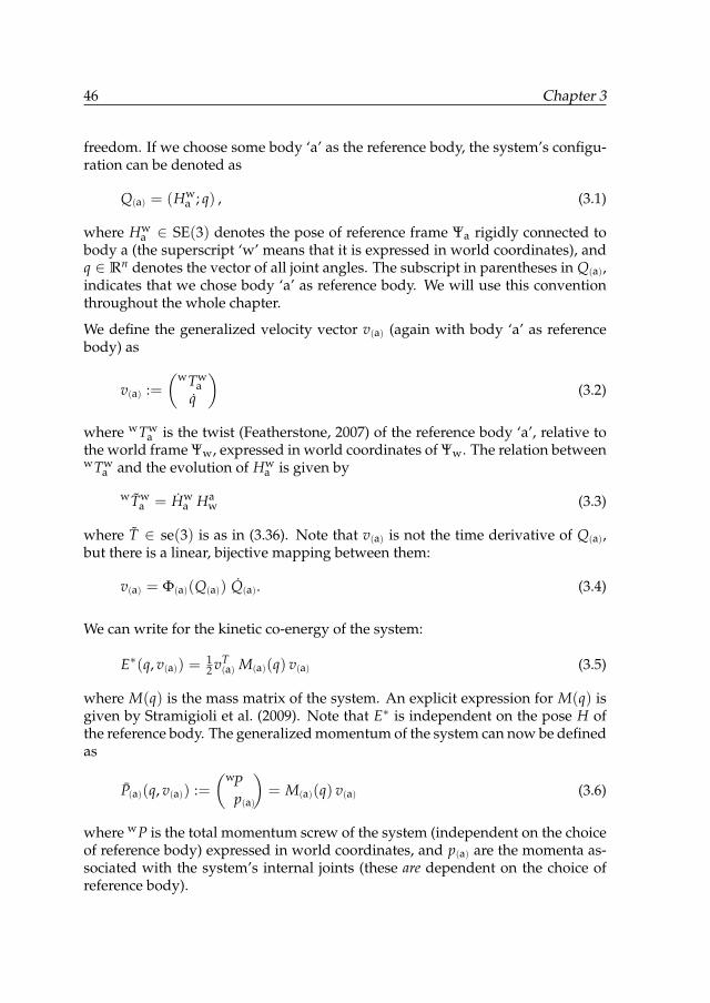
46 Chapter 3
freedom. If we choose some body ‘a’ as the reference body, the system’s configu-ration can be denoted as
Q(a) = (Hwa ; q) , (3.1)
where Hwa ∈ SE(3) denotes the pose of reference frame Ψa rigidly connected to
body a (the superscript ‘w’ means that it is expressed in world coordinates), andq ∈ Rn denotes the vector of all joint angles. The subscript in parentheses in Q(a),indicates that we chose body ‘a’ as reference body. We will use this conventionthroughout the whole chapter.
We define the generalized velocity vector v(a) (again with body ‘a’ as referencebody) as
v(a) :=(wTw
aq
)(3.2)
where wTwa is the twist (Featherstone, 2007) of the reference body ‘a’, relative to
the world frame Ψw, expressed in world coordinates of Ψw. The relation betweenwTw
a and the evolution of Hwa is given by
wTwa = Hw
a Haw (3.3)
where T ∈ se(3) is as in (3.36). Note that v(a) is not the time derivative of Q(a),but there is a linear, bijective mapping between them:
v(a) = Φ(a)(Q(a)) Q(a). (3.4)
We can write for the kinetic co-energy of the system:
E∗(q, v(a)) =12 vT
(a) M(a)(q) v(a) (3.5)
where M(q) is the mass matrix of the system. An explicit expression for M(q) isgiven by Stramigioli et al. (2009). Note that E∗ is independent on the pose H ofthe reference body. The generalized momentum of the system can now be definedas
P(a)(q, v(a)) :=(wP
p(a)
)= M(a)(q) v(a) (3.6)
where wP is the total momentum screw of the system (independent on the choiceof reference body) expressed in world coordinates, and p(a) are the momenta as-sociated with the system’s internal joints (these are dependent on the choice ofreference body).
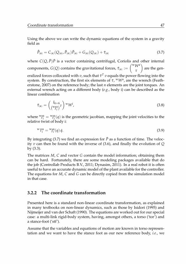
Coordinate transformation 47
Using the above we can write the dynamic equations of the system in a gravityfield as
˙P(a) = C(a)(Q(a), P(a))P(a) + G(a)(Q(a)) + τ(a) (3.7)
where C(Q, P)P is a vector containing centrifugal, Coriolis and other internal
components, G(Q) contains the gravitational forces, τ(a) :=(wWa
τ
)are the gen-
eralized forces collocated with v, such that τT v equals the power flowing into thesystem. By construction, the first six elements of τ, wWa, are the wrench (Feath-erstone, 2007) on the reference body; the last n elements are the joint torques. Anexternal wrench acting on a different body (e.g., body i) can be described as thelinear combination
τ(a) =
(I6×6(wJa
i)T
)wWi, (3.8)
where wJai = wJa
i (q) is the geometric jacobian, mapping the joint velocities to therelative twist of body i:
wTai = wJa
i (q) q. (3.9)
By integrating (3.7) we find an expression for P as a function of time. The veloc-ity v can then be found with the inverse of (3.6), and finally the evolution of Qby (3.3).
The matrices M, C and vector G contain the model information; obtaining themcan be hard. Fortunately, there are some modeling packages available that dothe job (Controllab Products B.V., 2011; Dynasim, 2011). In a real robot it is oftenuseful to have an accurate dynamic model of the plant available for the controller.The equations for M, C and G can be directly copied from the simulation modelin that case.
3.2.2 The coordinate transformation
Presented here is a standard non-linear coordinate transformation, as explainedin many textbooks on non-linear dynamics, such as those by Isidori (1995) andNijmeijer and van der Schaft (1990). The equations are worked out for our specialcase: a multi-link rigid-body system, having, amongst others, a torso (‘tor’) anda stance-foot (‘stf’).
Assume that the variables and equations of motion are known in torso represen-tation and we want to have the stance foot as our new reference body, i.e., we
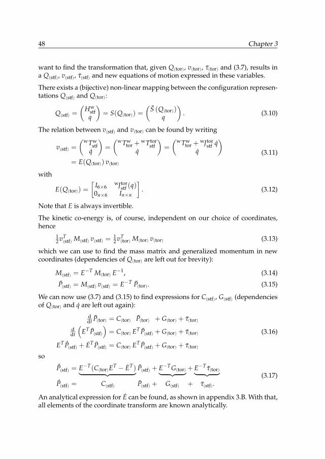
48 Chapter 3
want to find the transformation that, given Q(tor), v(tor), τ(tor) and (3.7), results ina Q(stf), v(stf), τ(stf) and new equations of motion expressed in these variables.
There exists a (bijective) non-linear mapping between the configuration represen-tations Q(stf) and Q(tor):
Q(stf) =
(Hw
stfq
)= S(Q(tor)) =
(S (Q(tor))
q
). (3.10)
The relation between v(stf) and v(tor) can be found by writing
v(stf) =
(wTwstf
q
)=
(wTwtor +
wTtorstf
q
)=
(wTwtor +
wJtorstf q
q
)
= E(Q(tor)) v(tor)
(3.11)
with
E(Q(tor)) =
[I6×6
wJtorstf (q)
0n×6 In×n
]. (3.12)
Note that E is always invertible.
The kinetic co-energy is, of course, independent on our choice of coordinates,hence
12 vT
(stf) M(stf) v(stf) =12 vT
(tor) M(tor) v(tor) (3.13)
which we can use to find the mass matrix and generalized momentum in newcoordinates (dependencies of Q(tor) are left out for brevity):
M(stf) = E−T M(tor) E−1, (3.14)
P(stf) = M(stf) v(stf) = E−T P(tor). (3.15)
We can now use (3.7) and (3.15) to find expressions for C(stf), G(stf) (dependenciesof Q(tor) and q are left out again):
ddt P(tor) = C(tor) P(tor) + G(tor) + τ(tor)
ddt
(ET P(stf)
)= C(tor) ET P(stf) + G(tor) + τ(tor)
ET ˙P(stf) + ET P(stf) = C(tor) ET P(stf) + G(tor) + τ(tor)
(3.16)
so˙P(stf) = E−T(C(tor)ET − ET)︸ ︷︷ ︸ P(stf) + E−TG(tor)︸ ︷︷ ︸+ E−T τ(tor)︸ ︷︷ ︸˙P(stf) = C(stf) P(stf) + G(stf) + τ(stf).
(3.17)
An analytical expression for E can be found, as shown in appendix 3.B. With that,all elements of the coordinate transform are known analytically.
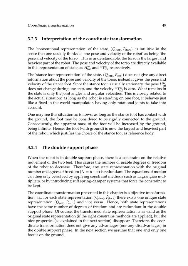
Coordinate transformation 49
3.2.3 Interpretation of the coordinate transformation
The ‘conventional representation’ of the state, (Q(tor), P(tor)), is intuitive in thesense that one usually thinks as ‘the pose and velocity of the robot’ as being ‘thepose and velocity of the torso’. This is understandable; the torso is the largest andheaviest part of the robot. The pose and velocity of the torso are directly availablein this representation of state, as Hw
tor and wTwtor respectively.
The ‘stance foot representation’ of the state,(Q(stf), P(stf)
)does not give any direct
information about the pose and velocity of the torso; instead it gives the pose andvelocity of the stance foot. Since the stance foot is usually stationary, the pose Hw
stfdoes not change during one step, and the velocity wTw
stf is zero. What remains inthe state is only the joint angles and angular velocities. This is closely related tothe actual situation: as long as the robot is standing on one foot, it behaves justlike a fixed-in-the-world manipulator, having only rotational joints to take intoaccount.
One may see this situation as follows: as long as the stance foot has contact withthe ground, the foot may be considered to be rigidly connected to the ground.Consequently, the apparent mass of the foot will be increased by the ground,being infinite. Hence, the foot (with ground) is now the largest and heaviest partof the robot, which justifies the choice of the stance foot as reference body.
3.2.4 The double support phase
When the robot is in double support phase, there is a constraint on the relativemovement of the two feet. This causes the number of usable degrees of freedomof the robot to decrease. Therefore, any state representation with the originalnumber of degrees of freedom (N = 6+ n) is redundant. The equations of motioncan then only be solved by applying constraint methods such as Lagrangian mul-tipliers, or by introducing stiff spring-damper systems that force the constraint tobe kept.
The coordinate transformation presented in this chapter is a bijective transforma-tion, i.e., for each state representation (Q(tor), P(tor)) there exists one unique staterepresentation
(Q(stf), P(stf)
)and vice versa. Hence, both state representations
have the same number of degrees of freedom and are redundant in the doublesupport phase. Of course, the transformed state representation is as valid as theoriginal state representation (if the right constrains methods are applied), but thenice properties (as explained in the next section) disappear. Therefore, the coor-dinate transformation does not give any advantages (nor any disadvantages) inthe double support phase. In the next section we assume that one and only onefoot is on the ground.
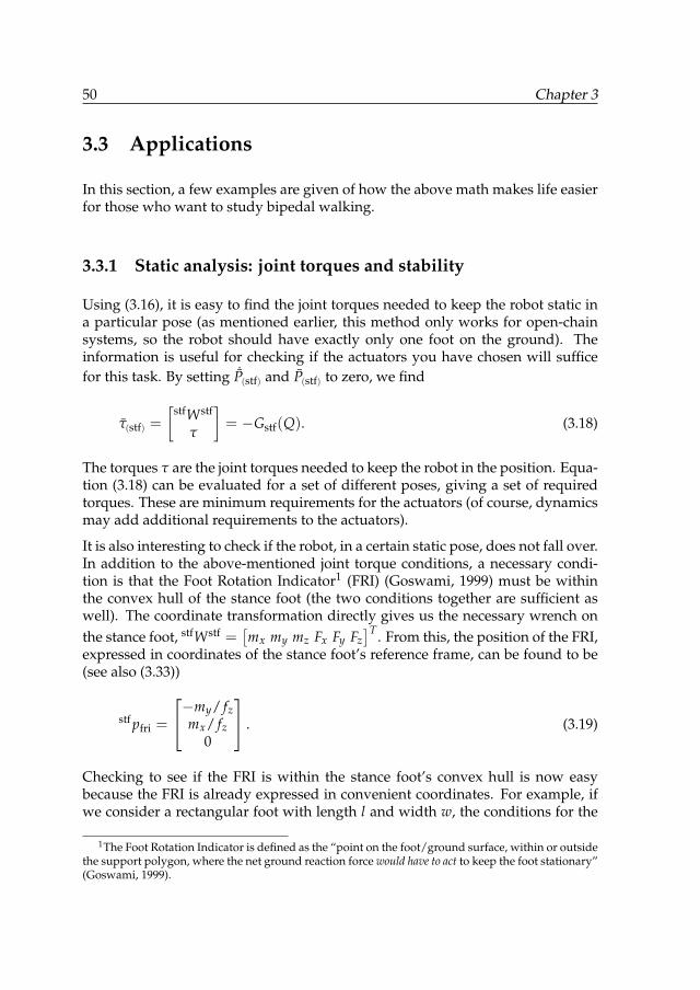
50 Chapter 3
3.3 Applications
In this section, a few examples are given of how the above math makes life easierfor those who want to study bipedal walking.
3.3.1 Static analysis: joint torques and stability
Using (3.16), it is easy to find the joint torques needed to keep the robot static ina particular pose (as mentioned earlier, this method only works for open-chainsystems, so the robot should have exactly only one foot on the ground). Theinformation is useful for checking if the actuators you have chosen will sufficefor this task. By setting ˙P(stf) and P(stf) to zero, we find
τ(stf) =
[stfWstf
τ
]= −Gstf(Q). (3.18)
The torques τ are the joint torques needed to keep the robot in the position. Equa-tion (3.18) can be evaluated for a set of different poses, giving a set of requiredtorques. These are minimum requirements for the actuators (of course, dynamicsmay add additional requirements to the actuators).
It is also interesting to check if the robot, in a certain static pose, does not fall over.In addition to the above-mentioned joint torque conditions, a necessary condi-tion is that the Foot Rotation Indicator1 (FRI) (Goswami, 1999) must be withinthe convex hull of the stance foot (the two conditions together are sufficient aswell). The coordinate transformation directly gives us the necessary wrench onthe stance foot, stfWstf =
[mx my mz Fx Fy Fz
]T . From this, the position of the FRI,expressed in coordinates of the stance foot’s reference frame, can be found to be(see also (3.33))
stf pfri =
−my/ fzmx/ fz
0
. (3.19)
Checking to see if the FRI is within the stance foot’s convex hull is now easybecause the FRI is already expressed in convenient coordinates. For example, ifwe consider a rectangular foot with length l and width w, the conditions for the
1The Foot Rotation Indicator is defined as the “point on the foot/ground surface, within or outsidethe support polygon, where the net ground reaction force would have to act to keep the foot stationary”(Goswami, 1999).
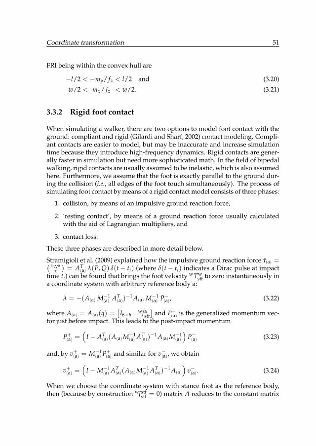
Coordinate transformation 51
FRI being within the convex hull are
−l/2 < −my/ fz < l/2 and (3.20)
−w/2 < mx/ fz < w/2. (3.21)
3.3.2 Rigid foot contact
When simulating a walker, there are two options to model foot contact with theground: compliant and rigid (Gilardi and Sharf, 2002) contact modeling. Compli-ant contacts are easier to model, but may be inaccurate and increase simulationtime because they introduce high-frequency dynamics. Rigid contacts are gener-ally faster in simulation but need more sophisticated math. In the field of bipedalwalking, rigid contacts are usually assumed to be inelastic, which is also assumedhere. Furthermore, we assume that the foot is exactly parallel to the ground dur-ing the collision (i.e., all edges of the foot touch simultaneously). The process ofsimulating foot contact by means of a rigid contact model consists of three phases:
1. collision, by means of an impulsive ground reaction force,
2. ‘resting contact’, by means of a ground reaction force usually calculatedwith the aid of Lagrangian multipliers, and
3. contact loss.
These three phases are described in more detail below.
Stramigioli et al. (2009) explained how the impulsive ground reaction force τ(a) =( aWaτ
)= AT
(a) λ(P, Q) δ(t− ti) (where δ(t− ti) indicates a Dirac pulse at impacttime ti) can be found that brings the foot velocity wTw
stf to zero instantaneously ina coordinate system with arbitrary reference body a:
λ = −(A(a) M−1(a) AT
(a))−1 A(a) M−1
(a) P−(a), (3.22)
where A(a) = A(a)(q) =[I6×6
wJastf]
and P−(a) is the generalized momentum vec-tor just before impact. This leads to the post-impact momentum
P+(a) =
(I − AT
(a)(A(a)M−1(a) AT
(a))−1 A(a)M−1
(a)
)P−(a) (3.23)
and, by v+(a) = M−1(a) P+
(a) and similar for v−(a), we obtain
v+(a) =(
I −M−1(a) AT
(a)(A(a)M−1(a) AT
(a))−1 A(a)
)v−(a). (3.24)
When we choose the coordinate system with stance foot as the reference body,then (because by construction wJstf
stf = 0) matrix A reduces to the constant matrix
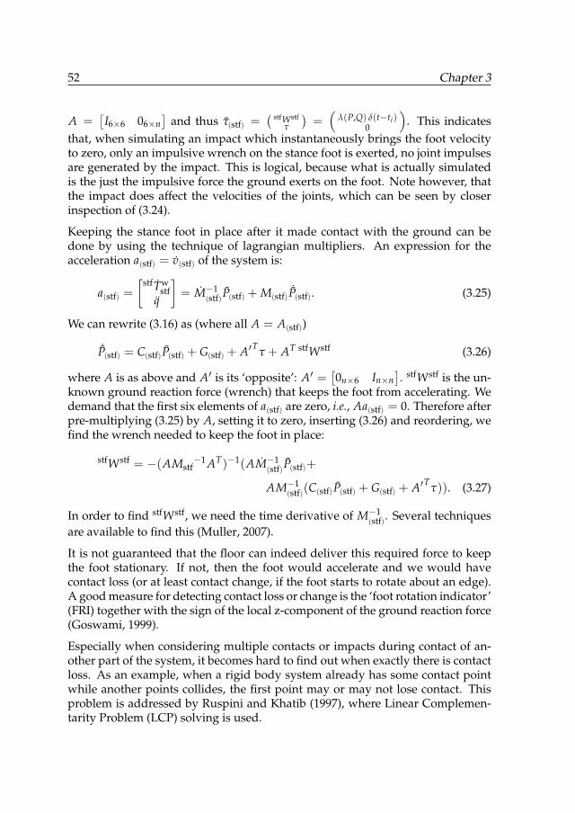
52 Chapter 3
A =[I6×6 06×n
]and thus τ(stf) =
( stfWstfτ
)=(
λ(P,Q) δ(t−ti)0
). This indicates
that, when simulating an impact which instantaneously brings the foot velocityto zero, only an impulsive wrench on the stance foot is exerted, no joint impulsesare generated by the impact. This is logical, because what is actually simulatedis the just the impulsive force the ground exerts on the foot. Note however, thatthe impact does affect the velocities of the joints, which can be seen by closerinspection of (3.24).
Keeping the stance foot in place after it made contact with the ground can bedone by using the technique of lagrangian multipliers. An expression for theacceleration a(stf) = v(stf) of the system is:
a(stf) =
[stfTw
stfq
]= M−1
(stf)P(stf) + M(stf)˙P(stf). (3.25)
We can rewrite (3.16) as (where all A = A(stf))
˙P(stf) = C(stf)P(stf) + G(stf) + A′Tτ + AT stfWstf (3.26)
where A is as above and A′ is its ‘opposite’: A′ =[0n×6 In×n
]. stfWstf is the un-
known ground reaction force (wrench) that keeps the foot from accelerating. Wedemand that the first six elements of a(stf) are zero, i.e., Aa(stf) = 0. Therefore afterpre-multiplying (3.25) by A, setting it to zero, inserting (3.26) and reordering, wefind the wrench needed to keep the foot in place:
stfWstf = −(AMstf−1 AT)−1(AM−1
(stf)P(stf)+
AM−1(stf)(C(stf)P(stf) + G(stf) + A′Tτ)). (3.27)
In order to find stfWstf, we need the time derivative of M−1(stf). Several techniques
are available to find this (Muller, 2007).
It is not guaranteed that the floor can indeed deliver this required force to keepthe foot stationary. If not, then the foot would accelerate and we would havecontact loss (or at least contact change, if the foot starts to rotate about an edge).A good measure for detecting contact loss or change is the ‘foot rotation indicator’(FRI) together with the sign of the local z-component of the ground reaction force(Goswami, 1999).
Especially when considering multiple contacts or impacts during contact of an-other part of the system, it becomes hard to find out when exactly there is contactloss. As an example, when a rigid body system already has some contact pointwhile another points collides, the first point may or may not lose contact. Thisproblem is addressed by Ruspini and Khatib (1997), where Linear Complemen-tarity Problem (LCP) solving is used.
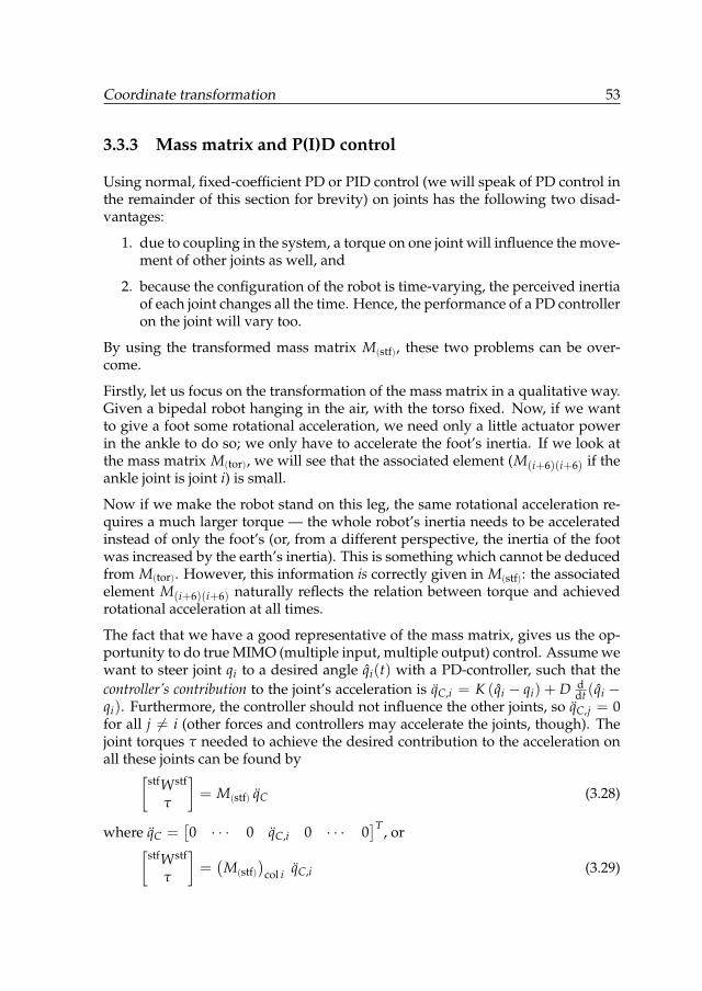
Coordinate transformation 53
3.3.3 Mass matrix and P(I)D control
Using normal, fixed-coefficient PD or PID control (we will speak of PD control inthe remainder of this section for brevity) on joints has the following two disad-vantages:
1. due to coupling in the system, a torque on one joint will influence the move-ment of other joints as well, and
2. because the configuration of the robot is time-varying, the perceived inertiaof each joint changes all the time. Hence, the performance of a PD controlleron the joint will vary too.
By using the transformed mass matrix M(stf), these two problems can be over-come.
Firstly, let us focus on the transformation of the mass matrix in a qualitative way.Given a bipedal robot hanging in the air, with the torso fixed. Now, if we wantto give a foot some rotational acceleration, we need only a little actuator powerin the ankle to do so; we only have to accelerate the foot’s inertia. If we look atthe mass matrix M(tor), we will see that the associated element (M(i+6)(i+6) if theankle joint is joint i) is small.
Now if we make the robot stand on this leg, the same rotational acceleration re-quires a much larger torque — the whole robot’s inertia needs to be acceleratedinstead of only the foot’s (or, from a different perspective, the inertia of the footwas increased by the earth’s inertia). This is something which cannot be deducedfrom M(tor). However, this information is correctly given in M(stf): the associatedelement M(i+6)(i+6) naturally reflects the relation between torque and achievedrotational acceleration at all times.
The fact that we have a good representative of the mass matrix, gives us the op-portunity to do true MIMO (multiple input, multiple output) control. Assume wewant to steer joint qi to a desired angle qi(t) with a PD-controller, such that thecontroller’s contribution to the joint’s acceleration is qC,i = K (qi − qi) + D d
dt (qi −qi). Furthermore, the controller should not influence the other joints, so qC,j = 0for all j 6= i (other forces and controllers may accelerate the joints, though). Thejoint torques τ needed to achieve the desired contribution to the acceleration onall these joints can be found by
[stfWstf
τ
]= M(stf) qC (3.28)
where qC =[0 · · · 0 qC,i 0 · · · 0
]T , or[
stfWstf
τ
]=(
M(stf))
col i qC,i (3.29)
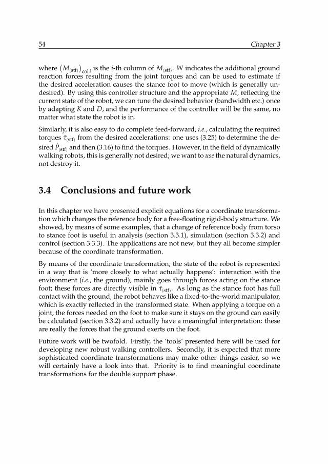
54 Chapter 3
where(
M(stf))
col i is the i-th column of M(stf). W indicates the additional groundreaction forces resulting from the joint torques and can be used to estimate ifthe desired acceleration causes the stance foot to move (which is generally un-desired). By using this controller structure and the appropriate M, reflecting thecurrent state of the robot, we can tune the desired behavior (bandwidth etc.) onceby adapting K and D, and the performance of the controller will be the same, nomatter what state the robot is in.
Similarly, it is also easy to do complete feed-forward, i.e., calculating the requiredtorques τ(stf) from the desired accelerations: one uses (3.25) to determine the de-sired ˙P(stf) and then (3.16) to find the torques. However, in the field of dynamicallywalking robots, this is generally not desired; we want to use the natural dynamics,not destroy it.
3.4 Conclusions and future work
In this chapter we have presented explicit equations for a coordinate transforma-tion which changes the reference body for a free-floating rigid-body structure. Weshowed, by means of some examples, that a change of reference body from torsoto stance foot is useful in analysis (section 3.3.1), simulation (section 3.3.2) andcontrol (section 3.3.3). The applications are not new, but they all become simplerbecause of the coordinate transformation.
By means of the coordinate transformation, the state of the robot is representedin a way that is ‘more closely to what actually happens’: interaction with theenvironment (i.e., the ground), mainly goes through forces acting on the stancefoot; these forces are directly visible in τ(stf). As long as the stance foot has fullcontact with the ground, the robot behaves like a fixed-to-the-world manipulator,which is exactly reflected in the transformed state. When applying a torque on ajoint, the forces needed on the foot to make sure it stays on the ground can easilybe calculated (section 3.3.2) and actually have a meaningful interpretation: theseare really the forces that the ground exerts on the foot.
Future work will be twofold. Firstly, the ‘tools’ presented here will be used fordeveloping new robust walking controllers. Secondly, it is expected that moresophisticated coordinate transformations may make other things easier, so wewill certainly have a look into that. Priority is to find meaningful coordinatetransformations for the double support phase.
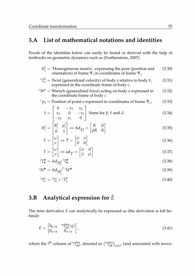
Coordinate transformation 55
3.A List of mathematical notations and identities
Proofs of the identities below can easily be found or derived with the help oftextbooks on geometric dynamics such as (Featherstone, 2007).
H ji = ‘Homogeneous matrix’, expressing the pose (position and
orientation) of frame Ψi in coordinates of frame Ψj.(3.30)
cTba = Twist (generalized velocity) of body a relative to body b,
expressed in the coordinate frame of body c.(3.31)
cWa = Wrench (generalized force) acting on body a expressed inthe coordinate frame of body c.
(3.32)
c pa = Position of point a expressed in coordinates of frame Ψc, (3.33)
x =
0 −x3 x2x3 0 −x1−x2 x1 0
Same for p, v and ω (3.34)
H ji =
[Rj
j pji
0 1
]⇔ AdH =
[R 0
pR R
](3.35)
T =
[ωv
]⇔ T =
[ω v0 0
](3.36)
T =
[ωv
]⇔ adT =
[ω 0v ω
](3.37)
jT•• = AdH ji
iT•• (3.38)
jW• = AdHij
T iW• (3.39)
jTca = jTc
b +jTb
a (3.40)
3.B Analytical expression for E
The time derivative E can analytically be expressed as (the derivation is left be-hind):
E =
[06×6
wJtorstf (q)
0n×6 0n×n
], (3.41)
where the ith column of wJtorstf , denoted as
(wJtorstf
)col i, (and associated with move-
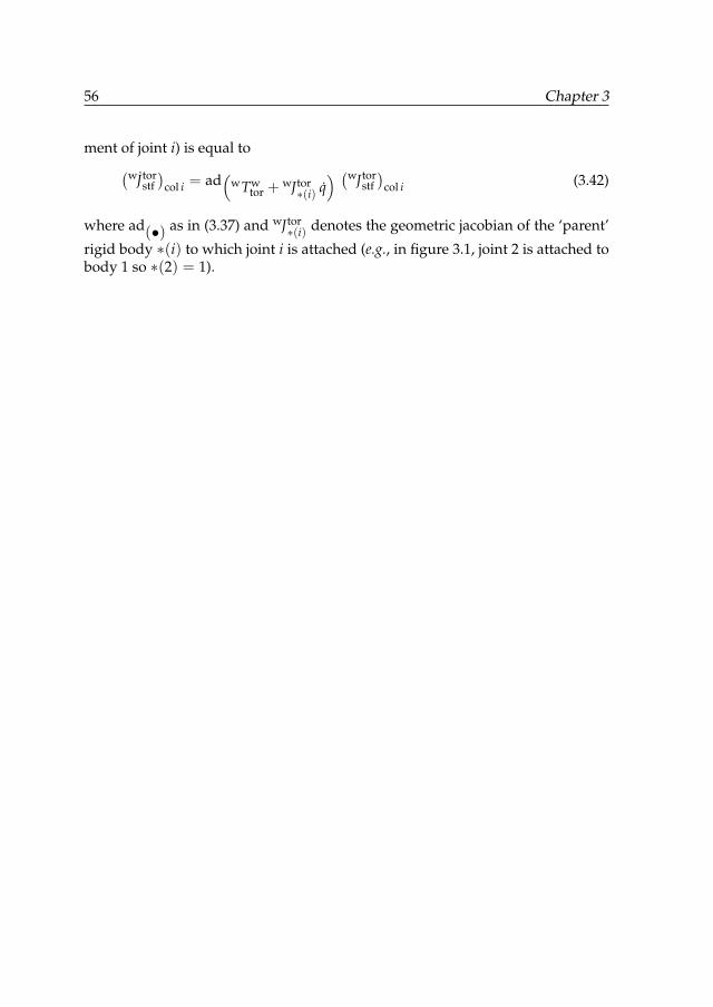
56 Chapter 3
ment of joint i) is equal to(wJtor
stf)
col i = ad(
wTwtor +
wJtor∗(i) q
) (wJtorstf)
col i (3.42)
where ad(•) as in (3.37) and wJtor∗(i) denotes the geometric jacobian of the ‘parent’
rigid body ∗(i) to which joint i is attached (e.g., in figure 3.1, joint 2 is attached tobody 1 so ∗(2) = 1).
Chapter 4
Geometric interpretation of theZero-Moment Point
This chapter is based on the following article (van Oort and Stramigioli, 2011):
Geometric interpretation of the Zero-Moment PointGijs van Oort and Stefano Stramigioli
Proc., IEEE International Conference on Robotics and Automation (ICRA’11)pages 575–580, May 2011.
Abstract—In this chapter we show that the concept of screws and wrenchesgives us tools to geometrically establish the relation between the ground reac-tion wrench and the Zero-Moment Point. In order to arrive at this, we showhow a wrench can be decomposed into separate components. The proposedmethod gives a general, completely coordinate-free way to find the ZMP andcontributes in improving the geometrical insight.
57
58 Chapter 4
4.1 Introduction
The Zero-Moment Point, ZMP (Vukobratovic and Borovac, 2004), is widely knownin the area of walking robots. Numerous researchers have investigated this pointand have given their own definitions and interpretations of it (for references, seesection 4.2). The theory on screws, introduced by Ball (1900) is a 6D generaliza-tion of velocity and force, being the Twist and Wrench respectively. This approachis coordinate-free, meaning that the equations and their results are invariant forthe choice of coordinates. The absence of coordinates gives greater flexibility (theequations work for any orientation of the robot; they are not limited to a certainpose in the world), reduces the chance of errors (e.g., one cannot be tempted tomake assumptions like ‘the robot will walk approximately in x-direction, so let’suse the x-coordinate for the distance traveled’ because the lack of coordinatesimplies that no x-direction was defined in the first place), and most importantly,mimics what happens in nature: nature does not have coordinates at all; the lawsare completely dictated by the physics of the system, by nothing more. The con-cept is also called ‘geometric dynamics’, emphasizing the fact that everythingfollows from the geometric properties of the system (in a broad sense, e.g., geo-metric mass and force distribution), not from the way you look at the system (i.e.,which coordinates you use).
In this chapter we combine the knowledge of the Zero-Moment Point and screwtheory, to give a novel, geometric interpretation of the Zero-Moment Point. Wewill show how the position of the ZMP can be found from the ground reactionwrench (the generalization of the ground reaction force) and geometric rules onwrench decomposition. This leads to more insight in the position of the ZMP andhow this relates to the ground wrench exerted on the foot.
The relation between ground reaction wrench and ZMP has been (indirectly) pre-sented before (Takao et al., 2003; Park et al., 2005; Sardain and Bessonnet, 2004),but without any discussion nor proof. The mathematical expression for the ZMPhas been known for over 40 years now, so in that sense the final result of thischapter is not new. The insightful, graphical way of achieving the result howeveris the real contribution of this chapter.
In sections 4.2 and 4.3 we introduce the key terms of this chapter further. We willaddress some issues of the ZMP, and show how a wrench can be shown uniquelyin a graphical way. In section 4.4 we show and prove three ways of decomposinga wrench into two separate components (analogous to decomposition of a forceinto two components). In section 4.5 we present the main contribution of thischapter, being the geometric relation between the ground reaction wrench and theZMP. In section 4.6 it will be shown that this leads to a simple explicit expressionfor the ZMP position. Conclusions are discussed in section 4.7.
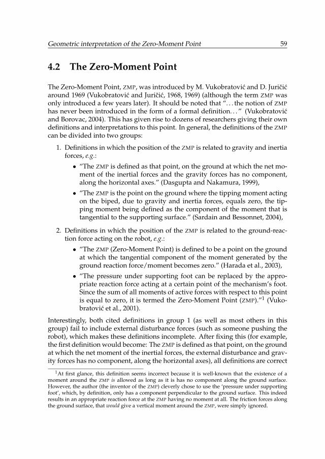
Geometric interpretation of the Zero-Moment Point 59
4.2 The Zero-Moment Point
The Zero-Moment Point, ZMP, was introduced by M. Vukobratovic and D. Juricicaround 1969 (Vukobratovic and Juricic, 1968, 1969) (although the term ZMP wasonly introduced a few years later). It should be noted that “. . . the notion of ZMPhas never been introduced in the form of a formal definition. . . ” (Vukobratovicand Borovac, 2004). This has given rise to dozens of researchers giving their owndefinitions and interpretations to this point. In general, the definitions of the ZMPcan be divided into two groups:
1. Definitions in which the position of the ZMP is related to gravity and inertiaforces, e.g.:
• “The ZMP is defined as that point, on the ground at which the net mo-ment of the inertial forces and the gravity forces has no component,along the horizontal axes.” (Dasgupta and Nakamura, 1999),
• “The ZMP is the point on the ground where the tipping moment actingon the biped, due to gravity and inertia forces, equals zero, the tip-ping moment being defined as the component of the moment that istangential to the supporting surface.” (Sardain and Bessonnet, 2004),
2. Definitions in which the position of the ZMP is related to the ground-reac-tion force acting on the robot, e.g.:
• “The ZMP (Zero-Moment Point) is defined to be a point on the groundat which the tangential component of the moment generated by theground reaction force/moment becomes zero.” (Harada et al., 2003),
• “The pressure under supporting foot can be replaced by the appro-priate reaction force acting at a certain point of the mechanism’s foot.Since the sum of all moments of active forces with respect to this pointis equal to zero, it is termed the Zero-Moment Point (ZMP).”1 (Vuko-bratovic et al., 2001).
Interestingly, both cited definitions in group 1 (as well as most others in thisgroup) fail to include external disturbance forces (such as someone pushing therobot), which makes these definitions incomplete. After fixing this (for example,the first definition would become: The ZMP is defined as that point, on the groundat which the net moment of the inertial forces, the external disturbance and grav-ity forces has no component, along the horizontal axes), all definitions are correct
1At first glance, this definition seems incorrect because it is well-known that the existence of amoment around the ZMP is allowed as long as it is has no component along the ground surface.However, the author (the inventor of the ZMP) cleverly chose to use the ‘pressure under supportingfoot’, which, by definition, only has a component perpendicular to the ground surface. This indeedresults in an appropriate reaction force at the ZMP having no moment at all. The friction forces alongthe ground surface, that would give a vertical moment around the ZMP, were simply ignored.
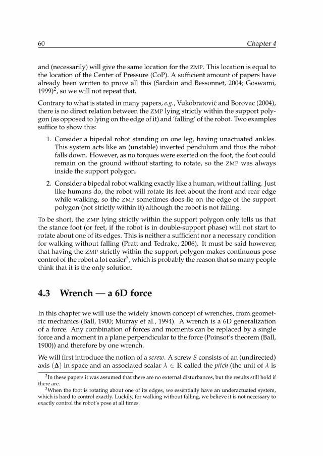
60 Chapter 4
and (necessarily) will give the same location for the ZMP. This location is equal tothe location of the Center of Pressure (CoP). A sufficient amount of papers havealready been written to prove all this (Sardain and Bessonnet, 2004; Goswami,1999)2, so we will not repeat that.
Contrary to what is stated in many papers, e.g., Vukobratovic and Borovac (2004),there is no direct relation between the ZMP lying strictly within the support poly-gon (as opposed to lying on the edge of it) and ‘falling’ of the robot. Two examplessuffice to show this:
1. Consider a bipedal robot standing on one leg, having unactuated ankles.This system acts like an (unstable) inverted pendulum and thus the robotfalls down. However, as no torques were exerted on the foot, the foot couldremain on the ground without starting to rotate, so the ZMP was alwaysinside the support polygon.
2. Consider a bipedal robot walking exactly like a human, without falling. Justlike humans do, the robot will rotate its feet about the front and rear edgewhile walking, so the ZMP sometimes does lie on the edge of the supportpolygon (not strictly within it) although the robot is not falling.
To be short, the ZMP lying strictly within the support polygon only tells us thatthe stance foot (or feet, if the robot is in double-support phase) will not start torotate about one of its edges. This is neither a sufficient nor a necessary conditionfor walking without falling (Pratt and Tedrake, 2006). It must be said however,that having the ZMP strictly within the support polygon makes continuous posecontrol of the robot a lot easier3, which is probably the reason that so many peoplethink that it is the only solution.
4.3 Wrench — a 6D force
In this chapter we will use the widely known concept of wrenches, from geomet-ric mechanics (Ball, 1900; Murray et al., 1994). A wrench is a 6D generalizationof a force. Any combination of forces and moments can be replaced by a singleforce and a moment in a plane perpendicular to the force (Poinsot’s theorem (Ball,1900)) and therefore by one wrench.
We will first introduce the notion of a screw. A screw S consists of an (undirected)axis (∆) in space and an associated scalar λ ∈ R called the pitch (the unit of λ is
2In these papers it was assumed that there are no external disturbances, but the results still hold ifthere are.
3When the foot is rotating about one of its edges, we essentially have an underactuated system,which is hard to control exactly. Luckily, for walking without falling, we believe it is not necessary toexactly control the robot’s pose at all times.
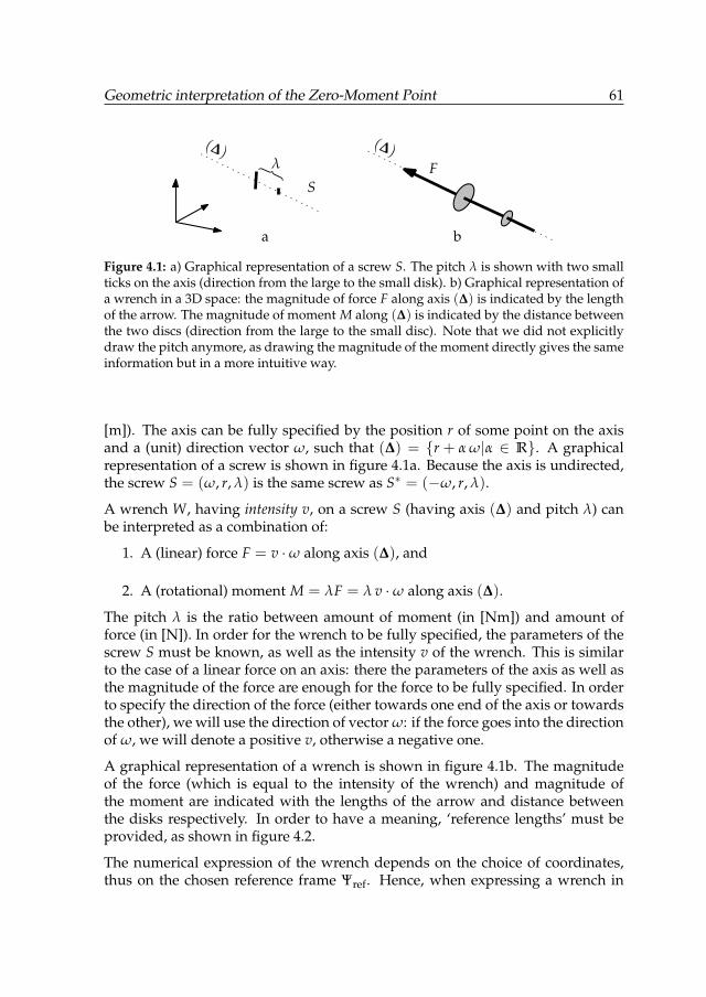
Geometric interpretation of the Zero-Moment Point 61
Fλ}
(∆)(∆)
a b
S
Figure 4.1: a) Graphical representation of a screw S. The pitch λ is shown with two smallticks on the axis (direction from the large to the small disk). b) Graphical representation ofa wrench in a 3D space: the magnitude of force F along axis (∆) is indicated by the lengthof the arrow. The magnitude of moment M along (∆) is indicated by the distance betweenthe two discs (direction from the large to the small disc). Note that we did not explicitlydraw the pitch anymore, as drawing the magnitude of the moment directly gives the sameinformation but in a more intuitive way.
[m]). The axis can be fully specified by the position r of some point on the axisand a (unit) direction vector ω, such that (∆) = {r + α ω|α ∈ R}. A graphicalrepresentation of a screw is shown in figure 4.1a. Because the axis is undirected,the screw S = (ω, r, λ) is the same screw as S∗ = (−ω, r, λ).
A wrench W, having intensity v, on a screw S (having axis (∆) and pitch λ) canbe interpreted as a combination of:
1. A (linear) force F = v ·ω along axis (∆), and
2. A (rotational) moment M = λF = λ v ·ω along axis (∆).
The pitch λ is the ratio between amount of moment (in [Nm]) and amount offorce (in [N]). In order for the wrench to be fully specified, the parameters of thescrew S must be known, as well as the intensity v of the wrench. This is similarto the case of a linear force on an axis: there the parameters of the axis as well asthe magnitude of the force are enough for the force to be fully specified. In orderto specify the direction of the force (either towards one end of the axis or towardsthe other), we will use the direction of vector ω: if the force goes into the directionof ω, we will denote a positive v, otherwise a negative one.
A graphical representation of a wrench is shown in figure 4.1b. The magnitudeof the force (which is equal to the intensity of the wrench) and magnitude ofthe moment are indicated with the lengths of the arrow and distance betweenthe disks respectively. In order to have a meaning, ‘reference lengths’ must beprovided, as shown in figure 4.2.
The numerical expression of the wrench depends on the choice of coordinates,thus on the chosen reference frame Ψref. Hence, when expressing a wrench in
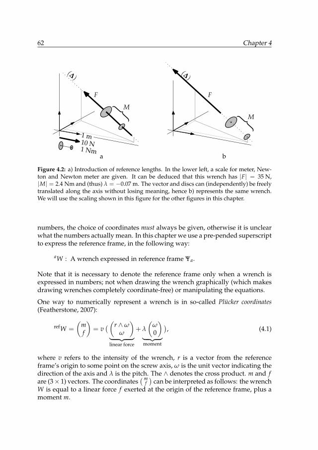
62 Chapter 4
1 m10 N1 Nm
F
M}
(∆)
a
F
M}
(∆)
b
Figure 4.2: a) Introduction of reference lengths. In the lower left, a scale for meter, New-ton and Newton meter are given. It can be deduced that this wrench has |F| = 35 N,|M| = 2.4 Nm and (thus) λ = −0.07 m. The vector and discs can (independently) be freelytranslated along the axis without losing meaning, hence b) represents the same wrench.We will use the scaling shown in this figure for the other figures in this chapter.
numbers, the choice of coordinates must always be given, otherwise it is unclearwhat the numbers actually mean. In this chapter we use a pre-pended superscriptto express the reference frame, in the following way:
aW : A wrench expressed in reference frame Ψa.
Note that it is necessary to denote the reference frame only when a wrench isexpressed in numbers; not when drawing the wrench graphically (which makesdrawing wrenches completely coordinate-free) or manipulating the equations.
One way to numerically represent a wrench is in so-called Plücker coordinates(Featherstone, 2007):
refW =
(mf
)= v
( (r ∧ωω
)
︸ ︷︷ ︸linear force
+ λ
(ω0
)
︸ ︷︷ ︸moment
), (4.1)
where v refers to the intensity of the wrench, r is a vector from the referenceframe’s origin to some point on the screw axis, ω is the unit vector indicating thedirection of the axis and λ is the pitch. The ∧ denotes the cross product. m and fare (3× 1) vectors. The coordinates
( mf)
can be interpreted as follows: the wrenchW is equal to a linear force f exerted at the origin of the reference frame, plus amoment m.
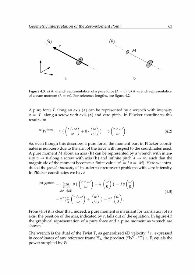
Geometric interpretation of the Zero-Moment Point 63
F
(a) (b)
M
a b
Figure 4.3: a) A wrench representation of a pure force (λ = 0). b) A wrench representationof a pure moment (λ = ∞). For reference lengths, see figure 4.2.
A pure force F along an axis (a) can be represented by a wrench with intensityv = |F| along a screw with axis (a) and zero pitch. In Plücker coordinates thisresults in:
refWforce = v( (r ∧ω
ω
)+ 0 ·
(ω0
) )= v
(r ∧ω
ω
). (4.2)
So, even though this describes a pure force, the moment part in Plücker coordi-nates is non-zero due to the arm of the force with respect to the coordinates used.A pure moment M about an axis (b) can be represented by a wrench with inten-sity v → 0 along a screw with axis (b) and infinite pitch λ → ∞; such that themagnitude of the moment becomes a finite value: v∗ = λv = |M|. Here we intro-duced the pseudo-intensity v∗ in order to circumvent problems with zero intensity.In Plücker coordinates we have:
refWmom = limv→0
λv→|M|
v( (r ∧ω
ω
)+ λ
(ω0
) )= λv
(ω0
)
= v∗( 1
λ
(r ∧ω
ω
)+
(ω0
) )= v∗
(ω0
).
(4.3)
From (4.3) it is clear that, indeed, a pure moment is invariant for translation of itsaxis: the position of the axis, indicated by r, falls out of the equation. In figure 4.3the graphical representation of a pure force and a pure moment as wrench areshown.
The wrench is the dual of the Twist T, as generalized 6D velocity; i.e., expressedin coordinates of any reference frame Ψa, the product (aWT · aT) ∈ R equals thepower supplied by W.
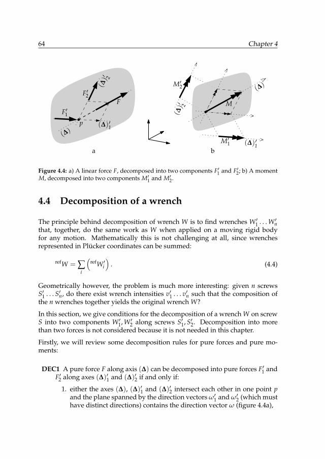
64 Chapter 4
FF′1
F′2
(∆)
(∆)′1
(∆)′ 2
M
M′1
M′2
a b
(∆)
(∆)′ 2
(∆)′1
p
Figure 4.4: a) A linear force F, decomposed into two components F′1 and F′2; b) A momentM, decomposed into two components M′1 and M′2.
4.4 Decomposition of a wrench
The principle behind decomposition of wrench W is to find wrenches W ′1 . . . W ′nthat, together, do the same work as W when applied on a moving rigid bodyfor any motion. Mathematically this is not challenging at all, since wrenchesrepresented in Plücker coordinates can be summed:
refW = ∑i
(refW ′i
). (4.4)
Geometrically however, the problem is much more interesting: given n screwsS′1 . . . S′n, do there exist wrench intensities v′1 . . . v′n such that the composition ofthe n wrenches together yields the original wrench W?
In this section, we give conditions for the decomposition of a wrench W on screwS into two components W ′1, W ′2 along screws S′1, S′2. Decomposition into morethan two forces is not considered because it is not needed in this chapter.
Firstly, we will review some decomposition rules for pure forces and pure mo-ments:
DEC1 A pure force F along axis (∆) can be decomposed into pure forces F′1 andF′2 along axes (∆)′1 and (∆)′2 if and only if:
1. either the axes (∆), (∆)′1 and (∆)′2 intersect each other in one point pand the plane spanned by the direction vectors ω′1 and ω′2 (which musthave distinct directions) contains the direction vector ω (figure 4.4a),
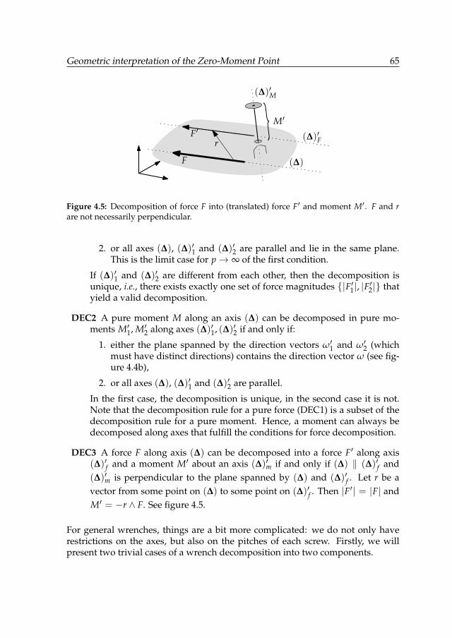
Geometric interpretation of the Zero-Moment Point 65
(∆)
(∆)′F
F
F′M′
(∆)′M
}r
Figure 4.5: Decomposition of force F into (translated) force F′ and moment M′. F and rare not necessarily perpendicular.
2. or all axes (∆), (∆)′1 and (∆)′2 are parallel and lie in the same plane.This is the limit case for p→ ∞ of the first condition.
If (∆)′1 and (∆)′2 are different from each other, then the decomposition isunique, i.e., there exists exactly one set of force magnitudes {|F′1|, |F′2|} thatyield a valid decomposition.
DEC2 A pure moment M along an axis (∆) can be decomposed in pure mo-ments M′1, M′2 along axes (∆)′1, (∆)′2 if and only if:
1. either the plane spanned by the direction vectors ω′1 and ω′2 (whichmust have distinct directions) contains the direction vector ω (see fig-ure 4.4b),
2. or all axes (∆), (∆)′1 and (∆)′2 are parallel.
In the first case, the decomposition is unique, in the second case it is not.Note that the decomposition rule for a pure force (DEC1) is a subset of thedecomposition rule for a pure moment. Hence, a moment can always bedecomposed along axes that fulfill the conditions for force decomposition.
DEC3 A force F along axis (∆) can be decomposed into a force F′ along axis(∆)′f and a moment M′ about an axis (∆)′m if and only if (∆) ‖ (∆)′f and(∆)′m is perpendicular to the plane spanned by (∆) and (∆)′f . Let r be avector from some point on (∆) to some point on (∆)′f . Then |F′| = |F| andM′ = −r ∧ F. See figure 4.5.
For general wrenches, things are a bit more complicated: we do not only haverestrictions on the axes, but also on the pitches of each screw. Firstly, we willpresent two trivial cases of a wrench decomposition into two components.
66 Chapter 4
Theorem 1 A wrench W on screw S can be decomposed into one wrench W ′f on screwS′f representing a pure force (λ′f = 0) plus one wrench W ′m on screw S′m representinga pure moment (λ′m = ∞), if axis (∆)′f coincides with (∆) and axis (∆)′m is parallel to(∆).
Proof Assume that the conditions on axes (∆)′f (defined by ω′f and r′f ) and (∆)′m(defined similarly) are met, i.e., ω′f = ±ω; r′f = r; ω′m = ±ω; r′m = arbitrary.Without loss of generality we can assume that ω′f = ω′m = ω (by changing thesign of the (pseudo-)intensities v′f and v∗′m if necessary). By expressing the wrenchin Plücker coordinates (and using (4.2) and (4.3)), we can show that indeed thereexist intensities v′f and v∗′m that give a valid decomposition W = W ′f + W ′m:
v(
r ∧ωω
)+ λv
(ω0
)= v′f
(r′f ∧ω′f
ω′f
)+ v∗′m
(ω′m0
)(4.5)
so choosing v′f = v and v∗′m = λv will do. This is actually the way a wrench isbuilt in the first place: it consists of a pure force F = v · ω along axis (∆) plus apure moment M = λv ·ω around this axis.
The converse of this theorem (decomposition is possible only if the screw axes sat-isfy the constraints) is not true. As a counter-example see DEC3, where a wrench(a pure force in this case) is decomposed into a pure force and pure moment whilethe screws are perpendicular instead of parallel.
Theorem 2 A wrench W of intensity v on screw S, can be decomposed into two wrenchesW ′1 and W ′2 on screws S′1 and S′2 if the axes (∆)′1 and (∆)′2 satisfy the conditions of DEC1and the pitches satisfy λ′1 = λ′2 = λ.
Proof Assume that all conditions are satisfied. Wrench W consists of a force Falong (∆) and a moment M = λF around it. According to DEC1, F can be de-composed into F′1 and F′2 along (∆)′1 and (∆)′2. The same holds for decompositionof M into M′1 = λF′1 and M′2 = λF′2. Now F′1 and M′1 can be taken together againto form wrench W ′1; similarly for W ′2. A more mathematical proof is given in theappendix.
The converse of this theorem is not true: there are many sets of screws {S′1, S′2}along which a wrench can be decomposed that do not satisfy the above condi-tions.
A more general theorem can be stated, which will be useful for the determinationof the ZMP later on:
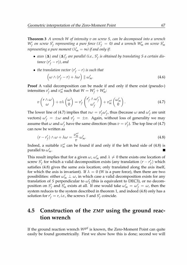
Geometric interpretation of the Zero-Moment Point 67
Theorem 3 A wrench W of intensity v on screw S, can be decomposed into a wrenchW ′f on screw S′f representing a pure force (λ′f = 0) and a wrench W ′m on screw S′mrepresenting a pure moment (λ′m = ∞) if and only if:
• axes (∆) and (∆)′f are parallel (i.e., S′f is obtained by translating S a certain dis-tance (r′f − r)), and
• the translation vector (r′f − r) is such that(ω ∧ (r′f − r) + λω
)‖ ω′m. (4.6)
Proof A valid decomposition can be made if and only if there exist (pseudo-)intensities v′f and v∗′m such that W = W ′f + W ′m:
v(
r ∧ωω
)+ vλ
(ω0
)= v′f
(r′f ∧ω′f
ω′f
)+ v∗′m
(ω′m0
). (4.7)
The lower line of (4.7) implies that vω = v′f ω′f , thus (because ω and ω′f are unitvectors) ω′f = ±ω and v′f = ±v. Again, without loss of generality we mayassume that ω and ω′f have the same direction (thus v = v′f ). The top line of (4.7)can now be written as
(r− r′f ) ∧ω + λω =v∗′mv
ω′m. (4.8)
Indeed, a suitable v∗′m can be found if and only if the left hand side of (4.8) isparallel to ω′m.
This result implies that for a given ω, ω′m and λ 6= 0 there exists one location ofscrew S′f for which a valid decomposition exists (any translation (r − r′f ) whichsatisfies (4.8) gives the same axis location; only translated along the axis itself,for which the axis is invariant). If λ = 0 (W is a pure force), then there are twopossibilities: either ω′m ⊥ ω, in which case a valid decomposition exists for anytranslation of S perpendicular to ω′2 (this is equivalent to DEC3), or no decom-position on S′f and S′m exists at all. If one would take ω′m = ω′f = ω, then thesystem reduces to the system described in theorem 1, and indeed (4.8) only has asolution for r′f = r, i.e., the screws S and S′f coincide.
4.5 Construction of the ZMP using the ground reac-tion wrench
If the ground reaction wrench Wgrf is known, the Zero-Moment Point can quiteeasily be found geometrically. First we show how this is done; second we will
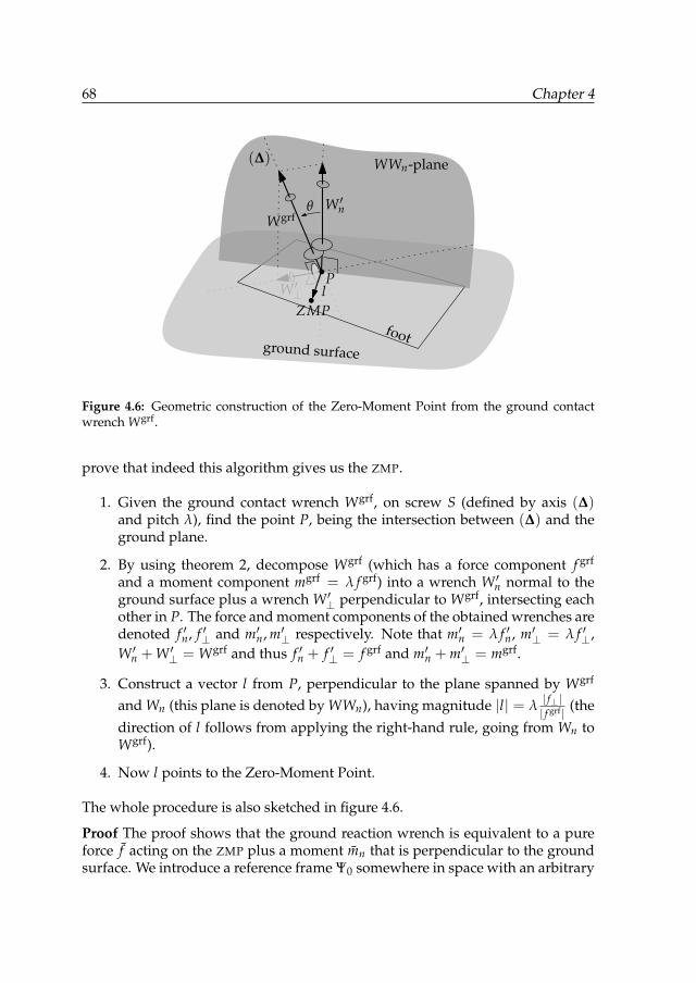
68 Chapter 4
W ′n
W ′⊥
Wgrf
l
footground surface
P
ZMP
WWn-plane(∆)
θ
Figure 4.6: Geometric construction of the Zero-Moment Point from the ground contactwrench Wgrf.
prove that indeed this algorithm gives us the ZMP.
1. Given the ground contact wrench Wgrf, on screw S (defined by axis (∆)and pitch λ), find the point P, being the intersection between (∆) and theground plane.
2. By using theorem 2, decompose Wgrf (which has a force component f grf
and a moment component mgrf = λ f grf) into a wrench W ′n normal to theground surface plus a wrench W ′⊥ perpendicular to Wgrf, intersecting eachother in P. The force and moment components of the obtained wrenches aredenoted f ′n, f ′⊥ and m′n, m′⊥ respectively. Note that m′n = λ f ′n, m′⊥ = λ f ′⊥,W ′n + W ′⊥ = Wgrf and thus f ′n + f ′⊥ = f grf and m′n + m′⊥ = mgrf.
3. Construct a vector l from P, perpendicular to the plane spanned by Wgrf
and Wn (this plane is denoted by WWn), having magnitude |l| = λ| f⊥ || f grf| (the
direction of l follows from applying the right-hand rule, going from Wn toWgrf).
4. Now l points to the Zero-Moment Point.
The whole procedure is also sketched in figure 4.6.
Proof The proof shows that the ground reaction wrench is equivalent to a pureforce f acting on the ZMP plus a moment mn that is perpendicular to the groundsurface. We introduce a reference frame Ψ0 somewhere in space with an arbitrary
Geometric interpretation of the Zero-Moment Point 69
orientation, a vector p pointing from its origin to point P and a vector z = p + lpointing from its origin to the supposed position of the ZMP. f and mn can be
written as a wrench as W f =
(z ∧ f
f
)and Wmn =
(mn0
)respectively.
Assume that indeed l points to the ZMP, then the above defined f and mn shouldexist such that
Wgrf = W f + Wmn
(p ∧ f grf
f grf
)+ λ
(f grf
0
)=
(z ∧ f
f
)+
(mn0
).
(4.9)
From this, it follows directly that f = f grf. Because z = p + l, we can write thetop row of (4.9) as p ∧ f grf + λ f grf = p ∧ f + l ∧ f + mn which can be simplifiedto ( f = f grf)
λ f grf = l ∧ f grf + mn. (4.10)
It can be shown that l ∧ f grf = m′⊥ by proving the following (sufficient) condi-tions:
1. m′⊥ ⊥ l — l is perpendicular to Wgrf and W ′n and, consequently, to anyvector in the plane spanned by them. Now W ′⊥ is in this plane, and thus sois m′⊥ (which has the same direction as W ′⊥).
2. m′⊥ ⊥ f grf — W ′⊥ was constructed perpendicularly to Wgrf. By constructionm′⊥ ‖W ′⊥ and f grf ‖Wgrf. Therefore we have indeed m′⊥ ⊥ f grf.
3. |l ∧ f grf| = |m′⊥| — because l ⊥ f grf, we have |l ∧ f grf| = |l| · | f grf| =λ| f ′⊥ || f grf| · | f
grf| = |λ f ′⊥| = |m′⊥|.
4. l ∧ f grf = m′⊥ follows the right-hand rule — by inspection of figure 4.6.
By using l ∧ f grf = m′⊥ and the identities of step 2 of the ZMP construction algo-rithm, (4.10) can be rewritten as
λ f grf = mgrf = m′⊥ + m′n = m′⊥ + mn (4.11)
so we can conclude that indeed there exists an f = f grf and mn = m′n (which isperpendicular to the ground surface) that satisfy (4.9), so indeed l points to theZero-Moment Point.
Remark 1 Both step 1 and 2 of the algorithm are only possible if (∆) is not parallel to theground plane. This is logical because if (∆) were parallel to the ground plane, the grounddoes not exert a normal force; i.e., the ground does not support the foot and in that casethe ZMP does not exist.
70 Chapter 4
Remark 2 If (∆) is almost vertical, i.e., the friction forces are much smaller than thenormal force, we can approximate the magnitude |l| as follows: let θ be the angle between
f ′n and f grf (see figure 4.6); then | f ′⊥ || f grf| = tan θ ≈ θ ⇒ |l| ≈ λθ.
Remark 3 As l is perpendicular to W ′n (and thus to the ground’s normal), it it automati-cally parallel to the ground surface. Therefore, l points to a point belonging to the groundsurface; which is in agreement with the commonly-known fact that the ZMP is a point onthe ground surface.
Remark 4 We never stated that the ground should be horizontal. In fact, we did noteven draw the reference from which a ‘world’s horizontal plane’ could be deduced. Thismethod works for any orientation of the ground plane (and the orientation does not needto be known either). Of course, in order for the ZMP to make sense, the foot must make fullcontact with the ground surface and therefore the ground surface under the foot shouldbe flat. It is however no problem to have different (possibly discontinuous) parts of flatground where the robot steps on.
Remark 5 From a decomposition point of view, the algorithm can be interpreted as fol-lows. The ground reaction wrench consists of a force f grf and a moment mgrf along thesame axis (∆). In order to find the ZMP, we want to find a decomposition in a purelyvertical moment and a pure force. The moment mgrf can be seen as the composition of a‘wanted’ vertical component m′n and an ‘unwanted’ remainder m′⊥. In order to cancel thelatter, we can translate f grf (according to theorem 3) along l, which introduces a cancel-ing moment −m′⊥. The result is a translated version of f grf and the sum of all momentsm′n + m′⊥ + (−m′⊥) = m′n. The intersection of the translated f grf and the ground planeis the ZMP.
4.6 Explicit expression for the ZMP position, giventhe ground reaction wrench
4.6.1 Expression for the ZMP
The purpose of this section is to show that, when the ground reaction force/mo-ment is known as a wrench, the expression for the ZMP is simple. Of course,these equations give the same results as any ZMP other equation. Hence the ex-pression presented here is most useful if the ground reaction force/moment isalready available as a wrench (otherwise other ZMP equations are usually moredirect and thus faster).
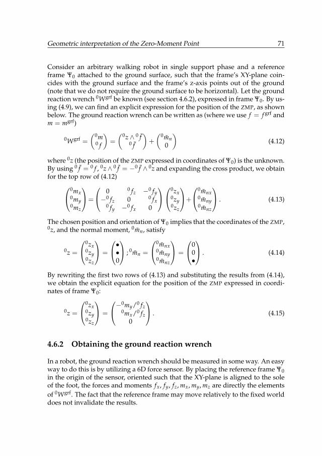
Geometric interpretation of the Zero-Moment Point 71
Consider an arbitrary walking robot in single support phase and a referenceframe Ψ0 attached to the ground surface, such that the frame’s XY-plane coin-cides with the ground surface and the frame’s z-axis points out of the ground(note that we do not require the ground surface to be horizontal). Let the groundreaction wrench 0Wgrf be known (see section 4.6.2), expressed in frame Ψ0. By us-ing (4.9), we can find an explicit expression for the position of the ZMP, as shownbelow. The ground reaction wrench can be written as (where we use f = f grf andm = mgrf)
0Wgrf =
(0m0 f
)=
(0z ∧ 0 f0 f
)+
(0mn0
)(4.12)
where 0z (the position of the ZMP expressed in coordinates of Ψ0) is the unknown.By using 0 f = 0 f , 0z∧ 0 f = −0 f ∧ 0z and expanding the cross product, we obtainfor the top row of (4.12)
0mx0my0mz
=
0 0 fz −0 fy−0 fz 0 0 fx
0 fy −0 fx 0
0zx0zy0zz
+
0mnx0mny0mnz
. (4.13)
The chosen position and orientation of Ψ0 implies that the coordinates of the ZMP,0z, and the normal moment, 0mn, satisfy
0z =
0zx0zy0zz
=
••0
; 0mn =
0mnx0mny0mnz
=
00•
. (4.14)
By rewriting the first two rows of (4.13) and substituting the results from (4.14),we obtain the explicit equation for the position of the ZMP expressed in coordi-nates of frame Ψ0:
0z =
0zx0zy0zz
=
−0my/0 fz
0mx/0 fz0
. (4.15)
4.6.2 Obtaining the ground reaction wrench
In a robot, the ground reaction wrench should be measured in some way. An easyway to do this is by utilizing a 6D force sensor. By placing the reference frame Ψ0in the origin of the sensor, oriented such that the XY-plane is aligned to the soleof the foot, the forces and moments fx, fy, fz, mx, my, mz are directly the elementsof 0Wgrf. The fact that the reference frame may move relatively to the fixed worlddoes not invalidate the results.
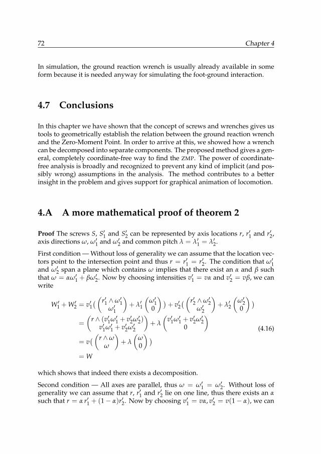
72 Chapter 4
In simulation, the ground reaction wrench is usually already available in someform because it is needed anyway for simulating the foot-ground interaction.
4.7 Conclusions
In this chapter we have shown that the concept of screws and wrenches gives ustools to geometrically establish the relation between the ground reaction wrenchand the Zero-Moment Point. In order to arrive at this, we showed how a wrenchcan be decomposed into separate components. The proposed method gives a gen-eral, completely coordinate-free way to find the ZMP. The power of coordinate-free analysis is broadly and recognized to prevent any kind of implicit (and pos-sibly wrong) assumptions in the analysis. The method contributes to a betterinsight in the problem and gives support for graphical animation of locomotion.
4.A A more mathematical proof of theorem 2
Proof The screws S, S′1 and S′2 can be represented by axis locations r, r′1 and r′2,axis directions ω, ω′1 and ω′2 and common pitch λ = λ′1 = λ′2.
First condition — Without loss of generality we can assume that the location vec-tors point to the intersection point and thus r = r′1 = r′2. The condition that ω′1and ω′2 span a plane which contains ω implies that there exist an α and β suchthat ω = αω′1 + βω′2. Now by choosing intensities v′1 = vα and v′2 = vβ, we canwrite
W ′1 + W ′2 = v′1( (r′1 ∧ω′1
ω′1
)+ λ′1
(ω′10
) )+ v′2
( (r′2 ∧ω′2ω′2
)+ λ′2
(ω′20
) )
=
(r ∧ (v′1ω′1 + v′2ω′2)
v′1ω′1 + v′2ω′2
)+ λ
(v′1ω′1 + v′2ω′2
0
)
= v( (r ∧ω
ω
)+ λ
(ω0
) )
= W
(4.16)
which shows that indeed there exists a decomposition.
Second condition — All axes are parallel, thus ω = ω′1 = ω′2. Without loss ofgenerality we can assume that r, r′1 and r′2 lie on one line, thus there exists an αsuch that r = α r′1 + (1− α)r′2. Now by choosing v′1 = vα, v′2 = v(1− α), we can
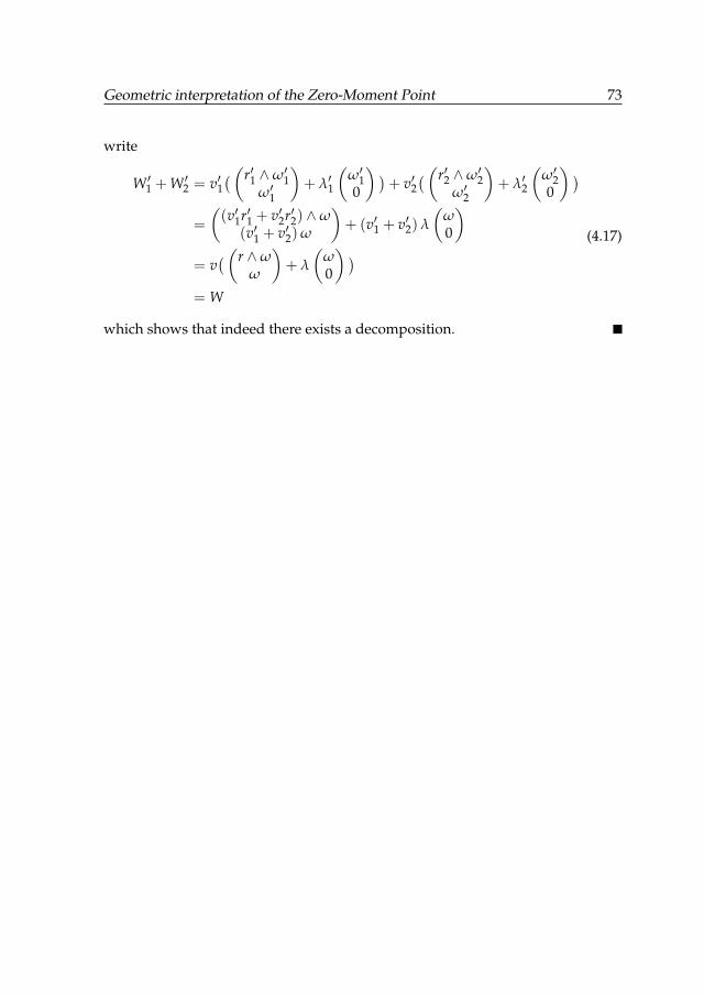
Geometric interpretation of the Zero-Moment Point 73
write
W ′1 + W ′2 = v′1( (r′1 ∧ω′1
ω′1
)+ λ′1
(ω′10
) )+ v′2
( (r′2 ∧ω′2ω′2
)+ λ′2
(ω′20
) )
=
((v′1r′1 + v′2r′2) ∧ω
(v′1 + v′2)ω
)+ (v′1 + v′2) λ
(ω0
)
= v( (r ∧ω
ω
)+ λ
(ω0
) )
= W
(4.17)
which shows that indeed there exists a decomposition.

74 Chapter 4
Chapter 5
Compact analysis of 3D bipedal gaitusing geometric dynamics of
simplified models
This chapter is based on the following article (Stramigioli et al., 2009):
Compact analysis of 3D bipedal gait using geometric dynamics of simplified modelsStefano Stramigioli, Vincent Duindam, Gijs van Oort and Ambarish GoswamiProc., IEEE International Conference on Robotics and Automation (ICRA’09)
pages 1978–1984, May 2009.
Abstract—The large number of degrees of freedom in legged robots give riseto complicated dynamics equations. Analyzing these equations or using themfor control can therefore be a difficult and non-intuitive task. A simplifica-tion of the complex multi-body dynamics can be achieved by instantaneouslyreducing it to an equivalent single inertial entity called the locked inertia.
In this chapter, we adopt the methods of geometric dynamics to analyze thegait using the locked inertia of the robot. The analysis includes the rolling of abiped on a 3D rigid foot and 3D impacts. An example of numerical optimiza-tion of foot shape parameters is shown.
Our long-term objective is to develop the theoretical framework and to pro-vide the necessary tools for systematic analysis, design, and control of efficientbiped robots.
75
76 Chapter 5
5.1 Introduction
The fundamental nature of locomotion has been compactly captured as “a ques-tion of relating internal shape changes to net changes in position via a couplingmechanism, most often either through interaction with the environment or viasome type of conservation law” (Marsden and Ostrowski, 1998). The use of ge-ometric tools has been found to be very useful in generating insights into thecomplex dynamics of locomotion systems. Geometric dynamics is a coordinate-neutral framework which yields results only pertaining to the physics of the sys-tem.
The utility of reduced models that capture the essentials of gait dynamics iswidely acknowledged. Simple biped models such as the different variations ofthe inverted pendulum models have been proven immensely beneficial for thestudy of gait and balance both for humans (Inman et al., 1981; Alexander, 1984,1990; McMahon, 1984) and humanoid robots (Kajita and Tani, 1991; Kajita et al.,2002; Sugihara and Nakamura, 2003; Komura et al., 2005).
Reduced humanoid models allow one to ignore the non-central aspects of dy-namics and to express the complex gait dynamics in a minimalist way. While atthe final implementation stage one still needs to formulate control laws for theentire system, it is at the analysis and planning stage where such reduced mod-els demonstrate their value. These models not only enhance our understandingof bipedal locomotion, but open the way to new classes of control laws, whichwould otherwise be difficult or impossible to conceive.
Many studies have been performed for 2D passive dynamic walkers, startingwith the ground-breaking work of McGeer (1990b), and later on with varioussystematic approaches, e.g., based on Poincaré mappings (Goswami et al., 1998;Garcia et al., 1998) and passivity (Spong and Bullo, 2005; Duindam and Strami-gioli, 2005). Several successful three-dimensional walking robots have been builtas well (Wisse and Schwab, 2001; Wisse, 2004; Collins et al., 2001), but most ofthese results were achieved relying more in engineering insight and smart de-signs rather than systematic analytical methods. The main difficulty when tryingto use analytic methods for 3D robots is the sheer complexity of the mechanismsand their interaction with the 3D world.
Our present approach to tackling the complexity of 3D walking robots relies onthe very useful concept of locked inertia (Marsden and Ostrowski, 1998), morecommonly known in robotics as the composite rigid body inertia (Walker and Orin,1982). The locked inertia of a humanoid robot is its instantaneous generalizedinertia, assuming that all of its joints are frozen. It has the same structure asthe generalized inertia of a single rigid body. We have recently shown (Lee andGoswami, 2007) how using this concept an entire humanoid can be mapped into
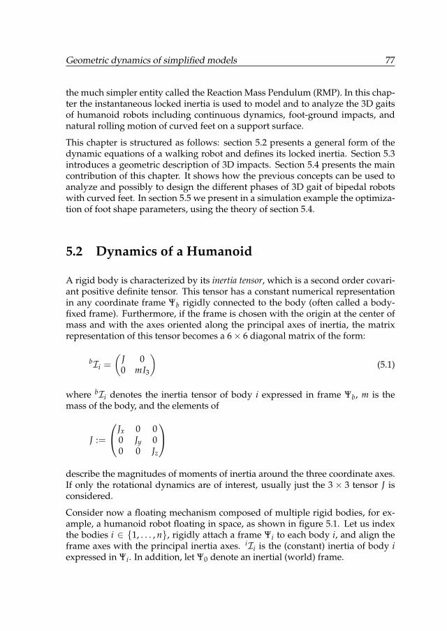
Geometric dynamics of simplified models 77
the much simpler entity called the Reaction Mass Pendulum (RMP). In this chap-ter the instantaneous locked inertia is used to model and to analyze the 3D gaitsof humanoid robots including continuous dynamics, foot-ground impacts, andnatural rolling motion of curved feet on a support surface.
This chapter is structured as follows: section 5.2 presents a general form of thedynamic equations of a walking robot and defines its locked inertia. Section 5.3introduces a geometric description of 3D impacts. Section 5.4 presents the maincontribution of this chapter. It shows how the previous concepts can be used toanalyze and possibly to design the different phases of 3D gait of bipedal robotswith curved feet. In section 5.5 we present in a simulation example the optimiza-tion of foot shape parameters, using the theory of section 5.4.
5.2 Dynamics of a Humanoid
A rigid body is characterized by its inertia tensor, which is a second order covari-ant positive definite tensor. This tensor has a constant numerical representationin any coordinate frame Ψb rigidly connected to the body (often called a body-fixed frame). Furthermore, if the frame is chosen with the origin at the center ofmass and with the axes oriented along the principal axes of inertia, the matrixrepresentation of this tensor becomes a 6× 6 diagonal matrix of the form:
bIi =
(J 00 mI3
)(5.1)
where bIi denotes the inertia tensor of body i expressed in frame Ψb, m is themass of the body, and the elements of
J :=
Jx 0 00 Jy 00 0 Jz
describe the magnitudes of moments of inertia around the three coordinate axes.If only the rotational dynamics are of interest, usually just the 3× 3 tensor J isconsidered.
Consider now a floating mechanism composed of multiple rigid bodies, for ex-ample, a humanoid robot floating in space, as shown in figure 5.1. Let us indexthe bodies i ∈ {1, . . . , n}, rigidly attach a frame Ψi to each body i, and align theframe axes with the principal inertia axes. iIi is the (constant) inertia of body iexpressed in Ψi. In addition, let Ψ0 denote an inertial (world) frame.
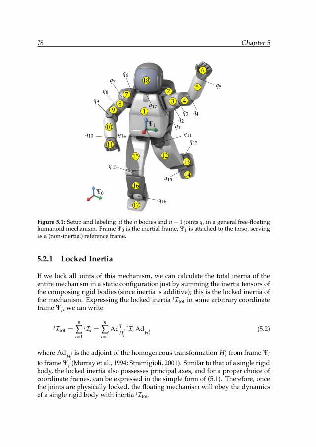
78 Chapter 5
Ψ0
Ψ1 q1
q2
q3 q4
q5
q6q7
q8
q9
q10 q11q12
q13
q14
q15
q16
q174
25
87
6
1
39
11
15
16
10
14
1213
17
18
Figure 5.1: Setup and labeling of the n bodies and n− 1 joints qi in a general free-floatinghumanoid mechanism. Frame Ψ0 is the inertial frame, Ψ1 is attached to the torso, servingas a (non-inertial) reference frame.
5.2.1 Locked Inertia
If we lock all joints of this mechanism, we can calculate the total inertia of theentire mechanism in a static configuration just by summing the inertia tensors ofthe composing rigid bodies (since inertia is additive); this is the locked inertia ofthe mechanism. Expressing the locked inertia jItot in some arbitrary coordinateframe Ψj, we can write
jItot =n
∑i=1
jIi =n
∑i=1
AdTH j
i
iIi AdH j
i(5.2)
where AdH j
iis the adjoint of the homogeneous transformation H j
i from frame Ψi
to frame Ψj (Murray et al., 1994; Stramigioli, 2001). Similar to that of a single rigidbody, the locked inertia also possesses principal axes, and for a proper choice ofcoordinate frames, can be expressed in the simple form of (5.1). Therefore, oncethe joints are physically locked, the floating mechanism will obey the dynamicsof a single rigid body with inertia jItot.
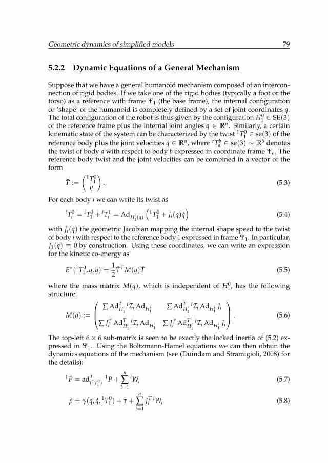
Geometric dynamics of simplified models 79
5.2.2 Dynamic Equations of a General Mechanism
Suppose that we have a general humanoid mechanism composed of an intercon-nection of rigid bodies. If we take one of the rigid bodies (typically a foot or thetorso) as a reference with frame Ψ1 (the base frame), the internal configurationor ‘shape’ of the humanoid is completely defined by a set of joint coordinates q.The total configuration of the robot is thus given by the configuration H0
1 ∈ SE(3)of the reference frame plus the internal joint angles q ∈ Rn. Similarly, a certainkinematic state of the system can be characterized by the twist 1T0
1 ∈ se(3) of thereference body plus the joint velocities q ∈ Rn, where cTb
a ∈ se(3) ∼ R6 denotesthe twist of body a with respect to body b expressed in coordinate frame Ψc. Thereference body twist and the joint velocities can be combined in a vector of theform
T :=(1T0
1q
). (5.3)
For each body i we can write its twist as
iT0i = iT0
1 + iT1i = AdHi
1(q)
(1T0
1 + Ji(q)q)
(5.4)
with Ji(q) the geometric Jacobian mapping the internal shape speed to the twistof body i with respect to the reference body 1 expressed in frame Ψ1. In particular,J1(q) ≡ 0 by construction. Using these coordinates, we can write an expressionfor the kinetic co-energy as
E∗(1T01 , q, q) =
12
TT M(q)T (5.5)
where the mass matrix M(q), which is independent of H01 , has the following
structure:
M(q) :=
∑ AdTHi
1
iIi AdHi1
∑ AdTHi
1
iIi AdHi1
Ji
∑ JTi AdT
Hi1
iIi AdHi1
∑ JTi AdT
Hi1
iIi AdHi1
Ji
. (5.6)
The top-left 6× 6 sub-matrix is seen to be exactly the locked inertia of (5.2) ex-pressed in Ψ1. Using the Boltzmann-Hamel equations we can then obtain thedynamics equations of the mechanism (see (Duindam and Stramigioli, 2008) forthe details):
1P = adT(1T0
1 )1P +
n
∑i=1
iWi (5.7)
p = γ(q, q, 1T01 ) + τ +
n
∑i=1
JTi
iWi (5.8)
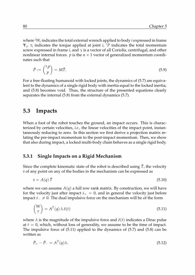
80 Chapter 5
where jWi indicates the total external wrench applied to body i expressed in frameΨj, τi indicates the torque applied at joint i, iP indicates the total momentumscrew expressed in frame i, and γ is a vector of all Coriolis, centrifugal, and othernonlinear internal forces. p is the n× 1 vector of generalized momentum coordi-nates such that
P :=(1P
p
)= MT. (5.9)
For a free-floating humanoid with locked joints, the dynamics of (5.7) are equiva-lent to the dynamics of a single rigid body with inertia equal to the locked inertia,and (5.8) becomes void. Thus, the structure of the presented equations clearlyseparates the internal (5.8) from the external dynamics (5.7).
5.3 Impacts
When a foot of the robot touches the ground, an impact occurs. This is charac-terized by certain velocities, i.e., the linear velocities of the impact point, instan-taneously reducing to zero. In this section we first derive a projection matrix re-lating the pre-impact momentum to the post-impact momentum. Then, we showthat also during impact, a locked multi-body chain behaves as a single rigid body.
5.3.1 Single Impacts on a Rigid Mechanism
Since the complete kinematic state of the robot is described using T, the velocitys of any point on any of the bodies in the mechanism can be expressed as
s = A(q) T (5.10)
where we can assume A(q) a full row rank matrix. By construction, we will havefor the velocity just after impact s+ = 0, and in general the velocity just beforeimpact s− 6= 0. The dual impulsive force on the mechanism will be of the form
(Wτ
)= AT(q) λ δ(t) (5.11)
where λ is the magnitude of the impulsive force and δ(t) indicates a Dirac pulseat t = 0, which, without loss of generality, we assume to be the time of impact.The impulsive force of (5.11) applied to the dynamics of (5.7) and (5.8) can bewritten as
P+ − P− = AT(q)λ. (5.12)
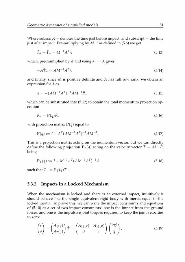
Geometric dynamics of simplified models 81
Where subscript − denotes the time just before impact, and subscript + the timejust after impact. Pre-multiplying by M−1 as defined in (5.6) we get
T+ − T− = M−1 ATλ (5.13)
which, pre-multiplied by A and using s+ = 0, gives
−AT− = AM−1 ATλ (5.14)
and finally, since M is positive definite and A has full row rank, we obtain anexpression for λ as
λ = −(AM−1 AT)−1 AM−1P− (5.15)
which can be substituted into (5.12) to obtain the total momentum projection op-eration
P+ = P(q)P− (5.16)
with projection matrix P(q) equal to
P(q) := I − AT(AM−1 AT)−1 AM−1. (5.17)
This is a projection matrix acting on the momentum vector, but we can directlydefine the following projection PT(q) acting on the velocity vector T = M−1P,being
PT(q) := I −M−1 AT(AM−1 AT)−1 A (5.18)
such that T+ = PT(q)T−.
5.3.2 Impacts in a Locked Mechanism
When the mechanism is locked and there is an external impact, intuitively itshould behave like the single equivalent rigid body with inertia equal to thelocked inertia. To prove this, we can write the impact constraints and equationsof (5.10) as a set of two impact constraints: one is the impact from the groundforces, and one is the impulsive joint torques required to keep the joint velocitiesto zero:
(sq
)=
(A1(q)A2(q)
)T =
(A11(q) A12(q)
0 I
)(1T0
1q
). (5.19)
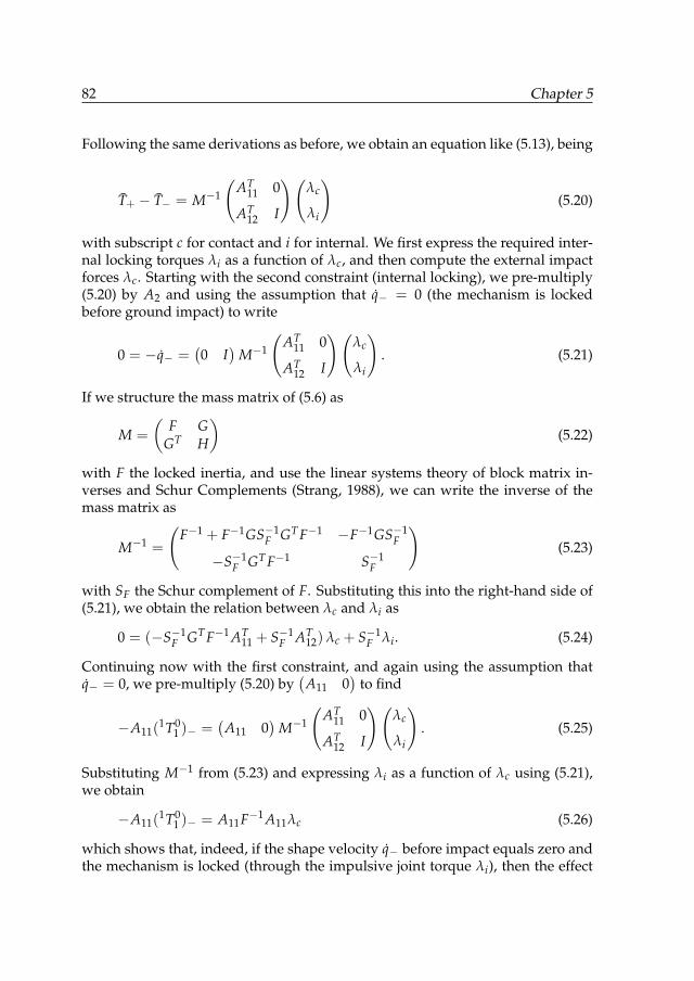
82 Chapter 5
Following the same derivations as before, we obtain an equation like (5.13), being
T+ − T− = M−1
(AT
11 0
AT12 I
)(λc
λi
)(5.20)
with subscript c for contact and i for internal. We first express the required inter-nal locking torques λi as a function of λc, and then compute the external impactforces λc. Starting with the second constraint (internal locking), we pre-multiply(5.20) by A2 and using the assumption that q− = 0 (the mechanism is lockedbefore ground impact) to write
0 = −q− =(0 I
)M−1
(AT
11 0
AT12 I
)(λc
λi
). (5.21)
If we structure the mass matrix of (5.6) as
M =
(F G
GT H
)(5.22)
with F the locked inertia, and use the linear systems theory of block matrix in-verses and Schur Complements (Strang, 1988), we can write the inverse of themass matrix as
M−1 =
(F−1 + F−1GS−1
F GT F−1 −F−1GS−1F
−S−1F GT F−1 S−1
F
)(5.23)
with SF the Schur complement of F. Substituting this into the right-hand side of(5.21), we obtain the relation between λc and λi as
0 = (−S−1F GT F−1 AT
11 + S−1F AT
12) λc + S−1F λi. (5.24)
Continuing now with the first constraint, and again using the assumption thatq− = 0, we pre-multiply (5.20) by
(A11 0
)to find
−A11(1T0
1 )− =(
A11 0)
M−1
(AT
11 0
AT12 I
)(λc
λi
). (5.25)
Substituting M−1 from (5.23) and expressing λi as a function of λc using (5.21),we obtain
−A11(1T0
1 )− = A11F−1 A11λc (5.26)
which shows that, indeed, if the shape velocity q− before impact equals zero andthe mechanism is locked (through the impulsive joint torque λi), then the effect
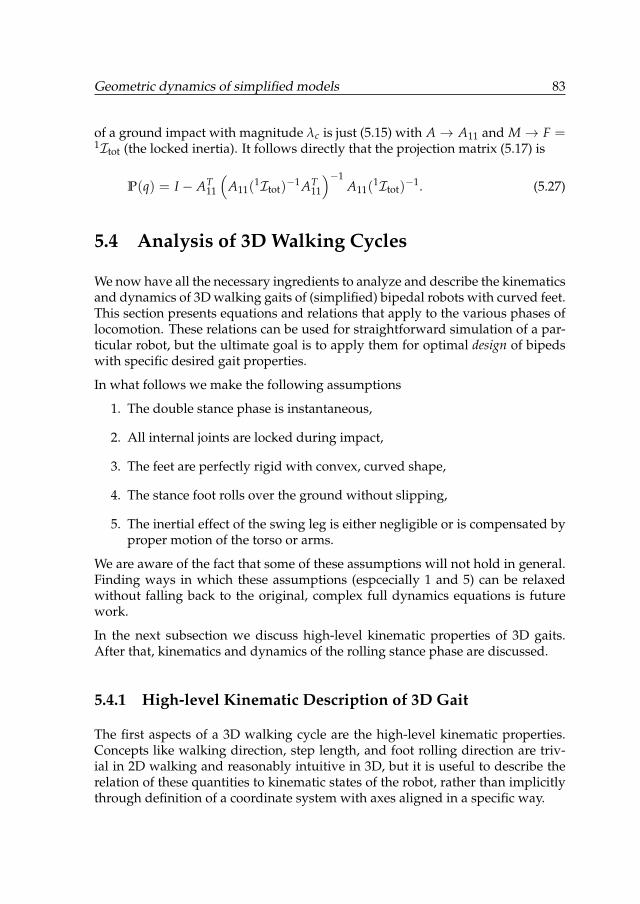
Geometric dynamics of simplified models 83
of a ground impact with magnitude λc is just (5.15) with A→ A11 and M→ F =1Itot (the locked inertia). It follows directly that the projection matrix (5.17) is
P(q) = I − AT11
(A11(
1Itot)−1 AT
11
)−1A11(
1Itot)−1. (5.27)
5.4 Analysis of 3D Walking Cycles
We now have all the necessary ingredients to analyze and describe the kinematicsand dynamics of 3D walking gaits of (simplified) bipedal robots with curved feet.This section presents equations and relations that apply to the various phases oflocomotion. These relations can be used for straightforward simulation of a par-ticular robot, but the ultimate goal is to apply them for optimal design of bipedswith specific desired gait properties.
In what follows we make the following assumptions
1. The double stance phase is instantaneous,
2. All internal joints are locked during impact,
3. The feet are perfectly rigid with convex, curved shape,
4. The stance foot rolls over the ground without slipping,
5. The inertial effect of the swing leg is either negligible or is compensated byproper motion of the torso or arms.
We are aware of the fact that some of these assumptions will not hold in general.Finding ways in which these assumptions (espcecially 1 and 5) can be relaxedwithout falling back to the original, complex full dynamics equations is futurework.
In the next subsection we discuss high-level kinematic properties of 3D gaits.After that, kinematics and dynamics of the rolling stance phase are discussed.
5.4.1 High-level Kinematic Description of 3D Gait
The first aspects of a 3D walking cycle are the high-level kinematic properties.Concepts like walking direction, step length, and foot rolling direction are triv-ial in 2D walking and reasonably intuitive in 3D, but it is useful to describe therelation of these quantities to kinematic states of the robot, rather than implicitlythrough definition of a coordinate system with axes aligned in a specific way.
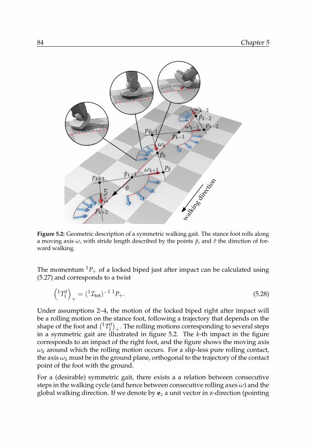
84 Chapter 5
ωk−2
ωk−1
ωk
ωk+1
ωk+
2
pk−2pk−1
pk
pk+1
pk−2
pk−1
pk
pk+1
pk+2
vw
alki
ngdi
rect
ion
Figure 5.2: Geometric description of a symmetric walking gait. The stance foot rolls alonga moving axis ω, with stride length described by the points p, and v the direction of for-ward walking.
The momentum 1P+ of a locked biped just after impact can be calculated using(5.27) and corresponds to a twist
(1T0
1
)+= (1Itot)
−1 1P+. (5.28)
Under assumptions 2–4, the motion of the locked biped right after impact willbe a rolling motion on the stance foot, following a trajectory that depends on theshape of the foot and
(1T01)+. The rolling motions corresponding to several steps
in a symmetric gait are illustrated in figure 5.2. The k-th impact in the figurecorresponds to an impact of the right foot, and the figure shows the moving axisωk around which the rolling motion occurs. For a slip-less pure rolling contact,the axis ωk must be in the ground plane, orthogonal to the trajectory of the contactpoint of the foot with the ground.
For a (desirable) symmetric gait, there exists a a relation between consecutivesteps in the walking cycle (and hence between consecutive rolling axes ω) and theglobal walking direction. If we denote by ez a unit vector in z-direction (pointing
Geometric dynamics of simplified models 85
upwards) and by v the unit vector in the walking direction, it can be seen that
v =(ωk × ez) + (ωk+1 × ez)
|| (ωk × ez) + (ωk+1 × ez) ||(5.29)
where × denotes the vector product (think of ez as a vector pointing from theground up to some point of the robot, e.g., the hip, and note that ω × ez denotesthe linear velocity of that point).
Let us assume that the shape of the curves traced by the contact points is out-ward, that is, during rolling, the contact points move away from the center lineand then return (as in figure 5.2). For efficiency reasons, it is clear that this is anecessary property: through the outward bending shape, the final rolling axis ofone foot just before impact will be more or less aligned with the initial rolling axisof the other foot just after impact. In this way, the motion continues reasonablysmoothly across impacts and little energy is lost. If the trajectory of the contactpoint were to bend inward during rolling, the rolling axes just before and afterimpact would be misaligned, leading to significant energy loss. Because we candesign the contact point trajectory ourselves (see section 5.5), we can design it insuch a way that the assumption holds. In that case, we can use a simpler equationfor the walking direction, being
v =ωk + (−ωk+1)
||ωk + (−ωk+1)||. (5.30)
If the locations of the impacts are known, we can define the points pk in the figureas the intersections of the lines defined by the twist axes of two consecutive stepsk and k + 1. For a symmetric gait, the sequence of middle points
pk := (pk + p(k−1))/2 (5.31)
will lie on a center line in the walking direction v. The distance between subse-quent points pk corresponds to the longitudinal step length. The lateral distanceof a point pk describes how much the foot trajectories curve away from v, i.e., itdepends on 〈v, ωk〉.
5.4.2 Kinematics of 3D Rolling
Continuing now with the details of the rolling motion during the stance phase,suppose we have decided on a desired walking direction v and rolling twist ωkafter impact, and suppose we have chosen a desired trajectory of the contact pointon the floor, for example a spline interpolating between the impact point androlling direction and the release point and rolling direction.
86 Chapter 5
Under these assumptions, we can write down a relation for the kinematics of3D rolling of the foot such that the contact point between the foot and the floorfollows the desired trajectory. If we take r to be the moving contact point, weknow from previous work (Duindam and Stramigioli, 2003) that
(g1∗ + H1
0 g0∗ H01
)r1 = 1T1
0 g1 − H10 g0∗ 0T0
1 r0 (5.32)
with r1 the contact point in body coordinates, r0 the contact point in floor coor-dinates, g1 the normal to the foot surface, and g0 the normal to the floor. Thetangent mappings g1∗ and g0∗ describe the local curvature of the foot and floorsurfaces at the contact point. Since the floor is assumed fully flat g0∗ ≡ 0 and theprevious equation reduces to
g1 = g1∗ r1 = 1T10 g1 = −1T0
1 g1. (5.33)
This equation gives a relation between the twist 1T01 of the foot and the change g1
of the normal vector to the foot surface, which is equal to the foot curvature g1∗ r1in the direction of the trajectory of the contact point. Since r1 must be along thesurface of the foot, we have an additional constraint
gT1 r1 = 0. (5.34)
Depending on the purpose of our analysis of the walking cycle, we can read theseequations in several ways. First, they give us the possible relative motions 1T0
1for a given foot surface shape g1∗. It can be seen that these correspond to thethree rolling directions around the contact point. Second, for given foot shape g1∗and relative motion 1T0
1 , the equations give us the motion of the contact point r1.Finally, and this is the most interesting application, (5.33) can give us design con-straints for the foot: for given desired motions r1 of the contact point and rollingmotion 1T0
1 , we can find local surface shapes g1∗ that satisfy the equation. Since(5.33) only gives us a relation for the curvature in the direction of motion, thecurvature in the orthogonal direction can be designed separately, e.g., to increasestability or efficiency of the rolling motion.
5.4.3 Dynamics of 3D Rolling
The next step in the analysis of the stance phase is the dynamics of the rollingmotion. Here, we use assumption 5 and neglect the inertial effect of the swing leg,or equivalently, we assume its effect is compensated by a counter-effect throughmotion of the torso or arms. These assumptions allow us to again study the bipedthrough its locked inertia.
Under assumption 5, the inertia of the system is constant, hence we study the dy-namics of the locked inertia, rolling on the stance foot. In other words, we look at
Geometric dynamics of simplified models 87
the dynamics of a rigid body with inertia equal to the locked inertia, with surfacedefined by the foot surface of the stance foot, rolling on a flat floor. As discussedbefore, the rolling constraint allows only motion around three rotation axes pass-ing through the contact point, and hence we can write the allowed relative twist1T0
1 of the body with respect to the floor as
1T01 = X(r)ω :=
(Tx(r) Ty(r) Tz(r)
)
wxwywz
(5.35)
with Ti(r) the twist describing rotation around axis i located at the contact pointr and wi the angular velocity around Ti. The columns of the matrix X(r) give abasis for the space of allowed twists. Note that this is similar but opposite to thematrix A in (5.10) which gives a basis for the space of constrained velocities.
Theorem 4 The dynamics of a locked biped with locked inertia tensor I , external wrenchW, and rolling on a foot with allowed twists given by 1T0
1 as in (5.35) and moving contactpoint r, are given as
Iw + Cw = XTW (5.36)
with I := (XTIX) and C := XTI X− XT adXw(IX).
Proof Since all the joints are locked, the behavior of the biped is the same asthe behavior of a single rigid body, and its dynamics are therefore given by thedynamics equation for a rigid body (Stramigioli, 2001)
I ddt
(1T0
1
)− ad1T0
1(I 1T0
1 ) = W + Wc (5.37)
where 1T01 is the twist of the body, ad1T0
1is its algebra representation adjoint, and
Wc are the external wrenches due to the rolling contact with the floor. Since wecan write 1T0
1 = X(r)w at all times, we can substitute this into (5.37) and write
I ddt
(X(r)w)− adX(r)w (IX(r)w) = W + Wc. (5.38)
As the contact wrenches Wc are dual to the allowed twists Xw, we have by defi-nition XTWc ≡ 0, and hence if we multiply the equation from the left by XT , weobtain
XTI ddt
(Xw)− XT adXw (IXw) = XTW (5.39)
XTIXw + XTI Xw− XT adXw (IXw) = XTW (5.40)(
XTIX)
w + XT (I X− adXw IX)
w = XTW (5.41)
which is the result in the theorem if we substitute the definitions of I and C.
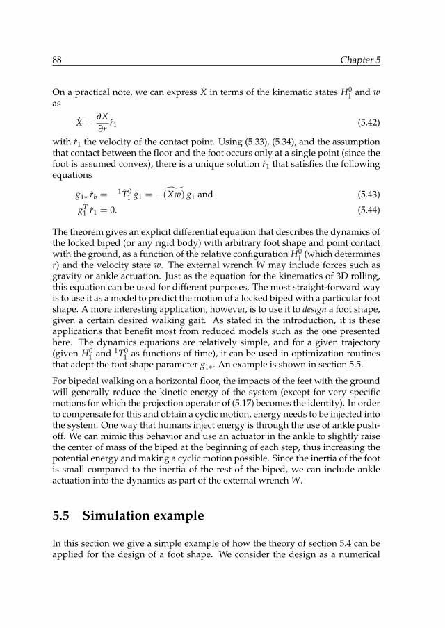
88 Chapter 5
On a practical note, we can express X in terms of the kinematic states H01 and w
as
X =∂X∂r
r1 (5.42)
with r1 the velocity of the contact point. Using (5.33), (5.34), and the assumptionthat contact between the floor and the foot occurs only at a single point (since thefoot is assumed convex), there is a unique solution r1 that satisfies the followingequations
g1∗ rb = −1T01 g1 = −(Xw) g1 and (5.43)
gT1 r1 = 0. (5.44)
The theorem gives an explicit differential equation that describes the dynamics ofthe locked biped (or any rigid body) with arbitrary foot shape and point contactwith the ground, as a function of the relative configuration H0
1 (which determinesr) and the velocity state w. The external wrench W may include forces such asgravity or ankle actuation. Just as the equation for the kinematics of 3D rolling,this equation can be used for different purposes. The most straight-forward wayis to use it as a model to predict the motion of a locked biped with a particular footshape. A more interesting application, however, is to use it to design a foot shape,given a certain desired walking gait. As stated in the introduction, it is theseapplications that benefit most from reduced models such as the one presentedhere. The dynamics equations are relatively simple, and for a given trajectory(given H0
1 and 1T01 as functions of time), it can be used in optimization routines
that adept the foot shape parameter g1∗. An example is shown in section 5.5.
For bipedal walking on a horizontal floor, the impacts of the feet with the groundwill generally reduce the kinetic energy of the system (except for very specificmotions for which the projection operator of (5.17) becomes the identity). In orderto compensate for this and obtain a cyclic motion, energy needs to be injected intothe system. One way that humans inject energy is through the use of ankle push-off. We can mimic this behavior and use an actuator in the ankle to slightly raisethe center of mass of the biped at the beginning of each step, thus increasing thepotential energy and making a cyclic motion possible. Since the inertia of the footis small compared to the inertia of the rest of the biped, we can include ankleactuation into the dynamics as part of the external wrench W.
5.5 Simulation example
In this section we give a simple example of how the theory of section 5.4 can beapplied for the design of a foot shape. We consider the design as a numerical
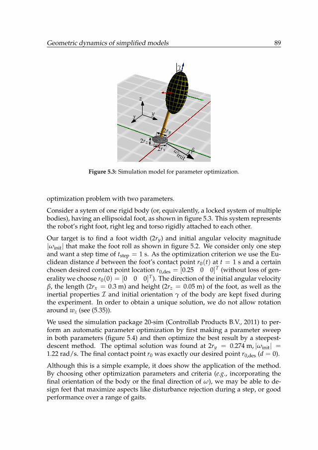
Geometric dynamics of simplified models 89
β2rx
x y
z
ωinit
γ
2ry
2rz
Figure 5.3: Simulation model for parameter optimization.
optimization problem with two parameters.
Consider a sytem of one rigid body (or, equivalently, a locked system of multiplebodies), having an ellipsoidal foot, as shown in figure 5.3. This system representsthe robot’s right foot, right leg and torso rigidly attached to each other.
Our target is to find a foot width (2ry) and initial angular velocity magnitude|ωinit| that make the foot roll as shown in figure 5.2. We consider only one stepand want a step time of tstep = 1 s. As the optimization criterion we use the Eu-clidean distance d between the foot’s contact point r0(t) at t = 1 s and a certainchosen desired contact point location r0,des = [0.25 0 0]T (without loss of gen-erality we choose r0(0) = [0 0 0]T). The direction of the initial angular velocityβ, the length (2rx = 0.3 m) and height (2rz = 0.05 m) of the foot, as well as theinertial properties I and initial orientation γ of the body are kept fixed duringthe experiment. In order to obtain a unique solution, we do not allow rotationaround wz (see (5.35)).
We used the simulation package 20-sim (Controllab Products B.V., 2011) to per-form an automatic parameter optimization by first making a parameter sweepin both parameters (figure 5.4) and then optimize the best result by a steepest-descent method. The optimal solution was found at 2ry = 0.274 m, |ωinit| =1.22 rad/s. The final contact point r0 was exactly our desired point r0,des (d = 0).
Although this is a simple example, it does show the application of the method.By choosing other optimization parameters and criteria (e.g., incorporating thefinal orientation of the body or the final direction of ω), we may be able to de-sign feet that maximize aspects like disturbance rejection during a step, or goodperformance over a range of gaits.
90 Chapter 5
Contact point position
x [m]
y[m
]
0.040.02
0−0.02
−0.04−0.06
−0.08−0.1−0.12
0.05 0.1 0.15 0.2 0.250
Figure 5.4: Foot contact point trails for different parameter values of (2ry) ∈ [0.1, 0.3 m]and |ωinit| ∈ [1.1, 1.6 rad/s] (dark lines) and the optimal solution as stated in the text (lightline).
5.6 Conclusions and Future Work
In this chapter we presented a systematic dynamic analysis of 3D bipedal gait.The gait has a foot rolling phase and an instantaneous phase of foot/ground im-pact. We showed how these phases can be analyzed separately and describedin approximation using simplified models described by the locked inertia and amomentum projection. The resulting equations are much simpler than the fullrobot dynamics and can be used as a starting point for analysis and foot shapedesign.
One feature of this analysis is the use of locked inertia, which is an instantaneoussingle rigid body equivalent of the full biped. Using this simplified model makesthe complex multi-joint robot dynamics more manageable for theoretical probing.The authors believe that insight from geometric dynamics can potentially lead toa more efficient bipedal gait that exploits natural dynamics.
Our long-term objective is to continue to develop a theoretical framework ofbiped gait based on geometric dynamics. As applications of this framework,we will address several specific topics. We would like to start from a desirednominal locomotion pattern and compute the required shape of the rigid 3D feet.Furthermore, practical applications require disturbance robustness of gait cyclesfor which both the foot shape and a proper foot placement strategy need to be de-vised. Finally, previous research has used concepts such as the energy ellipsoidand momentum sphere to describe the dynamics of a rigid body, and it would beinteresting to see how these ellipsoids and spheres change under the influence ofrolling motion on a convex foot surface.

Part II
Control and actuation
91

Chapter 6
Using time-reversal symmetry forstabilizing a simple 3D walker model
This chapter is based on the following article (van Oort and Stramigioli, 2007):
Using time-reversal symmetry for stabilizing a simple 3D walker modelGijs van Oort and Stefano Stramigioli
Proc., IEEE International Conference on Robotics and Automation (ICRA’07)pages 4673–4678, April 2007.
Abstract—A new method is presented for controlling the lateral foot placementof a simple 3D compass biped model. The method is based on the fact that, forthe specific model used in this chapter, limit cycle is time-reversal symmetricand that, after a disturbance, the degree of asymmetry in the cycle is indicatedby a single variable. This variable is used for feedback with a proportionalcontroller. Simulation results show that the controller works very well for alarge range of gaits, without any adaptation of the parameter values.
93
94 Chapter 6
6.1 Introduction
Dynamically walking robots (e.g., Denise (Wisse, 2004), Dribbel (Duindam, 2006)and the Cornell Walker (Collins et al., 2001)), have the advantage over ‘fully ac-tuated’ walkers that they consume far less energy. However, stability and robust-ness are serious problems for them. Particularly, the robustness of 3D dynamicwalkers to lateral disturbances is still very poor. Lateral foot placement is gen-erally seen as a promising method for increasing the robustness in the sidewaysdirection.
This chapter presents a new method for controlling the lateral foot placement ofa simple 3D compass biped model. It is based on the fact that, for the specificmodel used in this chapter, limit cycle is time-reversal symmetric and that, af-ter a disturbance, the degree of asymmetry in the cycle is indicated by a singlevariable. This variable is used for feedback with a proportional controller.
In section 6.2 the model of the 3D compass walker is presented. The configurationof the walker is given, the environmental assumptions are summed up and theequations of motion as well as the impact equations are discussed. In section 6.3the open-loop gait is analyzed. It is shown that the system has infinitely manylimit cycles. One ‘reference limit cycle’ is chosen and by linearization of the stridefunction it is shown that the limit cycle is unstable. It is also shown that a feweigenvalues are intrinsic to the model and cannot be changed. In section 6.4 weshow that each step is time-reversal symmetric when the walker is in its limitcycle. In section 6.5 we use this knowledge and propose a controller with oneparameter K, and in section 6.6 we show by simulation that the controller canstabilize the walker well for a large range of gaits. We give a different view of thecontroller in section 6.7 and we end with conclusions and recommendations insection 6.8.
6.2 Model description
6.2.1 General
Consider a 3D compass biped model as sketched in figure 6.1. This biped consistsof a pointmass at the hip, having mass m, and two massless legs of length `;each with two degrees of freedom: ϕhip and ϕsplay (the hip can thus be seen asa ball-joint). We distinguish the stance leg (subscripted st) and the swing leg(subscripted sw). The ‘feet’ are modeled as point contacts. Ground contact isinelastic and rigid, and since the legs are infinitely stiff, the support transfer isinstantaneous. The ground is considered to have an infinite friction coefficient:no sliding of the feet can occur. In this chapter the following parameters werechosen: m=1 kg; `=1 m; g=9.81 m/s2 (gravitational acceleration).
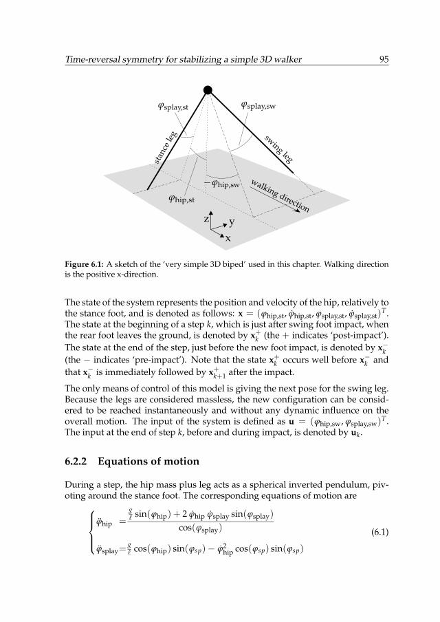
Time-reversal symmetry for stabilizing a simple 3D walker 95
ϕhip,st
−ϕhip,sw
ϕsplay,st ϕsplay,sw
stan
cele
g swing leg
x
yz
walking direction
Figure 6.1: A sketch of the ‘very simple 3D biped’ used in this chapter. Walking directionis the positive x-direction.
The state of the system represents the position and velocity of the hip, relatively tothe stance foot, and is denoted as follows: x = (ϕhip,st, ϕhip,st, ϕsplay,st, ϕsplay,st)
T .The state at the beginning of a step k, which is just after swing foot impact, whenthe rear foot leaves the ground, is denoted by x+k (the + indicates ‘post-impact’).The state at the end of the step, just before the new foot impact, is denoted by x−k(the − indicates ‘pre-impact’). Note that the state x+k occurs well before x−k andthat x−k is immediately followed by x+k+1 after the impact.
The only means of control of this model is giving the next pose for the swing leg.Because the legs are considered massless, the new configuration can be consid-ered to be reached instantaneously and without any dynamic influence on theoverall motion. The input of the system is defined as u = (ϕhip,sw, ϕsplay,sw)
T .The input at the end of step k, before and during impact, is denoted by uk.
6.2.2 Equations of motion
During a step, the hip mass plus leg acts as a spherical inverted pendulum, piv-oting around the stance foot. The corresponding equations of motion are
ϕhip =
g` sin(ϕhip) + 2 ϕhip ϕsplay sin(ϕsplay)
cos(ϕsplay)
ϕsplay=g` cos(ϕhip) sin(ϕsp)− ϕ2
hip cos(ϕsp) sin(ϕsp)
(6.1)

96 Chapter 6
padd ploss
v−k
v+k+1
Figure 6.2: A 2D representation of the impulses during foot impact.
where all angles ϕ• refer to the stance leg. These equations can be integratedto obtain the state of the system. Because the swing leg is massless, it does notinfluence the motion of the system during the step. Therefore, the input u doesnot appear in the equations.
6.2.3 Impact equations and energy injection
When the swing foot hits the ground (foot impact), energy is lost and velocity ofthe hip changes instantaneously. The inelastic, instantaneous collision is modeledas the ground applying an upward impulse ploss to the walker, along the leg. Theloss of kinetic energy due to this impulse is denoted by Eloss. In order to keep theinternal energy of the walker at level, energy is added to the system by applyingan upward impulse padd along the posterior leg (which becomes the new swingleg), as shown in figure 6.2. This impulse can be interpreted as the equivalent ofthe push-off of the human ankle during a normal gait. The kinetic energy addedto the system is denoted by Eadd. In order to keep the energy level constant, weneed to find a padd such that Eadd = Eloss. Since we consider the push-off withenergy injection right before the swinging leg touches the floor, ploss is dependenton padd. To understand this, it is sufficient to consider the extreme case in whichpadd would be extremely large. In this situation the walker would be launchedand the front leg would not even touch the ground.
Given the state of the walker (x−k , uk) just before impact, the required impulsepadd can be calculated that makes Eloss = Eadd using (without proof)
padd= m`sin u2
(ϕ−sp cos ϕ−sp
)+cos u2
(ϕ−sp sin ϕ−sp cos(ϕ−hip−u1)+ ϕ−hip cos ϕ−sp sin(ϕ−hip−u1)
)
1− sin u2 sin ϕ−sp + cos u2 cos ϕ−sp cos(ϕ−hip − u1)
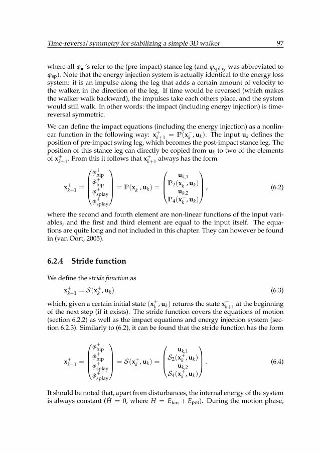
Time-reversal symmetry for stabilizing a simple 3D walker 97
where all ϕ−• ’s refer to the (pre-impact) stance leg (and ϕsplay was abbreviated toϕsp). Note that the energy injection system is actually identical to the energy losssystem: it is an impulse along the leg that adds a certain amount of velocity tothe walker, in the direction of the leg. If time would be reversed (which makesthe walker walk backward), the impulses take each others place, and the systemwould still walk. In other words: the impact (including energy injection) is time-reversal symmetric.
We can define the impact equations (including the energy injection) as a nonlin-ear function in the following way: x+k+1 = P(x−k , uk). The input uk defines theposition of pre-impact swing leg, which becomes the post-impact stance leg. Theposition of this stance leg can directly be copied from uk to two of the elementsof x+k+1. From this it follows that x+k+1 always has the form
x+k+1 =
ϕ+hip
ϕ+hip
ϕ+splay
ϕ+splay
= P(x−k , uk) =
uk,1P2(x−k , uk)
uk,2P4(x−k , uk)
, (6.2)
where the second and fourth element are non-linear functions of the input vari-ables, and the first and third element are equal to the input itself. The equa-tions are quite long and not included in this chapter. They can however be foundin (van Oort, 2005).
6.2.4 Stride function
We define the stride function as
x+k+1 = S(x+k , uk) (6.3)
which, given a certain initial state (x+k , uk) returns the state x+k+1 at the beginningof the next step (if it exists). The stride function covers the equations of motion(section 6.2.2) as well as the impact equations and energy injection system (sec-tion 6.2.3). Similarly to (6.2), it can be found that the stride function has the form
x+k+1 =
ϕ+hip
ϕ+hip
ϕ+splay
ϕ+splay
= S(x+k , uk) =
uk,1S2(x+k , uk)
uk,2S4(x+k , uk)
. (6.4)
It should be noted that, apart from disturbances, the internal energy of the systemis always constant (H = 0, where H = Ekin + Epot). During the motion phase,
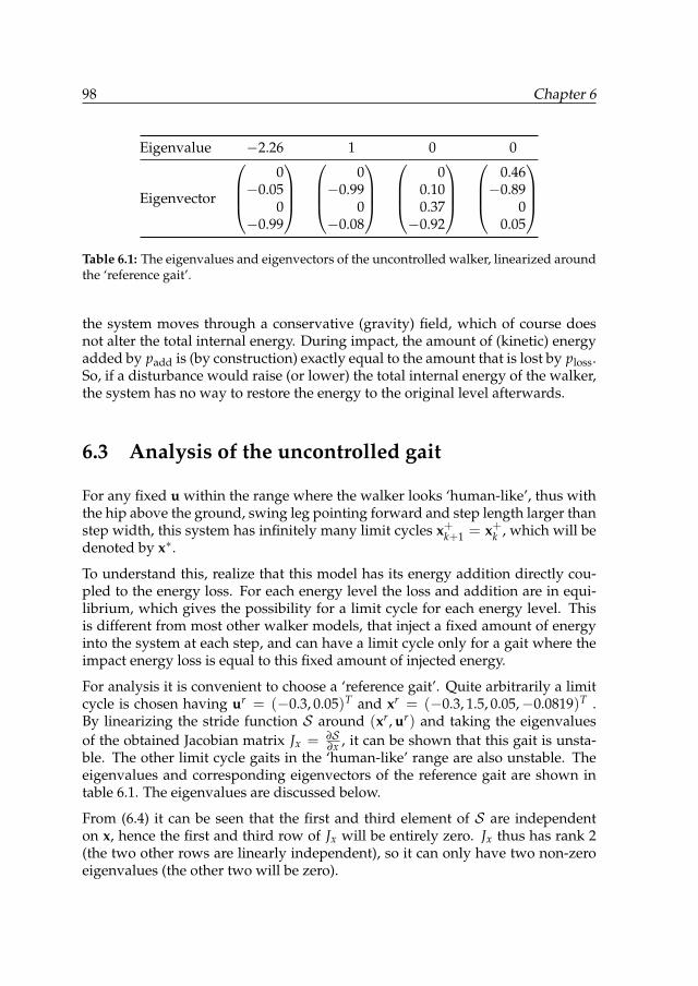
98 Chapter 6
Eigenvalue −2.26 1 0 0
Eigenvector
0−0.05
0−0.99
0−0.99
0−0.08
00.100.37−0.92
0.46−0.89
00.05
Table 6.1: The eigenvalues and eigenvectors of the uncontrolled walker, linearized aroundthe ‘reference gait’.
the system moves through a conservative (gravity) field, which of course doesnot alter the total internal energy. During impact, the amount of (kinetic) energyadded by padd is (by construction) exactly equal to the amount that is lost by ploss.So, if a disturbance would raise (or lower) the total internal energy of the walker,the system has no way to restore the energy to the original level afterwards.
6.3 Analysis of the uncontrolled gait
For any fixed u within the range where the walker looks ‘human-like’, thus withthe hip above the ground, swing leg pointing forward and step length larger thanstep width, this system has infinitely many limit cycles x+k+1 = x+k , which will bedenoted by x∗.
To understand this, realize that this model has its energy addition directly cou-pled to the energy loss. For each energy level the loss and addition are in equi-librium, which gives the possibility for a limit cycle for each energy level. Thisis different from most other walker models, that inject a fixed amount of energyinto the system at each step, and can have a limit cycle only for a gait where theimpact energy loss is equal to this fixed amount of injected energy.
For analysis it is convenient to choose a ‘reference gait’. Quite arbitrarily a limitcycle is chosen having ur = (−0.3, 0.05)T and xr = (−0.3, 1.5, 0.05,−0.0819)T .By linearizing the stride function S around (xr, ur) and taking the eigenvaluesof the obtained Jacobian matrix Jx = ∂S
∂x , it can be shown that this gait is unsta-ble. The other limit cycle gaits in the ‘human-like’ range are also unstable. Theeigenvalues and corresponding eigenvectors of the reference gait are shown intable 6.1. The eigenvalues are discussed below.
From (6.4) it can be seen that the first and third element of S are independenton x, hence the first and third row of Jx will be entirely zero. Jx thus has rank 2(the two other rows are linearly independent), so it can only have two non-zeroeigenvalues (the other two will be zero).
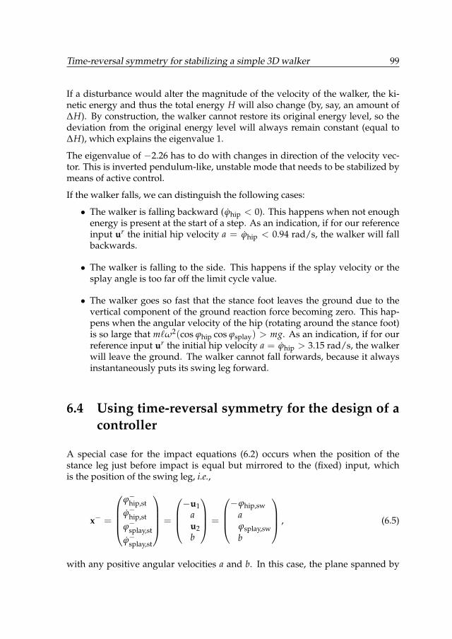
Time-reversal symmetry for stabilizing a simple 3D walker 99
If a disturbance would alter the magnitude of the velocity of the walker, the ki-netic energy and thus the total energy H will also change (by, say, an amount of∆H). By construction, the walker cannot restore its original energy level, so thedeviation from the original energy level will always remain constant (equal to∆H), which explains the eigenvalue 1.
The eigenvalue of −2.26 has to do with changes in direction of the velocity vec-tor. This is inverted pendulum-like, unstable mode that needs to be stabilized bymeans of active control.
If the walker falls, we can distinguish the following cases:
• The walker is falling backward (ϕhip < 0). This happens when not enoughenergy is present at the start of a step. As an indication, if for our referenceinput ur the initial hip velocity a = ϕhip < 0.94 rad/s, the walker will fallbackwards.
• The walker is falling to the side. This happens if the splay velocity or thesplay angle is too far off the limit cycle value.
• The walker goes so fast that the stance foot leaves the ground due to thevertical component of the ground reaction force becoming zero. This hap-pens when the angular velocity of the hip (rotating around the stance foot)is so large that m`ω2(cos ϕhip cos ϕsplay) > mg. As an indication, if for ourreference input ur the initial hip velocity a = ϕhip > 3.15 rad/s, the walkerwill leave the ground. The walker cannot fall forwards, because it alwaysinstantaneously puts its swing leg forward.
6.4 Using time-reversal symmetry for the design of acontroller
A special case for the impact equations (6.2) occurs when the position of thestance leg just before impact is equal but mirrored to the (fixed) input, whichis the position of the swing leg, i.e.,
x− =
ϕ−hip,stϕ−hip,stϕ−splay,stϕ−splay,st
=
−u1au2b
=
−ϕhip,swaϕsplay,swb
, (6.5)
with any positive angular velocities a and b. In this case, the plane spanned by
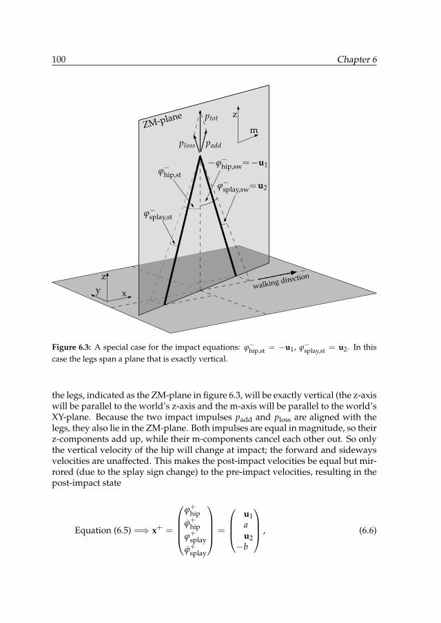
100 Chapter 6
z
mZM-plane
walking direction
ϕ−hip,st
ϕ−splay,st
−ϕ−hip,sw=−u1
ϕ−splay,sw=u2
paddploss
ptot
xyz
Figure 6.3: A special case for the impact equations: ϕ−hip,st = −u1, ϕ−splay,st = u2. In thiscase the legs span a plane that is exactly vertical.
the legs, indicated as the ZM-plane in figure 6.3, will be exactly vertical (the z-axiswill be parallel to the world’s z-axis and the m-axis will be parallel to the world’sXY-plane. Because the two impact impulses padd and ploss are aligned with thelegs, they also lie in the ZM-plane. Both impulses are equal in magnitude, so theirz-components add up, while their m-components cancel each other out. So onlythe vertical velocity of the hip will change at impact; the forward and sidewaysvelocities are unaffected. This makes the post-impact velocities be equal but mir-rored (due to the splay sign change) to the pre-impact velocities, resulting in thepost-impact state
Equation (6.5) =⇒ x+ =
ϕ+hip
ϕ+hip
ϕ+splay
ϕ+splay
=
u1au2−b
, (6.6)
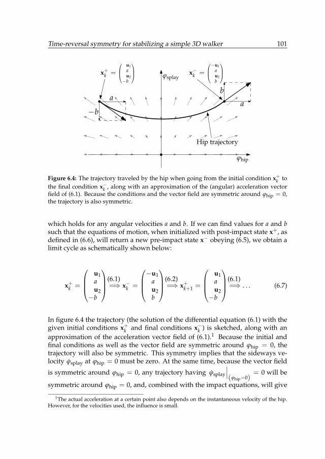
Time-reversal symmetry for stabilizing a simple 3D walker 101
Hip trajectory
x+k =
u1au2−b
x−k =
−u1
au2b
ϕsplay
ϕhip
aa
b
−b
Figure 6.4: The trajectory traveled by the hip when going from the initial condition x+k tothe final condition x−k , along with an approximation of the (angular) acceleration vectorfield of (6.1). Because the conditions and the vector field are symmetric around ϕhip = 0,the trajectory is also symmetric.
which holds for any angular velocities a and b. If we can find values for a and bsuch that the equations of motion, when initialized with post-impact state x+, asdefined in (6.6), will return a new pre-impact state x− obeying (6.5), we obtain alimit cycle as schematically shown below:
x+k =
u1au2−b
(6.1)=⇒ x−k =
−u1au2b
(6.2)=⇒ x+k+1 =
u1au2−b
(6.1)=⇒ . . . (6.7)
In figure 6.4 the trajectory (the solution of the differential equation (6.1) with thegiven initial conditions x+k and final conditions x−k ) is sketched, along with anapproximation of the acceleration vector field of (6.1).1 Because the initial andfinal conditions as well as the vector field are symmetric around ϕhip = 0, thetrajectory will also be symmetric. This symmetry implies that the sideways ve-locity ϕsplay at ϕhip = 0 must be zero. At the same time, because the vector field
is symmetric around ϕhip = 0, any trajectory having ϕsplay
∣∣∣(ϕhip=0)
= 0 will be
symmetric around ϕhip = 0, and, combined with the impact equations, will give
1The actual acceleration at a certain point also depends on the instantaneous velocity of the hip.However, for the velocities used, the influence is small.
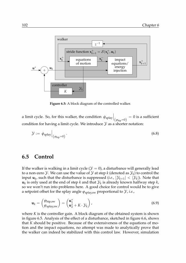
102 Chapter 6
walker
u∗
Yk
x+kx+k+1
equationsof motion
impactequations/
energyinjection
z−1
stride function x+k+1 = S(x+k , uk)
+
x−k
uk
controller
K
Figure 6.5: A block diagram of the controlled walker.
a limit cycle. So, for this walker, the condition ϕsplay
∣∣∣(ϕhip=0)
= 0 is a sufficient
condition for having a limit cycle. We introduce Y as a shorter notation:
Y := ϕsplay
∣∣∣(ϕhip=0)
. (6.8)
6.5 Control
If the walker is walking in a limit cycle (Y = 0), a disturbance will generally leadto a non-zero Y . We can use the value of Y at step k (denoted as Yk) to control theinput uk, such that the disturbance is suppressed (i.e., |Yk+1| < |Yk|). Note thatuk is only used at the end of step k and that Yk is already known halfway step k,so we won’t run into problems here. A good choice for control would be to givea setpoint offset for the splay angle ϕsplay,sw proportional to Y , i.e.,
uk =
(ϕhip,swϕsplay,sw
)=
(u∗1u∗2 + K · Yk
), (6.9)
where K is the controller gain. A block diagram of the obtained system is shownin figure 6.5. Analysis of the effect of a disturbance, sketched in figure 6.6, showsthat K should be positive. Because of the extensiveness of the equations of mo-tion and the impact equations, no attempt was made to analytically prove thatthe walker can indeed be stabilized with this control law. However, simulation
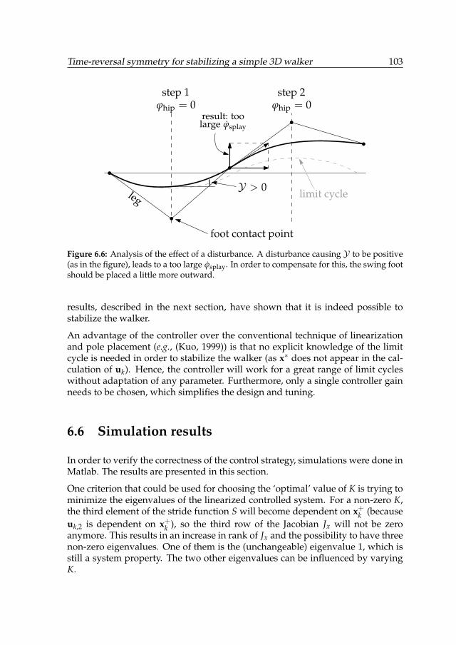
Time-reversal symmetry for stabilizing a simple 3D walker 103
ϕhip = 0 ϕhip = 0
Y > 0
step 2step 1
limit cycleleg
foot contact point
result: toolarge ϕsplay
Figure 6.6: Analysis of the effect of a disturbance. A disturbance causing Y to be positive(as in the figure), leads to a too large ϕsplay. In order to compensate for this, the swing footshould be placed a little more outward.
results, described in the next section, have shown that it is indeed possible tostabilize the walker.
An advantage of the controller over the conventional technique of linearizationand pole placement (e.g., (Kuo, 1999)) is that no explicit knowledge of the limitcycle is needed in order to stabilize the walker (as x∗ does not appear in the cal-culation of uk). Hence, the controller will work for a great range of limit cycleswithout adaptation of any parameter. Furthermore, only a single controller gainneeds to be chosen, which simplifies the design and tuning.
6.6 Simulation results
In order to verify the correctness of the control strategy, simulations were done inMatlab. The results are presented in this section.
One criterion that could be used for choosing the ‘optimal’ value of K is trying tominimize the eigenvalues of the linearized controlled system. For a non-zero K,the third element of the stride function S will become dependent on x+k (becauseuk,2 is dependent on x+k ), so the third row of the Jacobian Jx will not be zeroanymore. This results in an increase in rank of Jx and the possibility to have threenon-zero eigenvalues. One of them is the (unchangeable) eigenvalue 1, which isstill a system property. The two other eigenvalues can be influenced by varyingK.

104 Chapter 6
−2 −1 0 1 2 3
−2
−1
0
1
2
Re(s)
Im(s
)
Figure 6.7: Root locus plot of the controlled reference gait. For K = 0.252 . . . 0.398 all polesare within the unit circle, so the system is stable. The smallest eigenvalue is reached atK = 0.259.
1 1.5 2 2.5 30
1
2
3
4
Wal
ker
fal
ls b
ack
Sta
nce
leg
lea
ves
th
e g
rou
ndK=0.000
K=0.200
K=0.259
K=0.500
a = ϕ+hip [rad/s]
max(|λ|)
Figure 6.8: The eigenvalues of the controlled system for different gait velocities, with dif-ferent values for K. It can be seen that K = 0.259 can not only stabilize our reference gaitwell, but also all gaits with higher velocity.
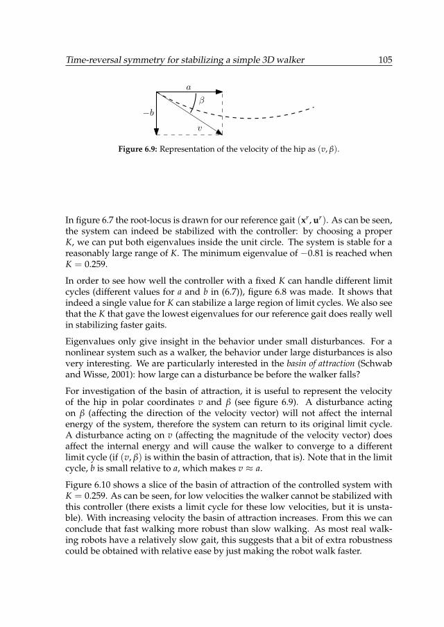
Time-reversal symmetry for stabilizing a simple 3D walker 105
β
v
a
−b
Figure 6.9: Representation of the velocity of the hip as (v, β).
In figure 6.7 the root-locus is drawn for our reference gait (xr, ur). As can be seen,the system can indeed be stabilized with the controller: by choosing a properK, we can put both eigenvalues inside the unit circle. The system is stable for areasonably large range of K. The minimum eigenvalue of −0.81 is reached whenK = 0.259.
In order to see how well the controller with a fixed K can handle different limitcycles (different values for a and b in (6.7)), figure 6.8 was made. It shows thatindeed a single value for K can stabilize a large region of limit cycles. We also seethat the K that gave the lowest eigenvalues for our reference gait does really wellin stabilizing faster gaits.
Eigenvalues only give insight in the behavior under small disturbances. For anonlinear system such as a walker, the behavior under large disturbances is alsovery interesting. We are particularly interested in the basin of attraction (Schwaband Wisse, 2001): how large can a disturbance be before the walker falls?
For investigation of the basin of attraction, it is useful to represent the velocityof the hip in polar coordinates v and β (see figure 6.9). A disturbance actingon β (affecting the direction of the velocity vector) will not affect the internalenergy of the system, therefore the system can return to its original limit cycle.A disturbance acting on v (affecting the magnitude of the velocity vector) doesaffect the internal energy and will cause the walker to converge to a differentlimit cycle (if (v, β) is within the basin of attraction, that is). Note that in the limitcycle, b is small relative to a, which makes v ≈ a.
Figure 6.10 shows a slice of the basin of attraction of the controlled system withK = 0.259. As can be seen, for low velocities the walker cannot be stabilized withthis controller (there exists a limit cycle for these low velocities, but it is unsta-ble). With increasing velocity the basin of attraction increases. From this we canconclude that fast walking more robust than slow walking. As most real walk-ing robots have a relatively slow gait, this suggests that a bit of extra robustnesscould be obtained with relative ease by just making the robot walk faster.
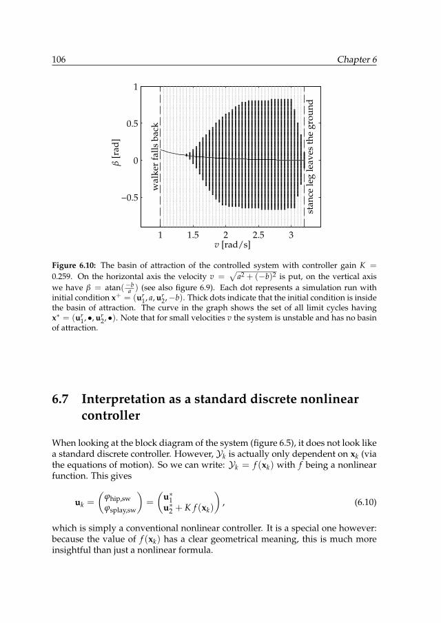
106 Chapter 6
1 1.5 2 2.5 3
−0.5
0
0.5
1
walk
er f
all
s b
ack
sta
nce l
eg
leav
es t
he g
ro
un
d
v [rad/s]
β[r
ad]
Figure 6.10: The basin of attraction of the controlled system with controller gain K =
0.259. On the horizontal axis the velocity v =√
a2 + (−b)2 is put, on the vertical axiswe have β = atan(−b
a ) (see also figure 6.9). Each dot represents a simulation run withinitial condition x+ = (ur
1, a, ur2,−b). Thick dots indicate that the initial condition is inside
the basin of attraction. The curve in the graph shows the set of all limit cycles havingx∗ = (ur
1, •, ur2, •). Note that for small velocities v the system is unstable and has no basin
of attraction.
6.7 Interpretation as a standard discrete nonlinearcontroller
When looking at the block diagram of the system (figure 6.5), it does not look likea standard discrete controller. However, Yk is actually only dependent on xk (viathe equations of motion). So we can write: Yk = f (xk) with f being a nonlinearfunction. This gives
uk =
(ϕhip,swϕsplay,sw
)=
(u∗1u∗2 + K f (xk)
), (6.10)
which is simply a conventional nonlinear controller. It is a special one however:because the value of f (xk) has a clear geometrical meaning, this is much moreinsightful than just a nonlinear formula.
Time-reversal symmetry for stabilizing a simple 3D walker 107
6.8 Conclusions and future work
A new method has been described for controlling lateral foot placement of a 3Dcompass biped model, based on time-reversal symmetry of the limit cycle. Ifa disturbance occurs, the step becomes asymmetric. It was shown that Y :=ϕsplay
∣∣∣(ϕhip=0)
is a good measure for the degree of asymmetry of the step, and
can be used for feedback. A proportional controller was proposed where thesplay angle offset is proportional to Y (with controller gain K).
Simulation results showed that the controller can stabilize the walker in a largerange of gaits (at different velocities) without any adjustment of the parameter,and that the basin of attraction is large, especially for fast walking. It was shownthat the controller is actually a conventional nonlinear controller, with the ad-ditional property that the non-linear function has a clear geometrical meaning,which gives more insight in the actual control strategy.
The control method as described here works well with the compass model, but itcannot directly be used for more complex models, because generally the gait ofsuch models is not time-reversal symmetric. This study will be continued by in-vestigating how the method can be generalized to work with other walker modelsas well. Our goal is to build a real 3D biped soon, which will, amongst others,make use of the lateral foot placement control method.

108 Chapter 6
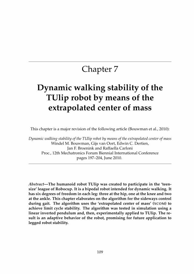
Chapter 7
Dynamic walking stability of theTUlip robot by means of theextrapolated center of mass
This chapter is a major revision of the following article (Bouwman et al., 2010):
Dynamic walking stability of the TUlip robot by means of the extrapolated center of massWindel M. Bouwman, Gijs van Oort, Edwin C. Dertien,
Jan F. Broenink and Raffaella CarloniProc., 12th Mechatronics Forum Biennial International Conference
pages 197–204, June 2010.
Abstract—The humanoid robot TUlip was created to participate in the ‘teen-size’ league of Robocup. It is a bipedal robot intended for dynamic walking. Ithas six degrees of freedom in each leg: three at the hip, one at the knee and twoat the ankle. This chapter elaborates on the algorithm for the sideways controlduring gait. The algorithm uses the ‘extrapolated center of mass’ (XCOM) toachieve limit cycle stability. The algorithm was tested in simulation using alinear inverted pendulum and, then, experimentally applied to TUlip. The re-sult is an adaptive behavior of the robot, promising for future application tolegged robot stability.
109
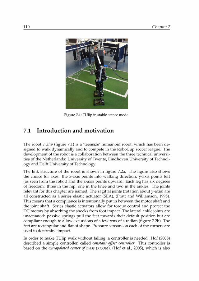
110 Chapter 7
Figure 7.1: TUlip in stable stance mode.
7.1 Introduction and motivation
The robot TUlip (figure 7.1) is a ‘teensize’ humanoid robot, which has been de-signed to walk dynamically and to compete in the RoboCup soccer league. Thedevelopment of the robot is a collaboration between the three technical universi-ties of the Netherlands: University of Twente, Eindhoven University of Technol-ogy and Delft University of Technology.
The link structure of the robot is shown in figure 7.2a. The figure also showsthe choice for axes: the x-axis points into walking direction; y-axis points left(as seen from the robot) and the z-axis points upward. Each leg has six degreesof freedom: three in the hip, one in the knee and two in the ankles. The jointsrelevant for this chapter are named. The sagittal joints (rotation about y-axis) areall constructed as a series elastic actuator (SEA), (Pratt and Williamson, 1995).This means that a compliance is intentionally put in between the motor shaft andthe joint shaft. Series elastic actuators allow for torque control and protect theDC motors by absorbing the shocks from foot impact. The lateral ankle joints areunactuated: passive springs pull the feet towards their default position but arecompliant enough to allow excursions of a few tens of a radian (figure 7.2b). Thefeet are rectangular and flat of shape. Pressure sensors on each of the corners areused to determine impact.
In order to make TUlip walk without falling, a controller is needed. Hof (2008)described a simple controller, called constant offset controller. This controller isbased on the extrapolated center of mass (XCOM), (Hof et al., 2005), which is also
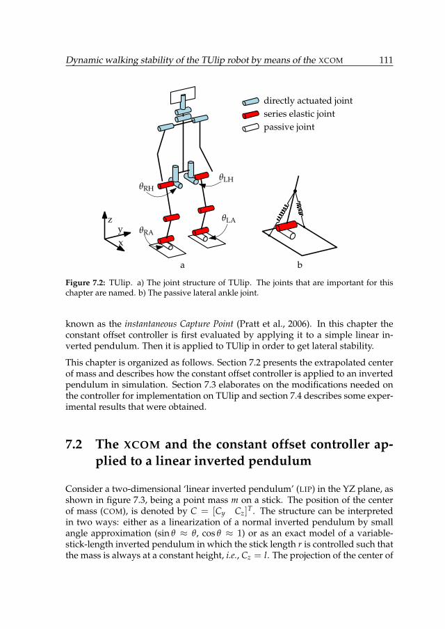
Dynamic walking stability of the TUlip robot by means of the XCOM 111
a b
θLAθRA
θRH
xy
z
θLH
directly actuated jointseries elastic jointpassive joint
Figure 7.2: TUlip. a) The joint structure of TUlip. The joints that are important for thischapter are named. b) The passive lateral ankle joint.
known as the instantaneous Capture Point (Pratt et al., 2006). In this chapter theconstant offset controller is first evaluated by applying it to a simple linear in-verted pendulum. Then it is applied to TUlip in order to get lateral stability.
This chapter is organized as follows. Section 7.2 presents the extrapolated centerof mass and describes how the constant offset controller is applied to an invertedpendulum in simulation. Section 7.3 elaborates on the modifications needed onthe controller for implementation on TUlip and section 7.4 describes some exper-imental results that were obtained.
7.2 The XCOM and the constant offset controller ap-plied to a linear inverted pendulum
Consider a two-dimensional ‘linear inverted pendulum’ (LIP) in the YZ plane, asshown in figure 7.3, being a point mass m on a stick. The position of the centerof mass (COM), is denoted by C = [Cy Cz]T . The structure can be interpretedin two ways: either as a linearization of a normal inverted pendulum by smallangle approximation (sin θ ≈ θ, cos θ ≈ 1) or as an exact model of a variable-stick-length inverted pendulum in which the stick length r is controlled such thatthe mass is always at a constant height, i.e., Cz = l. The projection of the center of
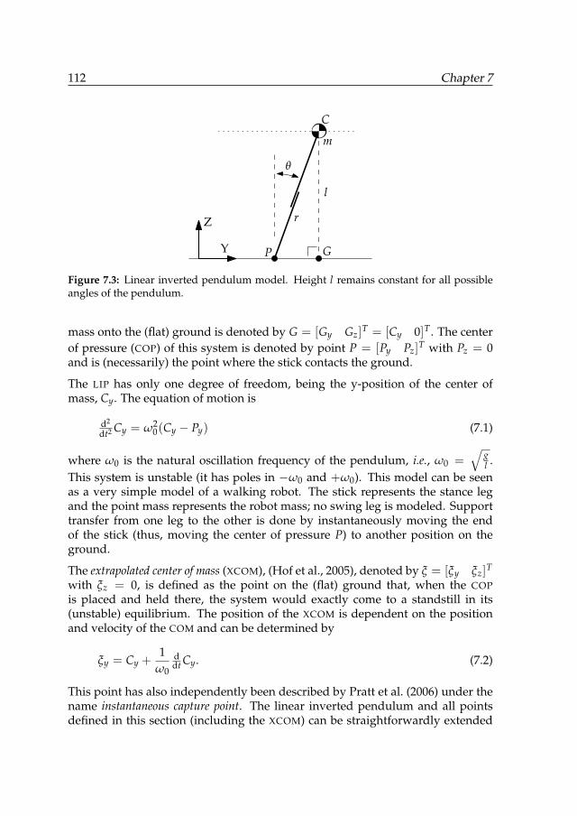
112 Chapter 7
Y
Z
C
P G
l
θ
m
r
Figure 7.3: Linear inverted pendulum model. Height l remains constant for all possibleangles of the pendulum.
mass onto the (flat) ground is denoted by G = [Gy Gz]T = [Cy 0]T . The centerof pressure (COP) of this system is denoted by point P = [Py Pz]T with Pz = 0and is (necessarily) the point where the stick contacts the ground.
The LIP has only one degree of freedom, being the y-position of the center ofmass, Cy. The equation of motion is
d2
dt2 Cy = ω20(Cy − Py) (7.1)
where ω0 is the natural oscillation frequency of the pendulum, i.e., ω0 =√
gl .
This system is unstable (it has poles in −ω0 and +ω0). This model can be seenas a very simple model of a walking robot. The stick represents the stance legand the point mass represents the robot mass; no swing leg is modeled. Supporttransfer from one leg to the other is done by instantaneously moving the endof the stick (thus, moving the center of pressure P) to another position on theground.
The extrapolated center of mass (XCOM), (Hof et al., 2005), denoted by ξ = [ξy ξz]T
with ξz = 0, is defined as the point on the (flat) ground that, when the COPis placed and held there, the system would exactly come to a standstill in its(unstable) equilibrium. The position of the XCOM is dependent on the positionand velocity of the COM and can be determined by
ξy = Cy +1
ω0
ddt Cy. (7.2)
This point has also independently been described by Pratt et al. (2006) under thename instantaneous capture point. The linear inverted pendulum and all pointsdefined in this section (including the XCOM) can be straightforwardly extended
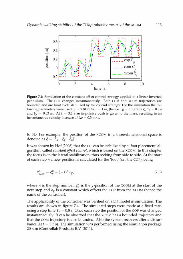
Dynamic walking stability of the TUlip robot by means of the XCOM 113
0 2 4 6 8 10
−0.2
0
0.2
0.4
0.6
time [s]
po
sit
ion
[m
]
cop Py
com Cy
xcom ξy
Figure 7.4: Simulation of the constant offset control strategy applied to a linear invertedpendulum. The COP changes instantaneously. Both COM and XCOM trajectories arebounded and are limit cycle stabilized by the control strategy. For the simulation the fol-lowing parameters were used: g = 9.81 m/s, l = 1 m, (hence ω0 = 3.13 rad/s), Ts = 0.8 sand by = 0.03 m. At t = 3.5 s an impulsive push is given to the mass, resulting in aninstantaneous velocity increase of ∆v = 0.3 m/s.
to 3D. For example, the position of the XCOM in a three-dimensional space isdenoted as ξ = [ξx ξy ξz]T .
It was shown by Hof (2008) that the LIP can be stabilized by a ‘foot placement’ al-gorithm, called constant offset control, which is based on the XCOM. In this chapterthe focus is on the lateral stabilization, thus rocking from side to side. At the startof each step n a new position is calculated for the ‘foot’ (i.e., the COP), being
Pny,des = ξn
y + (−1)n by, (7.3)
where n is the step number, ξny is the y-position of the XCOM at the start of the
new step and by is a constant which offsets the COP from the XCOM (hence thename of the controller).
The applicability of the controller was verified on a LIP model in simulation. Theresults are shown in figure 7.4. The simulated steps were made at a fixed rate,using a step time Ts = 0.8 s. Once each step the position of the COP was changedinstantaneously. It can be observed that the XCOM has a bounded trajectory andthat the COM trajectory is also bounded. Also the system recovers after a distur-bance (at t = 3.5 s). The simulation was performed using the simulation package20-sim (Controllab Products B.V., 2011).
114 Chapter 7
7.3 Stability by foot placement applied to TUlip
The constant offset controller has been designed with an ideal linear invertedpendulum in mind. In order to be able to use it for controlling the robot TUlip,some adaptations need to be made to it because TUlip differs from a LIP in thefollowing ways:
• TUlip has a double support phase during walking during which the COPgradually moves from one foot to the other. The LIP has instantaneous sup-port transfer and therefore instantaneous relocation of the COP;
• The legs of TUlip cannot be positioned arbitrarily fast, while the ‘leg’ of theLIP can;
• The duration of each step, Tn, is unknown a priori and is a result of thesystem dynamics. Therefore, the step time is influenced by disturbances.This is in contrast to the LIP, where the step time is a control choice, i.e., anew step can be initiated at any moment in time;
• Contrary to the LIP, the region where the foot of TUlip can be placed islimited due to physical constraints;
• During single support, the COP P moves around within the convex hull ofthe stance foot. In the sagittal plane Px can be moved actively by control. Inthe lateral plane Py is a function of the stance ankle angle θ•A.
The unknown step time issue would not seem like a problem because in the con-trol law (7.3) no notion of timing is used. However, because the legs of TUlipcannot be moved arbitrarily fast, the step time is an important factor becausethe leg should be moved to the right position within this time. In order to pro-vide a solution, a minimum step time Tmin should be determined experimentally(Tmin = min(Tn)) or estimated.
7.3.1 State machine of the gait
The gait cycle of TUlip consists of four states, described shortly below. After that,in the subsequent sections, implementation details are discussed. For robot andcontroller parameters, see table 7.1.
• Double stance, left push-off. At the start of the new step, the left footpushes off with the ankle. Because during this phase both feet are on theground, lateral foot movements are impossible. Exit condition for this stateis that the left heel has lost contact with the floor and t > Tpush-off.
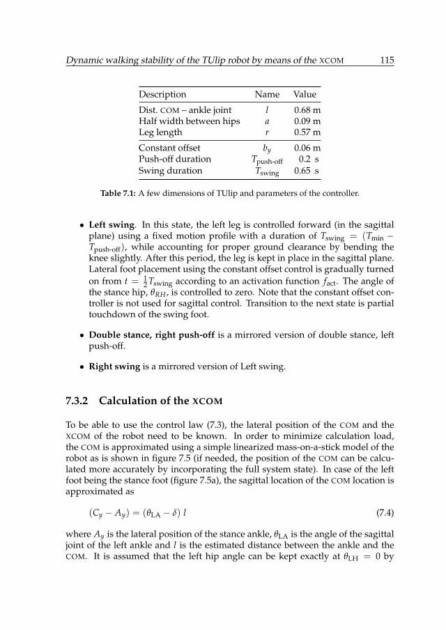
Dynamic walking stability of the TUlip robot by means of the XCOM 115
Description Name Value
Dist. COM – ankle joint l 0.68 mHalf width between hips a 0.09 mLeg length r 0.57 m
Constant offset by 0.06 mPush-off duration Tpush-off 0.2 sSwing duration Tswing 0.65 s
Table 7.1: A few dimensions of TUlip and parameters of the controller.
• Left swing. In this state, the left leg is controlled forward (in the sagittalplane) using a fixed motion profile with a duration of Tswing = (Tmin −Tpush-off), while accounting for proper ground clearance by bending theknee slightly. After this period, the leg is kept in place in the sagittal plane.Lateral foot placement using the constant offset control is gradually turnedon from t = 1
2 Tswing according to an activation function fact. The angle ofthe stance hip, θRH , is controlled to zero. Note that the constant offset con-troller is not used for sagittal control. Transition to the next state is partialtouchdown of the swing foot.
• Double stance, right push-off is a mirrored version of double stance, leftpush-off.
• Right swing is a mirrored version of Left swing.
7.3.2 Calculation of the XCOM
To be able to use the control law (7.3), the lateral position of the COM and theXCOM of the robot need to be known. In order to minimize calculation load,the COM is approximated using a simple linearized mass-on-a-stick model of therobot as is shown in figure 7.5 (if needed, the position of the COM can be calcu-lated more accurately by incorporating the full system state). In case of the leftfoot being the stance foot (figure 7.5a), the sagittal location of the COM location isapproximated as
(Cy − Ay) = (θLA − δ) l (7.4)
where Ay is the lateral position of the stance ankle, θLA is the angle of the sagittaljoint of the left ankle and l is the estimated distance between the ankle and theCOM. It is assumed that the left hip angle can be kept exactly at θLH = 0 by
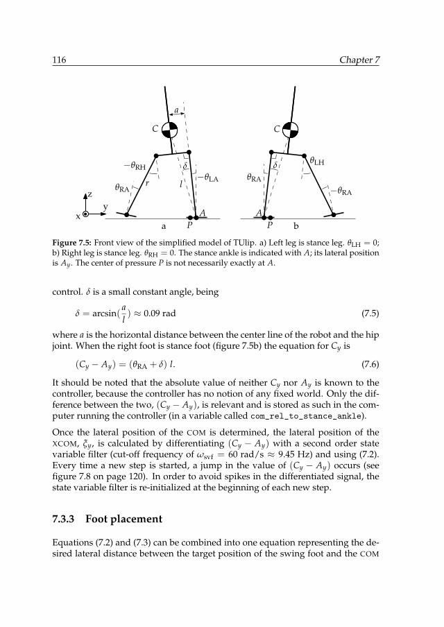
116 Chapter 7
δ
lr−θLA
−θRH
θRA
A
C
a b
δ
θRA
θLH
−θRA
A
C
xy
z
a
P P
Figure 7.5: Front view of the simplified model of TUlip. a) Left leg is stance leg. θLH = 0;b) Right leg is stance leg. θRH = 0. The stance ankle is indicated with A; its lateral positionis Ay. The center of pressure P is not necessarily exactly at A.
control. δ is a small constant angle, being
δ = arcsin(al) ≈ 0.09 rad (7.5)
where a is the horizontal distance between the center line of the robot and the hipjoint. When the right foot is stance foot (figure 7.5b) the equation for Cy is
(Cy − Ay) = (θRA + δ) l. (7.6)
It should be noted that the absolute value of neither Cy nor Ay is known to thecontroller, because the controller has no notion of any fixed world. Only the dif-ference between the two, (Cy − Ay), is relevant and is stored as such in the com-puter running the controller (in a variable called com_rel_to_stance_ankle).
Once the lateral position of the COM is determined, the lateral position of theXCOM, ξy, is calculated by differentiating (Cy − Ay) with a second order statevariable filter (cut-off frequency of ωsvf = 60 rad/s ≈ 9.45 Hz) and using (7.2).Every time a new step is started, a jump in the value of (Cy − Ay) occurs (seefigure 7.8 on page 120). In order to avoid spikes in the differentiated signal, thestate variable filter is re-initialized at the beginning of each new step.
7.3.3 Foot placement
Equations (7.2) and (7.3) can be combined into one equation representing the de-sired lateral distance between the target position of the swing foot and the COM
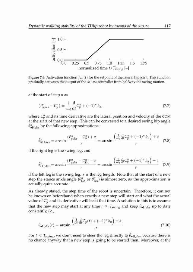
Dynamic walking stability of the TUlip robot by means of the XCOM 117
0.0 0.25 0.5 0.75 1.0 1.25 1.5 1.75normalized time t/Tswing [–]
0.0
0.5
1.0
acti
vati
on[–
]
Figure 7.6: Activation function fact(t) for the setpoint of the lateral hip joint. This functiongradually activates the output of the XCOM controller from halfway the swing motion.
at the start of step n as
(Pny,des − Cn
y ) =1
ω0
ddt
Cny + (−1)n bn, (7.7)
where Cny and its time derivative are the lateral position and velocity of the COM
at the start of that new step. This can be converted to a desired swing hip angleθn•H,des by the following approximations:
θnRH,des = arcsin
(Pny,des − Cn
y ) + a
r= arcsin
(1
ω0ddt Cn
y + (−1)n bn
)+ a
r(7.8)
if the right leg is the swing leg, and
θnLH,des = arcsin
(Pny,des − Cn
y )− a
r= arcsin
(1
ω0ddt Cn
y + (−1)n bn
)− a
r(7.9)
if the left leg is the swing leg. r is the leg length. Note that at the start of a newstep the stance ankle angle (θn
LA or θnRA) is almost zero, so the approximation is
actually quite accurate.
As already stated, the step time of the robot is uncertain. Therefore, it can notbe known on beforehand when exactly a new step will start and what the actualvalue of Cn
y and its derivative will be at that time. A solution to this is to assumethat the new step may start at any time t ≥ Tswing and keep θ•H,des up to dateconstantly, i.e.,
θ•H,des(t) = arcsin
(1
ω0ddt Cy(t) + (−1)n bn
)± a
r. (7.10)
For t < Tswing, we don’t need to steer the leg directly to θ•H,des, because there isno chance anyway that a new step is going to be started then. Moreover, at the
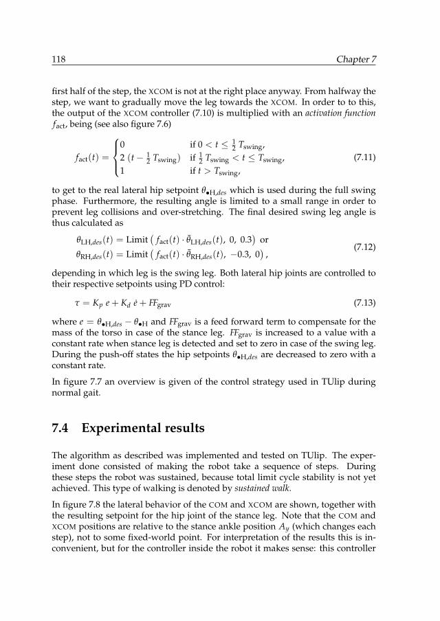
118 Chapter 7
first half of the step, the XCOM is not at the right place anyway. From halfway thestep, we want to gradually move the leg towards the XCOM. In order to to this,the output of the XCOM controller (7.10) is multiplied with an activation functionfact, being (see also figure 7.6)
fact(t) =
0 if 0 < t ≤ 12 Tswing,
2 (t− 12 Tswing) if 1
2 Tswing < t ≤ Tswing,1 if t > Tswing,
(7.11)
to get to the real lateral hip setpoint θ•H,des which is used during the full swingphase. Furthermore, the resulting angle is limited to a small range in order toprevent leg collisions and over-stretching. The final desired swing leg angle isthus calculated as
θLH,des(t) = Limit(
fact(t) · θLH,des(t), 0, 0.3)
or
θRH,des(t) = Limit(
fact(t) · θRH,des(t), −0.3, 0)
,(7.12)
depending in which leg is the swing leg. Both lateral hip joints are controlled totheir respective setpoints using PD control:
τ = Kp e + Kd e + FFgrav (7.13)
where e = θ•H,des − θ•H and FFgrav is a feed forward term to compensate for themass of the torso in case of the stance leg. FFgrav is increased to a value with aconstant rate when stance leg is detected and set to zero in case of the swing leg.During the push-off states the hip setpoints θ•H,des are decreased to zero with aconstant rate.
In figure 7.7 an overview is given of the control strategy used in TUlip duringnormal gait.
7.4 Experimental results
The algorithm as described was implemented and tested on TUlip. The exper-iment done consisted of making the robot take a sequence of steps. Duringthese steps the robot was sustained, because total limit cycle stability is not yetachieved. This type of walking is denoted by sustained walk.
In figure 7.8 the lateral behavior of the COM and XCOM are shown, together withthe resulting setpoint for the hip joint of the stance leg. Note that the COM andXCOM positions are relative to the stance ankle position Ay (which changes eachstep), not to some fixed-world point. For interpretation of the results this is in-convenient, but for the controller inside the robot it makes sense: this controller
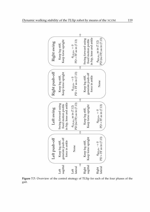
Dynamic walking stability of the TUlip robot by means of the XCOM 119
⇒⇒
⇒⇒
⇒
Left
sagi
ttal
Left
late
ral
Rig
htsa
gitt
al
Rig
htla
tera
l
Left
push
-off
Kee
ple
gst
iff,
gene
rate
push
-off
forc
ein
ankl
e
Non
e
Kee
ple
gst
iff,
Kee
pto
rso
upri
ght
θ RH
,des→
0PD
+FF
asin
(7.1
3)
' &
$ %
Left
swin
g
Swin
gfo
rwar
dus
ing
fixed
mot
ion
profi
lein
hip,
knee
and
ankl
e
θ LH
,des
asin
(7.1
2)PD
(no
FF)a
sin
(7.1
3)
Kee
ple
gst
iff,
Kee
pto
rso
upri
ght
θ RH
,des=
0PD
+FF
asin
(7.1
3)
' &
$ %Rig
htpu
sh-o
ff
Kee
ple
gst
iff,
Kee
pto
rso
upri
ght
θ LH
,des→
0PD
+FF
asin
(7.1
3)
Kee
ple
gst
iff,
gene
rate
push
-off
forc
ein
ankl
e
Non
e
' &
$ %
Rig
htsw
ing
Kee
ple
gst
iff,
Kee
pto
rso
upri
ght
θ LH
,des=
0PD
+FF
asin
(7.1
3)
Swin
gfo
rwar
dus
ing
fixed
mot
ion
profi
lein
hip,
knee
and
ankl
e
θ RH
,des
asin
(7.1
2)PD
(no
FF)a
sin
(7.1
3)
' &
$ %
Figure 7.7: Overview of the control strategy of TUlip for each of the four phases of thegait.
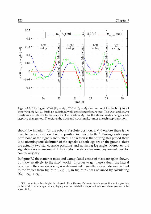
120 Chapter 7
24 25 26 27 28 29
−0.1
−0.05
0
0.05
0.1
0.15
0.2
0.25
time [s]
po
sit
ion
[m
] /
an
gle
[rad
]
Left
swing
Right
swing
Left
swing
Right
swing
Do
ub
le s
up
po
rt, r
igh
t pu
sh
−o
ff
Do
ub
le s
up
po
rt, le
ft pu
sh
−o
ff
Do
ub
le s
up
po
rt, r
igh
t pu
sh
−o
ff
(Cy−A
y) [m] (ξ
y−A
y) [m] θ
•H,des [rad]
Figure 7.8: The logged COM (Cy − Ay), XCOM (ξy − Ay) and setpoint for the hip joint ofthe swing leg θ•H,des during a sustained walk consisting of four steps. The COM and XCOMpositions are relative to the stance ankle position Ay. As the stance ankle changes eachstep, Ay changes too. Therefore, the COM and XCOM make jumps at each step transition.
should be invariant for the robot’s absolute position, and therefore there is noneed to have any notion of world position in this controller1. During double sup-port, none of the signals are plotted. The reason is that during this period thereis no unambiguous definition of the signals: as both legs are on the ground, thereare actually two stance ankle positions and no swing leg angle. Moreover, thesignals are not so meaningful during double stance because they are not used forcontrol anyway.
In figure 7.9 the center of mass and extrapolated center of mass are again shown,but now relatively to the fixed world. In order to get these values, the lateralposition of the stance ankle Ay was determined manually for each step and addedto the values from figure 7.8, e.g., Cy in figure 7.9 was obtained by calculating(Cy − Ay) + Ay.
1Of course, for other (higher-level) controllers, the robot’s should have some notion of it’s positionin the world. For example, when playing a soccer match it is important to know where you are in thesoccer field.
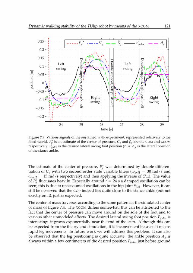
Dynamic walking stability of the TUlip robot by means of the XCOM 121
24 25 26 27 28 29
−0.2
−0.15
−0.1
−0.05
0
0.05
0.1
0.15
0.2
0.25
time [s]
po
sit
ion
[m
]
Left
swing
Right
swing
Left
swing
Right
swing
Do
ub
le s
up
po
rt, r
igh
t pu
sh
−o
ff
Do
ub
le s
up
po
rt, le
ft pu
sh
−o
ff
Do
ub
le s
up
po
rt, r
igh
t pu
sh
−o
ff
Py* C
yξ
yP
y,desA
y
Figure 7.9: Various signals of the sustained walk experiment, represented relatively to thefixed world. P∗y is an estimate of the center of pressure, Cy and ξy are the COM and XCOMrespectively. Py,des is the desired lateral swing foot position (7.3). Ay is the lateral positionof the stance ankle.
The estimate of the center of pressure, P∗y was determined by double differen-tiation of Cy with two second order state variable filters (ωsvf1 = 30 rad/s andωsvf2 = 15 rad/s respectively) and then applying the inverse of (7.1). The valueof P∗y fluctuates heavily. Especially around t = 24 s a damped oscillation can beseen; this is due to unaccounted oscillations in the hip joint θRH. However, it canstill be observed that the COP indeed lies quite close to the stance ankle (but notexactly on it), just as expected.
The center of mass traverses according to the same pattern as the simulated centerof mass of figure 7.4. The XCOM differs somewhat; this can be attributed to thefact that the center of pressure can move around on the sole of the foot and tovarious other unmodeled effects. The desired lateral swing foot position Py,des isinteresting: it grows exponentially near the end of the step. Although this canbe expected from the theory and simulation, it is inconvenient because it meansrapid leg movements. In future work we will address this problem. It can alsobe observed that the leg positioning is quite accurate: the ankle position Ay isalways within a few centimeters of the desired position Py,des just before ground
122 Chapter 7
contact. From an investigation of figures 7.8 and 7.9, it can be seen that the swingleg does not follow the entire trajectory of Py,des; thanks to the limitation of thehip angle, only the last part of each step is followed.
7.5 Conclusions
Lateral stability by foot placement was implemented in our walking robot TUlipby using a constant offset controller: a controller which is based on the extrapo-lated center of mass (XCOM). First the control strategy as proposed by (Hof, 2008)was verified in a computer simulation. The algorithm was then adapted to suitTUlip. Finally an experiment was carried out that shows lateral stability and re-semblance with the simulation. We therefore conclude that the constant offsetcontrol is usable in the control for bipedal robots.
In the experiment, TUlip required additional energy input (a gentle push from thehuman guiding the robot) to remain in limit cycle gait. In future work the push-off phase of TUlip will be improved in order to insert more energy in the dynamicwalking system. Also an effort will be put in predicting the required lateral legposition Py,des earlier during the step so that sudden movements during the endof the step are not necessary anymore.
Chapter 8
A concept for a new energy efficientactuator
This chapter is based on the following article (Stramigioli et al., 2008):
A concept for a new energy efficient actuator — in pursuit of the ideal actuatorStefano Stramigioli, Gijs van Oort and Edwin Dertien
Proc., IEEE/ASME International Conference on Advanced IntelligentMechatronics (AIM’08)
pages 671–675, July 2008.
Abstract—In this chapter a novel concept of embedded robotic actuator is pre-sented which has been named the Very Versatile Energy Efficient (V2E2) ac-tuator. This actuator stores energy during any force profile which generatesnegative work on the load and it does therefore have unprecedented potentialsfor robotics applications.
123
124 Chapter 8
8.1 Introduction
For mobile robotics and powered prosthetics, the energy consumption is a crucialfactor for usability. A reduction of the amount of energy consumed can yieldlonger operation on a mobile energy source (e.g., a battery), or can allow for useof smaller energy storage devices.
There are a number of strategies for reducing energy consumption. One approachis to increase the mechanical efficiency of a device. A second method is to limitwaste of energy. Normally, mechanical energy is wasted in a system when doingnegative work. Adding a buffer element for storage of mechanical energy, suchas a spring, seems a logical solution.
The development of actuators incorporating elastic elements has got a lot of at-tention in the recent years. One of the first and well known examples is the SeriesElastic Actuator (SEA) as developed by Pratt and Williamson (1995). Also a num-ber of compliant actuators with tunable elastic elements are under development,such as the MACCEPA by van Ham et al. (2005) or the ‘Jack Spring’TM by Hol-lander et al. (2005), which allow adjustment of the zero-position of a series elasticelement. Another approach is to enable adjustment of the spring constant, byvarying the pre-tension of a system using non-linear springs. This approach hasbeen used in for example the VSSEA (Variable Stiffness SEA) by Thorson et al.(2007) and the AMASC by Hurst et al. (2004). An elaborate overview of the cur-rent state of the art is given in by Ham et al. (2009).
An actuator able to intelligently store energy whenever negative work is done,and able to reuse this energy whenever necessary would be a great breakthroughin the robotic and active prosthetics world. In this chapter a concept of an actuatoris presented which does address the energy efficiency explicitly.
This chapter is organized as follows. Section 8.2 elaborates on actuators in gen-eral. Then, in section 8.3, the concept of our new actuator is introduced, stepby step. Section 8.4 and 8.5 describe two specific aspects on the realization andcontrol and the chapter end with conclusions and discussion in section 8.6.
8.2 Reflections on actuators
Usually an actuator is considered as a ‘signal processor’ which translates a com-mand generated by a controller to a physical quantity which is applied on theplant, like a force or torque. More correctly, acting on a physical system, energyis exchanged and in order to describe this properly, it is better to consider an ac-tuator as a controlled device that converts energy from a certain domain in which
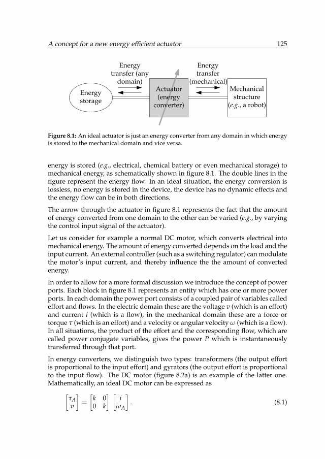
A concept for a new energy efficient actuator 125
Energytransfer (any
domain)
Energytransfer
(mechanical)Mechanical
structure(e.g., a robot)
Energystorage
Actuator(energy
converter)
Figure 8.1: An ideal actuator is just an energy converter from any domain in which energyis stored to the mechanical domain and vice versa.
energy is stored (e.g., electrical, chemical battery or even mechanical storage) tomechanical energy, as schematically shown in figure 8.1. The double lines in thefigure represent the energy flow. In an ideal situation, the energy conversion islossless, no energy is stored in the device, the device has no dynamic effects andthe energy flow can be in both directions.
The arrow through the actuator in figure 8.1 represents the fact that the amountof energy converted from one domain to the other can be varied (e.g., by varyingthe control input signal of the actuator).
Let us consider for example a normal DC motor, which converts electrical intomechanical energy. The amount of energy converted depends on the load and theinput current. An external controller (such as a switching regulator) can modulatethe motor’s input current, and thereby influence the the amount of convertedenergy.
In order to allow for a more formal discussion we introduce the concept of powerports. Each block in figure 8.1 represents an entity which has one or more powerports. In each domain the power port consists of a coupled pair of variables calledeffort and flows. In the electric domain these are the voltage v (which is an effort)and current i (which is a flow), in the mechanical domain these are a force ortorque τ (which is an effort) and a velocity or angular velocity ω (which is a flow).In all situations, the product of the effort and the corresponding flow, which arecalled power conjugate variables, gives the power P which is instantaneouslytransferred through that port.
In energy converters, we distinguish two types: transformers (the output effortis proportional to the input effort) and gyrators (the output effort is proportionalto the input flow). The DC motor (figure 8.2a) is an example of the latter one.Mathematically, an ideal DC motor can be expressed as
[τAv
]=
[k 00 k
] [i
ωA
]. (8.1)
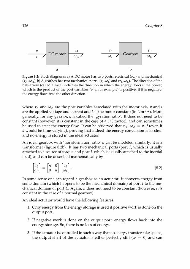
126 Chapter 8
DC motoriv τA
ωAGearbox
ωI
τI τL
ωL
a b
Figure 8.2: Block diagrams; a) A DC motor has two ports: electrical (v, i) and mechanical(τA, ωA); b) A gearbox has two mechanical ports: (τI , ωI) and (τL, ωL). The direction of thehalf-arrow (called a bond) indicates the direction in which the energy flows if the power,which is the product of the port variables (v · i, for example) is positive; if it is negative,the energy flows into the other direction.
where τA and ωA are the port variables associated with the motor axis, v and iare the applied voltage and current and k is the motor constant (in Nm/A). Moregenerally, for any gyrator, k is called the ‘gyration ratio’. It does not need to beconstant (however, it is constant in the case of a DC motor), and can sometimesbe used to steer the energy flow. It can be observed that τA ·ωA = v · i (even ifk would be time-varying), proving that indeed the energy conversion is losslessand no energy is stored in the ideal actuator.
An ideal gearbox with ‘transformation ratio’ n can be modeled similarly; it is atransformer (figure 8.2b). It has two mechanical ports (port I, which is usuallyattached to a source of torque and port L which is usually attached to the inertialload), and can be described mathematically by
[τLωI
]=
[n 00 n
] [τIωL
]. (8.2)
In some sense one can regard a gearbox as an actuator: it converts energy fromsome domain (which happens to be the mechanical domain) of port I to the me-chanical domain of port L. Again, n does not need to be constant (however, it isconstant in the case of a normal gearbox).
An ideal actuator would have the following features:
1. Only energy from the energy storage is used if positive work is done on theoutput port.
2. If negative work is done on the output port, energy flows back into theenergy storage. So, there is no loss of energy.
3. If the actuator is controlled in such a way that no energy transfer takes place,the output shaft of the actuator is either perfectly stiff (ω = 0) and can
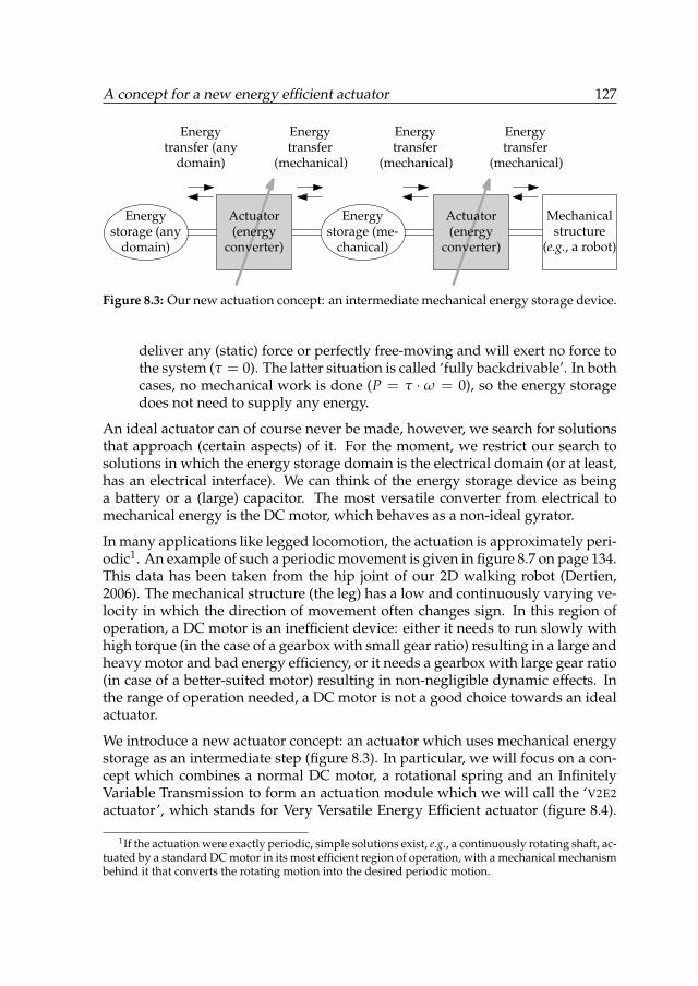
A concept for a new energy efficient actuator 127
Mechanicalstructure
(e.g., a robot)
Energystorage (me-
chanical)
Actuator(energy
converter)
Actuator(energy
converter)
Energystorage (any
domain)
Energytransfer (any
domain)
Energytransfer
(mechanical)
Energytransfer
(mechanical)
Energytransfer
(mechanical)
Figure 8.3: Our new actuation concept: an intermediate mechanical energy storage device.
deliver any (static) force or perfectly free-moving and will exert no force tothe system (τ = 0). The latter situation is called ‘fully backdrivable’. In bothcases, no mechanical work is done (P = τ · ω = 0), so the energy storagedoes not need to supply any energy.
An ideal actuator can of course never be made, however, we search for solutionsthat approach (certain aspects) of it. For the moment, we restrict our search tosolutions in which the energy storage domain is the electrical domain (or at least,has an electrical interface). We can think of the energy storage device as beinga battery or a (large) capacitor. The most versatile converter from electrical tomechanical energy is the DC motor, which behaves as a non-ideal gyrator.
In many applications like legged locomotion, the actuation is approximately peri-odic1. An example of such a periodic movement is given in figure 8.7 on page 134.This data has been taken from the hip joint of our 2D walking robot (Dertien,2006). The mechanical structure (the leg) has a low and continuously varying ve-locity in which the direction of movement often changes sign. In this region ofoperation, a DC motor is an inefficient device: either it needs to run slowly withhigh torque (in the case of a gearbox with small gear ratio) resulting in a large andheavy motor and bad energy efficiency, or it needs a gearbox with large gear ratio(in case of a better-suited motor) resulting in non-negligible dynamic effects. Inthe range of operation needed, a DC motor is not a good choice towards an idealactuator.
We introduce a new actuator concept: an actuator which uses mechanical energystorage as an intermediate step (figure 8.3). In particular, we will focus on a con-cept which combines a normal DC motor, a rotational spring and an InfinitelyVariable Transmission to form an actuation module which we will call the ‘V2E2actuator’, which stands for Very Versatile Energy Efficient actuator (figure 8.4).
1If the actuation were exactly periodic, simple solutions exist, e.g., a continuously rotating shaft, ac-tuated by a standard DC motor in its most efficient region of operation, with a mechanical mechanismbehind it that converts the rotating motion into the desired periodic motion.
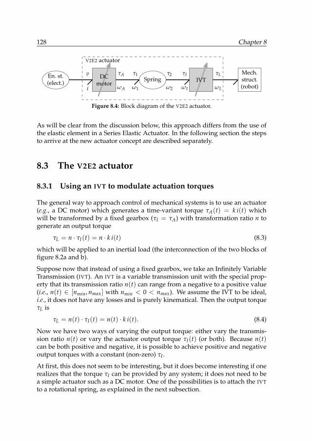
128 Chapter 8
τA
ωA
v
i
τ1 τ2
ω1 ω2
DCmotor IVT
Mech.struct.(robot)
En. st.(elect.)
τI τL
ωI ωL
Spring
V2E2 actuator
Figure 8.4: Block diagram of the V2E2 actuator.
As will be clear from the discussion below, this approach differs from the use ofthe elastic element in a Series Elastic Actuator. In the following section the stepsto arrive at the new actuator concept are described separately.
8.3 The V2E2 actuator
8.3.1 Using an IVT to modulate actuation torques
The general way to approach control of mechanical systems is to use an actuator(e.g., a DC motor) which generates a time-variant torque τA(t) = k i(t) whichwill be transformed by a fixed gearbox (τI = τA) with transformation ratio n togenerate an output torque
τL = n · τI(t) = n · k i(t) (8.3)
which will be applied to an inertial load (the interconnection of the two blocks offigure 8.2a and b).
Suppose now that instead of using a fixed gearbox, we take an Infinitely VariableTransmission (IVT). An IVT is a variable transmission unit with the special prop-erty that its transmission ratio n(t) can range from a negative to a positive value(i.e., n(t) ∈ [nmin, nmax] with nmin < 0 < nmax). We assume the IVT to be ideal,i.e., it does not have any losses and is purely kinematical. Then the output torqueτL is
τL = n(t) · τI(t) = n(t) · k i(t). (8.4)
Now we have two ways of varying the output torque: either vary the transmis-sion ratio n(t) or vary the actuator output torque τI(t) (or both). Because n(t)can be both positive and negative, it is possible to achieve positive and negativeoutput torques with a constant (non-zero) τI .
At first, this does not seem to be interesting, but it does become interesting if onerealizes that the torque τI can be provided by any system; it does not need to bea simple actuator such as a DC motor. One of the possibilities is to attach the IVTto a rotational spring, as explained in the next subsection.
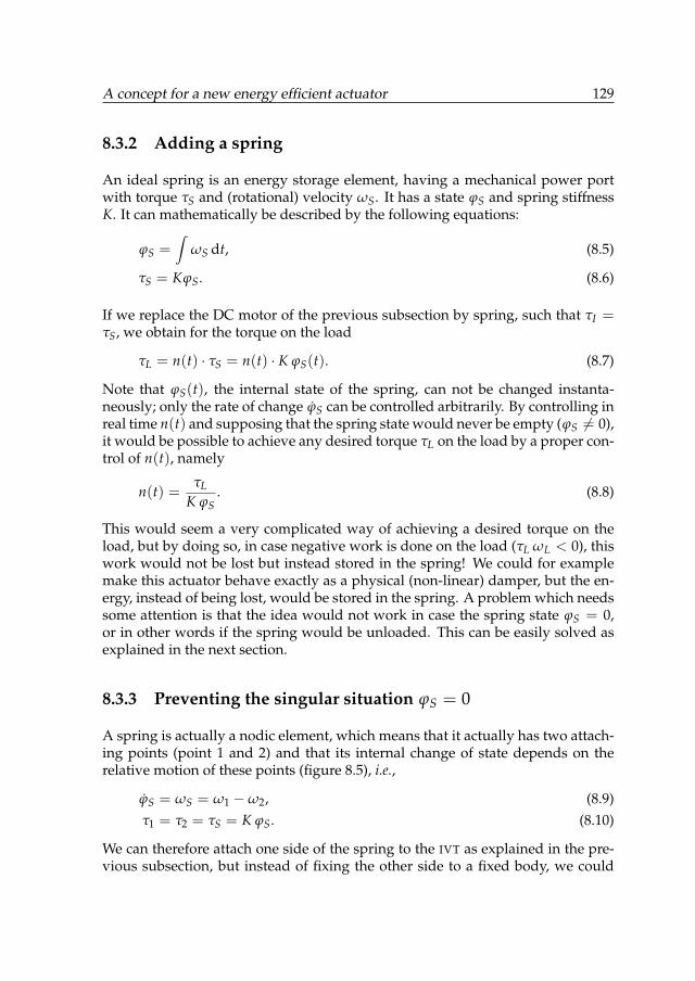
A concept for a new energy efficient actuator 129
8.3.2 Adding a spring
An ideal spring is an energy storage element, having a mechanical power portwith torque τS and (rotational) velocity ωS. It has a state ϕS and spring stiffnessK. It can mathematically be described by the following equations:
ϕS =∫
ωS dt, (8.5)
τS = KϕS. (8.6)
If we replace the DC motor of the previous subsection by spring, such that τI =τS, we obtain for the torque on the load
τL = n(t) · τS = n(t) · K ϕS(t). (8.7)
Note that ϕS(t), the internal state of the spring, can not be changed instanta-neously; only the rate of change ϕS can be controlled arbitrarily. By controlling inreal time n(t) and supposing that the spring state would never be empty (ϕS 6= 0),it would be possible to achieve any desired torque τL on the load by a proper con-trol of n(t), namely
n(t) =τL
K ϕS. (8.8)
This would seem a very complicated way of achieving a desired torque on theload, but by doing so, in case negative work is done on the load (τL ωL < 0), thiswork would not be lost but instead stored in the spring! We could for examplemake this actuator behave exactly as a physical (non-linear) damper, but the en-ergy, instead of being lost, would be stored in the spring. A problem which needssome attention is that the idea would not work in case the spring state ϕS = 0,or in other words if the spring would be unloaded. This can be easily solved asexplained in the next section.
8.3.3 Preventing the singular situation ϕS = 0
A spring is actually a nodic element, which means that it actually has two attach-ing points (point 1 and 2) and that its internal change of state depends on therelative motion of these points (figure 8.5), i.e.,
ϕS = ωS = ω1 −ω2, (8.9)τ1 = τ2 = τS = K ϕS. (8.10)
We can therefore attach one side of the spring to the IVT as explained in the pre-vious subsection, but instead of fixing the other side to a fixed body, we could
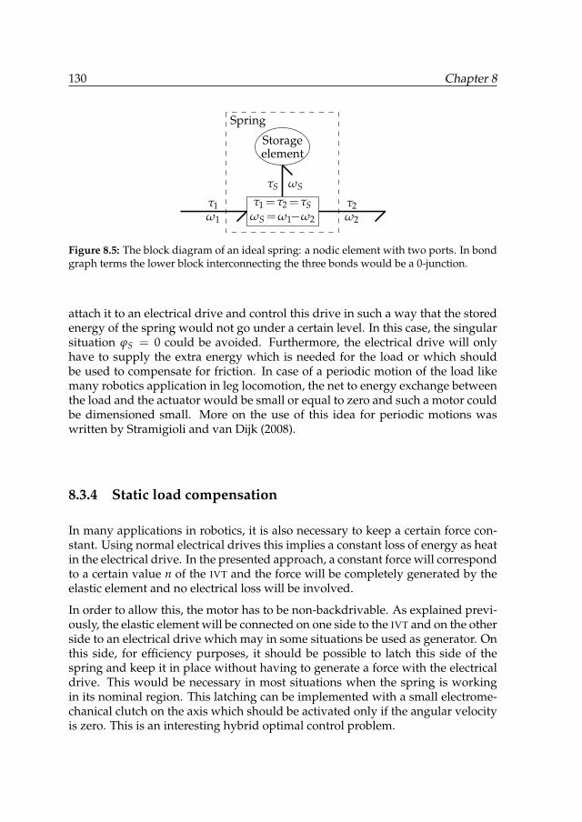
130 Chapter 8
τ1 τ2ω1 ω2
τS ωS
Spring
τ1=τ2=τSωS =ω1−ω2
Storageelement
Figure 8.5: The block diagram of an ideal spring: a nodic element with two ports. In bondgraph terms the lower block interconnecting the three bonds would be a 0-junction.
attach it to an electrical drive and control this drive in such a way that the storedenergy of the spring would not go under a certain level. In this case, the singularsituation ϕS = 0 could be avoided. Furthermore, the electrical drive will onlyhave to supply the extra energy which is needed for the load or which shouldbe used to compensate for friction. In case of a periodic motion of the load likemany robotics application in leg locomotion, the net to energy exchange betweenthe load and the actuator would be small or equal to zero and such a motor couldbe dimensioned small. More on the use of this idea for periodic motions waswritten by Stramigioli and van Dijk (2008).
8.3.4 Static load compensation
In many applications in robotics, it is also necessary to keep a certain force con-stant. Using normal electrical drives this implies a constant loss of energy as heatin the electrical drive. In the presented approach, a constant force will correspondto a certain value n of the IVT and the force will be completely generated by theelastic element and no electrical loss will be involved.
In order to allow this, the motor has to be non-backdrivable. As explained previ-ously, the elastic element will be connected on one side to the IVT and on the otherside to an electrical drive which may in some situations be used as generator. Onthis side, for efficiency purposes, it should be possible to latch this side of thespring and keep it in place without having to generate a force with the electricaldrive. This would be necessary in most situations when the spring is workingin its nominal region. This latching can be implemented with a small electrome-chanical clutch on the axis which should be activated only if the angular velocityis zero. This is an interesting hybrid optimal control problem.
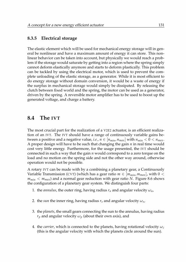
A concept for a new energy efficient actuator 131
8.3.5 Electrical storage
The elastic element which will be used for mechanical energy storage will in gen-eral be nonlinear and have a maximum amount of energy it can store. This non-linear behavior can be taken into account, but physically we would reach a prob-lem if the storage would saturate by getting into a region where the spring simplycannot deform elastically anymore and starts to deform plastically. This problemcan be tackled by using the electrical motor, which is used to prevent the com-plete unloading of the elastic storage, as a generator. While it is most efficient todo energy storage without domain conversion, it would be a waste of energy ifthe surplus in mechanical storage would simply be dissipated. By releasing theclutch between fixed world and the spring, the motor can be used as a generator,driven by the spring. A reversible motor amplifier has to be used to boost up thegenerated voltage, and charge a battery.
8.4 The IVT
The most crucial part for the realization of a V2E2 actuator, is an efficient realiza-tion of an IVT. The IVT should have a range of continuously variable gains be-tween a positive and a negative value, i.e., n ∈ [nmin, nmax] with nmin < 0 < nmax.A proper design will have to be such that changing the gain n in real time wouldcost very little energy. Furthermore, for the usage presented, the IVT should beconnected in such a way that the gain n would correspond to a zero torque on theload and no motion on the spring side and not the other way around, otherwiseoperation would not be possible.
A rotary IVT can be made with by a combining a planetary gear, a ContinuouslyVariable Transmission (CVT) (which has a gear ratio m ∈ [mmin, mmax], with 0 <mmin < mmax) and a normal gear reduction with gear ratio N. Figure 8.6 showsthe configuration of a planetary gear system. We distinguish four parts:
1. the annulus, the outer ring, having radius ra and angular velocity ωa,
2. the sun the inner ring, having radius rs and angular velocity ωs,
3. the planets, the small gears connecting the sun to the annulus, having radiusrp and angular velocity ωp (about their own axis), and
4. the carrier, which is connected to the planets, having rotational velocity ωc(this is the angular velocity with which the planets circle around the sun).
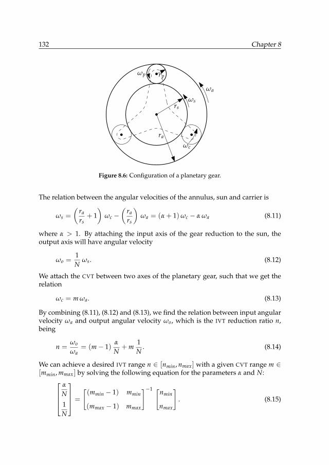
132 Chapter 8
rs
rp
ra
ωc
ωs
ωp
ωa
Figure 8.6: Configuration of a planetary gear.
The relation between the angular velocities of the annulus, sun and carrier is
ωs =
(ra
rs+ 1)
ωc −(
ra
rs
)ωa = (α + 1)ωc − α ωa (8.11)
where α > 1. By attaching the input axis of the gear reduction to the sun, theoutput axis will have angular velocity
ωo =1N
ωs. (8.12)
We attach the CVT between two axes of the planetary gear, such that we get therelation
ωc = m ωa. (8.13)
By combining (8.11), (8.12) and (8.13), we find the relation between input angularvelocity ωa and output angular velocity ωo, which is the IVT reduction ratio n,being
n =ωo
ωa= (m− 1)
α
N+ m
1N
. (8.14)
We can achieve a desired IVT range n ∈ [nmin, nmax] with a given CVT range m ∈[mmin, mmax] by solving the following equation for the parameters α and N:
α
N
1N
=
[(mmin − 1) mmin
(mmax − 1) mmax
]−1 [nmin
nmax
]. (8.15)
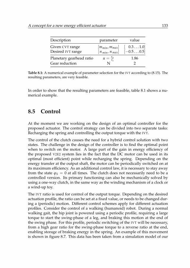
A concept for a new energy efficient actuator 133
Description parameter value
Given CVT range [mmin, mmax] [ 0.3 . . . 1.0]Desired IVT range [n min, n max] [−0.5 . . . 0.5]
Planetary gearhead ratio α = rars
1.86Gear reduction N 2
Table 8.1: A numerical example of parameter selection for the IVT according to (8.15). Theresulting parameters, are very feasible.
In order to show that the resulting parameters are feasible, table 8.1 shows a nu-merical example.
8.5 Control
At the moment we are working on the design of an optimal controller for theproposed actuator. The control strategy can be divided into two separate tasks:Recharging the spring and controlling the output torque with the IVT.
The control of the clutch causes the need for a hybrid control solution with twostates. The challenge in the design of the controller is to find the optimal pointwhen to switch on the motor. A large part of the gain in energy efficiency ofthe proposed V2E2 system lies in the fact that the DC motor can be used in itsoptimal (most efficient) point while recharging the spring. Depending on theenergy transfer at the output shaft, the motor can be periodically switched on atits maximum efficiency. As an additional control law, it is necessary to stay awayfrom the state ϕS = 0 at all times. The clutch does not necessarily need to be acontrolled version. Its primary functioning can also be mechanically solved byusing a one-way clutch, in the same way as the winding mechanism of a clock ora wind-up toy.
The IVT ratio is used for control of the output torque. Depending on the desiredactuation profile, the ratio can be set at a fixed value, or needs to be changed dur-ing a (periodic) motion. Different control schemes apply for different actuationprofiles. Consider the control of a walking (humanoid) robot. During a normalwalking gait, the hip joint is powered using a periodic profile, requiring a largetorque to start the swing-phase of a leg, and braking this motion at the end ofthe swing phase. For this profile, periodic switching of the IVT will be necessary,from a high gear ratio for the swing-phase torque to a reverse ratio at the end,enabling storage of braking energy in the spring. An example of this movementis shown in figure 8.7. This data has been taken from a simulation model of our
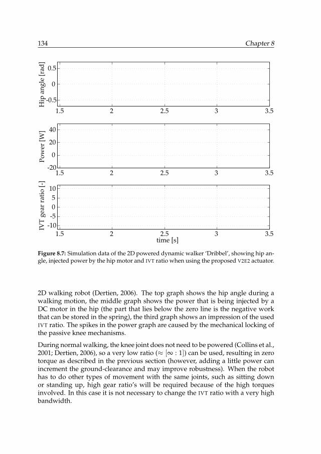
134 Chapter 8H
ip a
ng
le [
rad
]P
ower
[W
]IV
T g
ear
rati
o [-
]
time [s]1.5 2 2.5 3 3.5
-10
-5
0
510
-20
0
20
40
-0.5
0
0.5
1.5 2 2.5 3 3.5
1.5 2 2.5 3 3.5
Figure 8.7: Simulation data of the 2D powered dynamic walker ‘Dribbel’, showing hip an-gle, injected power by the hip motor and IVT ratio when using the proposed V2E2 actuator.
2D walking robot (Dertien, 2006). The top graph shows the hip angle during awalking motion, the middle graph shows the power that is being injected by aDC motor in the hip (the part that lies below the zero line is the negative workthat can be stored in the spring), the third graph shows an impression of the usedIVT ratio. The spikes in the power graph are caused by the mechanical locking ofthe passive knee mechanisms.
During normal walking, the knee joint does not need to be powered (Collins et al.,2001; Dertien, 2006), so a very low ratio (≈ [∞ : 1]) can be used, resulting in zerotorque as described in the previous section (however, adding a little power canincrement the ground-clearance and may improve robustness). When the robothas to do other types of movement with the same joints, such as sitting downor standing up, high gear ratio’s will be required because of the high torquesinvolved. In this case it is not necessary to change the IVT ratio with a very highbandwidth.
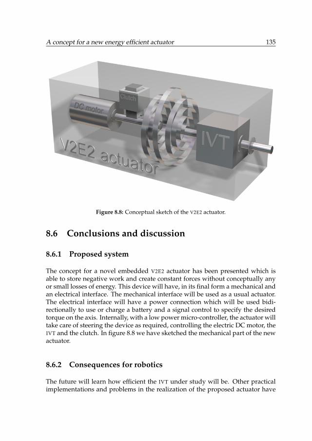
A concept for a new energy efficient actuator 135
Figure 8.8: Conceptual sketch of the V2E2 actuator.
8.6 Conclusions and discussion
8.6.1 Proposed system
The concept for a novel embedded V2E2 actuator has been presented which isable to store negative work and create constant forces without conceptually anyor small losses of energy. This device will have, in its final form a mechanical andan electrical interface. The mechanical interface will be used as a usual actuator.The electrical interface will have a power connection which will be used bidi-rectionally to use or charge a battery and a signal control to specify the desiredtorque on the axis. Internally, with a low power micro-controller, the actuator willtake care of steering the device as required, controlling the electric DC motor, theIVT and the clutch. In figure 8.8 we have sketched the mechanical part of the newactuator.
8.6.2 Consequences for robotics
The future will learn how efficient the IVT under study will be. Other practicalimplementations and problems in the realization of the proposed actuator have
136 Chapter 8
yet to be tackled, but if this will be successful, the implications for robotics willbe substantial. In legged locomotion people either develop highly geared, fullyactuated, robust but not efficient machines or minimally actuated, not robust, butextremely energy efficient machines. A machine which has the robustness of thefirst group and the energy efficient of the second as yet to come. Such actuatorscould drastically change this and this was originally the idea which brought theauthor to conceive V2E2 actuators. We could make a fully V2E2 actuated machineand control it using the most advanced nonlinear control methods without hav-ing to worry about the efficiency since the actuators would take care of that. Suchdevices would therefore bridge the gap which is still existing between advancedbut complex and inefficient nonlinear control methods and simple non-robustminimalistic efficient approaches. In the opinion of the authors, this would be amajor achievement for robotic locomotion.
8.6.3 Ongoing work
Some practical problems have still to be solved before the proposed concept willbe applicable, first of all the realization of an efficient Infinitely Variable Transmis-sion. A lot of progress has been made in this direction and the team of the authorsis currently working on a patent. The authors believe that if the practical prob-lems will be overcome, such an actuator could cause a revolution in the world ofmany robotic applications especially in legged locomotion and prosthetics.
8.A Acknowledgments
The authors would like to thank MSc. student Jos Ansink who worked on the IVTdesign and made vital contributions to the ideas expressed in this chapter.

Part III
Design
137

Chapter 9
Design and realization of an energyefficient knee-locking mechanismfor a dynamically walking robot
This chapter is based on the following article (van Oort et al., 2011a):
An energy efficient knee locking mechanism for a dynamically walking robotGijs van Oort, Raffaella Carloni, Dian J. Borgerink and Stefano Stramigioli
Proc., IEEE International Conference on Robotics and Automation (ICRA’11)pages 2003–2008, May 2011.
Abstract—In this work, we present the design and the implementation of aninnovative knee locking mechanism for a dynamically walking robot. Themechanism consists of a four-bar linkage that realizes a mechanical singularityfor locking the knee when the leg is in the extended position. Once extended,the knee remains locked without energy consumption, while unlocking it onlycosts a small amount of energy. Tests showed that the robot walks robustly andthat the energy consumption of the new system is low.
139
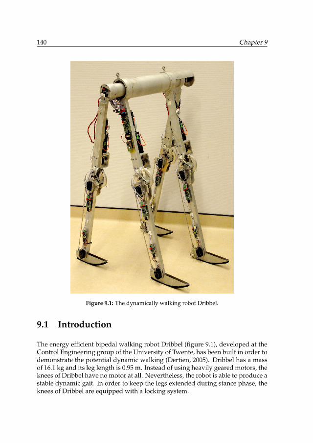
140 Chapter 9
Figure 9.1: The dynamically walking robot Dribbel.
9.1 Introduction
The energy efficient bipedal walking robot Dribbel (figure 9.1), developed at theControl Engineering group of the University of Twente, has been built in order todemonstrate the potential dynamic walking (Dertien, 2005). Dribbel has a massof 16.1 kg and its leg length is 0.95 m. Instead of using heavily geared motors, theknees of Dribbel have no motor at all. Nevertheless, the robot is able to produce astable dynamic gait. In order to keep the legs extended during stance phase, theknees of Dribbel are equipped with a locking system.
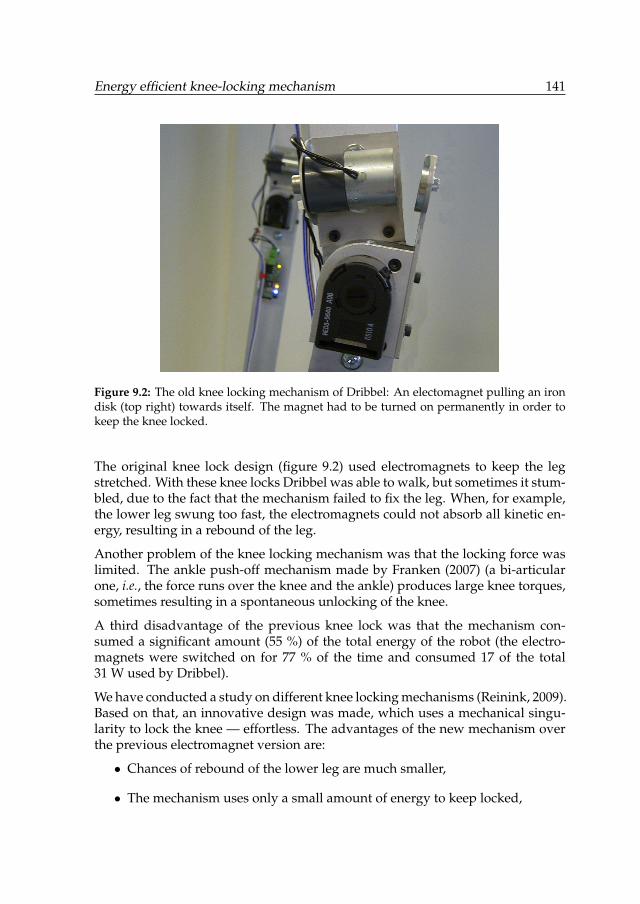
Energy efficient knee-locking mechanism 141
Figure 9.2: The old knee locking mechanism of Dribbel: An electomagnet pulling an irondisk (top right) towards itself. The magnet had to be turned on permanently in order tokeep the knee locked.
The original knee lock design (figure 9.2) used electromagnets to keep the legstretched. With these knee locks Dribbel was able to walk, but sometimes it stum-bled, due to the fact that the mechanism failed to fix the leg. When, for example,the lower leg swung too fast, the electromagnets could not absorb all kinetic en-ergy, resulting in a rebound of the leg.
Another problem of the knee locking mechanism was that the locking force waslimited. The ankle push-off mechanism made by Franken (2007) (a bi-articularone, i.e., the force runs over the knee and the ankle) produces large knee torques,sometimes resulting in a spontaneous unlocking of the knee.
A third disadvantage of the previous knee lock was that the mechanism con-sumed a significant amount (55 %) of the total energy of the robot (the electro-magnets were switched on for 77 % of the time and consumed 17 of the total31 W used by Dribbel).
We have conducted a study on different knee locking mechanisms (Reinink, 2009).Based on that, an innovative design was made, which uses a mechanical singu-larity to lock the knee — effortless. The advantages of the new mechanism overthe previous electromagnet version are:
• Chances of rebound of the lower leg are much smaller,
• The mechanism uses only a small amount of energy to keep locked,
142 Chapter 9
• The locking force is independent on the energy consumption of the mecha-nism; it is only dependent on the mechanical strength of the mechanism.
A prototype of the new knee mechanism has been built and tested (Borgerink,2008). The results of these tests show that indeed the new knee mechanismis more reliable, stronger and more efficient than the electromagnet precursor.Based on these tests, a final design was made and implemented on Dribbel, whichcan now walk safer and more energy efficiently than before.
All dynamically walking robots with knees suffer from the problem of needinga knee mechanism. The first kneed walker, by McGeer (1993), did not have anylocking mechanism at all; it only had a de-bouncing mechanism and an endstop.The 2D biped Mike, byWisse and van Frankenhuyzen (2003), used a mechanicallatch and a solenoid for unlocking. The 3D walker by Collins and Ruina (2005)has an electromagnetic release system for a movable latch. At MIT, Baines devel-oped a knee mechanism with a DC motor for actuation and an electromagneticclutch for uncoupling the actuator from the knee (Baines, 2005). This mecha-nism was later improved by Reynolds (2006) by using bevel gears. Trifonov andHashimoto (2007) tried a totally passive locking system with permanent magnets,but this could not be tuned well enough. Later they developed a mechanism witha locking hook.
In the world of prosthetics there are many patents on knee mechanisms. Manydescribe four-bar linkages that create a virtual rotation point outside the mecha-nism, or a virtual rotation point that moves during the flexion of the knee (Mar-low, 1990; Townsend, 1994; Kramer, 1998). Generally, these systems are con-structed such that exerting a pressure on the knee (i.e., leaning on the extendedleg) helps locking the system. Another four-bar mechanism is found in (Radcliffe,1992), where the mechanism is constructed such that it acts as a pivot lock. A kneesystem with a dedicated locking hook is described by Townsend (2002). A lock-ing system using a mechanical singularity is described by Hieronymus (2003),although it has noting to do with prostheses or robots (it is used for printing orvarnishing machines).
This chapter is organized as follows. In section 9.2 we state the design require-ments for our new knee lock. Then, in section 9.3 we present the new knee lockingsystem and discuss some of the features. A few tests and measurements done onthe new actuator itself and on Dribbel are described in section 9.4. Finally, beforeconcluding, we show in section 9.5 how mechanical play (backlash) appears to beadvantageous.
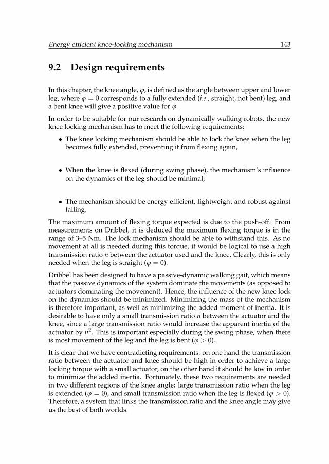
Energy efficient knee-locking mechanism 143
9.2 Design requirements
In this chapter, the knee angle, ϕ, is defined as the angle between upper and lowerleg, where ϕ = 0 corresponds to a fully extended (i.e., straight, not bent) leg, anda bent knee will give a positive value for ϕ.
In order to be suitable for our research on dynamically walking robots, the newknee locking mechanism has to meet the following requirements:
• The knee locking mechanism should be able to lock the knee when the legbecomes fully extended, preventing it from flexing again,
• When the knee is flexed (during swing phase), the mechanism’s influenceon the dynamics of the leg should be minimal,
• The mechanism should be energy efficient, lightweight and robust againstfalling.
The maximum amount of flexing torque expected is due to the push-off. Frommeasurements on Dribbel, it is deduced the maximum flexing torque is in therange of 3–5 Nm. The lock mechanism should be able to withstand this. As nomovement at all is needed during this torque, it would be logical to use a hightransmission ratio n between the actuator used and the knee. Clearly, this is onlyneeded when the leg is straight (ϕ = 0).
Dribbel has been designed to have a passive-dynamic walking gait, which meansthat the passive dynamics of the system dominate the movements (as opposed toactuators dominating the movement). Hence, the influence of the new knee lockon the dynamics should be minimized. Minimizing the mass of the mechanismis therefore important, as well as minimizing the added moment of inertia. It isdesirable to have only a small transmission ratio n between the actuator and theknee, since a large transmission ratio would increase the apparent inertia of theactuator by n2. This is important especially during the swing phase, when thereis most movement of the leg and the leg is bent (ϕ > 0).
It is clear that we have contradicting requirements: on one hand the transmissionratio between the actuator and knee should be high in order to achieve a largelocking torque with a small actuator, on the other hand it should be low in orderto minimize the added inertia. Fortunately, these two requirements are neededin two different regions of the knee angle: large transmission ratio when the legis extended (ϕ = 0), and small transmission ratio when the leg is flexed (ϕ > 0).Therefore, a system that links the transmission ratio and the knee angle may giveus the best of both worlds.
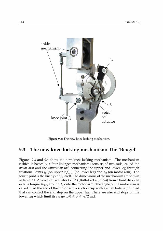
144 Chapter 9
voicecoilactuator
anklemechanism
Ju
Jl
Jm
knee joint Jk
Figure 9.3: The new knee locking mechanism.
9.3 The new knee locking mechanism: The ‘Beugel’
Figures 9.3 and 9.4 show the new knee locking mechanism. The mechanism(which is basically a four-linkages mechanism) consists of two rods, called themotor arm and the connection rod, connecting the upper and lower leg throughrotational joints Ju (on upper leg), Jl (on lower leg) and Jm (on motor arm). Thefourth joint is the knee joint Jk itself. The dimensions of the mechanism are shownin table 9.1. A voice coil actuator (VCA) (Buttolo et al., 1994) from a hard disk canexert a torque τVCA around Ju onto the motor arm. The angle of the motor arm iscalled α. At the end of the motor arm a suction cup with a small hole is mountedthat can contact the end stop on the upper leg. There are also end stops on thelower leg which limit its range to 0 ≤ ϕ ≤ π/2 rad.
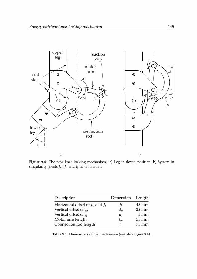
Energy efficient knee-locking mechanism 145
Jk
Ju
Jl
Jm
upperleg
α
suctioncup
endstops
connectionrod
motorarm
ϕ
l m
d u
h
dl
l c
lowerleg
τVCA
a b
Figure 9.4: The new knee locking mechanism. a) Leg in flexed position; b) System insingularity (joints Jm, Ju and Jk lie on one line).
Description Dimension Length
Horizontal offset of Ju and Jl h 45 mmVertical offset of Ju du 25 mmVertical offset of Jl dl 5 mmMotor arm length lm 55 mmConnection rod length lc 75 mm
Table 9.1: Dimensions of the mechanism (see also figure 9.4).
146 Chapter 9
9.3.1 Four-linkages mechanism
There is a fixed relation between the motor arm angle and the lower leg angle, asshown in figure 9.5. This relation is dependent on the exact geometry of the mech-anism and was found using numerical optimization by Reinink (2009). The trans-mission ratio n(ϕ) between motor arm angle (on which the actuator is mounted)and knee angle is the slope n = dα/dϕ and is shown in figure 9.6. Indeed, wehave the best of both worlds: a very large (even infinity) transmission ratio nearϕ = 0 and a small transmission ratio for a bent knee. The torque on the lower leg(around Jk) that the system can generate is τl = n(ϕ) · τVCA.
Figure 9.4a shows the leg in a flexed state. When the lower leg rotates, the mo-tor arm (and thus the actuator) rotates with it at relatively low angular velocity(α ≈ ϕ). This does not influence the motion of the lower leg very much. Whenthe knee is almost extended (ϕ is small), the motor arm will be almost vertical.A small angular displacement of the knee will now result in a large angular dis-placement of the motor arm (large transmission ratio, i.e., α� ϕ), and conversely,the actuator can exert a high torque on the lower leg.
Figure 9.4b shows the system in its mechanical singularity. The transmission ratiois infinity, implying that the lower leg cannot rotate at all and, irrespective of the(external) torque on the knee, the motor arm can be kept in place with minimumenergy consumption. This is an unstable equilibrium.
The motor arm can go through the singularity, such that α < 0. This way, thesuction cup on the motor arm can contact the end stop on the upper leg. Thelower leg is then flexed a minimal small amount. If an (external) flexing forceacts on the knee, it will cause the motor arm to be pressed harder against the endstop. Hence the knee cannot be flexed any further, i.e., the knee is locked.
The apparent inertia of a body, for example the leg, can be expressed as Iapp = τϕ
(where τ is the torque exerted on the joint), or, in words, the amount of torqueneeded for one unit acceleration. The apparent inertia of the lower leg (includ-ing the foot) consists of two parts: the inertia of the lower leg itself (includingthe foot) and the inertia added by the knee mechanism with actuator: Iapp =
Ileg + Iknee-mech. The former is fixed and was measured to be Ileg = 0.095 kgm2.The latter is heavily dependent on the transmission ratio n(ϕ) and can be ap-proximated by Iknee-mech = n2(ϕ) · Imotor-arm, for which we measured Imotor-arm =4.5 · 10−5 kgm2. In figure 9.7 the apparent inertia as a function of the leg angleis shown. Indeed, the influence of the mechanism in negligible for almost thewhole range of motion of the lower leg, which is exactly what we desired. Forvery small leg angles (the leg almost extended), the inertia becomes large, whichis not a problem because the leg does not need to swing freely anyway aroundthose angles. Over the whole stroke of the system, the connection rod keeps more
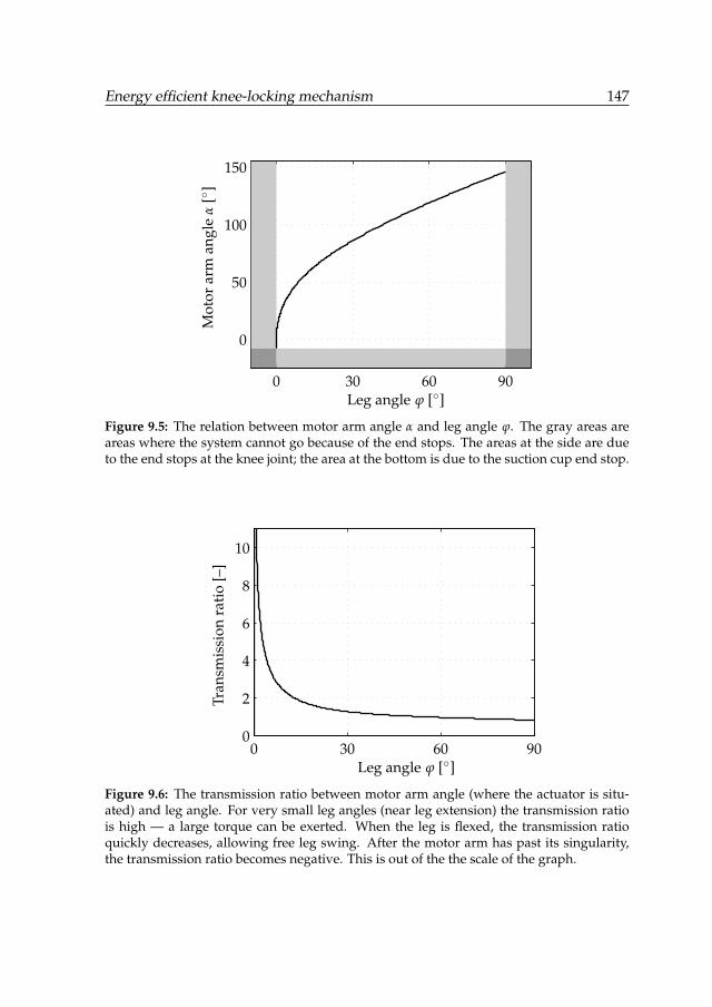
Energy efficient knee-locking mechanism 147
0 30 60 90
0
50
100
150
Leg angle ϕ [◦]
Mot
orar
man
gle
α[◦
]
Figure 9.5: The relation between motor arm angle α and leg angle ϕ. The gray areas areareas where the system cannot go because of the end stops. The areas at the side are dueto the end stops at the knee joint; the area at the bottom is due to the suction cup end stop.
0 30 60 900
2
4
6
8
10
Leg angle ϕ [◦]
Tran
smis
sion
rati
o[–
]
Figure 9.6: The transmission ratio between motor arm angle (where the actuator is situ-ated) and leg angle. For very small leg angles (near leg extension) the transmission ratiois high — a large torque can be exerted. When the leg is flexed, the transmission ratioquickly decreases, allowing free leg swing. After the motor arm has past its singularity,the transmission ratio becomes negative. This is out of the the scale of the graph.
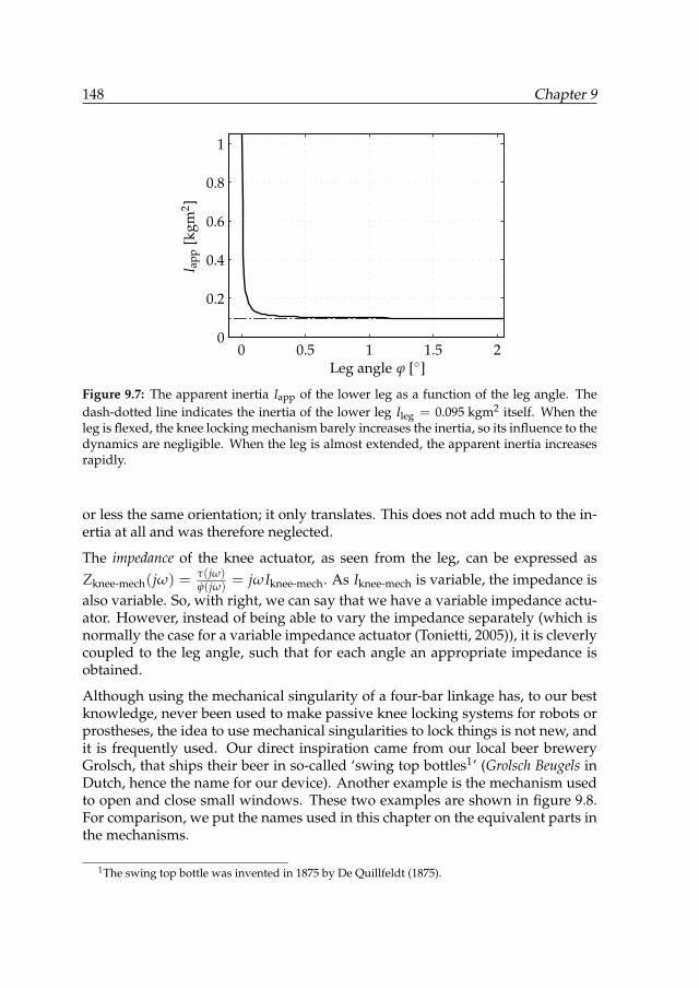
148 Chapter 9
0 0.5 1 1.5 20
0.2
0.4
0.6
0.8
1
Leg angle ϕ [◦]
I app
[kgm
2 ]
Figure 9.7: The apparent inertia Iapp of the lower leg as a function of the leg angle. Thedash-dotted line indicates the inertia of the lower leg Ileg = 0.095 kgm2 itself. When theleg is flexed, the knee locking mechanism barely increases the inertia, so its influence to thedynamics are negligible. When the leg is almost extended, the apparent inertia increasesrapidly.
or less the same orientation; it only translates. This does not add much to the in-ertia at all and was therefore neglected.
The impedance of the knee actuator, as seen from the leg, can be expressed asZknee-mech(jω) = τ(jω)
ϕ(jω)= jωIknee-mech. As Iknee-mech is variable, the impedance is
also variable. So, with right, we can say that we have a variable impedance actu-ator. However, instead of being able to vary the impedance separately (which isnormally the case for a variable impedance actuator (Tonietti, 2005)), it is cleverlycoupled to the leg angle, such that for each angle an appropriate impedance isobtained.
Although using the mechanical singularity of a four-bar linkage has, to our bestknowledge, never been used to make passive knee locking systems for robots orprostheses, the idea to use mechanical singularities to lock things is not new, andit is frequently used. Our direct inspiration came from our local beer breweryGrolsch, that ships their beer in so-called ‘swing top bottles1’ (Grolsch Beugels inDutch, hence the name for our device). Another example is the mechanism usedto open and close small windows. These two examples are shown in figure 9.8.For comparison, we put the names used in this chapter on the equivalent parts inthe mechanisms.
1The swing top bottle was invented in 1875 by De Quillfeldt (1875).
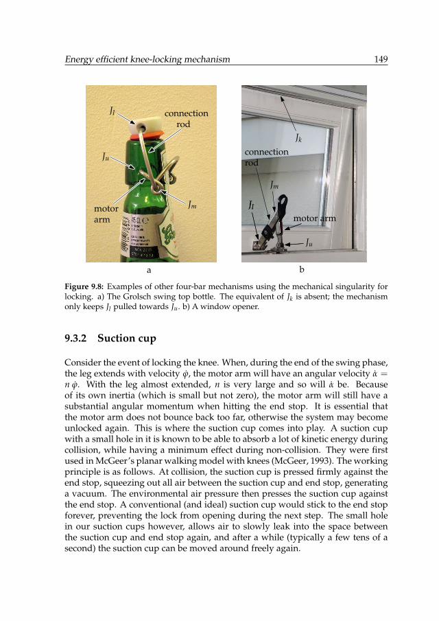
Energy efficient knee-locking mechanism 149
Ju
Jk
Jm
Jl
motor arm
Jm Jl
Ju
Jlmotorarm
connectionrod
connectionrod
a b
Figure 9.8: Examples of other four-bar mechanisms using the mechanical singularity forlocking. a) The Grolsch swing top bottle. The equivalent of Jk is absent; the mechanismonly keeps Jl pulled towards Ju. b) A window opener.
9.3.2 Suction cup
Consider the event of locking the knee. When, during the end of the swing phase,the leg extends with velocity ϕ, the motor arm will have an angular velocity α =n ϕ. With the leg almost extended, n is very large and so will α be. Becauseof its own inertia (which is small but not zero), the motor arm will still have asubstantial angular momentum when hitting the end stop. It is essential thatthe motor arm does not bounce back too far, otherwise the system may becomeunlocked again. This is where the suction cup comes into play. A suction cupwith a small hole in it is known to be able to absorb a lot of kinetic energy duringcollision, while having a minimum effect during non-collision. They were firstused in McGeer’s planar walking model with knees (McGeer, 1993). The workingprinciple is as follows. At collision, the suction cup is pressed firmly against theend stop, squeezing out all air between the suction cup and end stop, generatinga vacuum. The environmental air pressure then presses the suction cup againstthe end stop. A conventional (and ideal) suction cup would stick to the end stopforever, preventing the lock from opening during the next step. The small holein our suction cups however, allows air to slowly leak into the space betweenthe suction cup and end stop again, and after a while (typically a few tens of asecond) the suction cup can be moved around freely again.
150 Chapter 9
9.3.3 Actuator
The stroke of a typical voice coil motor from a hard disk is quite small (the onewe used was 45◦); from figure 9.5 it can be seen that the stroke of the VCA shouldbe at least 155◦ (as it it fixed to the motor arm, it should be capable of rotatingthrough the full range of α). Therefore, one of the end stops of the actuator wasremoved so that the voice coil can leave the magnet housing of the VCA whenthe lower leg flexes. Outside the magnet housing, the VCA cannot generate anytorque. However, this is not a problem, because the knee should not be actu-ated when the leg is flexed anyway. In the range (α < 31◦) the VCA can exerttorques, such that the system can be actuated. This is described in more detail insection 9.4.2.
9.3.4 Mechanical integration
Dribbel has been designed with modularity in mind. Mechanically, each joint is aseparate unit which can be fit onto the robot with just eight (knee) or four (ankle)bolts. The new knee lock continues on this modularity. It was designed such thatit does not require major adaptations on the robot itself. It forms an add-on thatcan easily be mounted using the eight bolts that fix the knee joint in the upperand lower leg.
9.3.5 Electronics
Dribbel’s electronics are also modular. It has one master module, the main con-troller board, containing an ATMega128 microcontroller and 13 slave boards: ahip actuator module, four ankle actuator modules, four knee joint modules andfour ankle sensor modules. Each slave module is equipped with an ATMega8microcontroller to perform local tasks such as interfacing with sensors, doing el-ementary calculations and passing its status or other data to the main controller.Communication is done using a TWI field bus.
The original knee joint modules were designed to simply turn on or off the elec-tromagnet through a power transistor. The modules were adapted to the newknee lock by adding a full H-bridge. This allows both positive and negative ac-tuation of the VCA’s, as well as PWM regulation.
9.3.6 Sensors
In order to properly control the knee mechanism, the angle of the motor armneeds to be known. An encoder was already available on Dribbel to measure
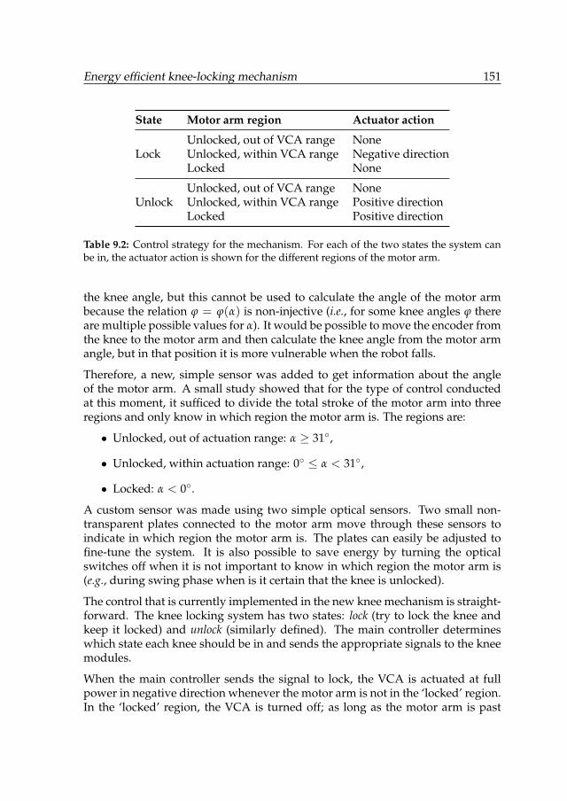
Energy efficient knee-locking mechanism 151
State Motor arm region Actuator action
Unlocked, out of VCA range NoneLock Unlocked, within VCA range Negative direction
Locked None
Unlocked, out of VCA range NoneUnlock Unlocked, within VCA range Positive direction
Locked Positive direction
Table 9.2: Control strategy for the mechanism. For each of the two states the system canbe in, the actuator action is shown for the different regions of the motor arm.
the knee angle, but this cannot be used to calculate the angle of the motor armbecause the relation ϕ = ϕ(α) is non-injective (i.e., for some knee angles ϕ thereare multiple possible values for α). It would be possible to move the encoder fromthe knee to the motor arm and then calculate the knee angle from the motor armangle, but in that position it is more vulnerable when the robot falls.
Therefore, a new, simple sensor was added to get information about the angleof the motor arm. A small study showed that for the type of control conductedat this moment, it sufficed to divide the total stroke of the motor arm into threeregions and only know in which region the motor arm is. The regions are:
• Unlocked, out of actuation range: α ≥ 31◦,
• Unlocked, within actuation range: 0◦ ≤ α < 31◦,
• Locked: α < 0◦.
A custom sensor was made using two simple optical sensors. Two small non-transparent plates connected to the motor arm move through these sensors toindicate in which region the motor arm is. The plates can easily be adjusted tofine-tune the system. It is also possible to save energy by turning the opticalswitches off when it is not important to know in which region the motor arm is(e.g., during swing phase when is it certain that the knee is unlocked).
The control that is currently implemented in the new knee mechanism is straight-forward. The knee locking system has two states: lock (try to lock the knee andkeep it locked) and unlock (similarly defined). The main controller determineswhich state each knee should be in and sends the appropriate signals to the kneemodules.
When the main controller sends the signal to lock, the VCA is actuated at fullpower in negative direction whenever the motor arm is not in the ‘locked’ region.In the ‘locked’ region, the VCA is turned off; as long as the motor arm is past
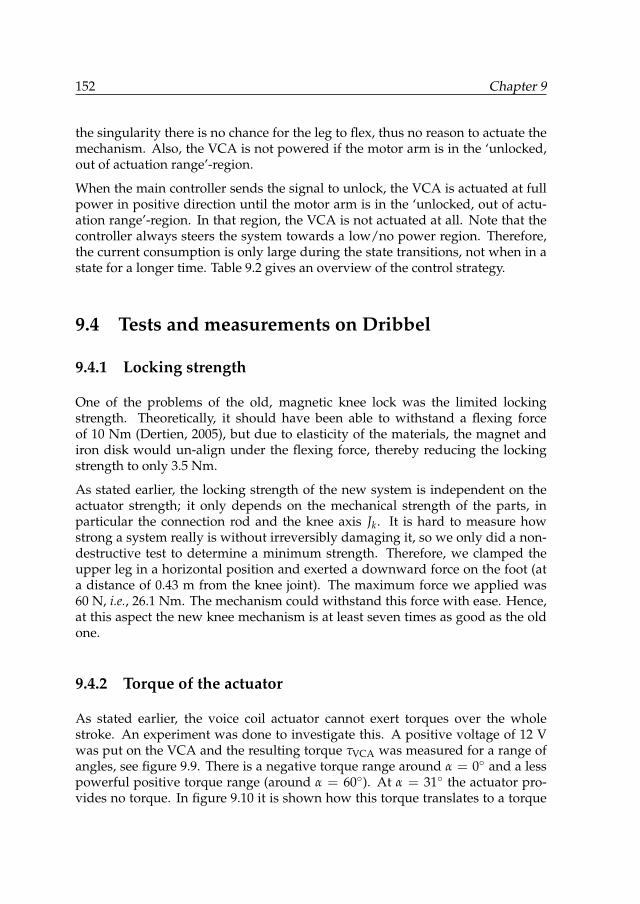
152 Chapter 9
the singularity there is no chance for the leg to flex, thus no reason to actuate themechanism. Also, the VCA is not powered if the motor arm is in the ‘unlocked,out of actuation range’-region.
When the main controller sends the signal to unlock, the VCA is actuated at fullpower in positive direction until the motor arm is in the ‘unlocked, out of actu-ation range’-region. In that region, the VCA is not actuated at all. Note that thecontroller always steers the system towards a low/no power region. Therefore,the current consumption is only large during the state transitions, not when in astate for a longer time. Table 9.2 gives an overview of the control strategy.
9.4 Tests and measurements on Dribbel
9.4.1 Locking strength
One of the problems of the old, magnetic knee lock was the limited lockingstrength. Theoretically, it should have been able to withstand a flexing forceof 10 Nm (Dertien, 2005), but due to elasticity of the materials, the magnet andiron disk would un-align under the flexing force, thereby reducing the lockingstrength to only 3.5 Nm.
As stated earlier, the locking strength of the new system is independent on theactuator strength; it only depends on the mechanical strength of the parts, inparticular the connection rod and the knee axis Jk. It is hard to measure howstrong a system really is without irreversibly damaging it, so we only did a non-destructive test to determine a minimum strength. Therefore, we clamped theupper leg in a horizontal position and exerted a downward force on the foot (ata distance of 0.43 m from the knee joint). The maximum force we applied was60 N, i.e., 26.1 Nm. The mechanism could withstand this force with ease. Hence,at this aspect the new knee mechanism is at least seven times as good as the oldone.
9.4.2 Torque of the actuator
As stated earlier, the voice coil actuator cannot exert torques over the wholestroke. An experiment was done to investigate this. A positive voltage of 12 Vwas put on the VCA and the resulting torque τVCA was measured for a range ofangles, see figure 9.9. There is a negative torque range around α = 0◦ and a lesspowerful positive torque range (around α = 60◦). At α = 31◦ the actuator pro-vides no torque. In figure 9.10 it is shown how this torque translates to a torque
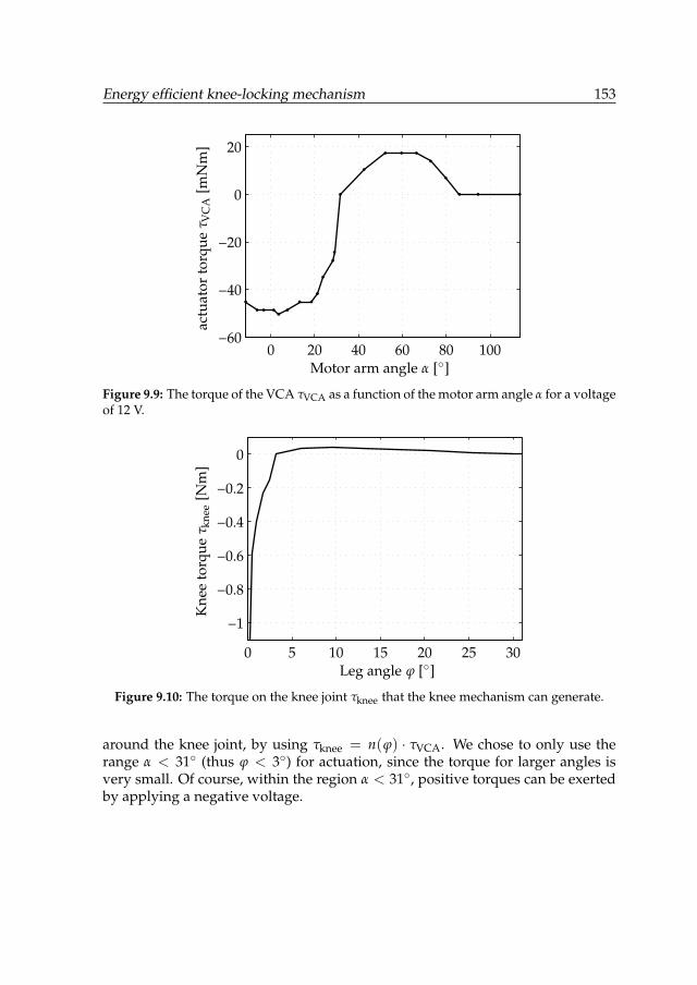
Energy efficient knee-locking mechanism 153
0 20 40 60 80 100−60
−40
−20
0
20
Motor arm angle α [◦]
actu
ator
torq
ueτ V
CA
[mN
m]
Figure 9.9: The torque of the VCA τVCA as a function of the motor arm angle α for a voltageof 12 V.
0 5 10 15 20 25 30
−1
−0.8
−0.6
−0.4
−0.2
0
Leg angle ϕ [◦]
Kne
eto
rque
τ kne
e[N
m]
Figure 9.10: The torque on the knee joint τknee that the knee mechanism can generate.
around the knee joint, by using τknee = n(ϕ) · τVCA. We chose to only use therange α < 31◦ (thus ϕ < 3◦) for actuation, since the torque for larger angles isvery small. Of course, within the region α < 31◦, positive torques can be exertedby applying a negative voltage.
154 Chapter 9
9.4.3 Power consumption of the knee mechanisms during nor-mal gait
When fully powered (U = 12 V), the VCA of the knee mechanism takes approxi-mately I = 0.39 A, which results in a power consumption of PVCA = U · I = 4.7 Wfor each actuator. This is a significant amount, but it should be remembered thatmost of the time the actuators don’t have to work at full power. During a normalwalk, we measured the average actuation time for each actuator to be approx-imately 10 % of the gait cycle, which implies that the four knee locks togetherconsume approximately 1.9 W.
9.4.4 Total power consumption, specific cost of transport
The specific cost of transport Cet is a non-dimensional indicator of the energy-efficiency of transportation. It equals the amount of (electrical) energy needed totransport a unit weight over a unit distance:
cet =E
m · g · d =Pavg
m · g · vavg(9.1)
where E is the energy used, m the mass of the system, g the earth’s gravitationalacceleration, d the distance traveled, Pavg the average power consumed and vavgthe average velocity.
In order to obtain the average power consumption, we made Dribbel walk andrecorded the power consumption as a function of time. Over four typical, con-secutive steps, we measured an average power consumption of 27.7 W. The hipactuator was controlled by a simple PD controller that instantaneously switchesthe setpoint for the inter-leg angle when the front foot touches the ground (simi-lar to Wisse et al. (2005), but with the difference that we used very low controllergains such that the swing phase more or less resembles natural swinging motion).
Dribbel’s velocity was measured by making it walk 14 consecutive steps, cover-ing a distance of 4.0 m. This took 14.0 s, giving an average velocity of vavg =0.29 m/s. Together with the mass of Dribbel being 16.1 kg, we find a specificcost of transport of cet = 0.60. Table 9.3 shows some important specifications ofDribbel.
9.5 How mechanical play is —for once— our friend
When we first implemented the new knee mechanisms on Dribbel, the system didnot work entirely as expected. Often, the motor arm did not pass its singularity
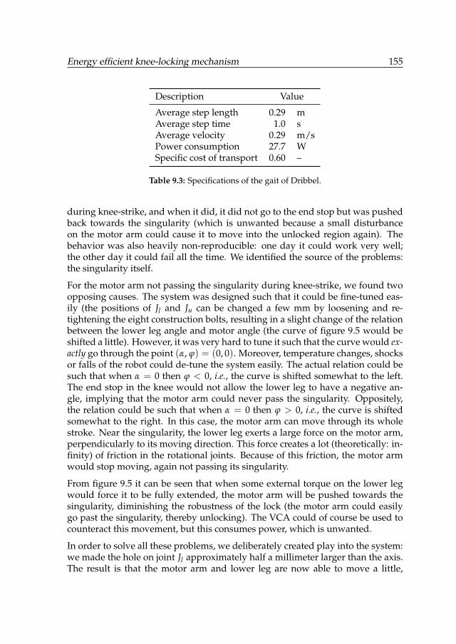
Energy efficient knee-locking mechanism 155
Description Value
Average step length 0.29 mAverage step time 1.0 sAverage velocity 0.29 m/sPower consumption 27.7 WSpecific cost of transport 0.60 –
Table 9.3: Specifications of the gait of Dribbel.
during knee-strike, and when it did, it did not go to the end stop but was pushedback towards the singularity (which is unwanted because a small disturbanceon the motor arm could cause it to move into the unlocked region again). Thebehavior was also heavily non-reproducible: one day it could work very well;the other day it could fail all the time. We identified the source of the problems:the singularity itself.
For the motor arm not passing the singularity during knee-strike, we found twoopposing causes. The system was designed such that it could be fine-tuned eas-ily (the positions of Jl and Ju can be changed a few mm by loosening and re-tightening the eight construction bolts, resulting in a slight change of the relationbetween the lower leg angle and motor angle (the curve of figure 9.5 would beshifted a little). However, it was very hard to tune it such that the curve would ex-actly go through the point (α, ϕ) = (0, 0). Moreover, temperature changes, shocksor falls of the robot could de-tune the system easily. The actual relation could besuch that when α = 0 then ϕ < 0, i.e., the curve is shifted somewhat to the left.The end stop in the knee would not allow the lower leg to have a negative an-gle, implying that the motor arm could never pass the singularity. Oppositely,the relation could be such that when α = 0 then ϕ > 0, i.e., the curve is shiftedsomewhat to the right. In this case, the motor arm can move through its wholestroke. Near the singularity, the lower leg exerts a large force on the motor arm,perpendicularly to its moving direction. This force creates a lot (theoretically: in-finity) of friction in the rotational joints. Because of this friction, the motor armwould stop moving, again not passing its singularity.
From figure 9.5 it can be seen that when some external torque on the lower legwould force it to be fully extended, the motor arm will be pushed towards thesingularity, diminishing the robustness of the lock (the motor arm could easilygo past the singularity, thereby unlocking). The VCA could of course be used tocounteract this movement, but this consumes power, which is unwanted.
In order to solve all these problems, we deliberately created play into the system:we made the hole on joint Jl approximately half a millimeter larger than the axis.The result is that the motor arm and lower leg are now able to move a little,
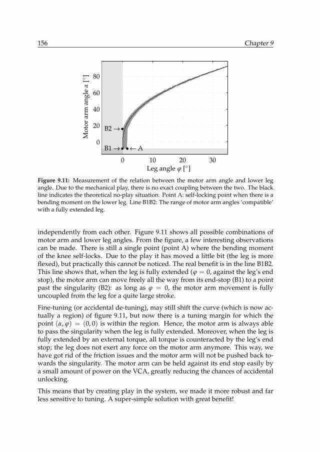
156 Chapter 9
0 10 20 30
0
20
40
60
80
••
•
← AB1 →
B2 →
Leg angle ϕ [◦]
Mot
orar
man
gle
α[◦
]
Figure 9.11: Measurement of the relation between the motor arm angle and lower legangle. Due to the mechanical play, there is no exact coupling between the two. The blackline indicates the theoretical no-play situation. Point A: self-locking point when there is abending moment on the lower leg. Line B1B2: The range of motor arm angles ‘compatible’with a fully extended leg.
independently from each other. Figure 9.11 shows all possible combinations ofmotor arm and lower leg angles. From the figure, a few interesting observationscan be made. There is still a single point (point A) where the bending momentof the knee self-locks. Due to the play it has moved a little bit (the leg is moreflexed), but practically this cannot be noticed. The real benefit is in the line B1B2.This line shows that, when the leg is fully extended (ϕ = 0, against the leg’s endstop), the motor arm can move freely all the way from its end-stop (B1) to a pointpast the singularity (B2): as long as ϕ = 0, the motor arm movement is fullyuncoupled from the leg for a quite large stroke.
Fine-tuning (or accidental de-tuning), may still shift the curve (which is now ac-tually a region) of figure 9.11, but now there is a tuning margin for which thepoint (α, ϕ) = (0, 0) is within the region. Hence, the motor arm is always ableto pass the singularity when the leg is fully extended. Moreover, when the leg isfully extended by an external torque, all torque is counteracted by the leg’s endstop; the leg does not exert any force on the motor arm anymore. This way, wehave got rid of the friction issues and the motor arm will not be pushed back to-wards the singularity. The motor arm can be held against its end stop easily bya small amount of power on the VCA, greatly reducing the chances of accidentalunlocking.
This means that by creating play in the system, we made it more robust and farless sensitive to tuning. A super-simple solution with great benefit!
Energy efficient knee-locking mechanism 157
9.6 Conclusions and future work
We have designed, implemented and tested a new knee locking mechanism forthe energy efficiently walking robot Dribbel. It uses a four-bar mechanism and amechanical singularity for locking the knee in extended position. Once extended,the knee remains locked without energy consumption, while un-locking onlycosts a small amount of energy. We used suction cups for passive de-bouncingof the system, which has been proven to be an effective method. A simple con-troller was implemented that is locally executed by the knee-module. The testsshowed that the knee locks function well, that the energy consumption indeedhas decreased and the robot walks robustly.
Future work will focus on improving the control algorithm. Firstly, the energyconsumption could be further decreased by actively monitoring the exact move-ment of the motor arm, and only activate the VCA if strictly necessary. For exam-ple, when locking, if the motor arm is already moving towards the end stop withenough velocity, it is not necessary to help it by turning on the VCA. Secondly,the VCA could be used for active de-bouncing. If, when locking, the motor armgoes really fast, the VCA could be used to decelerate it, reducing the chance of arebound. Both enhancements require more accurate measurement of the motorarm angle α, which will be provided by a more accurate sensor.

158 Chapter 9
Chapter 10
New ankle actuation mechanism fora humanoid robot
This chapter is based on the following article (van Oort et al., 2011b):
New Ankle Actuation Mechanism for a Humanoid RobotGijs van Oort, Roelof Reinink and Stefano Stramigioli
Proc., 18th IFAC World Congress (IFAC’11)August 2011.
Abstract—In this chapter we discuss the design of a new ankle actuation mech-anism for the humanoid robot TUlip. The new mechanism consists of twocoupled series-elastic systems. We discuss the choice of actuators accordingto calculations for maximum achievable walking speed. Some control issues,MIMO and non-linearities are also discussed.
159
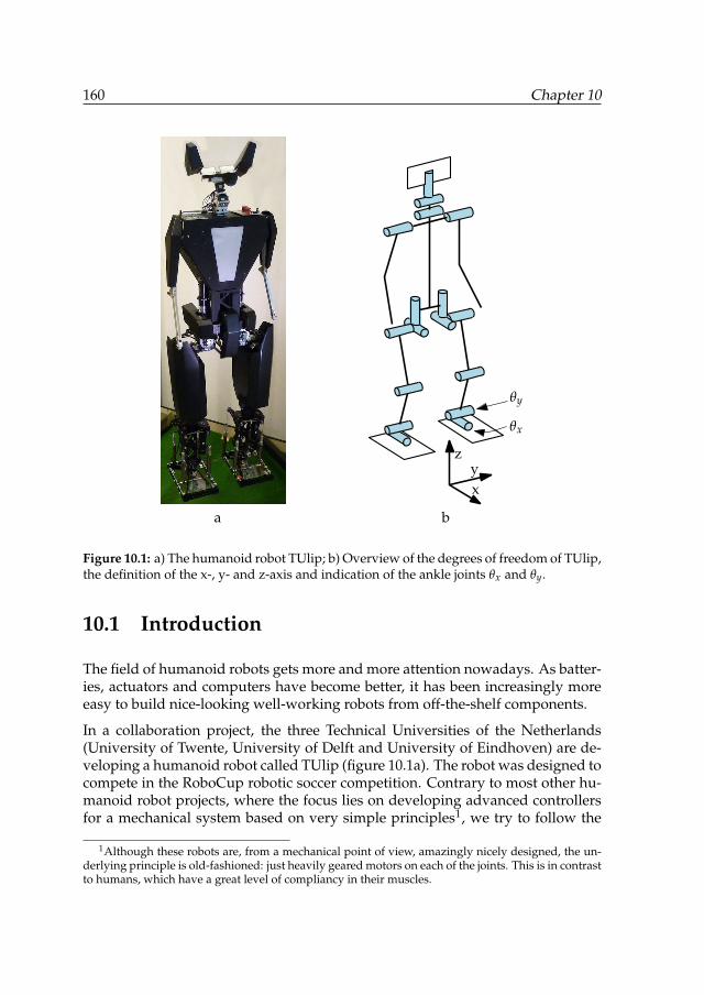
160 Chapter 10
θx
θy
xy
z
a b
Figure 10.1: a) The humanoid robot TUlip; b) Overview of the degrees of freedom of TUlip,the definition of the x-, y- and z-axis and indication of the ankle joints θx and θy.
10.1 Introduction
The field of humanoid robots gets more and more attention nowadays. As batter-ies, actuators and computers have become better, it has been increasingly moreeasy to build nice-looking well-working robots from off-the-shelf components.
In a collaboration project, the three Technical Universities of the Netherlands(University of Twente, University of Delft and University of Eindhoven) are de-veloping a humanoid robot called TUlip (figure 10.1a). The robot was designed tocompete in the RoboCup robotic soccer competition. Contrary to most other hu-manoid robot projects, where the focus lies on developing advanced controllersfor a mechanical system based on very simple principles1, we try to follow the
1Although these robots are, from a mechanical point of view, amazingly nicely designed, the un-derlying principle is old-fashioned: just heavily geared motors on each of the joints. This is in contrastto humans, which have a great level of compliancy in their muscles.
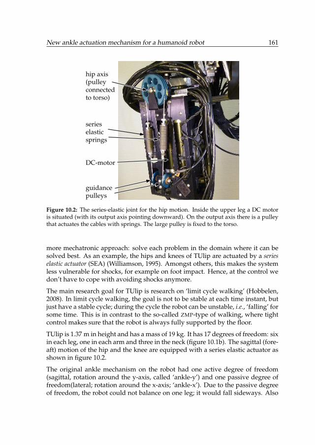
New ankle actuation mechanism for a humanoid robot 161
hip axis(pulleyconnectedto torso)
serieselasticsprings
guidancepulleys
DC-motor
Figure 10.2: The series-elastic joint for the hip motion. Inside the upper leg a DC motoris situated (with its output axis pointing downward). On the output axis there is a pulleythat actuates the cables with springs. The large pulley is fixed to the torso.
more mechatronic approach: solve each problem in the domain where it can besolved best. As an example, the hips and knees of TUlip are actuated by a serieselastic actuator (SEA) (Williamson, 1995). Amongst others, this makes the systemless vulnerable for shocks, for example on foot impact. Hence, at the control wedon’t have to cope with avoiding shocks anymore.
The main research goal for TUlip is research on ‘limit cycle walking’ (Hobbelen,2008). In limit cycle walking, the goal is not to be stable at each time instant, butjust have a stable cycle; during the cycle the robot can be unstable, i.e., ‘falling’ forsome time. This is in contrast to the so-called ZMP-type of walking, where tightcontrol makes sure that the robot is always fully supported by the floor.
TUlip is 1.37 m in height and has a mass of 19 kg. It has 17 degrees of freedom: sixin each leg, one in each arm and three in the neck (figure 10.1b). The sagittal (fore-aft) motion of the hip and the knee are equipped with a series elastic actuator asshown in figure 10.2.
The original ankle mechanism on the robot had one active degree of freedom(sagittal, rotation around the y-axis, called ‘ankle-y’) and one passive degree offreedom(lateral; rotation around the x-axis; ‘ankle-x’). Due to the passive degreeof freedom, the robot could not balance on one leg; it would fall sideways. Also
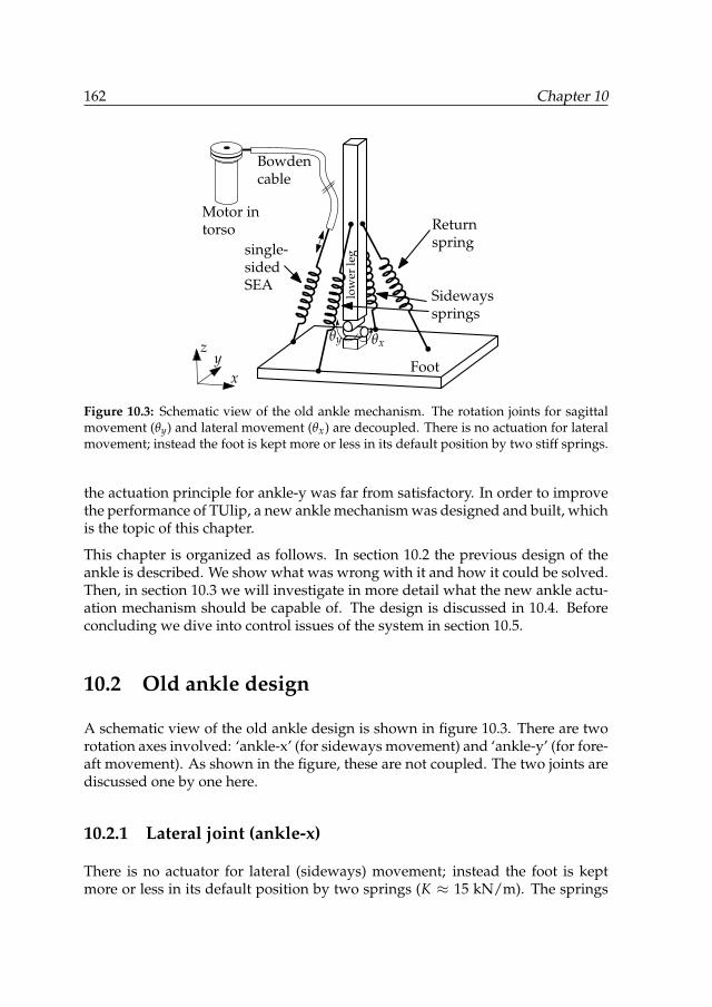
162 Chapter 10
θxθylo
wer
leg
Motor intorso
Bowdencable
Returnspringsingle-
sidedSEA
Sidewayssprings
Footx
yz
Figure 10.3: Schematic view of the old ankle mechanism. The rotation joints for sagittalmovement (θy) and lateral movement (θx) are decoupled. There is no actuation for lateralmovement; instead the foot is kept more or less in its default position by two stiff springs.
the actuation principle for ankle-y was far from satisfactory. In order to improvethe performance of TUlip, a new ankle mechanism was designed and built, whichis the topic of this chapter.
This chapter is organized as follows. In section 10.2 the previous design of theankle is described. We show what was wrong with it and how it could be solved.Then, in section 10.3 we will investigate in more detail what the new ankle actu-ation mechanism should be capable of. The design is discussed in 10.4. Beforeconcluding we dive into control issues of the system in section 10.5.
10.2 Old ankle design
A schematic view of the old ankle design is shown in figure 10.3. There are tworotation axes involved: ‘ankle-x’ (for sideways movement) and ‘ankle-y’ (for fore-aft movement). As shown in the figure, these are not coupled. The two joints arediscussed one by one here.
10.2.1 Lateral joint (ankle-x)
There is no actuator for lateral (sideways) movement; instead the foot is keptmore or less in its default position by two springs (K ≈ 15 kN/m). The springs
New ankle actuation mechanism for a humanoid robot 163
are not strong enough to stabilize the robot passively when standing on one leg;neither were they intended to. The idea behind this set-up was to allow the robotto rock from one foot to the other (instead of going to a stable equilibrium on oneleg); a prerequisite for dynamic walking. The rocking frequency can be tuned bychanging the equilibrium position of the springs.
However, standing on one foot during a kick is really hard. Using Acrobot-likecontrol (Hauser and Murray, 1990) was considered nearly impossible, due to thelimited actuation range in the hip and the need to do other tasks simultaneously,such as ball kicking. Moreover, severe torso motions make it impractical or evendangerous to catch the robot when it is falling. Therefore, we decided not to trythis and improve the mechanics instead.
10.2.2 Sagittal joint (ankle-y)
The sagittal (fore-aft) motion is unilaterally actuated, i.e., the foot can be rotatedactively in one direction but not in the other. A DC motor placed in the torso isconnected to a bowden cable with series-elastic spring, which in turn is connectedto the rear of the foot. Pulling the bowden cable makes the foot plantarflex (i.e.,toes down). A return spring on the front of the foot makes the foot dorsiflex (i.e.,toes up) again when the cable is loosened again.
The main reason why this design choice was made was to keep the weight of thelower leg and foot as low as possible. By putting the motor in the torso, the lowerleg and foot only had to be some structural pieces of aluminum, without anyheavy structures for actuation. The system however did not work as expected. Inorder to be able to dorsiflex the foot with a large enough torque, the return springhad to be quite stiff. This implied that the actuator had to deliver a large torquejust to keep the foot still (in order to obtain a zero resultant torque). The inducedtension in the bowden cable in its turn caused an enormous amount of friction,which made it virtually impossible to do precise control.
10.3 Requirements for new design
For the new actuator mechanism we had a few qualitative as well as quantitativerequirements. Qualitatively, the system should not suffer from the problems de-scribed in the previous section, so unilateral actuation, bowden cables and under-actuation were not an option. Furthermore, the system should be robust and aslightweight as possible. If mounted on the lower leg, its position should be ashigh as possible in order not to disturb the passive-dynamic swing properties ofthe leg too much (Franken, 2007). One of the demands is that the actuation is
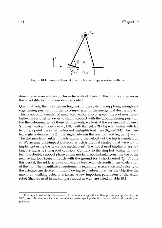
164 Chapter 10
2α
l
dfoot
vm
dstep
π2 − ϕ
x
z
Figure 10.4: Simple 2D model of our robot: a compass walker with feet.
done in a series-elastic way. This reduces shock loads on the motors and gives usthe possibility to mimic zero-torque control.
Quantitatively, the most demanding task for the system is supplying enough en-ergy during push-off in order to compensate for the energy lost during impact.This is not only a matter of much torque, but also of speed: the foot must plan-tarflex fast enough in order to stay in contact with the ground during push-off.For the determination of these requirements, we look at the system as if it were a‘simplest walker’ (Garcia et al., 1998) with flat feet: a 2D, bipedal walker with leglength l, a point mass m at the hip and negligible foot mass (figure 10.4). The inter-leg angle is denoted by 2α, the angle between the rear foot and leg by (π
2 − ϕ).The distance from ankle to toe is dfoot and the velocity of the hip is denoted byv. We assume post-impact push-off, which is the first strategy that we want toimplement using the new ankle mechanism2. The model used implies an instan-taneous inelastic swing foot collision. Contrary to the simplest walker withoutfeet, the double support phase of this model is not instantaneous: the toe of thenew swing foot keeps in touch with the ground for a short period Tp. Duringthis period, the ankle actuator can exert a torque which results in an accelerationof the hip. The quantitative requirements regarding acceleration and velocity ofthe actuator are derived in the following two subsections. As the objective themaximum walking velocity is taken. A few important parameters of the actualrobot (that are used in the compass model as well) are listed in table 10.1.
2Pre-impact push-off has been shown to be more energy efficient than post-impact push-off (Kuo,2002), so if the new mechanism can achieve post-impact push-off, it is also able to do pre-impactpush-off.
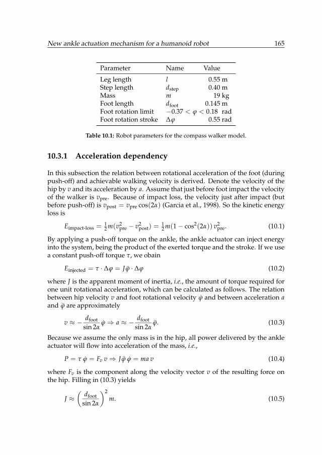
New ankle actuation mechanism for a humanoid robot 165
Parameter Name Value
Leg length l 0.55 mStep length dstep 0.40 mMass m 19 kgFoot length dfoot 0.145 mFoot rotation limit −0.37 < ϕ < 0.18 radFoot rotation stroke ∆ϕ 0.55 rad
Table 10.1: Robot parameters for the compass walker model.
10.3.1 Acceleration dependency
In this subsection the relation between rotational acceleration of the foot (duringpush-off) and achievable walking velocity is derived. Denote the velocity of thehip by v and its acceleration by a. Assume that just before foot impact the velocityof the walker is vpre. Because of impact loss, the velocity just after impact (butbefore push-off) is vpost = vpre cos(2α) (Garcia et al., 1998). So the kinetic energyloss is
Eimpact-loss =12 m(v2
pre − v2post) =
12 m(1− cos2(2α)) v2
pre. (10.1)
By applying a push-off torque on the ankle, the ankle actuator can inject energyinto the system, being the product of the exerted torque and the stroke. If we usea constant push-off torque τ, we obain
Einjected = τ · ∆ϕ = J ϕ · ∆ϕ (10.2)
where J is the apparent moment of inertia, i.e., the amount of torque required forone unit rotational acceleration, which can be calculated as follows. The relationbetween hip velocity v and foot rotational velocity ϕ and between acceleration aand ϕ are approximately
v ≈ − dfootsin 2α
ϕ⇒ a ≈ − dfootsin 2α
ϕ. (10.3)
Because we assume the only mass is in the hip, all power delivered by the ankleactuator will flow into acceleration of the mass, i.e.,
P = τ ϕ = Fv v⇒ J ϕ ϕ = ma v (10.4)
where Fv is the component along the velocity vector v of the resulting force onthe hip. Filling in (10.3) yields
J ≈(
dfootsin 2α
)2m. (10.5)
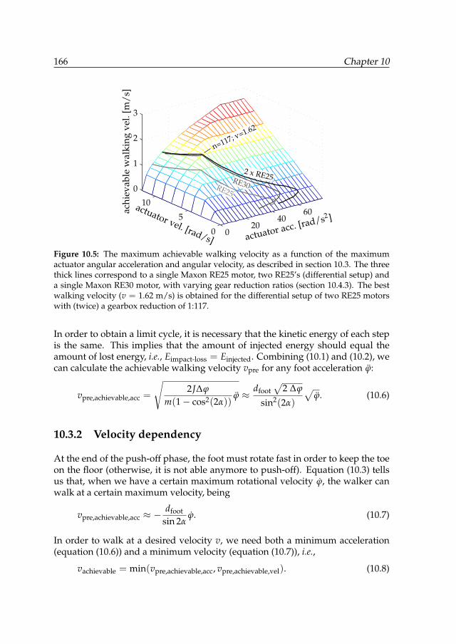
166 Chapter 10
020
4060
0
5
10
0
1
2
3
2 x RE25RE30RE25
n=117; v=1.62
actuator acc. [rad/s2 ]actuator vel. [rad/s]
achi
evab
lew
alki
ngve
l.[m
/s]
Figure 10.5: The maximum achievable walking velocity as a function of the maximumactuator angular acceleration and angular velocity, as described in section 10.3. The threethick lines correspond to a single Maxon RE25 motor, two RE25’s (differential setup) anda single Maxon RE30 motor, with varying gear reduction ratios (section 10.4.3). The bestwalking velocity (v = 1.62 m/s) is obtained for the differential setup of two RE25 motorswith (twice) a gearbox reduction of 1:117.
In order to obtain a limit cycle, it is necessary that the kinetic energy of each stepis the same. This implies that the amount of injected energy should equal theamount of lost energy, i.e., Eimpact-loss = Einjected. Combining (10.1) and (10.2), wecan calculate the achievable walking velocity vpre for any foot acceleration ϕ:
vpre,achievable,acc =
√2J∆ϕ
m(1− cos2(2α))ϕ ≈ dfoot
√2 ∆ϕ
sin2(2α)
√ϕ. (10.6)
10.3.2 Velocity dependency
At the end of the push-off phase, the foot must rotate fast in order to keep the toeon the floor (otherwise, it is not able anymore to push-off). Equation (10.3) tellsus that, when we have a certain maximum rotational velocity ϕ, the walker canwalk at a certain maximum velocity, being
vpre,achievable,acc ≈ −dfoot
sin 2αϕ. (10.7)
In order to walk at a desired velocity v, we need both a minimum acceleration(equation (10.6)) and a minimum velocity (equation (10.7)), i.e.,
vachievable = min(vpre,achievable,acc, vpre,achievable,vel). (10.8)
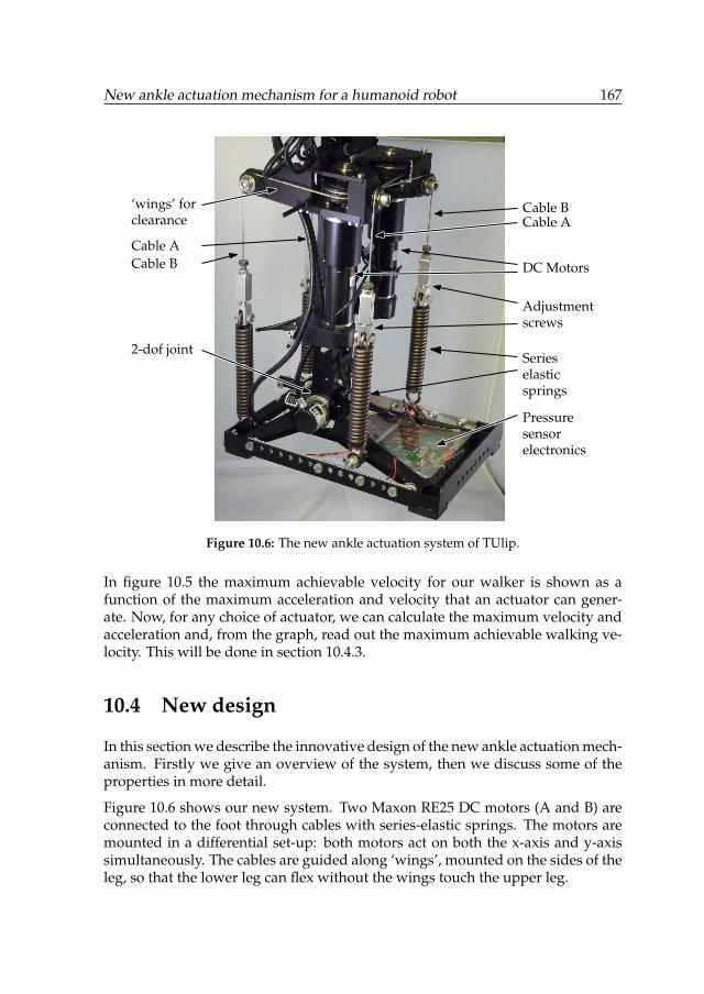
New ankle actuation mechanism for a humanoid robot 167
Serieselasticsprings
DC Motors
Cable ACable B
2-dof joint
‘wings’ forclearance
Cable BCable A
Adjustmentscrews
Pressuresensorelectronics
Figure 10.6: The new ankle actuation system of TUlip.
In figure 10.5 the maximum achievable velocity for our walker is shown as afunction of the maximum acceleration and velocity that an actuator can gener-ate. Now, for any choice of actuator, we can calculate the maximum velocity andacceleration and, from the graph, read out the maximum achievable walking ve-locity. This will be done in section 10.4.3.
10.4 New design
In this section we describe the innovative design of the new ankle actuation mech-anism. Firstly we give an overview of the system, then we discuss some of theproperties in more detail.
Figure 10.6 shows our new system. Two Maxon RE25 DC motors (A and B) areconnected to the foot through cables with series-elastic springs. The motors aremounted in a differential set-up: both motors act on both the x-axis and y-axissimultaneously. The cables are guided along ‘wings’, mounted on the sides of theleg, so that the lower leg can flex without the wings touch the upper leg.
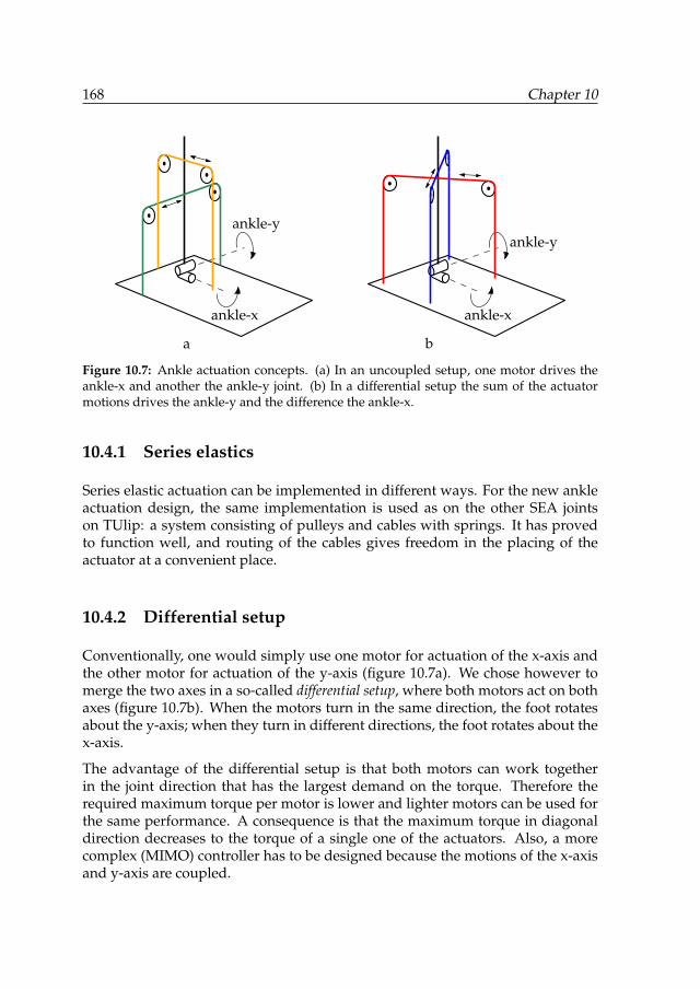
168 Chapter 10
ankle-x
ankle-y
ankle-x
ankle-y
a b
Figure 10.7: Ankle actuation concepts. (a) In an uncoupled setup, one motor drives theankle-x and another the ankle-y joint. (b) In a differential setup the sum of the actuatormotions drives the ankle-y and the difference the ankle-x.
10.4.1 Series elastics
Series elastic actuation can be implemented in different ways. For the new ankleactuation design, the same implementation is used as on the other SEA jointson TUlip: a system consisting of pulleys and cables with springs. It has provedto function well, and routing of the cables gives freedom in the placing of theactuator at a convenient place.
10.4.2 Differential setup
Conventionally, one would simply use one motor for actuation of the x-axis andthe other motor for actuation of the y-axis (figure 10.7a). We chose however tomerge the two axes in a so-called differential setup, where both motors act on bothaxes (figure 10.7b). When the motors turn in the same direction, the foot rotatesabout the y-axis; when they turn in different directions, the foot rotates about thex-axis.
The advantage of the differential setup is that both motors can work togetherin the joint direction that has the largest demand on the torque. Therefore therequired maximum torque per motor is lower and lighter motors can be used forthe same performance. A consequence is that the maximum torque in diagonaldirection decreases to the torque of a single one of the actuators. Also, a morecomplex (MIMO) controller has to be designed because the motions of the x-axisand y-axis are coupled.
New ankle actuation mechanism for a humanoid robot 169
10.4.3 Actuator choice
For TUlip the RE line-up of motors by Maxon is used. They have a good perfor-mance versus weight ratio and there is good experience with them at the depart-ment. We considered two motors: the RE25 (a 20 W motor) and the RE30 (a 60 Wmotor). Smaller motors are unlikely to be powerful enough and stronger modelsare unlikely to be needed, and would certainly be too heavy.
The amount of acceleration that a motor can produce is not only dependent on theamount of torque it can generate, but also on the actuator’s own inertia (this is thereason that we expressed the actuator demands in acceleration instead of torquein section 10.3.1). The angular acceleration that can be achieved by a DC motorwith maximum motor torque τmot,max, gearbox ratio n and gearbox efficiencyη = 0.7 is
ϕmax =n τmot,max η
J + n2 Jmot, (10.9)
where J is the moment of inertia of the load and Jmot is the moment of inertia ofthe motor and gearbox. The maximum angular velocity of an actuator is simply
ϕmax =1n
ωmot,max, (10.10)
where we assume that the friction in the joint is negligible relative to the motorfriction (this is a valid assumption because the joint velocity is small relativelyto the motor velocity and we use ball bearings in the joint axes). With these twoequations and the motor parameters (table 10.2), we can plot a point in figure 10.5and read, for the specific actuator, the maximum achievable walking velocity. Inthe figure we have plot three lines, representing a single Maxon RE25, a MaxonRE25-pair in differential setup and a single Maxon RE30 motor, all with varyinggearbox ratio.
It seems that we can get approximately the same performance for a single RE30and two RE25s in differential setup. The difference is that, in the case of one RE30driving ankle-y we need another motor (an RE25) for ankle-x, while in the differ-ential setup, two smaller motors suffice for both axes. Hence, the total system islighter without giving in on performance.
The ideal transmission ratio of 1:117 should be the total ratio between revolutionsof the DC motor axis and the foot. On top of the gearbox, there is also a smallpulley-system involved, of which the transfer ratio can be freely chosen (up tosome limits). The total ratio is then the product of the gearbox ratio and thepulley system ratio.
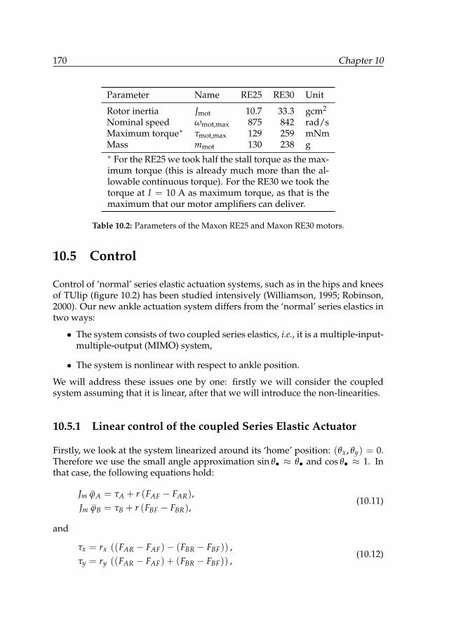
170 Chapter 10
Parameter Name RE25 RE30 Unit
Rotor inertia Jmot 10.7 33.3 gcm2
Nominal speed ωmot,max 875 842 rad/sMaximum torque∗ τmot,max 129 259 mNmMass mmot 130 238 g∗ For the RE25 we took half the stall torque as the max-imum torque (this is already much more than the al-lowable continuous torque). For the RE30 we took thetorque at I = 10 A as maximum torque, as that is themaximum that our motor amplifiers can deliver.
Table 10.2: Parameters of the Maxon RE25 and Maxon RE30 motors.
10.5 Control
Control of ‘normal’ series elastic actuation systems, such as in the hips and kneesof TUlip (figure 10.2) has been studied intensively (Williamson, 1995; Robinson,2000). Our new ankle actuation system differs from the ‘normal’ series elastics intwo ways:
• The system consists of two coupled series elastics, i.e., it is a multiple-input-multiple-output (MIMO) system,
• The system is nonlinear with respect to ankle position.
We will address these issues one by one: firstly we will consider the coupledsystem assuming that it is linear, after that we will introduce the non-linearities.
10.5.1 Linear control of the coupled Series Elastic Actuator
Firstly, we look at the system linearized around its ‘home’ position: (θx, θy) = 0.Therefore we use the small angle approximation sin θ• ≈ θ• and cos θ• ≈ 1. Inthat case, the following equations hold:
Jm ϕA = τA + r (FAF − FAR),Jm ϕB = τB + r (FBF − FBR),
(10.11)
and
τx = rx ((FAR − FAF)− (FBR − FBF)) ,τy = ry ((FAR − FAF) + (FBR − FBF)) ,
(10.12)
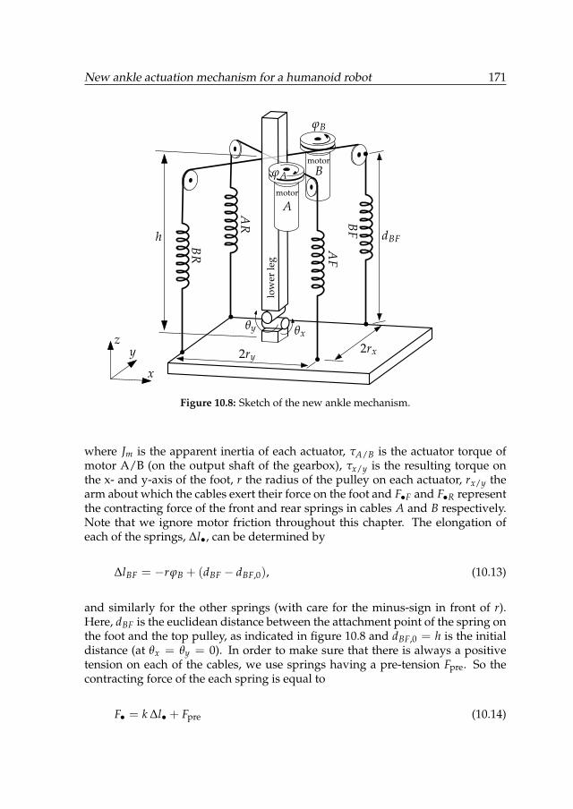
New ankle actuation mechanism for a humanoid robot 171
x
yz
ϕB
h dBF
2ry2rx
BF
AF
AR
BR
θxθy
Bmotor
Amotor
low
erle
g
ϕA
Figure 10.8: Sketch of the new ankle mechanism.
where Jm is the apparent inertia of each actuator, τA/B is the actuator torque ofmotor A/B (on the output shaft of the gearbox), τx/y is the resulting torque onthe x- and y-axis of the foot, r the radius of the pulley on each actuator, rx/y thearm about which the cables exert their force on the foot and F•F and F•R representthe contracting force of the front and rear springs in cables A and B respectively.Note that we ignore motor friction throughout this chapter. The elongation ofeach of the springs, ∆l•, can be determined by
∆lBF = −rϕB + (dBF − dBF,0), (10.13)
and similarly for the other springs (with care for the minus-sign in front of r).Here, dBF is the euclidean distance between the attachment point of the spring onthe foot and the top pulley, as indicated in figure 10.8 and dBF,0 = h is the initialdistance (at θx = θy = 0). In order to make sure that there is always a positivetension on each of the cables, we use springs having a pre-tension Fpre. So thecontracting force of the each spring is equal to
F• = k ∆l• + Fpre (10.14)
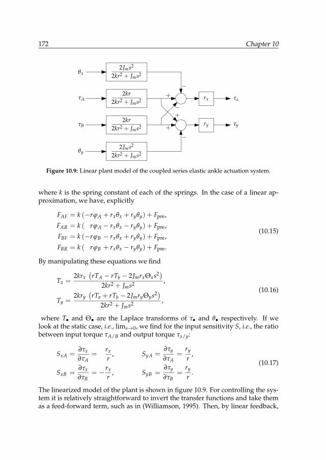
172 Chapter 10
θx
θy
τA
τB
τx
τy
−+
−+
+
−
2kr2kr2 + Jms2
2Jms2
2kr2 + Jms2
2kr2kr2 + Jms2
2Jms2
2kr2 + Jms2
ry
rx
Figure 10.9: Linear plant model of the coupled series elastic ankle actuation system.
where k is the spring constant of each of the springs. In the case of a linear ap-proximation, we have, explicitly
FAF = k (−rϕA + rxθx + ryθy) + Fpre,
FAR = k ( rϕA − rxθx − ryθy) + Fpre,
FBF = k (−rϕB − rxθx + ryθy) + Fpre,
FBR = k ( rϕB + rxθx − ryθy) + Fpre.
(10.15)
By manipulating these equations we find
Tx =2krx
(rTA − rTb − 2JmrxΘxs2)
2kr2 + Jms2 ,
Ty =2kry
(rTa + rTb − 2JmryΘys2)
2kr2 + Jms2 ,
(10.16)
where T• and Θ• are the Laplace transforms of τ• and θ• respectively. If welook at the static case, i.e., lims→0, we find for the input sensitivity S, i.e., the ratiobetween input torque τA/B and output torque τx/y:
SxA =∂τx
∂τA=
rx
r, SyA =
∂τy
∂τA=
ry
r,
SxB =∂τx
∂τB= − rx
r, SyB =
∂τy
∂τB=
ry
r.
(10.17)
The linearized model of the plant is shown in figure 10.9. For controlling the sys-tem it is relatively straightforward to invert the transfer functions and take themas a feed-forward term, such as in (Williamson, 1995). Then, by linear feedback,
New ankle actuation mechanism for a humanoid robot 173
disturbances and model mismatch can be suppressed. However, as we will seein the following subsection, the non-linear effects are so large that it is wise tocompensate for them with a decent non-linear feed-forward controller.
10.5.2 Nonlinearity
In the system we recognize two main sources of non-linearity:
1. The cable attachment points on the foot describe a sphere under variationof θx and θy, i.e., the small angle approximation for these variables does nothold exactly,
2. The rotation axes of the foot are not in the same plane as the cable attach-ment points, which also gives rise to non-linearities.
The goal of the following subsections is to investigate how bad the non-linearitiesare and (thus) how much effort should be put in compensating for these non-linearities (especially because we don’t want to use too much computational pow-er or look-up tables, if unnecessary). It should be noted that the ‘top’ part of thesystem (the motors with pulleys) does show linear behavior and we considerthe springs as having a linear force-elongation relationship. Therefore, (10.11),(10.13) and (10.14) still hold during the non-linear analysis. The other equationsof section 10.5.1 are linear approximations and will be replaced by non-linearequivalents.
10.5.3 Nonlinearity — releasing the small-angle approximation
The effect of releasing the small angle approximation can be investigated by re-placing (10.12) by
τx = (rx cos θx) (FAR + FBF − FAF − FBR),τy = (ry cos θy − rx sin θx sin θy) (FAR+FBR−FAF−FBF)
(10.18)
and replacing rxθx and ryθy in (10.15) by (rx sin θx cos θy) and (ry sin θy) respec-tively. We assume here that the cables still pull exactly vertically (which can beassumed valid if h� rxθx, ryθy). By doing the math we find
τx =rx
rcos θx(τA − τB),
τy =ry
rcos θy(τA + τB)−
rx
rsin θx sin θy(τA − τB)
(10.19)
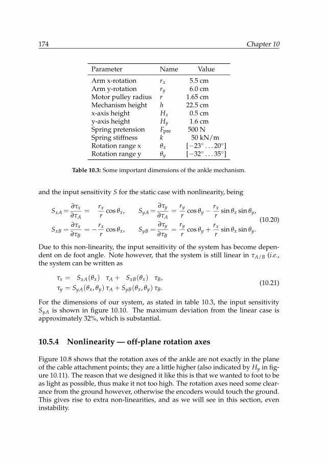
174 Chapter 10
Parameter Name Value
Arm x-rotation rx 5.5 cmArm y-rotation ry 6.0 cmMotor pulley radius r 1.65 cmMechanism height h 22.5 cmx-axis height Hx 0.5 cmy-axis height Hy 1.6 cmSpring pretension Fpre 500 NSpring stiffness k 50 kN/mRotation range x θx [−23◦ . . . 20◦]Rotation range y θy [−32◦ . . . 35◦]
Table 10.3: Some important dimensions of the ankle mechanism.
and the input sensitivity S for the static case with nonlinearity, being
SxA =∂τx
∂τA=
rx
rcos θx, SyA =
∂τy
∂τA=
ry
rcos θy −
rx
rsin θx sin θy,
SxB =∂τx
∂τB= − rx
rcos θx, SyB =
∂τy
∂τB=
ry
rcos θy +
rx
rsin θx sin θy.
(10.20)
Due to this non-linearity, the input sensitivity of the system has become depen-dent on de foot angle. Note however, that the system is still linear in τA/B (i.e.,the system can be written as
τx = SxA(θx) τA + SxB(θx) τB,τy = SyA(θx, θy) τA + SyB(θx, θy) τB.
(10.21)
For the dimensions of our system, as stated in table 10.3, the input sensitivitySyA is shown in figure 10.10. The maximum deviation from the linear case isapproximately 32%, which is substantial.
10.5.4 Nonlinearity — off-plane rotation axes
Figure 10.8 shows that the rotation axes of the ankle are not exactly in the planeof the cable attachment points; they are a little higher (also indicated by Hy in fig-ure 10.11). The reason that we designed it like this is that we wanted to foot to beas light as possible, thus make it not too high. The rotation axes need some clear-ance from the ground however, otherwise the encoders would touch the ground.This gives rise to extra non-linearities, and as we will see in this section, eveninstability.
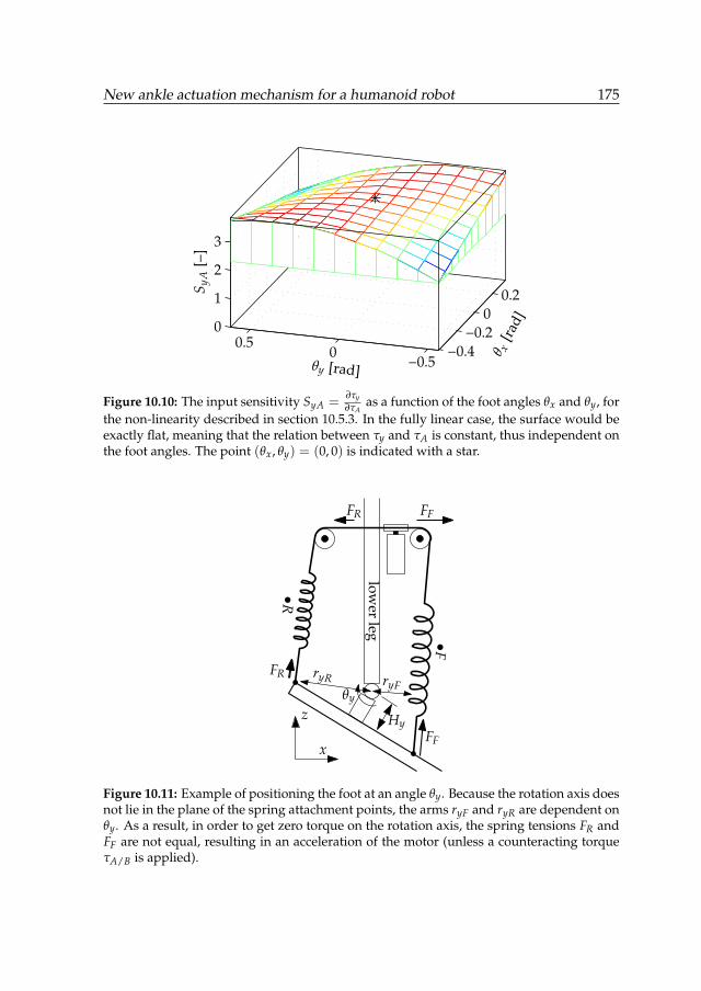
New ankle actuation mechanism for a humanoid robot 175
0
1
2
3
0.2
0
−0.2
−0.4−0.5
00.5
θy [rad]
S yA
[–]
θ x[r
ad]
Figure 10.10: The input sensitivity SyA =∂τy∂τA
as a function of the foot angles θx and θy, forthe non-linearity described in section 10.5.3. In the fully linear case, the surface would beexactly flat, meaning that the relation between τy and τA is constant, thus independent onthe foot angles. The point (θx, θy) = (0, 0) is indicated with a star.
θy
ryR ryF
•F
•R
FR FF
FR
FF
lower
leg
x
z Hy
Figure 10.11: Example of positioning the foot at an angle θy. Because the rotation axis doesnot lie in the plane of the spring attachment points, the arms ryF and ryR are dependent onθy. As a result, in order to get zero torque on the rotation axis, the spring tensions FR andFF are not equal, resulting in an acceleration of the motor (unless a counteracting torqueτA/B is applied).
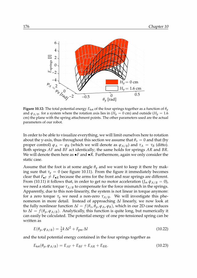
176 Chapter 10
−2
0
2
−4
−2
0
2
4
6
0.50
−0.5
Hy = 0 cm
Hy = 1.6 cm
θy [rad]
E spr
ings
[J]
ϕA =
ϕB [rad]
Figure 10.12: The total potential energy Etot of the four springs together as a function of θyand ϕA/B. for a system where the rotation axis lies in (Hy = 0 cm) and outside (Hy = 1.6cm) the plane with the spring attachment points. The other parameters used are the actualparameters of our robot.
In order to be able to visualize everything, we will limit ourselves here to rotationabout the y-axis, thus throughout this section we assume that θx = 0 and that (byproper control) ϕA = ϕB (which we will denote as ϕA/B) and τA = τB (ditto).Both springs AF and BF act identically; the same holds for springs AR and BR.We will denote them here as •F and •R. Furthermore, again we only consider thestatic case.
Assume that the foot is at some angle θy and we want to keep it there by mak-ing sure that τy = 0 (see figure 10.11). From the figure it immediately becomesclear that F•F 6= F•R because the arms for the front and rear springs are different.From (10.11) it follows that, in order to get no motor acceleration (Jm ϕA/B = 0),we need a static torque τA/B to compensate for the force mismatch in the springs.Apparently, due to this non-linearity, the system is not linear in torque anymore:for a zero torque τy we need a non-zero τA/B. We will investigate this phe-nomenon in more detail. Instead of approaching ∆l linearly, we now look atthe fully nonlinear function ∆l = f (θx, θy, ϕA, ϕB), which in our 2D case reducesto ∆l = f (θy, ϕA/B). Analytically, this function is quite long, but numerically itcan easily be calculated. The potential energy of one pre-tensioned spring can bewritten as
E(θy, ϕA/B) =12 k ∆l2 + Fpre ∆l (10.22)
and the total potential energy contained in the four springs together as
Etot(θy, ϕA/B) = EAF + EBF + EAR + EBR. (10.23)
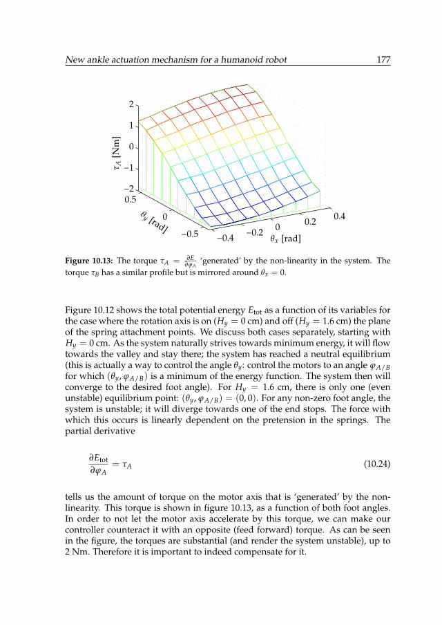
New ankle actuation mechanism for a humanoid robot 177
−0.4−0.2
00.2
0.4
−0.5
0
0.5
−2
−1
0
1
2
θx [rad]
θy [rad]
τ A[N
m]
Figure 10.13: The torque τA = ∂E∂ϕA
‘generated’ by the non-linearity in the system. Thetorque τB has a similar profile but is mirrored around θx = 0.
Figure 10.12 shows the total potential energy Etot as a function of its variables forthe case where the rotation axis is on (Hy = 0 cm) and off (Hy = 1.6 cm) the planeof the spring attachment points. We discuss both cases separately, starting withHy = 0 cm. As the system naturally strives towards minimum energy, it will flowtowards the valley and stay there; the system has reached a neutral equilibrium(this is actually a way to control the angle θy: control the motors to an angle ϕA/Bfor which (θy, ϕA/B) is a minimum of the energy function. The system then willconverge to the desired foot angle). For Hy = 1.6 cm, there is only one (evenunstable) equilibrium point: (θy, ϕA/B) = (0, 0). For any non-zero foot angle, thesystem is unstable; it will diverge towards one of the end stops. The force withwhich this occurs is linearly dependent on the pretension in the springs. Thepartial derivative
∂Etot
∂ϕA= τA (10.24)
tells us the amount of torque on the motor axis that is ‘generated’ by the non-linearity. This torque is shown in figure 10.13, as a function of both foot angles.In order to not let the motor axis accelerate by this torque, we can make ourcontroller counteract it with an opposite (feed forward) torque. As can be seenin the figure, the torques are substantial (and render the system unstable), up to2 Nm. Therefore it is important to indeed compensate for it.

178 Chapter 10
10.6 Conclusions
In this chapter we discussed the design and control of a new ankle mechanismfor the humanoid robot TUlip. It has been shown that the problems of the pre-vious design could be eliminated by using a differential motor setup, resultingin a coupled MIMO system. Calculations were done to determine the best motorand gearbox ratio, where achievable walking speed was chosen as optimizationcriterion. Some issues on controlling the system were discussed, mainly the non-linearities induced by the system.
We have not yet been able to do intensive testing with the new ankle system,therefore, we cannot tell yet how well the system behaves. Mechanically, wethink the new system will easily outperform its predecessor. From a control pointof view, the non-linearities can be compensated in software, but we will probablyalso try to reduce the amount of non-linearity in the system by moving the cableattachment points such that the rotation axes are in the same plane.
Chapter 11
Conclusions
In this chapter the main conclusions from this thesis are recapitulated. After that,the work is discussed and recommendations for future work are given.
11.1 Conclusions
In section 1.4.1 five research goals for this thesis were formulated, being:
1. How can we analyze the behavior of a 2D passive dynamic walker that iswalking on rough terrain?
2. By looking at the robot from a different ‘perspective’, can we gain moreinsight in its dynamics?
3. How can we control a walking robot in order to stabilize it in the lateral(sideways) direction?
4. How can we improve the actuators in order to get minimum energy con-sumption?
5. How can we design parts of a walking robot optimally?
In this section each research goal will be reviewed and evaluated separately. Formore detailed conclusions about a specific subject, please look at the conclusionsections at the end of each chapter. At the end of this section some overall con-clusions will be stated.
179
180 Chapter 11
Analyze behavior of 2D passive dynamic walker on rough terrain
In chapter 2 it was shown that the commonly used post-impact Poincaré sectionfor walking robots can not be used directly in the case of irregular terrain becauseon an irregular floor the post-impact states of all steps do not lie on one Poincarésection. A solution was provided that extends the applicability of the post-impactPoincaré section to rough terrain by means of the Integration mapping ΠI, whichmaps any post-impact state to a state on the post-impact Poincaré section associ-ated with a flat floor.
Furthermore, a method was introduced to relate disturbances of different magni-tude to curves on the Poincaré section. This gives more insight in the effect of thedisturbance on the gait and it gives hints on where to extend the Poincaré sectionin order to increase the robustness for the specific disturbance.
The methods presented open new possibilities for disturbance analysis using thePoincaré section and its derivative tools such as the stride function and the basinof attraction.
Gaining more insight by looking from different ‘perspective’
In chapter 3 it was shown that a proper coordinate transformation makes theequations of motion and analysis easier. Ready-to-use equations were providedto do the coordinate transformation. The method has successfully been used inthe programming of our limit cycle walker TUlip.
In chapter 4 it was shown that the concept of screws and wrenches gives us toolsto geometrically establish the relation between the ground reaction wrench andthe Zero-Moment Point. The coordinate-free nature of the method has the advan-tage of preventing implicit (and possibly wrong) coordinate-related assumptionsin the analysis.
In chapter 5 a systematic dynamic analysis was presented of the 3D bipedal gait.The analysis was done using simplified models in which the robot is described asa single rigid body, called the ‘locked inertia’. The phases of the gait (foot rollingphase and impact phase) were discussed separately and explicit equations forboth were given. Because of the simplified models the equations became man-ageable and a good starting point for theoretical probing.
The three chapters introduced different ways of looking at the dynamics of walk-ing robots. Indeed, the presented methods give more insight in the dynamics:by application of them, the analysis of the walker’s gait becomes easier and theresults are better understandable.
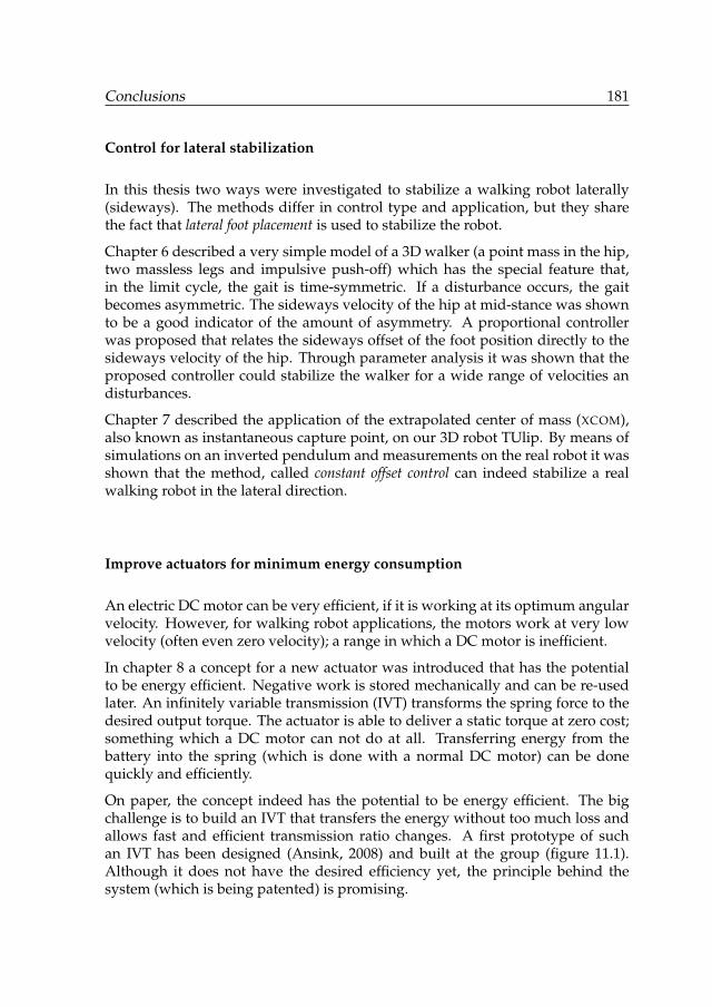
Conclusions 181
Control for lateral stabilization
In this thesis two ways were investigated to stabilize a walking robot laterally(sideways). The methods differ in control type and application, but they sharethe fact that lateral foot placement is used to stabilize the robot.
Chapter 6 described a very simple model of a 3D walker (a point mass in the hip,two massless legs and impulsive push-off) which has the special feature that,in the limit cycle, the gait is time-symmetric. If a disturbance occurs, the gaitbecomes asymmetric. The sideways velocity of the hip at mid-stance was shownto be a good indicator of the amount of asymmetry. A proportional controllerwas proposed that relates the sideways offset of the foot position directly to thesideways velocity of the hip. Through parameter analysis it was shown that theproposed controller could stabilize the walker for a wide range of velocities andisturbances.
Chapter 7 described the application of the extrapolated center of mass (XCOM),also known as instantaneous capture point, on our 3D robot TUlip. By means ofsimulations on an inverted pendulum and measurements on the real robot it wasshown that the method, called constant offset control can indeed stabilize a realwalking robot in the lateral direction.
Improve actuators for minimum energy consumption
An electric DC motor can be very efficient, if it is working at its optimum angularvelocity. However, for walking robot applications, the motors work at very lowvelocity (often even zero velocity); a range in which a DC motor is inefficient.
In chapter 8 a concept for a new actuator was introduced that has the potentialto be energy efficient. Negative work is stored mechanically and can be re-usedlater. An infinitely variable transmission (IVT) transforms the spring force to thedesired output torque. The actuator is able to deliver a static torque at zero cost;something which a DC motor can not do at all. Transferring energy from thebattery into the spring (which is done with a normal DC motor) can be donequickly and efficiently.
On paper, the concept indeed has the potential to be energy efficient. The bigchallenge is to build an IVT that transfers the energy without too much loss andallows fast and efficient transmission ratio changes. A first prototype of suchan IVT has been designed (Ansink, 2008) and built at the group (figure 11.1).Although it does not have the desired efficiency yet, the principle behind thesystem (which is being patented) is promising.
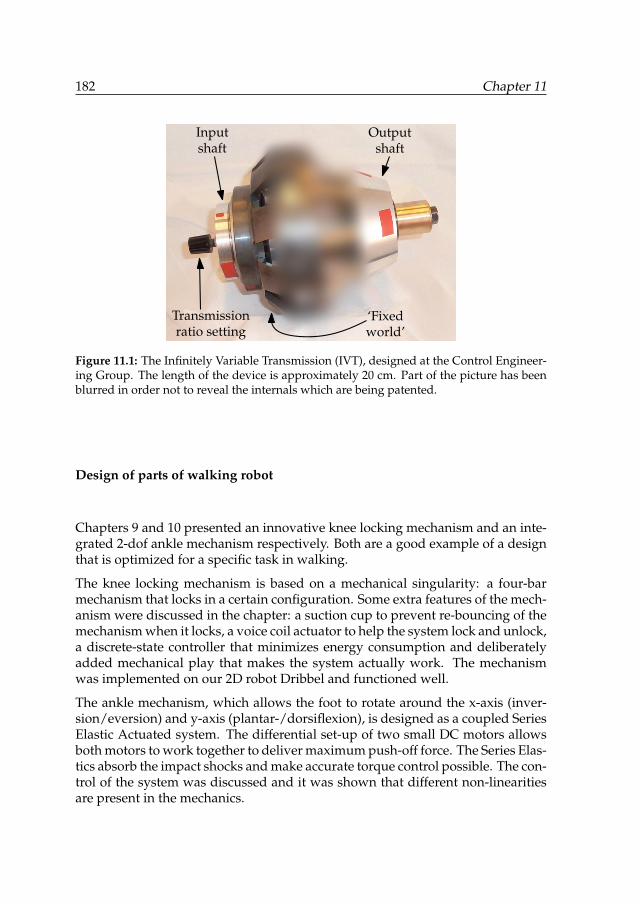
182 Chapter 11
Inputshaft
Outputshaft
Transmissionratio setting
‘Fixedworld’
Figure 11.1: The Infinitely Variable Transmission (IVT), designed at the Control Engineer-ing Group. The length of the device is approximately 20 cm. Part of the picture has beenblurred in order not to reveal the internals which are being patented.
Design of parts of walking robot
Chapters 9 and 10 presented an innovative knee locking mechanism and an inte-grated 2-dof ankle mechanism respectively. Both are a good example of a designthat is optimized for a specific task in walking.
The knee locking mechanism is based on a mechanical singularity: a four-barmechanism that locks in a certain configuration. Some extra features of the mech-anism were discussed in the chapter: a suction cup to prevent re-bouncing of themechanism when it locks, a voice coil actuator to help the system lock and unlock,a discrete-state controller that minimizes energy consumption and deliberatelyadded mechanical play that makes the system actually work. The mechanismwas implemented on our 2D robot Dribbel and functioned well.
The ankle mechanism, which allows the foot to rotate around the x-axis (inver-sion/eversion) and y-axis (plantar-/dorsiflexion), is designed as a coupled SeriesElastic Actuated system. The differential set-up of two small DC motors allowsboth motors to work together to deliver maximum push-off force. The Series Elas-tics absorb the impact shocks and make accurate torque control possible. The con-trol of the system was discussed and it was shown that different non-linearitiesare present in the mechanics.
Conclusions 183
11.2 Recommendations for future work
After five years of research, resulting in this thesis, many questions have an-swered. The answers have however led to many new questions and ideas forfuture research. Some of them are discussed below, organized by topic.
Analysis
• Research on the Poincaré section and its derivative tools should be contin-ued. An example is the applicability of the post-impact Basin of Attraction(BOA) to walkers with feedback control. Often, it is assumed that the robust-ness against disturbances and the size of the BOA are correlated. In chapter 2it was already shown that this does not have to be the case. For an actuatedwalker however, there is another reason to question this assumption. Awalker is robust against a disturbance if the disturbance leads the walker toa state on the post-impact Poincaré section which is inside the BOA. Fromthis it follows that there are actually two ways to increase robustness: eitherenlarging the BOA by making a controller that can handle large deviationsfrom the fixed point on the Poincaré section, or making sure that deviationsfrom the fixed point as a result of the disturbance are not too large by mak-ing a controller that immediately reacts on the disturbance. The latter maywork best because the controller reacts earlier, thereby preventing that thedeviation from the limit cycle grows too much. It would be interesting tosee if there is a BOA-like property that can successfully compare the robust-ness of a walker for both situations.
• For many-dof robots it is convenient to reduce the control problems to a‘state space’ with less dimensions than the number of degrees of freedom.Therefore research should be continued on (bijective) coordinate transfor-mations, focusing on transformations that split the state into a relevant partand a non-relevant part (analogous to the ‘null space’) for the specific con-trol task.
• The approximation of a many-dof walker by a locked inertia (chapter 5) issomewhat crude. Firstly, the foot of a robot would not be rigidly attached tothe leg, and secondly the torso would be approximately upright and not ro-tate with the leg. A logical extension to the model presented in the chapterwould therefore be to approximate the robot by two or three locked inertiasinstead of one. It should be investigated how well such a model can repre-sent the real behavior of the walker and if analytical conclusions still can bedrawn from the simplified model.
184 Chapter 11
• Even after years of research in this field, measures for ‘performance’ of awalking robot are still vague. On one hand this is no wonder because judg-ing the performance is highly subjective and dependent on the specific task(which often is also vague). On the other hand it is strange because hav-ing a good performance criterion is essential when doing optimization orcomparison between walkers. It is therefore suggested that more researchshould be dedicated to finding meaningful performance measures. Someideas about this will be discussed now.
A performance measure, or metric, should be homeomorphic to R (or a sub-set of it) so that two walkers can unambiguously be compared: the onewith the higher score is is the best. If multiple of criteria are considered,they should be scaled in some way to get to one single metric. This scalingis an important design choice and should be chosen with care.
The meaningfulness of a metric is a point which is often paid only littleattention to. Assumptions are often made that some measurable property(e.g., the largest eigenvalue) of the walker is correlated to a less measur-able property like robustness or efficiency — without proof, and withoutelaborating on what exactly is meant with robustness or efficiency. Somecommonly used performance measures said to be related to robustness arethe area of basin of attraction (which is, mathematically speaking, not evendefined), maximum allowable relative deviation from the limit cycle (whichis highly dependent on the arbitrary choice of coordinates) and maximumeigenvalue. The specific resistance, the energy consumption per distancetraveled per kilogram mass per gravity (Wisse et al., 2004) (also known asthe specific cost of transport) is a good example of an unfortunate choice as anefficiency metric when used for a passive dynamic walker: when used as anoptimization criterion it will come up with a walker walking at an infinitelylow speed (Garcia et al., 2000; Chatterjee and Garcia, 2000).
For metrics indicating robustness against a disturbance, the author thinksthe only good solution is to really test the walker against the disturbanceand record the maximum magnitude of the disturbance for which the walk-er does not fall. The ‘maximum step-down’ seems therefore a good metric,although it should be noticed that the metric only tells us something aboutthe robustness against drops in floor height and not against other distur-bances such as pushes.
Some commonly used metrics (such as the specific resistance) are scaled bymass and/or length of the walker, such that walkers of different size (in thecase of the specific resistance even walkers on different planets; the metricis scaled by gravity too) can be compared to each other. For simple systemssuch as models of 3-dof limit cycle walkers, this is okay, but in the opinion ofthe author, this method should be abandoned for more sophisticated walk-
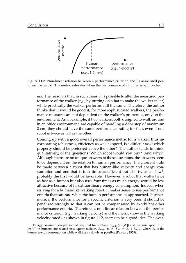
Conclusions 185
performance(e.g., velocity)
perf
orm
ance
met
ric
humanperformance(e.g., 1.2 m/s)
Figure 11.2: Non-linear relation between a performance criterion and its associated per-formance metric. The metric saturates when the performance of a human is approached.
ers. The reason is that, in such cases, it is possible to alter the measured per-formance of the walker (e.g., by putting on a hat to make the walker taller)while practically the walker performs still the same. Therefore, the authorthinks that it would be good if, for more sophisticated walkers, the perfor-mance measures are not dependent on the walker’s properties, only on theenvironment. As an example, if two walkers, both designed to walk aroundin an office environment, are capable of handling a door step of maximum2 cm, they should have the same performance rating for that, even if onerobot is twice as tall as the other.
Coming up with a good overall performance metric for a walker, thus in-corporating robustness, efficiency as well as speed, is a difficult task: whichproperty should be preferred above the other? The author tends to think,qualitatively, of the questions ‘Which robot would you buy? And why?’.Although there are no unique answers to these questions, the answers seemto be dependent on the relation to human performance. If a choice shouldbe made between a robot that has human-like velocity and energy con-sumption and one that is four times as efficient but also twice as slow1,probably the first would be favorable. However, a robot that walks twiceas fast as a human but also uses four times as much energy would be lessattractive because of its extraordinary energy consumption. Indeed, whenstriving for a human-like walking robot, it makes sense to use performancecriteria that saturate when the human performance is approached. Further-more, if the performance for a specific criterion is very poor, it should bepenalized strongly so that it can not be compensated by exorbitant otherperformance criteria. Therefore, a non-linear relation between the perfor-mance criterion (e.g., walking velocity) and the metric (how is the walkingvelocity rated), as shown in figure 11.2, seems to be a good idea. The over-
1Energy consumption per second required for walking Ewalk (in [W]) and walking speed v (in[m/s]) in humans are related in a square fashion, Ewalk ∝ v2; Etot = E0 + Ewalk, where E0 is thehuman energy consumption while walking as slowly as possible (Ralston, 1958).
186 Chapter 11
all performance can then be taken as the sum of all individual performancemetrics. More research is needed on this topic in order to find the best per-formance metrics.
Control and actuation
• The two foot placement controllers described in this thesis are both a lit-tle limited. The XCOM-controller only controls lateral foot placement; notsagittal. The time-reversal controller does control both, but is based on anover-simplified model of a 3D robot. Combining control of both planes,including coupling, rotation about the vertical axis and push-off could im-prove the gait and make it more robust.
• Most humanoid walking robots use only their legs and (counterswinging)arms for stabilizing the gait; the upper body remains vertical all the time.For rejection of large disturbances however, the upper body may be of greathelp. Thanks to its large moment of inertia, rotational acceleration of the up-per body can — momentarily — shift the Center of Pressure towards a con-venient place, thereby preventing a fall. The Reaction Mass Pendulum (Leeand Goswami, 2007) theory will be useful in designing such controllers.
• The idea behind limit cycle walking is to let the passive dynamics do mostof the work and not to influence it too much by control. However, in or-der to stabilize a walker, control is needed. In order to benefit from thepassive dynamics, the precise position control for stabilization should beabandoned and replaced by some new form of control that at the same timeis functional but respects the passive dynamics as much as possible. Thisfield of controllers needs to be explored further.
• For high-magnitude disturbances, people use different strategies to recover.Examples are taking extra steps within a short period of time and landingwith a bent knee. Both strategies allow for fast dissipation of excess kineticenergy. Walking robots often have difficulty with taking many steps persecond because of their limited actuation power. Therefore it would be niceto investigate the ability of walking robots to land with a bent knee in orderto recover from high-magnitude disturbances.
• In this thesis a conceptual study was presented on the the Very Versatile En-ergy Efficient (V2E2) actuator. In order for such an actuator to meet our re-quirements (especially, efficiency of all the sub-parts), firstly the IVT needsto be optimized. Furthermore, a prototype of the whole actuator should bebuilt and tested, especially to find out how to control the unit in an energyefficient way.
Conclusions 187
• It is the author’s belief that DC motors are not the type of actuators thatare suitable for driving humanoid robots. The two main problems is thatthey are highly inefficient at low angular velocities and that, in the case oflarge gear reduction, they are not backdrivable. In order to bring humanoidrobots to the next level, new types of actuators should be used, which aremore muscle-like.
Pneumatic muscles (Daerden and Lefeber, 2002) have been around for quitea long time. Some walking robots have successfully been constructed withthem, but the disadvantages, such as weight of the valves and air tank,inefficiency and non-linearity of the stiffness make them unsuitable for ad-vanced control (Wisse, 2004, chap. 9).
Research is being conducted on different types of artificial muscles basedon deformation of materials.
– Shape Memory Alloys (SMAs) are wires that change length when heated(Kratz et al., 2007; Sangbae et al., 2009), but the contraction speed is notvery good (Ishikawa and Nakada, 2010).
– Electroactive Polymers (EAPs) react on an electrical stimulation. Twotypes exist: electronic (driven by Coulomb forces) and ionic (drivenby the transport of ions). The first can generate a static displacementwithout consuming energy, but needs a huge voltage to work on (inthe order of kV). The second only requires a few Volts to operate butsuffer from low electromechanical coupling (Bar-Cohen et al., 2007).Examples of EAP’s are Dielectric elastomers (DE) (Chuc et al., 2009), andCarbon nanotubes (Mirfakhrai et al., 2007).
– Experiments have also been done with using living muscle in robotics(Herr and Dennis, 2004; Dennis and Herr, 2005).
The current state of the art in artificial muscles is not good enough yet toreliably use them in walking robots; additional research in this field is es-sential for the progression in walking robot research.
Design
• Specifically for the ankle mechanism described in chapter 10 a recommen-dation is to try to reduce the amount of non-linearity, especially the sourcesthat render the system unstable. A few extra mechanical parts on the footshould be sufficient for that.
• When working on TUlip, one of the things the author noticed was that at-tempts to do precise control not always resulted in the desired movements.This was partly due to the control in which some simplifications were made,

188 Chapter 11
but also partly due to non-optimal design. For example, at some places inthe robot sliding bearings were used instead of ball bearings. In order tomake a well-working robot, it is important to make everything as good ascan be; any concessions done in the mechanical design will be directly no-ticed in degradation of performance.
• The two designs presented in this thesis were both inspired by mechanicalpossibilities, not by looking at nature. Although we can learn a great dealfrom nature, the author thinks that this is more useful for general princi-ples (such as walking or flying), not so much for mechanical solutions of aspecific problem. There are several reasons for this thought.
1. During evolution most body parts have been optimized. Most bodyparts have multiple functions however, and as long as we’re not ex-actly replicating human beings, it is likely that not all functions areneeded in the robot, so the optimization criteria differ from nature’scriteria.
2. The building materials are different for nature and robots. Thereforethe optimal constructions are too.
3. Nature has no ball bearings. And it does not have the possibility to cre-ate rotating parts (if it did, ducks probably would have had the equiv-alent of a propeller and some land animals would certainly have hada set of wheels). In that sense, mechanics offers more possibilities thannature does.
It is suggested to always look at nature to see how it solves complex designproblems. However, a clever mechanical solution may outperform nature’ssolution on a very specific task; therefore it is encouraged to always be cre-ative and explore all the possibilities that mechanics offers.
Bibliography
R. M. Alexander. The gaits of bipedal and quadrupedal animals. InternationalJournal of Robotics Research, 3(2):49–59, 1984.
R. M. Alexander. Three uses for springs in legged locomotion. International Journalof Robotics Research, 9(2):53–61, 1990.
J. Ansink. Design and analysis of an infinitely variable transmission for energyefficient actuation. Msc thesis, Control Laboratory, University of Twente, Apr.2008.
A. Baines. Knee design for a bipedal walking robot based on a passive-dynamicwalker. Technical report, Massachusetts Institute of Technology, June 2005.URL http://mit.dspace.org/handle/1721.1/32883.
R. S. Ball. A treatise on the theory of screws. Cambridge University Press, Cam-bridge, 1900.
J. Bar-Cohen, K. J. Kim, H. R. Choi, and J. D. W. Madden. Electroactive polymermaterials. Smart Materials and Structures, 16(2), 2007.
N. Beekman. Analysis and development of a 2d walking machine. Msc thesis,Control Laboratory, University of Twente, Dec. 2004.
D. J. Borgerink. Design and implementation of a knee mechanism for walkingrobots. BSc thesis 027CE2008, University of Twente, Dec. 2008.
W. M. Bouwman, G. van Oort, E. C. Dertien, J. F. Broenink, and R. Carloni. Dy-namic walking stability of the TUlip robot by means of the extrapolated cen-ter of mass. In Proc., 12th Mechatronics Forum Biennial International Conference,pages 197–204, June 2010. ISBN 078-3-033-02507-3.
F. Bullo and A. D. Lewis. Geometric Control of Mechanical Systems, volume 49of Texts in Applied Mathematics. Springer Verlag, New York-Heidelberg-Berlin,2004. ISBN 0-387-22195-6.
189
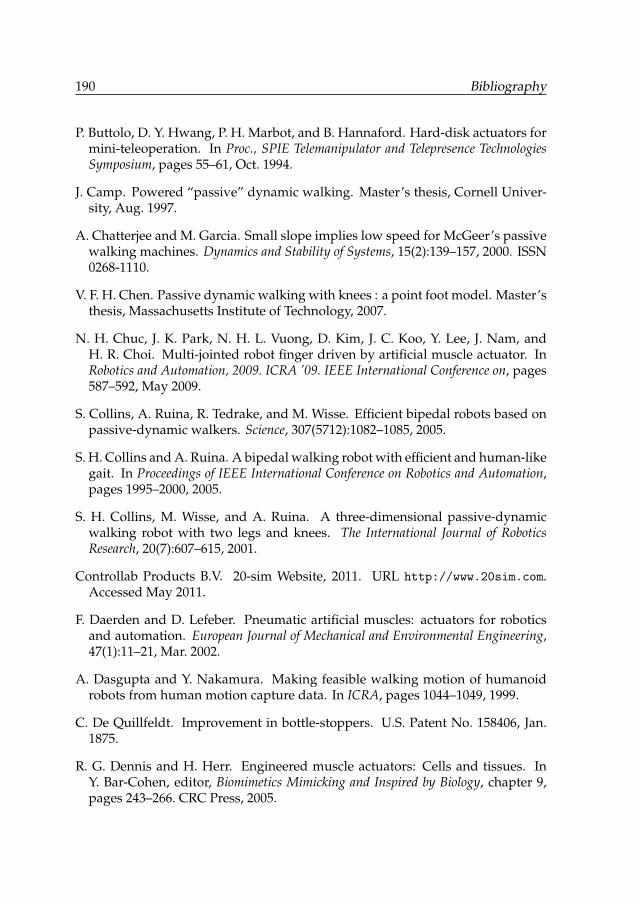
190 Bibliography
P. Buttolo, D. Y. Hwang, P. H. Marbot, and B. Hannaford. Hard-disk actuators formini-teleoperation. In Proc., SPIE Telemanipulator and Telepresence TechnologiesSymposium, pages 55–61, Oct. 1994.
J. Camp. Powered “passive” dynamic walking. Master’s thesis, Cornell Univer-sity, Aug. 1997.
A. Chatterjee and M. Garcia. Small slope implies low speed for McGeer’s passivewalking machines. Dynamics and Stability of Systems, 15(2):139–157, 2000. ISSN0268-1110.
V. F. H. Chen. Passive dynamic walking with knees : a point foot model. Master’sthesis, Massachusetts Institute of Technology, 2007.
N. H. Chuc, J. K. Park, N. H. L. Vuong, D. Kim, J. C. Koo, Y. Lee, J. Nam, andH. R. Choi. Multi-jointed robot finger driven by artificial muscle actuator. InRobotics and Automation, 2009. ICRA ’09. IEEE International Conference on, pages587–592, May 2009.
S. Collins, A. Ruina, R. Tedrake, and M. Wisse. Efficient bipedal robots based onpassive-dynamic walkers. Science, 307(5712):1082–1085, 2005.
S. H. Collins and A. Ruina. A bipedal walking robot with efficient and human-likegait. In Proceedings of IEEE International Conference on Robotics and Automation,pages 1995–2000, 2005.
S. H. Collins, M. Wisse, and A. Ruina. A three-dimensional passive-dynamicwalking robot with two legs and knees. The International Journal of RoboticsResearch, 20(7):607–615, 2001.
Controllab Products B.V. 20-sim Website, 2011. URL http://www.20sim.com.Accessed May 2011.
F. Daerden and D. Lefeber. Pneumatic artificial muscles: actuators for roboticsand automation. European Journal of Mechanical and Environmental Engineering,47(1):11–21, Mar. 2002.
A. Dasgupta and Y. Nakamura. Making feasible walking motion of humanoidrobots from human motion capture data. In ICRA, pages 1044–1049, 1999.
C. De Quillfeldt. Improvement in bottle-stoppers. U.S. Patent No. 158406, Jan.1875.
R. G. Dennis and H. Herr. Engineered muscle actuators: Cells and tissues. InY. Bar-Cohen, editor, Biomimetics Mimicking and Inspired by Biology, chapter 9,pages 243–266. CRC Press, 2005.
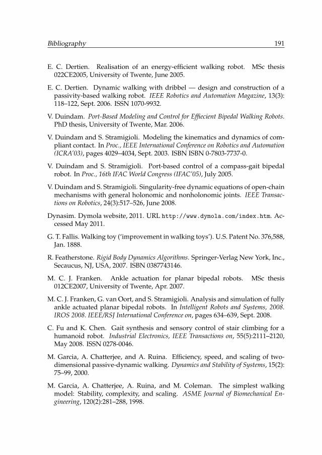
Bibliography 191
E. C. Dertien. Realisation of an energy-efficient walking robot. MSc thesis022CE2005, University of Twente, June 2005.
E. C. Dertien. Dynamic walking with dribbel — design and construction of apassivity-based walking robot. IEEE Robotics and Automation Magazine, 13(3):118–122, Sept. 2006. ISSN 1070-9932.
V. Duindam. Port-Based Modeling and Control for Effiecient Bipedal Walking Robots.PhD thesis, University of Twente, Mar. 2006.
V. Duindam and S. Stramigioli. Modeling the kinematics and dynamics of com-pliant contact. In Proc., IEEE International Conference on Robotics and Automation(ICRA’03), pages 4029–4034, Sept. 2003. ISBN ISBN 0-7803-7737-0.
V. Duindam and S. Stramigioli. Port-based control of a compass-gait bipedalrobot. In Proc., 16th IFAC World Congress (IFAC’05), July 2005.
V. Duindam and S. Stramigioli. Singularity-free dynamic equations of open-chainmechanisms with general holonomic and nonholonomic joints. IEEE Transac-tions on Robotics, 24(3):517–526, June 2008.
Dynasim. Dymola website, 2011. URL http://www.dymola.com/index.htm. Ac-cessed May 2011.
G. T. Fallis. Walking toy (‘improvement in walking toys’). U.S. Patent No. 376,588,Jan. 1888.
R. Featherstone. Rigid Body Dynamics Algorithms. Springer-Verlag New York, Inc.,Secaucus, NJ, USA, 2007. ISBN 0387743146.
M. C. J. Franken. Ankle actuation for planar bipedal robots. MSc thesis012CE2007, University of Twente, Apr. 2007.
M. C. J. Franken, G. van Oort, and S. Stramigioli. Analysis and simulation of fullyankle actuated planar bipedal robots. In Intelligent Robots and Systems, 2008.IROS 2008. IEEE/RSJ International Conference on, pages 634–639, Sept. 2008.
C. Fu and K. Chen. Gait synthesis and sensory control of stair climbing for ahumanoid robot. Industrial Electronics, IEEE Transactions on, 55(5):2111–2120,May 2008. ISSN 0278-0046.
M. Garcia, A. Chatterjee, and A. Ruina. Efficiency, speed, and scaling of two-dimensional passive-dynamic walking. Dynamics and Stability of Systems, 15(2):75–99, 2000.
M. Garcia, A. Chatterjee, A. Ruina, and M. Coleman. The simplest walkingmodel: Stability, complexity, and scaling. ASME Journal of Biomechanical En-gineering, 120(2):281–288, 1998.
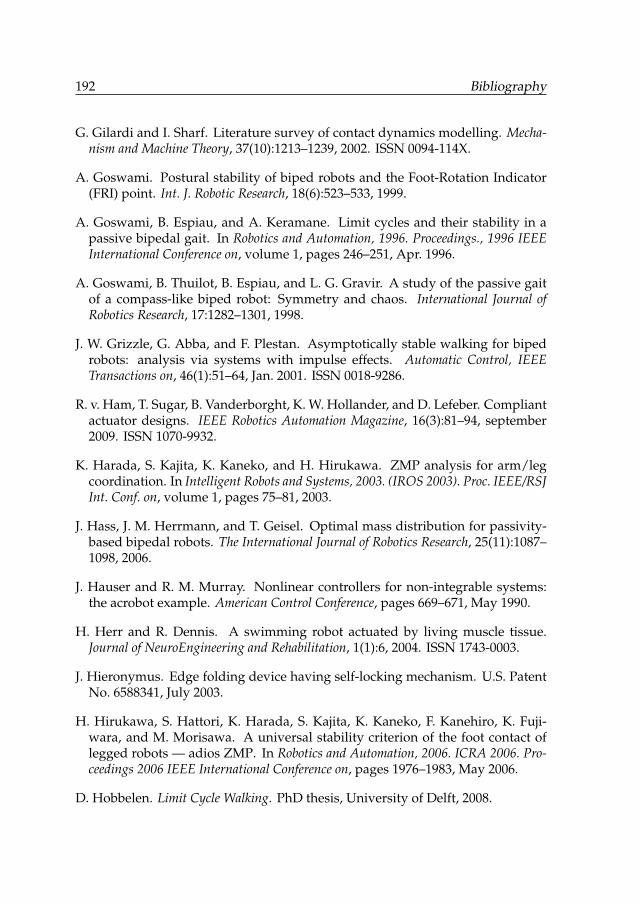
192 Bibliography
G. Gilardi and I. Sharf. Literature survey of contact dynamics modelling. Mecha-nism and Machine Theory, 37(10):1213–1239, 2002. ISSN 0094-114X.
A. Goswami. Postural stability of biped robots and the Foot-Rotation Indicator(FRI) point. Int. J. Robotic Research, 18(6):523–533, 1999.
A. Goswami, B. Espiau, and A. Keramane. Limit cycles and their stability in apassive bipedal gait. In Robotics and Automation, 1996. Proceedings., 1996 IEEEInternational Conference on, volume 1, pages 246–251, Apr. 1996.
A. Goswami, B. Thuilot, B. Espiau, and L. G. Gravir. A study of the passive gaitof a compass-like biped robot: Symmetry and chaos. International Journal ofRobotics Research, 17:1282–1301, 1998.
J. W. Grizzle, G. Abba, and F. Plestan. Asymptotically stable walking for bipedrobots: analysis via systems with impulse effects. Automatic Control, IEEETransactions on, 46(1):51–64, Jan. 2001. ISSN 0018-9286.
R. v. Ham, T. Sugar, B. Vanderborght, K. W. Hollander, and D. Lefeber. Compliantactuator designs. IEEE Robotics Automation Magazine, 16(3):81–94, september2009. ISSN 1070-9932.
K. Harada, S. Kajita, K. Kaneko, and H. Hirukawa. ZMP analysis for arm/legcoordination. In Intelligent Robots and Systems, 2003. (IROS 2003). Proc. IEEE/RSJInt. Conf. on, volume 1, pages 75–81, 2003.
J. Hass, J. M. Herrmann, and T. Geisel. Optimal mass distribution for passivity-based bipedal robots. The International Journal of Robotics Research, 25(11):1087–1098, 2006.
J. Hauser and R. M. Murray. Nonlinear controllers for non-integrable systems:the acrobot example. American Control Conference, pages 669–671, May 1990.
H. Herr and R. Dennis. A swimming robot actuated by living muscle tissue.Journal of NeuroEngineering and Rehabilitation, 1(1):6, 2004. ISSN 1743-0003.
J. Hieronymus. Edge folding device having self-locking mechanism. U.S. PatentNo. 6588341, July 2003.
H. Hirukawa, S. Hattori, K. Harada, S. Kajita, K. Kaneko, F. Kanehiro, K. Fuji-wara, and M. Morisawa. A universal stability criterion of the foot contact oflegged robots — adios ZMP. In Robotics and Automation, 2006. ICRA 2006. Pro-ceedings 2006 IEEE International Conference on, pages 1976–1983, May 2006.
D. Hobbelen. Limit Cycle Walking. PhD thesis, University of Delft, 2008.
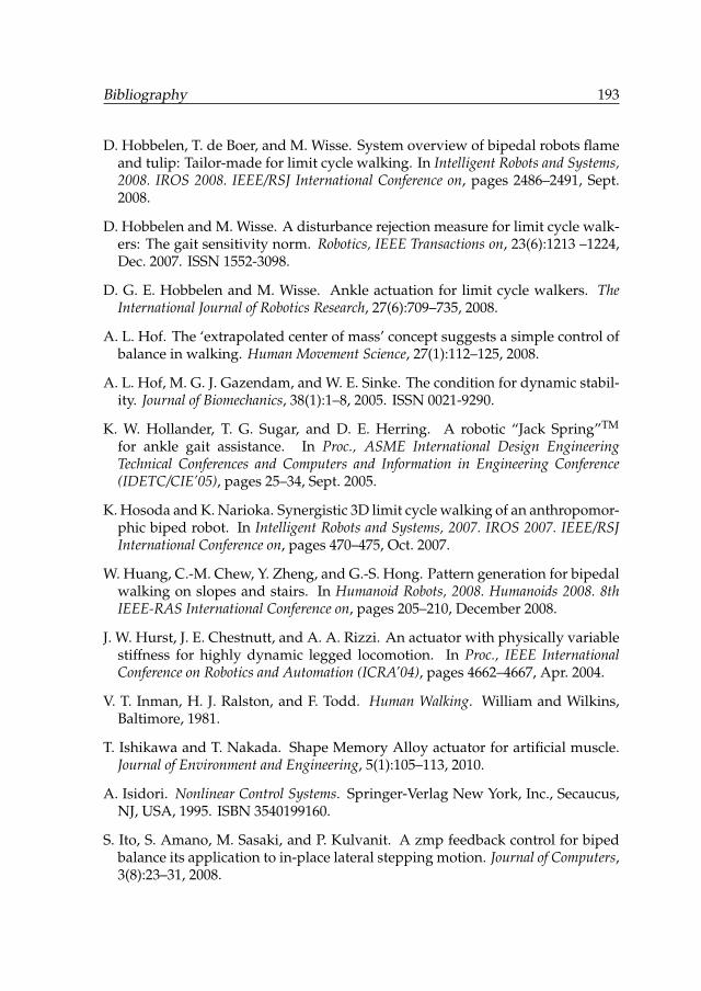
Bibliography 193
D. Hobbelen, T. de Boer, and M. Wisse. System overview of bipedal robots flameand tulip: Tailor-made for limit cycle walking. In Intelligent Robots and Systems,2008. IROS 2008. IEEE/RSJ International Conference on, pages 2486–2491, Sept.2008.
D. Hobbelen and M. Wisse. A disturbance rejection measure for limit cycle walk-ers: The gait sensitivity norm. Robotics, IEEE Transactions on, 23(6):1213 –1224,Dec. 2007. ISSN 1552-3098.
D. G. E. Hobbelen and M. Wisse. Ankle actuation for limit cycle walkers. TheInternational Journal of Robotics Research, 27(6):709–735, 2008.
A. L. Hof. The ‘extrapolated center of mass’ concept suggests a simple control ofbalance in walking. Human Movement Science, 27(1):112–125, 2008.
A. L. Hof, M. G. J. Gazendam, and W. E. Sinke. The condition for dynamic stabil-ity. Journal of Biomechanics, 38(1):1–8, 2005. ISSN 0021-9290.
K. W. Hollander, T. G. Sugar, and D. E. Herring. A robotic “Jack Spring”TM
for ankle gait assistance. In Proc., ASME International Design EngineeringTechnical Conferences and Computers and Information in Engineering Conference(IDETC/CIE’05), pages 25–34, Sept. 2005.
K. Hosoda and K. Narioka. Synergistic 3D limit cycle walking of an anthropomor-phic biped robot. In Intelligent Robots and Systems, 2007. IROS 2007. IEEE/RSJInternational Conference on, pages 470–475, Oct. 2007.
W. Huang, C.-M. Chew, Y. Zheng, and G.-S. Hong. Pattern generation for bipedalwalking on slopes and stairs. In Humanoid Robots, 2008. Humanoids 2008. 8thIEEE-RAS International Conference on, pages 205–210, December 2008.
J. W. Hurst, J. E. Chestnutt, and A. A. Rizzi. An actuator with physically variablestiffness for highly dynamic legged locomotion. In Proc., IEEE InternationalConference on Robotics and Automation (ICRA’04), pages 4662–4667, Apr. 2004.
V. T. Inman, H. J. Ralston, and F. Todd. Human Walking. William and Wilkins,Baltimore, 1981.
T. Ishikawa and T. Nakada. Shape Memory Alloy actuator for artificial muscle.Journal of Environment and Engineering, 5(1):105–113, 2010.
A. Isidori. Nonlinear Control Systems. Springer-Verlag New York, Inc., Secaucus,NJ, USA, 1995. ISBN 3540199160.
S. Ito, S. Amano, M. Sasaki, and P. Kulvanit. A zmp feedback control for bipedbalance its application to in-place lateral stepping motion. Journal of Computers,3(8):23–31, 2008.
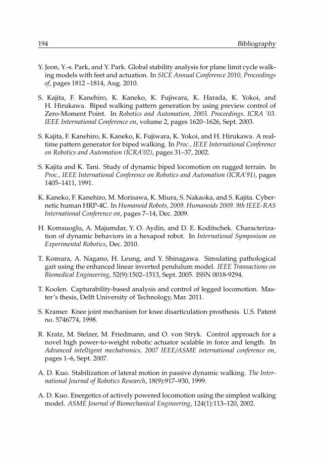
194 Bibliography
Y. Jeon, Y.-s. Park, and Y. Park. Global stability analysis for plane limit cycle walk-ing models with feet and actuation. In SICE Annual Conference 2010, Proceedingsof, pages 1812 –1814, Aug. 2010.
S. Kajita, F. Kanehiro, K. Kaneko, K. Fujiwara, K. Harada, K. Yokoi, andH. Hirukawa. Biped walking pattern generation by using preview control ofZero-Moment Point. In Robotics and Automation, 2003. Proceedings. ICRA ’03.IEEE International Conference on, volume 2, pages 1620–1626, Sept. 2003.
S. Kajita, F. Kanehiro, K. Kaneko, K. Fujiwara, K. Yokoi, and H. Hirukawa. A real-time pattern generator for biped walking. In Proc., IEEE International Conferenceon Robotics and Automation (ICRA’02), pages 31–37, 2002.
S. Kajita and K. Tani. Study of dynamic biped locomotion on rugged terrain. InProc., IEEE International Conference on Robotics and Automation (ICRA’91), pages1405–1411, 1991.
K. Kaneko, F. Kanehiro, M. Morisawa, K. Miura, S. Nakaoka, and S. Kajita. Cyber-netic human HRP-4C. In Humanoid Robots, 2009. Humanoids 2009. 9th IEEE-RASInternational Conference on, pages 7–14, Dec. 2009.
H. Komsuoglu, A. Majumdar, Y. O. Aydin, and D. E. Koditschek. Characteriza-tion of dynamic behaviors in a hexapod robot. In International Symposium onExperimental Robotics, Dec. 2010.
T. Komura, A. Nagano, H. Leung, and Y. Shinagawa. Simulating pathologicalgait using the enhanced linear inverted pendulum model. IEEE Transactions onBiomedical Engineering, 52(9):1502–1513, Sept. 2005. ISSN 0018-9294.
T. Koolen. Capturability-based analysis and control of legged locomotion. Mas-ter’s thesis, Delft University of Technology, Mar. 2011.
S. Kramer. Knee joint mechanism for knee disarticulation prosthesis. U.S. Patentno. 5746774, 1998.
R. Kratz, M. Stelzer, M. Friedmann, and O. von Stryk. Control approach for anovel high power-to-weight robotic actuator scalable in force and length. InAdvanced intelligent mechatronics, 2007 IEEE/ASME international conference on,pages 1–6, Sept. 2007.
A. D. Kuo. Stabilization of lateral motion in passive dynamic walking. The Inter-national Journal of Robotics Research, 18(9):917–930, 1999.
A. D. Kuo. Energetics of actively powered locomotion using the simplest walkingmodel. ASME Journal of Biomechanical Engineering, 124(1):113–120, 2002.
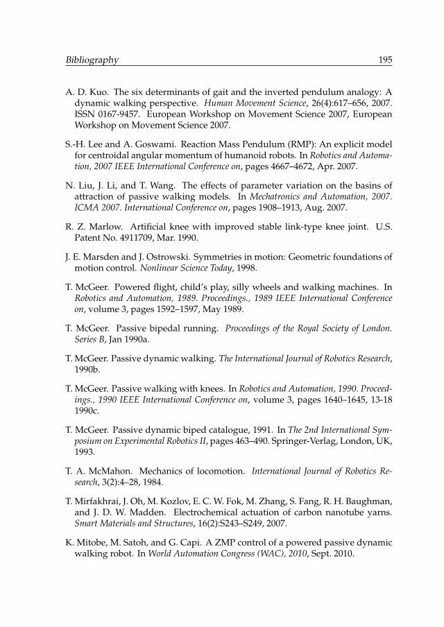
Bibliography 195
A. D. Kuo. The six determinants of gait and the inverted pendulum analogy: Adynamic walking perspective. Human Movement Science, 26(4):617–656, 2007.ISSN 0167-9457. European Workshop on Movement Science 2007, EuropeanWorkshop on Movement Science 2007.
S.-H. Lee and A. Goswami. Reaction Mass Pendulum (RMP): An explicit modelfor centroidal angular momentum of humanoid robots. In Robotics and Automa-tion, 2007 IEEE International Conference on, pages 4667–4672, Apr. 2007.
N. Liu, J. Li, and T. Wang. The effects of parameter variation on the basins ofattraction of passive walking models. In Mechatronics and Automation, 2007.ICMA 2007. International Conference on, pages 1908–1913, Aug. 2007.
R. Z. Marlow. Artificial knee with improved stable link-type knee joint. U.S.Patent No. 4911709, Mar. 1990.
J. E. Marsden and J. Ostrowski. Symmetries in motion: Geometric foundations ofmotion control. Nonlinear Science Today, 1998.
T. McGeer. Powered flight, child’s play, silly wheels and walking machines. InRobotics and Automation, 1989. Proceedings., 1989 IEEE International Conferenceon, volume 3, pages 1592–1597, May 1989.
T. McGeer. Passive bipedal running. Proceedings of the Royal Society of London.Series B, Jan 1990a.
T. McGeer. Passive dynamic walking. The International Journal of Robotics Research,1990b.
T. McGeer. Passive walking with knees. In Robotics and Automation, 1990. Proceed-ings., 1990 IEEE International Conference on, volume 3, pages 1640–1645, 13-181990c.
T. McGeer. Passive dynamic biped catalogue, 1991. In The 2nd International Sym-posium on Experimental Robotics II, pages 463–490. Springer-Verlag, London, UK,1993.
T. A. McMahon. Mechanics of locomotion. International Journal of Robotics Re-search, 3(2):4–28, 1984.
T. Mirfakhrai, J. Oh, M. Kozlov, E. C. W. Fok, M. Zhang, S. Fang, R. H. Baughman,and J. D. W. Madden. Electrochemical actuation of carbon nanotube yarns.Smart Materials and Structures, 16(2):S243–S249, 2007.
K. Mitobe, M. Satoh, and G. Capi. A ZMP control of a powered passive dynamicwalking robot. In World Automation Congress (WAC), 2010, Sept. 2010.
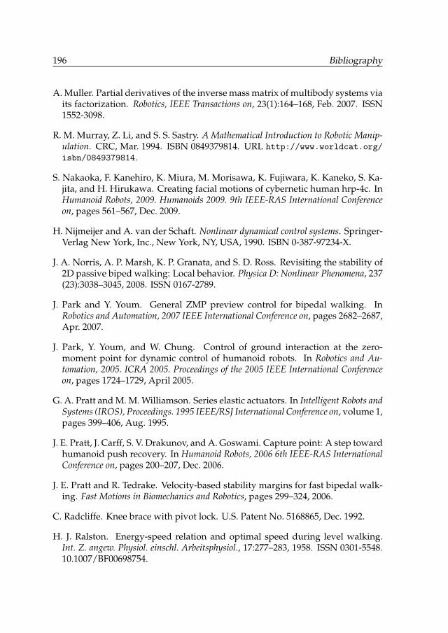
196 Bibliography
A. Muller. Partial derivatives of the inverse mass matrix of multibody systems viaits factorization. Robotics, IEEE Transactions on, 23(1):164–168, Feb. 2007. ISSN1552-3098.
R. M. Murray, Z. Li, and S. S. Sastry. A Mathematical Introduction to Robotic Manip-ulation. CRC, Mar. 1994. ISBN 0849379814. URL http://www.worldcat.org/isbn/0849379814.
S. Nakaoka, F. Kanehiro, K. Miura, M. Morisawa, K. Fujiwara, K. Kaneko, S. Ka-jita, and H. Hirukawa. Creating facial motions of cybernetic human hrp-4c. InHumanoid Robots, 2009. Humanoids 2009. 9th IEEE-RAS International Conferenceon, pages 561–567, Dec. 2009.
H. Nijmeijer and A. van der Schaft. Nonlinear dynamical control systems. Springer-Verlag New York, Inc., New York, NY, USA, 1990. ISBN 0-387-97234-X.
J. A. Norris, A. P. Marsh, K. P. Granata, and S. D. Ross. Revisiting the stability of2D passive biped walking: Local behavior. Physica D: Nonlinear Phenomena, 237(23):3038–3045, 2008. ISSN 0167-2789.
J. Park and Y. Youm. General ZMP preview control for bipedal walking. InRobotics and Automation, 2007 IEEE International Conference on, pages 2682–2687,Apr. 2007.
J. Park, Y. Youm, and W. Chung. Control of ground interaction at the zero-moment point for dynamic control of humanoid robots. In Robotics and Au-tomation, 2005. ICRA 2005. Proceedings of the 2005 IEEE International Conferenceon, pages 1724–1729, April 2005.
G. A. Pratt and M. M. Williamson. Series elastic actuators. In Intelligent Robots andSystems (IROS), Proceedings. 1995 IEEE/RSJ International Conference on, volume 1,pages 399–406, Aug. 1995.
J. E. Pratt, J. Carff, S. V. Drakunov, and A. Goswami. Capture point: A step towardhumanoid push recovery. In Humanoid Robots, 2006 6th IEEE-RAS InternationalConference on, pages 200–207, Dec. 2006.
J. E. Pratt and R. Tedrake. Velocity-based stability margins for fast bipedal walk-ing. Fast Motions in Biomechanics and Robotics, pages 299–324, 2006.
C. Radcliffe. Knee brace with pivot lock. U.S. Patent No. 5168865, Dec. 1992.
H. J. Ralston. Energy-speed relation and optimal speed during level walking.Int. Z. angew. Physiol. einschl. Arbeitsphysiol., 17:277–283, 1958. ISSN 0301-5548.10.1007/BF00698754.
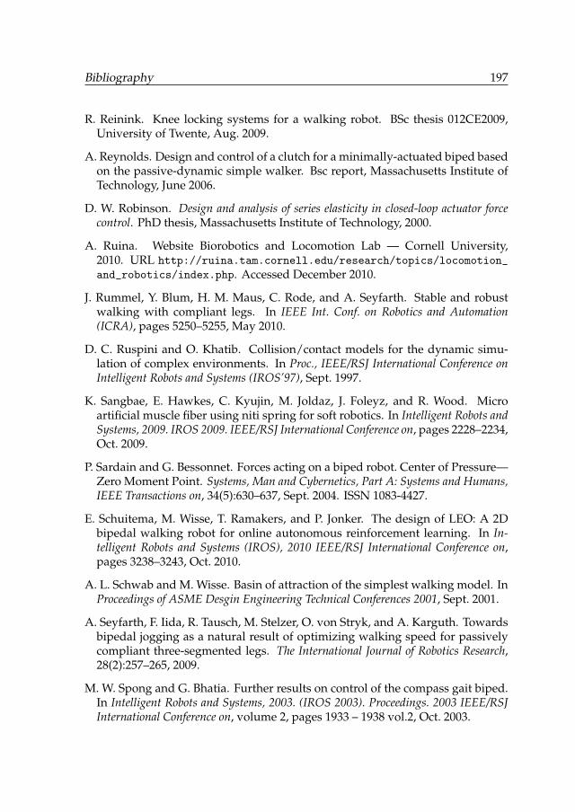
Bibliography 197
R. Reinink. Knee locking systems for a walking robot. BSc thesis 012CE2009,University of Twente, Aug. 2009.
A. Reynolds. Design and control of a clutch for a minimally-actuated biped basedon the passive-dynamic simple walker. Bsc report, Massachusetts Institute ofTechnology, June 2006.
D. W. Robinson. Design and analysis of series elasticity in closed-loop actuator forcecontrol. PhD thesis, Massachusetts Institute of Technology, 2000.
A. Ruina. Website Biorobotics and Locomotion Lab — Cornell University,2010. URL http://ruina.tam.cornell.edu/research/topics/locomotion_and_robotics/index.php. Accessed December 2010.
J. Rummel, Y. Blum, H. M. Maus, C. Rode, and A. Seyfarth. Stable and robustwalking with compliant legs. In IEEE Int. Conf. on Robotics and Automation(ICRA), pages 5250–5255, May 2010.
D. C. Ruspini and O. Khatib. Collision/contact models for the dynamic simu-lation of complex environments. In Proc., IEEE/RSJ International Conference onIntelligent Robots and Systems (IROS’97), Sept. 1997.
K. Sangbae, E. Hawkes, C. Kyujin, M. Joldaz, J. Foleyz, and R. Wood. Microartificial muscle fiber using niti spring for soft robotics. In Intelligent Robots andSystems, 2009. IROS 2009. IEEE/RSJ International Conference on, pages 2228–2234,Oct. 2009.
P. Sardain and G. Bessonnet. Forces acting on a biped robot. Center of Pressure—Zero Moment Point. Systems, Man and Cybernetics, Part A: Systems and Humans,IEEE Transactions on, 34(5):630–637, Sept. 2004. ISSN 1083-4427.
E. Schuitema, M. Wisse, T. Ramakers, and P. Jonker. The design of LEO: A 2Dbipedal walking robot for online autonomous reinforcement learning. In In-telligent Robots and Systems (IROS), 2010 IEEE/RSJ International Conference on,pages 3238–3243, Oct. 2010.
A. L. Schwab and M. Wisse. Basin of attraction of the simplest walking model. InProceedings of ASME Desgin Engineering Technical Conferences 2001, Sept. 2001.
A. Seyfarth, F. Iida, R. Tausch, M. Stelzer, O. von Stryk, and A. Karguth. Towardsbipedal jogging as a natural result of optimizing walking speed for passivelycompliant three-segmented legs. The International Journal of Robotics Research,28(2):257–265, 2009.
M. W. Spong and G. Bhatia. Further results on control of the compass gait biped.In Intelligent Robots and Systems, 2003. (IROS 2003). Proceedings. 2003 IEEE/RSJInternational Conference on, volume 2, pages 1933 – 1938 vol.2, Oct. 2003.
198 Bibliography
M. W. Spong and F. Bullo. Controlled symmetries and passive walking. IEEETransactions on Automatic Control, 50(7):1025–1031, July 2005.
S. Stramigioli. Modeling and IPC Control of Interactive Mechanical Systems: aCoordinate-free Approach. Springer-Verlag, 2001.
S. Stramigioli, V. Duindam, G. van Oort, and A. Goswami. Compact analysis of3D bipedal gait using geometric dynamics of simplified models. In Robotics andAutomation, 2009. ICRA ’09. IEEE International Conference on, pages 1978–1984,May 2009.
S. Stramigioli and M. van Dijk. Energy conservative limit cycle oscillations. InProc., 17th IFAC World Congress (IFAC’08), pages 15666–15671, July 2008.
S. Stramigioli, G. van Oort, and E. C. Dertien. A concept for a new energy efficientactuator. In Proc., IEEE/ASME International Conference on Advanced IntelligentMechatronics (AIM’08), pages 671–675, July 2008.
G. Strang. Linear Algebra and its Applications. Brooks Cole, third edition, 1988.
T. Sugihara and H. Nakamura. Variable impedant inverted pendulum modelcontrol for a seamless contact phase transition on humanoid robot. In Proc.,IEEE International Conference on Humanoid Robots (Humanoids’03), Oct. 2003.
S. Takao, Y. Yokokohji, and T. Yoshikawa. FSW (feasible solution of wrench) formulti-legged robots. In Robotics and Automation. (ICRA ’03). Proc. IEEE Int. Conf.on, volume 3, pages 3815–3820, Sept. 2003.
I. Thorson, M. Svinin, S. Hosoe, F. Asano, and K. Taji. Design considerationsfor a variable stiffness actuator in a robot that walks and runs. In Proc., JSMEConference on Robotics and Mechatronics (ROBOMEC’07), May 2007.
G. Tonietti. Variable impedance actuation. PhD thesis, Univ. of Pisa, 2005.
J. H. Townsend. Multiaxis controlled motion knee brace with a four bar joint andmethod for producing same. U.S. Patent No. 5330418, July 1994.
J. H. Townsend. Orthopedic knee brace joint assembly having a trigger lockingmechanism. U.S. Patent No. 6500139, Dec. 2002.
K. Trifonov and S. Hashimoto. Active knee-lock release for passive-dynamicwalking machines. Proceedings of IEEE International Conference on Robotics andBiomimetics, pages 958 – 963, 2007.
R. van Ham, B. Vanderborght, M. van Damme, B. Verrelst, and D. Lefeber. MAC-CEPA: the actuator with adaptable compliance for dynamic walking bipeds. InProc., 8th International Conference on Climbing and Walking Robots (CLAWAR’05),pages 759–766, Sept. 2005.
Bibliography 199
G. van Oort. Strategies for stabilizing a 3d dynamically walking robot. Msc thesis,Control Laboratory, University of Twente, June 2005.
G. van Oort, R. Carloni, D. J. Borgerink, and S. Stramigioli. An energy efficientknee locking mechanism for a dynamically walking robot. In Proc., IEEE Inter-national Conference on Robotics and Automation (ICRA’11), pages 2003–2008, May2011a.
G. van Oort, R. Reilink, and S. Stramigioli. New ankle actuation mechanism fora humanoid robot. In Proc., 18th IFAC World Congress, Aug. 2011b.
G. van Oort and S. Stramigioli. Using time-reversal symmetry for stabilizing asimple 3D walker model. In Proc., IEEE International Conference on Robotics andAutomation (ICRA’07), pages 4673–4678, Apr. 2007. ISBN ISBN 1-4244-0601-3.
G. van Oort and S. Stramigioli. Geometric interpretation of the zero-momentpoint. In Proc., IEEE International Conference on Robotics and Automation(ICRA’11), pages 575–580, May 2011.
G. van Oort and S. Stramigioli. The Poincaré section and basin of attraction of a2D passive dynamic walker on an irregular floor. Submitted to: IEEE Interna-tional Conference on Robotics and Automation (ICRA’12), 2012.
B. Vanderborght. Dynamic stabilisation of the biped Lucy powered by actuators withcontrollable stiffness. PhD thesis, Vrije Universiteit Brussel, May 2007.
B. Verrelst, R. van Ham, B. Vanderborght, F. Daerden, D. Lefeber, and J. Ver-meulen. The pneumatic biped “Lucy” actuated with pleated pneumatic arti-ficial muscles. Autonomous Robots, 18(2):201–213, 2005. ISSN 0929-5593.
Viactors. VIACTORS website, 2011. URL http://www.viactors.org. AccessedApril, 2011.
M. Vukobratovic and B. Borovac. Zero-Moment Point — thirty five years of itslife. International journal of humanoid robotics, 1(1):157–173, 2004.
M. Vukobratovic, B. Borovac, and D. Surdilovic. Zero-moment point — properinterpretation and new applications. Int. Conf. on Humanoid Robots, 2001.
M. Vukobratovic and D. Juricic. Contribution to the synthesis of biped gait. Proc.IFAC Symp. Technical and Biological Problem and Control, 1968.
M. Vukobratovic and D. Juricic. Contribution to the synthesis of biped gait.Biomedical Engineering, IEEE Transactions on, 16(1):1–6, Jan. 1969. ISSN 0018-9294.
200 Bibliography
M. W. Walker and D. Orin. Efficient dynamic computer simulation of roboticmechanisms. ASME Journal of Dynamic Systems, Measurement, and Control, 104:205–211, Sept. 1982.
Q. Wang, Y. Huang, and L. Wang. Passive dynamic walking with flat feet andankle compliance. Robotica, 28(03):413–425, 2010.
Q. Wang, Y. Huang, L. Wang, and L. Dongjiao. Stability and adaptability ofpassivity-based bipedal locomotion with flat feet and ankle compliance. InNorth American Congress of Biomechanics, Aug. 2008.
B. J. Whipp and K. Wasserman. Efficiency of muscular work. Journal of AppliedPhysiology, 26(5):644–648, May 1969.
M. M. Williamson. Series elastic actuators. Master’s thesis, Massachusetts Insti-tute of Technology, June 1995.
M. Wisse. Essentials of dynamic walking; Analysis and design of two-legged robots.PhD thesis, TU Delft, 2004.
M. Wisse and A. L. Schwab. A 3D passive dynamic biped with roll and yawcompensation. Robotica, 19:275–284, 2001.
M. Wisse, A. L. Schwab, and F. C. T. van der Helm. Passive dynamic walkingmodel with upper body. Robotica, 22:681–688, 2004.
M. Wisse, A. L. Schwab, R. Q. van der Linde, and F. C. T. van der Helm. Howto keep from falling forward: elementary swing leg action for passive dynamicwalkers. IEEE Transactions on Robotics, 21(3):393–401, June 2005. ISSN 1552-3098.
M. Wisse and J. van Frankenhuyzen. Design and construction of MIKE; a 2Dautonomous biped based on passive dynamic walking. In Proc., InternationalSymposium of Adaptive Motion and Animals and Machines (AMAM’03), 2003.
Dankwoord
Een van de doelen van promoveren is laten zien dat je op eigen houtje een gede-gen onderzoek kan uitvoeren. Nou heb ik inderdaad veel zelf zitten doen, maargelukkig had ik al die tijd een boel mensen om me heen — op mijn werk en in deprivésfeer — die op een of andere manier hebben geholpen om van de afgelopenvijf jaar vijf fijne jaren te maken. Enkele van hen wil ik graag specifiek bedanken.
Allereerst een woord van dank aan mijn promotor, Prof. dr. ir. Stramigioli. Ste-fano, enorm bedankt voor alles wat je voor me gedaan en geregeld hebt afge-lopen jaren. Tijdens mijn jaren als promovendus heb ik heel veel met je kunnenkletsen over interessante wiskunde en geometrische dynamica. Ik heb ontzettendveel van je geleerd! Jouw onuitputtelijke en aanstekelijke enthousiasme, enormebetrokkenheid (zowel zakelijk als privé) en aangename persoonlijkheid hebbenervoor gezorgd dat ik me als promovendus onder jouw hoede helemaal op mijnplek voelde. Een fijnere ‘baas’ en collega had ik niet kunnen wensen! Ook hebik erg genoten van de momenten dat we samen muziek maakten. De repetitiesvan onze vakgroepband ‘Out of Control’ waren soms wat ongestructureerd, maaraltijd erg leuk. Stefano, bedankt!
Dan mijn beste vriend en collega, Edwin. Wat hebben we samen een boel gedaan!Meer dan tien jaar samen in Drienerlalala gezongen (met vanaf ons afstudereniedere dinsdagavond pannenkoeken met wijn in de vakgroepkeuken), vijf jaarGonnagles en nog steeds af en toe samen achtergrondmuziek. Ook in de tech-niek blijven we elkaar tegenkomen: als collega’s op de vakgroep waar we samentientallen studenten begeleid hebben en aan Dribbel en TUlip sleutelden, ‘voor dehobby’ (muziekdoosjes), en sinds juni ook bij Kunst- en Techniekwerk. Hopelijkkan ik daar na het schrijven van mijn boekje wat vaker komen werken. Edwin,bedankt voor je steun in goede en in slechte tijden. Ik weet zeker dat we in detoekomst nog veel meer leuks gaan beleven!
I would also like to thank all co-authors of the articles we have produced. It hasbeen a pleasure to work with you! Andy, Martijn, Job, Bart Koopman and PieterJonker, thank you very much for taking place in my graduation committee. Ihope you enjoyed reading my thesis and I look forward to see you in real life
201
202 Dankwoord
and answer all the difficult questions you undoubtedly will have for me. Para-nimfen Wietse en Edwin, fijn dat jullie me bij willen staan tijdens de verdedigingtegenover de hierboven genoemde Professoren.
Raffaella, thanks for helping me with a lot of things and taking over much workwhen I didn’t have time for it. Ludo, buurman die altijd een luisterend oor haden mee wilde denken als ik er weer eens niet uitkwam, ik heb veel aan je gehad!Michel, dank voor alle informatie die je me verstrekt hebt over het regelen van depromotie. I also want to thank all colleagues of the group, Controllab and DutchRobotics (also TUD and TU/e) for all the fun; it was a pleasure working with youall.
Enkele bachelor- en masterstudenten die ik begeleid heb wil ik speciaal bedan-ken. Eddy, als een van de eerste studenten die ik (samen met Edwin) begeleidde,heb jij óns uitstekend begeleid in het leren om begeleider te zijn. Windel, Roe-lof en Bart, de gezamenlijke hackavondjes als voorbereiding op ons RoboCup-avontuur in Graz (en Graz zelf ook) waren super.
Vincent, ondanks dat we maar zo kort samen hebben gewerkt, heb je een on-uitwisbare indruk op mij achtergelaten. Het gemak waarmee jij de moeilijkstewiskunde begrijpelijk op papier weet te zetten en vooral je altijd ontspannen in-druk maakten jou als een soort voorbeeldpromovendus voor mij. Bedankt ookvoor het mogen gebruiken van je mooie LATEX-template voor dit proefschrift.
Parkweggers & uitpandige inboedel, Gonnagles en Bragi-vrienden (hoewel ikniet eens bij Bragi gezeten heb. . . ), met veel plezier denk ik terug aan alle Maan-dagavondjes, feestjes, zeilweekenden, optredens, reisjes, repetities, concertjes,trouwpartijen, oud-en-nieuw’en en andere activiteiten met jullie!
Misschien is het wat raar om dingen te bedanken, maar voor de Sagitta, de bootvan Opa Jan en Oma Keetje, maak ik graag een uitzondering. Boot, bedanktvoor de weekjes ‘extended thuiswerken’. Midden in de Biesbosch op mijn laptopaan een paper schrijven terwijl Marlies in de voorkajuit aan haar harprepertoirewerkt; idyllischer kan toch niet?
Papa en mama, jullie onvoorwaardelijke steun betekent heel veel voor me; wat ikook doe, ik weet dat jullie altijd achter me staan, met raad en daad. Bart & Cox,Marleen & Peter & kinderen, Opa Boerdijk en Oma Keetje, wat fijn dat jullie mijnfamilie zijn! Bedankt voor jullie support, interesse en gezellige afleiding!
Tot slot, Marlies, niets is zo fijn als na een lange dag werken weer thuiskomen.Dat komt door jou, jij bent mijn thuis. Ook al die dagen dat ik op de studeer-kamer zat te werken en jij me kopjes koffie, thee en paaseitjes kwam brengen enbeneden pedaalharp speelde waren heerlijk. Jouw motivatie, betrokkenheid engoede zorgen hebben me enorm gesteund en zullen me altijd steunen. Wat eengenot om altijd bij je te mogen zijn! Marlies, dank je wel dat je er bent.
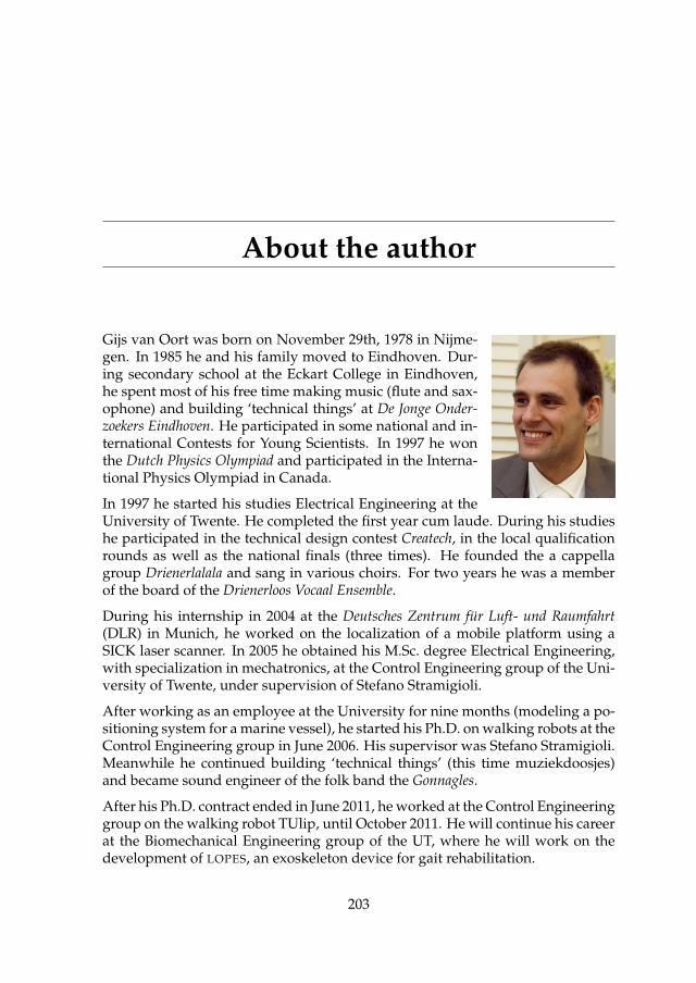
About the author
Gijs van Oort was born on November 29th, 1978 in Nijme-gen. In 1985 he and his family moved to Eindhoven. Dur-ing secondary school at the Eckart College in Eindhoven,he spent most of his free time making music (flute and sax-ophone) and building ‘technical things’ at De Jonge Onder-zoekers Eindhoven. He participated in some national and in-ternational Contests for Young Scientists. In 1997 he wonthe Dutch Physics Olympiad and participated in the Interna-tional Physics Olympiad in Canada.
In 1997 he started his studies Electrical Engineering at theUniversity of Twente. He completed the first year cum laude. During his studieshe participated in the technical design contest Createch, in the local qualificationrounds as well as the national finals (three times). He founded the a cappellagroup Drienerlalala and sang in various choirs. For two years he was a memberof the board of the Drienerloos Vocaal Ensemble.
During his internship in 2004 at the Deutsches Zentrum für Luft- und Raumfahrt(DLR) in Munich, he worked on the localization of a mobile platform using aSICK laser scanner. In 2005 he obtained his M.Sc. degree Electrical Engineering,with specialization in mechatronics, at the Control Engineering group of the Uni-versity of Twente, under supervision of Stefano Stramigioli.
After working as an employee at the University for nine months (modeling a po-sitioning system for a marine vessel), he started his Ph.D. on walking robots at theControl Engineering group in June 2006. His supervisor was Stefano Stramigioli.Meanwhile he continued building ‘technical things’ (this time muziekdoosjes)and became sound engineer of the folk band the Gonnagles.
After his Ph.D. contract ended in June 2011, he worked at the Control Engineeringgroup on the walking robot TUlip, until October 2011. He will continue his careerat the Biomechanical Engineering group of the UT, where he will work on thedevelopment of LOPES, an exoskeleton device for gait rehabilitation.
203