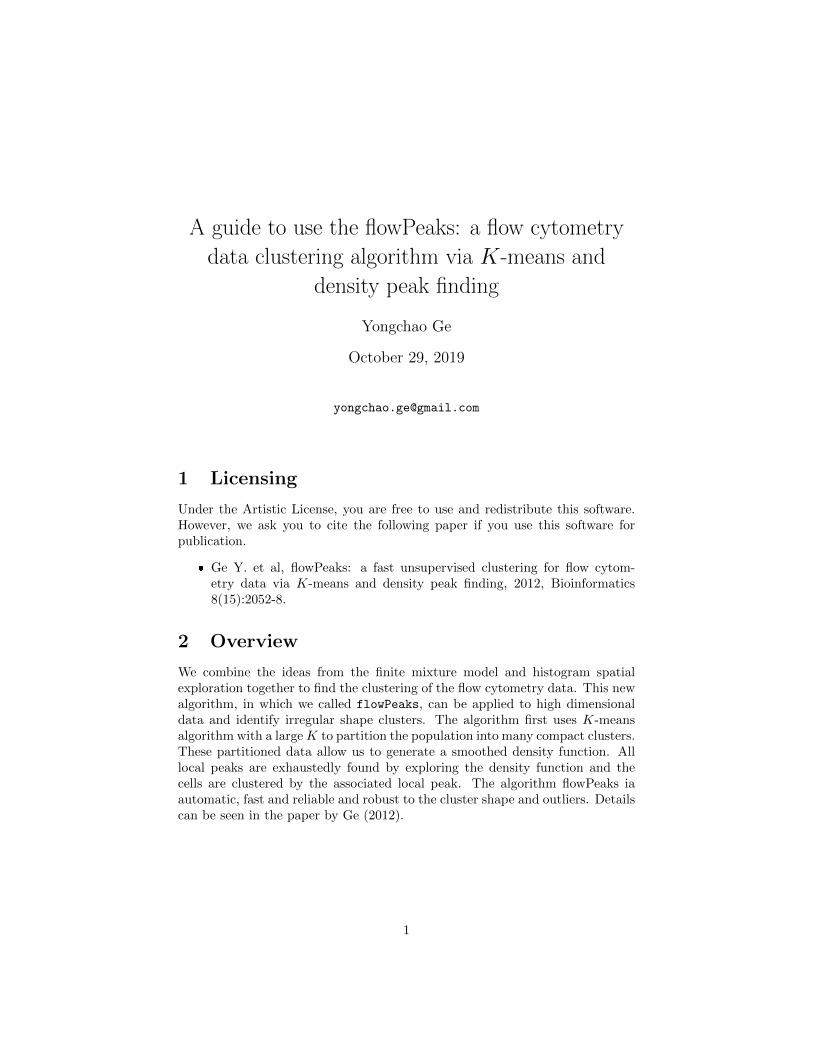
A guide to use the flowPeaks: a flow cytometry

data clustering algorithm via K-means and

density peak finding

Yongchao Ge

October 29, 2019

yongchao.ge@gmail.com

1 Licensing

Under the Artistic License, you are free to use and redistribute this software.However, we ask you to cite the following paper if you use this software forpublication.

� Ge Y. et al, flowPeaks: a fast unsupervised clustering for flow cytom-etry data via K-means and density peak finding, 2012, Bioinformatics8(15):2052-8.

2 Overview

We combine the ideas from the finite mixture model and histogram spatialexploration together to find the clustering of the flow cytometry data. This newalgorithm, in which we called flowPeaks, can be applied to high dimensionaldata and identify irregular shape clusters. The algorithm first uses K-meansalgorithm with a large K to partition the population into many compact clusters.These partitioned data allow us to generate a smoothed density function. Alllocal peaks are exhaustedly found by exploring the density function and thecells are clustered by the associated local peak. The algorithm flowPeaks iaautomatic, fast and reliable and robust to the cluster shape and outliers. Detailscan be seen in the paper by Ge (2012).

1

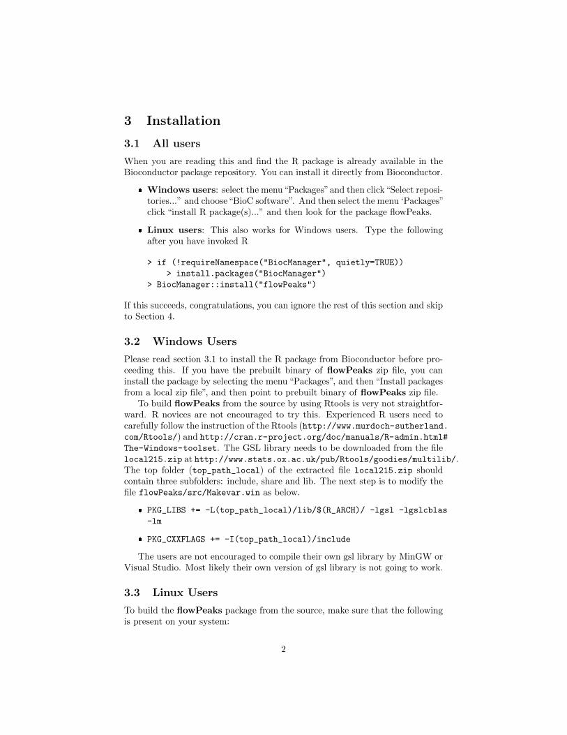
3 Installation

3.1 All users

When you are reading this and find the R package is already available in theBioconductor package repository. You can install it directly from Bioconductor.

� Windows users: select the menu“Packages”and then click“Select reposi-tories...” and choose“BioC software”. And then select the menu ‘Packages”click “install R package(s)...” and then look for the package flowPeaks.

� Linux users: This also works for Windows users. Type the followingafter you have invoked R

> if (!requireNamespace("BiocManager", quietly=TRUE))

> install.packages("BiocManager")

> BiocManager::install("flowPeaks")

If this succeeds, congratulations, you can ignore the rest of this section and skipto Section 4.

3.2 Windows Users

Please read section 3.1 to install the R package from Bioconductor before pro-ceeding this. If you have the prebuilt binary of flowPeaks zip file, you caninstall the package by selecting the menu “Packages”, and then “Install packagesfrom a local zip file”, and then point to prebuilt binary of flowPeaks zip file.

To build flowPeaks from the source by using Rtools is very not straightfor-ward. R novices are not encouraged to try this. Experienced R users need tocarefully follow the instruction of the Rtools (http://www.murdoch-sutherland.com/Rtools/) and http://cran.r-project.org/doc/manuals/R-admin.html#

The-Windows-toolset. The GSL library needs to be downloaded from the filelocal215.zip at http://www.stats.ox.ac.uk/pub/Rtools/goodies/multilib/.The top folder (top_path_local) of the extracted file local215.zip shouldcontain three subfolders: include, share and lib. The next step is to modify thefile flowPeaks/src/Makevar.win as below.

� PKG_LIBS += -L(top_path_local)/lib/$(R_ARCH)/ -lgsl -lgslcblas

-lm

� PKG_CXXFLAGS += -I(top_path_local)/include

The users are not encouraged to compile their own gsl library by MinGW orVisual Studio. Most likely their own version of gsl library is not going to work.

3.3 Linux Users

To build the flowPeaks package from the source, make sure that the followingis present on your system:

2

� C++ compiler

� GNU Scientific Library (GSL)

A C++ compiler is needed to build the package as the core function is coded inC++. GSL can be downloaded directly from http://www.gnu.org/software/

gsl/ and follow its instructions to install the GSL from the source code. Alter-natively, GSL can also be installed from your linux specific package manager (forexample, Synaptic Package Manager for Ubuntu system). Other than the GSLbinary library, please make sure the GSL development package is also installed,which includes the header files when building flowPeaks package.

Now you are ready to install the package:

R CMD INSTALL flowPeaks_x.y.z.tar.gz

If GSL is installed at some non-standard location such that it cannot befound when installing flowPeaks. You need to do the following

1. Find out the GSL include location (<path-to-include>) where the GSLheader files are stored in the sub folder gsl, and GSL library location(<path-to-lib>) where the lib files are stored. If the GSL’s gsl_config

can be run, you can get them easily by gsl-config - -cflags and gsl-

config - -libs

2. In the file flowPeaks/src/Makevars, you may need to change the lasttwo lines as below:

� PKG_CXXFLAGS = -I<path-to-include>

� PKG_LIBS = -L<path-to-lib>

4 Examples

To illustrate how to use the core functions of this package, we use a barcode flowcytometry data, which can be accessed by the command data(barcode). Thebarcode data is just a simple data matrix of 180,000 rows and 3 columns. Theclustering analysis is done by using the following commands.

> library(flowPeaks)

> data(barcode)

> summary(barcode)

Pacific.blue Alexa APC

Min. : 153 Min. : 81.0 Min. : 92

1st Qu.:1198 1st Qu.: 602.0 1st Qu.: 503

Median :1900 Median : 699.0 Median :1817

Mean :1817 Mean : 688.7 Mean :1565

3rd Qu.:2522 3rd Qu.: 789.0 3rd Qu.:2393

Max. :3503 Max. :1119.0 Max. :3369

3

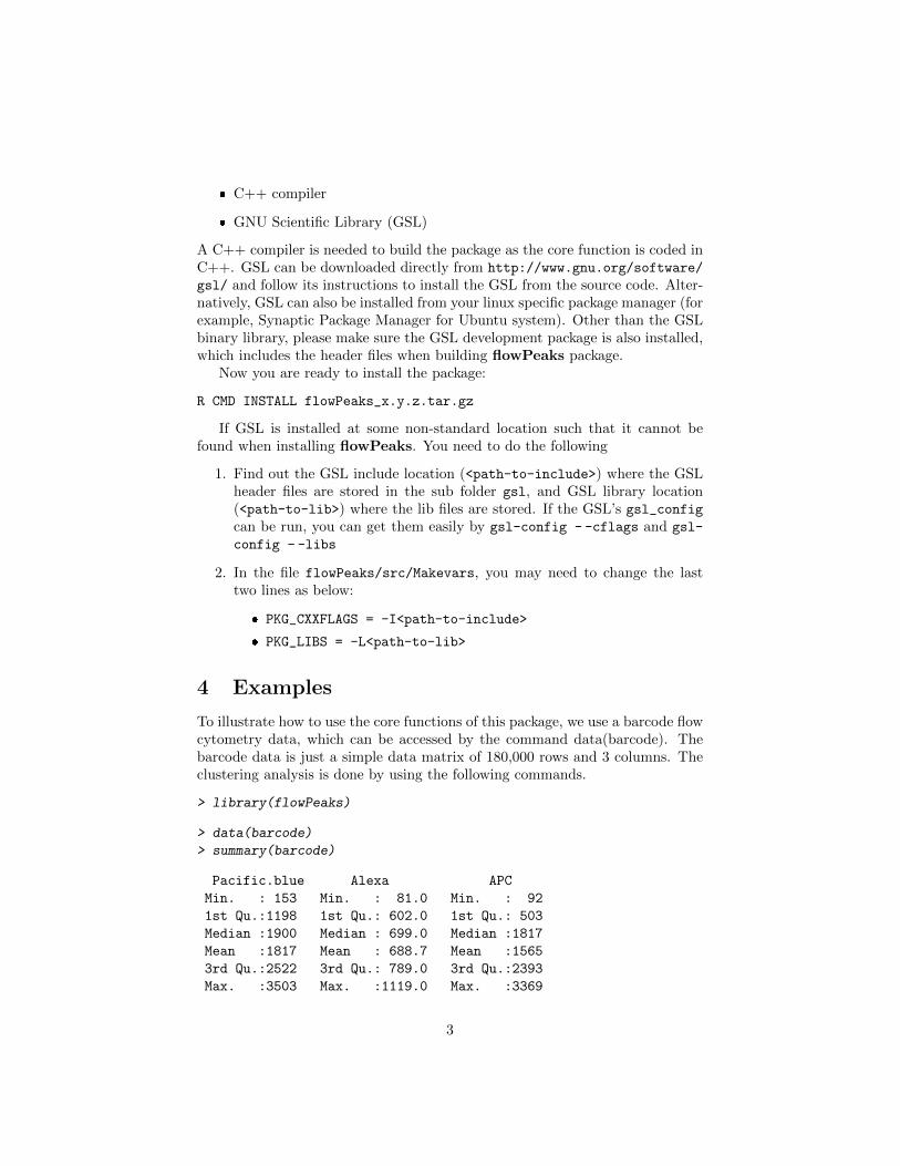
> plot(fp,idx=c(1,3))

Figure 1: The scatter plot of clustering results for the first column and thethird column. Two clusters may share the same color as the automatic colorspecification is not unique for all clusters. The users may have option to changethe col option in the plot function to have their own taste of color specifications.The flowPeaks cluster are drawn in different colors with the centers (⊕), theunderlying K-means cluster centers are indicated by ◦.

> fp<-flowPeaks(barcode)

step 0, set the intial seeds, tot.wss=5.47711e+09

step 1, do the rough EM, tot.wss=3.52259e+09 at 0.496538 sec

step 2, do the fine transfer of Hartigan-Wong Algorithm

tot.wss=3.52028e+09 at 0.693184 sec

If we want to visualize the results, we can draw scatter plot for any twocolumns of the data matrix. The result is shown in Figure 1. Different colorsspecify different clusters, and the dots represent the center of the initial K-

4

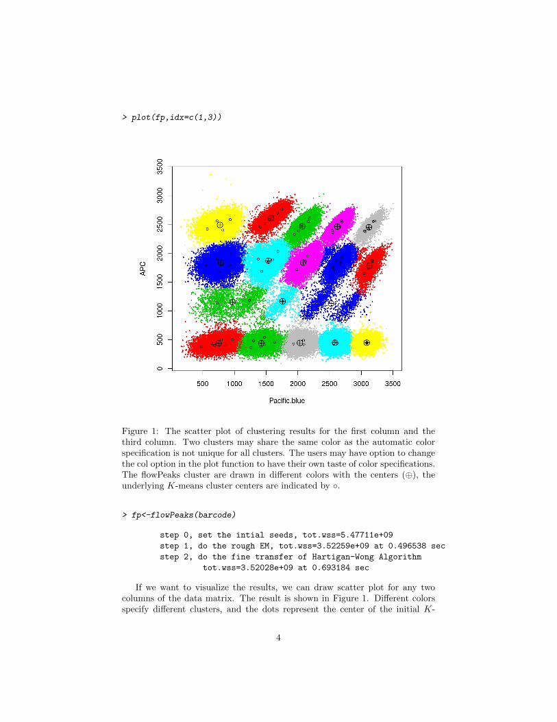
> par(mfrow=c(2,2))

> plot(fp,idx=c(1,2,3))

Figure 2: Pairwise plot of all columns

means, and triangles are the peaks found by flowPeaks. We can see all pairwisescatter plots, the R commands and the plot are shown in Figure 2.

We find out that the data displays better clustering in the Pacific.blue andAPC. We could choose to redo the clustering just focusing on these two dimen-sions as shown in Figure 3.

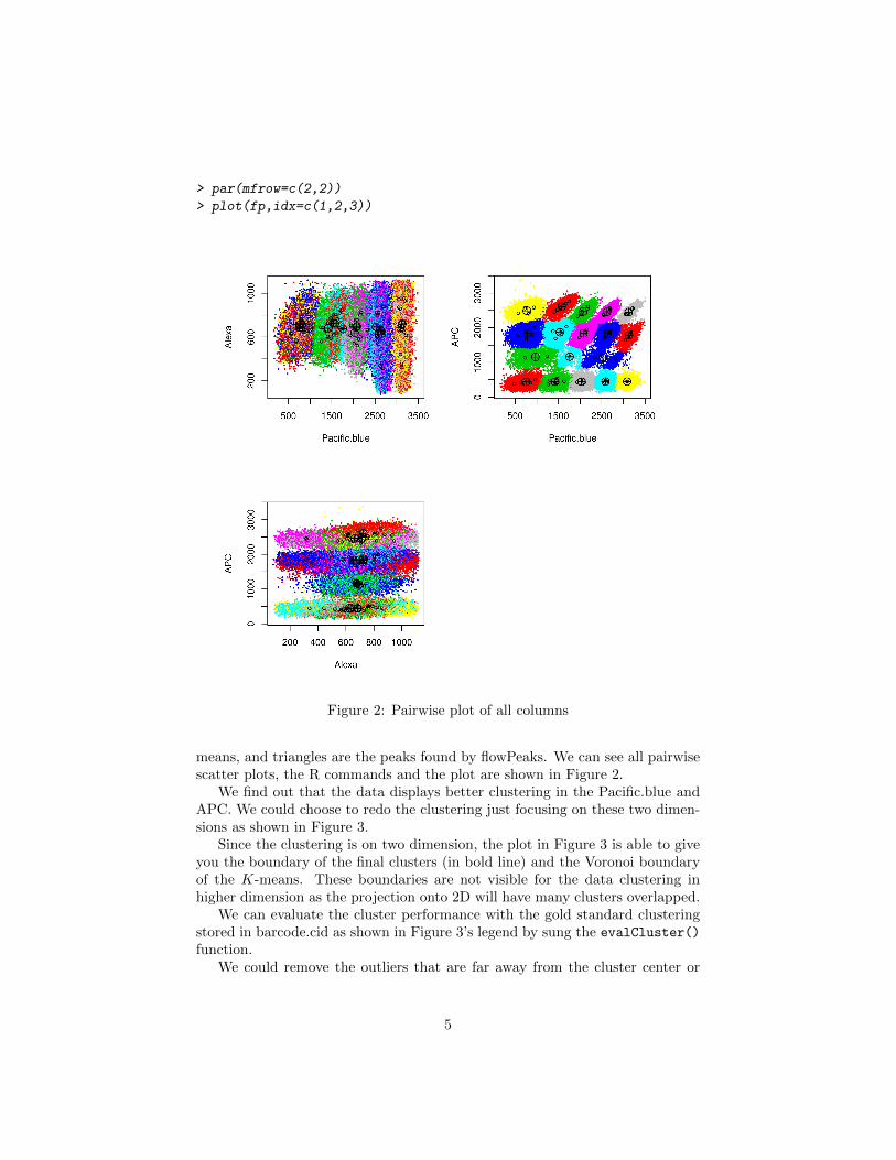
Since the clustering is on two dimension, the plot in Figure 3 is able to giveyou the boundary of the final clusters (in bold line) and the Voronoi boundaryof the K-means. These boundaries are not visible for the data clustering inhigher dimension as the projection onto 2D will have many clusters overlapped.

We can evaluate the cluster performance with the gold standard clusteringstored in barcode.cid as shown in Figure 3’s legend by sung the evalCluster()

function.We could remove the outliers that are far away from the cluster center or

5

> fp2<-flowPeaks(barcode[,c(1,3)])

> plot(fp2)

> evalCluster(barcode.cid,fp2$peaks.cluster,method="Vmeasure")

[1] 0.9983352

Figure 3: Clustering results based on only the Pacific.blue and APC

can not be ambiguously assigned to one of the neighboring cluster as shown inFigure 4.

5 Reading the data from flowFrame

If a user has the data that is of class flowFrame in the flowCore package, he justneeds to use the transformed data of the expression slot of the flowFrame whereonly channles of interest are selected. See Figure 5 for the details

6

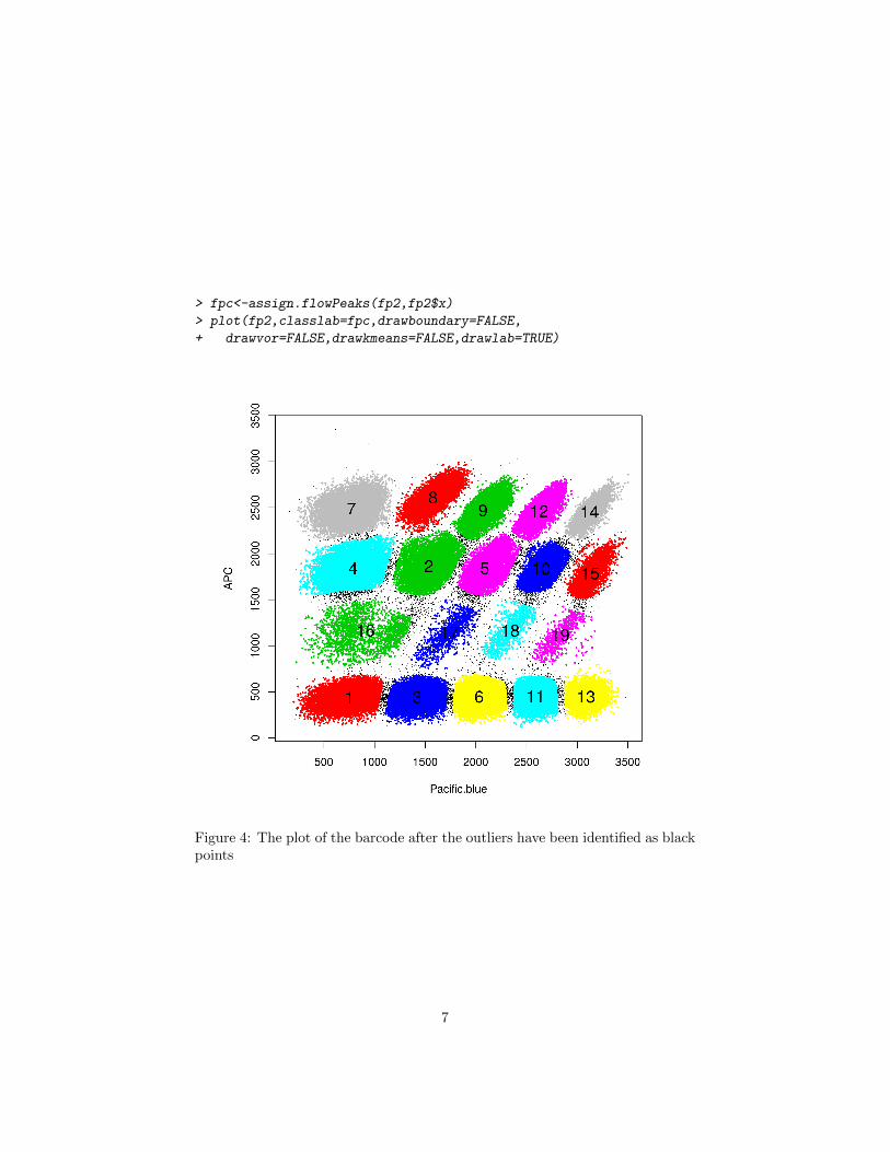
> fpc<-assign.flowPeaks(fp2,fp2$x)

> plot(fp2,classlab=fpc,drawboundary=FALSE,

+ drawvor=FALSE,drawkmeans=FALSE,drawlab=TRUE)

Figure 4: The plot of the barcode after the outliers have been identified as blackpoints

7

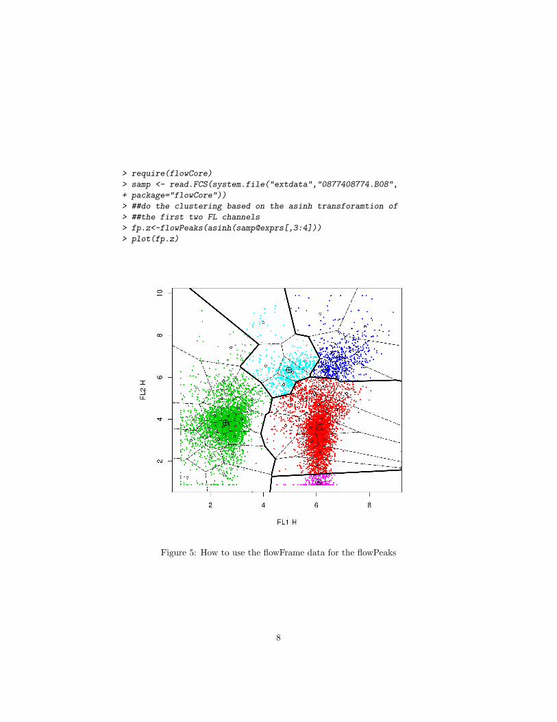
> require(flowCore)

> samp <- read.FCS(system.file("extdata","0877408774.B08",

+ package="flowCore"))

> ##do the clustering based on the asinh transforamtion of

> ##the first two FL channels

> fp.z<-flowPeaks(asinh(samp@exprs[,3:4]))

> plot(fp.z)

Figure 5: How to use the flowFrame data for the flowPeaks

8