
VRIJE UNIVERSITEIT - arXiv · The solution came from a quantum field theory. In quantum field...
160
arXiv:hep-ph/0604226v1 26 Apr 2006 VRIJE UNIVERSITEIT Single spin asymmetries and gauge invariance in hard scattering processes ACADEMISCH PROEFSCHRIFT ter verkrijging van de graad Doctor aan de Vrije Universiteit Amsterdam, op gezag van de rector magnificus prof.dr. T. Sminia, in het openbaar te verdedigen ten overstaan van de promotiecommissie van de faculteit der Exacte Wetenschappen op donderdag 12 januari 2006 om 13.45 uur in de aula van de universiteit, De Boelelaan 1105 door Fetze Pijlman geboren te Leiden
Transcript of VRIJE UNIVERSITEIT - arXiv · The solution came from a quantum field theory. In quantum field...
arX
iv:h
ep-p
h/06
0422
6v1
26
Apr
200
6
VRIJE UNIVERSITEIT
Single spin asymmetries and gauge invariancein hard scattering processes
ACADEMISCH PROEFSCHRIFT
ter verkrijging van de graad Doctor aande Vrije Universiteit Amsterdam,op gezag van de rector magnificus
prof.dr. T. Sminia,in het openbaar te verdedigen
ten overstaan van de promotiecommissievan de faculteit der Exacte Wetenschappenop donderdag 12 januari 2006 om 13.45 uur
in de aula van de universiteit,De Boelelaan 1105
door
Fetze Pijlman
geboren te Leiden

promotor: prof.dr. P.J.G. Mulders
This thesis is partly based on the following publications:
B. L. G. Bakker, M. van Iersel, and F. Pijlman,Comparison of relativistic bound-state calculations in front-form and instant-form dy-namics,Few Body Syst.33, 27 (2003).
D. Boer, P. J. Mulders, and F. Pijlman,Universality of T-odd effects in single spin and azimuthal asymmetries,Nucl. Phys. B667, 201 (2003).
A. Bacchetta, P. J. Mulders, and F. Pijlman,New observables in longitudinal single-spin asymmetries in semi-inclusive DIS,Phys. Lett. B595, 309 (2004).
C. J. Bomhof, P. J. Mulders, and F. Pijlman,Gauge link structure in quark-quark correlators in hard processes,Phys. Lett. B596, 277 (2004).
F. Pijlman,Color gauge invariance in hard processes,Few Body Syst.36, 209 (2005).
F. Pijlman,Factorization and universality in azimuthal asymmetries,Proceedings of the 16th international spin physics symposium 2004, hep-ph/0411307.
A. Bacchetta, C. J. Bomhof, P. J. Mulders, and F. Pijlman,Single spin asymmetries in hadron-hadron collisions,Phys. Rev. D72, 034030 (2005).

Printed by Universal Press - Veenendaal, The Netherlands.
Contents
1 Introduction 71.1 Particle physics, it is amazing! . . . . . . . . . . . . . . . . . . . .. . 71.2 QCD and single spin asymmetries . . . . . . . . . . . . . . . . . . . . 81.3 Outline of the thesis . . . . . . . . . . . . . . . . . . . . . . . . . . . . 12
2 High energy scattering and quark-quark correlators 132.1 Kinematics of electromagnetic scattering processes . .. . . . . . . . . 14
2.1.1 Semi-inclusive deep-inelastic lepton-hadron scattering . . . . . 142.1.2 The Drell-Yan process . . . . . . . . . . . . . . . . . . . . . . 172.1.3 Semi-inclusive electron-positron annihilation . . .. . . . . . . 18
2.2 Cross sections . . . . . . . . . . . . . . . . . . . . . . . . . . . . . . . 192.3 Operator product expansion . . . . . . . . . . . . . . . . . . . . . . . .212.4 The diagrammatic expansion and the parton model . . . . . . .. . . . 232.5 Quark distribution functions for spin-1
2 hadrons . . . . . . . . . . . . . 292.5.1 Integrated distribution functions . . . . . . . . . . . . . . .. . 312.5.2 Transverse momentum dependent distribution functions . . . . 33
2.6 Quark fragmentation functions into spin-12 hadrons . . . . . . . . . . . 38
2.6.1 Integrated fragmentation functions . . . . . . . . . . . . . .. . 382.6.2 Transverse momentum dependent fragmentation functions . . . 40
2.7 Summary and conclusions . . . . . . . . . . . . . . . . . . . . . . . . 422.A Outline of proof of Eq. 2.18 . . . . . . . . . . . . . . . . . . . . . . . . 432.B The diagrammatic expansion . . . . . . . . . . . . . . . . . . . . . . . 45
3 Electromagnetic scattering processes at leading order inαS 493.1 Leading order inαS . . . . . . . . . . . . . . . . . . . . . . . . . . . . 503.2 Semi-inclusive deep-inelastic scattering . . . . . . . . . .. . . . . . . 51
3.2.1 Leading order inM/Q . . . . . . . . . . . . . . . . . . . . . . 54
6 CONTENTS
3.2.2 Next-to-leading order inM/Q . . . . . . . . . . . . . . . . . . 633.2.3 Some explicit cross sections and asymmetries . . . . . . .. . . 67
3.3 The Drell-Yan process . . . . . . . . . . . . . . . . . . . . . . . . . . 743.4 Semi-inclusive electron-positron annihilation . . . . .. . . . . . . . . 783.5 Fragmentation and universality . . . . . . . . . . . . . . . . . . . .. . 803.6 Deeply virtual Compton scattering . . . . . . . . . . . . . . . . . .. . 823.7 Summary and conclusions . . . . . . . . . . . . . . . . . . . . . . . . 863.A Hadronic tensors . . . . . . . . . . . . . . . . . . . . . . . . . . . . . 87
4 Color gauge invariance in hard scattering processes 894.1 Gauge links in tree-level diagrams . . . . . . . . . . . . . . . . . .. . 90
4.1.1 Gauge links in quark-quark scattering . . . . . . . . . . . . .. 904.1.2 Gauge links in semi-inclusive DIS and Drell-Yan with an additional gluon in the final state 954.1.3 Prescription for deducing gauge links in tree-level diagrams . . 101
4.2 Relating correlators with different gauge links . . . . . . . . . . . . . . 1054.3 Unitarity in two-gluon production . . . . . . . . . . . . . . . . . .. . 1084.4 Gauge links in gluon-gluon correlators . . . . . . . . . . . . . .. . . . 1124.5 Factorization and universality . . . . . . . . . . . . . . . . . . . .. . . 115
4.5.1 Virtual corrections . . . . . . . . . . . . . . . . . . . . . . . . 1174.5.2 Evolution, factorization, and universality . . . . . . .. . . . . 120
4.6 Summary and conclusions . . . . . . . . . . . . . . . . . . . . . . . . 125
5 Results for single spin asymmetries in hadronic scattering 1275.1 Introduction . . . . . . . . . . . . . . . . . . . . . . . . . . . . . . . . 1285.2 Calculating cross sections for hadronic scattering . . .. . . . . . . . . 1295.3 Results for cross sections and asymmetries . . . . . . . . . . .. . . . . 1355.4 Summary and conclusions . . . . . . . . . . . . . . . . . . . . . . . . 1395.A Partonic cross sections . . . . . . . . . . . . . . . . . . . . . . . . . . 140
6 Summary and conclusions 143
Acknowledgements 147
Bibliography 149
Samenvatting 157
1Introduction
1.1 Particle physics, it is amazing!
Progress in the understanding of elementary particles is amazing. For more than a cen-tury the smallest building blocks of nature have been studied, and discoveries are stillbeing made today. While studying the ingredients of nature,fundamental and inspiringtheories have been developed making this field of increasinginterest.
At the beginning of the last century, Einstein studied the concept of time in order toexplain the discrepancy between the theories of Newton and Maxwell. This led to thepublication of his theory of special relativity in 1905 [1].Combining this theory andthe quantum theory, Dirac predicted the existence of the antiparticle of both the electronand proton [2]. The antiparticle of the electron, the positron, was discovered in 1933 byAnderson [3] and the antiproton was found in 1955 by Chamberlain et al.[4]
Around the 1930’s, explanations were sought forβ-decay, which is one particularform of nucleus-disintegration. Experimental studies of this phenomenon seemed toshow that the energy before and after the decay were not the same: some energy wasmissing. To circumvent the potential violation of energy conservation (Newton’s law),Pauli suggested between 1930 and 1933 at several conferences a new kind of particle1,which would be produced during radioactive decay without notice. This new particle,
1Pauli publicized this new particle at several conferences among which the Solvay Congresses in 1930and 1933.
8 1 Introduction
called neutrino by Fermi, was observed in 1956 by Reines and Cowan [5].Around 1960 particle accelerators discovered new kinds of hadronic matter. In
order to classify the observed hadrons Gell-Mann in Ref. [6]and Zweig in Ref. [7]introduced, independently, a substructure with three types of quarks. Since then severalother quark-types have been discovered and just a decade agothe last quark with a massof almost 200 times the proton mass, the top quark, was discovered at Fermilab [8, 9].Since this quark and its mass were already predicted on the basis of data taken by thelarge electron-positron collider at CERN, this was once again a stunning success forparticle physics.
In the last century particles have been found which were predicted by theory andtheories have been developed on the basis of experimental observations. It is expectedthat during this century some of the predicted particles, such as the ones responsiblefor spontaneous symmetry breaking (the Higgs-sector), will be observed. The interplaybetween experiment and theory in this field is a guaranteed success to explore whatnature will offer us next.
1.2 QCD and single spin asymmetries
Quantum chromodynamics (QCD) describes the interactions between quarks and glu-ons and is constructed from powerful theories and concepts.The main ingredients are:the theory of relativity, the quantum theory, and the concept of gauge invariance. Thefirst gauge theory was developed more than a century ago. Around 1865 Maxwellwrote down his equations describing the interactions between electromagnetic fieldsand matter. The equations are a set of differential equations which also raised somequestions, one of which was that the potentials obeying the equations are not unique.This point became clarified towards the end of the nineteenthcentury; it was consideredas a mathematical symmetry which was apparently left in the equations. This mathe-matical symmetry allowed for a set of transformations of thepotentials which wouldnot affect physical observables. Nowadays this symmetry is namedgauge invarianceand the potentials are often called the gauge fields.
In the beginning of the twentieth century gauge invariance was considered moreseriously. While incorporating the symmetry in quantum mechanics, Fock discoveredthat, besides the gauge fields, the wave function of the electron should transform as wellto maintain consistency with the theory of relativity. In order to preserve invarianceof observables under gauge transformations, the wave function of the electron mustobtain a space-time-dependent phase. However, the question remained whether thegauge fields were to be considered as fundamental fields or whether they just alleviatedcomplex calculations. For a review on the historical roots of gauge invariance the readeris referred to Jackson, Okun [10].
In the second half of the twentieth century the question on whether potentials aremore fundamental than electric and magnetic fields was finally addressed. Aharonov
1.2 QCD and single spin asymmetries 9
PSfrag replacements
S
screen
B
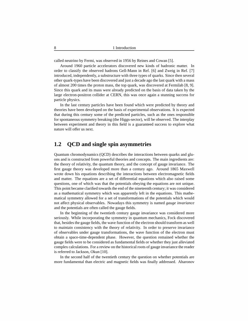
Figure 1.1: The schematic setup of an Aharonov-Bohm like experiment. S representsa source of electrons producing an interference pattern on the screen owing to the twoslits. The interference pattern shifts in a particular direction if the solenoid in B, point-ing out of the plane, is given a current. If the screen is far away from the two slitsthen the shift is proportional to
∮dx · A(x). The path of the integral is the closed path
formed by the two dashed lines andA(x) is the potential field. One can call this shiftof interference pattern an asymmetry because the directionof the shift depends on thedirection of the magnetic field.
and Bohm apparently2 rediscovered that an electron can obtain a phase shift from itsinteraction with the potential even if it only travels in regions in which there is noelectric or magnetic field [13]. The experiment carried out by Chambers showed thatinstead of the electric and magnetic fields, the non-uniquely defined potentials shouldbe considered as the fundamental fields in quantum electrodynamics [14]. A schematicsetup of the experiment is given in Fig. 1.1.
As compared to electrons and photons, the situation of quarks and gluons is muchmore involved. In contrast to electrons and photons, free quarks and gluons have forinstance never been observed. They only seem to exist in a hadron (confinement) whichindicates a strong interaction. On the other hand, perturbation theory turns out to pro-vide a satisfactory description for collisions involving hadrons at high energies, showingthat the interaction at high energies must be weak. This particular scale dependence ofthe interaction strength confronted physicists with a big challenge.
The solution came from a quantum field theory. In quantum fieldtheories infinitiesoften appear. In the 1940’s Dyson, Feynman, Schwinger, and Tomonaga showed that inquantum electrodynamics such infinities can be handled by renormalizing the observ-ables. In contrast to the general expectation, ’t Hooft and Veltman showed in 1972 thatthis was also possible for non-Abelian gauge theories [16, 17]. Using the machinery of
2It seems that Ehrenberg and Siday already pointed out that enclosed magnetic fluxes could cause phaseshifts. Their work [11] has been cited in the subsequent paper of Aharonov and Bohm [12].
10 1 Introduction
electron
electron
target
target-remnant
quark-jet
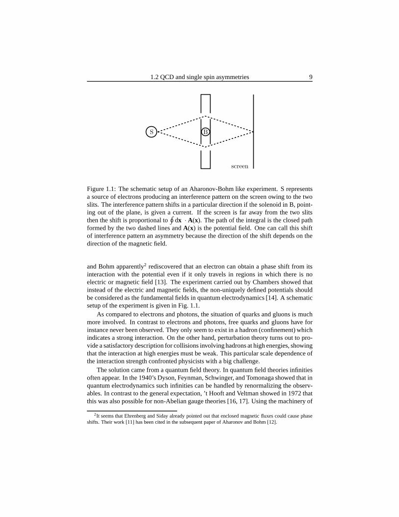
Figure 1.2: An illustration of the interactions between thequark-jet and the target-remnant (Sivers effect). These interactions, which are on the amplitude level and leadto phases as we will see in chapter 3, give rise to interference contributions in the crosssection and could produce single spin asymmetries in the idealized jet-production insemi-inclusive deep-inelastic scattering.
-0.05
0
0.05
0.1
0.15
-0.05
0
0.05
0.1
0.1 0.2 0.3
2 ⟨s
in(φ
- φ
S)⟩
UT
π π+
x
π-
z0.3 0.4 0.5 0.6 0.7
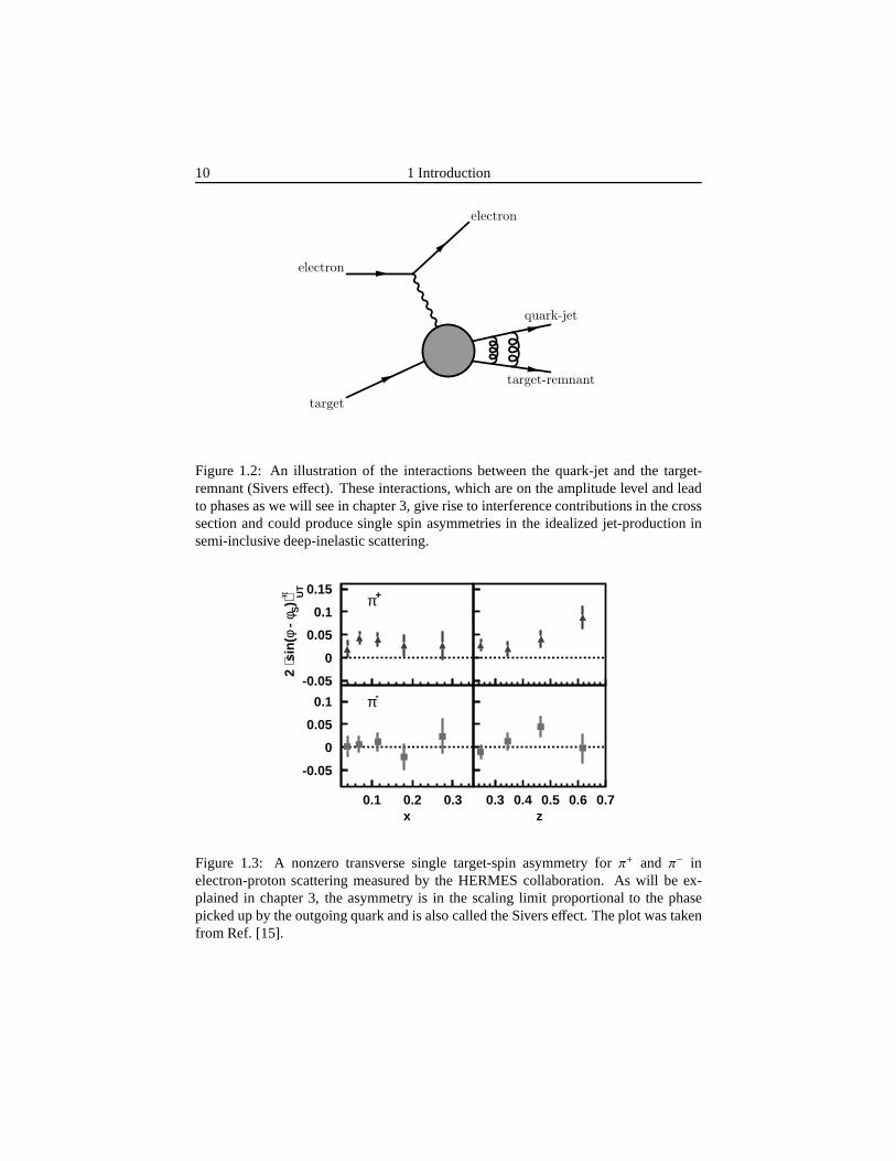
Figure 1.3: A nonzero transverse single target-spin asymmetry for π+ and π− inelectron-proton scattering measured by the HERMES collaboration. As will be ex-plained in chapter 3, the asymmetry is in the scaling limit proportional to the phasepicked up by the outgoing quark and is also called the Sivers effect. The plot was takenfrom Ref. [15].
1.2 QCD and single spin asymmetries 11
’t Hooft and Veltman, Gross, Politzer, and Wilczek derived in Ref. [18, 19] that a scale-dependent interaction strength appears when quarks and gluons are characterized witha color. The constructed non-Abelian gauge theory, called quantum chromodynamics,has a vanishing interaction strength at large momentum transfers - as those occurring inhigh energy collision experiments - which is called asymptotic freedom.
Not being able to apply perturbation theory, most of the low energy regime of quan-tum chromodynamics is at present not calculable from first principles. Bjorken andFeynman introduced the idea of absorbing the nonperturbative part in parton probabil-ity functions which could be measured in several experiments. These functions describehow quarks are distributed in hadrons (distribution functions) or how they “decay” intoa hadron and accompanying jet (fragmentation functions). The functions introduced byFeynman depend only on the longitudinal momentum fraction because at high energiesthe transverse momenta of quarks in hadrons can often be neglected. This somewhatad hoc procedure of absorbing the nonperturbative part in functions, called the partonmodel, can be translated into more rigorous QCD and is very successful in describingvarious kinds of data.
One observation, studied in this thesis, cannot be explained by the parton model,namely the observation of single spin asymmetries. In single spin asymmetries, one ofthe participating particles in a scattering process carries or acquires a certain polariza-tion. If the scattering cross section depends on the direction of this polarization, onehas a single spin asymmetry. Large single spin asymmetries in inelastic collisions werediscovered in hyperon-production in hadron-hadron scattering at Fermilab [20]. Sincethen, single spin asymmetries have been observed in variousprocesses.
Several explanations for single spin asymmetries at large scales were developedover the last two decades. One of the most important ideas, proposed by Sivers inRef. [21, 22], was to allow for a nontrivial correlation between the transverse momen-tum of the quark and its polarization. After incorporating the transverse momenta ofquarks in an extended version of the parton model, it is at present understood that thereare two sources for single spin asymmetries. The first is the presence of interactionswithin a fragmentation process (see Collins [23]). The other source, appearing in theidealized single jet-production in semi-inclusive deep-inelastic scattering, see Fig. 1.2,turns out to be the phase which the struck quark picks up due toits interaction withthe target-remnant (also exists for fragmentation). This particular phase shows up as agauge link, which is a mathematical operator, in the definition of transverse momentumdependent distribution functions. Since these functions are defined in terms of non-local operators inside matrix elements, the presence of this gauge link is also neededfor invariance under local gauge transformations. Note that the obtained phase of theoutgoing quark has similarities with the phases of the electrons in the Aharonov-Bohmexperiment. Having the same origin of the effect for both asymmetries is surprising.The first nonzero experimental data which directly measuresthis phase was obtainedby the HERMES collaboration in 2004 and is given in Fig. 1.3.
12 1 Introduction
1.3 Outline of the thesis
The appearance and treatment of phases in several hard scattering processes will bestudied in this thesis. In 2002 this particular topic becamepopular after Brodsky,Hwang, and Schmidt showed that such phases, leading to single spin asymmetries,could be generated within a model calculation [24]. The obtained phases were at-tributed by Collins [25], Belitsky, Ji, and Yuan [26] to the presence of a fully closedgauge link in the definition of parton distribution functions. In this thesis these ideasare implemented in a diagrammatic expansion which is a field theoretical descriptionof hard scattering processes. The effect of the gauge link is studied in several hard pro-cesses like hadron-hadron and lepton-hadron scattering. Although only QCD is studiedin this thesis, gauge links also appear in other gauge theories like quantum electrody-namics. It is therefore to be expected that gauge links couldprovide a description ofsingle spin asymmetries in pure electromagnetic scattering as well.
For a full appreciation of the contents of this thesis familiarity with particle physicsand quantum field theory is needed. Some excellent textbooksor reviews have beenwritten by Anselmino, Efremov, Leader [27], Barone, Ratcliffe [28], Halzen, Mar-tin [29], Leader [30], Peskin, Schroeder [31], Ryder [32], Weinberg [33, 34].
Chapter 2 will begin with an introduction of the kinematics of some processes inwhich the hard scale is set by an electromagnetic interaction. A discussion of the di-agrammatic approach will be given together with the definitions of distribution andfragmentation functions. This chapter contains some new results from Ref. [35, 36].
In chapter 3, the diagrammatic approach will be applied to obtain cross sectionsof some electromagnetic processes assuming factorization. The gauge link inside thedefinition of parton distribution and fragmentation functions will be derived, showingthe consistency of the applied approach at leading order inαS (tree-level). The pres-ence of the gauge link will lead to the interesting prediction of Collins [25] that T-odddistribution functions in the Drell-Yan process appear with a different sign compared tosemi-inclusive deep-inelastic scattering. This chapter is based on Ref. [35, 36].
Chapter 4 will begin by considering gauge links in more complicated processes (andbeyond tree-level). Besides the gauge links which are foundin the electromagnetic pro-cesses new gauge links will be encountered which is quite a surprise. We will also seethat the appearance of these new structures is an essential ingredient in the discussion offactorization. A set of tools will be developed which allowsfor a quick determinationof the gauge link for arbitrary scattering processes. This chapter contains unpublishedmaterial of which some results were given in Ref. [37, 38, 39].
In chapter 5 the physical effect of the new gauge links will be illustrated in almostback-to-back hadron-production in hadron-hadron scattering. A new observable is con-structed which is directly sensitive to the intrinsic transverse momenta of partons. In thesame way as T-odd distribution functions change sign in the electromagnetic processes,the T-odd distribution functions receive a gauge link dependent factor in the studiedasymmetries of hadron-hadron scattering. This chapter is based on Ref. [40].
2High energy scattering
and quark-quarkcorrelators
The formalism will be introduced which was initiated by Collins, Ralston, and Soper inRef. [41, 42, 43, 44]. The formalism carefully considers therole of intrinsic transversemomenta of partons in hard scattering processes. Although the first part of the chapteris already present in the literature (and partly based on Ref. [45]), it remains worthwhileto look at some parts in more detail to elaborate upon the approximations and the phi-losophy behind certain approaches. Since this part is meantas an introduction for thenon-experts, the reader can skip those sections which are familiar to him or her.
Starting from section 2.5, the second part contains new elements which have beendeveloped over the last few years. These new elements, whichare one of the highlightsin QCD-phenomenology, originate from the presence of Wilson lines or gauge linksin parton distribution and fragmentation functions. Thesefunctions will be defined andthey turn out to provide valuable information of partons inside hadrons and parton decayinto hadrons. As we will see in the following chapters, the presence of these Wilsonlines in the definitions of these functions lead to interesting predictions. A summarywill be given at the end of this chapter.

14 2 High energy scattering and quark-quark correlators
2.1 Kinematics of electromagnetic scattering processes
Physicists use often the Lorentz-invariance of the theory to choose the most conve-nient frame for their purposes. This has produced several frame definitions and frame-dependent interpretations. In principle the definitions and results can be compared bymaking the appropriate coordinate transformations but in practice this has often led toconfusion. In this section several scattering processes will be introduced and their kine-matics will be set up such that theoretical predictions and experimental results can becompared frame-independently.
As was advocated at the Transversity workshop in Trento 2004(see also Ref. [46]),one can, in order to clarify this situation, express all results in easy-to-compare frame-independent observables which is possible owing to the Lorentz-invariance of the the-ory. For example, the variables in the invariant cross section are usually the momentumand spin vectors which have specific transformation properties. A much better choicewould be to express the cross section in terms of the possibleinvariants. The invariantsare frame-independent and can therefore be directly calculated in any frame!
A drawback of this approach is that equations become rather lengthy and that we arenot used to think in a frame-independent manner. To aid our intuition and to supportthe frames which are already in use, a Cartesian basis will beemployed which willserve as an interface. Such bases were already introduced before, see for instance Lam,Tung [47] and Meng, Olness, Soper [48]. This will result in short expressions whilemaintaining manifest frame-independence.
In this thesis the metric tensor of Bjorken and Drell [49] will be employed, reading
g00 = −g11 = −g22 = −g33 = 1, gi j = 0 for i , j, (2.1)
and the antisymmetric tensor is normalized such thatǫ0123= 1. The Einstein summationconvention will also be used, meaning that if a certain indexappears twice in a productit is automatically summed over all its values unless statedotherwise. Furthermore,natural units with~ = c = 1 will be used.
2.1.1 Semi-inclusive deep-inelastic lepton-hadron scattering
In the deep-inelastic scattering (DIS) process, a lepton with momentuml and massme,strikes with a large momentum difference (l · P≫ M2) a hadron (sometimes called tar-get), with momentumP and massM. The interaction, mediated through the exchangeof a highly virtual photon with momentumq (and−M2 ≫ q2), causes the hadron tobreak up into all kinds of particles being most often other hadrons. The measurementis called:inclusiveif only the scattered electron is measured,semi-inclusiveif an addi-tional particle (or more) with momentumPh and massMh is measured, andexclusiveifall (but one) final-state particles are detected. The semi-inclusive process is illustratedin Fig. 2.1a.
2.1 Kinematics of electromagnetic scattering processes 15
P
PX
l
l′
q Ph
PSfrag replacements
ex
ey
ezPl
l′
Ph
(a) (b)
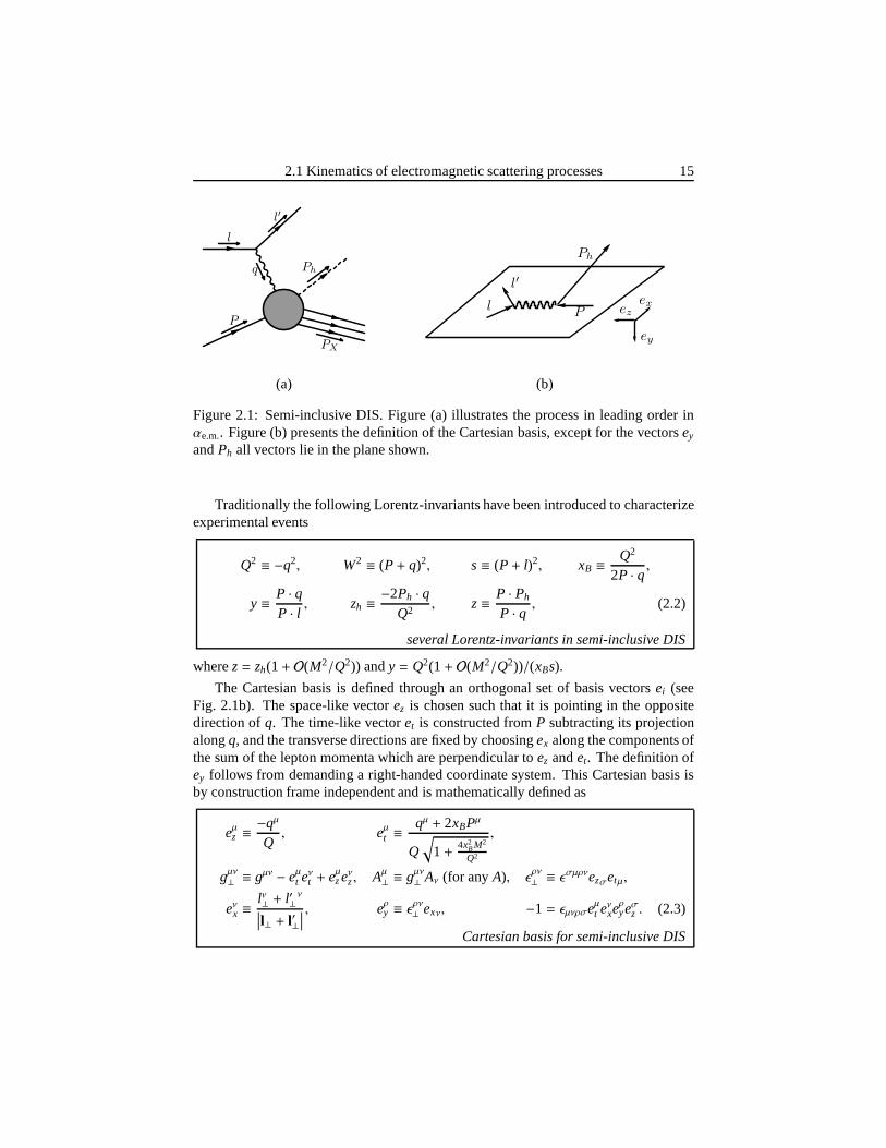
Figure 2.1: Semi-inclusive DIS. Figure (a) illustrates theprocess in leading order inαe.m.. Figure (b) presents the definition of the Cartesian basis, except for the vectorsey
andPh all vectors lie in the plane shown.
Traditionally the following Lorentz-invariants have beenintroduced to characterizeexperimental events
Q2 ≡ −q2, W2 ≡ (P+ q)2, s≡ (P+ l)2, xB ≡Q2
2P · q,
y ≡ P · qP · l , zh ≡
−2Ph · qQ2
, z≡ P · Ph
P · q , (2.2)
several Lorentz-invariants in semi-inclusive DIS
wherez= zh(1+ O(M2/Q2)) andy = Q2(1+ O(M2/Q2))/(xBs).
The Cartesian basis is defined through an orthogonal set of basis vectorsei (seeFig. 2.1b). The space-like vectorez is chosen such that it is pointing in the oppositedirection ofq. The time-like vectoret is constructed fromP subtracting its projectionalongq, and the transverse directions are fixed by choosingex along the components ofthe sum of the lepton momenta which are perpendicular toez andet. The definition ofey follows from demanding a right-handed coordinate system. This Cartesian basis isby construction frame independent and is mathematically defined as
eµz ≡−qµ
Q, eµt ≡
qµ + 2xBPµ
Q√
1+4x2
BM2
Q2
,
gµν⊥ ≡ gµν − eµt eνt + eµzeνz, Aµ⊥ ≡ gµν⊥ Aν (for anyA), ǫ
ρν⊥ ≡ ǫσµρνezσetµ,
eνx ≡lν⊥ + l′⊥
ν
∣∣∣l⊥ + l′⊥∣∣∣, eρy ≡ ǫρν⊥ exν, −1 = ǫµνρσeµt eνxe
ρyeσz . (2.3)
Cartesian basis for semi-inclusive DIS
16 2 High energy scattering and quark-quark correlatorsPSfrag replacements
x
yz
Pl
l′
Ph
φ
PSfrag replacements
xyz
Pl
l′
Ph
φ
(a) (b)
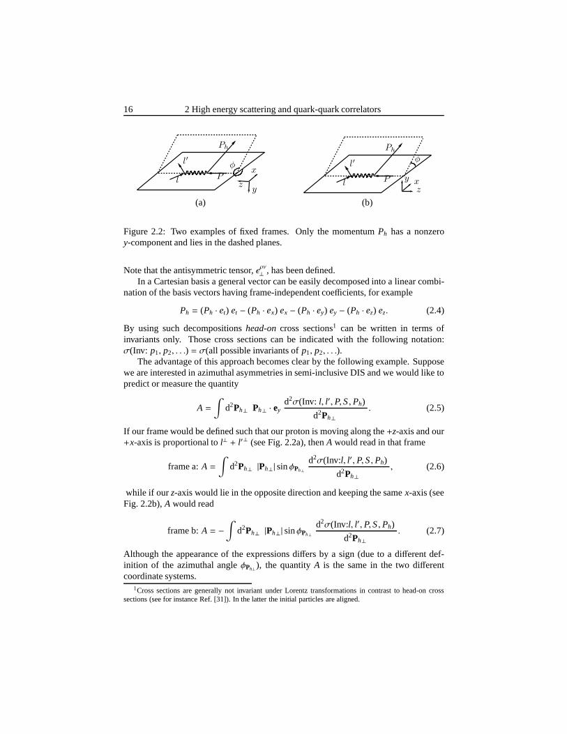
Figure 2.2: Two examples of fixed frames. Only the momentumPh has a nonzeroy-component and lies in the dashed planes.
Note that the antisymmetric tensor,ǫρν⊥ , has been defined.In a Cartesian basis a general vector can be easily decomposed into a linear combi-
nation of the basis vectors having frame-independent coefficients, for example
Ph = (Ph · et) et − (Ph · ex) ex − (Ph · ey) ey − (Ph · ez) ez. (2.4)
By using such decompositionshead-oncross sections1 can be written in terms ofinvariants only. Those cross sections can be indicated withthe following notation:σ(Inv: p1, p2, . . .) = σ(all possible invariants ofp1, p2, . . .).
The advantage of this approach becomes clear by the following example. Supposewe are interested in azimuthal asymmetries in semi-inclusive DIS and we would like topredict or measure the quantity
A =∫
d2Ph⊥ Ph⊥ · eyd2σ(Inv: l, l′,P,S,Ph)
d2Ph⊥. (2.5)
If our frame would be defined such that our proton is moving along the+z-axis and our+x-axis is proportional tol⊥ + l′⊥ (see Fig. 2.2a), thenA would read in that frame
frame a:A =∫
d2Ph⊥ |Ph⊥| sinφPh⊥
d2σ(Inv:l, l′,P,S,Ph)
d2Ph⊥, (2.6)
while if our z-axis would lie in the opposite direction and keeping the same x-axis (seeFig. 2.2b),A would read
frame b:A = −∫
d2Ph⊥ |Ph⊥| sinφPh⊥
d2σ(Inv:l, l′,P,S,Ph)
d2Ph⊥. (2.7)
Although the appearance of the expressions differs by a sign (due to a different def-inition of the azimuthal angleφPh⊥), the quantityA is the same in the two differentcoordinate systems.
1Cross sections are generally not invariant under Lorentz transformations in contrast to head-on crosssections (see for instance Ref. [31]). In the latter the initial particles are aligned.
2.1 Kinematics of electromagnetic scattering processes 17
P2
P1
PX
l′
lq
PSfrag replacements
ez
ey
ex
P1
l
l′
P2
(a) (b)
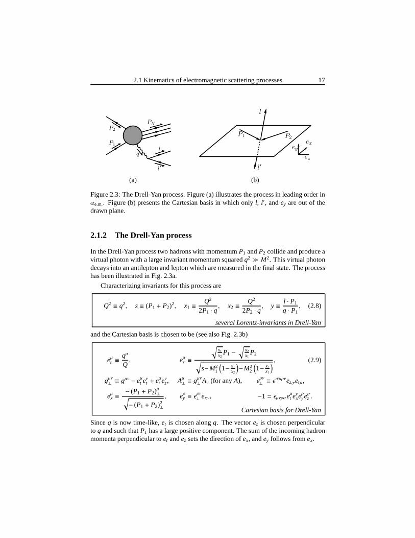
Figure 2.3: The Drell-Yan process. Figure (a) illustrates the process in leading order inαe.m.. Figure (b) presents the Cartesian basis in which onlyl, l′, andey are out of thedrawn plane.
2.1.2 The Drell-Yan process
In the Drell-Yan process two hadrons with momentumP1 andP2 collide and produce avirtual photon with a large invariant momentum squaredq2 ≫ M2. This virtual photondecays into an antilepton and lepton which are measured in the final state. The processhas been illustrated in Fig. 2.3a.
Characterizing invariants for this process are
Q2 ≡ q2, s≡ (P1 + P2)2, x1 ≡Q2
2P1 · q, x2 ≡
Q2
2P2 · q, y ≡ l · P1
q · P1, (2.8)
several Lorentz-invariants in Drell-Yan
and the Cartesian basis is chosen to be (see also Fig. 2.3b)
eµt ≡qµ
Q, eµz ≡
√x1x2
P1 −√
x2x1
P2
√s−M2
1
(1− x1
x2
)−M2
2
(1− x2
x1
) , (2.9)
gµν⊥ ≡ gµν − eµt eνt + eµzeνz, Aµ⊥ ≡ gµν⊥ Aν (for anyA), ǫ
ρν⊥ ≡ ǫσµρνezσetµ,
eµx ≡− (P1 + P2)µ⊥√− (P1 + P2)2
⊥
, eρy ≡ ǫρν⊥ exν, −1 = ǫµνρσeµt eνxeρyeσz .
Cartesian basis for Drell-Yan
Sinceq is now time-like,et is chosen alongq. The vectorez is chosen perpendicularto q and such thatP1 has a large positive component. The sum of the incoming hadronmomenta perpendicular toet andez sets the direction ofex, andey follows fromex.
18 2 High energy scattering and quark-quark correlators
Ph2
Ph1
PX
l′
l
q
PSfrag replacements
ex
eyez
Ph1
l′
l
Ph2
(a) (b)
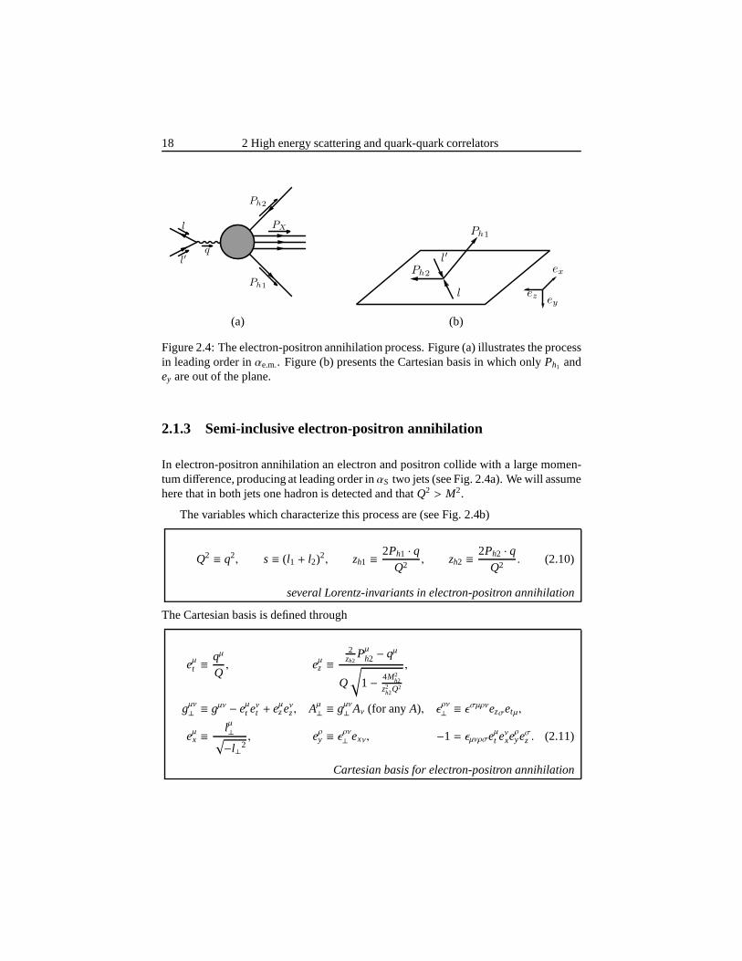
Figure 2.4: The electron-positron annihilation process. Figure (a) illustrates the processin leading order inαe.m.. Figure (b) presents the Cartesian basis in which onlyPh1 andey are out of the plane.
2.1.3 Semi-inclusive electron-positron annihilation
In electron-positron annihilation an electron and positron collide with a large momen-tum difference, producing at leading order inαS two jets (see Fig. 2.4a). We will assumehere that in both jets one hadron is detected and thatQ2 > M2.
The variables which characterize this process are (see Fig.2.4b)
Q2 ≡ q2, s≡ (l1 + l2)2, zh1 ≡2Ph1 · q
Q2, zh2 ≡
2Ph2 · qQ2
. (2.10)
several Lorentz-invariants in electron-positron annihilation
The Cartesian basis is defined through
eµt ≡qµ
Q, eµz ≡
2zh2
Pµ
h2 − qµ
Q
√1− 4M2
h2
z2h2Q2
,
gµν⊥ ≡ gµν − eµt eνt + eµzeνz, Aµ⊥ ≡ gµν⊥ Aν (for anyA), ǫ
ρν⊥ ≡ ǫσµρνezσetµ,
eµx ≡lµ⊥√−l⊥2
, eρy ≡ ǫρν⊥ exν, −1 = ǫµνρσeµt eνxeρyeσz . (2.11)
Cartesian basis for electron-positron annihilation
2.2 Cross sections 19
2.2 Cross sections
In this section the cross section formula for semi-inclusive DIS will be derived andresults for Drell-Yan and electron-positron annihilationwill be stated. First, some con-ventions will be given.
The helicity of a parton with momentump and spins is defined here to be
λ ≡ s · p|s · p| . (2.12)
Dirac spinors and particle states are normalized such that
u(k, λ) u(k, λ′) = 2mδλλ′ , (2.13)
〈P, λ | P′, λ′〉 = 2EP (2π)3 δ3(P′ − P) δλλ′ . (2.14)
The standard cross section for semi-inclusive DIS is (see for example Ref. [31])
dσ =1F
d3Ph
(2π)32EPh
d3l′
(2π)32El′
×∑
X
∫d3PX
(2π)32EPX
|M|2 (2π)4δ4 (l + P− PX − Ph − l′
). (2.15)
As we can see from this equation, the cross section is built upout of: several phase-space factors, a sum over all possible final states, an invariant amplitude, a delta-function which expresses momentum conservation, and a flux factorF which is givenby
F ≡ 4 ElEP |vl − vP|, (2.16)
wherevl andvP are the velocities. The phase-space factors together with the delta-function are Lorentz invariant. Since the invariant amplitude is also Lorentz invariantthe transformation properties of the cross section are set by the flux. In this thesis onlyhead-oncollisions will be considered, meaning that the motion of the initial particles isaligned. In that case the flux takes the form
F = 2s(1+ O
(M2/Q2
)). (2.17)
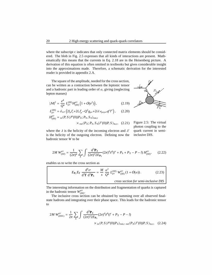
For nucleons, consisting of strongly interacting quarks and gluons, the interactionbetween the electrons and the hadrons is at lowest order inα ≡ e2/(4π) mediatedthrough the exchange of a virtual photon. Owing to the presence of charged quarks,the virtual photon feels the electromagnetic current between the incoming and outgo-ing hadrons. The process is illustrated in Fig. 2.5 and leadsfor the invariant amplitudeto
iM = (−ie) u(l′, λ′)γρu(l, λ)−iq2 out〈Ph,PX|(−ie)Jρ(0)|P,S〉in,c+ O(e3), (2.18)
20 2 High energy scattering and quark-quark correlators
where the subscript c indicates that only connected matrix elements should be consid-ered. The blob in Fig. 2.5 expresses that all kinds of interactions are present. Math-ematically this means that the currents in Eq. 2.18 are in theHeisenberg picture. Aderivation of this equation is often omitted in textbooks but gives considerable insightinto the approximations made. Therefore, a schematic derivation for the interestedreader is provided in appendix 2.A.
P
PX
l
l′
q Ph
Figure 2.5: The virtualphoton coupling to thequark current in semi-inclusive DIS.
The square of the amplitude, needed for the cross section,can be written as a contraction between the leptonic tensorand a hadronic part in leading order ofα, giving (neglectinglepton masses)
|M|2 = e4
Q4L(lH )µν Hµν
(lH )
(1+ O(e2)
), (2.19)
L(lH )µν = δλλ′
(2lµl
′ν+2lνl
′µ−Q2gµν+2iλ ǫµνρσqρlσ
), (2.20)
Hµν
(lH ) = in〈P,S|Jµ(0)|PX; Ph,Sh〉out,c
× out〈PX; Ph,Sh|Jν(0)|P,S〉in,c, (2.21)
where theλ is the helicity of the incoming electron andλ′
is the helicity of the outgoing electron. Defining now thehadronic tensorW to be
2M Wµν
(lH ) =1
(2π)4
∑
X
∫d3PX
(2π)32EPX
(2π)4δ4(l′ + Ph + PX − P− l) Hµν
(lH ), (2.22)
enables us to write the cross section as
EPhEl′d6σ
d3l′ d3Ph
=Msα2
Q4L(lH )µν Wµν
(lH ) (1+ O(α)) . (2.23)
cross section for semi-inclusive DIS
The interesting information on the distribution and fragmentation of quarks is capturedin the hadronic tensorWµν
(lH ).The inclusive cross section can be obtained by summing over all observed final-
state hadrons and integrating over their phase space. This leads for the hadronic tensorto
2M Wµν
(DIS) =12π
∑
X
∫d3PX
(2π)32EPX
(2π)4δ4(l′ + PX − P− l)
× in〈P,S|Jµ(0)|PX〉out,c out〈PX|Jν(0)|P,S〉in,c, (2.24)
2.3 Operator product expansion 21
and gives for the cross section
El′d3σ
d3l′=
2Msα2
Q4L(lH )µν Wµν
(DIS) (1+ O(α)) . (2.25)
cross section for inclusive DIS
The cross sections for Drell-Yan and electron-positron annihilation can be derivedsimilarly. One obtains for Drell-Yan in terms of
L(DY)µν = δλλ′
(2lµl
′ν + 2lνl
′µ − Q2gµν + 2iλǫµνρσqρlσ
), (2.26)
Hµν
(DY) = in〈PA,SA; PB,SB|Jµ(0)|PX〉out,c out〈PX|Jν(0)|PA,SA; PB,SB〉in,c, (2.27)
Wµν
(DY) =1
(2π)4
∑
X
∫d3PX
(2π)32EPX
(2π)4δ4(P1 + P2 − l − l′ − PX)Hµν
(DY), (2.28)
the following cross section (a factor 2 was included for summing over lepton polariza-tions)
ElEl′d6σ
d3l d3l′=
α2
sQ4L(DY)µν Wµν
(DY) (1+ O(α)) . (2.29)
cross section for Drell-Yan
For electron-positron annihilation the cross section for producing two almost back-to-back hadrons reads (a factor1
2 was included for averaging over lepton polarizations)
EPh1EPh2
d6σ
d3Ph1 d3Ph2=
α2
4Q6L(e+e−)µν Wµν
(e+e−) (1+ O(α)) , (2.30)
cross section for electron-positron annihilation
where (with|Ω〉 representing the physical vacuum)
L(e+e−)µν = δλλ′
(2lµl
′ν + 2lνl
′µ − Q2gµν + 2iλ ǫµνρσlρl′σ
), (2.31)
Hµν
(e+e−) = 〈Ω|Jµ(0)|PX; Ph1,Sh1; Ph2,Sh2〉out,c
× out〈PX; Ph1,Sh1; Ph2,Sh2|Jν(0)|Ω〉c, (2.32)
Wµν
(e+e−) =1
(2π)4
∫d3PX
(2π)32EPX
(2π)4δ4(q− PX − Ph1 − Ph2) Hµν
(e+e−). (2.33)
2.3 Operator product expansion
There are two methods to gain more information from the hadronic tensor. In 1968 thefirst method was proposed by Wilson in Ref. [50] and is called the operator product
22 2 High energy scattering and quark-quark correlators
expansion. The second method,the diagrammatic expansion, was proposed by Politzerin Ref. [51] in 1980 and will be introduced in the next section.
The operator product expansion is useful for inclusive measurements. As an illus-tration let us consider the inclusive DIS process. Having nohadrons observed in thefinal state, the sum over all final QCD-states is complete. Together with the fact thatthe proton is a stable particle one can rewrite the hadronic tensor in Eq. 2.24 into2
2MWµν
(DIS) =12π
∫d4x eiqx〈P,S| [Jµ(x), Jν(0)
] |P,S〉c. (2.34)
According to the Einstein causality principle the commutator of two physical operatorsshould vanish for space-like separations. In our case this means that only the areax2 > 0gives a contribution. Under the assumption that the hadronic tensor is well behavingfor x2 > 0 one can show that the main contribution comes fromx2 ≈ 0 in the Bjorkenlimit (fixed xB andQ→ ∞), implying light-cone dominance.
The idea of Wilson, which was later proven in perturbation theory in 1970 by Zim-merman3, is that for small separations one can make a Taylor expansion for operators.This expansion is called the operator product expansion andreads
OA(x)OB(0) ≈x≈0
∑
n
CnABOn(0). (2.35)
This above relation also holds for commutators and by using dispersion relations theshort distance expansion can be applied for inclusive DIS.
In Drell-Yan the sum over final QCD-states is complete which enables one to obtaina product of current operators. One can gain insight in the various structure functionsin which the cross section can be decomposed but since these structure functions willdepend on the two hadrons they are inconvenient for the studyof the structure of asingle nucleon. In addition, the process is not light-cone dominated which complicatesthe application of the operator product expansion.
Another situation is encountered in electron-positron annihilation. When summingover all final states the commutator can be obtained, but if weare interested in howquarks decay into hadrons we would not be able to sum over sucha complete set. Theuse of the operator product expansion is therefore limited here as well.
Summarizing, the operator product expansion is a useful approach that finds appli-cations in inclusive DIS and electron-positron annihilation. At the same time, it is alsolimited to those processes. Parton distribution functionswhich are measured in DIScannot be compared to more complex or less inclusive processes and quark decay can-not be studied within this approach. We will proceed by applying an extended form of
2A necessary condition to have a stable particle is that the sum over energies of its possible decay prod-ucts is larger than the energy of the considered particle. Together with the fact that the zeroth momentumcomponent of the virtual photon in DIS is positive, it can be shown that the hadronic tensor vanishes ifq isreplaced by−q. This enables one to obtain the commutator.
3For reference, please consider chapter 20 of Ref. [34].
2.4 The diagrammatic expansion and the parton model 23
Feynman’s parton model. In the original parton model it is assumed that the underlyingprocess is a partonic scattering process multiplied by distribution and fragmentationfunctions. These functions describe the probability of finding on shell constituents in ahadron or how a quark decays into a particular hadron. In the next section the diagram-matic approach as an extension of this model will be discussed.
2.4 The diagrammatic expansion and the parton model
Background of the diagrammatic expansion
The operator product expansion is of limited use for the study of the nucleon’s structure.In the case of Drell-Yan we were not able to study the structure of a single nucleonalthough one could imagine that the chance of producing a virtual photon should justbe proportional to the chances of finding a quark in the nucleon and an antiquark in theother nucleon. This idea of expressing the cross section in terms of probability functionswhich are then convoluted with some parton scattering crosssection was suggested byFeynman and is nowadays called theparton model.
The parton model had already lots of successes. It gave for instance an intuitiveexplanation for the approximate Bjorken scaling which was observed at SLAC. In anQCD-improved version of the parton model one could even predict the scaling vio-lation with a set of equations calledevolution equations(for example see Altarelli,Parisi [52]). Another success of the parton model is the observation of jets. A jet isa set of particles of which their momentum differences can be characterized with ahadronic size. By assuming that these jets are produced by partons which “decay” intothese jets one is able to predict the number of jets appearingin scattering processes.However, the appearance of jets also creates a problem with color. Since partons carrycolor charges, they should somehow loose this color when decaying into a set of color-less hadrons. It appears that this issue does not influence the scattering cross sectionsat large momentum transfers.
The success of the parton model relies on the asymptotic freedom property ofQCD [18, 19]. This property allows one to apply perturbationtheory for elementaryparticle scattering in strong interaction physics in the presence of large scales. Strictlyspeaking, it remains, however, to be proven whether one can apply perturbation theoryin hadronic scattering processes as well. The present idea is that suitable hadronic scat-tering processes can be described in terms of short-distance physics, the hard scatteringpart, and the long-distance nonperturbative physics whichis captured in probability anddecay functions. Since the latter are nonperturbative in nature, the approach should atleast be self-consistent to all orders in perturbation theory. This description in separatedterms is calledfactorization.
The diagrammatic approach is an extended form of Feynman’s parton model. Orig-inating from field theory, the approach includes the possibility that several parton-fieldsfrom a hadron can participate in a scattering process (involving multi-parton correla-
24 2 High energy scattering and quark-quark correlators
tors), whereas the parton model only considers the possibility of hitting a single parton.The approach agrees with the operator product expansion when applicable. In 1980it was suggested by Politzer in Ref. [51] in order to describethe subleading orders inM/Q, involving “higher twist” operators in matrix elements (tobe discussed in chap-ter 3). Subsequently, it was applied by Ellis, Furmanski, and Petronzio in Ref. [53, 54].Although similar assumptions as in the parton model are made, the starting point ismore general because it allows for more possible interactions. As we will see later,some of these interactions will provide an explanation for single spin asymmetries (seethe work of Qiu and Sterman [55, 56, 57]). The diagrammatic approach was furtherdeveloped and used in several applications, some of which tobe discussed later in thisthesis.
The assumption in the diagrammatic approach is that in-
ti tf
P
PX1
PX2
l
l′
q
Ph
Figure 2.6: The dia-grammatic approach il-lustrated for two jet-production and an ob-served hadron in semi-inclusive DIS.
teractions between the incoming hadrons and outgoing jetscan be described in perturbation theory and hence can be di-agrammatically expanded with in the hard part a sufficientlysmall coupling constant. With respect to asymptotic free-dom this requires the incoming hadrons and outgoing jetsto be well separated in momentum space. We will there-fore impose that the products of external momenta are large(Pi ·P j ≫ M2 for i , j) and assume that interactions betweenoutgoing jets can be neglected. Non-perturbative physics in-side the jets and hadrons is maintained. Together with theassumption of adiabatically switching on and off the interac-tions, the applied assumptions are sufficient to describe gen-eral QCD-scattering processes.
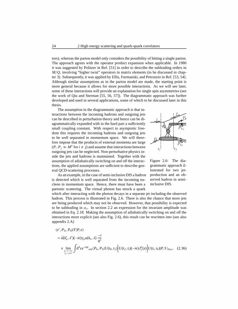
As an example, in the case of semi-inclusive DIS a hadronis detected which is well separated from the incoming nu-cleon in momentum space. Hence, there must have been apartonic scattering. The virtual photon has struck a quarkwhich after interacting with the photon decays in a separatejet including the observedhadron. This process is illustrated in Fig. 2.6. There is also the chance that more jetsare being produced which may not be observed. However, that possibility is expectedto be subleading inαs. In section 2.2 an expression for the invariant amplitude wasobtained in Eq. 2.18. Making the assumption of adiabatically switching on and off theinteractions more explicit (see also Fig. 2.6), this resultcan be rewritten into (see alsoappendix 2.A)
〈e′,PX,Ph|iT |P, e〉
= u(k′e, λ′)(−ie)γµu(ke, λ)
−iq2
× limti→−∞t f→∞
∫d4ze−iqz
out〈Ph,PX|U(t0, t f )[U(t f , ti)(−ie)JµI (z)
]U(ti, t0)|P,S〉in,c, (2.36)
2.4 The diagrammatic expansion and the parton model 25
where the subscriptI denotes the interaction picture andt0 defines the quantizationplane.
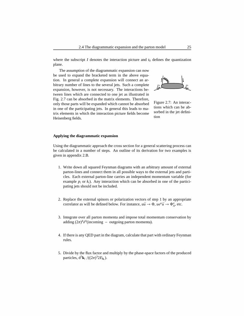
The assumption of the diagrammatic expansion can now
P P
Figure 2.7: An interac-tions which can be ab-sorbed in the jet defini-tion
be used to expand the bracketed term in the above equa-tion. In general a complete expansion will connect an ar-bitrary number of lines to the several jets. Such a completeexpansion, however, is not necessary. The interactions be-tween lines which are connected to one jet as illustrated inFig. 2.7 can be absorbed in the matrix elements. Therefore,only those parts will be expanded which cannot be absorbedin one of the participating jets. In general this leads to ma-trix elements in which the interaction picture fields becomeHeisenberg fields.
Applying the diagrammatic expansion
Using the diagrammatic approach the cross section for a general scattering process canbe calculated in a number of steps. An outline of its derivation for two examples isgiven in appendix 2.B.
1. Write down all squared Feynman diagrams with an arbitraryamount of externalparton-lines and connect them in all possible ways to the external jets and parti-cles. Each external parton-line carries an independent momentum variable (forexamplepi or ki). Any interaction which can be absorbed in one of the partici-pating jets should not be included.
2. Replace the external spinors or polarization vectors of step 1 by an appropriatecorrelator as will be defined below. For instance,uu→ Φ, uǫµu→ ΦαA, etc.
3. Integrate over all parton momenta and impose total momentum conservation byadding (2π)4δ4(incoming − outgoing parton momenta).
4. If there is any QED part in the diagram, calculate that partwith ordinary Feynmanrules.
5. Divide by the flux factor and multiply by the phase-space factors of the producedparticles, d3k i /((2π)32Ek i ).
26 2 High energy scattering and quark-quark correlators
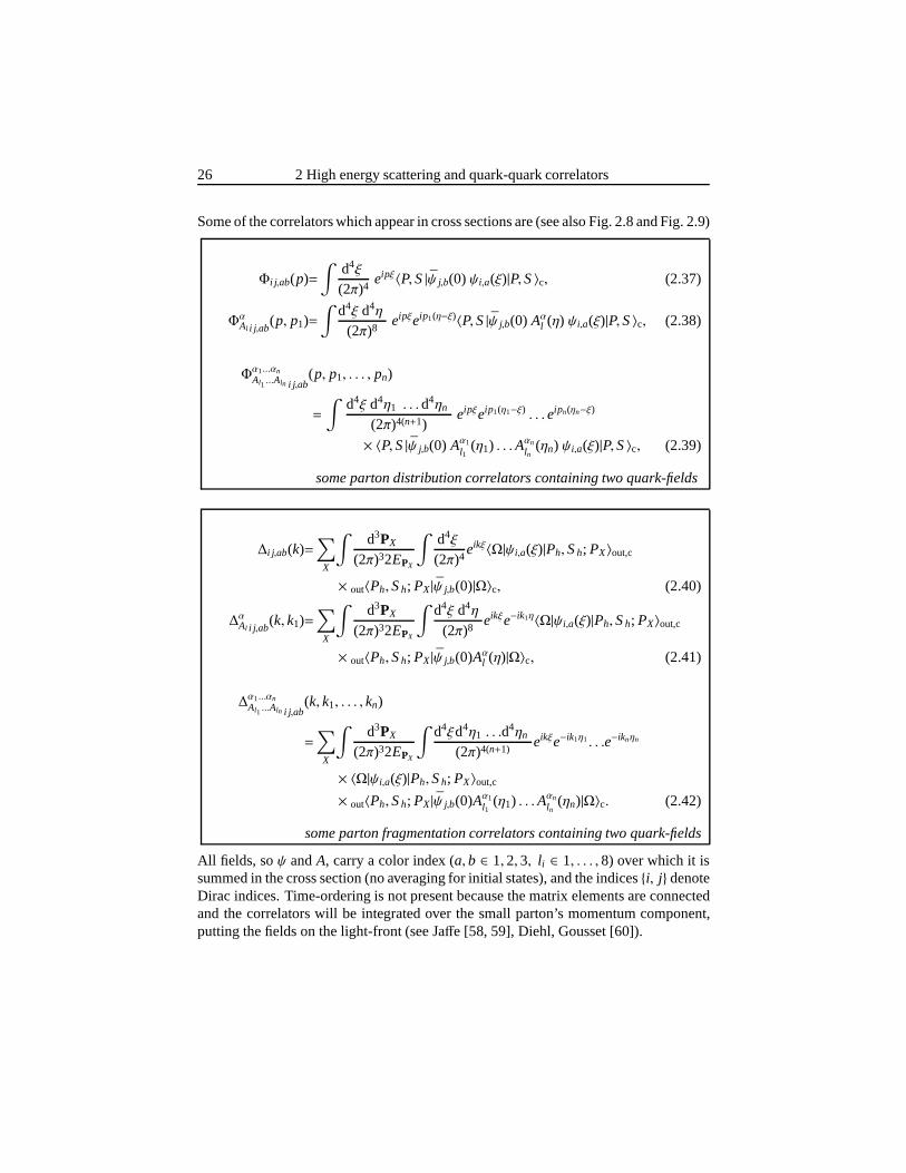
Some of the correlators which appear in cross sections are (see also Fig. 2.8 and Fig. 2.9)
Φi j,ab(p)=∫
d4ξ
(2π)4eipξ〈P,S|ψ j,b(0) ψi,a(ξ)|P,S〉c, (2.37)
ΦαAl i j,ab(p, p1)=
∫d4ξ d4η
(2π)8eipξeip1(η−ξ)〈P,S|ψ j,b(0) Aα
l (η) ψi,a(ξ)|P,S〉c, (2.38)
Φα1...αnAl1 ...Aln i j,ab
(p, p1, . . . , pn)
=
∫d4ξ d4η1 . . .d4ηn
(2π)4(n+1)eipξeip1(η1−ξ) . . .eipn(ηn−ξ)
× 〈P,S|ψ j,b(0) Aα1
l1(η1) . . .Aαn
ln(ηn) ψi,a(ξ)|P,S〉c, (2.39)
some parton distribution correlators containing two quark-fields
∆i j,ab(k)=∑
X
∫d3PX
(2π)32EPX
∫d4ξ
(2π)4eikξ〈Ω|ψi,a(ξ)|Ph,Sh; PX〉out,c
× out〈Ph,Sh; PX|ψ j,b(0)|Ω〉c, (2.40)
∆αAl i j,ab(k, k1)=
∑
X
∫d3PX
(2π)32EPX
∫d4ξ d4η
(2π)8eikξe−ik1η〈Ω|ψi,a(ξ)|Ph,Sh; PX〉out,c
× out〈Ph,Sh; PX|ψ j,b(0)Aαl (η)|Ω〉c, (2.41)
∆α1...αnAl1 ...Aln i j,ab
(k, k1, . . . , kn)
=∑
X
∫d3PX
(2π)32EPX
∫d4ξd4η1 . . .d4ηn
(2π)4(n+1)eikξe−ik1η1. . .e−iknηn
× 〈Ω|ψi,a(ξ)|Ph,Sh; PX〉out,c
× out〈Ph,Sh; PX|ψ j,b(0)Aα1l1
(η1) . . .Aαn
ln(ηn)|Ω〉c. (2.42)
some parton fragmentation correlators containing two quark-fields
All fields, soψ andA, carry a color index (a, b ∈ 1, 2, 3, l i ∈ 1, . . . , 8) over which it issummed in the cross section (no averaging for initial states), and the indicesi, j denoteDirac indices. Time-ordering is not present because the matrix elements are connectedand the correlators will be integrated over the small parton’s momentum component,putting the fields on the light-front (see Jaffe [58, 59], Diehl, Gousset [60]).
2.4 The diagrammatic expansion and the parton model 27
Φ
p p
P P ΦαA
p1p− p1 p
P P Φα1α2
AA
p1
p2p−∑pi p
P P
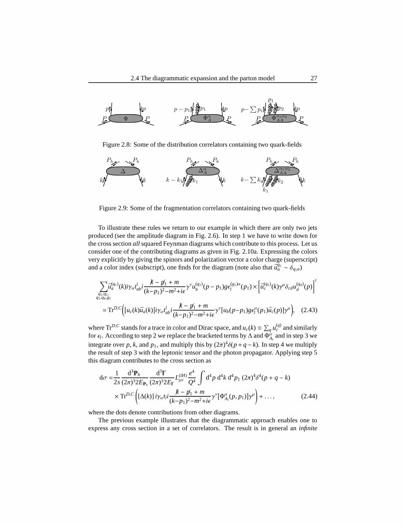
Figure 2.8: Some of the distribution correlators containing two quark-fields
∆
k k
Ph Ph
∆αA
k − k1 kk1
Ph Ph
∆α1α2
AA
k−∑ki k
k1
k2
Ph Ph
Figure 2.9: Some of the fragmentation correlators containing two quark-fields
To illustrate these rules we return to our example in which there are only two jetsproduced (see the amplitude diagram in Fig. 2.6). In step 1 wehave to write down forthe cross sectionall squared Feynman diagrams which contribute to this process.Let usconsider one of the contributing diagrams as given in Fig. 2.10a. Expressing the colorsvery explicitly by giving the spinors and polarization vector a color charge (superscript)and a color index (subscript), one finds for the diagram (notealso that ¯uq1
a ∼ δq1a)
∑
q1,q2,q3,q4,g1
u(q1)a (k)iγαtlabi
/k− p/1 +m(k−p1)2−m2+iǫ
γνu(q2)b (p− p1)gǫ(g1)α
l (p1)×[u(q3)
c (k)γµδcdu(q4)d (p)
]†
=TrD,C([
uc(k)ua(k)]iγαtlabi
/k− p/1 +m(k−p1)2−m2+iǫ
γν[ub(p−p1)gǫαl (p1)uc(p)
]γµ
), (2.43)
where TrD,C stands for a trace in color and Dirac space, anduc(k) ≡ ∑q u(q)
c and similarlyfor ǫl . According to step 2 we replace the bracketed terms by∆ andΦαAl
and in step 3 weintegrate overp, k, andp1, and multiply this by (2π)4δ(p+q− k). In step 4 we multiplythe result of step 3 with the leptonic tensor and the photon propagator. Applying step 5this diagram contributes to the cross section as
dσ =12s
d3Ph
(2π)32EPh
d3l′
(2π)32El′L(lH )µν
e4
Q4
∫d4p d4k d4p1 (2π)4δ4(p+ q− k)
× TrD,C
([∆(k)] iγαtl i
/k− p/1 +m(k−p1)2−m2+iǫ
γν[ΦαAl
(p, p1)]γµ
)+ . . . , (2.44)
where the dots denote contributions from other diagrams.The previous example illustrates that the diagrammatic approach enables one to
express any cross section in a set of correlators. The resultis in general aninfinite
28 2 High energy scattering and quark-quark correlators
incoming proton
and its outgoing remnant
outgoing hadron
and its parent jet
p− p1
k
p1p
kq q
ΦαA
∆
p− p1
k
p1p
k
P P
q q
Ph Ph
(a) (b)
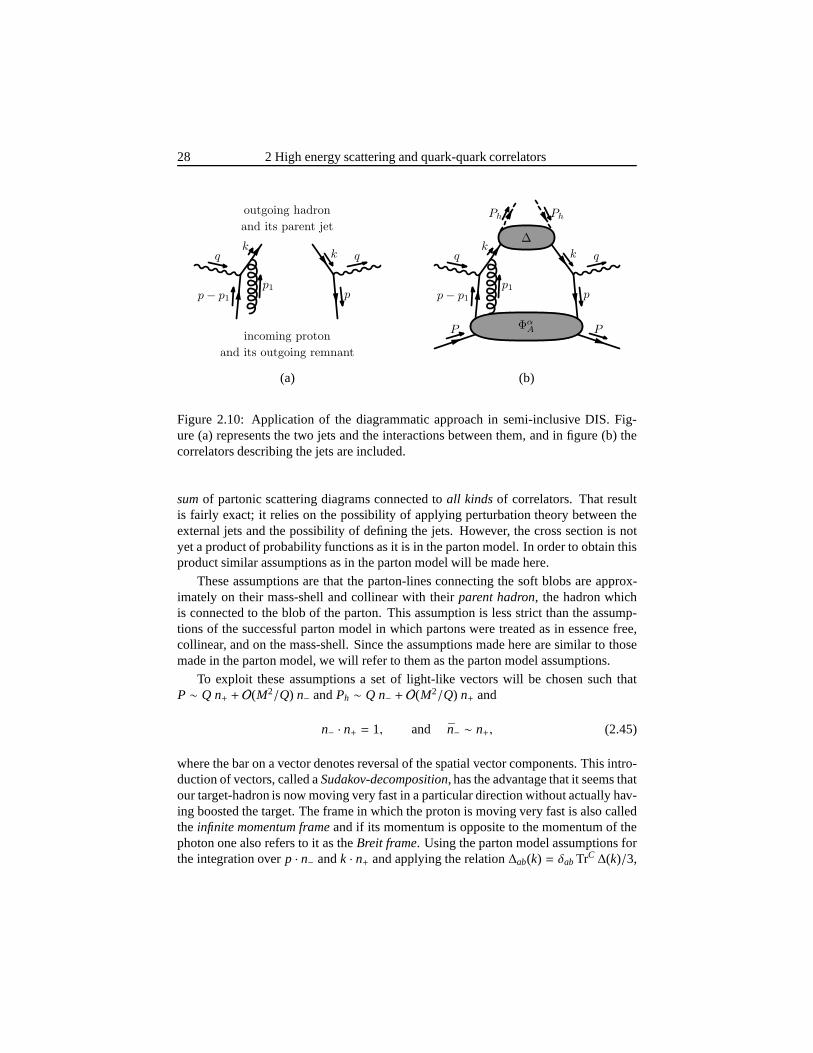
Figure 2.10: Application of the diagrammatic approach in semi-inclusive DIS. Fig-ure (a) represents the two jets and the interactions betweenthem, and in figure (b) thecorrelators describing the jets are included.
sumof partonic scattering diagrams connected toall kindsof correlators. That resultis fairly exact; it relies on the possibility of applying perturbation theory between theexternal jets and the possibility of defining the jets. However, the cross section is notyet a product of probability functions as it is in the parton model. In order to obtain thisproduct similar assumptions as in the parton model will be made here.
These assumptions are that the parton-lines connecting thesoft blobs are approx-imately on their mass-shell and collinear with theirparent hadron, the hadron whichis connected to the blob of the parton. This assumption is less strict than the assump-tions of the successful parton model in which partons were treated as in essence free,collinear, and on the mass-shell. Since the assumptions made here are similar to thosemade in the parton model, we will refer to them as the parton model assumptions.
To exploit these assumptions a set of light-like vectors will be chosen such thatP ∼ Q n+ + O(M2/Q) n− andPh ∼ Q n− + O(M2/Q) n+ and
n− · n+ = 1, and n− ∼ n+, (2.45)
where the bar on a vector denotes reversal of the spatial vector components. This intro-duction of vectors, called aSudakov-decomposition, has the advantage that it seems thatour target-hadron is now moving very fast in a particular direction without actually hav-ing boosted the target. The frame in which the proton is moving very fast is also calledthe infinite momentum frameand if its momentum is opposite to the momentum of thephoton one also refers to it as theBreit frame. Using the parton model assumptions forthe integration overp · n− andk · n+ and applying the relation∆ab(k) = δab TrC ∆(k)/3,
2.5 Quark distribution functions for spin-12 hadrons 29
one obtains for Eq. 2.44 (p± ≡ p · n∓, etc.)
dσ =12s
d3Ph
(2π)32EPh
d3l′
(2π)32El′L(lH )µν
e4
Q4
∫d2pT d2kT d2p1T dp+1 (2π)4δ2(pT + qT − kT)
× TrD
[13
TrC
( ∫dk+ ∆(k)
)TrC
(iγαtl i
/k− p/1 +m(k− p1)2 −m2 + iǫ
∣∣∣∣p−1=0k+=0
γν
×∫
dp− dp−1 ΦαAl
(p, p1))γν
)]∣∣∣∣∣∣p+=−q+
k−=q−
(1+ O
(M2/Q2
))+ . . . , (2.46)
where the subscriptT denotes transverse components with respect ton− andn+.The applied Sudakov-decomposition can be used for general scattering processes
as long as the scalar product of the observed momenta is large. For each observedhadron one can introduce a light-like vector along which thehadron is moving. Sincethe parton-lines are approximately collinear and on shell,one of the components of theparton momenta,p · n, must appear to be very small. In general one should be ableto neglect these components in the hard scattering part suchthat one can integrate theconsidered correlator over this variable. In the next section we will see that correlatorswhich are integrated over the small momentum components areprobabilities in leadingorder inM/Q.
2.5 Quark distribution functions for spin- 12 hadrons
The various functions for spin-12 hadrons will be introduced and their relevance will be
pointed out. For spin-1 targets the reader is referred to Bacchetta, Mulders [61]. Todefine the parton distributions a set of light-like vectors is constructed such that
1 = n− · n+, n− ∼ n+,
P =M2
2P+n− + P+n+, ǫ
µν
T ≡ ǫρσµνn+ρn−σ,
gµνT = gµν − nµ+nν− − nν+n
µ−, Aµ
T = gµνT Aν, for anyA. (2.47)
the basis in which parton distribution functions are defined
For any vectorA we also defineA± ≡ A · n∓, which means thatP+ is defined to be aLorentz-invariant. To describe the spin of the hadron one usually introduces
S = −SLM
2P+n− + SL
P+
Mn+ + ST , with S2
L + S2T = 1, (2.48)
which satisfies the necessary constraints:P · S = 0, S0 = 0 if P = 0, andS2 = −1.
30 2 High energy scattering and quark-quark correlators
In the next subsections we will parametrize an expansion inM/P+ of quark-quarkcorrelators, butM/P+ does not have to be small. However, in order to make use ofthe truncated expansion, calculations in the next chapterswill be performed such thatP+ ≫ M. Since the light-like vectorsn− andn+ are defined up to a rescaling (n+→αn+,n−→α−1n−), this does not put any constraint onP or the frame. In fact, for a target atrest one has for instancen+ = (M/2P+) (1, 0, 0, 1) andn− = (P+/M) (1, 0, 0,−1) whereP+ ≫ M can still be chosen.
As discussed in the previous section, one encounters in the diagrammatic expan-sion an infinite set of correlators which can all be integrated over the small momentumcomponents. As we will see in the next chapter, this infinite set can be rewritten into asingle new correlator containing the gauge link (to be defined below). In the discussedelectromagnetic processes basically two kinds of correlators appear in the final result.
The first kind appears in cross sections which are not sensitive to the transversemomenta of the constituents and is the so-calledintegratedcorrelator. Including aWilson line operatorL, it reads
Φi j (x,P,S) =∫
dξ−
2πeixP+ξ−〈P,S|ψ j(0)L0T, ξ
+
(0−, ξ−)ψi(ξ)|P,S〉c∣∣∣ξ+=0ξT=0
, (2.49)
where over the color indices was summed and wherex is the longitudinal momentumfraction of the quark with respect to its parent hadron,x ≡ p+/P+. The Wilson lineoperator, or also calledgauge link, is a 3× 3 color-matrix-operator and makes thebilocal operatorψ j,b(0) ψi,a(ξ) invariant under color gauge transformations. A Wilsonline along a pathΞµ(λ) with Ξµ(0) = aµ andΞµ(1) = bµ is defined as
L(a, b) ≡ 1− ig
1∫
0
dλdΞµ
dλAµ(Ξ(λ))
+ (−ig)2
1∫
0
dλ1dΞµ
dλ1Aµ(Ξ(λ1))
1∫
λ1
dλ2dΞµ
dλ2Aµ(Ξ(λ2)) + . . . , (2.50)
whereAµ = Aµ
l tl . In Eq. 2.49 an abbreviation was introduced for links along straightpaths. In the abbreviation it is indicated which variables are constant along the path (0T
andξ+) and which coordinates are running (the minus components).The path for thiscase is illustrated in Fig. 2.11a. The integrated correlator will be parametrized in thenext subsection.
The second kind of correlator is encountered in cross sections which are sensitiveto the transverse momenta of the quarks. Calling it theunintegrated correlator, it alsocontains a Wilson line operator and reads
Φ[±]i j (x, pT ,P,S) =
∫dξ− d2ξT
(2π)3eipξ〈P,S|ψ j(0)L[±](0, ξ−) ψi(ξ)|P,S〉c
∣∣∣∣∣ ξ+=0p+=xP+
, (2.51)
2.5 Quark distribution functions for spin-12 hadrons 31
ξ−ψ(0)
ψ(ξ)
ξ−
ξT
ψ(0)
ψ(ξ)
a:L0T, ξ+
(0−, ξ−) b: L[+](0, ξ−)
ξ−
ξT
ψ(0)
ψ(ξ)
ξ−
ξT
c: L[−](0, ξ−) d: L[](0, ξ−)
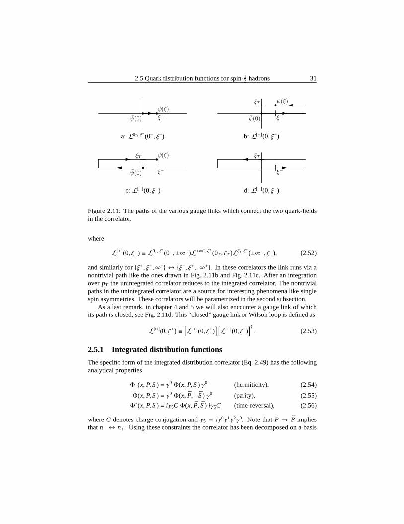
Figure 2.11: The paths of the various gauge links which connect the two quark-fieldsin the correlator.
where
L[±](0, ξ−) ≡ L0T, ξ+
(0−,±∞−)L±∞−, ξ+ (0T , ξT)LξT, ξ+
(±∞−, ξ−), (2.52)
and similarly forξ+, ξ−,∞− ↔ ξ−, ξ+, ∞+. In these correlators the link runs via anontrivial path like the ones drawn in Fig. 2.11b and Fig. 2.11c. After an integrationover pT the unintegrated correlator reduces to the integrated correlator. The nontrivialpaths in the unintegrated correlator are a source for interesting phenomena like singlespin asymmetries. These correlators will be parametrized in the second subsection.
As a last remark, in chapter 4 and 5 we will also encounter a gauge link of whichits path is closed, see Fig. 2.11d. This “closed” gauge link or Wilson loop is defined as
L[](0, ξ±) ≡[L[+](0, ξ±)
] [L[−](0, ξ±)
]†. (2.53)
2.5.1 Integrated distribution functions
The specific form of the integrated distribution correlator(Eq. 2.49) has the followinganalytical properties
Φ†(x,P,S) = γ0 Φ(x,P,S) γ0 (hermiticity), (2.54)
Φ(x,P,S) = γ0 Φ(x, P,−S) γ0 (parity), (2.55)
Φ∗(x,P,S) = iγ5C Φ(x, P, S) iγ5C (time-reversal), (2.56)
whereC denotes charge conjugation andγ5 ≡ iγ0γ1γ2γ3. Note thatP → P impliesthatn− ↔ n+. Using these constraints the correlator has been decomposed on a basis
32 2 High energy scattering and quark-quark correlators
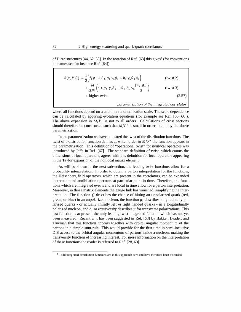
of Dirac structures [44, 62, 63]. In the notation of Ref. [63]this gives4 (for conventionson names see for instance Ref. [64])
Φ(x,P,S) =12
(f1 /n+ + SL g1 γ5 /n+ + h1 γ5/ST /n+
)(twist 2)
+M
2P+
(e+ gT γ5/ST + SL hL γ5
[ /n+, /n−]2
)(twist 3)
+ higher twist. (2.57)
parametrization of the integrated correlator
where all functions depend onx and on a renormalization scale. The scale dependencecan be calculated by applying evolution equations (for example see Ref. [65, 66]).The above expansion inM/P+ is not to all orders. Calculations of cross sectionsshould therefore be constructed such thatM/P+ is small in order to employ the aboveparametrization.
In the parametrization we have indicated the twist of the distribution functions. Thetwist of a distribution function defines at which order inM/P+ the function appears inthe parametrization. This definition of “operational twist” for nonlocal operators wasintroduced by Jaffe in Ref. [67]. The standard definition of twist, which countsthedimensions of local operators, agrees with this definition for local operators appearingin the Taylor expansion of the nonlocal matrix element.
As will be shown in the next subsection, the leading twist functions allow for aprobability interpretation. In order to obtain a parton interpretation for the functions,the Heisenberg field operators, which are present in the correlators, can be expandedin creation and annihilation operators at particular pointin time. Therefore, the func-tions which are integrated overx and are local in time allow for a parton interpretation.Moreover, in those matrix elements the gauge link has vanished, simplifying the inter-pretation. The functionf1 describes the chance of hitting an unpolarized quark (red,green, or blue) in an unpolarized nucleon, the functiong1 describes longitudinally po-larized quarks - or actually chirally left or right handed quarks - in a longitudinallypolarized nucleon, andh1 or transversitydescribes it for transverse polarizations. Thislast function is at present the only leading twist integrated function which has not yetbeen measured. Recently, it has been suggested in Ref. [68] by Bakker, Leader, andTrueman that this function appears together with orbital angular momentum of thepartons in a simple sum-rule. This would provide for the firsttime in semi-inclusiveDIS access to the orbital angular momentum of partons insidea nucleon, making thetransversity function of increasing interest. For more information on the interpretationof these functions the reader is referred to Ref. [28, 69].
4T-odd integrated distribution functions are in this approach zero and have therefore been discarded.
2.5 Quark distribution functions for spin-12 hadrons 33
2.5.2 Transverse momentum dependent distribution functions
Gauge Invariant correlators and T-odd behavior
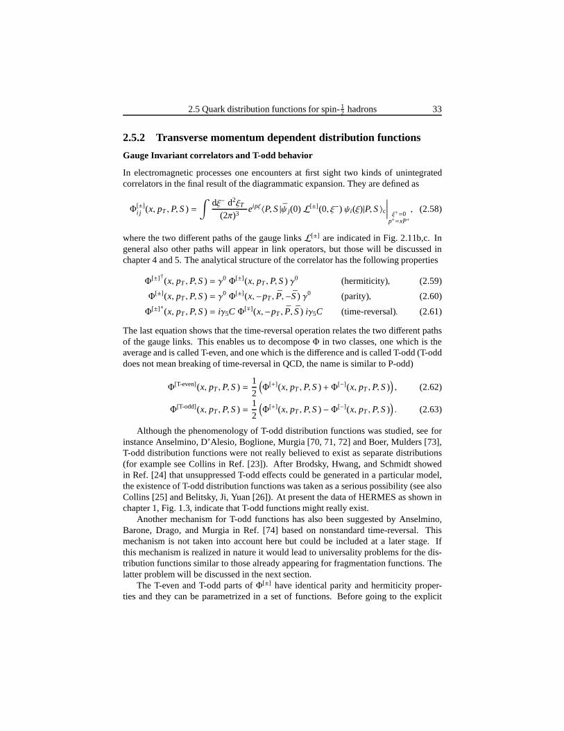
In electromagnetic processes one encounters at first sight two kinds of unintegratedcorrelators in the final result of the diagrammatic expansion. They are defined as
Φ[±]i j (x, pT ,P,S) =
∫dξ− d2ξT
(2π)3eipξ〈P,S|ψ j(0)L[±](0, ξ−) ψi(ξ)|P,S〉c
∣∣∣∣∣ ξ+=0p+=xP+
, (2.58)
where the two different paths of the gauge linksL[±] are indicated in Fig. 2.11b,c. Ingeneral also other paths will appear in link operators, but those will be discussed inchapter 4 and 5. The analytical structure of the correlator has the following properties
Φ[±]†(x, pT ,P,S) = γ0 Φ[±](x, pT ,P,S) γ0 (hermiticity), (2.59)
Φ[±](x, pT ,P,S) = γ0 Φ[±](x,−pT , P,−S) γ0 (parity), (2.60)
Φ[±]∗(x, pT ,P,S) = iγ5C Φ[∓](x,−pT , P, S) iγ5C (time-reversal). (2.61)
The last equation shows that the time-reversal operation relates the two different pathsof the gauge links. This enables us to decomposeΦ in two classes, one which is theaverage and is called T-even, and one which is the difference and is called T-odd (T-odddoes not mean breaking of time-reversal in QCD, the name is similar to P-odd)
Φ[T-even](x, pT ,P,S) =12
(Φ[+](x, pT ,P,S) + Φ[−](x, pT ,P,S)
), (2.62)
Φ[T-odd](x, pT ,P,S) =12
(Φ[+](x, pT ,P,S) − Φ[−](x, pT ,P,S)
). (2.63)
Although the phenomenology of T-odd distribution functions was studied, see forinstance Anselmino, D’Alesio, Boglione, Murgia [70, 71, 72] and Boer, Mulders [73],T-odd distribution functions were not really believed to exist as separate distributions(for example see Collins in Ref. [23]). After Brodsky, Hwang, and Schmidt showedin Ref. [24] that unsuppressed T-odd effects could be generated in a particular model,the existence of T-odd distribution functions was taken as aserious possibility (see alsoCollins [25] and Belitsky, Ji, Yuan [26]). At present the data of HERMES as shown inchapter 1, Fig. 1.3, indicate that T-odd functions might really exist.
Another mechanism for T-odd functions has also been suggested by Anselmino,Barone, Drago, and Murgia in Ref. [74] based on nonstandard time-reversal. Thismechanism is not taken into account here but could be included at a later stage. Ifthis mechanism is realized in nature it would lead to universality problems for the dis-tribution functions similar to those already appearing forfragmentation functions. Thelatter problem will be discussed in the next section.
The T-even and T-odd parts ofΦ[±] have identical parity and hermiticity proper-ties and they can be parametrized in a set of functions. Before going to the explicit
34 2 High energy scattering and quark-quark correlators
parametrizations it is interesting to note that a distribution correlator can now be givenby a T-even and a sign dependent T-odd part
Φ[±](x, pT ,P,S) = Φ[T-even](x, pT ,P,S) ±Φ[T-odd](x, pT ,P,S). (2.64)
This means that T-odd distribution functions enter with a sign [25, 75] depending onthe path of the gauge link. In the next chapters we will see that this path is set by theprocess or subprocess.
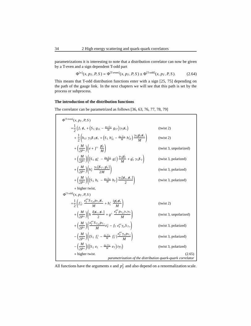
The introduction of the distribution functions
The correlator can be parametrized as follows [36, 63, 76, 77, 78, 79]
Φ[T-even](x, pT ,P,S)
=12
(f1 /n+ +
(SL g1L − pT ·ST
M g1T
)γ5 /n+
)(twist 2)
+12
(h1T γ5/ST /n+ +
(SL h⊥1L −
pT ·STM h⊥1T
) γ5p/T /n+M
)(twist 2)
+
( M2P+
) (e+ f ⊥
p/TM
)(twist 3, unpolarized)
+
( M2P+
) ((SL g⊥L −
pT ·STM g⊥T
) γ5p/TM+ g′T γ5/ST
)(twist 3, polarized)
+
( M2P+
) (h⊥T
γ5[/ST , p/T ]2M
)(twist 3, polarized)
+
( M2P+
) ((SL hL − pT ·ST
M hT
) γ5[ /n+, /n−]2
)(twist 3, polarized)
+ higher twist,
Φ[T-odd](x, pT ,P,S)
=12
(f ⊥1T
ǫµν
T STµpT ν /n+M
+ h⊥1ip/T /n+
M
)(twist 2)
+
( M2P+
) hi[ /n+, /n−]
2+ g⊥
ǫµν
T pTµγνγ5
M
(twist 3, unpolarized)
+
( M2P+
) ( ǫµνT STµpT ν
Me⊥T − fT ǫ
µν
T γµSTν
)(twist 3, polarized)
−( M2P+
) ((SL f ⊥L −
pT ·STM f ⊥T
) ǫµνT γµpT ν
M
)(twist 3, polarized)
−( M2P+
) ((SL eL − pT ·ST
M eT
)iγ5
)(twist 3, polarized)
+ higher twist. (2.65)parametrization of the distribution quark-quark correlator
All functions have the argumentsx andp2T and also depend on a renormalization scale.
2.5 Quark distribution functions for spin-12 hadrons 35
In contrast to the integrated distribution functions the scale dependence is not knownfor transverse momentum dependent functions (see for instance Henneman [66]).
In the T-odd correlator the new functionsg⊥, e⊥T , and f⊥T are included. The functiong⊥ (as defined in Ref. [36]) and the existence of the others were discovered in Ref. [36].Subsequently, a complete parametrization was given by Goeke, Metz, and Schlegel inRef. [79]. The fact that
∫d2pT Φ
[T-odd](x, pT) = 0 leads to constraints for the T-oddfunctionsh, fT , eL, and f⊥T (see for example Ref. [35, 79]).
The first transverse moment of the correlatorΦ and some functionfi is defined as
Φα∂(x,P,S) ≡∫
d2pT pαT Φ(x, pT ,P,S). (2.66)
f (1)i (x) ≡
∫d2pT
p2T
2M2fi(x, p2
T). (2.67)
The introduced functions describe how the quarks are distributed in the nucleon.The leading twist functions (twist 2) are again probabilityfunctions and therefore con-tain valuable information. For instance, the functionsf1(x, p2
T) andg1L(x, p2T) are gen-
eralizations off1(x) andg1(x). For more information on the interpretation of T-evenfunctions the reader is referred to Ref. [64, 80].
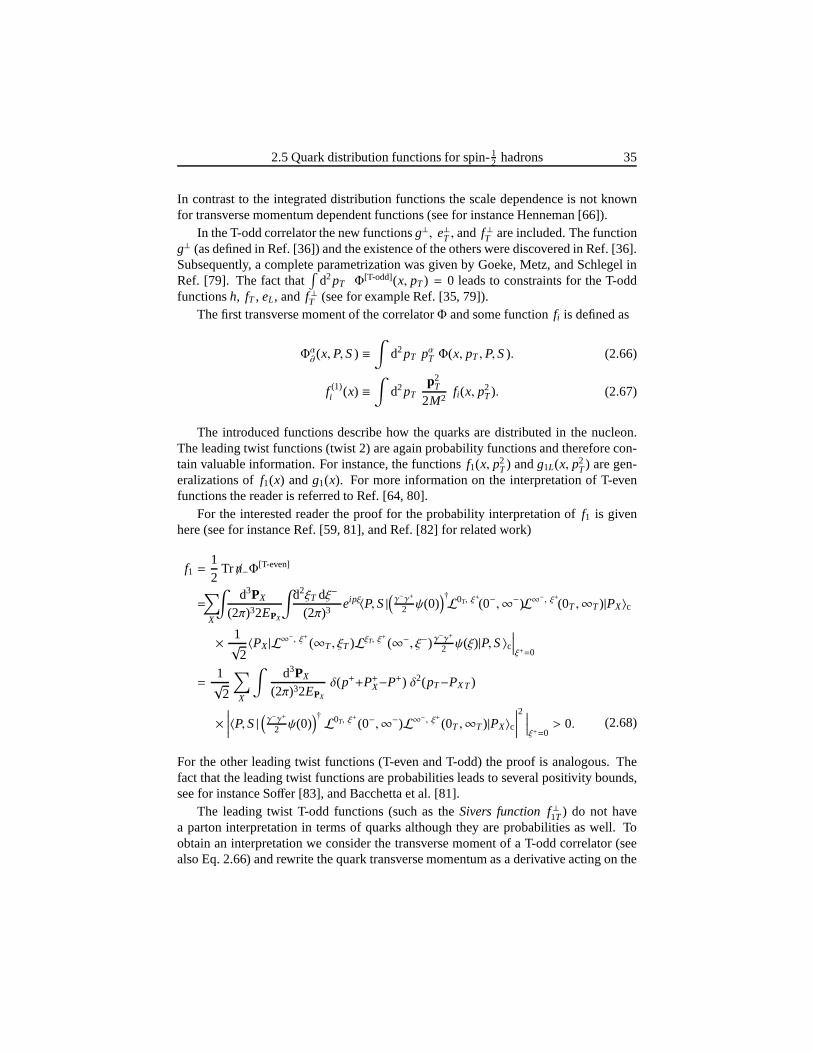
For the interested reader the proof for the probability interpretation of f1 is givenhere (see for instance Ref. [59, 81], and Ref. [82] for related work)
f1 =12
Tr /n−Φ[T-even]
=∑
X
∫d3PX
(2π)32EPX
∫d2ξT dξ−
(2π)3eipξ〈P,S|
(γ−γ+
2 ψ(0))†L0T, ξ
+
(0−,∞−)L∞−, ξ+(0T ,∞T)|PX〉c
× 1√
2〈PX|L∞
−, ξ+ (∞T , ξT )LξT, ξ+
(∞−, ξ−) γ−γ+
2 ψ(ξ)|P,S〉c∣∣∣∣ξ+=0
=1√
2
∑
X
∫d3PX
(2π)32EPX
δ(p++P+X−P+) δ2(pT−PXT)
×∣∣∣∣∣〈P,S|
(γ−γ+
2 ψ(0))†L0T, ξ
+
(0−,∞−)L∞−, ξ+(0T ,∞T)|PX〉c∣∣∣∣∣2 ∣∣∣∣ξ+=0
> 0. (2.68)
For the other leading twist functions (T-even and T-odd) theproof is analogous. Thefact that the leading twist functions are probabilities leads to several positivity bounds,see for instance Soffer [83], and Bacchetta et al. [81].
The leading twist T-odd functions (such as theSivers function f⊥1T ) do not havea parton interpretation in terms of quarks although they areprobabilities as well. Toobtain an interpretation we consider the transverse momentof a T-odd correlator (seealso Eq. 2.66) and rewrite the quark transverse momentum as aderivative acting on the
36 2 High energy scattering and quark-quark correlators
gauge links alone
Φ[T-odd]α∂
(x,P,S) =12
∫d2pT
∫dξ− d2ξT
(2π)3eipξ〈P,S|ψ j(0)
×(i∂αξT
[L[+](0, ξ−)−L[−](0, ξ−)
])ψi(ξ)|P,S〉c
∣∣∣∣ξ+=0p+=xP+
. (2.69)
Using identities of Ref. [35] (the second identity can be proven by using thatG+α ∼[iD+, iDα], i∂+ξLξ
+ ,ξT (η−, ξ−) = Lξ+ ,ξT (η−, ξ−)iD+(ξ), and shiftingiD+ to the side)
i∂αξTL±∞−, a+ (0T , ξT )
= L±∞−, a+ (0T , ξT)iDαT(±∞, a+, ξT),
iDαT(ζ−, a+, ξT )LξT, a+(ζ−, ξ−)
= LξT, a+ (ζ−, ξ−)iDαT(ξ−, a+, ξT)
− g
ξ−∫
ζ−
dη− LξT, a+ (ζ−, η−)G+αT (η−, a+, ξT)LξT, a+ (η−, ξ−), (2.70)
identities concerning gauge links
wherea+ is some constant andiDαT(ξ−, a+, ξT) ≡ i∂α
ξT+ gAαT(ξ−, a+, ξT), the derivative
on the difference of the links can be written as
Φ[T-odd]α∂
(x,P,S) =g2
∫dξ−dη−
2πeixP+ξ−〈P,S|ψ j(0)
× L0T, ξ+
(0−, η−)G+αT (η)L0T, ξ+
(η−, ξ−)ψi(ξ)|P,S〉c∣∣∣η+=ξ+=0ηT=ξT=0
. (2.71)
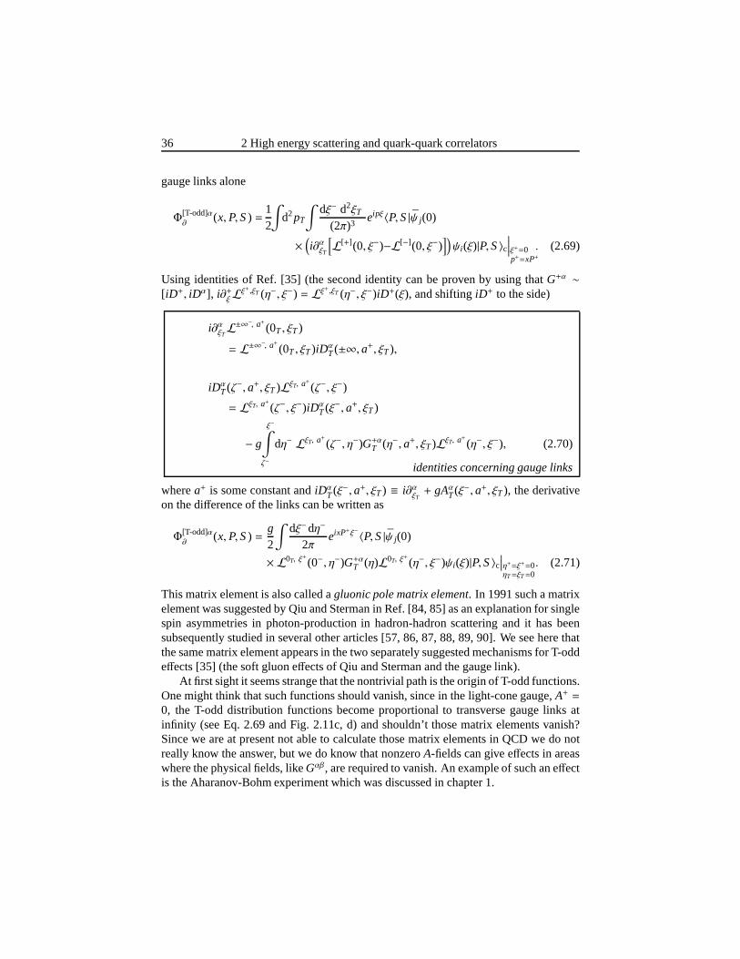
This matrix element is also called agluonic pole matrix element. In 1991 such a matrixelement was suggested by Qiu and Sterman in Ref. [84, 85] as anexplanation for singlespin asymmetries in photon-production in hadron-hadron scattering and it has beensubsequently studied in several other articles [57, 86, 87,88, 89, 90]. We see here thatthe same matrix element appears in the two separately suggested mechanisms for T-oddeffects [35] (the soft gluon effects of Qiu and Sterman and the gauge link).
At first sight it seems strange that the nontrivial path is theorigin of T-odd functions.One might think that such functions should vanish, since in the light-cone gauge,A+ =0, the T-odd distribution functions become proportional totransverse gauge links atinfinity (see Eq. 2.69 and Fig. 2.11c, d) and shouldn’t those matrix elements vanish?Since we are at present not able to calculate those matrix elements in QCD we do notreally know the answer, but we do know that nonzeroA-fields can give effects in areaswhere the physical fields, likeGαβ, are required to vanish. An example of such an effectis the Aharanov-Bohm experiment which was discussed in chapter 1.
2.5 Quark distribution functions for spin-12 hadrons 37
The Lorentz invariance relations and g⊥⊥⊥
Before the paper of Brodsky, Hwang, and Schmidt [24] appeared, physical effects fromthe gauge link were assumed to be absent which led to several interesting observations.Not only did T-odd effects disappear, but relations between the various functions inthe correlator were also obtained. By arguing that the correlatorΦ(x, pT ,P,S) couldbe written in terms of only fermion fields, the starting pointthen was another objectΦ(p,P,S) which is defined by
Φi j (p,P,S) =∫
d4ξ
(2π)4eipξ 〈P,S| ψ j(0) ψi(ξ) |P,S〉c. (2.72)
This quantityΦ(p,P,S) is the fully unintegrated correlator, from whichΦ(x, pT ,P,S)(without gauge link) is obtained via
Φ(x, pT ,P,S) =∫
dp− Φ(p,P,S). (2.73)
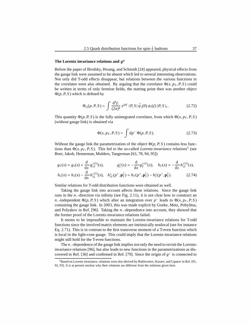
Without the gauge link the parametrization of the objectΦ(p,P,S) contains less func-tions thanΦ(x, pT ,P,S). This led to the so-calledLorentz-invariance relations5 (seeBoer, Jakob, Henneman, Mulders, Tangerman [63, 78, 94, 95])
gT(x) = g1(x) +ddx
g⊥(1)1T (x), g⊥L (x) = − d
dxg⊥(1)
T (x), hT(x) = − ddx
h⊥(1)1T (x),
hL(x) = h1(x) − ddx
h⊥(1)1L (x), h⊥1L(p+, p2
T) = hT(p+, p2T) − h⊥T (p+, p2
T). (2.74)
Similar relations for T-odd distribution functions were obtained as well.Taking the gauge link into account affects these relations. Since the gauge link
runs in then−-direction via infinity (see Fig. 2.11), it is not clear how toconstruct ann−-independentΦ(p,P,S) which after an integration overp− leads toΦ(x, pT ,P,S)containing the gauge link. In 2003, this was made explicit byGoeke, Metz, Pobylitsa,and Polyakov in Ref. [96]. Taking then−-dependence into account, they showed thatthe former proof of the Lorentz-invariance relations failed.
It seems to be impossible to maintain the Lorentz-invariance relations for T-oddfunctions since the involved matrix elements are intrinsically nonlocal (see for instanceEq. 2.71). This is in contrast to the first transverse moment of a T-even function whichis local in the light-cone gauge. This could imply that the Lorentz-invariance relationsmight still hold for the T-even functions.
Then−-dependence of the gauge link implies not only the need to revisit the Lorentz-invariance relations [96], but also leads to new functions in the parametrizations as dis-covered in Ref. [36] and confirmed in Ref. [79]. Since the origin of g⊥ is connected to
5Based on Lorentz invariance, relations were also derived byBukhvostov, Kuraev, and Lipatov in Ref. [91,92, 93]. It is at present unclear why their relations are different from the relations given here.
38 2 High energy scattering and quark-quark correlators
the non-validity of the Lorentz-invariance relations, a measurement ofg⊥ or checkingthe Lorentz-invariance relations (Eq. 2.74) would be interesting. In the next chapter itwill be pointed out howg⊥ can be accessed.
2.6 Quark fragmentation functions into spin-12 hadrons
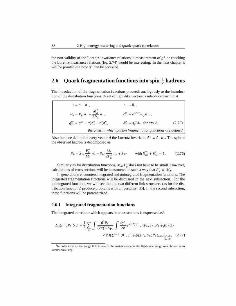
The introduction of the fragmentation functions proceeds analogously to the introduc-tion of the distribution functions. A set of light-like vectors is introduced such that
1 = n− · n+, n− ∼ n+,
Ph = P−h n− +M2
h
2P−hn+, ǫ
µν
T ≡ ǫρσµνn+ρn−σ,
gµνT = gµν − nµ+nν− − nν+n
µ−, Aµ
T = gµνT Aν, for anyA. (2.75)
the basis in which parton fragmentation functions are defined
Also here we define for every vectorA the Lorentz-invariantsA± ≡ A · n∓. The spin ofthe observed hadron is decomposed as
Sh = ShLP−hMh
n− − ShLMh
2P−hn+ + ShT with S2
hL + S2hT = 1. (2.76)
Similarly as for distribution functions,Mh/P−h does not have to be small. However,calculations of cross sections will be constructed in such away thatP−h ≫ Mh.
In general one encounters integrated and unintegrated fragmentation functions. Theintegrated fragmentation functions will be discussed in the next subsection. For theunintegrated functions we will see that the two different link structures (as for the dis-tribution functions) produce problems with universality [35]. In the second subsection,these functions will be parametrized.
2.6.1 Integrated fragmentation functions
The integrated correlator which appears in cross sections is expressed as6
∆i j (z−1,Ph,Sh) ≡13
∑
X
∫d3PX
(2π)32EPX
∫dη+
2πeiz−1P−hη
+
out〈Ph,Sh; PX|ψ j(0)|Ω〉c
× 〈Ω|L0T, η−(0+, η+)ψi(η)|Ph,Sh; PX〉out,c
∣∣∣η−=0ηT=0
, (2.77)
6In order to write the gauge link in one of the matrix elements the light-cone gauge was chosen in anintermediate step.
2.6 Quark fragmentation functions into spin-12 hadrons 39
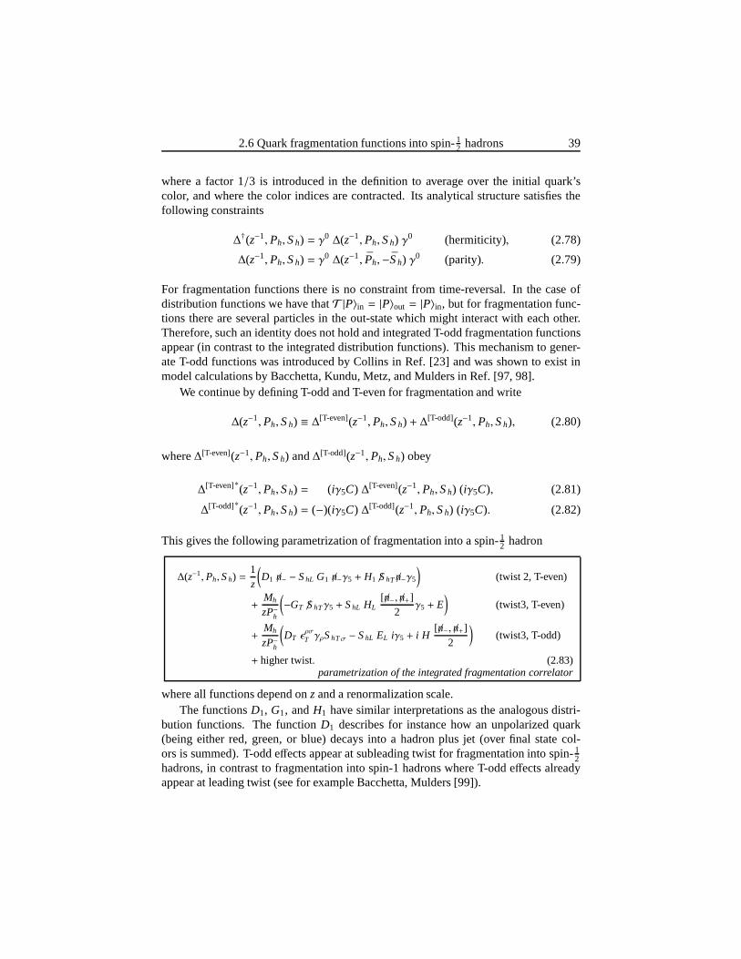
where a factor 1/3 is introduced in the definition to average over the initial quark’scolor, and where the color indices are contracted. Its analytical structure satisfies thefollowing constraints
∆†(z−1,Ph,Sh) = γ0 ∆(z−1,Ph,Sh) γ0 (hermiticity), (2.78)
∆(z−1,Ph,Sh) = γ0 ∆(z−1, Ph,−Sh) γ0 (parity). (2.79)
For fragmentation functions there is no constraint from time-reversal. In the case ofdistribution functions we have thatT |P〉in = |P〉out = |P〉in, but for fragmentation func-tions there are several particles in the out-state which might interact with each other.Therefore, such an identity does not hold and integrated T-odd fragmentation functionsappear (in contrast to the integrated distribution functions). This mechanism to gener-ate T-odd functions was introduced by Collins in Ref. [23] and was shown to exist inmodel calculations by Bacchetta, Kundu, Metz, and Mulders in Ref. [97, 98].
We continue by defining T-odd and T-even for fragmentation and write
∆(z−1,Ph,Sh) ≡ ∆[T-even](z−1,Ph,Sh) + ∆[T-odd](z−1,Ph,Sh), (2.80)
where∆[T-even](z−1,Ph,Sh) and∆[T-odd](z−1,Ph,Sh) obey
∆[T-even]∗(z−1,Ph,Sh) = (iγ5C) ∆[T-even](z−1,Ph,Sh) (iγ5C), (2.81)
∆[T-odd]∗(z−1,Ph,Sh) = (−)(iγ5C) ∆[T-odd](z−1,Ph,Sh) (iγ5C). (2.82)
This gives the following parametrization of fragmentationinto a spin-12 hadron
∆(z−1,Ph,Sh) =1z
(D1 /n− − ShL G1 /n−γ5 + H1 /ShT /n−γ5
)(twist 2, T-even)
+Mh
zP−h
(−GT /ShTγ5 + ShL HL
[ /n−, /n+]2
γ5 + E)
(twist3, T-even)
+Mh
zP−h
(DT ǫ
ρσ
T γρShTσ − ShL EL iγ5 + i H[ /n−, /n+]
2
)(twist3, T-odd)
+ higher twist. (2.83)parametrization of the integrated fragmentation correlator
where all functions depend onzand a renormalization scale.The functionsD1, G1, andH1 have similar interpretations as the analogous distri-
bution functions. The functionD1 describes for instance how an unpolarized quark(being either red, green, or blue) decays into a hadron plus jet (over final state col-ors is summed). T-odd effects appear at subleading twist for fragmentation into spin- 1
2hadrons, in contrast to fragmentation into spin-1 hadrons where T-odd effects alreadyappear at leading twist (see for example Bacchetta, Mulders[99]).
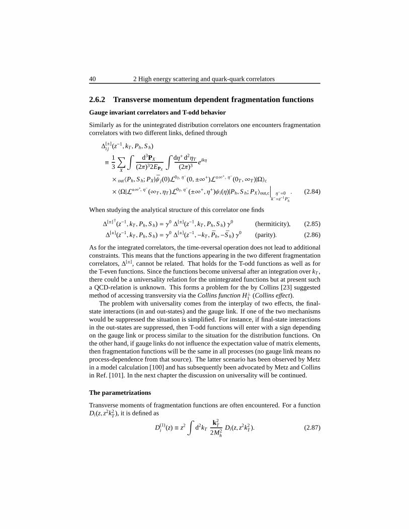
40 2 High energy scattering and quark-quark correlators
2.6.2 Transverse momentum dependent fragmentation functions
Gauge invariant correlators and T-odd behavior
Similarly as for the unintegrated distribution correlators one encounters fragmentationcorrelators with two different links, defined through
∆[±]i j (z−1, kT ,Ph,Sh)
≡ 13
∑
X
∫d3PX
(2π)32EPX
∫dη+d2ηT
(2π)3eikη
× out〈Ph,Sh; PX|ψ j(0)L0T, η−(0,±∞+)L±∞+, η−(0T ,∞T)|Ω〉c
× 〈Ω|L±∞+, η− (∞T , ηT)L0T, η−(±∞+, η+)ψi(η)|Ph,Sh; PX〉out,c
∣∣∣∣ η−=0k−=z−1P−h
. (2.84)
When studying the analytical structure of this correlator one finds
∆[±] †(z−1, kT ,Ph,Sh) = γ0 ∆[±](z−1, kT ,Ph,Sh) γ0 (hermiticity), (2.85)
∆[±](z−1, kT ,Ph,Sh) = γ0 ∆[±](z−1,−kT , Ph,−Sh) γ0 (parity). (2.86)
As for the integrated correlators, the time-reversal operation does not lead to additionalconstraints. This means that the functions appearing in thetwo different fragmentationcorrelators,∆[±] , cannot be related. That holds for the T-odd functions as well as forthe T-even functions. Since the functions become universalafter an integration overkT ,there could be a universality relation for the unintegratedfunctions but at present sucha QCD-relation is unknown. This forms a problem for the by Collins [23] suggestedmethod of accessing transversity via theCollins function H⊥1 (Collins effect).
The problem with universality comes from the interplay of two effects, the final-state interactions (in and out-states) and the gauge link. If one of the two mechanismswould be suppressed the situation is simplified. For instance, if final-state interactionsin the out-states are suppressed, then T-odd functions willenter with a sign dependingon the gauge link or process similar to the situation for the distribution functions. Onthe other hand, if gauge links do not influence the expectation value of matrix elements,then fragmentation functions will be the same in all processes (no gauge link means noprocess-dependence from that source). The latter scenariohas been observed by Metzin a model calculation [100] and has subsequently been advocated by Metz and Collinsin Ref. [101]. In the next chapter the discussion on universality will be continued.
The parametrizations
Transverse moments of fragmentation functions are often encountered. For a functionDi(z, z2k2
T), it is defined as
D(1)i (z) ≡ z2
∫d2kT
k2T
2M2h
Di(z, z2k2
T). (2.87)
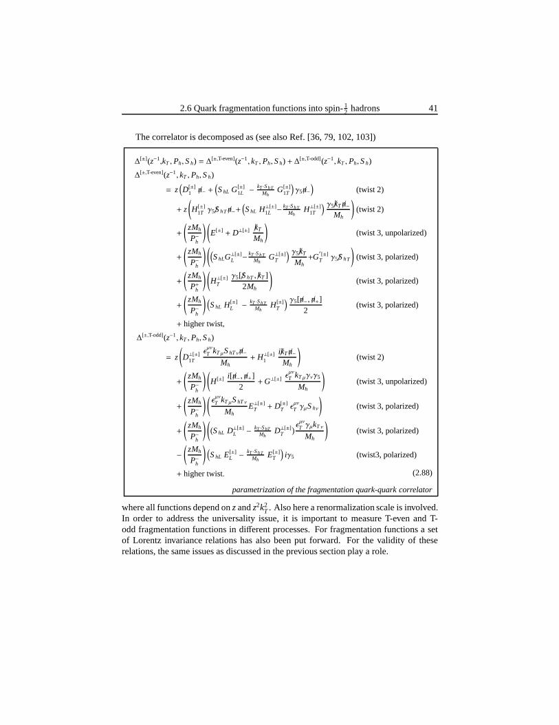
2.6 Quark fragmentation functions into spin-12 hadrons 41
The correlator is decomposed as (see also Ref. [36, 79, 102, 103])
∆[±](z−1,kT ,Ph,Sh) = ∆[±,T-even](z−1, kT ,Ph,Sh) + ∆
[±,T-odd](z−1, kT ,Ph,Sh)
∆[±,T-even](z−1, kT ,Ph,Sh)
= z(D[±]
1 /n− +(ShL G[±]
1L −kT ·ShT
MhG[±]
1T
)γ5 /n−
)(twist 2)
+ z
(H[±]
1T γ5/ShT /n−+(ShL H⊥[±]
1L −kT ·ShT
MhH⊥[±]
1T
) γ5/kT /n−Mh
)(twist 2)
+
(zMh
P−h
) (E[±] + D⊥[±] /kT
Mh
)(twist 3, unpolarized)
+
(zMh
P−h
) ((ShLG
⊥[±]L − kT ·ShT
MhG⊥[±]
T
) γ5/kT
Mh+G
′ [±]T γ5/ShT
)(twist 3, polarized)
+
(zMh
P+h
) (H⊥[±]
T
γ5[/ShT , /kT ]2Mh
)(twist 3, polarized)
+
(zMh
P−h
) (ShL H[±]
L − kT ·ShTMh
H[±]T
) γ5[ /n−, /n+]2
(twist 3, polarized)
+ higher twist,
∆[±,T-odd](z−1, kT ,Ph,Sh)
= z
(D⊥[±]
1T
ǫµν
T kTµShTν /n−Mh
+ H⊥[±]1
i/kT /n−Mh
)(twist 2)
+
(zMh
P−h
) (H[±] i[ /n−, /n+]
2+G⊥[±] ǫ
µν
T kTµγνγ5
Mh
)(twist 3, unpolarized)
+
(zMh
P−h
) (ǫµν
T kTµShTν
MhE⊥[±]
T + D[±]T ǫ
µν
T γµShν
)(twist 3, polarized)
+
(zMh
P−h
) ((ShL D⊥[±]
L − kT ·ShTMh
D⊥[±]T
) ǫµνT γµkT ν
Mh
)(twist 3, polarized)
−(zMh
P−h
) (ShL E[±]
L −kT ·ShT
MhE[±]
T
)iγ5 (twist3, polarized)
+ higher twist. (2.88)
parametrization of the fragmentation quark-quark correlator
where all functions depend onzandz2k2T . Also here a renormalization scale is involved.
In order to address the universality issue, it is important to measure T-even and T-odd fragmentation functions in different processes. For fragmentation functions a setof Lorentz invariance relations has also been put forward. For the validity of theserelations, the same issues as discussed in the previous section play a role.
42 2 High energy scattering and quark-quark correlators
2.7 Summary and conclusions
We introduced several Cartesian bases and expressed head-on cross sections in terms ofLorentz-invariants. It was shown how frame-independent observables can be defined,simplifying comparisons between theoretical predictions, experimental observations,and fixed frame definitions which are already in use in the literature.
Two approaches were discussed to access the parton distribution functions. The firstapproach is the operator product expansion. Although this method has a firm theoreti-cal basis its applicability turns out to be limited. The other approach, the diagrammaticexpansion, is a field theoretical extension of the parton model. Although slightly lessrigorous than the operator product expansion, it can be applied to most hadronic scat-tering processes and agrees with the operator product expansion when applicable. Thediagrammatic approach will be used in the rest of the thesis.
It was indicated that an infinite set of diagrams, appearing in the diagrammaticexpansion, can be rewritten such that transverse momentum dependent correlators in-cluding a gauge link appear. These correlators underlie thedefinition of parton distri-butions, and provide important information on the partonicstructure of hadrons. Thedefinition of these correlators contains a bilocal operatorand a gauge link which ensuresinvariance under local color gauge transformations. Sincethe path of the gauge link in-troduces a directional dependence, new parton distribution and fragmentation functionswere discovered at twist three (for related work, see Goeke,Metz, Schlegel [79]). Ameasurement of these new functions would contribute to the understanding of the the-oretical description.
Using time-reversal, the functions can be divided in two classes, called T-even andT-odd. It was shown that the first transverse moment of T-odd distribution functionscorresponds to the gluonic pole matrix element, which Qiu and Sterman suggestedto explain T-odd effects [84, 85]. As discovered by Collins [25], it was also foundthat T-odd distribution functions appear with opposite signs in the parametrization ofcorrelators which have a gauge link via plus or minus infinity. In chapter 4 we will seethat other link structures in correlators can appear, giving more complex factors.
For fragmentation functions a universality problem was encountered due to the twopossible mechanisms to produce T-odd effects, the final-state interactions and the pres-ence of a gauge link. This means that the value of unintegrated fragmentation functionsand their transverse moments can be different for different experiments, forming a po-tential problem for extracting transversity via the Collins effect. It is therefore importantto compare fragmentation functions which are measured in different processes (for ex-ample theirz-dependences). If for instance one of the two effects is suppressed, a simplesign relation (plus or minus) should appear between functions which have gauge linksvia plus or minus infinity. The discussion on the universality of fragmentation functionswill be continued in the next chapter.
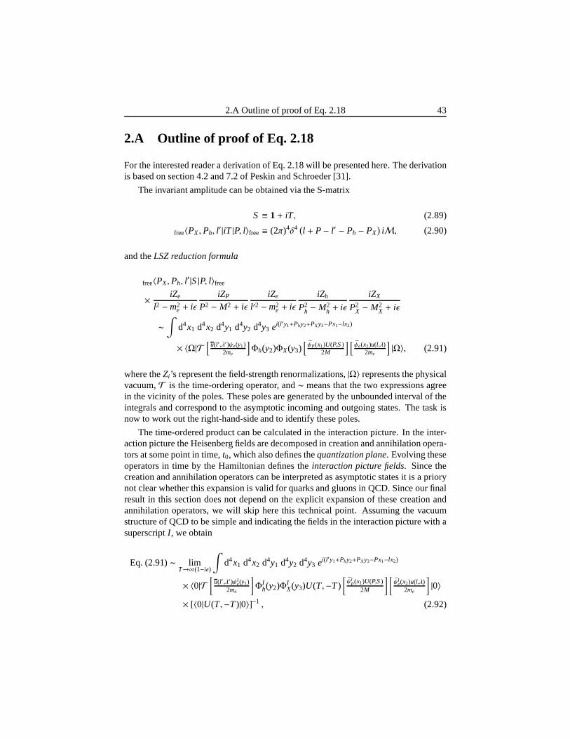
2.A Outline of proof of Eq. 2.18 43
2.A Outline of proof of Eq. 2.18
For the interested reader a derivation of Eq. 2.18 will be presented here. The derivationis based on section 4.2 and 7.2 of Peskin and Schroeder [31].
The invariant amplitude can be obtained via the S-matrix
S ≡ 1+ iT, (2.89)
free〈PX,Ph, l′|iT |P, l〉free ≡ (2π)4δ4 (
l + P− l′ − Ph − PX)iM, (2.90)
and theLSZ reduction formula
free〈PX,Ph, l′|S|P, l〉free
× iZe
l2 −m2e + iǫ
iZP
P2 − M2 + iǫiZe
l′2 −m2e + iǫ
iZh
P2h − M2
h + iǫ
iZX
P2X − M2
X + iǫ
∼
∫d4x1 d4x2 d4y1 d4y2 d4y3 ei(l′y1+Phy2+PXy3−Px1−lx2)
× 〈Ω|T[
u(l′ ,λ′)ψe(y1)2me
]Φh(y2)ΦX(y3)
[ψP(x1)U(P,S)
2M
] [ψe(x2)u(l,λ)
2me
]|Ω〉, (2.91)
where theZi ’s represent the field-strength renormalizations,|Ω〉 represents the physicalvacuum,T is the time-ordering operator, and∼ means that the two expressions agreein the vicinity of the poles. These poles are generated by theunbounded interval of theintegrals and correspond to the asymptotic incoming and outgoing states. The task isnow to work out the right-hand-side and to identify these poles.
The time-ordered product can be calculated in the interaction picture. In the inter-action picture the Heisenberg fields are decomposed in creation and annihilation opera-tors at some point in time,t0, which also defines thequantization plane. Evolving theseoperators in time by the Hamiltonian defines theinteraction picture fields. Since thecreation and annihilation operators can be interpreted as asymptotic states it is a priorynot clear whether this expansion is valid for quarks and gluons in QCD. Since our finalresult in this section does not depend on the explicit expansion of these creation andannihilation operators, we will skip here this technical point. Assuming the vacuumstructure of QCD to be simple and indicating the fields in the interaction picture with asuperscriptI , we obtain
Eq. (2.91)∼ limT→∞(1−iǫ)
∫d4x1 d4x2 d4y1 d4y2 d4y3 ei(l′y1+Phy2+PXy3−Px1−lx2)
× 〈0|T[
u(l′ ,λ′)ψIe(y1)
2me
]ΦI
h(y2)ΦIX(y3)U(T,−T)
[ψI
P(x1)U(P,S)2M
] [ψI
e(x2)u(l,λ)2me
]|0〉
× [〈0|U(T,−T)|0〉]−1 , (2.92)
44 2 High energy scattering and quark-quark correlators
where
ΦIi (x) ≡ U(x0, t0) Φ(x) U†(x0, t0), (2.93)
U(tb, ta) ≡ T exp
−i
tb∫
ta
dt′ HI (t′)
, (2.94)
and whereHI is the interacting part of the Hamiltonian in the interaction picture, and|0〉is the bare vacuum. The interaction Hamiltonian contains the electromagnetic and QCDinteractions. The electromagnetic interactions can be treated in perturbation theorywhile the QCD interactions in general cannot.
To produce nonforward matrix elements there should be at least two electromag-netic interactions, once between the incoming and outgoingelectron and once betweenthe incoming and outgoing hadrons, giving
free〈PX,Ph, l′|iT |P, l〉free
× iZe
l2 −m2e + iǫ
iZP
P2 − M2 + iǫiZe
l′2 −m2e + iǫ
iZh
P2h − M2
h + iǫ
iZX
P2X − M2
X + iǫ
∼
∫d4x1 d4x2 d4y1 d4y2 d4y3 ei(l′y1+Phy2+PXy3−Px1−lx2)(−i)2 lim
T→∞(1−iǫ)
∫d4z1 d4z2
× 〈0|T[
u(l′ ,λ′)ψIe(y1)
2me
]ΦI
h(y2)ΦIX(y3)U(T, z1)A
Iρ(z1)eJρe,I (z1)U(z1, z2)AI
σ(z2)
× eJσq,I (z2)U(z2,−T)[ψI
P(x1)U(P,S)2M
] [ψI
e(x2)u(l,λ)2me
]|0〉 [〈0|U(T,−T)|0〉]−1 , (2.95)
whereJρe/q,I (z) = Qe/q ψIe/q(z)γ
ρψIe/q(z). Using Wick’s theorem the lowest nontrivial
order inecan be worked out, giving explicitly
Eq. (2.95)
=
∫d4x1 d4x2 d4y1 d4y2 d4y3 ei(l′y1+Phy2+PXy3−Px1−lx2)(−i)2 lim
T→∞(1−iǫ)
∫d4z1 d4z2
× 〈0|T[
u(l′ ,λ′)ψIe(y1)
2me
]eJρe,I (z1)
[ψI
e(x2)u(l,λ)2me
]|0〉〈0|TAI
ρ(z1)AIσ(z2)|0〉
× 〈0|TΦIh(y2)ΦI
X(y3)U(T, z1)U(z1, z2)eJσq,I (z2)U(z2,−T)[ψI
P(x1)U(P,S)2M
]|0〉
× [〈0|U(T,−T)|0〉]−1 + O(e3)
=i
l2 −m22 + iǫ
i
l′2 −m22 + iǫ
(−ie)u(l′, λ′)γρu(l, λ)∫
d4x1 d4y2 d4y3 ei(Phy2+PXy3−Px1)
× (−i) limT→∞(1−iǫ)
∫d4z2 e−iqz2
−iq2〈0|TΦI
h(y2)ΦIX(y3)U(T, z1)U(z1, z2)eJσI (z2)
× U(z2,−T)[ψI
P(x1)U(P,S)2M
]|0〉 [〈0|U(T,−T)|0〉]−1 + O(e3). (2.96)
2.B The diagrammatic expansion 45
In order to obtain the singularities in the hadron energies it is assumed that the incominghadron only starts interacting after some point in time,ti , and that the outgoing hadronsare well-separated wave-packets after some point in time called t f . These assumptions,known asadiabatically switching on and off the interactions, restrictsz0
2 to be ti <z02 < t f . By doing so, the poles of the incoming nucleon and outgoing hadrons can be
identified after which the limitsti → −∞ andt f → ∞ can be taken. One obtains
Eq. (2.96)=i
l2 −m22 + iǫ
i
l′2 −m22 + iǫ
(−ie)u(l′, λ′)γρu(l, λ)−iq2
×∫
d4x1 d4y2 d4y3 ei(Phy2+PXy3−Px1)(−i) limti→−∞t f→∞
limT→(∞−iǫ)
∫d4z2 e−iqz2
× 〈0|TΦIh(y2)ΦI
X(y3)U(T, t f )[U(t f , ti)eJσI (z2)
]U(ti,−T)
[ψI
P(x1)U(P,S)2M
]|0〉
× [〈0|U(T,−T)|0〉]−1 + O(e3)
=i
l2 −m22 + iǫ
i
l′2 −m22 + iǫ
iZP
P2 − M2 + iǫiZX
P2X − M2
X + iǫ
iZh
P2h − M2
h + iǫ
× (−ie)u(l′, λ′)γρu(l, λ)(−i) limti→−∞t f→∞
∫d4z2 e−iqz2
−iq2
× out〈Ph,PX|TU(t0, t f )[U(t f , ti)eJσI (z2)
]U(ti, t0)|P,S〉in,c + O(e3). (2.97)
Note that all the necessary poles including the field-strength renormalizations at ordere2 (for nonforward matrix elementsZe = 1 at this order) have been produced. Aftershifting the current,Jσ(z2), yielding the delta-function which expresses momentumconservation, we can read off the invariant amplitudeM from Eq. 2.90, giving
iM = (−ie)u(l′, λ′)γρu(l, λ)
× limti→−∞t f→∞
−iq2 out〈Ph,PX|U(t0, t f )
[U(t f , ti)(−ie)JρI (0)
]U(ti, t0)|P,S〉in,c + O(e3)
= (−ie) u(l′, λ′)γρu(l, λ)−iq2 out〈Ph,PX|(−ie)Jρ(0)|P,S〉in,c+ O(e3). (2.98)
Note that the current,Jρ, is here in the Heisenberg picture.
2.B The diagrammatic expansion
For the interested reader a short outline of the derivation of two diagrams in the dia-grammatic approach will be given here. It will be pointed outhow the results can begeneralized.
46 2 High energy scattering and quark-quark correlators
Following the same procedure as applied for semi-inclusiveDIS in the previousappendix, one can derive that the invariant amplitude for general processes reads
〈free statesP|iT |free statesQ〉= limti→−∞t f→∞
out〈P|U(t0, t f )[U(t f , ti)
]U(ti, t0)|Q〉in,c, (2.99)
where theU ’s are defined in Eq. 2.94. When applying the diagrammatic expansion oneexpands the bracketed term.
At tree-level the result is expressed in terms of fields inside matrix elements. Thesefields can always be transported to the origin, yielding momentum conservation forthe incoming and outgoing particles. The lowest order result is the tree-level squaredFeynman diagram with spinors or polarization vectors replaced by Heisenberg fields inmatrix elements, multiplied by a delta-function expressing momentum conservation.
For example, consider hadron-hadron scattering with momenta P1 andP2 produc-ing two hadrons with momentaK1 andK2 approximately back-to-back in the azimuthalplane. It is assumed that the outgoing hadrons are well separated from the incominghadrons. If this is not the case then fracture functions are needed to describe the com-bined process of distribution and fragmentation. Althoughthe incoming and outgoingpartons can be quarks or gluons, we will restrict ourselves to (anti)quarks as externalpartons, the gluons can be included later on. In that case theincoming quarks or anti-quarks interact via a gluon giving quarks and antiquarks in the final state. Expandingthe bracketed term of Eq. 2.99 to lowest order this contribution is
〈K1,K2,X|iT |P1,P2〉
= (ig)2∫
d4xd4y out〈K1,K2,X|T ψ(x) /A(x)ψ(x)ψ(y) /A(y)ψ(y)|P1,P2〉in,c+O(g3). (2.100)
Overall momentum conservation can be simply obtained by making an overall shift ofx and subsequently redefiningy. One finds
〈K1,K2,X|iT |P1,P2〉 =∫
d4y out〈K1,K2,X|T ψ(0) /A(0)ψ(0)ψ(y) /A(y)ψ(y)|P1,P2〉in,c
× (2π)4δ4(P1+P2−K1−K2−∑
i
PXi
)+ O(g3). (2.101)
Since no gluons appear in the initial or final state, those fields need to be contractedwith each other yielding the gluon propagator (Wick’s theorem). Each of the quark-fields can be connected to one of the incoming or outgoing jets. All possibilities shouldbe included. Picking one of the contributions as displayed in Fig. 2.12a and workingout the contractions gives (k1 ≡ PX3+K1, k2 ≡ PX4+K2, pi ≡ Pi−Pxi )
Eq. (2.101)=(2π)4δ4(P1+P2−K1−K2−∑
i
PXi
) −ig2
(p2 − k2)2 + iǫ
× out〈K1,PX3|ψ(0)|Ω〉c (itbγµ) out〈PX1|ψ(0)|P1〉in,c
× out〈K2,PX4|ψ(0)|Ω〉c (itbγµ) out〈PX2|ψ(0)|P2〉in,c. (2.102)
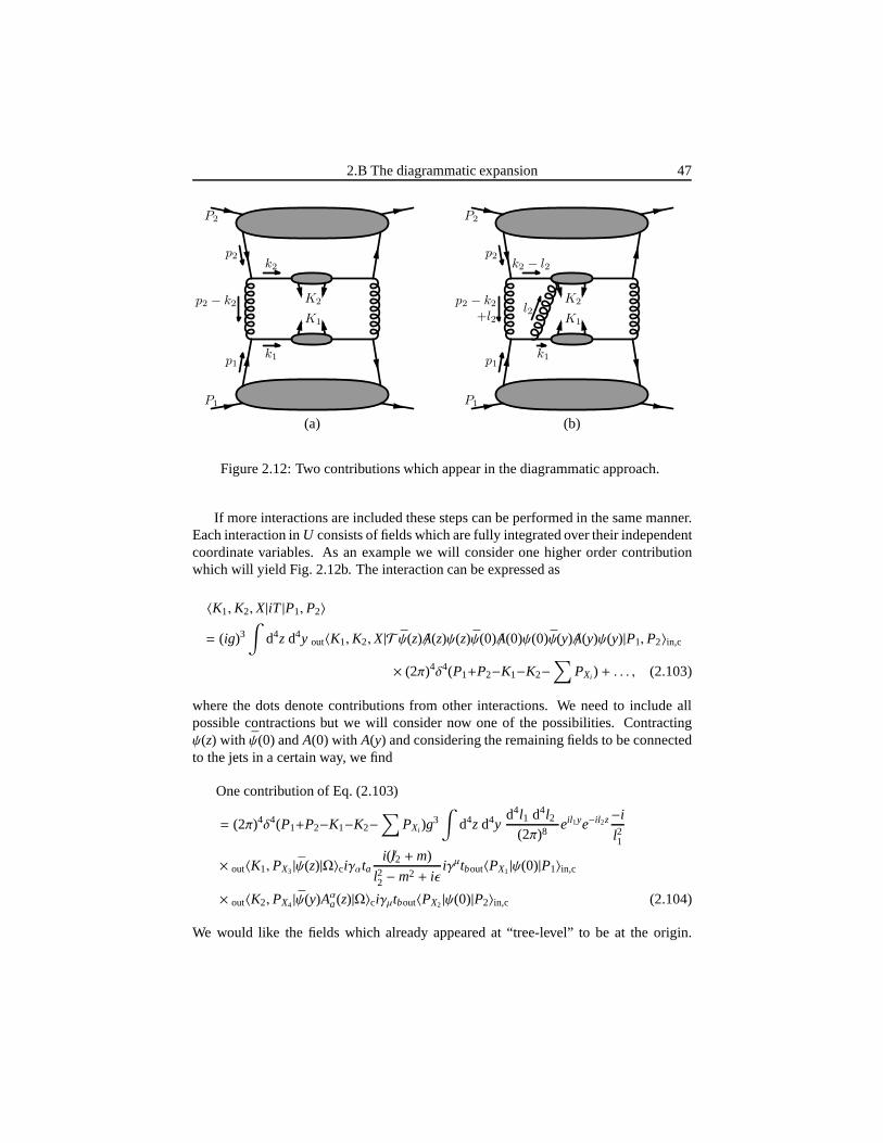
2.B The diagrammatic expansion 47
K1
K2
P1
P2
p2k2
p1k1
p2 − k2
K1
K2
P1
P2
p2k2 − l2
p1k1
l2p2 − k2
+l2
(a) (b)
Figure 2.12: Two contributions which appear in the diagrammatic approach.
If more interactions are included these steps can be performed in the same manner.Each interaction inU consists of fields which are fully integrated over their independentcoordinate variables. As an example we will consider one higher order contributionwhich will yield Fig. 2.12b. The interaction can be expressed as
〈K1,K2,X|iT |P1,P2〉
= (ig)3∫
d4zd4y out〈K1,K2,X|T ψ(z) /A(z)ψ(z)ψ(0) /A(0)ψ(0)ψ(y) /A(y)ψ(y)|P1,P2〉in,c
× (2π)4δ4(P1+P2−K1−K2−∑
PXi ) + . . . , (2.103)
where the dots denote contributions from other interactions. We need to include allpossible contractions but we will consider now one of the possibilities. Contractingψ(z) with ψ(0) andA(0) with A(y) and considering the remaining fields to be connectedto the jets in a certain way, we find
One contribution of Eq. (2.103)
= (2π)4δ4(P1+P2−K1−K2−∑
PXi )g3∫
d4zd4yd4l1 d4l2
(2π)8eil1ye−il2z−i
l21
× out〈K1,PX3 |ψ(z)|Ω〉ciγαtai(/l2 +m)
l22 −m2 + iǫiγµtbout〈PX1 |ψ(0)|P1〉in,c
× out〈K2,PX4 |ψ(y)Aαa(z)|Ω〉ciγµtbout〈PX2 |ψ(0)|P2〉in,c (2.104)
We would like the fields which already appeared at “tree-level” to be at the origin.
48 2 High energy scattering and quark-quark correlators
Shifting those fields and redefining the other integration variables, one finds
Eq. (2.104)=(2π)4δ4(P1+P2−K1−K2−∑
i
PXi
)g3
∫d4z
d4l2(2π)4
e−il2z 1(l2+p2−k2)2
× out〈K1,PX3 |ψ(0)|Ω〉ciγαtai(/l2 + /k1 +m)
(l2+k1)2−m2 + iǫiγµtbout〈PX1 |ψ(0)|P1〉in,c
× out〈K2,PX4 |ψ(0)Aαa(z)|Ω〉ciγµtbout〈PX2 |ψ(0)|P2〉in,c
(2.105)
The result is the original expression plus an additional interaction which contains in-tegrals overz and l2. We are actually deriving the Feyman rules. If we would haveconsidered a virtual correction there would have been an additional contraction and onewould remain with one integral overl2.
In general one should have the following situation: the tree-level result consists ofmomentum conservation and matrix elements containing fields at the origin; if moreexternal partons7 are present then the corresponding fields are integrated over their co-ordinates and momenta, and their interactions are described by the Feynman rules. Vir-tual corrections are similar except that the integral over the coordinates can be carriedout.
The cross section is obtained by removing the delta-function related to momentumconservation, taking the square, and multiplying with the removed delta-function (seeEq. 2.15, 2.89, 2.90). Except for the phase-space and flux factors this is the crosssection. In general the total momentum conservation can be rewritten by giving eachmatrix element a number (i) and naming the sum of the outgoing momenta (alsoPXi
here)Ki out and incoming momentumPi in. The total momentum conservation can thenbe written as
(2π)4δ4
∑
i=1
Ki out −∑
j=1
P j int
=∏
n
[∫d4tn δ
4(tn ± Pnin ∓ Knout)
]
× (2π)4δ4(external parton momenta), (2.106)
whereti are the momenta of the external partons and where the last delta-function ex-presses the momentum conservation of the external partons.The firstn delta-functionsare used to shift the fields of the matrix elements by introducing another integral overthe coordinates
δ4(tn ± Pnin ∓ Knout) =∫
d4ξn
(2π)4ei(tn±Pnin∓Knout)ξn. (2.107)
After an integration over the unobserved momenta one obtains the correlators as intro-duced in section 2.4.
7External partons are incoming or outgoing partons connected to correlators or decaying as a jet.
3Electromagnetic
scattering processes atleading order in αS
The diagrammatic approach, introduced in the previous chapter, will be employed todescribe at leading order inαS cross sections in which the hard scale is set by an elec-tromagnetic interaction. In the discussion on the meaning of αS it will be argued thateven at leading order there is an infinite amount of interactions that should be consid-ered. Including next-to-leading order corrections in inverse powers of the hard scale,these leading-order-αS-interactions will be evaluated in order to obtain the crosssec-tions for semi-inclusive DIS, electron-positron annihilation, and Drell-Yan in terms ofdistribution and fragmentation correlators. These correlators contain gauge links ofwhich their paths are different for different processes. Using the parametrizations ofthese correlators some explicit asymmetries for semi-inclusive DIS will be given.
In the second part of this chapter, the universality of fragmentation functions will bediscussed and the link structures appearing in deeply-virtual Compton scattering willbe studied. The calculation of the latter illustrates the wide-ranging applicability of thediagrammatic approach. A summary is provided at the end of this chapter.
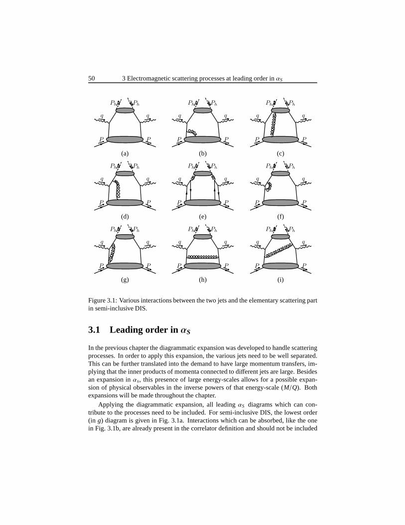
50 3 Electromagnetic scattering processes at leading orderin αS
P P
q q
Ph Ph
P P
q q
Ph Ph
P P
q q
Ph Ph
(a) (b) (c)
P P
q q
Ph Ph
P P
q q
Ph Ph
P P
q q
Ph Ph
(d) (e) (f)
P P
q q
Ph Ph
P P
q q
Ph Ph
P P
q q
Ph Ph
(g) (h) (i)
Figure 3.1: Various interactions between the two jets and the elementary scattering partin semi-inclusive DIS.
3.1 Leading order inαS
In the previous chapter the diagrammatic expansion was developed to handle scatteringprocesses. In order to apply this expansion, the various jets need to be well separated.This can be further translated into the demand to have large momentum transfers, im-plying that the inner products of momenta connected to different jets are large. Besidesan expansion inαs, this presence of large energy-scales allows for a possibleexpan-sion of physical observables in the inverse powers of that energy-scale (M/Q). Bothexpansions will be made throughout the chapter.
Applying the diagrammatic expansion, all leadingαS diagrams which can con-tribute to the processes need to be included. For semi-inclusive DIS, the lowest order(in g) diagram is given in Fig. 3.1a. Interactions which can be absorbed, like the onein Fig. 3.1b, are already present in the correlator definition and should not be included
3.2 Semi-inclusive deep-inelastic scattering 51
separately. Diagrams which have several jets areαs suppressed compared to diagramswhich contain less jets. The restriction to leading order inαs leads to only two outgo-ing jets for semi-inclusive DIS, electron-positron annihilation, and Drell-Yan. Further,the interactions between the jets as illustrated in Fig. 3.1c are considered to be weakand will be neglected. This assumption is directly related to the question on whetherfactorization holds for the correlators. This will be discussed in the next chapter.
Another possible contribution is that a gluon-line will connect a jet with the elemen-tary scattering diagram. Since there can be interferences,such as depicted in Fig. 3.1d,such an interaction is proportional to the coupling constant, g, and is notαs suppressed.We shall see in the next section that one can resum all collinear gluon-lines connectingthe correlator and the scattering diagram to all orders ing. The other possibility ofadditional collinear quarks, such as in Fig. 3.1e, is not taken into account here. Ellis,Furmanski, and Petronzio [53, 54], found that such contributions are suppressed withM2/Q2 and are therefore beyond the aimed accuracy of this chapter.
Besides additional parton-lines from the correlator one might wonder whether thereare other corrections in the scattering diagram itself which need to be included at lead-ing orderαs. Such corrections consist of loops and gluon radiation and can partly beabsorbed in the correlator definitions. For instance, if theloop diagram in Fig. 3.1fcontains a far off shell gluon, then it cannot be absorbed. However, if the gluon is ap-proximately on shell and collinear to one of the jets, as illustrated in Fig. 3.1g, then itis absorbed in the correlator definition up to some scale. Forgluon radiation a similarsituation applies. If the gluon in Fig. 3.1h has a small transverse momentum with re-spect to the parent hadron (P), then it is already present in the correlator definition. Thegluon in Fig. 3.1i cannot be absorbed and represents anαS correction.
Absorbing interactions in the correlator introduces a particular scale. There werea few attempts to calculate this scale dependence (evolution equations), but includingeffects from intrinsic transverse momentum this has not been achieved so far. For adiscussion on the scale dependence and various other difficulties the reader is referredto Ellis, Furmanski, Petronzio [54], Collins, Soper, Sterman [104, 105], Hagiwara,Hikasa, Kai [106], Ahmed, Gehrmann [107], Boer [108], and Henneman [66].
The conclusion of this section is that, restricted to leading order inαs, one mustresum over all possible gluons which connect the correlators and the scattering diagramto obtain the cross section (generalizations of Fig. 3.1.d). Such resummations will beperformed for several processes in this chapter.
3.2 Semi-inclusive deep-inelastic scattering
In the first two subsections the expressions for the hadronictensor includingM/Q cor-rections will be derived. In the third subsection the results for the hadronic tensor willbe used to express some asymmetries in terms of distributionand fragmentation func-tions. We will begin here by introducing the calculation of the hadronic tensor.
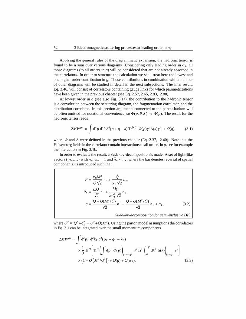
52 3 Electromagnetic scattering processes at leading orderin αS
Applying the general rules of the diagrammatic expansion, the hadronic tensor isfound to be a sum over various diagrams. Considering only leading order inαs, allthose diagrams (to all orders ing) will be considered that are not already absorbed inthe correlators. In order to structure the calculation we shall treat here the lowest andone higher order contribution ing. Those contributions in combination with a numberof other diagrams will be studied in detail in the next subsections. The final result,Eq. 3.46, will consist of correlators containing gauge links for which parametrizationshave been given in the previous chapter (see Eq. 2.57, 2.65, 2.83, 2.88).
At lowest order ing (see also Fig. 3.1a), the contribution to the hadronic tensoris a convolution between the scattering diagram, the fragmentation correlator, and thedistribution correlator. In this section arguments connected to the parent hadron willbe often omitted for notational convenience, soΦ(p,P,S) → Φ(p). The result for thehadronic tensor reads
2MWµν =
∫d4p d4k δ4(p+ q− k) TrD,C [
Φ(p)γµ∆(k)γν]+ O(g), (3.1)
whereΦ and∆ were defined in the previous chapter (Eq. 2.37, 2.40). Note that theHeisenberg fields in the correlator contain interactions toall orders ing, see for examplethe interaction in Fig. 3.1b.
In order to evaluate the result, a Sudakov-decomposition ismade. A set of light-likevectors (n−, n+ with n− · n+ = 1 andn− ∼ n+, where the bar denotes reversal of spatialcomponents) is introduced such that
P =xBM2
Q√
2n− +
Q
xB
√2
n+,
Ph =zhQ√
2n− +
M2h
zhQ√
2n+,
q =Q+ O(M2/Q)
√2
n− −Q+ O(M2/Q)
√2
n+ + qT , (3.2)
Sudakov-decomposition for semi-inclusive DIS
whereQ2 ≡ Q2+q2T = Q2+O(M2). Using the parton model assumptions the correlators
in Eq. 3.1 can be integrated over the small momentum components
2MWµν =
∫d2pT d2kT δ
2(pT + qT − kT)
× 13
TrD
TrC
(∫dp− Φ(p)
)
p+=−q+γµ TrC
(∫dk+ ∆(k)
)
k−=q−γν
×(1+ O
(M2/Q2
))+ O(g) + O(αS), (3.3)
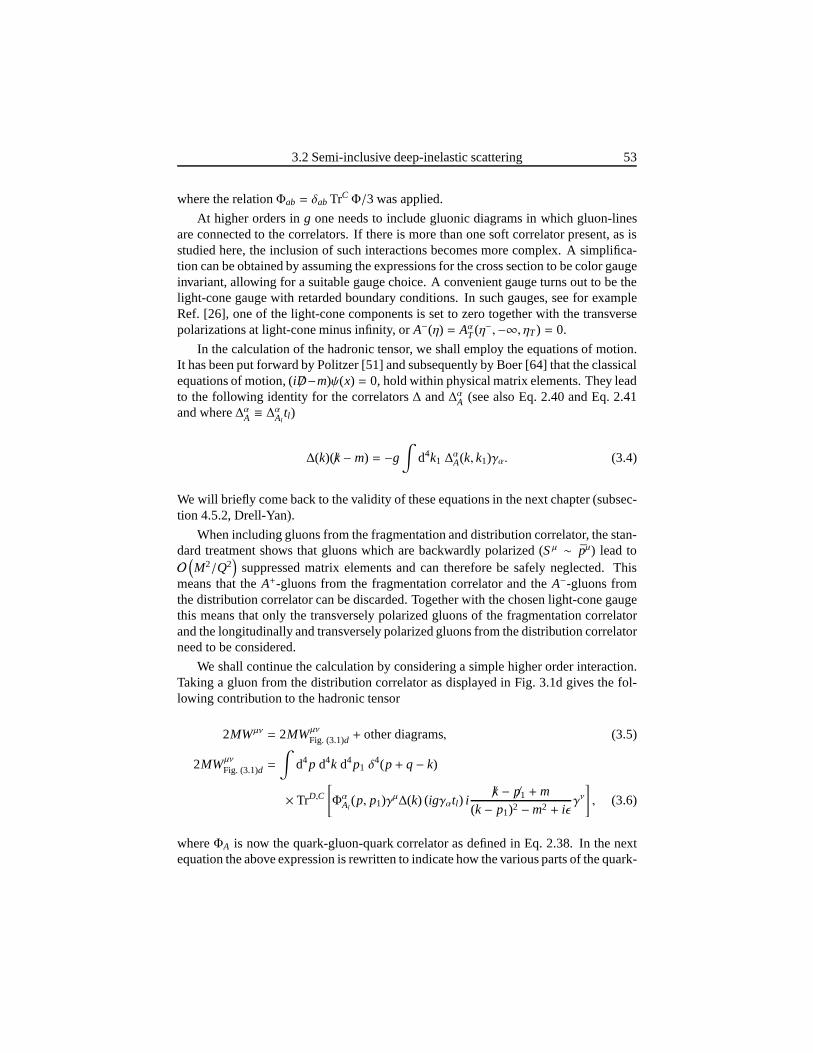
3.2 Semi-inclusive deep-inelastic scattering 53
where the relationΦab = δab TrCΦ/3 was applied.
At higher orders ing one needs to include gluonic diagrams in which gluon-linesare connected to the correlators. If there is more than one soft correlator present, as isstudied here, the inclusion of such interactions becomes more complex. A simplifica-tion can be obtained by assuming the expressions for the cross section to be color gaugeinvariant, allowing for a suitable gauge choice. A convenient gauge turns out to be thelight-cone gauge with retarded boundary conditions. In such gauges, see for exampleRef. [26], one of the light-cone components is set to zero together with the transversepolarizations at light-cone minus infinity, orA−(η) = Aα
T(η−,−∞, ηT) = 0.
In the calculation of the hadronic tensor, we shall employ the equations of motion.It has been put forward by Politzer [51] and subsequently by Boer [64] that the classicalequations of motion, (i /D−m)ψ(x) = 0, hold within physical matrix elements. They leadto the following identity for the correlators∆ and∆αA (see also Eq. 2.40 and Eq. 2.41and where∆αA ≡ ∆αAl
tl)
∆(k)(/k−m) = −g∫
d4k1 ∆αA(k, k1)γα. (3.4)
We will briefly come back to the validity of these equations inthe next chapter (subsec-tion 4.5.2, Drell-Yan).
When including gluons from the fragmentation and distribution correlator, the stan-dard treatment shows that gluons which are backwardly polarized (Sµ ∼ pµ) lead toO
(M2/Q2
)suppressed matrix elements and can therefore be safely neglected. This
means that theA+-gluons from the fragmentation correlator and theA−-gluons fromthe distribution correlator can be discarded. Together with the chosen light-cone gaugethis means that only the transversely polarized gluons of the fragmentation correlatorand the longitudinally and transversely polarized gluons from the distribution correlatorneed to be considered.
We shall continue the calculation by considering a simple higher order interaction.Taking a gluon from the distribution correlator as displayed in Fig. 3.1d gives the fol-lowing contribution to the hadronic tensor
2MWµν = 2MWµν
Fig. (3.1)d + other diagrams, (3.5)
2MWµν
Fig. (3.1)d =
∫d4p d4k d4p1 δ
4(p+ q− k)
× TrD,C
[ΦαAl
(p, p1)γµ∆(k) (igγαtl) i/k− p/1 +m
(k− p1)2 −m2 + iǫγν
], (3.6)
whereΦA is now the quark-gluon-quark correlator as defined in Eq. 2.38. In the nextequation the above expression is rewritten to indicate how the various parts of the quark-
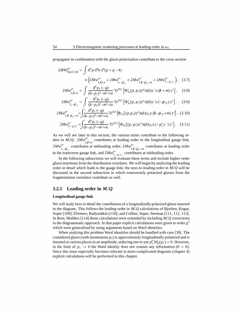
54 3 Electromagnetic scattering processes at leading orderin αS
propagator in combination with the gluon polarization contribute to the cross section
2MWµν
Fig (3.1)d =
∫d4p d4k δ4(p+ q− k)
×(2Mwµν
L,/k+m+ 2Mwµν
L,−p/1T
+ 2Mwµν
T,/k−p/1T+m+ 2Mwµν
T,−p+1γ−
), (3.7)
2Mwµν
L,/k+m=
∫d4p1 (−g)
(k−p1)2−m2+iǫTrD,C
[Φ+Al
(p, p1)γµ∆(k)γ−tl (/k+m) γν], (3.8)
2Mwµν
L,−p/1T
=
∫d4p1 (−g)
(k−p1)2−m2+iǫTrD,C
[Φ+Al
(p, p1)γµ∆(k)γ−tl
(−p/1T)γν
], (3.9)
2Mwµν
T,/k−p/1T+m=
∫d4p1 (−g)
(k−p1)2−m2+iǫTrD,C
[ΦAl
αT (p,p1)γµ∆(k)γαtl
(/k−p/1T+m
)γν], (3.10)
2Mwµν
T,−p+1γ−=
∫d4p1 (−g)
(k−p1)2−m2+iǫTrD,C
[ΦAl
αT(p, p1)γµ∆(k)γαtl
(−p+1γ−) γν
]. (3.11)
As we will see later in this section, the various terms contribute to the following or-ders inM/Q: 2Mwµν
L,/k+mcontributes at leading order to the longitudinal gauge link,
2Mwµν
L,−p/1T
contributes at subleading order, 2Mwµν
T,/k−p/1T+mcontributes at leading order
to the transverse gauge link, and 2Mwµν
T,−p+1γ− contributes at subleading order.
In the following subsections we will evaluate these terms and include higher ordergluon insertions from the distribution correlator. We willbegin by analyzing the leadingorder in detail which leads to the gauge link; the next-to-leading order inM/Q will bediscussed in the second subsection in which transversely polarized gluons from thefragmentation correlator contribute as well.
3.2.1 Leading order in M/Q
Longitudinal gauge link
We will study here in detail the contribution of a longitudinally polarized gluon insertedin the diagram. This follows the leading order inM/Q calculations of Bjorken, Kogut,Soper [109]; Efremov, Radyushkin [110]; and Collins, Soper, Sterman [111, 112, 113].In Boer, Mulders [114] those calculations were extended by includingM/Q correctionsin the diagrammatic approach. In that paper explicit calculations were given to orderg2
which were generalized by using arguments based on Ward identities.When studying this problem Ward identities should be handled with care [39]. The
considered gluon (with momentump1) is approximately longitudinally polarized and isinserted at various places in an amplitude, seducing one to usepµ1Mµ(p1) = 0. However,in the limit of p1 → 0 the Ward identity does not contain any information (0= 0).Since this issue especially becomes relevant in more complicated diagrams (chapter 4)explicit calculations will be performed in this chapter.
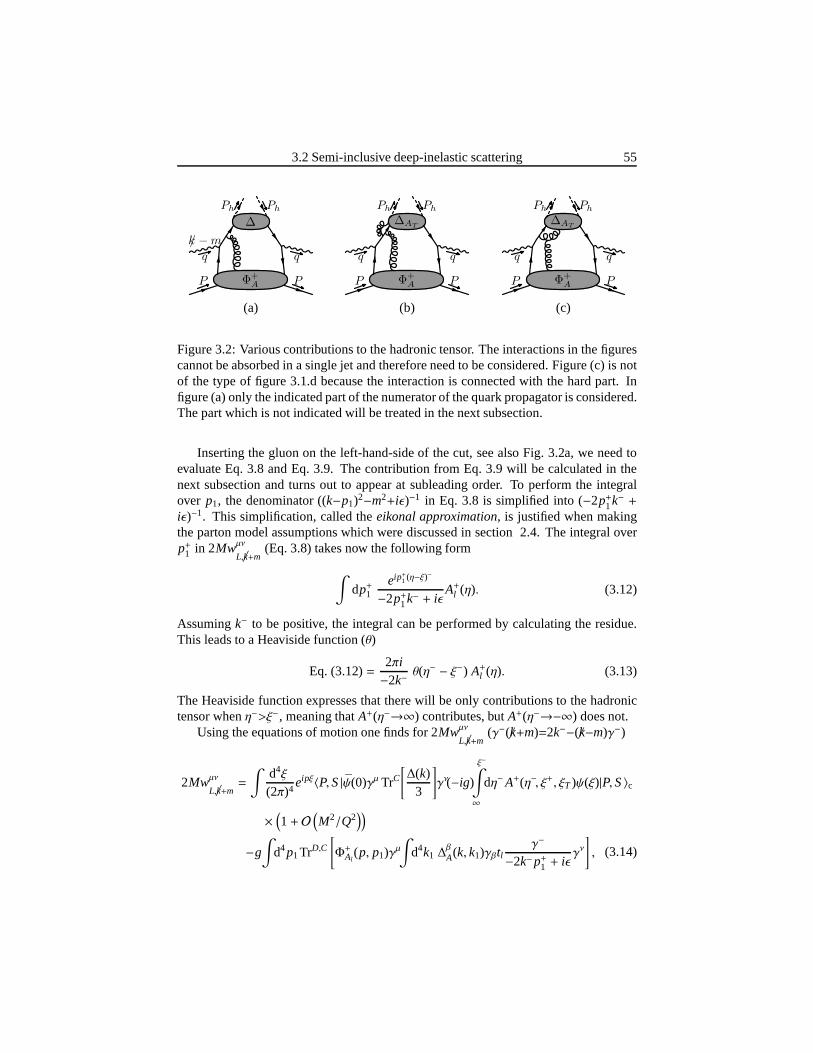
3.2 Semi-inclusive deep-inelastic scattering 55
Φ+A
∆
k/−m
P P
q q
Ph Ph
Φ+A
∆AT
P P
q q
Ph Ph
Φ+A
∆AT
P P
q q
Ph Ph
(a) (b) (c)
Figure 3.2: Various contributions to the hadronic tensor. The interactions in the figurescannot be absorbed in a single jet and therefore need to be considered. Figure (c) is notof the type of figure 3.1.d because the interaction is connected with the hard part. Infigure (a) only the indicated part of the numerator of the quark propagator is considered.The part which is not indicated will be treated in the next subsection.
Inserting the gluon on the left-hand-side of the cut, see also Fig. 3.2a, we need toevaluate Eq. 3.8 and Eq. 3.9. The contribution from Eq. 3.9 will be calculated in thenext subsection and turns out to appear at subleading order.To perform the integralover p1, the denominator ((k−p1)2−m2+iǫ)−1 in Eq. 3.8 is simplified into (−2p+1k− +iǫ)−1. This simplification, called theeikonal approximation, is justified when makingthe parton model assumptions which were discussed in section 2.4. The integral overp+1 in 2Mwµν
L,/k+m(Eq. 3.8) takes now the following form
∫dp+1
eip+1 (η−ξ)−
−2p+1k− + iǫA+l (η). (3.12)
Assumingk− to be positive, the integral can be performed by calculatingthe residue.This leads to a Heaviside function (θ)
Eq. (3.12)=2πi−2k−
θ(η− − ξ−) A+l (η). (3.13)
The Heaviside function expresses that there will be only contributions to the hadronictensor whenη−>ξ−, meaning thatA+(η−→∞) contributes, butA+(η−→−∞) does not.
Using the equations of motion one finds for 2Mwµν
L,/k+m(γ−(/k+m)=2k−−(/k−m)γ−)
2Mwµν
L,/k+m=
∫d4ξ
(2π)4eipξ〈P,S|ψ(0)γµ TrC
[∆(k)
3
]γν(−ig)
ξ−∫
∞
dη−A+(η−, ξ+, ξT )ψ(ξ)|P,S〉c
×(1+ O
(M2/Q2
))
−g∫
d4p1TrD,C
[Φ+Al
(p, p1)γµ
∫d4k1 ∆
β
A(k, k1)γβtlγ−
−2k−p+1 + iǫγν
], (3.14)
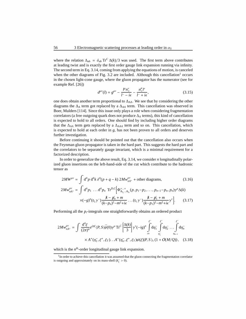
56 3 Electromagnetic scattering processes at leading orderin αS
where the relation∆ab = δab TrC ∆(k)/3 was used. The first term above contributesat leading twist and is exactly the first order gauge link expansion running via infinity.The second term in Eq. 3.14, coming from applying the equations of motion, is canceledwhen the other diagrams of Fig. 3.2 are included. Although this cancellation1 occursin the chosen light-cone gauge, where the gluon propagator has the numerator (see forexample Ref. [26])
dµν(l) = gµν − lµnν+l− − iǫ
− nµ+lν
l− + iǫ, (3.15)
one does obtain another term proportional to∆AA. We see that by considering the otherdiagrams the∆A term got replaced by a∆AA term. This cancellation was observed inBoer, Mulders [114]. Since this issue only plays a role when considering fragmentationcorrelators (a free outgoing quark does not produce∆A terms), this kind of cancellationis expected to hold to all orders. One should find by includinghigher order diagramsthat the∆AA term gets replaced by a∆AAA term and so on. This cancellation, whichis expected to hold at each order ing, has not been proven to all orders and deservesfurther investigation.
Before continuing it should be pointed out that the cancellation also occurs whenthe Feynman gluon propagator is taken in the hard part. This suggests the hard part andthe correlators to be separately gauge invariant, which is aminimal requirement for afactorized description.
In order to generalize the above result, Eq. 3.14, we consider n longitudinally polar-ized gluon insertions on the left-hand-side of the cut whichcontribute to the hadronictensor as
2MWµν =
∫d4p d4k δ4(p+ q− k) 2Mwµν
nA+ + other diagrams, (3.16)
2Mwµν
nA+ =
∫d4p1 . . .d4pn TrD,C
[Φ+...+Al1 ...Aln
(p, p1−p2, . . . , pn−1−pn, pn)γµ∆(k)
×(−g)n(tlnγ−)/k− p/n +m
(k−pn)2−m2+iǫ. . . (tl1γ
−)/k− p/1 +m
(k−p1)2−m2+iǫγν
]. (3.17)
Performing all thepi-integrals one straightforwardly obtains an ordered product
2Mwµν
nA+ =
∫d4ξ
(2π)4eipξ〈P,S|ψ(0)γµ TrC
[∆(k)
3
]γν(−ig)n
ξ−∫
∞
dη−1
ξ−∫
η−1
dη−2 . . .
ξ−∫
ηn−1
dη−n
× A+(η−1 , ξ+, ξT ). . .A+(η−n , ξ
+, ξT)ψ(ξ)|P,S〉c (1+ O(M/Q)) , (3.18)
which is thenth-order longitudinal gauge link expansion.
1In order to achieve this cancellation it was assumed that thegluon connecting the fragmentation correlatoris outgoing and approximately on its mass-shell (k−1 > 0).
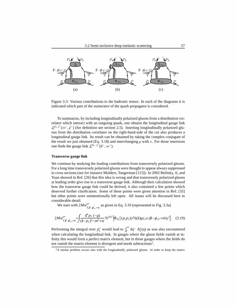
3.2 Semi-inclusive deep-inelastic scattering 57
ΦAT
∆
k/−p/1T−m
P P
q q
Ph Ph
ΦAT
∆AT
k/−p/1T−m
P P
q q
Ph Ph
ΦAT
∆AT
k/−p/1T−m
P P
q q
Ph Ph
(a) (b) (c)
Figure 3.3: Various contributions to the hadronic tensor. In each of the diagrams it isindicated which part of the numerator of the quark propagator is considered.
To summarize, by including longitudinally polarized gluons from a distribution cor-relator which interact with an outgoing quark, one obtains the longitudinal gauge linkLξT, ξ
+
(∞−, ξ−) (for definition see section 2.5). Inserting longitudinally polarized glu-ons from the distribution correlator on the right-hand-side of the cut also produces alongitudinal gauge link. Its result can be obtained by taking the complex conjugate ofthe result we just obtained (Eq. 3.18) and interchangingµ with ν. For those insertionsone finds the gauge linkL0T , ξ
+
(0−,∞−).
Transverse gauge link
We continue by studying the leading contributions from transversely polarized gluons.For a long time transversely polarized gluons were thought to appear always suppressedin cross sections (see for instance Mulders, Tangerman [115]). In 2002 Belitsky, Ji, andYuan showed in Ref. [26] that this idea is wrong and that transversely polarized gluonsat leading order give rise to a transverse gauge link. Although their calculation showedhow the transverse gauge link could be derived, it also contained a few points whichdeserved further clarification. Some of these points were given attention in Ref. [35]but other points were unintentionally left open. All issueswill be discussed here inconsiderable detail.
We start with 2Mwµν
T,/k−p/1T+mas given in Eq. 3.10 (represented in Fig. 3.3a)
2Mwµν
T,/k−p/1T+m=
∫d4p1 (−g)
(k−p1)2−m2+iǫTrD,C
[ΦAl
αT(p,p1)γµ∆(k)gγαtl (/k−p/1T+m)γν
]. (3.19)
Performing the integral overp+1 would lead to∫ ∞ξ−
dη− AαT(η) as was also encountered
when calculating the longitudinal link. In gauges where thegluon fields vanish at in-finity this would form a perfect matrix element, but in those gauges where the fields donot vanish the matrix element is divergent and needs subtractions2.
2A similar problem occurs also with the longitudinally polarized gluons. In order to keep the matrix
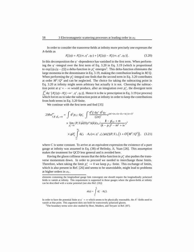
58 3 Electromagnetic scattering processes at leading orderin αS
In order to consider the transverse fields at infinity more precisely one expresses theA-fields as
AαT(η) = Aα
T(∞, η+, ηT) +[Aα
T(η) − AαT(∞, η+, ηT)
]. (3.20)
In this decomposition theη−-dependence has vanished in the first term. When perform-ing theη−-integral over the first term of Eq. 3.20 in Eq. 3.19 (which is proportionalto exp [ip1(η − ξ)]) a delta-function inp+1 emerges3. This delta-function eliminates thelarge momenta in the denominator in Eq. 3.19, making the contribution leading inM/Q.When performing thep+1 -integral one finds that the second term in Eq. 3.20 contributesat orderM2/Q2 and can be neglected. The choice for taking the subtracting point inEq. 3.20 at infinity might seem arbitrary but actually it is not. Choosing the subtrac-tion point atη−= − ∞ would produce, after an integration overp+1 , the divergent term∫ ξ−
∞ dη− [AαT(η)−Aα
T(−∞−, η+, ηT)]. Hence it is theiǫ prescription in Eq. 3.19 (or process)which forces us to take the subtraction point at infinity in order to keep the contributionsfrom both terms in Eq. 3.20 finite.
We continue with the first term and find [35]
2Mwµν
T,/k−p/1T+m=
∫d2p1T dp−1
∫d4ξ dη+ d2ηT
(2π)7eipξ+ip1T (η−ξ)T+ip−1 (η−ξ)+
× limp+1→0〈P,S|ψ(0)γµ∆(k)iγαi
/k− p/1T +m
(k− p1)2 −m2 + iǫγν
× g∂αη
ηT∫
C
dζT · AT(∞, η+, ζT)ψ(ξ)|P,S〉c(1+ O
(M2/Q2
)), (3.21)
whereC is some constant. To arrive at an equivalent expression the existence of a puregauge at infinity was assumed in Eq. (38) of Belitsky, Ji, Yuan[26]. This assumptionmakes the treatment for QCD less general and is avoided here.
Having the gluon collinear means that the delta-function inp+1 also pushes the trans-verse momentum down. In order to proceed we needed to interchange those limits.Therefore, when taking the limitp+1 → 0 we keepp1T finite. This exchange of limits,which is also present in Ref. [26] and seems to be unavoidable, might lead to problemsat higher orders inαS.
elements containing the longitudinal gauge link convergent one should require the longitudinally polarizedfields to vanish at infinity. This requirement is supported inthose gauges where the gluon-fields at infinitycan be described with a scalar potential (see also Ref. [26])
φ(η) =
η∫
C
dζ · A(ζ).
In order to have the potential finite atη− = ∞ which seems to be physically reasonable, theA+-fields need tovanish at that point. This argument does not hold for transversely polarized gluons.
3The boundary terms were also studied by Boer, Mulders, and Teryaev in Ref. [87].
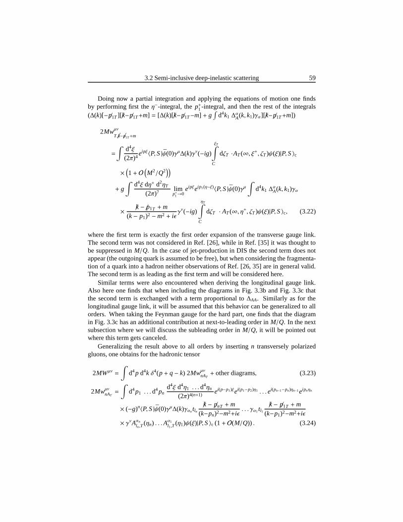
3.2 Semi-inclusive deep-inelastic scattering 59
Doing now a partial integration and applying the equations of motion one findsby performing first theη−-integral, thep+1 -integral, and then the rest of the integrals(∆(k)[−p/1T ][ /k−p/1T+m] = [∆(k)[/k−p/1T−m] + g
∫d4k1 ∆
αA(k, k1)γα][ /k−p/1T+m])
2Mwµν
T,/k−p/1T+m
=
∫d4ξ
(2π)4eipξ〈P,S|ψ(0)γµ∆(k)γν(−ig)
ξT∫
C
dζT ·AT(∞, ξ+, ζT)ψ(ξ)|P,S〉c
×(1+ O
(M2/Q2
))
+ g∫
d4ξ dη+ d2ηT
(2π)7limp+1→0
eipξeip1(η−ξ)〈P,S|ψ(0)γµ∫
d4k1 ∆αA(k, k1)γα
× /k− /p1T +m
(k− p1)2 −m2 + iǫγν(−ig)
ηT∫
C
dζT · AT(∞, η+, ζT)ψ(ξ)|P,S〉c, (3.22)
where the first term is exactly the first order expansion of thetransverse gauge link.The second term was not considered in Ref. [26], while in Ref.[35] it was thought tobe suppressed inM/Q. In the case of jet-production in DIS the second term does notappear (the outgoing quark is assumed to be free), but when considering the fragmenta-tion of a quark into a hadron neither observations of Ref. [26, 35] are in general valid.The second term is as leading as the first term and will be considered here.
Similar terms were also encountered when deriving the longitudinal gauge link.Also here one finds that when including the diagrams in Fig. 3.3b and Fig. 3.3c thatthe second term is exchanged with a term proportional to∆AA. Similarly as for thelongitudinal gauge link, it will be assumed that this behavior can be generalized to allorders. When taking the Feynman gauge for the hard part, one finds that the diagramin Fig. 3.3c has an additional contribution at next-to-leading order inM/Q. In the nextsubsection where we will discuss the subleading order inM/Q, it will be pointed outwhere this term gets canceled.
Generalizing the result above to all orders by insertingn transversely polarizedgluons, one obtains for the hadronic tensor
2MWµν =
∫d4p d4k δ4(p+ q− k) 2Mwµν
nAT+ other diagrams, (3.23)
2Mwµν
nAT=
∫d4p1 . . .d4pn
d4ξ d4η1 . . .d4ηn
(2π)4(n+1)ei(p−p1)ξei(p1−p2)η1 . . .ei(pn−1−pn)ηn−1eipnηn
× (−g)n〈P,S|ψ(0)γµ∆(k)γαntln/k− p/nT +m
(k−pn)2−m2+iǫ. . . γα1tl1
/k− p/1T +m
(k−p1)2−m2+iǫ
× γνAαn
ln,T(ηn) . . .Aα1
l1,T(η1)ψ(ξ)|P,S〉c (1+ O(M/Q)) . (3.24)
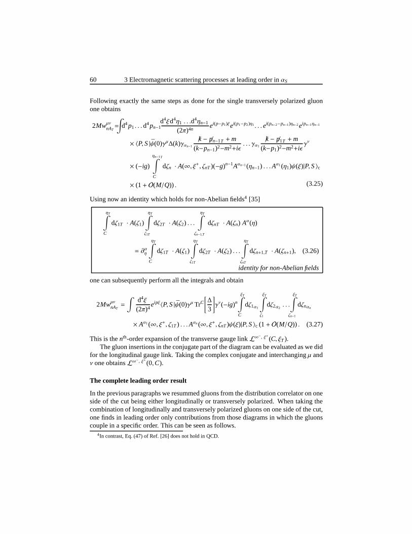
60 3 Electromagnetic scattering processes at leading orderin αS
Following exactly the same steps as done for the single transversely polarized gluonone obtains
2Mwµν
nAT=
∫d4p1 . . .d4pn−1
d4ξd4η1 . . .d4ηn−1
(2π)4nei(p−p1)ξei(p1−p2)η1. . .ei(pn−2−pn−1)ηn−2eipn−1ηn−1
× 〈P,S|ψ(0)γµ∆(k)γαn−1
/k− p/n−1T +m
(k−pn−1)2−m2+iǫ. . . γα1
/k− p/1T +m
(k−p1)2−m2+iǫγν
× (−ig)
ηn−1T∫
C
dζn · A(∞, ξ+, ζnT)(−g)n−1Aαn−1(ηn−1) . . .Aα1(η1)ψ(ξ)|P,S〉c
× (1+ O(M/Q)) . (3.25)
Using now an identity which holds for non-Abelian fields4 [35]
ηT∫
C
dζ1T · A(ζ1)
ηT∫
ζ1T
dζ2T · A(ζ2) . . .
ηT∫
ζn−1,T
dζnT · A(ζn) Aα(η)
= ∂αη
ηT∫
C
dζ1T · A(ζ1)
ηT∫
ζ1T
dζ2T · A(ζ2) . . .
ηT∫
ζnT
dζn+1,T · A(ζn+1), (3.26)
identity for non-Abelian fields
one can subsequently perform all the integrals and obtain
2Mwµν
nAT=
∫d4ξ
(2π)4eipξ〈P,S|ψ(0)γµ TrC
[∆
3
]γν(−ig)n
ξT∫
C
dζ1α1
ξT∫
ζ1
dζ2α2. . .
ξT∫
ζn−1
dζnαn
× Aα1(∞, ξ+, ζ1T) . . .Aαn(∞, ξ+, ζnT)ψ(ξ)|P,S〉c (1+ O(M/Q)) . (3.27)
This is thenth-order expansion of the transverse gauge linkL∞− , ξ+ (C, ξT).The gluon insertions in the conjugate part of the diagram canbe evaluated as we did
for the longitudinal gauge link. Taking the complex conjugate and interchangingµ andν one obtainsL∞−, ξ+ (0,C).
The complete leading order result
In the previous paragraphs we resummed gluons from the distribution correlator on oneside of the cut being either longitudinally or transverselypolarized. When taking thecombination of longitudinally and transversely polarizedgluons on one side of the cut,one finds in leading order only contributions from those diagrams in which the gluonscouple in a specific order. This can be seen as follows.
4In contrast, Eq. (47) of Ref. [26] does not hold in QCD.
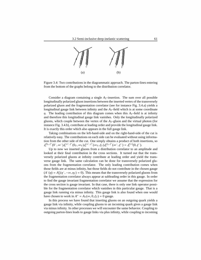
3.2 Semi-inclusive deep-inelastic scattering 61
T + + T
(a) (b)
Figure 3.4: Two contributions in the diagrammatic approach. The parton-lines enteringfrom the bottom of the graphs belong to the distribution correlator.
Consider a diagram containing a singleAT-insertion. The sum over all possiblelongitudinally polarized gluon insertions between the inserted vertex of the transverselypolarized gluon and the fragmentation correlator (see for instance Fig. 3.4.a) yields alongitudinal gauge link between infinity and theAT-field which is at some coordinateη. The leading contribution of this diagram comes when thisAT-field is at infinityand therefore this longitudinal gauge link vanishes. Only the longitudinally polarizedgluons, which couple between the vertex of theAT -gluon and the virtual photon (forinstance Fig. 3.4.b), contribute at leading order and provide the longitudinal gauge link.It is exactly this order which also appears in the full gauge link.
Taking combinations on the left-hand-side and on the right-hand-side of the cut isrelatively easy. The contributions on each side can be evaluated without using informa-tion from the other side of the cut. One simply obtains a product of both insertions, soL0T, ξ
+
(0−,∞−)L∞−, ξ+ (0T ,∞T)L∞−, ξ+ (∞T , ξT )LξT, ξ+
(∞−, ξ−) = L[+](0, ξ−).Up to now we inserted gluons from a distribution correlator to an amplitude and
looked at their final contribution in the cross sections. It turned out that the trans-versely polarized gluons at infinity contribute at leading order and yield the trans-verse gauge link. The same calculation can be done for transversely polarized glu-ons from the fragmentation correlator. The only leading contribution comes whenthose fields are at minus infinity, but those fields do not contribute in the chosen gauge(A−(η) = Aα
T(η−,−∞, ηT) = 0). This means that the transversely polarized gluons fromthe fragmentation correlator always appear at subleading order in this gauge. In orderto find the gauge invariant fragmentation correlator we assume that the expression forthe cross section is gauge invariant. In that case, there is only one link operator possi-ble for the fragmentation correlator which vanishes in thisparticular gauge. That is agauge link running via minus infinity. This gauge link is alsofound when one wouldhave chosen to work inA+ = AT(∞, 0, ξT) = 0 gauge.
In this process we have found that inserting gluons on an outgoing quark yields agauge link via infinity, while coupling gluons to an incomingquark gives a gauge linkvia minus infinity. In other processes we will encounter the same behavior. Coupling tooutgoing parton-lines leads to gauge links via plus infinity, while coupling to incoming
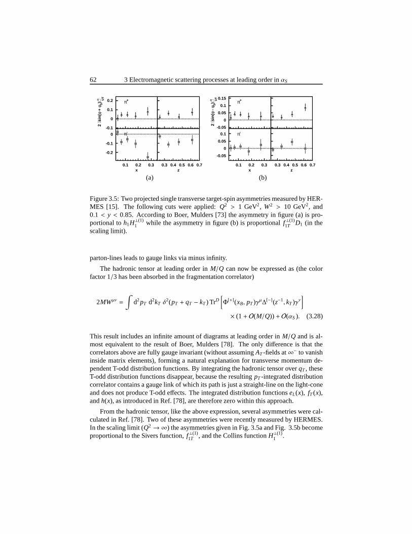
62 3 Electromagnetic scattering processes at leading orderin αS
-0.1
0
0.1
0.2
-0.2
-0.1
0
0.1 0.2 0.3
2 ⟨s
in(φ
+ φ
S)⟩
UT
π π+
x
π-
z0.3 0.4 0.5 0.6 0.7
-0.05
0
0.05
0.1
0.15
-0.05
0
0.05
0.1
0.1 0.2 0.3
2 ⟨s
in(φ
- φ
S)⟩
UT
π π+
x
π-
z0.3 0.4 0.5 0.6 0.7
(a) (b)
Figure 3.5: Two projected single transverse target-spin asymmetries measured by HER-MES [15]. The following cuts were applied:Q2 > 1 GeV2, W2 > 10 GeV2, and0.1 < y < 0.85. According to Boer, Mulders [73] the asymmetry in figure (a) is pro-portional toh1H⊥(1)
1 while the asymmetry in figure (b) is proportionalf⊥(1)1T D1 (in the
scaling limit).
parton-lines leads to gauge links via minus infinity.
The hadronic tensor at leading order inM/Q can now be expressed as (the colorfactor 1/3 has been absorbed in the fragmentation correlator)
2MWµν =
∫d2pT d2kT δ
2(pT + qT − kT) TrD[Φ[+](xB, pT)γµ∆[−](z−1, kT)γν
]
× (1+ O(M/Q)) + O(αS). (3.28)
This result includes an infinite amount of diagrams at leading order inM/Q and is al-most equivalent to the result of Boer, Mulders [78]. The onlydifference is that thecorrelators above are fully gauge invariant (without assuming AT-fields at∞− to vanishinside matrix elements), forming a natural explanation fortransverse momentum de-pendent T-odd distribution functions. By integrating the hadronic tensor overqT , theseT-odd distribution functions disappear, because the resulting pT -integrated distributioncorrelator contains a gauge link of which its path is just a straight-line on the light-coneand does not produce T-odd effects. The integrated distribution functionseL(x), fT(x),andh(x), as introduced in Ref. [78], are therefore zero within thisapproach.
From the hadronic tensor, like the above expression, several asymmetries were cal-culated in Ref. [78]. Two of these asymmetries were recentlymeasured by HERMES.In the scaling limit (Q2→ ∞) the asymmetries given in Fig. 3.5a and Fig. 3.5b becomeproportional to the Sivers function,f⊥(1)
1T , and the Collins functionH⊥(1)1 .
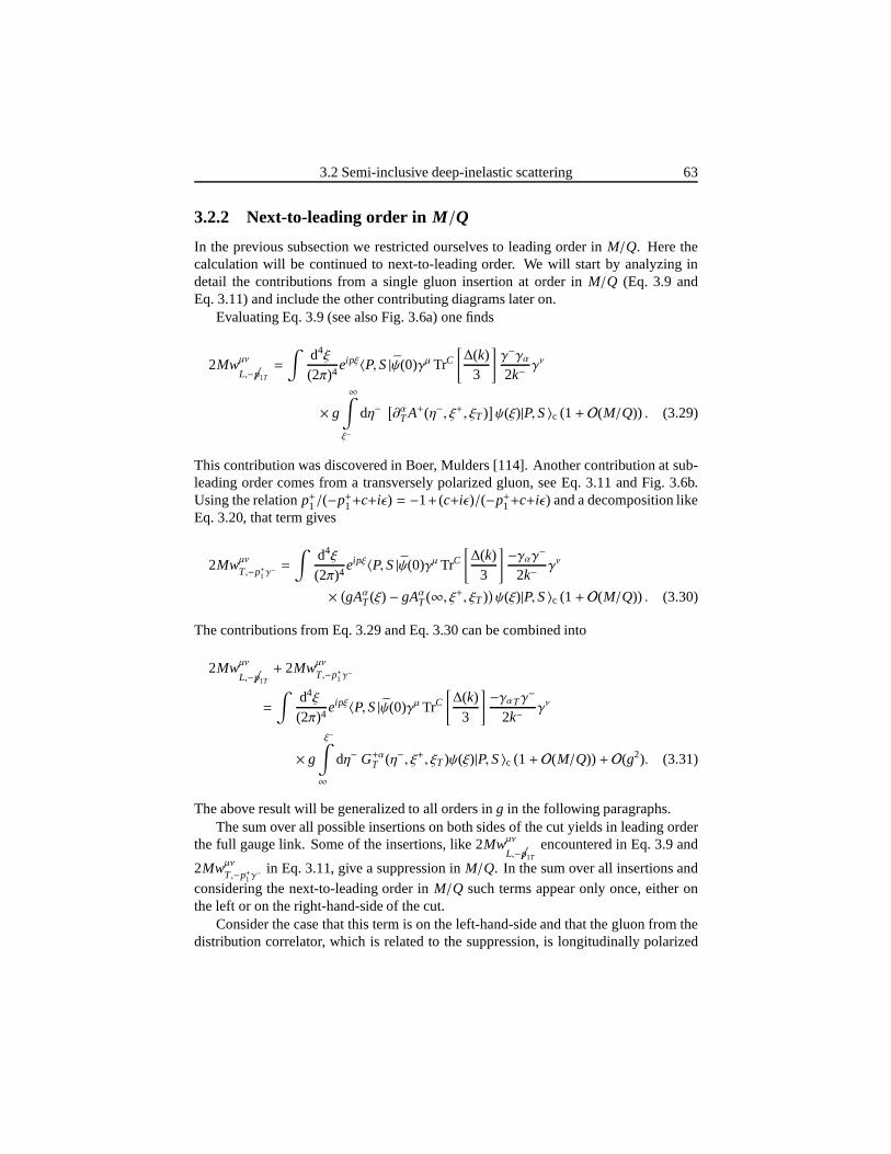
3.2 Semi-inclusive deep-inelastic scattering 63
3.2.2 Next-to-leading order inM/Q
In the previous subsection we restricted ourselves to leading order inM/Q. Here thecalculation will be continued to next-to-leading order. Wewill start by analyzing indetail the contributions from a single gluon insertion at order in M/Q (Eq. 3.9 andEq. 3.11) and include the other contributing diagrams lateron.
Evaluating Eq. 3.9 (see also Fig. 3.6a) one finds
2Mwµν
L,−p/1T
=
∫d4ξ
(2π)4eipξ〈P,S|ψ(0)γµ TrC
[∆(k)
3
]γ−γα2k−
γν
× g
∞∫
ξ−
dη−[∂αTA+(η−, ξ+, ξT)
]ψ(ξ)|P,S〉c (1+ O(M/Q)) . (3.29)
This contribution was discovered in Boer, Mulders [114]. Another contribution at sub-leading order comes from a transversely polarized gluon, see Eq. 3.11 and Fig. 3.6b.Using the relationp+1/(−p+1+c+iǫ) = −1+ (c+iǫ)/(−p+1+c+iǫ) and a decomposition likeEq. 3.20, that term gives
2Mwµν
T,−p+1γ− =
∫d4ξ
(2π)4eipξ〈P,S|ψ(0)γµ TrC
[∆(k)
3
]−γαγ−
2k−γν
× (gAαT(ξ) − gAαT(∞, ξ+, ξT)
)ψ(ξ)|P,S〉c (1+ O(M/Q)) . (3.30)
The contributions from Eq. 3.29 and Eq. 3.30 can be combined into
2Mwµν
L,−p/1T
+ 2Mwµν
T,−p+1γ−
=
∫d4ξ
(2π)4eipξ〈P,S|ψ(0)γµ TrC
[∆(k)
3
]−γαTγ
−
2k−γν
× g
ξ−∫
∞
dη− G+αT (η−, ξ+, ξT)ψ(ξ)|P,S〉c (1+ O(M/Q)) + O(g2). (3.31)
The above result will be generalized to all orders ing in the following paragraphs.The sum over all possible insertions on both sides of the cut yields in leading order
the full gauge link. Some of the insertions, like 2Mwµν
L,−p/1T
encountered in Eq. 3.9 and
2Mwµν
T,−p+1γ− in Eq. 3.11, give a suppression inM/Q. In the sum over all insertions and
considering the next-to-leading order inM/Q such terms appear only once, either onthe left or on the right-hand-side of the cut.
Consider the case that this term is on the left-hand-side andthat the gluon from thedistribution correlator, which is related to the suppression, is longitudinally polarized
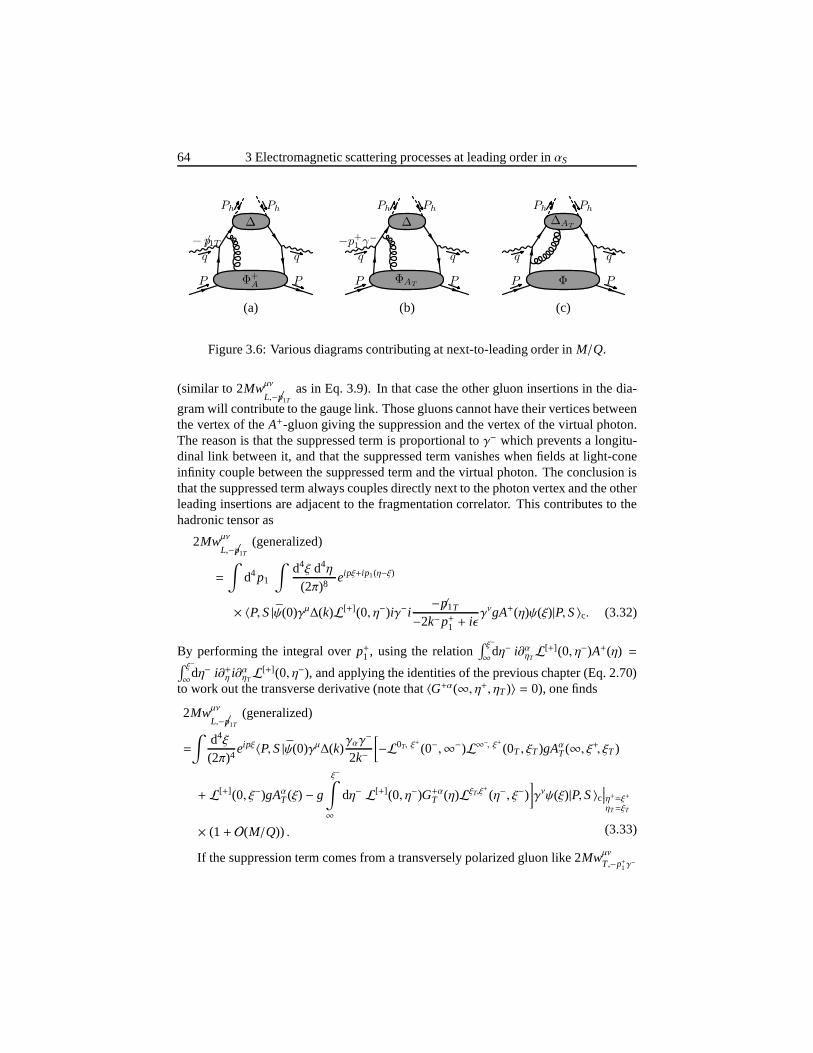
64 3 Electromagnetic scattering processes at leading orderin αS
Φ+A
∆
− p/1T
P P
q q
Ph Ph
ΦAT
∆
−p+1 γ
−
P P
q q
Ph Ph
Φ
∆AT
P P
q q
Ph Ph
(a) (b) (c)
Figure 3.6: Various diagrams contributing at next-to-leading order inM/Q.
(similar to 2Mwµν
L,−p/1T
as in Eq. 3.9). In that case the other gluon insertions in the dia-
gram will contribute to the gauge link. Those gluons cannot have their vertices betweenthe vertex of theA+-gluon giving the suppression and the vertex of the virtual photon.The reason is that the suppressed term is proportional toγ− which prevents a longitu-dinal link between it, and that the suppressed term vanisheswhen fields at light-coneinfinity couple between the suppressed term and the virtual photon. The conclusion isthat the suppressed term always couples directly next to thephoton vertex and the otherleading insertions are adjacent to the fragmentation correlator. This contributes to thehadronic tensor as
2Mwµν
L,−p/1T
(generalized)
=
∫d4p1
∫d4ξ d4η
(2π)8eipξ+ip1(η−ξ)
× 〈P,S|ψ(0)γµ∆(k)L[+](0, η−)iγ−i−p/1T
−2k−p+1 + iǫγνgA+(η)ψ(ξ)|P,S〉c. (3.32)
By performing the integral overp+1 , using the relation∫ ξ−
∞dη− i∂αηTL[+](0, η−)A+(η) =
∫ ξ−
∞dη− i∂+η i∂αηTL[+](0, η−), and applying the identities of the previous chapter (Eq. 2.70)
to work out the transverse derivative (note that〈G+α(∞, η+, ηT)〉 = 0), one finds
2Mwµν
L,−p/1T
(generalized)
=
∫d4ξ
(2π)4eipξ〈P,S|ψ(0)γµ∆(k)
γαγ−
2k−
[−L0T, ξ
+
(0−,∞−)L∞−, ξ+ (0T , ξT)gAαT(∞, ξ+, ξT)
+ L[+](0, ξ−)gAαT(ξ) − g
ξ−∫
∞
dη− L[+](0, η−)G+αT (η)LξT,ξ+
(η−, ξ−)]γνψ(ξ)|P,S〉c
∣∣∣η+=ξ+ηT=ξT
× (1+ O(M/Q)) . (3.33)
If the suppression term comes from a transversely polarizedgluon like 2Mwµν
T,−p+1γ−
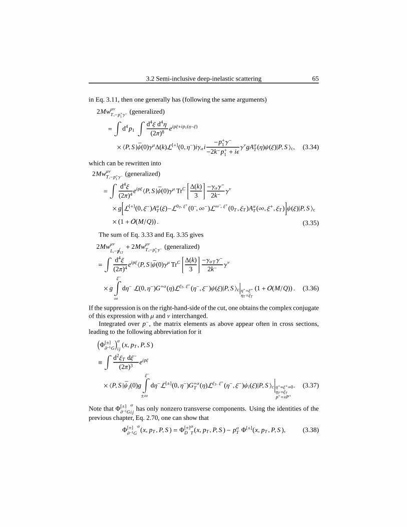
3.2 Semi-inclusive deep-inelastic scattering 65
in Eq. 3.11, then one generally has (following the same arguments)
2Mwµν
T,−p+1γ− (generalized)
=
∫d4p1
∫d4ξ d4η
(2π)8eipξ+ip1(η−ξ)
× 〈P,S|ψ(0)γµ∆(k)L[+](0, η−)iγαi−p+1γ
−
−2k−p+1 + iǫγνgAαT(η)ψ(ξ)|P,S〉c, (3.34)
which can be rewritten into
2Mwµν
T,−p+1γ− (generalized)
=
∫d4ξ
(2π)4eipξ〈P,S|ψ(0)γµ TrC
[∆(k)
3
]−γαγ−
2k−γν
× g[L[+](0, ξ−)Aα
T(ξ)−L0T, ξ+
(0−,∞−)L∞−, ξ+(0T , ξT)AαT(∞, ξ+, ξT)
]ψ(ξ)|P,S〉c
× (1+ O(M/Q)) . (3.35)
The sum of Eq. 3.33 and Eq. 3.35 gives
2Mwµν
L,−p/1T
+ 2Mwµν
T,−p+1γ− (generalized)
=
∫d4ξ
(2π)4eipξ〈P,S|ψ(0)γµ TrC
[∆(k)
3
] −γαTγ−
2k−γν
× g
ξ−∫
∞
dη− L(0, η−)G+α(η)LξT, ξ+
(η−, ξ−)ψ(ξ)|P,S〉c∣∣∣∣η+=ξ+ηT=ξT
(1+ O(M/Q)) . (3.36)
If the suppression is on the right-hand-side of the cut, one obtains the complex conjugateof this expression withµ andν interchanged.
Integrated overp−, the matrix elements as above appear often in cross sections,leading to the following abbreviation for it
(Φ
[±]∂−1G
)αi j
(x, pT ,P,S)
≡∫
d2ξT dξ−
(2π)3eipξ
× 〈P,S|ψ j(0)g
ξ−∫
±∞
dη−L[±](0, η−)G+αT (η)LξT, ξ+
(η−, ξ−)ψi(ξ)|P,S〉c∣∣∣∣∣η+=ξ+=0ηT=ξTp+=xP+
. (3.37)
Note thatΦ[±]∂−1G
α
i jhas only nonzero transverse components. Using the identities of the
previous chapter, Eq. 2.70, one can show that
Φ[±]∂−1G
α(x, pT ,P,S) = Φ[±]
D
α
T(x, pT ,P,S) − pαT Φ[±](x, pT ,P,S), (3.38)
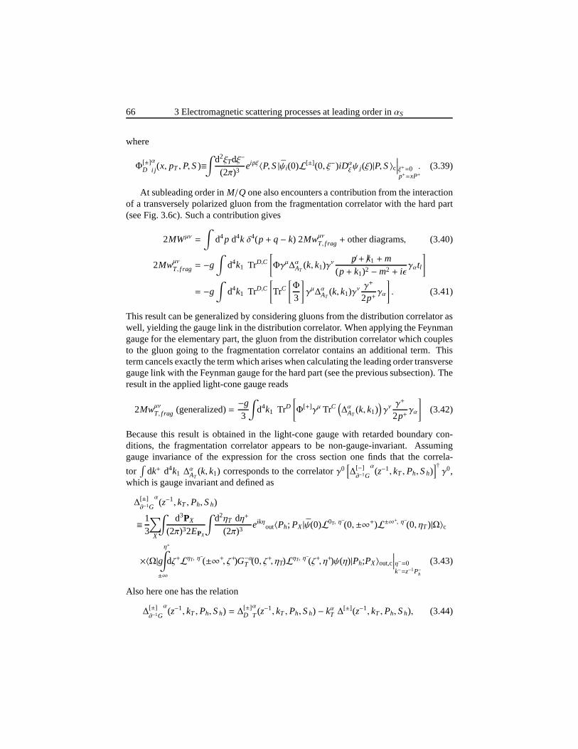
66 3 Electromagnetic scattering processes at leading orderin αS
where
Φ[±]D
α
i j (x, pT ,P,S)≡∫
d2ξTdξ−
(2π)3eipξ〈P,S|ψi(0)L[±](0, ξ−)iDα
ξψ j(ξ)|P,S〉c∣∣∣∣ξ+=0p+=xP+
. (3.39)
At subleading order inM/Q one also encounters a contribution from the interactionof a transversely polarized gluon from the fragmentation correlator with the hard part(see Fig. 3.6c). Such a contribution gives
2MWµν =
∫d4p d4k δ4(p+ q− k) 2Mwµν
T, f rag + other diagrams, (3.40)
2Mwµν
T, f rag = −g∫
d4k1 TrD,C
[Φγµ∆αAT
(k, k1)γν p/ + /k1 +m(p+ k1)2 −m2 + iǫ
γαtl
]
= −g∫
d4k1 TrD,C
[TrC
[Φ
3
]γµ∆αAT
(k, k1)γνγ+
2p+γα
]. (3.41)
This result can be generalized by considering gluons from the distribution correlator aswell, yielding the gauge link in the distribution correlator. When applying the Feynmangauge for the elementary part, the gluon from the distribution correlator which couplesto the gluon going to the fragmentation correlator containsan additional term. Thisterm cancels exactly the term which arises when calculatingthe leading order transversegauge link with the Feynman gauge for the hard part (see the previous subsection). Theresult in the applied light-cone gauge reads
2Mwµν
T, f rag (generalized)=−g3
∫d4k1 TrD
[Φ[+]γµ TrC
(∆αAT
(k, k1))γν
γ+
2p+γα
](3.42)
Because this result is obtained in the light-cone gauge withretarded boundary con-ditions, the fragmentation correlator appears to be non-gauge-invariant. Assuminggauge invariance of the expression for the cross section onefinds that the correla-
tor∫
dk+ d4k1 ∆αAT
(k, k1) corresponds to the correlatorγ0[∆
[−]∂−1G
α(z−1, kT ,Ph,Sh)
]†γ0,
which is gauge invariant and defined as
∆[±]∂−1G
α(z−1, kT ,Ph,Sh)
≡ 13
∑
X
∫d3PX
(2π)32EPX
∫d2ηT dη+
(2π)3eikη
out〈Ph; PX|ψ(0)L0T, η−(0,±∞+)L±∞+, η−(0, ηT)|Ω〉c
×〈Ω|gη+∫
±∞
dζ+LηT, η−(±∞+, ζ+)G−αT (0, ζ+, ηT)LηT, η
−(ζ+, η+)ψ(η)|Ph;PX〉out,c
∣∣∣∣η−=0k−=z−1P−h
(3.43)
Also here one has the relation
∆[±]∂−1G
α(z−1, kT ,Ph,Sh) = ∆[±]
D
α
T(z−1, kT ,Ph,Sh) − kαT ∆[±](z−1, kT ,Ph,Sh), (3.44)
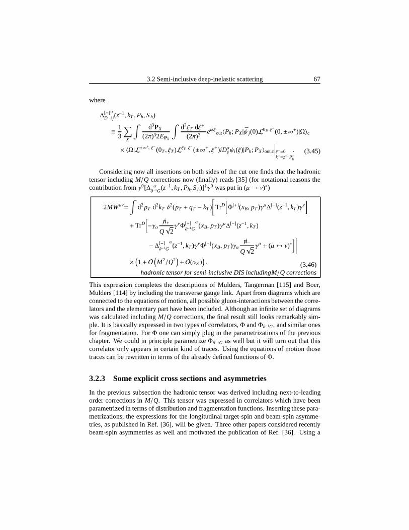
3.2 Semi-inclusive deep-inelastic scattering 67
where
∆[±]D
α
i j (z−1, kT ,Ph,Sh)
≡ 13
∑
X
∫d3PX
(2π)32EPX
∫d2ξT dξ+
(2π)3eikξ
out〈Ph; PX|ψ j(0)L0T, ξ−(0,±∞+)|Ω〉c
× 〈Ω|L±∞+, ξ− (0T , ξT)LξT, ξ−(±∞+, ξ+)iDα
ξψi(ξ)|Ph; PX〉out,c
∣∣∣∣ξ−=0k−=z−1P−h
. (3.45)
Considering now all insertions on both sides of the cut one finds that the hadronictensor includingM/Q corrections now (finally) reads [35] (for notational reasons thecontribution fromγ0[∆−α
∂−1G(z−1, kT ,Ph,Sh)]†γ0 was put in (µ→ ν)∗)
2MWµν=
∫d2pT d2kT δ
2(pT + qT − kT )
[TrD
[Φ[+](xB, pT)γµ∆[−](z−1, kT)γν
]
+ TrD[−γα
/n+
Q√
2γνΦ
[+]∂−1G
α(xB, pT)γµ∆[−](z−1, kT)
− ∆[−]∂−1G
α(z−1, kT)γνΦ[+](xB, pT)γα
/n−
Q√
2γµ + (µ↔ ν)∗
]]
×(1+ O
(M2/Q2
)+ O(αS)
). (3.46)
hadronic tensor for semi-inclusive DIS includingM/Q corrections
This expression completes the descriptions of Mulders, Tangerman [115] and Boer,Mulders [114] by including the transverse gauge link. Apartfrom diagrams which areconnected to the equations of motion, all possible gluon-interactions between the corre-lators and the elementary part have been included. Althoughan infinite set of diagramswas calculated includingM/Q corrections, the final result still looks remarkably sim-ple. It is basically expressed in two types of correlators,Φ andΦ∂−1G, and similar onesfor fragmentation. ForΦ one can simply plug in the parametrizations of the previouschapter. We could in principle parametrizeΦ∂−1G as well but it will turn out that thiscorrelator only appears in certain kind of traces. Using theequations of motion thosetraces can be rewritten in terms of the already defined functions ofΦ.
3.2.3 Some explicit cross sections and asymmetries
In the previous subsection the hadronic tensor was derived including next-to-leadingorder corrections inM/Q. This tensor was expressed in correlators which have beenparametrized in terms of distribution and fragmentation functions. Inserting these para-metrizations, the expressions for the longitudinal target-spin and beam-spin asymme-tries, as published in Ref. [36], will be given. Three other papers considered recentlybeam-spin asymmetries as well and motivated the publication of Ref. [36]. Using a

68 3 Electromagnetic scattering processes at leading orderin αS
model calculation, Afanasev and Carlson estimated in Ref. [116] the beam-spin asym-metry and compared their results to CLAS data. Yuan obtainedin Ref. [117] an ex-pression for the asymmetry and made an estimation by using a chiral quark model anda bag model. Metz and Schlegel claimed in Ref. [118], which also considers longitu-dinal target-spin asymmetries, that the calculation of Ref. [116] is incomplete. Theycompleted the model by including other diagrams which, as the authors point out them-selves, are not compatible with the parton model at orderM/Q. In Ref. [36] the analysisof Yuan [117] is completed by including quark-mass effects and the new functiong⊥.
Explicit leading order cross sections can easily be obtained by replacing the correla-torsΦ[+] and∆[−] in Eq. 3.46 with the explicit parametrizations of the previous chapter(see Eq. 2.57, 2.65, 2.83, 2.88). Note that our choice of light-like vectors, Eq. 3.2, iseasily related to the frame in which the correlators were defined, Eq. 2.47, 2.75. AtorderM/Q the other correlatorsΦ[+]
∂−1G
αand∆[−]
∂−1G
αneed to be included. They will be
handled here by making aFierz-decompositionwhich relies on the identity
TrD[AB
]= a1b1 + a2b2 + aα3b3α + aα4b4α + aαβ5 b5αβ,
where a1 =12
TrD[A], a2 =
12
TrD[Aγ5
], aα3 =
12
TrD[Aγα
],
aα4 =12
TrD[Aiγαγ5
], aαβ5 =
1
2√
2TrD[
Aσαβγ5]
and similarly forbi .
Using the Fierz-decomposition one encountersΦ∂−1G and∆∂−1G only in particularcombinations of traces which allow for a simplification by the use of the equations ofmotion. Showing only the argument connected to the polarization of the parent hadron,the correlatorsΦ∂−1G and∆∂−1G are decomposed into
Φ[+]∂−1G
α(S) = Φ[+]
∂−1G
α(0)+ Φ[+]
∂−1G
α(SL) + Φ[+]
∂−1G
α(ST), (3.47)
∆[−]∂−1G
α(Sh) = ∆
[−]∂−1G
α(0)+ ∆[−]
∂−1G
α(ShL) + ∆[−]
∂−1G
α(ShT). (3.48)
Using the relation [i /D−m]ψ = 0, which straightforwardly gives [iDµ+σµνDν−mγµ]ψ =[iγµDν−iγνDµ+imσµν+iǫµνρσγσγ5iDρ]ψ = 0, one finds for an unpolarized target (thefunctions depend onx andp2
T)
12
Tr[Φ
[+]∂−1G
α(0)σ +
α
]= iMx e− im f1 + Mx h−
p2T
Mh⊥1 , (3.49)
12
Tr[Φ
[+]∂−1G
α(0) iσ +
α γ5]= 0, (3.50)
12
Tr[Φ
[+]∂−1G
α(0)γ+
]−12ǫαβ
T Tr[Φ
[+]∂−1Gβ
(0) iγ+γ5]= pαT
(x f⊥+i
mM
h⊥1+ix g⊥− f1), (3.51)
and for unpolarized observed hadrons (where the functions depend onz andz2k2T)
14
Tr[∆
[−]∂−1G
α(0)σ −
α
]= iMhE[−] − imzD[−]
1 + MhH[−] −zk2
T
MhH⊥[−]
1 , (3.52)
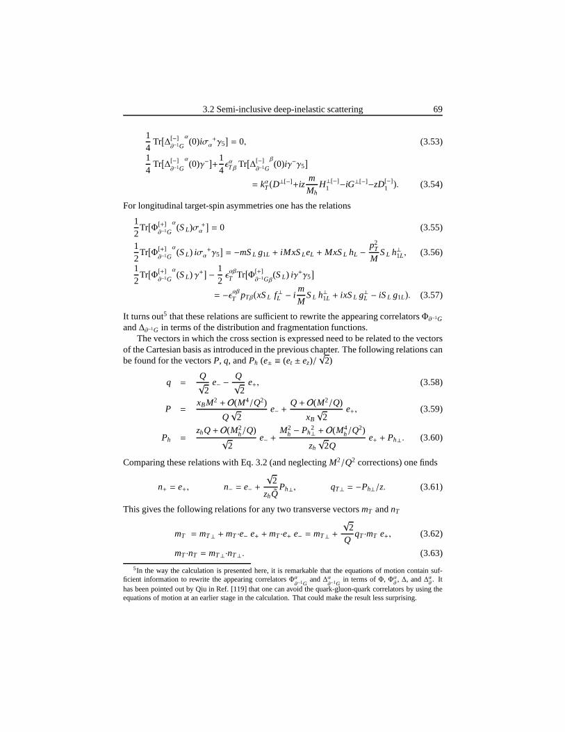
3.2 Semi-inclusive deep-inelastic scattering 69
14
Tr[∆
[−]∂−1G
α(0)iσ +
α γ5]= 0, (3.53)
14
Tr[∆
[−]∂−1G
α(0)γ−
]+
14ǫαTβ Tr
[∆
[−]∂−1G
β(0)iγ−γ5
]
= kαT(D⊥[−]+iz
mMh
H⊥[−]1 −iG⊥[−]−zD[−]
1
). (3.54)
For longitudinal target-spin asymmetries one has the relations
12
Tr[Φ
[+]∂−1G
α(SL)σ +α
]= 0 (3.55)
12
Tr[Φ
[+]∂−1G
α(SL) iσ +
α γ5]= −mSL g1L + iMxSLeL + MxSL hL −
p2T
MSL h⊥1L, (3.56)
12
Tr[Φ
[+]∂−1G
α(SL) γ+
] − 12ǫαβ
T Tr[Φ
[+]∂−1Gβ
(SL) iγ+γ5]
= −ǫαβT pTβ(xSL f⊥L − i
mM
SL h⊥1L + ixSL g⊥L − iSL g1L). (3.57)
It turns out5 that these relations are sufficient to rewrite the appearing correlatorsΦ∂−1G
and∆∂−1G in terms of the distribution and fragmentation functions.The vectors in which the cross section is expressed need to berelated to the vectors
of the Cartesian basis as introduced in the previous chapter. The following relations canbe found for the vectorsP, q, andPh (e± ≡ (et ± ez)/
√2)
q =Q√
2e− −
Q√
2e+, (3.58)
P =xBM2 + O(M4/Q2)
Q√
2e− +
Q+ O(M2/Q)
xB
√2
e+, (3.59)
Ph =zhQ+ O(M2
h/Q)√
2e− +
M2h − Ph
2⊥ + O(M4
h/Q2)
zh
√2Q
e+ + Ph⊥. (3.60)
Comparing these relations with Eq. 3.2 (and neglectingM2/Q2 corrections) one finds
n+ = e+, n− = e− +
√2
zhQPh⊥, qT⊥ = −Ph⊥/z. (3.61)
This gives the following relations for any two transverse vectorsmT andnT
mT = mT⊥ +mT ·e− e+ +mT ·e+ e− = mT⊥ +
√2
QqT ·mT e+, (3.62)
mT ·nT = mT⊥·nT⊥. (3.63)
5In the way the calculation is presented here, it is remarkable that the equations of motion contain suf-ficient information to rewrite the appearing correlatorsΦα
∂−1Gand∆α
∂−1Gin terms ofΦ, Φα
∂, ∆, and∆α
∂. It
has been pointed out by Qiu in Ref. [119] that one can avoid thequark-gluon-quark correlators by using theequations of motion at an earlier stage in the calculation. That could make the result less surprising.
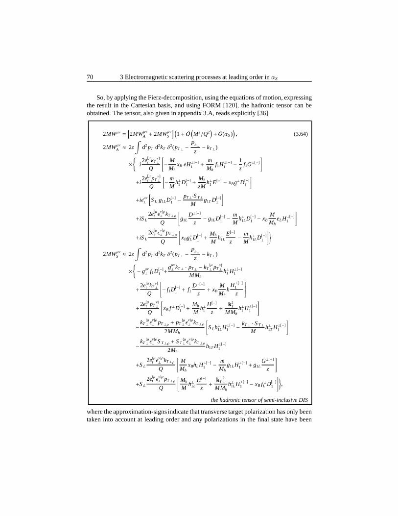
70 3 Electromagnetic scattering processes at leading orderin αS
So, by applying the Fierz-decomposition, using the equations of motion, expressingthe result in the Cartesian basis, and using FORM [120], the hadronic tensor can beobtained. The tensor, also given in appendix 3.A, reads explicitly [36]
2MWµν =[2MWµν
A + 2MWµν
S
] (1+ O
(M2/Q2
)+ O(αS)
), (3.64)
2MWµν
A ≈ 2z∫
d2pT d2kT δ2(pT⊥ −
Ph⊥z− kT⊥)
×
i2e[µ
t kTν]⊥
Q
[− M
MhxB eH⊥[−]
1 +mMh
f1H⊥[−]1 − 1
zf1G
⊥[−]
]
+i2e[µ
t pTν]⊥
Q
[−m
Mh⊥1 D[−]
1 +Mh
zMh⊥1 E[−] − xBg⊥D[−]
1
]
+iǫµν⊥
[SL g1LD[−]
1 −pT⊥·ST⊥
Mg1T D[−]
1
]
+iSL
2e[µt ǫ
ν]ρ⊥ kT⊥ρ
Q
[g1L
D⊥[−]
z− g1LD[−]
1 −mM
h⊥1LD[−]1 − xB
MMh
eLH⊥[−]1
]
+iSL
2e[µt ǫ
ν]ρ⊥ pT⊥ρ
Q
[xBg⊥L D[−]
1 +Mh
Mh⊥1L
E[−]
z− m
Mh⊥1LD[−]
1
]
2MWµν
S ≈ 2z∫
d2pT d2kT δ2(pT⊥ −
Ph⊥z− kT⊥)
×− gµν⊥ f1D[−]
1 +gµν⊥ kT⊥ · pT⊥ − kT
µ⊥ pT
ν⊥
MMhh⊥1 H⊥[−]
1
+2eµt kT
ν⊥
Q
− f1D[−]1 + f1
D⊥[−]
z+ xB
MMh
hH⊥[−]
1
z
+2eµt pT
ν⊥
Q
[xB f ⊥D[−]
1 +Mh
Mh⊥1
H[−]
z+
k2T
MMhh⊥1 H⊥[−]
1
]
−kTµ⊥ ǫ
νρ⊥ pT⊥ρ + pT
µ⊥ ǫ
νρ⊥ kT⊥ρ
2MMh
[SLh⊥1LH⊥[−]
1 − kT⊥ · ST⊥M
h⊥1T H⊥[−]1
]
−kTµ⊥ ǫ
νρ⊥ ST⊥ρ + ST
µ⊥ ǫ
νρ⊥ kT⊥ρ
2Mhh1T H⊥[−]
1
+SL
2eµt ǫνρ⊥ kT⊥ρ
Q
[MMh
xBhLH⊥[−]1 − m
Mhg1LH⊥[−]
1 + g1LG⊥[−]
z
]
+SL
2eµt ǫνρ⊥ pT⊥ρ
Q
[Mh
Mh⊥1L
H[−]
z+
kT2⊥
MMhh⊥1LH⊥[−]
1 − xB f ⊥L D[−]1
],
the hadronic tensor of semi-inclusive DIS
where the approximation-signs indicate that transverse target polarization has only beentaken into account at leading order and any polarizations inthe final state have been
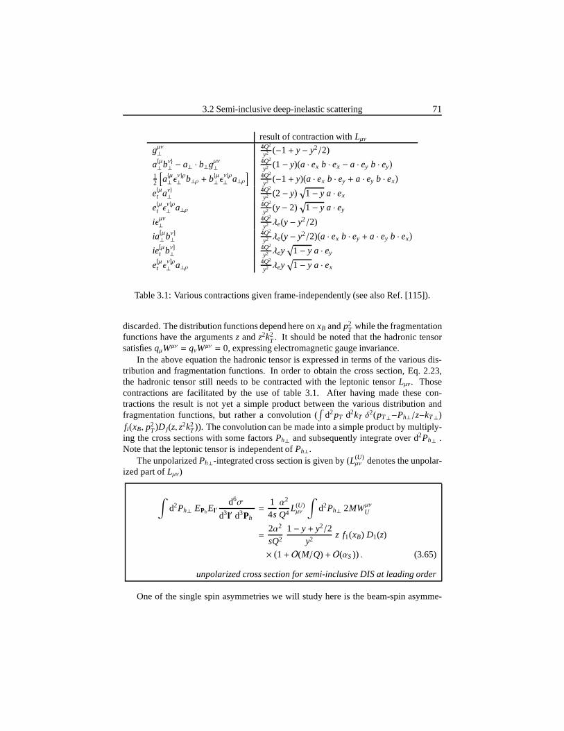
3.2 Semi-inclusive deep-inelastic scattering 71
result of contraction withLµνgµν⊥
4Q2
y2 (−1+ y− y2/2)
aµ⊥bν⊥ − a⊥ · b⊥gµν⊥4Q2
y2 (1− y)(a · ex b · ex − a · ey b · ey
)12
[aµ⊥ ǫ
νρ⊥ b⊥ρ + bµ⊥ ǫ
νρ⊥ a⊥ρ
]4Q2
y2 (−1+ y)(a · ex b · ey + a · ey b · ex
)
eµt aν⊥4Q2
y2 (2− y)√
1− y a · ex
eµt ǫνρ⊥ a⊥ρ
4Q2
y2 (y− 2)√
1− y a · ey
iǫµν⊥4Q2
y2 λe(y− y2/2)
ia[µ⊥bν]⊥
4Q2
y2 λe(y− y2/2)(a · ex b · ey + a · ey b · ex
)
ie[µt bν]⊥
4Q2
y2 λey√
1− y a · ey
e[µt ǫ
ν]ρ⊥ a⊥ρ
4Q2
y2 λey√
1− y a · ex
Table 3.1: Various contractions given frame-independently (see also Ref. [115]).
discarded. The distribution functions depend here onxB andp2T while the fragmentation
functions have the argumentsz andz2k2T . It should be noted that the hadronic tensor
satisfiesqµWµν = qνWµν = 0, expressing electromagnetic gauge invariance.In the above equation the hadronic tensor is expressed in terms of the various dis-
tribution and fragmentation functions. In order to obtain the cross section, Eq. 2.23,the hadronic tensor still needs to be contracted with the leptonic tensorLµν. Thosecontractions are facilitated by the use of table 3.1. After having made these con-tractions the result is not yet a simple product between the various distribution andfragmentation functions, but rather a convolution (
∫d2pT d2kT δ
2(pT⊥−Ph⊥/z−kT⊥)fi(xB, p2
T)D j(z, z2k2T)). The convolution can be made into a simple product by multiply-
ing the cross sections with some factorsPh⊥ and subsequently integrate over d2Ph⊥ .Note that the leptonic tensor is independent ofPh⊥.
The unpolarizedPh⊥-integrated cross section is given by (L(U)µν denotes the unpolar-
ized part ofLµν)
∫d2Ph⊥ EPhEl′
d6σ
d3l′ d3Ph
=14s
α2
Q4L(U)µν
∫d2Ph⊥ 2MWµν
U
=2α2
sQ2
1− y+ y2/2y2
z f1(xB) D1(z)
× (1+ O(M/Q) + O(αS)) . (3.65)
unpolarized cross section for semi-inclusive DIS at leading order
One of the single spin asymmetries we will study here is the beam-spin asymme-
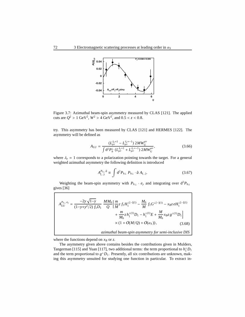
72 3 Electromagnetic scattering processes at leading orderin αS
-0.04
-0.02
0
0.02
0.04
0 2 4 6φ
A(φ
) LU
ALU=P1+P2sinφ
P2=0.038+/-0.005
Figure 3.7: Azimuthal beam-spin asymmetry measured by CLAS[121]. The appliedcuts areQ2 > 1 GeV2, W2 > 4 GeV2, and 0.5 < z< 0.8.
try. This asymmetry has been measured by CLAS [121] and HERMES [122]. Theasymmetry will be defined as
ALU =
(Lλe=1µν − Lλe=−1
µν
)2MWµν
U∫d2P⊥h
(Lλe=1µν + Lλe=−1
µν
)2MWµν
U
, (3.66)
whereλe = 1 corresponds to a polarization pointing towards the target. For a generalweighted azimuthal asymmetry the following definition is introduced
APh⊥ ·a(...) ≡
∫d2Ph⊥ Ph⊥ · a A(...). (3.67)
Weighting the beam-spin asymmetry withPh⊥ · ey and integrating over d2Ph⊥gives [36]
APh⊥ ·ey
LU =−2y
√1−y
(1−y+y2/2) f1D1
MMh
Q
[ mM
z f1H⊥[−](1)1 − Mh
Mf1G
⊥[−](1) − xBz eH⊥[−](1)1
+mMh
z h⊥(1)1 D1 − h⊥(1)
1 E +MMh
xBz g⊥(1)D1
]
× (1+ O(M/Q) + O(αS)) , (3.68)
azimuthal beam-spin asymmetry for semi-inclusive DIS
where the functions depend onxB or z.The asymmetry given above contains besides the contributions given in Mulders,
Tangerman [115] and Yuan [117], two additional terms: the term proportional toh⊥1 D1
and the term proportional tog⊥D1. Presently, all six contributions are unknown, mak-ing this asymmetry unsuited for studying one function in particular. To extract in-
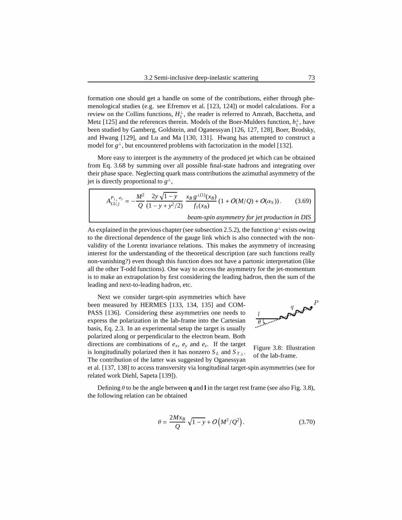
3.2 Semi-inclusive deep-inelastic scattering 73
formation one should get a handle on some of the contributions, either through phe-menological studies (e.g. see Efremov et al. [123, 124]) or model calculations. For areview on the Collins functions,H⊥1 , the reader is referred to Amrath, Bacchetta, andMetz [125] and the references therein. Models of the Boer-Mulders function,h⊥1 , havebeen studied by Gamberg, Goldstein, and Oganessyan [126, 127, 128], Boer, Brodsky,and Hwang [129], and Lu and Ma [130, 131]. Hwang has attemptedto construct amodel forg⊥, but encountered problems with factorization in the model [132].
More easy to interpret is the asymmetry of the produced jet which can be obtainedfrom Eq. 3.68 by summing over all possible final-state hadrons and integrating overtheir phase space. Neglecting quark mass contributions theazimuthal asymmetry of thejet is directly proportional tog⊥,
AP j⊥ ·ey
LU, j = −M2
Q
2y√
1− y
(1− y+ y2/2)xB g⊥(1)(xB)
f1(xB)(1+ O(M/Q) + O(αS)) . (3.69)
beam-spin asymmetry for jet production in DIS
As explained in the previous chapter (see subsection 2.5.2), the functiong⊥ exists owingto the directional dependence of the gauge link which is alsoconnected with the non-validity of the Lorentz invariance relations. This makes the asymmetry of increasinginterest for the understanding of the theoretical description (are such functions reallynon-vanishing?) even though this function does not have a partonic interpretation (likeall the other T-odd functions). One way to access the asymmetry for the jet-momentumis to make an extrapolation by first considering the leading hadron, then the sum of theleading and next-to-leading hadron, etc.
Next we consider target-spin asymmetries which havePSfrag replacements
P
lq
θ
Figure 3.8: Illustrationof the lab-frame.
been measured by HERMES [133, 134, 135] and COM-PASS [136]. Considering these asymmetries one needs toexpress the polarization in the lab-frame into the Cartesianbasis, Eq. 2.3. In an experimental setup the target is usuallypolarized along or perpendicular to the electron beam. Bothdirections are combinations ofex, ey and ez. If the targetis longitudinally polarized then it has nonzeroSL andST⊥.The contribution of the latter was suggested by Oganessyanet al. [137, 138] to access transversity via longitudinal target-spin asymmetries (see forrelated work Diehl, Sapeta [139]).
Definingθ to be the angle betweenq andl in the target rest frame (see also Fig. 3.8),the following relation can be obtained
θ =2MxB
Q
√1− y+ O
(M2/Q2
). (3.70)
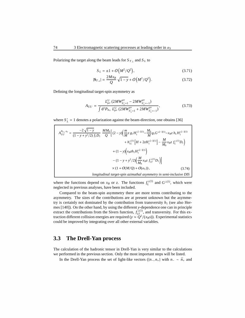
74 3 Electromagnetic scattering processes at leading orderin αS
Polarizing the target along the beam leads forST⊥ andSL to
SL = ±1+ O(M2/Q2
), (3.71)
|ST⊥| =2MxB
Q
√1− y+ O
(M2/Q2
). (3.72)
Defining the longitudinal target-spin asymmetry as
AUL′ =LUµν
(2MWµν
S′L=1 − 2MWµν
S′L=−1
)∫
d2Ph⊥ LUµν
(2MWµν
S′L=1 + 2MWµν
S′L=−1
) , (3.73)
whereS′L = 1 denotes a polarization against the beam-direction, one obtains [36]
APh⊥ ·ey
UL′ =−2
√1− y
(1− y+ y2/2) f1D1
MMh
Q
[(2− y)
( mM
z g1H⊥[−](1)1 −Mh
Mg1G
⊥[−](1)−xBz hLH⊥[−](1)1
+ h⊥(1)1L
[H + 2zH⊥[−](1)
1
]− M
MhxBz f⊥(1)
L D1
)
+ (1− y)(xBzh1H⊥[−](1)
1
)
− (1− y+ y2/2)( MMh
xBz f⊥(1)1T D1
)]
× (1+ O(M/Q) + O(αS)) , (3.74)
longitudinal target-spin azimuthal asymmetry in semi-inclusive DIS
where the functions depend onxB or z. The functionsf⊥(1)L andG⊥(1), which were
neglected in previous analyses, have been included.Compared to the beam-spin asymmetry there are more terms contributing to the
asymmetry. The sizes of the contributions are at present unknown but the asymme-try is certainly not dominated by the contribution from transversityh1 (see also Her-mes [140]). On the other hand, by using the differenty-dependence one can in principleextract the contributions from the Sivers function,f⊥(1)
1T , and transversity. For this ex-traction different collision energies are required (y ≈ Q2/(xBs)). Experimental statisticscould be improved by integrating over all other external variables.
3.3 The Drell-Yan process
The calculation of the hadronic tensor in Drell-Yan is very similar to the calculationswe performed in the previous section. Only the most important steps will be listed.
In the Drell-Yan process the set of light-like vectors (n−, n+ with n− ∼ n+ and
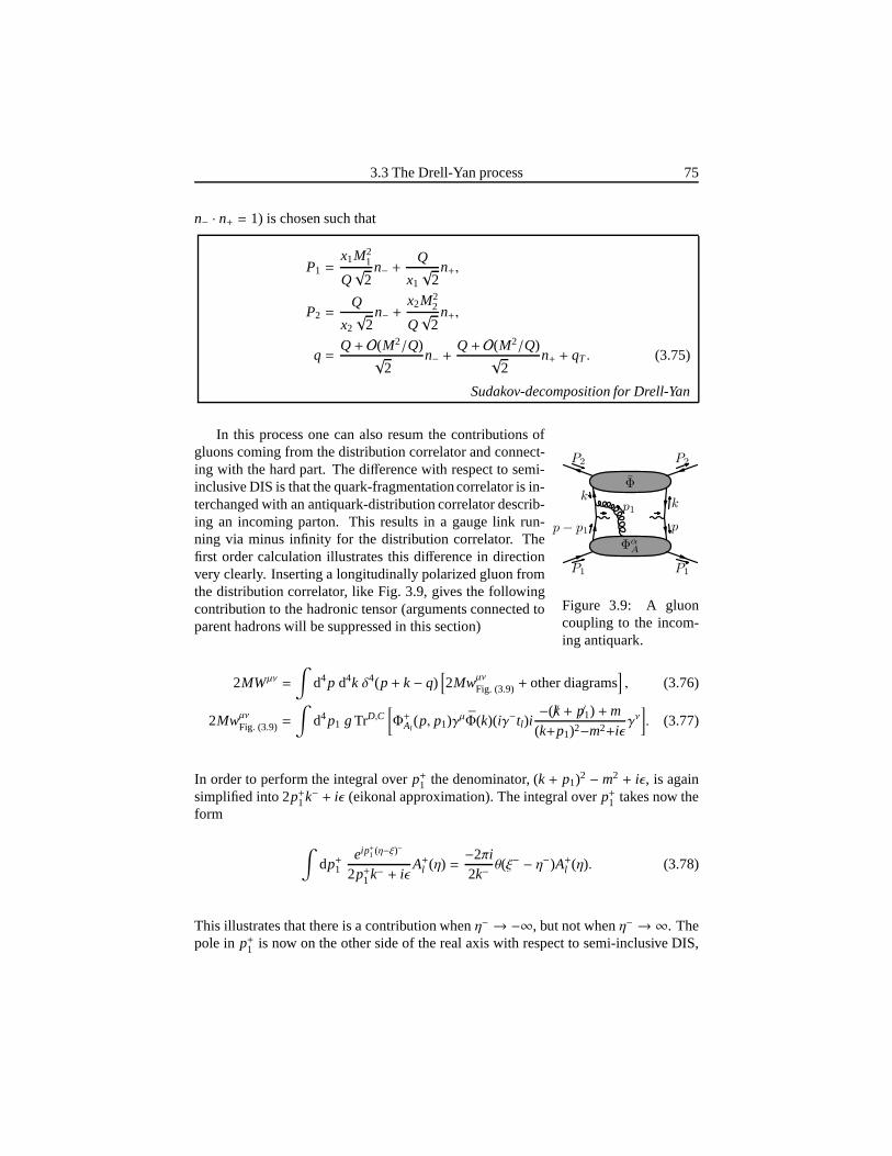
3.3 The Drell-Yan process 75
n− · n+ = 1) is chosen such that
P1 =x1M2
1
Q√
2n− +
Q
x1
√2
n+,
P2 =Q
x2
√2
n− +x2M2
2
Q√
2n+,
q =Q+ O(M2/Q)
√2
n− +Q+ O(M2/Q)
√2
n+ + qT . (3.75)
Sudakov-decomposition for Drell-Yan
In this process one can also resum the contributions of
ΦαA
Φ
p− p1
p1
k
p
k
P1 P1
P2 P2
Figure 3.9: A gluoncoupling to the incom-ing antiquark.
gluons coming from the distribution correlator and connect-ing with the hard part. The difference with respect to semi-inclusive DIS is that the quark-fragmentationcorrelator is in-terchanged with an antiquark-distribution correlator describ-ing an incoming parton. This results in a gauge link run-ning via minus infinity for the distribution correlator. Thefirst order calculation illustrates this difference in directionvery clearly. Inserting a longitudinally polarized gluon fromthe distribution correlator, like Fig. 3.9, gives the followingcontribution to the hadronic tensor (arguments connected toparent hadrons will be suppressed in this section)
2MWµν =
∫d4p d4k δ4(p+ k− q)
[2Mwµν
Fig. (3.9)+ other diagrams], (3.76)
2Mwµν
Fig. (3.9)=
∫d4p1 gTrD,C
[Φ+Al
(p, p1)γµΦ(k)(iγ−tl)i−(/k+ p/1) +m
(k+p1)2−m2+iǫγν
]. (3.77)
In order to perform the integral overp+1 the denominator, (k + p1)2 −m2 + iǫ, is againsimplified into 2p+1k− + iǫ (eikonal approximation). The integral overp+1 takes now theform
∫dp+1
eip+1 (η−ξ)−
2p+1k− + iǫA+l (η) =
−2πi2k−
θ(ξ− − η−)A+l (η). (3.78)
This illustrates that there is a contribution whenη− → −∞, but not whenη− → ∞. Thepole in p+1 is now on the other side of the real axis with respect to semi-inclusive DIS,
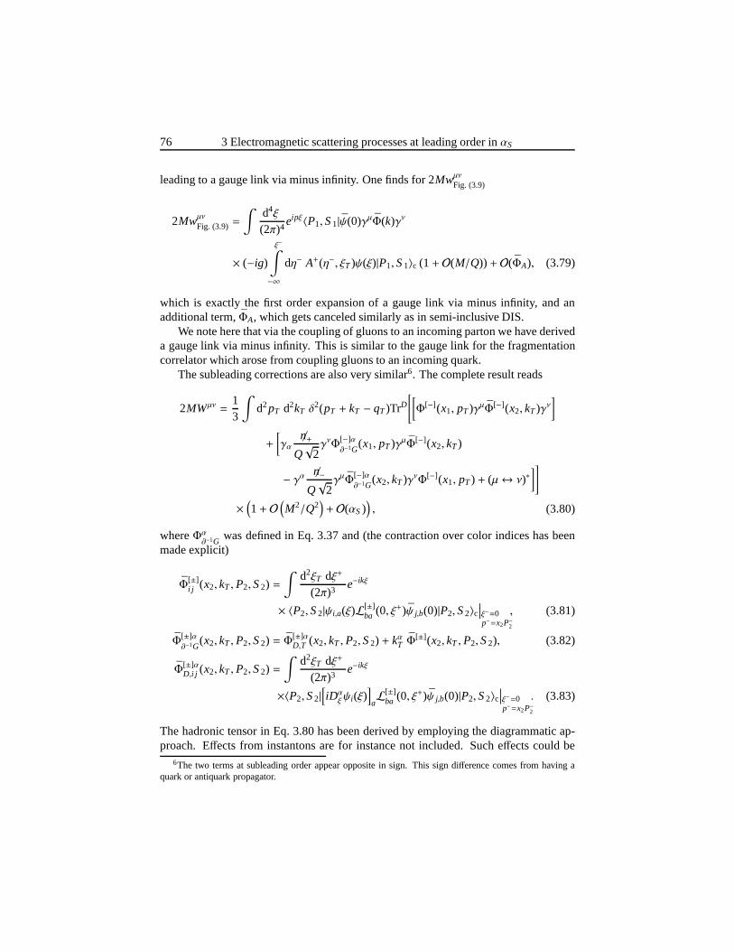
76 3 Electromagnetic scattering processes at leading orderin αS
leading to a gauge link via minus infinity. One finds for 2Mwµν
Fig. (3.9)
2Mwµν
Fig. (3.9)=
∫d4ξ
(2π)4eipξ〈P1,S1|ψ(0)γµΦ(k)γν
× (−ig)
ξ−∫
−∞
dη− A+(η−, ξT)ψ(ξ)|P1,S1〉c (1+ O(M/Q)) + O(ΦA), (3.79)
which is exactly the first order expansion of a gauge link via minus infinity, and anadditional term,ΦA, which gets canceled similarly as in semi-inclusive DIS.
We note here that via the coupling of gluons to an incoming parton we have deriveda gauge link via minus infinity. This is similar to the gauge link for the fragmentationcorrelator which arose from coupling gluons to an incoming quark.
The subleading corrections are also very similar6. The complete result reads
2MWµν =13
∫d2pT d2kT δ
2(pT + kT − qT)TrD
[[Φ[−](x1, pT)γµΦ[−](x2, kT)γν
]
+
[γα
n/+Q√
2γνΦ
[−]α∂−1G
(x1, pT)γµΦ[−](x2, kT)
− γα n/−Q√
2γµΦ
[−]α∂−1G
(x2, kT)γνΦ[−](x1, pT) + (µ↔ ν)∗]]
×(1+ O
(M2/Q2
)+ O(αS)
), (3.80)
whereΦα∂−1G
was defined in Eq. 3.37 and (the contraction over color indices has beenmade explicit)
Φ[±]i j (x2, kT ,P2,S2) =
∫d2ξT dξ+
(2π)3e−ikξ
× 〈P2,S2|ψi,a(ξ)L[±]ba (0, ξ+)ψ j,b(0)|P2,S2〉c
∣∣∣ξ−=0p−=x2P−2
, (3.81)
Φ[±]α∂−1G
(x2, kT ,P2,S2) = Φ[±]αD,T (x2, kT ,P2,S2) + kαT Φ
[±](x2, kT ,P2,S2), (3.82)
Φ[±]αD,i j (x2, kT ,P2,S2) =
∫d2ξT dξ+
(2π)3e−ikξ
×〈P2,S2|[iDα
ξψi(ξ)]aL[±]
ba (0, ξ+)ψ j,b(0)|P2,S2〉c∣∣∣ξ−=0p−=x2P−2
. (3.83)
The hadronic tensor in Eq. 3.80 has been derived by employingthe diagrammatic ap-proach. Effects from instantons are for instance not included. Such effects could be
6The two terms at subleading order appear opposite in sign. This sign difference comes from having aquark or antiquark propagator.
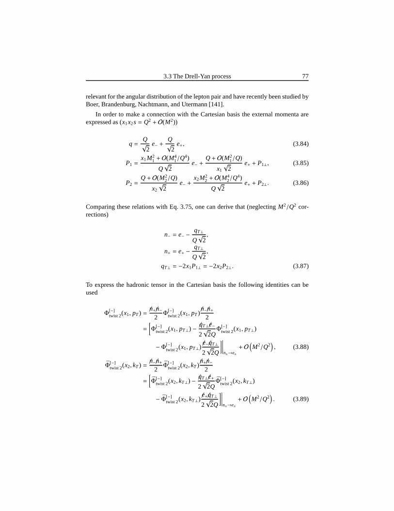
3.3 The Drell-Yan process 77
relevant for the angular distribution of the lepton pair andhave recently been studied byBoer, Brandenburg, Nachtmann, and Utermann [141].
In order to make a connection with the Cartesian basis the external momenta areexpressed as (x1x2s= Q2 + O(M2))
q =Q√
2e− +
Q√
2e+, (3.84)
P1 =x1M2
1 + O(M41/Q
4)
Q√
2e− +
Q+ O(M21/Q)
x1√
2e+ + P1⊥, (3.85)
P2 =Q+ O(M2
2/Q)
x2
√2
e− +x2M2
2 + O(M42/Q
4)
Q√
2e+ + P2⊥. (3.86)
Comparing these relations with Eq. 3.75, one can derive that(neglectingM2/Q2 cor-rections)
n− = e− −qT⊥
Q√
2,
n+ = e+ −qT⊥
Q√
2,
qT⊥ = −2x1P1⊥ = −2x2P2⊥. (3.87)
To express the hadronic tensor in the Cartesian basis the following identities can beused
Φ[−]twist 2(x1, pT) =
/n+/n−2Φ
[−]twist 2(x1, pT)
/n−/n+2
=
[Φ
[−]twist 2(x1, pT⊥) − /qT⊥/e−
2√
2QΦ
[−]twist 2(x1, pT⊥)
−Φ[−]twist 2(x1, pT⊥)
/e−/qT⊥
2√
2Q
]∣∣∣∣∣n±→e±
+ O(M2/Q2
), (3.88)
Φ[−]twist 2(x2, kT) =
/n−/n+2Φ
[−]twist 2(x2, kT)
/n+/n−2
=
[Φ
[−]twist 2(x2, kT⊥) − /qT⊥/e+
2√
2QΦ
[−]twist 2(x2, kT⊥)
− Φ[−]twist 2(x2, kT⊥)
/e+/qT⊥
2√
2Q
]∣∣∣∣∣n±→e±
+ O(M2/Q2
). (3.89)
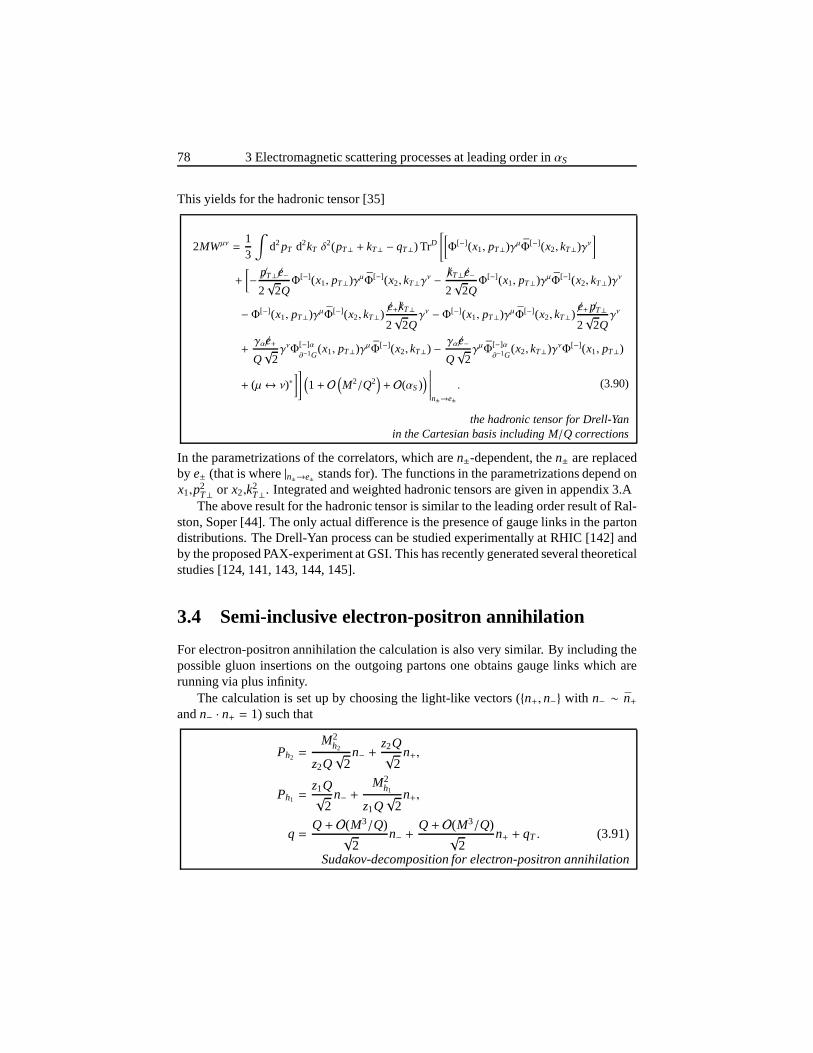
78 3 Electromagnetic scattering processes at leading orderin αS
This yields for the hadronic tensor [35]
2MWµν =13
∫d2pT d2kT δ
2(pT⊥ + kT⊥ − qT⊥) TrD
[[Φ[−](x1, pT⊥)γµΦ[−](x2, kT⊥)γν
]
+
[− p/T⊥/e−
2√
2QΦ[−](x1, pT⊥)γµΦ[−](x2, kT⊥γ
ν − /kT⊥/e−
2√
2QΦ[−](x1, pT⊥)γµΦ[−](x2, kT⊥)γν
− Φ[−](x1, pT⊥)γµΦ[−](x2, kT⊥)/e+/kT⊥
2√
2Qγν − Φ[−](x1, pT⊥)γµΦ[−](x2, kT⊥)
/e+p/T⊥2√
2Qγν
+γα/e+
Q√
2γνΦ
[−]α∂−1G
(x1, pT⊥)γµΦ[−](x2, kT⊥) − γα/e−
Q√
2γµΦ
[−]α∂−1G
(x2, kT⊥)γνΦ[−](x1, pT⊥)
+ (µ↔ ν)∗]] (
1+ O(M2/Q2
)+ O(αS)
) ∣∣∣∣∣∣n±→e±
. (3.90)
the hadronic tensor for Drell-Yanin the Cartesian basis including M/Q corrections
In the parametrizations of the correlators, which aren±-dependent, then± are replacedby e± (that is where|n±→e± stands for). The functions in the parametrizations depend onx1,p2
T⊥ or x2,k2T⊥. Integrated and weighted hadronic tensors are given in appendix 3.A
The above result for the hadronic tensor is similar to the leading order result of Ral-ston, Soper [44]. The only actual difference is the presence of gauge links in the partondistributions. The Drell-Yan process can be studied experimentally at RHIC [142] andby the proposed PAX-experiment at GSI. This has recently generated several theoreticalstudies [124, 141, 143, 144, 145].
3.4 Semi-inclusive electron-positron annihilation
For electron-positron annihilation the calculation is also very similar. By including thepossible gluon insertions on the outgoing partons one obtains gauge links which arerunning via plus infinity.
The calculation is set up by choosing the light-like vectors(n+, n− with n− ∼ n+andn− · n+ = 1) such that
Ph2 =M2
h2
z2Q√
2n− +
z2Q√
2n+,
Ph1 =z1Q√
2n− +
M2h1
z1Q√
2n+,
q =Q+ O(M3/Q)
√2
n− +Q+ O(M3/Q)
√2
n+ + qT . (3.91)
Sudakov-decomposition for electron-positron annihilation
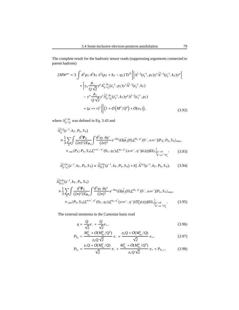
3.4 Semi-inclusive electron-positron annihilation 79
The complete result for the hadronic tensor reads (suppressing arguments connected toparent hadrons)
2MWµν = 3∫
d2pT d2kT δ2(pT + kT − qT) TrD
[[∆[−] (z−1
1 , pT)γν∆[−](z−12 , kT)γµ
]
+
[γα/n−
Q√
2γµ∆
[−]α∂−1G
(z−11 , pT)γν∆[−](z−1
2 , kT)
− γα /n+Q√
2γν∆
[−]α∂−1G
(z−12 , kT)γµ∆[−](z−1
1 , pT)
+ (µ↔ ν)∗]] (
1+ O(M2/Q2
)+ O(αS)
), (3.92)
where∆[−]α∂−1G
was defined in Eq. 3.43 and
∆[±]i j (z−1, kT ,Ph,Sh)
≡ 13
∑
X
∫d3PX
(2π)32EPX
∫d2ηT dη−
(2π)3e−ikη〈Ω|ψ j(0)L0T, η
+
(0−,±∞−)|PX; Ph,Sh〉out,c
× out〈PX; Ph,Sh|L±∞−, η+ (0T , ηT)LηT, η
+
(±∞−, η−)ψi(η)|Ω〉c∣∣∣∣η+=0k+=z−1P+h
, (3.93)
∆[±]α∂−1G
(z−1, kT ,Ph,Sh) ≡ ∆[±]αD,T (z−1, kT ,Ph,Sh) + kαT ∆
[±](z−1, kT ,Ph,Sh), (3.94)
∆[±]αD,i j (z−1, kT ,Ph,Sh)
≡ 13
∑
X
∫d3PX
(2π)32EPX
∫d2ηT dη+
(2π)3e−ikη〈Ω|ψ j(0)L0T, η
+
(0−,±∞−)|Ph,Sh〉out,c
× out〈Ph,Sh|L±∞−, η+(0T , ηT)LηT, η
+
(±∞−, η−)iDαηψi(η)|Ω〉c
∣∣∣∣η+=0k+=z−1P+h
, (3.95)
The external momenta in the Cartesian basis read
q =Q√
2e− +
Q√
2e+, (3.96)
Ph2 =M2
h2+ O(M4
h2/Q2)
z2Q√
2e− +
z2Q+ O(M2h2/Q)
√2
e+, (3.97)
Ph1 =z1Q+ O(M2
h1/Q)
√2
e− +M2
h1+ O(M4
h1/Q2)
z1Q√
2e+ + Ph1⊥, (3.98)
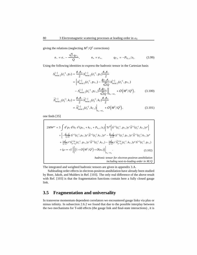
80 3 Electromagnetic scattering processes at leading orderin αS
giving the relations (neglectingM2/Q2 corrections)
n− = e− −√
2 qT⊥Q
, n+ = e+, qT⊥ = −Ph1⊥/z1. (3.99)
Using the following identities to express the hadronic tensor in the Cartesian basis
∆[−]twist 2(z
−11 , pT) =
/n−/n+2∆
[−]twist 2(z
−11 , pT)
/n+/n−2
=
[∆
[−]twist 2(z
−11 , pT⊥) − /qT⊥/e+√
2Q∆
[−]twist 2(z
−11 , pT⊥)
− ∆[−]twist 2(z
−11 , pT⊥)
/e+/qT⊥√2Q
]∣∣∣∣∣n±→e±
+ O(M2/Q2
), (3.100)
∆[−]twist 2(z
−12 , kT) =
/n+/n−2∆
[−]twist 2(z
−12 , kT)
/n−/n+2
= ∆[−]twist 2(z
−12 , kT⊥)
∣∣∣∣∣n±→e±
+ O(M2/Q2
), (3.101)
one finds [35]
2MWµν = 3∫
d2pT d2kT δ2(pT⊥ + kT⊥ + Ph1⊥/z1)
[TrD
[∆[+](z−1
1 , pT⊥)γν∆[+](z−12 , kT⊥)γµ
]
+
[− p/T⊥/e+
Q√
2∆[+](z−1
1 , pT⊥)γν∆[+](z−12 , kT⊥)γµ − /kT⊥/e+
Q√
2∆[+](z−1
1 , pT⊥)γν∆[+](z−12 , kT⊥)γµ
+γα/e−Q√
2γµ∆
[+]α∂−1G
(z−11 , pT⊥)γν∆[+](z−1
2 , kT⊥) − γα/e+Q√
2γν∆
[+]α∂−1G
(z−11 , kT⊥)γµ∆[+](z−1
1 , pT⊥)
+ (µ↔ ν)∗]] (
1+ O(M2/Q2
)+ O(αS)
) ∣∣∣∣∣∣n±→e±
. (3.102)
hadronic tensor for electron-positron annihilationincluding next-to-leading order in M/Q
The integrated and weighted hadronic tensors are given in appendix 3.A.Subleading order effects in electron-positron annihilation have already been studied
by Boer, Jakob, and Mulders in Ref. [103]. The only real difference of the above resultwith Ref. [103] is that the fragmentation functions containhere a fully closed gaugelink.
3.5 Fragmentation and universality
In transverse momentum dependent correlators we encountered gauge links via plus orminus infinity. In subsection 2.6.2 we found that due to the possible interplay betweenthe two mechanisms for T-odd effects (the gauge link and final-state interactions) , it is

3.5 Fragmentation and universality 81
(a) (b)
Figure 3.10: Two typical diagrams which appear in model calculations and produceT-odd effects. Diagram (a) appears in electron-positron annihilation and diagram (b)appears in semi-inclusive DIS. The dashed-lines representsome kind of particle (forinstance a scalar diquark).
not possible to relate those correlators which have different link structures. However,if one of the mechanisms turns out to be absent or heavily suppressed, then relationsbetween fragmentation functions having different gauge links can be derived.
In 2002, an article written by Metz [100] appeared in which universality of frag-mentation was argued. In that paper the effect of the gauge link is modeled through aset of diagrams in semi-inclusive DIS and electron-positron annihilation, see Fig. 3.10.Within the model it is found that the Collins function appears with the same sign inboth processes. In order to achieve this result the momentumin the loop in Fig. 3.10 isnot integrated over the full integration domain. This restriction is justified to make themodel consistent with the parton model but also makes it unclear whether the univer-sality result still holds if this restriction is lifted.
The result of Ref. [100] was formalized in a subsequent paperby Collins andMetz [101] in which it is claimed that the gauge link is taken into account. Havingsimilar diagrams as in Fig. 3.10, the authorseikonalizethe quark-propagator next to theexchanged gluon, meaning that its transverse momentum is assumed to be small. Thisprocedure is similar to the restriction made in Ref. [100] because it effectively limits theintegration domain over the momenta. When comparing the twoprocesses, it was foundin Ref. [101] that the pole of the eikonal propagator does notcontribute7 in the crosssection and consequently the difference between the processes vanishes8. According tothe authors this shows that fragmentation functions are universal in QCD.
A first comment on both papers is that restricting the integration domain of themomenta in the loop makes the interesting result less rigorous. It is not clear whether
7Gamberg, Goldstein, and Oganessyan find in Ref. [146] in a slightly different formulation that the eikonalpole does contribute in T-odd effects, giving a sign dependent fragmentation function if only the gauge linkis considered (no final-state interactions). This result has been challenged by Amrath, Bacchetta, and Metzin Ref. [125]. However, if the result of Ref. [146] holds then, together with the final-state interactions, thismodel would illustrate the universality problems with fragmentation.
8After a single momentum integration all poles fall on one side of the real axis. This allows one to closethe contour on the other side of this axis and one finds that thedifference between the processes vanishes.
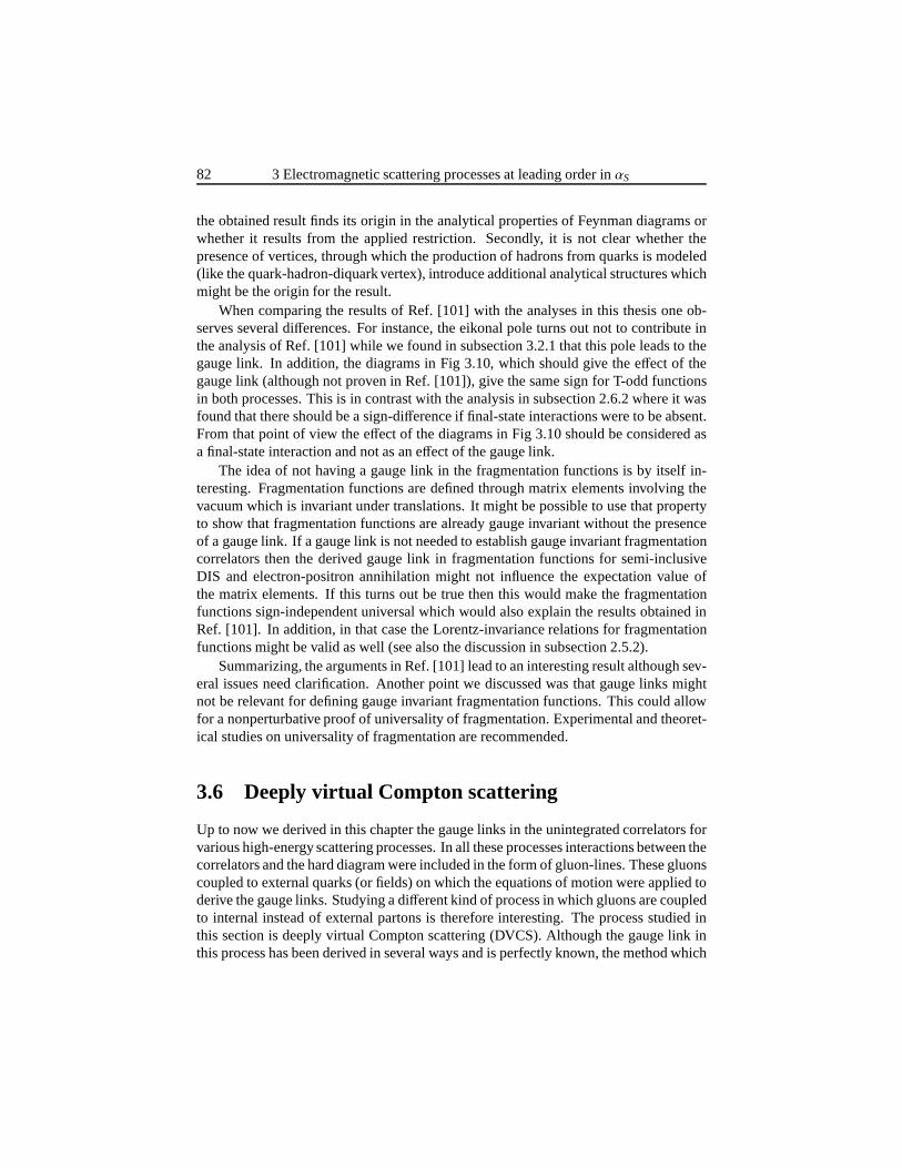
82 3 Electromagnetic scattering processes at leading orderin αS
the obtained result finds its origin in the analytical properties of Feynman diagrams orwhether it results from the applied restriction. Secondly,it is not clear whether thepresence of vertices, through which the production of hadrons from quarks is modeled(like the quark-hadron-diquark vertex), introduce additional analytical structures whichmight be the origin for the result.
When comparing the results of Ref. [101] with the analyses inthis thesis one ob-serves several differences. For instance, the eikonal pole turns out not to contribute inthe analysis of Ref. [101] while we found in subsection 3.2.1that this pole leads to thegauge link. In addition, the diagrams in Fig 3.10, which should give the effect of thegauge link (although not proven in Ref. [101]), give the samesign for T-odd functionsin both processes. This is in contrast with the analysis in subsection 2.6.2 where it wasfound that there should be a sign-difference if final-state interactions were to be absent.From that point of view the effect of the diagrams in Fig 3.10 should be considered asa final-state interaction and not as an effect of the gauge link.
The idea of not having a gauge link in the fragmentation functions is by itself in-teresting. Fragmentation functions are defined through matrix elements involving thevacuum which is invariant under translations. It might be possible to use that propertyto show that fragmentation functions are already gauge invariant without the presenceof a gauge link. If a gauge link is not needed to establish gauge invariant fragmentationcorrelators then the derived gauge link in fragmentation functions for semi-inclusiveDIS and electron-positron annihilation might not influencethe expectation value ofthe matrix elements. If this turns out be true then this wouldmake the fragmentationfunctions sign-independent universal which would also explain the results obtained inRef. [101]. In addition, in that case the Lorentz-invariance relations for fragmentationfunctions might be valid as well (see also the discussion in subsection 2.5.2).
Summarizing, the arguments in Ref. [101] lead to an interesting result although sev-eral issues need clarification. Another point we discussed was that gauge links mightnot be relevant for defining gauge invariant fragmentation functions. This could allowfor a nonperturbative proof of universality of fragmentation. Experimental and theoret-ical studies on universality of fragmentation are recommended.
3.6 Deeply virtual Compton scattering
Up to now we derived in this chapter the gauge links in the unintegrated correlators forvarious high-energy scattering processes. In all these processes interactions between thecorrelators and the hard diagram were included in the form ofgluon-lines. These gluonscoupled to external quarks (or fields) on which the equationsof motion were applied toderive the gauge links. Studying a different kind of process in which gluons are coupledto internal instead of external partons is therefore interesting. The process studied inthis section is deeply virtual Compton scattering (DVCS). Although the gauge link inthis process has been derived in several ways and is perfectly known, the method which
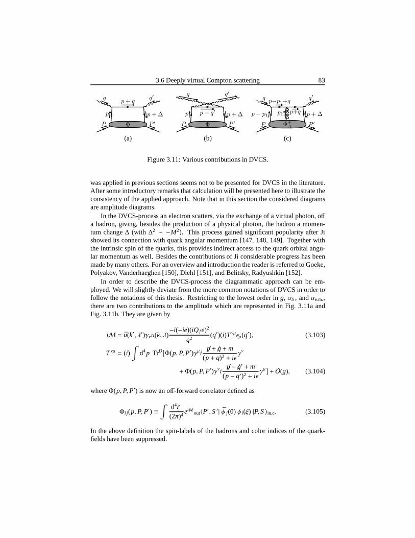
3.6 Deeply virtual Compton scattering 83
Φ
p
p+ q
p+ ∆
P P ′
q q′
Φ
p p− q′ p+ ∆
P P ′
q q′
Φ+A
p− p1
p−p1+q
p+qp1 p+ ∆
P P ′
q q′
(a) (b) (c)
Figure 3.11: Various contributions in DVCS.
was applied in previous sections seems not to be presented for DVCS in the literature.After some introductory remarks that calculation will be presented here to illustrate theconsistency of the applied approach. Note that in this section the considered diagramsare amplitude diagrams.
In the DVCS-process an electron scatters, via the exchange of a virtual photon, offa hadron, giving, besides the production of a physical photon, the hadron a momen-tum change∆ (with ∆2 ∼ −M2). This process gained significant popularity after Jishowed its connection with quark angular momentum [147, 148, 149]. Together withthe intrinsic spin of the quarks, this provides indirect access to the quark orbital angu-lar momentum as well. Besides the contributions of Ji considerable progress has beenmade by many others. For an overview and introduction the reader is referred to Goeke,Polyakov, Vanderhaeghen [150], Diehl [151], and Belitsky,Radyushkin [152].
In order to describe the DVCS-process the diagrammatic approach can be em-ployed. We will slightly deviate from the more common notations of DVCS in order tofollow the notations of this thesis. Restricting to the lowest order ing, αS, andαe.m.,there are two contributions to the amplitude which are represented in Fig. 3.11a andFig. 3.11b. They are given by
iM = u(k′, λ′)γνu(k, λ)−i(−ie)(iQ fe)2
q2(q′)(i)Tνµǫµ(q′), (3.103)
Tνµ = (i)∫
d4p TrD[Φ(p,P,P′)γµi
p/ + /q+m(p+ q)2 + iǫ
γν
+ Φ(p,P,P′)γνip/ − /q′ +m
(p− q′)2 + iǫγµ
]+ O(g), (3.104)
whereΦ(p,P,P′) is now an off-forward correlator defined as
Φi j (p,P,P′) ≡
∫d4ξ
(2π)4eipξ
out〈P′,S′| ψ j(0)ψi(ξ) |P,S〉in,c. (3.105)
In the above definition the spin-labels of the hadrons and color indices of the quark-fields have been suppressed.
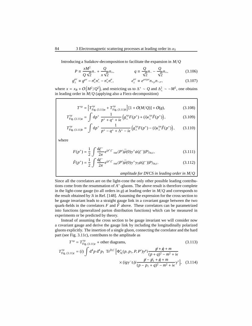
84 3 Electromagnetic scattering processes at leading orderin αS
Introducing a Sudakov-decomposition to facilitate the expansion inM/Q
P ≡ xM2
Q√
2n− +
Q
x√
2n+, q ≡ Q
√2
n− −Q√
2n+, (3.106)
gµν⊥ ≡ gµν − nµ+nν− − nν+n
µ−, ǫ
µν⊥ ≡ ǫρσµνn+ρn−σ, (3.107)
wherex = xB + O(M2/Q2
), and restricting us to∆+ ∼ Q and∆2
⊥ ∼ −M2, one obtainsin leading order inM/Q (applying also a Fierz-decomposition)
Tνµ =[Tνµ
Fig. (3.11)a + Tνµ
Fig. (3.11)b
][1 + O(M/Q)] + O(g), (3.108)
Tνµ
Fig. (3.11)a =
∫dp+
1p+ + q+ + iǫ
(gνµ⊥ F(p+) + (i)ǫνµ⊥ F(p+)
), (3.109)
Tνµ
Fig. (3.11)b =
∫dp+
1p+ − q+ + ∆+ − iǫ
(gνµ⊥ F(p+) − (i)ǫνµ⊥ F(p+)
), (3.110)
where
F(p+) =12
∫dξ−
2πeip+ξ−
out〈P′|ψ(0)γ+ψ(ξ−)|P〉in,c, (3.111)
F(p+) =12
∫dξ−
2πeip+ξ−
out〈P′|ψ(0)γ+γ5ψ(ξ−)|P〉in,c. (3.112)
amplitude for DVCS in leading order in M/Q
Since all the correlators are on the light-cone the only other possible leading contribu-tions come from the resummation ofA+-gluons. The above result is therefore completein the light-cone gauge (to all orders ing) at leading order inM/Q and corresponds tothe result obtained by Ji in Ref. [148]. Assuming the expression for the cross section tobe gauge invariant leads to a straight gauge link in a covariant gauge between the twoquark-fields in the correlatorsF and F above. These correlators can be parametrizedinto functions (generalized parton distribution functions) which can be measured inexperiments or be predicted by theory.
Instead of assuming the cross section to be gauge invariant we will consider nowa covariant gauge and derive the gauge link by including the longitudinally polarizedgluons explicitly. The insertion of a single gluon, connecting the correlator and the hardpart (see Fig. 3.11c), contributes to the amplitude as
Tνµ = Tνµ
Fig. (3.11)c + other diagrams, (3.113)
Tνµ
Fig. (3.11)c = (i)∫
d4p d4p1 TrD,C[Φ+Al
(p, p1,P,P′)γµi
p/ + /q+m(p+ q)2 −m2 + iǫ
× (igγ−tl)ip/ − p/1 + /q+m
(p− p1 + q)2 −m2 + iǫγν
], (3.114)
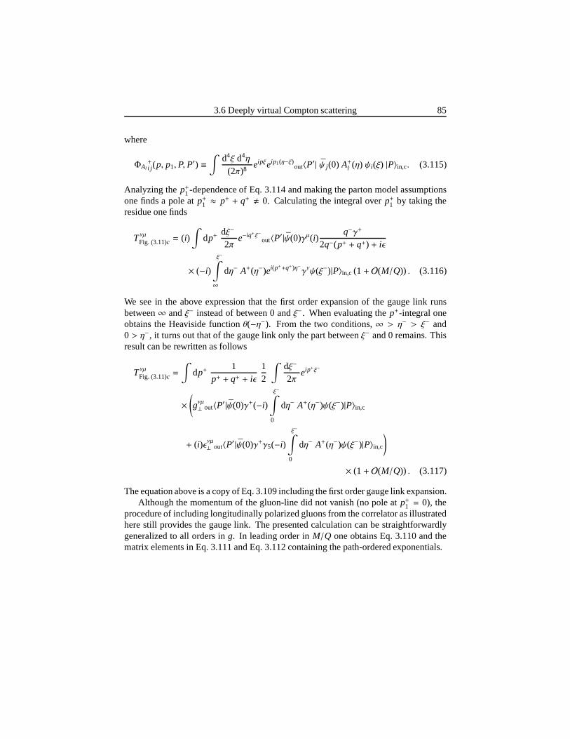
3.6 Deeply virtual Compton scattering 85
where
ΦAl+i j (p, p1,P,P
′) ≡∫
d4ξ d4η
(2π)8eipξeip1(η−ξ)
out〈P′| ψ j(0) A+l (η) ψi(ξ) |P〉in,c. (3.115)
Analyzing thep+1 -dependence of Eq. 3.114 and making the parton model assumptionsone finds a pole atp+1 ≈ p+ + q+ , 0. Calculating the integral overp+1 by taking theresidue one finds
Tνµ
Fig. (3.11)c = (i)∫
dp+dξ−
2πe−iq+ξ−
out〈P′|ψ(0)γµ(i)q−γ+
2q−(p+ + q+) + iǫ
× (−i)
ξ−∫
∞
dη− A+(η−)ei(p++q+)η−γνψ(ξ−)|P〉in,c (1+ O(M/Q)) . (3.116)
We see in the above expression that the first order expansion of the gauge link runsbetween∞ andξ− instead of between 0 andξ−. When evaluating thep+-integral oneobtains the Heaviside functionθ(−η−). From the two conditions,∞ > η− > ξ− and0 > η−, it turns out that of the gauge link only the part betweenξ− and 0 remains. Thisresult can be rewritten as follows
Tνµ
Fig. (3.11)c =
∫dp+
1p+ + q+ + iǫ
12
∫dξ−
2πeip+ξ−
×(gνµ⊥ out〈P′|ψ(0)γ+(−i)
ξ−∫
0
dη− A+(η−)ψ(ξ−)|P〉in,c
+ (i)ǫνµ⊥ out〈P′|ψ(0)γ+γ5(−i)
ξ−∫
0
dη− A+(η−)ψ(ξ−)|P〉in,c
)
× (1+ O(M/Q)) . (3.117)
The equation above is a copy of Eq. 3.109 including the first order gauge link expansion.Although the momentum of the gluon-line did not vanish (no pole at p+1 = 0), the
procedure of including longitudinally polarized gluons from the correlator as illustratedhere still provides the gauge link. The presented calculation can be straightforwardlygeneralized to all orders ing. In leading order inM/Q one obtains Eq. 3.110 and thematrix elements in Eq. 3.111 and Eq. 3.112 containing the path-ordered exponentials.
86 3 Electromagnetic scattering processes at leading orderin αS
3.7 Summary and conclusions
The diagrammatic approach was applied to various scattering processes. Following theideas of Boer, Mulders, Tangerman [114, 115], and Belitsky,Ji, Yuan [26], we assumedfactorization for the correlators and produced the leadingorder inαS cross section forsemi-inclusive DIS, electron-positron annihilation, andDrell-Yan. In Ref. [115] crosssections were obtained by choosing effectively theA+ + A− = 0 gauge, leaving onlythe AT-fields from the correlators to consider. That result, whichincludes subleadingorder corrections inM/Q, was studied in Ref. [114] in more detail by considering theA− = 0 gauge. In that gauge longitudinally polarized gluons between the correlatorsand the elementary scattering diagram need to be consideredas well. In Ref. [114]they were explicitly calculated to orderg2 of which the result was generalized to allorders ing by using Ward identities. Afterwards it was pointed out in Ref. [26] thatthere is an additional contribution which was not identifiedbefore (the transverse gaugelink). The theoretical description was here extended by including all leading orderαS
corrections and includingM/Q corrections. The obtained result is similar to the resultsof Ref. [115] except that T-odd distribution functions are now also included and theapproach is fully color gauge invariant.
The hadronic tensors were expressed in gauge invariant correlators containing gaugelinks. These gauge links arise from including leading-order-αS-interactions which con-sist of gluons interacting between correlators and the elementary scattering diagram.The paths of these gauge links run via plus infinity if the gluons are coupled to an out-going parton, and via minus infinity if the gluons are coupledto an incoming parton.Following the same approach we also considered the DVCS-process in which gluonscouple to internal parton-lines. The path of the obtained gauge link for this process isjust a straight line between the two quark-fields as also encountered in DIS.
Using the expressions for the hadronic tensor in semi-inclusive DIS, some explicitasymmetries were derived. One of the more interesting asymmetries is the beam-spinasymmetry for jet-production in DIS, which is proportionalto the distribution functiong⊥. This function was discussed in chapter 2 and originates from the directional de-pendence of the gauge link. Whether or not such functions arereally non-vanishing isat present an open question. Its measurement would contribute to the understanding ofthe theoretical description.
In the second part of this chapter, it was pointed out that theinteresting argumentsfor universality of fragmentation as given in Collins, Metz[101] contain some issueswhich need clarification. Therefore, the difference in paths of the gauge links in thefragmentation functions appearing in semi-inclusive DIS and electron-positron anni-hilation could lead to different fragmentation functions for the two processes. Thismight create a problem for extracting transversity via the Collins effect. Alternativeways to access transversity, besides Drell-Yan, are for instanceJ/ψ production inpp-scattering [153], and via interference fragmentation functions [154, 155, 156, 157] (inwhich the nonlocality of the operators is light-like).
3.A Hadronic tensors 87
3.A Hadronic tensors
Based on Ref. [35] some hadronic tensors will be given. Contributions from antiquarkscan be included by interchangingq with −q andµ with ν. The following definitionswere used (suppressing arguments of parent hadrons):
Φ[±]α∂
(x) =∫
d2pT pαT Φ[±](x, pT), Φ
[±]α∂
(x) = −∫
d2pT pαT Φ[±](x, pT),
∆[±]α∂
(z−1) =∫
d2kT kαT ∆[±](z−1, kT), ∆[±]α
∂(z−1) = −
∫d2kT kαT ∆
[±] (z−1, kT),
ΦαD(x) =∫
d2pT Φ[±]αD (x, pT), ΦαD(x) =
∫d2pT Φ
[±]αD (x, pT),
∆αD(z−1) =∫
d2kT ∆[±]αD (z−1, kT), ∆αD(z−1) =
∫d2kT ∆
[±]αD (z−1, kT). (3.118)
Semi-inclusive DIS
The translation of Eq. 3.46 into the Cartesian basis is similar as was done for semi-inclusive electron-positron annihilation or Drell-Yan (see Ref. [35] for details). Theunintegrated hadronic tensor reads
2MWµν =
∫d2pT d2kT δ
2(pT⊥ − Ph⊥/z− kT⊥) TrD[ (Φ(xB, pT⊥)γµ∆(z−1
1 , kT⊥)γν)
+(Φ(xB, pT⊥)γµ p/T⊥ /e+
Q√
2∆(z−1
1 , kT⊥)γν −Φ(xB, pT⊥)γµ k/T⊥ /e+Q√
2∆(z−1
1 , kT⊥)γν
− γα /e+Q√
2γνΦ
[+]α∂−1G
(xB,pT⊥)γµ∆[−](z−1, kT⊥)−∆[+]α∂−1G
(z−1, kT⊥)γνΦ[+](xB,pT⊥) γα /e−Q√
2γµ
+ (µ↔ ν)∗)] (
1+ O(M2/Q2
)+ O(αS)
) ∣∣∣∣n±→e±
. (3.119)
The integrated hadronic tensor reads (employing Eq. 3.38 and Eq. 3.44)∫d2Ph⊥ 2MWµν =z2 TrD
[Φ(xB)γµ∆(z−1)γν
+( /e+γαQ√
2γνΦαD(xB)γµ∆(z−1) +
/e−γα
Q√
2γµ∆αD(z−1)γνΦ(xB)
− /e−γαQ√
2γµ∆
[−]∂
(z−1)γνΦ(xB) − γµ γα /e+Q√
2∆
[−]α∂
(z−1)γνΦ(xB)
+ (µ↔ ν)∗)] (
1+ O(M2/Q2
)+ O(αS)
) ∣∣∣∣n±→e±
. (3.120)
The single weighted hadronic tensor reads∫d2Ph⊥ Pα
h⊥ 2MWµν = z3 TrD[−Φ[+]α
∂(xB)γµ∆(z−1)γν + Φ(xB)γµ∆[−]α
∂(z−1)γν
]
× (1+ O(M/Q) + O(αS))∣∣∣∣n±→e±
. (3.121)
88 3 Electromagnetic scattering processes at leading orderin αS
The Drell-Yan process
The integrated hadronic tensor reads (employing Eq. 3.38 and Eq. 3.82)∫
d2qT⊥ 2MWµν =13
TrD[Φ(x1)γµΦ(x2)γν
+(− /e+γα
Q√
2γνΦαD(x1)γµΦ(x2) +
/e−γα
Q√
2γµΦαD(x2)γνΦ(x1)
+12/e+γα
Q√
2γνΦ
[−]α∂
(x1)γµΦ(x2) − 12γνγα /e−
Q√
2Φ
[−]α∂
(x1)γµΦ(x2)
− 12/e−γα
Q√
2γµΦ
[−]α∂
(x2)γνΦ(x1) +12γµγα /e+
Q√
2Φ
[−]α∂
(x2)γνΦ(x1)
+ (µ↔ ν)∗)] (
1+ O(M2/Q2
)+ O(αS)
) ∣∣∣∣n±→e±
. (3.122)
The single weighted hadronic tensor reads∫
d2qT⊥ qαT⊥ 2MWµν =13
TrD[Φ
[−]α∂
(x1)γµΦ(x2)γν −Φ(x1)γµΦ[−]α∂
(x2)γν]
× (1+ O(M/Q) + O(αS))∣∣∣∣n±→e±
. (3.123)
Semi-inclusive electron-positron annihilation
The integrated hadronic tensor reads (employing Eq. 3.44 and Eq. 3.94)∫
d2qT⊥ 2MWµν = 3 TrD[∆(z−1
2 )γµ∆(z−11 )γν
+( /e+γαQ√
2γν∆αD(z−1
2 )γµ∆(z−11 ) − /e−γα
Q√
2γµ∆αD(z−1
1 )γν∆(z−12 )
+/e−γα
Q√
2γµ∆
[+]α∂
(z−11 )γν∆(z−1
1 ) − γµ γα /e+Q√
2∆
[+]α∂
(z−11 )γν∆(z−1
2 )
+ (µ↔ ν)∗)] (
1+ O(M2/Q2
)+ O(αS)
) ∣∣∣∣n±→e±
. (3.124)
The single weighted hadronic tensor reads
∫d2qT⊥ qαT⊥ 2MWµν = 3 TrD
[∆(z−1
2 )γµ∆[+]α∂
(z−11 )γν − ∆[+]α
∂(z−1
2 )γµ∆(z−11 )γν
]
× (1+ O(M/Q) + O(αS))∣∣∣∣n±→e±
. (3.125)
4Color gauge invariance
in hard scatteringprocesses
In the previous chapter several processes were studied at tree-level (leading orderαS).The hard scale was set by an electromagnetic interaction involving two hadrons and, as-suming factorization, cross sections were expressed in nonlocal scale-dependent corre-lators. These correlators contain gauge links of which the path depends on the process.As first noted by Collins [25], this produces a sign-flip for T-odd distribution functionswhen comparing Drell-Yan with semi-inclusive DIS.
Following the same approach in this chapter, scattering processes will be analyzedin which the hard scale is set by an QCD-interaction (besidesthe participating hadrons).We will find that the gauge link does not only depend on the process, but even withina process different gauge links appear; the gauge links will depend on the hard part orsubprocess. How awkward this at first may seem, the procedureappears to be consis-tent. A prescription for deducing gauge links will be given together with some resultsfor gluon-gluon correlators.
The fact that the gauge link depends on the diagram and not only on the processimmediately raises questions on factorization and universality. This particular topicwill be discussed in the last part of this chapter.
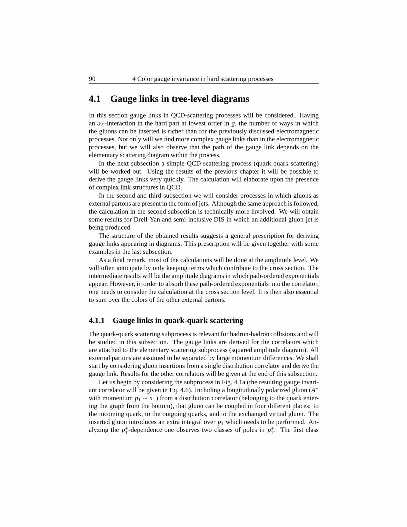
90 4 Color gauge invariance in hard scattering processes
4.1 Gauge links in tree-level diagrams
In this section gauge links in QCD-scattering processes will be considered. HavinganαS-interaction in the hard part at lowest order ing, the number of ways in whichthe gluons can be inserted is richer than for the previously discussed electromagneticprocesses. Not only will we find more complex gauge links thanin the electromagneticprocesses, but we will also observe that the path of the gaugelink depends on theelementary scattering diagram within the process.
In the next subsection a simple QCD-scattering process (quark-quark scattering)will be worked out. Using the results of the previous chapterit will be possible toderive the gauge links very quickly. The calculation will elaborate upon the presenceof complex link structures in QCD.
In the second and third subsection we will consider processes in which gluons asexternal partons are present in the form of jets. Although the same approach is followed,the calculation in the second subsection is technically more involved. We will obtainsome results for Drell-Yan and semi-inclusive DIS in which an additional gluon-jet isbeing produced.
The structure of the obtained results suggests a general prescription for derivinggauge links appearing in diagrams. This prescription will be given together with someexamples in the last subsection.
As a final remark, most of the calculations will be done at the amplitude level. Wewill often anticipate by only keeping terms which contribute to the cross section. Theintermediate results will be the amplitude diagrams in which path-ordered exponentialsappear. However, in order to absorb these path-ordered exponentials into the correlator,one needs to consider the calculation at the cross section level. It is then also essentialto sum over the colors of the other external partons.
4.1.1 Gauge links in quark-quark scattering
The quark-quark scattering subprocess is relevant for hadron-hadron collisions and willbe studied in this subsection. The gauge links are derived for the correlators whichare attached to the elementary scattering subprocess (squared amplitude diagram). Allexternal partons are assumed to be separated by large momentum differences. We shallstart by considering gluon insertions from a single distribution correlator and derive thegauge link. Results for the other correlators will be given at the end of this subsection.
Let us begin by considering the subprocess in Fig. 4.1a (the resulting gauge invari-ant correlator will be given in Eq. 4.6). Including a longitudinally polarized gluon (A+
with momentump1 ∼ n+) from a distribution correlator (belonging to the quark enter-ing the graph from the bottom), that gluon can be coupled in four different places: tothe incoming quark, to the outgoing quarks, and to the exchanged virtual gluon. Theinserted gluon introduces an extra integral overp1 which needs to be performed. An-alyzing thep+1 -dependence one observes two classes of poles inp+1 . The first class
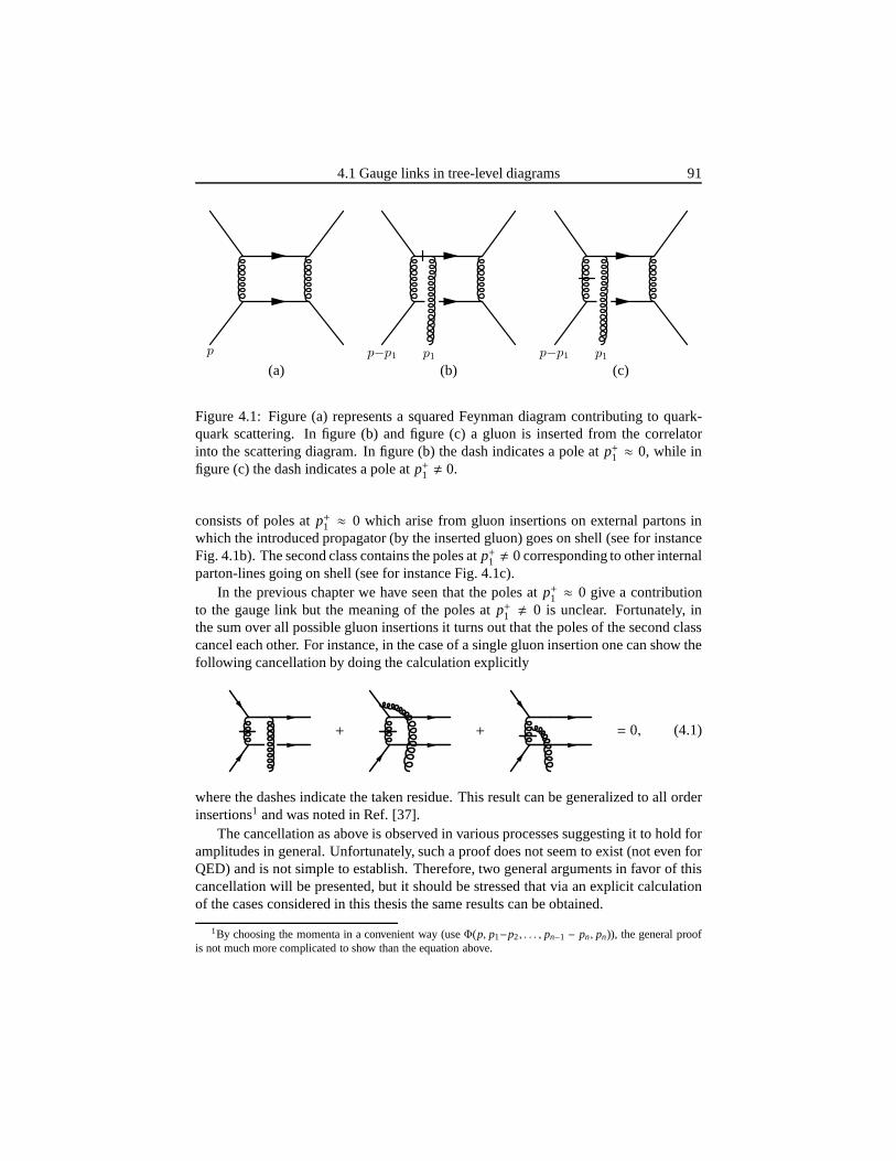
4.1 Gauge links in tree-level diagrams 91
p p−p1 p1 p−p1 p1
(a) (b) (c)
Figure 4.1: Figure (a) represents a squared Feynman diagramcontributing to quark-quark scattering. In figure (b) and figure (c) a gluon is inserted from the correlatorinto the scattering diagram. In figure (b) the dash indicatesa pole atp+1 ≈ 0, while infigure (c) the dash indicates a pole atp+1 , 0.
consists of poles atp+1 ≈ 0 which arise from gluon insertions on external partons inwhich the introduced propagator (by the inserted gluon) goes on shell (see for instanceFig. 4.1b). The second class contains the poles atp+1 , 0 corresponding to other internalparton-lines going on shell (see for instance Fig. 4.1c).
In the previous chapter we have seen that the poles atp+1 ≈ 0 give a contributionto the gauge link but the meaning of the poles atp+1 , 0 is unclear. Fortunately, inthe sum over all possible gluon insertions it turns out that the poles of the second classcancel each other. For instance, in the case of a single gluoninsertion one can show thefollowing cancellation by doing the calculation explicitly
+ + = 0, (4.1)
where the dashes indicate the taken residue. This result canbe generalized to all orderinsertions1 and was noted in Ref. [37].
The cancellation as above is observed in various processes suggesting it to hold foramplitudes in general. Unfortunately, such a proof does notseem to exist (not even forQED) and is not simple to establish. Therefore, two general arguments in favor of thiscancellation will be presented, but it should be stressed that via an explicit calculationof the cases considered in this thesis the same results can beobtained.
1By choosing the momenta in a convenient way (useΦ(p, p1−p2, . . . , pn−1 − pn, pn)), the general proofis not much more complicated to show than the equation above.

92 4 Color gauge invariance in hard scattering processes
The first argument is connected with a Ward identity, which states that a longi-tudinally polarized gluon (on shell) with nonzero momentumdoes not couple to anamplitude which has only physical external partons. Since the inserted gluon (withp+i , 0) is coupled to all possible places, except for one particular interaction whichis already absorbed in the correlator definition (see for example Fig. 3.1b), such glu-ons should not be able to contribute in the sum. The second argument in favor is thatin the present case (see for instance Fig. 4.1c) the pole atp+i , 0 corresponds to theinternal gluon-line being on shell. However, this configuration is physically not possi-ble, because the coupling between two on shell quarks (with unequal momenta) and anon shell gluon is forbidden by momentum conservation. This is also connected to thefact that all tree-level Feynman amplitudes are finite as long as the external partons arewell separated. According to this argument the cancellation in the above equation takesplace in a nonphysical area. This argument for a single gluoninsertion can be extendedto an arbitrary amount of insertions.
Having only the poles atp+i ≈ 0, the task to perform is to evaluate those poles whicharise from inserting gluons on the external parton legs. Thecalculation of inserting lon-gitudinally polarized gluons to a single external parton leg is similar to the calculationsperformed in the previous chapter. An explicit example willbe shown below. By in-serting the gluons on a single quark-line and following the same steps as in the previouschapter, one can derive the gauge link to all orders. There isonly one important dif-ference: the color matrices of the inserted vertices (of theinserted gluons) cannot besimply pulled into the considered correlator because of thepresence of the virtual gluoninside the graph. Therefore, those color matrices are “standing” on the quark-line onwhich the gluons were inserted. Taking combinations of insertions on several externallegs is relatively straightforward because the manipulations of the inserted gluons on acertain external leg can be performed without using information from the other externallegs. As a result, the combination of insertions gives a product of gauge links of whichtheir color matrices remain on the quark-lines on which the gluons were inserted.
As an example, let us reconsider the subprocess given in Fig.4.1a (also given inFig. 4.2a). Summing over the colors of the incoming and outgoing partons, its contri-bution to the cross section is proportional to (whereΦ was defined in Eq. 2.37)
σFig. (4.2)a = K TrC [tbtaΦ(p)
]TrC [tbta]
=2K3
TrC [Φ(p)
](whereK is some constant). (4.2)
Using the machinery of the previous chapter2, the inserted longitudinally polarized glu-ons from the correlatorΦ produce in the amplitude diagram (left-hand-side of the cut)the following gauge links:LξT, ξ
+
(∞−,ξ−) on the outgoing quarks andLξT, ξ+
(ξ−,−∞−) onthe incoming quarks (the coordinateξ is related to the fieldψ(ξ) in the correlatorΦ(p)).Insertions on the right-hand-side of the cut yield similar gauge links. The result of the
2Issues related to the equations of motion will be discarded in this section.
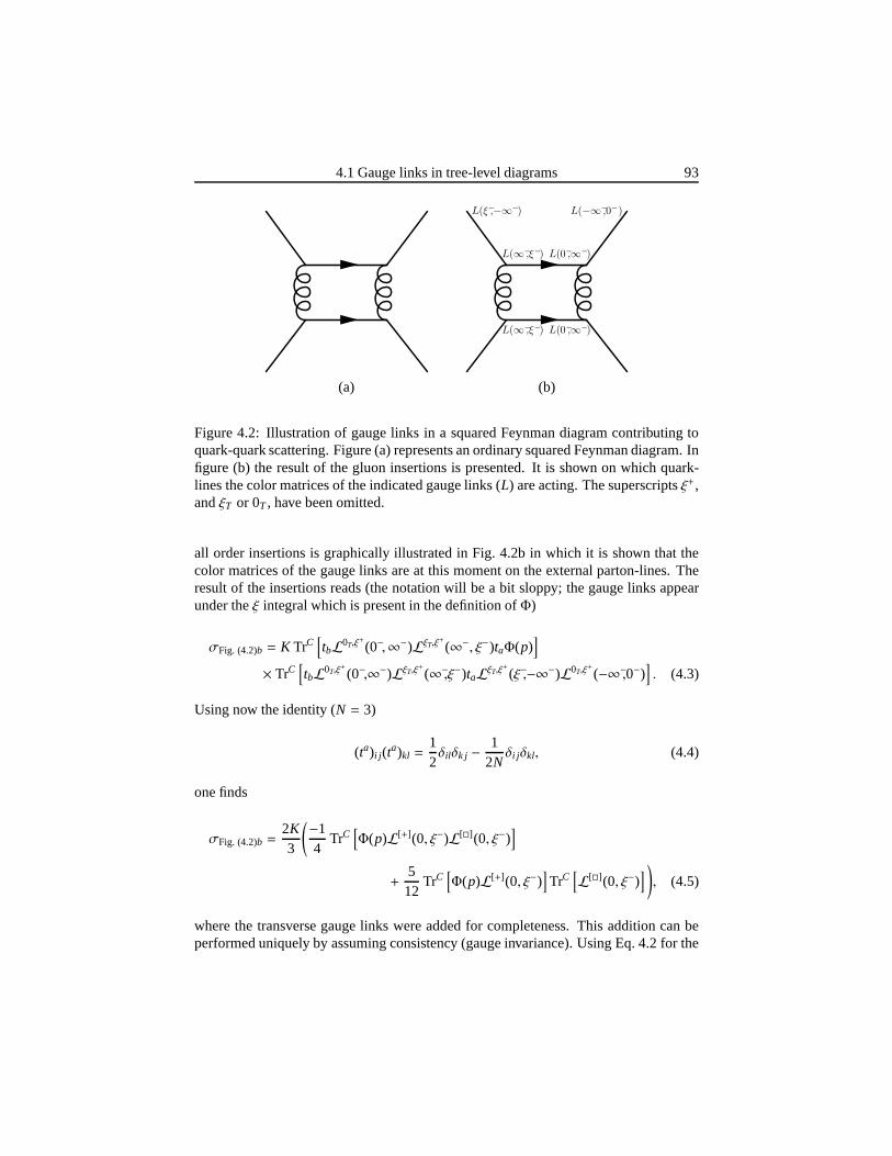
4.1 Gauge links in tree-level diagrams 93
L(ξ−,−∞−)
L(∞−,ξ−) L(0−,∞−)
L(∞−,ξ−) L(0−,∞−)
L(−∞−,0−)
(a) (b)
Figure 4.2: Illustration of gauge links in a squared Feynmandiagram contributing toquark-quark scattering. Figure (a) represents an ordinarysquared Feynman diagram. Infigure (b) the result of the gluon insertions is presented. Itis shown on which quark-lines the color matrices of the indicated gauge links (L) are acting. The superscriptsξ+,andξT or 0T , have been omitted.
all order insertions is graphically illustrated in Fig. 4.2b in which it is shown that thecolor matrices of the gauge links are at this moment on the external parton-lines. Theresult of the insertions reads (the notation will be a bit sloppy; the gauge links appearunder theξ integral which is present in the definition ofΦ)
σFig. (4.2)b = K TrC[tbL0T,ξ
+
(0−,∞−)LξT,ξ+
(∞−, ξ−)taΦ(p)]
× TrC[tbL0T,ξ
+
(0−,∞−)LξT,ξ+
(∞−,ξ−)taLξT,ξ+
(ξ−,−∞−)L0T,ξ+
(−∞−,0−)]. (4.3)
Using now the identity (N = 3)
(ta)i j (ta)kl =12δilδk j −
12N
δi jδkl, (4.4)
one finds
σFig. (4.2)b =2K3
(−14
TrC[Φ(p)L[+](0, ξ−)L[](0, ξ−)
]
+512
TrC[Φ(p)L[+](0, ξ−)
]TrC
[L[](0, ξ−)
] ), (4.5)
where the transverse gauge links were added for completeness. This addition can beperformed uniquely by assuming consistency (gauge invariance). Using Eq. 4.2 for the
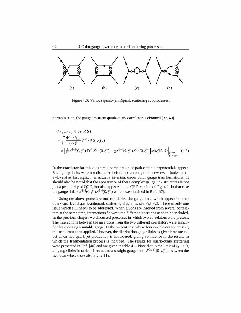
94 4 Color gauge invariance in hard scattering processes
(a) (b) (c) (d)
Figure 4.3: Various quark-(anti)quark scattering subprocesses.
normalization, the gauge invariant quark-quark correlator is obtained [37, 40]
ΦFig. (4.2),i j (x, pT ,P,S)
=
∫dξ− d2ξT
(2π)3eipξ 〈P,S|ψ j(0)
×[
512L
[+](0, ξ−) TrCL[](0, ξ−) − 14L
[+](0, ξ−)L[](0, ξ−)]ψi(ξ)|P,S〉
∣∣∣∣∣ξ+=0p+=xP+
. (4.6)
In the correlator for this diagram a combination of path-ordered exponentials appear.Such gauge links were not discussed before and although thisnew result looks ratherawkward at first sight,it is actually invariant under color gauge transformations. Itshould also be noted that the appearance of these complex gauge link structures is notjust a peculiarity of QCD, but also appears in the QED-version of Fig. 4.2. In that casethe gauge link isL[+](0, ξ−)L[](0, ξ−) which was obtained in Ref. [37].
Using the above procedure one can derive the gauge links which appear in otherquark-quark and quark-antiquark scattering diagrams, seeFig. 4.3. There is only oneissue which still needs to be addressed. When gluons are inserted from several correla-tors at the same time, interactionsbetweenthe different insertions need to be included.In the previous chapter we discussed processes in which two correlators were present.The interactions between the insertions from the two different correlators were simpli-fied by choosing a suitable gauge. In the present case where four correlators are present,this trick cannot be applied. However, the distribution gauge links as given here are ex-act when two quark-jet production is considered, giving confidence in the results inwhich the fragmentation process is included. The results for quark-quark scatteringwere presented in Ref. [40] and are given in table 4.1. Note that in the limit ofξT → 0,all gauge links in table 4.1 reduce to a straight gauge link,L0T, ξ
+
(0−, ξ−), between thetwo quark-fields, see also Fig. 2.11a.
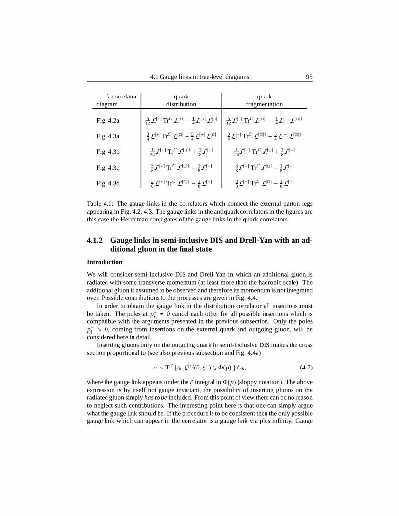
4.1 Gauge links in tree-level diagrams 95
\ correlator quark quarkdiagram distribution fragmentation
Fig. 4.2a 512L[+] TrCL[] − 1
4L[+]L[] 512L[−] TrCL[]† − 1
4L[−]L[]†
Fig. 4.3a 34L[+] TrCL[] − 5
4L[+]L[] 34L[−] TrCL[]† − 5
4L[−]L[]†
Fig. 4.3b 124L[+] TrCL[]† + 7
8L[−] 124L[−] TrCL[] + 7
8L[+]
Fig. 4.3c 38L[+] TrCL[]† − 1
8L[−] 38L[−] TrCL[] − 1
8L[+]
Fig. 4.3d 38L[+] TrCL[]† − 1
8L[−] 38L[−] TrCL[] − 1
8L[+]
Table 4.1: The gauge links in the correlators which connect the external parton legsappearing in Fig. 4.2, 4.3. The gauge links in the antiquark correlators in the figures arethis case the Hermitean conjugates of the gauge links in the quark correlators.
4.1.2 Gauge links in semi-inclusive DIS and Drell-Yan with an ad-ditional gluon in the final state
Introduction
We will consider semi-inclusive DIS and Drell-Yan in which an additional gluon isradiated with some transverse momentum (at least more than the hadronic scale). Theadditional gluon is assumed to be observed and therefore itsmomentum is not integratedover. Possible contributions to the processes are given in Fig. 4.4.
In order to obtain the gauge link in the distribution correlator all insertions mustbe taken. The poles atp+i , 0 cancel each other for all possible insertions which iscompatible with the arguments presented in the previous subsection. Only the polesp+i ≈ 0, coming from insertions on the external quark and outgoinggluon, will beconsidered here in detail.
Inserting gluons only on the outgoing quark in semi-inclusive DIS makes the crosssection proportional to (see also previous subsection and Fig. 4.4a)
σ ∼ TrC[tb L[+](0, ξ−) ta Φ(p)
]δab, (4.7)
where the gauge link appears under theξ integral inΦ(p) (sloppy notation). The aboveexpression is by itself not gauge invariant, the possibility of inserting gluons on theradiated gluon simplyhas to beincluded. From this point of view there can be no reasonto neglect such contributions. The interesting point here is that one can simply arguewhat the gauge link should be. If the procedure is to be consistent then the only possiblegauge link which can appear in the correlator is a gauge link via plus infinity. Gauge
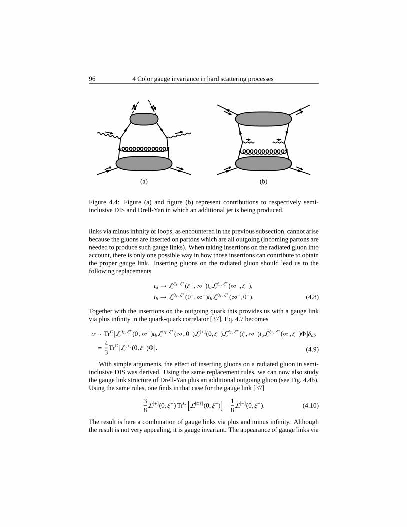
96 4 Color gauge invariance in hard scattering processes
(a) (b)
Figure 4.4: Figure (a) and figure (b) represent contributions to respectively semi-inclusive DIS and Drell-Yan in which an additional jet is being produced.
links via minus infinity or loops, as encountered in the previous subsection, cannot arisebecause the gluons are inserted on partons which are all outgoing (incoming partons areneeded to produce such gauge links). When taking insertionson the radiated gluon intoaccount, there is only one possible way in how those insertions can contribute to obtainthe proper gauge link. Inserting gluons on the radiated gluon should lead us to thefollowing replacements
ta→ LξT, ξ+
(ξ−,∞−)taLξT, ξ+
(∞−, ξ−),tb→ L0T, ξ
+
(0−,∞−)tbL0T, ξ+
(∞−, 0−). (4.8)
Together with the insertions on the outgoing quark this provides us with a gauge linkvia plus infinity in the quark-quark correlator [37], Eq. 4.7becomes
σ ∼ TrC[L0T, ξ+
(0−,∞−)tbL0T, ξ+
(∞−, 0−)L[+](0, ξ−)LξT, ξ+
(ξ−,∞−)taLξT, ξ+
(∞−, ξ−)Φ]δab
=43
TrC[L[+](0, ξ−)Φ]. (4.9)
With simple arguments, the effect of inserting gluons on a radiated gluon in semi-inclusive DIS was derived. Using the same replacement rules, we can now also studythe gauge link structure of Drell-Yan plus an additional outgoing gluon (see Fig. 4.4b).Using the same rules, one finds in that case for the gauge link [37]
38L[+](0, ξ−) TrC
[L[†](0, ξ−)
]− 1
8L[−](0, ξ−). (4.10)
The result is here a combination of gauge links via plus and minus infinity. Althoughthe result is not very appealing, it is gauge invariant. The appearance of gauge links via
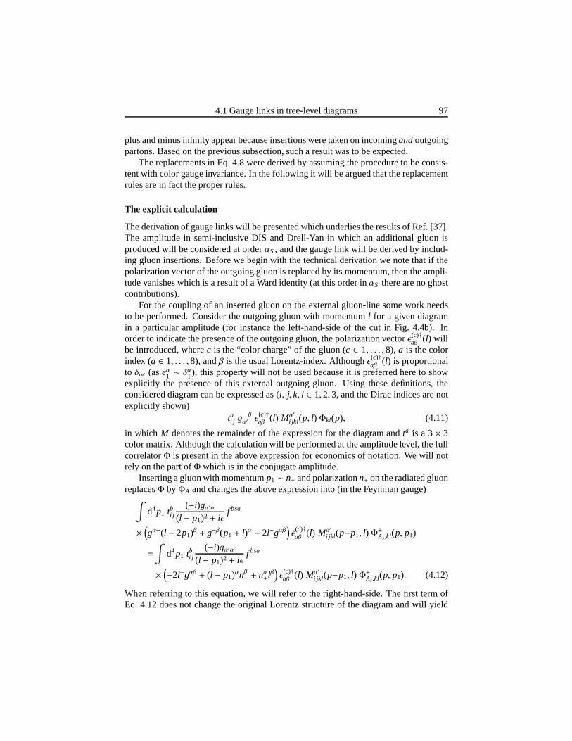
4.1 Gauge links in tree-level diagrams 97
plus and minus infinity appear because insertions were takenon incomingandoutgoingpartons. Based on the previous subsection, such a result wasto be expected.
The replacements in Eq. 4.8 were derived by assuming the procedure to be consis-tent with color gauge invariance. In the following it will beargued that the replacementrules are in fact the proper rules.
The explicit calculation
The derivation of gauge links will be presented which underlies the results of Ref. [37].The amplitude in semi-inclusive DIS and Drell-Yan in which an additional gluon isproduced will be considered at orderαS, and the gauge link will be derived by includ-ing gluon insertions. Before we begin with the technical derivation we note that if thepolarization vector of the outgoing gluon is replaced by itsmomentum, then the ampli-tude vanishes which is a result of a Ward identity (at this order inαS there are no ghostcontributions).
For the coupling of an inserted gluon on the external gluon-line some work needsto be performed. Consider the outgoing gluon with momentuml for a given diagramin a particular amplitude (for instance the left-hand-sideof the cut in Fig. 4.4b). Inorder to indicate the presence of the outgoing gluon, the polarization vectorǫ(c)†
aβ (l) willbe introduced, wherec is the “color charge” of the gluon (c ∈ 1, . . . , 8), a is the colorindex (a ∈ 1, . . . , 8), andβ is the usual Lorentz-index. Althoughǫ(c)†
aβ (l) is proportionalto δac (aseα1 ∼ δα1), this property will not be used because it is preferred hereto showexplicitly the presence of this external outgoing gluon. Using these definitions, theconsidered diagram can be expressed as (i, j, k, l ∈ 1, 2, 3, and the Dirac indices are notexplicitly shown)
tai j g β
α′ ǫ(c)†aβ (l) Mα′
i jkl (p, l) Φkl(p), (4.11)
in which M denotes the remainder of the expression for the diagram andta is a 3× 3color matrix. Although the calculation will be performed atthe amplitude level, the fullcorrelatorΦ is present in the above expression for economics of notation. We will notrely on the part ofΦ which is in the conjugate amplitude.
Inserting a gluon with momentump1 ∼ n+ and polarizationn+ on the radiated gluonreplacesΦ byΦA and changes the above expression into (in the Feynman gauge)
∫d4p1 tbi j
(−i)gα′α(l − p1)2 + iǫ
f bsa
×(gα−(l − 2p1)β + g−β(p1 + l)α − 2l−gαβ
)ǫ
(c)†aβ (l) Mα′
i jkl (p−p1, l) Φ+As,kl(p, p1)
=
∫d4p1 tbi j
(−i)gα′α(l − p1)2 + iǫ
f bsa
×(−2l−gαβ + (l − p1)αnβ+ + nα+l
β)ǫ
(c)†aβ (l) Mα′
i jkl (p−p1, l) Φ+As,kl(p, p1). (4.12)
When referring to this equation, we will refer to the right-hand-side. The first term ofEq. 4.12 does not change the original Lorentz structure of the diagram and will yield
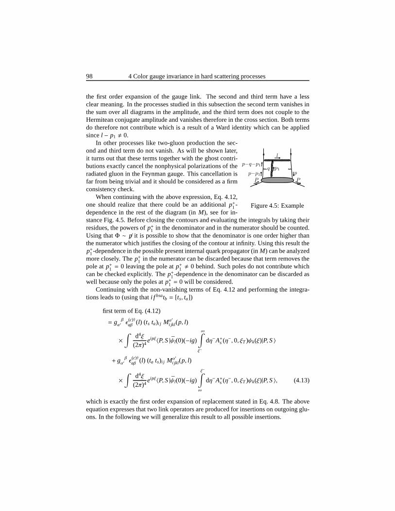
98 4 Color gauge invariance in hard scattering processes
the first order expansion of the gauge link. The second and third term have a lessclear meaning. In the processes studied in this subsection the second term vanishes inthe sum over all diagrams in the amplitude, and the third termdoes not couple to theHermitean conjugate amplitude and vanishes therefore in the cross section. Both termsdo therefore not contribute which is a result of a Ward identity which can be appliedsincel − p1 , 0.
In other processes like two-gluon production the sec-
qp−p1
p−q−p1
p
l
p1
P P
Figure 4.5: Example
ond and third term do not vanish. As will be shown later,it turns out that these terms together with the ghost contri-butions exactly cancel the nonphysical polarizations of theradiated gluon in the Feynman gauge. This cancellation isfar from being trivial and it should be considered as a firmconsistency check.
When continuing with the above expression, Eq. 4.12,one should realize that there could be an additionalp+1 -dependence in the rest of the diagram (inM), see for in-stance Fig. 4.5. Before closing the contours and evaluatingthe integrals by taking theirresidues, the powers ofp+1 in the denominator and in the numerator should be counted.Using thatΦ ∼ p/ it is possible to show that the denominator is one order higher thanthe numerator which justifies the closing of the contour at infinity. Using this result thep+1 -dependence in the possible present internal quark propagator (in M) can be analyzedmore closely. Thep+1 in the numerator can be discarded because that term removes thepole atp+1 = 0 leaving the pole atp+1 , 0 behind. Such poles do not contribute whichcan be checked explicitly. Thep+1 -dependence in the denominator can be discarded aswell because only the poles atp+1 = 0 will be considered.
Continuing with the non-vanishing terms of Eq. 4.12 and performing the integra-tions leads to (using thati f bsatb = [ts, ta])
first term of Eq. (4.12)
= g β
α′ ǫ(c)†aβ (l) (ts ta)i j Mα′
i jkl (p, l)
×∫
d4ξ
(2π)4eipξ〈P,S|ψl(0)(−ig)
∞∫
ξ−
dη−A+s (η−, 0, ξT)ψk(ξ)|P,S〉
+ g β
α′ ǫ(c)†aβ (l) (ta ts)i j Mα′
i jkl (p, l)
×∫
d4ξ
(2π)4eipξ〈P,S|ψl(0)(−ig)
ξ−∫
∞
dη−A+s (η−, 0, ξT)ψk(ξ)|P,S〉, (4.13)
which is exactly the first order expansion of replacement stated in Eq. 4.8. The aboveequation expresses that two link operators are produced forinsertions on outgoing glu-ons. In the following we will generalize this result to all possible insertions.
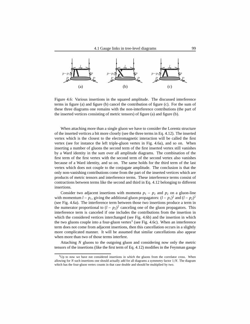
4.1 Gauge links in tree-level diagrams 99
p−p1 p
l
P P
p−p1 p
l
P P
p−p1 p
l
P P
(a) (b) (c)
Figure 4.6: Various insertions in the squared amplitude. The discussed interferenceterms in figure (a) and figure (b) cancel the contribution of figure (c). For the sum ofthese three diagrams one remains with the non-interferencecontributions (the part ofthe inserted vertices consisting of metric tensors) of figure (a) and figure (b).
When attaching more than a single gluon we have to consider the Lorentz structureof the inserted vertices a bit more closely (see the three terms in Eq. 4.12). The insertedvertex which is the closest to the electromagnetic interaction will be called the firstvertex (see for instance the left triple-gluon vertex in Fig. 4.6a), and so on. Wheninserting a number of gluons the second term of the first inserted vertex still vanishesby a Ward identity in the sum over all amplitude diagrams. Thecombination of thefirst term of the first vertex with the second term of the secondvertex also vanishesbecause of a Ward identity, and so on. The same holds for the third term of the lastvertex which does not couple to the conjugate amplitude. Theconclusion is that theonly non-vanishing contributions come from the part of the inserted vertices which areproducts of metric tensors and interference terms. These interference terms consist ofcontractions between terms like the second and third in Eq. 4.12 belonging to differentinsertions.
Consider two adjacent insertions with momentap1 − p2 and p2 on a gluon-linewith momentuml − p1, giving the additional gluon propagators: (l − p1)2 and (l − p2)2
(see Fig. 4.6a). The interference term between those two insertions produce a term inthe numerator proportional to (l − p2)2 canceling one of the gluon propagators. Thisinterference term is canceled if one includes the contributions from the insertion inwhich the considered vertices interchanged (see Fig. 4.6b)and the insertion in whichthe two gluons couple into a four-gluon vertex3 (see Fig. 4.6c). When an interferenceterm does not come from adjacent insertions, then this cancellation occurs in a slightlymore complicated manner. It will be assumed that similar cancellations also appearwhen more than two of those terms interfere.
Attaching N gluons to the outgoing gluon and considering now only the metrictensors of the insertions (like the first term of Eq. 4.12) modifies in the Feynman gauge
3Up to now we have not considered insertions in which the gluons from the correlator cross. Whenallowing for N such insertions one should actually add for all diagrams a symmetry factor 1/N. The diagramwhich has the four-gluon vertex counts in that case double and should be multiplied by two.
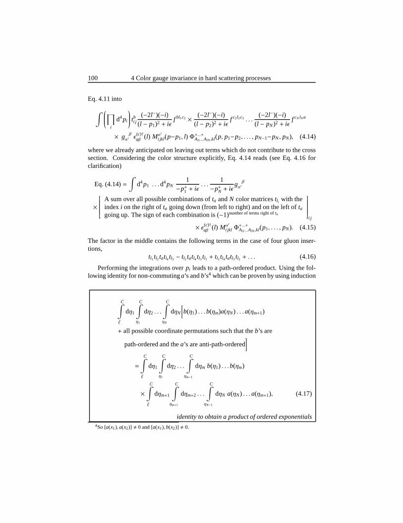
100 4 Color gauge invariance in hard scattering processes
Eq. 4.11 into
∫ ∏
i
d4pi
tbi j(−2l−)(−i)
(l − p1)2 + iǫf bl1c2 × (−2l−)(−i)
(l − p2)2 + iǫf c2l2c3 . . .
(−2l−)(−i)(l − pN)2 + iǫ
f cN lNa
× g β
α′ ǫ(c)†aβ (l) Mα′
i jkl (p−p1, l) Φ+...+Al1...AlN ,kl(p, p1−p2, . . . , pN−1−pN, pN), (4.14)
where we already anticipated on leaving out terms which do not contribute to the crosssection. Considering the color structure explicitly, Eq. 4.14 reads (see Eq. 4.16 forclarification)
Eq. (4.14)=∫
d4p1 . . .d4pN1
−p+1 + iǫ. . .
1−p+N + iǫ
g β
α′
×
A sum over all possible combinations ofta andN color matricestl i with theindexi on the right ofta going down (from left to right) and on the left oftagoing up. The sign of each combination is (−1)number of terms right ofta
i j
× ǫ(c)†aβ (l) Mα′
i jkl Φ+...+Al1...AlN ,kl(p1, . . . , pN). (4.15)
The factor in the middle contains the following terms in the case of four gluon inser-tions,
tl1tl2tatl4tl3 − tl2tatl4tl3tl1 + tl1tl4tatl3tl2 + . . . (4.16)
Performing the integrations overpi leads to a path-ordered product. Using the fol-lowing identity for non-commutinga’s andb’s4 which can be proven by using induction
C∫
ξ
dη1
C∫
η1
dη2 . . .
C∫
ηN
dηN
[b(η1) . . .b(ηm)a(ηN) . . .a(ηm+1)
+ all possible coordinate permutations such that theb’s are
path-ordered and thea’s are anti-path-ordered]
=
C∫
ξ
dη1
C∫
η1
dη2 . . .
C∫
ηm−1
dηm b(η1) . . .b(ηm)
×C∫
ξ
dηm+1
C∫
ηm+1
dηm+2 . . .
C∫
ηN−1
dηN a(ηN) . . .a(ηm+1), (4.17)
identity to obtain a product of ordered exponentials4So [a(x1), a(x2)] , 0 and [a(x1), b(x2)] , 0.
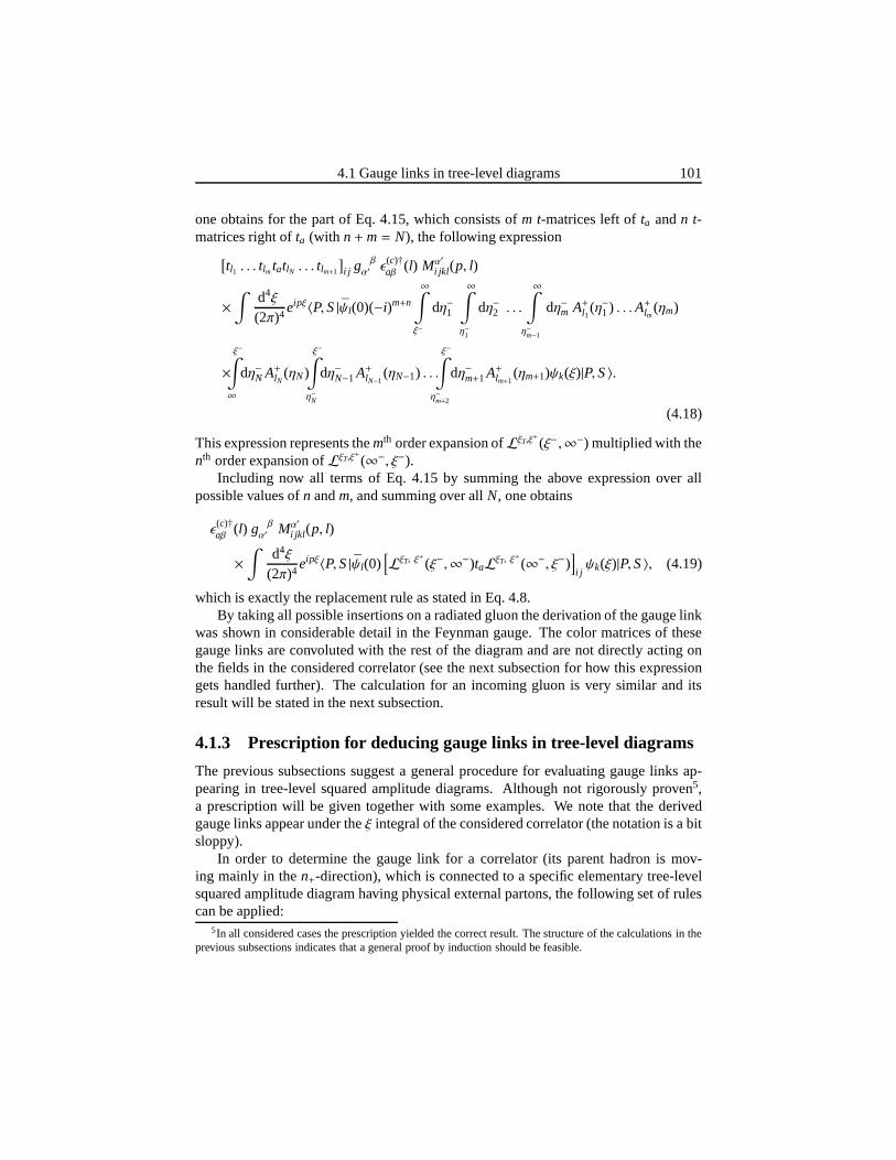
4.1 Gauge links in tree-level diagrams 101
one obtains for the part of Eq. 4.15, which consists ofm t-matrices left ofta andn t-matrices right ofta (with n+m= N), the following expression
[tl1 . . . tlmtatlN . . . tlm+1
]i j g β
α′ ǫ(c)†aβ (l) Mα′
i jkl (p, l)
×∫
d4ξ
(2π)4eipξ〈P,S|ψl(0)(−i)m+n
∞∫
ξ−
dη−1
∞∫
η−1
dη−2 . . .
∞∫
η−m−1
dη−m A+l1(η−1) . . .A+lm(ηm)
×ξ−∫
∞
dη−N A+lN(ηN)
ξ−∫
η−N
dη−N−1 A+lN−1(ηN−1) . . .
ξ−∫
η−m+2
dη−m+1A+lm+1(ηm+1)ψk(ξ)|P,S〉.
(4.18)
This expression represents themth order expansion ofLξT,ξ+
(ξ−,∞−) multiplied with thenth order expansion ofLξT,ξ
+
(∞−, ξ−).Including now all terms of Eq. 4.15 by summing the above expression over all
possible values ofn andm, and summing over allN, one obtains
ǫ(c)†aβ (l) g β
α′ Mα′
i jkl (p, l)
×∫
d4ξ
(2π)4eipξ〈P,S|ψl(0)
[LξT, ξ
+
(ξ−,∞−)taLξT, ξ+
(∞−, ξ−)]i jψk(ξ)|P,S〉, (4.19)
which is exactly the replacement rule as stated in Eq. 4.8.By taking all possible insertions on a radiated gluon the derivation of the gauge link
was shown in considerable detail in the Feynman gauge. The color matrices of thesegauge links are convoluted with the rest of the diagram and are not directly acting onthe fields in the considered correlator (see the next subsection for how this expressiongets handled further). The calculation for an incoming gluon is very similar and itsresult will be stated in the next subsection.
4.1.3 Prescription for deducing gauge links in tree-level diagrams
The previous subsections suggest a general procedure for evaluating gauge links ap-pearing in tree-level squared amplitude diagrams. Although not rigorously proven5,a prescription will be given together with some examples. Wenote that the derivedgauge links appear under theξ integral of the considered correlator (the notation is a bitsloppy).
In order to determine the gauge link for a correlator (its parent hadron is mov-ing mainly in then+-direction), which is connected to a specific elementary tree-levelsquared amplitude diagram having physical external partons, the following set of rulescan be applied:
5In all considered cases the prescription yielded the correct result. The structure of the calculations in theprevious subsections indicates that a general proof by induction should be feasible.
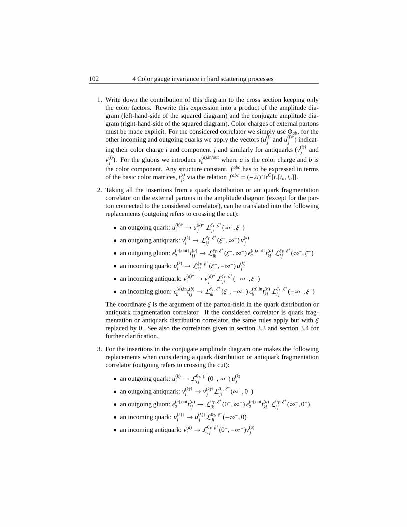
102 4 Color gauge invariance in hard scattering processes
1. Write down the contribution of this diagram to the cross section keeping onlythe color factors. Rewrite this expression into a product ofthe amplitude dia-gram (left-hand-side of the squared diagram) and the conjugate amplitude dia-gram (right-hand-side of the squared diagram). Color charges of external partonsmust be made explicit. For the considered correlator we simply useΦab, for theother incoming and outgoing quarks we apply the vectors (u(i)
j andu(i)†j ) indicat-
ing their color chargei and componentj and similarly for antiquarks (v(i)†j and
v(i)j ). For the gluons we introduceǫ(a),in/out
b wherea is the color charge andb is
the color component. Any structure constant,f abc has to be expressed in termsof the basic color matrices,t(i)jk via the relationf abc = (−2i) TrC[tc[ta, tb]].
2. Taking all the insertions from a quark distribution or antiquark fragmentationcorrelator on the external partons in the amplitude diagram(except for the par-ton connected to the considered correlator), can be translated into the followingreplacements (outgoing refers to crossing the cut):
• an outgoing quark:u(k)†i → u(k)†
j LξT, ξ
+
ji (∞−, ξ−)
• an outgoing antiquark:v(k)i → L
ξT, ξ+
i j (ξ−,∞−) v(k)j
• an outgoing gluon:ǫ(c),out†a t(a)
i j → LξT, ξ
+
ik (ξ−,∞−) ǫ(c),out†a t(a)
kl LξT, ξ
+
l j (∞−, ξ−)
• an incoming quark:u(k)i → L
ξT, ξ+
i j (ξ−,−∞−) u(k)j
• an incoming antiquark:v(a)†i → v(a)†
j LξT, ξ
+
ji (−∞−, ξ−)
• an incoming gluon:ǫ(a),inb t(b)
i j → LξT, ξ
+
ik (ξ−,−∞−) ǫ(a),inb t(b)
kl LξT, ξ
+
l j (−∞−, ξ−)
The coordinateξ is the argument of the parton-field in the quark distributionorantiquark fragmentation correlator. If the considered correlator is quark frag-mentation or antiquark distribution correlator, the same rules apply but withξreplaced by 0. See also the correlators given in section 3.3 and section 3.4 forfurther clarification.
3. For the insertions in the conjugate amplitude diagram onemakes the followingreplacements when considering a quark distribution or antiquark fragmentationcorrelator (outgoing refers to crossing the cut):
• an outgoing quark:u(k)i → L
0T, ξ+
i j (0−,∞−) u(k)j
• an outgoing antiquark:v(k)†i → v(k)†
j L0T, ξ
+
ji (∞−, 0−)
• an outgoing gluon:ǫ(c),outa t(a)
i j → L0T, ξ
+
ik (0−,∞−) ǫ(c),outa t(a)
kl L0T, ξ
+
l j (∞−, 0−)
• an incoming quark:u(k)†i → u(k)†
j L0T, ξ
+
ji (−∞−, 0)
• an incoming antiquark:v(a)i → L
0T, ξ+
i j (0−,−∞−)v(a)j
4.1 Gauge links in tree-level diagrams 103
• an incoming gluon:ǫ(a)in†b t(b)
i j → L0T, ξ
+
ik (0−,−∞−)ǫ(a)in†b t(b)
kl L0T, ξ
+
l j (−∞−, 0−)
and replaces 0 byξ when considering a quark fragmentation or antiquark distri-bution correlator.
4. Using thatu(r)b = δrb, ǫ(r)
b = δrb, etc., simplify the obtained expression. At thispoint it is essential to sum over the colors of the other external partons. In thefinal expression the transverse gauge link pieces are included which can be doneuniquely.
5. Divide the expression by the normalization which can be obtained by replacingall L’s by 1 andΦ by 1/3.
6. The result is the gauge link of the considered correlator.
To illuminate this set of rules three examples with explicitresults will be given.
Example: Drell-Yan
We will reconsider the gauge link in the distribution correlator in Drell-Yan. The parenthadron is assumed to be moving mainly in then+-direction. The result of each step ofthe prescription is as follows:
1 :σ = K TrC [Φ[v(r)(k)v(r)†(k)]
],whereK is some constant. In analogy with Dirac
spinors one has in this trace [v(r)(k)v(r)†(k)] i j ≡ v(r)i (k)v(r)†
j (k).
2 :σ = K TrC [Φ[v(r)(k)v(r)†(k)]LξT, ξ
+
(−∞−, ξ−)].
3 :σ = K TrC [ΦL0T, ξ
+
(0−,−∞−)[v(r)(k)v(r)†(k)]LξT, ξ+
(−∞−, ξ−)].
4 :σ = K TrC[ΦL0T, ξ+
(0−,−∞−)LξT, ξ+
(−∞−, ξ−)] = K TrC[ΦL[−](0, ξ−)],
where in the last step the transverse gauge link was included.
5 : normalization isK.
6 : the gauge link isL[−](0, ξ−).
Example: Drell-Yan and gluon-jet
In this example the gauge link is calculated for a distribution correlator (with parenthadron alongn+) in Drell-Yan with an extra gluon-jet in the final state, see for instance
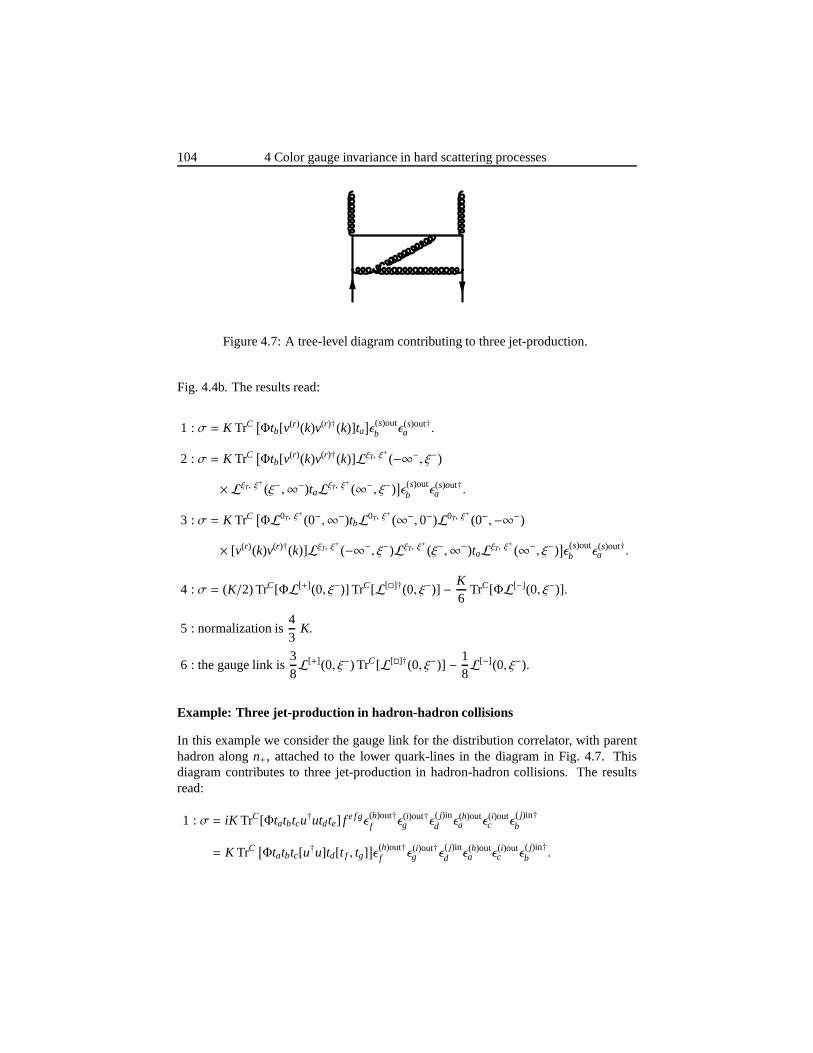
104 4 Color gauge invariance in hard scattering processes
Figure 4.7: A tree-level diagram contributing to three jet-production.
Fig. 4.4b. The results read:
1 :σ = K TrC [Φtb[v(r)(k)v(r)†(k)]ta
]ǫ
(s)outb ǫ(s)out†
a .
2 :σ = K TrC [Φtb[v(r)(k)v(r)†(k)]LξT, ξ
+
(−∞−, ξ−)
× LξT, ξ+
(ξ−,∞−)taLξT, ξ+
(∞−, ξ−)]ǫ(s)outb ǫ(s)out†
a .
3 :σ = K TrC [ΦL0T, ξ
+
(0−,∞−)tbL0T, ξ+
(∞−, 0−)L0T, ξ+
(0−,−∞−)
× [v(r)(k)v(r)†(k)]LξT, ξ+
(−∞−, ξ−)LξT, ξ+
(ξ−,∞−)taLξT, ξ+
(∞−, ξ−)]ǫ(s)outb ǫ(s)out†
a .
4 :σ = (K/2) TrC[ΦL[+](0, ξ−)] TrC[L[]†(0, ξ−)] − K6
TrC[ΦL[−](0, ξ−)].
5 : normalization is43
K.
6 : the gauge link is38L[+](0, ξ−) TrC[L[]†(0, ξ−)] − 1
8L[−](0, ξ−).
Example: Three jet-production in hadron-hadron collisions
In this example we consider the gauge link for the distribution correlator, with parenthadron alongn+, attached to the lower quark-lines in the diagram in Fig. 4.7. Thisdiagram contributes to three jet-production in hadron-hadron collisions. The resultsread:
1 :σ = iK TrC[Φtatbtcu†utdte] f e fgǫ
(h)out†f ǫ(i)out†
g ǫ( j)ind ǫ(h)out
a ǫ(i)outc ǫ
( j)in†b
= K TrC [Φtatbtc[u
†u]td[t f , tg]]ǫ
(h)out†f ǫ(i)out†
g ǫ( j)ind ǫ(h)out
a ǫ(i)outc ǫ
( j)in†b .
4.2 Relating correlators with different gauge links 105
2 :σ = K TrC[Φtatbtc[u†u]LξT, ξ+
(∞−,−∞−)tdLξT, ξ+
(−∞−,∞−)[t f , tg]LξT, ξ+
(∞−, ξ−)]
× ǫ(h)out†f ǫ(i)out†
g ǫ( j)ind ǫ(h)out
a ǫ(i)outc ǫ
( j)in†b ,
3 :σ = K TrC[ΦL0T, ξ+
(0−,∞−)taL0T, ξ+
(∞−,−∞−)tbL0T, ξ+
(−∞−,∞−)tc[u†u]
× LξT, ξ+
(∞−,−∞−)tdLξT, ξ+
(−∞−,∞−)[t f , tg]LξT, ξ+
(∞−, ξ−)]
× ǫ(h)out†f ǫ(i)out†
g ǫ( j)ind ǫ(h)out
a ǫ(i)outc ǫ
( j)in†b .
4 :σ =−K24
TrC[ΦL[+](0, ξ−)
]+
K8
TrC[ΦL[+](0, ξ−)L[](0, ξ−)
]TrC
[L[]†(0, ξ−)
].
5 : normalization isK/3.
6 : gauge link is−18L[+](0, ξ−) +
38L[+](0, ξ−)L[](0, ξ−) TrC
[L[]†(0, ξ−)
].
4.2 Relating correlators with different gauge links
The gauge invariant correlators, appearing in the diagrams, will here be related to thecorrelators introduced in chapter 2. We will find that the T-odd functions, appearing indifferent diagrams, can in general differ by more than just a sign.
The gauge link structure consists in general of several terms of which each termconsists of a link (L[+] orL[−]) multiplied by some traces of gauge loops. After an inte-gration over the transverse momentum of a correlator these gauge links collapse on thelight-cone, one remains with a simple straight gauge link. The transverse momentumintegrated distribution and fragmentation functions are therefore universal6.
To treat the first transverse moment of T-even distribution functions, one can usetime-reversal to project out the T-even structure of the unintegrated correlator. Thisenables one to write the T-even part of the correlator as the average of itself and thecorrelator having the time-reversed gauge link (∞ ↔ −∞, as done in Eq. 2.62). Usingthe identities in Eq. 2.70, which also gives the relation (based on TrC ta = 0)
∂αξTTrC
[L[](0, ξ−)
] ∣∣∣∣ξT=0= 0, (4.20)
one can show that the first transverse moment of the unintegrated correlator is link-independent. The first transverse moment of T-even distribution functions is thereforeuniversal.
The first transverse moment of T-odd distribution functionshaving some gauge linkis treated analogously. The T-odd part of the correlator is projected out by taking the
6In a fragmentation correlator the gauge links appear in two different matrix elements. To show theuniversality of integrated fragmentation correlators with an arbitrary gauge link, one can choose the light-cone gauge.
106 4 Color gauge invariance in hard scattering processes
difference of itself and the time-reversed one (see for example Eq. 2.63). Using theidentities in Eq. 2.70 and Eq. 4.20 one can show that the first transverse moment of aT-odd distribution correlator equals the T-odd correlatoras defined in Eq. 2.63 up toa constant. Therefore one can relate the first transverse moment of T-odd distributionfunctions to the ones appearing in semi-inclusive DIS.
For example, let us consider the first transverse moment of the T-odd part of adistribution correlator containing the gauge link:L′ = 3
8L[+](0, ξ−) TrC[L[]†(0, ξ−)] −18L[−](0, ξ−). Using time reversal the first transverse moment reads as follows [37]
Φ[T-odd]L′α∂
=12
∫d2pT pαT
∫dξ− d2ξT
(2π)3eipξ
×(〈P,S|ψ(0)
[38L
[+](0, ξ−) TrC[L[]†(0, ξ−)] − 18L
[−](0, ξ−)]ψ(ξ)|P,S〉c
− 〈P,S|ψ(0)[3
8L[−](0, ξ−) TrC[L[](0, ξ−)] − 1
8L[+](0, ξ−)
]ψ(ξ)|P,S〉c
)∣∣∣∣ξ+=0p+=xP+
=54Φ
[T-odd]α∂ (4.21)
The above expression is equivalent to54 times the first transverse moment of the T-odd
correlator as defined in Eq. 2.63. The first transverse momentof the T-odd functions(like the Sivers functionf⊥(1)
1T ) is therefore54-times the T-odd function which is mea-
sured in semi-inclusive DIS.For fragmentation functions the interplay of the two possible mechanisms for T-odd
effects created the problem for comparing the fragmentation functions in semi-inclusiveDIS with the functions in electron-positron annihilation.The first transverse momentof those fragmentation functions read
∆[±]α∂
(z−1) =13
∑
X
∫d3PX
(2π)32EPX
∫dξ+
2πeiP−h ξ
+/zout〈Ph,PX|ψ(0)L0T,ξ
−(0+,±∞+)|Ω〉c
× 〈Ω|[(−g)
ξ+∫
±∞
dη+ L0T, ξ−(±∞+, η+)G−αT (η)L0T, ξ
+
(η+, ξ+)
+L0T, ξ−(±∞+, ξ+)iDα
T
]ψ(ξ)|Ph,PX〉out,c
∣∣∣∣η−=ξ−=0ηT=ξT=0
. (4.22)
By making comparisons in the light-cone gauge, the first transverse moment of a frag-mentation correlator with some gauge link can be expressed in the transverse momentsof the fragmentation functions appearing in semi-inclusive DIS and electron-positronannihilation.
As an example, let us consider the correlator with the gauge link structureL′ =
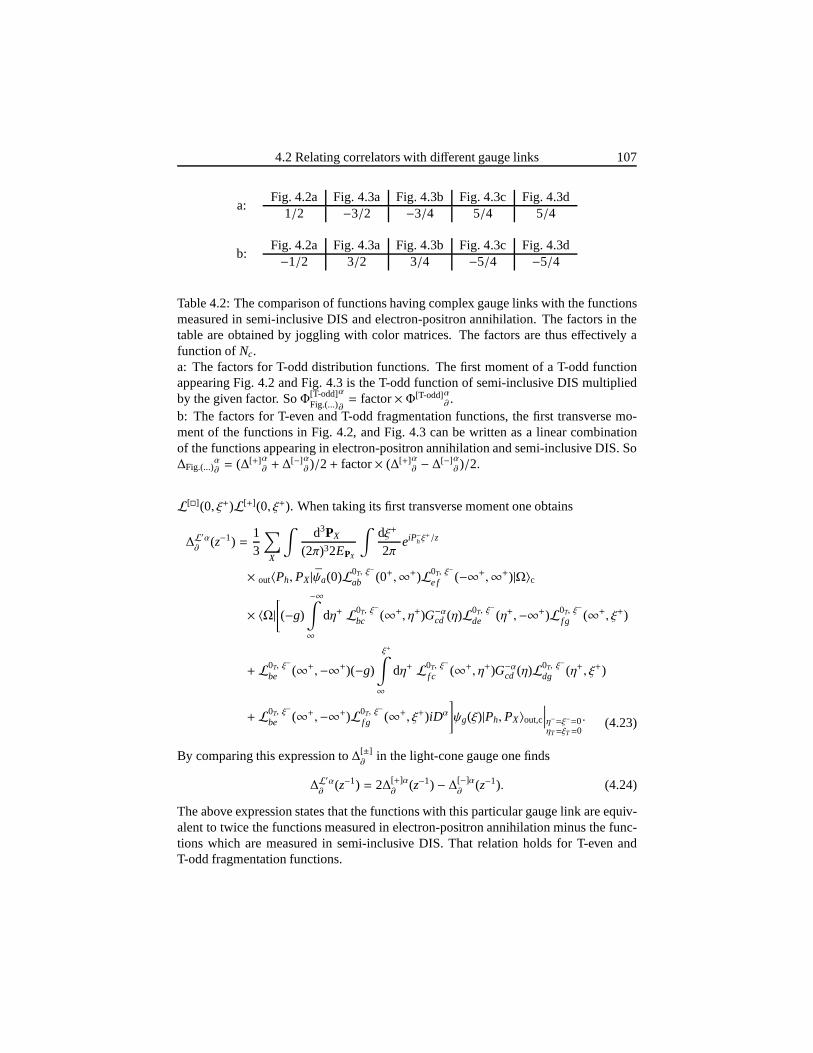
4.2 Relating correlators with different gauge links 107
a:Fig. 4.2a Fig. 4.3a Fig. 4.3b Fig. 4.3c Fig. 4.3d
1/2 −3/2 −3/4 5/4 5/4
b:Fig. 4.2a Fig. 4.3a Fig. 4.3b Fig. 4.3c Fig. 4.3d−1/2 3/2 3/4 −5/4 −5/4
Table 4.2: The comparison of functions having complex gaugelinks with the functionsmeasured in semi-inclusive DIS and electron-positron annihilation. The factors in thetable are obtained by joggling with color matrices. The factors are thus effectively afunction ofNc.a: The factors for T-odd distribution functions. The first moment of a T-odd functionappearing Fig. 4.2 and Fig. 4.3 is the T-odd function of semi-inclusive DIS multipliedby the given factor. SoΦ[T-odd]
Fig.(...)
α
∂= factor× Φ[T-odd]α
∂ .b: The factors for T-even and T-odd fragmentation functions, the first transverse mo-ment of the functions in Fig. 4.2, and Fig. 4.3 can be written as a linear combinationof the functions appearing in electron-positron annihilation and semi-inclusive DIS. So∆Fig.(...)
α∂= (∆[+]α
∂ + ∆[−]α
∂ )/2+ factor× (∆[+]α∂ − ∆[−]α
∂ )/2.
L[](0, ξ+)L[+](0, ξ+). When taking its first transverse moment one obtains
∆L′α
∂(z−1) =
13
∑
X
∫d3PX
(2π)32EPX
∫dξ+
2πeiP−hξ
+/z
× out〈Ph,PX|ψa(0)L0T, ξ−
ab (0+,∞+)L0T, ξ−
e f (−∞+,∞+)|Ω〉c
× 〈Ω|[(−g)
−∞∫
∞
dη+ L0T, ξ−
bc (∞+, η+)G−αcd (η)L0T, ξ−
de (η+,−∞+)L0T, ξ−
f g (∞+, ξ+)
+ L0T, ξ−
be (∞+,−∞+)(−g)
ξ+∫
∞
dη+ L0T, ξ−
f c (∞+, η+)G−αcd (η)L0T, ξ−
dg (η+, ξ+)
+ L0T, ξ−
be (∞+,−∞+)L0T, ξ−
f g (∞+, ξ+)iDα
]ψg(ξ)|Ph,PX〉out,c
∣∣∣∣η−=ξ−=0ηT=ξT=0
. (4.23)
By comparing this expression to∆[±]∂
in the light-cone gauge one finds
∆L′α
∂(z−1) = 2∆[+]α
∂(z−1) − ∆[−]α
∂(z−1). (4.24)
The above expression states that the functions with this particular gauge link are equiv-alent to twice the functions measured in electron-positronannihilation minus the func-tions which are measured in semi-inclusive DIS. That relation holds for T-even andT-odd fragmentation functions.
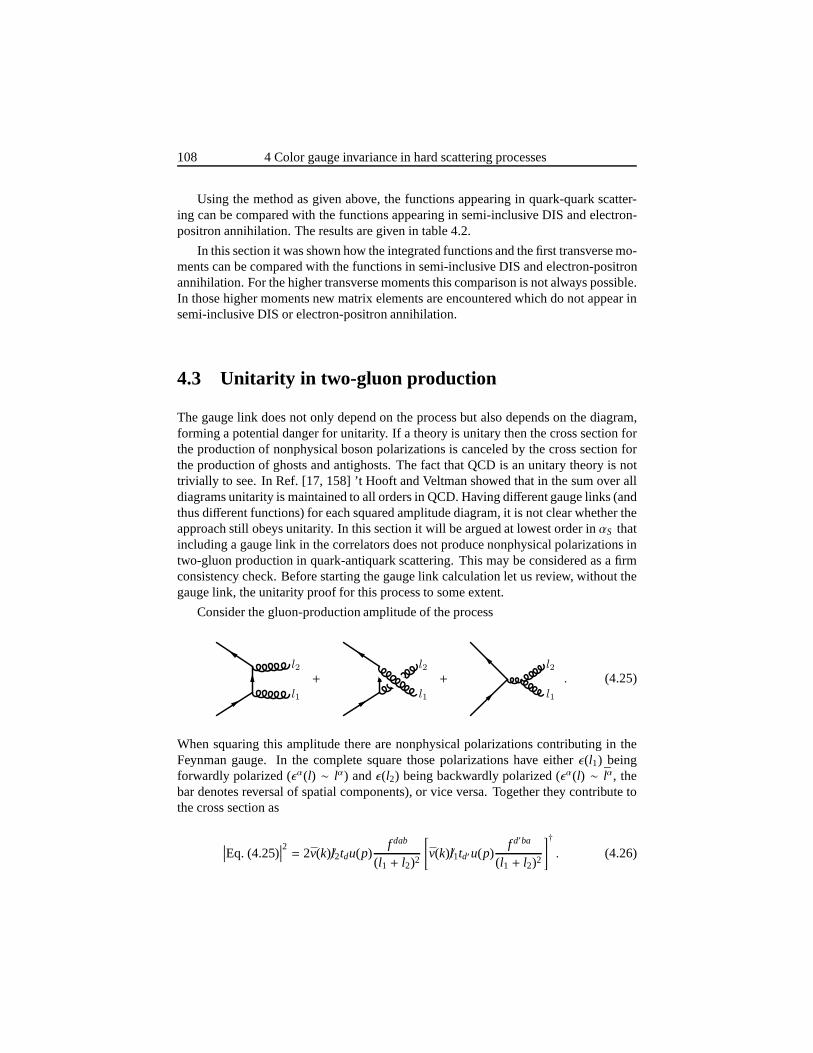
108 4 Color gauge invariance in hard scattering processes
Using the method as given above, the functions appearing in quark-quark scatter-ing can be compared with the functions appearing in semi-inclusive DIS and electron-positron annihilation. The results are given in table 4.2.
In this section it was shown how the integrated functions andthe first transverse mo-ments can be compared with the functions in semi-inclusive DIS and electron-positronannihilation. For the higher transverse moments this comparison is not always possible.In those higher moments new matrix elements are encounteredwhich do not appear insemi-inclusive DIS or electron-positron annihilation.
4.3 Unitarity in two-gluon production
The gauge link does not only depend on the process but also depends on the diagram,forming a potential danger for unitarity. If a theory is unitary then the cross section forthe production of nonphysical boson polarizations is canceled by the cross section forthe production of ghosts and antighosts. The fact that QCD isan unitary theory is nottrivially to see. In Ref. [17, 158] ’t Hooft and Veltman showed that in the sum over alldiagrams unitarity is maintained to all orders in QCD. Having different gauge links (andthus different functions) for each squared amplitude diagram, it is not clear whether theapproach still obeys unitarity. In this section it will be argued at lowest order inαS thatincluding a gauge link in the correlators does not produce nonphysical polarizations intwo-gluon production in quark-antiquark scattering. Thismay be considered as a firmconsistency check. Before starting the gauge link calculation let us review, without thegauge link, the unitarity proof for this process to some extent.
Consider the gluon-production amplitude of the process
l1
l2+
l1
l2+
l1
l2. (4.25)
When squaring this amplitude there are nonphysical polarizations contributing in theFeynman gauge. In the complete square those polarizations have eitherǫ(l1) beingforwardly polarized (ǫα(l) ∼ lα) andǫ(l2) being backwardly polarized (ǫα(l) ∼ lα, thebar denotes reversal of spatial components), or vice versa.Together they contribute tothe cross section as
∣∣∣Eq. (4.25)∣∣∣2 = 2v(k)/l2tdu(p)
f dab
(l1 + l2)2
[v(k)/l1td′u(p)
f d′ba
(l1 + l2)2
]†. (4.26)
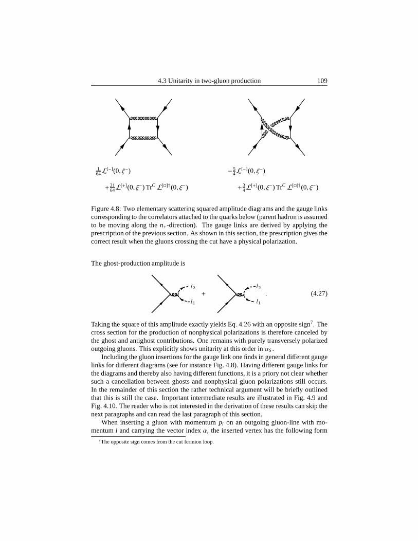
4.3 Unitarity in two-gluon production 109
164L[−](0, ξ−) − 5
4L[−](0, ξ−)
+ 2164L[+](0, ξ−) TrCL[]†(0, ξ−) + 3
4L[+](0, ξ−) TrCL[]†(0, ξ−)
Figure 4.8: Two elementary scattering squared amplitude diagrams and the gauge linkscorresponding to the correlators attached to the quarks below (parent hadron is assumedto be moving along then+-direction). The gauge links are derived by applying theprescription of the previous section. As shown in this section, the prescription gives thecorrect result when the gluons crossing the cut have a physical polarization.
The ghost-production amplitude is
l1
l2+
l1
l2. (4.27)
Taking the square of this amplitude exactly yields Eq. 4.26 with an opposite sign7. Thecross section for the production of nonphysical polarizations is therefore canceled bythe ghost and antighost contributions. One remains with purely transversely polarizedoutgoing gluons. This explicitly shows unitarity at this order inαS.
Including the gluon insertions for the gauge link one finds ingeneral different gaugelinks for different diagrams (see for instance Fig. 4.8). Having different gauge links forthe diagrams and thereby also having different functions, it is a priory not clear whethersuch a cancellation between ghosts and nonphysical gluon polarizations still occurs.In the remainder of this section the rather technical argument will be briefly outlinedthat this is still the case. Important intermediate resultsare illustrated in Fig. 4.9 andFig. 4.10. The reader who is not interested in the derivationof these results can skip thenext paragraphs and can read the last paragraph of this section.
When inserting a gluon with momentumpi on an outgoing gluon-line with mo-mentuml and carrying the vector indexα, the inserted vertex has the following form
7The opposite sign comes from the cut fermion loop.
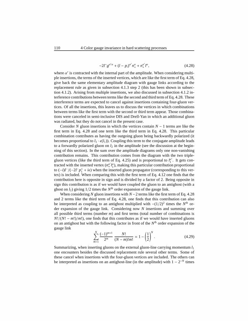
110 4 Color gauge invariance in hard scattering processes
−2l−gα′α + (l − pi)
α′nα+ + nα′
+ lα, (4.28)
whereα′ is contracted with the internal part of the amplitude. When considering multi-ple insertions, the terms of the inserted vertices, which are like the first term of Eq. 4.28,give back the same elementary amplitude diagram with gauge links according to thereplacement rule as given in subsection 4.1.3 step 2 (this has been shown in subsec-tion 4.1.2). Arising from multiple insertions, we also discussed in subsection 4.1.2 in-terference contributions between terms like the second andthird term of Eq. 4.28. Theseinterference terms are expected to cancel against insertions containing four-gluon ver-tices. Of all the insertions, this leaves us to discuss the vertices in which combinationsbetween terms like the first term with the second or third termappear. Those combina-tions were canceled in semi-inclusive DIS and Drell-Yan in which an additional gluonwas radiated, but they do not cancel in the present case.
ConsiderN gluon insertions in which the vertices containN − 1 terms are like thefirst term in Eq. 4.28 and one term like the third term in Eq. 4.28. This particularcombination contributes as having the outgoing gluon beingbackwardly polarized (itbecomes proportional tol1 · ǫ(l1)). Coupling this term to the conjugate amplitude leadsto a forwardly polarized gluon onl2 in the amplitude (see the discussion at the begin-ning of this section). In the sum over the amplitude diagramsonly one non-vanishingcontribution remains. This contribution comes from the diagram with the two triple-gluon vertices (like the third term of Eq. 4.25) and is proportional to lα
′
1 . It gets con-tracted with the inserted vertex (nα
′+ lα1), making this particular contribution proportional
to (−i)l−/(−2l−p+1 + iǫ) when the inserted gluon propagator (corresponding to thisver-tex) is included. When comparing this with the first term of Eq. 4.12 one finds that thecontribution here is opposite in sign and is divided by a factor of 2. Being opposite insign this contribution is as if we would have coupled the gluon to an antighost (with aghost onl2) giving 1/2 times theNth order expansion of the gauge link.
When consideringN gluon insertions withN−2 terms like the first term of Eq. 4.28and 2 terms like the third term of Eq. 4.28, one finds that this contribution can alsobe interpreted as coupling to an antighost multiplied with−(1/2)2 times theNth or-der expansion of the gauge link. Considering nowN insertions and summing overall possible third terms (numberm) and first terms (total number of combinations isN!/(N! − m!)/m!), one finds that this contributes as if we would have inserted gluonson an antighost but with the following factor in front of theNth order expansion of thegauge link
N∑
m=1
(−1)m+1
2m
N!(N −m)!m!
= 1−(12
)N
. (4.29)
Summarizing, when inserting gluons on the external gluon-line carrying momentuml1one encounters besides the discussed replacement rule several other terms. Some ofthese cancel when insertions with the four-gluon vertices are included. The others canbe interpreted as insertions on an antighost-line (in the amplitude) with 1− 2−N times

4.3 Unitarity in two-gluon production 111
l1
l2
*
+
l1
l2
*
+
l1
l2
*
+
l1
l2
=
L(∞−, ξ−)
L(ξ−,∞−)
l1
l2+
L(∞−, ξ−)
L(ξ−,∞−)
l1
l2
Figure 4.9: Illustration of the calculation. The∗ indicates that of all the insertions onl1 and l2 only certain parts are included. Each of those parts consists of several (zeroor more) terms like the first term of Eq. 4.28, and several terms (one or more) like thesecondor third term of Eq. 4.28.
the Nth order expansion of the gauge link. The replacement rule is similar as for thegluons.
InsertingN gluons on external ghost-lines and antighost-lines is relatively simple.One obtains the original amplitude diagram times theNth-order expansion of the gaugelink multiplied by (1/2)N. The replacement rule is similar to the replacement rule as forinsertions on external gluon-lines, but the factor (1/2)N at each order of the expansionprevents one forming a gauge link which would make the correlator gauge invariant.However, the insertions on an antighost-line together withthe contributions of inser-tions on an external gluon-line, in which terms appear like the third of Eq. 4.28, canbe recast into a ghost-antighost production diagram with a full gauge link ((1/2)N+Eq. 4.29= 1).
The contributions, arising from insertions with terms likethe second term ofEq. 4.28, work out in very similar way. Those terms can be interpreted as couplingto a ghost-line. Together with the insertions on a ghost-line the result can be written asthe production of ghost-antighost multiplied with a full gauge link. The result of theabove calculation has been represented in Fig. 4.9.
Summarizing, when inserting gluons in the two-gluon production amplitude, oneobtains the gauge link for each amplitude diagram plus some additional terms. Part ofthese additional terms (interferences between the second and the third term of Eq. 4.28)should be canceled by four-gluon vertices as explained in subsection 4.1.2. The otherterms together with the insertions on ghost-lines combine into full gauge links with anelementary ghost-antighost production-diagram. We remain now with the same set ofelementary scattering diagrams in which gauge links according to the replacement rulesappear. Those gauge links are at this moment not absorbed in the correlator. The result
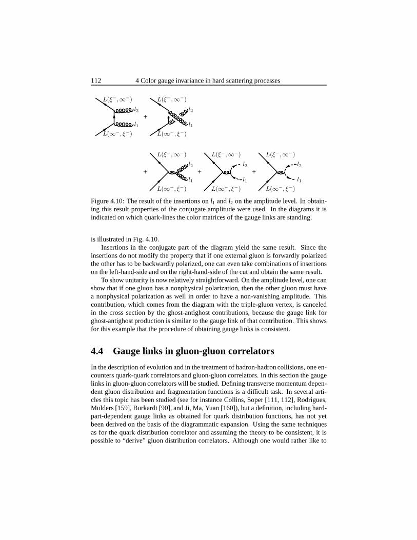
112 4 Color gauge invariance in hard scattering processes
L(∞−, ξ−)
L(ξ−,∞−)
l1
l2+
L(∞−, ξ−)
L(ξ−,∞−)
l1
l2
+
L(∞−, ξ−)
L(ξ−,∞−)
l1
l2+
L(∞−, ξ−)
L(ξ−,∞−)
l1
l2+
L(∞−, ξ−)
L(ξ−,∞−)
l1
l2
Figure 4.10: The result of the insertions onl1 andl2 on the amplitude level. In obtain-ing this result properties of the conjugate amplitude were used. In the diagrams it isindicated on which quark-lines the color matrices of the gauge links are standing.
is illustrated in Fig. 4.10.Insertions in the conjugate part of the diagram yield the same result. Since the
insertions do not modify the property that if one external gluon is forwardly polarizedthe other has to be backwardly polarized, one can even take combinations of insertionson the left-hand-side and on the right-hand-side of the cut and obtain the same result.
To show unitarity is now relatively straightforward. On theamplitude level, one canshow that if one gluon has a nonphysical polarization, then the other gluon must havea nonphysical polarization as well in order to have a non-vanishing amplitude. Thiscontribution, which comes from the diagram with the triple-gluon vertex, is canceledin the cross section by the ghost-antighost contributions,because the gauge link forghost-antighost production is similar to the gauge link of that contribution. This showsfor this example that the procedure of obtaining gauge linksis consistent.
4.4 Gauge links in gluon-gluon correlators
In the description of evolution and in the treatment of hadron-hadron collisions, one en-counters quark-quark correlators and gluon-gluon correlators. In this section the gaugelinks in gluon-gluon correlators will be studied. Defining transverse momentum depen-dent gluon distribution and fragmentation functions is a difficult task. In several arti-cles this topic has been studied (see for instance Collins, Soper [111, 112], Rodrigues,Mulders [159], Burkardt [90], and Ji, Ma, Yuan [160]), but a definition, including hard-part-dependent gauge links as obtained for quark distribution functions, has not yetbeen derived on the basis of the diagrammatic expansion. Using the same techniquesas for the quark distribution correlator and assuming the theory to be consistent, it ispossible to “derive” gluon distribution correlators. Although one would rather like to
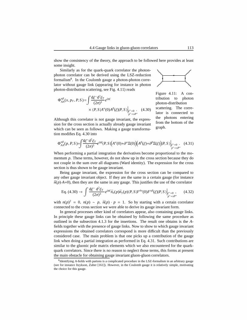
4.4 Gauge links in gluon-gluon correlators 113
show the consistency of the theory, the approach to be followed here provides at leastsome insight.
Similarly as for the quark-quark correlator the photon-
Figure 4.11: A con-tribution to photonphoton-distributionscattering. The corre-lator is connected tothe photons enteringfrom the bottom of thegraph.
photon correlator can be derived using the LSZ-reductionformalism8. In the Coulomb gauge a photon-photon corre-lator without gauge link (appearing for instance in photonphoton-distribution scattering, see Fig. 4.11) reads
Φαβ
AA(x, pT ,P,S)=∫
dξ−d2ξT
(2π)3eipξ
× 〈P,S|Aα(0)Aβ(ξ)|P,S〉∣∣∣∣ξ+=0p+=xP+
. (4.30)
Although this correlator is not gauge invariant, the expres-sion for the cross section is actually already gauge invariantwhich can be seen as follows. Making a gauge transforma-tion modifies Eq. 4.30 into
Φαβ
AA(p,P,S)=∫
dξ−d2ξT
(2π)3eipξ〈P,S|
(Aα(0)+∂αΞ(0)
)(Aβ(ξ)+∂βΞ(ξ)
)|P,S〉
∣∣∣∣ξ+=0p+=xP+
. (4.31)
When performing a partial integration the derivatives become proportional to the mo-mentump. These terms, however, do not show up in the cross section because they donot couple in the sum over all diagrams (Ward identity). The expression for the crosssection is thus shown to be gauge invariant.
Being gauge invariant, the expression for the cross sectioncan be compared toany other gauge invariant object. If they are the same in a certain gauge (for instancen(p)·A=0), then they are the same in any gauge. This justifies the use of the correlator
Eq. (4.30)→∫
dξ− d2ξT
(2π)3eipξnδ(p)nγ(p)〈P,S|Fδα(0)Fγβ(ξ)|P,S〉
∣∣∣∣ξ+=0p+=xP+
, (4.32)
with n(p)2 = 0, n(p) ∼ p, n(p) · p = 1. So by starting with a certain correlatorconnected to the cross section we were able to derive its gauge invariant form.
In general processes other kind of correlators appear, alsocontaining gauge links.In principle these gauge links can be obtained by following the same procedure asoutlined in the subsection 4.1.3 for the insertions. The result one obtains is theA-fields together with the presence of gauge links. Now to show to which gauge invariantexpressions the obtained correlators correspond is more difficult than the previouslyconsidered case. The main problem is that one picks up a contribution of the gaugelink when doing a partial integration as performed in Eq. 4.31. Such contributions aresimilar to the gluonic pole matrix elements which we also encountered for the quark-quark correlators. Since there is no reason to neglect thoseterms, this forms at presentthe main obstacle for obtaining gauge invariant gluon-gluon correlators.
8Identifying A-fields with partons is a complicated procedure in the LSZ-formalism in an arbitrary gauge(see for instance Itzykson, Zuber [161]). However, in the Coulomb gauge it is relatively simple, motivatingthe choice for this gauge.
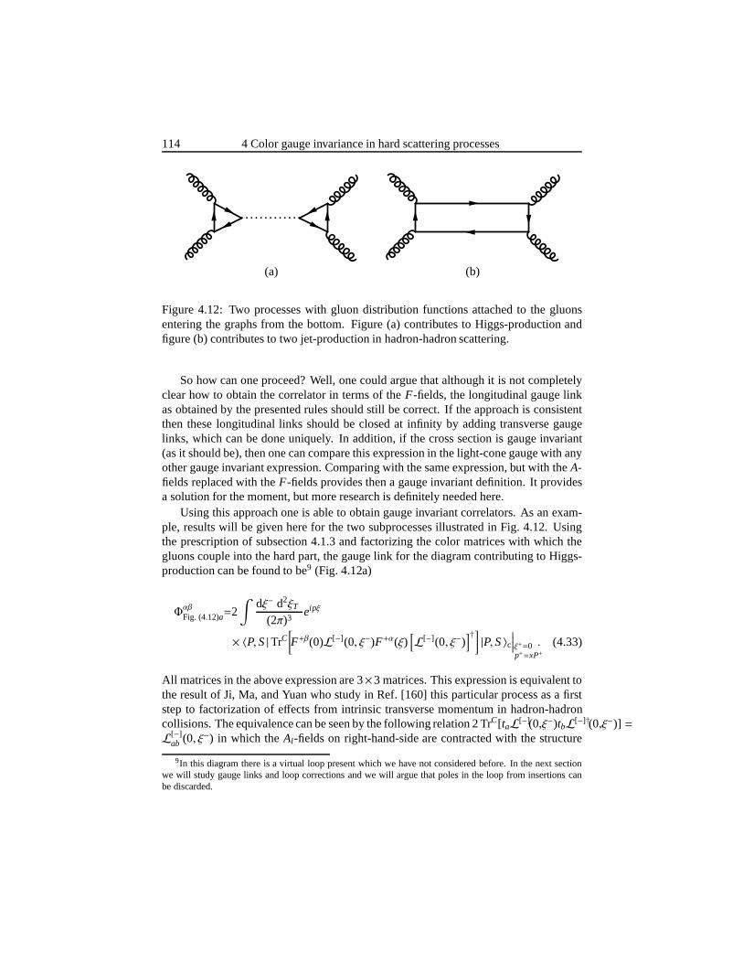
114 4 Color gauge invariance in hard scattering processes
(a) (b)
Figure 4.12: Two processes with gluon distribution functions attached to the gluonsentering the graphs from the bottom. Figure (a) contributesto Higgs-production andfigure (b) contributes to two jet-production in hadron-hadron scattering.
So how can one proceed? Well, one could argue that although itis not completelyclear how to obtain the correlator in terms of theF-fields, the longitudinal gauge linkas obtained by the presented rules should still be correct. If the approach is consistentthen these longitudinal links should be closed at infinity byadding transverse gaugelinks, which can be done uniquely. In addition, if the cross section is gauge invariant(as it should be), then one can compare this expression in thelight-cone gauge with anyother gauge invariant expression. Comparing with the same expression, but with theA-fields replaced with theF-fields provides then a gauge invariant definition. It providesa solution for the moment, but more research is definitely needed here.
Using this approach one is able to obtain gauge invariant correlators. As an exam-ple, results will be given here for the two subprocesses illustrated in Fig. 4.12. Usingthe prescription of subsection 4.1.3 and factorizing the color matrices with which thegluons couple into the hard part, the gauge link for the diagram contributing to Higgs-production can be found to be9 (Fig. 4.12a)
Φαβ
Fig. (4.12)a=2∫
dξ− d2ξT
(2π)3eipξ
× 〈P,S|TrC[F+β(0)L[−](0, ξ−)F+α(ξ)
[L[−](0, ξ−)
]†] |P,S〉c∣∣∣∣ξ+=0p+=xP+
. (4.33)
All matrices in the above expression are 3×3 matrices. This expression is equivalent tothe result of Ji, Ma, and Yuan who study in Ref. [160] this particular process as a firststep to factorization of effects from intrinsic transverse momentum in hadron-hadroncollisions. The equivalence can be seen by the following relation 2 TrC[taL[−](0,ξ−)tbL[−]†(0,ξ−)] =L[−]
ab (0, ξ−) in which theAl-fields on right-hand-side are contracted with the structure
9In this diagram there is a virtual loop present which we have not considered before. In the next sectionwe will study gauge links and loop corrections and we will argue that poles in the loop from insertions canbe discarded.
4.5 Factorization and universality 115
constants (i f alb) instead of the color matrices. In a sense this relation was obtained insubsection 4.1.2.
Another example is the gauge link of a subprocess which contributes to two jet-production in hadron-hadron scattering (see Fig. 4.12b). The gauge invariant gluon-gluon correlator is found to be
Φαβ
Fig. (4.12)b = 2∫
dξ− d2ξT
(2π)3eipξ
× 〈P,S|[38
TrC[F+α(ξ)[L[+](0, ξ−)]†F+β(0)L[−](0, ξ−)
]TrC
[L[](0, ξ−)
]
− 18
TrC[F+α(ξ)L[+]†(0, ξ−)F+β(0)L[+](0, ξ−)
] ]|P,S〉c
∣∣∣∣ξ+=0p+=xP+
. (4.34)
In this new result various gauge links via plus and minus infinity appear. It is notpossible to rewrite this result in terms of gauge links in which only structure constantsare used (as in the previous example).
In Ref. [90] Burkardt studied gluon distribution functionsand suggested a sum rulefor the Sivers quark and gluon distribution functions. It may be good to point out thatthose gluon distribution functions, containing gauge links via plus infinity, appear insemi-inclusive lepton-hadron scattering, like two-jet production. A contribution to thatcross section would be Fig. 4.12b in which the incoming gluons from the top of thegraph are replaced by incoming virtual photons.
In this section a method for obtaining gauge invariant gluon-gluon correlators hasbeen suggested although a significant amount of work remainsto be done. Note thatone still needs to look for observables sensitive to the pathof the gauge link. Thoseobservables should be sensitive to the intrinsic transverse momenta of the gluons. Oneparticular observable will be discussed for hadron-hadronscattering in the next chapter.
4.5 Factorization and universality
Up to now processes have been described by using the diagrammatic approach in whichcorrelators were attached to an infinite number of hard scattering diagrams. These cor-relators, likeΦ, ΦA, and∆AA’s as defined in section 2.4, contained a certain renormal-ization scale and it has been assumed that these correlatorscould be factorized, enablingone to calculate in principle its scale dependence process-independently. We found atleading order inαS that in several semi-inclusive processes, this infinite setof hardscattering diagrams and correlators combined into a finite set of diagrams convolutedwith a finite set of gauge invariant correlators (containinga gauge link). Although thestarting point was purely process-independent, it turned out that the hard scattering partdetermined the path of the gauge links in the final result. In this section the validity ofthe applied factorized approach will be discussed.
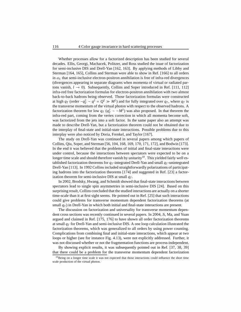
116 4 Color gauge invariance in hard scattering processes
Whether processes allow for a factorized description has been studied for severaldecades. Ellis, Georgi, Machacek, Politzer, and Ross studied the issue of factorizationfor semi-inclusive DIS and Drell-Yan [162, 163]. By applying methods of Libby andSterman [164, 165], Collins and Sterman were able to show in Ref. [166] to all ordersin αS that semi-inclusive electron-positron annihilation is free of infra-red divergences(divergences appearing in separate diagrams when momenta of virtual or radiated par-tons vanish,l → 0). Subsequently, Collins and Soper introduced in Ref. [111, 112]infra-red free factorization formulas for electron-positron annihilation with two almostback-to-back hadrons being observed. Those factorizationformulas were constructedat highqT (order−q2
T ∼ q2 = Q2 ≫ M2) and for fully integrated overqT , whereqT isthe transverse momentum of the virtual photon with respect to the observed hadrons. Afactorization theorem for lowqT (q2
T ∼ −M2) was also proposed. In that theorem theinfra-red part, coming from the vertex correction in which all momenta become soft,was factorized from the jets into a soft factor. In the same paper also an attempt wasmade to describe Drell-Yan, but a factorization theorem could not be obtained due tothe interplay of final-state and initial-state interactions. Possible problems due to thisinterplay were also noticed by Doria, Frenkel, and Taylor [167].
The study on Drell-Yan was continued in several papers amongwhich papers ofCollins, Qiu, Soper, and Sterman [56, 104, 168, 169, 170, 171, 172], and Bodwin [173].In the end it was believed that the problems of initial and final-state interactions wereunder control, because the interactions between spectators were expected to be on alonger time scale and should therefore vanish by unitarity10. This yielded fairly well es-tablished factorization theorems forqT-integrated Drell-Yan and smallqT-unintegratedDrell-Yan [113]. In 1992 Collins included straightforwardly polarizations of participat-ing hadrons into the factorization theorems [174] and suggested in Ref. [23] a factor-ization theorem for semi-inclusive DIS at smallqT .
In 2002, Brodsky, Hwang, and Schmidt showed that final-stateinteractions betweenspectators lead to single spin asymmetries in semi-inclusive DIS [24]. Based on thissurprising result, Collins concluded that the studied interactions are actually on a shortertime-scale than it at first sight seems. He pointed out in Ref.[25] that such interactionscould give problems for transverse momentum dependent factorization theorems (atsmallqT) in Drell-Yan in which both initial and final-state interactions are present.
The discussion on factorization and universality for transverse momentum depen-dent cross sections was recently continued in several papers. In 2004, Ji, Ma, and Yuanargued and claimed in Ref. [175, 176] to have shown all order factorization theoremsat smallqT for Drell-Yan and semi-inclusive DIS. A one loop calculation illustrated thefactorization theorems, which was generalized to all orders by using power counting.Complications from combining final and initial-state interactions, which appear at twoloops or higher (see for instance Fig. 4.13), were not explicitly addressed. Further, itwas not discussed whether or not the fragmentation functions are process-independent.
By showing explicit results, it was subsequently pointed out in Ref. [37, 38, 39]that there could be a problem for the transverse momentum dependent factorization
10Being on a longer time scale it was not expected that those interactions could influence the short timescale production of the virtual photon.
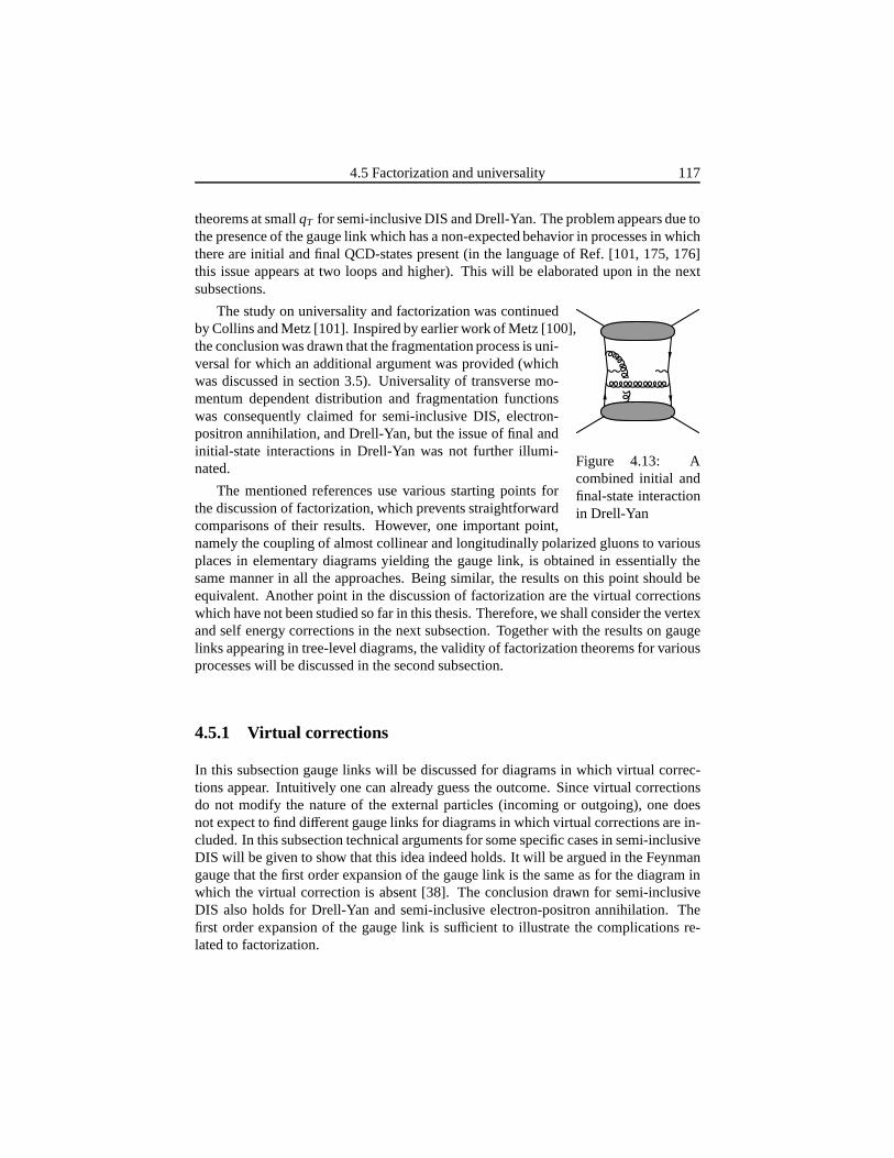
4.5 Factorization and universality 117
theorems at smallqT for semi-inclusive DIS and Drell-Yan. The problem appears due tothe presence of the gauge link which has a non-expected behavior in processes in whichthere are initial and final QCD-states present (in the language of Ref. [101, 175, 176]this issue appears at two loops and higher). This will be elaborated upon in the nextsubsections.
The study on universality and factorization was continued
Figure 4.13: Acombined initial andfinal-state interactionin Drell-Yan
by Collins and Metz [101]. Inspired by earlier work of Metz [100],the conclusion was drawn that the fragmentation process is uni-versal for which an additional argument was provided (whichwas discussed in section 3.5). Universality of transverse mo-mentum dependent distribution and fragmentation functionswas consequently claimed for semi-inclusive DIS, electron-positron annihilation, and Drell-Yan, but the issue of finalandinitial-state interactions in Drell-Yan was not further illumi-nated.
The mentioned references use various starting points forthe discussion of factorization, which prevents straightforwardcomparisons of their results. However, one important point,namely the coupling of almost collinear and longitudinallypolarized gluons to variousplaces in elementary diagrams yielding the gauge link, is obtained in essentially thesame manner in all the approaches. Being similar, the results on this point should beequivalent. Another point in the discussion of factorization are the virtual correctionswhich have not been studied so far in this thesis. Therefore,we shall consider the vertexand self energy corrections in the next subsection. Together with the results on gaugelinks appearing in tree-level diagrams, the validity of factorization theorems for variousprocesses will be discussed in the second subsection.
4.5.1 Virtual corrections
In this subsection gauge links will be discussed for diagrams in which virtual correc-tions appear. Intuitively one can already guess the outcome. Since virtual correctionsdo not modify the nature of the external particles (incomingor outgoing), one doesnot expect to find different gauge links for diagrams in which virtual correctionsare in-cluded. In this subsection technical arguments for some specific cases in semi-inclusiveDIS will be given to show that this idea indeed holds. It will be argued in the Feynmangauge that the first order expansion of the gauge link is the same as for the diagram inwhich the virtual correction is absent [38]. The conclusiondrawn for semi-inclusiveDIS also holds for Drell-Yan and semi-inclusive electron-positron annihilation. Thefirst order expansion of the gauge link is sufficient to illustrate the complications re-lated to factorization.
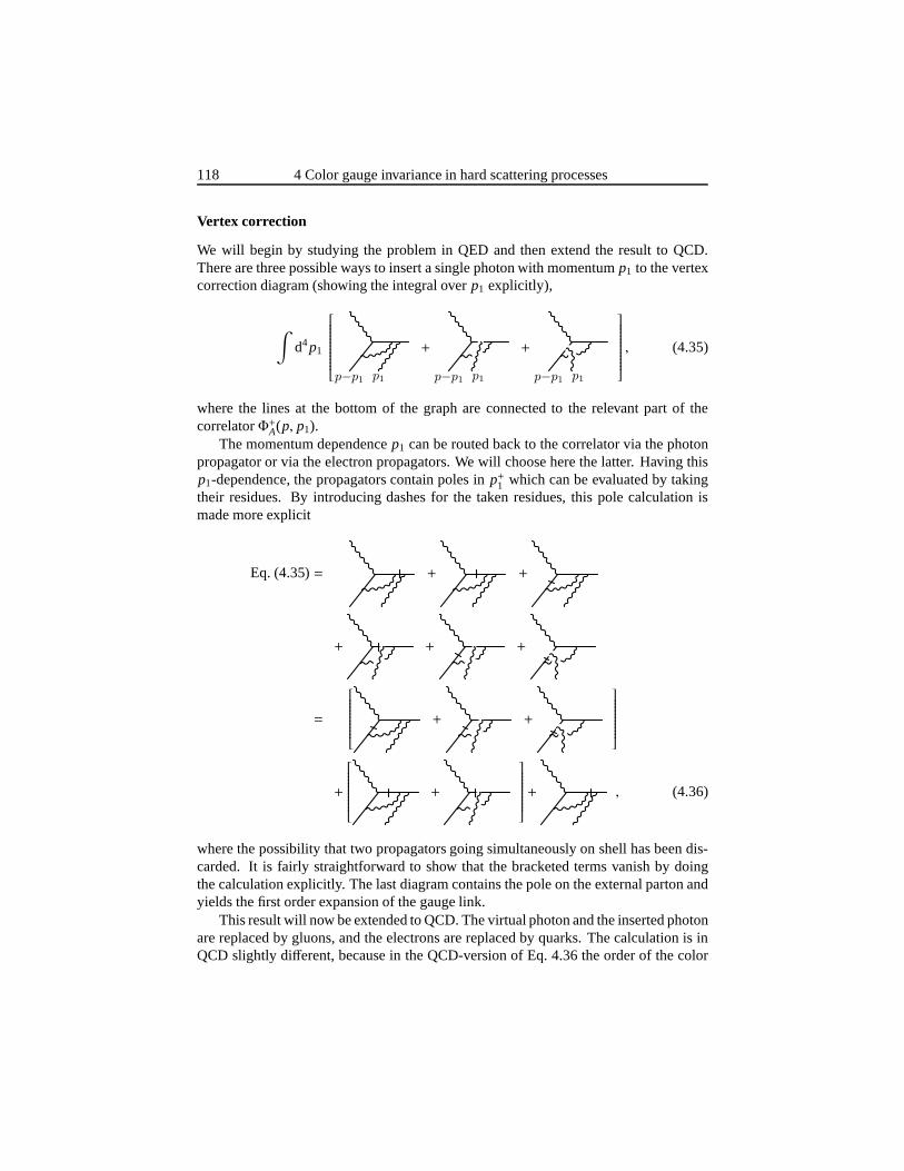
118 4 Color gauge invariance in hard scattering processes
Vertex correction
We will begin by studying the problem in QED and then extend the result to QCD.There are three possible ways to insert a single photon with momentump1 to the vertexcorrection diagram (showing the integral overp1 explicitly),
∫d4p1
p−p1 p1
+
p−p1 p1
+
p−p1 p1
, (4.35)
where the lines at the bottom of the graph are connected to therelevant part of thecorrelatorΦ+A(p, p1).
The momentum dependencep1 can be routed back to the correlator via the photonpropagator or via the electron propagators. We will choose here the latter. Having thisp1-dependence, the propagators contain poles inp+1 which can be evaluated by takingtheir residues. By introducing dashes for the taken residues, this pole calculation ismade more explicit
Eq. (4.35)= + +
+ + +
=
+ +
+
+
+ , (4.36)
where the possibility that two propagators going simultaneously on shell has been dis-carded. It is fairly straightforward to show that the bracketed terms vanish by doingthe calculation explicitly. The last diagram contains the pole on the external parton andyields the first order expansion of the gauge link.
This result will now be extended to QCD. The virtual photon and the inserted photonare replaced by gluons, and the electrons are replaced by quarks. The calculation is inQCD slightly different, because in the QCD-version of Eq. 4.36 the order of thecolor
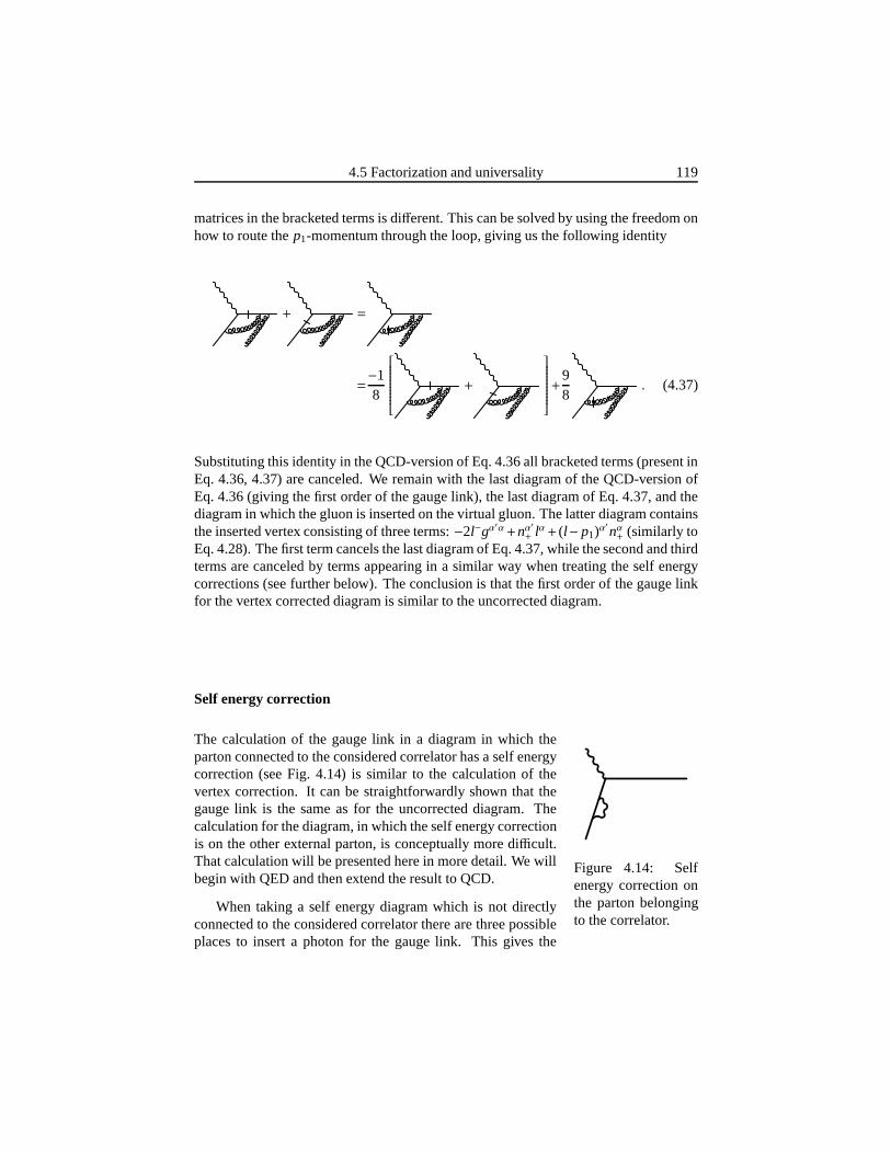
4.5 Factorization and universality 119
matrices in the bracketed terms is different. This can be solved by using the freedom onhow to route thep1-momentum through the loop, giving us the following identity
+ =
=−18
+
+
98
. (4.37)
Substituting this identity in the QCD-version of Eq. 4.36 all bracketed terms (present inEq. 4.36, 4.37) are canceled. We remain with the last diagramof the QCD-version ofEq. 4.36 (giving the first order of the gauge link), the last diagram of Eq. 4.37, and thediagram in which the gluon is inserted on the virtual gluon. The latter diagram containsthe inserted vertex consisting of three terms:−2l−gα
′α+nα′+ lα+ (l− p1)α
′nα+ (similarly to
Eq. 4.28). The first term cancels the last diagram of Eq. 4.37,while the second and thirdterms are canceled by terms appearing in a similar way when treating the self energycorrections (see further below). The conclusion is that thefirst order of the gauge linkfor the vertex corrected diagram is similar to the uncorrected diagram.
Self energy correction
The calculation of the gauge link in a diagram in which the
Figure 4.14: Selfenergy correction onthe parton belongingto the correlator.
parton connected to the considered correlator has a self energycorrection (see Fig. 4.14) is similar to the calculation of thevertex correction. It can be straightforwardly shown that thegauge link is the same as for the uncorrected diagram. Thecalculation for the diagram, in which the self energy correctionis on the other external parton, is conceptually more difficult.That calculation will be presented here in more detail. We willbegin with QED and then extend the result to QCD.
When taking a self energy diagram which is not directlyconnected to the considered correlator there are three possibleplaces to insert a photon for the gauge link. This gives the
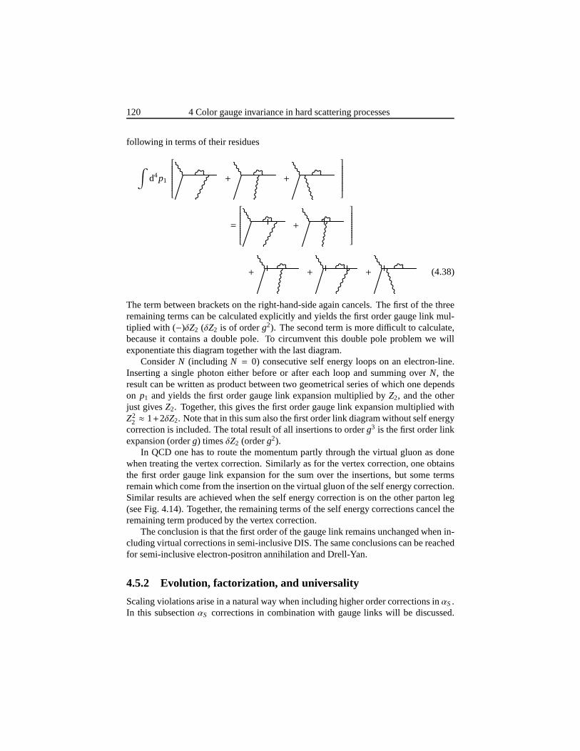
120 4 Color gauge invariance in hard scattering processes
following in terms of their residues
∫d4p1
+ +
=
+
+ + + (4.38)
The term between brackets on the right-hand-side again cancels. The first of the threeremaining terms can be calculated explicitly and yields thefirst order gauge link mul-tiplied with (−)δZ2 (δZ2 is of orderg2). The second term is more difficult to calculate,because it contains a double pole. To circumvent this doublepole problem we willexponentiate this diagram together with the last diagram.
ConsiderN (including N = 0) consecutive self energy loops on an electron-line.Inserting a single photon either before or after each loop and summing overN, theresult can be written as product between two geometrical series of which one dependson p1 and yields the first order gauge link expansion multiplied byZ2, and the otherjust givesZ2. Together, this gives the first order gauge link expansion multiplied withZ2
2 ≈ 1+2δZ2. Note that in this sum also the first order link diagram without self energycorrection is included. The total result of all insertions to orderg3 is the first order linkexpansion (orderg) timesδZ2 (orderg2).
In QCD one has to route the momentum partly through the virtual gluon as donewhen treating the vertex correction. Similarly as for the vertex correction, one obtainsthe first order gauge link expansion for the sum over the insertions, but some termsremain which come from the insertion on the virtual gluon of the self energy correction.Similar results are achieved when the self energy correction is on the other parton leg(see Fig. 4.14). Together, the remaining terms of the self energy corrections cancel theremaining term produced by the vertex correction.
The conclusion is that the first order of the gauge link remains unchanged when in-cluding virtual corrections in semi-inclusive DIS. The same conclusions can be reachedfor semi-inclusive electron-positron annihilation and Drell-Yan.
4.5.2 Evolution, factorization, and universality
Scaling violations arise in a natural way when including higher order corrections inαS.In this subsectionαS corrections in combination with gauge links will be discussed.
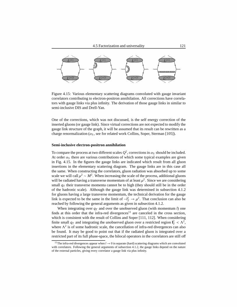
4.5 Factorization and universality 121
L[+]†
L[+]
L[+]†
L[+]
L[+]†
L[+]
L[+]†
L[+]
Figure 4.15: Various elementary scattering diagrams convoluted with gauge invariantcorrelators contributing to electron-positron annihilation. All corrections have correla-tors with gauge links via plus infinity. The derivation of those gauge links in similar tosemi-inclusive DIS and Drell-Yan.
One of the corrections, which was not discussed, is the self energy correction of theinserted gluons (or gauge link). Since virtual correctionsare not expected to modify thegauge link structure of the graph, it will be assumed that itsresult can be rewritten as acharge renormalization (αS, see for related work Collins, Soper, Sterman [105]).
Semi-inclusive electron-positron annihilation
To compare the process at two different scalesQ2, corrections inαS should be included.At orderαS there are various contributions of which some typical examples are givenin Fig. 4.15. In the figures the gauge links are indicated which result from all gluoninsertions in the elementary scattering diagram. The gaugelinks are in this case allthe same. When constructing the correlators, gluon radiation was absorbed up to somescale we will callµ2 ∼ M2. When increasing the scale of the process, additional gluonswill be radiated having a transverse momentum of at leastµ2. Since we are consideringsmallqT their transverse momenta cannot be to high (they should still be in the orderof the hadronic scale). Although the gauge link was determined in subsection 4.1.2for gluons having a large transverse momentum, the technical derivation for the gaugelink is expected to be the same in the limit of−l2T → µ2. That conclusion can also bereached by following the general arguments as given in subsection 4.1.2.
When integrating overqT and over the unobserved gluon (with momentuml) onefinds at this order that the infra-red divergences11 are canceled in the cross section,which is consistent with the result of Collins and Soper [111, 112]. When consideringfinite smallqT and integrating the unobserved gluon over a restricted region l2T < Λ2,whereΛ2 is of some hadronic scale, the cancellation of infra-red divergences can alsobe found. It may be good to point out that if the radiated gluonis integrated over arestricted part of its full phase-space, the bilocal operators in the correlators are still off
11The infra-red divergences appear whenl → 0 in separate (hard) scattering diagrams which are convolutedwith correlators. Following the general arguments of subsection 4.1.2, the gauge links depend on the natureof the external particles, giving every correlator a gauge link via plus infinity.
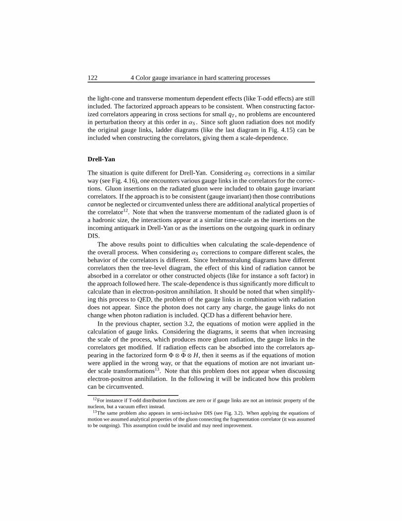
122 4 Color gauge invariance in hard scattering processes
the light-cone and transverse momentum dependent effects (like T-odd effects) are stillincluded. The factorized approach appears to be consistent. When constructing factor-ized correlators appearing in cross sections for smallqT , no problems are encounteredin perturbation theory at this order inαS. Since soft gluon radiation does not modifythe original gauge links, ladder diagrams (like the last diagram in Fig. 4.15) can beincluded when constructing the correlators, giving them a scale-dependence.
Drell-Yan
The situation is quite different for Drell-Yan. ConsideringαS corrections in a similarway (see Fig. 4.16), one encounters various gauge links in the correlators for the correc-tions. Gluon insertions on the radiated gluon were includedto obtain gauge invariantcorrelators. If the approach is to be consistent (gauge invariant) then those contributionscannotbe neglected or circumvented unless there are additional analytical properties ofthe correlator12. Note that when the transverse momentum of the radiated gluon is ofa hadronic size, the interactions appear at a similar time-scale as the insertions on theincoming antiquark in Drell-Yan or as the insertions on the outgoing quark in ordinaryDIS.
The above results point to difficulties when calculating the scale-dependence ofthe overall process. When consideringαS corrections to compare different scales, thebehavior of the correlators is different. Since brehmsstralung diagrams have differentcorrelators then the tree-level diagram, the effect of this kind of radiation cannot beabsorbed in a correlator or other constructed objects (likefor instance a soft factor) inthe approach followed here. The scale-dependence is thus significantly more difficult tocalculate than in electron-positron annihilation. It should be noted that when simplify-ing this process to QED, the problem of the gauge links in combination with radiationdoes not appear. Since the photon does not carry any charge, the gauge links do notchange when photon radiation is included. QCD has a different behavior here.
In the previous chapter, section 3.2, the equations of motion were applied in thecalculation of gauge links. Considering the diagrams, it seems that when increasingthe scale of the process, which produces more gluon radiation, the gauge links in thecorrelators get modified. If radiation effects can be absorbed into the correlators ap-pearing in the factorized formΦ ⊗ Φ ⊗ H, then it seems as if the equations of motionwere applied in the wrong way, or that the equations of motionare not invariant un-der scale transformations13. Note that this problem does not appear when discussingelectron-positron annihilation. In the following it will be indicated how this problemcan be circumvented.
12For instance if T-odd distribution functions are zero or if gauge links are not an intrinsic property of thenucleon, but a vacuum effect instead.
13The same problem also appears in semi-inclusive DIS (see Fig. 3.2). When applying the equations ofmotion we assumed analytical properties of the gluon connecting the fragmentation correlator (it was assumedto be outgoing). This assumption could be invalid and may need improvement.
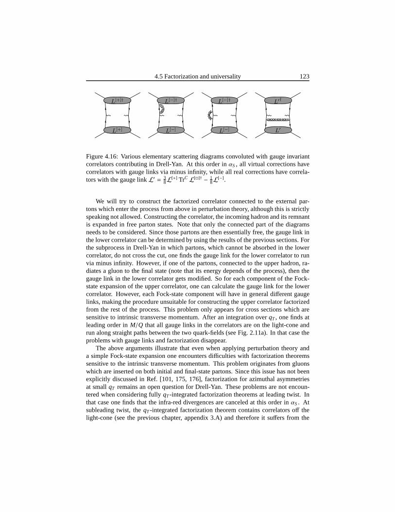
4.5 Factorization and universality 123
L[+]
L[+]†
L[−]
L[−]†
L[−]
L[−]†
L′
L′†
Figure 4.16: Various elementary scattering diagrams convoluted with gauge invariantcorrelators contributing in Drell-Yan. At this order inαS, all virtual corrections havecorrelators with gauge links via minus infinity, while all real corrections have correla-tors with the gauge linkL′ = 3
8L[+] TrCL[]† − 18L[−] .
We will try to construct the factorized correlator connected to the external par-tons which enter the process from above in perturbation theory, although this is strictlyspeaking not allowed. Constructing the correlator, the incoming hadron and its remnantis expanded in free parton states. Note that only the connected part of the diagramsneeds to be considered. Since those partons are then essentially free, the gauge link inthe lower correlator can be determined by using the results of the previous sections. Forthe subprocess in Drell-Yan in which partons, which cannot be absorbed in the lowercorrelator, do not cross the cut, one finds the gauge link for the lower correlator to runvia minus infinity. However, if one of the partons, connectedto the upper hadron, ra-diates a gluon to the final state (note that its energy dependsof the process), then thegauge link in the lower correlator gets modified. So for each component of the Fock-state expansion of the upper correlator, one can calculate the gauge link for the lowercorrelator. However, each Fock-state component will have in general different gaugelinks, making the procedure unsuitable for constructing the upper correlator factorizedfrom the rest of the process. This problem only appears for cross sections which aresensitive to intrinsic transverse momentum. After an integration overqT , one finds atleading order inM/Q that all gauge links in the correlators are on the light-coneandrun along straight paths between the two quark-fields (see Fig. 2.11a). In that case theproblems with gauge links and factorization disappear.
The above arguments illustrate that even when applying perturbation theory anda simple Fock-state expansion one encounters difficulties with factorization theoremssensitive to the intrinsic transverse momentum. This problem originates from gluonswhich are inserted on both initial and final-state partons. Since this issue has not beenexplicitly discussed in Ref. [101, 175, 176], factorization for azimuthal asymmetriesat smallqT remains an open question for Drell-Yan. These problems are not encoun-tered when considering fullyqT-integrated factorization theorems at leading twist. Inthat case one finds that the infra-red divergences are canceled at this order inαS. Atsubleading twist, theqT-integrated factorization theorem contains correlators off thelight-cone (see the previous chapter, appendix 3.A) and therefore it suffers from the
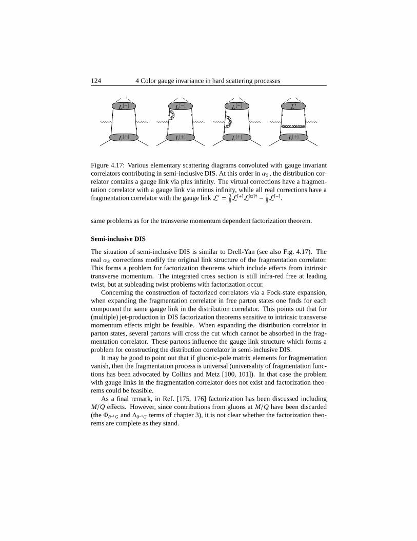
124 4 Color gauge invariance in hard scattering processes
L[+]
L[−]
L[+]
L[−]
L[+]
L[−]
L[+]
L′
Figure 4.17: Various elementary scattering diagrams convoluted with gauge invariantcorrelators contributing in semi-inclusive DIS. At this order inαS, the distribution cor-relator contains a gauge link via plus infinity. The virtual corrections have a fragmen-tation correlator with a gauge link via minus infinity, whileall real corrections have afragmentation correlator with the gauge linkL′ = 3
8L[+]L[]† − 18L[−] .
same problems as for the transverse momentum dependent factorization theorem.
Semi-inclusive DIS
The situation of semi-inclusive DIS is similar to Drell-Yan(see also Fig. 4.17). TherealαS corrections modify the original link structure of the fragmentation correlator.This forms a problem for factorization theorems which include effects from intrinsictransverse momentum. The integrated cross section is stillinfra-red free at leadingtwist, but at subleading twist problems with factorizationoccur.
Concerning the construction of factorized correlators viaa Fock-state expansion,when expanding the fragmentation correlator in free partonstates one finds for eachcomponent the same gauge link in the distribution correlator. This points out that for(multiple) jet-production in DIS factorization theorems sensitive to intrinsic transversemomentum effects might be feasible. When expanding the distribution correlator inparton states, several partons will cross the cut which cannot be absorbed in the frag-mentation correlator. These partons influence the gauge link structure which forms aproblem for constructing the distribution correlator in semi-inclusive DIS.
It may be good to point out that if gluonic-pole matrix elements for fragmentationvanish, then the fragmentation process is universal (universality of fragmentation func-tions has been advocated by Collins and Metz [100, 101]). In that case the problemwith gauge links in the fragmentation correlator does not exist and factorization theo-rems could be feasible.
As a final remark, in Ref. [175, 176] factorization has been discussed includingM/Q effects. However, since contributions from gluons atM/Q have been discarded(theΦ∂−1G and∆∂−1G terms of chapter 3), it is not clear whether the factorization theo-rems are complete as they stand.
4.6 Summary and conclusions 125
4.6 Summary and conclusions
In this chapter gauge links appearing in more complicated diagrams were considered.When deriving those gauge links by considering gluon interactions between the correla-tors and the hard part, two classes of poles were encountered. The first class contains thepolesp+i ≈ 0 which correspond to the limit in which the gluon momenta vanish. Thisclass yields contributions to the gauge link. The second class contains the other polesand in the examples shown, those poles canceled. Supplementing general argumentsin favor of this cancellation have been given and a set of rules has been conjecturedthat allows one to deduce gauge links for arbitrary diagrams. Applying these rules forgluon-gluon correlators, gauge invariant transverse momentum dependent gluon distri-bution functions were obtained. In a sense, these rules factorize interactions between acorrelator and the elementary scattering part.
It was found that gauge links do in general not only depend on the overall processbut also depend on the elementary scattering diagram. The encountered gauge links alsohad more complicated paths than the ones appearing in semi-inclusive DIS or Drell-Yan. To compare the correlators with these different gauge links, we considered thefirst transverse moments of distribution and fragmentationfunctions. It was found thatthese transverse moments can be related to the transverse moments appearing in semi-inclusive DIS and electron-positron annihilation. For thehigher transverse moments norelations were obtained.
The fact that the gauge link in the correlator depends on the subprocess insteadof the overall process could form a potential danger for the unitarity of the approach.However, in an explicit nontrivial example (two-gluon production) it was found that thefactorized description in terms of gauge invariant correlators still respects unitarity.
We also discussed the subject of factorization and universality for semi-inclusiveDIS, electron-positron annihilation, and Drell-Yan. In semi-inclusive electron-positronannihilation we did not encounter any inconsistencies because QCD-states appearedonly in the final state. For semi-inclusive DIS and Drell-Yanthere was in Ref. [101,175, 176] recently important progress reported on smallqT-unintegrated14 factoriza-tion theorems, but one particular issue of dealing with bothfinal and initial-state in-teractions has not satisfactory been treated. This issue isrelated to the observationthat gauge links in transverse momentum dependent correlators can get modified whenconsidering radiation effects. This could create a problem for factorizing effects fromintrinsic transverse momentum appearing in cross sectionsfor semi-inclusive DIS andDrell-Yan. Since fullyqT-integrated factorization theorems contain at subleadingtwisteffects from intrinsic transverse momentum (see appendix 3.A), it forms at that ordera potential problem as well. Factorization of intrinsic transverse momentum depen-dent effects in Drell-Yan and semi-inclusive DIS remains thereforeat present an openissue [39]. Similar problems also appear for semi-inclusive hadron-hadron scattering.
The non-Abelian character plays an essential role in the discussion of final and
14q is the momentum of the virtual photon and−q2T ∼ M2

126 4 Color gauge invariance in hard scattering processes
initial-state interactions. For instance, in QED where photons do not carry charge, pho-ton radiation does not modify the gauge link structure. Although more complicatedgauge links than the ones appearing in semi-inclusive DIS and Drell-Yan are still en-countered, factorization of effects from intrinsic transverse momentum in hard QEDscattering processes should be feasible.
It may be good to point out that in QCD the problems for semi-inclusive DIS orig-inate from the gauge link in the fragmentation correlator incombination with gluonradiation. If this gauge link turns out to be irrelevant (which means that gluonic-polematrix elements for fragmentation functions would be suppressed), then the problemswith factorizing effects from intrinsic transverse momentum disappear. In thatscenario,which is favored by the in section 3.5 differently given interpretation of the results ob-tained by Collins and Metz [101], factorization theorems including effects from intrinsictransverse momentum might be obtainable. Such factorization theorems can also be ex-pected to hold for (multiple) jet-production in DIS, because in those cases the problemwith fragmentation functions is not present.
As a last remark, in the diagrammatic approach used in this thesis, no assumptionswere made for the correlators other than the assumptions similar to the parton model(see chapter 2). Many issues might be unknown for that reason, one of them being theevolution equations for transverse momentum dependent functions (for a detailed studyof this problem see Henneman [66]). It is possible that additional assumptions, whichshould be physically justified, might solve some of the issues. One possibility could bethat gauge links in general do not influence the expectation values of matrix elements.In that case T-odd distribution functions would be zero and proofs on factorization anduniversality would be simplified significantly. Another possibility could be that gaugelinks correspond to certain interactions in the hard part ina particular kinematical limit(for instance the vertex correction in the limit that the gluon is collinear with one of theexternal quarks). In that case the gauge link is not an intrinsic property of the nucleon,allowing (part of) its contribution to be possibly absorbedin other matrix elements orfactors.
5
Results for single spinasymmetries in
hadronic scattering
In the previous chapter the necessary tools were developed to determine the Wilsonlines which appear in correlators in hard scattering processes. As discussed, it is notclear whether effects from intrinsic transverse momentum allow for a factorized de-scription in hadron-hadron scattering. We will assume it does and obtain results forsingle spin asymmetries. In these asymmetries the effect of the gauge link appears to bemore than just a sign; it also determines the sizes of the asymmetries. It will be shownhow the intrinsic transverse momenta of quarks can be accessed by observing unpolar-ized hadrons in opposite jets. For the ease of the calculation, only contributions fromquark distribution and fragmentation functions will be considered. Gluon distributionand fragmentation functions are neglected, but can be straightforwardly incorporatedby following the same procedure.

128 5 Results for single spin asymmetries in hadronic scattering
5.1 Introduction
We will study the transverse momentum dependent distribution and fragmentation func-tions via single spin asymmetries in hadron-hadron scattering. Within the applied di-agrammatic approach, an odd number of T-odd functions is needed to produce crosssections for single spin asymmetries at leading order inαS. At leading twist, T-oddfunctions are transverse momentum dependent. Integrated T-odd distribution functionsare assumed to be zero and unpolarized integrated T-odd fragmentation functions ap-pear only at subleading twist [99]. Single spin asymmetriesat leading order in inversepowers of the hard scale must therefore arise from intrinsictransverse momenta.
The validity of the applied theoretical description depends on two issues. The firstissue is connected to factorization. This was discussed in the previous chapter and inthe present study it will be assumed to hold. The second issueis related to asymptoticfreedom. It is expected that only those processes can be described perturbatively inwhich observed external hadrons are well separated in momentum space. The observedoutgoing hadrons must have a large perpendicular momentum with respect to the beam-axis. For observed hadrons close to the beam-axis, one does not only have a problemwith perturbation theory, but one will also encounter interference effects between thehard scattering process and the remnant of the incoming hadrons. In that case fracturefunctions need to be included.
One of the most studied semi-inclusive cross section in hadron-hadron collisionsis single hadron production. It is also this process in whichthe first single spin asym-metries in inelastic collisions were observed [20]. Since then, single spin asymmetrieshave been measured in several processes (see for instance Ref. [177, 178, 179, 180,181, 182, 183, 184]), and extensive theoretical studies have been made (see for instanceRef. [57, 72, 185, 186, 187, 188, 189, 190, 191]). The main theoretical challengewith single hadron production at large transverse momentumis that there is no ob-servable which is directly connected to the intrinsic transverse momenta of the partons.This makes the extraction of the transverse momentum dependent functions complex. Itcould be that the only possible manner of extracting information is to consider a specificform for the transverse momentum dependence of distribution or fragmentation func-tions (for example exp[−k2
T/M2]). Such a form can lead to problems with the gauge
link because it generally contains higher order transversemoments. At present onlythe first transverse moment of functions can be easily related to the transverse momentof functions appearing in semi-inclusive DIS and electron-positron annihilation. In thehigher transverse moments new matrix elements are involvedwhich are more difficultto relate (see also section 4.2). Besides, for the higher transverse moments convergencebecomes an issue as well.
The two hadron production process, in which the two hadrons belong to differentjets and are approximately back-to-back in the perpendicular plane, does offer an ob-servable directly sensitive to the intrinsic transverse momenta. The fact that the twohadrons are not completely back-to-back can at leading order in αS be interpreted as an
5.2 Calculating cross sections for hadronic scattering 129
effect from intrinsic transverse momentum. This process will be studied in this chapter.Having obtained transverse target-spin asymmetries, a simple extension will be madeto jet-jet production by just summing over the observed hadrons and observing the jetinstead. This latter process has been studied by Boer and Vogelsang in Ref. [192] (seealso Vogelsang, Yuan [193] for related work). The study hereshould be considered asan extension of Ref. [192] to hadron-hadron production including a full treatment ofgauge links.
To find out what observables are present, let us reconsider the Drell-Yan process.The extraction of the intrinsic transverse momenta is connected with momentum con-servation in the hard scattering cross section, which in thecase of Drell-Yan is ex-pressed by a four dimensional delta-function in Eq. 3.76. The presence of a hard scale,originating from the electromagnetic interaction involving two hadrons, allows for aSudakov-decomposition. This enables one to eliminate two delta-functions, leading tothe fixed light-cone momentum fractionsx1 and x2. The remaining two-dimensionaldelta-function,δ2(pT+kT−qT) in Eq. 3.80, is directly connected to the intrinsic trans-verse momenta of quarks. Note that the momentapT andkT are transverse with respectto their parent hadron. These momenta can be accessed by considering azimuthal asym-metries (see Drell-Yan in appendix 3.A).
In the hadron-hadron production process, there are four correlators and two hardscales present. If we use the large momentum difference of the initial hadrons to fix theperpendicular plane (⊥) and the light-cone momentum fractions of the initial quarks,then the remaining two dimensional delta-function readsδ2(p1⊥+p2⊥−k1⊥−k2⊥). Themomentumpi⊥ is already transverse with respect to its parent hadron, sop1⊥=p1T⊥.This is not the case forki⊥ because the momenta of the outgoing hadrons,Ki , have largeperpendicular components. It is convenient to make the decompositionki=Ki/zi+kiT ,wherekiT is defined to be transverse with respect toKi and is of a hadronic scale. Thelarge momentum difference betweenK1⊥ and K2⊥, which is still present in the two-dimensional delta-function, can then be used to fix one of theremaining light-conemomentum fractions,zi . This leaves one delta-function behind which contains the non-back-to-backness and forms a natural observable as we will see. In the case of two-jetproduction there is no other light-cone momenta to fix. In that case the sum of the twojet momenta in the perpendicular plane is already proportional to the intrinsic transversemomenta of the partons, providing one a two-dimensional vector variable.
5.2 Calculating cross sections for hadronic scattering
The calculation for the cross sections will be outlined. After considering kinematics,observables will be defined which are sensitive to transverse momentum dependentfunctions. The cross sections will be expressed in an elementary hard scattering crosssection, fragmentation functions, and distribution functions. Those functions are de-fined through bilocal matrix elements and contain a gauge link which depends on the
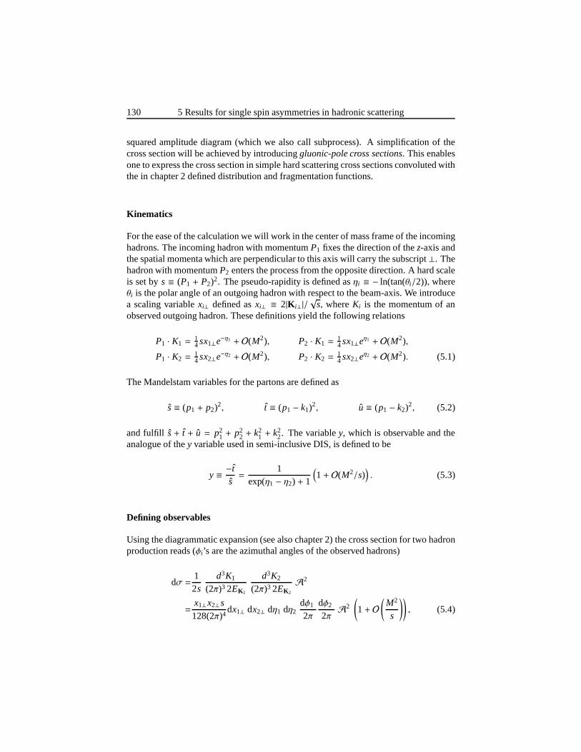
130 5 Results for single spin asymmetries in hadronic scattering
squared amplitude diagram (which we also call subprocess).A simplification of thecross section will be achieved by introducinggluonic-pole cross sections. This enablesone to express the cross section in simple hard scattering cross sections convoluted withthe in chapter 2 defined distribution and fragmentation functions.
Kinematics
For the ease of the calculation we will work in the center of mass frame of the incominghadrons. The incoming hadron with momentumP1 fixes the direction of thez-axis andthe spatial momenta which are perpendicular to this axis will carry the subscript⊥. Thehadron with momentumP2 enters the process from the opposite direction. A hard scaleis set bys ≡ (P1 + P2)2. The pseudo-rapidity is defined asηi ≡ − ln(tan(θi/2)), whereθi is the polar angle of an outgoing hadron with respect to the beam-axis. We introducea scaling variablexi⊥ defined asxi⊥ ≡ 2|K i⊥|/
√s, whereKi is the momentum of an
observed outgoing hadron. These definitions yield the following relations
P1 · K1 =14 sx1⊥e−η1 + O(M2), P2 · K1 =
14 sx1⊥eη1 + O(M2),
P1 · K2 =14 sx2⊥e−η2 + O(M2), P2 · K2 =
14 sx2⊥eη2 + O(M2). (5.1)
The Mandelstam variables for the partons are defined as
s≡ (p1 + p2)2, t ≡ (p1 − k1)2, u ≡ (p1 − k2)2, (5.2)
and fulfill s+ t + u = p21 + p2
2 + k21 + k2
2. The variabley, which is observable and theanalogue of they variable used in semi-inclusive DIS, is defined to be
y ≡ −ts=
1exp(η1 − η2) + 1
(1+ O(M2/s)
). (5.3)
Defining observables
Using the diagrammatic expansion (see also chapter 2) the cross section for two hadronproduction reads (φi ’s are the azimuthal angles of the observed hadrons)
dσ =12s
d3K1
(2π)3 2EK1
d3K2
(2π)3 2EK2
A2
=x1⊥x2⊥s
128(2π)4dx1⊥ dx2⊥ dη1 dη2
dφ1
2πdφ2
2πA2
(1+ O
(M2
s
)), (5.4)

5.2 Calculating cross sections for hadronic scattering 131
whereA2 =∑
X
∫d3PX
(2π)32EPX(2π)4δ(P1+P2−K1−K2−PX) |M|2 which is generically ex-
pressed as
A2 =
∫d4p1 d4p2 d4k1 d4k2 (2π)4 δ4(p1+p2−k1−k2)
× TrD,C Φ(p1) ⊗ Φ(p2) ⊗ ∆(k1) ⊗ ∆(k2)
⊗ H(p1, p2, k1, k2) ⊗ H∗(p1, p2, k1, k2), (5.5)
suppressing the momenta and spins of parent hadrons. The symbol ⊗ represent a con-volution in color and Dirac indices, and the hard elementaryscattering amplitudes aredenoted byH. The gauge links of the correlators can be derived by applying tech-niques developed in the previous chapter. Those gauge linksdepend in general on thesubprocess.
Each of the external partons and its parent hadron have both anearly light-likemomentum in a more or less common direction (parton model assumption). The intro-duction of the light-like vectors,nPi , with nPi · nPi = 1 (bar denotes reversal of spatialcomponents) such thatnPi is proportional toPi in the asymptotic limit, allows us toclassify at which order components appear. The componentspi · nPi appear at order√
s (and similarly for fragmentation), the spatial transversecomponents appear all ata hadronic scale. The light-like components which are left,pi · nPi , appear at orderM2/√
s. Parton momentum fractions are defined as usual
xi ≡pi · nPi
Pi · nPi
, zi ≡Ki · nKi
ki · nKi
. (5.6)
The light-cone momentum componentspi ·nPi can be simply integrated because they aresuppressed in the hard parts. The hard scalescan be used to fix the incoming light-conemomentum fractions,x1 andx2, in terms ofz1 andz2. This gives∫
d4p1 d4p2 d4k1 d4k2 δ4(p1 + p2 − k1 − k2)
=2s
∫d(p1 · nP1) d(p2 · nP2) d(k1 · nK1) d(k2 · nK2) δ(x1 − 2
sr · P2) δ(x2 − 2sr · P1)
×∫
d2p1T d2p2T d2k1T d2k2T δ2(qT⊥ − r⊥)
×∫
d(p1 · nP1) d(p2 · nP2) d(k1 · nK1) d(k2 · nK2)(1+ O(M2/s)
), (5.7)
with qT ≡ p1T + p2T − k1T − k2T , r ≡ K1
z1+
K2
z2. (5.8)
The transverse parton momenta (p1T , p2T , k1T , k2T ) are four-vectors and defined tobe transverse with respect to their parent hadron while the symbol⊥ means perpendic-ular with respect toP1 andP2. The vectorqT is thus of a hadronic scale and all its
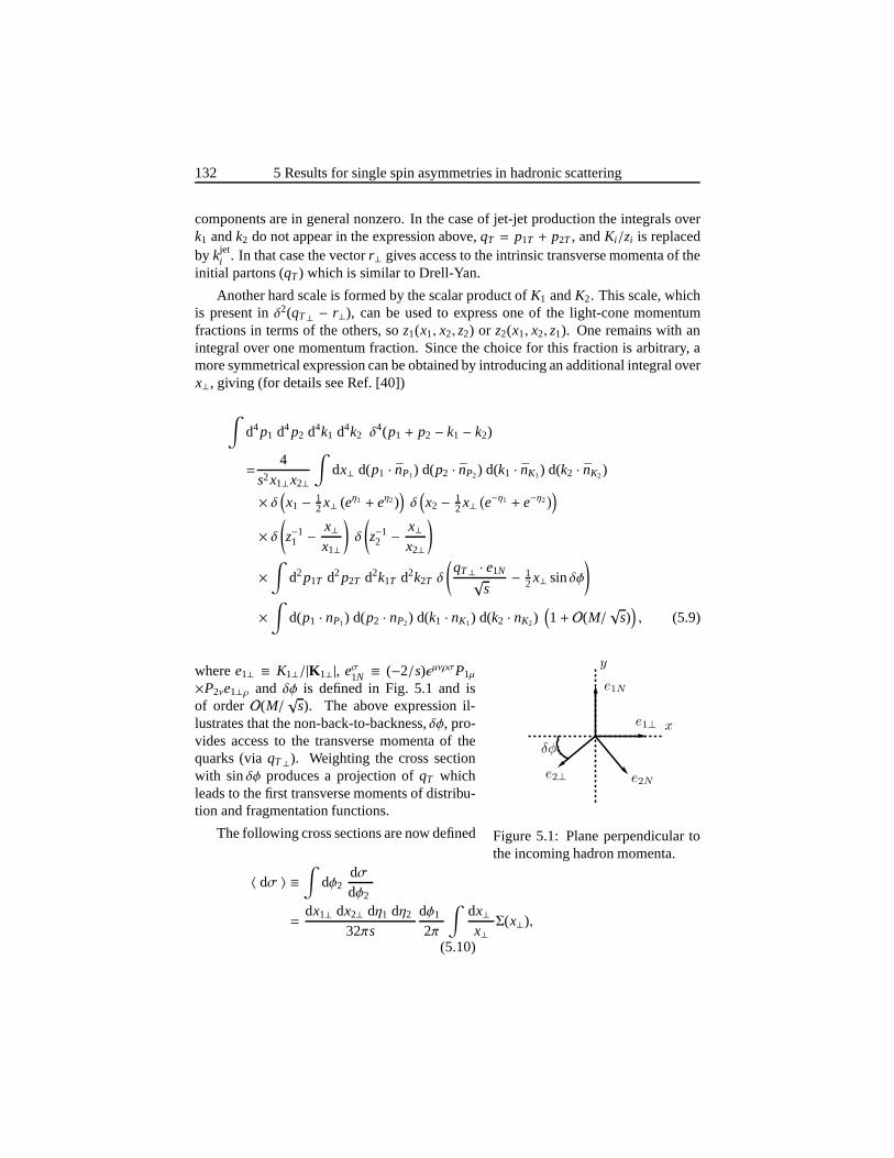
132 5 Results for single spin asymmetries in hadronic scattering
components are in general nonzero. In the case of jet-jet production the integrals overk1 andk2 do not appear in the expression above,qT = p1T + p2T , andKi/zi is replacedby kjet
i . In that case the vectorr⊥ gives access to the intrinsic transverse momenta of theinitial partons (qT) which is similar to Drell-Yan.
Another hard scale is formed by the scalar product ofK1 andK2. This scale, whichis present inδ2(qT⊥ − r⊥), can be used to express one of the light-cone momentumfractions in terms of the others, soz1(x1, x2, z2) or z2(x1, x2, z1). One remains with anintegral over one momentum fraction. Since the choice for this fraction is arbitrary, amore symmetrical expression can be obtained by introducingan additional integral overx⊥, giving (for details see Ref. [40])
∫d4p1 d4p2 d4k1 d4k2 δ4(p1 + p2 − k1 − k2)
=4
s2x1⊥x2⊥
∫dx⊥ d(p1 · nP1) d(p2 · nP2) d(k1 · nK1) d(k2 · nK2)
× δ(x1 − 1
2 x⊥ (eη1 + eη2))δ(x2 − 1
2 x⊥(e−η1 + e−η2
))
× δ(z−11 −
x⊥x1⊥
)δ
(z−12 −
x⊥x2⊥
)
×∫
d2p1T d2p2T d2k1T d2k2T δ
(qT⊥ · e1N√
s− 1
2 x⊥ sinδφ
)
×∫
d(p1 · nP1) d(p2 · nP2) d(k1 · nK1) d(k2 · nK2)(1+ O(M/
√s)), (5.9)
wheree1⊥ ≡ K1⊥/|K1⊥|, eσ1N ≡ (−2/s)ǫµνρσP1µPSfrag replacements
x
y
δφ
e1⊥
e1N
e2⊥ e2N
Figure 5.1: Plane perpendicular tothe incoming hadron momenta.
×P2νe1⊥ρ and δφ is defined in Fig. 5.1 and isof orderO(M/
√s). The above expression il-
lustrates that the non-back-to-backness,δφ, pro-vides access to the transverse momenta of thequarks (viaqT⊥). Weighting the cross sectionwith sinδφ produces a projection ofqT whichleads to the first transverse moments of distribu-tion and fragmentation functions.
The following cross sections are now defined
〈 dσ 〉 ≡∫
dφ2dσdφ2
=dx1⊥ dx2⊥ dη1 dη2
32πsdφ1
2π
∫dx⊥x⊥Σ(x⊥),
(5.10)
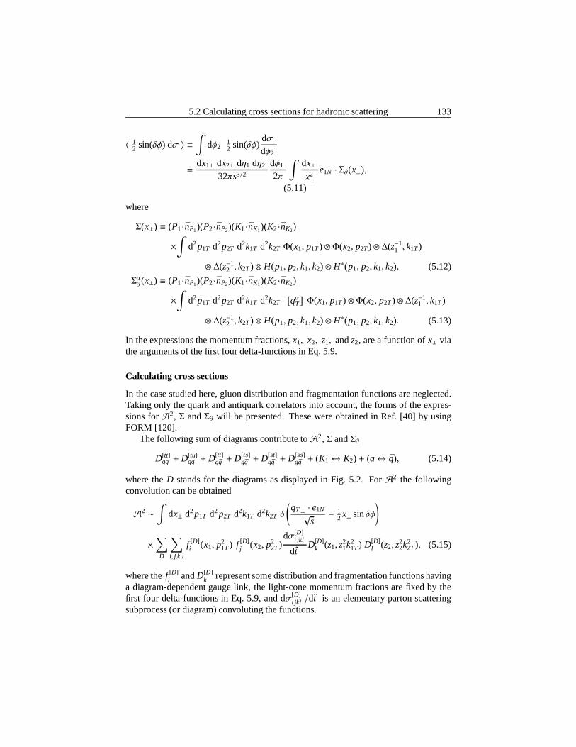
5.2 Calculating cross sections for hadronic scattering 133
〈 12 sin(δφ) dσ 〉 ≡
∫dφ2
12 sin(δφ)
dσdφ2
=dx1⊥ dx2⊥ dη1 dη2
32πs3/2
dφ1
2π
∫dx⊥x2⊥
e1N · Σ∂(x⊥),
(5.11)
where
Σ(x⊥) ≡ (P1·nP1)(P2·nP2)(K1·nK1)(K2·nK2)
×∫
d2p1T d2p2T d2k1T d2k2T Φ(x1, p1T) ⊗Φ(x2, p2T) ⊗ ∆(z−11 , k1T)
⊗ ∆(z−12 , k2T) ⊗ H(p1, p2, k1, k2) ⊗ H∗(p1, p2, k1, k2), (5.12)
Σα∂ (x⊥) ≡ (P1·nP1)(P2·nP2)(K1·nK1)(K2·nK2)
×∫
d2p1T d2p2T d2k1T d2k2T[qαT
]Φ(x1, p1T) ⊗Φ(x2, p2T) ⊗ ∆(z−1
1 , k1T)
⊗ ∆(z−12 , k2T) ⊗ H(p1, p2, k1, k2) ⊗ H∗(p1, p2, k1, k2). (5.13)
In the expressions the momentum fractions,x1, x2, z1, andz2, are a function ofx⊥ viathe arguments of the first four delta-functions in Eq. 5.9.
Calculating cross sections
In the case studied here, gluon distribution and fragmentation functions are neglected.Taking only the quark and antiquark correlators into account, the forms of the expres-sions forA2, Σ andΣ∂ will be presented. These were obtained in Ref. [40] by usingFORM [120].
The following sum of diagrams contribute toA2, Σ andΣ∂
D[tt]qq + D[tu]
qq + D[tt]qq + D[ts]
qq + D[st]qq + D[ss]
qq + (K1 ↔ K2) + (q↔ q), (5.14)
where theD stands for the diagrams as displayed in Fig. 5.2. ForA2 the followingconvolution can be obtained
A2 ∼∫
dx⊥ d2p1T d2p2T d2k1T d2k2T δ
(qT⊥ · e1N√
s− 1
2 x⊥ sinδφ
)
×∑
D
∑
i, j,k,l
f [D]i (x1, p
21T) f [D]
j (x2, p22T)
dσ[D]i jkl
dtD[D]
k (z1, z21k2
1T) D[D]l (z2, z
22k2
2T), (5.15)
where thef [D]i andD[D]
k represent some distribution and fragmentation functions havinga diagram-dependent gauge link, the light-cone momentum fractions are fixed by thefirst four delta-functions in Eq. 5.9, and dσ[D]
i jkl /dt is an elementary parton scatteringsubprocess (or diagram) convoluting the functions.
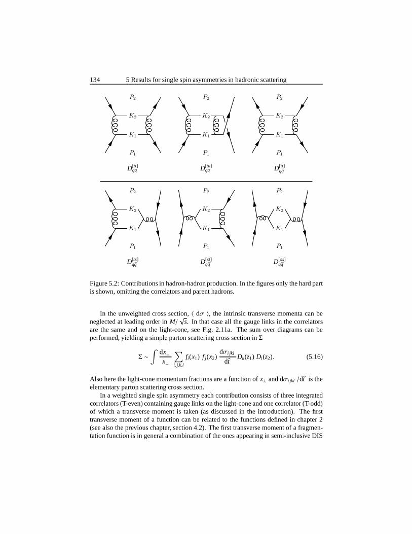
134 5 Results for single spin asymmetries in hadronic scattering
P1
P2
K1
K2
P1
P2
K1
K2
P1
P2
K1
K2
D[tt]qq D[tu]
qq D[tt]qq
P1
P2
K1
K2
P1
P2
K1
K2
P1
P2
K1
K2
D[ts]qq D[st]
qq D[ss]qq
Figure 5.2: Contributions in hadron-hadron production. Inthe figures only the hard partis shown, omitting the correlators and parent hadrons.
In the unweighted cross section,〈 dσ 〉, the intrinsic transverse momenta can beneglected at leading order inM/
√s. In that case all the gauge links in the correlators
are the same and on the light-cone, see Fig. 2.11a. The sum over diagrams can beperformed, yielding a simple parton scattering cross section inΣ
Σ ∼∫
dx⊥x⊥
∑
i, j,k,l
fi(x1) f j(x2)dσi jkl
dtDk(z1) Dl(z2). (5.16)
Also here the light-cone momentum fractions are a function of x⊥ and dσi jkl /dt is theelementary parton scattering cross section.
In a weighted single spin asymmetry each contribution consists of three integratedcorrelators (T-even) containing gauge links on the light-cone and one correlator (T-odd)of which a transverse moment is taken (as discussed in the introduction). The firsttransverse moment of a function can be related to the functions defined in chapter 2(see also the previous chapter, section 4.2). The first transverse moment of a fragmen-tation function is in general a combination of the ones appearing in semi-inclusive DIS
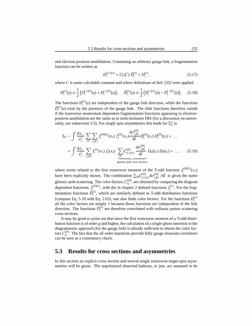
5.3 Results for cross sections and asymmetries 135
and electron positron annihilation. Containing an arbitrary gauge link, a fragmentationfunction can be written as
D[L′](1)i = C(L′) D(1)
i + D(1)i , (5.17)
whereC is some calculable constant and where definitions of Ref. [35] were applied
D(1)i (z) ≡ 1
2
(D[+](1)
i (z) + D[−](1)i (z)
), D(1)
i (z) ≡ 12
(D[+](1)
i (z) − D[−](1)i (z)
). (5.18)
The functionsD(1)i (z) are independent of the gauge link direction, while the functions
D(1)i (z) exist by the presence of the gauge link. The tilde functionstherefore vanish
if the transverse momentum dependent fragmentation functions appearing in electron-positron annihilation are the same as in semi-inclusive DIS(for a discussion on univer-sality, see subsection 3.5). For single spin asymmetries this leads forΣα
∂to
Σ∂ ∼∫
dx⊥x2⊥
∑
D
∑
i, j,k,l
f [D](1)i (x1) f [D]
j (x2)dσ[D]
i jkl
dtD[D]
k (z1) D[D]l (z2) + . . .
=
∫dx⊥x2⊥
∑
i, j,k,l
f (1)i (x1) f j(x2)
∑
D
C[D]G, f (1)
dσ[D]i jkl
dt︸ ︷︷ ︸gluonic-pole cross section
Dk(z1) Dl(z2) + . . . , (5.19)
where terms related to the first transverse moment of the T-odd function f [D](1)i (x1)
have been explicitly shown. The combination∑
DC[D]G, f (1)dσ
[D]i jkl /dt is given the name
gluonic-pole scattering. The color factors,C[D]G , are obtained by comparing the diagram
dependent functions,f [D](1)i , with the in chapter 2 defined functionsf (1)
i . For the frag-mentation functionsD(1)
i , which are similarly defined as T-odd distribution functions(compare Eq. 5.18 with Eq. 2.63), one also finds color factors. For the functionsD(1)
iall the color factors are simply 1 because those functions are independent of the linkdirection. The functionsD(1)
i are therefore convoluted with ordinary parton scatteringcross sections.
It may be good to point out that since the first transverse moment of a T-odd distri-bution function is of orderg and higher, the calculation of a single gluon insertion in thediagrammatic approach (for the gauge link) is already sufficient to obtain the color fac-torsC[D]
G . The fact that the all order insertions provide fully gauge invariant correlatorscan be seen as a consistency check.
5.3 Results for cross sections and asymmetries
In this section an explicit cross section and several singletransverse target-spin asym-metries will be given. The unpolarized observed hadrons, orjets, are assumed to be
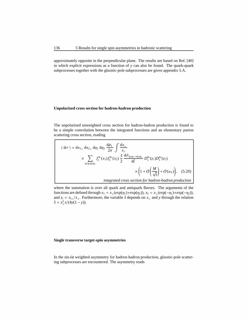
136 5 Results for single spin asymmetries in hadronic scattering
approximately opposite in the perpendicular plane. The results are based on Ref. [40]in which explicit expressions as a function ofy can also be found. The quark-quarksubprocesses together with the gluonic-pole subprocessesare given appendix 5.A.
Unpolarized cross section for hadron-hadron production
The unpolarized unweighted cross section for hadron-hadron production is found tobe a simple convolution between the integrated functions and an elementary partonscattering cross section, reading
〈 dσ 〉 = dx1⊥ dx2⊥ dη1 dη2dφ1
2π
∫dx⊥x⊥
×∑
q1q2q3q4
f q1
1 (x1) f q2
1 (x2)s2
dσq1q2→q3q4
dtDq3
1 (z1)Dq4
1 (z2)
×(1+ O
(M√
s
)+ O (αS)
), (5.20)
integrated cross section for hadron-hadron production
where the summation is over all quark and antiquark flavors. The arguments of thefunctions are defined throughx1 = x⊥(exp(η1)+exp(η2)), x2 = x⊥(exp(−η1)+exp(−η2)),andzi = xi⊥/x⊥. Furthermore, the variable ˆs depends onx⊥ andy through the relations= x2
⊥s/(4y(1− y)).
Single transverse target-spin asymmetries
In the sinδφ weighted asymmetry for hadron-hadron production, gluonic-pole scatter-ing subprocesses are encountered. The asymmetry reads
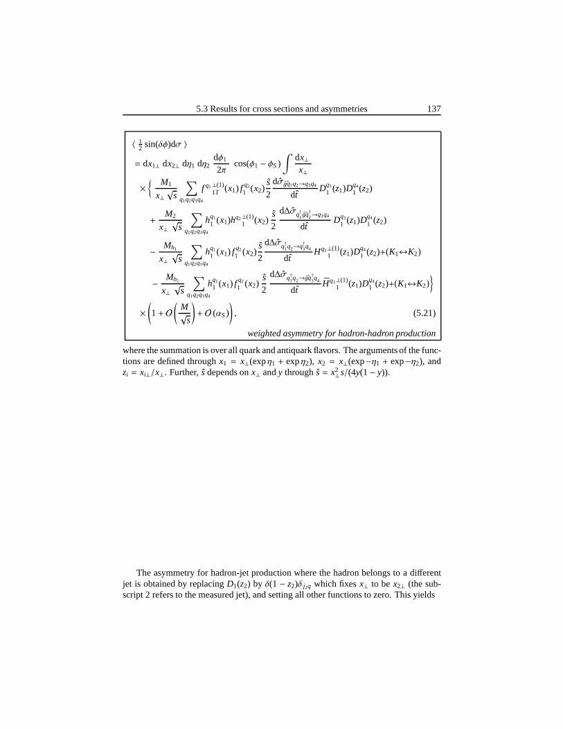
5.3 Results for cross sections and asymmetries 137
〈 12 sin(δφ)dσ 〉
= dx1⊥ dx2⊥ dη1 dη2dφ1
2πcos(φ1 − φS)
∫dx⊥x⊥
× M1
x⊥√
s
∑
q1q2q3q4
f q1⊥(1)1T (x1) f q2
1 (x2)s2
dσgq1q2→q3q4
dtDq3
1 (z1)Dq4
1 (z2)
+M2
x⊥√
s
∑
q1q2q3q4
hq1
1 (x1)hq2⊥(1)1 (x2)
s2
d∆σq↑1gq↑2→q3q4
dtDq3
1 (z1)Dq4
1 (z2)
− Mh1
x⊥√
s
∑
q1q2q3q4
hq1
1 (x1) f q2
1 (x2)s2
d∆σq↑1q2→q↑3q4
dtHq3⊥(1)
1 (z1)Dq4
1 (z2)+(K1↔K2
)
− Mh1
x⊥√
s
∑
q1q2q3q4
hq1
1 (x1) f q2
1 (x2)s2
d∆σq↑1q2→gq↑3q4
dtHq3⊥(1)
1 (z1)Dq4
1 (z2)+(K1↔K2
)
×(1+ O
(M√
s
)+ O (αS)
), (5.21)
weighted asymmetry for hadron-hadron production
where the summation is over all quark and antiquark flavors. The arguments of the func-tions are defined throughx1 = x⊥(expη1 + expη2), x2 = x⊥(exp−η1 + exp−η2), andzi = xi⊥/x⊥. Further,sdepends onx⊥ andy throughs= x2
⊥s/(4y(1− y)).
The asymmetry for hadron-jet production where the hadron belongs to a differentjet is obtained by replacingD1(z2) by δ(1 − z2)δ j2q which fixesx⊥ to bex2⊥ (the sub-script 2 refers to the measured jet), and setting all other functions to zero. This yields
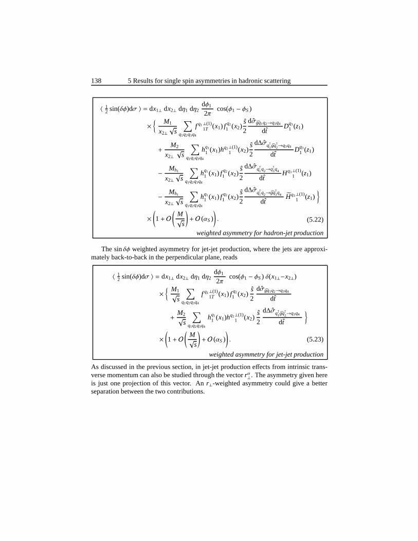
138 5 Results for single spin asymmetries in hadronic scattering
〈 12 sin(δφ)dσ 〉 = dx1⊥ dx2⊥ dη1 dη2
dφ1
2πcos(φ1 − φS)
× M1
x2⊥√
s
∑
q1q2q3q4
f q1⊥(1)1T (x1) f q2
1 (x2)s2
dσgq1q2→q3q4
dtDq3
1 (z1)
+M2
x2⊥√
s
∑
q1q2q3q4
hq1
1 (x1)hq2⊥(1)1 (x2)
s2
d∆σq↑1gq↑2→q3q4
dtDq3
1 (z1)
− Mh1
x2⊥√
s
∑
q1q2q3q4
hq1
1 (x1) f q2
1 (x2)s2
d∆σq↑1q2→q↑3q4
dtHq3⊥(1)
1 (z1)
− Mh1
x2⊥√
s
∑
q1q2q3q4
hq1
1 (x1) f q2
1 (x2)s2
d∆σq↑1q2→gq↑3q4
dtHq3⊥(1)
1 (z1)
×(1+ O
(M√
s
)+ O (αS)
). (5.22)
weighted asymmetry for hadron-jet production
The sinδφ weighted asymmetry for jet-jet production, where the jets are approxi-mately back-to-back in the perpendicular plane, reads
〈 12 sin(δφ)dσ 〉 = dx1⊥ dx2⊥ dη1 dη2
dφ1
2πcos(φ1 − φS) δ(x1⊥−x2⊥)
× M1√
s
∑
q1q2q3q4
f q1⊥(1)1T (x1) f q2
1 (x2)s2
dσgq1q2→q3q4
dt
+M2√
s
∑
q1q2q3q4
hq1
1 (x1)hq2⊥(1)1 (x2)
s2
d∆σq↑1gq↑2→q3q4
dt
×(1+ O
(M√
s
)+ O (αS)
). (5.23)
weighted asymmetry for jet-jet production
As discussed in the previous section, in jet-jet productioneffects from intrinsic trans-verse momentum can also be studied through the vectorrα⊥. The asymmetry given hereis just one projection of this vector. Anr⊥-weighted asymmetry could give a betterseparation between the two contributions.
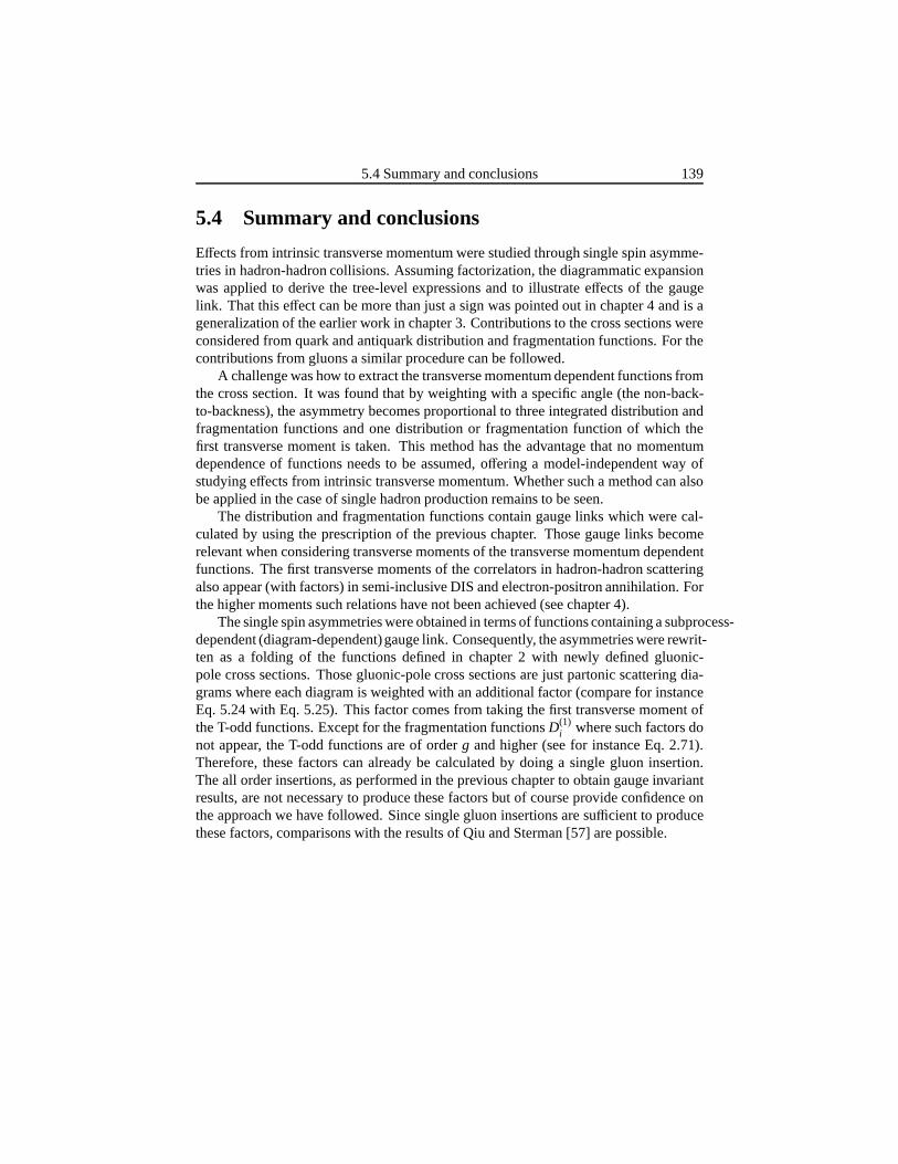
5.4 Summary and conclusions 139
5.4 Summary and conclusions
Effects from intrinsic transverse momentum were studied through single spin asymme-tries in hadron-hadron collisions. Assuming factorization, the diagrammatic expansionwas applied to derive the tree-level expressions and to illustrate effects of the gaugelink. That this effect can be more than just a sign was pointed out in chapter 4 andis ageneralization of the earlier work in chapter 3. Contributions to the cross sections wereconsidered from quark and antiquark distribution and fragmentation functions. For thecontributions from gluons a similar procedure can be followed.
A challenge was how to extract the transverse momentum dependent functions fromthe cross section. It was found that by weighting with a specific angle (the non-back-to-backness), the asymmetry becomes proportional to threeintegrated distribution andfragmentation functions and one distribution or fragmentation function of which thefirst transverse moment is taken. This method has the advantage that no momentumdependence of functions needs to be assumed, offering a model-independent way ofstudying effects from intrinsic transverse momentum. Whether such a method can alsobe applied in the case of single hadron production remains tobe seen.
The distribution and fragmentation functions contain gauge links which were cal-culated by using the prescription of the previous chapter. Those gauge links becomerelevant when considering transverse moments of the transverse momentum dependentfunctions. The first transverse moments of the correlators in hadron-hadron scatteringalso appear (with factors) in semi-inclusive DIS and electron-positron annihilation. Forthe higher moments such relations have not been achieved (see chapter 4).
The single spin asymmetries were obtained in terms of functions containing a subprocess-dependent (diagram-dependent)gauge link. Consequently,the asymmetries were rewrit-ten as a folding of the functions defined in chapter 2 with newly defined gluonic-pole cross sections. Those gluonic-pole cross sections arejust partonic scattering dia-grams where each diagram is weighted with an additional factor (compare for instanceEq. 5.24 with Eq. 5.25). This factor comes from taking the first transverse moment ofthe T-odd functions. Except for the fragmentation functionsD(1)
i where such factors donot appear, the T-odd functions are of orderg and higher (see for instance Eq. 2.71).Therefore, these factors can already be calculated by doinga single gluon insertion.The all order insertions, as performed in the previous chapter to obtain gauge invariantresults, are not necessary to produce these factors but of course provide confidence onthe approach we have followed. Since single gluon insertions are sufficient to producethese factors, comparisons with the results of Qiu and Sterman [57] are possible.
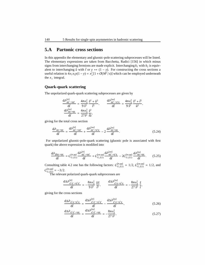
140 5 Results for single spin asymmetries in hadronic scattering
5.A Partonic cross sections
In this appendix the elementary and gluonic-pole scattering subprocesses will be listed.The elementary expressions are taken from Bacchetta, Radici [156] in which minussigns from interchanging fermions are made explicit. Interchangingk1 with k2 is equiv-alent to interchanging ˆu with t or y ↔ (1 − y). For constructing the cross sections auseful relation is 4x1x2y(1− y) = x2
⊥[1 +O(M2/s)] which can be employed underneaththex⊥ integral.
Quark-quark scattering
The unpolarized quark-quark scattering subprocesses are given by
dσ[tt]qq′→qq′
dt=
4πα2S
9 s2
s2 + u2
t2,
dσ[uu]qq′→q′q
dt=
4πα2S
9 s2
s2 + t2
u2,
dσ[tu]qq→qq
dt=
4πα2S
27s2
s2
tu,
giving for the total cross section
dσqq→qq
dt=
dσ[tt]qq′→qq′
dt+
dσ[uu]qq′→q′q
dt− 2
dσ[tu]qq→qq
dt. (5.24)
For unpolarized gluonic-pole-quark scattering (gluonic pole is associated with firstquark) the above expression is modified into
dσgqq→qq
dt= C[tt,qq]
G, f (1)
dσ[tt]qq′→qq′
dt+ C[uu,qq]
G, f (1)
dσ[uu]qq′→q′q
dt− 2C[tu,qq]
G, f (1)
dσ[tu]qq→qq
dt. (5.25)
Consulting table 4.2 one has the following factors:C[tt,qq]G, f (1) = 1/2, C[uu,qq]
G, f (1) = 1/2, and
C[tu,qq]G, f (1) = −3/2.
The relevant polarized quark-quark subprocesses are
d∆σ[tt]q↑q′→q↑q′
dt= −
8πα2S
9 s2
us
t2,
d∆σ[tu]q↑q→q↑q
dt= −
8πα2S
27 s2
s
t,
giving for the cross sections
d∆σq↑q→q↑q
dt=
d∆σ[tt]q↑q′→q↑q′
dt−
d∆σ[tu]q↑q→q↑q
dt, (5.26)
d∆σq↑q↑→qq
dt=
d∆σ[tu]q↑q↑→qq
dt= −
8πα2S
27 s2, (5.27)
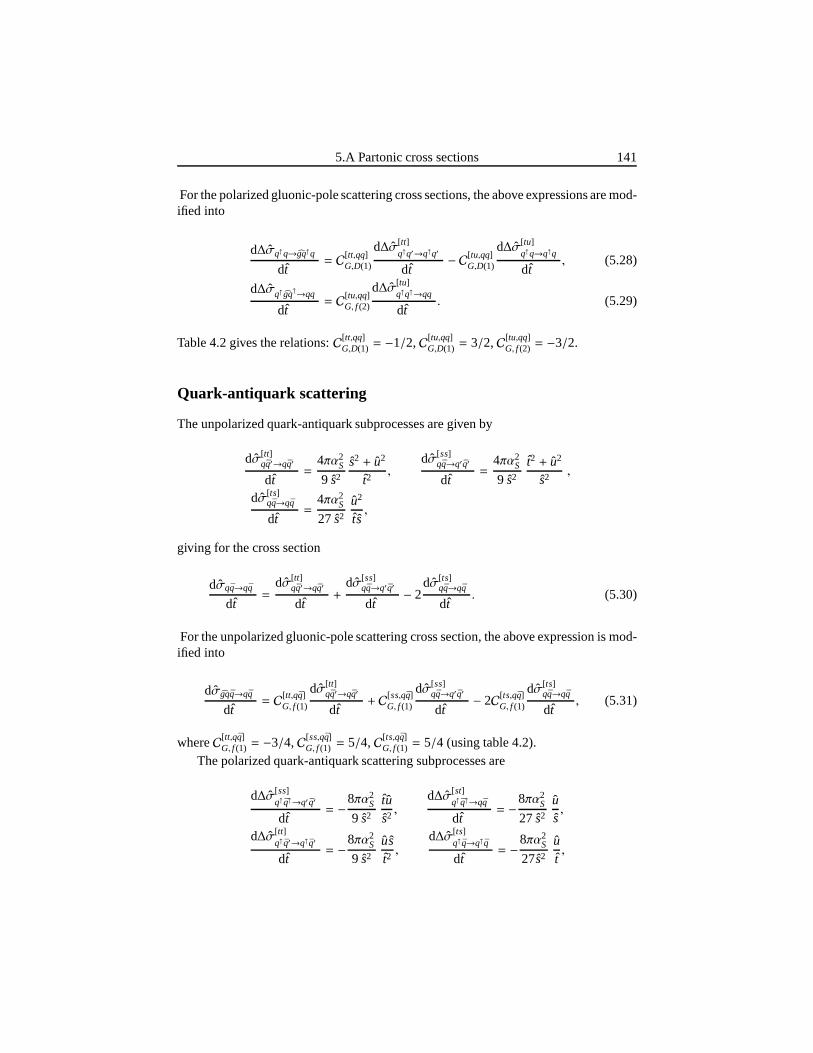
5.A Partonic cross sections 141
For the polarized gluonic-pole scattering cross sections,the above expressions are mod-ified into
d∆σq↑q→gq↑q
dt= C[tt,qq]
G,D(1)
d∆σ[tt]q↑q′→q↑q′
dt− C[tu,qq]
G,D(1)
d∆σ[tu]q↑q→q↑q
dt, (5.28)
d∆σq↑ gq↑→qq
dt= C[tu,qq]
G, f (2)
d∆σ[tu]q↑q↑→qq
dt. (5.29)
Table 4.2 gives the relations:C[tt,qq]G,D(1) = −1/2,C[tu,qq]
G,D(1) = 3/2,C[tu,qq]G, f (2) = −3/2.
Quark-antiquark scattering
The unpolarized quark-antiquark subprocesses are given by
dσ[tt]qq′→qq′
dt=
4πα2S
9 s2
s2 + u2
t2,
dσ[ss]qq→q′q′
dt=
4πα2S
9 s2
t2 + u2
s2,
dσ[ts]qq→qq
dt=
4πα2S
27 s2
u2
t s,
giving for the cross section
dσqq→qq
dt=
dσ[tt]qq′→qq′
dt+
dσ[ss]qq→q′q′
dt− 2
dσ[ts]qq→qq
dt. (5.30)
For the unpolarized gluonic-pole scattering cross section, the above expression is mod-ified into
dσgqq→qq
dt= C[tt,qq]
G, f (1)
dσ[tt]qq′→qq′
dt+ C[ss,qq]
G, f (1)
dσ[ss]qq→q′q′
dt− 2C[ts,qq]
G, f (1)
dσ[ts]qq→qq
dt, (5.31)
whereC[tt,qq]G, f (1) = −3/4,C[ss,qq]
G, f (1) = 5/4,C[ts,qq]G, f (1) = 5/4 (using table 4.2).
The polarized quark-antiquark scattering subprocesses are
d∆σ[ss]q↑ q↑→q′q′
dt= −
8πα2S
9 s2
tus2,
d∆σ[st]q↑ q↑→qq
dt= −
8πα2S
27 s2
us,
d∆σ[tt]q↑ q′→q↑q′
dt= −
8πα2S
9 s2
us
t2,
d∆σ[ts]q↑ q→q↑q
dt= −
8πα2S
27s2
u
t,
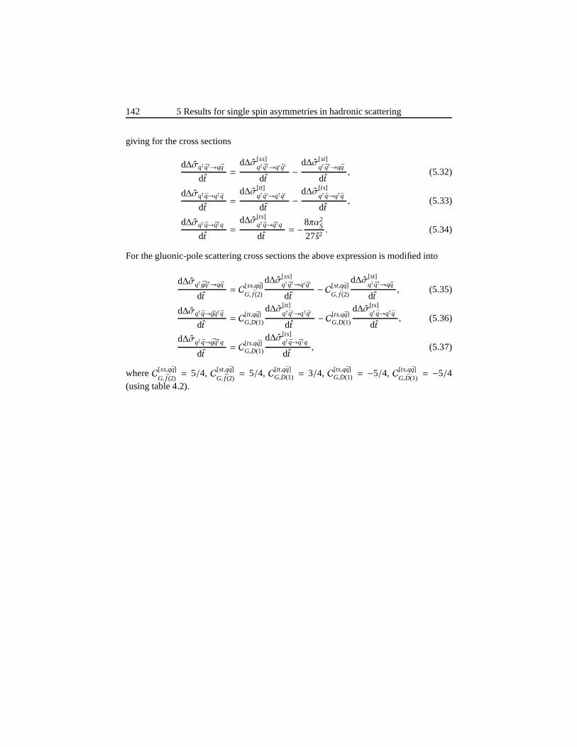
142 5 Results for single spin asymmetries in hadronic scattering
giving for the cross sections
d∆σq↑ q↑→qq
dt=
d∆σ[ss]q↑ q↑→q′q′
dt−
d∆σ[st]q↑ q↑→qq
dt, (5.32)
d∆σq↑ q→q↑q
dt=
d∆σ[tt]q↑ q′→q↑q′
dt−
d∆σ[ts]q↑ q→q↑q
dt, (5.33)
d∆σq↑ q→q↑q
dt=
d∆σ[ts]q↑ q→q↑q
dt= −
8πα2S
27s2. (5.34)
For the gluonic-pole scattering cross sections the above expression is modified into
d∆σq↑ gq↑→qq
dt= C[ss,qq]
G, f (2)
d∆σ[ss]q↑ q↑→q′q′
dt− C[st,qq]
G, f (2)
d∆σ[st]q↑q↑→qq
dt, (5.35)
d∆σq↑ q→gq↑q
dt= C[tt,qq]
G,D(1)
d∆σ[tt]q↑q′→q↑q′
dt− C[ts,qq]
G,D(1)
d∆σ[ts]q↑ q→q↑q
dt, (5.36)
d∆σq↑ q→gq↑q
dt= C[ts,qq]
G,D(1)
d∆σ[ts]q↑q→q↑q
dt, (5.37)
whereC[ss,qq]G, f (2)
= 5/4, C[st,qq]G, f (2)
= 5/4, C[tt,qq]G,D(1) = 3/4, C[ts,qq]
G,D(1) = −5/4, C[ts,qq]G,D(1)
= −5/4(using table 4.2).
6Summary and
conclusions
Effects from intrinsic transverse momentum of partons were studied in several hardscattering processes with an emphasis on color gauge invariance. In order to describethe processes, the diagrammatic expansion was employed which is a field-theoreticalapproach. Extending the work of Boer, Mulders [114] and Belitsky, Ji, Yuan [26],factorization of effects from intrinsic transverse momentum was assumed, and bycon-sidering an infinite number of diagrams the tree-level expressions includingM/Q cor-rections were evaluated in chapter 3 for semi-inclusive DIS, Drell-Yan, and electron-positron annihilation. In those processes transverse momentum dependent distributionand fragmentation functions were encountered which are defined through matrix el-ements in which bilocal operators are folded with a gauge link. From a theoreticalpoint of view, the presence of this gauge link (also called Wilson line) is pleasant be-cause it makes the bilocal operator invariant under color gauge transformations. Thesegauge links are of increasing interest because by several papers, among which Brodsky,Hwang, Schmidt [24], Collins [25], and Belitsky, Ji, Yuan [26], it has been shown thatthe gauge links are not the same in every process and could lead to observable effects.
Distribution and fragmentation functions containing a gauge link were discussed inchapter 2. These functions describe the way in which quarks are distributed in a nu-
144 Summary and conclusions
cleon or how a quark decays into a jet and a particular hadron.They form a bridgebetween theoretical predictions and experimental observations, and are vital for ourunderstanding of the nucleon’s substructure. In the diagrammatic approach these func-tions naturally appear when studying hard scattering processes. The exact form of thesefunctions, including the path of the gauge link, is thus not astarting point but rather de-rived.
In the transverse momentum integrated distribution functions the presence of thegauge link did not produce new effects in contrast to the transverse momentum depen-dent functions. In the latter the gauge link does not run along a straight path betweenthe two quark-fields and therefore allows for the existence of T-odd distribution func-tions. The existence of such functions was conjectured by Sivers [21, 22] in order toexplain the observation of single spin asymmetries. As pointed out by Collins [25],those functions have the interesting property that they appear with different signs whencomparing Drell-Yan with semi-inclusive DIS. This interesting prediction should ofcourse be experimentally verified.
Another possible source for T-odd effects was uncovered by Qiu and Sterman [84,85]. They suggested that the presence of gluonic pole matrixelements could producesingle spin asymmetries in hadron-hadron collisions. It was shown in chapter 2 thatthose matrix elements have the same form as matrix elements from which the T-odddistribution functions are defined. The presence of the gauge link and the gluonic polematrix elements are therefore in essence the same mechanism.
The path of the gauge link in the transverse momentum dependent functions runsin a particular direction via the light-cone boundary (see Fig. 2.11). In chapter 2 it wasdiscussed that this direction is a potential source for new effects or functions (see for re-lated work Goeke, Metz, Schlegel [79]). While calculating the longitudinal target-spinand beam-spin asymmetries for semi-inclusive DIS in chapter 3, it was found that oneof these new functions,g⊥, could produce a nonzero azimuthal single spin asymmetryfor jet-production in lepton-hadron scattering. Given thereason for the existence of thisfunction, this prediction deserves experimental verification.
The presence of gauge links in transverse momentum dependent fragmentationfunctions confronted us in chapter 2 with issues related to universality. It was found thattransverse momentum dependent fragmentation functions could appear to be differentwhen comparing semi-inclusive DIS with electron-positronannihilation. The reasonfor this difference is that for fragmentation functions there are two possible sources forT-odd effects: the gauge link and final-state interactions. If one of the two mechanismsis suppressed, relations between the two processes can be drawn. It should be pointedout that Collins and Metz obtained in Ref. [100, 101] in a quite general treatment frag-mentation functions which appear with the same sign in the two different processes.This interesting result was discussed in chapter 3 and deserves further attention. Alsofrom the experimental side this universality issue can be addressed. For instance, bycomparing properties, like thez-dependence, of transverse momentum dependent frag-mentation functions between different processes.
Summary and conclusions 145
In chapter 4 it was discovered that gauge links can arise which are much morecomplex than the gauge links in the discussed electromagnetic processes. Besides be-ing more complex, the path of the gauge link turned out to not only depend on theprocess, but also on the subprocess (or squared amplitude diagram). These complexstructures predict that T-odd distribution functions can in general differ by more thanjust a sign when comparing different processes. In fact only their first transverse mo-ment can be straightforwardly compared between different processes. A prescriptionwas given in order to deduce the gauge link in squared amplitude diagrams, and it wasshown in a two gluon-production process that nonphysical polarizations of the gluonsare canceled among diagrams although separate diagrams areconvoluted with functionshaving diagram-dependent gauge links. This is a firm consistency test of the appliedapproach.
An illustration of these more complex gauge links was given in hadron-hadron pro-duction in hadron-hadron scattering. In hadron-hadron scattering the challenge is toextract the transverse momentum dependent functions. In chapter 5 such an observablewas presented. This observable has the advantage that it does not require input on theexplicit form for the momentum dependence of the functions.By using this observable,it was shown that effects from the gauge link yield more than just a sign in single spinasymmetries. The expression for the single spin asymmetry was found to be a set ofelementary scattering subprocesses convoluted with universal integrated functions anda function of which a transverse moment was taken. In this latter function the gaugelink depends on the subprocess. Since the first transverse moment of functions can berelated to a set of “standard” functions, which also appear in semi-inclusive DIS andelectron-positron annihilation (just a factor), the asymmetries were rewritten in termsof these “standard” functions folded with the newly defined gluonic-pole cross sec-tions. Gluonic-pole cross sections are just elementary parton scattering cross sectionsin which the various subprocesses (squared amplitude diagrams) are weighted with aparticular factor. Contributions from gluon distributionand fragmentation functionswere discarded for the ease of the calculation, but should beincluded in future studiesto make realistic estimates of single spin asymmetries. Thedefinition of transverse mo-mentum dependent gluon distribution functions was addressed in chapter 4, but needsfurther improvement. Just like experiments could verify inthe Drell-Yan process thesign change of T-odd distribution functions, experiments should also be able to checkthe more involved appearance of T-odd distribution functions in hadron-hadron produc-tion. Other processes which also contain such more complicated effects are photon-jetproduction, and two jet-production.
Besides leading to new effects, the gauge link also poses theoretical challengesamong which the issue of factorization of intrinsic transverse momentum dependenteffects. This issue underlies most treatments and results in this field including thisthesis. Recently, significant progress was made by Ji, Ma, and Yuan in Ref. [175, 176]and by Collins and Metz in Ref. [101]. They considered semi-inclusive DIS and Drell-Yan at small measuredqT (q is the momentum of the virtual photon andq2
T ∼ −M2).
146 Summary and conclusions
One particular issue which was not explicitly addressed is the path of the gauge link indistribution and fragmentation functions connected to higher order diagrams (two loopsor higher). At those orders it was argued in chapter 4 that theeffect of gauge links mightendanger factorization of intrinsic transverse momentum dependent effects in semi-inclusive DIS and Drell-Yan. This could form a problem for azimuthal asymmetriesat smallqT at leading order inM/Q and at subleading order for fullyqT-integratedcross sections. This issue awaits further clarification. Model calculations could bevery useful here. Just like a model calculation uncovered the possible existence of T-odd distribution functions, a two loop model calculation could illustrate some of theimportant aspects related to factorization.
In this thesis effects from intrinsic transverse momentum were studied in hard scat-tering processes. The existing theoretical formalism was further developed and severalissues have been clarified. Various cross sections and asymmetries were obtained. Theirmeasurement can contribute to our understanding of the nucleon’s substructure withinthe framework of QCD and very likely will guide physicists inanswering several re-maining questions.
Acknowledgements
Several persons are acknowledged for the support they have given me in the last fouryears. First I would like to acknowledge my supervisor Piet Mulders. Piet, in het beginvond ik het moeilijk om m’n eigen weg te zoeken, maar achterafben ik je dankbaar voorde zelfstandigheid die je mij hebt gegeven. Verder heb je mijerg gemotiveerd door mijvanaf het begin als een zelfstandig natuurkundige te behandelen en door mij de mogeli-jkheid te geven om naar workshops en conferenties te gaan. Naast onze samenwerkingaan artikelen waardeer ik ook zeer dat je er altijd was op de momenten dat ik je echtnodig had.
The second person who I would like to thank is Daniel Boer. Daniel, de inspiratiedie je kunt geven tijdens het discussieren, je snelle maniervan begrijpen, en je talentvan meedenken zijn uitzonderlijk. Ik wil je bedanken voor desamenwerking van deafgelopen jaren en voor het nauwkeurig lezen van het proefschrift. Mede dankzij joukan ik nu met tevredenheid terugkijken op de resultaten van dit proefschrift.
I also would like to acknowledge Alessandro Bacchetta and Cedran Bomhof. Iappreciate the collaboration we had and the results we obtained. In addition, it was alsoa pleasure to share an office with you. Acknowledged are also my collaborators BenBakker and Miranda van Iersel. Ook hier kijk ik met plezier terug naar de resultatendie we hebben bereikt. En Ben, ik dank je voor de vele uiteenlopende discussies die wegehad hebben en voor je altijd beschikbare wijze adviezen.
I also would like to thank the reading comittee, Mauro Anselmino, Daniel Boer,Markus Diehl, Eric Laenen, and Gerard van der Steenhoven forthe time they havespent on reading my thesis and for the suggestions they have made. Acknowledged isalso Bob van Eijk for leading the useful evaluation meetingsin the last four years. Ikkeek altijd naar dit soort gesprekken uit. I also would like to thank Philipp Hagler, JohnMcNamara, and Paul van der Nat for reading and correcting parts of the thesis.
Besides the people alread mentioned, I met in the last years several others at con-ferences and workshops with whom I had nice discussions: Umberto D’Alesio, Elke
148 Acknowledgements
Aschenauer, Harut Avakian, Elena Boglione, John Collins, Delia Hasch, Leonard Gam-berg, Dae Sung Hwang, Elliot Leader, Andreas Metz, Gunar Schnell, Dennis Sivers,and Werner Vogelsang. I also would like to thank the members of the theory group(including secretaries) for a stimulating and friendly atmosphere. Especially I acknowl-edge Paul Becherer, Henk Blok, Hartmut Erzgraber, David Fokkema, Hugo Schouten,Harmen Warringa, and Erik Wessels for their endless discussions.
Acknowledged are also my friends for their support in the last years. I also thankmy parents, sister, and their families. Ik dank jullie voor de gegeven mogelijkheid omte kunnen studeren en voor de gegeven ondersteuning.
The last person I would like to thank is Calina Ciuhu. Calina, ıntelegerea si sprijinultau mi-au fost de mare ajutor. Dar mai ales ıti multumescpentru dragostea si motivatiaoferita de-a lungul acestor ani.

Bibliography
[1] A. Einstein,Annalen Phys.17: 891–921 (1905).
[2] P. A. M. Dirac,Proc. Roy. Soc. Lond.A133: 60–72 (1931).
[3] C. D. Anderson,Phys. Rev.43: 491–494 (1933).
[4] O. Chamberlain, E. Segre, C. Wiegand, and T. Ypsilantis,Phys. Rev.100:947–950 (1955).
[5] F. Reines and C. L. Cowan,Phys. Rev.92: 830–831 (1953).
[6] M. Gell-Mann,Phys. Lett.8: 214–215 (1964).
[7] G. Zweig,An su(3) model for strong interaction symmetry and its breaking. 2(1964), CERN-TH-412.
[8] F. Abe et al. (CDF),Phys. Rev. Lett.74: 2626–2631 (1995),hep-ex/9503002.
[9] S. Abachi et al. (D0),Phys. Rev. Lett.74: 2632–2637 (1995),hep-ex/9503003.
[10] J. D. Jackson and L. B. Okun,Rev. Mod. Phys.73: 663–680 (2001),hep-ph/0012061.
[11] W. Ehrenberg and R. E. Siday,Proc. Phys. Soc.B62: 8 (1949).
[12] Y. Aharonov and D. Bohm,Phys. Rev.123: 1511–1524 (1961).
[13] Y. Aharonov and D. Bohm,Phys. Rev.115: 485–491 (1959).
[14] R. G. Chambers,Phys. Rev. Lett.5: 3–5 (1960).
[15] A. Airapetian et al. (HERMES),Phys. Rev. Lett.94: 012002 (2005),hep-ex/0408013.
[16] G. ’t Hooft and M. J. G. Veltman,Nucl. Phys.B44: 189–213 (1972).
[17] G. ’t Hooft and M. J. G. Veltman,Nucl. Phys.B50: 318–353 (1972).
[18] D. J. Gross and F. Wilczek,Phys. Rev. Lett.30: 1343–1346 (1973).
[19] H. D. Politzer,Phys. Rev. Lett.30: 1346–1349 (1973).
150 BIBLIOGRAPHY
[20] G. Bunce et al.,Phys. Rev. Lett.36: 1113–1116 (1976).
[21] D. W. Sivers,Phys. Rev.D41: 83 (1990).
[22] D. W. Sivers,Phys. Rev.D43: 261–263 (1991).
[23] J. C. Collins,Nucl. Phys.B396: 161–182 (1993),hep-ph/9208213.
[24] S. J. Brodsky, D. S. Hwang, and I. Schmidt,Phys. Lett.B530: 99–107 (2002),hep-ph/0201296.
[25] J. C. Collins,Phys. Lett.B536: 43–48 (2002),hep-ph/0204004.
[26] A. V. Belitsky, X. Ji, and F. Yuan,Nucl. Phys.B656: 165–198 (2003),hep-ph/0208038.
[27] M. Anselmino, A. Efremov, and E. Leader,Phys. Rept.261: 1–124 (1995),hep-ph/9501369.
[28] V. Barone and P. Ratcliffe,Transverse spin physics(World scientific publishingco., River Edge, USA, 2003).
[29] F. Halzen and A. D. Martin,Quarks and leptons: An introductory course inmodern particle physics(Wiley, New York, USA, 1984).
[30] E. Leader,Spin in particle physics(Cambridge University Press, Cambridge,UK, 2001).
[31] M. E. Peskin and D. V. Schroeder,An Introduction to quantum field theory(Addison-Wesley, Cambridge, USA, 1995).
[32] L. H. Ryder,Quantum field theory(Cambridge University Press, Cambridge,UK, 1985).
[33] S. Weinberg,The Quantum theory of fields: Foundations, volume 1 (CambridgeUniversity Press, Cambridge, UK, 1995).
[34] S. Weinberg,The Quantum theory of fields: Modern applications, volume 2(Cambridge University Press, Cambridge, UK, 1996).
[35] D. Boer, P. J. Mulders, and F. Pijlman,Nucl. Phys.B667: 201–241 (2003),hep-ph/0303034.
[36] A. Bacchetta, P. J. Mulders, and F. Pijlman,Phys. Lett.B595: 309–317 (2004),hep-ph/0405154.
[37] C. J. Bomhof, P. J. Mulders, and F. Pijlman,Phys. Lett.B596: 277–286 (2004),hep-ph/0406099.
[38] F. Pijlman,Few Body Syst.36: 209–213 (2005),hep-ph/0409332.
[39] F. Pijlman (2004),hep-ph/0411307.
[40] A. Bacchetta, C. J. Bomhof, P. J. Mulders, and F. Pijlman, Phys. Rev.D72:034030 (2005),hep-ph/0505268.
[41] D. E. Soper,Phys. Rev.D15: 1141 (1977).
[42] J. C. Collins and D. E. Soper,Phys. Rev.D16: 2219 (1977).
[43] D. E. Soper,Phys. Rev. Lett.43: 1847 (1979).
BIBLIOGRAPHY 151
[44] J. P. Ralston and D. E. Soper,Nucl. Phys.B152: 109 (1979).
[45] P. J. Mulders,Transverse momentum dependence in structure functions in hardscattering processes(2001), Vrije universiteit Amsterdam, unpublished notes.
[46] A. Bacchetta, U. D’Alesio, M. Diehl, and C. A. Miller,Phys. Rev.D70: 117504(2004),hep-ph/0410050.
[47] C. S. Lam and W.-K. Tung,Phys. Rev.D18: 2447 (1978).
[48] R.-b. Meng, F. I. Olness, and D. E. Soper,Nucl. Phys.B371: 79–110 (1992).
[49] J. D. Bjorken and S. D. Drell,Relativistic quantum fields(McGraw-Hill BookCompany, 1965).
[50] K. G. Wilson,Phys. Rev.179: 1499–1512 (1969).
[51] H. D. Politzer,Nucl. Phys.B172: 349 (1980).
[52] G. Altarelli and G. Parisi,Nucl. Phys.B126: 298 (1977).
[53] R. K. Ellis, W. Furmanski, and R. Petronzio,Nucl. Phys.B207: 1 (1982).
[54] R. K. Ellis, W. Furmanski, and R. Petronzio,Nucl. Phys.B212: 29 (1983).
[55] J.-w. Qiu and G. Sterman,Nucl. Phys.B353: 105–136 (1991).
[56] J.-w. Qiu and G. Sterman,Nucl. Phys.B353: 137–164 (1991).
[57] J.-w. Qiu and G. Sterman,Phys. Rev.D59: 014004 (1999),hep-ph/9806356.
[58] R. L. Jaffe,Nucl. Phys.B229: 205 (1983).
[59] R. L. Jaffe Lectures presented at the Los Alamos School on Quark NuclearPhysics, Los Alamos, N.Mex., Jun 10-14, 1985.
[60] M. Diehl and T. Gousset,Phys. Lett.B428: 359–370 (1998),hep-ph/9801233.
[61] A. Bacchetta and P. J. Mulders,Phys. Rev.D62: 114004 (2000),hep-ph/0007120.
[62] R. L. Jaffe and X.-D. Ji,Nucl. Phys.B375: 527–560 (1992).
[63] P. J. Mulders and R. D. Tangerman,Nucl. Phys.B461: 197–237 (1996),Hep-ph/9510301.
[64] D. Boer,Azimuthal asymmetries in hard scattering processes, Ph.D. thesis,Vrije universiteit Amsterdam (1998).
[65] R. Brock et al. (CTEQ),Rev. Mod. Phys.67: 157–248 (1995).
[66] A. A. Henneman,Scale dependence of correlations on the light-front, Ph.D.thesis, Vrije universiteit Amsterdam (2005).
[67] R. L. Jaffe (1996), Lectures on QCD,hep-ph/9602236.
[68] B. L. G. Bakker, E. Leader, and T. L. Trueman,Phys. Rev.D70: 114001 (2004),hep-ph/0406139.
[69] A. Bacchetta,Probing the transverse spin of quarks in deep inelastic scattering,Ph.D. thesis, Vrije Universiteit Amsterdam (2002),hep-ph/0212025.
[70] M. Anselmino, M. Boglione, and F. Murgia,Phys. Lett.B362: 164–172 (1995),hep-ph/9503290.
152 BIBLIOGRAPHY
[71] M. Anselmino and F. Murgia,Phys. Lett.B442: 470–478 (1998),hep-ph/9808426.
[72] M. Anselmino, U. D’Alesio, and F. Murgia,Phys. Rev.D67: 074010 (2003),hep-ph/0210371.
[73] D. Boer and P. J. Mulders,Phys. Rev.D57: 5780–5786 (1998),hep-ph/9711485.
[74] M. Anselmino, V. Barone, A. Drago, and F. Murgia (2002),hep-ph/0209073.
[75] S. J. Brodsky, D. S. Hwang, and I. Schmidt,Nucl. Phys.B642: 344–356 (2002),hep-ph/0206259.
[76] J. Levelt and P. J. Mulders,Phys. Rev.D49: 96–113 (1994),hep-ph/9304232.
[77] R. D. Tangerman and P. J. Mulders,Phys. Rev.D51: 3357–3372 (1995),hep-ph/9403227.
[78] D. Boer and P. J. Mulders,Phys. Rev.D57: 5780–5786 (1998),hep-ph/9711485.
[79] K. Goeke, A. Metz, and M. Schlegel,Phys. Lett.B618: 90–96 (2005),hep-ph/0504130.
[80] D. Boer (2003),hep-ph/0312149.
[81] A. Bacchetta, M. Boglione, A. Henneman, and P. J. Mulders,Phys. Rev. Lett.85: 712–715 (2000),hep-ph/9912490.
[82] S. J. Brodsky, P. Hoyer, N. Marchal, S. Peigne, and F. Sannino,Phys. Rev.D65:114025 (2002),hep-ph/0104291.
[83] J. Soffer,Phys. Rev. Lett.74: 1292–1294 (1995),hep-ph/9409254.
[84] J.-w. Qiu and G. Sterman,Phys. Rev. Lett.67: 2264–2267 (1991).
[85] J.-w. Qiu and G. Sterman,Nucl. Phys.B378: 52–78 (1992).
[86] N. Hammon, O. Teryaev, and A. Schafer,Phys. Lett.B390: 409–412 (1997),hep-ph/9611359.
[87] D. Boer, P. J. Mulders, and O. V. Teryaev,Phys. Rev.D57: 3057–3064 (1998),hep-ph/9710223.
[88] Y. Kanazawa and Y. Koike,Phys. Rev.D64: 034019 (2001),hep-ph/0012225.
[89] D. Boer and J.-w. Qiu,Phys. Rev.D65: 034008 (2002),hep-ph/0108179.
[90] M. Burkardt,Phys. Rev.D69: 091501 (2004),hep-ph/0402014.
[91] A. P. Bukhvostov, E. A. Kuraev, and L. N. Lipatov,Yad. Fiz.39: 194–207(1983).
[92] A. P. Bukhvostov, E. A. Kuraev, and L. N. Lipatov,Yad. Fiz.38: 439–453(1983).
[93] A. P. Bukhvostov, E. A. Kuraev, and L. N. Lipatov,Zh. Eksp. Teor. Fiz.87:37–55 (1984).
[94] R. Jakob, P. J. Mulders, and J. Rodrigues,Nucl. Phys.A626: 937–965 (1997),
BIBLIOGRAPHY 153
hep-ph/9704335.
[95] A. A. Henneman, D. Boer, and P. J. Mulders,Nucl. Phys.B620: 331–350(2002),hep-ph/0104271.
[96] K. Goeke, A. Metz, P. V. Pobylitsa, and M. V. Polyakov,Phys. Lett.B567:27–30 (2003),hep-ph/0302028.
[97] A. Bacchetta, R. Kundu, A. Metz, and P. J. Mulders,Phys. Lett.B506: 155–160(2001),hep-ph/0102278.
[98] A. Bacchetta, R. Kundu, A. Metz, and P. J. Mulders,Phys. Rev.D65: 094021(2002),hep-ph/0201091.
[99] A. Bacchetta and P. J. Mulders,Phys. Lett.B518: 85–93 (2001),hep-ph/0104176.
[100] A. Metz,Phys. Lett.B549: 139–145 (2002),hep-ph/0209054.
[101] J. C. Collins and A. Metz,Phys. Rev. Lett.93: 252001 (2004),hep-ph/0408249.
[102] J. Levelt and P. J. Mulders,Phys. Lett.B338: 357–362 (1994),hep-ph/9408257.
[103] D. Boer, R. Jakob, and P. J. Mulders,Nucl. Phys.B504: 345–380 (1997),hep-ph/9702281.
[104] J. C. Collins, D. E. Soper, and G. Sterman,Phys. Lett.B109: 388 (1982).
[105] J. C. Collins, D. E. Soper, and G. Sterman,Nucl. Phys.B223: 381 (1983).
[106] K. Hagiwara, K.-i. Hikasa, and N. Kai,Phys. Rev.D27: 84 (1983).
[107] M. Ahmed and T. Gehrmann,Phys. Lett.B465: 297–302 (1999),hep-ph/9906503.
[108] D. Boer,Nucl. Phys.B603: 195–217 (2001),hep-ph/0102071.
[109] J. D. Bjorken, J. B. Kogut, and D. E. Soper,Phys. Rev.D3: 1382 (1971).
[110] A. V. Efremov and A. V. Radyushkin,Theor. Math. Phys.44: 774 (1981).
[111] J. C. Collins and D. E. Soper,Nucl. Phys.B193: 381 (1981).
[112] J. C. Collins and D. E. Soper,Nucl. Phys.B194: 445 (1982).
[113] J. C. Collins, D. E. Soper, and G. Sterman,Adv. Ser. Direct. High Energy Phys.5: 1–91 (1988),hep-ph/0409313.
[114] D. Boer and P. J. Mulders,Nucl. Phys.B569: 505–526 (2000),hep-ph/9906223.
[115] P. J. Mulders and R. D. Tangerman,Nucl. Phys.B461: 197–237 (1996),hep-ph/9510301.
[116] A. Afanasev and C. E. Carlson (2003),hep-ph/0308163.
[117] F. Yuan,Phys. Lett.B589: 28–34 (2004),hep-ph/0310279.
[118] A. Metz and M. Schlegel,Eur. Phys. J.A22: 489–494 (2004),hep-ph/0403182.
154 BIBLIOGRAPHY
[119] J.-W. Qiu,Phys. Rev.D42: 30–44 (1990).
[120] J. A. M. Vermaseren (2000),math-ph/0010025.
[121] H. Avakian et al. (CLAS),Phys. Rev.D69: 112004 (2004),hep-ex/0301005.
[122] E. Avetisyan, A. Rostomyan, and A. Ivanilov (HERMES) (2004),hep-ex/0408002.
[123] A. V. Efremov, K. Goeke, and P. V. Pobylitsa,Phys. Lett.B488: 182–186(2000),hep-ph/0004196.
[124] A. V. Efremov, K. Goeke, S. Menzel, A. Metz, and P. Schweitzer,Phys. Lett.B612: 233–244 (2005),hep-ph/0412353.
[125] D. Amrath, A. Bacchetta, and A. Metz,Phys. Rev.D71: 114018 (2005),hep-ph/0504124.
[126] G. R. Goldstein and L. Gamberg (2002),hep-ph/0209085.
[127] L. Gamberg, G. R. Goldstein, and K. A. Oganessyan,AIP Conf. Proc.675:489–493 (2003),hep-ph/0211155.
[128] L. P. Gamberg, G. R. Goldstein, and K. A. Oganessyan,Phys. Rev.D67:071504 (2003),hep-ph/0301018.
[129] D. Boer, S. J. Brodsky, and D. S. Hwang,Phys. Rev.D67: 054003 (2003),hep-ph/0211110.
[130] Z. Lu and B.-Q. Ma,Phys. Rev.D70: 094044 (2004),hep-ph/0411043.
[131] Z. Lu and B.-Q. Ma,Phys. Lett.B615: 200–206 (2005),hep-ph/0504184.
[132] D. Hwang,T-odd effects in sidis, Presented at SIR-2005, JLAB, Newport News(2005).
[133] A. Airapetian et al. (HERMES),Phys. Rev. Lett.84: 4047–4051 (2000),hep-ex/9910062.
[134] A. Airapetian et al. (HERMES),Phys. Rev.D64: 097101 (2001),hep-ex/0104005.
[135] A. Airapetian et al. (HERMES),Phys. Lett.B562: 182–192 (2003),hep-ex/0212039.
[136] P. Pagano (COMPASS) (2005),hep-ex/0501035.
[137] K. A. Oganessian, H. R. Avakian, N. Bianchi, and A. M. Kotzinian (1998),hep-ph/9808368.
[138] K. A. Oganessyan, P. J. Mulders, and E. De Sanctis,Phys. Lett.B532: 87–92(2002),hep-ph/0201061.
[139] M. Diehl and S. Sapeta,Eur. Phys. J.C41: 515–533 (2005),hep-ph/0503023.
[140] A. Airapetian et al. (HERMES),Phys. Lett.B622: 14–22 (2005),hep-ex/0505042.
[141] D. Boer, A. Brandenburg, O. Nachtmann, and A. Utermann, Eur. Phys. J.C40:55–61 (2005),hep-ph/0411068.
BIBLIOGRAPHY 155
[142] M. Grosse Perdekamp and A. Ogawa,Nucl. Phys.A711: 69–75 (2002).
[143] A. V. Efremov, K. Goeke, and P. Schweitzer,Eur. Phys. J.C35: 207–210(2004),hep-ph/0403124.
[144] A. Bianconi and M. Radici,J. Phys.G31: 645–658 (2005),hep-ph/0501055.
[145] L. P. Gamberg and G. R. Goldstein (2005),hep-ph/0506127.
[146] L. P. Gamberg, G. R. Goldstein, and K. A. Oganessyan,Phys. Rev.D68:051501 (2003),hep-ph/0307139.
[147] X.-D. Ji,Phys. Rev. Lett.78: 610–613 (1997),hep-ph/9603249.
[148] X.-D. Ji,Phys. Rev.D55: 7114–7125 (1997),hep-ph/9609381.
[149] X.-D. Ji,Phys. Rev.D58: 056003 (1998),hep-ph/9710290.
[150] K. Goeke, M. V. Polyakov, and M. Vanderhaeghen,Prog. Part. Nucl. Phys.47:401–515 (2001),hep-ph/0106012.
[151] M. Diehl,Phys. Rept.388: 41–277 (2003),hep-ph/0307382.
[152] A. V. Belitsky and A. V. Radyushkin,Phys. Rept.418: 1–387 (2005),hep-ph/0504030.
[153] M. Anselmino, V. Barone, A. Drago, and N. N. Nikolaev,Phys. Lett.B594:97–104 (2004),hep-ph/0403114.
[154] R. L. Jaffe, X.-m. Jin, and J. Tang,Phys. Rev. Lett.80: 1166–1169 (1998),hep-ph/9709322.
[155] A. Bacchetta and M. Radici,Phys. Rev.D69: 074026 (2004),hep-ph/0311173.
[156] A. Bacchetta and M. Radici,Phys. Rev.D70: 094032 (2004),hep-ph/0409174.
[157] P. B. van der Nat and K. Griffioen (HERMES) (2005),hep-ex/0501009.
[158] G. ’t Hooft,Nucl. Phys.B33: 173–199 (1971).
[159] P. J. Mulders and J. Rodrigues,Phys. Rev.D63: 094021 (2001),hep-ph/0009343.
[160] X.-d. Ji, J.-P. Ma, and F. Yuan,JHEP07: 020 (2005),hep-ph/0503015.
[161] C. Itzykson and J. B. Zuber,Quantum field theory(Mcgraw-hill, New York,USA, 1980).
[162] R. K. Ellis, H. Georgi, M. Machacek, H. D. Politzer, andG. G. Ross,Phys. Lett.B78: 281 (1978).
[163] R. K. Ellis, H. Georgi, M. Machacek, H. D. Politzer, andG. G. Ross,Nucl.Phys.B152: 285 (1979).
[164] G. Sterman,Phys. Rev.D17: 2773 (1978).
[165] S. B. Libby and G. Sterman,Phys. Rev.D18: 3252 (1978).
[166] J. C. Collins and G. Sterman,Nucl. Phys.B185: 172 (1981).
[167] R. Doria, J. Frenkel, and J. C. Taylor,Nucl. Phys.B168: 93 (1980).
156 BIBLIOGRAPHY
[168] J. C. Collins, D. E. Soper, and G. Sterman,Phys. Lett.B126: 275 (1983).
[169] J. C. Collins, D. E. Soper, and G. Sterman,Phys. Lett.B134: 263 (1984).
[170] J. C. Collins, D. E. Soper, and G. Sterman,Nucl. Phys.B250: 199 (1985).
[171] J. C. Collins, D. E. Soper, and G. Sterman,Nucl. Phys.B261: 104 (1985).
[172] J. C. Collins, D. E. Soper, and G. Sterman,Nucl. Phys.B308: 833 (1988).
[173] G. T. Bodwin,Phys. Rev.D31: 2616 (1985).
[174] J. C. Collins,Nucl. Phys.B394: 169–199 (1993),hep-ph/9207265.
[175] X.-d. Ji, J.-p. Ma, and F. Yuan,Phys. Rev.D71: 034005 (2005),hep-ph/0404183.
[176] X.-d. Ji, J.-P. Ma, and F. Yuan,Phys. Lett.B597: 299–308 (2004),hep-ph/0405085.
[177] D. L. Adams et al. (E581),Phys. Lett.B261: 201–206 (1991).
[178] D. L. Adams et al. (FNAL-E704),Phys. Lett.B264: 462–466 (1991).
[179] A. Bravar et al. (Fermilab E704),Phys. Rev. Lett.77: 2626–2629 (1996).
[180] L. Apanasevich et al. (Fermilab E706),Phys. Rev. Lett.81: 2642–2645 (1998),hep-ex/9711017.
[181] K. Krueger et al.,Phys. Lett.B459: 412–416 (1999).
[182] S. S. Adler et al. (PHENIX),Phys. Rev. Lett.91: 241803 (2003),hep-ex/0304038.
[183] J. Adams et al. (STAR),Phys. Rev. Lett.92: 171801 (2004),hep-ex/0310058.
[184] S. S. Adler (PHENIX) (2005),hep-ex/0507073.
[185] R. L. Jaffe and N. Saito,Phys. Lett.B382: 165–172 (1996),hep-ph/9604220.
[186] M. Anselmino, M. Boglione, and F. Murgia,Phys. Rev.D60: 054027 (1999),hep-ph/9901442.
[187] M. Anselmino, M. Boglione, U. D’Alesio, E. Leader, andF. Murgia,Phys. Rev.D70: 074025 (2004),hep-ph/0407100.
[188] B. Jager, M. Stratmann, and W. Vogelsang,Phys. Rev.D70: 034010 (2004),hep-ph/0404057.
[189] U. D’Alesio and F. Murgia,Phys. Rev.D70: 074009 (2004),hep-ph/0408092.
[190] M. Anselmino, M. Boglione, U. D’Alesio, E. Leader, andF. Murgia,Phys. Rev.D71: 014002 (2005),hep-ph/0408356.
[191] W. Vogelsang (2005),hep-ph/0503036.
[192] D. Boer and W. Vogelsang,Phys. Rev.D69: 094025 (2004),hep-ph/0312320.
[193] W. Vogelsang and F. Yuan,Phys. Rev.D72: 054028 (2005),hep-ph/0507266.
Samenvatting
Enkelvoudige spin asymmetrieen en ijkinvariantiein harde verstrooiingsprocessen
De materie om ons heen is opgebouwd uit kleinere bouwsteentjes. De kleinste bouw-steentjes die wij kennen, worden deelementaire deeltjesgenoemd en zijn op dit momentdus niet op te delen in nog kleinere deeltjes. Voorbeelden van deze elementaire deeltjeszijn het elektron en het foton. Op dit moment is de grootte vandeze deeltjes niet bek-end, ze worden beschouwd oneindig klein te zijn oftewel puntachtig klein. In de studievan elementaire deeltjes speelt een bepaalde familie van deeltjes, genaamdhadronen,een belangrijke rol. In tegenstelling tot de elementaire deeltjes hebben hadronen weldegelijk een zekere grootte. Een voorbeeld van een hadron isbijvoorbeeld het pro-ton met een afmeting van ongeveer 0, 0000000000001 cm. Hadronen zijn echter geenelementaire deeltjes, ze zijn opgebouwd uit kleinere puntdeeltjes diequarksen glu-onenheten. Op dit moment weten we al aardig wat over de opbouw van hadronenuit deze quarks en gluonen, en daar zouden we graag nog veel meer over willen weten.Niet alleen vanwege de structuur, maar ook omdat de daaraan gerelateerde natuurkundeuitdagend en verrassend is. In dit proefschrift zullen dan ook de drie pijlers van de mod-erne natuurkunde: derelativiteitstheorie, dequantumtheorieen het concept symmetrie(in het bijzonderijkinvariantie), worden aangewend om een beschrijving te realiseren.
De natuurkunde die nodig is voor de beschrijving van elementaire deeltjes is inveel opzichten totaal anders dan waar wij in ons dagelijks leven aan gewend zijn. Zospelen op die hele kleine schaal quantumeffecten een belangrijke rol. Intuititief zijn wegewend dat objectengelokaliseerdzijn, betekenende dat objecten altijd op een bepaaldelokatie zijn (de Dom staat bijvoorbeeld ergens in Utrecht).In een quantumtheorie is ditanders. De positie van een bepaald deeltje is wel meetbaar, maar indien er geen metingwordt uitgevoerd, dan is het deeltje in zekere zin overal (indat geval is de Dom overalin Utrecht). Dat lijkt misschien absurd (in het geval van de Dom), maar voor hele kleinedeeltjes is dit wel degelijk het geval en experimenteel geverifieerd.
Het feit dat deeltjes niet meer gelokaliseerd zijn, leidt tot effecten die in de klas-sieke theorie (zonder quantumeffecten) niet bestaan. Een voorbeeld is het twee-spleten-experiment met elektronen, zie figuur 6.1. Wanneer een elektronenbron een elektron pertijdseenheid produceert, dan blijkt er een interferentiepatroon te ontstaan op het schermachter de twee spleten. Dit interferentiepatroon is te verklaren door aan te nemen dathet enkele elektron in plaats van door een spleet, door beide spletentegelijk is gegaan.Het niet lokaal zijn van de deeltjes is dus de oorzaak van het effect.
Doordat deeltjes niet gelokaliseerd zijn, is de beschrijving van de krachten op deelt-jes anders dan in een klassieke theorie. In hetzelfde twee-spleten-experiment veran-dert het interferentiepartoon bijvoorbeeld als er een lange staafmagneet wordt geplaatsttussen de twee spleten (inM). Ondanks dat het elektron klassiek gezien deze magneetniet voelt, verandert het interferentiepatroon toch. Dit quantumeffect is simpelweg on-
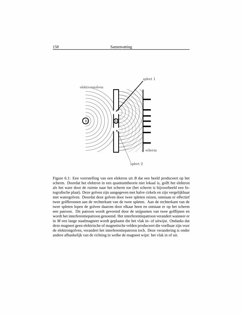
158 Samenvatting
PSfrag replacements
B
scherm
M
spleet 1
spleet 2
elektrongolven
Figure 6.1: Een voorstelling van een elektron uitB dat een beeld produceert op hetscherm. Doordat het elektron in een quantumtheorie niet lokaal is, golft het elektronals het ware door de ruimte naar het scherm toe (het scherm is bijvoorbeeld een fo-tografische plaat). Deze golven zijn aangegeven met halve cirkels en zijn vergelijkbaarmet watergolven. Doordat deze golven door twee spleten reizen, ontstaan er effectieftwee golfbronnen aan de rechterkant van de twee spleten. Aande rechterkant van detwee spleten lopen de golven daarom door elkaar heen en ontstaat er op het schermeen patroon. Dit patroon wordt gevormd door de snijpunten van twee golflijnen enwordt het interferentiepatroon genoemd. Het interferentiepatroon verandert wanneer erin M een lange staafmagneet wordt geplaatst die het vlak in- of uitwijst. Ondanks datdeze magneet geen elektrische of magnetische velden produceert die voelbaar zijn voorde elektrongolven, verandert het interferentiepatroon toch. Deze verandering is onderandere afhankelijk van de richting in welke de magneet wijst: het vlak in of uit.
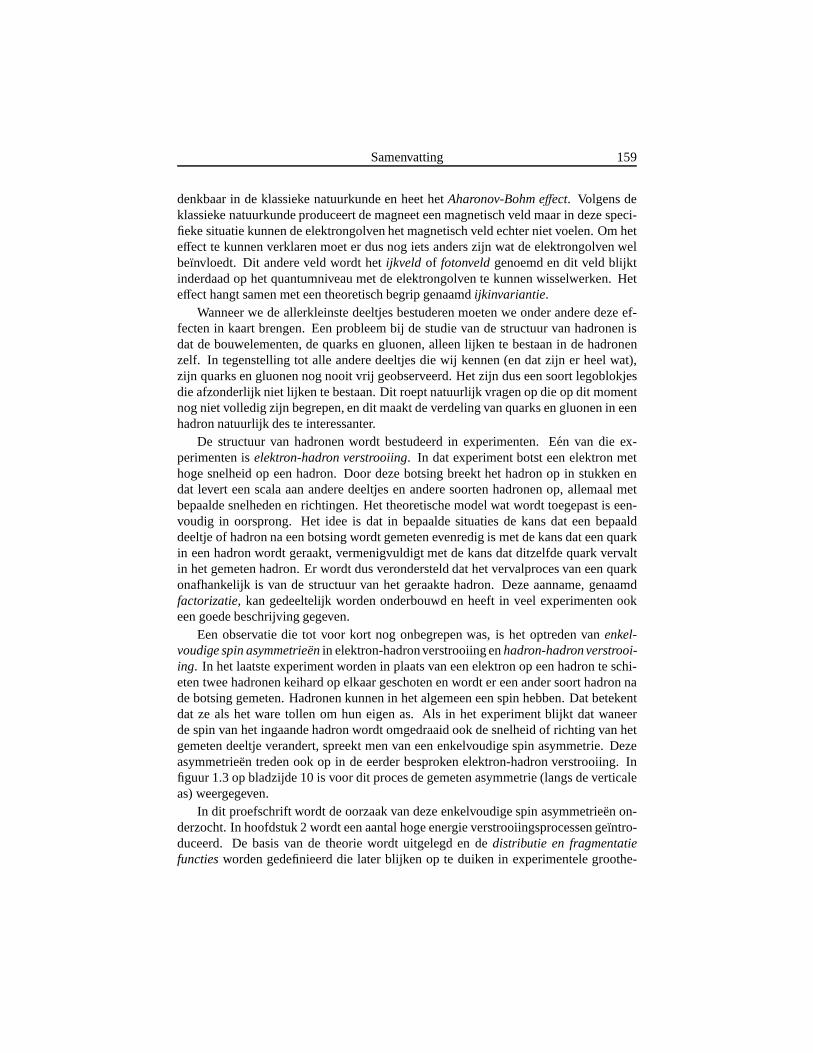
Samenvatting 159
denkbaar in de klassieke natuurkunde en heet hetAharonov-Bohm effect. Volgens deklassieke natuurkunde produceert de magneet een magnetisch veld maar in deze speci-fieke situatie kunnen de elektrongolven het magnetisch veldechter niet voelen. Om heteffect te kunnen verklaren moet er dus nog iets anders zijn wat deelektrongolven welbeınvloedt. Dit andere veld wordt hetijkveld of fotonveldgenoemd en dit veld blijktinderdaad op het quantumniveau met de elektrongolven te kunnen wisselwerken. Heteffect hangt samen met een theoretisch begrip genaamdijkinvariantie.
Wanneer we de allerkleinste deeltjes bestuderen moeten we onder andere deze ef-fecten in kaart brengen. Een probleem bij de studie van de structuur van hadronen isdat de bouwelementen, de quarks en gluonen, alleen lijken tebestaan in de hadronenzelf. In tegenstelling tot alle andere deeltjes die wij kennen (en dat zijn er heel wat),zijn quarks en gluonen nog nooit vrij geobserveerd. Het zijndus een soort legoblokjesdie afzonderlijk niet lijken te bestaan. Dit roept natuurlijk vragen op die op dit momentnog niet volledig zijn begrepen, en dit maakt de verdeling van quarks en gluonen in eenhadron natuurlijk des te interessanter.
De structuur van hadronen wordt bestudeerd in experimenten. Een van die ex-perimenten iselektron-hadron verstrooiing. In dat experiment botst een elektron methoge snelheid op een hadron. Door deze botsing breekt het hadron op in stukken endat levert een scala aan andere deeltjes en andere soorten hadronen op, allemaal metbepaalde snelheden en richtingen. Het theoretische model wat wordt toegepast is een-voudig in oorsprong. Het idee is dat in bepaalde situaties dekans dat een bepaalddeeltje of hadron na een botsing wordt gemeten evenredig is met de kans dat een quarkin een hadron wordt geraakt, vermenigvuldigt met de kans datditzelfde quark vervaltin het gemeten hadron. Er wordt dus verondersteld dat het vervalproces van een quarkonafhankelijk is van de structuur van het geraakte hadron. Deze aanname, genaamdfactorizatie, kan gedeeltelijk worden onderbouwd en heeft in veel experimenten ookeen goede beschrijving gegeven.
Een observatie die tot voor kort nog onbegrepen was, is het optreden vanenkel-voudige spin asymmetrieenin elektron-hadronverstrooiing enhadron-hadron verstrooi-ing. In het laatste experiment worden in plaats van een elektronop een hadron te schi-eten twee hadronen keihard op elkaar geschoten en wordt er een ander soort hadron nade botsing gemeten. Hadronen kunnen in het algemeen een spinhebben. Dat betekentdat ze als het ware tollen om hun eigen as. Als in het experiment blijkt dat waneerde spin van het ingaande hadron wordt omgedraaid ook de snelheid of richting van hetgemeten deeltje verandert, spreekt men van een enkelvoudige spin asymmetrie. Dezeasymmetrieen treden ook op in de eerder besproken elektron-hadron verstrooiing. Infiguur 1.3 op bladzijde 10 is voor dit proces de gemeten asymmetrie (langs de verticaleas) weergegeven.
In dit proefschrift wordt de oorzaak van deze enkelvoudige spin asymmetrieen on-derzocht. In hoofdstuk 2 wordt een aantal hoge energie verstrooiingsprocessen geıntro-duceerd. De basis van de theorie wordt uitgelegd en dedistributie en fragmentatiefunctiesworden gedefinieerd die later blijken op te duiken in experimentele groothe-
160 Samenvatting
den. Deze functies beschrijven de structuur van het hadron en bevatten de informatiedie we willen weten. In hoofstuk 2 is een nieuwe klasse van functies ontdekt die onsbegrip van de structuur kunnen vergroten. Een voorbeeld vandeze nieuwe functies isg⊥, aangegeven in vergelijking 2.65 (op bladzijde 34).
In hoofdstuk 3 wordt getracht een aantal verstrooiingsprocessen te beschrijven. Indeze beschrijving blijkt dat ijkinvariantie een grote rol speelt. Ijkinvariantie is eenwiskundige symmetrie die aanwezig zou moeten zijn in de theoretische beschrijving.Tot voor kort was dit niet helemaal netjes meegenomen, maar men wist ook niet ofhet missen van de symmetrie werkelijk een probleem zou kunnen zijn. Door in ditproefschrift de theorie nauwkeurig uit te werken, wordt er een bijdrage geleverd aanhet herstellen van ijkinvariantie. Behalve dat dit een verbeterde theoretische beschrijv-ing oplevert, blijkt er een subtiel effect te zijn wat een natuurlijke verklaring voor hetoptreden van enkelvoudige spin asymmetrieen geeft. Een verklaring in elektron-hadronverstrooiing is de wisselwerking tussen de geraakte quark en het ijkveld (gluonveld)van het hadron (de gluonen zijn geıllustreerd in figuur 1.2 door gekrulde lijnen). Heteffect is daardoor in een aantal opzichten vergelijkbaar met het Aharonov-Bohm ef-fect. In beide gevallen wordt het effect veroorzaakt doordat een deeltje (hetzij elektronof quark) wisselwerkt met een ijkveld in gebieden waar de elektrische en magnetischevelden geen effect hebben.
Deze effecten in kaart brengend, zien we in hoofdstuk 3 dat de functies van hoofd-stuk 2 kunnen worden gemeten in elektron-hadron verstrooiing. Vergelijking 3.64is bijvoorbeeld belangrijk om de verscheidene functies te kunnen meten. In hoofd-stuk 4 wordt de theorie verder ontwikkeld om ook hadron-hadron verstrooiing te kun-nen beschrijven. Een van de belangrijkste resultaten, maar technisch van aard, wordtgeıllustreerd in de figuren 4.9 en 4.10. In dit hoofdstuk wordt verder ook de consisten-tie van de gefactorizeerde aanpak besproken: Is het vervalproces van quarks in hadro-nen wel onafhankelijk van de structuur van het geraakte hadron? Het antwoord opdeze vraag blijkt niet eenvoudig. In hoofdstuk 5 worden de ontwikkelde techniekenvan hoofdstuk 4 gebruikt om voorspellingen te doen voor asymmetrieen in hadron-hadron verstrooiingsprocessen. Experimenten kunnen dezevoorspellingen verifierenen daarmee de geldigheid van de ontwikkelde ideeen toetsen.