RIJKS INSTITUUT VOOR VOLKSGEZONDHEID EN MILIEUHYGIENE BILTHOVEN

RAPPORT nr. 222901001

TEKPKRATUEE INCREAS ING POTENTIAIS

(TIPS) FOR GREENHOUSE GASES

J. Rotmans

M.G.J. den Elzen maart 1990

Dit onderzoek werd verricht in het kader van de Referentiefunctie Mondiale

Luchtverontreiniging, project nr. 222901 in opdracht van de Directie Lucht

van het Directoraat-Generaal Milieubeheer

- 11 -

VERZENDLIJ ST

1 Directeur Lucht van het Directoraat-Generaal voor Milieubeheer

2 Directeur-Generaal van de Volksgezondheid

3 Directeur-Generaal Milieubeheer

4 Plv. Directeur-Generaal Milieubeheer

5 Dr. P. Vellinga, DGM/L

6 Drs. J.B. Weenink, DGM/L

7-22 Programmaraad NWO werkgemeenschap C02-problematiek

23-27 KNAW klimaatcommissie

28 Prof. Dr.drs.ir. 0.J. Vrieze, RU Limburg

29 Prof. Dr. J.P.C. Kleijnen, KU Brabant

30 Ir. T.C.A. Mensch, TU Delft

31 Prof. Dr. H.G. Wind, TU Twente

32 Drs. P.A. Okken, ESC

33 Ir. M.J.P.H. Waltmans, DIV-Rijkswaterstaat

34 Ir. H. Kroon, DIV Rijkswaterstaat

35 Dr. M. Jonas, IIASA, Laxenburg

36 Dr. S. Bernow, ERSG, Boston

37 Dr. 1. Mintzer, University of Maryland

38 Depot van Nederlandse publicaties en Nederlandse bibliografie

39 Directie RIVM

40 Dr.ir. T. Schneider

41 Ir. F. Langeweg

42 Drs. S. Zwerver

43 Ir. R.J. Swart

44 Dr. H. de Boois

45 Dr. R.M. van Aalst

46 Drs. L. Hordijk

47 Drs. R.J.M. Maas

48 Ir. P.K. Koster

49 Ir. T.N. Olsthoorn

50 Drs. T. Aldenberg

51 M.J.C. Middelburg

52-71 auteurs

72 Bureau Projecten- en Rapportenregistratie

73-75 bibliotheek RIVM

76-100 reserve exemplaren

- 111 -

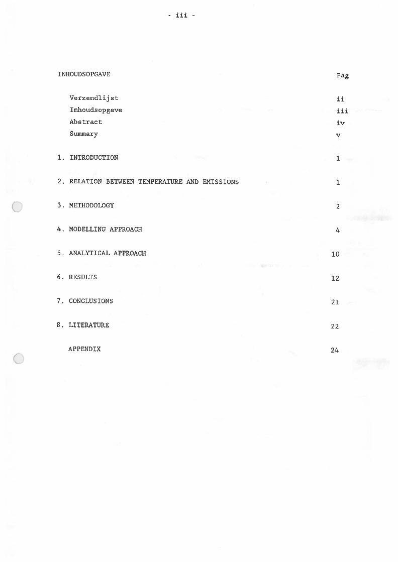
INHOUDSOPGAVE Pag

Verzendlijst ii

Inhoudsopgave iii

Abstract iv

Sunmiary v

1. INTRODUCTION 1

2. RELATION BETWEEN TEMPERATURE AND EMISSIONS 1

3. METHODOLOCY 2

4. MODELLING APPROACH 4

5. ANALYTICAL APPROACH 10

6. RESULTS 12

7. CONCLUSIONS 21

8. LITERATURE 22

APPENDIX 24

- iv -

ABSTRACT

In order to develop long-term environmental goals with respect to global

climate change an index to compare the temperature increasing effect of

greenhouse gas emissions is needed. In this report for the most important

greenhouse gases CO, CH4, N20, CFC-ll and CFC-12 the concept of

Temperature Increasing Potential (TIP) is introduced as a greenhouse

pendant to the ozone depleting potential (ODP). To obtain the relationship

between an emission and its associated effect on global temperature both

model approach and analytical approach is used. In determining the TIP with

help of models, IMAGE (the Integrated Model for the Assessment of the

Creenhouse Effect) is used. The analytical method to obtain TIP values

involves a direct way (from emissions to globaltemperature increase) and

an indirect way (from emissions via concentrations to global temperature

increase). Finally both methods are compared to previous efforts to

determine relative greenhouse gas potentials.

-v

SUNKARY

In order to develop long-term environmental goals with respect to global

climate change an index to compare the temperature increasing effect of

greenhouse gas emissions is needed. In this report for the most important

greenhouse gases GO2, N20, CFC-ll and CFC-12 the concept of

Temperature Increasing Potential (TIP) is introduced as a greenhouse

pendant to the ozone depleting potential (ODP). To obtain the relationship

between an emission and its associated effect on global temperature both

model approach and analytical approach is used. Indetermining the TIP with

help of models, IMAGE (the Integrated Model for the Assessment of the

Greenhouse Effect) is used. The analytical method to obtain TIP values

involves a direct way (from emissions to global temperature increase) and

an indirect way (from emissions via concentrations to global temperature

increase). Finally both methods. are compared to previous efforts to

determine relative greenhouse gas potentials.

-1-

1. INTRODUCTION

In order to develop environmental long-term goals with respect to climate

change an index to compare the temperature increasing effect of greenhouse

gas emissions is needed. Here the concept of the Temperature Increasing

Potential (TIP) is introduced as a greenhouse pendant to the ozone depleting

potential (ODP). To obtain the relationship between an emission and its

associated effect on temperature both model approach and analytical approach

is used. In determing the TIP with help of models, the Integrated Model for

the Assessment of the Creenhouse Effect, IMAGE is used. Furthermore both

approaches are compared to previous efforts to determine relative greenhouse

gas potentials.

2. RELATION BETWEEN TEMPEPATURE AND EMISSIONS

In deriving emission targets from a set goal for global mean temperature

increase, many nonlinear relationships within the atmosphere have to be

considered. The emission of greenhouse gases initially leads to increased

atmospheric concentrations. These gases are removed by a diversity of

processes, varying with each gas and its atmospheric concentration: uptake

by oceans, deposition, photochemical reactions, uptake by biota and soils.

These removal processes determine the atmospheric lifetime of the gases.

Furthermore many other factors related to the greenhouse problem interact

with the removal processes; for example, the concentration of other energy

related gases like carbon monoxide (GO) and non-methane hydrocarbons and the

influence of climate change on the carbon cycle and on methane (CH4) release

from natural reservoirs. Additionally the radiative absorption rate is

neither constant nor proportional to their respective concentrations.

Finally these processes and their underlying assuinptions are scenario

dependent.

Cenerally, in order to compare the results with previous efforts (e.g.

Lashof and Ahuja, 1990) equilibrium temperature effects will be used in

stead of transient responses.

-2-

The relation between an emission and its associated effect on temperature

can be expres sed in terms of temperature increasing potential (TIP). This is

comparable to the ozone depletion potential (ODP) which interrelates

different ozone-depleting substances. However the actual TIP is time

dependent, and not a scalar constant with which one could multiply emissions

like the ODPs. Nevertheless, for want of a Setter alternative, the relative

radiative potential of the trace gases will 5e approximated by a scalar.

3. METHODOLOGY

To achieve a direct relationship between an emission of a greenhouse gas and

its corresponding temperature response the following strategy will 5e

followed. For the greenhouse gas GO2, CH4, N20, CFC-ll and GFC-l2 one

emission impulse of 1 Gt will 5e generated during one year, the year 1986.

Grams and not moles are used, because in international literature emissions

are mostly expressed in grams.

Then the Temperature Increasing Potential, or TIP, of a greenhouse gas is

defined as the temperature effect (which consists of the integral of time

dependent temperature distributions from 0 to a time t) of 1 Gt emission of

that specific gas compared to that of GO2:

temperature effect of 1 Gt emission of trace gas i at time tTIP(t)

— temperature effect of 1 Gt emission of carbon dioxide at timewith:

TIP.(t) = temperature increasing potential of trace gas i at time t

In determining the TIP, two quintessential matters must 5e considered.

Firstly, the influence of the rather arbitrarily chosen time-span and height

of the emission impulse. An emission impulse of 1 Gt (for GO2, CH4, N20, GO,

and GFGs: CtC, GtGH4, GtN2O, CtCO, and GtCFC respectively) during one year

is chosen. To measure the influence of various kinds of pulses a sensitivity

analysis has been carried out with emission impulses of 0.25, 0.50, and 1.0

Gt, during 1, 5, and 10 years respectively. The resuits of this analysis

will 5e presented in the resuits section. Secondly the target point in time

of the TIP, being a crucial aspect in the TIP analysis, Sas to be

-3-

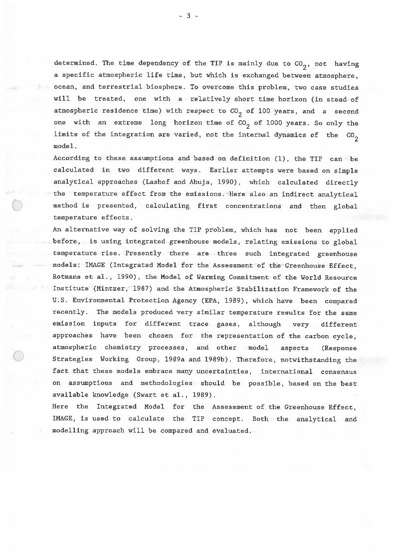
determined. The time dependency of the TIP is mainly due to GO2, not having

a specific atmospheric life time, but which is exchanged between atmosphere,

ocean, and terrestrial biosphere. To overcome this problem, two case studies

will be treated, one with a relatively short time horizon (in stead of

atmospheric residence time) with respect to GO2 of 100 years, and a second

one with an extreme long horizon time of GO2 of 1000 years. So only the

limits of the integration are varied, not the internal dynamics of the GO2

model.

According to these assumptions and based on definition (1), the TIP can 5e

calculated in two different ways. Earlier attempts were based on simple

analytical approaches (Lashof and Ahuja, 1990), which calculated directly

the temperature effect from the emissions. Here also an indirect analytical

C) method is presented, calculating first concentrations and then global

temperature effects.

An alternative way of solving the TIP problem, which has not been applied

before, is using integrated greenhouse models, relating emissions to global

temperature rise. Presently there are three such integrated greenhouse

models: IMAGE (Integrated Model for the Assessment of the Greenhouse Effect,

Rotmans et al., 1990), the Model of Warming Gommitment of the World Resource

Institute (Mintzer, 1987) and the Atmospheric Stabilization Framework of the

U.S. Envirorunental Protection Agency (EPA, 1989), which have been compared

recently. The models produced very similar temperature results for the same

emission inputs for different trace gases, although very different

approaches have been chosen for the representation of the carbon cycle,

atmospheric chemistry processes, and other model aspects (Response

() Strategies Working Group, 1989a and 1989b). Therefore, notwithstanding the

fact that these models embrace many uncertainties, international consensus

on assumptions and methodologies should be possible, based on the best

available knowledge (Swart et al., 1989).

Here the Integrated Model for the Assessment of the Greenhouse Effect,

IMAGE, is used to calculate the TIP concept. Both the analytical and

modelling approach will 5e compared and evaluated.

-4-

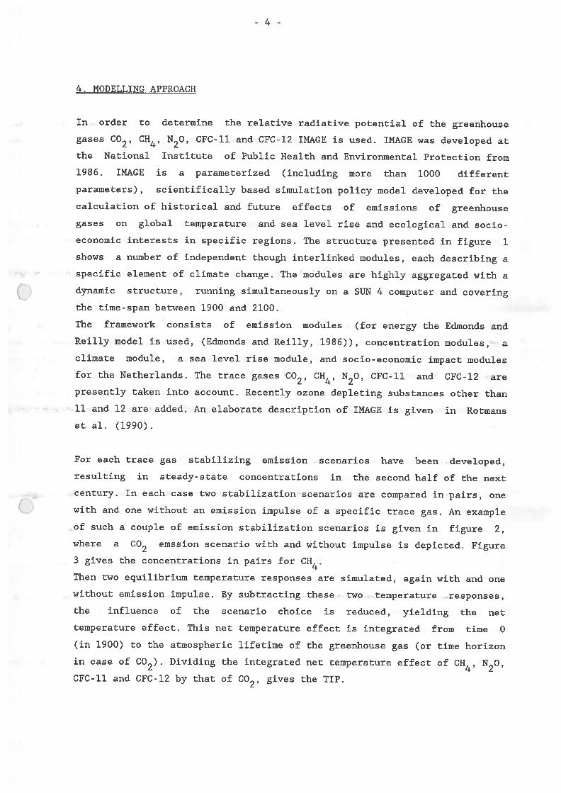
4. MODELLING APPROACH

In order to determine the relative radiative potential of the greenhouse

gases GO2, CH4, N20, CFC-11 and CFC-12 IMAGE is used. IMAGE was developed at

the National Institute of Public Health and Environmental Protection from

1986. IMAGE is a parameterized (inciuding more than 1000 different

parameters), scientifically based simulation policy model developed for the

calculation of historical and future effects of emissions of greenhouse

gases on global temperature and sea level rise and ecological and socio

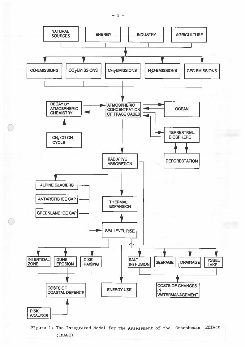
economic interests in specific regions. The structure presented in figure 1

shows a number of independent though interlinked modules, each describing &

specific element of climate change. The modules are highly aggregated with a

dynamic structure, running simultaneously on a SUN 4 computer and covering

the time-span between 1900 and 2100.

The framework consists of emission modules (for energy the Edmonds and

Reilly model is used, (Edmonds and Reilly, 1986)), concentration modules, a

climate module, a sea level rise module, and socio-economic impact modules

for the Netherlands. The trace gases GO2, CH4, N20, CFC-ll and CFC-12 are

presently taken into account. Recently ozone depleting substances other than

11 and 12 are added. An elaborate description of IMAGE is given in Rotmans

et al. (1990).

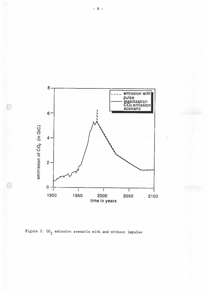
For each trace gas stabilizing emission scenarios have been developed,

resulting in steady-state concentrations in the second half of the next

century. In each case two stabilization scenarios are compared in pairs, one

with and one without an emission impulse of a specific trace gas. An example

of such a couple of emission stabilization scenarios is given in figure 2,

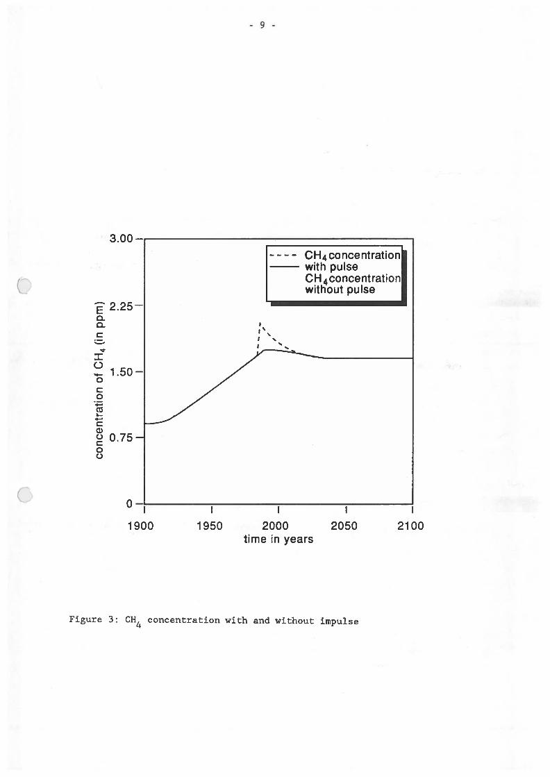
where & GO2 emssion scenario with and without impulse is depicted. Figure

3 gives the concentrations in pairs for CH4.

Then two equilibrium temperature responses are simulated, again with and one

without emission impulse. By subtracting these two temperature responses,

the influence of the scenario choice is reduced, yielding the net

temperature effect. This net temperature effect is integrated from time 0

(in 1900) to the atmospheric lifetime of the greenhouse gas (or time horizon

in case of GO2). Dividing the integrated net temperature effect of CH4, N20,

CFG-ll and CFG-l2 by that of GO2, gives the TIP.

—5—

NATURALSOURCES ENERGY INDUSTRY AGRICULTURE

T T T

DECAY BYATMOSPHERICCHEMISTRY

TERRESTRIALBIOSPHERE

4,

CO-EMISSIONS

+

COzEMISSIONS 1 CHEMISSIONS 1 1 NEMISSIONS CFCEMISSIONS

OCEAN

CH4-CO-OHCYCLE

RADIATIVEABSORPTION

DEFORESTATION

-TALPINE GLACIERS

ANTARCTIC ICE CAP

GREENLAND ICE CAP—

THERMALEXPANSION

COSTS OFCOASTAL DEFENCE

RISKANALYSIS

COSIS OF CHANGESINWATERMANAGEMENT

Figure 1: The Integrated Model for the Assessment of the Greenhouse Effect

(IMAGE)

-6-

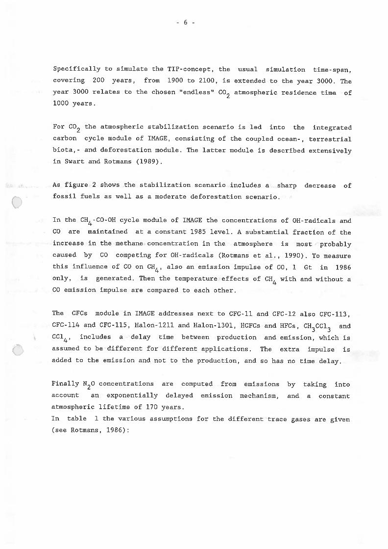
Specifically to simulate the TIP-concept, the usual simulation time-span,

covering 200 years, from 1900 to 2100, is extended to the year 3000. The

year 3000 relates to the chosen “endless” GO2 atmospheric residence time of

1000 years.

For GO2 the atmospheric stabilization scenario is led into the integrated

carbon cycle module of IMAGE, consisting of the coupled ocean-, terrestrial

biota,- and deforestation module. The latter module is described extensively

in Swart and Rotmans (1989).

As figure 2 shows the stabilization scenario inciudes a sharp decrease of

fossil fuels as well as a moderate deforestation scenario.

In the GH4-GO-OH cycle module of IMAGE the concentrations of OH-radicals and

GO are maintained at a constant 1985 level. A substantial fraction of the

increase in the methane concentration in the atmosphere is most’probab1y

caused by GO competing for OH-radicals (Rotmans et al., 1990). To measure

this influence of GO on CH4, also an emission impulse of GO, 1 Gt in 1986

only, is generated. Then the temperature effects of CH4 with and without a

GO emission impulse are compared to each other.

The GFCs module in IMAGE addresses next to GFG-ll and GFG-12 also GFG-1l3,

GFG-114 and GFG-115, Halon-121l and Halon-l3Ol, HGFGs and HFGs, GH3GG13 and

GG14, includes a delay time between production and emission, which is

assumed to be different for different applications. The extra impulse is

added to the emission and not to the production, and so has no time delay.

Finally N2O concentrations are computed from emissions by taking into

account an exponentially delayed emission mechanism, and a constant

atmospheric lifetime of 170 years.

In table 1 the various assumptions for the different trace gases are given

(see Rotmans, 1986):

-7-

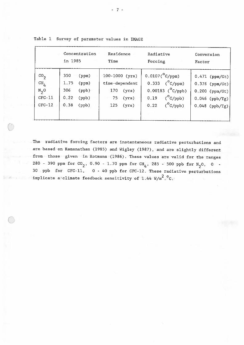
Table 1 $urvey of parameter values in IMAGE

Concentration Residence Radiative Conversion

in 1985 Time Forcing Factor

C02 350 (ppm) 100-1000 (yrs) 0.0107f°C/ppm) 0.471 (ppm/Gt)

CH4 1.75 (ppm) time-dependent 0.333 (°C/ppm) 0.376 (ppm/Gt)

N20 306 (ppb) 170 (yrs) 0.00183 (°C/ppb) 0.200 (ppm/Gt)

CFC-11 0.22 (ppb) 75 (yrs) 0.19 (°C/ppb) 0.046 (ppb/Tg)

CFC-12 0.38 (ppb) 125 (yrs) 0.22 (°C/ppb) 0.048 (ppb/Tg)

The radiative forcing factors are instantaneous radiative perturbations and

are based on Ramanathan (1985) and Wigley (1987), and are slightly different

from those given in Rotmans’(1986). These values are valid for the ranges

280 - 390 ppm for GO2, 0.90 - 1.70 ppm for CH4, 285 - 500 ppb for N20, 0 -

30 ppb for CFC-11, 0 - 40 ppb for CFC-12. These radiative perturbations

implicate ac1imate feedback sensitivity of 1.44 W/m2.°C.

-8-

0

0

0

000

E2

1900 1950 2000 2050 2100time in years

Figure 2: GO2 emission scenario with and without impulse

-9-

---- CH4concentrationwith pulseCH4concentrationwithout pulse

3.00—

‘ 2.25—

z1.50—

0.75—

0

t %

1900 1950

t t

2000time in years

2050 2100

Figure 3: CH4 concentration with and without impulse

- 10 -

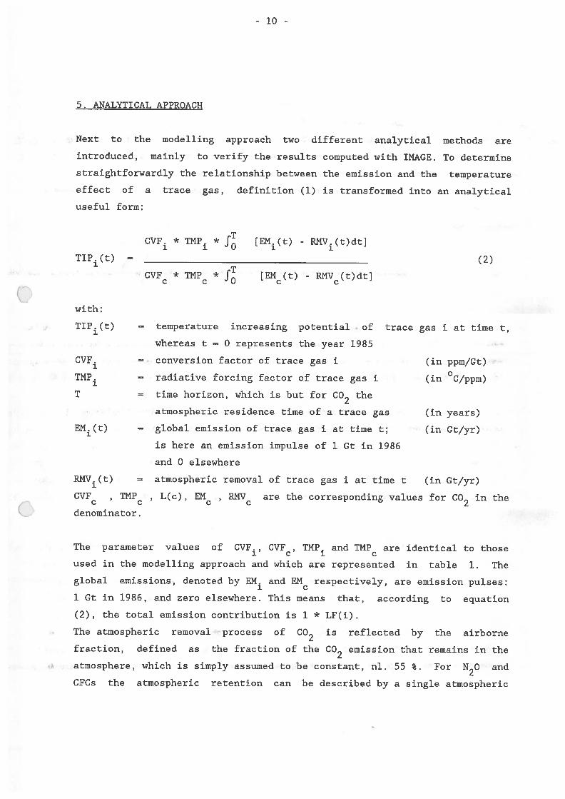
5. ANALYTICAL APPROACH

Next to the modelling approach two different analytical methods are

introduced, mainly to verify the resuits computed with IMAGE. To determine

straightforwardly the relationship between the emission and the temperature

effect of a trace gas, definition (1) is transformed into en analytical

useful form:

CVF. * TMP. * [EM.(t) - RMV.(t)dtJ

TIP.(t)

_________________________________________

(2)

CVF * TMPc * [EMc(t) -

RNV(t)dt]

with:

TIP.(t) = temperature inereasing potential of trace gas i at time t,

whereas t = 0 represents the year 1985

CVF. = conversion factor of trace gas i (in ppm/Ct)

TMP = radiative forcing factor of trace gas i (in °C/ppm)

T = time horizon, which is but for GO2 the

atmospheric residence time of & trace gas (in years)

EM.(t) = global emission of trace gas i at time t; (in Gt/yr)

is here an emission impulse of 1 Gt in 1986

and 0 elsewhere

RMV.(t) = atmospheric removal of trace gas i at time t (in Gt/yr)

CVFc , TMP , L(c), EM Rc are the corresponding values for GO2 in the

denominator.

The parameter values of CVF., CVF , TMP. and TMP are identical to those1 c 1 c

used in the modelling approach and which are represented in table 1. The

global emissions, denoted by EM and EMc respectively, are emission pulses:

1 Gt in 1986, and zero elsewhere. This means that, according to equation

(2), the total emission contribution is 1 * LF(i).

The atmospheric removal process of GO2 is reflected by the airborne

fraction, defined as the fraction of the GO2 emission that remains in the

atmosphere, which is simply assumed to be constant, ni. 55 %. For N2O and

GFGs the atmospheric retention can be described by & single atmospheric

- 11 -

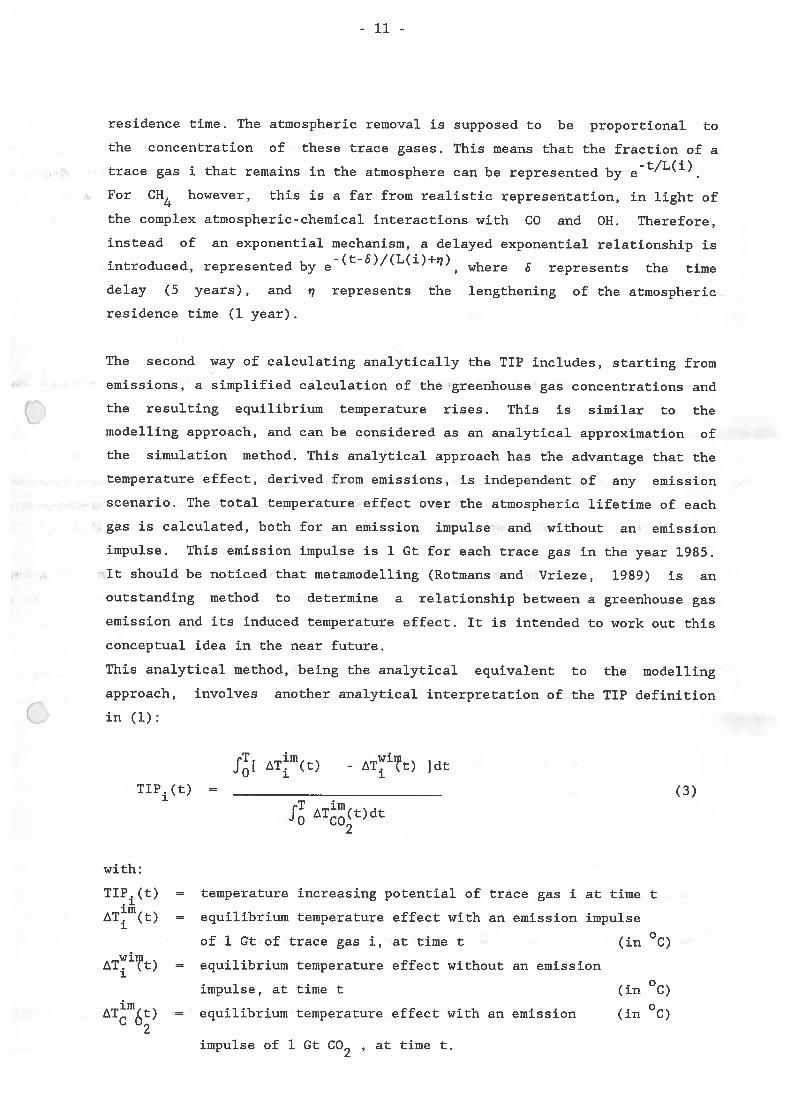
residence time. The atmospheric removal is supposed to 5e proportional to

the concentration of these trace gases. This means that the fraction of a

trace gas i that remains in the atmosphere can be represented by et1’1).

For CH4 however, this is a far from realistic representation, in light of

the complex atmospheric-chemical interactions with CO and OH. Therefore,

instead of an exponential mechanism, a delayed exponential relationship is

introduced, represented sy et6, where S represents the time

delay (5 years), and r, represents the lengthening of the atmospheric

residence time (1 year).

The second way of calculating analytically the TIP inciudes, starting from

emissions, a simplified calculation of the greenhouse gas concentrations and

the resulting equilibrium temperature rises. This is similar to the

modelling approach, and can be considered as an analytical approximation of

the simulation method. This analytical approach has the advantage that the

temperature effect, derived from emissions, is independent of any emission

scenario. The total temperature effect over the atmospheric lifetime of each

gas is calculated, both for an emission impulse..and without an emission

impulse. This emission impulse is 1 Gt for each trace gas in the year 1985.

It should 5e noticed that metamodelling (Rotmans and Vrieze, 1989) is an

outstanding method to determine a relationship between a greenhouse gas

emission and its induced temperature effect. It is intended to work out this

conceptual idea in the near future.

This analytical method, being the analytical equivalent to the modelling

approach, involves another analytical interpretation of the TIP definition

in (1)

f[ TEm(t) - T’t) Jdt

TIP.(t) =

___________________________

(3)

f T(t)dt

with:

TIP.(t) = temperature increasing potential of trace gas i at time t

Tm()= equilibrium temperature effect with an emission impulse

of 1 Ct of trace gas i, at time t (in °C)

= equilibrium temperature effect without an emission

impulse, at time t (in °C)

Tm6)= equilibrium temperature effect with an emission (in °C)

2impulse of 1 Gt C02 , at time t.

- 12 -

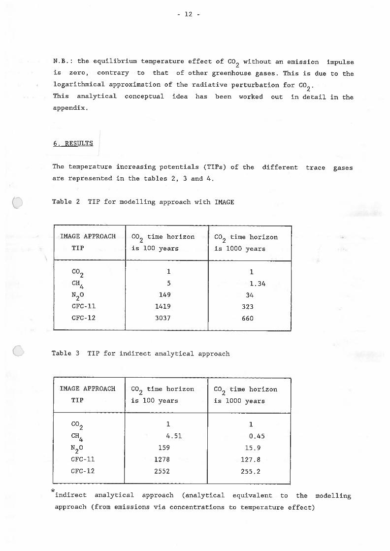
N.B.: the equilibrium temperature effect of GO2 without an emission impulse

is zero, contrary to that of other greenhouse gases. This is due to the

logarithmical approximation of the radiative perturbation for GO2.

This analytical conceptual idea bas been worked Out in detail in the

appendix.

6. RESULTS

The temperature increasing potentials (TIPs) of the different trace gases

are represented in the tables 2, 3 and 4.

Table 2 TIP for modelling approach with IMAGE

IMAGE APPROACH GO2 time horizon GO2 time horizon

TIP is 100 years is 1000 years

Go2 1 1

CH4 5 1.34

N20 149 34

GFC-ll 1419 323

GFC-12 3037 660

Table 3 TIP for indirect analytical approach

IMAGE APPROACH GO2 time horizon GO2 time horizon

TIP is 100 years is 1000 years

GO2 1 1

CH4 4.51 0.45

N20 159 15.9

GFC-1l 1278 127.8

GFG-12 2552 255.2

*indirect analytical approach (analytical equivalent to the modelling

approach (from emissions via concentrations to temperature effect)

- 13 -

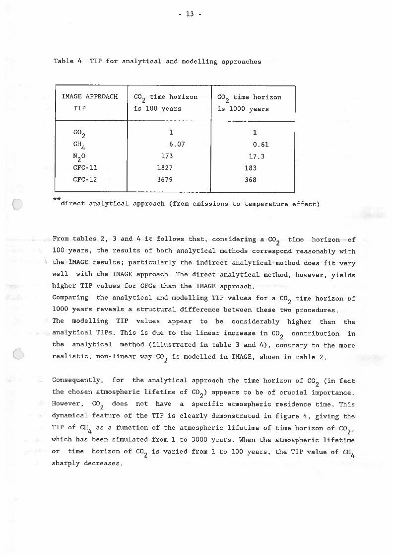
Table 4 TIP for analytical and modelling approaches

IMAGE APPROACH GO2 time horizon GO2 time horizon

TIP is 100 years is 1000 years

GO2 1 1

CH4 6.07 0.61

N20 173 17.3

CFC-11 1827 183

GFC-12 3679 368

**direct analytical approach (from emissions to temperature effect)

From tables 2, 3 and 4 it follows that, considering a GO2 time horizon of

100 years, the resuits of both analytical methods correspond reasonably with

the IMAGE resuits; particularly the indirect analytical method does fit very

well with the IMAGE approach. The direct analytical method, however, yields

higher TIP values for GFGs than the IMAGE approach.

Gomparing the analytical and modelling TIP values for a GO2 time horizon of

1000 years reveals a structural difference between these two procedures.

The modelling TIP values appear to be considerably higher than the

analytical TIPs. This is due to the linear increase in GO2 contribution in

the analytical method (illustrated in table 3 and 4), contrary to the more

realistic, non-linear way CO2 is modelled in IMAGE, shown in table 2.

Gonsequently, for the analytical approach the time horizon of GO2 (in fact

the chosen atmospheric lifetime of GO2) appears to be of crucial importance.

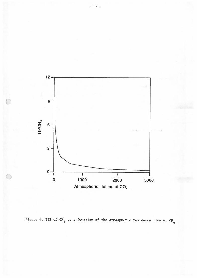
However, GO2 does not have a specific atmospheric residence time. This

dynamical feature of the TIP is clearly demonstrated in figure 4, giving the

TIP of CH4 as a function of the atmospheric lifetime of time horizon of GO2,

which has been simulated from 1 to 3000 years. When the atmospheric lifetime

or time horizon of GO2 is varied from 1 to 100 years, the TIP value of CH4

sharply decreases.

- 14 -

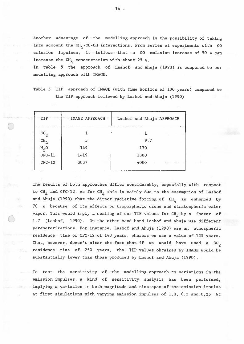
Another advantage of the modelling approach is the possibility of taking

into account the CH4-CO-OH interactions. From series of experiments with GO

emission impulses, it follows that a GO emission increase of 50 % can

increase the CH4 concentration with about 25 %.

In table 5 the approach of Lashof and Ahuja (1990) is compared to our

modelling approach with IMAGE.

Table 5 TIP approach of IMAGE (with time horizon of 100 years) compared to

the TIP approach followed by Lashof and Ahuja (1990)

t)

The resuits of both approaches differ considerably, especially with respect

to CH4 and CFC-12. As for CH4 this is mainly due to the assumption of Lashof

and Ahuja (1990) that the direct radiative forcing of CH4 is enhanced by

70 % because of its effects on tropospheric ozone and stratospheric water

vapor. This would imply a scaling of our TIP values for CH4 by a factor of

1.7 (Lashof, 1990). On the other hand hand Lashof and Ahuja use different

parameterizations. For instance, Lashof and Ahuja (1990) use an atmospheric

residence time of CFC-12 of 140 years, whereas we use a value of 125 years.

That, however, doesn’t alter the fact that if we would have used a C02

residence time of 250 years, the TIP values obtained by IMAGE would be

substantially lower than those produced by Lashof and Ahuja (1990).

To test the sensitivity of the modelling approach to variations in the

emission impulses, a kind of sensitivity analysis bas been performed,

.... implying a variation in both magnitude and time-span of the emission impulse

At first simulations with varying emission impulses of 1.0, 0.5 and 0.25 Gt

TIP IMAGE APPROACH Lashof and Ahuja APPROACH

GO2 1 1

CH4 5 9.7

N20 149 170

CFC-ll 1419 1300

CFG-12 3037 4000

- 15 -

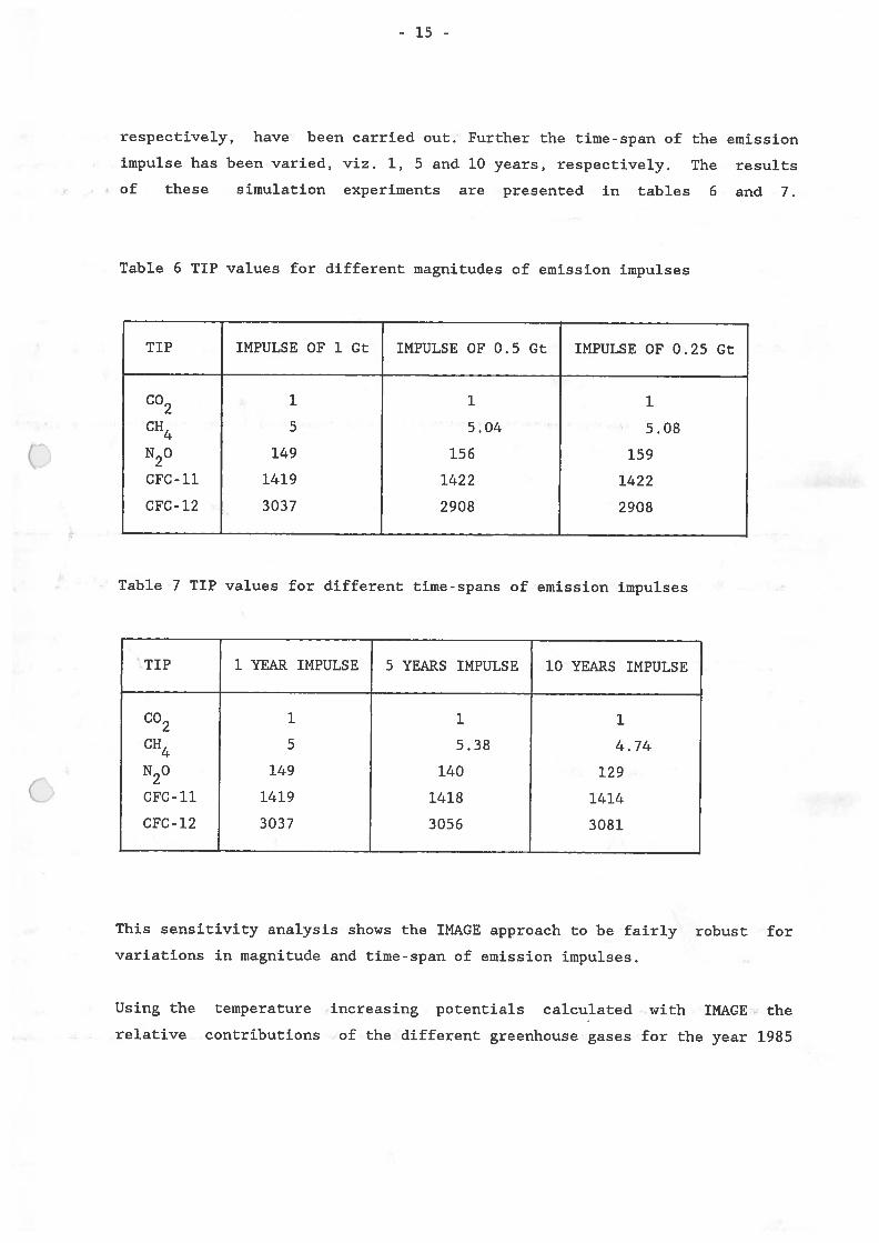
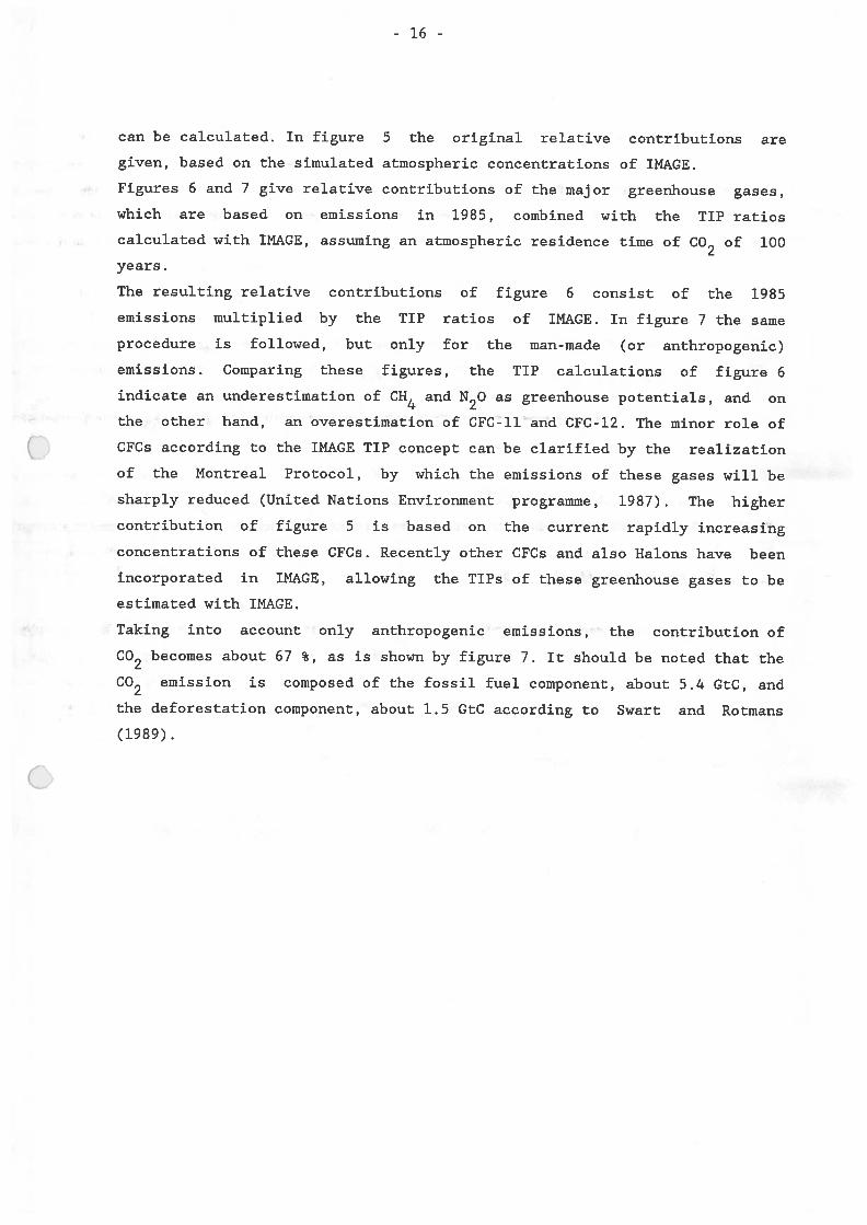
respectively, have been carried out. Further the time-span of the emission

impulse has been varied, viz. 1, 5 and 10 years, respectively. The resuits

of these simulation experiments are presented in tables 6 and 7.

Table 6 TIP values for different magnitudes of emission impulses

TIP IMPULSE OF 1 Gt IMPULSE OF 0.5 Gt IMPULSE OF 0.25 Gt

Go2 1 1 1

CH4 5 5.04 5.08

N20 149 156 159

CFC-11 1419 1422 1422

CFC-12 3037 2908 2908

Table 7 TIP values for different time-spans of emission impulses

‘TIP 1 YEAR IMPULSE 5 YEARS IMPULSE 10 YEARS IMPULSE

Go2 1 1 1

CH4 5 5.38 4.74

N20 149 140 129

CFC-l1 1419 1418 1414

CFC-12 3037 3056 3081

This sensitivity analysis shows the IMAGE approach to be fairly robust for

variations in magnitude and time-span of emission impulses.

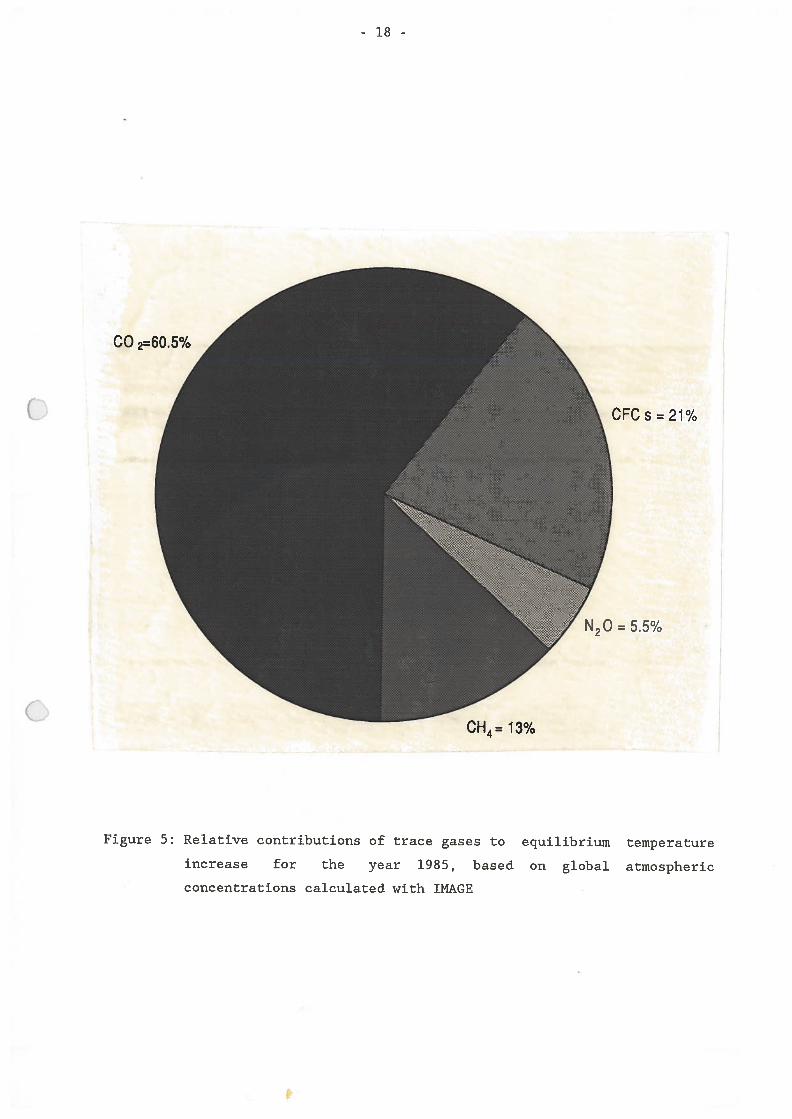
Using the temperature increasing potentials calculated with IMAGE the

relative contributions of the different greenhouse gases for the year 1985

- 16 -

can be calculated. In figure 5 the original relative contributions are

given, based on the simulated atmospheric concentrations of IMAGE.

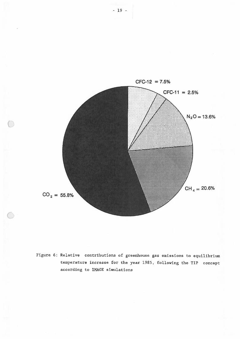
Figures 6 and 7 give relative contributions of the major greenhouse gases,

which are based on emissions in 1985, combined with the TIP ratios

calculated with IMAGE, assuming an atmospheric residence time of C02 of 100

years.

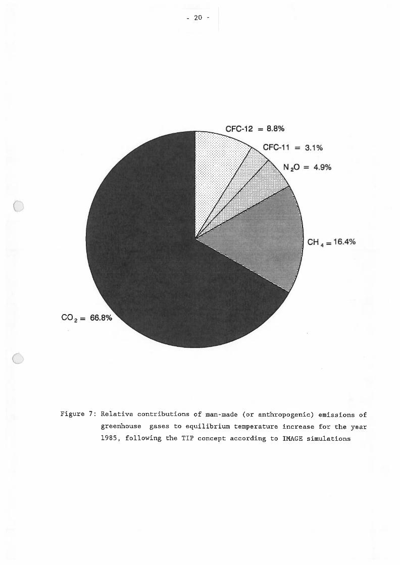
The resulting relative contributions of figure 6 consist of the 1985

emissions multiplied by the TIP ratios of IMAGE. In figure 7 the same

procedure is followed, but only for the man-made (or anthropogenic)

emissions. Comparing these figures, the TIP calculations of figure 6

indicate an underestimation of CH4 and N20 as greenhouse potentials, and on

the other hand, an overestimation of CFC-11 and CFC-12. The minor role of

CFCs according to the IMAGE TIP concept can be clarified by the realization

of the Montreal Protocol, by which the emissions of these gases will be

sharply reduced (United Nations Environment programme, 1987). The higher

contribution of figure 5 is based on the current rapidly increasing

concentrations of these CFCs. Recently other CFCs and also Halons have been

incorporated in IMAGE, allowing the TIPs of these greenhouse gases to be

estimated with IMAGE.

Taking into account only anthropogenic emissions, the contribution of

C02 becomes about 67 %, as is shown by figure 7. It should be noted that the

C02 emission is composed of the fossil fuel component, about 5.4 GtC, and

the deforestation component, about 1.5 GtC according to Swart and Rotmans

(1989).

- 17 -

z00

12

0

9

6

3

0 1000 2000 3000

Atmospheric lifetime of C02

Figure 4: TIP of CH4 as a function of the atmospheric residence tinie of CH4

- 18 -

4•1

CD 2=60.5%

CFCs=21%

N20 = 5.5%

Figure 5: Relative contributions of trace gases to equilibrium

increase for the year 1985, based on global

concentrations calculated with IMAGE

temperature

atmospheric

CH4= 13%

- 19 -

C02 = 55.8%

N20 = 13.6%

CH4 = 20.6%

Figure 6: Relative contributions of greenhouse gas emissions to equilibriuiri

temperature increase for the year 1985, following the TIP concept

according to IMAGE simulations

CFC-12 = 7.5%

CFC-1 1 = 2.5%

- 20 -

N20 = 4.9%

CH4 = 16.4%

Figure 7: Relative contributions of man-made (or anthropogenic) emissions of

greenhouse gases to equilibrium temperature increase for the year

1985, following the TIP concept according to IMAGE simulations

CFC-12 = 8.8%

CFC-11 = 3.1%

C02= 66.8%

- 21 -

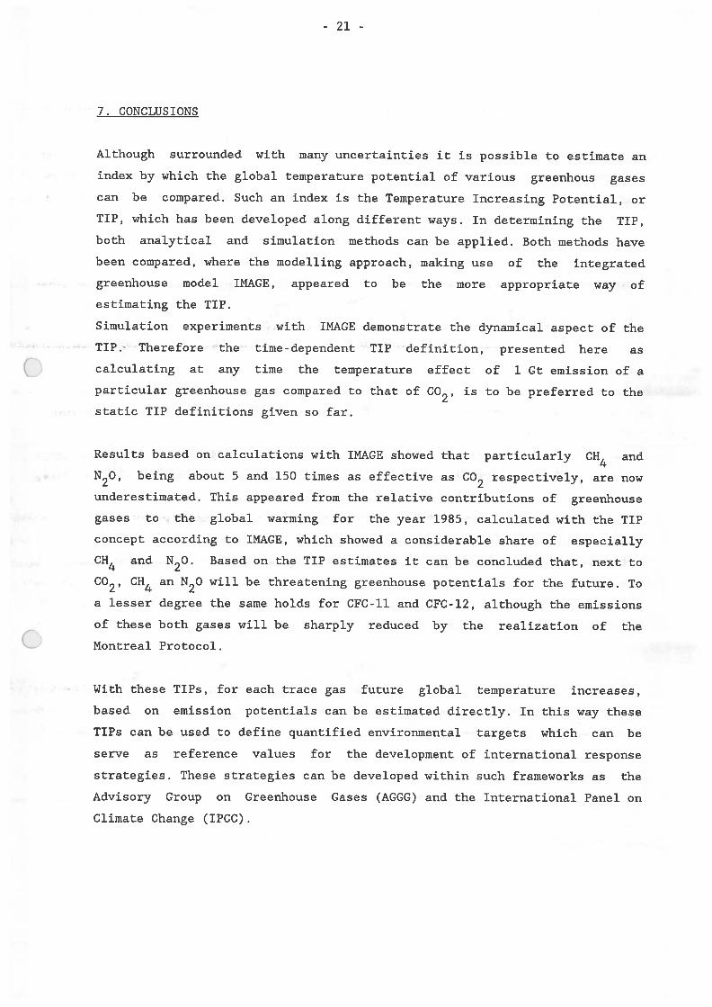
7. CONCLUSIONS

Although surrounded with many uncertainties it is possible to estimate an

index by which the global temperature potential of various greenhous gases

can be compared. Such an index is the Temperature Increasing Potential, or

TIP, which has been developed along different ways. In determining the TIP,

both analytical and simulation methods can be applied. Both methods have

been compared, where the modelling approach, making use of the integrated

greenhouse model IMAGE, appeared to be the more appropriate way of

estimating the TIP.

Simulation experiments with IMAGE demonstrate the dynamical aspect of the

TIP. Therefore the time-dependent TIP definition, presented here as

calculating at any time the temperature effect of 1 Gt emission of a

particular greenhouse gas compared to that of GO2, is to be preferred to the

static TIP definitions given so far.

Resuits based on calculations with IMAGE showed that particularly CH4 and

N20, being about 5 and 150 times as effective as GO2 respectively, are now

underestimated. This appeared from the relative contributions of greenhouse

gases to the global warming for the year 1985, calculated with the TIP

concept according to IMAGE, which showed a considerable share of especially

CH4 and N20. Based on the TIP estimates It can be conciuded that, next to

GO2, CH4 an N20 will be threatening greenhouse potentials for the future. To

a lesser degree the same holds for CFC-ll and CFC-12, although the emissions

of these both gases will be sharply reduced by the realization of the

Montreal Pro tocol.

With these TIPs, for each trace gas future global temperature increases,

based on emission potentials can 5e estimated directly. In this way these

TIPs can be used to define quantified environmental targets which can lie

serve as reference values for the development of international response

strategies. These strategies can be developed within such frameworks as the

Advisory Group on Greenhouse Gases (AGGG) and the International Panel on

Climate Change (IPCC).

- 22 -

8. LITERATURE

- Edmonds, J.A. and Reilly, J.M. (1986) ‘The Long-Term Global Energy-C02

Model: PC-version A84PC’, Carbon Dioxide Information Center, Oak Ridge.

- Environmental Protection Agency (1989) ‘Policy Options for Stabilizing

Global Climate’, Draft Report to Congress, Washington, D.C.

- Kiehi, J.T. and Dickinson, R.E. (198?) ‘A Study of the Radiative Effects

of Enhanced Atmospheric C02 and CH4 on early Earth Surface Temperatures’,

Journal of Geophysical Research 92, 2991-2998

- Lashof, D.A., and Ahuja, D.R. (1990) ‘Relative Global Warming Potentials

of Greenhouse Gas Emissions’, submitted to Nature, Washington, D.C.

- Lashof, D.A. (1990) Personal communication

- Mintzer, 1. (1987) ‘A Matter of Degrees’, World Resources Institute,

Washington, D.C.

- Ramanathan, V., Cicerone, R.J., Singh, H.B. and Kiehl, J.T. (1985) ‘Trace

Gas Trends and their Potential Role in Climate Change’, Journal of

Geophysical Research 90, 5547-5566

- Response Strategies Working Group (1989a) ‘Emissions Scenarios of the

Response Strategies Working Group of the Intergovernmental Panel on

Climate Change’, Draft Report of the U.S.-Netherlands Expert Group on

Emissions Scenarios, Bilthoven, The Netherlands.

- Response Strategies Working Group (1989b) ‘Emissions Scenarios of the

Response Strategies Working Group of the Intergovernniental Panel on

Climate Change’, Draft Appendix of the U.S.-Netherlands Expert Group on

Emissions Scenarios, Bilthoven, The Netherlands.

- Rotmans, J. (1986) ‘The development of a simulation model for the global

C02-problem’ (in Dutch), reportnr. 840751001, RIVM, Bilthoven, The

Ne ther lands

- Rotmans, J., Swart, R.J., Vrieze, O.J. (1990) ‘The role of the CH4-CO-OH

cycle in the greenhouse problem’, Science of the Total Environment, in

press.

- Rotmans, J., de Boois, H., and Swart, R.J. (1990) ‘An Integrated Model for

the Assessment of the Greenhouse Effect: the Dutch Approach’, Climatic

Change, in press.

- Rotmans, J., Vrieze, O.J. (1989) ‘Metamodelling and Experimental Design:

Case Study of the Greenhouse Effect’, to 5e published in the European

- 23 -

Journal of Operations Research, and is also a research report of the

University of Limburg, Report M 88-03, Maastricht, the Netherlands.

Swart, R.J. and Rotmans, J. (1989) ‘A scenario study on causes of tropical

deforestation and effects on the global carbon cycle’, RIVM-report

758471007, Bilthoven, The Netherlands.

Swart, R.J., de Boois, H., and Rotmans, J. (1989) ‘Targeting Climate

Change’, International Environinental Affairs, A Journal for Research and

Policy 1, no 3, 222-234.

- United Nations Environment Programme (1987) ‘Montreal Protocol on

Substances that deplete the Ozone Layer: Final Act’, Montreal.

- United Nations Environinent Programme, and World Meteorological

Organization (1989) ‘Scientific Assessment of Stratospheric Ozone’

chapter 4: ODPs and GWPs.

- Wigley, T.M.L. (1987) ‘Relative Contributions of Different Trace Gases to

the Creenhouse Effect’, Climate monitor 16, no. 1, 14-28

- 24 -

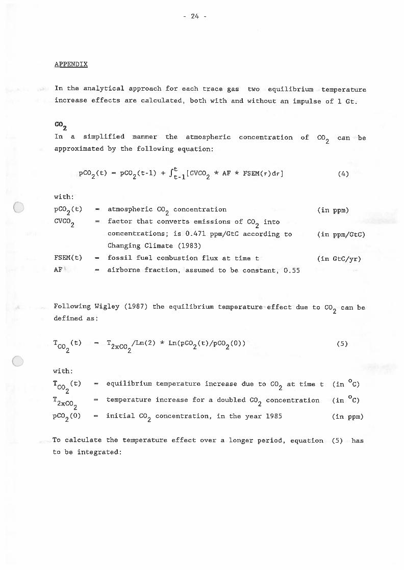
APPENDIX

In the analytical approach for each trace gas two equilibrium temperature

increase effects are calculated, both with and without an impulse of 1 Gt.

Go2In a simplified manner the atmospheric concentration of GO2 can 5e

approximated by the following equation:

pCO2(t) = pCO2(t-1) + f1[ct02 * AF * FSEM(T)dTJ (4)

with:

pCO2(t) = atmospheric GO2 concentration (in ppm)

CVCO2 = factor that converts emissions of GO2 into

concentrations; is 0.471 ppm/GtG according to (in ppm/GtG)

Changing Glimate (1983)

FSEM(t) fossil fuel combustion flux at time t (in GtG/yr)

AF airborne fraction, assumed to be constant, 0.55

Following Wigley (1987) the equilibrium temperature effect due to GO2 can 5e

defined as:

Tco(t) = T2co/Ln(2) * Ln(pGO2(t)/pGO2(O)) (5)

with:

TGO (t) equilibrium teniperature increase diie to GO2 at time t (in °C)2

T2co = temperature increase for a doubled GO2 concentration (in °C)2

pGO2(0) = initial GO2 concentration, in the year 1985 (in ppm)

To calculate the temperature effect over a longer period, equation (5) has

to 5e integrated:

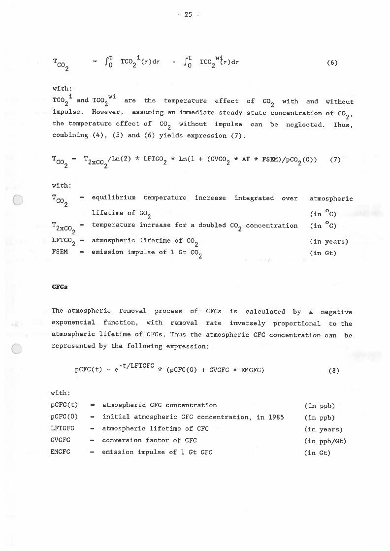
- 25 -

Tco f TC021(T)dr-

TGO2WtT)dT (6)

with:

TCO2’ and TGO2 are the temperature effect of GO2 with and without

impulse. However, assuming an immediate steady state concentration of GO2,

the temperature effect of GO2 without impulse can be neglected. Thus,

combining (4), (5) and (6) yields expression (7).

with:

— T20/Ln(2) * LFTCO2 * Ln(1 + (CVCO2 * AF * FSEM)/pCO2(O)) (7)

Tco = equilibrium temperature increase integrated over atmospheric2

lifetime of GO2

= temperature increase for a doubled GO2 concentration

The atmospheric removal process of

exponential function, with removal

atmospheric lifetime of CFCs. Thus the

represented by the following expression

CFCs is calculated by a negative

rate inversely proportional to the

atmospheric GFC concentration can be

with:

pGFG(t)

pGFC(O)

LFTGFG

CVCFC

EMGFG

- t/LFTCFCpGFG(t) = e * (pCFC(O) + CVCFG * EMCFC) (8)

(in ppb)

(in ppb)

(in years)

(in ppb/Gt)

(in Ct)

TGO

T2GO

LFTGO2

FSEM

atmospheric lifetime of GO2

emission impulse of 1 Gt GO2

CFCs

• 0(in G)

• 0(in G)

(in years)

(in Gt)

= atmospheric CFC concentration

= initial atmospheric GFG concentration, in 1985

= atmospheric lifetime of GFG

= conversion factor of CFG

= emission impulse of 1 Ct CFC

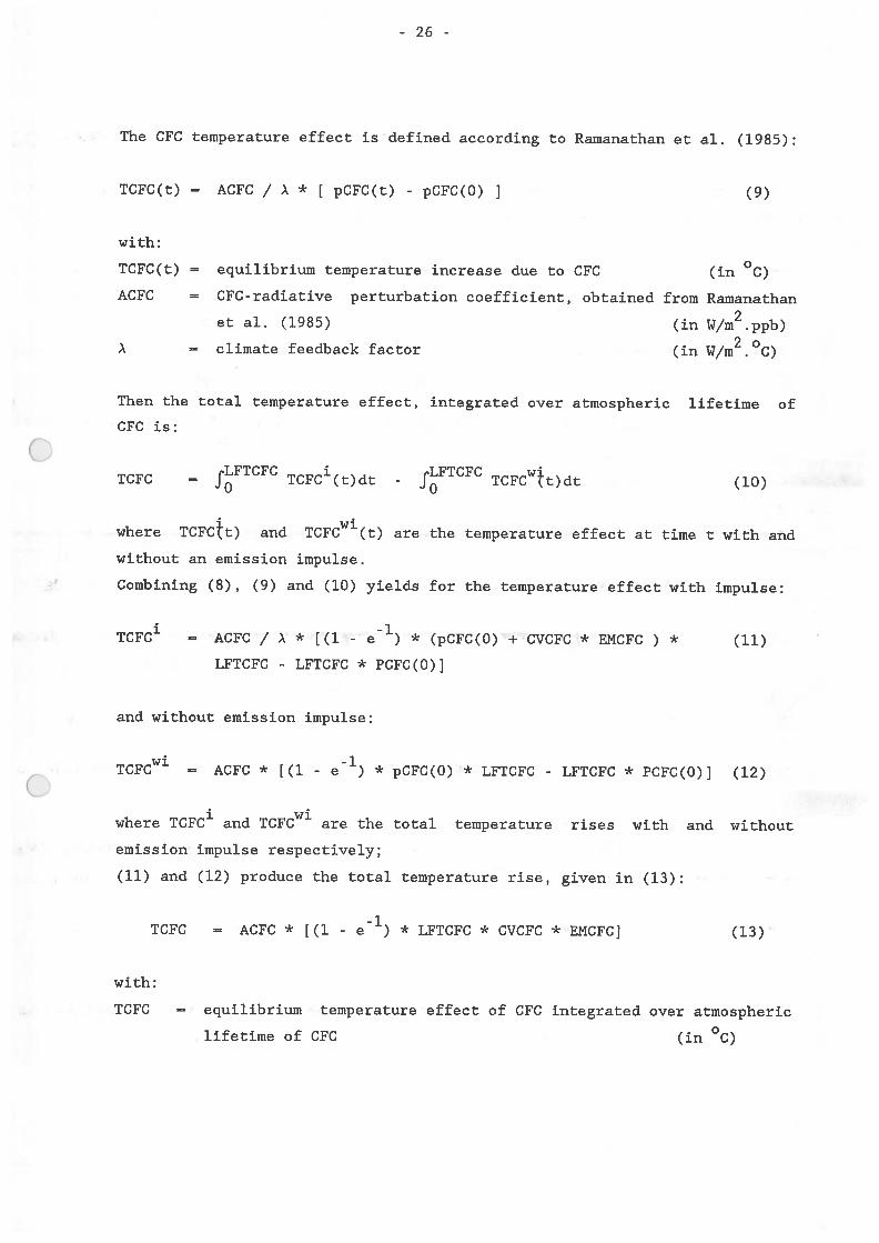
- 26 -

The CFC temperature effect is defined according to Ramanathan et al. (1985):

TCFC(t) = ACFC / ) * [ pCFC(t) - pCFC(O) ] (9)

with:

TCFC(t) = equilibrium temperature increase due to CFC (in °C)

ACFC = CFC-radiative perturbation coefficient, obtained from Ramanathan

et al. (1985) (in W/m2.ppb)

= climate feedback factor (in W/m2.°C)

Then the total temperature effect, integrated over atmospheric lifetime of

CFC is:

TCFC= JLFTCFC

TCFC’(t)dt- fLFTCFC TCFCWtt)dt (10)

where TCFCtt) and TCFC(t) are the temperature effect at time t with and

without an emission impulse.

Combining (8), (9) and (10) yields for the temperature effect with impulse:

TCFC’ ACFC / ). * [(1 - e) * (pCFC(0) + CVCFC * EMCFC ) * (11)

LFTCFC - LFTCFC * PCFC(0)J

and without emission impulse:

TCFCW1= ACFC * [(1 - e) * pCFC(0) * LFTCFC - LFTCFC * PCFC(0)] (12)

where TCFC’ and TCFCW are the total temperature rises with and without

emission impulse respectively;

(11) and (12) produce the total temperature rise, given in (13):

TCFC = ACFC * [(1 - e) * LFTCFC * CVCFC * EMCFC] (13)

with:

TCFC = equilibriwn temperature effect of CFC integrated over atmospheric0lifetime of CFC (in C)

- 27 -

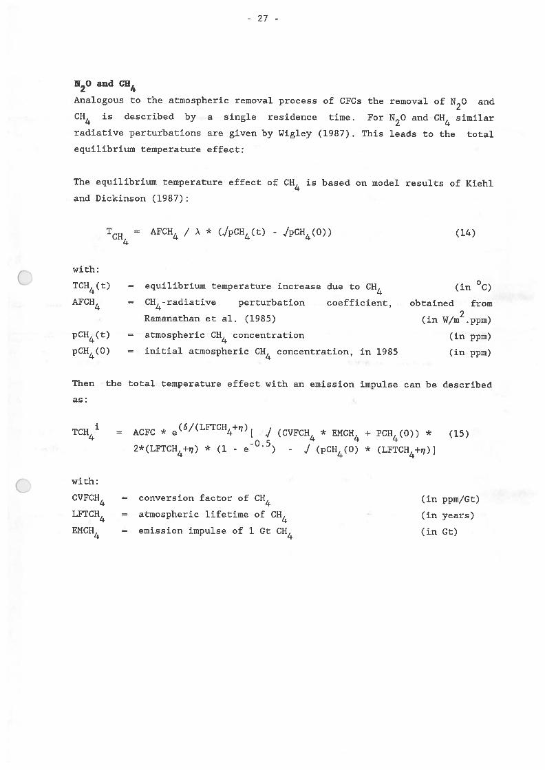
N20 and C114

Analogous to the atmospheric removal process of CFCs the removal of N20 and

CH4 is described by a single residence time. For N20 and CH4 similar

radiative perturbations are given by Wigley (1987). This leads to the total

equilibrium temperature effect:

The equilibrium temperature effect of CH4 is based on model results of Kiehi

and Dickinson (1987):

with:

TCH4(t)

AFCH4

pCH4(t)

pCH4(O)

with:

CVFCH4

LFTCH4

EMCH4

= AFCH4 / ).. * (q”pCH4(t) - JpCH4(O)) (14)

• 0(in C)

obtained from

(in W/m2.ppm)

(in ppm)

(in ppm)

(in

(in

(in

ppm/Gt)

years)

Gt)

= equilibrium temperature increase due to CH4

= CH4-radiative perturbation coefficient,

Ramanathan et al. (1985)

= atmospheric CH4 concentration

= initial atmospheric CH4 concentration, in 1985

Then the total temperature effect with an emission impulse can be described

as:

TCH4’ = ACFC * e(S LFTCH4T)[J (CVFCH4 * EMCH4 + PCH4(O)) * (15)

2*(LFTCH4+,7) * (1 - e°5) - / (pCH4(O) * (LFTCH4+,7)J

= conversion factor of CH4

= atmospheric lifetime of CH4

= emission impulse of 1 Gt CH4

- 28 -

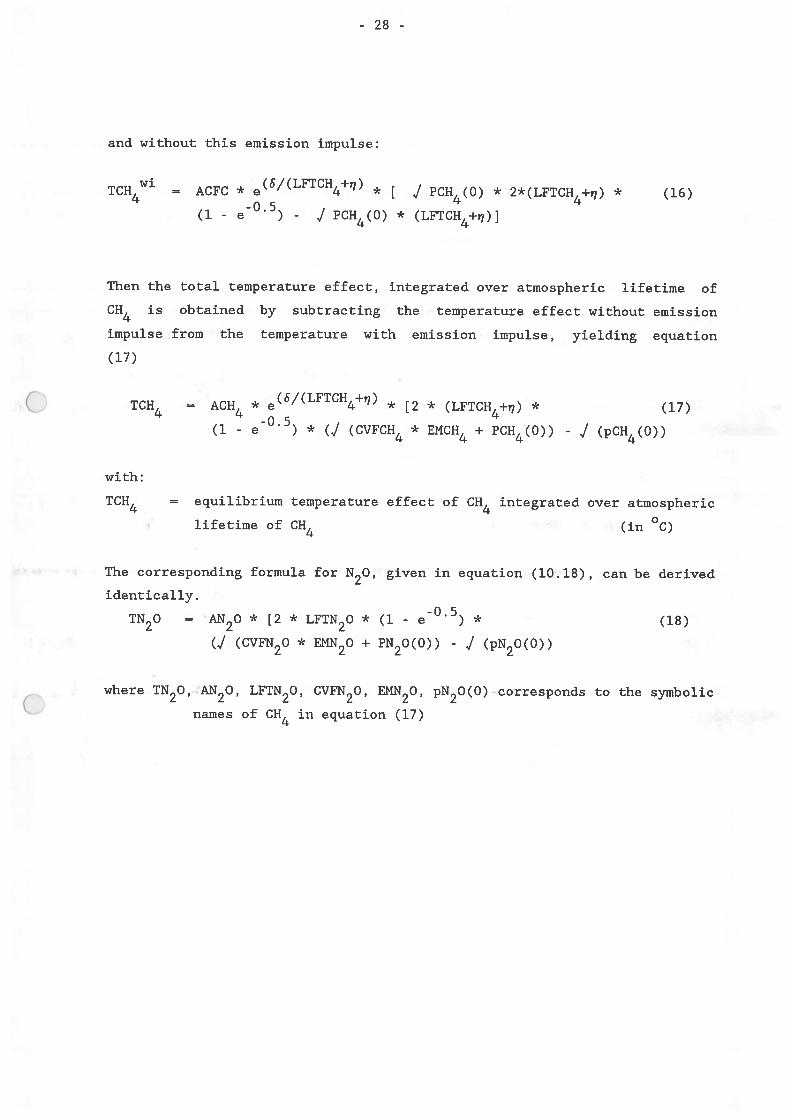
and without this emission impulse:

TCH4W1= ACFC * e(S/ FTCH4-H)

* [ J PCH(O) * 2*(LFTCH4+,7) * (16)

(1- O.5)

- J PCH(O) * (IFTCH4+i7)]

Then the total temperature effect, integrated over atmospheric lifetime of

CH4 is obtained by subtracting the temperature effect without emission

impulse from the temperature with emission impulse, yielding equation

(17)

TCH4 = ACH4 * e(S/ FTCH4+,7)* [2 * (LFTCH4+,7) * (17)

(1 - e°5) * (J (CVFCH * EMCH4 + PCH4(O))- J (pCH(O))

with:

TCH4 = equilibrium temperature effect of CH4 integrated over atmospheric

lifetime of CH4 (in °C)

The corresponding formula for N20, given in equation (10.18), can be derived

identically.

TN2O= 2°

* [2 * LFTN2O * (1 - e°5) * (18)

(J (CVFNO * EMN2O + PN2O(0)) - J (pN0(0))

where TN2O, 201 LFTN2O, CVFN2O, EMN2O, pN2O(O) corresponds to the symbolic

names of CH4 in equation (17)