variability in metric-based assessment of surface waters using ...
224
Transcript of variability in metric-based assessment of surface waters using ...

Stellingen Behorende bij het proefschrift “Fifty shades of grey: variability in metric-based assessment of surface waters using macroinvertebrates” door Hanneke Keizer-Vlek.
1. In Nederland staat biologische beoordeling gelijk aan het standaardiseren van expert-judgement (dit proefschrift).
2. Het werkvoorschrift beschreven in het “Handboek Hydrobiologie” voor het bemonsteren en verwerken van macrofauna monsters verdient niet de kwalificatie ‘standaard’ of ‘uniform’(dit proefschrift).
3. Biologische beoordeling en soortbescherming van zeldzame aquatische macroinvertebraten vragen om verschillende vormen van monitoring (dit proefschrift).
4. Eutrofiëring staat het herstel van Nederlandse oppervlaktewateren nog steeds in de weg.
5. De KRW maatlat hindert het ecologisch herstel van oppervlaktewateren in Nederland.
6. Wanneer vijftig verschillende aquatisch ecologen hetzelfde water beoordelen heeft dat vijftig tinten grijs tot gevolg.
7. Wanneer alle artikelen waarin statistiek wordt toegepast, zouden worden beoordeeld door een statisticus, zouden significant meer artikelen worden afgewezen voor publicatie.
8. In de praktijk wordt regelmatig over het hoofd gezien dat een significante correlatie niet gelijk staat aan causaliteit of een sterk verband tussen twee variabelen.
9. De titel van het proefschrift “Fifty shades of grey” zal in de media meer aandacht krijgen dan de inhoud van het proefschrift.
10. Verhoogde controle van werknemers in crisistijd leidt tot een extra daling van de productiviteit.
199249-st-Keizer-Vlek.indd 1 06-11-13 10:35

Fifty shades of grey
Variability in metric-based assessment of surface waters using macroinvertebrates
The research presented in this thesis was conducted at Alterra in Wageningen, The Netherlands Alterra, part of Wageningen UR, 2014 Alterra Scientific Contributions 44 ISBN: 978-90-327-0402-5 Keizer-Vlek, H.E., 2014. Fifty shades of grey. Variability in metric-based assessment of surface waters using macroinvertebrates. Alterra Scientific Contributions 44, Alterra, part of Wageningen UR, Wageningen. Illustratie omslag: Mariëlle van Riel (tekening), Hanneke Keizer (foto), John Wiltink Layout: Hanneke Keizer-Vlek Drukwerk: Ipskamp Drukkers B.V.
Fifty shades of grey
Variability in metric-based assessment of surface waters using macroinvertebrates
ACADEMISCH PROEFSCHRIFT
ter verkrijging van de graad van doctor aan de Universiteit van Amsterdam op gezag van de Rector Magnificus
prof. dr. D.C. van den Boom ten overstaan van een door het college voor promoties
ingestelde commissie, in het openbaar te verdedigen in de Agnietenkapel
op woensdag 22 januari 2014, te 14:00 uur
door
Hanneke Erica Vlek
geboren te Amsterdam
Promotiecommissie Promotor: Prof. dr. ir. P.F.M. Verdonschot Co-promotor: Prof. dr. H. Siepel Overige leden: Prof. dr. W. Admiraal
Prof. dr. D. Hering Prof. dr. R.K. Johnson Prof. dr. K. Kalbitz Dr. H.G. van der Geest Dr. ir. G.J. van Geest
Faculteit der Natuurwetenschappen, Wiskunde en Informatica

To my parents
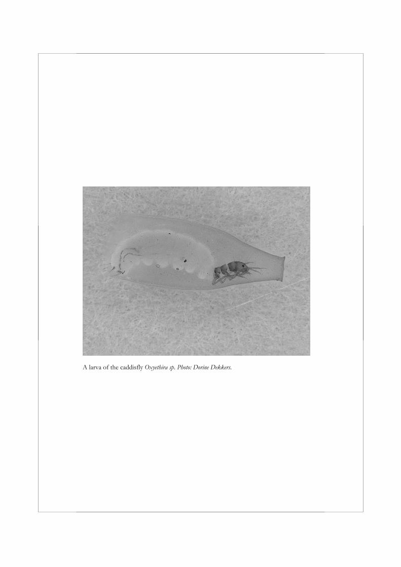
A larva of the caddisfly Oxyethira sp. Photo: Dorine Dekkers.
Contents
Samenvatting 9
Summary 15
1 General introduction 21
2 Towards a multimetric index for the assessment of Dutch streams using benthic macroinvertebrates 35
3 Influence of macroinvertebrate sample size on bioassessment of streams 69
4 Influence of seasonal variation on bioassessment of streams using macroinvertebrates 105
5 Comparison of bioassessment results and costs between preserved and unpreserved macroinvertebrate samples from streams 125
6 Quantifying spatial and temporal variability of macroinvertebrate metrics 143
7 Synthesis 169
Dankwoord 213
Curriculum vitae 215
List of publications 217

Samenvatting
9
Samenvatting
Sinds het begin van de 20ste eeuw zijn diverse methoden ontwikkeld voor de biologische beoordeling van oppervlaktewateren. Biologische beoordeling van oppervlaktewateren wordt vaak gebaseerd op gegevens over de aanwezige macrofaunagemeenschap. Sinds de introductie van de Europese Kaderrichtlijn Water (KRW) in 2000 is iedere lidstaat verplicht om de effecten van menselijke activiteiten op de ecologische toestand van alle oppervlaktewaterlichamen te beoordelen, alsmede in de stroomgebiedsbeheerplannen aan te geven wat de betrouwbaarheid en precisie is van de gegevens die voortkomen uit de monitoringsprogramma’s. In de huidige situatie ontbreekt inzicht in de betrouwbaarheid en precisie van gegevens die voortkomen uit biologische monitoring. Het belangrijkste doel van dit proefschrift is daarom het kwantificeren van de betrouwbaarheid en precisie die gepaard gaat met biologische beoordeling gebaseerd op de macrofaunagegevens, om daarmee richting te geven aan: 1) het proces van metric selectie voor de ontwikkeling van biologische beoordelingssystemen en 2) het proces van standaardisatie ten aanzien van het verzamelen en verwerken van macrofaunamonsters.
Ten tijde van de publicatie van de KRW voldeden de in Nederland beschikbare biologische beoordelingssystemen niet aan de door de KRW gestelde eisen. Hoofdstuk 2 beschrijft daarom de ontwikkeling van een beoordelingssysteem voor langzaam en snel stromende beken in Nederland. Een grote dataset met 949 monsters verzameld door waterbeheerders in verschillende regio’s in Nederland is gebruikt voor de ontwikkeling van een multimetric index. Op basis van zowel abiotische als biotische gegevens is de ecologische toestand van alle locaties geclassificeerd van 1 (slecht) tot 4 (goed) (post-classificatie), door gebruik te maken van een combinatie van multivariate analyse en expert-judgement. Voor beide beektypen (langzaam en snel stromend) zijn meer dan 100 metrics getoetst op hun vermogen om onderscheid te maken tussen beeklocaties van verschillende ecologische toestand. Uiteindelijk zijn 10 metrics geselecteerd voor de beoordeling van langzaam stromende beken en 11 metrics voor de beoordeling van snel stromende beken. De individuele metrics zijn gecombineerd in een multimetric index. Kalibratie toonde aan dat 67% van de monsters uit langzaam stromende en 65% van de monsters uit snel stromende beken werden beoordeeld overeenkomstig post-classificatie. In slechts 8% van de gevallen week de ecologische toestand van een monster na beoordeling meer dan één klasse af van de post-classificatie. De multimetric index is gevalideerd met ‘nieuwe’
Samenvatting
10
gegevens verzameld op 82 locaties. Uit validatie bleek dat 54% van de monsters correct werden geclassificeerd.
Om biologische beoordeling van oppervlaktewateren in Europa te standaardiseren is in het Europese project AQEM een standaard protocol opgesteld voor de bemonstering, het verwerken en het identificeren van macrofauna. In de praktijk is deze AQEM methode erg tijdrovend gebleken, daarom worden in hoofdstuk 3 de gevolgen verkend van een reductie van de omvang van een macrofaunamonster op de precisie en betrouwbaarheid van de resultaten en de kosten van het verzamelen en verwerken van een monster. In vier beken in Nederland en twee beken in Slowakije zijn macrofaunamonsters verzameld. In elke beek zijn met een macrofaunanet 20 sampling units (25 x 25 cm) verzameld van één of twee dominant aanwezige habitats. Op basis van de verzamelde data is voor zes metrics en de in hoofdstuk 2 ontwikkelde multimetric index voor langzaam stromende beken het effect van een toename/afname in monstergrootte op de precisie (variatiecoëfficiënt) en betrouwbaarheid (mean relative deviation from the “reference” sample) onderzocht. De betrouwbaarheid en precisie van de resultaten nam toe met een toename van de monstergrootte. De betrouwbaarheid en precisie varieerden, gegeven monstergrootte x, afhankelijk van het habitat en de metric. Het AQEM protocol schrijft bemonstering van alle aanwezige habitats over een totale lengte van 5 m voor. De resultaten impliceren dat het bemonsteren van minder dan 5 m voldoende is om een CV (variatiecoëfficiënt) en MRD (mean relative deviation) ≤ 10% te bereiken voor de metrics ASPT (Average Score Per Taxon), de Saprobic Index en de metric type Aka+Lit+Psa (%) (het percentage individuen met een voorkeur voor zand en grind). De metrics aantal taxa, aantal individuen en EPT-taxa (%) vereisten een monstergrootte van meer dan 5 m om een CV en MRD ≤ 10% te garanderen. Voor de metrics aantal individuen en het aantal taxa is een multihabitat monster van 5 m zelfs niet voldoende om een CV en MRD van ≤ 20% te bereiken. De MRD van de multimetric index voor langzaam stromende beken kan worden teruggebracht van ≤ 20% naar ≤ 10% met een extra investering van 2 uur. Gezien de relatief lage toename in kosten en de mogelijke gevolgen van een incorrecte beoordeling van de ecologische toestand, wordt aanbevolen om te streven naar een MRD van ≤ 10%. Om een MRD van ≤ 10% te garanderen, zou een multihabitatmonster van de vier habitats bemonsterd in de Nederlandse beken een monstergrootte van 2.5 m vereisen en een inspanning van 26 uur (exclusief identificatie van Oligochaeta en Diptera) of 38 uur (inclusief identificatie van Oligochaeta and Diptera).
Om de kosten van routinematige monitoring te drukken verzamelen waterbeheerders meestal slechts één macrofaunamonster per jaar. Een gebrek
Samenvatting
11
aan standaardisatie van de periode waarin wordt bemonsterd (seizoen), introduceert een bron van variatie in de resultaten van biologische beoordeling. In hoofdstuk 4 wordt daarom de variatie in de samenstelling van de macrofaunagemeenschap tussen maanden bestudeerd, inclusief de effecten hiervan op de variatie in metricwaarden. Voor dit doel zijn om de maand twee macrofaunamonsters (replica’s) verzameld uit de Stupavský potok; een beek van de 4de orde in de Westelijke Karpaten, een gebergte gelegen in Centraal Europa. Een afzonderlijk monster bevatte 42% van alle taxa verzameld gedurende de hele studie. Met behulp van multivariate analyse konden op basis van de samenstelling van de macrofaunagemeenschap duidelijk drie groepen monsters worden onderscheiden: (1) monsters verzameld in April, (2) monsters verzameld Juni en Augustus en (3) monsters verzameld in Oktober, December en Februari. De waarden voor 31 van de 76 metrics waren significant verschillend tussen maanden (p<0.05, α=0.05). Het overgrote deel van de metircs die verschillen in waarden toonden tussen maanden waren kwantitatieve metrics (metrics gebaseerd op (relatieve) aantallen individuen). Bij de toepassing van kwantitatieve metrics bij beoordeling is het daarom belangrijk dat men zich realiseert, dat het seizoen waarin een monster verzameld wordt een groot effect kan hebben op het uiteindelijke resultaat. De verschillen in waarden tussen maanden hangen sterk af van de metric. Dit maakt het moeilijk om een algemene aanbeveling te doen ten aanzien van de maand of het seizoen waarin het beste kan worden bemonsterd. In het geval van metrics die worden gekenmerkt door een grote seizoensvariatie is de beste oplossing om altijd gedurende dezelfde periode te bemonsteren of om rekening te houden met de seizoensvariatie bij het vaststellen van klassengrenzen voor beoordelingsdoeleinden.
Naast seizoensvariatie is de keuze om een monster al of niet te fixeren (het uitzoeken van dode versus levende organismen) een ander aspect van het verzamelen en verwerken van macrofaunamonsters, dat de resultaten van biologische beoordeling kan beïnvloeden in termen van betrouwbaarheid, precisie en kosten. In hoofdstuk 5 worden gefixeerde en niet gefixeerde macrofaunamonsters met elkaar vergeleken. Voor dit doel zijn in drie verschillende laaglandbeken in Nederland ieder zes monsters verzameld, waarvan er drie zijn gefixeerd en drie niet. Afgezien van het al of niet fixeren zijn de monsters allemaal op dezelfde wijze verzameld en verwekt. Het aantal Ephemeroptera individuen, Hydracarina taxa en individuen verschilde significant tussen gefixeerde en niet gefixeerde monsters. Wanneer bij biologische beoordeling specifiek gebruik wordt gemaakt van deze individuele metrics is het daarom noodzakelijk het al of niet fixeren van monsters te standaardiseren. In beken met Ephemeroptera is het fixeren van monsters
Samenvatting
12
noodzakelijk om het aantal verzamelde Ephemeroptera individuen te optimaliseren. Daarentegen, in beken met Hydracarina leidt het fixeren van monsters tot een onderschatting van het aantal aanwezige Hydracarina taxa en individuen. Slechts in één geval werd een verschil in ecologische toestand geconstateerd tussen gefixeerde en niet gefixeerde monsters. Dit is een aanwijzing dat de beoordeling van Nederlandse beken, met het in hoofdstuk 2 ontwikkelde beoordelingssysteem, niet vereist dat het protocol voor het verzamelen en verwerken van macrofaunamonsters richtlijnen omvat betreffende het al of niet fixeren van monsters. We hebben geen significante verschillen ontdekt in de kosten voor het verwerken van gefixeerde en niet gefixeerde monsters.
Sinds de introductie van de Habitatrichtlijn en de Kaderrichtlijn Water zijn waterschappen verplicht om veranderingen in de natuurwaarde/ecologische toestand te monitoren op grote ruimtelijke schaal (bijvoorbeeld op het niveau van waterlichamen in plaats van locaties). Daarnaast zijn ze verplicht om in de stroomgebiedsbeheerplannen een schatting te geven van de betrouwbaarheid en precisie van de resultaten die worden verkregen uit de monitoring (European Commission, 2000). Momenteel hebben waterbeheerders weinig inzicht bij in de betrouwbaarheid en precisie van monitoringsgegevens. Om dit inzicht te vergoten wordt in hoofdstuk 6 de ruimtelijke en temporele variatie gekwantificeerd voor zeven metrics gebaseerd op taxonomische rijkdom. Voor dit doel zijn in 25 meso-eutrofe sloten in het natuurgebied de Wieden gedurende drie opeenvolgende jaren macrofaunamonsters verzameld. Uit deze studie blijkt duidelijk dat het in het algemeen makkelijker is om veranderingen in een slotencomplex te ontdekken gebaseerd op metrics dan op individuele soorten. De inspanning die nodig is om individuele (zeldzame) soorten te monitoren impliceert automatisch, dat gegevens verzameld door waterbeheerders voor KRW-doeleinden niet bruikbaar zijn voor natuurbeheerders. Wanneer men geïnteresseerd is in individuele (zeldzame) soorten, dan is het noodzakelijk om de wijze van bemonstering specifiek op deze soorten te richten, om zo de trefkans van de soort te vergrootten. Als gevolg van de grote ruimtelijk variatie zal, ongeacht de metric die wordt toegepast bij beoordeling, een grote inspanning noodzakelijk zijn om veranderingen te kunnen constateren (bijvoorbeeld als gevolg van herstelmaatregelen) in een slotencomplex als de Wieden. Het is daarom noodzakelijk om de mogelijkheden te onderzoeken voor het toepassen van alternatieve, meer kosteneffectieve methoden voor het verzamelen en verwerken van macrofaunamonsters in biologische monitoringsprogramma’s.
Samenvatting
13
In dit proefschrift wordt aangetoond dat de variatie in de waarden van metrics, die worden toegepast bij biologische beoordeling, vaak groot is. Bovendien is de omvang van de variatie afhankelijk van het watertype, seizoen (bemonsteringsperiode) en de toegepaste methode voor het verzamelen en verwerken van monsters. Hierdoor is het moeilijk om een ‘universeel’ advies te geven ten aanzien van metrics die het ‘’beste’ kunnen worden opgenomen in een beoordelingssysteem en wat de optimale keuzes zijn in relatie tot het standaardiseren van het verzamelen en verwerken van macrofaunamonsters. We moeten ons echter realiseren dat de omvang van de variatie niet alleen in de biologie een uitdaging vormt bij het opzetten van monitoringsprogramma’s. Hoewel de variatie in biologische data groot is, kan de ruimtelijke en temporele variatie in fysische en chemische variabelen net zo goed groot zijn (Veeningen, 1982). We kunnen deze variatie het hoofd bieden door aan de ene kant meer inzicht te verkrijgen in het functioneren van het aquatische ecosystemen en het ontrafelen van oorzaak-gevolg relaties en aan de andere kant door het ontwikkelen van meer kosteneffectieve methoden van monitoren. Een oplossing om de variatie op korte termijn te reduceren en de betrouwbaarheid van de huidige beoordelingssystemen te verbeteren, is het implementeren van procedures voor kwaliteitsborging en -controle. In Groot-Brittannië zijn dergelijke procedures al geïmplementeerd en is de effectiviteit ervan bewezen. In Nederland is verder standaardisatie van methoden voor het verzamelen en verwerken van monsters vereist, zeker op het vlak van de inspanning bij het uitzoeken. Daarnaast moet personeel worden getraind in het verzamelen en uitzoeken van monsters en moeten audits worden afgenomen op het vlak van determinatie en het uitzoeken van monsters. Op de lange termijn moeten waterbeheerders het toepassen van ‘probability sampling’ overwegen om statistisch betrouwbare uitspraken op nationale schaal of de schaal van een waterlichaam mogelijk te maken. ‘Probability sampling’ in combinatie met een relatief goedkope methode voor het verzamelen en verwerken van monsters om de ecologische toestand van oppervlaktewateren te beoordelen (Quick Scan) zal resulteren in meer kosteneffectieve monitoringsprogramma’s.

Summary
15
Summary
Since the beginning of the 20th century, a wide variety of methods have been developed for the biological assessment of surface waters. Macroinvertebrates are a commonly applied taxonomic group for assessing water quality. Since the introduction of the European Water Framework Directive (WFD) in 2000, every member state is obligated to assess the effects of human activities on the ecological quality of all water bodies and indicate the level of confidence and precision of the results provided by the monitoring programs in their river basin management plans (European Commission, 2000). Currently, the statistical properties associated with aquatic monitoring programs are often unknown. Therefore, the overall objective of this thesis is to quantify the variability and accuracy associated with biological assessment based on macroinvertebrates in order to guide (1) the process of metric selection in the development of biological assessment systems and (2) the process of standardizing sampling and sample processing.
At the time the WFD was published, the biological assessment system(s) applied in the Netherlands did not meet the criteria for biological assessment systems set by the WFD. Chapter 2 describes the development of a macroinvertebrate-based WFD compliant biological assessment system for fast and slow running streams in the Netherlands. A large dataset of 949 samples collected by water authorities from different regions in the Netherlands was used to construct a multimetric index. All sites received an ecological quality (post-) classification ranging from 1 (bad status) to 4 (good status) based on biotic and abiotic variables using a combination of multivariate analysis and expert judgment. More than 100 hundred metrics were tested for both stream types to examine their power to discriminate between streams of different ecological quality. Finally, 10 metrics were selected for the assessment of slow running streams and 11 metrics for the assessment of fast running streams. The individual metrics were combined into a multimetric index. Calibration showed that 67% of the samples from slow running streams and 65% of the samples from fast running streams were classified in agreement with their post-classification. In total, only 8% of the samples differed more than one quality class from the post-classification. The multimetric index was validated with ‘new’ data collected from 82 sites. Validation showed that 54% of the streams were classified correctly.
In order to standardize the biological assessment of surface waters in Europe, a standardized method for sampling, sorting, and identifying benthic
Summary
16
macroinvertebrates in running waters was developed during the AQEM project. The AQEM method has proved to be relatively time-consuming. Chapter 3 explores the consequences of reducing sample size on the variability, accuracy, and costs of bioassessment results. Macroinvertebrate samples were collected from six different streams: four streams located in the Netherlands and two in Slovakia. Twenty sampling units were collected from one or two dominant habitats in each stream using a pond net (25 x 25 cm) over a length of approximately 25 cm per sampling unit. The effect of increasing sample size on variability and accuracy was examined for six metrics and the multimetric index developed in Chapter 2 for the assessment of Dutch slow running streams. The accuracy of metric results increased and variability decreased with increasing sample size. In addition, accuracy and variability varied depending on the habitat and metric. The AQEM sampling method prescribes a multihabitat sample of 5 m. The results suggest that a sample size of less than 5 m is adequate to attain a coefficient of variation (CV) and mean relative deviation (MRD) of 10% or less for the metrics Average Score Per Taxon (ASPT), Saprobic Index, and the percentage of individuals with a preference for the akal, littoral, and psammal (type Aka+Lit+Psa (%)). The metrics number of taxa, number of individuals, and EPT-taxa (%) required a multihabitat sample size of more than 5 m to attain a CV and MRD of ≤ 10%. For the metrics number of individuals and number of taxa, a multihabitat sample size of 5 m is not adequate to attain a CV and MRD of ≤ 20%. The accuracy of the multimetric index for Dutch slow running streams can be increased from ≤ 20% to ≤ 10% by increasing labor time by 2 hours. Considering this low increase in cost and the possible implications of incorrectly assessing the results, striving for this ≤ 10% accuracy is recommended. To achieve an accuracy of ≤ 10%, a multihabitat sample of the four habitats studied in the Netherlands requires a sample size of 2.5 m and a labor time of 26 hours (excluding identification of Oligochaeta and Diptera) or 38 hours (including identification of Oligochaeta and Diptera).
To reduce the costs of surveillance monitoring, water managers often collect only one sample a year. A lack of standardization of the sampling period (season) introduces a source of variation in bioassessment results. In Chapter 4, the monthly variation in the composition of the macroinvertebrate community is examined, including the effect this has on variations in metric values. For this purpose, two replicate samples were collected every other month for one year from a fourth order calcareous stream in the western Carpathian Mountains of central Europe, the Stupavský potok brook. Any single replicate contained, on average, 42% of the total number of taxa collected during this study. Multivariate analysis of the macroinvertebrate
Summary
17
communities clearly separated the samples into three groups: (1) April samples, (2) June and August samples, and (3) October, December, and February samples. Thirty-one of 76 metrics showed significant (p<0.05, α=0.05) differences between months. The majority of metrics exhibiting significant differences between months were quantitative metrics (i.e., metrics based on the relative abundance of a particular taxonomic group). The CV of most qualitative metrics did not exceed 20%. However, the highest CV values (above 40%) were found in most cases for the quantitative metrics. Thus, when using quantitative metrics, it is important to recognize that the season in which samples are collected can, and often will, have a strong influence on the results. In terms of individual metrics, differences between months strongly depend on the metric being evaluated. This makes it difficult to recommend a preferred sampling month or season. For metrics with high seasonal variation, the best solution is to always sample during the same month or to take into account seasonal variation when setting class boundaries for assessment purposes.
Another aspect of sampling and sample processing, which may influence bioassessment results in terms of variability, accuracy, and cost, is the choice of whether or not to use a preservative before sorting macroinvertebrate samples (i.e., dead specimens vs. living specimens). In Chapter 5, preserved and unpreserved samples collected from three lowland streams in the Netherlands were compared using identical sample processing protocols. Significantly different numbers of Ephemeroptera individuals and Hydracarina taxa and individuals were collected from preserved samples compared to unpreserved samples. In assessments based on these individual metrics, sample processing will need to be standardized. In streams with Ephemeroptera, the preservation of samples is necessary to optimize the number of Ephemeroptera individuals collected. In streams that contain Hydracarina, the preservation of samples will result in an underestimation of the number of Hydracarina taxa and individuals. A difference in ecological quality between preserved and unpreserved samples was observed in only one case, indicating that assessing small Dutch lowland streams does not require standardization of sample preservation in the sample processing protocol. We did not detect significant differences in sample processing costs between preserved and unpreserved samples.
Since the introduction of the Habitat Directive and the WFD, water authorities are obliged to monitor changes in conservation value/ecological quality on larger spatial scales (as opposed to site scale) and, indicate the level of confidence and precision of the results provided by the monitoring programs in their river basin management plans (European Commission,
Summary
18
2000). To increase insight into the statistical properties associated with aquatic monitoring programs, the spatial and temporal variability of taxonomic richness metrics were quantified in Chapter 6. We collected macroinvertebrate samples from 25 meso-eutrophic drainage ditches located in the Wieden natural preserve in the Netherlands and selected seven taxonomic richness metrics for the evaluation of spatial and temporal variability. The results from this study clearly indicated that, in general, it is easier to detect changes in a drainage ditch network based on metrics than on individual species. The required monitoring effort for rare species automatically implies that data collected by water authorities in biomonitoring programs developed to meet the requirements of the WFD will not meet the requirements of conservation managers. When interested in an individual species, sampling methods will have to be adjusted to the specific species in order to increase the frequency of collection. Irrespective of the metric applied, a large effort will be required to detect changes within the drainage ditches of the Wieden due to high spatial variability. Therefore, we need to explore the possibilities of applying alternative, more cost-effective methods for sampling and sample processing in biomonitoring programs.
This thesis shows that the variability in metric values applied in biological assessment is often high. Also, the variability in metric values varies between stream types, season (sampling period), and the sampling and sample processing method, making it difficult to give ‘universal’ advice on metrics to be included in biological assessment systems and optimal choices regarding the standardization of sampling and sample processing. However, high variability is not solely an issue of biology. Although the variation in biological data can be high, the temporal and spatial variation in physical and chemical variables can also be high (Veeningen, 1982). We should face the issue of high variability by gaining a better understanding of ecosystem functioning and unraveling cause-effect mechanisms, as well as by developing more cost-effective sampling and sample processing methods. A short-term solution to reduce variability and improve the performance of currently applied assessment systems in the Netherlands would be the implementation of quality assurance and quality control procedures, which have been successful in the United Kingdom. Apart from training personnel in sampling and sorting and performing audits of identification and sorting, additional standardization of the sampling and sample processing protocol is required, especially in terms of sorting effort. In the long run, water managers need to consider applying probability sampling to draw statistically sound conclusions at water body/national level. Combining probability sampling with a relatively cheap

Summary
19
sampling and sample processing method to assess ecological status (‘Quick Scan’ method) will result in more cost-effective monitoring programs.

Chapter 1
21
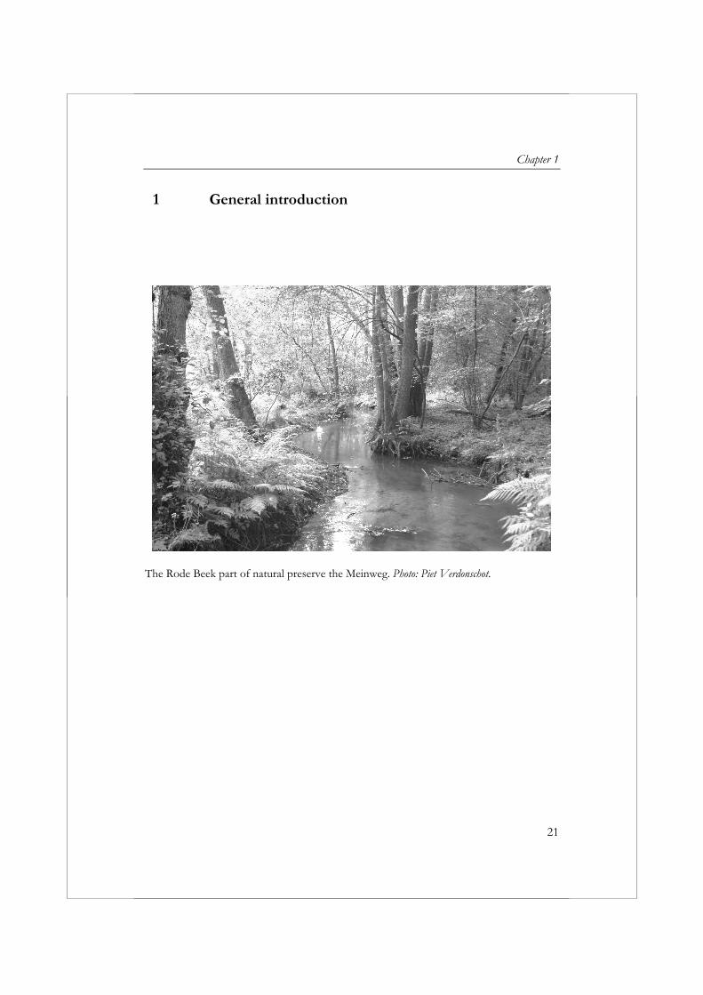
1 General introduction
The Rode Beek part of natural preserve the Meinweg. Photo: Piet Verdonschot.
General introduction
22
1 General introduction
History of biological assessment based on macroinvertebrates Since the beginning of the 20th century, a wide variety of methods have been developed for biological assessment of surface waters. Macroinvertebrates are a commonly applied group of organisms for assessing water quality (e.g., Hawkes, 1979; Hellawell, 1986; Bailey et al., 2001; Hering et al., 2006). Many authors have stressed the advantages of using macroinvertebrates compared to other groups for biological monitoring and assessment purposes (e.g., Hellawell, 1986; Metcalfe, 1989). First, their intermediate life span makes it possible for them to exhibit a relatively quick response to stress (compared to macrophytes) while simultaneously reflecting ‘past’ environmental conditions (compared to algae). Second, their relatively sedentary lifestyle makes them representative of local conditions. Third, because of the heterogeneity of the macroinvertebrate community, the community will likely respond to a wide range of stressors. As such, macroinvertebrates are able to exhibit an integrative response to a combination of stressors.
With their Saprobien system, Kolkwitz & Marsson (1909) were the first in Europe to introduce the concept of organisms as indicators of environmental conditions. The Saprobien system was developed to detect organic pollution. Since its introduction the Saprobien system has been extended and revised by numerous European ecologists (Liebmann, 1951; Sládeček, 1965). In Germany, the Netherlands, and the Czech Republic the focus was mainly on improving the Saprobien system, but in countries such as Belgium, France, and the United Kingdom, ‘score systems’ focusing on the detection of general degradation were developed. Score systems such as the Trent Biotic Index (Woodiwiss, 1964) and the Indice Biotique (Tuffery & Verneaux, 1968) were developed in the 1960s following the introduction of the first diversity indices in the 1940s. Later, multivariate approaches, such as RIVPACS (Wright et al., 1984) in the UK and EKOO (Verdonschot, 1990) in the Netherlands, were introduced.
Developments comparable to those in Europe took place in the United States. In the 1980s, a multimetric index for fish was introduced in the United States(Karr, 1981). This was an approach to assessment not generally known in Europe. A multimetric index consists of a combination of several metrics, each providing different ecological information about the observed community and acting as an overall indicator of the biological integrity of a water resource. The
Chapter 1
23
strength of the multimetric index is its ability to integrate information from individual, population, community, and ecosystem levels (Karr & Chu, 1999). A multimetric index provides detection capability over a broad range of stressors, creating a more complete picture of the ecosystem than single biological indicators (Intergovernmental Task Force on Monitoring Water Quality, 1993). Throughout this thesis the word metric is used to refer to any measure that can be calculated based on a sample from the macroinvertebrate community (e.g., the percentage of rheophilic species, Average Score Per Taxon, and German Saprobic Index) and a multimetric index is defined as the combination of two or more metrics to obtain a final assessment.
Rosenberg & Resh (1993) listed seven different approaches for assessing streams by using macroinvertebrates: richness measures, enumerations, diversity indices, similarity indices, biotic indices, functional feeding group measures, and the multimetric approach. In the Netherlands, only biotic indices focusing on the detection of organic pollution have been applied widely, and multivariate approaches have been developed (Verdonschot & Nijboer, 2000).
The first biotic indices applied in the Netherlands were those developed by Kolkwitz & Marsson (1909) and Sládeček (1973). These were already existing saprobic indices developed to detect organic pollution in Mid-European streams. It soon became clear that Dutch streams often possess distinctive features that require a different approach to assessment. For example, the current velocity in most Dutch streams is considerably lower than that of streams in other more mountainous European countries. These experiences initiated the development of a Dutch assessment system for organic pollution in lowland streams (Moller Pillot, 1971). The K135-index (Tolkamp & Gardeniers, 1971) was based on the Moller Pillot classification (Moller Pillot, 1971) and used for decades.
The biotic indices discussed above are generally limited to a single impact factor, namely organic pollution. The disadvantage of an index reflecting a single aspect of the stream is that it may fail to reveal the effects of other or combined impact factors (Fore et al., 1994; Barbour et al., 1996). This problem was overcome by the introduction of EBEOSWA (ecological assessment of running waters) (Stichting Toegepast Onderzoek Waterbeheer, 1992), a system for the biological assessment of Dutch streams. EBEOSWA assesses more than one impact factor; as such it can be qualified as a multimetric index. The system considers metrics related to stream velocity, saproby, trophy, functional feeding groups, and substrate. The disadvantages of the system are separate scores for each metric instead of one final classification for a location and not determining the ecological status of a water
General introduction
24
body by comparing the actual status of a body with near-natural reference conditions. Furthermore, EBEOSWA is based on data collected in the 1980s. These data comprised mainly impacted sites, and collection and identification was not performed in a standardized manner. Also, EBEOSWA has never been validated or subjected to peer review.
The European Water Framework Directive (WFD) has led to a demand for a ‘new’ Dutch assessment system. With the implementation of the WFD, every EU member state is obligated to assess the effects of human activities on the ecological quality of all water bodies. The criteria set by the WFD for the assessment of streams are (European Commission, 2000): the use of different biological water quality elements: benthic
invertebrate fauna, macrophytes and phytobenthos, phytoplankton, fish fauna;
the ecological status of a water body is determined by comparing the composition of the biological community in the investigated body with near-natural reference conditions;
it is based on a stream-type specific approach; the final classification of water bodies ranges from 5 (high status) to 1
(bad status).
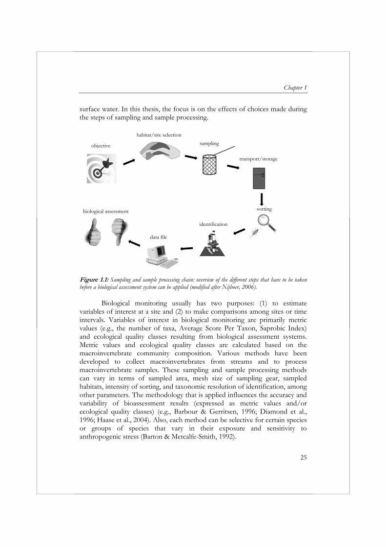
One of the objectives of this thesis is to develop and test a multimetric index for Dutch streams based on macroinvertebrates that meets the criteria of the WFD. Chapter 2 describes the development and validation of this multimetric index.* Variation and accuracy in biological monitoring Before the biological condition can be assessed at a site, samples from the macroinvertebrate community present at the site will have to be collected and processed. The collection and processing of macroinvertebrate samples consists of a sequence of steps (Fig. 1.1). Each step in this sampling and sample processing chain represents choices that have to be made, such as “Do we sample all habitats?” and “Do we identify to genus or species level?” Depending on the choice, the actual composition and condition of the macroinvertebrate community may be misinterpreted (Diamond et al., 1996). The choice will influence the final result, the taxa list, including the number of individuals per taxon. Because biological assessment is based on this taxa list, results can vary based on the choices made during sampling and sample processing. Nijboer (2006) focused on the effects of choices made during data analysis on the results of an ecological typology or assessment system for
* Since the introduction of the mulitimetric index described in Chapter 2 a WFD compliant bioassessment system has been developed that can be applied to most types of Dutch surface waters: the ‘KRW maatlatten’(Van der Molen et al., 2012).
Chapter 1
25
surface water. In this thesis, the focus is on the effects of choices made during the steps of sampling and sample processing.
habitat/site selection
objective
transport/storage
sorting
identification
sampling
data file
biological assessment
Figure 1.1: Sampling and sample processing chain: overview of the different steps that have to be taken before a biological assessment system can be applied (modified after Nijboer, 2006).
Biological monitoring usually has two purposes: (1) to estimate variables of interest at a site and (2) to make comparisons among sites or time intervals. Variables of interest in biological monitoring are primarily metric values (e.g., the number of taxa, Average Score Per Taxon, Saprobic Index) and ecological quality classes resulting from biological assessment systems. Metric values and ecological quality classes are calculated based on the macroinvertebrate community composition. Various methods have been developed to collect macroinvertebrates from streams and to process macroinvertebrate samples. These sampling and sample processing methods can vary in terms of sampled area, mesh size of sampling gear, sampled habitats, intensity of sorting, and taxonomic resolution of identification, among other parameters. The methodology that is applied influences the accuracy and variability of bioassessment results (expressed as metric values and/or ecological quality classes) (e.g., Barbour & Gerritsen, 1996; Diamond et al., 1996; Haase et al., 2004). Also, each method can be selective for certain species or groups of species that vary in their exposure and sensitivity to anthropogenic stress (Barton & Metcalfe-Smith, 1992).
General introduction
26
Accuracy and variability are both important aspects of bioassessment. Variability refers to the extent to which data points in a statistical distribution or data set diverge from the average or mean value. Accuracy refers to the closeness of a measurement to its true value (Norris et al., 1992). Therefore, differences in accuracy between methods may result in different bioassessment results. Differences in accuracy depend on the spatial and temporal scale at which the true value is defined - a method might be accurate at representing the organisms present in a sample, but less accurate at representing the biota at a site. Variability is important when making comparisons because the validity of conclusions depends on data variability (Norris et al., 1992); higher variability increases the probability of incorrect bioassessment results. An increase in accuracy or a reduction in variability is not always possible because the associated costs are often high. However, when assessing ecological quality for biological monitoring purposes, catching all organisms or taxa present at a site is not necessary (Barbour & Gerritsen, 1996). The standardization of sampling is required, though, for valid comparisons among sites and points in time (Courtemanch, 1996; Vinson & Hawkins, 1996). Thus, the question to focus on is which steps of sampling and sample processing need to be standardized. When two methods are equally variable and provide comparable bioassessment results, standardization is not necessary. Extensive evidence indicates that at least two steps in the sampling and sample processing chain require standardization when metrics based on taxa richness are considered: the sampled area and the effort spent sorting samples. For example, several studies have shown that the number of taxa collected from a sample increases asymptotically with an increase in sampled area and/or sorting effort (e.g., May, 1975; Verdonschot, 1990; Colwell & Coddington, 1995; Vinson & Hawkins, 1996).
In addition to accuracy and variability, cost plays an important role in decision-making related to method standardization. The cost of collecting and processing macroinvertebrate samples is high and can depend strongly on the sampling technique used (e.g., Barbour & Gerritsen, 1996; Metzeling et al., 2003; Vlek et al., 2006). Higher variability and lower accuracy increases the risk of incorrect assessment results. In the case that ecological quality at a site is incorrectly assessed as less than good, water managers will unnecessarily take costly restoration measures to reach a good ecological quality by 2015 (European Commission, 2000). From this point of view, the consequences of poor decision-making due to low accuracy and/or high variability potentially outweighs the savings associated with a less time consuming sampling and sample processing method (Doberstein, 2000).
Chapter 1
27
Information on variability and accuracy is not only important in relation to the standardization of sampling and sample processing methods, but this information can also play an important role in deciding which metrics to incorporate in a biological assessment system. Metrics that exhibit relatively high variability will have more problems discerning signal (sensitivity to anthropogenic stress) from noise (variability).
Since the introduction of the WFD, water authorities have been obliged to monitor changes in ecological quality on larger spatial scales as opposed to site scale and to indicate the level of confidence and precision of the results provided by the monitoring programs in their river basin management plans (European Commission, 2000). To meet these requirements, the statistical power of the monitoring programs should be analyzed. The statistical properties associated with freshwater monitoring programs are often unknown. Power analysis (assessing the ability of a program to accurately detect change) could help avoid unnecessary expenditures for monitoring programs that cannot provide meaningful results or that lead to overspending. The statistical power of monitoring programs depends, in part, on the variability of biological assessment results.
Given the importance of accuracy, variability, and cost in the decision-making process, one of the main objectives of this thesis is, to gain insight into the variability/accuracy of individual metrics in order to guide (1) the process of metric selection in the development of biological assessment systems and (2) the process of standardizing sampling and sample processing. Three different steps from the sampling and sample processing chain that can influence the variability/accuracy of assessment results were studied: sample area (Chapter 3), sampling period (Chapter 4), and the use of preservative before sorting samples (i.e., dead specimens vs. living specimens) (Chapter 5).
In Chapter 3 the implications of a change in (physical) sample size, or sample area, on the variability and accuracy of metric values, bioassessment results, and costs is studied. In order to standardize the biological assessment of surface waters in Europe, a standardized method for sampling, sorting, and identifying benthic macroinvertebrates in running waters was developed during the AQEM project (AQEM consortium, 2002). The AQEM method is relatively time-consuming. Thus, the study described in Chapter 3 explores the consequences of reducing the sample size in regards to cost and bioassessment results. In Chapter 4 the effect of seasonal variation in macroinvertebrate community composition on metric values is studied. National monitoring protocols are available in many European countries (e.g., Spain, Sweden, Slovakia, Germany, The Netherlands). All these protocols dictate when to collect macroinvertebrate samples, but in most cases scientific evidence for the
General introduction
28
indicated time period is lacking. Chapter 5 deals with whether significant differences exist in the metric values, bioassessment results, and costs of sample processing between preserved (i.e., sorting dead specimens) and unpreserved (i.e., sorting living specimens) samples (accuracy). In the few studies that compared sorting results between preserved and unpreserved samples, unpreserved samples were sorted in the field and preserved samples were sorted in the laboratory (e.g., Humphrey et al., 2000; Metzeling et al., 2003; Haase et al., 2004; Nichols & Norris, 1996). The findings of these studies are the result of field sorting and other aspects of sample processing rather than sorting living specimens. Therefore, sorting under laboratory conditions is studied in this thesis.
Whereas chapters 3, 4, and 5 deal with specific aspects of sampling and sample processing and their influence on variability and accuracy, Chapter 6 deals with the subject of variability from a broader perspective. The main objective of this chapter is to quantify the spatial and temporal variability of taxonomic richness metrics based on macroinvertebrates in a minimally impaired system of drainage ditches. This information makes it possible to determine the minimum number of monitoring sites required to detect changes due to anthropogenic disturbances and/or restoration measures (power analysis). Conservation ecology The assessment of biological quality has a long history in freshwater ecosystems. With the introduction of the WFD and the Clean Water Act this focus has become even stronger in Europe and the United States, respectively. In terms of macroinvertebrates, the assessment and monitoring of freshwater ecosystems is focused primarily on sampling the “complete” community. Terrestrial ecosystem monitoring is focused primarily on the conservation of species diversity in general, and more specifically on the conservation of rare or threatened species. Because monitoring all species is not feasible in terms of cost, a selection of individual species is used to represent the integrity of the complete ecosystem (Manley et al., 2004). As stated by Maxwell & Jennings (2005), composite indicators composed of several species have the disadvantage that positive trends in some species can mask negative trends in other species. Thus, the extinction of individual species could occur without being noticed, which might be judged as unacceptable by conservation managers. Water managers, on the other hand, are generally more interested in changes in the ecological status of macroinvertebrate communities than changes in the presence/absence or numeric abundance of individual species.
Chapter 1
29
One reason for this is that natural variability in community metrics is generally much lower than natural variability in the presence-absence and numeric abundance of individual species (Fore et al., 1996). Another reason is that water managers often reason that the disappearance of individual species does not necessarily cause significant biological effects on the functioning of a complete community (e.g., Chapin et al., 1997; Holling, 1973).
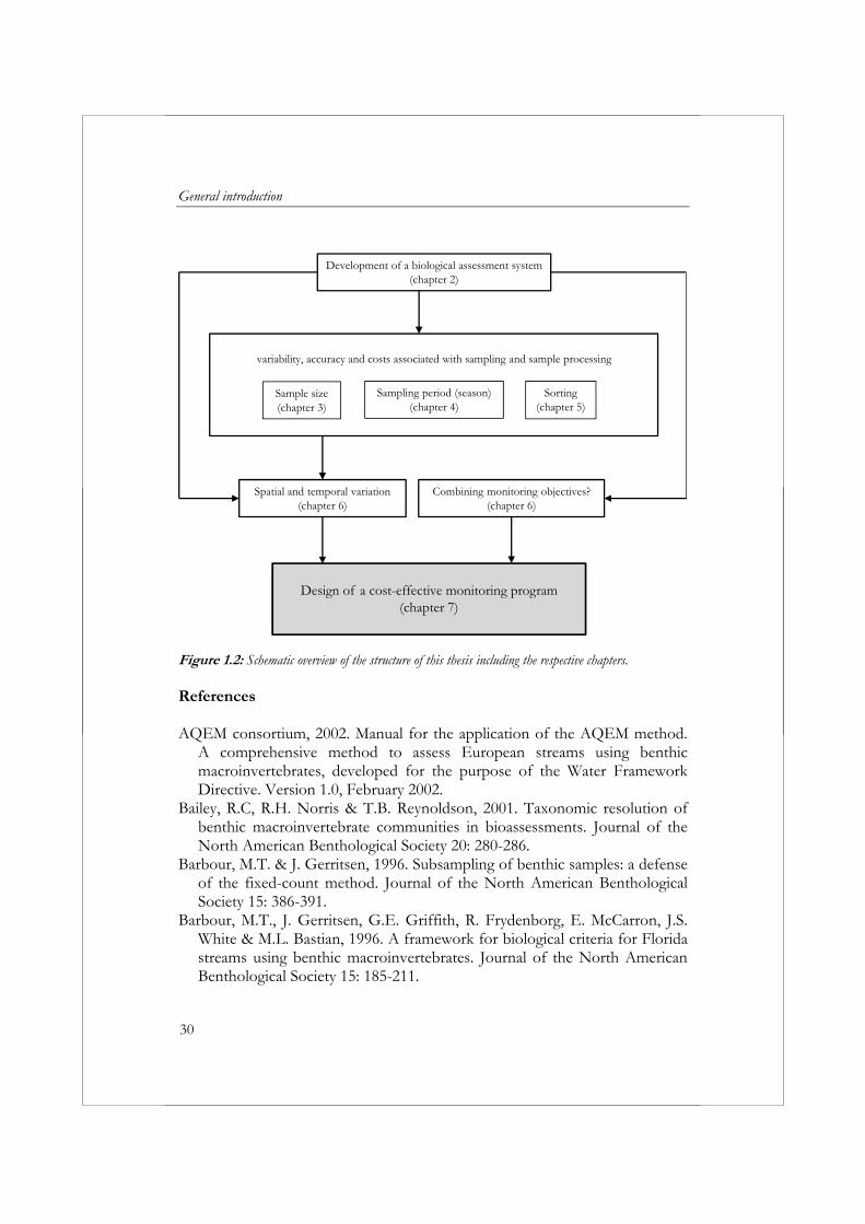
Thomas (2005) concluded that no nationally reliable monitoring schemes exist for estimating long-term (i.e., 20+ years) changes in freshwater invertebrate species frequency and distribution. In the Netherlands, the introduction of the Red Data Books for Ephemeroptra, Plecoptera, Trichoptera, and Tricladida (Verdonschot et al., 2003) and the obligation arising from the Habitat Directive to report the first assessment of the conservation status of all habitats and species of Community interest, have led to an increased demand for information about the frequency and distribution of individual freshwater invertebrate species. To make monitoring programs cheaper in the future, it is an important question whether samples collected for the purpose of assessing ecological quality of surface waters, can also be used to provide conservation managers with reliable information on individual freshwater invertebrate species. Thomas (2005) already recommended that conservation organizations can take advantage of the existing monitoring programs for the biological assessment of surface waters to monitor changes in freshwater invertebrate biodiversity. Therefore, the study described in Chapter 6 aimed to determine whether water authorities’ current monitoring programs can provide the information on trends in the frequency and distribution of individual freshwater invertebrate species required by conservation mangers. Finally, a synthesis of the preceding chapters is provided in Chapter 7. The implications of the results from the previous chapters on the design of cost-effective monitoring programs will be discussed. Here, the question of how the results from this thesis can be applied to guide (1) the process of metric selection in the development of biological assessment systems and (2) the process of standardizing sampling and sample processing is addressed. Furthermore, Chapter 7 deals with some other important issues in biological assessment: (1) the need for biological assessment in addition to assessment based on physical and chemical water quality variables, (2) the lessons that can be learned from the development of biological assessment systems in the past and present, (3) the lack of diagnostic power of current biological assessment systems, and (4) the role of species traits in developing ‘new’ tools for biological assessment. Figure 1.2 provides a schematic overview of the structure of this thesis, including the relationships between the different chapters.
General introduction
30
Development of a biological assessment system
(chapter 2)
variability, accuracy and costs associated with sampling and sample processing
Sample size(chapter 3)
Sampling period (season) (chapter 4)
Sorting (chapter 5)
Spatial and temporal variation(chapter 6)
Design of a cost-effective monitoring program(chapter 7)
Combining monitoring objectives?(chapter 6)
Figure 1.2: Schematic overview of the structure of this thesis including the respective chapters. References AQEM consortium, 2002. Manual for the application of the AQEM method.
A comprehensive method to assess European streams using benthic macroinvertebrates, developed for the purpose of the Water Framework Directive. Version 1.0, February 2002.
Bailey, R.C, R.H. Norris & T.B. Reynoldson, 2001. Taxonomic resolution of benthic macroinvertebrate communities in bioassessments. Journal of the North American Benthological Society 20: 280-286.
Barbour, M.T. & J. Gerritsen, 1996. Subsampling of benthic samples: a defense of the fixed-count method. Journal of the North American Benthological Society 15: 386-391.
Barbour, M.T., J. Gerritsen, G.E. Griffith, R. Frydenborg, E. McCarron, J.S. White & M.L. Bastian, 1996. A framework for biological criteria for Florida streams using benthic macroinvertebrates. Journal of the North American Benthological Society 15: 185-211.
Chapter 1
31
Barton, D.R. & J.L. Metcalfe-Smith, 1992. A comparison of sampling techniques and summary indices for assessment of water quality in the Yamaska River Québec, based on benthic macroinvertebrates. Environmental Monitoring and Assessment 21: 225-244.
Chapin, F.S, B.W. Walker, R.J. Hobbs, D.U. Hooper, J.H. Lawton, O.E. Sala & D. Tilman, 1997. Biotic control over the functioning of ecosystems. Science 277: 500-504.
Colwell, R.K. & J.A. Coddington, 1995. Estimating terrestrial biodiversity through extrapolation. In: Hawksworth, D.L. (ed), Biodiversity – measurement and estimation. 1st edition. Chapman & Hall, London, United Kingdom , pp.: 101-118.
Courtemanch, D.L., 1996. Commentary on the subsampling procedures used for rapid bioassessments. Journal of the North American Benthological Society 15: 381–385.
Diamond, J.M., M.T. Barbour & J.B. Stribling, 1996. Characterizing and comparing bioassessment methods and their results: A perspective. Journal of the North American Benthological Society 15(4): 713-727.
Doberstein, C.P., J.R. Karr & L.L Conquest (2000). The effect of fixed-count subsampling on macroinvertebrate biomonitoring in small streams. Freshwater Biology 44(2): 355-371.
European Commission, 2000. Directive 2000/60/EC OF THE EUROPEAN PARLIAMENT AND COUNCIL - Establishing a framework for Community action in the field of water policy. Official Journal of the European Community L327: 1-72.
Fore, L.S., J.R. Karr & L.L. Conquest, 1994. Statistical properties of an Index of Biological Integrity used to evaluate water resources. Canadian Journal of Fisheries and Aquatic Sciences 51: 1077-1087.
Fore, L.S., J.R. Karr & R. Wisseman, 1996. Assessing invertebrate response to human activities: Evaluating alternative approaches. Journal of the North American Benthological Society 15: 212-231.
Haase, P., S. Pauls, A. Sundermann & A. Zenker, 2004. Testing different sorting techniques in macroinvertebrate samples from running water. Limnologica 34: 366-378.
Hawkes, H.A., 1979. Invertebrates as indicators of river water quality. In: James, A. & L. Evison (eds.), Biological Indicators of Water Quality. John Wiley, Chichester.
Hellawell, J.M., 1986. Biological indicators of freshwater pollution and environmental management. Elsevier Applied Science, London.
Hering, D., R.K. Johnson, S. Kramm, S. Schmutz, K. Szoszkiewicz & P.F.M. Verdonschot, 2006. Assessment of European streams with diatoms,
General introduction
32
macrophytes, macroinvertebrates and fish: a comparative metric-based analysis of organism response to stress. Freshwater Biology 51(9): 1757-1785.
Holling, C.S., 1973. Resilience and stability of ecological systems. Annual Review of Ecology and Systematics 4: 1-23.
Humphrey, C.L., A.W. Storey & L. Thurtell, 2000. AUSRIVAS: operator sample processing errors and temporal variability - implications for model sensitivity. In: Wright, J.F., D.W. Sutcliffe, M.T. Furse (eds.), Assessing the Biological Quality of Freshwaters: RIVPACS and Other Techniques. Freshwater Biological Association, Cumbria, United Kingdom, pp.: 143-146.
Intergovernmental Task Force on Monitoring Water Quality, 1993. The Multimetric Approach for describing ecological condition. EPA, Position Paper No. 2.
Karr, J.R. & E.W. Chu, 1999. Restoring life in running waters: better biological monitoring. Island Press, Washington, DC.
Karr, J.R., 1981. Assessment of biotic integrity using fish communities. Fisheries 6(6): 21-27.
Kolkwitz, R. & M. Marsson, 1909. Ökologie der tierischen Saprobien. Beiträge zur lehre von der biologischen gewässerbeurteilung. International Review of Hydrobiology 2: 126-152.
Liebmann, H., 1951. The biological community of Sphaerotilus flocs and the physio-chemical basis of their formation. Vom Wasser 20: 24.
Manley, P.N., W.J. Zielinski, M.D. Schlesinger & S. Mori S, 2004. Evaluation of a multiple-species approach to monitoring species at the ecoregional scale. Ecological Applications 14(1): 296-310.
Maxwell, D. & S. Jennings, 2005. Power of monitoring programmes to detect decline and recovery of rare and vulnerable fish. Journal of Applied Ecology 42: 25-37.
May, R.M., 1975. Patterns of species abundance and diversity. In: Cody, M.L. & J.M. Diamond (eds.), Ecology and evolution of communities. Harvard University Press, Cambridge, Massachusetts, pp.: 81-120.
Metcalfe, J.L. 1989. Biological water quality assessment of running waters based on macroinvertebrate communities: History and present status in Europe. Environmental Pollution 60: 101-139.
Metzeling, L., B. Chessman, R. Hardwick & V. Wong, 2003. Rapid assessment of rivers using macroinvertebrates: the role of experience, and comparisons with quantitative methods. Hydrobiologia 510: 39-52.
Moller Pillot, H.K.M., 1971. Faunistische beoordeling van de verontreiniging in laaglandbeken. Proefschrift, Tilburg, The Netherlands, 286 pp.
Chapter 1
33
Nichols, S.J. & R.H. Norris, 2006. River condition assessment may depend on the sub-sampling method: field live-sort versus laboratory sub-sampling of invertebrates for bioassessment. Hydrobiologia 572: 195-213.
Nijboer, R.C.M., 2006. The myth of communities. Determining ecological quality of surface waters using macroinvertebrate community patterns. Alterra Scientific Contributions 17, Alterra, Wageningen UR, Wageningen, The Netherlands.
Norris, R.H., E.P. McElravy & V.H. Resh, 1992. The sampling problem. In: Calow, P. & G.E. Petts (eds.), Rivers Handbook. Blackwell Scientific Publications, Oxford, pp.: 282-306.
Rosenberg, D.M. & V.H. Resh (eds.), 1993. Freshwater biomonitoring and benthic macroinvertebrates. Chapman & Hall, London, 461 pp.
Sládeček, V., 1965. The future of the saprobity system. Hydrobiologia 25: 518-537.
Sládeček, V., 1973. System of water quality from the biological point of view. Archiv für Hydrobiologie–Beiheft Ergebnisse der Limnologie 7: 1-218.
Stichting Toegepast Onderzoek Waterbeheer, 1992. Ecologische beoordeling en beheer van oppervlaktewater: Beoordelingssysteem voor stromende wateren op basis van macrofauna. STOWA, Utrecht, The Netherlands, 58 pp.
Thomas, J.A., 2005. Monitoring change in the abundance and distribution of insects using butterflies and other indicator groups Philosophical Transactions of the Royal Society Biological Sciences 360: 339-357.
Tolkamp, H.H. & J.J.P. Gardeniers, 1971. Hydrobiological survey of lowland streams. PhD Thesis, Standaard boekhandel, Tilburg, The Netherlands, 286 pp.
Tuffery, G. & J. Verneaux, 1968. Méthode de détermination de la qualité biologique des eaux courantes. Exploitation codifiée des inventaires de fauna du fond. Ministère de l’Agriculture, France, 23 pp.
Van der Molen, D.T., R. Pot, C.H.M. Evers & L.L.J. van Nieuwerburgh (eds.), 2012. Referenties en maatlatten voor natuurlijke watertypen voor de kaderrichtlijn water 2015-2021. STOWA- rapport 2012-31, STOWA, Amersfoort, The Netherlands.
Verdonschot, P.F.M., 1990. Ecological characterisation of surface waters in the province of Overijssel (The Netherlands). PhD. dissertation, Institute for Forestry and Nature Research, Wageningen, The Netherlands, 255 pp.
Verdonschot, P.F.M. & R.C. Nijboer, 2000. Typology of macrofaunal assemblages applied to water and nature management: a Dutch approach. In Wright, J. F., W. Sutcliffe & M.T. Furse (eds.), Assessing the biological
General introduction
34
quality of fresh waters: RIVPACS and other techniques. Freshwater Biological Association, Cumbria, United Kingdom.
Verdonschot, P.F.M., L.W.G. Higler, R.C. Nijboer & Tj.H. van den Hoek; 2003. Naar een doelsoortenlijst van aquatische macrofauna in Nederland; Platwormen (Tricladida), Steenvliegen (Plecoptera), Haften (Ephemeroptera) en Kokerjuffers (Trichoptera). Alterra-rapport 858, Alterra, Wageningen, The Netherlands.
Vinson, M.R. & C.P. Hawkins, 1996. Effects of sampling area and subsampling procedure on comparisons of taxa richness among streams. Journal of the North American Benthological Society 15: 392-399.
Vlek, H.E., F. Šporka & I. Krno, 2006. Influence of macroinvertebrate sample size on bioassessment of streams. Hydrobiologia 566: 523-542.
Woodiwiss, F.S., 1964. The biological system of stream classification used by the Trent River Board. Chemical Industry 11: 443-447.
Wright, J.F., D. Moss, P.D. Armitage & M.T. Furse, 1984. A preliminary classification of running-water sites in Great Britain based on macroinvertebrate species and the prediction of community type using environmental data. Freshwater Biology 14: 221-256.
Chapter 2
35
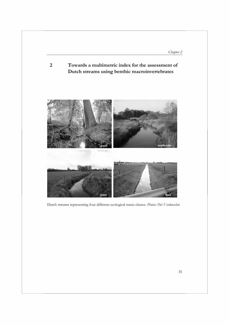
2 Towards a multimetric index for the assessment of Dutch streams using benthic macroinvertebrates
Dutch streams representing four different ecological status classes. Photos: Piet Verdonschot.
Towards a multimetric index for Dutch streams
36
2 Towards a multimetric index for the assessment of Dutch streams using benthic macroinvertebrates
Hanneke E. Vlek, Piet F.M. Verdonschot & Rebi C. Nijboer Hydrobiologia (2004) 516: 173-189. Abstract This study describes the development of a macroinvertebrate based multimetric index for two stream types, fast and slow running streams, in the Netherlands within the AQEM project. Existing macroinvertebrate data (949 samples) were collected from these stream types from all over the Netherlands. All sites received a ecological quality (post-)classification ranging from 1 (bad status) to 4 (good status) based on biotic and abiotic variables, using a combination of multivariate analysis and expert-judgement. A number of bioassessment metrics was tested for both stream types (fast and slow running streams) to examine their power to discriminate between streams of different ecological quality within each stream type. A metric was selected for inclusion in the final multimetric index when there was no overlap of the 25th and 75th percentile between one (or more) ecological quality class(es). Out of all metrics tested, none could distinguish between all four ecological quality classes without overlap of the 25th and 75th percentile between one or more of the classes. Instead, metrics were selected that could distinguish between one (or more) ecological quality class(es) and all others. Finally, 10 metrics were selected for the assessment of slow running streams and 11 metrics for the assessment of fast running streams. Class boundaries were established, to make the assignment of scores to the individual metrics possible. The class boundaries were set at the 25th and/or 75th percentile of the individual metric values. The individual metrics were combined into a multimetric index. Calibration showed that 67% of the samples from slow running streams and 65% of the samples from fast running streams were classified in accordance to their post-classification. In total, only 8% of the samples differed more than one quality class from the post-classification. The multimetric index was validated with data collected in the Netherlands from 82 sites for the purpose of the AQEM project. Validation showed that 54% of the streams were classified correctly.
Chapter 2
37
Keywords: streams, assessment, macroinvertebrates, AQEM, multimetric index, multivariate analysis, the Netherlands Introduction Since the beginning of the 20th century a wide variety of methods for the biological assessment of streams has been developed. In practice, macroinvertebrates are the most commonly used organism group for assessing water quality (Hawkes, 1979; Hellawell, 1986). With their Saprobien system Kolkwitz and Marsson (1909) were the first in Europe to introduce the concept of organisms as indicators of environmental condition. Since its introduction the Saprobien system has been extended and revised by numerous European ecologists (Liebmann, 1951; Sládeček, 1965). While in Germany, the Netherlands and the Czech Republic the focus was mainly on the improvement of the Saprobien system, in countries like Belgium, France and the UK ‘score systems’ were developed. Score systems, like the Trent Biotic Index (Woodiwiss, 1964) and the Indice Biotique (Tuffery & Verneaux, 1968), occurred in the 1960s and followed the introduction of the first diversity indices in the 1940s. More recently multivariate approaches, like RIVPACS (Wright et al., 1984) from the UK and EKOO (Verdonschot, 1990) from the Netherlands, have been introduced.
Developments comparable to those in Europe could be seen in the United States. In the 1980s a multimetric index for fish (Karr, 1981) was introduced in the United States, which was an approach to assessment unknown by the European countries. A multimetric index consists of a combination of several metrics that each provides different ecological information about the observed community and acts as an overall indicator of the biological integrity of a water resource. The strength of the multimetric index is its ability to integrate information from individual, population, community and ecosystem level (Karr & Chu, 1999). A multimetric index provides detection capability over a broad range of stressors, and provides a more complete picture of the ecosystem than single biological indicators do (Intergovernmental Task Force on Monitoring Water Quality, 1993).
Rosenberg & Resh, (1993) listed seven different approaches to assess streams by using macroinvertebrates: richness measures, enumerations, diversity indices, similarity indices, biotic indices, functional feeding-group measures, and the multimetric approach. In the Netherlands only biotic indices, focussed on the detection of organic pollution, have been applied widely. Furthermore, multivariate approaches are being developed (Verdonschot & Nijboer, 2000).
Towards a multimetric index for Dutch streams
38
The first biotic indices applied in the Netherlands were those developed by Kolkwitz & Marsson (1909) and Sládeček (1973). These were already existing saprobic indices, developed to detect organic pollution affecting Mid European streams. It soon became clear that Dutch streams often possess distinctive features, which require a different approach to assessment. For example, the current velocity in most Dutch streams is considerably lower in comparison to streams in other European countries. These experiences initiated the development of an assessment system for organic pollution of lowland streams (Moller Pillot, 1971). The K135-index (Tolkamp & Gardeniers, 1971) was based on the Moller Pillot system and was used for decades.
The mentioned biotic indices, in general, are limited to a single impact factor, namely organic pollution. The disadvantage of an index reflecting a single aspect of the stream is that it may fail to reveal the effects of other or of combined impact factors (Fore et al., 1994; Barbour et al., 1996). This problem was overcome with the introduction of EBEOSWA (ecological assessment of running waters) (Stichting Toegepast Onderzoek Waterbeheer, 1992). EBEOSWA is a system for the biological assessment of Dutch streams. At the moment EBEOSWA is the national standard. EBEOSWA assesses more than one impact factor; as such it can be qualified as a multimetric index. The system considers metrics related to stream velocity, saproby, trophy, functional feeding-groups and substrate. The disadvantages of the system are that it gives separate scores for each metric instead of one final classification for a location, and the ecological status of a water body is not determined by comparing the actual status of a water body with near-natural reference conditions. Furthermore, EBEOSWA is based on data collected in the 1980s. These data comprise mainly impacted sites, and collection and identification was not done in a standardised manner.
The Water Framework Directive (WFD) has led to a demand for a ‘new’ Dutch assessment system. With the implementation of the WFD every EU member state is obligated to assess the effects of human activities on the ecological quality of all water bodies. The criteria set by the WFD, to which assessment should comply, are (European Commission, 2000): the use of different water quality elements: benthic invertebrate fauna,
phytoplankton, fish fauna, and aquatic flora; the ecological status of a water body is determined by comparing the
biological community composition of the investigated water body with near-natural reference conditions;
it is based on a stream-type specific approach;
Chapter 2
39
the final classification of water bodies ranges from 5 (high status) to 1 (bad status).
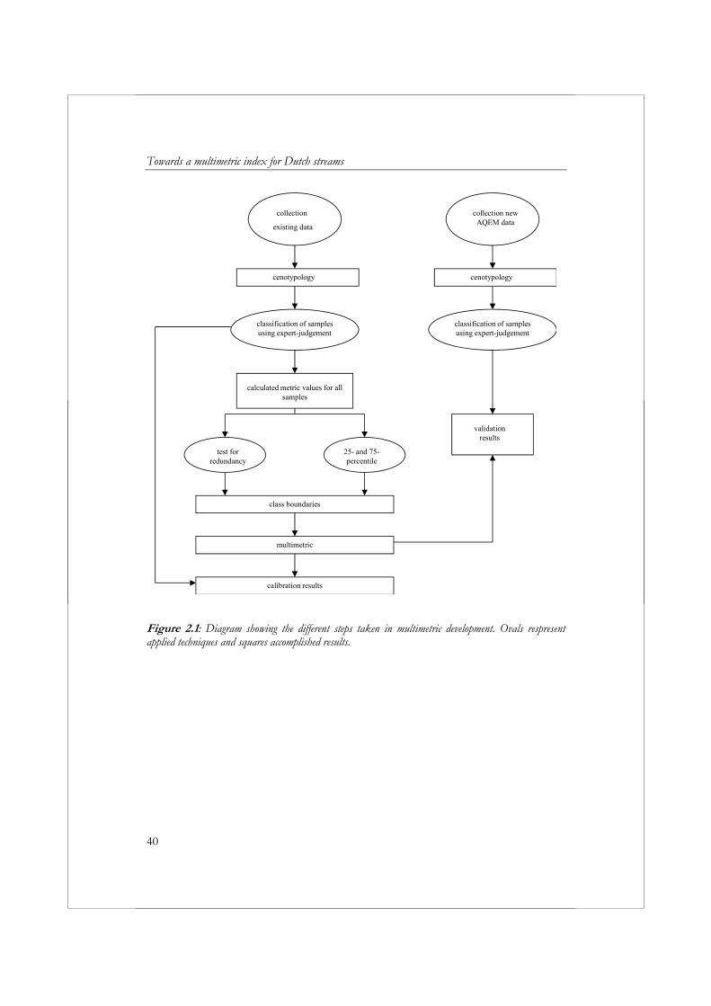
The objective of this study is to develop and test a multimetric index for Dutch streams based on macroinvertebrates that meets the criteria of the WFD. Materials and methods In this study two different data sets were used: (1) an existing data set for the development of the multimetric index and (2) a new data set for the validation of the multimetric index. The application of both data sets is discussed separately. A summary of the different steps taken in the process of multimetric development is shown in Fig. 2.1. (1) Existing data Data collection For the development of the multimetric index no new field data were collected. Instead, a procedure was set up to gather existing data from regional water district managers. The data had to comply with the following criteria: sampling took place after 1990; samples were taken in a standardised manner similar to the AQEM
samples (see biological sampling and laboratory processing of new data);
information about environmental variables was available. After the selection of appropriate samples for the data set a list of environmental variables was sent to the water district managers. Experts considered the environmental variables on the list relevant for analysis. The water district managers provided data for quantitative, qualitative and nominal variables. This resulted in a data set containing information about macroinvertebrate fauna, macrophytes and environmental variables for 949 samples taken in streams from every region in the Netherlands. To assure that the data set would contain samples from the whole degradation spectrum an ‘a priori’ classification was made (Conquest et al., 1994). This pre-classification
Towards a multimetric index for Dutch streams
40
collection
existing data
cenotypology
classification of samples using expert-judgement
calculated metric values for allsamples
test for redundancy
25- and 75-percentile
multimetric
class boundaries
collection new AQEM data
cenotypology
classification of samples using expert-judgement
validation results
calibration results
Figure 2.1: Diagram showing the different steps taken in multimetric development. Ovals respresent applied techniques and squares accomplished results.
Chapter 2
41
was solely based on observations in the field and performed by different water district managers. For selection of the metrics and development of the multimetric index the ‘a priori’ classification was replaced by a less biased ‘a posteriori’ classification (post-classification). Post-classification was considered less biased for two reasons: (1) it was based on multivariate analysis using data on macroinvertebrate community composition and environmental variables and (2) final classification was achieved by looking at all samples in the data set using expert-judgement. Both pre- and post-classification resulted in a quality class. In the context of this article classification always refers to the process of determining the quality class of a water body. A quality class is described as a value ranging from 5 (high) to 1 (bad) that indicates the ecological status (or the state of degradation) of a water body. Post-classification Post-classification was based on multivariate analysis. Multivariate analysis was used to develop a cenotypology. For this study an existing cenotypology was used, which was built from the existing data set in another study. A cenotypology describes different water types and their stages of degradation (Verdonschot & Nijboer, 2000). A cenotype is a group of samples with similar macroinvertebrate composition and environmental circumstances. Environmental variables describing a cenotype can refer to natural circumstances (water type) or a certain degree of degradation. For the purpose of developing the cenotypology and classifying the sites the following steps were taken: (1) The macroinvertebrate data and environmental data were pre-processed. For each macroinvertebrate sample the number of individuals per taxon was standardised to a total sample area of 1.25 m2. Samples from the same location were not averaged, but treated as separate samples. Prior to analysis it was necessary to perform a taxonomic adjustment on the macroinvertebrate data to assure unambiguous data processing. Differences in taxonomic level could otherwise later prove to be the cause of differences between species groups. In this study a weighed taxonomic adjustment was applied. For this purpose, the number of samples in which a taxon occurred was calculated (frequency). The following criteria were used for taxonomic adjustment: when a genus, apart from a few exceptions, was identified to species
level, the genus was removed and the species were kept;
Towards a multimetric index for Dutch streams
42
when a genus was very abundant (frequency of occurrence of the genus > 20% of all the species belonging to this genus), we looked at the indicative value of the genus as a whole and the indicative value of the separate species. When there were clear ecological differences between the species, the species information were kept and the genus was removed. In case the genus was very indicative and there were no real ecological differences between species, the species were assigned to genus level. This procedure can be illustrated with the following example: a data set of 90 samples containing 20 samples with Baetis sp, 4 samples with Baetis tracheatus, 80 samples with Baetis vernus and 6 samples with Baetis fuscatus. According to the criterion mentioned above all species should be assigned to genus level, because the frequency of occurrence of the genus is 22% (20/90) of all the species. However, in this case an exception is made. The species level is kept and the genus removed, because the different Baetis species each indicate different environmental circumstances.
After taxonomic adjustment the macroinvertebrate abundances of each sample were transformed into logarithmic classes (Preston, 1962; Verdonschot, 1990).
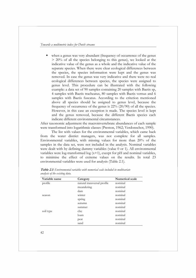
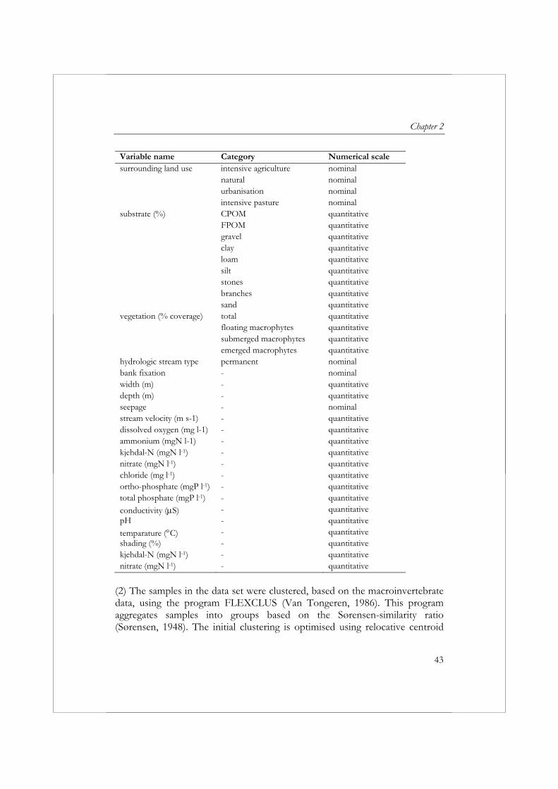
The list with values for the environmental variables, which came back from the water district managers, was not complete for all samples. Environmental variables, with missing values for more than 20% of the samples in the data set, were not included in the analysis. Nominal variables were dealt with by defining dummy variables (value 0 or 1). All environmental variables were log-transformed log (x+1), except for pH and nominal variables, to minimise the effect of extreme values on the results. In total 23 environmental variables were used for analysis (Table 2.1). Table 2.1: Environmental variables with numerical scale included in multivariate analysis of the existing data.
Variable name Category Numerical scale profile natural transversal profile nominal meandering nominal dam nominalseason winter nominal spring nominal autumn nominal summer nominalsoil type clay nominal loam nominal peat nominal sand nominal
Chapter 2
43
Variable name Category Numerical scale surrounding land use intensive agriculture nominal natural nominal urbanisation nominal intensive pasture nominalsubstrate (%) CPOM quantitative FPOM quantitative gravel quantitative clay quantitative loam quantitative silt quantitative stones quantitative branches quantitative sand quantitativevegetation (% coverage) total quantitative floating macrophytes quantitative submerged macrophytes quantitative emerged macrophytes quantitativehydrologic stream type permanent nominalbank fixation - nominalwidth (m) - quantitativedepth (m) - quantitativeseepage - nominalstream velocity (m s-1) - quantitativedissolved oxygen (mg l-1) - quantitativeammonium (mgN l-1) - quantitativekjehdal-N (mgN l-1) - quantitativenitrate (mgN l-1) - quantitativechloride (mg l-1) - quantitativeortho-phosphate (mgP l-1) - quantitativetotal phosphate (mgP l-1) - quantitative
conductivity (S) - quantitativepH - quantitative
temparature (C) - quantitativeshading (%) - quantitativekjehdal-N (mgN l-1) - quantitativenitrate (mgN l-1) - quantitative
(2) The samples in the data set were clustered, based on the macroinvertebrate data, using the program FLEXCLUS (Van Tongeren, 1986). This program aggregates samples into groups based on the Sørensen-similarity ratio (Sørensen, 1948). The initial clustering is optimised using relocative centroid
Towards a multimetric index for Dutch streams
44
sorting. The number of resulting clusters depends on the chosen threshold value. (3) The samples were ordinated by detrended (canonical) correspondence analysis (D(C) CA) using the program CANOCO (Ter Braak, 1987). DCA was used to determine the variation within the data set. Based on the results of the DCA it was decided to use a unimodal technique (DCCA) for further analysis. DCCA is an ordination based on both species and environmental data. The program CANOCO offers different options on how to present and analyse data. The choices made in CANOCO will influence the result of the ordination. In this study the following options were selected: downweighting of rare species: reduces the influence of rare species on
the analysis; inter-sample distance: optimises the position of the samples in the
ordination diagram; detrending by segments (DCA); detrending by 2nd order polynomals (DCCA); forward selection: enables the user to rank environmental variables in
their importance for determining the species data or for reducing a large set of environmental variables.
All techniques are fully explained by Ter Braak & Šmilauer (1998). (4) The results of clustering and ordination were combined in ordination diagrams. Clusters were, therefore projected on the first two axes of the DCCA ordination diagrams. In an ideal situation, the samples of one cluster were positioned closely together in the ordination diagram and showed no overlap with samples of another cluster. Samples that did cause overlap between clusters were examined further. The decision, whether a sample was placed in another cluster or set apart, was based on spatial separation on the third and sometimes the fourth axes as well as upon the macroinvertebrate community composition.
From the above, it can be deducted that a sample group (cenotype) was established if the respective group was clearly recognisable along an identified environmental gradient and thus had a specific macroinvertebrate community composition (Verdonschot & Nijboer, 2000). (5) Classification (or biological assessment) is only meaningful when it is applied to regions having a relative small range in environmental conditions and a relative homogenous macroinvertebrate community composition under reference conditions (Barbour et al., 1996; Karr & Chu, 1999). Based on the

Chapter 2
45
cenotypology four different regions or major stream types of reference conditions could be distinguished (1) fast running streams (v > 30 cm sec-1) (2) slow running streams (v < 30 cm sec-1) (3) periodic or episodic streams and (4) (weak) acidic streams. These four major stream types could be divided further based on dimension into 15 stream types. The decision was made to develop a separate multimetric index for each stream type distinguished under reference conditions, since natural environmental variables were affecting macroinvertebrate community composition (Weigel, 2003). This was done to avoid selection of metrics related to differences between streams under natural circumstances, instead of metrics related to the extent of degradation.
The establishment of cenotypes facilitated the assignment of quality classes to the sites. Because a cenotype is a group of samples with similar macroinvertebrate composition and environmental circumstances, all sites belonging to the same cenotype were considered to be at the same stage of degradation. To determine the degradation stage (or quality class) of each cenotype the macroinvertebrate community composition and values for environmental variables of each cenotype were used for interpretation with expert-judgement. All environmental variables mentioned in Table 2.1 were used to support classification except for variables indicating natural features of stream types. To facilitate the interpretation of the biological data the preferences of the species (of each cenotype) for microhabitat, dimension, current velocity and saprobic conditions were determined with the help of an autecological database (AQEM consortium, 2002). For the same purpose, the following biotic characteristics were calculated: locomotion types, functional feeding-group types and trophic levels. Quality classes from 1 (bad) to 4 (good) were assigned to the sites, using expert-judgement. Quality class 5 (high) was never assigned to a site, because pristine or reference sites have disappeared from the Dutch environment due to extensive habitat degradation and organic pollution.
During classification, it became clear that not enough sites representing each quality class were available for each of the 15 stream types to develop an index. Only the two major stream types, fast and slow running streams, had enough sites representing all quality classes with sufficient variation to develop a sound index. For this reason, all samples from (weak) acidic streams and periodic/episodic streams were removed from the data set and the division into stream types according to dimension was dropped. The decision was made to develop two separate multimetric indices; one for fast running streams and one for slow running streams. Quality classes were assigned separately to the cenotypes of the slow and fast running streams.
Towards a multimetric index for Dutch streams
46
Metric selection Rosenberg & Resh (1993) identified seven different approaches for the assessment of streams based on macroinvertebrates: richness measures, enumerations, diversity indices, similarity indices, biotic indices, functional feeding-group measures and the multimetric approach. Recently multimetric systems with stressor-specific approaches have been developed for many European river types (Brabec et al., 2004; Buffagni et al., 2004; Ofenböck et al., 2004; Sandin et al., 2004). In this study we considered a large number of metrics, more than hundred, (Hering et al., 2004) representing five of the above approaches. For an explanation of the different metrics used in this article see Hering et al. (2004).
Before selection was possible, the metric values for each sample in the data set had to be calculated. These calculations were based on an extended list of autecological information of European macroinvertebrate fauna. In order to assess the ability of all metrics to discriminate between the different stages of degradation, graphical analysis using box-and-whisker plots was applied. This method is similar to the methods described by Barbour et al. (1996), Fore et al. (1996), Blocksom et al. (2000) and Royer et al. (2001). Fore et al. (1996) and Karr & Chu (1999) suggest that graphical methods have fundamental advantages over statistical techniques in this context. Graphs provide more insight in the response of macroinvertebrates to degradation. From a graph one can determine over which range a metric is most sensitive and whether a metric response is linear, unimodal or occurs at a threshold level.
The calculated metric values and degradation stage (= post-classification) for each sample from the data set were combined in a box-and whisker-plot. A metric was judged suitable for index development when there was no interquartile overlap between one or more quality classes in the box-and-whisker plot (Fig. 2.2). This complies to Fore et al. (1996), who selected metric as suited in case of no or little overlap between classes and Barbour et al. (1996) and Royer et al. (2001), who judged a metric as highly sensitive in case of no overlap in the interquartile range. To determine possible overlap in the interquartile range, the 25th and 75th percentile were calculated for all metrics for each quality class. Preferably, metrics were selected that showed no interquartile overlap between all four quality classes. If there was no other option metrics that showed no interquartile overlap between one class and all other classes were selected.
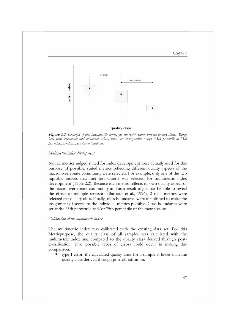
Chapter 2
47
met
ric
valu
e
quality class
overlap
no overlap
Figure 2.2: Example of (no) interquartile overlap for the metric values between quality classes. Range bars show maximum and minimum values; boxes are interquartile ranges (25th percentile to 75th percentile); small stripes represent medians. Multimetric index development Not all metrics judged suited for index development were actually used for this purpose. If possible, suited metrics reflecting different quality aspects of the macroinvertebrate community were selected. For example, only one of the two saprobic indices that met test criteria was selected for multimetric index development (Table 2.2). Because each metric reflects its own quality aspect of the macroinvertebrate community and as a result might not be able to reveal the effect of multiple stressors (Barbour et al., 1996), 2 to 4 metrics were selected per quality class. Finally, class boundaries were established to make the assignment of scores to the individual metrics possible. Class boundaries were set at the 25th percentile and/or 75th percentile of the metric values. Calibration of the multimetric index The multimetric index was calibrated with the existing data set. For this Metricpurpose, the quality class of all samples was calculated with the multimetric index and compared to the quality class derived through post-classification. Two possible types of errors could occur in making this comparison: type I error: the calculated quality class for a sample is lower than the
quality class derived through post-classification.
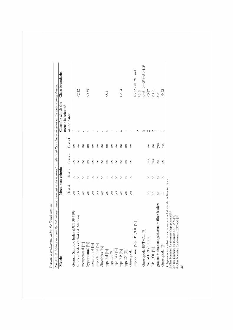
Tow
ards
a m
ultim
etric
inde
x fo
r Dut
ch st
ream
s
48T
able
2.2
: Metr
ics th
at m
et th
e tes
t crit
eria
, metr
ics in
clude
d in
the m
ultim
etric
inde
x an
d th
eir cl
ass b
ound
aries
for t
he sl
ow ru
nnin
g str
eam
s. M
etri
cM
eets
tes
t cr
iter
iaC
lass
for
wh
ich
th
e m
etri
c is
sel
ecte
d
as in
dic
ator
Cla
ss b
oun
dar
ies
Cla
ss 4
C
lass
3
Cla
ss 2
C
lass
1
Ger
man
Sap
robi
c In
dex
(DIN
38
410)
yes
nono
no
-1
Sa
prob
ic I
ndex
(Zel
inka
& M
arva
n)ye
sno
nono
4
<2.
12
met
apot
amal
[%]
yes
nono
no
-
hypo
pota
mal
[%]
yes
nono
no
4 <
0.55
m
etar
hith
ral [
%]
yes
nono
no
-
hypo
rhith
ral [
%]
yes
nono
no
-
Shre
dder
s [%
] ye
sno
nono
-
ty
pe P
el [%
] ye
sno
nono
4
<8.
4 ty
pe L
it [%
] ye
sno
nono
-
ty
pe A
ka [%
] ye
sno
nono
-
ty
pe R
P [%
] ye
sno
nono
4
>29
.4
type
IN
[%]
yes
nono
no
-
Gas
trop
oda
yes
nono
no
-
hypo
pota
mal
[%]-
EP
T/O
L [%
]
3 <
3.22
->
0.91
2an
d >
1.33
Gas
trop
oda-
EP
T/O
L [%
]
3 <
=6
- >
=22
and
>1.
34
No.
of
EP
T/O
Lta
xa
nono
yes
no
2 <
0.67
E
PT
/OL
[%]
nono
yes
no
2 <
0.51
gr
azer
s +
scr
aper
s/ga
ther
ers
+ f
ilter
fee
ders
nono
noye
s 1
>2
Gas
trop
oda
[%]
nono
noye
s 1
>9.
92
1) H
yphe
n in
dica
tes
that
the
met
ric
was
not
incl
uded
in th
e m
ultim
etri
c in
dex
2) C
lass
bou
ndar
y fo
r th
e m
etri
c hy
popo
tam
al [%
] 3)
Cla
ss b
ound
ary
for
the
met
ric
EP
T/O
L [%
] 4)
Cla
ss b
ound
ary
for
the
met
ric
EP
T/O
L [%
]
Chapter 2
49
type II error: the calculated quality class for a sample is higher than the quality class derived through post-classification.
(2) New data Site selection New data were collected to validate the multimetric index. These data were collected within the AQEM project. See AQEM consortium (2002) for the methodology applied. To assure sampling of the whole degradation spectrum an ‘a priori’ classification of the sites was made into the five quality classes used by the WFD (European Commission, 2000). Sites were selected and pre-classified by local water district managers. For the validation of the multimetric index the pre-classification was later replaced by a less biased post-classification. In total the AQEM data set composed 156 samples divided over 82 sites distributed over all regions in the Netherlands. At each site also environmental data were recorded. In total, information on 230 environmental variables was collected. Biological sampling and laboratory processing The AQEM samples were taken between May 2000 and May 2001, partly by water district managers and partly by Alterra. Most sites were sampled twice, in spring and autumn. The coverage of each habitat present at a sampling site was estimated before sampling. For the collection of the samples a D-frame dip net (25 or 30 cm wide with a 500 μm mesh) was used to collect a composite sample from several habitats at each site. The sample was taken by pushing the dip net through the upper part (2-5 cm) of the substratum. Each habitat was sampled over a distance that ensured collection of most species present at the habitat. All samples of mineral substrates were sampled in the same ratio as their coverage in the stream and put together in one bucket. The same procedure was repeated for the organic substrates. Mineral and organic samples were kept apart. All habitats with less than 5% coverage were sampled in only very small amounts, just to collect any species that were not present in the major habitats. After sampling, the buckets with samples were transported to the laboratory and stored in a refrigerator. The mineral and organic part of the sample were kept separate during processing. The samples were sieved using a 1000 and 350 µm sieve. The coarse fraction (> 1000 µm) and fine fraction were kept separate during sorting. The samples were sorted live by eye. If the coarse or fine fraction contained over 500 individuals, subsamples of at
Towards a multimetric index for Dutch streams
50
least 500 individuals were sorted. Organisms were identified to the lowest possible taxonomic level (species level for almost all groups). Collection of environmental data Environmental data were collected at all AQEM sites. The collection of environmental data and biological sampling took place simultaneously. The environmental data recorded for the purpose of the AQEM project were not used for analysis in this study. Post-classification Post-classification of the samples in the new data set was not based on multivariate analysis. Instead the already developed cenotypology based on the existing data was used to classify the new samples. The following steps were taken to classify the AQEM samples: (1) The macroinvertebrate data from the coarse and fine fraction were combined and standardised to a total sample area of 1.25 m2. If there were more samples from one location these samples were not combined to form one sample, but they were treated like samples from different locations. The macroinvertebrate data were adjusted to the same taxonomic level as used for the existing data. The macroinvertebrate abundances were transformed into logarithmic classes (Pretson, 1962; Verdonschot, 1990) (2) The AQEM samples were classified using the program ASSOCIA. ASSOCIA is a program originally developed for the identification of plant communities, but ASSOCIA can also be used to allocate macroinvertebrate samples to existing (ceno)types. For the allocation of samples ASSOCIA uses both qualitative and quantitative features of a sample in the form of the maximum likelihood principle and a measure of distance. The maximum likelihood principle is based on a calculation of probability; with the macroinvertebrate species list the chance that the species composition of a sample can be found in a cenotype is calculated. Final allocation takes place based on an index that combines maximum likelihood and measure of distance.
The AQEM samples were allocated to the cenotypes with ASSOCIA. The samples were allocated to the cenotype with the lowest value for the combined index, because the value of the combined index increases with
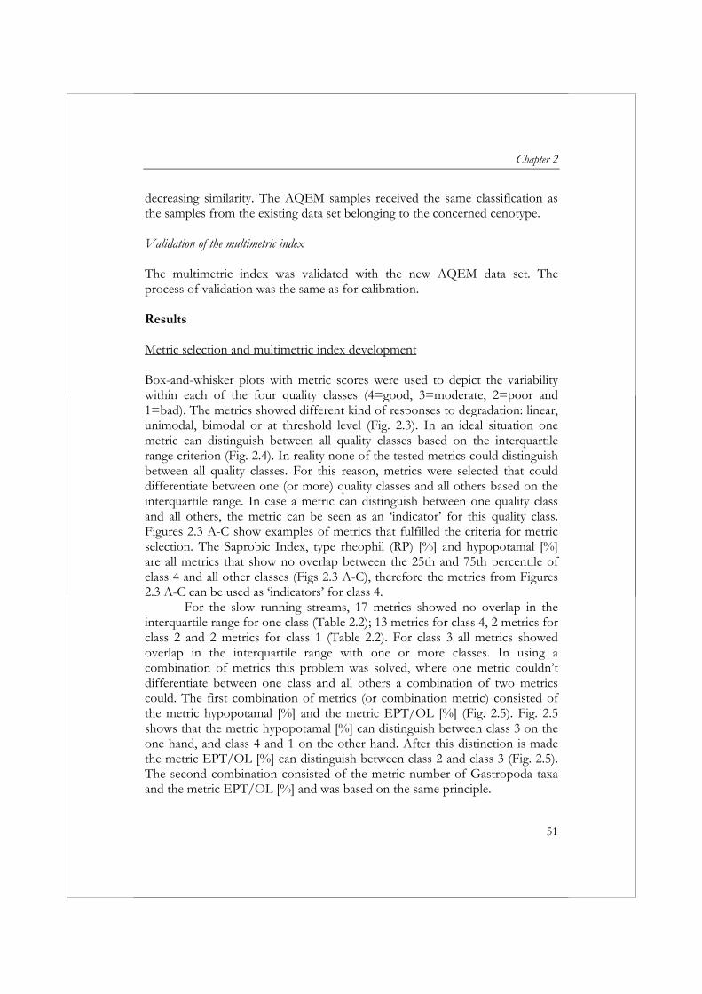
Chapter 2
51
decreasing similarity. The AQEM samples received the same classification as the samples from the existing data set belonging to the concerned cenotype. Validation of the multimetric index The multimetric index was validated with the new AQEM data set. The process of validation was the same as for calibration. Results Metric selection and multimetric index development Box-and-whisker plots with metric scores were used to depict the variability within each of the four quality classes (4=good, 3=moderate, 2=poor and 1=bad). The metrics showed different kind of responses to degradation: linear, unimodal, bimodal or at threshold level (Fig. 2.3). In an ideal situation one metric can distinguish between all quality classes based on the interquartile range criterion (Fig. 2.4). In reality none of the tested metrics could distinguish between all quality classes. For this reason, metrics were selected that could differentiate between one (or more) quality classes and all others based on the interquartile range. In case a metric can distinguish between one quality class and all others, the metric can be seen as an ‘indicator’ for this quality class. Figures 2.3 A-C show examples of metrics that fulfilled the criteria for metric selection. The Saprobic Index, type rheophil (RP) [%] and hypopotamal [%] are all metrics that show no overlap between the 25th and 75th percentile of class 4 and all other classes (Figs 2.3 A-C), therefore the metrics from Figures 2.3 A-C can be used as ‘indicators’ for class 4.
For the slow running streams, 17 metrics showed no overlap in the interquartile range for one class (Table 2.2); 13 metrics for class 4, 2 metrics for class 2 and 2 metrics for class 1 (Table 2.2). For class 3 all metrics showed overlap in the interquartile range with one or more classes. In using a combination of metrics this problem was solved, where one metric couldn’t differentiate between one class and all others a combination of two metrics could. The first combination of metrics (or combination metric) consisted of the metric hypopotamal [%] and the metric EPT/OL [%] (Fig. 2.5). Fig. 2.5 shows that the metric hypopotamal [%] can distinguish between class 3 on the one hand, and class 4 and 1 on the other hand. After this distinction is made the metric EPT/OL [%] can distinguish between class 2 and class 3 (Fig. 2.5). The second combination consisted of the metric number of Gastropoda taxa and the metric EPT/OL [%] and was based on the same principle.
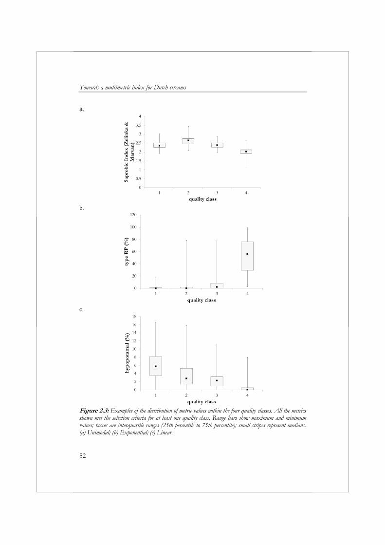
Towards a multimetric index for Dutch streams
52
a.
0
0.5
1
1.5
2
2.5
3
3.5
4
1 2 3 4
Sapr
obic
In
dex
(Z
elin
ka &
M
arva
n)
quality class
b.
0
20
40
60
80
100
120
1 2 3 4
typ
e R
P (
%)
quality class
c.
0
2
4
6
8
10
12
14
16
18
1 2 3 4
hyp
opot
amal
(%
)
quality class
Figure 2.3: Examples of the distribution of metric values within the four quality classes. All the metrics shown met the selection criteria for at least one quality class. Range bars show maximum and minimum values; boxes are interquartile ranges (25th percentile to 75th percentile); small stripes represent medians. (a) Unimodal; (b) Exponential; (c) Linear.
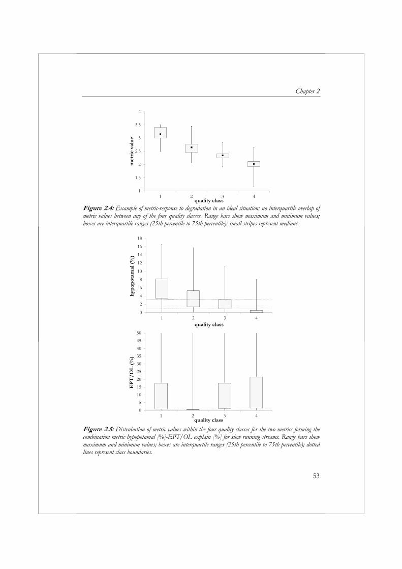
Chapter 2
53
1
1.5
2
2.5
3
3.5
4
1 2 3 4
met
ric
valu
e
quality class Figure 2.4: Example of metric-response to degradation in an ideal situation; no interquartile overlap of metric values between any of the four quality classes. Range bars show maximum and minimum values; boxes are interquartile ranges (25th percentile to 75th percentile); small stripes represent medians.
0
2
4
6
8
10
12
14
16
18
1 2 3 4
hyp
opot
amal
(%
)
quality class
0
5
10
15
20
25
30
35
40
45
50
1 2 3 4
EP
T/
OL
(%
)
quality class Figure 2.5: Distrubution of metric values within the four quality classes for the two metrics forming the combination metric hypopotamal [%]-EPT/OL explain [%] for slow running streams. Range bars show maximum and minimum values; boxes are interquartile ranges (25th percentile to 75th percentile); dotted lines represent class boundaries.
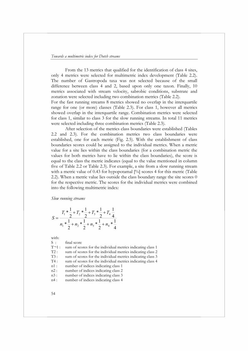
Towards a multimetric index for Dutch streams
54
From the 13 metrics that qualified for the identification of class 4 sites, only 4 metrics were selected for multimetric index development (Table 2.2). The number of Gastropoda taxa was not selected because of the small difference between class 4 and 2, based upon only one taxon. Finally, 10 metrics associated with stream velocity, sabrobic conditions, substrate and zonation were selected including two combination metrics (Table 2.2). For the fast running streams 8 metrics showed no overlap in the interquartile range for one (or more) classes (Table 2.3). For class 1, however all metrics showed overlap in the interquartile range. Combination metrics were selected for class 1, similar to class 3 for the slow running streams. In total 11 metrics were selected including three combination metrics (Table 2.3).
After selection of the metrics class boundaries were established (Tables 2.2 and 2.3). For the combination metrics two class boundaries were established, one for each metric (Fig. 2.5). With the establishment of class boundaries scores could be assigned to the individual metrics. When a metric value for a site lies within the class boundaries (for a combination metric the values for both metrics have to lie within the class boundaries), the score is equal to the class the metric indicates (equal to the value mentioned in column five of Table 2.2 or Table 2.3). For example, a site from a slow running stream with a metric value of 0.43 for hypopotamal [%] scores 4 for this metric (Table 2.2). When a metric value lies outside the class boundary range the site scores 0 for the respective metric. The scores for the individual metrics were combined into the following multimetric index: Slow running streams
4
1*
2
1*
2
1*
2
1*
4
1
2
1*
2
1*
2
1*
4321
4321
nnnn
TTTTS
with: S : final score T¬1 : sum of scores for the individual metrics indicating class 1 T2 : sum of scores for the individual metrics indicating class 2 T3 : sum of scores for the individual metrics indicating class 3 T4 : sum of scores for the individual metrics indicating class 4 n1 : number of indices indicating class 1 n2 : number of indices indicating class 2 n3 : number of indices indicating class 3 n4 : number of indices indicating class 4
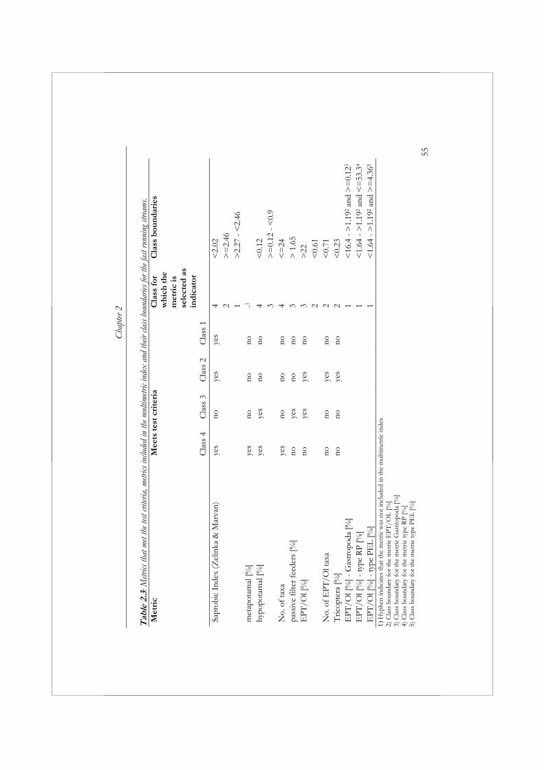
C
hapt
er 2
55
Tab
le 2
.3: M
etrics
that
met
the t
est c
riter
ia, m
etrics
inclu
ded
in th
e mul
timetr
ic in
dex
and
their
clas
s bou
ndar
ies fo
r the
fast
runn
ing
strea
ms.
Met
ric
Mee
ts t
est
crit
eria
Cla
ss f
or
wh
ich
th
e m
etri
c is
se
lect
ed a
s in
dic
ator
Cla
ss b
oun
dar
ies
Cla
ss 4
Cla
ss 3
Cla
ss 2
Cla
ss 1
Sapr
obic
Ind
ex (Z
elin
ka &
Mar
van)
ye
s no
ye
s ye
s
4 <
2.02
2 >
=2.
46
1
>2.
27 -
<2.
46
met
apot
amal
[%]
yes
no
no
no
-1
hy
popo
tam
al [%
] ye
s ye
s no
no
4
<0.
12
3 >
=0.
12 -
<0.
9 N
o. o
f ta
xa
yes
no
no
no
4 <
=24
pa
ssiv
e fil
ter
feed
ers
[%]
no
yes
no
no
3 >
1.6
5 E
PT
/Ol [
%]
no
yes
yes
no
3 >
22
2 <
0.61
N
o. o
f E
PT
/Ol t
axa
no
no
yes
no
2 <
0.71
T
ricop
tera
[%]
no
no
yes
no
2 <
0.23
E
PT
/Ol [
%] -
Gas
trop
oda
[%]
1 <
16.4
- >
1.19
2 and
>=
0.12
3
EP
T/O
l [%
] - ty
pe R
P [%
]
1
<1.
64 -
>1.
192 a
nd <
=53
.34
EP
T/O
l [%
] - ty
pe P
EL
[%]
1 <
1.64
- >
1.19
2 and
>=
4.36
5
1) H
yphe
n in
dica
tes
that
the
met
ric
was
not
incl
uded
in th
e m
ultim
etri
c in
dex
2) C
lass
bou
ndar
y fo
r th
e m
etri
c E
PT
/OL
[%]
3) C
lass
bou
ndar
y fo
r th
e m
etri
c G
astr
opod
a [%
] 4)
Cla
ss b
ound
ary
for
the
met
ric ty
pe R
P [%
] 5)
Cla
ss b
ound
ary
for
the
met
ric ty
pe P
EL
[%]
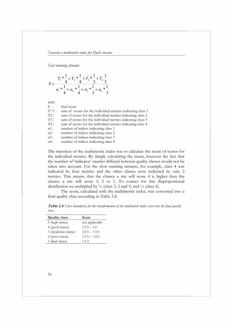
Towards a multimetric index for Dutch streams
56
Fast running streams
3
1*
3
1*
4
1*
4
1*
3
1
3
1*
4
1*
4
1*
4321
4321
nnnn
TTTTS
with: S : final score T¬1 : sum of scores for the individual metrics indicating class 1 T2 : sum of scores for the individual metrics indicating class 2 T3 : sum of scores for the individual metrics indicating class 3 T4 : sum of scores for the individual metrics indicating class 4 n1 : number of indices indicating class 1 n2 : number of indices indicating class 2 n3 : number of indices indicating class 3 n4 : number of indices indicating class 4 The intention of the multimetric index was to calculate the mean of scores for the individual metrics. By simply calculating the mean, however the fact that the number of ‘indicator’ metrics differed between quality classes would not be taken into account. For the slow running streams, for example, class 4 was indicated by four metrics and the other classes were indicated by only 2 metrics. This means, that the chance a site will score 4 is higher than the chance a site will score 3, 2 or 1. To correct for this disproportional distribution we multiplied by ½ (class 3, 2 and 1) and ¼ (class 4).
The score, calculated with the multimetric index, was converted into a final quality class according to Table 2.4. Table 2.4: Class boundaries for the transformation of the multimetric index score into the final quality class.
Quality class Score 5 (high status) not applicable 4 (good status) ≥3.5 – ≤4 3 (moderate status) ≥2.5 – <3.5 2 (poor status) ≥1.5 – <2.5 1 (bad status) <1.5
Chapter 2
57
Calibration of the multimetric index First the multimetric index was calibrated using the existing data set. Samples from cenotype 9, 14a, 14b, 16, 24a and 31 were often classified incorrect (Tables 2.5 and 2.6). All these cenotypes consisted of a low number of samples (12 and less), except for cenotype 24a. For the remaining cenotypes the percentage of correctly classified samples varied between 48 and 100%.
Only a very low percentage of the samples (8% for the slow running streams and 9% for the fast running streams) deviated more than one class from the post-classification (Figs 2.6, 2.7). Again, cenotype 9,14a, 14b, 24a and 31 were an exception to this rule.
In total, 67% of the slow running streams and 65% of the fast running streams were classified correctly. The percentage type I and type II errors varied between 19 and 15. Most errors occurred with the classification of samples that received a quality class 3 during post-classification (Figs 2.6, 2.7). Validation of the multimetric index After calibration, the multimetric index was validated with the new AQEM data set. In total, 54% of the samples were classified correctly (Fig. 2.8). Most of the samples that were not classified correctly, differed only one quality class from the post-classification (Fig 2.8.). The percentage type I errors for the total data set was 32. The percentage type II errors for the total data set was 14.
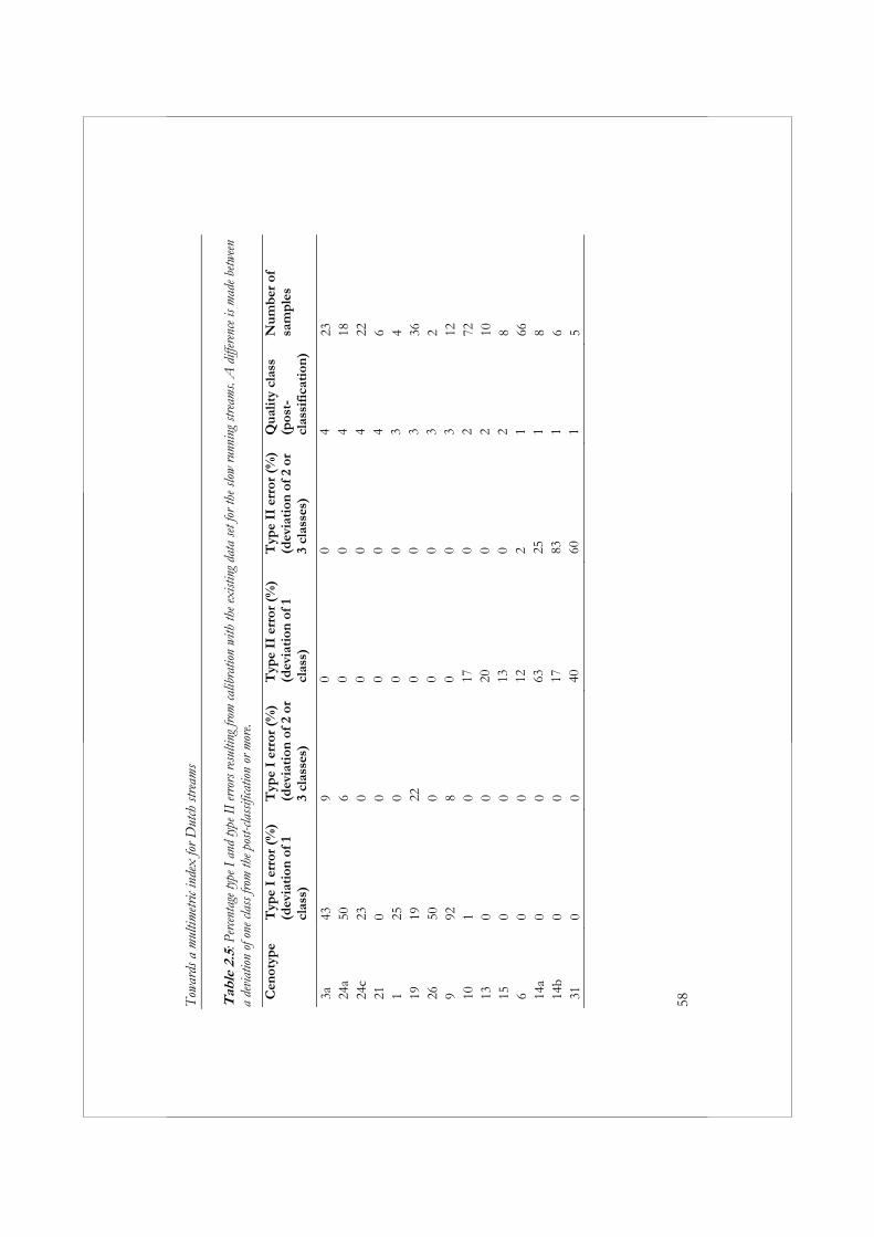
Tow
ards
a m
ultim
etric
inde
x fo
r Dut
ch st
ream
s
58 T
able
2.5
: Per
centa
ge ty
pe I
and
type
II
erro
rs re
sulti
ng fr
om ca
libra
tion
with
the e
xisti
ng d
ata
set f
or th
e slo
w ru
nnin
g str
eam
s. A
diff
eren
ce is
mad
e betw
een
a de
viat
ion
of o
ne cl
ass f
rom
the p
ost-c
lass
ifica
tion
or m
ore.
Cen
otyp
e T
ype
I er
ror
(%)
(dev
iati
on o
f 1
clas
s)
Typ
e I
erro
r (%
)(d
evia
tion
of
2 or
3
clas
ses)
Typ
e II
err
or (
%)
(dev
iati
on o
f 1
clas
s)
Typ
e II
err
or (
%)
(d
evia
tion
of
2 or
3
clas
ses)
Qu
alit
y cl
ass
(pos
t-cl
assi
fica
tion
)
Nu
mb
er o
f sa
mp
les
3a
43
9 0
0 4
23
24a
50
6 0
0 4
18
24c
23
0 0
0 4
22
21
0 0
00
46
1 25
0
00
34
19
19
22
00
336
26
50
0
00
32
9 92
8
00
312
10
1
0 17
0 2
72
13
0 0
200
210
15
0
0 13
0 2
8 6
0 0
122
166
14
a 0
0 63
25
18
14b
0 0
1783
1
6 31
0
0 40
60
15
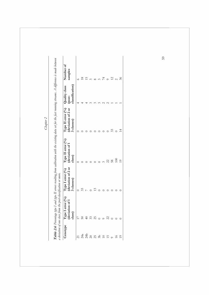
C
hapt
er 2
59
Tab
le 2
.6: P
ercen
tage
type
I a
nd ty
pe I
I er
rors
resu
lting
from
calib
ratio
n wi
th th
e exi
sting
dat
a se
t for
the f
ast r
unni
ng st
ream
s. A
diff
eren
ce is
mad
e betw
een
a de
viat
ion
of o
ne cl
ass f
rom
the p
ost-c
lass
ifica
tion
or m
ore.
Cen
otyp
e T
ype
I er
ror
(%)
(dev
iati
on o
f 1
clas
s)
Typ
e I
erro
r (%
)(d
evia
tion
of
2 or
3
clas
ses)
Typ
e II
err
or (
%)
(dev
iati
on o
f 1
clas
s)
Typ
e II
err
or (
%)
(d
evia
tion
of
2 or
3
clas
ses)
Qu
alit
y cl
ass
(pos
t-cl
assi
fica
tion
)
Nu
mb
er o
f sa
mp
les
2117
0
00
46
24a
50
330
0 4
1824
b40
7
00
415
2033
0
00
33
2525
13
00
38
3b0
00
0 3
310
9 0
30
274
1522
0
220
29
90
058
33
112
160
010
00
12
190
019
14
136
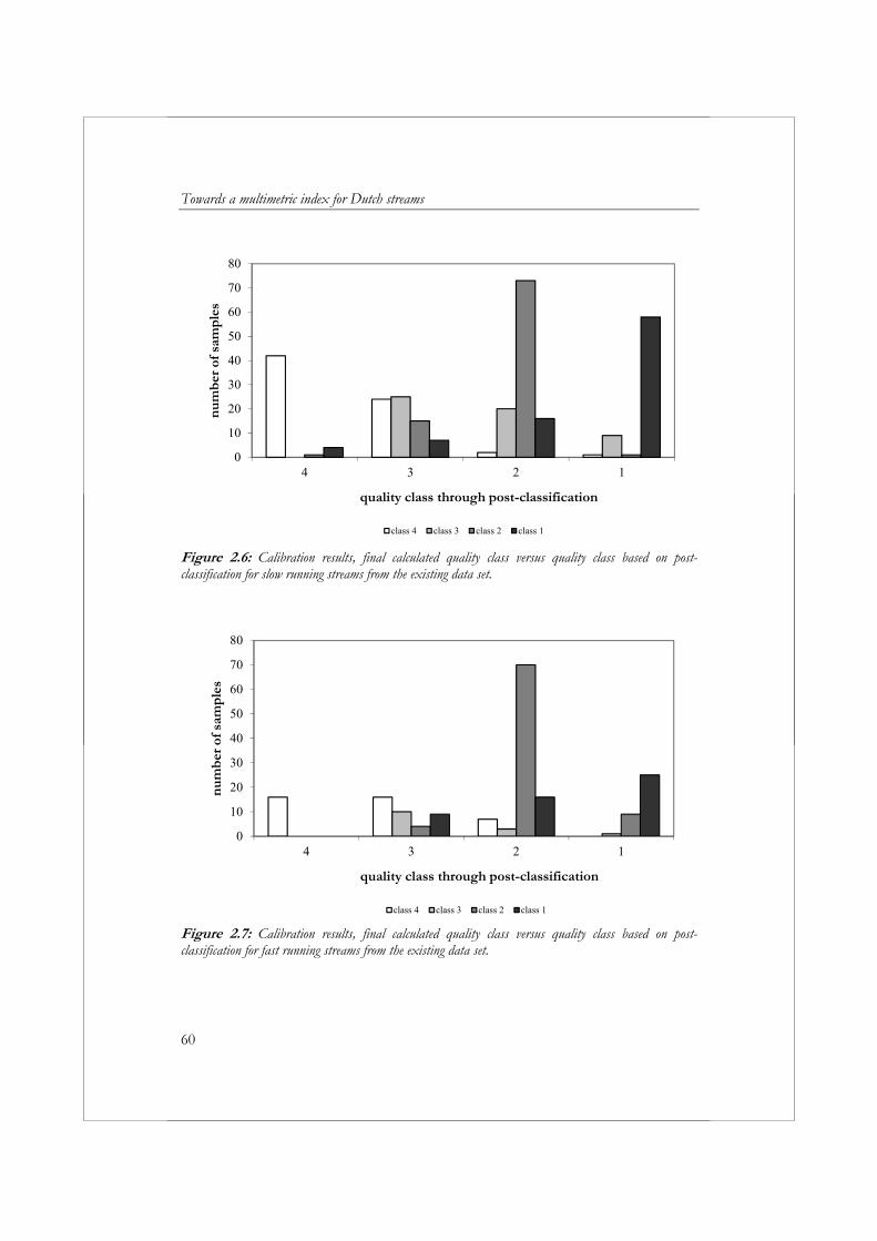
Towards a multimetric index for Dutch streams
60
0
10
20
30
40
50
60
70
80
4 3 2 1
nu
mb
er o
f sam
ple
s
quality class through post-classification
class 4 class 3 class 2 class 1
Figure 2.6: Calibration results, final calculated quality class versus quality class based on post-classification for slow running streams from the existing data set.
0
10
20
30
40
50
60
70
80
4 3 2 1
nu
mb
er o
f sam
ple
s
quality class through post-classification
class 4 class 3 class 2 class 1
Figure 2.7: Calibration results, final calculated quality class versus quality class based on post-classification for fast running streams from the existing data set.
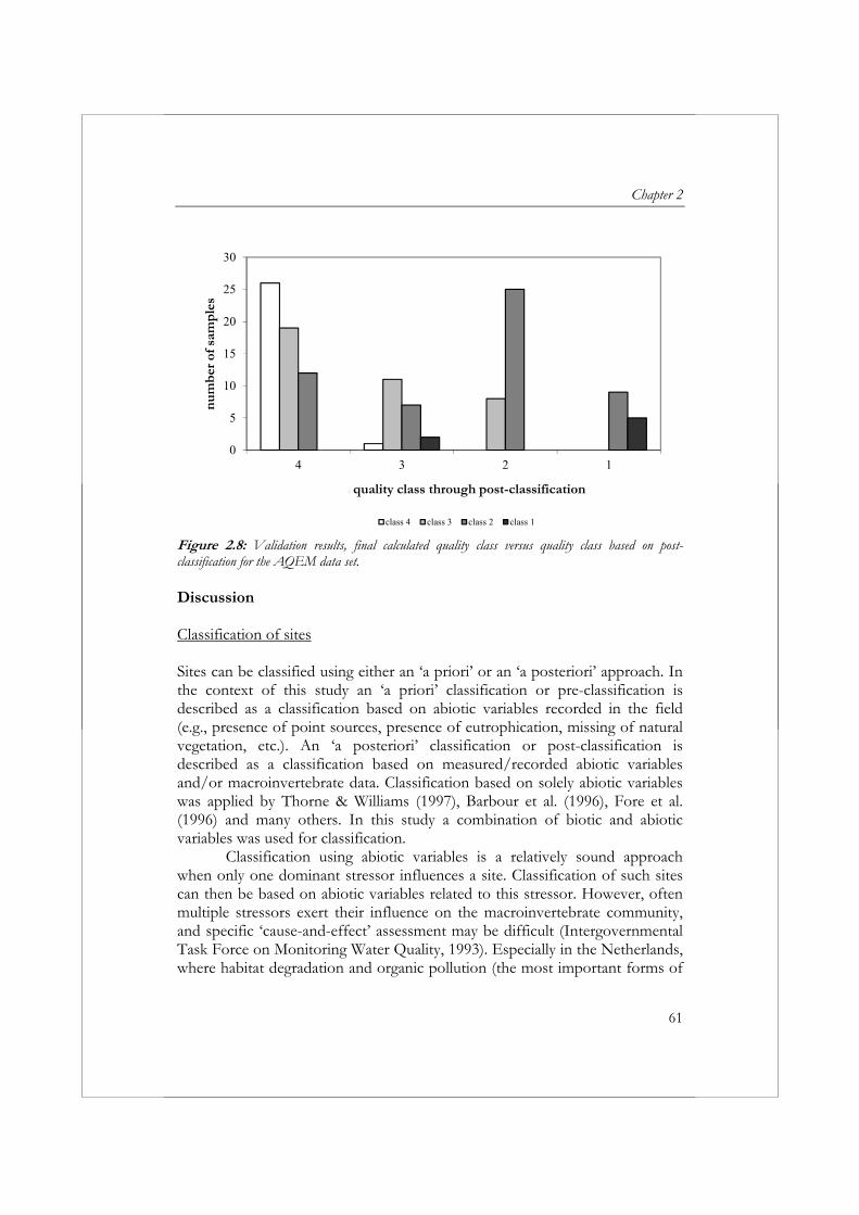
Chapter 2
61
0
5
10
15
20
25
30
4 3 2 1
nu
mb
er o
f sam
ple
s
quality class through post-classification
class 4 class 3 class 2 class 1
Figure 2.8: Validation results, final calculated quality class versus quality class based on post-classification for the AQEM data set. Discussion Classification of sites Sites can be classified using either an ‘a priori’ or an ‘a posteriori’ approach. In the context of this study an ‘a priori’ classification or pre-classification is described as a classification based on abiotic variables recorded in the field (e.g., presence of point sources, presence of eutrophication, missing of natural vegetation, etc.). An ‘a posteriori’ classification or post-classification is described as a classification based on measured/recorded abiotic variables and/or macroinvertebrate data. Classification based on solely abiotic variables was applied by Thorne & Williams (1997), Barbour et al. (1996), Fore et al. (1996) and many others. In this study a combination of biotic and abiotic variables was used for classification.
Classification using abiotic variables is a relatively sound approach when only one dominant stressor influences a site. Classification of such sites can then be based on abiotic variables related to this stressor. However, often multiple stressors exert their influence on the macroinvertebrate community, and specific ‘cause-and-effect’ assessment may be difficult (Intergovernmental Task Force on Monitoring Water Quality, 1993). Especially in the Netherlands, where habitat degradation and organic pollution (the most important forms of
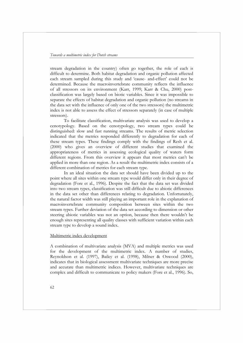
Towards a multimetric index for Dutch streams
62
stream degradation in the country) often go together, the role of each is difficult to determine. Both habitat degradation and organic pollution affected each stream sampled during this study and ‘cause- and-effect’ could not be determined. Because the macroinvertebrate community reflects the influence of all stressors on its environment (Karr, 1999; Karr & Chu, 2000) post-classification was largely based on biotic variables. Since it was impossible to separate the effects of habitat degradation and organic pollution (no streams in the data set with the influence of only one of the two stressors) the multimetric index is not able to assess the effect of stressors separately (in case of multiple stressors).
To facilitate classification, multivariate analysis was used to develop a cenotypology. Based on the cenotypology, two stream types could be distinguished: slow and fast running streams. The results of metric selection indicated that the metrics responded differently to degradation for each of these stream types. These findings comply with the findings of Resh et al. (2000) who gives an overview of different studies that examined the appropriateness of metrics in assessing ecological quality of waters form different regions. From this overview it appears that most metrics can’t be applied in more than one region. As a result the multimetric index consists of a different combination of metrics for each stream type.
In an ideal situation the data set should have been divided up to the point where all sites within one stream type would differ only in their degree of degradation (Fore et al., 1996). Despite the fact that the data set was divided into two stream types, classification was still difficult due to abiotic differences in the data set other than differences relating to degradation. Unfortunately, the natural factor width was still playing an important role in the explanation of macroinvertebrate community composition between sites within the two stream types. Further deviation of the data set according to dimension or other steering abiotic variables was not an option, because then there wouldn’t be enough sites representing all quality classes with sufficient variation within each stream type to develop a sound index. Multimetric index development A combination of multivariate analysis (MVA) and multiple metrics was used for the development of the multimetric index. A number of studies, Reynoldson et al. (1997), Bailey et al. (1998), Milner & Oswood (2000), indicates that in biological assessment multivariate techniques are more precise and accurate than multimetric indices. However, multivariate techniques are complex and difficult to communicate to policy makers (Fore et al., 1996). So,
Chapter 2
63
instead of developing an assessment system completely based on MVA, MVA was only used to set post-classification. Post-classification was followed by metric selection. The results of metric selection showed that not many metrics could meet the selection criteria. None of the metrics could differ between all four quality classes and most were only capable of indicating one class. This poor result can have different causes. First, mistakes in the post-classification due to abiotic differences in the data set could have played an important role. Second, the autecological data behind the metrics could have been of importance. These autecological data comprise indicator values for current velocity, acidity, etc. In determining these indicator values data from all over Europe were used, this means the indicator values can deviate from the Dutch optima. Third, it might just not be feasible to differentiate between four ecological quality classes based on the biological metrics tested in this study.
After metric selection class boundaries were set. Class boundaries for individual metrics can be set in two different ways: 1) based on statistical rules 2) based on an ecological response to degradation. Examples of the first option are: dividing the 95-percentile of all sites by four (Ohio Environmental
Protection Agency, 1987; DeSohn, 1995); the 50- and 10-percentile of all reference locations (Roth et al., 1997); dividing the 25- or 75-percentile of all reference locations (Barbour et
al., 1996; Royer et al., 2001). In this study, the second option to set class boundaries was chosen, because the first approach has a lot of disadvantages. First, selection based on statistical rules assumes each metric responds in the exact same way to degradation, while in fact each metric has its own ecological response. Second, a metric can only be qualified as suited when it shows a linear response to environmental degradation, while the second option doesn’t rule out a metric response that is unimodal, bimodal or occurs at threshold level.
In the final step of multimetric development, one of the criteria set by the WFD was not followed. According to this criterion the calculation of ecological quality class should be based on the deviation from the reference condition. This criterion was ignored, because reference sites were not present in the Netherlands and it was not possible within the scope of this research to construct valid hypothetical reference situations. However, when descriptions of reference conditions of Dutch streams become available in the future the multimetric index can be adapted easily to include these references.
Towards a multimetric index for Dutch streams
64
Calibration and validation of the multimetric index The multimetric index developed in this study has been validated with an internal and external data set. In the first case 66% of the samples were classified correctly, in the second 54%. The difference in correctly classified samples between the data sets was not caused by differences in the collection of samples, since the collection of samples was performed in a similar way for both data sets.
The errors in the classifications for the internal data set can be explained from the approach that was used for metric selection. Class boundaries were set at the 25- and/or 75-percentile, which means that for testing with a random data set, there is a 50% chance of misclassification for class 2 and class 3 sites and a 25% chance for class 4 and class 1 sites. Automatically, the chance of an incorrect classification will range between 50% and 75%. Changing the criteria for metric selection (for example: no overlap between the 10- and 90-percentile) to lower the chance of misclassification was not an option, because not enough metrics would comply with these criteria to develop a multimetric index.
Maxted et al. (2000) concluded that the Coastal Plain Macroinvertebrate Index (CPMI) classified 86% of the sites correctly. This is much better than the 66% for the multimetric index developed in this study. However, the CPMI can only differ between 2 classes (reference and impaired sites), compared to five classes for the multimetric index. The higher number of classes in an assessment system, the higher the chance of misclassification. Furthermore, for the calibration of the CPMI only clearly degraded sites were used, whereas the classification of moderate degraded sites creates the biggest problems. For the calibration of the multimetric index, sites ranging from good quality to bad quality were used. Acknowledgements This study was carried out within the AQEM project, which was funded by the European Commission, 5th Framework Program, Energy, Environment and Sustainable Development, Key Action Water, Contract no. EVK1-CT1999-00027. The authors are very grateful for the sampling efforts made by all participating water authorities. Special thanks goes to Tjeerd-Harm van den Hoek en Martin van den Hoorn for their big efforts in data entry, field and laboratory work. We would also like to thank L.S. Fore and an anonymous reviewer for their thorough review of this paper
Chapter 2
65
References AQEM consortium, 2002. Manual for the application of the AQEM system. A
comprehensive method to assess European streams using benthic macroinvertebrates, developed for the purpose of the Water Framework Directive. Version 1.0, February 2002.
Bailey, R.C., M.G. Kennedy, M.Z. Dervish & R.M. Taylor, 1998. Biological assessment of freshwater ecosystems using a reference condition approach: comparing predicted and actual benthic invertebrate communities in Yukon streams. Freshwater Biology 39: 765-774.
Barbour, M.T., J. Gerritsen, G.E. Griffith, R. Frydenborg, E. McCarron, J.S. White & M.L. Bastian, 1996. A framework for biological criteria for Florida streams using benthic macroinvertebrates. Journal of the North American Benthological Society 15: 185-211.
Blocksom, K.A., J.P. Kurtenbach, D.J. Klemm, F.A. Fulk & S.M. Cormier, 2000. Development and evaluation of the lake macroinvertebrate integrity index (LMII) for New Jersey lakes and resevoirs. Environmental Monitoring and Assessment 77: 311-333.
Brabec K., J. Kokes, D. Nemejcova & S. Zahrádková, 2004. Assessment of organic pollution effect considering differences between lotic and lentic stream habitats. Hydrobiologia 516: 331-346.
Buffagni, A., S. Erba, M. Cazzola & J.L. Kemp, 2004. The AQEM multimetric system for the southern Italian Apennines: assessing the impact of water quality and habitat degradation on pool macroinvertebrates in Mediterranean rivers. Hydrobiologia 516: 313-329.
Conquest, L.L., S.C. Ralph & R.J. Naiman, 1994. Implementation of large-scale stream monitoring efforts: sampling design and data analysis issues. In: Loeb, S.L. & A. Spacie (eds.), Biological monitoring of aquatic systems. CRC Press LLC, Boca Raton, Florida.
DeShon, J.E, 1995. Development and application of the invertebrate community index (ICI). In: Davis, W.S. & T.P. Simon (eds.), Biological assessment and criteria: Tools for water resource planning and decision making. Lewis Publishers, Ann Arbor, Michigan.
European Commission, 2000. Directive 2000/60/EC OF THE EUROPEAN PARLIAMENT AND COUNCIL - Establishing a framework for Community action in the field of water policy. Official Journal of the European Community L327: 1-72.
Fore, L.S., J.R. Karr & L.L. Conquest, 1994. Statistical properties of an index of biological integrity used to evaluate water resources. Canadian Journal of Fisheries and Aquatic Sciences 51: 1077-1087.
Towards a multimetric index for Dutch streams
66
Fore, L.S., J.R. Karr & R.W. Wisseman, 1996. Assessing invertebrate responses to human activities: evaluating alternative approaches. Journal of the North American Benthological Society 15: 212-231.
Hawkes, H.A., 1979. Invertebrates as indicators of river water quality. In: James, A. & L. Evison (eds.), Biological indicators of water quality. John Wiley, Chichester.
Hellawell, J.M., 1986. Biological indicators of freshwater pollution and environmental management. Elsevier Applied Science, London.
Hering, D., O. Moog, L. Sandin & P.F.M. Verdonschot, 2004. Overview and application of the AQEM assessment system. Hydrobiologia 516: 1-20.
Intergovernmental Task Force on Monitoring Water Quality, 1993. The Multimetric Approach for describing ecological condition. EPA, Position Paper No. 2.
Karr, J.R., 1981. Assessment of biotic integrity using fish communities. Fisheries 6: 21-27.
Karr, J.R., 1999. Defining and measuring river health. Freshwater Biology 41: 221-234.
Karr, J.R. & E.W. Chu, 1999. Restoring life in running waters: better biological monitoring. Island Press, Washington, DC, USA..
Karr, J.R. & E.W. Chu, 2000. Sustaining living rivers. Hydrobiologia 422/423: 1-14.
Kolkwitz, R. & M. Marsson, 1909. Ökologie der tierischen saprobien. Beiträge zur lehre von der biologischen gewässerbeurteilung. International Review of Hydrobiology 2: 126-152.
Liebmann, H., 1951. The biological community of Sphaerotilus flocs and the physio-chemical basis of their formation. Vom Wasser 20: 24.
Maxted, J.R., M.T. Barbour, J. Gerritsen, V. Poretti, N. Primrose, A. Silvia, D. Penrose & R. Renfrow, 2000. Assessment framework for mid-Atlantic coastal plain streams using benthic macroinvertebrates. Journal of the North American Benthological Society 19: 128-144.
Milner, A.M. & M.W. Oswood, 2000. Urbanization gradients in streams of Anchorage, Alaska: a comparison of multivariate and multimetric approaches to classification. Hydrobiologia 422/423: 209-223.
Moller Pillot, H.K.M., 1971. Faunistische beoordeling van de verontreiniging in laaglandbeken. Proefschrift, Tilburg, The Netherlands.
Ofenböck, T., O. Moog, J. Gerritsen & M. Barbour, 2004. A stressor specific multimetric approach for monitoring running waters in Austria using benthic macro-invertebrates. Hydrobiologia 516: 251-268.
Ohio Environmental Protection Agency, 1987. Biological criteria for the protection of aquatic life: Volume I-III. Ohio EPA, Division of Water
Chapter 2
67
Quality Monitoring and Assessment, Surface Water Section, Columbus, Ohio.
Preston, F.W., 1962. The canonical distribution of commonness and rarity: part 1. Ecology 43: 185-215.
Resh, V.H., D.M. Rosenberg & T.B. Reynoldson, 2000. Selection of benthic macroinvertebrate metrics for monitoring water quality of the Fraser River, British Columbia: implications for both multimetric approaches and multivariate models. In: Wright, J.F., W. Sutcliffe & M.T. Furse (eds.), Assessing the biological quality of fresh waters: RIVPACS and other techniques. Freshwater Biological Association, Cumbria, United Kingdom.
Reynoldson, T.B., R.H. Norris, V.H. Resh, K.E. Day & D.M. Rosenberg, 1997. The reference condition: a comparison of multimetric and multivariate approaches to assess water-quality impairment using benthic macroinvertebrates. Journal of the North American Benthological Society 16: 833-852.
Rosenberg, D.M. & V.H. Resh (eds.), 1993. Freshwater biomonitoring and benthic macroinvertebrates. Chapman & Hall, London.
Roth, N.E., M.T. Southerland, J.C. Chaillou, J.H. Volstad, S.B. Weisberg, H.T. Wilson, D.G. Heimbuch & J.C. Seibel, 1997. Maryland biological stream survey: ecological status of non-tidal streams in six basins sampled in 1995. Report no. CBWP-MANTA-EA-97-2. Maryland Department of Natural Resources, Annapolis, Maryland.
Royer, T.V., C.T. Robinson & G.W. Minshall, 2001. Development of macroinvertebrate-based index for bioassessment of Idaho rivers. Environmental Management 27: 627-636.
Sandin, L., J. Dahl & R.K. Johnson, 2004. Assessing acid stress in Swedish boreal and alpine streams using benthic macroinvertebrates. Hydrobiologia 516: 129-148.
Sládeček, V., 1965. The future of the saprobity system. Hydrobiologia 25: 518-537.
Sládeček, V., 1973. System of water quality from the biological point of view. Arch. f. Hydrobiol. Beih. Ergebnisse Limnology 7: 1-218.
Sørensen, T., 1948. A method of establishing groups of equal amplitude in plant sociology based on similarity of species content and its application to analyses of the vegetation on Danish commons. Biologiske Skrifter 5: 1-34.
Stichting Toegepast Onderzoek Waterbeheer, 1992. Ecologische beoordeling en beheer van oppervlaktewater: Beoordelingssysteem voor stromende wateren op basis van macrofauna. STOWA, Utrecht, The Netherlands, 58 pp.
Towards a multimetric index for Dutch streams
68
Ter Braak, C.J.F., 1987. CANOCO – A FORTRAN program for canonical community ordination by [partial] [detrended] [canonical] correspondene analysis, principal component analysis and redundancy analysis (version 2.1). TNO Institute of Applied Computer Science, Wageningen, The Netherlands, 95 pp.
Ter Braak, C.J.F. & P. Šmilauer, 1998. CANOCO reference manual and user’s guide to Canoco for Windows: software for canonical community ordination (version 4). Microcomputer Power, Ithaca, NY, USA, 352 pp.
Thorne, R.J. & W.P. Williams, 1997. The response of benthic macroinvertebrates to pollution in developing countries: a multimetric system of bioassessment. Freshwater Biology 37: 671-686.
Tolkamp, H.H. & J.J.P. Gardeniers, 1971. Hydrobiological survey of lowland streams. PhD Thesis, Standaard boekhandel, Tilburg, The Netherlands, 286 pp.
Tuffery, G. & J. Verneaux, 1968. Méthode de détermination de la qualité biologique des eaux courantes. Exploitation codifiée des inventaires de fauna du fond. Ministère de l’Agriculture, France, 23 pp.
Van Tongeren, O., 1986. FLEXCLUS, an interactive flexible cluster program. Acta Botanica Neerlandica 35: 137-142.
Van Tongeren, O. (s.a.). Programma ASSOCIA: Gebruikershandleiding en voorwaarden.
Verdonschot, P.F.M., 1990. Ecological characterisation of surface waters in the province of Overijssel (The Netherlands). PhD. dissertation, Institute for Forestry and Nature Research, Wageningen, The Netherlands, 255 pp.
Verdonschot, P.F.M. & R.C. Nijboer, 2000. Typology of macrofaunal assemblages applied to water and nature management: a Dutch approach. In: Wright, J.F., W. Sutcliffe & M.T. Furse (eds.), Assessing the biological quality of fresh waters: RIVPACS and other techniques. Freshwater Biological Association, Cumbria, United Kingdom.
Weigel, B.M., 2003. Development of stream macroinvertebrate models that predict watershed and local stressors in Wisconsin. Journal of the North American Benthological Society 22: 123-142.
Woodiwiss, F.S., 1964. The biological system of stream classification used by the Trent River Board. Chem. Industry 11: 443-447.
Wright, J.F., D. Moss, P.D. Armitage & M.T. Furse, 1984. A preliminary classification of running-water sites in Great Britain based on macroinvertebrate species and the prediction of community type using environmental data. Freshwater Biology 14: 221-256.
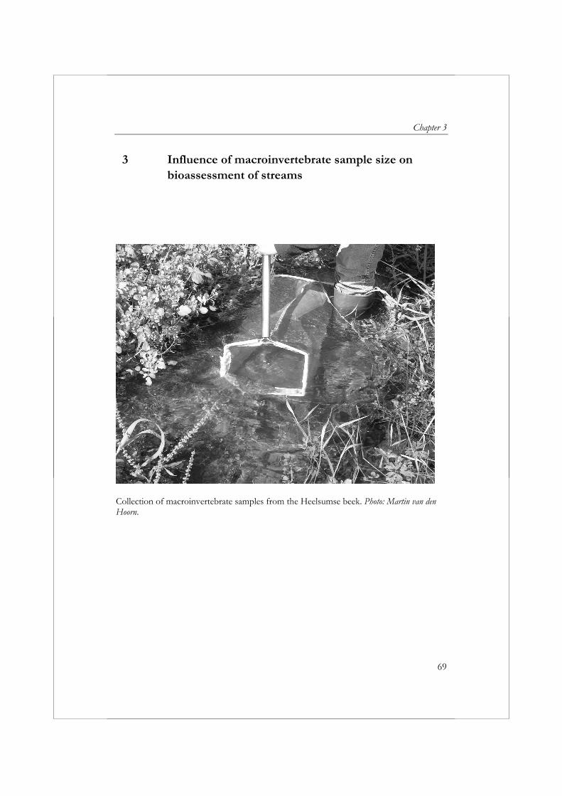
Chapter 3
69
3 Influence of macroinvertebrate sample size on bioassessment of streams
Collection of macroinvertebrate samples from the Heelsumse beek. Photo: Martin van den Hoorn.
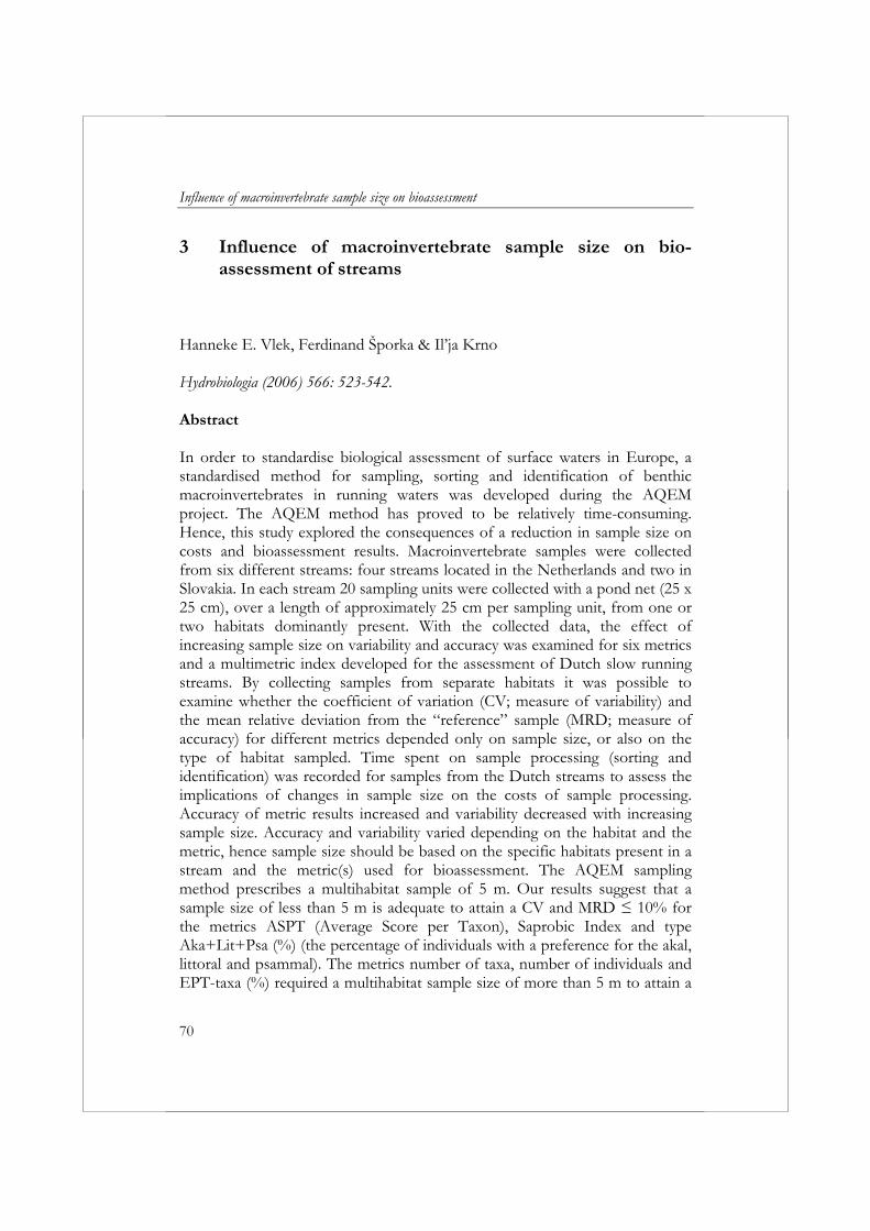
Influence of macroinvertebrate sample size on bioassessment
70
3 Influence of macroinvertebrate sample size on bio-assessment of streams
Hanneke E. Vlek, Ferdinand Šporka & Il’ja Krno Hydrobiologia (2006) 566: 523-542. Abstract In order to standardise biological assessment of surface waters in Europe, a standardised method for sampling, sorting and identification of benthic macroinvertebrates in running waters was developed during the AQEM project. The AQEM method has proved to be relatively time-consuming. Hence, this study explored the consequences of a reduction in sample size on costs and bioassessment results. Macroinvertebrate samples were collected from six different streams: four streams located in the Netherlands and two in Slovakia. In each stream 20 sampling units were collected with a pond net (25 x 25 cm), over a length of approximately 25 cm per sampling unit, from one or two habitats dominantly present. With the collected data, the effect of increasing sample size on variability and accuracy was examined for six metrics and a multimetric index developed for the assessment of Dutch slow running streams. By collecting samples from separate habitats it was possible to examine whether the coefficient of variation (CV; measure of variability) and the mean relative deviation from the “reference” sample (MRD; measure of accuracy) for different metrics depended only on sample size, or also on the type of habitat sampled. Time spent on sample processing (sorting and identification) was recorded for samples from the Dutch streams to assess the implications of changes in sample size on the costs of sample processing. Accuracy of metric results increased and variability decreased with increasing sample size. Accuracy and variability varied depending on the habitat and the metric, hence sample size should be based on the specific habitats present in a stream and the metric(s) used for bioassessment. The AQEM sampling method prescribes a multihabitat sample of 5 m. Our results suggest that a sample size of less than 5 m is adequate to attain a CV and MRD ≤ 10% for the metrics ASPT (Average Score per Taxon), Saprobic Index and type Aka+Lit+Psa (%) (the percentage of individuals with a preference for the akal, littoral and psammal). The metrics number of taxa, number of individuals and EPT-taxa (%) required a multihabitat sample size of more than 5 m to attain a
Chapter 3
71
CV and MRD of ≤ 10%. For the metrics number of individuals and number of taxa a multihabitat sample size of 5 m is not even adequate to attain a CV and MRD of ≤ 20%. Accuracy of the multimetric index for Dutch slow running streams can be increased from ≤ 20% to ≤ 10% with an increase in labour time of two hours. Considering this low increase in costs and the possible implications of incorrect assessment results it is recommended to strive for this ≤ 10% accuracy. To achieve an accuracy of ≤ 10% a multihabitat sample of the four habitats studied in the Netherlands would require a sample size of 2.5 m and a labour time of 26 hours (excluding identification of Oligochaeta and Diptera) or 38 hours (including identification of Oligochaeta and Diptera). Keywords: sample size, costs, macroinvertebrates, metrics, bioassessment, streams, the Netherlands, Slovakia Introduction One of the objectives of the European Water Framework Directive (WFD; European Commission, 2000) is to standardise the biological assessment of surface waters in Europe. In the AQEM project assessment systems based on macroinvertebrates, which meet the requirements of the WFD (Hering et al., 2004), were developed. For example, an assessment system for slow running streams was developed in the Netherlands (Dutch AQEM assessment system; Vlek et al., 2004). For the development of the assessment systems data were collected in eight European countries using a standardised method for sampling, sorting and identification (Hering et al., 2004). This standardised AQEM method requires a pond net (width: 25 cm) or kick sample collected over a length of 5 m, divided into 20 sampling units of 25 cm. The 20 sampling units are proportionally distributed over the habitats present in a stream consistent with their relative coverage. The AQEM method has proved to be relatively time consuming, i.e., sample processing of Dutch samples can take 155 hours per sample (Vlek, 2004). Before water managers are willing to apply the AQEM method for the purpose of biological monitoring the costs associated with the method will have to be drastically reduced.
Costs of monitoring can, among others, be reduced by reducing the sample size. The interpretation of the concept of sample size is variable. Cao et al. (1997) and Bartsch et al. (1998) interpreted sample size as the number of samples (replicates), while Metzling & Miller (2001) interpreted sample size as the physical size of a sample. In most cases a decrease in the costs of biological monitoring programs has been achieved by limiting the number of samples or restricting the number of organisms picked (Metzling & Miller, 2001). The

Influence of macroinvertebrate sample size on bioassessment
72
implications of these measures to reduce costs have been the subject of many studies (e.g., Needham & Usinger, 1956; Chutter, 1972; Elliot, 1977; Barbour et al., 1996; Somers et al., 1998; Lorenz et al., 2004). The implications of reducing the physical sample size, however, have hardly been studied. Also, investigations concerning the number of replicate samples are not relevant in the context of biological monitoring by water managers, since water managers usually take only one multihabitat sample for the purpose of biological monitoring. This multihabitat sample consists of several sampling units from different habitats and all sampling units together form one composite multihabitat sample. In this study we, therefore, addressed the influence of physical sample size instead of the number of replicate samples.
Two important aspects of biological monitoring results should be considered in making decisions on the applied sample size: variability and accuracy. Biological monitoring usually has two purposes: (1) to estimate variables of interest at one site and (2) to make comparisons among sites or times. Variables of interest in biological monitoring are primarily metric values (e.g., the number of taxa, ASPT values, BMWP values) and ecological quality indications resulting from assessment systems. Accuracy is a very important aspect of estimating metric values, since accuracy refers to the closeness of a measurement to its true value (Norris et al., 1992). For the purpose of this study the definition of accuracy by Norris et al. (1992) has been adopted. The aspect of variability is very important in making comparisons, because the validity of conclusions depends on data variability (Norris et al., 1992). Higher variability and lower accuracy increase the risk of incorrect assessment results. In case the ecological quality at a site is incorrectly assessed as less than good, water managers will unnecessarily take costly restoration measures to reach a good ecological quality by 2015 (European Commission, 2000). From this point of view, the consequences of poor decision making due to low accuracy and/or high variability potentially outweigh the savings associated with a smaller sample size (Doberstein, 2000).
Given the importance of accuracy, variability and costs in the process of decision making, the aim of this study was to assess the implications of changes in sample size for different habitats on: (1) the variability and accuracy in metric values, (2) the variability and accuracy of assessment results calculated with the Dutch AQEM assessment system and (3) the costs of sample processing.
Chapter 3
73
Methods Study site and data collection The Netherlands Streams dominated by a single habitat (coverage > 50%) were selected to enable sampling of that habitat over a total length of 5 m. In total, four sites at four different streams (the Oude beek, the Heelsumse beek, the Tongerensche beek and the Molenbeek) were sampled. Each stream is dominated by a different habitat. The streams represent slow flowing (current velocity < 50 cm/s) middle and downstream reaches of poor to moderate ecological quality in the Netherlands, except for the Oude Beek. The Oude Beek is an upstream reach of good ecological quality. The catchment area of all streams is smaller than 100 km2 and is located between 0 and 200 m a.s.l. Fine to medium-sized gravel (0.2–2 cm; akal) was sampled in the Oude Beek (N 52º 9′ 47.9″ E 5º 57′ 30.1″), submerged macrophytes (Callitriche sp.) in the Heelsumse beek (N 51º 58′ 40.7″ E 5º 45′ 30.6″), sand in the Tongerensche beek (N 52° 20΄ 22.9˝ E 5° 55΄ 47.3˝) and FPOM (fine particulate organic matter) in the Molenbeek (N 51° 59΄ 26.2˝ E 5° 43΄ 53.5˝). The Heelsumse beek, the Tongerensche beek, and the Molenbeek were selected because they represent a stream type and ecological quality which frequently occurs in the Netherlands. The Oude Beek was selected because gravel is frequently found in streams of good ecological quality.
Sampling took place between June and September 2002. From each stream 20 sampling units of the dominant habitat were collected. A sampling unit was collected by pushing a rectangular pond net (25 cm x 25 cm, mesh size 500 μm) through the upper part of the substratum (2 - 5 cm) over a length of approximately 25 cm. A ruler was used to visually point out the length of approximately 25 cm. The 20 sampling units were collected in buckets, and kept separately during sample processing. In the laboratory the sampling units were stored overnight in a refrigerator, where they were oxygenated until sorting. The sampling units were washed through a 1000 and a 250 μm sieve prior to sorting. Live organisms were sorted from the sampling units by eye and preserved in 70% ethanol, except for Oligochaeta and Hydracarina. Oligochaeta were preserved in 4% formaldehyde and Hydracarina in Koenike fluid. Organisms were identified to the lowest taxonomic level possible, i.e., species level for almost all specimens. Literature used for identification purposes is listed in AQEM consortium (2002: 156, Appendix 8). Time spent
Influence of macroinvertebrate sample size on bioassessment
74
on sorting and identification of all specimens in each sampling unit was recorded. Slovakia In Slovakia, four different habitats were sampled in two streams: Pokútsky potok (N 48° 34΄ 14.8˝ E 18° 40΄ 16.5˝) and Hostiansky potok (N 48° 29΄ 36.3˝ E 18° 28΄ 40.1˝). Both streams are siliceous mountain streams in the West Carpathian. Their catchment is smaller than 100 km2 and is located between 200 and 500 m a.s.l. Pokútsky potok represents streams of high ecological quality and Hostiansky potok represents streams of good to moderate ecological quality. Two dominating habitats were sampled in both streams: macrolithal (20 – 40 cm) and mesolithal (6 – 20 cm) in Pokútsky potok, akal and microlithal (2 – 6 cm) in Hostiansky potok. The streams were selected because they represent a range in ecological quality that is frequently found in small siliceous mountain streams in the West Carpathian.
Sampling took place in June 2003. From each habitat 20 sampling units were collected as described for the Dutch streams. The 20 sampling units were collected in buckets, preserved in 4% formaldehyde, and kept separately during sample processing. The buckets were transported to the laboratory. The sampling units were washed through a 1000 μm and a 500 μm sieve in the laboratory prior to sorting. Preserved organisms were sorted from the sampling units by stereomicroscope and preserved in 70% ethanol. Organisms were identified to the lowest taxonomic level possible, i.e. species level for almost all specimens. Literature used for identification purposes is listed in AQEM consortium (2002: p. 143, Appendix 8). Data analysis In total 158 sampling units were collected from eight different habitats. The assumption was made that the 20 pooled sampling units from one habitat would accurately represent the macroinvertebrate community composition of the respective habitat. The 20 pooled sampling units (with a total sample size of 5 m) are therefore referred to as the “reference” sample. The sample size is expressed as the length over which the pond net was pushed through the substratum. This length can be easily converted into the sampled area by multiplying it by 0.25 m (width of the pond net). Different numbers and combinations of sampling units were pooled per habitat to “construct” composite samples of different sizes. To gain insight into the effect of sample size on variability and accuracy the sampling units from each habitat were
Chapter 3
75
randomly reordered 50 times. In case of one sampling unit or 19 sampling units it was only possible to reorder 20 times. For each sample size the randomly selected sampling units were pooled to form a composite sample. Sampling units were selected randomly without replacement because in the field the same area is normally not sampled twice. The described procedure resulted in 50 or 20 replicate (composite) samples per sample size with sample size ranging from 0.25 m to 4.75 m. For example, 50 randomly selected combinations of eight sampling units were used to study a sample size of 2 m.
For evaluation, six metrics were selected from an extensive list of metrics that can be calculated with the program ASTERICS version 1.0 (AQEM/STAR Ecological RIver Classification System; http://www.aqem.de): the Saprobic Index (Zelinka & Marvan, 1961), the Average Score per Taxon (ASPT; Armitage et al., 1983), the number of individuals, the number of taxa, the percentage of Epehemeroptera, Plecoptera and Trichoptera taxa (EPT-taxa (%); Lenat, 1988), and the percentage of individuals with a preference for the akal, littoral and psammal (type Aka+Lit+Psa (%); Schmedtje & Colling, 1996). The first reason to select these metrics was that they represent a variety of metric types (taxon richness, community composition, tolerance-intolerance, habitat preference, population attributes). Second, some of these metrics are frequently used in Europe. Third, EPT-taxa (%), type Aka+Lit+Psa (%) and ASPT have proven to be well correlated to anthropogenic stress in Dutch slow running streams and are incorporated in a revised version of the multimetric index for the assessment of Dutch slow running streams described by Vlek et al. (2004). Fourth, EPT-taxa (%) and ASPT have proven to be well correlated to anthropogenic stress in streams with habitats similar to the habitats present in Slovakian mountain streams (Hering et al., 2004).
Metric values were calculated for all composite samples and plotted against the sample size (number of pooled sampling units) (Heyer & Berven, 1973; Bartsch et al., 1998). Species abundances in a sample of a certain size were always standardised to a sample size of 5 m (abundance x 5/sample size (m)), e.g., species abundances in a composite sample consisting of 10 sampling units (2.5 m) were multiplied by two to make them comparable to the species abundances in a composite sample consisting of 20 pooled sampling units (5 m). To compare accuracy between metrics, habitats and sample size, the relative deviation of the metric value for each composite sample from the “reference” sample (true value) was calculated. The information concerning accuracy was summarised by calculating the mean relative deviation (MRD) over all composite samples of a certain size.
The coefficient of variation (CV = SD / mean), a measure of variability, was calculated for the metric values of each sample size per habitat.
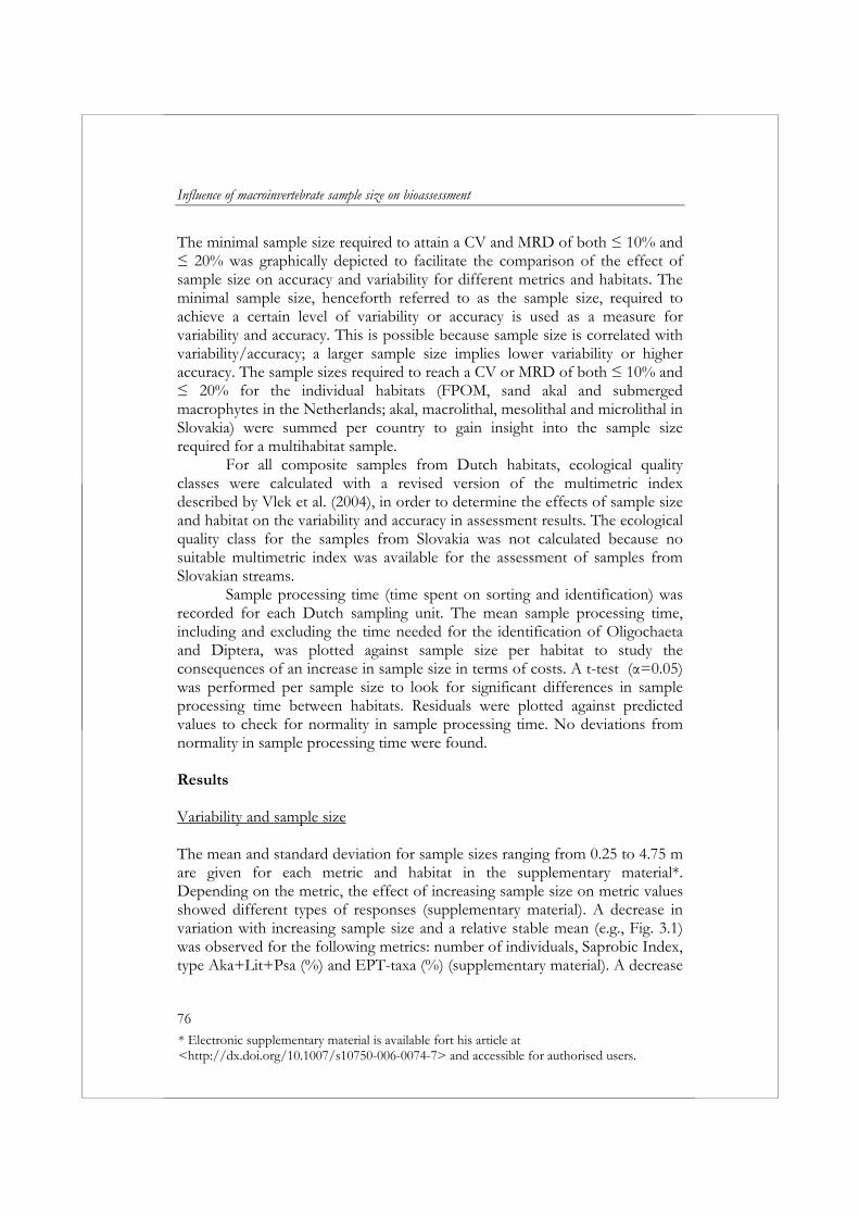
Influence of macroinvertebrate sample size on bioassessment
76
The minimal sample size required to attain a CV and MRD of both ≤ 10% and ≤ 20% was graphically depicted to facilitate the comparison of the effect of sample size on accuracy and variability for different metrics and habitats. The minimal sample size, henceforth referred to as the sample size, required to achieve a certain level of variability or accuracy is used as a measure for variability and accuracy. This is possible because sample size is correlated with variability/accuracy; a larger sample size implies lower variability or higher accuracy. The sample sizes required to reach a CV or MRD of both ≤ 10% and ≤ 20% for the individual habitats (FPOM, sand akal and submerged macrophytes in the Netherlands; akal, macrolithal, mesolithal and microlithal in Slovakia) were summed per country to gain insight into the sample size required for a multihabitat sample.
For all composite samples from Dutch habitats, ecological quality classes were calculated with a revised version of the multimetric index described by Vlek et al. (2004), in order to determine the effects of sample size and habitat on the variability and accuracy in assessment results. The ecological quality class for the samples from Slovakia was not calculated because no suitable multimetric index was available for the assessment of samples from Slovakian streams.
Sample processing time (time spent on sorting and identification) was recorded for each Dutch sampling unit. The mean sample processing time, including and excluding the time needed for the identification of Oligochaeta and Diptera, was plotted against sample size per habitat to study the consequences of an increase in sample size in terms of costs. A t-test (α=0.05) was performed per sample size to look for significant differences in sample processing time between habitats. Residuals were plotted against predicted values to check for normality in sample processing time. No deviations from normality in sample processing time were found. Results Variability and sample size The mean and standard deviation for sample sizes ranging from 0.25 to 4.75 m are given for each metric and habitat in the supplementary material*. Depending on the metric, the effect of increasing sample size on metric values showed different types of responses (supplementary material). A decrease in variation with increasing sample size and a relative stable mean (e.g., Fig. 3.1) was observed for the following metrics: number of individuals, Saprobic Index, type Aka+Lit+Psa (%) and EPT-taxa (%) (supplementary material). A decrease
* Electronic supplementary material is available fort his article at <http://dx.doi.org/10.1007/s10750-006-0074-7> and accessible for authorised users.
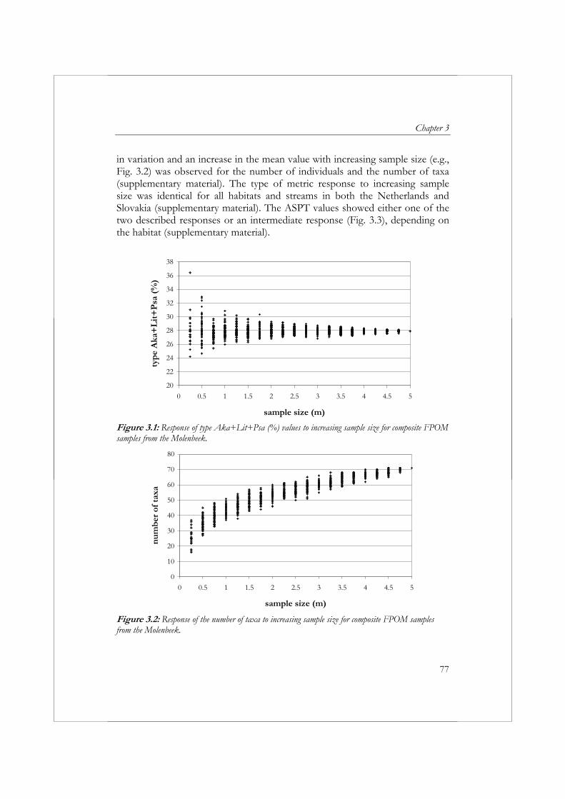
Chapter 3
77
in variation and an increase in the mean value with increasing sample size (e.g., Fig. 3.2) was observed for the number of individuals and the number of taxa (supplementary material). The type of metric response to increasing sample size was identical for all habitats and streams in both the Netherlands and Slovakia (supplementary material). The ASPT values showed either one of the two described responses or an intermediate response (Fig. 3.3), depending on the habitat (supplementary material).
20
22
24
26
28
30
32
34
36
38
0 0.5 1 1.5 2 2.5 3 3.5 4 4.5 5
sample size (m)
typ
e A
ka+
Lit
+P
sa (
%)
Figure 3.1: Response of type Aka+Lit+Psa (%) values to increasing sample size for composite FPOM samples from the Molenbeek.
0
10
20
30
40
50
60
70
80
0 0.5 1 1.5 2 2.5 3 3.5 4 4.5 5
sample size (m)
nu
mb
er o
f ta
xa
Figure 3.2: Response of the number of taxa to increasing sample size for composite FPOM samples from the Molenbeek.
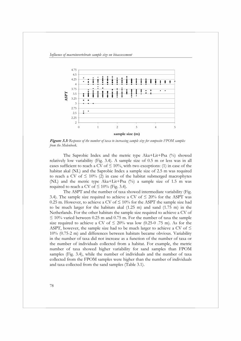
Influence of macroinvertebrate sample size on bioassessment
78
2
2.25
2.5
2.75
3
3.25
3.5
3.75
4
4.25
4.5
4.75
0 1 2 3 4 5
sample size (m)
ASP
T
Figure 3.3: Response of the number of taxa to increasing sample size for composite FPOM samples from the Molenbeek.
The Saprobic Index and the metric type Aka+Lit+Psa (%) showed
relatively low variability (Fig. 3.4). A sample size of 0.5 m or less was in all cases sufficient to reach a CV of ≤ 10%, with two exceptions: (1) in case of the habitat akal (NL) and the Saprobic Index a sample size of 2.5 m was required to reach a CV of ≤ 10% (2) in case of the habitat submerged macrophytes (NL) and the metric type Aka+Lit+Psa (%) a sample size of 1.5 m was required to reach a CV of ≤ 10% (Fig. 3.4).
The ASPT and the number of taxa showed intermediate variability (Fig. 3.4). The sample size required to achieve a CV of ≤ 20% for the ASPT was 0.25 m. However, to achieve a CV of ≤ 10% for the ASPT the sample size had to be much larger for the habitats akal (1.25 m) and sand (1.75 m) in the Netherlands. For the other habitats the sample size required to achieve a CV of ≤ 10% varied between 0.25 m and 0.75 m. For the number of taxa the sample size required to achieve a CV of ≤ 20% was low (0.25-0 .75 m). As for the ASPT, however, the sample size had to be much larger to achieve a CV of ≤ 10% (0.75-2 m) and differences between habitats became obvious. Variability in the number of taxa did not increase as a function of the number of taxa or the number of individuals collected from a habitat. For example, the metric number of taxa showed higher variability for sand samples than FPOM samples (Fig. 3.4), while the number of individuals and the number of taxa collected from the FPOM samples were higher than the number of individuals and taxa collected from the sand samples (Table 3.1).
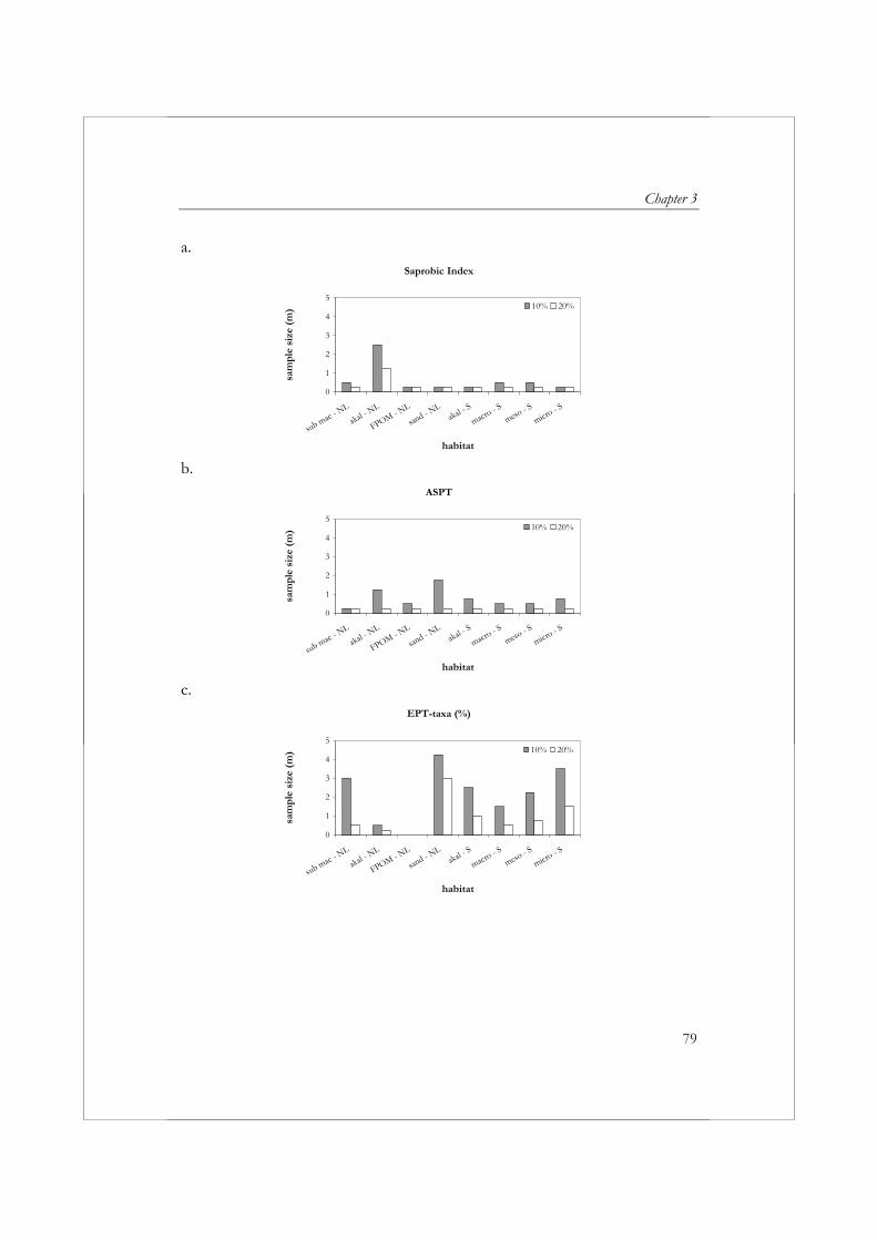
Chapter 3
79
a. Saprobic Index
0
1
2
3
4
5
sub mac - NL
akal - NL
FPOM - NL
sand - N
Lakal -
S
macro - S
meso - S
micro - S
habitat
sam
ple
siz
e (m
) 10% 20%
b.
ASPT
0
1
2
3
4
5
sub mac - NL
akal - NL
FPOM - NL
sand - N
Lakal -
S
macro - S
meso - S
micro - S
habitat
sam
ple
siz
e (m
) 10% 20%
c.
EPT-taxa (%)
0
1
2
3
4
5
sub mac - NL
akal - NL
FPOM - NL
sand - N
Lakal -
S
macro - S
meso - S
micro - S
habitat
sam
ple
siz
e (m
) 10% 20%
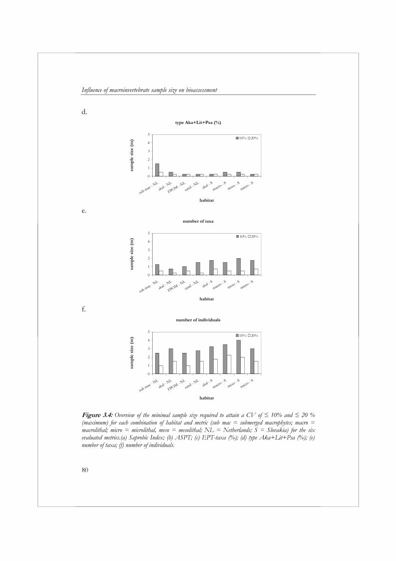
Influence of macroinvertebrate sample size on bioassessment
80
d. type Aka+Lit+Psa (%)
0
1
2
3
4
5
sub mac - NL
akal - NL
FPOM - NL
sand - N
Lakal -
S
macro - S
meso - S
micro - S
habitat
sam
ple
siz
e (m
) 10% 20%
e.
number of taxa
0
1
2
3
4
5
sub mac - NL
akal - NL
FPOM - NL
sand - N
Lakal -
S
macro - S
meso - S
micro - S
habitat
sam
ple
siz
e (m
) 10% 20%
f.
number of individuals
0
1
2
3
4
5
sub mac - NL
akal - NL
FPOM - NL
sand - N
Lakal -
S
macro - S
meso - S
micro - S
habitat
sam
ple
siz
e (m
) 10% 20%
Figure 3.4: Overview of the minimal sample size required to attain a CV of ≤ 10% and ≤ 20 % (maximum) for each combination of habitat and metric (sub mac = submerged macrophytes; macro = macrolithal; micro = microlithal, meso = mesolithal; NL = Netherlands; S = Slovakia) for the six evaluated metrics.(a) Saprobic Index; (b) ASPT; (c) EPT-taxa (%); (d) type Aka+Lit+Psa (%); (e) number of taxa; (f) number of individuals.

Chapter 3
81
Table 3.1: Overview of the number of individuals and number of taxa collected from the 20 sampling units per habitat and country.
Habitat Number of individuals Number of taxaThe Netherlands akal 2759 59submerged macrophytes 3032 44FPOM 7693 71sand 5404 63Slovakia akal 3246 54microlithal 2152 59mesolithal 1056 58macrolithal 1198 66
The EPT-taxa (%) and the number of individuals showed high
variability in most cases (Fig. 3.4). The sample size required to achieve a CV of ≤ 10% for the EPT-taxa (%) varied highly from 0.5 to 4.25 m in both countries, depending on the habitat. Results for the EPT-taxa (%) from the habitat FPOM are not depicted in Figure 3.4, because EPT-taxa were only found in three of the 20 sampling units and in very low percentages (3.4% on average). The sample size required to achieve a CV of ≤ 10% for the EPT-taxa (%) was 2.5 m on average, whereas it was 1 m on average to achieve a CV of ≤ 20%. To achieve a CV of ≤ 10%, all habitats required a sample size of at least 1.75 m, except for the habitats akal (NL) and macrolithal (S). The differences between habitats were somewhat smaller for the number of individuals than for the EPT-taxa (%) with the sample size required to achieve a CV of ≤ 10% ranging from 2.5 to 4 m. On average sampling of 3 m (CV of ≤ 20%) and 1.5 m (CV of ≤ 10%) was required for the number of individuals.
Akal was the only habitat sampled both in the Netherlands and in Slovakia. The difference in the sample size required to achieve a CV of ≤ 10% for this habitat between the Netherlands and Slovakia was less than 0.75 m for the number of individuals, the ASPT and the metric type Aka+Lit+Psa (%) (Fig. 3.4). The differences in the sample size required to achieve a CV of ≤ 10% were much higher for the number of taxa (1 m), the EPT-taxa (%) (2 m) and the Saprobic Index (2.25 m). The sample size required to reach a CV of ≤ 10% and ≤ 20% for a multihabitat sample from streams in the Netherlands and Slovakia is shown in Table 3.2. The sample size required to attain a CV ≤ 10% for the Saprobic index, the metric type Aka+Lit+Psa (%) and the ASPT was considerable smaller than 5 m (between 1.5 m and 3.75 m). The minimal sample size required to attain a CV of ≤ 10% for the metrics number of taxa, number of

Influ
ence
of m
acro
inve
rtebr
ate s
ampl
e siz
e on
bioa
sses
smen
t
82 T
able
3.2
: Ove
rview
of t
he m
inim
al m
ultih
abita
t sam
ple s
ize r
equi
red
to a
ttain
a C
V o
f ≤ 1
0%, a
CV
of ≤
20%
, a M
RD
of ≤
10%
and
MR
D o
f ≤
20%
for e
ach
com
bina
tion
of m
etric
and
coun
try (N
L =
the N
ether
land
s; S
= S
lova
kia)
.
Met
ric
Cou
ntr
ySa
mp
le s
ize
(m)
CV≤
10%
MR
D≤
10%
CV≤
20%
MR
D≤
20%
type
Aka
+L
it+P
sa (%
) N
L2.
52.
51.
251.
25
type
Aka
+L
it+P
sa (%
) S
1.5
1.25
11
EP
T-t
axa
(%)
NL
7.75
9.75
3.75
5.25
E
PT
-tax
a (%
) S
9.75
9.25
3.75
3.5
num
ber
of in
divi
dual
s N
L10
.75
6.75
52.
75
num
ber
of in
divi
dual
s S
13.7
512
.25
7.5
6 A
SPT
NL
3.75
31
1.5
ASP
TS
2.5
4.5
11
num
ber
of ta
xa
NL
4.5
13.7
51.
59.
75
num
ber
of ta
xa
S7
15.5
2.5
11.2
5 Sa
prob
ic I
ndex
N
L3.
53.
252
1.75
Sa
prob
ic I
ndex
S
1.5
1.25
11
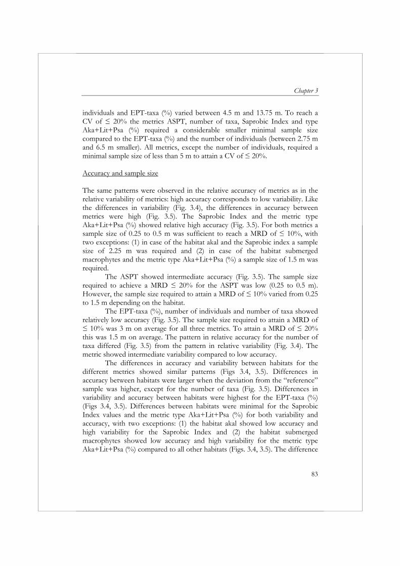
Chapter 3
83
individuals and EPT-taxa (%) varied between 4.5 m and 13.75 m. To reach a CV of ≤ 20% the metrics ASPT, number of taxa, Saprobic Index and type Aka+Lit+Psa (%) required a considerable smaller minimal sample size compared to the EPT-taxa (%) and the number of individuals (between 2.75 m and 6.5 m smaller). All metrics, except the number of individuals, required a minimal sample size of less than 5 m to attain a CV of ≤ 20%. Accuracy and sample size The same patterns were observed in the relative accuracy of metrics as in the relative variability of metrics: high accuracy corresponds to low variability. Like the differences in variability (Fig. 3.4), the differences in accuracy between metrics were high (Fig. 3.5). The Saprobic Index and the metric type Aka+Lit+Psa (%) showed relative high accuracy (Fig. 3.5). For both metrics a sample size of 0.25 to 0.5 m was sufficient to reach a MRD of ≤ 10%, with two exceptions: (1) in case of the habitat akal and the Saprobic index a sample size of 2.25 m was required and (2) in case of the habitat submerged macrophytes and the metric type Aka+Lit+Psa (%) a sample size of 1.5 m was required.
The ASPT showed intermediate accuracy (Fig. 3.5). The sample size required to achieve a MRD ≤ 20% for the ASPT was low (0.25 to 0.5 m). However, the sample size required to attain a MRD of ≤ 10% varied from 0.25 to 1.5 m depending on the habitat.
The EPT-taxa (%), number of individuals and number of taxa showed relatively low accuracy (Fig. 3.5). The sample size required to attain a MRD of ≤ 10% was 3 m on average for all three metrics. To attain a MRD of ≤ 20% this was 1.5 m on average. The pattern in relative accuracy for the number of taxa differed (Fig. 3.5) from the pattern in relative variability (Fig. 3.4). The metric showed intermediate variability compared to low accuracy.
The differences in accuracy and variability between habitats for the different metrics showed similar patterns (Figs 3.4, 3.5). Differences in accuracy between habitats were larger when the deviation from the “reference” sample was higher, except for the number of taxa (Fig. 3.5). Differences in variability and accuracy between habitats were highest for the EPT-taxa (%) (Figs 3.4, 3.5). Differences between habitats were minimal for the Saprobic Index values and the metric type Aka+Lit+Psa (%) for both variability and accuracy, with two exceptions: (1) the habitat akal showed low accuracy and high variability for the Saprobic Index and (2) the habitat submerged macrophytes showed low accuracy and high variability for the metric type Aka+Lit+Psa (%) compared to all other habitats (Figs. 3.4, 3.5). The difference

Influence of macroinvertebrate sample size on bioassessment
84
in accuracy between habitats for the number of taxa was low compared to the differences in variability.
The differences in the sample size required to attain a MRD of ≤ 10% for the habitat akal between the Netherlands and Slovakia was less than 0.75 m for all metrics, except for the Saprobic Index (2 m; Fig. 3.5).
The sample size required to reach a MRD of ≤ 10% and ≤ 20% for a multihabitat sample from streams in the Netherlands and Slovakia is shown in Table 3.2 . The sample size required to attain a MRD ≤ 10% for the Saprobic index, the metric type Aka+Lit+Psa (%) and ASPT was smaller than 5 m (between 1.25 m and 4 m). The sample size required to attain a MRD ≤ 10% for the metrics number of taxa, number of individuals and EPT-taxa (%) varied between 6.75 m and 15.5 m. To reach a MRD of ≤ 20% the metrics ASPT, Saprobic Index and type Aka+Lit+Psa (%) required a considerable smaller sample size compared to the EPT-taxa (%), the number of taxa and the number of individuals (between 1 m and 10.25 m smaller). All metrics, except the EPT-taxa (%) from Dutch streams and the number of taxa, required a sample size of less than 5 m to attain a CV of ≤ 20%.
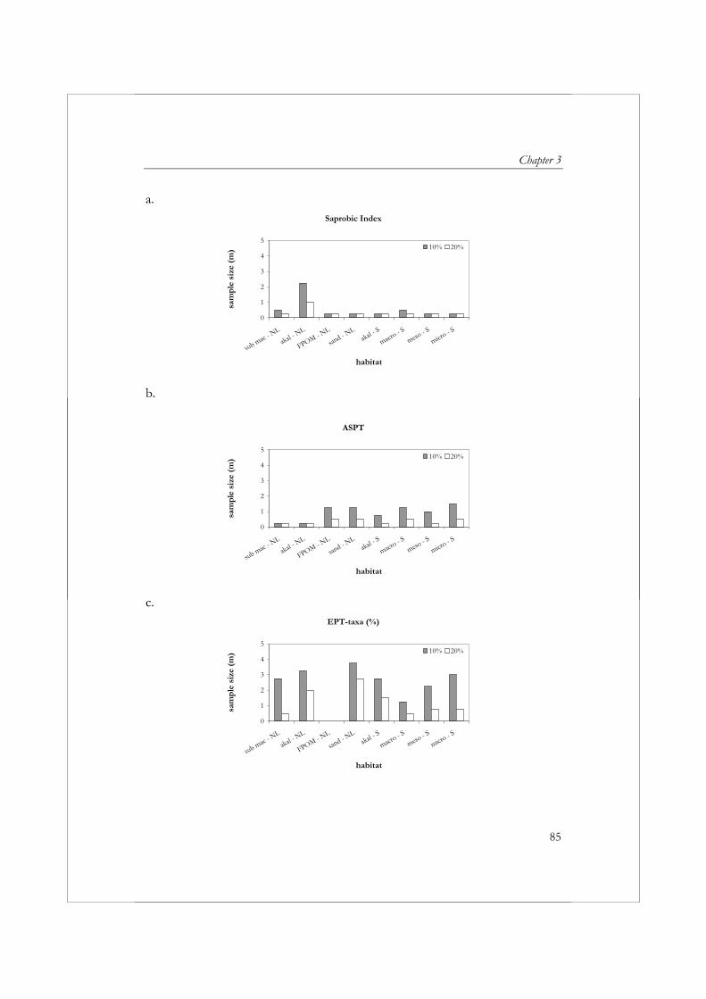
Chapter 3
85
a. Saprobic Index
0
1
2
3
4
5
sub mac - NL
akal - NL
FPOM - NL
sand - N
Lakal -
S
macro - S
meso - S
micro - S
habitat
sam
ple
size
(m
) 10% 20%
b.
ASPT
0
1
2
3
4
5
sub mac - NL
akal - NL
FPOM - NL
sand - N
Lakal -
S
macro - S
meso - S
micro - S
habitat
sam
ple
size
(m
) 10% 20%
c. EPT-taxa (%)
0
1
2
3
4
5
sub mac - NL
akal - NL
FPOM - NL
sand - N
Lakal -
S
macro - S
meso - S
micro - S
habitat
sam
ple
size
(m
) 10% 20%
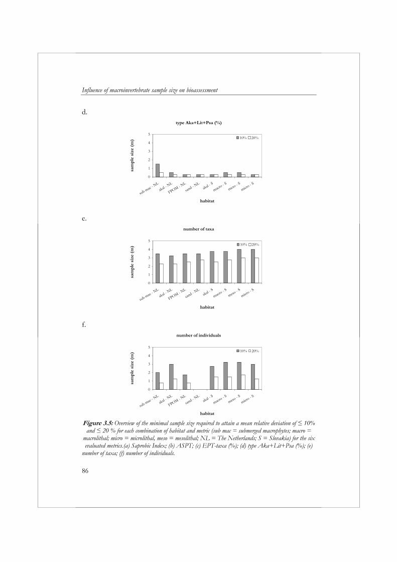
Influence of macroinvertebrate sample size on bioassessment
86
d. type Aka+Lit+Psa (%)
0
1
2
3
4
5
sub mac - NL
akal - NL
FPOM - NL
sand - N
Lakal -
S
macro - S
meso - S
micro - S
habitat
sam
ple
size
(m
) 10% 20%
e. number of taxa
0
1
2
3
4
5
sub mac - NL
akal - NL
FPOM - NL
sand - N
Lakal -
S
macro - S
meso - S
micro - S
habitat
sam
ple
siz
e (m
) 10% 20%
f. number of individuals
0
1
2
3
4
5
sub mac - NL
akal - NL
FPOM - NL
sand - N
Lakal -
S
macro - S
meso - S
micro - S
habitat
sam
ple
siz
e (m
) 10% 20%
Figure 3.5: Overview of the minimal sample size required to attain a mean relative deviation of ≤ 10%
and ≤ 20 % for each combination of habitat and metric (sub mac = submerged macrophytes; macro = macrolithal; micro = microlithal, meso = mesolithal; NL = The Netherlands; S = Slovakia) for the six evaluated metrics.(a) Saprobic Index; (b) ASPT; (c) EPT-taxa (%); (d) type Aka+Lit+Psa (%); (e)
number of taxa; (f) number of individuals.
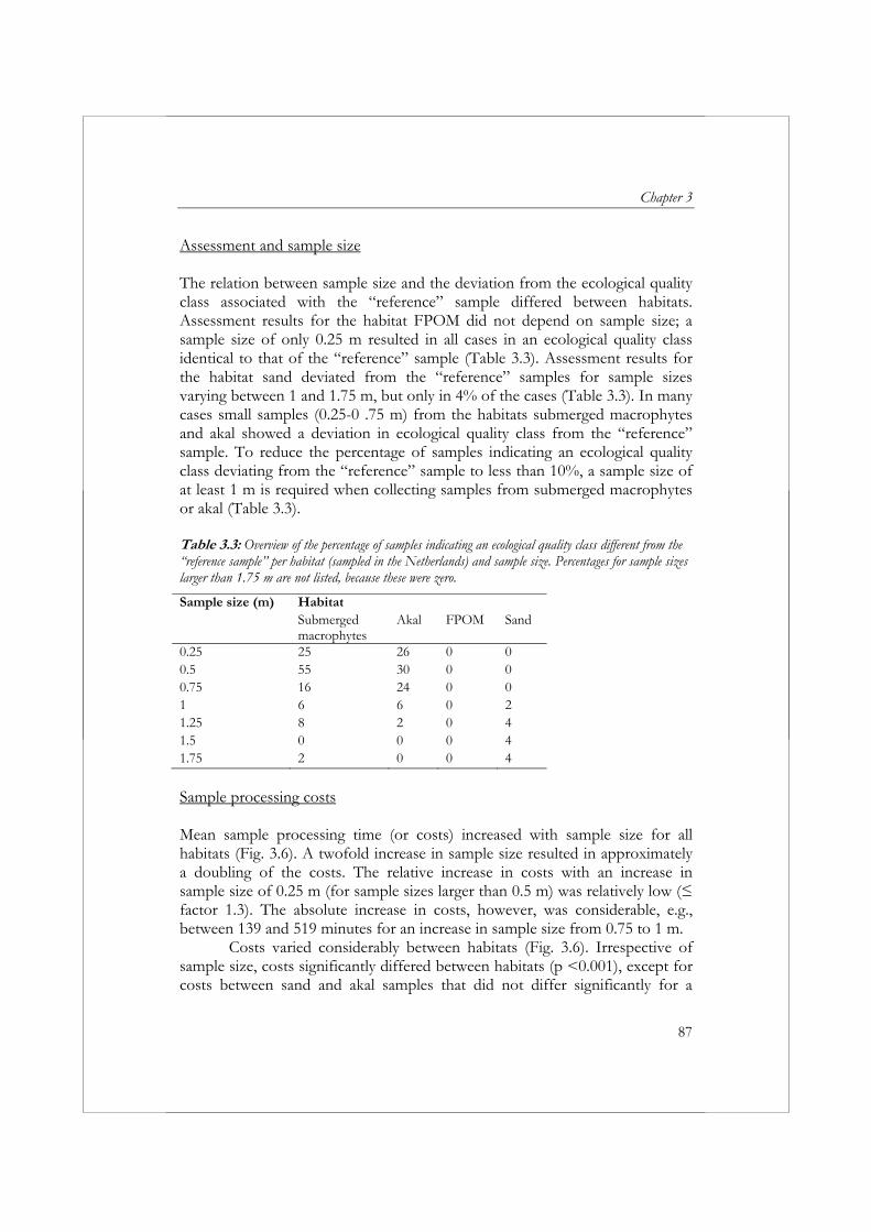
Chapter 3
87
Assessment and sample size The relation between sample size and the deviation from the ecological quality class associated with the “reference” sample differed between habitats. Assessment results for the habitat FPOM did not depend on sample size; a sample size of only 0.25 m resulted in all cases in an ecological quality class identical to that of the “reference” sample (Table 3.3). Assessment results for the habitat sand deviated from the “reference” samples for sample sizes varying between 1 and 1.75 m, but only in 4% of the cases (Table 3.3). In many cases small samples (0.25-0 .75 m) from the habitats submerged macrophytes and akal showed a deviation in ecological quality class from the “reference” sample. To reduce the percentage of samples indicating an ecological quality class deviating from the “reference” sample to less than 10%, a sample size of at least 1 m is required when collecting samples from submerged macrophytes or akal (Table 3.3). Table 3.3: Overview of the percentage of samples indicating an ecological quality class different from the “reference sample” per habitat (sampled in the Netherlands) and sample size. Percentages for sample sizes larger than 1.75 m are not listed, because these were zero.
Sample size (m) Habitat Submerged
macrophytes Akal FPOM Sand
0.25 25 26 0 00.5 55 30 0 00.75 16 24 0 01 6 6 0 21.25 8 2 0 41.5 0 0 0 41.75 2 0 0 4
Sample processing costs Mean sample processing time (or costs) increased with sample size for all habitats (Fig. 3.6). A twofold increase in sample size resulted in approximately a doubling of the costs. The relative increase in costs with an increase in sample size of 0.25 m (for sample sizes larger than 0.5 m) was relatively low (≤ factor 1.3). The absolute increase in costs, however, was considerable, e.g., between 139 and 519 minutes for an increase in sample size from 0.75 to 1 m.
Costs varied considerably between habitats (Fig. 3.6). Irrespective of sample size, costs significantly differed between habitats (p <0.001), except for costs between sand and akal samples that did not differ significantly for a
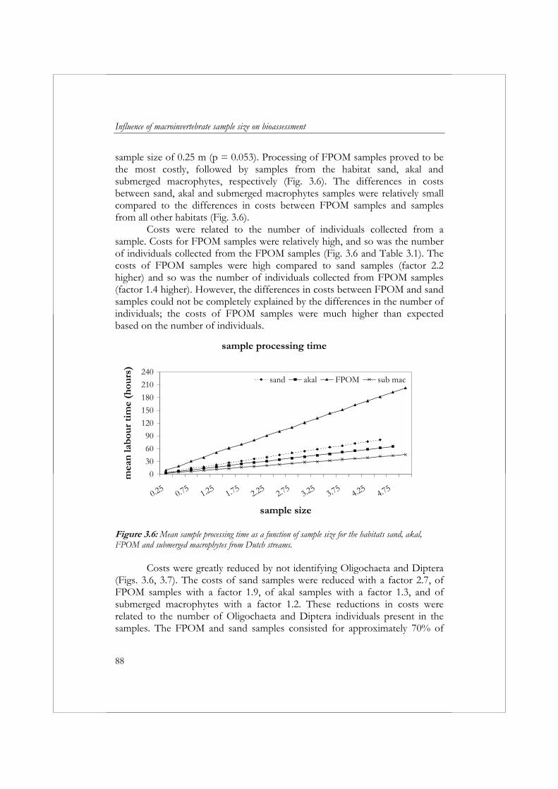
Influence of macroinvertebrate sample size on bioassessment
88
sample size of 0.25 m (p = 0.053). Processing of FPOM samples proved to be the most costly, followed by samples from the habitat sand, akal and submerged macrophytes, respectively (Fig. 3.6). The differences in costs between sand, akal and submerged macrophytes samples were relatively small compared to the differences in costs between FPOM samples and samples from all other habitats (Fig. 3.6).
Costs were related to the number of individuals collected from a sample. Costs for FPOM samples were relatively high, and so was the number of individuals collected from the FPOM samples (Fig. 3.6 and Table 3.1). The costs of FPOM samples were high compared to sand samples (factor 2.2 higher) and so was the number of individuals collected from FPOM samples (factor 1.4 higher). However, the differences in costs between FPOM and sand samples could not be completely explained by the differences in the number of individuals; the costs of FPOM samples were much higher than expected based on the number of individuals.
sample processing time
0
30
60
90
120
150
180
210
240
0.250.75
1.251.75
2.252.75
3.253.75
4.254.75
sample size
mea
n la
bou
r ti
me
(hou
rs)
sand akal FPOM sub mac
Figure 3.6: Mean sample processing time as a function of sample size for the habitats sand, akal, FPOM and submerged macrophytes from Dutch streams.
Costs were greatly reduced by not identifying Oligochaeta and Diptera (Figs. 3.6, 3.7). The costs of sand samples were reduced with a factor 2.7, of FPOM samples with a factor 1.9, of akal samples with a factor 1.3, and of submerged macrophytes with a factor 1.2. These reductions in costs were related to the number of Oligochaeta and Diptera individuals present in the samples. The FPOM and sand samples consisted for approximately 70% of
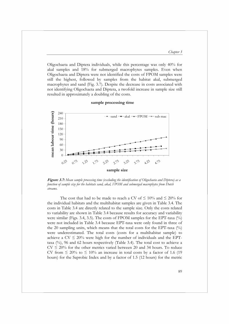
Chapter 3
89
Oligochaeta and Diptera individuals, while this percentage was only 40% for akal samples and 18% for submerged macrophytes samples. Even when Oligochaeta and Diptera were not identified the costs of FPOM samples were still the highest, followed by samples from the habitat akal, submerged macrophytes and sand (Fig. 3.7). Despite the decrease in costs associated with not identifying Oligochaeta and Diptera, a twofold increase in sample size still resulted in approximately a doubling of the costs.
sample processing time
0
30
60
90
120
150
180
210
240
0.250.75
1.251.75
2.252.75
3.253.75
4.254.75
sample size
mea
n la
bou
r ti
me
(hou
rs)
sand akal FPOM sub mac
Figure 3.7: Mean sample processing time (excluding the identification of Oligochaeta and Diptera) as a function of sample size for the habitats sand, akal, FPOM and submerged macrophytes from Dutch streams.
The cost that had to be made to reach a CV of ≤ 10% and ≤ 20% for
the individual habitats and the multihabitat samples are given in Table 3.4. The costs in Table 3.4 are directly related to the sample size. Only the costs related to variability are shown in Table 3.4 because results for accuracy and variability were similar (Figs. 3.4, 3.5). The costs of FPOM samples for the EPT-taxa (%) were not included in Table 3.4 because EPT-taxa were only found in three of the 20 sampling units, which means that the total costs for the EPT-taxa (%) were underestimated. The total costs (costs for a multihabitat sample) to achieve a CV ≤ 20% were high for the number of individuals and the EPT-taxa (%), 96 and 62 hours respectively (Table 3.4). The total cost to achieve a CV ≤ 20% for the other metrics varied between 20 and 34 hours. To reduce CV from ≤ 20% to ≤ 10% an increase in total costs by a factor of 1.6 (19 hours) for the Saprobic Index and by a factor of 1.5 (12 hours) for the metric
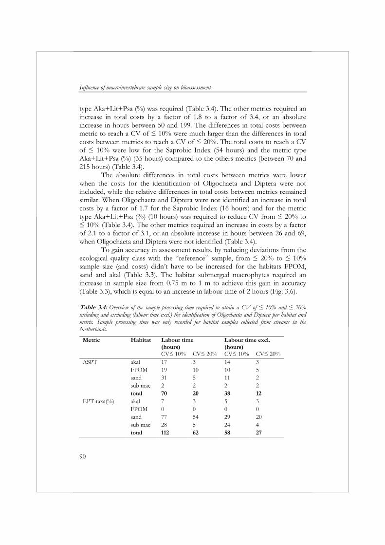
Influence of macroinvertebrate sample size on bioassessment
90
type Aka+Lit+Psa (%) was required (Table 3.4). The other metrics required an increase in total costs by a factor of 1.8 to a factor of 3.4, or an absolute increase in hours between 50 and 199. The differences in total costs between metric to reach a CV of ≤ 10% were much larger than the differences in total costs between metrics to reach a CV of ≤ 20%. The total costs to reach a CV of ≤ 10% were low for the Saprobic Index (54 hours) and the metric type Aka+Lit+Psa (%) (35 hours) compared to the others metrics (between 70 and 215 hours) (Table 3.4).
The absolute differences in total costs between metrics were lower when the costs for the identification of Oligochaeta and Diptera were not included, while the relative differences in total costs between metrics remained similar. When Oligochaeta and Diptera were not identified an increase in total costs by a factor of 1.7 for the Saprobic Index (16 hours) and for the metric type Aka+Lit+Psa (%) (10 hours) was required to reduce CV from ≤ 20% to ≤ 10% (Table 3.4). The other metrics required an increase in costs by a factor of 2.1 to a factor of 3.1, or an absolute increase in hours between 26 and 69, when Oligochaeta and Diptera were not identified (Table 3.4).
To gain accuracy in assessment results, by reducing deviations from the ecological quality class with the “reference” sample, from ≤ 20% to ≤ 10% sample size (and costs) didn’t have to be increased for the habitats FPOM, sand and akal (Table 3.3). The habitat submerged macrophytes required an increase in sample size from 0.75 m to 1 m to achieve this gain in accuracy (Table 3.3), which is equal to an increase in labour time of 2 hours (Fig. 3.6). Table 3.4: Overview of the sample processing time required to attain a CV of ≤ 10% and ≤ 20% including and excluding (labour time excl.) the identification of Oligochaeta and Diptera per habitat and metric. Sample processing time was only recorded for habitat samples collected from streams in the Netherlands.
Metric Habitat Labour time(hours)
Labour time excl. (hours)
CV≤ 10% CV≤ 20% CV≤ 10% CV≤ 20% ASPT akal 17 3 14 3 FPOM 19 10 10 5 sand 31 5 11 2 sub mac 2 2 2 2 total 70 20 38 12EPT-taxa(%) akal 7 3 5 3 FPOM 0 0 0 0 sand 77 54 29 20 sub mac 28 5 24 4 total 112 62 58 27
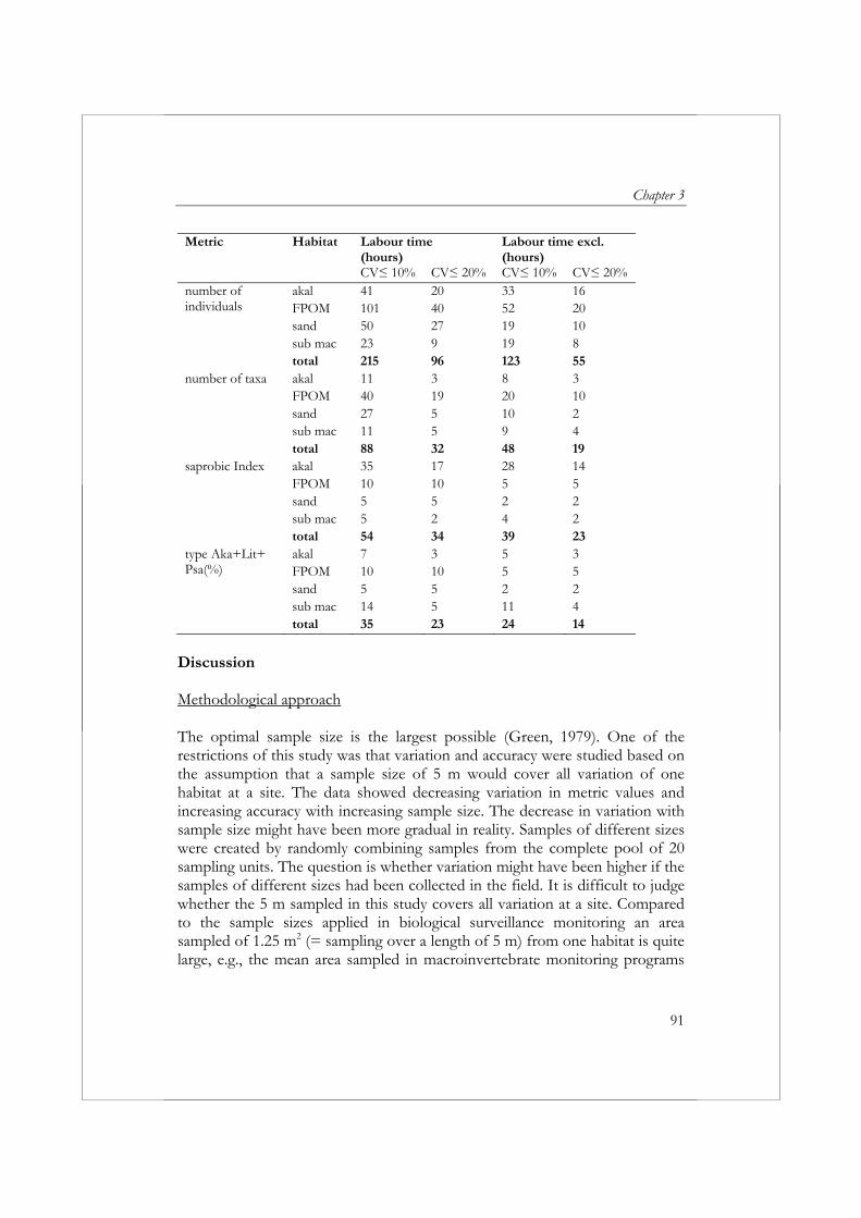
Chapter 3
91
Metric Habitat Labour time(hours)
Labour time excl. (hours)
CV≤ 10% CV≤ 20% CV≤ 10% CV≤ 20% number of individuals
akal 41 20 33 16FPOM 101 40 52 20
sand 50 27 19 10 sub mac 23 9 19 8 total 215 96 123 55number of taxa akal 11 3 8 3 FPOM 40 19 20 10 sand 27 5 10 2 sub mac 11 5 9 4 total 88 32 48 19saprobic Index akal 35 17 28 14 FPOM 10 10 5 5 sand 5 5 2 2 sub mac 5 2 4 2 total 54 34 39 23type Aka+Lit+Psa(%)
akal 7 3 5 3FPOM 10 10 5 5
sand 5 5 2 2 sub mac 14 5 11 4 total 35 23 24 14
Discussion Methodological approach The optimal sample size is the largest possible (Green, 1979). One of the restrictions of this study was that variation and accuracy were studied based on the assumption that a sample size of 5 m would cover all variation of one habitat at a site. The data showed decreasing variation in metric values and increasing accuracy with increasing sample size. The decrease in variation with sample size might have been more gradual in reality. Samples of different sizes were created by randomly combining samples from the complete pool of 20 sampling units. The question is whether variation might have been higher if the samples of different sizes had been collected in the field. It is difficult to judge whether the 5 m sampled in this study covers all variation at a site. Compared to the sample sizes applied in biological surveillance monitoring an area sampled of 1.25 m2 (= sampling over a length of 5 m) from one habitat is quite large, e.g., the mean area sampled in macroinvertebrate monitoring programs
Influence of macroinvertebrate sample size on bioassessment
92
by USA state agencies is 1.7 m2 for a mulitihabitat sample (Carter & Resh, 2001).
The sample size of the individual sampling units was approximately 25 cm. It was not possible to sample exactly 25 cm without disturbing the substrate prior to sampling. The small variation in sample size between the sampling units is not expected to have consequences regarding the applicability of the results of this study, since it will always be a problem to determine the exact sample size when sampling with a pond net in slow running streams.
Samples in this study have been collected between June and September. The fact that the habitats were not sampled simultaneously might have influenced the results. Studies performed in the Netherlands and in Slovakia, however, indicated that there are no significant differences in the number of individuals, the number of taxa, the EPT-taxa (%), ASPT values or Saprobic Index values between months (Šporka et al., 2006; Vlek, 2004). These findings make it unlikely that differences in variability between habitats were the result of differences between months.
In many European countries samples are preserved prior to sorting, while the samples (from the Netherlands) collected during this study were not preserved. Findings by Vlek (2004) suggest that the choice to preserve a sample or not will not influence variability and accuracy in metric values, i.e., Vlek (2004) detected no significant differences in the number of individuals, the number of taxa, the EPT-taxa (%), ASPT values or Saprobic Index values between preserved and unpreserved macroinvertebrate samples collected in the Netherlands.
The samples collected in this study came from different streams which makes it difficult to determine the effect of sample size on variability in metric values of a multihabitat sample. In this study the the assumption was made that by reaching a CV (or MRD) of ≤ 10% for the individual habitats, a CV (or MRD) of ≤ 10% for the multihabitat samples would be guaranteed. Unfortunately, it was not possible to test this assumption since the habitats in this study came from different streams. Generally, macroinvertebrate community composition differs more among streams than within sites (e.g., Doberstein et al., 2000; Sandin & Johnson, 2000). Consequently, variability would be much higher in combining habitat samples from different streams than combining habitat samples from one stream. According to Beisel (1998) the variability in taxon richness and total abundance does not depend on the number of habitats sampled. This would suggest that metric values based on multihabitat samples would not be more variable than metric values based on single habitat samples, as was assumed in this study. Another difficulty was that the relation between variability/accuracy and multihabitat sample size was
Chapter 3
93
based on the four specific habitats sampled in the Netherlands and in Slovakia. This relation will have to be adjusted depending on the number and type of habitats present in the stream that is subjected to monitoring. Carter & Resh (2001) suggested that multihabitat samples would be more variable than single habitat samples, since sampling from multiple habitats in proportion to their cover is most likely to be operator dependent and therefore more difficult to standardize than collecting from a single habitat samples. The variability in habitat coverage estimates is an extra source of variation that should be studied in the future. Variability and sample size High variability in metric values creates problems with assessment. As a result of high variability metric values will overlap between ecological quality classes. This overlap makes it impossible to distinguish between many ecological quality classes, complicating assessment (Doberstein et al., 2000).
When considering costs the metrics type Aka+Lit+Psa (%), Saprobic Index and ASPT should be preferred over the number of individuals, the number of taxa and EPT-taxa (%), for these showed relative low variability and high accuracy, which means that the required sample size to attain a certain degree of variability is smaller. For biological assessment it is important to know whether these metrics are also (highly) correlated to anthropogenic stress. Both the ASPT and the Saprobic Index are frequently applied in Europe and have proven to be highly correlated to organic pollution. The ASPT has been incorporated in multimetric indices in the Czech Rebuplic (Brabec et al., 2004), Greece (Skoulikidis et al., 2004), Italy (Buffagni et al., 2004), Sweden (Dahl et al., 2004) and the United Kingdom (Clarke et al., 2002). The Saprobic Index (or derivations from this index) has been incorporated in multimetric indices in Austria (Ofenböck et al., 2004), the Czech Republic (Brabec et al., 2004), Germany (Rolauffs et al., 2004), the Netherlands (Vlek et al., 2004) and Sweden (Dahl et al., 2004). A possible correlation between anthropogenic stress and type Aka+Lit+Psa (%) values are yet to be established.
The number of taxa and the number of individuals are notoriously poor metrics (Karr & Chu, 1999). The number of individuals showed high variation compared to the other metrics evaluated in this study. Apparently, significant variation in faunal densities occurs over small spatial scale, possibly caused by invertebrate aggregations (Downes et al., 1993).
Differences in variability between habitats depended on the metric studied, indicating that differences in variability between habitats could not be explained based on general assumptions about habitat heterogeneity. In
Influence of macroinvertebrate sample size on bioassessment
94
general, metrics characterised by higher variability showed larger differences between habitats.
The large differences in variability for the number of taxa, the EPT-taxa (%) and the Saprobic Index between akal samples from the Netherlands and Slovakia might have been the result of regional differences or different sample processing protocols. The Slovakian samples were washed through a 500 μm mesh size sieve, while the Dutch samples were washed through a 250 μm mesh size sieve. It is not clear why the differences in variability are so high for the EPT-taxa (%) and the Saprobic Index compared to the other metrics. Accuracy and sample size As long as metric values are highly correlated to anthropogenic stress high accuracy is not per definition required for assessment purposes, since class boundaries applied in an assessment system should always be calibrated based on data. In cases where scientists are interested in the ‘true’ community composition instead of biological assessment, accuracy (apart from variability) becomes very important. It is difficult to obtain accurate measurements of richness due to the collector’s curve phenomenon (Colwell & Coddington, 1994; Fig. 2). This phenomenon resulted in high costs to establish accurate values for the number of taxa and the percentage of EPT-taxa. Colwell & Coddington (1994) stated that the number of taxa encountered in a sample increases asymptotically as a function of both the area sampled and the number of individuals in a sample. Lorenz et al. (2004) suggested that the curve is also a function of taxa diversity and that in streams with lower species diversity richness measures are likely to approach an asymptote at a smaller sample size. In this study no evidence was found to suggest that the number of taxa collected increased as a function of the number of individuals or the number of taxa in a sample. Cao et al. (2002) and Clarke et al. (2002) found that sampling variability in the number of taxa increased with the mean number of taxa recorded at a site. Doberstein et al. (2000) found low variances in metric values in streams with relatively few taxa. This study did not confirm the findings of Doberstein et al. (2000), Cao et al. (2002) and Clarke et al. (2002) because no evidence was found to suggest that the number of taxa collected increases as a function of the number of taxa in a sample and only minor differences were detected between habitats (determines the number of taxa in a sample) in variability and accuracy in the number of taxa compared to Cao et al. (2002). Where Cao et al. (2002) compared differences between habitats in the same river or site we compared habitats from different streams in different countries. Cao et al. (2002) detected differences in total taxon richness of more
Chapter 3
95
than 30% (based on one sampling unit). We detected differences in total taxon richness between Dutch habitats of 8% and between Slovakian habitats of 18%. An explanation for the differences between our study and that of Doberstein et al. (2000), Cao et al. (2002) and Clarke et al. (2002) might be the range in the number of taxa collected from the habitats in our study (between 44 and 71 taxa). This assumption is supported by Cao et al. (2002), who showed that relative differences in total taxon richness (%) are much larger when comparing a community of 20 taxa with a community of 60 taxa, than when comparing a community of 60 with a community of 100 taxa. So, caution should be taken in basing decisions concerning sample size on the results of this study when sampling habitats with less than 44 taxa.
Differences in accuracy between habitats depended on the metric studied, indicating that differences in accuracy between habitats could not be explained based on general assumptions about habitat characteristics. In general, metrics characterised by lower accuracy showed larger differences between habitats.
The large differences in accuracy for the Saprobic Index between akal samples from the Netherlands and Slovakia might have been the result of regional differences or different sample processing protocols. Sample processing costs Costs were based on identifications to species level and identification of all specimens. Some metrics, however, do not necessitate identification to species level or identification of all groups. For example, the calculation of the Saprobic Index, the metric type Aka+Lit+Psa (%), the ASPT or the EPT-taxa (%) doesn’t require the identification of Oligochaeta and Diptera. In the Netherlands Oligochaeta and Diptera can make up a large part of the total number of individuals in a sample. Instead of determining the costs for the different metrics separately, which would be lengthy, the costs excluding the identification of Oligochaeta and Diptera were determined. This means that the costs for the ASPT and the EPT-taxa (%) are in reality lower than indicated in this study because these metrics do not necessitate the identification of other groups besides Oligochaeta and Diptera. The assumption made in this study was that often a combination of metrics (multimetric) will be used for assessment, thereby requiring the identification of the majority of the groups. For this reason, differences in costs between metrics were not taken into account. In case these differences in costs are taken into account the metrics ASPT and EPT-taxa (%) might still be calculated against reasonable costs, despite their high variability.
Influence of macroinvertebrate sample size on bioassessment
96
Apart from the groups that are identified, taxonomic resolution plays an important role in the costs associated with sample processing. All cost related comparisons made in this study have been based on identifications to species level. The ASPT is a metric that requires identification to family level only. When the ASPT is the only metric used for bioassessment purposes and identifications can be performed at family level, the cost associated with the ASPT would probably be comparable to the costs associated with the Saprobic Index or the metric type Aka+Lit+Psa (%).
Differences in sample processing costs between habitats could not completely be related to the number of individuals collected. Other factors, e.g., the characteristics of the collected material sampled (large amounts of small dark particulate matter makes it more difficult to detect organisms) or previous experience of the analysts with the taxa collected also might have played a role.
The samples in this study were collected by pushing the net through the upper layer of the substratum, collecting the complete upper layer. The amount of material and the number of individuals collected through kick sampling or jabbing the substratum would have been much lower (Vlek, 2004). Since costs are directly related to the amount of material and the number of individuals collected (Barbour & Gerritsen, 1996), sample processing costs can expected to be much lower in case of kick sampling or jabbing the substratum instead of sampling the complete upper layer of the substratum. Assessment and sample size Reason for this study was the large amount of time that is needed for the processing of samples collected with the AQEM method. In the AQEM project multimetric indices were developed based on multihabitat samples collected according to the AQEM method (Hering et al., 2004). The assessment of anthropogenic stress with multimetric indices based on multihabitat samples has been frequently applied in the United States (Ohio EPA, 1987; Plafkin et al., 1989; Barbour et al., 1992; Kerans et al., 1992; Barbour et al., 1996; Major et al., 1998 and Maxted et al., 2000) and Europe (Hering et al., 2004). Arguments in favour of this approach are: (1) by collecting macroinvertebrates from all the habitats present in proportion to their coverage a sample is a better representative of the habitats (and organisms) present in the sampled reach than when collecting from a single habitat (Carter & Resh, 2001); limiting sampling to a single habitat means that certain kinds of anthropogenic stress, which only influence specific habitats, may go undetected (Kerans et al., 1992) (2) multimetric indices provide
Chapter 3
97
detection capability over a broader range and nature of stressors and give a more complete picture about ecosystem health (Karr et al., 1986; Barbour et al., 1996).
The calculation of ecological quality classes in this study was based on samples from one habitat. However, the multimetric index used to calculate the classes was calibrated based on multihabitat samples (Vlek et al., 2004). Calculations of the ecological quality classes based on multihabitat samples would most likely have resulted in different classes compared to the calculations based on samples from one habitat. Still, the acquired information is very valuable in the sense that it gives an idea about the sensitivity of assessment results to reductions in sample size.
The differences in the percentage of misclassifications (a deviation in ecological quality class from the “reference” sample) between habitats could not be explained based on general assumptions about habitat heterogeneity; otherwise the variability in metric values would have been higher for samples from submerged macrophytes and akal than for samples from sand and FPOM for all metrics studied. Of the metrics evaluated in this study the metrics EPT-taxa (%), ASPT and type Aka+Lit+Psa (%) are incorporated in the multimetric index. The differences in misclassification between habitats could neither be explained by the variation in EPT-taxa (%) values. Variability in EPT-taxa (%), ASPT and type Aka+Lit+Psa (%) values together were not higher for submerged macrophytes and akal samples than for sand and FPOM samples. The differences in misclassification between habitats seemed to be related to other metrics incorporated in the multimetric index. The low number of misclassifications for the sand samples did not reflect the relatively high variation in EPT-taxa (%) values, two possible explanations can be: (1) EPT-taxa (%) values did not happen to fall near a breakpoint in the scoring criteria (Fore et al., 2001) and/or (2) the combination of several metrics makes the multimetric index robust.
It is difficult to predict the influence of variability/accuracy for different individual metrics on the variability and accuracy of the final assessment result (Vlek, 2004). This is, among others, due to the fact that it is very important whether metric values for a single sample happen to fall near a breakpoint in the scoring criteria (Fore et al., 2001). Water managers will be interested in the probability that assessment results indicate less than good ecological quality while in reality ecological quality is good (false positives, type I error), because false positives will lead to unnecessary restoration measures (CIS working group 2.3, 2003). Organisations dealing with nature conservation will of course be interested in the the probability that assessment results indicate good quality while in reality the ecological quality is less than good
Influence of macroinvertebrate sample size on bioassessment
98
(false negatives, type II error). It is unlikely that water managers will take more than one multihabitat sample for the purpose of routine biological monitoring, due to costs considerations. So, instead of calculating the number of samples necessary to achieve a low error, they would be interested in knowing the error associated with taking only one sample. With information on the variability in individual metric values, the program STARBUGS (Clarke, 2004) can be used to calculate the effect of differences in estimates of habitat coverage and the effect of variability in individual metric values on the final assessment result of individual samples. The information on variability in the supplementary material can be used to perform the mentioned calculations for different multimetric indices. However, assumptions will have to be made about the variability of multihabitat samples based on single habitat variability. Because it is not clear whether the differences in variability and accuracy between samples from the Netherlands and Slovakia were caused by regional differences or different sample processing protocols, the application of the information in the supplementary material should be limited to the studied stream types in Slovakia and in the Netherlands.
The information in this paper gives scientists and water managers the opportunity of weighing a decrease in variability and an increase in accuracy on the one hand against the increase in costs on the other hand. Hopefully, the outlined approach shows water managers that the consequences of poor decision making potentially outweigh the savings associated with smaller sample area (Doberstein et al., 2000). Conclusions and recommendations Accuracy and variability varied depending on the habitat and the metric examined. This leads to the conclusion that sample size applied for biological monitoring should be based on the specific habitats present in a stream and the metric(s) used for bioassessment.
Assessment based on the number of taxa, the ASPT, the EPT-taxa (%) or the number of individuals is relative expensive compared to assessment based on the Saprobic Index or the metric type Aka+Lit+Psa (%), when specimens are identified to species level and a CV of 10% is aspired. These relative expensive metrics also require a high absolute increase in costs to realise a decrease in CV from ≤ 20% to ≤ 10%, while this decrease in costs requires (for most habitats) a relative low (or even no) increase in costs for the Saprobic Index and the metric type Aka+Lit+Psa (%). The increase in costs necessary to reduce variability for the Saprobic Index and the metric type Aka+Lit+Psa (%) is certainly justifiable given the possible implications of
Chapter 3
99
incorrect assessment results. When assessment of Dutch streams is based on the Saprobic Index or the metric type Aka+Lit+Psa (%) it is, therefore, recommended to strive for a CV of ≤ 10%. A CV of ≤ 10% can be achieved by sampling 3.5 m (54 hours, including identification of Oligochaeta and Diptera) in case of the Saprobic Index or 2.5 m (35 hours, Oligochaeta and Diptera) in case of the metric type Aka+Lit+Psa (%).The indicated sample sizes for multihabitat samples are based on streams in the Netherlands where the habitats FPOM, akal, submerged macrophytes and sand are present. For streams in Slovakia (small siliceous mountain streams in the West Carpathian) a CV of ≤ 10% can be achieved by sampling 1.5 m in case of both metrics. The indicated sample size is based on multihabitat samples from streams in Slovakia where the habitats akal, macrolithal, mesolithal and microlithal are present.
The recommended multihabitat sample sizes are based on a fixed sample size per habitat and don’t depend on the coverage of the individual habitats in a stream. Results of this study suggested that a multihabitat sample size of less than 5 m is also adequate to attain a CV and MRD ≤ 10% for the metric ASPT. The metrics number of taxa, number of individuals and EPT-taxa (%) require a multihabitat sample size of more than 5 m to attain a CV and MRD of ≤ 10%. For the metrics number of individuals and number of taxa a multihabitat sample size of 5 m is not even adequate to attain a CV and MRD of ≤ 20%.
Accuracy of the multimetric index for Dutch slow running streams depends on the sampled habitat(s). No extra costs are associated with an increase in accuracy from ≤ 20% to ≤ 10% for akal, FPOM and sand samples. However, the sample size of submerged macrophytes samples has to be increased from 0.75 m to 1 m to achieve this increase in accuracy. This increase in sample sizes equals an increase in labour time of two hours, which is not much considering the possible implications of incorrect assessment results. Hence, it is recommended to strive for a an accuracy of ≤ 10%, which requires a multihabitat sample size of 2.5 m (0.25 m FPOM, 0.25 m sand, 1 m akal and 1 m submerged macrophytes) and a labour time of 26 hours (excluding Oligochaeta and Diptera) or 38 hours (including Oligochaeta and Diptera). Acknowledgements This study was carried out within the STAR project funded by the European Commission, 5th Framework Program, Energy Environment and Sustainable Development, Key Action Water, Contract no. EVK1-CT-2001-00089. We are
Influence of macroinvertebrate sample size on bioassessment
100
very grateful for the helpful comments made by Rebi Nijboer and two anonymous reviewers on an earlier version of the manuscript. We would like to thank Tjeerd-Harm van den Hoek, Martin van den Hoorn, Rink Wiggers, Tomáš Derka, Eva Bulánková, Daniela Illéšová, Zuzana Pastuchová and Zuzana Zaťovičová for their efforts in collecting the data on which this study was based. References AQEM consortium, 2002. Manual for the application of the AQEM system. A
comprehensive method to assess European streams using benthic macroinvertebrates, developed for the purpose of the Water Framework Directive. Version 1.0, February, 2002.
Armitage, P.D., D. Moss, J.F. Wright & M.T. Furse, 1983. The performance of a new biological water quality score system based on macroinvertebrates over a wide range of unpolluted running-water sites. Water Research 17: 333-347.
Barbour, M.T. & J. Gerritsen, 1996. Subsampling of benthic samples: a defense of the fixed-count method. Journal of the North American Benthological Society 15: 386-391.
Barbour, M.T., J. Gerritsen, G.E. Griffith, R. Frydenborg, E. McCarron, J.S. White & M.L. Bastian, 1996. A framework for biological criteria for Florida streams using benthic macroinvertebrates. Journal of the North American Benthological Society 15: 185-211.
Barbour, M.T., J.L. Plafkin, B.P. Bradley, C.G. Graves & R.W. Wisseman, 1992. Evaluation of EPA’s rapid bioassessment benthic metrics: metric redundancy and variability among reference stream sites. Environmental Toxicology and Chemistry 11: 437-449.
Bartsch, L.A., W.B. Richarson & T.J. Naimo, 1998. Sampling benthic macroinvertebrates in a large floodplain river: considerations of study design, sample size and cost. Environmental Monitoring and Assessment 52: 425-439.
Beisel, J.N., P. Usseglio-Polatera, S. Thomas & J.C. Moreteau, 1998. Effects of mesohabitat sampling strategy on the assessment of stream quality with benthic invertebrate assemblages. Archiv für Hydrobiologie 142: 493-510.
Brabec, K., S. Zahrádlová, D. Němejcová, P. Pařil, K. Kokeš & J. Jarkovský, 2004. Assessment of organic pollution effect considering differences between lotic and lentic stream habitats. Hydrobiologia 516: 331-346.
Buffagni, A., S. Erba, M. Cazzola & J.L. Kemp, 2004. The AQEM multimetric system for the southern Italian Apennines: assessing the impact of water
Chapter 3
101
quality and habitat degradation on pool macroinvertebrates in Mediterranean rivers. Hydrobiologia 516: 313-329.
Cao, Y., W.P. Williams & A.W. Bark, 1997. Effects of sample size (replicate number) on similarity measures in river benthic Aufwuchs community analysis. Water Environment Research 69: 107-114.
Cao, Y., D. Williams & D.P. Larsen, 2002. Comparison of ecological communities: the problem of sample representativeness. Ecological Monographs 72: 41-56.
Carter, J.L. & V.H. Resh, 2001. After site selection and before data analysis: sampling, sorting, and laboratory procedures used in stream benthic macroinvertebrate monitoring programs by USA state agencies. Journal of the North American Benthological Society 20: 658-682.
Chutter, F.M., 1972. A reappraisal of Needham and Usinger’s data on the vriability of a stream fauna when sampled with a Surber sampler. Limnology and Oceanography 17: 139-141.
Common Implementation Strategy (CIS) working group 2.3 - REFCOND, 2003. Guidance on establishing reference conditions and ecological status class boundaries for inland surface waters. European Commission, Version 7.0, 93 pp.
Clarke, R.T., 2004. Error/uncertainty module software STARBUGS (STAR Bioassessment Uncertainty Guidance Software) User Manual. STAR (Standardisation of river classifications) Deliverable 9. Produced under European Union 5th Framework Programme Contract EVK1-CT 2001-00089.
Clarke, R.T., M.T. Furse, R.J.M. Gunn, J.M. Winder & J.F. Wright, 2002. Sampling variation in macroinvertebrate data and implications for river quality indices. Freshwater Biology 47: 1735-1751.
Colwell, R.K. & J.A. Coddington, 1994. Estimating terrestrial biology through extrapolation. Philosophical Transactions of the Royal Society (Series B) 345: 101-118.
Dahl, J., R.K. Johnson, L. Sandin, 2004. Detection of organic pollution of streams in southern Sweden using benthic macroinvertebrates. Hydrobiologia 516: 161-172.
Doberstein, C.P., J.R. Karr & L.L. Conquest, 2000. The effect of fixed-count subsampling on macroinvertebrate biomonitoring in small streams. Freshwater Biology 44: 355-371.
Downes, B.J., P.S. Lake & E.S.G. Schreiber, 1993. Spatial variation in the distribution of stream macroinvertebrates. Implications of patchiness for models of community organization. Freswater Biology 30: 119-132.
Influence of macroinvertebrate sample size on bioassessment
102
Elliot, J.M., 1977. Some methods for the statistical analysis of benthic invertebrates. 2nd ed., Sci. Publ. No. 25, Freshwater Biological Association, Ferry House, U.K., 156 pp.
European Commission, 2000. Directive 2000/60/EC OF THE EUROPEAN PARLIAMENT AND COUNCIL - Establishing a framework for Community action in the field of water policy. Official Journal of the European Community L327: 1-72.
Fore, L.S., K. Paulsen & K. O' Laughlin, 2001. Assessing the performance of volunteers in monitoring streams. Freshwater Biology 46(1): 109-123.
Green, R. H., 1979. Sampling design and statistical methods for environmental biologists. John Wiley and Sons, New York, New York, 257 pp.
Heyer, R.W. & K.A. Berven, 1973. Sepcies diversity of herpetofauna samples from similar microhabitats at two tropical stations. Ecology 54: 642-645.
Hering, D., O. Moog, L. Sandin & P.F.M. Verdonschot, 2004. Overview and application of the AQEM assessment system. Hydrobiologia 516: 1-20.
Karr, J.R., K.D. Fausch, P.L. Angermeier, P.R. Yant & I.J. Schlosser, 1986. Assessing biological integrity in running waters: a method and its rationale. Illinois National History Survey, Champaigne, Illinois, Special Publication 5.
Karr J.R. & E.W. Chu, 1999. Restoring life in running waters: better biological monitoring. Island Press, Washington, DC.
Kerans, B.L., J.R. Karr & S.A. Ahlstedt, 1992. Aquatic invertebrate assemblages: spatial and temporal differences among sampling protocols. Journal of the North American Benthological Society 11: 377-390.
Lenat D.R., 1988. Water quality assessment of streams using a qualitative collection method for benthic macroinvertebrates. Journal of the North American Benthological Society 7: 222-233.
Lorenz, A., L. Kirchner & D. Hering, 2004. ‘Electronic subsampling’ of macrobenthic samples: how many individuals are needed for a valid assessment result? Hydrobiologia 516: 299-312.
Major, E.B., M.T. Barbour, J.S. White & L.S. Houston, 1998. Development of a biological assessment approach for Alaska streams: A pilot study on the Kenai Peninsula. Environment and Natural Resources Institute, University of Alaska Anchorage, Anchorage, AK, 31 pp.
Maxted, J.R., M.T. Barbour, J. Gerritsen, V. Poretti, N. Primrose, A. Silvia, D. Penrose & R. Renfrow, 2000. Assessment framework for mid-Atlantic coastal plain streams using benthic macroinvertebrates. Journal of the North American Benthological Society 19: 128-144.
Metzeling, L. & J. Miller, 2001. Evaluation of sample size used for the rapid bioassessment of rivers using macroinvertebrates. Hydrobiologia 444: 159-170.
Chapter 3
103
Needham, P.R. & R.L. Usinger, 1956. Variability in the macrofauna of a single riffle in Prosser Creek, California, as indicated by the Surber sampler. Hilgardia 24: 383-409.
Norris, R. H., E. P. McElravy & V. H. Resh, 1992. The sampling problem. In: Calow, P. & G.E. Petts (eds.), Rivers Handbook. Blackwell Scientific Publications, Oxford, pp.: 282-306.
Ofenböck, T., O. Moog, J. Gerritsen & M. Barbour, 2004. A stressor specific multimetric approach for monitoring running waters in Austria using benthic macro-invertebrates. Hydrobiologia 516: 251-268.
Ohio EPA (Enviromental Protection Agency), 1987. Biological Criteria for the Protection of Aquatic Life: Volume I-III. Ohio EPA, Division of Water Quality Monitoring and Assessment, Surface Water Section, Columbus, Ohio.
Plafkin, J.L., M.T. Barbour, K.D. Porter, S.K. Gross & R.M. Hughes, 1989. Rapid bioassessment protocols for use in streams and rivers: Benthic macroinvertebrates and fish. EPA/440/4-89/001. U.S. EPA Office of Water, Washington, DC.
Rolauffs, P., I. Stubauer, S. Zahrádlová, K. Brabec & O. Moog, 2004. Integration of the saprobic system into the European Union Water Framework Directive. Hydrobiologia 516: 285-298.
Sandin, L. & R.K. Johnson, 2000. The statistical power of selected indicator metrics using macroinvertebrates for assessing acidification and eutrophication of running waters. Hydrobiologia 422/423: 233-243.
Schmedtje, U. & M. Colling, 1996. Ökologische typisierung der aquatischen makrofauna. Informationsberichte des Bayerischen Landesamtes für Wasserwirtschaft 4/96.
Skoulikidis, N.Th ., K.C. Gritzalis, T. Kouvarda & A. Buffagni, 2004. The development of an ecological quality assessment and classification system for Greek running waters based on benthic macroinvertebrates. Hydrobiologia 516: 149-160.
Somers, K.M., R.A. Reid & S.M. David, 1998. Rapid biological assessments: how many animals are enough? Journal of the North American Benthological Society 17: 348-358.
Šporka, F., H.E. Vlek, E. Bulánková & I. Krno, 2006. Influence of seasonal variation on bioassessment of streams using macroinvertebrates. Hydrobiologia 566: 543-555.
Vlek, H. E. (ed.), 2004. Comparison of (cost) effectiveness between various macroinvertebrate field and laboratory protocols. European Commssion, STAR (Standardisation of River Classifications), Deliverable N1, 78 pp.

Influence of macroinvertebrate sample size on bioassessment
104
Vlek, H.E., P.F.M. Verdonschot & R.C. Nijboer, 2004. Towards a multimetric index for the assessment of Dutch streams using benthic macroinvertebrates. Hydrobiologia 516: 173-189.
Zelinka, M. & P. Marvan, 1961. Zur präzisierung der biologischen klassifikation der reinheit fließender gewässer. Archiv für Hydrobiology 57: 389-407.
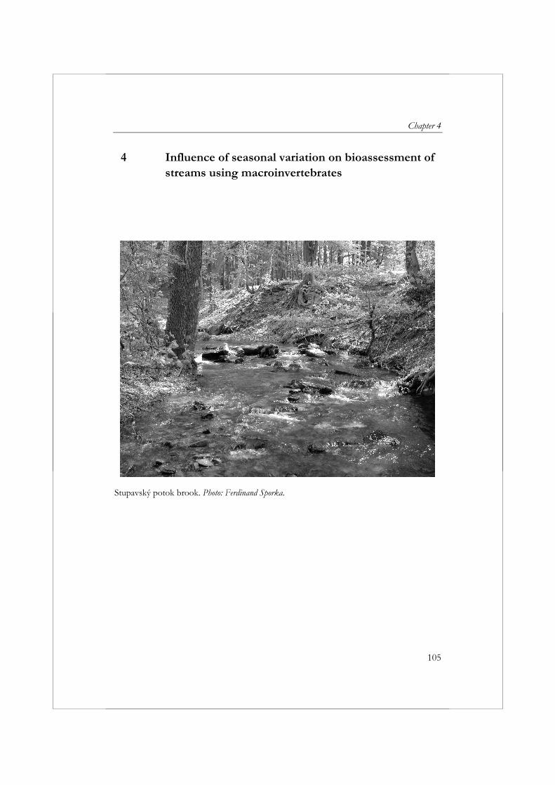
Chapter 4
105
4 Influence of seasonal variation on bioassessment of streams using macroinvertebrates
Stupavský potok brook. Photo: Ferdinand Sporka.
Influence of seasonal variation on bioassessment
106
4 Influence of seasonal variation on bioassessment of streams using macroinvertebrates
Ferdinand Šporka, Hanneke E. Vlek, Eva Bulánková & Il’ja Krno Hydrobiologia (2006) 566: 543-555. Abstract The EU Water Framework Directive requires assessment of the ecological quality of running waters using macroinvertebrates. One of the problems of obtaining representative samples of organisms from streams is the choice of sampling date, as the scores obtained from macroinvertebrate indices vary naturally between seasons, confounding the detection of anthropogenic environmental change. We investigated this problem in a 4th order calcareous stream in the western Carpathian Mountains of central Europe, the Stupavský potok brook. We divided our 100 m study site into two stretches and took two replicate samples every other month alternately from each stretch for a period of one year, sampling in the months of February, April, June, August, October and December. Multivariate analysis of the macroinvertebrate communities (PCA) clearly separated the samples into three groups: (1) April samples (2) June and August samples (3) October, December and February samples. Metric scores were classified into two groups those that were stable with respect to sampling month, and those that varied. Of the metrics whose values increase with amount of allochthonous organic material (ALPHA_MESO, hyporhithral, littoral, PASF, GSI new, DSI, CSI), the highest scores occurred in February, April, October and December, while for metrics whose values decrease with content of organic material (DSII, DIS, GFI D05, PORI, RETI, hypocrenal, metarhithral, RP, AKA, LITHAL, SHRED, HAI) the highest values occurred in February, April, June and December. We conclude that sampling twice a year, in early spring and late autumn, is appropriate for this type of metarhithral mountain stream. Sampling in summer is less reliable due to strong seasonal influences on many of the metrics examined while sampling in winter is inappropriate for logistical reasons. Keywords: seasonal variation, macroinvertebrates, bioassessment, stream, Slovakia
Chapter 4
107
Introduction With the implementation of the Water Framework Directive (WFD) every EU member state is obligated to assess the effects of human activities on the ecological quality of all water bodies (European Commission, 2000). Assessment of the ecological state of surface waters based on selected groups of living organisms as required by the Water Framework Directive (WFD) poses the problem of obtaining samples representative of the stream community. In collecting macroinvertebrate samples temporal and spatial changes in the community composition are two of the most important aspects that should be taken into account when collecting representative samples.
Temporal distributions of freshwater communities, both on the bottom and in the water column, are known to be influenced by the life histories of the various species (Hynes, 1972; Williams, 1981). Ormerod (1987) showed that the most precise categorization of assemblage type required a sampling strategy that combines both habitat and seasonal data. While many physical factors that have been shown to affect faunal assemblages are known to change seasonally (e.g. hydrological regime, water chemistry, light levels and temperature), lotic assemblages of invertebrates vary both seasonally and with spatial position within the stream (Matthews & Bao, 1991; Cowell et al., 2004). Setting a suitable time period for sampling a given habitat type is therefore a complex problem.
The establishment of reliable biomonitoring programmes is central to the effective implementation of the WFD for surface waters. Water managers prefer cost efficient methods, e.g. sampling in most cases only once a year for the purpose of surveillance monitoring. In contrast, studies aiming to assess conservation value normally require more than one sampling occasion within a given year to obtain adequate site evaluations (Furse et al., 1984). The choices made related to sampling strategies are always a trade off between biological reliability and economic considerations. When cost do not allow to take more than one sample a year at a site for the purpose of surveillance monitoring a higher level of standardisation and between site comparability could be reached if samples from the same area were collected in the same time period, thereby minimising variability in the observed communities due to natural seasonal differences. In many European countries there is an agreement about the period most suited for sampling macroinvertebrates, however in most cases scientific background to these agreements is lacking.
The aim of this study was therefore (1) to examine the variation in macroinvertebrate community composition between months (2) to assess the effects of natural seasonal community variation on metric values, and (3) to
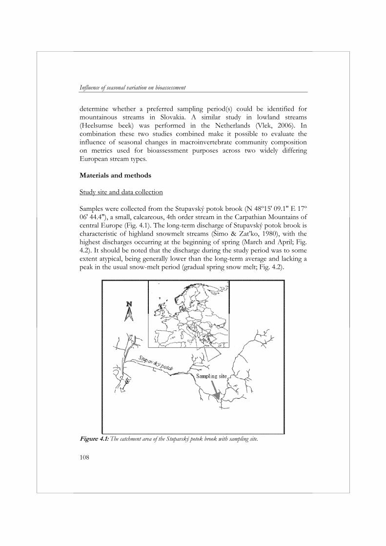
Influence of seasonal variation on bioassessment
108
determine whether a preferred sampling period(s) could be identified for mountainous streams in Slovakia. A similar study in lowland streams (Heelsumse beek) was performed in the Netherlands (Vlek, 2006). In combination these two studies combined make it possible to evaluate the influence of seasonal changes in macroinvertebrate community composition on metrics used for bioassessment purposes across two widely differing European stream types. Materials and methods Study site and data collection Samples were collected from the Stupavský potok brook (N 48º15′ 09.1″ E 17º 06′ 44.4″), a small, calcareous, 4th order stream in the Carpathian Mountains of central Europe (Fig. 4.1). The long-term discharge of Stupavský potok brook is characteristic of highland snowmelt streams (Šimo & Zaťko, 1980), with the highest discharges occurring at the beginning of spring (March and April; Fig. 4.2). It should be noted that the discharge during the study period was to some extent atypical, being generally lower than the long-term average and lacking a peak in the usual snow-melt period (gradual spring snow melt; Fig. 4.2).
Figure 4.1: The catchment area of the Stupavský potok brook with sampling site.
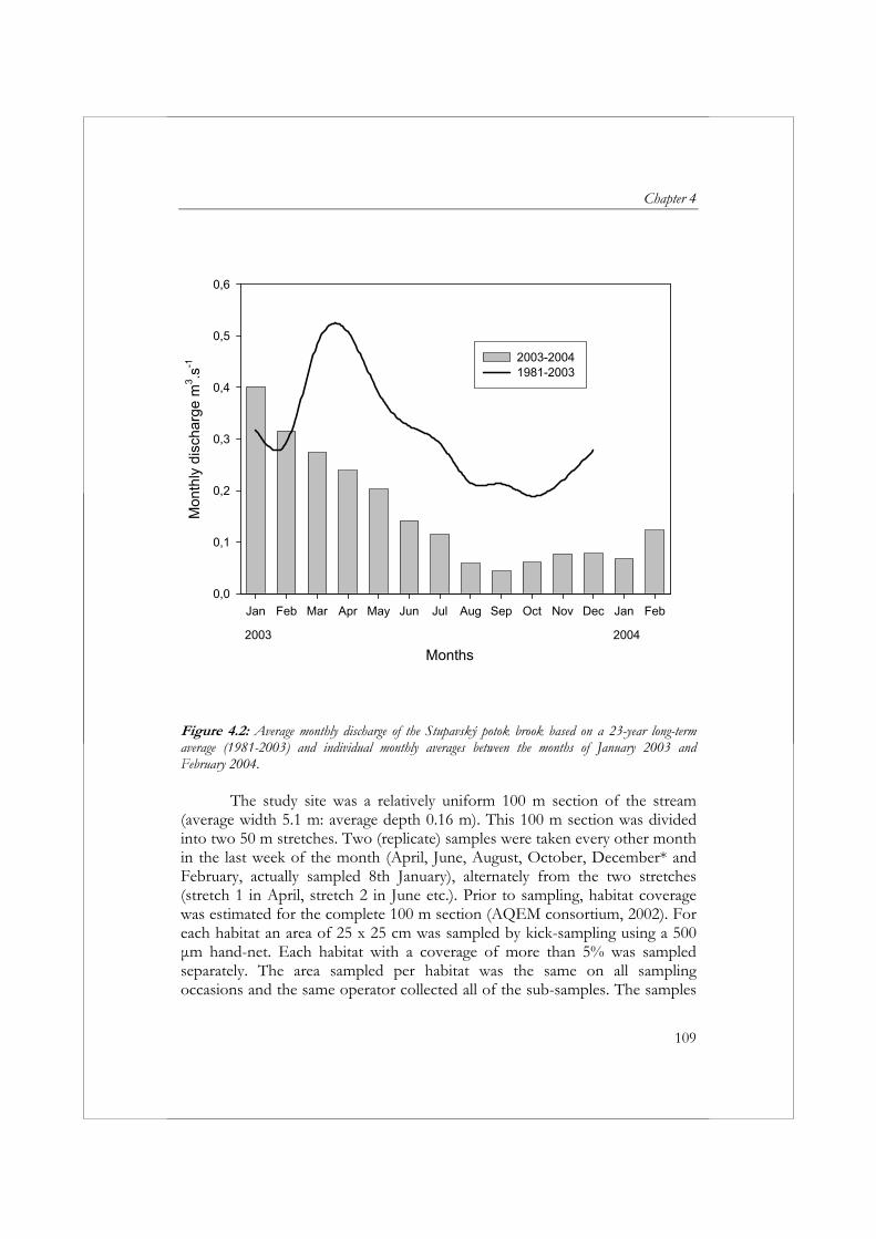
Chapter 4
109
Months
Jan Feb Mar Apr May Jun Jul Aug Sep Oct Nov Dec Jan Feb
Mon
thly
dis
char
ge m
3.s
-1
0,0
0,1
0,2
0,3
0,4
0,5
0,6
2003-2004 1981-2003
2003 2004
Figure 4.2: Average monthly discharge of the Stupavský potok brook based on a 23-year long-term average (1981-2003) and individual monthly averages between the months of January 2003 and February 2004.
The study site was a relatively uniform 100 m section of the stream (average width 5.1 m: average depth 0.16 m). This 100 m section was divided into two 50 m stretches. Two (replicate) samples were taken every other month in the last week of the month (April, June, August, October, December* and February, actually sampled 8th January), alternately from the two stretches (stretch 1 in April, stretch 2 in June etc.). Prior to sampling, habitat coverage was estimated for the complete 100 m section (AQEM consortium, 2002). For each habitat an area of 25 x 25 cm was sampled by kick-sampling using a 500 μm hand-net. Each habitat with a coverage of more than 5% was sampled separately. The area sampled per habitat was the same on all sampling occasions and the same operator collected all of the sub-samples. The samples
Influence of seasonal variation on bioassessment
110
were preserved in 4% formaldehyde prior to transportation to the laboratory for processing. In the laboratory the samples collected from the different habitats were sieved using 1000 and 500 μm sieves, and fully sorted under a stereomicroscope. Sorting was performed by a group of three people. The same specialist preformed all identifications of each major organism group. Macroinvertebrates were identified to the lowest taxonomic level possible (species level for almost all groups). Data analysis Prior to analysis, samples from the different habitats were pooled together to form two composite samples. The number of individuals per taxon were standardised to a total sample area of 1.25 m2 for each composite sample based on habitat coverage and sampled area (abundance * 1.25/area sampled). A Principal Components Analysis (PCA) using CANOCO 4.5 (Ter Braak & Smilauer, 2002) was performed to examine variation in macroinvertebrate community composition between months. Species data were log2 (x+1) transformed before analysis.
The effects of natural seasonal variation in community composition on metric values were assessed using a list of metrics commonly used in Europe (Supplementary Material*). The metrics were selected from an extensive list given by Hering et al. (2004). In addition to these metrics the number of taxa and the number of individuals for each major macroinvertebrate group (e.g. Diptera, Ephemeroptera, Plecoptera) was also evaluated. Some groups were only present at low abundances and in just a few samples. These groups were therefore excluded from our analyses because of the difficulties of finding appropriate transformations to normalise the data and the problems of having many zero values (Metzling et al., 2003). Metric values were calculated with the software ASTERICS version 1.0 (AQEM/STAR Ecological RIver Classification System; http://www.aqem.de) for all composite samples, except for the Slovak Saprobic index which is not included in the software. Slovak Saprobic index values were obtained from Šporka (2003). The coefficient of variation (CV = SD / mean), a measure of variability, was calculated for the different metrics. One-way analysis of variance (ANOVA) was used to identify significant differences between months (α=0.05) by SigmaStat 3.1 for Windows software.
Assumptions for normality and homogeneity of variance could not be tested in a reliable way due to the low number of samples. For this reason it might have been more appropriate to perform a non-parametric test. However, a non-parametric test would never be able to detect significant differences
* Electronic supplementary material is available fort his article at <http://dx.doi.org/ 10.1007/s10750-006-0073-8> and accessible for authorised users.
Chapter 4
111
between protocols based on two replicates. Therefore it was decided to use the ANOVA and to transform metric values based on experiences in other studies. Abundance metrics were ln(x+1) transformed (Supplementary Material type 1). Taxa counts were not transformed and proportions were transformed ln(x+1)-ln(y+1) (Supplementary Material type 2), where x = the number of individual taxa and y = the number of total taxa (Kerans et al., 1992). Biotic index data (e.g. Saprobic Index, BMWP, ASPT) were not transformed (Norris & Georges, 1993). Metrics like XENO (%), SHRED (%) and littoral (%) are not simple proportional metrics. The values for these metrics also depend on the strength with which a species prefers a certain category (AQEM consortium, 2002). The decision was made not to transform values of these metrics, since no information could be found to describe a suitable transformation. Acronym, metric description and type of transformation are given in Supplementary Material. Results Taxa analysis In total 218 taxa were collected during this study. Each replicate contained on average 42% of the total number of taxa, and the total number of taxa occurring in both replicates from any one month varied between 56% and 70%. In macroinvertebrate community of the Stupavský potok brook the highest of number of taxa reached Diptera and Trichoptera (Fig. 4.3). Samples from different months did not exhibit major differences in the number of taxa per organism groups (Fig. 4.3, Table 4.1). Similarly, there was no significant difference in the total number of taxa between months (p=0.185). There was also no significant difference in the total number of individuals between months (p=0.062), although, the percentage of individuals for some of the major organism groups did vary significantly between months (Fig. 4.4, Supplementary Material).
During most months (except February and April) the Crustacea formed the largest proportion of the community (varying between 25 and 57%), followed by the Diptera (varying between 15 and 38%). In February however, the Diptera represented the largest part of the community, while Crustacea numbers were far lower and conversely represented the smallest proportion of the community (Fig. 4.4). Multivariate analysis clearly divided the samples into three groups: (1) April samples (2) June and August samples (3) October, December and February samples (Fig. 4.5).
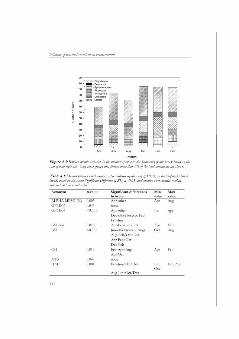
Influence of seasonal variation on bioassessment
112
Figure 4.3: Between month variation in the number of taxa in the Stupavský potok brook based on the sum of both replicates. Only those groups that formed more than 5% of the total abundance are shown. Table 4.1: Months between which metrics values differed significantly (p<0.05) in the Stupavský potok brook, based on the Least Significant Difference (LSD, α=0,05) and months when metrics reached minimal and maximal value.
Acronym p-value Significant differences between
Min value
Max value
ALPHA-MESO (%) 0.003 Apr-other Apr Aug GFI D03 0.045 none GFI D05 <0.001 Apr-other Jun Apr Dec-other (except Feb) Feb-Jun GSI new 0.018 Apr-Feb/Jun/Oct Apr Feb DSI <0.001 Jun-other (except Aug) Oct Aug Aug-Feb/Oct/Dec Apr-Feb/Oct Dec-Feb CSI 0.013 Feb-Apr/Aug Apr Feb Apr-Oct MTS 0.049 none HAI 0.001 Feb-Jun/Oct/Dec Jun,
Oct Feb, Aug
Aug-Jun/Oct/Dec
month
Apr Jun Aug Oct Dec Feb
num
ber
of ta
xa
0
10
20
30
40
50
60
70
80
90
100
110
120- Oligochaeta - Crustacea - Ephemeroptera - Plecoptera - Trichoptera - Coleoptera - Diptera
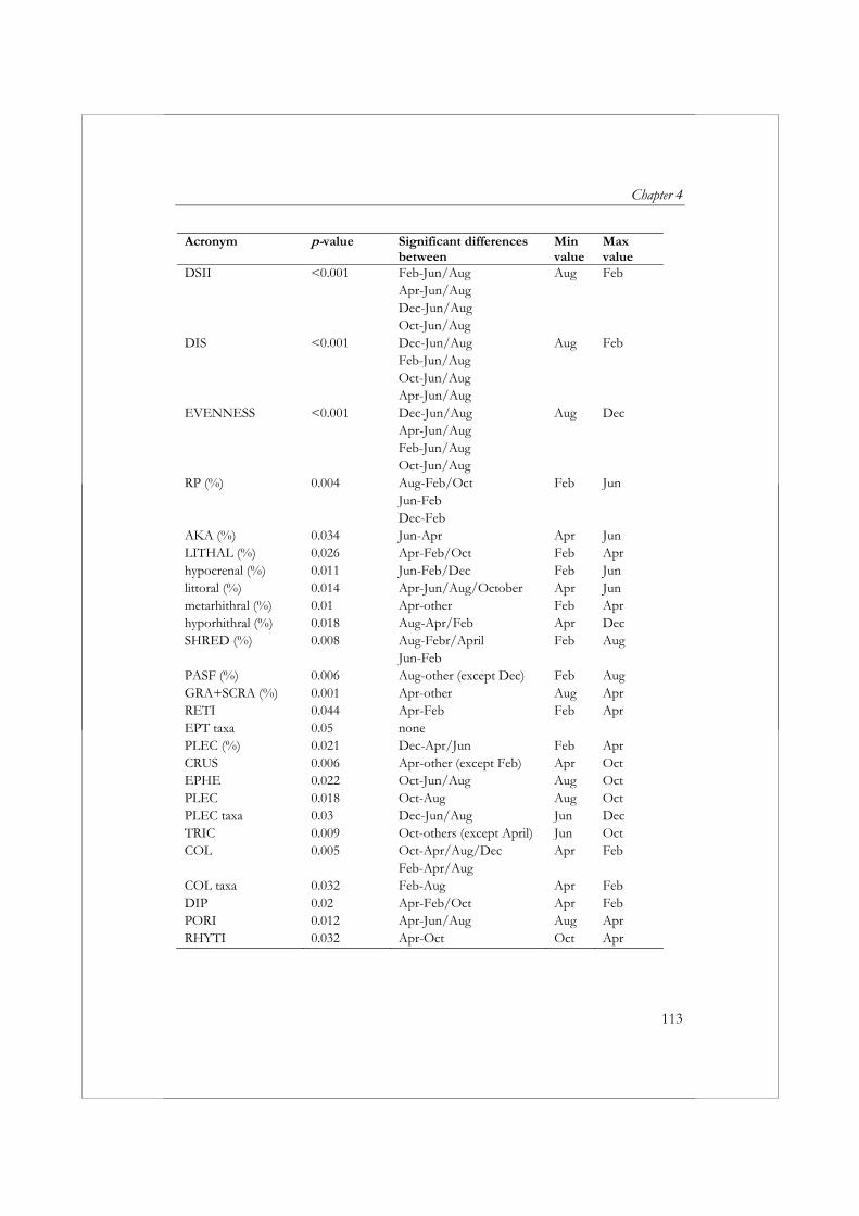
Chapter 4
113
Acronym p-value Significant differences between
Min value
Max value
DSII <0.001 Feb-Jun/Aug Aug Feb Apr-Jun/Aug Dec-Jun/Aug Oct-Jun/Aug DIS <0.001 Dec-Jun/Aug Aug Feb Feb-Jun/Aug Oct-Jun/Aug Apr-Jun/Aug EVENNESS <0.001 Dec-Jun/Aug Aug Dec Apr-Jun/Aug Feb-Jun/Aug Oct-Jun/Aug RP (%) 0.004 Aug-Feb/Oct Feb Jun Jun-Feb Dec-Feb AKA (%) 0.034 Jun-Apr Apr Jun LITHAL (%) 0.026 Apr-Feb/Oct Feb Apr hypocrenal (%) 0.011 Jun-Feb/Dec Feb Jun littoral (%) 0.014 Apr-Jun/Aug/October Apr Jun metarhithral (%) 0.01 Apr-other Feb Apr hyporhithral (%) 0.018 Aug-Apr/Feb Apr Dec SHRED (%) 0.008 Aug-Febr/April Feb Aug Jun-Feb PASF (%) 0.006 Aug-other (except Dec) Feb Aug GRA+SCRA (%) 0.001 Apr-other Aug Apr RETI 0.044 Apr-Feb Feb Apr EPT taxa 0.05 none PLEC (%) 0.021 Dec-Apr/Jun Feb Apr CRUS 0.006 Apr-other (except Feb) Apr Oct EPHE 0.022 Oct-Jun/Aug Aug Oct PLEC 0.018 Oct-Aug Aug Oct PLEC taxa 0.03 Dec-Jun/Aug Jun Dec TRIC 0.009 Oct-others (except April) Jun Oct COL 0.005 Oct-Apr/Aug/Dec Apr Feb Feb-Apr/Aug COL taxa 0.032 Feb-Aug Apr Feb DIP 0.02 Apr-Feb/Oct Apr Feb PORI 0.012 Apr-Jun/Aug Aug Apr RHYTI 0.032 Apr-Oct Oct Apr
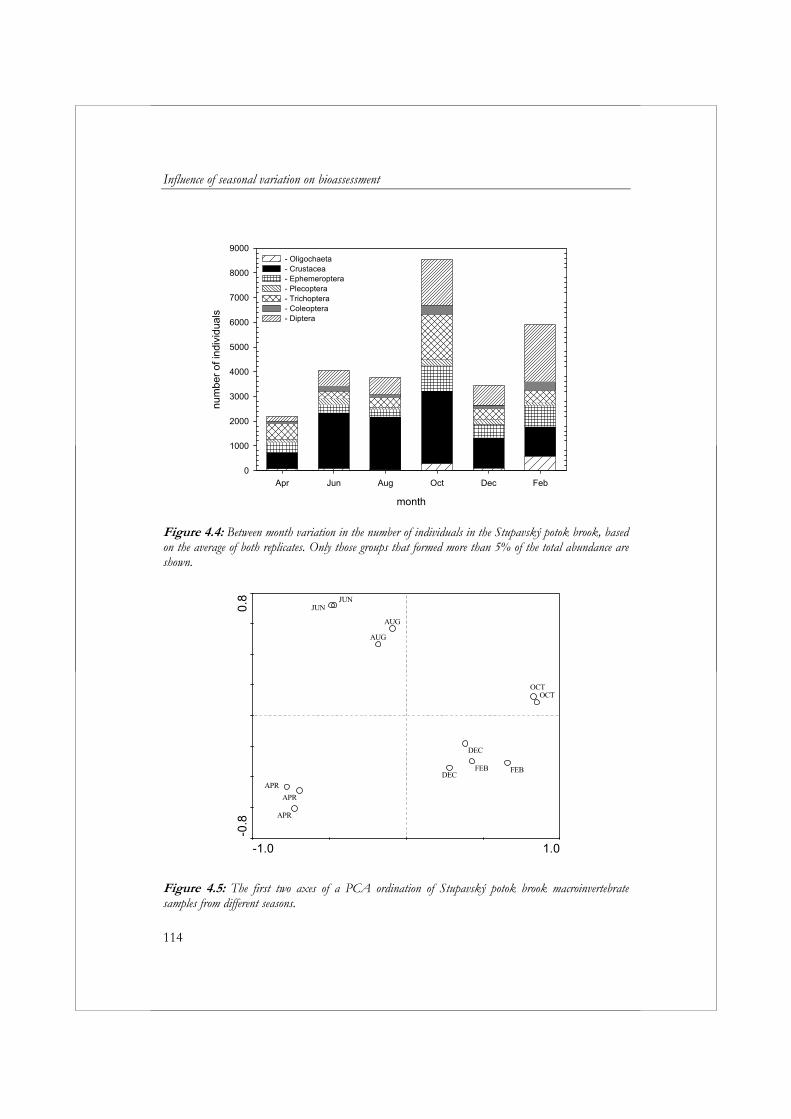
Influence of seasonal variation on bioassessment
114
month
Apr Jun Aug Oct Dec Feb
num
ber
of in
divi
dual
s
0
1000
2000
3000
4000
5000
6000
7000
8000
9000- Oligochaeta - Crustacea - Ephemeroptera - Plecoptera - Trichoptera - Coleoptera - Diptera
Figure 4.4: Between month variation in the number of individuals in the Stupavský potok brook, based on the average of both replicates. Only those groups that formed more than 5% of the total abundance are shown.
-1.0 1.0
-0.8
0.8
APR
APR
APR
JUNJUN
AUG
AUG
OCTOCT
DECFEB FEB
DEC
Figure 4.5: The first two axes of a PCA ordination of Stupavský potok brook macroinvertebrate samples from different seasons.
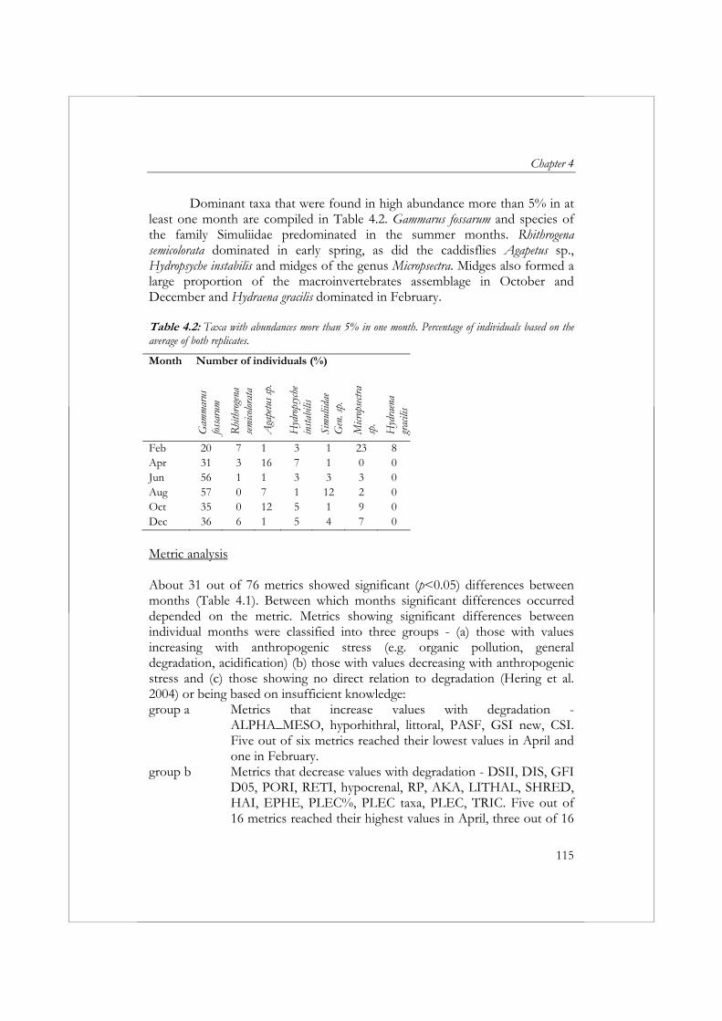
Chapter 4
115
Dominant taxa that were found in high abundance more than 5% in at least one month are compiled in Table 4.2. Gammarus fossarum and species of the family Simuliidae predominated in the summer months. Rhithrogena semicolorata dominated in early spring, as did the caddisflies Agapetus sp., Hydropsyche instabilis and midges of the genus Micropsectra. Midges also formed a large proportion of the macroinvertebrates assemblage in October and December and Hydraena gracilis dominated in February.
Table 4.2: Taxa with abundances more than 5% in one month. Percentage of individuals based on the average of both replicates.
Month Number of individuals (%)
Gam
mar
us
foss
arum
Rhi
thro
gena
se
mico
lora
ta
Aga
petu
s sp.
Hyd
rops
yche
in
stabi
lis
Sim
uliid
ae
Gen
. sp.
Micr
opse
ctra
sp.
Hyd
raen
a gr
acili
s
Feb 20 7 1 3 1 23 8Apr 31 3 16 7 1 0 0Jun 56 1 1 3 3 3 0Aug 57 0 7 1 12 2 0Oct 35 0 12 5 1 9 0Dec 36 6 1 5 4 7 0
Metric analysis About 31 out of 76 metrics showed significant (p<0.05) differences between months (Table 4.1). Between which months significant differences occurred depended on the metric. Metrics showing significant differences between individual months were classified into three groups - (a) those with values increasing with anthropogenic stress (e.g. organic pollution, general degradation, acidification) (b) those with values decreasing with anthropogenic stress and (c) those showing no direct relation to degradation (Hering et al. 2004) or being based on insufficient knowledge: group a Metrics that increase values with degradation -
ALPHA_MESO, hyporhithral, littoral, PASF, GSI new, CSI. Five out of six metrics reached their lowest values in April and one in February.
group b Metrics that decrease values with degradation - DSII, DIS, GFI D05, PORI, RETI, hypocrenal, RP, AKA, LITHAL, SHRED, HAI, EPHE, PLEC%, PLEC taxa, PLEC, TRIC. Five out of 16 metrics reached their highest values in April, three out of 16

Influence of seasonal variation on bioassessment
116
in August and October, two out of 16 in February, June and December.
group c Metrics with unidentified or insignificant relationships with degradation: GRA+SCRA, metarhithral, DSI, COL taxa, RHYTI, CRUS, COL, DIP, Evenness. Among them, 3 metrics showed highest values in February and April and 1 in August, October and December, respectively. Four metrics reached the lowest values in April, two metrics in August and October and 1 in February.
Metrics that reached their maximum values in summer (group a) and
differed significantly in value between summer and the other months were associated with poor water quality caused by low discharges (high CSI, PASF %, littoral %). Values of metrics indicating impairment of water quality in summer samples (June, August) are also influenced by summer emergence and the consequent absence of larval stages. The effects of summer emergence were also evident in the low values of the diversity (DIS, DSII) and evenness and low abundance values for certain taxonomic groups e.g. Plecoptera (Table 4.1). Percentage of dominant feeding types shows differences in individual months during the year (Fig. 4.6).
month
Apr Jun Aug Oct Dec Feb
%
0
20
40
60
80
100
algivores Detritovores others
Figure 4.6: Between month variations in invertebrate food guilds in the Stupavský potok brook. Percentage of functional feeding groups based on the average of both replicates. Only dominant food guilds are shown.
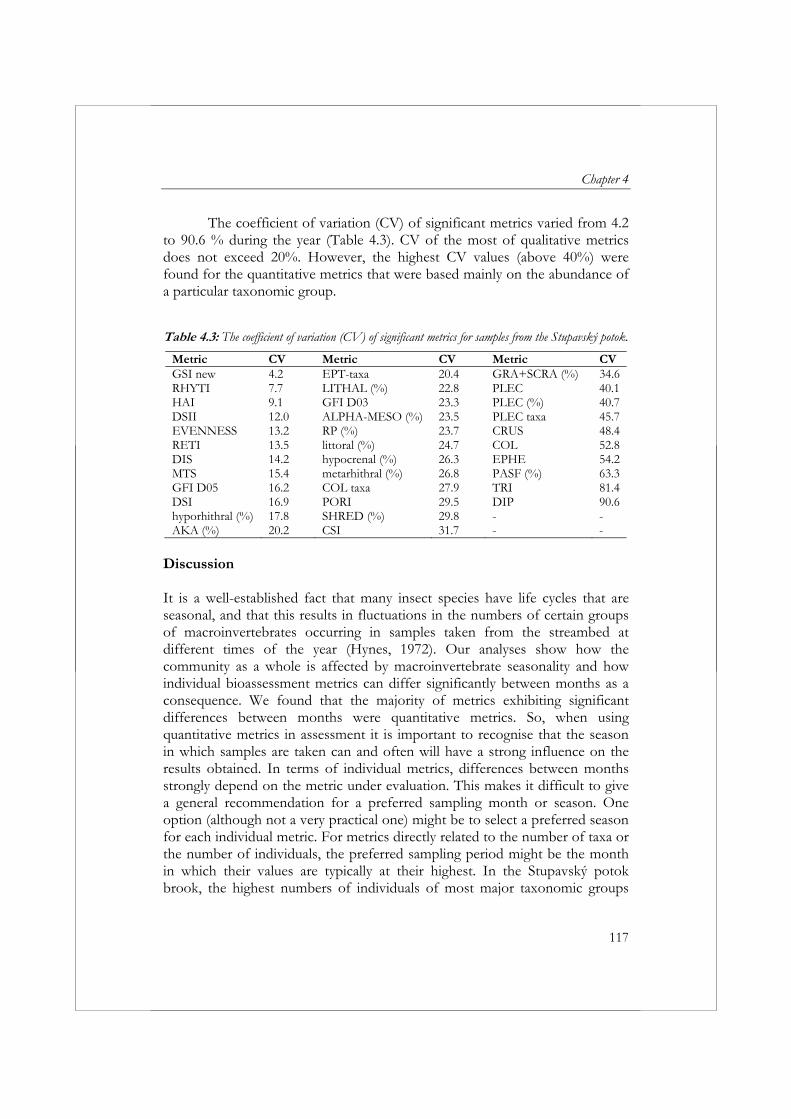
Chapter 4
117
The coefficient of variation (CV) of significant metrics varied from 4.2 to 90.6 % during the year (Table 4.3). CV of the most of qualitative metrics does not exceed 20%. However, the highest CV values (above 40%) were found for the quantitative metrics that were based mainly on the abundance of a particular taxonomic group. Table 4.3: The coefficient of variation (CV) of significant metrics for samples from the Stupavský potok.
Metric CV Metric CV Metric CV GSI new 4.2 EPT-taxa 20.4 GRA+SCRA (%) 34.6 RHYTI 7.7 LITHAL (%) 22.8 PLEC 40.1 HAI 9.1 GFI D03 23.3 PLEC (%) 40.7 DSII 12.0 ALPHA-MESO (%) 23.5 PLEC taxa 45.7 EVENNESS 13.2 RP (%) 23.7 CRUS 48.4 RETI 13.5 littoral (%) 24.7 COL 52.8 DIS 14.2 hypocrenal (%) 26.3 EPHE 54.2 MTS 15.4 metarhithral (%) 26.8 PASF (%) 63.3 GFI D05 16.2 COL taxa 27.9 TRI 81.4 DSI 16.9 PORI 29.5 DIP 90.6 hyporhithral (%) 17.8 SHRED (%) 29.8 - - AKA (%) 20.2 CSI 31.7 - -
Discussion It is a well-established fact that many insect species have life cycles that are seasonal, and that this results in fluctuations in the numbers of certain groups of macroinvertebrates occurring in samples taken from the streambed at different times of the year (Hynes, 1972). Our analyses show how the community as a whole is affected by macroinvertebrate seasonality and how individual bioassessment metrics can differ significantly between months as a consequence. We found that the majority of metrics exhibiting significant differences between months were quantitative metrics. So, when using quantitative metrics in assessment it is important to recognise that the season in which samples are taken can and often will have a strong influence on the results obtained. In terms of individual metrics, differences between months strongly depend on the metric under evaluation. This makes it difficult to give a general recommendation for a preferred sampling month or season. One option (although not a very practical one) might be to select a preferred season for each individual metric. For metrics directly related to the number of taxa or the number of individuals, the preferred sampling period might be the month in which their values are typically at their highest. In the Stupavský potok brook, the highest numbers of individuals of most major taxonomic groups
Influence of seasonal variation on bioassessment
118
were found at the end of October. Hynes (1972) showed that autumn is a period of egg hatching, and for many species it is a period of increasing or often of maximum, numbers, including many small individuals. Similarly, in lowland headwater streams of the Alafia River, Cowell et al. (2004) also found the highest abundances in autumn.
On the other hand, EPT metric values did not markedly differ between seasons because in any single month a reasonably representative selection of the three groups that make up this index was always present. Sprules (1947) similarly showed that while the number and diversity of Plecoptera decreases with increasing average summer temperature, the number and diversity of Ephemeroptera and Trichoptera increase, thereby avoiding strong seasonal differences of EPT index scores. This effect has also been observed in the lowland stream Heelsumse beek in the Netherlands (Vlek, 2006).
By examining the whole community using multivariate analyses we identified three distinct seasonal assemblages from spring (April), summer (June and August), and autumn and winter (October, December, and February). Individual metric results also indicated that macroinvertebrate community composition in the Stupavský potok brook in April differed from all other months. ALPHA-MESO (%) values were significantly lower in April than in all other months. The low values of ALPHA-MESO (%) in April indicate low amounts of allochthonous organic material. The significantly low CSI values can also be related to organic pollution. The low CSI values and the high values of RETI, GFI, PLEC (%), PORI in April suggest that the water quality of the Stupavský potok is better in April than in all other months.
With increasing temperature in summer oxygen levels decrease and therefore saprobity increases. Under extreme conditions these changes become readily apparent, as shown by Coimbra et al. (1996) in their investigation of macroinvertebrate community in a temporary stream in Portugal. On the basis of multivariate analysis they classified macroinvertebrate communities into three groups according to environmental variables related to seasons and anthropogenic influences. Morais et al. (2004) studied the robustness of metrics under different hydrological conditions in temporary streams. Seasonal changes over the study period followed the general temporal pattern observed in other Mediterranean streams, with taxa sensitive to organic pollution being present under high discharge and more tolerant taxa under low discharge. The same pattern could be observed in the Stupavský potok brook. In summer due to low discharge the fauna consisted mostly of eurytopic species e.g. Simulium sp.
Several other studies have also shown that eurytopic species of the family Simuliidae are dominant in streams of the Small Carpathians Mts. in
Chapter 4
119
summer (Halgoš & Jedlička, 1974; Illéšová & Halgoš, 2003). Dahl et al. (2004) stated “However, though a summer sampling window may result in a better detection of oxygen stress, the summer emergence by aquatic insects often precludes the use of this season in bioassessment programmes in Sweden.” Nijboer & Schmidt-Kloiber (2004) found that taxa indicating oligosaprobic conditions were taxa with small distribution ranges living in close proximity to stones and gravel (i.e. lithal). In the Stupavský potok brook, colonization of the lithal substrate was at its greatest in April.
Many studies have shown that seasonal abundance of food may strongly influence the life cycles of the stream community (Ross, 1963; Neel, 1968; Cummins, 1977; Williams & Hynes, 1973; Moore 1977; Townsend & Hildrew, 1979; Williams 1981). Based on the evaluation of energy flow, Krno (1996) distinguished two significantly different time periods within a year in terms of abiotic factors and food availability: Cold season: high discharge, periphyton biomass and production of
scrapers. Warm season: high temperature, biomass FPOM and production of
filterers and collectors. In the Stupavský potok brook similar relationships between abiotic factors, food resources, and the composition of trophic groups were found. The highest values of the metrics GRA + SCRA % were found in April when discharge was highest. Representation of feeding types during the year in Stupavský potok brook shows a strong dominance of algophagous forms in spring and, on the contrary, dominance by detritophagous taxa during other parts of year. Similarly, Krno & Hullová (1988) found the largest proportion of this trophic group in the metarithral stretch of the Vydrica stream in the Carpathians in spring, when periphyton (representing an important food resource in this system) develops under the influence of increasing illumination. Krno (1996) also recorded the highest percentage of PASF % in summer when water temperatures were highest. These studies support the view that temperature is a key abiotic factor influencing macrozoobenthos structure (Sprules, 1947, Williams & Hynes, 1974). High temperatures result in high microbial activity and subsequently low oxygen concentrations (Dahl et al., 2004). The metrics reaching significantly higher values in August and June in relation to other months are typically regarded as indicators of poor water quality caused by reduced discharges and high temperatures (CSI, PASF %, hypocrenal % and littoral %).
In this study we have shown that seasonal changes in macroinvertebrate community composition have marked effects on many biotic indices. The life cycles of stream invertebrates, and the seasonal changes
Influence of seasonal variation on bioassessment
120
in community composition reflect on metric values, are caused primarily by the seasonal dynamics of variables such as temperature, light regime and the supply of nutrients and allochthonous organic material (Clifford, 1978; Krno & Hullová, 1988; Doledec, 1989; Bunn, 1986; Krno 1996). Spring is characterised by an increase in temperature, discharge, light and nutrient supply which results in an increase in primary production and abundance of algophagous invertebrates. This situation is accompanied by a stronger representation of lithophiles and rheophils, and the rapid development of spring forms of macrozoobenthos and emergence of water insects. In spring the metabolism of Small Carpathian streams has been shown to be predominantly autotrophic (Krno & Hullová, 1988; Rodrigez & Derka, 2003). In the Stupavský potok brook this was confirmed by the highest values of the metric LITHAL % in April and the dominance of algophagous invertebrates (GRA+SCRA%). The progression to summer is characterised by relatively stable and high temperatures, reduced discharge and reduced illumination due to shadowing, and the concurrent development of summer forms of the macrozoobenthos. Signatures of these changes are readily apparent in the metrics littoral, hypocrenal and hyporhithral, which all peak in summer. In autumn and winter, a marked decrease in temperature, lower illumination, and (in contrast to earlier months of the year) a strong supply of allochthonous organic material result in the development of detritophagous invertebrates. Development of detritophagous invertebrates can however be slower than the onset of the preceding seasonal changes in the macroinvertebrate community and in winter it can be strongly inhibited or even stopped. During the winter, the metabolism of Small Carpathian streams has been shown to predominantly heterotrophic (Krno & Hullová, 1988; Rodriguez & Derka, 2003). The strong development detritophagous Crustacea, Plecoptera, Ephemeroptera, and Coleoptera in our study confirms these findings.
The question of determining an appropriate number of sampling occasions during the year is important. From an economic perspective there is a desire to minimise the frequency of sampling while biological studies tend to indicate the reverse. Several studies (e.g. Ormerod, 1987) have demonstrated the benefit of combining datasets from at least two seasons so that taxa rarely recorded in one season are gained from the additional season. Similarly, Furse et al. (1984) showed that combined season data enabled better categorization and prediction of macroinvertebrate communities than single season data. They advocated sampling in three seasons wherever feasible to allow the characteristic annual pattern of change in the fauna of a site to be incorporated into the analyses. The advantage of taking more than one sample a year was also evident from this study. The complementary value of a late autumn or
Chapter 4
121
winter sample to a spring sample was obvious. The autumn and winter community consisted of many species that were uncommon in spring yet were found in high abundances in the later part of the year. It should be noted, however, that mid winter sampling is not suitable for purely logistic reasons (e.g. problems reaching and entering streams and sampling in ice and snow). Furthermore sampling three times a year can be very time-consuming, particularly if identifications are to be taken to species level.
Since seasonal changes are a natural phenomenon it is not possible to give advice on the time period most suited for sampling. For metrics that show high seasonal variation the best solution would be to always sample during the same month or to take into account seasonal variation in setting class boundaries for assessment purposes.
Many of the metrics evaluated in this study depend on indicator values. In many cases indicator values for these taxa were unknown and the influence of taxa with indicator values (and high abundance) and the sensitivity of the metrics to seasonal variation will be overestimated. Increasing the knowledge of autecology will help to reduce this problem. For metrics where the optimal sampling period is not directly related to the highest metric value, the best solution would be to sample in a comparable month or months or to take into account seasonal variation in setting class boundaries.
In this study only the effects of seasonal variation in macroinvertebrate community composition on metric values were evaluated. When selecting metrics for the development of a biological assessment system apart from variability and differences in values between months it is most important to know whether metrics are (highly) correlated to anthropogenic stress. Acknowledgements This study was carried out within the STAR project, a research project under the 5th Framework programme of the European Union (EVK1-CT-2001-00089) and grant 1/292/04 from the Slovak Grant Agency for Sciences. We would like to thank John Davy-Bowker for linguistic revision of the manuscript. We would like to thank Tomáš Derka, Daniela Illéšová and Zuzana Pastuchová for their efforts in collecting the data on which this study was based.

Influence of seasonal variation on bioassessment
122
References AQEM consortium, 2002. Manual for the application of the AQEM system.
2002. A comprehensive method to assess European streams using benthic macroinvertebrates, developed for the purpose of the Water Framework Directive. Version 1.0. February 2002.
Bunn, S.E., 1986. Spatial and temporal variation in the macroinvertebrate fauna of streams of the northern jarrah forest, Western Australia: functional organization. Freshwater Biology 16: 621-632.
Clifford, H,F., 1978. Descriptive phenology and seasonality of a Canadian Brown-water stream. Hydrobiologia 58: 213-231.
Coimbra, C.N., M.A.S. Graqa & R.M. Cortes, 1996: The effects of a basic effluent on macroinvertebrate community structure in a temporary Mediterranean river. Environmental Pollution 94: 301-307.
Cowell, B.C., A.H. Remley & D.M. Lynch, 2004. Seasonal changes in the distribution and abundance of benthic invertebrates in six headwater streams in central Florida. Hydrobiologia 522: 99-115.
Cummins, K.W., 1977. From headwater streams to river. American Biology Teacher (May) 305 312.
Dahl, J., R.K. Johnson & L. Sandin, 2004. Detection of organic pollution of streams in southern Sweden using benthic macroinvertebrates. Hydrobiologia 516: 161-172.
Dolédec, S., 1989. Seasonal dynamics of benthic macroinvertebrate communities in the Lower Ardeche River (France). Hydrobiologia 183: 73-89.
European Commission, 2000. Directive 2000/60/EC OF THE EUROPEAN PARLIAMENT AND COUNCIL - Establishing a framework for Community action in the field of water policy. Official Journal of the European Community L327: 1-72.
Furse, M.T., D. Moss, J.F. Wright & P.D. Armitage, 1984. The influence of seasonal and taxonomic factors on the ordination and classification of running-water sites in Great Britain and on the prediction of their macro-invertebrate communities. Freshwater Biology 14: 257-280.
Halgoš, J. & L. Jedlička, 1974. The distribution of black flies (Diptera, Simuliidae) in the Little Carpathians. Acta Rerum Naturalium Musei Nationalis Slovaci, Bratislava 19: 173-193.
Hering, D., O. Moog, L. Sandin & P.F.M. Verdonschot, 2004. Overview and application of the AQEM assessment system. Hydrobiologia 516: 1-20.
Hynes, H.B.N., 1972. The ecology of running waters. University of Toronto Press. 555 pp.
Chapter 4
123
Illéšová, D. & J. Halgoš, 2003. Phenology of Blackflies (Diptera, Simuliidae) in the Gidra River Basin. Acta Zoologica Universitatis Comenianae 45: 69-75.
Kerans, B.L., J.R. Karr & S.A. Ahlstedt, 1992. Aquatic invertebrate assemblages: spatial and temporal differences among sampling protocols. Journal of the North American Benthological Society 11: 377-390.
Krno, I. & D. Hullová, 1988. Influence of the water pollution on the structure and dynamics of benthos in the stream Vydrica (Small Carpathians), Biologia (Bratislava) 43: 513-526.
Krno, I. (ed) 1996. Limnology of the Turiec river basin (West Carpathians, Slovakia). Biologia (Bratislava) 51 Suppl. 2: 1-122.
Matthews, R.C., jr. & Y. Bao, 1991. Alternative instream flow assessment methodologies for warm water river systems. In: Cooper, J.L. & R.H. Hamre (eds.), Proceedings of Warmwater Fisheries Symposium 1. General Technical Report RM–207. Fort Collins, CO U.S. Forest Service pp.: 189-196.
Metzeling, L., B. Chessman, R. Hardwick & V. Wong, 2003. Rapid assessment of rivers using macroinvertebrates: the role of experience, and comparisons with quantitative methods. Hydrobiologia 510: 39-52.
Moore, J.W., 1977: Seasonal succession of algae in rivers II. Examples from Highland water, a small woodland stream. Archiv für Hydrobiologie 80: 160-171.
Morais M., P. Pinto, P. Guilherme, J. Rosado & I. Antunes, 2004. Assessment of temporary streams: the robustness of metric and multimetric indices under different hydrological conditions. Hydrobiologia 516: 231-251.
Neel, J.K., 1968. Seasonal succession of benthic algae and their macroinvertebrate residents in head-water limestone stream. Journal Water Pollution Control Federation 40: 10-30.
Nijboer, R.C. & A. Schmidt-Kloiber, 2004. The effect of excluding taxa with low abundances or taxa with small distribution ranges on ecological assessment. Hydrobiologia 516: 349-366.
Norris, R.H. & A. Georges, 1993. Analysis and interpretation of benthic macroinvertebrate surveys. In: Rosenberg, D.M. & V.H. Resh (eds.), Freshwater biomonitoring and benthic macroinvertebrates. Chapman & Hall, New York and London, pp.: 234-286.
Ormerod, S.J., 1987. The influences of habital and seasonal sampling regimes on the ordination and classification of macroinvertebrate assemblages in the catchment of the River Wye, Wales. Hydrobiologia 150: 143-151.
Rodriguez, A. & T. Derka, 2003. Physiographical and hydrobiological characteristics of the Gidra river basin. Acta Zoologica Universitatis Comenianae 45: 11-18.
Influence of seasonal variation on bioassessment
124
Ross, H.H., 1963. Stream communities and terestrial biomes. Archiv für Hydrobiologie 59: 235-242.
Šimo, E. & M. Zaťko, 1980. Typy režimu odtoku, s. 65. In Mazúr, M. (ed.) Atlas Slovenskej socialistickej republiky, SAV, 296 pp.
Šporka, F. (ed), 2003. Vodné bezstavovce (makroevertebráta) Slovenska. Súpis druhov a autekologické chrakteristiky. Slovak aquatic macroinvertebrates. Checklist and catalogue of autecological notes. Slovenský hydrometeorologický ústav, Bratislava, 590 pp.
Sprules, V.M., 1947. An ecological investigation of stream insects in Algonquin Park, Ontario. University Toronto Studies, Biology Series 56: 1-81.
Ter Braak, C.J.F. & P. Smilauer, 2002. Canoco reference manual and CanoDraw for Windows user´s guide: software for canonical community ordination (version 4.5). Microcomputer Power, Ithaca, NY, USA, 500 pp.
Townsend, C.R. & A.G. Hildrew, 1979. Foraging strategies and coexistence in a seasonal environment. Oecologia 38: 231-234.
Vlek, H.E., 2006. Influence of seasonal variation on bioassessment of streams using macroinvertebrates. Verhandlungen der Internationalen Vereinigung für Limnologie 29: 1971-1975.
Williams, D.D., 1981. Emergence pathways of adult insects in the upper reaches of a stream. Internationale Revue der gesamten Hydrobiologie 67: 223-234.
Williams, D.D. & H.B.N. Hynes, 1974. The occurrence of benthos deep in the substratum of a stream, Freshwater Biology 4: 233-256.
Williams, D.D., 1981. Migrations and distributions of stream benthos. In: Lock, M.A. & D.D. Williams (eds.), Perspectives in running water ecology. Plenum Press, New York and London, pp.: 155-207.
Williams, N.E. & H.B.N. Hynes, 1973. Microdistribution and feeding of the net-spinning caddisflies (Trichoptera) of a Canadian stream. Oikos 24: 73-84.
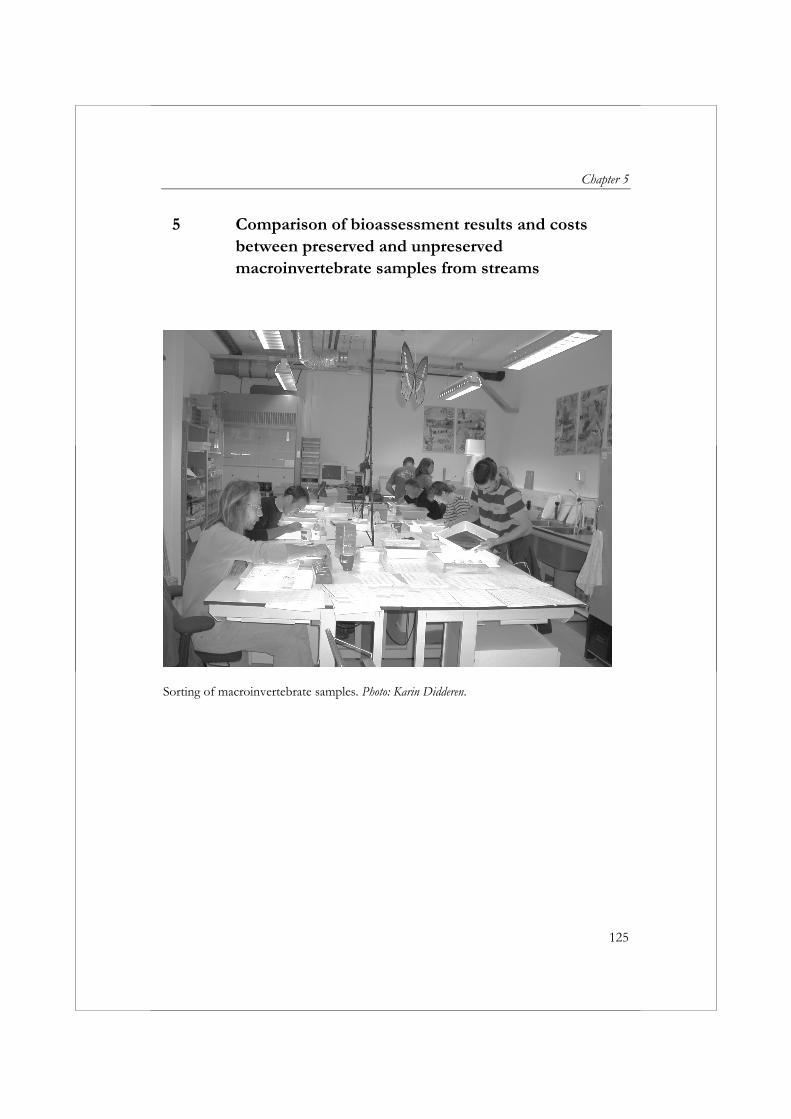
Chapter 5
125
5 Comparison of bioassessment results and costs between preserved and unpreserved macroinvertebrate samples from streams
Sorting of macroinvertebrate samples. Photo: Karin Didderen.
Comparison between preserved and unpreserved macroinvertebrate samples
126
5 Comparison of bioassessment results and costs between preserved and unpreserved macroinvertebrate samples from streams
Hanneke E. Keizer-Vlek, Paul W. Goedhart & Piet F. M. Verdonschot Environmental Monitoring and Assessment (2011) 175: 613-621. Abstract The choice to use or not use a preservative before sorting macroinvertebrate samples (i.e., dead specimens vs. living specimens) is based on studies not solely focused on the effects of preservation. Using identical sample processing protocols, we compared preserved and unpreserved samples for the following parameters: (1) the number of taxa and individuals for each major macroinvertebrate group, (2) ecological quality classes calculated with a multimetric index developed for the assessment of small Dutch lowland streams, and (3) costs of sample processing. We collected macroinvertebrate samples from three lowland streams in the Netherlands. At each site, we collected six replicate samples, of which three samples were preserved, and three were not. Significantly different numbers of Ephemeroptera individuals and Hydracarina taxa and individuals were collected from preserved samples compared to unpreserved samples. In assessments based on these individual metrics, standardization of sample processing will be required. In streams with Ephemeroptera, the preservation of samples is necessary to optimize the number of Ephemeroptera individuals collected. In streams that contain Hydracarina, the preservation of samples will result in an underestimation of the number of Hydracarina taxa and individuals present. In only one instance there was a difference in ecological quality between preserved and unpreserved samples, indicating that assessing small Dutch lowland streams does not require standardization of sample preservation as part of the sample processing protocol. We detected no significant differences in sample processing costs between preserved and unpreserved samples. Keywords: preservative, costs, macroinvertebrates, bioassessment, streams
Chapter 5
127
Introduction Macroinvertebrates are the most commonly used organisms to assess the biological quality of streams in monitoring programs (Hawkes, 1979; Hellawell, 1986; Chessman, 1995). Biological monitoring usually has two purposes: (1) to estimate variables of interest at a site, and (2) to make comparisons among sites or time intervals. Variables of interest in biological monitoring are primarily metric values (e.g., the number of taxa, Average Score Per Taxon values, Saprobic Index values) and ecological quality classes resulting from biological assessment systems. Metric values and ecological quality classes are calculated based on the macroinvertebrate community composition. Various methods have been developed to collect macroinvertebrates from streams and to process macroinvertebrate samples. These sampling and sample processing methods can vary in terms of sampled area, mesh size of sampling gear, sampled habitats, intensity of sorting, and taxonomic resolution of identification, among other parameters. The methodology applied influences the accuracy and variability of bioassessment results (expressed as metric values and/or ecological quality classes) (e.g., Barbour & Gerritsen, 1996; Diamond et al., 1996; Haase et al., 2004). Also, each method can be selective for certain species or groups of species that vary in their exposure and sensitivity to anthropogenic stress (Barton & Metcalfe-Smith, 1992).
Accuracy and variability are both important aspects of bioassessment. Accuracy refers to the closeness of a measurement to its true value (Norris et al., 1992). Differences in accuracy between methods may, therefore, result in different bioassessment results. Differences in accuracy depend on the spatial and temporal scale at which the true value is defined - a method might be accurate at representing the organisms present in a sample, but less accurate at representing the biota at a site. Variability is important in making comparisons because the validity of conclusions depends on data variability (Norris et al., 1992); higher variability increases the probability of incorrect bioassessment results. An increase in accuracy or a reduction in variability is not always possible because associated costs are often high. When assessing ecological quality for biological monitoring purposes, however, it is not necessary to catch all organisms or taxa present at a site (Barbour & Gerritsen, 1996). Standardization of sampling is required, though, for valid comparisons among sites and points in time (Courtemanch, 1996; Vinson & Hawkins, 1996). The question then focuses on which steps to standardize in sampling and sample processing. After all, when two methods are equally variable and give comparable bioassessment results, standardization is not necessary. Apart from accuracy and variability, costs play an important role in decision-making related
Comparison between preserved and unpreserved macroinvertebrate samples
128
to the standardization of methods. The costs for collection and processing of macroinvertebrate samples are high and (can) depend strongly on the sampling technique used (e.g., Barbour & Gerritsen, 1996; Metzeling et al., 2003; Vlek et al., 2006).
Many studies have focused on variability, accuracy, and/or costs in terms of sampled area (e.g., Metzeling & Miller, 2001; Vlek et al., 2006), number of samples (e.g., Canton & Chadwick, 1988), sampling device (e.g., Drake & Elliott, 1982; Mackey et al., 1984; Barton & Metcalfe-Smith, 1992; Cheal et al., 1993), sampled habitats (e.g., Kerans et al., 1992), intensity of sorting (e.g., Barbour & Gerritsen, 1996; Courtemanch, 1996; Growns et al., 1997), and taxonomic resolution of identification (e.g., Nijboer & Verdonschot, 2000; Bailey et al., 2001; Lenat & Resh, 2001). An important aspect of sample processing, which has only been the subject of a few studies, is the preservation (or not) of samples immediately after collection. Many sampling protocols recommend ‘live sorting’ in which organisms are collected from the sample while still alive. Live sorting is frequently applied in the Netherlands, Southern European countries (Buffagni, CNR-IRSA, personal communication), and Germany (Braukmann, 2000). Live sorting is also commonly applied in Australia for the rapid biological assessment of rivers (Metzeling et al., 2003), either for set periods (Chessman & Robinson, 1987) or until a fixed number of specimens is collected (Chessman, 1995).
In the few studies comparing sorting results between preserved and unpreserved samples, sorting of the unpreserved samples has been performed in the field, and sorting of the preserved samples has been performed in the laboratory (e.g., Humphrey et al., 2000; Metzeling et al., 2003; Haase et al., 2004; Nichols & Norris, 1996). In these studies, other aspects of the sample processing protocol also differed between preserved and unpreserved samples. Humphrey et al. (2000) state that the live-sort procedure results in poor recovery of small and cryptic taxa. Metzeling et al. (2003) found that Oligochaeta were underrepresented in unpreserved/field samples compared to preserved/laboratory samples. In our view, these findings are the result of field sorting and other sample processing aspects, rather than live sorting. In fact, live sorting in the laboratory might increase accuracy and reduce variability and costs. Sorting in the Netherlands is commonly performed in the laboratory to avoid (1) the high variability associated with field sorting (Haase et al., 2004), arising from differences in weather conditions and illumination at the sampling site (Carter & Resh, 2001; Rawer-Joost, 2001), and (2) loss of small organisms.
People who prefer using preservatives often mention the following disadvantages of live sorting: (1) specimens may be eaten by others before sorting is completed; (2) specimens may disintegrate before sorting is
Chapter 5
129
completed; (3) removing fast-moving taxa (like Gammarus sp.) from a sample may be time consuming; and (4) as a consequence of arguments 1 and 2, samples have to be sorted as soon as possible (within 5 days) after collection, making it impossible to collect a large number of samples at the same time. People in favor of live sorting often mention the following disadvantages of using preservatives: (1) it is more difficult to spot dead than living specimens because of the lack of movement, and (2) it is not possible to use different preservatives depending on macroinvertebrate group, i.e., identification of Chironomidae and Bivalvia is less time consuming when they are preserved in ethanol compared to formaldehyde, while Oligochaeta are easier to identify when preserved in formaldehyde. The question is whether these disadvantages will significantly influence bioassessment results and/or the costs of sample processing. The aim of this study was (1) to compare bioassessment results between preserved (i.e., sorting dead specimens) and unpreserved samples (i.e., sorting living specimens), and (2) to compare sample processing costs between preserved and unpreserved samples. Methods Study site and data collection For this study, we used data collected from three streams in the Netherlands, the Springendalse beek, the Tongerensche beek, and the Swalm. Catchment areas of all streams are smaller than 100 km2, with all sites located between 0 and 200 m above sea level. We sampled the Springendalse beek in September 2002, the Tongerensche beek in June 2003, and the Swalm in April 2003. In each stream, a uniform 100-m stretch of the stream was selected for sampling. At each site, we collected six replicate composite samples, each consisting of sampling units from different habitats. In each stream, three habitats were sampled, and sample size varied between streams (Table 5.1); replicate samples collected from the same stream did not differ in sample size. To ensure collection of most species present in the habitat (expert judgment), we sampled each habitat that represented at least 5% of the total surface area over a set distance. Prior to sampling, the surface area covered by the different habitats was estimated at each site (Table 5.1). The samples were collected by pushing a pond net (25 cm x 25 cm, 500-μm-mesh) through the upper part (2–5 cm) of the substrate. The sampling units from the different habitats were stored separately in buckets. Three out of six sampling units from each habitat were preserved in 4% formaldehyde directly after sampling. The buckets were transported to the laboratory, where the sampling units without formaldehyde
Comparison between preserved and unpreserved macroinvertebrate samples
130
were stored in a refrigerator, oxygenated, until sorting. All sampling units were kept separately during sample processing, which began with units being washed through 1000- and 250-μm-mesh sieves. Live sorting was performed for the three unpreserved replicate sampling units (per stream and habitat). From the remaining three preserved sampling units, we collected dead organisms. After washing, the sampling units were poured into transparent trays and placed on a light box. According to Dutch common practice, units were sorted in their entirety and organisms picked from the trays using unaided visual guidance. Organisms were preserved in 70% ethanol, except for live Oligochaeta and Hydracarina. Live Oligochaeta were preserved in 4% formaldehyde and live Hydracarina in Koenike fluid (20% acetic acid, 50% glycerol, and 30% demineralized water). Organisms were identified to the lowest taxonomic level possible, i.e., at the species level for almost all specimens. Time spent on sorting and identification of all specimens in each sampling unit was recorded. Table 5.1: Habitat coverage and sampled length of each habitat for the three streams sampled in this study.
Stream Habitat Sampled length (m) Coverage (%) Tongerensche beek mud 0.5 50 sand 0.5 20 submerged vegetation 0.5 30Swalm mud/detritus 0.25 5 gravel 0.75 75 sand 0.75 20Springendalse beek gravel 0.5 5 sand 0.5 95 submerged vegetation 0.25 5
Data analysis In total, 18 composite samples were collected from three different streams. The number of taxa and the number of individuals for each major macroinvertebrate group (e.g., Diptera, Ephemeroptera, Plecoptera) were evaluated to determine whether (potential) differences between preserved and unpreserved samples varied depending on the macroinvertebrate group. We refer to the number of taxa and the number of individuals for each major macroinvertebrate group as a metric.
Chapter 5
131
The number of individuals per taxon was standardized to a total sampled length of 5 m according to formula 1.
(1)
h
i i
ixix c
laT
1 100/5
where Tx is the total number of individuals of taxon x; axi is the abundance of taxon x for habitat i, li is the sampled length (m) of habitat i; ci is the habitat coverage (%) of habitat i; and h is the total number of habitats sampled.
For the composite samples from each of the three streams, we calculated ecological quality classes. For this purpose, we used a revised version of the multimetric index described by Vlek et al. (2004). The multimetric index consists of 11 metrics and has been developed to assess the ecological quality of small Dutch lowland streams (Vlek et al., 2004). The multimetric index assigns samples to an ecological quality class that can range from 1 (bad ecological quality) to 5 (high ecological quality or reference situation) based on a macroinvertebrate species list. The ecological quality classes were calculated with the program ASTERICS.
An ANOVA with blocks (streams) (α=0.05) was applied to assess differences in metric values between preserved and unpreserved samples. Prior to statistical analysis, abundance data were log10(x+1) transformed according to Brinkman & Duffy (1996) and Growns et al. (1997). Taxa counts were not transformed, according to Kerans et al. (1992).
For the macroinvertebrate groups Gastropoda, Heteroptera, Hirudinea, Megaloptera, Odonata, Plecoptera, and Turbellaria, low numbers of specimens were collected from the samples. In some samples, these macroinvertebrate groups were not present at all. Performing a statistical test in these cases would be misleading because significant differences will not be observed simply because of few or no specimens in the samples. To avoid conclusions based on very low numbers of specimens, for analyses we used only macroinvertebrate groups with abundances higher than 0 in 17 out of 18 samples.
To determine whether nonsignificant results were the result of inadequate power of the study design, we performed an a posteriori power analysis (Peterman, 1990). Power is defined as 1-beta, or the inverse probability of committing a type II error in a statistical test. Low power indicates that little confidence should be placed in a conclusion based on a failure to reject H0, i.e., no difference in metric values between preserved and unpreserved samples. Minimum detectable differences (MDDs) were calculated given the experimental design applied in this study using an alpha of 0.05 and power of
Comparison between preserved and unpreserved macroinvertebrate samples
132
0.80 as commonly accepted values for significance level and power (Peterman, 1990; Carlisle & Clements, 1999). MDD is the effect size (expressed as the difference in metric values between preserved and unpreserved samples) that is necessary to generate acceptably high power (Rotenberry & Wiens, 1985; Cohen, 1988), which was considered to be 0.8 in this study.
Sample processing time (time spent on sorting and identification) was recorded for each sample. Costs of a person-hour vary, so we used the time required for sample processing as a measure of sample processing costs for preserved and unpreserved samples. Because the time required for sorting and identification strongly depends on the number of individuals sorted and identified (Barbour & Gerritsen, 1996), differences between replicate samples in the number of individuals could confound results. Therefore, the recorded time was divided by the number of specimens in a sample and multiplied by the average number of individuals for all six samples from the respective stream. Data on recorded times (corrected for the number of individuals) were ln(x) transformed according to Growns et al. (1997) prior to analysis. To test for differences in sample processing time between preserved and unpreserved samples, we performed an ANOVA with blocks (streams) (α=0.05). Residuals were plotted against predicted values to check for normality in sample processing time (sorting and identification), and no deviations from normality were found. Results Metrics In total, four of the 16 metrics showed differences (p<0.05) between preserved and unpreserved samples (Table 5.2). The number of Ephemeroptera individuals and Trichoptera taxa was consistently higher in preserved than in unpreserved samples (Table 5.3). The number of Hydracarina taxa and individuals was consistently lower in preserved samples (Table 5.3).
Power analysis revealed large differences between metrics in the required MDD (Table 5.2). Most metrics required an MDD of less than 50% (MDD/overall mean) to reach a power of 0.8 (Table 5.2). Only the number of Coleoptera taxa and Coleoptera individuals required MDDs of more than 50% (Table 5.2).
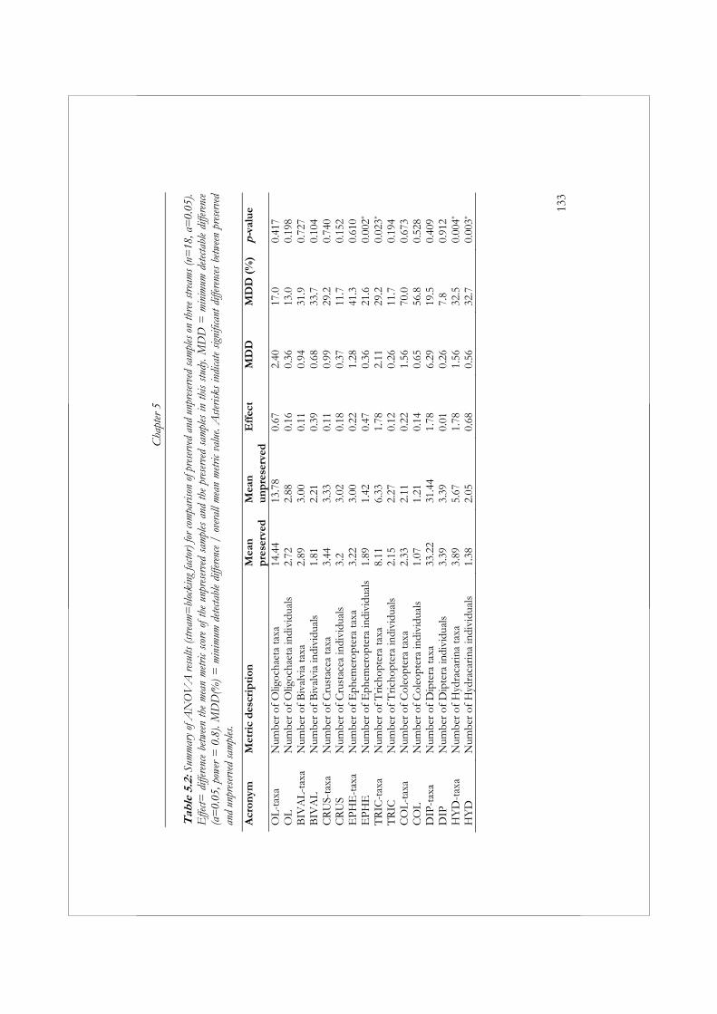
C
hapt
er 5
13
3
Tab
le 5
.2: S
umm
ary
of A
NO
VA
resu
lts (s
tream
=bl
ocki
ng fa
ctor)
for c
ompa
rison
of p
rese
rved
and
unp
rese
rved
sam
ples
on
thre
e stre
ams (
n=18
, α=
0.05
). E
ffect=
diff
eren
ce b
etwee
n th
e m
ean
metr
ic sc
ore
of t
he u
npre
serv
ed s
ampl
es a
nd t
he p
rese
rved
sam
ples
in t
his
study
. MD
D =
min
imum
dete
ctabl
e di
ffere
nce
(α=
0.05
, pow
er =
0.8
). M
DD
(%)
= m
inim
um d
etecta
ble
diffe
renc
e /
over
all m
ean
metr
ic va
lue.
Aste
risks
indi
cate
signi
fican
t diff
eren
ces
betw
een
pres
erve
d an
d un
pres
erve
d sa
mpl
es.
Acr
onym
M
etri
c d
escr
ipti
onM
ean
p
rese
rved
M
ean
un
pre
serv
ed
Eff
ect
MD
DM
DD
(%
)p-
valu
e
OL
-tax
aN
umbe
r of
Olig
ocha
eta
taxa
14.4
413
.78
0.67
2.40
17.0
0.41
7O
L
Num
ber
of O
ligoc
haet
a in
divi
dual
s2.
722.
880.
160.
3613
.00.
198
BIV
AL
-tax
a N
umbe
r of
Biv
alvi
a ta
xa2.
893.
000.
110.
9431
.90.
727
BIV
AL
N
umbe
r of
Biv
alvi
a in
divi
dual
s1.
812.
210.
390.
6833
.70.
104
CR
US-
taxa
N
umbe
r of
Cru
stac
ea ta
xa3.
443.
330.
110.
9929
.20.
740
CR
US
Num
ber
of C
rust
acea
indi
vidu
als
3.2
3.02
0.18
0.37
11.7
0.15
2E
PH
E-t
axa
Num
ber
of E
phem
erop
tera
taxa
3.22
3.00
0.22
1.28
41.3
0.61
0E
PH
EN
umbe
r of
Eph
emer
opte
ra in
divi
dual
s 1.
891.
420.
470.
3621
.60.
002*
TR
IC-t
axa
Num
ber
of T
richo
pter
a ta
xa8.
116.
331.
782.
1129
.20.
023*
TR
ICN
umbe
r of
Tric
hopt
era
indi
vidu
als
2.15
2.27
0.12
0.26
11.7
0.19
4C
OL
-tax
a N
umbe
r of
Col
eopt
era
taxa
2.33
2.11
0.22
1.56
70.0
0.67
3C
OL
Num
ber
of C
oleo
pter
a in
divi
dual
s 1.
071.
210.
140.
6556
.80.
528
DIP
-tax
a N
umbe
r of
Dip
tera
taxa
33.2
231
.44
1.78
6.29
19.5
0.40
9D
IPN
umbe
r of
Dip
tera
indi
vidu
als
3.39
3.39
0.01
0.26
7.8
0.91
2H
YD
-tax
a N
umbe
r of
Hyd
raca
rina
taxa
3.89
5.67
1.78
1.56
32.5
0.00
4*
HY
DN
umbe
r of
Hyd
raca
rina
indi
vidu
als
1.38
2.05
0.68
0.56
32.7
0.00
3*
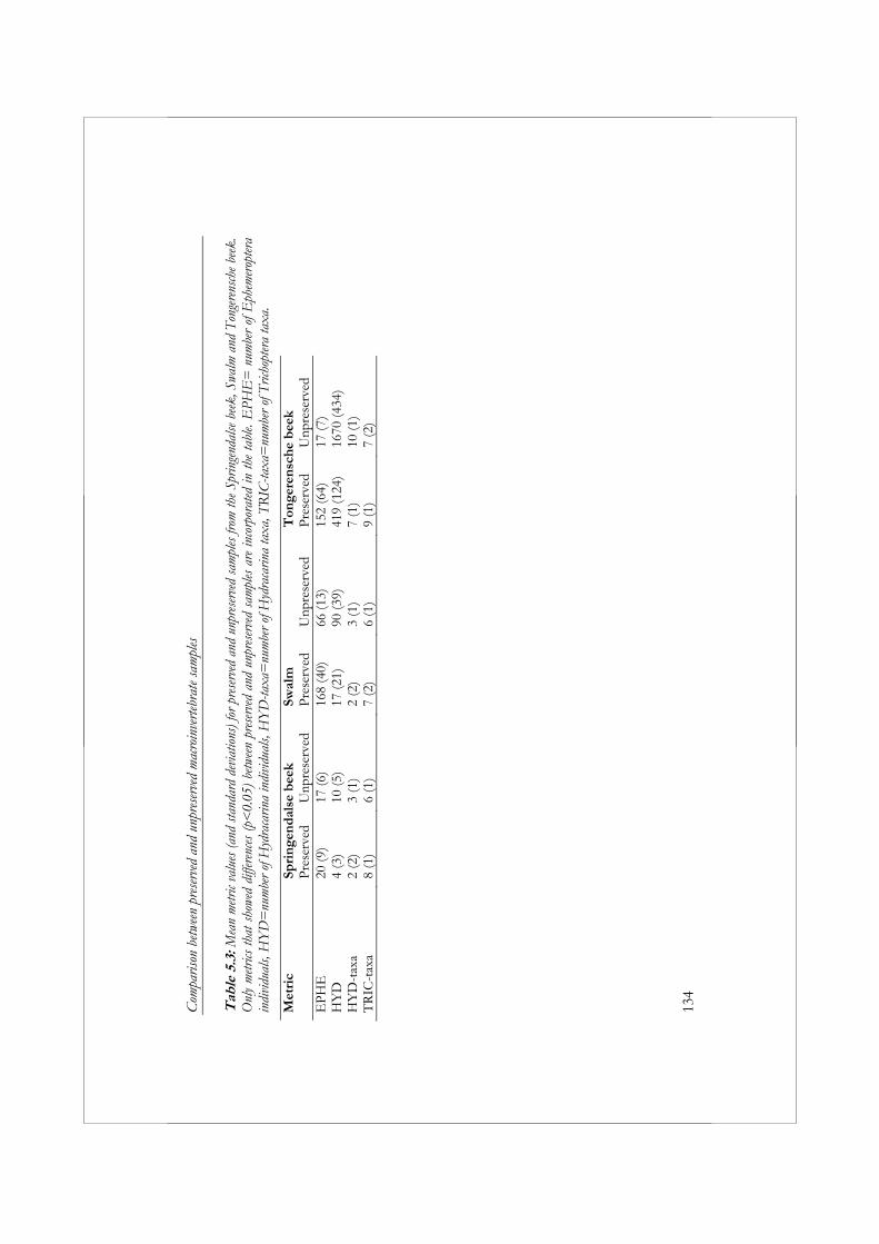
Com
paris
on b
etwee
n pr
eser
ved
and
unpr
eser
ved
mac
roin
verte
brat
e sam
ples
13
4
Tab
le 5
.3: M
ean
metr
ic va
lues
(and
stan
dard
dev
iatio
ns) f
or p
rese
rved
and
unp
rese
rved
sam
ples
from
the S
prin
gend
alse
bee
k, S
walm
and
Ton
gere
nsch
e bee
k.
Onl
y m
etrics
that
sho
wed
diffe
renc
es (
p<0.
05)
betw
een
pres
erve
d an
d un
pres
erve
d sa
mpl
es a
re in
corp
orat
ed in
the
tabl
e. E
PHE
= n
umbe
r of
Eph
emer
opter
a in
divi
dual
s, H
YD
=nu
mbe
r of H
ydra
carin
a in
divi
dual
s, H
YD
-taxa
=nu
mbe
r of H
ydra
carin
a ta
xa, T
RIC
-taxa
=nu
mbe
r of T
richo
pter
a ta
xa.
Met
ric
Spri
nge
nd
alse
bee
kSw
alm
Ton
gere
nsc
he
bee
kP
rese
rved
Unp
rese
rved
Pre
serv
edU
npre
serv
ed
Pre
serv
edU
npre
serv
edE
PHE
20 (9
)17
(6)
168
(40)
66 (1
3)15
2 (6
4)17
(7)
HY
D4
(3)
10 (5
)17
(21)
90 (3
9)41
9 (1
24)
1670
(434
)H
YD
-tax
a 2
(2)
3 (1
)2
(2)
3 (1
)7
(1)
10 (1
)T
RIC
-tax
a 8
(1)
6 (1
)7
(2)
6 (1
)9
(1)
7 (2
)
Chapter 5
135
Multimetric index The only difference in ecological quality class between preserved and unpreserved samples was detected in samples from the Swalm. One preserved sample indicated good ecological quality, while all unpreserved samples indicated poor ecological quality. All samples from the Tongerensche beek indicated poor ecological quality. Two preserved and two unpreserved samples from the Springendalse beek indicated good ecological quality, while one preserved and one unpreserved sample indicated high ecological quality. Sample processing costs We detected no significant difference between preserved and unpreserved samples in the total time required for sample processing (F=1.64, p=0.221). When comparing the time required for sorting and identification separately, we also detected no significant differences between preserved and unpreserved samples (F=0.25, p=0.626 and F=1.11, p=0.310). Discussion For most major macroinvertebrate groups (five out of eight), we detected no significant differences in the number of taxa or individuals between preserved and unpreserved samples. The required MDD for the number of Coleoptera taxa and individuals suggests our study was not adequately designed to detect significant differences with acceptable power. Carlisle & Clements (1999), however, suggested that metrics requiring MDDs of more than 50% to reach a power of 0.8 cannot possibly detect ecologically relevant changes given realistic sampling efforts. Therefore, we conclude that the low power of our study design is not relevant. As a result of the high within-site variability in the number of Coleoptera taxa and individuals, these metrics are per definition not suited for biological assessment purposes in the case of the studied streams.
The metrics that required MDDs of less than 50% and showed no significant differences between preserved and unpreserved samples necessitate closer consideration. The question is whether these nonsignificant results should be considered as: (1) the true absence of ecologically relevant differences between preserved and unpreserved samples, or (2) as a reflection of inadequate power. To answer this question, the degree of change that is considered ecologically relevant for bioassessment purposes must be determined. This degree of change will vary depending on the method used for
Comparison between preserved and unpreserved macroinvertebrate samples
136
bioassessment and is also not an entirely scientific decision (Carlisle & Clements, 1999).
For metrics that did show significant differences in values between methods, values were not always higher for the same method. Instead, the method that resulted in higher values depended on the organism group. Significantly higher numbers of Ephemeroptera individuals and Trichoptera taxa were collected from the preserved samples. The lower number of Ephemeroptera individuals collected from the unpreserved samples might have been caused by disintegration during transportation, storage, and sorting because of a lack of oxygen in the samples. Supporting this suggestion is the fact that during sorting, we often found only parts instead of complete Ephemeroptera specimens. The difference in Trichoptera taxa collected between both methods is considered an artifact. When we counted the number of species instead of the number of taxa, two out of three preserved samples contained five species and one preserved sample contained four species. All three unpreserved samples contained four species. Significantly higher numbers of Hydracarina individuals and taxa were collected from the unpreserved samples. This finding supports the suggestion that small organisms, like Hydracarina, are easier to detect when they are moving.
Our results seem to contradict those of studies by Humphrey et al. (2000), Metzling (2003), and Nichols & Norris (2006), who found that small and cryptic taxa such as Oligochaeta, Diptera, and Hydracarina were often overlooked in unpreserved samples. However, in these studies, sample processing procedures varied for preserved and unpreserved samples, making it impossible to identify the exact cause of overlooking small and cryptic taxa in unpreserved samples. Nichols & Norris (2006) suggest that the small taxa were missed because operators sorted the unpreserved samples unaided by a microscope. However, Growns et al. (2006) showed that using magnification did not improve the efficiency of collection of small and cryptic taxa.
Some macroinvertebrate groups were not included in the analyses because they were absent from some samples. These macroinvertebrate groups may show significant differences in the number of individuals and the number of taxa between preserved and unpreserved samples in streams where they are more abundant.
In only one instance, we identified a difference in ecological quality class between preserved and unpreserved samples. This difference was the result of higher values for the metric EPT-taxa (%). Although values of individual metrics may vary between preserved and unpreserved samples, the final assessment result will not necessarily also differ between sample processing methods. Indeed, Fore et al. (2001) and Lorenz et al. (2004) showed
Chapter 5
137
that differences in metric values will not necessarily result in differences in the final assessment result. Differences in the final assessment result develop when metric values happen to fall near a break point in the scoring criteria (Fore et al., 2001), as observed for the metric EPT-taxa (%).
In addition, we found no significant differences between preserved and unpreserved samples in the time required for sorting. Two possible explanations for this finding are that (1) the advantage of easier detection of moving organisms is cancelled out by the disadvantage of their being more difficult to catch, and/or that (2) differences between replicates are so large that they efface statistically significant differences between methods. The results show that differences between replicates are large, possibly because of differences in macroinvertebrate community composition between exact sampling locations or other sources of variation resulting from differences in sample processing (e.g., differences in refrigerator storage time).
Considering the results of this study, two things should be kept in mind. First, we used formaldehyde to preserve the samples, leaving the question of whether using ethanol as a preservative would have resulted in the same findings. Second, all samples were sorted in the laboratory, as is common practice in the Netherlands. The results of sorting unpreserved samples in the laboratory cannot be compared to the results of sorting samples in the field, especially given that circumstances for sorting in the field can be far from optimal (Carter & Resh, 2001; Rawer-Joost, 2001).
In some cases, we found a significant difference between preserved and unpreserved samples for individual metrics. When assessment is based on these individual metrics, the choice to use a preservative or not becomes relevant. This study indicates that in streams with Ephemeroptera, the preservation of samples is necessary to optimize the number of Ephemeroptera individuals collected. In streams that contain Hydracarina, the preservation of samples will result in underestimation of the number of Hydracarina taxa and individuals present. Problems arise when both groups are likely to be present in a stream, and a sample processing method has to be chosen. The decision should always be made based on the system/metric(s) used for assessment. Additionally, in this study, ecological quality classes did not depend on the sample processing method used. This finding indicates that for the assessment of small Dutch lowland streams, the sample processing protocol does not require standardization in terms of sample preservation. However, standardization of sampling and sample processing methods, including sample preservation, remains essential in case of (long-term) routine monitoring programs. Since there are limits to standardization, e.g. among different agencies and water types, we agree with Diamond et al. (1996) that it
Comparison between preserved and unpreserved macroinvertebrate samples
138
is important to document method performance characteristics through monitoring of data quality to make comparisons between monitoring programs possible. Conclusions Significantly different numbers of Ephemeroptera individuals and Hydracarina taxa and individuals were collected from preserved samples compared to unpreserved samples. In assessments based on these individual metrics, standardization of sample processing will be required. In streams with Ephemeroptera, the preservation of samples is necessary to optimize the number of Ephemeroptera individuals collected. In streams that contain Hydracarina, the preservation of samples will result in an underestimation of the number of Hydracarina taxa and individuals present. In only one instance there was a difference in ecological quality between preserved and unpreserved samples, indicating that assessing small Dutch lowland streams does not require standardization of sample preservation as part of the sample processing protocol. We detected no significant differences in sample processing costs between preserved and unpreserved samples. Acknowledgements This study was carried out within the STAR project funded by the European Commission, 5th Framework Program, Energy Environment and Sustainable Development, Key Action Water, Contract no. EVK1-CT-2001-00089. We are grateful for the helpful comments from Ralf Verdonschot, Karin Didderen, and anonymous reviewers. We would like to thank Tjeerd-Harm van den Hoek, Martin van den Hoorn, and Rink Wiggers for their efforts in collecting the data on which this study was based. References Alba-Tercedor, J. & A. Sanches-Ortega, 1988. Un methoda rapido y simple
para evaluar la calidadbiologica de las aguas vorrientes basado en el de Hellawell (1978). Limnetica 4: 51-56.
Bailey, R.C, R.H. Norris & T.B. Reynoldson, 2001. Taxonomic resolution of benthic macroinvertebrate communities in bioassessments. Journal of the North American Benthological Society 20: 280-286.
Chapter 5
139
Barbour, M.T. & J. Gerritsen, 1996. Subsampling of benthic samples: a defense of the fixed-count method. Journal of the North American Benthological Society 15: 386-391.
Barton, D.R. & J.L. Metcalfe-Smith, 1992. A comparison of sampling techniques and summary indices for assessment of water quality in the Yamaska River Québec, based on benthic macroinvertebrates. Environmental Monitoring and Assessment 21: 225-244.
Braukmannn, U., 2000. Hydrochemische und biologische merkmale regionaler bachtypen in Baden-Württemberg. Oberirdische Gewässer, Gewässerökologie 56: 1-501.
Brinkman, M.A. & W.G. Duffy, 1996. Evaluation of four wetland aquatic invertebrate samplers and four sample sorting methods. Journal of Freshwater Ecology 11: 193-200.
Canton, S.P. & J.W. Chadwick, 1988. Variability in benthic invertebrate density estimates from stream samples. Journal of Freshwater Ecology 4: 291-297.
Carlisle, M.D. & W.H. Clements, 1999. Sensitivity and variability of metrics used in biological assessments of running waters. Environmental Toxicology and Chemistry 18: 285-291.
Carter, J.L. & V.H. Resh, 2001. After site selection and before data analysis: sampling, sorting, and laboratory procedures used in stream benthic macroinvertebrate monitoring programs by USA state agencies. Journal of the North American Benthological Society 20: 658-682.
Cheal, F., A. Davis, J.E. Growns, J.S. Bradley & F.H. Whittles, 1993. The influence of sampling method on the classification of wetland macroinvertebrate communities. Hydrobiologia 257: 47-56.
Chessman, B.C. & D.P. Robinson, 1987. Some effects of the 1982-83 drought on water quality and macroinvertebrate fauna in the lower La Trobe River, Victoria. Australian Journal of Marine and Freshwater Research 38: 289-299.
Chessman, B.C., 1995. Rapid river assessment using macroinvertebrates: A procedure based on habitat-specific family level identification and a biotic index. Australian Journal of Ecology 20: 122-129.
Cohen, J., 1988. Statistical analysis for the behavioural sciences. Second edition. Lawrence Erlbaum Associates, Hillsdale, New Jersey, USA:
Courtemanch, D.L., 1996. Commentary on the subsampling procedures used for rapid bioassessments. Journal of the North American Benthological Society 15: 381-385.
Diamond, J.M., M.T. Barbour & J.B. Stribling, 1996. Characterizing and comparing bioassessment methods and their results: a perspective. Journal of the North American Benthological Society 15: 713-727.
Comparison between preserved and unpreserved macroinvertebrate samples
140
Drake, C.M. & J.M. Elliott, 1982. A comparative study of three air-lift samplers used for sampling benthic macro-invertebrates in rivers. Freshwater Biology 12: 511-533.
European Commission, 2000. Directive 2000/60/EC OF THE EUROPEAN PARLIAMENT AND COUNCIL - Establishing a framework for Community action in the field of water policy. Official Journal of the European Community L327: 1-72.
Fore, L.S., K. Paulsen & K. O' Laughlin, 2001. Assessing the performance of volunteers in monitoring streams. Freshwater Biology 46: 109-123.
Growns, J.E., B.C. Chessman, J.E. Jackson & D.G. Ross, 1997. Rapid assessment of Australian rivers using macroinvertebrates: cost and efficiency of 6 methods of sample processing. Journal of the North American Benthological Society 16: 682-693.
Growns, I., C. Schiller, N. O’Conner, A. Cameron & B. Gray, 2006. Evaluation of four live-sorting methods for use in rapid biological assessments using macroinvertebrates. Environmental Monitoring and Assessment 117: 173-192.
Haase, P., S. Pauls, A. Sundermann & A. Zenker, 2004. Testing different sorting techniques in macroinvertebrate samples from running water. Limnologica 34: 366-378.
Hawkes, H. A., 1979. Invertebrates as indicators of river water quality. In: James, A. & L. Evison (eds.), Biological indicators of water quality. John Wiley and Sons, New York, pp.: 2-1 to 2-45.
Hellawell, J.M., 1986. Biological indicators of freshwater pollution and environmental management. Elsevier Applied Science, London.
Hering, D., O. Moog, L. Sandin, P.F.M. Verdonschot, 2004. Overview and application of the AQEM assessment system. Hydrobiologia 516: 1-20.
Humphrey, C.L., A.W. Storey L. Thurtell, 2000. AUSRIVAS: operator sample processing errors and temporal variability - implications for model sensitivity. In: Wright, J.F., D.W. Sutcliffe, M.T. Furse (eds.), Assessing the biological quality of freshwaters: RIVPACS and other techniques. Freshwater Biological Association, Cumbria, United Kingdom, pp.: 143–146.
Kerans, B.L., J.R. Karr & S.A. Ahlstedt, 1992. Aquatic invertebrate assemblages: spatial and temporal differences among sampling protocols. Journal of the North American Benthological Society 11: 377-390.
Lehmann, E.L., 1975. Nonparametrics: statistical methods bases on ranks. Holden-Day, San Francisco.
Chapter 5
141
Lenat, D.R & V.H. Resh, 2001. Taxonomy and stream ecology - The benefits of genus and species-level identification. Journal of the North American Benthological Society 20: 287-298.
Lorenz, A., L. Kirchner & D. Hering, 2004. “Electronic subsampling” of macrobenthic samples: how many individuals are needed for a valid assessment result? Hydrobiologia 516: 299-312.
Mackey, A.P., D.A. Cooling & A.D. Berrie, 1984. An evaluation of sampling strategies for qualitative surveys of macro-invertebrates in rivers, using pond nets. Journal of Applied Ecology 21: 515-534.
Metzeling, L. & J. Miller, 2001. Evaluation of the sample size used for the rapid bioassessment of rivers using macroinvertebrates. Hydrobiologia 444: 159-170.
Metzeling, L., B. Chessman, R. Hardwick & V. Wong, 2003. Rapid assessment of rivers using macroinvertebrates: the role of experience, and comparisons with quantitative methods. Hydrobiologia 510: 39-52.
Nichols, S.J. & R.H. Norris, 2006. River condition assessment may depend on the sub-sampling method: field live-sort versus laboratory sub-sampling of invertebrates for bioassessment. Hydrobiologia 572: 195-213.
Nijboer, R.C. & P.F.M. Verdonschot, 2000. Taxonomic adjustment affects data analysis: an often forgotten error. Verhandlungen Internationale Vereinigung für Theoretische und Angewandte Limnologie 27: 2546-2549.
Norris, R.H., E.P. McElravy & V.H. Resh, 1992. The sampling problem. In: Calow, P. & G.E. Petts (eds.), Rivers Handbook. Scientific Publications, Oxford, pp: 282-306.
Peterman, R.M., 1990. The importance of reporting statistical power: the forest decline and acidic deposition example. Ecology 71: 2024-2027.
Rawer-Joost, C., 2001. Eignung und variabilität von verfahren zur ökologischen bewertung von fließgewässern im mittelgebirge auf der basis autökologischer kenngrössen des makrozoobenthos. PhD-thesis: University of Hohenheim.
Resh, V.H., 1994. Variability, accuracy and taxonomic costs of rapid assessment approaches in benthic macroinvertebrate monitoring. Bollettino di Zoologia 61: 375-383.
Rotenberry, J.T. & J.A. Wiens, 1985. Statistical power analysis and community-wide patterns. American Naturalist 125: 164-168.
Vinson, M.R. & C.P. Hawkins, 1996. Effects of sampling area and subsampling procedure on comparisons of taxa richness among streams. Journal of the North American Benthological Society 15: 392-399.
Vlek, H.E., F. Šporka & I. Krno, 2006. Influence of macroinvertebrate sample size on bioassessment of streams. Hydrobiologia 566: 523-542.

Comparison between preserved and unpreserved macroinvertebrate samples
142
Vlek, H.E., P.F.M. Verdonschot & R.C. Nijboer, 2004. Towards a multimetric index for the assessment of Dutch streams using benthic macroinvertebrates. Hydrobiologia 516: 173-189.
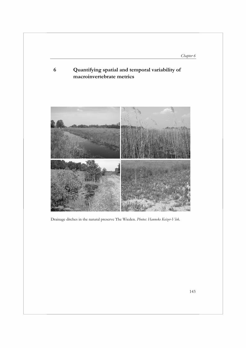
Chapter 6
143
6 Quantifying spatial and temporal variability of macroinvertebrate metrics
Drainage ditches in the natural preserve The Wieden. Photos: Hanneke Keizer-Vlek.
Quantifying spatial and temporal variability of macroinvertebrate metrics
144
6 Quantifying spatial and temporal variability of macro-invertebrate metrics
Hanneke E. Keizer-Vlek, Piet F.M. Verdonschot, Ralf C.M. Verdonschot & Paul W. Goedhart Ecological Indicators (2012) 23: 384-393. Abstract Since the introductions of the Habitat Directive and the European Water Framework Directive, water authorities are now obliged to monitor changes in conservation value/ecological quality on larger spatial scales (opposed to site scale), as well as to indicate the level of confidence and precision of the results provided by the monitoring programs in their river basin management plans (European Commission, 2000). To meet these requirements, analyses of the statistical power of the monitoring programs should be implemented. Currently, the statistical properties associated with aquatic monitoring programs are often unknown. We collected macroinvertebrate samples from 25 meso-eutrophic drainage ditches in the Netherlands and selected 7 taxonomic richness metrics for the evaluation of spatial and temporal variability. Simulations were performed to investigate the effects of changes in (1) the total number of species included in a taxonomic richness metric and (2) the relative number of rare species included in a taxonomic richness metric. Of the 7 metrics evaluated, the number of common species required the smallest number of monitoring sites, followed by the number of Gastropoda species, and the number of species. Also, results showed that metric variability will decrease when the proportion of rare species included in a taxonomic richness metric is reduced or the total number of species included is increased. Irrespective of the metric applied a large effort will be required to detect change within drainage ditches in the Wieden, due to high spatial variability. Therefore, we need to explore the possibilities of applying alternative more cost-effective methods for sampling and sample processing in biomonitoring programs. Keywords: spatial variability, temporal variability, rare species, macroinvertebrates, biomonitoring, detection of change
Chapter 6
145
Introduction The ecological quality of surface waters in the Netherlands has been monitored for several decades by regional water authorities. Until recently, they were focused on determining the ecological quality at a specific site and they collected a single sample at the site for this purpose, as is also a common practice in the United States (Carter & Resh, 2001). Since the introductions of the Habitat Directive and the European Water Framework Directive, water authorities are now obliged to monitor changes in conservation value/ecological quality on larger spatial (regional) scales, as well as to indicate the level of confidence and precision of the results provided by the monitoring programs in their river basin management plans (European Commission, 2000). To meet these new requirements, the process of designing monitoring programs and interpreting the data resulting from these programs should implement analyses of the statistical power of the programs.
Power analysis (assessing the ability of a program to accurately detect change) could help avoid unnecessary expenditures on monitoring programs that cannot provide meaningful results or that will lead to overspending. In the final step of testing a statistical hypothesis, a decision will be made about the validity of the null hypothesis. Two types of errors can be made in making this decision, a type I error or a type II error. A type I error can be described as “drawing the conclusion that change has occurred when in fact it has not”. Conversely, concluding that change has not occurred when in fact it has is called a type II error. Both errors can have large consequences. Type I errors could lead to serious negative financial effects if costly and unnecessary restoration measures are taken. Type II errors could have serious negative effects on reaching ecological goals if failure to detect a negative trend leads to the dismissal of required restoration measures (Taylor & Gerrodette, 1993). The probability of making a type I error is usually denoted as α (statistical significance), and the probability of making a type II error is usually denoted as β. Power (1 − β) is defined as the probability that change will be detected (Gerrodette, 1987). Statistical power depends on a number of factors: (1) statistical significance, (2) the magnitude of effect to be detected (i.e., effect size), (3) sample size and variability, and (4) statistical assumptions (e.g., use of one-tailed tests versus two-tailed tests). Currently, the statistical properties associated with aquatic monitoring programs are often unknown.
Changes in ecological quality can be the result of restoration measures or anthropogenic disturbance. However, such changes can be masked by several sources of variation, sampling effects, spatial variation, and temporal variation. To determine whether change is the result of anthropogenic
Quantifying spatial and temporal variability of macroinvertebrate metrics
146
disturbance requires the determination of natural variability ( Johnson, 1998; Leunda et al., 2009; Resh & Rosenberg, 1989). Insight into both spatial and temporal variability is required. Most studies that have quantified temporal and/or spatial variability were focused on lotic ecosystems (e.g., Dolph et al., 2010; Downes et al., 1993; Gebler, 2004; Springe et al., 2006). The majority of surface waters in the Netherlands, however, are lentic ecosystems. Of these lentic ecosystems, drainage ditches are particularly interesting because they are important drivers of biodiversity in agricultural areas (Armitage et al., 2003; Herzon and Helenius, 2008; Painter, 1999,). They are also a prominent feature in the landscape of the lowlands of northwestern Europe; in the Netherlands alone, total ditch length is approximately 300,000 km (Verdonschot et al., 2012).
There are several studies that have dealt with spatial or temporal variation of macroinvertebrate communities in lentic systems in relation to biological assessment (Hämäläinen et al. 2003; Kashian & Burton, 2000; Tangen et al., 2003). However, only a few have quantified both spatial and temporal variations with the purpose of defining statistical properties of future monitoring programs (Johnson, 1998; Trigal et al., 2006). The first objective of this study was therefore to quantify spatial and temporal variability of taxonomic richness metrics based on macroinvertebrates in a minimally impaired system of drainage ditches. This information makes it possible to determine the minimum number of monitoring sites required to detect changes due to anthropogenic disturbance and/or restoration measures.
The decision whether to include rare species in analysis for bioassessment purposes may affect statistical power (Cao et al., 2001). Many studies have addressed the use of rare species in biological assessment. Some advocate the use of rare species, because they may be good indicators of ecological quality (e.g., Lenat & Resh, 2001; Lyons et al., 1995; Nijboer & Schmidt-Kloiber, 2006; Poos & Jackson, 2012). Others, favor the exclusion of rare species because they add noise to the analysis (e.g., Gauch, 1982; Marchant, 2002), thus diminishing power. None of these studies, however, have looked at the effects of including/excluding rare species from metrics and the effect that this has on metric variability. The second objective of this study was therefore to determine the influence of rare species on variability of taxonomic richness metrics.
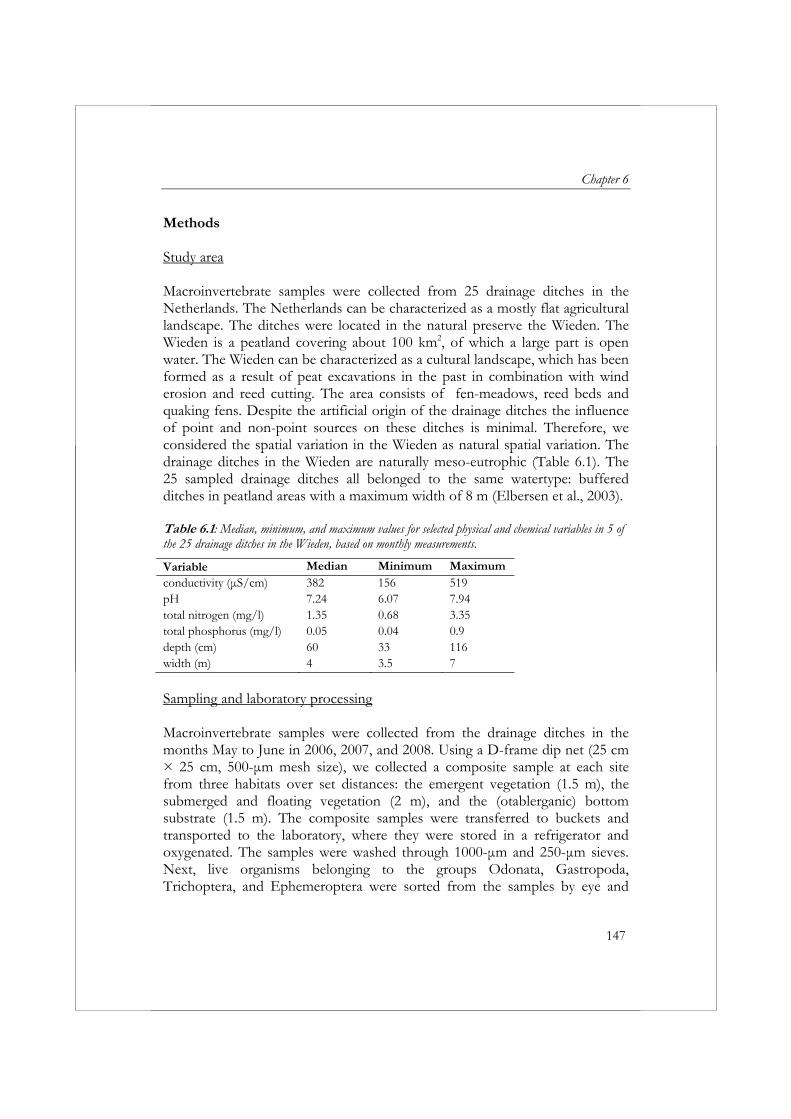
Chapter 6
147
Methods Study area Macroinvertebrate samples were collected from 25 drainage ditches in the Netherlands. The Netherlands can be characterized as a mostly flat agricultural landscape. The ditches were located in the natural preserve the Wieden. The Wieden is a peatland covering about 100 km2, of which a large part is open water. The Wieden can be characterized as a cultural landscape, which has been formed as a result of peat excavations in the past in combination with wind erosion and reed cutting. The area consists of fen-meadows, reed beds and quaking fens. Despite the artificial origin of the drainage ditches the influence of point and non-point sources on these ditches is minimal. Therefore, we considered the spatial variation in the Wieden as natural spatial variation. The drainage ditches in the Wieden are naturally meso-eutrophic (Table 6.1). The 25 sampled drainage ditches all belonged to the same watertype: buffered ditches in peatland areas with a maximum width of 8 m (Elbersen et al., 2003). Table 6.1: Median, minimum, and maximum values for selected physical and chemical variables in 5 of the 25 drainage ditches in the Wieden, based on monthly measurements.
Variable Median Minimum Maximumconductivity (μS/cm) 382 156 519pH 7.24 6.07 7.94total nitrogen (mg/l) 1.35 0.68 3.35total phosphorus (mg/l) 0.05 0.04 0.9depth (cm) 60 33 116width (m) 4 3.5 7
Sampling and laboratory processing Macroinvertebrate samples were collected from the drainage ditches in the months May to June in 2006, 2007, and 2008. Using a D-frame dip net (25 cm × 25 cm, 500-μm mesh size), we collected a composite sample at each site from three habitats over set distances: the emergent vegetation (1.5 m), the submerged and floating vegetation (2 m), and the (otablerganic) bottom substrate (1.5 m). The composite samples were transferred to buckets and transported to the laboratory, where they were stored in a refrigerator and oxygenated. The samples were washed through 1000-μm and 250-μm sieves. Next, live organisms belonging to the groups Odonata, Gastropoda, Trichoptera, and Ephemeroptera were sorted from the samples by eye and
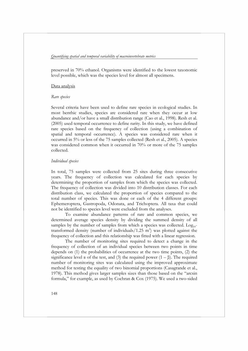
Quantifying spatial and temporal variability of macroinvertebrate metrics
148
preserved in 70% ethanol. Organisms were identified to the lowest taxonomic level possible, which was the species level for almost all specimens. Data analysis Rare species Several criteria have been used to define rare species in ecological studies. In most benthic studies, species are considered rare when they occur at low abundance and/or have a small distribution range (Cao et al., 1998). Resh et al. (2005) used temporal occurrence to define rarity. In this study, we have defined rare species based on the frequency of collection (using a combination of spatial and temporal occurrence). A species was considered rare when it occurred in 5% or less of the 75 samples collected (Resh et al., 2005). A species was considered common when it occurred in 70% or more of the 75 samples collected. Individual species In total, 75 samples were collected from 25 sites during three consecutive years. The frequency of collection was calculated for each species by determining the proportion of samples from which the species was collected. The frequency of collection was divided into 10 distribution classes. For each distribution class, we calculated the proportion of species compared to the total number of species. This was done or each of the 4 different groups: Ephemeroptera, Gastropoda, Odonata, and Trichoptera. All taxa that could not be identified to species level were excluded from the analyses.
To examine abundance patterns of rare and common species, we determined average species density by dividing the summed density of all samples by the number of samples from which a species was collected. Log10-transformed density (number of individuals/1.25 m2) was plotted against the frequency of collection and this relationship was fitted with a linear regression.
The number of monitoring sites required to detect a change in the frequency of collection of an individual species between two points in time depends on (1) the probabilities of occurrence at the two time points, (2) the significance level α of the test, and (3) the required power (1 – β). The required number of monitoring sites was calculated using the improved approximate method for testing the equality of two binomial proportions (Casagrande et al., 1978). This method gives larger samples sizes than those based on the “arcsin formula,” for example, as used by Cochran & Cox (1975). We used a two-sided
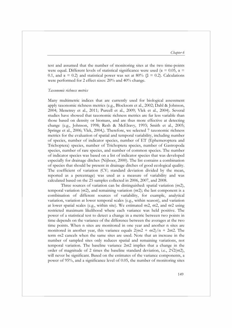
Chapter 6
149
test and assumed that the number of monitoring sites at the two time-points were equal. Different levels of statistical significance were used (α = 0.05, α = 0.1, and α = 0.2) and statistical power was set at 80% (β = 0.2). Calculations were performed for 2 effect sizes: 20% and 40% change. Taxonomic richness metrics Many multimetric indices that are currently used for biological assessment apply taxonomic richness metrics (e.g., Blocksom et al., 2002; Dahl & Johnson, 2004; Menetrey et al., 2011; Purcell et al., 2009; Vlek et al., 2004). Several studies have showed that taxonomic richness metrics are far less variable than those based on density or biomass, and are thus more effective at detecting change (e.g., Johnson, 1998; Resh & McElravy, 1993; Smith et al., 2005; Springe et al., 2006; Vlek, 2004,). Therefore, we selected 7 taxonomic richness metrics for the evaluation of spatial and temporal variability, including number of species, number of indicator species, number of ET (Ephemeroptera and Trichoptera) species, number of Trichoptera species, number of Gastropoda species, number of rare species, and number of common species. The number of indicator species was based on a list of indicator species that was developed especially for drainage ditches (Nijboer, 2000). The list contains a combination of species that should be present in drainage ditches of good ecological quality. The coefficient of variation (CV; standard deviation divided by the mean, reported as a percentage) was used as a measure of variability and was calculated based on the 25 samples collected in 2006, 2007, and 2008.
Three sources of variation can be distinguished: spatial variation (σs2), temporal variation (σt2), and remaining variation (σr2); the last component is a combination of different sources of variability, for example, analytical variation, variation at lower temporal scales (e.g., within season), and variation at lower spatial scales (e.g., within site). We estimated σs2, σt2, and σr2 using restricted maximum likelihood where each variance was held positive. The power of a statistical test to detect a change in a metric between two points in time depends on the variance of the difference between the averages at the two time points. When n sites are monitored in one year and another n sites are monitored in another year, this variance equals 2(σs2 + σr2)/n + 2σt2. The term σs2 cancels when the same sites are used. Note that an increase in the number of sampled sites only reduces spatial and remaining variations, not temporal variation. The baseline variance 2σt2 implies that a change in the order of magnitude of 2 times the baseline standard deviation, i.e., 2√2(σt2), will never be significant. Based on the estimates of the variance components, a power of 95%, and a significance level of 0.05, the number of monitoring sites
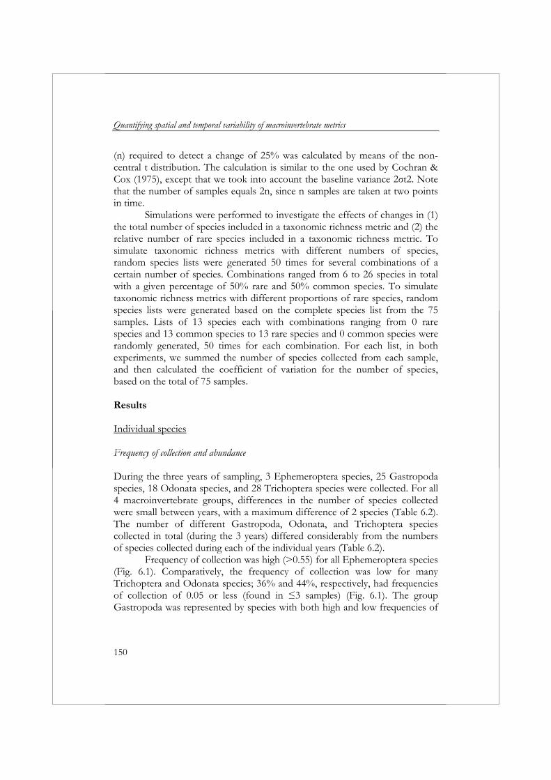
Quantifying spatial and temporal variability of macroinvertebrate metrics
150
(n) required to detect a change of 25% was calculated by means of the non-central t distribution. The calculation is similar to the one used by Cochran & Cox (1975), except that we took into account the baseline variance 2σt2. Note that the number of samples equals 2n, since n samples are taken at two points in time.
Simulations were performed to investigate the effects of changes in (1) the total number of species included in a taxonomic richness metric and (2) the relative number of rare species included in a taxonomic richness metric. To simulate taxonomic richness metrics with different numbers of species, random species lists were generated 50 times for several combinations of a certain number of species. Combinations ranged from 6 to 26 species in total with a given percentage of 50% rare and 50% common species. To simulate taxonomic richness metrics with different proportions of rare species, random species lists were generated based on the complete species list from the 75 samples. Lists of 13 species each with combinations ranging from 0 rare species and 13 common species to 13 rare species and 0 common species were randomly generated, 50 times for each combination. For each list, in both experiments, we summed the number of species collected from each sample, and then calculated the coefficient of variation for the number of species, based on the total of 75 samples. Results Individual species Frequency of collection and abundance During the three years of sampling, 3 Ephemeroptera species, 25 Gastropoda species, 18 Odonata species, and 28 Trichoptera species were collected. For all 4 macroinvertebrate groups, differences in the number of species collected were small between years, with a maximum difference of 2 species (Table 6.2). The number of different Gastropoda, Odonata, and Trichoptera species collected in total (during the 3 years) differed considerably from the numbers of species collected during each of the individual years (Table 6.2).
Frequency of collection was high (>0.55) for all Ephemeroptera species (Fig. 6.1). Comparatively, the frequency of collection was low for many Trichoptera and Odonata species; 36% and 44%, respectively, had frequencies of collection of 0.05 or less (found in ≤3 samples) (Fig. 6.1). The group Gastropoda was represented by species with both high and low frequencies of
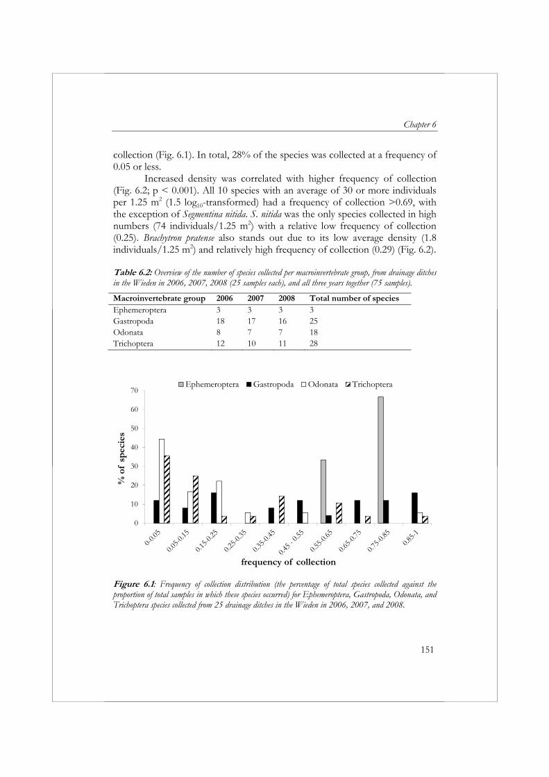
Chapter 6
151
collection (Fig. 6.1). In total, 28% of the species was collected at a frequency of 0.05 or less.
Increased density was correlated with higher frequency of collection (Fig. 6.2; p < 0.001). All 10 species with an average of 30 or more individuals per 1.25 m2 (1.5 log10-transformed) had a frequency of collection >0.69, with the exception of Segmentina nitida. S. nitida was the only species collected in high numbers (74 individuals/1.25 m2) with a relative low frequency of collection (0.25). Brachytron pratense also stands out due to its low average density (1.8 individuals/1.25 m2) and relatively high frequency of collection (0.29) (Fig. 6.2). Table 6.2: Overview of the number of species collected per macroinvertebrate group, from drainage ditches in the Wieden in 2006, 2007, 2008 (25 samples each), and all three years together (75 samples).
Macroinvertebrate group 2006 2007 2008 Total number of species Ephemeroptera 3 3 3 3Gastropoda 18 17 16 25Odonata 8 7 7 18Trichoptera 12 10 11 28
0
10
20
30
40
50
60
70
% o
f sp
ecie
s
frequency of collection
Ephemeroptera Gastropoda Odonata Trichoptera
Figure 6.1: Frequency of collection distribution (the percentage of total species collected against the proportion of total samples in which these species occurred) for Ephemeroptera, Gastropoda, Odonata, and Trichoptera species collected from 25 drainage ditches in the Wieden in 2006, 2007, and 2008.
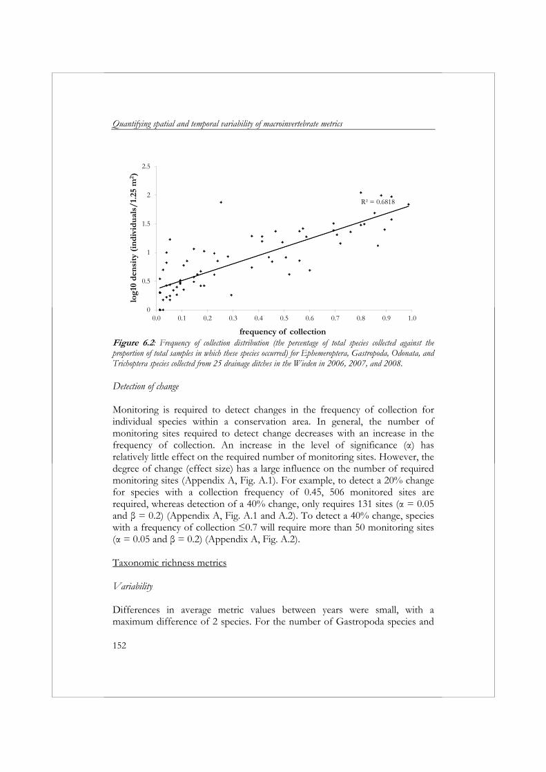
Quantifying spatial and temporal variability of macroinvertebrate metrics
152
R² = 0.6818
0
0.5
1
1.5
2
2.5
0.0 0.1 0.2 0.3 0.4 0.5 0.6 0.7 0.8 0.9 1.0
log1
0 d
ensi
ty (
ind
ivid
ual
s/1.
25 m
2 )
frequency of collection Figure 6.2: Frequency of collection distribution (the percentage of total species collected against the proportion of total samples in which these species occurred) for Ephemeroptera, Gastropoda, Odonata, and Trichoptera species collected from 25 drainage ditches in the Wieden in 2006, 2007, and 2008. Detection of change Monitoring is required to detect changes in the frequency of collection for individual species within a conservation area. In general, the number of monitoring sites required to detect change decreases with an increase in the frequency of collection. An increase in the level of significance (α) has relatively little effect on the required number of monitoring sites. However, the degree of change (effect size) has a large influence on the number of required monitoring sites (Appendix A, Fig. A.1). For example, to detect a 20% change for species with a collection frequency of 0.45, 506 monitored sites are required, whereas detection of a 40% change, only requires 131 sites (α = 0.05 and β = 0.2) (Appendix A, Fig. A.1 and A.2). To detect a 40% change, species with a frequency of collection ≤0.7 will require more than 50 monitoring sites (α = 0.05 and β = 0.2) (Appendix A, Fig. A.2). Taxonomic richness metrics Variability Differences in average metric values between years were small, with a maximum difference of 2 species. For the number of Gastropoda species and
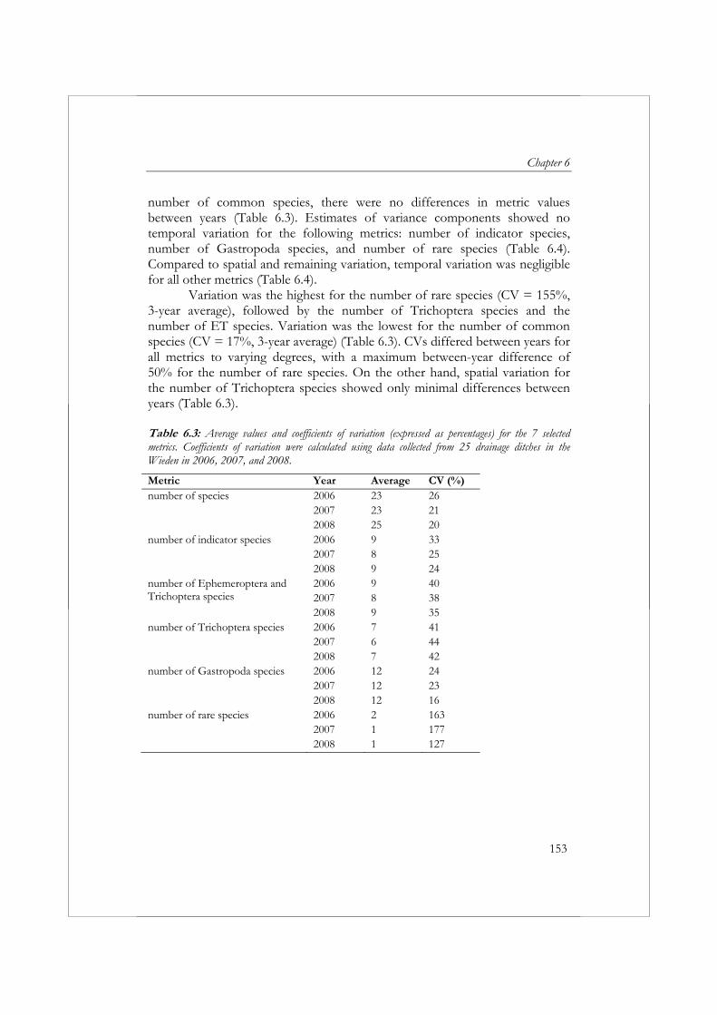
Chapter 6
153
number of common species, there were no differences in metric values between years (Table 6.3). Estimates of variance components showed no temporal variation for the following metrics: number of indicator species, number of Gastropoda species, and number of rare species (Table 6.4). Compared to spatial and remaining variation, temporal variation was negligible for all other metrics (Table 6.4).
Variation was the highest for the number of rare species (CV = 155%, 3-year average), followed by the number of Trichoptera species and the number of ET species. Variation was the lowest for the number of common species (CV = 17%, 3-year average) (Table 6.3). CVs differed between years for all metrics to varying degrees, with a maximum between-year difference of 50% for the number of rare species. On the other hand, spatial variation for the number of Trichoptera species showed only minimal differences between years (Table 6.3). Table 6.3: Average values and coefficients of variation (expressed as percentages) for the 7 selected metrics. Coefficients of variation were calculated using data collected from 25 drainage ditches in the Wieden in 2006, 2007, and 2008.
Metric Year Average CV (%)number of species 2006 23 26 2007 23 21 2008 25 20number of indicator species 2006 9 33 2007 8 25 2008 9 24number of Ephemeroptera and Trichoptera species
2006 9 402007 8 38
2008 9 35number of Trichoptera species 2006 7 41 2007 6 44 2008 7 42number of Gastropoda species 2006 12 24 2007 12 23 2008 12 16number of rare species 2006 2 163 2007 1 177 2008 1 127
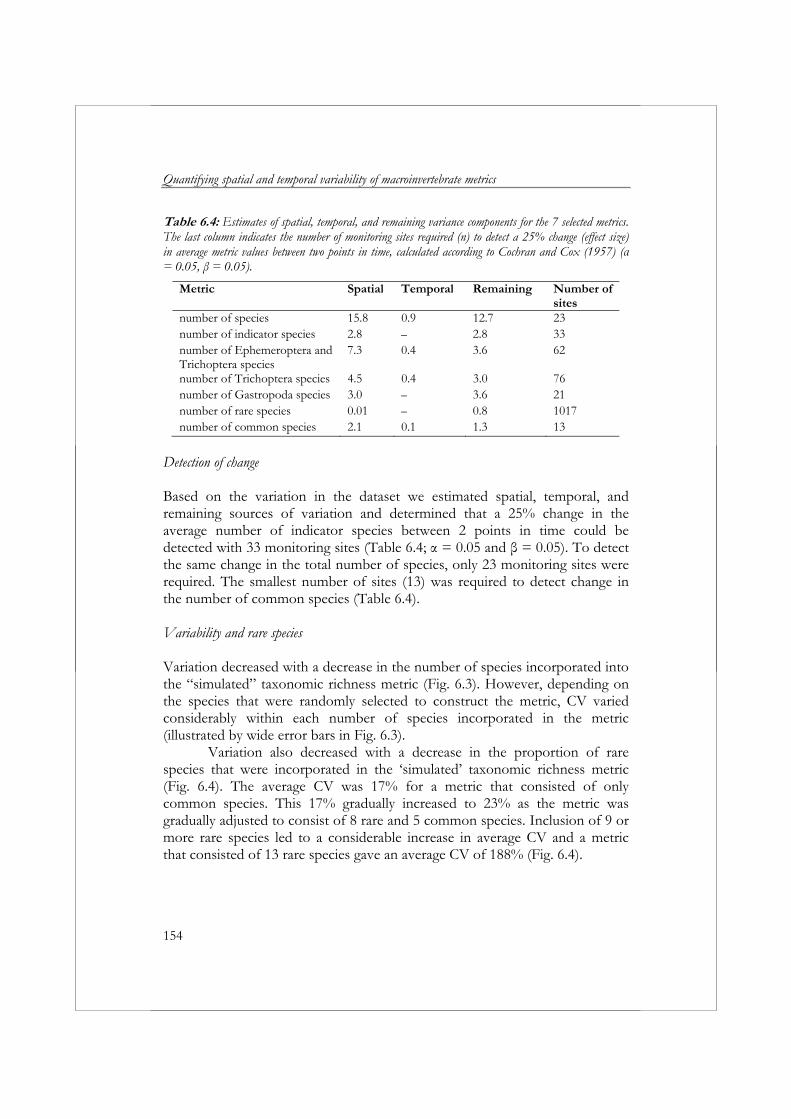
Quantifying spatial and temporal variability of macroinvertebrate metrics
154
Table 6.4: Estimates of spatial, temporal, and remaining variance components for the 7 selected metrics. The last column indicates the number of monitoring sites required (n) to detect a 25% change (effect size) in average metric values between two points in time, calculated according to Cochran and Cox (1957) (α = 0.05, β = 0.05).
Metric Spatial Temporal Remaining Number of sites
number of species 15.8 0.9 12.7 23 number of indicator species 2.8 – 2.8 33 number of Ephemeroptera and Trichoptera species
7.3 0.4 3.6 62
number of Trichoptera species 4.5 0.4 3.0 76 number of Gastropoda species 3.0 – 3.6 21 number of rare species 0.01 – 0.8 1017 number of common species 2.1 0.1 1.3 13
Detection of change Based on the variation in the dataset we estimated spatial, temporal, and remaining sources of variation and determined that a 25% change in the average number of indicator species between 2 points in time could be detected with 33 monitoring sites (Table 6.4; α = 0.05 and β = 0.05). To detect the same change in the total number of species, only 23 monitoring sites were required. The smallest number of sites (13) was required to detect change in the number of common species (Table 6.4). Variability and rare species Variation decreased with a decrease in the number of species incorporated into the “simulated” taxonomic richness metric (Fig. 6.3). However, depending on the species that were randomly selected to construct the metric, CV varied considerably within each number of species incorporated in the metric (illustrated by wide error bars in Fig. 6.3).
Variation also decreased with a decrease in the proportion of rare species that were incorporated in the ‘simulated’ taxonomic richness metric (Fig. 6.4). The average CV was 17% for a metric that consisted of only common species. This 17% gradually increased to 23% as the metric was gradually adjusted to consist of 8 rare and 5 common species. Inclusion of 9 or more rare species led to a considerable increase in average CV and a metric that consisted of 13 rare species gave an average CV of 188% (Fig. 6.4).
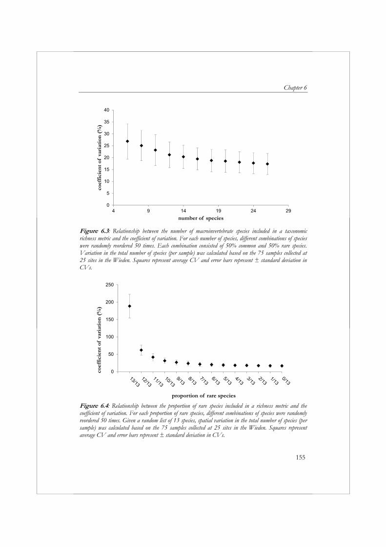
Chapter 6
155
0
5
10
15
20
25
30
35
40
4 9 14 19 24 29
coef
fici
ent
of v
aria
tion
(%
)
number of species
Figure 6.3: Relationship between the number of macroinvertebrate species included in a taxonomic richness metric and the coefficient of variation. For each number of species, different combinations of species were randomly reordered 50 times. Each combination consisted of 50% common and 50% rare species. Variation in the total number of species (per sample) was calculated based on the 75 samples collected at 25 sites in the Wieden. Squares represent average CV and error bars represent ± standard deviation in CVs.
0
50
100
150
200
250
coef
fici
ent
of v
aria
tion
(%
)
proportion of rare species
Figure 6.4: Relationship between the proportion of rare species included in a richness metric and the coefficient of variation. For each proportion of rare species, different combinations of species were randomly reordered 50 times. Given a random list of 13 species, spatial variation in the total number of species (per sample) was calculated based on the 75 samples collected at 25 sites in the Wieden. Squares represent average CV and error bars represent ± standard deviation in CVs.
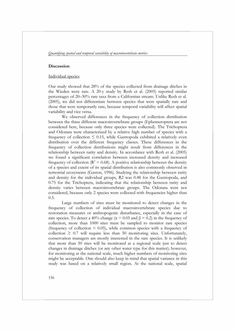
Quantifying spatial and temporal variability of macroinvertebrate metrics
156
Discussion Individual species Our study showed that 28% of the species collected from drainage ditches in the Wieden were rare. A 20-y study by Resh et al. (2005) reported similar percentages of 20–30% rare taxa from a Californian stream. Unlike Resh et al. (2005), we did not differentiate between species that were spatially rare and those that were temporarily rare, because temporal variability will affect spatial variability and vice versa.
We observed differences in the frequency of collection distribution between the three different macroinvertebrate groups (Ephemeroptera are not considered here, because only three species were collected). The Trichoptera and Odonata were characterized by a relative high number of species with a frequency of collection ≤ 0.15, while Gastropoda exhibited a relatively even distribution over the different frequency classes. These differences in the frequency of collection distributions might result from differences in the relationship between rarity and density. In accordance with Resh et al. (2005) we found a significant correlation between increased density and increased frequency of collection (R2 = 0.68). A positive relationship between the density of a species and extent of its spatial distribution is also commonly observed in terrestrial ecosystems (Gaston, 1996). Studying the relationship between rarity and density for the individual groups, R2 was 0.48 for the Gastropoda, and 0.75 for the Trichoptera, indicating that the relationship between rarity and density varies between macroinvertebrate groups. The Odonata were not considered, because only 2 species were collected with frequencies higher than 0.3.
Large numbers of sites must be monitored to detect changes in the frequency of collection of individual macroinvertebrate species due to restoration measures or anthropogenic disturbance, especially in the case of rare species. To detect a 40% change (α = 0.05 and β = 0.2) in the frequency of collection, more than 1000 sites must be sampled to monitor rare species (frequency of collection < 0.05), while common species with a frequency of collection ≥ 0.7 will require less than 50 monitoring sites. Unfortunately, conservation managers are mostly interested in the rare species. It is unlikely that more than 50 sites will be monitored at a regional scale just to detect changes in drainage ditches (or any other water type for this matter); however, for monitoring at the national scale, much higher numbers of monitoring sites might be acceptable. One should also keep in mind that spatial variance in this study was based on a relatively small region. At the national scale, spatial

Chapter 6
157
variation will be higher and the frequency of collection of the individual species will probably be far lower (than at the regional scale), resulting in more sites for monitoring to achieve equal power.
The results from this study clearly indicate that in general it will be easier to detect change based on metrics than on individual species (Fig. A.1 and Table 6.4). As already stated by Maxwell and Jennings (2005), composite indicators (composed of several species) have the disadvantage that positive trends in some species can mask negative trends in other species. This means the extinction of individual species could take place without being noticed, which might be judged to be unacceptable by conservation managers. Water managers, on the other hand, are generally more interested in changes in the ecological status of macroinvertebrate communities than they are interested in the changes in presence/absence or numeric abundance of individual species. One reason for this is that natural variability in community metrics is generally much lower than natural variability in the presence-absence and numeric abundance of individual species (Fore et al., 1996). Another is that water managers often reason that the disappearance of individual species does not necessarily cause significant biological effects on the functioning of a complete community (e.g., Chapin et al., 1997; Holling, 1973). Taxonomic richness metrics Spatial and temporal variation Both spatial and temporal variations can vary at different scales. A wide variety of studies have examined variation at different spatial and temporal scales, i.e., among-season, among-year, within-site, within-reach, and among-streams/lakes (e.g., Gebler, 2004; Sandin & Johnson, 2000; Springe et al., 2006; Trigal et al., 2006). Apart from spatial and temporal differences, variation can also result from analytical error. We did not explicitly examine each of these different scales, or the variation due to analytical error. This study was merely meant to gain insight into the sampling effort required to detect changes in ecological quality within a system of drainage ditches between years. For this purpose, it was not necessary to tease out variation at different scales. We combined analytical error and variation at lower temporal scales (i.e., within-season) and spatial scales (i.e., within-site variability) into one overall term (sample variation). Information about the different sources of variation can be very valuable when you want to increase statistical power by making changes to your sampling protocol and/or sampling design.
Quantifying spatial and temporal variability of macroinvertebrate metrics
158
To reduce variability, sampling was stratified in time, i.e., all samples were taken in May/June, and one operator collected all samples. When using the results of this study to design a monitoring program, it should be kept in mind that variability will increase if (1) more than one operator collects samples and/or (2) sample collection is not limited to one season. Studies by Trigal et al. (2006) and Clarke et al. (2002) indicate the extents to which these sources can contribute to overall variation. Trigal et al. (2006) showed seasonal variation of 32% for sweep-net samples collected in June, July, February, and May in a Mediterranean shallow lake. Clarke et al. (2002) estimated that less than 12% of sampling variation was due to inter-operator sampling effects using trained staff.
The magnitude of spatial variation in this study varied considerably between metrics. Although this is in line with the findings of many others (e.g., Gebler, 2004; Johnson, 1998; Trigal et al., 2006), we encountered some difficulties when we tried to compare coefficients of variation for the number of species (taxon richness) with those reported by others. Different studies covered different temporal and spatial scales, different water types, different habitats, and different sampling and sample processing protocols. Caution should be taken in making comparisons between studies, because variability in metric values can differ depending on the water type (Clarke et al., 2006) and even among different water bodies of the same water type (Porst & Irvine, 2009); the magnitude of metric variability also varies between sampling protocols (Vlek, 2004). This also makes it crucial to define variability at the scale appropriate for the aim of your study when developing a monitoring scheme.
In this study, (among-year) temporal variation appeared to be negligible for all 7 metrics, especially compared to spatial variation and remaining sources of variation. This is not in line with findings of Johnson (1998), who showed that among-year variability in total taxon richness was higher than among-sample and among-lake variability for littoral habitats in 16 Swedish lakes. In our study, temporal variation was calculated based on only three collections (2006, 2007, and 2008) and thus might have been underestimated; this needs to be studied further in the near future. These first results, however, suggest that temporal variation will hardly influence the monitoring effort required to detect change.
Our results showed that very large differences in metric values can be observed within a relatively small region, e.g., CV 38% for the number of ET species. This implies that making inferences at a higher spatial scale based on one site might lead to completely erroneous conclusions. This is in line with
Chapter 6
159
the findings of Downes et al. (2000) and Gebler (2004), who each concluded that individual sites cannot be representative of larger stream sections. (Reduction of) sampling effort Of the 7 metrics evaluated, the number of common species required the smallest number of monitoring sites to detect change in the Wieden, followed by the number of Gastropoda species and the number of species. The largest number of monitoring sites was required for the number of rare species, with 1017 sites needed to detect a 25% change.
Results showed that an increase in the number of species included in a taxonomic richness metric will reduce variation in metric values, and thus decrease the number of monitoring sites required to detect change. Including more species in a metric reduces the chance of high variability, due to the fact that the absence of one species may be compensated by the presence of another. It would be advantageous to increase the number of species included in a metric to reduce spatial variability and increase statistical power of a given number of monitoring sites. However, Fore et al. (1996) suggested that in some cases, signal may be lost in the noise, i.e., a strong response by a few taxa can be missed because macroinvertebrate communities are usually dominated by taxa that are neither sensitive nor insensitive to human impact. Both statistics and ecological relevance should be balanced in developing or selecting metrics for the monitoring of changes in ecological quality. Increasing the number species included in an index may have statistical advantages, but can also make it more difficult to detect a relevant ecological signal. In this study we did not consider the sensitivity of metrics to anthropogenic disturbance. To develop a reliable assessment system the sensitivity of the metrics applied in this study needs to be determined. For this purpose, information on metric values at sites of different ecological qualities is required. Studies by Vlek et al.(2004) and Verdonschot et al. (2012) are examples of methods that can be applied to select metrics that are sensitive to anthropogenic disturbance.
A negative trend was observed between the relative number of rare species included in a taxonomic richness metric and the variability of metric values. This means that, from the point of statistical power, the inclusion of rare species in richness metrics should be restricted. Fore et al. (1996) stressed that, “excluding rare taxa for statistical purposes only is contradictory to biological common sense”. We agree with Cao et al. (2001) that statistics should be used to look for important ecological signals and that these might not be the strongest statistical signals. On the other hand, what is the point of monitoring if spatial variability is so high it becomes impossible to detect any
Quantifying spatial and temporal variability of macroinvertebrate metrics
160
signals? Again, we want to stress the importance of weighing statistics and ecological relevance and the necessity to determine the sensitivity to anthropogenic disturbance of the metrics applied in this study.
Despite taking into account the number of species and the relative number of rare species in constructing a richness metric, a large effort will be required to detect change within a region. For example, we calculated that 13 sites must be monitored (at 2 points in time) to detect a 25% change in the number of common species in the Wieden (α = 0.05, β = 0.05). Such a sampling effort would be considered too costly by water authorities in the Netherlands. Johnson (1998) also concluded that sample sizes required to document changes between sites or years were so high that they are seldom used in field assessments of environmental impact. He suggested increasing statistical power by stratifying sampling in space and time (Johnson, 1998). However, in our study, sampling was already stratified in time and stratifying in space within ditches is almost impossible because they are much smaller than lakes and it is difficult to discern between habitats. Another option is to increase statistical power by increasing α and β. The question at what level statistical significance and power should be set has been dealt with by numerous authors (e.g., Field et al., 2007; Mapstone 1995,). The traditionally applied 5%-level of statistical significance resulting from adherence to the “five-eighty” convention (Di Stefano, 2003) places the “burden of proof” with those trying to prove environmental change due to human impact. A commonly voiced opinion is that this task should be shifted towards those who are trying to prove that no environmental change has taken place (e.g., Dayton, 2001; Field et al., 2004; Gray 1990). To balance the burden of proof, Field et al. (2004) derived a cost function approach that minimizes the total costs of both type I and type II errors. However, such a cost function requires information on the costs of type I and type II errors. In the case of macroinvertebrates, no information is available on the costs of type II errors, which are difficult to determine because macroinvertebrates do not have a direct economic function/value, e.g., like fish that serve as a food source or coral reefs that attract tourist. Maxwell & Jennings (2005) considered the intrinsic value of macroinvertebrate species to be higher than the costs associated with unnecessary management actions, and therefore relaxed α from the traditional 0.05–0.2. The levels of statistical significance and power applied in this study are intended only as examples. Prior to developing monitoring schemes, appropriate levels of significance and power should be discussed with all stakeholders. Important in this discussion is the realization that by increasing α and β, error rates will increase up to a point where one might
Chapter 6
161
question the purpose of monitoring, i.e., the costs of wrong decisions can become far higher than the costs of monitoring.
In cases where statistical power can not be increased through stratifying of sampling and/or increasing α and/or β, the only option is to develop more cost-effective methods for sampling and sample processing. For example, Verdonschot (2010) has applied activity traps in drainage ditches, which saved 65% time compared to sweep net sampling (R. C. M. Verdonschot, Alterra, Wageningen University and Research Centre, personal communication.). Another more cost-effective method would be to target specific organism groups (i.e., Trichoptera). We need to explore the possibilities of applying alternative more cost-effective methods for sampling and sample processing in biomonitoring programs.
Since the introductions of the Habitat Directive and the European Water Framework Directive, water authorities are now obliged to monitor changes in conservation value/ecological quality on larger spatial (regional) scales. Therefore, it is remarkable that the issue of probability sampling in aquatic monitoring programs has not received many attentions in Europe. Probability sampling is well suited to eliminate selection bias since, by construction, every site has a known nonzero probability of being selected (Cochran, 1977). In Europe the selection of sample sites by water authorities is often based on their assumed representativeness, or practical matters like accessibility. This manner of site selection is called non-probability sampling. The problem with non-probability sampling is that statistically based inferences about trends at higher/larger spatial scales cannot be made (Edwards, 1998; Stoddard et al., 1998; Parr et al., 2002). To our knowledge EMAP (Environmental Monitoring and Assessment Program), developed in the United States, is the first and only attempt to use probability sampling for the purpose of site selection in the design of aquatic monitoring programs. The use of probability sampling in aquatic monitoring programs should also be considered in Europe. Conclusions This study shows that, large numbers of sites must be monitored to detect changes in the frequency of collection of individual macroinvertebrate species, due to restoration measures or anthropogenic disturbance, especially in the case of rare species and rare species based metrics. Unfortunately, conservation managers are most interested in these rare species. The required monitoring effort automatically implies, that data collected by water authorities in biomonitoring programs developed to meet the requirements of the European
Quantifying spatial and temporal variability of macroinvertebrate metrics
162
Water Framework Directive, will not meet the requirements of conservation managers. When interested in an individual species, sampling methods will have to be adjusted to this specific species to increase the frequency of collection.
The results from this study clearly indicate that in general it will be easier to detect change in a drainage ditch network based on metrics than on individual species. Of the 7 metrics evaluated in this study, the number of common species required the smallest number of monitoring sites, followed by the number of Gastropoda species, and the number of species. Also, results showed that metric variability will decrease when the proportion of rare species included in a taxonomic richness metric is reduced or the total number of species included is increased. Irrespective of the metric applied a large effort will still be required to detect change within the drainage ditch network of the Wieden, due to high spatial variability. Therefore, we need to explore the possibilities of applying alternative more cost-effective methods for sampling and sample processing in biomonitoring programs. Acknowledgements This study was funded by the Ministry of Economic Affairs, Agriculture and Innovation (Ministry of Agriculture, Nature, and Food Quality), Contract no. BO-02-007-002. We would like to thank Martin van den Hoorn for his efforts in collecting the data on which this study was based. References Armitage, P.D., K. Szoszkiewicz, J.H. Blackburn & I. Nesbitt, 2003. Ditch
communities: a major contributor to floodplain biodiversity. Aquatic Conservation: Marine and Freshwater Ecosystems 13: 165-185.
Blocksom, K.A., J.P. Kurtenbach, D.J. Klemm, F.A. Fulk, S.M. Cormier, 2002. Development and evaluation of the Lake Macroinvertebrate Integrity Index (LMII) for New Jersey lakes and reservoirs. Environmental Monitoring and Assessment 77: 311-333.
Cao, Y., D.P. Larsen & R.St.-J. Thorne, 2001. Rare species in multivariate analysis for bio-assessment: some considerations. Journal of the North American Benthological Society 20: 144-153.
Cao, Y., D.D. Williams & N.E. Williams, 1998. How important are rare species in aquatic community ecology and bio-assessment? Limnology and Oceanography 43: 1403-1409.
Chapter 6
163
Carter, J.L. & V.H. Resh, 2001. After site selection and before data analysis: sampling, sorting, and laboratory procedures used in stream benthic macroinvertebrate monitoring programs by USA state agencies. Journal of the North American Benthological Society 20: 658-682.
Casagrande, J.T, M.C. Pike & P.G. Smith, 1978. An improved approximate formula for calculating sample sizes for comparing two binomial distributions. Biometrics 34: 483-486.
Chapin, F.S, B.W. Walker, R.J. Hobbs, D.U. Hooper, J.H. Lawton, O.E. Sala, & D. Tilman, 1997. Biotic control over the functioning of ecosystems. Science 277: 500-504.
Clarke, R.T., M.T. Furse, R.J.M. Gunn, J.M. Winder & J.F. Wright, 2002. Sampling variation in macroinvertebrate data and implication for river quality indices. Freshwater Biology 47: 1735-1751.
Clarke, R.T., A. Lorenz, L. Sandin, A. Schmidt-Kloiber, J. Strackbein, N.T. Kneebone & P. Haase, 2006. Effects of sampling and sub-sampling variation using the STAR-AQEM sampling protocol on the precision of macroinvertebrate metrics. Hydrobiologia 566: 441-459.
Cochran, W.G. & G.M. Cox, 1975. Experimental Designs. Second edition. Wiley, New York.
Cochran, W.G., 1977. Sampling techniques: Wiley Series in probability and mathematical statistics. New York, Wiley.
Dahl, J. & R.K. Johnson, 2004. A multimetric macroinvertebrate index for detecting organic pollution of streams in southern Sweden. Archiv für Hydrobiologie 160: 487-513.
Dayton, P.K., 2001. Reversal of the burden of proof in fisheries management. Science 279: 821-822.
Di Stefano, J., 2003. How much power is enough? Against the development of an arbitrary convention for statistical power calculations. Functional Ecology 17: 707-709.
Dolph, C.L., A.Y. Sheshukov, C.J. Chizinski, B. Vondracek & B. Wilson, 2010. The Index of Biological Integrity and the bootstrap: can random sampling error affect stream impairment decisions? Ecological Indicators 10: 527-537.
Downes, B.J., J.S. Hindell & N.R. Bond, 2000. What’s in a site? Variation in lotic macroinvertebrate density and diversity in a spatially replicated experiment. Austral Ecology 25: 128-139.
Downes, B.J., P.S. Lake & E.S.G. Schreiber, 1993. Spatial variation in the distribution of stream invertebrates: implications of patchiness for models of community organization. Freshwater Biology 30: 119-130.
Edwards, D., 1998. Issues and themes for natural resources trend and change detection. Ecological Applications 8: 323-325.
Quantifying spatial and temporal variability of macroinvertebrate metrics
164
Elbersen , J.W.H., P.F.M. Verdonschot, B. Roels & J.G. Hartholt, 2003. Definitiestudie KaderRichtlijn Water (KRW). I. Typologie van de Nederlandse Oppervlaktewateren. Alterra-rapport 669. Alterra, Wageningen, The Netherlands.
European Commission, 2000. Directive 2000/60/EC OF THE EUROPEAN PARLIAMENT AND COUNCIL - Establishing a framework for Community action in the field of water policy. Official Journal of the European Community L327: 1-72.
Field, S.A., P.J. O’Connor, A.J. Tyre & H.P. Possingham, 2007. Making monitoring meaningful. Austral Ecology 32: 485-491.
Field, S.A., A.J. Tyre, J.M. Rhodes, N. Jonzen & H. Possingham, 2004. Minimizing the cost of environmental management decisions by optimizing statistical thresholds. Ecology Letters 7: 669-675.
Fore, L.S., J.R. Karr & R. Wisseman, 1996. Assessing invertebrate response to human activities: evaluating alternative approaches. Journal of the North American Benthological Society 15: 212-231.
Gaston, K.J., 1996. The multiple forms of the interspecific abundance–distribution relationship. Oikos 75: 211-220.
Gauch, H.G., 1982. Multivariate analysis in community ecology. Cambridge University Press, Cambridge.
Gebler, J.B., 2004. Mesoscale spatial variability of selected aquatic invertebrate community metrics from a minimally impaired stream segment. Journal of the North American Benthological Society 23: 616-633.
Gerrodette, T., 1987. A power analysis for detecting trends. Ecology 68: 1364-1372.
Gray, J., 1990. Statistics and the precautionary principle. Marine Pollution Bulletin 21: 174-176.
Hämäläinen, H., H. Luotonen, E. Koskenniemi & P. Liljaniemi, 2003. Inter-annual variation in macroinvertebrate communities in a shallow forest lake in eastern Finland during 1990–2001. Hydrobiologia 506/509: 389-397.
Herzon, I. & J. Helenius, 2008. Agricultural drainage ditches, their biological importance and functioning. Biological Conservation 141: 1171-1183.
Holling, C.S., 1973. Resilience and stability of ecological systems. Annual Review of Ecology and Systematics 4: 1-23.
Johnson, R.K., 1998. Spatiotemporal variability of temperate lake macroinvertebrate communities: detection of impact. Ecological Applications 8: 61-70.
Kashian, D.R. & T.M. Burton, 2000. A comparison of macroinvertebrates of two Great Lakes coastal wetlands: testing potential metrics for and index of ecological integrity. Journal of Great Lakes Research 26: 460-481.

Chapter 6
165
Lenat, D.R. & V.H. Resh, 2001. Taxonomy and stream ecology–the benefits of genus and species-level identifications. Journal of the North American Benthological Society 20: 287-298.
Leunda, P.M., J. Oscoz, R. Miranda & A.H. Arĩno, 2009. Longitudinal and seasonal variation in the benthic macroinvertebrate community and biotic indices in an undisturbed Pyrenean river. Ecological Indicators 9: 52-63.
Lyons, J., S. Navarro-Pérez, P.A. Cochran, E.C. Santana & M. Guzman-Arroyo, 1995. Index of biotic integrity based on fish assemblages for the conservation of streams and rivers in westcentral Mexico. Conservation Biology 9: 569-584.
Mapstone, B., 1995. Scalable decision rules for environmental impact studies: effect size, type 1, and type 2 errors. Ecological Applications 5: 401-410.
Marchant, R., 2002. Do rare species have any place in multivariate analysis for bio-assessment? Journal of the North American Benthological Society 21: 311-313.
Maxwell, D. & S. Jennings, 2005. Power of monitoring programmes to detect decline and recovery of rare and vulnerable fish. Journal of Applied Ecology 42: 25-37.
Menetrey, N., B. Oertli & J. Lachavanne, 2011. The CIEPT: a macroinvertebrate-based multimetric index for assessing the ecological quality of Swiss lowland ponds. Ecological Indicators 11: 590-600.
Nijboer, R.C., 2000. Natuurlijke levensgemeenschappen van de Nederlandse binnenwateren. Deel 6, Sloten. Achtergronddocument bij het ‘Handboek Natuurdoeltypen’ in Nederland. Rapport AS-06, EC-LNV. Alterra, Wageningen, The Netherlands.
Nijboer, R.C. & A. Schmidt-Kloiber, 2006. The effect of excluding taxa with low abundances or taxa with small distribution ranges on ecological assessment. Hydrobiologia 516: 347-363.
Painter, D., 1999. Macroinvertebrate distributions and the conservation value of aquatic Coleoptera, Mollusca and Odonata in the ditches of traditionally managed and grazing fen at Wicken Fen, United Kingdom. Journal of Applied Ecology 36: 33-48.
Parr, T.W., M. Ferretti, I.C. Simpson, M. Forsius & E. Kovács-Láng, 2002. Towards a long-term integrated monitoring programme in Europe: network design in theory and practice. Environmental Monitoring and Assessment 78: 253-290.
Porst, G., & K. Irvine, 2009. Implications of the spatial variability of macroinvertebrate communities for monitoring of ephemeral lakes: an example from turloughs. Hydrobiologia 636: 421-438.
Quantifying spatial and temporal variability of macroinvertebrate metrics
166
Poos, M.S. & D.A. Jackson, 2012. Addressing the removal of rare species in multivariate bioassessments: the impact of methodological choices. Ecological Indicators 18: 82-90.
Purcell, A.H., D.W. Bressler, M.J. Paul, M.T. Barbour, E.T. Rankin, J.L. Carter & V.H. Resh, 2009. Assessment tools for urban catchments: developing biological indicators based on benthic macroinvertebrates. Journal of the American Water Resources Association 45: 306-319.
Resh, V.H., L.A. Bêche & E.P. McElravy, 2005. How common are rare taxa in long-term benthic macroinvertebrate surveys? Jornal of the North American Benthological Society 24: 976-989.
Resh, V.M. & E.P. McElravy, 1993. Contemporary quantitative approaches to biomonitoring using benthic macroinvertebrates. In: Rosenberg, D.M., & V.H. Resh (eds.), Freshwater Biomonitoring and Benthic Macroinvertebrates. Chapman & Hall, New York, NY, USA, pp.: 159-194.
Resh, V.H. & D.M. Rosenberg, 1989. Spatial-temporal variability and the study of aquatic insects. Canadian Entomology 121: 941-963.
Sandin, L. & R.K. Johnson, 2000. The statistical power of selected indicator metrics using macroinvertebrates for assessing acidification and eutrophication of running waters Hydrobiologia 422/423: 233-243.
Smith, J.G., J.J. Beauchamp & A.J. Stewart, 2005. Alternative approach for establishing acceptable thresholds on macroinvertebrate community metrics. Journal of the North American Benthological Society 24: 428-440.
Springe, G., L. Sandin, A. Briede & A. Skuja, 2006. Biological quality metrics: their variability and appropriate scale for assessing streams. Hydrobiologia 566: 153-172.
Stoddard, J. L., C.T. Driscoll, J.S. Kahl & J.P. Kellog, 1998. Can site-specific trends be extrapolated to a region? An acidification example for the northeast. Ecological Applications 2: 288-299.
Tangen, B.A., M.G. Butler & M.J. Ell, 2003. Weak correspondence between macroinvertebrate assemblages and land use in prairie pothole region wetlands, USA. Wetlands 23: 104-115.
Taylor, B.L. & T. Gerrodette, 1993. The uses of statistical power in conservation biology: the vaquita and northern spotted owl. Conservation Biology 7, 489-500.
Trigal, C., F. García-Criado & C. Fernandez-Aláez, 2006. Among-habitat and temporal variability of selected macroinvertebrate based metrics in a Mediterranean shallow lake (NW Spain). Hydrobiologia 563: 371-384.
Verdonschot, R.C.M., 2010. Optimizing the use of activity traps for aquatic biodiversity studies. Journal of the North American Benthological Society 29: 1228-1240.
Chapter 6
167
Verdonschot, R.C.M., H.E. Keizer-Vlek & P.F.M. Verdonschot, 2012. Development of a multimetric index based on macroinvertebrates for drainage ditch networks in agricultural areas. Ecological Indicators 13: 232-242.
Vlek, H.E., 2004. Comparison of (cost) effectiveness between various macroinvertebrate field and laboratory protocols. European Commission, STAR (Standardisation of river classifications), Deliverable N1, 78 pp.
Vlek, H.E., P.F.M. Verdonschot & R.C. Nijboer, 2004. Towards a multimetric index for the assessment of Dutch streams using benthic macroinvertebrates. Hydrobiologia 516: 173-189.
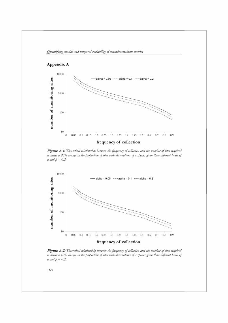
Quantifying spatial and temporal variability of macroinvertebrate metrics
168
Appendix A
10
100
1000
10000
0 0.05 0.1 0.15 0.2 0.25 0.3 0.35 0.4 0.45 0.5 0.6 0.7 0.8 0.9
num
ber
of
mon
itor
ing
site
s
frequency of collection
alpha = 0.05 alpha = 0.1 alpha = 0.2
Figure A.1: Theoretical relationship between the frequency of collection and the number of sites required to detect a 20% change in the proportion of sites with observations of a species given three different levels of α and β = 0.2.
10
100
1000
10000
0 0.05 0.1 0.15 0.2 0.25 0.3 0.35 0.4 0.45 0.5 0.6 0.7 0.8 0.9
num
ber
of
mon
itor
ing
site
s
frequency of collection
alpha = 0.05 alpha = 0.1 alpha = 0.2
Figure A.2: Theoretical relationship between the frequency of collection and the number of sites required to detect a 40% change in the proportion of sites with observations of a species given three different levels of α and β = 0.2.
Chapter 7
169
7 Synthesis
Stream restoration Renkumse Beekdal. Photo: Hanneke Keizer-Vlek.
Synthesis
170
7 Synthesis
This synthesis starts with explaining why there is a need for biological assessment in addition to assessment based on physical and chemical water quality variables. Although the answer to this question is obvious to most scientists, water managers are asking this question more and more. In the second paragraph, an overview of the lessons that can be learned from the development of biological assessment systems in the past is provided, as well as which aspects of the developmental process require explicit choices that need to be considered thoroughly. The third paragraph discusses the lack of diagnostic power of current biological assessment systems. The fourth paragraph discusses how the results from the chapters on the variability, accuracy, and cost of individual metrics can be applied to guide (1) the process of standardizing sampling and sample processing and (2) the process of metric selection in the development of biological assessment systems. The fifth paragraph deals with the implications of the results from the previous chapters for the design of cost-effective monitoring programs. This paragraph addresses the possibility of applying both probability sampling (random selection of sites) and a less time-consuming ‘Quick Scan’ method for sampling and sample processing in the Netherlands. In the sixth paragraph, the development of ‘new’ tools for biological assessment using species traits is discussed. This paragraph addresses whether species traits can improve the diagnostic power of biological assessment systems, reduce their variability, and make broader geographic application possible. In the final paragraph I address whether conservation ecologists can benefit from monitoring performed for the purpose of the biological assessment of surface waters and make future monitoring programs more cost-effective. Biotic versus abiotic assessment of aquatic ecosystems Water managers in the Netherlands keep raising the question: “Why do we still apply very costly bioassessment methods instead of measuring based on measurements of the physical and chemical water quality variables on which they were based?” Numerous authors have explained the problems associated with assessments based on water quality variables (e.g., BOD, nutrients, heavy metals) (e.g., Karr, 1981; De Pauw & Vanhooren, 1983; Courtemanch et al., 1989; Harris & Silveira, 1999; Barbour et al., 2000). The most important arguments in favor of biological assessment are (1) that it takes into account
Chapter 7
171
the combined effects of different stressors, (2) the measurement of effect as opposed to problem, i.e. due to biotic interactions and/or varying abiotic circumstances, the ecological impact may differ from what is expected based on previous studies, 3) that it incorporates water quality history, i.e. short-term events that have an ecological impact may be missed by monitoring water quality variables, (4) it can be used to determine the ecological success of restoration or management that cannot be revealed by physical and chemical data alone (Clews & Ormerod, 2009), (5) in Europe the Water Framework Directive (WFD) has set goals expressed in terms of biological variables, and (6) it is not the abiotic condition, but the biological effect, society notices, i.e. eutrophication is only noticed when blue-green algae start to appear.
On the other hand, most methods that have been applied to develop biological assessment systems do not make use of the potential benefits of biological assessment. A popular method for designing biological assessment systems has been to post-classify sites based solely on a selection of abiotic variables and to select biological indicators/metrics that best discern between these different classes (e.g., Barbour et al., 1996; Fore et al., 1996; Thorne & Williams, 1997; Johnson et al., 2006). When post-classification is based solely on abiotic variables, monitoring can be restricted to these abiotic variables as long as the costs of biological monitoring are higher. To determine the cost associated with monitoring abiotic variables, the time span and frequency of monitoring should be taken into account. For example, post-classification might have been based on the average phosphate concentrations resulting from monthly sampling of phosphate concentrations during one year.
In most cases in the Netherlands, multiple stressors exert their influence on the macroinvertebrate community. Many studies have shown that variation in the composition of the biological community remains, for a large part, unexplained by the abiotic variables considered in aquatic monitoring programs. For example, Murphy & Davy-Bowker (2006) showed that abiotic variables explain only 26% of lotic macroinvertebrate assemblage composition across England and Wales. Sandin & Johnson (2004) showed that only 22% of the variation in species data across Swedish streams could be explained by environmental variables, and Jyväsjärvi et al. (2009) reported this percentage as 29% for 55 minimally disturbed Finnish lake basins. This is due to the fact that community composition is partly the result of stochastic mechanisms related to differential colonization/extinction dynamics after disturbance (Chase, 2010; Verdonschot, 2012). However, we might not be measuring the appropriate abiotic variables at the appropriate temporal and/or spatial scale. Continuous measurements of oxygen concentrations, for example, might give better insight into cause–effect relationships than monthly measurements of oxygen
Synthesis
172
concentrations. For this reason, the biological assessment system proposed in Chapter 2 does not use only abiotic variables for post-classification, but is based on expert knowledge of both biotic and abiotic variables. The post-classification was based on multivariate analysis (a combination of clustering and ordination), which was used to develop a cenotypology that describes different water types and their stages of degradation (Verdonschot & Nijboer, 2000). A cenotype is a group of samples with similar macroinvertebrate composition and environmental conditions. Environmental variables can refer to natural circumstances (water type) or a certain degree of degradation. The establishment of cenotypes facilitates the assignment of quality classes to the sites. To determine the degradation stage (quality class) of each cenotype, the macroinvertebrate community composition and values for the environmental variables of each cenotype were used for interpretation by expert judgment. Of course this approach to post-classification also has flaws, including that it lacks objectivity. However, any technique applied to assess the ecological quality of a site based on biotic variables or abiotic variables will lack complete objectivity.
To improve biological assessment systems in the future, we need to gain better understanding of ecosystem functioning by detecting causal mechanisms. In addition to observational data collected by water authorities in routine monitoring programs, we need experimental data to elucidate potential cause-effect linkages (e.g., Adams & Greeley, 2000; King & Richardson, 2004). When collecting these data, more focus should be placed on measuring on different temporal scales as opposed to current monitoring programs (e.g., more continuous measurements) and on abiotic variables that are not part of current routine monitoring programs (e.g., discharge). After the major drivers of community composition have been elucidated, it will be clear as to whether it is more cost-effective to monitor abiotic or biotic variables (or a combination of both). The costs associated with research necessary to gain a better understanding of ecosystem functioning are often considered to be too high. However, people tend to forget that incorrect assessment might (1) require very costly restoration measures or (2) have detrimental ecological consequences. In the Netherlands, 4.2 billion euros will be spent on the restoration of surface waters by 2027 in order to achieve the goals of the WFD. However, due to a lack of knowledge on river restoration (Palmer et al., 2007; Feld et al., 2011), we do not know whether these restoration measures will guarantee achievement of the goals set by the WFD. This issue has also been raised by Ferraro & Pattanayak (2006) in relation to the investments made in biodiversity conservation; they stated, ”For far too long, conservation scientists and practitioners have depended on intuition and anecdote to guide the design of conservation investments.”
Chapter 7
173
Lessons learned from biological assessment systems developed in the past The discussion on how to collect samples from macroinvertebrate communities and assess their ecological state has been extensive, and it is still undecided. The major issues that have been raised concerning sampling and sample processing are: sampling one habitat versus multiple habitats (e.g., Kerans et al., 1992;
Carter & Resh, 2001); sampling riffles versus pools (e.g., Kerans et al., 1992; Rosenberg &
Resh, 1993); qualitative versus quantitative sampling (e.g., Mackey et al., 1984; Storey
et al., 1991; Kerans et al., 1992; Metzling et al., 2003); fixed count subsample size (e.g., Growns et al., 1997; Doberstein et al.,
2000; King & Richardson, 2002; Ostermiller & Hawkins, 2004).
Issues related to index development are: the taxonomic resolution of identification (e.g., Resh & Unzicker, 1975;
Hawkins & Norris, 2000; Bailey et al., 2001; Verdonschot, 2006; Chessman et al., 2007; Jones, 2008);
assessment based on single metrics versus mulitmetrics, multivariate analyses, and other community based approaches (Lücke & Johnson, 2009; Hawkins et al., 2010);
whether to include rare taxa in analysis (e.g., Cao et al., 1998; Cao & Williams, 1999; Marchant, 1999; Cao et al., 2001; Marchant, 2002; Nijboer & Schmidt-Kloiber, 2004).
The conclusions drawn from these issues seem to be conflicting in a
number of cases for different reasons. First, these studies were performed under different environmental conditions (different ecoregions, countries, water types). A metric, such as the number of Ephemeroptera, Plecoptera, and Trichoptera (EPT), may better discern between reference and degraded sites in a geographic region or stream type with many EPT species than in a region or stream type where species diversity is naturally relatively low. Second, the different studies had different objectives and compared different assessment methods. For example, a big difference may exist between the ‘best’ method to describe the complete macroinvertebrate community or the ‘best’ method to discern between unimpaired and impaired sites based on the number of Ephemeroptera, Plecoptera, and Trichoptera. However, the main problem is that all of the mentioned studies focused on accuracy instead of variability (a
Synthesis
174
measure of precision). In Chapter 3 I explain that accuracy refers to the closeness of a measurement to its true value (Norris et al., 1992). Several authors have stressed the importance of both accuracy and precision in biological assessment (e.g., Resh & Mc Elravy, 1993; Norris et al., 1992). Resh & Mc Elravy (1993) stated that “conclusions regarding impact too often have been based on significant differences in main-effect means that really resulted from the influence of either covariate factors or sampling bias, or both”. However, this remains inevitable as long as we do not completely understand ecosystem functioning. Given the fact that an average sample only contains 50% to 64% of the taxa actually present at a site at a given moment in time, and only 25% to 37% of the taxa present at a site during the course of a year (Verdonschot, 1990; Vlek, 2006), an accurate sample is utopia. Moreover, we will never know whether differences in community composition are the result of impact, measurement error, or some other environmental variable/biotic interaction we did not measure. Until we have completely unraveled ecosystem functioning, bioassessment will always include some form of subjectivity. Barbour & Gerritsen (1996) stressed that, when assessing ecological quality for biological monitoring purposes, it is not necessary to catch all organisms or taxa present at a site (accuracy). Accuracy is important in the sense that the same sampling and sample processing method should be applied for assessment purposes because differences in accuracy between methods may result in different bioassessment results. However, as long as the same method is applied at all sites, and this combination has been proven to discern signal (sensitivity to anthropogenic stress) from noise (variability), accuracy is a non-issue. Instead, the discussion should focus on variability to assure the validity of conclusions.
When developing an assessment system, methodological choices are made concerning sampling and sample processing, either consciously or unconsciously. From a financial perspective, it is impossible to test the consequences of each methodological choice and combination of choices in the process of developing an assessment system. A more pragmatic approach is to use the data you have to assess ecological status (post-classification) and then develop an assessment system weighing costs and performance (sensitivity and variability). Post-classification or the definition of pristine conditions is the first step in the process of developing an assessment system. The data used for post-classification should be based on species data and a relatively extensive sampling method (full count) to minimize the loss of information beforehand. The second step encompasses the selection of appropriate indices to discern between signal and noise. During this step, it might become evident that family level data suffice to develop an assessment
Chapter 7
175
system with adequate power to detect human impact. After selecting an appropriate assessment method, the effects of applying alternative sampling and sample processing methods can be tested in terms of accuracy (Chapter 5) and variability (Chapters 3, 4, and 6). Importantly, the results are intertwined; for example, the choice to perform family level identification may be more variable for a metric counting the number of Trichoptera taxa compared to a metric counting the number of Gastropoda taxa. Most likely, there are several solutions with equal performance. Considerations for developing an assessment system Many choices are made during the process of developing an assessment system, ranging from the definition of reference conditions to the number of quality classes discerned. All of these different choices influence the outcome of the development process. When developing an assessment system it should be made clear how different choices might have affected the results of the development process. Therefore, I have listed some important issues that should be considered prior to developing an assessment system. The list will make it easier to understand the often conflicting conclusions from existing studies, and will hopefully stimulate researchers to make more explicit choices and communicate these choices when developing assessment systems. Water type One of the major difficulties associated with developing assessment systems is that macroinvertebrate community composition correlates with both human-induced changes and natural gradients in environmental variables. To prevent an assessment from being confounded by a natural gradient in environmental variables, it should be developed at the appropriate spatial scale. In many cases, a priori classifications, such as ecoregions or stream order, have been used to partition natural variation (Hawkins et al., 2010). However, a priori classifications are often ineffective at accounting for much of the natural variation in community composition (e.g., Hawkins et al., 2000; Heino & Mykra, 2006). Therefore, the appropriate spatial scale should be determined by analyzing both biotic and abiotic data prior to developing an assessment system, as shown in Chapter 2. In an ideal world, macroinvertebrate data from pristine sites could be analyzed to determine whether differences in community composition/metric values exist between different water types/geographic regions. If so, different assessment systems could be developed for the different water types. When (sufficient) data from pristine sites are lacking, it
Synthesis
176
would be possible to determine which environmental variables are important in explaining macroinvertebrate community composition, and then hypothesize whether these can vary under reference conditions in different geographic regions. It should be kept in mind that water chemistry, for example, is not only related to human interference, but can also be strongly related to surface geology. As mentioned in Chapter 2, the spatial scale applied should be at the level where all sites within one water type only differ in their degree of degradation. However, this might result in a situation where data availability is too low to develop a reliable assessment system. This appeared to be the case in the Netherlands, where stream width was correlated to macroinvertebrate community composition (Chapter 2) and it was not possible to develop separate assessment systems for the different steam orders. In cases like this, the choice between data availability and performance of the assessment system should be balanced. Reference conditions Since the introduction of the WFD, the definition of ‘reference condition’ has received a lot of attention because of the requirement to determine the ecological status of a water body by assessing its deviation from the reference condition. Particularly in countries where pristine conditions are lacking, the question of how ’to construct’ theoretical community composition given pristine conditions has been asked. Several options for how to do this were addressed by Nijboer et al. (2004): the use of historic data, the use of data from other geographical areas, the use of paleolimnological data, the use of existing knowledge on ecology and biogeography of species, and the use of models. Instead of ‘constructing’ theoretical communities, we should ask what the risk is of using best available sites as the end-point for assessment. For obvious reasons, it is not very likely that reference conditions will be ‘created’ in the future in countries where reference conditions are currently lacking. However, it should be made explicit that the reference condition in a system is lacking, for example, by including a quality class ‘high ecological status’ that will never be reached given the current situation. Of course the use of best available sites should only be recommended in cases where these sites still comply with at least good ecological status as described in the WFD. Notably, the end-point of assessment, whether this is the ‘reference condition’ or the best available sites, is a shifting baseline due to natural stochastic processes and less obvious forms of anthropogenic stress on the large spatial scale, resulting in atmospheric deposition of contaminants and climate change. This implies that end-points have to be monitored and adjusted regularly.
Chapter 7
177
Classification/degradation gradient To develop an assessment system, the ecological status of the sites in the dataset has to be determined (classification). Many studies describe the development of an assessment system based on impacted sites versus sites that are not impacted (e.g., Barbour et al., 1996; Fore et al., 1996; Thorne & Williams, 1997; Johnson et al., 2006), though some cases do not clearly describe how impact is defined. The definition is important for two reasons. First, it is important whether the degradation gradient is based on abiotic variables or a combination of biotic and abiotic variables. Classification solely based on abiotic variables introduces a risk that the biotic conditions do not correspond to the abiotic conditions. This phenomenon can often be observed after restoration (e.g., abiotic conditions are restored but the biotic condition is still degraded due to, for example, migration barriers or ‘unknown’ abiotic variables that were not considered). Thus, the biological assessment system proposed in Chapter 2 is based on both biotic and abiotic variables. Second, one should realize that when non-impacted is described as ‘pristine’ and impacted as ‘devoid of life’, it will be much easier to discern between (five) quality classes compared to situations in which data from pristine conditions and very degraded conditions are lacking. This could explain the differences in performance between different biological assessment systems. In theory, it would be best to study a metric’s response across the full range of possible stress (Hawkins et al., 2010). However, in the Netherlands, as in many other countries around the world, reference sites are lacking. In cases where reference sites or severely impacted sites are lacking, this should be made explicit as it is in Chapter 2. Number of quality classes When developing a bioassessment system, the number of quality classes the system should be able to discern should be taken into account. For example, the WFD distinguishes between five ecological quality classes. The boundary between moderate and good ecological status is of main importance, (i.e., below good ecological status, restoration measures have to be taken to improve ecological status). When a system has to discern between less quality classes, there is a smaller chance of misclassification. The only problem is that a system based on two quality classes cannot detect changes in ecological quality in the lower part of the degradation gradient. When developing a bioassessment system, the ability to discern between more quality classes has to
Synthesis
178
be balanced against the greater chance of misclassification, as at each class boundary there is a chance of misclassification. This balance may vary depending on the water type. Regardless of the number of quality classes, it is essential that all classes discerned reflect ecological boundaries or an ecological gradient (see next paragraph). Class boundaries and metric response Class boundaries for individual metrics can be set in two different ways: (1) based on statistical rules or (2) based on the ecological response to degradation. Examples of the first option are: dividing the 95-percentile of all sites by four (Ohio Environmental Protection Agency, 1987; DeSohn, 1995), the 50- and 10-percentile of all reference locations (Roth et al., 1977), or dividing the 15- or 75-percentile of all reference locations (Barbour et al., 1996; Royer et al., 2001). Obviously, this is not good scientific practice. First, it implies that each metric responds to degradation in the exact same way. Second, it rules out the use of metrics that do not exhibit a linear response to environmental degradation. Most publications on the development of bioassessment systems only consider metrics that exhibit a linear response to anthropogenic stress because it is easy to test for. By not considering other types of responses (e.g., unimodal, threshold, bimodal), some potentially sensitive metrics might be overlooked. Niche theory assumes response curves to be symmetric Gaussian-shaped unimodal curves (Austin, 2007). Class boundaries should be based on metric responses to anthropogenic stress, whether this response is linear, unimodal, bimodal, or occurs at threshold levels. Also, when setting class boundaries, the width of the different quality classes might differ and the gradient should only span the ecologically relevant range. For example, a pH value below 3 or above 10 is not part of the ecologically relevant range for the macroinvertebrate community. Single metrics versus multimetrics, predictive models, and/or multivariate approaches Several studies have focused on whether single metrics, multimetrics, predictive models, or multivariate clustering or ordination should be used for assessment purposes. In many cases, improper arguments are used to value one method over the other. For example, Lücke & Johnson (2009) concluded that multivariate analysis or multimetric indices are superior to single metric approaches for detecting the effects of nutrient enrichment. However, the single metrics applied in the study were not based on Swedish data, which the
Chapter 7
179
approaches were tested against, but the multimetric index and multivariate approach were. Another example is a study by Hawkins et al. (2010), who concluded that multimetric index responses to stress saturate at intermediate levels of stress, whereas O/E indices that describe the departure of taxonomic composition from that expected under reference conditions do not. They explained this as follows: “multimetric indices are calibrated against both reference sites and degraded sites, whereas O/E indices are calibrated against only reference sites.” Therefore, Hawkins et al. (2010) and Lücke & Johnson (2009) were not talking about different metrics, but different techniques used to develop an assessment system. Metric and methodological techniques (e.g., predictive models, multivariate analysis) are two different things and should clearly be separated in order to make objective choices regarding metric selection. The performance of metrics can only be judged when the same techniques are used for data analysis, or vice versa. Considering the different techniques used to develop assessment systems, I think that ‘a posteriori’ or ‘a priori’ classification (both in terms of ecological quality and reference stream types) will define the outcome of the development process. Only metrics that show obvious patterns between quality classes will result in a reliable quality assessment system, irrespective of the techniques used.
The concept of a multimetric index comprising several metrics and integrating information from the ecosystem, community, population, and individual levels was introduced by Karr (1981, 1991). Karr & Chu (1997) stated, “The best, most comprehensive, and accurate multimetric indices explicitly embrace several attributes of the sampled assemblage, including taxa richness, indicator taxa or guilds (e.g., tolerant and intolerant groups), health of individual organisms, and assessment of processes (e.g., as reflected by trophic structure or reproductive biology)”. Karr (1981) advocated the use of a multimetric index to assess overall biotic integrity. However, in an environment where multiple stressors exert influence, a diagnostic assessment system to determine the cause of degradation is essential. Therefore, the ideal assessment system should not only use multiple metrics, but these metrics should exhibit a stressor-specific response. In this way, water managers will be provided with a tool to make adequate decisions regarding the restoration of surface waters and that will stress the need to gain a better understanding of the link between metrics/indicators and ecosystem processes (Van Riel & Verdonschot, in preparation).
Synthesis
180
Metrics based on ecological preferences Especially in Europe, metrics based on ecological preferences (e.g., substrate preferences, preferences for current velocity, saprobic preferences) have been regularly applied/tested during the development of assessment systems. The assessment system described in Chapter 2 also includes some metrics based on ecological preferences, but before applying metrics based on ecological preferences the information content of the accompanying autecological database should be checked. When preferences can only be assigned to 20% of the species in a sample, this might result in misleading conclusions considering metric variability. Validation –Validation should be a major issue of concern. In the Netherlands we have two bioassessment systems that are currently being used to assess the ecological quality of surface waters: EBEOSWA and ‘KRW maatlatten’. The second was developed for the purpose of the WFD, but the systems have never been properly validated. To properly validate a biological assessment system, it has to be tested against an ‘external’ dataset, i.e., a dataset other than the one used to develop the system. The macroinvertebrate samples from this ‘external’ dataset have to be post-classified using the same method applied to the samples from the original dataset. Next, the quality class resulting from post-classification should be compared to the quality class indicated by the biological assessment system. Biological assessment as a diagnostic tool Apart from the general assessment of ecological status, water authorities would benefit from a system that enables them to identify the cause of an observed change in ecological quality or the reason surface water fails to meet the ecological quality objectives. Especially in countries where often several stressors exert their influence on ecological quality (e.g., the Netherlands), a diagnostic system is essential. Unfortunately, most of the bioassessment systems in use today cannot serve as diagnostic tools. Although several studies have used a multimetric approach to develop an assessment system, they use this approach to ‘better’ indicate general degradation rather than to assess the separate effects of individual stressors.
Indices initially developed to detect organic pollution and/or eutrophication pollutants (e.g., BMWP score) have been widely applied as indicators of degradation in general. Not only different forms of pollution, but also modifications in flow pattern or river habitat structure, can decrease index scores, which makes it difficult to identify the cause(s) of this score (Clews &
Chapter 7
181
Ormerod, 2009). A reduction in the index score by stressors other than organic pollution might be explained by the fact that other major stressors can also influence oxygen concentrations in the water. For example, reduced flow will result in lower oxygen concentrations, as will a lack of trees in the riparian zone due to increased water temperature (e.g., Burton & Likens, 1973; Rutherford et al., 2004; Wilkerson et al., 2006).
The majority of existing bioassessment systems were developed to detect organic pollution (Friberg et al., 2006). Friberg et al. (2009) stressed the importance of developing indices related to hydromorphological degradation. Their view is based on the extensive literature on linkages between the in-stream physical environment and benthic macroinvertebrates. However, Friberg et al. (2009) found only relatively weak relationships between various measures of hydromorphological stress and commonly used macroinvertebrate assessment tools. Lorenz et al. (2004a) developed an index to detect the impact of hydromorphological degradation, the German Fauna Index. Although this index shows a strong correlation with hydromorphological degradation (R2=0.67), it is almost as sensitive to organic pollution (R2=0.55). This suggests that organic pollution and hydromorphological degradation are not the variables driving community composition, but that both stressors (at least in part) are influencing the same variable (i.e., the oxygen concentration), which is driving macroinvertebrate community composition. It is imperative that we unravel the primary drivers of macroinvertebrate community composition (e.g., oxygen concentration, shear stress, biotic interaction) at the appropriate temporal and spatial scales. The only way to do this is to combine observational data and data from experimental work. The development of bioassessment systems has been based primarily on observational data. However, observational data are only suited for detecting general patterns and correlations (data on primary drivers at the appropriate temporal and spatial scale are usually lacking). Experimental datasets are required to confirm whether correlations derived from observational data actually represent cause-effect relationships.
Although Friberg et al. (2009) and Lorenz et al. (2004a) implied to have studied hydromorphological degradation, the environmental variables considered in their studies mainly relate to the morphology of streams, not the hydrology. Apart from the Lotic-invertebrate Index for Flow Evaluation (LIFE) developed by Extence et al. (1999), no attempt has been made to assess hydrologic degradation. Although the LIFE method is very valuable in the sense that it provides the opportunity to relate several hundreds of flow variables to the macroinvertebrate community, it also has two important disadvantages. First, the LIFE method is designed to reflect the faunal
Synthesis
182
responses to ‘flow conditions’ and their change over time, not for the sole purpose of biological assessment. This means that the interpretation of LIFE scores is not straightforward, limiting its applicability in biological assessment. Second, Extence et al. (1999) stated that “a link exists between poor habitat quality and depressed LIFE scores”, which means that the LIFE methodology, although developed to study changes in flow, also responds to at least one other stressor, namely habitat quality.
Apart from hydrological and morphological variables, toxic substances (e.g., heavy metals, pesticides) are hardly ever considered in European biological assessment systems. Toxic substances are considered in risk assessment studies, but their effects are mainly based on laboratory tests on individual species or solely on chemical endpoints without accounting for assemblage-level consequences. Biological assessment of heavy metal pollution is more common in the USA, Australia, and New Zealand. This difference is probably related to the magnitude of heavy metal pollution. A study by Peeters et al. (2001), however, showed that elevated contaminant concentrations of polycyclic aromatic hydrocarbons, trace metals, oil, and polychlorinated biphenyls are significantly associated with differences in the macroinvertebrate food web structure in the Rhine-Meuse Delta of the Netherlands. This suggests that it would be a good idea to combine expertise from both research areas to develop diagnostic tools in bioassessment.
To develop a stressor-specific biological assessment system remains a major challenge, especially since the variation in macroinvertebrate community composition remains, for a large part, unexplained by the abiotic variables considered in aquatic monitoring programs. This is due, in part, to stochastic mechanisms related to differential colonization/extinction dynamics after disturbance (Chase, 2010; Verdonschot, 2012). Merovich & Petty (2010) suggested that metacommunity dynamics might prevent a strong correspondence between macroinvertebrate community composition and the water quality template in the Monongahela River basin of West Virginia, despite the localized effects of water chemistry. However, the fact remains that we might not be measuring the appropriate abiotic variables at the appropriate temporal and/or spatial scale. Diagnosing specific water-quality stressors will remain difficult until we have completely unraveled ecosystem functioning, including the effects of species interactions (e.g., competition, predation), invertebrate dispersal, and assemblage dynamics on a watershed scale. For example, many studies have indicated that (biological) restoration might fail without the presence of near-natural and undisturbed sites within range of the dispersal capacity of source populations (e.g., Brooks et al., 2002; Muotka et al., 2002; Parkyn et al., 2003).
Chapter 7
183
Sources of variation In Chapter 6, three different sources of variation are distinguished: temporal variation, spatial variation, and remaining variation. Remaining variation describes a combination of different sources of variability, such as analytical variation, variation at smaller temporal scales (e.g., within season), and variation at smaller spatial scales (e.g., within site). For practical reasons, remaining variation is referred to as within-site variation and defined as the inability of a sampling and sample processing technique to capture all organisms present at a site at a certain moment in time. In this paragraph the different sources of variation and their relative importance to overall variability are discussed, as well as their implications for the development and application of assessment systems. Temporal variation We can discern temporal variation on the scale of days up to decennia. In most studies related to biological assessment, among-seasons and/or inter-annual variation have been studied. Seasonal variation can cause differences in metric values between months (Chapter 4; Alvarez-Cabria et al., 2010), and seasonal variation can result in highly variable metric values (Chapter 4; Trigal et al., 2006; Johnson et al., 2012). The magnitude of seasonal variation varies greatly depending on the metric, as well as the stream type studied (Clarke et al., 2006a) and the level of degradation (Johnson et al., 2012). To solve the issue of seasonal variation, samples from different seasons can be combined to gain more reliable estimates of ecological status (Clarke et al., 2002), or sampling can be standardized to a single season for the purpose of biological assessment (e.g., Kappes et al., 2010). Many studies have addressed the issue of which season is most suitable for sampling in relation to bioassessment; advice varies depending on the stream type and stressor studied.
Studies on inter-annual variation have shown relatively low variation in metrics directly or indirectly related to the number of taxa compared to metrics based on (relative) abundance (e.g., Robinson et al., 2000; Hämäläinen et al., 2003; Trigal et al., 2006). Many studies on inter-annual variation were not directly related to bioassessment issues and/or variation, but showed a frequent occurrence of rare taxa (e.g., Resh et al., 2005) as we did in Chapter 6. This indicates that the inclusion of rare taxa can influence metric variability. Boulton et al. (1992) showed that variation among years can also depend on the season during which samples were collected, i.e. autumn macroinvertebrate assemblages differed considerably among years compared to spring
Synthesis
184
assemblages, which were ‘consistent’ among years. In general, inter-annual variation, as well as seasonal variation, will most likely vary depending on the stream type studied and the level of degradation. Hämäläinen et al. (2003) showed few correlations between community variation and single environmental variables or their inter-annual variation. This suggested that the relatively high observed variation in invertebrate communities is stochastic in nature or driven by biotic interactions rather than by the abiotic environment. However, as mentioned before, we might not be measuring the appropriate abiotic variables at the appropriate temporal and spatial scale. To develop metrics that exhibit less temporal variation, we need to gain a better understanding of what is driving both seasonal and inter-annual variability. Are environmental variables, such as precipitation, temperature, and discharge, driving temporal variation in the composition of macroinvertebrate communities? Also, what is the role of biotic interactions and/or stochastic processes? The next challenge will be to unravel how anthropogenic disturbance affects seasonal variability.
Unfortunately, unlike seasonal variation, inter-annual variation cannot be ‘solved’ through standardization. A potential solution is described in Chapter 6. The results from the study described in Chapter 6 suggest that, although variation among years can be high for individual sites within a drainage ditch network, inter-annual variation might be negligible when assessment is performed on the larger spatial scale of a drainage ditch network. However, assessment on larger spatial scales poses completely different problems, especially in terms of the design of monitoring programs.
Verdonschot (2012) also suggested that variation in macroinvertebrate species composition might be reduced by monitoring and assessing on a larger spatial scale. He refers to meta-population and metacommunity theory (Levins, 1969; Wilson, 1992; Hanski, 1999) to explain this phenomenon; although species may become extinct locally (i.e., habitat patch level), on a larger spatial scale (i.e., drainage ditch network) the species survives due to a continuous exchange of individuals between ditches within the drainage ditch network (regional species pool). However, meta-population and metacommunity theory might not be the sole explanation for the reduced inter-annual variation on a larger spatial scale. In most studies, what is called inter-annual variation is in fact a combination of inter-annual and within-site variability (as described in the next paragraph). Therefore, collecting replicate samples from the same ditch/streams may reduce inter-annual variation as much as collecting more samples from several ditches within a drainage ditch network. To design a cost-effective monitoring program that provides reliable answers to the questions raised, it is essential to gain insight into what extent the different
Chapter 7
185
sources of variation (natural temporal, natural spatial, and within-site variability) contribute to overall variability. Within-site variation Within-site variation is the result of an inability of a given sampling and sample processing method to sample the complete community present at a site at a certain moment in time. Verdonschot (1990) showed that a macroinvertebrate sample from a stream contains, on average, 50% of the taxa present at a site at a given moment in time. Within-site variation will vary depending on the sample and sample processing method applied. The magnitude of within-site variation can be influenced in many ways by adjusting the sampling and sample processing protocol. In Chapter 3 we studied the effects of sample size on variability. Apart from sample size being a source of variation, the main issues addressed in the literature are subsample size, differences between operators (sorting and identification errors), and subsample size. Sample size The implications of reducing the physical size of a sample, as opposed to the number of replicates, have hardly been studied. In Chapter 3 we show that within-site variability can be decreased by increasing physical sample size. To decrease the variability in metric values from 20% to 10%, doubling the sample size is required for most combinations of habitat and metric. Operator/sorting and identification errors The relative contribution of operator differences to overall within-site variability remains unclear. On the one hand, Furse et al. (1981) and Mackey et al. (1984) found some differences in taxon yield and community composition between operators. Mackey et al. (1984) concluded that qualitative differences in the fauna may be more important than the number of taxa collected, as all four operators collected approximately the same number of taxa. On the other hand, Clarke et al. (2002) showed that inter-operator influences on sample values are negligible (4–12% of total sampling SD). However, these results were based on family-level metrics. Clarke et al. (2002) suggested that the minor contribution of inter-operator differences to overall within-site variability results from the use of a standardized sampling and sample processing protocol by trained staff.
Synthesis
186
Although opinions on the importance of operator differences vary, the importance of applying standardized protocols and training personnel should be stressed, especially in the Netherlands, where personnel collecting macroinvertebrate samples are not trained and the sampling and sample processing methods are not standardized. In the Netherlands “standardization” is only suggested through the use of a handbook. In practice the handbook is either not applied or allows multiple approaches for sampling and sample processing. From personal experience it is apparent that a sample collected by one institute could contain twice as many species as a sample collected from the same site and month by another institute. This difference is most likely related to differences in sampling and sample processing, as opposed to differences between operators.
A sorting audit in a study by Haase et al. (2010) revealed that 29% of the specimens and 21% of the taxa had been overlooked by the primary analyst. An identification audit in the same study found that 30% of taxa differed between the primary analysts and auditors. These differences resulted in a different final biological assessment for 16% of the samples. Another study by Haase et al. (2006) and a study by Stribling et al. (2008) showed a considerable amount of operator-related sorting and identification error. The results of these studies stress the importance of implementing quality control mechanisms in macroinvertebrate monitoring and of training personnel involved with processing macroinvertebrate samples. Subsample size Several studies have shown that variance can be reduced by sorting a larger proportion of the sample (fixed fraction) (Petkovska & Urbanic, 2010) and/or collecting more individuals from the samples (fixed count) (Doberstein et al., 2000; Lorenz et al., 2004b). However, subsampling variance can vary widely depending on the combination of stream type and metric (Clarke et al., 2006a; Petkovska & Urbanic, 2010). In regards to the sources of variability that contribute to within-site variability, both Fore et al. (2007) and Clarke et al. (2006a) showed that variation due to subsampling can be high. Fore et al. (2007) reported that laboratory subsampling (100 individuals) accounted for approximately 49% of the variation in Stream Condition Index (SCI) values between same site, same year visits. Clark et al. (2006a) reported that the percentage of subsampling variance in the overall variance between replicate samples varied between 3% and 100% depending on the stream type (subsample fixed fraction and minimum of 700 individuals). However, comparing results from studies on subsample variance
Chapter 7
187
is difficult because they depend on the number of individuals collected (fixed count) and/or the fraction sorted (fixed fraction). Spatial variation Based on the information in Chapter 5, we determined that approximately 50% of all variation in values for a specific metric, i.e. the number of indicator species values, was due to natural spatial variation between sites within a drainage ditch network; the other 50% was a combination of inter-annual variability and within-site variability. Seasonal variation and operator variability where not included in this study due to stratification. By combining these data with unpublished data, it was possible to estimate replicate sampling variability, which was calculated based on five replicate samples collected from two different ditches included in the study mentioned in chapter 5 (var 0.89 and 1.67). Replicate sampling variability would explain between 32% and 60% of variability, respectively. The difference in replicate sampling variability between the two sites is the result of a difference in the average number of indicator species. However, how useful this information is can be questioned given that the proportion of variance explained by different sources varies extensively depending on the metric (Carlisle & Clements, 1999). Conclusions Based on the current literature it is very difficult to gain insight on the extent to which the different sources of variation (i.e., natural spatial, natural temporal, and within-site variation) contribute to overall variation. For example, most studies that considered seasonal variation looked at a combination of seasonal and within-site variation. Thus, what is noted as seasonal variation could in fact be within-site variation. Only a few cases used variance partition to separate the different sources of variability. Carlisle & Clements (1999) showed that the proportion of variance explained by different sources (site, season, year, and interaction terms) varies extensively depending on the metric. However, their ‘site term’ in the variance partition included both natural variation and variation due to different ecological quality at the sites. Carlisle & Clements (1999) did show relatively high statistical power for richness measures (total number of taxa, number of Ephemeroptera, Plecoptera, and Trichoptera taxa, and number of Ephemeroptera taxa) compared to metrics based on (relative) abundance.
To develop an assessment system, it is not crucial to know the different sources of within-site variability. As long as overall variation due to natural
Synthesis
188
temporal, natural spatial, and within-site variability is known, we can determine metric performance. For all of the different sources of within-site variation, they are only important when within-site variability is large compared to natural temporal and spatial variation and the range in metric values among sites of varying quality (Clark et al., 2006a). When within-site variation appears to be relatively large, the different sources of within-site variability should be determined. For example, if within-site variability appears to be primarily the result of subsampling variance, the variability can be reduced by sorting more individuals from the sample or sorting a larger fraction of the sample. As previously discussed, sorting and identification errors during sample processing are common. This automatically implies that the implementation of quality control mechanisms in macroinvertebrate monitoring and training personnel involved with processing macroinvertebrate samples will reduce within-site variation. In cases where natural temporal variation is high, there are several options to deal with it. First, in the case of seasonal variation, it is possible to standardize sampling to a single season or to combine samples from different seasons. Second, increasing sample size is an option as, in many cases, the variation described as temporal in the literature is in fact the inability to collect all taxa present at a site. The third option is to develop metrics that are less responsive to variables driving temporal variation in the composition of macroinvertebrate communities.
When developing an assessment system, variability is not the only important issue that needs to be considered. The cost associated with sampling and sample processing and the sensitivity of the assessment system to anthropogenic stress are also important. To weigh these different aspects, information is required regarding the variability of different metrics on different temporal and spatial scales. In an ideal world, the selection of metrics for the development of an assessment system would be based on labor-intensive sampling and sample processing methods as applied in the studies described in Chapters 3-5. By collecting samples over a 5-m length and completely sorting the samples, variation due to sampling and sample processing is minimized (Chapter 3) and an optimal situation is created to study the ability of a metric to separate ‘signal’ (responsiveness to stress) from ‘noise’ (variation). Replicate samples should be collected to gain insight into within-site variability, and samples from pristine sites should be collected to establish natural temporal and spatial variability. After a metric is proven to be capable of separating signal from noise, it can be determined whether less time-consuming sampling and sample processing methods may be adequate to achieve similar accuracy and variability. Unfortunately, in the Netherlands, assessment systems, such as EBEOSWA, EKO, AQEM, and the KRW
Chapter 7
189
maatlatten, have traditionally been based on samples collected by different water authorities. The fact that sampling and sample processing methods vary between water authorities and the time invested in the collection and processing of samples by water authorities is relatively low (compared to the methods applied in Chapters 3-5) means higher variability and a risk of not discerning signal from noise.
Given the extensive sampling and sample processing method that was applied, the information on variability described in Chapters 3, 4, and 6 can serve as a starting point for metric selection. As already discussed, metric variability varies depending on, among other factors, the stream type, season, and sampling and sample processing method. In line with other studies, we have shown that, despite the ‘variability in variation’, metrics based on (relative) abundance are generally variable. This does not automatically mean that these metrics based on (relative) abundance cannot be used for assessment purposes. For example, the assessment system described in Chapter 2 incorporates several metrics based on (relative) abundance. Because this assessment system works with discrete class boundaries and a combination of several metrics to discern one quality class from all others, the final assessment result is less variable. In addition, several other aspects should be considered when selecting metrics for assessment purposes: 1) the sensitivity of a metric to anthropogenic disturbance, 2) the number of quality classes the assessment system should discern, and 3) the rate of misclassification that is deemed acceptable. Design of cost-effective monitoring programs The design of monitoring programs is very complex, especially when monitoring serves multiple (unknown) objectives. Many authors have stressed the importance of clearly formulated objectives prior to designing monitoring programs (e.g., Cullen, 1990; Box, 1996; Field et al., 2007). An example of a clear objective is the aim to detect a 20% change in biological water quality within 5 years with a power of 0.8 and a significance level of 0.05. Such quantified objectives make it possible to develop an effective monitoring program that provides reliable answers to the questions that are raised (Vos et al., 2000). These specifications focus solely on statistical power (as opposed to diagnostic power). However, without clear objectives, monitoring might turn into an uncontrolled desire to collect more data (Hellawell, 1991) and/or the collected data will not provide the required information to meet the objective(s).
Synthesis
190
In the Netherlands, we collect large amounts of ecological data from surface waters (sampled sites per square meter), probably because the Netherlands is the 27th most densely populated country in the world. The majority of the ecological data are collected by water authorities. In most cases, clear objectives for monitoring are lacking. Water authorities distinguish between ‘routine monitoring’, which is the routine collection of samples at the same sites at a pre-determined frequency (in most cases somewhere between twice a year and once every 4 years), and ‘project-based monitoring’, which is all sampling that is not routine. However, in many cases the data do not seem to meet any purpose; in many cases they are not used for analysis or they appear after collection to be unsuited for the purpose for which they were collected. An example of this is the lack of proper monitoring of restoration management (e.g., Bernhardt et al., 2007; Feld et al., 2011). Remarkably, applied sampling techniques and assessment methods often do not differ between the two types of monitoring.
There are two major problems with the way data are being collected in the Netherlands: (1) the data collected by individual water authorities are being used by policy makers to make statements about the ecological quality of all surface waters in the Netherlands and (2) the WFD requires an assessment of the ecological state of the level of a water body. Both of these approaches require an unbiased estimate of the ecological water quality at a higher spatial scale than the sites at which the samples are being collected. The selection of sample sites by water authorities is based on their assumed representativeness, their relationship to point source pollution, and their downstream position in the catchment, in combination with practical matters such as accessibility. This method of site selection is called non-probability sampling. The problem with non-probability sampling is that statistically based inferences about trends on higher/lager spatial scales cannot be made (Edwards, 1998; Stoddard et al., 1998; Parr et al., 2002). Unknown or ignored selection bias can result in erroneous conclusions. Probability sampling is well suited to eliminate selection bias as, by construction, every site has a known non-zero probability of being selected (Cochran, 1977). Olsen et al. (1999) studied sampling programs in the United States and found that terrestrial resource programs predominately used probability sampling and aquatic resource programs used site criteria. Currently, I am aware of only one aquatic monitoring program based on probability sampling: Environmental Monitoring and Assessment Program (EMAP). EMAP is applied across a large geographic area of the western United States.
Because we are obliged in the Netherlands to make inferences at water body/national level, we need to apply probability sampling to draw statistically
Chapter 7
191
sound conclusions. People tend to be afraid of the costs associated with probability sampling, which is not surprising as temporal and spatial variation in ecological data can be high (Chapters 4 and 6). However, this reasoning is shortsighted and focuses on the short-term economic benefits instead of looking at the money that can be saved in the long run when probability sampling is implemented. How much money is spent each year on ecological monitoring? Some of these data are never used for analysis and some of the data are used to draw erroneous conclusions due to associated bias. Thus, ecological degradation may go unnoticed or costly, but unnecessary, restoration measures may be applied. What about the 4.2 billion euros that will be spent in the Netherlands over the next few years on restoration measures in order to meet the standards set by the WFD? At the moment no scientific proof is available that these measures will have the desired ecological effects. Apart from the indirect long-term cost savings of probability sampling, there are other ways to reduce the costs associated with current monitoring programs. In both the United States and many European countries, sampling and sample processing methods are far less time consuming than the methods applied in the Netherlands. In the United States, these methods are referred to as Rapid Bioassessment Protocols (RBPs). The use of RBPs has been criticized in the past (Cao et al., 1998; Courtmanch, 1996; Doberstein et al., 2000), but most of the critical remarks have been directed at accuracy, not variability, and at using another sample and sample processing method in combination with a known metric and/or assessment system. As long as a ‘Quick Scan’ method can be developed that assigns ecological quality scores in accordance with post-classification of the sites, accuracy is not really an issue.
The ‘Quick Scan’ method is a combination of an assessment system and a sampling and sample processing method. To develop a ‘Quick Scan’ method, the considerations in developping an assessment system, presented earlier in the synthesis, should be taken into account. With the development of a ‘Quick Scan’ method based on, for example, identification at the family level and fixed-count subsamples, or based on a single taxonomic group (e.g., Tricoptera), monitoring would be much cheaper. This relatively cheap method can then be used in a probability sampling scheme to scan larger regions for ecological problems without collecting information on abiotic variables. This ‘Quick Scan’ can partly replace routine monitoring by water authorities (only status monitoring). When ecological status at certain sites is classified as at risk/failing to meet the objectives, then operational monitoring should be applied on the local scale/site level using diagnostic tools to determine the problem. The information from the ‘Quick Scan’ can also be used to draw inferences at the level of the water body and/or national level for statutory
Synthesis
192
purposes, as it is based on probability sampling. To achieve the above, a sound diagnostic tool also has to be developed. In this paragraph I focused on the design of monitoring programs for the purpose of status monitoring and did not consider the monitoring of trends. Parr et al. (2002) stated, “The detection of environmental change arising from large-scale long-term monitoring programs has been of proven value in warning politicians and the public about dangers to the environment and in informing policy responses”. Parr et al. (2002) seemed to overlook the fact that most long-term monitoring programs are set up after there were already signals that something had gone wrong, usually related to a reduction in ecosystem system services (e.g., fisherman who notice they are catching fewer fish). Thus, the warning is usually in hindsight (Vaughan et al., 2001). This does not mean that monitoring is not necessary to prove something is wrong. Many authors state that long-term monitoring can serve as an early-warning function. However, this is only possible when the variability of the measured entity is low, otherwise it will take years to detect a trend. An example of this is mentioned by Peterman (1990); he refers to a study by De la Mare (1984), who showed that, due to high variability, there is a 69% chance that a 50% decline in whale abundance over a period of 20 years would go undetected. Given the variability in the metrics used for assessment purposes in aquatic systems (Chapters 3, 4, and 6), it is not likely that current biological systems can function as an early-warning system. In the Netherlands, samples are collected once every 6 years for the purpose of the WFD, so there is no chance of any early warning. However, long-term monitoring is essential for the generation of hypotheses on ecosystem change and the variables driving this change. However, when long-term monitoring is applied, it should be clear that the observational data can only provide a hypothesis of the probable cause of ecosystem change based on correlations. The data do not provide information on underlying cause-effect mechanisms.
When probability sampling is applied at the regional level, we can also make inferences at the national level. Another option is to develop a separate national monitoring program based on probability sampling. In many European countries, such a national monitoring program is in place, though they are not based on probability sampling. The advantage of a national monitoring program is that the whole process from the design of the monitoring program to data analysis and reporting is performed by a single institute. This makes it easier to develop a high-quality monitoring program because, among other things, it is easier to apply standardized protocols and quality assessment procedures. The question remains whether we want to assess trends in ecological water quality at the national level. Does probability
Chapter 7
193
at the national level of sampling provide us with all the answers we need? Probably not, because when a downward trend in ecological quality is observed we need to know the cause and whether this is a general trend or the result of a downward trend in certain areas/water bodies. The only way to solve this issue is to base sampling by water authorities on probability sampling, then we can make inferences at the national and regional levels based on one network of sites.
Why species traits are not the Holy Grail in bioassessment Following the extensive work of Statzner and colleagues (e.g., Dolédec & Statzner, 1994; Usseglio-Polatera et al., 2000; Statzner et al., 2001; Statzner et al., 2004), recent publications advocate the use of species traits in bioassessment (Culp et al., 2011; Van den Brink et al., 2011). Van den Brink et al. (2011) distinguished between biological traits and ecological traits. Biological traits consist of life-history characteristics, such as fecundity, oviposition, and body size, whereas ecological traits consist of the preferences of an organism, such as stream velocity, pH, salinity, and saprobity (Van den Brink et al., 2011). The major strengths of applying species traits for bioassessment purposes that are often mentioned in the literature are:
1. Mechanistic linkages of biotic responses to environmental conditions, allowing use as diagnostic tools (e.g., Poff, 1997; Statzner et al., 2001).
2. The trait composition of communities is more uniform over geographic scales than their taxonomic composition (e.g., Charvet et al., 2000; Statzner et al., 2001; Statzner et al., 2005).
3. More seasonal and inter-annual stability compared to taxonomic measures (Bêche et al., 2006).
I want to explain why, in my view, these are not ‘strengths’. re 1: The link between traits and functional processes might seem obvious, but it still has to be proven. For example, Culp et al. (2011) provided a table with trait-stressor linkages based on published studies. One of these linkages was the relationship between clinger taxa and sediment deposition described by Pollard & Yuan (2010), i.e., clinger abundance decreases with increasing sediment deposition. The explanation for this linkage seems obvious; increased sediment deposition reduces the availability of hard bottom substrates and, as a result, the percentage of clinger individuals declines. However, the described relationship is based on observational data/regression. Also, Pollard & Yuan (2010) noticed that the percentage of clinger individuals is not specific or
Synthesis
194
limited to the sediment gradient; adding additional environmental covariates changed the regression coefficients. This example shows that there is no difference in the approach for the selection of trait metrics compared to taxonomically based metrics for the purpose of biological assessment. Also, the trait stressor-linkages provided by Culp et al. (2011) based on studies by Tullos et al. (2009) and Poff & Allan (1995) were based solely on observational data. re 2: To advocate the application of species traits in bioassessment, two arguments are often made. The first argument is based on the “habitat template concept” as described by Southwood (1977), which assumes that the presence of a species indicates that it possesses the ecological strategy necessary to cope with environmental conditions at the site (Culp et al., 2011). This argument is used to stress the value of traits to provide mechanistic linkages. The second argument is the implied uniformity of trait composition over geographic scales; Statzner et al. (2001) showed stability in a measure of functional condition based on multiple biological traits between stream types under natural circumstances. The studied streams ranged from large rivers in France to a glacier-fed high mountain stream in the Caucasus. Remarkably, advocates of the species traits approach base their reasoning on these two arguments, as they are clearly contradictive. According to the habitat template concept, differences in environmental circumstances between stream types should result in different ecological strategies. According to the second argument, different geographic regions are characterized by uniform trait composition. re 3: Ecological trait metrics (e.g., stream velocity preferences, saprobic preferences) have been applied extensively in Europe and not been shown to be less or more variable than taxonomic composition metrics. We showed that seasonal variability is not lower or higher for ecological trait metrics compared to taxonomic metrics (Chapter 4). Variability depends on the stream type studied, the metric used, and the method (protocol) used for sampling and sample processing (Chapters 3 and 4; Clarke et al., 2006a, 2006b). Culp et al. (2011) referred to Bêche et al. (2006) when they stated that “biological traits appear to be more stable than taxonomic composition”. Bêche et al. (2006) studied the overall trait profile, i.e. a combination of 16 biological traits, including body shape and life span. The important questions are whether this overall trait profile can be used to assess the ecological quality of surface water and whether it can be applied to indicate the cause of ecological impairment when it occurs.
Chapter 7
195
In addition to discussing whether the mentioned ‘strengths’ ascribed to traits really exist, many authors have mentioned difficulties associated with the application of trait information (e.g., Nijboer, 2006; Culp et al., 2011): Population variation in traits is ignored in trait databases (Culp et al.,
2011). In trait databases, a static value (trait value) is assigned to each taxon, e.g., taxon x prefers polysabrobic conditions as indicated by trait value x. There are several ways variations in trait values can occur. First, trait values for a species can vary depending on the larval stage and/or size of the organism. For example, Sagnes et al. (2008) showed that aquatic insect larvae can exhibit different hydraulic habitat use while growing. Second, Southwood (1977) suggested that local events may make a habitat very adverse and population dynamics atypical, especially near the edge of a species’ range. Therefore, trait values may vary depending on the biogeographical region. Schröder et al. (2013) showed that habitat preferences for a species can differ between lowland and mountain streams. Third, in many studies traits are linked to genera or families instead of species. Nijboer (2006) discussed that this might result in errors in assigning the affinity to trait categories for both ecological and biological traits.
Low availability of trait data, both in terms of geographical and taxonomical coverage, and in terms of the number of traits (e.g., Van den Brink et al., 2011; Verdonschot, 2012).
The division of traits into categories is artificial and the way categories are defined will influence the performance of species trait analysis (Nijboer, 2006).
Including all relevant traits while excluding apparently irrelevant traits (Nijboer, 2006).
Applicability of trait modalities to all taxa (Culp et al., 2011). Lack of standardization of nomenclature (Baird et al., 2011) and lack of
uniformity between different existing trait databases.
In general, advocates of species traits seem to ‘forget’ that traits are prone to exactly the same problems as taxonomic composition metrics. For example, Verberk (2008) stated that, based on findings by Nijboer (2006), complex methods (e.g., multivariate analysis techniques) used in biological assessment might lead to different conclusions depending on the subjective choices made during data analysis. An example of such a choice is whether to include rare species in data analysis. However, the choice of whether to include rare species in trait analyses will most likely also lead to different conclusions. Although
Synthesis
196
traits might not be the Holy Grail for bioassessment, there is no reason to believe that they cannot be applied for the purpose of bioassessement systems after the current issues with trait information/databases have been resolved. However, traits that respond to anthropogenic stress in a causal way (preferably stressor-specific traits to increase diagnostic power) will have to be identified first. At the very least, trait information is essential to gaining a better understanding of ecosystem functioning, provided that trait information is gathered at the species level. Conservation ecology versus biological assessment As stated in the introduction, monitoring for the purpose of biological assessment has a completely different focus compared to monitoring for the purpose of biodiversity conservation. Whether samples collected for the purpose of assessing the ecological quality of surface waters can also be used to provide conservation managers with information on individual species is an interesting question when attempting to make future monitoring programs more cost-effective. Thomas (2005) recommended that conservation organizations take advantage of existing monitoring schemes to monitor changes in aquatic biodiversity.
To estimate trends in population dynamics based on abundance, monitoring applied in existing monitoring schemes is not feasible for rare or common aquatic invertebrates. Measured aquatic invertebrate densities are basically too variable due to their patchy distribution. For the same reason, most biological assessment systems do not incorporate metrics based on abundance. If they do incorporate a metric based on abundance, it will most likely be based on relative numbers (e.g., percentage of individuals with a preference for polysaprobic conditions). Whether it is possible to monitor changes based on presence-absence data is not clear. In the case of rare species, the answer to this question is no; especially in the case of rare species, large numbers of sites must be monitored to detect changes in the frequency of collection of individual macroinvertebrate species due to restoration measures or anthropogenic disturbance (Chapter 6). Unfortunately, conservation managers are most interested in these rare species. The required monitoring effort automatically implies that data collected by water authorities in biomonitoring programs developed to meet the requirements of the WFD will not meet the requirements of conservation managers in relation to the Habitat Directive/Natura 2000 network, among others. When interested in individual species, sampling methods will have to be adjusted to target these specific species and drastically increase the frequency of collection (probability of

Chapter 7
197
detection) of these species to make monitoring more cost-effective. Even if the probability of detection is increased, it remains to be seen whether long-term monitoring of rare aquatic invertebrate species can help protect rare species. There are two reasons for this. First, it is necessary to detect population declines at an early stage to prevent extinction (Burbidge et al., 2007), which has proven to be difficult, even in the case of common species. There are many examples of studies in which large monitoring programs were not able to detect trends in population dynamics within a time frame of 5 years. A study by Maxwell & Jennings (2005) showed that the chance to detect a <20% change in the numerical abundance of adult fish after 5 years, with data resulting from the English bottom trawl survey, was high for abundant species, but very low for less abundant and vulnerable species. A study by Van Strien et al. (1997) reported that the British butterfly monitoring scheme using a 10-year detection period detected a change in population size of less than 25% with a probability of 80% in only two out of 51 species. Second, aquatic invertebrate monitoring is an invasive technique that requires the removal of individuals from their habitat, often killing them for the purpose of identification. This would be unacceptable, especially in case of rare species.
Given the detection of a 40% change, monitoring common aquatic invertebrate species (frequency of collection ≥ 0.7) on the regional scale might be deemed acceptable in terms of cost; i.e., this will require less than 50 monitoring sites (Chapter 6). Nijboer & Verdonschot (2004) reported that the frequency of collection at the national level is far lower than the frequency of collection within a region. Data collected from 7608 sites between 1980 and 1988 by water authorities in the Netherlands differed between six distribution classes based on the percentage of sites with occurrences of a certain taxon. The highest class (abundant taxa) considered species that occurred in at least 12% of the sampled sites. A collection frequency of 0.12 would mean sampling more than 880 sites at two points in time to detect a 40% change in the frequency of collection (α = 0.05 and β = 0.2) (Fig. A.2., Appendix Chapter 6). As it takes between one and three days to collect and process a macroinvertebrate sample, it is unlikely that the cost associated with monitoring aquatic invertebrates at 880 sites would be deemed acceptable in the Netherlands. Even if it is acceptable and a change in population dynamics can be detected, a national monitoring program does not provide answers to the questions regarding which area experienced change and what caused the change to occur.
Nielsen et al. (2009) promoted the use of common species in long-term monitoring programs by arguing that even small proportional declines in the abundance of common species can significantly alter ecosystem structure,
Synthesis
198
function, and services, as suggested by the work of Gaston & Fuller (2008). However, selecting common species that will respond to anthropogenic stress and/or are indicators of ecosystem integrity remains a challenge. Otherwise, what is the point of monitoring common species apart from their intrinsic value?
In the Netherlands, there is one group of aquatic invertebrates monitored not only by water authorities, but also by conservation managers in a long-term national monitoring program: the Odonata. Remarkably, no one seems to have combined the information collected by conservation managers on the adult stage of the species with the information from water authorities on the distribution of the larvae. Combining this information might result in unexpected findings. For example, adult specimens of the Leuccorhinia albifrons dragonfly were found near Heerenveen between 2000 and 2012 (www.libellennet.nl), whereas the larvae have only been recorded near Waalwijk (2005) and Venray (1998) (www.piscaria.nl). Surprisingly, adult specimens were also recorded in Brabant prior to 1980 (www.libellennet.nl).
Given the results from Chapter 6, I would advise against monitoring individual freshwater macroinvertebrate species, especially since it is not an option to involve volunteers in the monitoring of freshwater macroinvertebrate larvae due to the specific expertise required for identification, unlike national monitoring programs for birds and butterflies. However, it is clear that the more ‘pristine’ (small) freshwater habitats are currently underrepresented in water authority monitoring programs. From a conservation perspective, such waters are far more interesting than water bodies of ‘average’ ecological quality. Not only are these ‘pristine’ (small) freshwater habitats often more susceptible to stressors, they also harbor a relatively large number of rare species. An example is springs, which are sensitive to falling groundwater levels and small-scale changes in land use. Therefore, more focus should be placed on monitoring these more ‘pristine’ (small) freshwater habitats. Concluding remarks The issues raised in the synthesis can be summarized as follows: The development of a biological assessment system for surface waters
should be based on both biotic and abiotic variables, despite the fact that this introduces some form of subjectivity and circularity, especially in countries where pristine conditions are lacking for surface waters.
Chapter 7
199
When the development of a biological assessment system is based solely on abiotic values (calibration/post-classification) it is just as useful to measure these abiotic variables as long as the cost of biological monitoring is higher.
Only when we have further unraveled ecosystem functioning can we decide whether it is more cost-effective to monitor biotic or abiotic variables to assess ecological quality, i.e., biological monitoring might prove to be more cost-effective than continuously monitoring a large suite of physical and chemical variables. At the moment, however, variation in biological community composition remains mostly unexplained by the abiotic variables considered in aquatic monitoring programs.
To improve biological assessment systems and develop diagnostic tools, we need to gain a better understanding of ecosystem functioning by detecting causal mechanisms.
We need experimental data to determine whether correlations derived from observational data represent cause-effect relationships. When collecting these data, more focus should be placed on measuring on different temporal scales as opposed to current monitoring programs (e.g., more continuous measurements) and on abiotic variables that are not part of current routine monitoring programs (e.g., discharge), but potentially are major drivers of ecosystem processes.
Accuracy is important in the sense that the same sampling and sample processing method should be applied for assessment purposes, as differences in accuracy between methods may result in different bioassessment results. However, as long as the same method is applied at all sites, and this combination has been proven to discern signal (sensitivity to anthropogenic stress) from noise (variability), accuracy is a non-issue. Instead, the discussion should focus on variability to assure the validity of conclusions.
Variability in metric values varies between stream types, season (sampling date), and sampling and sample processing method.
Synthesis
200
Species traits are not the Holy Grail for biological assessment, but they are essential to gain a better understanding of ecosystem functioning and, as a result, the development of diagnostic tools.
Data collected by water authorities in biomonitoring programs developed to meet the requirements of the WFD will not meet the requirements of conservation managers. When interested in population dynamics of individual species, sampling methods will have to be adjusted to target these specific species and drastically increase the frequency of collection (probability of detection) of these species in order to make monitoring more cost-effective. Finally, I want to stress that we should not forget that high variability is
not solely an issue of biology. Although variation in biological data can be high, temporal and spatial variation in physical and chemical variables can also be high (e.g., Veeningen, 1982). We should face the issue of high variability by gaining a better understanding of ecosystem functioning and unraveling cause-effect mechanisms, as well as by developing more cost-effective sampling and sample processing methods. A short-term solution to reduce variability and improve the performance of current assessment systems in the Netherlands would be to implement quality assurance and quality control procedures that have been successful in the United Kingdom. In addition to training personnel in sampling and sorting and performing audits of identification and sorting, additional standardization of the sampling and sample processing protocol is required, especially in terms of sorting effort. In the long run, water managers need to consider applying probability sampling to draw statistically sound conclusions at the water body/national level. Probability sampling in combination with a relatively cheap sampling and sample processing method for assessing ecological status (‘Quick Scan’ method) will result in more cost-effective monitoring programs. References Adams, S.M. & M.S. Greeley, 2000. Ecotoxicological indicators of water
quality: using multi-response indicators to assess the health of aquatic ecosystems. Water Air and Soil Pollution 123:103-115.
Álvarez-Cabria, M., J. Barquín & J.A. Juanes, 2010. Spatial and seasonal variability of macroinvertebrate metrics: Do macroinvertebrate communities track river health? Ecological Indicators 10(2): 370-379.
Chapter 7
201
Austin, M., 2007. Species distribution models and ecological theory: A critical assessment and some possible new approaches. Ecological Indicators 200: 1-19.
Bailey, R.C., R.H. Norris & T.B. Reynoldson, 2001. Taxonomic resolution of benthic macroinvertebrate communities in bioassessments. Journal of the North American Benthological Society 20(2): 280-286.
Baird D.J., C.J.O. Baker, R. Brua, M. Hajibabaei, K. McNicol, T.J. Pascoe & D. de Zwart, 2011. Towards a knowledge infrastructure for traits-based ecological risk assessment. Integrated Environmental Assessment and Management 7:209-215.
Barbour, M.T. & J. Gerritsen, 1996. Subsampling of benthic samples: A defense of the fixed-count method. Journal of the North American Benthological Society 15(3): 386-391.
Barbour, M.T., J. Gerritsen, G.E. Griffith, R. Frydenborg, E. McCarron, J.S. White & M.L. Bastian, 1996. A framework for biological criteria for Florida streams using benthic macroinvertebrates. Journal of the North American Benthological Society 15: 185-211.
Barbour, M.T., W.F. Swietlik, S.K. Jackson, D.L. Courtemanch, S.P. Davies & C.O. Yoder, 2000. Measuring the attainment of biological integrity in the USA: a critical element of ecological integrity. Hydrobiologia 422/423: 453-464.
Bêche L.A., E.P. McElravy & V.H. Resh, 2006. Long-term seasonal variation in the biological traits of benthic-macroinvertebrates in two Mediterranean-climate streams in California, USA. Freshwater Biology 51: 56-75.
Bernhardt, E.S., E.B. Sudduth, M.A. Palmer, J.D. Allan, J.L. Meyer, G. Alexander, J. Follastad-Shah, B. Hassett, R. Jenkinson, R. Lave, J. Rumps, & L. Pagano, 2007. Restoring rivers one reach at a time: results from a survey of U.S. river restoration practitioners. Restoration Ecology 15(3): 482-493.
Boulton, A.J., C.G. Peterson, N.B. Grimm & S.G. Fisher, 1992. Stability of an aquatic macroinvertebrate community in a multiyear hydrologic disturbance regime. Ecology 73: 2192-2207.
Box, J, 1996. Setting objectives and defining outputs for ecological restoration and habitat creation. Restoration Ecology 4(4): 427-432.
Brooks, S.S., M.A. Palmer, B.J. Cardinale, C.M. Swan & S. Ribblett, 2002. Assessing ecosystem rehabilitation: limitations of community structure data. Restoration Ecology 10: 156-168.
Burbidge, A.H., J. Rolfe, S. McNee, B. Newbey & M. Williams, 2007.Monitoring population change in the cryptic and threatened Western Ground Parrot in relation to fire. Emu 107: 79-88.
Synthesis
202
Burton, T.M. & G.E. Likens, 1973. The effect of strip-cutting on stream temperatures in the Hubbard Brook experimental forest, New Hampshire. BioScience 23: 433-435.
Cao, Y., D.P. Larsen, R.S. Thorne, 2001. Rare species in multivariate analysis for bioassessment: some considerations. Journal of the North American Benthological Society 20: 144-153.
Cao, Y. & D.D. Williams, 1999. Rare species are important in bioassessment (reply to the comment by Marchant). Limnology and Oceanography 44: 1841-1842.
Cao, Y., D.D. Williams & N.E. Williams, 1998. How important are rare species in aquatic community ecology and bioassessment? Limnology and Oceanography 43: 1403-1409.
Carlisle, D.M. & W.H. Clements, 1999. Sensitivity and variability of metrics used in biological assessments of running waters. Environmental Toxicology and Chemistry18(2): 285-291.
Carter, J.L. & V.H. Resh, 2001. After site selection and before data analysis: sampling, sorting, and laboratory procedures used in stream benthic macroinvertebrate monitoring programs by USA state agencies. Journal of the North American Benthological Society 20(4): 658-682.
Charvet, S., B. Statzner, P. Usseglio-Polatera & B. Dumont, 2000. Traits of benthic macroinvertebrates in semi-natural French streams: an initial application to biomonitoring in Europe. Freshwater Biology 43:277-296.
Chase, J.M., 2010. Stochastic community assembly causes higher biodiversity in more productive environments. Science 328: 1388-1391.
Chessman, B., S. Williams & C. Besley, 2007. Bioassessment of streams with macroinvertebrates: effect of sampled habitat and taxonomic resolution. Journal of the North American Benthological Society 26(3): 546-565.
Clarke, R.T., J. Davy-Bowker, L. Sandin, N, Friberg, R.K. Johnson & B. Bis, 2006b. Estimates and comparisons of the effects of sampling variation using ‘national’ macroinvertebrate sampling protocols on the precision of metrics used to assess ecological status. Hydrobiologia 566: 477-503.
Clarke, R.T., M.T. Furse, R.J.M. Gunn, J.M. Winder & J.F. Wright, 2002. Sampling variation in macroinvertebrate data and implications for river quality indices. Freshwater Biology 47: 1753-1751.
Clarke, R.T., A. Lorenz, L. Sandin, A. Schmidt-Kloiber, J. Strackbein, N.T. Kneebone & P. Haase. 2006a. Effects of sampling and sub-sampling variation using the STAR-AQEM sampling protocol on the precision of macroinvertebrate metrics. Hydrobiologia 566: 441-459.
Chapter 7
203
Clews, E. & S.J. Ormerod, 2009. Improving bio-diagnostic monitoring using simple combinations of standard biotic indices. River Research and Applications 25: 348-361.
Cochran, W.G., 1977. Sampling Techniques: Wiley Series in Probability and Mathematical Statistics. Wiley, New York.
Courtemanch, D.L., S.P. Davies & E.B. Laverty, 1989. Incorporation of biological information in water quality planning. Environmental Management 13(1): 35-41.
Cullen, P., 1990. Biomonitoring and environmental management. Environmental. Monitoring and Assessment 14: 107-114.
Culp, J.M., D.G. Armanini, M.J. Dunbar, J.M. Orlofske, N.L. Poff, A.I. Pollard, A.G. Yates & G.C. Hose, 2011. Incorporating traits in aquatic biomonitoring to enhance causal diagnosis and prediction. Integrated Environmental Assessment and Management 7(2): 187-197.
De la Mare, W.K., 1984. On the power of catch per unit effort series to detect declines in whale stocks. Reports of the International Whaling Commmission 34: 655-662.
De Pauw, N. & G. Vanhooren, 1983. Method for biological quality assessment of watercourses in Belgium. Hydrobiologia 100: 153 168.
DeShon, J.E, 1995. Development and application of the invertebrate community index (ICI). In: Davis, W. S. & T. P. Simon (eds), Biological assessment and criteria: Tools for water resource planning and decision making. Lewis Publishers, Ann Arbor, Michigan.
Doberstein, C.P., J.R. Karr & L.L. Conquest, 2000. The effect of fixed-count subsampling on macroinvertebrate biomonitoring in small streams. Freshwater Biology 44(2): 355-371.
Dolédec S. & B. Statzner, 1994. Theoretical habitat templets, species traits, and species richness: 548 plant and animal species in the Upper Rhône River and its floodplain. Freshwater Biology 31: 523–538.
Edwards, D., 1998. Issues and themes for natural resources trend and change detection. Ecological Applications 8: 323-325.
Extence, C.A., D.M. Balbi & R.P. Chadd, 1999. River flow indexing using benthic macroinvertebrates: A framework for setting hydrobiological objectives. Regulated Rivers-research & Management 15: 543-574.
Feld, C.K., S. Birk, D.C. Bradley, D. Hering, J. Kail, A. Marzin, A. Melcher, D. Nemitz, M.L. Pedersen, F. Pletterbauer, D. Pont, P.F.M. Verdonschot, N. Friberg, 2011. From natural to degraded rivers and back again: a test of restoration ecology theory and practice. Advances in Ecological Research 44: 119-209.
Synthesis
204
Ferraro, P.J. & S.K. Pattanayak, 2006. Money for nothing? A call for empirical evaluation of biodiversity conservation investments. PLoS Biol 4: 482-88.
Field, S.A., P.J. O’Connor, A.J. Tyre & H.P. Possingham, 2007. Making monitoring meaningful. Austral Ecology 32: 485-491.
Fore, L.S., R. Frydenborg, D. Miller , T. Frick, D. Whiting, J. Espy & L. Wolfe, 2007. Development and testing of biomonitoring tools for macroinvertebrates in Florida streams (Stream Condition Index and Biorecon). Florida Department of Environmental Protection, Tallahassee, FL, U.S.A.
Fore, L.S., J.R. Karr & R. Wisseman, 1996. Assessing invertebrate response to human activities: Evaluating alternative approaches. Journal of the North American Benthological Society 15: 212-231.
Friberg, N., L. Sandin, M.T. Furse, S.E. Larsen, R.T. Clarke & P. Haase, 2006. Comparison of macroinvertebrate sampling methods in Europe. Hydrobiologia 566: 365-378.
Friberg, N., L. Sandin & M.L. Pedersen, 2009. Assessing impacts of hydromorphological degradation on macroinvertebrate indicators in rivers: Examples, constraints and outlook. Integrated Environmental Assessment and Management 5: 86-96.
Furse, M.T., J.F. Wright, P.D. Armitage & D. Moss, 1981. An appraisal of pond-net samples for biological monitoring of lotic macro-invertebrates. Water Research 15(6): 679-689.
Gaston, K.J. & R.A. Fuller, 2008. Commonness, population depletion and conservation biology. Trends in Ecology and Evolution 23(1):14-19.
Growns, J.E., B.C. Chessman, J.E. Jackson & D.G. Ross, 1997. Rapid assessment of Australian rivers using macroinvertebrates: cost and efficiency of 6 methods of sample processing. Journal of the North American Benthological Society 16: 682-692.
Haase, P., S.U. Pauls, K. Schindehütte & A. Sundermann, 2010. First audit of macroinvertebrate samples from an EU Water Framework Directive monitoring program: human error greatly lowers precision of assessment results. Journal of the North American Benthological Society 29(4):1279-1291.
Haase, P., J. Murray-Bligh, S. Lohse, S. Pauls, A. Sundermann, R. Gunn & R.T. Clarke. 2006. Assessing the impact of errors in sorting and identifying macroinvertebrate samples. Hydrobiologia 566: 505-521.
Hämäläinen, H., H. Luotonen, E. Koskenniemi & P. Liljaniemi, 2003. Inter-annual variation in macroinvertebrate communities in a shallow forest lake in eastern Finland during 1990–2001. Hydrobiologia 506-509 (1-3): 389-397.
Chapter 7
205
Hanski, I., 1999. Metapopulation Ecology. Oxford University Press, Oxford, United Kingdom.
Harris, J.H. & R. Silveira, 1999. Large-scale assessments of river health using an Index of Biotic Integrity with low-diversity fish communities. Freshwater Biology 41: 235-252.
Hawkins, C.P., Y. Cao & B. Roper, 2010. Method of predicting reference condition biota affects the performance and interpretation of ecological indices. Freshwater Biology 55:1066-1085.
Hawkins, C.P. & R.H. Norris, 2000. Effects of taxonomic resolution and use of subsets of the fauna on the performance of RIVPACS-type models. In: Wright, J.F., D.W. Sutcliffe & M.T. Furse (eds.), Assessing the biological quality of fresh waters: RIVPACS and other techniques. Freshwater Biological Association, Ambleside, United Kingdom, pp.: 217–228.
Hawkins, C.P., R.H. Norris, J. Gerritsen, R.M. Hughes, S.K. Jackson, R.K Johnson & R.J. Stevenson, 2000. Evaluation of the use of landscape classifications for the prediction of freshwater biota: synthesis and recommendations. Journal North American Benthological Society 19: 541-556.
Heino, J. & H. Mykra, 2006. Assessing physical surrogates for biodiversity: do tributary and stream type classifications reflect macroinvertebrate assemblage diversity in running waters? Biological Conservation 129: 418-426.
Hellawell, J.A., 1991. ‘Development of a rationale for monitoring’. In: Goldsmith, F.B. (ed.),Monitoring for Conservation and Ecology. Chapman & Hall, London, pp.: 1–14.
Johnson, R.C., M.M. Carreiro, H. Jin & J.D. Jack, 2012. Within-year temporal variation and life-cycle seasonality affect stream macroinvertebrate community structure and biotic metrics. Ecological Indicators 13(1): 206-214.
Johnson, R.K., D. Hering, M.T. Furse & R.T. Clarke, 2006. Detection of ecological change using multiple organism groups: metrics and uncertainty. Hydrobiologia 566: 115-137.
Jones, F.C., 2008. Taxonomic sufficiency: the influence of taxonomic resolution on freshwater bioassessment using benthic macroinvertebrates. Environmental Reviews 16: 45-69.
Jyväsjärvi, J., K.T. Tolonen &H. Hämäläinen, 2009. Natural variation of profundal macroinvertebrate communities in boreal lakes is related to lake morphometry: implications for bioassessment. Canadian Journal of Fisheries and Aquatic Sciences 66: 589-601.
Synthesis
206
Kappes, H., A. Sundermann & P. Haase, 2010. High spatial variability biases the space for time approach in environmental monitoring. Ecological Indicators 10: 1202-1205.
Karr, J.R., 1981. Assessment of biotic integrity using fish communities. Fisheries 6(6): 21-27.
Karr, J. R. 1991. Biological integrity: A long-neglected aspect of water resource management. Ecological Applications 1: 66-84.
Karr, J.R. & E.W. Chu, 1997. Biological monitoring: Essential foundation for ecological risk assessment. Human and Ecological Risk Assessment: An International Journal 3(6): 993-1004.
Kerans, B.L., J.R. Karr & S.A. Ahlstedt, 1992. Aquatic invertebrate assemblages: spatial and temporal differences among sampling protocols. Journal of the North American Benthological Society 11(4): 377-390.
King, R.S. & C.J. Richardson, 2002. Evaluating subsampling approaches and macroinvertebrate taxonomic resolution for wetland bioassessment. Journal of the North American Benthological Society 21(1): 150-171.
King, R.S. & C. J. Richardson, 2004. Integrating bioassessment and ecological risk assessment: an approach to developing numerical water-quality criteria. Environmental Management 31(6): 795-809.
Levins, R., 1969. Some demographic and genetic consequences of environmental heterogeneity for biological control. Bulletin of the Entomological Society of America 15: 237-240.
Lorenz, A., D. Hering, C.K. Feld & P. Rolauffs, 2004a. A new method for assessing the impact of hydromorphological degradation on the macroinvertebrate fauna of five German stream types. Hydrobiologia 516: 107–127.
Lorenz, A., L. Kirchner & D. Hering, 2004b. ‘Electronicsubsampling’ of macrobenthic samples: How many individuals are needed for a valid assessment result? Hydrobiologia 516: 299-312.
Lücke, J.D. & R.K. Johnson, 2009.Detection of ecological change in stream macroinvertebrate assemblages using single metric, multimetric or multivariate approaches. Ecological Indicators 9(4): 659-669.
Mackey, A.P., D.A. Cooling & A.D. Berrie, 1984. An evaluation of sampling strategies for qualitative surveys of macro-invertebrates in rivers, using pond nets. Journal of Applied Ecology 21:515-534.
Marchant, R., 1999. How important are rare species in aquatic community ecology and bioassessment—a comment on the conclusions by Cao et al. Limnology and Oceanograpy 44: 1840-1841.
Chapter 7
207
Marchant, R., 2002. Do rare species have any place in multivariate analysis of bioassessment. Journal of the North American Benthological Society 21: 311-313.
Maxwell, D. & S. Jennings, 2005. Power of monitoring programmes to detect decline and recovery of rare and vulnerable fish. Journal of Applied Ecology 42: 25-37.
Merovich, G.T. Jr & J.T. Petty, 2010. Continuous response of benthic macroinvertebrate assemblages to a discrete disturbance gradient: consequences for diagnosing stressors. Journal of the North American Benthological Society 29(4): 1241-1257.
Metzling, L., B. Chessman, R. Hardwick & V. Wong, 2003. Rapid assessment of rivers using macroinvertebrates: the role of experience, and comparisons with quantitative methods. Hydrobiologia 510: 39-52.
Murphy, J.F. & J. Davy-Bowker, 2006. Spatial structure in lotic macroinvertebrate communities in England and Wales: relationship with physical, chemical and anthropogenic stress variables. Hydrobiologia 534: 151-164.
Muotka, T., R. Paavola, A. Haapala, M. Novikmec & P. Laasonen, 2002. Long-term recovery of stream habitat structure and benthic invertebrate communities from in-stream restoration. Biological Conservation 105: 243-253.
Nielsen, S.E., D.L. Haughland, E. Bayne & J. Schieck, 2009. Capacity of large-scale, long-term biodiversity monitoring programmes to detect trends in species prevalence. Biodiversity and Conservation 18: 2961-2978.
Nijboer, R.C., 2006. The myth of communities. Determining ecological quality of surface waters using macroinvertebrate community patterns. Alterra Scientific Contributions 17, Alterra, Wageningen UR, Wageningen, The Netherlands.
Nijboer, R.C., R.K. Johnson, P.F.M. Verdonschot, M. Sommerhäuser & A. Buffagni, 2004. Establishing reference condition for European streams. Hydrobiologia 516: 91-105.
Nijboer, R.C. & A. Schmidt-Kloiber , 2004. The effect of excluding taxa with low abundances or taxa with small distribution ranges on ecological assessment. Hydrobiologia 516: 347-363.
Nijboer, R.C. & P.F.M. Verdonschot, 2004. Rare and common macroinvertebrates: definition of distribution classes and their boundaries. Archiv für Hydrobiologie 161(1): 45-64.
Norris, R. H., E. P. McElravy & V. H. Resh, 1992. The sampling problem. In: Calow, P. & G.E. Petts (eds.), Rivers Handbook. Blackwell Scientific Publications, Oxford, pp.: 282-306.
Synthesis
208
Ohio Environmental Protection Agency, 1987. Biological criteria for the protection of aquatic life: Volume I-III. Ohio EPA, Division of Water Quality Monitoring and Assessment, Surface Water Section, Columbus, Ohio.
Olsen, A.R., J. Sedransk, D. Edwards, C.A. Gotway, W. Liggett, S. Rathbun, K.H. Reckhow & L.J. Young, 1999. Statistical issues for monitoring ecological and natural resources in the United States. Environmental Monitoring and Assessment 54: 1-45.
Ostermiller, J.D. & C.P. Hawkins, 2004. Effects of sampling error on bioassessments of stream ecosystems: application to RIVPACS-type models. Journal of the North American Benthological Society 23(2): 363-382.
Palmer, M., J.D. Allan, J. Meyer & E.S. Bernhardt, 2007. River restoration in the twenty-first century: data and experiential knowledge to inform future efforts. Restoration Ecology 15: 472- 481.
Parkyn, S.M., R.J. Davies-Colley, N.J. Halliday, K.J. Costley & G.F. Croker, 2003. Planted riparian buffer zones in New Zealand: do they live up to expectations? Restoration Ecology 11: 436-447.
Parr, T.W., M. Ferretti, I.C. Simpson, M. Forsius & E. Kovács-Láng, 2002. Towards a long-term integrated monitoring programme in Europe: Network design in theory and practice. Environmental Monitoring and Assessment 78: 253-290.
Peeters, E.T.H.M., A. Dewitte, A.A. Koelmans, J.A. van der Velden & P.J. den Besten, 2001. Evaluation of bioassays versus contaminant concentrations in explaining the macroinvertebrate community structure in the Rhine-Meuse Delta, The Netherlands. Environmental Toxicology and Chemistry 20(12): 2883-2891.
Peterman, R.M., 1990. The importance of reporting statistical power: the forest decline and acidic deposition example. Ecology 71(5):2024-2027.
Petkovska, V. & G. Urbanič, 2010. Effect of fixed-fraction subsampling on macroinvertebrate bioassessment of rivers. Environmental Monitoring and Assessment 169: 179-201.
Poff, N.L., 1997. Landscape filters and species traits: towards mechanistic understanding and prediction in stream ecology. Journal of the North American Benthological Society 16: 391-409.
Poff, N.L. & J.D. Allan, 1995. Functional organization of stream fish assemblages in relation to hydrologic variability. Ecology 76: 606-627.
Pollard A.I. & L.L. Yuan, 2010. Assessing the consistency of response metrics of the invertebrate benthos: a comparison of trait- and identity-based measures. Freshwater Biology 55:1420-1429.
Chapter 7
209
Resh, V.H., L.A. Bêche & E.P. McElravy, 2005. How common are rare taxa in long-term, benthic macroinvertebrate surveys? Journal of the North American Benthological Society 24: 976-989.
Resh, V.H. & E.P. McElravy, 1993. Contemporary quantitative approaches to biomonitoring using benthic macroinvertebrates. In: Rosenberg, D.M. & V.H. Resh (eds.), Freshwater biomonitoring and benthic macroinvertebrates. Chapman & Hall, New York, pp.: 159–194.
Resh V.H. & J.D. Unzicker, 1975. Water quality monitoring and aquatic organisms: the importance of species identification. Journal of the Water Pollution Control Federation 47: 9-19.
Robinson, C.T., G.W. Minshall & T.V. Royer, 2000. Inter-annual patterns in macroinvertebrate communities of wilderness streams in Idaho, U.S.A. Hydrobiologia 421: 187-198.
Rosenberg, D.M. & V.H. Resh, 1993. Introduction to freshwater biomonitoring and benthic macroinvertebrates. In: Rosenberg, D.M. & V.H. Resh (eds.), Freshwater biomonitoring and benthic macroinvertebrates. Chapman & Hall, New York, pp.: 1-9.
Roth, N.E., M.T. Southerland, J.C. Chaillou, J.H. Volstad, S.B. Weisberg, H.T. Wilson, D.G. Heimbuch & J.C. Seibel, 1997. Maryland biological stream survey: ecological status of non-tidal streams in six basins sampled in 1995. Report no. CBWP-MANTA-EA-97-2. Maryland Department of Natural Resources, Annapolis, Maryland.
Royer, T.V., C. T. Robinson & G.W. Minshall, 2001. Development of macroinvertebrate-based index for bioassessment of Idaho rivers. Environmental Management 27: 627-636.
Rutherford, J.C., N.A. Marsh, P.M. Davies & S.E. Bunn, 2004. Effects of patchy shade on stream water temperature: how quickly do small streams heat and cool? Marine and Freshwater Research 55: 737-748.
Sagnes, P., S. Mérigoux & N. Péru, 2008. Hydraulic habitat use with respect to body size of aquatic insect larvae: Case of six species from a French Mediterranean type stream. Limnologica 38: 23-33.
Sandin, L & R.K. Johnson, 2004. Local, landscape and regional factors structuring benthic macroinvertebrate assemblages in Swedish streams. Landscape Ecology 19: 501-514.
Schröder, M., J. Kiesel, A. Schattmann, S.C. Jähnig, A.W. Lorenz, S. Kramm, H. Keizer-Vlek, P. Rolauffs, W. Graf, P. Leitner & D. Hering, 2013. Substratum associations of benthic invertebrates in lowland and mountain streams. Ecological Indicators 30: 178-189.
Southwood, T.R.E., 1977. Habitat, the templet for ecological strategies? Journal of Animal Ecology 46: 337-365.
Synthesis
210
Statzner, B., P. Bady, S. Dolédec & F Schöll, 2005. Invertebrate traits for the biomonitoring of large European rivers: An intitial assessment of trait patterns in least impacted river reaches. Freshwater Biology 50: 2136-2161.
Statzner, B., B. Bis, S. Dolédec & P. Usseglio-Polatera, 2001. Perspectives for biomonitoring at larger spatial scales: a unified measure for the functional composition of invertebrate communities in European running waters. Basic Applied Ecology 2: 73-85.
Statzner B., S. Dolédec & B. Hugueny, 2004. Biological trait composition of European stream invertebrate communities: assessing the effects of various trait filter types. Ecography 27: 470-488.
Stoddard, J.L., C.T. Driscoll, J.S. Kahl & J.P. Kellog, 1998. Can site-specific trends be extrapolated to a region? An acidification example for the northeast. Ecological Applications 2: 288-299.
Storey, A.W., D.H.D. Edward & P.Gazey, 1991. Surber and kick sampling: a comparison for the assessment of macroinvertebrate community structure in streams of south-western Australia. Hydrobiologia 211: 111-121.
Stribling, J.B., K.L. Pavlik, S.M. Holdsworth & E.W. Leppo, 2008. Data quality, performance, and uncertainty in taxonomic identification for biological assessments. Journal of the North American Benthological Society 27: 906-919.
Thomas, J.A., 2005. Monitoring change in the abundance and distribution of insects using butterflies and other indicator groups Philosophical Transactions of the Royal Society Biological Sciences 360: 339-357.
Thorne, R. & P. Williams, 1997. The response of benthic macroinvertebrates to pollution in developing countries: a multimetric system of bioassessment. Freshwater Biology 37: 671-686.
Trigal, C., F. Garcia-Criado & C. Fernandez-Alaez, 2006. Among-habitat and temporal variability of selected macroinvertebrate based metrics in a Mediterranean shallow lake (NW Spain). Hydrobiologia, 563: 371-384.
Tullos, D.D., D.L., Penrose, G.D. Jennings, 2009. Analysis of functional traits in reconfigured channels: Implications for the bioassessment and disturbance of river restoration. Journal of the North American Benthological Society 28: 80-92.
Usseglio-Polatera, P., M. Bournaud, P. Richoux & H. Tachet, 2000. Biological and ecological traits of benthic freshwater macroinvertebrates: relationships and definition of groups with similar traits. Freshwater Biology 43: 175-205.
Van den Brink, P.J., A. Alexander , M. Desrosiers, W. Goedkoop, P. Goethals, M. Liess & S. Dyer, 2011. Traits-based approaches in bioassessment and ecological risk assessment: strengths, weaknesses, opportunities and threats. Integrated Environmental Assessment and Management 7: 198-208.
Chapter 7
211
Van Riel, M.C. & P.F.M. Verdonschot, in preparation. Combining macroinvertebrate quality indicators without merging them facilitates prospective assessment of lowland stream restoration.
Van Strien, A.J., R. van de Pavert, D. Moss, T. J. Yates, C.A.M. van Swaay & P. Vos. 1997. The statistical power of two butterfly monitoring schemes to detect trends. Journal of Applied Ecology 34: 817-828.
Vaughan, H., T. Brydges, A. Fenech & A. Lumb, 2001. Monitoring long-term ecological changes through the ecological monitoring and assessment network: science-based and policy relevant. Environmental Monitoring and Assessment 67: 3-28.
Veeningen, R., 1982. Temporal and spatial variation of dissolved oxygen concentartions in some Dutch polder ditches. Hydrobiologia 95: 369-383.
Verberk, W.C.E.P., 2008. Matching species to a changing landscape. Aquatic macroinvetebrates in a heterogeneous landscape. PhD thesis, Radboud University Nijmegen, Nijmegen, The Netherlands.
Verdonschot, P.F.M., 1990. Ecological characterization of surface waters in the province of Overijssel (the Netherlands). Landbouwuniversiteit Wageningen, Wagningen, The Netherlands.
Verdonschot, P.F.M., 2006. Data composition and taxonomic resolution in macroinvertebrate stream typology. Hydrobiologia 566: 59-74.
Verdonschot, P.F.M. & R.C. Nijboer, 2000. Typology of macrofaunal assemblages applied to water and nature management: a Dutch approach. In: Wright, J.F., W. Sutcliffe & M.T. Furse (eds.), Assessing the biological quality of fresh waters: RIVPACS and other techniques. Freshwater Biological Association, Cumbria, United Kingdom.
Verdonschot, R.C.M., 2012. Drainage ditches, biodiversity hotspots for aquatic invertebrates. Defining and assessing the ecological status of a man-made ecosystem based on macroinvertebrates. Alterra Scientific Contributions 40, Alterra, part of Wageningen UR, Wageningen, The Netherlands.
Vlek , H.E., 2006. Influence of seasonal variation on bioassessment of streams using macroinvertebrates. Verhandlungen der Internationalen Vereinigung für Limnologie 29: 1971-1975.
Vos, P., E. Meelis & W.J. ter Keurs, 2000. A Framework for the design of ecological monitoring programs as a tool for environmental and nature management. Environmental Monitoring and Assessment 61(3): 317-344.
Wilkerson, E., J.M. Hagan, D. Siegel & A.A. Whitman, 2006.The effectiveness of different buffer widths for protecting headwater stream temperature in Maine. Forest Science 52(3): 221-231.

Synthesis
212
Wilson, D.S., 1992. Complex interactions in metacommunities, with implications for biodiversity and higher levels of selection. Ecology 73: 1984-2000.
Dankwoord
213
Dankwoord
Tijdens mijn studie heb ik altijd heel hard geroepen dat ik nooit AIO wilde worden. Vier jaar lang werken aan één onderzoek, het leek me maar saai. Nu, na bijna 13 jaar gewerkt te hebben bij Alterra en gedurende die tijd mijn proefschrift te hebben geschreven, denk ik hier iets genuanceerder over. Het valt niet altijd mee om alle ballen in de lucht te houden. Gelukkig zijn er heel veel mensen geweest die mij hierbij hebben geholpen en die wil ik via deze weg graag bedanken
Het onderzoek beschreven in dit proefschrift is gefinancierd vanuit twee Europese projecten ‘AQEM’ en ‘STAR’ en het project ‘KRW monitoring in VHR-gebieden’, uitgevoerd in opdracht van het toenmalige Ministerie van Landbouw, Natuurbeheer en Voedselkwaliteit. Beide Europese projecten waren gericht op ondersteuning van de lidstaten bij de implementatie van de Europese Kaderrichtlijn Water (KRW). In het AQEM-project heb ik een op macrofauna gebaseerd beoordelingssysteem voor Nederlandse beken ontwikkeld. Binnen het STAR-project heb ik onderzoek gedaan naar diverse technieken om macrofaunamonsters te verzamelen en te verwerken en wat de invloed is van deze technieken op de juistheid en precisie van biologische beoordelingen. Met het project ‘KRW monitoring in VHR-gebieden’ kon ik hierop naadloos aansluiten door onderzoek te doen naar ‘natuurlijke’ ruimtelijke variatie en de gevolgen van deze variatie op de vereiste monitoringsinspanning in relatie tot het vaststellen van veranderingen in aquatische natuurwaarden. Naast de noodzakelijke financiering, was dit onderzoek niet mogelijk geweest zonder de inzet van verschillende water- en natuurbeherende instanties: Waterschap Hunze en Aa’s, Waterschap Aa en Maas, Waterschap Brabantse Delta, Waterschap De Dommel, Waterschap Noorderzijlvest, Waterschap Reest en Wieden, Waterschap Regge en Dinkel, Waterschap Rijn en IJssel, Waterschap Velt en Vecht, Waterschap Groot Salland, Waterschap Vallei en Veluwe, Waterschap Roer en Overmaas, Waterschap Peel en Maasvallei en Natuurmonumenten (De Wieden).
Piet Verdonschot, zonder jouw betrokkenheid, eindeloze geduld en aanmoediging had ik het niet zo ver gebracht. Ik kon altijd bij je terecht voor vragen en een goede discussie. De wijze waarop je het schrijfproces weer vlot weet te trekken is ongekend. Ik heb het vooral erg gewaardeerd, dat de ruimte er was om het ook met elkaar oneens te zijn. Heel erg bedankt voor alles! Henk Siepel, ik heb heel lang in het midden gelaten of er überhaupt wel een
Dankwoord
214
proefschrift zou komen. Voor jou onbegrijpelijk. Uiteindelijk ben jij dan ook degene die me het laatste zetje in de goede richting heeft geven, bedankt daarvoor.
Naast Piet, wil ik alle ZWE teamleden, waarmee ik in de loop der jaren heb samengewerkt, bedanken voor alle gezelligheid en de discussies tijdens de koffie- en lunchpauze en de soms diepzinnige gesprekken tijdens het uitzoeken van de monsters. Ik wil Martin van den Hoorn, Rink Wiggers en Tjeerd-Harm van den Hoek bedanken voor hun inzet tijdens het veldwerk, uitzoeken van de monsters en het determineren van de macrofauna. Rebi Nijboer, Roos Loeb en Mariëlle van Riel, als mijn kamergenootjes wil ik jullie bedanken voor de gezellige tijd en het aanhoren van mijn eeuwige gemopper over computers, reviewers en andere zaken. Ralf Verdonschot, zeker in de laatste fase van onze beider proefschriften hebben we veel aan elkaar gehad, wat tevens heeft geleid tot een aantal gezamenlijke publicaties. Nooit was je te beroerd om even mee te denken of teksten te becommentariëren.
Mijn vriendinnen Alies Visser, Baukje Vlemmix, Rebi Nijboer en Marjolijn Kuyper zorgden voor de broodnodige ontspanning tijdens bezoekjes aan de sauna, high tea’s, kano- en wandeltochten. Jullie waren alles wat ik nodig had om mijn zinnen te verzetten, bedankt daarvoor!
Pap en mam, ik wil jullie bedanken voor jullie niet aflatende steun op alle vlakken. Het is fijn om te weten dat er altijd mensen zijn die achter je staan, wat je ook besluit. Mam, vooral het laatste jaar heb je me vaak de helpende hand geboden door op de kinderen te passen. Eindelijk is dan zover! Je kunt tegen meneer van Doorn zeggen dat ik ben gepromoveerd. Tim en Jeroen, jullie zijn gelukkig altijd zo slim geweest om het onderwerp proefschrift niet aan te roeren. Oma, wat is het toch mooi dat je ook dit nog mee mag maken! Wat zou opa trots op me zijn geweest en wat hadden we hem er graag nog bij gehad. De zomervakanties bij jou en opa in de caravan aan de Nieuwkoopse plassen zal ik nooit vergeten, ze hebben mijn voorliefde voor water gevoed.
Tenslotte wil ik mijn man en kinderen bedanken. Robert, op onze eindeloze wandelingen heb je me alles laten zien wat groeit en bloeit en zo mijn algehele interesse in de biologie aangewakkerd. Vooral het afgelopen jaar heb je nogal wat gemopper en chagrijn moeten verduren, maar je hebt je er zonder mokken doorheen geslagen. Met je scherpe blik heb je je als een ware editor op mijn proefschrift gestort, zodat het er nu perfect uitziet. Robin en Mirthe, jullie komst heeft me alles gebracht wat ik ervan verwachtte en meer. Jullie hebben gezorgd voor de broodnodige afleiding en hebben de afronding van dit proefschrift in een ander daglicht geplaatst.
Curriculum vitae
215
Curriculum vitae
Hanneke Erica Keizer-Vlek is geboren op 17 mei 1978 te Amsterdam. In 1996 bepaalde zij haar VWO diploma aan het Gertrudis College in Roosendaal en in datzelfde jaar startte zij met de studie Milieuhygiëne aan de toenmalige Landbouwuniversiteit Wageningen. In haar tweede jaar koos zij voor de specialisatie Water, puur vanwege de grote affiniteit met water als kind (zwemmen, schaatsen, varen). Gedurende het verloop van haar studie kreeg zij steeds meer interesse in de ecologische vakken en koos zij ervoor om haar ‘vrije keuze ruimte’ in te richten met vakken op het vlak van de aquatische en terrestrische ecologie. Met de keuze voor haar afstudeervakken en stage besloot zij zich toch uitsluitend te richten op de aquatische ecologie. Haar eerste afstudeervak volgde zij bij de Vakgroep Aquatische Ecologie en Waterkwaliteitsbeheer. Hier deed zij onderzoek naar de effecten van bioturbatie door bodemwoelende vis op de dichtheid en samenstelling van de fytoplanktongemeenschap in ondiepe uiterwaardplassen, onder begeleiding van Frank Roozen en Rudi Roijackers. Na dit avontuur in het stilstaande water wilde zij graag het stromende water ontdekken, wat leidde tot een stageplek bij Waterschap Regge en Dinkel. Gedurende deze stage deed zij onderzoek naar de effecten van een rioolwateroverstort op de samenstelling van de macrofaunagemeenschap van de Fleringermolenbeek. Tijdens deze stage werd ze door Gertie Schmidt, Bert Knol en Eveline Broos ingewijd in de wondere wereld van de macrofauna en werd de eerste ervaring opgedaan met het determineren van muggenlarven en wormen. De kennismaking met het stromende water beviel haar zo goed, dat zij haar tweede en laatste afstudeervak besloot te volgen bij het toenmalige Team Zoetwaterecosystemen van Alterra, Wageningen UR. Zij heeft daarvoor onderzoek gedaan naar de vraag of laaglandbeken uit Polen, Duitsland en Denemarken kunnen dienen als referentie voor Nederlandse laaglandbeken. Na haar afstuderen in 2001, kon zij haar werk bij het Team Zoetwatecosystemen voortzetten in een betaalde functie. Haar eerste werkzaamheden als betaalde kracht bestonden uit het ontwikkelen van een nieuw beoordelingssysteem voor Nederlandse beken binnen het Europese project AQEM. Hiermee werd het zaadje voor haar proefschrift geplant. Met onderzoek naar de variatie in macrofaunadata binnen het Europese project STAR en het project ‘KRW monitoring voor VHR doeleinden’, werd de afronding van haar proefschrift een feit. Momenteel is zij nog steeds werkzaam bij Alterra en verricht onderzoek aan zowel macrofauna

Curriculum vitae
216
als waterplanten op het gebied van ecologische beoordeling, monitoring en de implementatie van de Europese Kaderrichtlijn Water en de Habitatrichtlijn.
List of publications
217
List of publications
Peer-reviewed publications Schröder, M.; J. Kiesel, A. Schattmann, S.C. Jähnig, A.W. Lorenz, S. Kramm,
H. Keizer-Vlek, P. Rolauffs, W. Graf, P. Leitner & D. Hering, 2013. Substratum associations of benthic invertebrates in lowland and mountain streams. Ecological Indicators 30: 178-189.
Verdonschot, P.F.M., B.M. Spears, C.K. Feld, S. Brucet, H. Keizer-Vlek, A. Borja, M. Elliott, M. Kernan & R.K. Johnson, 2013. A comparative review of recovery processes in rivers, lakes, estuarine and coastal waters. Hydrobiologia 704(1): 453-474.
Keizer-Vlek, H.E., P.F.M. Verdonschot, R.C.M. Verdonschot & P.W. Goedhart, 2012. Quantifying spatial and temporal variability of macroinvertebrate metrics. Ecological Indicators 23: 384–393.
Verdonschot, R.C.M., H. E. Keizer-Vlek & P.F.M. Verdonschot, 2012. Development of a multimetric index based on macroinvertebrates for drainage ditch networks in agricultural areas. Ecological Indicators 13: 232-242.
Keizer-Vlek, H.E., P.W. Goedhart & P.F.M. Verdonschot, 2011. Comparison of bioassessment results and costs between preserved and unpreserved macroinvertebrate samples from streams. Environmental Monitoring and Assessment 175: 613-621.
Verdonschot, R.C.M., H.E. Keizer-Vlek & P.F.M. Verdonschot, 2011. Biodiversity value of agricultural drainage ditches: a comparative analysis of the aquatic invertebrate fauna of ditches and small lakes. Aquatic Conservation: Marine and Freshwater Ecosystems 21: 715-727.
Roozen, F.C.J.M. M. Lürling, H. Vlek, E.A.J. Van der Pauw Kraan, B.W. Ibelings & M. Scheffer, 2007. Resuspension of algal cells by benthivorous fish boosts phytoplankton biomass and alters community structure in shallow lakes. Freshwater Biology 52 (6): 977-987.
Vlek, H.E., 2006. Influence of seasonal variation on bioassessment of streams using macroinvertebrates. Verhandlungen des Internationalen Verein Limnologie 29: 1971-1975.
Vlek, H.E., F. Šporka & I. Krno, 2006. Influence of macroinvertebrate sample size on bioassessment of streams. Hydrobiologia 566: 523-542.
Šporka, F., H.E. Vlek, E. Bulánková & I. Krno, 2006. Influence of seasonal variation on bioassessment of streams using macroinvertebrates. Hydrobiologia 566: 543-555.
List of publications
218
Vlek, H.E., P.F.M. Verdonschot & R.C. Nijboer, 2004. Towards a multimetric index for the assessment of Dutch streams using benthic macroinvertebrates. Hydrobiologia 516: 173-189.
Other publications Keizer-Vlek, H.E., R. Gylstra, R.C.M. Verdonschot & P.F.M. Verdonschot,
2013. KRW QuickScan macrofauna ‘overige wateren’. http://vakbladh2o.nl, juni 2013.
Keizer-Vlek, H.E., P.F.M. Verdonschot, R.C.M. Verdonschot & D. Dekkers, 2013. Floatlands veelbelovend als waterzuiveraar in stadswateren. http://vakbladh2o.nl, juli 2013.
Lange, H.J. de; D.R. Lammertsma & H.E. Keizer-Vlek, 2013. De invloed van watervogels op de bacteriologische zwemwaterkwaliteit. Amersfoort, STOWA, STOWA-rapport 2013-12.
Verdonschot, R.C.M., H.E. Keizer-Vlek & P.F.M. Verdonschot, 2013. De effecten van schaliegaswinning op aquatische systemen. http://vakbladh2o.nl, augustus 2013.
Altenburg, W., D.T. van der Molen, G.H.P. Arts, R.J.M. Franken, L.W.G. Higler, P.F.M. Verdonschot, H.E. Keizer-Vlek, H.E.; J.J. de Leeuw, J.S. van der Molen & R.C. Nijboer, 2012. Referenties en maatlatten voor natuurlijke watertypen voor de kaderrichtlijn water 2015-2021. Amersfoort, STOWA, STOWA-rapport 2012-31.
Keizer-Vlek, H.E. & P.F.M. Verdonschot, 2012. Bruikbaarheid van SNL-monitoringgegevens voor EC-rapportage voor Natura 2000-gebieden; Tweede fase: aquatische habitattypen. Wageningen, Wettelijke Onderzoekstaken Natuur & Milieu, WOt-werkdocument 286.
Grift, E.A., R. van der; Pouwels, B. de Knegt, G.W.W. Wamelink, M. van Eupen, F.G.W.A. Ottburg, A.J. Griffioen, R.M.A. Wegman, H.E. Keizer-Vlek, T.P. van Tol-Leenders & E.M.P.M. van Boekel, 2012. Toets herijking EHS Gelderland. Wageningen, Alterra, Alterra-rapport 2332.
Sanders, M.E., H.E. Keizer-Vlek & J.G.M. van der Greft-van Rossum, 2012. Watermaatregelen in Natura 2000-gebieden: rapportage over synergie van watermaatregelen in Natura 2000-gebieden en KRW-waterlichamen. Wageningen, Alterra, Alterra-rapport 2356.
Verdonschot, P.F.M., H.E. Keizer-Vlek, B.M. Spears, S. Brucet, R.K. Johnson , C.K. Feld & M. Kernan, 2012. Final report on impact of catchment scale processes and climate change on cause-effect and recovery-chains. Brussel, European Commision, WISER, Deliverable D6.4-3,116 pp.
Feld, C.K., V. Dahm, A. Lorenz, M. Logez, A. Marzin, P.F.M. Verdonschot, H.C.U. Michels & H.E. Keizer-Vlek, 2011. Driver-pressure-impact and
List of publications
219
response-recovery chains in European rivers: observed and predicted effects on BQEs. Brussel, European Commission, WISER, Deliverable D5.1-2, 227 pp.
Keizer-Vlek, H.E., H.J. de Lange & P.F.M. Verdonschot, 2010. Abiotische randvoorwaarden; Deel 3: Matig grote, ondiepe laagveenplassen. Wageningen, Alterra, Alterra-rapport 2089.
Keizer-Vlek, H.E., K. Didderen & P.F.M. Verdonschot, 2009. Abiotische randvoorwaarden en natuurdoelen in kunstmatige wateren; Deel 2: Ondiepe laagveenplassen. Wageningen, Alterra, Alterra-rapport 1884.
Keizer-Vlek, H.E., P.F.M. Verdonschot, M.W. van den Hoorn & J.A. Sinkeldam, 2009. Effecten van grondwatertoevoer op oppervlaktewater: onderzoek naar watertemperatuur, waterkwaliteit en diatomeeën. Wageningen, Alterra, Alterra-rapport 2013.
Keizer-Vlek, H.E., P.F.M. Verdonschot, 2009. Monitoring van aquatische natuur: KRW monitoring voor natuurdoelen in de Wieden. Wageningen, Alterra, Alterra-rapport 1999.
Epe, M.J., M.F. Wallis de Vries, I. M. Bouwma, J.A.M. Janssen, H. Kuipers, H. Keizer-Vlek, C.M. Niemeijer, 2009. Urgent bedreigde typische soorten en vegetatietypen van Natura 2000-habitattypen. Wageningen, Alterra, Alterra-rapport 1909.
H.E. Keizer-Vlek, K. Didderen & P.J. Goedhart, 2008. Bruikbaarheid van monitoring voor de evaluatie van natuurdoelen in oppervlaktewateren. In: Kotters, M. (red). Een blik op monitoring van de natuurlijke leefomgeving. Wageningen, WOt, WOt-studies nr. 6.
Keizer-Vlek, H.E. & P.F.M. Verdonschot, 2008. Abiotische randvoorwaarden en natuurdoelen in kunstmatige wateren; Deel 1: Gebufferde laagveensloten. Wageningen, Alterra, Alterra-rapport 1716.
Verdonschot, P.F.M. & H.E. Keizer-Vlek, 2008. Abiotische randvoorwaarden; Deel 1: Permanente bronnen. Wageningen, Alterra, Alterra-rapport 1715.
Knotters, M., S.P.J. van Delft, H.E. Keizer-Vlek, P.C. Jansen, J.R. van Asmuth, F.P. Sival & C.E. van ’t Klooster, 2008. Evaluatie monitoring Deurnse Peel en Mariapeel. Kwantificering van effecten van maatregelen en advies over het monitoringsplan. Wageningen, Alterra, Alterra-rapport 1717.
Keizer-Vlek, H.E. & P.F.M. Verdonschot, 2007. Gebruikersinstructie voor de Ecologische Karakterisering van Oppervlaktewateren (EKO 4.7). Wageningen, Alterra, Alterra-rapport 1509.
Keizer-Vlek, H.E., M. A. K.. Bleeker & P.F.M. Verdonschot, 2007. Abiotische randvoorwaarden; Deel 2: Langzaam stromende midden- en benedenlopen op zand. Wageningen, Alterra, Alterra-rapport 1472.
List of publications
220
Knotters, M., B. De Vos, M. Sonneveld & H.E. Keizer-Vlek, 2007. Zelfsturing door monitoring in de noordelijke Friese wouden. H2O 20/2007: 41-43.
Vlek, H.E., 2006. Bouwstenen voor uitvoering KRW in Nederland. In: Leenders, T.P. & C. Kwakernaak (red.) 20 Puzzelstukjes voor de KRW. Een bloemlezing uit het onderzoek van Wageningen UR voor de Europese Kaderrichtlijn Water. Wageningen Universiteit en Researchcentrum, blz 10-12.
Vlek, H.E., 2006. Naar een ecologische monitoring voor de KRW. In: Leenders, T.P. & C. Kwakernaak (red.) 20 Puzzelstukjes voor de KRW. Een bloemlezing uit het onderzoek van Wageningen UR voor de Europese Kaderrichtlijn Water. Wageningen Universiteit en Researchcentrum, blz 51-53.
Vlek, H.E., K. Didderen, P.F.M. Verdonschot, 2006. Monitoring van aquatische natuur; KRW monitoring voor VHR doeleinden? Wageningen, Alterra, Alterra-rapport 1328.
Vlek, H.E., L.T.A. van Diepen & P.F.M. Verdonschot, 2005. Omslagpunten in het functioneren van aquatische ecosystemen? Wageningen, Alterra, Alterra-rapport1178.
Vlek, H.E. & P.F.M. Verdonschot, 2005. Knelpuntenanalyse toestand- en trendmonitoring KRW: Biologische monitoring in het Vechtstroomgebied in relatie tot KRW verplichtingen. Wageningen, Alterra, Alterra-rapport 1175.
Van der Molen , D.T. (red.), 2004. Referenties en concept-maatlatten voor rivieren voor de kaderrichtlijn water. Utrecht, STOWA.
Vlek, H. E. (eds.), 2004. Comparison of (cost) effectiveness between various macroinvertebrate field and laboratory protocols. Brussel, European Commission, STAR (Standardisation of river classifications), Deliverable N1.
Vlek, H.E., M.W. van den Hoorn & P.F.M. Verdonschot, 2004. Ecologische typologie, ontwikkelingsreeksen en waterstreefbeelden Limburg; IV: Onderzoek naar aanscherping van de cenotypologie. Wageningen, Alterra, Alterra-rapport 171.5.
Vlek, H.E., J.S. van der Molen & P.F.M. Verdonschot, 2004. Doelbenadering aquatische natuur in Waternood; I: Invloed van hydromorfologische factoren op aquatische levensgemeenschappen. Wageningen, Alterra, Alterra-rapport 1088.
Vlek, H.E., P.F.M. Verdonschot & R.C. Nijboer, 2003. De ontwikkeling van een op macrofauna gebaseerd beoordelingssysteem voor Nederlandse beken in Europees verband. Wageningen, Alterra, Alterra-rapport 827.
List of publications
221
Verdonschot, P.F.M., P.W. Goedhart, R.C. Nijboer & H.E. Vlek, 2003. Voorspelling van effecten van ingrepen in het waterbeheer op aquatische gemeenschappen; De ontwikkeling van voorspellingsmodellen voor beken en sloten in Nederland. Wageningen, Alterra, Alterra-rapport 738.
Verdonschot, P.F.M., R.C. Nijboer & H.E. Vlek, 2003. Definitiestudie Kaderrichtlijn Water (KRW); II. De ontwikkeling van maatlatten. Wageningen, Alterra, Alterra-rapport 753.
MISSION: Alterra is the main centre of expertise on rural areas and water management in the Netherlands. It was founded 1 January 2000. Alterra combines a huge range of expertise on rural areas and their sustainable use, including aspects such as water, wildlife, forests, the environment, soils, landscape, climate and recreation, as well as various other aspects relevant to the development and management of the environment we live in. Alterra engages in strategic and applied research to support design processes, policymaking and management at the local, national and international level. This includes not only innovative, interdisciplinary research on complex problems relating to rural areas, but also the production of readily applicable knowledge and expertise enabling rapid and adequate solutions to practical problems. The many themes of Alterra's research effort include relations between cities and their surrounding countryside, multiple use of rural areas, economy and ecology, integrated water management, sustainable agricultural systems, planning for the future, expert systems and modelling, biodiversity, landscape planning and landscape perception, integrated forest management, geo-information and remote sensing, spatial planning of leisure activities, habitat creation in marine and estuarine waters, green belt development and ecological webs, and pollution risk assessment. Alterra is part of Wageningen University & Research centre (Wageningen UR).