
urban stormwater
37
Environmental Modelling & Software 16 (2001) 195–231 www.elsevier.com/locate/envsoft Review Review of urban storm water models Christopher Zoppou 1,* Research School of Information Sciences and Engineering, Computer Sciences Laboratory, The Australian National University, Canberra, ACT 0200, Australia Received 25 February 2000; received in revised form 9 August 2000; accepted 24 October 2000 Abstract This paper reviews models for simulating storm water quantity and quality in an urban environment. This has been achieved by examining a number of storm water models in current use. The important features of twelve models, which represent a wide range of capabilities and spatial and temporal resolution have been described. Specific topics covered are: identifying important urban water quality parameters; the classification of modelling approaches; modelling approaches used to estimate water quantity and quality. These include statistical, empirical, hydraulic and hydrological models. Water resources management and planning tools, that are included in some urban storm water models, such as economic analysis, optimisation and risk analysis are also discussed. Features of twelve storm water models have been summarised. These models have been chosen because they demonstrate how components that are important in managing urban storm water have been incorporated in a modelling framework. These models have been categorised in terms of their functionality, accessibility, water quantity and quality components included in the model and their temporal and spatial scale. The information in this paper provides planners and managers with an overview of modelling approaches that have been used to simulate storm water quantity and quality. In particular, it provides managers with an appreciation of the limitations and assumptions made in various modelling approaches. This review will also benefit modellers by providing a comprehensive summary of approaches and capabilities of a number of storm water models in current use. Potential urban storm water research opportunities have also been identified. 2001 Elsevier Science Ltd. All rights reserved. Keywords: Water quality; Urban stormwater; Hydrology; Hydraulics; Modelling; Models 1. Introduction It is estimated that in the year 2000 half of the world’s population will be living in urban areas. In many coun- tries, the land occupied by the urban population is often less than 5% of the total area. This concentration of human activities intensifies local competition for all types of resources, with water amongst the most vital. Water is essential for human existence and human settle- ment and it is employed extensively in urban areas for the disposal of wastes. Water can also have a negative impact on human activity. This includes flooding, drain- age, erosion and sedimentation. These problems are exacerbated in urban catchments by altering natural watercourses and increasing impervious areas. Urban * Tel.: + 61-2-6279-8641; fax: + 61-2-6279-8651. E-mail address: [email protected] (C. Zoppou). 1 Principal Research Scientist, CSIRO, Land and Water/Technical Specialist, Water Division, ACTEW Corporation/Visiting Fellow. 1364-8152/01/$ - see front matter 2001 Elsevier Science Ltd. All rights reserved. PII:S1364-8152(00)00084-0 run-off is typically highly polluted with pathogenic and organic substances that are a public health threat. The development of water resources requires the con- ception, planning, design, construction, and operation of facilities to control and utilise water for a variety of pur- poses. Flood mitigation is an example of the control of water so that it will not cause excessive damage to pro- perty or loss of life and inconvenience to the public. Water supply is an example of the utilisation of water for beneficial purposes. Pollution threatens the utility of water for municipal and irrigation uses and seriously despoils the aesthetic value of natural watercourses. Water resource managers are faced not only with the control and management of runoff quantity but with the maintenance of water quality as well. This is compli- cated by the unequal distribution of water and its avail- ability at any place varying with time. The interest in urban storm water quality has also increased with the introduction of legislation, which regulates storm water quality. Computer models of urban storm water flow and
-
Upload
amalina-idris-alphonso -
Category
Documents
-
view
224 -
download
0
Transcript of urban stormwater
Environmental Modelling & Software 16 (2001) 195–231www.elsevier.com/locate/envsoft
Review
Review of urban storm water models
Christopher Zoppou1,*
Research School of Information Sciences and Engineering, Computer Sciences Laboratory, The Australian National University, Canberra,ACT 0200, Australia
Received 25 February 2000; received in revised form 9 August 2000; accepted 24 October 2000
Abstract
This paper reviews models for simulating storm water quantity and quality in an urban environment. This has been achieved byexamining a number of storm water models in current use. The important features of twelve models, which represent a wide rangeof capabilities and spatial and temporal resolution have been described. Specific topics covered are: identifying important urbanwater quality parameters; the classification of modelling approaches; modelling approaches used to estimate water quantity andquality. These include statistical, empirical, hydraulic and hydrological models. Water resources management and planning tools,that are included in some urban storm water models, such as economic analysis, optimisation and risk analysis are also discussed.Features of twelve storm water models have been summarised. These models have been chosen because they demonstrate howcomponents that are important in managing urban storm water have been incorporated in a modelling framework. These modelshave been categorised in terms of their functionality, accessibility, water quantity and quality components included in the modeland their temporal and spatial scale. The information in this paper provides planners and managers with an overview of modellingapproaches that have been used to simulate storm water quantity and quality. In particular, it provides managers with an appreciationof the limitations and assumptions made in various modelling approaches. This review will also benefit modellers by providing acomprehensive summary of approaches and capabilities of a number of storm water models in current use. Potential urban stormwater research opportunities have also been identified. 2001 Elsevier Science Ltd. All rights reserved.
Keywords:Water quality; Urban stormwater; Hydrology; Hydraulics; Modelling; Models
1. Introduction
It is estimated that in the year 2000 half of the world’spopulation will be living in urban areas. In many coun-tries, the land occupied by the urban population is oftenless than 5% of the total area. This concentration ofhuman activities intensifies local competition for alltypes of resources, with water amongst the most vital.Water is essential for human existence and human settle-ment and it is employed extensively in urban areas forthe disposal of wastes. Water can also have a negativeimpact on human activity. This includes flooding, drain-age, erosion and sedimentation. These problems areexacerbated in urban catchments by altering naturalwatercourses and increasing impervious areas. Urban
* Tel.: +61-2-6279-8641; fax:+61-2-6279-8651.E-mail address:[email protected] (C. Zoppou).
1 Principal Research Scientist, CSIRO, Land and Water/TechnicalSpecialist, Water Division, ACTEW Corporation/Visiting Fellow.
1364-8152/01/$ - see front matter 2001 Elsevier Science Ltd. All rights reserved.PII: S1364-8152 (00)00084-0
run-off is typically highly polluted with pathogenic andorganic substances that are a public health threat.
The development of water resources requires the con-ception, planning, design, construction, and operation offacilities to control and utilise water for a variety of pur-poses. Flood mitigation is an example of the control ofwater so that it will not cause excessive damage to pro-perty or loss of life and inconvenience to the public.Water supply is an example of the utilisation of waterfor beneficial purposes. Pollution threatens the utility ofwater for municipal and irrigation uses and seriouslydespoils the aesthetic value of natural watercourses.
Water resource managers are faced not only with thecontrol and management of runoff quantity but with themaintenance of water quality as well. This is compli-cated by the unequal distribution of water and its avail-ability at any place varying with time. The interest inurban storm water quality has also increased with theintroduction of legislation, which regulates storm waterquality. Computer models of urban storm water flow and
196 C. Zoppou / Environmental Modelling & Software 16 (2001) 195–231
Nomenclature
A area, either cross-sectional or in planB width of the channelC concentration of substance or runoff coefficientCBOD concentration of biochemical oxygen demandCDO concentration of dissolved oxygenc Chezy coefficientD diffusion coefficientF(U) flux vectorg acceleration due to gravityI rainfall intensity or inflowi rainfall intensityK conveyance or storage or reaction coefficientkB pollutant buildup coefficientkw pollutant removal coefficientO outflowP wetted perimeterPB(t) mass of pollutant buildupPw(t) mass of pollutant washoffp antecedent precipitation indexQ flowq lateral inflow per unit length perpendicular to the channelR hydraulic radiusRi,mi
return functionr runoff flow rateS vector of source variablesS source or sink of contaminant or storageSij sensitivity coefficientS0 bed slopeSf friction slopet timeU vector of conservative variablesu velocityV Kleitz–Seddon law or volumeX independent variable or explanatory variablex distance or variableY dependent variable or model responsey water depthZ objective functiona K(I2X)+Dt/2Dx computational distance stepDt computational time steph the Manning resistance coefficientm means standard deviation
quality have been extremely useful in establishingwhether various management strategies produce waterquality that conforms to the legislation.
In this review, features of a number of well-knownand not so well-known storm water models are summar-ised. In addition, a number of watershed models capableof simulating urban storm water are also described. This
is not a comprehensive list of urban storm water modelsin current use. There are literally hundreds of modelsthat have been developed by academic institutions, regu-latory authorities, government departments and engin-eering consultants. This review illustrates the diversityof approaches and parameters that are considered inurban storm water models. In other reviews, the empha-
197C. Zoppou / Environmental Modelling & Software 16 (2001) 195–231
sis is on modelling quality. Due to the importance offlow as the dominant mechanism for transporting pol-lutants, this review describes flow routing in more detail.
In the next section, storm water issues confrontingurban catchments are described. In Section 3 the model-ling approaches that have been used to model both stormwater quantity and quality in an urban environment aredescribed. Useful management tools that have beenincorporated in storm water models are described in Sec-tion 4. These include optimisation, uncertainty analysisand economic analysis. Twelve storm water models aredescribed in this review. They represent a wide range ofcapabilities with spatial and temporal resolution. Thesemodels have been chosen because they demonstrate howvarious features described in the previous sections havebeen incorporated in a model. Eight urban storm watermodels have been reviewed in Section 5. These modelshave been categorised in terms of their functionality,accessibility, water quality and quantity componentsincluded in the model and their temporal and spatialscale. A number of other available storm water modelsare listed in Section 6. Four non-urban models, whichare capable of simulating urban storm water quantity andquality, are described in Section 7. A number of con-clusions resulting from this review of storm water mod-els are listed in Section 8. Potential urban storm waterresearch opportunities have been identified and aredescribed in Section 9.
2. Urban hydrology
Rain falling over a watershed will fall on either animpervious or a pervious area. On a pervious area, somerainfall may infiltrate the sub-surface and the remainderis surface runoff. Surface runoff and perhaps infiltrationwill eventually flow into a watercourse or a receivingwater body. This is not the case for an impervious area,where nearly all the rainfall becomes runoff. An urbanarea is by definition an area of concentrated humanactivity, which is characterised by extensive imperviousareas and man made watercourses. The result is anincrease in runoff volume and flow that can result inflooding, watercourse and habitat destruction.
Pollutants are also transported through the urbanwatershed. Rainfall precipitates atmospheric pollutants.The impact of rainfall will dislodge particles on the sur-face of the ground. Many pollutants adhere to these par-ticles and are conveyed along with soluble pollutants bythe runoff. The momentum associated with the runoffdislodges other contaminant-laden particles. These aretransported to a watercourse by the flowing water andprogress through the urban watershed. Pollutants gener-ated on and discharged from land surfaces as the resultof the action of precipitation on and the subsequentmovement of water over the land surface, are commonly
referred to asnon-point pollutants or dispersedpol-lutants. Pollutants resulting from the application of waterto the land by human activity augment these pollutants.Depending on the type of activity on the land, the vol-ume of runoff and the amount and types of pollutantscarried with it will vary. The intensity and duration ofprecipitation and the time since the last precipitationevent also affect the quantity and transport of pollutantsgenerated. Failures in the urban infrastructure (sewerinfiltration, leachate from landfills, direct connection ofsanitary sewers to storm water drains) represent anothersource of pollutant. The diversity in the source and typeof pollutants encountered on an urban catchment makesmanaging storm water very complicated.
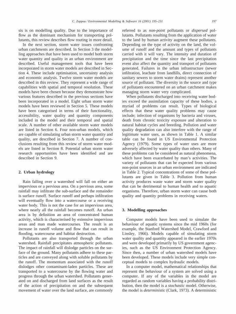
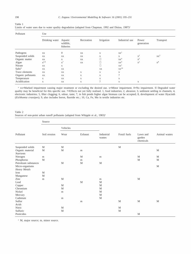
When pollutants discharged into receiving water bod-ies exceed the assimilation capacity of these bodies, amyriad of problems can result. Types of biologicaleffects that these water quality problems may causeinclude; infection of organisms by bacteria and viruses,death from chronic toxicity exposure and alteration tonatural habitat cycles and breeding. Pollution and waterquality degradation can also interfere with the range oflegitimate water uses, as shown in Table 1. A similartable can be found in US Environmental ProtectionAgency (1979). Some types of water uses are moreadversely affected by water quality than others. Many ofthese problems can be considered as natural phenomena,which have been exacerbated by man’s activities. Thevariety of pollutants that can be expected from variousnon-point sources in an urban environment are indicatedin Table 2. Typical concentrations of some of these pol-lutants are given in Table 3. Pollution from humanactivity produces waste water and storm water qualitythat can be detrimental to human health and to aquaticorganisms. Therefore, urban storm water can cause bothquality and quantity problems in receiving waters.
3. Modelling approaches
Computer models have been used to simulate thebehaviour of aquatic systems since the mid 1960s (forexample, the Stanford Watershed Model, Crawford andLinsley, 1966). Models capable of simulating stormwater quality and quantity appeared in the earlier 1970sand were developed primarily by US government agenc-ies, such as the US Environment Protection Agency.Since then, a number of urban watershed models havebeen developed. These models include very simple con-ceptual models to complex hydraulic models.
In a computer model, mathematical relationships thatrepresent the behaviour of a system are solved using acomputer. If any of the variables in the model areregarded as random variables having a probability distri-bution, then the model is astochasticmodel. Otherwise,the model isdeterministic(Clark, 1973). A deterministic
198 C. Zoppou / Environmental Modelling & Software 16 (2001) 195–231
Table 1Limits of water uses due to water quality degradation (adapted from Chapman, 1992 and Dinius, 1987)a
Pollutant Use
Drinking water Aquatic Recreation Irrigation Industrial use Power Transportwildlife, generationfisheries
Pathogens xx 0 xx x xx1
Suspended solids xx xx xx x x x2 xx3
Organic matter xx x xx + xx4 x5
Algae x5,6 x7 xx + xx4 x5 x8
Nitrate xx x + xx1
Salts9 xx xx xx xx10
Trace elements xx xx x x xOrganic pollutants xx xx x x ?Temperature x xx x x xAcidification x xx x ? x x
a xx=Marked impairment causing major treatment or excluding the desired use. x=Minor impairment. 0=No impairment.+=Degraded waterquality may be beneficial for this specific use. ?=Effects not yet fully realised. 1, food industries; 2, abrasion; 3, sediment settling in channels; 4,electronic industries; 5, filter clogging; 6, odour, taste; 7, in fish ponds higher algae biomass can be accepted; 8, development of water Hyacinth(Eichhomia crassipes); 9, also includes boron, fluoride etc.; 10, Ca, Fe, Mn in textile industries etc.
Table 2Sources of non-point urban runoff pollutants (adapted from Whipple et al., 1983)a
Source
Vehicles
Pollutant Soil erosion Wear Exhaust Industrial Fossil fuels Lawn and Animal wasteswastes garden
chemicals
Suspended solids M M MOrganic material M M m MNutrientsNitrogen m M m M MPhosphorus M m M MPetroleum substances M M MMicro-organisms MHeavy MetalsIron MManganese MZinc m M m MLead M MCopper M MChromium M MNickel m MMercury MCadmium m MSulfur m M M MAcidsNitric M MSulfuric M MPesticides M
a M, major source; m, minor source.
199C. Zoppou / Environmental Modelling & Software 16 (2001) 195–231
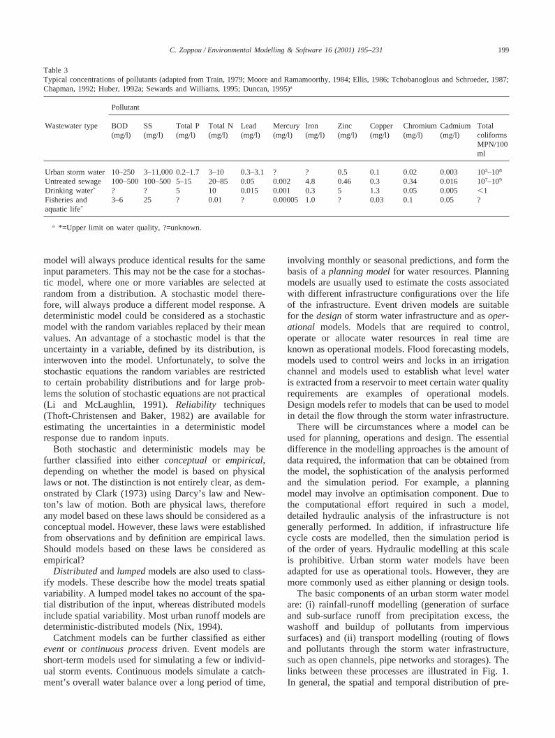
Table 3Typical concentrations of pollutants (adapted from Train, 1979; Moore and Ramamoorthy, 1984; Ellis, 1986; Tchobanoglous and Schroeder, 1987;Chapman, 1992; Huber, 1992a; Sewards and Williams, 1995; Duncan, 1995)a
Pollutant
Wastewater type BOD SS Total P Total N Lead Mercury Iron Zinc Copper Chromium Cadmium Total(mg/l) (mg/l) (mg/l) (mg/l) (mg/l) (mg/l) (mg/l) (mg/l) (mg/l) (mg/l) (mg/l) coliforms
MPN/100ml
Urban storm water 10–250 3–11,000 0.2–1.7 3–10 0.3–3.1 ? ? 0.5 0.1 0.02 0.003 103–108
Untreated sewage 100–500 100–500 5–15 20–85 0.05 0.002 4.8 0.46 0.3 0.34 0.016 107–109
Drinking water* ? ? 5 10 0.015 0.001 0.3 5 1.3 0.05 0.005 ,1Fisheries and 3–6 25 ? 0.01 ? 0.00005 1.0 ? 0.03 0.1 0.05 ?aquatic life*
a *=Upper limit on water quality, ?=unknown.
model will always produce identical results for the sameinput parameters. This may not be the case for a stochas-tic model, where one or more variables are selected atrandom from a distribution. A stochastic model there-fore, will always produce a different model response. Adeterministic model could be considered as a stochasticmodel with the random variables replaced by their meanvalues. An advantage of a stochastic model is that theuncertainty in a variable, defined by its distribution, isinterwoven into the model. Unfortunately, to solve thestochastic equations the random variables are restrictedto certain probability distributions and for large prob-lems the solution of stochastic equations are not practical(Li and McLaughlin, 1991). Reliability techniques(Thoft-Christensen and Baker, 1982) are available forestimating the uncertainties in a deterministic modelresponse due to random inputs.
Both stochastic and deterministic models may befurther classified into eitherconceptualor empirical,depending on whether the model is based on physicallaws or not. The distinction is not entirely clear, as dem-onstrated by Clark (1973) using Darcy’s law and New-ton’s law of motion. Both are physical laws, thereforeany model based on these laws should be considered as aconceptual model. However, these laws were establishedfrom observations and by definition are empirical laws.Should models based on these laws be considered asempirical?
Distributedandlumpedmodels are also used to class-ify models. These describe how the model treats spatialvariability. A lumped model takes no account of the spa-tial distribution of the input, whereas distributed modelsinclude spatial variability. Most urban runoff models aredeterministic-distributed models (Nix, 1994).
Catchment models can be further classified as eithereventor continuous processdriven. Event models areshort-term models used for simulating a few or individ-ual storm events. Continuous models simulate a catch-ment’s overall water balance over a long period of time,
involving monthly or seasonal predictions, and form thebasis of aplanning modelfor water resources. Planningmodels are usually used to estimate the costs associatedwith different infrastructure configurations over the lifeof the infrastructure. Event driven models are suitablefor thedesignof storm water infrastructure and asoper-ational models. Models that are required to control,operate or allocate water resources in real time areknown as operational models. Flood forecasting models,models used to control weirs and locks in an irrigationchannel and models used to establish what level wateris extracted from a reservoir to meet certain water qualityrequirements are examples of operational models.Design models refer to models that can be used to modelin detail the flow through the storm water infrastructure.
There will be circumstances where a model can beused for planning, operations and design. The essentialdifference in the modelling approaches is the amount ofdata required, the information that can be obtained fromthe model, the sophistication of the analysis performedand the simulation period. For example, a planningmodel may involve an optimisation component. Due tothe computational effort required in such a model,detailed hydraulic analysis of the infrastructure is notgenerally performed. In addition, if infrastructure lifecycle costs are modelled, then the simulation period isof the order of years. Hydraulic modelling at this scaleis prohibitive. Urban storm water models have beenadapted for use as operational tools. However, they aremore commonly used as either planning or design tools.
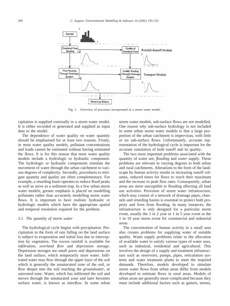
The basic components of an urban storm water modelare: (i) rainfall-runoff modelling (generation of surfaceand sub-surface runoff from precipitation excess, thewashoff and buildup of pollutants from impervioussurfaces) and (ii) transport modelling (routing of flowsand pollutants through the storm water infrastructure,such as open channels, pipe networks and storages). Thelinks between these processes are illustrated in Fig. 1.In general, the spatial and temporal distribution of pre-
200 C. Zoppou / Environmental Modelling & Software 16 (2001) 195–231
Fig. 1. Overview of processes incorporated in a storm water model.
cipitation is supplied externally to a storm water model.It is either recorded or generated and supplied as inputdata to the model.
The dependence of water quality on water quantityshould be emphasised for at least two reasons. Firstly,in most water quality models, pollutant concentrationsand loads cannot be estimated without having estimatedthe flows. It is for this reason that most water qualitymodels include a hydrologic or hydraulic component.The hydrologic or hydraulic components simulate themovement of water through the urban catchment to vari-ous degrees of complexity. Secondly, procedures to miti-gate quantity and quality are often complementary. Forexample, a retarding basin operates to reduce flood peaksas well as serve as a sediment trap. In a few urban stormwater models, greater emphasis is placed on modellingpollutants rather than accurately modelling storm waterflows. It is important to have realistic hydraulic orhydrologic models which have the appropriate spatialand temporal resolution required for the problem.
3.1. The quantity of storm water
The hydrological cycle begins with precipitation. Pre-cipitation in the form of rain falling on the land surfaceis subject to evaporation and initial loss due to intercep-tion by vegetation. The excess rainfall is available forinfiltration, overland flow and depression storage.Depression storages are small pores and depressions onthe land surface, which temporarily store water. Infil-trated water may flow through the upper layer of the soilwhich is generally theunsaturated zoneof the soil, orflow deeper into the soil reaching thegroundwater, orsaturated zone. Water, which has infiltrated the soil andmoves through the unsaturated zone and later becomessurface water, is known asinterflow. In some urban
storm water models, sub-surface flows are not modelled.One reason why sub-surface hydrology is not includedin some urban storm water models is that a large pro-portion of the urban catchment is impervious, with littleor no sub-surface flows. Unfortunately, accurate rep-resentation of the hydrological cycle is important for theaccurate simulation of both runoff and its quality.
The two most important problems associated with thequantity of water are;floodingandwater supply. Theseproblems are relevant in varying degrees to both urbanand rural catchments. Alterations to the form of the land-scape by human activity results in increasing runoff vol-umes, reduced times for flows to reach their maximumand the increase in peak flow rates. Consequently, urbanareas are more susceptible to flooding affecting all landuse activities. Provision of storm water infrastructure,which may consist of a network of drainage pipes, chan-nels and retarding basins is essential to protect both pro-perty and lives from flooding. In many instances, theinfrastructure is only designed for a particular stormevent, usually the 1 in 2 year or 1 in 5 year event or the1 in 10 year storm event for commercial and industrialareas.
The concentration of human activity in a small areaalso creates problems for supplying water of suitablequality. Water supply problems relate to the allocationof available water to satisfy various types of water uses,such as industrial, residential and agricultural. Thisinvolves the design of a supply and treatment infrastruc-ture such as reservoirs, pumps, pipes, reticulation sys-tems and water treatment plants to meet the requireddemands. Therefore, models developed to simulatestorm water flows from urban areas differ from modelsdeveloped to estimate flows in rural areas. Models ofurban areas are generally more complicated because theymust include additional factors such as gutters, streets,
201C. Zoppou / Environmental Modelling & Software 16 (2001) 195–231
sewers, overflows, surcharging, closed conduits underpressure, storm water drainage networks, culverts, openchannels, roof top storage, open and natural water-courses and storages.Surchargesoccur when a closedconduit, which would normally act as an open channel,becomes full and acts a conduit under pressure. Undersome circumstances, this is desirable because it has thepotential to increase the capacity of the storm waterdrain. If there is sufficient pressure so that the water risesabove the ground level, then overflow occurs where theexcess volume of flow becomes surface runoff. Urbancatchments respond considerably faster to rainfall thanrural catchments. Therefore, models developed for anurban catchment must be able to capture the rapidresponse of the catchment to storm events.
Another main objective of the analysis of storm waterflows is to determine inputs of pollutants to receivingwaters. Flowing water is the main mechanism, alongwith the impact of rain for transporting pollutants in theurban catchment.
3.2. The quality of storm water
The five natural processes which affect the movementand transformation of pollutants in an urban catchmentare: chemical, physicochemical, biological, ecologicalandphysical. Chemical processes involve the reaction oftwo or more compounds with each other to form one ormore different compounds. An example of a chemicalprocess in a natural system is the transformation of SO2
into SO3 and eventually H2SO4 (sulfuric acid) in theatmosphere. Biochemical processes are a result ofchemical transformations taking place within a biologi-cal organism, such as bacterial decomposition of organicmaterial and photosynthesis. Physicochemical processesinvolve the chemistry and physics of molecules inter-acting with their surroundings. The most importantphysicochemical processes are;adsorption, desorptionand absorption. Adsorption is the adhesion of a subst-ance to the surface of a solid or liquid. Adsorption isan important process because many pollutants such asnitrogen, phosphorus, various pesticides and heavy met-als attach themselves to sediment particles and are inturn transported with the particles in flowing water. Thequantities of pollutants that become attached to sedimentparticles are a function of the concentration of pollutantsin the runoff and temperature. Desorption is the releaseof pollutants from sediment particles. Absorption is thepenetration of a substance into or through another. Itusually takes place at the air–water interface where gasesare absorbed into water. This is the primary mechanismwhereby receiving water bodies obtain oxygen. Ecologi-cal processes involve interactions between differentorganisms in the food chain. This includes consumption,growth, mortality and respiration from organisms. Trans-port or physical processes describe the movement of pol-
lutants by fluid motion. This is primarily by the actionof advection, the fluid moving, anddiffusion, the motionof molecules and turbulent fluctuations in the fluid dis-persing material. The transport process acts indepen-dently of the transformations of nonconservative sub-stances and is equally valid for both conservative andnonconservative substances. Materials that are not trans-formed chemically while being transported are termedconservative substances, otherwise they arenoncon-servative substances. For example, dissolved salts areconservative because, generally they do not interact withother substances. Nitrogen, in its ionic state will undergochemical, physicochemical and biological transformationin a water body.
Major water quality problems in urban storm waterare produced by: salinity, temperature, sedimentation,dissolved oxygen, toxic substances and biologicaleffects. Temperature has impacts on: physicochemicalreactions, biochemical reactions, biological processesand on the behavioural pattern of organisms. Tempera-ture can also result in synergistic effects. For example,higher water temperatures exacerbate the adverse effectsof low dissolved oxygen concentrations. Salinity prob-lems are associated with high concentrations of total dis-solved salts. Salinity affects aquatic organisms as wellas uses of water withdrawn from receiving water. Sedi-mentation is a natural process, which has been acceler-ated in many areas by man’s activities. Suspended sedi-ments in high concentrations diminish light penetration,thereby inhibiting photosynthesis by aquatic organisms.Sediments that are deposited can smother plants andorganisms and destroy fish spawning grounds. Sedimentsentering receiving waters can also carry attached nutri-ents, pesticides and heavy metals. Sediments can alsoclog water treatment plant filters, block channels andpipes. Dissolved oxygen is important as an indicator ofwater quality. Organisms in aquatic systems must haveoxygen to survive. The primary demand for oxygen inreceiving waters is by decomposing organic material.Three indicators used in relation to oxygen demand are;biochemical oxygen demand(BOD), chemical oxygendemand(COD) andtotal organic carbon(TOC). TOCand COD are an indicator of the total amount of organicmaterial present. BOD is a measure of the total amountof oxygen required to biochemically oxidise organicmatter at a specific temperature and time. It is generallyconsidered a major indicator of the health of a waterbody. Toxic substances include; herbicides, insecticides,pesticides, heavy metals, radioactive materials, oils andreduced ions. The sources, health and environmentalconsequences of a variety of pollutants that can occur inurban storm water are given in Appendix A.
The rates at which chemical, physicochemical andbiochemical reactions occur are important in understand-ing ambient water quality. However, due to the shortresponse times in urban runoff, impacts of chemical and
202 C. Zoppou / Environmental Modelling & Software 16 (2001) 195–231
biochemical processes on urban runoff quality are usu-ally negligible, the only exception being storages thatare used as wetlands. Hence, these processes are neg-lected in most urban runoff models.
Modifications which man has made to the land surfacehave exacerbated physicochemical and transport pro-cesses in many regions, thereby increasing the quantityof pollutants and altering both the types of pollutantsand the time pattern of flows. Consequently, in order toestimate the quantity and quality of water from an urbanarea, these processes must be included in a stormwater model.
3.3. Approaches to storm water quantity estimation
Nix (1994) uses three categories (i)simple, (ii) simplerouting and (iii) complex routingmodels to categorisemodels. Each category has different demands on dataand computing resources and provides results at differenttime scales and spatial resolution. In simple models, norouting is performed, little data is required, calculationsare not repetitive and a computer may not be requiredto perform the calculations. These models provide verylittle detail of the behaviour of the flow or pollutant.In general, these models are used to provide long-termaverages or peak values. They are specific to a particularsite and catchment behaviour. Empirical models couldbe considered as simple models. Although some statisti-cal models are based on complicated techniques, theyonly reflect the current behaviour of a catchment at aparticular site. Some empirical models involve very sim-ple expressions that do not require the use of a computer.Both simple and complex routing models are based onphysical laws describing the flow within the catchment.Although, they are deterministic models, they describethe behaviour of the catchment at different complexities.The complexity of a model has implications on the com-putational resources required, limitations of the modeland the reliability of the results produced by the model.
Results from simpler models can also be extractedfrom the results from more sophisticated models, how-ever the converse is not generally true. Simple stormwater models do not simulate some important processes.For example, the commonly used storage routing tech-nique is a lumped model. Processes that are time depen-dent, such as the decay of some pollutants cannot bemodelled because processes are assumed to occur instan-taneously. To overcome this problem, models incorpor-ate time, such as a lag in the routing process. This intro-duces another subjective parameter for the user toestimate and this approach is independent of the behav-iour of the process being modelled. Lumped models areusually used in planning models where the time stepsare much larger than the time scale of the transients thatoccur through the system. Therefore, they use averagevalues for the various processes. This ignores the tem-
poral and spatial variability of the system, which arerequired to test the integrity of the storm water system.The spatial and temporal variability must be artificiallyintroduced into the modelling process. For example, aplanning model for allocating potable water may use anaverage monthly demand to test a water allocation strat-egy. However, peak demands are required to test theintegrity of the water supply infrastructure. The assess-ment of the integrity of the infrastructure is integral tothe success of the water allocation strategy and cannotbe performed independently of the water allocationanalysis. Therefore, an empirical relationship betweenpeak and average demands must be established. Thisadds additional subjectivity and uncertainty in the mod-elling process. These problems could be overcome byusing models that are more complicated, but at a cost.
The importance of selecting a quantity model with theappropriate temporal and spatial resolution is not empha-sised in other reviews. If flow is not modelledadequately, then water quality predictions will not reflectthe true behaviour of the catchment.
3.3.1. Statistical and empirical modelsStatistical models that have been used for estimating
storm water flows and water quality loads are usuallybased on regression models. These relate measuredquantities, such as water quantity, with measurablephysical parameters that are considered important in aparticular process. Regression models are an example ofa stochastic modelling approach. These may include cli-matic characteristics, such as rainfall intensity and catch-ment parameters (impervious area, land-use and catch-ment slope). For example, the nonlinear regressionmodel
Y5b0 Pn
i51Xibi
in which Y is the dependent variable,Xi are theexplana-tory or observer variables andbi are the unknownregression coefficients, is a common statistical modelused for modelling both water quality and quantity.Other regression models include simple linear, multiplelinear, semi-log transform and the log–log transform(see, for example Bidwell, 1971; Jewell and Adrian,1981). Examples of statistical models used in urbanwatershed modelling can be found in Jewell and Adrian(1981), Driver and Tasker (1988) and Yao and Terakaura(1999). It is recognised that linear regression is inad-equate in urban catchment modelling (Jewell and Adrian,1981). The most important limitation of statistical mod-els is that the statistical relationship developed from agiven set of data reflects a particular spatial arrangement.For any markedly different spatial patterns and pro-cesses, new data and a new statistical relationship mustbe developed. Because of these limitations, the statisticalapproach has been primarily used only for crude analysis
203C. Zoppou / Environmental Modelling & Software 16 (2001) 195–231
or in situations where deterministic approaches cannotbe used because of insufficient data or resources. Driverand Tasker (1988) describe regression models as suf-ficient for planning purposes only.
An example of a regression method for analysing run-off is based on theantecedent precipitation index(API).It is the most frequently used and important explanatoryvariable in surface water runoff. The antecedent precipi-tation index is essentially the summation of the precipi-tation amounts occurring prior to the storm, weightedaccording to the time of occurrence. An example of aquantity antecedent regression model is (Betson et al.,1969):
C5c1(a1dS)exp(2bp), Q5(in1Cn)1/n2C
in which Q is the surface runoff,C runoff coefficient,Sa seasonal index parameter,p antecedent precipitationindex, i rainfall and a, b, c, d and n are model coef-ficients to be determined from the data usingregression analysis.
Empirical models involve a functional relationshipbetween a dependent variable and variables that are con-sidered germane to the process. These variables arechosen from knowledge of the physical processesinvolved and from empirical measurements. An exampleof an empirical approach for estimating runoff is therational formula:
Q5CiA.
The rational method is the simplest approach to model-ling peak runoff volumes, which are important for stormwater infrastructure design. The rational method is asimple relationship between flowQ, the catchment areaA, the rainfall intensityi, and a runoff coefficientCwhere 0#C#1.
3.3.2. Deterministic modelsDeterministic models are based on conservation laws,
which govern the behaviour of a fluid. These laws gener-ally involve theconservation of volume, known asconti-nuity, theconservation of momentumor theconservationof energy. In almost all cases, one-dimensional flowanalysis is undertaken. Deterministic models used instorm water modelling can be classified as eitherhydrologicor hydraulicmodels. Hydrologic models usu-ally satisfy the continuity equation only. Hydraulic mod-els solve the continuity equation as well as either themomentum or the energy equations as a coupled systemof equations. The major difference between these model-ling approaches is that hydraulic models describe thespatial behaviour of a process. It is the momentum equ-ation that defines the speed at which a process can occur.
Many engineers in Australia do not make this distinc-tion. The distinction between hydrology and hydraulicsis determined by the process that is being modelled. Forexample, the rainfall-runoff process is considered as a
hydrological process and modelling flows through openchannels is a hydraulic problem. This distinction is dueto the historical development of models used to simulateoverland and open channel flows. Traditionally, due tothe complexity of overland flow, only the continuity equ-ation was solved. The dynamic equations (momentumor energy) are considered of secondary importance. Astechniques emerge for simulating overland flow by solv-ing simultaneously the continuity and dynamic equa-tions, this distinction is not clear. Therefore in thisreport, the distinction between hydrologic and hydraulicmodels is based on the equations that are used todescribe a process and not the process that is being mod-elled.
3.3.2.1. Hydraulic models For very simple problems,analytical solutions are available for the solution of thegoverning equations. However, numerical schemes areused to solve these equations. Hydrological methodshave a greater scope for solution using analyticalmethods. In complicated problems, numerical schemessuch asfinite differences, finite elementsor themethod ofcharacteristicsare used. Finite differences are the mostcommonly used approach and these can be eitherimplicitor explicit schemes. In explicit schemes, a singleunknown value can be written in terms of known values.This produces a large number of simple linear equationsthat can be solved directly for the unknown. In implicitschemes, a number of unknowns at a particular time arewritten in terms of the knowns, established previously,as well as unknowns at the current time. This results ina system of coupled simultaneous equations that mustbe solved. The major advantage with implicit schemesis that they are considered as unconditionally stable,therefore there should be no restriction on the compu-tational time step that can be used in the model. Theadditional computational effort required to solve a sys-tem of equations is compensated for by a relaxation inthe restriction in the time step that can be used in thesimulation. However, the adequate description of bound-ary conditions and truncation errors, due to the finite dif-ference approximations, may preclude the use of verylarge time steps in an implicit finite difference scheme.This is in contrast to explicit schemes, where there is arestriction on the time step that may be employed.Although the time step restriction is inversely pro-portional to the speed of the transients being modelled,this may not be a disadvantage in modelling rapidlyvarying transients. Here a small time step is required toadequately capture the behaviour of the transient. Rap-idly varying transients are common in urban watershedproblems, such as overland flow and flash flooding.
3.3.2.2. Shallow water wave equationsThe conserva-tive form of the one-dimensional continuity and momen-tum equations can be written as
204 C. Zoppou / Environmental Modelling & Software 16 (2001) 195–231
∂U∂t
1∂F∂x
5S (1)
whereU is a vector of conservative variables
U5FA
QG
F is the flux vector
F(U)53QQ2
A+gI14
andS represents the source vector
S5Fq
gA(S0−Sf)+gI2G
in which A is the cross-sectional area,Q is the discharge,q is the lateral inflow per unit length perpendicular tothe channel so that it has no downstream velocitycomponent,x is the distance,t is the time,g is the accel-eration due to gravity,S0 is the bed slope,Sf is the fric-tion slope andI1 is given by
I15 Ey(x)
0
(y(x)2x)B(x)dx
in which B is the width of the channel,y is the waterdepth. The effects of forces exerted by contraction orexpansion of the channel walls on the flow isdescribed by
I25 Ey(x)
0
(y(x)2x)F∂B(x)∂x G
y(x)=y0
dx
wherey0 is a constant water depth, is zero for a uniformchannel. These equations are known as theshallowwater wave equationsor theSaint Venant equations.
The shallow water wave equations written in non-con-servative form with the flow velocityu=Q/A and y asthe dependent variables are for a unit width of channel:continuity equation
∂y∂t
1∂(uy)
∂x5q (2)
momentum equation
1g
∂u∂t
1ug
∂u∂x
1∂y∂x
5S02Sf2qg
uy. (3)
The friction slopeSf, is approximated using either the
Manning or Chezy equations. The Manning equation isgiven by
Sf5K2|Q|Q5u|u|h2
R4/3
in which h is the Manning resistance coefficient andRis the hydraulic radius, defined byR=A/P with P thewetted perimeter andK is known as theconveyance. TheChezy equation is given by
Sf5u|u|cR
in which c is the Chezy resistance coefficient. In bothequations, the absolute sign for the velocity will ensurethat the friction always opposes the flow.
The continuity Eq. (2) is based on the law of conser-vation of mass in a slice of the channel. It simply statesthat the rate of change in water depth with time in aslice of the channel is equal to the net inflow into theslice of the channel. The momentum Eq. (3) is a math-ematical expression for the conservation of momentumwithin a slice of the channel. It simply states that the rateof change in momentum within a slice of the channel isequal to the sum of forces acting on the slice. It is themomentum equation that determines the velocity orspeed of the fluid through a slice of the channel.
The shallow water wave equations arehyperbolicandit is this feature that distinguishes them from othermethods of routing, which are generally subsets of theseequations. The distinguishing feature of the shallowwater wave equations is that they have two character-istics. These characteristics represent the paths in (x,t)space that information can travel. In the case of the shal-low water wave equations, depending on the flow con-ditions, information can propagate both upstream anddownstream. This is important because downstreamobstructions will influence the flow upstream of theobstruction. For example, flow upstream of a weir willbe influenced by the weir. This influence can only besimulated if there is an interaction of information travel-ling both upstream and downstream of the weir orobstruction to the flow.
The shallow water wave equations can be used tosimulate unsteady one-dimensional gradually and rapidlyvarying flows, if Eq. (1) is used (see, for example Zop-pou and Roberts, 1999) in open and natural channels andin pressurised closed conduits using the Preissmann slot(Abbott, 1979). Two-dimensional overland flows canalso be simulated using the shallow water wave equa-tions.
Under steady flow conditions, the continuity equationis simply d(uy)/dx=q, and the momentum equationbecomes
S02Sf2quy
5d(y+u2/2g)
dx(4)
205C. Zoppou / Environmental Modelling & Software 16 (2001) 195–231
which is used to calculate the water surface profile in anopen channel where an obstacle impedes the flow. Stan-dard techniques could be employed to solve this ordinarydifferential equation. For subcritical flows, where thecontrol is downstreambackwater analysis, whichinvolves the solution of Eq. (4) using an iterative scheme(see, for example Henderson, 1966) is commonlyemployed.
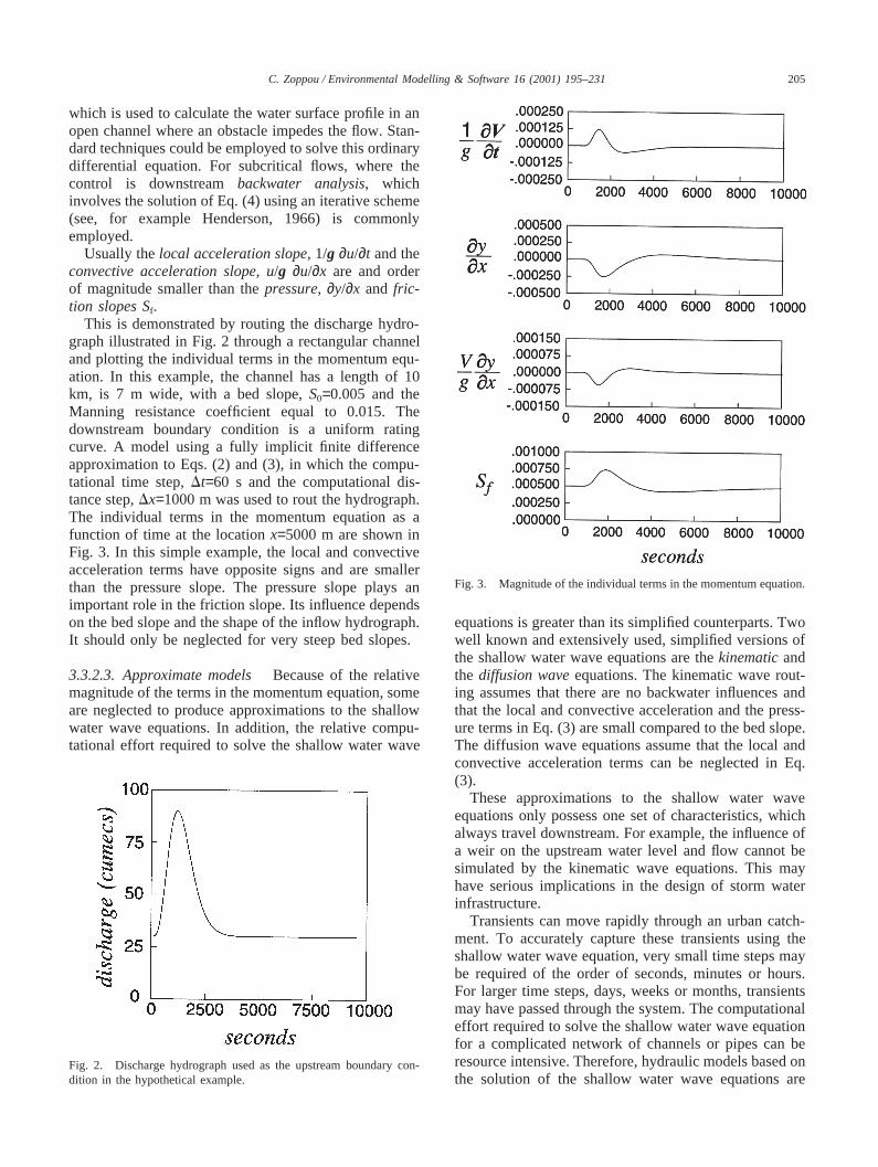
Usually thelocal acceleration slope, 1/g ∂u/∂t and theconvective acceleration slope, u/g ∂u/∂x are and orderof magnitude smaller than thepressure, ∂y/∂x and fric-tion slopes Sf.
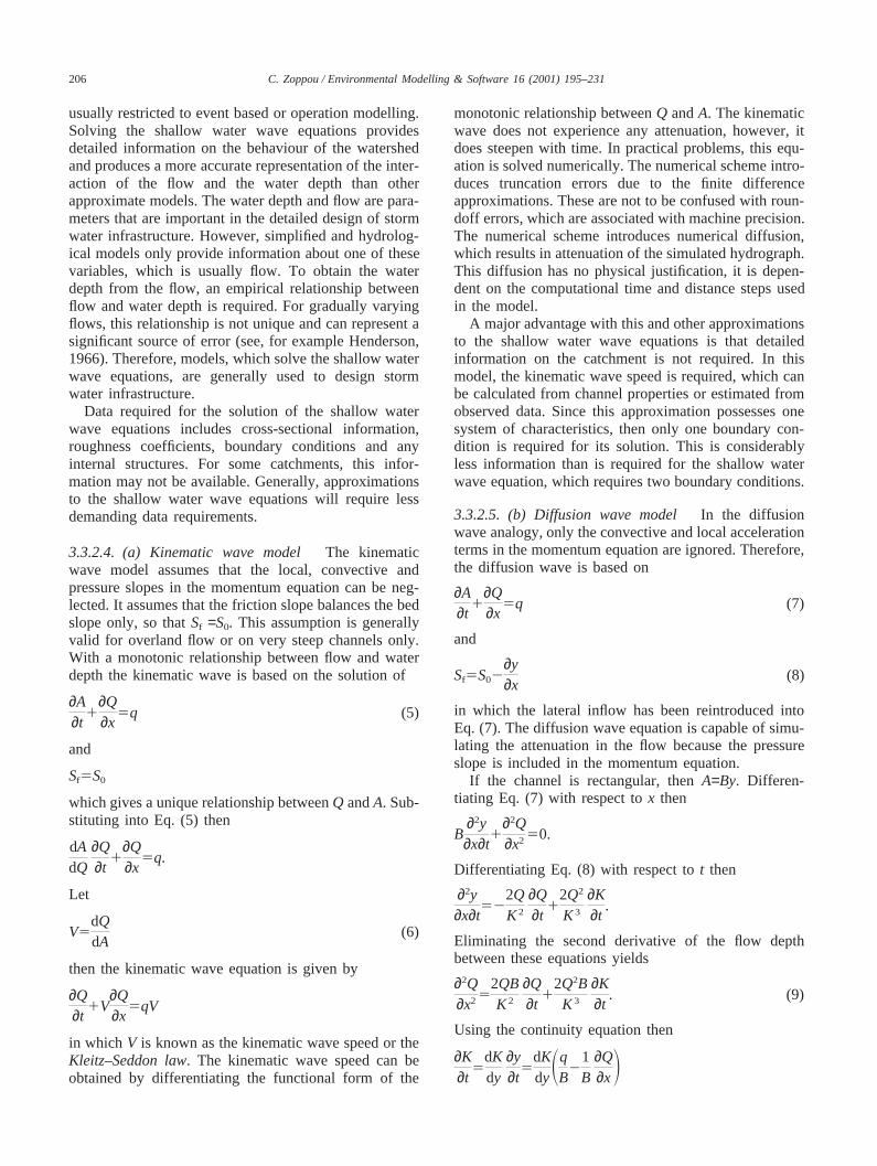
This is demonstrated by routing the discharge hydro-graph illustrated in Fig. 2 through a rectangular channeland plotting the individual terms in the momentum equ-ation. In this example, the channel has a length of 10km, is 7 m wide, with a bed slope,S0=0.005 and theManning resistance coefficient equal to 0.015. Thedownstream boundary condition is a uniform ratingcurve. A model using a fully implicit finite differenceapproximation to Eqs. (2) and (3), in which the compu-tational time step,Dt=60 s and the computational dis-tance step,Dx=1000 m was used to rout the hydrograph.The individual terms in the momentum equation as afunction of time at the locationx=5000 m are shown inFig. 3. In this simple example, the local and convectiveacceleration terms have opposite signs and are smallerthan the pressure slope. The pressure slope plays animportant role in the friction slope. Its influence dependson the bed slope and the shape of the inflow hydrograph.It should only be neglected for very steep bed slopes.
3.3.2.3. Approximate models Because of the relativemagnitude of the terms in the momentum equation, someare neglected to produce approximations to the shallowwater wave equations. In addition, the relative compu-tational effort required to solve the shallow water wave
Fig. 2. Discharge hydrograph used as the upstream boundary con-dition in the hypothetical example.
Fig. 3. Magnitude of the individual terms in the momentum equation.
equations is greater than its simplified counterparts. Twowell known and extensively used, simplified versions ofthe shallow water wave equations are thekinematicandthe diffusion waveequations. The kinematic wave rout-ing assumes that there are no backwater influences andthat the local and convective acceleration and the press-ure terms in Eq. (3) are small compared to the bed slope.The diffusion wave equations assume that the local andconvective acceleration terms can be neglected in Eq.(3).
These approximations to the shallow water waveequations only possess one set of characteristics, whichalways travel downstream. For example, the influence ofa weir on the upstream water level and flow cannot besimulated by the kinematic wave equations. This mayhave serious implications in the design of storm waterinfrastructure.
Transients can move rapidly through an urban catch-ment. To accurately capture these transients using theshallow water wave equation, very small time steps maybe required of the order of seconds, minutes or hours.For larger time steps, days, weeks or months, transientsmay have passed through the system. The computationaleffort required to solve the shallow water wave equationfor a complicated network of channels or pipes can beresource intensive. Therefore, hydraulic models based onthe solution of the shallow water wave equations are
206 C. Zoppou / Environmental Modelling & Software 16 (2001) 195–231
usually restricted to event based or operation modelling.Solving the shallow water wave equations providesdetailed information on the behaviour of the watershedand produces a more accurate representation of the inter-action of the flow and the water depth than otherapproximate models. The water depth and flow are para-meters that are important in the detailed design of stormwater infrastructure. However, simplified and hydrolog-ical models only provide information about one of thesevariables, which is usually flow. To obtain the waterdepth from the flow, an empirical relationship betweenflow and water depth is required. For gradually varyingflows, this relationship is not unique and can represent asignificant source of error (see, for example Henderson,1966). Therefore, models, which solve the shallow waterwave equations, are generally used to design stormwater infrastructure.
Data required for the solution of the shallow waterwave equations includes cross-sectional information,roughness coefficients, boundary conditions and anyinternal structures. For some catchments, this infor-mation may not be available. Generally, approximationsto the shallow water wave equations will require lessdemanding data requirements.
3.3.2.4. (a) Kinematic wave model The kinematicwave model assumes that the local, convective andpressure slopes in the momentum equation can be neg-lected. It assumes that the friction slope balances the bedslope only, so thatSf =S0. This assumption is generallyvalid for overland flow or on very steep channels only.With a monotonic relationship between flow and waterdepth the kinematic wave is based on the solution of
∂A∂t
1∂Q∂x
5q (5)
and
Sf5S0
which gives a unique relationship betweenQ andA. Sub-stituting into Eq. (5) then
dAdQ
∂Q∂t
1∂Q∂x
5q.
Let
V5dQdA
(6)
then the kinematic wave equation is given by
∂Q∂t
1V∂Q∂x
5qV
in which V is known as the kinematic wave speed or theKleitz–Seddon law. The kinematic wave speed can beobtained by differentiating the functional form of the
monotonic relationship betweenQ andA. The kinematicwave does not experience any attenuation, however, itdoes steepen with time. In practical problems, this equ-ation is solved numerically. The numerical scheme intro-duces truncation errors due to the finite differenceapproximations. These are not to be confused with roun-doff errors, which are associated with machine precision.The numerical scheme introduces numerical diffusion,which results in attenuation of the simulated hydrograph.This diffusion has no physical justification, it is depen-dent on the computational time and distance steps usedin the model.
A major advantage with this and other approximationsto the shallow water wave equations is that detailedinformation on the catchment is not required. In thismodel, the kinematic wave speed is required, which canbe calculated from channel properties or estimated fromobserved data. Since this approximation possesses onesystem of characteristics, then only one boundary con-dition is required for its solution. This is considerablyless information than is required for the shallow waterwave equation, which requires two boundary conditions.
3.3.2.5. (b) Diffusion wave model In the diffusionwave analogy, only the convective and local accelerationterms in the momentum equation are ignored. Therefore,the diffusion wave is based on
∂A∂t
1∂Q∂x
5q (7)
and
Sf5S02∂y∂x
(8)
in which the lateral inflow has been reintroduced intoEq. (7). The diffusion wave equation is capable of simu-lating the attenuation in the flow because the pressureslope is included in the momentum equation.
If the channel is rectangular, thenA=By. Differen-tiating Eq. (7) with respect tox then
B∂2y∂x∂t
1∂2Q∂x2 50.
Differentiating Eq. (8) with respect tot then
∂2y∂x∂t
522QK2
∂Q∂t
12Q2
K3
∂K∂t
.
Eliminating the second derivative of the flow depthbetween these equations yields
∂2Q∂x2 5
2QBK2
∂Q∂t
12Q2BK3
∂K∂t
. (9)
Using the continuity equation then
∂K∂t
5dKdy
∂y∂t
5dKdySq
B2
1B
∂Q∂xD
207C. Zoppou / Environmental Modelling & Software 16 (2001) 195–231
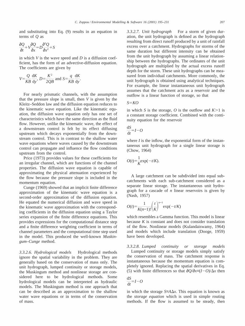
and substituting into Eq. (9) results in an equation interms ofQ as
∂Q∂t
1V∂Q∂x
5D∂2Q∂x21S
in which V is the wave speed andD is a diffusion coef-ficient, has the form of an advective-diffusion equation.The coefficients are given by
V5Q
KBdKdy
, D5K2
2QBandS5
qKB
dKdy
.
For nearly prismatic channels, with the assumptionthat the pressure slope is small, thenV is given by theKleitz–Seddon law and the diffusion equation reduces tothe kinematic wave equation. Like the kinematic equ-ation, the diffusion wave equation only has one set ofcharacteristics which have the same direction as the fluidflow. However, unlike the kinematic wave, the effect ofa downstream control is felt by its effect diffusingupstream which decays exponentially from the down-stream control. This is in contrast to the shallow waterwave equations where waves caused by the downstreamcontrol can propagate and influence the flow conditionsupstream from the control.
Price (1973) provides values for these coefficients foran irregular channel, which are functions of the channelproperties. The diffusion wave equation is capable ofapproximating the physical attenuation experienced bythe flow because the pressure slope is included in themomentum equation.
Cunge (1969) showed that an implicit finite differenceapproximation of the kinematic wave equation is asecond-order approximation of the diffusion equation.He equated the numerical diffusion and wave speed inthe kinematic wave approximation with the correspond-ing coefficients in the diffusion equation using a Taylorseries expansion of the finite difference equations. Thisprovides expressions for the computational distance stepand a finite difference weighting coefficient in terms ofchannel parameters and the computational time step usedin the model. This produced the well-knownMuskin-gum–Cungemethod.
3.3.2.6. Hydrological models Hydrological methodsignore the spatial variability in the problem. They aregenerally based on the conservation of mass only. Theunit hydrograph, lumped continuity or storage models,the Muskingum method and nonlinear storage are con-sidered here to be hydrological methods. Somehydrological models can be interpreted as hydraulicmodels. The Muskingum method is one approach thatcan be described as an approximation to the shallowwater wave equations or in terms of the conservationof mass.
3.3.2.7. Unit hydrograph For a storm of given dur-ation, the unit hydrograph is defined as the hydrographresulting from direct runoff produced by a unit of rainfallexcess over a catchment. Hydrographs for storms of thesame duration but different intensity can be obtainedfrom the unit hydrograph by assuming a linear relation-ship between the hydrographs. The ordinates of the unithydrograph are multiplied by the actual excess runoffdepth for the storm. These unit hydrographs can be mea-sured from individual catchments. More commonly, theunit hydrograph is obtained using analytical techniques.For example, the linear instantaneous unit hydrographassumes that the catchment acts as a reservoir and theoutflow is a linear function of storage, so that
S5KO
in which S is the storage,O is the outflow andK.1 isa constant storage coefficient. Combined with the conti-nuity equation for the reservoir
dSdt
5I2O
whereI is the inflow, the exponential form of the instan-taneous unit hydrograph for a single linear storage is(Chow, 1964)
O(t)51K
exp(2t/K).
A large catchment can be subdivided into equal sub-catchments with each sub-catchment considered as aseparate linear storage. The instantaneous unit hydro-graph for a cascade ofn linear reservoirs is given by(Nash, 1957)
O(t)51
K(n−1)!S tKDn−1
exp(2t/K)
which resembles a Gamma function. This model is linearbecauseK is constant and does not consider translationof the flow. Nonlinear models (Kulandaiswamy, 1964)and models which include translation (Dooge, 1959)have been developed.
3.3.2.8. Lumped continuity or storage modelsLumped continuity or storage models simply satisfy
the conservation of mass. The catchment response isinstantaneous because the momentum equation is com-pletely ignored. Replacing the spatial derivatives in Eq.(5) with finite differences so that∂Q/∂x=(I2O)/Dx then
dSdt
5I2O
in which the storageS=ADx. This equation is known asthe storage equationwhich is used in simple routingmethods. If the flow is assumed to be steady, then
208 C. Zoppou / Environmental Modelling & Software 16 (2001) 195–231
dS/dt=0 and the flow model is simply a mass balance(I=O). This equation is simply an ordinary differentialequation and there are a number of standard techniquesthat could be employed for its solution.
The Modified Puls method solves the storage equ-ation, which is expressed over a finite time interval,Dt as
Dt(I11I2)1S12DtO1/25S21DtO2/2. (10)
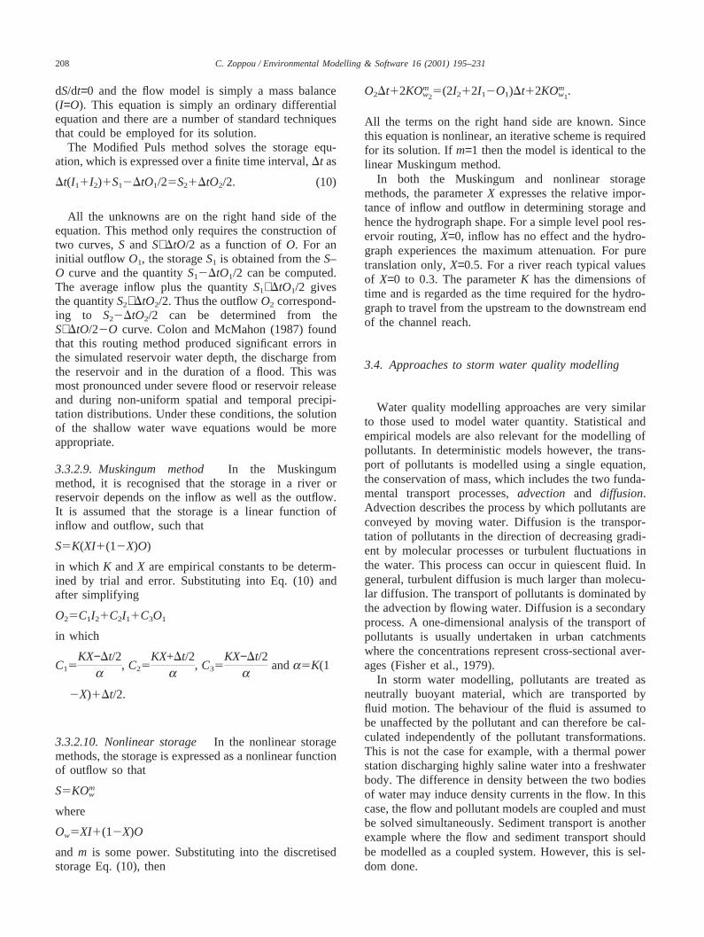
All the unknowns are on the right hand side of theequation. This method only requires the construction oftwo curves,S and S+DtO/2 as a function ofO. For aninitial outflow O1, the storageS1 is obtained from theS–O curve and the quantityS12DtO1/2 can be computed.The average inflow plus the quantityS1+DtO1/2 givesthe quantityS2+DtO2/2. Thus the outflowO2 correspond-ing to S22DtO2/2 can be determined from theS+DtO/22O curve. Colon and McMahon (1987) foundthat this routing method produced significant errors inthe simulated reservoir water depth, the discharge fromthe reservoir and in the duration of a flood. This wasmost pronounced under severe flood or reservoir releaseand during non-uniform spatial and temporal precipi-tation distributions. Under these conditions, the solutionof the shallow water wave equations would be moreappropriate.
3.3.2.9. Muskingum method In the Muskingummethod, it is recognised that the storage in a river orreservoir depends on the inflow as well as the outflow.It is assumed that the storage is a linear function ofinflow and outflow, such that
S5K(XI1(12X)O)
in which K andX are empirical constants to be determ-ined by trial and error. Substituting into Eq. (10) andafter simplifying
O25C1I21C2I11C3O1
in which
C15KX−Dt/2a
, C25KX+Dt/2a
, C35KX−Dt/2a
anda5K(1
2X)1Dt/2.
3.3.2.10. Nonlinear storage In the nonlinear storagemethods, the storage is expressed as a nonlinear functionof outflow so that
S5KOmw
where
Ow5XI1(12X)O
and m is some power. Substituting into the discretisedstorage Eq. (10), then
O2Dt12KOmw2
5(2I212I12O1)Dt12KOmw1
.
All the terms on the right hand side are known. Sincethis equation is nonlinear, an iterative scheme is requiredfor its solution. Ifm=1 then the model is identical to thelinear Muskingum method.
In both the Muskingum and nonlinear storagemethods, the parameterX expresses the relative impor-tance of inflow and outflow in determining storage andhence the hydrograph shape. For a simple level pool res-ervoir routing,X=0, inflow has no effect and the hydro-graph experiences the maximum attenuation. For puretranslation only,X=0.5. For a river reach typical valuesof X=0 to 0.3. The parameterK has the dimensions oftime and is regarded as the time required for the hydro-graph to travel from the upstream to the downstream endof the channel reach.
3.4. Approaches to storm water quality modelling
Water quality modelling approaches are very similarto those used to model water quantity. Statistical andempirical models are also relevant for the modelling ofpollutants. In deterministic models however, the trans-port of pollutants is modelled using a single equation,the conservation of mass, which includes the two funda-mental transport processes,advection and diffusion.Advection describes the process by which pollutants areconveyed by moving water. Diffusion is the transpor-tation of pollutants in the direction of decreasing gradi-ent by molecular processes or turbulent fluctuations inthe water. This process can occur in quiescent fluid. Ingeneral, turbulent diffusion is much larger than molecu-lar diffusion. The transport of pollutants is dominated bythe advection by flowing water. Diffusion is a secondaryprocess. A one-dimensional analysis of the transport ofpollutants is usually undertaken in urban catchmentswhere the concentrations represent cross-sectional aver-ages (Fisher et al., 1979).
In storm water modelling, pollutants are treated asneutrally buoyant material, which are transported byfluid motion. The behaviour of the fluid is assumed tobe unaffected by the pollutant and can therefore be cal-culated independently of the pollutant transformations.This is not the case for example, with a thermal powerstation discharging highly saline water into a freshwaterbody. The difference in density between the two bodiesof water may induce density currents in the flow. In thiscase, the flow and pollutant models are coupled and mustbe solved simultaneously. Sediment transport is anotherexample where the flow and sediment transport shouldbe modelled as a coupled system. However, this is sel-dom done.
209C. Zoppou / Environmental Modelling & Software 16 (2001) 195–231
3.4.1. Statistical and empirical approachesStatistical models for estimating storm water quality
are also based on regression analysis between waterquality and relevant explanatory variables (see, forexample Driscoll et al., 1979; Driver and Tasker, 1990;Driver and Troutman, 1989). Regression models havebeen widely used to describe event mean concentrations(EMC) and total storm event load (Huber, 1992a).
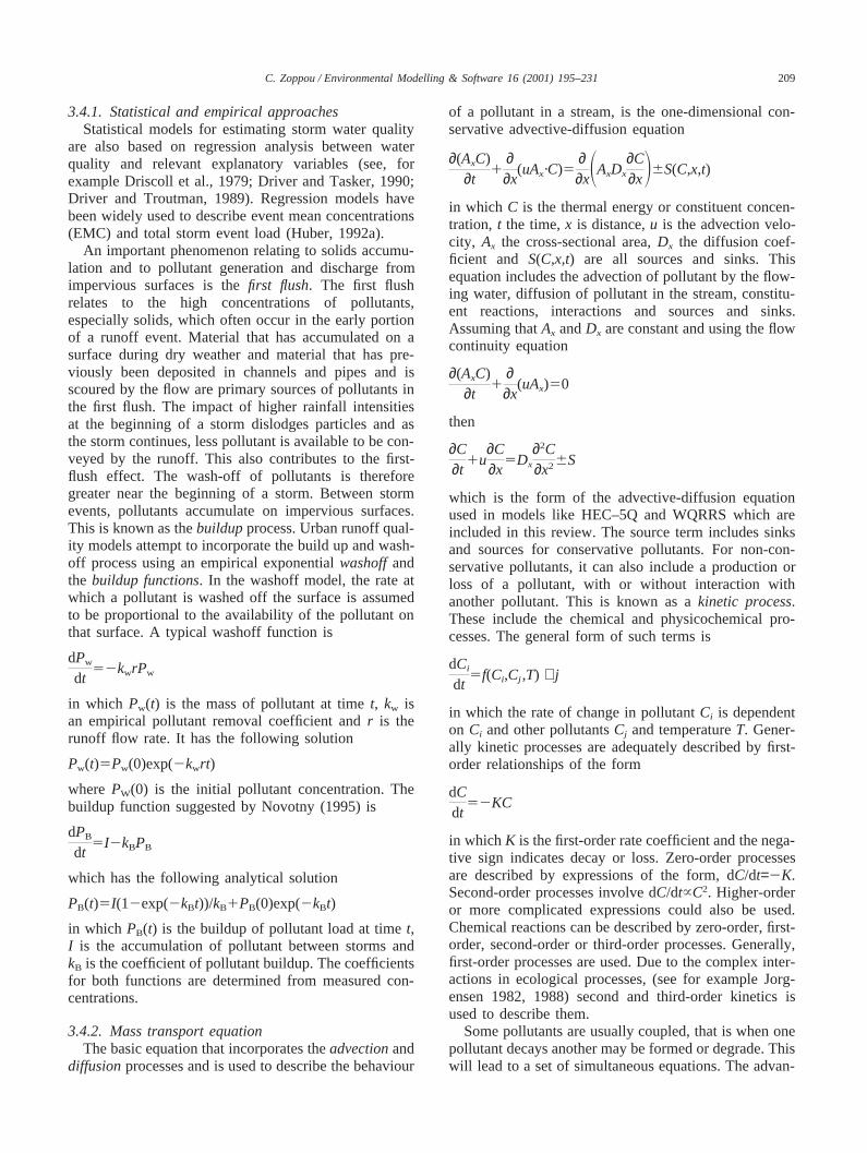
An important phenomenon relating to solids accumu-lation and to pollutant generation and discharge fromimpervious surfaces is thefirst flush. The first flushrelates to the high concentrations of pollutants,especially solids, which often occur in the early portionof a runoff event. Material that has accumulated on asurface during dry weather and material that has pre-viously been deposited in channels and pipes and isscoured by the flow are primary sources of pollutants inthe first flush. The impact of higher rainfall intensitiesat the beginning of a storm dislodges particles and asthe storm continues, less pollutant is available to be con-veyed by the runoff. This also contributes to the first-flush effect. The wash-off of pollutants is thereforegreater near the beginning of a storm. Between stormevents, pollutants accumulate on impervious surfaces.This is known as thebuildupprocess. Urban runoff qual-ity models attempt to incorporate the build up and wash-off process using an empirical exponentialwashoffandthe buildup functions. In the washoff model, the rate atwhich a pollutant is washed off the surface is assumedto be proportional to the availability of the pollutant onthat surface. A typical washoff function is
dPw
dt52kwrPw
in which Pw(t) is the mass of pollutant at timet, kw isan empirical pollutant removal coefficient andr is therunoff flow rate. It has the following solution
Pw(t)5Pw(0)exp(2kwrt)
wherePW(0) is the initial pollutant concentration. Thebuildup function suggested by Novotny (1995) is
dPB
dt5I2kBPB
which has the following analytical solution
PB(t)5I(12exp(2kBt))/kB1PB(0)exp(2kBt)
in which PB(t) is the buildup of pollutant load at timet,I is the accumulation of pollutant between storms andkB is the coefficient of pollutant buildup. The coefficientsfor both functions are determined from measured con-centrations.
3.4.2. Mass transport equationThe basic equation that incorporates theadvectionand
diffusionprocesses and is used to describe the behaviour
of a pollutant in a stream, is the one-dimensional con-servative advective-diffusion equation
∂(AxC)∂t
1∂∂x
(uAx·C)5∂∂xSAxDx
∂C∂xD6S(C,x,t)
in which C is the thermal energy or constituent concen-tration, t the time,x is distance,u is the advection velo-city, Ax the cross-sectional area,Dx the diffusion coef-ficient and S(C,x,t) are all sources and sinks. Thisequation includes the advection of pollutant by the flow-ing water, diffusion of pollutant in the stream, constitu-ent reactions, interactions and sources and sinks.Assuming thatAx andDx are constant and using the flowcontinuity equation
∂(AxC)∂t
1∂∂x
(uAx)50
then
∂C∂t
1u∂C∂x
5Dx
∂2C∂x26S
which is the form of the advective-diffusion equationused in models like HEC–5Q and WQRRS which areincluded in this review. The source term includes sinksand sources for conservative pollutants. For non-con-servative pollutants, it can also include a production orloss of a pollutant, with or without interaction withanother pollutant. This is known as akinetic process.These include the chemical and physicochemical pro-cesses. The general form of such terms is
dCi
dt5f(Ci,Cj ,T) ∀j
in which the rate of change in pollutantCi is dependenton Ci and other pollutantsCj and temperatureT. Gener-ally kinetic processes are adequately described by first-order relationships of the form
dCdt
52KC
in whichK is the first-order rate coefficient and the nega-tive sign indicates decay or loss. Zero-order processesare described by expressions of the form, dC/dt=2K.Second-order processes involve dC/dt~C2. Higher-orderor more complicated expressions could also be used.Chemical reactions can be described by zero-order, first-order, second-order or third-order processes. Generally,first-order processes are used. Due to the complex inter-actions in ecological processes, (see for example Jorg-ensen 1982, 1988) second and third-order kinetics isused to describe them.
Some pollutants are usually coupled, that is when onepollutant decays another may be formed or degrade. Thiswill lead to a set of simultaneous equations. The advan-
210 C. Zoppou / Environmental Modelling & Software 16 (2001) 195–231
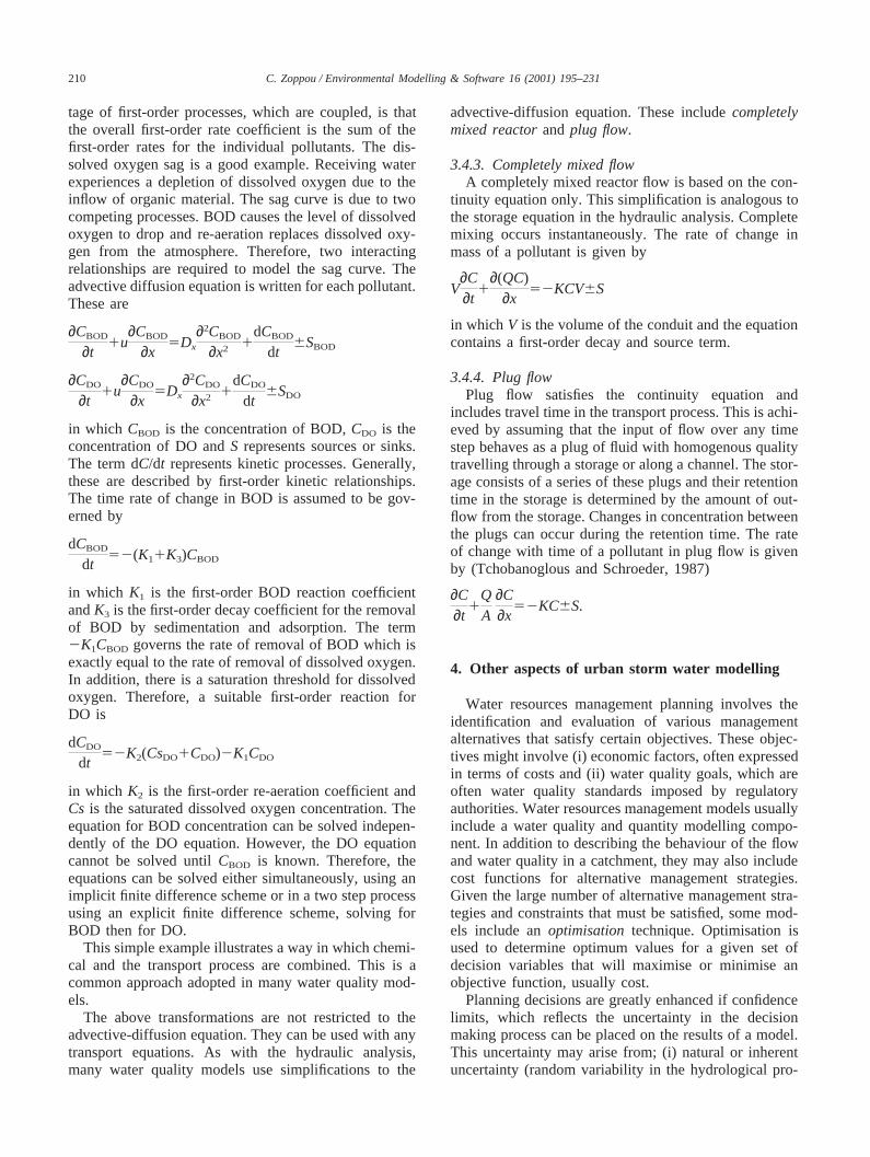
tage of first-order processes, which are coupled, is thatthe overall first-order rate coefficient is the sum of thefirst-order rates for the individual pollutants. The dis-solved oxygen sag is a good example. Receiving waterexperiences a depletion of dissolved oxygen due to theinflow of organic material. The sag curve is due to twocompeting processes. BOD causes the level of dissolvedoxygen to drop and re-aeration replaces dissolved oxy-gen from the atmosphere. Therefore, two interactingrelationships are required to model the sag curve. Theadvective diffusion equation is written for each pollutant.These are
∂CBOD
∂t1u
∂CBOD
∂x5Dx
∂2CBOD
∂x2 1dCBOD
dt6SBOD
∂CDO
∂t1u
∂CDO
∂x5Dx
∂2CDO
∂x2 1dCDO
dt6SDO
in which CBOD is the concentration of BOD,CDO is theconcentration of DO andS represents sources or sinks.The term dC/dt represents kinetic processes. Generally,these are described by first-order kinetic relationships.The time rate of change in BOD is assumed to be gov-erned by
dCBOD
dt52(K11K3)CBOD
in which K1 is the first-order BOD reaction coefficientandK3 is the first-order decay coefficient for the removalof BOD by sedimentation and adsorption. The term2K1CBOD governs the rate of removal of BOD which isexactly equal to the rate of removal of dissolved oxygen.In addition, there is a saturation threshold for dissolvedoxygen. Therefore, a suitable first-order reaction forDO is
dCDO
dt52K2(CsDO1CDO)2K1CDO
in which K2 is the first-order re-aeration coefficient andCs is the saturated dissolved oxygen concentration. Theequation for BOD concentration can be solved indepen-dently of the DO equation. However, the DO equationcannot be solved untilCBOD is known. Therefore, theequations can be solved either simultaneously, using animplicit finite difference scheme or in a two step processusing an explicit finite difference scheme, solving forBOD then for DO.
This simple example illustrates a way in which chemi-cal and the transport process are combined. This is acommon approach adopted in many water quality mod-els.
The above transformations are not restricted to theadvective-diffusion equation. They can be used with anytransport equations. As with the hydraulic analysis,many water quality models use simplifications to the
advective-diffusion equation. These includecompletelymixed reactorandplug flow.
3.4.3. Completely mixed flowA completely mixed reactor flow is based on the con-
tinuity equation only. This simplification is analogous tothe storage equation in the hydraulic analysis. Completemixing occurs instantaneously. The rate of change inmass of a pollutant is given by
V∂C∂t
1∂(QC)
∂x52KCV6S
in which V is the volume of the conduit and the equationcontains a first-order decay and source term.
3.4.4. Plug flowPlug flow satisfies the continuity equation and
includes travel time in the transport process. This is achi-eved by assuming that the input of flow over any timestep behaves as a plug of fluid with homogenous qualitytravelling through a storage or along a channel. The stor-age consists of a series of these plugs and their retentiontime in the storage is determined by the amount of out-flow from the storage. Changes in concentration betweenthe plugs can occur during the retention time. The rateof change with time of a pollutant in plug flow is givenby (Tchobanoglous and Schroeder, 1987)
∂C∂t
1QA
∂C∂x
52KC6S.
4. Other aspects of urban storm water modelling
Water resources management planning involves theidentification and evaluation of various managementalternatives that satisfy certain objectives. These objec-tives might involve (i) economic factors, often expressedin terms of costs and (ii) water quality goals, which areoften water quality standards imposed by regulatoryauthorities. Water resources management models usuallyinclude a water quality and quantity modelling compo-nent. In addition to describing the behaviour of the flowand water quality in a catchment, they may also includecost functions for alternative management strategies.Given the large number of alternative management stra-tegies and constraints that must be satisfied, some mod-els include anoptimisation technique. Optimisation isused to determine optimum values for a given set ofdecision variables that will maximise or minimise anobjective function, usually cost.
Planning decisions are greatly enhanced if confidencelimits, which reflects the uncertainty in the decisionmaking process can be placed on the results of a model.This uncertainty may arise from; (i) natural or inherentuncertainty (random variability in the hydrological pro-
211C. Zoppou / Environmental Modelling & Software 16 (2001) 195–231
cesses or in costs), (ii) model uncertainty (from the useof a simplified model to describe a complex physicalprocess) and (iii) parameter uncertainty (model para-meters are not known with certainty).Uncertainty analy-sis is a technique that can be used to quantify uncertaintyin the modelling results. Uncertainty analysis can beused to identify the dominant sources of uncertaintyaffecting the reliability of the results from a model. Thiswill focus both data gathering and research activities inan attempt to reduce the uncertainty in these parametersand in the modelled results.
4.1. Optimisation
Optimisation provides a mechanism to automate a sys-tematic series of executions of a model in search of anoptimum solution from a range of possible outcomes.The best solution may be a minimum in the least costsense or the largest improvement for a given investment.This is defined mathematically by theobjective function.The coupling of a storm water model with an optimis-ation technique represents an important and powerfultool for the management of urban storm water. Optimis-ation techniques available include; (i) linear program-ming, (ii) nonlinear programming, (iii) dynamic pro-gramming and (iv) simulated annealing. Simulatedannealing (Kirkpatrick et al., 1983) is not commonlyemployed in water resources problems, with otherapproaches being more common. Examples in waterresources projects where optimisation techniques havebeen reported are: Allen and Bridgeman (1986), Beheraet al. (1999), Brendecke et al. (1989), Carriaga and Mays(1995), Chu and Yeh (1978), Chung et al. (1989), Diazand Fontane (1989), Ford et al. (1981), Labadie et al.(1980), Lansey and Basnet (1991), Lindell et al. (1987),Martin (1983, 1987), Nitivattananon et al. (1996) andOstfeld and Shamir (1996).
Optimisation is also used in some models tocalibratemodel parameters. This is a process whereby the modelresponse is fitted to an observed catchment response byadjusting a number of model parameters. This is donein an automatic and systematic way using an optimis-ation procedure.
4.1.1. Linear programmingThe general form of the linear programming problem
is as follows
minimise (or maximise) Z=Onj51
cjxj
subject to Onj21
aij xj #bi for i=1, 2, . . .,m
and xj $0 for j=1, 2, . . .,n
in which Z is the objective function,xj are the decision
variables,cj, aij andbi are constants,n is the number ofdecision variables andm is the number of constraints.The problem consists of minimising a linear objectivefunction subject to a set of linear constraints. Theiradvantage is that simple and efficient solution algorithmsexist, such asthe simplex algorithm(Press et al., 1992).It is relatively simple to include the nonegativity con-straint. This is important when dealing with physicalquantities, for example, the number of pipes must havea positive value. The linearity restriction of linear pro-gramming restricts its applicability. Nevertheless, manywater resources problems can be described realisticallyby linear objective functions and constraints.
4.1.2. Dynamic programmingThe dynamic programming approach involves decom-
posing a complex problem into a series of simpler sub-problems, which are solved sequentially by transferringinformation from one level to the next level of the com-putations. These stages can represent different points inspace or time or activities with a decision required ateach stage. For anN-stage problem, the order of thefor-ward computation is
f1(x1)→f2(x2)→ · · ·→fi−1(xi−1)→fi(xi)→ · · ·→fN(xN)
in which fi(xi) is the cumulative optimum return forstages 1, 2, . . ., andi given the state of the system isxi. This pattern can be written as a recursive equationrelating the statesfi(xi) to fi21(xi21) as
f1(x1)5 maxm1
c1,m1#x1
{ R1,m1}
and
fi(xi)5 maxmi
ci,mi#xi
{ Ri,mi1fi−1(xi2ci,mi
)}, i51, 2, . . .,N
in which ci,miis the penalty for alternativemi for statei
andRi,miis thereturn functionof a decision. The conver-
sion fromxi21 to xi is usually referred to asstate trans-formation. Each stage must have a number of other statesassociated with it. The states describe the possible con-ditions in which the system might be at that stage of thecomputations. The effect of a decision at each stage ofthe problem is to transform the current state of the sys-tem into a state associated with the next stage. The con-nection between various states is defined by a decision.Thestateof the system represents the link between suc-cessful stages so that when each stage is optimised separ-ately, the resulting decision is automatically feasible forthe entire problem. It also allows for the optimumdecision to be made for the remaining stages withoutchecking the effect future decisions have on decisionsmade previously. A return function is the utility or costof each potential state transformation. The optimality of
212 C. Zoppou / Environmental Modelling & Software 16 (2001) 195–231
the decision required at the current stage is judged interms of its impact on the return function for the currentstage and all subsequent stages.
The recursive equations are the only unifying theoryfor dynamic programming, it does not provide details onhow the optimisation for each sub-problem is solved. Inaddition, there is no guarantee that each sub-problem canbe solved. Dynamic programming, although consideredas a powerful technique, is generally more difficult tolearn and understand than linear programming.
4.1.3. Nonlinear programmingMany problems in water resources are nonlinear. In
some instances, the problem may be linearised and linearprogramming is employed in an iterative scheme wherethe solution is refined with each iteration. Robustmethods are available for optimising nonlinear functions.Nonlinear optimisation algorithms can be classifiedbroadly as search methods. The algorithm systematicallyand automatically searches through all feasible solutionsand finds a solution which satisfies the objective func-tion. Search techniques such as conjugate gradient andpattern search methods are simple to implement withcomplex models. In many nonlinear programming tech-niques, the search direction is governed by the localslope of the function being optimised. Successful movesare generally in a downhill direction. Unfortunately, thisstrategy may only locate a local and not the global mini-mum and the iterative nature of the approach means thatnonlinear programming can be computationally expens-ive.
4.2. Uncertainty analysis
Uncertainty analysis attempts to quantify the effectmodel parameters that are not known with certainty haveon the models response. Uncertainty analysis can be per-formed analytically or numerically. For complex prob-lems, numerical techniques are exclusively used.Numerical reliability techniques include, in order ofaccuracy: (i)sensitivity analysis, (ii) mean value first-order second moment analysis(iii) point estimatemethod, (vi) Monte Carlo simulationand (v) Mellintransform. There are very few applications of the pointestimate and Mellin transform to water resources prob-lems. The point estimate is a relatively new techniqueand the Mellin transform is restricted to certain func-tional relationships not generally satisfied in complicatedmodels. Examples of the application of uncertaintyanalysis to water resources problems can be found inBurges and Lettenmaier (1975), Chatterton et al. (1982),Jaffe and Parker (1984), Melching and Yoon (1996),Melching et al. (1991), Scavia et al. (1981), Reddy et al.(1996), Tung (1987, 1989, 1990), Warwick and Wilson(1990), Willey (1986), Xu and Goulter (1998), Yeh andTung (1993) and Zoppou and Li (1992, 1993).
4.2.1. Sensitivity analysisSensitivity analysis is simply establishing the change
in model response,Y due to a small perturbation in eachk independent model variablesx=(x1, . . .,xk). The modelis considered most sensitive to the parameters that pro-duce the greatest model response. This is equivalent toestimating the derivative
∂Yj
∂xi
∀i.
Greater resources should be allocated to those para-meters that produce the greatest model response. Toeffectively compare the sensitivity of a model to variousparameters the derivative must be normalised. Therefore,the normal sensitivity coefficientSij for outputYj to inputxi is given by
Sij 5DYj /Yj
Dxj /xj
in which Dx and Dy are the magnitudes of the pertur-bations andxj and Yi are the reference values for theoutput and input variables respectively. Sensitivityanalysis does not consider the variability in a parameter.A highly sensitive parameter that is relatively welldefined may have less influence on the reliability of theresults from a model than a much less sensitive para-meter that has large uncertainties. In this case, parameteruncertainty must be considered.
4.2.2. Mean value first-order second moment analysisConsider a model response that is a function of a sin-
gle variable, x so that Y=f(x). The function can beexpanded as a Taylor series aroundx=mx, wheremx isthe mean value ofx to give
Y5f(mx)1dfdx
(x2mx)112
d2fdx2(x2mx)1 · · ·
where the derivatives df/dx, d2f/dx2,… are evaluated atx=mx. If second and higher-order terms are neglected, theresultingfirst-order expression forY is
Y<f(mx)1dfdx
(x2mx).
Taking the expectation of both sides, then
mY5E[Y]5f(mx)
that is the expected value ofE[Y] is the mean value ofYand is obtained by evaluatingf(x) using the mean valueof x=mx. Combining the above results, the variance ofYdefined by
s2Y5E[(Y2mx)2]
can be approximated by
s2Y<EFSdf
dx(x2mx)D2G5Sdf
dxD2
s2x
213C. Zoppou / Environmental Modelling & Software 16 (2001) 195–231
in which s2x is the variance ofx. If Y is dependent onk
mutually independent variablesx=(x1, . . ., xk) it can beshown that
mY5f(mx1, . . .,mxk
) ands2Y5Ok
i51
S dfdxi
D2
s2xi.
The components of the output variance representweights of the input variances multiplied by the squareof the sensitivity of the model output to the input. There-fore, it is relatively simple to extend sensitivity analysisto perform mean value first-order second moment analy-sis. The only additional information that is required isthe standard deviation of the input variables, which is ameasure of what is not known about the variable. Corre-lated random variables can be considered in first-ordersecond moment analysis. Implicit in mean value first-order second moment analysis is that the model responseis linear or approximately linear near the perturbedvalues. Since only the mean and variance of the modelresponse is provided in mean value first-order secondmoment analysis, only a two parameter distribution canbe fitted to the model response so that confidence limitscan be inferred from the fitted distribution.
4.2.3. Monte Carlo simulationIn Monte Carlo simulation, variables are sampled at
random from pre-defined probability distributions, withor without correlation and the distribution of the modelresponse is obtained from repeated simulations. The val-idity of this model is not affected by non-linearities inthe water quality model. Comparing the standard devi-ation estimates from Monte Carlo simulations with thosefrom first-order second moment analysis provides anindication of the model non-linearity. The major draw-back with Monte Carlo simulation is that the probabilitydistribution of the uncertain parameters must be knownor assumed. This may not be possible if there is insuf-ficient data to establish these distributions. The othermajor problem with Monte Carlo simulation is that itcan be computationally expensive. In some problems1000s of repeated simulations of the model are required.
Monte Carlo simulation has the advantage of estimat-ing model frequency distributions, but it is compu-tationally expensive if a large number of random vari-ables are involved in the problem. The cumulativefrequency distribution of the model response is useful inevaluating overall dispersion in the model predictionsand in assessing the likelihood of violating a water qual-ity standard.
The US Environmental Protection Agency (Salhotraet al., 1988) has developed a generic Monte Carlo mod-ule for use with any transport model. The generator cansample from Normal, log Normal, uniform, exponential,empirical, triangular and JohnsonSB and SU distri-butions. Correlated random variables can also be gener-ated.
4.3. Economic analysis
Water resources managers must be able to identify thebest management strategy from a number of alternativescenarios. The best management strategy could bechosen from those alternatives that do not compromisethe storm water infrastructure using hydraulic analysis.Water quality objectives could be used to select the bestmanagement strategy. Economic analysis providesanother method for assessing alternative storm watermanagement options. Traditionally, economic analysisgenerally involved a cost–benefit analysis. The use ofcost–benefit criteria as a decision-making tool is a matterof expediency, since they primarily deal with tangibleand quantifiable factors and hence they can be analysedobjectively. These tangible factors are commonlyreferred to aslife-cyclecosts and include such things as:maintenance, capital, operating, replacement, disposaland land acquisition costs.
Economists often lump criteria that are difficult toassign a monetary value asexternalities. Externalitiesmight include social well being, national security,regional growth and stability, preservation of naturalareas and risk management costs. It is clear that societyalso has constraints it wants to impose on projects thatdo not necessarily have a monetary value. Traditionalcost–benefit analysis does not consider these factors. Theproblem is that externalities are intangible and non-quan-tifiable, hence would be treated rather subjectively. Thereal question is not whether externalities should be con-sidered as a planning objective, but rather how theyshould be considered objectively within the planningframework. These objectives are not mutually exclusive,in fact they are often conflicting. Contributions to onemay only be made at the expense of the other. Forexample, the cost of increasing the capacity of a wastewater infrastructure to eliminate overflows may be sig-nificantly greater than the cost associated with the over-flow. Using cost–benefit analysis to eliminate overflowsin a design may not be economically feasible. However,social acceptance of overflows may reverse the decisionbased on a cost–benefit analysis alone. The problem ishow a trade-off should occur. Does an intangible socialdis-benefit, in terms of environmental degradation forexample, provide sufficient justification for rejecting aproject, irrespective of the cost–benefit objective?
Fortunately, planners do not make the final decision,nor do they pass legislation that may influence planningdecisions. The real decision-making lies with politicians.Planners do however, demonstrate the cost-effectiveness,the social, environmental and technical feasibility of aproject. Therefore, the impacts of life-cycle costs andexternalities should be considered in project design andranking. An economic analysis of various managementstrategies can be misleading if the infrastructure model-ling is inadequate.
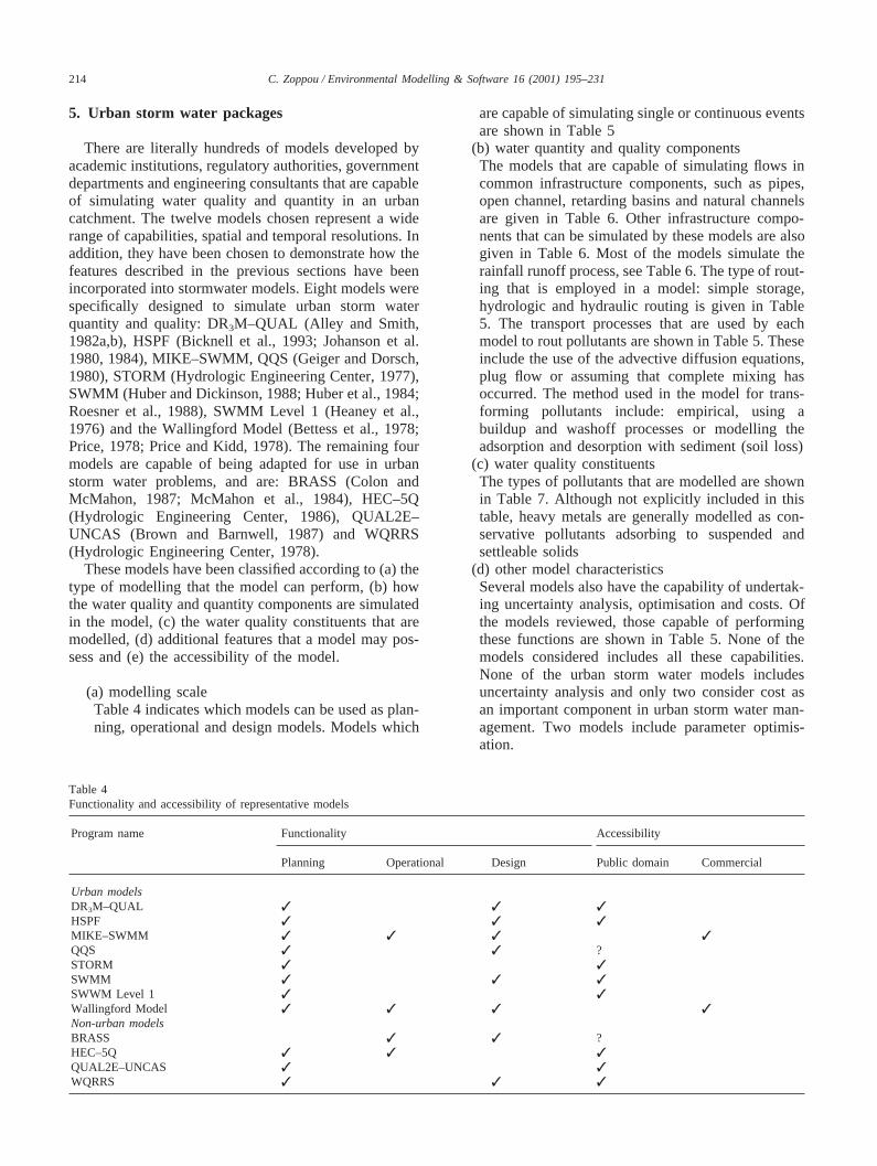
214 C. Zoppou / Environmental Modelling & Software 16 (2001) 195–231
5. Urban storm water packages
There are literally hundreds of models developed byacademic institutions, regulatory authorities, governmentdepartments and engineering consultants that are capableof simulating water quality and quantity in an urbancatchment. The twelve models chosen represent a widerange of capabilities, spatial and temporal resolutions. Inaddition, they have been chosen to demonstrate how thefeatures described in the previous sections have beenincorporated into stormwater models. Eight models werespecifically designed to simulate urban storm waterquantity and quality: DR3M–QUAL (Alley and Smith,1982a,b), HSPF (Bicknell et al., 1993; Johanson et al.1980, 1984), MIKE–SWMM, QQS (Geiger and Dorsch,1980), STORM (Hydrologic Engineering Center, 1977),SWMM (Huber and Dickinson, 1988; Huber et al., 1984;Roesner et al., 1988), SWMM Level 1 (Heaney et al.,1976) and the Wallingford Model (Bettess et al., 1978;Price, 1978; Price and Kidd, 1978). The remaining fourmodels are capable of being adapted for use in urbanstorm water problems, and are: BRASS (Colon andMcMahon, 1987; McMahon et al., 1984), HEC–5Q(Hydrologic Engineering Center, 1986), QUAL2E–UNCAS (Brown and Barnwell, 1987) and WQRRS(Hydrologic Engineering Center, 1978).
These models have been classified according to (a) thetype of modelling that the model can perform, (b) howthe water quality and quantity components are simulatedin the model, (c) the water quality constituents that aremodelled, (d) additional features that a model may pos-sess and (e) the accessibility of the model.
(a) modelling scaleTable 4 indicates which models can be used as plan-ning, operational and design models. Models which
Table 4Functionality and accessibility of representative models
Program name Functionality Accessibility
Planning Operational Design Public domain Commercial
Urban modelsDR3M–QUAL ✓ ✓ ✓HSPF ✓ ✓ ✓MIKE–SWMM ✓ ✓ ✓ ✓QQS ✓ ✓ ?STORM ✓ ✓SWMM ✓ ✓ ✓SWWM Level 1 ✓ ✓Wallingford Model ✓ ✓ ✓ ✓Non-urban modelsBRASS ✓ ✓ ?HEC–5Q ✓ ✓ ✓QUAL2E–UNCAS ✓ ✓WQRRS ✓ ✓ ✓
are capable of simulating single or continuous eventsare shown in Table 5
(b) water quantity and quality componentsThe models that are capable of simulating flows incommon infrastructure components, such as pipes,open channel, retarding basins and natural channelsare given in Table 6. Other infrastructure compo-nents that can be simulated by these models are alsogiven in Table 6. Most of the models simulate therainfall runoff process, see Table 6. The type of rout-ing that is employed in a model: simple storage,hydrologic and hydraulic routing is given in Table5. The transport processes that are used by eachmodel to rout pollutants are shown in Table 5. Theseinclude the use of the advective diffusion equations,plug flow or assuming that complete mixing hasoccurred. The method used in the model for trans-forming pollutants include: empirical, using abuildup and washoff processes or modelling theadsorption and desorption with sediment (soil loss)
(c) water quality constituentsThe types of pollutants that are modelled are shownin Table 7. Although not explicitly included in thistable, heavy metals are generally modelled as con-servative pollutants adsorbing to suspended andsettleable solids
(d) other model characteristicsSeveral models also have the capability of undertak-ing uncertainty analysis, optimisation and costs. Ofthe models reviewed, those capable of performingthese functions are shown in Table 5. None of themodels considered includes all these capabilities.None of the urban storm water models includesuncertainty analysis and only two consider cost asan important component in urban storm water man-agement. Two models include parameter optimis-ation.
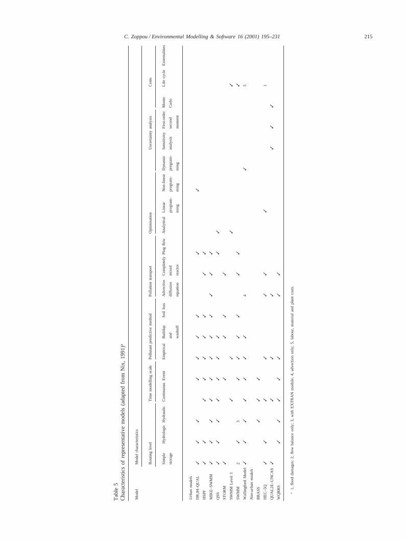
215C. Zoppou / Environmental Modelling & Software 16 (2001) 195–231
Tab
le5
Cha
ract
eris
tics
ofre
pres
enta
tive
mod
els
(ada
pted
from
Nix
,19
91)
a
Mod
elM
odel
char
acte
ristic
s
Rou
ting
leve
lT
ime
mod
ellin
gsc
ale
Pol
luta
ntpr
edic
tive
met
hod
Pol
lutio
ntr
ansp
ort
Opt
imis
atio
nU
ncer
tain
tyan
alys
isC
osts
Sim
ple
Hyd
rolo
gic
Hyd
raul
icC
ontin
uous
Eve
ntE
mpi
rical
Bui
ldup
Soi
llo
ssA
dvec
tive
Com
plet
ely
Plu
gflo
wA
naly
tical
Line
arN
on-li
near
Dyn
amic
Sen
siti
vity
Firs
t-or
der
Mon
teLi
fecy
cle
Ext
erna
litie
s
stor
age
and
diffu
sion
mix
edpr
ogra
m-
prog
ram
-pr
ogra
m-
anal
ysis
seco
ndC
arlo
was
hoff
equa
tion
reac
tor
min
gm
ing
min
gm
omen
t
Urb
an
mo
de
ls
DR
3M
–QU
AL
✓✓
✓✓
✓✓
✓✓
✓
HS
PF
✓✓
✓✓
✓✓
✓✓
✓
MIK
E–S
WM
M✓
✓✓
✓✓
✓✓
✓✓
✓✓
QS
S✓
✓✓
✓✓
✓✓
✓✓
ST
OR
M✓
✓✓
✓✓
SW
MM
Leve
l1
✓✓
✓✓
SW
MM
2✓
3✓
✓✓
✓✓
✓✓
Wal
lingf
ord
Mod
el✓
✓✓
✓✓
✓✓
4✓
5
No
n-u
rba
nm
od
els
BR
AS
S✓
✓✓
HE
C–5
Q✓
✓✓
✓✓
✓✓
1
QU
AL2
E–U
NC
AS
✓✓
✓✓
✓✓
✓
WQ
RR
S✓
✓✓
✓✓
✓✓
a1,
flood
dam
ages
;2,
flow
bala
nce
only
;3,
with
EX
TR
AN
mod
ule,
4,ad
vect
ion
only
;5,
labo
ur,
mat
eria
lan
dpl
ant
cost
s.
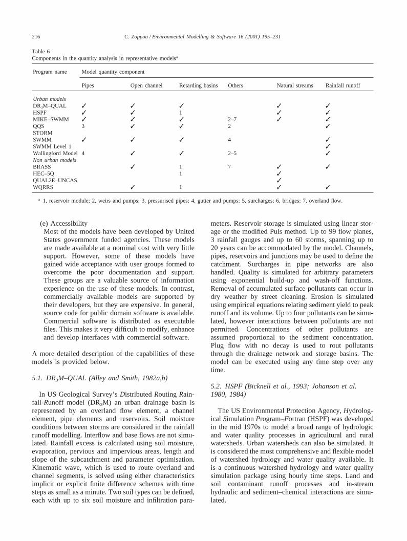
216 C. Zoppou / Environmental Modelling & Software 16 (2001) 195–231
Table 6Components in the quantity analysis in representative modelsa
Program name Model quantity component
Pipes Open channel Retarding basins Others Natural streams Rainfall runoff
Urban modelsDR3M–QUAL ✓ ✓ ✓ ✓ ✓HSPF ✓ ✓ 1 ✓ ✓MIKE–SWMM ✓ ✓ ✓ 2–7 ✓ ✓QQS 3 ✓ ✓ 2 ✓STORMSWMM ✓ ✓ ✓ 4 ✓SWMM Level 1 ✓Wallingford Model 4 ✓ ✓ 2–5 ✓Non urban modelsBRASS ✓ 1 7 ✓ ✓HEC–5Q 1 ✓QUAL2E–UNCAS ✓WQRRS ✓ 1 ✓ ✓
a 1, reservoir module; 2, weirs and pumps; 3, pressurised pipes; 4, gutter and pumps; 5, surcharges; 6, bridges; 7, overland flow.
(e) AccessibilityMost of the models have been developed by UnitedStates government funded agencies. These modelsare made available at a nominal cost with very littlesupport. However, some of these models havegained wide acceptance with user groups formed toovercome the poor documentation and support.These groups are a valuable source of informationexperience on the use of these models. In contrast,commercially available models are supported bytheir developers, but they are expensive. In general,source code for public domain software is available.Commercial software is distributed as executablefiles. This makes it very difficult to modify, enhanceand develop interfaces with commercial software.
A more detailed description of the capabilities of thesemodels is provided below.
5.1. DR3M–QUAL (Alley and Smith, 1982a,b)
In US Geological Survey’sDistributedRouting Rain-fall-Runoff model (DR3M) an urban drainage basin isrepresented by an overland flow element, a channelelement, pipe elements and reservoirs. Soil moistureconditions between storms are considered in the rainfallrunoff modelling. Interflow and base flows are not simu-lated. Rainfall excess is calculated using soil moisture,evaporation, pervious and impervious areas, length andslope of the subcatchment and parameter optimisation.Kinematic wave, which is used to route overland andchannel segments, is solved using either characteristicsimplicit or explicit finite difference schemes with timesteps as small as a minute. Two soil types can be defined,each with up to six soil moisture and infiltration para-
meters. Reservoir storage is simulated using linear stor-age or the modified Puls method. Up to 99 flow planes,3 rainfall gauges and up to 60 storms, spanning up to20 years can be accommodated by the model. Channels,pipes, reservoirs and junctions may be used to define thecatchment. Surcharges in pipe networks are alsohandled. Quality is simulated for arbitrary parametersusing exponential build-up and wash-off functions.Removal of accumulated surface pollutants can occur indry weather by street cleaning. Erosion is simulatedusing empirical equations relating sediment yield to peakrunoff and its volume. Up to four pollutants can be simu-lated, however interactions between pollutants are notpermitted. Concentrations of other pollutants areassumed proportional to the sediment concentration.Plug flow with no decay is used to rout pollutantsthrough the drainage network and storage basins. Themodel can be executed using any time step over anytime.
5.2. HSPF (Bicknell et al., 1993; Johanson et al.1980, 1984)
The US Environmental Protection Agency,Hydrolog-ical SimulationProgram–Fortran (HSPF) was developedin the mid 1970s to model a broad range of hydrologicand water quality processes in agricultural and ruralwatersheds. Urban watersheds can also be simulated. Itis considered the most comprehensive and flexible modelof watershed hydrology and water quality available. Itis a continuous watershed hydrology and water qualitysimulation package using hourly time steps. Land andsoil contaminant runoff processes and in-streamhydraulic and sediment–chemical interactions are simu-lated.
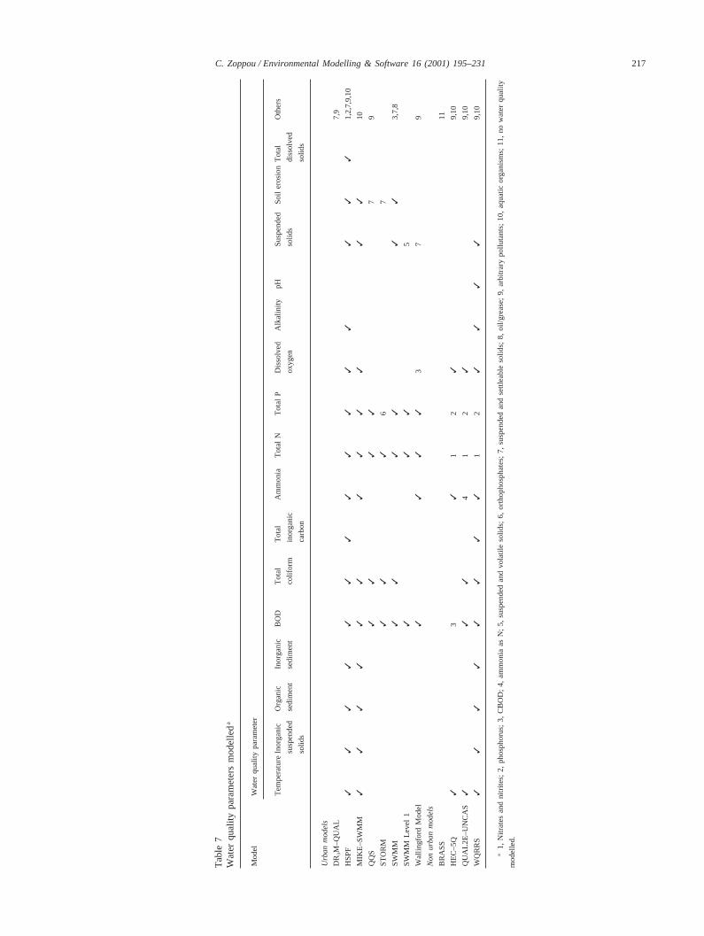
217C. Zoppou / Environmental Modelling & Software 16 (2001) 195–231
Tab
le7
Wat
erqu
ality
para
met
ers
mod
elle
da
Mod
elW
ater
qual
itypa
ram
eter
Tem
pera
ture
Inor
gani
cO
rgan
icIn
orga
nic
BO
DT
otal
Tot
alA
mm
onia
Tot
alN
Tot
alP
Dis
solv
edA
lkal
inity
pHS
uspe
nded
Soi
ler
osio
nT
otal
Oth
ers
susp
ende
dse
dim
ent
sedi
men
tco
lifor
min
orga
nic
oxyg
enso
lids
diss
olve
d
solid
sca
rbon
solid
s
Urb
an
mo
de
ls
DR
3M
–QU
AL
7,9
HS
PF
✓✓
✓✓
✓✓
✓✓
✓✓
✓✓
✓✓
✓1,
2,7,
9,10
MIK
E–S
WM
M✓
✓✓
✓✓
✓✓
✓✓
✓✓
✓10
S✓
✓✓
✓7
9
ST
OR
M✓
✓✓
67
SW
MM
✓✓
✓✓
✓✓
3,7,
8
SW
MM
Leve
l1
✓✓
✓5
Wal
lingf
ord
Mod
el✓
✓✓
✓3
79
No
nu
rba
nm
od
els
BR
AS
S11
HE
C–5
Q✓
3✓
12
✓9,
10
QU
AL2
E–U
NC
AS
✓✓
✓4
12
✓9,
10
WQ
RR
S✓
✓✓
✓✓
✓✓
✓1
2✓
✓✓
✓9,
10
a1,
Nitr
ates
and
nitr
ites;
2,ph
osph
orus
;3,
CB
OD
;4,
amm
onia
asN
;5,
susp
ende
dan
dvo
latil
eso
lids;
6,or
thop
hosp
hate
s;7,
susp
ende
dan
dse
ttlea
ble
sol
ids;
8,oi
l/gre
ase;
9,ar
bitr
ary
pollu
tant
s;10
,aq
uatic
orga
nism
s;11
,no
wat
erqu
ality
mod
elle
d.
218 C. Zoppou / Environmental Modelling & Software 16 (2001) 195–231
For overland flow temperature, DO, CO2, (at satu-ration levels) coliform, nitrogen, phosphorus, pesticidesand arbitrary conservative pollutants are modelled usingempirical relationships between pollutant and water aswell as sediment yield. Rainfall-runoff modellingincludes snowmelt, water balance in the upper and lowersoil storage and groundwater storage for both perviousand impervious surfaces. Interception, evaporation andevapotranspiration are included in the water balancealong with displacement of soil by rainfall. Deepgroundwater storage can become base flow to a stream.Total stream flow is a combination of overland and baseflow. Washoff quality is estimated using linear buildupwith washoff rates directly proportional to runoff. Separ-ate washoff functions are used for each pollutant. Pol-lutants that can be simulated with the runoff include:temperature, pesticides, sediments, nitrogen, phos-phorus, ammonia and conservative pollutants. Absorp-tion and desorption of pollutants between bed sedimentsand water is allowed. Settling and re-suspension of sand,clay and silt sediments are possible. Re-suspension andsettling of silts and clays are based on bed shear stress.Absorption and desorption of many of these pollutants isoptional via first-order kinetics. For impervious surfaces,empirical relationships are used for the washoff, whichis a function of runoff and street cleaning. The advectionof pollutant is estimated using plug flows and completemixing in storages. Overland flow, open and closedchannel flow and sewer routing is with the modifiedkinematic wave equation incorporating the Manningequation. It flags surcharges in the sewer system and res-ervoir routing can be included. Total dissolved solids,chlorides, pesticides, temperature, sediment scour anddeposition, pH, CO2, algae, nitrate, nitrite, orthophosph-orus, total inorganic carbon, DO, BOD, ammonia, photo-plankton, zooplankton and attached algae can be mod-elled in streams and in storages.
5.3. MIKE–SWMM
This package combines MIKE 11 (Havno et al., 1995)and the well known SWMM (Huber et al., 1984; Huberand Dickinson, 1988; Roesner et al., 1988) models. Themerger is intended to use the strengths of MIKE 11 inone-dimensional unsteady flow modelling, which solvesthe shallow water wave equations using an implicit finitedifference scheme, replacing the temperamentalEXTRAN module in SWMM. The combined model canperform hydrologic, hydraulic and water quality analysisof storm water and waste water drainage systems,including sewage treatment plants and water quality con-trol devices. Pipes, pumps, culverts, retarding, detentionponds, pressurised flow in looped connections and over-flows from sewers can be modelled.
Mass balance is used for runoff computations, whichinclude surface detention, lower soil storage and upper
and lower groundwater storage. Runoff consists of over-land and base flow. Two-dimensional overland floodingcan also be simulated using the shallow water wave equ-ation. A sediment budget accounts for erosion and depo-sition. The advective diffusion equation is used to simu-late the transport of pollutants, which are subject to first-order kinetics. It is also solved using an implicit finitedifference scheme. Dissolved and suspended sediments,BOD, DO, nutrients, macrophytes and plankton can besimulated.
MIKE–SWMM can interface with the full suite ofDanish Hydraulic Institute models. They have beenlinked with STORMPAC, a rainfall generation program,the urban sewer network model, MOUSE (Lindberg etal., 1989), MIKE 21 (Dudley et al., 1994) for modellingof estuaries, lagoons and coastal areas, including waterquality and STOAT to assess treatment plant perform-ance. Water quality parameters include: total coliform,total P, total N, DO, temperature, ammonia, nitrate,heavy metals using kinetic descriptions of absorption/desorption to particles, suspended sediments and bedsediments and BOD as both dissolved and attached tosuspended sediments. Sediments are defined as eithercohesive or non-cohesive according to their size andbehaviour. The dynamics of primary production by pho-toplankton and the grazing by zooplankton are described.Primary production by benthic vegetation can also bemodelled. MOUSE can perform real-time control simul-ations and sediment transport in pipe networks. All thesemodels are capable of simulating water quality and quan-tity at any temporal and spatial scale. They can be usedin design, management and operation of a diverse rangeof water resource problems.
5.4. QQS (Geiger and Dorsch, 1980)
The Quality–Quantity Simulator (QQS) can performcontinuous or single event simulation using five-minutetime intervals. It can simulate flows in pipes and chan-nels using an implicit finite difference approximation ofthe kinematic wave equations, storage routing, back-water analysis and pipes under pressure. Looped net-works, weirs and pumps can be simulated. Dry weatherflow and quality based on empirical relationships havea diurnal and population dependency. Washoff functionis dependent on the accumulation of dust and the timeinterval between storms and street sweeping. Qualityrouting through channels and pipes, storage units andreceiving water is performed using plug flow. Up to fourarbitrary conservative pollutants can be routed. Empiri-cal washoff functions are available for BOD, COD, sus-pended solids, settleable solids, total nitrogen, total Pand faecal coliform.
219C. Zoppou / Environmental Modelling & Software 16 (2001) 195–231
5.5. STORM: (Hydrologic Engineering Center, 1977)
The US Corps of Engineers,Storage, Treatment,Overflow, Runoff Model is capable of simulating runoffand pollutant loads from urban and rural watersheds inresponse to precipitation. It is a continuous model usinghourly time steps and it can be used for single events.Using hourly precipitation, runoff from a catchment issimply the accumulation of runoff from upstream sub-catchment. There is no attempt to rout the runoff throughthe catchment. Three methods are available for calculat-ing the hourly runoff: coefficient method, soil-complex-cover method and the unit hydrograph method. The run-off coefficient method is identical to that used in SWMMLevel 1. Runoff is a linear relationship between runoffand the precipitation minus rainfall interception. How-ever, here the impervious and pervious runoff coef-ficients and the fraction of impervious area are variableand not fixed. Erosion is estimated using an empiricalrelationship. Two methods are available to simulate pol-lutant accumulation. The pollutant accumulation is pro-portional to the dust and dirt accumulated or a simplerlinear function of time. Washoff is proportional to theamount of pollutant remaining. Pollutants that are treatedas conservative include: suspended and settleable solids,BOD, total nitrogen and orthophosphates. Coliforms arealso modelled. No treatment is assumed to occur in astorage.
5.6. SWMM (Huber et al., 1984; Huber andDickinson, 1988; Roesner et al., 1988)
SWMM simulates both water quality and quantity ofurban storm water runoff and combined sewer overflow.This is both a continuous and single event model. Sur-face runoff is based on rainfall intensities and antecedentmoisture conditions, land use and topography. A simplenonlinear reservoir storage is used to simulate therainfall-runoff process, which includes infiltrationdepression storage, evaporation and surface runoff.Infiltration is routed through upper and lower subzonesand may return as runoff. Surface pollutant allows bothlinear and nonlinear accumulation with time. Washoff issimulated as a simple function of runoff or as a first-order decay relationship. Sewer flows are generatedusing land use, population density and other factors.Infiltration into the sewer system is dependent on thesewer condition and groundwater levels. Flows and pol-lutants are routed through the sewer system using amodified kinematic wave approximation and assumingcomplete mixing. Hydrographs along the sewer systemare modified to represent storage and treatment effects.This includes retention time, treatment efficiency as wellas estimating costs. Surcharging is not included. Pol-lutants in storage systems can be modelled as eithercomplete mixing or plug flow. The stand-alone module
EXTRAN permits SWMM to rout inflow hydrographsthrough open channel and a closed conduit system usingan explicit numerical solution of the shallow water waveequations. Unfortunately, routing of pollutant loads,sewer infiltration and dry-weather flows are not currentlymodelled. Eight conservative pollutants are: suspendedsolids, settleable solids, BOD, COD, total nitrogen, totalP, oil/grease, total coliforms as well as an arbitrary pol-lutant and erosion simulated in surface runoff.
5.7. SWMM Level 1: (Heaney et al., 1976)
SWMM Level 1 estimates average annual runoff froma watershed with the minimum of input data. The aver-age annual runoff is a simple linear function of the aver-age annual precipitation. Losses from rainfall intercep-tion are considered. The runoff coefficient is a functionof pervious and impervious areas, with the latter a func-tion of population. Simple relationships are used to esti-mate the annual load of pollutant. The pollutants aretreated as independent and they are directly proportionalto the average annual precipitation, population density,the effectiveness of street sweeping and the catchmentarea. Land uses considered are residential, commercial,industrial and other developed areas. Pollutants con-sidered are: BOD, suspended solids, volatile solids, totalP and total N. Preliminary estimates for costs of storingand treating storm water pollutants have been includedin SWMM Level 1. This is a simple linear function withconstant costs for treatment and storage. The simple costfunction is solved analytically to provide a function rep-resenting the least cost combination of storage and treat-ment required satisfying a certain level of pollutantremoval. SWMM Level 1 is not implemented on a com-puter, it is applied with tables and nomographs. It is partof the EPA’s SWMM package.
5.8. Wallingford Model (Price, 1978; Price and Kidd,1978; Bettess et al., 1978)
The Wallingford model is a suite of models developedat the Hydraulics Research Institute, Wallingford, UnitedKingdom. It includes a rainfall-runoff model (WASSP),a simple (WALLRUS) and full dynamic pipe routingmodel (SPIDA) and a water quality module(MOSQITO). The model can be applied to storm wateror sewer systems or to the combined system using 15minute time steps. It has been used for real time oper-ational, design and planning simulations.
Hyetographs can be defined as input if required. Alter-natively, synthetic rain storms can be generated using avariety of techniques including: depth–duration–fre-quency relationships and the modified Chicago method.An empirical relationship is used to determine the aver-age spatial rainfall over a catchment using rainfall inten-sity and a spatial smoothing factor. The rainfall-runoff
220 C. Zoppou / Environmental Modelling & Software 16 (2001) 195–231
model employs a modified rational method, which isessentially the same as the rational method with theinclusion of a routing coefficient. The routing coefficientincorporates the proportion of impervious area, soil type,evapotranspiration and antecedent conditions. Five ante-cedent moisture models are provided. The runoff is esti-mated by distributing rainfall between impervious, roofsand pervious areas. The amount of runoff from theseareas is based on area type, catchment slope, initial lossto depression storage and continuing loss by infiltration.The attenuation caused by surface storage is simulatedby a non-linear reservoir storage model. Two empiricalrunoff routing models available. One is for catchmentsup to 1 ha and up to 100 ha. The latter relationship is anonlinear relationship and uses area, slope and length ofthe catchment. Due to the size of a large catchment, therunoff is also lagged. The time delay is also a nonlinearempirical relationship based on area, bed slope andlength of the catchment. For small catchments, overlandflow is routed using two equal linear reservoirs in serieswith routing coefficients dependent on rainfall intensity,contributing area and surface slope. The use ofSWMM’s runoff model is optional. Four other runoffmodelling approaches are available which utilise simplestorages. A time delay is also introduced so that the peakrunoff lags the peak rainfall.
The Muskingum–Cunge method and the solution ofthe full shallow water wave equations are options forrouting flows through the storm water network. Bothdefined and user-specified pipes and channels areoptions. Pressurised pipes are modelled with either theSt. Venant equations using a Preissmann slot or the St.Venant equations with the local acceleration term neg-lected. An implicit finite difference scheme is used tosolve the equations. The advection equation is used inthe pollution transport process, while diffusion isignored. Erosion and deposition processes are modelled,including sedimentation in pipes. Manholes, overflows,tanks, pump wells or storages can be modelled in thepipe network. Suspended sediments in tanks are assumedto be well mixed with a layer of cleaner water availableat the top of the tank for overflow. Water quality pol-lutants that can be modelled are BOD, COD, ammonia,kjeldahl nitrogen, total P and four arbitrary conservativepollutants that may be attached to sediments or in sol-ution.
Buildup of pollutants on impervious surfaces is anempirical relationship, which is based on time. Washoffis also a first-order decay model that is a function ofrainfall intensity. Pollutants that are available to bewashed off impervious surfaces are BOD, COD, total N,ammonia, total P and four arbitrary pollutants. Washoffpollutants can be transported by absorption to sedimentsor in solution.
A dynamic programming technique is used to deter-mine the minimum construction costs of a storm water
network using pipe diameter, trench depth and gradientas the optimised variables. Both existing and proposeddesigns can be simulated by taking into account stormwater overflows, on-line and off-line detention storagesand pumping stations. The Wallingford model includesa module for calculating life cycle costs. The cost model-ling includes labour, plant and materials costs. A numberof construction costs such as excavations, pavementdestruction, bedding, backfill etc. are included in the lab-our costs.
6. Other urban storm water quantity and qualitymodels
A number of publications have compared and sum-marised the capability of a number of urban storm watermodels. These include (Brandstetter, 1976; Chu andBowers, 1977; Dendrou, 1982; DeVries and Hromadka,1992; Hall, 1984; Huber, 1986; Huber, 1992b; Huberand Heaney, 1982; Reckhow et al., 1985; Whipple et al.,1983; Wurbs, 1994). A useful bibliography on urbanstorm water modelling can be found in Duncan (1995).
This review is by no means a comprehensive list ofurban storm water models. It is meant to provide a briefsummary of the capability and approaches adopted tosimulate storm water quantity and quality by a few well,and not so well known models.
Other urban storm water models include;
6.1. (a) Simple models
O Regional Hydrologic Regression and Network Analy-sis Using Generalised Least Squares (GLSNET)(Tasker and Stedinger, 1989).
6.2. (b) Continuous models
O Precipitation-Runoff Modelling Systems (PRMS)(Leavesley et al., 1983)
O The Hydrologic Modeling System (HEC–HMS)(Charley et al., 1995)
6.3. (c) Single event models
O US Geological Survey Rainfall Runoff Model forPeak Flow Synthesis (Dawdy et al., 1972; Dawdy andO’Donnell, 1965)
O Kinematic Wave Generation Model (Woolhiser,1977; Rovey and Woolhiser, 1977)
O Battelle Urban Wastewater Management Model(Brandstetter et al., 1973; Brandstetter, 1976)
O Computer Augmented Treatment and Disposal Sys-tem (Leiser, 1974)
221C. Zoppou / Environmental Modelling & Software 16 (2001) 195–231
O Distributed Routing Rainfall-Runoff Model: VersionII (Alley and Smith, 1982a)
O Illinois Storm Sewer System Simulation Model(Sevuk et al., 1973)
O Illinois Urban Drainage Area Simulator (ILLDAS)(Terstriep and Stall, 1974)
O SOGREAH (SOGREAH, 1977)O Sacramento Catchment Model (Peck, 1976)O TOMCAT (Brown, 1986)O KINEROS—A Kinematic Runoff and Erosion Model
(Woolhiser et al., 1990)O MIKE–SHE (Danish Hydraulic Institute, 1990)
7. Other models capable of simulating urban stormwater quantity and quality
The models described above have been developedspecifically for the modelling of water quality and quan-tity in an urban environment. There are other water qual-ity and quantity models of watersheds that are capableof modelling various components of the urban waterproblem. Some of these models are described as follows.
7.1. BRASS (McMahon et al., 1984; Colon andMcMahon, 1987)
The Basin Runoff and Streamflow Simulation(BRASS) was developed by the US Army Corps ofEngineers to provide flood management decision supportfor the operation of a reservoir system in both real-timeand as a design model. Continuous and event basedsimulations can be performed. It is an interactivehydrologic/hydraulic simulation model, which includesrainfall-runoff modelling, storage routing through regu-lated reservoirs and dynamic streamflow routing capa-bilities. BRASS incorporates the National Weather Ser-vice Operational Dynamic Wave Model (DWOPER)(Fread, 1978) which computes unsteady flows in openchannels and due to dam failures. It can be used as acontinuous or event based model for design and real timesimulations. The model can handle 15 rivers or tribu-taries, 90 sub-areas and it can provide hourly runoff androuting for up to 30 days. In continuous simulation, 100days of rainfall records from a total of 20 rainfall gaugescan be simulated. The rainfall-runoff modelling incor-porates: evaporation, infiltration, baseflow, spatial andtemporal rainfall distribution. It requires user specifiedunit hydrographs and infiltration losses to determine run-off hydrographs from sub-catchments. Infiltration is afunction of rainfall, evaporation and soil moisture. Base-flow is a simple exponential recession, which is a func-tion of time. Storage routing is used to rout sub-areaoutflows and shallow water wave equations are used torout these flows through river channels. The full
dynamic analysis includes: bridges, embankments over-topping and flows through control structures and througha dentric system. The shallow water wave equations aresolved using the stable implicit finite difference scheme.Missing rainfall data is accommodated in BRASS byinterpolation from neighbouring rainfall gauges. Nowater quality modelling is performed by BRASS.
7.2. HEC–5Q (Hydrologic Engineering Center, 1986)
The Simulation of Flood Control and ConservationSystems (Including Water Quality Analysis) model,HEC–5Q, has the ability to decide how to regulate acomplex network of reservoirs. The model will definethe optimum system operation for water quality andquantity. The decision criteria consider flood control,hydropower, instream flow (municipal, industrial, irri-gation, water supply, fish habitat) and water qualityrequirements. The model uses linear programming toevaluate the optimum reservoir operating rules. Up toten reservoirs and up to thirty control points can be con-sidered. Temperature and up to three conservative andthree non conservative water quality constituents can bemodelled using
V∂C∂t
1DxQx
∂C∂x
5DxAxDc
∂2C∂x21QiCi2Q0C6VS.
A phytoplankton option requires eight constituents:temperature, total dissolved solids, nitrate nitrogen,phosphate phosphorus, CBOD, ammonia nitrogen anddissolved oxygen. Non-conservative constituents arereplaced by first-order kinetic decay formulations. Themodel simulates either daily or monthly data. Therefore,its use is restricted to large catchments. Hydrologicalstreamflow routing methods such as modified Puls andMuskingum are used in HEC–5Q. This model alsoincludes the capability to modify the flows to improvewater quality at control points using linear programming.HEC–5Q provides economic evaluation capabilities forcomputing average flood damage.
7.3. QUAL2E–UNCAS (Brown and Barnwell, 1987)
This is a US Environmental Protection Agency modelfor simulating stream water quality. It was intended foruse as a planning tool and can simulate steady andunsteady transport of pollutants. However, it assumessteady flow. It can simulate the interaction of up to 15water quality constituents. These include: dissolved oxy-gen, BOD, temperature, algae as chlorophylla, organicnitrogen as N, ammonia as N, nitrite as N, nitrate asN, organic phosphorus as P, dissolved phosphorus as P,coliforms, arbitrary non-conservative constituents andthree conservative constituents. All parameters can be
222 C. Zoppou / Environmental Modelling & Software 16 (2001) 195–231
simulated as either steady state or dynamic conditions.Diurnal variations in meteorological data on water qual-ity only can be studied. Other dynamic forcing functionssuch as flow variations cannot be modelled. Uncertaintyanalysis can be performed. This includes sensitivityanalysis, first-order and Monte Carlo analysis. This isonly applied to the steady state simulations. A maximumof 25 river reaches containing no more than 20 compu-tational elements per reach are permitted. Only six riverjunctions and seven headwater elements and up to 25input and withdrawal nodes are allowed. Flow balance isthe only routing that is performed by this model. Storagewithin an element is ignored and flow is considered assteady. The water depth is estimated by solving the Man-ning equation.
The basic equation that is used to describe the behav-iour of a pollutant in a stream is the one-dimensionalconservative advective-diffusion equation:
Ax
∂C∂t
1∂∂x
(uAxC)5∂∂xSAxDc
∂C∂xD1
dCdt
6S(C,x,t)
in which, C is the thermal energy or constituent concen-tration, t the time,x is distance,u is the advection velo-city, Ax the cross-sectional area,Dx the diffusion coef-ficient, S(C,x,t) are all sources and sinks and the termdC/dt defines the first-order kinetics for non-conserva-tive constituents. Coliforms are modelled as non-con-servative constituents. These and arbitrary non-conserva-tive constituents are modelled as first-order decayingconstituents dependent on temperature and do not inter-act with other constituents. Sensitivity analysis of modelto individual parameters can be performed using theUNCAS extension to QUAL2E. In first-order analysisand Monte Carlo simulations, the variables are assumedto be independent.
7.4. WQRRS (Hydrologic Engineering Center, 1978)
The US Army Corps of Engineers,WaterQuality forRiver–Reservoir Systems (WQRRS) was designed tomodel water quality and quantity within an entire catch-ment. It consists of three independent modules: a reser-voir module (WQRRSR), a stream hydraulic module(SHP) (Hydrologic Engineering Center, 1988) and thestream quality module (WQRRSQ), that can be coupledif necessary. The model is capable of simulating 18 dif-ferent physical, chemical and biological water qualityparameters in a river or reservoir or a river–reservoirsystem. It has the capability to rout flows on open chan-nels using the shallow water wave equations, kinematicwave equations, Muskingum method or using the modi-fied Puls method. Steady flows using either stage-flowrelationships or backwater analysis can also be perfor-med.
Conservative water quality parameters are modelledusing the advective diffusion equation:
V∂C∂t
1DxQx
∂C∂x
5DxAxDc
∂2C∂x21QiCi2QoC6VS
in which C is the thermal energy or constituent concen-tration, V is the volume,t is the time,x is the spacecoordinate (vertical for the reservoir and horizontal forthe stream),Qx is the advective flow,Ax is the surfacearea,Dc is the effective diffusion coefficient,Qi is thelateral inflow,Ci is the inflow thermal or concentration,Qo is the lateral outflow andS are all the sources andsinks. It is interesting to note that this equation is notconservative unless the advection is assumed to be con-stant. The source and sink term is limited to externalheat fluxes for temperature. It includes settling, first-order decay, reaeration, chemical transformation, bio-logical uptake and release, growth, respiration and mor-tality including predation. For constituents that affix tothe bottom or are mobile, their transformation is gov-erned by
V∂C∂t
56VS.
The biological and chemical constituents consideredare: fish, aquatic insects, benthic animals, zooplankton,phytoplankton, benthic algae, detritus, organic sedi-ments, inorganic suspended solids, inorganic sediments,dissolved phosphate, total inorganic carbon, dissolvedammonia, dissolved nitrites, dissolved nitrates, BOD,coliform bacteria, total alkalinity, total dissolved solids,pH and unit alkalinity. All chemical and biological rateprocesses occur in an aerobic environment. In addition tothe transport processes, advection and dispersion, otherprocesses included in WQRRS are shown in Table 8.The interdependence of constituents as represented inWQRRS are given in Table 9.
8. Summary
Urban storm water models should be capable of simu-lating flows and the transport of pollutants over impervi-ous and pervious areas, through channel and pipe net-works and through storages. They should be able toproduce results summarising the behaviour of the catch-ment response as a function of time and at severallocations throughout the catchment. Due to the amountof data required and the complexity of some of thesemodels, the simulation requires the use of a computer.Very few serious models of urban storm water rely onstatistical techniques, such as regression analysis. Gener-ally, they are based on a deterministic modellingapproach.
There are numerous models capable of simulatingurban water quantity and quality employing diverseapproaches to handling the problem. However, there
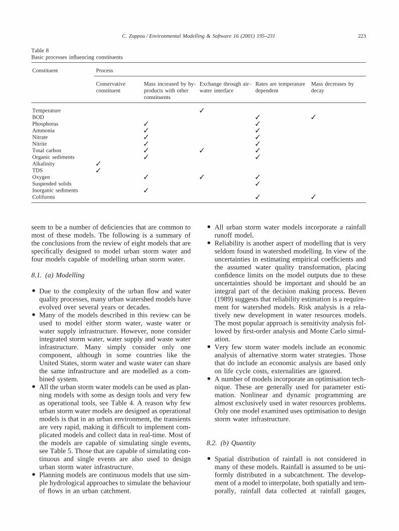
223C. Zoppou / Environmental Modelling & Software 16 (2001) 195–231
Table 8Basic processes influencing constituents
Constituent Process
Conservative Mass increased by by- Exchange through air– Rates are temperature Mass decreases byconstituent products with other water interface dependent decay
constituents
Temperature ✓BOD ✓ ✓Phosphorus ✓ ✓Ammonia ✓ ✓Nitrate ✓ ✓Nitrite ✓ ✓Total carbon ✓ ✓ ✓Organic sediments ✓ ✓Alkalinity ✓TDS ✓Oxygen ✓ ✓ ✓Suspended solids ✓Inorganic sediments ✓Coliforms ✓ ✓
seem to be a number of deficiencies that are common tomost of these models. The following is a summary ofthe conclusions from the review of eight models that arespecifically designed to model urban storm water andfour models capable of modelling urban storm water.
8.1. (a) Modelling
O Due to the complexity of the urban flow and waterquality processes, many urban watershed models haveevolved over several years or decades.
O Many of the models described in this review can beused to model either storm water, waste water orwater supply infrastructure. However, none considerintegrated storm water, water supply and waste waterinfrastructure. Many simply consider only onecomponent, although in some countries like theUnited States, storm water and waste water can sharethe same infrastructure and are modelled as a com-bined system.
O All the urban storm water models can be used as plan-ning models with some as design tools and very fewas operational tools, see Table 4. A reason why fewurban storm water models are designed as operationalmodels is that in an urban environment, the transientsare very rapid, making it difficult to implement com-plicated models and collect data in real-time. Most ofthe models are capable of simulating single events,see Table 5. Those that are capable of simulating con-tinuous and single events are also used to designurban storm water infrastructure.
O Planning models are continuous models that use sim-ple hydrological approaches to simulate the behaviourof flows in an urban catchment.
O All urban storm water models incorporate a rainfallrunoff model.
O Reliability is another aspect of modelling that is veryseldom found in watershed modelling. In view of theuncertainties in estimating empirical coefficients andthe assumed water quality transformation, placingconfidence limits on the model outputs due to theseuncertainties should be important and should be anintegral part of the decision making process. Beven(1989) suggests that reliability estimation is a require-ment for watershed models. Risk analysis is a rela-tively new development in water resources models.The most popular approach is sensitivity analysis fol-lowed by first-order analysis and Monte Carlo simul-ation.
O Very few storm water models include an economicanalysis of alternative storm water strategies. Thosethat do include an economic analysis are based onlyon life cycle costs, externalities are ignored.
O A number of models incorporate an optimisation tech-nique. These are generally used for parameter esti-mation. Nonlinear and dynamic programming arealmost exclusively used in water resources problems.Only one model examined uses optimisation to designstorm water infrastructure.
8.2. (b) Quantity
O Spatial distribution of rainfall is not considered inmany of these models. Rainfall is assumed to be uni-formly distributed in a subcatchment. The develop-ment of a model to interpolate, both spatially and tem-porally, rainfall data collected at rainfall gauges,
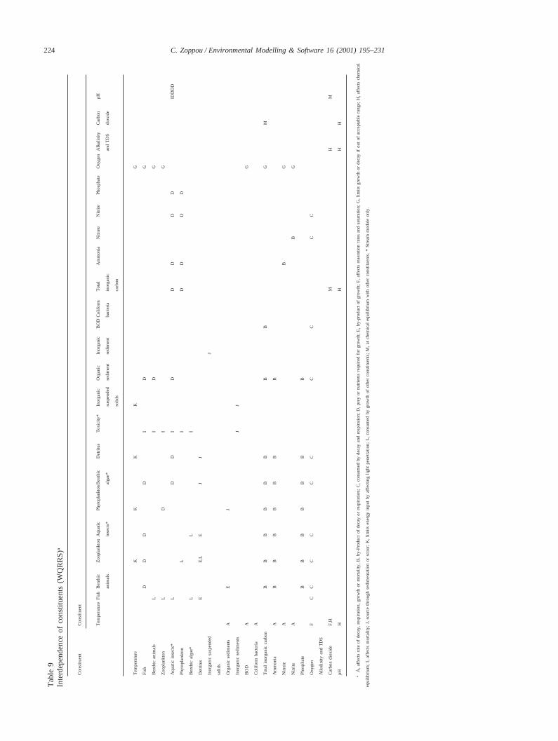
224 C. Zoppou / Environmental Modelling & Software 16 (2001) 195–231T
able
9In
terd
epen
denc
eof
cons
titue
nts
(WQ
RR
S)
a
Con
stitu
ent
Con
stitu
ent
Tem
pera
ture
Fis
hB
enth
icZ
oopl
ankt
onA
quat
icP
hyto
plan
kton
Ben
thic
Det
ritus
Tox
icity
*In
orga
nic
Org
anic
Inor
gani
cB
OD
Col
iform
Tot
alA
mm
onia
Ni
trat
eN
itrite
Pho
spha
teO
xyge
nA
lkal
inity
Car
bon
pH
anim
als
inse
cts*
alga
e*su
spen
ded
sedi
men
tse
dim
ent
bact
eria
inor
gani
can
dT
DS
diox
ide
solid
sca
rbon
Tem
pera
ture
KK
KK
G
Fis
hD
DD
DI
DG
Ben
thic
anim
als
LI
DG
Zoo
plan
kton
LD
IG
Aqu
atic
inse
cts*
LD
DI
DD
DD
DID
DD
D
Phy
topl
ankt
onL
ID
DD
D
Ben
thic
alga
e*L
LI
Det
ritus
EE
,LE
JJ
Inor
gani
csu
spen
ded
J
solid
s
Org
anic
sedi
men
tsA
EJ
Inor
gani
cse
dim
ents
JJ
BO
DA
G
Col
iform
bact
eria
A
Tot
alin
orga
nic
carb
onB
BB
BB
BB
BG
M
Am
mon
iaA
BB
BB
BB
B
Nitr
ate
AB
G
Nitr
iteA
BG
Pho
spha
teB
BB
BB
BB
Oxy
gen
FC
CC
CC
CC
CC
C
Alk
alin
ityan
dT
DS
Car
bon
diox
ide
F,H
MH
M
pHH
HH
H
aA
,af
fect
sra
teof
deca
y,re
spira
tion,
grow
thor
mor
talit
y,B
,by
-Pro
duct
ofde
cay
orre
spira
tion;
C,
cons
umed
byde
cay
and
resp
iratio
n;D
,pr
eyor
nut
rient
sre
quire
dfo
rgr
owth
;E
,by
-pro
duct
ofgr
owth
;F
,af
fect
sre
aera
tion
rate
san
dsa
tura
tion;
G,
limits
grow
thor
deca
yif
out
ofac
cept
able
rang
e;H
,af
fect
sch
emic
al
equi
libriu
m;
I,af
fect
sm
orta
lity;
J,so
urce
thro
ugh
sedi
men
tatio
nor
scou
r;K
,lim
itsen
ergy
inpu
tby
affe
ctin
glig
htpe
netr
atio
n;L,
cons
umed
byg
row
thof
othe
rco
nstit
uent
s;M
,at
chem
ical
equi
libriu
mw
ithot
her
cons
titue
nts.
*S
trea
mm
odul
eon
ly.
225C. Zoppou / Environmental Modelling & Software 16 (2001) 195–231
which are sparsely distributed within a catchment,would be a huge advancement in rainfall runoff mod-elling.
O For overland flow, the linear storage method is themost popular approach. The shallow water waveequations or their approximations are seldomemployed, although their popularity is increasing.
O Simple storage is the most common approach to rout-ing flows. There is a trend towards the use ofhydraulic analysis of storm water infrastructure, withmany of the more recently developed models includ-ing a number of hydraulic routing techniques asoptions.
O Design models employ hydraulic modelling for runoffsimulation and model the behaviour of storm waterflows. More recently, the Saint Venant equations havebeen solved. This is not due to new techniques beingdeveloped to solve these equations but to the avail-ability of cheaper and more powerful computers mak-ing the solution of large systems of equations moretractable.
O Very few of the models examined have the capabilityof modelling flash flooding in urban areas. OnlyMIKE–SWMM seem to be capable of modelling two-dimensional overland flow.
O Very few model reviews mention the implications ofusing approximations to the shallow water waveequations. The shallow water wave equations are cap-able of simulating the effect of obstacles to the flow,loops in the network and pressurised pipe flows. Thediffusion wave and kinematic wave equations possessone set of characteristics which travel downstream.Therefore, these models are not capable of simulatingwaves travelling upstream due to channel and pipejunctions and obstacles to the flow. In addition, thekinematic wave is not capable of simulating theattenuation in the flow. However, the diffusion waveequation approximates the physical attenuation of theflow and the diffusion term in the equation allowssome effect of a downstream control to be feltupstream. The effect decays exponentially from thedownstream control. More importantly, in stormwater flows the local and convective accelerationterms may be the same order of magnitude as thepressure slope. Under these circumstances the dif-fusion wave assumption may not be valid and the dif-fusion and kinematic wave equations are not suitablefor modelling storm water flows. These may be seri-ous limitation if these models are being used to designstorm water infrastructure. Lumped models, whichinclude many hydrological models, ignore the spatialvariability of the problem. This approach assumes thatthe behaviour of the catchment is instantaneous. Thishas serious implications in water quality modellingand other processes that are time dependent.
8.3. (c) Quality
O Washoff and buildup of pollutants on imperviousareas is described by an empirical relationship basedon first-order kinetic type relationships.
O Buildup and washoff of pollutants is not very wellunderstood. The simple exponential relationship thatis generally used is not reliable and there are very fewdata sets available to verify or establish new empiricalrelationships. More studies, such as those undertakenby Mackay (1999) are required to establish new orverify these relationships.
O In general, water quality modelling involves first-order kinetics, with adsorption to sediments being amajor component. Very few models have a sedimenttransport module. In this module the sediment trans-port equations are solved simultaneously with theshallow water wave equations.
O The most common water quality parameters that aremodelled in urban storm water models are: BOD, totalcoliforms, total P and N and both suspended and bedsediment transport. The non-urban models includearbitrary conservative pollutants and the modelling ofaquatic organisms. Because the effect of pollutants onorganisms is important, temperature, DO andammonia are also included in non-urban models.
O Only one of the urban storm water models solves theadvective-diffusion equation for the transport of pol-lutants in pipes, channels or storages. All the othersuse simpler techniques, such as plug flow or assumingsimply that the pollutant is completely mixed. This isin contrast to the non-urban models which all use theadvective-diffusion equation for the transport of con-taminants. Two reasons why the advective-diffusionequation is not solved for urban problems are: Dueto the rapid response of an urban catchment, the trans-port of contaminants by diffusion is considered to beinsignificant compared to the influence of advectionin the transport of these contaminants. Urban stormwater infrastructure networks are generally morecomplicated than river networks. The numerical sol-ution of the advective-diffusion equation for compli-cated networks may be computationally expensive.
8.4. (d) Data
O Orlob (1982) commented that in the late 1970s thetechnology of modelling, at least that of water quality,reached a point where advancement seems to dependmore on the availability of reliable data from the fieldthan on the ingenuity of the modeller or on the com-puter. It seems that this situation has not improved.
226 C. Zoppou / Environmental Modelling & Software 16 (2001) 195–231
9. Opportunities in storm water modelling
This review has highlighted potential research opport-unities instorm water modelling, process understandinganddata management. The implementation of many ofthese research opportunities in a modelling frameworkis currently achievable.
9.1. (a) Modelling
O Rapidly Varying Flows and Flows over a Dry BedOne-dimensional unsteady flow models havematured and there have been very few innovativeadvancements in these models over the past fewyears. They are robust, efficient and suitable forsimulating gradually varied flows in well definedchannels or conduits. This is not the case for rapidlyvarying flows and unsteady flows over a dry bed.One and two-dimensional algorithms for handlingthis type of flows are emerging. The simulation offlash flooding and storm water infrastructure failure,which are increasing problems in urban areas, canbe modelled with such algorithms. Accurate model-ling of two-dimensional unsteady flows over steepslopes and dry beds is an emerging area of research.These models will also gain prominence in model-ling two-dimensional overland flow.
O Sediment TransportAdsorption to sediments is a major component in thetransport of pollutants. Some models use algorithmsthat are abstract. Whilst these may be intuitive, theyare often difficult to relate to physical measurements.Sediment transport models should be more physi-cally based. Sediment transport and flow are co-dependent, therefore the sediment and flow equa-tions should be solved simultaneously. Very fewmodels solve these equations simultaneously.
O Rainfall InterpolationFailures in storm water infrastructure are generallyassociated with high intensity rainfall. The spatialand temporal variability in rainfall is not adequatelyconsidered in rainfall-runoff models. Tools that canaccurately interpolate both spatial and temporalvariability in rainfall would provide more reliableestimates of point rainfall and consequently runoff.
O Integrated Water SystemStorm water is only one component of the urbanwater system. Very few models integrate waterresources systems. They do not include storm water,waste water and potable water systems. Therefore,it is not possible to consider water reuse in optionsor the impact of one system on another.
O Economic AnalysisThe few storm water models that include economicanalysis are based only on life cycle costs. Exter-nalities are ignored. The occurrence of rare events
that result in the failure of urban infrastructure isanother emerging aspect of urban storm water man-agement. Assessing the costs associated with infra-structure failure is seldom included in an economicanalysis of urban systems. For example, flash flood-ing is disruptive, destructive and places life and pro-perty at risk. Recent events in major city centres inAustralia have demonstrated the huge costs associa-ted with the inadequacy of urban infrastructure toconvey storm water. The costs associated with infra-structure failure are seldom included in the cost ofstorm water infrastructure.
O Risk analysisUncertainty analysis is not adequately addressed inmodelling. Placing confidence limits on the modelresults, which reflect the uncertainties in a model, isextremely important. With the model uncertaintiesquantified, its results can be viewed in perspective.
O OptimisationOptimisation has been used in urban storm watermodels for a number of years. However, they aregenerally used for model parameter estimation.There are opportunities for the use of optimisationfor the selection of storm water infrastructure. Anobvious example is the use of simulated annealingto size storm water infrastructure.
9.2. (b) Process understanding
O Head Losses in ManholesManholes and drop structures in a storm water net-work can have a significant impact on the behaviourof flow through these systems. Hydraulic modelsgenerally treat these structures as internal boundaryconditions. However, their behaviour under varyingflow is not well understood. Laboratory experimentsare required to establish the empirical relationshipsthat accurately reflect the impact of these structureson the flow.
O Buildup and Washoff FunctionMost model development activity has been devotedto porting models to personal computers, improvingthe numerical procedures or improving their “userfriendliness”. This diverts effort from enhancing ourunderstanding of urban runoff and of better ways tomodel it. This is particularly true for the accumu-lation and subsequent transport of pollutants by run-off. There is a limited knowledge of buildup andwashoff of pollutants and methods for simulating theaccumulation and washoff of surface pollutants havenot been verified (Nix, 1994). The simpleexponential relationship that is generally used is notreliable and there are very few data sets available toverify or establish new empirical relationships. Morestudies, such as those undertaken by Mackay (1999),

227C. Zoppou / Environmental Modelling & Software 16 (2001) 195–231
are required to establish new or verify existingrelationships.
O Water Quality InteractionsThere are numerous algorithms to handle variousfacets of water quality modelling. Few, if any, arecapable of studying a particular facet with scientificrigour. The interaction of various water quality para-meters may have a more significant influence on anaquatic system than the individual parameters in iso-lation. Most water quality models ignore or restrictthe interaction of water quality parameters. A greaterunderstanding of the significance of the interactionbetween water quality parameters is necessarybefore reliable algorithms can be developed todescribe these interactions.
9.3. (c) Data management
O Expert System for Model SelectionThere are numerous urban storm water models. Thelevel of apparent detail in a model may lead someuser to believe that the results are equally impress-ive. This is simply not the case. What is required isan expert system that can be used to assist the userin selecting a model that will balance the modellingeffort with the needs of the study.
O Data ArchivesModels move ahead of the database available to sup-port them (Nix, 1994). Large runoff models requirelarge amounts of expensive data. What is lacking isan intelligent system that streamlines the manage-ment of data. The provision of interfaces with popu-lar data base management software and spreadsheetswill increase the utility of existing models and data.
O Data CollectionData is essential in defining the forcing functionsand delineating the limits of a region being mod-elled. It is very expensive to collect and the temporaland spatial acquisition of data is usually driven bythe need to satisfy regulatory requirements. Con-sideration might be given to developing data moni-toring systems that are driven by model needsinstead of limiting the choice of models by the avail-able data.
Appendix A. Contaminant Sources, Health andEnvironmental Consequences
A.1. Nitrogen
Amongst the major point sources of nitrogen in waterbodies are: municipal and industrial waste water andseptic tanks. Diffuse sources of nitrogen include ferti-
lisers, animal wastes, leachate from landfill and atmos-pheric fall-out. Nitrates become toxic only under con-ditions in which they are reduced to nitrites. In highconcentrations nitrate is known to cause methemoglobi-nemia in bottle fed infants.
A.2. Phosphorus
In the elemental form, phosphorus is highly toxic.Phosphorus as phosphate is one of the major nutrientsrequired by plants. Phosphorus is not the sole cause ofeutrophication, but it is a limiting factor for aquaticplants. Phosphates enter waterways from several differ-ent sources. These include human and animal excreta,surface runoff and atmospheric fallout. High concen-trations of total phosphate may interfere in water treat-ment plants. Algal growth imparts undesirable tastes andodours to water, interferes with water treatment andbecomes aesthetically unpleasant.
A.3. Copper
Prolonged excessive quantities of copper may resultin liver and kidney damage. Copper may impart sometaste to water. The toxicity of copper to aquatic life isdependent on alkalinity. The lower the alkalinity, themore toxic copper is to aquatic life. It is rapidly adsorbedto sediments. It is highly toxic to most aquatic plants aswell as most freshwater and marine invertebrates. It isconsidered more toxic to freshwater fish than any otherheavy metal except mercury. Major sources of copperoccur in: steel production, sewage treatment plantwastes, corrosion of brass and copper pipes. It is used inelectrical wiring, plumbing and the automobile industry.Copper sulfate has been widely used in the control ofalgae in water supplies.
A.4. Coliforms
Coliforms are an indicator organism for faecal col-iforms, steptococcal and other pathogenic bacteria. Sew-age and animal wastes are the major sources of coliformbacteria. Possible chronic health effects of coliform bac-teria include; gastroenteritis, salmonella infection, dys-entery, typhoid fever and cholera.
A.5. Chromium
Chromium was used in making paint pigment, textilecolouring and tanning. More recently, it is used in theproduction of stainless steel, photoelectric cells and cer-amic glazes. The principal emissions of chromium intosurface waters are from electroplating, waste inciner-ation, contaminated laundry detergent and bleaches andseptic systems. Toxicity of chromium to humans andaquatic organisms is generally low. Under most con-
228 C. Zoppou / Environmental Modelling & Software 16 (2001) 195–231
ditions, mercury, cadmium and copper are more toxicthan chromium. Soluble compounds can cause liver, kid-ney and lung damage.
A.6. Cadmium
Cadmium is toxic to man, causing chronic kidney andliver disease. It is deposited and accumulates in varioushuman body tissues. Its major source is industrial pro-duction such as: electroplating, pigments, plastic stabil-isers, discarded batteries, paints, corrosion of galvanisedpipes, fertilisers and sewage sludge. In aquatic systems,it is adsorbed to sediment particles. Certain invertebratesand fish are very sensitive to cadmium. Increased hard-ness and alkalinity decreases the toxicity of cadmium foraquatic organisms.
A.7. Iron
Pollution sources of iron are industrial wastes, iron-bearing groundwater and leaching from cast iron pipes inwater reticulation systems. In the presence of dissolvedoxygen, iron will precipitate as a hydroxide, forminggels or flocs. These may be detrimental to fish and otheraquatic life as they settle over stream beds smotheringinvertebrates, plants and spawning grounds. In watersupplies, it affects taste and stains clothes and plumbingfixtures. For some industries, low concentrations of ironare required. These include paper manufacturing andflood processing.
A.8. Lead
Lead is used in storage batteries, pipes, paint, petroladditive, solder and fusible alloys. Combustion of oil andpetrol is the major source of lead absorbed by humans.Lead enters the aquatic environment through precipi-tation, leaching of soil, street and municipal runoff, cor-rosion of lead pipes, discarded storage batteries, lead-soldered pipe joints and industrial waste discharges. Itis a toxic metal that accumulates in the tissue of organ-isms by ingestion or inhalation of dust or fumes. Itresults in irreversible nerve and brain damage in infants.Kidney damage, blood disorders and hypertension aresymptoms of health problems associated with lead. Themajor toxic effects of lead include anaemia, neurologicaldysfunction and renal impairment. Lead is less toxic toinvertebrates than copper, cadmium, zinc and mercury.
A.9. Mercury
Mercury is highly toxic to aquatic plants, organismsand humans. It can accumulate by: ingestion, skinadsorption and inhalation of vapour. Long-term exposurecan produce brain, nerve and kidney damage. Birthdefects and skin rash have also been attributable to
exposure to mercury. Sources of mercury include: amal-gams, electrical equipment, fungicides, mirror coatingsand sewage. In the aquatic environment, mercury associ-ates strongly with suspended solids.
A.10. Suspended solids
For aquatic life, suspended solids can reduce lightpenetration, which will adversely affect photosyntheticactivity. Suspended sediments provide areas wheremicroorganisms do not come in contact with chlorinedisinfectant. Therefore, it can influence the efficiency ofwater treatment processes such as coagulation, sedimen-tation, filtration and chlorination.
A.11. Zinc
Zinc is used in brass, galvanising, die-casting andleaching of galvanised pipes and fittings. It is an essen-tial element in human metabolism. It has however, a bit-ter or astringent taste. Toxic concentrations of zinc com-pounds cause adverse changes in the morphology andphysiology of fish. The toxicity of zinc is dependent onpH and water hardness. Under most circumstances, mer-cury and copper are more toxic to aquatic plants andinvertebrates than zinc, whereas chromium, cadmium,nickel and lead may be more or less toxic, dependingon conditions (Moore and Ramamoorthy, 1984). Mer-cury and copper are more toxic to fish than zinc. Therare toxicity of zinc arises from its synergistic interactionwith other heavy metals.
References
Abbott, M.B., 1979. A modelling system for the design and operationof storm-sewer networks. In: Abbott, M.B. (Ed.), ComputationalHydraulics. Pitman, pp. 11–39, Chapter 2.
Allen, R.B., Bridgeman, S.G., 1986. Dynamic programming in hydro-power scheduling. Journal of Water Resources Planning and Man-agement, ASCE 112 (3), 339–353.
Alley, W.M. and Smith, P.E., 1982a. Distributed Routing Rainfall-Runoff Model: Version II. US Geological Survey, Geological Sur-vey Open File Report 82-344.
Alley, W.M. and Smith, P.E., 1982b. Multi-Event Urban Runoff Qual-ity Model. US Geological Survey, Open File Report 82-764,Reston, Virginia.
Behera, P.K., Papa, F., Adams, B.J., 1999. Optimisation of regionalstorm-water management systems. Journal of Water ResourcesPlanning and Management, ASCE 125 (2), 107–114.
Betson, R.P., Tucker, R.L., Haller, F.M., 1969. Using analyticalmethods to develop a surface-runoff model. Water ResourcesResearch 5 (1), 103–111.
Bettess, R., Pitfield, R.A., Price, R.K., 1978. A surcharging model forstorm sewer systems. In: Halliwell, P.R. (Ed.), Urban Storm Drain-age. Pentech Press, London, pp. 306–316.
Beven, K.J., 1989. Changing ideas in hydrology: the case of physicallybased models. Journal of Hydrology 105, 157–172.
Bicknell, B.R., Imhoff, J.C., Kittle, J.L., Donigan, A.S. and Johanson,R.C., 1993. Hydrologic Simulation Program: Fortran User’s Man-
229C. Zoppou / Environmental Modelling & Software 16 (2001) 195–231
ual for Release 10. US Environmental Protection Agency, Athens,Georgia, Report EPA/600/R-93/174.
Bidwell, V.J., 1971. Regression analysis of nonlinear catchment sys-tems. Water Resources Research 7 (5), 1118–1126.
Brandstetter, A.B., 1976. Assessment of Mathematical Models forStorm and Combined Sewer Management. US Environmental Pro-tection Agency, Cincinnati, Ohio, Report EPA/600/2-76-175a.
Brandstetter, A.B., Engel, R.L., Cearlock, D.B., 1973. A mathematicalmodel for optimum design and control of metropolitan wastewatermanagement systems. Water Resources Bulletin 9 (6), 1188–1200.
Brendecke, C.M., DeOreo, W.B., Payton, E.A., Rozaklis, L.T., 1989.Network Modes of Water Rights and System Operations. Journalof Water Resources Planning and Management, ASCE 115 (5),684–696.
Brown, L.C. and Barnwell, T.O., 1987. The Enhanced Stream WaterQuality Models QUAL2E and QUAL2e-UNCAS: Documentationand Users Manual. US Environmental Protection Agency, Athens,Georgia, Report EPA/600/3-87/007.
Brown, S.R., 1986. TOMCAT: a computer model designed specificallyfor catchment quality planning within the water industry. In: Inter-national Conference on Water Quality Modelling in the InlandNatural Environment. British Hydraulic Research Association,Cranfield, UK, pp. 37–49.
Burges, S.J., Lettenmaier, D.P., 1975. Probabilistic methods in streamquality management. Water Resources Bulletin 11 (1), 242–247.
Carriaga, C.C., Mays, L.W., 1995. Optimisation modeling for sedimen-tation in alluvial rivers. Journal of Water Resources Planning andManagement, ASCE 121 (3), 251–259.
Chapman, D., 1992. Water Quality Assessments: A Guide to the Useof Biota, Sediments and Water in Environmental Monitoring.Chapman and Hall, London.
Charley, W., Pabst, A. and Peters, J., 1995. The Hydrologic ModelingSystem (HEC-HMS): Design and Development Issues. Hydrolog-ical Engineering Center, US Army Corps of Engineers, TechnicalPaper No. 149.
Chatterton, R.A., Miller, A.C., McDonnell, A.J., 1982. Uncertaintyanalysis of dissolved oxygen model. Journal of the EnvironmentalEngineering Division, ASCE 108 (EE5), 1003–1013.
Chow, V.T., 1964. Handbook of Applied Hydrology. McGraw-HillBook Co., New York.
Chu, C.S. and Bowers, C.E., 1977. Computer programs in waterresources. Water Resources Research Center, University of Minne-sota, WRRC Bulletin 97.
Chu, W.S., Yeh, W.W.G., 1978. A nonlinear programming algorithmfor real time hourly reservoir operations. Water Resources Bulletin14 (5), 1048–1063.
Chung, F.I., Archer, M.C., DeVries, J.J., 1989. Network flow algorithmapplied to California aqueduct simulation. Journal of WaterResources Planning and Management, ASCE 115 (2), 131–147.
Clark, R.T., 1973. Mathematical models in hydrology, irrigation anddrainage. Paper, Food and Agriculture Organization of the UnitedNations, Rome.
Colon, R., McMahon, G.F., 1987. BRASS model: application to Sav-annah River system reservoirs. Journal of Water Resources Plan-ning and Management, ASCE 113 (2), 177–190.
Crawford, N.H. and Linsley, R.K., 1966. Digital Simulation inHydrology, Stanford Watershed Model. Department of Civil Engin-eers, Stanford University, Technical Report No. 39.
Cunge, J.A., 1969. On the subject of a flood propagation method. Jour-nal of Hydraulic Research 7 (2), 205–230.
Danish Hydraulic Institute 1990. MIKE 11 — A Microcomputer BasedModelling System for Rivers and Channels, Users Manual. DanishHydraulic Institute, Horsholm, Denmark.
Dawdy, D.R., O’Donnell, T., 1965. Mathematical models of catchmentbehaviour. Journal of the Hydraulics Division, Proceedings of theASCE 91 (HY4), 123–137.
Dawdy, D.R., Lichty, R.W. and Bergman, J.M., 1972. A Rainfall-Run-
off Simulation Model for Estimation of Flood Peaks for SmallDrainage Basins. US Geological Survey, Professional Paper 506-B.
Dendrou, S.A., 1982. Overview of urban stormwater models. In:Kibler, D.F. (Ed.), Urban Stormwater Hydrology. American Geo-physical Union, Washington, DC, pp. 219–247.
DeVries, J.J. and Hromadka, T.V., 1992. Computer models for surfacewater. In: Maidment, D.R. (Ed.), Handbook of Hydrology, Chap-ter 12.
Diaz, G.E., Fontane, D.G., 1989. Hydropower optimisation via sequen-tial quadratic programming. Journal of Water Resources Planningand Management, ASCE 115 (6), 715–734.
Dinius, S.H., 1987. Design of an index of water quality. WaterResources Bulletin 23 (5), 833–843.
Dooge, J.C.I., 1959. A general theory of the unit hydrograph. Journalof Geophysical Research 64 (1), 241–256.
Driscoll, D., Toro, D.M.D. and Thomann, R.V., 1979. A StatisticalMethod for Assessment of Urban Runoff. US Environmental Pro-tection Agency, Washington, DC, Report EPA/440/3-79-023.
Driver, N.E. and Tasker, G.D., 1988. Techniques for Estimation ofStorm-Runoff Loads, Volumes, and Selected Constituent Concen-trations in Urban Watersheds in the United States. US GeologicalSurvey, Open File Report 88-191.
Driver, N.E. and Tasker, G.D., 1990. Techniques for Estimation ofStorm-Runoff Loads, Volumes, and Selected Constituent Concen-trations in Urban Watersheds in the United States. US GeologicalSurvey, Water Supply Paper 2363.
Driver, N.E., Troutman, B.M., 1989. Regression models for estimatingurban storm-runoff quality and quantity in the United States. Jour-nal of Hydrology 109, 221–236.
Dudley, J., Bryan, D., Chambers, B., 1994. STOAT — Developmentand Application of a Fully Dynamic Sewage Treatment WorksModel. In: International User Group Meeting: Computer AidedAnalysis and Operation in Sewage Transport and Treatment Tech-nology, Goteborg, Sweden.
Duncan, H.P., 1995. A Bibliography of Urban Stormwater Quality.Cooperative Research Centre for Catchment Hydrology, Report95/8.
Ellis, J.B., 1986. Pollutional aspects of urban runoff. In: Marsalek,H.J., Desbordes, M. (Eds.), Urban Runoff Pollution. NATA ASISeries, Series G: Ecological Sciences, vol. 10. Springer-Verlag,Berlin.
Fisher, H.B., List, E.J., Koh, R.C.Y., Imberger, J., Brooks, N.H., 1979.Mixing in Inland and Coastal Waters. Academic Press, Boston.
Ford, D.T., Garland, R., Sullivan, C., 1981. Operation policy analysis:Sam Rayburn reservoir. Journal of Water Resources Planning andManagement, ASCE 107 (WR2), 339–350.
Fread, D.L., 1978. NWS operational dynamic wave model. In: Pro-ceedings of the Specialty Conference on Verification of Mathemat-ical and Physical Models in Hydraulic Engineering. AmericanSociety of Civil Engineers, College Park, MD, pp. 455–464.
Geiger, W.P., Dorsch, H.R., 1980. Quantity–Quality Simulation(QQS): A Detailed Continuous Planning Model for Urban RunoffControl, Volume 1, Model Description, Testing and Applications.US Environmental Protection Agency, Cincinnati, OH. ReportEPA/600/2-80-011.
Hall, M.J., 1984. Urban Hydrology. Elsevier Applied-Science, NewYork.
Havno, K., Madsen, M.N., Dorge, J., 1995. MIKE 11 — A generalisedriver modelling package. In: Singh, V.P. (Ed.), Computer Modelsof Watershed Hydrology. Water Resources Publications, Colorado,pp. 733–782.
Heaney, J.P., Huber, W.C. and Nix, S.J., 1976. Storm Water Manage-ment Model: Level 1 — Preliminary Screening Procedures. USEnvironmental Protection Agency, Cincinnati, OH. ReportEPA/600/2-77-083.
Henderson, F.M., 1966. Open Channel Flow. Macmillan and Co,New York.
230 C. Zoppou / Environmental Modelling & Software 16 (2001) 195–231
Huber, W.C., 1986. Deterministic modeling of urban runoff quality.In: Torno, H., Marsalek, J., Desbordes, M. (Eds.), Urban RunoffPollution. NAT0 ASI Series, Series G: Ecological Sciences, vol.10. Springer-Verlag, Berlin, pp. 166–242.
Huber, W.C., 1992a. Contaminant transport in surface water. In: Maid-ment, D.R. (Ed.), Handbook of Hydrology. McGraw-Hill, NewYork, Chapter 14.
Huber, W.C., 1992b. Prediction of urban nonpoint source water qualitymethods and models. In: International Symposium on UrbanStormwater Management. The Institution of Engineers, Sydney,Australia, pp. 1–17.
Huber, W.C. and Dickinson, R.E., 1988. Storm Water ManagementModel, Version 4, User’s Manual. US Environmental ProtectionAgency, Athens, Georgia. Report EPA/600/3-88-001a.
Huber, W.C. and Heaney, J.P., 1982. Analyzing Residuals Dischargeand Generation from Urban and Non-Urban Surfaces. US Environ-mental Protection Agency, Athens, Georgia. Report EPA/600/3-83-046.
Huber, W.C., Heaney, J.P, Nix, S.J., Dickinson, R.E. and Polmann,D.J., 1984. Storm Water Management Model, User’s Manual, Ver-sion III. US Environmental Protection Agency, Athens, Georgia.Report EPA/600/2-84-109a.
Hydrologic Engineering Center, 1977. Storage, Treatment, Overflow,Runoff Model, STORM, Generalised Computer Program 723-58-L7520. Hydrologic Engineering Center, US Corps of Engineers,Davis, California.
Hydrologic Engineering Center, 1978. WQRRS Water Quality forRiver-Reservoir Systems: User’s Manual. Hydrologic EngineeringCenter, US Army Corps of Engineers, Report CPD-8.
Hydrologic Engineering Center, 1986. HEC–5Q Simulation of FloodControl and Conservation Systems: Appendix on Water QualityAnalysis. Hydrologic Engineering Center, US Army Corps ofEngineers, Report CPD-5Q.
Hydrologic Engineering Center, 1988. SHP Stream Hydraulics Pack-age. Hydrologic Engineering Center, US Army Corps of Engineers,Report CPD-54.
Jaffe, P.R., Parker, F.L., 1984. Uncertainty analysis of first order decaymodel. Journal of Environmental Engineering, ASCE 110 (1),131–140.
Jewell, T.K., Adrian, D.D., 1981. Development of improved storm-water quality models. Journal of the Environmental EngineeringDivision, Proceedings of the ASCE 107 (EE5), 957–974.
Johanson, R.C., Imhoff, J.C. and Dana, H., 1980. Users Manual forHydrological Simulation Program — Fortran (HSPF). US Environ-mental Protection Agency. Report EPA/9-80-015, Athens Georgia.
Johanson, R.C., Imhoff, J.C. and Davis, H.H., 1984. User’s Manual forHydrological Simulation Program: Fortran. HSPF: User’s ManualRelease 8.0. US Environmental Protection Agency, Athens, Geor-gia. Report EPA/600/3-84-066.
Jorgensen, S.E., 1982. Modeling the ecological processes. In: Orlob,G.T. (Ed.), Mathematical Modeling of Water Quality: Streams,Lakes, and Reservoirs. Wiley, Chichester, pp. 116–149.
Jorgensen, S.E., 1988. Fundamentals of Ecological Modelling. Devel-opments in Environmental Modelling, vol. 9. Elsevier, Amsterdam.
Kirkpatrick, S., Gelatt, C.D., Vecchi, M.P., 1983. Optimisation bysimulated annealing. Science 220 (4598), 671–680.
Kulandaiswamy, V.C., 1964. A Basic Study of the Rainfall Excess-Surface Runoff Relationship in a Basin System. Ph.D. thesis, Uni-versity of Illinois, Urbana, IL.
Labadie, J.W., Morrow, D.M., Chen, Y.H., 1980. Optimal control ofunsteady combined sewer flow. Journal of the Water ResourcesPlanning and Management Division, ASCE 106 (WR1), 205–223.
Lansey, K.E., Basnet, C., 1991. Parameter estimation for water distri-bution networks. Journal of Water Resources Planning and Man-agement, ASCE 117 (1), 126–144.
Leavesley, G.H., Lichty, R.W., Troutman, B.M. and Saindon, L.G.,1983. Precipitation-Runoff Modeling System: User’s Manual. US
Geological Survey, Water Resources Investigations Report 83-4238.
Leiser, C.P., 1974. Computer Management of a Combined Sewer Sys-tem. US Environmental Protection Agency, Cincinnati, OH. ReportEPA/670/2-74-022.
Li, S.G., McLaughlin, D., 1991. A nonstationary spectral method forsolving stochastic groundwater problems: unconditional analysis.Water Resources Research 27 (7), 1589–1605.
Lindberg, S., Nielson, J.B., Carr, R., 1989. An integrated PC-modellingsystem for hydraulic analysis of drainage systems. In: The FirstAustralian Conference on Technical Computing in the Water Indus-try, WATERCOMP ’89. The Institution of Engineers, Melbourne,Australia, pp. 127–130.
Lindell, E.O., Houck, M.H., Delleur, J.W., 1987. Design of dual-pur-pose systems using dynamic programming. Journal of WaterResources Planning and Management, ASCE 113 (4), 471–484.
Mackay, S., 1999. Sediment, Nutrient and Heavy Metal Characteristicsof Urban Stormwater Runoff. Urban Water Research Associationof Australia, Research Report No. 139.
Martin, Q.W., 1983. Optimal operation of multiple reservoir systems.Journal of Water Resources Planning and Management, ASCE 109(1), 58–74.
Martin, Q.W., 1987. Optimal daily operation of surface-water systems.Journal of Water Resources Planning and Management, ASCE 113(4), 453–470.
McMahon, G.F., Fitzgerald, R., McCarthy, B., 1984. BRASS model:practical aspects. Journal of Water Resources Planning and Man-agement, ASCE 110 (1), 75–89.
Melching, C.S., Yen, B.C., Wenzel, H.G., 1991. Output reliability asa guide for selection of rainfall-runoff models. Journal of WaterResources Planning and Management, ASCE 117 (3), 383–398.
Melching, C.S., Yoon, C.G., 1996. Key sources of uncertainty inQUAL2E model of Passaic River. Journal of Water ResourcesPlanning and Management, ASCE 122 (2), 105–113.
Moore, J.W., Ramamoorthy, S., 1984. Heavy Metals in Natural Wat-ers: Applied Monitoring and Impact Assessment. Springer-Verlag,New York.
Nash, J.E., 1957. The form of the instantaneous unit hydrograph. Inter-national Association of Scientific Hydrology 45 (3), 114–121.
Nitivattananon, V., Sadowski, E.C., Quimpo, R.G., 1996. Optimisationof water supply system operation. Journal of Water Resources Plan-ning and Management, ASCE 122 (5), 374–384.
Nix, S.J., 1991. Applying runoff models. Water Environmental Tech-nology 3 (6), 47–49.
Nix, S.J., 1994. Urban Stormwater Modelling and Simulation. LewisPublishers, Boca Raton.
Novotny, V., 1995. Non-Point Pollution and Urban Stormwater Man-agement. Water Quality Management Library, vol. 9. TechnomicPublishing Co.
Orlob, G.T., 1982. Introduction. In: Orlob, G.T. (Ed.), MathematicalModeling of Water Quality: Streams, Lakes, and Reservoirs. Wiley,Chichester, pp. 1–10.
Ostfeld, A., Shamir, U., 1996. Design of optimal reliable multiqualitywater-supply systems. Journal of Water Resources Planning andManagement, ASCE 122 (5), 322–333.
Peck, E.L., 1976. Catchment Modeling and Initial Parameter Esti-mation for the National Weather Service River Forecasting System.US National Weather Service, NOAA Technical MemorandumNWS Hydro-31.
Press, W.H., Teukolsky, S.A., Vetterling, W.T., Flannery, B.P., 1992.Numerical Recipes in Fortran: The Art of Scientific Computing.Cambridge University Press, Cambridge.
Price, R.K., 1973. Flood Routing Methods in British Rivers. HydraulicResearch Station, Wallingford, Report No. INT 111.
Price, R.K., 1978. Design of storm sewers for minimum constructioncosts. In: Halliwell, P.R. (Ed.), International Conference on UrbanStorm Drainage. Pentech Press, London, pp. 636–647.
231C. Zoppou / Environmental Modelling & Software 16 (2001) 195–231
Price, R.K., Kidd, C.H.R., 1978. A design and simulation method forstorm sewers. In: Halliwell, P.R. (Ed.), International Conferenceon Urban Storm Drainage. Pentech Press, London, pp. 327–337.
Reckhow, K.H., Butcher, J.B., Marin, C.M., 1985. Pollutant runoffmodels: selection and use in decision making. Water ResourcesBulletin 21 (2), 185–195.
Reddy, P.V.N., Sridharan, K., Rao, P.V., 1996. WLS method for para-meter estimation in water distribution networks. Journal of WaterResources Planning and Management, ASCE 122 (3), 157–164.
Roesner, L.A., Aldrich, J.A. and Dickinson, R.E., 1988. Storm WaterManagement Model, User’s Manual, Version 4: Addendum I,EXTRAN. US Environmental Protection Agency, Athens, Georgia.Report EPA/600/3-88-001b.
Rovey, E.W., Woolhiser, D.A., 1977. Urban storm runoff model. Jour-nal of the Hydraulics Division, ASCE 103 (HY11), 1339–1351.
Salhotra, A.M., Schanz, R., and Mineart, P., 1988. A Generic MonteCarlo Simulation Shell for Uncertainty Analysis of ContaminantTransport Models. Environmental Research Laboratory, Office ofResearch and Development, US Environmental Protection Agency,Athens, Georgia. Report 8720123-AB.
Sevuk, A.S., Yen, B.C. and Peterson, G.E., 1973. Illinois Storm SewerSystem Simulation Model: User’s Manual. Water ResourcesCenter, University of Illinios, Research Report No. 73.
Sewards, G.J., Williams, G.C.H., 1995. Intermittently decantedextended aeration process. In: Kolarik, L.O., Priestley, A.J. (Eds.),Modern Techniques in Water and Wastewater Treatment. CSIROPublishing, Melbourne, pp. 107–113.
Scavia, D., Powers, W.F., Canale, R.P., Moody, J.L., 1981. Compari-son of first-order error analysis and Monte Carlo simulation intime-dependent lake eutrophication models. Water ResourcesResearch 17 (4), 1051–1059.
SOGREAH, 1977. Mathematical Model of Flow in an Urban DrainageProgramme. SOGREAH, Greoble France, SOGREAH Brochure06-77-33-05-A.
Tasker, G.D., Stedinger, J.R., 1989. An operational GLS model forhydrologic regression. Journal of Hydrology 111, 361–375.
Tchobanoglous, G., Schroeder, E.D., 1987. Water Quality: Character-istics Modeling Modification. Addison-Wesley, Reading, MA.
Terstriep, M.L. and Stall, J.B., 1974. The Illinois Urban DrainageSimulator ILLDAS. Illinios State Water Survey, Urbana, IL. Bull-etin 58.
Thoft-Christensen, P., Baker, M.J., 1982. Structural Reliability Theoryand Its Applications. Springer-Verlag, Berlin.
Train, R.E., 1979. Quality Criteria for Water. Castle House Publi-cations.
Tung, Y.K., 1987. Uncertainty analysis of National Weather Servicerainfall frequency atlas. Journal of the Hydraulics Division, ASCE113 (2), 893–913.
Tung, Y.K., 1989. Uncertainty on travel time in kinematic wave chan-
nel routing. In: Yen, B.C. (Ed.), Proceedings of the InternationalConference on Channel Flow and Catchment Runoff: Centennial ofManning’s Formula and Kuichling’s Rational Formula. AmericanSociety of Civil Engineers, pp. 767–781.
Tung, Y.K., 1990. Mellin Transform applied to uncertainty analysis inhydrology/hydraulics. Journal of Hydraulic Engineering, ASCE116 (5), 659–674.
US Environmental Protection Agency, 1979. Benefit Analysis forCombined Sewer Overflow Control. US Environmental ProtectionAgency, Environment Research Information Center, Cincinnati,OH. Report EPA/625/4-79-013.
Warwick, J.J., Wilson, J.S., 1990. Estimating uncertainty of storm-water runoff computations. Journal of Water Resources Planningand Management, ASCE 116 (2), 187–203.
Whipple, W., Grigg, S., Gizzard, T., Randall, C.W., Shubinski, R.P.,Tucker, L.S., 1983. Stormwater Management in Urbanizing Areas.Prentice-Hall, Englewood Cliffs, NJ.
Willey, R.G., 1986. Kanawha River Basin Water Quality Modeling.Hydrologic Engineering Center, US Army Corps of Engineers,Special Projects Report No. 86-5.
Woolhiser, D.A., 1977. Numerical simulation of direct surface runofffrom a small watershed using program KINGEN. In: Ciriani, T.A.,Maione, U., Wallis, J.R. (Eds.), Mathematical Models for SurfaceWater Hydrology. Wiley, New York.
Woolhiser, D.A., Smith, R.E. and Goodrich, D.C., 1990. KINEROS,A Kinematic Runoff and Erosion Model: Documentation and UserManual. US Department of Agriculture, Agricultural Research Ser-vice. Report ARS-77.
Wurbs, R.A., 1994. Computer Models for Water Resources Planningand Management. Institute for Water Resources, US Army Corpsof Engineers, Alexandria, Virginia. Report 94-NDS-7.
Xu, C., Goulter, I.C., 1998. Probabilistic model for water distributionreliability. Journal of Water Resources Planning and Management,ASCE 124 (4), 218–228.
Yao, H., Terakaura, A., 1999. Distributed hydrological model for FujiRiver basin. Journal of Hydrologic Engineering, ASCE 4 (2),108–116.
Yeh, K.C., Tung, Y.K., 1993. Uncertainty and sensitivity analysis ofpit-migration Model. Journal of Hydraulic Engineering, ASCE 119(2), 262–283.
Zoppou, C. and Li, K.S., 1992. Estimation of Uncertainty in HydrologyUsing Reliability Theory. Department of Civil and Maritime Engin-eering, University College, University of New South Wales, Can-berra, Australia. Research Report R127.
Zoppou, C., Li, K.S., 1993. New point estimate method for waterresources modeling. Journal of Hydraulic Engineering, ASCE 119(11), 1300–1307.
Zoppou, C., Roberts, S., 1999. Catastrophic collapse of water supplyreservoirs in urban areas. Journal of Hydraulic Engineering, ASCE125 (7), 686–695.