
Universiteit Gent Vakgroep Informatietechnologie
313
Universiteit Gent Faculteit Ingenieurswetenschappen Vakgroep Informatietechnologie Proefschrift tot het behalen van de graad van Doctor in de Ingenieurswetenschappen: Computerwetenschappen Academiejaar 2009-2010 Promotoren: prof. dr. ir. Mario Pickavet dr. ir. Didier Colle Universiteit Gent Faculteit Ingenieurswetenschappen Vakgroep Informatietechnologie Gaston Crommenlaan 8, bus 201 B-9050 Gent, België Tel: +32 9 331 49 00 Fax: +32 9 331 48 99 Web: http://www.intec.ugent.be
Transcript of Universiteit Gent Vakgroep Informatietechnologie

Universiteit Gent Faculteit Ingenieurswetenschappen
Vakgroep Informatietechnologie
Proefschrift tot het behalen van de graad van Doctor in de Ingenieurswetenschappen:
Computerwetenschappen Academiejaar 2009-2010
Promotoren: prof. dr. ir. Mario Pickavet dr. ir. Didier Colle Universiteit Gent Faculteit Ingenieurswetenschappen Vakgroep Informatietechnologie Gaston Crommenlaan 8, bus 201 B-9050 Gent, België Tel: +32 9 331 49 00 Fax: +32 9 331 48 99 Web: http://www.intec.ugent.be

iii
Table of Contents
Dankwoord .......................................................................................................... i Nederlandse samenvatting ........................................................................... xxxi English summary ......................................................................................... xxxv
1 Introduction and Publications ........................................................................ 1 1.1 Overview of This Work......................................................................... 3 1.2 Publications ............................................................................................ 5
1.2.1 A1 Publications Referenced in the Science Citation Index ................. 5 1.2.2 P1 Publications Referenced in Conf. Proc. Citation Index................. 6 1.2.3 Other Publications ............................................................................... 7
2 Techno-Economic Background..................................................................... 11 2.1 Technological Background ................................................................. 12
2.1.1 High Level Views on the Network.................................................... 12 2.1.2 Core Network .................................................................................... 15 2.1.3 Metro Network .................................................................................. 15 2.1.4 Access Network................................................................................. 16
2.2 Economic Background ........................................................................ 25 2.2.1 Design Phase ..................................................................................... 26 2.2.2 Model Phase ...................................................................................... 28 2.2.3 Evaluate Phase................................................................................... 32 2.2.4 Extend Phase ..................................................................................... 35
2.3 Conclusion ............................................................................................ 40 References.......................................................................................................... 41
3 Dimensioning the Infrastructure .................................................................. 45 3.1 Fibre to the Home ................................................................................ 47
3.1.1 FTTH Architectures .......................................................................... 51 3.1.2 FTTH Standards ................................................................................ 52 3.1.3 FTTH Evolution ................................................................................ 55
3.2 Cost Model for an FTTH Rollout....................................................... 56
iv
3.2.1 Outside Plant ..................................................................................... 58 3.2.2 Inside Plant........................................................................................ 67 3.2.3 Customer Premises Equipment ......................................................... 68
3.3 Infrastructure Equipment Prices ....................................................... 70 3.4 Conclusions .......................................................................................... 74 References.......................................................................................................... 75
4 Dimensioning the Operations........................................................................ 79 4.1 Overview of Operational Research for Telecom............................... 80
4.1.1 Classification of Telecom Operational Processes ............................. 81 4.1.2 Operational Process Modelling ......................................................... 83 4.1.3 Process Cost Estimation and Optimization ....................................... 87
4.2 Operational Processes for FTTH........................................................ 89 4.2.1 Connecting the Customers................................................................. 89 4.2.2 Repairing Network Faults ................................................................. 94 4.2.3 Other Operating Expenses............................................................... 100
4.3 Optimising Operational Processes ................................................... 103 4.3.1 Optimization of Repair Teams and Service Level........................... 104 4.3.2 Working with Freelance Personnel ................................................. 108
4.4 Conclusions ........................................................................................ 112 References........................................................................................................ 113
5 Integrated Techno-Economic Studies ....................................................... 117 5.1 Optimization in a Non-Competitive Setting .................................... 118
5.1.1 Design Phase ................................................................................... 119 5.1.2 Model Phase .................................................................................... 124 5.1.3 Evaluate Phase................................................................................. 126
5.2 Optimization in a Competitive Setting............................................. 143 5.2.1 Design Phase ................................................................................... 144 5.2.2 Extended Evaluation ....................................................................... 150
5.3 Conclusions ........................................................................................ 160 References........................................................................................................ 162
6 Applicability in a Broader Technological or Economic Context ............. 167 6.1 Extending the Technological Studies ............................................... 168
6.1.1 From FTTH to Fixed Access Networks .......................................... 168 6.1.2 From Fixed Access to All Access Technologies ............................. 170 6.1.3 From Access Networks to Metro and Core Networks..................... 171
6.2 Extending the Economic Studies ...................................................... 172
v
6.3 Conclusions ........................................................................................ 176 References........................................................................................................ 177
7 Conclusions................................................................................................... 179 Overall conclusion .......................................................................................... 181 Future work..................................................................................................... 182 References........................................................................................................ 185
A Analytical Models for the Installation and Fibre Length........................ 187 A.1 Street Based Models .......................................................................... 188 A.2 Aerial Based Models .......................................................................... 193 References........................................................................................................ 199
B Adoption and Pricing; the Underestimated Elements of a Realistic IPTV Business Case.......................................................................... 201
Abstract ........................................................................................................... 201 B.1 Introduction ....................................................................................... 202 B.2 Business Case Overview.................................................................... 203 B.3 Adoption of IPTV .............................................................................. 204 B.4 What to Do with the Costs ................................................................ 208 B.5 Conclusion .......................................................................................... 213 References........................................................................................................ 214
C Impact of Sensitivity and Iterative Calculations on Cost-Based Pricing................................................................................................ 215
Abstract ........................................................................................................... 215 C.1 Introduction ....................................................................................... 216 C.2 Cost-driven Pricing............................................................................ 218 C.3 Sensitivity ........................................................................................... 220 C.4 Iterative Calculations ........................................................................ 224 C.5 Conclusion .......................................................................................... 231 Acknowledgment............................................................................................. 233 References........................................................................................................ 233
D Municipalities as a Driver for Wireless Broadband Access .................... 235 Abstract ........................................................................................................... 235 D.1 Introduction ....................................................................................... 236 D.2 Methodology....................................................................................... 236
vi
D.3 Considered Wireless Technologies ................................................... 238 D.4 Municipality Network ....................................................................... 245 D.5 Business case ...................................................................................... 247 D.6 Conclusions ........................................................................................ 258 Acknowledgements ......................................................................................... 259 References........................................................................................................ 259
E Future Proof Strategies towards Fibre to the Home................................ 263 Abstract ........................................................................................................... 263 E.1 Introduction ....................................................................................... 264 E.2 Technologies ....................................................................................... 265 E.3 Value Network ................................................................................... 266 E.4 Value Networks for Competition Models ........................................ 269 E.5 Actor Influence on Competition Models.......................................... 277 E.6 Conclusions ........................................................................................ 280 Acknowledgements ......................................................................................... 281 References........................................................................................................ 281
vii
List of Figures
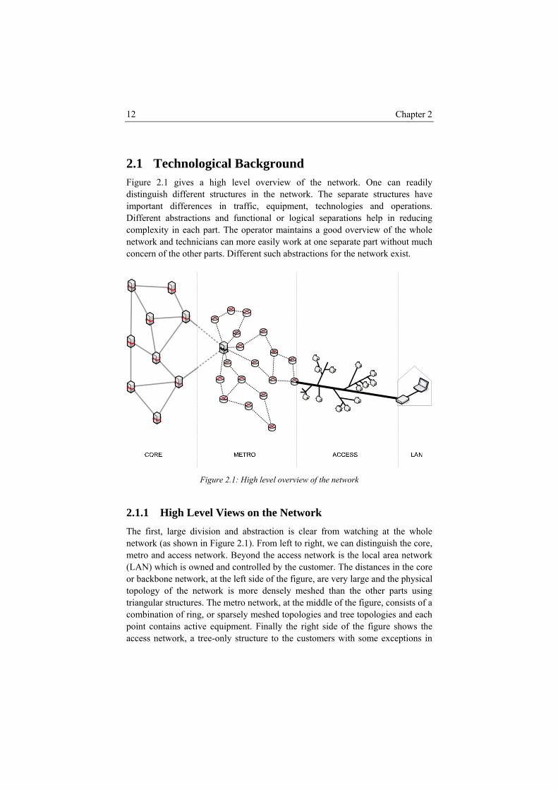
Figure 2.1: High level overview of the network ................................................. 12 Figure 2.2: Reference models for the layered communication and network
protocol design................................................................................ 14 Figure 2.3: Bandwidth evolution in the access network ..................................... 16 Figure 2.4: Broadband wireless technologies for moving users: data rate
versus user speed [2.11] .................................................................. 18 Figure 2.5: xDSL technologies - data rate vs. reach [2.12]................................. 19 Figure 2.6: Overview of a digital subscriber line network.................................. 20 Figure 2.7: Overview of a hybrid fibre coax network......................................... 21 Figure 2.8: Overview of an FTTH network ........................................................ 23 Figure 2.9: Methodology used for the Techno-Economic research .................... 26 Figure 2.10: Ishikawa breakdown of the cost estimate of an FTTH rollout
with focus on the impact of the part on the final cost (indicated by text size and weight) .................................................................. 27
Figure 2.11: Example of a process using a flowchart based modelling approach.......................................................................................... 31
Figure 2.12: Fictitious project cash flows (left) and discounted cash flows (right) .............................................................................................. 33
Figure 2.13: Types of real options: the 7S framework........................................ 37 Figure 2.14: Exemplary uncertainty and decision tree for real options in an
FTTH rollout case. Decisions are indicated (right) by a dark background and white text .............................................................. 38
Figure 2.15: Fictitious game in strategic form (matrix) for the competition between two operators who can decide to roll out FTTH ............... 39
Figure 3.1: Attenuation as a function of the spectrum for evolution of optical fibre [source: Cisco [3.2]] ................................................... 48
Figure 3.2: Schematic overview of the alternative FTTH network architectures .................................................................................... 51
Figure 3.3: High level overview of an FTTH network from a cost modelling perspective with a distinction between ASN and HRN / PON........ 57
Figure 3.4: Schematic view on the installation and physical cable infrastructure in a buried outside plant............................................ 58
viii
Figure 3.5: Façade and Aerial installation as alternatives for a buried outside plant .................................................................................... 61
Figure 3.6: Impact of focussing on the most profitable areas first, by not connecting all houses in a given area (left) and by selecting those areas with the highest residential density (right) ................... 62
Figure 3.7: General naming for the different aggregation points in the network ........................................................................................... 64
Figure 3.8: Schematic overview of passive equipment required in the installation of the outside plant ....................................................... 66
Figure 3.9: Schematic overview of the inside plant equipment .......................... 67 Figure 3.10: Price evolution forecast as a function of time (in years) for
optical and electronic equipment according to the extended learning curve model....................................................................... 72
Figure 4.1: eTOM Level 0 view of Level 1 process groupings [source: TMForum [4.1]] .............................................................................. 81
Figure 4.2: Operational classification of telecom specific processes.................. 83 Figure 4.3: Exemplary process model representations ....................................... 83 Figure 4.4: Simplified processes used in examples for the cost calculation ....... 87 Figure 4.5 - High level overview of the customer connection process ............... 89 Figure 4.6: process for the physical deployment of fibre from CO to drop
box .................................................................................................. 90 Figure 4.7: Administrative installation sub process............................................ 90 Figure 4.8: Installation process at the customer premises................................... 92 Figure 4.9: Central office installation process .................................................... 92 Figure 4.10: high level overview of the repair process....................................... 95 Figure 4.11: fault diagnosis process.................................................................... 96 Figure 4.12: Fault isolation and traffic recovery process.................................... 97 Figure 4.13: hardware, software and external repair processes .......................... 97 Figure 4.14: Fibre cable repair process............................................................... 98 Figure 4.15: Copper cable and preventive repair processes................................ 98 Figure 4.16: Simplified network repair process used in optimization studies .. 103 Figure 4.17: Extension of the network repair process with time constraints .... 104 Figure 4.18: Decomposition of the different cost factors in a repair process
for a fixed number of locations (in this case 3) and a variable service level .................................................................................. 106
Figure 4.19: Influence of service level and number of locations on the network repair cost........................................................................ 107
Figure 4.20: Opportunities for reduction of repair cost in a core network by optimizing the number and location of repair teams ..................... 108
Figure 4.21: Extension of the network repair process with the use of freelance personnel ....................................................................... 109
ix
Figure 4.22: Determination of the optimal technical freelance personnel count.............................................................................................. 110
Figure 4.23: Cost of freelance versus fixed personnel...................................... 110 Figure 4.24: Influence of the team size on the repair time in a core network
for 8h and 24h shifts...................................................................... 111 Figure 5.1: Rogers distribution of adoption in 5 categories.............................. 120 Figure 5.2: Overview of different adoption models.......................................... 121 Figure 5.3: High level cost breakdown for a semi-urban FTTH deployment ... 127 Figure 5.4: Breakdown of the deployment costs for a semi-urban FTTH
deployment.................................................................................... 129 Figure 5.5: Breakdown of the inside plant costs for a semi-urban FTTH
deployment.................................................................................... 130 Figure 5.6: Cost Breakdown for one customer installation for a semi-urban
FTTH deployment......................................................................... 131 Figure 5.7: Cost breakdown for customer installation for a semi-urban
FTTH deployment - Pre-installation vs. later installation ............. 132 Figure 5.8: Breakdown of the operational expenditures for a semi-urban
FTTH deployment......................................................................... 133 Figure 5.9: Proportion of infrastructure deployment and operations to total
cost for an urban FTTH deployment ............................................. 136 Figure 5.10: Discounted cash flows at each year of the urban FTTH
deployment for the three rollout speeds ........................................ 137 Figure 5.11: Net present value (cumulative)at each year of the urban FTTH
deployment for the three rollout speeds ....................................... 138 Figure 5.12: Cost per home passed at moderate rollout speed considering
only the outside plant (left) or all expenditures (right).................. 139 Figure 5.13: Analysis per home connected at moderate rollout speed (left)
of costs, revenues and profits and (right) of costs logarithmic...... 140 Figure 5.14: Discounted cash flows for a breakdown of the costs and at
each year of the urban FTTH deployment at moderate rollout speed ............................................................................................. 141
Figure 5.15: Comparison of the NPV for a municipality and non-municipality (private company) urban FTTH rollout at moderate rollout speed .................................................................. 142
Figure 5.16: Game solved using iterated (strict) dominance (upper) and the sequential variant of the same game solved using backward induction (bottom)......................................................................... 146
Figure 5.17: Impact of delayed introduction (left) and early mover advantage (right) on the adoption.................................................. 149
Figure 5.18: Yearly rollout speed in areas covered per year for the strategy set of analysis 1 ............................................................................. 151
x
Figure 5.19: QRE for the best rollout speed strategies of FTTH and HFC player ............................................................................................ 152
Figure 5.20: QRE for the best rollout sequence strategies of FTTH and HFC player.................................................................................... 155
Figure 5.21: Uncertainty tree used as input to the sensitivity analysis over the game theoretic evaluation........................................................ 156
Figure 5.22: Distribution of the optimal rollout speed strategies for FTTH (left) and HFC (right) under the 3 sensitivity tests defined........... 157
Figure 5.23: Cumulative distribution of the NPV for FTTH and HFC under the 3 sensitivity tests defined, also the result without game theory (orig.) is shown. ................................................................. 158
Figure 5.24: Distribution of the optimal rollout sequence strategies for FTTH and HFC under the 3 sensitivity tests defined.................... 158
Figure 6.1: Cost per occurrence of the repair process for copper reactive/preventive and FTTH HRN / PON.................................. 169
Figure 6.2: Overall estimated repair cost for copper and FTTH HRN / PON. ............................................................................................. 170
Figure 6.3: Ishikawa breakdown of the cost estimate of a wireless network rollout with focus on the impact on the final cost (indicated by text size and weight) ..................................................................... 170
Figure 6.4: Overview of the costs for wireless rollout scenarios ...................... 171 Figure 6.5:Network infrastructure opened at the physical (trenching) layer.
The operators share (parts of) the installation trenches................. 174 Figure 6.6: Network infrastructure opened at the data link layer to other
operators, resembling currently existing bitstream access unbundling .................................................................................... 174
Figure 6.7: Options at the disposal of an operator when considering an FTTH deployment......................................................................... 175
Figure A.1: Schematic overview of the logical structure and parameters for
the analytical installation and fibre length calculations ................ 188 Figure A.2: Logical structure for the fibre connections in a simplified
Manhattan street length. ................................................................ 189 Figure A.3: Logical structure for the fibre connections in a street length......... 190 Figure A.4: Logical structure for the fibre connections in a double street
length ............................................................................................ 191 Figure A.5: Logical structure for the fibre connections in a diagonal tree........ 193 Figure A.6: Installation Length for connecting four houses from one drop
box using straight lines ................................................................. 194 Figure A. 7: Recursive structure used in the analytical calculation of the
fibre length .................................................................................... 195
xi
Figure A. 8: Logical structure for the fibre connections in a simplified Steiner tree .................................................................................... 197
Figure A.9: Installation Length for connecting four houses by means of a Steiner Tree................................................................................... 197
Figure B.1: Methodology for building a business case..................................... 203 Figure B.2: Adoption for broadband access with the impact of competition
and analog switch-off.................................................................... 208 Figure B.3: Price boundaries depending on the cost-allocation scheme used
(normalized to max. SAC (C)) ...................................................... 210 Figure B.4: profit per movie as traffic congestion increases............................. 212 Figure C.1: Overview of different cost-margins............................................... 219 Figure C.2: Comparison of the normal margins to the margins in best and
worst case scenarios ...................................................................... 221 Figure C.3: Comparison of the FAC/LRIC margin to the default (A), worst
(B) and best (C) case margins ....................................................... 222 Figure C.4: Trend and reliability of the FAC/LRIC margin from 2008-2015 .. 223 Figure C.5: forecast and 10%-90% percentile of all considered margins
using variation on the initial forecast ............................................ 223 Figure C.6: Integration of the results of Crystal ball on the sensitivity of the
FAC, LRIC/FAC and LRIC margins for variations of cost-erosion and EOS............................................................................ 224
Figure C.7: Tariff as function of the planning horizon ..................................... 226 Figure C.8: Cumulative adoption curves incorporating marketing effort
corresponding to P0/P1 = 0.9 - 1.0 - 1.1. ...................................... 227 Figure C.9: Tariff as a function of the planning horizon deduced with
iterative calculation for (A1) quadratic response with P0/P1 = 0.9 (A2) quadratic response with P0/P1 = 1.1 (B1) linear response with P0/P1 = 0.9 (B2) linear response with P0/P1 = 1.1 ................................................................................................. 229
Figure C.10: Tariff deduced at 2015 as a function of P0/P1 (A) quadratic response (B) linear response ......................................................... 230
Figure C.11: Percentage difference of tariff (2015) to P0/P1 of 1.0 for (A) quadratic response (B) linear response.......................................... 231
Figure D.1: General methodology for the techno-economic evaluation of
technologies .................................................................................. 237 Figure D.2: Area vs. population for the city of Ghent (left) and overall
adoption forecasting (right)........................................................... 249 Figure D.3: Cost breakdown for the rollout of a wireless network................... 250
xii
Figure D.4: Trade-off number of access points & base stations vs. fixed backhaul points ............................................................................. 252
Figure D.5: Cost breakdown for all scenarios, scaled to the most expensive scenario ......................................................................................... 253
Figure D.6: Revenue breakdown ...................................................................... 255 Figure D.7: Overview NPV scenarios (evaluation period = 10 years,
discount rate = 15%) ..................................................................... 257 Figure D.8: Influence of adoption on the overall NPV results for the city
centre case..................................................................................... 257 Figure D.9: Influence of municipality rollout on the overall NPV results for
the city centre case ........................................................................ 258 Figure E.1: Relations between roles of FttH network rollout. .......................... 267 Figure E.2: Value network for physical infrastructure based competition
(trench).......................................................................................... 271 Figure E.3: Value network for physical infrastructure based competition
(duct). ............................................................................................ 272 Figure E.4: Value network for physical infrastructure based competition
(fibre). ........................................................................................... 273 Figure E.5: Value network for data link layer based competition (UNE =
fibre).............................................................................................. 274 Figure E.6: Value network for data link layer based competition (UNE =
wavelength):.................................................................................. 275 Figure E.7: Value network for network layer based competition. .................... 276 Figure E.8: Value network for application layer competition........................... 277
xiii
List of Tables
Table 3.1: Loss and budget values for typical FTTH components ..................... 50 Table 3.2: FTTH standards with indication of the maximum transmission
bandwidth, split factor, dedicated user bandwidth and reach.......... 53 Table 3.3: Parameterized description of the main equipment types in an
FTTH rollout ................................................................................... 72 Table 3.4: Indicative Prices for FTTH equipment for a full deployment............ 73 Table 4.1: Duration of activities in the provisioning process in FTTH
network (in hours)........................................................................... 94 Table 4.2: Duration of activities in cable cut repair process in FTTH
network (in hours)........................................................................... 99 Table 4.3: Energy consumption per incoming fibre and per user ..................... 100 Table 4.4: Maintenance fee per year for typical equipment.............................. 102 Table 5.1: Overview of the monthly tariffs for an FTTH deployment.............. 124 Table 5.2: Overview of the main characteristics for the 8 areas of
deployment in Ghent. .................................................................... 135 Table 5.3: Generations of technologies used as input for the competition
model ............................................................................................ 147 Table 5.4: Strategic form with dominant strategies for rollout speed
analysis (NPV in M€) ................................................................... 152 Table 5.5: Strategic form with dominant strategies for rollout sequence
analysis (NPV in M€) ................................................................... 153 Table 5.6: Strategic form with dominant strategies for rollout sequence
analysis (NPV in M€) ................................................................... 154 Table C.1: Bass adoption parameters obtained using least squares fitting to
historical data ................................................................................ 225 Table D.1: Characteristics of the WiFi and WiMAX system under
consideration [D.3],[D.5] .............................................................. 240 Table D.2: Deployment scenarios..................................................................... 242 Table E.1: Overview of the open access models .............................................. 278

xiv
xv
List of Acronyms
3GPP Third Generation Partnership Project A AAA Authentication, Authorization and Accounting ABC Activity Based Costing ADSL Asynchronous Digital Subscriber Line AMST Artificial Minimal Spanning Tree AON Active Optical Network AP Access Point (in wireless technologies) Aggregation Point (in FTTH) Application Provider (LLU) ARPU Average Return Per User ASN Active Star Network ATM Asynchronous Transfer Mode AWG Arrayed Waveguide Grating B BE Break Even BIPT Belgian Institute for Postal services & Telecommunications BoM Bill of Material BPMN Business Process Modelling Notation BPEL Business Process Execution Language BPSK Binary Phase Shift Keying BS Base Station C CapEx Capital Expenditures CC Cable Cut CCI Co-Channel Interference
xvi
CLEC Competitive Local Exchange Carrier CM Cable Modem CMTS Cable Modem termination System CO Central Office CONN Customer Connection CP Cyclic Prefix CPE Customer Premises Equipment CRM Customer Relationship Management D DBA Dynamic Bandwidth Allocation DCF Discounted Cash Flow DECT Digital Enhanced Cordless Telecommunications DiY Do it Yourself DL Downlink DOCSIS Data Over Cable Service Interface Specifications DPB Discounted Payback Period DR Direct Revenues DSL Digital Subscriber Line DSLAM DSL Access Multiplexer DTV Digital Television DVB-T/S Digital Video Broadcasting Terrestrial/Satellite DVD Digital Versatile Disc DWDM Dense WDM E EDGE Enhanced Data Rates for GSM Evolution EFM Ethernet in the First Mile EFMC Ethernet in the First Mile – Copper EFMF Ethernet in the First Mile – Fibre EFMP Ethernet in the First Mile – Passive EOS Economy of Scale eTOM Enhanced Telecom Operations Map F FAC Fully Allocated Cost FCC Federal Communications Commission FDF Fibre Distribution Frame
xvii
FEC Forward Error Correction FSAN Full Service Access Network FTTB Fibre to the Building FTTC Fibre to the Curb (or Cabinet) FTTH Fibre to the Home FTTN Fibre to the Node FTTP Fibre to the Premises FTTx Fibre to the x FP Flexibility Point G GEM GPON Encapsulation Method GMPLS Generalized Multi Protocol Label Switching GPRS General Packet Radio Service GSM Global System for Mobile communication GIS Geographical Information System H HC Homes Connected HDTV High Definition Television HFC Hybrid Fibre Coax HP Homes Passed HRN Home Run Network HSDPA High Speed Downlink Packet Access HW Hardware I IEEE Institute of Electrical and Electronics Engineers ILEC Incumbent Local Exchange Carrier IP Internet Protool (technology)
Inside Plant (access network component) IPTV Internet Protocol TV IR Indirect Revenues IRR Internal Rate of Return ISDN Integrated Services Digital Network ITIL Information Technology Infrastructure Library ITU International Telecommunication Union IX Internet Exchange
xviii
L LAN Local Area Network LEX Local Exchange LLU Local Loop Unbundling LOS Line of Sight LRIC Long Run Incremental Cost LTE Long Term Evolution M MDF Main Distribution Frame MDU Multi Dwelling Unit MIMO Multiple Input Multiple Output MIRR Modified Internal Rate of Return MPLS Multi Protocol Label Switching MRC Maximum Ratio Combining MTBF Mean Time Between Failure N NE Nash Equilibrium NGA Next Generation Access NIP Network Infrastructure Provider NLOS Non Line of Sight NOC Network Operations Center NPV Net Present Value NPVR Network Personal Video Recorder NRA National Regulatory Agency O OAM Operations Administration Maintenance ODF Optical Distribution Frame OFDM Orthogonal Frequency Division Multiplexing OLO Other Licensed Operator OLT Optical Line Terminal ONT Optical Network Termination ONTP Optical Network Termination Point ONU Optical Node Unit OpEx Operational Expenditures
xix
OSI Open Systems Interconnection P P2MP Point to Multi Point P2P Point to Point PB Payback Period PDCA Plan Do Check Act PDF Probability Distribution Function PHY Physical Layer PIP Physical Infrastructure Provider POF Polymer (or Plastic) Optical Fibre PON Passive Optical Network POP Point of Presence PSTN Public Switched Telephone Network Q QAM Qaudrature Amplitude Modulation QoS Quality of Service QPSK Quadrature Phase Shift Keying QRE Quantal Response Equilibrium R RF Radio Frequency RoI Return on Investment RoF Radio over Fibre RoW Right of Way S SAC Stand Alone Cost SC Street Cabinet SDH Synchronous Digital Hierarchy SDTV Standard Definition Television SLA Service Level Agreement SME Small to Medium Enterprise SNR Signal to Noise Ratio SOFDMA Scalable Orthogonal Frequency Division Multiple Access SP Service Provider

xx
SS Subscriber Station SW Software SWOT Strength Weakness Opportunity Threat T TCP Transmission Control Protocol TDM Time Division Multiplexing TT Trouble Ticket U UHDTV Ultra High Definition Television UL Uplink UMTS Universal Mobile Telecommunication System UNE Unbundled Network Element UWB Ultra Wide Band V VAT Value Added Taxes VDSL Very-high bit rate Digital Subscriber Line VLAN Virtual Local Area Network VoD Video on Demand VoIP Voice over IP W WACC Weighted Average Cost of Capital WCDMA Wideband Code Division Multiple Access WDM Wavelength Division Multiplexing WiFi Wireless Fidelity WiMAX Worldwide Interoperability for Microwave Access WMAN Wireless Metro Area Network X XIRR Extended Internal Rate of Return XPDL XML Process Description Language XML Extensible Markup Language

xxi
Y YAWL Yet Another Workflow Language

xxii
xxiii
Nederlandstalige samenvatting - Dutch Summary -
Dit proefschrift neemt de techno-economische aspecten onder de loep, die gepaard gaan met het installeren van een glasvezel toegangsnetwerk. Telecommunicatie kent al sinds het begin een gestage technologische vooruitgang. De bandbreedte waarmee de klanten geconnecteerd zijn aan de rest van het netwerk vertienvoudigde gemiddeld iedere zes jaar. Deze trend drijft op de continue ontwikkeling van rijkere interactieve applicaties, in de laatste jaren gekenmerkt door het toenemende gebruik van video in netwerk applicaties. Deze evolutie naar hogere bandbreedte zal naar alle verwachtingen ook de volgende jaren blijven gelden. Voor telecom operatoren leidt dit tot een continue inspanning om het netwerk uit te breiden. Huidige breedband netwerken zijn opgebouwd rond een kern die bestaat uit hoge bandbreedte connecties die data van een volledige regio samennemen en transporteren over lange afstand. Meerdere regionale netwerken koppelen aan elke knoop van dit kernnetwerk meerdere kleinere regionale distributiepunten. Vanuit elk distributiepunt vertrekt dan een netwerk naar de klanten in de directe omgeving. Dit laatste netwerk wordt het toegangsnetwerk genoemd en daar worden typisch koper of coax kabels gebruikt als transportmedium. De fysische eigenschappen van deze kabels bepalen de maximale uitbreidingen aan het toegangsnetwerk. Glasvezel en optische telecommunicatie apparatuur, die al een hele tijd in de regionale en kern netwerken gebruikt worden, laten daarentegen heel eenvoudig toe om veel hogere bandbreedtes over veel langere afstanden te versturen. Recente technologische ontwikkelingen maken het gebruik van glasvezel en optische telecommunicatie apparatuur in het toegangsnetwerk mogelijk. Een dergelijk glasvezel toegangsnetwerk kan op een kosten efficiëntere manier huidige en toekomstige bandbreedtes voorzien. Een glasvezel toegangsnetwerk wordt dan ook vaak aanzien als de meest logische volgende stap in de evolutie van het toegangsnetwerk. Bij het overschakelen naar een toegangsnetwerk dat volledig uit glasvezel opgebouwd is, moet alle bestaande infrastructuur vanaf de regionale distributiepunten vervangen worden. Dit brengt gigantische investeringen met zich mee, waarbij de kosten voor het aansluiten in een stedelijk gebied oplopen
xxiv
tot 750€ per huis. Voor minder verstedelijkte gebieden liggen deze kosten nog veel hoger. Een operator zal natuurlijk alleen maar investeren in een glasvezel toegangsnetwerk indien hij ervan overtuigd is dat dit op langere termijn een positief rendement zal opleveren. Een gedetailleerde berekening van alle kosten en opbrengsten is dus cruciaal bij het nemen van een dergelijke beslissing. Heel erg belangrijk hierbij is de optimalisatie van de graafwerken en een goede inschatting van de kosten die hiermee gepaard gaan. Daarnaast zullen ook alle operationele kosten voor het onderhouden en uitbaten van het netwerk een belangrijke rol spelen. Hoewel die kosten vaak tot een derde van de totale kostprijs belopen, worden die meestal nauwelijks meegerekend, of slechts heel summier behandeld in bestaande berekeningen. Bij het evalueren van een dergelijk omvangrijk project mag men natuurlijk nooit de reactie van de markt uit het oog verliezen. Wanneer te weinig klanten bereid zijn te betalen voor de verschillende nieuwe diensten over het glasvezel toegangsnetwerk, kan de operator zijn investeringen onvoldoende recupereren. Wanneer de klanten sterke interesse vertonen voor de nieuwe diensten en sneller dan verwacht hiervoor intekenen, zal de operator die het eerst een glasvezel netwerk installeert een groot aandeel van de markt veroveren. De competitie op de markt is dan ook van heel groot belang in de techno-economische evaluatie van het project. Belangrijk in elk onderzoek is de methodiek om tot een volledig en betrouwbaar resultaat te komen. In het begin van dit proefschrift gaan we in op de methodologie die gebruikt werd binnen elk facet van het onderzoek. Zoals reeds vermeld, zullen de kosten voor het aankopen en installeren van de infrastructuur van het toegangsnetwerk alle andere kosten overheersen. De kosten voor het installeren van de glasvezel naar alle klanten is hierbij opnieuw dominant. Hierbij zal de operator ook verschillende keuzes moeten maken, zoals de specifieke glasvezel technologie, architectuur van het toegangsnetwerk of praktische manier van installatie. In ons onderzoek wordt een techno-economisch model opgebouwd voor het inschatten van de dimensies van de totale infrastructuur. Hierbij wordt met de verschillende mogelijke keuzes van de operator rekening gehouden. Er wordt ook specifiek aandacht besteed aan de fysische installatie, waarbij verschillende algoritmes voor minimalisatie van de installatielengte worden voorgesteld. Deze inschatting naar benodigde infrastructuur levert, in combinatie met informatie over kostprijs van de apparatuur, een schatting van de totale infrastructuurkost op. Het is absoluut noodzakelijk om hierbij ook de evolutie van de prijzen in rekening te nemen, gezien onder andere de prijzen van optische apparatuur heel snel dalen. Operationele kosten vormen een tweede luik van het totale kostenoverzicht voor deze overstap. Operationele processen zijn in hun opzet en opbouw fundamenteel verschillend van infrastructuur. Het is dan ook noodzakelijk om die op een andere manier te modelleren. In ons onderzoek wordt een inschatting
xxv
gemaakt van alle operationele kosten die van belang zijn in een glasvezel toegangsnetwerk. De belangrijkste operationele processen; het aansluiten van klanten en het onderhoud en herstel van het netwerk, worden meer in detail uitgewerkt. Het onderhoud en herstel proces wordt verder uitgewerkt naar optimalisatie van operationele processen met het oog op kostenminimalisatie. De uiteindelijke doelstelling van een operator en van dit onderzoek bestaat erin om een duidelijk beeld te krijgen van de haalbaarheid en de belangrijkste overwegingen die gepaard gaan met de installatie van een volledig glasvezel toegangsnetwerk. Het onderzoek in deze context wordt hierbij opgesplitst in twee studies. De eerste studie richt zich specifiek op de technische en financiële evaluatie van het uitbouwen van een glasvezel toegangsnetwerk zonder hierbij rekening te houden met de invloeden van competitie. Alle modellen voor kostenschatting worden gebundeld en er wordt gekeken naar de specifieke afwegingen voor een installatie in een halfstedelijk gebied. Deze studie behandelt ook een volledige investeringsanalyse, die vertrekt van een gelijkaardig kostenmodel en dit koppelt aan klant adoptie en inkomsten, waarbij wordt uitgegaan van een sterk verstedelijkt gebied. In de tweede studie wordt verder ingegaan op deze laatste investeringsanalyse en het onderzoek richt zich op de invloed van competitie voor dezelfde installatie in sterk verstedelijkt gebied. Tenslotte geven we aan hoe dezelfde modellen ook kunnen toegepast worden in een bredere context. Een groot deel van de informatie en modellen uit dit proefschrift kunnen zonder veel aanpassingen toegepast worden op andere vaste en in iets mindere mate op draadloze toegangsnetwerken. Dezelfde werkwijze kan ook toegepast worden op andere economische domeinen naast de in dit proefschrift uitgewerkte investeringsanalyse. Hierbij wordt verwezen naar onderzoek naar het vinden van een optimale prijszetting, het openstellen van het toegangsnetwerk voor andere operatoren en het incalculeren van specifieke beleidsopties in de investeringsanalyse.

xxvi
xxvii
English Summary
This dissertation takes a close look at the techno-economic aspects of a fibre to the home network deployment. Telecommunication has seen a constant technological evolution from its start. The bandwidth at which the customers are connected to the network has increased tenfold every 6 years. This constant pace is fed by the development of ever richer interactive applications, especially in the last years characterised by the growing use of video in networked applications. The push to higher bandwidth will most probably hold for the coming years. Telecom operators, striving to keep up with this evolution, are forced to continuously upgrade their network. Current broadband networks are built around a core network, consisting of high bandwidth conduits that aggregate data of a huge area and transport this over long distances. Several regional networks are attached to each node of the core network and contain a multitude of smaller regional (metro) nodes. Finally from each metro node, a smaller network reaches to all customers in the environment. This network connecting the customers is called the access network and often uses copper or coax as its transport medium. Their physical characteristics as a transport medium limit the upgradeability of (existing) access networks. Optical fibre and optical telecommunication equipment, which are already used in metro and core networks, allow an easier transport of much higher bandwidths over much longer distances. Recent technological advances open up the use of optical fibre and technology in the access network. A so called fibre to the home access network allows to cost efficiently provision current and future bandwidths to the customers. A fibre to the home network is often considered the logical next step in the evolution of the access network. The switch to a fibre to the home network involves the replacement of all existing infrastructure from the customer up to the metro node. This will lead to huge investments, in which the cost for connecting one single home quickly rises to 750€ in an urban environment. In less urbanised environments, this cost is even substantially higher. An operator will clearly only invest in a fibre to the home network, in case he is convinced that this will payoff in the long run. A detailed estimation of all costs and revenues in such project is critical when taking a decision. It is crucial to optimise and accurately estimate the costs for the digging of the trenches and for the installation of the fibre. Also all
xxviii
operational expenditures for the maintenance and the exploitation of the network are very important. While these expenditures often accumulate to a third of all costs, they are generally disregarded or only treated with too little detail in existing calculations. In the evaluation of such an immense project, the operator has to constantly keep an eye on the reaction of the market. In case too little customers are willing to pay for the new services offered over the fibre to the home network, the operator will have a hard time recuperating his investments. On the other hand the first or fastest mover might capture a substantial part of the market, when customers are fond of the new services and subscribe faster than expected. The competition will clearly be an important factor in the techno-economic evaluation of the project. The methodology to get to a complete and reliable view on the outcome of the project is, as always an important step in the research process. At the start of this dissertation we detail the methodology that has been used in each aspect of this research. As mentioned, the costs for acquiring and installing the fibre to the home equipment in the access network will dominate all other costs. The main cause of this cost is the physical installation of the optical fibre from the metro node up to the customer. At this point, the operator has to decide on various points, for instance which type of optical technology to install, which installation architecture to choose or how to install the fibre up to the customers, etc. In our research we have built a techno-economic model for the dimensioning of all infrastructures to be installed in the network, taking into account the various options an operator has at this point. The physical installation is treated in more detail, and different algorithms for minimizing the installation length are proposed. The resulting estimated dimensioning leads to an estimation of the overall infrastructure expenditures, when combined with information on prices of equipment. It is absolutely necessary to take the evolution of these prices into account, as particularly the prices of optical equipment decrease very fast. Operational expenditures are the second part of the costs for the deployment of a new fibre to the home network. There are fundamental differences in the goal, modelling and dimensioning of operational process in comparison to infrastructure. In our research we present an estimation approach for all operational processes involved in a fibre to the home network. The most important operational processes; connecting the customers to the network and repair of the network, are described in more detail. The network repair process is used as example in an extension towards optimizing the operational process, aimed at a reduction of the operational expenditures. The ultimate goal of the operator and of this research consists of gaining a clear and balanced view on the viability and the most important considerations in a fibre to the home deployment project. The research is split in two different

xxix
studies. The first study looks into the technological and economic evaluation of a fibre to the home deployment disregarding all effects of competition. All dimensioning and cost estimation models developed before are bundled in the scope of a semi-urban rollout. In addition the first study also works up to a full fledged investment analysis, attaching a customer adoption and revenue model to the a cost estimation model comparable to the one mentioned before. This investment analysis is conducted for an urban environment. The second study introduces the effects of competition into the previously mentioned investment analysis study. It considers again the urban rollout scenario. Finally we describe how the models developed in the scope of this dissertation and research can be applied in a broader context. Many of the models and information presented in this dissertation can also be used in the scope of other fixed access networks and to a lesser extent also wireless access networks. The same economic methodology can also be used in other economic evaluation studies besides the investment analysis study presented in this dissertation. Examples of such extensions are: finding the optimal pricing for a networked service, opening the network to other operators or incorporating additional managerial flexibility in the investment analysis study.


1 Introduction and Publications
“True interactivity is not about clicking on icons or downloading files, it's about encouraging communication”, Edwin Shlossberg
History has shown a constant effort to decouple human interaction from distance. Early communication systems served mainly for conveying simple, mostly military messages. All advances in telecommunications have both enriched the content and increased the distance. Current telecommunication systems allow humans to interact almost everywhere, using voice, video and/or data. As technology is evolving fast, telecommunication is closing in on real life interaction. We could assume that this trend continues and will lead to real immersive long distance interactions between people in the future. When translated to technological terminology this means that people want to have the ability to be always and everywhere connected at a very high bandwidth. Initially voice and later data were transported, requiring a limited bandwidth. With the recent inclusion of digital video as a means of interaction, a broad range of bandwidth hungry applications have emerged. On this level, we see a constant evolution to higher resolution of the video and an increased interest in real video interaction as opposed to broadcasting. The future might bring communication with much higher resolution and/or 3D video, haptic information, etc. From the point of view of the telecom operators, all these trends require a much higher bandwidth connection to the customer. Current networks are built around
Chapter 1 2
a core containing high bandwidth conduits. They aggregate and transport huge data over long distances (e.g. between Brussels and Paris, Paris and Berlin, etc.). Smaller sub networks called metro networks originate there and transport part of the digitized content to/from several centralised distribution points, from where the access network conveys the digitized content to/from the customer. A lot of the current access networks typically consist of copper or coax cables, and form the bandwidth bottleneck in developed countries. Optical fiber, which is already used in core and metro networks, easily allows much higher bandwidths over longer distances. Only recently its application comes in reach of access networks through a so-called fiber to the home (FTTH) network. Such an FTTH network provides the opportunity to cost-efficiently enable current and future interactivity over the network. FTTH is therefore often seen as the logical next step in the evolution of the access network. The move to FTTH requires the installation of a fiber from the current centralised distribution points up to the customer. This requires immense investments often estimated for an urban environment at 750€ per home connected. This cost increases fast for a longer distance to the customer as is the case in a rural environment. An operator will logically only invest in FTTH when he believes this will pay off in the long run. A detailed calculation of all infrastructure investments in this context is extremely important. An optimal dimensioning of the physical installation path will often be the main parameter in this calculation. Next to the upfront infrastructure investments, also the operational expenditures (OpEx) for the exploitation of the network will be very important. Although the OpEx generally sums up to more than 30% of the total costs for the operator, they are often neglected or modelled in little detail. A more thorough calculation of OpEx in combination with detailed models for the upfront infrastructure investments will give the operator a detailed analysis of the real viability and tradeoffs in the deployment of an FTTH network. Considering the huge investments involved in the deployment of an FTTH network, the reaction of the market will play a crucial role in the feasibility of the business case. When too little customers are willing to pay for the new services offered over FTTH, the operator might not reach a break-even situation. On the other hand, if customers take to the new services and subscribe faster than expected, the first moving operator might capture a large share of the customer base. The effects of market competition will be an important factor in the deployment. In this respect the particular situations of non-telecom companies, which are often inclined to invade this market, are of interest.
Introduction and Publications 3
1.1 Overview of This Work In this dissertation, we give a general overview how to perform an techno-economic evaluation of the deployment and exploitation of an FTTH network. This work presents the most important results obtained during the course of our research in this field. A complete list of all publications realised in line of this work is given in section 1.2. The remainder of this section gives an overview of the different chapters in this dissertation and links them to all related publications. We start by explaining the link between technology and economics. Chapter 2 gives a broad overview on both topics. A very high level view of the structure of telecommunication networks is given in the technological part. We describe the different parts of the operators’ networks – core, metro and access – and zoom into the access network. From there we proceed with a description of the existing access network technologies. We briefly describe wireless access networks and quickly move to fixed access network technologies – digital subscriber line (DSL), hybrid fiber coax (HFC) and fiber to the home – as these are in the primary scope of this dissertation. On the economic part, this chapter introduces the overall methodology used in the studies in this dissertation. This methodology consists of 4 phases – design, model, evaluate and extend – which are all described in more detail. [10], [38] and [39]. Chapter 3 explains how the infrastructure for an FTTH network can be dimensioned. First this requires a more detailed description of the optical technology with respect to its use in an FTTH network and an overview on the most important FTTH standards. At this point we also make a distinction between the most commonly used FTTH architectures, the passive optical network (PON) vs. the active optical network (AON). The latter consists again of two architectures – home run network (HRN) and active star network (ASN). This short technology specific part is closed with an outlook on possible directions for future FTTH technology. The remainder of chapter 3 describes the different parts of the network in more detail and proposes different models for the dimensioning. A lot of attention goes to the dimensioning of the outside plant, as the installation typically requires the highest investments in the project, especially in case of a fully buried network. The chapter closes by making the link between the dimensioning and the costs. Clearly in this context the evolution of costs, and more in particular the forecasting of price erosion for optical and electronic equipment is important.[2], [30] and [35]. It is generally agreed that operational expenditures (OpEx) also consume a considerable part of the costs in a telecom network. Still they are often only summarily mentioned and modelled. Chapter 4 presents calculation models for the different operations involved in the setup and exploitation of an FTTH network. A background on the research of telecom operational expenditures is
Chapter 1 4
given first. This combines information on classification, modelling, calculation and optimization approaches. We choose the business process modelling notation (BPMN) for representing dedicated operational models. The second part of this chapter contains dimensioning models and descriptions covering most of the FTTH setup and exploitation operations. Most detail goes to the customer connection and network repair processes. The final part describes the results obtained in several studies on optimization of operational expenditures for telecom operators. In this section we slightly broaden the scope to include results from comparable studies in core networks [6], [8], [11], [27], [28], [33] and [37]. Once the foundations for the dimensioning and cost model of both the infrastructure and operations are constructed, we proceed in Chapter 5 with integrated studies using this cost model. The first study uses the cost model to calculate the total cost and tradeoffs between different architectures and installation parameters. This study considers a semi-urban deployment. The cost model is also linked to customer adoption models. Traditional investment analysis techniques are used to evaluate the viability of this business case of a municipality FTTH deployment, this time in a dense- urban environment. The second study extends this business case into a full competition model, where we consider the FTTH operator to compete for customers with a HFC operator in the same urban area. We assumed the HFC operator to upgrade his equipment to DOCSIS 3.0 instead of rolling out FTTH. This study is analysed using game theory and in extension sensitivity analysis is performed on top of the game theory [1], [4], [9], [13], [26], [29], [31], [32], [35], [36] and [42]. In line of our research, we were involved in several projects with a scope beyond the deployment of an FTTH network. We also wrote several papers on topics not mentioned in the main reasoning of this dissertation. Still those topics all relate to the same methodology. Chapter 6 shows how the techno-economic methodology presented in this dissertation, is also applicable to other techno-economic network studies. The scope is broadened both in technological as in economic perspective. As such this chapter discusses alternative business models for the deployment of an FTTH network, e.g. the effects of opening the network to other operators through legislation. It also discusses extensions made in each of the phases of the methodology – design, model, evaluate and extend – but not necessarily considering an FTTH network. From a technological point of view, the network perspective is broadened to wireless access and further to metro and core networks to show our application of the methodology in other studies [1], [3], [5], [8], [12], [25], [40], [44], [22], [24], [34] [41], [43] and [44]. The main publications of such extensions [1], [3], [5] and [25] are only summarily referred here and have been added as appendices B, D, E and C, respectively. We conclude the dissertation with a short overview of the main work and results in Chapter 7. We close with a view on future research topics that are logically linked to the outcomes of this dissertation.
Introduction and Publications 5
1.2 Publications The results of our work are disseminated in several papers published in international journals and presented on international conferences. Below an overview is given of all publications realized during the course of this research.
1.2.1 A1 Publications Referenced in the Science Citation Index
[1] K. Casier, B. Lannoo, J. Van Ooteghem, S. Verbrugge, D. Colle, M. Pickavet, P. Demeester, “Adoption and Pricing: The Underestimated Elements of a Realistic IPTV Business Case”, IEEE Communications Magazine, ISSN 0163-6804, vol. 46, no. 8, pp.112-118, August 2008
[2] K. Casier, S. Verbrugge, R. Meersman, D. Colle, M. Pickavet, P. Demeester, “A clear and balanced view on FTTH deployment costs”, Journal of the Institute of Telecommunications Professionals, Vol. 2, Part 3, pp. 27-30, December 2008
[3] J. Van Ooteghem, B. Lannoo, K. Casier, S. Verbrugge, P. Demeester, “Municipalities as a Driver for Wireless Broadband Access”, Wireless Personal Communications, Springer Netherlands, ISSN 0929-6212 (Print) 1572-834X (Online), vol. 49, no. 3, pp. 391-414 , May 2009
[4] K. Casier, B. Lannoo, J. Van Ooteghem, S. Verbrugge, D. Colle, M. Pickavet, P. Demeester, “Game-Theoretic optimization of an FTTH Municipality Network Rollout”, Journal of Optical Communications and Networking (JOCN), Vol. 1, pp. 30-42, July 2009 merger of the IEEE JSAC–OCN (SCI - 1.799) with JON (SCI – 0.701)
[5] J. Van Ooteghem, S. Verbrugge, K. Casier, M. Pickavet, P. Demeester, “Future Proof Strategies towards Fiber to the Home”, submitted to Telecommunications Policy, ISSN 0308-5961
[6] K. Casier, S. Verbrugge, C. Mas Machuca, M. Jaegher, C. Gruber, “Telecom Network Repair Process and Associated Operational Expenditures”, submitted to IEEE Network, ISSN 0890-8044
Chapter 1 6
1.2.2 P1 Publications Referenced in Conf. Proc. Citation Index
[7] K. Casier, S. Verbrugge, D. Colle, I. Lievens, A. Groebbens, M. Pickavet, P. Demeester, “Dimensioning studies for transparent optical backbone networks”, ICTON 2005, (Barcelona, Spain, July 2005), pp. 252-255
[8] S. Verbrugge, K. Casier, B. Lannoo, J. Van Ooteghem, R. Meersman, D. Colle, P. Demeester, "FTTH deployment and its impact on network maintenance and repair costs", Anniversary International Conference on Transparent Optical Networks (ICTON), ISBN 978-1-4244-2625-6, Athens, Greece, 22-26 June 2008, pp. 2-5
[9] K. Casier, B. Lannoo, J. Van Ooteghem, B. Wouters, S. Verbrugge, D. Colle, M. Pickavet, P. Demeester, “Game-Theoretic Evaluation of a Municipality FTTH Rollout“, NFOEC 2009, San Diego, USA, March 22-26, 2009
[10] K. Casier, S. Verbrugge, J. Van Ooteghem, B. Lannoo, “Practical steps in techno-economic evaluation of network deployment planning”, Tutorial accepted for presentation at IEEE Globecom 2009, Honolulu, Hawaii, US, 30 November - 4 December 2009
[11] C. Mas Machuca, M. Jaegher, S. Verbrugge, K. Casier, “The First International Workshop on Network Operation Cost Modeling”, Workshop organized at IEEE Globecom 2009, Honolulu, Hawaii, US, 30 November - 4 December 2009
[12] K. Casier, W Tavernier, D. Colle, M. Pickavet, D. Papadimitriou, P. Demeester, “Forecasting Cost Trends for Carrier Ethernet”, accepted for presentation at the 1st IEEE Workshop on Below IP Networking (BIPN) in conjunction with IEEE Globecom 2009, Honolulu, Hawaii, US, 30 November 2009
[13] B. Lannoo, M. Kantor, L. Wosinska, K. Casier, J. Van Ooteghem, S. Verbrugge, J. Chen, K. Wajda, M. Pickavet, “Economic analysis of future access network deployment and operation”, invited for presentation at ICTON 2009, Island of São Miguel, Azores, Portugal, June 28 - July 2, 2009
Introduction and Publications 7
1.2.3 Other Publications [14] K. Casier, S. Verbrugge, D. Colle, M. Pickavet, P. Demeester, "Using
aspect-oriented programming for event-handling in a telecom research softwave library", Poster presentation at ICSR-8, the 8th International Conference on Software Reuse, Madrid, Spain, July 5-9, 2004.
[15] D. Papadimitriou, B. Berde, R. Theillaud, K. Casier, "TBONES : a GMPLS unified control plane for multi-area networks", Demo at the 24th IEEE International Conference on Computer Communications, IEEE INFOCOM 2005, Miami, Florida, USA, 13-17 March 2005.
[16] B. Berde, C. Pinart, J. Gonzales Ordas, J. Jimenez, P. Demeester, K. Casier, R. Theillaud, V. Piperaud, D. Papadimitriou, "An experience in implementing network management for a GMPLS network", IV Workshop in G/MPLS Networks, Girona, Italy, 21-22 April 2005, pp. 151-162.
[17] K. Casier, S. Verbrugge, A. Groebbens, D. Colle, I. Lievens, M. Pickavet, P. Demeester, "Evaluation of the dimensioning and economical benefits of Intelligent Optical Networks", Workshop on Guaranteed Optical Service Provisioning (GOSP2005), held on Broadnets 2005, Boston, USA, 3-7 October 2005, pp. 349-357
[18] K. Casier, S. Verbrugge, L. Depre, P. Audenaert, D. Colle, M. Pickavet, P. Demeester, "Techno-economical optimizations in optical backbone networks", 6th FTW PHD Symposium, Interactive poster session, paper nr. 114, Gent, Belgium, 30 November 2005.
[19] S. Verbrugge, J. Van Ooteghem, K. Casier, L. Depré, P. Audenaert, D. Colle, I. Lievens, M. Pickavet, P. Demeester, "Techno-economic concepts and techniques used for strategic planning of optical telecommunication networks", Workshop on Design of Next Generation Optical Networks, Ghent, Belgium, 6 February 2006, pp. 3-4.
[20] K. Casier, S. Verbrugge, R. Meersman, J. Van Ooteghem, D. Colle, M. Pickavet, P. Demeester, "A two-phased scheme for allocating shared costs to services in a converged network", BCN2006, the 1e International Workshop on Broadband Convergence Networks, part of NOMS2006, the 10th IEEE/IFIP Network Operations & Man, Vanvouver, Canada, 7 April 2006, pp. 83-92
[21] K. Casier, S. Verbrugge, R. Meersman, J. Van Ooteghem, D. Colle, M. Pickavet, P. Demeester, “A fair cost allocation scheme for CapEx and OpEx for a network service provider”, CTTE2006, June 8-9 2006 (Athens).
Chapter 1 8
[22] K. Casier, S. Verbrugge, R. Meersman, J. Van Ooteghem, D. Colle, M. Pickavet, P. Demeester, “Adding cost-drivers to the pricing process by using a bottom-up cost-allocation approach” FITCE 2006, August 30-Sept 2 2006 (Athens).
[23] K. Casier, D. Papadimitriou, "Celtic TIGER project", IST BroadBand Europe conference, papers online (www.bbeurope.org), Geneva, Switzerland, 12-14 December 2006.
[24] K. Casier, S. Verbrugge, R. Meersman, J. Van Ooteghem, D. Colle, M. Pickavet, P. Demeester, "Using a long-term cost-allocation approach for calculating reliable pricing-margins", IST BroadBand Europe conference, papers online (www.bbeurope.org), Geneva, Switzerland, 12-14 December 2006.
[25] K. Casier, S. Verbrugge, J. Van Ooteghem, D. Colle, R. Meersman, M. Pickavet, P Demeester, “Impact of sensitivity and iterative calculations on cost-based pricing”, CTTE 2007, 14-15 June 2007, Helsinki, Finland
[26] S. Verbrugge, R. Meersman, K. Casier, D. Colle, J. Vanhaverbeke, J. Van Ooteghem, P. Demeester, "Issues in techno-economic evaluation of VDSL/FTTH access networks roll-out", NOC2007, the 12th European Conference on Networks and Optical Communications, Stockholm, Zweden, 19-21 June 2007, pp. 208-215.
[27] K. Casier, L. Van Halewyck, S. Verbrugge, D. Colle, M. Pickavet, P. Demeester, ”Extending operational models to perform micro optimizations”, ECOC 2007, September 16-20, 2007, Berlin, Germany.
[28] K. Casier, D. Colle, S. Verbrugge, R. Meersman, P. Demeester, “Impact of reliability constraints and operational expenses on equipment planning”, DRCN 2007, 7-10 October 2007 - La Rochelle, France.
[29] K. Casier, B. Lannoo, J. Van Ooteghem, S. Verbrugge, D. Colle, M. Pickavet, P. Demeester, "Case study for a wired versus wireless city network in Ghent", BroadBand Europe 2007, Antwerp, Belgium, 3-6 December 2007, pp. Tu2B3.
[30] R. Meersman, S. Verbrugge, K. Casier, "Dimensioning & Optimising FTTx Networks To Minimise Investments And Operational Costs" , presented in IIR conference, London 03 December - 07 December 2007 : "Allocating Costs & Calculating Profitability in Telecoms"
[31] K. Casier, B. Lannoo, J. Van Ooteghem, S. Verbrugge, M. Pickavet, "Game theoretic analysis of a fiber to the home (FttH) rolout in Ghent", 8th UGent PhD symposium, Ghent, Belgium, 5 December 2007, pp. 60.
[32] K. Casier, B. Lannoo, J. Van Ooteghem, S. Verbrugge, D. Colle, M. Pickavet, P. Demeester, "Case study for a wired versus wireless city
Introduction and Publications 9
network in Ghent", KEIO and Gent University G-COE Joint workshop for future network, Ghent, Belgium, 20-21 March 2008, pp. 31-36.
[33] K. Casier, S. Verbrugge, R. Meersman, D. Colle, P. Demeester, “On the costs of operating a next-generation access network”, CTTE 2008, Paris, France, June 18, 2008.
[34] J. Van Ooteghem, K. Casier, B. Lannoo, S. Verbrugge, D. Colle, M. Pickavet, P. Demeester, “The implications of community network rollouts on the future telecom market structure”, Conference for the International Telecommunications Society (ITS 2008), Montreal, Canada, June 24-27, 2008.
[35] K. Casier, S. Verbrugge, R. Meersman, D. Colle, M. Pickavet, P. Demeester, "Techno-economic evaluations of FTTH roll-out scenarios", European Conference on Networks and Optical Communications (NOC), Krems, Austria, 01-03 July 2008, pp. 113-120.
[36] B. Lannoo, K. Casier, J. Van Ooteghem, B. Wouters, S. Verbrugge, D. Colle, M. Pickavet, P. Demeester, “Economic Benefits of a Community Driven Fiber to the Home Rollout”, Broadnets 2008, London, Sept UK, 8-11, 2008.
[37] K. Casier, A. Gouwy, S. Verbrugge, D. Colle, M. Pickavet, P. Demeester, “Using discrete event simulation to reduce operational expenses for a telecom operator”, Networks 2008, Budapest, Hungary, Sept 28 – Oct 2, 2008.
[38] S. Verbrugge, K. Casier, J. Van Ooteghem, B. Lannoo, “Practical steps in techno-economic evaluation of network deployment planning – Part 1: methodology overview,”, Tutorial in Networks 2008, Budapest, Hungary, Sept 28 – Oct 2, 2008, 101pp.
[39] S. Verbrugge, K. Casier, J. Van Ooteghem, B. Lannoo, “Practical steps in techno-economic evaluation of network deployment planning – Part 2: case study FTTH rollout in Ghent,”, Tutorial in Networks 2008, Budapest, Hungary, Sept 28 – Oct 2, 2008, 50pp.
[40] J. Van Ooteghem, S. Verbrugge, K. Casier, M. Pickavet, P. Demeester, “Future Proof Strategies towards Fiber to the Home”, Public Private Interplay (PPI) conference, Sevilla, Spain, 10-12 December 2008.
[41] K. Casier, S. Verbrugge, B. Lannoo, J. Van Ooteghem, R. Meersman, D. Colle, M. Pickavet, P. Demeester, “Using cost based price calculations in a converged network”, Emerald INFO journal, ISSN 1463-6697, Vol 11, No 3, pp. 6-18 ,May 2009
[42] K. Casier, J. Vanhaverbeke, B. Lannoo, J. Van Ooteghem, S. Verbrugge, R. Meersman, D. Colle, M. Pickavet, P. Demeester,
Chapter 1 10
“economics of FTTH: a comparative study between active and passive optical networks”, accepted for publication and presentation in FITCE 2009, Prague, Czech Republic, 3-5 September 2009
[43] J. Van Ooteghem, T. Evens, D. Schuurman., K. Casier, B. Lannoo, L. De Marez, I. Moerman, P. Demeester, “Segmentation and adoption forecasts for wireless Internet services onboard trains”, accepted for publication and presentation in FITCE 2009, Prague, Czech Republic, 3-5 September 2009
[44] B. Lannoo, J. Van Ooteghem, K. Casier, S. Verbrugge, M. Pickavet, P. Demeester, “Game-theoretic evaluation of competing wireless access networks for offering Mobile Internet”, submitted to Second Annual Conference on Competition and Regulation in Network Industries (CRNI), Brussels, Belgium, November 20, 2009
2 Techno-Economic Background
“Frankly I’m not sure people have the brains to manage the technology they’ve got”, Bill Watterson
The focus of this dissertation is on the evaluation of a next generation fixed access network deployment. This merges knowledge of technological background with an economic evaluation methodology. This chapter provides a detailed overview and introduction to both. The technological background, which comes first, gives an overview of the network and its subparts. It delves into this network as seen from different angles or abstractions – logical, business, functional, operational and infrastructure-wise – and delimits as such the focus of this dissertation. At each point the parts not in focus are summarily described, while the parts in focus are given the most detail. Note that chapter 3 contains a much more detailed description of the technological state of the art considering FTTH. The technological background is followed by the description of the economic methodology followed throughout the whole research period. It is based on a cyclical refining approach consisting of four steps – design, model, evaluate and extend. The techniques used at each stage in this cycle are described in more detail in this chapter.
Chapter 2 12
2.1 Technological Background Figure 2.1 gives a high level overview of the network. One can readily distinguish different structures in the network. The separate structures have important differences in traffic, equipment, technologies and operations. Different abstractions and functional or logical separations help in reducing complexity in each part. The operator maintains a good overview of the whole network and technicians can more easily work at one separate part without much concern of the other parts. Different such abstractions for the network exist.
Figure 2.1: High level overview of the network
2.1.1 High Level Views on the Network The first, large division and abstraction is clear from watching at the whole network (as shown in Figure 2.1). From left to right, we can distinguish the core, metro and access network. Beyond the access network is the local area network (LAN) which is owned and controlled by the customer. The distances in the core or backbone network, at the left side of the figure, are very large and the physical topology of the network is more densely meshed than the other parts using triangular structures. The metro network, at the middle of the figure, consists of a combination of ring, or sparsely meshed topologies and tree topologies and each point contains active equipment. Finally the right side of the figure shows the access network, a tree-only structure to the customers with some exceptions in
Techno-Economic Background 13
which business customers are connected by two links to the topology. It unites both fixed and wireless access networks. Each of those parts will have its own set of equipment, technologies, protocols, operations, requirements, etc. They will be discussed in more detail from section 2.1.2 onwards. The network is, due to its huge size and complexity, split between different operators. The so-called tier 1 operators are “networks that don't pay any other network for transit yet still can reach all networks connected to the internet” [2.1]. As such they are often considered to be closest to the centre of the internet and are often referred to as backbone networks. A tier 2 operator peers with other networks and will purchase transit from other operators (tier 1 or 2) to reach some portions of the internet. As such they can still play the same backbone role to smaller operators. Finally a tier 3 operator will solely purchase transit traffic from other operators to reach the internet. Connections to the other networks are handled in internet exchanges (IXs) or points of presence (POPs). Another way of abstracting the network makes use of different layers in which the functionalities and protocols are abstracted. In such abstraction, the lower layers provide functionalities to be used in higher layers. As thus this resembles a server-client relation between the two layers. There exist two important reference models for the layered communication and network protocol design: the Open Systems Interconnection (OSI) [2.2] and the Transmission Control Protocol/Internet Protocol (TCP/IP) model [2.3]. The different layers in both models provide the following functionality: 1. Physical layer: transmits raw bits over a communication channel. 2. Data link layer: provides transparent and reliable transfer of data between
two adjacent network entities (error detection and correction, flow control) 3. Network layer: provides end-to-end connectivity and data transfer over one
or more networks. 4. Transport layer: provides reliable transfer of data between two end users,
controlling the reliability of a given link through flow control, (de)segmentation, and error control.
5. Session layer: controls sessions (or connections) between end users. It establishes, manages and terminates the sessions between the local and remote application
6. Presentation layer: is concerned with the syntax and semantics of the information transferred
7. Application layer: allows an exchange of application specific messages In the TCP/IP reference model, the session and presentation layer are collapsed within the application layer. The physical and data link layer are combined in one host-to-network layer.
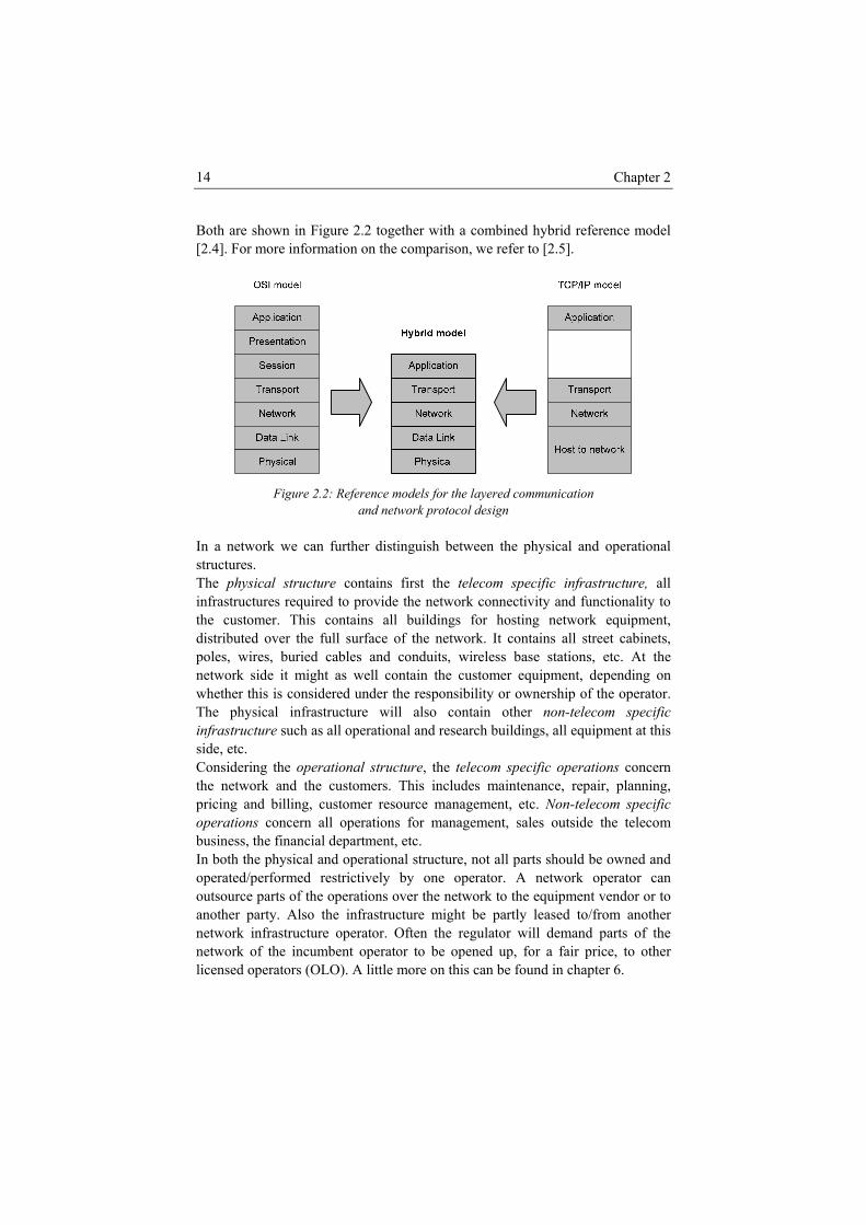
Chapter 2 14
Both are shown in Figure 2.2 together with a combined hybrid reference model [2.4]. For more information on the comparison, we refer to [2.5].
Figure 2.2: Reference models for the layered communication
and network protocol design In a network we can further distinguish between the physical and operational structures. The physical structure contains first the telecom specific infrastructure, all infrastructures required to provide the network connectivity and functionality to the customer. This contains all buildings for hosting network equipment, distributed over the full surface of the network. It contains all street cabinets, poles, wires, buried cables and conduits, wireless base stations, etc. At the network side it might as well contain the customer equipment, depending on whether this is considered under the responsibility or ownership of the operator. The physical infrastructure will also contain other non-telecom specific infrastructure such as all operational and research buildings, all equipment at this side, etc. Considering the operational structure, the telecom specific operations concern the network and the customers. This includes maintenance, repair, planning, pricing and billing, customer resource management, etc. Non-telecom specific operations concern all operations for management, sales outside the telecom business, the financial department, etc. In both the physical and operational structure, not all parts should be owned and operated/performed restrictively by one operator. A network operator can outsource parts of the operations over the network to the equipment vendor or to another party. Also the infrastructure might be partly leased to/from another network infrastructure operator. Often the regulator will demand parts of the network of the incumbent operator to be opened up, for a fair price, to other licensed operators (OLO). A little more on this can be found in chapter 6.
Techno-Economic Background 15
This dissertation will focus on tier 3 and in extension tier 2 operators. The focus is further restricted to the lowest functional layers, especially layer 1 and in extension up to layer 3. Finally the dissertation will also look into more detail to the access network and only secondary look at metro and core networks (as extensions described in chapter 6). The main study of this dissertation will consider all physical and operational structures required for providing connectivity to the customer up to the point where layer 2 or layer 3 functionality and equipment is provided. It will neglect all physical and operational structures which are non-telecom specific.
2.1.2 Core Network The core, or backbone network aggregates and routes huge amounts of traffic. Such network operates at layer 3 or below1, and routers will direct the traffic from source to destination via a shortest, or otherwise constrained, path. The huge amount of traffic in combination with the long distances between the nodes pushes the network to use the most advanced networking technologies available. The physical medium at this level is always optical fibre over which optical signals are transmitted. At the sender site, a laser source transmits optical pulses according to an incoming electronic signal at a given wavelength. The optical signal of different sources/wavelengths can be multiplexed over one fibre. This is called wavelength division multiplexing (WDM) and current technology allows up to 80 wavelength channels each transporting up to 40Gbps, rendering a bandwidth of 3.2Tbps over one fibre. The meshed physical topology of the network allows providing backup for single failures, and in some cases beyond single failures in the network.
2.1.3 Metro Network The metropolitan network, as its name indicates, will stretch from the surface of a metropolis up to the surface of a full country. Often the local operator will further subdivide the network in different smaller areas connected by means of hierarchies of ring, or sparsely meshed structures. At the centre, this network is connected to one or more backbone networks. The structures become less and less meshed further away from the centre of the network. This metropolitan network is entirely built using optical fibre. In the centre, WDM and high-bandwidth (10G) optical sources and receivers can be used, depending on the size of the network and the traffic in this part of the network. More to the edge of the network, less bandwidth is required and often this can already be provided
1 In order to save on routing large amounts of traffic, only the absolutely required functionality is offered. As such this might contain only a limited subset of all layer 3 functionality, while still providing more than mere layer 2 functionality.
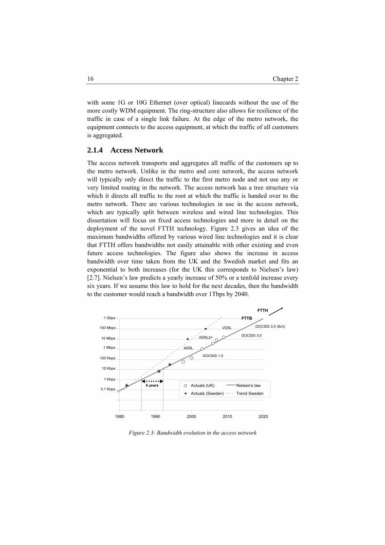
Chapter 2 16
with some 1G or 10G Ethernet (over optical) linecards without the use of the more costly WDM equipment. The ring-structure also allows for resilience of the traffic in case of a single link failure. At the edge of the metro network, the equipment connects to the access equipment, at which the traffic of all customers is aggregated.
2.1.4 Access Network The access network transports and aggregates all traffic of the customers up to the metro network. Unlike in the metro and core network, the access network will typically only direct the traffic to the first metro node and not use any or very limited routing in the network. The access network has a tree structure via which it directs all traffic to the root at which the traffic is handed over to the metro network. There are various technologies in use in the access network, which are typically split between wireless and wired line technologies. This dissertation will focus on fixed access technologies and more in detail on the deployment of the novel FTTH technology. Figure 2.3 gives an idea of the maximum bandwidths offered by various wired line technologies and it is clear that FTTH offers bandwidths not easily attainable with other existing and even future access technologies. The figure also shows the increase in access bandwidth over time taken from the UK and the Swedish market and fits an exponential to both increases (for the UK this corresponds to Nielsen’s law) [2.7]. Nielsen’s law predicts a yearly increase of 50% or a tenfold increase every six years. If we assume this law to hold for the next decades, then the bandwidth to the customer would reach a bandwidth over 1Tbps by 2040.
1
10
100
1000
10000
100000
1000000
10000000
100000000
1000000000
1980 1990 2000 2010 2020
Actuals (UK) Nielsen's law
Actuals (Sweden) Trend Sweden
1 Gbps
100 Mbps
10 Mbps
1 Mbps
100 Kbps
10 Kbps
1 Kbps
0.1 Kbps
ADSL2+
VDSL
FTTB
FTTH
6 years
ADSL
DOCSIS 1.0
DOCSIS 3.0
DOCSIS 3.0 (8ch)
Figure 2.3: Bandwidth evolution in the access network
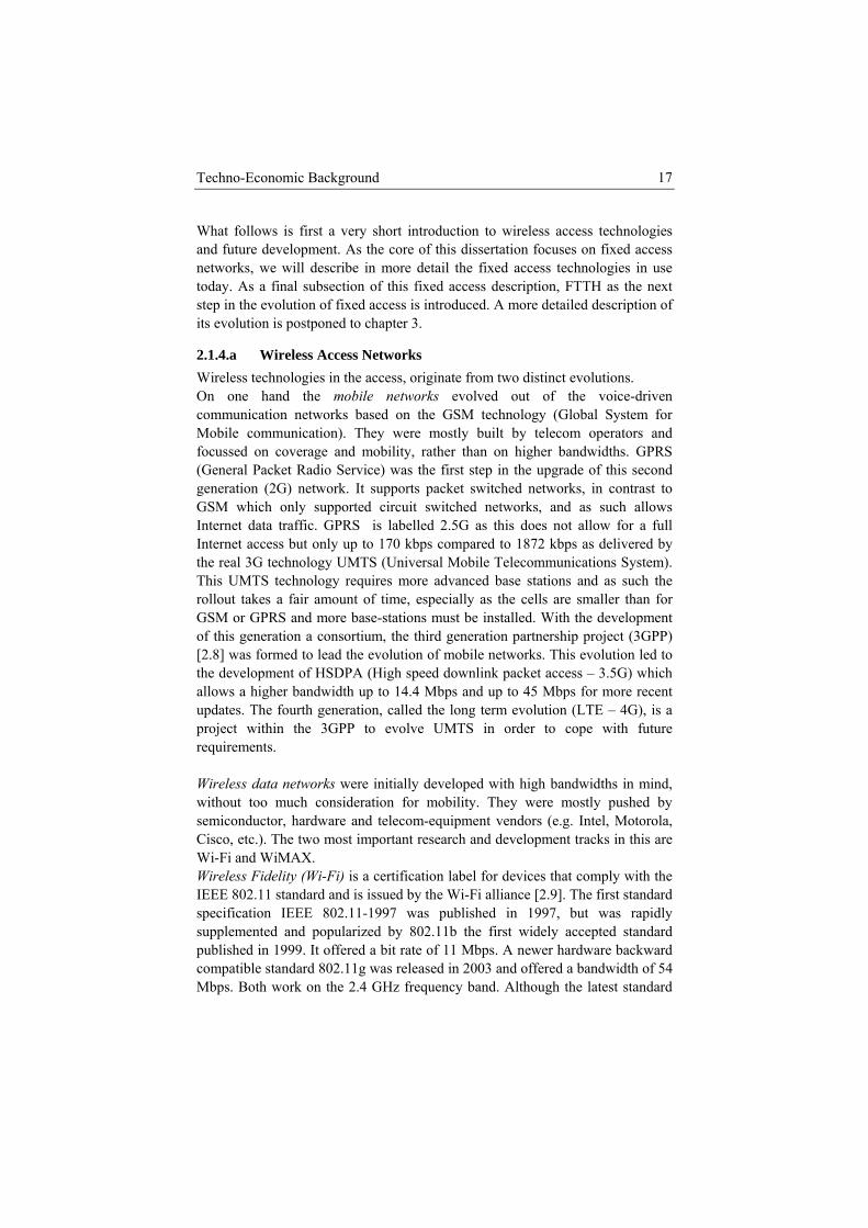
Techno-Economic Background 17
What follows is first a very short introduction to wireless access technologies and future development. As the core of this dissertation focuses on fixed access networks, we will describe in more detail the fixed access technologies in use today. As a final subsection of this fixed access description, FTTH as the next step in the evolution of fixed access is introduced. A more detailed description of its evolution is postponed to chapter 3.
2.1.4.a Wireless Access Networks Wireless technologies in the access, originate from two distinct evolutions. On one hand the mobile networks evolved out of the voice-driven communication networks based on the GSM technology (Global System for Mobile communication). They were mostly built by telecom operators and focussed on coverage and mobility, rather than on higher bandwidths. GPRS (General Packet Radio Service) was the first step in the upgrade of this second generation (2G) network. It supports packet switched networks, in contrast to GSM which only supported circuit switched networks, and as such allows Internet data traffic. GPRS is labelled 2.5G as this does not allow for a full Internet access but only up to 170 kbps compared to 1872 kbps as delivered by the real 3G technology UMTS (Universal Mobile Telecommunications System). This UMTS technology requires more advanced base stations and as such the rollout takes a fair amount of time, especially as the cells are smaller than for GSM or GPRS and more base-stations must be installed. With the development of this generation a consortium, the third generation partnership project (3GPP) [2.8] was formed to lead the evolution of mobile networks. This evolution led to the development of HSDPA (High speed downlink packet access – 3.5G) which allows a higher bandwidth up to 14.4 Mbps and up to 45 Mbps for more recent updates. The fourth generation, called the long term evolution (LTE – 4G), is a project within the 3GPP to evolve UMTS in order to cope with future requirements. Wireless data networks were initially developed with high bandwidths in mind, without too much consideration for mobility. They were mostly pushed by semiconductor, hardware and telecom-equipment vendors (e.g. Intel, Motorola, Cisco, etc.). The two most important research and development tracks in this are Wi-Fi and WiMAX. Wireless Fidelity (Wi-Fi) is a certification label for devices that comply with the IEEE 802.11 standard and is issued by the Wi-Fi alliance [2.9]. The first standard specification IEEE 802.11-1997 was published in 1997, but was rapidly supplemented and popularized by 802.11b the first widely accepted standard published in 1999. It offered a bit rate of 11 Mbps. A newer hardware backward compatible standard 802.11g was released in 2003 and offered a bandwidth of 54 Mbps. Both work on the 2.4 GHz frequency band. Although the latest standard
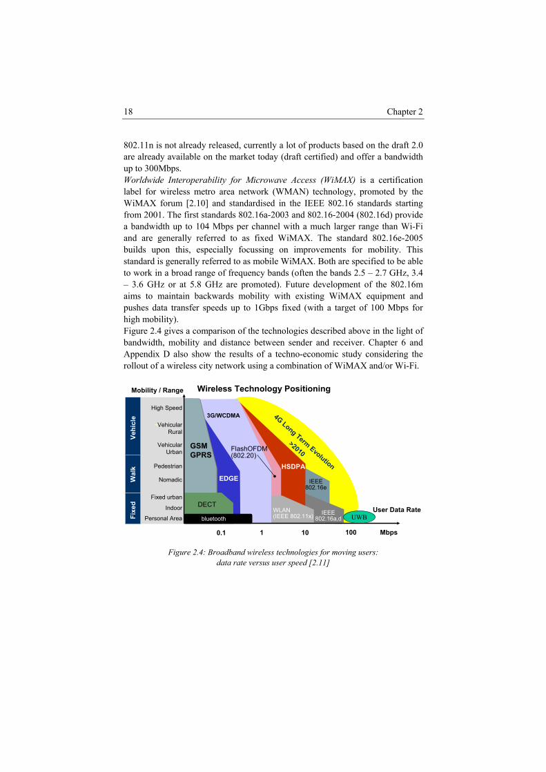
Chapter 2 18
802.11n is not already released, currently a lot of products based on the draft 2.0 are already available on the market today (draft certified) and offer a bandwidth up to 300Mbps. Worldwide Interoperability for Microwave Access (WiMAX) is a certification label for wireless metro area network (WMAN) technology, promoted by the WiMAX forum [2.10] and standardised in the IEEE 802.16 standards starting from 2001. The first standards 802.16a-2003 and 802.16-2004 (802.16d) provide a bandwidth up to 104 Mbps per channel with a much larger range than Wi-Fi and are generally referred to as fixed WiMAX. The standard 802.16e-2005 builds upon this, especially focussing on improvements for mobility. This standard is generally referred to as mobile WiMAX. Both are specified to be able to work in a broad range of frequency bands (often the bands 2.5 – 2.7 GHz, 3.4 – 3.6 GHz or at 5.8 GHz are promoted). Future development of the 802.16m aims to maintain backwards mobility with existing WiMAX equipment and pushes data transfer speeds up to 1Gbps fixed (with a target of 100 Mbps for high mobility). Figure 2.4 gives a comparison of the technologies described above in the light of bandwidth, mobility and distance between sender and receiver. Chapter 6 and Appendix D also show the results of a techno-economic study considering the rollout of a wireless city network using a combination of WiMAX and/or Wi-Fi.
4GLong Term Evolution
>2010
4GLong Term Evolution
>2010
Fixe
dW
alk
Vehi
cle
Mobility / Range
Indoor
Pedestrian
High Speed
VehicularRural
Personal Area
VehicularUrban
Fixed urban
User Data Rate
10 Mbps0.1
IEEE802.16a,d
1 100
HSDPA
IEEE802.16e
Nomadic
WLAN(IEEE 802.11x)
GSMGPRS
DECT
bluetooth
3G/WCDMA
EDGE
FlashOFDM(802.20)
Wireless Technology Positioning
UWB
Figure 2.4: Broadband wireless technologies for moving users:
data rate versus user speed [2.11]
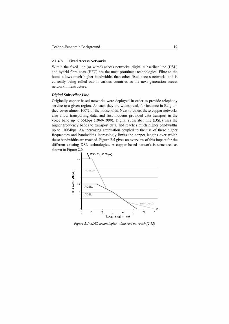
Techno-Economic Background 19
2.1.4.b Fixed Access Networks Within the fixed line (or wired) access networks, digital subscriber line (DSL) and hybrid fibre coax (HFC) are the most prominent technologies. Fibre to the home allows much higher bandwidths than other fixed access networks and is currently being rolled out in various countries as the next generation access network infrastructure.
Digital Subscriber Line Originally copper based networks were deployed in order to provide telephony service to a given region. As such they are widespread, for instance in Belgium they cover almost 100% of the households. Next to voice, these copper networks also allow transporting data, and first modems provided data transport in the voice band up to 55kbps (1960-1990). Digital subscriber line (DSL) uses the higher frequency bands to transport data, and reaches much higher bandwidths up to 100Mbps. An increasing attenuation coupled to the use of these higher frequencies and bandwidths increasingly limits the copper lengths over which these bandwidths are reached. Figure 2.5 gives an overview of this impact for the different existing DSL technologies. A copper based network is structured as shown in Figure 2.6.
Figure 2.5: xDSL technologies - data rate vs. reach [2.12]
Chapter 2 20
Figure 2.6: Overview of a digital subscriber line network
The DSL modem at the right of the figure connects to the twisted copper in-house wiring. The in-house wiring connects to the outside plant by means of a wall plug. The incoming data is separated from the voice before the telephone by means of a splitter. Both voice and data are transported over the outside plant to the first active point. The outside copper plant has a continuous dedicated twisted copper pair connected at aggregation points and flexibility points such as the street cabinet (SC). The first active point is called the DSL access multiplexer (DSLAM) and will translate the upstream2 DSL signal to an Ethernet or ATM (asynchronous transfer mode) signal and send this into the metro network. In downstream it will translate the Ethernet or ATM signals to a DSL signal and send this to the customer. In the case of ADSL (and its different flavours), the DSLAM is located in the local exchange (LEX) around 3-4km in distance from the customer. Before the DSLAM, voice and data are split again and the voice signal is sent to the public switched telecom network (PSTN) switch and data is sent to the DSLAM. This split and an aggregation in larger structured copper connectors happens at the copper or main distribution frame (MDF). In the case of VDSL (and its different flavours), the DSLAM is located much closer to the customer, typically less than 1km away. It also splits voice and data, where voice is further sent over copper to the LEX (and the PSTN switch). Data is handled by the DSLAM at this remote location and the resulting signal is sent over optical fibre to the LEX or to a metro switch further away. In the Belgian market, the incumbent operator Belgacom [2.13] offers from 1998 onwards a full ADSL coverage with a current downstream bandwidth of 4Mbps to 4.6Mbps and an upstream bandwidth of 512kbps. The ADSL equipment has been gradually upgraded to ADSL2+ and VDSL2 is introduced over this network
2 We denote the signal coming from the customer as upstream, and the signal going in the reverse direction as downstream.
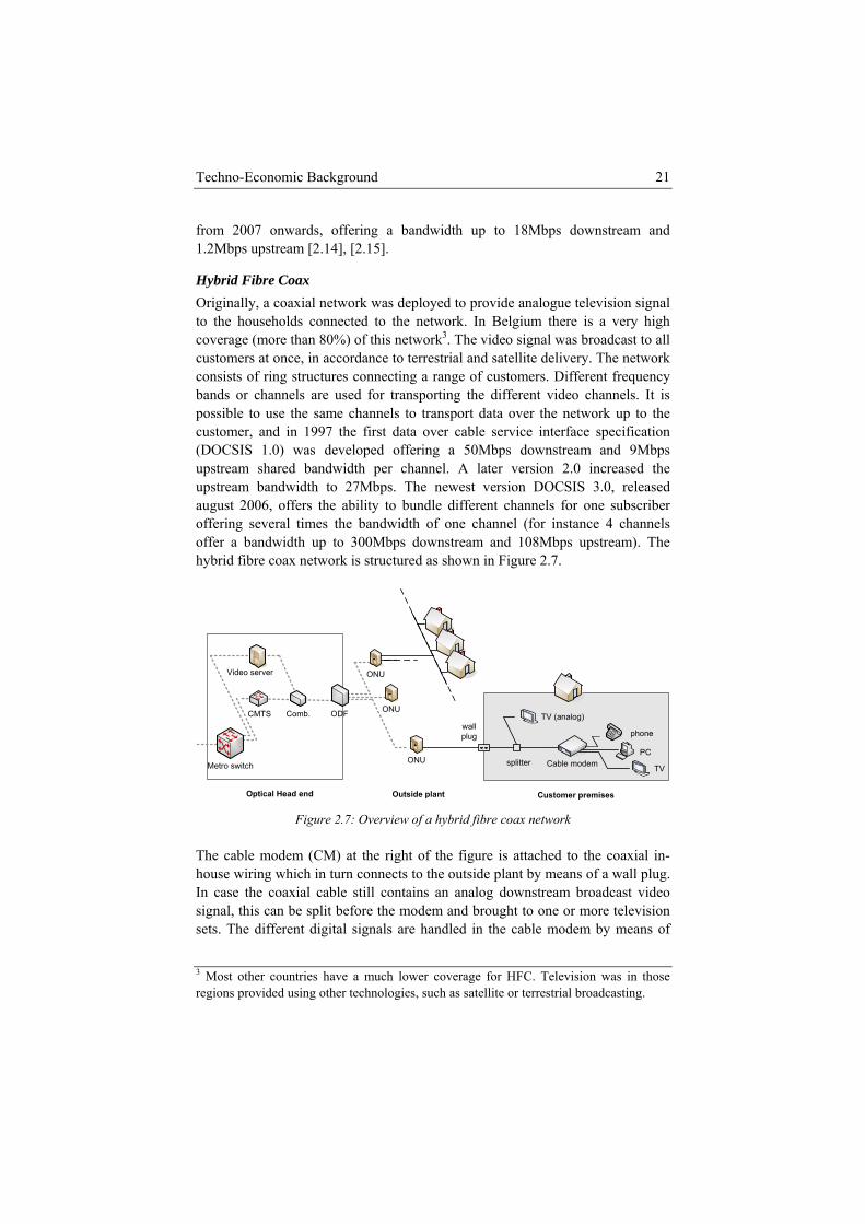
Techno-Economic Background 21
from 2007 onwards, offering a bandwidth up to 18Mbps downstream and 1.2Mbps upstream [2.14], [2.15].
Hybrid Fibre Coax Originally, a coaxial network was deployed to provide analogue television signal to the households connected to the network. In Belgium there is a very high coverage (more than 80%) of this network3. The video signal was broadcast to all customers at once, in accordance to terrestrial and satellite delivery. The network consists of ring structures connecting a range of customers. Different frequency bands or channels are used for transporting the different video channels. It is possible to use the same channels to transport data over the network up to the customer, and in 1997 the first data over cable service interface specification (DOCSIS 1.0) was developed offering a 50Mbps downstream and 9Mbps upstream shared bandwidth per channel. A later version 2.0 increased the upstream bandwidth to 27Mbps. The newest version DOCSIS 3.0, released august 2006, offers the ability to bundle different channels for one subscriber offering several times the bandwidth of one channel (for instance 4 channels offer a bandwidth up to 300Mbps downstream and 108Mbps upstream). The hybrid fibre coax network is structured as shown in Figure 2.7.
ONU
ONU
ONU
Outside plantOptical Head end
ODF
Metro switch
CMTS Comb.
splitter
phone
PC
TVCable modem
Customer premises
wallplug
TV (analog)
Video server
Figure 2.7: Overview of a hybrid fibre coax network
The cable modem (CM) at the right of the figure is attached to the coaxial in-house wiring which in turn connects to the outside plant by means of a wall plug. In case the coaxial cable still contains an analog downstream broadcast video signal, this can be split before the modem and brought to one or more television sets. The different digital signals are handled in the cable modem by means of
3 Most other countries have a much lower coverage for HFC. Television was in those regions provided using other technologies, such as satellite or terrestrial broadcasting.
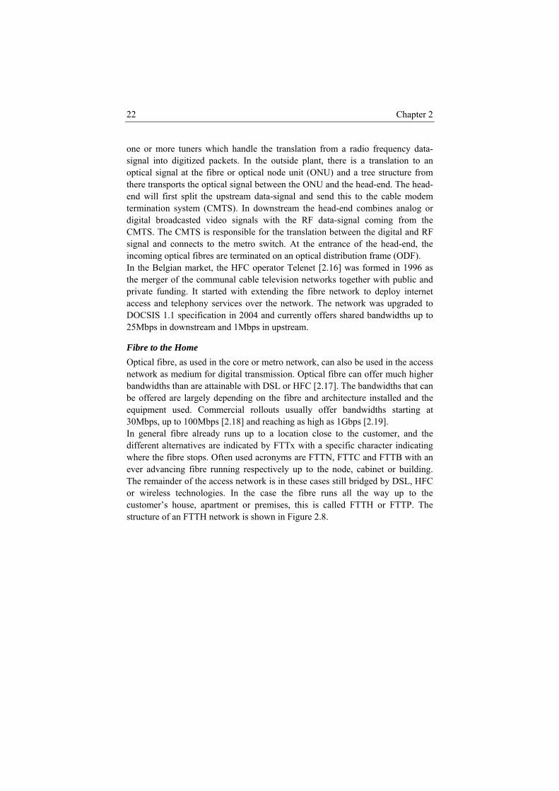
Chapter 2 22
one or more tuners which handle the translation from a radio frequency data-signal into digitized packets. In the outside plant, there is a translation to an optical signal at the fibre or optical node unit (ONU) and a tree structure from there transports the optical signal between the ONU and the head-end. The head-end will first split the upstream data-signal and send this to the cable modem termination system (CMTS). In downstream the head-end combines analog or digital broadcasted video signals with the RF data-signal coming from the CMTS. The CMTS is responsible for the translation between the digital and RF signal and connects to the metro switch. At the entrance of the head-end, the incoming optical fibres are terminated on an optical distribution frame (ODF). In the Belgian market, the HFC operator Telenet [2.16] was formed in 1996 as the merger of the communal cable television networks together with public and private funding. It started with extending the fibre network to deploy internet access and telephony services over the network. The network was upgraded to DOCSIS 1.1 specification in 2004 and currently offers shared bandwidths up to 25Mbps in downstream and 1Mbps in upstream.
Fibre to the Home Optical fibre, as used in the core or metro network, can also be used in the access network as medium for digital transmission. Optical fibre can offer much higher bandwidths than are attainable with DSL or HFC [2.17]. The bandwidths that can be offered are largely depending on the fibre and architecture installed and the equipment used. Commercial rollouts usually offer bandwidths starting at 30Mbps, up to 100Mbps [2.18] and reaching as high as 1Gbps [2.19]. In general fibre already runs up to a location close to the customer, and the different alternatives are indicated by FTTx with a specific character indicating where the fibre stops. Often used acronyms are FTTN, FTTC and FTTB with an ever advancing fibre running respectively up to the node, cabinet or building. The remainder of the access network is in these cases still bridged by DSL, HFC or wireless technologies. In the case the fibre runs all the way up to the customer’s house, apartment or premises, this is called FTTH or FTTP. The structure of an FTTH network is shown in Figure 2.8.
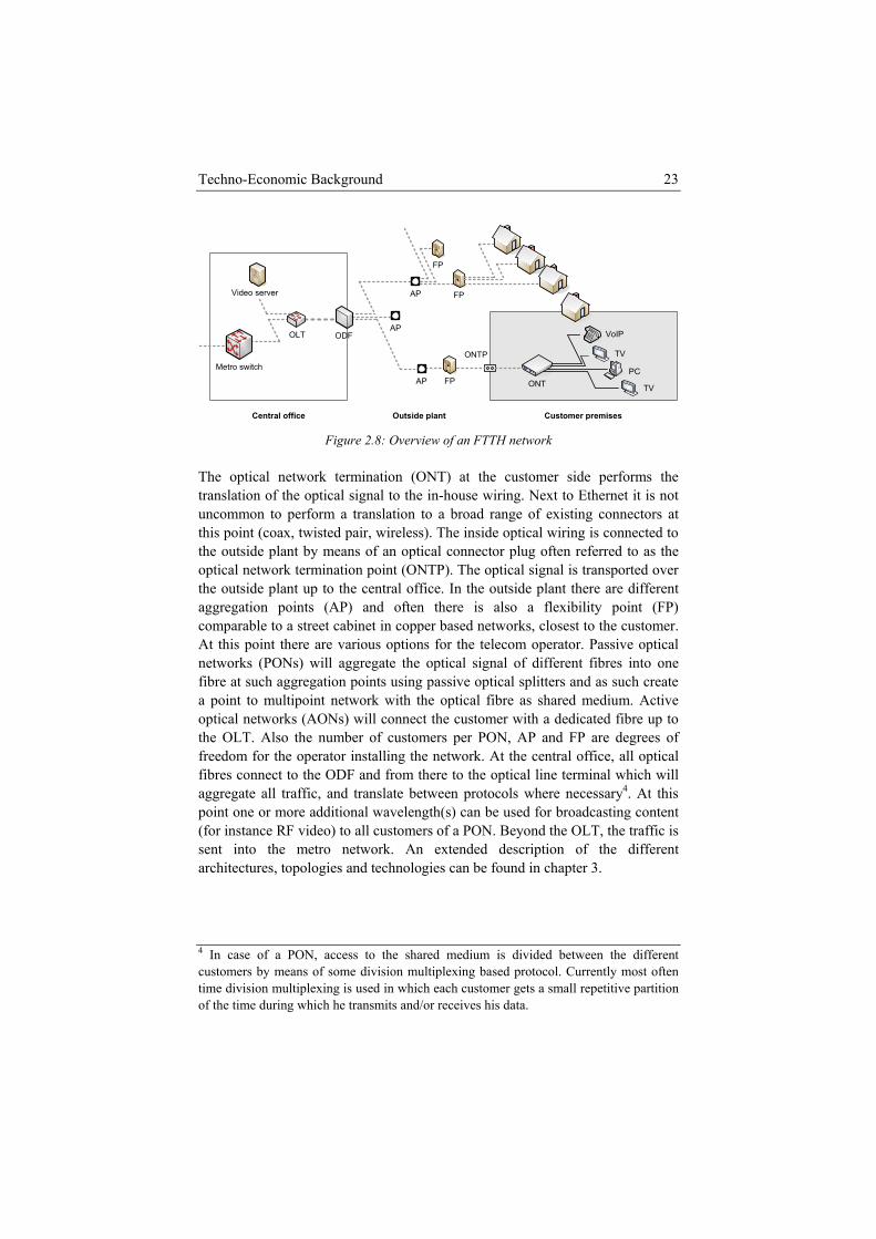
Techno-Economic Background 23
Central office
ONT
Customer premises
FP
Outside plant
ODF
Metro switchONTP
FP
AP
AP
AP
TV
PC
TV
VoIP
FP
Video server
OLT
Figure 2.8: Overview of an FTTH network
The optical network termination (ONT) at the customer side performs the translation of the optical signal to the in-house wiring. Next to Ethernet it is not uncommon to perform a translation to a broad range of existing connectors at this point (coax, twisted pair, wireless). The inside optical wiring is connected to the outside plant by means of an optical connector plug often referred to as the optical network termination point (ONTP). The optical signal is transported over the outside plant up to the central office. In the outside plant there are different aggregation points (AP) and often there is also a flexibility point (FP) comparable to a street cabinet in copper based networks, closest to the customer. At this point there are various options for the telecom operator. Passive optical networks (PONs) will aggregate the optical signal of different fibres into one fibre at such aggregation points using passive optical splitters and as such create a point to multipoint network with the optical fibre as shared medium. Active optical networks (AONs) will connect the customer with a dedicated fibre up to the OLT. Also the number of customers per PON, AP and FP are degrees of freedom for the operator installing the network. At the central office, all optical fibres connect to the ODF and from there to the optical line terminal which will aggregate all traffic, and translate between protocols where necessary4. At this point one or more additional wavelength(s) can be used for broadcasting content (for instance RF video) to all customers of a PON. Beyond the OLT, the traffic is sent into the metro network. An extended description of the different architectures, topologies and technologies can be found in chapter 3.
4 In case of a PON, access to the shared medium is divided between the different customers by means of some division multiplexing based protocol. Currently most often time division multiplexing is used in which each customer gets a small repetitive partition of the time during which he transmits and/or receives his data.
Chapter 2 24
There is currently no large scale FTTH-network deployed in the Belgian market. Belgacom announced they will be performing FTTH trials at the end of this year [2.20]. The FTTH scene in Europe is also very small, with some countries in which FTTH is rolled out fast (especially Sweden). On a world scale, FTTH is prevalent in Asia, especially in Japan and Korea. It is deployed on a much smaller scale in US; however the US still has a much larger customer base than Europe (2.5 Million customers vs. less than 1 Million customers).
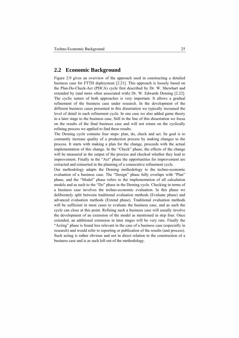
Techno-Economic Background 25
2.2 Economic Background Figure 2.9 gives an overview of the approach used in constructing a detailed business case for FTTH deployment [2.21]. This approach is loosely based on the Plan-Do-Check-Act (PDCA) cycle first described by Dr. W. Shewhart and extended by (and more often associated with) Dr. W. Edwards Deming [2.22]. The cyclic nature of both approaches is very important. It allows a gradual refinement of the business case under research. In the development of the different business cases presented in this dissertation we typically increased the level of detail in each refinement cycle. In one case we also added game theory in a later stage to the business case. Still in the line of this dissertation we focus on the results of the final business case and will not return on the cyclically refining process we applied to find these results. The Deming cycle contains four steps: plan, do, check and act. Its goal is to constantly increase quality of a production process by making changes to the process. It starts with making a plan for the change, proceeds with the actual implementation of this change. In the “Check” phase, the effects of the change will be measured in the output of the process and checked whether they lead to improvement. Finally in the “Act” phase the opportunities for improvement are extracted and reinserted in the planning of a consecutive refinement cycle. Our methodology adapts the Deming methodology to the techno-economic evaluation of a business case. The “Design” phase fully overlaps with “Plan” phase, and the “Model” phase refers to the implementation of all calculation models and as such to the “Do” phase in the Deming cycle. Checking in terms of a business case involves the techno-economic evaluation. In this phase we deliberately split between traditional evaluation methods (Evaluate phase) and advanced evaluation methods (Extend phase). Traditional evaluation methods will be sufficient in most cases to evaluate the business case, and as such the cycle can close at this point. Refining such a business case will usually involve the development of an extension of the model as mentioned in step four. Once extended, an additional extension in later stages will be very rare. Finally the “Acting” phase is found less relevant in the case of a business case (especially in research) and would refer to reporting or publication of the results (and process). Such acting is rather obvious and not in direct relation to the construction of a business case and is as such left out of the methodology.
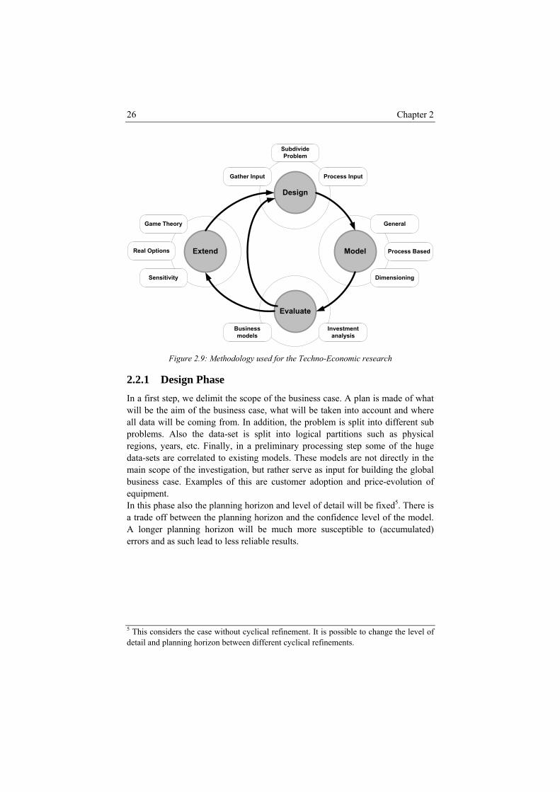
Chapter 2 26
Evaluate
Model
Design
Extend
Game Theory
Real Options
Sensitivity
Business models
Investment analysis
General
Process Based
Dimensioning
Gather Input
Subdivide Problem
Process Input
Figure 2.9: Methodology used for the Techno-Economic research
2.2.1 Design Phase In a first step, we delimit the scope of the business case. A plan is made of what will be the aim of the business case, what will be taken into account and where all data will be coming from. In addition, the problem is split into different sub problems. Also the data-set is split into logical partitions such as physical regions, years, etc. Finally, in a preliminary processing step some of the huge data-sets are correlated to existing models. These models are not directly in the main scope of the investigation, but rather serve as input for building the global business case. Examples of this are customer adoption and price-evolution of equipment. In this phase also the planning horizon and level of detail will be fixed5. There is a trade off between the planning horizon and the confidence level of the model. A longer planning horizon will be much more susceptible to (accumulated) errors and as such lead to less reliable results.
5 This considers the case without cyclical refinement. It is possible to change the level of detail and planning horizon between different cyclical refinements.
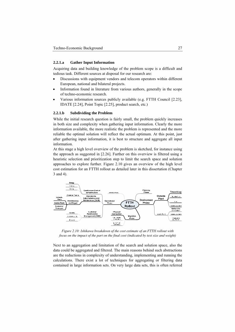
Techno-Economic Background 27
2.2.1.a Gather Input Information Acquiring data and building knowledge of the problem scope is a difficult and tedious task. Different sources at disposal for our research are: • Discussions with equipment vendors and telecom operators within different
European, national and bilateral projects. • Information found in literature from various authors, generally in the scope
of techno-economic research. • Various information sources publicly available (e.g. FTTH Council [2.23],
IDATE [2.24], Point Topic [2.25], product search, etc.)
2.2.1.b Subdividing the Problem While the initial research question is fairly small, the problem quickly increases in both size and complexity when gathering input information. Clearly the more information available, the more realistic the problem is represented and the more reliable the optimal solution will reflect the actual optimum. At this point, just after gathering input information, it is best to structure and aggregate all input information. At this stage a high level overview of the problem is sketched, for instance using the approach as suggested in [2.26]. Further on this overview is filtered using a heuristic selection and prioritization step to limit the search space and solution approaches to explore further. Figure 2.10 gives an overview of the high level cost estimation for an FTTH rollout as detailed later in this dissertation (Chapter 3 and 4).
Figure 2.10: Ishikawa breakdown of the cost estimate of an FTTH rollout with
focus on the impact of the part on the final cost (indicated by text size and weight) Next to an aggregation and limitation of the search and solution space, also the data could be aggregated and filtered. The main reasons behind such abstractions are the reductions in complexity of understanding, implementing and running the calculations. There exist a lot of techniques for aggregating or filtering data contained in large information sets. On very large data sets, this is often referred
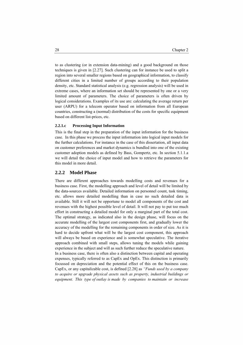
Chapter 2 28
to as clustering (or in extension data-mining) and a good background on those techniques is given in [2.27]. Such clustering can for instance be used to split a region into several smaller regions based on geographical information, to classify different cities in a limited number of groups according to their population density, etc. Standard statistical analysis (e.g. regression analysis) will be used in extreme cases, where an information set should be represented by one or a very limited amount of parameters. The choice of parameters is often driven by logical considerations. Examples of its use are: calculating the average return per user (ARPU) for a telecom operator based on information from all European countries, constructing a (normal) distribution of the costs for specific equipment based on different list-prices, etc.
2.2.1.c Processing Input Information This is the final step in the preparation of the input information for the business case. In this phase we process the input information into logical input models for the further calculations. For instance in the case of this dissertation, all input data on customer preferences and market dynamics is bundled into one of the existing customer adoption models as defined by Bass, Gompertz, etc. In section 5.1.1.a we will detail the choice of input model and how to retrieve the parameters for this model in more detail.
2.2.2 Model Phase There are different approaches towards modelling costs and revenues for a business case. First, the modelling approach and level of detail will be limited by the data-sources available. Detailed information on personnel count, task timing, etc. allows more detailed modelling than in case no such detailed data is available. Still it will not be opportune to model all components of the cost and revenues with the highest possible level of detail. It will not pay to put too much effort in constructing a detailed model for only a marginal part of the total cost. The optimal strategy, as indicated also in the design phase, will focus on the accurate modelling of the largest cost components first, and gradually lower the accuracy of the modelling for the remaining components in order of size. As it is hard to decide upfront what will be the largest cost component, this approach will always be based on experience and is somewhat speculative. The iterative approach combined with small steps, allows tuning the models while gaining experience in the subject and will as such further reduce the speculative nature. In a business case, there is often also a distinction between capital and operating expenses, typically referred to as CapEx and OpEx. This distinction is primarily focussed on depreciation and the potential effect of this on the business case. CapEx, or any capitalizable cost, is defined [2.28] as “Funds used by a company to acquire or upgrade physical assets such as property, industrial buildings or equipment. This type of outlay is made by companies to maintain or increase
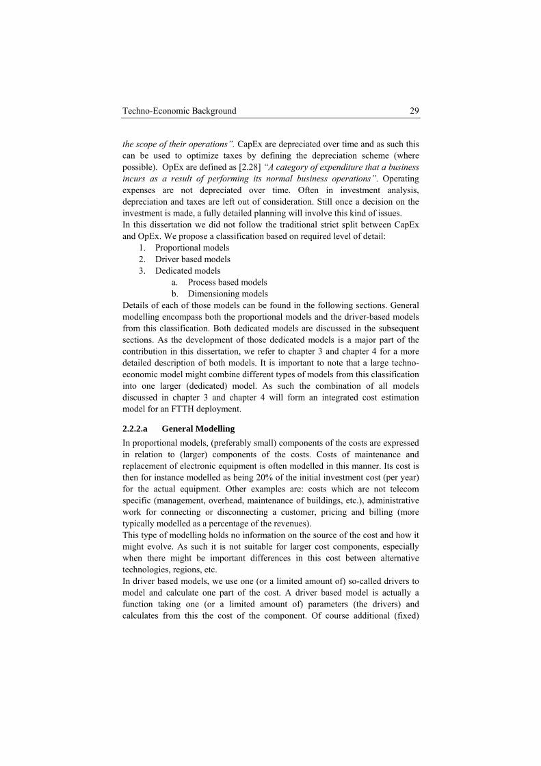
Techno-Economic Background 29
the scope of their operations”. CapEx are depreciated over time and as such this can be used to optimize taxes by defining the depreciation scheme (where possible). OpEx are defined as [2.28] “A category of expenditure that a business incurs as a result of performing its normal business operations”. Operating expenses are not depreciated over time. Often in investment analysis, depreciation and taxes are left out of consideration. Still once a decision on the investment is made, a fully detailed planning will involve this kind of issues. In this dissertation we did not follow the traditional strict split between CapEx and OpEx. We propose a classification based on required level of detail:
1. Proportional models 2. Driver based models 3. Dedicated models
a. Process based models b. Dimensioning models
Details of each of those models can be found in the following sections. General modelling encompass both the proportional models and the driver-based models from this classification. Both dedicated models are discussed in the subsequent sections. As the development of those dedicated models is a major part of the contribution in this dissertation, we refer to chapter 3 and chapter 4 for a more detailed description of both models. It is important to note that a large techno-economic model might combine different types of models from this classification into one larger (dedicated) model. As such the combination of all models discussed in chapter 3 and chapter 4 will form an integrated cost estimation model for an FTTH deployment.
2.2.2.a General Modelling In proportional models, (preferably small) components of the costs are expressed in relation to (larger) components of the costs. Costs of maintenance and replacement of electronic equipment is often modelled in this manner. Its cost is then for instance modelled as being 20% of the initial investment cost (per year) for the actual equipment. Other examples are: costs which are not telecom specific (management, overhead, maintenance of buildings, etc.), administrative work for connecting or disconnecting a customer, pricing and billing (more typically modelled as a percentage of the revenues). This type of modelling holds no information on the source of the cost and how it might evolve. As such it is not suitable for larger cost components, especially when there might be important differences in this cost between alternative technologies, regions, etc. In driver based models, we use one (or a limited amount of) so-called drivers to model and calculate one part of the cost. A driver based model is actually a function taking one (or a limited amount of) parameters (the drivers) and calculates from this the cost of the component. Of course additional (fixed)

Chapter 2 30
parameters can be used in this calculation function. The following example, also used in the infrastructure model described later in this dissertation, will clarify this. The cost for call-centre and helpdesk is in this model related to the number of customers, which is as such the driver for the cost. In the calculations we considered that one customer would lead to (statistically of course) 1.8 calls per year and handling one such call costs 12€ on average. As such the call-centre and helpdesk cost can be calculated based on the actual number of customers in each year. Of course a more detailed model could be used, where the helpdesk cost will be depending more on the new customers as they encounter more problems. In this case there are two drivers, all customers and new customers, and a slightly different function for the calculation of the cost. Such model was used in the evaluation of wireless network rollout, as discussed in chapter 6. The driver based model can easily resemble other types of models, by changing the driver and the function. In case the driver is set to the cost of another component of the cost, the driver based model replaces the proportional models. Increasing the number of drivers and the complexity of the functions, allows driver based models to resemble all dedicated models as well. We distinguish driver based from proportional models by the requirement of a driver which is logically linked to the final cost6, and is preferably the most important logical parameter. While driver based (or more in general function based) models can be used to represent all dedicated models, there is a difference in logical structure and solution approach. Operational processes for instance are more intuitively comprehensible and manageable when modelled with flowcharts or other dedicated models.
2.2.2.b Process Based Modelling Process based modelling is a dedicated approach, aimed at modelling costs caused by the repetitive execution of a (non-trivial) process. A first research task consists of detecting and documenting the process which is actually executed. There are different types of modelling paradigms and even more languages and graphical representations that can be used in this task. In this dissertation we preferred to use a flowchart based modelling approach (see also Figure 2.11), as it allows sufficiently detailed documentation and is most intuitively comprehensible for non-initiated readers.
6 For instance modelling all customer specific costs as a driver based model, logically linked to the number of customers is preferred over a proportional model in which this logical link is not existing (e.g. proportional to overall cost).
Techno-Economic Background 31
Figure 2.11: Example of a process using a flowchart based modelling approach
Once the process is adequately documented, the cost of executing this process once can be estimated using for instance activity based costing (ABC) [2.29]. Each rectangle in the flowchart represents a task assigned to a person or a team. Each diamond in the flowchart represents a conditional split in the execution of subsequent steps. By assigning a cost to the execution of a task, or in extension resources such as time and tools consumed when executing that task, and probabilities to the diverging paths of a split, analytical methods can be used for estimating the process execution cost. More detailed information in the documented processes in combination with advanced calculation and simulation approaches allows doing more than just estimating cost. Depending on the extra information, it might allow to detect bottlenecks and deadlocks, calculate optimized scheduling rules, etc. [2.30] More on modelling, calculation and optimization of operational processes can be found in chapter 4.
2.2.2.c Network Dimensioning In network dimensioning the researcher tries to find out the amount of equipment necessary to provide a given functionality over a telecom network. Even more than simple calculation of a sufficient infrastructure solution, the researcher is often interested in the most efficient, or as efficient as possible, use of infrastructure. In techno-economic modelling a network dimensioning will lead to a so called bill-of-material (BoM) containing a list of all equipment that should be installed to provide the required functionality. This bill-of-material easily allows calculating the actual cost of the infrastructure, as this is just a question of multiplying each part with its (estimated) cost. More on network dimensioning approaches and the calculation of infrastructure costs can be found in chapter 3.
Chapter 2 32
2.2.3 Evaluate Phase As input for the evaluation, we assume that a cost and revenue model is developed, using the approach as discussed in the previous section. This cost and revenue model enables us to calculate the cash flows at each point in time. Based on this information, a decision on whether or not to implement this business case should be taken. This decision often also involves the comparison of different possible projects to each other. Figure 2.12 gives a visualisation of such cash flows and will be used in the following section to explain the different techniques in use in traditional investment analysis [2.31]. Beyond the point of evaluating a single project on its profitability also the position of the firm in the business landscape can be investigated. In such broader business modelling, the different roles, actors and money streams are sketched. The company can draw a lot of conclusions from this information on opportunities and risks, competitors, co-operations and alliances, etc.
2.2.3.a Investment Analysis Cash flow analysis gives a good idea of the profitability of the project and the annual investment costs or profits. One can also easily spot the moment at which the revenues become important. A summation of all cash flows gives the profitability of the project over the lifetime. The cumulative of the cash flows, also shown in Figure 2.12, gives an idea of the point at which the revenues balance all investment costs. This moment is called the payback time (PB) and can be used as limiting factor for the project. The project can then only be carried out on condition that the payback time is smaller than or equal to some predefined (acceptable) period. It also gives an idea of the total profit of the project. Return on investment (RoI) is calculated from the cash flows by dividing the average future cash flow by the average initial investment (both are averaged over the economic lifetime or planning horizon of the project). In case this is used in the decision process, the project can only be carried out on condition that the return on investment of the project exceeds a certain predefined minimum return on investment.
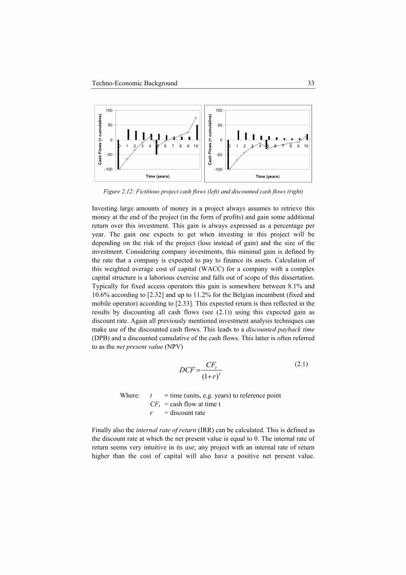
Techno-Economic Background 33
-100
-50
0
50
100
0 1 2 3 4 5 6 7 8 9 10
Time (years)
Cas
h Fl
ows
(+ c
umul
ativ
e)
-100
-50
0
50
100
0 1 2 3 4 5 6 7 8 9 10
Time (years)
Cas
h Fl
ows
(+ c
umul
ativ
e)
Figure 2.12: Fictitious project cash flows (left) and discounted cash flows (right)
Investing large amounts of money in a project always assumes to retrieve this money at the end of the project (in the form of profits) and gain some additional return over this investment. This gain is always expressed as a percentage per year. The gain one expects to get when investing in this project will be depending on the risk of the project (loss instead of gain) and the size of the investment. Considering company investments, this minimal gain is defined by the rate that a company is expected to pay to finance its assets. Calculation of this weighted average cost of capital (WACC) for a company with a complex capital structure is a laborious exercise and falls out of scope of this dissertation. Typically for fixed access operators this gain is somewhere between 8.1% and 10.6% according to [2.32] and up to 11.2% for the Belgian incumbent (fixed and mobile operator) according to [2.33]. This expected return is then reflected in the results by discounting all cash flows (see (2.1)) using this expected gain as discount rate. Again all previously mentioned investment analysis techniques can make use of the discounted cash flows. This leads to a discounted payback time (DPB) and a discounted cumulative of the cash flows. This latter is often referred to as the net present value (NPV)
t
t
rCF
DCF)1( +
=
Where: t = time (units, e.g. years) to reference point CFt = cash flow at time t r = discount rate
(2.1)
Finally also the internal rate of return (IRR) can be calculated. This is defined as the discount rate at which the net present value is equal to 0. The internal rate of return seems very intuitive in its use; any project with an internal rate of return higher than the cost of capital will also have a positive net present value.

Chapter 2 34
However the internal rate of return has some important drawbacks, also highlighted in [2.34]: • It assumes that interim positive cash flows are reinvested at the same rates of
return of the project that generated them. More probably the funds will be reinvested at a rate close to the cost of capital. When greater than the cost of capital the internal rate of return gives an overly optimistic percentage.
• In projects that have irregular cash flows alternating between positive and negative values several times, numerous internal rates of return can be identified. This leads to confusion and possibly also to a wrong investment decision.
Solutions for this problem exist in the form of the extended and the modified internal rate of return (XIRR and MIRR) [2.35]. The net present value is generally considered the most reliable static comparison and selection criterion. A project can only be selected on condition that it has a positive net present value, as the gain is in this case higher than the cost of capital and the project will add value to the firm. Net present value can also be used in comparing two projects, in which the project with the highest net present value will be chosen over the other project. Only in case two projects have the same net present value (within confidence margin of the calculation model) decision could be based on the other techniques. In the evaluation of telecom projects further in this dissertation we based conclusions only on the NPV value.
2.2.3.b Business Modelling While a business case looks at the profitability of one project which might be interesting for the company, business modelling will look outside this case and will consider the project in a broader context. It is good practice to start by identifying the different roles of importance to the considered business case. A role is defined by a task (or functionality) in the business. Examples of such tasks in the telecom world are: equipment production, equipment vending, operating network, deploying network, regulating network prices, retail network services, wholesale network services, retail customer, etc. Again the level of detail will be important, as it is often possible to split roles into smaller sub roles. Several actors will exist in the considered business segment. Each of the actors can be associated with a set of roles previously defined. Mind that roles can be executed by several actors. After this step, all important actors will be identified and can easily be classified using for instance the forces driving industry competition as defined by Porter [2.36]: competition, suppliers, buyers, substitutes and potential entrants. This detailed analysis of roles and actors allows performing a value chain analysis. In this analysis, the money streams between the different actors are identified, with a main focus of course on the money streams involving the firm
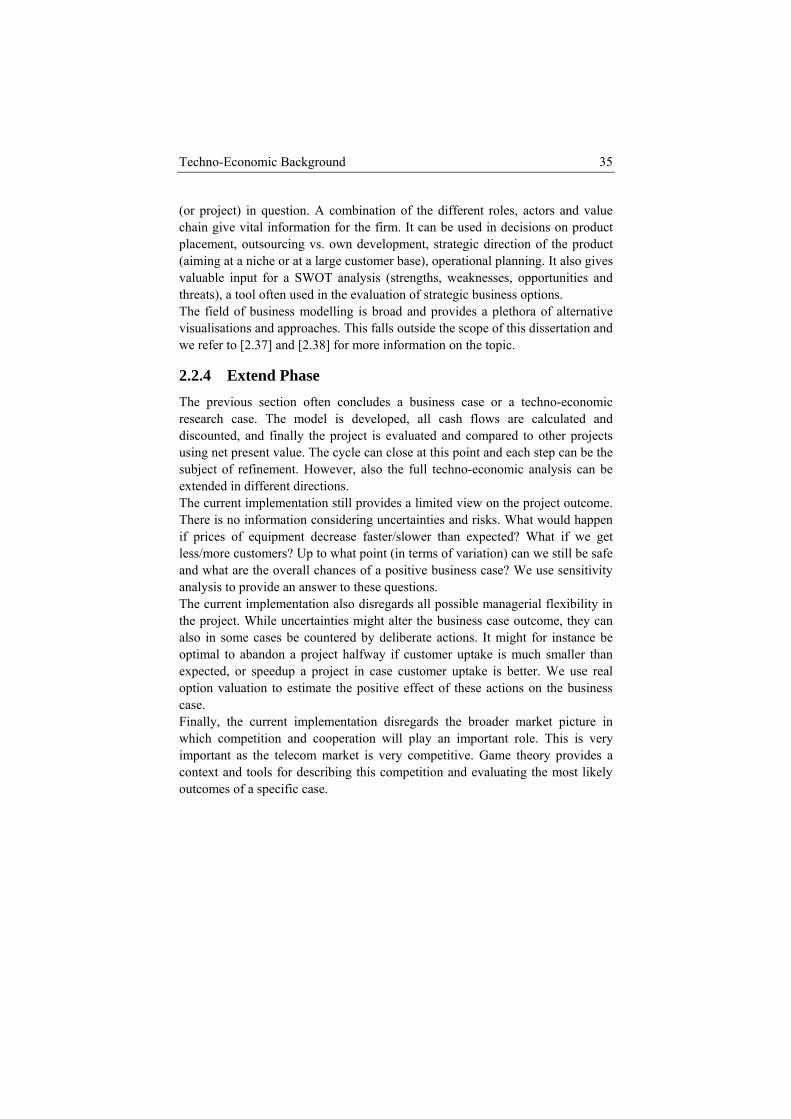
Techno-Economic Background 35
(or project) in question. A combination of the different roles, actors and value chain give vital information for the firm. It can be used in decisions on product placement, outsourcing vs. own development, strategic direction of the product (aiming at a niche or at a large customer base), operational planning. It also gives valuable input for a SWOT analysis (strengths, weaknesses, opportunities and threats), a tool often used in the evaluation of strategic business options. The field of business modelling is broad and provides a plethora of alternative visualisations and approaches. This falls outside the scope of this dissertation and we refer to [2.37] and [2.38] for more information on the topic.
2.2.4 Extend Phase The previous section often concludes a business case or a techno-economic research case. The model is developed, all cash flows are calculated and discounted, and finally the project is evaluated and compared to other projects using net present value. The cycle can close at this point and each step can be the subject of refinement. However, also the full techno-economic analysis can be extended in different directions. The current implementation still provides a limited view on the project outcome. There is no information considering uncertainties and risks. What would happen if prices of equipment decrease faster/slower than expected? What if we get less/more customers? Up to what point (in terms of variation) can we still be safe and what are the overall chances of a positive business case? We use sensitivity analysis to provide an answer to these questions. The current implementation also disregards all possible managerial flexibility in the project. While uncertainties might alter the business case outcome, they can also in some cases be countered by deliberate actions. It might for instance be optimal to abandon a project halfway if customer uptake is much smaller than expected, or speedup a project in case customer uptake is better. We use real option valuation to estimate the positive effect of these actions on the business case. Finally, the current implementation disregards the broader market picture in which competition and cooperation will play an important role. This is very important as the telecom market is very competitive. Game theory provides a context and tools for describing this competition and evaluating the most likely outcomes of a specific case.
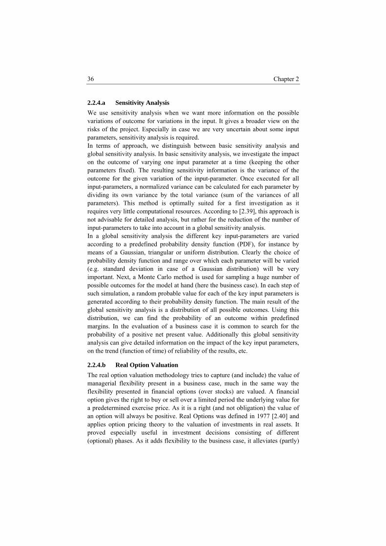
Chapter 2 36
2.2.4.a Sensitivity Analysis We use sensitivity analysis when we want more information on the possible variations of outcome for variations in the input. It gives a broader view on the risks of the project. Especially in case we are very uncertain about some input parameters, sensitivity analysis is required. In terms of approach, we distinguish between basic sensitivity analysis and global sensitivity analysis. In basic sensitivity analysis, we investigate the impact on the outcome of varying one input parameter at a time (keeping the other parameters fixed). The resulting sensitivity information is the variance of the outcome for the given variation of the input-parameter. Once executed for all input-parameters, a normalized variance can be calculated for each parameter by dividing its own variance by the total variance (sum of the variances of all parameters). This method is optimally suited for a first investigation as it requires very little computational resources. According to [2.39], this approach is not advisable for detailed analysis, but rather for the reduction of the number of input-parameters to take into account in a global sensitivity analysis. In a global sensitivity analysis the different key input-parameters are varied according to a predefined probability density function (PDF), for instance by means of a Gaussian, triangular or uniform distribution. Clearly the choice of probability density function and range over which each parameter will be varied (e.g. standard deviation in case of a Gaussian distribution) will be very important. Next, a Monte Carlo method is used for sampling a huge number of possible outcomes for the model at hand (here the business case). In each step of such simulation, a random probable value for each of the key input parameters is generated according to their probability density function. The main result of the global sensitivity analysis is a distribution of all possible outcomes. Using this distribution, we can find the probability of an outcome within predefined margins. In the evaluation of a business case it is common to search for the probability of a positive net present value. Additionally this global sensitivity analysis can give detailed information on the impact of the key input parameters, on the trend (function of time) of reliability of the results, etc.
2.2.4.b Real Option Valuation The real option valuation methodology tries to capture (and include) the value of managerial flexibility present in a business case, much in the same way the flexibility presented in financial options (over stocks) are valued. A financial option gives the right to buy or sell over a limited period the underlying value for a predetermined exercise price. As it is a right (and not obligation) the value of an option will always be positive. Real Options was defined in 1977 [2.40] and applies option pricing theory to the valuation of investments in real assets. It proved especially useful in investment decisions consisting of different (optional) phases. As it adds flexibility to the business case, it alleviates (partly)
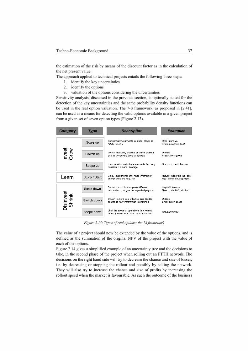
Techno-Economic Background 37
the estimation of the risk by means of the discount factor as in the calculation of the net present value. The approach applied to technical projects entails the following three steps:
1. identify the key uncertainties 2. identify the options 3. valuation of the options considering the uncertainties
Sensitivity analysis, discussed in the previous section, is optimally suited for the detection of the key uncertainties and the same probability density functions can be used in the real option valuation. The 7-S framework, as proposed in [2.41], can be used as a means for detecting the valid options available in a given project from a given set of seven option types (Figure 2.13).
Figure 2.13: Types of real options: the 7S framework
The value of a project should now be extended by the value of the options, and is defined as the summation of the original NPV of the project with the value of each of the options. Figure 2.14 gives a simplified example of an uncertainty tree and the decisions to take, in the second phase of the project when rolling out an FTTH network. The decisions on the right hand side will try to decrease the chance and size of losses, i.e. by decreasing or stopping the rollout and possibly by selling the network. They will also try to increase the chance and size of profits by increasing the rollout speed when the market is favourable. As such the outcome of the business
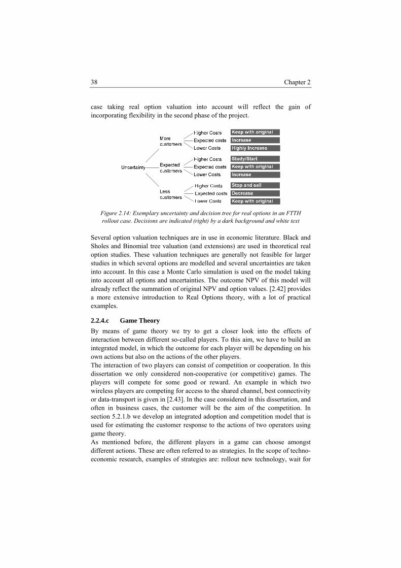
Chapter 2 38
case taking real option valuation into account will reflect the gain of incorporating flexibility in the second phase of the project.
Figure 2.14: Exemplary uncertainty and decision tree for real options in an FTTH rollout case. Decisions are indicated (right) by a dark background and white text
Several option valuation techniques are in use in economic literature. Black and Sholes and Binomial tree valuation (and extensions) are used in theoretical real option studies. These valuation techniques are generally not feasible for larger studies in which several options are modelled and several uncertainties are taken into account. In this case a Monte Carlo simulation is used on the model taking into account all options and uncertainties. The outcome NPV of this model will already reflect the summation of original NPV and option values. [2.42] provides a more extensive introduction to Real Options theory, with a lot of practical examples.
2.2.4.c Game Theory By means of game theory we try to get a closer look into the effects of interaction between different so-called players. To this aim, we have to build an integrated model, in which the outcome for each player will be depending on his own actions but also on the actions of the other players. The interaction of two players can consist of competition or cooperation. In this dissertation we only considered non-cooperative (or competitive) games. The players will compete for some good or reward. An example in which two wireless players are competing for access to the shared channel, best connectivity or data-transport is given in [2.43]. In the case considered in this dissertation, and often in business cases, the customer will be the aim of the competition. In section 5.2.1.b we develop an integrated adoption and competition model that is used for estimating the customer response to the actions of two operators using game theory. As mentioned before, the different players in a game can choose amongst different actions. These are often referred to as strategies. In the scope of techno-economic research, examples of strategies are: rollout new technology, wait for
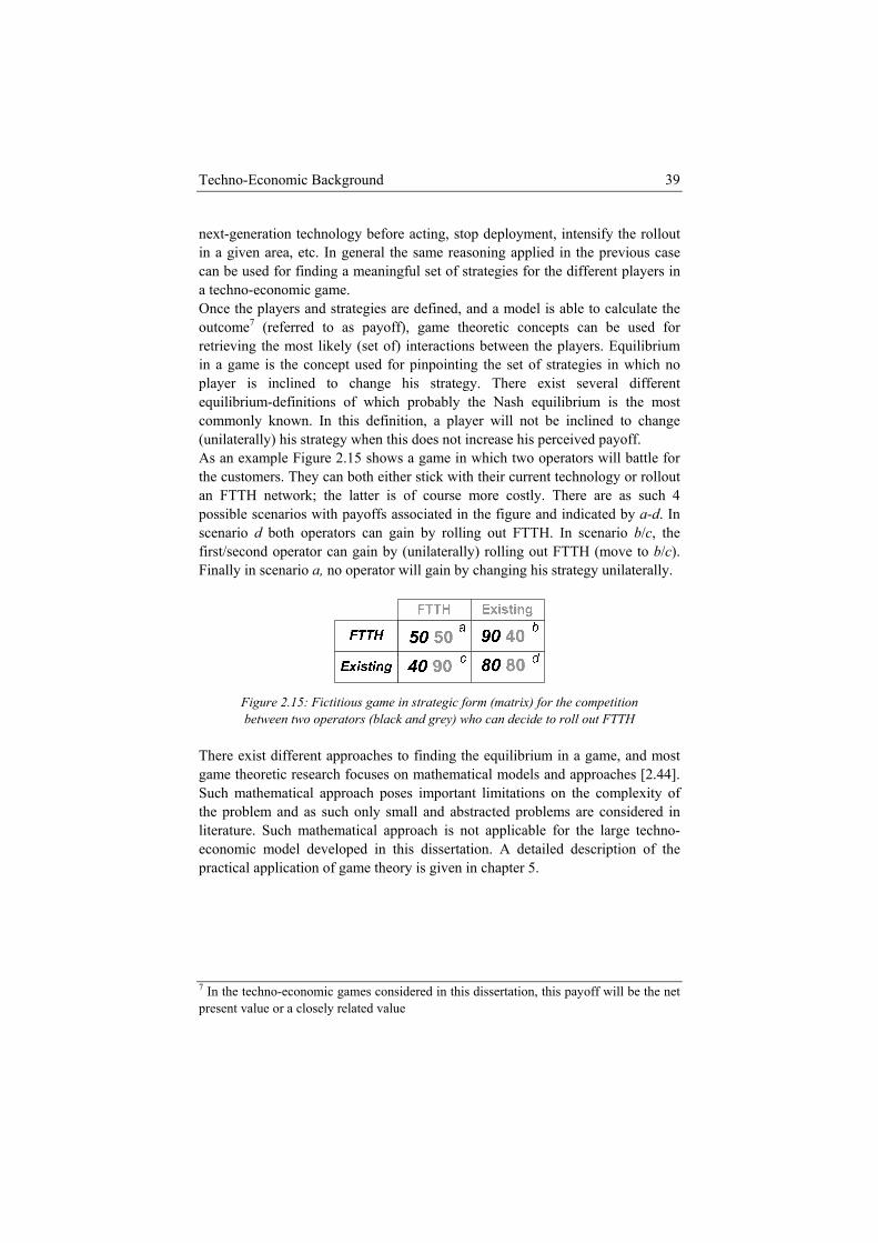
Techno-Economic Background 39
next-generation technology before acting, stop deployment, intensify the rollout in a given area, etc. In general the same reasoning applied in the previous case can be used for finding a meaningful set of strategies for the different players in a techno-economic game. Once the players and strategies are defined, and a model is able to calculate the outcome7 (referred to as payoff), game theoretic concepts can be used for retrieving the most likely (set of) interactions between the players. Equilibrium in a game is the concept used for pinpointing the set of strategies in which no player is inclined to change his strategy. There exist several different equilibrium-definitions of which probably the Nash equilibrium is the most commonly known. In this definition, a player will not be inclined to change (unilaterally) his strategy when this does not increase his perceived payoff. As an example Figure 2.15 shows a game in which two operators will battle for the customers. They can both either stick with their current technology or rollout an FTTH network; the latter is of course more costly. There are as such 4 possible scenarios with payoffs associated in the figure and indicated by a-d. In scenario d both operators can gain by rolling out FTTH. In scenario b/c, the first/second operator can gain by (unilaterally) rolling out FTTH (move to b/c). Finally in scenario a, no operator will gain by changing his strategy unilaterally.
Figure 2.15: Fictitious game in strategic form (matrix) for the competition between two operators (black and grey) who can decide to roll out FTTH
There exist different approaches to finding the equilibrium in a game, and most game theoretic research focuses on mathematical models and approaches [2.44]. Such mathematical approach poses important limitations on the complexity of the problem and as such only small and abstracted problems are considered in literature. Such mathematical approach is not applicable for the large techno-economic model developed in this dissertation. A detailed description of the practical application of game theory is given in chapter 5.
7 In the techno-economic games considered in this dissertation, this payoff will be the net present value or a closely related value
Chapter 2 40
2.3 Conclusion This section has given an overview of the network. The difference between core, metro and access has been highlighted, and a summary of the requirements, structure, topology and technologies used in each of those parts has been added. Access networks, and especially the latest generations of fixed access network, fibre to the home, have been discussed in detail. This section has also given a short overview of the field of techno-economic research and the methodology used for research in this field. This methodology contains four steps – design, model, evaluate and extend – and the techniques appropriate in each of those steps have been discussed summarily. The remainder of this dissertation will proceed on the development of a cost model for the deployment of an FTTH network. This cost model spans both the costs for infrastructure and operations of the network, and both are modelled using dedicated modelling approaches. Chapter 3 shows how dimensioning is best suited for the calculation of the infrastructure cost and chapter 4 uses operational flowchart based models for the calculation and optimization of the costs for operating the network. This cost model is embedded in the full economic methodology in two studies in chapter 5. The first study will combine both cost models and explore the tradeoffs between both. The combined cost model is further enriched with an extensive design and evaluation step. The second study will make use of game theory and sensitivity analysis to extend the research further. Chapter 6 shows where the same techno-economic background has been used in a broader context to evaluate cases in wireless access, and in the metro and core network. It also shows where more of the economic methodology was used. Finally chapter 7 concludes this dissertation with a short overview of the main findings.
Techno-Economic Background 41
References [2.1] R. Van der Berg, “How the Net Works: an Introduction to Peering and
Transit”, Ars Technica, Sept 2, 2008, http://arstechnica.com/old/content/2008/09/peering-and-transit.ars/4
[2.2] ITU-T Recommendation X.200: “Data Networks and Open Systems Communications: Open Systems Interconnection-model and notation,” July 1994.
[2.3] V. Cerf, R. Kahn: “A protocol for packet network interconnection,” IEEE Transactions on Communications, May 1974, vol. 22, pp. 637-648.
[2.4] A. S. Tanenbaum: Computer Networks, 4th edition, Prentice Hall, New Jersey, 2003.
[2.5] D. M. Piscitello, A.L. Chapin: Open Systems Networking: TCP/IP and OSI, Addison-Wesley, Boston, 1993.
[2.6] A. Farrel, “GMPLS, Architecture and Implementations,” Morgan Kauffman Series in Networking, Elsevier, 2005, ISBN 978-0120884223
[2.7] FTTH Council, “Study to Assess Broadband Bandwidth Usage and Key Trends in Europe”, http://www.vandenberg.nl/publicaties/ftthrapport.pdf
[2.8] The 3th Generation Partnership Project, http://www.3gpp.org/
[2.9] The Wi-Fi alliance, http://www.wi-fi.org/
[2.10] The WiMAX forum, http://www.wimaxforum.org
[2.11] J. P. Bienaimé, “3G Evolution – UMTS Forum View”, 2nd International Mobile Services Forum, Montpellier, 14 November 2006.
[2.12] DSL Forum, “Marketig Report MR-001, DSL Anywhere – Issue 2”, http://www.broadband-forum.org/marketing/download/mktgdocs/ DSLAnywhere_Issue2.pdf, Sept. 2004, p70
[2.13] Belgacom group, http://www.belgacom.com
[2.14] Belgacom, “Belgacom kiest voor de VDSL2 fiber-to-the-node-oplossing van Alcatel-Lucent” (in dutch) , http://www.belgacom.com/group/gallery/content/shared/PressRelease/20071010_vdsl2_nl.pdf
[2.15] P. Barnard, “Ikanos' Chipsets Powering Belgacom's New Fiber/VDSL2 Network”, TMCNet, http://europe.tmcnet.com/topics/othercountries /articles/52030-ikanos-chipsets-powering-belgacoms-new-fibervdsl2-network.htm
[2.16] Telenet, http://www.telenet.be
Chapter 2 42
[2.17] P. E. Green, “Fiber-to-the-Home: The Next Big Broadband Thing”, IEEE Communications Magazine, vol. 42, no. 9, pp. 100-106, Sep. 2004.
[2.18] Glasvezelnet Amsterdam (dutch) , http://www.glasvezelamsterdam.nl/ gna_algemeen/index.php?page_id=12
[2.19] Cisco, “Hong Kong Broadband Driving World's Fastest Residential Broadband Service with Cisco Powered Network QoS-certified Metro Ethernet Solution” http://newsroom.cisco.com/dlls/global/asiapac/news/ 2005/pr_10- 26b.html
[2.20] IT Professional (dutch) , http://www.itprofessional.be/news.cfm?id= 94678, and http://www.itprofessional.be/news.cfm?id=91730
[2.21] S. Verbrugge, K. Casier, J. Van Ooteghem, B. Lannoo, “Practical steps in techno-economic evaluation of network deployment planning,”, tutorial in Networks 2008, Budapest, Hungary, Sept 28 – Oct 2, 2008.
[2.22] W. E. Deming, “Out of the Crisis”, MIT Center for Advanced Engineering Study, ISBN 0-911379-01-0, 1986.
[2.23] Fibre to the Home Council, http://www.ftthcouncil.org
[2.24] IDATE - Institut de l’Audiovisuel et des Télécommunications en Europe, http://www.idate.fr
[2.25] Point Topic (ltd.), http://point-topic.com
[2.26] K. Ishikawa, “Introduction to Quality Control”, Taylor and Francis, ISBN: 9784906224616, 1990
[2.27] P. Berkhin, “Survey of Clustering Data Mining Techniques”, Technical report, Accrue Software, San Jose, CA, 2002
[2.28] Investopedia, http://www.investopedia.com
[2.29] R.S. Kaplan, S. Anderson: “Time–Driven Activity-Based Costing,” Harvard Business Review, 2004, vol. 82, no. 11, pp. 131-138.
[2.30] W. L. Winston, “Operations Research – Applications and Algorithms”, Thomson – Brooks/Cole, 2004, ISBN 0-534-42362-0
[2.31] E. Mansfield, W.B. Allen, N.A. Doherty, K. Weigelt, “Managerial economics: theory, applications and cases”, W.W. Norton & Company, Fifth edition, 2002, ISBN 0-393-97677-7
[2.32] Commission of the European Communities, “COMMISSION DECISION of 11.XII.2007 ON THE STATE AID case C 53/2006 (ex N 262/2005, ex CP 127/2004), Investment by the city of Amsterdam in a fibre-to-the home (FttH) network”, Brussels, December 11, 2007.
Techno-Economic Background 43
[2.33] Belgacom, “The Belgacom S.A. cost accounting system, General Description, Financial year 2007”, http://www.bipt.be/GetDocument.aspx?forObjectID=3013&lang=nl, October 2008.
[2.34] J. C. Kelleher, J. J. MacCormack, “Internal Rate of Return: A Cautionary Tale”, The McKinsey Quarterly, McKinsey Co., http://www.cfo.com/article.cfm/3304945/1/c_3348836, October 20, 2004.
[2.35] Wikipedia, “Modified Internal Rate of Return”, http://en.wikipedia.org/wiki/Modified_Internal_Rate_of_Return
[2.36] M. Porter, “Competitive advantage: creating and sustaining superior performance”, The Free Press, New York, 1985.
[2.37] G. Friend, S. Zehle, “Guide to business planning”, The economist, profile books Ltd., ISBN-10 1 86197 474 4, 2004
[2.38] F. Li, J. Whalley, “Deconstruction of the telecommunications industry: from value chains to value networks”, Telecommunications Policy, October-November 2002, Vol. 26, Issues 9-10, Pages 451-472
[2.39] Stefano Tarantola, "Global Sensitivity Analysis of complex models", Joint Research Centre of the European Commission, Seminar Series 2008, Centre for Process Systems Engineering, Imperial College, London, April 16, 2008.
[2.40] S. Myers, “Determinants of Corporate Borrowing”, Journal of Financial Economics, 1997, vol. 5, no. 2, pp.147-175.
[2.41] T. Copeland, P. Keenan, “How Much is Flexibility Worth?”, The McKinsey Quarterly, 1998, vol. 2, 38-49.
[2.42] W. De Maeseneire, “The real options approach to strategic capital budgeting and company valuation”, ISBN: 2-8044-2318-2, Financiële Cahiers, Larcier, 2006.
[2.43] M. Felegyhazi, J.P. Hubaux, “Game Theory in Wireless Networks: A Tutorial,” EPFL technical report, LCA-REPORT-2006-002, February 2006.
[2.44] E. Altman, T. Boulogne, R. El-Azouzi, T. Jiménez, L. Wynter, “A survey on networking games in telecommunications”, Computers and Operations Research, 2004, Vol. 33 (2006), pp. 286-311.

Chapter 2 44
3 Dimensioning the Infrastructure
“You and I come by road or rail, but economists travel on infrastructure.”, Margaret Thatcher
In this chapter we consider the techno-economic modelling of the infrastructure part of the network. The move to a full FTTH network involves the replacement of all existing cables containing copper or coax by cables containing optical fibre. Clearly all equipment in the central office (CO) will need to be replaced in a full FTTH rollout scenario. Also the customer will have to replace his modem or gateway with a fibre capable gateway called the optical network termination (ONT). A high level overview of the fixed networks infrastructure was already given in chapter 2 and an FTTH access network in particular was sketched in Figure 2.8. In this dissertation we focus on the costs of the operator and disregard the cost of the customer network. Note how the point of handoff between operator and customer might be dependent on the technology, applications and operator strategy. We consider the rollout of an FTTH network, where we expect the operator to stick with current strategic practice of giving the customer the in-

Chapter 3 46
house installation and ONT for free8. Especially for the rollout of a completely new network, the battle for the customers will become very important, and the gateway might be an important opportunity for winning and holding the customer. The rollout of an FTTH network and the complete replacement of all equipment and cables obviously is a very cost- and time-intensive project. A lot of parameters will have an important impact on the costs9 and the outcome of the business case. A very important choice here is which technology and architecture to use for the FTTH network. While optical networks are already existing for some time in core networks, its application to the access network can still be considered quite recent [3.1] with first rollouts in 1986 to business users and 1997 towards residential customers. There is still a lot of evolution in research, standards and equipment. In the next section we will discuss in detail the different existing FTTH flavours and also give a glimpse on possible future developments and the impact on the FTTH network rolled out. Once the technical background is set, a detailed cost model for FTTH is constructed. To this aim, we split the network in three parts – outside plant, inside plant and customer premises – according to their impact on the cost and on the calculation approach. For each of the parts we indicate its structure, components and impact on the costs and finally describe the models used for estimating the cost (either dedicated or general). Additionally, we point where optimizations are possible and either show how this can be done, or relate to existing problem and solution descriptions. Finally the dimensioning models can be combined with the prices of the equipment to get an overall estimate of the total infrastructure cost. In the last sub section we show how to do this, point to models for forecasting the evolution of component prices and give indicative values for the prices of equipment.
8 It is not uncommon to offer a free use/lease of the gateway, while the actual gateway remains property of the operator. Additionally this moves the handoff between operator and customer up to this gateway, and offers the operator future opportunities of remote management. 9 Some choices of the operator will also have an impact on possible revenues
Dimensioning the Infrastructure 47
3.1 Fibre to the Home In a fibre to the home network, all data is transported using optical signals over a pure glass medium, the fibre. Optical fibre is installed rather than the other media (e.g. twisted copper or coaxial) as it has superior physical characteristics. The most important characteristics of a medium when used for data transport are its attenuation and dispersion10. Attenuation refers to the gradual loss in intensity of the signal, or more in general a flux, through the medium. Dispersion refers to the effect where different wavelengths, for chromatic dispersion, and polarization, for polarization mode dispersion, do not propagate through the fibre at exactly the same velocity. The effects of attenuation increase with distance and might lead over longer distance to a situation in which the detector can no longer recover the signal. The attenuation of a medium thus determines the maximum distance over which the signal can travel without the use of active amplifiers. The attenuation is also dependent on the transmission wavelength and Figure 3.1 shows the attenuation spectrum of an optical fibre, with the three most interesting windows indicated in grey. The first window – 800nm-900nm – is especially interesting as there are very cheap silicon based sources and detectors available in this window. Considering the high attenuation and dispersion only very limited distances are reachable in glass optical fibre and it is unusable in FTTH. It is used for short distance communication in data-centres and for optical in-house installations using polymer optical fibre (POF). The second window – 1260nm-1360nm – combines a very low attenuation with nearly zero chromatic dispersion around 1310nm (see also below). The third window – 1430n-1580nm – has the lowest attenuation in the spectrum. Both the second and third window are used in FTTH.
10 In addition also noise and immunity to electromagnetic interference will have an impact on the fitness of the medium for data transport.
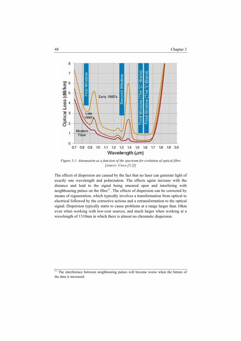
Chapter 3 48
Figure 3.1: Attenuation as a function of the spectrum for evolution of optical fibre
[source: Cisco [3.2]]
The effects of dispersion are caused by the fact that no laser can generate light of exactly one wavelength and polarization. The effects again increase with the distance and lead to the signal being smeared open and interfering with neighbouring pulses on the fibre11. The effects of dispersion can be corrected by means of regeneration, which typically involves a transformation from optical to electrical followed by the corrective actions and a retransformation to the optical signal. Dispersion typically starts to cause problems at a range larger than 10km even when working with low-cost sources, and much larger when working at a wavelength of 1310nm in which there is almost no chromatic dispersion.
11 The interference between neighbouring pulses will become worse when the bitrate of the data is increased.
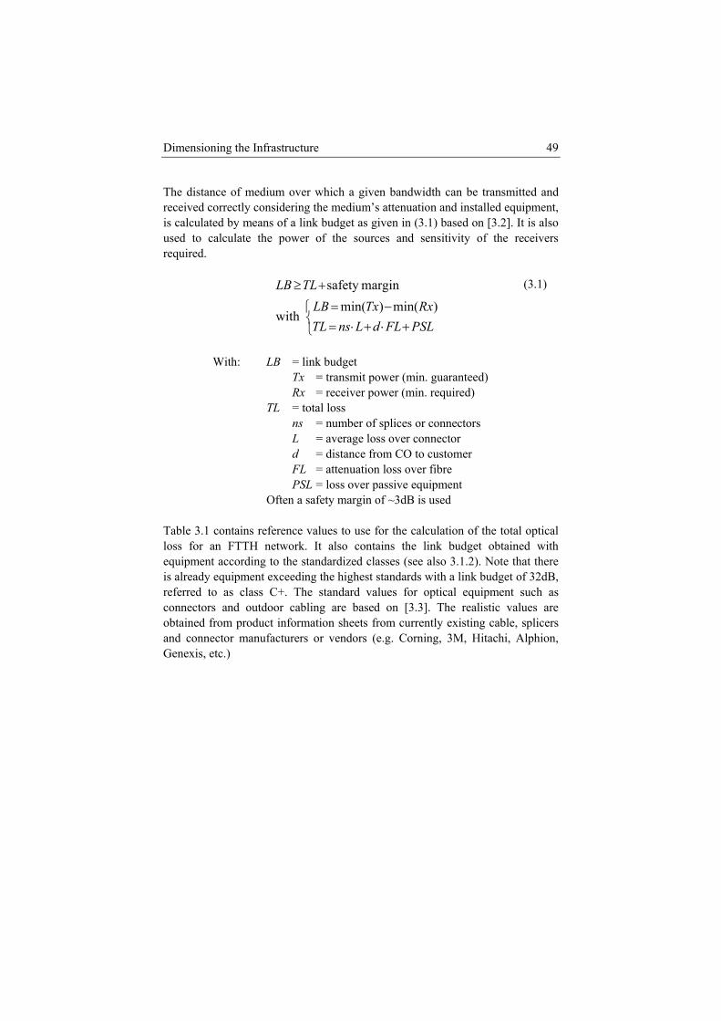
Dimensioning the Infrastructure 49
The distance of medium over which a given bandwidth can be transmitted and received correctly considering the medium’s attenuation and installed equipment, is calculated by means of a link budget as given in (3.1) based on [3.2]. It is also used to calculate the power of the sources and sensitivity of the receivers required.
⎩⎨⎧
+⋅+⋅=−=
+≥
PSLFLdLnsTLRxTxLB
TLLB)min()min(
with
marginsafety
With: LB = link budget Tx = transmit power (min. guaranteed) Rx = receiver power (min. required) TL = total loss ns = number of splices or connectors L = average loss over connector d = distance from CO to customer FL = attenuation loss over fibre PSL = loss over passive equipment Often a safety margin of ~3dB is used
(3.1)
Table 3.1 contains reference values to use for the calculation of the total optical loss for an FTTH network. It also contains the link budget obtained with equipment according to the standardized classes (see also 3.1.2). Note that there is already equipment exceeding the highest standards with a link budget of 32dB, referred to as class C+. The standard values for optical equipment such as connectors and outdoor cabling are based on [3.3]. The realistic values are obtained from product information sheets from currently existing cable, splicers and connector manufacturers or vendors (e.g. Corning, 3M, Hitachi, Alphion, Genexis, etc.)
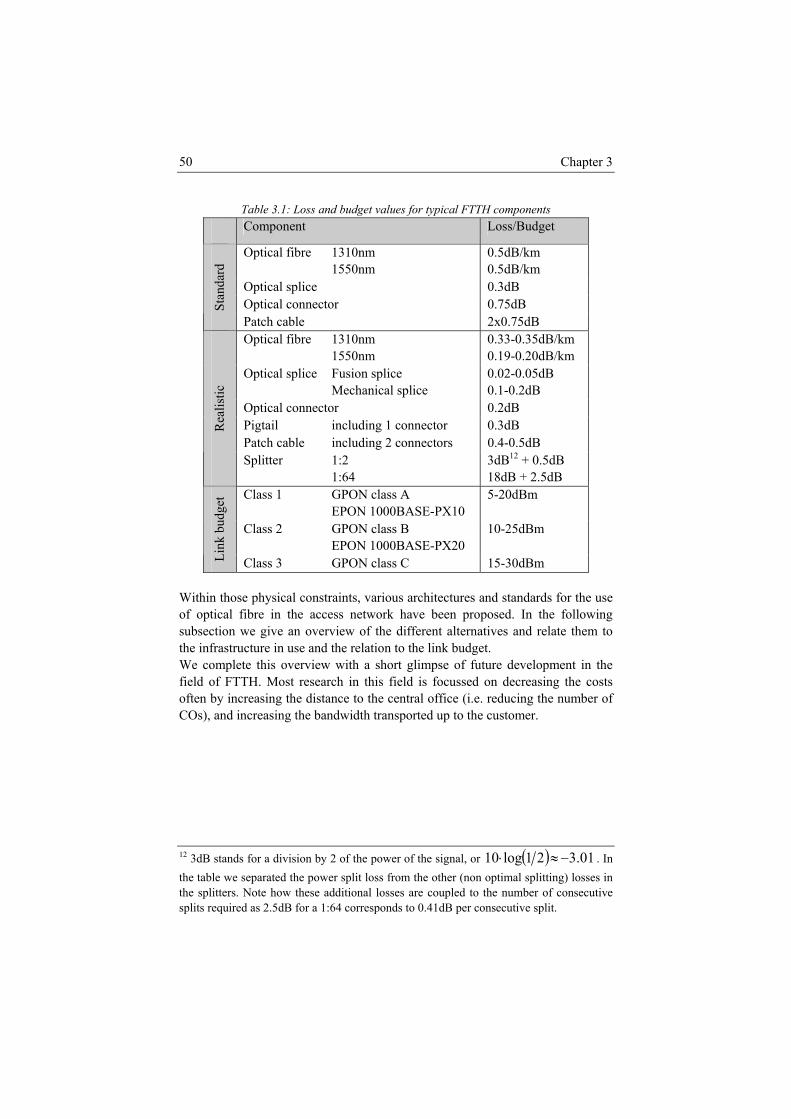
Chapter 3 50
Table 3.1: Loss and budget values for typical FTTH components Component Loss/Budget
Optical fibre 1310nm 1550nm
0.5dB/km 0.5dB/km
Optical splice 0.3dB Optical connector 0.75dB St
anda
rd
Patch cable 2x0.75dB Optical fibre 1310nm 1550nm
0.33-0.35dB/km 0.19-0.20dB/km
Optical splice Fusion splice Mechanical splice
0.02-0.05dB 0.1-0.2dB
Optical connector 0.2dB Pigtail including 1 connector 0.3dB Patch cable including 2 connectors 0.4-0.5dB
Rea
listic
Splitter 1:2 1:64
3dB12 + 0.5dB 18dB + 2.5dB
Class 1 GPON class A EPON 1000BASE-PX10
5-20dBm
Class 2 GPON class B EPON 1000BASE-PX20
10-25dBm
Link
bud
get
Class 3 GPON class C 15-30dBm Within those physical constraints, various architectures and standards for the use of optical fibre in the access network have been proposed. In the following subsection we give an overview of the different alternatives and relate them to the infrastructure in use and the relation to the link budget. We complete this overview with a short glimpse of future development in the field of FTTH. Most research in this field is focussed on decreasing the costs often by increasing the distance to the central office (i.e. reducing the number of COs), and increasing the bandwidth transported up to the customer.
12 3dB stands for a division by 2 of the power of the signal, or ( ) 01.321log10 −≈⋅ . In the table we separated the power split loss from the other (non optimal splitting) losses in the splitters. Note how these additional losses are coupled to the number of consecutive splits required as 2.5dB for a 1:64 corresponds to 0.41dB per consecutive split.
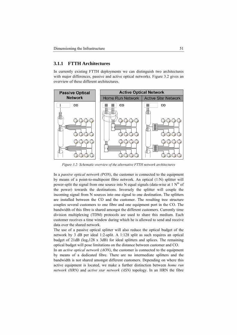
Dimensioning the Infrastructure 51
3.1.1 FTTH Architectures In currently existing FTTH deployments we can distinguish two architectures with major differences, passive and active optical networks. Figure 3.2 gives an overview of these different architectures.
Figure 3.2: Schematic overview of the alternative FTTH network architectures
In a passive optical network (PON), the customer is connected to the equipment by means of a point-to-multipoint fibre network. An optical (1:N) splitter will power-split the signal from one source into N equal signals (data-wise at 1 Nth of the power) towards the destinations. Inversely the splitter will couple the incoming signal from N sources into one signal to one destination. The splitters are installed between the CO and the customer. The resulting tree structure couples several customers to one fibre and one equipment port in the CO. The bandwidth of this fibre is shared amongst the different customers. Currently time division multiplexing (TDM) protocols are used to share this medium. Each customer receives a time window during which he is allowed to send and receive data over the shared network. The use of a passive optical splitter will also reduce the optical budget of the network by 3 dB per ideal 1:2-split. A 1:128 split as such requires an optical budget of 21dB (log2128 x 3dB) for ideal splitters and splices. The remaining optical budget will pose limitations on the distance between customer and CO. In an active optical network (AON), the customer is connected to the equipment by means of a dedicated fibre. There are no intermediate splitters and the bandwidth is not shared amongst different customers. Depending on where this active equipment is located, we make a further distinction between home run network (HRN) and active star network (ASN) topology. In an HRN the fibre
Chapter 3 52
runs all the way to the CO while in an ASN, the active equipment is placed much closer to the customer and an active street cabinet (SC) will serve a comparable number of customers as in a traditional PON (~32-256 customers per SC). Since there are no optical splitters, the optical budget is only constrained by the attenuation and all splice- and connector losses. In this case, even low optical budgets will still allow for very high distances between customer and CO. For instance an optical budget of 20dBm would reach up to 50km when considering up to 20 fusion splices and 5 connectors on the fibre.
3.1.2 FTTH Standards There is clearly more effort in the standardization of PON than for AON. This might be caused by the historical evolution, dominance in rollout and more strict requirements: • FTTH has been first deployed in Japan, at which time their choice was on
PON. ATM PON (shortly APON) was a logical extension of the metro protocol at that time (ATM) towards the access. The dominant FTTH architecture from that time on has been a PON, with two different standardisation bodies involved in two different standards.
• There is a need for stricter standardisation for the more complex protocol and requirements in a PON. First, as mentioned before there is a very important impact of the split-ratio and distance in a PON. Standardisation defines classes of equipment in terms of link budget and losses along with maximum split ratios and distances. Secondly also TDM and the more advanced dynamic bandwidth allocation (DBA) protocols require more standardisation to have correct separation of the different customer signals and synchronisation of the data transport. Finally also security will play a more important role and require as such more standardisation for a PON than for AON because of the shared medium.
The following sub sections will first describe the two paths in (TDM) PON standardisation. The final sub section gives a short overview of standards used for AON which are typically based on point-to-point Ethernet over optical fibre based standards. A summary of the specifications of the currently most commercialised standards is given in Table 3.2. It is important to note that BPON only specifies an upstream bandwidth of 622Mbps (*), and a (+) and (-) is used to indicate the relation of the physical limitations to the specified reach. A (+) indicates a situation in which a longer reach is physically possible and a (-) where the physically attainable reach is (currently) smaller than the specified maximum reach.
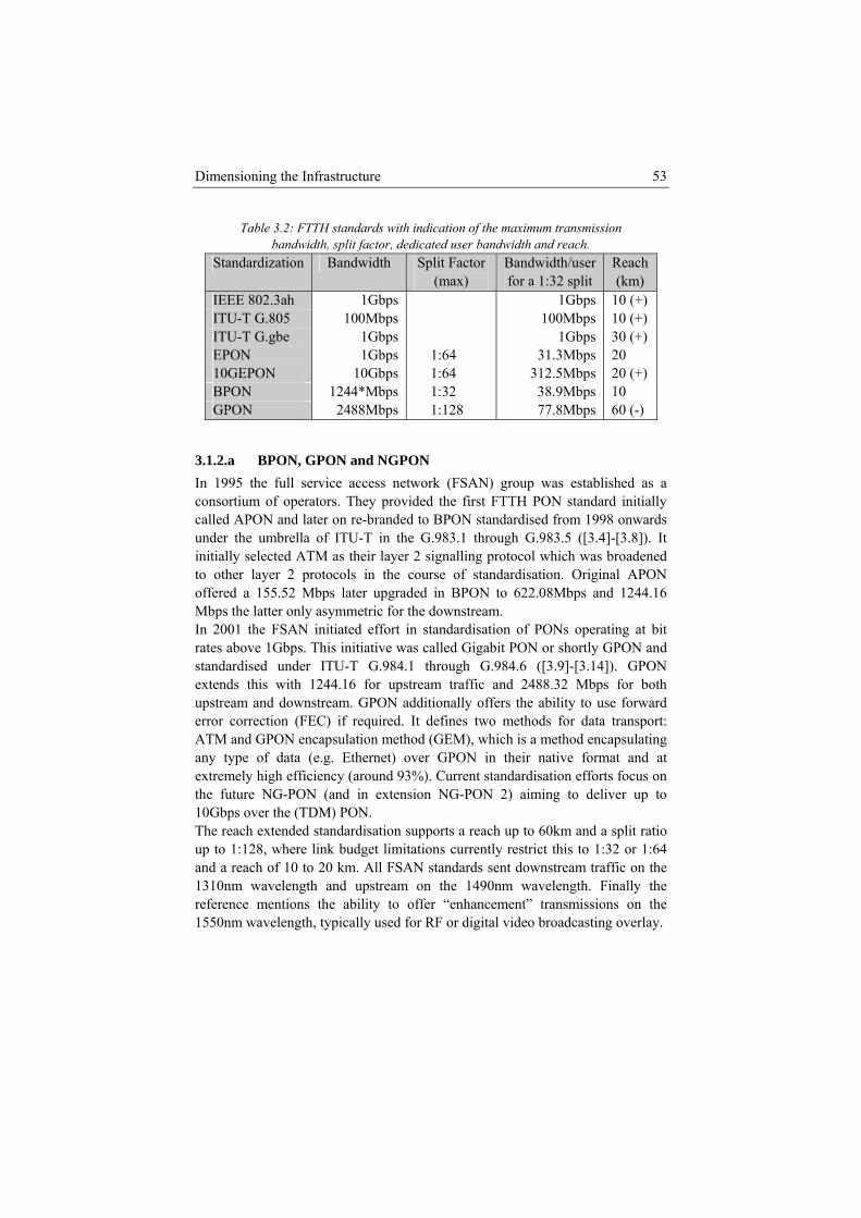
Dimensioning the Infrastructure 53
Table 3.2: FTTH standards with indication of the maximum transmission bandwidth, split factor, dedicated user bandwidth and reach.
Standardization Bandwidth Split Factor (max)
Bandwidth/user for a 1:32 split
Reach (km)
IEEE 802.3ah 1Gbps 1Gbps 10 (+) ITU-T G.805 100Mbps 100Mbps 10 (+) ITU-T G.gbe 1Gbps 1Gbps 30 (+) EPON 1Gbps 1:64 31.3Mbps 20 10GEPON 10Gbps 1:64 312.5Mbps 20 (+) BPON 1244*Mbps 1:32 38.9Mbps 10 GPON 2488Mbps 1:128 77.8Mbps 60 (-)
3.1.2.a BPON, GPON and NGPON In 1995 the full service access network (FSAN) group was established as a consortium of operators. They provided the first FTTH PON standard initially called APON and later on re-branded to BPON standardised from 1998 onwards under the umbrella of ITU-T in the G.983.1 through G.983.5 ([3.4]-[3.8]). It initially selected ATM as their layer 2 signalling protocol which was broadened to other layer 2 protocols in the course of standardisation. Original APON offered a 155.52 Mbps later upgraded in BPON to 622.08Mbps and 1244.16 Mbps the latter only asymmetric for the downstream. In 2001 the FSAN initiated effort in standardisation of PONs operating at bit rates above 1Gbps. This initiative was called Gigabit PON or shortly GPON and standardised under ITU-T G.984.1 through G.984.6 ([3.9]-[3.14]). GPON extends this with 1244.16 for upstream traffic and 2488.32 Mbps for both upstream and downstream. GPON additionally offers the ability to use forward error correction (FEC) if required. It defines two methods for data transport: ATM and GPON encapsulation method (GEM), which is a method encapsulating any type of data (e.g. Ethernet) over GPON in their native format and at extremely high efficiency (around 93%). Current standardisation efforts focus on the future NG-PON (and in extension NG-PON 2) aiming to deliver up to 10Gbps over the (TDM) PON. The reach extended standardisation supports a reach up to 60km and a split ratio up to 1:128, where link budget limitations currently restrict this to 1:32 or 1:64 and a reach of 10 to 20 km. All FSAN standards sent downstream traffic on the 1310nm wavelength and upstream on the 1490nm wavelength. Finally the reference mentions the ability to offer “enhancement” transmissions on the 1550nm wavelength, typically used for RF or digital video broadcasting overlay.
Chapter 3 54
3.1.2.b EPON, NGEPON and 10GEPON In 2000 the IEEE started the 802.3ah task force, often referred to as the Ethernet in the first mile (EFM) [3.15]. This task force had as goal to enable effective Ethernet network designs for subscriber access networks at a reasonable cost. It targeted three access architectures: point-to-point on optical fibre (EFMF), point-to-multipoint on optical fibre (EFMP) and point-to-point on copper (EFMC). It uses Ethernet as the layer 2 protocol. The EPON standard 802.3ah, which is now part of the IEEE 802.3-2005 clause 56-67 [3.16], defines a symmetrical bandwidth of 1250Mbps (~nominal 1Gbps), with an optional FEC. Two different standards are defined: 1000Base-PX10 and 1000Base-PX20 with a maximal reach of respectively 10km and 20km. A typical split ratio of 1:16 is defined and more is possible. Next generation EPON or 10GEPON, began standardization in 2006 under 802.3av working group [3.17] and will offer a symmetrical bandwidth of 10Gbps and a maximal reach of 20km. Downstream and upstream traffic is usually sent on the 1490nm (or in extension 1550nm) wavelength and the 1310nm wavelength, respectively, but this is no restriction. Finally the 1550nm wavelength can also be used in EPON to overlay a third channel of communication.
3.1.2.c AON Standards As mentioned before, the EFM already envisaged point-to-point Ethernet communication for FTTH. The specifications however are in line with the PON specifications and as such disregard the specific setting of a dedicated fibre connection. IEEE 802.3ah defines 1000Base-BX and LX for single and double fibre point-to-point connections at a nominal rate of 1Gbps full duplex. All wavelengths can be used for the transmission of data; typically LX will prefer two times 1310nm while BX will use 1490nm in downstream and 1310nm in upstream. The standards define a distance up to 10km just like for BPON where in AON a much higher distance can easily be reached due to the much lower optical loss (no splitters). Considering a link budget of 20dB, comparable to the lowest defined equipment class in PON networks, this could reach a distance up to 60km. Within ITU-T G.985 [3.18], the specification of FSAN for point-to-point FTTH communication is given. It describes a bandwidth of 100Mbps over a distance of 10km. The extension in G.gbe (under ITU-T study group 15 [3.19]) would provide a 1Gbps Ethernet point-to-point connection over a distance of 30km. Currently IEEE 802.3ae (in IEEE 802.3-2005 clause 44-53 [3.16]) is in use in the metro and core of the network and offers a dedicated bandwidth of 10Gbps. This is under extension in 802.3ba [3.20] and will offer point-to-point bandwidths in metro and core networks of 10Gbps up to 100Gbps over distances up to 80km. Both could be used for point-to-point FTTH equipment as well.
Dimensioning the Infrastructure 55
3.1.3 FTTH Evolution Most of the research in FTTH technologies and standardisation is focussing on one (or several at the same time) of the following: • Higher bandwidth of the sources and detectors. Much in the same way as
APON evolved into BPON and GPON increasing the bandwidth gradually up to 2.5Gbps, next generation sources will enable a higher bandwidth of the data transported over the fibre. Clearly 10G is the next step in this evolution and 40G which is currently used in the core network might come into reach of the access network when prices decay significantly. The working groups IEEE 802.3av, IEEE 802.3ba and ITU-T G.gbe are examples of this move in standardisation.
• Manufacturing and installation practices. High-end optical equipment has been historically used exclusively in the core network. As such its deployment and maintenance was restricted to more skilled personnel using expensive automated tooling. In the access network, prices for the installation will take a larger part of the costs per customer and reducing this cost at the expense of some core-grade requirements (e.g. less fine splice quality) can lead to large overall cost savings. Also equipment manufactured with techniques not qualified for use in core networks, might be still fit for use in access, especially when this would lead to a much lower production cost.
• Introduction of wavelength division multiplexing. WDM allows multiple wavelengths to be transmitted over one fibre. In the case of core networks dense WDM (DWDM) allows to multiplex up to 80 and in future versions 160 wavelengths over the same fibre. Main research on this topic for deployment in the access is focussed on the future of PON networks. When DWDM could be used in a PON connecting up to 64 customers, each customer could get a dedicated wavelength and as such a bandwidth comparable to that of an AON now. For such migration, all splitters must be replaced by wavelength splitting equipment such as an arrayed wavelength grating (AWG). Besides increasing the dedicated bandwidth this will also increase the link budget, as wavelength splitting does not split the power of the signal. In combination with TDM into a hybrid WDM-TDM PON, this allows reaching much more customers from one PON and from limited equipment.
• Moving to new network architectures. The miniaturization of the equipment, increase in optical budget, decrease of power per bit transmitted, etc. allows for a longer distance between customer and CO. Amplifiers are often used to
Chapter 3 56
increase this distance even further13. The motivation for longer reaching PONs or AONs is the aim to close down intermediate switching locations which should be independently rented, maintained and powered. Several projects and research papers tackle this research topic [3.21]. Longer reach is not the only goal for introducing novel architectures. Two other important goals are flexibility and resilience. Flexibility aims to provide the bandwidth to the customer at demand, much in the same way as DBA in TDM PONs can allow customers to be allocated a larger time window. In WDM or WDM-TDM PONs this could be further extended to allow a customer to receive the full bandwidth of one (or more) wavelengths for a given period of time. [3.22] provides an example of research in this field. Resilience aims to protect the connection with the customer even under failure of equipment. Especially with a longer reaching network, connecting more customers, this might become an important aspect. Resilience all the way to the customer requires two disjoint paths coming from the CO to end at the customer premises and some equipment in between or at the ends capable of switching between those two paths on failure. Often only a part of the network closest to the CO will be resilient and the last connection to the customer is still non-resilient. More information on resilience in FTTH networks can be found in [3.23].
Future development of FTTH as such aims to provide more bandwidth, passively shared over more customers, from a longer distance less costly. Additionally it aims to increase flexibility of this bandwidth and add resilience to the connection or part of it. Beyond the pure fixed FTTH networks other research aims to more closely integrate wireless access networks with optical networks (e.g. radio over fibre (RoF)) and extend the fibre connection further into the house (e.g. using polymer optical fibre (POF)).
3.2 Cost Model for an FTTH Rollout Figure 3.3 gives a very high level view on the FTTH access network. In this we distinguish three (cost-) logical parts. The inside plant is typically located close to the geographical center of the area14. Depending on the number of customers served and the distance to the customer, we refer to the inside plant as the central office (HRN or PON) or a street cabinet (ASN). A CO will serve somewhere up to 20.000 customers [3.24] and connects from there to the metro network. As mentioned before, we limited the access
13 Such a network, while still resembling the structure of a PON, can strictly speaking no longer be called “passive”. 14 This is not a restriction and in very expensive areas, it might be optimal to move the active equipment to a cheaper nearby area.
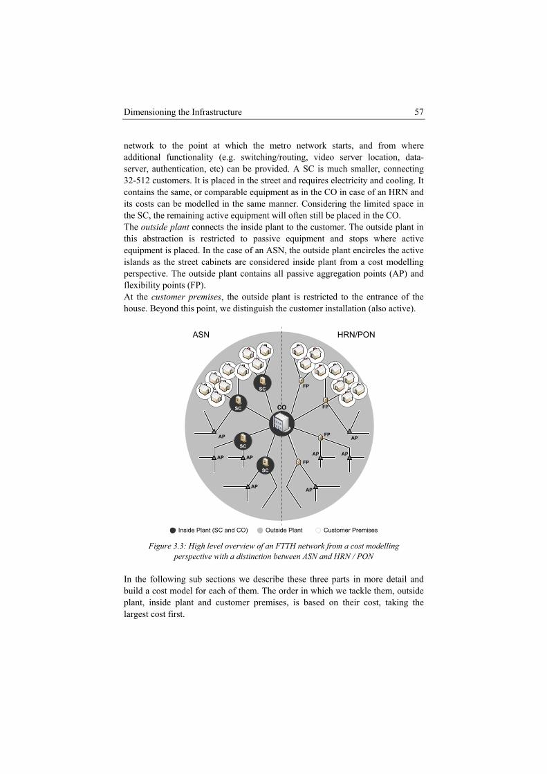
Dimensioning the Infrastructure 57
network to the point at which the metro network starts, and from where additional functionality (e.g. switching/routing, video server location, data-server, authentication, etc) can be provided. A SC is much smaller, connecting 32-512 customers. It is placed in the street and requires electricity and cooling. It contains the same, or comparable equipment as in the CO in case of an HRN and its costs can be modelled in the same manner. Considering the limited space in the SC, the remaining active equipment will often still be placed in the CO. The outside plant connects the inside plant to the customer. The outside plant in this abstraction is restricted to passive equipment and stops where active equipment is placed. In the case of an ASN, the outside plant encircles the active islands as the street cabinets are considered inside plant from a cost modelling perspective. The outside plant contains all passive aggregation points (AP) and flexibility points (FP). At the customer premises, the outside plant is restricted to the entrance of the house. Beyond this point, we distinguish the customer installation (also active).
FPSC
SC
SC
SC
CO
FP
FP
FP
ASN HRN/PON
Inside Plant (SC and CO) Outside Plant Customer Premises
AP
AP AP
APAP
AP AP
AP
Figure 3.3: High level overview of an FTTH network from a cost modelling
perspective with a distinction between ASN and HRN / PON In the following sub sections we describe these three parts in more detail and build a cost model for each of them. The order in which we tackle them, outside plant, inside plant and customer premises, is based on their cost, taking the largest cost first.
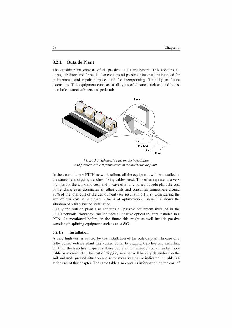
Chapter 3 58
3.2.1 Outside Plant The outside plant consists of all passive FTTH equipment. This contains all ducts, sub ducts and fibres. It also contains all passive infrastructure intended for maintenance and repair purposes and for incorporating flexibility or future extensions. This equipment consists of all types of closures such as hand holes, man holes, street cabinets and pedestals.
Figure 3.4: Schematic view on the installation
and physical cable infrastructure in a buried outside plant.
In the case of a new FTTH network rollout, all the equipment will be installed in the streets (e.g. digging trenches, fixing cables, etc.). This often represents a very high part of the work and cost, and in case of a fully buried outside plant the cost of trenching even dominates all other costs and consumes somewhere around 70% of the total cost of the deployment (see results in 5.1.3.a). Considering the size of this cost, it is clearly a focus of optimization. Figure 3.4 shows the situation of a fully buried installation. Finally the outside plant also contains all passive equipment installed in the FTTH network. Nowadays this includes all passive optical splitters installed in a PON. As mentioned before, in the future this might as well include passive wavelength splitting equipment such as an AWG.
3.2.1.a Installation A very high cost is caused by the installation of the outside plant. In case of a fully buried outside plant this comes down to digging trenches and installing ducts in the trenches. Typically these ducts would already contain either fibre cable or micro-ducts. The cost of digging trenches will be very dependent on the soil and underground situation and some mean values are indicated in Table 3.4 at the end of this chapter. The same table also contains information on the cost of
Dimensioning the Infrastructure 59
a duct and fibre cable, and this clearly shows why trenching will dominate all other outside plant costs (and often even inside plant costs). Different analytical models can be used for estimating the installation length. Appendix A gives an overview of different analytical installation topologies when considering customers which are uniformly spread over a given area. In all models we indicate the distance between two neighbouring houses by l and the length of one size of the square (in number of houses) by n. In all situations the central office is placed in the middle of the square, as this will reduce the length of fibre to be installed in the trenches. In all buried installations, crossing a street will cost much more (per meter) than all other trenches installed along the streets. In case of aerial deployment, or when existing ducts can be reused this difference is small or non-existent. In the analytical models taking this difference into account, we indicate the street-width by w. We differentiate between the analytical models according to the type of installation they resemble the most – all buried or aerial. All analytical models return an installation length function ∼x.n2.l, in which x is a factor depending on the installation type. as there are n2 customers in the area, a dedicated length of x.l must be installed per customer. Depending on the analytical model, the factor x is between ~0.9 (simplified Steiner tree) and ~1.5 (double street length). The different analytical models can be used to estimate the installation length based on the customer base and area size. The choice of the most appropriate analytical model is based on the problem at hand. However, considering the dominant size of the trenching costs for a fully buried FTTH deployment, a better dimensioning is often still required. The full optimal trenching topology can be calculated by constructing a Steiner-tree connecting all customers. The Steiner tree solves the problem of connecting N points with a minimal cost tree structure [3.26] (p. 339) with the freedom to use any number of additional intermediate points. The Steiner tree over a uniformly distributed customer base is shown in the last analytical model. In a realistic setting with existing streets and houses, we consider the Steiner tree problem in graphs. The formal definition of this problem is: Given a weighted graph G(V,E,w)15 and a vertices subset S ⊆ V, find a tree of minimal weight which includes all vertices in S. This problem is NP hard and we thus relied on existing heuristic methods [3.25] for calculating a near optimal tree structure. We implemented the AMST (artificial minimal spanning tree) heuristic algorithm for the calculation of the optimal tree structure connecting all houses in a given area considering detailed data obtained from a geographic information system (GIS). The heuristic starts with the computation of shortest paths between all nodes (customers and CO) in the neighborhood and constructs a minimal spanning tree over this. This minimal
15 The graph consists of a set of vertices or nodes (V) connected by means of a set of edges or links (E). A weight or cost model (w) is coupled to the graph and its elements.
Chapter 3 60
spanning tree is further reduced by means of local optimizations. In general those local optimizations will break part of the minimal spanning tree and reconnect the tree using the cheapest possible path16. In this calculation, we also split the original GIS information for all streets into an information base containing the street sides and crossings17. This allows reflecting reality much better, where the cost of crossing the street is important and must be taken into account. The Steiner tree provides the most cost efficient topology for connecting a given customer base to the CO. On the other hand, a tree-shaped topology will not deliver resilience to fibre breaking. In some cases, such as connecting banks or larger industrial and commercial customers, such reliability might be required. In this case the optimal topology is a ring-based topology, and finding the most cost-efficient ring topology comes down to finding the shortest Hamiltonian cycle18 [3.26] (p. 323) or a solution for the vehicle routing problem19 [3.27]. When restricting the amount of customers connected to one ring, this comes down to finding the solution to a capacitated vehicle routing problem20. All problems referred to before are NP hard and more information and links can also be found in [3.28]. NP hard problems lead to prohibitive running times when solving to optimality. Heuristic algorithms such as proposed by [3.25] can be used and an implementation for a ring constructing algorithm was made.
16 All edges in the remaining, non-removed parts of the tree will have a zero cost associated as they are already scheduled to be opened for installation. The new connected tree might use some of those edges to reconnect and as such this might lead to a local optimization. 17 This level of detail is not available in currently existing GIS bases 18 A Hamiltonian cycle is defined as a cycle in an undirected graph which visits each vertex once and also returns to the starting vertex. 19 The vehicle routing problem is defined as finding the optimal set of routes for a fleet of vehicles in order to serve a given set of customers. As such it is related to the Hamiltonian cycle problem [3.26] (p. 311) in which case the fleet consists of one vehicle. 20 The capacitated vehicle routing problem is an extension of the vehicle routing problem in which each vehicle has a maximum number of customers it can serve.
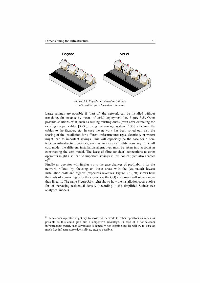
Dimensioning the Infrastructure 61
Figure 3.5: Façade and Aerial installation as alternatives for a buried outside plant
Large savings are possible if (part of) the network can be installed without trenching, for instance by means of aerial deployment (see Figure 3.5). Other possible solutions exist, such as reusing existing ducts (even after extracting the existing copper cables [3.29]), using the sewage system [3.30], attaching the cables to the facades, etc. In case the network has been rolled out, also the sharing of the installation for different infrastructures (gas, electricity or water) might lead to important savings. This will especially be the case for a non-telecom infrastructure provider, such as an electrical utility company. In a full cost model the different installation alternatives must be taken into account in constructing the cost model. The lease of fibre (or duct) connections to other operators might also lead to important savings in this context (see also chapter 6)21. Finally an operator will further try to increase chances of profitability for the network rollout, by focusing on those areas with the (estimated) lowest installation costs and highest (expected) revenues. Figure 3.6 (left) shows how the costs of connecting only the closest (to the CO) customers will reduce more than linearly. The same Figure 3.6 (right) shows how the installation costs evolve for an increasing residential density (according to the simplified Steiner tree analytical model).
21 A telecom operator might try to close his network to other operators as much as possible as this could give him a ompetitive advantage. In case of a non-telecom infrastructure owner, such advantage is generally non-existing and he will try to lease as much free infrastructure (ducts, fibres, etc.) as possible.
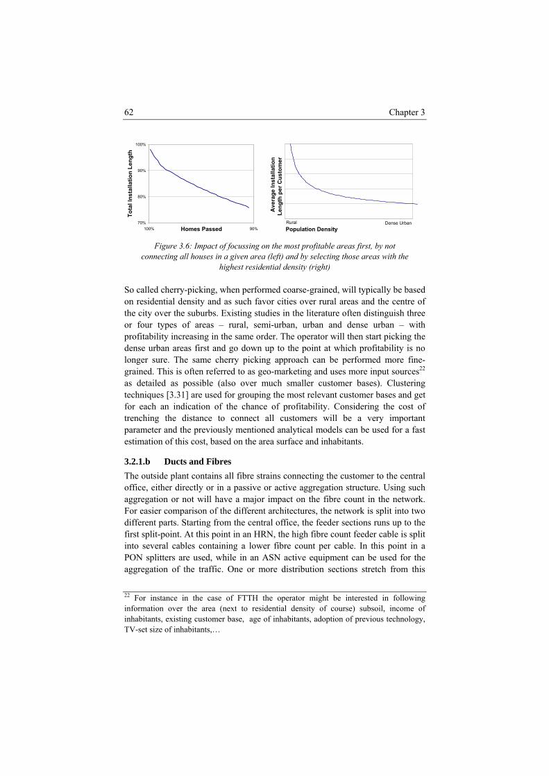
Chapter 3 62
70%
80%
90%
100%
90%100% Homes Passed
Tota
l Ins
talla
tion
Leng
th
Rural Dense UrbanPopulation Density
Ave
rage
Inst
alla
tion
Leng
th p
er C
usto
mer
Figure 3.6: Impact of focussing on the most profitable areas first, by not
connecting all houses in a given area (left) and by selecting those areas with the highest residential density (right)
So called cherry-picking, when performed coarse-grained, will typically be based on residential density and as such favor cities over rural areas and the centre of the city over the suburbs. Existing studies in the literature often distinguish three or four types of areas – rural, semi-urban, urban and dense urban – with profitability increasing in the same order. The operator will then start picking the dense urban areas first and go down up to the point at which profitability is no longer sure. The same cherry picking approach can be performed more fine-grained. This is often referred to as geo-marketing and uses more input sources22 as detailed as possible (also over much smaller customer bases). Clustering techniques [3.31] are used for grouping the most relevant customer bases and get for each an indication of the chance of profitability. Considering the cost of trenching the distance to connect all customers will be a very important parameter and the previously mentioned analytical models can be used for a fast estimation of this cost, based on the area surface and inhabitants.
3.2.1.b Ducts and Fibres The outside plant contains all fibre strains connecting the customer to the central office, either directly or in a passive or active aggregation structure. Using such aggregation or not will have a major impact on the fibre count in the network. For easier comparison of the different architectures, the network is split into two different parts. Starting from the central office, the feeder sections runs up to the first split-point. At this point in an HRN, the high fibre count feeder cable is split into several cables containing a lower fibre count per cable. In this point in a PON splitters are used, while in an ASN active equipment can be used for the aggregation of the traffic. One or more distribution sections stretch from this
22 For instance in the case of FTTH the operator might be interested in following information over the area (next to residential density of course) subsoil, income of inhabitants, existing customer base, age of inhabitants, adoption of previous technology, TV-set size of inhabitants,…
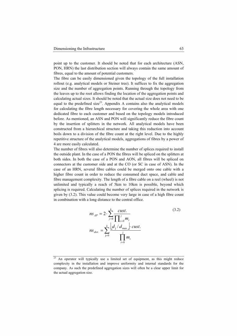
Dimensioning the Infrastructure 63
point up to the customer. It should be noted that for each architecture (ASN, PON, HRN) the last distribution section will always contain the same amount of fibres, equal to the amount of potential customers. The fibre can be easily dimensioned given the topology of the full installation rollout (e.g. analytical models or Steiner tree). It suffices to fix the aggregation size and the number of aggregation points. Running through the topology from the leaves up to the root allows finding the location of the aggregation points and calculating actual sizes. It should be noted that the actual size does not need to be equal to the predefined size23. Appendix A contains also the analytical models for calculating the fibre length necessary for covering the whole area with one dedicated fibre to each customer and based on the topology models introduced before. As mentioned, an ASN and PON will significantly reduce the fibre count by the insertion of splitters in the network. All analytical models have been constructed from a hierarchical structure and taking this reduction into account boils down to a division of the fibre count at the right level. Due to the highly repetitive structure of the analytical models, aggregations of fibres by a power of 4 are more easily calculated. The number of fibres will also determine the number of splices required to install the outside plant. In the case of a PON the fibres will be spliced on the splitters at both sides. In both the case of a PON and AON, all fibres will be spliced on connectors at the customer side and at the CO (or SC in case of ASN). In the case of an HRN, several fibre cables could be merged onto one cable with a higher fibre count in order to reduce the consumed duct space, and cable and fibre management complexity. The length of a fibre cable on a reel (wheel) is not unlimited and typically a reach of 5km to 10km is possible, beyond which splicing is required. Calculating the number of splices required in the network is given by (3.2). This value could become very large in case of a high fibre count in combination with a long distance to the central office.
⎣ ⎦∑∏
∑∏
=
=
==
⋅=
⋅=
k
ii
dist
k
jj
i i
AP
m
custddns
mcustns
0jj
0
maxj.
00
./
.2
(3.2)
23 An operator will typically use a limited set of equipment, as this might reduce complexity in the installation and improve uniformity and internal standards for the company. As such the predefined aggregation sizes will often be a clear upper limit for the actual aggregation size.
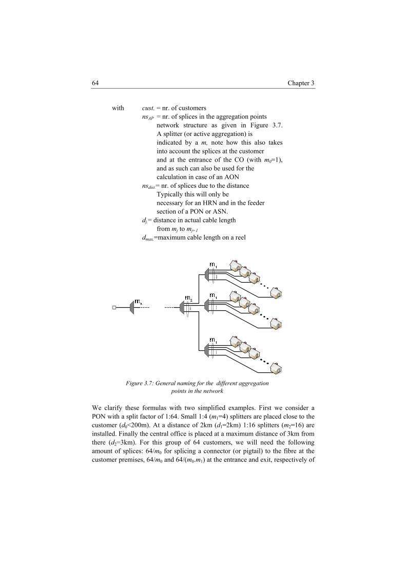
Chapter 3 64
with cust. = nr. of customers nsAP = nr. of splices in the aggregation points network structure as given in Figure 3.7. A splitter (or active aggregation) is indicated by a m, note how this also takes into account the splices at the customer and at the entrance of the CO (with m0=1), and as such can also be used for the calculation in case of an AON nsdist.= nr. of splices due to the distance Typically this will only be necessary for an HRN and in the feeder section of a PON or ASN. dj.= distance in actual cable length from mj to mj+1
dmax.=maximum cable length on a reel
Figure 3.7: General naming for the different aggregation
points in the network We clarify these formulas with two simplified examples. First we consider a PON with a split factor of 1:64. Small 1:4 (m1=4) splitters are placed close to the customer (d0<200m). At a distance of 2km (d1=2km) 1:16 splitters (m2=16) are installed. Finally the central office is placed at a maximum distance of 3km from there (d2=3km). For this group of 64 customers, we will need the following amount of splices: 64/m0 for splicing a connector (or pigtail) to the fibre at the customer premises, 64/m0 and 64/(m0.m1) at the entrance and exit, respectively of
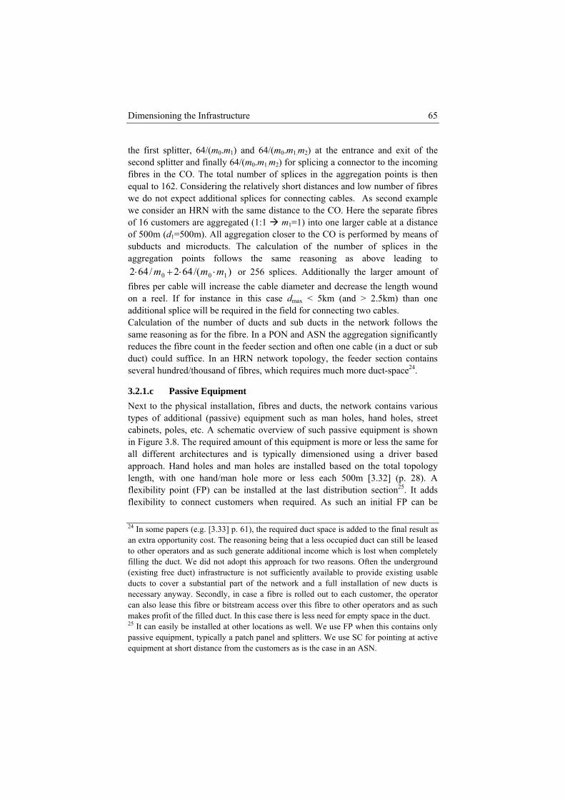
Dimensioning the Infrastructure 65
the first splitter, 64/(m0.m1) and 64/(m0.m1.m2) at the entrance and exit of the second splitter and finally 64/(m0.m1.m2) for splicing a connector to the incoming fibres in the CO. The total number of splices in the aggregation points is then equal to 162. Considering the relatively short distances and low number of fibres we do not expect additional splices for connecting cables. As second example we consider an HRN with the same distance to the CO. Here the separate fibres of 16 customers are aggregated (1:1 m1=1) into one larger cable at a distance of 500m (d1=500m). All aggregation closer to the CO is performed by means of subducts and microducts. The calculation of the number of splices in the aggregation points follows the same reasoning as above leading to
)/(642/642 100 mmm ⋅⋅+⋅ or 256 splices. Additionally the larger amount of fibres per cable will increase the cable diameter and decrease the length wound on a reel. If for instance in this case dmax < 5km (and > 2.5km) than one additional splice will be required in the field for connecting two cables. Calculation of the number of ducts and sub ducts in the network follows the same reasoning as for the fibre. In a PON and ASN the aggregation significantly reduces the fibre count in the feeder section and often one cable (in a duct or sub duct) could suffice. In an HRN network topology, the feeder section contains several hundred/thousand of fibres, which requires much more duct-space24.
3.2.1.c Passive Equipment Next to the physical installation, fibres and ducts, the network contains various types of additional (passive) equipment such as man holes, hand holes, street cabinets, poles, etc. A schematic overview of such passive equipment is shown in Figure 3.8. The required amount of this equipment is more or less the same for all different architectures and is typically dimensioned using a driver based approach. Hand holes and man holes are installed based on the total topology length, with one hand/man hole more or less each 500m [3.32] (p. 28). A flexibility point (FP) can be installed at the last distribution section25. It adds flexibility to connect customers when required. As such an initial FP can be 24 In some papers (e.g. [3.33] p. 61), the required duct space is added to the final result as an extra opportunity cost. The reasoning being that a less occupied duct can still be leased to other operators and as such generate additional income which is lost when completely filling the duct. We did not adopt this approach for two reasons. Often the underground (existing free duct) infrastructure is not sufficiently available to provide existing usable ducts to cover a substantial part of the network and a full installation of new ducts is necessary anyway. Secondly, in case a fibre is rolled out to each customer, the operator can also lease this fibre or bitstream access over this fibre to other operators and as such makes profit of the filled duct. In this case there is less need for empty space in the duct. 25 It can easily be installed at other locations as well. We use FP when this contains only passive equipment, typically a patch panel and splitters. We use SC for pointing at active equipment at short distance from the customers as is the case in an ASN.
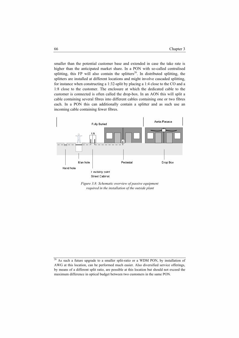
Chapter 3 66
smaller than the potential customer base and extended in case the take rate is higher than the anticipated market share. In a PON with so-called centralised splitting, this FP will also contain the splitters26. In distributed splitting, the splitters are installed at different locations and might involve cascaded splitting, for instance when constructing a 1:32-split by placing a 1:4 close to the CO and a 1:8 close to the customer. The enclosure at which the dedicated cable to the customer is connected is often called the drop-box. In an AON this will split a cable containing several fibres into different cables containing one or two fibres each. In a PON this can additionally contain a splitter and as such use an incoming cable containing fewer fibres.
Figure 3.8: Schematic overview of passive equipment
required in the installation of the outside plant
26 As such a future upgrade to a smaller split-ratio or a WDM PON, by installation of AWG at this location, can be performed much easier. Also diversified service offerings, by means of a different split ratio, are possible at this location but should not exceed the maximum difference in optical budget between two customers in the same PON.
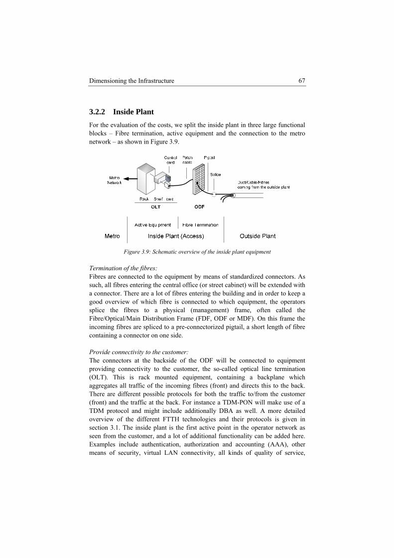
Dimensioning the Infrastructure 67
3.2.2 Inside Plant For the evaluation of the costs, we split the inside plant in three large functional blocks – Fibre termination, active equipment and the connection to the metro network – as shown in Figure 3.9.
Figure 3.9: Schematic overview of the inside plant equipment
Termination of the fibres: Fibres are connected to the equipment by means of standardized connectors. As such, all fibres entering the central office (or street cabinet) will be extended with a connector. There are a lot of fibres entering the building and in order to keep a good overview of which fibre is connected to which equipment, the operators splice the fibres to a physical (management) frame, often called the Fibre/Optical/Main Distribution Frame (FDF, ODF or MDF). On this frame the incoming fibres are spliced to a pre-connectorized pigtail, a short length of fibre containing a connector on one side. Provide connectivity to the customer: The connectors at the backside of the ODF will be connected to equipment providing connectivity to the customer, the so-called optical line termination (OLT). This is rack mounted equipment, containing a backplane which aggregates all traffic of the incoming fibres (front) and directs this to the back. There are different possible protocols for both the traffic to/from the customer (front) and the traffic at the back. For instance a TDM-PON will make use of a TDM protocol and might include additionally DBA as well. A more detailed overview of the different FTTH technologies and their protocols is given in section 3.1. The inside plant is the first active point in the operator network as seen from the customer, and a lot of additional functionality can be added here. Examples include authentication, authorization and accounting (AAA), other means of security, virtual LAN connectivity, all kinds of quality of service,

Chapter 3 68
monitoring and accounting, etc. This backplane is structured as a rack-mounted shelf (4-5 shelves in a rack) and allows for line-cards and control cards to be inserted. The line cards will perform the conversion from optical to electronic and vice-versa (OEO). They either contain fibre connector ports or ports for small form pluggables (SFP/XFP27), which perform the actual conversion between the optical and electronic signal28. Connect to the metro/core network and services: The back of the OLT-racks are finally connected to the metro network and possibly to services as well. The main equipment at this point (switch or router) will work on OSI-layer 2 or above and probably most common here is Ethernet (or SDH/ATM which is gradually being replaced by Ethernet), GMPLS or IP. When extra service equipment is provided at this point, it typically consists of video servers acting as a video cache to reduce the transport of huge video streams in the metro and core. Finally there are some additional costs in the inside plant which are not telecom specific. There will be requirements for housing (acquiring or renting), preparing the building, cooling of the equipment, etc. Dimensioning of the inside plant is driver based, with the number of incoming fibres as the main driver. The number of ports is directly driven by this value, the number of cards, shelves and racks by granularity (e.g. 4 ports on a card) as well. The non-telecom specific inside plant costs are often known from existing installations and they are driven by the number of COs.
3.2.3 Customer Premises Equipment At the customer premises, the fibre is brought into the house and connected to the in-house wiring or equipment. In a fully buried case, often a pedestal, or buried analogue is installed for every two customers and contains enough fibre length for both customers in-house installation. In the case of an aerial installation, the closest cable is ended using an optical connector block (drop box) at which an optical patch-cable or pigtail can be attached and brought into the house at installation time. In a full aerial distribution network, the operator can decide to gradually install the full fibre network, and in chapter 4, we detail the process of installation in this case.
27 An XFP is the standardized small form pluggable for bandwidths of 10 Gbps, in contrast to the SFP which offers 1 Gbps. 28 By using a small form pluggable, the operator decouples the optical signal (sources and detectors) from the electronics in the switch. As such they allow a transparent choice in optical technology (WDM, optical budget, etc.). Finally this flexibility also allows for easier maintenance operations and future upgrades.

Dimensioning the Infrastructure 69
At the point of entrance the installer will drill through the wall and install a protective bend-aid to allow the fibre to be installed safely and without snapping. Finally the fibre is connected, again by means of a connector, to an optical network terminal (ONT) which translates the optical signal and protocol into the in-house signal and protocol. This currently consists of a translation to one or more Ethernet port(s), coaxial television cable(s), telephone jack(s) and wireless antenna. In some cases this ONT is preceded by an optical network termination point (ONTP) which contains a wall socket for a fibre connector and is connected by means of a patch cable to the ONT. Clearly the dimensioning of customer premises equipment and installation is driver based with the number of expected customers as driver.
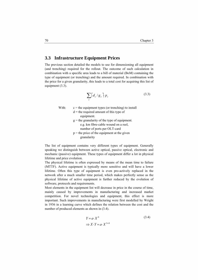
Chapter 3 70
3.3 Infrastructure Equipment Prices The previous section detailed the models to use for dimensioning all equipment (and trenching) required for the rollout. The outcome of such calculation in combination with a specific area leads to a bill of material (BoM) containing the type of equipment (or trenching) and the amount required. In combination with the price for a given granularity, this leads to a total cost for acquiring this list of equipment (3.3).
⎡ ⎤∑ ⋅c
ccc pgd /
With: c = the equipment types (or trenching) to install d = the required amount of this type of equipment. g = the granularity of the type of equipment. e.g. km fibre-cable wound on a reel, number of ports per OLT-card p = the price of the equipment at the given granularity
(3.3)
The list of equipment contains very different types of equipment. Generally speaking we distinguish between active optical, passive optical, electronic and mechanic (passive) equipment. These types of equipment differ a lot in physical lifetime and price evolution. The physical lifetime is often expressed by means of the mean time to failure (MTTF). Active equipment is typically more sensitive and will have a lower lifetime. Often this type of equipment is even pro-actively replaced in the network after a much smaller time period, which makes perfectly sense as the physical lifetime of active equipment is further reduced by the evolution of software, protocols and requirements. Most elements in the equipment list will decrease in price in the course of time, mainly caused by improvements in manufacturing and increased market competition. For novel technologies and equipment, this effect is more important. Such improvements in manufacturing were first modelled by Wright in 1936 in a learning curve which defines the relation between the cost and the number of produced elements as shown in (3.4).
b
b
XaYX
XaY+⋅=⋅⇒
⋅=1
(3.4)

Dimensioning the Infrastructure 71
With: Y = the average production cost per unit X = the number of elements to produce from the start of production XY = the total production cost for producing X elements from the start of production a = the cost of production for the first element b = the (logarithmic) slope of the learning curve function with Lb 2log= , where L indicates the relation of the average cost to the original cost for doubling production.
In [3.34] this is combined with a customer adoption curve to get an idea of the relation of the cost to the time instead of production size (3.5). Figure 3.10 gives an overview of the extended learning curve for electronics and optics. Finally own research [3.35] has shown how the cost evolution of electronic components can be reliably modelled using an exponential decreasing curve with up to 50% decrease in cost per year.
( ) ( ) ( )( )[ ]
K
tT
n
rccr
enptp
21
log19ln2
10ln1 100
⎥⎥⎥⎥
⎦
⎤
⎢⎢⎢⎢
⎣
⎡
⎟⎟⎟
⎠
⎞
⎜⎜⎜
⎝
⎛+=
−
⎭⎬⎫
⎩⎨⎧
⋅⎥⎦⎤
⎢⎣⎡∆
−−−
−
With: t = point in time in units (e.g. years) pc(t) = price of the component at time t pc(0) = price of the component at reference time nr(0) = relative accumulated volume at reference time ∆T = time for the accumulated volume to grow from 10% to 90% K = learning curve coefficient (= 12 −⋅L ) with L as in (3.4) = percentage cost increase for a doubling of the production volume.
(3.5)
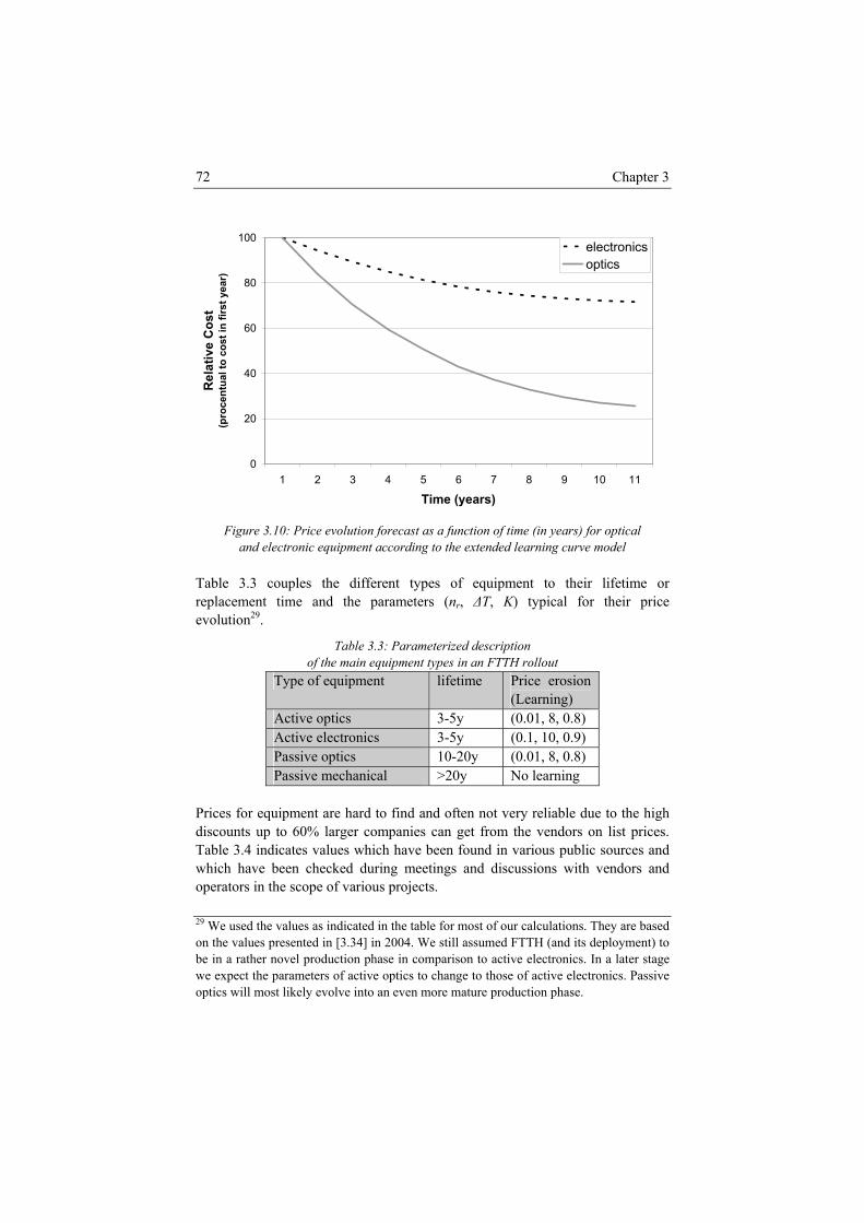
Chapter 3 72
0
20
40
60
80
100
1 2 3 4 5 6 7 8 9 10 11
Time (years)
Rel
ativ
e C
ost
(pro
cent
ual t
o co
st in
firs
t yea
r)
electronicsoptics
Figure 3.10: Price evolution forecast as a function of time (in years) for optical
and electronic equipment according to the extended learning curve model Table 3.3 couples the different types of equipment to their lifetime or replacement time and the parameters (nr, ∆T, K) typical for their price evolution29.
Table 3.3: Parameterized description of the main equipment types in an FTTH rollout
Type of equipment lifetime Price erosion (Learning)
Active optics 3-5y (0.01, 8, 0.8) Active electronics 3-5y (0.1, 10, 0.9) Passive optics 10-20y (0.01, 8, 0.8) Passive mechanical >20y No learning
Prices for equipment are hard to find and often not very reliable due to the high discounts up to 60% larger companies can get from the vendors on list prices. Table 3.4 indicates values which have been found in various public sources and which have been checked during meetings and discussions with vendors and operators in the scope of various projects. 29 We used the values as indicated in the table for most of our calculations. They are based on the values presented in [3.34] in 2004. We still assumed FTTH (and its deployment) to be in a rather novel production phase in comparison to active electronics. In a later stage we expect the parameters of active optics to change to those of active electronics. Passive optics will most likely evolve into an even more mature production phase.
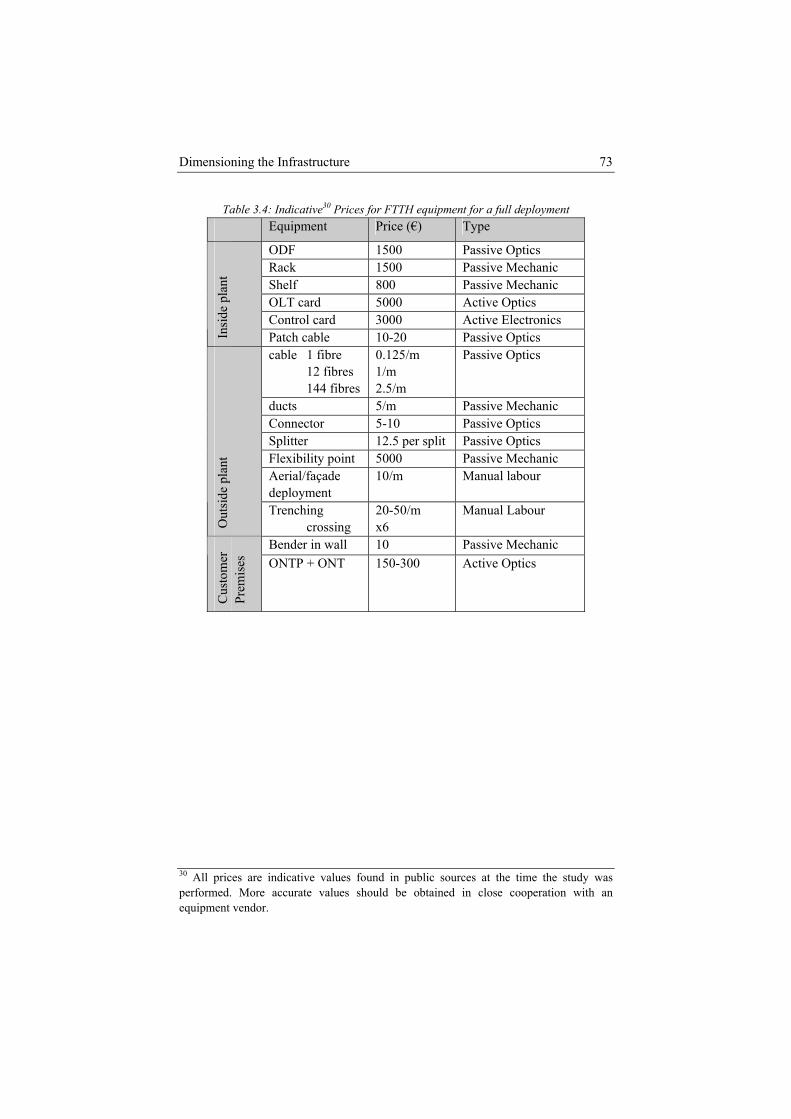
Dimensioning the Infrastructure 73
Table 3.4: Indicative30 Prices for FTTH equipment for a full deployment Equipment Price (€) Type
ODF 1500 Passive Optics Rack 1500 Passive Mechanic Shelf 800 Passive Mechanic OLT card 5000 Active Optics Control card 3000 Active Electronics
Insi
de p
lant
Patch cable 10-20 Passive Optics cable 1 fibre 12 fibres 144 fibres
0.125/m 1/m 2.5/m
Passive Optics
ducts 5/m Passive Mechanic Connector 5-10 Passive Optics Splitter 12.5 per split Passive Optics Flexibility point 5000 Passive Mechanic Aerial/façade deployment
10/m Manual labour
Out
side
pla
nt
Trenching crossing
20-50/m x6
Manual Labour
Bender in wall 10 Passive Mechanic
Cus
tom
er
Prem
ises
ONTP + ONT 150-300 Active Optics
30 All prices are indicative values found in public sources at the time the study was performed. More accurate values should be obtained in close cooperation with an equipment vendor.
Chapter 3 74
3.4 Conclusions This chapter first gave a short overview of the background of optical communications with a focus on optical access networks. This is extended with an outline of the different FTTH technologies and standards. This technological part is closed with an outlook on the future evolution of FTTH technology. The main focus of this chapter lies on the development of a dimensioning model for the infrastructure of an FTTH network. The access network is broken into three parts – outside plant, inside plant and customer premises – with a detailed breakdown of each part in components and dimensioning models. As the highest cost by far is caused by the installation topology of the outside plant, this is tackled in most detail. Applying these dimensioning models to a specific setting (area, customer base, etc.) lead to a list of equipment (and installation) which in combination with their price leads to the overall expenditures. The last section completes the infrastructure dimensioning with a description of commonly used price evolution curves and a table with an “indicative” price of equipment.
Dimensioning the Infrastructure 75
References [3.1] H. Shinohara, “Broadband Access in Japan: Rapidly Growing FTTH
Market”, IEEE Communications Magazine, Sept 2005, pp. 72-78.
[3.2] Cisco, “Fiber Types in Gigabit Optical Communications”, white paper, http://www.cisco.com/en/US/prod/collateral/modules/ps5455/white_paper_c11-463661.html
[3.3] ANSI/TIA/EIA-568-B.3-2000, “Optical Fibre Cabling Components Standard”, 30 March 2000.
[3.4] ITU-T Recommendation G.983.1, “Broadband optical access systems based on Passive Optical Networks (PON)”, revised version 2005, http://www.itu.int/rec/T-REC-G.983.1/en
[3.5] ITU-T Recommendation G.983.2, “ONT management and control interface specification for B-PON” revised version 2005, http://www.itu.int/rec/T-REC-G.983.2/en
[3.6] ITU-T Recommendation G.983.3, “A broadband optical access system with increased service capability by wavelength allocation”, 2001, http://www.itu.int/rec/T-REC-G.983.3/en
[3.7] ITU-T Recommendation G.983.4, “A broadband optical access system with increased service capability using dynamic bandwidth assignment”, 2001, http://www.itu.int/rec/T-REC-G.983.4/en
[3.8] ITU-T Recommendation G.983.5, “A broadband optical access system with enhanced survivability”, 2002, http://www.itu.int/rec/T-REC-G.983.5/en
[3.9] ITU-T Recommendation G.984.1, “Gigabit-capable Passive Optical Networks (GPON): General characteristics”, 2003, http://www.itu.int/rec/T-REC-G.984.1/en
[3.10] ITU-T Recommendation G.984.2, “GPON: Physical Media Dependent (PMD) layer specification”, 2003, http://www.itu.int/rec/T-REC-G.984.2/en
[3.11] ITU-T Recommendation G.984.3, “G-PON: Transmission convergence layer specification”, 2004, http://www.itu.int/rec/T-REC-G.984.3/en
[3.12] ITU-T Recommendation G.984.4, “G-PON: ONT management and control interface (OMCI) specification”, 2004, http://www.itu.int/rec/T-REC-G.984.4/en
Chapter 3 76
[3.13] ITU-T Recommendation G.984.5, “Enhancement band for gigabit capable optical access networks”, 2007, http://www.itu.int/rec/T-REC-G.984.5/en
[3.14] ITU-T Recommendation G.984.6, “Gigabit-capable passive optical networks (GPON): Reach extension”, 2008, http://www.itu.int/rec/T-REC-G.984.6/en
[3.15] IEEE 802.3ah, “Ethernet in the First Mile working group”, http://www.ieee802.org/3/efm/public/index.html
[3.16] IEEE Std. 802.3-2005, “IEEE Standard for Information technology - Telecommunications and information exchange between systems - Local and metropolitan area networks - Specific requirements - Part 3: Carrier Sense Multiple Access with Collision Detection (CSMA/CD) Access Method and Physical Layer Specifications”, 2005, http://standards.ieee.org/getieee802/802.3.html
[3.17] IEEE 802.3av, “10GEPON task force”, http://www.ieee802.org/3/av/index.html
[3.18] ITU-T Recommendation G.985, “100 Mbit/s point-to-point Ethernet based optical access system”, 2003, http://www.itu.int/rec/T-REC-G.985/en
[3.19] ITU-T study group 15, http://www.itu.int/ITU-T/studygroups/com15/index.asp
[3.20] IEEE 802.3ba, “40Gb/s and 100Gb/s Ethernet Task Force”, http://www.ieee802.org/3/ba/public/index.html
[3.21] D. P. Shea, J. E. Mitchell, “Long-Reach Optical Access Technologies”, IEEE Network, Vol. 21 (5). pp. 5-11, 2007
[3.22] A. Koonen, “Fiber to the Home/Fiber to the Premises:What, Where, andWhen?”, Proceedings of the IEEE, Vol. 49, no. 5, May 2006, pp. 911-934.
[3.23] M. Kantor, J. Chen, L. Wosinska, K. Wajda, “Techno-economic analysis of PON protection schemes”, published in proceedings of BBEurope 2007, Antwerp, Belgium, 3-6 December, 2007.
[3.24] P. Fournier, “From FTTH Pilot to Pre-rollout in France”, 2007, http://www.orange.com/en_EN/finance/invest-analysts/meetings-conferences/att00009692/2007/0626_FTTH.pdf
[3.25] P. Arijs, “Planning of Ring-Based Telecommunication Networks”, dissertation of University of Ghent, 2000-2001.
Dimensioning the Infrastructure 77
[3.26] S. Skiena, “The algorithm design manual”, Springer, 1998, ISBN 0387948600
[3.27] G. Clarke, J. Wright, “Scheduling vehicles from a central depot to a number of delivery points”, Operations Research, Vol 12, pp. 568-581, 1964
[3.28] Wikipedia, “Category of NP complete Problems”, http://en.wikipedia.org/wiki/Category:NP-complete_problems
[3.29] Kabel-X Technology, http://www.kabel-x.com/index.php
[3.30] K. Ruderman, “France Telecom plans massive FTTH roll-out in 2009”, Lightwave Europe, January 2008, http://lw.pennnet.com/display_article/321309/63/ARTCL/none/none/1/France-Telecom-plans-massive-FTTH-roll-out-in-2009/
[3.31] P. berkhin, Survey of clustering Data Mining Techniques, “Grouping Multidimensional Data”, Springer Berlin Heidelberg, 2006
[3.32] FTTH Council Europe, “FTTH Handbook”, revision 2009, http://www.ftthcouncil.eu/documents/studies/FTTH_Handbook.pdf
[3.33] M. El-Sayed, “Fiber-to-the-X: Technologies & Economics”, Tutorial presented at Networks 2008, 28 September – 2 October 2008, Budapest, Hungary.
[3.34] B. T. Olsen, K. Stordahl, “Models for forecasting cost evolution of components and technologies”, Telektronikk, 2004, Vol. 4, pp. 138-148.
[3.35] K. Casier, W. Tavernier, D. Colle, M. Pickavet, P. Papadimitriou, P. Demeester, “Forecasting cost trends for carrier Ethernet”, to be presented in Globecom 2009 – Workshop on Below IP Networking, 30 November 2009, Honolulu, Hawaii, US

Chapter 3 78
4 Dimensioning the Operations
“The first rule of any technology used in a business is that automation applied to an efficient operation will magnify the efficiency.
The second is that automation applied to an inefficient operation will magnify the inefficiency”, Bill Gates
During the initial phase of an FTTH network deployment, the infrastructure investments will be dominant. The largest part in this initial cost is often, especially in a fully buried case, the cost of installation. Once installed, all additional infrastructure costs are mostly limited to equipment upgrades. Once rolled out, the operational expenditures (OpEx) quickly take the lead as all customers should be migrated from the existing to the new FTTH network. The network must also be kept operational and upgraded to cope with future demands. OpEx accumulates over all operational years of the network and as such sum up to a considerable part of the total amount of expenditures. For instance for an FTTH network in an urban environment, the OpEx grows to a third of all costs as shown in section 5.1.3.b (even discounted). Still operational expenditures are often neglected or modelled in little detail, very often relative to the capital expenditures (CapEx). In this chapter we build more detailed operational models for the processes taking place in an FTTH network deployment and over its lifetime. It starts with a sketch of the existing background in operational research. First it introduces the
Chapter 4 80
different existing classification frameworks for telecom OpEx. It proceeds with an overview of modelling approaches and languages and gives a short introduction to the business process modelling notation (BPMN), the modelling approach used in this dissertation. Finally this section shows how the modelling can be used in cost calculations and optimizations. The main section in this chapter is dedicated to the presentation and description of the operational process models in an FTTH network. Most attention goes to the description of the customer connection and the network repair processes. Both are clearly linked to the specific nature of an FTTH network and are dominant in cost and uncertainty, respectively. This view is completed with an integral description of the remaining operational processes and driver based models for each of them. Once all operational expenditures are detailed, this information allows looking for optimization opportunities. The final section in this chapter builds on the network repair process and indicates how this can be used in various optimization studies. In two studies we focus on the optimization of number and location of repair teams and the use of freelance personnel for coping with peak workload. Both studies focus on access networks and in addition we make a relation to comparable studies in core networks.
4.1 Overview of Operational Research for Telecom As mentioned before, there is very little information available in literature on modelling and optimizing operational expenditures for telecom operators. In many case studies, especially capital expenditures are considered in much detail. Operational expenditures are then modelled proportional on top of that, or based on one or two simple drivers. The classification of operational processes which are relevant for a telecom operator, at a higher level of abstraction, is a first approach to more detailed information on OpEx. Different classifications exist and they are discussed in more detail in the first subsection. Classification gives a good overview of all sources of OpEx. However, it does not give information on the size of those costs or how to estimate and reduce them. The first step consists of constructing a detailed model of each of the operational processes, or at least the ones of interest. These detailed models can be used in a second step for the estimation of the process costs. Additionally they can also be used to gather information on process throughput, processing times, bottlenecks, workload, etc. Sections 4.1.2 and 4.1.3 discuss existing modelling and calculation approaches in more detail.
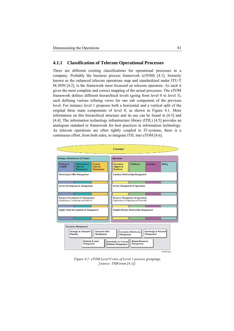
Dimensioning the Operations 81
4.1.1 Classification of Telecom Operational Processes There are different existing classifications for operational processes in a company. Probably the business process framework (eTOM) [4.1], formerly known as the enhanced telecom operations map and standardized under ITU-T M.3050 [4.2], is the framework most focussed on telecom operators. As such it gives the most complete and correct mapping of the actual processes. The eTOM framework defines different hierarchical levels (going from level 0 to level 3), each defining various refining views for one sub component of the previous level. For instance level 1 proposes both a horizontal and a vertical split of the original three main components of level 0, as shown in Figure 4.1. More information on this hierarchical structure and its use can be found in [4.3] and [4.4]. The information technology infrastructure library (ITIL) [4.5] provides an analogous standard or framework for best practices in information technology. As telecom operations are often tightly coupled to IT-systems, there is a continuous effort, from both sides, to integrate ITIL into eTOM [4.6].
Figure 4.1: eTOM Level 0 view of Level 1 process groupings
[source: TMForum [4.1]]
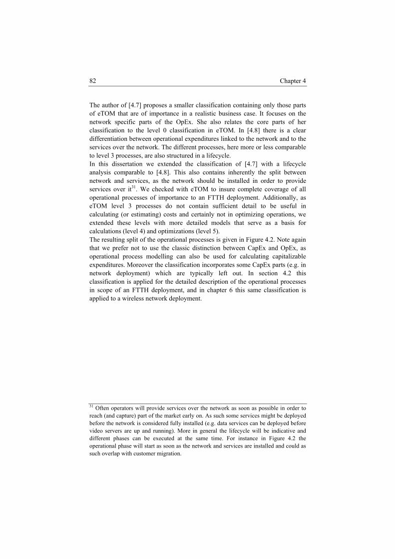
Chapter 4 82
The author of [4.7] proposes a smaller classification containing only those parts of eTOM that are of importance in a realistic business case. It focuses on the network specific parts of the OpEx. She also relates the core parts of her classification to the level 0 classification in eTOM. In [4.8] there is a clear differentiation between operational expenditures linked to the network and to the services over the network. The different processes, here more or less comparable to level 3 processes, are also structured in a lifecycle. In this dissertation we extended the classification of [4.7] with a lifecycle analysis comparable to [4.8]. This also contains inherently the split between network and services, as the network should be installed in order to provide services over it31. We checked with eTOM to insure complete coverage of all operational processes of importance to an FTTH deployment. Additionally, as eTOM level 3 processes do not contain sufficient detail to be useful in calculating (or estimating) costs and certainly not in optimizing operations, we extended these levels with more detailed models that serve as a basis for calculations (level 4) and optimizations (level 5). The resulting split of the operational processes is given in Figure 4.2. Note again that we prefer not to use the classic distinction between CapEx and OpEx, as operational process modelling can also be used for calculating capitalizable expenditures. Moreover the classification incorporates some CapEx parts (e.g. in network deployment) which are typically left out. In section 4.2 this classification is applied for the detailed description of the operational processes in scope of an FTTH deployment, and in chapter 6 this same classification is applied to a wireless network deployment.
31 Often operators will provide services over the network as soon as possible in order to reach (and capture) part of the market early on. As such some services might be deployed before the network is considered fully installed (e.g. data services can be deployed before video servers are up and running). More in general the lifecycle will be indicative and different phases can be executed at the same time. For instance in Figure 4.2 the operational phase will start as soon as the network and services are installed and could as such overlap with customer migration.
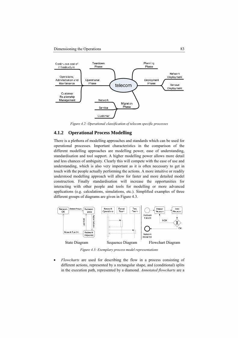
Dimensioning the Operations 83
Figure 4.2: Operational classification of telecom specific processes
4.1.2 Operational Process Modelling There is a plethora of modelling approaches and standards which can be used for operational processes. Important characteristics in the comparison of the different modelling approaches are modelling power, ease of understanding, standardisation and tool support. A higher modelling power allows more detail and less chances of ambiguity. Clearly this will compete with the ease of use and understanding, which is also very important as it is often necessary to get in touch with the people actually performing the actions. A more intuitive or readily understood modelling approach will allow for faster and more detailed model construction. Finally standardisation will increase the opportunities for interacting with other people and tools for modelling or more advanced applications (e.g. calculations, simulations, etc.). Simplified examples of three different groups of diagrams are given in Figure 4.3.
State Diagram Sequence Diagram Flowchart Diagram
Figure 4.3: Exemplary process model representations • Flowcharts are used for describing the flow in a process consisting of
different actions, represented by a rectangular shape, and (conditional) splits in the execution path, represented by a diamond. Annotated flowcharts are a
Chapter 4 84
logical extension of the general flowchart model with annotations attached to each building block. For operational processes, these annotations can include all kinds of information such as personnel type, working hours, resources (spare equipment) consumed, etc. Many modelling languages build on this approach and provide annotations in which several links to entities in other models (e.g. actual people within the organization chart) are easy to make and maintain. BPMN [4.9] is an example of such (standardized) approach and has extensions towards persistence (i.e. XML Process Definition Language (XPDL) [4.10]) or execution (i.e. Business Process Execution Language (BPEL) [4.11]). Next to BPMN, there are a lot of other examples based on the annotated flowchart modelling approach and they differ slightly in formatting (symbols), standardization effort and functionality.
• Sequence diagram [4.13] is a type of diagram typically aimed at modelling the interaction between different entities (such as interrelated processes, IT-systems or personnel). It can be used in detecting bottleneck and deadlock situations. It is generally not applied to cost calculation or optimization.
• Petri-nets [4.12] probably give the highest level of detail to the operational processes. On the other hand, Petri-nets are delicate to construct and interpret by non-professionals. They are represented by a graph consisting of states and transitions. Unlike a regular state diagram, a Petri-net is not restricted to be in one state at any time.
• State diagram [4.13] is a subset of Petri-nets in which a system is modelled to be in one of the predefined set of states and is able to evolve into another state by means of transitions (possibly following rules). This is a type of diagram used in computer science and related fields to describe the behaviour of systems with focus on correctness of states and transitions. When modelled as a Markov chain defining transitions by their probability, it can be used for analytical estimation of the relative occurrence of each state/transition.
• YAWL [4.14] stands for - yet another workflow language - and is an approach which tries to encompass the functionality of most of the existing workflow languages and combine these with some of the power of Petri-nets [4.15].
Many other modelling approaches exist, each with their own focus and intended field of application. In this dissertation we chose to make use of an annotated flowchart model (we chose BPMN), as it is one of the more intuitive standardized modelling tools which did not pose any restrictions to our intended use. YAWL, state diagrams and especially Petri-nets have more modelling power at the price of a less intuitive modelling formalism and graphical notation.

Dimensioning the Operations 85
A Short Introduction to BPMN A process model in BPMN is built around three basic building blocks: events, activities and gateways, indicated by circles, rectangles and diamonds respectively32. Additional graphical notations give intuitive information on the type, occurrences, causes, etc. of the elements. The following text lists all specific elements in use in the models further in this dissertation. A complete detailed description of all elements can be found in [4.14]. Events indicate the start, intermediate and end points of the process.
From the start event, an incoming request for execution of the process is fired. When reaching the end event, all activities (if any) still running in the process are stopped, the request is consumed and control is handed back to the encompassing process. Intermediate events indicate situations in which a given part of the process is triggered during the running of the process. The following more specific events have been used in the course of this dissertation:
Message start event Contains some information within the event that can be used in the running of the process (e.g. cause of the execution)
Timer intermediate event Will trigger an intermediate event once a predetermined time has elapsed. The timer starts counting from the moment this intermediate event is reached in the process.
Link intermediate and end event Will trigger the execution of the corresponding link end event. All link intermediate events with the same name will link to the same (unique) link end event in the process. It is often used to link two situations to the same execution path and for graphically structuring the process.
End cancelling event An ending event which will cancel all process steps up to this point and leave the overall process.
32 Actually BPMN starts from one level above this with four core elements – Flow objects, Connecting Objects, Artefacts and Swim lanes. The three elements discussed above are all part of the connecting objects, the core part of the model. All additional objects add information on the type of connection (and flow of information) between those objects, information on the objects and on the structure or group these objects reside in.

Chapter 4 86
Activities indicate the actions taking place in the execution of the process. They will contain a descriptive name and can contain parameters for the calculation of the costs.
Simple activity This can have additional indications for repetitive execution and multiple parallelised instances indicated at the bottom border.
Collapsed sub process An activity linking to a sub process which is indicated by its (unique) name and will have a start and end event linking to entrance and exit of this activity.
Gateways indicate splits or joins in the process. Those splits can either be conditional or unconditional and can have multiple incoming and outgoing execution paths of which more than one can be chosen at the same time. The incoming and outgoing paths are distinguished by their names.
Exclusive gateway Only one of the outgoing paths is taken. The default path can be indicated by a small strikethrough ( ). Additional information can be added on the probabilities of the different outgoing paths. An exclusive join is typically not used in the model. Paths are just aggregated, often at the next mutual activity, without the use of this symbol.
Fork or Join gateway A fork will trigger execution along all outgoing paths in parallel. A join will wait for all incoming paths to end and trigger execution on the outgoing path in this case. Sometimes a fork is not explicated and paths are split at the last mutual activity, without the use of this symbol.
Finally all kinds of data objects can be used to hold crucial information on one of those elements, or give more verbose explanation in some parts of the model. Very important in this are all types of aggregation through different structural groups (e.g. administration, technical personnel, etc.). Such aggregation is most often indicated by means of horizontal bars called pools and swim lanes.
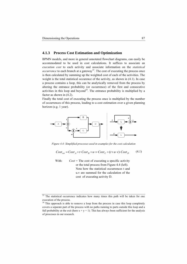
Dimensioning the Operations 87
4.1.3 Process Cost Estimation and Optimization BPMN models, and more in general annotated flowchart diagrams, can easily be accommodated to be used in cost calculations. It suffices to associate an execution cost to each activity and associate information on the statistical occurrence to each branch at a gateway33. The cost of executing the process once is then calculated by summing up the weighted cost of each of the activities. The weight is the total statistical occurence of the activity, as shown in (4.1). In case a process contains a loop, this can be analytically removed from the process by altering the entrance probability (or occurrence) of the first and consecutive activities in this loop and beyond34. The entrance probability is multiplied by a factor as shown in (4.2). Finally the total cost of executing the process once is multiplied by the number of occurrences of this process, leading to a cost estimation over a given planning horizon (e.g. 1 year).
Figure 4.4: Simplified processes used in examples for the cost calculation
DCBAtot CostvutCostvuCosttCostCost ⋅⋅++⋅⋅+⋅+= )(
With: Cost = The cost of executing a specific activity or the total process from Figure 4.4 (left). Note how the statistical occurrences t and u.v are summed for the calculation of the cost of executing activity D.
(4.1)
33 The statistical occurrence indicates how many times this path will be taken for one execution of the process. 34 This approach is able to remove a loop from the process in case this loop completely covers a separate part of the process with no paths running to parts outside this loop and a full probability at the exit (here x + y = 1). This has always been sufficient for the analysis of processes in our research.

Chapter 4 88
xzxzxxzz
i
i
−=⋅=+++⋅= ∑
∞
= 1...)1('
0
2
With: z’ = The new entrance statistical occurrence (i.e. replacement for z) when removing the loop link from the process. This will alter the statistical occurrence of all consecutive activities and gateways in the process.
(4.2)
The cost of executing an activity can be closely reflected by detailing which type of personnel is required and what time it (statistically) will take to execute the activity. This approach is suggested in activity based costing (ABC) [4.17]. Next to working hours, also other resources could be used in the execution of a process. This is for instance necessary when modelling parts of the CapEx using operational processes, e.g. an activity that involves the insertion of new linecards. Finally the information contained in the operational models and annotations can also be used for optimization purposes. The following approaches were used in this research and will be detailed further on in this dissertation: • Comparison of different technologies using the same operational process.
The cost of the operational process can be lowered by selecting the right technology.
• Comparison of different operational processes to achieve the same goal. The cost of the operational process is lowered by selecting the cheapest process.
• Optimizing different parameters for the operational process. Further in the dissertation we give an example of how the number and location of repair teams can be optimized to reduce operational costs of the repair process.
• Investigation of the process by means of simulation techniques. This allows an identification of bottlenecks and deadlocks. Later in this dissertation we also use this technique to investigate the impact of using freelance personnel in existing operational processes to cope with peak demands.
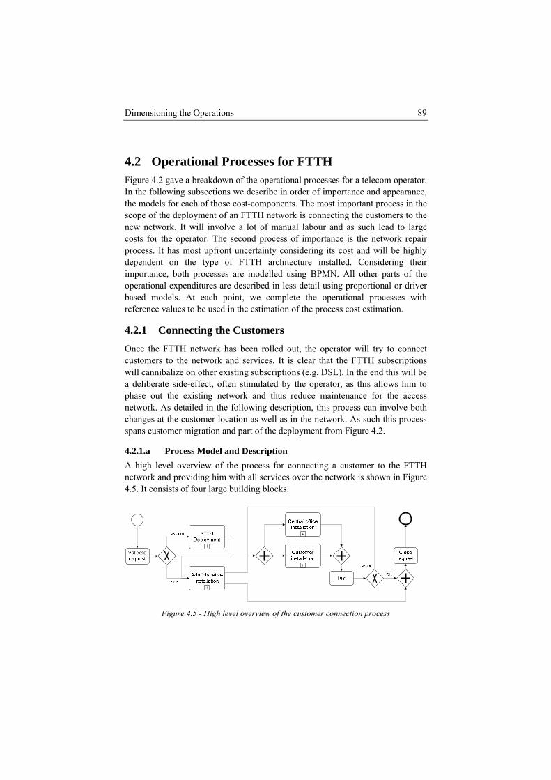
Dimensioning the Operations 89
4.2 Operational Processes for FTTH Figure 4.2 gave a breakdown of the operational processes for a telecom operator. In the following subsections we describe in order of importance and appearance, the models for each of those cost-components. The most important process in the scope of the deployment of an FTTH network is connecting the customers to the new network. It will involve a lot of manual labour and as such lead to large costs for the operator. The second process of importance is the network repair process. It has most upfront uncertainty considering its cost and will be highly dependent on the type of FTTH architecture installed. Considering their importance, both processes are modelled using BPMN. All other parts of the operational expenditures are described in less detail using proportional or driver based models. At each point, we complete the operational processes with reference values to be used in the estimation of the process cost estimation.
4.2.1 Connecting the Customers Once the FTTH network has been rolled out, the operator will try to connect customers to the network and services. It is clear that the FTTH subscriptions will cannibalize on other existing subscriptions (e.g. DSL). In the end this will be a deliberate side-effect, often stimulated by the operator, as this allows him to phase out the existing network and thus reduce maintenance for the access network. As detailed in the following description, this process can involve both changes at the customer location as well as in the network. As such this process spans customer migration and part of the deployment from Figure 4.2.
4.2.1.a Process Model and Description A high level overview of the process for connecting a customer to the FTTH network and providing him with all services over the network is shown in Figure 4.5. It consists of four large building blocks.
Figure 4.5 - High level overview of the customer connection process
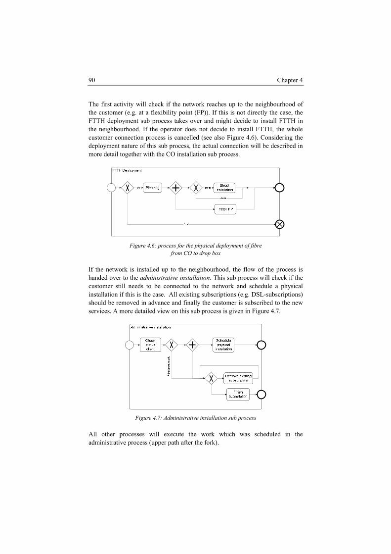
Chapter 4 90
The first activity will check if the network reaches up to the neighbourhood of the customer (e.g. at a flexibility point (FP)). If this is not directly the case, the FTTH deployment sub process takes over and might decide to install FTTH in the neighbourhood. If the operator does not decide to install FTTH, the whole customer connection process is cancelled (see also Figure 4.6). Considering the deployment nature of this sub process, the actual connection will be described in more detail together with the CO installation sub process.
Figure 4.6: process for the physical deployment of fibre
from CO to drop box If the network is installed up to the neighbourhood, the flow of the process is handed over to th will check if the ustomer still needs to edule a physical
e administrative installation. This sub process be connected to the network and schc
installation if this is the case. All existing subscriptions (e.g. DSL-subscriptions) should be removed in advance and finally the customer is subscribed to the new services. A more detailed view on this sub process is given in Figure 4.7.
Figure 4.7: Administrative installation sub process
All other processes will execute the work which was scheduled in the administrative process (upper path after the fork).
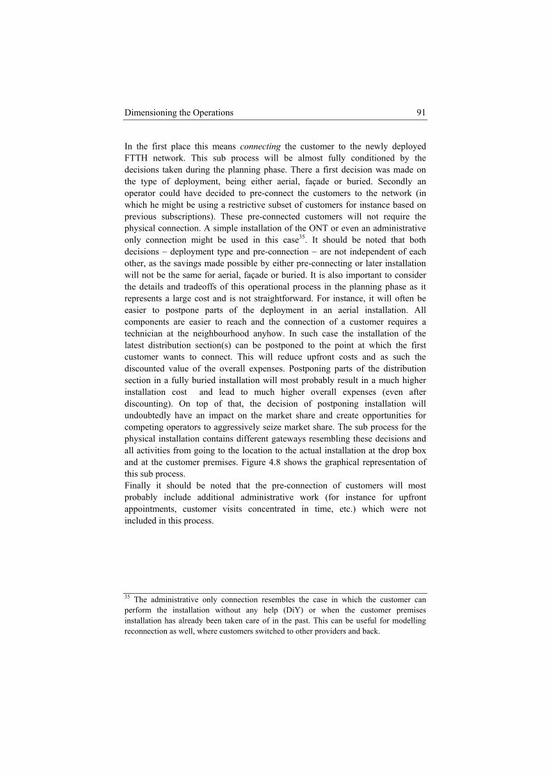
Dimensioning the Operations 91
In the first place this means connecting the customer to the newly deployed FTTH network. This sub process will be almost fully conditioned by the decisions taken during the planning phase. There a first decision was made on the type of deployment, being either aerial, façade or buried. Secondly an operator could have decided to pre-connect the customers to the network (in which he might be using a restrictive subset of customers for instance based on previous subscriptions). These pre-connected customers will not require the physical connection. A simple installation of the ONT or even an administrative only connection might be used in this case35. It should be noted that both decisions – deployment type and pre-connection – are not independent of each other, as the savings made possible by either pre-connecting or later installation will not be the same for aerial, façade or buried. It is also important to consider the details and tradeoffs of this operational process in the planning phase as it represents a large cost and is not straightforward. For instance, it will often be easier to postpone parts of the deployment in an aerial installation. All components are easier to reach and the connection of a customer requires a technician at the neighbourhood anyhow. In such case the installation of the
stallation will most probably result in a much higher stallation cost and lead to much higher overall expenses (even after
discounting). On top of that, the decision of postponing installation will undoubtedly have an impact on the market share and create opportunities for competing operators to aggressively seize market share. The sub process for the physical installation contains different gateways resembling these decisions and all activities from going to the location to the actual installation at the drop box and at the customer premises. Figure 4.8 shows the graphical representation of this sub process. Finally it should be noted that the pre-connection of customers will most probably include additional administrative work (for instance for upfront appointments, customer visits concentrated in time, etc.) which were not included in this process.
35 The administrative only connection resembles the case in which the customer can
latest distribution section(s) can be postponed to the point at which the first customer wants to connect. This will reduce upfront costs and as such the discounted value of the overall expenses. Postponing parts of the distribution section in a fully buried inin
perform the installation without any help (DiY) or when the customer premises installation has already been taken care of in the past. This can be useful for modelling reconnection as well, where customers switched to other providers and back.
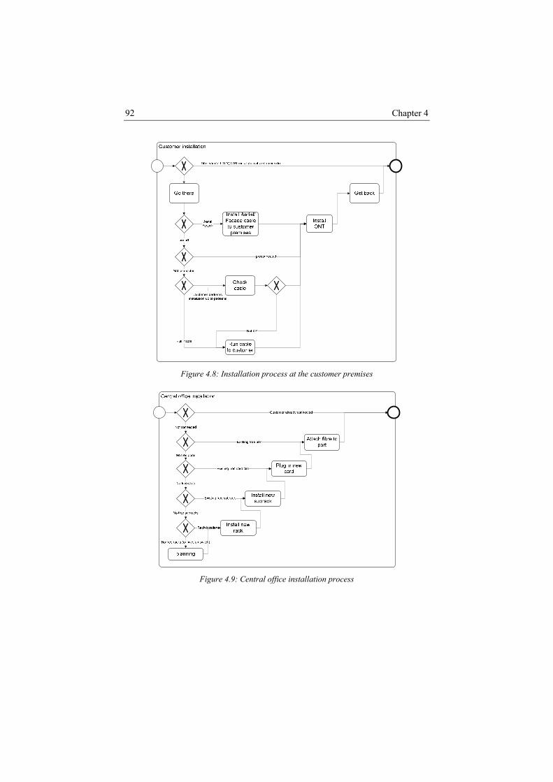
Chapter 4 92
Figure 4.8: Installation process at the customer premises
Figure 4.9: Central office installation process
Dimensioning the Operations 93
The two remaining sub processes detail the activities to be taken for providing connection from the CO up to the drop-box. The amount of upfront installation and later installation in terms of residential areas and equipment is a decision taken by the operator during the planning phase. The sub processes shown in Figure 4.6 and Figure 4.9 contain all details and will work with whatever granularity of installation envisaged by the operator. As mentioned before, here part of the CapEx are actually modelled and can be calculated using operational models. The choice whether to use an upfront installation or an on demand approach for FTTH is depending on the operator. In section 5.1 we look in more detail into the different tradeoffs for an FTTH deployment.
4.2.1.b Process Model Input Physically connecting the customer to the network is a very costly process, especially in the initial phase of the network. Given the historical use of the copper wires for telephone services, almost all houses are already connected to the copper network. Newly built houses will typically have a connection to one or more fixed broadband access networks, which in the case of Belgium is either the copper network or the HFC network. It is often possible to relate to the same (or comparable) processes for copper (or HFC) based broadband access networks, or more in general to other administrative, equipment or deployment processes. We based the input for calculations as much as possible on public sources. In the absence of such information we based the timings on experience gained from field visits or from discussions with field experts. The execution times have not been based on any measurement or time registration. An estimation of the execution times, based on the various inputs as mentioned before for the different activities, is aggregated in Table 4.1. Some execution times are still very hard to quantify and/or very dependent on the specific situation at hand (for instance on the type of hardware used). In the infrastructure dimensioning, detailed in chapter 3, an estimation of the cost of equipment and installation has been given. We marked those situations here with an X.
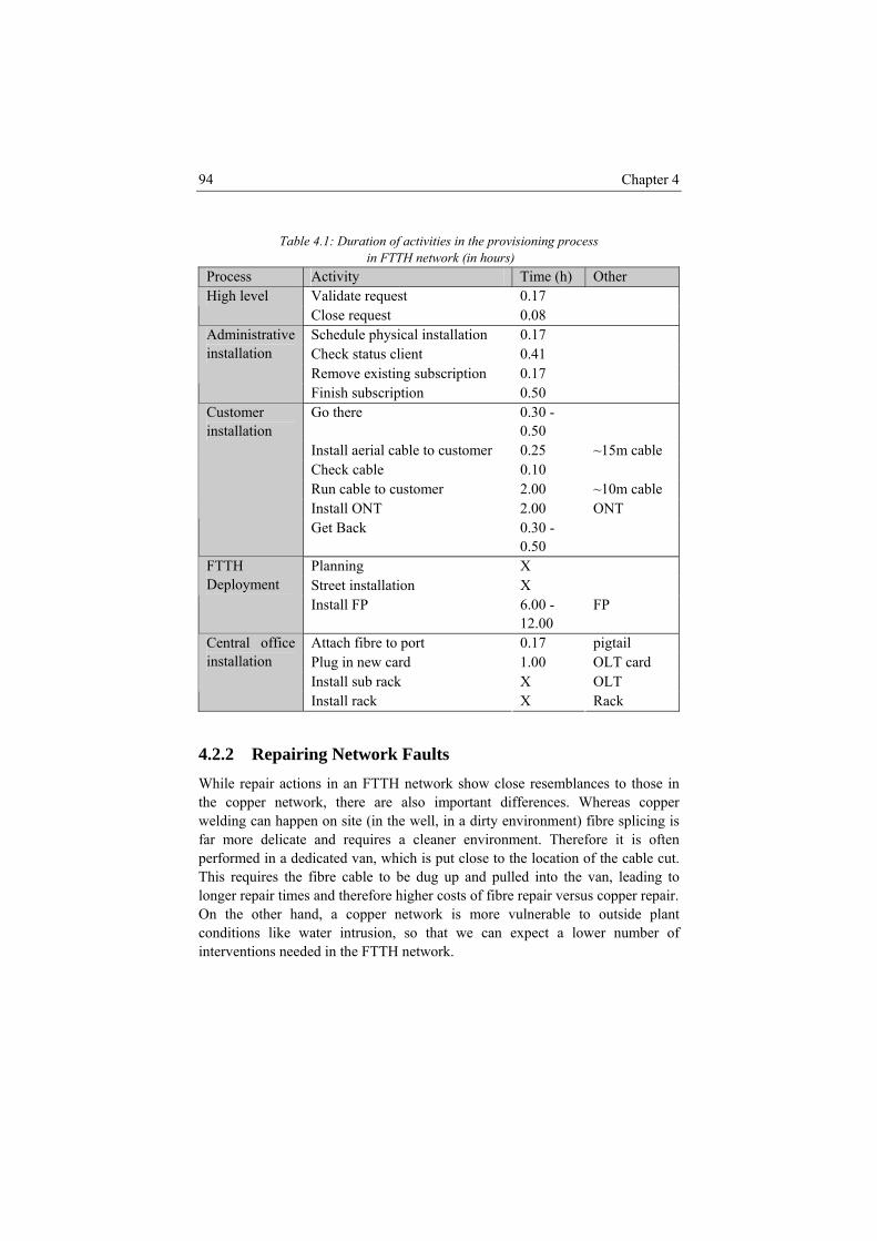
Chapter 4 94
Table 4.1: Duration of activities in the provisioning process in FTTH network (in hours)
Process Activity Time (h) Other Validate request 0.17 High level Close request 0.08 Schedule physical installation 0.17 Check status client 0.41 Remove existing subscription 0.17
Administrative installation
Finish subscription 0.50 Go there 0.30 -
0.50
Install aerial cable to customer 0.25 ~15m cable Check cable 0.10 Run cable to customer 2.00 ~10m cable Install ONT 2.00 ONT
Customer installation
Get Back 0.30 - 0.50
Planning X Street installation X
FTTH Deployment
Install FP 6.00 - 12.00
FP
Attach fibre to port 0.17 pigtail Plug in new card 1.00 OLT card Install sub rack X OLT
Central office installation
Install rack X Rack
4.2.2 Repairing Network Faults While repair actions in an FTTH network show close resemblances to those in the copper network, there are also important differences. Whereas copper welding can happen on site (in the well, in a dirty environment) fibre splicing is far more delicate and requires a cleaner environment. Therefore it is often performed in a dedicated van, which is put close to the location of the cable cut. This requires the fibre cable to be dug up and pulled into the van, leading to longer repair times and therefore higher costs of fibre repair versus copper repair. On the other hand, a copper network is more vulnerable to outside plant conditions like water intrusion, so that we can expect a lower number of interventions needed in the FTTH network.
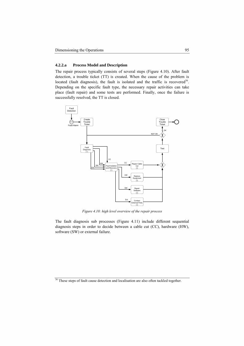
Dimensioning the Operations 95
4.2.2.a Process Model and Description The repair process typically consists of several steps (Figure 4.10). After fault detection, a trouble ticket (TT) is created. When the cause of the problem is located (fault diagnosis), the fault is isolated and the traffic is recovered36. Depending on the specific fault type, the necessary repair activities can take place (fault repair) and some tests are performed. Finally, once the failure is successfully resolved, the TT is closed.
Fault Detection
Create Trouble Ticket
Close Trouble Ticket
Test
Fault Alarm
OK
NOT OK
CC
HW
SW
Ext.
Fault Diagnosis
Fault Isolation and Recovery
Repair Cable Cut
Repair Software
Contact External Party
Replace Equipment
CC
HWSW
Ext.
Figure 4.10: high level overview of the repair process
The fault diagnosis sub processes (Figure 4.11) include different sequential diagnosis steps in order to decide between a cable cut (CC), hardware (HW), software (SW) or external failure.
36 These steps of fault cause detection and localisation are also often tackled together.
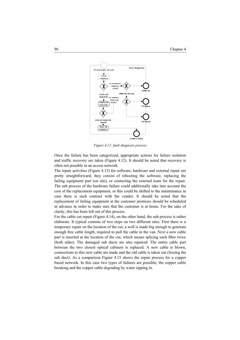
Chapter 4 96
Figure 4.11: fault diagnosis process
Once the failure has been categorized, appropriate actions for failure isolation and traffic recovery are taken (Figure 4.12). It should be noted that recovery is
ften not possible in an access network. The repair activities (Figure 4.13) for software, hardware and external repair are pretty straightforward; they consist of rebooting the software, replacing the failing equipment part (on site), or contacting the external team for the repair. The sub process of the hardware failure could additionally take into account the cost of the replacement equipment, or this could be shifted to the maintenance in case there is such contract with the vendor. It should be noted that the replacement of failing equipment at the customer premises should be scheduled in advance in order to make sure that the customer is at home. For the sake of clarity, this has been left out of this process. For the cable cut repair (Figure 4.14), on the other hand, the sub process is rather elaborate. It typical consists of two steps on two different sites. First there is a temporary repair on the location of the cut, a well is made big enough to generate enough free cable length, required to pull the cable in the van. Next a new cable part is inserted at the location of the cut, which means splicing each fibre twice (both sides). T etween the two closest optical cabinets is replaced. A new cable is blown,
connections to this new cable are made and the old cable is taken out (freeing the sub duct). A r a copper based network. In this case two types of failures are possible; the copper cable
king and the copper cable degrading water sipping in.
o
he damaged sub ducts are also repaired. The entire cable partb
s a comparison Figure 4.15 shows the repair process fo
brea by
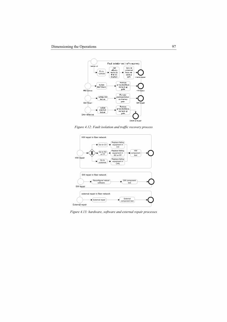
Dimensioning the Operations 97
Figure 4.12: Fault isolation traffic recovery process
and
Go to CO
Go to SCor FP
Go to customer
Replace failing equipment in
CO
Replace failing equipment in
SC or FP
Replace failing equipment in
CPE
HW repair in fiber network
HW component
test
SW repair in fiber network
Reconfigure/ reboot software
SW component test
external repair in fiber network
External repair External component test
HW repair
SW repair
External repair Figure 4.13: hardware, software and external repair processes
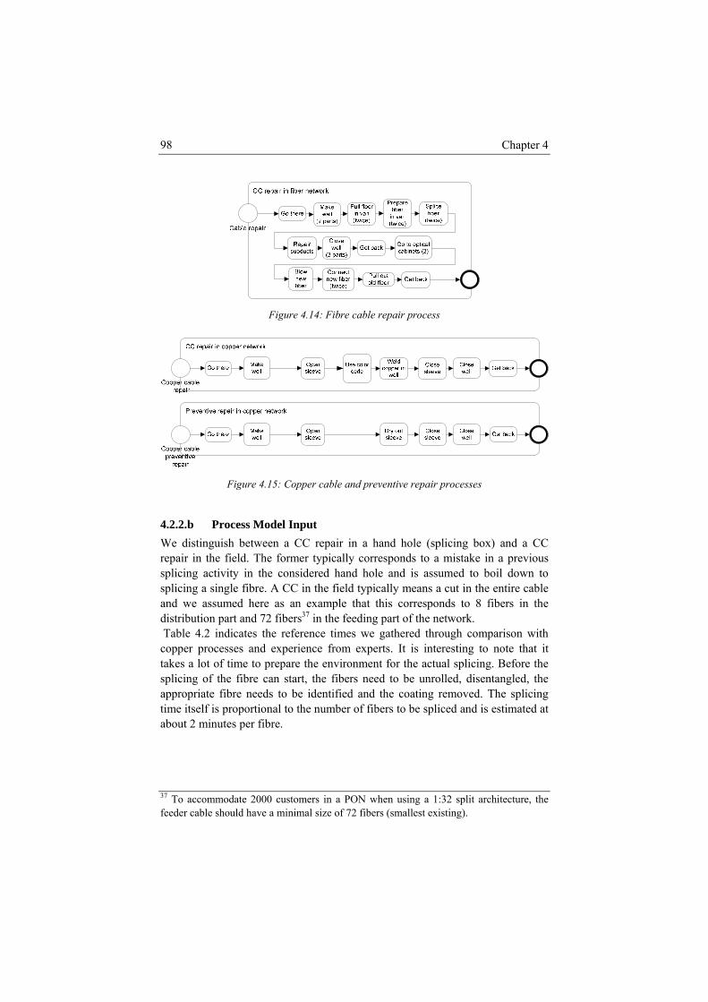
Chapter 4 98
Figure 4.14: Fibre cable repair p
rocess
Fi opper cable and preventive proc
4. Proce odel Input W inguish between a CC repair in a hand ho icin ) C
pair in the field. The former typically corresponds to a mistake in a previous
d through comparison with
e coating removed. The splicing
odate 2000 customers in a PON when using a 1:32 split architecture, the
gure 4.15: C repair esses
2.2.b ss Me dist le (spl g box and a C
resplicing activity in the considered hand hole and is assumed to boil down to splicing a single fibre. A CC in the field typically means a cut in the entire cable and we assumed here as an example that this corresponds to 8 fibers in the distribution part and 72 fibers37 in the feeding part of the network. Table 4.2 indicates the reference times we gatherecopper processes and experience from experts. It is interesting to note that it takes a lot of time to prepare the environment for the actual splicing. Before the splicing of the fibre can start, the fibers need to be unrolled, disentangled, the appropriate fibre needs to be identified and thtime itself is proportional to the number of fibers to be spliced and is estimated at about 2 minutes per fibre.
37 To accommfeeder cable should have a minimal size of 72 fibers (smallest existing).
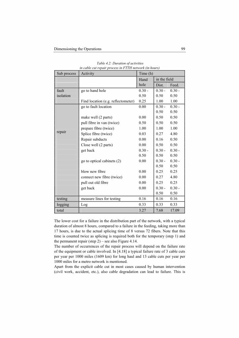
Dimensioning the Operations 99
Table 4.2: Durationin cable cut repair process in FT
of activities TH network (in hours)
Sub process Activity Time (h) in the field
Hand hole Dist. Feed.
go to hand hole 0.30 - 0.50
0.30 -0.50
0.30 - 0.50
fault isolation Find location (e.g. reflectometer) 0.25 1.00 1.00
go to fault location 0.00
0.30 -0.50
0.30 -0.50
make well (2 parts) 0.00 0.50 0.50 pull fibre in van (twice) 0.50 0.50 0.50 prepare fibre (twice) 1.00 1.00 1.00 Splice fibre (twice) 0.03 0.27 4.80 Repair subducts 0.00 0.16 0.50 Close well (2 parts) 0.00 0.50 0.50 get back 0.30 -
0.50 0.30 -0.50
0.30 -0.50
go to optical cabinets (2) 0.00
0.30 -0.50
0.30 -0.50
blow new fibre 0.00 0.25 0.25 connect new fibre (twice) 0.00 0.27 4.80 pull out old fibre 0.00 0.25 0.25
repair
ge0.50
t back 0.00 0.30 -0.50
0.30 -
te m lines for testing 0.16 0.16 sting easure 0.16 lo 0.33 0.33 gging Log 0.33 total 3.27 7.68 17.09
The lower cost for a failure in the distribution part of the network, with a typical duration of almost 8 hours, compared to a failure in the feeding, taking more than 17 hours, is due to the actual splicing time of 8 versus 72 fibers. Note that this time is counted twice as splicing is required both for the temporary (step 1) and the permanent repair (step 2) – see also Figure 4.14.
er 1000 miles (1609 km) for long haul and 13 cable cuts per year per
The number of occurrences of the repair process will depend on the failure rate of the equipment or cable involved. In [4.18] a typical failure rate of 3 cable cuts per year p1000 miles for a metro network is mentioned. Apart from the explicit cable cut in most cases caused by human intervention (civil work, accident, etc.), also cable degradation can lead to failure. This is
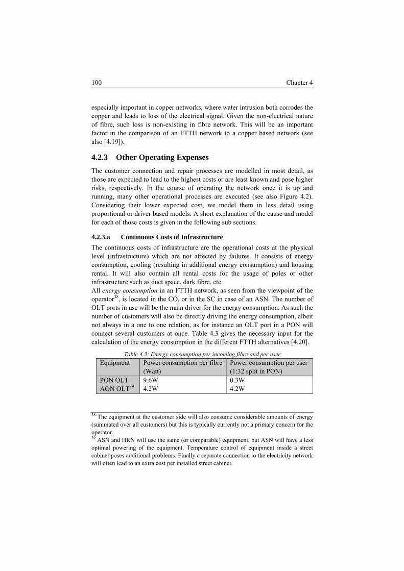
Chapter 4 100
especially important in copper networks, where water intrusion both corrodes the copper and leads to loss of the electrical signal. Given the non-electrical nature of fibre, such loss is non-existing in fibre network. This will be an important factor in the comparison of an FTTH network to a copper based network (see also [4.19]).
4.2.3 Other Operating Expenses to d in most detail, as The cus mer connection and repair processes are modelle
those are expected to lead to the highest costs or are least known and pose higher risks, respectively. In the course of operating the network once it is up and running, many other operational processes are executed (see also Figure 4.2). Considering their lower expected cost, we model them in less detail using proportional or driver based models. A short explanation of the cause and model for each of those costs is given in the following sub sections.
4.2.3.a Continuous Costs of Infrastructure The continuous costs of infrastructure are the operational costs at the physical level (infrastructure) which are not affected by failures. It consists of energy consumption, cooling (resulting in additional energy consumption) and housing rental. It will also contain all rental costs for the usage of poles or other infrastructure such as duct space, dark fibre, etc. All energy consumption in an FTTH network, as seen from the viewpoint of the operator38, is located in the CO, or in the SC in case of an ASN. The number of OLT ports in use will be the main driver for the energy consumption. As such the number of customers will also be directly driving the energy consumption, albeit not always in a one to one relation, as for instance an OLT port in a PON will connect several customers at once. Table 4.3 gives the necessary input for the calculation of the energy consumption in the different FTTH alternatives [4.20].
Table 4.3: Energy consumption per incoming fibre and per user Equipment Power consumption per fibre
(Watt) Power consumption per user (1:32 split in PON)
PON OLT 9.6W 0.3W AON OLT 4.2W 4.2W 39
38 The equipment at the customer side will also consume considerable amounts of energy (summated over all customers) but this is typically currently not a primary concern for the operator. 39 ASN and HRN will use the same (or comparable) equipment, but ASN will have a less optimal powering of the equipment. Temperature control of equipment inside a street cabinet poses additional problems. Finally a separate connection to the electricity network will often lead to an extra cost per installed street cabinet.
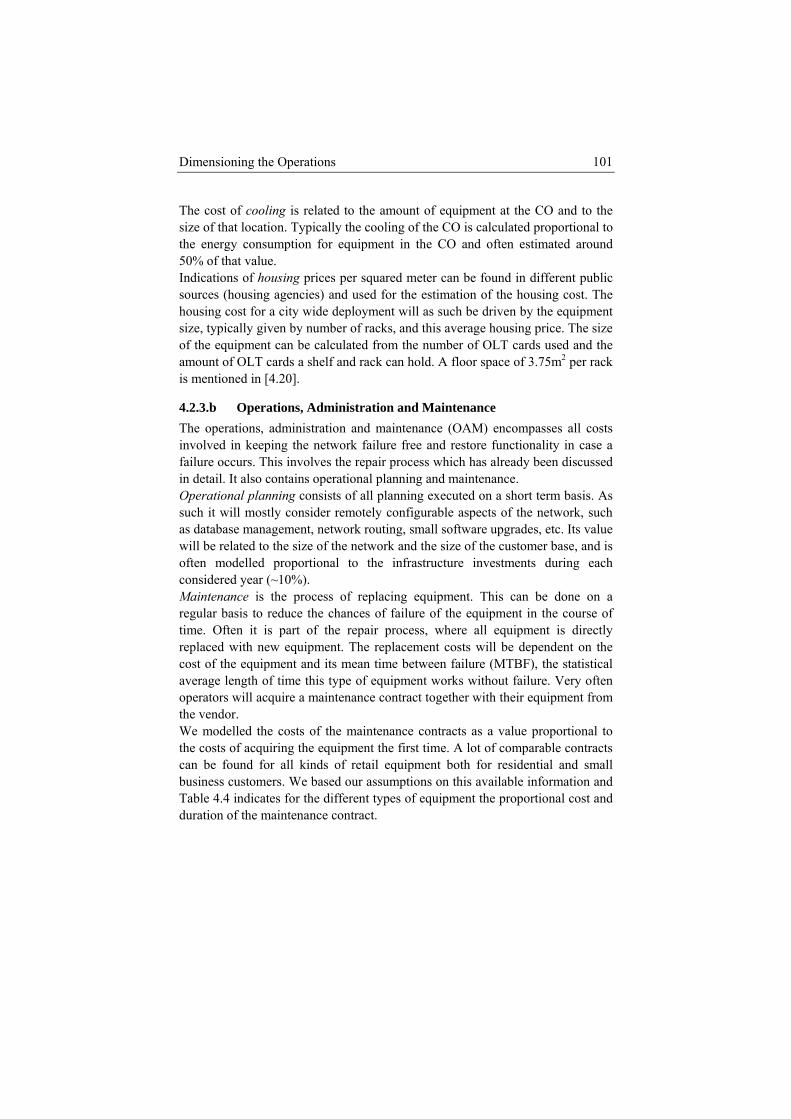
Dimensioning the Operations 101
The cost of c O and to the size of that lo the coo proportional to the energy c equipme and often estimated around 50% of that vIndications o ua be found in different public sources (housing agencies) and used for the estimation of the housing cost. The
co h be driven by the equipment
ecuted on a short term basis. As
during each considered year (~10%). Maintenance is the process of replacing equipment. This can be done on a regular basis to reduce the chances of failure of the equipment in the course of time. Often it is part of the repair process, where all equipment is directly replaced with new equipment. The replacement costs will be dependent on the cost of the equipment and its mean time between failure (MTBF), the statistical average length of time this type of equipment works without failure. Very often operators will acquire a maintenance contract together with their equipment from the vendor. We modelled the costs of the maintenance contracts as a value proportional to the costs of acquiring the equipment the first time. A lot of comparable contracts can be found for all kinds of retail equipment both for residential and small business customers. We based our assumptions on this available information and Table 4.4 indicates for the different types of equipment the proportional cost and duration of the maintenance contract.
ooling is related to the amount of equipment at the Ccation. Typically ling of the CO is calculatedonsumption for nt in the COalue. f housing prices per sq red meter can
housing st for a city wide deployment will as sucsize, typically given by number of racks, and this average housing price. The size of the equipment can be calculated from the number of OLT cards used and the amount of OLT cards a shelf and rack can hold. A floor space of 3.75m2 per rack is mentioned in [4.20].
4.2.3.b Operations, Administration and Maintenance The operations, administration and maintenance (OAM) encompasses all costs involved in keeping the network failure free and restore functionality in case a failure occurs. This involves the repair process which has already been discussed in detail. It also contains operational planning and maintenance. Operational planning consists of all planning exsuch it will mostly consider remotely configurable aspects of the network, such as database management, network routing, small software upgrades, etc. Its value will be related to the size of the network and the size of the customer base, and is often modelled proportional to the infrastructure investments
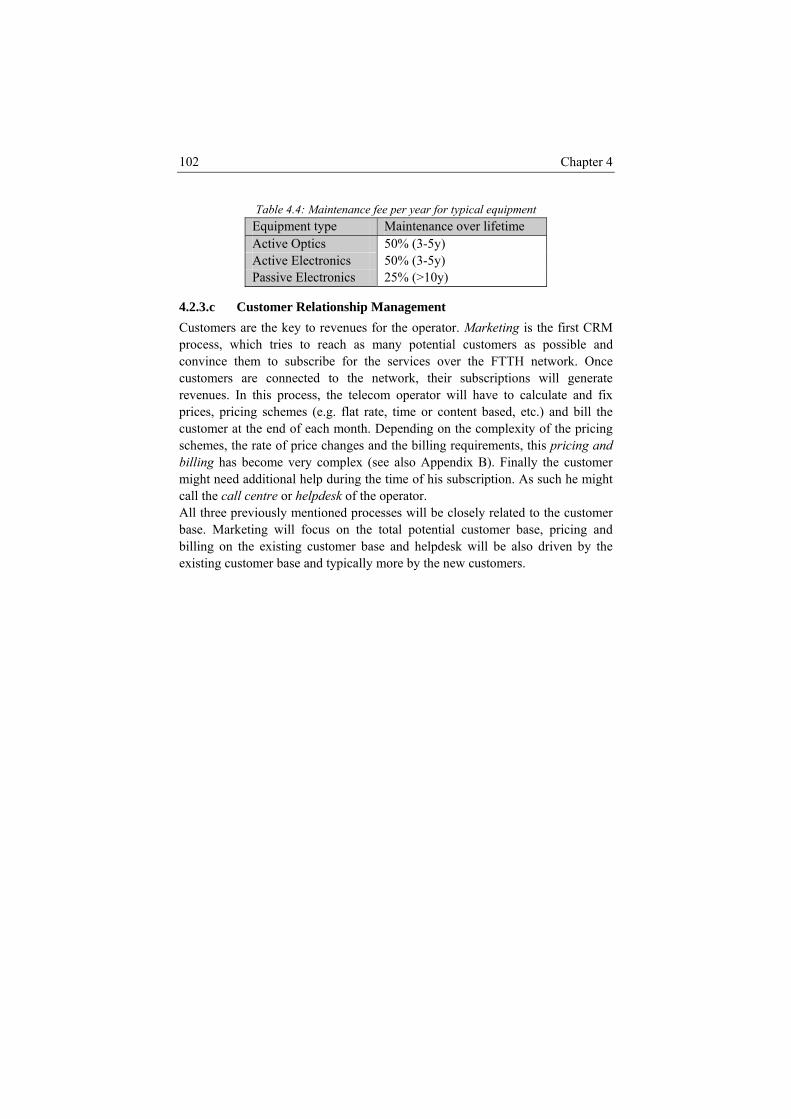
Chapter 4 102
Table 4.4: Maintenance fee per year for typical equipment Equipment type Maintenance over lifetime Active Optics 50% (3-5y) Active Electronics 50% (3-5y) Passive Electronics 25% (>10y)
4.2.3.c Customer Relationship Management Customers are the key to revenues for the operator. Marketing is the first CRM process, which tries to reach as many potential customers as possible and convince them to subscribe for the services over the FTTH network. Once customers are connected to the network, their subscriptions will generate revenues. In this process, the telecom operator will have to calculate and fix prices, pricing schemes (e.g. flat rate, time or content based, etc.) and bill the customer at the end of each month. Depending on the complexity of the pricing schemes, the rate of price changes and the billing requirements, this pricing and
migcallAll er
sebilliexis
billing has become very complex (see also Appendix B). Finally the customer ht need additional help during the time of his subscription. As such he might the call centre or helpdesk of the operator. three previously mentioned processes will be closely related to the custom
ba . Marketing will focus on the total potential customer base, pricing and ng on the existing customer base and helpdesk will be also driven by the ting customer base and typically more by the new customers.
Dimensioning the Operations 103
4.3 Optimising Operational Processes The models previously presented allow estimating the operational expenditures for a telecom operator. As mentioned in the introduction section we can also use this information to optimize (minimize) the operational expenditures. In this section we start from the simplest network repair process based on that of Figure 4.10 and indicate how to gradually extend this to contain information required for detailed optimization. In this research, we closely cooperated with other partners who were mainly interested in the OpEx in core networks, and as such the models and optimizations presented here will broaden the scope slightly. We started in all cases from a simplified network repair process as shown in Figure 4.16 with a main focus on hardware and cable cut repair. The case studies investigate the following approaches for optimizing the network repair process: • Optimization of the number and location of repair teams in the access
network. Comparable results are sh n for the core. This optimization is als . The optimization is based on a heuristic search for the optimal parameter set.
• Reduction of the operational expenditures by means of freelance or more flexible and multi trained personnel. A discrete event simulation approach has been used and a scan of the full working range allows finding the optimal freelance personnel size. Again the results of a comparable study for the core network are added.
Additional studies exist for both approaches, and are described in more detail in [4.21] and [4.22] considering the access network, and in [4.23], [4.24], [4.25] and [4.26] considering the core networks.
owo extended to reflect the effect of the service level on the costs
Fault Detection
Create Trouble Ticket
Close Trouble Ticket
Test
Fault Alarm
OK
NOT OK
Fault Diagnosis
Fault Isolation and Recovery
Go to the Fault Location Repair Fault
Figure 4.16: Simplified network repair process used in optimization studies
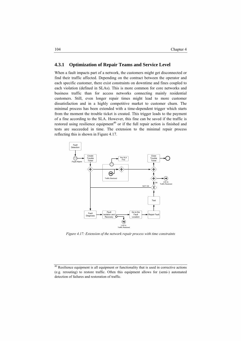
Chapter 4 104
4.3.1 Optimization of Repair Teams and Service Level When a fault impacts part of a network, the customers might get disconnected or find their traffic affected. Depending on the contract between the operator and each specific customer, there exist constraints on downtime and fines coupled to each violation (defined in SLAs). This is more common for core networks and business traffic than for access networks connecting mainly residential customers. Still, even longer repair times might lead to more customer dissatisfaction and in a highly competitive market to customer churn. The minimal process has been extended with a time-dependent trigger which starts from the moment the trouble ticket is created. This trigger leads to the payment of a fine according to the SLA. However, this fine can be saved if the traffic is restored using resilience equipment40 or if the full repair action is finished and tests are succeeded in time. The extension to the minimal repair process reflecting this is shown in Figure 4.17.
Fault Detection
Create Trouble Ticket
Close Trouble Ticket
Fault Diagnosis
Fault Isolation and
Recovery
Go to the Fault
LocationRepair Fault
Test
Fault Alarm
Link to: Traffic Restored
OK
NOT OK
Link to: Traffic Restored
Pay SLA Fine
Traffic Restored
Figure 4.17: Extension of the network repair process with time constraints
40 Resilience equipment is all equipment or functionality that is used in corrective actions (e.g. rerouting) to restore traffic. Often this equipment allows for (semi-) automated detection of failures and restoration of traffic.
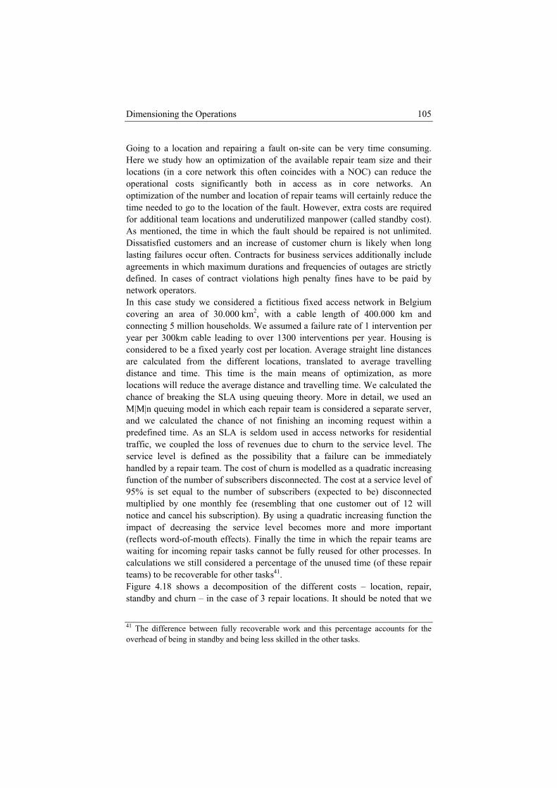
Dimensioning the Operations 105
Going to a location and repairing a fault on-site can be very time consuming. Here we study how an optimization of the available repair team size and their locations (in a core network this often coincides with a NOC) can reduce the operational costs significantly both in access as in core networks. An optimization of the number and location of repair teams will certainly reduce the time needed to go to the location of the fault. However, extra costs are required for additional team locations and underutilized manpower (called standby cost).
ding to over 1300 interventions per year. Housing is onsidered to be a fixed yearly cost per location. Average straight line distances
are calculated from the different locations, translated to average travelling distance and time. This time is the main means of optimization, as more locations will reduce the average distance and travelling time. We calculated the chance of breaking the SLA using queuing theory. More in detail, we used an M|M|n queuing model in which each repair team is considered a separate server, and we calculated the chance of not finishing an incoming request within a predefined time. As an SLA is seldom used in access networks for residential traffic, we coupled the loss of revenues due to churn to the service level. The service level is defined as the possibility that a failure can be immediately handled by a repair team. The cost of churn is modelled as a quadratic increasing function of the number of subscribers disconnected. The cost at a service level of 95% is set equal to the number of subscribers (expected to be) disconnected multiplied by one monthly fee (resembling that one customer out of will noti the impact o portant
eflects word-of-mouth effects). Finally the time in which the repair teams are waiting for incoming repair tasks cannot be fully reused for other processes. In calculations ese repair teams) to be
igure 4.18 shows a decomposition of the different costs – location, repair,
As mentioned, the time in which the fault should be repaired is not unlimited. Dissatisfied customers and an increase of customer churn is likely when long lasting failures occur often. Contracts for business services additionally include agreements in which maximum durations and frequencies of outages are strictly defined. In cases of contract violations high penalty fines have to be paid by network operators. In this case study we considered a fictitious fixed access network in Belgium covering an area of 30.000 km2, with a cable length of 400.000 km and connecting 5 million households. We assumed a failure rate of 1 intervention per year per 300km cable leac
12ce and cancel his subscription). By using a quadratic increasing function
f decreasing the service level becomes more and more im(r
we still considered a percentage of the unused time (of th recoverable for other tasks41.
Fstandby and churn – in the case of 3 repair locations. It should be noted that we
41 The difference between fully recoverable work and this percentage accounts for the overhead of being in standby and being less skilled in the other tasks.
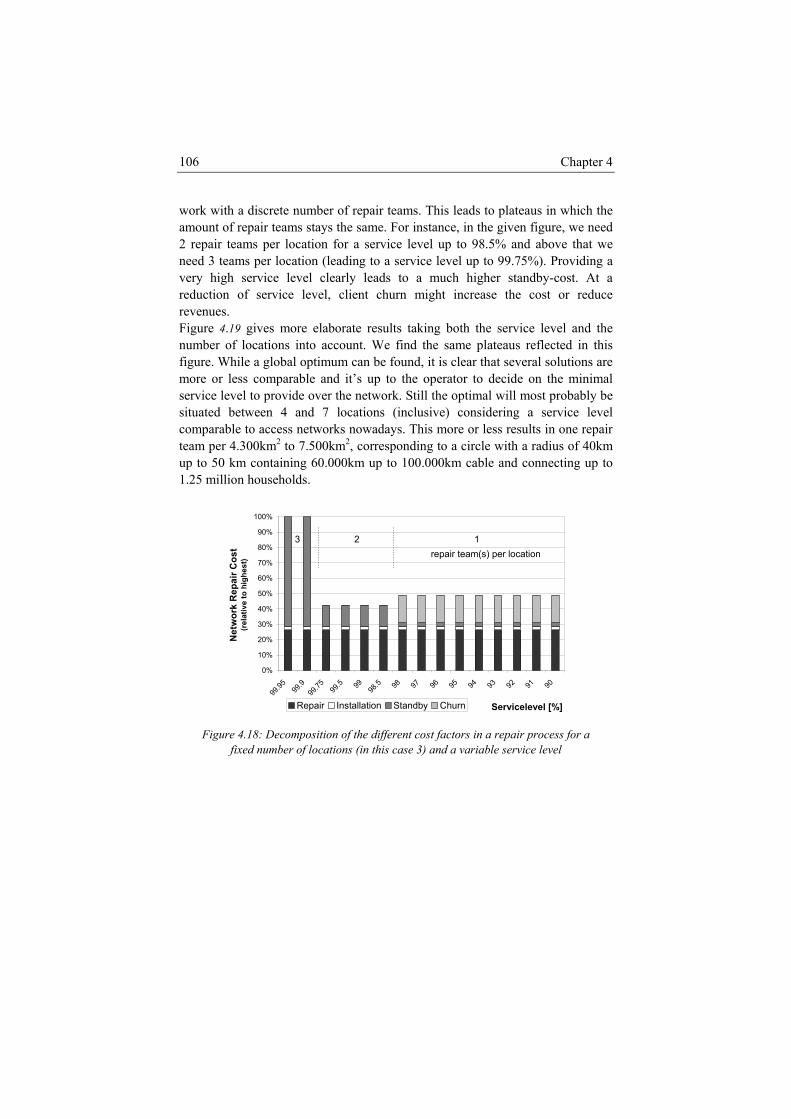
Chapter 4 106
work with a discrete number of repair teams. This leads to plateaus in which the amount of repair teams stays the same. For instance, in the given figure, we need 2 repair teams per location for a service level up to 98.5% and above that we
very st. At a u
reve
rovide over the network. Still the optimal will most probably be tuated between 4 and 7 locations (inclusive) considering a service level
comparable to access networks nowadays. This more or less results in one repair team per 4.300km2 to 7.500km2, corresponding to a circle with a radius of 40km up to 50 km containing 60.000km up to 100.000km cable and connecting up to 1.25 million households.
need 3 teams per location (leading to a service level up to 99.75%). Providing a high service level clearly leads to a much higher standby-co
red ction of service level, client churn might increase the cost or reduce nues.
Figure 4.19 gives more elaborate results taking both the service level and the number of locations into account. We find the same plateaus reflected in this figure. While a global optimum can be found, it is clear that several solutions are more or less comparable and it’s up to the operator to decide on the minimal service level to psi
0%
10%
20%
30%
99.95 99
.999
.75 99.5 99 98
.5 98 97 96 95 94 93 92 91 90
Servicelevel [%]
Net
wor
(rel
at
40%
50%
70%
80%
90%
100%
k R
epai
Cos
t iv
e to
t)
repair team(s) p tion123
er loca
60%r h
ighe
s
Repair Installation Standby Churn
Figure 4.18: Decomposition of the different cost factors in a repair process for a riable service level fixed number of locations (in this case 3) and a va
Dimensioning the Operations 107
99.9599.75
99
98
96
94
92
90
1 2 3 4 5 6 7 8 9 10
0%[%]
number of locations
5%
Figure 4.19: Influence of service level and number of locations on the network repair cost.
In a core network in contrast to the access, infrastructure is often placed in a limited number of locations. These locations are connected by means of cables forming a sparsely meshed backbone network. Distances between the nodes are much larger than for access networks. Considering the larger size and complexity of the node equipment and the fibre cable, the repair in a core network requires more trained personnel. In [4.23] the author uses two core networks available from [4.27]: • Germany50 covering Germany (357.000 km2) with 50 nodes, 87 links, an
average link length of 130 km and a total link length of 11.000 km. • USA26 covering the United States (9.522.000 km2) with 26 nodes, 41 links,
an average link length of 600 km and a total link length of 25.000 km. Figure 4.20 shows the results for the study over those two networks. The time reduction is corresponding to the average time to repair one failure from any location. Depending on the number of repair teams per location, this will result in cost savings. In this study the effects of changing the SLA has not been considered.
10%
Network Repair Cost increase relative to
lowest cost
Servicelevel
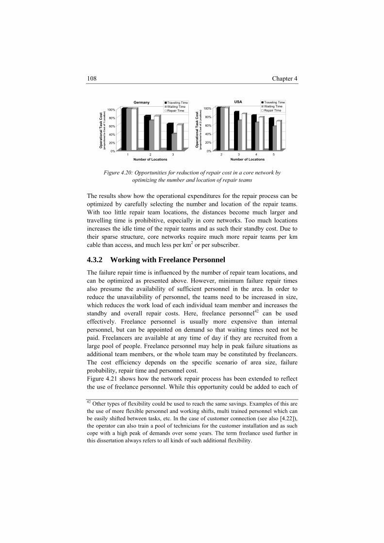
Chapter 4 108
0%
20%
40%
60%
80%
100%
Ope
ratio
nal T
ask
Cos
t (p
ropo
rtio
nal t
o C
ost o
f 1 L
ocat
ion)
1 2 3Number of Locations
Germany Traveling TimeWaiting TimeRepair Time
0%
20%
40%
60%
80%
100%
Ope
ratio
nal T
ask
Cos
t (p
ropo
rtio
nal t
o C
ost o
f 2 L
ocat
ions
)
2 3 4 5
USA
Number of Locations
Traveling TimeWaiting TimeRepair Time
Figure 4.20: Opportunities for reduction of repair cost in a core network by
optimizing the number and location of repair teams The results show how the operational expenditures for the repair process can be optimized by carefully selecting the number and location of the repair teams. With too little repair team locations, the distances become much larger and travelling time is prohibitive, especially in core networks. Too much locations increases the idle time of the repair teams and as such their standby cost. Due to their sparse structure, core networks require much more repair teams per km cable than access, and much less per km2 or per subscriber.
4.3.2 Working with Freelance Personnel The failure repair time is influenced by t umber of repair team locations, and can be optim pair times also presum In order to
duce the unavailability of person s need to be increased in size, ch reduces the work load of each individual team member and increases the
standby and overall repair costs. Here, freelance personnel42 can be used effectively. Freelance personnel is usually more expensive than internal personnel, but can be appointed on demand so that waiting times need not be paid. Freelancers are available at any time of day if they are recruited from a large pool of people. Freelance personnel may help in peak failure situations as additional team members, or the whole team may be constituted by freelancers. The cost efficiency depends on the specific scenario of area size, failure probability, repair time and personnel cost. Figure 4.21 shows how the network repair process has been extended to reflect the use of freelance personnel. While this opportunity could be added to each of 42 Other types of f mples of this are
he nized as presented above. However, minimum failure re
e the availability of sufficient personnel in the area. nel, the teamre
whi
lexibility could be used to reach the same savings. Exathe use of more flexible personnel and work g shifts, multi trained personnel which can be easily shifted between tasks, etc. In the ca of customer connection (see also [4.22]), the operator can also train a pool of technicians for the customer installation and as such cope with a high peak of demands over some years. The term freelance used further in this dissertation always refers to all kinds of such additional flexibility.
inse
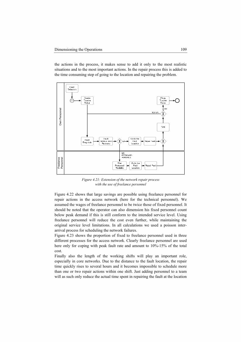
Dimensioning the Operations 109
the actions in ost realistic situations and to the m rocess this is added to the time consuming step of going to the l cation and repairing the problem.
the process, it makes sense to add it only to the most important actions. In the repair p
o
Free
lanc
e Pe
rson
nel
Ow
n P
erso
nnel
Figure 4.21: Extension of the network repair process
with the use of freelance personnel Figure 4.22 shows that large savings are possible using freelance personnel for repair actions in the access network (here for the technical personnel). We assumed the wages of freelance personnel to be twice those of fixed personnel. It should be noted that the operator can also dimension his fixed personnel count below peak demand if this is still conform to the intended service level. Using freelance personnel will reduce the cost even further, while maintaining the original service level limitations. In all calculations we used a poisson inter-arrival process for scheduling the network failures. Figure 4.23 shows the proportion of fixed to freelance personnel used in three different processes for the access network. Clearly freelance personnel are used here only for coping with peak fault rate and amount to 10%-15% of the total cost. Finally also the length of the working shifts will play an important role, especially in core networks. Due to the distance to the fault location, the repair time quickly rises to several hours and it becomes impossible to schedule more than one or two repair actions within one shift. Just adding personnel to a team will as such only reduce the actual time spent in repairing the fault at the location
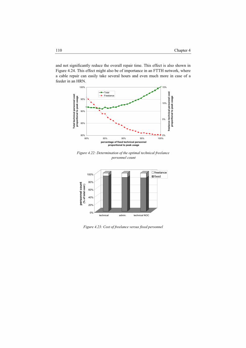
Chapter 4 110
and not significantly reduce the overall repair time. This effect is also shown in ght also be of importance in an FTTH network, where ake several hours and even much more in case of a
Figure 4.24. This effect mia cable repair can easily tfeeder in an HRN.
80%
85%
90%
80% 85% 90% 95% 100%
Tota
l tec
hnic
al p
erso
prop
ortio
nal t
o pe
ak
0%
5%
10%
free
lanc
e te
chni
cal p
erso
prop
ortio
nal t
o pe
ak
95%
100%
nnel
cos
t u
sage
15%
el c
ost
age
TotalFreelance
percentage of fixed technical personnel
nn us
proportional to peak usage Figure 4.22: Determination of the optimal technical freelance
personnel count
0%
20%
40%
60%
80%
100%
t pe
rson
nel c
oun
(% o
f tot
al c
ost )
technical admin. technical NOC
freelancefixed
Figure 4.23: Cost of freelance versus fixed personnel
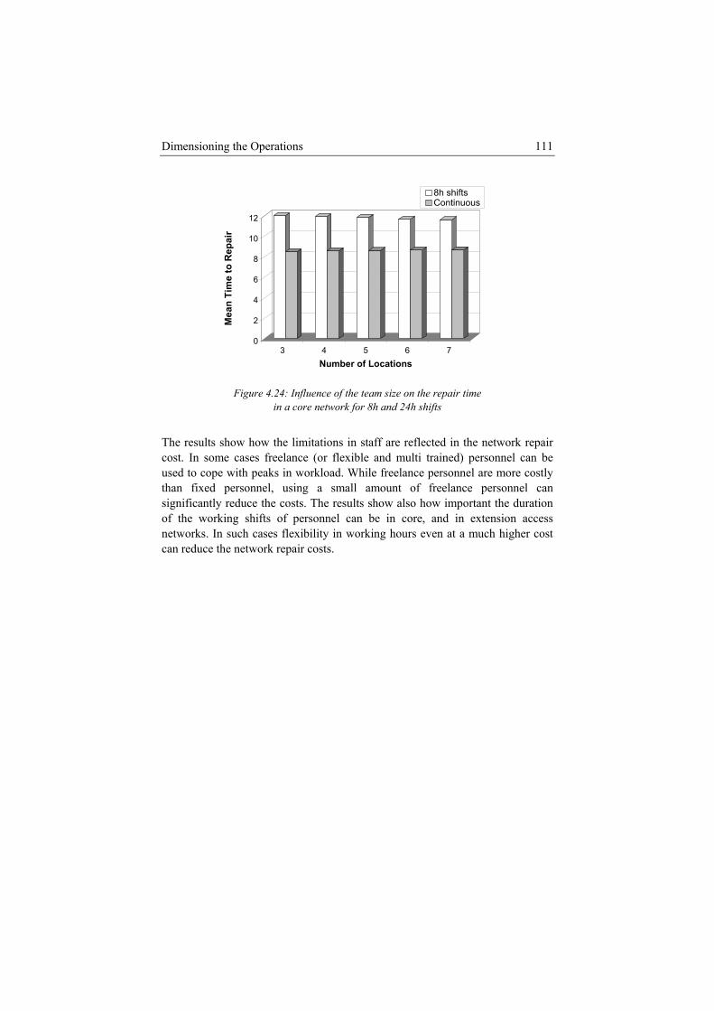
Dimensioning the Operations 111
4
6
8
an T
ime
to R
10ep
air
0
2Me
12
3 4 5 6 7Number of Locations
8h shiftsContinuous
shifts
The res ed in the network repair coused to than fi using a small amount of freelance personnel can siof the network ing hours even at a much higher cost can reduce
Figure 4.24: Influence of the team size on the repair time
in a core network for 8h and 24h
ults show how the limitations in staff are reflect
st. In some cases freelance (or flexible and multi trained) personnel can be cope with peaks in workload. While freelance personnel are more costly xed personnel,
gnificantly reduce the costs. The results show also how important the duration working shifts of personnel can be in core, and in extension access s. In such cases flexibility in work
the network repair costs.
Chapter 4 112
4.4 CTcalculatclassific choice in this dissertation for onotationToperatiotelecom network. We started wiuThese tremainidriver bIn addit he models, the network repair process and its Bbroaden ion in core net the number and location opersonnsubstan
onclusions his chapter introduces the reader to the use of operational modelling,
ion and optimization. It also gives a short outline of the existing ations used for telecom OpEx. The
perational modelling is BPMN and a very short introduction to its graphical is added as well.
he main part of this chapter focuses on the modelling and estimation of nal expenditures, and more in general all process based expenditures, a operator will face when rolling out a new FTTH
th a high level breakdown of the processes and selected the two most costly or nknown – customer connection and network repair – as our points of focus.
wo are modelled in much detail. A short description is added for the ng processes indicating how they are estimated using proportional or ased models. ion to the description of t
PMN representation are extended to allow optimization. The scope is slightly ed to reflect where the same approach could be used for optimizatworks. The studies focus on an optimization of
f repair teams within a predefined service level and the use of freelance el for coping with peak workloads. The results show opportunities for tial savings (up to 10%) in the OpEx for an access network.
Dimensioning the Operations 113
Refer[4.1] TM Forum, “the business process framework (eTOM)”,
http://www.tmforum.org/BusinessProcessFramework/1647/home.html
[4.2] ITU-T Recommendation M.3050, “Enhanced Telecommunications Operations Map (eTOM) – Supplements”, 2007, http://www.itu.int/rec/T-REC-M.3050/en
[4.3] ITU-T Recommendation M.3050.1, “Enhanced Telecom Operations Map (eTOM) - The business process framework”, 2007, http://www.itu.int/rec/T-REC-M.3050.1/en
[4.4] ITU-T Recommendation M3050.2, “Enhanced Telecom Operations Map (eTOM) - Process decompositions and descriptions”, 2007, http://www.itu.int/rec/T-REC-M.3050.2/en
[4.5] ITIL – The Information Technology Infrastructure Library, http://www.itil-officialsite.com/home/home.asp
[4.6] TM Forum, “GB921 Business Process Framework Release 8.0”, http://www.tmforum.org/DocumentsBusiness/GB921BusinessProcess/36653/article.html
[4.7] S. Verbrugge, “Strategic Planning of Optical Telecommunication Networks in a Dynamic and Uncertain Environment”, Ph.D. thesis UGent, ISBN 978-90-8578-131-8
[4.8] C. M. Machuca, O. Moe, and M. Jäger, "Impact of protection schemes and network component's availability on operational expenditures," Journal on Optical Networking (JON), Vol. 7, pp. 142-150, 2008.
[4.9] Object Management Group/Business Process Management Initiative, http://www.bpmn.org/
[4.10] Workflow Management Coalition, XML Process Definition Language, http://www.wfmc.org/xpdl.html
[4.11] OASIS Standard, “Web Services Business Process Execution Language”, 2007, http://docs.oasis-open.org/wsbpel/2.0/wsbpel-v2.0.pdf
[4.12] J. Peterson, “Petri Nets”, Computing Surveys, Vol 9, No. 3, pp.223-252, 1977
[4.13] M. Fowler, “UML Distilled, rev. 3”, Addison-Wesley Professional, ISBN-978-0321193681, 2003
[4.14] YAWL – Yet Another Workflow Language, http://www.yawl-system.com/
ences
Chapter 4 114
[4.15] W. van der Aalst, A. ter Hofstede, “YAWL: Yet Another Workflow” Language. Information Systems, Vol. 30, No. 4, pp.245-275, 2005.
[4.16] The Object Management Group (OMG) Specification BPMN 1.2, “Business Process Modelling Notation (BPMN)”, 2009, http://www.omg.org/spec/BPMN/1.2/
[4.17] R.S. Kaplan, S. Anderson: “Time–Driven Activity-Based Costing,” Harvard Business Review, 2004, vol. 82, no. 11, pp. 131-138.
[4.18] G. Booker, A. Sprintson, C. Singh, S. Guikema, “Efficient Availability Evaluation for Transport Backbone Networks”, ONDM 2008, Vilanova i la Geltrú, Catalonia, Spain, on March 12-14, 2008
[4.19] S. Verbrugge K. Casier B. Lannoo J. Van Ooteghem R. Meersman D. Colle P. Demeester, “FTTH deployment and its impact on network maintenance and repair costs”, International Conference on Transparent Optical Networks (ICTON), ISBN 978-1-4244-2625-6, Athens, Greece, 22-26 June 2008, pp. 2-5
[4.20] P. Fournier, “From FTTH pilot to pre-rollout in France”, 2007, http://www.orange.com/en_EN/finance/invest-analysts/meetings-conferences/att00009692/20070626_FTTH.pdf
[4.21] K. Casier, L. Van Halewyck, S. Verbrugge, D. Colle, M. Pickavet, P. Demeester, ”Extending operational models to perform micro optimizations”, ECOC 2007, September 16-20, 2007, Berlin, Germany
[4.22] K. Casier, A. Gouwy, S. Verbrugge, D. Colle, M. Pickavet, P. Demeester, “Using discrete event simulation to reduce operational expenses for a telecom operator”, Networks 2008, Budapest, Hungary, Sept 28 – Oct 2, 2008.
[4.23] C. Mas Machuca, O. Moe, M. Jäger, “Impact of the protection schemes and network component availability on the operational expenditures”, Journal of Optical Networking Vol. 7, No. 2, pp. 142-150, February 2008
[4.24] C. Mas Machuca, O. Moe, M. Jäger, “Modelling of OpEx in network and service life-cycles”, ECOC 2007 OpEx Workshop September 2007 Berlin, Germany
[4.25] O. Moe, “Study of the integration of the different nature OpEx costs of a network”, Master thesis, Technical University Munich, 2007.
[4.26] B. Correa, “Modelling and Analysis of layer 2 OpEx processes”, Master thesis, Technical University Munich, 2007.
[4.27] S. Orlowski, M. Pioro, A. Tomaszewski, R. Wessaely. “SNDlib 1.0-Survivable Network Design Library”, In Proceedings of the Third

Dimensioning the Operations 115
International Network Optimization Conference (INOC 2007), Spa, Belgium, April 2007. http://sndlib.zib.de

Chapter 4 116
5 Integrated
Techno-Economic Studies
io ension the infrastructure and
(see Figure 2.9). he remainder of the chapter falls apart in two sections. The first section focuses
on the inner cycle and builds a business model without an extension towards sensitivity analysis, real option valuation or game theory. It starts with an overview of the input sources used in the economic model. Customer adoption is very important in this respect and is treated in more detail. We continue with the description of the integrated dimensioning model, and information on revenue
“Business is a game, the greatest game in the world if you know how to play it”, Thomas J. Watson
The prev us two chapters have detailed how to dimthe operations in an FTTH network deployment. They both cover the second step in the economic methodology, the modelling phase. Their combination leads to a detailed modelling of all costs involved in the deployment and exploitation of an FTTH network. This chapter aims to use the models developed in the previous chapters in an economic evaluation of a full deployment project. This involves the addition of the missing phases (evaluate and extend) of the methodology ntroduced in chapter 2i
T
modelling is added to this integration. Once all input and integrated models are in place, an evaluation of a business case can be performed. We consider two
Chapter 5 118
FTTH deployment studies in this inner cycle. The first study focuses on the integrated cost model and considers a semi-urban area. We calculate all costs for the rollout in case of a PON and an HRN. The comparison gives information on some of the cost trade-offs in the deployment of an FTTH network. A second study builds a full business case for an HRN rollout in the dense urban area of the city of Ghent. The subsequent section extends this with the development of a game theoretic evaluation model. This starts with the construction of a model for the competition between operators using different technologies. The competition model is used as basis for the development of two economic models, one for the FTTH player and the second for its competitor. For the FTTH player, we base the calculatio the city of
hent. We envisaged a HFC player to go in direct competition with the FTTH
.1 Optimization in a Non-Competitive Setting In this section, we build an economic odel for the evaluation of an operatrolling ou . T count the effects of
e base t e construction ness model on the methodology
ns on the previously mentioned deployment study inGplayer by upgrading to DOCSIS 3.0. By varying the rollout strategy both in speed as in sequence, the operators are allowed to optimize their strategy with regards to the competition. The joint optimization of both operators’ strategies is evaluated using concepts and techniques from game theory. Finally sensitivity analysis has been applied on top of the game theoretic evaluation. The chapter ends with a conclusion of the different studies performed.
5m or
t FTTH he studies in this section will not take into ac competition on the business case. h of the integrated busiW
introduced in chapter 2. We start with the description of the design phase, and give special attention to the customer adoption as this will be the most important driver for the business case. In this scope we describe and compare different existing mathematical modelling approaches. Next, the modelling phase builds on the information described in chapter 3 and 4 and integrates this with the missing part of revenue modelling. Finally the evaluation section describes the results obtained in two separate studies. The first study considers an integrated cost study in a semi-urban city. The second study considers a full business model for the rollout in an urban city.
Integrated Techno-Economic Studies 119
5.1.1 Design Phase The design phase consists of three sub steps: gathering input, subdividing the problem and processing input where necessary. Gathering information is a part of the work which precedes every calculation and uses a broad realm of sources. In the course of the research, there were several national and European projects, bila ral meetings, field visits and informal discussions with field experts. In the B lgi situation we considered a (mainly) buried installation43 of the FTTH network and one of the most important sources in this type of deployment is geographical of nature. In an initial phase we used several maps and performed a sampling of the street length on top of this information. This information has been replaced in later research by a GIS. Subdividing the problem is the second step in the design process. This will explore the full scope of FTTH deployment and limit the model to a subpart of the total problem scope. Cost decom tion has already been given in Figure 2.10, and chapter ion 3.1 has given a detailed overview of the different FTTH technologies, standards and
. Finally Figure 4.2 has also given a breakdown or classification of
puts for the usiness model of an FTTH rollout. The following subsection will introduce the
concept of customer adoption and the models often used for its estimation
5.1.1.a Estimation of the Customer Adoption The custo ill b on of their adoption r i siness model. People do no the same time. Rog ve distinct classes: in ggards, as shown in
43 In the Belgian con t, l prefer the operator to
tee an
posi 3 and 4 have built upon that. Additionally sect
architecturesthe different types of processes encountered by the telecom operator. Processing input is the final step in the design phase. It takes care of finding suitable models for the different input sources. Models for estimating the evolution of prices in function of time have already been discussed in section 0. Customer adoption will probably be one of the most important inb
.
mers w e the main focus of the operator, and the estimatibehaviou s probably the most important source of input for a bu
t adopt a new service, technology or good all aters [5.1] categorized people according to their adoption in finovators, early adopters, early majority, late majority and laFigure 5.1.
tex ocal authorities (currently) stronglydeploy a fully buried network. legislation or additional administrative tasks for other installation types.
This is either translated in local
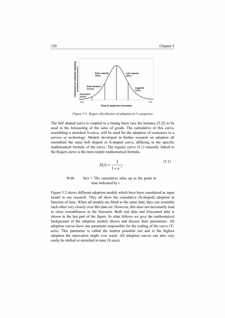
Chapter 5 120
Like
lyho
og
(pr
d of
cus
tom
er a
dopt
inob
abili
ty d
ensi
ty fu
nctio
n)
Time to adopt the innovation
Innovators(2.5%)
(13.5%)(16%)
ear
Figure es
The bell s ance [5.2]) to be used in the forecasting o is curve, resemblin a stretch S- n of customers to a service or technology. Models developed in further research on adoption all
bled the same bell shaped or S-shaped curve, differing in the specific
Early adopters
Early majority(34%)
Late majority(34%)
Laggards
ly Late
5.1: Rogers distribution of adoption in 5 categori
haped curve is coupled to a timing basis (see for instf the sales of goods. The cumulative of th
g ed curve, will be used for the adoptio
resemmathematical formula of the curve. The logistic curve (5.1) naturally linked to the Rogers curve is the most simple mathematical formula.
te
tS −+=
11)(
With: S(t) = The cumulative sales up to the point in time indicated by t
(5.1)
igure 5.2 shows different adoption models which have been consiF
mdered as input
odel in our research. They all show the cumulative (S-shaped) adop func on of time. When all models are fitted to the same data, they can re each other very closely over this data set. However, this does not necessarily lead to close resemblences in the forecasts. Both real data and forecasted data is shown in the last part of the figure. In what follows we give the mathematical background he ado eters. All adoption av urve (Y-axis). Th paramet is e highest adoption e innova n can also very easily be shifted or st tch
tion insembleti
hof t ption models s own and discuss their param
curves h e one parameter responsible for the scaling of the cis er called the market potential (m) and is thth tio might ever reach. All adoption curves
re ed in time (X-axis).
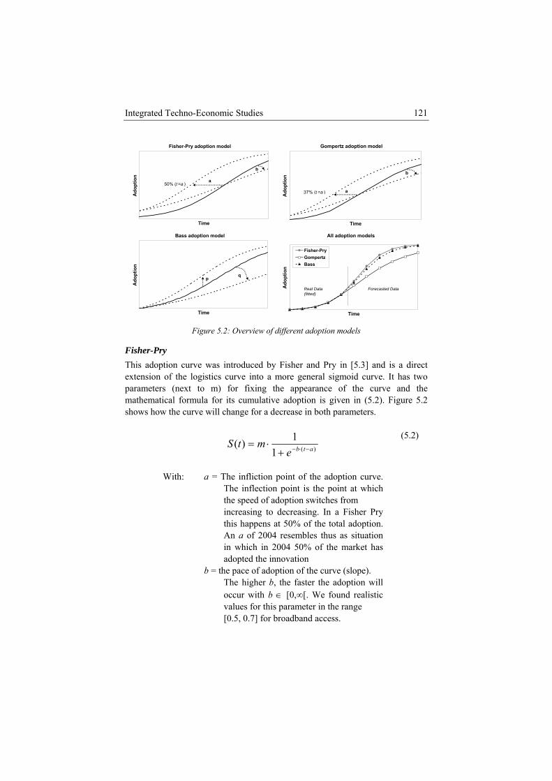
Integrated Techno-Economic Studies 121
Fisher-Pry adoption odelm
Ti
Ado
ptio
n
me
Gompertz adoption model
ptio
n
Time
Ado a37% (t =a )
a% (t =a )
b
b
50
Bass adoption model
Ado
ptio
n
All adoption models
dopt
ion
Time
A
Fisher-PryGompertzBass
Real(fitte
qp
Time
Datad)
Forecasted Data
Figure 5.2: Overview of different adoption models
Fisher-Pry
tshow
This adoption curve was introduced by Fisher and Pry in [5.3] and is a direct extension of the logistics curve into a more general sigmoid curve. It has two parameters (next to m) for fixing the appearance of the curve and the ma hematical formula for its cumulative adoption is given in (5.2). Figure 5.2
s how the curve will change for a decrease in both parameters.
)(1
1)( atbemtS −⋅−+⋅=
With: a = The infliction point of the adoption curve. The inflection point is the point at which
(5.2)
the speed of adoption switches from increasing to decreasing. In a Fisher Pry this happens at 50% of the total adoption. An a of 2004 resembles thus as situation in which in 2004 50% of the market has adopted the innovation b = the pace of adoption of the curve (slope). The higher b, the faster the adoption will occur with b ∈ [0,∞[. We found realistic values for this parameter in the range [0.5, 0.7] for broadband access.
Chapter 5 122
Gompertz This adoption curve is based on a general mathematical curve formulated by Benjamin Gompertz [5.4] as given in (5.3). This mathematical formula was found very well suited for the prediction of customer adoption and is as such a
[0.3, 0.4] for broadband access.
much used curve for forecasting, see e.g. [5.5], [5.6] and [5.7]. Figure 5.2 shows again how the curve will change for a decrease in both parameters.
)(
)(atbeemtS
−−−⋅=
With: a = The infliction point of the adoption curve. (at 37% in a Gompertz curve) b = the pace of adoption of the curve. The higher b, the faster the adoption will occur with b ∈ [0,∞[. We found realistic44 values for this parameter in the range
(5.3)
Bass The Bass diffusion model was developed by Frank Bass [5.8]. It is highly influenced by the diffusion of innovation from Rogers. Unlike the previous two mathematical models, the Bass model starts from two separated adopter groups: innovators, who are initial adopters not influenced by others, and imitators, who learn from prior adopters. The cumulative number of adopters again forms a kind of S-shaped curve and is given in (5.4). Compared to the Rogers’s model, all adopters except the innovators are now grouped as imitators. In contrast to all previously mentioned models, the size of the different groups is no longer defined by fixed percentages. Figure 5.2 shows how the curve will be impacted by a change in its parameters (an increase in p or a decrease in q).
tqp
tqp
epqemtS
⋅+−
⋅+−
+
−⋅=
)(
)(
1
1)( (5.4)
p = the influence of the innoWith: v
on ∈ [ faster adoption esp ly in the i l pha hen not i bination e
We fitted the four adoption models presented here to the actual adoption data for
ators on the . A higher p adopti 0,∞[ will lead to a
ecial nitia se. W n com of th
44
broadband access in Belgium using linear least squares.
Integrated Techno-Economic Studies 123
imitation coefficient, the innovation coefficient will lead to an equal fraction of the remaining market potential to adopt each year. We found realistic values for p in the range [0.005, 0.03] q = the influence of the imitators on the adoption. A higher q ∈ [0,∞[ will lead to a faster adoption. As the imitation is depending on existing adoption, a p of 0 which is equal to no innovation, will lead to no adoption at all regardless of the value of q. We found realistic values for this parameter in the range [0.3, 0.6]
Com
closlimi come to the actual data, and especially
wRouof th be gained from two sources:
ot be sufficient to perform a reliable fitting.
tion.
for forecasting the adoption. The full study, focusing on IPTV adoption, is described in [5.9] and is also given in appendix B. To make a well-considered
for broadband access.
paring Adoption Models As shown before all different models resemble an S-shaped curve and can
ely resemble each other. The exact mathematical formulation will still put a tation on how closely the model can
ho reliably the model can predict adoption in a later stage. ghly speaking information used for properly estimating the parameter values ese models can
• Fitting of the mathematical adoption models to existing adoption data available. This requires sufficient data to be available and thus requires an existing customer base. E.g. for FTTH, especially in case of AON, this might n
• Extrapolation from existing comparable technologies. In the case of FTTH we could make an extrapolation based on general telecom broadband adoption. We could also base this on broadcast television data as currently video is the main driver for the increasing capacity and broadband adopFor television as well as broadband adoption, there is a lot of information available.
The reliability of the forecasted adoption is of huge importance. We have performed a study detailing one approach for selecting the most reliable model
selection, we have fitted the adoption models to existing data in two different ways. First, we have investigated the reliability of the models in the range of the data. Therefore we have fitted each model to all available data and have calculated the difference between the fitted and exact data. The more reliable a model, the more closely it will follow the exact data. Secondly we have investigated the reliability of the model for forecasts beyond existing data.
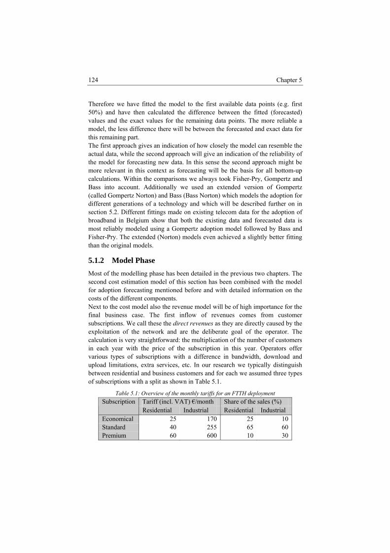
Chapter 5 124
Therefore we have fitted the model to the first available data points (e.g. first 50%) and have then calculated the difference between the fitted (forecasted) values and the exact values for the remaining data points. The more reliable a model, the less difference there will be between the forecasted and exact data for this remaining part. The first approach indication of how closely the model can resemble the actual data, while the second approach will give an indication of the reliability of the model for forecasting new data. In this sense the second approach might be more relevant in this context as forecasting will be the
gives an
basis for all bottom-up arisons we always took Fisher-Pry, Gompertz and
different components. e cost model also the revenue model will be of high importance for the
omer
ce of the subscription in this year. Operators offer
calculations. Within the compBass into account. Additionally we used an extended version of Gompertz (called Gompertz Norton) and Bass (Bass Norton) which models the adoption for different generations of a technology and which will be described further on in section 5.2. Different fittings made on existing telecom data for the adoption of broadband in Belgium show that both the existing data and forecasted data is most reliably modeled using a Gompertz adoption model followed by Bass and Fisher-Pry. The extended (Norton) models even achieved a slightly better fitting than the original models.
5.1.2 Model Phase Most of the modelling phase has been detailed in the previous two chapters. The second cost estimation model of this section has been combined with the model for adoption forecasting mentioned before and with detailed information on the costs of theNext to thfinal business case. The first inflow of revenues comes from custsubscriptions. We call these the direct revenues as they are directly caused by the exploitation of the network and are the deliberate goal of the operator. The calculation is very straightforward: the multiplication of the number of customers in each year with the privarious types of subscriptions with a difference in bandwidth, download and upload limitations, extra services, etc. In our research we typically distinguish between residential and business customers and for each we assumed three types of subscriptions with a split as shown in Table 5.1.
Table 5.1: Overview of the monthly tariffs for an FTTH deployment Tariff (incl. VAT) €/month Share of the sales (%) Subscription Residential Industrial Residential Industrial
Economical 25 170 25 10 Standard 40 255 65 60 Premium 60 600 10 30
Integrated Techno-Economic Studies 125
In our research we also incorporate indirect revenues. These are a quantification of (deliberate) positive side effects coupled to the installation of an FTTH network. Indirect revenues are in general more important when telecommunication is not the core of the companies business, but is used as a “tool” to improve the core business. For instance for a telecom operator, these revenues are not taken into account as the direct revenues are by far the dominant
and, when for instance a municipality is involved s network will induce a lot of deliberate positive
Overall macro-economic municipality project will have as effect on income, unemployment, level of education, etc. Some nationwide models exist for modelling this effect [5.11].
From the previous classification we choose to focus on the effects of external reallocation and gain of efficiency, especially in case of a municipality. The valuation of internal reallocation and overall macro-economic impact are typically very subjective in nature and very complex t odel realistically. More detailed economic studies of indirect effects are out of the scope of this study. We have made an estimate of the economic impact by relating it to the values found in [5.12] and [5.13]. Within calculations, we related the actual indirect revenues on the state of the rollout and the adoption45. According to
45 New higher bandwidth applications could enable new value streams and efficiency
type of revenues. On the other hin the FTTH deployment, thiside effects for the municipality. According to [5.10] a large infrastructural project can have following typical impacts on the indirect revenues. We used this classification and indicate below how this would relate to the case where a municipality is involved in the rollout, as this situation is considered in the second study. • Internal reallocation (of economical advantages) within the considered
project area. This can be of importance as one of the aims of a municipality is often to reduce inequalities in the city.
• External reallocation (of economical advantages). In this case economical advantages (such as high-tech companies) from outside the municipality are directed towards the municipality,
• Gain of efficiency will have a positive impact on the economic welfare within the municipality without having a negative effect outside of the municipality.
• impact. It is very hard to estimate the impact a
o m
gains in closely interacting companies or for customers connected by FTTH (see also [5.14]). We believe that high bandwidth intera tions will preferably occur between people with a com ons of
) ber of stomers makes more sense than alternative calculations (e.g. evenly distributed, upfront
or at the end).
cparable access bandwidth and at a smaller distance (see also conclusi
. According to this reasoning, coupling the indirect revenues to the num[5.15]cu
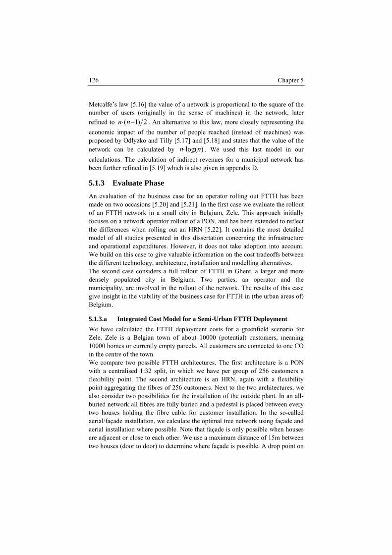
Chapter 5 126
Metcalfe’s law [5.16] the value of a network is proportional to the square of the number of users (originally in the sense of machines) in the network, later refined to 2)1( −⋅ nn . An alternative to this law, more closely representing the economic impact of the number of people reached (instead of machines) was proposed by Odlyzko and Tilly [5.17] and [5.18] and states that the value of the network can be calculated by )log(nn⋅ . We used this last model in our calculations. The calculation of indirect revenues for a municipal network has
in [5.19] which is also given in appendix D.
Two parties, an operator and the municipality, are involved in the rollout of the network. The results of this case give insight in the viability of the business case for FTTH in (the urban areas of) Belgium.
5.1.3.a Integrated Cost Model for a Semi-Urban FTTH Deployment We have calculated the FTTH deployment costs for a greenfield scenario for Zele. Zele is a Belgian town of about 10000 (potential) customers, meaning 10000 homes or currently empty parcels. All customers are connected to one CO in the centre of the town. We compare two possible FTTH architectures. The first architecture is a PON with a centralised 1:32 split, in which we have per group of 256 customers a flexibility point. The second architecture is an HRN, again with a flexibility
been further refined
5.1.3 Evaluate Phase An evaluation of the business case for an operator rolling out FTTH has been made on two occasions [5.20] and [5.21]. In the first case we evaluate the rollout of an FTTH network in a small city in Belgium, Zele. This approach initially focuses on a network operator rollout of a PON, and has been extended to reflect the differences when rolling out an HRN [5.22]. It contains the most detailed model of all studies presented in this dissertation concerning the infrastructure and operational expenditures. However, it does not take adoption into account. We build on this case to give valuable information on the cost tradeoffs between the different technology, architecture, installation and modelling alternatives. The second case considers a full rollout of FTTH in Ghent, a larger and more densely populated city in Belgium.
point aggregating the fibres of 256 customers. Next to the two architectures, we also consider two possibilities for the installation of the outside plant. In an all-buried network all fibres are fully buried and a pedestal is placed between every two houses holding the fibre cable for customer installation. In the so-calledaerial/façade installation, we calculate the optimal tree network using façade and aerial installation where possible. Note that façade is only possible when houses are adjacent or close to each other. We use a maximum distance of 15m between two houses (door to door) to determine where façade is possible. A drop point on
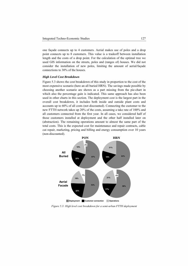
Integrated Techno-Economic Studies 127
one façade connects up to 4 customers. Aerial makes use of poles and a drop point connects up to 8 customers. This value is a tradeoff between installation length and the costs of a drop point. For the calculation of the optimal tree we used GIS information on the streets, poles and (ranges of) houses. We did not consider the installation of new poles, limiting the amount of aerial/façade connections to 30% of the houses.
High Level Cost Breakdown Figure 5.3 shows the cost breakdown of this study in proportion to the cost of the most expensive scenario (here an all buried HRN). The savings made possible by choosing another scenario are shown as a part missing from the pie-chart in which also the percentage gain is indicated. This same approach has also been used in other charts in this section. The deployment cost is the largest part in the overall cost breakdown, it includes both inside and outside plant costs and accounts up to 60% of all costs (not discounted). Connecting the customer to the new FTTH network takes up 20% of the costs, assumi a take rate of 100% and all customers connected from the first year. In all cases, we considered alf of those customers in installed later on (abstraction). The rem e part of the
tal costs. This is the expected cost for maintenance and repair contracts, cable
ng h
stalled at deployment and the other half aining operations amount to almost the sam
tocut repair, marketing, pricing and billing and energy consumption over 10 years (non-discounted). PON HRN
All Buried
3%
57%
18%
22%63%
21%
16%
Aerial Facade
17%
4%
58%
21%
18%
53%
7%
22%
Deployment Customer connection Operations
Figure 5.3: High level cost breakdown for a semi-urban FTTH deployment
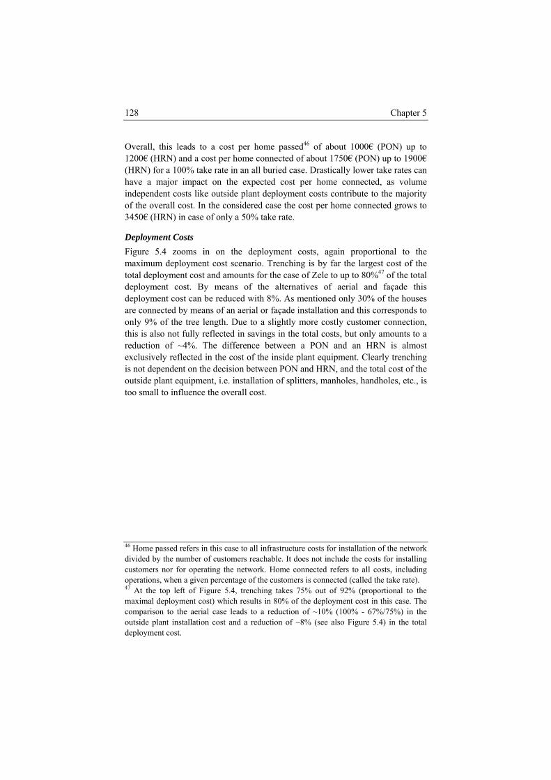
Chapter 5 128
Overall, this leads to a cost per home passed46 of about 1000€ (PON) up to 1200€ (HRN) and a cost per home connected of about 1750€ (PON) up to 1900€ (HRN) for a 100% take rate in an all buried case. Drastically lower take rates can have a major impact on the expected cost per home connected, as volume independent costs like outside plant deployment costs contribute to the majority of the overall cost. In the considered case the cost per home connected grows to 3450€ (HRN) in case of only a 50% take rate.
Deployment Costs Figure 5.4 zooms in on the deploym nt costs, again proportional to the maximum deploym rgest cost of the total deployment cost an o 80%47 of the total
s of the alternatives of aerial and façade this
46 Home passed refers in this case to all infrastructure costs for installation of the network
eent cost scenario. Trenching is by far the la
d amounts for the case of Zele to up tdeployment cost. By meandeployment cost can be reduced with 8%. As mentioned only 30% of the houses are connected by means of an aerial or façade installation and this corresponds to only 9% of the tree length. Due to a slightly more costly customer connection, this is also not fully reflected in savings in the total costs, but only amounts to a reduction of ~4%. The difference between a PON and an HRN is almost exclusively reflected in the cost of the inside plant equipment. Clearly trenching is not dependent on the decision between PON and HRN, and the total cost of the outside plant equipment, i.e. installation of splitters, manholes, handholes, etc., is too small to influence the overall cost.
divided by the number of customers reachable. It does not include the costs for installing customers nor for operating the network. Home connected refers to all costs, including operations, when a given percentage of the customers is connected (called the take rate). 47 At the top left of Figure 5.4, trenching takes 75% out of 92% (proportional to the maximal deployment cost) which results in 80% of the deployment cost in this case. The comparison to the aerial case leads to a reduction of ~10% (100% - 67%/75%) in the outside plant installation cost and a reduction of ~8% (see also Figure 5.4) in the total deployment cost.
Integrated Techno-Economic Studies 129
PON HRN
All Buried
13%
75%
8%
4% 4%
74%
22%
Aerial Facade
4%67%
13%
16%
4%
8%
66%
22%
Outside plant installation Outside plant equipment Inside plant equipment
Figure 5.4: Breakdown of the deployment costs for a semi-urban FTTH deployment
The inside plant (shown in Figure 5.5) costs can be split in a part proportional to the number of fibres, a part proportional to the number of customers and a part for the installation of the CO. For the considered case in Zele, we neglect the CO-driven costs for airco and backup generator. All active equipment (mainly OLT-cards) and fibre handling equipment (ODF, jumpering, internal cabling) is considered fibre based. All remaining equipment (racks, shelves, control-cards and L2-switch to the backbone) is considered customer driven. In a PON, 52% of the inside plant cost is fibre-driven, while 24% is customer-driven. The remaining 24% is found in the installation of the equipment. An HRN is clearly much more costly than a PON for the inside plant. Note that in HRN one fibre will also coincide with one customer. We still used the same calculation model, and 60% of the costs are fibre driven. In this we considered one OLT-card to hold up to 16 fibre ports. Especially this OLT equipment cost is much higher than in the case of a PON. Next, the costs for the installation of all inside plant equipment are also higher compared to the PON because of the higher amount of equipment. Finally the customer related costs stay more or less the same. The costs for connecting to the backbone ma up a large part of this ke cost and are the same in both cases.
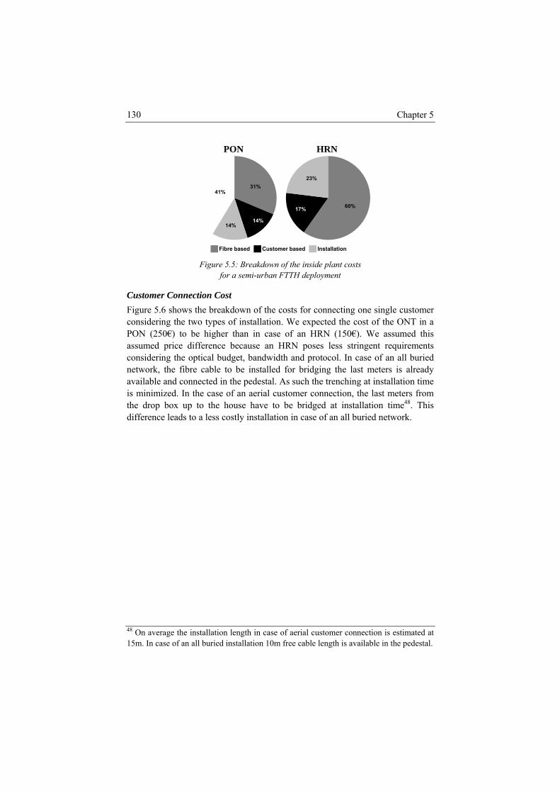
Chapter 5 130
PON HRN
14%
31%41%
14%
17% 60%
23%
Fibre based Customer based Installation
Figure 5.5: Breakdown of the inside plant costs for a semi-urban FTTH deployment
Customer Connection Cost Figure 5.6 shows the breakdown of the costs for connecting one single customer considering the two types of installation. We expected th ONT in a PON (250€) to be higher than in case of an HRN (150€). We assumed this assumed price difference because an HRN poses less stringent requirements consi ried network, the fibr eters is already vailable and connected in the pedestal. As such the trenching at installation time
aerial customer connection, the last meters from have to be bridged at installation time48. This
48 On average the installation length in case of aerial customer connection is estimated at
e cost of the
dering the optical budget, bandwidth and protocol. In case of an all bue cable to be installed for bridging the last m
ais minimized. In the case of anthe drop box up to the housedifference leads to a less costly installation in case of an all buried network.
15m. In case of an all buried installation 10m free cable length is available in the pedestal.
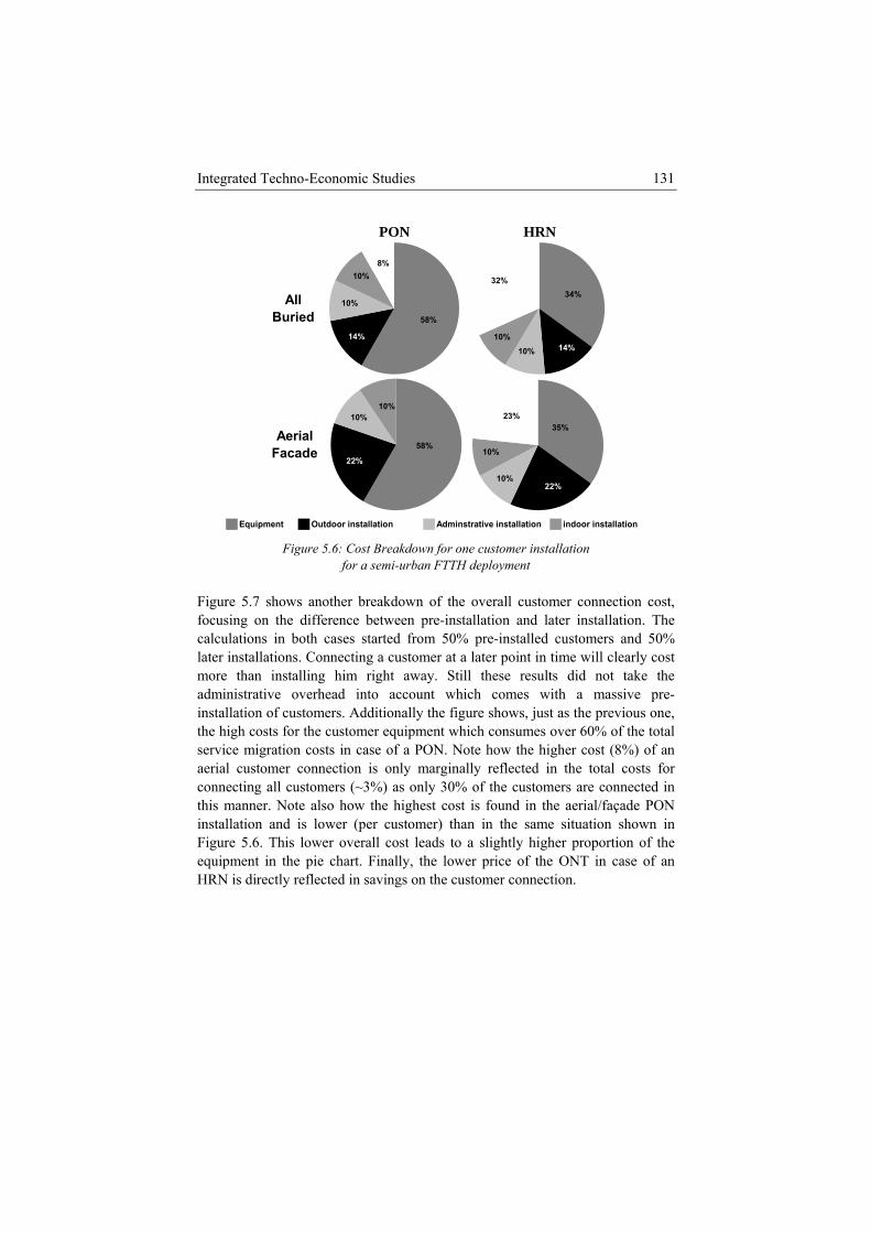
Integrated Techno-Economic Studies 131
PON HRN
All Buried
8%
10%
58%
10%
14%
32%
10%
34%
10%14%
Aerial Facade
10%10%
58%
22%
23%
10%
10%
35%
22%
Equipment Outdoor installation Adminstrative installation indoor installation
er connection is only marginally reflected in the total costs for
he
Figure 5.6: Cost Breakdown for one customer installation for a semi-urban FTTH deployment
Figure 5.7 shows another breakdown of the overall customer connection cost, focusing on the difference between pre-installation and later installation. The calculations in both cases started from 50% pre-installed customers and 50% later installations. Connecting a customer at a later point in time will clearly cost more than installing him right away. Still these results did not take the administrative overhead into account which comes with a massive pre-installation of customers. Additionally the figure shows, just as the previous one, the high costs for the customer equipment which consumes over 60% of the total service migration costs in case of a PON. Note how the higher cost (8%) of an aerial customconnecting all customers (~3%) as only 30% of the customers are connected in this manner. Note also how the highest cost is found in the aerial/façade PON installation and is lower (per customer) than in the same situation shown in Figure 5.6. This lower overall cost leads to a slightly higher proportion of tequipment in the pie chart. Finally, the lower price of the ONT in case of an HRN is directly reflected in savings on the customer connection.
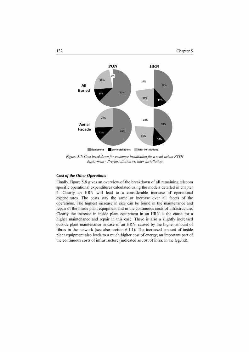
Chapter 5 132
PON HRN
3%
23% 27%
All 39%
Buried 63%
11%
11%23%
Aerial Facade
25%
63%12%25%
39%
24%
12%
Equipment pre-installations later installations
Figure 5.7: Cost breakdown for customer installation for a semi-urban FTTH deployment - Pre-installation vs. later installation
Cost of the Other Operations Finally Figure 5.8 gives an overview of the breakdown of all remaining telecom specific operational expenditures calculated using the models detailed in chapter 4. Clearly an HRN will lead to a considerable increase of operational expenditures. The costs stay the same or increase over all facets of the operations. The highest increase in size can be found in the maintenance and repair of the inside plant equipment and in the continuous costs of infrastructure. Clearly the increase in inside plant equipment in an HRN is the cause for a higher maintenance and repair in this case. There is also a slightly increased outside plant maintenance in case of an HRN, caused by the higher amount of fibres in the network (see also section 6.1.1). The increased amount of inside plant equipment also leads to a much higher cost of energy, an important part of the continuous costs of infrastructure (indicated as cost of infra. in the legend).
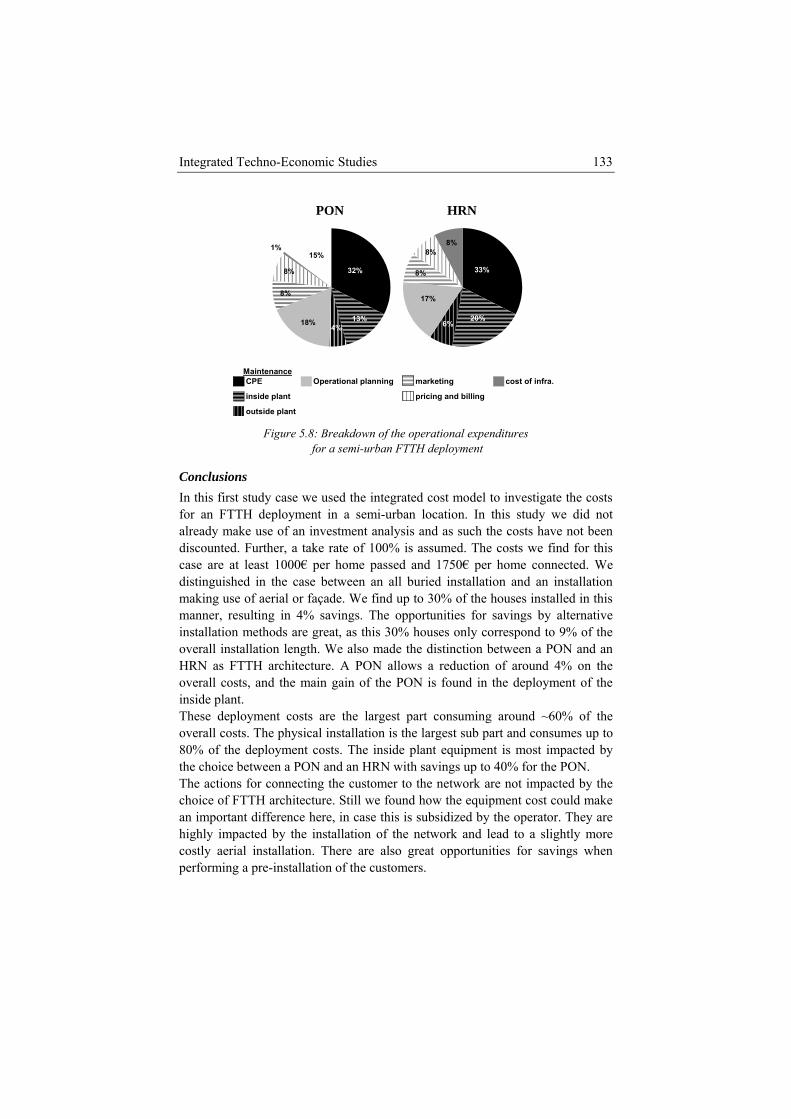
Integrated Techno-Economic Studies 133
PON HRN
8%8%
8%
17%
13%
32%
4%18%
8%
8%
1%15%
6%
33%
20%
CPE Ope pla m cos a.
in p d bi
ou
Marational nning arketing t of infr
side plant ricing an lling
tside plant
intenance
igur : Breakdown of the operational expenditure
r r TH oym
cost e largest sub part and consumes up to . The inside plant equipment is most impacted by
performing a pre-installation of the customers.
F e 5.8 s fo a semi-u ban FT depl ent
Conclusions In this first study case we used the integrated cost model to investigate the costs for an FTTH deployment in a semi-urban location. In this study we did not already make use of an investment analysis and as such the costs have not been discounted. Further, a take rate of 100% is assumed. The costs we find for this case are at least 1000€ per home passed and 1750€ per home connected. We distinguished in the case between an all buried installation and an installation making use of aerial or façade. We find up to 30% of the houses installed in this manner, resulting in 4% savings. The opportunities for savings by alternative installation methods are great, as this 30% houses only correspond to 9% of the overall installation length. We also made the distinction between a PON and an HRN as FTTH architecture. A PON allows a reduction of around 4% on the overall costs, and the main gain of the PON is found in the deployment of the inside plant. These deployment costs are the largest part consuming around ~60% of the overall s. The physical installation is th80% of the deployment coststhe choice between a PON and an HRN with savings up to 40% for the PON. The actions for connecting the customer to the network are not impacted by the choice of FTTH architecture. Still we found how the equipment cost could make an important difference here, in case this is subsidized by the operator. They are highly impacted by the installation of the network and lead to a slightly more costly aerial installation. There are also great opportunities for savings when
Chapter 5 134
We finally also gave an overview of the remaining operational expenditures. Especially the maintenance of the inside plant equipment and the cost of infrastructure will rise for an installation of an HRN in comparison to a PON.
5.1.3.b Integrated Business Case for an Urban FTTH Deployment A full business case has been developed and calculated for a municipality FTTH deployment in the urban environment of the city of Ghent. Ghent is the third largest city of Belgium with 237,250 inhabitants (2008) and an area of 156.2 km² (corresponding to an average population density of 1,496 residents per km²). The considered FTTH rollout does not cover the whole area of 156.2 km², but is limited to a central part of approximately 20 km², counting 90,000 inhabitants or ca. 43,000 households and 222 industrial companies (simply indicated as the “city” during the remainder of the study). Because of practical reasons, it is unfeasible to fully roll out this considered area from the beginning. For this analysis, we have divided the city of Ghent in eight areas. To achieve this, we
erformed a clustering based on information concerning geographical s
density . This ordering is then used to determine the rollout sequence of the FTTH network. Table 5.2 gives a condensed overview of the 8 different areas in this study and their main characteristics. Note that each connection (residential market potential) runs to a family and not to a single inhabitant and as such will serve several people at once (on average 2.1 for Ghent). Digging distances are calculated from the street lengths. In a residential area the pavement at both sides of existing streets will be opened (as crossing the street is much more expensive) and the diggin length is estimated at twice the street length in that area. A sampling of the street length per area has been made in advance (see Table 5.2). This results in a total digging distance of 456 km for the considered area. Spread over 43,000 households this corresponds to an average digging distance of ∼11m per customer. In an industrial area (note that some of them are still under development), we expect that both sides could be served from a fibre installed at one side of the street. This leads to a total digging distance of 58 km. Further, due to its intrinsic nature, a municipality has the advantage that, in limited cases, it can c bine different civil works (e.g. road wor of 10% f
49 Indications run from - (no public services/high tech companies) up to ++++ (a very high
pinformation, residential and indu trial density as well as public services
49
g
omks), resulting in a reduction of the digging costs. We consider a possibility
or such reductions.
level of public services/high tech companies). The average value is indicated by ++.
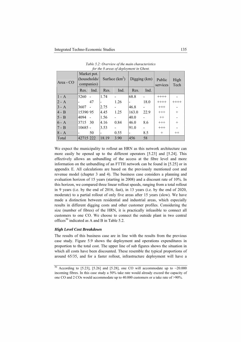
Integrated Techno-Economic Studies 135
Table 5.2: Overview of the main characteristics for the 8 areas of deployment in Ghent.
Market pot. (households/ companies)
Surface (km2) Digging (km)Area - CO
Res. Ind. Res. Ind. Res. Ind.
Public services
High Tech
1 - A 5260 - 1.74 - 68.8 - ++++ - 2 - A - 47 - 1.26 - 18.0 ++++ ++++ 3 - A 3607 - 2.75 - 46.8 - +++ - 4 - B 15390 95 4.45 1.25 163.0 22.9 +++ + 5 - B 4094 - 1.56 - 40.0 - ++ - 6 - A 3715 30 4.16 0.84 46.0 8.6 +++ + 7 - B 10685 - 3.53 - 91.0 - +++ - 8 - A - 50 - 0.55 - 8.5 + ++ Total 42715 222 18.19 3.90 456 58
We expect the municipality to rollout an HRN as this network architecture can more easily be opened up to the different operators [5.23] and [5.24]. This effectively allows an unbundling of the access at the fibre level and more information on the unbundling of an FTTH network can be found in [5.25] or in ppendix E. All calculations are based on the previously mentioned cost and
revenue model (chapter 3 and 4). The business case considers a planning and evaluation horizon of 15 years (starting in 2008) and a discount rate of 10%. In this horizon, we compared three linear rollout speeds, ranging from a total rollout in 9 years (i.e. by the end of 2016, fast), in 13 years (i.e. by the end of 2020, moderate) to a partial rollout of only five areas after 15 years (slow). We have made a distinction between residential and industrial areas, which especially results in different digging costs and other customer profiles. Considering the size (number of fibres) of the HRN, it is practically infeasible to connect all customers to one CO. We choose to connect the outside plant in two central offices50 indicated as A and B in Table 5.2.
High Level Cost Breakdown The results of this business case are in line with the results from the evious case study. Figur expenditures in
roportion to n in hich all costs have been discounted. Th resemble the typical proportions of
around 65/35, and for a faster rollout, frastructure deployment will have a 50 According p to ~20.000
a
pre 5.9 shows the deployment and operations
the total cost. The upper line of sub figures shows the situatiopw ese
in
to [5.23], [5.26] and [5.28], one CO will accommodate uincoming fibres. In this case study a 50% take rate would already exceed the capacity of one CO and 2 COs would accommodate up to 40.000 customers or a take rate of >90%.
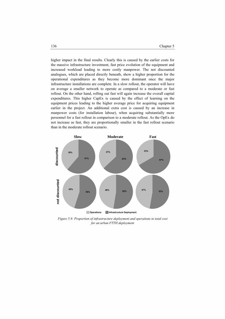
Chapter 5 136
higher impact in the final results. Clearly this is caused by the earlier costs for the massive infrastructure investment, fast price evolution of the equipment and increased workload leading to more costly manpower. The not discounted analogues, which are placed directly beneath, show a higher proportion for the operational expenditures as they become more dominant once the major infrastructure installations are complete. In a slow rollout, the operator will have on average a smaller network to operate as compared to a moderate or fast rollout. On the other hand, rolling out fast will again increase the overall capital expenditures. This higher CapEx is caused by the effect of learning on the equipment prices leading to the higher average price for acquiring equipment earlier in the project. An additional extra cost is caused by an increase in manpower costs (for installation labour), when acquiring substantially more personnel for a fast rollout in comparison to a moderate rollout. As the OpEx do not increase as fast, they are proportionally smaller in the fast rollout scenario than in the moderate rollout scenario. Slow Moderate Fast
scou
nted
di
67%
33%37%
63%
39%
61%
not d
isco
unte
d
55%45% 48% 52% 53%47%
Operations Infrastructure Deployment
Figure 5.9: Proportion of infrastructure deployment and operations to total cost for an urban FTTH deployment
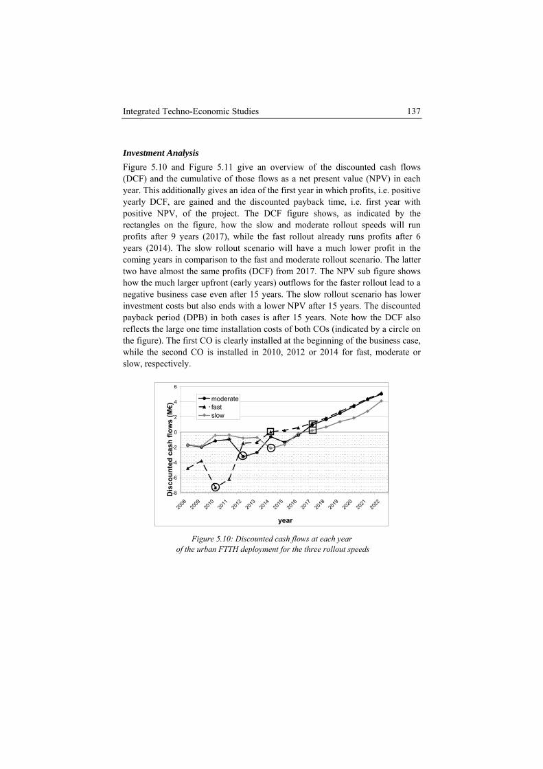
Integrated Techno-Economic Studies 137
Investment Analysis Figure 5.10 and Figure 5.11 give an overview of the discounted cash flows (DCF) and the cumulative of those flows as a net present value (NPV) in each year. This additionally gives an idea of the first year in which profits, i.e. positive yearly DCF, are gained and the discounted payback time, i.e. first year with positive NPV, of the project. The DCF figure shows, as indicated by the rectangles on the figure, how the slow and moderate rollout speeds will run profits after 9 years (2017), while the fast rollout already runs profits after 6 years (2014). The slow rollout scenario will have a much lower profit in the coming years in comparison to the fast and moderate rollout scenario. The latter two have almost the same profits (DCF) from 2017. The NPV sub figure shows how the much larger upfront (early years) outflows for the faster rollout lead to a negative business case even after 15 years. The slow rollout scenario has lower
ment costs but also ends with a lower NPV after 15 years. The discounted payback period (DPB) in both cases is after 15 years. Note how the DCF also reflects the large one time installation costs of both COs (indicated by a circle on the figure). The first CO is clearly installed at the beginning of the business case, while the second CO is installed in 2010, 2012 or 2014 for fast, moderate or slow, respectively.
invest
0
2
ws
(M
4
6
flo
€)
moderatefastslow
-8
-6
-4
2008
2009
2010
2011
2012
2013
2014
2015
2016
2017
2018
2019
2020
2021
2022
year
Dis
coun
ted
ca
-2sh
Figure 5.10: Discounted cash flows at each year
of the urban FTTH deployment for the three rollout speeds
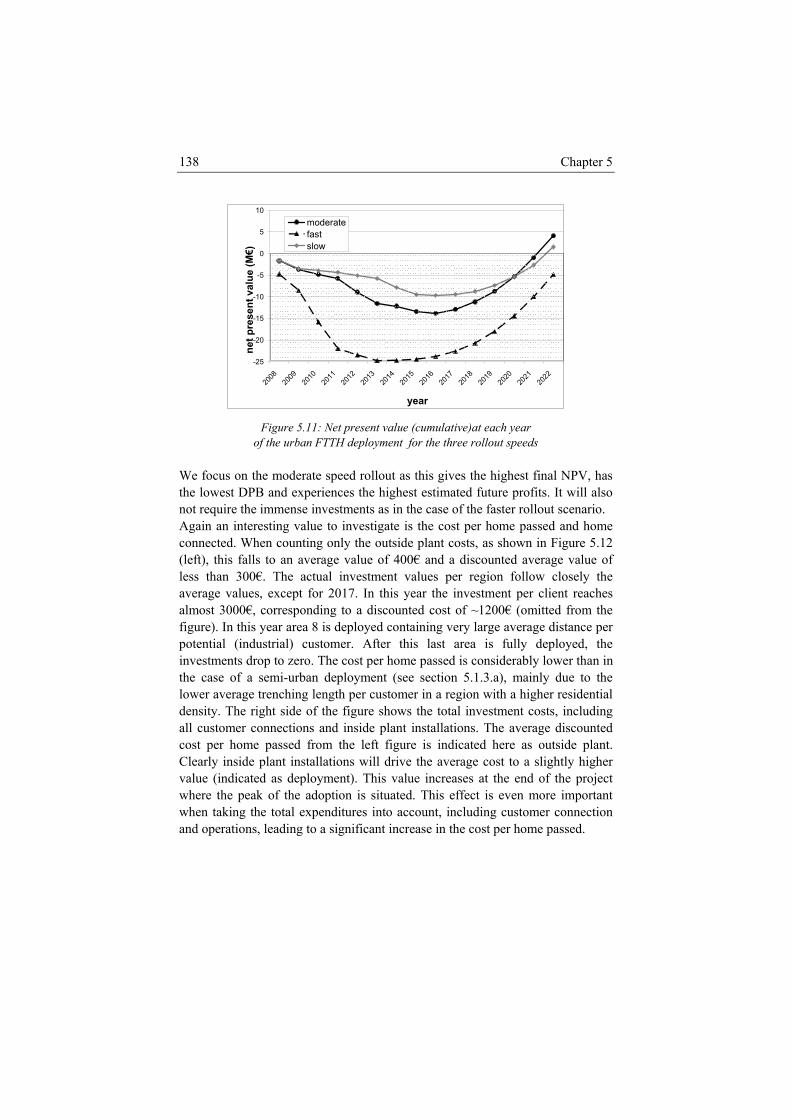
Chapter 5 138
-25
-20
-15
-10
-5
0
5
10
net p
rese
nt v
alue
(M€)
2008
2009
2010
2011
2012
2013
2014
2015
2016
2017
2018
2019
2020
2021
2022
year
moderatefastslow
Figure 5.11: Net present value (cumulative)at each year
of the urban FTTH deployment for the three rollout speeds We focus on the moderate speed rollout as this gives the highest final NPV, has the lowest DPB and experiences the highest estimated future profits. It will also not require the immense investments as in the case of the faster rollout scenario. Again an interesting value to investigate is the cost per home passed and home connected. When counting only the outside plant costs, as shown in Figure 5.12 (left), this falls to an average value of 400€ and a discounted average value of less than 300€. The actual investment values per region follow closely the average values, except for 2017. In this year the investment per client reaches almost 300 from the figure) ce per
otential (industrial) customer. After this last area is fully deployed, the investments drop to zero. The cost per home passed is considerably lower than in
oyment (see section 5.1.3.a), mainly due to the
0€, corresponding to a discounted cost of ~1200€ (omitted. In this year area 8 is deployed containing very large average distan
p
the case of a semi-urban depllower average trenching length per customer in a region with a higher residential density. The right side of the figure shows the total investment costs, including all customer connections and inside plant installations. The average discounted cost per home passed from the left figure is indicated here as outside plant. Clearly inside plant installations will drive the average cost to a slightly higher value (indicated as deployment). This value increases at the end of the project where the peak of the adoption is situated. This effect is even more important when taking the total expenditures into account, including customer connection and operations, leading to a significant increase in the cost per home passed.
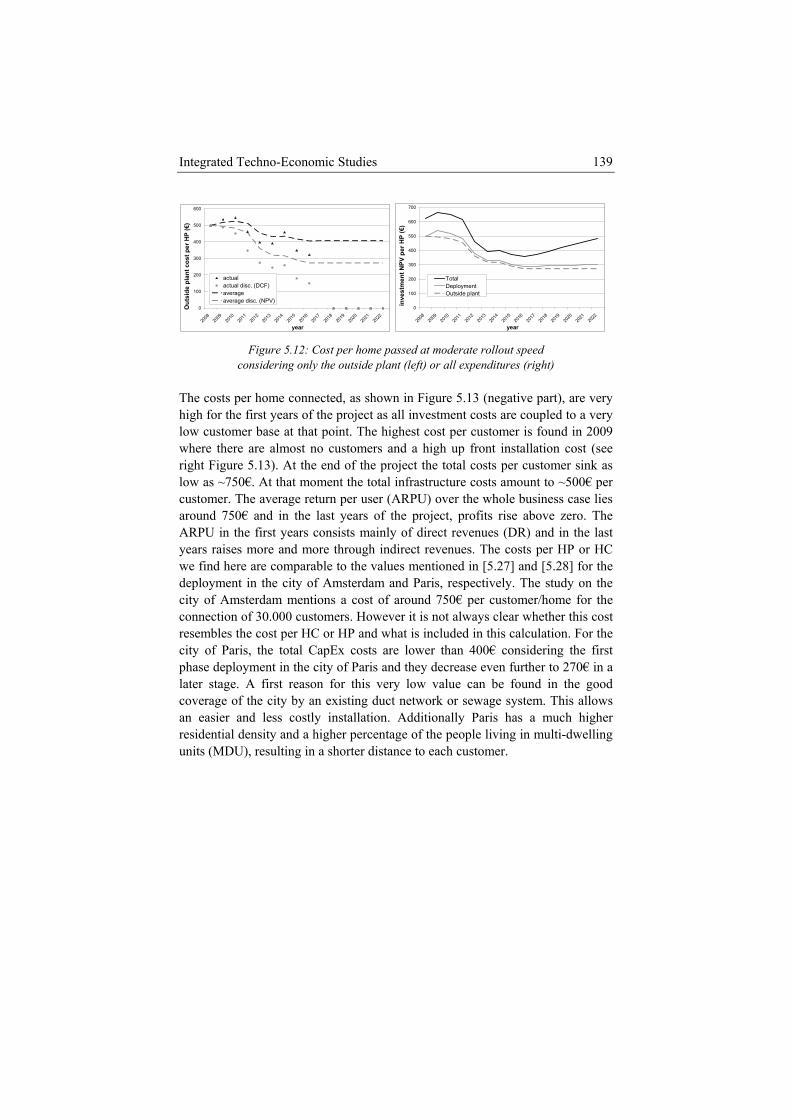
Integrated Techno-Economic Studies 139
00
100
200
300
400
500
600
2008
2009
2010
2011
2012
2013
2014
2015
2016
2017
2018
2019
2020
2021
2022
year
utsi
de p
lant
cos
tO
per
HP
(€)
actualactual disc. (DCF)averageaverage disc. (NPV)
100
200
inve
stm
ent N
300
400
2008
2009
2010
2011
2012
2013
2014
2015
2016
2017
2018
2019
2020
2021
2022
year
per
HP 500
600
700
(€)
PV
TotalDeploymentOutside plant
igure 5.12: Cost per home passed at moderate rollout speed
Amsterdam and Paris, respectively. The study on the
age. A first reason for this very low value can be found in the good coverage of the city by an existing duct network or sewage system. This allows
a much higher n multi-dwelling
Fconsidering only the outside plant (left) or all expenditures (right)
The costs per home connected, as shown in Figure 5.13 (negative part), are very high for the first years of the project as all investment costs are coupled to a very low customer base at that point. The highest cost per customer is found in 2009 where there are almost no customers and a high up front installation cost (see right Figure 5.13). At the end of the project the total costs per customer sink as low as ~750€. At that moment the total infrastructure costs amount to ~500€ per customer. The average return per user (ARPU) over the whole business case lies around 750€ and in the last years of the project, profits rise above zero. The ARPU in the first years consists mainly of direct revenues (DR) and in the last years raises more and more through indirect revenues. The costs per HP or HC we find here are comparable to the values mentioned in [5.27] and [5.28] for the deployment in the city of city of Amsterdam mentions a cost of around 750€ per customer/home for the connection of 30.000 customers. However it is not always clear whether this cost resembles the cost per HC or HP and what is included in this calculation. For the city of Paris, the total CapEx costs are lower than 400€ considering the first phase deployment in the city of Paris and they decrease even further to 270€ in a later st
an easier and less costly installation. Additionally Paris has reside tial density and a higher percentage of the people living inunits (MDU), resulting in a shorter distance to each customer.
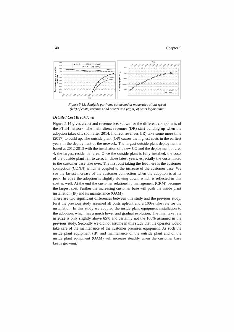
Chapter 5
140
-3000
-2500
-2000
-1500
-1000
-500
0
500
1000
1500
2000
2009
2010
2011
2012
2013
2014
2015
2016
2017
2018
2019
2020
2021
2022
year
Cos
ts, r
even
ues
and
prof
its
per H
C (€
)
Profit ARPU CostsDR Infra
100
1000
10000
100000
1000000
10000000
2009
2010
2011
2012
2013
2014
2015
2016
2017
2018
2019
2020
2021
2022
year
Cos
ts (l
og) p
er H
C (€
)
CostsInfra
-100€
-1K€
-10K€
-100K€
-1M€
Figure 5.13: Analysis per home connected at moderate rollout speed (left) of costs, revenues and profits and (right) of costs logarithmic
Detailed Cost Breakdown Figure 5.14 gives a cost and revenue breakdown for the different components of the FTTH network. The main direct revenues (DR) start building up when the adoption takes off, soon after 2014. Indirect revenues (IR) take some more time (2017) to build up. The outside plant (OP) causes the highest costs in the earliest years in the deployment of the network. The largest outside plant deployment is based at 2012-2013 with the installation of a new CO and the deployment of area 4, the largest residential area. Once the outside plant is fully installed, the costs of the outside plant fall to zero. In those latest years, especially the costs linked to the customer base take over. The first cost taking the lead here is the customer connection (CONN) which is coupled to the increase of the customer base. We see the fastest increase of the customer connection when the adoption is at its peak. In 2022 the adoption is slightly slowing down, which is reflected in this cost as well. At the end the customer relationship management (CRM) becomes the largest cost. Further the increasing customer base will push the inside plant installation (IP) and its maintenance (OAM). There are two significant differences between this study and the previous study. First the previous study assumed all costs upfront and a 100% take rate for the installation. In this study we coupled the inside plant equipment installation to the adoption, which has a much lower and gradual evolution. The final take rate in 2022 is only slightly above 65% and certainly not the 100% assumed in the previous study. Secondly we did not assume in this study that the operator would take care of the maintenance of the customer premises equipment. As such the inside plant equipment (IP) and maintenance of the outside plant and of the inside plant equipment (OAM) will increase steadily when the customer base keeps growing.
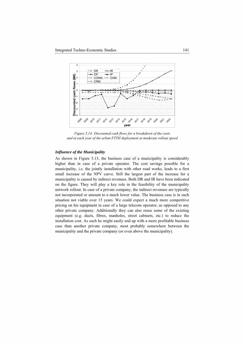
Integrated Techno-Economic Studies 141
-4
-3
-2
-1
0
1
2008
2009
2010
2011
2012
2013
2014
2015
2016
2017
2018
2019
2020
2021
2022
year
Dis
coun
ted
cash
fl2
ows
(M€)
3
4
DR IROP IPCONN. OAMCRM
Figure 5.14: Discounted cash flows for a breakdown of the costs
t easily end up with a more profitable business
mun
and at each year of the urban FTTH deployment at moderate rollout speed
Influence of the Municipality As shown in Figure 5.15, the business case of a municipality is considerably higher than in case of a private operator. The cost savings possible for a municipality, i.e. the jointly installation with other road works, leads to a first small increase of the NPV curve. Still the largest part of the increase for a municipality is caused by indirect revenues. Both DR and IR have been indicated on the figure. They will play a key role in the feasibility of the municipality network rollout. In case of a private company, the indirect revenues are typically not incorporated or amount to a much lower value. The business case is in such situation not viable over 15 years. We could expect a much more competitive pricing on his equipment in case of a large telecom operator, as opposed to any other private company. Additionally they can also reuse some of the existing equipment (e.g. ducts, fibres, manholes, street cabinets, etc.) to reduce the installation cost. As such he mighcase than another private company, most probably somewhere between the
icipality and the private company (or even above the municipality).
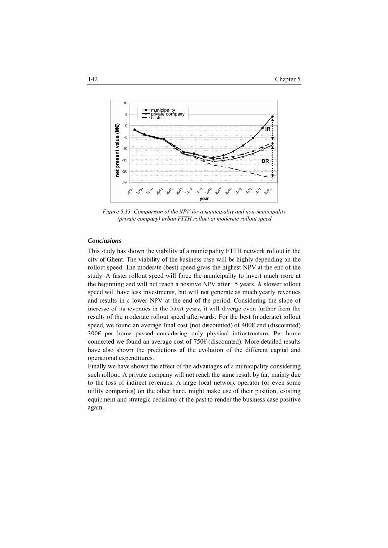
Chapter 5 142
5
10
municipalityprivate company
-25
-20
-15
-10
-5
0
2008
2009
2010
2011
2012
2013
2014
2015
2016
2017
2018
2019
2020
2021
2022
year
net p
rese
nt v
alue
(M€)
costs
IR
DR
Figure 5.15: Comparison of the NPV for a municipality and non-municipality
(private company) urban FTTH rollout at moderate rollout speed
clusions study has shown the viability of a municipality FTTH network rollout in the
of Ghent. The viability of the business case will be highly depending on the ut speed. The
ConThiscityrollo moderate (best) speed gives the highest NPV at the end of the
dthe speeandincrresuspee300conhave the predictions of the evolution of the different capital and operational expenditures. Finally we have shown the effect of the advantages of a municipality considering such rollout. A private company will not reach the same result by far, mainly due to the loss of indirect revenues. A large local network operator (or even some utility companies) on the other hand, might make use of their position, existing equipment and strategic decisions of the past to render the business case positive again.
stu y. A faster rollout speed will force the municipality to invest much more at beginning and will not reach a positive NPV after 15 years. A slower rollout d will have less investments, but will not generate as much yearly revenues
results in a lower NPV at the end of the period. Considering the slope of ease of its revenues in the latest years, it will diverge even further from the lts of the moderate rollout speed afterwards. For the best (moderate) rollout d, we found an average final cost (not discounted) of 400€ and (discounted)
€ per home passed considering only physical infrastructure. Per home nected we found an average cost of 750€ (discounted). More detailed results also shown
Integrated Techno-Economic Studies 143
5.2 Optimization in a Competitive Setting Deploying FTTH is a very cost intensive project. On the other hand, once deployed the operator owns a network which allows him to keep pace with the future bandwidth demands. It offers him as such a strategic advantage over the other non-FTTH fixed network operators. The current strategy of many telecom operators is to exploit their existing access networks as long as possible. Since a few years, a new trend is ongoing in which other players, such as municipalities, utility companies and housing companies, are investing more and more in the physical infrastructure of new telecom networ tially redu nto direct competition with one or more existing network operators, the interaction
b
r provider will find it viable to roll out an alternative FTTH
re to deliver competing roadband applications.
Th following sub sections will detail the design, model and extension pthe overall economic methodology fo e case of this competition study.
51 Different structu s fo o install
ks [5.29]. They take into account indirect revenues and can potence costs as mentioned in the previous business case. As they will move i
between oth is important. In this section we extend the previous business case into a competition study. We consider a realistic case in which we opt for a public-private-partnership51 between the city of Ghent and the Belgian main Digital Subscriber Line (DSL) provider, as the latter has the broadband expertise the city is lacking. In return the DSL provider would get an opportunity to build a new customer base on FTTH (which is certainly more future proof than DSL). The new co-operation will compete with the Belgian main cable operator who chooses to upgrade its Hybrid Fibre Coax (HFC) network. For the duration of the case (2008-2022) we assume that no othearchitecture in Ghent52. In the best interest of the municipality we consider the co-operation to end in 2022. From then, the network will be opened to other providers so they can also use the fibre architectub
e hase of r th
re r such cooperation are possible. We would expect Ghent tand m e outsid clusive usage for 15 years to the DSL operator. The latte tomers. Further analys ing) or plausible and al ote that the study is performed inde nde DSL and cable operator. 52 This assumptio will y as DOCSIS 3.0 provides enough o xpect DOCSIS to evolve er it is opened (after the 15 ears).
aintain th e plant and to lease its exr would then install all equipment and connect the cus
is into whether such cooperation is valid (cf. local loop unbundll details of such co-operation fall outside the scope of this study. N
pe ntly from the city of Ghent or the mentioned
n certainly hold for the first years of the studpportunities in these first years. Later on we could e
to a high standard (X.0) or step into the FTTH network once y
Chapter 5 144
5.2.1 Design PhThe design pha ag construct input-mode ation regard g the co pet e input and model HRN) as th nt. In the first sub section e theory. We
troduce the differen ntext of this study and detail the
thoro d as “ med at tuatio in which decision makers have to m ctions l, ssibly conflicting uences”. O makers a ions a referred to as strategies, an nsequ toU we igated nt games with unicipality rolling out FTTH and C operator a each g we assumed
oth players to act at the same time and have sufficiently good knowledge of
players play a strategy. This can be represented in a d the extensive form. In scope of this research, we sequentially in a sequential multi-stage game. This
ase se ain will gather all important input and
ls for the calculations. Very important in this context is all informin m ition between the two players. We use the sam ( in e previous business case study for the city of Ghe
we give more background to the use of gamt concepts used in the coin
approaches we used for finding one or all solutions to the game. As competition will form the basis for the game theoretic extension, we replaced the adoption model with existing competition models originally based on the Bass model. In the second sub section we give a detailed description and describe how the same extension can be applied to the other adoption models (e.g. Gompertz) as well. In the light of the different strategies available to both players, we also extend this competition model with the notion of delayed introduction and captured market share.
5.2.1.a Game Theoretic Setup A very summary introduction to the purpose of game theory in economic research has already been given in chapter 2. We extend this overview here and rapidly focus on the problem at hand and its solution using concepts of game theory. As such we only touch a small part of the broad research in game theory and disregard its mathematical foundations. We refer to [5.30] for a more
ugh tutorial and references to game theory. Game theory is there defineA discipline ai modeling si ns ake specific a that have mutua po , conseqften decision are referred to s players, act re
d co ences are referred as payoffs. sing game theory have invest differe the m
the HF s players. In amebeach others possible strategies and payoffs. These assumptions allow representing the game by means of a payoff matrix. This matrix has a payoff for both players for each possible combination of strategies (one strategy for each player). This is called the strategic form of the game. In some more elaborate games, we made use of a so-called multi-stage game; a game of multiple stages, in which at each stage both tree structure which is calleassumed both players to actcan again be flattened into a strategic form. Both representations allow using tools for searching equilibrium states in the game. Such an equilibrium state is a set of strategies (one for each player) at which both players are not inclined to
Integrated Techno-Economic Studies 145
change their strategy. Solving a game comes down to finding one or preferably all equilibrium situations. Within the remainder of this study we used the following equilibrium concepts: • The Nash equilibrium (NE): This is the most commonly known equilibrium,
hich is defined as a situation in which no player can gain b unil changing its strategy. In a pure NE, each player will use a pure strategy, while ixe bilistic combinations (or mixe rate en repetitively playi the gam his equilibrium as criterion, is e osen. It is easy to check in the ex ituations (1B,2B) or (1C, rategy into 1A. In both situa uld rather change to 2A. The NE in
er payoff than another (dominant) strategy for all possible counter strategies. No fully rational player would play a (strict) dominated strategy, but would instead play the (strict) dominant strategy. As such the (strictly) dominated strategy can be removed (deleting row or column from the payoff matrix) for the considered player. By iteratively using this approach for the different players, we can in some cases end up with strict dominant strategies. In Figure 5.16 we first can eliminate 1B and 1C as they have a lower payoff for player 1 in all situations than 1A. This dominant strategy is indicated in black. In the remaining (black) game we find that 2B is strictly dominated b d by iterated (strict) dominan quential multi-stage games,
be used [5.30]. In this we iteratively remove e leaves of the tree. In a next iteration we move up one
player), called λ. This λ more or less corresponds to the rationality or experience of the players. For a λ of ∞, i.e. a fully rational or high experience game this results in the NE for the game. For a λ of 0 the players
w y aterally
in a m d NE the players can play proba of sts) gies [5.30]. Such mixes are more useful wh
g tng e. A game with fully rational players, usinxpected to result in one of the NE being chemplary game shown in Figure 5.16 how the s
2B) are no NE as player 1 can gain by changing his sttions player 2 wo
this situation is (1A, 2A), where neither player 1 nor player 2 can gain by changing their strategy unilaterally.
• Iterated (strict) dominance: Typically static games (the game has one stage in which the players interact) can also be reduced or solved by removing strict dominated strategies. These dominated strategies have a strictly low
, y 2A for player 2. Finally we find the same NE. Any solution derive
ce is a NE. Within sebackward induction can unlogical moves at thlevel and can perform the same operation. If this is possible up to the first action of the game, we again find the NE. This process is also shown in Figure 5.16.
• Quantal response equilibrium (QRE) [5.31]: This equilibrium uses bounded rationality instead of full rational behavior (as for NE). It resembles a more realistic case in which the players are assumed to make errors in their decision process, but still have the highest probability of choosing the strategy with the best payoff. This equilibrium has one free parameter (per
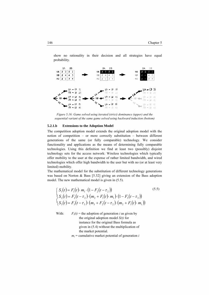
Chapter 5 146
show no rationality in their decision and all strategies have equal probability.
Figure 5.16: Ga inance (upper) and the
sequ (bottom)
5.2.1.b ons to The com on ad odel with the notion of tion – between different generatio of the y. We consider functiona y and ap lica mparable technolog Using this ly) disjoint technology sets for the access network: Wireless technologies which typically
ffer mobility to the user at the expense of rather limited bandwidth, and wired log th to the user but with no (or at least very )
me solved using iterated (strict) domential variant of the same game solved using backward induction
odel Extensi the Adoption Mpetiti option model extends the original adoption m competition – or more correctly substituns same (or fully comparable) technologlit p tions as the means of determining fully coies. definition we find at least two (possib
otechno ies which offer high bandwidlimited mobility. The mathematical model for the substitution of different technology generations was based on Norton & Bass [5.32] giving an extension of the Bass adoption model. The new mathematical model is given in (5.5).
( ) ( ) ( )( )( ) ( ) ( )( ) ( )( )( ) ( ) ( ) ( )( )( )⎪
⎩
⎪⎨
⎧
⋅+⋅−+⋅−=−−⋅⋅+⋅−=
−−⋅⋅=
112223333
33112222
22111
11
mtFmtFmtFtStFmtFmtFtS
tFmtFtS
ττττ
τ
With: Fi(t) = the adoption of generation i as given by the original adoption model S(t) for instance for the original Bass formula as given in (5.4) without the multiplication of the market potential. mi = cumulative market potential of generation i
(5.5)
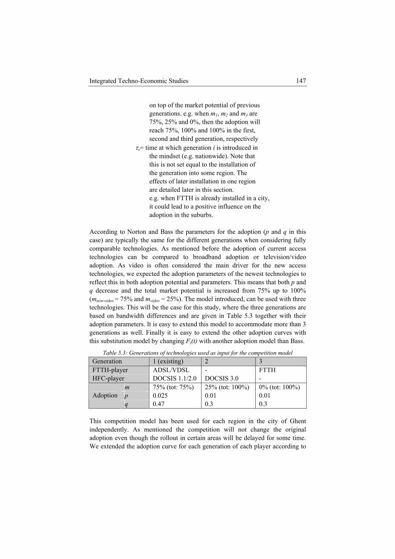
Integrated Techno-Economic Studies 147
on top of the market potential of previous generations. e.g. when m1, m2 and m3 are
tion will e first,
hich ed in e m dset
lead to a positive influence on the adoption in the suburbs.
driver for the new access chnologies, we expected the adoption parameters of the newest technologies to
reflect this in both adoption potential and parameters. This means that boq decrease and the total market pote creased from 75% up to 100% (mnon-video nd e used with three technolog erations are
75%, 25% and 0%, then the adop reach 75%, 100% and 100% in th second and third generation, respectively τx= time at w generation i is introduc th in (e.g. nationwide). Note that this is not set equal to the installation of the generation into some region. The effects of later installation in one region are detailed later in this section. e.g. when FTTH is already installed in a city, it could
According to Norton and Bass the parameters for the adoption (p and q in this case) are typically the same for the different generations when considering fully comparable technologies. As mentioned before the adoption of current access technologies can be compared to broadband adoption or television/video adoption. As video is often considered the main te
th p and ntial is in
= 75% a mvideo = 25%). The model introduced, can bies. This will be the case for this study, where the three gen
based on bandwidth differences and are given in Table 5.3 together with their adoption parameters. It is easy to extend this model to accommodate more than 3 generations as well. Finally it is easy to extend the other adoption curves with this substitution model by changing Fi(t) with another adoption model than Bass.
Table 5.3: Generations of technologies used as input for the competition model Generation 1 (existing) 2 3 FTTH-player ADSL/VDSL - FTTH HFC-player DOCSIS 1.1/2.0 DOCSIS 3.0 -
m 75% (tot: 75%) 25% (tot: 100%) 0% (tot: 100%) p 0.025 0.01 0.01 Adoption q 0.47 0.3 0.3
This competition model has been used for each region in the city of Ghent independently. As mentioned the competition will not change the original adoption even though the rollout in certain areas will be delayed for some time. We extended the adoption curve for each generation of each player according to
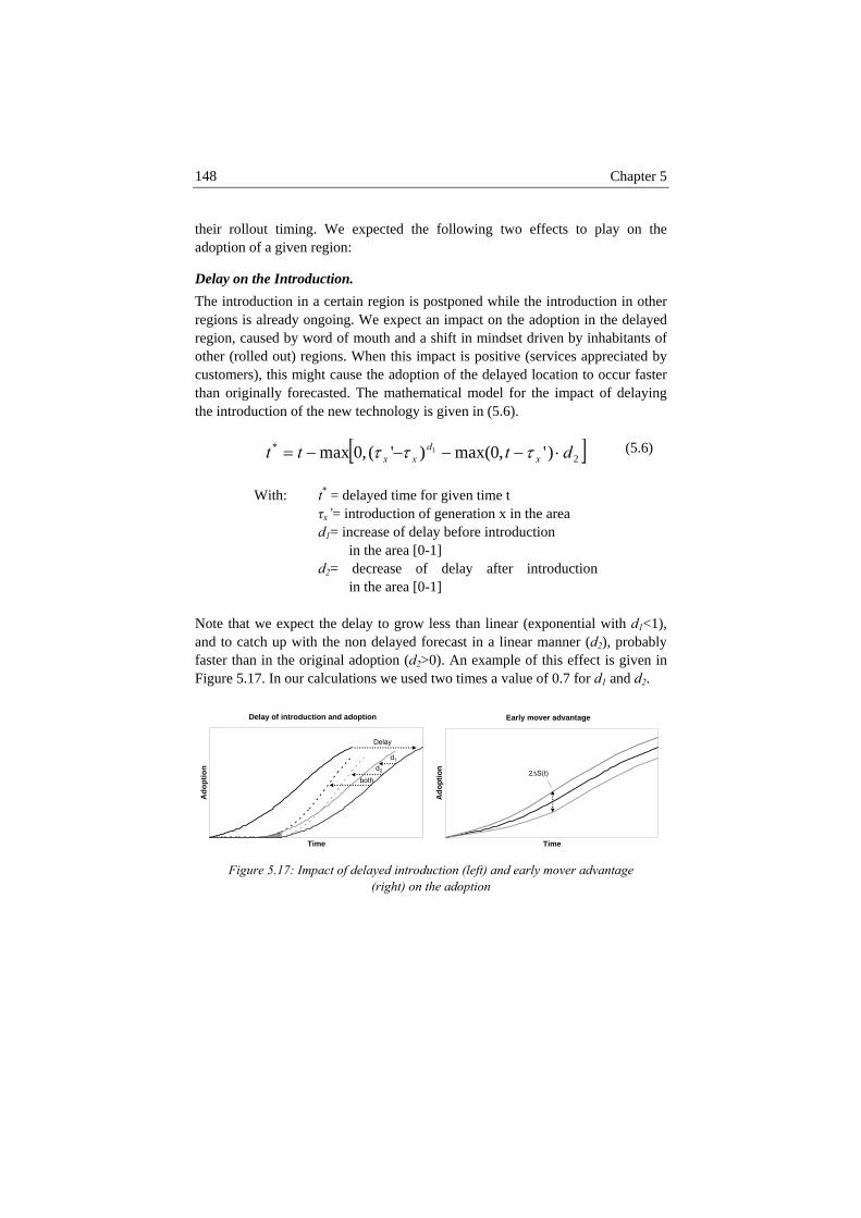
Chapter 5
148
their rollout timing. We expected the following two effects to play on the adoption of a given region:
Delay on the Introduction. The introduction in a certain region is postponed while the introduction in other regions is already ongoing. We expect an impact on the adoption in the delayed region, caused by word of mouth and a shift in mindset driven by inhabitants of other (rolled out) regions. When this impact is positive (services appreciated by customers), this might cause the adoption of the delayed location to occur faster than originally forecasted. The mathematical model for the impact of delaying the introduction of the new technology is given in (5.6).
[ ]2* )',0max()'(,0max 1 dttt x
dxx ⋅−−−−= τττ
With: t* = delayed time for given time t τx’= introduction of generation x in the area d1= increase of delay before introduction in the area [0-1] d2= decrease of delay after introduction in the area [0-1]
(5.6)
Note that we expect the delay to grow less than linear (exponential with d1<1), and to catch up with the non delayed forecast in a linear manner (d2), probably faster than in the original adoption (d2>0). An example of this effect is given in Figure 5.17. In our calculations we used two times a value of 0.7 for d1 and d2.
Delay of introduction and adoption
Time
Ado
ptio
n
Delay
d1
d2
both
Early mover advantage
Time
Ado
ptio
n
2∆S(t)
Figure 5.17: Impact of delayed introduction (left) and early mover advantage
(right) on the adoption
Integrated Techno-Economic Studies 149
Captured Market Share Once a customer is connected to a broadband service which fully satisfies his needs, he is generally more reluctant to change53. This means the earlier a player introduces a superior technology, the larger market share he will be able to grasp and hold. We only expect an impact of this captured market share when there is a substantial amount of time between the introductions of the two technologies in a given area. We assume more than 2 years. The mathematical model for the captured market share is given in (5.7). Figure 5.17 shows the effect of this loss of market share on the adoption when considering original adoption for both players to follow the same adoption indicated in black. The last mover will lose part of its market potential to the first mover. Note that this is not the actual adoption for the last mover, but the maximum attainable adoption. The real adoption will still be subject to the delay function mentioned before.
Before the introduction time of the last mover (t ≤ τlast)
( ) ( ) ( )( ) ( )⎩
⎨⎧
⋅−=⋅+=
tSrtStSrtStS
lastlast
lastfirstfirst
)1(*
*
From the introduction time of the last mover (t ≥ τlast)
( ) ( ) ( )( ) ( ) ( )⎩
⎨⎧
∆−=∆+=
tStStStStStS
lastlast
firstfirst*
*
With: first/last= first/last mover in a certain area (i.e. either FTTH or HFC) S*
x = the possible market share (adoption potential) incorporating the impact of an early mover Sx = the original non delayed adoption of the first/last mover. r = part of the market share that the early mover will capture. In our calculations we used a value of 0.5 for this parameter. ( ) )( lastlastSrtS τ⋅=∆
(5.7)
53 Operators also use several mechanisms to increase this lock-in of customers (e.g. single operator setup box).
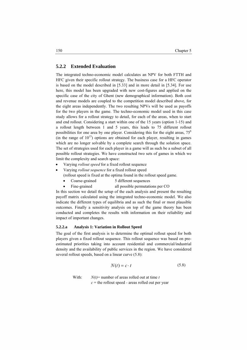
Chapter 5 150
5.2.2 ExtenThe integrated techno-economic model calculates an NPV for both FTTH and HFC given their specific rollout strategy. The business case for a HFC operator is based on the model described in [5.33] and in more detail in [5.34]. For use here, this model has been upgraded with new cost-figures and applied on the specific case of the city of Ghent (new demographical information). Both cost and revenue models are coupled to the competition model described above, for the eight areas independently. The two resulting NPVs will be used as payoffs for the two players in the game. The techno-economic model used in this case study allows for a rollout strategy to de il, for each of the areas, when to start
for a fixed rollout speed (rollout speed d game. • Coarse-grai• Fine-grained all possible permutations per CO
In this section we detail the setup of th each analysis and present the resulting
idered veral rollout speeds, based on a linear curve (5.8):
ded Evaluation
taand end rollout. Considering a start within one of the 15 years (option 1-15) and a rollout length between 1 and 5 years, this leads to 75 different rollout possibilities for one area by one player. Considering this for the eight areas, 758 (in the range of 1015) options are obtained for each player, resulting in games which are no longer solvable by a complete search through the solution space. The set of strategies used for each player in a game will as such be a subset of all possible rollout strategies. We have constructed two sets of games in which we limit the complexity and search space: • Varying rollout speed for a fixed rollout sequence • Varying rollout sequence
is fixed at the optima found in the rollout speened 5 different sequences
e payoff matrix calculated using the integrated techno-economic model. We also indicate the different types of equilibria and as such the final or most plausible outcomes. Finally a sensitivity analysis on top of the game theory has been conducted and completes the results with information on their reliability and impact of important changes.
5.2.2.a Analysis 1: Variation in Rollout Speed The goal of the first analysis is to determine the optimal rollout speed for both players given a fixed rollout sequence. This rollout sequence was based on pre-estimated priorities taking into account residential and commercial/industrial density and the availability of public services in the region. We have consse
tctN ⋅=)(
With: N(t)= number of areas rolled out at time t c = the rollout speed - areas rolled out per year
(5.8)
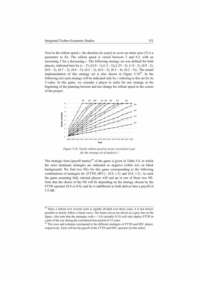
Integrated Techno-Economic Studies 151
Next to the rollout speed c, the duration (in years) to cover an entire area (T) is a parameter to fix. The rollout speed is varied between 2 and 0.2, with an increasing T for a decreasing c .The following strategy set was defined for both players, indicated here by (c - T):{(2.0 - 1),(1.5 - 2),(1.25 - 2), (1.0 - 2), (0.9 - 2), (0.8 - 2), (0.7 - 2), (0.6 - 3), (0.5 - 2), (0.4 - 3), (0.3 - 4), (0.2 - 5)}, The actual implementation of this strategy set is also shown in Figure 5.1854. In the following text each strategy will be indicated only by c referring to this set for its T-value. In this game, we consider a player to settle for one strategy at the beginning of the planning horizon and not change his rollout speed in the course of the project.
0
1
2
2008 2009 2010 2011 2012 2013 2014 2015 2016 2017 2018 2019 2020 2021 2022
Year
3
4
5
6
Are
as c
over
ed
0.4
0.3
0.2
7
0.5
layers will end up in one of those two NE. Note that the choice of the NE will be depending on the strategy chosen by the FTTH operator (0.8 or 0.9), and he is indifferent as both deliver him a payoff of 5.5 M€.
54 Since a rollout over several years is equally divided over these years, it is not always
8
2.0 1.5 1.25 1.0 0.9 0.8 0.7 0.6
Figure 5.18: Yearly rollout speed in areas covered per year for the strategy set of analysis 1
The strategic form (payoff matrix)55 of the game is given in Table 5.4, in which the strict dominant strategies are indicated as negative (white text on black background). We find two NEs for this game corresponding to the following combinations of strategies for {FTTH, HFC}: {0.9, 1.5} and {0.8, 1.5}. As such the game assuming fully rational p
possible to strictly follow a linear curve. The linear curves are shown as a grey line on the figure. Also note that the strategies with c < 0.6 (actually 8/15) will only deploy FTTH in a part of the city during the considered time-period of 15 years. 55 The rows and columns correspond to the different strategies of FTTH and HFC player, respectively. Each cell has the payoff of the FTTH and HFC operator (in this order).
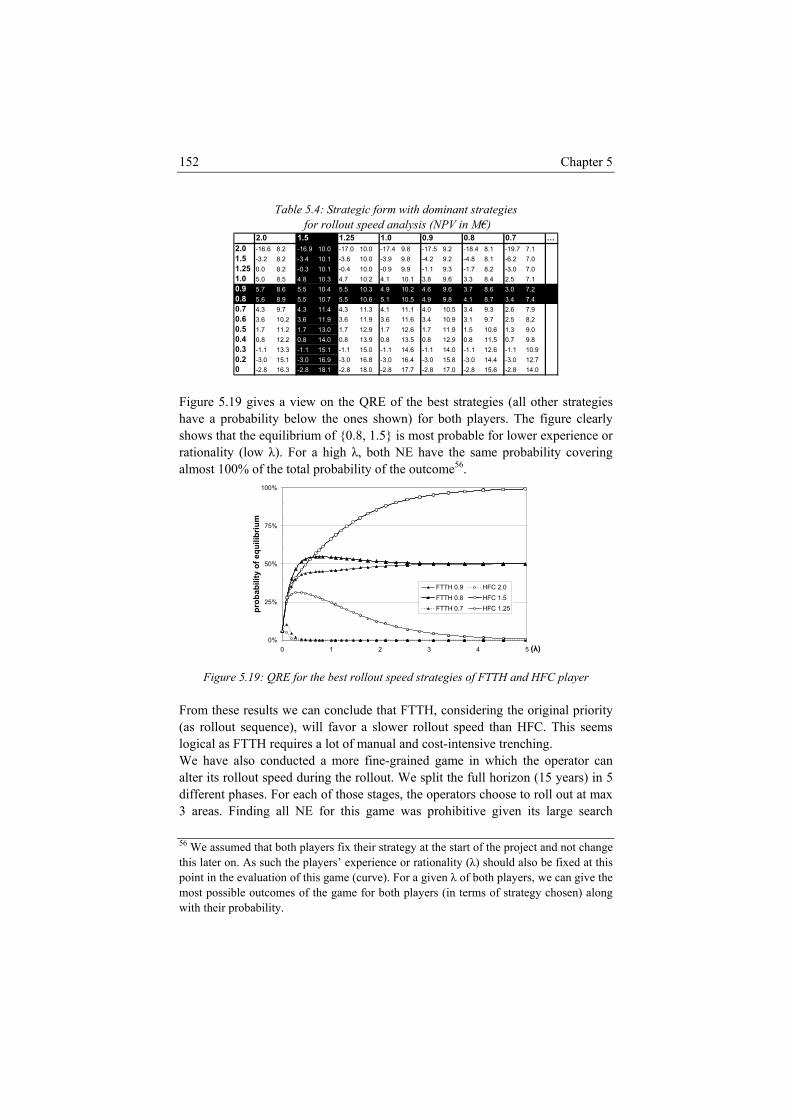
Chapter 5 152
Table 5.4: Strategic form with dominant strategies d analysis (NPV in M€) for rollout spee
…2.0 -16.6 8.2 -16.9 10.0 -17.0 10.0 -17.4 9.8 -17.5 9.2 -18.4 8.1 -19.7 7.11.5 -3.2 8.2 -3.4 10.1 -3.6 10.0 -3.9 9.8 -4.2 9.2 -4.8 8.1 -6.2 7.01.25 0.0 8.2 -0.3 10.1 -0.4 10.0 -0.9 9.9 -1.1 9.3 -1.7 8.2 -3.0 7.01.0 5.0 8.5 4.8 10.3 4.7 10.2 4.1 10.1 3.8 9.6 3.3 8.4 2.5 7.10.9 5.7 8.6 5.5 10.4 5.5 10.3 4.9 10.2 4.6 9.6 3.7 8.6 3.0 7.20.8 5.6 8.9 5.5 10.7 5.5 10.6 5.1 10.5 4.9 9.8 4.1 8.7 3.4 7.4
0.9 0.8 0.72.0 1.5 1.25 1.0
0.7 4.3 9.7 4.3 11.4 4.3 11.3 4.1 11.1 4.0 10.5 3.4 9.3 2.6 7.90.6 3.6 10.2 3.6 11.9 3.6 11.9 3.6 .6 3.4 10.9 3.1 9.7 2.5 8.20.5 1.7 11.2 1.7 13.0 1.7 12.9 1.7 .6 1.7 11.9 1.5 10.6 1.3 9.00.4
0 -2.8 16.3 -2.8 15.6 -2.8 14.0
1112
0.8 12.2 0.8 14.0 0.8 13.9 0.8 13.5 0.8 12.9 0.8 11.5 0.7 9.80.3 -1.1 13.3 -1.1 15.1 -1.1 15.0 -1.1 14.6 -1.1 14.0 -1.1 12.6 -1.1 10.90.2 -3.0 15.1 -3.0 16.9 -3.0 16.8 -3.0 16.4 -3.0 15.8 -3.0 14.4 -3.0 12.7
18.1 -2.8 18.0 -2.8 17.7 -2.8 17.0 -2.8 Figure 5.19 gives a view on the QRE of the best strategies (all other strategies have a probability below the ones shown) for both players. The figure clearly shows that the equilibrium of {0.8, 1.5} is most probable for lower experience or rationality (low λ). For a high λ, both NE have the same probability covering almost 100% of the total probability of the outcome56.
75%
100%
ibriu
m
50%
abili
ty o
f equ
il
0%
25%
0 1 2 3 4 5 (λ)
prob
FTTH 0.9 HFC 2.0FTTH 0.8 HFC 1.5FTTH 0.7 HFC 1.25
Figure 5.19: QRE for the best rollout speed strategies of FTTH and HFC player
From these results we can conclude that FTTH, considering the original priority (as rollout sequence), will favor a slower rollout speed than HFC. This seems logical as FTTH requires a lot of manual and cost-intensive trenching. We have also conducted a more fine-grained game in which the operator can alter its rollout speed during the rollout. We split the full horizon (15 years) in 5 different phases. For each of those stages, the operators choose to roll out at max 3 areas. Finding all NE for this game was prohibitive given its large search 56 We assumed that both players fix their strategy at the start of the project and not change this later on. As such the players’ experience or rationality (λ) should also be fixed at this point in the evaluation of this game (curve). For a given λ of both players, we can give the most possible outcomes of the game for both players (in terms of strategy chosen) along with their probability.
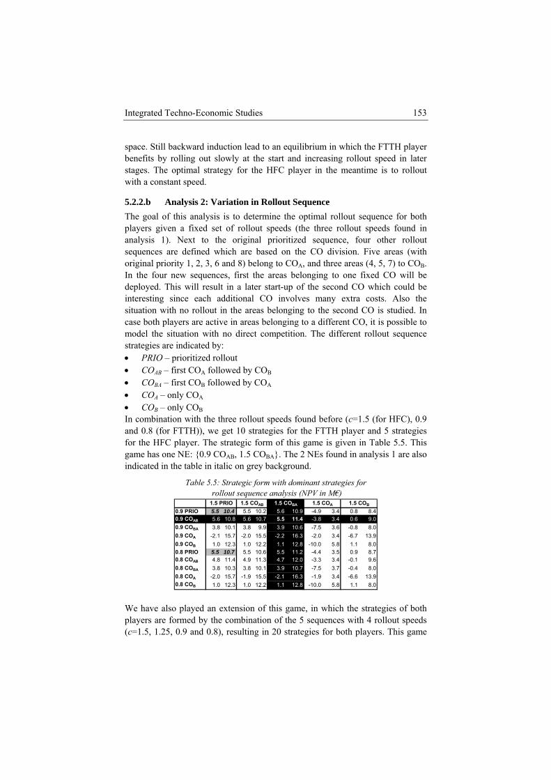
Integrated Techno-Economic Studies 153
space. Still backward induction lead to an equilibrium in which the FTTH player benefits by rolling out slowly at the start and increasing rollout speed in later stages. The optimal strategy for the HFC player in the meantime is to rollout with a constant speed.
5.2.2.b Analysis 2: Variation in Rollout Sequence The goal of this analysis is to determine the optimal rollout sequence for both players given a fixed set of rollout speeds (the three rollout speeds found in analysis 1). Next to the original prioritized sequence, four other rollout sequences are defined which are based on the CO division. Five areas (with original priority 1, 2, 3, 6 and 8) belong to COA, and three areas (4, 5, 7) to COB. In the four new sequences, first the areas belonging to o e fixed CO will be deployed. This will result in a later start-up of the second O which could be inter the situation with no O is studied. In ase both players are active in areas belonging to a different CO, it is possible to
able in italic on grey background.
Table 5.5: Strategic form with dominant strategies for rollout sequence analysis (NPV in M€)
n C
esting since each additional CO involves many extra costs. Also rollout in the areas belonging to the second C
cmodel the situation with no direct competition. The different rollout sequence strategies are indicated by: • PRIO – prioritized rollout • COAB – first COA followed by COB • COBA – first COB followed by COA • COA – only COA • COB – only COB In combination with the three rollout speeds found before (c=1.5 (for HFC), 0.9 and 0.8 (for FTTH)), we get 10 strategies for the FTTH player and 5 strategies for the HFC player. The strategic form of this game is given in Table 5.5. This game has one NE: {0.9 COAB, 1.5 COBA}. The 2 NEs found in analysis 1 are also indicated in the t
0.9 PRIO 5.5 10.4 5.5 10.2 5.6 10.9 -4.9 3.4 0.8 8.40.9 COAB 5.6 10.8 5.6 10.7 5.5 11.4 -3.8 3.4 0.6 9.00.9 COBA 3.8 10.1 3.8 9.9 3.9 10.6 -7.5 3.6 -0.8 8.00.9 COA -2.1 15.7 -2.0 15.5 -2.2 16.3 -2.0 3.4 -6.7 13.90.9 COB 1.0 12.3 1.0 12.2 1.1 12.8 -10.0 5.8 1.1 8.00.8 PRIO 5.5 10.7 5.5 10.6 5.5 11.2 -4.4 3.5 0.9 8.70.8 COAB 4.8 11.4 4.9 11.3 4.7 12.0 -3.3 3.4 -0.1 9.60.8 COBA 3.8 10.3 3.8 10.1 3.9 10.7 -7.5 3.7 -0.4 8.00.8 COA -2.0 15.7 -1.9 15.5 -2.1 16.3 -1.9 3.4 -6.6 13.90.8 COB 1.0 12.3 1.0 12.2 1.1 12.8 -10.0 5.8 1.1 8.0
1.5 COB1.5 PRIO 1.5 COAB 1.5 COBA 1.5 COA
We have also played an extension of this game, in which the strategies of both players are formed by the combination of the 5 sequences with 4 rollout speeds (c=1.5, 1.25, 0.9 and 0.8), resulting in 20 strategies for both players. This game
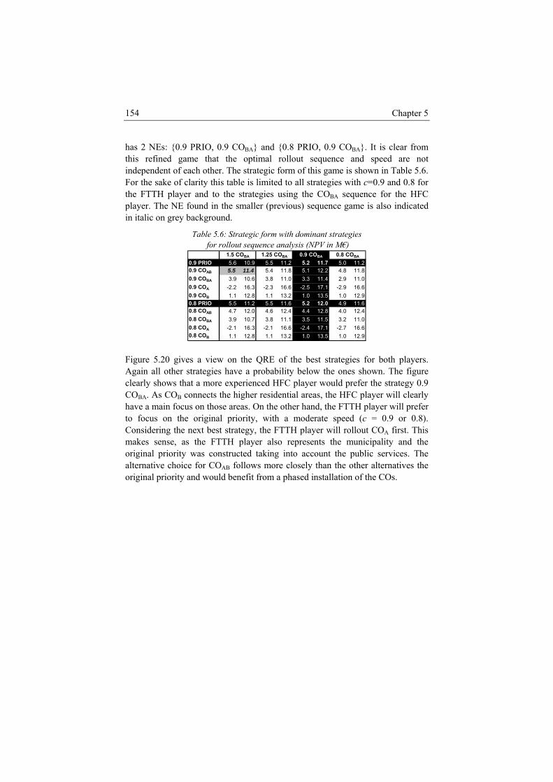
Chapter 5 154
has 2 NEs: {0.9 PRIO, 0.9 COBA} and {0.8 PRIO, 0.9 COBA}. It is clear from this refined game that the optimal rollout sequence and speed are not independent of each other. The strategic form of this game is shown in Table 5.6. For the sake of clarity this table is limited to all strategies with c=0.9 and 0.8 for the FTTH player and to the strategies using the COBA sequence for the HFC player. The NE found in the smaller (previous) sequence game is also indicated in italic on grey background.
Table 5.6: Strategic form with dominant strategies for rollout sequence analysis (NPV in M€)
0.9 PRIO 5.6 10.9 5.5 11.2 5.2 11.7 5.0 11.20.9 COAB 5.5 11.4 5.4 11.8 5.1 12.2 4.8 11.80.9 COBA 3.9 10.6 3.8 11.0 3.3 11.4 2.9 11.00.9 COA -2.2 16.3 -2.3 16.6 -2.5 17.1 -2.9 16.60.9 COB 1.1 12.8 1.1 13.2 1.0 13.5 1.0 12.90.8 PRIO 5.5 11.2 5.5 11.6 5.2 12.0 4.9 11.60.8 COAB 4.7 12.0 4.6 12.4 4.4 12.8 4.0 12.40.8 COBA 3.9 10.7 3.8 11.1 3.5 11.5 3.2 11.00.8 COA -2.1 16.3 -2.1 16.6 -2.4 17.1 -2.7 16.60.8 COB 1.1 12.8 1.1 13.2 1.0 13.5 1.0 12.9
1.5 COBA 1.25 COBA 0.9 COBA 0.8 COBA
Figure 5.20 gives a view on the QRE of the best strategies for both players.
the original priority and would benefit from a phased installation of the COs.
Again all other strategies have a probability below the ones shown. The figure clearly shows that a more experienced HFC player would prefer the strategy 0.9 COBA. As COB connects the higher residential areas, the HFC player will clearly have a main focus on those areas. On the other hand, the FTTH player will prefer to focus on the original priority, with a moderate speed (c = 0.9 or 0.8). Considering the next best strategy, the FTTH player will rollout COA first. This makes sense, as the FTTH player also represents the municipality and the original priority was constructed taking into account the public services. The alternative choice for COAB follows more closely than the other alternatives
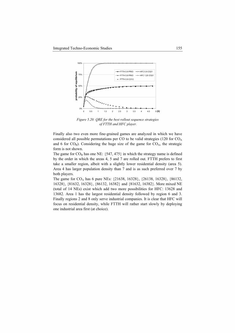
Integrated Techno-Economic Studies 155
100%
0%
25%
50%
75%
0 0.5 1 1.5 2 2.5 3 3.5 4 4.5 5 (λ)
prob
abili
ty o
f equ
ilibr
ium FTTH 0.9 PRIO HFC 0.9 CO21
FTTH 0.8 PRIO HFC 1.25 CO21
FTTH 0.9 CO12
Figure 5.20: QRE for the best rollout sequence strategies
of FTTH and HFC player. Finally also two even more fine-grained games are analyzed in which we have considered all possible permutations per CO to be valid strategies (120 for COA
ightly lower residential density (area 5). Area 4 has larger population density than 7 and is as such preferred over 7 by both players. The game for COA has 6 pure NEs: {21638, 16328}, {26138, 16328}, {86132, 16328}, {81632, 16328}, {86132, 16382} and {81632, 16382}. More mixed NE (total of 14 NEs) exist which add two more possibilities for HFC: 13628 and 13682. Area 1 has the largest residential density followed by region 6 and 3. Finally regions 2 and 8 only serve industrial companies. It is clear that HFC will focus on residential density, while FTTH will rather start slowly by deploying one industrial area first (at choice).
and 6 for COB). Considering the huge size of the game for COA, the strategic form is not shown. The game for COB has one NE: {547, 475} in which the strategy name is defined by the order in which the areas 4, 5 and 7 are rolled out. FTTH prefers to first take a smaller region, albeit with a sl
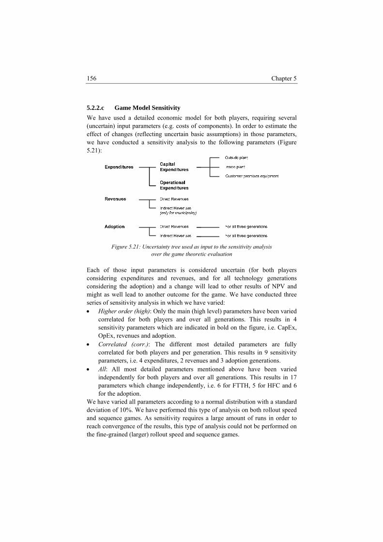
Chapter 5 156
5.2.2.c Game Model SWe h ve used a detailed
ensitivity a economic model for both players, requiring several
s, (uncertain) input parameters (e.g. costs of components). In order to estimate the effect of changes (reflecting uncertain basic assumptions) in those parameterwe have conducted a sensitivity analysis to the following parameters (Figure 5.21):
Figure 5.21: Uncertainty tree used as input to the sensitivity analysis
over the game theoretic evaluation Each of those input parameters is considered uncertain (for both players considering expenditures and revenues, and for all technology generations considering the adoption) and a change will lead to other results of NPV and might as well lead to another outcome for the game. We have conducted three series of sensitivity analysis in which we have varied: • Higher order (high): Only the main (high level) parameters have been varied
correlated for both players and over all generations. This results in 4 sensitivity parameters which are indicated in bold on the figure, i.e. CapEx, OpEx, revenues and adoption.
• Correlated (corr.): The different most detailed parameters are fully correlated for both players and per generation. This results in 9 sensitivity parameters, i.e. 4 expenditures, 2 revenues and 3 adoption generations.
• All: All most detailed parameters mentioned above have been varied independently for both players and over all generations. This results in 17 parameters which change independently, i.e. 6 for FTTH, 5 for HFC and 6 for the adoption.
We have varied all parameters according to a normal distribution with a standard deviation of 10%. We have performed this type of analysis on both rollout speed and sequence games. As sensitivity requires a large amount of runs in order to reach convergence of the results, this type of analysis could not be performed on the fine-grained (larger) rollout speed and sequence games.
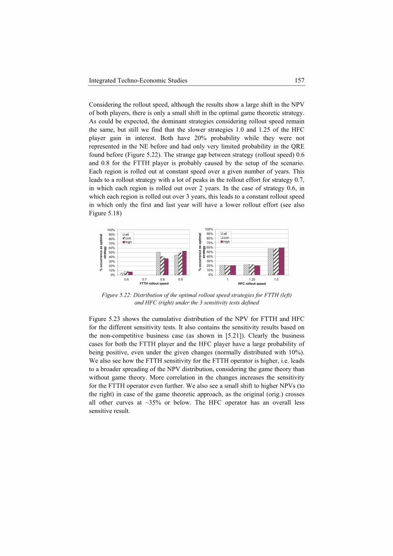
Integrated Techno-Economic Studies 157
Considering the rollout speed, although the results show a large shift in the NPV of both players, there is only a small shift in the optimal game theoretic strategy. As could be expected, the dominant strategies considering rollout speed remain the same, but still we find that the slower strategies 1.0 and 1.25 of the HFC player gain in interest. Both have 20% probability while they were not represented in the NE before and had only very limited probability in the QRE found before (Figure 5.22). The strange gap between strategy (rollout speed) 0.6 and 0.8 for the FTTH player is probably caused by the setup of the scenario. Each region is rolled out at constant speed over a given number of years. This leads to a rollout strategy with a lot of peaks in the rollout effort for strategy 0.7, in which each region is rolled out over 2 years. In the case of strategy 0.6, in which each region is rolled out over 3 years, this leads to a constant rollout speed in which only the first and last year will have a lower rollout effort (see also Figure 5.18)
0%10%20%30%40%50%60%70%80%90%
100%
0.6 0.7 0.8 0.9FTTH rollout speed
% o
ccur
renc
e as
opt
imal
st
rate
gy
allcorr.high
0%10%20%30%40%50%60%70%80%90%
100%
1 1.25 1.5HFC rollout speed
% o
ccur
renc
e as
opt
imal
st
rate
gy
allcorr.high
Figure 5.22: Distribution of the optimal rollout speed strategies for FTTH (left)
and HFC (right) under the 3 sensitivity tests defined Figure 5.23 shows the cumulative distribution of the NPV for FTTH and HFC for the different sensitivity tests. It also contains the sensitivity results based on the non-competitive business case (as shown in [5.21]). Clearly the business cases for both the FTTH player and the HFC player have a large probability of being positive, even under the given changes (normally distributed with 10%). We also see how the FTTH sensitivity for the FTTH operator is higher, i.e. leads to a broader spreading of the NPV distribution, considering the game theory than without game theory. More correlation in the changes increases the sensitivity for the FTTH operator even further. We also see a small shift to higher NPVs (to the right) in case of the game theoretic approach, as the original (orig.) crosses all other curves at ~35% or below. The HFC operator has an overall less sensitive result.
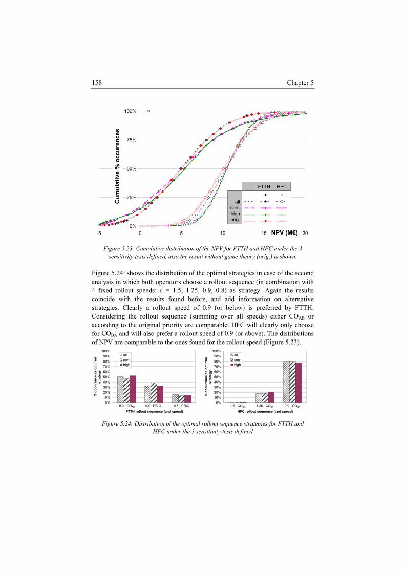
Chapter 5 158
100%
75%
Cum
ulat
ive
% o
ccur
en
0%
25%
50%
ces
FTTH HFC
allcorr.highorig.
-5 0 5 10 15 20NPV (M€)
ure 5.23: Cumulative distribution of the NPV for FTTH and HFC under the 3 nsitivity tests defined, also the result without game theory (orig.) is shown.
Figse
Fianalysis bination with 4 coincidstrategi llout speed of 0.9 (or below) is preferred by FTTH. Cacfor COB
of NPV
gure 5.24: shows the distribution of the optimal strategies in case of the second in which both operators choose a rollout sequence (in com
fixed rollout speeds: c = 1.5, 1.25, 0.9, 0.8) as strategy. Again the results e with the results found before, and add information on alternative es. Clearly a ro
onsidering the rollout sequence (summing over all speeds) either COAB or cording to the original priority are comparable. HFC will clearly only choose
A and will also prefer a rollout speed of 0.9 (or above). The distributions are comparable to the ones found for the rollout speed (Figure 5.23).
0%10%20%30%40%50%60%
stra
teg
70%
% o
ccur
ence
as
optim
al
y
80%90%
100%
0%
FTTH rollout sequence (and speed)
allcorr.high
0.9 - COAB 0.9 - PRIO 0.8 - PRIO
10%20%30%40%50%60%
% o
ccur
ence
as
ost
rate
g
70%80%90%
100%
ptim
al
y
allcorr.high
HFC rollout sequence (and speed)1.5 - COBA 1.25 - COBA 0.9 - COBA
Figu
re 5.24: Distribution of the optimal rollout sequence strategies for FTTH and
HFC under the 3 sensitivity tests defined
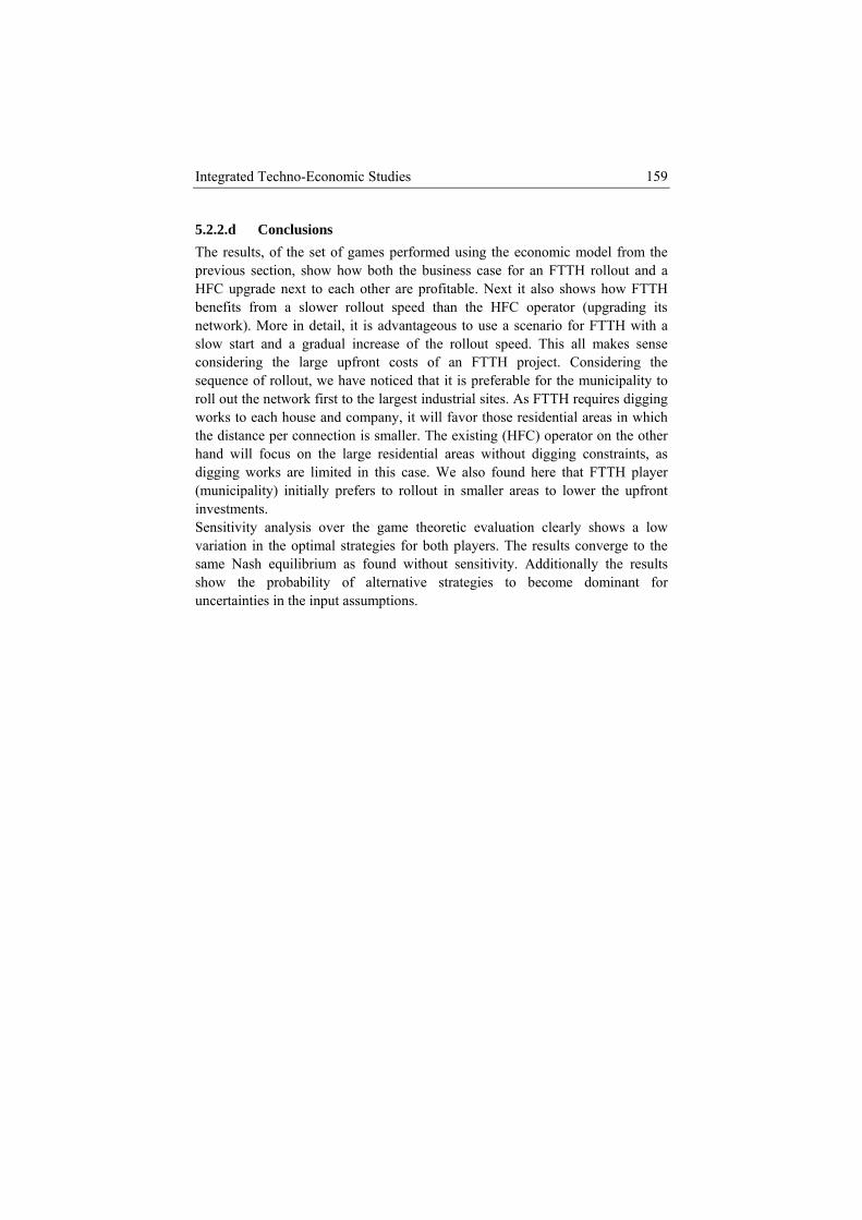
Integrated Techno-Economic Studies 159
5The respreviou and a Hbenefits eed than the HFC operator (upgrading its nsconside project. Considering the sroll out works t eas in which thand wdigging re limited in this case. We also found here that FTTH player (iSensitiv s a low vsame Nshow tuncerta sumptions.
.2.2.d Conclusions ults, of the set of games performed using the economic model from the s section, show how both the business case for an FTTH rollout
FC upgrade next to each other are profitable. Next it also shows how FTTH from a slower rollout sp
etwork). More in detail, it is advantageous to use a scenario for FTTH with a low start and a gradual increase of the rollout speed. This all makes sense
ring the large upfront costs of an FTTH equence of rollout, we have noticed that it is preferable for the municipality to
the network first to the largest industrial sites. As FTTH requires digging o each house and company, it will favor those residential ar
he distance per connection is smaller. The existing (HFC) operator on the other ill focus on the large residential areas without digging constraints, as works a
municipality) initially prefers to rollout in smaller areas to lower the upfront nvestments.
ity analysis over the game theoretic evaluation clearly showariation in the optimal strategies for both players. The results converge to the
ash equilibrium as found without sensitivity. Additionally the results he probability of alternative strategies to become dominant for inties in the input as
Chapter 5 160
5.3 CIthe prevWe starinto acc d models used fmodelli modelli apters and is elaborated here. We also mcontainecost mopresents d of an HRN, as well as for an all btassumeGhent). Th the project after 15 yA faste t speed will introduce the largest investments too early in the pproject In the scompet siness case. We assumed a case in which the existing DSL oThequipmen ropose an integrated csame rethe noti lay and first mover advantage. This serves as the basis for a full ein the c both tvthe HFCuse a sce dual increase of the rollout sproject.for the FTTH rresident nnection is smaller. The existing (HFC) operator on the other hand will focus on the large residential areas
onclusions n this chapter we made the link between the calculation models introduced in
ious two chapters and the full business case for an FTTH deployment. ted with the construction of a business case without taking competition ount. We give a detailed description of the input data an
or the business case. Customer adoption is very important in this context. The ng phase logically builds upon the previous two chapters. Revenueng is missing from previous ch
ake a distinction between direct and indirect revenues. The evaluation phase d two study cases. The first study case only considered the integrated del and investigates the deployment in a semi-urban location. This case results for the deployment of a PON an
uried or partially aerial façade installation. As such the results show different radeoffs in the deployment of an FTTH network. In the second study case, we
a municipal FTTH deployment in a dense urban location (the city of e results of this case show the possible viability of
ears. The outcome of this business case will be dependent on the rollout speed. r rollou
roject. Rolling out slower will result in a much lower take rate at the end of the and less revenues than in other cases. econd part we extended the urban business case in the city of Ghent into a ition aware bu
perator joins forces with the municipality for the rollout of the FTTH network. e competition comes from the HFC operator which will upgrade his existing
t to DOCSIS 3.0. In this study we first pompetition model for the two players rolling out telecom infrastructure in the
gion. This model is based on existing models and extended to incorporate on of de
conomic competition model of both players introducing their newest technology ity. The results of a set of games on the economic model show how
he business case for an FTTH rollout and a HFC upgrade next to each other are iable. Next it also shows how FTTH benefits from a slower rollout speed than
operator (upgrading its network). More in detail, it is advantageous to nario for FTTH with a slow start and a gra
peed. This all makes sense considering the large upfront costs of an FTTH- Considering the sequence of rollout, we have noticed that it is preferable municipality to roll out the network first to the largest industrial sites. As equires digging works to each house and company, it will favor those ial areas in which the distance per co

Integrated Techno-Economic Studies 161
wWe also ers to rollout in smaller areas to lower the upfront investments. Sensitivity analysis over the game theoretic evaluation clearly shows a low variation in the optimal strategies for both players. The results converge to the same Nash equilibrium as found without sensitivity. Additionally the results show the probability of alternative strategies to become dominant for uncertainties in the input assumptions. Finally the introduction of an FTTH network will clearly be a very costly project. In a dense urban area we find a (discounted) cost of around 750€ per home connected. In a semi-urban case the cost per home connected is 1750€ (not discounted) in a PON and 1900€ (not discounted) in an HRN for a 100% take rate. This is much higher than in the dense urban case in which also an HRN is considered with a not discounted cost of 1500€ and a 65% take rate. Still deploying FTTH can be a viable case when selecting the right location, architecture and installation type. Considering the competitive advantage of an FTTH network, the rollout might be less of a question when another operator would otherwise take the lead and offer far more bandwidth. It is often not clear for an operator what strategy exactly to choose. While for instance starting slow is advantageous, starting too late will allow the opponent to capture market share and result in a far worse business case. Game theory can help to balance all strategic constraints based on the economic model for both players. Even under uncertain assumptions considering input costs, revenues and adoption, game theory can help to reliably choose the best (set of) strategies.
ithout digging constraints, as digging works are much more limited in this case. found here that FTTH player (municipality) initially pref
Chapter 5 162
References
[5.1] E. M. Rogers, “Diffusion of innovations”, 3rd ed., Free Press, New York, ISBN 0 02 926650 5, 1983
[5.2] J. Van Ooteghem, T. Evens, D. Schuurman., K. Casier, B. Lannoo, L. De Marez, I. Moerman, P. Demeester, “Segmentation and adoption forecasts for wireless Internet services onboard trains”, accepted for publication and presentation in FITCE 2009, Prague, Czech Republic, 3-5 September 2009
[5.3] J. C. Fisher, R. H. Pry, “A Simple Substitution Model of Technological Change”, Technology Forecasting and Social Change, vol. 3, pp. 75–88, 1971.
[5.4] B. Gompertz, “On the nature of the function expressive of the law of human mortality, and on a new method of determining the value of life contingencies”, Philosophical Transactions of the Royal Society, vol. 36, pp. 513-585, 1825.
[5.5] J. V. Gregg, C. H. Hassel, J. T. Richardson, “Mathematical trend curves: An aid to forecasting”, Oliver & Boyd, Edinburgh, 1964.
[5.6] P. J. Harrison, S. F. Pearce, “The use of trend curves as an aid to market forecasting”, Industrial Marketing Management, vol. 1, no 2, pp. 149-170, Jan. 1972.
[5.7] A. Cárdenas et al, “A New Model of Bandwidth Growth Estimation Based on the Gompertz Curve: Application to Optical Access Networks”, Journal of Lightwave Technology, vol. 22, no 11, pp. 2460-2468, Nov. 2004.
[5.8] F.M. Bass, “A new Product Growth for Model Consumer Durables”, Management Science, vol. 15, no 5, pp. 215-227, 1969.
[5.9] K. Casier, B. Lannoo, J. Van Ooteghem, S. Verbrugge, D. Colle, M. Pickavet, P. Demeester, "Adoption and pricing: the underestimated elements of a realistic IPTV business case", IEEE Commun. Mag. 46, 112-118 (August 2008).
[5.10] Evaluatie van grote infrastructuurprojecten – Leidraad voor kosten-baten analyse - Deel I&II, Ministerie van verkeer en waterstaat & Ministerie van economie, http://www.verkeerenwaterstaat.nl/Images/ Deel%20II%20Capita%20Selecta_tcm195-160756.pdf
Integrated Techno-Economic Studies 163
[5.11] Athena – A multi-sector model of the Dutch economy, Centraal Planbureau (CPB), January 2006, http://www.cpb.nl/eng/pub/cpbreeksen/document/105/doc105.pdf
[5.12] The Allen Consulting Group, “True Broadband: Exploring the economic impacts”, September 2003
[5.13] Strategic Networks Group, “Economic Impact Study of the South Dundas Township Fibre Network”, June 2003
[5.14] M. Forzatti, C. P. Larsen, “A study of Broadband Access: Policy and Status in Sweden and Global Economic Impact”, In proceedings of OFC/NFOEC 2009, NMC3, March 22-26, San Diego, US.
[5.15] D. Mok, J. A. Carrasco, B. Wellman, “Does Distance Still Matter in the Age of the Internet?”, Social Networks Vol. 29, No. 3 (July 2007), pp. 430-61.
[5.16] B. Metcalfe, “Mreaches more use
[5.1
preprint version, March 2005, http://www.dtc.umn.edu/~odlyzko /doc/metcalfe.pdf
[5.18] B. Briscoe, A. Odlyzko and B. Tilly, “Metcalfe's Law is Wrong”, IEEE S4109
[5.19] J. Van Ooteghem, B. Lannoo, K. Casier, S. Verbrugge, P. Demeester,
parative study between active
etcalfe’s Law: A network becomes more valuable as it rs”, Infoworld, vol. 17, no 40, pp. 53-54, 1995
7] A. Odlyzko and B. Tilly, “A refutation of Metcalfe’s Law and a better estimate for the value of networks and network interconnections”,
pectrum, July 2006, pp. 26-31, http://www.spectrum.ieee.org/jul06/
“Municipalities as a Driver for Wireless Broadband Access”, Wireless Personal Communications, Springer Netherlands, ISSN 0929-6212 (Print) 1572-834X (Online), vol. 49, no. 3, pp. 391-414 , May 2009
[5.20] K. Casier, S. Verbrugge, R. Meersman, D. Colle, M Pickavet, P. Demeester, “A clear and balanced view on FTTH deployment costs”, The journal of the Institute of Telecommunications Professionals (ITP) 2 (3), 27-30 (December 2008).
[5.21] B. Lannoo, K. Casier, J. Van Ooteghem, B. Wouters, S. Verbrugge, D. Colle, M. Pickavet, P. Demeester, “Economic benefits of a community driven fiber to the home rollout,” in Proceedings of International Conference on Broadband Communications, Networks, and Systems (Broadnets), ISBN 978-1-4244-2392-7, London, (08-11 September 2008).
[5.22] Koen Casier, Jeroen Vanhaverbeke, Bart Lannoo, Jan Van Ooteghem, Sofie Verbrugge, Raf Meersman, Didier Colle, Mario Pickavet, Piet Demeester, “economics of FTTH: a com
Chapter 5 164
and passive optical networks”, accepted for publicatioPrague, Czech Republic, 3-5 September 2009
n in FITCE 2009,
itchell, “Fiber to the Home: Technology Wars”, m/web/about/ac79/docs/wp/Tech_Wars_Part__1_Ex
Switzerland, (12-14 December 2006).
[5.23] A. Banerjee and M. Sirbu, “Towards Technologically and Competitively Neutral Fiber to the Home (FttH) Infrastructure,” in Proceedings of The 31st Research Conference on Communication, Information and Internet Policy, Washington DC, USA (19-21 September 2003).
[5.24] R. Medcalf, S. Mhttp://www.cisco.cot_EI_0128.pdf (January 2008).
[5.25] J. Van Ooteghem, S. Verbrugge, K. Casier, “Future proof strategies towards fiber to the home”, published in proceedings of public private interplay, next generation communications conference (PPI-NGC), Seville, Spain, 10-12 December 2008.
[5.26] Analysys Mason, “Final report for the Broadband Stakeholder Group: The costs of deploying fibre-based next-generation broadband infrastructure”, Ref: 12726-371 (8 September 2008).
[5.27] Glasvezel Amsterdam, “Realisation fibreoptic network Amsterdam”, 2006.
[5.28] P. Fournier, "From FttH pilot to pre-rollout in France", CAI Cheuvreux conference, http://www.francetelecom.com/en_EN/finance/invest-analysts/meetings-conferences/att00003205/20070626_FTTH.pdf (26 June 2007).
[5.29] IDATE Consulting & Research, “Telecoms in Europe 2015 (Final report),” (Academic, February 2007).
[5.30] M. Felegyhazi and J.P. Hubaux, “Game Theory in Wireless Networks: A Tutorial,” in EPFL technical report, LCA-REPORT-2006-002, (February 2006).
[5.31] R. D. Mc.Kelvey and T. R. Palfrey, “Quantal Response Equilibria for Normal Form Games,” Game. Econ. Behav. 10, pp. 6-38, (1995).
[5.32] J.A. Norton and F.M. Bass, “A Diffusion Theory Model of Adoption and Substitution for Successive Generations of High-Technology Products,” Management Sci. 33 (9), 1069-1086 (1987).
[5.33] B. Lannoo, S. Verbrugge, J. Van Ooteghem, E. Boonefaes, K. Haelvoet, D. Colle, M. Pickavet, P. Demeester, “The evolution of fixed access networks in Belgium: the road to Fibre to the Home, an economic assessment,” in Proceedings of BroadBand Europe, Geneva,

Integrated Techno-Economic Studies 165
[5.34] E. Boonefaes, “Evolutie van vaste toegangsnetwerken in Belgie – de weg naar fiber to the home”, Master thesis UGent, 2006.

Chapter 5 166
6 Applicability in a Broader
Technological or Economic Context
ly it.
encompasses other economic studies and extensions not covered before. However as some parts of our research also considered those extensions, we discuss the approaches and results in section 6.2.
One pound of learning requires ten pounds of common sense to appPersian Proverb
In this dissertation we developed a methodology for the evaluation of investment projects in telecommunication networks. The main focus was on the evaluation of the business case for an FTTH deployment, and a lot of work was devoted to the development of infrastructure and operations dimensioning models. The methodology and the specific models developed in this dissertation can also be applied in other contexts. In our research, we have used the same approach outside the scope of an FTTH deployment study. In the first section we broaden the technological scope of this dissertation. In section 6.1.1 we extend the work to include fixed access networks. We further open this in section 6.1.2 to wireless access network deployments. Finally we shortly show the limited applicability in metro and core networks (section 6.1.3). Within the dissertation, we explored the evaluation of the FTTH deployment with the extension of game theory and sensitivity analysis. The methodology
Chapter 6 168
6.1 Extending the Technological Studies
n can be reused on n the FTTH
The techno-economic study in this dissertation was focussed on the fixed access network. In chapter 2, we looked at the network from a much higher point of view and gradually refined the description to get up to the point of the FTTH access network. In this section we gradually zoom out again. At each point, we indicate which models could be easily reused. Where applicable, we add results from our existing studies.
6.1.1 From FTTH to Fixed Access Networks There are good resemblences between FTTH and other fixed access networks, and as such most of the information discussed in this dissertatiothere. C sidering the infrastructure, a large part of the calculations icase were devoted to the dimensioning of the outside plant installations. This calculation can be fully reused when considering a new installation of other fixed access technologies (e.g. in a newly built neighbourhood). Also when looking at upgrades of existing infrastructure, e.g. from ADSL to VDSL, additional fibre will be installed. In this case a lot less optical nodes (e.g. VDSL street cabinets) should be connected with fibre and a full optimal Steiner tree can be more easily constructed. Often an operator will connect different optical nodes in a ring. Finally it is also very straightforward to translate the calculation of all other costs such as inside plant equipment and customer premises equipment to a non-FTTH situation. Next to infrastructure, also large parts of the operational modelling can be reused in the scope of the deployment or exploitation of other networks. For instance, we can expect more or less the same operations for keeping the network up and running. In the case of an existing network infrastructure, the physical installation of the customer connection process, i.e. connecting the cable to the network, will not be triggered a lot as most customers are already connected to the network. In order to reduce additional travelling to/from the customer, operators try to promote a do-it-yourself installation57 as much as possible. In chapter 4, we have already shown the differences between a fibre based and a copper based access network. In [6.1] we made a cost comparison of the repair process for both network technologies. Figure 6.1 gives an overview of the costs for one occurrence of the repair process in a copper based network (according to Figure 4.15), a preventive repair for copper, i.e. a solution for the effects of water intrusion (also shown in Figure 4.15) and the repair in a fibre based network (according to Figure 4.14). All assumptions for this study case can be found in [6.1]. Clearly the high amount of fibres in the feeder section of an HRN will 57 This goal to reduce all additional travelling to the customer is also an important driver for remote management.
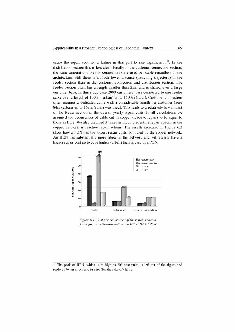
Applicability in a Broader Technological or Economic Context 169
cause the repair cost for a failure in this part to rise significantly58. In the distribution section this is less clear. Finally in the customer connection section, the same amount of fibres or copper pairs are used per cable regardless of the
trajectory) in the architecture. Still there is a much lower distance (trenchingfeeder section than in the customer connection and distribution section. The feeder section often has a length smaller than 2km and is shared over a large customer base. In this study case 2000 customers were connected to one feeder cable over a length of 1000m (urban) up to 1500m (rural). Customer connection often requires a dedicated cable with a considerable length per customer (here 84m (urban) up to 168m (rural) was used). This leads to a relatively low impact of the feeder section in the overall yearly repair costs. In all calculations we assumed the occurrences of cable cut in copper (reactive repair) to be equal to those in fibre. We also assumed 3 times as much preventive repair actions in the copper network as reactive repair actions. The results indicated in Figure 6.2 show how a PON has the lowest repair costs, followed by the copper network. An HRN has substantially more fibres in the network and will clearly have a higher repair cost up to 33% higher (urban) than in case of a PON.
0
10
20
30
40
50
60
unit cost (rep
air du
ration
)
copper, reactivecopper, preventiveFTTH HRNFTTH PON
209
feeder distri tion customer connectionbu
58 The peak of HRN, which is as high as 209 cost units, is left out of the figure and
Figure 6.1: Cost per occurrence of the repair process for copper reactive/preventive and FTTH HRN / PON
replaced by an arrow and its size (for the sake of clarity).
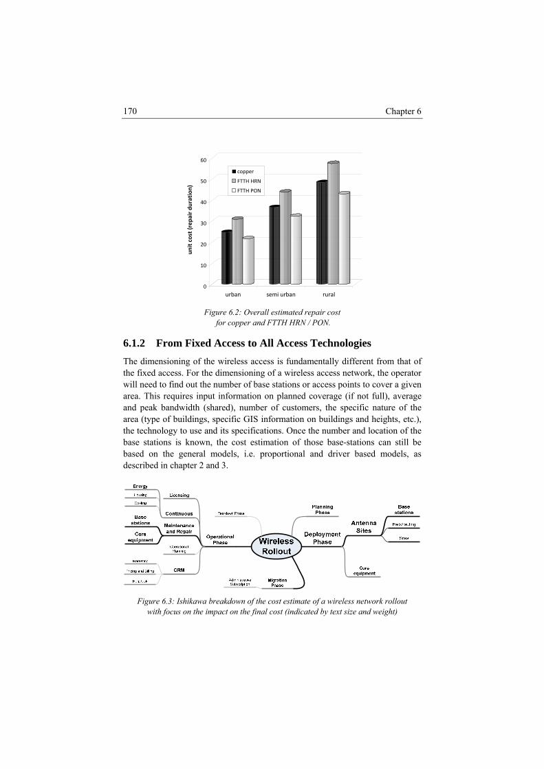
Chapter 6 170
0
10
20
30
40
50
60
unit cost (rep
air du
ration
)
urban semi urban rural
copper
FTTH HRN
FTTH PON
Figure 6.2: Overall timated repair cost
6.1.2 en t of
es for copper and FTTH HRN / PON.
From Fixed Access to All Access Technologies The dim sioning of the wireless access is fundamentally different from thathe fixed access. For the dimensioning of a wireless access network, the operator will need to find out the number of base stations or access points to cover a given area. This requires input information on planned coverage (if not full), average and peak bandwidth (shared), number of customers, the specific nature of the area (type of buildings, specific GIS information on buildings and heights, etc.), the technology to use and its specifications. Once the number and location of the base stations is known, the cost estimation of those base-stations can still be based on the general models, i.e. proportional and driver based models, as described in chapter 2 and 3.
Figure 6.3: Ishikawa breakdown of the cost estimate of a wireless network rollout
with focus on the impact on the final cost (indicated by text size and weight)
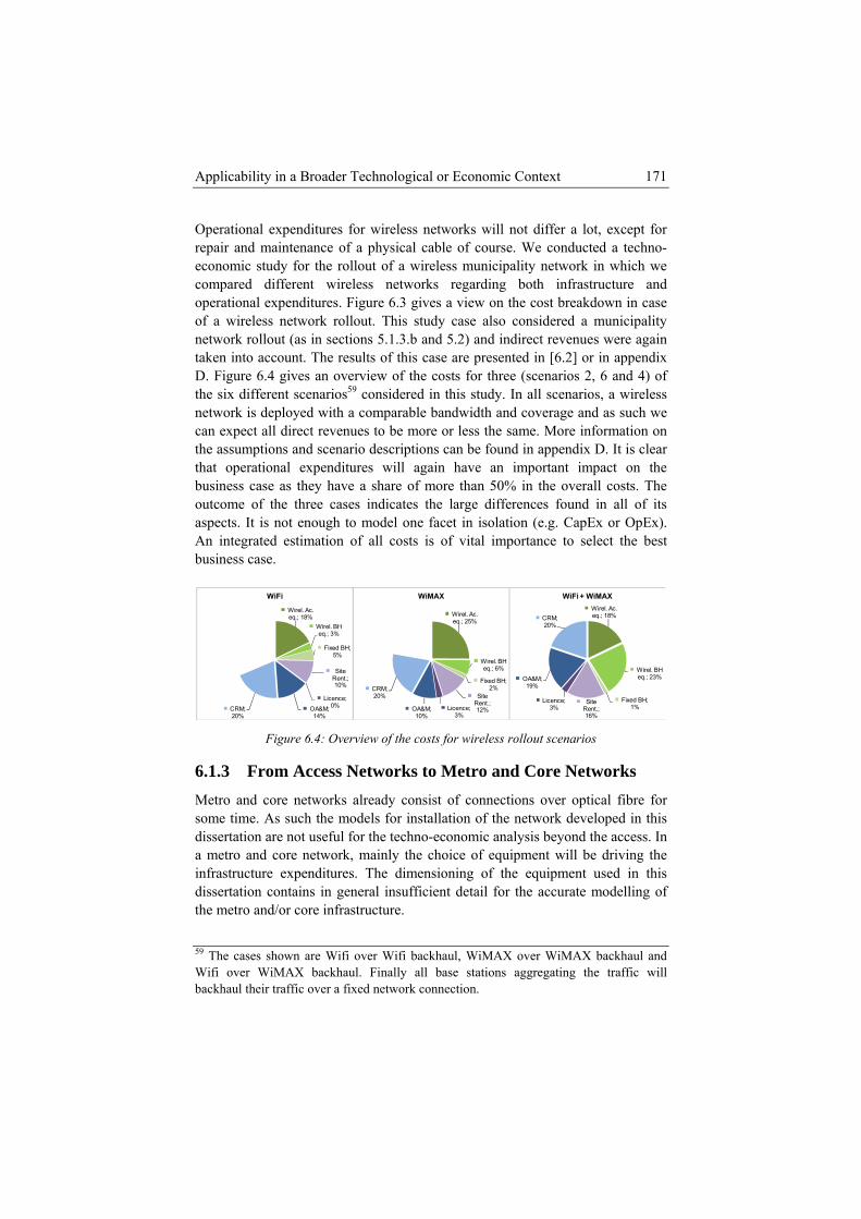
Applicability in a Broader Technological or Economic Context 171
Operational expenditures for wireless networks will not differ a lot, except for repair and maintenance of a physical cable of course. We conducted a techno-economic study for the rollout of a wireless municipality network in which we compared different wireless networks regarding both infrastructure and operational expenditures. Figure 6.3 gives a view on the cost breakdown in case of a wireless network rollout. This study case also considered a municipality
dered in this study. In all scenarios, a wireless
d in appendix D. It is clear that operational expenditures will again have an important impact on the
a share of more than 50% in the overall costs. The indicates the large differences found in all of its
ase.
network rollout (as in sections 5.1.3.b and 5.2) and indirect revenues were again taken into account. The results of this case are presented in [6.2] or in appendix D. Figure 6.4 gives an overview of the costs for three (scenarios 2, 6 and 4) of the six different scenarios59 consinetwork is deployed with a comparable bandwidth and coverage and as such we can expect all direct revenues to be more or less the same. More information on the assumptions and scenario descriptions can be foun
business case as they haveoutcome of the three casesaspects. It is not enough to model one facet in isolation (e.g. CapEx or OpEx). An integrated estimation of all costs is of vital importance to select the best business c
Wirel. Ac. eq.; 18%
Wirel. BH eq.; 3%
Fixed BH; 5%
Site Rent.; 10%
Licence; 0%OA&M;
14%CRM; 20%
WiFi
Wirel. Ac. eq.; 25%
Wirel. BH eq.; 6%
Fixed BH; 2%
Site Rent.; 12%Licence;
3%OA&M; 10%
CRM; 20%
WiMAXWirel. Ac. eq.; 18%CRM;
20%
WiFi + WiMAX
Wirel. BH eq.; 23%
Fixed BH; 1%
Site Rent.; 16%
Licence; 3%
OA&M; 19%
Figure 6.4: Overview of the costs for wireless rollout scenarios
6.1.3 From Access Networks to Metro and Core Networks Metro and core networks already consist of connections over optical fibre for some time. As such the models for installation of the network developed in this dissertation are not useful for the techno-economic analysis beyond the access. In a metro and core network, mainly the choice of equipment will be driving the infrastructure expenditures. The dimensioning of the equipment used in this dissertation contains in general insufficient detail for the accurate modelling of the metro and/or core infrastructure.
59 The cases shown are Wifi over Wifi backhaul, WiMAX over WiMAX backhaul and Wifi over WiMAX backhaul. Finally all base stations aggregating the traffic will backhaul their traffic over a fixed network connection.
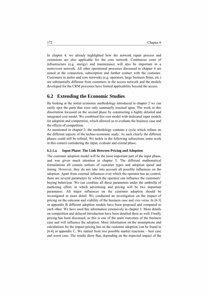
Chapter 6 172
In chapter 4, we already highlighted how the network repair process and lso applicable for the core network. Continuous costs of g. energy) and maintenance will also be important in a
maimed aCustomare subsdevelop nd the access.
6.2 EBy look can eadiintegratfor adopthe effects oAthe diffphases in this c uate and extend phase.
6.The cusand wa n chapter 5. The different mathematical
rmulations all contain notions of customer types and adoption speed and ming. However, they do not take into account all possible influences on the doption. Apart from external influences over which the operator has no control, ere are several parameters by which the operator can influence the customers’
buying behaviour. We can combine all those parameters under the umbrella of marketing effort, in which advertising and pricing will be two important parameters. All major influences on the customer adoption should be investigated in more detail. We conducted an investigation on the impact of pricing on the outcome and viability of the business case and vice versa. In [6.3] or appendix B different adoption models have been proposed and compared to each other. We have used this information extensively in chapter 5. More details on competition and delayed introduction have been detailed there as well. Finally pricing has been discussed, as this is one of the main outcomes of the business case and will influence the adoption. More information on the assumptions and calculations for the impact pricing has on the customer adoption, can be found in [6.4] or appendix C. We started from two possible market reactions – best case and worst case. The results show that, depending on the expected impact of the
extensions are ainfrastructure (e.
etro/core network. All other operational processes discussed in chapter 4 are t the connection, subscription and further contact with the customer. ers in metro and core networks (e.g. operators, large business firms, etc.) tantially different from customers in the access network and the models ed for the CRM processes have limited applicability beyo
xtending the Economic Studies ing at the initial economic methodology introduced in chapter 2 we
sily spot the parts that were only summarily touched upon. The work in this ssertation focussed on the second phase by constructing a highly detailed and
ed cost model. We combined this cost model with dedicated input models tion and competition, which allowed us to evaluate the business case and
f competition. s mentioned in chapter 2, the methodology contains a cycle which refines on
erent aspects of the techno-economic study. As such clearly the different could still be refined. We tackle in the following subsections some work ontext considering the input, eval
2.1.a Input Phase: The Link Between Pricing and Adoption tomer adoption model will be the most important part of the input phase, s given much attention i
fotiath
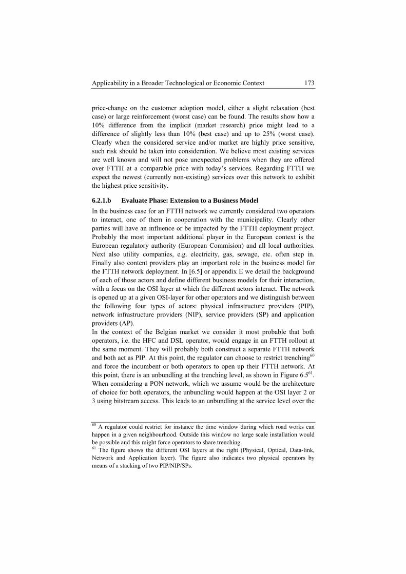
Applicability in a Broader Technological or Economic Context 173
price-change on the customer adoption model, either a slight relaxation (best case) or large reinforcement (worst case) can be found. The results show how a 10% difference from the implicit (market research) price might lead to a difference of slightly less than 10% (best case) and up to 25% (worst case). Clearly when the considered service and/or market are highly price sensitive, such risk should be taken into consideration. We believe most existing services are well known and will not pose unexpected problems when they are offered over FTTH at a comparable price with today’s services. Regarding FTTH we expect the newest (currently non-existing) services over this network to exhibit the highest price sensitivity.
6.2.1.b Evaluate Phase: Extension to a Business Model In the business case for an FTTH network we currently considered two operators to interact, one of them in cooperation with the municipality. Clearly other parties will have an influence or be impacted by the FTTH deployment project. Probably the most important additional player in the European context is the European regulatory authority (European Commision) and all local authorities. Next also utility companies, e.g. electricity, gas, sewage, etc. often step in. Finally also content providers play an important role in the business model for the FTTH network deployment. In [6.5] or appendix E we detail the background of each of those actors and define different business models for their interaction, with a focus on the OSI layer at which the different actors interact. The network is opened up at a given OSI-layer for other operators and we distinguish between the following four types of actors: physical infrastructure providers (PIP), network infrastructure providers (NIP), service providers (SP) and application providers (AP). In the context of the Belgian market we consider it most probable that both operators, i.e. the HFC and DSL operator, would engage in an FTTH rollout at the same moment. They will probably both construct a separate FTTH network and both act as PIP. At this point, the regulator can choose to restrict trenching60 and force the incumbent or both operators to open up their FTTH network. At this point, there is an unbundling at the trenching level, as shown in Figure 6.561. When considering a PON network, which we assume would be the architecture of choice for both operators, the unbundling would happen at the OSI layer 2 or 3 using bitstream access. This leads to an unbundling at the service level over the
60 A regulator could restrict for instance the time window during which road works can happen in a given neighbourhood. Outside this window no large scale installation would be possible and this might force operators to share trenching. 61 The figure shows the different OSI layers at the right (Physical, Optical, Data-link, Network and Application layer). The figure also indicates two physical operators by means of a stacking of two PIP/NIP/SPs.
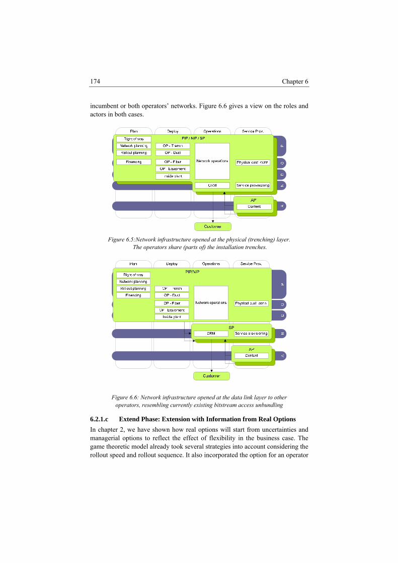
Chapter 6 174
incumbent or both operators’ networks. Figure 6.6 gives a view on the roles and actors in both cases.
ical (trenching) layer.
trenches. Figure 6.5:Network infrastructure opened at the phys
The operators share (parts of) the installation
Figure 6.6: Network infrastructure opened at the data link layer to other operators, resembling currently existing bitstream access unbundling
6.2.1.c Extend Phase: Extension with Information from Real Options In chapter 2, we have shown how real options will start from uncertainties and managerial options to reflect the effect of flexibility in the business case. The game theoretic model already took several strategies into account considering the rollout speed and rollout sequence. It also incorporated the option for an operator
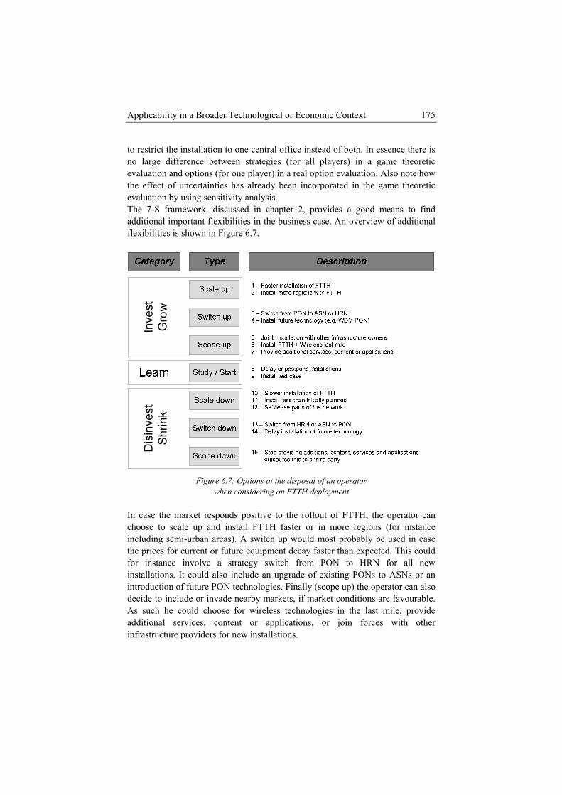
Applicability in a Broader Technological or Economic Context 175
to restrict the installation to one central office instead of both. In essence there is no large difference between strategies (for all players) in a game theoretic evaluation and options (for one player) in a real option evaluation. Also note how the effect of uncertainties has already been incorporated in the game theoretic evaluation by using sensitivity analysis. The 7-S framework, discussed in chapter 2, provides a good means to find additional important flexibilities in the business case. An overview of additional flexibilities is shown in Figure 6.7.
Inve
st
Gro
wD
isin
vest
Shr
ink
Figure 6.7: Options at the disposal of an operator
when considering an FTTH deployment In case the market responds positive to the rollout of FTTH, the operator can choose to scale up and install FTTH faster or in more regions (for instance including semi-urban areas). A switch up would most probably be used in case the prices for current or future equipment decay faster than expected. This could for instance involve a strategy switch from PON to HRN for all new installations. It could also include an upgrade of existing PONs to ASNs or an
technologies. Finally (scope up) the operator can also introduction of future PON decide to include or invade nearby markets, if market conditions are favourable. As such he could choose for wireless technologies in the last mile, provide additional services, content or applications, or join forces with other infrastructure providers for new installations.
Chapter 6 176
Considering the immense investments involved in a FTTH deployment, the option to wait and study is always very important. However, as we have shown in the competitive study, the operator should beware not to wait to long in order not to lose a large market share. Finally the operator has another set of options at his disposal, in case the market responds worse than expected. Naturally these options are diametrical to the options used in case of a positive market response.
the FTTH network to other operators. Finally the
6.3 Conclusions The methodology and models developed in the dissertation are focussed on the deployment of an FTTH network, but they can easily be used in a broader context. We have first shown how most of the same models and information could be used in the scope of other fixed access networks (e.g. DSL or HFC). In a second step we have shown how large parts, especially of the operational modelling, can still be used in a wireless access network deployment. We related in both cases to results from techno-economic studies we performed. The economic methodology presented in this dissertation can also be easily broadened. Regarding the input modelling of the business case, we have investigated how the pricing could influence the customer adoption and as such the whole business case. In a second extension, a full business model of the FTTH deployment is constructed that sheds a light on the choices and opportunities for openingtheory of real options, and more in detail the 7-S framework, has been applied on the case of an FTTH deployment. The different options found here could easily be used to extend the strategy set of the game theoretic evaluation used in chapter 5.
Applicability in a Broader Technological or Economic Context 177
References [6.1] S. Verbrugge K. Casier B. Lannoo J. Van Ooteghem R. Meersman D.
Colle P. Demeester, "FTTH deployment and its impact on network
Verbrugge, D. Colle, M. Pickavet, P. Demeester, “Adoption and Pricing: The Underestimated
a Realistic IPTV Business Case”, IEEE Communications
maintenance and repair costs", published in Anniversary International Conference on Transparent Optical Networks (ICTON), ISBN 978-1-4244-2625-6, Athens, Greece, 22-26 June 2008, pp. 2-5
[6.2] J. Van Ooteghem, B. Lannoo, K. Casier, S. Verbrugge, P. Demeester, “Municipalities as a Driver for Wireless Broadband Access”, Wireless Personal Communications, Springer Netherlands, ISSN 0929-6212 (Print) 1572-834X (Online), vol. 49, no. 3, pp. 391-414 , May 2009
[6.3] K. Casier, B. Lannoo, J. Van Ooteghem, S.
Elements ofMagazine, ISSN 0163-6804, vol. 46, no. 8, pp.112-118, August 2008
[6.4] K. Casier, S. Verbrugge, B. Lannoo, J. Van Ooteghem, R. Meersman, D. Colle, M. Pickavet, P. Demeester, “Using cost based price calculations in a converged network”, Emerald INFO journal, ISSN 1463-6697, Vol 11, No 3, pp. 6-18 ,May 2009.
[6.5] J. Van Ooteghem, S. Verbrugge, K. Casier, M. Pickavet, P. Demeester, “Future Proof Strategies towards Fiber to the Home”, published in proceedings of Public Private Interplay (PPI) conference, Sevilla, Spain, 10-12 December 2008.

Chapter 6 178
7 Conclusions
“The world is full of obvious things which nobody by any chance ever observes”, Sr. Arthur Conan Doyle
Bandwidth demand keeps on growing in time; much in the same way as computing power has done in the last decades. Nielsen’s law62 predicts an annual increase of 50% in bandwidth provided to the customer. The existing access network infrastructure is increasingly becoming the bottleneck in this evolution, especially in developed countries. Many operators try to upgrade their existing access network as much as possible. However when this trend holds, a mainstream connection would offer a tenfold the bandwidth of today’s connections within 6 years and a hundredfold the bandwidth 12 years from now. This bandwidth can no longer be provided cost-efficiently over the existing copper-based or coaxial access networks. An access network using optical fibre as its medium, offers much higher bandwidths in a more cost-efficient manner and an FTTH network is therefore often seen as the logical next step in the evolution of the access network.
62 Nielsen’s law is the telecom alternative for the more commonly known Moore’s law (electronics) predicting a doubling of the number of transistors on a chip every two years. This is believed to correspond with a doubling of processing power every 18 months.
Chapter 7 180
The costs and complexity involved in a move to FTTH are very large. All network, including cabling, must be replaced. There are also
ible FTTH architectures between which an operator has to hoose for the deployment. On the other hand FTTH could also give the operator
a tly project, an operator will require a detailed and reliable techno-economic evaluation. This d sertation investigates the economies of the rollout and exploitation of an FTTH network. First a generally applicable methodology for techno-economic studies, consisting of four phases – design, model, evaluate and extend – is presented. We mainly focussed on the model phase and made a split between the dimensioning of infrastructure and of operations. By fitting the models in the overall methodology, we could proceed with an evaluation of the overall FTTH deployment business case. In extension we also applied game theory and sensitivity analysis on top of this business case to get a better view on the impact of competition. The techno-economic study starts from a Belgian context and is applicable for most developed countries. The remainder of this chapter summarizes the most important work and results obtained in our research. We give a general conclusion on FTTH deployment and close with some directions for future work.
Infrastructure Dimensioning The most important aspect in the infrastructure, from a cost perspective, will be the physical installation of the fibre in the outside plant. Especially when legislation obliges operators to install a fully buried network, the cost of trenching will exceed all other infrastructure costs. We developed analytical models for the estimation of the outside plant installation length. A more detailed, hence more reliable dimensioning approach makes use of the Steiner tree. We implemented a faster heuristic Steiner search algorithm which works on highly detailed GIS information. In addition to the installation length, we have constructed dedicated models for the dimensioning of all other passive equipment in the outside plant as well as for the dimensioning of the inside plant and customer premises equipment. It is straightforward to couple the dimensioning results to the equipment prices and get an estimation of the global infrastructure costs. Forecasting the evolution of equipment prices in time is very important in this context.
Operations Dimensioning While up to half of all expenditures in an FTTH deployment originate from operating the network and services, these costs are often neglected or modelled in little detail. We have constructed dedicated, flowchart based models for the estimation of the customer connection and network repair processes, and have
equipment in the several incompatc
competitive advantage. Clearly, before embarking on such strategic but cos
is
Conclusions 181
completed this overview with driver-based models for all remaining operational processes. Dedicated models open up opportunities for minimizing operational expenditures. We showed how important savings can be achieved for the network repair process in an access network by optimizing the number and location of repair teams and the service level. Adding flexibility in the process by means of freelance personnel could also lead to considerable cost reductions (~10%).
Business Case Evaluation Deploying FTTH is clearly very costly, but the biggest question for the operator is whether he would gain by such project. This problem is tackled in two steps. We first focussed on a (fictitious) non-competitive situation. In this situation, the cost model applied on a semi-urban deployment shows important tradeoffs for the operator. The results already clearly indicate savings made possible by using aerial/façade installation instead of a fully buried installation (4% for only 9% alternative installation length) or by installing a PON instead of an HRN (3%). We have shown the benefits of using pre-installation for connecting the customers, especially in a fully buried FTTH network. A cost per home passed in this situation is at least 1000€. A full business case for a dense urban municipality-driven rollout is viable over a planning horizon of 15 years. The viability will be largely depending on the rollout speed and the positive effects of indirect revenues in a municipality rollout. The average cost per home passed and home connected starts very high, but quickly decreases to a value of ∼300€ and ∼750€, respectively. We also considered an FTTH deployment in a more realistic competitive setting in which the other operator chooses to upgrade his existing (in this case HFC) equipment. We have evaluated the business case using concepts from game theory. The results indicate a viable business case for both operators in all games considered over a project horizon of 15 years. The FTTH operator will prefer areas with a high residential density and industrial areas. He will choose for a slow start and increase its rollout speed in a later stage. The HFC operator will favour the largest residential areas and will rollout very fast from the beginning.
Overall conclusion FTTH is very likely the next and inevitable step in the evolution of the access network. The transition from copper or coax cables to FTTH is no more than logical when looking at its technological superiority. When focussing on the economies of such FTTH deployment, the picture changes substantially. The project is viable, when considered over a long time horizon and in selected areas. Typically FTTH will focus on areas with high residential and/or industrial density. Technological advances will only slightly ameliorate this situation as the
Chapter 7 182
largest costs are caused by the labour intensive installation of the outside plant. The impact of legislative changes might in this context be very important, for instance by allowing aerial/façade or other alternative installation types. For semi-urban and rural areas, additional public incentives might be required to get a nationwide coverage. In this conundrum, most operators choose the safest option of postponing the move to FTTH. They currently compete by using their existing infrastructure and gradually upgrading their equipment to provide a higher bandwidth to the customer. These rules might change when one operator breaks the standoff and installs FTTH. At this point the late mover risks losing a large share of the market and will most likely quickly follow. For an operator it is crucial to be well prepared for this situation, and understand the tradeoffs, economics and rules of competition playing in an FTTH deployment.
Future work This dissertation improvesdeployment. Withintricacies and opbroaden our view on the problem space and show possible extensions to our research. We start with a list of clear extensions which are fully in scope of our research: the investigation of the economics of an FTTH deployment. Next to
the outside plant costs, all other expenditures could be modelled in more detail. In case cheap installation methods would be abundantly available (e.g all aerial), all other expenditures will become more important. Research in this field should focus first on the expenditures directly impacted by the technology or architecture – namely outside plant fibre, inside plant fibre connection and equipment, network repair, energy, floor space. In the absence of
on several topics in the context of an FTTH network in the scope of this research it is impossible to incorporate all tions of a real FTTH deployment. In this section we gradually
that we describe extensions of our research to make it applicable to other network studies. Indeed, the methodology and some of the calculation approaches and results can easily be applied outside this scope as well. However the more divergence in scope, the faster the analogies to this dissertation fall apart. We close with a conceptual view on communication to get an idea of possible future directions or applications.
Extending the research Considering the high cost of the outside plant, reducing the installation cost will most probably be the main focus of the operator. Several alternative types of installation exist, and only aerial/façade has been taken into account in the research in this dissertation. It is important to note how additional installation methods (e.g. micro-trenching) might require changes to the algorithms and at the same time increase the time and memory complexity of those algorithms. In addition to
Conclusions 183
a dominant trenching cost, all cost components have a larger share in the total costs. In such case an integrated optimization of CapEx and OpEx could lead to savings when compared to a rollout along a length-optimal installation tree. Geomarketing, which has been discussed only briefly, could of course also play a crucial role in this optimization. We have already shown how the evaluation of the business case could be further enhanced to more closely reflect reality, for instance by using information from real option valuation theory. The business case developed in this dissertation could also benefit substantially by a close collaboration with the most important players on the market. It would most probably bring the input and calculation models closer to the business values and the results would as such better reflect the economies of a real FTTH rollout.
Extending the context of the research We have shown the applicability of the techno-economic methodology in a conte th cont ave
be adapted. Th d it is not
nstance be enhanced with tools and models from econometric, ate modelling research. Gathering
e part of the input phase, as often such
would take place in a cooperative action (e.g. research project) of many
lso for rural areas, long installations can be avoided by connecting small customer base using wireless tech logies.
An integrated techno-economic study of access and metro network could be interesting, as a steep increase in bandwidth in the access will drive bandwidth demands for the metro network as well.
xt beyond the deployment of an FTTH network. The more distance toext of this dissertation, the more the methodology and the models will h
e dimensioning models quickly reach their limits an
e
toadvisable to use them for cases outside access networks. As mentioned before, in the case of wireless access networks the outside plant dimensioning is also completely different compared to fixed access networks. Extensions could also envisage the economic elements of this research. The input phase could for istatistics (curve fitting, regression) or surroginput is also a critical and cumbersominformation is considered highly confidential, e.g. customer base, ARPU, equipment prices, etc. All kinds of automatic gathering or cooperative construction of datasets could ameliorate this situation. On the evaluation phase, transforming the business case into a business model, incorporating ideas from multi-actor analysis, will greatly enrich results and conclusions. Optimally this
important players on the market. Up to this point, we mainly focussed on either fixed or wireless next generation access networks. We did not conduct a detailed techno-economic study of an integrated solution, in which fibre access runs up to a point close to the customers and the final meters are crossed using wireless technologies. At short distances and small customer bases, wireless technologies can be competitive to fixed access. Aa no
Chapter 7 184
Conceptual viOnce an FTTH network t-efficiently provide the
dths of 100Mbps, and much higher bandwidths (1Gbps,
(voice) up to 10Mbps (DVD-audio). Much igh r bandwidths are required for video from 4Mbps for standard d
(SD V) up to more than 100Mbps for future ultra high definition (Uccording to Nielsen’s law we could be far beyond this point within less than 2
decades (1Gbps and more per connection). In addition Edholm’s law [7.1] similarity in growth of bandwidth in wireless and wireline
e network would optimize the bandwidth at the expense of computing power in the network. It is uncertain whether the further evolution will lea
n width and aggregation at the customer side, or move n which the network transports only one dedicated
ew on the scope of the research is deployed, the operator can cos
customer with bandwi10Gbps) are allowed over the same optical fibre as technology advances. To see this evolution in its context, it is good to reflect at the origins of the telecommunication, namely a means to allow interaction over distance. Sound equires limited data from 100kbps r
h eT
efinition HDTV).
A
indicates the technologies and shows how they come closer to each other (proportionally). This might lead to an interesting conclusion if this holds for the coming decades: “At some point, though, we'll reach some fundamental human limit: the human eyeball can process only so many pixels per second, for example. When wireless can hit those limits, we can abandon our wirelines, and all telecommunications will be completely untethered and mobile [7.1].” In such case, where all interaction can be abundantly provided, the main challenges will reside in the integration of data within the network. Currently most integration is handled at the customer side, where different video, audio and data streams are aggregated on one or more interaction platforms, e.g. multiple data, sound (voice) and video signals presented on one laptop. Integration within th
d to an explosio of network bandto an extreme aggregation iand aggregated interaction stream from/to one person. The likelihood of both scenarios will depend on the technological and economic hurdles in the coming decades. We believe an operator would certainly gain by keeping an eye on the economic opportunities of incorporating several levels of content aggregation within the network.

Conclusions 185
References
[7.1] S. Cherry, “Edholm's Law of Bandwidth”, IEEE Spectrum, July 2004

Chapter 7 186
Analytical Models for the Calculation of the Installation and Fibre Length 187
A Analytical Models for the
Installation and Fibre Length
This appendix details the calculations of the different analytical models referred to in section 3.2.1.a. The different analytical models are constructed from highly symmetric graphical models over a uniformly distributed potential customer base. As mentioned before, the potential customer base is uniformly distributed over a squared area (see Figure A.1). One side of the square contains n houses and the square contains as such n2 houses. The distance between two houses is indicated by l. When considering only the connection points of the houses, the longest distance horizontally or vertically between the two most distant houses is (n-1).l. When considering a house to have a square perimeter separating this from the neighbouring houses and the graphical model to continue beyond the selected square, the longest distance horizontally or vertically is n.l. The surface of the square is at most n2.l. The central office (CO) is always situated in the middle of the square.

Appendix A 188
Fi e
analytical installation and fibre length calculations
The rst model is a very simplified model, assuming that all houseconnected in one line through the middle of the house ee Figure A.2). This simplified Manhattan model is of course not realistic, but could closely resemble façade installation of the FTTH network. All streets are connected using one
divider street.
gure A.1: Schematic overview of the logical structure and parameters for th
The following sections will detail the different analytical models. We start with a graphical representation of the model for n = 8 and indicate the relation of this analytical model to reality. Next, we deduce the installation length (I) and the fibre length (F).
A.1 Street Based Models In a fully buried FTTH installation, the trenching will run along the side of the streets, typically in the pavements. In new installations of residential or industrial areas, the fibre could be run along one side of the street connecting the customers. We distinguish following three street side installations: simplified streets, streets and double street. They are detailed in the following sub sections.
A.1.1 Simplified Street Length fi s can be
(s
a
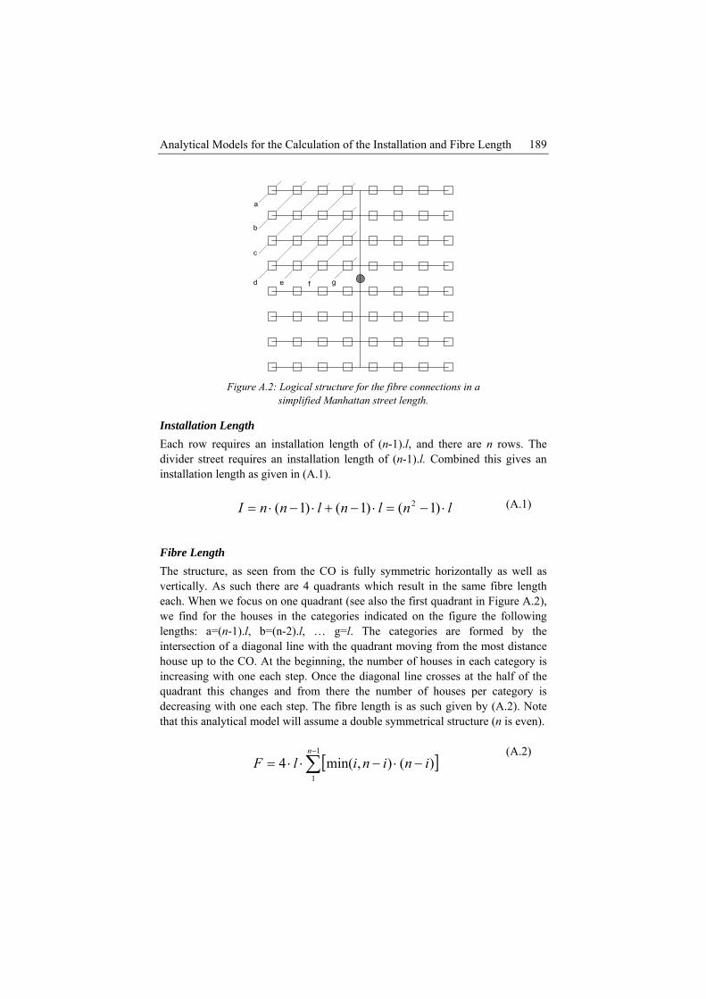
Analytical Models for the Calculation of the Installation and Fibre Length 189
a
b
c
d e f g
Figure A.2: Logical structure for the fibre connections in a
simplified Manhattan street length.
Installation Length Each row requires an installation length of (n-1).l, and there are n rows. The divider street require lation length of (n-1).l. Combined this gives an installation length as given in (A.1).
s an instal
(A.1)
the first q for the houses in the categories indicated on the figure the following
n-1).l, b=(n-2).l, … g=l. The categories are formed by the intersection of a diagonal line with the quadrant moving from the most distance house up t tegory is
with one each step. line crosses at the half of the
]
lnlnlnnI ⋅−=⋅−+⋅−⋅= )1()1()1( 2
Fibre Length The structure, as seen from the CO is fully symmetric horizontally as well as vertically. As such there are 4 quadrants which result in the same fibre length each. When we focus on one quadrant (see also uadrant in Figure A.2), we findlengths: a=(
o the CO. At the beginning, the number of houses in each caOnce the diagonalincreasing
quadrant this changes and from there the number of houses per category is decreasing with one each step. The fibre length is as such given by (A.2). Note that this analytical model will assume a double symmetrical structure (n is even).
[∑
−
−⋅−⋅⋅=1
)(),min(4n
ininilF(A.2)
1

Appendix A 190
A.1.2 Street Length The street length model will more closely follow one street and connect all houses from one street-wise cable along the street (see Figure A.3). Within the calculation of the analytical model, the cable is located at the middle of the street, but could easily be envisaged at one side of the street as well. As such it could consider an aerial installation in which the poles are placed at one side along the street and all houses at both sides can be connected from those poles.
Figure A.3: Logical structure for the fibre connections in a street length.
Installation Length In this structure we can group all houses per 2 as indicated in Figure A.3. For onnecting all couples of houses in 2 adjacent rows (one street) we use an
installation length of n.l. There are n/2 such adjacent rows. For connecting these connected couples of houses into one fully connected street, we need an installation length of (n-1).l, and again in n/2 adjacent rows. Finally the connection to the central office happens in the divider street which has a length of (n-2).l. Combined this gives an installation length as given in (A.3).
c
lnnlnlnnlnI ⋅−+=⋅−+⋅−⋅
+⋅
= )22
()2(2
)1(2
22
(A.3)
Fibre Length For the fibre length we can again follow the same reasoning as in the Manhattan case. Figure A.3 shows the structure and the categories in the first quadrant. The distances are the same as in the Manhattan case. The groupi gories is different and is as follows: a=2, b=2, c=4, d=4, e=2, f=2. The g ouping is per two
ng in cater

Analytical Models for the Calculation of the Installation and Fibre Length 191
hou s n group (a+b), (c+d), (e+f). For each of those
ber of houses is the same and the distance is double of the smallest + 1. Finally all this information ads to the following fibre distance in the structure (A.4). Note that this an ytical model assumes a symmetrical structure for the horizontal rows of houses (n/2 is even).
(A.4)
A.1.3 Double Street Length The double street length considers a street to consist of two sides. Crossing the street is often et side. This analytical model reduces the s to a minimum. As such it losely resembles a fully buried installation in the area (see Figure A.4).
ses and the distance between two consecutive horizontal streets is 2.l. Asuch per two categories we can againew groups, the num
leal
[ ]( )∑−
=
+⋅−⋅−⋅⋅⋅=12/
1
14)2/()2/,min(24n
i
ininilF
much more costly than the installation along the stre number of street crossing
c
Figure A.4: Logical structure for the fibre connections in a double street length
Installation Length Again we can make use of the structure mentioned above for the grouping of two houses. In this case the adjacent houses are not directly connected to each other as there is no crossing of the street with distance w. As such the installation length in this part is (l-w) and there are again n2/2 such adjacent houses. Considering the connecting in the rows, we need an installation length at both sides of the street. In all cases except the upper street side of the upper row and the lower street side of the lower row, we require an installation length of (n-1).l minus the street width w of the divider street which is not crossed here. In the

Appendix A 192
upper and lower street we do not need to take this into account. We have in total such n street sides. g the divider street, the installation length at both sides of the
sand thestreets t nd the number of connectors (at both sides) is as such 2.(n/2-1).(2.l-w). The resulting installation length is given in (A.5). In this calculation one should still add the length of installation crossing the streets. We need to do this at both sides for every two streets, except for the top and bottom street, where the street is only crossed at one side. Finally there is also one street crossing for connecting both sides of the street at the CO (A.6). Note again that the model assumes a highly symmetrical structure in which n is even.
n/2 streets and as Finally considerintreet will be the same. Again the horizontal streets are spaced at a distance of 2.l
length at one side to connect two streets is as such 2.l-w. The number of o connect is n/2 a
[ ]( )[ ]
wnnlnn
wln
lnwlnnwlnI
⋅⎥⎦
⎤⎢⎣
⎡−⋅+−⋅⎥
⎦
⎤⎢⎣
⎡−+
⋅=
−⋅⋅−⋅+
⋅−⋅+−⋅−⋅−+−⋅=
422
42
3
)2()12/(2
)1(21)2()(2
22
2
(A.5)
wnwnI SC ⋅−=⎥⎦⎤
⎢⎣⎡ +−⋅= )1(.12
22
(A.6)
Fibre Length The fibre length and cost is independent of the crossing of the street. It will be the same as in the case for the street length with the difference that in half of the houses, i.e. for each of the horizontal streets this is the street side closest to the CO, we can save a fibre distance of w. The fibre distance is given in (A.7).
F = Fibre street length – wn ⋅)2( 2 (A.7)

Analytical Models for the Calculation of the Installation and Fibre Length 193
A.2 Aerial Based Models In an aerial installation the choice of path is completely free. In these analytical models we consider the smallest possible installation length. We consider following two installation models: diagonal tree and simplified Steiner tree.
A.2.1 Diagonal Tree The diagonal tree considers an installation per four houses from the geometrical center of those four houses (see Figure A.5). The difference between the center and another location will not matter a lot as we will indicate in this section as well.
Figure A.5: Logical structure for the fibre connections in a diagonal tree
ngth ture is a repetitive structure (see also Figure A.5). In each block
s, we need 1 such structure, for 16 we need 4+1
Installation LeThe tree strucconnecting 4 houses, we find one smaller structure consisting of 4 connections from the center of this structure. Each 4 blocks are again combined by one structure of the same size in the center of the 4 structures. This aggregation is repeated in different levels combining always by a factor of four. Considering the combination of 4 housestructures, for 64 we need 16+4+1, etc. In general, we will need at the last level always 1, at the last but one level we need 4 and later on we need 4i structures and we will need log4n2 levels. Note that the last level has 40 structures. We need a number of structures as defined by (A.8). In this the (*) indicates the usage of a

Appendix A 194
partial sum of a geometric series. Although the formula does not indicate the highly symmetrical structure, the model will assume a structure in which n is a power of 2, especially regarding the fibre length.
3410 −=i
141421)1(log*1log 2
42
4 −=
−=
+−−
∑ nnni
(A.8)
( )laI
lla
⋅⋅=⋅=
⋅=⋅=
224
2/2)45cos()2/( o
lblI
lab
⋅+=+⋅=
⋅=⋅=
)22(2
22
Figure A.6: Installation Length for connecting four houses from one drop box using straight lines
The total installation length is then this number multiplied by the length of the structure for connecting 4 houses. In this case the length of the middle of the
houses perimeter to the center of the four houses is equal to l⋅⋅ )22( (see also Figure A.6). As mentioned before, the longest distance from one house to the
other three houses would be l⋅+ )22( instead (see also Figure A.6). In case the installation is performed from the center of the four house, the total installation length is given in (A.9).
lnI ⋅⋅⋅⎟⎟
⎠
⎞⎜⎜⎝
⎛ −= )22(
312
(A.9)
Fibre Length The fibre length is calculated in a recursive manner. Figure A. 7 links to the different steps in this approach. The smallest fibre length that we will need in the
calculations is indicated by y and is equal to ( ) l⋅2/2 (see also a in Figure A.6).

Analytical Models for the Calculation of the Installation and Fibre Length 195
Figure A. 7: Recursive structure used in the analytical calculation
ngth
er, has no extra fibre length and will as such stop the cursion.
At each level we will also need additional fibre for connecting the three most remote blocks to the edge of the block (by which it connects to a larger block). In this manner we lengthen the fibre of 3/4th of all customers residing in the considered block. The number of customers at one side of the block is equal to 2x and the total number of customers residing in the block is equal to 2x.2 or 4x. The number of customers to connect is then 3.4x-1. Finally the fibre length to connect each customer to the edge will also be depending on the size of the block. A block of level x, has a total length of 2.(2x-1).y from edge to edge. To connect all three smaller blocks to the edge we need a length from the edge to the center and one extra y beyond this center to connect to the edge of the smaller block. As such we need a locks.
he total length i
of the fibre le At the highest level we find four equal blocks, in which each blocks connects n2/4 customers. For connecting those four blocks, we need a fibre length of y dedicated for each customer (from a to b). The total length is then given by n2.y + 4.(length of each block). We indicate the level of the block by an x which is the number of customers on one side as a factor of 2 (log2). At all lower levels, we always connect again four smaller blocks. F0, which contains only one customre
fibre length of 2x.y per customer of the 3 smaller bs given in (A.10). T
1)(log2
24 −⋅+⋅ nFyn (A.10)
⎩⎨⎧
=⋅⋅+⋅= −
−
02434
0
11
FyFF xx
xx

Appendix A
196
A.2.2 Simplified Steiner Tree The simplified Steiner tree uses the optimal structure for the connection of every block of four houses (see Figure A. 8). It is easy to find a Steiner tree for this structure considering the fact that in a geometrical Steiner tree a Steiner point will always connect three links at an angle of 120° between each two adjacent links [A.1] (see especially thumbnail 15). This is the smallest possible connection of the four houses and serves as such as the lower boundary of the installation length. It is hardly useable in a realistic installation as the operator would need to install a dedicated pole for each two houses.
Figure A. 8: Logical structure for the fibre connections in a simplified Steiner tree
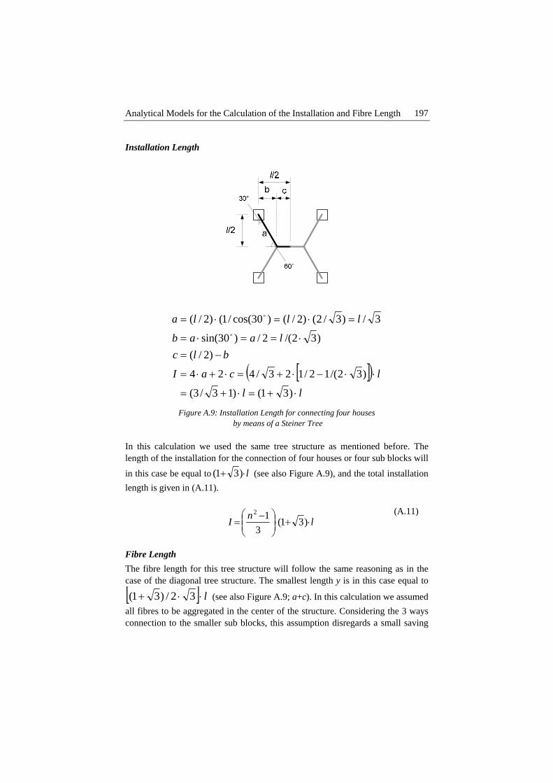
Analytical Models for the Calculation of the Installation and Fibre Length 197
Installation Length
[ ]( )ll
lcaI
blclaab
llla
⋅+=⋅+=
⋅⋅−⋅+=⋅+⋅=
−=⋅==⋅=
=⋅=⋅=
)31()13/3(
)32/(12/123/424
)2/()32/(2/)30sin(
3/)3/2()2/()30cos(/1()2/(o
o
Figure A.9: Installation Length for connecting four houses by means of a Steiner Tree
In this calculation we used the same tree structure as mentioned before. The length of the installation for the connection of four houses or four sub blocks will
in this case be equal to l⋅+ )31( (see also Figure A.9), and the total installation length is given in (A.11).
lnI ⋅+⋅⎟⎟
⎠
⎞⎜⎜⎝
⎛ −= )31(
312
(A.11)
Fibre Length The fibre length for this tree structure will follow the same reasoning as in the case of the diagonal tree structure. The smallest length y is in this case equal to
[ ] l⋅⋅+ 32/)31( (see also Figure A.9; a+c). In this calculation we assumed all fibres to be aggregated in the center of the structure. Considering the 3 ways connection to the smaller sub blocks, this assumption disregards a small saving

Appendix A 198
possible by connecting the closest edge over the shortest path (2 times a in Figure A.9).

Analytical Models for the Calculation of the Installation and Fibre Length 199
References [A.1] R. L. Graham, “The shortest network problem”, University Video
Communications, Open Source Video http://www.archive.org/details /RonaldLG1988.

B Adoption and Pricing;
Koer avet, Piet Demeester
IEEE Communications Magazine, ISSN 0163-6804, vol. 46, no. 8, pp.112-118, August 2008
Abstract The adoption of IPTV increases the competition for the telecom operators. Especially video on demand (VoD) and the move to high definition television (HDTV) push the bandwidth requirements to the limits. It is very challenging for the operator to construct a successful and sustainable introduction of IPTV over the existing infrastructure. This paper gives an overview of a typical business case followed by a detailed discussion on the adoption and the evaluation of the outcome. The results of this paper indicate the importance of a correct choice of adoption model and related parameters. It illustrates how different IPTV-specific effects on adoption, i.e.
the Underestimated Elements of a Realistic IPTV Business Case
en Casier, Bart Lannoo, Jan Van Ooteghem, Sofie brugge, Didier Colle, Mario PickV
Appendix B 202
competition and analog switch-off, might have a considerable impact on the outcome. Next to the adoption, the paper shows how the outcome of the business case can be used within pricing decisions by setting sustainable and competitive boundaries on the tariff. Finally as pricing will also have an important impact on the adoption (e.g. a price reduction could lead to an increase in adoption) the possible impact of this feedback loop is indicated in the paper. In this sense the approach discussed in the paper could easily be extended with a highly detailed cost model of the network architecture and technology, leading to a full business case for IPTV introduction by a telecom operator.
B.1 Introduction Broadband access is gaining widespread adoption on a global scale, and is becoming in most advanced regions more and more a commodity service on which customers rely constantly. Additionally, broadband access technologies currently offer a bandwidth ranging roughly from 3 up to 100 Mbps in the access er an enjoyable video service on et access services, the fast
higher bandwidths opens up the field for digital television s
premises a setup box is attached to their existing video
r the IPTV offering and the right implementation over the
ks of such a business case. As
the iconstruct a full business case.
. While the lower boundary of this bandwidth is hardly enough to off top of telephony and Intern
evolution to overalloffering . Digital television (DTV) services are actually a broad realm of different services (e.g. video on demand (VoD), broadcast, network personal video recorder (NPVR), etc.) and technical platforms (digital video broadcasting terrestrial (DVB-T) or satellite (DVB-S), IPTV, over-the-top video (e.g. YouTube), etc.). We focus on DTV as offered by fixed broadband access networks. In the remainder of the paper, we refer to this as IPTV. At the customers’infrastructure and it decodes the digital signal into the required television signal. Thus, from a customer point of view there is little change and the meaningful differences between alternative IPTV offerings are functionality, quality and tariff. From an operator point of view, the different possible services and technical platforms will have an important impact on traffic and thus on the costs. In order to find the sweet spot for IPTV, an operator should build a business case in which the costs, caused by functionality and quality, and revenues, gained from customer adoption, are in balance to each other. This means selecting the right set of conditions fonetwork. In section 2 we detail the different building blocthe focus of this paper is on adoption and evaluation, this section indicates how
nformation of this paper should be completed with a detailed cost model to
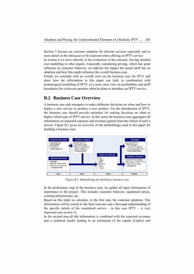
Adoption and Pricing; the Underestimated Elements of a Realistic IPTV … 203
Se tion 3 focuses on customer adoption for telecom services especially and in e detail on the intricacies to be expected when offering an IPTV service. ection 4 we
cmorIn s move directly to the evaluation of the outcome, leaving detailed
stinfluado
ashowtechbou TV service.
co modelling to other papers. Especially considering pricing, which has great ence on customer behavior, we indicate the impact the actual tariff has on
ption and how this might influence the overall business case. Fin lly we conclude with an overall view on the business case for IPTV and
how the information in this paper can lead, in combination with nological modelling of IPTV, to a more clear view on profitability and tariff ndaries for a telecom operator when he plans to introduce an IP
B.2 Business Case Overview A business case aids managers to make deliberate decisions on when and how to deploy a new service or produce a new product. For the introduction of IPTV, the business case should provide rationales for making decisions on when to deploy which type of IPTV service. In this sense the business case aggregates all information on expected expenses and revenues gained from the rollout of such a service. Figure B.1 gives an overview of the methodology used in this paper for building a business case.
Figure B.1: Methodology for building a business case
In the preliminary step of the business case, we gather all input information of importance to the project. This includes customer behavior, equipment prices, existing infrastructure, etc. Based on this input we calculate, in the first step, the customer adoption. This
formation will be crucial to the final outcome and a thorough understanding of the specific details of the considered s in this case IPTV – is very important (see section 3). In the second step all this information is combined with the expected revenues and a technical model leading to an estimation of the capital (CapEx) and
inervice –
Appendix B 204
operational (O s plenty of iew of an approach
l s on CapEx. Fewer articles
view on the expected evolution of customer usage of the ddition the possible impact of two important effects
nd analog switch-off – is described.
pEx) expenses. Considering the cost modelling, there iliterature available. For instance [B.1] contains a clear overvto calcu ate the expenses for IPTV, with a main focuelaborate on OpEx as these are typically much harder to model, require a deep introspection of the telecom operator and might involve confidential information on operational processes, costs of manpower and tooling. For an operator itself however, confidentiality and introspection will not pose any problems and OpEx can be calculated by basing them on activity based costing as is done in [B.2] or [B.3]. As already mentioned, this paper will not treat the construction of a cost and revenue model. To elaborate a full business case however, it should be completed with detailed information about both costs and revenues. The final step of the business case relates the different cash flows generated by the revenues and expenses for deploying IPTV over the network. In order to evaluate the project, we can calculate important economical indicators, like return-on-investment (ROI), net present value (NPV) or payback period. Further, in a valid business case we expect all expenses to be at least covered by all revenues over the given period of the project. Bottom prices for the service can then be calculated from the expected costs and expenses. It should be noted that the proposed business case focuses on the adoption and pricing and does not contain all possible intricacies of the parameters of such problem, but only a subset of the interactions between the different elements. Considering the high number of technological, strategic and business parameters, constructing a fully detailed model is a very complex task.
B.3 Adoption of IPTV The purpose of a good adoption model is to forecast in a reliable manner the number of customers and their behavior as a function of time. In this way it fits within the first step of the business case overview as proposed before. Different models exist and will not all lead to the same reliability in case of IPTV. Therefore we first select the most reliable adoption model for IPTV. We complement this with a different IPTV services. In afor IPTV – competition a
B.3.1 Customer Adoption Different models can be used for modelling the adoption of a new technology or service. These models typically resemble an S-shaped curve for presenting the adoption as a function of the time. Different mathematical formulations can be used for these S-curves, leading to slight variations in the adoption models. Often used models within literature, both in telecom and more in general, are Rogers,
Adoption and Pricing; the Underestimated Elements of a Realistic IPTV … 205
Bass, Fisher-Pry and Gompertz. Roughly speaking information used for properly estimating the parameter values of these models can be gained from two sources: • Fitting of the mathematical adoption models to existing adoption data
available. This requires sufficient data to be available and thus requires an existing customer base. For IPTV this might not always be the case.
• Extrapolation from existing comparable technologies. In the case of IPTV we could make an extrapolation based on telecom broadband adoption on the one hand and on broadcast television (color or black and white) on the other hand. For television as well as broadband adoption, there is a lot of information available.
When considering the different mathematical formulations for modelling the adoption it is clear that not all fittings will be as close to the actual data. However, the reliability of the forecasted adoption is of huge importance. Intrinsically IPTV is built on both broadband and television. As broadband access (and its adoption) is more novel compared to broadcast television, we have used the broadband data to select the most reliable model for forecasting IPTV adoption. To make a well-considered selection, we have fitted the adoption models to existing data in two different ways. First, we have investigated the reliability of the models in the range of the data. Therefore we have fitted each model to all available data and have calculated the difference between the fitted and exact data. The more reliable a model, the more closely it will follow the exact data. Secondly we have investigated the reliability of the model for forecasts beyond existing data. Therefore we have fitted the model to the first available data points (e.g. first 50%) and have then calculated the difference between the fitted (forecasted) values and the exact values for the remaining data points. The more reliable a model, the less difference there will be between the forecasted and exact data for this remaining part. Different fittings made on existing telecom data for the adoption of broadband in Belgium show that both the existing data and forecasted data is most reliably modelled using a Gompertz adoption model.
B.3.2 Service Adoption In addition to the size of the customer base, the operator should also estimate how often the customers will use the functionality and different services of IPTV. From a cost point of view, especially the expected uptake of VoD and more personalized content (e.g. commercials, NPVR) is important. Since the increased functionality and freedom of choice offered by the above services allows exploiting the Long Tail of video content, a gradual shift to more unicast instead of broadcast and multicast traffic can be expected. In combination with a
Appendix B 206
growing number of TV-sets per household, this could (in the end) lead to a (far) th a dedicated video stream per person. ost probably also bring an increase in quality which currently
stTypicaltempereAlthoug ct of both the move to personalization and higher quality is hfitted to e seen as ab(e.g. SD
B.3.3 Within rket, as is the case for telecom services and etelecoimpact er DTV offerivGame competplayers nt business cases shIt thus which mOn the substitu [B.4]. In such a model, diSDTV v eneral a notion of the perceived quality) will
teract with each other and with the initial customer adoption. A generation with perior technology, quality or service will take over the adoption of the other
enerations. It is fairly straightforward to extend the best fitting – here Gompertz – adoption models with an identical substitution model.
B.3.4 Analog Switch Off Regulation might also have a considerable influence on the final adoption. In the case of DTV, a high impact will probably be caused by the transition to digital TV, commissioned by the Federal Communications Commission (FCC) to take place on February 17th 2009 in America and scheduled from now up to 2012 in several European countries.
future scenario wiThe future will m
arted with a move from standard definition television (SDTV) towards HDTV. ly this will increase the bandwidth required per stream, somewhat d by the continuous advances in video codecs. h the impa
ard to estimate, an increase in both is very likely and their evolution could be existing trends to get a more clear view. As both could b
dditional services (e.g. VoD-service, HDTV-service, etc.), they can be modelled y adoption curves as well, albeit in competition with the other IPTV services
TV-service). The issue of competition is tackled in the next paragraph.
Competition a highly competitive ma
specially for an IPTV service where different players (e.g. content providers, m operators, etc.) are offering comparable services, there will be a direct
of competition on the adoption. Also the competition with othngs (not over fixed broadband access) such as DVB-T or DVB-S will be
ery important for the success of IPTV. theory is a very complete approach for modelling the effect of ition. It involves the construction of a detailed business model of all and their possible actions. Additionally all the differe
ould interact with each other to reflect the impact of the actions of all players. involves a lot of work on the integrated models and a lot of input data ight not be available. other hand, it might suffice to use a combination of an adoption and tion model as proposed by Norton and Bass
fferent generations of the same or comparable technology or service (e.g. ersus HDTV, or more in g
insug
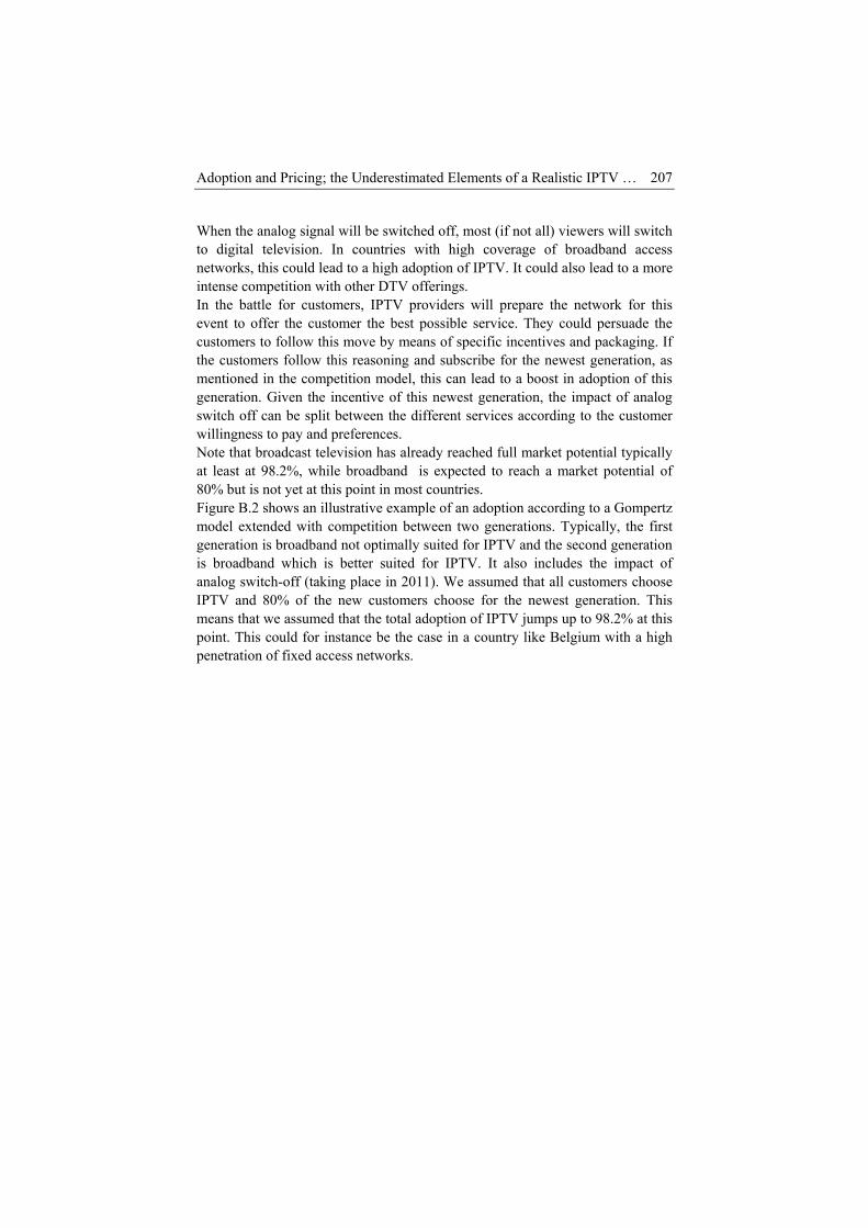
Adoption and Pricing; the Underestimated Elements of a Realistic IPTV … 207
When the analog signal will be switched off, most (if not all) viewers will switch to digital television. In countries with high coverage of broadband access networks, this could lead to a high adoption of IPTV. It could also lead to a more intense competition with other DTV offerings. In the battle for customers, IPTV providers will prepare the network for this event to offer the customer the best possible service. They could persuade the customers to follow this move by means of specific incentives and packaging. If the customers follow this reasoning and subscribe for the newest generation, as mentioned in the competition model, this can lead to a boost in adoption of this generation. Given the incentive of this newest generation, the impact of analog switch off can be split between the different services according to the customer willingness to pay and preferences. Note that broadcast television has already reached full market potential typically at least at 98.2%, while broadband is expected to reach a market potential of80% but is not yet at this point in most countries. Figure Bmodel egeneris broanalog switch-off (taking place in 2011). We assumed that all customers choose IPTV and 80% of the new customers choose for the newest generation. This means that we assumed that the total adoption of IPTV jumps up to 98.2% at this
th a high
.2 shows an illustrative example of an adoption according to a Gompertz xtended with competition between two generations. Typically, the first
ation is broadband not optimally suited for IPTV and the second generation adband which is better suited for IPTV. It also includes the impact of
point. This could for instance be the case in a country like Belgium wipenetration of fixed access networks.
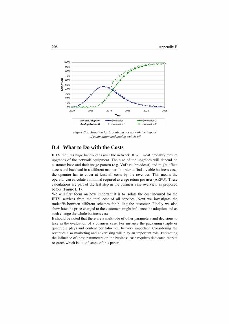
Appendix B 208
0%
10%
20%
30%
40%
50%
60%
70%
80%
90%
100%
2000 2005 2010 2015 2020 2025
Year
Ado
ptio
n
Normal Adoption Generation 1 Generation 2Analog Swith-off Generation 1 Generation 2
ption for broadband access with the impact Figure B.2: Ado of competition and analog switch-off
B.4 What to Do with the Costs IPTV requires huge bandwidths over the network. It will most probably require upgrades of the network equipment. The size of the upgrades will depend on customer base and their usage pattern (e.g. VoD vs. broadcast) and might affect access and backhaul in a different manner. In order to find a viable business case, the operator has to cover at least all costs by the revenues. This means the operator can calculate a minimal required average return per user (ARPU). These calculations are part of the last step in the business case overview as proposed before (Figure B.1). We will first focus on how important it is to isolate the cost incurred for the IPTV services from the total cost of all services. Next we investigate the tradeoffs between different schemes for billing the customer. Finally we also show how the price charged to the customers might influence the adoption and as such change the whole business case. It should be noted that there are a multitude of other parameters and decisions to take in the evaluation of a business case. For instance the packaging (triple or quadruple play) and content portfolio will be very important. Considering the revenues also marketing and advertising will play an important role. Estimating the influence of these parameters on the business case requires dedicated market research which is out of scope of this paper.
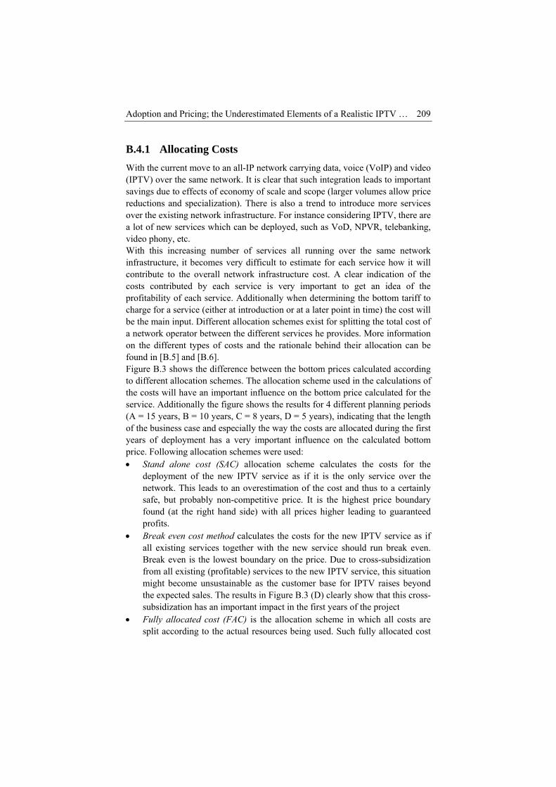
Adoption and Pricing; the Underestimated Elements of a Realistic IPTV … 209
B.4.1 Allocating Costs With the current move to an all-IP network carrying data, voice (VoIP) and video (IPTV) over the same network. It is clear that such integration leads to important savings due to effects of economy of scale and scope (larger volumes allow price reductions and specialization). There is also a trend to introduce more services over the existing network infrastructure. For instance considering IPTV, there are a lot of new services which can be deployed, such as VoD, NPVR, telebanking, video phony, etc. With this increasing number of services all running over the same network infrastructure, it becomes very difficult to estimate for each service how it will contribute to the overall network infrastructure cost. A clear indication of the costs contributed by each service is very important to get an idea of the profitability of each service. Additionally when determining the bottom tariff to charge for a service (either at introduction or at a later point in time) the cost will be the main input. Different allocation schemes exist for splitting the total cost of a network operator between the different services he provides. More information on the different types of costs and the rationale behind their allocation can be found in [B.5] and [B.6]. Figure B.3 shows the difference between the bottom prices calculated according to different allocation schemes. The allocation scheme used in the calculations of
ttom price calcuthe costs will have an important influence on the bo lated for the
osts for the
(at the right hand side) with all prices higher leading to guaranteed
• Break even cost method calculates the costs for the new IPTV service as if all existing services together with the new service should run break even. Break even is the lowest boundary on the price. Due to cross-subsidization from all existing (profitable) services to the new IPTV service, this situation might become unsustainable as the customer base for IPTV raises beyond the expected sales. The results in Figure B.3 (D) clearly show that this cross-subsidization has an important impact in the first years of the project
• Fully allocated cost (FAC) is the allocation scheme in which all costs are split according to the actual resources being used. Such fully allocated cost
service. Additionally the figure shows the results for 4 different planning periods (A = 15 years, B = 10 years, C = 8 years, D = 5 years), indicating that the length of the business case and especially the way the costs are allocated during the first years of deployment has a very important influence on the calculated bottom price. Following allocation schemes were used: • Stand alone cost (SAC) allocation scheme calculates the c
deployment of the new IPTV service as if it is the only service over the network. This leads to an overestimation of the cost and thus to a certainly safe, but probably non-competitive price. It is the highest price boundary found profits.
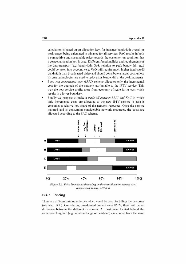
Appendix B 210
calculation is based on an allocation key, for instance bandwidth overall or vance for all services. FAC results in both
owards the customer, on condition that
h at the peak moment)
st which
trade-off between LRIC and FAC in which e allocated to the new IPTV service in case it
e low share of the network resources. Once the service matured and is consuming considerable network resources, the costs are llocated according to the FAC scheme.
peak usage, being calculated in ada competitive and sustainable price ta correct allocation key is used. Different functionalities and requirements of the data-transport (e.g. bandwidth, QoS, relation to peak bandwidth, etc.) could be taken into account. (e.g. VoD will require much higher (dedicated) bandwidth than broadcasted video and should contribute a larger cost, unless if some technologies are used to reduce this bandwidt
• Long run incremental cost (LRIC) scheme allocates only the incremental cost for the upgrade of the network attributable to the IPTV service. This way the new service profits more from economy of scale for its coresults in a lower boundary.
• Finally we propose to make aonly incremental costs arconsumes a relativ
a
Figure B.3: Price boundaries depending on the cost-allocation scheme used
(normalized t max. SAC (C))
.4.2 Pricing There are different pricing schemes which could be used for billing the customer
d content over IPTV, there will be no ifference between the different customers. All customers located behind the
same switching hub (e.g. local exchange or head-end) can choose from the same
o
B
(see also [B.7]). Considering broadcasted

Adoption and Pricing; the Underestimated Elements of a Realistic IPTV … 211
stream of channels at the same time, and are charged the same hewatch or not (in some cases there is an additional charge for extra channels with specific content).
hen VoD is considered, the situation is different. Providing VoD to many
makes more sense to use advanced pricing schemes. The revenue effect of using a specific pr ing scheme can be found through simulations, in whi lated according to
e specific pricing scheme used. The reaction (renting a video or not) of each of
ricing schemes: Flat rate or content-based – charging a fixed tariff per movie possibly
epending on the content, quality or length of the movie. • Time of day based – charging a tariff depending on the time of day the
movie is rented. A higher tariff is charged for movies rented during a peak period.
• Congestion based – the tariff charged is depending on the level of cong is linearly incre e eak.
• Auct d) Vickrey aucti pay, from whic arket rice will be the tariff charge
Traffic u t 0% traffic congestio thout any blocking. e situat gure as the advanced icing sc than those of flat f . Finally emes were initialized give thGoing fro flat rat e for the customer avoid th parency of
e tariff charged to n based it is
ing traffic
w ther they
Wcustomers requires large amounts of bandwidth and could lead to congestion. In such a situation, it
icch the tariff charged to the customer is calcu
ththe customers is simulated consistently with probability, the tariff and their willingness to pay. The final outcome is a simulated list of films being rented, along with the charged tariff. It is easy to calculate the revenues for the different pricing schemes. Figure B.4 shows the profit per movie as a function of the traffic congestion in the network for the following p•
d
estion in the network. In our implementation the tariff ased onc more than 70% of the bandwidth is consumed at pion based – the tariff charged is deduced from a (agent base
. In this ton he customers indicate the price they are willing toh a m clearing price is deduced. This market clearing p
d to all customers who bid at least this price.
sed for the simulation has peaks between 18h and 22h. A the highn est peak consumes up all available bandwidth wi
Th ion below 0% traffic congestion is left out of the fi pr hemes lead to profits per movie which are lower ee the parameters for the different pricing sch to e same results at 0% traffic congestion. m e to auction based, there is an increasing incentiv
to e congested periods. On the other hand, the transthe customer will decrease and in case of auctioth
even questionable whether the customers would accept such pricing scheme. On the other hand, auction based will clearly give the best results, followed by congestion based. Flat rate and time-of-day have lower profits per movie. It is important to note the result of the time-of-day pricing scheme. This pricing scheme will result in a decrease of profit per movie for increas
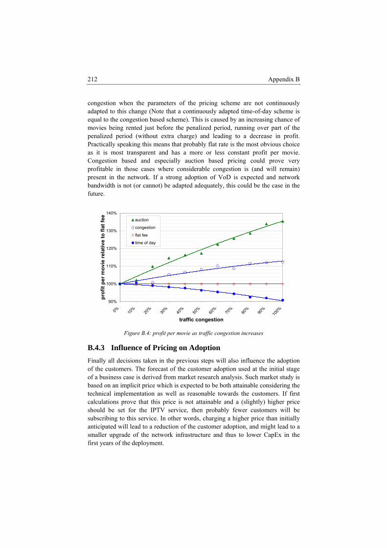
Appendix B 212
co gestion when the parameters of the pricing scheme are not continuously ted to this change (Note that a continuously adapted time-of-day scheme is
al to the cong
nadapequ estion based scheme). This is caused by an increasing chance of
vpen .
ractically speaking this means that probably flat rate is the most obvious choice
ases where considerable congestion is (and will remain) present in the network. If a strong adoption of VoD is expected and network
not) be adapted adequately, this could be the case in the
mo ies being rented just before the penalized period, running over part of the alized period (without extra charge) and leading to a decrease in profit
Pas it is most transparent and has a more or less constant profit per movie. Congestion based and especially auction based pricing could prove very profitable in those c
bandwidth is not (or canfuture.
90%
0% 10%
20%
30%
40%
50%
60%
70%
80%
90%
100%
traffic congestion
100%
pr
110%
120%
130%
140%
ofit
per m
ovie
rela
tive
to fl
at fe
e
auction
congestion
flat fee
time of day
Figure B.4: profit per movie as traffic congestion increases
.3 Influence of Pricing on AB.4 doption Finaof thof abase e both attainable considering the
calc ot attainable and a (slightly) higher price ould be set for the IPTV service, then probably fewer customers will be
tructure and thus to lower CapEx in the first years of the deployment.
lly all decisions taken in the previous steps will also influence the adoption e customers. The forecast of the customer adoption used at the initial stage
business case is derived from market research analysis. Such market study is d on an implicit price which is expected to b
technical implementation as well as reasonable towards the customers. If first ulations prove that this price is n
shsubscribing to this service. In other words, charging a higher price than initially anticipated will lead to a reduction of the customer adoption, and might lead to a smaller upgrade of the network infras
Adoption and Pricing; the Underestimated Elements of a Realistic IPTV … 213
In an IPTV environment there might be considerable investments at the start of
esults from such an iterative calculation have been indicated in [B.6] and show that, depending on the expected impac of the price-change on the customer adoption m nd. We considered t . In a best ase scenario we considered ponse to the change in
tariff. In the worst case scenario we considered a much higher customer response (quadratic). More in detail the results show a 10% difference from the implicit (market research) price might lead to a difference of slightly less than 10% (best case) and up to 25% (worst case). Clearly this risk cannot be discarded and should be taken into calculations.
B.5 Conclusion When building a business case for the deployment of an IPTV service, there are more than just technical issues (e.g. comparing technologies, optimizing traffic, etc.) to take into account. The paper shows where the more technical papers can be extended to a full business case. First doption, both in customer base and in usage, will play an important role. Th re the paper contains an overview of the customer adoption models and di ent parameters which influence this adoption in case of IPTV. Most impor eters here are the choice of the adoption model (for which Gompertz is found to be the best), the extension towards modelling competition and the effect of analog switch-off. Secondly the evaluation of costs and especially pricing will have an important influence on the business case. By allocating costs fairly to the IPTV and all other services, more competitive yet still sustainable lower-boundaries on the pricing can be calculated. The second pricing parameter is the pricing scheme to use, for which flat rate pricing is optimal in a low congestion situation and congestion-based or auction-based are promising for situations with higher congestion in the network. Finally, as the pricing will also influence the customer adoption, the outcome of the business case might change its inputs. This effect should not be neglected as it might lead to important differences and coupled risks or opportunities.
the deployment for installing the content servers, acquiring the right content and upgrading the bandwidth in the access network where necessary. As thus for IPTV the loss of revenues, caused by the reduction of the customer base, could impact the business case more substantially than the reduction (postponing) of CapEx. In such case this leads to a further increase of the price. R
t odel either a slight relaxation or reinforcement can be fouwo different impacts of the tariff on the adoption model
a limited (linear) customer resc
aerefoffer
tant param
Appendix B 214
References [B.1] S. Han, S. Lisle and G. Nehib, “IPTV Transport Architecture
Alternatives and Economic Considerations.” IEEE Commun. Mag., Feature Issue: IPTV Systems, Standards and Architectures, Feb. 2008, pp. 70-77.
[B.2] R. Kaplan, S. Anderson, ”Time–Driven Activity-Based Costing,” Harvard Business Review, Vol. 82 , no. 11, 2004, pp.131-138.
[B.3] S. Verbrugge, D. Colle, M. Pickavet, P. Demeester, S. Pasqualini, A. Iselt, A. Kirstädter, R. Hϋlsermann, F-J. Westphal, M. Jäger, “Methodology and input availability parameters for calculati g OpEx and CapEx costs for realistic work scenarios,” Journal of Optical Networki y, Vol. 5, nr. 6, June 20
[B.4] J.A. Norton and F.M. Bass, “A Diffusion Theory Model of Adoption and
- Investment analysis modeling.” vol. 2 of 4, “annex A Investment, operation, administration and maintenance cost modeling,” 2000.
[B.6] K. Ca eersman, M. Pickavet, P. Demeester, itivity and iterative calculations on cost-based pricing,” published in Proceedings (on CD-ROM) of CTTE2007, the 6th Conference on Telecommunication Techno-Economics, Espoo, Finland, 14-15 June 2007.
[B.7] C. Courcoubetis and R. Weber, “Pricing Communication Networks,” John Wiley & Sons, 2003.
n net
ng, Feature Issue: Optical Network Availabilit06, pp. 509-520.
Substitution for Successive Generations of High-Technology Products,” Management Science, Vol. 33, no. 9, Sept. 1987, pp. 1069-1086
[B.5] Eurescom, Project P901-PF, “Extended investment analysis of telecommunication operator strategies, Deliverable 2
sier, S. Verbrugge, J. Van Ooteghem, D. Colle, R. M“Impact of sens

C e
Calculations on Cost-Based Pricing Impact of Sensitivity and Iterativ
K. Casier, S. Verbrugge, J. Van Ooteghem, D. Colle, R. Meersman, M. Pickavet, P. Demeester Proc. of Conference of Telecommunication, Media and Internet Techno-Economics (CTTE) 2007, Helsinki, Finland, 14-15 June 2007 Key words pricing, cost-allocation, techno-economic
Abstract When introducing a new telecom service it is very important for the operator to set the tariff right. Being too prudent by setting the tariff too high will most probably put the operator out of competition. On the other hand, setting the tariff too low might skim profits, lead to cannibalization of other services, forcing the operator to raise the tariffs – which clearly has a negative impact on the user satisfaction and coupled market share. Current telecom networks make progressively use of an all IP network, in which all services run over the same infrastructure. While this move allows reducing costs due to economies of scale
Appendix C 216
and scope, it disguises the costs of each of the different services within the full costs of the network. As the tariff is expected to be sustainable in the long run, the costs associated to the roll-out of the new service should at least be covered by the (forecasted) revenues. Different allocation schemes can be used for discovering the costs associated to each of the services over the network, and
rtant changes to these margins when quantifyin
C.1 Introduction Pricing is t determinin o charg customers for a specific goo ariff will cle ly have a great influence on the customers d o buy th servic etting the right tariff is very the elastici nd in t ather high, it is also practic se the a later is means that, when an op service at a tariff which is set too low, he will run an unpro ight in more ad han expected. This is clea able situa e othe ing a tariff too high will re tive in whi rator will most probably no xpe ted and might lose market share to other, more compeWhen intro rvice, the erator has lots take into account and ke during th pricing process
the first place the operator can choose which pricing scheme to use for
more advanced pricing schemes require additional logic in the network, will have a better incentive-coupling of the customer, resulting in
per capacity, but are less transparent to the customer,
ff,
their use leads to a better understanding of the margins on sustainable tariffs as opposed to stand alone or break even calculations. The whole calculation is largely dependent on the forecasts of adoption, bandwidth growth and cost evolution. Within this paper we will first investigate the sensitivity of the calculated tariff margins on changes of these inputs. In a second phase we will investigate what impact the calculated tariff margin might have on the adoption of the service. We also indicate that there are impo
g this impact and using iterative calculations.
he process of g what t e to the d or service. As this t arecision whether t e good or e or not, s important. As ty of dema elecom is r
ally infeasible to rai tariff in stadium. Therator introduces a new
which mfitable service, rly an unsustain
even tion. On th
ga option tr hand, sett
sult in a non competit get the adoption as e
situation, ch the opec
titive operators. ducing a new se op of parameters to choices to ma e :
Incharging the service. Different alternatives exist in which each has its own pros and cons. Typically the
a more optimized revenuenegatively impacting satisfaction and possibly adoption as well. Following papers discuss in more detail a comparison of these pricing schemes [C.1], [C.2], [C.3], [C.4], [C.5], [C.6]. Coupled to the pricing scheme, the operator can also choose how to charge the tariff to the customer, in which either prepaid and post-paid charging can be used. Finally, and most importantly, the operator should also choose which tariff (mean) to charge to the customers. He aims to be as profitable as possible while maintaining a competitive position. It is clear that the boundary to this tari

Impact of Sensitivity and Iterative Calculations on Cost-Based Pricing 217
under which the service will no longer be profitable, is to be calculated from the costs for introducing this new service and will be depending on the estimated number of customers for the service. In this paper we will focus on how to determine such a tariff and what its
plications are. For the calculations we start from [C.7] in which a refined calculation of this boundary, making use of cost-allocation is given. Within this calculation, the lated from the xpected adoptio isting over the
deduce different realistic Bass adoption how the tariff might influence this adoption n could lead to important differences with a
ection 2 describes in short the calculations as defined in [C.7] and will indicate
From this sensitivity information it is clear that changes to the doption-curve might have an important impact on the final result.
Section 4 describes how the original case-study can be extended to make use of the new adoption-curves and iterative calculations. The results of these calculations are compared to the results obtained in case no iterative calculations are used. Finally, section 5 contains a summary of the main conclusions of the work
im
costs of introducing a new service are calcun and allocated to the different services exe
network. From this cost, the tariff to charge to each customer can be calculated. Considering now that the operator uses this tariff as introduction tariff for the new service, this could have an impact on the adoption of the service. In case the adoption curve for the new service is constructed taking a higher (implicit) tariff into account, the adoption will most probably increase faster as the introduction tariff is lower than the tariff (implicitly) assumed while constructing the adoption curve. In the remainder we will first curves [C.8], make an estimation of and show how an iterative calculationon-iterative calculation when the assumed introduction tariff (original adoption curve) differs from the final tariff. Additionally we will also extend the non-iterative calculation with sensitivity analysis in order to determine the most important input-parameters. The remainder of the paper is organized as follows: Sthe points of extension and give more details on the inputs for the calculations. Different adoption-curves will be fitted to existing information. Section 3 adds sensitivity analysis to the existing calculations and results of the original paper. a
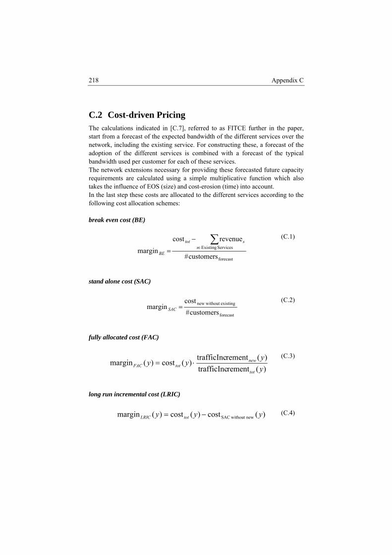
Appendix C 218
C.2 Cost-driv
h of the different services over the etwork, including the existing service. For constructing these, a forecast of the
adoption of the different services is co bined with a forecast of the typical bandwidth used per customer for each se services. The network extensions necessary for providing these forecasted future capacity requirements are calculated using a simple multiplicative function which also takes the influence of EOS (size) and cost-erosion (time) into account. In the last step these costs are allocated to the different services according to the following cost allocation schemes: break even cost (BE)
en Pricing The calculations indicated in [C.7], referred to as FITCE further in the paper, start from a forecast of the expected bandwidtn
mof the
forecast
ServicesExisting
customers#
revenuecostmargin
∑∈
−
= sstot
BE
(C.1)
stand alone cost (SAC)
forecast
existingwithoutnew
customers#cost
margin =SAC (C.2)
fully allocated cost (FAC)
)(rementtrafficInc)(rementtrafficInc
)(cost)(marginyy
yytot
newtotFAC ⋅=
(C.3)
long run incremental cost (LRIC)
)(cost)(cost)(margin new without SAC yyy totLRIC −= (C.4)
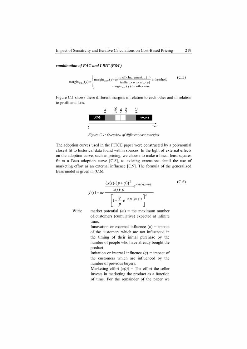
Impact of Sensitivity and Iterative Calculations on Cost-Based Pricing 219
combination of
FAC and LRIC (F&L)
⎪⎩
⎪⎨⎧
⇔
≥⇔
otherwise)(margin
th)(rementtrafficInc)(rementtrafficInc)(margin
yyyy
FAC
tot
newLRIC=
reshold)(margin & yLF
(C.5)
Figure C.1 shows these different margins in relation to each other and in relation to profit and loss.
Figure C.1: Overview of different cost-margins
The adoption curves used in the FITCE paper were constructed by a polynomial closest fit to historical data found within sources. In the light of external effects
n the adoption curve, such as pricing, we choose to make a linear least squares a Bass adoption curve [C.8], as existing extensions detail the use of
marketing effort as an external influe C.9]. The formula of the generalized Bass model is given in (C.6).
ofit to
nce [
2)()(
)()(2
1
)())()((
)(
⎥⎦
⎤⎢⎣
⎡⋅+
⋅⋅+⋅
⋅=⋅+⋅−
⋅+⋅−
tqptx
tqptx
epq
eptxqptx
mtf
With: market potential (m) = the maximum number of customers (cumulative) expected at infinite time. Innovation or external influence (p) = impact of the customers which are not influenced in the timing of th initial purchase by the product Imitation o e (q) = impact of the customers which are influenced by the number of previous yers. Marketing effort ) = The effort the seller invests in marketing the product as a function of time. For the remainder of the paper we
(C.6)
eir number of people who have already bought the
r internal influenc
bu(x(t)

Appendix C 220
consider this function to be constant over time. Other models for fitting a Bass curve to historical data can be also found in [C.10] and [C.11]. As marketing effort is not the same as the tariff, an estimation of the marketing-effort corresponding to a lower or higher tariff should be made. In the remainder of this paper we consider the following two models: • The marketing effort changes (inverse) linearly with the tariff-change. E.g.
if the tariff is halved this will lead to the marketing effort to be doubled and vice versa.
• The marketing effort changes (inverse) quadratic with the tariff-change. E.g. if the tariff is halved this will lead to the marketing effort to be quadrupled.
We believe that the actual interaction he tariff and the adoption curve will probably lie within ering very abrupt changes to the tariff.
C.3 Sensitivity to find out the sensitivity of the calculations (tariff) to proposed parameters. We based the sensitivity analysis
he margins with
e extracted:
of the base case while IPTV grows at 70% of the base case. We called this best case, since the faster growth of BB will increase the benefits of EOS reducing the tariffs of IPTV. Additionally the slower growth of IPTV will cause the tariffs to be reduced even further.
of t these two boundaries, when not consid
In this section we want variations in the differenton the data of the case study presented in [C.7], in which an IPTV service is introduced in a network in which already a broadband internet service is offered (called BB). Since all the calculations are based on forecasts, variations of these might prove very interesting. Considering a best and worst case forecast gives additional information for the pricing process by refining tinformation about associated risks. Further sensitivity-analysis was performed using the crystal ball tool [C.12]. Additionally the sensitivity of the margins for variations in EOS and cost-erosion are analyzed using this tool.
C.3.1 Forecast First the effects of a more optimistic and pessimistic forecast were evaluated by considering a 30% change (constant over time) in the forecasted evolution of bandwidth or user-adoption of both BB and IPTV. From the 81 different possible cases the following three scenarios wer• Base case scenario, which equals the case in which both BB and IPTV
forecast is as indicated in FITCE. • Best case scenario, in which both BB users and bandwidth grow at 130%
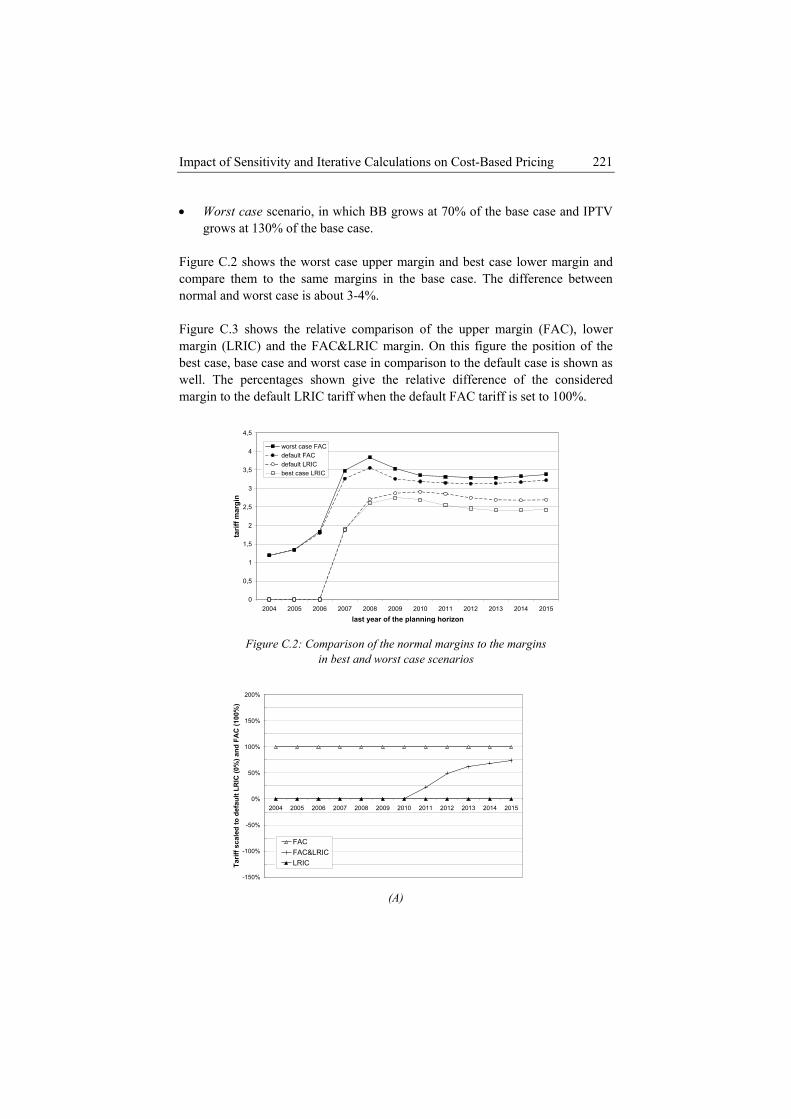
Impact of Sensitivity and Iterative Calculations on Cost-Based Pricing 221
• Worst case scenario, in which BB grows at 70% of the base case and IPTV grows at 130% of the base case.
Figure C.2 shows the worst case upper margin and best case lower margin and
m me margins in the base case. The difference between rm e is about 3-4%.
percentages shown give the relative difference of the considered
co pare them to the sano al and worst cas Figure C.3 shows the relative comparison of the upper margin (FAC), lower margin (LRIC) and the FAC&LRIC margin. On this figure the position of the best case, base case and worst case in comparison to the default case is shown as well. Themargin to the default LRIC tariff when the default FAC tariff is set to 100%.
0
0,5
1
1,5
2
2,5
3
3,5
rgin
4
4,5
2004 2005 2006 2007 2008 2009 2010 2011 2012 2013 2014 2015
last year of the planning horizon
tarif
f ma
worst case FACdefault FACdefault LRICbest case LRIC
Figure C.2: Comparison of the normal margins to the margins
in best and worst case scenarios
-150%
-100%
-50%
0%
50%
100%
150%
200%
2004 2005 2006 2007 2008 2009 2010 2011 2012 2013 2014 2015
Tarif
f sca
led
to d
efau
lt LR
IC (0
%) a
nd F
AC
(100
%)
FACFAC&LRICLRIC
(A)

Appendix C 222
-50%
200%
2004 2005 2006 2007 2008 2009 2010 2011 2012 2013 2014 2015
d to
0%
50%
100%
def
ault
LRIC
(0%
) and
FA
C (1
150%00%
)
-150%
Ta
-100%
riff s
cale
FACFAC&LRICLRIC
(B)
150%
200%
AC
(100
%)
-150%
Tarif
f -100%
-50%
0%2004 2005 2006 2007 2008 2009 2010 2011 2012 2013 2014 2015
sca
led
to d
efau
50%
100%
lt LR
IC (0
%) a
nd F
FACFAC&LRICLRIC
(B) and best (C) case margins Ftool. Heparamestandard
(C)
Figure C.3: Comparison of the FAC/LRIC margin to the default (A), worst
igure C.4 and Figure C.5 show additional results obtained using the crystal ball re a Monte Carlo simulation is used in which the variation of all four
ters is defined by a normal distribution with a mean of 100% and a deviation of 10% for all years in the considered forecast.
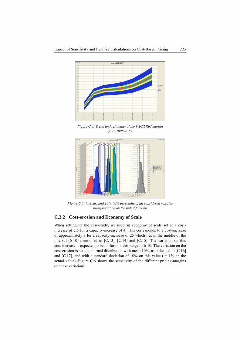
Impact of Sensitivity and Iterative Calculations on Cost-Based Pricing 223
Figure C.4: Trend and reliability of the FAC/LRIC margin
from 2008-2015
Figure C.5: forecast and 10%-90% percentile of all considered margins
using variation on the initial forecast
C.3.2 Cost-erosion and Economy of Scale up the case-study, we used an economy of scale set at a coWh
inen setting st-
crease of 2.5 for a capacity-increase of 4. This corresponds to a cost-increase f approximately 8 for a capacity-increase of 25 which lies in the middle of the
interval (6-10) mentioned in [C.13], [C.14] and [C.15]. The variation on this cost-increase is expected to be uniform in this range of 6-10. The variation on the cost-erosion is set to a normal distribution with mean 10%, as indicated in [C.16] and [C.17], and with a standard deviation of 10% on this value ( = 1% on the actual value). Figure C.6 shows the sensitivity of the different pricing-margins on these variations.
o
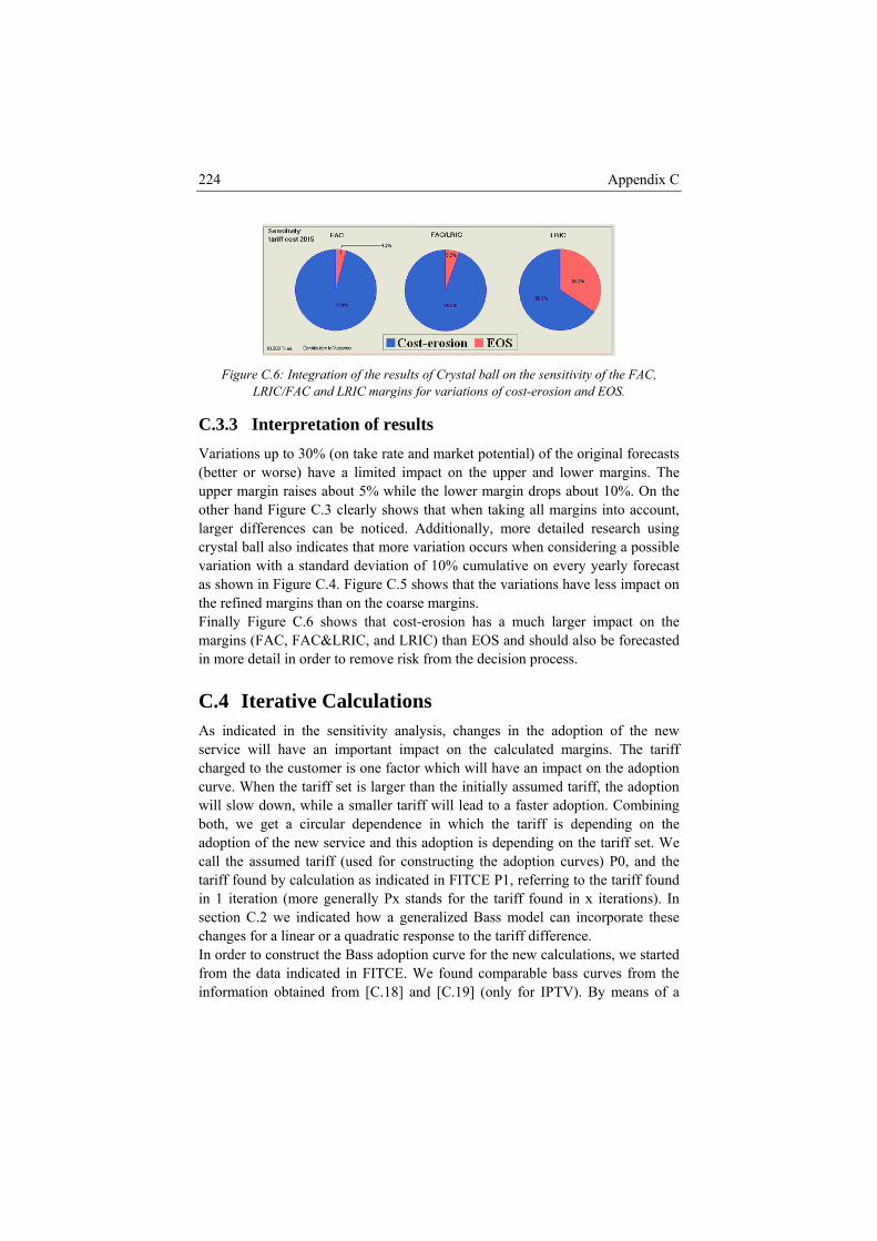
Appendix C 224
Figure C.6: Integration of the results of Crystal ball on the sensitivity of the FAC,
LRIC/FAC and LRIC margins for variations of cost-erosion and EOS.
C.3.3 Interpretation of results Variations up to 30% (on take rate and market potential) of the original forecasts (better or worse) have a limited impact on the upper and lower margins. Theupper margin raises about 5% while the lower margin drops about 10%. On theother hand Figurelarger differencescrystal ball also indicavariation with a standas shown in Figure C.4. Figure C.5 shows that the variations have less impact on the refined margins than on the coarse margins. Finally Figure C.6 shows that cost-erosion has a much larger impact on the
ns
urve. When the tariff set is larger than the initially assumed tariff, the adoption , while a smaller tariff will lead to a faster adoption. Combining
vice and this adoption is depending on the tariff set. We call the assumed tariff (used for constructing the adoption curves) P0, and the
calculation as indicated in FITCE P1, referring to the tariff found ore generally Px stands for the tariff found in x iterations). In
C.3 clearly shows that when taking all margins into account, can be noticed. Additionally, more detailed research using
tes that more variation occurs when considering a possible ard deviation of 10% cumulative on every yearly forecast
margins (FAC, FAC&LRIC, and LRIC) than EOS and should also be forecasted in more detail in order to remove risk from the decision process.
C.4 Iterative CalculatioAs indicated in the sensitivity analysis, changes in the adoption of the new service will have an important impact on the calculated margins. The tariff charged to the customer is one factor which will have an impact on the adoption cwill slow downboth, we get a circular dependence in which the tariff is depending on the adoption of the new ser
tariff found byin 1 iteration (msection C.2 we indicated how a generalized Bass model can incorporate these changes for a linear or a quadratic response to the tariff difference. In order to construct the Bass adoption curve for the new calculations, we started from the data indicated in FITCE. We found comparable bass curves from the information obtained from [C.18] and [C.19] (only for IPTV). By means of a
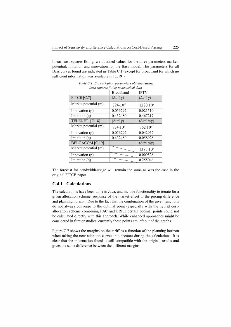
Impact of Sensitivity and Iterative Calculations on Cost-Based Pricing 225
linear least squares fitting, we obtained values for the three parameters market-potential, imitation and innovation for the Bass model. The parameters for all Bass curves found are indicated in Table C.1 (except for broadband for which no sufficient information was available in [C.19]).
Table C.1: Bass adoption parameters obtained using least squares fitting to historical data
Broadband IPTV FITCE [C.7] (∆t=1y) (∆t=1y) Market potential (m) 310724⋅ 3101280⋅ Innovation (p) 0.056792 0.021510 Imitation (q) 0.432480 0.467217 TELENET [C.18] (∆t=1y) (∆t=1/4y) Market potential (m) 310874⋅ 310862⋅ Innovation (p) 0.056792 0.042952 Imitation (q) 0.432480 0.058928 BELGACOM [C.19] (∆t=1/4y) Market potential (m) 3101385⋅ Innovation (p) 0.009528 Imitation (q) 0.255046
The forecast for bandwidth-usage will remain the same as was the case in the original FITCE-paper.
C.4.1 Calculations The calculations have been done in Java, and include functionality to iterate for a given allocation scheme, response of the market effort to the pricing difference
o the fact that the combination of the given functions he optimal point (especially with the hybrid cost-
margins on the tariff as a function of the planning horizon
and planning horizon. Due tdo not always converge to tallocation scheme combining FAC and LRIC) certain optimal points could not be calculated directly with this approach. While enhanced approaches might be considered in further studies, currently these points are left out of the graphs.
Figure C.7 shows thewhen taking the new adoption curves into account during the calculations. It is clear that the information found is still compatible with the original results and gives the same difference between the different margins.
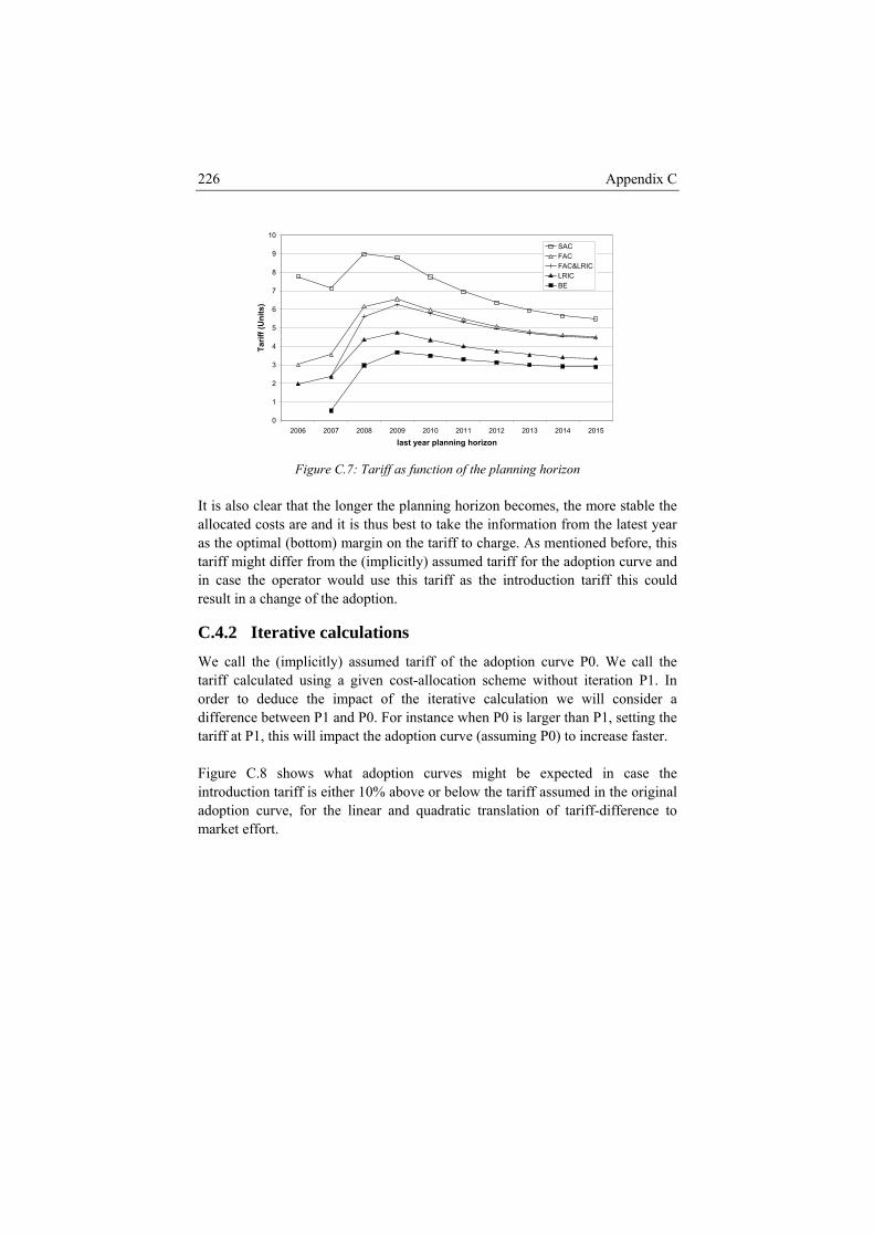
Appendix C 226
7
8
9
10SACFACFAC&LRICLRIC
2
3
5
6
iff (U
nits
)
4Tar
1
02006 2007 2008 2009 2010 2011 2012 2013 2014 2015
last year planning horizon
BE
.8 shows what adoption curves might be expected in case the er 10% above or below the tariff assumed in the original linear and quadratic translation of tariff-difference to
Figure C.7: Tariff as function of the planning horizon
It is also clear that the longer the planning horizon becomes, the more stable the allocated costs are and it is thus best to take the information from the latest year as the optimal (bottom) margin on the tariff to charge. As mentioned before, this tariff might differ from the (implicitly) assumed tariff for the adoption curve and in case the operator would use this tariff as the introduction tariff this could result in a change of the adoption.
C.4.2 Iterative calculations We call the (implicitly) assumed tariff of the adoption curve P0. We call the tariff calculated using a given cost-allocation scheme without iteration P1. In order to deduce the impact of the iterative calculation we will consider a difference between P1 and P0. For instance when P0 is larger than P1, setting the tariff at P1, this will impact the adoption curve (assuming P0) to increase faster. Figure Cintroduction tariff is eithadoption curve, for themarket effort.
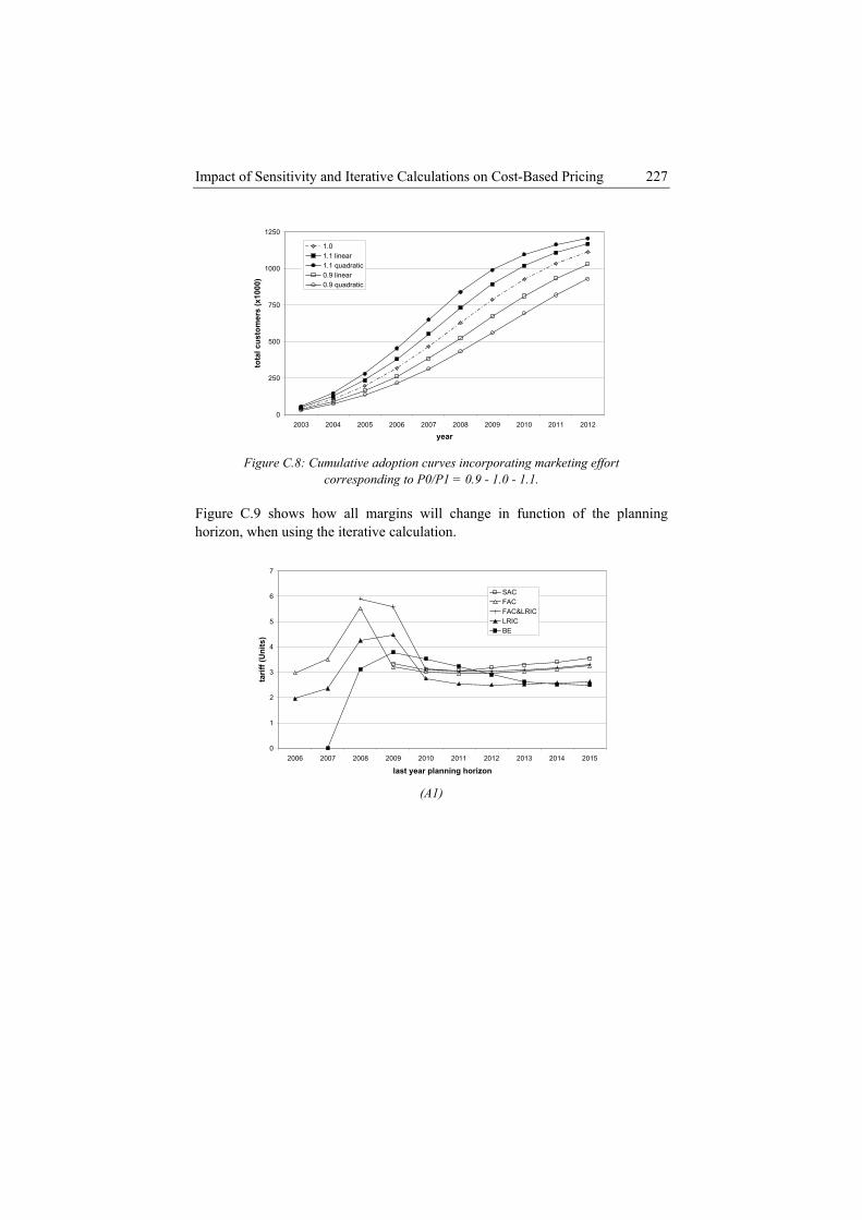
Impact of Sensitivity and Iterative Calculations on Cost-Based Pricing 227
1250
0
250
500
750
1000
2003 2004 2005 2006 2007 2008 2009 2010 2011 2012
year
tota
l cus
tom
ers
(x10
00)
1.01.1 linear1.1 quadratic0.9 linear0.9 quadratic
Figure C.8: Cumulative adoption curves incorporating marketing effort
corresponding to P0/P1 = 0.9 - 1.0 - 1.1.
tion of the planning Figure C.9 shows how all margins will change in funchorizon, when using the iterative calculation.
0
2
3
4
5
6
7
tarif
f (U
nits
)
SACFACFAC&LRICLRICBE
1
2006 2007 2008 2009 2010 2011 2012 2013 2014 2015
last year planning horizon
(A1)
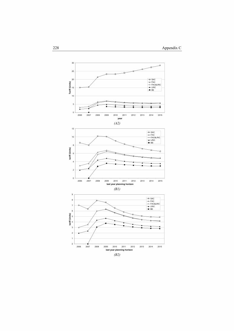
Appendix C 228
0
5
10
15
20
25
30
2006 2007 2008 2009 2010 2011 2012 2013 2014 2015
year
Tarif
f (U
nits
)
SACFACFAC&LRICLRICBE
(A2)
12
0
2
4
6
8
2006 2007 2008 2009 2010 2011 2012 2013 2014 2015
last year planning horizon
tarif
f (U
nits
)
SACFACFAC&LRICLRIC
10
BE
(B1)
0
1
2
3
4
5
6
7
8
9
2006 2007 2008 2009 2010 2011 2012 2013 2014 2015
last year planning horizon
tarif
f (U
nits
)
SACFACFAC&LRICLRICBE
(B2)
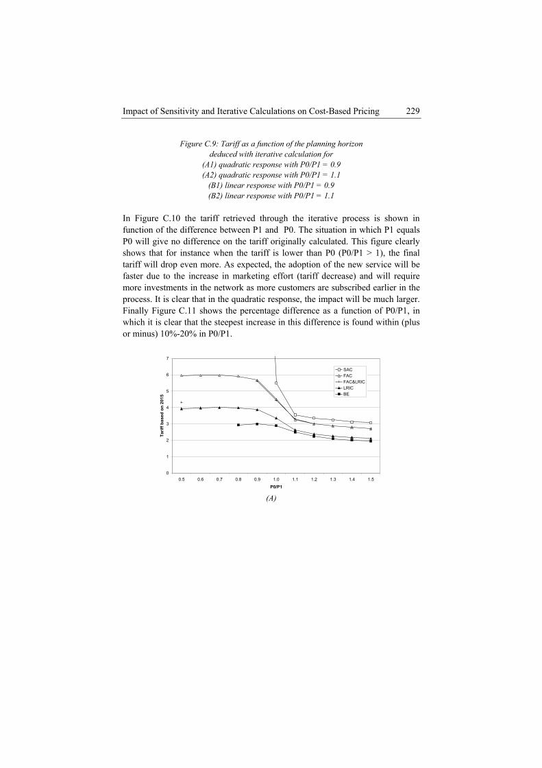
Impact of Sensitivity and Iterative Calculations on Cost-Based Pricing 229
Figure C.9: Tariff as a function of the planning horizon deduced with iterative calculation for
(A1) quadratic response with P0/P1 = 0.9 (A2) quadratic response with P0/P1 = 1.1
(B1) linear response with P0/P1 = 0.9 (B2) linear response with P0/P1 = 1.1
In Figure C.10 wn in fun difference bet P1 equals P0 will g difference on the tariff o re clearly shows that for instance when the tariff is an P0 (P , the final tar op even more. As expected, the adoption of the n ice will be fas ase in marketing e ff decreas ill require mo network as more s are subs lier in the pro n the quadratic re e impact ch larger. Fin .11 shows the percentag rence as a fu of P0/P1, in wh that the steepest increase difference i ithin (plus or P0/P1.
the tariff retrieved through the iterative process is shoween P1 anction of the
ive nod P0. The situationriginally calculated
lower th
in which. This figu0/P1 > 1)
ew serviff will drter due to the incre ffort (tari
re) and w
rre investments in thecess. It is clear that i
customesponse, th
cribed eawill be mu
ally Figure C e diffe nctionich it is clear in this s found wminus) 10%-20% in
0
1
2
Tar
3
iff b
a
4
sed
on
5
6
0.9 1 1.2 1.3
P0
7
0.5 0.6 0.7 0.8 .0 1.1
/P11.4 1.5
201
5
SACFACFAC&LRICLRICB
(A
E
)
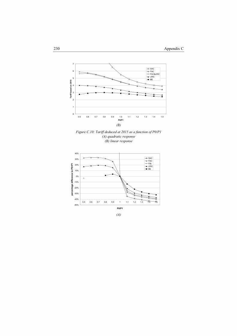
Appendix C 230
0
1
2
3
4
P0/P1
Tarif
f bas
ed o
n 20
15
5
6
7
0.5 0.6 0.7 0.8 0.9 1.0 1.1 1.2 1.3 1.4 1.5
SACFACFAC&LRICLRICBE
(B)
Figure C.10: Tariff deduced at 2015 as a function of P0/P1 ) quadratic response (A(B) linear response
-20%
-10%
0%
10%
20%
30%
40%
enta
ge d
iffer
ence
to P
0=P1
SACFACF&LLRICBE
-50%
-40%
-30%
0,5 0,6 0,7 0,8 0,9 1 1,1 1,2 1,3 1,4 1,5
P0/P1
perc
(A)
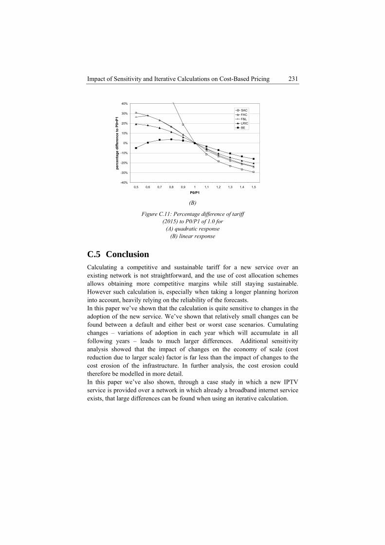
Impact of Sensitivity and Iterative Calculations on Cost-Based Pricing 231
-40%
-30%
-20%
-10%
0%
0,5 0,6 0,7 0,8 0,9 1 1,1 1,2 1,3 1,4 1,5
P0/P1
perc
enta
ge d
iffer
e
10%
20%
30%
40%
nce
to P
0=P1
SACFACF&LLRICBE
(B)
Figure C.11: Percentage difference of tariff (2015) to P0/P1 of 1.0 for
(A) quadratic response (B) linear response
C n Calculating e and s ble tarif se an exi ting netw straightfo and the u oc es a ta competit argins w in le. However su s, esp en tak a n i account ing on th of thIn this paper n that the n is q o e adoption of ice. We’ that r c be found betwe lt and eit r wor riochanges – v f adoption year cufo years – s to much ifferen n ity a ysis sho e impact es on cost reduction du cale) fact ss tha the c erosion rastructure er an t therefore be modelled in more detail.
p rough a case study in which a new IPTV n which already a broadband internet service
.5 Co clusionva competiti ustaina f for a new rvice over
s ork is not rward, se of cost ally
ation schemllows ob ining more ive m hile still sta g sustainab
ch calculation ily
ecially wh ing a longer pl nning horizonto , heavily re e reliability
latioe forecasts.
we’ve showthe new serv
calcuve sho
uite sensitive telatively small
changes in thhanges canwn
her best oen a defau st case scena s. Cumulating mulate in all al se
ariations o in each which will acllowing
nal lead
wed that th larger d
of changces. Additio
the economy nsitiv
of scale (e to larger s or is far le n the impact of changes to
ost of the inf . In furth alysis, the cos erosion could
In this aper we’ve also shown, thservice is provided over a network iexists, that large differences can be found when using an iterative calculation.

Appendix C 232
In order to find this information we first fitted a Bass adoption curve to the existing historical adoption data. This (generalized) Bass adoption curve allows for decision variables such as marketing effort to be taken into account. During
tariff-changes to the marketing effort used are:
riff and
calculation (P∞)
calculations, the influences of • quadratic response • linear response From the iterative calculations it is clear that when P1 is larger than P0, meaning that the tariff calculated in the first iteration is larger than the original tathat the adoption will be slower than initially forecasted, the final tariff P∞ will be higher than P1. When P1 is larger than P0, the final tariff P∞ will be lower than P1. More in detail, the calculations indicate that even for only 10% change in tariff (FAC, FAC&LRIC or LRIC) P0 to P1, the result of the iterative might change more than 10% and up to 25% considering a quadratic response and more than 5% up to 10% considering a linear response. Finally the results also show that the difference between the different margins – and especially between stand alone costing – becomes much larger when P0 is smaller than P1. In case P0 is larger than P1, these differences become slightly smaller.
Impact of Sensitivity and Iterative Calculations on Cost-Based Pricing 233
Acknowledgment This work has been financed by IWT-Flanders through the IWT-project “Cost
nications environment” and a PhD grant for S.
ltiple levels-of-service, Computer Communications 27 (2004) 374-
[C.6] C. Courcebetis, F. Kelly, V. Siris, R. Weber, “A study of simple usage-based charging schemes for broadband networks”, Telecommunication Systems 15 (2000) 323-343.
[C.7] K. Casier, S. Verbrugge, R. Meersman, J. Van Ooteghem, D. Colle, M. Pickavet, P. Demeester, "Adding cost-drivers to the pricing process by using a bottom-up cost-allocation approach", published in Proceedings of FITCE2006, the 45th Federation of Telecommunications Engineers of the European Community Congress, Athens, Greece, 30 August-2 September 2006, pp. 79-84.
[C.8] F. Bass, “A new product growth model for consumer durables”, Management Science Vol. 15 No. 5 (1969) 215-227
[C.9] F. Bass, T. Krishnan, D. Jain, “Why the bass model fits without decision variables”, Marketing science Vol. 13 No. 3 (1994) 203-223
modeling in a converged commuVerbrugge. It was also supported by Ghent University through the RODEO-project and by the European Commission through IST-NOBEL phase 2 and ePhoton/One+.
References [C.1] S. Jagannathan, K. Almeroth, A dynamic Pricing scheme for e-content at
mu385
[C.2] P. Reichl, D. Hausheer, B. Stiller, The cumulus pricing model as an adaptive framework for feasible, efficient, and user-friendly tariffing of Internet services, Computer Networks 43 (2003) 3-24
[C.3] M. Karsten, J. Schmitt, B. Stiller, L. Wolf, “Charging for packet-switched communication – motivation and overview”, Computer Communications 23 (2000) 290-302
[C.4] N. Blefari-Melazzi, D. Di Sorte, G. Reali, Accounting and pricing: a forecast of the scenario of the next generation Internet, Computer Communications 26 (2003) 2037-2051
[C.5] B. Briscoe et al., A market managed multi-service Internet (M3I), Computer Communications 26 (2003) 404-414
Appendix C 234
[C.10] D. Schmittlein, V. Mahajan, “Maximum likelihood estimation for an w product acceptance”, Marketing
sed intelligent optical networks, Optical Networks M 2, 2003, pp. 20-31.
P. C . Odlyzko, Dynamic Behavior of Differential
innovation diffusion model of nescience, Vol.1 No. 1, (1982) 57-78
[C.11] V. Srinivasan, C. Mason, “Nonlinear least squares estimation of new product diffusion models”, Marketing science, Vol. 5 No. 2 (1986) 169-178
[C.12] Decisioneering Crystal Ball software, http://www.decisioneering.com/cbpro/index.html
[C.13] N. Geary, A. Antonopoulos, J. O’Reilly, Analysis of the potential benefits of OXC-ba
agazine, vol 4 No
[C.14] . Fishburn and A. MPricing and Quality of Service Options for the Internet, Proc. First International Conference on Information and Computation Economies (ICE-98), ACM Press, 1998, pp. 128-139
[C.15] A. Odlyzko, The economics of the Internet: Utility, utilization, pricing, and Quality of Service, http://www.dtc.umn.edu/~odlyzko/doc/internet.economics.pdf
[C.16] B. Olsen and K. Stordahl, Models for forecasting cost evolution of components and technologies, Telektronikk 4, 2004
[C.17] J. Derkacz, M. Leszczuk, K. Wajda, R. Leone, G. Monari, I. Lievens, S De Maesschalck, S. Verbrugge, D. Colle, IP/OTN cost model and photonic equipment cost forecast – IST LION project, Proc. of Workshop on Telecommunication Techno-Economics, (Rennes, France, May 2002), pp. 126-138
[C.18] Annual reports Telenet Belgium, http://www.telenet.be/nl/overtelenet/publicaties/
[C.19] Annual reports Belgacom Belgium, http://www.belgacom.be/company/nl/jsp/dynamic/pressreleaselist.jsp
D Municipalities as a Driver for
Wireless Broadband Access
J. Van Ooteghem, B. Lannoo, K. Casier, S. Verbrugge,
ons, Springer Netherlands, ISSN 0929-
pality networks, Techno-economic
E. Tanghe, W. Joseph, L. Martens, D. Colle, M. Pickavet, I. Moerman, P. Demeester Wireless Personal Communicati6212 (Print) 1572-834X (Online), vol. 49, no. 3, pp. 391-414 , May 2009 Key words Wireless access networks, Broadband, Municianalysis, Business case
Abstract Municipalities can form a driving force behind the deployment of new telecom infrastructure. While a telecom operator focuses on direct (financial) profits, a municipality is mainly interested in the social benefits for its inhabitants. In this paper, we evaluate a wireless municipality network from both a technical and an economic point of view. WiFi and WiMAX are considered as the most suited technologies for this purpose. A detailed techno-economic study has been
Appendix D 236
performed including forecasting of the user adoption, dimensioning of the wireless network and modelling the related costs and revenues. The trade-off
n i Fi access points, and a ns for delivering full
ure-proof commendations are given in section D.6.
rvices, which actors are playing a role in the value network, which technical scenarios will be analyzed, and what are the
betwee nstalling a high number of relatively cheap Wismaller number of more expensive WiMAX base statiocoverage is investigated in several scenarios.
D.1 Introduction Within the current telecom market, there is an important demand for broadband access. Worldwide 386 million subscribers [D.1] are currently using broadband Internet services like Internet browsing, file sharing or IP Television (IPTV). Next to bandwidth, also mobility is becoming more and more important for people, manifested by the immense growth in the number of mobile phone users. This is also reflected in a growing number of Internet users, who are demanding a continuous connection (important for services such as Voice over IP (VoIP)), irrespective of where they are located. As an effect of this trend, there is an increase in rollout of wireless data networks worldwide in the last years. The role municipalities can play here is extensively discussed in this paper. In section D.2, the used methodology to tackle techno-economic studies is described. For a wireless data network, several technologies, like 3G networks, WiFi, WiMAX, or a combination of them can be used. In this paper, we focus on WiFi and WiMAX and both technologies are treated in more detail in section D.3. Telecom operators as well as municipalities have their motivations for investing in such networks, each with different objectives. The rationale behind government influences and investments is discussed in section D.4. In section D.5, a business model has been developed for the city of Ghent (Belgium) to evaluate the technical scenarios and to define the most viable futsolution. Conclusions and re
D.2 Methodology We have developed a methodology for the elaboration of techno-economic projects, which is summarized in Figure D.1. This framework, roughly based on the Deming Wheel, contains four steps: plan, model, evaluate and refine [D.2].
D.2.1 Planning The first step, planning, encloses three phases. At first, all necessary input must be collected, such as information about the targeted area, market situation and technologies that can be used. Within the second phase the problem is divided into subproblems of lower size and/or complexity. Which areas will be regarded, who are the targeted users, which se
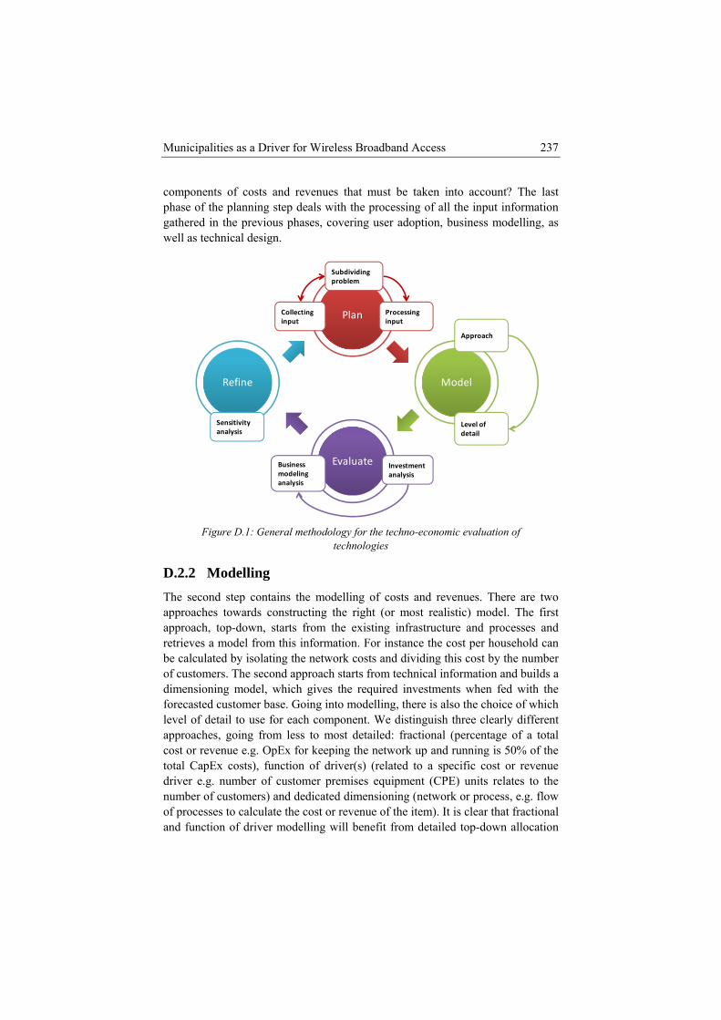
Municipalities as a Driver for Wireless Broadband Access 237
compone ts of costs and ren venues that must be taken into account? The last phase of the planning step deals with the processing of all the input information gathered in the previous phases, covering user adoption, business modelling, as well as technical design.
Model
Evaluate
Refine
Plan
Approach
Level of detail
Collectinginput
Processing input
Subdividingproblem
Investmentanalysis
Business modelinanalysis
g
Sensitivityanalysis
Figure D.1: General methodology for the techno-economic evaluation of
technologies
D.2.2 Modelling The second step contains the modelling of costs and revenues. There are two approaches towards constructing the right (or most realistic) model. The first approach, top-down, starts from the existing infrastructure and processes and retrieves a model from this information. For instance the cost per household can
of c
foreleveapp
st of the
be calculated by isolating the network costs and dividing this cost by the number ustomers. The second approach starts from technical information and builds a
dimensioning model, which gives the required investments when fed with the casted customer base. Going into modelling, there is also the choice of which l of detail to use for each component. We distinguish three clearly different roaches, going from less to most detailed: fractional (percentage of a total
co or revenue e.g. OpEx for keeping the network up and running is 50%total CapEx costs), function of driver(s) (related to a specific cost or revenue driver e.g. number of customer premises equipment (CPE) units relates to the number of customers) and dedicated dimensioning (network or process, e.g. flow of processes to calculate the cost or revenue of the item). It is clear that fractional and function of driver modelling will benefit from detailed top-down allocation
Appendix D 238
for finding accurate percentages or costs to use within a bottom-up calculation. Dedicated dimensioning is a step in which much less or no top-down information is used.
D.2.3 Evaluation The third step is the evaluation consisting of investment and business modelling
D used for the investment analysis. The most y s Net Present Value (NPV) analysis, a standard
ithin the last step, we refine both the existing model and the evaluation. A commonly used method is sensitivity analysis, where the uncertainty of input parameters is tested (e.g. by performing Monte Carlo simulations) and their importance is discovered. Combining this approach with a definition of options (representing managerial flexibility) and their impact on the project outcomes can be used for further refinement. Such a real options approach provides us with a more detailed evaluation methodology and e.g. allows a dynamic (strategic) planning depending on the outcome of the investment analysis. Another elaborated method is game theory, where the interactions between actors can be modelled. The results of the above refinements are used in the feedback loop, back to the fi rent steps at several levels of deta introduction of new
s ost modelling, etc.
cal and physical parameters used within further technical calculations and dimensioning.
analysis. ifferent methods can be commonl known method imethod to assess the financial feasibility of long-term projects. It corresponds to the summation of the discounted cash flows over the evaluation period. For the business modelling, each actor in the value network has its own roles and as such its own cost and revenue model, thus for each actor, a separate NPV must be calculated. The complete value network is then analyzed based on the results from the individual actors.
D.2.4 Refining W
rst step, where adaptations can be made in the diffeil e.g. adaptation of input parameters,
variable , more detailed c
D.3 Considered Wireless Technologies This section outlines the wireless technologies, WiFi (Wireless Fidelity) and WiMAX (Worldwide Interoperability for Microwave Access), considered for the network rollout of a cellular-based wireless municipality network. Different combinations of these two wireless technologies for user connectivity and backhauling (the latter also includes fixed network connectivity) are considered, leading to six scenarios which are potentially most future proof, and which are analyzed from a technical as well as economic point of view in this paper. In this section we also give detailed information of the techni
Municipalities as a Driver for Wireless Broadband Access 239
D.3.1 verview ofO WiFi and WiMAX
d e IEEE 802.11 standards and a, g xtensions use an Orthogonal
ing FDM al layer (PHY) air interface.
such as line-of-sight (LOS) could have a negative impact on the achievable data rate gain by MIMO). Besides, the 802.11n supports a channel bandwidth of 40 MHz by merging two channels (so-called channel bonding) and provides thus a higher data rate of two times 65 Mbps, but this poses interference problems, especially in the 2.4 GHz frequency band where only three non-overlapping 20 MHz channels are available. In this study, we use the 802.11n standard because of the higher throughput and the possibility to use MIMO, compared to the 802.11a/g. However, we choose for a 20 MHz channel bandwidth, sacrificing larger data rates for re
profiles are defined: Fixed WiMAX (based on IEEE 802.16-2004) and
nt to multi-
WiFi and WiMAX are considered as the most suited technologies for the wireless municipality network. In this subsection, the technical characteristics of both are summarized.
D.3.1.1 WiFi
WiFi (Wireless Fidelity) is standard within thopular
izesub-standards of which the p , and n eFrequency Division Multiplex (O ) physicFor the wireless municipality network, we expect to work within the license-free 2.4 GHz frequency band for which the main 802.11 standard defines three non-overlapping 20 MHz channels. For the 802.11a/g standard, a maximum achievable PHY data-rate of 54 Mbps per 20 MHz-channel can be attained. For the 802.11n standard [D.3], this is extended to 65 Mbps by using more OFDM data subcarriers and higher Forward Error Correction (FEC) code rates. Besides, the 802.11n standard also supports multiple antenna techniques like Multiple-Input Multiple-Output (MIMO), which can extend either the data rate or the range of the WiFi signals. For an outdoor scenario, MIMO is better used to extend the wireless range while keeping a 65 Mbps channel, than to increase the data rate (note that environmental conditions
duced interference.
D.3.1.2 WiMAX
WiMAX (Worldwide Interoperability for Microwave Access) is standardized within the IEEE 802.16 standards and sub-standards. Today, two important WiMAX Mobile WiMAX (based on IEEE 802.16e-2005). 802.16-2004 [D.4] specifies three PHY air interfaces of which an OFDM-based system using 256 subcarriers is used for Fixed WiMAX. 802.16e-2005 [D.5] uses Scalable Orthogonal Frequency Division Multiple Access (SOFDMA), which allows scaling the number of OFDM subcarriers with the channel bandwidth, and is used for Mobile WiMAX. This affords 802.16e-2005 more efficient use of the full spectrum bandwidth and transmission power. Additionally, SOFDMA can also cope with larger delay spreads, making the technology more resista
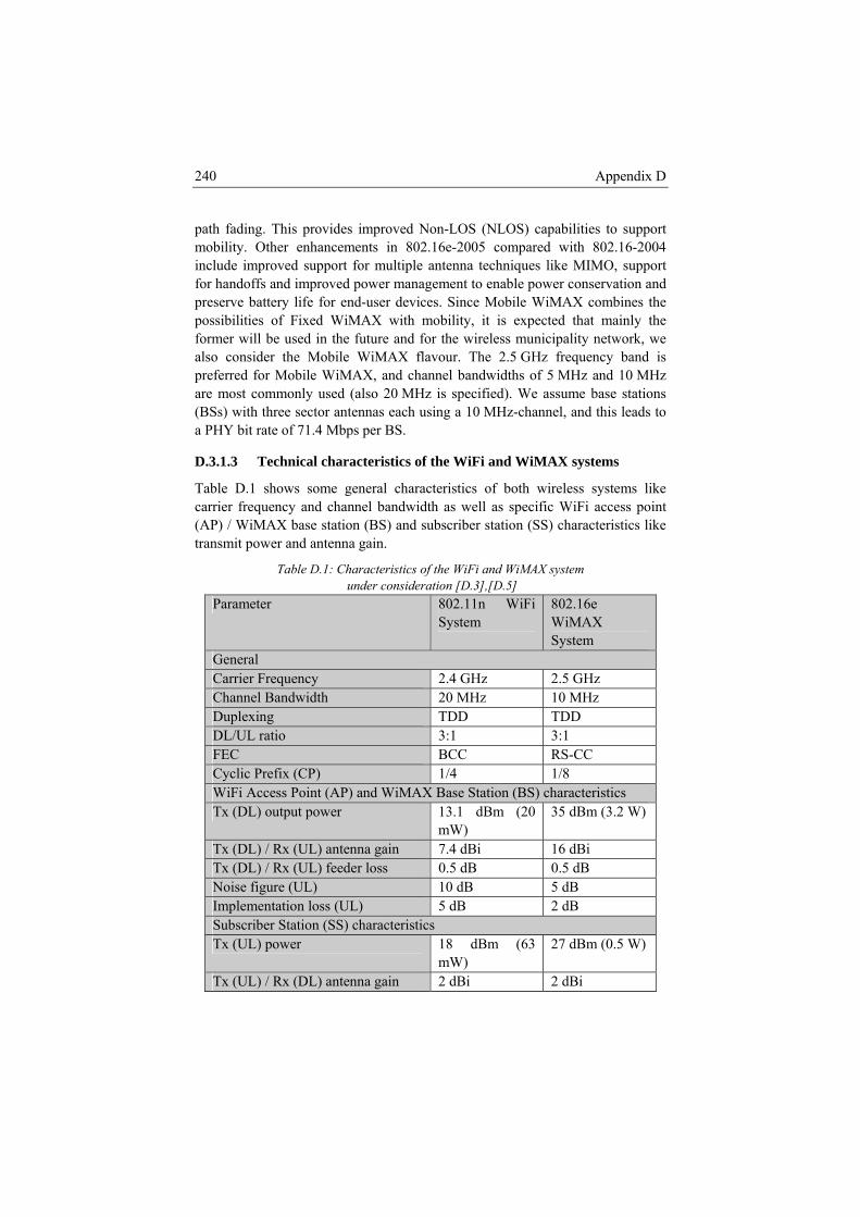
Appendix D 240
path fading. This provides improved Non-LOS (NLOS) capabilities to support
Mobile WiMAX combines the
Table D.1: Characteristics of the WiFi and WiMAX system
mobility. Other enhancements in 802.16e-2005 compared with 802.16-2004 include improved support for multiple antenna techniques like MIMO, support for handoffs and improved power management to enable power conservation and preserve battery life for end-user devices. Sincepossibilities of Fixed WiMAX with mobility, it is expected that mainly the former will be used in the future and for the wireless municipality network, we also consider the Mobile WiMAX flavour. The 2.5 GHz frequency band is preferred for Mobile WiMAX, and channel bandwidths of 5 MHz and 10 MHz are most commonly used (also 20 MHz is specified). We assume base stations (BSs) with three sector antennas each using a 10 MHz-channel, and this leads to a PHY bit rate of 71.4 Mbps per BS.
D.3.1.3 Technical characteristics of the WiFi and WiMAX systems
Table D.1 shows some general characteristics of both wireless systems like carrier frequency and channel bandwidth as well as specific WiFi access point (AP) / WiMAX base station (BS) and subscriber station (SS) characteristics like transmit power and antenna gain.
under consideration [D.3],[D.5] Parameter 802.11n WiFi
System 802.16e WiMAX System
General Carrier Frequency 2.4 GHz 2.5 GHz Channel Bandwidth 20 MHz 10 MHz Duplexing TDD TDD DL/UL ratio 3:1 3:1 FEC BCC RS-CC Cyclic Prefix (CP) 4 1/8 1/WiFi Ac stics cess Point (AP) and WiMAX Base Station (BS) characteriTx (DL) output power (20
mW) 35 dBm (3.2 W) 13.1 dBm
Tx (DL) / Rx (UL) antenna gain 7.4 dBi 16 dBi Tx (DL) / Rx (UL) feeder loss 0.5 dB 0.5 dB Noise figure (UL) 10 dB 5 dB Implementation loss (UL) 5 dB 2 dB Subscriber Station (SS) characteristics Tx (UL) power 18 dBm (63 27 dBm (0.5 W)
mW) Tx (UL) / Rx (DL) antenna gain 2 dBi 2 dBi
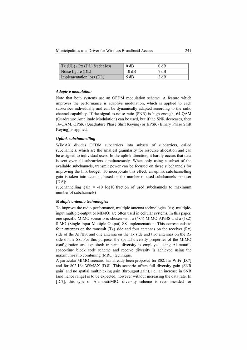
Municipalities as a Driver for Wireless Broadband Access 241
Tx (UL) / Rx (DL) feeder loss 0 dB 0 dB Noise figure (DL) 10 dB 7 dB Implementation loss (DL) 5 dB 2 dB
Adaptive modulation Note that both systems use an OFDM modulation scheme. A feature which improves the performance is adaptive modulation, which is applied to each
es, then
ich are the smallest granularity for resource allocation and can be assigned to individual users. In the uplink direction, it hardly occurs that data
r all subcarriers simultaneously. When only using a subset of the
ceiver (Rx) si of the AP/BS, and one antenna on the Tx side and two antennas on the Rx side of the SS. For this purpose, the spatial diversity properties of the MIMO configuration are exploited: transmit diversity is employed using Alamouti’s space-time block code scheme and receive diversity is achieved using the maximum-ratio combining (MRC) technique. A particular MIMO scenario has already been proposed for 802.11n WiFi [D.7] and for 802.16e WiMAX [D.8]. This scenario offers full diversity gain (SNR gain) and no spatial multiplexing gain (througput gain), i.e., an increase in SNR (and hence range) is to be expected, however without increasing the data rate. In [D.7], this type of Alamouti/MRC diversity scheme is recommended for
subscriber individually and can be dynamically adapted according to the radio channel capability. If the signal-to-noise ratio (SNR) is high enough, 64-QAM (Quadrature Amplitude Modulation) can be used, but if the SNR decreas16-QAM, QPSK (Quadrature Phase Shift Keying) or BPSK (Binary Phase Shift Keying) is applied.
Uplink subchannelling WiMAX divides OFDM subcarriers into subsets of subcarriers, called subchannels, wh
is sent oveavailable subchannels, transmit power can be focused on these subchannels for improving the link budget. To incorporate this effect, an uplink subchannelling gain is taken into account, based on the number of used subchannels per user [D.6]: subchannelling gain = -10 log10(fraction of used subchannels to maximum number of subchannels)
Multiple antenna technologies To improve the radio performance, multiple antenna technologies (e.g. multiple-input multiple-output or MIMO) are often used in cellular systems. In this paper, one specific MIMO scenario is chosen with a (4x4) MIMO AP/BS and a (1x2) SIMO (Single-Input Multiple-Output) SS implementation. This corresponds to four antennas on the transmit (Tx) side and four antennas on the re
de
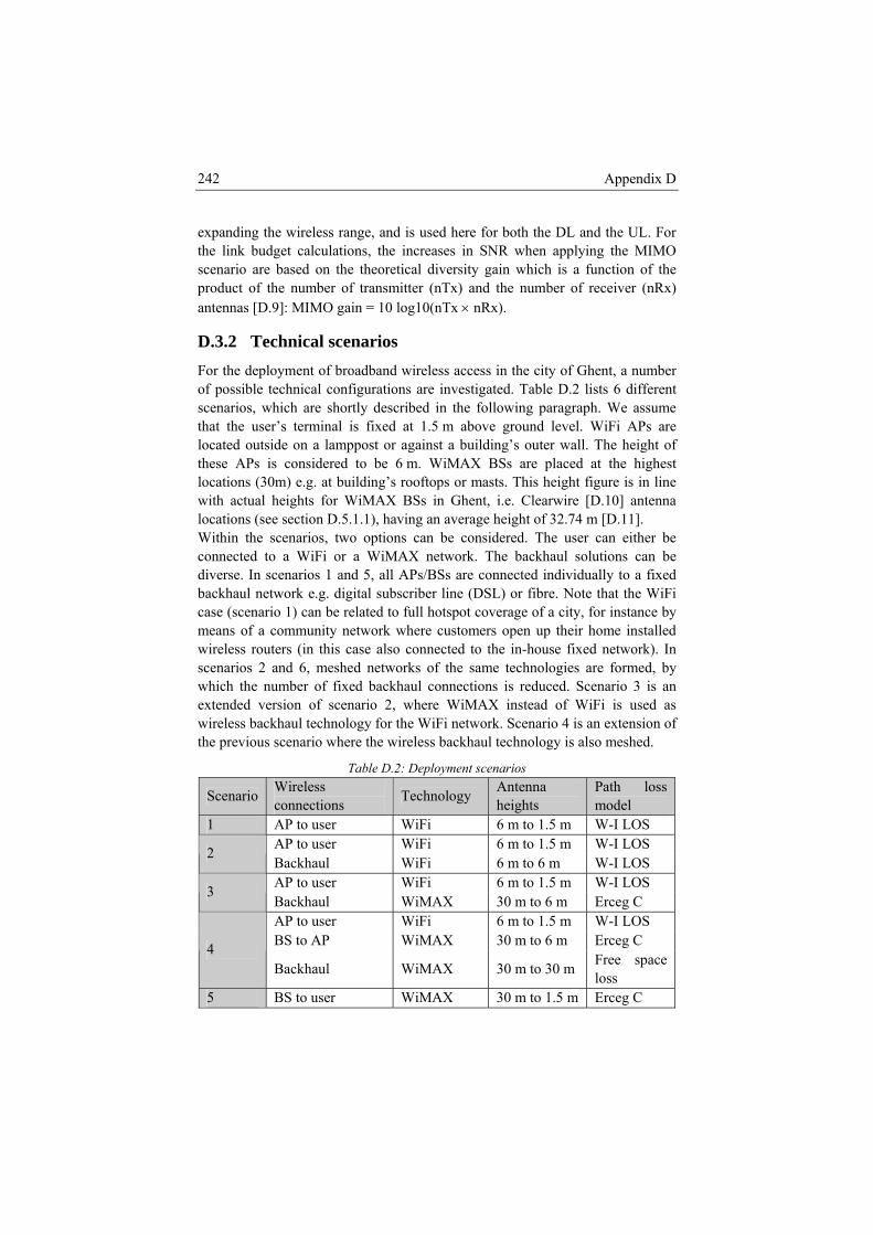
Appendix D 242
expanding the wireless range, and is used here for both the DL and the UL. For the link budget calculations, the increases in SNR when applying the MIMO scenario are based on the theoretical diversity gain which is a function of the product of the number of transmitter (nTx) and the number of receiver (nRx) antennas [D.9]: MIMO gain = 10 log10(nTx × nRx).
D.3.2 Technical scenarios For the deployment of broadband wireless access in the city of Ghent, a number of possible technical configurations are investigated. Table D.2 lists 6 different scenarios, which are shortly described in the following paragraph. We assume that the user’s terminal is fixed at 1.5 m above ground level. WiFi APs are located outside on a lamppost or against a building’s outer wall. The height of these APs is considered to be 6 m. WiMAX BSs are placed at the highest locations (30m) e.g. at building’s rooftops or masts. This height figure is in li e with actual height e [D.10] antenna locations (see section 4 m [D.11]. Within the scenarios, two options can be considered. The user can either be
d or a WiMAX network. The backhaul solutions can be
ns for WiMAX BSs in Ghent, i.e. Clearwir
D.5.1.1), having an average height of 32.7
connecte to a WiFi diverse. In scenarios 1 and 5, all APs/BSs are connected individually to a fixed backhaul network e.g. digital subscriber line (DSL) or fibre. Note that the WiFi case (scenario 1) can be related to full hotspot coverage of a city, for instance by means of a community network where customers open up their home installed wireless routers (in this case also connected to the in-house fixed network). In scenarios 2 and 6, meshed networks of the same technologies are formed, by which the number of fixed backhaul connections is reduced. Scenario 3 is an extended version of scenario 2, where WiMAX instead of WiFi is used as wireless backhaul technology for the WiFi network. Scenario 4 is an extension of the previous scenario where the wireless backhaul technology is also meshed.
Table D.2: Deployment scenarios
Scenario Wireless connections Technology Antenna
heights Path loss model
1 AP to user WiFi 6 m to 1.5 m W-I LOS AP to user WiFi 6 m to 1.5 m W-I LOS 2 Backhaul WiFi 6 m to 6 m W-I LOS AP to user WiFi 6 m to 1.5 m W-I LOS 3 Backhaul WiMAX 30 m to 6 m Erceg C AP to user WiFi 6 m to 1.5 m W-I LOS BS to AP WiMAX 30 m to 6 m Erceg C 4
Free Backhaul WiMAX 30 m to 30 m space loss
5 BS to user WiMAX 30 m to 1.5 m Erceg C
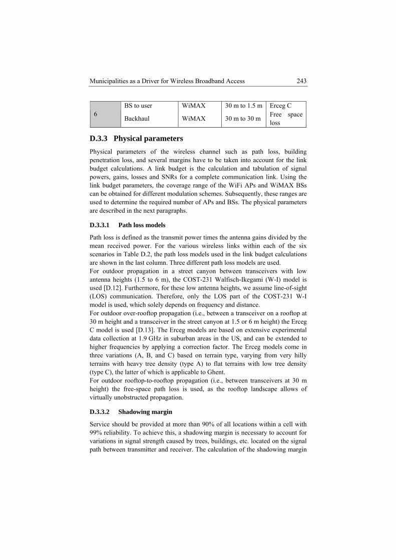
Municipalities as a Driver for Wireless Broadband Access 243
BS to user WiMAX 30 m to 1.5 m Erceg C 6
loss Backhaul WiMAX 30 m to 30 m Free space
D.3Phypenbud
w
can usedare
3.
Pathmea
en dels used in the link budget calculations re shown in the last column. Three different path loss models are used.
For outdoor propagation in a street canyon between transceivers with low antenna heights (1.5 to 6 ami (W-I) model is
.1 for these low antenna heights, we assume line-of-sight Therefore, only the LOS part of the COST-231 W-I
ying a correction factor. The Erceg models come in i ) based on terrain type, varying from very hilly
.3 Physical parameters sical parameters of the wireless channel such as path loss, building etration loss, and several margins have to be taken into account for the link get calculations. A link budget is the calculation and tabulation of signal ers, gains, losses and SNRs for a complete communicapo tion link. Using the
link budget parameters, the coverage range of the WiFi APs and WiMAX BSs be obtained for different modulation schemes. Subsequently, these ranges are to determine the required number of APs and BSs. The physical parameters
described in the next paragraphs.
D. 3.1 Path loss models
loss is defined as the transmit power times the antenna gains divided by the n received power. For the various wireless links within each of the six arios in Table D.2, the path loss mosc
a
m), the COST-231 Walfisch-Ikegused [D 2]. Furthermore, (LOS) communication. model is used, which solely depends on frequency and distance. For outdoor over-rooftop propagation (i.e., between a transceiver on a rooftop at 30 m height and a transceiver in the street canyon at 1.5 or 6 m height) the Erceg C model is used [D.13]. The Erceg models are based on extensive experimental data collection at 1.9 GHz in suburban areas in the US, and can be extended to higher frequencies by applthree var ations (A, B, and Cterrains with heavy tree density (type A) to flat terrains with low tree density (type C), the latter of which is applicable to Ghent. For outdoor rooftop-to-rooftop propagation (i.e., between transceivers at 30 m height) the free-space path loss is used, as the rooftop landscape allows of virtually unobstructed propagation.
D.3.3.2 Shadowing margin
Service should be provided at more than 90% of all locations within a cell with 99% reliability. To achieve this, a shadowing margin is necessary to account for variations in signal strength caused by trees, buildings, etc. located on the signal path between transmitter and receiver. The calculation of the shadowing margin
Appendix D 244
is based on the variance of the path loss and the intended coverage percentage: a larger path loss variance and a larger coverage percentage will mean a higher value for the shadowing margin. To achieve a coverage percentage of 90% on
ing margin is taken into account because of the um at can cause shadowing.
nce (at sector boundaries). For WiFi, an
D.3.3.5 Building penetration loss
tion is accompanied by
er to obtain the total variance of the received
the edge of the cell, shadowing margins of 10 dB and 10.5 dB are used for the W-I and Erceg C models, respectively [D.14]. For the rooftop-to-rooftop free-space path loss model, no shadowlimited n ber of obstructions th
D.3.3.3 Fade margin
The fade margin takes the yearly availability of the system into account. The link availability is affected by clear-air and rain multipath fading. We use the ITU-R P.530 model described in the ECC report [D.15] for the fade margin. A fade margin of 10 dB is used which results in a yearly availability of 99.995% for a cell radius of 10 km.
D.3.3.4 Interference margin
The system’s performance is limited by co-channel interference (CCI). The most common sources of CCI are due to frequency reuse: inter-cell interference (at cell edges) and intra-cell interfereinterference margin of 3 dB for both DL and UL is incorporated into the link budget in correspondence with [D.16]. For WiMAX, maximum interference margins of 2 dB for DL and 3 dB for UL are proposed in [D.17], and are also used here.
Outdoor-to-indoor and indoor-to-outdoor propagasignificant attenuation of the received power depending on the materials and the construction of the building. Therefore, building penetration loss values have to be taken into account in case indoor coverage is desired with outdoor APs. Penetration loss values used here are based on results reported in [D.18]. For this study, building penetration loss is assumed to be log-normally distributed with a mean of 11 dB and a standard deviation of 6 dB. Note that the variance of the building penetration loss should be added to the variance of the path loss in ordsignal strength. Adding building penetration loss variance would therefore mean a higher variability of received power, which will in turn raise the value of the shadowing margin parameter previously mentioned.
Municipalities as a Driver for Wireless Broadband Access 245
D.4 Municipality Network In this section, the rationale behind government influences and investments will be discussed. The telecommunication sector, related to new infrastructure
vestments, is regulated at European, national and even local level. Regulation is most important for spectrum management, competition law and financial involvement by governments. Next to this, we discuss the different initiatives a municipality can take in stimulating telecom network rollouts. We summarize this section with a SWOT (Strengths, Weaknesses, Opportunities, and Threats) analysis for a municipality.
D.4.1 Regulation The telecommunications sector is regulated at several levels, either at European, national or local level, depending on the specific matter. Viviane Reding, commissioner for information society and media, has proposed the review of the telecoms regulatory framework [D.19]. A new agency BERT (Body of European Regulators on Telecom) will be formed, which will be an expert advisory ody. Its goal is “to promote ervices across the EU by ensuring that ed with similar
arket situations”. Another measure that is currently discussed in the European
is located between 200 MHz and 1 GHz, and ould be allocated on a technology neutral base [D.20].
The national regulatory instance in Belg , BIPT (Belgium Institute for Postal serv first activ ons
arkets, so that competition can devel lly and fairly, and public interests are
in
b fair competition and high-quality s
national regulators use similar tools when facmParliament, is the use of the digital dividend. This focuses on the strategic planning, co-ordination and harmonization of radio spectrum use, throughout Europe. As spectrum is a scarce public good, and demand is high, a fair and well-balanced reallocation of the spectrum between wireless mobile broadband, broadcasting and ICT industries will ensure social and economic benefits for the society. The spectrum released c
iumices and Telecommunications) focuses currently on two activities. The ity relates to new regulatory tasks in the liberalized telecommunicati
op fumdefended. The second concerns a more technical task, related to scarce resources such as the electromagnetic spectrum or the numbering space. Some of these task descriptions will be changed due to the new European regulation. At the local level more practical issues are regulated, such as right of way and construction permits.

Appendix D 246
D.4.2 Municipality initiatives The financing of the network investment should be separated from the business case. A taxonomy of local and regional initiatives has been described in [D.21]. Four models could be defined in which a municipality takes initiative, listed in an increasing degree of involvement: government as broadband user, rule-maker, financier or infrastructure developer. In a first step the government could aggregate demand and as such stimulate infrastructure developers to invest in new networks. This way service adoption for the new network can be increased (for inhabitants) and guaranteed (for eGovernment processes and applications) and will improve the business case. For the second step, regulation can be altered in order to enable an easier infrastructure rollout e.g. less administration for construction permits or a better planning lining up these construction phases in relation with other utility projects such as road or sewer works. The , in order to build a new network. T fferent forms: tax reductions, subsidies per customer, trenching costs for the infrastructure owners allocated to
unicipality, etc. ved option contains financial as well as operational
n new networks. Several
municipality. The European Commission will investigate whether illegitimate government funds are used (resulting in distortion of competition) or not. This investigation was for instance executed for the Prague municipal wireless network – “In particular, the project will only serve the public sector and provide
third initiative is providing subsidies for broadband users or providershis can be in di
road works costs for the mThe final and most involinvolvement of the municipality in this project. This relates to controlling the project, placing infrastructure at disposal of the operator of the network, help building and maintaining the network, service provisioning, etc. Different business models could be proposed for the different involvement strategies for the municipality. In this paper, we will focus on the second model, where the municipality facilitates the investment iregulations have to be taken into account when considering government participation for such investments: Other private investors must participate; otherwise there might be a risk that some players are given a preferential treatment. The proportion of investments of the private investors involved must be significant in terms of real economic impact. The moment of municipality investment must coincide with the other private partners. Private and public investors must have the same investment conditions in terms of expected return. In case these rules have been broken or there is doubt about the correctness of the business case, competitive players could question the financing by the
Municipalities as a Driver for Wireless Broadband Access 247
citizens with free broadband access limited to public-sector websites and public-, such as eGovernment services” [D.22]
D.4.3 SWOT analysis municipality network
the municipality itself, and opportunities and threats concerning the market. In [D.23] different drivers and bottlenecks have been
ss networks. We will place them more in perspective related to s.
T play in the roinhabitterms oKnowlemunicip ners are involved in the pbe twirelessThe mcompetincrease ng the digital divide, lower prices for Internet servicesTcompet
DIn the technolbroadba We now consider the city of Ghent (Belgium) for the e th
D.5.1 Cmajor bexistingmodel i
sector non-commercial content
The business case for a municipality is substantially different than for a commercial telecom operator, as the major motivation for municipalities lies in the field of social welfare. A SWOT analysis consists of outlining the strengths and weaknesses for
outlined for wirelemunicipality network
he main strength for a municipality is the facilitating role it could llout. A reduction in administration, giving right of way, trust (from
ants and companies), etc. will give the project a more feasible outlook in f costs and rollout speed. dge and experience about networks is the main weakness for the ality. This could be solved when other part
roject. Additionally, the negative perception about human exposure also has to ackled, e.g. by accurately informing the inhabitants about the impact of
technologies and its potential health effects. ost important opportunities for the municipality are image, city itiveness, economic development, decrease in ICT expenses, productivity , social benefits (e.g. bridgi), eGovernment services, etc.
he main threats are financial involvement (possibly violation with EU ition regulation) and competition with other telecom operators.
.5 Business case two previous sections, we have discussed the considered wireless
ogies, as well as the reasons why municipalities are drivers for wireless nd access.
valuation of the viability of a wireless municipality network. The structure inis section will follow the methodology described in section D.2.
Planning ollecting input, subdividing the problem and processing the input are the three
locks of the planning step. In this step, the rollout area is fixed, the networks are mapped, the offered services are defined, an adoption s chosen, etc.
Appendix D 248
D
Ghent i n area of 153 km² and 237,000 tudent population (55,000),
somTwo telecom ntly possess a market share of over 90% of the fixed
Telenet arket,
coveragoperatoWiMAX ntennas) in the licensed 3.5 GHz
otcurrentlmostly bps downlink) and stays very expe v
Internet
D.
We focparticip in 25 communities, each
number s, students, tourists and business
requires t and rural area (Figure D.2, left),
evaluati• city g
ca.• city ity centre extended with the
concity
• cityIn the blow and128 kbp ertising, mainly for eGovernment and low Internet data rate best effort services. Vouchers (down: 1 Mbps, up: 256 kbps) are
.5.1.1 Collecting input
s the third largest city in Belgium, with ainhabitants. The city also houses the largest Belgian s150,000 employees are working in the area, and the city is visited each year by
e 300,000 tourists. operators curre
access networks: Belgacom, the incumbent providing copper DSL access, and , the cable operator. Both have taken some steps in the wireless m
offering only WiFi hotspot services, but by far too few to offer substantial e for the complete city area. Next to these fixed network telecom rs, other players offer mobile Internet services. Clearwire offers a pre-
service with a citywide coverage (24 aband. This service is offered at the same tariff as fixed broadband services from
her providers, but at lower bandwidth. On the other hand, mobile operators are y rolling out 3G networks and offer mobile Internet services, although limited to only smallband (best effort 384 k
nsi e. As such, the uptake of 3G services is rather low in Belgium. From this analysis we conclude that the current quality to price ratio for mobile
services is still low.
5.1.2 Subdividing the problem
us on the complete area of Ghent as we assume that the city would ate in this project. The area has been split
further divided in smaller subsections. For each subsection we calculated the of potential customers (inhabitant
people), total surface and housing area. This way, we could determine the housing density of each area. This is important for the technical model, as it
he division into dense, urban, suburbanand will be used for determining the rollout sequence and speed. For the
on, we will consider three different rollout areas: centre: consisting of 9 communities in the centre of Ghent, containin
40% of the population living on 9% of the territory of the city of Ghent centre & suburban: consisting of the c
suburban surroundings (i.e. (dense) urban + suburban from Figure D.2, left), taining ca. 71% of the population living on 19% of the territory of the of Ghent of Ghent: the whole city also including the rural areas in Ghent usiness case four services will be considered: free subscription, voucher, high subscription. The first offers a free service (down: 512 kbps, up: s), possibly with adv
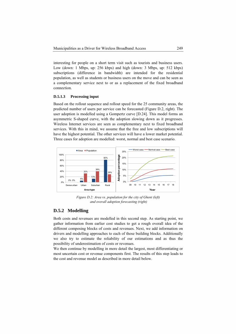
Municipalities as a Driver for Wireless Broadband Access 249
interesting for people on a short term visit such as tourists and business users. own: 1 Mbps, up: 256 kbps) and high (down: 3 Mbps, up: 512 kLow (d bps)
poa compconnect
Based opredicte ght). The
asymme ogresses.
serviceshave th otential. The other services will have a lower market potential. Three cases for adoption are modelled: worst, normal and best case scenario.
subscriptions (difference in bandwidth) are intended for the residential pulation, as well as students or business users on the move and can be seen as
lementary service next to or as a replacement of the fixed broadband ion.
D.5.1.3 Processing input
n the rollout sequence and rollout speed for the 25 community areas, the d number of users per service can be forecasted (Figure D.2, ri
user adoption is modelled using a Gompertz curve [D.24]. This model forms an tric S-shaped curve, with the adoption slowing down as it pr
Wireless Internet services are seen as complementary next to fixed broadband . With this in mind, we assume that the free and low subscriptions will
e highest p
0%6%
13%
82%
0%
32%39%
29%
0%
20%
40%
60%
80%
100%
Dense urban Urban Suburban Rural
Area type
Area Population
0%
5%
10%
15%
20%
25%
09 10 11 12 13 14 15 16 17 18
Adop
tion
perc
enta
ge
Year
Worst case Normal case Best case
Figure D.2: Area vs. population for the city of Ghent (left)
and overall adoption forecasting (right)
D.5.2 Modelling Both costs and revenues are modelled in this second step. As starting point, we gather information from earlier cost studies to get a rough overall idea of the different composing blocks of costs and revenues. Next, we add information on drivers and modelling approaches to each of those building blocks. Additionally we also try to estimate the reliability of our estimations and as thus the possibility of underestimation of costs or revenues. We then continue by modelling in more detail the largest, most differentiating or most uncertain cost or revenue components first. The results of this step leads to the cost and revenue model as described in more detail below.
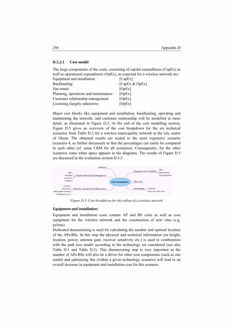
Appendix D 250
D.5.2.1 Cost model
he large components of the costs, consisting of capital expenditures (CapEx) as ell as operational expenditures (OpEx), as expected for a wireless network are:
Equipment and installation [CapEx] Backhauling [CapEx & OpEx] Site rental [OpEx] Planning, operations and maintenance [OpEx] Customer relationship management [OpEx] Licensing (largely unknown) [OpEx] Major cost blocks like equipment and installation, backhauling, operating and maintaining the network, and customer relationship will be modelled in more detail, as illustrated in Figure D.3. At the end of the cost modelling section, Figure D.5 gives an overview of the cost breakdown for the six technical scenarios from Table D.2 for a wireless municipality network in the city centre of Ghent. The obtained results are scaled to the most expensive scenario (scenario 4, as further discussed) so that the percentages can easily be compared to each other (cf. same CRM for all scenarios). Consequently, for the other scenarios some white space appears in the diagrams. The results of Figure D.5 are discussed in the evaluation section D.5.3.
Tw
Figure D.3: Cost breakdown for the rollout of a wireless network
Equipment and installation: Equipment and installation costs contain AP and BS costs as well as core equipment for the wireless network and the construction of new sites (e.g. pylons). Dedicated dimensioning is used for calculating the number and optimal location of the APs/BSs. In this step the physical and technical information (on height, location, power, antenna gain, receiver sensitivity etc.) is used in combination with the path loss model according to the technology set considered (see also Table D.1 and Table D.2). This dimensioning step is very important as the number of APs/BSs will also be a driver for other cost components (such as site rental) and optimizing this (within a given technology scenario) will lead to an overall decrease in equipment and installation cost for this scenario.
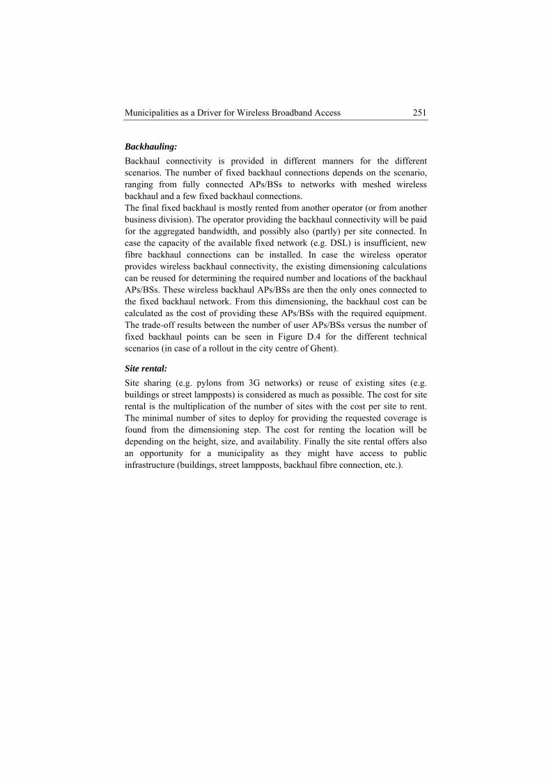
Municipalities as a Driver for Wireless Broadband Access 251
Backhauling: Backhaul connectivity is provided in different manners for the different scenarios. The number of fixed backhaul connections depends on the scenario, ranging from fully connected APs/BSs to networks with meshed wireless backhaul and a few fixed backhaul connections. The final fixed backhaul is mostly rented from another operator (or from another business division). The operator providing the backhaul connectivity will be paid for the aggregated bandwidth, and possibly also (partly) per site connected. In case the capacity of the available fixed network (e.g. DSL) is insufficient, new fibre backhaul connections can be installed. In case the wireless operator provides wireless backhaul connectivity, the existing dimensioning calculations can be reused for determining the required number and locations of the backhaul APs/BSs. These wireless backhaul APs/BSs are then the only ones connected to the fixed backhaul network. From this dimensioning, the backhaul cost can becalculated as t ired equipment.The trade-offixed backhscenarios (in case of a rollout in the city c
Site rental: Site sharing (e.g. pylons from 3G networks) or reuse of existing sites (e.g. buildings or street lampposts) is considered as much as possible. The cost for site
to rent. rage is
imensioning step. The cost for renting the location will be
blic frastructure (buildings, street lampposts, backhaul fibre connection, etc.).
he cost of providing these APs/BSs with the requ
f results between the number of user APs/BSs versus the number of aul points can be seen in Figure D.4 for the different technical
entre of Ghent).
rental is the multiplication of the number of sites with the cost per site The minimal number of sites to deploy for providing the requested covefound from the ddepending on the height, size, and availability. Finally the site rental offers also an opportunity for a municipality as they might have access to puin
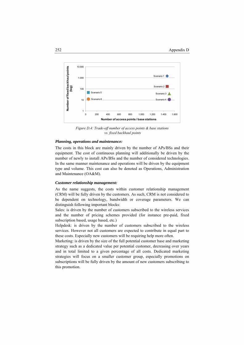
Appendix D 252
Scenario 1
Scenario 2
10.000 p
oint
s
1.000
)
Scenario 3
Scenario 4
Scenario 5
Scenario 6
1
10
100
0 200 400 600 800 1.000 1.200 1.400 1.600
Num
ber o
f fi
(log
Number of access points / base stations
xed
back
haul
Figure D.4: Trade-off number of access points & base stations
vs. fixed backhaul points
Planning, operations and maintenance: The costs in this block are mainly driven by the number of APs/BSs and their equipment. The cost of continuous planning will additionally be driven by the number of newly to install APs/BSs and the number of considered technologies. In the same manner maintenance and operations will be driven by the equipment type and volume. This cost can also be denoted as Operations, Administration and Maintenance (OA&M).
Customer relationship management: As the name suggests, the costs within customer relationship management (CRM) will be fully driven by the customers. As such, CRM is not considered to be dependent on technology, bandwidth or coverage parameters. We can distinguish following important blocks: Sales: is driven by the number of customers subscribed to the wireless services
dedicated value per potential customer, decreasing over years
and the number of pricing schemes provided (for instance pre-paid, fixed subscription based, usage based, etc.) Helpdesk: is driven by the number of customers subscribed to the wireless services. However not all customers are expected to contribute in equal part to these costs. Especially new customers will be requiring help more often. Marketing: is driven by the size of the full potential customer base and marketing strategy such as a and in total limited to a given percentage of all costs. Dedicated marketing strategies will focus on a smaller customer group, especially promotions on subscriptions will be fully driven by the amount of new customers subscribing to this promotion.
Municipalities as a Driver for Wireless Broadband Access 253
Licensing As WiFi is operating in a license-free band, license costs are only required for the scenarios using WiMAX. License costs vary from country to country depending on regulations, and can be either CapEx or OpEx [D.25]. In some countries, they are obtained for several years e.g. by an auction process. The paid amount can then be considered as a CapEx cost. In other countries, the operator has to pay a yearly fee to the operator to lease the spectrum, which then corresponds to an OpEx cost. As e.g. Clearwire has to pay a yearly fee to the Belgian regulator BIPT [D.11], we consider an OpEx cost for the WiMAX spectrum license. The license cost typically depends on the channel bandwidth (amount per MHz), and can further depend on e.g. the population of the covered area [D.25] or the number of used BSs [D.11]. As the exact cost is also determined by the market situation, it is difficult to estimate a correct cost. We have assumed a fixed annual cost based on a mix of diverse sources.
Wirel. Ac. eq.; 18% Wirel. BH
eq.; 3%
Fixed BH cap.; 1%
Fixed BH op.; 3%
CRM; 20%
OA&M; 13%
Licence; 0%
Site rental; 10%
Scenario 2
Wirel. Ac. eq.; 18%
Wirel. BH eq.; 0%
Fixed BH cap.; 7%
Fixed BH op.; 24%
CRM; 20%
OA&M; 13%
Licence; 0%
Site rental; 10%
Scenario 1
Wirel. Ac. eq.; 18%
Wirel. BH eq.; 23%
Fixed BH cap.; 0%
Fixed BH op.; 1%
CRM; 20%
OA&M; 19%
Licence; 3%
Site rental; 16%
Scenario 4
Wirel. Ac. eq.; 25%
Wirel. BH eq.; 0%
Fixed BH cap.; 2%
Fixed BH op.; 4%
CRM; 20%OA&M;
9%
Licence; 3%
Site rental; 12%
Scenario 5
Wirel. Ac. eq.; 25%
Wirel. BH eq.; 6%
Fixed BH cap.; 0%Fixed BH op.; 1%
CRM; 20%
OA&M; 10%
Licence; 3%
Site rental; 12%
Scenario 6
Wirel. Ac. eq.; 18%
Licence; 3%
Wirel. BH eq.; 20%
Fixed BH cap.; 1%
Fixed BH op.; 3%CRM;
20%
OA&M; 18%
Site rental; 16%
Scenario 3
Figure D.5: Cost breakdown for all scenarios,
scaled to the most expensive scenario
D.5.2.2 Revenues
The revenues are divided in two parts: direct and indirect. The first category of revenues can be directly derived from the forecasted number of customers. For the free Internet service, advertising will be allowed, which leads to fixed revenues per customer. The other services are priced lower than competitor services offered by telecom operators, as increased competition and thus lower tariffs are motives for the municipality to invest in such networks. An overview of the revenues for the considered wireless municipality network can be found in Figure D.6.

Appendix D 254
Indirect revenues are not directly linked to the main activity, here selling wireless access to the customers. They are caused by additional advantages experienced by providing the main activity. More in particular for the considered case, in which a municipality rolls out a wireless network, examples of such advantages are: efficiency gains in public services, the development of an eGovernment platform, attracting more high tech companies and educated
s opportunities, etc. Considering the broad range ment might have on a municipality, its companies
lect a potentially important part of nuesm e (monetary) impact of the indirect effects on the economy of
citizens, enabling new businesof influences a wireless deployand citizens, predicting the total impact in detail is infeasible. By leaving it out of the revenue model, on the other hand, you negthe reve . For esti ating ththe municipality, we distinguished between the following main drivers: • Fixed (or no driver): The setup of a wireless platform enables new public
and private applications to be deployed. This in turn could allow (future) benefits e.g. efficiency gain, cost reductions, etc.
• Customer based: As customers are the main users of the wireless platform, many indirect effects could also be traced back to those customers. Examples are the influence of eGovernment applications which are directly driven by the actual number of participating customers, word-of-mouth effects (positive image, attracting new citizens) which are driven by the number of contacts each customer has with others, etc.
• Service based: While some applications (e.g. tourist or other localized information) only require local connectivity (around the point of interest) and limited bandwidth, other applications such as web browsing and video services might benefit from an increase in both wireless coverage and bandwidth.
• Investment based: The investments (or part of it) made for deploying a new wireless network will (preferably) be spent in companies regionally close to the municipality and as such part of the invested money can be expected to flow back into the local economy.
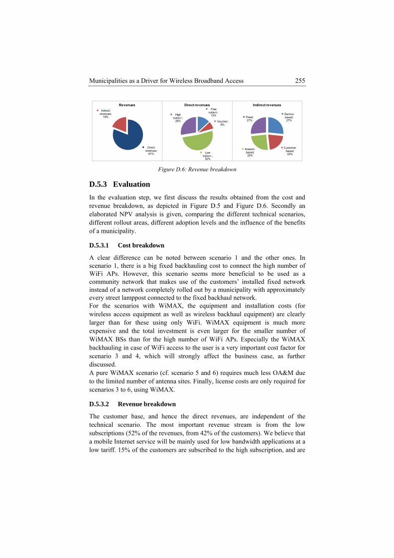
Municipalities as a Driver for Wireless Broadband Access 255
Direct revenues;
81%
Indirect revenues;
19%
RevenuesFree
subscr.; 13%
Voucher; 8%
Low subscr.;
52%
High subscr.;
28%
Direct revenues
Service based; 27%
Customer based; 22%
Investm. based; 25%
Fixed; 27%
Indirect revenues
Figure D.6: Revenue breakdown
D.5.3 Evaluation In the evaluation step, we first discuss the results obtained from the cost and revenue breakdown, as depicted in Figure D.5 and Figure D.6. Secondly an
fits f a municipality.
D.5.3.1 Cos
A clear difference s. In scenar of WiFi A d as a communi etwork instead of a network approximately
r st connected to the fixed backhaul network. with WiMAX, the equipment and installation costs (for
(cf. scenario 5 and 6) requires much less OA&M due i tenna sites. Finally, license costs are only required for
elaborated NPV analysis is given, comparing the different technical scenarios, different rollout areas, different adoption levels and the influence of the beneo
t breakdown
can be noted between scenario 1 and the other oneio 1, there is a big fixed backhauling cost to connect the high number
Ps. However, this scenario seems more beneficial to be usety network that makes use of the customers’ installed fixed n
completely rolled out by a municipality withevery st eet lamppoFor the scenarios wireless access equipment as well as wireless backhaul equipment) are clearly larger than for these using only WiFi. WiMAX equipment is much more expensive and the total investment is even larger for the smaller number of WiMAX BSs than for the high number of WiFi APs. Especially the WiMAX backhauling in case of WiFi access to the user is a very important cost factor for scenario 3 and 4, which will strongly affect the business case, as further discussed. A pure WiMAX scenario to the lim ted number of anscenarios 3 to 6, using WiMAX.
D.5.3.2 Revenue breakdown
The customer base, and hence the direct revenues, are independent of the technical scenario. The most important revenue stream is from the low subscriptions (52% of the revenues, from 42% of the customers). We believe that a mobile Internet service will be mainly used for low bandwidth applications at a low tariff. 15% of the customers are subscribed to the high subscription, and are
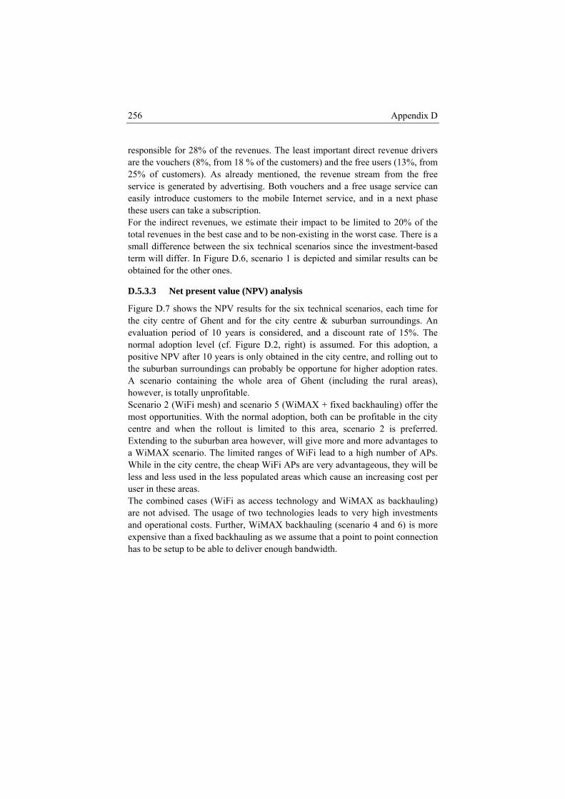
Appendix D 256
responsible for 28% of the revenues. The least important direct revenue drivers are the vouchers (8%, from 18 % of the customers) and the free users (13%, from 25% of customers). As already mentioned, the revenue stream from the free service is generated by advertising. Both vouchers and a free usage service can easily introduce customers to the mobile Internet service, and in a next phase these users can take a subscription. For the indirect revenues, we estimate their impact to be limited to 20% of the total revenues in the best case and to be non-existing in the worst case. There is a small difference between the six technical scenarios since the investment-based term will differ. In Figure D.6, scenario 1 is depicted and similar results can be obtained for the other ones.
D.5.3.3 Net present value (NPV) analysis
Figure D.7 shows the NPV results for the six technical scenarios, each time for the city centre of Ghent and for the city centre & suburban surroundings. An evaluation period of 10 years is considered, and a discount rate of 15%. The normal adoption level (cf. Figure D.2, right) is assumed. For this adoption, a positive NPV after 10 years is only obtained in the city centre, and rolling out to the suburban surroundings can probably be opportune for higher adoption rates. A scenario containing the whole area of Ghent (including the rural areas), however, is totally unprofitable. Scenario 2 (WiFi mesh) and scenario 5 (WiMAX + fixed backhauling) offer the
rmal adoption, both can be profitable in the city nd s limited to this area, scenario 2 is preferred.
most opportunities. With the nocentre a when the rollout iExtending to the suburban area however, will give more and more advantages to a WiMAX scenario. The limited ranges of WiFi lead to a high number of APs. While in the city centre, the cheap WiFi APs are very advantageous, they will be less and less used in the less populated areas which cause an increasing cost per user in these areas. The combined cases (WiFi as access technology and WiMAX as backhauling) are not advised. The usage of two technologies leads to very high investments and operational costs. Further, WiMAX backhauling (scenario 4 and 6) is more expensive than a fixed backhauling as we assume that a point to point connection has to be setup to be able to deliver enough bandwidth.
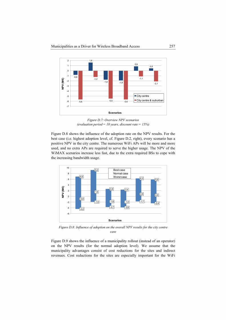
Municipalities as a Driver for Wireless Broadband Access 257
0
1
2 1,6
0,90,5
-0,8
-1,8 -1,9
-5,6
-1,2
-5,5 -5,6
-1,1
-2,1
-7
-6
-5
-4
-3
NPV
(M
-2
Scenarios
-1
€)
City centreCity centre & suburban
numerous WiFi APs will be more and more used, and no extra APs are required to serve the higher usage. The NPV of the
o cope with
Figure D.7: Overview NPV scenarios (evaluation period = 10 years, discount rate = 15%)
Figure D.8 shows the influence of the adoption rate on the NPV results. For the best case (i.e. highest adoption level, cf. Figure D.2, right), every scenario has a positive NPV in the city centre. The
WiMAX scenarios increase less fast, due to the extra required BSs tthe increasing bandwidth usage.
6,9
9,2
2,6 2,4
4
6
8
10
€)
Best caseNormal caseWorst case 6,3 5,9
-0,8
1,6
-1,8 -1,9
0,9 0,5
-4,4
-1,9
-3,7 -3,8
-1,7-2,4
-6
-4
-2
0
2
NPV
(M
Scenarios Figure D.8: Influence of adoption on the overall NPV results for the city centre
case Figure D.9 shows the influence of a municipality rollout (instead of an operator) on the NPV results (for the normal adoption level). We assume that the municipality advantages consist of cost reductions for the sites and indirect revenues. Cost reductions for the sites are especially important for the WiFi
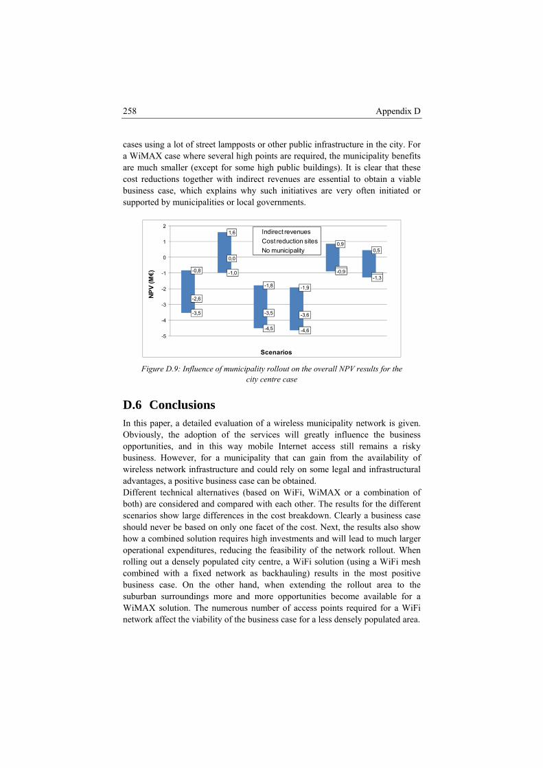
Appendix D 258
cases using a lot of street lampposts or other public infrastructure in the city. For a WiMAX case where several high points are required, the municipality benefits are much smaller (except for some high public buildings). It is clear that these cost reductions together with indirect revenues are essential to obtain a viable
often initiated or business case, which explains why such initiatives are very supported by municipalities or local governments.
-0,8
1,6
-1,8 -1,9
0,90,5
-2,6
0,0
-3,5 -3,6
-0,8-1,2
-3,5
-1,0
-4,5 -4,6
-0,9-1,3
-5
-4
-3
-2
-1
0
1
2
NPV
(M€)
Scenarios
Indirect revenuesCost reduction sitesNo municipality
llout on the overall NPV results for the
sults for the different enarios show large differences in the cost breakdown. Clearly a business case
should never be based on only one facet of the cost. Next, the results also show how a combined solution requires high investments and will lead to much larger operational expenditures, reducing the feasibility of the network rollout. When rolling out a densely populated city centre, a WiFi solution (using a WiFi mesh combined with a fixed network as backhauling) results in the most positive business case. On the other hand, when extending the rollout area to the suburban surroundings more and more opportunities become available for a WiMAX solution. The numerous number of access points required for a WiFi network affect the viability of the business case for a less densely populated area.
Figure D.9: Influence of municipality rocity centre case
D.6 Conclusions In this paper, a detailed evaluation of a wireless municipality network is given. Obviously, the adoption of the services will greatly influence the business opportunities, and in this way mobile Internet access still remains a risky business. However, for a municipality that can gain from the availability of wireless network infrastructure and could rely on some legal and infrastructural advantages, a positive business case can be obtained. Different technical alternatives (based on WiFi, WiMAX or a combination of
oth) are considered and compared with each other. The rebsc
Municipalities as a Driver for Wireless Broadband Access 259
Acknowledgements
This work was partially supported by the EC through Network of Excellence BONE. We would also like to acknowledge different researchers from the COST605 project Econ@Tel for relevant discussions on this topic. W. Joseph would like to thank the FWO-V (Research Foundation at Flanders) for his Post-Doctoral Fellowship.
References [D.1] Point topic. World Broadband Statistics Q2 2008. Sep. 2008.
[D ). yment ional
um
[D.3 for Informatio ation exchange
e metropolitan area networks-Specific e ss LAN Medium Access Control (MAC)
roughput. Sep. 2007.
D
D
D
[D
[D , B., Sari. H. (2007). Diversity, Interference Cancellation and Spatial Multiplexing in MIMO Mobile WiMAX Systems. IEEE Mobile WiMAX Symposium, pp. 74-79, Orlando, USA.
.2] Verbrugge, S., Casier, K., Van Ooteghem, J., Lannoo, B. (2008Practical steps in techno-economic evaluation of network deploplanning. Presented at Networks 2008, 13th InternatTelecommunications Network Strategy and Planning Symposi(tutorial T12), Budapest, Hungary, Sep. 2008.
] IEEE P802.11n/D3.00. Draft Amendment to IEEE Standardn Technology-Telecommunications and inform
b tween systems-Local andr quirements, Part 11: Wireleand Physical Layer (PHY) specifications: Enhancements for Higher Th
[ .4] IEEE Std. 802.16-2004. IEEE Standard for Local and Metropolitan Area Networks, Part 16: Air Interface for Fixed Broadband Wireless Access Systems. Oct. 2004.
[ .5] IEEE Std. 802.16e-2005. Amendment to IEEE Standard for Local and Metropolitan Area Networks, Part 16: Air interface for fixed broadband wireless access systems - Physical and Medium Access Control Layers for Combined Fixed and Mobile Operations in Licensed Bands. Feb. 2006.
[ .6] WiMAX Forum. Simulation Results for Subchannelization. Nov. 2002.
.7] IEEE report 802.11-03/845r1. Receiver Sensitivity Tables for MIMO-OFDM 802.11n. Nov. 2003.
.8] Biglieri, E., Goldsmith, A., Muquet
Appendix D 260
[D.9] Nuaymi L. (2007). WiMAX: Technology for Broadband Wireless
[D.1
[D.1 T).
[D.1 ture Generation S ssels, 1999.
r jandra, S. Y., Parkoff, S. R., Gupta, A., Ku i, R. (1999). An empirically based path
C Design and Their Performance. IEEE Transactions on
deo Broadcasting (DVB); DVB-H .
[D.19] European Parliament. Telecoms package: more competition and improved consumer rights. Information society - press release. Aug. 2008, http://www.europarl.europa.eu/pdfs/news/expert/background/20080827BKG35492/20080827BKG35492_en.pdf
[D.20] Communication from European Commission to the European Parliament, the Council, the European Economic and Social Committee and the Committee of the Regions. Reaping the full benefits of the digital dividend in Europe: A common approach to the use of the spectrum released by the digital switchover. Brussels, Nov. 2007, http://ec.europa.eu/information_society/policy/ecomm/doc/library/proposals/com_dd_en.pdf
Access. John Wiley & Sons, Jan. 2007.
0] Clearwire Belgium. http://www.clearwire.be
1] Belgium Institute for Postal services and Telecommunications (BIPhttp://www.bipt.be
2] COST 231 Final Report (1999). Digital Mobile Radio Towards Fuystems. COST Telecom Secretariat, Bru
[D.13] E ceg, V., Greenstein, L. J., Tlic, B., Julius, A. A., Bianch
loss model for wireless channels in suburban environments. IEEE J. Sel. Areas Commun., 17 (7), pp. 1205-1211
[D.14] Joseph, W., Martens, L. (2006). Performance Evaluation of Broadband Fixed Wireless System based on IEEE 802.16. IEEE Wireless Communications and Networking Conference (WCNC2006), vol. 2, pp. 978-983, Las Vegas, USA, Apr. 2006
[D.15] ECC report 33. The analysis of the coexistence of FWA cells in the 3.4 – 3.8 GHz band. May 2003.
[D.16] Leung, K. K., Clark, M. V., McNair, B., Kostic, Z., Cimini, Jr., L. J., Winters, J. H. (2007). Outdoor IEEE 802.11 Cellular Networks: Radio and MAVehicular Technology, 56 (5), pp. 2673-2684
[D.17] WiMAX Forum. Mobile WiMAX-Part 1: A Technical Overview and Performance Evaluation. Jun. 2006.
[D.18] ETSI, TR 102 377 v1.1.1. Digital ViImplementation Guidelines. Feb. 2005
Municipalities as a Driver for Wireless Broadband Access 261
[D.21] Gillett, S.E., Lehr, W.H., Osorio, C. (2004). Local government broadband initiatives. Telecommunications Policy, 28, pp. 537–558
[D.22] European Commission. State aid decisions - NN 24 / 2007 - Prague Municipal Wireless Network. 24.04.2007, http://ec.europa.eu/comm/competition/state_aid/register/ii/doc/NN-24-2007-WLWL-en-30.05.2007.pdf
[D.23] Ballon, P. (2007). Changing business models for Europe’s mobile telecommunications industry: The impact of alternative wireless technologies. Telematics and Informatics, 24 (3), pp. 192-205
[D.24] Gregg, J. V., Hassel, C. H. and Richardson, J. T. (1964). Mathematical trend curves: An aid to forecasting. Edinburgh: Oliver & Boyd
[D.25] WiMAX Forum. Business Case Models for Fixed Broadband Wireless Access based on WiMAX Technology and the 802.16 Standa . Oct. 2004
rd

Appendix D 262
E Future Proof Strategies towards
J. Van Ooteghem, S. M. Pickavet,
ue networks, Real options
AbThehapfinafar for techrolevalu ing technological needs, economic and regulatory conditions. An indication is given where real
Fibre to the Home
Verbrugge, K. Casier, P. Demeester Submitted to Telecommunications Policy, Elsevier, ISSN 0308-5961 Key words Fibre to the home, Competition models, Val
stract rollout of new fibre access networks or the upgrade towards FttH is pening in most Western countries at a much slower rate than expected. The l step in migrating to an all fibre (last mile) access network is one bridge to for most telecom operators. Nevertheless, FttH is considered as the solution access networks in the long run. In this paper we will analyse different nical, as well as future proof strategies for the rollout of FttH. The different s and actors are considered, and for each type of competition model, the e network is presented and analysed in the light of chang
264 Appendix E
op ons analysis could be used for the quantitative analysis of FttH business s.
ticase
ern world. ccording to Point Topic [E.1], Western Europe has the second largest
penetration rate for broadband Internet rvices, but the market is reaching its saturation po ered, more than ia copper acce is conne louts, We re specifically China, South Korea ading with a staggering 84% of
). olling out FttH and the
H will be required [E.2].
t in the rollout of next generation networks (NGA). illett, Lehr, & Osorio [E.5], Analysys Mason [E.6] and A.T. Kearney [E.7]
describe the interventions governments can make. As investments in NGA are multi-billion euro investments, co-operations between actors (e.g. municipalities, customers, telecom operators) become a necessity for the economic viability of the business case. Infrastructure competition is one of the main drivers for migrating towards FttH. A lack of competition will lead to postponements of new infrastructure investments (due to very high costs compared to low incremental ARPU). Telecom is more and more seen as another utility next to electricity, gas, sewage, etc. The separation of passive and network infrastructure, and service provisioning could lead to more cost efficient networks, combining the
E.1 Introduction Broadband Internet is becoming a commodity product in the WestA
seint (2.58% growth last year). When technologies are consid
84% of the subscribers are xDSL (digital subscriber lines, vss networks) customers, 14% make use of cable networks, and only 1.5%
cted via fibre. Concerning overall fibre to the home (FttH) rolstern Europe is lagging (3.37%) compared to the rest of the world. Asia, mo
and Japan, is leall worldwide fibre access connections (34 million usersSeveral actors are involved in the overall process of rmotives for each of these actors differ. Incumbent telecom operators try to postpone large network investments in the access network by exploiting their current infrastructure. Small upgrades are implemented to keep up with the current bandwidth demand, but these migrations tend to be short term solutions. If the threat for cable operator competition is low and there is low willingness by governments to change access rules (like in Europe), rollout initiatives for FttH are limited. If telcos have overseas interests, FttH investment funds are mostly postponed to more value added markets. When cable competition threat is high (as in some European countries), migrating towards FttNew public or private actors are showing their interest to invest in new future proof telecom networks. Municipalities (or government initiatives), utility companies, etc. have good strengths and opportunities to invest in such initiatives as a result of economies of scale, scope [E.3], right of way [E.4], etc. Either demand or supply side motivations will be used by actors when considering involvemenG
Future Proof Strategies towards Fibre to the Home 265
advantages of each actor involved. Banerjee & Sirbu [E.8], Ehrler, Brusic, Reichl, & Ruhle [E.9] and Felten [E.10] have proposed different competition models, based on the division of passive, network and service level. In this paper we describe and rank all competition models based on the OSI Reference model [E.11]. In the next section we start by describing shortly the diverse fibre technologies and architectures, paying attention to the current situation and migration options for telecom operators. In section E.3, the different roles considered in the rollout of FttH, are discussed, and the relevant actors are presented. For each of the different competition models, we present in section E.4 the value model and map the diverse actors upon the roles. A comparison is made, related to choice of technology, network architecture, accessibility for competitors and e ic viability. An uld be used for th with some con
wards the customer is still copper or b k, a choice must be
ive or active, and the
to as passive ptical networks (PON), where the access fibre is shared by 16 to 128 users. egardless of the used architecture, in the central office (CO) the fibre lines of e users are terminated and connected to the different Internet service providers. rom the CO, feeder cables with fibers run into ducts, to one or more termediate flexibility points (FP) where a split is made, either in sub-cables
with fibers (in ca inated on active equipment (active connected via a spM towar st y be sufficient for the upcoming years as the dis as art is the bottleneck for offering more bandwidth [E.12]. The cable operators are also trying to extend the potential of their Hybrid Coax Fibre (HFC) network. Upgrading to DOCSIS 3.0 allows reaching bandwidths up to 120 Mbps, but requires smaller service areas. Even higher bandwidths could be reached in the future with new to be deployed DOCSIS standards [E.13] but this will also require migration towards a PON
conom indication is given in Section E.5 where real options analysis co
e analysis of FttH rollouts. We end this paper clusions.
E.2 Technologies At this moment, two types of technologies are used for offering broadband services to the customer: copper based digital subscriber lines (xDSL) and hybrid fibre coax (HFC) networks. In both cases, fibre has already been installed in the core and metro network, but the last part tocoax ca le. When considering the rollout of an FttH networmade between two categories of fibre networks, either passconsidered network topology, either point-to-multipoint (P2MP) or point-to-point (P2P). In a P2P topology, there are again two possible architectures: home run fibre and active star. P2MP topologies are typically referred oRthFin
se of home run), either the fibers are termstar) or the fibers are physically split and
litter upon a nigration
ew fibre structuds new xDSL
tance of the ‘l
re (PON). andards will onlt mile’ copper p
266 Appendix E
to lec n pt for Pth rrent n ructure (eithe In case of mu ality ne architecturcost is slightly ON, but it perm ssibilities [E.14].
E.3 Value Network This part describes the different roles requirenetwork, as well as the main actors involved.
E Roles The PEST framework (Political, Economicdesigned to model the external environmframework. This framework will influence tnetwork. We based our analysis on [E.15], wh analysis was made for broadband data access, related to the migra ccess towards faster xDSL and cable networks. The politica ion and investment regulation, determining which nregulation for copper and cable networkinfrastructure must be opened for competitio n sc lie gulatoryin ection op unbundlin subsidies, etc. Economic facto clude degree of comconditions at l markets, equ d demographic factors determine market willingness to pay for telecommunication services, adoption rate for new technologies and services, etc. The technodecision which technology could be us network upgrading options, possibilities of opening up the networ s, security, co es, etc. Th etwork de sition 6] and methodivided in four plan, deploy, oThe planning p ided in four role n the right of way (RoW). Several authorities can grant (or facilities on,
ver or under private or public property. The network planning determines which
pology. Teeir cunicip
om operators teetwork infrast
tworks, a home run
d to o ON networks, which is in line with r xDSL or HFC). e is mostly chosen. The investment its more competition pohigher than P
d in the rollout process of an FttH
.3.1 , Social and Technological) was ental influences on the business he rollout parameters for an FttH
re a PESTetion from dial-up al factors include competitetworks are considered (different s), at which level the network n (cf. Section E.4), cost allocatio
hemes appterconn
d by the natioand local lo
rs in
nal re agency (NRA) for determining g (LLU) tariffs, petition, economic growth, loan ipment costs, etc. Social anthe financiapotential, Internet penetration,
logical factor will influence the ed, k, killer application
mbinations we business compo
ith wireless techroles in an Fmodel in [E.1
nologittH n rollout are based on the cost
dology described in [E.17], and perations and service provisioning. major phases:
hase is subdiv s. The first focuses o deny) RoW to install
opart of the market to focus on (users, areas and services) and customer forecast, and technical design including choice of technology, topology and architecture. An important factor to consider is the current network infrastructure as new incremental investments could furthermore expand its lifecycle. The next role is determining a (practical) rollout planning, based on the previous roles and
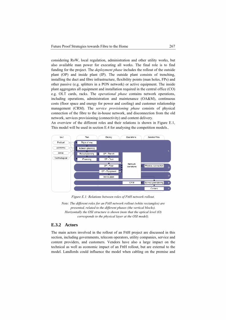
Future Proof Strategies towards Fibre to the Home 267
considering RoW, local regulation, administration and other utility works, but also available man power for executing all works. The final role is to find funding for the project. The deployment phase includes the rollout of the outside plant (OP) and inside plant (IP). The outside plant consists of trenching, installing the duct and fibre infrastructure, flexibility points (man holes, FPs) and other passive (e.g. splitters in a PON network) or active equipment. The inside plant aggregates all equipment and installation required in the central office (CO) e.g. OLT cards, racks. The operational phase contains network operations, including operations, administration and maintenance (OA&M), continuous costs (floor space and energy for power and cooling) and customer relationship management (CRM). The service provisioning phase consists of physical connection of the fibre to the in-house network, and disconnection from the old network, services provisioning (connectivity) and content delivery. An overview of the different roles and their relations is shown in Figure E.1, This model will be used in section E.4 for analysing the competition models..
Figure E.1: Relations between roles of FttH network rollout.
Note: The different roles for an FttH network rollout (white rectangles) are presented, related to the different phases (the vertical blocks).
Horizontally the OSI structure is shown (note that the optical level (O) corresponds to the physical layer at the OSI model).
E.3.2 Actors Th main actors involved in the rollout of an FttH project are discussed in this
ion, including governments, telecom operators, utility companies, service and ent providers, and customers. Vendors have also a large impact on the nical as well as economic impact of an FttH rollout, but are external to the el. Landlords could influence the model when cabling on the premise and
esectconttechmod
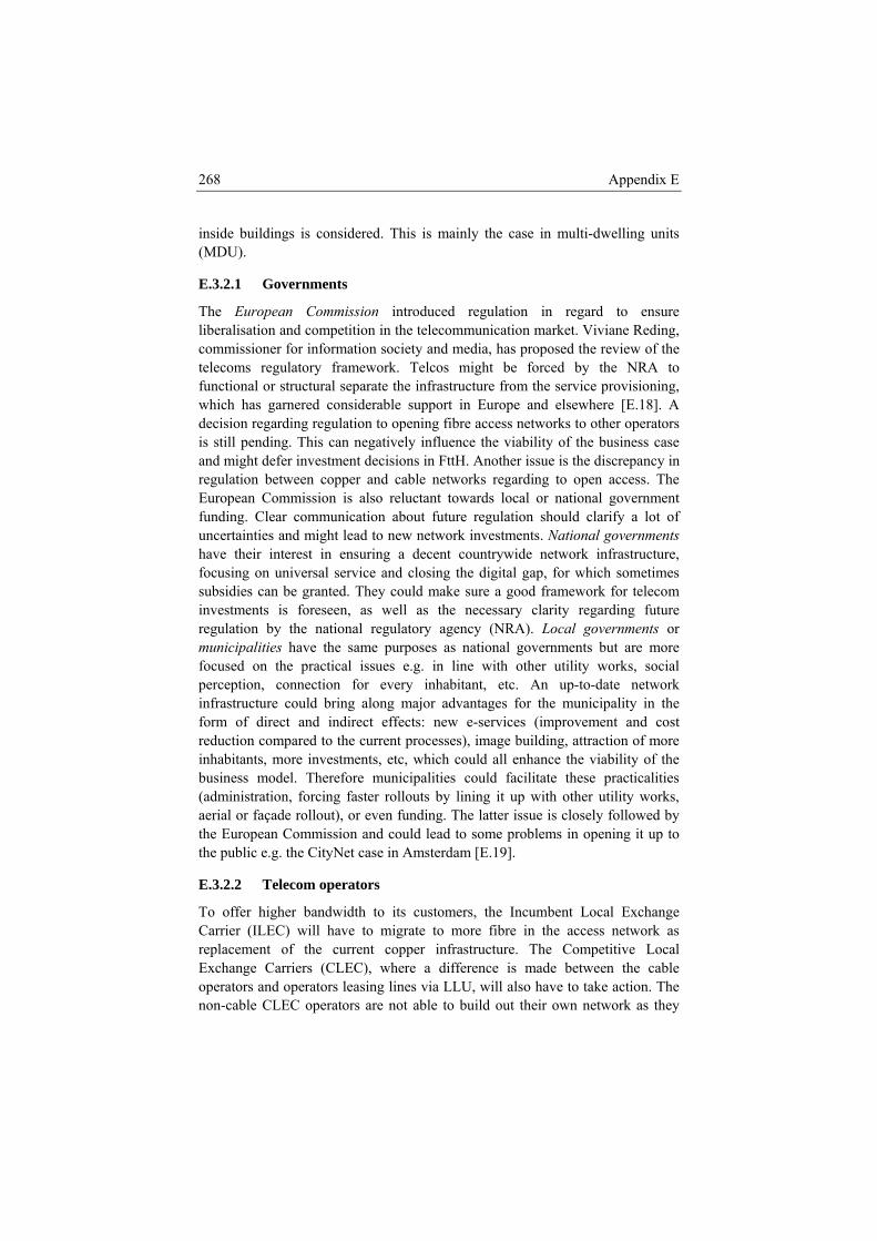
268 Appendix E
ins de buildings is considered. This is mainly the case in multi-dwelling units U).
2.1 Governments
European Commission introduced regulation in regard to ensure ralisation and competition in the telecommunicatio
i(MD
E.3.
The libe n market. Viviane Reding,
mtelefunc te the infrastructure from the service provisioning,
ideciis st is can negatively influence the viability of the business case
ble networks regarding to open access. The European Commission is also reluctant towards local or national government
ation about future regulation should clarify a lot of to new network investments. National governments
orks, social
e more fibre in the access network as
copper infrastructure. The Competitive Local
co missioner for information society and media, has proposed the review of the coms regulatory framework. Telcos might be forced by the NRA to tional or structural separa
wh ch has garnered considerable support in Europe and elsewhere [E.18]. A sion regarding regulation to opening fibre access networks to other operators ill pending. Th
and might defer investment decisions in FttH. Another issue is the discrepancy in regulation between copper and ca
funding. Clear communicuncertainties and might lead have their interest in ensuring a decent countrywide network infrastructure, focusing on universal service and closing the digital gap, for which sometimes subsidies can be granted. They could make sure a good framework for telecom investments is foreseen, as well as the necessary clarity regarding future regulation by the national regulatory agency (NRA). Local governments or municipalities have the same purposes as national governments but are more focused on the practical issues e.g. in line with other utility wperception, connection for every inhabitant, etc. An up-to-date network infrastructure could bring along major advantages for the municipality in the form of direct and indirect effects: new e-services (improvement and cost reduction compared to the current processes), image building, attraction of more inhabitants, more investments, etc, which could all enhance the viability of the business model. Therefore municipalities could facilitate these practicalities (administration, forcing faster rollouts by lining it up with other utility works, aerial or façade rollout), or even funding. The latter issue is closely followed by the European Commission and could lead to some problems in opening it up to the public e.g. the CityNet case in Amsterdam [E.19].
E.3.2.2 Telecom operators
To offer higher bandwidth to its customers, the Incumbent Local ExchangCarrier (ILEC) will have to migrate toreplacement of the current Exchange Carriers (CLEC), where a difference is made between the cable operators and operators leasing lines via LLU, will also have to take action. The non-cable CLEC operators are not able to build out their own network as they
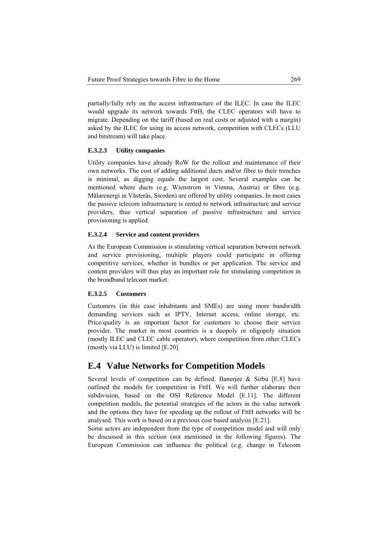
Future Proof Strategies towards Fibre to the Home 269
partially/fully rely on the access infrastructure of the ILEC. In case the ILEC would upgrade its network towards FttH, the CLEC operators will have to migrate. Depending on the tariff (based on real costs or adjusted with a margin) asked by the ILEC for using its access network, competition with CLECs (LLU
l take place.
E
Uown ne re to their trenches ismMälarenthe passi nted to network infrastructure and service prprovisio
E.3.2.4 ders
Aand ser fering ccontentthe broa
E.3.2.5
CdemandPrice/qu provide ligopoly situation (m ILEC(m
E.4 V ion Models Soutlinedsubdivicompet ies of the actors in the value network
analyse .21]. Some actors are independent from the type of competition model and will only be discussed in this section (not mentioned in the following figures). The European Commission can influence the political (e.g. change in Telecom
and bitstream) wil
.3.2.3 Utility companies
tility companies have already RoW for the rollout and maintenance of their tworks. The cost of adding additional ducts and/or fib
minimal, as digging equals the largest cost. Several examples can be entioned where ducts (e.g. Wienstrom in Vienna, Austria) or fibre (e.g.
ergi in Västerås, Sweden) are offered by utility companies. In most cases ve telecom infrastructure is re
oviders, thus vertical separation of passive infrastructure and service ning is applied.
Service and content provi
s the European Commission is stimulating vertical separation between network vice provisioning, multiple players could participate in of
ompetitive services, whether in bundles or per application. The service and providers will thus play an important role for stimulating competition in dband telecom market.
Customers
ustomers (in this case inhabitants and SMEs) are using more bandwidth ing services such as IPTV, Internet access, online storage, etc. ality is an important factor for customers to choose their service
r. The market in most countries is a duopoly or oostly and CLEC cable operator), where competition from other CLECs ostly via LLU) is limited [E.20].
alue Networks for Competiteveral levels of competition can be defined. Banerjee & Sirbu [E.8] have
the models for competition in FttH. We will further elaborate their sion, based on the OSI Reference Model [E.11]. The different ition models, the potential strateg
and the options they have for speeding up the rollout of FttH networks will be d. This work is based on a previous cost based analysis [E

270 Appendix E
Package) and economic (e.g. subsidies for broadband network investments, such reece) framework [E.7] which will impact competition in the telecom and investments in next generation
as in Gmarket access (NGA) networks. National
influemunicipi
shared operatin that need immediate interventions (e.g.
or cableFor the physical rastructure providers (NIP),
differen specific type.
The “phlayer of ench, duct or
level oftrench. solutionoverall rollo frastructure is offered by one
the ductspeed a sical level,
E.4.1.1
In this mThe loc s on collecting broadband users and rule
better a ion). This is the pure infrastructure competition
(e.g. no (e.g. muphysica
(more specifically NRA measures) and local governments have comparable nce. The latter has also an impact on the social framework. Widely, local
alities are the competent authorities dealing with granting RoW and the ssuing of building permits. With regard to co-location and sharing of the RoW
(passive infrastructure such as trenches, ducts, fibers, FPs, etc.), competences are with the NRA [E.4]. Some providers have already RoW, required for g necessary repair processes
water or gas problems), or for connecting customers to their networks (e.g. ILEC operators). comparison of the value networks, we have defined four types of actors: infrastructure providers (PIP), network inf
service providers (SP) and application providers (AP). Depending on the model, t actors could fulfil the role of a
E.4.1 Physical infrastructure based competition ysical infrastructure based competition” model is situated at the lowest the network, and is further split up into three models: tr
fibre. The ‘trench’ level comprises the current infrastructure competition model, where every telecom operator owns a network in separate trenches. The ‘duct’
competition consists of the rollout of multiple networks in the same This could impact the viability of the business case as in a buried FttH for instance, the trenching costs comprises over more than 70% of the
ut costs [E.16]. In case a shared duct inactor, the NIP can incrementally roll out their fibre networks by blowing it into
s, each having the opportunity of choosing their fibre architecture, rollout nd area. This is called competition at the ‘fibre’. For the phy
all fibre architectures and technologies could be used.
Competition at trench level
odel (Figure E.2) there is only one scenario for stimulating investments. al government will have to focu
making decisions, thus facilitating the processes for the network rollout (e.g. nd faster administrat
model known today (e.g. ILEC versus cable operator networks). Multiple networks are rolled out next to each other, leading to surplus costs for each PIP
communal trenching) and extra inconvenience for customers/inhabitants ltiple road works in short term). Competition is only guaranteed on the
l level, thus only the big players will be able to rollout such an
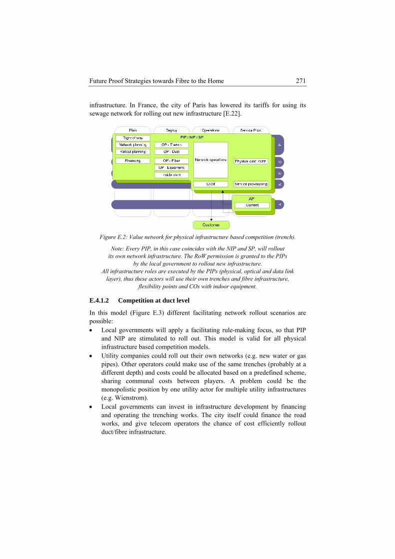
Future Proof Strategies towards Fibre to the Home 271
infrastructure. In France, the city of Paris has lowered its tariffs for using its network for rolling out new infrastructure [E.22]. sewage
re E.2: Value network for physical infrastructure baFigu sed competition (trench).
Note: Every PIP, in this case coincides with the NIP and SP, will rollout its own network infrastructure. The RoW permission is granted to the PIPs
by the local government to rollout new infrastructure. All infrastructure roles are executed by the PIPs (physical, optical and data link
layer), thus these actors will use their own trenches and fibre infrastructure, flexibility points and COs with indoor equipment.
E.4.1.2 Competition at duct level
In this model (Figure E.3) different facilitating network rollout scenarios are possible: • Local governments will apply a facilitating rule-making focus, so that PIP
and NIP are stimulated to roll out. This model is valid for all physical infrastructure based competition models.
• Utility companies could roll out their own networks (e.g. new water or gas pipes). Other operators could make use of the same trenches (probably at a different depth) and costs could be allocated based on a predefined scheme, sharing communal costs between players. A problem could be the monopolistic position by one utility actor for multiple utility infrastructures (e.g. Wienstrom).
• Local governments can invest in infrastructure development by financing and operating the trenching works. The city itself could finance the road works, and give telecom operators the chance of cost efficiently rollout duct/fibre infrastructure.
272 Appendix E
Figure E.3: Value network for physical infrastructure based competition (duct).
Note: a new PIP will be in charge of network and rollout planning, operations, as well as financing the trenching works. The NIPs roll out their own duct and
fibre network, as well as equipment for optical and data network layer. They will also take the roles of SP. Each customer can choose its provider (NIP/SP) and will be connected to its network. As in previous model this leads to duplicated
network architectures, and excessive costs.
E.4.1.3 Competition at fibre level
The next variant of the model is competition at fibre level (Figure E.4). Local governments (or subsidiary e.g. local utility company) could invest in a duct infrastructure. These ducts can than be leased or sold to NIPs. The NIPs will have to invest in their own fibre and equipment infrastructure, having the possibility to choose the technology and architecture, but not the topology. The FPs and COs of the PIP will have to be used for equipment storing. In France for example, all operators could make use of the duct infrastructure network of France Telecom (FT). In this case, FT is PIP as well as NIP, and other telecom infrastructure providers (NIP) are rolling out their network making use of the PIP’s duct network [E.23]. In Barcelona, possibilities for multiple fibre infrastructures have been taken into account in the dimensioning of the duct network [E.24]. Multiple networks could be rolled out incrementally next to each other, leaving the NIPs the choice of choosing their rollout areas. Fibre will have to be blown into the ducts. A disadvantage of this model is churn cost. Each customer will have to be migrated physically from one network to another, leading to new fibre blowing, connection cost and administration.
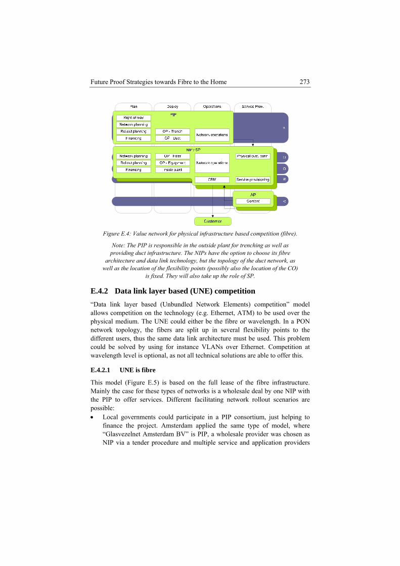
Future Proof Strategies towards Fibre to the Home 273
Figure E.4: Value network for physical infrastructure based competition (fibre).
Note: The PIP is responsible in the outside plant for trenching as well as providing duct infrastructure. The NIPs have the option to choose its fibre
architecture and data link technology, but the topology of the duct network, as well as the location of the flexibility points (possibly also the location of the CO)
is fixed. They will also take up the role of SP.
E.4.2 Data link layer based (UNE) competition “Data link layer based (Unbundled Network Elements) competition” model allows competition on the technology (e.g. Ethernet, ATM) to be used over the physical medium. The UNE could either be the fibre or wavelength. In a PON network topology, the fibers are split up in several flexibility points to the different users, thus the same data link architecture must be used. This problem could be solved by using for instance VLANs over Ethernet. Competition at wavelength level is optional, as not all technical solutions are able to offer this.
E.4.2.1 UNE is fibre
This model (Figure E.5) is based on the full lease of the fibre infrastructure. Mainly the case for these types of networks is a wholesale deal by one NIP with the PIP to offer services. Different facilitating network rollout scenarios are possible: • Local governments could participate in a PIP consortium, just helping to
finance the project. Amsterdam applied the same type of model, where “Glasvezelnet Amsterdam BV” is PIP, a wholesale provider was chosen as NIP via a tender procedure and multiple service and application providers
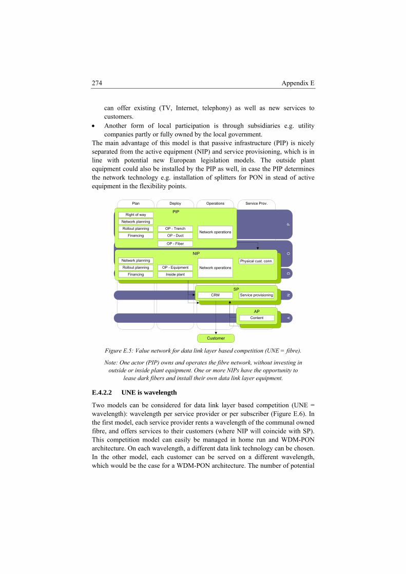
274 Appendix E
can offer existing (TV, Internet, telephony) as well as new services to customers.
• Another form of local participation is through subsidiaries e.g. utility companies partly or fully owned by the local government.
The main advantage of this model is that passive infrastructure (PIP) is nicely separated from the active equipment (NIP) and service provisioning, which is in line with potential new European legislation models. The outside plant equipment could also be installed by the PIP as well, in case the PIP determines the network technology e.g. installation of splitters for PON in stead of active equipment in the flexibility points.
OperationsPlan Deploy Service Prov.
A
AP
NSPD
PO
NIP
PIP
AP
SP
NIP
Inside plant
Physical cust. conn.
Network operations
CRM Service provisioning
Content
OP - Duct
OP - TrenchRollout planning
Rollout planning
Network planning
Network operations
Netwerk planning
OP - Fiber
Customer
Financing
Financing
Right of way
OP - Equipment
Figure E.5: Value network for data link layer based competition (UNE = fibre).
Note: One actor (PIP) owns and operates the fibre network, without investing in outside or inside plant equipment. One or more NIPs have the opportunity to
lease dark fibers and install their own data link layer equipment.
E.4.2.2 UNE is wavelength
Two models can be considered for data link layer based competition (UNE = wavelength): wavelength per service provider or per subscriber (Figure E.6). In the first model, each service provider rents a wavelength of the communal owned fibre, and offers services to their customers (where NIP will coincide with SP). This competition model can easily be managed in home run and WDM-PON architecture. On each wavelength, a different data link technology can be chosen. In the other model, each customer can be served on a different wavelength, which would be the case for a WDM-PON architecture. The number of potential
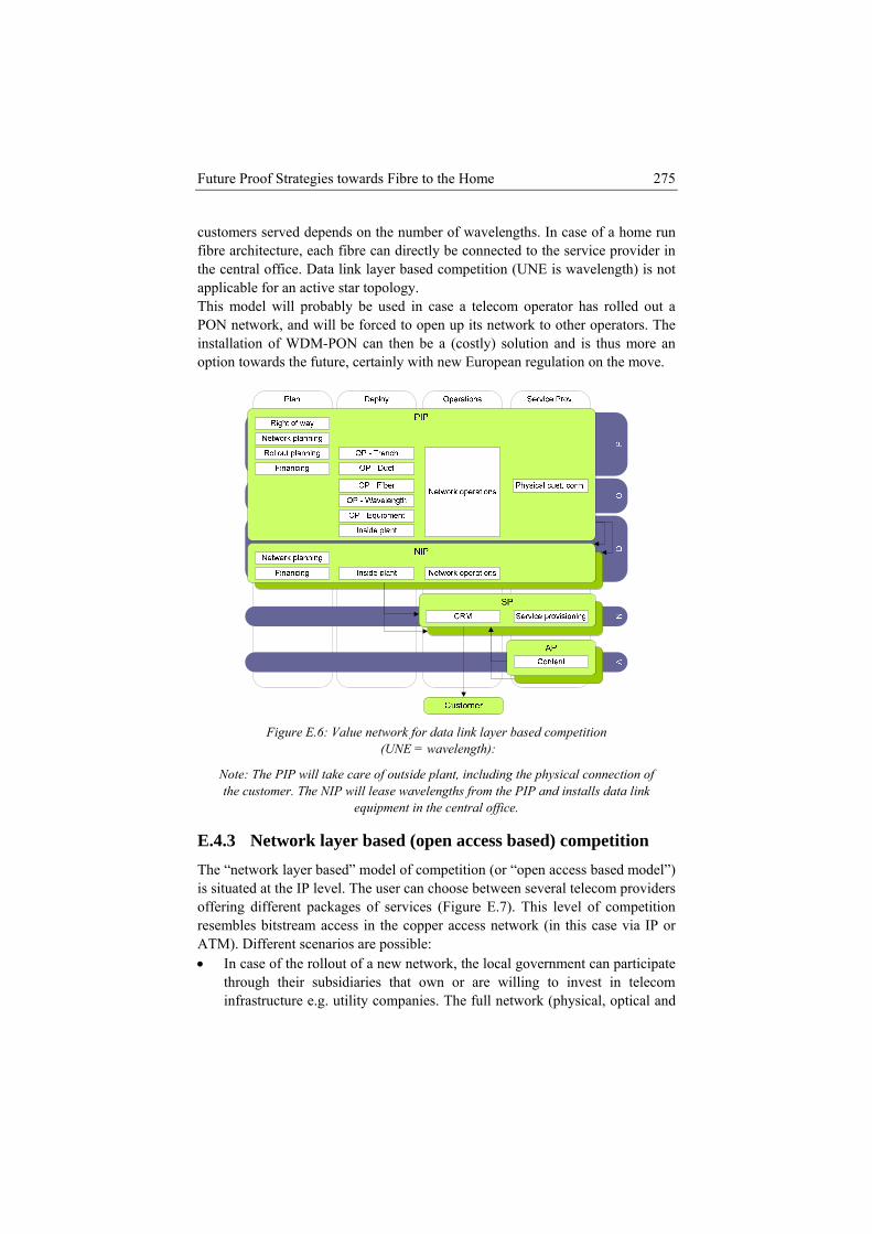
Future Proof Strategies towards Fibre to the Home 275
customers served depends on the number of wavelengths. In case of a home run fibre architecture, each fibre can directly be connected to the service provider in the central office. Data link layer based competition (UNE is wavelength) is not applicable for an active star topology. This model will probably be used in case a telecom operator has rolled out a PON network, and will be forced to open up its network to other operators. The installation of WDM-PON can then be a (costly) solution and is thus more an option towards the future, certainly with new European regulation on the move.
Figure E.6: Value network for data link layer based competition
(UNE = wavelength):
Note: The PIP will take care of outside plant, including the physical connection of the customer. The NIP will lease wavelengths from the PIP and installs data link
equipment in the central office.
E.4.3 Network layer based (open access based) competition The “network layer based” model of competition (or “open access based model”) is situated at the IP level. The user can choose between several telecom providers offering different packages of services (Figure E.7). This level of competition resembles bitstream access in the copper access network (in this case via IP or ATM). Different scenarios are possible: • In case of the rollout of a new network, the local government can participate
through their subsidiaries that own or are willing to invest in telecom infrastructure e.g. utility companies. The full network (physical, optical and
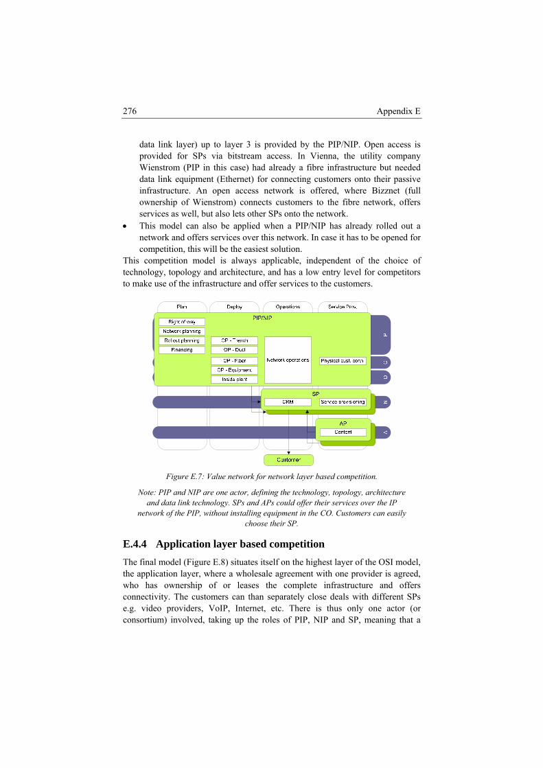
276 Appendix E
data link layer) up to layer 3 is provided by the PIP/NIP. Open access is provided for SPs via bitstream access. In Vienna, the utility company TWienstrom (PIP in this case) had already a Tfibre infrastructure but needed data link equipment (Ethernet) for connecting customers onto their passive infrastructure. An open access network is offered, where Bizznet (full ownership of Wienstrom) connects customers to the fibre network, offers services as well, but also lets other SPs onto the network.
• This model can also be applied when a PIP/NIP has already rolled out a network and offers services over this network. In case it has to be opened for competition, this will be the easiest solution.
This competition model is always applicable, independent of the choice of technology, topology and architecture, and has a low entry level for competitors to make use of the infrastructure and offer services to the customers.
Figure E.7: Value network for network layer based competition.
Note: PIP and NIP are one actor, defining the technology, topology, architecture and data link technology. SPs and APs could offer their services over the IP
network of the PIP, without installing equipment in the CO. Customers can easily choose their SP.
E.4.4 Application layer based competition The final model (Figure E.8) situates itself on the highest layer of the OSI model, the application layer, where a wholesale agreement with one provider is agreed, who has ownership of or leases the complete infrastructure and offers connectivity. The customers can than separately close deals with different SPs e.g. video providers, VoIP, Internet, etc. There is thus only one actor (or consortium) involved, taking up the roles of PIP, NIP and SP, meaning that a
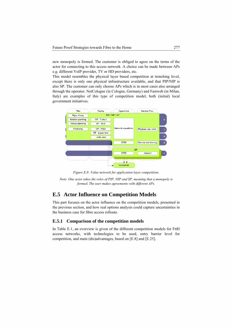
Future Proof Strategies towards Fibre to the Home 277
new monopoly is formed. The customer is obliged to agree on the terms of the actor for connecting to this access network. A choice can be made between APs e.g. different VoIP provider, TV or HD providers, etc. This model resembles the physical layer based competition at trenching level, except there is only one physical infrastructure available, and that PIP/NIP is also SP. The customer can only choose APs which is in most cases also arranged through the operator. NetCologne (in Cologne, Germany) and Fastweb (in Milan, Italy) are examples of this type of competition model, both (initial) local government initiatives.
Figure E.8: Value network for application layer competition.
Note: One actor takes the roles of PIP, NIP and SP, meaning that a monopoly is formed. The user makes agreements with different APs.
E.5 Actor Influence on Competition Models This part focuses on the actor influence on the competition models, presented in the previous section, and how real options analysis could capture uncertainties in the business case for fibre access rollouts.
E.5.1 Comparison of the competition models In Table E.1, an overview is given of the different competition models for FttH access networks, with technologies to be used, entry barrier level for competition, and main (dis)advantages, based on [E.8] and [E.25].
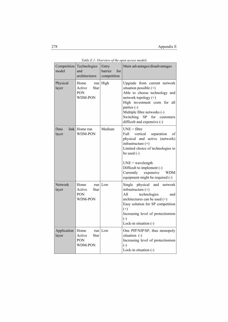
278 Appendix E
Table E.1: Overview of the open access models
Competition model
Technologies and architectures
Entry barrier for competition
Main advantages/disadvantages
Physical layer
Home runActive StarPON WDM-PON
High Upgrade from current network situation possible (+) Able to choose technology and network topology (+) High investment costs for all parties (-) Multiple fibre networks (-) Switching SP for customers difficult and expensive (-)
Data link layer
Home run WDM-PON
Medium UNE = fibre Full vertical separation of physical and active (network) infrastructure (+) Limited choice of technologies to be used (-) UNE = wavelength Difficult to implement (-) Currently expensive WDM equipment might be required (-)
Network layer
Home runActive StarPON WDM-PON
Low Single physical and network infrastructure (+) All technologies and architectures can be used (+) Easy solution for SP competition (+) Increasing level of protectionism (-) Lock-in situation (-)
Application layer
Home runActive StarPON WDM-PON
Low One PIP/NIP/SP, thus monopoly situation (-) Increasing level of protectionism (-) Lock-in situation (-)
Future Proof Strategies towards Fibre to the Home 279
The physical infrastructure layer competition model is interesting for ILEC and CLEC (cable operators) as they can reuse current network infrastructure in the rollout of fibre directly to the user [E.2]. Each PIP can choose its network technology, architecture and topology (in case of ‘trench’ model). The use of a communal CO is required from ‘fibre’ infrastructure competition on (due to fixed duct infrastructure), where each NIP can blow its fibers in the leased ducts. As customers are connected to the network of one PIP, switching SP (and thus PIP) is difficult (new fibre connection, lots of administration and operational processes) and thus expensive. At data link layer, the passive infrastructure is separated from the active (network) infrastructure. The PIP is owner of the fibre network, and mostly a wholesale deal is signed and access is provided to the customers via network layer competition (bitstream access). Network topology is fixed; architecture and technology could be chosen when data link layer competition is applied to the full fibre network (installation of outside plant equipment by the NIP). Different technologies could be used next to each other by different NIPs e.g. PON network next to an active star. This is not the case for wavelength competition as inside equipment is required (installed by the PIP) in the CO. The network layer competition model is always applicable, independent of technology and architecture choice, and entry level for competitors is low. Customers can easily choose their SP, and cost efficiently switch service provider. A lock-in situation might occur in case packages (e.g. triple play services) are offered by the PIP/NIP/SP as he can push down prices and compete in this way with CLECs making use of its network. The highest competition model, at application layer, represents a new monopolistic situation where passive and active (network) infrastructure, as well as service provisioning is owned and operated by one actor (or consortium of actors). No competition is possible at this level, only a choice can be made between application providers. This model is in fact a degraded version of the physical infrastructure based competition model at trench level, as there is only one PIP instead of (possibly) multiple PIPs.
E.5.2 Introduction of real options analysis A real option is the right but not the obligation to undertake some business decision, typically the option to make, or abandon a capital investment [E.26]. This type of analysis could be of interest when business cases for fibre access network rollouts are considered. Different actors in the value network create real options on future value-generating actions during the course of the network deployment. This means that, based on the actual outcome of some uncertain evolutions, they will use the inherent flexibility to choose the most value-generating action. A few examples for different actors are given below. • ILECs could install in the current network rollout of xDSL extra
infrastructure (ducts, fibers, flexibility points) that will facilitate the rollout
280 Appendix E
of fibre in a latter stadium. In this case, extra investments made today, will give them the option to cost efficiently rollout fibre at a future stage. In case they are not (fully) migrating towards fibre, the cost for the option is not lost as this infrastructure could be sold to competitors.
• Local governments could change regulation procedures regarding physical infrastructure e.g. requiring the installation of duct infrastructure to each premise in new housing areas. This can at a later stage be used for connecting the customers at a low cost to one or more fibre networks. This type of pre-installation could also be aligned with other ‘utility’ investments such as road, sewage, gas and/or water networks.
• Utility companies acting as PIP (for past or current network investments) have the option to lease or sell their telecom infrastructure, depending on the current market situation.
• CLECs have the option to be less dependent of the ILEC by switching from LLU or bitstream access (via the ILEC network) to own network investments.
Further study and quantification of these real options in fibre network rollout form an issue for future research.
E.6 Conclusions In this paper we have presented different strategies for future proof FttH rollouts, based on four levels of competition: physical infrastructure, data link layer, network layer and application layer. The different business roles and their internal relations are presented. Many actors are involved in the whole process, such as governmental institutions, telecom operators, service and content providers and customers. The value networks, where different actors are mapped onto the business roles, were presented for all competition models. Each actor could influence, and facilitate, the rollout decision for FttH. Governmental instances should focus on making rules and regulation policies to facilitate the rollout of fibre access networks, this by communicating transparently about future policies so that the framework in which infrastructure developers act or will act, is clear and long term decisions can be taken. Current physical infrastructure owners (mostly ILEC and cable operators, but also new actors such as utility companies) can build out their network towards future proof fibre access networks. CLEC operators will have more options (LLU, bitstream access, rollout of own network) depending on the competition model. A separation of physical (and network) infrastructure and service provisioning will attract competition. A real options analysis for the different actors could furthermore shine a light on the value of different potential strategies considering uncertain market parameters (e.g. regulation, financing, market adoption, etc).
Future Proof Strategies towards Fibre to the Home 281
Acknowledgements This work was partially supported by the EC through Network of Excellence BONE, and of IWT-Flanders through the IWT-project “Cost modelling in a converged communications environment”. We would also like to acknowledge different researchers from the COST605 project Econ@Tel for relevant discussions on this topic.
References [E.1] Point Topic (2008). World Broadband Statistics Q2 2008. October 2008.
[E.2] Katz, R.L. (2008). Ultrabroadband investment models. Communications & Strategies, Special issue, November 2008, 99-116.
[E.3] Gillett, S.E., Lehr, W.H., & Osorio, C. (2006). Municipal electric utilities’ role in telecommunications services. Telecommunications Policy, 30, 464-480.
[E.4] Kittl, J., Ruhle, E-O., & Schuster F. (2008). The comeback of rights-of-way as essence for facilities based NGA and broadband roll out. Biennial Conference of the International Telecommunications Society (ITS), Montréal, June 24-27, 2008.
[E.5] Gillett, S.E., Lehr, W.H., & Osorio, C. (2004). Local government broadband initiatives. Telecommunications Policy, 28, 537–558.
[E.6] Analysys Mason (2008). Models for efficient and effective public-sector interventions in next-generation broadband access networks. Final report for the Broadband Stakeholder Group, June 9, 2008, Website: HThttp://www.broadbanduk.org/component...008/Itemid,63/TH.
[E.7] A.T. Kearney (2008). Developing the Hellenic Ministry of Transport and Communications 5-year broadband strategy for Greece”, May 2008, Website: HThttp://www.strategyforum.gr/downloads/Broadband_Strategy_for_Greece_Workshop_for_public_consultation_may2008.pdfTH .
[E.8] Banerjee, A., & Sirbu, M. (2003). Towards Technologically and Competitively Neutral Fiber to the Home (FttH) Infrastructure. The 31st Research Conference on Communication, Information and Internet Policy, Washington DC, USA, Sep. 2003.
[E.9] Ehrler, M., Brusic, I., Reichl, W., & Ruhle, E-O. (2008). Deployment of fiber optic networks within the framework of PPP projects. ICT-Public & Private Interplay Next Generation Communication conference, Sevilla, December 10-12, 2008.
282 Appendix E
[E.10] Felten, B. (2008). Exploring Open Access Models. Broadband Cities 2008 conference, Trikala, Greece, October 20-23, 2008.
[E.11] Zimmermann, H. (1980). OSI Reference Model - The ISO Model of Architecture for Open Systems Interconnection. IEEE Transactions on Communications, 28(4), 425 - 432.
[E.12] De Marchis, G. (2003). Tutorial on Access Technologies. ITU-T workshop “Outside plant for the Access Network, Hanoi, November 24, 2003.
[E.13] Bernstein, A., & Gorshe, S. (2008). A Proposal for DOCSIS 4.0: The Best of DOCSIS and PON. Emerging Technologies conference, Los Angeles, January 14-16, 2008.
[E.14] Lannoo, B., Casier, K., Van Ooteghem, J., Wouters, B., Verbrugge, S., Colle, D., Pickavet, M., & Demeester P. (2008). Economic Benefits of a Community Driven Fiber to the Home Rollout. Broadnets 2008 conference, London, September 8-11, 2008.
[E.15] Friend, G., & Zehle, S. (2004), Guide to business planning. Published by Economist Books, 1st edition.
[E.16] Casier, K., Verbrugge, S., Meersman, R., Colle, D., Pickavet, M., & Demeester, P. (2008). A clear and balanced view on FTTH deployment costs. FITCE congress: Transformation: Next Stop… True Convergence?, London, September 21-24, 2008, 109-112.
[E.17] Verbrugge, S., Casier, K., Van Ooteghem, J., & Lannoo, B. (2008). Practical steps in techno-economic evaluation of network deployment planning. Networks 2008, 13th International Telecommunications Network Strategy and Planning Symposium (tutorial T12), Budapest, Hungary, September 28 - October 2, 2008.
[E.18] Hills, T. (2008, November 5). The Future of Fiber Access. Light Reading - Networking the Telecom Industry, Website: HThttp://www.lightreading.com/document.asp?doc_id=164134 TH.
[E.19] European Union (2007). Procedures relating to the implementation of the competition policy: State aid — The Netherlands — State aid C 53/06 (ex N 262/05) — Citynet Amsterdam: investment by the city of Amsterdam in a fibre-to-the home (FttH) network. Official Journal of the European Union, C 134, 50, 9.
[E.20] IDATE (2008). DigiWorld Yearbook 2008: the digital world’s challenges. IDATE.
[E.21] Van Ooteghem, J., Casier, K., Lannoo, B., Verbrugge, S., Colle, D., Pickavet, M., & Demeester, P. (2008). The implications of community network rollouts on the future telecom market structure. Biennial
Future Proof Strategies towards Fibre to the Home 283
Conference of the International Telecommunications Society (ITS), Montréal, June 24-27, 2008.
[E.22] Van der Woude, D. (2007). An overview of fiber. June 2007, Website: HThttp://www.citynet.nl/upload/FttX-in-Europe-25june2007.pdf TH.
[E.23] Fournier, P-F. (2007). From FttH pilot to pre-rollout in France. CAI Cheuvreux conference, June 26, 2007.
[E.24] Infante, J., Sagarra, R., Macian, C., & Oliver M. (2008). Ducts, fibers, municipalities, barriers to entry and effective competition: A case study of successful public-private partnership in the provision of neutral FTTX infrastructure in Barcelona. ICT-Public & Private Interplay Next Generation Communication conference, Sevilla, December 10-12, 2008.
[E.25] OECD (2008). Convergence and next generation networks. DSTI/ICCP/CISP(2007)2/FINAL prepared as background for the OECD Ministers’ meeting on The Future of the Internet Economy, Seoul, Korea, June 17-18, 2008
[E.26] Copeland, T., & Antikarov, V. (2003). Real Options: A Practitioner's Guide. TEXERE, W. W. Norton & Company.