
Understanding and Improving Belief Propagation - Faculteit der
182
Understanding and Improving Belief Propagation Een wetenschappelijke proeve op het gebied van de Natuurwetenschappen, Wiskunde en Informatica Proefschrift ter verkrijging van de graad van doctor aan de Radboud Universiteit Nijmegen, op gezag van de rector magnificus prof. mr. S.C.J.J. Kortmann, volgens besluit van het College van Decanen in het openbaar te verdedigen op woensdag 7 mei 2008 om 13.30 uur precies door Joris Marten Mooij geboren op 11 maart 1980 te Nijmegen
Transcript of Understanding and Improving Belief Propagation - Faculteit der

Understanding and Improving
Belief Propagation
Een wetenschappelijke proeve op het gebied van deNatuurwetenschappen, Wiskunde en Informatica
Proefschrift
ter verkrijging van de graad van doctor
aan de Radboud Universiteit Nijmegen,
op gezag van de rector magnificus prof. mr. S.C.J.J. Kortmann,
volgens besluit van het College van Decanen
in het openbaar te verdedigen op woensdag 7 mei 2008om 13.30 uur precies
door
Joris Marten Mooij
geboren op 11 maart 1980te Nijmegen

Promotor:
Prof. dr. H.J. Kappen
Manuscriptcommissie:
Prof. dr. N.P. LandsmanProf. dr. M. Opper (University of Southampton)Prof. dr. Z. Ghahramani (University of Cambridge)Prof. dr. T.S. Jaakkola (Massachusetts Institute of Technology)Dr. T. Heskes
The research reported here was sponsored by the Interactive Collaborative Informa-tion Systems (ICIS) project (supported by the Dutch Ministry of Economic Affairs,grant BSIK03024) and by the Dutch Technology Foundation (STW).
Copyright c© 2008 Joris Mooij
ISBN 978-90-9022787-0Gedrukt door PrintPartners Ipskamp, Enschede

Contents
Title page i
Table of Contents iii
1 Introduction 11.1 A gentle introduction to graphical models 1
1.1.1 The Asia network: an example of a Bayesian network 21.1.2 The trade-off between computation time and accuracy 71.1.3 Image processing: an example of a Markov random field 91.1.4 Summary 16
1.2 A less gentle introduction to Belief Propagation 171.2.1 Bayesian networks 171.2.2 Markov random fields 181.2.3 Factor graphs 191.2.4 Inference in graphical models 201.2.5 Belief Propagation: an approximate inference method 211.2.6 Related approximate inference algorithms 241.2.7 Applications of Belief Propagation 24
1.3 Outline of this thesis 25
2 Sufficient conditions for convergence of BP 292.1 Introduction 292.2 Background 30
2.2.1 Factor graphs 302.2.2 Belief Propagation 31
2.3 Special case: binary variables with pairwise interactions 332.3.1 Normed spaces, contractions and bounds 342.3.2 The basic tool 352.3.3 Sufficient conditions for BP to be a contraction 352.3.4 Beyond norms: the spectral radius 372.3.5 Improved bound for strong local evidence 39
2.4 General case 412.4.1 Quotient spaces 42
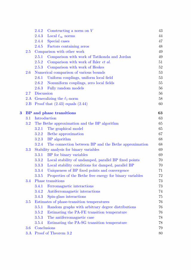
2.4.2 Constructing a norm on V 432.4.3 Local `∞ norms 442.4.4 Special cases 472.4.5 Factors containing zeros 48
2.5 Comparison with other work 492.5.1 Comparison with work of Tatikonda and Jordan 492.5.2 Comparison with work of Ihler et al. 512.5.3 Comparison with work of Heskes 52
2.6 Numerical comparison of various bounds 532.6.1 Uniform couplings, uniform local field 532.6.2 Nonuniform couplings, zero local fields 552.6.3 Fully random models 56
2.7 Discussion 562.A Generalizing the `1-norm 582.B Proof that (2.43) equals (2.44) 60
3 BP and phase transitions 633.1 Introduction 633.2 The Bethe approximation and the BP algorithm 65
3.2.1 The graphical model 653.2.2 Bethe approximation 673.2.3 BP algorithm 683.2.4 The connection between BP and the Bethe approximation 68
3.3 Stability analysis for binary variables 693.3.1 BP for binary variables 693.3.2 Local stability of undamped, parallel BP fixed points 703.3.3 Local stability conditions for damped, parallel BP 703.3.4 Uniqueness of BP fixed points and convergence 713.3.5 Properties of the Bethe free energy for binary variables 72
3.4 Phase transitions 733.4.1 Ferromagnetic interactions 733.4.2 Antiferromagnetic interactions 743.4.3 Spin-glass interactions 75
3.5 Estimates of phase-transition temperatures 763.5.1 Random graphs with arbitrary degree distributions 763.5.2 Estimating the PA-FE transition temperature 763.5.3 The antiferromagnetic case 783.5.4 Estimating the PA-SG transition temperature 78
3.6 Conclusions 793.A Proof of Theorem 3.2 80

4 Loop Corrections 834.1 Introduction 834.2 Theory 85
4.2.1 Graphical models and factor graphs 854.2.2 Cavity networks and loop corrections 864.2.3 Combining approximate cavity distributions to cancel out errors 884.2.4 A special case: factorized cavity distributions 914.2.5 Obtaining initial approximate cavity distributions 934.2.6 Differences with the original implementation 94
4.3 Numerical experiments 964.3.1 Random regular graphs with binary variables 984.3.2 Multi-variable factors 1054.3.3 Alarm network 1064.3.4 Promedas networks 107
4.4 Discussion and conclusion 1094.A Original approach by Montanari and Rizzo (2005) 112
4.A.1 Neglecting higher-order cumulants 1144.A.2 Linearized version 114
5 Novel bounds on marginal probabilities 1175.1 Introduction 1175.2 Theory 118
5.2.1 Factor graphs 1195.2.2 Convexity 1205.2.3 Measures and operators 1205.2.4 Convex sets of measures 1225.2.5 Boxes and smallest bounding boxes 1245.2.6 The basic lemma 1265.2.7 Examples 1275.2.8 Propagation of boxes over a subtree 1305.2.9 Bounds using self-avoiding walk trees 133
5.3 Related work 1405.3.1 The Dobrushin-Tatikonda bound 1405.3.2 The Dobrushin-Taga-Mase bound 1415.3.3 Bound Propagation 1415.3.4 Upper and lower bounds on the partition sum 142
5.4 Experiments 1425.4.1 Grids with binary variables 1435.4.2 Grids with ternary variables 1455.4.3 Medical diagnosis 145
5.5 Conclusion and discussion 148
List of Notations 151

Bibliography 155
Summary 163
Samenvatting 167
Publications 171
Acknowledgments 173
Curriculum Vitae 175

Chapter 1. Introduction 1
Chapter 1
Introduction
This chapter gives a short introduction to graphical models, explains the BeliefPropagation algorithm that is central to this thesis and motivates the researchreported in later chapters. The first section uses intuitively appealing examples toillustrate the most important concepts and should be readable even for those whohave no background in science. Hopefully, it succeeds in giving a relatively clearanswer to the question “Can you explain what your research is about?” that oftencauses the author some difficulties at birthday parties. The second section doesassume a background in science. It gives more precise definitions of the conceptsintroduced earlier and it may be skipped by the less or differently specialized reader.The final section gives a short introduction to the research questions that are studiedin this thesis.
1.1 A gentle introduction to graphical models
Central to the research reported in this thesis are the concepts of probability theoryand graph theory, which are both branches of mathematics that occur widely inmany different applications. Quite recently, these two branches of mathematicshave been combined in the field of graphical models. In this section I will explainby means of two “canonical” examples the concept of graphical models. Graphicalmodels can be roughly divided into two types, called Bayesian networks and Markovrandom fields. The concept of a Bayesian network will be introduced in the firstsubsection using an example from the context of medical diagnosis. In the secondsubsection, we will discuss the basic trade-off in the calculation of (approximationsto) probabilities, namely that of computation time and accuracy. In the thirdsubsection, the concept of a Markov random field will be explained using an examplefrom the field of image processing. The fourth subsection is a short summary and

2 Chapter 1
A
T
E
S
L
B
DX
Random variable Meaning
A Recent trip to Asia
T Patient has tuberculosis
S Patient is a smoker
L Patient has lung cancer
B Patient has bronchitis
E Patient has T and/or L
X Chest X-Ray is positive
D Patient has dyspnoea
Figure 1.1: The Asia network, an example of a Bayesian network.
briefly describes the research questions addressed in this thesis.
1.1.1 The Asia network: an example of a Bayesian network
To explain the concept of a Bayesian network, I will make use of the highly simplifiedand stylized hypothetical example of a doctor who tries to find the most probablediagnosis that explains the symptoms of a patient. This example, called the Asia
network, is borrowed from Lauritzen and Spiegelhalter [1988].The Asia network is a simple example of a Bayesian network. It describes the
probabilistic relationships between different random variables, which in this partic-ular example correspond to possible diseases, possible symptoms, risk factors andtest results. The Asia network illustrates the mathematical modeling of reasoningin the presence of uncertainty as it occurs in medical diagnosis.
A graphical representation of the Asia network is given in figure 1.1. The nodesof the graph (visualized as circles) represent random variables. The edges of thegraph connecting the nodes (visualized as arrows between the circles) representprobabilistic dependencies between the random variables. Qualitatively, the modelrepresents the following (highly simplified) medical knowledge. A recent trip toAsia (A) increases the chance of contracting tuberculosis (T ). Smoking (S) is arisk factor for both lung cancer (L) and bronchitis (B). The presence of either (E)tuberculosis or lung cancer can be detected by an X-ray (X), but the X-ray cannotdistinguish between them. Dyspnoea (D), or shortness of breath, may be caused byeither (E) tuberculosis or lung cancer, but also by bronchitis (B). In this particularBayesian network, all these random variables can have two possible values: either“yes” or “no”, which we will abbreviate as “y” and “n”, respectively.1
This model can be used to answer several questions in the following hypotheticalsituation. Imagine a patient who complains about dyspnoea and has recently visited
1In general, the possible number of values of random variables is unlimited.
Chapter 1. Introduction 3
Asia. The doctor would like to know the probabilities that each of the diseases (lungcancer, tuberculosis and bronchitis) is present. Suppose that tuberculosis can beruled out by another test, how would that change the belief in lung cancer? Further,would knowing smoking history or getting an X-ray be most informative about theprobability of lung cancer? Finally, which information was the most important forforming the diagnosis?
In order to proceed, it will be convenient to introduce some notation from prob-ability theory. The probability that some statement F is true is denoted by P(F ).Probabilities are numbers between 0 and 1, where P(F ) = 0 means that F is falsewith absolute certainty, and P(F ) = 1 means that F is true with absolute certainty,and if P(F ) is anything in between, it means that it is not certain whether F istrue or false. If P(F ) is close to 0, it is unlikely that F is true, wherease if P(F )is close to 1 it is likely that F is true. For our purposes, the statement F can beany instantiation of (one or more of) the random variables that we are considering.For example, the statement can be “the patient has bronchitis”, which is an instan-tiation of the random variable B, that can be abbreviated as “B = y”. Anotherpossible statement is “the patient does not have bronchitis”, which we can writeas “B = n”. Thus P(B = y) is the probability that the patient has bronchitis andP(B = n) is the probability that the patient does not have bronchitis. Both prob-abilities have to sum to one: P(B = y) + P(B = n) = 1, because the patient eitherhas or does not have bronchitis. The statement can also be a more complicatedcombination of random variables, e.g., P(S = y, L = n) is the probability that thepatient smokes but does not have lung cancer.
In addition we need another notion and notation from probability theory, namelythat of conditional probabilities. If we are given more information about the patient,probabilities may change. For example, the probability that the patient has lungcancer increases if we learn that the patient smokes. For statements F and G,the conditional probability of F , given that G is true, is denoted as P(F |G). Asbefore, the statements F and G are instantiations of (some of the) random variablesthat we are considering. For example, the conditional probability that the patienthas lung cancer given that the patient smokes is denoted as P(L = y |S = y).The value of this conditional probability is higher than P(L = y), which is theprobability that the patient has lung cancer if we have no further information aboutwhether the patient smokes or not. Another example of a conditional probability isP(D = y |B = y, E = n); this is the probability that a patient has dyspnoea, giventhat the patient has bronchitis but has neither tuberculosis nor lung cancer.
The numerical values for the probabilities can be provided by medical studies.For example, according to the results of Villeneuve and Mao [1994], the lifetimeprobability of developing lung cancer, given that one is a smoker, is about 14%,whereas it is only about 1.4% if one has never smoked.2 The complete conditional
2In reality, the probability of developing lung cancer is different for males and females and
depends on many other variables, such as age and the smoking history of the patient. We will
come back to this point later.
4 Chapter 1
probability table for L given S (i.e., whether the patient develops lung cancer, giventhe smoking status of the patient), is then:
P(L |S) S = y S = nL = y 14% 1.4%L = n 86% 98.6%
Note that each column sums to 100%, which expresses that with absolute certaintythe patient either develops lung cancer or not. This conditional probability tablefor P(L |S) corresponds with the edge from S to L in figure 1.1.
Another conditional probability table that we can easily specify (even withoutconsulting medical studies) is P(E |T, L):
P(E |T, L) T = y T = n T = y T = nL = y L = y L = n L = n
E = y 100% 100% 100% 0%E = n 0% 0% 0% 100%
This simply reflects the definition of “T and/or L” in terms of T and L accordingto elementary logics. The conditional probability table for P(E |T, L) correspondswith the edges from T and L to E in figure 1.1.
Another probability table (not a conditional one) that is relevant here is P(S),the probability that the patient smokes. In 2006, the percentage of smokers in TheNetherlands was 29.6%.3 Therefore a realistic probability table for P(S) is:
S P(S)y 29.6%n 70.4%
This probability table corresponds with the node S in figure 1.1.In order to give a complete quantitative specification of the graphical model
shown in figure 1.1, one would have to specify each of the following probabilitytables: P(A), P(T |A), P(L |S), P(B |S), P(D |B,E), P(E |T, L), P(X |E) andP(S). Note how this corresponds with the graph: for each random variable, weneed the probability distribution of that variable conditional on its parents. By theparents of a variable we mean those random variables that point directly towardsit. For example, the parents of D are E and B, whereas S has no parents. Thismeans that we have to specify the conditional probability table for P(D |E,S) andthe probability table of P(S). We will not explicitly give all these (conditional)probability tables here but will assume that they are known and that the graphicalmodel illustrated in figure 1.1 is thus completely specified. Then, the complete
3According to the CBS (Centraal Bureau voor Statistiek).

Chapter 1. Introduction 5
joint probability distribution of all the random variables can be obtained simply bymultiplying all the (conditional) probability tables:
P(A, T, L, S,B,X,E,D)
= P(A)× P(T |A)× P(L |S)× P(B |S)
× P(E |T, L)× P(D |B,E)× P(X |E)× P(S).
(1.1)
This formula should be read as follows. Given an instantiation of all 8 randomvariables, e.g., A = n, T = n,L = n, S = y,B = n,X = n,E = n,D = n, wecan calculate the probability of that instantiation by multiplying the correspondingvalues in the smaller probability tables:
P(A = n, T = n,L = n, S = y,B = n,X = n,E = n,D = n)
= P(A = n)× P(T = n |A = n)× P(L = n |S = y)
× P(B = n |S = y)× P(E = n |T = n,L = n)
× P(D = n |B = n,E = n)× P(X = n |E = n)× P(S = y)
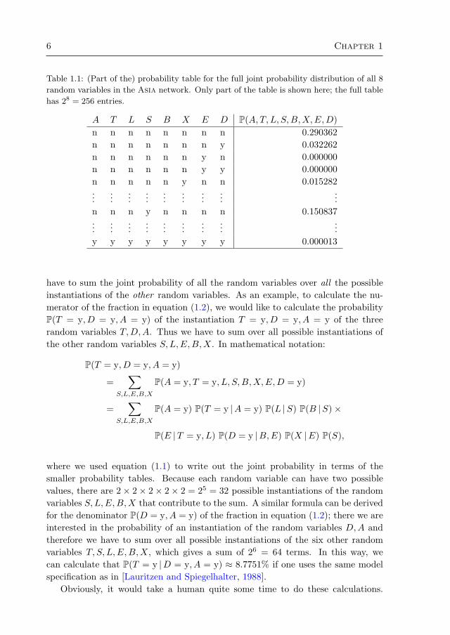
which will give us some number (0.150837 if you use the original model by Lauritzenand Spiegelhalter [1988]). Because the model consists of 8 binary (i.e., yes/novalued) random variables, the complete probability table for the joint probabilitydistribution P(A, T, L, S,B,X,E,D) would contain 28 = 256 entries: one value foreach possible assignment of all the random variables. Part of this table is given intable 1.1.4
The completely specified model can be used to answer many different questionsthat a doctor might be interested in. Let us return to the hypothetical exampleof the patient who complains about dyspnoea and has recently visited Asia. Thedoctor would like to know the probability that each of the diseases (T , L and B) ispresent. Thus, e.g., the doctor would like to know the value of:
P(T = y |D = y, A = y)
according to the model. An elementary fact of probability theory tells us that wecan calculate this quantity by dividing two other probabilities:
P(T = y |D = y, A = y) =P(T = y, D = y, A = y)
P(D = y, A = y). (1.2)
Another elementary result of probability says that, if we would like to calculatea probability of some instantiation of a particular subset of random variables, we
4Note that by representing the joint probability distribution as a Bayesian network we actually
need less than 256 numbers to specify the complete probabilistic model; indeed, we need just
2 + 4 + 4 + 4 + 8 + 8 + 4 + 2 = 36 numbers to specify all the probability tables P(A), P(T |A),
P(L |S), P(B |S), P(E |T, L), P(D |B,E), P(X |E), P(S). In fact, we can use even less numbers
because the columns of the tables sum to one. This efficiency of representation is one of the
advantages of using a Bayesian network to specify a probability distribution over the alternative
of “simply” writing down the complete joint probability table. By using equation (1.1), we can
calculate any probability that we need.
6 Chapter 1
Table 1.1: (Part of the) probability table for the full joint probability distribution of all 8
random variables in the Asia network. Only part of the table is shown here; the full table
has 28 = 256 entries.
A T L S B X E D P(A, T, L, S,B,X,E,D)n n n n n n n n 0.290362n n n n n n n y 0.032262n n n n n n y n 0.000000n n n n n n y y 0.000000n n n n n y n n 0.015282...
......
......
......
......
n n n y n n n n 0.150837...
......
......
......
......
y y y y y y y y 0.000013
have to sum the joint probability of all the random variables over all the possibleinstantiations of the other random variables. As an example, to calculate the nu-merator of the fraction in equation (1.2), we would like to calculate the probabilityP(T = y, D = y, A = y) of the instantiation T = y, D = y, A = y of the threerandom variables T,D,A. Thus we have to sum over all possible instantiations ofthe other random variables S,L,E,B,X. In mathematical notation:
P(T = y, D = y, A = y)
=∑
S,L,E,B,X
P(A = y, T = y, L, S,B,X,E,D = y)
=∑
S,L,E,B,X
P(A = y) P(T = y |A = y) P(L |S) P(B |S)×
P(E |T = y, L) P(D = y |B,E) P(X |E) P(S),
where we used equation (1.1) to write out the joint probability in terms of thesmaller probability tables. Because each random variable can have two possiblevalues, there are 2× 2× 2× 2× 2 = 25 = 32 possible instantiations of the randomvariables S,L,E,B,X that contribute to the sum. A similar formula can be derivedfor the denominator P(D = y, A = y) of the fraction in equation (1.2); there we areinterested in the probability of an instantiation of the random variables D,A andtherefore we have to sum over all possible instantiations of the six other randomvariables T, S, L,E,B,X, which gives a sum of 26 = 64 terms. In this way, wecan calculate that P(T = y |D = y, A = y) ≈ 8.7751% if one uses the same modelspecification as in [Lauritzen and Spiegelhalter, 1988].
Obviously, it would take a human quite some time to do these calculations.
Chapter 1. Introduction 7
However, computers can calculate very fast nowadays and we could instruct a com-puter in such a way that it performs precisely these calculations. Thereby it couldassist the doctor by calculating (according to the model) the probabilities that eachof the diseases is present, given that the patient has dyspnoea and has recentlyvisited Asia. In a similar way, the elementary rules of probability theory can beapplied in a rather straightforward manner to answer more difficult questions, like“If tuberculosis were ruled out by another test, how would that change the beliefin lung cancer?”, “Would knowing smoking history or getting an X-ray contributemost information about cancer, given that smoking may ‘explain away’ the dysp-noea since bronchitis is considered a possibility?” and “When all information is in,can we identify which was the most influential in forming our judgment?”
For readers that have not had any previous exposure to probability theory, thereasoning above may be difficult to understand. However, the important point isthe following: any probability distribution that the doctor may be interested in(concerning the random variables in the model) in order to obtain a diagnosis forthe patient, can be calculated using elementary probability theory and the precisespecification of the Bayesian network. For a human this would be a lengthy calcula-tion, but a computer can do these calculations very fast (at least for this particularBayesian network).
As a final note, let us return to the probability that one develops lung cancergiven that one smokes. One might object that this probability depends in realityon many other factors, such as the gender, the age, the amount of smoking and thenumber of years that the patient has been smoking. However, we can in principleeasily improve the realism of the model to take these dependences into account,e.g., by adding nodes for gender (G), age (Y ), smoking history (H), adding edgesfrom these new nodes to L (lung cancer) and replacing the conditional probabilitytable P(L |S) by a more complicated table P(L |S,G, Y,H) where the probabilityof developing lung cancer depends on more variables than in our simple model.This illustrates the modularity inherent in this way of modeling: if new medicalstudies result in more accurate knowledge about the chances of getting lung cancerfrom smoking, one only needs to modify the model locally (i.e., only change themodel in the neighborhood of the nodes S and L). The rules of probability theorywill ensure that answers to questions like “What disease most likely causes thepositive X-ray?” depend on the complete model; improving the realism of the partof the model involving lung cancer and smoking will also automatically give a moreaccurate answer to those questions.
1.1.2 The trade-off between computation time and accuracy
For this small and simplified model, the calculations involved could even be doneby hand. However, for larger and more realistic models, which may involve tens ofthousands of variables which interact in highly complicated ways, the computationalcomplexity to calculate the answer to questions like “What is the most likely disease

8 Chapter 1
Table 1.2: The number of possible instantiations (i.e., joint assignments of all variables)
as a function of the number N of binary variables.
N 2N , the number of possible instantiations
1 2
2 4
3 8
4 16
5 32
10 1024
20 1048576
50 1125899906842624
100 1267650600228229401496703205376
200 1606938044258990275541962092341162602522202993782792835301376
that causes these symptoms?” explodes. Although it is easy in principle to writedown a formula that gives the answer to that question (this would be a rather longformula, but similar to the ones we have seen before), to actually calculate the resultwould involve adding enormous amounts of numbers. Indeed, in order to calculatea probability involving a few random variables, we have to add many probabilities,namely one for each possible instantiation of all the other random variables that weare not interested in. The number of such instantiations quickly increases with thenumber of variables, as shown in table 1.2. Even if we include only 200 diseases andsymptoms in our model, in order to calculate the probability of one disease givena few symptoms would require adding an enormous amount of terms. Although amodern desktop computer can do many additions per second (about one billion, i.e.,1000000000), we conclude that for a realistic model involving thousands of variables,the patient will have died before the computer can calculate the probability of asingle disease, even if we use the fastest supercomputer on earth.5 Thus althoughfor small models we can actually calculate the probabilities of interest according tothe model, it is completely impractical for large realistic models.
It turns out that for the specific case of medical diagnosis, using certain assump-tions on the probability distributions and several clever tricks (which are outsidethe scope of this introduction) one can significantly decrease the computation timeneeded to calculate the probabilities. Such a model, called Promedas, which con-tains thousands of diseases, symptoms and tests, is currently being developed inNijmegen. It can calculate probabilities of interest within a few seconds on an
5In fact, it is likely that the earth and maybe even the universe have ceased to exist before a
computer (using current technology) will have calculated the probability of interest if one uses this
“brute force” method of calculating probabilities. On the other hand, computers get faster each
year: processing speed roughly doubles every 24 months. Extrapolating this variant of “Moore’s
law” into the far future (which is not very realistic), it would take about three centuries before
the calculation could be done within one day.

Chapter 1. Introduction 9
Figure 1.2: Left: reference image. Right: input image. The reference image defines the
background and the input image consists of some interesting foreground imposed on the
background. The task is to decide which part of the input image belongs to the foreground.
ordinary computer.6
However, there are many other applications (for which these simplifying as-sumptions cannot be made and the clever tricks cannot be applied) where the exactcalculation of probabilities is impossible to perform within a reasonable amountof time. In these cases, one can try to calculate approximate probabilities usingadvanced approximation methods which have been specially developed for this pur-pose. If the approximate result can be calculated within a reasonable amount oftime and its accuracy is enough for the application considered (e.g., knowing theprobabilities that some disease causes the observed symptoms to ten decimal placesis usually not necessary, one or two decimal places may be more than enough), thenthis forms a viable alternative to the exact calculation. This illustrates the ba-sic trade-off in the field known as approximate inference: computation time versusaccuracy.
1.1.3 Image processing: an example of a Markov random
field
To introduce the concept of a Markov random field, another type of graphical mod-els, I will use an example from the field of image processing. The task that we willconsider is that of separating foreground from background. Suppose that we havetwo images, one of which is the reference image that defines the background, andone where there is some foreground in front of the background, which we call theinput image (see figure 1.2 for an example). By comparing the input image withthe reference image, we try to infer which part of the input image is foreground andwhich part belongs to the background. We can then extract only the foregroundpart of the input image, filtering out the background. This may have applicationsin surveillance (surveillance cameras only need to store the interesting parts of the
6A demonstration version of Promedas is available at http://www.promedas.nl/

10 Chapter 1
Figure 1.3: An image consists of many pixels, small squares with a uniform intensity. The
images used here consist of 640× 480 = 307200 pixels.
Figure 1.4: Left: difference between input and reference image. Right: simple estimate of
foreground, obtained by thresholding the difference image on the left.
video frames, i.e., the foreground, and thus save storage space) and video conferenc-ing (if we only transmit the foreground, this will save bandwidth and thus costs),but I have chosen this example mainly for educational purposes.
As illustrated in figure 1.3, an image is digitally represented as a grid of manypixels: small squares that have a uniform intensity. The intensity of a pixel isa number between 0 and 255, where 0 is black and 255 is white, and anythingin between is a shade of gray, where a larger intensity value corresponds with alighter shade of gray. The images used in this example are 640 pixels in width and480 pixels in height and were made by a surveillance camera. We will denote theintensity of a pixel at some location i of the reference image by Ri and the intensityof a pixel at the same location i of the input image by Ii.
A crude way to separate foreground from background is to consider the differ-ences between the images. More precisely, for each location i, we can calculate theabsolute value of the difference in intensity for both pixels corresponding to thatlocation, i.e., di := |Ii −Ri|.7 This can be done using some of the more advancedimage processing applications, e.g., GIMP or Adobe R© PhotoShop R©. Figure 1.4
7For a real number x, its absolute value |x| is x if x ≥ 0 and −x if x < 0.

Chapter 1. Introduction 11
shows the difference image, where the absolute difference di between the intensityvalues Ii and Ri of the input and reference image is represented by a shade ofgray (black corresponding to the maximum possible difference of 255 and whitecorresponding to the minimum possible difference of 0). We can now choose somethreshold value c, and decide that all pixels i for which the absolute difference di islarger than c belong to the foreground, and all pixels for which the absolute differ-ence di is smaller than c belong to the background. The result is shown in figure1.4. This is a fast method, but the quality of the result is not satisfying: instead ofidentifying the whole person as foreground, it only identifies parts of the person asforeground, omitting many little and a few larger regions that (according to the hu-man eye) clearly belong to the foreground. On the other hand, many little parts ofthe background, where the intensities of the reference and input image differ slightlybecause of changed lightning conditions, get incorrectly classified as foreground. Inorder to improve the classification, we would like to somehow impose the criterionthat we are only interested in large contiguous foreground objects: we would liketo catch a burglar, not a fly.
The key idea is to also take into account neighboring pixels. Every pixel (exceptthose on the border of the image) has four neighboring pixels: one to the left, oneto the right, one above and one below. We are going to construct a probabilitymodel such that if the absolute difference di is large, the probability that the pixelat location i belongs to the foreground should be high. Furthermore, if the ma-jority of the neighboring pixels of the pixel at location i belong to the foregroundwith high probability, then the probability that the pixel itself belongs to the fore-ground should also be high. Vice versa, if the neighboring pixels belong to thebackground with high probability, then the probability that the pixel itself belongsto the background should increase.
For each location i, we introduce a random variable xi that can have two pos-sible values: either xi = −1, which means “the pixel at location i belongs to thebackground”, or xi = +1, which means “the pixel at location i belongs to theforeground”. We are going to construct a probability distribution that takes intoaccount all the 640×480 = 307200 random variables xi. We choose this probabilitydistribution in such a way that P(xi = 1) is large if di > c (in words, the probabilitythat pixel i belongs to the foreground is large if the difference between input andreference image at that location is large) and P(xi = 1) is small if di < c. Notethat P(xi = 1) + P(xi = −1) = 1 because the pixel at location i either belongs tothe foreground or to the background. Thus, if P(xi = 1) is large then P(xi = −1)is small and vice versa. Furthermore, the probability P(xi = 1) depends on theprobabilities P(xj = 1) for other pixels j. Indeed, if j is a neighbor of i, then weshould have that P(xi = 1 |xj = 1) is larger than P(xi = 1), i.e., the probability thatpixel i belongs to the foreground should increase when we learn that its neighbor jbelongs to the foreground.
The actual construction of this probability distribution is a bit technical, but inprinciple we only translate our qualitative description above into a more quantita-

12 Chapter 1
tive and precise mathematical formulation. The complete probability distributionP(xi) is a function of all the 307200 random variables xi (we write xi whenwe refer to the whole collection of random variables xi for all pixels i).8 The fullprobability distribution will be a product of two types of factors: a “local evidence”factor ψi(xi) for each pixel i and a “compatibility” factor ψij(xi, xj) for each pairi, j of neighboring pixels i and j. We take the full probability distribution to bethe product of all these factors:
P(xi) =1Z
(∏i
ψi(xi)
)∏i,j
ψij(xi, xj)
. (1.3)
This probability distribution is an example of a Markov random field. We have useda convenient mathematical abbreviation for what would otherwise be an enormousformula:
∏i ψi(xi) means that we have to take the product of the functions ψi(xi)
for each possible pixel location i (in this case, that would be a product of 307200factors). Similarly,
∏i,j ψij(xi, xj) means that we have to take the product of
the functions ψij(xi, xj) for each possible pair of neighboring pixels i and j (whichwould be a product of 613280 factors). As an example, if we would have imagesconsisting of 3 pixels in one row (with labels i, j, k), writing out equation (1.3)would give:
P(xi, xj , xk) =1Z
(ψi(xi)ψj(xj)ψk(xk)
)(ψij(xi, xj)ψjk(xj , xk)
). (1.4)
Obviously, I will not write out equation (1.3) for the larger images considered here,because that would just be a waste of paper; instead, please use your imagination.Graphical representations of the Markov random field defined in equation (1.3)are given in figure 1.5 for two cases, the first being the example of 3 pixels on arow, the second a slightly larger image of 5 × 5 pixels. The nodes in the graphs(represented as circles) correspond to random variables and the edges (representedas lines connecting the circles) correspond to the compatibility functions.
The constant Z is the normalization constant, which ensures that the functionP(xi) is actually a probability distribution: if we add the values of P(xi) for allpossible configurations of xi, i.e., for all possible background/foreground assign-ments (which is an enormous number of terms, namely 2307200; imagine how largethis number is by comparing the values in table 1.2), we should obtain 1. For the
8Compare this with the Asia network, where the complete probability distribution was a func-
tion of only 8 random variables.

Chapter 1. Introduction 13
xi xj xk
ψi ψj ψk
ψi,j ψj,k
Figure 1.5: Examples of Markov random fields. Left: corresponding with three pixels on
a row, labeled i, j and k. Right: corresponding with an image of 5× 5 pixels.
simple example of images consisting of only 3 pixels on a row, this means that∑xi=±1
∑xj=±1
∑xk=±1
P(xi, xj , xk) =
= P(xi = 1, xj = 1, xk = 1) + P(xi = 1, xj = 1, xk = −1)
+ P(xi = 1, xj = −1, xk = 1) + P(xi = 1, xj = −1, xk = −1)
+ P(xi = −1, xj = 1, xk = 1) + P(xi = −1, xj = 1, xk = −1)
+ P(xi = −1, xj = −1, xk = 1) + P(xi = −1, xj = −1, xk = −1)
= 1.
Using equation (1.4) for each of the eight terms in this sum, we obtain an equationfor Z, which can be solved for the value of the normalization constant Z. A similar,but much longer equation, can be used in principle (but not in practice) to calculatethe value of Z for the 640× 480 images that we are interested in.
We still have to specify which functions ψi(xi) and ψij(xi, xj) we will use. Forthe “local evidence” functions, we use
ψi(xi) = exp(xi θ tanh
di − cw
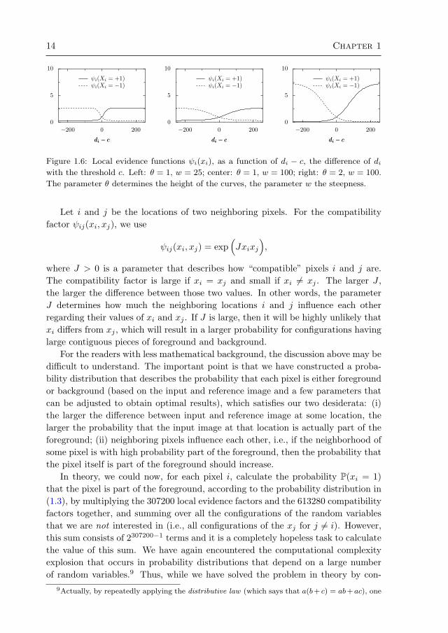
)This function is shown in figure 1.6 for three different choices of the parameters θand w. The parameter θ determines the height of the curves, whereas the parameterw determines how steep the curves are. Note that ψi(xi = 1) is large if di is largerthan the threshold c (i.e., if the difference between input and reference image atlocation i is larger than the threshold) and small if di is smaller than the threshold c;for ψi(xi = −1), the opposite is true. This means that the contribution of the localevidence function to the joint probability is as discussed before: a larger differencebetween input and reference image at location i increases the probability that xi = 1(and at the same time, decreases the probability that xi = −1).
14 Chapter 1
0
5
10
−200 0 200
di − cdi − c
ψi(Xi = +1)ψi(Xi = −1)
0
5
10
−200 0 200
di − cdi − c
ψi(Xi = +1)ψi(Xi = −1)
0
5
10
−200 0 200
di − cdi − c
ψi(Xi = +1)ψi(Xi = −1)
Figure 1.6: Local evidence functions ψi(xi), as a function of di − c, the difference of diwith the threshold c. Left: θ = 1, w = 25; center: θ = 1, w = 100; right: θ = 2, w = 100.
The parameter θ determines the height of the curves, the parameter w the steepness.
Let i and j be the locations of two neighboring pixels. For the compatibilityfactor ψij(xi, xj), we use
ψij(xi, xj) = exp(Jxixj
),
where J > 0 is a parameter that describes how “compatible” pixels i and j are.The compatibility factor is large if xi = xj and small if xi 6= xj . The larger J ,the larger the difference between those two values. In other words, the parameterJ determines how much the neighboring locations i and j influence each otherregarding their values of xi and xj . If J is large, then it will be highly unlikely thatxi differs from xj , which will result in a larger probability for configurations havinglarge contiguous pieces of foreground and background.
For the readers with less mathematical background, the discussion above may bedifficult to understand. The important point is that we have constructed a proba-bility distribution that describes the probability that each pixel is either foregroundor background (based on the input and reference image and a few parameters thatcan be adjusted to obtain optimal results), which satisfies our two desiderata: (i)the larger the difference between input and reference image at some location, thelarger the probability that the input image at that location is actually part of theforeground; (ii) neighboring pixels influence each other, i.e., if the neighborhood ofsome pixel is with high probability part of the foreground, then the probability thatthe pixel itself is part of the foreground should increase.
In theory, we could now, for each pixel i, calculate the probability P(xi = 1)that the pixel is part of the foreground, according to the probability distribution in(1.3), by multiplying the 307200 local evidence factors and the 613280 compatibilityfactors together, and summing over all the configurations of the random variablesthat we are not interested in (i.e., all configurations of the xj for j 6= i). However,this sum consists of 2307200−1 terms and it is a completely hopeless task to calculatethe value of this sum. We have again encountered the computational complexityexplosion that occurs in probability distributions that depend on a large numberof random variables.9 Thus, while we have solved the problem in theory by con-
9Actually, by repeatedly applying the distributive law (which says that a(b+ c) = ab+ac), one

Chapter 1. Introduction 15
Figure 1.7: Top left: result of applying the approximation method Belief Propagation to
the probability distribution in equation (1.3), using J = 3, θ = 3.5, w = 40 and c = 20. Top
right: the corresponding filtered input image, where the background has been removed.
Bottom left: simple threshold image for comparison. Bottom right: result of a different
approximation method (Mean Field), which is not as good as the Belief Propagation result.
structing a probability distribution that can be used to calculate for each pixel theprobability that it is either foreground or background, it is not possible to do thesecalculations exactly within a reasonable amount of time (using hardware currentlyavailable).
However, we can calculate approximations to the probabilities P(xi = 1) usingapproximation techniques that have been developed for this purpose. These approx-imation techniques will not yield the exact probabilities according to the probabilitydistribution we constructed, but can give reasonable approximations within a rea-sonable amount of time. We have applied one such approximation technique, calledBelief Propagation, and shown the result in figure 1.7. Although it is an approx-imation, it is clearly a much better approximation to the truth than the one weobtained by the fast local thresholding technique discussed earlier. Note that our
can greatly reduce the computational complexity in this case, reducing it to a sum of “only” 2960
terms. Although this is an enormous reduction, it is still impossible to calculate that sum within
a reasonable amount of time with current technology.
16 Chapter 1
probability distribution has correctly filled in the missing spots in the body, apartfrom one hole in the hair. It has also correctly removed the noise in the background,apart from two remaining regions (which are actually shades and reflections causedby the human body). In the incorrectly classified hair region, the reference imageand the input image turn out to be almost indistinguishable. A human that doesthe foreground classification task will probably decide that this region also belongsto the foreground, based on his knowledge about how haircuts are supposed to look.However, our probability distribution does not know anything about haircuts; it hasmade the decision purely by looking at the difference of the intensities of the inputand reference images in that region, and thus we can understand why it makes anerror in that region.
1.1.4 Summary
Graphical models are used and studied in various applied statistical and computa-tional fields, e.g., machine learning and artificial intelligence, computational biology,statistical signal/image processing, communication and information theory, and sta-tistical physics. We have seen two examples (one from medical diagnosis, the otherfrom image processing) in which graphical models can be used to model real worldproblems. A fundamental technical problem that we encountered is the explosionof the computational complexity when the number of random variables increases.We have seen that in some cases, the exact calculation of probabilities of interestis still possible, whereas in other cases, it is completely hopeless. In the lattercases, one can instead use approximation methods to calculate approximations tothe probabilities of interest. If the approximations are accurate enough and canbe obtained within a reasonable amount of time, this is a viable alternative to theexact calculation.
Over the last century, researchers have developed many different approximationmethods, each with their own characteristics of accuracy and computation time.One of the most elementary yet successful approximation methods (not in the leastplace because it is a very fast method), is Belief Propagation. This is the approxi-mation method that we have applied to solve our image processing problem in thelast example. Belief Propagation is the object of further study in the rest of thisthesis. Although it has been applied in many different situations, sometimes withspectacular success, the theoretical understanding of its accuracy and the compu-tation time it needs was not very well developed when I started working on thisresearch topic four years ago. It was not fully understood in what circumstancesBelief Propagation would actually yield an approximation, how much computationtime would be needed to calculate the approximation, and how accurate the ap-proximation would be. The results of my research, reported in the next chapters ofthis thesis, can be very briefly summarized as contributing better answers to thesequestions, a deeper understanding of the Belief Propagation method, as well as away to improve the accuracy of the Belief Propagation approximation.

Chapter 1. Introduction 17
1.2 A less gentle introduction to Belief Propaga-
tion
We continue this introduction by giving more formal definitions of the concepts in-troduced in the previous section. This requires a stronger mathematical backgroundof the reader.
A (probabilistic) graphical model is a convenient representation in terms of agraph of the dependency relations between random variables. The qualitative in-formation provided by the graph, together with quantitative information aboutthese dependencies, forms a modular specification of the joint distribution of therandom variables. From a slightly different point of view, the graph represents afactorization of the joint distribution in terms of factors that depend only on localsubsets of random variables. The structure of this factorization can be exploited toimprove the efficiency of calculations of expectation values and marginals of the jointdistribution or as a basis for calculating approximations of quantities of interest.
The class of graphical models can be subdivided into directed and undirectedgraphical models. Directed graphical models are also known as Bayesian networks,belief networks, causal networks or influence diagrams. We have seen an exampleof a Bayesian network in subsection 1.1.1, the Asia network. The subclass ofundirected graphical models can be subdivided again into Markov random fields(also called Markov networks) and factor graphs. We have seen an example of aMarkov random field (the probability distribution corresponding to the foregroundclassification task) in subsection 1.1.3.
We will repeatedly use the following notational conventions. Let N ∈ N∗ andV := 1, 2, . . . , N. Let (xi)i∈V be a family of N discrete random variables, whereeach variable xi takes values in a discrete domain Xi. In this thesis, we focus onthe case of discrete variables for simplicity; it may be possible to generalize ourresults towards the case of continuous random variables. We will frequently use thefollowing multi-index notation: let A = i1, i2, . . . , im ⊆ V with i1 < i2 < · · · < im;we write XA := Xi1×Xi2×· · ·×Xim and for any family10 (Yi)i∈B withA ⊆ B ⊆ V, wewrite YA := (Yi1 , Yi2 , . . . , Yim). For example, x5,3 = (x3, x5) ∈ X5,3 = X3 ×X5.
1.2.1 Bayesian networks
A directed graph G = (V,D) is a pair of vertices (nodes) V and directed edgesD ⊆ (i, j) : i, j ∈ V, i 6= j. A directed path in G is a sequence of nodes (it)Tt=1
such that (it, it+1) ∈ D for each t = 1, . . . , T −1; if i1 = iT then the directed path iscalled a directed cycle. A directed acyclic graph G = (V,D) is a directed graph withno directed cycles, i.e., there is no (nonempty) directed path in G that starts and
10Note the difference between a family and a set : a family (Yi)i∈B is a mapping from some set
B to another set which contains Yi : i ∈ B. We use families as the generalization to arbitrary
index sets of (ordered) n-tuples, and sets if the ordering or the number of occurrences of each
element is unimportant.
18 Chapter 1
ends at the same vertex. For i ∈ V, we define the set par(i) of parent nodes of i tobe the set of nodes that point directly towards i, i.e., par(i) := j ∈ V : (j, i) ∈ D.
A Bayesian network consists of a directed acyclic graph G = (V,D) and afamily (Pi)i∈V of (conditional) probability distributions, one for each vertex in V.Each vertex i ∈ V represents a random variable xi which takes values in a finiteset Xi. If par(i) = ∅, then Pi is a probability distribution for xi; otherwise, Piis a conditional probability distribution for xi given xpar(i). The joint probabilitydistribution represented by the Bayesian network is the product of all the probabilitydistributions (Pi)i∈V :
P(xV) =∏i∈V
Pi(xi |xpar(i)). (1.5)
where Pi(xi |xpar(i)) = Pi(xi) if par(i) = ∅.
Causal networks
A Bayesian network describes conditional independencies of a set of random vari-ables, not necessarily their causal relations. However, causal relations can be mod-eled by the closely related causal Bayesian network. The additional semantics ofthe causal Bayesian network specify that if a random variable xi is actively causedto be in a state ξ (an operation written as “do(xi = ξ)”), then the probabilitydistribution changes to the one of the Bayesian network obtained by cutting theedges from par(i) to i, and setting xi to the caused value ξ [Pearl, 2000], i.e., bydefining Pi(xi) = δξ(xi). Note that this is very different from observing that xi isin some state ξ; the latter is modeled by conditioning on xi = ξ, i.e., by calculating
P(xV |xi = ξ) =P(xV , xi = ξ)
P(xi = ξ).
1.2.2 Markov random fields
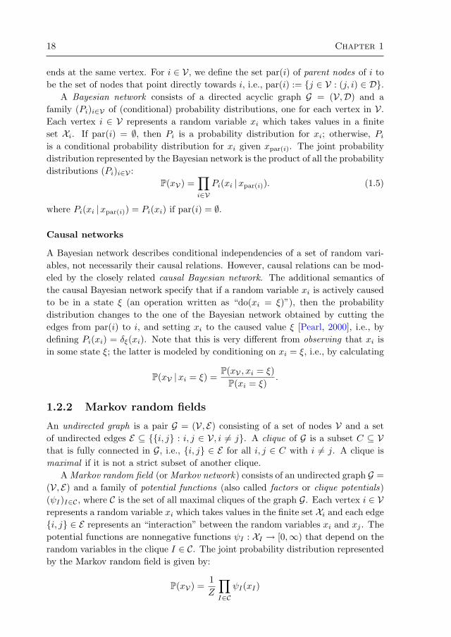
An undirected graph is a pair G = (V, E) consisting of a set of nodes V and a setof undirected edges E ⊆ i, j : i, j ∈ V, i 6= j. A clique of G is a subset C ⊆ Vthat is fully connected in G, i.e., i, j ∈ E for all i, j ∈ C with i 6= j. A clique ismaximal if it is not a strict subset of another clique.
A Markov random field (or Markov network) consists of an undirected graph G =(V, E) and a family of potential functions (also called factors or clique potentials)(ψI)I∈C , where C is the set of all maximal cliques of the graph G. Each vertex i ∈ Vrepresents a random variable xi which takes values in the finite set Xi and each edgei, j ∈ E represents an “interaction” between the random variables xi and xj . Thepotential functions are nonnegative functions ψI : XI → [0,∞) that depend on therandom variables in the clique I ∈ C. The joint probability distribution representedby the Markov random field is given by:
P(xV) =1Z
∏I∈C
ψI(xI)
Chapter 1. Introduction 19
where xI is the state of the random variables in the clique I, and the normalizingconstant Z (also called partition function) is defined as
Z =∑
xV∈XV
∏I∈C
ψI(xI).
An example of a Markov random field that is studied in statistical physics is theIsing model.
1.2.3 Factor graphs
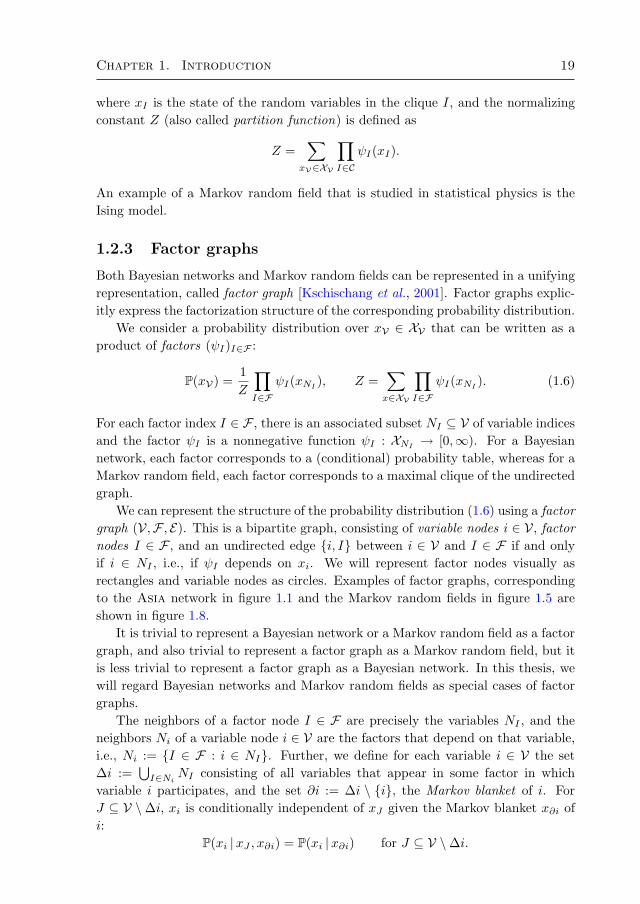
Both Bayesian networks and Markov random fields can be represented in a unifyingrepresentation, called factor graph [Kschischang et al., 2001]. Factor graphs explic-itly express the factorization structure of the corresponding probability distribution.
We consider a probability distribution over xV ∈ XV that can be written as aproduct of factors (ψI)I∈F :
P(xV) =1Z
∏I∈F
ψI(xNI ), Z =∑x∈XV
∏I∈F
ψI(xNI ). (1.6)
For each factor index I ∈ F , there is an associated subset NI ⊆ V of variable indicesand the factor ψI is a nonnegative function ψI : XNI → [0,∞). For a Bayesiannetwork, each factor corresponds to a (conditional) probability table, whereas for aMarkov random field, each factor corresponds to a maximal clique of the undirectedgraph.
We can represent the structure of the probability distribution (1.6) using a factorgraph (V,F , E). This is a bipartite graph, consisting of variable nodes i ∈ V, factornodes I ∈ F , and an undirected edge i, I between i ∈ V and I ∈ F if and onlyif i ∈ NI , i.e., if ψI depends on xi. We will represent factor nodes visually asrectangles and variable nodes as circles. Examples of factor graphs, correspondingto the Asia network in figure 1.1 and the Markov random fields in figure 1.5 areshown in figure 1.8.
It is trivial to represent a Bayesian network or a Markov random field as a factorgraph, and also trivial to represent a factor graph as a Markov random field, but itis less trivial to represent a factor graph as a Bayesian network. In this thesis, wewill regard Bayesian networks and Markov random fields as special cases of factorgraphs.
The neighbors of a factor node I ∈ F are precisely the variables NI , and theneighbors Ni of a variable node i ∈ V are the factors that depend on that variable,i.e., Ni := I ∈ F : i ∈ NI. Further, we define for each variable i ∈ V the set∆i :=
⋃I∈Ni NI consisting of all variables that appear in some factor in which
variable i participates, and the set ∂i := ∆i \ i, the Markov blanket of i. ForJ ⊆ V \∆i, xi is conditionally independent of xJ given the Markov blanket x∂i ofi:
P(xi |xJ , x∂i) = P(xi |x∂i) for J ⊆ V \∆i.

20 Chapter 1
B
D
L
X
S
TE
A
P(B |S)
P(L |S)
P(X |E)
P(S)
P(T |A)
P(A)
P(D |B,E)
P(E |T, L)
ψi
xi ψi,j
ψj
xj ψj,k
ψk
xk
Figure 1.8: Examples of factor graphs, corresponding with the Bayesian network in figure
1.1 and the two Markov random fields in figure 1.5.
We will generally use uppercase letters for indices of factors (I, J,K, . . . ∈ F) andlowercase letters for indices of variables (i, j, k, . . . ∈ V).
1.2.4 Inference in graphical models
In this thesis, we will define inference in a graphical model to be the task of cal-culating marginal probabilities of subsets of random variables, possibly conditionalon observed values of another subset of random variables. This can be done exactly(exact inference) or in an approximate way (approximate inference). Another in-ference task that is often considered is to calculate the MAP state, i.e., the jointassignment of a subset of random variables which has the largest probability (possi-bly conditional on observed values of another subset of random variables). We focuson the first inference problem, i.e., the approximation of marginal probabilities.
In general, the normalizing constant Z in (1.6) (also called partition function)is not known and exact computation of Z is infeasible, due to the fact that thenumber of terms to be summed is exponential in N . Similarly, computing marginaldistributions P(xJ) of P(xV) for subsets of variables J ⊆ V is known to be NP-hard[Cooper, 1990]. Furthermore, approximate inference within given error bounds isNP-hard [Dagum and Luby, 1993; Roth, 1996]. Because of the many applications

Chapter 1. Introduction 21
in which inference plays a role, the development and understanding of approximateinference methods is thus an important topic of research.
1.2.5 Belief Propagation: an approximate inference method
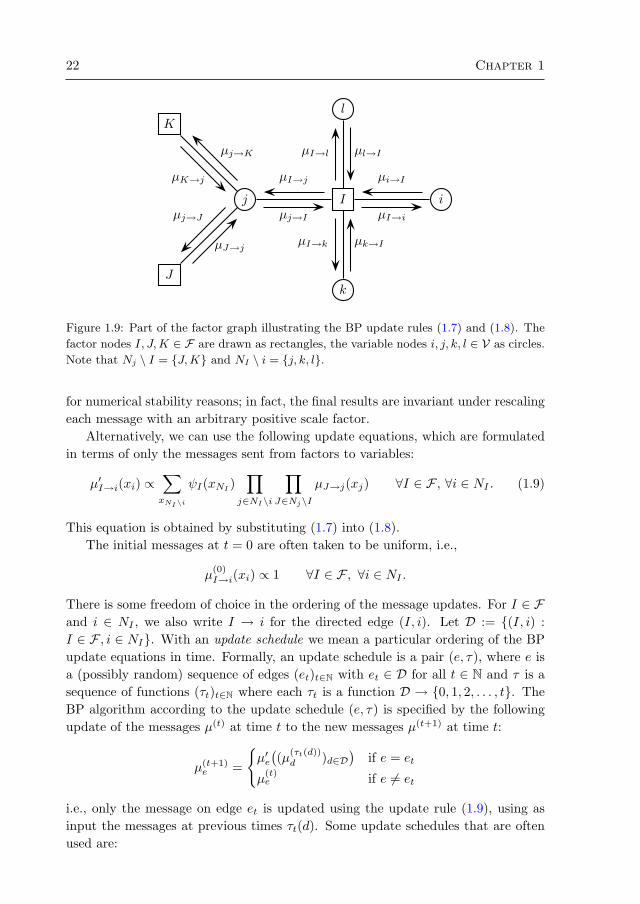
Belief Propagation (BP) is a popular algorithm for approximate inference that hasbeen reinvented many times in different fields. It is also known as Loopy BeliefPropagation (where the adjective “loopy” is used to emphasize that it is used ona graphical model with cycles), the Sum-Product Algorithm and the Bethe-Peierlsapproximation. In artificial intelligence, it is commonly attributed to Pearl [1988].In the context of error-correcting (LDPC) codes, it was already proposed by Gal-lager [1963]. The earliest description of Belief Propagation in the statistical physicsliterature known to the author is [Nakanishi, 1981] (for the special case of a binary,pairwise Markov random field). A few years ago it became clear [Yedidia et al.,2001] that the BP algorithm is strongly related to the Bethe-Peierls approxima-tion, which was invented originally in statistical mechanics [Bethe, 1935; Peierls,1936]; this discovery led to a renewed interest in Belief Propagation and relatedinference methods. We will henceforth use the acronym “BP” since it can be inter-preted as being an abbreviation for either “Belief Propagation” or “Bethe-Peierlsapproximation”.
BP calculates approximations to the factor marginals (P(xI))I∈F and the vari-able marginals (P(xi))i∈V of the probability distribution (1.6) of a factor graph[Kschischang et al., 2001; Yedidia et al., 2005]. The calculation is done by message-passing on the factor graph. Each node passes messages to its neighbors: variablenodes pass messages to factor nodes and factor nodes pass messages to variablenodes. The outgoing messages are functions of the incoming messages at each node.This iterative process is repeated using some schedule that describes the sequenceof message updates in time. This process can either converge to some fixed pointor go on ad infinitum. If BP converges, the approximate marginals (called beliefs)can be calculated from the fixed point messages.
For the factor graph formulation of BP (see also figure 1.9), it is convenient todiscriminate between two types of messages: messages µI→i : Xi → [0,∞) sent fromfactors I ∈ F to neighboring variables i ∈ NI and messages µi→I : Xi → [0,∞)from variables i ∈ V to neighboring factors I ∈ Ni. The messages that are sent bya node depend on the incoming messages; the new messages, designated by µ′, aregiven in terms of the incoming messages by the following BP update equations:
µ′j→I(xj) ∝∏
J∈Nj\IµJ→j(xj) ∀j ∈ V, ∀I ∈ Nj , (1.7)
µ′I→i(xi) ∝∑xNI\i
ψI(xNI )∏
j∈NI\iµj→I(xj) ∀I ∈ F , ∀i ∈ NI . (1.8)
Usually, one normalizes the messages such that∑xi∈Xi µ(xi) = 1. This is only done
22 Chapter 1
J
K
µJ→j
µj→J
µj→K
µK→j
jµj→I
µI→j
IµI→i
µi→I
i
k
µk→IµI→k
l
µl→IµI→l
Figure 1.9: Part of the factor graph illustrating the BP update rules (1.7) and (1.8). The
factor nodes I, J,K ∈ F are drawn as rectangles, the variable nodes i, j, k, l ∈ V as circles.
Note that Nj \ I = J,K and NI \ i = j, k, l.
for numerical stability reasons; in fact, the final results are invariant under rescalingeach message with an arbitrary positive scale factor.
Alternatively, we can use the following update equations, which are formulatedin terms of only the messages sent from factors to variables:
µ′I→i(xi) ∝∑xNI\i
ψI(xNI )∏
j∈NI\i
∏J∈Nj\I
µJ→j(xj) ∀I ∈ F , ∀i ∈ NI . (1.9)
This equation is obtained by substituting (1.7) into (1.8).The initial messages at t = 0 are often taken to be uniform, i.e.,
µ(0)I→i(xi) ∝ 1 ∀I ∈ F , ∀i ∈ NI .
There is some freedom of choice in the ordering of the message updates. For I ∈ Fand i ∈ NI , we also write I → i for the directed edge (I, i). Let D := (I, i) :I ∈ F , i ∈ NI. With an update schedule we mean a particular ordering of the BPupdate equations in time. Formally, an update schedule is a pair (e, τ), where e isa (possibly random) sequence of edges (et)t∈N with et ∈ D for all t ∈ N and τ is asequence of functions (τt)t∈N where each τt is a function D → 0, 1, 2, . . . , t. TheBP algorithm according to the update schedule (e, τ) is specified by the followingupdate of the messages µ(t) at time t to the new messages µ(t+1) at time t:
µ(t+1)e =
µ′e((µ(τt(d))d )d∈D
)if e = et
µ(t)e if e 6= et
i.e., only the message on edge et is updated using the update rule (1.9), using asinput the messages at previous times τt(d). Some update schedules that are oftenused are:
Chapter 1. Introduction 23
• Parallel updates: calculate all new messages as a function of the currentmessages and then simultaneously set all messages to their new values.
• Sequential updates in fixed order : determine some fixed linear ordering of Dand update in that order, using the most recent messages available for eachupdate.
• Sequential updates in random order : before doing a batch of #(D) messageupdates, construct a new random linear ordering of D and update the nextbatch in that order, using the most recent messages available for each indi-vidual update.
• Random updates: at each timestep t, draw a random element from D andupdate the corresponding message, using the most recent messages available.
• Maximum residual updating [Elidan et al., 2006]: calculate all residuals, i.e.,the differences between the updated and current messages, and update onlythe message with the largest residual (according to some measure). Then, onlythe residuals that depend on the updated message need to be recalculated andthe process repeats.
If the messages converge to some fixed point µ(∞), the approximate marginals,often called beliefs, are calculated as follows:
P(xi) ≈ bi(xi) ∝∏I∈Ni
µ(∞)I→i(xi) ∀i ∈ V,
P(xI) ≈ bI(xI) ∝ ψI(xNI )∏i∈I
µ(∞)i→I(xi) ∀I ∈ F .
The beliefs are normalized such that∑xi∈Xi
bi(xi) = 1 ∀i ∈ V,∑xI∈XI
bI(xI) = 1 ∀I ∈ F .
If the factor graph is acyclic, i.e., it contains no loops, then BP with any reasonableupdate schedule will converge towards a unique fixed point within a finite numberof iterations and the beliefs can be shown to be exact. However, if the factorgraph contains cycles, then the BP marginals are only approximations to the exactmarginals; in some cases, these approximations can be surprisingly accurate, inother cases, they can be highly inaccurate.
A fixed point µ(∞) always exists if all factors are strictly positive [Yedidia et al.,2005]. However, the existence of a fixed point does not necessarily imply convergencetowards the fixed point. Indeed, fixed points may be unstable, and there may bemultiple fixed points (corresponding to different final beliefs).
If BP does not converge, one can try to damp the message updates as a possibleremedy. The new message is then a convex combination of the old and the updatedmessage, either according to:
µ(t+1)d = εµ
(t)d + (1− ε)µ′d d ∈ D,
24 Chapter 1
or in the logarithmic domain:
logµ(t+1)d = ε logµ(t)
d + (1− ε) logµ′d d ∈ D,
for some ε ∈ [0, 1).Other methods that can be applied if BP does not converge (or converges too
slowly) are double-loop methods [Yuille, 2002; Heskes et al., 2003; Heskes, 2006].Yedidia et al. [2001] showed that fixed points of BP correspond to stationary pointsof the Bethe free energy. The double-loop methods exploit this correspondenceby directly minimizing the Bethe free energy. The corresponding non-convex con-strained minimization problem can be solved by performing a sequence of convexconstrained minimizations of upper bounds on the Bethe free energy. In this way,the method is guaranteed to converge to a minimum of the Bethe free energy, whichcorresponds with a BP fixed point.
1.2.6 Related approximate inference algorithms
BP can be regarded as the most elementary one in a family of related algorithms,consisting of
• the Max-Product algorithm [Weiss and Freeman, 2001], a zero temperatureversion of BP;
• Generalized Belief Propagation (GBP) [Yedidia et al., 2005] and the ClusterVariation Method (CVM) [Pelizzola, 2005], where variables are clustered in“regions” or “clusters” in order to increase accuracy;
• Double-loop algorithms [Yuille, 2002; Heskes et al., 2003; Heskes, 2006], wherethe inner loop is equivalent to GBP;
• Expectation Propagation (EP) [Minka, 2001; Welling et al., 2005] and theExpectation Consistent (EC) approximation [Opper and Winter, 2005], whichcan be regarded as generalizations of BP [Heskes et al., 2005];
• Survey Propagation (SP) [Braunstein and Zecchina, 2004; Braunstein et al.,2005], which turned out to be equivalent to a special case of the BP algorithm;
• Fractional Belief Propagation [Wiegerinck and Heskes, 2003].
A good theoretical understanding of BP may therefore be beneficial to understand-ing these other algorithms as well. In this thesis, we focus on BP because of itssimplicity and its successes in solving nontrivial problems.
1.2.7 Applications of Belief Propagation
We have given two examples of situations where approximate inference can be usedto solve real world problems. In recent years, mainly due to increased computational

Chapter 1. Introduction 25
power, the number of applications of approximate inference methods has seen anenormous growth. To convey some sense of the diversity of these applications, weprovide a few references to a small subset of these applications (found by searchingon the internet for scientific articles reporting the application of Belief Propagation).
Many applications can be found in vision and image processing. Indeed, BPhas been applied to stereo vision [Felzenszwalb and Huttenlocher, 2004, 2006; Sunet al., 2003; Tappen and Freeman, 2003], super-resolution [Freeman et al., 2000,2002; Gupta et al., 2005], shape matching [Coughlan and Ferreira, 2002; Cough-lan and Shen, 2004], image reconstruction [Felzenszwalb and Huttenlocher, 2006;Tanaka, 2002], inference of human upper body motion [Gao and Shi, 2004], pa-naroma generation [Brunton and Shu, 2006], surface reconstruction [Petrovic et al.,2001], skin detection [Zheng et al., 2004], hand tracking [Sudderth et al., 2004],inferring facial components [Sudderth et al., 2003], and unwrapping phase images[Frey et al., 2002]. Very successful applications can also be found in error correct-ing codes, e.g., Turbo Codes [McEliece et al., 1998] and Low Density Parity Checkcodes [Gallager, 1963; Frey and MacKay, 1997]. In combinatorial optimization, inparticular satisfiability and graph coloring, an algorithm called Survey Propaga-tion recently redefined the state-of-the-art [Mezard and Zecchina, 2002; Braunsteinet al., 2005]. Later it was discovered that it was actually equivalent to a specialcase of BP [Braunstein and Zecchina, 2004]. BP has been applied for diagnosis, forexample in medical diagnosis [Murphy et al., 1999; Wemmenhove et al., 2007]. Incomputer science, it was suggested as a natural algorithm in sensor networks [Ihleret al., 2005c; Crick and Pfeffer, 2003], for data cleaning [Chu et al., 2005] and forcontent distribution in peer-to-peer networks [Bickson et al., 2006]. In biology, ithas been used to predict protein folding [Kamisetty et al., 2006]. Finally, conformthe latest fashions, BP has even been used for solving Sudokus [Dangauthier, 2006].
1.3 Outline of this thesis
In this section, we briefly motivate the research questions addressed in this thesisand summarize the results obtained in later chapters.
In practice, there are at least three important issues when applying BP to con-crete problems: (i) it is usually not known a priori whether BP will converge andhow many iterations are needed; (ii) if BP converges, it is not known how large theerror of the resulting approximate marginals is; (iii) if the error is too large for theapplication, can the error be reduced in some way?
The issues of convergence and accuracy may actually be interrelated: the “folk-lore” is that convergence difficulties of BP often indicate low quality of the corre-sponding Bethe approximation. This would imply that the pragmatic solution forthe convergence problem (forcing BP to converge by means of damping, the use ofother update schemes or applying double-loop methods) would yield low quality re-sults. Furthermore, if we could quantify the relation between error and convergence

26 Chapter 1
rate, this might yield a practical way of estimating the error from the observed rateof convergence.
For the case of a graphical model with a single loop, these questions have beensolved by Weiss [2000]. However, it has turned out to be difficult to generalizethat work to factor graphs with more than one loop. Significant progress has beenmade in recent years regarding the question under what conditions BP converges[Tatikonda and Jordan, 2002; Tatikonda, 2003; Ihler et al., 2005b,a], on the unique-ness of fixed points [Heskes, 2004], and on the accuracy of the marginals [Tatikonda,2003; Taga and Mase, 2006a], but the theoretical understanding was (and is) stillincomplete. Further, even though many methods have been proposed in recentyears to reduce the error of BP marginals, these methods are all in some sense“local” (although more global than BP). We felt that it should be possible to takeinto account longer loops in the factor graph (which may be important when theinteractions along those loops are strong), instead of only taking into account shortloops (as usually done with GBP).
These questions have been the motivation for the research reported in the nextchapters. We finish this introductory chapter with a short summary of all thefollowing chapters.
Convergence of BP
In chapter 2, we study the question of convergence and uniqueness of the fixed pointfor parallel, undamped BP. We derive novel conditions that guarantee convergenceof BP to a unique fixed point, irrespective of the initial messages. The conditionsare applicable to arbitrary factor graphs with discrete variables and factors thatcontain zeros. For the special case of binary variables with pairwise interactions,we derive stronger results that take into account single-variable factors and the typeof pairwise interactions (attractive, mixed or repulsive). We show empirically thatthese bounds improve upon existing bounds.
Phase transitions and BP
While we focussed on undamped parallel BP in chapter 2, in the next chapter, weinvestigate the influence of damping and the use of alternative update schemes. Wefocus on the special case of binary variables with pairwise interactions and zerolocal fields in the interest of simplicity. Whereas in the previous chapter we studiedthe global (“uniform”) convergence properties of BP, in chapter 3 we analyze thelocal stability of the “high-temperature” fixed point of BP.11 Further, we investigatethe relationship between the properties of this fixed point and the properties of thecorresponding stationary point of the Bethe free energy.
11If the interactions are weak enough, BP has a unique fixed point. In statistical physics, weak
interactions correspond to high temperatures. Therefore, we call this particular fixed point the
high-temperature BP fixed point.
Chapter 1. Introduction 27
We distinguish three cases for the interactions: ferromagnetic (attractive), an-tiferromagnetic (repulsive) and spin-glass (mixed). We prove that the convergenceconditions for undamped, parallel BP derived in chapter 2 are sharp in the ferro-magnetic case. Also, the use of damping would only slow down convergence to thehigh-temperature fixed point. In contrast, in the antiferromagnetic case, the useof damping or sequential updates significantly improves the range of instances onwhich BP converges. In the spin-glass case, we observe that damping only slightlyimproves convergence of BP.
Further, we show how one can estimate analytically the temperature (interactionstrength) at which the high-temperature BP fixed point becomes unstable for ran-dom graphs with arbitrary degree distributions and random interactions, extendingthe worst-case results with some average-case results. The results we obtain arein agreement with the results of the replica method from statistical physics. Thisprovides a link between statistical physics and the properties of the BP algorithm.In particular, it leads to the conclusion that the behavior of BP is closely relatedto the phase transitions in the underlying graphical model.
Reducing the BP error
In the fourth chapter, we show how the accuracy of BP can be improved by takinginto account the influence of loops in the graphical model. Extending a methodproposed by Montanari and Rizzo [2005], we propose a novel way of generalizingthe BP update equations by dropping the basic BP assumption of independence ofincoming messages. We call this method the Loop Correction (LC) method.
The basic idea behind the Loop Correction method is the following. A cavitydistribution of some variable in a graphical model is the probability distribution onits Markov blanket for a modified graphical model, in which all factors involving thatvariable have been removed, thereby breaking all the loops involving that variable.The Loop Correction method consists of two steps: first, the cavity distributions ofall variables are estimated (using some approximate inference method), and second,these initial estimates are improved by a message-passing algorithm, which reducesthe errors in the estimated cavity distributions.
If the initial cavity approximations are taken to be uniform (or completely fac-torized) distributions, the Loop Correction algorithm reduces to the BP algorithm.In that sense, it can be considered to be a generalization of BP. On the otherhand, if the initial cavity approximations contain the effective interactions betweenvariables in the cavity, application of the Loop Correction method usually givessignificantly better results than the original (uncorrected) approximate inferencealgorithm used to estimate the cavity approximations. Indeed, we often observethat the loop-corrected error is approximately the square of the error of the uncor-rected approximate inference method.
We report the results of an extensive experimental comparison of various ap-proximate inference methods on a variety of graphical models, including real world
28 Chapter 1
networks. We conclude that the LC method obtains the most accurate results ingeneral, at the cost of significantly increased computation time compared to BP.
Bounds on marginal probabilities
In the final chapter, we further develop some of the ideas that arose out of theconvergence analysis in chapter 2 and the cavity interpretation in chapter 4. Fromchapter 2, we take the idea of studying how the distance between two differentmessage vectors (for the same factor graph) evolves during BP iterations. Fromchapter 4, we take the cavity interpretation that relates the exact marginals to theBP marginals. The key insight exploited in chapter 5 is that by combining andextending these ideas, it is possible to derive rigorous bounds on the exact single-variable marginals. By construction, the same bounds also apply to the BP beliefs.We also derive a related method that propagates bounds over a “self-avoiding-walktree”, inspired by recent results of Ihler [2007]. We show empirically that our boundsoften outperform existing bounds in terms of accuracy and/or computation time.We apply the bounds on factor graphs arising in a medical diagnosis applicationand show that the bounds can yield nontrivial results.

Chapter 2. Sufficient conditions for convergence of BP 29
Chapter 2
Sufficient conditions for
convergence of BP
We derive novel conditions that guarantee convergence of Belief Propagation (BP) to
a unique fixed point, irrespective of the initial messages, for parallel (synchronous)
updates. The computational complexity of the conditions is polynomial in the
number of variables. In contrast with previously existing conditions, our results
are directly applicable to arbitrary factor graphs (with discrete variables) and are
shown to be valid also in the case of factors containing zeros, under some additional
conditions. We compare our bounds with existing ones, numerically and, if possible,
analytically. For binary variables with pairwise interactions, we derive sufficient
conditions that take into account local evidence (i.e., single-variable factors) and
the type of pairwise interactions (attractive or repulsive). It is shown empirically
that this bound outperforms existing bounds.
2.1 Introduction
Belief Propagation [Pearl, 1988; Kschischang et al., 2001], also known as “LoopyBelief Propagation” and as the “Sum-Product Algorithm”, which we will henceforthabbreviate as BP, is a popular algorithm for approximate inference in graphical mod-els. Applications can be found in diverse areas such as error correcting codes (iter-ative channel decoding algorithms for Turbo Codes and Low Density Parity CheckCodes [McEliece et al., 1998]), combinatorial optimization (satisfiability problemssuch as 3-SAT and graph coloring [Braunstein and Zecchina, 2004]) and computervision (stereo matching [Sun et al., 2003] and image restoration [Tanaka, 2002]). BP
c©2007 IEEE. Reprinted, with permission, from [Mooij and Kappen, 2007b], which extends
[Mooij and Kappen, 2005b].

30 Chapter 2
can be regarded as the most elementary one in a family of related algorithms, con-sisting of double-loop algorithms [Heskes et al., 2003], GBP [Yedidia et al., 2005], EP[Minka, 2001], EC [Opper and Winter, 2005], the Max-Product Algorithm [Weissand Freeman, 2001], the Survey Propagation Algorithm [Braunstein and Zecchina,2004; Braunstein et al., 2005] and Fractional BP [Wiegerinck and Heskes, 2003]. Agood understanding of BP may therefore be beneficial to understanding these otheralgorithms as well.
In practice, there are two major obstacles in the application of BP to concreteproblems: (i) if BP converges, it is not clear whether the results are a good approx-imation of the exact marginals; (ii) BP does not always converge, and in these casesgives no approximations at all. These two issues might actually be interrelated: the“folklore” is that failure of BP to converge often indicates low quality of the Betheapproximation on which it is based. This would mean that if one has to “force” BPto converge (e.g., by using damping or double-loop approaches), one may expectthe results to be of low quality.
Although BP is an old algorithm that has been reinvented in many fields, athorough theoretical understanding of the two aforementioned issues and their re-lation is still lacking. Significant progress has been made in recent years regardingthe question under what conditions BP converges [Tatikonda and Jordan, 2002;Tatikonda, 2003; Ihler et al., 2005b]1, on the uniqueness of fixed points [Heskes,2004], and on the accuracy of the marginals [Tatikonda, 2003], but the theoreticalunderstanding is still incomplete. For the special case of a graphical model con-sisting of a single loop, it has been shown that convergence rate and accuracy areindeed related [Weiss, 2000].
In this work, we study the question of convergence of BP and derive new suffi-cient conditions for BP to converge to a unique fixed point. Our results are moregeneral and in certain cases stronger than previously known sufficient conditions.
2.2 Background
To introduce our notation, we give a short treatment of factorizing probabilitydistributions, the corresponding visualizations called factor graphs, and the BPalgorithm on factor graphs. For an excellent, more extensive treatment of thesetopics we refer the reader to [Kschischang et al., 2001].
2.2.1 Factor graphs
Consider N random variables xi for i ∈ V := 1, 2, . . . , N, with xi taking valuesin a finite set Xi. We will frequently use the following multi-index notation. Let
1After initial submission of this work, we came to the attention of [Ihler et al., 2005a], which
contains improved versions of results in [Ihler et al., 2005b], some of which are similar or identical
to results presented here (see also section 2.5.2).
Chapter 2. Sufficient conditions for convergence of BP 31
A = i1, i2, . . . , im ⊆ V with i1 < i2 < . . . im. We write XA := Xi1×Xi2×· · ·×Ximand for any family (Yi)i∈B with A ⊆ B ⊆ V, we write YA := (Yi1 , Yi2 , . . . , Yim).
We are interested in the class of probability measures on XV that can be writtenas a product of factors (also called potentials or interactions):
P(x1, . . . , xN ) :=1Z
∏I∈F
ψI(xNI ). (2.1)
For each factor index I ∈ F , there is an associated subset NI ⊆ V of variable indicesand the factor ψI is a positive function2 ψI : XNI → (0,∞). Z is a normalizing con-stant ensuring that
∑xV∈XV P(xV) = 1. The class of probability measures described
by (2.1) contains Markov random fields as well as Bayesian networks. We will useuppercase letters for indices of factors (I, J,K, . . . ∈ F) and lowercase letters forindices of variables (i, j, k, . . . ∈ V).
The factor graph that corresponds to the probability distribution (2.1) is a bi-partite graph with variable nodes i ∈ V, factor nodes I ∈ F and edges betweenvariable nodes and factor nodes; there is an edge between variable node i and factornode I if and only if the factor ψI depends on the variable xi, i.e., if i ∈ NI . Theneighbors of a factor node I ∈ F are precisely the variables NI , and the neigh-bors Ni of a variable node i ∈ V are the factors that depend on that variable, i.e.,Ni := I ∈ F : i ∈ NI. For each variable node i ∈ V, we define the set of itsneighboring variable nodes by ∂i :=
(⋃I∈Ni NI
) \ i, i.e., ∂i is the set of indicesof those variables that interact directly with xi.
2.2.2 Belief Propagation
Belief Propagation is an algorithm that calculates approximations to the marginals(P(xNI )
)I∈F and
(P(xi)
)i∈V of the probability measure (2.1). The calculation is
done by message-passing on the factor graph: each node passes messages to itsneighbors (see also figure 2.1). One usually discriminates between two types ofmessages: messages µI→i(xi) from factors to variables and messages µi→I(xi) fromvariables to factors (where i ∈ V, I ∈ Ni). Both messages are positive functions onXi, or, equivalently, vectors in RXi (with positive components). The messages thatare sent by a node depend on the incoming messages; the new messages, designatedby µ′, are given in terms of the incoming messages by the following BP updaterules:3
µ′j→I(xj) ∝∏
J∈Nj\IµJ→j(xj) ∀j ∈ V, ∀I ∈ Nj ; (2.2)
µ′I→i(xi) ∝∑xNI\i
ψI(xNI )∏
j∈NI\iµj→I(xj) ∀I ∈ F , ∀i ∈ NI . (2.3)
2In subsection 2.4.5 we will loosen this assumption and allow for factors containing zeros.3We abuse notation slightly by writing X \ x instead of X \ x for sets X.

32 Chapter 2
J
J ′
µJ→j
µJ′→j
jµj→I
IµI→i
i
j′
µj′→I
j′′
µj′′→I
Figure 2.1: Part of the factor graph illustrating the BP update rules (2.2) and (2.3). The
factor nodes I, J, J ′ ∈ F are drawn as rectangles, the variable nodes i, j, j′, j′′ ∈ V as
circles. Note that Nj \ I = J, J ′ and NI \ i = j, j′, j′′. Apart from the messages that
have been drawn, each edge also carries a message flowing in the opposite direction.
Usually, one normalizes the messages in the `1-sense, i.e., such that∑xi∈Xi
µi→I(xi) = 1,∑xi∈Xi
µI→i(xi) = 1 ∀i ∈ V, ∀I ∈ Ni.
If all messages have converged to some fixed point µ(∞), one calculates the approx-imate marginals, called beliefs, as follows:
bi(xi) ∝∏I∈Ni
µ(∞)I→i(xi) ≈ P(xi) ∀i ∈ V,
bI(xNI ) ∝ ψI(xNI )∏i∈NI
µ(∞)i→I(xi) ≈ P(xNI ) ∀I ∈ F ,
where the normalization is by definition in `1-sense. A fixed point always existsif all factors are strictly positive [Yedidia et al., 2005]. However, the existence ofa fixed point does not necessarily imply convergence towards the fixed point, andfixed points may be unstable.
Note that the beliefs are invariant under rescaling of the messages
µ(∞)I→i(xi) 7→ αI→iµ
(∞)I→i(xi), µ
(∞)i→I(xi) 7→ αi→Iµ
(∞)i→I(xi)
for arbitrary positive constants α, which shows that the precise way of normalizingthe messages in (2.2) and (2.3) is irrelevant. For numerical stability however, someway of normalization (not necessarily in `1-sense) is desired to ensure that themessages stay in some compact domain.
In the following, we will formulate everything in terms of the messages µI→i(xi)from factors to variables; the update equations are then obtained by substituting(2.2) in (2.3):
µ′I→i(xi) = CI→i∑xNI\i
ψI(xNI )∏
j∈NI\i
∏J∈Nj\I
µJ→j(xj). (2.4)
with CI→i such that∑xi∈Xi µ
′I→i(xi) = 1. We consider here BP with a parallel
update scheme, which means that all message updates (2.4) are done in parallel.

Chapter 2. Sufficient conditions for convergence of BP 33
2.3 Special case: binary variables with pairwise
interactions
In this section we investigate the simple case of binary variables (i.e., #(Xi) = 2for all i ∈ V), and in addition we assume that all potentials consist of at mosttwo variables (“pairwise interactions”). Although this is a special case of the moregeneral theory to be presented later on, we start with this simple case because itillustrates most of the underlying ideas without getting involved with the additionaltechnicalities of the general case.
We will assume that all variables are ±1-valued, i.e., Xi = −1,+1 for all i ∈ V.We take the factor index set as F = F1 ∪ F2 with F1 = V (the “local evidence”)and F2 ⊆
i, j : i, j ∈ V, i 6= j
(the “pair potentials”). The probability measure(2.1) can then be written as
P(xV) =1Z
exp
∑i,j∈F2
Jijxixj +∑i∈F1
θixi
(2.5)
for some choice of the parameters Jij (“couplings”) and θi (“local fields”), withψi(xi) = exp(θixi) for i ∈ F1 and ψij(xi, xj) = exp(Jijxixj) for i, j ∈ F2.
Note from (2.4) that the messages sent from single-variable factors F1 to vari-ables are constant. Thus the question whether messages converge can be decided bystudying only the messages sent from pair potentials F2 to variables. It turns outto be advantageous to use the following “natural” parameterization of the messages(often used in statistical physics):
tanh νi→j := µi,j→j(xj = 1)− µi,j→j(xj = −1), (2.6)
where νi→j ∈ R is now interpreted as a message sent from variable i to variablej (instead of a message sent from the factor i, j to variable j). Note that inthe pairwise case, the product over j ∈ NI \ i in (2.4) becomes trivial. Some ele-mentary algebraic manipulations show that the BP update equations (2.4) becomeparticularly simple in this parameterization: they can be written as
tanh(ν′i→j) = tanh(Jij) tanh
θi +∑t∈∂i\j
νt→i
, (2.7)
where ∂i = t ∈ V : i, t ∈ F2 are the variables that interact with i via a pairpotential.
Defining the set of ordered pairs D := i → j : i, j ∈ F2, we see that theparallel BP update is a mapping f : RD → RD; (2.7) specifies the component(f(ν)
)i→j := ν′i→j in terms of the components of ν. Our goal is now to derive
sufficient conditions under which the mapping f is a contraction. For this we needsome elementary but powerful mathematical theorems.
34 Chapter 2
2.3.1 Normed spaces, contractions and bounds
In this subsection we introduce some (standard) notation and remind the readerof some elementary but important properties of vector norms, matrix norms, con-tractions and the Mean Value Theorem in arbitrary normed vector spaces, whichare the main mathematical ingredients for our basic tool, Lemma 2.3. The readerfamiliar with these topics can skip this subsection and proceed directly to Lemma2.3 in section 2.3.2.
Let (V, ‖·‖ ) be a normed finite-dimensional real vector space. Examples ofnorms that will be important later on are the `1-norm on RN , defined by
‖x‖1 :=N∑i=1
|xi|
and the `∞-norm on RN , defined by
‖x‖∞ := maxi∈1,...,N
|xi| .
A norm on a vector space V induces a metric on V by the definition d(v, w) :=‖v − w‖ . The resulting metric space is complete.4
Let (X, d) be a metric space. A mapping f : X → X is called a contraction withrespect to d if there exists 0 ≤ K < 1 such that
d(f(x), f(y)) ≤ Kd(x, y) for all x, y ∈ X. (2.8)
In case d is induced by a norm ‖·‖ , we will call a contraction with respect to d a‖·‖ -contraction. If (X, d) is complete, we can apply the following theorem, due toBanach:
Theorem 2.1 (Contracting Mapping Principle) Let f : X → X be a contrac-tion of a complete metric space (X, d). Then f has a unique fixed point x∞ ∈ Xand for any x ∈ X, the sequence x, f(x), f2(x), . . . obtained by iterating f convergesto x∞. The rate of convergence is at least linear, since d(f(x), x∞) ≤ Kd(x, x∞)for all x ∈ X.
Proof. Can be found in many textbooks on analysis.
Note that linear convergence means that the error decreases exponentially, indeedd(fn(x), x∞) ≤ CKn for some C.
Let (V, ‖·‖ ) be a normed space. The norm induces a matrix norm (also calledoperator norm) on linear mappings A : V → V , defined as follows:
‖A‖ := supv∈V,‖v‖≤1
‖Av‖ .
4Completeness is a topological property which we will not further discuss, but we need this to
apply Theorem 2.1.

Chapter 2. Sufficient conditions for convergence of BP 35
The `1-norm on RN induces the following matrix norm:
‖A‖1 = maxj∈1,...,N
N∑i=1
|Aij | (2.9)
where Aij := (Aej)i with ej the jth canonical basis vector. The `∞-norm on RN
induces the following matrix norm:
‖A‖∞ = maxi∈1,...,N
N∑j=1
|Aij | . (2.10)
In the following consequence of the well-known Mean Value Theorem, the matrixnorm of the derivative (“Jacobian”) f ′(v) at v ∈ V of a differentiable mappingf : V → V is used to bound the distance of the f -images of two vectors:
Lemma 2.2 Let (V, ‖·‖ ) be a normed space and f : V → V a differentiable map-ping. Then, for x, y ∈ V :
‖f(y)− f(x)‖ ≤ ‖y − x‖ · supz∈[x,y]
‖f ′(z)‖
where we wrote [x, y] for the segment λx+ (1− λ)y : λ ∈ [0, 1] joining x and y.
Proof. See [Dieudonne, 1969, Thm. 8.5.4].
2.3.2 The basic tool
Combining Theorem 2.1 and Lemma 2.2 immediately yields our basic tool:
Lemma 2.3 Let (V, ‖·‖ ) be a normed space, f : V → V differentiable and supposethat
supv∈V‖f ′(v)‖ < 1.
Then f is a ‖·‖ -contraction by Lemma 2.2. Hence, for any v ∈ V , the sequencev, f(v), f2(v), . . . converges to a unique fixed point v∞ ∈ V with a convergence ratethat is at least linear by Theorem 2.1.
2.3.3 Sufficient conditions for BP to be a contraction
We apply Lemma 2.3 to the case at hand: the parallel BP update mapping f :RD → RD, written out in components in (2.7). Different choices of the vector normon RD will yield different sufficient conditions for whether iterating f will convergeto a unique fixed point. We will study two examples: the `1 norm and the `∞ norm.
The derivative of f is easily calculated from (2.7) and is given by(f ′(ν)
)i→j,k→l
=∂ν′i→j∂νk→l
= Ai→j,k→lBi→j(ν) (2.11)

36 Chapter 2
where5
Bi→j(ν) :=1− tanh2
(θi +
∑t∈∂i\j νt→i
)1− tanh2
(ν′i→j(ν)
) sgn Jij (2.12)
Ai→j,k→l := tanh |Jij | δil1∂i\j(k). (2.13)
Note that we have absorbed all ν-dependence in the factor Bi→j(ν); the reasonfor this will become apparent later on. The factor Ai→j,k→l is nonnegative andindependent of ν and captures the structure of the graphical model. Note thatsupν∈V |Bi→j(ν)| = 1, implying that∣∣∣∣∂ν′i→j∂νk→l
∣∣∣∣ ≤ Ai→j,k→l (2.14)
everywhere on V .
Example: the `∞-norm
The `∞-norm on RD yields the following condition:
Corollary 2.4 For binary variables with pairwise interactions and probability dis-tribution (2.5), if
maxi∈V
((#(∂i)− 1
)maxj∈∂i
tanh |Jij |)< 1, (2.15)
BP is an `∞-contraction and converges to a unique fixed point, irrespective of theinitial messages.
Proof. Using (2.10), (2.13) and (2.14):
‖f ′(ν)‖∞ = maxi→j
∑k→l
∣∣∣∣∂ν′i→j∂νk→l
∣∣∣∣ ≤ maxi→j
∑k→l
tanh |Jij | δil1∂i\j(k)
= maxi∈V
maxj∈∂i
∑k∈∂i\j
tanh |Jij | = maxi∈V
((#(∂i)− 1
)maxj∈∂i
tanh |Jij |)
and now simply apply Lemma 2.3.
Another example: the `1-norm
Using the `1-norm instead, we find:
Corollary 2.5 For binary variables with pairwise interactions and probability dis-tribution (2.5), if
maxi∈V
maxk∈∂i
∑j∈∂i\k
tanh |Jij | < 1, (2.16)
BP is an `1-contraction and converges to a unique fixed point, irrespective of theinitial messages.
5For a set X, we define the indicator function 1X of X by 1X(x) = 1 if x ∈ X and 1X(x) = 0
if x 6∈ X.

Chapter 2. Sufficient conditions for convergence of BP 37
Proof. Similar to the proof of Corollary 2.4, now using (2.9) instead of (2.10):
‖f ′(ν)‖1 ≤ maxk→l
∑i→j
tanh |Jij | δil1∂i\j(k) = maxi∈V
maxk∈∂i
∑j∈∂i\k
tanh |Jij | .
It is easy to see that condition (2.16) is implied by (2.15), but not conversely;thus in this case the `1-norm yields a tighter bound than the `∞-norm.
2.3.4 Beyond norms: the spectral radius
Instead of pursuing a search for the optimal norm, we will derive a criterion forconvergence based on the spectral radius of the matrix (2.13). The key idea is tolook at several iterations of BP at once. This will yield a significantly strongercondition for convergence of BP to a unique fixed point.
For a square matrix A, we denote by σ(A) its spectrum, i.e., the set of eigenvaluesof A. By ρ(A) we denote its spectral radius, which is defined as ρ(A) := sup |σ(A)|,i.e., the largest modulus of eigenvalues of A.6
Lemma 2.6 Let f : X → X be a mapping, d a metric on X and suppose that fN
is a d-contraction for some N ∈ N. Then f has a unique fixed point x∞ and forany x ∈ X, the sequence x, f(x), f2(x), . . . obtained by iterating f converges to x∞.
Proof. Take any x ∈ X. Consider the N sequences obtained by iterating fN ,starting respectively in x, f(x), . . . , fN−1(x):
x, fN (x), f2N (x), . . .
f(x), fN+1(x), f2N+1(x), . . ....
fN−1(x), f2N−1(x), f3N−1(x), . . .
Each sequence converges to x∞ since fN is a d-contraction with fixed point x∞.But then the sequence x, f(x), f2(x), . . . must converge to x∞.
Theorem 2.7 Let f : Rm → Rm be differentiable and suppose that f ′(x) = B(x)A,where A has nonnegative entries and B is diagonal with bounded entries |Bii(x)| ≤1. If ρ(A) < 1 then for any x ∈ Rm, the sequence x, f(x), f2(x), . . . obtained byiterating f converges to a fixed point x∞, which does not depend on x.
Proof. For a matrix B, we will denote by |B| the matrix with entries |B|ij = |Bij |.For two matrices B,C we will write B ≤ C if Bij ≤ Cij for all entries (i, j). Notethat if |B| ≤ |C|, then ‖B‖1 ≤ ‖C‖1 . Also note that |BC| ≤ |B| |C|. Finally, if0 ≤ A and B ≤ C, then AB ≤ AC and BA ≤ CA.
6One should not confuse the spectral radius ρ(A) with the spectral norm ‖A‖2 =pρ(ATA)
of A, the matrix norm induced by the `2-norm.
38 Chapter 2
Using these observations and the chain rule, we have for any n ∈ N∗ and anyx ∈ Rm:
|(fn)′(x)| =∣∣∣∣∣n∏i=1
f ′(f i−1(x)
)∣∣∣∣∣ ≤n∏i=1
( ∣∣B(f i−1(x))∣∣A) ≤ An,
hence ‖(fn)′(x)‖1 ≤ ‖An‖1 .By the Gelfand spectral radius theorem,
limn→∞
( ‖An‖1 )1/n = ρ(A).
Choose ε > 0 such that ρ(A) + ε < 1. For some N ,∥∥AN∥∥
1≤ (ρ(A) + ε)N < 1.
Hence for all x ∈ Rm,∥∥(fN )′(x)
∥∥1< 1. Applying Lemma 2.3, we conclude that
fN is a `1-contraction. Now apply Lemma 2.6.
Using (2.11), (2.12) and (2.13), this immediately yields:
Corollary 2.8 For binary variables with pairwise interactions and probability dis-tribution (2.5), BP converges to a unique fixed point (irrespective of the initialmessages), if the spectral radius of the #(D)×#(D) matrix
Ai→j,k→l := tanh |Jij | δil1∂i\j(k)
is strictly smaller than 1.
The calculation of the spectral norm of the (sparse) matrix A can be done usingstandard numerical techniques in linear algebra.
Any matrix norm of A is actually an upper bound on the spectral radius ρ(A),since for any eigenvalue λ of A with eigenvector v we have |λ| ‖v‖ = ‖λv‖ =‖Av‖ ≤ ‖A‖ ‖v‖ , hence ρ(A) ≤ ‖A‖ . This implies that no norm in Lemma 2.3will result in a sharper condition than Corollary 2.8, hence the title of this section.
Further, for a given matrix A and some ε > 0, there exists a vector norm ‖·‖such that the induced matrix norm of A satisfies ρ(A) ≤ ‖A‖ ≤ ρ(A) + ε; see[Deutsch, 1975] for a constructive proof. Thus for given A one can approximateρ(A) arbitrarily close by induced matrix norms. This immediately gives a resulton the convergence rate of BP (in case ρ(A) < 1): for any ε > 0, there exists anorm-induced metric such that the linear rate of contraction of BP with respect tothat metric is bounded from above by ρ(A) + ε.
One might think that there is a shorter proof of Corollary 2.8: it seems quiteplausible intuitively that in general, for a continuously differentiable f : Rm → Rm,iterating f will converge to a unique fixed point if
supx∈Rm
ρ(f ′(x)) < 1.
However, this conjecture (which has been open for a long time) has been shown tobe true in two dimensions but false in higher dimensions [Cima et al., 1997].

Chapter 2. Sufficient conditions for convergence of BP 39
2.3.5 Improved bound for strong local evidence
Empirically, it is known that the presence of strong local fields (i.e., single-variablefactors which are far from uniform) often improves the convergence of BP. However,our results so far are completely independent of the parameters (θi)i∈V that measurethe strength of the local evidence. By proceeding more carefully than we have doneabove, the results can easily be improved in such a way that local evidence is takeninto account.
Consider the quantity Bi→j defined in (2.12). We have bounded this quantityby noting that supν∈V |Bi→j(ν)| = 1. Note that for all BP updates (except forthe first one), the argument ν (the incoming messages) is in f(V ), which can beconsiderably smaller than the complete vector space V . Thus, after the first BPupdate, we can use
supν∈f(V )
|Bi→j(ν)| = supν∈f(V )
1− tanh2(θi +
∑k∈∂i\j νk→i
)1− tanh2
(ν′i→j(ν)
)= supν∈f(V )
1− tanh2(ηi\j)
1− tanh2(Jij) tanh2(ηi\j)
where we used (2.7) and defined the cavity field
ηi\j(ν) := θi +∑
k∈∂i\jνk→i. (2.17)
The function
x 7→ 1− tanh2 x
1− tanh2 Jij · tanh2 x
is strictly decreasing for x ≥ 0 and symmetric around x = 0, thus, defining
η(∗)i\j := inf
ν∈f(V )
∣∣ηi\j(ν)∣∣ , (2.18)
we obtain
supν∈f(V )
|Bi→j(ν)| =1− tanh2
(η
(∗)i\j)
1− tanh2(Jij) tanh2(η
(∗)i\j) .
Now, from (2.7) we derive that
νk→i : ν ∈ f(V ) = (− |Jki| , |Jki|),
henceηi\j(ν) : ν ∈ f(V ) =
(η
(−)i\j , η
(+)i\j)
where we definedη
(±)i\j := θi ±
∑k∈∂i\j
|Jki| .

40 Chapter 2
We conclude that η(∗)i\j is simply the distance between 0 and the interval
(η
(−)i\j , η
(+)i\j),
i.e.,
η(∗)i\j =
∣∣∣η(+)i\j∣∣∣ if η(+)
i\j < 0
η(−)i\j if η(−)
i\j > 0
0 otherwise.
Thus the element Ai→j,k→i (for i ∈ ∂j, k ∈ ∂i \ j) of the matrix A defined inCorollary 2.8 can be replaced by
tanh |Jij |1− tanh2
(η
(∗)i\j)
1− tanh2(Jij) tanh2(η
(∗)i\j) =
tanh( |Jij | − η(∗)
i\j)
+ tanh( |Jij |+ η
(∗)i\j)
2
which is generally smaller than tanh |Jij | and thus gives a tighter bound.This trick can be repeated arbitrarily often: assume that m ≥ 0 BP updates have
been done already, which means that it suffices to take the supremum of |Bi→j(ν)|over ν ∈ fm(V ). Define for all i→ j ∈ D and all t = 0, 1, . . . ,m:
η(t)i\j := infηi\j(ν) : ν ∈ f t(V ), (2.19)
η(t)i\j := supηi\j(ν) : ν ∈ f t(V ), (2.20)
and define the intervalsH(t)i\j := [η(t)
i\j , η(t)i\j ]. (2.21)
Specifically, for t = 0 we have η(0)i\j = −∞ and η
(0)i\j =∞, which means that
H(0)i\j = R. (2.22)
Using (2.7) and (2.17), we obtain the following recursive relations for the intervals(where we use interval arithmetic defined in the obvious way):
H(t+1)i\j = θi +
∑k∈∂i\j
tanh−1(
tanh Jki tanhH(t)k\i). (2.23)
Using this recursion relation, one can calculate H(m)i\j and define η(∗)
i\j as the distance
(in absolute value) of the interval H(m)i\j to 0:
η(∗)i\j =
∣∣∣η(m)i\j∣∣∣ if η(m)
i\j < 0
η(m)i\j if η(m)
i\j > 0
0 otherwise.
(2.24)
Thus by replacing the matrix A in Corollary 2.8 by
Ai→j,k→l =tanh
( |Jij | − η(∗)i\j)
+ tanh( |Jij |+ η
(∗)i\j)
2δil1∂i\j(k), (2.25)
we obtain stronger results that improve as m increases:

Chapter 2. Sufficient conditions for convergence of BP 41
Corollary 2.9 Let m ∈ N. For binary variables with pairwise interactions andprobability distribution (2.5), BP converges to a unique fixed point (irrespective ofthe initial messages) if the spectral radius of the #(D) × #(D) matrix defined in(2.25) (with η(∗)
i\j defined in equations (2.21)–(2.24)) is strictly smaller than 1.
2.4 General case
In the general case, when the domains Xi are arbitrarily large (but finite), we do notknow of a natural parameterization of the messages that automatically takes careof the invariance of the messages under scaling (like (2.6) does in the binary case).Instead of handling the scale invariance by the parameterization and using standardnorms and metrics, it seems easier to take a simple parameterization and to changethe norms and metrics in such a way that they are insensitive to the (irrelevant)extra degrees of freedom arising from the scale invariance. This is actually the keyinsight in extending the previous results beyond the binary case: once one sees howto do this, the rest follows in a (more or less) straightforward way.
A related important point is to reparameterize the messages: a natural pa-rameterization for our analysis is now in terms of logarithms of messages λI→i :=logµI→i. The BP update equations (2.4) can be written in terms of the log-messagesas:
λ′I→i(xi) = log∑xNI\i
ψI(xNI )hI\i(xNI\i), (2.26)
where we dropped the normalization and defined the “cavity field”
hI\i(xNI\i) := exp
∑j∈NI\i
∑J∈Nj\I
λJ→j(xj)
. (2.27)
Each log-message λI→i is a vector in the vector space VI→i := RXi ; we will useGreek letters as indices for the components, e.g., λI→i;α := λI→i(α) with α ∈ Xi.We will call everything that concerns individual vector spaces VI→i local and definethe global vector space V as the direct sum of the local vector spaces:
V :=⊕
i∈V,I∈NiVI→i.
The parallel BP update is the mapping f : V → V , written out in components in(2.26) and (2.27).
Note that the invariance of the message µI→i under scaling amounts to invari-ance of the log-message λI→i under translation. More formally, defining linearsubspaces
WI→i := λ ∈ VI→i : λα = λα′ for all α, α′ ∈ Xi (2.28)
and their direct sumW :=
⊕i∈V,I∈Ni
WI→i ⊆ V,

42 Chapter 2
the invariance amounts to the observation that
f(λ+ w)− f(λ) ∈W for all λ ∈ V , w ∈W.
Since λ+w and λ are equivalent for our purposes, we want our measures of distancein V to reflect this equivalence. Therefore we will “divide out” the equivalence rela-tion and work in the quotient space V/W , which is the topic of the next subsection.
2.4.1 Quotient spaces
Let V be a finite-dimensional vector space. Let W be a linear subspace of V . Wecan consider the quotient space V/W := v+W : v ∈ V , where v+W := v+w :w ∈ W. Defining addition and scalar multiplication on the quotient space in thenatural way, the quotient space is again a vector space.7 We will denote its elementsas v := v +W . Note that the projection π : V → V/W : v 7→ v is linear.
Let ‖·‖ be any vector norm on V . It induces a quotient norm on V/W , definedby
‖v‖ := infw∈W
‖v + w‖ , (2.29)
which is indeed a norm, as one easily checks. The quotient norm in turn inducesthe quotient metric d(v1, v2) := ‖v2 − v1‖ on V/W . The metric space (V/W, d) iscomplete (since any finite-dimensional normed vector space is complete).
Let f : V → V be a (possibly nonlinear) mapping with the following symmetry:
f(v + w)− f(v) ∈W for all v ∈ V , w ∈W. (2.30)
We can then unambiguously define the quotient mapping
f : V/W → V/W : v 7→ f(v),
which yields the following commutative diagram:
Vf−−−−→ Vyπ yπ
V/Wf−−−−→ V/W
π f = f π
For a linear mapping A : V → V , condition (2.30) amounts to AW ⊆W , i.e., Ashould leave W invariant; we can then unambiguously define the quotient mappingA : V/W → V/W : v 7→ Av.
If f : V → V is differentiable and satisfies (2.30), the symmetry property (2.30)implies that f ′(x)W ⊆W , hence we can define f ′(x) : V/W → V/W . The operationof taking derivatives is compatible with projecting onto the quotient space. Indeed,by using the chain rule and the identity π f = f π, one finds that the derivative
7Indeed, we have a null vector 0 + W , addition (v1 + W ) + (v2 + W ) := (v1 + v2) + W for
v1, v2 ∈ V and scalar multiplication λ(v +W ) := (λv) +W for λ ∈ R, v ∈ V .

Chapter 2. Sufficient conditions for convergence of BP 43
of the induced mapping f : V/W → V/W at x equals the induced derivative of fat x:
f′(x) = f ′(x) for all x ∈ V . (2.31)
By Lemma 2.3, f is a contraction with respect to the quotient norm if
supx∈V/W
∥∥∥f ′(x)∥∥∥ < 1.
Using (2.29) and (2.31), this condition can be written more explicitly as:
supx∈V
supv∈V,‖v‖≤1
infw∈W
‖f ′(x) · v + w‖ < 1.
2.4.2 Constructing a norm on V
Whereas in the binary case, each message νi→j was parameterized by a single realnumber, the messages are now #(Xi)-dimensional vectors λI→i (with componentsλI→i;α indexed by α ∈ Xi). In extending the `1-norm that proved to be useful in thebinary case to the more general case, we have the freedom to choose the “local” partof the generalized `1-norm. Here we show how to construct such a generalization ofthe `1-norm and its properties; for a more detailed account of the construction, seeAppendix 2.A.
The “global” vector space V is the direct sum of the “local” subspaces VI→i.Suppose that for each subspace VI→i, we have a local norm ‖·‖I→i . A naturalgeneralization of the `1-norm in the binary case is the following global norm on V :
‖λ‖ :=∑I→i‖λI→i‖I→i . (2.32)
It is easy to check that this is indeed a norm on V .Each subspace VI→i has a 1-dimensional subspaceWI→i defined in (2.28) and the
local norm on VI→i induces a local quotient norm on the quotient space VI→i/WI→i.The global norm (2.32) on V induces a global quotient norm on V/W , which issimply the sum of the local quotient norms (see (2.57)):∥∥λ∥∥ =
∑I→i
∥∥λI→i∥∥I→i . (2.33)
Let λ ∈ V . The derivative f ′(λ) of f : V → V at λ is a linear mappingf ′(λ) : V → V satisfying f ′(λ)W ⊆ W . It projects down to a linear mappingf ′(λ) : V/W → V/W . The matrix norm of f ′(λ) induced by the quotient norm(2.33) is given by (see (2.58)):∥∥∥f ′(λ)
∥∥∥ = maxJ→j
∑I→i
∥∥∥(f ′(λ))I→i,J→j
∥∥∥J→jI→i
(2.34)
44 Chapter 2
where the local quotient matrix norm of the “block”(f ′(λ)
)I→i,J→j is given by (see
(2.59)): ∥∥∥(f ′(λ))I→i,J→j
∥∥∥J→jI→i
= supv∈VJ→j ,‖v‖J→j ≤1
∥∥∥(f ′(λ))I→i,J→jv
∥∥∥I→i
. (2.35)
The derivative of the (unnormalized) parallel BP update (2.26) is easily calcu-lated:
∂λ′I→i(xi)∂λJ→j(yj)
= 1Nj\I(J)1NI\i(j)
∑xNI\i
ψI(xi, xj , xNI\i,j)δxjyjhI\i(xNI\i)∑xNI\i
ψI(xi, xNI\i)hI\i(xNI\i).
(2.36)Taking the global quotient norm (2.34) of (2.36) yields:∥∥∥f ′(λ)
∥∥∥ = maxJ→j
∑I→i
1Nj\I(J)1NI\i(j)BI→i,J→j(hI\i(λ)
), (2.37)
where
BI→i,J→j(hI\i(λ)
):=
∥∥∥∥∥∥∑xNI\i,j
ψI hI\i(λ)∑xNI\i
ψI hI\i(λ)
∥∥∥∥∥∥J→j
I→i
. (2.38)
Note that BI→i,J→j depends on λ via the dependence of hI\i on λ (see (2.27)). Wewill for the moment simplify matters by assuming that λ can be any vector in V ,and later discuss the more careful estimate (where λ ∈ fm(V )):
supλ∈V
BI→i,J→j(hI\i(λ)
) ≤ suphI\i>0
BI→i,J→j(hI\i). (2.39)
Defining the matrix A by the expression on the r.h.s. and using (2.35) and (2.29),we obtain:
AI→i,J→j := suphI\i>0
BI→i,J→j(hI\i) =
suphI\i>0
supv∈VJ→j‖v‖J→j ≤1
infw∈WI→i
∥∥∥∥∥∑xjv(xj)
∑xNI\i,j
ψI hI\i∑xNI\i
ψI hI\i− w
∥∥∥∥∥I→i
(2.40)
for I → i and J → j such that j ∈ NI \ i and J ∈ Nj \ I. Surprisingly, it turns outthat we can calculate (2.40) analytically if we take all local norms to be `∞ norms.We have also tried the `2 norm and the `1 norm as local norms, but were unableto calculate expression (2.40) analytically in these cases. Numerical calculationsturned out to be difficult because of the nested suprema.
2.4.3 Local `∞ norms
Take for each local norm ‖·‖I→i the `∞ norm on VI→i = RXi . The local subspaceWI→i is spanned by the vector 1 := (1, 1, . . . , 1) ∈ RXi . The local quotient norm of

Chapter 2. Sufficient conditions for convergence of BP 45
a vector v ∈ VI→i is thus given by
‖v‖I→i = ‖v‖∞ = infw∈R‖v + w1‖∞ =
12
supα,α′∈Xi
|vα − vα′ | . (2.41)
For a linear mapping A : VJ→j → VI→i that satisfies AWJ→j ⊆WI→i, the inducedquotient matrix norm (2.35) is given by∥∥A∥∥J→j
I→i = supv∈VJ→j ,‖v‖∞≤1
∥∥Av∥∥∞ = supv∈VJ→j ,‖v‖∞≤1
12
supα,α′∈Xi
∣∣∣∣ ∑β∈Xj
(Aαβ −Aα′β)vβ
∣∣∣∣=
12
supα,α′∈Xi
∑β∈Xj
|Aαβ −Aα′β | (2.42)
For the moment, fix I → i and J → j (such that j ∈ NI \ i and J ∈ Nj \ I).To lighten the notation, we will drop the corresponding subscripts and in addition,we will replace the arguments by Greek subscripts, where we let α correspond toxi, β to xj and γ to xNI\i,j. For example, we write hI\i(xNI\i) as hβγ andψI(xi, xj , xNI\i,j) as ψαβγ . Using (2.42), we can write (2.40) as
suph>0
12
supα,α′
∑β
∣∣∣∣∣∑γ ψαβγhβγ∑
β
∑γ ψαβγhβγ
−∑γ ψα′βγhβγ∑
β
∑γ ψα′βγhβγ
∣∣∣∣∣ .Interchanging the two suprema, fixing (for the moment) α and α′, defining ψβγ :=ψαβγ/ψα′βγ and hβγ := hβγψα′βγ , noting that we can assume (without loss ofgenerality) that h is normalized in `1 sense, the previous expression (apart from the12 supα,α′) simplifies to
suph>0,
‖h‖1 =1
∑β
∣∣∣∣∣∑γ
hβγ
(ψβγ∑
β
∑γ ψβγ hβγ
− 1
)∣∣∣∣∣ . (2.43)
In Appendix 2.B we show that (2.43) equals
2 supβ 6=β′
supγ,γ′
tanh
(14
logψβγ
ψβ′γ′
). (2.44)
We conclude that if we take all local norms to be the `∞ norms, then AI→i,J→jequals
N(ψI , i, j) := supα 6=α′
supβ 6=β′
supγ,γ′
tanh(
14
logψI;αβγψI;α′βγ
ψI;α′β′γ′
ψI;αβ′γ′
), (2.45)
which is defined for i, j ∈ NI with i 6= j and where ψI;αβγ is shorthand for ψI(xi =α, xj = β, xNI\i,j = γ); see figure 2.2 for an illustration.
Now combining (2.37), (2.39) and (2.45), we finally obtain:∥∥∥f ′(λ)∥∥∥ =∥∥∥f ′(λ)
∥∥∥ ≤ maxJ→j
∑I∈Nj\J
∑i∈NI\j
N(ψI , i, j).
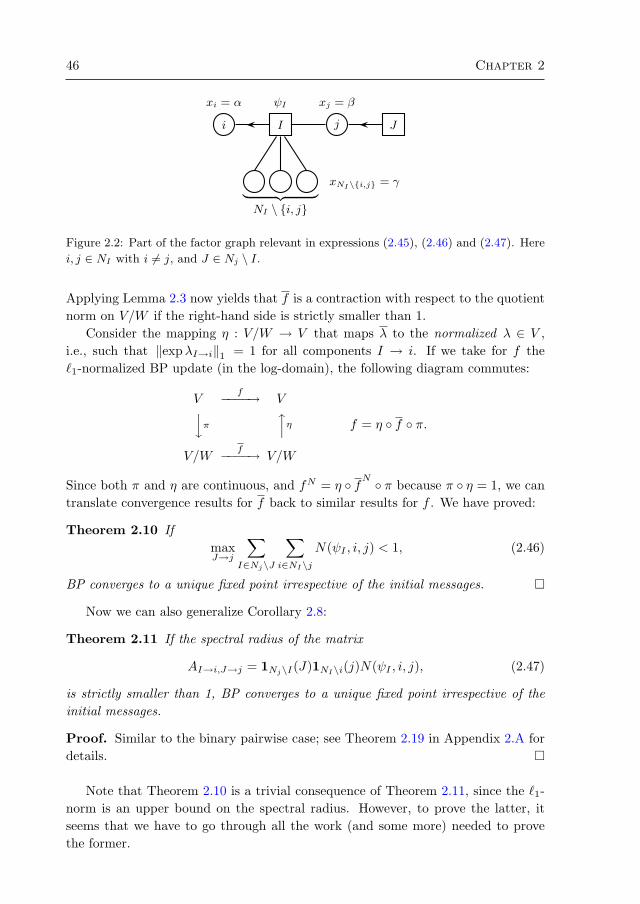
46 Chapter 2
i
xi = α
I
ψI
j
xj = β
J
| z NI \ i, j
xNI\i,j = γ
Figure 2.2: Part of the factor graph relevant in expressions (2.45), (2.46) and (2.47). Here
i, j ∈ NI with i 6= j, and J ∈ Nj \ I.
Applying Lemma 2.3 now yields that f is a contraction with respect to the quotientnorm on V/W if the right-hand side is strictly smaller than 1.
Consider the mapping η : V/W → V that maps λ to the normalized λ ∈ V ,i.e., such that ‖expλI→i‖1 = 1 for all components I → i. If we take for f the`1-normalized BP update (in the log-domain), the following diagram commutes:
Vf−−−−→ Vyπ xη
V/Wf−−−−→ V/W
f = η f π.
Since both π and η are continuous, and fN = η fN π because π η = 1, we cantranslate convergence results for f back to similar results for f . We have proved:
Theorem 2.10 IfmaxJ→j
∑I∈Nj\J
∑i∈NI\j
N(ψI , i, j) < 1, (2.46)
BP converges to a unique fixed point irrespective of the initial messages.
Now we can also generalize Corollary 2.8:
Theorem 2.11 If the spectral radius of the matrix
AI→i,J→j = 1Nj\I(J)1NI\i(j)N(ψI , i, j), (2.47)
is strictly smaller than 1, BP converges to a unique fixed point irrespective of theinitial messages.
Proof. Similar to the binary pairwise case; see Theorem 2.19 in Appendix 2.A fordetails.
Note that Theorem 2.10 is a trivial consequence of Theorem 2.11, since the `1-norm is an upper bound on the spectral radius. However, to prove the latter, itseems that we have to go through all the work (and some more) needed to provethe former.
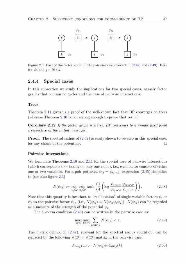
Chapter 2. Sufficient conditions for convergence of BP 47
k
k ψk
ψki
ki i
i ψi
ψij
ij j
j ψj
Figure 2.3: Part of the factor graph in the pairwise case relevant in (2.48) and (2.49). Here
k ∈ ∂i and j ∈ ∂i \ k.
2.4.4 Special cases
In this subsection we study the implications for two special cases, namely factorgraphs that contain no cycles and the case of pairwise interactions.
Trees
Theorem 2.11 gives us a proof of the well-known fact that BP converges on trees(whereas Theorem 2.10 is not strong enough to prove that result):
Corollary 2.12 If the factor graph is a tree, BP converges to a unique fixed pointirrespective of the initial messages.
Proof. The spectral radius of (2.47) is easily shown to be zero in this special case,for any choice of the potentials.
Pairwise interactions
We formulate Theorems 2.10 and 2.11 for the special case of pairwise interactions(which corresponds to γ taking on only one value), i.e., each factor consists of eitherone or two variables. For a pair potential ψij = ψij;αβ , expression (2.45) simplifiesto (see also figure 2.3)
N(ψij) := supα6=α′
supβ 6=β′
tanh(
14
(log
ψij;αβψij;α′β
ψij;α′β′
ψij;αβ′
)). (2.48)
Note that this quantity is invariant to “reallocation” of single-variable factors ψi orψj to the pairwise factor ψij (i.e., N(ψij) = N(ψijψiψj)). N(ψij) can be regardedas a measure of the strength of the potential ψij .
The `1-norm condition (2.46) can be written in the pairwise case as:
maxi∈V
maxk∈∂i
∑j∈∂i\k
N(ψij) < 1. (2.49)
The matrix defined in (2.47), relevant for the spectral radius condition, can bereplaced by the following #(D)×#(D) matrix in the pairwise case:
Ai→j,k→l := N(ψij)δil1∂i\j(k). (2.50)

48 Chapter 2
For the binary case, we reobtain our earlier results, since
N(
exp(Jijxixj))
= tanh |Jij | .
2.4.5 Factors containing zeros
Until now, we have assumed that all factors are strictly positive. In many interestingapplications of Belief Propagation, this assumption is violated: the factors mayassume the value zero. It is thus interesting to see if and how our results can beextended towards this more general case.
The easiest way to extend the results is by assuming that—although the factorsmay contain zeros—the messages are guaranteed to remain strictly positive (i.e., thelog-messages remain finite) after each update.8 Even more general extensions withmilder conditions may exist, but we believe that considerably more work would berequired to overcome the technical problems that arise due to messages containingzeros.
Assume that each factor ψI is a nonnegative function ψI : XNI → [0,∞). Inaddition, assume that all factors involving only a single variable are strictly positive.This can be assumed without loss of generality, since the single-variable factorsthat contain one or more zeros can simply be absorbed into multi-variable factorsinvolving the same variable. Additionally, for each I ∈ F for which NI containsmore than one variable, assume that
∀i∈NI ∀xi∈Xi∃xNI\i∈XNI\i : ψI(xi, xNI\i) > 0. (2.51)
These conditions guarantee that strictly positive messages remain strictly positiveunder the update equations (2.4), as one easily checks, implying that we can stilluse the logarithmic parameterization of the messages and that the derivative (2.36)is still well-defined.
The expression for the potential strength (2.45) can be written in a way that isalso well-defined if the potential ψI contains zeros:
N(ψI , i, j) := supα6=α′
supβ 6=β′
supγ,γ′
√ψI;αβγψI;α′β′γ′ −
√ψI;α′βγψI;αβ′γ′√
ψI;αβγψI;α′β′γ′ +√ψI;α′βγψI;αβ′γ′
(2.52)
which is defined for i, j ∈ NI with i 6= j and where ψI;αβγ is shorthand for ψI(xi =α, xj = β, xNI\i,j = γ).
The immediate generalization of Theorem 2.11 is then as follows:
Theorem 2.13 Under the assumptions on the potentials described above (strictpositivity of single-variable factors and (2.51) for the other factors): if the spectralradius of the matrix
AI→i,J→j = 1Nj\I(J)1NI\i(j)N(ψI , i, j), (2.53)
8Additionally, the initial messages are required to be strictly positive, but this requirement is
easily met and is necessary for obtaining good BP results.

Chapter 2. Sufficient conditions for convergence of BP 49
(with N(ψI , i, j) defined in (2.52)) is strictly smaller than 1, BP converges to aunique fixed point irrespective of the initial messages.
Proof. Similar to the strictly positive case. The only slight subtlety occurs inAppendix 2.B where one has to take a limit of strictly positive factors convergingto the desired nonnegative factor and use the continuity of the relevant expressionswith respect to the factor entries to prove that the bound also holds in this limit.
This theorem is the main result of this work; all other convergence and uniquenesstheorems derived earlier, apart from Corollary 2.9, are implied by Theorem 2.13.
Example
Define, for ε ≥ 0, the (“ferromagnetic”) pairwise factor ψ(ε) by the following matrix:
ψ(ε) :=(
1 ε
ε 1
).
Now consider a binary pairwise factor graph, consisting of a single loop of N binaryvariables, i.e., the network topology is that of a circle. Take for the N − 1 pairwiseinteractions ψi,i+1 (for i = 1, 2, . . . , N − 1) the identity matrices (i.e., the abovepairwise factors for ε = 0) and take for the remaining one ψ1,N = ψ(ε) for someε ≥ 0. Note that the potential strength N(ψ(ε)) = 1−ε
1+ε converges to 1 as ε ↓ 0. Thespectral radius of the corresponding matrix AI→i,J→j can be shown to be equal to
ρ(A) =(
1− ε1 + ε
)1/N
which is strictly smaller than 1 if and only if ε > 0. Hence BP converges to a uniquefixed point if ε > 0. This result is sharp, since for ε = 0, BP simply “rotates” themessages around without changing them and hence no convergence occurs (except,obviously, if the initial messages already correspond to the fixed point of uniformmessages).
2.5 Comparison with other work
In this section we explore the relations of our results with previously existing work.
2.5.1 Comparison with work of Tatikonda and Jordan
In [Tatikonda and Jordan, 2002; Tatikonda, 2003], a connection is made betweentwo seemingly different topics, namely Belief Propagation on the one hand and thetheory of Gibbs measures [Georgii, 1988] on the other hand. The main result of[Tatikonda and Jordan, 2002] states that BP converges uniformly (to a unique fixed

50 Chapter 2
point) if the Gibbs measure on the corresponding computation tree is unique. Thecomputation tree is an “unwrapping” of the factor graph with respect to the BeliefPropagation algorithm; specifically, the computation tree starting at variable i ∈ Vconsists of all paths starting at i that never backtrack.
This is a remarkable and beautiful result; however, the question of convergenceof BP is replaced by the question of uniqueness of the Gibbs measure, which is nottrivial. Fortunately, sufficient conditions for the uniqueness of the Gibbs measureexist; the most well-known are Dobrushin’s condition and a weaker (but more easilyverifiable) condition known as Simon’s condition. In combination with the mainresult of [Tatikonda and Jordan, 2002], they yield directly testable sufficient con-ditions for convergence of BP to a unique fixed point. For reference, we will stateboth results in our notation below. For details, see [Tatikonda and Jordan, 2002;Tatikonda, 2003] and [Georgii, 1988]. Note that the results are valid for the case ofpositive factors depending on at most two variables.
BP convergence via Dobrushin’s condition
Define Dobrushin’s interdependence matrix as the N ×N matrix C with entries
Cij := supx∂i\j∈X∂i\j
supxj ,x′j∈Xj
12
∑xi∈Xi
∣∣P(xi |x∂i\j , xj)− P(xi |x∂i\j , x′j)∣∣ (2.54)
for j ∈ ∂i and 0 otherwise.
Theorem 2.14 For pairwise, positive factors, BP converges to a unique fixed pointif
maxi∈V
∑j∈∂i
Cij < 1.
Proof. For a proof sketch, see [Tatikonda, 2003]. For the proof of Dobrushin’scondition see [Georgii, 1988, Chapter 8].
We can rewrite the conditional probabilities in terms of factors:
P(xi |x∂i\j , xj) =ψi(xi)ψij(xi, xj)
∏k∈∂i\j ψik(xi, xk)∑
xiψi(xi)ψij(xi, xj)
∏k∈∂i\j ψik(xi, xk)
.
Note that the complexity of the calculation of this quantity is generally exponentialin the size of the neighborhood ∂i, which may prohibit practical application ofDobrushin’s condition.
For the case of binary ±1-valued variables, some elementary algebraic manipu-lations yield
Cij = supx∂i\j
sinh 2 |Jij |cosh 2Jij + cosh 2
(θi +
∑k∈∂i\j xkJik
)=
tanh(|Jij | −Hij) + tanh(|Jij |+Hij)2

Chapter 2. Sufficient conditions for convergence of BP 51
with
Hij := infx∂i\j
∣∣∣∣∣∣θi +∑
k∈∂i\jxkJik
∣∣∣∣∣∣ .BP convergence via Simon’s condition
Simon’s condition is a sufficient condition for Dobrushin’s condition (see [Georgii,1988, Proposition 8.8]). This leads to a looser, but more easily verifiable, bound:
Theorem 2.15 For pairwise, positive factors, BP converges to a unique fixed pointif
maxi∈V
∑j∈∂i
(12
supα,α′
supβ,β′
logψij;αβψij;α′β′
)< 1.
It is not difficult to show that this bound is less tight than (2.49). Furthermore,unlike Dobrushin’s condition and Corollary 2.9, it does not take into account single-variable factors.
2.5.2 Comparison with work of Ihler et al.
In the recent and independent work of Ihler et al. [2005b], a methodology was usedwhich is very similar to the one used in this work. In particular, the same local `∞quotient metric is used to derive sufficient conditions for BP to be a contraction. Inthe work presented here, the Mean Value Theorem (in the form of Lemma 2.2) isused in combination with a bound on the derivative in order to obtain a bound on theconvergence rate K in (2.8). In contrast, in [Ihler et al., 2005b] a direct bound on thedistance of two outgoing messages is derived in terms of the distance of two differentproducts of incoming messages [Ihler et al., 2005b, Equation (13)]. This boundbecomes relatively stronger as the distance of the products of incoming messagesincreases. This has the advantage that it can lead to stronger conclusions aboutthe effect of finite message perturbations than would be possible with our bound,based on the Mean Value Theorem. However, for the question of convergence, therelevant limit turns out to be that of infinitesimal message perturbations, i.e., itsuffices to study the derivative of the BP updates as we have done here.
In the limit of infinitesimal message perturbations, the basic bound (13) in [Ihleret al., 2005b] leads to the following measure of potential strength:
D(ψij) := tanh
(12
(supα,α′
supβ,β′
logψij;αβψij;α′β′
)).
Using this measure, Ihler et. al derive two different conditions for convergence ofBP. The first one is similar to our (2.49) and the second condition is equivalentto our spectral radius result (2.50), except that in both conditions, D(ψij) is usedinstead of N(ψij). The latter condition is formulated in [Ihler et al., 2005b] in terms

52 Chapter 2
of the convergence properties of an iterative BP-like algorithm. The equivalence ofthis formulation with a formulation in terms of the spectral radius of a matrixcan be seen from the fact that for any square matrix A, ρ(A) < 1 if and onlyif limn→∞An = 0. However, our result also gives a contraction rate, unlike theiterative formulation in [Ihler et al., 2005b].
Thus, the results in [Ihler et al., 2005b] are similar to ours in the pairwise case,except for the occurrence of D(ψij) instead of N(ψij). It is not difficult to see thatN(ψij) ≤ D(ψij) for any pairwise factor ψij ; indeed, for any choice of α, β, γ, δ:√
ψij;αγψij;βδ
/√ψij;βγψij;αδ ≤
(supστ
ψij;στ
)/(infστψij;στ
).
Thus the convergence results in [Ihler et al., 2005b] are similar to, but weaker thanthe results derived in the present work.
After initial submission of this work, [Ihler et al., 2005a] was published, whichimproves upon [Ihler et al., 2005b] by exploiting the freedom of choice of the single-variable factors (which can be “absorbed” to an arbitrary amount by correspondingpairwise factors). This leads to an improved measure of potential strength, whichturns out to be identical to our measure N(ψij). Thus, for pairwise, strictly positivepotentials, the results in [Ihler et al., 2005a] are equivalent to the results (2.49) and(2.50) presented here. Our most general results, Theorems 2.10, 2.11 and 2.13 andCorollary 2.9, are not present in [Ihler et al., 2005a].
2.5.3 Comparison with work of Heskes
A completely different methodology to obtain sufficient conditions for the unique-ness of the BP fixed point is used in [Heskes, 2004]. By studying the Bethe freeenergy and exploiting the relationship between properties of the Bethe free energyand the BP algorithm, conclusions are drawn about the uniqueness of the BP fixedpoint; however, whether uniqueness of the fixed point also implies convergence ofBP seems to be an open question. We state the main result of [Heskes, 2004] in ournotation below.
The following measure of potential strength is used in [Heskes, 2004]. For I ∈ F ,let
ωI := supxNI
supx′NI
(logψI(xNI ) + (#(NI)− 1) logψI(x′NI )−
∑i∈NI
logψI(x′NI\i, xi)).
The potential strength is then defined as σI := 1− e−ωI .
Theorem 2.16 BP has a unique fixed point if there exists an “allocation matrix”XIi between factors I ∈ F and variables i ∈ V such that
1. XIi ≥ 0 ∀I ∈ F ,∀i ∈ NI ;
2. (1− σI) maxi∈NI
XIi + σI∑i∈NI
XIi ≤ 1 ∀I ∈ F ;

Chapter 2. Sufficient conditions for convergence of BP 53
3.∑I∈Ni
XIi ≥ #(Ni)− 1 ∀i ∈ V.
Proof. See [Heskes, 2004, Theorem 8.1].
The (non-)existence of such a matrix can be determined using standard linear pro-gramming techniques.
2.6 Numerical comparison of various bounds
In this subsection, we compare various bounds on binary pairwise graphical models,defined in (2.5), for various choices of the parameters. First we study the case ofa completely uniform model (i.e., full connectivity, uniform couplings and uniformlocal fields). Then we study nonuniform couplings Jij , in the absence of local fields.Finally, we take fully random models in various parameter regimes (weak/stronglocal fields, strong/weak ferromagnetic/spin-glass/antiferromagnetic couplings).
2.6.1 Uniform couplings, uniform local field
The fully connected Ising model consisting of N binary ±1-valued variables withuniform couplings J and uniform local field θ is special in the sense that an exactdescription of the parameter region for which the Gibbs measure on the compu-tation tree is unique is available. Using the results of Tatikonda and Jordan, thisyields a strong bound on the parameter region for which BP converges to a uniquefixed point. Indeed, the corresponding computation tree is a uniform Ising modelon a Cayley tree of degree N − 2, for which (semi-)analytical expressions for theparamagnetic–ferromagnetic and paramagnetic–antiferromagnetic phase-transitionboundaries are known (see [Georgii, 1988, Section 12.2]). Since the Gibbs measureis known to be unique in the paramagnetic phase, this gives an exact descriptionof the (J, θ) region for which the Gibbs measure on the computation tree is unique,and hence a bound on BP convergence on the original model.
In figure 2.4 we have plotted various bounds on BP convergence in the (J, θ)plane for N = 4 (other values of N yield qualitatively similar results). The grayarea (g) marks regions where the Gibbs measure on the computation tree is notunique; in the white area, the Gibbs measure is unique and hence BP is guaranteedto converge. Note that this bound is only available due to the high symmetry of themodel. In [Taga and Mase, 2006b] it is shown that parallel BP does not convergein the lower (antiferromagnetic) gray region. In the upper (ferromagnetic) regionon the other hand, parallel BP does converge, but it may be that the fixed point isno longer unique.
The various lines correspond to different sufficient conditions for BP convergence;the regions enclosed by two lines of the same type (i.e., the inner regions for which|J | is small) mark the regions of guaranteed convergence. The lightly dotted lines
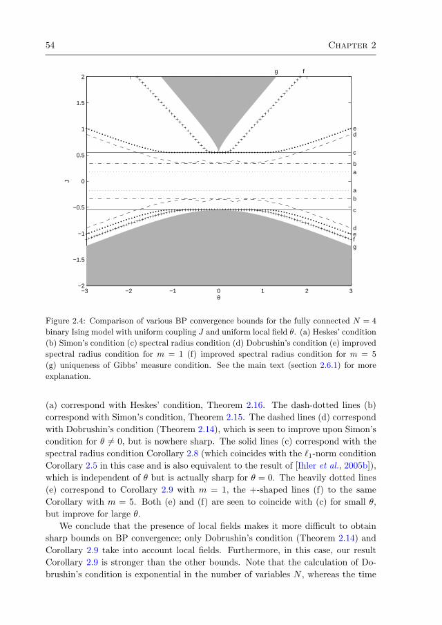
54 Chapter 2
−3 −2 −1 0 1 2 3−2
−1.5
−1
−0.5
0
0.5
1
1.5
2
θ
J
ab
c
de
f
ab
c
def
g
g
Figure 2.4: Comparison of various BP convergence bounds for the fully connected N = 4
binary Ising model with uniform coupling J and uniform local field θ. (a) Heskes’ condition
(b) Simon’s condition (c) spectral radius condition (d) Dobrushin’s condition (e) improved
spectral radius condition for m = 1 (f) improved spectral radius condition for m = 5
(g) uniqueness of Gibbs’ measure condition. See the main text (section 2.6.1) for more
explanation.
(a) correspond with Heskes’ condition, Theorem 2.16. The dash-dotted lines (b)correspond with Simon’s condition, Theorem 2.15. The dashed lines (d) correspondwith Dobrushin’s condition (Theorem 2.14), which is seen to improve upon Simon’scondition for θ 6= 0, but is nowhere sharp. The solid lines (c) correspond with thespectral radius condition Corollary 2.8 (which coincides with the `1-norm conditionCorollary 2.5 in this case and is also equivalent to the result of [Ihler et al., 2005b]),which is independent of θ but is actually sharp for θ = 0. The heavily dotted lines(e) correspond to Corollary 2.9 with m = 1, the +-shaped lines (f) to the sameCorollary with m = 5. Both (e) and (f) are seen to coincide with (c) for small θ,but improve for large θ.
We conclude that the presence of local fields makes it more difficult to obtainsharp bounds on BP convergence; only Dobrushin’s condition (Theorem 2.14) andCorollary 2.9 take into account local fields. Furthermore, in this case, our resultCorollary 2.9 is stronger than the other bounds. Note that the calculation of Do-brushin’s condition is exponential in the number of variables N , whereas the time

Chapter 2. Sufficient conditions for convergence of BP 55
−0.5 −0.4 −0.3 −0.2 −0.1 0 0.1 0.2 0.3 0.4 0.50
0.1
0.2
0.3
0.4
0.5
0.6
0.7
0.8
0.9
1
e
d
c
b
a
J0
σ J
Figure 2.5: Comparison of various bounds for BP convergence for toroidal Ising model of
size 10 × 10 with normally distributed couplings Jij ∼ N`J0, σJ
2´
and zero local fields.
(a) Heskes’ condition (b) Dobrushin’s condition (c) `1-norm condition (d) spectral radius
condition (e) empirical convergence boundary. See the main text (section 2.6.2) for more
explanation.
complexity of our bound is polynomial in N . Similar results are obtained for highervalues of N .
2.6.2 Nonuniform couplings, zero local fields
We have investigated in more detail the influence of the distribution of the cou-plings Jij , in the absence of local fields, and have also compared with the empiricalconvergence behavior of BP. We have taken a binary Ising model on a rectangulartoroidal grid (i.e., with periodic boundary conditions) of size 10 × 10. The cou-plings were random independent normally distributed nearest-neighbor couplingsJij ∼ N
(J0, σJ
2), the local fields were θi = 0. Let (rJ , φJ) be the polar coor-
dinates corresponding to the Cartesian coordinates (J0, σJ). For various anglesφJ ∈ [0, π], we have determined the critical radius rJ for each bound. The resultshave been averaged over 40 instances of the model and can be found in figure 2.5.The lines correspond to the mean bounds, the gray areas are “error bars” of onestandard deviation. The inner area (for which the couplings are small) boundedby each line means “convergence”, either guaranteed or empirical (thus the larger

56 Chapter 2
the enclosed area, the tighter the bound). From bottom to top: the thin solid line(a) corresponds with Heskes’ result (Theorem 2.16), the dash-dotted line (b) withDobrushin’s condition (Theorem 2.14), the dotted line (c) corresponds with the `1-norm condition Corollary 2.5, the dashed line (d) with the spectral radius conditionCorollary 2.8 and the thick solid line (e) with the empirical convergence behaviorof BP.
We conclude from figure 2.5 that the spectral radius condition improves uponthe `1-norm condition for nonuniform couplings and that the improvement can bequite substantial. For uniform couplings (and zero local fields), both conditionscoincide and it can be proved that they are sharp [Mooij and Kappen, 2005a].
2.6.3 Fully random models
Finally, we have considered fully connected binary pairwise graphical models withcompletely random couplings and local fields (in various parameter regimes). Wedrew random couplings and local fields as follows: first, we drew i.i.d. randomparameters J0, σJ , θ0, σθ from a normal distribution with mean 0 and variance1. Then, for each variable i we independently drew a local field parameter θi ∼N (θ0, σθ
2), and for each pair i, j we independently drew a coupling parameter
Jij ∼ N(J0, σJ
2).
For the resulting graphical model, we have verified whether various sufficientconditions for BP convergence hold. If condition A holds whereas condition B doesnot hold, we say that A wins from B. We have counted for each ordered pair (A,B)of conditions how often A wins from B. The results (for 50000 random modelsconsisting of N = 4, 8 variables) can be found in table 2.1: the number at rowA, column B is the number of trials for which bound A wins from bound B. Onthe diagonal (A = B) is the total number of trials for which bound A predictsconvergence. Theorem 2.14 is due to [Tatikonda, 2003], Corollary 2.8 was firstpublished (for the binary case) in [Ihler et al., 2005b] and Theorem 2.16 is due to[Heskes, 2004].
Our result Corollary 2.9 (for m = 1) outperforms the other bounds in each trial.For other values of N , we obtain similar results.
2.7 Discussion
In this paper we have derived sufficient conditions for convergence of BP to a uniquefixed point. Our conditions are directly applicable to arbitrary factor graphs withdiscrete variables and nonnegative factors. This is in contrast with the sufficientconditions of Tatikonda and Jordan and with the results of Ihler, Fisher and Willsky,which were only formulated for pairwise, positive factors. We have shown caseswhere our results are stronger than previously known sufficient conditions.
Our numerical experiments lead us to conjecture that Corollary 2.9 is strongerthan the other bounds. We have no proof for this conjecture at the moment, apart
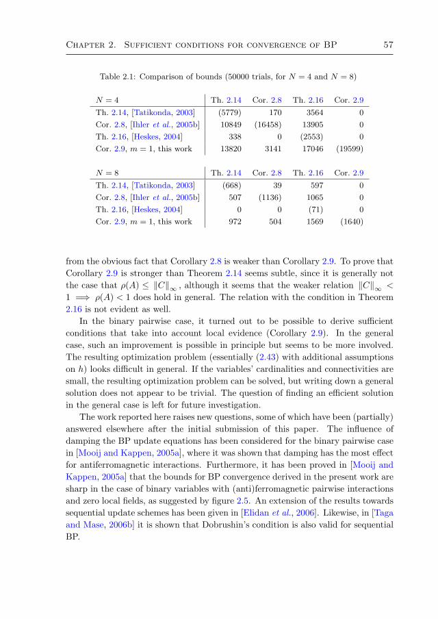
Chapter 2. Sufficient conditions for convergence of BP 57
Table 2.1: Comparison of bounds (50000 trials, for N = 4 and N = 8)
N = 4 Th. 2.14 Cor. 2.8 Th. 2.16 Cor. 2.9
Th. 2.14, [Tatikonda, 2003] (5779) 170 3564 0
Cor. 2.8, [Ihler et al., 2005b] 10849 (16458) 13905 0
Th. 2.16, [Heskes, 2004] 338 0 (2553) 0
Cor. 2.9, m = 1, this work 13820 3141 17046 (19599)
N = 8 Th. 2.14 Cor. 2.8 Th. 2.16 Cor. 2.9
Th. 2.14, [Tatikonda, 2003] (668) 39 597 0
Cor. 2.8, [Ihler et al., 2005b] 507 (1136) 1065 0
Th. 2.16, [Heskes, 2004] 0 0 (71) 0
Cor. 2.9, m = 1, this work 972 504 1569 (1640)
from the obvious fact that Corollary 2.8 is weaker than Corollary 2.9. To prove thatCorollary 2.9 is stronger than Theorem 2.14 seems subtle, since it is generally notthe case that ρ(A) ≤ ‖C‖∞ , although it seems that the weaker relation ‖C‖∞ <
1 =⇒ ρ(A) < 1 does hold in general. The relation with the condition in Theorem2.16 is not evident as well.
In the binary pairwise case, it turned out to be possible to derive sufficientconditions that take into account local evidence (Corollary 2.9). In the generalcase, such an improvement is possible in principle but seems to be more involved.The resulting optimization problem (essentially (2.43) with additional assumptionson h) looks difficult in general. If the variables’ cardinalities and connectivities aresmall, the resulting optimization problem can be solved, but writing down a generalsolution does not appear to be trivial. The question of finding an efficient solutionin the general case is left for future investigation.
The work reported here raises new questions, some of which have been (partially)answered elsewhere after the initial submission of this paper. The influence ofdamping the BP update equations has been considered for the binary pairwise casein [Mooij and Kappen, 2005a], where it was shown that damping has the most effectfor antiferromagnetic interactions. Furthermore, it has been proved in [Mooij andKappen, 2005a] that the bounds for BP convergence derived in the present work aresharp in the case of binary variables with (anti)ferromagnetic pairwise interactionsand zero local fields, as suggested by figure 2.5. An extension of the results towardssequential update schemes has been given in [Elidan et al., 2006]. Likewise, in [Tagaand Mase, 2006b] it is shown that Dobrushin’s condition is also valid for sequentialBP.

58 Chapter 2
Acknowledgments
We thank Martijn Leisink for stimulating discussions and the reviewers for theircritique, which has led to a considerable improvement of the initial manuscript.
2.A Generalizing the `1-norm
Let (Vi, ‖·‖i ) be a finite collection of normed vector spaces and let V =⊕
i Vi bethe direct sum of the Vi. The function ‖·‖ : V → R defined by
‖v‖ :=∑i
‖vi‖i (2.55)
is a norm on V , as one easily checks. Let A : V → V be a linear mapping with“blocks” Aij : Vj → Vi defined by
∀vj ∈ Vj : Avj =∑i
Aijvj , Aijvj ∈ Vi
for all j.
Theorem 2.17 The matrix norm of A induced by the vector norm ‖·‖ is given by:
‖A‖ = maxj
∑i
‖Aij‖ji (2.56)
where‖Aij‖ji := sup
v∈Vj ,‖v‖j ≤1
‖Aijv‖i .
Proof. Let vk ∈ Vk such that ‖vk‖k = 1. Then
‖Avk‖ =
∥∥∥∥∥∑i
Aikvk
∥∥∥∥∥ =∑i
‖Aikvk‖i ≤∑i
‖Aik‖ki ≤ maxj
∑i
‖Aij‖ji .
Now let v ∈ V such that ‖v‖ = 1. Then v can be written as the convex combinationv =
∑k ‖vk‖k vk, where
vk :=
vk‖vk‖k if vk 6= 0
0 if vk = 0.
Hence:
‖Av‖ =
∥∥∥∥∥∑k
‖vk‖k Avk∥∥∥∥∥ ≤∑
k
‖vk‖k ‖Avk‖ ≤ maxj
∑i
‖Aij‖ji .
It is evident that this value is also achieved for some v ∈ V with ‖v‖ = 1.
Chapter 2. Sufficient conditions for convergence of BP 59
An illustrative example is obtained by considering V = RN to be the direct sumof N copies of R with the absolute value as norm; then the norm (2.55) on RN issimply the `1-norm and the induced matrix norm (2.56) reduces to (2.9).
Suppose that each Vi has a linear subspace Wi. We can consider the quotientspaces Vi/Wi with quotient norms ‖·‖i . The direct sum W :=
⊕iWi is itself a
subspace of V , yielding a quotient space V/W . For v ∈ V we have v =∑i vi and
hence V/W =⊕
i(Vi/Wi). The quotient norm on V/W is simply the sum of thequotient norms on the Vi/Wi:
‖v‖ := infw∈W
‖v + w‖ = infw∈W
∑i
‖vi + wi‖i
=∑i
infwi∈Wi
‖vi + wi‖i =∑i
‖vi‖i .(2.57)
Let A : V → V be a linear mapping such that AW ⊆ W . Then A induces alinear A : V/W → V/W ; since AijWj ⊆ Wi, each block Aij : Vj → Vi induces alinear Aij : Vj/Wj → Vi/Wi, and A can be regarded as consisting of the blocks Aij .
Corollary 2.18 The matrix norm of A : V/W → V/W induced by the quotientnorm ‖·‖ on V/W is: ∥∥A∥∥ = max
j
∑i
∥∥Aij∥∥ji (2.58)
where ∥∥Aij∥∥ji = supv∈Vj ,‖v‖j ≤1
∥∥Aijv∥∥i . (2.59)
Proof. We can directly apply the previous Theorem to the quotient spaces toobtain (2.58); because
v ∈ Vj/Wj : ‖v‖j ≤ 1 = v ∈ Vj : ‖v‖j ≤ 1,
we have: ∥∥Aij∥∥ji := supv∈Vj/Wj
‖v‖j ≤1
∥∥Aijv∥∥i = supv∈Vj‖v‖j ≤1
∥∥Aijv∥∥i .
For a linear A : V → V such that AW ⊆ W , we define the matrix |A| withentries |A|ij :=
∥∥Aij∥∥ji . Let A,B be two such linear mappings; then
|AB|ij =∥∥∥(AB)ij
∥∥∥ji
=
∥∥∥∥∥∑k
AikBkj
∥∥∥∥∥j
i
≤∑k
∥∥AikBkj∥∥ji≤∑k
∥∥Aik∥∥ki ∥∥Bkj∥∥jk =∑k
|A|ik |B|kj
hence |AB| ≤ |A| |B|. Note that ‖|A|‖1 =∥∥A∥∥ . We can generalize Theorem 2.7
as follows:
60 Chapter 2
Theorem 2.19 Let f : V → V be differentiable and suppose that it satisfies (2.30).Suppose further that |f ′(v)| ≤ A for some matrix Aij (which does not depend on v)with ρ(A) < 1. Then for any v ∈ V/W , the sequence v, f(v), f
2(v), . . . obtained by
iterating f converges to a unique fixed point v∞.
Proof. Using the chain rule, we have for any n ∈ N∗ and any v ∈ V :
∥∥∥(fn)′(v)
∥∥∥ =∥∥∥(fn)′(v)
∥∥∥ =
∥∥∥∥∥n∏i=1
f ′(f i−1(v)
)∥∥∥∥∥ =
∥∥∥∥∥∣∣∣∣∣n∏i=1
f ′(f i−1(v)
)∣∣∣∣∣∥∥∥∥∥
1
≤∥∥∥∥∥n∏i=1
∣∣f ′(f i−1(v))∣∣∥∥∥∥∥
1
≤ ‖An‖1 .
By the Gelfand Spectral Radius Theorem,( ‖An‖1 )1/n → ρ(A) for n→∞. Choose
ε > 0 such that ρ(A) + ε < 1. For some N ,∥∥AN∥∥
1≤ (ρ(A) + ε)N < 1. Hence∥∥∥(fN)′(v)
∥∥∥ < 1 for all v ∈ V/W . By Lemma 2.3, fN
is a contraction with respectto the quotient norm on V/W . Now apply Lemma 2.6.
2.B Proof that (2.43) equals (2.44)
Let ψβγ be a matrix of positive numbers. Let
H := h : hβγ ≥ 0,∑β
∑γ
hβγ = 1.
Define the function g : H → R by
g(h) =∑β
∣∣∣∣∣∑γ
hβγ
(ψβγ∑
β
∑γ ψβγhβγ
− 1
)∣∣∣∣∣ .Theorem 2.20
suph∈H
g(h) = 2 supβ 6=β′
supγ,γ′
tanh(
14
logψβγψβ′γ′
).
Proof. First note that we can assume without loss of generality that all ψβγ aredifferent, because of continuity. Define
ψ− := infβγψβγ , ψ+ := sup
βγψβγ ,
Ψ := [ψ−, ψ+], Ψ′ := Ψ \ ψβγ : β, γ.
For φ ∈ Ψ, defineHφ := h ∈ H :
∑β,γ
ψβγhβγ = φ,

Chapter 2. Sufficient conditions for convergence of BP 61
which is evidently a closed convex set. The function
gφ : Hφ → R : h 7→∑β
∣∣∣∣∣∑γ
hβγ
(ψβγφ− 1)∣∣∣∣∣
obtained by restricting g to Hφ is convex. Hence it achieves its maximum on anextremal point of its domain.
DefineH2 :=
h ∈ H : #(β, γ) : hβγ > 0 = 2
as those h ∈ H with exactly two nonzero components. For h ∈ H2, define ψ−(h) :=infψβγ : hβγ 6= 0 and ψ+(h) := supψβγ : hβγ 6= 0. Because of continuity,we can restrict ourselves to the φ ∈ Ψ′, in which case the extremal points of Hφare precisely H∗φ = Hφ ∩ H2 (i.e., the extremal points have exactly two nonzerocomponents).
Now
suph∈H
g(h) = supφ∈Ψ
suph∈Hφ
gφ(h) = supφ∈Ψ′
suph∈H∗φ
gφ(h)
= suph∈H2
supψ−(h)≤φ≤ψ+(h)
gφ(h) = suph∈H2
g(h).
For those h ∈ H2 with components with different β, we can use the Lemmabelow. The h ∈ H2 with components with equal β are suboptimal, since the twocontributions in the sum over γ in g(h) have opposite sign. Hence
suph∈H2
g(h) = 2 supβ 6=β′
supγ,γ′
tanh(
14
logψβγψβ′γ′
).
Lemma 2.21 Let 0 < a < b. Then
supη∈(0,1)2
η1+η2=1
η1
∣∣∣∣ a
η1a+ η2b− 1∣∣∣∣+ η2
∣∣∣∣ b
η1a+ η2b− 1∣∣∣∣
= 2 tanh(
14
logb
a
)= 2
√b−√a√b+√a.
Proof. Elementary. The easiest way to see this is to reparameterize
η =(
eν
2 cosh ν,
e−ν
2 cosh ν
)with ν ∈ (−∞,∞).

62 Chapter 2

Chapter 3. BP and phase transitions 63
Chapter 3
BP and phase transitions
We analyze the local stability of the high-temperature fixed point of the Belief
Propagation (BP) algorithm and how this relates to the properties of the Bethe free
energy which BP tries to minimize. We focus on the case of binary variables with
pairwise interactions. In particular, we state sufficient conditions for convergence
of BP to a unique fixed point and show that these are sharp for purely ferromag-
netic interactions. In contrast, in the purely antiferromagnetic case, the undamped
parallel BP algorithm is suboptimal in the sense that the stability of the fixed point
breaks down much earlier than for damped or sequential BP, and we observe that
the onset of instability for those BP variants is directly related to the properties of
the Bethe free energy. For spin-glass interactions, damping BP only helps slightly.
We estimate analytically the temperature at which the high-temperature BP fixed
point becomes unstable for random graphs with arbitrary degree distributions and
random interactions.
3.1 Introduction
Techniques that were originally developed in the statistical physics of lattice modelsare nowadays increasingly often and successfully applied in diverse application areassuch as information theory, coding theory, combinatorial optimization and machinelearning. A prominent example is the Bethe-Peierls approximation [Bethe, 1935;Peierls, 1936], an extension of the ordinary Mean Field method that takes intoaccount correlations between nearest-neighbor sites. A more general and powerfulapproximation scheme, which is also currently being used as a general inferencetool in applications in the aforementioned areas, is the Cluster Variation Method
This chapter is based on [Mooij and Kappen, 2005a] and earlier work reported in [Mooij and
Kappen, 2005c].
64 Chapter 3
(CVM) [Kikuchi, 1951; Pelizzola, 2005], also called Kikuchi approximation. TheCVM treats arbitrarily large clusters of sites exactly; the Bethe approximation canbe seen as the simplest nontrivial case (the pair approximation) of the ClusterVariation Method.
The problems arising in the aforementioned application domains can often bereformulated as inference problems on graphical models, i.e., as the calculation ofmarginal probabilities of some probability distribution. Typically, this probabilitydistribution is proportional to a product of many factors, each factor depending ononly a few variables; this structure can be expressed in terms of a graph, hence thename graphical model. An illustrative example can be found in image restoration[Tanaka, 2002], where the 2D classical Ising model can be used to model features ofmonochromatic images. The pixels in the image correspond to the Ising spins, thelocal external fields correspond to observed, noisy pixels and the probability distri-bution over different images corresponds to the equilibrium Boltzmann distributionof the Ising model. The underlying graph is in this example the 2D rectangularlattice, and the interactions between the nearest neighbors correspond to factors inthe probability distribution. By taking the interactions to be of the ferromagnetictype, one can obtain a smoothing filter.
In statistical physics, one is predominantly interested in the thermodynamiclimit of infinitely large systems, and furthermore, in the case of disordered sys-tems, one usually averages over a whole ensemble of such systems. In contrast, inthe applications in computer science the primary interest lies in the properties ofindividual, finite systems—in the example above, one would be interested in in-dividual images. Given the probability distribution, the task is then to calculatemarginal probabilities, which in principle amounts to performing a summation or in-tegral. Unfortunately, the required computation time is generally exponential in thenumber of variables, and the calculation quickly becomes infeasible for real-worldapplications.
Therefore, one is often forced to use approximative methods, such as MonteCarlo methods or “deterministic approximations”. A prominent example of thelatter category is the successful Belief Propagation algorithm [Pearl, 1988], whichwas originally developed as a fast algorithm to calculate probabilities on graphicalmodels without loops (i.e., on trees), for which the results are exact. The same algo-rithm can also be applied on graphs that contain loops, in which case the results areapproximate, and it is then often called Loopy Belief Propagation (LBP) to empha-size the fact that the graph may contain loops. The results can be surprisingly good,even for small graphs with many short loops, e.g., in the case of decoding error-correcting codes [McEliece et al., 1998; Nishimori, 2001]. An important discoverywas that the BP algorithm in fact tries to minimize the Bethe free energy (moreprecisely, fixed points of the BP algorithm correspond to stationary points of theBethe free energy) [Yedidia et al., 2001]. This discovery has lead to renewed interestin the Bethe approximation and related methods and to cross-fertilization betweendisciplines, a rather spectacular example of which is the Survey Propagation (SP)

Chapter 3. BP and phase transitions 65
algorithm, which is now the state-of-the-art solution method for some difficult com-binatorial optimization problems [Braunstein and Zecchina, 2004]. Other examplesare the generalizations of BP obtained by replacing the Bethe free energy by themore complicated Kikuchi free energy, which has resulted in algorithms that aremuch faster than the NIM algorithm developed originally by Kikuchi [Pelizzola,2005].
This chapter is organized as follows. We start in section 3.2 with a brief review ofthe Bethe approximation and the Belief Propagation algorithm, trying to combinethe two different points of view, namely the statistical physicist’s perspective andthe one found in machine learning and computer science. A notorious problemplaguing applications of BP is the fact that it does not always converge to a fixedpoint. With the aim of better understanding these convergence issues, in section3.3 we discuss the local stability of BP fixed points, state “global” conditions forconvergence towards a unique fixed point, and discuss the stability of the high-temperature Bethe free energy minimum. In section 3.4, we discuss qualitativelyhow these properties are related and connect them with phase transitions in thethermodynamic limit. In section 3.5, we quantify the results of the previous sectionby estimating the phase-transition temperatures for random graphs with randominteractions.
This chapter is written primarily for statistical physicists, but we tried to makeit also understandable for readers with a background in computer science, whichmay explain some seemingly redundant remarks.
3.2 The Bethe approximation and the BP algo-
rithm
3.2.1 The graphical model
Let G = (V, E) be an undirected labeled graph without self-connections, defined bya set of vertices V = 1, . . . , N and a set of undirected edges E ⊆ i, j : 1 ≤i < j ≤ N
. The adjacency matrix M corresponding to G is defined as follows:
Mij = 1 if i, j ∈ E and 0 otherwise. Denote by ∂i the set of neighbors of vertexi, and the degree (connectivity) of vertex i by di := #(∂i) =
∑j∈VMij .
To each vertex i ∈ V we associate a random variable xi (called a “spin”), takingvalues in −1,+1. We put weights Jij on the edges i, j: let J be a real symmetricN × N matrix that is compatible with the adjacency matrix M , i.e., Jij = 0 ifMij = 0. Let θ ∈ RN be local “fields” (local “evidence”) acting on the vertices. Wewill study the Boltzmann distribution corresponding to the Hamiltonian
H = −∑i,j∈E
Jijxixj −∑i∈V
θixi = −12
∑i,j∈V
Jijxixj −∑i∈V
θixi, (3.1)
66 Chapter 3
i.e., the probability of the configuration x = (x1, . . . , xN ) ∈ −1,+1N is given by:
P(x) =1Z
exp
β ∑i,j∈E
Jijxixj + β∑i∈V
θixi
(3.2)
with β > 0 the inverse temperature and Z a normalization constant. The problemthat we would like to solve is calculating the first and second moments E (xi) andE (xixj) under this distribution. In general, this is an NP-hard problem [Cooper,1990], so in practice we often have to settle for approximations of these quantities.
The general model class that we have described above has been the subject ofnumerous investigations in statistical physics. There one often takes a lattice as theunderlying graph G, or studies an ensemble of random graphs (including the fully-connected SK model as a special case). The weights Jij and the local fields θi areoften taken to be i.i.d. according to some probability distribution (a special case iswhere this probability distribution is a delta function—this corresponds to uniform,deterministic interactions). In these cases one can take the thermodynamic limitN →∞, which is the subject of investigation of the major part of statistical physicsstudies (except for the studies of “finite-size effects”). Depending on these weightdistributions and on the graph structure, macroscopic order parameters can beidentified that distinguish between different phases, e.g., the ferromagnetic phasefor large positive weights or a spin-glass phase for weights that are distributedaround zero.
The probability distribution (3.2) is a special case of the class of probabilitydistributions over N discrete random variables (xi)Ni=1, with xi taking values insome finite set Xi, that factorize as a product of factors (often called “potentials”in computer science literature—not to be confused with the potentials in statisticalphysics, which are essentially the logarithms of the factors) in the following way:
P(x) =1Z
∏i,j∈E
ψij(xi, xj)∏i∈V
ψi(xi) (3.3)
with Z the normalization constant. These probability distributions are known inmachine learning as undirected graphical models (in this case consisting of N nodeswith pairwise potentials) or as Markov random fields. In fact, it is easy to seethat (3.2) is equivalent to (3.3) when all variables are binary (and the factors arepositive); in this case, equation (3.2) can obviously be written in the form of (3.3),but the converse also holds. In contrast with statistical physics studies, the numberof variables is usually finite and one is interested in a single instance instead of theproperties of an ensemble of instances.
In the following three subsections, we describe the BP algorithm and the Betheapproximation for the graphical model (3.3), and what is known about the relationbetween the two.
Chapter 3. BP and phase transitions 67
3.2.2 Bethe approximation
The calculation of properties such as marginals P(xi) of the probability distribution(3.2) is an NP-hard problem [Cooper, 1990]. Only in cases with high symmetry (e.g.,when all weights are equal and the field is uniform, i.e., Jij = J and θi = θ, andthe graph has a high permutation symmetry, such as translation symmetry in caseof a 2D rectangular lattice), or if N is small, or if the graph contains no cycles, it ispossible to calculate marginals exactly. In other cases, one has to use approximatemethods, such as Monte Carlo methods or “deterministic” approximation methods,the simplest of which is the well-known Mean Field method. An extension of theMean Field method that treats pairs of neighboring spins exactly is the Betheapproximation, also known as the Bethe-Peierls approximation [Bethe, 1935; Peierls,1936].
The Bethe approximation consists of minimizing the Bethe free energy, which forthe factorizing probability distribution (3.3) is defined as the following functional[Yedidia et al., 2001]:
FBethe((bi)i∈V , (bij)i,j∈E
)=
∑i,j∈E
∑xi,xj
bij(xi, xj) logbij(xi, xj)
ψij(xi, xj)ψi(xi)ψj(xj)
−∑i∈V
(di − 1)∑xi
bi(xi) logbi(xi)ψi(xi)
.
(3.4)
Its arguments, called beliefs, are single-node (pseudo)marginals bi(xi) and pairwise(pseudo)marginals bij(xi, xj). The Bethe approximation is obtained by minimizingthe Bethe free energy (3.4) with respect to the beliefs under the following nonneg-ativity, normalization and consistency constraints:
bi(xi) ≥ 0 ∀xi ∈ Xi (3.5a)
bij(xi, xj) ≥ 0 ∀xi ∈ Xi, ∀xj ∈ Xj (3.5b)∑xi
bi(xi) = 1 (3.5c)∑xi
bij(xi, xj) = bj(xj) (3.5d)
for all i ∈ V, j ∈ ∂i. The beliefs that minimize FBethe under these constraints arethen taken as approximations for the marginal distributions P(xi) and P(xi, xj).The beliefs are the exact marginals if the underlying graph G contains no cycles[Baxter, 1982]. Note that the local consistency constraints do not imply globalconsistency of the beliefs in general, i.e., there does not always exist a probabilitydistribution b(x1, . . . , xN ) such that the beliefs are marginals of b.
The rationale for minimizing the Bethe free energy is that the Bethe free energyis an approximate Gibbs free energy with an exact energy term and an approximateentropy term (the entropy is approximated by a combination of single-node and

68 Chapter 3
pairwise entropies). Minimizing the exact Gibbs free energy would recover theexact marginal distributions P(xi) and P(xi, xj), but this is infeasible in general;minimizing its approximation, the Bethe free energy, gives approximations bi(xi)and bij(xi, xj) to the exact marginal distributions.
3.2.3 BP algorithm
A popular and efficient algorithm for obtaining the Bethe approximation is BeliefPropagation (BP), also known under the names Sum-Product Algorithm [Kschis-chang et al., 2001] and Loopy Belief Propagation [Pearl, 1988]. The adjective“loopy” is used to emphasize the fact that the graph may contain cycles, in whichcase the beliefs are usually only approximations of the exact marginals.
The BP algorithm consists of the iterative updating of a family of messages(µi→j)i,j∈E . The new message µ′i→j that vertex i sends to its neighbor j is givenin terms of all incoming messages by the following update rule [Yedidia et al., 2001]:1
µ′i→j(xj) ∝∑xi
ψij(xi, xj)ψi(xi)∏
k∈∂i\jµk→i(xi), (3.6)
where one usually normalizes messages such that∑xjµ′i→j(xj) = 1. The up-
date schedule can be chosen to be parallel (“flooding schedule”), sequential (“serialschedule”) or random; the update schedule influences convergence properties.
If the messages (µi→j)i,j∈E converge to some fixed point µ(∞), the approximatemarginal distributions (beliefs) (bi)i∈V and (bij)i,j∈E are calculated by:
bi(xi) ∝ ψi(xi)∏k∈∂i
µ(∞)k→i(xi), (3.7)
bij(xi, xj) ∝ ψij(xi, xj)ψi(xi)ψj(xj)∏
k∈∂i\jµ
(∞)k→i(xi)
∏k∈∂j\i
µ(∞)k→j(xj). (3.8)
Note that these beliefs satisfy the constraints (3.5).Unfortunately, BP does not always converge. It can get trapped in limit cycles,
or it can wander around chaotically, depending on the problem instance. This non-robust behavior hampers application of BP as a “black box” inference algorithm.Furthermore, there is some empirical evidence that if BP does not converge, thequality of the Bethe approximation (which can also be obtained by using double-loop algorithms [Heskes et al., 2003] that are guaranteed to converge, but are slowerthan BP) is low. The analysis that we will perform in subsequent sections shouldbe seen as first steps in obtaining a better understanding of these issues.
3.2.4 The connection between BP and the Bethe approxima-
tion
Using Lagrange multipliers, one can prove [Yedidia et al., 2001] that the beliefs b(µ)corresponding to a BP fixed point µ are a stationary point of the Bethe free energy
1Here and in the following, if X is a set, we write X \ i as a shorthand notation for X \ i.
Chapter 3. BP and phase transitions 69
under the constraints (3.5). Conversely, a set of messages µ for which the corre-sponding beliefs b(µ) are a stationary point of the constrained Bethe free energy,are a fixed point of BP. In other words: stationary points of the Bethe free energycorrespond one-to-one to fixed points of BP.
It takes considerably more effort to prove that (locally) stable BP fixed points are(local) minima of the constrained Bethe free energy [Heskes, 2004]. The conversedoes not necessarily hold (as was already observed by Heskes [2004]), i.e., a minimumof the Bethe free energy need not be a stable fixed point of BP. In that case, BPcannot be used to obtain the Bethe approximation. We will see examples of this insection 3.4.
3.3 Stability analysis for binary variables
From now on, we consider the special case (3.2) for which all variables are binary.In this section, we derive conditions for the local stability of fixed points of par-allel BP, in the undamped and damped cases. We state sufficient conditions forthe uniqueness of the fixed point and “global” convergence properties of parallel,undamped BP. Finally, we discuss the properties of Bethe energy minima for binaryvariables. In section 3.4 we will study the relations between those properties. Wewill start with reformulating BP for the case of binary variables.
3.3.1 BP for binary variables
In the case of binary variables, we can parameterize each message µi→j by a singlereal number. A canonical choice is to transform to the variables νi→j defined by
νi→j := tanh−1(µi→j(xj = 1)− µi→j(xj = −1)
). (3.9)
The BP update equations (3.6) can be written in terms of these new messages as:
tanh(ν′i→j) = tanh(βJij) tanh(βηi\j), (3.10)
where we defined the cavity field ηi\j by
βηi\j := βθi +∑
k∈∂i\jνk→i. (3.11)
Our usage of the term “cavity field” corresponds to that in [Mezard and Parisi,2001] and is motivated by the fact that ηi\j is the effective field that acts on spin iin the absence of spin j (under the assumption that the spins k ∈ ∂i are independentin the absence of spin j).
The single-node beliefs bi(xi) can be parameterized by their means (“magneti-zations”)
mi := Ebi (xi) =∑xi=±1
xibi(xi), (3.12)
70 Chapter 3
and the pairwise beliefs bij(xi, xj) can be parameterized by mi, mj and the secondorder moment (“correlation”)
χij := Ebij (xixj) =∑xi=±1
∑xj=±1
xixjbij(xi, xj). (3.13)
The beliefs (3.7) and (3.8) at a fixed point ν can then be written as:
mi = tanh(βηi\j + νj→i), (3.14)
χij = tanh(βJij + tanh−1
(tanh(βηi\j) tanh(βηj\i)
)). (3.15)
3.3.2 Local stability of undamped, parallel BP fixed points
For the parallel update scheme, we can consider the update mapping F : ν 7→ ν′
written out in components in (3.10). Its derivative (“Jacobian”) is given by:
F ′(ν) =∂ν′i→j∂νk→l
=1− tanh2(βηi\j)
1− tanh2(βJij) tanh2(βηi\j)tanh(βJij) 1∂i\j(k) δi,l
(3.16)
where 1 is the indicator function (i.e., 1X(x) = 1 if x ∈ X and 0 otherwise) and δ
the Kronecker delta function.Let ν be a fixed point of parallel BP. We call ν locally stable if starting close
enough to the fixed point, BP will converge to it. A fixed point ν is locally stable ifall eigenvalues of the Jacobian F ′(ν) lie inside the unit circle in the complex plane[Kuznetsov, 1988]:
ν is locally stable ⇐⇒ σ(F ′(ν)
) ⊆ λ ∈ C : |λ| < 1, (3.17)
where σ(F ′) denotes the spectrum (set of eigenvalues) of the matrix F ′. If at leastone eigenvalue lies outside the unit circle, the fixed point is unstable.
3.3.3 Local stability conditions for damped, parallel BP
The BP equations can in certain cases lead to oscillatory behavior, which may beremedied by damping the update equations. This can be done by replacing theupdate map F : ν 7→ ν′ by the convex combination Fε := (1− ε)F + εI of F and theidentity I, for damping strength 0 ≤ ε < 1. Fixed points of F are also fixed pointsof Fε and vice versa. The spectrum of the local stability matrix of the damped BPupdate mapping becomes:
σ(F ′ε(ν)) = (1− ε)σ(F ′(ν)) + ε.
In words, all eigenvalues of the local stability matrix without damping are simplyinterpolated with the value 1 for damped BP. It follows that the condition for (local)stability of a fixed point ν under arbitrarily large damping is given by
ν is stable under Fε for some damping strength ε ∈ [0, 1)
⇐⇒ σ(F ′(ν)
) ⊆ λ ∈ C : <λ < 1, (3.18)

Chapter 3. BP and phase transitions 71
i.e., all eigenvalues of F ′(ν) should have real part smaller than 1.Note that conditions (3.17) and (3.18) do not depend on the chosen parameter-
ization of the messages. In other words, the local stability of the BP fixed pointsdoes not depend on whether one uses µ messages or ν messages, or some otherparameterization, i.e., the choice made in (3.9) has no influence on the results, butit does simplify the calculations.
3.3.4 Uniqueness of BP fixed points and convergence
The foregoing conditions are local and by themselves are not strong enough fordrawing conclusions about global behavior, i.e., whether or not BP will convergefor any initial set of messages.
In [Mooij and Kappen, 2005b] we have derived sufficient conditions for theuniqueness of the BP fixed point and convergence of undamped, parallel BP tothe unique fixed point, irrespective of the initial messages. For the binary case, ourresult can be stated as follows:2
Theorem 3.1 If the spectral radius3 of the square matrix
Ai→j,k→l := tanh(β |Jij |)δi,l1∂i\j(k) (3.19)
is strictly smaller than 1, undamped parallel BP converges to a unique fixed point,irrespective of the initial messages.
Proof. See Corollary 2.8.
Note that the matrix A, and hence the sufficient condition, depends neither on thefields θi, nor on the sign of the weights Jij .
These conditions are sufficient, but by no means necessary, as we will see in thenext section. However, for ferromagnetic interactions without local fields, they aresharp, as we will prove later on. First we discuss some properties of the Bethe freeenergy that we will need in section 3.4.
2An equivalent result but formulated in terms of an algorithm was derived independently in
[Ihler et al., 2005a].3The spectral radius ρ(A) of a matrix A is defined as ρ(A) := sup |σ(A)|, i.e., it is the largest
absolute value of the eigenvalues of A.
72 Chapter 3
3.3.5 Properties of the Bethe free energy for binary variables
For the case of binary variables, the Bethe free energy (3.4) can be parameterizedin terms of the means mi = Ebi (xi) and correlations χij = Ebij (xixj); it becomes:
FBethe(m,χ) = −β∑i,j∈E
Jijχij − β∑i∈V
θimi
+∑i∈V
(1− di)∑xi=±1
S
(1 +mixi
2
)+
∑i,j∈E
∑xi=±1
∑xj=±1
S
(1 +mixi +mjxj + xixjχij
4
) (3.20)
where S(x) := x log x. The constraints (3.5) can be formulated in terms of themeans and correlations as:
− 1 ≤ mi ≤ 1,
− 1 ≤ χij ≤ 1,
1 +miσ +mjσ′ + χijσσ
′ ≥ 0 for all σ, σ′ = ±1.
The stationary points of the Bethe free energy (3.20) are the points where thederivative of (3.20) vanishes; this yields the following equations:
0 =∂FBethe∂mi
= −βθi + (1− di) tanh−1mi +
+ 14
∑j∈∂i
log(1 +mi +mj + χij)(1 +mi −mj − χij)(1−mi +mj − χij)(1−mi −mj + χij)
.(3.21)
0 =∂FBethe∂χij
= −βJij + 14 log
(1 +mi +mj + χij)(1−mi −mj + χij)(1 +mi −mj − χij)(1−mi +mj − χij) . (3.22)
The last equation has a unique solution χij as a function of mi and mj [Wellingand Teh, 2001].
From now on we consider the special case of vanishing local fields (i.e., θi = 0)in the interest of simplicity. Note that in this case, the BP update equations (3.10)have a trivial fixed point, namely νi→j = 0. The corresponding beliefs have mi = 0and χij = tanh(βJij), as follows directly from (3.14) and (3.15); of course, this alsofollows from (3.21) and (3.22). We call this fixed point the paramagnetic fixed point(or the high-temperature fixed point to emphasize that it exists if the temperatureis high enough, i.e., for β small enough).
Whether the paramagnetic stationary point of the Bethe free energy is indeeda minimum depends on whether the Hessian of FBethe is positive-definite. The

Chapter 3. BP and phase transitions 73
Hessian at the paramagnetic stationary point is given by:
∂2FBethe∂mj∂mi
= δij
(1 +
∑k∈∂i
χ2ik
1− χ2ik
)+Mij
−χij1− χ2
ij
=: Uij , (3.23)
∂2FBethe∂mk∂χij
= 0,
∂2FBethe∂χkl∂χij
= δi,j,k,l1
1− χ2ij
.
The Hessian is of block-diagonal form; the χ-block is always positive-definite, hencethe Hessian is positive-definite if and only if the the m-block (Uij) is positive-definite. This depends on the weights Jij and on the graph structure; for β smallenough (i.e., high temperature), this is indeed the case. A consequence of thepositive-definiteness of the Hessian of the Bethe free energy is that the approximatecovariance matrix, given by U−1, is also positive-definite.
3.4 Phase transitions
In this section we discuss various phase transitions that may occur, depending onthe distribution of the weights Jij . We take the local fields θi to be zero. Our usageof the term “phase transition” is somewhat inaccurate, since we actually mean thefinite-N manifestations of the phase transition in the Bethe approximation and inthe dynamical behavior of the BP algorithm, instead of the common usage of theword, which refers to the N →∞ behavior of the exact probability distribution. Webelieve that, at least for the ferromagnetic and spin-glass phase transitions, thesedifferent notions coincide in the N →∞ limit.
3.4.1 Ferromagnetic interactions
Consider the case of purely ferromagnetic interactions, by which we mean that allinteractions Jij are positive. In that case, the local BP stability matrix F ′(0) atthe trivial fixed point, given by
F ′(0) = tanh(βJij)1∂i\j(k)δi,l (3.24)
is equal to the matrix A in Theorem 3.1. For high temperature (i.e., small β), theparamagnetic fixed point is locally stable, as is evident from (3.24). Theorem 3.1guarantees that this is the only BP fixed point and that parallel undamped BP willconverge to it. When we gradually lower the temperature (i.e., increase β), at asudden point the paramagnetic BP fixed point generally becomes unstable. Thisseems to hold for all graphs that have more than one cycle. By a generalizationof Perron’s theorem (Theorem 3.3 in the appendix), the eigenvalue of the matrixF ′(0) (which has positive entries) with the largest absolute value is actually positive.This property of the spectrum can be clearly seen in figure 3.1.I(a), where most

74 Chapter 3
eigenvalues are distributed in a roughly circular form, except for one outlier onthe positive real axis. Thus the onset of instability of the paramagnetic BP fixedpoint coincides with this outlier crossing the complex unit circle; the paramagneticfixed point bifurcates and two new stable fixed points arise, describing the twoferromagnetic states. Since A = F ′(0), we conclude that the sufficient condition inTheorem 3.1 for convergence to a unique fixed point is sharp in this case.
At high temperature, the corresponding stationary point of the Bethe free en-ergy is a minimum. However, as illustrated in figure 3.1.II(a), at a certain criticaltemperature the Hessian is no longer positive-definite. In the appendix, we provethe following theorem:
Theorem 3.2 For Jij ≥ 0 and θi = 0, the critical temperature at which the para-magnetic Bethe free energy minimum disappears is equal to the critical temperatureat which the paramagnetic BP fixed point becomes unstable.
Proof. See appendix.
Beyond the transition temperature, BP converges to either of the two new fixedpoints describing the two ferromagnetic phases. As can be seen in figure 3.1.III(a),the number of BP iterations needed for convergence has a peak precisely at thecritical temperature; far from the phase transition, BP converges rapidly to a stablefixed point.
3.4.2 Antiferromagnetic interactions
For purely antiferromagnetic interactions, i.e., all Jij < 0, the situation is different.Again, for high temperature, the paramagnetic fixed point is the unique fixed point,is locally stable and has the complete message space as an attractor. Since the localstability matrix F ′(0) is exactly the same as in the ferromagnetic case, except forthe minus sign (as can be seen in figure 3.1.I(b)), the local stability of the trivialfixed point is invariant under a sign change J 7→ −J. Hence the paramagneticfixed point becomes locally unstable for undamped BP exactly at the same temper-ature as in the ferromagnetic case (for fixed weight strengths |Jij |). However, thespectral radius of F ′(0) is now determined by a negative eigenvalue. Hence in thiscase damping helps to some extent. Empirically, we find that changing the updatescheme from parallel to sequential also helps, as illustrated by the dotted line infigure 3.1.III(b). Note that the temperature where sequential BP stops convergingroughly coincides with the minimum of the smallest eigenvalue of U (compare fig-ures 3.1.II(b) and 3.1.III(b)). This observation seems to be generic, i.e., not just acoincidence for the particular instance in figure 3.1. We have no theoretical expla-nation for this at the moment, but it might be possible to get such an explanationby relating U with F ′(0), using a technique similar to the one applied in the proofof Theorem 3.2 given in the appendix.
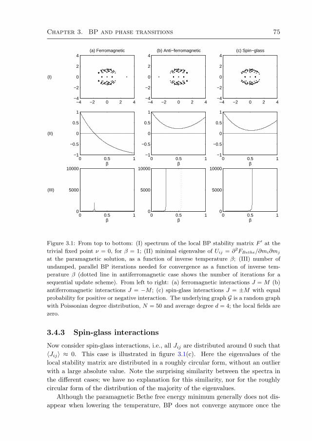
Chapter 3. BP and phase transitions 75
−4 −2 0 2 4−4
−2
0
2
4(a) Ferromagnetic
(I)
−4 −2 0 2 4−4
−2
0
2
4(b) Anti−ferromagnetic
−4 −2 0 2 4−4
−2
0
2
4(c) Spin−glass
0 0.5 1−1
−0.5
0
0.5
1
β
(II)
0 0.5 1−1
−0.5
0
0.5
1
β0 0.5 1
−1
−0.5
0
0.5
1
β
0 0.5 10
5000
10000
β
(III)
0 0.5 10
5000
10000
β0 0.5 1
0
5000
10000
β
Figure 3.1: From top to bottom: (I) spectrum of the local BP stability matrix F ′ at the
trivial fixed point ν = 0, for β = 1; (II) minimal eigenvalue of Uij = ∂2FBethe/∂mi∂mj
at the paramagnetic solution, as a function of inverse temperature β; (III) number of
undamped, parallel BP iterations needed for convergence as a function of inverse tem-
perature β (dotted line in antiferromagnetic case shows the number of iterations for a
sequential update scheme). From left to right: (a) ferromagnetic interactions J = M (b)
antiferromagnetic interactions J = −M ; (c) spin-glass interactions J = ±M with equal
probability for positive or negative interaction. The underlying graph G is a random graph
with Poissonian degree distribution, N = 50 and average degree d = 4; the local fields are
zero.
3.4.3 Spin-glass interactions
Now consider spin-glass interactions, i.e., all Jij are distributed around 0 such that〈Jij〉 ≈ 0. This case is illustrated in figure 3.1(c). Here the eigenvalues of thelocal stability matrix are distributed in a roughly circular form, without an outlierwith a large absolute value. Note the surprising similarity between the spectra inthe different cases; we have no explanation for this similarity, nor for the roughlycircular form of the distribution of the majority of the eigenvalues.
Although the paramagnetic Bethe free energy minimum generally does not dis-appear when lowering the temperature, BP does not converge anymore once the
76 Chapter 3
trivial fixed point becomes unstable, despite the possible existence of other, stable,fixed points. Neither damping nor changing the update scheme seems to help inthis case. Empirically we find that the temperature at which the trivial BP fixedpoint becomes locally unstable roughly coincides with the temperature at which thelowest eigenvalue of U attains its minimal value [Mooij and Kappen, 2005c]. Again,we have no theoretical explanation for this observation.
3.5 Estimates of phase-transition temperatures
In this section we estimate the critical temperatures corresponding to the onset ofinstability of the BP paramagnetic fixed point (which we discussed qualitatively inthe previous section) for a random graph with random interactions. The method isclosely related to the cavity method at the replica-symmetric level (see e.g., [Mezardet al., 1987; Mezard and Parisi, 2001; Wemmenhove et al., 2004]). A similar analysisof the stability of the BP paramagnetic fixed point has been done by Kabashima[Kabashima, 2003]; however, the results reported in that work are limited to thecase of infinite connectivity (i.e., the limit N → ∞, d → ∞). In this case, theresults turn out to be identical to the condition of replica symmetry breaking (the“AT line”) derived by de Almeida and Thouless [1978]. The analysis we presentbelow essentially extends the analysis of Kabashima [2003] to the larger class ofarbitrary degree distribution random graphs, which includes Erdos-Renyi graphs(with Poissonian degree distribution, as well as fixed degree random graphs) andpower-law graphs (which have power-law degree distributions), amongst others.
3.5.1 Random graphs with arbitrary degree distributions
We consider arbitrary degree distribution random graphs [Newman et al., 2001].This class of random graphs has a prescribed expected degree distribution P(d);apart from that they are completely random. Given an expected degree distributionP(d) and the number of nodes N , a particular sample of the corresponding ensembleof random graphs can be constructed as follows: for each node i, independently drawan expected degree δi from the degree distribution P(d). Then, for each pair of nodes(i, j), independently connect them with probability δiδj/
∑i δi; the expected degree
of node i is then indeed 〈di〉 = δi. We define the average degree 〈d〉 :=∑d P(d)d
and the second moment⟨d2⟩
:=∑d P(d)d2.
We consider the case of vanishing local fields (i.e., θi = 0) and draw the weightsJij independently from some probability distribution P(J). We also assume thatthe weights are independent of the graph structure.
3.5.2 Estimating the PA-FE transition temperature
Assume P(d) to be given and N to be large. Assume that v is an eigenvector witheigenvalue 1 of F ′(0), the Jacobian of the parallel BP update at the paramagnetic

Chapter 3. BP and phase transitions 77
fixed point ν = 0. Using (3.16) and writing ij instead of i→ j for brevity, we have:
vij =∑kl
(F ′(0)
)ij,kl
vkl = tanh(βJij)∑
k∈∂i\jvki. (3.25)
Consider an arbitrary spin i; conditional on the degree di of that spin, we cancalculate the expected value of vij as follows:
E (vij | di) = E(
tanh(βJij)∑k∈∂i\j vki | di
)(3.26a)
= E (tanh(βJij)) E(∑
k∈∂i\j vki | di)
(3.26b)
= 〈tanhβJ〉 (di − 1)∑dk
P(dk | di, k ∈ ∂i)E (vki | di, dk) (3.26c)
≈ 〈tanhβJ〉 (di − 1)∑dk
P(dk | di, k ∈ ∂i)E (vki | dk) (3.26d)
using, subsequently: (a) equation (3.25); (b) the independence of the weights fromthe graph structure; (c) conditioning on the degree dk of spin k and the equivalenceof the various k ∈ ∂i \ j; and finally, (d) neglecting the correlation between vki anddi, given dk. We have no formal argument for the validity of this approximation,but the result accurately describes the outcomes of numerical experiments.
For arbitrary degree distribution random graphs, the probability of dk given thedegree di and the fact that k is a neighbor of i is given by (see [Newman et al.,2001]):
P(dk | di, k ∈ ∂i) =dkP(dk)〈d〉 . (3.27)
Hence we obtain the relation
E (vij | di) = 〈tanhβJ〉 (di − 1)∑dk
dkP(dk)〈d〉 E (vki | dk)
A self-consistent nontrivial solution of these equations is
E (vij | di) ∝ (di − 1),
provided that
1 = 〈tanhβJ〉(⟨
d2⟩
〈d〉 − 1
). (3.28)
This gives us the critical temperature at which the paramagnetic–ferromagneticphase transition occurs, or in other words, where the paramagnetic BP fixed pointundergoes a pitchfork bifurcation. This result is identical to the one obtained bythe replica method in the replica-symmetric setting [Leone et al., 2002] and to theone found by applying the cavity method [Wemmenhove et al., 2004], as expected.Figure 3.2 illustrates the estimate; note that the accuracy is quite high already forlow N (N = 50 in this case), for higher N it becomes even better.

78 Chapter 3
Extending the analysis to the case of non-vanishing local fields does not appearto be straightforward, since in that case the value of the fixed point ν is not known.However, since the elements of F ′(0) are upper bounds for the elements of F ′(ν),we can at least conclude qualitatively that in the case of non-vanishing local fields,the transition temperature will be lower.
3.5.3 The antiferromagnetic case
This is similar to the ferromagnetic case, however the eigenvalue is now −1 insteadof +1. This yields the following equation for the transition temperature:
1 = 〈tanh(−βJ)〉(⟨
d2⟩
〈d〉 − 1
). (3.29)
As can be seen in figure 3.2, again the prediction turns out to be quite accurate.
3.5.4 Estimating the PA-SG transition temperature
For the paramagnetic–spin-glass phase transition, we can perform a similar calcula-tion, now assuming that v is an eigenvector with eigenvalue λ on the complex unitcircle:
E(|vij |2 | di
)= E
(|tanh(βJij)|2
∣∣∣∑k∈∂i\j vki∣∣∣2 | di)
=⟨tanh2(βJ)
⟩E(∣∣∣∑k∈∂i\j vki
∣∣∣2 | di)≈ ⟨tanh2(βJ)
⟩E(∑
k∈∂i\j |vki|2 | di)
≈ ⟨tanh2(βJ)⟩
(di − 1)∑dk
P(dk | di, k ∈ ∂i)E(|vki|2 | dk
),
where, in addition to the assumptions in the PA-FE case, we assumed that thecorrelations between the various vki can be neglected. Again, we can only motivatethis assumption in that it appears to give correct results.
Using relation (3.27), we find a nontrivial self-consistent solution
E(|vij |2 | di
)∝ (di − 1),
if the following equation holds:
1 =⟨tanh2(βJ)
⟩(⟨d2⟩
〈d〉 − 1
). (3.30)
This result is again identical to the one obtained by the cavity method [Wemmen-hove et al., 2004], as expected. As illustrated in figure 3.2 (the dashed line), theaccuracy is somewhat less than that of the ferromagnetic transition, but is never-theless quite good, even for N = 50.

Chapter 3. BP and phase transitions 79
−0.5 0 0.50
0.1
0.2
0.3
0.4
0.5
J0
J
Without damping
−0.5 0 0.50
0.1
0.2
0.3
0.4
0.5
J0
J
With damping
Figure 3.2: Onset of instability of the paramagnetic BP fixed point, for random graphs
with N = 50 and a Poissonian degree distribution with d = 10. The weights Jij are
independently drawn from a Gaussian distribution with mean J0 and variance J2. The
solid thick lines show the expected value for the (anti)ferromagnetic transitions (3.28) and
(3.29), the dashed thick line for the spin-glass transition (3.30). The dots show for indi-
vidual instances at which temperature the paramagnetic fixed point becomes unstable, for
undamped BP (left) and for damped BP (right). The lines in the right graph (the damped
case) are for reference only, they should not be interpreted as theoretical predictions,
except for the ferromagnetic transition (the solid line on the right-hand side).
For completeness we would like to state that the numerical results reported in[Mooij and Kappen, 2005c], in which we numerically studied the behavior of thelowest eigenvalue of U , are accurately described by the predictions (3.28) and (3.30),which supports the hypothesis that these notions coincide in the N →∞ limit.
3.6 Conclusions
We have derived conditions for the local stability of parallel BP fixed points, both inthe undamped and damped case for binary variables with pairwise interactions. Wehave shown how these relate to the sufficient conditions for uniqueness of the BPfixed point and convergence to this fixed point. In particular, we have shown thatthese sufficient conditions are sharp in the ferromagnetic case, exactly describingthe pitchfork bifurcation of the paramagnetic fixed point into two ferromagneticfixed points. For undamped BP, the local stability of the paramagnetic fixed point(for vanishing local fields) is invariant under a sign change of the interactions. Forantiferromagnetic interactions, parallel undamped BP stops converging at the PA-FE transition temperature. Damping or using a sequential update scheme remediesthis defect. However, although the paramagnetic minimum of the Bethe free energydoes not disappear, the trivial fixed point becomes locally unstable even for dampedBP at roughly the PA-SG transition temperature. Finally, for interactions thatare dominantly of the spin-glass type, using damping only marginally extends thedomain of convergence of BP.
80 Chapter 3
We estimated the PA-FE transition temperature and the PA-SG transition tem-perature for arbitrary degree distribution random graphs. The results are in goodagreement with numerical simulations. How this relates to the AT line is an openquestion and beyond the scope of this work.
We believe that the case that we have considered in detail in this work, namelyvanishing local fields θi = 0, is actually the worst-case scenario: numerically it turnsout that adding local fields helps BP to converge more quickly. We have no prooffor this conjecture at the moment; the local fields make an analytical analysis moredifficult and we have not yet been able to extend the analysis to this more generalsetting. We leave the generalization to nonzero local fields as possible future work.
Acknowledgments
We thank Bastian Wemmenhove and the anonymous reviewer for valuable com-ments on a draft of this paper.
3.A Proof of Theorem 3.2
For a square matrix A, we write A ≥ 0 iff all entries of A are nonnegative. σ(A) is theset of all eigenvalues of A, ρ(A) is the spectral radius of A, i.e., ρ(A) := max |σ(A)|.We will use the following generalization of Perron’s theorem:
Theorem 3.3 If A ≥ 0, then the spectral radius ρ(A) ∈ σ(A) and there exists anassociated eigenvector v ≥ 0 such that Av = ρ(A)v.
Proof. See [Meyer, 2000, p. 670].
Applying this theorem to the matrix A defined in (3.19), we deduce the existenceof an eigenvector v ≥ 0 with Av = ρ(A)v. Writing tij := tanh(β |Jij |) and λ :=ρ(A), we derive:
vij = λ−1tij
(∑k∈∂i
vki − vji)
= λ−1tij
∑k∈∂i
vki − λ−1tji
∑k∈∂j
vkj − vij .
Defining Vi :=∑k∈∂i vki, we obtain by summing over i ∈ ∂j:
Vj =∑i∈∂j
λtij
λ2 − tijtjiVi −∑i∈∂j
tijtjiλ2 − tijtjiVj ,
i.e., V is an eigenvector with eigenvalue 1 of the matrix
Mijρ(A) tanh(β |Jij |)
ρ(A)2 − tanh2(β |Jij |)− δij
∑k∈∂i
tanh2(β |Jik|)ρ(A)2 − tanh2(β |Jik|)
. (3.31)

Chapter 3. BP and phase transitions 81
Now, if all Jij are positive, and if ρ(A) = 1, this matrix is exactly I−U , where Uijis defined in (3.23). Hence, since in this case A = F ′(0), the critical temperature atwhich the paramagnetic BP fixed point becomes unstable coincides with the matrixI − U having an eigenvalue 1, or in other words U having eigenvalue 0. Thus theonset of instability of the paramagnetic BP fixed point in this case exactly coincideswith the disappearance of the paramagnetic Bethe free energy minimum.

82 Chapter 3
Chapter 4. Loop Corrections 83
Chapter 4
Loop Corrections
We propose a method to improve approximate inference methods by correcting for
the influence of loops in the graphical model. The method is a generalization and
alternative implementation of a recent idea from Montanari and Rizzo [2005]. It is
applicable to arbitrary factor graphs, provided that the size of the Markov blankets
is not too large. It consists of two steps: (i) an approximate inference method, for
example, Belief Propagation, is used to approximate cavity distributions for each
variable (i.e., probability distributions on the Markov blanket of a variable for a
modified graphical model in which the factors involving that variable have been
removed); (ii) all cavity distributions are improved by a message-passing algorithm
that cancels out approximation errors by imposing certain consistency constraints.
This Loop Correction (LC) method usually gives significantly better results than
the original, uncorrected, approximate inference algorithm that is used to estimate
the effect of loops. Indeed, we often observe that the loop-corrected error is approx-
imately the square of the error of the uncorrected approximate inference method.
In this chapter, we compare different variants of the Loop Correction method with
other approximate inference methods on a variety of graphical models, including
“real world” networks, and conclude that the LC method generally obtains the
most accurate results.
4.1 Introduction
In recent years, much research has been done in the field of approximate inference ongraphical models. One of the goals is to obtain accurate approximations of marginalprobabilities of complex probability distributions defined over many variables, using
This chapter is based on [Mooij and Kappen, 2007a], the extended version of [Mooij et al.,
2007].

84 Chapter 4
limited computation time and memory. This research has led to a large number ofapproximate inference methods. Apart from sampling (“Monte Carlo”) methods,there is a large number of “deterministic” approximate inference methods, such asvariational methods (for example, the Mean Field method [Parisi, 1988]), and afamily of algorithms that are in some way related to the highly successful BeliefPropagation (BP) algorithm [Pearl, 1988]. BP is also known as the “Sum-ProductAlgorithm” [Kschischang et al., 2001] and as “Loopy Belief Propagation” and isdirectly related to the Bethe approximation [Bethe, 1935; Yedidia et al., 2005] fromstatistical physics. It is well-known that Belief Propagation yields exact results ifthe graphical model is a tree, or, more generally, if each connected component isa tree. If the graphical model does contain loops, BP can still yield surprisinglyaccurate results using little computation time. However, if the influence of loops islarge, the approximate marginals calculated by BP can have large errors and thequality of the BP results may not be satisfactory.
One way to correct for the influence of short loops is to increase the cluster sizeof the approximation, using the Cluster Variation Method (CVM) [Pelizzola, 2005]or other region-based approximation methods [Yedidia et al., 2005]. These methodsare related to the Kikuchi approximation [Kikuchi, 1951], a generalization of theBethe approximation using larger clusters. Algorithms for calculating the CVMand related region-based approximation methods are Generalized Belief Propaga-tion (GBP) [Yedidia et al., 2005] and double-loop algorithms that have guaranteedconvergence [Yuille, 2002; Heskes et al., 2003]. By choosing the (outer) clusterssuch that they subsume as many loops as possible, the BP results can be improved.However, choosing a good set of outer clusters is highly nontrivial, and in generalthis method will only work if the clusters do not have many intersections, or inother words, if the loops do not have many intersections [Welling et al., 2005].
Another method that corrects for loops to a certain extent is TreeEP [Minka andQi, 2004], a special case of Expectation Propagation (EP) [Minka, 2001]. TreeEPdoes exact inference on the base tree, a subgraph of the graphical model which hasno loops, and approximates the other interactions. This corrects for the loops thatconsist of part of the base tree and exactly one additional factor. TreeEP yieldsgood results if the graphical model is dominated by the base tree, which is the casein very sparse models. However, loops that consist of two or more interactions thatare not part of the base tree are approximated in a similar way as in BP. Hence,for denser models, the improvement of TreeEP over BP usually diminishes.
In this chapter we propose a method that takes into account all the loops in thegraphical model in an approximate way and therefore obtains more accurate resultsin many cases. Our method is a variation on the theme introduced by Montanariand Rizzo [2005]. The basic idea is to first estimate the “cavity distributions”of all variables and subsequently improve these estimates by canceling out errorsusing certain consistency constraints. A cavity distribution of some variable is theprobability distribution on its Markov blanket (all its neighboring variables) fora modified graphical model, in which all factors involving that variable have been

Chapter 4. Loop Corrections 85
removed. The removal of the factors breaks all the loops in which that variable takespart. This allows an approximate inference algorithm to estimate the strength ofthese loops in terms of effective interactions or correlations between the variablesof the Markov blanket. Then, the influence of the removed factors is taken intoaccount, which yields accurate approximations to the probability distributions ofthe original graphical model. Even more accuracy is obtained by imposing certainconsistency relations between the cavity distributions, which results in a cancellationof errors to some extent. This error cancellation is done by a message-passingalgorithm which can be interpreted as a generalization of BP in case the factorgraph does not contain short loops of four nodes; indeed, assuming that the cavitydistributions factorize (which they do in case there are no loops), the BP results areobtained. On the other hand, using better estimates of the effective interactions inthe cavity distributions yields accurate loop-corrected results.
Although the basic idea underlying our method is very similar to that describedin [Montanari and Rizzo, 2005], the alternative implementation that we propose hereoffers two advantages. Most importantly, it is directly applicable to arbitrary factorgraphs, whereas the original method has only been formulated for the rather specialcase of graphical models with binary variables and pairwise factors, which excludes,for example, many interesting Bayesian networks. Furthermore, our implementationappears to be more robust and also gives improved results for relatively stronginteractions, as will be shown numerically.
This chapter is organized as follows. First we explain the theory behind ourproposed method and discuss the differences with the original method by Montanariand Rizzo [2005]. Then we report extensive numerical experiments regarding thequality of the approximation and the computation time, where we compare withother approximate inference methods. Finally, we discuss the results and stateconclusions.
4.2 Theory
In this work, we consider graphical models such as Markov random fields andBayesian networks. We use the general factor graph representation since it allows forformulating approximate inference algorithms in a unified way [Kschischang et al.,2001]. In the next subsection, we introduce our notation and basic definitions.
4.2.1 Graphical models and factor graphs
Consider N discrete random variables (xi)i∈V with V := 1, . . . , N. Each variablexi takes values in a discrete domain Xi. We will use the following multi-indexnotation: for any subset I ⊆ V, we write xI := (xi1 , xi2 , . . . , xim) ∈ XI := Xi1 ×Xi2×· · ·×Xim if I = i1, i2, . . . , im and i1 < i2 < . . . im. We consider a probability

86 Chapter 4
distribution over x = (x1, . . . , xN ) that can be written as a product of factors (alsocalled “interactions”) ψI :
P(x) =1Z
∏I∈F
ψI(xNI ), Z =∑x
∏I∈F
ψI(xNI ). (4.1)
For each factor index I ∈ F , there is an associated subset NI ⊆ V of variableindices and the factor ψI is a nonnegative function ψI : XNI → [0,∞). For aBayesian network, the factors are (conditional) probability tables. In case of Markovrandom fields, the factors are often called potentials (not to be confused with sta-tistical physics terminology, where “potential” refers to − 1
β logψI instead, with β
the inverse temperature). Henceforth, we will refer to a triple(V,F , (ψI)I∈F) that
satisfies the description above as a discrete graphical model (or network).In general, the normalizing constant Z is not known and exact computation of Z
is infeasible, due to the fact that the number of terms to be summed is exponentialin N . Similarly, computing marginal distributions P(xJ) of P(xV) for subsets ofvariables J ⊆ V is intractable in general. In this chapter, we focus on the task ofaccurately approximating single-variable marginals P(xi) =
∑xV\i
P(xV).We can represent the structure of the probability distribution (4.1) using a factor
graph. This is a bipartite graph, consisting of variable nodes i ∈ V and factor nodesI ∈ F , with an edge between i and I if and only if i ∈ NI , that is, if the factor ψIdepends on xi. We will represent factor nodes visually as rectangles and variablenodes as circles. See figure 4.1(a) for an example of a factor graph. The neighbors ofa factor node I ∈ F are precisely the variables NI , and the neighbors Ni of a variablenode i ∈ V are the factors that depend on that variable, i.e., Ni := I ∈ F : i ∈ NI.Further, we define for each variable i ∈ V the set ∆i :=
⋃I∈Ni NI consisting of all
variables that appear in some factor in which variable i participates, and the set∂i := ∆i \ i, the Markov blanket of i.
In the following, we will often abbreviate the set theoretical notation X \Y (i.e.,all elements in X that are not in Y ) by \Y if it is obvious from the context what theset X is. Also, we will write X \y instead of X \y. Further, we will use lowercasefor variable indices and uppercase for factor indices. For convenience, we will definefor any subset F ⊂ F the product ΨF of the corresponding factors ψI : I ∈ F:
ΨF (x(SI∈F NI)) :=
∏I∈F
ψI(xNI ).
4.2.2 Cavity networks and loop corrections
The notion of a cavity stems from statistical physics, where it was used originallyto calculate properties of random ensembles of certain graphical models [Mezardet al., 1987]. A cavity is obtained by removing one variable from the graphicalmodel, together with all the factors in which that variable participates.
In our context, we define cavity networks as follows (see also figure 4.1):

Chapter 4. Loop Corrections 87
(a) Original factor graph
i
j
k
l
m
n
o
I
J
K
L
M
O
(b) Cavity graph of i
j
k
l
m
n
o
L
M
O
Figure 4.1: (a) Original factor graph, with variables nodes V = i, j, k, l,m, n, oand factor nodes F = I, J,K,L,M,O and corresponding probability distribution
P(x) = 1ZψL(xj , xn, xo)ψI(xi, xj)ψM (xj , xk)ψK(xi, xm, xn)ψJ(xi, xk, xl)ψO(xl, xm); (b)
Factor graph corresponding to the cavity network of variable i, obtained by removing
variable i and the factor nodes that contain i (i.e., I, J and K). The Markov blanket
of i is ∂i = j, k, l,m, n. The cavity distribution Z\i(x∂i) is the (unnormalized) mar-
ginal on x∂i of the probability distribution corresponding to the cavity graph (b), i.e.,
Z\i(xj , xk, xl, xm, xn) =PxoψL(xj , xn, xo)ψM (xj , xk)ψO(xl, xm).
Definition 4.1 Given a graphical model(V,F , (ψI)I∈F) and a variable i ∈ V, the
cavity network of variable i is defined as the graphical model obtained by removingi and all factors depending on i, i.e.,
(V \ i,F \Ni, (ψI)I∈F\Ni).The probability distribution corresponding to the cavity network of variable i isthus proportional to:
Ψ\Ni(x\i) =∏I∈Fi 6∈I
ψI(xNI ).
Summing out all the variables, except for the neighbors ∂i of i, gives what we willcall the cavity distribution:
Definition 4.2 Given a graphical model(V,F , (ψI)I∈F) and a variable i ∈ V, the
cavity distribution of i is
Z\i(x∂i) :=∑x\∆i
Ψ\Ni(x\i). (4.2)
Thus the cavity distribution of i is proportional to the marginal of the cavity net-work of i on the Markov blanket ∂i. The cavity distribution describes the effectiveinteractions (or correlations) induced by the cavity network on the neighbors ∂i of
88 Chapter 4
variable i. Indeed, from equations (4.1) and (4.2) and the trivial observation thatΨF = ΨNiΨ\Ni we conclude:
P(x∆i) ∝ Z\i(x∂i)ΨNi(x∆i). (4.3)
Thus, given the cavity distribution Z\i(x∂i), one can calculate the marginal distri-bution of the original graphical model on x∆i, provided that the cardinality of X∆i
is not too large.In practice, exact cavity distributions are not known, and the only way to pro-
ceed is to use approximate cavity distributions. Given some approximate inferencemethod (e.g., BP), there are two ways to calculate P(x∆i): either use the methodto approximate P(x∆i) directly, or use the method to approximate Z\i(x∂i) and useequation (4.3) to obtain an approximation to P(x∆i). The latter approach generallygives more accurate results, since the complexity of the cavity network is less thanthat of the original network. In particular, the cavity network of variable i containsno loops involving that variable, since all factors in which i participates have beenremoved (e.g., the loop i − J − l − O −m −K − i in the original network, figure4.1(a), is not present in the cavity network, figure 4.1(b)). Thus the latter approachto calculating P(x∆i) takes into account loops involving variable i, although in anapproximate way. It does not, however, take into account the other loops in theoriginal graphical model. The basic idea of the loop correction approach of Monta-nari and Rizzo [2005] is to use the latter approach for all variables in the network,but to adjust the approximate cavity distributions in order to cancel out approxi-mation errors before (4.3) is used to obtain the final approximate marginals. Thisapproach takes into account all the loops in the original network, in an approximateway.
This basic idea can be implemented in several ways. Here we propose an im-plementation which we will show to have certain advantages over the original im-plementation proposed in [Montanari and Rizzo, 2005]. In particular, it is directlyapplicable to arbitrary factor graphs with variables taking an arbitrary (discrete)number of values and factors that may contain zeros and depend on an arbitrarynumber of variables. In the remaining subsections, we will first discuss our pro-posed implementation in detail. In section 4.2.6 we will discuss differences with theoriginal approach.
4.2.3 Combining approximate cavity distributions to cancel
out errors
Suppose that we have obtained an initial approximation ζ\i0 (x∂i) of the (exact) cav-ity distribution Z\i(x∂i), for each i ∈ V. Let i ∈ V and consider the approximationerror of the cavity distribution of i, that is, the exact cavity distribution of i dividedby its approximation:
Z\i(x∂i)
ζ\i0 (x∂i)
.

Chapter 4. Loop Corrections 89
In general, this is an arbitrary function of the variables x∂i. However, we willapproximate the error as a product of factors defined on small subsets of ∂i in thefollowing way:
Z\i(x∂i)
ζ\i0 (x∂i)
≈∏I∈Ni
φ\iI (xNI\i).
Thus we assume that the approximation error lies near a submanifold parameterizedby the error factors (φ\iI (xNI\i))I∈Ni . If we were able to calculate these error factors,we could improve our initial approximation ζ\i0 (x∂i) by replacing it with the product
ζ\i(x∂i) := ζ\i0 (x∂i)
∏I∈Ni
φ\iI (xNI\i) ≈ Z\i(x∂i). (4.4)
Using (4.3), this would then yield an improved approximation of P(x∆i).It turns out that the error factors can indeed be calculated by exploiting the
redundancy of the information in the initial cavity approximations (ζ\i0 )i∈V . Thefact that all ζ\i provide approximations to marginals of the same probability dis-tribution P(x) via (4.3) can be used to obtain consistency constraints. The numberof constraints obtained in this way is usually enough to solve for the unknown errorfactors (φ\iI (xNI\i))i∈V,I∈Ni .
Here we propose the following consistency constraints. Let Y ∈ F , i ∈ NYand j ∈ NY with i 6= j (see also figure 4.2). Consider the graphical model
(V,F \Y, (ψI)I∈F\Y
)that is obtained from the original graphical model by removing factor
ψY . The product of all factors (except ψY ) obviously satisfies:
Ψ\Y = ΨNi\Y Ψ\Ni = ΨNj\Y Ψ\Nj .
Using (4.2) and summing over all xk for k 6∈ NY \i, we obtain the following equation,which holds for the exact cavity distributions Z\i and Z\j :∑
xi
∑x∆i\Y
ΨNi\Y Z\i =
∑xi
∑x∆j\Y
ΨNj\Y Z\j .
By substituting our basic assumption (4.4) on both sides and pulling the factorφ\iY (xNY \i) in the l.h.s. through the summation, we obtain:
φ\iY
∑xi
∑x∆i\Y
ΨNi\Y ζ\i0
∏I∈Ni\Y
φ\iI =
∑xi
∑x∆j\Y
ΨNj\Y ζ\j0
∏J∈Nj
φ\jJ .
Since this should hold for each j ∈ NY \ i, we can take the geometric mean of ther.h.s. over all j ∈ NY \ i. After rearranging, this yields:
φ\iY =
∏j∈NY \i
∑xi
∑x∆j\Y
ΨNj\Y ζ\j0
∏J∈Nj
φ\jJ
1/#(NY \i)
∑xi
∑x∆i\Y
ΨNi\Y ζ\i0
∏I∈Ni\Y
φ\iI
∀i∈V∀Y ∈Ni . (4.5)

90 Chapter 4
I0
I1I1I2
J0
J1J2
Y
i
jk
Figure 4.2: Part of the factor graph, illustrating the derivation of (4.5). The two gray
variable nodes correspond to NY \ i = j, k.
Note that the numerator is an approximation of the joint marginal of the modifiedgraphical model
(V,F \ Y, (ψI)I∈F\Y ) on the variables NY \ i.Solving the consistency equations (4.5) simultaneously for the error factors
(φ\iI )i∈V,I∈Ni can be done using a simple fixed point iteration algorithm, for ex-ample, Algorithm 4.1. The input consists of the initial approximations (ζ\i0 )i∈V tothe cavity distributions. It calculates the error factors that satisfy (4.5) by fixedpoint iteration and from the fixed point, it calculates improved approximations ofthe cavity distributions (ζ\i)i∈V using equation (4.4).1 From the improved cavitydistributions, the loop-corrected approximations to the single-variable marginals ofthe original probability distribution (4.1) can be calculated as follows:
P(xi) ≈ bi(xi) ∝∑x∂i
ΨNi(x∆i)ζ\i(x∂i), (4.6)
where the factor ψY is now included. Algorithm 4.1 uses a sequential update scheme,but other update schemes are possible (e.g., random sequential or parallel). Inpractice, the fixed sequential update scheme often converges without the need fordamping.
Alternatively, one can formulate Algorithm 4.1 in terms of the “beliefs”
Qi(x∆i) ∝ ΨNi(x∆i)ζ\i0 (x∂i)
∏I∈Ni
φ\iI (xNI\i) = ΨNi(x∆i)ζ\i(x∂i). (4.7)
1Alternatively, one could formulate the updates directly in terms of the cavity distributions
ζ\i.
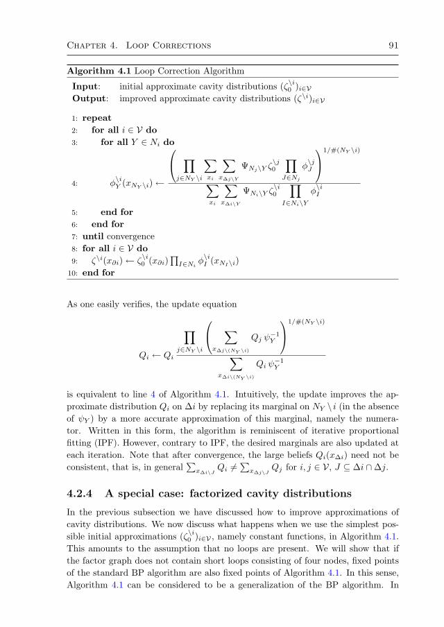
Chapter 4. Loop Corrections 91
Algorithm 4.1 Loop Correction Algorithm
Input: initial approximate cavity distributions (ζ\i0 )i∈VOutput: improved approximate cavity distributions (ζ\i)i∈V
1: repeat2: for all i ∈ V do3: for all Y ∈ Ni do
4: φ\iY (xNY \i)←
∏j∈NY \i
∑xi
∑x∆j\Y
ΨNj\Y ζ\j0
∏J∈Nj
φ\jJ
1/#(NY \i)
∑xi
∑x∆i\Y
ΨNi\Y ζ\i0
∏I∈Ni\Y
φ\iI
5: end for6: end for7: until convergence8: for all i ∈ V do9: ζ\i(x∂i)← ζ
\i0 (x∂i)
∏I∈Ni φ
\iI (xNI\i)
10: end for
As one easily verifies, the update equation
Qi ← Qi
∏j∈NY \i
∑x∆j\(NY \i)
Qj ψ−1Y
1/#(NY \i)
∑x∆i\(NY \i)
Qi ψ−1Y
is equivalent to line 4 of Algorithm 4.1. Intuitively, the update improves the ap-proximate distribution Qi on ∆i by replacing its marginal on NY \ i (in the absenceof ψY ) by a more accurate approximation of this marginal, namely the numera-tor. Written in this form, the algorithm is reminiscent of iterative proportionalfitting (IPF). However, contrary to IPF, the desired marginals are also updated ateach iteration. Note that after convergence, the large beliefs Qi(x∆i) need not beconsistent, that is, in general
∑x∆i\J
Qi 6=∑x∆j\J
Qj for i, j ∈ V, J ⊆ ∆i ∩∆j.
4.2.4 A special case: factorized cavity distributions
In the previous subsection we have discussed how to improve approximations ofcavity distributions. We now discuss what happens when we use the simplest pos-sible initial approximations (ζ\i0 )i∈V , namely constant functions, in Algorithm 4.1.This amounts to the assumption that no loops are present. We will show that ifthe factor graph does not contain short loops consisting of four nodes, fixed pointsof the standard BP algorithm are also fixed points of Algorithm 4.1. In this sense,Algorithm 4.1 can be considered to be a generalization of the BP algorithm. In

92 Chapter 4
fact, this holds even if the initial approximations factorize in a certain way, as willbe shown below.
If all factors involve at most two variables, one can easily arrange for the factorgraph to have no loops of four nodes. See figure 4.1(a) for an example of a factorgraph which has no loops of four nodes. The factor graph depicted in figure 4.2does have a loop of four nodes: k − Y − j − J2 − k.
Theorem 4.3 If the factor graph corresponding to (4.1) has no loops of exactlyfour nodes, and all initial approximate cavity distributions factorize in the followingway:
ζ\i0 (x∂i) =
∏I∈Ni
ξ\iI (xNI\i) ∀i ∈ V, (4.8)
then fixed points of the BP algorithm can be mapped to fixed points of Algorithm4.1. Furthermore, the corresponding variable and factor marginals obtained from(4.7) are identical to the BP beliefs.
Proof. Note that replacing the initial cavity approximations by
ζ\i0 (x∂i) 7→ ζ
\i0 (x∂i)
∏I∈Ni
ε\iI (xNI\i)
for arbitrary positive functions ε\iI (xNI\i) does not change the beliefs (4.7) corre-sponding to the fixed points of (4.5). Thus, without loss of generality, we can assumeζ\i0 (x∂i) = 1 for all i ∈ V. The BP update equations are [Kschischang et al., 2001]:
µj→I(xj) ∝∏
J∈Nj\IµJ→j(xj) j ∈ V, I ∈ Nj ,
µI→i(xi) ∝∑xNI\i
ψI(xNI )∏
j∈NI\iµj→I(xj) I ∈ F , i ∈ NI
(4.9)
in terms of messages(µJ→j(xj)
)j∈V,J∈Nj and
(µj→J(xj)
)j∈V,J∈Nj . Assume that
the messages µ are a fixed point of (4.9) and take the Ansatz
φ\iI (xNI\i) =
∏k∈NI\i
µk→I(xk) for i ∈ V, I ∈ Ni.
Then, for i ∈ V, Y ∈ Ni, j ∈ NY \ i, we can write out part of the numerator of (4.5)as follows: ∑
xi
∑x∆j\Y
ΨNj\Y ζ\j0
∏J∈Nj
φ\jJ =
∑xi
∑x∆j\Y
φ\jY
∏J∈Nj\Y
ψJφ\jJ
=∑xi
∏k∈NY \j
µk→Y
∏J∈Nj\Y
∑xNJ\j
ψJ∏
k∈NJ\jµk→J
=∑xi
∏k∈NY \j
µk→Y
µj→Y =∑xi
∏k∈NY
µk→Y
∝∏
k∈NY \iµk→Y = φ
\iY ,
Chapter 4. Loop Corrections 93
where we used the BP update equations (4.9) and rearranged the summations andproducts using the assumption that the factor graph has no loops of four nodes.Thus, the numerator of the r.h.s. of (4.5) is simply φ\iY . Using a similar calculation,one can derive that the denominator of the r.h.s. of (4.5) is constant, and hence(4.5) is valid (up to an irrelevant constant).
For Y ∈ F , i ∈ NY , the marginal on xY of the belief (4.7) can be written in asimilar way:∑
x∆i\Y
Qi ∝∑x∆i\Y
ΨNi
∏I∈Ni
φ\iI =
∑x∆i\Y
∏I∈Ni
ψI∏
k∈NI\iµk→I
= ψY
∏k∈NY \i
µk→Y
∏I∈Ni\Y
∑xNI\i
ψI∏
k∈NI\iµk→I
= ψY
∏k∈NY \i
µk→Y
∏I∈Ni\Y
µI→i = ψY
∏k∈NY \i
µk→Y
µi→Y
= ψY∏k∈NY
µk→Y ,
which is proportional to the BP belief bY (xY ) on xY . Hence, also the single-variablemarginal bi defined in (4.6) corresponds to the BP single-variable belief, since bothare marginals of bY for Y ∈ Ni.
If the factor graph does contain loops of four nodes, we usually observe thatthe fixed point of Algorithm 4.1 coincides with the solution of the “minimal” CVMapproximation when using factorized initial cavity approximations as in (4.8). Theminimal CVM approximation uses all maximal factors as outer clusters (a maximalfactor is a factor defined on a domain which is not a strict subset of the domainof another factor). In that case, the factor beliefs found by Algorithm 4.1 areconsistent, that is,
∑x∆i\NY
Qi =∑x∆j\NY
Qj for i, j ∈ NY , and are identicalto the minimal CVM factor beliefs. In particular, this holds for all the graphicalmodels used in section 4.3.2
4.2.5 Obtaining initial approximate cavity distributions
There is no principled way to obtain the initial approximations (ζ\i0 (x∂i))i∈V to thecavity distributions. In the previous subsection, we investigated the results of ap-plying the LC algorithm on factorizing initial cavity approximations. More sophis-ticated approximations that do take into account the effect of loops can significantlyenhance the accuracy of the final result. Here, we will describe one method, which
2In a draft version of this work [Mooij and Kappen, 2006], we conjectured that the result
of Algorithm 4.1, when initialized with factorizing initial cavity approximations, would always
coincide with the minimal CVM approximation. This conjecture no longer stands because we
have found a counter example.

94 Chapter 4
uses BP on clamped cavity networks. This method captures all interactions in thecavity distribution of i in an approximate way and can lead to very accurate results.Instead of BP, any other approximate inference method that gives an approximationof the normalizing constant Z in (4.1) can be used, such as Mean Field, TreeEP[Minka and Qi, 2004], a double-loop version of BP [Heskes et al., 2003] which hasguaranteed convergence towards a minimum of the Bethe free energy, or some vari-ant of GBP [Yedidia et al., 2005]. One could also choose the method for each cavityseparately, trading accuracy versus computation time. We focus on BP because itis a very fast and often relatively accurate algorithm.
Let i ∈ V and consider the cavity network of i. For each possible state of x∂i, runBP on the cavity network clamped to that state x∂i and calculate the correspondingBethe free energy F \iBethe(x∂i) [Yedidia et al., 2005]. Then, take the following initialapproximate cavity distribution:
ζ\i0 (x∂i) ∝ e−F
\iBethe(x∂i).
This procedure is exponential in the size of ∂i: it uses∏j∈∂i #(Xj) BP runs. How-
ever, many networks encountered in applications are relatively sparse and havelimited cavity size and the computational cost may be acceptable.
This particular way of obtaining initial cavity distributions has the following in-teresting property: in case the factor graph contains only a single loop and assumingthat the fixed point is unique, the final beliefs (4.7) resulting from Algorithm 4.1are exact. This can be shown using an argument similar to that given in [Montanariand Rizzo, 2005]. Suppose that the graphical model contains exactly one loop andlet i ∈ V. First, consider the case that i is part of the loop; removing i will breakthe loop and the remaining cavity network will be singly connected. The cavitydistribution approximated by BP will thus be exact. Now if i is not part of theloop, removing i will divide the network into several connected components, onefor each neighbor of i. This implies that the cavity distribution calculated by BPcontains no higher-order interactions, that is, ζ\i0 is exact modulo single-variableinteractions. Because the final beliefs (4.7) are invariant under perturbation of theζ\i0 by single-variable interactions, the final beliefs calculated by Algorithm 4.1 are
exact if the fixed point is unique.If all interactions are pairwise and each variable is binary and has exactly
#(∂i) = d neighbors, the time complexity of the resulting “Loop-Corrected BP”(LCBP) algorithm is given by O(N2dEIBP +Nd2d+1ILC), where E is the numberof edges in the factor graph, IBP is the average number of iterations of BP ona clamped cavity network and ILC is the number of iterations needed to obtainconvergence in Algorithm 4.1.
4.2.6 Differences with the original implementation
As mentioned before, the idea of estimating the cavity distributions and imposingcertain consistency relations amongst them has been first presented in [Montanari
Chapter 4. Loop Corrections 95
and Rizzo, 2005]. In its simplest form (i.e., the so-called first-order correction), theimplementation of that basic idea as proposed by Montanari and Rizzo [2005] differsfrom our proposed implementation in the following aspects.
First, the original method described by Montanari and Rizzo [2005] is only for-mulated for the rather special case of binary variables and pairwise interactions.In contrast, our method is formulated in a general way that makes it applicable tofactor graphs with variables having more than two possible values and factors con-sisting of more than two variables. Also, factors may contain zeros. The generalitythat our implementation offers is important for many practical applications. In therest of this section, we will assume that the graphical model (4.1) belongs to thespecial class of models with binary variables with pairwise interactions, allowingfurther comparison of both implementations.
An important difference is that Montanari and Rizzo [2005] suggest to deform theinitial approximate cavity distributions by altering certain cumulants (also called“connected correlations”), instead of altering certain interactions. In general, fora set V ⊆ V of ±1-valued random variables (xi)i∈V , one can define for any subsetA ⊆ V the moment
MA :=∑xV
P(xV )∏j∈A
xj .
The moments (MA)A⊆V are a particular parameterization of the probability distri-bution P(xV ). An alternative parameterization is given in terms of the cumulants.The (joint) cumulants (CA)A⊆V are certain polynomials of the moments, definedimplicitly by the following equations:
MA =∑
B∈Part(A)
∏E∈BCE
where Part(A) is the set of partitions of A.3 In particular, Ci = Mi and Cij =Mij −MiMj for all i, j ∈ V with i 6= j. Montanari and Rizzo [2005] propose toapproximate the cavity distributions by estimating the pair cumulants and assuminghigher-order cumulants to be zero. Then, the singleton cumulants (i.e., the single-variable marginals) are altered, keeping higher-order cumulants fixed, in such away as to impose consistency of the single-variable marginals, in the absence ofinteractions shared by two neighboring cavities. We refer the reader to Appendix4.A for a more detailed description of the implementation in terms of cumulantssuggested by Montanari and Rizzo [2005].
The assumption suggested in [Montanari and Rizzo, 2005] that higher-ordercumulants are zero is the most important difference with our method, which insteadtakes into account effective interactions in the cavity distribution of all orders. Inprinciple, the cumulant parameterization also allows for taking into account higher-order cumulants, but this would not be very efficient due to the combinatoricsneeded for handling the partitions.
3For a set X, a partition of X is a nonempty set Y such that each Z ∈ Y is a nonempty subset
of X andSY = X.

96 Chapter 4
A minor difference lies in the method to obtain initial approximations to thecavity distributions. Montanari and Rizzo [2005] propose to use BP in combinationwith linear response theory to obtain the initial pairwise cumulants. This differenceis not very important, since one could also use BP on clamped cavity networksinstead, which turns out to give almost identical results.
As we will show in section 4.3, our method of altering interactions appearsto be more robust and still works in regimes with strong interactions, whereas thecumulant implementation suffers from convergence problems for strong interactions.
Montanari and Rizzo [2005] also derive a linearized version of their cumulant-based scheme (by expanding up to first order in terms of the pairwise cumulants,see Appendix 4.A) which is quadratic in the size of the cavity. This linearized,cumulant-based version is currently the only one that can be applied to networkswith large Markov blankets (cavities), that is, where the maximum number of statesmaxi∈V #(X∆i) is large, provided that all variables are binary and interactions arepairwise.
4.3 Numerical experiments
We have performed various numerical experiments to compare the quality of theresults and the computation time of the following approximate inference methods:
MF Mean Field, with a random sequential update scheme and no damping.
BP Belief Bropagation. We have used the recently proposed update scheme [Elidanet al., 2006], which converges also for difficult problems without the need fordamping.
TreeEP TreeEP [Minka and Qi, 2004], without damping. We generalized themethod of choosing the base tree described in [Minka and Qi, 2004] to multiplevariable factors as follows: when estimating the mutual information betweenxi and xj , we take the product of the marginals on i, j of all the factorsthat involve xi and/or xj . Other generalizations of TreeEP to higher-orderfactors are possible (e.g., by clustering variables), but it is not clear how todo this in general in an optimal way.
LCBP (“Loop-Corrected Belief Propagation”) Algorithm 4.1, where the approxi-mate cavities are initialized according to the description in section 4.2.5.
LCBP-Cum The original cumulant-based loop correction scheme by Montanariand Rizzo [2005], using Response Propagation (also known as Linear Re-sponse) to approximate the initial pairwise cavity cumulants. The full updateequations (4.14) are used and higher-order cumulants are assumed to vanish.For strong interactions, the update equations (4.14) often yield values for theM\ij outside of the valid interval [−1, 1]. In this case, we project these values

Chapter 4. Loop Corrections 97
back into the valid interval in the hope that the method will converge to avalid result, which it sometimes does.
LCBP-Cum-Lin Similar to LCBP-Cum, but instead of the full update equa-tions (4.14), the linearized update equations (4.15) are used.
CVM-Min A double-loop implementation [Heskes et al., 2003] of the minimalCVM approximation, which uses (maximal) factors as outer clusters.
CVM-∆ A double-loop implementation of CVM using the sets (∆i)i∈V as outerclusters. These are the same sets of variables as used by LCBP (c.f. (4.7))and therefore it is interesting to compare both algorithms.
CVM-Loopk A double-loop implementation of CVM, using as outer clusters all(maximal) factors together with all loops in the factor graph that consist ofup to k different variables (for k = 3, 4, 5, 6, 8).
We have used a double-loop implementation of CVM instead of GBP becausethe former is guaranteed to converge to a local minimum of the Kikuchi free energy[Heskes et al., 2003] without damping, whereas the latter often only converges withstrong damping, or does not converge at all, even for arbitrary strong damping.Furthermore, even if damped GBP would converge, the problem is that the optimaldamping constant is not known a priori, thus requiring one or more trial runs withdifferent damping constants, until a suitable one is found. Using too much dampingslows down convergence, whereas a certain amount of damping is required to obtainconvergence in the first place. Therefore, even if (damped) GBP would converge, wewould not expect it to be much faster than a double-loop implementation becauseof the computational cost of finding the optimal damping constant.
To be able to assess the errors of the various approximate methods, we haveonly considered problems for which exact inference (using a standard JunctionTreemethod) was still feasible.
For each approximate inference method, we report the maximum `∞ error ofthe approximate single-variable marginals bi, calculated as follows:
Error := maxi∈V
maxxi∈Xi
|bi(xi)− P(xi)|
where P(xi) is the exact marginal calculated using the JunctionTree method.The computation time was measured as CPU time in seconds on a 2.4 GHz
AMD Opteron 64bits processor with 4 GB memory. The timings should be seenas indicative because we have not spent equal amounts of effort optimizing eachmethod.4
We consider an iterative method to be “converged” after T time steps if for eachvariable i ∈ V, the `∞ distance between the approximate probability distributionsof that variable at time step T and T + 1 is less than ε = 10−9.
4Our C++ implementation of various approximate inference algorithms is free/open source
software and can be downloaded from http://www.mbfys.ru.nl/~jorism/libDAI.
98 Chapter 4
We have studied four different model classes: (i) random graphs of uniformdegree with pairwise interactions and binary variables; (ii) random factor graphswith binary variables and factor nodes of uniform degree k = 3; (iii) the Alarm
network, which has variables taking on more than two possible values and factorsconsisting of more than two variables; (iv) Promedas networks, which have binaryvariables but factors consisting of more than two variables. For more extensiveexperiments, see [Mooij and Kappen, 2006].
4.3.1 Random regular graphs with binary variables
We have compared various approximate inference methods on random graphs con-sisting of N binary (±1-valued) variables, having only pairwise interactions, whereeach variable has the same degree #(∂i) = d. In this case, the probability distribu-tion (4.1) can be written in the following way:
P(x) =1Z
exp
∑i∈V
θixi +12
∑i∈V
∑j∈∂i
Jijxixj
.
The parameters (θi)i∈V are called the local fields; the parameters (Jij = Jji)i∈V,j∈∂iare called the couplings. The graph structure and the parameters θ and J weredrawn randomly for each instance. The local fields θi were drawn independentlyfrom a N
(0, (βΘ)2
)distribution (i.e., a normal distribution with mean 0 and stan-
dard deviation βΘ). For the couplings Jij, we took mixed (“spin-glass”) cou-plings, drawn independently from a normal distribution
Jij ∼ N(
0,(β tanh−1 1√
d− 1
)2).
The constant β (called “inverse temperature” in statistical physics) controls theoverall interaction strength and thereby the difficulty of the inference problem,larger β corresponding usually to more difficult problems. The constant Θ controlsthe relative strength of the local fields, where larger Θ result in easier inferenceproblems. The particular d-dependent scaling of the couplings is used in order toobtain roughly d-independent behavior. For Θ = 0 and for β ≈ 1, a phase transitionoccurs in the limit of N →∞, going from an easy “paramagnetic” phase for β < 1to a complicated “spin-glass” phase for β > 1.5
We have also done experiments with positive (“attractive” or “ferromagnetic”)couplings, but the conclusions from these experiments did not differ significantlyfrom those using mixed couplings [Mooij and Kappen, 2006]. Therefore we do notreport those experiments here.
5More precisely, the PA-SG phase transition occurs at Θ = 0 and (d − 1) =˙tanh2(βJij)
¸,
where 〈·〉 is the average over all Jij [Mooij and Kappen, 2005a]. What happens for Θ > 0 is not
known, to the best of our knowledge.
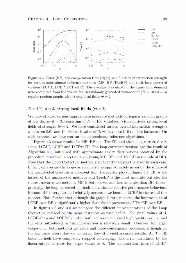
Chapter 4. Loop Corrections 99
10−8
10−6
10−4
10−2
100
Max
.er
ror
Max
.er
ror
0.01 0.1 1 10
ββ
10−2
100
102
104
Tim
e(s
)T
ime
(s)
0.01 0.1 1 10
ββ
MFBPTreeEPLCMFLCBPLCTreeEP
Figure 4.3: Error (left) and computation time (right) as a function of interaction strength
for various approximate inference methods (MF, BP, TreeEP) and their loop-corrected
versions (LCMF, LCBP, LCTreeEP). The averages (calculated in the logarithmic domain)
were computed from the results for 16 randomly generated instances of (N = 100, d = 3)
regular random graphs with strong local fields Θ = 2.
N = 100, d = 3, strong local fields (Θ = 2)
We have studied various approximate inference methods on regular random graphsof low degree d = 3, consisting of N = 100 variables, with relatively strong localfields of strength Θ = 2. We have considered various overall interaction strengthsβ between 0.01 and 10. For each value of β, we have used 16 random instances. Oneach instance, we have run various approximate inference algorithms.
Figure 4.3 shows results for MF, BP and TreeEP, and their loop-corrected ver-sions, LCMF, LCBP and LCTreeEP. The loop-corrected versions are the result ofAlgorithm 4.1, initialized with approximate cavity distributions obtained by theprocedure described in section 4.2.5 (using MF, BP, and TreeEP in the role of BP).Note that the Loop Correction method significantly reduces the error in each case.In fact, on average the loop-corrected error is approximately given by the square ofthe uncorrected error, as is apparent from the scatter plots in figure 4.4. BP is thefastest of the uncorrected methods and TreeEP is the most accurate but also theslowest uncorrected method. MF is both slower and less accurate than BP. Unsur-prisingly, the loop-corrected methods show similar relative performance behaviors.Because BP is very fast and relatively accurate, we focus on LCBP in the rest of thischapter. Note further that although the graph is rather sparse, the improvement ofLCBP over BP is significantly higher than the improvement of TreeEP over BP.
In figures 4.5 and 4.6 we compare the different implementations of the LoopCorrection method on the same instances as used before. For small values of β,LCBP-Cum and LCBP-Cum-Lin both converge and yield high quality results, andthe error introduced by the linearization is relatively small. However, for largervalues of β, both methods get more and more convergence problems, although forthe few cases where they do converge, they still yield accurate results. At β ≈ 10,both methods have completely stopped converging. The error introduced by thelinearization increases for larger values of β. The computation times of LCBP-

100 Chapter 4
10−8
10−6
10−4
10−2
100
LC
MF
erro
rLC
MF
erro
r
10−9 10−6 10−3 100
MF errorMF error
10−8
10−6
10−4
10−2
100
LC
Tre
eEP
erro
rLC
Tre
eEP
erro
r10−9 10−6 10−3 100
TreeEP errorTreeEP error
10−8
10−6
10−4
10−2
100
LC
BP
erro
rLC
BP
erro
r
10−9 10−6 10−3 100
BP errorBP error
Figure 4.4: Pairwise comparisons of errors of uncorrected and loop-corrected methods, for
the same instances as in figure 4.3. The solid lines correspond with y = x, the dotted
lines with y = x2. Only the cases have been plotted for which both approximate infer-
ence methods have converged. Saturation of errors around 10−9 is an artifact due to the
convergence criterion.
10−8
10−6
10−4
10−2
100
Max
.er
ror
Max
.er
ror
0.01 0.1 1 10
ββ
0.001
0.01
0.1
1
10
Tim
e(s
)T
ime
(s)
0.01 0.1 1 10
ββ
0
0.25
0.5
0.75
1
Frac
tion
ofco
nver
ged
inst
ance
sFr
acti
onof
conv
erge
din
stan
ces
0.01 0.1 1 10
ββ
BP LCBP-Cum-Lin LCBP-Cum LCBP
Figure 4.5: For the same instances as in figure 4.3: average error (left), average computa-
tion time (center) and fraction of converged instances (right) as a function of interaction
strength β for various variants of the LC method. The averages of errors and computation
time were calculated from the converged instances only. The average computation time
and fraction of converged instances for LCBP-Cum and LCBP-Cum-Lin are difficult to
distinguish, because they are (almost) identical.
Cum, LCBP-Cum-Lin and LCBP do not differ substantially in the regime where allmethods converge. However, the quality of the LCBP results is higher than that ofthe cumulant-based methods. This is mainly due to the fact that LCBP also takesinto account effective triple interactions in the initial estimates of the approximatecavity distributions.
We speculate that the reason for the break-down of LCBP-Cum and LCBP-Cum-Lin for strong interactions is due to the choice of cumulants instead of inter-actions. Indeed, consider two random variables xi and xj with fixed pair interac-tion exp(Jxixj). By altering the singleton interactions exp(θixi) and exp(θjxj),one can obtain any desired marginals of xi and xj . However, a fixed pair cumulantCij = E (xixj) − E (xi) E (xj) imposes a constraint on the range of possible expec-

Chapter 4. Loop Corrections 101
10−8
10−6
10−4
10−2
100LC
BP
-Cum
erro
rLC
BP
-Cum
erro
r
10−9 10−6 10−3 100
BP errorBP error
10−8
10−6
10−4
10−2
100
LC
BP
-Cum
-Lin
erro
rLC
BP
-Cum
-Lin
erro
r
10−9 10−6 10−3 100
LCBP-Cum errorLCBP-Cum error
10−8
10−6
10−4
10−2
100
LC
BP
erro
rLC
BP
erro
r
10−9 10−6 10−3 100
LCBP-Cum errorLCBP-Cum error
Figure 4.6: Pairwise comparisons of errors of various methods for the same instances as in
figure 4.3. Only the cases have been plotted for which both approximate inference methods
converged.
10−8
10−6
10−4
10−2
100
Max
.er
ror
Max
.er
ror
0.01 0.1 1 10
ββ
0.001
0.01
0.1
1
10
100
Tim
e(s
)T
ime
(s)
0.01 0.1 1 10
ββ
BPCVM-∆CVM-Loop4CVM-Loop6CVM-Loop8LCBP
Figure 4.7: Average errors (left) and computation times (right) for various CVM methods
(and LCBP, for reference) on the same instances as in figure 4.3. All methods converged
on all instances.
tation values E (xi) and E (xj) (hence on the single-variable marginals of xi andxj); the freedom of choice in these marginals becomes less as the pair cumulantbecomes stronger. We believe that something similar happens for LCBP-Cum (andLCBP-Cum-Lin): for strong interactions, the approximate pair cumulants in thecavity are strong, and even tiny errors can lead to inconsistencies which preventconvergence.
The results of the CVM approach to loop correction are shown in figures 4.7and 4.8. The CVM-Loop methods, with clusters reflecting the short loops presentin the factor graph, do indeed improve on BP. Furthermore, as expected, the use oflarger clusters (that subsume longer loops) improves the results, although compu-tation time quickly increases. CVM-Loop3 (not plotted) turned out not to give anyimprovement over BP, simply because there were (almost) no loops of 3 variablespresent. The most accurate CVM method, CVM-Loop8, needs more computationtime than LCBP, whereas it yields inferior results.6
6The CVM errors are often seen to saturate around 10−8, which indicates that the slow conver-
gence of the CVM double-loop algorithm in these cases requires a stricter convergence criterion.
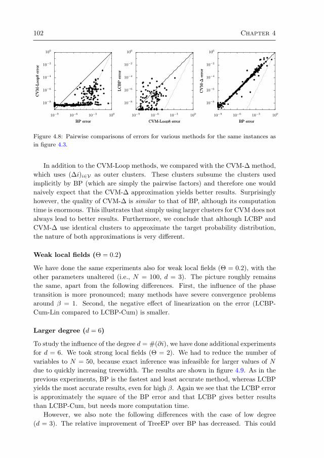
102 Chapter 4
10−8
10−6
10−4
10−2
100
CV
M-L
oop8
erro
rC
VM
-Loo
p8er
ror
10−9 10−6 10−3 100
BP errorBP error
10−8
10−6
10−4
10−2
100
LC
BP
erro
rLC
BP
erro
r10−9 10−6 10−3 100
CVM-Loop8 errorCVM-Loop8 error
10−8
10−6
10−4
10−2
100
CV
M-∆
erro
rC
VM
-∆er
ror
10−9 10−6 10−3 100
BP errorBP error
Figure 4.8: Pairwise comparisons of errors for various methods for the same instances as
in figure 4.3.
In addition to the CVM-Loop methods, we compared with the CVM-∆ method,which uses (∆i)i∈V as outer clusters. These clusters subsume the clusters usedimplicitly by BP (which are simply the pairwise factors) and therefore one wouldnaively expect that the CVM-∆ approximation yields better results. Surprisinglyhowever, the quality of CVM-∆ is similar to that of BP, although its computationtime is enormous. This illustrates that simply using larger clusters for CVM does notalways lead to better results. Furthermore, we conclude that although LCBP andCVM-∆ use identical clusters to approximate the target probability distribution,the nature of both approximations is very different.
Weak local fields (Θ = 0.2)
We have done the same experiments also for weak local fields (Θ = 0.2), with theother parameters unaltered (i.e., N = 100, d = 3). The picture roughly remainsthe same, apart from the following differences. First, the influence of the phasetransition is more pronounced; many methods have severe convergence problemsaround β = 1. Second, the negative effect of linearization on the error (LCBP-Cum-Lin compared to LCBP-Cum) is smaller.
Larger degree (d = 6)
To study the influence of the degree d = #(∂i), we have done additional experimentsfor d = 6. We took strong local fields (Θ = 2). We had to reduce the number ofvariables to N = 50, because exact inference was infeasible for larger values of Ndue to quickly increasing treewidth. The results are shown in figure 4.9. As in theprevious experiments, BP is the fastest and least accurate method, whereas LCBPyields the most accurate results, even for high β. Again we see that the LCBP erroris approximately the square of the BP error and that LCBP gives better resultsthan LCBP-Cum, but needs more computation time.
However, we also note the following differences with the case of low degree(d = 3). The relative improvement of TreeEP over BP has decreased. This could

Chapter 4. Loop Corrections 103
10−8
10−6
10−4
10−2
100M
ax.er
ror
Max
.er
ror
0.01 0.1 1 10
ββ
0.001
0.01
0.1
1
10
100
Tim
e(s
)T
ime
(s)
0.01 0.1 1 10
ββ
0
0.25
0.5
0.75
1
Frac
tion
ofco
nver
ged
inst
ance
sFr
acti
onof
conv
erge
din
stan
ces
0.01 0.1 1 10
ββ
BP TreeEP LCBP-Cum-Lin LCBP-CumLCBP CVM-Loop4
10−8
10−6
10−4
10−2
100
LC
BP
erro
rLC
BP
erro
r
10−9 10−6 10−3 100
BP errorBP error
10−8
10−6
10−4
10−2
100
LC
BP
erro
rLC
BP
erro
r
10−9 10−6 10−3 100
LCBP-Cum errorLCBP-Cum error
10−8
10−6
10−4
10−2
100
LC
BP
-Cum
-Lin
erro
rLC
BP
-Cum
-Lin
erro
r10−9 10−6 10−3 100
LCBP-Cum errorLCBP-Cum error
Figure 4.9: Selected results for (N = 50, d = 6) regular random graphs with strong local
fields Θ = 2. The averaged results for LCBP-Cum and LCBP-Cum-Lin nearly coincide
for β . 1.
have been expected, because in denser networks, the effect of taking out a treebecomes less.
Further, the relative improvement of CVM-Loop4 over BP has increased, prob-ably because there are more short loops present. On the other hand, computationtime of CVM-Loop4 has also increased and it is the slowest of all methods. Wedecided to abort the calculations for CVM-Loop6 and CVM-Loop8, because com-putation time was prohibitive due to the enormous amount of short loops present.We conclude that the CVM-Loop approach to loop correction is not very efficientif there are many loops present.
Surprisingly, the results of LCBP-Cum-Lin are now very similar in quality tothe results of LCBP-Cum, except for a few isolated cases (presumably on the edgeof the convergence region).
Scaling with N
We have investigated how computation time and error scale with the number ofvariables N , for fixed β = 0.1, Θ = 2 and d = 6. We used a machine with morememory (16 GB) to be able to do exact inference without swapping also for N = 60.
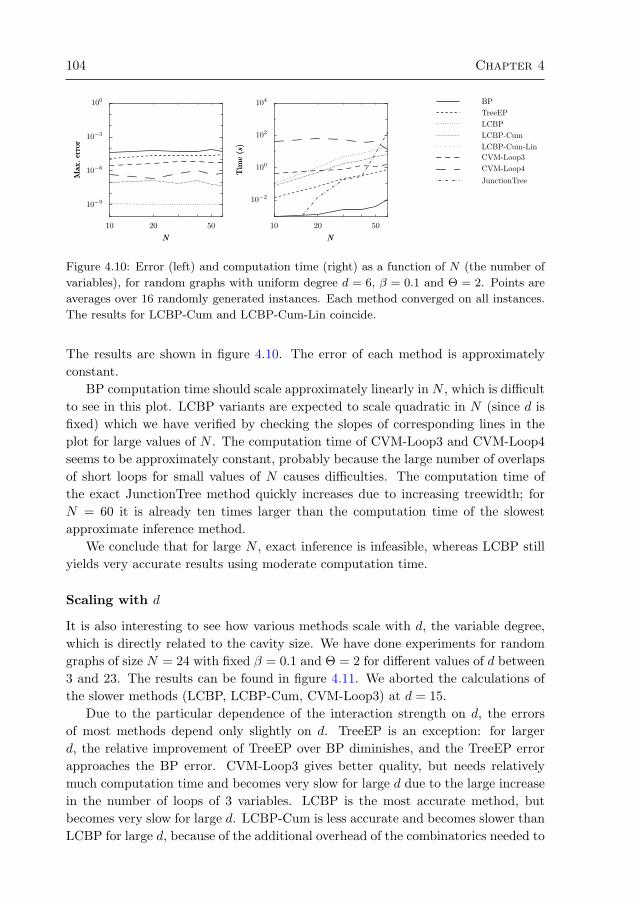
104 Chapter 4
10−9
10−6
10−3
100
Max
.er
ror
Max
.er
ror
10 20 50
NN
10−2
100
102
104
Tim
e(s
)T
ime
(s)
10 20 50
NN
BPTreeEPLCBPLCBP-CumLCBP-Cum-LinCVM-Loop3CVM-Loop4JunctionTree
Figure 4.10: Error (left) and computation time (right) as a function of N (the number of
variables), for random graphs with uniform degree d = 6, β = 0.1 and Θ = 2. Points are
averages over 16 randomly generated instances. Each method converged on all instances.
The results for LCBP-Cum and LCBP-Cum-Lin coincide.
The results are shown in figure 4.10. The error of each method is approximatelyconstant.
BP computation time should scale approximately linearly in N , which is difficultto see in this plot. LCBP variants are expected to scale quadratic in N (since d isfixed) which we have verified by checking the slopes of corresponding lines in theplot for large values of N . The computation time of CVM-Loop3 and CVM-Loop4seems to be approximately constant, probably because the large number of overlapsof short loops for small values of N causes difficulties. The computation time ofthe exact JunctionTree method quickly increases due to increasing treewidth; forN = 60 it is already ten times larger than the computation time of the slowestapproximate inference method.
We conclude that for large N , exact inference is infeasible, whereas LCBP stillyields very accurate results using moderate computation time.
Scaling with d
It is also interesting to see how various methods scale with d, the variable degree,which is directly related to the cavity size. We have done experiments for randomgraphs of size N = 24 with fixed β = 0.1 and Θ = 2 for different values of d between3 and 23. The results can be found in figure 4.11. We aborted the calculations ofthe slower methods (LCBP, LCBP-Cum, CVM-Loop3) at d = 15.
Due to the particular dependence of the interaction strength on d, the errorsof most methods depend only slightly on d. TreeEP is an exception: for largerd, the relative improvement of TreeEP over BP diminishes, and the TreeEP errorapproaches the BP error. CVM-Loop3 gives better quality, but needs relativelymuch computation time and becomes very slow for large d due to the large increasein the number of loops of 3 variables. LCBP is the most accurate method, butbecomes very slow for large d. LCBP-Cum is less accurate and becomes slower thanLCBP for large d, because of the additional overhead of the combinatorics needed to
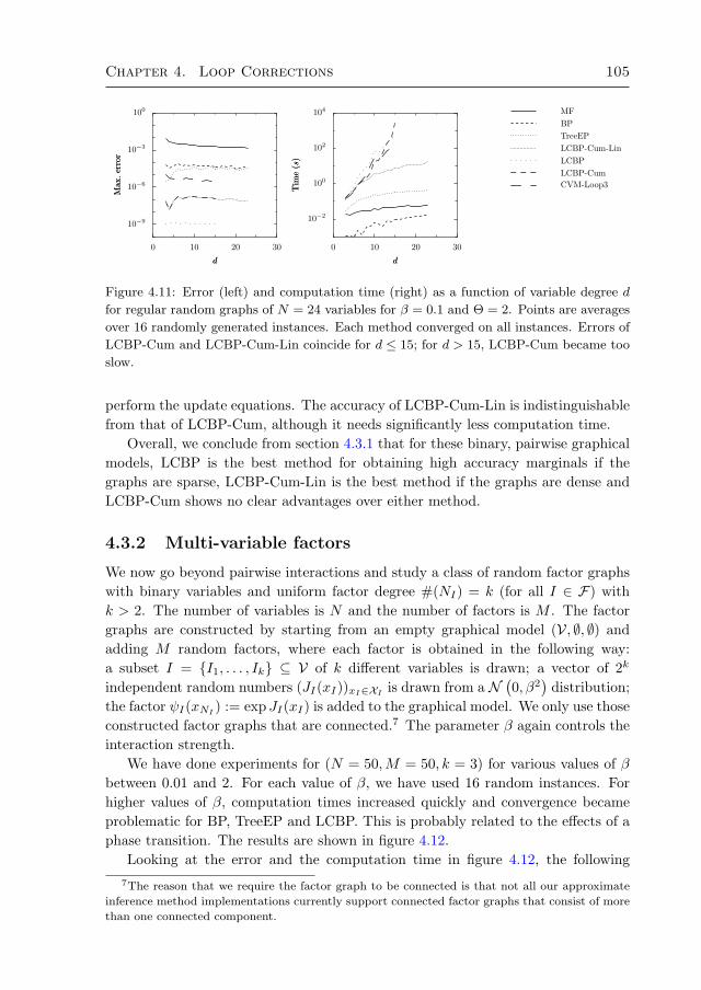
Chapter 4. Loop Corrections 105
10−9
10−6
10−3
100
Max
.er
ror
Max
.er
ror
0 10 20 30
dd
10−2
100
102
104
Tim
e(s
)T
ime
(s)
0 10 20 30
dd
MFBPTreeEPLCBP-Cum-LinLCBPLCBP-CumCVM-Loop3
Figure 4.11: Error (left) and computation time (right) as a function of variable degree d
for regular random graphs of N = 24 variables for β = 0.1 and Θ = 2. Points are averages
over 16 randomly generated instances. Each method converged on all instances. Errors of
LCBP-Cum and LCBP-Cum-Lin coincide for d ≤ 15; for d > 15, LCBP-Cum became too
slow.
perform the update equations. The accuracy of LCBP-Cum-Lin is indistinguishablefrom that of LCBP-Cum, although it needs significantly less computation time.
Overall, we conclude from section 4.3.1 that for these binary, pairwise graphicalmodels, LCBP is the best method for obtaining high accuracy marginals if thegraphs are sparse, LCBP-Cum-Lin is the best method if the graphs are dense andLCBP-Cum shows no clear advantages over either method.
4.3.2 Multi-variable factors
We now go beyond pairwise interactions and study a class of random factor graphswith binary variables and uniform factor degree #(NI) = k (for all I ∈ F) withk > 2. The number of variables is N and the number of factors is M . The factorgraphs are constructed by starting from an empty graphical model (V, ∅, ∅) andadding M random factors, where each factor is obtained in the following way:a subset I = I1, . . . , Ik ⊆ V of k different variables is drawn; a vector of 2k
independent random numbers (JI(xI))xI∈XI is drawn from a N (0, β2)
distribution;the factor ψI(xNI ) := expJI(xI) is added to the graphical model. We only use thoseconstructed factor graphs that are connected.7 The parameter β again controls theinteraction strength.
We have done experiments for (N = 50,M = 50, k = 3) for various values of βbetween 0.01 and 2. For each value of β, we have used 16 random instances. Forhigher values of β, computation times increased quickly and convergence becameproblematic for BP, TreeEP and LCBP. This is probably related to the effects of aphase transition. The results are shown in figure 4.12.
Looking at the error and the computation time in figure 4.12, the following7The reason that we require the factor graph to be connected is that not all our approximate
inference method implementations currently support connected factor graphs that consist of more
than one connected component.
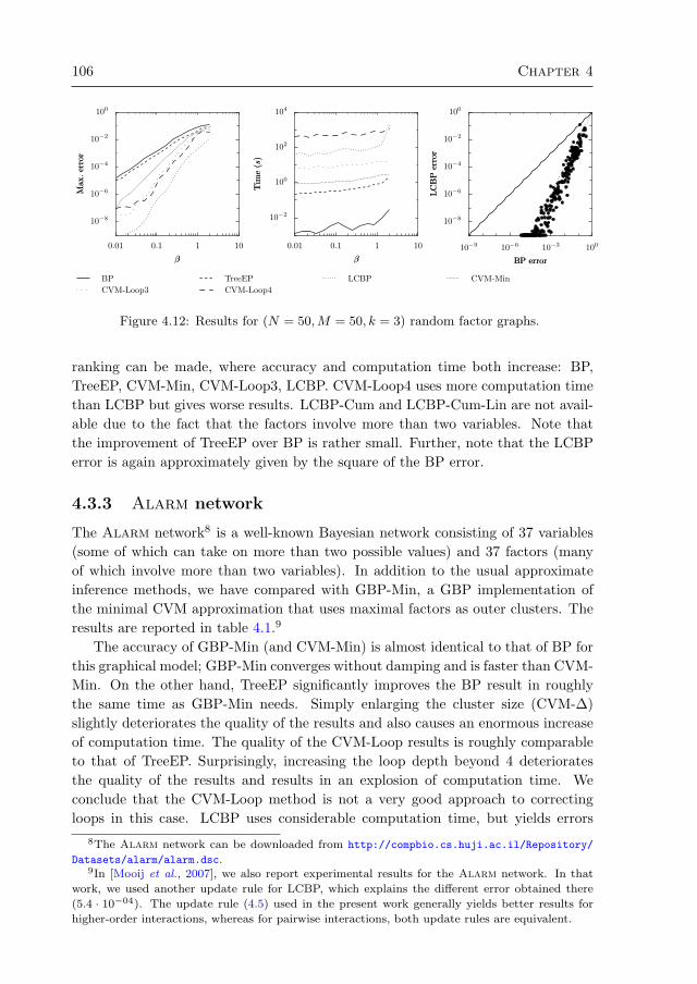
106 Chapter 4
10−8
10−6
10−4
10−2
100
Max
.er
ror
Max
.er
ror
0.01 0.1 1 10
ββ
10−2
100
102
104
Tim
e(s
)T
ime
(s)
0.01 0.1 1 10
ββ
10−8
10−6
10−4
10−2
100
LC
BP
erro
rLC
BP
erro
r
10−9 10−6 10−3 100
BP errorBP error
BP TreeEP LCBP CVM-MinCVM-Loop3 CVM-Loop4
Figure 4.12: Results for (N = 50,M = 50, k = 3) random factor graphs.
ranking can be made, where accuracy and computation time both increase: BP,TreeEP, CVM-Min, CVM-Loop3, LCBP. CVM-Loop4 uses more computation timethan LCBP but gives worse results. LCBP-Cum and LCBP-Cum-Lin are not avail-able due to the fact that the factors involve more than two variables. Note thatthe improvement of TreeEP over BP is rather small. Further, note that the LCBPerror is again approximately given by the square of the BP error.
4.3.3 Alarm network
The Alarm network8 is a well-known Bayesian network consisting of 37 variables(some of which can take on more than two possible values) and 37 factors (manyof which involve more than two variables). In addition to the usual approximateinference methods, we have compared with GBP-Min, a GBP implementation ofthe minimal CVM approximation that uses maximal factors as outer clusters. Theresults are reported in table 4.1.9
The accuracy of GBP-Min (and CVM-Min) is almost identical to that of BP forthis graphical model; GBP-Min converges without damping and is faster than CVM-Min. On the other hand, TreeEP significantly improves the BP result in roughlythe same time as GBP-Min needs. Simply enlarging the cluster size (CVM-∆)slightly deteriorates the quality of the results and also causes an enormous increaseof computation time. The quality of the CVM-Loop results is roughly comparableto that of TreeEP. Surprisingly, increasing the loop depth beyond 4 deterioratesthe quality of the results and results in an explosion of computation time. Weconclude that the CVM-Loop method is not a very good approach to correctingloops in this case. LCBP uses considerable computation time, but yields errors
8The Alarm network can be downloaded from http://compbio.cs.huji.ac.il/Repository/
Datasets/alarm/alarm.dsc.9In [Mooij et al., 2007], we also report experimental results for the Alarm network. In that
work, we used another update rule for LCBP, which explains the different error obtained there
(5.4 · 10−04). The update rule (4.5) used in the present work generally yields better results for
higher-order interactions, whereas for pairwise interactions, both update rules are equivalent.
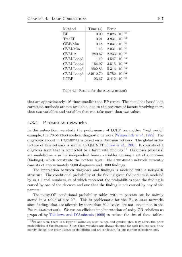
Chapter 4. Loop Corrections 107
Method Time (s) ErrorBP 0.00 2.026 · 10−01
TreeEP 0.21 3.931 · 10−02
GBP-Min 0.18 2.031 · 10−01
CVM-Min 1.13 2.031 · 10−01
CVM-∆ 280.67 2.233 · 10−01
CVM-Loop3 1.19 4.547 · 10−02
CVM-Loop4 154.97 3.515 · 10−02
CVM-Loop5 1802.83 5.316 · 10−02
CVM-Loop6 84912.70 5.752 · 10−02
LCBP 23.67 3.412 · 10−05
Table 4.1: Results for the Alarm network
that are approximately 104 times smaller than BP errors. The cumulant-based loopcorrection methods are not available, due to the presence of factors involving morethan two variables and variables that can take more than two values.
4.3.4 Promedas networks
In this subsection, we study the performance of LCBP on another “real world”example, the Promedas medical diagnostic network [Wiegerinck et al., 1999]. Thediagnostic model in Promedas is based on a Bayesian network. The global archi-tecture of this network is similar to QMR-DT [Shwe et al., 1991]. It consists of adiagnosis layer that is connected to a layer with findings.10 Diagnoses (diseases)are modeled as a priori independent binary variables causing a set of symptoms(findings), which constitute the bottom layer. The Promedas network currentlyconsists of approximately 2000 diagnoses and 1000 findings.
The interaction between diagnoses and findings is modeled with a noisy-ORstructure. The conditional probability of the finding given the parents is modeledby m + 1 real numbers, m of which represent the probabilities that the finding iscaused by one of the diseases and one that the finding is not caused by any of theparents.
The noisy-OR conditional probability tables with m parents can be naivelystored in a table of size 2m. This is problematic for the Promedas networkssince findings that are affected by more than 30 diseases are not uncommon in thePromedas network. We use an efficient implementation of noisy-OR relations asproposed by Takikawa and D’Ambrosio [1999] to reduce the size of these tables.
10In addition, there is a layer of variables, such as age and gender, that may affect the prior
probabilities of the diagnoses. Since these variables are always clamped for each patient case, they
merely change the prior disease probabilities and are irrelevant for our current considerations.

108 Chapter 4
The trick is to introduce dummy variables s and to make use of the property
OR(x|y1, y2, y3) =∑s
OR(x|y1, s)OR(s|y2, y3).
The factors on the right hand side involve at most 3 variables instead of the initial 4(left). Repeated application of this formula reduces all factors to triple interactionsor smaller.
When a patient case is presented to Promedas, a subset of the findings will beclamped and the rest will be unclamped. If our goal is to compute the marginalprobabilities of the diagnostic variables only, the unclamped findings and the diag-noses that are not related to any of the clamped findings can be summed out ofthe network as a preprocessing step. The clamped findings cause an effective inter-action between their parents. However, the noisy-OR structure is such that whenthe finding is clamped to a negative value, the effective interaction factorizes overits parents. Thus, findings can be clamped to negative values without additionalcomputation cost [Jaakkola and Jordan, 1999].
The complexity of the problem now depends on the set of findings that is givenas input. The more findings are clamped to a positive value, the larger the remain-ing network of disease variables and the more complex the inference task. Especiallyin cases where findings share more than one common possible diagnosis, and con-sequently loops occur, the model can become complex.
We use the Promedas model to generate virtual patient data by first clampingone of the disease variables to be positive and then clamping each finding to itspositive value with probability equal to the conditional distribution of the finding,given the positive disease. The union of all positive findings thus obtained constituteone patient case. For each patient case, the corresponding truncated graphicalmodel is generated. The number of disease nodes in this truncated graph is typicallyquite large.
The results can be found in figures 4.13 and 4.14. Surprisingly, neither TreeEPnor any of the CVM methods gives substantial improvements over BP. TreeEP evengives worse results compared to BP. The CVM-Min and CVM-Loop3 results appearto be almost identical to the BP results. CVM-Loop4 manages to improve over BPin a few cases. Increased loop depth (k = 5, 6) results in worse quality in manycases and also in an enormous increase in computation time.
LCBP, on the other hand, is the only method that gives a significant improve-ment over BP, in each case. Considering all patient cases, LCBP corrects the BPerror with more than one order of magnitude in half of the cases for which BP wasnot already exact. The improvement obtained by LCBP has its price: the com-putation time of LCBP is rather large compared to that of BP, as shown in figure4.14. In many cases, this is due to a few rather large cavities. The cumulant-basedloop correction methods are not available, due to the presence of factors involvingmore than two variables.
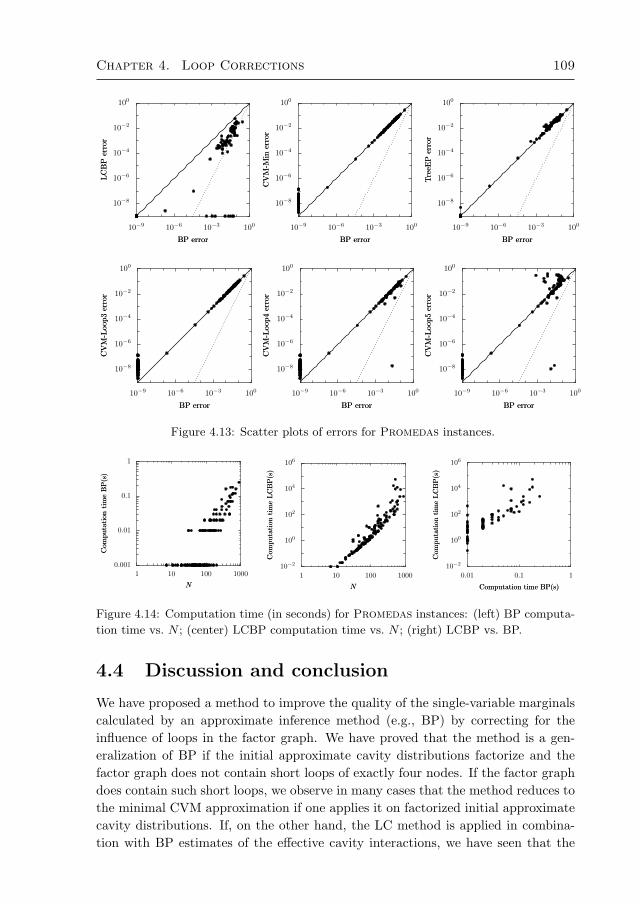
Chapter 4. Loop Corrections 109
10−8
10−6
10−4
10−2
100LC
BP
erro
rLC
BP
erro
r
10−9 10−6 10−3 100
BP errorBP error
10−8
10−6
10−4
10−2
100
CV
M-M
iner
ror
CV
M-M
iner
ror
10−9 10−6 10−3 100
BP errorBP error
10−8
10−6
10−4
10−2
100
Tre
eEP
erro
rTre
eEP
erro
r
10−9 10−6 10−3 100
BP errorBP error
10−8
10−6
10−4
10−2
100
CV
M-L
oop3
erro
rC
VM
-Loo
p3er
ror
10−9 10−6 10−3 100
BP errorBP error
10−8
10−6
10−4
10−2
100C
VM
-Loo
p4er
ror
CV
M-L
oop4
erro
r
10−9 10−6 10−3 100
BP errorBP error
10−8
10−6
10−4
10−2
100
CV
M-L
oop5
erro
rC
VM
-Loo
p5er
ror
10−9 10−6 10−3 100
BP errorBP error
Figure 4.13: Scatter plots of errors for Promedas instances.
0.001
0.01
0.1
1
Com
puta
tion
tim
eB
P(s
)C
ompu
tati
onti
me
BP
(s)
1 10 100 1000
NN
10−2
100
102
104
106
Com
puta
tion
tim
eLC
BP
(s)
Com
puta
tion
tim
eLC
BP
(s)
1 10 100 1000
NN
10−2
100
102
104
106
Com
puta
tion
tim
eLC
BP
(s)
Com
puta
tion
tim
eLC
BP
(s)
0.01 0.1 1
Computation time BP(s)Computation time BP(s)
Figure 4.14: Computation time (in seconds) for Promedas instances: (left) BP computa-
tion time vs. N ; (center) LCBP computation time vs. N ; (right) LCBP vs. BP.
4.4 Discussion and conclusion
We have proposed a method to improve the quality of the single-variable marginalscalculated by an approximate inference method (e.g., BP) by correcting for theinfluence of loops in the factor graph. We have proved that the method is a gen-eralization of BP if the initial approximate cavity distributions factorize and thefactor graph does not contain short loops of exactly four nodes. If the factor graphdoes contain such short loops, we observe in many cases that the method reduces tothe minimal CVM approximation if one applies it on factorized initial approximatecavity distributions. If, on the other hand, the LC method is applied in combina-tion with BP estimates of the effective cavity interactions, we have seen that the
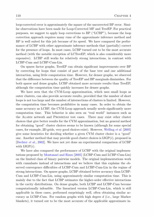
110 Chapter 4
loop-corrected error is approximately the square of the uncorrected BP error. Simi-lar observations have been made for Loop-Corrected MF and TreeEP. For practicalpurposes, we suggest to apply loop corrections to BP (“LCBP”), because the loopcorrection approach requires many runs of the approximate inference method andBP is well suited for this job because of its speed. We have compared the perfor-mance of LCBP with other approximate inference methods that (partially) correctfor the presence of loops. In most cases, LCBP turned out to be the most accuratemethod (with the notable exception of LCTreeEP, which is also considerably moreexpensive). LCBP still works for relatively strong interactions, in contrast withLCBP-Cum and LCBP-Cum-Lin.
On sparse factor graphs, TreeEP can obtain significant improvements over BPby correcting for loops that consist of part of the base tree and one additionalinteraction, using little computation time. However, for denser graphs, we observedthat the difference between the quality of TreeEP and BP marginals diminishes. Forboth sparse and dense graphs, LCBP obtained more accurate results than TreeEP,although the computation time quickly increases for denser graphs.
We have seen that the CVM-Loop approximation, which uses small loops asouter clusters, can also provide accurate results, provided that the number of shortloops is not too large and the number of intersections of clusters is limited. However,the computation time becomes prohibitive in many cases. In order to obtain thesame accuracy as LCBP, the CVM-Loop approach usually needs significantly morecomputation time. This behavior is also seen on “real world” instances such asthe Alarm network and Promedas test cases. There may exist other clusterchoices that give better results for the CVM approximation, but no general methodfor obtaining “good” cluster choices seems to be known (although for some specialcases, for example, 2D grids, very good choices exist). However, Welling et al. [2005]give some heuristics for deciding whether a given CVM cluster choice is a “good”one. Another method that may provide good cluster choices is IJGP(i), proposed in[Dechter et al., 2002]. We have not yet done an experimental comparison of LCBPwith IJGP(i).
We have also compared the performance of LCBP with the original implemen-tations proposed by Montanari and Rizzo [2005] (LCBP-Cum and LCBP-Cum-Lin)on the limited class of binary pairwise models. The original implementations workwith cumulants instead of interactions and we believe that this explains the ob-served convergence difficulties of LCBP-Cum and LCBP-Cum-Lin in the regime ofstrong interactions. On sparse graphs, LCBP obtained better accuracy than LCBP-Cum and LCBP-Cum-Lin, using approximately similar computation time. This ismainly due to the fact that LCBP estimates the higher-order effective interactionsin the cavity distributions. On dense graphs, both LCBP and LCBP-Cum becomecomputationally infeasible. The linearized version LCBP-Cum-Lin, which is stillapplicable in these cases, performed surprisingly well, often obtaining similar ac-curacy as LCBP-Cum. For random graphs with high degree d (i.e., large Markovblankets), it turned out to be the most accurate of the applicable approximate in-
Chapter 4. Loop Corrections 111
ference methods. It is rather fortunate that the negative effect of the linearizationerror on the accuracy of the result becomes smaller as the degree increases, since itis precisely for high degree where one needs the linearization because of performanceissues.
In the experiments reported here, the standard JunctionTree method was almostalways faster than LCBP. The reason is that we have intentionally selected experi-ments for which exact inference is still feasible, in order to be able to compare thequality of various approximate inference methods. However, as implied by figure4.10, there is no reason to expect that LCBP will suddenly give inaccurate resultswhen exact inference is no longer feasible. Thus we suggest that LCBP may beused to obtain accurate marginal estimates in cases where exact inference is impos-sible because of high treewidth. As illustrated in figure 4.10, the computation timeof LCBP scales very different from that of the JunctionTree method: whereas thelatter is exponential in treewidth, LCBP is exponential in the size of the Markovblankets.
The fact that computation time of LCBP (in its current form) scales exponen-tially with the size of the Markov blankets can be a severe limitation in practice.Many real world Bayesian networks have large Markov blankets, prohibiting appli-cation of LCBP. The linear cumulant-based implementation LCBP-Cum-Lin doesnot suffer from this problem, as it is quadratic in the size of the Markov blankets.Unfortunately, this particular implementation can in its current form only be ap-plied to graphical models that consist of binary variables and factors that involveat most two variables (which excludes any interesting Bayesian network, for exam-ple). Furthermore, problems may arise if some factors contain zeros. For generalapplication of loop correction methods, it will be of paramount importance to de-rive an implementation that combines the generality of LCBP with the speed ofLCBP-Cum-Lin. This topic will be left for future research. The work presentedhere provides some intuition that may be helpful for constructing a general and fastloop correction method that is applicable to arbitrary factor graphs that can havelarge Markov blankets.
Another important direction for future research would be to find an extensionof the loop correction framework that also gives a loop-corrected approximation ofthe normalization constant Z in (4.1). Additionally, and possibly related to that, itwould be desirable to find an approximate “free energy”, a function of the beliefs,whose stationary points coincide with the fixed points of Algorithm 4.1. This can bedone for many approximate inference methods (MF, BP, CVM, EP) so it is naturalto expect that the LC algorithm can also be seen as a minimization procedure ofa certain approximate free energy. Despite some efforts, we have not yet been ableto find such a free energy.
Recently, other loop correction approaches to the Bethe approximation havebeen proposed in the statistical physics literature [Parisi and Slanina, 2006; Chert-kov and Chernyak, 2006b]. In particular, Chertkov and Chernyak [2006b] havederived a series expansion of the exact normalizing constant Z in terms of the BP
112 Chapter 4
solution. The first term of the series is precisely the Bethe free energy evaluatedat the BP fixed point. The number of terms in the series is finite, but can be verylarge, even larger than the number of total states of the graphical model. Each termis associated with a “generalized loop”, which is a subgraph of the factor graph forwhich each node has at least connectivity two. By truncating the series, it is pos-sible to obtain approximate solutions that improve on BP by taking into account asubset of all generalized loops [Gomez et al., 2007; Chertkov and Chernyak, 2006a].Summarizing, the approach to loop corrections by Chertkov and Chernyak [2006b]takes a subset of loops into account in an exact way, whereas the loop correctionapproach presented in this chapter takes all loops into account in an approximateway. More experiments should be done to compare both approaches.
Summarizing, we have proposed a method to correct approximate inferencemethods for the influence of loops in the factor graph. We have shown that it canobtain very accurate results, also on real world graphical models, outperformingexisting approximate inference methods in terms of quality, robustness or applica-bility. We have shown that it can be applied to problems for which exact inferenceis infeasible. The rather large computation time required is an issue which deservesfurther consideration; it may be possible to use additional approximations on topof the loop correction framework that trade quality for computation time.
Acknowledgments
We thank Bastian Wemmenhove for stimulating discussions and for providing thePromedas test cases.
4.A Original approach by Montanari and Rizzo
(2005)
For completeness, we describe the implementation based on cumulants as originallyproposed by Montanari and Rizzo [2005]. The approach can be applied in recursivefashion. Here we will only discuss the first recursion level.
Consider a graphical model which has only binary (±1-valued) variables andfactors that involve at most two variables. The corresponding probability distri-bution can be parameterized in terms of the local fields (θi)i∈V and the couplings(Jij = Jji)i∈V,j∈∂i:
P(x) =1Z
exp
∑i∈V
θixi +12
∑i∈V
∑j∈∂i
Jijxixj
.
Let i ∈ V and consider the corresponding cavity network of i. For A ⊆ ∂i, thecavity moment M\iA is defined as the following expectation value under the cavity

Chapter 4. Loop Corrections 113
distribution:
M\iA :=
∑x∂i
Z\i(x∂i)∏j∈A
xj∑x∂i
Z\i(x∂i),
where we will not explicitly distinguish between approximate and exact quantities,following the physicists’ tradition.11 The cavity cumulants (also called “connectedcorrelations”) C\iA are related to the moments in the following way:
M\iA =∑
B∈Part(A)
∏E∈BC\iE
where Part(A) is the set of partitions of A.We introduce some notation: we define for A ⊆ ∂i:
tiA :=∏k∈A
tanh Jik.
Further, for a set X, we denote the even subsets of X as P+(X) := Y ⊆ X :#(Y ) is even and the odd subsets of X as P−(X) := Y ⊆ X : #(Y ) is odd.
Using standard algebraic manipulations, one can show that for j ∈ ∂i, theexpectation value of xj in the absence of the interaction ψij = exp(Jijxixj) can beexpressed in terms of cavity moments of i as follows:∑
A∈P+(∂i\j)tiAM\iA∪j + tanh θi
∑A∈P−(∂i\j)
tiAM\iA∪j∑A∈P+(∂i\j)
tiAM\iA + tanh θi∑
A∈P−(∂i\j)tiAM\iA
. (4.10)
On the other hand, the same expectation value can also be expressed in terms ofcavity moments of j as follows:
tanh θj∑
B∈P+(∂j\i)tjBM\jB +
∑B∈P−(∂j\i)
tjBM\jB∑B∈P+(∂j\i)
tjBM\jB + tanh θj∑
B∈P−(∂j\i)tjBM\jB
. (4.11)
The consistency equations are now given by equating (4.10) to (4.11) for all i ∈ V,j ∈ ∂i.
The expectation value of xi (in the presence of all interactions) can be similarlyexpressed in terms of cavity moments of i:
Mi :=∑xi=±1
P(xi)xi =
tanh θi∑
A∈P+(∂i)
tiAM\iA +∑
A∈P−(∂i)
tiAM\iA∑A∈P+(∂i)
tiAM\iA + tanh θi∑
A∈P−(∂i)
tiAM\iA. (4.12)
11In [Montanari and Rizzo, 2005], the notation C(i)A is used for the cavity moment M\iA .

114 Chapter 4
4.A.1 Neglecting higher-order cumulants
Montanari and Rizzo proceed by neglecting cavity cumulants C\iA with #(A) > 2.Denote by Part2(A) the set of all partitions of A into subsets which have cardinality2 at most. Thus, neglecting higher-order cavity cumulants amounts to the followingapproximation:
M\iA ≈∑
B∈Part2(A)
∏E∈BC\iE . (4.13)
By some algebraic manipulations, one can express the consistency equation (4.10) =(4.11) in this approximation as follows:
M\ij =
tanh θj∑
B∈P+(∂j\i)tjBM\jB +
∑B∈P−(∂j\i)
tjBM\jB∑B∈P+(∂j\i)
tjBM\jB + tanh θj∑
B∈P−(∂j\i)tjBM\jB
−∑
k∈∂i\jtikC\ijk
tanh θi∑
A∈P+(∂i\j,k)tiAM\iA +
∑A∈P−(∂i\j,k)
tiAM\iA∑A∈P+(∂i\j)
tiAM\iA + tanh θi∑
A∈P−(∂i\j)tiAM\iA
. (4.14)
One can use (4.13) to write (4.14) in terms of the singleton cumulants (M\ij )i∈V,j∈∂iand the pair cumulants (C\ijk)i∈V,j∈∂i,k∈∂i\j . Given (estimates of) the pair cumu-lants, the consistency equations (4.14) are thus fixed point equations in the singletoncumulants. The procedure is now:
• Estimate the pair cumulants (C\ijk)i∈V,j∈∂i,k∈∂i\j using BP in combinationwith linear response (called “Response Propagation” in [Montanari and Rizzo,2005]).
• Calculate the fixed point (M\ij )i∈V,j∈∂i of (4.14) using the estimated paircumulants.
• Use (4.12) in combination with (4.13) to calculate the final expectation values(Mj)j∈V using the estimated pair cumulants and the fixed point of (4.14).
4.A.2 Linearized version
The update equations can be linearized by expanding up to first order in the paircumulants C\ijk. This yields the following linearized consistency equation [Montanariand Rizzo, 2005]:
M\ij = T\ji −
∑l∈∂i\j
Ω\ij,ltilC\ijl +∑
l1,l2∈∂j\il1<l2
Γ\ji,l1l2tjl1tjl2C\jl1l2
(4.15)

Chapter 4. Loop Corrections 115
where
T\iA := tanh
θi +∑
k∈∂i\Atanh−1(tikM\ik )
,
Ω\ij,l :=T\ijl
1 + tilM\il T\ijl
,
Γ\ji,l1l2 :=T\jil1l2− T \ji
1 + tjl1tjl2M\jl1M\jl2
+ tjl1M\jl1 T\jil1l2
+ tjl2M\jl2 T\jil1l2
.
The final magnetizations (4.12) are, up to first order in the pair cumulants:
Mj = T \j +∑
l1,l2∈∂jl1<l2
Γ\jl1l2tjl1tjl2C\jl1l2
+O(C2)
where
Γ\jl1l2 :=T\jl1l2− T \j
1 + tjl1tjl2M\jl1M\jl2 + tjl1M\jl1 T
\jl1l2
+ tjl2M\jl2 T\jl1l2
.

116 Chapter 4

Chapter 5. Novel bounds on marginal probabilities 117
Chapter 5
Novel bounds on marginal
probabilities
We derive two related novel bounds on single-variable marginal probability distribu-
tions in factor graphs with discrete variables. The first method propagates bounds
over a subtree of the factor graph rooted in the variable, and the second method
propagates bounds over the self-avoiding walk tree starting at the variable. By con-
struction, both methods not only bound the exact marginal probability distribu-
tion of a variable, but also its approximate Belief Propagation marginal (“belief”).
Thus, apart from providing a practical means to calculate bounds on marginals,
our contribution also lies in an increased understanding of the error made by Be-
lief Propagation. Empirically, we show that our bounds often outperform existing
bounds in terms of accuracy and/or computation time. We also show that our
bounds can yield nontrivial results for medical diagnosis inference problems.
5.1 Introduction
Graphical models are used in many different fields. A fundamental problem in theapplication of graphical models is that exact inference is NP-hard [Cooper, 1990].In recent years, much research has focused on approximate inference techniques,such as sampling methods and deterministic approximation methods, e.g., BeliefPropagation (BP) [Pearl, 1988]. Although the approximations obtained by thesemethods can be very accurate, there are only few guarantees on the error of theapproximation, and often it is not known (without comparing with the exact solu-tion) how accurate an approximate result is. Thus it is desirable to calculate, in
The material in this chapter has been submitted to the Journal of Machine Learning Research.
A preprint is available as [Mooij and Kappen, 2008].

118 Chapter 5
addition to the approximate results, tight bounds on the approximation error. Ex-isting methods to calculate bounds on marginals include [Tatikonda, 2003; Leisinkand Kappen, 2003; Taga and Mase, 2006a; Ihler, 2007]. Also, upper bounds on thepartition sum, e.g., [Jaakkola and Jordan, 1996; Wainwright et al., 2005], can becombined with lower bounds on the partition sum, such as the well-known meanfield bound or higher-order lower bounds [Leisink and Kappen, 2001], to obtainbounds on marginals.
In this chapter, we derive novel bounds on exact single-variable marginals infactor graphs. The original motivation for this work was to better understandand quantify the BP error. This has lead to bounds which are at the same timebounds for the exact single-variable marginals as well as for the BP beliefs. Aparticularly nice feature of the bounds is that their computational cost is relativelylow, provided that the number of possible values of each variable in the factorgraph is small. Unfortunately, the computation time is exponential in the numberof possible values of the variables, which limits application to factor graphs inwhich each variable has a low number of possible values. On these factor graphshowever, our bounds perform exceedingly well and we show empirically that theyoutperform the state-of-the-art in a variety of factor graphs, including real-worldproblems arising in medical diagnosis.
This chapter is organized as follows. In the next section, we derive our novelbounds. In section 5.3, we discuss related work. In section 5.4 we present experi-mental results. We conclude with conclusions and a discussion in section 5.5.
5.2 Theory
In this work, we consider graphical models such as Markov random fields andBayesian networks. We use the unifying factor graph representation [Kschischanget al., 2001]. In the first subsection, we introduce our notation and some basicdefinitions concerning factor graphs. Then, we shortly remind the reader of somebasic facts about convexity. After that, we introduce some notation and conceptsfor measures on subsets of variables. We proceed with a subsection that considersthe interplay between convexity and the operations of normalization and multipli-cation. In the next subsection, we introduce “(smallest bounding) boxes” that willbe used to describe sets of measures in a convenient way. Then, we formulate thebasic lemma that will be used to obtain bounds on marginals. We illustrate thebasic lemma with two simple examples. Then we formulate our first result, an al-gorithm for propagating boxes over a subtree of the factor graph, which results ina bound on the marginal of the root variable of the subtree. In the last subsection,we show how one can go deeper into the computation tree and derive our secondresult, an algorithm for propagating boxes over self-avoiding walk trees. The resultof that algorithm is a bound on the marginal of the root variable (starting point)of the self-avoiding walk tree. For the special case where all factors in the factorgraph depend on two variables at most (“pairwise interactions”), our first result

Chapter 5. Novel bounds on marginal probabilities 119
is equivalent to a truncation of the second one. This is not true for higher-orderinteractions, however.
5.2.1 Factor graphs
Let V := 1, . . . , N and consider N discrete random variables (xi)i∈V . Each vari-able xi takes values in a discrete domain Xi. We will frequently use the followingmulti-index notation. Let A = i1, i2, . . . , im ⊆ V with i1 < i2 < . . . im. We writeXA := Xi1 ×Xi2 × · · · × Xim and for any family (Yi)i∈B with A ⊆ B ⊆ V, we writeYA := (Yi1 , Yi2 , . . . , Yim).
We consider a probability distribution over x = (x1, . . . , xN ) ∈ XV that can bewritten as a product of factors (also called “interactions”) (ψI)I∈F :
P(x) =1Z
∏I∈F
ψI(xNI ), Z =∑x∈XV
∏I∈F
ψI(xNI ). (5.1)
For each factor index I ∈ F , there is an associated subset NI ⊆ V of variable indicesand the factor ψI is a nonnegative function ψI : XNI → [0,∞). For a Bayesiannetwork, the factors are (conditional) probability tables. In case of Markov randomfields, the factors are often called potentials.1 In the following, we will use lowercasefor variable indices and uppercase for factor indices.
In general, the normalizing constant Z is not known and exact computation of Zis infeasible, due to the fact that the number of terms to be summed is exponentialin N . Similarly, computing marginal distributions P(xA) for subsets of variablesA ⊆ V is intractable in general. In this chapter, we focus on the task of obtainingrigorous bounds on single-variable marginals P(xi) =
∑xV\i
P(x).We can represent the structure of the probability distribution (5.1) using a factor
graph (V,F , E). This is a bipartite graph, consisting of variable nodes i ∈ V, factornodes I ∈ F , and edges e ∈ E , with an edge i, I between i ∈ V and I ∈ F ifand only if the factor ψI depends on xi (i.e., if i ∈ NI). We will represent factornodes visually as rectangles and variable nodes as circles. Figure 5.1 shows a simpleexample of a factor graph and the corresponding probability distribution. The set ofneighbors of a factor node I is precisely NI ; similarly, we denote the set of neighborsof a variable node i by Ni := I ∈ F : i ∈ NI. Further, we define for each variablei ∈ V the set ∆i :=
⋃Ni consisting of all variables that appear in some factor in
which variable i participates, and the set ∂i := ∆i \ i, the Markov blanket of i.We will assume throughout this chapter that the factor graph corresponding to
(5.1) is connected. Furthermore, we will assume that
∀I ∈ F ∀i ∈ NI ∀xNI\i ∈ XNI\i :∑xi∈Xi
ψI(xi, xNI\i) > 0.
1Not to be confused with statistical physics terminology, where “potential” refers to − 1β
logψIinstead, with β the inverse temperature.

120 Chapter 5
i
j k
J K
L
P(xi, xj , xk) = 1ZψJ(xi, xj)ψK(xi, xk)ψL(xj , xk)
Z =Xxi∈Xi
Xxj∈Xj
Xxk∈Xk
ψJ(xi, xj)ψK(xi, xk)ψL(xj , xk)
Figure 5.1: Example of a factor graph with three variable nodes (i, j, k), represented as
circles, and three factor nodes (J,K,L), represented as rectangles. The corresponding
random variables are xi, xj , xk; the corresponding factors are ψJ : Xi × Xj → [0,∞),
ψK : Xi × Xk → [0,∞) and ψL : Xj × Xk → [0,∞). The corresponding probability
distribution P(x) is written out on the right.
This will prevent technical problems regarding normalization later on.2
One final remark concerning notation: we will sometimes abbreviate i as i ifno confusion can arise.
5.2.2 Convexity
Let V be a real vector space. For T elements (vt)t=1,...,T of V and T nonnegativenumbers (λt)t=1,...,T with
∑Tt=1 λt = 1, we call
∑Tt=1 λtvt a convex combination of
the (vt)t=1,...,T with weights (λt)t=1,...,T . A subset X ⊆ V is called convex if forall x1, x2 ∈ X and all λ ∈ [0, 1], the convex combination λx1 + (1 − λ)x2 ∈ X.An extreme point of a convex set X is an element x ∈ X which cannot be writtenas a (nontrivial) convex combination of two different points in X. In other words,x ∈ X is an extreme point of X if and only if for all λ ∈ (0, 1) and all x1, x2 ∈ X,x = λx1 + (1 − λ)x2 implies x1 = x2. We denote the set of extreme points of aconvex set X by Ext (X). For a subset Y of the vector space V , we define theconvex hull of Y to be the smallest convex set X ⊆ V with Y ⊆ X; we denote theconvex hull of Y as Hull (Y ).
5.2.3 Measures and operators
For A ⊆ V, defineMA := [0,∞)XA , i.e.,MA is the set of nonnegative functions onXA. MA can be identified with the set of finite measures on XA. We will simplycall the elements of MA “measures on A”. We also define M∗A := MA \ 0. Wewill denote M :=
⋃A⊆VMA and M∗ :=
⋃A⊆VM∗A.
Adding two measures Ψ,Φ ∈ MA results in the measure Ψ + Φ in MA. ForA,B ⊆ V, we can multiply an element ofMA with an element ofMB to obtain anelement of MA∪B ; a special case is multiplication with a scalar. Note that thereis a natural embedding of MA in MB for A ⊆ B ⊆ V obtained by multiplying anelement Ψ ∈ MA by 1B\A ∈ MB\A, the constant function with value 1 on XB\A.
2This condition ensures that if one runs Belief Propagation on the factor graph, the messages
will always remain nonzero, provided that the initial messages are nonzero.

Chapter 5. Novel bounds on marginal probabilities 121
xi = +1
xi = −1
Mi
1
1
Pi Ψ
NΨ
Figure 5.2: Illustration of some concepts in the simple case of a binary random variable
xi ∈ Xi = ±1 and the subset A = i. A measure Ψ ∈Mi can be identified with a point
in the quarter plane as indicated in the figure. A normalized measure can be obtained by
scaling Ψ; the result NΨ is contained in the simplex Pi, a lower-dimensional submanifold
of Mi.
Another important operation is the partial summation: given A ⊆ B ⊆ V andΨ ∈MB , define
∑xA
Ψ to be the measure in MB\A that satisfies(∑xA
Ψ
)(xB\A) =
∑xA∈XA
Ψ(xA, xB\A) ∀xB\A ∈ XB\A.
Also, defining A′ = B\A, we will sometimes write this measure as∑x\A′
Ψ, which isan abbreviation of
∑xB\A′
Ψ. This notation does not make explicit which variablesare summed over (which depends on the measure that is being partially summed),although it shows which variables remain after summation.
In the following, we will implicitly define operations on sets of measures byapplying the operation on elements of these sets and taking the set of the resultingmeasures; e.g., if we have two subsets ΞA ⊆ MA and ΞB ⊆ MB for A,B ⊆ V, wedefine the product of the sets ΞA and ΞB to be the set of the products of elementsof ΞA and ΞB , i.e., ΞAΞB := ΨAΨB : ΨA ∈ ΞA,ΨB ∈ ΞB.
In figure 5.2, the simple case of a binary random variable xi and the subsetA = i is illustrated. Note that in this case, a measure Ψ ∈ Mi can be identifiedwith a point in the quarter plane [0,∞)× [0,∞).
We will define QA to be the set of completely factorized measures on A, i.e.,
QA :=∏a∈AMa =
∏a∈A
Ψa : Ψa ∈Ma for each a ∈ A.
Note thatMA is the convex hull ofQA. Indeed, we can write each measure Ψ ∈MA
as a convex combination of measures in QA; let Z :=∑xA
Ψ and note that
Ψ(x) =∑y∈XA
Ψ(y)Z
(Zδy(x)) ∀x ∈ XA.
122 Chapter 5
For any y ∈ XA, the Kronecker delta function δy ∈MA (which is 1 if its argumentis equal to y and 0 otherwise) is an element of QA because δy(x) =
∏a∈A δya(xa).
We denote Q∗A := QA \ 0.We define the partition sum operator Z : M → [0,∞) which calculates the
partition sum (normalization constant) of a measure, i.e.,
ZΨ :=∑
xA∈XAΨ(xA) for Ψ ∈MA, A ⊆ V.
We denote with PA the set of probability measures on A, i.e., PA = Ψ ∈ MA :ZΨ = 1, and define P :=
⋃A⊆V PA. The set PA is called a simplex (see also
figure 5.2). Note that a simplex is convex; the simplex PA has precisely #(XA)extreme points, each of which corresponds to putting all probability mass on one ofthe possible values of xA.
Define the normalization operator N : M∗ → P which normalizes a measure,i.e.,
NΨ :=1ZΨ
Ψ for Ψ ∈M∗.
Note that Z N = 1. Figure 5.2 illustrates the normalization of a measure in asimple case.
5.2.4 Convex sets of measures
To calculate marginals of subsets of variables in some factor graph, several op-erations performed on measures are relevant: normalization, taking products ofmeasures, and summing over subsets of variables. In this section we study the in-terplay between convexity and these operations; this will turn out to be useful lateron, because our bounds make use of convex sets of measures that are propagatedover the factor graph.
The interplay between normalization and convexity is described by the followingLemma, which is illustrated in figure 5.3.
Lemma 5.1 Let A ⊆ V, T ∈ N∗ and let (ξt)t=1,...,T be elements ofM∗A. Each con-vex combination of the normalized measures (N ξt)t=1,...,T can be written as a nor-malized convex combination of the measures (ξt)t=1,...,T (which has different weightsin general), and vice versa.
Proof. Let (λt)t=1,...,T be nonnegative numbers with∑Tt=1 λt = 1. Then
Z(
T∑t=1
λtN ξt)
=T∑t=1
λtZN ξt = 1,

Chapter 5. Novel bounds on marginal probabilities 123
xi = +1
xi = −1
Mi
1
1
Pi
ξ1
ξ2
ξ3
Nξ1Nξ2Nξ3
Figure 5.3: Any convex combination of N ξ1, N ξ2 and N ξ3 can be written as a normalized
convex combination of ξ1, ξ2 and ξ3. Vice versa, normalizing a convex combination of
ξ1, ξ2 and ξ3 yields a convex combination of N ξ1,N ξ2 and N ξ3.
thereforeT∑t=1
λt(N ξt) = N(
T∑t=1
λt(N ξt))
= N(
T∑t=1
λtZξt ξt
)
= N(
T∑t=1
λtZξt∑Ts=1
λsZξs
ξt
),
which is the result of applying the normalization operator to a convex combinationof the elements (ξt)t=1,...,T .
Vice versa, let (µt)t=1,...,T be nonnegative numbers with∑Tt=1 µt = 1. Then
N(
T∑t=1
µtξt
)=
T∑t=1
µtZξt
where
Z := Z(
T∑t=1
µtξt
)=
T∑t=1
µtZξt =T∑t=1
µtZt
where we defined Zt := Zξt for all t = 1, . . . , T . Thus
N(
T∑t=1
µtξt
)=
T∑t=1
µt∑Ts=1 µsZs
ξt =T∑t=1
µtZt∑Ts=1 µsZs
N ξt,
which is a convex combination of the normalized measures (N ξt)t=1,...,T .
The following lemma concerns the interplay between convexity and taking prod-ucts; it says that if we take the product of convex sets of measures on differentspaces, the resulting set is contained in the convex hull of the product of the ex-treme points of the convex sets. We have not made a picture corresponding to thislemma because the simplest nontrivial case would require at least four dimensions.
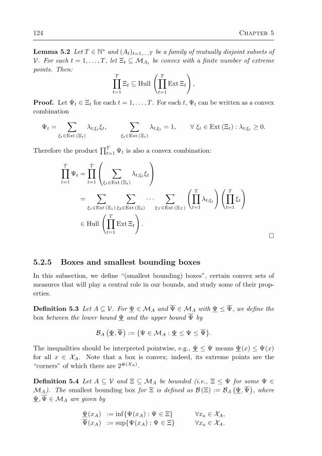
124 Chapter 5
Lemma 5.2 Let T ∈ N∗ and (At)t=1,...,T be a family of mutually disjoint subsets ofV. For each t = 1, . . . , T , let Ξt ⊆ MAt be convex with a finite number of extremepoints. Then:
T∏t=1
Ξt ⊆ Hull
(T∏t=1
Ext Ξt
),
Proof. Let Ψt ∈ Ξt for each t = 1, . . . , T . For each t, Ψt can be written as a convexcombination
Ψt =∑
ξt∈Ext (Ξt)
λt;ξtξt,∑
ξt∈Ext (Ξt)
λt;ξt = 1, ∀ ξt ∈ Ext (Ξt) : λt;ξt ≥ 0.
Therefore the product∏Tt=1 Ψt is also a convex combination:
T∏t=1
Ψt =T∏t=1
∑ξt∈Ext (Ξt)
λt;ξtξt
=
∑ξ1∈Ext (Ξ1)
∑ξ2∈Ext (Ξ2)
· · ·∑
ξT∈Ext (ΞT )
(T∏t=1
λt;ξt
)(T∏t=1
ξt
)
∈ Hull
(T∏t=1
Ext Ξt
).
5.2.5 Boxes and smallest bounding boxes
In this subsection, we define “(smallest bounding) boxes”, certain convex sets ofmeasures that will play a central role in our bounds, and study some of their prop-erties.
Definition 5.3 Let A ⊆ V. For Ψ ∈MA and Ψ ∈MA with Ψ ≤ Ψ, we define thebox between the lower bound Ψ and the upper bound Ψ by
BA(Ψ,Ψ
):= Ψ ∈MA : Ψ ≤ Ψ ≤ Ψ.
The inequalities should be interpreted pointwise, e.g., Ψ ≤ Ψ means Ψ(x) ≤ Ψ(x)for all x ∈ XA. Note that a box is convex; indeed, its extreme points are the“corners” of which there are 2#(XA).
Definition 5.4 Let A ⊆ V and Ξ ⊆ MA be bounded (i.e., Ξ ≤ Ψ for some Ψ ∈MA). The smallest bounding box for Ξ is defined as B (Ξ) := BA
(Ψ,Ψ
), where
Ψ,Ψ ∈MA are given by
Ψ(xA) := infΨ(xA) : Ψ ∈ Ξ ∀xa ∈ XA,Ψ(xA) := supΨ(xA) : Ψ ∈ Ξ ∀xa ∈ XA.

Chapter 5. Novel bounds on marginal probabilities 125
xi = +1
xi = −1
Mi
Ξ
Ψ
Ψ
B (Ξ) = Bi(Ψ,Ψ
)
Figure 5.4: The smallest bounding box B (Ξ) for Ξ is given by the box Bi`Ψ,Ψ
´with
lower bound Ψ and upper bound Ψ.
xi = +1
xi = −1
Mi
Ψ1
Ψ1Ψ2
Ψ2
xi = +1
xi = −1
Mi
Ψ1Ψ2
Ψ1Ψ2
Bi`Ψ1,Ψ1
´Bi `Ψ2,Ψ2
´
Figure 5.5: Multiplication of two boxes on the same variable set A = i.
Figure 5.4 illustrates this concept. Note that B (Ξ) = B (Hull (Ξ)). Therefore, ifΞ is convex, the smallest bounding box for Ξ depends only on the extreme pointsExt (Ξ), i.e., B (Ξ) = B (Ext (Ξ)).
The product of several boxes on the same subset A of variables can be easilycalculated as follows (see also figure 5.5).
Lemma 5.5 Let A ⊆ V, T ∈ N∗ and for each t = 1, . . . , T , let Ψt,Ψt ∈ MA suchthat Ψt ≤ Ψt. Then
T∏t=1
BA(Ψt,Ψt
)= BA
(T∏t=1
Ψt,
T∏t=1
Ψt
),
i.e., the product of the boxes is again a box, with as lower bound the product of thelower bounds of the boxes and as upper bound the product of the upper bounds ofthe boxes.
Proof. We prove the case T = 2; the general case follows by induction. We showthat
BA(Ψ1,Ψ1
)BA (Ψ2,Ψ2
)= BA
(Ψ1 Ψ2,Ψ1 Ψ2
).

126 Chapter 5
That is, for Φ ∈MA we have to show that
Ψ1(x)Ψ2(x) ≤ Φ(x) ≤ Ψ1(x)Ψ2(x) ∀x ∈ XA
if and only if there exist Φ1,Φ2 ∈MA such that:
Φ(x) = Φ1(x)Φ2(x) ∀x ∈ XA;
Ψ1(x) ≤ Φ1(x) ≤ Ψ1(x) ∀x ∈ XA;
Ψ2(x) ≤ Φ2(x) ≤ Ψ2(x) ∀x ∈ XA.
Note that the problem “decouples” for the various possible values of x ∈ XA so thatwe can treat each component (indexed by x ∈ XA) seperately. That is, the problemreduces to showing that
[a, b] · [c, d] = [ac, bd]
for 0 ≤ a ≤ b and 0 ≤ c ≤ d (take a = Ψ1(x), b = Ψ1(x), c = Ψ2(x) and d = Ψ2(x)).In other words, we have to show that y ∈ [ac, bd] if and only if there exist y1 ∈ [a, b],y2 ∈ [c, d] with y = y1y2. For the less trivial part of this assertion, it is easilyverified that choosing y1 and y2 according to the following table:
Condition y1 y2
bc ≤ y, b > 0 b yb
b = 0 0 c
bc ≥ y, c > 0 yc c
bc ≥ y, c = 0 b 0
does the job.
In general, the product of several boxes is not a box itself. Indeed, let i, j ∈ V betwo different variable indices. Then Bi
(Ψi,Ψi
)Bj (Ψj ,Ψj
)contains only factorizing
measures, whereas Bi,j(ΨiΨj ,ΨiΨj
)is not a subset of Qi,j in general. However,
we do have the following identity:
Lemma 5.6 Let T ∈ N∗ and for each t = 1, . . . , T , let At ⊆ V and Ψt,Ψt ∈ MAt
such that Ψt ≤ Ψt. Then
B(
T∏t=1
BAt(Ψt,Ψt
))= B(
STt=1 At)
(T∏t=1
Ψt,
T∏t=1
Ψt
).
Proof. Straightforward, using the definitions.
5.2.6 The basic lemma
After defining the elementary concepts, we can proceed with the basic lemma. Giventhe definitions introduced before, the basic lemma is easy to formulate. It is illus-trated in figure 5.6.
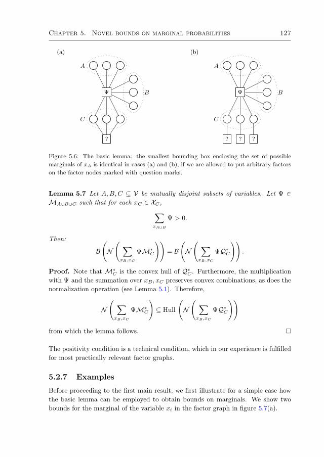
Chapter 5. Novel bounds on marginal probabilities 127
(a)
Ψ
?
A
B
C
(b)
Ψ
? ? ?
A
B
C
Figure 5.6: The basic lemma: the smallest bounding box enclosing the set of possible
marginals of xA is identical in cases (a) and (b), if we are allowed to put arbitrary factors
on the factor nodes marked with question marks.
Lemma 5.7 Let A,B,C ⊆ V be mutually disjoint subsets of variables. Let Ψ ∈MA∪B∪C such that for each xC ∈ XC ,∑
xA∪B
Ψ > 0.
Then:
B(N( ∑xB ,xC
ΨM∗C))
= B(N( ∑xB ,xC
ΨQ∗C))
.
Proof. Note that M∗C is the convex hull of Q∗C . Furthermore, the multiplicationwith Ψ and the summation over xB , xC preserves convex combinations, as does thenormalization operation (see Lemma 5.1). Therefore,
N( ∑xB ,xC
ΨM∗C)⊆ Hull
(N( ∑xB ,xC
ΨQ∗C))
from which the lemma follows.
The positivity condition is a technical condition, which in our experience is fulfilledfor most practically relevant factor graphs.
5.2.7 Examples
Before proceeding to the first main result, we first illustrate for a simple case howthe basic lemma can be employed to obtain bounds on marginals. We show twobounds for the marginal of the variable xi in the factor graph in figure 5.7(a).

128 Chapter 5
(a) i
j k
J K
L
(b) i
j k
J K
? ?
(c) i
j k
J K
δ
j′L
(d) i
j k
J K
?
j′
L
?
Figure 5.7: (a) Factor graph; (b) Illustration of the bound on P(xi) corresponding to
Example I; (c) Cloning node j by adding a new variable j′ and a factor ψδ(xj , xj′) =
δxj (xj′); (d) Illustration of the improved bound on P(xi), corresponding to Example (II),
based on (c).
Example I
First, note that the marginal of xi satisfies
P(xi) = N∑
xj
∑xk
ψJψKψL
∈ N∑
xj
∑xk
ψJψKM∗j,k
.
because, obviously, ψL ∈ M∗j,k. Now, applying the basic lemma with A = i,B = ∅, C = j, k and Ψ = ψJψK , we obtain
P(xi) ∈ BN
∑xj
∑xk
ψJψKQ∗j,k
.
Applying the distributive law, we conclude
P(xi) ∈ BN(∑
xj
ψJM∗j)(∑
xk
ψKM∗k) ,
which certainly implies
P(xi) ∈ BNBN
∑xj
ψJM∗j
· BN (∑xk
ψKM∗k) .
This is illustrated in figure 5.7(b), which should be read as “What can we say aboutthe range of P(xi) when the factors corresponding to the nodes marked with questionmarks are arbitrary?” Because of the various occurrences of the normalizationoperator, we can restrict ourselves to normalized measures on the question-markedfactor nodes:
P(xi) ∈ BNBN
∑xj
ψJPj · BN (∑
xk
ψKPk) .
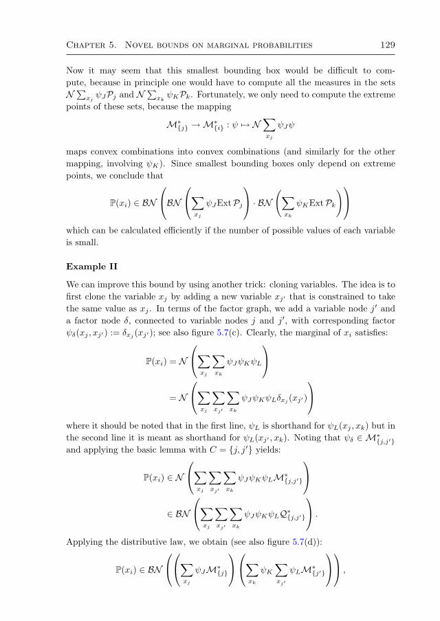
Chapter 5. Novel bounds on marginal probabilities 129
Now it may seem that this smallest bounding box would be difficult to com-pute, because in principle one would have to compute all the measures in the setsN∑xj
ψJPj and N∑xkψKPk. Fortunately, we only need to compute the extreme
points of these sets, because the mapping
M∗j →M∗i : ψ 7→ N∑xj
ψJψ
maps convex combinations into convex combinations (and similarly for the othermapping, involving ψK). Since smallest bounding boxes only depend on extremepoints, we conclude that
P(xi) ∈ BNBN
∑xj
ψJExtPj · BN (∑
xk
ψKExtPk)
which can be calculated efficiently if the number of possible values of each variableis small.
Example II
We can improve this bound by using another trick: cloning variables. The idea is tofirst clone the variable xj by adding a new variable xj′ that is constrained to takethe same value as xj . In terms of the factor graph, we add a variable node j′ anda factor node δ, connected to variable nodes j and j′, with corresponding factorψδ(xj , xj′) := δxj (xj′); see also figure 5.7(c). Clearly, the marginal of xi satisfies:
P(xi) = N∑
xj
∑xk
ψJψKψL
= N
∑xj
∑xj′
∑xk
ψJψKψLδxj (xj′)
where it should be noted that in the first line, ψL is shorthand for ψL(xj , xk) but inthe second line it is meant as shorthand for ψL(xj′ , xk). Noting that ψδ ∈ M∗j,j′and applying the basic lemma with C = j, j′ yields:
P(xi) ∈ N∑
xj
∑xj′
∑xk
ψJψKψLM∗j,j′
∈ BN
∑xj
∑xj′
∑xk
ψJψKψLQ∗j,j′
.
Applying the distributive law, we obtain (see also figure 5.7(d)):
P(xi) ∈ BN∑
xj
ψJM∗j
∑xk
ψK∑xj′
ψLM∗j′
,

130 Chapter 5
from which we conclude
P(xi) ∈ BNBN
∑xj
ψJPj
BN∑
xk
ψKBN∑xj′
ψLPj′
.
This can again be calculated efficiently by considering only extreme points.As a more concrete example, take all variables as binary and take for each factor
ψ =(
1 22 1
). Then the first bound (Example I) yields:
P(xi) ∈ Bi((
1/51/5
),(
4/54/5
)),
whereas the second, tighter, bound (Example II) gives:
P(xi) ∈ Bi((
2/72/7
),(
5/75/7
)).
Obviously, the exact marginal is
P(xi) =(
1/21/2
).
5.2.8 Propagation of boxes over a subtree
We now formulate a message passing algorithm that resembles Belief Propagation.However, instead of propagating measures, it propagates boxes (or simplices) ofmeasures; furthermore, it is only applied to a subtree of the factor graph, propagat-ing boxes from the leaves towards a root node, instead of propagating iterativelyover the whole factor graph several times. The resulting “belief” at the root nodeis a box that bounds the exact marginal of the root node. The choice of the subtreeis arbitrary; different choices lead to different bounds in general. We illustrate thealgorithm using the example that we have studied before (see figure 5.8).
Definition 5.8 Let (V,F , E) be a factor graph. We call the bipartite graph (V, F,E)a subtree of (V,F , E) with root i if i ∈ V ⊆ V, F ⊆ F , E ⊆ E such that (V, F,E)is a tree with root i and for all j, J ∈ E, j ∈ V and J ∈ F (i.e., there are no“loose edges”).3
An illustration of a factor graph and a possible subtree is given in figure 5.8(a)-(b). We denote the parent of j ∈ V according to (V, F,E) by par(j) and similarly,we denote the parent of J ∈ F by par(J). In the following, we will use the topologyof the original factor graph (V,F , E) whenever we refer to neighbors of variables orfactors.
Each edge of the subtree will carry one message, oriented such that it “flows”towards the root node. In addition, we define messages entering the subtree for
3Note that this corresponds to the notion of subtree of a bipartite graph; for a subtree of a
factor graph, one sometimes imposes the additional constraint that for all factors J ∈ F , all its
connecting edges J, j with j ∈ NJ have to be in E; here we do not impose this additional
constraint.
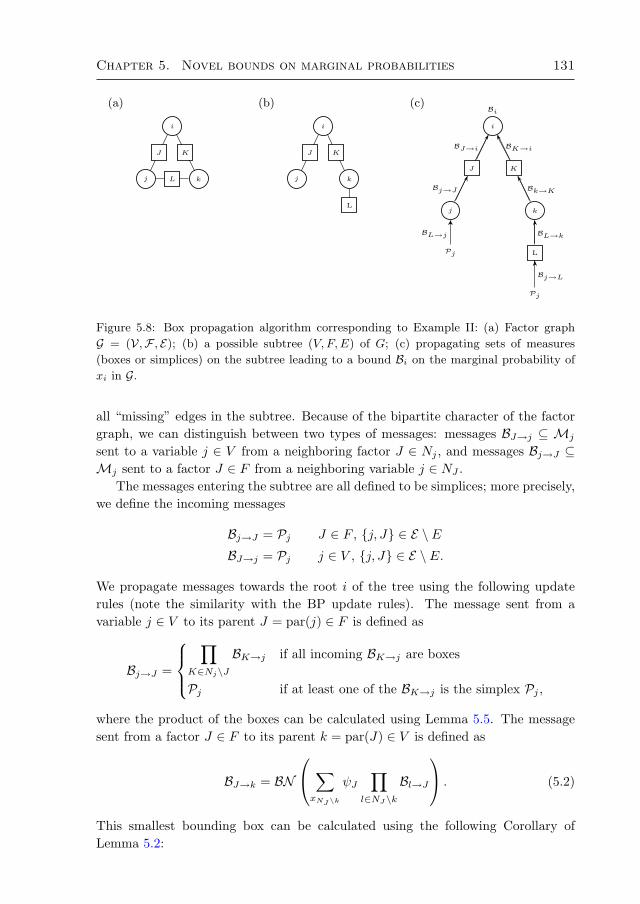
Chapter 5. Novel bounds on marginal probabilities 131
(a)
i
j k
J K
L
(b)
i
j k
J K
L
(c)
i
j k
J K
LPj
Pj
Bi
BJ→i BK→i
Bj→J Bk→K
BL→kBL→j
Bj→L
Figure 5.8: Box propagation algorithm corresponding to Example II: (a) Factor graph
G = (V,F , E); (b) a possible subtree (V, F,E) of G; (c) propagating sets of measures
(boxes or simplices) on the subtree leading to a bound Bi on the marginal probability of
xi in G.
all “missing” edges in the subtree. Because of the bipartite character of the factorgraph, we can distinguish between two types of messages: messages BJ→j ⊆ Mj
sent to a variable j ∈ V from a neighboring factor J ∈ Nj , and messages Bj→J ⊆Mj sent to a factor J ∈ F from a neighboring variable j ∈ NJ .
The messages entering the subtree are all defined to be simplices; more precisely,we define the incoming messages
Bj→J = Pj J ∈ F , j, J ∈ E \ EBJ→j = Pj j ∈ V , j, J ∈ E \ E.
We propagate messages towards the root i of the tree using the following updaterules (note the similarity with the BP update rules). The message sent from avariable j ∈ V to its parent J = par(j) ∈ F is defined as
Bj→J =
∏
K∈Nj\JBK→j if all incoming BK→j are boxes
Pj if at least one of the BK→j is the simplex Pj ,
where the product of the boxes can be calculated using Lemma 5.5. The messagesent from a factor J ∈ F to its parent k = par(J) ∈ V is defined as
BJ→k = BN ∑xNJ\k
ψJ∏
l∈NJ\kBl→J
. (5.2)
This smallest bounding box can be calculated using the following Corollary ofLemma 5.2:

132 Chapter 5
Corollary 5.9
BN ∑xNJ\k
ψJ∏
l∈NJ\kBl→J
= BN ∑xNJ\k
ψJ∏
l∈NJ\kExtBl→J
Proof. By Lemma 5.2,
∏l∈NJ\k
Bl→J ⊆ Hull
∏l∈NJ\k
ExtBl→J .
Because the multiplication with ψJ and the summation over xNJ\k preserves convexcombinations, as does the normalization (see Lemma 5.1), the statement follows.
The final “belief” Bi at the root node i is calculated by
Bi =
BN
∏K∈Nj
BK→j if all incoming BK→j are boxes
Pj if at least one of the BK→j is the simplex Pj .
Note that when applying this to the case illustrated in figure 5.8, we obtain thebound that we derived earlier on (“Example II”).
We can now formulate our first main result, which gives a rigorous bound onthe exact single-variable marginal of the root node:
Theorem 5.10 Let (V,F , E) be a factor graph with corresponding probability dis-tribution (5.1). Let i ∈ V and (V, F,E) be a subtree of (V,F , E) with root i ∈ V .Apply the “box propagation” algorithm described above to calculate the final “belief”Bi on the root node i. Then P(xi) ∈ Bi.Proof sketch. The first step consists in extending the subtree such that eachfactor node has the right number of neighboring variables by cloning the missingvariables. The second step consists of applying the basic lemma where the set Cconsists of all the variable nodes of the subtree which have connecting edges in E \E,together with all the cloned variable nodes. Then we apply the distributive law,which can be done because the extended subtree has no cycles. Finally, we relax thebound by adding additional normalizations and smallest bounding boxes at eachfactor node in the subtree. It should now be clear that the recursive algorithm “boxpropagation” described above precisely calculates the smallest bounding box at theroot node i that corresponds to this procedure.
Note that a subtree of the orginal factor graph is also a subtree of the computa-tion tree for i [Tatikonda and Jordan, 2002]. A computation tree is an “unwrapping”of the factor graph that has been used in analyses of the Belief Propagation algo-rithm. The computation tree starting at variable i ∈ V consists of all paths on the
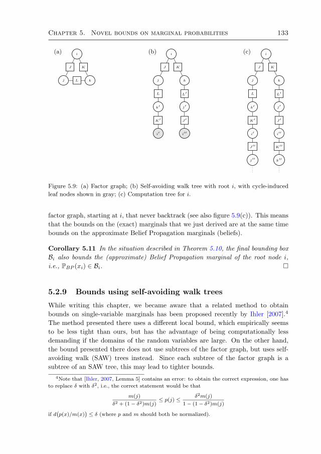
Chapter 5. Novel bounds on marginal probabilities 133
(a) i
j k
J K
L
(b) i
j k
J K
k′ j′
L L′
i′ i′′
K′ J′
(c) i
j k
J K
k′ j′
L L′
i′ i′′
K′ J′
j′′ k′′
J′′ K′′
Figure 5.9: (a) Factor graph; (b) Self-avoiding walk tree with root i, with cycle-induced
leaf nodes shown in gray; (c) Computation tree for i.
factor graph, starting at i, that never backtrack (see also figure 5.9(c)). This meansthat the bounds on the (exact) marginals that we just derived are at the same timebounds on the approximate Belief Propagation marginals (beliefs).
Corollary 5.11 In the situation described in Theorem 5.10, the final bounding boxBi also bounds the (approximate) Belief Propagation marginal of the root node i,i.e., PBP (xi) ∈ Bi.
5.2.9 Bounds using self-avoiding walk trees
While writing this chapter, we became aware that a related method to obtainbounds on single-variable marginals has been proposed recently by Ihler [2007].4
The method presented there uses a different local bound, which empirically seemsto be less tight than ours, but has the advantage of being computationally lessdemanding if the domains of the random variables are large. On the other hand,the bound presented there does not use subtrees of the factor graph, but uses self-avoiding walk (SAW) trees instead. Since each subtree of the factor graph is asubtree of an SAW tree, this may lead to tighter bounds.
4Note that [Ihler, 2007, Lemma 5] contains an error: to obtain the correct expression, one has
to replace δ with δ2, i.e., the correct statement would be that
m(j)
δ2 + (1− δ2)m(j)≤ p(j) ≤
δ2m(j)
1− (1− δ2)m(j)
if d`p(x)/m(x)
´≤ δ (where p and m should both be normalized).

134 Chapter 5
The idea of using a self-avoiding walk tree for calculating marginal probabilitiesseems to be generally attributed to Weitz [2006], but can already be found in [Scottand Sokal, 2005]. In this subsection, we show how this idea can be combined withthe propagation of bounding boxes. The result Theorem 5.13 will turn out to bean improvement over Theorem 5.10 in case there are only pairwise interactions,whereas in the general case, Theorem 5.10 often yields tighter bounds empirically.
Definition 5.12 Let G := (V,F , E) be a factor graph and let i ∈ V. A self-avoiding walk (SAW) starting at i ∈ V of length n ∈ N∗ is a sequence α =(α1, α2, α3, . . . , αn) ∈ (V ∪ F)n that
(i) starts at i ∈ V, i.e., α1 = i;
(ii) subsequently visits neighboring nodes in the factor graph, i.e., αj+1 ∈ Nαj forall j = 1, 2, . . . , n− 1;
(iii) does not backtrack, i.e., αj 6= αj+2 for all j = 1, 2, . . . , n− 2;
(iv) the first n − 1 nodes are all different, i.e., αj 6= αk if j 6= k for j, k ∈1, 2, . . . , n− 1.5
The set of all self-avoiding walks starting at i ∈ V has a natural tree struc-ture, defined by declaring each SAW (α1, α2, . . . , αn, αn+1) to be a child of the SAW(α1, α2, . . . , αn), for all n ∈ N∗; the resulting tree is called the self-avoiding walk(SAW) tree with root i ∈ V, denoted TSAWG (i).
Note that the name “self-avoiding walk tree” is slightly inaccurate, because thelast node of a SAW may have been visited already. In general, the SAW tree canbe much larger than the original factor graph. Following Ihler [2007], we call aleaf node in the SAW tree a cycle-induced leaf node if it contains a cycle (i.e., ifits final node has been visited before in the same walk), and call it a dead-end leafnode otherwise. We denote the parent of node α in the SAW tree by par(α) and wedenote its children by ch(α). The final node of a SAW α = (α1, . . . , αn) is denotedby G(α) = αn. An example of a SAW tree for our running example factor graph isshown in figure 5.9(b).
Let G = (V,F , E) be a factor graph and let i ∈ V. We now define a propagationalgorithm on the SAW tree TSAWG (i), where each node α ∈ TSAWG (i) (except forthe root i) sends a message Bα→par(α) to its parent node par(α) ∈ TSAWG (i). Eachcycle-induced leaf node of TSAWG (i) sends a simplex to its parent node: if α is acycle-induced leaf node, then
Bα→par(α) =
PG(α) if G(α) ∈ VPG(par(α)) if G(α) ∈ F .
(5.3)
5Note that (iii) almost follows from (iv), except for the condition that αn−2 6= αn.
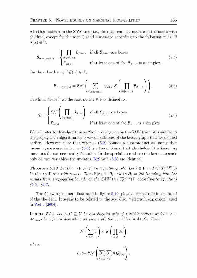
Chapter 5. Novel bounds on marginal probabilities 135
All other nodes α in the SAW tree (i.e., the dead-end leaf nodes and the nodes withchildren, except for the root i) send a message according to the following rules. IfG(α) ∈ V,
Bα→par(α) =
∏
β∈ch(α)
Bβ→α if all Bβ→α are boxes
PG(α) if at least one of the Bβ→α is a simplex.(5.4)
On the other hand, if G(α) ∈ F ,
Bα→par(α) = BN ∑x\G(par(α))
ψG(α)B ∏β∈ch(α)
Bβ→α . (5.5)
The final “belief” at the root node i ∈ V is defined as:
Bi =
BN
∏β∈ch(i)
Bβ→i if all Bβ→i are boxes
PG(i) if at least one of the Bβ→i is a simplex.
(5.6)
We will refer to this algorithm as “box propagation on the SAW tree”; it is similar tothe propagation algorithm for boxes on subtrees of the factor graph that we definedearlier. However, note that whereas (5.2) bounds a sum-product assuming thatincoming measures factorize, (5.5) is a looser bound that also holds if the incomingmeasures do not necessarily factorize. In the special case where the factor dependsonly on two variables, the updates (5.2) and (5.5) are identical.
Theorem 5.13 Let G := (V,F , E) be a factor graph. Let i ∈ V and let TSAWG (i)be the SAW tree with root i. Then P(xi) ∈ Bi, where Bi is the bounding box thatresults from propagating bounds on the SAW tree TSAWG (i) according to equations(5.3)–(5.6).
The following lemma, illustrated in figure 5.10, plays a crucial role in the proofof the theorem. It seems to be related to the so-called “telegraph expansion” usedin Weitz [2006].
Lemma 5.14 Let A,C ⊆ V be two disjoint sets of variable indices and let Ψ ∈MA∪C be a factor depending on (some of) the variables in A ∪ C. Then:
N(∑xC
Ψ
)∈ B
(∏i∈A
Bi
)
where
Bi := BN∑xA\i
∑xC
ΨQ∗A\i
.
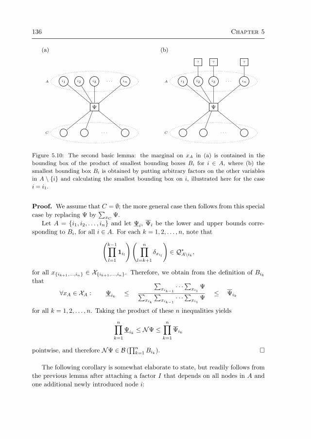
136 Chapter 5
(a)
Ψ
i1 i2 i3 . . . in
. . .
A
C
(b)
Ψ
i1 i2 i3 . . . in
. . .
A
C
? ? ?
Figure 5.10: The second basic lemma: the marginal on xA in (a) is contained in the
bounding box of the product of smallest bounding boxes Bi for i ∈ A, where (b) the
smallest bounding box Bi is obtained by putting arbitrary factors on the other variables
in A \ i and calculating the smallest bounding box on i, illustrated here for the case
i = i1.
Proof. We assume that C = ∅; the more general case then follows from this specialcase by replacing Ψ by
∑xC
Ψ.Let A = i1, i2, . . . , in and let Ψi, Ψi be the lower and upper bounds corre-
sponding to Bi, for all i ∈ A. For each k = 1, 2, . . . , n, note that(k−1∏l=1
1il
)(n∏
l=k+1
δxil
)∈ Q∗A\ik ,
for all xik+1,...,in ∈ Xik+1,...,in. Therefore, we obtain from the definition of Bikthat
∀xA ∈ XA : Ψik≤
∑xik−1
· · ·∑xi1Ψ∑
xik
∑xik−1
· · ·∑xi1Ψ
≤ Ψik
for all k = 1, 2, . . . , n. Taking the product of these n inequalities yields
n∏k=1
Ψik≤ NΨ ≤
n∏k=1
Ψik
pointwise, and therefore NΨ ∈ B (∏nk=1Bik).
The following corollary is somewhat elaborate to state, but readily follows fromthe previous lemma after attaching a factor I that depends on all nodes in A andone additional newly introduced node i:
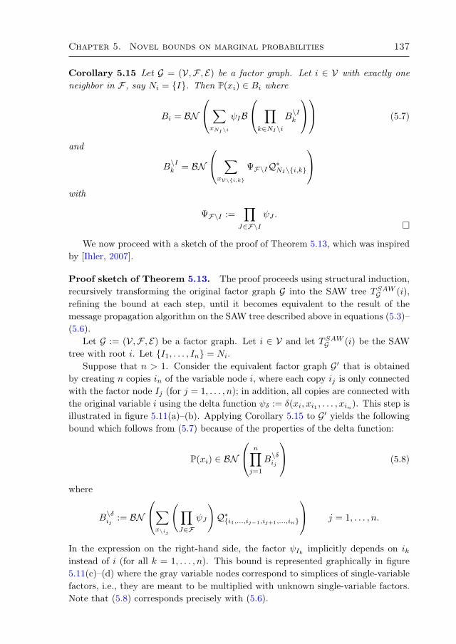
Chapter 5. Novel bounds on marginal probabilities 137
Corollary 5.15 Let G = (V,F , E) be a factor graph. Let i ∈ V with exactly oneneighbor in F , say Ni = I. Then P(xi) ∈ Bi where
Bi = BN∑xNI\i
ψIB ∏k∈NI\i
B\Ik
(5.7)
and
B\Ik = BN
∑xV\i,k
ΨF\IQ∗NI\i,k
with
ΨF\I :=∏
J∈F\IψJ .
We now proceed with a sketch of the proof of Theorem 5.13, which was inspiredby [Ihler, 2007].
Proof sketch of Theorem 5.13. The proof proceeds using structural induction,recursively transforming the original factor graph G into the SAW tree TSAWG (i),refining the bound at each step, until it becomes equivalent to the result of themessage propagation algorithm on the SAW tree described above in equations (5.3)–(5.6).
Let G := (V,F , E) be a factor graph. Let i ∈ V and let TSAWG (i) be the SAWtree with root i. Let I1, . . . , In = Ni.
Suppose that n > 1. Consider the equivalent factor graph G′ that is obtainedby creating n copies in of the variable node i, where each copy ij is only connectedwith the factor node Ij (for j = 1, . . . , n); in addition, all copies are connected withthe original variable i using the delta function ψδ := δ(xi, xi1 , . . . , xin). This step isillustrated in figure 5.11(a)–(b). Applying Corollary 5.15 to G′ yields the followingbound which follows from (5.7) because of the properties of the delta function:
P(xi) ∈ BN n∏j=1
B\δij
(5.8)
where
B\δij
:= BN∑x\ij
(∏J∈F
ψJ
)Q∗i1,...,ij−1,ij+1,...,in
j = 1, . . . , n.
In the expression on the right-hand side, the factor ψIk implicitly depends on ikinstead of i (for all k = 1, . . . , n). This bound is represented graphically in figure5.11(c)–(d) where the gray variable nodes correspond to simplices of single-variablefactors, i.e., they are meant to be multiplied with unknown single-variable factors.Note that (5.8) corresponds precisely with (5.6).
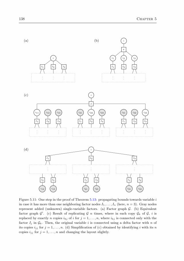
138 Chapter 5
(a)
i
I1 I2 I3
.
.
.
.
.
.
.
.
.
(b) i
δ
i1 i2 i3
I1 I2 I3
.
.
.
.
.
.
.
.
.
(c)
i11 i12 i13
I1 I2 I3
.
.
.
.
.
.
.
.
.
i21 i22 i23
I1 I2 I3
.
.
.
.
.
.
.
.
.
i31 i32 i33
I1 I2 I3
.
.
.
.
.
.
.
.
.
δ
i
(d)
I1
.
.
.
I2 I3
i12 i13
I2
.
.
.
I1 I3
i21 i23
I3
.
.
.
I1 I2
i31 i32
i
Figure 5.11: One step in the proof of Theorem 5.13: propagating bounds towards variable i
in case it has more than one neighboring factor nodes I1, . . . , In (here, n = 3). Gray nodes
represent added (unknown) single-variable factors. (a) Factor graph G. (b) Equivalent
factor graph G′. (c) Result of replicating G n times, where in each copy Gk of G, i is
replaced by exactly n copies ikj of i for j = 1, . . . , n, where ikj is connected only with the
factor Ij in Gk. Then, the original variable i is connected using a delta factor with n of
its copies ijj for j = 1, . . . , n. (d) Simplification of (c) obtained by identifying i with its n
copies ijj for j = 1, . . . , n and changing the layout slightly.
Chapter 5. Novel bounds on marginal probabilities 139
(a) i
I
j1 j2 j3
.
.
.
.
.
.
.
.
.
(b)
j11 j12 j13
.
.
.
.
.
.
.
.
.
j21 j22 j23
.
.
.
.
.
.
.
.
.
j31 j32 j33
.
.
.
.
.
.
.
.
.
I
i
(c)
j11
.
.
.
j12 j13
I I
j22
.
.
.
j21 j23
I I
j33
.
.
.
j31 j32
I I
i
I
Figure 5.12: Another step in the proof of Theorem 5.13: propagating bounds towards
variable i in case it has exactly one neighboring factor node I which has m+1 neighboring
variables i, j1, . . . , jm. (a) Factor graph G. (b) Result of replicating G \ i, I m times
and connecting the factor I with i and with copy jkk of jk for k = 1, . . . ,m. (c) Equivalent
to (b) but with a slightly changed layout. The gray copies of I represent (unknown)
single-variable factors (on their neighboring variable).
140 Chapter 5
The case that n = 1 is simpler because there is no need to introduce the deltafunction. It is illustrated in figure 5.12. Let I = Ni and let j1, . . . , jm = NI \ i.Applying Corollary 5.15 yields the following bound:
P(xi) ∈ BN∑xNI\i
ψIB(
m∏k=1
B\Ijk
) (5.9)
where
B\Ijk
:= BN ∑x\i,jk
∏J∈F\I
ψJ
Q∗j1,...,jk−1,jk+1,...,jm
k = 1, . . . ,m.
This bound is represented graphically in figure 5.12(b)–(c) where the gray nodescorrespond with simplices of single-variable factors. Note that (5.9) correspondsprecisely with (5.5).
Recursively iterating the factor graph operations in figures 5.12 and 5.11, theconnected component that remains in the end is precisely the SAW tree TSAWG (i);the bounds derived along the way correspond precisely with the message passingalgorithm on the SAW tree described above.
Again, the self-avoiding walk tree with root i is a subtree of the computationtree for i. This means that the bounds on the exact marginals given by Theorem5.13 are bounds on the approximate Belief Propagation marginals (beliefs) as well.
Corollary 5.16 In the situation described in Theorem 5.13, the final bounding boxBi also bounds the (approximate) Belief Propagation marginal of the root node i,i.e., PBP (xi) ∈ Bi.
5.3 Related work
There exist many other bounds on single-variable marginals. Also, bounds on thepartition sum can be used to obtain bounds on single-variable marginals. For allbounds known to the authors, we will discuss how they compare with our bounds.In the following, we will denote exact marginals as pi(xi) := P(xi) and BP marginals(beliefs) as bi(xi) := PBP (xi).
5.3.1 The Dobrushin-Tatikonda bound
Tatikonda [2003] derived a bound on the error of BP marginals using mathematicaltools from Gibbs measure theory [Georgii, 1988], in particular using a result knownas Dobrushin’s theorem. The bounds on the error of the BP marginals can be easilytranslated into bounds on the exact marginals:
|bi(xi)− pi(xi)| ≤ ε =⇒ pi(xi) ∈ [bi(xi)− ε, bi(xi) + ε]
Chapter 5. Novel bounds on marginal probabilities 141
for all i ∈ V and xi ∈ Xi.The Dobrushin-Tatikonda bound depends on the girth of the graph (the number
of edges in the shortest cycle, or infinity if there is no cycle) and the properties ofDobrushin’s interdependence matrix, which is a N × N matrix C. The entry Cijis only nonzero if i ∈ ∂j and in that case, the computational cost of computingits value is exponential in the size of the Markov blanket. Thus the computationalcomplexity of the Dobrushin-Tatikonda bound is O(maxi∈V #(X∂i)), plus the costof running BP.
5.3.2 The Dobrushin-Taga-Mase bound
Inspired by the work of Tatikonda and Jordan [2002], Taga and Mase [2006a] derivedanother bound on the error of BP marginals, also based on Dobrushin’s theorem.This bound also depends on the properties of Dobrushin’s interdependence matrixand has similar computational cost. Whereas the Dobrushin-Tatikonda bound givesone bound for all variables, the Dobrushin-Taga-Mase bound gives a different boundfor each variable.
5.3.3 Bound Propagation
Leisink and Kappen [2003] proposed a method called “Bound Propagation” whichcan be used to obtain bounds on exact marginals. The idea underlying this methodis very similar to the one employed in this work, with one crucial difference. Whereaswe use a cavity approach, using as basis equation
P(xi) ∝∑x∂i
(∏I∈Ni
ψI
)P\i(x∂i), P\i(x∂i) ∝
∑xV\∆i
∏I∈F\Ni
ψI
and bound the quantity P(xi) by optimizing over P\i(x∂i), the basis equation em-ployed by Bound Propagation is
P(xi) =∑x∂i
P(xi |x∂i)P(x∂i)
and the optimization is over P(x∂i). Unlike in our case, the computational com-plexity is exponential in the size of the Markov blanket, because of the requiredcalculation of the conditional distribution P(xi |x∂i). On the other hand, the ad-vantage of this approach is that a bound on P(xj) for j ∈ ∂i is also a bound onP(x∂i), which in turn gives rise to a bound on P(xi). In this way, bounds can prop-agate through the graphical model, eventually yielding a new (tighter) bound onP(x∂i). Although the iteration can result in rather tight bounds, the main disad-vantage of Bound Propagation is its computational cost: it is exponential in theMarkov blanket and often many iterations are needed for the bounds to becometight. Indeed, for a simple tree of N = 100 variables, it can happen that BoundPropagation needs several minutes and still obtains very loose bounds (whereas our
142 Chapter 5
bounds give the exact marginal as lower and as upper bound, i.e., they arrive atthe optimally tight bound).
5.3.4 Upper and lower bounds on the partition sum
Various upper and lower bounds on the partition sum Z in (5.1) exist. An upperand a lower bound on Z can be combined to obtain bounds on marginals in thefollowing way. First, note that the exact marginal of i satisfies
P(xi) =Zi(xi)Z
,
where we defined the partition sum of the clamped model as follows:
Zi(xi) :=∑xV\i
∏I∈F
ψI .
Thus, we can boundZ−i (xi)Z+
≤ pi(xi) ≤ Z+i (xi)Z−
where Z− ≤ Z ≤ Z+ and Z−i (xi) ≤ Zi(xi) ≤ Z+i (xi) for all xi ∈ Xi.
A well-known lower bound of the partition sum is the Mean Field bound. Atighter lower bound was derived by Leisink and Kappen [2001]. An upper boundon the log partition sum was derived by Wainwright et al. [2005]. Other lower andupper bounds (for the case of binary variables with pairwise interactions) have beenderived by Jaakkola and Jordan [1996].
5.4 Experiments
We have done several experiments to compare the quality and computation time ofvarious bounds empirically. For each variable in the factor graph under considera-tion, we calculated the gap for each bound Bi
(Ψi,Ψi
) 3 P(xi), which we define asthe `0-norm
∥∥Ψi −Ψi
∥∥0
= maxxi∈Xi∣∣Ψi(xi)−Ψi(xi)
∣∣.We have used the following bounds in our comparison:
DT: Dobrushin-Tatikonda [Tatikonda, 2003, Proposition V.6].
DTM: Dobrushin-Taga-Mase [Taga and Mase, 2006a, Theorem 1].
BoundProp: Bound Propagation [Leisink and Kappen, 2003], using the imple-mentation of M. Leisink, where we chose the maximum cluster size to bemaxi∈V #(∆i).
BoxProp-SubT: Theorem 5.10, where we used a simple breadth-first algorithmto recursively construct the subtree.
BoxProp-SAWT: Theorem 5.13, where we truncated the SAW tree to at most5000 nodes.
Chapter 5. Novel bounds on marginal probabilities 143
Ihler-SAWT: Ihler’s bound [Ihler, 2007]. This bound has only been formulatedfor pairwise interactions.
Ihler-SubT: Ihler’s bound [Ihler, 2007] applied on a truncated version of the SAWtree, namely on the same subtree as used in BoxProp-SubT. This bound hasonly been formulated for pairwise interactions.
In addition, we compared with appropriate combinations of the following bounds:
MF: Mean-field lower bound.
LK3: Third-order lower bound [Leisink and Kappen, 2001, Eq. (10)], where wetook for µi the mean field solutions. This bound has been formulated only forthe binary, pairwise case.
JJ: Refined upper bound [Jaakkola and Jordan, 1996, Section 2.2], with a greedyoptimization over the parameters. This bound has been formulated only forthe binary, pairwise case.
TRW: Our implementation of [Wainwright et al., 2005]. This bound has beenformulated only for pairwise interactions.
For reference, we calculated the Belief Propagation (BP) errors by comparing withthe exact marginals, using the `0 distance as error measure.
5.4.1 Grids with binary variables
We considered a 5× 5 Ising grid with binary (±1-valued) variables, i.i.d. spin-glassnearest-neighbor interactions Jij ∼ N
(0, β2
)and i.i.d. local fields θi ∼ N
(0, β2
),
with probability distribution
P(x) =1Z
exp
∑i∈V
θixi +12
∑i∈V
∑j∈∂i
Jijxixj
.
We took one random instance of the parameters J and θ (drawn for β = 1) andscaled these parameters with the interaction strength parameter β, for which wetook values in 10−2, 10−1, 1, 10.
The results are shown in figure 5.13. For very weak interactions (β = 10−2),BoxProp-SAWT gave the tightest bounds of all other methods, the only exceptionbeing BoundProp, which gave a somewhat tighter bound for 5 variables out of25. For weak and moderate interactions (β = 10−1, 1), BoxProp-SAWT gave thetightest bound of all methods for each variable. For strong interactions (β = 10),the results were mixed, the best methods being BoxProp-SAWT, BoundProp,MF-TRW and LK3-TRW. Of these, BoxProp-SAWT was the fastest method,

144 Chapter 5
BP
DT
DTM
BoundProp
BoxProp-SubT
Ihler-SubT
BoxProp-SAWT
Ihler-SAWT
MF-TRW
MF-JJ
LK3-TRW
LK3-JJ
1e-09 1e-08 1e-07 1e-06 1e-05 0.0001 0.001 0.01 0.1 1
Gaps
β = 10-2
BP
DT
DTM
BoundProp
BoxProp-SubT
Ihler-SubT
BoxProp-SAWT
Ihler-SAWT
MF-TRW
MF-JJ
LK3-TRW
LK3-JJ
1e-09 1e-08 1e-07 1e-06 1e-05 0.0001 0.001 0.01 0.1 1
Gaps
β = 10-1
BP
DT
DTM
BoundProp
BoxProp-SubT
Ihler-SubT
BoxProp-SAWT
Ihler-SAWT
MF-TRW
MF-JJ
LK3-TRW
LK3-JJ
1e-09 1e-08 1e-07 1e-06 1e-05 0.0001 0.001 0.01 0.1 1
Gaps
β = 100
BP
DT
DTM
BoundProp
BoxProp-SubT
Ihler-SubT
BoxProp-SAWT
Ihler-SAWT
MF-TRW
MF-JJ
LK3-TRW
LK3-JJ
1e-09 1e-08 1e-07 1e-06 1e-05 0.0001 0.001 0.01 0.1 1
Gaps
β = 101
0.01
0.1
1
10
100
1000
10000
BP
DT
DT
M
Bou
ndP
rop
Box
Pro
p-S
ubT
Ihle
r-S
ubT
Box
Pro
p-S
AW
T
Ihle
r-S
AW
T
MF
-TR
W
MF
-JJ
LK3-
TR
W
LK3-
JJ
Com
puta
tion
time
(s)
β = 10-2
β = 10-1
β = 100
β = 101
Figure 5.13: Results for grids with binary variables. The first four graphs show, for
different values of the interaction strength β, the gaps of bounds on marginals calculated
using different methods. Also shown for reference are the errors in the BP approximations
to the same marginals. The final graph shows the total computation time for each method.
whereas the methods using TRW were the slowest.6 For β = 10, we present scatterplots in figure 5.14 to compare the results of some methods in more detail. These
6We had to loosen the convergence criterion for the inner loop of TRW, otherwise it would have
taken hours. Since some of the bounds are significantly tighter than the convergence criterion we
used, this may suggest that one can loosen the convergence criterion for TRW even more and still
obtain good results using less computation time than the results we present here. Unfortunately, it
is not clear how this criterion should be chosen in an optimal way without actually trying different
values and using the best one.

Chapter 5. Novel bounds on marginal probabilities 145
1e-10
1e-08
1e-06
0.0001
0.01
1
1e-
10
1e-
08
1e-
06
0.0
001
0.0
1 1
Box
Pro
p-S
AW
T
BoundProp
1e-10
1e-08
1e-06
0.0001
0.01
1
1e-
10
1e-
08
1e-
06
0.0
001
0.0
1 1
Box
Pro
p-S
AW
T
MF-TRW
1e-10
1e-08
1e-06
0.0001
0.01
1
1e-
10
1e-
08
1e-
06
0.0
001
0.0
1 1
Box
Pro
p-S
AW
T
LK-TRW
Figure 5.14: Scatter plots comparing some methods in detail for grids with binary variables
for strong interactions (β = 10).
plots illustrate that the tightness of bounds can vary widely over methods andvariables.
Among the methods yielding the tightest bounds, the computation time of ourbounds is relatively low in general; only for low interaction strengths, BoundProp
is faster tahn BoxProp-SAWT. Furthermore, the computation time of our boundsdoes not depend on the interaction strength, in contrast with iterative methodssuch as BoundProp and MF-TRW, which need more iterations for increasinginteraction strength (as the variables become more and more correlated). Further,as expected, BoxProp-SubT needs less computation time than BoxProp-SAWT
but also yields less tight bounds. Another observation is that our bounds outperformthe related versions of Ihler’s bounds.
5.4.2 Grids with ternary variables
To evaluate the bounds beyond the special case of binary variables, we have per-formed experiments on a 5 × 5 grid with ternary variables and pairwise factorsbetween nearest-neighbor variables on the grid. The entries of the factors werei.i.d., drawn by taking a random number from a normal distribution N (0, β2
)with
mean 0 and standard deviation β and taking the exp of that random number.The results are shown in figure 5.15. We have not compared with bounds in-
volving JJ or LK3 because these methods have only been formulated originally forthe case of binary variables. This time, our method BoxProp-SAWT yielded thetightest bounds for all interaction strengths and for all variables (although this isnot immediately clear from the plots).
5.4.3 Medical diagnosis
We also applied the bounds on simulated Promedas patient cases [Wemmenhoveet al., 2007]. These factor graphs have binary variables and singleton, pairwiseand triple interactions (containing zeros). Two examples of such factor graphs are
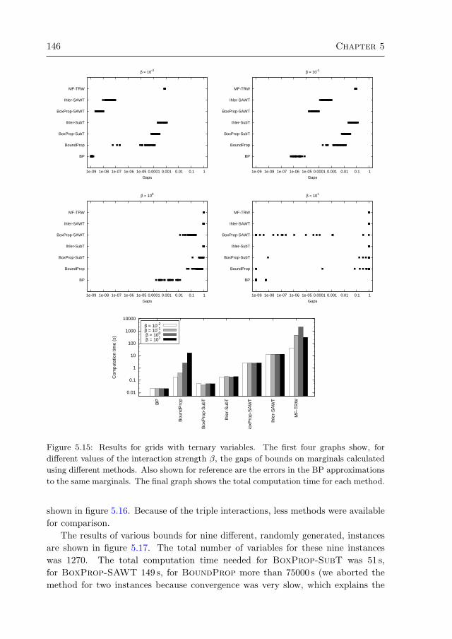
146 Chapter 5
BP
BoundProp
BoxProp-SubT
Ihler-SubT
BoxProp-SAWT
Ihler-SAWT
MF-TRW
1e-09 1e-08 1e-07 1e-06 1e-05 0.0001 0.001 0.01 0.1 1
Gaps
β = 10-2
BP
BoundProp
BoxProp-SubT
Ihler-SubT
BoxProp-SAWT
Ihler-SAWT
MF-TRW
1e-09 1e-08 1e-07 1e-06 1e-05 0.0001 0.001 0.01 0.1 1
Gaps
β = 10-1
BP
BoundProp
BoxProp-SubT
Ihler-SubT
BoxProp-SAWT
Ihler-SAWT
MF-TRW
1e-09 1e-08 1e-07 1e-06 1e-05 0.0001 0.001 0.01 0.1 1
Gaps
β = 100
BP
BoundProp
BoxProp-SubT
Ihler-SubT
BoxProp-SAWT
Ihler-SAWT
MF-TRW
1e-09 1e-08 1e-07 1e-06 1e-05 0.0001 0.001 0.01 0.1 1
Gaps
β = 101
0.01
0.1
1
10
100
1000
10000
BP
Bou
ndP
rop
Box
Pro
p-S
ubT
Ihle
r-S
ubT
Box
Pro
p-S
AW
T
Ihle
r-S
AW
T
MF
-TR
W
Com
puta
tion
time
(s)
β = 10-2
β = 10-1
β = 100
β = 101
Figure 5.15: Results for grids with ternary variables. The first four graphs show, for
different values of the interaction strength β, the gaps of bounds on marginals calculated
using different methods. Also shown for reference are the errors in the BP approximations
to the same marginals. The final graph shows the total computation time for each method.
shown in figure 5.16. Because of the triple interactions, less methods were availablefor comparison.
The results of various bounds for nine different, randomly generated, instancesare shown in figure 5.17. The total number of variables for these nine instanceswas 1270. The total computation time needed for BoxProp-SubT was 51 s,for BoxProp-SAWT 149 s, for BoundProp more than 75000 s (we aborted themethod for two instances because convergence was very slow, which explains the

Chapter 5. Novel bounds on marginal probabilities 147
x14
p1p220
p270
p668
x15
p669
x16
p2
p221
p271p670
x17
p3
p222
p272
p671
x18
p4
p223
p273
p672
x19
p5
p224
p274
p673
x20
p6
p225
p275
p674
x21
p7
p226
p276
p675
x22
p8
p227
p277p676
x23
p9
p228
p278
p677
x24
p10
p229
p279
p678
x25
p11
p230
p280
p679
x26
p12
p231
p281
p680
x27
p13
p320
p370
p681
x28 p14
p410p467
p682
x29
p15p232
p282
p683
x30
p16
p233p283
p524
p548
p684
x31
p17
p685
x32
p18
p686
x33
p19
p687
x34
p20
p688x35
p21
p689
x36
p22
p690
x37
p23
p691
x38p24
p692
x39 p25p693
x40p26
p525
p694
x41
p27
p695
x42
p28
p696
x43
p29
p697
x44
p30
p417
p474
p698
x45
p31
p234p284
p699
x46p32
p700
x47
p33
p701
x48
p34
p702
x49
p35
p703
x50 p36
p704
x51p37
p236p286
p335
p418p475
p528
p557
p598p613
p705
x52 p38
p706
x53p39
p707
x54
p40
p708 x55
p41
p709
x56
p42
p237p287
p710
x57
p43
p711
x58
p44
p712
x59
p45
p239p289
p713
x60
p46
p714
x61
p47
p715
x62
p48
p716
x63
p49
p717
x64p50
p718
x65p51
p719
x66
p52
p422p479
p720
x67
p53
p423p480
p721
x68
p54
p424p481
p722
x69
p55
p240p290
p723
x70
p56
p724
x71
p57
p241p291
p725
x72
p58
p726
x73
p59
p727
x74
p60
p728
x75
p61
p729
x76
p62
p730
x77
p63
p731
x78
p64
p732
x79
p65
p733
x80
p66 p242p292
p338
p426p483
p530p563
p599
p619p734
x81
p67
p735
x82
p68
p736
x83
p69
p737
x84
p70
p738
x85
p71
p739
x86
p72
p740
x87
p73
p741
x88
p74
p742
x89
p75
p743
x90
p76
p744
x91
p77
p243p293
p342
p429p486
p531
p565
p600
p620p745
x92
p78
p746
x93
p79
p747
x94
p80p244p294p343
p430p487
p532p566
p601
p748
x95
p81p245p295
p344
p533
p567
p602
p621
p749
x96
p82
p750
x97
p83
p751
x98
p84
p346
p752
x99
p85
p753
x100
p86
p754
x101
p87
p755
x102
p88
p756
x103
p89
p757
x104
p90
p758
x105
p91
p759
x106
p92
p760
x107
p93
p761
x108
p94
p762
x109
p95
p763
x110
p96
p764
x111
p97
p431p488
p765
x112
p98
p766
x113
p99
p767
x114
p100
p768
x115
p101
p769
x116
p102
p770
x117
p103
p771
x118
p104
p772x119
p105
p773
x120
p106
p774
x121
p107
p775
x122
p108
p776
x123
p109
p777
x124
p110
p778
x125
p111
p779
x126
p112
p780
x127p113
p434p491
p781
x128
p114
p389
p435p492
p782
x129
p115
p783
x130
p116
p784
x131
p117
p785
x132p118
p786
x133
p119
p787
x134
p120
p788
x135p121
p789
x136p122
p790
x137
p123
p791
x138
p124
p792
x139
p125
p793
x140
p126
p794
x141
p127
p795
x142
p128
p796
x143
p129
p797
x144
p130
p798
x145
p131
p799
x146
p132
p800
x147
p133
p437p494
p801
x148
p134
p802
x149
p135
p803
x150
p136
p246p296
p438p495
p804x151
p137
p805
x152
p138
p439p496
p806
x153
p139
p248p298p351 p442
p499
p535
p578
p603p627
p807
x154p140
p808x155
p141
p443
p500
p809
x156
p142
p810
x157
p143
p811
x158
p144
p812
x159
p145
p813
x160p146
p814
x161
p147
p815
x162
p148
p446
p503
p816
x163
p149
p817
x164
p150p818
x165
p151
p249p299
p536
p580
p819
x166
p152p250p300p353
p447p504
p537p581
p604
p629
p820
x167p153
p251p301
p355p449p506
p538p582
p605
p630p821
x168
p154
p822
x169
p155
p823
x170
p156
p252p302
p824
x171
p157
p825
x172
p158
p398
p826
x173
p159
p827
x174
p160
p828
x175
p161
p829
x176
p162
p830
x177
p163
p831
x178
p164
p255p305
p401
p832
x179
p165
p833
x180
p166
p834
x181
p167
p835
x182
p168
p836
x183
p169
p837
x184
p170
p838
x185
p171
p256p306
p839
x186
p172
p840
x187
p173
p403 p841
x188
p174
p842
x189
p175
p843
x190
p176
p844
x191
p177
p845
x192
p178
p453p510
p846
x193
p179
p847
x194
p180
p848
x195
p181
p257p307
p358
p454p511
p539
p591
p606
p631
p849
x196
p182
p850
x197
p183
p851
x198
p184
p852
x199
p185
p853
x200
p186
p258p308
p359
p455
p512
p540
p592
p607
p632p854
x201
p187
p361 p457p514
p656
p855
x202
p188
p362p541
p593
p856
x203p189
p857 x204
p190
p858
x205 p191
p458p515
p859
x206
p192 p860
x207
p193
p861
x208
p194
p862
x209
p195
p262p312
p365
p459p516p544
p594
p608
p633
p863
x210
p196
p864
x211
p197
p263
p313
p366
p545
p595
p865
x212
p198
p866x213
p199
p867
x214
p200
p868
x215
p201
p869
x216
p202
p264
p314
p367
p460p517
p546
p596
p609
p635
p870
x217
p203
p871
x218
p204
p872
x219
p205
p873
x220
p206
p874
x221
p207
p265
p315
p461p518
p875
x222
p208p876
x223
p209
p877
x224
p210
p266p316
p462
p519
p660
p878
x225
p211
p879
x226
p212
p880
x227p213
p881
x228 p214p463
p520
p882
x229
p215p267
p317
p465
p522
p883
x230
p216
p268
p318
p884
x231
p217
p885
x232
p218
p886
x233
p235
p285p887
x234
p238p288
p420p477
p888
x235
p247p297
p654
p889
x236
p253p303
p890
x237
p254p304p588
p891
x238
p259
p309
p892
x239
p260p310
p543
p657
p893
x240
p261
p311
p894
x241
p372
p411p468
p611
p895
x242
p321
p896
x243
p322
p550
p897
x244
p323
p898
x245p324
p899
x246p325
p412
p469
p900
x247
p326
p901
x248p327p902
x249
p328
p903
x250
p329
p904
x251
p330
p551
p905
x252
p331
p414
p471
p906
x253
p332
p907
x254
p333
p527p908
x255
p334
p909
x256
p336
p910
x257
p337
p529
p562
p911
x258
p339
p912
x259
p340p564
p913
x260
p341
p644p914
x261
p345
p568
p915
x262
p347
p383
p916
x263
p348
p917
x264
p349
p918
x265
p350
p919
x266
p352
p920
x267
p354p448p505
p921
x268
p356
p589
p922x269
p357
p923
x270
p360
p924
x271
p363
p925x272
p364
p926
x273
p369
p927
x274
p928
x275
p371
p929
x276
p373
p930
x277
p374
p931 x278
p375
p932
x279
p376
p933
x280
p377
p934
x281
p378
p935
x282p379
p643
p936
x283
p380
p937
x284
p381
p938
x285
p382
p939
x286
p384
p624
p650p663
p940
x287
p385
p651
p941
x288
p386
p652
p664
p942
x289
p387
p943
x290
p388
p944
x291
p390
p945
x292
p391
p946
x293
p392
p655
p947
x294
p393
p948
x295
p394
p949
x296p395 p950
x297
p396
p951
x298
p397
p952
x299
p399
p953
x300
p400
p954x301
p402
p955
x302
p404
p956
x303
p405
p957
x304
p406
p958
x305
p407
p959
x306
p408
p960
x307
p413
p470p961
x308
p415
p472
p962
x309
p416
p473
p963 x310p419
p476
p964
x311
p421p478
p965
x312
p425p482
p966
x313
p427p484
p967
x314
p428p485
p968
x315
p432p489
p969
x316
p433p490
p970
x317
p436
p493
p971
x318
p440p497
p972
x319p441
p498p973
x320
p444p501
p974
x321p445p502
p975
x322
p450p507
p976
x323
p451p508
p977
x324
p452p509
p978
x325
p456
p513
p979
x326
p464
p521p980
x327 p526p981
x328
p534
p982
x329
p542
p667
p983
x330
p549
p984
x331
p552
p985
x332
p553
p986
x333
p554
p987
x334
p555
p988
x335p556p989
x336p558
p990
x337
p559
p991
x338
p560
p992
x339
p561
p617
p993
x340
p569
p994
x341
p570
p995
x342
p571
p996
x343
p572
p997
x344
p573
p998
x345
p574
p999
x346
p575
p1000
x347p576
p1001
x348p577
p1002
x349
p579
p1003
x350
p583
p1004
x351
p584
p1005
x352
p585
p1006
x353
p586
p1007
x354
p587
p1008
x355
p590
p1009
x356p1010
x357
p612
p1011
x358p614
p1012
x359
p615
p1013
x360
p616
p1014
x361
p618
p1015
x362
p622
p1016
x363
p623
p649
p1017
x364
p625
p1018
x365
p626
p1019
x366
p628
p1020
x367
p634
p1021
x368
p637
p1022
x369
p1023
x370
p638
p1024
x371
p639
p1025
x372
p640
p1026
x373
p641
p1027
x374
p642
p1028
x375
p645
p1029
x376
p646
p1030
x377
p647
p1031
x378
p648
p1032
x379
p653
p1033
x380
p658
p1034
x381
p659
p1035
x382
p661
p1036
x383
p665
p1037
x384
p666
p1038
x385
x386
x387
x388
x389
x390
x391
x392
x393
x394
x395
x396
x397
x398
x399 x400
x401x402x403
x404x405
x406x407
x408
x409
x410
x411
x412
x413
x414x415
x416
x417
x418
x419
x420
x421
x422
x423
x424
x425
x426
x427
x428
x429
x430
x431
x432
x433
x434
x435
x436
x437
x438x439
x440
x441
x442
x443
x444
x445
x446
x447
x448
x449x450
x451
x452
x453
x454
x455
x456
x457
x458
x459
x460
x461
x462
x463
x464
x465
x466
x467
x468
x469
x470
x471
x472
x473
x474
x475
x476
x477
x478
x479
x480 x481
x482
x483
x484
x485
x486
x487
x488
x489
x490
x491
x492
x493
x494
x495
x496
x497
x498
x499
x500
x501
x502
x503
x504
x505
x506
x507
x508
x509
x510
x511
x512
x513
x514
x515
x516
x517
x518
x519
x520
x521
x522
x523
x524
x525
x526
x527
x528
x529
x530
x531
x532
x533
x534
x535
x536
x537
x538
x539
x540
x541
x542
x543
x544x545
x546
x547x548
x549
x550x551
x552
x553
x554 x555
x556
x557
x558
x559
x560
x561
x562
x563
x564 x565
x566
x567
x568
x569
x570
x571x572
x573
x574
x575
x576
x577
x578
x579
x580
x581
x582x583
x584
x585
x586
x587
x588
x589
x590
x591
x592
x593
x594
x595
x596
x597
x598
x599
x600
x601x602 p0
x603x604
x605
x606
x607
x608
x609
x610
x611
x612
x613
x614
x615
x616
x617
x618
x619
x620
x621
x622
x623
x624
x625x626
x627x628
x629
x630
x631
x632
x633
x634
x635
x636
x637
x638
x639
x640 x641
x642
x643
x644
x645
x646
x647
x648x649
x650
x651
p219
x652
x653
x654x655
x656
x657
x658
x659
x660
x661
x662
x663
x664
x665
x666
x667
x668
x669
x670
x671
x672
x673
x674x675
x676x677
x678
x679
x680
x681
x682
x683
x684
x685
x686
x687
x688
x689x690
x691
x692
x693
x694
x695
x696
x697x698
x699
x700
p269
x701
x702
x703
x704
x705
x706
x707
x708
x709
x710
x711
x712
x713
x714
x715x716
x717
x718
x719
x720
x721 x722
x723
x724
x725
x726
x727
x728
x729
x730
x731
x732
x733
x734
x735
x736
x737
x738
x739
x740
x741
x742
x743
x744
x745
x746
x747 x748
p319
x749
x750
x751
x752
x753
x754
x755
x756
x757
x758
x759
x760
x761
x762
x763
x764
x765 x766
x767
x768
x769
x770
x771
x772
x773
x774
x775
x776
x777
x778
x779
x780
x781
x782
x783
x784
x785
x786
x787
x788
p368
x789
x790
x791
x792
x793
x794
x795
x796
x797
x798
x799
x800
x801
x802
x803
x804x805
x806
x807
x808
x809
x810
x811
x812
x813
x814
x815
x816
x817
x818
x819
x820
x821x822
x823
x824
x825
x826
x827
x828
x829
x830x831
x832
x833
x834
x835
x836
x837
x838 x839
x840
x841
x842
x843
x844p409
x845
x846
x847
x848
x849
x850
x851
x852
x853
x854
x855
x856
x857
x858
x859
x860 x861
x862
x863
x864
x865
x866
x867
x868
x869
x870
x871
x872
x873
x874
x875
x876
x877x878
x879
x880
x881
x882
x883
x884
x885
x886
x887
x888
x889
x890
x891
x892
x893
x894 x895
x896
x897
x898
x899
x900p466
x901
x902
x903
x904
x905
x906
x907
x908
x909
x910
x911
x912
x913
x914
x915 x916
x917
x918
x919
x920
x921
x922
x923
p523
x924
x925
x926
x927
x928
x929
x930
x931
x932
x933
x934
x935
x936
x937
x938
x939
x940
x941x942
x943
x944
x945
x946
x947
x948
x949
x950
x951
x952
x953
x954
x955
x956
x957
x958
x959
x960
x961
x962
x963
x964
x965
x966
x967x968
x969
x970
x971x972
p547
x973
x974
x975
x976
x977
x978
x979
x980
x981
x982
x983
x984
p597
x985
x986
x987
x988
x989
x990
x991
x992x993
x994
x995
x996
x997
x998
x999
x1000
x1001
x1002
x1003
x1004
x1005
x1006
x1007
x1008
x1009
p610
x1010
x1011
x1012
x1013
x1014
x1015
x1016
x1017
x1018
x1019
x1020
x1021
x1022x1023
x1024
x1025
x1026
x1027
x1028
x1029x1030
x1031
x1032x1033
x1034
p636
x1035
x1036
x1037
x1038
x1039
p662
x5
p1
p301
x6
p302
x7
p2
p303
x8
p3
p116
p304
x9
p4
p149
p250p305
x10 p5p306
x11
p6
p307
x12
p7
p251
p308
x13
p8
p309
x14
p9p118
p154
p253
p310
x15
p10
p119
p311
x16
p11
p120
p155
p254
p312
x17
p12
p121
p156
p255
p313
x18
p13
p122
p157
p256
p314
x19
p14
p123
p158
p257
p315
x20
p15 p124
p159
p258
p316
x21
p16p125
p160p259
p317
x22p17
p126p161
p260 p318
x23
p18
p319
x24
p19
p320
x25
p20
p321
x26
p21
p127p162
p264
p322
x27
p22
p323
x28
p23
p324
x29
p24
p325
x30
p25
p326
x31
p26
p327
x32
p27
p328
x33
p28p329
x34
p29
p130
p173
p330
x35
p30
p331
x36
p31
p332
x37
p32
p179
p333
x38
p33
p334
x39
p34
p335
x40
p35
p336
x41
p36
p337
x42
p37
p338
x43
p38
p339
x44
p39
p340
x45p40
p341
x46p41
p342
x47
p42
p343
x48
p43
p131
p189
p274p344
x49
p44
p345
x50
p45
p346
x51
p46
p347
x52
p47
p348
x53p48
p349
x54p49 p350
x55
p50
p133
p195
p276
p351
x56p51
p134
p352
x57
p52
p353
x58p53
p354
x59 p54
p355
x60
p55
p356
x61
p56
p357
x62
p57
p358
x63
p58
p359
x64
p59
p360
x65
p60
p361
x66
p61
p204
p362
x67
p62
p363
x68
p63
p138
p364
x69 p64
p365
x70
p65
p366
x71
p66
p367
x72
p67
p368
x73
p68
p212
p369
x74
p69
p370
x75
p70
p371
x76
p71
p372
x77
p72
p373
x78
p73
p374
x79
p74
p375
x80
p75
p376
x81
p76
p377
x82
p77
p378
x83
p78
p379
x84 p79
p140
p216
p287
p380
x85
p80
p381
x86
p81
p382
x87
p82
p383
x88
p83
p384
x89
p84
p385
x90
p85
p386
x91
p86
p387
x92
p87
p388
x93
p88
p389
x94p89
p390
x95
p90
p391
x96
p91
p392
x97
p92
p221
p393
x98p93
p142
p394
x99
p94
p144p224
p292
p395
x100
p95
p396
x101
p96
p397
x102
p97
p398
x103
p98
p225
p399
x104
p99
p226
p400
x105 p100
p145p237
p295
p401
x106p101
p146
p296
p402
x107
p102
p403
x108
p103
p404
x109
p104
p405
x110
p105
p406
x111
p106
p407
x112
p107
p245
p408
x113
p108
p409
x114
p109
p410
x115
p110
p411
x116
p111
p412
x117
p112
p413
x118
p113
p414
x119
p114
p415
x120
p416
x121
p117
p417
x122
p128
p418 x123
p129
p169
p419
x124
p132
p420
x125
p135
p281p421
x126
p136
p422
x127
p137
p423
x128
p139
p424
x129
p141
p425
x130
p143
p426
x131
p148
p427
x132p428
x133
p150
p429
x134
p151
p430
x135
p152
p431
x136
p153
p252
p432
x137
p163
p433
x138
p164
p434
x139
p165
p435
x140
p166
p436
x141
p167
p437
x142
p168
p438
x143
p170
p439
x144
p171
p440
x145
p172
p441
x146p174
p442
x147
p175
p443
x148
p176
p444
x149
p177
p445
x150
p178
p271
p446
x151
p180
p447
x152
p181
p448
x153
p182
p449
x154
p183
p450
x155
p184
p451
x156p185
p452
x157p186
p453
x158p187
p454
x159
p188
p455
x160
p190
p456
x161
p191
p457
x162
p192
p458
x163p193
p459
x164
p194
p460
x165 p196
p461
x166 p197
p462
x167p198
p463
x168
p199
p464
x169
p200
p465
x170
p201
p466
x171
p202
p467x172
p203
p468
x173
p205
p469
x174
p206
p470
x175
p207
p471
x176
p208
p472
x177
p209
p473
x178
p210
p474
x179
p211
p475
x180
p213
p476
x181
p214
p477
x182
p215
p478
x183
p217
p479
x184
p218
p480
x185
p219
p481 x186
p220
p482
x187
p222
p483
x188
p223
p484
x189
p227
p293
p485
x190
p228
p486
x191
p229
p487
x192
p230
p294
p488
x193
p231
p489
x194
p232
p490
x195
p233
p491
x196
p234
p492
x197p235
p493
x198p236
p494
x199
p238
p495
x200p239
p496
x201
p240
p497 x202
p241
p498
x203
p242
p499
x204
p243
p500
x205
p244
p501
x206
p246
p502
x207
p247
p503
x208
p248
p504
x209
p505
x210
p261
p506
x211
p262
p507
x212
p263
p508x213
p265
p509
x214
p266
p510
x215
p267
p511x216
p268
p512
x217
p269
p513
x218
p270
p514
x219
p272
p515
x220 p273
p516
x221p275
p517
x222
p277
p518
x223
p278
p519
x224
p279
p520
x225
p280
p521
x226
p282
p522
x227
p283
p523
x228
p284
p524
x229
p285
p525
x230p286
p526
x231
p288
p527
x232
p289
p528x233
p290
p529
x234
p291
p530
x235p297 p531
x236p298p532
x237
p299
p533
x238
p300
p534
x239
x240
x241
x242
x243x244
x245x246
x247x248
x249x250
x251
x252
x253
x254
x255
x256x257
x258
x259
x260
x261
x262
x263
x264
x265
x266
x267
x268
x269
x270
x271
x272
x273
x274
x275
x276
x277
x278
x279
x280
x281
x282
x283
x284
x285
x286
x287
x288
x289
x290
x291
x292
x293
x294
x295
x296
x297
x298
x299
x300x301
x302
x303
x304
x305
x306
x307
x308
x309
x310
x311
x312
x313
x314
x315
x316
x317
x318
x319
x320
x321
x322
x323 x324
x325
x326
x327
x328
x329
x330
x331
x332
x333
x334
x335
x336
x337
x338
x339
x340
x341
x342
x343
x344
x345
x346
x347
x348
x349
x350
x351
x352
p0
x353
x354 x355 x356
x357
x358
x359x360
x361
x362
x363
x364
x365x366 x367
x368
x369
x370
x371
x372
x373
x374
x375x376 x377 x378
x379
x380
x381
x382
x383
p115
x384
x385
x386x387
x388
x389
x390 x391x392
x393
x394x395
x396
x397
x398
x399
x400
x401x402
x403
x404
x405
x406
x407
x408
x409
x410
x411
x412
x413
x414
x415
x416
x417
x418
x419
x420
x421
x422
x423
x424
x425
x426
x427
x428
x429
x430
x431
x432
x433
x434
x435
x436
x437
x438
x439
x440
x441
x442
x443
x444x445
x446
x447
x448
x449
x450
x451
x452
x453
x454
x455
x456
x457
x458
x459
x460
x461
x462
x463
x464
x465 x466
x467
x468
x469
x470
x471
x472
x473
x474
x475
x476
x477x478
x479
x480
x481
x482
x483
x484p147
x485 x486x487
x488
x489
x490
x491
x492
x493
x494
x495
x496x497
x498
x499
x500
x501
x502 x503
x504
x505
x506
x507
x508
x509
x510
x511
x512x513
x514
x515
x516x517
x518
x519
x520
x521
x522
x523
x524
x525
x526
x527
x528
x529
x530
x531
x532
x533
x534
x535
p249
Figure 5.16: Two of the Promedas factor graphs.
0
2
4
6
8
10
1e-09 1e-08 1e-07 1e-06 1e-05 0.0001 0.001 0.01 0.1 1
inst
ance
Gaps
Belief Propagation
0
2
4
6
8
10
1e-09 1e-08 1e-07 1e-06 1e-05 0.0001 0.001 0.01 0.1 1
inst
ance
Gaps
BoundProp
0
2
4
6
8
10
1e-09 1e-08 1e-07 1e-06 1e-05 0.0001 0.001 0.01 0.1 1
inst
ance
Gaps
BoxProp-SubT
0
2
4
6
8
10
1e-09 1e-08 1e-07 1e-06 1e-05 0.0001 0.001 0.01 0.1 1
inst
ance
Gaps
BoxProp-SAWT
Figure 5.17: Results for nine different factor graphs corresponding to simulated Promedas
patient cases. In reading order: Belief Propagation errors, BoundProp, BoxProp-SubT
and BoxProp-SAWT.
missing results in the plot) and to calculate the Belief Propagation errors took 254 s.BoundProp gave the tightest bound for only 1 out of 1270 variables, BoxProp-
SAWT for 5 out of 1270 variables and BoxProp-SubT gave the tightest boundfor the other 1264 variables.
Interestingly, whereas for pairwise interactions, BoxProp-SAWT gives tighter

148 Chapter 5
bounds than BoxProp-SubT, for the factor graphs considered here, the boundscalculated by BoxProp-SAWT were generally less tight than those calculated byBoxProp-SubT. This is presumably due to the local bound (5.5) needed on theSAW tree, which is quite loose compared with the local bound (5.2) that assumesindependent incoming bounds.
Not only does BoxProp-SubT give the tightest bounds for almost all variables,it is also the fastest method. Finally, note that the tightness of these bounds stillvaries widely depending on the instance and on the variable of interest.
5.5 Conclusion and discussion
We have derived two related novel bounds on exact single-variable marginals. Bothbounds also bound the approximate Belief Propagation marginals. The bounds arecalculated by propagating convex sets of measures over a subtree of the computationtree, with update equations resembling those of BP. For variables with a limitednumber of possible values, the bounds can be computed efficiently. Empirically,our bounds often outperform the existing state-of-the-art in that case. Althoughwe have only shown results for factor graphs for which exact inference was stilltractable (in order to be able to calculate the BP error), we would like to stresshere that it is not difficult to construct factor graphs for which exact inference isno longer tractable but the bounds can still be calculated efficiently. An exampleare large Ising grids (of size m × m with m larger than 30). Indeed, for binaryIsing grids, the computation time of the bounds (for all variables in the network)scales linearly in the number of variables, assuming that we truncate the subtreesand SAW trees to a fixed maximum size.
Whereas the results of different approximate inference methods usually cannotbe combined in order to get a better estimate of marginal probabilities, for boundsone can combine different methods simply by taking the tightest bound or theintersection of the bounds. Thus it is generally a good thing to have differentbounds with different properties (such as tightness and computation time).
An advantage of our methods BoxProp-SubT and BoxProp-SAWT overiterative methods like BoundProp and MF-TRW is that the computation timeof the iterative methods is difficult to predict (since it depends on the number ofiterations needed to converge which is generally not known a priori). In contrast, thecomputation time needed for our bounds BoxProp-SubT and BoxProp-SAWT
only depends on the structure of the factor graph (and the chosen subtree) and isindependent of the values of the interactions. Furthermore, by truncating the treeone can trade some tightness for computation time.
By far the slowest methods turned out to be those combining the upper boundTRW with a lower bound on the partition sum. The problem here is that TRW
usually needs many iterations to converge, especially for stronger interactions whereconvergence rate can go down significantly. In order to prevent exceedingly long

Chapter 5. Novel bounds on marginal probabilities 149
computations, we had to hand-tune the convergence criterion of TRW according tothe case at hand.
BoundProp can compete in certain cases with the bounds derived here, butmore often than not it turned out to be rather slow or did not yield very tightbounds. Although BoundProp also propagates bounding boxes over measures, itdoes this in a slightly different way which does not exploit independence as muchas our bounds. On the other hand, it can propagate bounding boxes several times,refining the bounds more and more each iteration.
Regarding the related bounds BoxProp-SubT, BoxProp-SAWT and Ihler-
SAWT we can draw the following conclusions. For pairwise interactions and vari-ables that have not too many possible values, BoxProp-SAWT is the method ofchoice, yielding the tightest bounds without needing too much computation time.The bounds are more accurate than the bounds produced by Ihler-SAWT dueto the more precise local bound that is used; the difference is largest for stronginteractions. However, the computation time of this more precise local bound is ex-ponential in the number of possible values of the variables, whereas the local boundused in Ihler-SAWT is only polynomial in the number of possible values of thevariables. Therefore, if this number is large, BoxProp-SAWT may be no longerapplicable in practice, whereas Ihler-SAWT still may be applicable. If factors arepresent that depend on more than two variables, it seems that BoxProp-SubT isthe best method to obtain tight bounds, especially if the interactions are strong.Note that it is not immediately obvious how to extend Ihler-SAWT beyond pair-wise interactions, so we could not compare with that method in that case.
This work also raises some new questions and opportunities for future work.First, the bounds can be used to generalize the improved conditions for conver-gence of Belief Propagation that were derived in [Mooij and Kappen, 2007b] beyondthe special case of binary variables with pairwise interactions. Second, it may bepossible to combine the various ingredients in BoundProp, BoxProp-SubT andBoxProp-SAWT in novel ways in order to obtain even better bounds. Third, itis an interesting open question whether the bounds can be extended to continuousvariables in some way. Finally, although our bounds are a step forward in quan-tifying the error of Belief Propagation, the actual error made by BP is often atleast one order of magnitude lower than the tightness of these bounds. This is dueto the fact that (loopy) BP cycles information through loops in the factor graph;this cycling apparently improves the results. The interesting and still unansweredquestion is why it makes sense to cycle information in this way and whether thiserror reduction effect can be quantified.
Acknowledgments
We thank Wim Wiegerinck for several fruitful discussions, Bastian Wemmenhovefor providing the Promedas test cases, and Martijn Leisink for kindly providinghis implementation of Bound Propagation.

150 Chapter 5. Novel bounds on marginal probabilities

List of Notations 151
List of Notations
General
N Natural numbers, including 0 . . . . . . . . . . . . . . . . . . . . . . . . . . . . . . . . . . . 17
N∗ Natural numbers, excluding 0 . . . . . . . . . . . . . . . . . . . . . . . . . . . . . . . . . . . 17
R Real numbers . . . . . . . . . . . . . . . . . . . . . . . . . . . . . . . . . . . . . . . . . . . . . . . . . . . 31
C Complex numbers. . . . . . . . . . . . . . . . . . . . . . . . . . . . . . . . . . . . . . . . . . . . . . . 70
1X Indicator function on X . . . . . . . . . . . . . . . . . . . . . . . . . . . . . . . . . . . . . . . . . 36
#(X) Cardinality of the set X . . . . . . . . . . . . . . . . . . . . . . . . . . . . . . . . . . . . . . . . 33
|x| Absolute value of x . . . . . . . . . . . . . . . . . . . . . . . . . . . . . . . . . . . . . . . . . . . . . 10
‖v‖ Norm of v . . . . . . . . . . . . . . . . . . . . . . . . . . . . . . . . . . . . . . . . . . . . . . . . . . . . . . 34
‖v‖1 `1-Norm of v . . . . . . . . . . . . . . . . . . . . . . . . . . . . . . . . . . . . . . . . . . . . . . . . . . . . 34
‖v‖∞ `∞-Norm of v . . . . . . . . . . . . . . . . . . . . . . . . . . . . . . . . . . . . . . . . . . . . . . . . . . . 34
d(v, w) Distance from v to w . . . . . . . . . . . . . . . . . . . . . . . . . . . . . . . . . . . . . . . . . . . 34
sgnx Sign of x . . . . . . . . . . . . . . . . . . . . . . . . . . . . . . . . . . . . . . . . . . . . . . . . . . . . . . . . 36
Ext (X) Extreme points of convex set X . . . . . . . . . . . . . . . . . . . . . . . . . . . . . . . . 120
Hull (X) Convex hull of set X . . . . . . . . . . . . . . . . . . . . . . . . . . . . . . . . . . . . . . . . . . . 120
Probabilities
P(X) Probability of X . . . . . . . . . . . . . . . . . . . . . . . . . . . . . . . . . . . . . . . . . . . . . . . . 19
E (X) Expectation of X . . . . . . . . . . . . . . . . . . . . . . . . . . . . . . . . . . . . . . . . . . . . . . . 66
EP (X) Expectation of X under probability measure P . . . . . . . . . . . . . . . . . . 70
〈X〉 Average of X . . . . . . . . . . . . . . . . . . . . . . . . . . . . . . . . . . . . . . . . . . . . . . . . . . . 75
N (µ, σ2)
Normal distribution with mean µ and variance σ2 . . . . . . . . . . . . . . . 55

152 List of Notations
Graphical models, factor graphs
G Graph . . . . . . . . . . . . . . . . . . . . . . . . . . . . . . . . . . . . . . . . . . . . . . . . . . . . . . . . . . 17
V Index set of random variables in graphical model . . . . . . . . . . . . . . . . 17
N Number of random variables in graphical model . . . . . . . . . . . . . . . . . 17
D Set of directed edges . . . . . . . . . . . . . . . . . . . . . . . . . . . . . . . . . . . . . . . . . . . . 17
E Set of undirected edges . . . . . . . . . . . . . . . . . . . . . . . . . . . . . . . . . . . . . . . . . 18
F Index set of factors in graphical model . . . . . . . . . . . . . . . . . . . . . . . . . . 19
i, j, k, . . . Indices of random variables, i.e., elements of V . . . . . . . . . . . . . . . . . . 20
xi Random variable with index i . . . . . . . . . . . . . . . . . . . . . . . . . . . . . . . . . . . 17
Xi Domain of random variable xi . . . . . . . . . . . . . . . . . . . . . . . . . . . . . . . . . . 17
Ni Factor nodes adjacent to variable i . . . . . . . . . . . . . . . . . . . . . . . . . . . . . . 19
∂i Markov blanket of variable i . . . . . . . . . . . . . . . . . . . . . . . . . . . . . . . . . . . . 19
∆i All variables that share a factor with variable i . . . . . . . . . . . . . . . . . . 19
ch(α) Children of node α . . . . . . . . . . . . . . . . . . . . . . . . . . . . . . . . . . . . . . . . . . . . 134
par(i) Parent(s) of node i . . . . . . . . . . . . . . . . . . . . . . . . . . . . . . . . . . . . . . . . . . . . . . 18
I, J,K, . . . Indices of factors, i.e., elements of F . . . . . . . . . . . . . . . . . . . . . . . . . . . . 20
ψI Factor (potential, interaction) with index I . . . . . . . . . . . . . . . . . . . . . . 19
NI Variable nodes adjacent to factor I . . . . . . . . . . . . . . . . . . . . . . . . . . . . . . 19
ΨF Product of factors in F ⊆ F . . . . . . . . . . . . . . . . . . . . . . . . . . . . . . . . . . . . 86
Z Partition sum (normalizing constant) of graphical model . . . . . . . . 19
θi Local field on binary variable i . . . . . . . . . . . . . . . . . . . . . . . . . . . . . . . . . . 33
Jij Coupling of binary variables i and j . . . . . . . . . . . . . . . . . . . . . . . . . . . . . 33
Belief Propagation
D Indices of BP messages . . . . . . . . . . . . . . . . . . . . . . . . . . . . . . . . . . . . . . . . . 22
I → i Index of BP message . . . . . . . . . . . . . . . . . . . . . . . . . . . . . . . . . . . . . . . . . . . . 22
bi(xi) BP belief (approximate marginal) of xi . . . . . . . . . . . . . . . . . . . . . . . . . . 23
bI(xNI ) BP belief (approximate marginal) of xNI . . . . . . . . . . . . . . . . . . . . . . . . 23

List of Notations 153
µI→i(xi) BP message from factor I to variable i . . . . . . . . . . . . . . . . . . . . . . . . . . 21
µ′I→i(xi) Updated BP message from factor I to variable i . . . . . . . . . . . . . . . . . 21
µ(t)I→i(xi) BP message from factor I to variable i at time t . . . . . . . . . . . . . . . . 22
µi→I(xi) BP message from variable i to factor I . . . . . . . . . . . . . . . . . . . . . . . . . . 21
µ′i→I(xi) Updated BP message from variable i to factor I . . . . . . . . . . . . . . . . . 21
µ(t)i→I(xi) BP message from variable i to factor I at time t . . . . . . . . . . . . . . . . 22
hI\i(xNI\i) Incoming i-cavity field on xNI\i . . . . . . . . . . . . . . . . . . . . . . . . . . . . . . . . . 41
λI→i(xi) BP log message from factor I to variable i . . . . . . . . . . . . . . . . . . . . . . 41
λ′I→i(xi) Updated BP log message from factor I to variable i . . . . . . . . . . . . . 41
λI→i;α BP log message from factor I to variable i, component α . . . . . . . . 41
νi→j Binary BP message from variable i to variable j . . . . . . . . . . . . . . . . . 33
ν′i→j Updated binary BP message from variable i to variable j . . . . . . . . 33
ηi\j Incoming binary j-cavity field on xi . . . . . . . . . . . . . . . . . . . . . . . . . . . . . 39
Chapter 2
VI→i Local vector space of log messages from I to i . . . . . . . . . . . . . . . . . . . 41
WI→i Local invariant subspace of log messages from I to i . . . . . . . . . . . . . 41
v Quotient vector v . . . . . . . . . . . . . . . . . . . . . . . . . . . . . . . . . . . . . . . . . . . . . . . 42
‖v‖ Induced quotient norm of v . . . . . . . . . . . . . . . . . . . . . . . . . . . . . . . . . . . . . 42
‖λI→i‖I→i Local norm of λI→i in VI→i . . . . . . . . . . . . . . . . . . . . . . . . . . . . . . . . . . . . . 43∥∥λI→i∥∥I→i Local quotient norm of λI→i in VI→i/WI→i . . . . . . . . . . . . . . . . . . . . . 43∥∥A∥∥J→jI→i Local quotient matrix norm of A . . . . . . . . . . . . . . . . . . . . . . . . . . . . . . . . 44
Chapter 3
M Adjacency matrix of the pairwise Markov random field . . . . . . . . . . 65
di Degree (number of neighbor variables) of variable i . . . . . . . . . . . . . . 65
Chapter 4
Z\i(x∂i) Unnormalized cavity distribution of i . . . . . . . . . . . . . . . . . . . . . . . . . . . 87
P\i(x∂i) Normalized cavity distribution for i . . . . . . . . . . . . . . . . . . . . . . . . . . . . 141

154 List of Notations
ζ\i(x∂i) Approximate cavity distribution of i . . . . . . . . . . . . . . . . . . . . . . . . . . . . 89
ζ\i0 (x∂i) Initial approximation for cavity distribution of i . . . . . . . . . . . . . . . . . 88
φ\iI (xNI\i) Error factor in approximate cavity distribution . . . . . . . . . . . . . . . . . . 89
Qi(x∆i) Loop-corrected belief on ∆i . . . . . . . . . . . . . . . . . . . . . . . . . . . . . . . . . . . . . 91
M\iA Cavity moment on A ⊆ ∂i . . . . . . . . . . . . . . . . . . . . . . . . . . . . . . . . . . . . . 112
C\iA Cavity cumulant on A ⊆ ∂i . . . . . . . . . . . . . . . . . . . . . . . . . . . . . . . . . . . . 113
Chapter 5
MA Set of nonnegative functions on XA . . . . . . . . . . . . . . . . . . . . . . . . . . . . 120
QA Set of completely factorized nonnegative functions on XA . . . . . . 121
PA Set of normalized nonnegative functions on XA . . . . . . . . . . . . . . . . . 122
Z Partition sum operator . . . . . . . . . . . . . . . . . . . . . . . . . . . . . . . . . . . . . . . . 122
N Normalization operator . . . . . . . . . . . . . . . . . . . . . . . . . . . . . . . . . . . . . . . . 122
BA(Ψ,Ψ
)Bounding box between Ψ ∈MA and Ψ ∈MA . . . . . . . . . . . . . . . . . 124
B (Ξ) Smallest bounding box enclosing Ξ. . . . . . . . . . . . . . . . . . . . . . . . . . . . . 124
Bi Bounding box belief of variable i . . . . . . . . . . . . . . . . . . . . . . . . . . . . . . . 132
BI→i Bounding box message from factor I to variable i . . . . . . . . . . . . . . 131

BIBLIOGRAPHY 155
Bibliography
J. R. L. de Almeida and D. J. Thouless (1978). “Stability of the Sherrington-
Kirkpatrick solution of a spin glass model”. J. Phys. A, 11:983.
R. J. Baxter (1982). Exactly Solved Models in Statistical Mechanics. Academic, New
York.
H. Bethe (1935). “Statistical theory of superlattices”. Proc. R. Soc. A, 150:552–575.
D. Bickson, D. Dolev and Y. Weiss (2006). “Efficient large scale content distribu-
tion”. Technical Report TR-2006-07, Leibniz Center, The Hebrew University.
A. Braunstein, M. Mezard and R. Zecchina (2005). “Survey propagation: an
algorithm for satisfiability”. Random Structures and Algorithms, 27(2):201–226.
URL http://dx.doi.org/10.1002/rsa.20057
A. Braunstein and R. Zecchina (2004). “Survey propagation as local equilibrium
equations”. Journal of Statistical Mechanics: Theory and Experiment, 2004(06):P06007.
URL http://stacks.iop.org/1742-5468/2004/P06007
A. Brunton and C. Shu (2006). “Belief propagation for panorama generation”. In
“Proceedings of the Third International Symposium on 3D Data Processing, Visualiza-
tion and Transmission”, pages 885–892. Chapel Hill, NC, USA. ISBN 0-7695-2825-2.
M. Chertkov and V. Y. Chernyak (2006a). “Loop calculus helps to improve be-
lief propagation and linear programming decodings of low-density-parity-check codes”.
arXiv.org, arXiv:cs/0609154v1 [cs.IT].
URL http://arxiv.org/abs/cs/0609154v1
M. Chertkov and V. Y. Chernyak (2006b). “Loop series for discrete statistical models
on graphs”. Journal of Statistical Mechanics: Theory and Experiment, 2006(06):P06009.
URL http://stacks.iop.org/1742-5468/2006/P06009
F. Chu, Y. Wang, D. S. Parker and C. Zaniolo (2005). “Data cleaning using
belief propagation”. In “Proceedings of the 2nd international workshop on Information
quality in information systems (IQIS’05)”, pages 99–104. ACM Press, New York, NY,
USA. ISBN 1-59593-160-0.
A. Cima, A. van den Essen, A. Gasull, E. Hubbers and F. Manosas (1997). “A
polynomial counterexample to the Markus-Yamabe conjecture”. Advances in Mathe-
matics, 131(2):453–457.

156 BIBLIOGRAPHY
G. Cooper (1990). “The computational complexity of probabilistic inferences”. Artificial
Intelligence, 42(2-3):393–405.
J. Coughlan and H. Shen (2004). “Shape matching with belief propagation: Using
dynamic quantization to accomodate occlusion and clutter”. In “CVPRW ’04: Proceed-
ings of the 2004 Conference on Computer Vision and Pattern Recognition Workshop
(CVPRW’04)”, volume 12, page 180. IEEE Computer Society, Washington, DC, USA.
ISBN 0-7695-2158-4.
J. M. Coughlan and S. J. Ferreira (2002). “Finding deformable shapes using loopy
belief propagation”. In “ECCV ’02: Proceedings of the 7th European Conference on
Computer Vision-Part III”, pages 453–468. Springer-Verlag, London, UK. ISBN 3-540-
43746-0.
URL http://www.springerlink.com/content/a044dpw9ql1kp0r0/
C. Crick and A. Pfeffer (2003). “Loopy belief propagation as a basis for communication
in sensor networks”. In “Proceedings of the 19th Annual Conference on Uncertainty in
Artificial Intelligence (UAI-03)”, pages 159–16. Morgan Kaufmann, San Francisco, CA.
P. Dagum and M. Luby (1993). “Approximating probabilistic inference in Bayesian
belief networks is NP-hard”. Artifical Intelligence, 60(1):141–153.
P. Dangauthier (2006). “Sudoku and belief propagation”. http://emotion.inrialpes.
fr/~dangauthier/blog/2006/03/06/sudoku-and-belief-propagation/.
R. Dechter, K. Kask and R. Mateescu (2002). “Iterative join-graph propagation”.
In “Proceedings of the 18th Annual Conference on Uncertainty in Artificial Intelligence
(UAI-02)”, pages 128–13. Morgan Kaufmann, San Francisco, CA.
E. Deutsch (1975). “On matrix norms and logarithmic norms”. Numerische Mathematik,
24(1):49–51.
J. Dieudonne (1969). Foundations of Modern Analysis, volume 10-I of Pure and Applied
Mathematics. Academic Press, New York.
G. Elidan, I. McGraw and D. Koller (2006). “Residual belief propagation: Informed
scheduling for asynchronous message passing”. In “Proceedings of the 22nd Annual
Conference on Uncertainty in Artificial Intelligence (UAI-06)”, Boston, Massachussetts.
P. F. Felzenszwalb and D. P. Huttenlocher (2004). “Efficient belief propagation
for early vision”. In “Proceedings of the IEEE Computer Society Conference on Com-
puter Vision and Pattern Recognition (CVPR’04)”, volume 01, pages 261–268. IEEE
Computer Society, Los Alamitos, CA, USA. ISSN 1063-6919.
P. F. Felzenszwalb and D. P. Huttenlocher (2006). “Efficient belief propagation for
early vision”. International Journal of Computer Vision, 70(1):41–54. ISSN 0920-5691.
W. T. Freeman, T. R. Jones and E. C. Pasztor (2002). “Example-based super-
resolution”. IEEE Computer Graphics and Applications, 22(2):56–65.
W. T. Freeman, E. C. Pasztor and O. T. Carmichael (2000). “Learning low-level
vision”. International Journal of Computer Vision, 40(1):25–47. ISSN 0920-5691.
BIBLIOGRAPHY 157
B. Frey and D. MacKay (1997). “A revolution: Belief propagation in graphs with
cycles”. In “Advances in Neural Information Processing Systems”, volume 10, pages
479–485.
B. J. Frey, R. Koetter and N. Petrovic (2002). “Very loopy belief propagation for
unwrapping phase images”. In “Advances in Neural Information Processing Systems
(NIPS 2001)”, volume 14.
R. G. Gallager (1963). Low Density Parity Check Codes. M.I.T Press, Cambridge,
Massachusetts.
J. Gao and J. Shi (2004). “Multiple frame motion inference using belief propagation”. In
“Proceedings of the 6th IEEE International Conference on Automatic Face and Gesture
Recognition 2004 (FGR 2004)”, pages 875–880.
H.-O. Georgii (1988). Gibbs Measures and Phase Transitions. Walter de Gruyter,
Berlin.
V. Gomez, J. M. Mooij and H. J. Kappen (2007). “Truncating the loop series
expansion for belief propagation”. Journal of Machine Learning Research, 8:1987–2016.
URL http://www.jmlr.org/papers/volume8/gomez07a/gomez07a.pdf
M. D. Gupta, S. Rajaram, N. Petrovic and T. S. Huang (2005). “Non-parametric
image super-resolution using multiple images”. In “IEEE International Conference on
Image Processing (ICIP 2005)”, volume 2, pages 89–92.
T. Heskes (2004). “On the uniqueness of loopy belief propagation fixed points”. Neural
Computation, 16(11):2379–2413.
T. Heskes (2006). “Convexity arguments for efficient minimization of the Bethe and
Kikuchi free energies”. Journal of Artificial Intelligence Research, 26:153–190.
T. Heskes, C. A. Albers and H. J. Kappen (2003). “Approximate inference and con-
strained optimization”. In “Proceedings of the 19th Annual Conference on Uncertainty
in Artificial Intelligence (UAI-03)”, pages 313–320. Morgan Kaufmann Publishers, San
Francisco, CA.
T. Heskes, M. Opper, W. Wiegerinck, O. Winther and O. Zoeter (2005). “Ap-
proximate inference techniques with expectation constraints”. Journal of Statistical
Mechanics: Theory and Experiment, 2005(11):P11015.
URL http://stacks.iop.org/1742-5468/2005/P11015
A. Ihler (2007). “Accuracy bounds for belief propagation”. In “Proceedings of the 23th
Annual Conference on Uncertainty in Artificial Intelligence (UAI-07)”, .
A. T. Ihler, J. W. Fisher and A. S. Willsky (2005a). “Loopy belief propagation:
Convergence and effects of message errors”. Journal of Machine Learning Research,
6:905–936.
A. T. Ihler, J. W. Fisher and A. S. Willsky (2005b). “Message errors in belief
propagation”. In L. K. Saul, Y. Weiss and L. Bottou, editors, “Advances in Neural In-
formation Processing Systems 17 (NIPS*2004)”, pages 609–616. MIT Press, Cambridge,
MA.

158 BIBLIOGRAPHY
A. T. Ihler, J. W. F. III, R. L. Moses and A. S. Willsky (2005c). “Nonparametric
belief propagation for self-localization of sensor networks”. IEEE Journal on Selected
Areas in Communications, 23(4):809–819.
T. Jaakkola and M. I. Jordan (1999). “Variational probabilistic inference and the
QMR-DT network”. Journal of Artificial Intelligence Research, 10:291–322.
URL http://www.jair.org/papers/paper583.html
T. S. Jaakkola and M. Jordan (1996). “Recursive algorithms for approximating prob-
abilities in graphical models”. In “Proc. Conf. Neural Information Processing Systems
(NIPS 9)”, pages 487–493. Denver, CO.
Y. Kabashima (2003). “Propagating beliefs in spin glass models”. J. Phys. Soc. Japan,
72:1645–1649.
H. Kamisetty, E. P. Xing and C. J. Langmead (2006). “Free energy estimates
of all-atom protein structures using generalized belief propagation”. Technical Report
CMU-CS-06-160, Carnegie Mellon University.
URL http://reports-archive.adm.cs.cmu.edu/anon/2006/CMU-CS-06-160.pdf
R. Kikuchi (1951). “A theory of cooperative phenomena”. Phys. Rev., 81:988–1003.
F. R. Kschischang, B. J. Frey and H.-A. Loeliger (2001). “Factor graphs and the
sum-product algorithm”. IEEE Trans. Inform. Theory, 47(2):498–519.
Y. A. Kuznetsov (1988). Elements of Applied Bifurcation Theory, volume 112 of Applied
Mathematical Sciences. Springer, New York, 2nd edition.
S. L. Lauritzen and D. J. Spiegelhalter (1988). “Local computations with probabili-
ties on graphical structures and their application to expert systems”. J. Royal Statistical
Society B, 50:154–227.
M. Leisink and B. Kappen (2003). “Bound propagation”. Journal of Artificial Intel-
ligence Research, 19:139–154.
M. A. R. Leisink and H. J. Kappen (2001). “A tighter bound for graphical mod-
els”. In L. K. Saul, Y. Weiss and L. Bottou, editors, “Advances in Neural Information
Processing Systems 13 (NIPS*2000)”, pages 266–272. MIT Press, Cambridge, MA.
M. Leone, A. Vazquez, A. Vespignani and R. Zecchina (2002). “Ferromagnetic
ordering in graphs with arbitrary degree distribution”. Eur. Phys. Jour. B, 28:191 –
197.
R. J. McEliece, D. J. C. MacKay and J.-F. Cheng (1998). “Turbo decoding as
an instance of Pearl’s ‘belief propagation’ algorithm”. IEEE J. Select. Areas Commun.,
16:140–152.
C. D. Meyer (2000). Matrix Analysis and Applied Linear Algebra. SIAM, Philadelphia.
M. Mezard and G. Parisi (2001). “The Bethe lattice spin glass revisited”. Eur. Phys.
Jour. B, 20:217–233.
BIBLIOGRAPHY 159
M. Mezard, G. Parisi and M. A. Virasoro (1987). Spin Glass Theory and Beyond.
World Scientific, Singapore.
M. Mezard and R. Zecchina (2002). “Random K-satisfiability: from an analytic
solution to a new efficient algorithm”. Phys. Rev. E, 66:056126.
T. Minka (2001). “Expectation propagation for approximate Bayesian inference”. In
“Proceedings of the 17th Annual Conference on Uncertainty in Artificial Intelligence
(UAI-01)”, pages 362–369. Morgan Kaufmann Publishers, San Francisco, CA.
T. Minka and Y. Qi (2004). “Tree-structured approximations by expectation propaga-
tion”. In S. Thrun, L. Saul and B. Scholkopf, editors, “Advances in Neural Information
Processing Systems 16”, MIT Press, Cambridge, MA.
A. Montanari and T. Rizzo (2005). “How to compute loop corrections to the
Bethe approximation”. Journal of Statistical Mechanics: Theory and Experiment,
2005(10):P10011.
URL http://stacks.iop.org/1742-5468/2005/P10011
J. M. Mooij and H. J. Kappen (2005a). “On the properties of the Bethe approximation
and loopy belief propagation on binary networks”. Journal of Statistical Mechanics:
Theory and Experiment, 2005(11):P11012.
URL http://stacks.iop.org/1742-5468/2005/P11012
J. M. Mooij and H. J. Kappen (2005b). “Sufficient conditions for convergence of
loopy belief propagation”. In F. Bacchus and T. Jaakkola, editors, “Proceedings of
the 21st Annual Conference on Uncertainty in Artificial Intelligence (UAI-05)”, pages
396–403. AUAI Press, Corvallis, Oregon.
J. M. Mooij and H. J. Kappen (2005c). “Validity estimates for loopy belief propa-
gation on binary real-world networks”. In L. K. Saul, Y. Weiss and L. Bottou, editors,
“Advances in Neural Information Processing Systems 17 (NIPS*2004)”, pages 945–952.
MIT Press, Cambridge, MA.
J. M. Mooij and H. J. Kappen (2006). “Loop corrections for approximate inference”.
arXiv.org, arXiv:cs/0612030v1 [cs.AI].
URL http://arxiv.org/abs/cs/0612030v1
J. M. Mooij and H. J. Kappen (2007a). “Loop corrections for approximate inference
on factor graphs”. Journal of Machine Learning Research, 8:1113–1143.
URL http://www.jmlr.org/papers/volume8/mooij07a/mooij07a.pdf
J. M. Mooij and H. J. Kappen (2007b). “Sufficient conditions for convergence of the
sum-product algorithm”. IEEE Transactions on Information Theory, 53(12):4422–4437.
J. M. Mooij and H. J. Kappen (2008). “Novel bounds on marginal probabilities”.
arXiv.org, arXiv:0801.3797 [math.PR]. Submitted to Journal of Machine Learning Re-
search.
URL http://arxiv.org/abs/0801.3797
160 BIBLIOGRAPHY
J. M. Mooij, B. Wemmenhove, H. J. Kappen and T. Rizzo (2007). “Loop
corrected belief propagation”. In “Proceedings of the Eleventh International Conference
on Artificial Intelligence and Statistics (AISTATS-07)”, volume 11.
URL http://www.stat.umn.edu/~aistat/proceedings/start.htm
K. Murphy, Y. Weiss and M. Jordan (1999). “Loopy belief propagation for approx-
imate inference: an empirical study”. In “Proc. of the Conf. on Uncertainty in AI”,
pages 467–475.
K. Nakanishi (1981). “Two- and three-spin cluster theory of spin-glasses”. Physical
Review B, 23(7).
M. E. J. Newman, S. H. Strogatz and D. J. Watts (2001). “Random graphs with
arbitrary degree distributions and their applications”. Phys. Rev. E, 64:026118.
H. Nishimori (2001). Statistical Physics of Spin Glasses and Information Processing -
an Introduction. Oxford Press, Oxford.
M. Opper and O. Winter (2005). “Expectation consistent approximate inference”.
Journal of Machine Learning Research, 6:2177–2204.
G. Parisi (1988). Statistical Field Theory. Addison-Wesley, Redwood City, Ca.
G. Parisi and F. Slanina (2006). “Loop expansion around the Bethe-Peierls approxi-
mation for lattice models”. Journal of Statistical Mechanics: Theory and Experiment,
2006(02):L02003.
URL http://stacks.iop.org/1742-5468/2006/L02003
J. Pearl (1988). Probabilistic Reasoning in Intelligent systems: Networks of Plausible
Inference. Morgan Kaufmann, San Francisco, CA.
J. Pearl (2000). Causality: Models, Reasoning, and Inference. Cambridge University
Press.
R. E. Peierls (1936). “On Isings model of ferromagnetism”. Proc. Cambridge Philos.
Soc., 32:477.
A. Pelizzola (2005). “Cluster variation method in statistical physics and probabilistic
graphical models”. J. Phys. A: Math. Gen., 38:R309–R339.
N. Petrovic, I. Cohen, B. J. Frey, R. Koetter and T. S. Huang (2001). “Enforcing
integrability for surface reconstruction algorithms using belief propagation in graphical
models”. IEEE Computer Society Conference on Computer Vision and Pattern Recog-
nition (CVPR’01), 01:743. ISSN 1063-6919.
D. Roth (1996). “On the hardness of approximate reasoning”. Artificial Intelligence,
82(1-2):273–302.
A. D. Scott and A. D. Sokal (2005). “The repulsive lattice gas, the independent-set
polynomial, and the lovasz local lemma”. Journal of Statistical Physics, 118:1151–1261.

BIBLIOGRAPHY 161
M. A. Shwe, B. Middleton, D. E. Heckerman, M. Henrion, E. J. Horvitz, H. P.
Lehmann and G. F. Cooper (1991). “Probabilistic diagnosis using a reformulation
of the INTERNIST-1/QMR knowledge base. I. The probabilistic model and inference
algorithms”. Methods of information in Medicine, 30(4):241–255.
E. Sudderth, A. Ihler, W. Freeman and A. Willsky (2003). “Nonparametric belief
propagation”. In “Proceedings of the IEEE Conference on Computer Vision and Pattern
Recognition (CVPR’03)”, .
E. Sudderth, M. Mandel, W. Freeman and A. Willsky (2004). “Visual hand
tracking using nonparametric belief propagation”. Technical Report 2603, MIT LIDS
Technical Report.
J. Sun, N.-N. Zheng and H.-Y. Shum (2003). “Stereo matching using belief propaga-
tion”. IEEE Transactions on Pattern Analysis and Machine Intelligence, 25(7):787–800.
ISSN 0162-8828.
N. Taga and S. Mase (2006a). “Error bounds between marginal probabilities and
beliefs of loopy belief propagation algorithm”. In “MICAI”, pages 186–196.
URL http://dx.doi.org/10.1007/11925231_18
N. Taga and S. Mase (2006b). “On the convergence of loopy belief propagation algo-
rithm for different update rules”. IEICE Trans. Fundamentals, E89-A(2):575–582.
M. Takikawa and B. D’Ambrosio (1999). “Multiplicative factorization of noisy-max”.
In “Proceedings of the 15th Annual Conference on Uncertainty in Artificial Intelligence
(UAI-99)”, pages 622–63. Morgan Kaufmann, San Francisco, CA.
K. Tanaka (2002). “Statistical-mechanical approach to image processing”. Journal of
Physics A: Mathematical and General, 35(37):R81–R150.
URL http://stacks.iop.org/0305-4470/35/R81
M. F. Tappen and W. T. Freeman (2003). “Comparison of graph cuts with belief
propagation for stereo, using identical MRF parameters”. In “ICCV ’03: Proceedings
of the Ninth IEEE International Conference on Computer Vision”, page 900. IEEE
Computer Society, Washington, DC, USA. ISBN 0-7695-1950-4.
S. C. Tatikonda (2003). “Convergence of the sum-product algorithm”. In “Proceedings
2003 IEEE Information Theory Workshop”, pages 222–225.
S. C. Tatikonda and M. I. Jordan (2002). “Loopy belief propagation and Gibbs
measures”. In “Proc. of the 18th Annual Conf. on Uncertainty in Artificial Intelligence
(UAI-02)”, pages 493–500. Morgan Kaufmann Publishers, San Francisco, CA.
P. J. Villeneuve and Y. Mao (1994). “Lifetime probability of developing lung cancer,
by smoking status, canada”. Canadian Journal of Public Health, 85(6):385–8.
M. J. Wainwright, T. Jaakkola and A. S. Willsky (2005). “A new class of upper
bounds on the log partition function”. IEEE Transactions on Information Theory,
51:2313–2335.

162 BIBLIOGRAPHY
Y. Weiss (2000). “Correctness of local probability propagation in graphical models with
loops”. Neur. Comp., 12:1–41.
Y. Weiss and W. T. Freeman (2001). “On the optimality of solutions of the max-
product belief propagation algorithm in arbitrary graphs”. IEEE Transactions on In-
formation Theory, 47(2):736–744.
D. Weitz (2006). “Counting independent sets up to the tree threshold”. In “Proceedings
ACM symposium on Theory of Computing”, page 140149. ACM.
M. Welling, T. Minka and Y. W. Teh (2005). “Structured region graphs: Morphing
EP into GBP”. In “Proceedings of the 21st Annual Conference on Uncertainty in
Artificial Intelligence (UAI-05)”, page 609. AUAI Press, Arlington, Virginia.
M. Welling and Y. W. Teh (2001). “Belief optimization for binary networks: A
stable alternative to loopy belief propagation”. In “Proc. of the 17th Annual Conf.
on Uncertainty in Artificial Intelligence (UAI-01)”, pages 554–561. Morgan Kaufmann
Publishers, San Francisco, CA.
B. Wemmenhove, J. M. Mooij, W. Wiegerinck, M. Leisink, H. J. Kappen and
J. P. Neijt (2007). “Inference in the Promedas medical expert system”. In “Pro-
ceedings of the 11th Conference on Artificial Intelligence in Medicine (AIME 2007)”,
volume 4594 of Lecture Notes in Computer Science, pages 456–460. Springer. ISBN
978-3-540-73598-4.
B. Wemmenhove, T. Nikoletopoulos and J. P. L. Hatchett (2004). “Replica sym-
metry breaking in the ‘small world’ spin glass”. arXiv.org, arXiv:cond-mat/0405563v1
[cond-mat.dis-nn].
URL http://arxiv.org/abs/cond-mat/0405563v1
W. Wiegerinck and T. Heskes (2003). “Fractional belief propagation”. In S. T.
S. Becker and K. Obermayer, editors, “Advances in Neural Information Processing
Systems 15”, pages 438–445. MIT Press, Cambridge, MA.
W. Wiegerinck, H. J. Kappen, E. W. M. T. ter Braak, W. J. P. P. ter Burg,
M. J. Nijman, Y. L. O and J. P. Neijt (1999). “Approximate inference for medical
diagnosis”. Pattern Recognition Letters, 20:1231–1239.
J. S. Yedidia, W. T. Freeman and Y. Weiss (2001). “Generalized belief propaga-
tion”. In L. K. Saul, Y. Weiss and L. Bottou, editors, “Advances in Neural Information
Processing Systems 13 (NIPS*2000)”, pages 689–695. MIT Press, Cambridge, MA.
J. S. Yedidia, W. T. Freeman and Y. Weiss (2005). “Constructing free-energy
approximations and generalized belief propagation algorithms”. IEEE Transactions on
Information Theory, 51(7):2282–2312.
A. L. Yuille (2002). “CCCP algorithms to minimize the Bethe and Kikuchi free energies:
Convergent alternatives to belief propagation”. Neural Computation, 14(7):1691–1722.
H. Zheng, M. Daoudi and B. Jedynak (2004). “From maximum entropy to belief
propagation: an application to skin detection”. In “Proceedings of the British Machine
Vision Conference (BMVC’04)”, .

Summary 163
Summary
The research reported in this thesis focuses on the study of existing approximationtechniques for inference in graphical models and on introducing novel techiquesfor approximate inference. Approximate inference can be defined as the task ofcalculating approximations for certain probabilities in large, complex probabilisticmodels, such as Bayesian networks, Markov random fields or Ising spin systems (allof which are special cases of “graphical models”). We have focussed on the case ofgraphical models with variables with a finite number of possible values. Calculat-ing these probabilities is simple in principle, but computationally hard in practice,because it requires a summation over an exponential number of terms. However,the practical relevance is enormous: application areas include genetic linkage anal-ysis, medical diagnosis, expert systems, error correcting codes, speech recognition,computer vision and many more. Because the probabilities that one is interested incannot always be calculated exactly (given a limited amount of computation time),one often uses approximate methods, which use less computation time but only givean approximation of the quantities of interest.
In this thesis we have tried to better understand and improve upon Belief Prop-agation (BP), a popular approximate inference method that performs surprisinglywell on many problems. It has been rediscovered many times in different fields and istherefore known under different names: “Belief Propagation”, “Loopy Belief Propa-gation”, the “Sum-Product Algorithm” and the “Bethe-Peierls approximation”. BPis an iterative fixed point algorithm that minimises the Bethe free energy. It yieldsexact results if the underlying graphical model has no loops. If the graphical modeldoes have loops, the BP results are approximate but can be surprisingly accurate.However, if variables become highly dependent, the error made by BP can becomesignificant. In some cases, BP does not even converge anymore.
The results in this thesis have contributed to a better understanding of theseissues. In addition, we introduced a method that improves the accuracy of BPby taking into account the influence of loops in the graphical model. Finally, weproposed a method to calculate exact bounds on marginal probabilities, which wasinspired by BP. Below we summarize the various chapters in more detail.
164 Summary
Convergence of BP
In chapter 2, we studied the question of convergence and uniqueness of the fixedpoint for parallel, undamped BP. We derived novel conditions that guarantee con-vergence of BP to a unique fixed point, irrespective of the initial messages. Incontrast with previously existing conditions, our conditions are directly applica-ble to arbitrary factor graphs (with discrete variables) and are shown to be validalso in the case of factors containing zeros, under some additional conditions. Forthe special case of binary variables with pairwise interactions, we derived strongerresults that take into account local evidence (i.e., single variable factors) and thetype of pair interactions (attractive or repulsive). We showed empirically that theseconvergence bounds outperform all known existing bounds. This research has sig-nificantly improved our theoretical understanding of the convergence properties ofBP. Extensions to other update schedules have later been provided by Elidan et al.[2006].
BP and phase transitions
Chapter 3 studies the local stability of the “high-temperature” (also known as“weak-interactions”) fixed point of BP. The relationship with the properties of thecorresponding stationary point of the Bethe free energy has been investigated indetail, focussing on the special case of binary variables with pairwise interactionsand zero local fields in the interest of simplicity. This has led to conclusions aboutthe influence of damping and alternative update schedules.
In the case of ferromagnetic (attractive) interactions, we proved that the suf-ficient conditions for convergence of parallel undamped BP and the uniqueness ofits fixed point derived in chapter 2 are sharp. Furthermore, we showed that theuse of damping would only slow down convergence to this fixed point. In contrast,for antiferromagnetic (repulsive) interactions, the fixed point of undamped parallelBP becomes unstable already for significantly lower interaction strengths than fordamped BP or sequential BP. Thus in this case, the use of damping or sequentialupdates significantly improves the range of instances on which BP converges. Inthe spin-glass case, we observe that damping only slightly improves convergence ofBP.
Further, we showed how one can estimate analytically the temperature (inter-action strength) at which the high-temperature BP fixed point becomes unstablefor random graphs with arbitrary degree distributions and random interactions,extending earlier worst-case results with some average-case results. The resultsprovide a link between statistical physics and the properties of the BP algorithm.In particular, we conclude that the behavior of BP is closely related to the phasetransitions in the underlying graphical model.

Summary 165
Loop corrections
After having studied the limitations of BP, we showed in chapter 4 how the accuracyof BP can be improved by taking into account the influence of loops in the graphicalmodel. Extending a method proposed by Montanari and Rizzo [2005], we proposea novel way of generalizing the BP update equations by dropping the basic BPassumption of independence of incoming messages. We call this method the LoopCorrection (LC) method. Contrary to the original implementation, our extensionis applicable to arbitrary factor graphs, provided that the Markov blankets are nottoo large.
The basic idea behind the Loop Correction method is the following. A cavitydistribution of some variable in a graphical model is the probability distribution onits Markov blanket for a modified graphical model, in which all factors involving thatvariable have been removed, thereby breaking all the loops involving that variable.The Loop Correction method consists of two steps: first, the cavity distributions ofall variables are estimated (using some approximate inference method), and second,these initial estimates are improved by a message-passing algorithm, which reducesthe errors in the estimated cavity distributions.
If the initial cavity approximations are taken to be uniform (or completely fac-torized) distributions, the Loop Correction algorithm reduces to the BP algorithm.In that sense, it can be considered to be a generalization of BP. On the other hand, ifthe initial cavity approximations contain the effective interactions between variablesin the cavity, application of the Loop Correction method usually gives significantlybetter results than the original (uncorrected) approximate inference algorithm usedto estimate the cavity approximations.
We report the results of an extensive experimental comparison of various ap-proximate inference methods on a variety of graphical models, including real worldnetworks. We found that the LC error is usually approximately the square of theerror of the uncorrected approximate inference method. Furthermore, the results ofLC were in most cases more accurate than those of all other approximate inferencemethods that we considered.
Error bounds
By further developing some of the ideas from earlier chapters, we derived rigorousbounds on the exact single-variable marginals in chapter 5. These bounds alsoapply, by construction, to the BP marginals (beliefs). We introduced two relatedmethods for calculating bounds: the first one propagates bounds on a subtree ofthe graphical model, whereas the second one propagates bounds on the (larger)“self-avoiding walk tree”. The advantage of bounds over mere approximations isthat the bounds also specify the accuracy of the answer, whereas with approximatemethods, the accuracy is often unknown. We showed empirically that our newbounds are competitive or even outperform existing bounds in terms of quality or

166 Summary
computation time. We applied the bounds to factor graphs arising in a medicaldiagnosis application and showed that the bounds can yield nontrivial results.

Samenvatting 167
Samenvatting
In dit proefschrift worden bestaande methodes voor benaderende inferentie bestu-deerd en worden nieuwe methodes hiervoor geıntroduceerd. Met benaderende infe-rentie wordt hier bedoeld het berekenen van benaderingen voor kansverdelingen inveelal grote, complexe kansmodellen, zoals Bayesiaanse netwerken, Markov veldenen Ising spinsystemen (met als overkoepelende term “grafische modellen”). Hierbijhebben we ons beperkt tot het geval van grafische modellen met variabelen met eeneindig aantal mogelijke waarden. Het exact berekenen van deze kansverdelingen iseenvoudig in theorie, maar kan lastig zijn in de praktijk omdat het aantal termenwaarover gesommeerd moet worden in het algemeen exponentieel is in het aantalvariabelen in het model. De praktische relevantie is echter enorm: er zijn legio toe-passingen in bijvoorbeeld de genetica, medische diagnose, fout-corrigerende codes,spraakherkenning en de visuele herkenning van objecten. Omdat de kansen waar-in men geınteresseerd is niet altijd exact te berekenen zijn (gegeven een beperktehoeveelheid rekentijd), zoekt men vaak de toevlucht tot benaderingstechnieken, diebinnen afzienbare rekentijd een (hopelijk goede) benadering van deze kansen geven.
In dit proefschrift is met name gepoogd om Belief Propagation (BP), een popu-laire methode voor benaderende inferentie, die verbazingwekkend goede resultatenlevert voor veel problemen, beter te begrijpen en te verbeteren. BP is herhaaldelijkopnieuw ontdekt in verscheidene vakgebieden en staat daarom onder verscheidenenamen bekend (“Belief Propagation”, “Loopy Belief Propagation”, “Sum-ProductAlgorithm” en de “Bethe-Peierls benadering”). BP is een iteratief vaste puntenalgorithme dat de zogenaamde Bethe vrije energie minimaliseert. Het levert exacteresultaten als het onderliggende grafische model geen cykels heeft. Als dit wel hetgeval is, zijn de resultaten van BP slechts benaderingen, maar deze benaderingenkunnen verbazingwekkend nauwkeurig zijn. Echter, als de variabelen in het gra-fische model sterke afhankelijkheden vertonen, kan de fout in de BP benaderingaanzienlijk zijn. In sommige gevallen convergeert BP zelfs helemaal niet meer naareen vast punt.
De resultaten in dit proefschrift hebben bijgedragen aan een beter begrip vandeze materie. Verder hebben we een methode geıntroduceerd waarbij de nauwkeu-righeid van de benadering van BP kan worden verbeterd door rekening te houdenmet de cykels in het grafische model. Tot slot hebben we, geınspireerd door BP,een methode voorgesteld waarmee exacte ongelijkheden voor kansen kunnen worden

168 Samenvatting
berekend. We vatten hieronder de verschillende hoofdstukken in meer detail samen.
Convergentie van BP
In hoofdstuk 2 hebben we de vraag van convergentie naar en uniciteit van hetvaste punt bestudeerd voor een bepaalde vorm van BP (namelijk met parallelle,ongedempte updates). We hebben nieuwe condities afgeleid waaronder deze variantvan BP gegarandeerd convergeert naar een uniek vast punt, onafhankelijk van debeginvoorwaarden. In contrast met eerder voorhanden zijnde condities, zijn onzecondities direct toepasbaar op willekeurige factorgrafen (met discrete variabelen)en ze zijn, onder bepaalde voorwaarden, ook geldig in het extreme geval dat defactoren nullen bevatten. Voor het speciale geval van binaire variabelen met paars-gewijze interacties, hebben we sterkere resultaten afgeleid die ook rekening houdenmet factoren die van een enkele variabele afhangen en met het type paarinteracties(aantrekkend of afstotend). We hebben empirisch aangetoond dat deze voorwaar-den sterker zijn dan alle tot op heden bekende voorwaarden. Dit onderzoek heefteen significante bijdrage geleverd aan ons theoretisch begrip van de convergentie ei-genschappen van BP. Uitbreidingen naar andere varianten van BP zijn later gegevendoor Elidan et al. [2006].
BP en fase-overgangen
Hoofdstuk 3 bestudeert de lokale stabiliteit van het “hoge temperatuur” (d.w.z.zwakke interacties) vaste punt van BP. De relatie met de eigenschappen van het be-treffende stationaire punt van de Bethe vrije energie is in detail bestudeerd, waarbijwe ons in het belang van de eenvoud hebben beperkt tot het speciale geval van bi-naire variabelen met paarsgewijze interacties en geen lokale velden. Op deze wijzehebben we conclusies kunnen trekken over de invloed van “demping” en alternatieve“update schedules”.
In het geval van ferromagnetische (aantrekkende) interacties hebben we bewezendat de voldoende voorwaarden voor convergentie van parallelle, ongedempte BP ende uniciteit van het vaste punt die zijn afgeleid in hoofdstuk 2, scherp zijn. Verderhebben we aangetoond dat het gebruik van demping alleen maar zou leiden tottragere convergentie naar dit vaste punt. Daarentegen, voor antiferromagnetische(afstotende) interacties, wordt het vaste punt van parallelle, ongedempte BP al on-stabiel voor significant lagere interactiesterktes dan voor gedempte BP of sequentieleBP. Dus in dit geval kan het gebruik van demping of sequentiele updates de klassevan instanties waarvoor BP convergeert significant vergroten. In het spin-glas gevalobserveren we dat demping slechts een kleine bijdrage levert aan de convergentievan BP.
Verder hebben we aangetoond hoe men analytisch de temperatuur (ofwel in-teractie sterkte) kan bepalen waarvoor het hoge temperatuur vaste punt van BPonstabiel wordt, voor toevallige grafen met willekeurige connectiviteitsdistributies

Samenvatting 169
en toevallige interacties; hiermee worden de eerdere “worst-case” resultaten uitge-breid met “average-case” resultaten. Deze resultaten vormen een brug tussen destatistische fysica en de eigenschappen van het BP algorithme. In het bijzonderconcluderen we dat het gedrag van BP sterk gerelateerd is aan de fase-overgangenin het onderliggende grafische model.
Cykel correcties
Nadat we de limitaties van BP hebben bestudeerd, hebben we in hoofdstuk 4 latenzien hoe de nauwkeurigheid van BP verbeterd kan worden door rekening te houdenmet de invloed van cykels in het grafische model. We stellen een nieuwe maniervoor om de BP vergelijkingen te generaliseren door de basis aanname van onaf-hankelijkheid van binnenkomende boodschappen te laten vallen. Dit werk is eenuitbreiding op en variant van het werk van Montanari and Rizzo [2005]. We noemendeze methode de “cykel correctie” (“Loop Correction”, afgekort LC) methode. Integenstelling tot de oorspronkelijke implementatie, is onze aanpak toepasbaar opalgemene factorgrafen, mits de Markov dekens niet te groot zijn.
Het basis idee achter de LC methode is het volgende. Een “cavity” distributievan een variabele in een grafisch model is de kansverdeling op de Markov deken vandiezelfde variabele voor een gewijzigd grafisch model, waaruit alle factoren die vandie variabele afhangen zijn verwijderd. Dit breekt alle cykels waarvan die varia-bele deel uitmaakt. De LC methode bestaat uit twee stappen: ten eerste wordende cavity distributies van alle variabelen geschat (gebruik makend van een bena-derende inferentie methode); ten tweede worden deze schattingen verbeterd dooreen “message passing” algorithme, dat de fouten in de geschatte cavity distributiesreduceert.
Als de aanvankelijke cavity distributies uniform zijn (of compleet gefactoriseerd),dan reduceert het LC algorithme tot het BP algorithme. In die zin kan het wordenopgevat als een generalisatie van BP. Aan de andere kant, als de aanvankelijke cavitydistributies de effectieve interacties tussen variabelen in de cavity bevatten, dan leidthet toepassen van het LC algorithme meestal tot significant betere resultaten dandie, die zouden zijn verkregen uit de aanvankelijke, ongecorrigeerde, schattingenvan de cavity distributies.
We rapporteren de resultaten van een uitgebreide experimentele vergelijkingvan verscheidene benaderende inferentie methoden voor een verscheidenheid aangrafische modellen, waaronder “real-world” netwerken. We vonden dat de fout vande LC methode meestal ongeveer het kwadraat is van de fout van de ongecorrigeerdebenaderende inferentie methode. Bovendien waren de resultaten van de LC methodein de meeste gevallen nauwkeuriger dan die van alle andere benaderende inferentiemethoden waarmee we hebben vergeleken.

170 Samenvatting
Ongelijkheden voor (BP) marginals
In hoofdstuk 5 hebben we, door het verder ontwikkelen van de ideeen van voorgaan-de hoofdstukken, rigoreuze ongelijkheden afgeleid voor de exacte kansverdelingenvan afzonderlijke variabelen in het grafische model. Deze ongelijkheden zijn perconstructie ook van toepassing op de resultaten van BP. We introduceren twee ge-relateerde methodes voor het berekenen van ongelijkheden: de eerste propageertongelijkheden over een deelboom van de factorgraaf, de tweede over de (grotere)“self-avoiding walk tree”. Het voordeel van zulke ongelijkheden boven een benade-ring is, dat ongelijkheden tevens de nauwkeurigheid van het antwoord specificeren,terwijl bij een benadering vaak onbekend is hoe nauwkeurig het antwoord is. Wehebben empirisch laten zien dat deze ongelijkheden vaak niet onderdoen voor of zelfsbeter presteren (in termen van kwaliteit of rekentijd) dan andere reeds bestaandemethodes voor het berekenen van ongelijkheden. We hebben de ongelijkheden toe-gepast op factorgrafen die voorkomen in een medische diagnose toepassing en wehebben aangetoond dat onze methodes hiervoor niet-triviale resultaten kunnen le-veren.

Publications 171
Publications
Journal publications
R. Tolboom, N. Dam, H. ter Meulen, J. Mooij and H. Maassen (2004). “Quan-
titative Imaging through a Spectrograph. 1. Principles and Theory”. Applied Optics
43(30):5669–81.
J. M. Mooij and H. J. Kappen (2005a). “On the properties of the Bethe approxima-
tion and Loopy Belief Propagation on binary networks”. Journal of Statistical Mechanics:
Theory and Experiment P11012.
J. M. Mooij and H. J. Kappen (2007a). “Loop Corrections for Approximate Inference
on Factor Graphs”. Journal of Machine Learning Research 8(May):1113–43.
J. M. Mooij and H. J. Kappen (2007b). “Sufficient Conditions for Convergence of
the Sum-Product Algorithm”, IEEE Transactions on Information Theory 53(12):4422–37.
V. Gomez, J. M. Mooij and H. J. Kappen (2007). “Truncating the loop series
expansion for Belief Propagation” Journal of Machine Learning Research 8(Sep):1987–
2016.
Conference Proceedings
J. M. Mooij and H. J. Kappen (2005c). “Validity estimates for Loopy Belief Prop-
agation on binary real-world networks”. In “Advances in Neural Information Processing
Systems 17 (NIPS*2004)”, pages 945–952. MIT Press, Cambridge, MA.
J. M. Mooij and H. J. Kappen (2005b). “Sufficient conditions for convergence of
Loopy Belief Propagation”. In “Proceedings of the 21st Annual Conference on Uncertainty
in Artificial Intelligence (UAI-05)”, pages 396–403. AUAI Press, Corvallis, Oregon.
J. M. Mooij, B. Wemmenhove, H. J. Kappen and T. Rizzo (2007). “Loop Cor-
rected Belief Propagation”. In “Proceedings of the Eleventh International Conference on
Artificial Intelligence and Statistics (AISTATS-07)”, http://www.stat.umn.edu/~aistat/
proceedings/start.htm.
B. Wemmenhove, J. M. Mooij, W. Wiegerinck, M. Leisink, H. J. Kappen
and J. P. Neijt (2007). “Inference in the Promedas medical expert system”. In
“Proceedings of the 11th Conference on Artificial Intelligence in Medicine (AIME 2007)”,
volume 4594 of Lecture Notes in Computer Science, pages 456–460. Springer. ISBN 978-

172 Publications
3-540-73598-4.
Preprints and technical reports
J. M. Mooij and H. J. Kappen (2004). “Spin-glass phase transitions on real-world
graphs”, arXiv:cond-mat/0408378v2.
J. M. Mooij and H. J. Kappen (2008). “Novel Bounds on Marginal Probabilities”,
arXiv:0801.3797 [math.PR], submitted to Journal of Machine Learning Research.

Acknowledgments 173
Acknowledgments
I wish to thank everyone who has contributed in some way to creating this thesis.First of all, I would like to thank Bert for his supervision. I appreciate the
freedom, trust and encouragement that he gave me to pursue what gradually becamemore and more my personal research interests. Although he was often very busy,Bert would always make time for me whenever I needed his help. Bert, thank youfor everything you have taught me and for your guidance whenever I was uncertainabout how to proceed.
I am also grateful to my colleagues at SNN and the rest of our department(the name of which I lost track of because of all the reorganisations throughout theyears). Thanks for all the interesting discussions about scientific and less scientifictopics, the relaxed and friendly atmosphere, and all the moral, practical and othersupport provided. In particular, I would like to thank Kees for being my constantand enjoyable office mate from beginning to end.
Lies, Aleta, Pallieter, Ton, and Sofie: thank you for your willingness to act aslaymen and take the effort to read, understand and even provide useful feedback tothe first part of the introduction of my thesis. The seemingly very difficult problemof explaining the subject of this thesis to laymen transformed into a fun challengewhen I imagined that the result would finally enable you and others to understand(well, more or less) what I have been doing all these years. Everything that is stillunclear is of course my own responsibility.
I am indebted to the countless people who contribute to Free and Open SourceSoftware (FOSS): their hard, often voluntary, work for the greater cause has sparedme significant amounts of time, money and frustrations while producing this thesis.
My friends and climbing mates were indispensible in helping me to temporarilyforget the troubling scientific problems I was working on and to just enjoy lifeinstead. Thanks to all of you for the good times spent together.
I am also very grateful to my parents for all their practical and moral supportthroughout my life; without them, this thesis would not exist.
Finally, I would like to thank Aleta for all the love, support, joy and happinessshe gave me during the last two and a half years. It is because of you, Aleta, thatI can say without any doubt that my time as a Ph.D. student has been the best ofmy life so far.

174 Acknowledgments

Curriculum Vitae 175
Curriculum Vitae
Joris Marten Mooij was born in Nijmegen, the Netherlands, on March 11th, 1980.At primary school he skipped two years and he went to secondary school when hewas ten years old, graduating cum laude in eleven subjects in 1996.
He then went on to study physics at what was then called the Katholieke Uni-versiteit Nijmegen and is now known by the name Radboud Universiteit Nijmegen.In his first year studying physics, he came into contact with “real” mathematics(as opposed to the mathematics taught at secondary school) and was so fascinatedby it that he decided to follow some additional mathematics courses. After a fewyears he had done so much mathematics courses that he decided to obtain a de-gree in mathematics as well. In 2002, he obtained the M.Sc. degree in TheoreticalPhysics cum laude. One year later, he also obtained the M.Sc. degree cum laude inMathematics.
He decided to stay in Nijmegen and started his Ph.D. research at the sameuniversity under supervision of Prof. Bert Kappen on the subject of approximateinference in graphical models. About four years later, after a short intermezzo asan intern at Microsoft Research (Cambridge, UK), he started working as a postdocat the Max Planck Institute for Biological Cybernetics in Tubingen, Germany.

176 Curriculum Vitae