Tal, The Impact

8/3/2019 Tal, The Impact

http://slidepdf.com/reader/full/tal-the-impact 1/13

R E G U L A R A R T I C L E

The Impact of Gene–Environment Interaction

and Correlation on the Interpretation of Heritability

Omri Tal

Received: 16 November 2010 / Accepted: 10 August 2011Ó Springer Science+Business Media B.V. 2011

Abstract The presence of gene–environment statistical interaction (GxE ) and

correlation (rGE ) in biological development has led both practitioners and philos-

ophers of science to question the legitimacy of heritability estimates. The paper

offers a novel approach to assess the impact of GxE and rGE on the way genetic and

environmental causation can be partitioned. A probabilistic framework is developed,

based on a quantitative genetic model that incorporates GxE and rGE , offering a

rigorous way of interpreting heritability estimates. Specifically, given an estimate of heritability and the variance components associated with estimates of GxE and rGE ,

I arrive at a probabilistic account of the relative effect of genes and environment.

Keywords Heritability Á Quantitative genetics Á Probability Á GxE interaction ÁG–E correlation

1 Introduction

We may want to get an intuitive feeling for the ‘importance’ of genetic

variation in the population and a reasonable measure of this relative

importance is the broad heritability.

—Lewontin (1975)

Can the broad heritability provide reliable intuition on the importance of genetic

causes in producing phenotypic variation? Heritability is variably expressed as the

correspondence between a latent genetic variable and a measurable phenotypic one,

the slope of the parent-offspring regression, or the proportion of phenotypic

variance due to genetic differences. This latter formulation is common in the

O. Tal (&)

School of Philosophy and The Cohn Institute for the History and Philosophy of Science and Ideas,

Tel Aviv University, Tel Aviv 69978, Israel

e-mail: [email protected]

123

Acta Biotheor

DOI 10.1007/s10441-011-9139-8



literature, and perhaps the least confusing to conceptualize. However, the variance

is only one measure of population dispersion in a certain quantity. The standard

deviation (SD), specified in the underlying units of the target variables, is arguably a

more natural description, and mathematically, a particular variance ratio V G / V P

necessarily implies a different (higher) ratio of SD. But even the SD is not naturallycongruent with how individual differences are commonly conceptualized, since it is

essentially based on squared distances from the population mean, rather than on

pairwise differences. Moreover, heritability estimates are population measures, and

consequently say little about the relative impact of genetic and environmental causal

factors on individual phenotypic development. When nonlinear and interactive

elements are introduced into the developmental framework, the interpretation and

usage of heritability estimates become even more contentious. In a discussion on the

role of genes in development Rose (1999)criticizes the use of heritability estimates,

arguing that such estimates are meaningful only in the absence of gene–environmentinteraction and under a random distribution of genotypes across environments,

If genotypes are distributed randomly across environments, it is possible to

estimate heritability, which defines the proportion of the variance which is

genetically determined. However, the mathematics only works if all the

relevant simplifying assumptions are made. If there is a great deal of

interaction between genes and environment, that is if genes behave according

to Dobzhansky’s (1973) vision of norms of reaction, if genes interact with

each other, and if the relationships are not linear and additive but interactive,

the entire mathematical apparatus of heritability estimates falls apart. Thus themeaningful application of heritability estimates is only possible in very special

cases, from which the majority of traits of interest outside the special world of

artificial selection are likely to escape [added emphasis].

The following observation may shed some light on Rose’s assertion. A partition of

the phenotypic variance into genetic and nongenetic components is related to the

correspondence of a latent variable to a measured one. The quantification of the

correspondence between phenotypic and genotypic values is central to the analysis

of response to selection, familial resemblance and phenotypic development in

quantitative genetics (Lynch and Walsh 1998). A useful measure of the linear

correspondence of P and G under an additive linear model (P = G ? E ) is the

squared correlation coefficient, or the coefficient of determination. Formally, this

measures the proportion of the variance in P that is explained by assuming that the

true regression E [P|G] is linear (ibid., p. 47). From basic principles,

q2ðP; GÞ ¼ COVðG þ E ; GÞ

rP Á rG

2

¼ V G þ COVðG; E Þð Þ2

V P Á V G¼ V G

V P:

Crucially, the coefficient of determination is equivalent to the common formulation

for broad heritability—the proportion of the phenotypic variance due to genetic

variation—only when the phenotypic model is additive and COV(G, E ) is zero.

Discussions of gene–environment interaction have been mired with conceptual

confusion. The term ‘GxE interaction’ is often used loosely to mean that both genes

O. Tal

123



and environment contribute to the response variable, but quantitative geneticists

employ the term in the stricter statistical sense. Simply stated, GxE designates a

contribution that some non-additive function of the hidden variables G and E makes to

the phenotypic value, independently of the main effects of these variables. It can also

be conceptualized as a relationship between the environment and a phenotype thatdepends on the genotype, or alternatively a genotype-phenotype relationship that

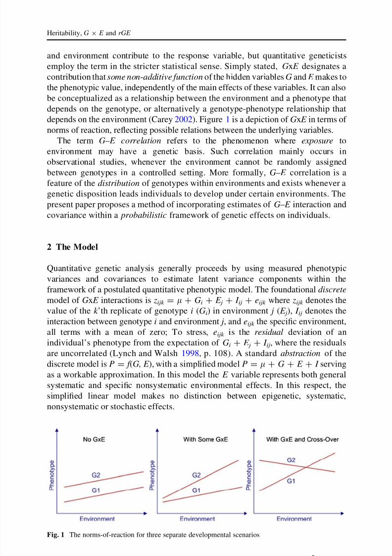
depends on the environment (Carey 2002). Figure 1 is a depiction of GxE in terms of

norms of reaction, reflecting possible relations between the underlying variables.

The term G–E correlation refers to the phenomenon where exposure to

environment may have a genetic basis. Such correlation mainly occurs in

observational studies, whenever the environment cannot be randomly assigned

between genotypes in a controlled setting. More formally, G–E correlation is a

feature of the distribution of genotypes within environments and exists whenever a

genetic disposition leads individuals to develop under certain environments. Thepresent paper proposes a method of incorporating estimates of G–E interaction and

covariance within a probabilistic framework of genetic effects on individuals.

2 The Model

Quantitative genetic analysis generally proceeds by using measured phenotypic

variances and covariances to estimate latent variance components within the

framework of a postulated quantitative phenotypic model. The foundational discretemodel of GxE interactions is zijk = l ? Gi ? E j ? I ij ? eijk where zijk denotes the

value of the k ’th replicate of genotype i (Gi) in environment j (E j), I ij denotes the

interaction between genotype i and environment j, and eijk the specific environment,

all terms with a mean of zero; To stress, eijk is the residual deviation of an

individual’s phenotype from the expectation of Gi ? E j ? I ij, where the residuals

are uncorrelated (Lynch and Walsh 1998, p. 108). A standard abstraction of the

discrete model is P = f (G, E ), with a simplified model P = l ? G ? E ? I serving

as a workable approximation. In this model the E variable represents both general

systematic and specific nonsystematic environmental effects. In this respect, the

simplified linear model makes no distinction between epigenetic, systematic,

nonsystematic or stochastic effects.

Fig. 1 The norms-of-reaction for three separate developmental scenarios

Heritability, G 9 E and rGE

123



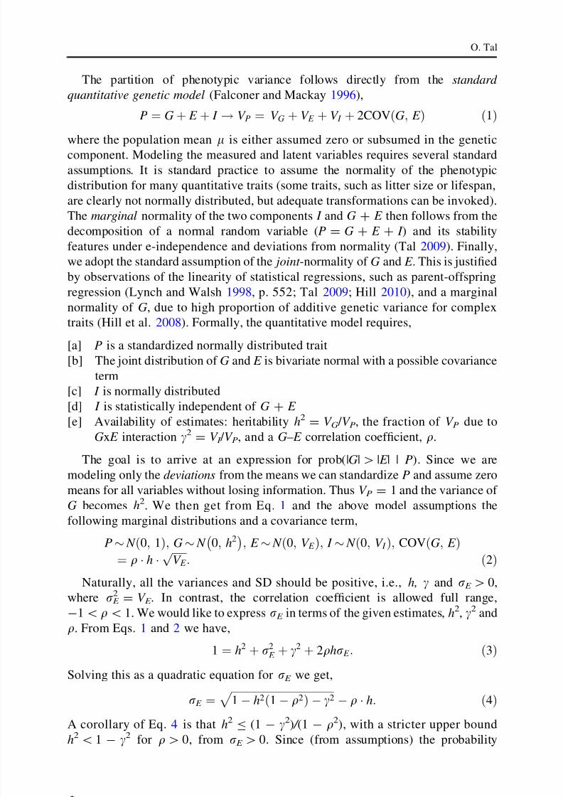
The partition of phenotypic variance follows directly from the standard

quantitative genetic model (Falconer and Mackay 1996),

P ¼ G þ E þ I V P ¼ V G þ V E þ V I þ 2COVðG; E Þ ð1Þ

where the population mean l is either assumed zero or subsumed in the geneticcomponent. Modeling the measured and latent variables requires several standard

assumptions. It is standard practice to assume the normality of the phenotypic

distribution for many quantitative traits (some traits, such as litter size or lifespan,

are clearly not normally distributed, but adequate transformations can be invoked).

The marginal normality of the two components I and G ? E then follows from the

decomposition of a normal random variable (P = G ? E ? I ) and its stability

features under e-independence and deviations from normality (Tal 2009). Finally,

we adopt the standard assumption of the joint -normality of G and E . This is justified

by observations of the linearity of statistical regressions, such as parent-offspringregression (Lynch and Walsh 1998, p. 552; Tal 2009; Hill 2010), and a marginal

normality of G, due to high proportion of additive genetic variance for complex

traits (Hill et al. 2008). Formally, the quantitative model requires,

[a] P is a standardized normally distributed trait

[b] The joint distribution of G and E is bivariate normal with a possible covariance

term

[c] I is normally distributed

[d] I is statistically independent of G ? E

[e] Availability of estimates: heritability h2 = V G / V P, the fraction of V P due toGxE interaction c

2= V I / V P, and a G–E correlation coefficient, q.

The goal is to arrive at an expression for prob(|G|[ |E | | P). Since we are

modeling only the deviations from the means we can standardize P and assume zero

means for all variables without losing information. Thus V P = 1 and the variance of

G becomes h2. We then get from Eq. 1 and the above model assumptions the

following marginal distributions and a covariance term,

P $ N 0; 1ð Þ; G $ N 0; h2À Á; E $ N 0; V E ð Þ; I $ N 0; V I ð Þ; COV G; E ð Þ¼ q Á h Á ffiffiffiffiffiffiV E p : ð2Þ

Naturally, all the variances and SD should be positive, i.e., h, c and rE [0,

where rE 2

= V E . In contrast, the correlation coefficient is allowed full range,

-1\q\1. We would like to express rE in terms of the given estimates, h2, c2 and

q. From Eqs. 1 and 2 we have,

1 ¼ h2 þ r2E þ c

2 þ 2qhrE : ð3ÞSolving this as a quadratic equation for rE we get,

rE ¼ ffiffiffiffiffiffiffiffiffiffiffiffiffiffiffiffiffiffiffiffiffiffiffiffiffiffiffiffiffiffiffiffiffiffiffiffiffiffiffi1 À h2 1 À q2ð Þ À c2

p À q Á h: ð4ÞA corollary of Eq. 4 is that h2 B (1 - c

2) / (1 - q2), with a stricter upper bound

h2\1 - c2 for q[0, from rE [0. Since (from assumptions) the probability

O. Tal

123



density function ( pdf ) for G and E is bivariate normal with correlation of q, the

general expression is,

f h2;rE ;qðg; eÞ ¼ 1

2phrE ffiffiffiffiffiffiffiffiffiffiffiffiffiffiffiffiffi

1 À q

2

ð Þp Á eÀ 1

2Á 1Àq2ð Þg2

h2À2qg

hÁ erE

þe2

r2E h i: ð5Þ

To formalize the probability that |G|[ |E | we first need to arrive at the joint

density function of G and E conditional on P, denoted F . From first principles of

conditional probability we have,

F p;h2;c2;qðg; eÞ ¼ pG;E jPðg; ej pÞ ¼ pG;E ;Pðg; e; pÞ pPð pÞ ¼ pPjG;E ð pjg; eÞ Á pG;E ðg; eÞ

pPð pÞ¼ p I ð p À g À eÞ Á pG;E ðg; eÞ

pPð pÞ : ð6Þ

Note that p I ð p À g À eÞ ¼ pPjG;E ð pjg; eÞ since P = G ? E ? I ; hence pPjG;E ð pjg; eÞhas same variance as I (c2) but a mean of g ? e. The pdf of a normal random

variable X with zero mean and non- zero variance v (we assume G, E , and I G xE in

Eq. 1 are non-degenerate random variables) is given by

uvð xÞ ¼ 1 ffiffiffiffiffiffiffiffi2pv

p eÀ x2=2v: ð7Þ

In terms of uvð xÞ and f we have,

F p;h2;c2;qðg; eÞ ¼ uc2ð p À g À eÞ Á f h2;rE ;qðg; eÞu1

ð p

Þð8Þ

which results in a bivariate normal pdf after explicit substitution and arranging of

terms (see ‘‘Appendix’’),

F ðg; eÞ ¼ 1

2pr1r2

ffiffiffiffiffiffiffiffiffiffiffiffiffiffiffiffiffiffiffi1 À q

212

À Áq e

À1

2Á 1Àq212ð Þ

gÀl1r1

2

À2q12

gÀl1r1

Á eÀl2

r2

þ eÀl2

r2

2 !

: ð9Þ

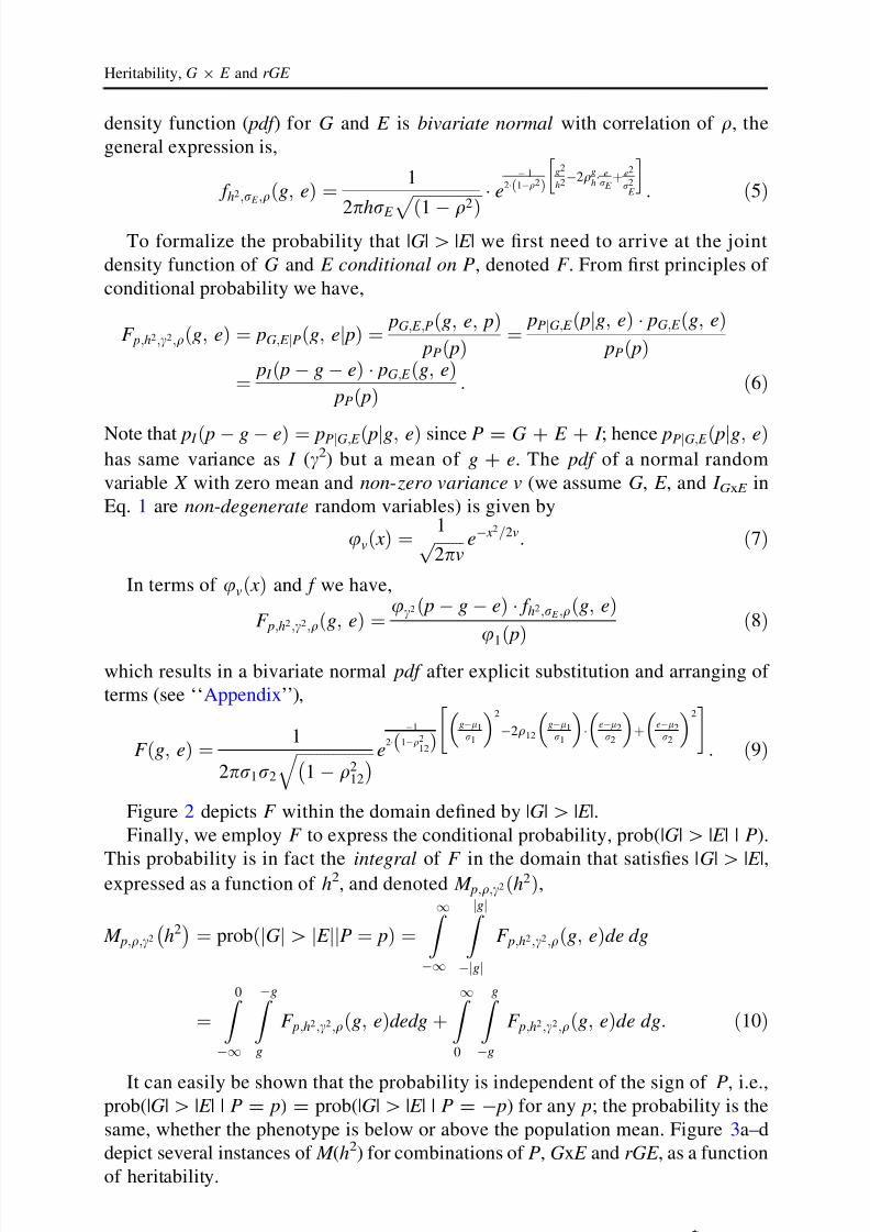
Figure 2 depicts F within the domain defined by |G|[ |E |.

Finally, we employ F to express the conditional probability, prob(|G|[ |E | | P).

This probability is in fact the integral of F in the domain that satisfies |G|[ |E |,expressed as a function of h2, and denoted M p;q;c2 h2ð Þ,

M p;q;c2 h2À Á ¼ prob Gj j[ E j jjP ¼ pð Þ ¼

Z 1À1

Z jgj

Àjgj

F p;h2;c2;qðg; eÞde dg

¼Z 0

À1

Z Àg

g

F p;h2;c2;qðg; eÞdedg þZ 10

Z gÀg

F p;h2;c2;qðg; eÞde dg: ð10Þ

It can easily be shown that the probability is independent of the sign of P, i.e.,prob(|G|[ |E | | P = p) = prob(|G|[ |E | | P = - p) for any p; the probability is the

same, whether the phenotype is below or above the population mean. Figure 3a–d

depict several instances of M (h2) for combinations of P, GxE and rGE , as a function

of heritability.


123



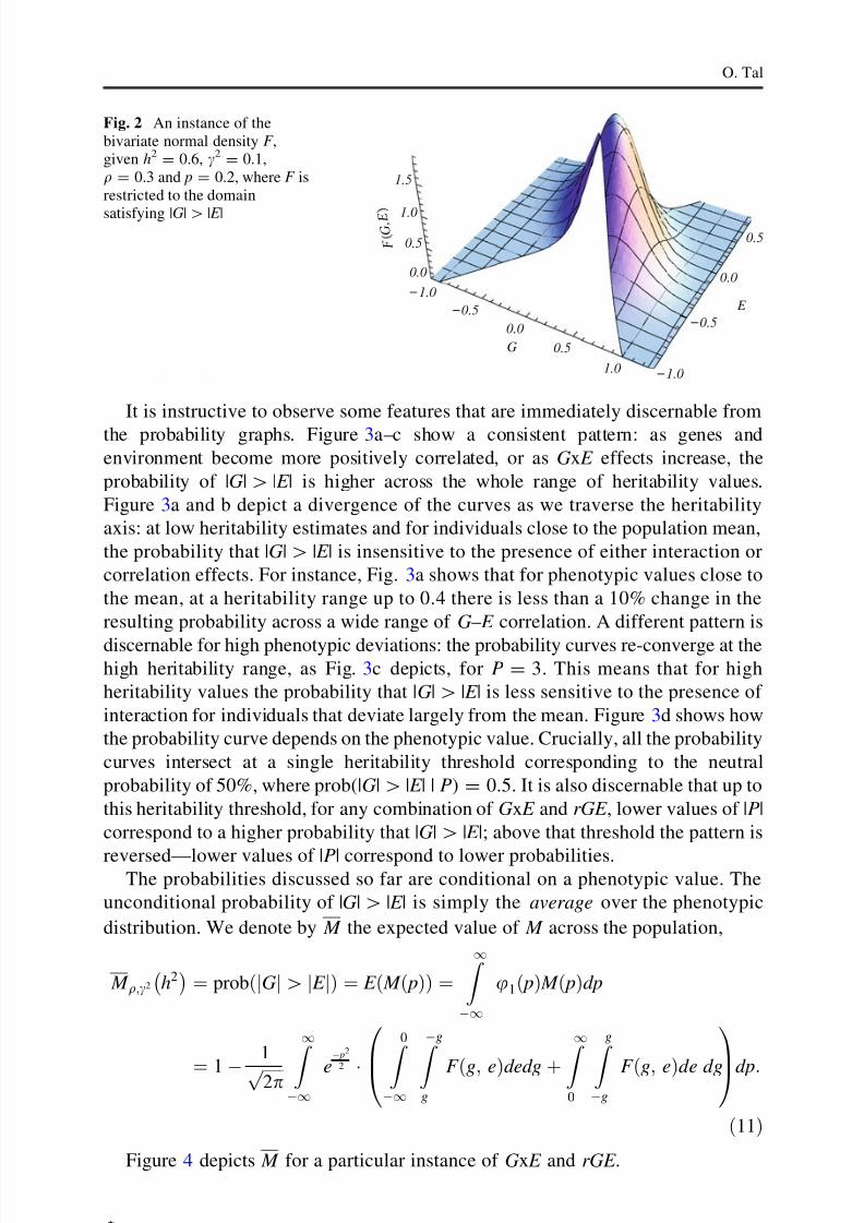
It is instructive to observe some features that are immediately discernable from

the probability graphs. Figure 3a–c show a consistent pattern: as genes andenvironment become more positively correlated, or as GxE effects increase, the

probability of |G|[ |E | is higher across the whole range of heritability values.

Figure 3a and b depict a divergence of the curves as we traverse the heritability

axis: at low heritability estimates and for individuals close to the population mean,

the probability that |G|[ |E | is insensitive to the presence of either interaction or

correlation effects. For instance, Fig. 3a shows that for phenotypic values close to

the mean, at a heritability range up to 0.4 there is less than a 10% change in the

resulting probability across a wide range of G–E correlation. A different pattern is

discernable for high phenotypic deviations: the probability curves re-converge at thehigh heritability range, as Fig. 3c depicts, for P = 3. This means that for high

heritability values the probability that |G|[ |E | is less sensitive to the presence of

interaction for individuals that deviate largely from the mean. Figure 3d shows how

the probability curve depends on the phenotypic value. Crucially, all the probability

curves intersect at a single heritability threshold corresponding to the neutral

probability of 50%, where prob(|G|[ |E | | P) = 0.5. It is also discernable that up to

this heritability threshold, for any combination of GxE and rGE , lower values of |P|

correspond to a higher probability that |G|[ |E |; above that threshold the pattern is

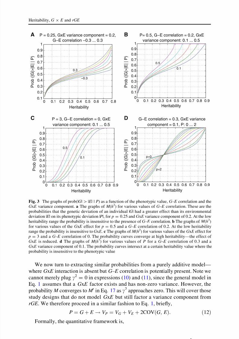
reversed—lower values of |P| correspond to lower probabilities.The probabilities discussed so far are conditional on a phenotypic value. The

unconditional probability of |G|[ |E | is simply the average over the phenotypic

distribution. We denote by M the expected value of M across the population,

M q;c2 h2À Á ¼ prob Gj j[ E j jð Þ ¼ E ð M ð pÞÞ ¼

Z 1À1

u1ð pÞ M ð pÞdp

¼ 1 À1 ffiffiffiffiffiffi2pp Z

1

À1e

À p2

2

Á Z 0

À1Z Àg

gF ðg; eÞdedg þ Z

1

0

Z g

ÀgF ðg; eÞde dg

0B@ 1CAdp:

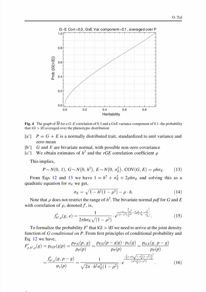
ð11ÞFigure 4 depicts M for a particular instance of GxE and rGE .

1.0

0.5

0.0

0.5

1.0

G

1.0

0.5

0.0

0.5

E

0.0

0.5

1.0

1.5

F

G , E

Fig. 2 An instance of the

bivariate normal density F ,

given h2

= 0.6, c2 = 0.1,

q = 0.3 and p = 0.2, where F is

restricted to the domain

satisfying |G|[ |E |

O. Tal

123



We now turn to extracting similar probabilities from a purely additive model—

where GxE interaction is absent but G–E correlation is potentially present. Note we

cannot merely plug c2

= 0 in expressions (10) and (11), since the general model in

Eq. 1 assumes that a GxE factor exists and has non-zero variance. However, the

probability M converges to M 0 in Eq. 17 as c2 approaches zero. This will cover those

study designs that do not model GxE but still factor a variance component fromrGE . We therefore proceed in a similar fashion to Eq. 1, briefly,

P ¼ G þ E V P ¼ V G þ V E þ 2COVðG; E Þ: ð12ÞFormally, the quantitative framework is,

0 0.1 0.2 0.3 0.4 0.5 0.6 0.7 0.8 0.90

0.1

0.2

0.3

0.4

0.5

0.6

0.7

0.8

0.9

1

Heritability

P r o b ( | G | > | E | | P )

P = 3, G−E correlation = 0, GxE

0.5

0.1

0 0.1 0.2 0.3 0.4 0.5 0.6 0.7 0.8 0.90

0.1

0.2

0.3

0.4

0.5

0.60.7

0.8

0.9

1

Heritability

P r o b ( | G | > | E | | P

)

P= 0.5, G−E correlation = 0.2, GxE

0.5

0.1

0 0.1 0.2 0.3 0.4 0.5 0.6 0.7 0.80.1

0.2

0.3

0.4

0.5

0.6

0.7

0.8

0.9

1

Heritability

P r o b ( | G | > | E | | P

)

P = 0.25, GxE variance component = 0.2,

0.3

−0.3

0 0.1 0.2 0.3 0.4 0.5 0.6 0.7 0.8 0.90

0.1

0.2

0.3

0.4

0.5

0.6

0.7

0.8

0.9

1

Heritability

P r o b ( | G | > | E | | P )

G−E correlation = 0.3, GxE variance

p=0

p=2

component = 0.1, P: 0 ... 2

variance component: 0.1 ... 0.5G−E correlation −0.3 ... 0.3

variance component: 0.1 ... 0.5

A B

C D

Fig. 3 The graphs of prob(|G|[ |E | | P) as a function of the phenotypic value, G–E correlation and the

GxE variance component. a The graphs of M (h2) for various values of G–E correlation. These are the

probabilities that the genetic deviation of an individual |G| had a greater effect than its environmental

deviation |E | on its phenotypic deviation |P|, for p = 0.25 and GxE variance component of 0.2. At the low

heritability range the probability is insensitive to the presence of G–E correlation. b The graphs of M (h2)

for various values of the GxE effect for p = 0.5 and a G–E correlation of 0.2. At the low heritability

range the probability is insensitive to GxE . c The graphs of M (h2) for various values of the GxE effect for

p = 3 and a G–E correlation of 0. The probability curves converge at high heritability—the effect of GxE is reduced. d The graphs of M (h2) for various values of P for a G–E correlation of 0.3 and a

GxE variance component of 0.1. The probability curves intersect at a certain heritability value where the

probability is insensitive to the phenotypic value


123



[a’] P = G ? E is a normally distributed trait, standardized to unit variance and

zero mean

[b’] G and E are bivariate normal, with possible non-zero covariance

[c’] We obtain estimates of h2

and the rGE correlation coefficient q

This implies,

P $ N 0; 1ð Þ; G $ N 0; h2À Á

; E $ N 0; r2E

À Á; COV G; E ð Þ ¼ qhrE : ð13Þ

From Eqs. 12 and 13 we have 1 = h2 ? rE 2

? 2qhrE and solving this as a

quadratic equation for rE we get,

rE ¼ ffiffiffiffiffiffiffiffiffiffiffiffiffiffiffiffiffiffiffiffiffiffiffiffiffiffiffiffiffiffi

1 À h2 1 À q2ð Þp

À q Á h: ð14ÞNote that q does not restrict the range of h2. The bivariate normal pdf for G and E

with correlation of q, denoted f 0, is,

f 0h2;qðg; eÞ ¼ 1

2phrE

ffiffiffiffiffiffiffiffiffiffiffiffiffiffiffiffiffi1 À q2ð Þp Á e

À1

2Á 1Àq2ð Þg2

h2À2qg

hÁ erE

þe2

r2E

h i: ð15Þ

To formalize the probability F 0 that |G|[ |E | we need to arrive at the joint density

function of G conditional on P. From first principles of conditional probability and

Eq. 12 we have,

F 0 p;h2;qðgÞ ¼ pGjPðgj pÞ ¼ pP;Gð p; gÞ pPð pÞ ¼ pE jGð p À gjgÞ Á pGðgÞ

pPð pÞ ¼ pG;E ðg; p À gÞ pPð pÞ

¼ f 0

h2;qðg; p À gÞu1ð pÞ ¼ 1 ffiffiffiffiffiffiffiffiffiffiffiffiffiffiffiffiffiffiffiffiffiffiffiffiffiffiffiffiffiffiffiffiffiffiffi

2p Á h2r2E 1 À q2ð Þ

p Á e

À gÀ ph ffiffiffiffiffiffiffiffiffiffiffiffiffiffiffi

1Àr2E

1Àq2ð Þp ð Þ2

2Áh2r2E

1Àq2ð Þ : ð16Þ

0.0 0.2 0.4 0.6 0.8

0.0

0.2

0.4

0.6

0.8

1.0

Heritability

G−E Corr=0.3 , GxE Var component=0.1 , averaged over P

P r o b ( | G | > | E | )

Fig. 4 The graph of M for a G–E correlation of 0.3 and a GxE variance component of 0.1: the probability

that |G|[ |E | averaged over the phenotypic distribution

O. Tal

123



F 0 is expressed in Eq. 16 in a form easily recognizable as a normal pdf , where the

variance is h2r

2E 1 À q

2ð Þand the mean is ph ffiffiffiffiffiffiffiffiffiffiffiffiffiffiffiffiffiffiffiffiffiffiffiffiffiffiffiffiffiffi

1 À r2E 1 À q2ð Þ

p . The expression for

M 0 ¼ prob Gj j[ E j jjPð Þ is finally,

M 0 p;h2 ¼ prob Gj j[ E j jjPð Þ ¼R 1

p=2

F 0 p;h2;qðgÞdg if p ! 0

R p=2

À1F 0

p;h2;qðgÞdg if p\0

8>>><>>>:

: ð17Þ

The expected value of M 0 across the population is denoted M 0,

M 0 h2

À Á¼ prob Gj j[ E j jð Þ ¼ E M 0h2ð pÞ

À Á¼

Z 1

À1

u1ð pÞ M 0h2ð pÞdp

¼Z 0

À1u1ð pÞ

Z p=2

À1F 0 p;h2;qðgÞdgdp þ

Z 10

u1ð pÞZ 1

p=2

F 0 p;h2;qðgÞdgdp

¼ 2

Z 10

1 ffiffiffiffiffiffi2p

p eÀ p2

2

Z 1 p=2

F 0 p;h2;qðgÞdgdp: ð18Þ

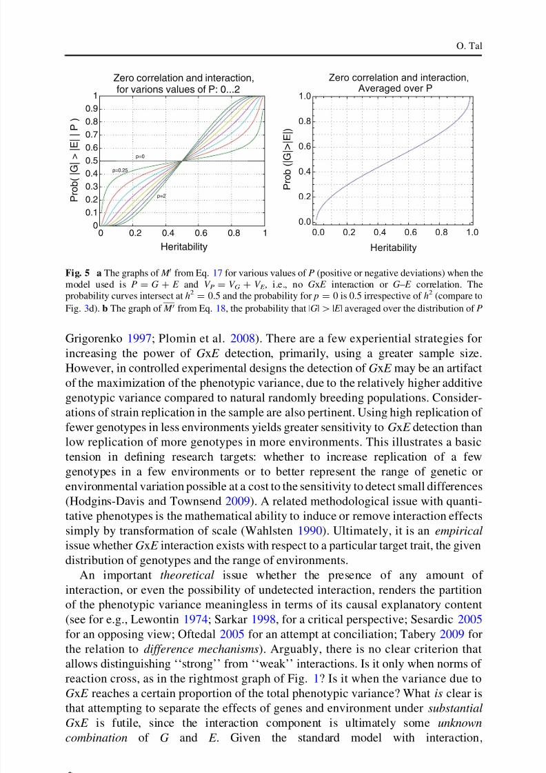
Figure 5a and b depict the probabilities generated within this additive framework

for the most basic scenario where G–E correlation is zero.

3 Discussion

The framework outlined in this paper allows incorporating estimates of gene–

environment interaction and covariance within a probabilistic interpretation of

heritability (Tal 2009; see Tal et al. 2010, for an extension that includes a putative

epigenetic variable). Specifically, given estimates of heritability and the variance

components associated with GxE and rGE , a method based on the standard quantitative

model generates the conditional probability that genetic factors had a greater effect than

environmental factors on a deviation from the population mean. Previous approaches of

reformulating heritability arise from the application of more complex mixed

quantitative models (see Oakey et al. 2007, for a ‘‘generalized heritability’’ that

incorporates pedigree information to form an extended pedigree model).

Two underlying assumptions of the present framework should be reemphasized.

First, the model takes as a point of departure the standard linear quantitative model

with interaction, P = G ? E ? I , where the three latent terms are modeled as

continuous variables. Second, the probabilistic framework relies on the availability of

estimates of variance components describing the non-additive effects. In this respect,it is a methodological issue whether a particular sample size or genetic model has

sufficient power to detect and quantify GxE for a target experimental design or

observational study. Indeed, it is well known that the power to detect interaction is

considerably less than that of the main effects (Wahlsten 1990; Sternberg and


123



Grigorenko 1997; Plomin et al. 2008). There are a few experiential strategies for

increasing the power of GxE detection, primarily, using a greater sample size.

However, in controlled experimental designs the detection of GxE may be an artifact

of the maximization of the phenotypic variance, due to the relatively higher additive

genotypic variance compared to natural randomly breeding populations. Consider-

ations of strain replication in the sample are also pertinent. Using high replication of

fewer genotypes in less environments yields greater sensitivity to GxE detection than

low replication of more genotypes in more environments. This illustrates a basic

tension in defining research targets: whether to increase replication of a few

genotypes in a few environments or to better represent the range of genetic or

environmental variation possible at a cost to the sensitivity to detect small differences

(Hodgins-Davis and Townsend 2009). A related methodological issue with quanti-

tative phenotypes is the mathematical ability to induce or remove interaction effects

simply by transformation of scale (Wahlsten 1990). Ultimately, it is an empirical

issue whether GxE interaction exists with respect to a particular target trait, the givendistribution of genotypes and the range of environments.

An important theoretical issue whether the presence of any amount of

interaction, or even the possibility of undetected interaction, renders the partition

of the phenotypic variance meaningless in terms of its causal explanatory content

(see for e.g., Lewontin 1974; Sarkar 1998, for a critical perspective; Sesardic 2005

for an opposing view; Oftedal 2005 for an attempt at conciliation; Tabery 2009 for

the relation to difference mechanisms). Arguably, there is no clear criterion that

allows distinguishing ‘‘strong’’ from ‘‘weak’’ interactions. Is it only when norms of

reaction cross, as in the rightmost graph of Fig. 1? Is it when the variance due toGxE reaches a certain proportion of the total phenotypic variance? What is clear is

that attempting to separate the effects of genes and environment under substantial

GxE is futile, since the interaction component is ultimately some unknown

combination of G and E . Given the standard model with interaction,

0.0 0.2 0.4 0.6 0.8 1.0

0.0

0.2

0.4

0.6

0.8

1.0

Heritability

Zero correlation and interaction,

0 0.2 0.4 0.6 0.8 10

0.1

0.2

0.3

0.4

0.5

0.60.7

0.8

0.9

1

Heritability

P r o b ( | G | > | E | |

P

)

P r o b ( | G | > | E | )

Zero correlation and interaction,

p=0

p=0.25

p=2

for varions values of P: 0...2 Averaged over P

Fig. 5 a The graphs of M 0 from Eq. 17 for various values of P (positive or negative deviations) when themodel used is P = G ? E and V P = V G ? V E , i.e., no GxE interaction or G–E correlation. The

probability curves intersect at h2 = 0.5 and the probability for p = 0 is 0.5 irrespective of h2 (compare to

Fig. 3d). b The graph of M 0 from Eq. 18, the probability that |G|[ |E | averaged over the distribution of P

O. Tal

123



P = G ? E ? I , if I is large compared to G and E , our probabilistic framework

cannot capture the full relation between the latent genetic and environmental values.

On the other hand, the presence of strong G–E correlation does not pose such

difficulty. This follows from the fact that the correlation is not a separate component

of the phenotypic value, P = G ? E ? I , but only a characteristic of the jointdistribution of G and E , which is fully captured by the conditional probability

prob(|G|[ |E | | P).

Finally, an application of the probabilistic framework would involve plugging the

various estimates of variance components in the probability function M in Eq. 10, or

M in Eq. 11. For instance, if rGE = 0.3 and the variance portion due to GxE is 0.2,

then for a heritability of 0.7 the probability that |G|[ |E | is 0.8 for individuals at �

SD from the population mean (see Fig. 3a). It is instructive to compare such results

with the probabilities generated from a model that ignores GxE and rGE , via M 0 in

Eq. 17. Using, for comparative illustration, a phenotypic deviation of � SD andheritability of 0.7, we have M 0(0.7) = prob(|G|[ |E | | P = �) = 0.55, quite in

contrast with the higher probability M (0.7) = 0.8, based on a model with some GxE

and rGE effects. In a similar fashion, one could compare the averaged probabilities

from M in Eq. 11 with M 0 in Eq. 18. Such comparisons are most pertinent in the

context of studies that employ a dual design: a reduced - fit additive model that

ignores GxE and rGE effects, and a better - fit model that incorporates these effects.

The probabilities generated using variance component estimates from the better-fit

model may better describe the relative weight of genes and environment on the

deviation of a target trait from the population mean.

Acknowledgments I would like to thank Jim Tabery, Eva Jablonka, John Loehlin, John C. DeFries,

Neven Sesardic, Samir Okasha, Tamir Tassa and two anonymous reviewers for insightful feedback and

suggestions.

Appendix: Derivation of the Bivariate Normal Form for F

We wish to express F from Eq. 8 such that it complies with a bivariate normal form

Eq. 9, if indeed it can be expressed as such. Towards that end we need to findexpressions for r1, r2, l1, l2 and q12 in terms of the parameters of F . Therefore, we

write F such that terms involving powers of its independent variables g and e are

separately expressed,

F ðg; eÞ ¼ 1

2p Á h Á c Á rE Á ffiffiffiffiffiffiffiffiffiffiffiffiffi

1 À q2p Á e

X

2Ác2 1Àq2ð Þh2r2E ð19Þ

where,

X ¼ Àg

2

1 À q

2À Áh

2

hr2

E þ c

2

r

2

E À ÁÀ e

2

1 À q

2À Áh

2

r

2

E þ c

2

h

2À Áþ ðg þ eÞ 2 p 1 À q

2À Á

h2r

2E

À ÁÀ 2ge 1 À q2

À Áh2r

2E þ c

2qhrE

À ÁÀ p2 1 À q

2À Á

h2r

2E 1 À c

2À Á ð20Þ

and where rE ¼ ffiffiffiffiffiffiffiffiffiffiffiffiffiffiffiffiffiffiffiffiffiffiffiffiffiffiffiffiffiffiffiffiffiffiffiffiffiffiffi

1 À h2 1 À q2ð Þ À c2p

À q Á h, as derived in Eq. 3.


123



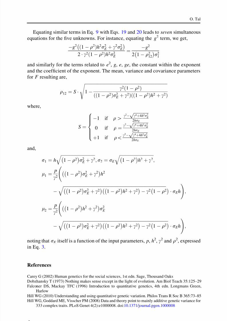
Equating similar terms in Eq. 9 with Eqs. 19 and 20 leads to seven simultaneous

equations for the five unknowns. For instance, equating the g2 term, we get,

Àg2 1 À q2ð Þh2

r2E þ c

2r

2E À Á

2 Á c2

1 À q2

ð Þh2

r

2

E ¼

Àg2

2 1 À q

2

12À Á

r

2

1

and similarly for the terms related to e2, g, e, ge, the constant within the exponent

and the coefficient of the exponent. The mean, variance and covariance parameters

for F resulting are,

q12 ¼ S Á ffiffiffiffiffiffiffiffiffiffiffiffiffiffiffiffiffiffiffiffiffiffiffiffiffiffiffiffiffiffiffiffiffiffiffiffiffiffiffiffiffiffiffiffiffiffiffiffiffiffiffiffiffiffiffiffiffiffiffiffiffiffiffiffiffiffiffiffiffiffiffiffiffiffiffiffiffiffi

1 À c2 1 À q2ð Þ1 À q2ð Þr2

E þ c2ð Þ 1 À q2ð Þh2 þ c2ð Þ

s

where,

S ¼À1 if q[

c2À ffiffiffiffiffiffiffiffiffiffiffiffiffiffic4þ4h2r

2E

p 2hrE

0 if q ¼ c2À ffiffiffiffiffiffiffiffiffiffiffiffiffiffic4þ4h2r2

E

p 2hrE

þ1 if q\c

2À ffiffiffiffiffiffiffiffiffiffiffiffiffiffic4þ4h2r

2E

p 2hrE

8>>><>>>:

and,

r1 ¼ h ffiffiffiffiffiffiffiffiffiffiffiffiffiffiffiffiffiffiffiffiffiffiffiffiffiffiffiffiffiffiffiffiÀ1 À q2

Ár2E þ c2

q ; r2 ¼ rE ffiffiffiffiffiffiffiffiffiffiffiffiffiffiffiffiffiffiffiffiffiffiffiffiffiffiffiffiffiffiffiffiÀ1 À q2

Áh2 þ c2

q ;

l1 ¼ p

c2

ÀÀ1 À q

2Ár

2E þ c

2Á

h2

À ffiffiffiffiffiffiffiffiffiffiffiffiffiffiffiffiffiffiffiffiffiffiffiffiffiffiffiffiffiffiffiffiffiffiffiffiffiffiffiffiffiffiffiffiffiffiffiffiffiffiffiffiffiffiffiffiffiffiffiffiffiffiffiffiffiffiffiffiffiffiffiffiffiffiffiffiffiffiffiffiffiffiffiffiffiffiffiffiffiffiffiffiffiffiffiffiffiÀÀ

1 À q2Ár

2E þ c2

ÁÀÀ1 À q2

Áh2 þ c2

ÁÀ c2À

1 À q2

q Á Á rE h

;

l2 ¼ p

c2

ÀÀ1 À q

2Á

h2 þ c2Ár

2E

À ffiffiffiffiffiffiffiffiffiffiffiffiffiffiffiffiffiffiffiffiffiffiffiffiffiffiffiffiffiffiffiffiffiffiffiffiffiffiffiffiffiffiffiffiffiffiffiffiffiffiffiffiffiffiffiffiffiffiffiffiffiffiffiffiffiffiffiffiffiffiffiffiffiffiffiffiffiffiffiffiffiffiffiffiffiffiffiffiffiffiffiffiffiffiffiffiffiffiffiÀÀ1 À q2

Ár2E þ c2

ÁÀÀ1 À q2

Áh2 þ c2

ÁÀ c2À

1 À q2Áq Á rE h

;

noting that rE itself is a function of the input parameters, p, h2, c2 and q2, expressed

in Eq. 3.

References

Carey G (2002) Human genetics for the social sciences, 1st edn. Sage, Thousand Oaks

Dobzhansky T (1973) Nothing makes sense except in the light of evolution. Am Biol Teach 35:125–29Falconer DS, Mackay TFC (1996) Introduction to quantitative genetics, 4th edn. Longmans Green,

Harlow

Hill WG (2010) Understanding and using quantitative genetic variation. Philos Trans R Soc B 365:73–85

Hill WG, Goddard ME, Visscher PM (2008) Data and theory point to mainly additive genetic variance for

333 complex traits. PLoS Genet 4(2):e1000008. doi:10.1371/journal.pgen.1000008

O. Tal

123

http://dx.doi.org/10.1371/journal.pgen.1000008

http://dx.doi.org/10.1371/journal.pgen.1000008



Hodgins-Davis A, Townsend JP (2009) Evolving gene expression: from G to E to GxE . Trends Ecol Evol

24(12):649–658

Lewontin RC (1974) The analysis of variance and the analysis of causes. Am J Hum Genet 26:400–411

Lewontin RC (1975) Genetic aspects of intelligence. Annu Rev Genet 9:382–405

Lynch M, Walsh B (1998) Genetics and analysis of quantitative traits, 1st edn. Sinauer Associates,

SunderlandOakey H, Verbyla AP, Cullis BR, Wei X, Pitchford WS (2007) Joint modeling of additive and non-

additive (genetic line) effects in multi-environment trials. Theor Appl Genet 114:1319–1332

Oftedal G (2005) Heritability and causation. Philos Sci 72:699–709

Plomin R, DeFries JC, McClearn GE, McGuffin P (2008) Behavioral genetics, 5th edn. Worth, New York

Rose S (1999) Precis of lifelines: biology, freedom, determinism. Behav Brain Sci 22(5):871–885

Sarkar S (1998) Genetics and reductionism. Cambridge University Press, Cambridge

Sesardic N (2005) Making sense of heritability. Cambridge University Press, Cambridge

Sternberg RJ, Grigorenko E (1997) Intelligence, heredity, and environment. Cambridge University Press,

Cambridge

Tabery J (2009) Difference mechanisms: explaining variation with mechanisms. Biol Philos 24:645–664

Tal O (2009) From heritability to probability. Biol Philos 24:81–105

Tal O, Kisdi E, Jablonka E (2010) Epigenetic contribution to covariance between relatives. Genetics

184:1037–1050

Wahlsten D (1990) Insensitivity of the analysis of variance to heredity-environment interaction. Behav

Brain Sci 13:109–161


123

Tal, The Impact

Documents

Transcript of Tal, The Impact