![Induccion a MATLAB´ Algebra Lineal...Induccion a MATLAB (´ Algebra Lineal)´ Escuela de Matem´aticas Universidad Nacional 4 / 1 Ingresando vectores Alt + 91 = [ Alt + 93 = ] Alt](https://static.fdocuments.nl/doc/165x107/601a3a7bbb044460fe2b95fa/induccion-a-matlab-algebra-lineal-induccion-a-matlab-algebra-lineal.jpg)
South American plate motion, asthenospheric flow and its ......FACULTAD DE CIENCIAS F ´ISICAS Y...
72
UNIVERSIDAD DE CONCEPCI ´ ON FACULTAD DE CIENCIAS F ´ ISICAS Y MATEM ´ ATICAS DEPARTAMENTO DE GEOF ´ ISICA South American plate motion, asthenospheric flow and its implications for Andean orogeny since the late Cretaceous. Ingo Leonardo Stotz Canales Habilitaci´ on Profesional para optar al T´ ıtulo de Geof´ ısico Profesor Gu´ ıa: Dr. Andr´ es Tassara Dr. Hans-Peter Bunge Dr. Giampiero Iaffaldano Comisi´ on: Dr. Matthew Miller, Dr. Andr´ es Sepulveda, Enero de 2013
Transcript of South American plate motion, asthenospheric flow and its ......FACULTAD DE CIENCIAS F ´ISICAS Y...
UNIVERSIDAD DE CONCEPCION
FACULTAD DE CIENCIAS FISICAS Y MATEMATICAS
DEPARTAMENTO DE GEOFISICA
South American plate motion,
asthenospheric flow and its implications
for Andean orogeny since the late Cretaceous.
Ingo Leonardo Stotz Canales
Habilitacion Profesional para optar al Tıtulo de Geofısico
Profesor Guıa:
Dr. Andres Tassara
Dr. Hans-Peter Bunge
Dr. Giampiero Iaffaldano
Comision:
Dr. Matthew Miller, Dr. Andres Sepulveda,
Enero de 2013
Contents
1 Introduction 9
2 Methodology 15
3 Geology of the Andes 17
3.1 Anatomy of the Andes . . . . . . . . . . . . . . . . . . . . . . . . . . . . . . . . . . . . . . 17
3.2 The Andean evolution . . . . . . . . . . . . . . . . . . . . . . . . . . . . . . . . . . . . . . 19
4 Force balance for South America 26
4.1 Driving forces . . . . . . . . . . . . . . . . . . . . . . . . . . . . . . . . . . . . . . . . . . . 27
4.2 Resisting forces . . . . . . . . . . . . . . . . . . . . . . . . . . . . . . . . . . . . . . . . . . 29
4.3 Asthenosphere flow . . . . . . . . . . . . . . . . . . . . . . . . . . . . . . . . . . . . . . . . 30
4.4 Andes elevation . . . . . . . . . . . . . . . . . . . . . . . . . . . . . . . . . . . . . . . . . . 33
5 Discussion 38
6 Conclusion 46
A Geologic time scale 54
B Mantle convection 56
C Andean geology table 61
D Force balance results 66
1

List of Figures
1.1 Half-spreading rates of conjugate plates from Muller et al. (2008a). . . . . . . . . . . . . . 9
1.2 Spreading velocity record for South America with respect to Africa (Africa fix). The velocity
record reveals short time velocity variations that can not be attributed to large-scale mantle
buoyancy forces. The x-axis shows the time scale since Cretaceous (140 ma) to the present
(right to left, respectively) and the magnitude of the velocity in the y-axis. The color lines
represents the different model used to constrain the data (Bianchi et al., 2011) . . . . . . 10
1.3 Residual basement depth grid computed by calculating the difference between the predicted
basement depth and the sediment unloaded basement depth. Predicted basement depth is
obtained by applying Crosby et al.’s (2006) North Pacific thermal boundary layer model to
the age-area distribution from Muller et al. (2008a). . . . . . . . . . . . . . . . . . . . . . 11
1.4 Topographic map of the South Atlantic and adjacent continents from ETOPO1 (Amante &
Eakins, 2009), annotated with major structural elements cited in the text. Craton names
are boldface, while stars denote prominent hotspots (F: Fernando de Noronha; As: Ascen-
sion; Af: Afar; SH: Saint Helena; TM: Trinidade and Martim Vaz; Tr: Tristan da Cunha;
G: Gough Island; B: Bouvet Island; M: Marion; C: Crozet Islands) . . . . . . . . . . . . . 12
3.1 Topographic map of the South American continent and its most prominent geological fea-
ture, the Andes. The Andean Cordillera extends along the whole continent from north to
south. The Andes is also segmented in three main zones the Central, South and North.
Further the Central Andean Zone, is separated also in three regions the North, Central
Orocline and South-central. (Gansser, 1973) . . . . . . . . . . . . . . . . . . . . . . . . . 18
3.2 Paleogeographic sketch of the Peruvian margin, and location of main areas cited. 1: Cre-
taceous allochthonous terranes, and suture. 2: Coastal Cordillera. 3: Coastal Troughs. 4:
Western Trough. 5: Axial Swell. 6: Eastern Basin. 7: Brazilianand Guianese (Colom-
bian) Precambrianshields. 8: Jurassic suture (Jaillard, 1994). . . . . . . . . . . . . . . . . 19
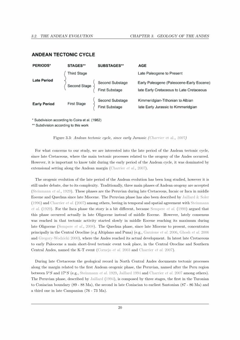
3.3 Andean tectonic cycle, since early Jurassic (Charrier et al., 2007) . . . . . . . . . . . . . 20
3.4 Timing and propagation of Andean uplift from southern to northern, in the Northern Cen-
tral Andes (Picard et al., 2008). . . . . . . . . . . . . . . . . . . . . . . . . . . . . . . . . 23
2
LIST OF FIGURES LIST OF FIGURES
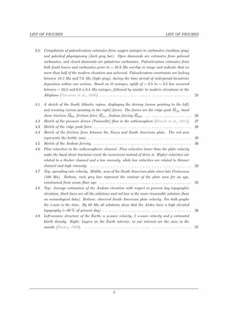
3.5 Compilation of paleoelevation estimates from oxygen isotopes in carbonates (medium gray)
and paleoleaf physiognomy (dark gray bar). Open diamonds are estimates from paleosol
carbonates, and closed diamonds are palustrine carbonates. Paleoelevation estimates from
both fossil leaves and carbonates prior to ∼ 10.3 Ma overlap in range and indicate that no
more than half of the modern elevation was achieved. Paleoelevation constraints are lacking
between 10.3 Ma and 7.6 Ma (light gray), during the time period of widespread lacustrine
deposition within our section. Based on O isotopes, uplift of ∼ 2.5 to ∼ 3.5 km occurred
between ∼ 10.3 and 6.8± 0.4 Ma isotopes, followed by similar to modern elevations in the
Altiplano (Garzione et al., 2006). . . . . . . . . . . . . . . . . . . . . . . . . . . . . . . . . 24
4.1 A sketch of the South Atlantic region, displaying the driving (arrow pointing to the left)
and resisting (arrow pointing to the right) forces. The forces are the ridge push ~Mrp, basal
shear traction ~Mbd, friction force ~Mfr, Andean forcing ~Mmb. . . . . . . . . . . . . . . . . 26
4.2 Sketch of the pressure driven (Poiseuille) flow in the asthenosphere (Hoeink et al., 2011). 27
4.3 Sketch of the ridge push force. . . . . . . . . . . . . . . . . . . . . . . . . . . . . . . . . . . 28
4.4 Sketch of the friction force between the Nazca and South American plate. The red area
represents the brittle zone. . . . . . . . . . . . . . . . . . . . . . . . . . . . . . . . . . . . . 29
4.5 Sketch of the Andean forcing. . . . . . . . . . . . . . . . . . . . . . . . . . . . . . . . . . . 30
4.6 Flow velocities in the asthenospheric channel. Flow velocities lower than the plate velocity
make the basal shear tractions resist the movement instead of drive it. Higher velocities are
related to a thicker channel and a low viscosity, while low velocities are related to thinner
channel and high viscosity. . . . . . . . . . . . . . . . . . . . . . . . . . . . . . . . . . . . 33
4.7 Top, spreading rate velocity. Middle, area of the South American plate since late Cretaceous
(100 Ma). Bottom, each grey line represent the contour of the plate area for an age,
constrained from ocean floor age. . . . . . . . . . . . . . . . . . . . . . . . . . . . . . . . . 35
4.8 Top: Average estimation of the Andean elevation with respect to present day topographic
elevation, black lines are all the solutions and red line is the more reasonable solution (base
on seismological data). Bottom: observed South American plate velocity. For both graphs
the x-axis is the time. By 60 Ma all solutions show that the Andes have a high elevated
topography (∼80 % of present day) . . . . . . . . . . . . . . . . . . . . . . . . . . . . . . . 36
4.9 Left:seismic structure of the Earth, α p-wave velocity, β s-wave velocity and ρ estimated
Earth density. Right: Layers on the Earth interior, to our interest are the ones in the
mantle (Davies, 1999). . . . . . . . . . . . . . . . . . . . . . . . . . . . . . . . . . . . . . 37
3

LIST OF FIGURES LIST OF FIGURES
5.1 Top: Estimate elevation of the Andean topography, red line in the more reasonable solution
and in grey are the other solutions. Middle: Observed South American plate velocity.
Bottom: Andean orogenic evolution since late Cretaceous. 1: oxygen isotopes is carbonates
(Garzione et al. 2006 and Ghosh et al. 2006), 2: leaf morphology method in the Altiplano,
Western and Eastern Cordillera (Gregory-Wodzicki, 2000), 3: AFT North Central Andes
and Central Orocline (Hoorn et al., 2010), 4: AFT in the Central Orocline (Gillis et al.,
2006), 5: unconformities in the Central Orocline (Cornejo et al., 2003), 6: tectonic activity
related to uplift in the Central Orocline (Sempere et al., 1997), 7: tectonic activity related
to uplift in the Northern Central Andes (Jaillard 1994 and Jaillard & Soler 1996), 8:
Estimated Andean average elevation. . . . . . . . . . . . . . . . . . . . . . . . . . . . . . . 39
5.2 Full waveform tomography image for the South Atlantic region. Left: 200 km depth seismic
images for the South Atlantic. Right: Two vertical profiles(Colli et al., 2012). . . . . . . . 40
5.3 Geoid image for the South American region. Warm colour regions are related to high
density zones, while cold colour regions are related to lower density zones. . . . . . . . . . 41
5.4 Evolution of the Plate configuration since late Cretaceous (120 Ma). It the figure can be
appreciated that Africa has remain almost in the same place, whereas the South American
continent has moved westward and how has evolved the plates in the side of the Pacific
(e.g., Farallon, Phoenix and Nazca plates) (Muller et al., 2008b). . . . . . . . . . . . . . . 42
5.5 Top: Estimate elevation of the Andean topography, red line is the more reasonable solution
and in grey are the other solutions and blue line is the new estimation of the elevation of
the Andes considering a pressure driven (Poiseuille) flux from Africa to South America.
Middle: Observed South American plate velocity. Bottom: Andean orogenic evolution
since late Cretaceous. 1: oxygen isotopes is carbonates (Garzione et al. 2006 and Ghosh
et al. 2006), 2: leaf morphology method in the Altiplano, Western and Eastern Cordillera
(Gregory-Wodzicki, 2000), 3: AFT North Central Andes and Central Orocline (Hoorn
et al., 2010), 4: AFT in the Central Orocline (Gillis et al., 2006), 5: unconformities
in the Central Orocline (Cornejo et al., 2003), 6: tectonic activity related to uplift in
the Central Orocline (Sempere et al., 1997), 7: tectonic activity related to uplift in the
Northern Central Andes (Jaillard 1994 and Jaillard & Soler 1996), 8: Estimated Andean
average elevation. . . . . . . . . . . . . . . . . . . . . . . . . . . . . . . . . . . . . . . . . . 44
D.1 Evolution of the South American plate since 100 Ma. All 9 figures show a viscosity of
1× 10¹⁸ Pa s and all the combinations of channel thickness (see table 4.1). In each Figure
from top to bottom: Average elevation of the Andean Margin with respect to present day,
basal shear tractions exerted by the asthenosphere, size of the South American plate and
South American plate velocity. . . . . . . . . . . . . . . . . . . . . . . . . . . . . . . . . . 67
D.2 Evolution of the South American plate since 100 Ma. All 9 figures show a viscosity of
5× 10¹⁸ Pa s and all the combinations of channel thickness (see table 4.1). In each Figure
from top to bottom: Average elevation of the Andean Margin with respect to present day,
basal shear tractions exerted by the asthenosphere, size of the South American plate and
South American plate velocity. . . . . . . . . . . . . . . . . . . . . . . . . . . . . . . . . . 68
4

LIST OF FIGURES LIST OF FIGURES
D.3 Evolution of the South American plate since 100 Ma. All 9 figures show a viscosity of
1× 10¹⁹ Pa s and all the combinations of channel thickness (see table 4.1). In each Figure
from top to bottom: Average elevation of the Andean Margin with respect to present day,
basal shear tractions exerted by the asthenosphere, size of the South American plate and
South American plate velocity. . . . . . . . . . . . . . . . . . . . . . . . . . . . . . . . . . 69
D.4 Evolution of the South American plate since 100 Ma. All 9 figures show a viscosity of
5× 10¹⁹ Pa s and all the combinations of channel thickness (see table 4.1). In each Figure
from top to bottom: Average elevation of the Andean Margin with respect to present day,
basal drag shear tractions by the asthenosphere, size of the South American plate and South
American plate velocity. . . . . . . . . . . . . . . . . . . . . . . . . . . . . . . . . . . . . 70
D.5 Evolution of the South American plate since 100 Ma. All 9 figures show a viscosity of
1× 10²⁰ Pa s and all the combinations of channel thickness (see table 4.1). In each Figure
from top to bottom: Average elevation of the Andean Margin with respect to present day,
basal shear tractions exerted by the asthenosphere, size of the South American plate and
South American plate velocity. . . . . . . . . . . . . . . . . . . . . . . . . . . . . . . . . . 71
5

List of Tables
4.1 Values of the flow velocity in asthenosphere in cm per yr for a variety of thickness and
viscosity combinations. High flow velocities are related to low viscosity and thicker channel,
while the low velocities are related to high viscosities and a thin channel. . . . . . . . . . 32
C.1 Table containing the geological information of the Andes . . . . . . . . . . . . . . . . . . . 62
6

Acknowledgements
To my family for his unconditional help and support during this process: my mother Alina Canales,
my father Wolfgang Stotz and my sister Gisela Stotz.
To the Universidad de Concepcion for financing my studies with the scholarship ”Beca Deportiva”.
To the department of Geophysics of the University, the administratives and professors, for the all the
valuable education given along the years. Specially to Dante Figueroa and Aldo Montecinos for the trust
handed.
To the Technische Universitat Munchen and the Department of Geophysics for the scholarship given
to go to Germany for a semester aboard.
To Andres Tassara, from the Department of Geology at the Universidad de Concepcion, for his support
and confidence during my stay in Germany.
To Hans-Peter Bunge, chair from the Department of Geophysics at the Ludwig Maximmilians Univer-
sitat, for his support this project, and all the confidence given during the process.
To Giampiero Iaffaldano, from the Department of Geophysics at the Australian National University,
for all the help and support given during this process.
To the commission in charge to review this document, Matthew Miller, Andres Sepulveda and Andres
Tassara.
7

Abstract
Temporal variations of the oceanic spreading rate are an outstanding observation in the South Atlantic.
The South American plate velocity record displays clear temporal velocity variations. The short duration
of the South American plate velocity changes makes it difficult to attribute them to variations of the
large-scale mantle buoyancy distribution, which evolves on longer time scales on the order of 50 to 100
Ma. However, geologic processes such as the creation of high elevated topography (orogeny) vary in a
short time scale, on the order of 20 Ma. By a simple force balance analysis between the boundary forces
(e.g ridge push, friction and Andean forcing) and the basal shear forces (e.g., pressure driven (Poiseuille)
asthenosphere flow), the hypothesis to test is that the Andean orogenic evolution can explains the velocity
variations and that the South American plate motions are driven by basal shear forces related to pres-
sure driven (Poiseuille) low viscosity asthenosphere flow beneath the lithosphere, with an estimated flow
velocity on the order of 10 cm/yr at present day to balance with the other forces, considering a channel
thickness of 250 km and a viscosity of 1× 10¹⁹ Pa s. Our results show that in order for the evolution of
the elevation on the Andean topography to explain the velocity variations observed, the Andes should
have for the past an high elevated topography. The geological record of the Andes, disagrees with our
results. Because geological information shows that the Andes did have a low topographic elevation for
past times, and that higher elevations were reached in a later stage. We tested our consdirations on the
thickness and viscosity of the asthenospheric channel by comparing them with independent information
sources (e.g., seismic tomography and the geoid), finding consistency. Pressure gradients affects astheno-
spheric flow velocities, due to lateral topographic variations (e.g Dynamic topography). The pronounced
dynamic topography gradient across the South Atlantic region (e.g., African superswell), implies signif-
icant westward flow in the asthenosphere. This new hypothesis is tested using a Poiseuille flux in the
asthenosphere, resulting in a flow velocity variation on the order of 10 cm/yr, this value is comparable
to asthenosphere flow velocities estimated to balance present day Andean topography. Results shows
that vertical plateau motions, have important implications on plate motions. Thus, our novel approach
contributes to a more integral understanding of plate motion, not only due to boundary forces, but also
by basal shear forces and the influence of far field effects, such as dynamic topography in the adjacent
plates.
8
Chapter 1
Introduction
The South Atlantic holds a prominent place in the history of plate tectonics from the time when Bullard
et al. (1965) proposed a fit of South America and Africa which convincingly showed how both continents
were once joined. Owing to its passive margin environment the South Atlantic preserves an exceptional
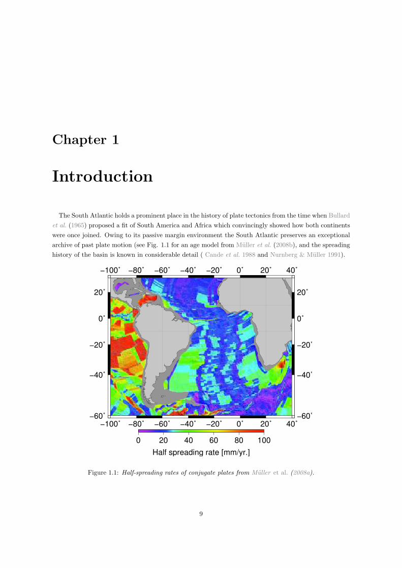
archive of past plate motion (see Fig. 1.1 for an age model from Muller et al. (2008b), and the spreading
history of the basin is known in considerable detail ( Cande et al. 1988 and Nurnberg & Muller 1991).
−100˚
−100˚
−80˚
−80˚
−60˚
−60˚
−40˚
−40˚
−20˚
−20˚
0˚
0˚
20˚
20˚
40˚
40˚
−60˚ −60˚
−40˚ −40˚
−20˚ −20˚
0˚ 0˚
20˚ 20˚
0 20 40 60 80 100
Half spreading rate [mm/yr.]
Figure 1.1: Half-spreading rates of conjugate plates from Muller et al. (2008a).
9
CHAPTER 1. INTRODUCTION
Temporal variations of the oceanic spreading rate are an outstanding observation in the South Atlantic.
Figure 1.1 shows ocean floor spreading half-rates of the South Atlantic taken from the recent global
compilation of Muller et al. (2008b) on the basis of marine magnetic anomaly identifications and following
the techniques outlined by Muller et al. (1997). The compilation reveals abrupt velocity changes over
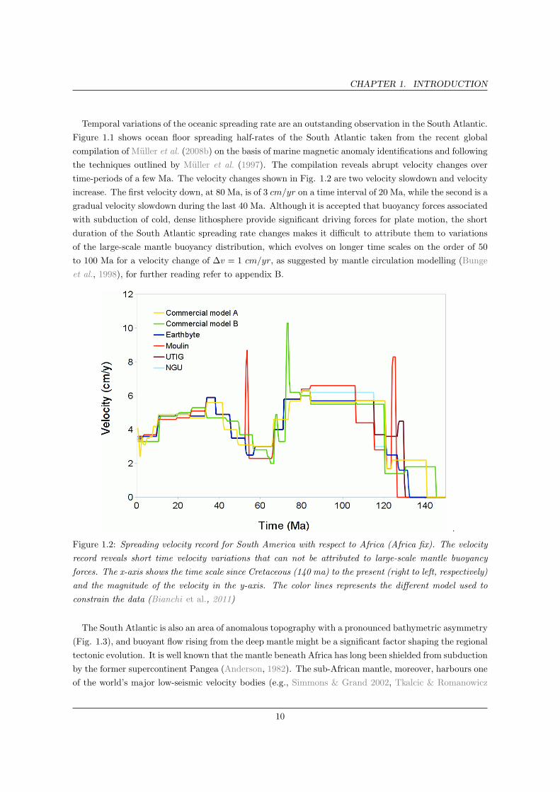
time-periods of a few Ma. The velocity changes shown in Fig. 1.2 are two velocity slowdown and velocity
increase. The first velocity down, at 80 Ma, is of 3 cm/yr on a time interval of 20 Ma, while the second is a
gradual velocity slowdown during the last 40 Ma. Although it is accepted that buoyancy forces associated
with subduction of cold, dense lithosphere provide significant driving forces for plate motion, the short
duration of the South Atlantic spreading rate changes makes it difficult to attribute them to variations
of the large-scale mantle buoyancy distribution, which evolves on longer time scales on the order of 50
to 100 Ma for a velocity change of ∆v = 1 cm/yr, as suggested by mantle circulation modelling (Bunge
et al., 1998), for further reading refer to appendix B.
.
Figure 1.2: Spreading velocity record for South America with respect to Africa (Africa fix). The velocity
record reveals short time velocity variations that can not be attributed to large-scale mantle buoyancy
forces. The x-axis shows the time scale since Cretaceous (140 ma) to the present (right to left, respectively)
and the magnitude of the velocity in the y-axis. The color lines represents the different model used to
constrain the data (Bianchi et al., 2011)
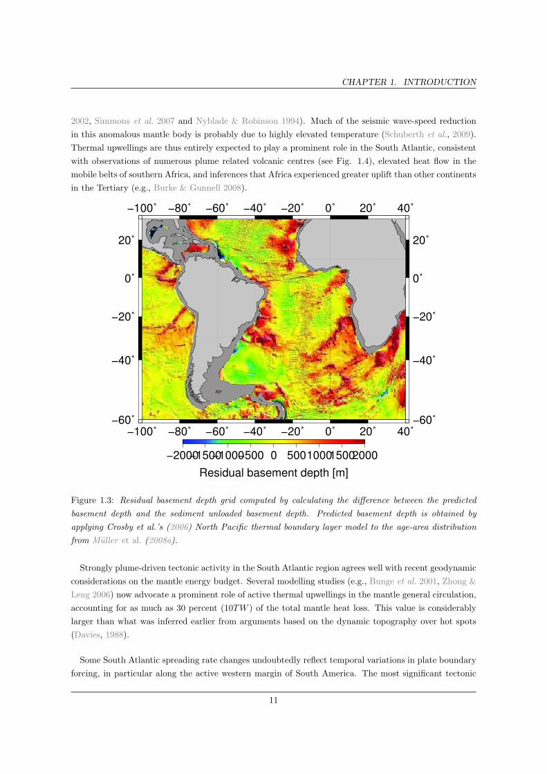
The South Atlantic is also an area of anomalous topography with a pronounced bathymetric asymmetry
(Fig. 1.3), and buoyant flow rising from the deep mantle might be a significant factor shaping the regional
tectonic evolution. It is well known that the mantle beneath Africa has long been shielded from subduction
by the former supercontinent Pangea (Anderson, 1982). The sub-African mantle, moreover, harbours one
of the world’s major low-seismic velocity bodies (e.g., Simmons & Grand 2002, Tkalcic & Romanowicz
10
CHAPTER 1. INTRODUCTION
2002, Simmons et al. 2007 and Nyblade & Robinson 1994). Much of the seismic wave-speed reduction
in this anomalous mantle body is probably due to highly elevated temperature (Schuberth et al., 2009).
Thermal upwellings are thus entirely expected to play a prominent role in the South Atlantic, consistent
with observations of numerous plume related volcanic centres (see Fig. 1.4), elevated heat flow in the
mobile belts of southern Africa, and inferences that Africa experienced greater uplift than other continents
in the Tertiary (e.g., Burke & Gunnell 2008).
−100˚
−100˚
−80˚
−80˚
−60˚
−60˚
−40˚
−40˚
−20˚
−20˚
0˚
0˚
20˚
20˚
40˚
40˚
−60˚ −60˚
−40˚ −40˚
−20˚ −20˚
0˚ 0˚
20˚ 20˚
−2000−1500−1000−500 0 500100015002000
Residual basement depth [m]
Figure 1.3: Residual basement depth grid computed by calculating the difference between the predicted
basement depth and the sediment unloaded basement depth. Predicted basement depth is obtained by
applying Crosby et al.’s (2006) North Pacific thermal boundary layer model to the age-area distribution
from Muller et al. (2008a).
Strongly plume-driven tectonic activity in the South Atlantic region agrees well with recent geodynamic
considerations on the mantle energy budget. Several modelling studies (e.g., Bunge et al. 2001, Zhong &
Leng 2006) now advocate a prominent role of active thermal upwellings in the mantle general circulation,
accounting for as much as 30 percent (10TW ) of the total mantle heat loss. This value is considerably
larger than what was inferred earlier from arguments based on the dynamic topography over hot spots
(Davies, 1988).
Some South Atlantic spreading rate changes undoubtedly reflect temporal variations in plate boundary
forcing, in particular along the active western margin of South America. The most significant tectonic
11

CHAPTER 1. INTRODUCTION
change in the region over the past 25 Ma is the growth of the high Andes, especially the rise of the
Altiplano and Puna plateau some 10 Ma ago (e.g., Garzione et al., 2006, Gregory-Wodzicki 2000, Charrier
et al. 2007). Estimates for the tectonic forces associated with the current Andean topography amount to
∼ 8×10¹² N/m on average, comparable to the driving forces in plate tectonics (Husson & Ricard 2004 and
Iaffaldano et al. 2006). The temporal correlations between Andean uplift and plate kinematic changes
around South America support the notion that the load of this newly elevated topography affected plate
motions in the South Atlantic region. For instance, the 30 percent convergence velocity reduction across
the Nazca/South America margin in the late Miocene, commonly attributed to growth of the high Andes
(e.g., Norabuena et al. 1999), has been linked explicitly to a corresponding reduction of South Atlantic
spreading rates in a global coupled model of the mantle/lithosphere system (Iaffaldano et al., 2006). Far
field effects are thus an important factor influencing the South Atlantic spreading record. Husson et al.
(2012), moreover, attributed the most recent South Atlantic spreading rate reduction to the formation
of an optimal aspect ratio in a deep mantle circulation cell beneath the South Atlantic.
−100˚
−100˚
−80˚
−80˚
−60˚
−60˚
−40˚
−40˚
−20˚
−20˚
0˚
0˚
20˚
20˚
40˚
40˚
−60˚ −60˚
−40˚ −40˚
−20˚ −20˚
0˚ 0˚
20˚ 20˚
−7 −6 −5 −4 −3 −2 −1 0 1 2 3 4
Elevation a.s.l. [km]
Rio Grande Rise
Walvi
s Rid
ge
Argentine Basin
Falkland Plateau
Agulhas Plateau
Camero
on Lin
e
Scotia Basin
Angola Basin
Cape Basin
Meteor R
ise
KalahariCraton
CongoCraton
West AfricanCraton
Rio de la PlataCraton
AmazoniaCraton
São FranciscoCraton
Tr
G
B
SH
AsF
TM
G
Figure 1.4: Topographic map of the South Atlantic and adjacent continents from ETOPO1 (Amante &
Eakins, 2009), annotated with major structural elements cited in the text. Craton names are boldface,
while stars denote prominent hotspots (F: Fernando de Noronha; As: Ascension; Af: Afar; SH: Saint
Helena; TM: Trinidade and Martim Vaz; Tr: Tristan da Cunha; G: Gough Island; B: Bouvet Island; M:
Marion; C: Crozet Islands)
12
CHAPTER 1. INTRODUCTION
Rapid spreading rate changes, observed in Fig. 1.2, suggest a significant decoupling of plate motion
from the large scale mantle buoyancy distribution, as noted before, presumably through a mechanically
weak layer known as asthenosphere. An asthenosphere was advocated early on in the history of plate
tectonics to lubricate plate motion. Abundant evidence for the asthenosphere comes from a variety of
observations, including the Geoid (e.g., Hager & Richards 1989), glacial rebound (e.g., Mitrovica & Forte
2004), oceanic intraplate seismicity (e.g., Wiens & Stein 1985), ocean ridge bathymetry (e.g., Buck et al.
2009), seismic anisotropy (e.g., Debayle et al. 2005). While the cause for low mechanical strength of the
asthenosphere is probably due to weakening effects associated with partial melt and/or water (e.g.,Karato
& Jung 1998), consequences include a concentration of upper mantle flow into a narrow channel of greatly
enhanced material mobility. Fluid dynamic considerations based on numerical and analytic models (e.g.,
Bunge et al. 1996) confirm that high material mobility in the asthenosphere is essential to promote the
unique long wavelength pattern of mantle flow observed on Earth.
Morgan et al. (1995) argued for asthenosphere flow with a pressure driven component due to plumes,
which would explain a variety of observations related to mantle geochemistry, heat flow and ocean
bathymetry. In a series of remarkable papers, Hoeink and Lenardic (2008, 2010, 2011) substantiated
this idea. They predicted that plate motion in the South Atlantic region arises predominantly from
basal shear forces related to pressure driven (Poiseuille) asthenosphere flow (Hoeink et al., 2011). The
concept of asthenospheric flow driven by high and low pressure regions is productive. It relates spread-
ing rate changes driven by evolving basal shear forces explicitly to non-isostatic vertical motion known
as dynamic topography, which one can test with independent data. In fact, Japsen et al. (2012) (and
references therein) has drawn attention recently to episodic burial and exhumation of passive continental
margins. Such events are documented along the Brazilian coast and are difficult to understand in terms
of a simple lithosphere cooling process, presumably reflecting temporal changes in dynamic topography,
which refers to topography generated by the motion of zones of differing degrees of buoyancy (convection)
in the Earth’s mantle.
Consequently, the hypothesis to test is that the South American plate motions are driven by basal shear
forces related to pressure driven (Poiseuille) low viscosity asthenosphere flow beneath the lithosphere.
And the plate velocity variations are related to the Andean orogenic evolution (e.g paleoelevation) along
the west boundary of the South American plate. Thus, the objectives are,
Understand and quantify the forces acting on the South American plate.
Using a force balance estimate the paleo elevation of the Andes.
Reconstitute the geologic evolution of the Andes base on the available literature, to have a geologic
paleo elevation of the Andes.
Compare both results to test the hypothesis.
However, far field effect (e.g., African plateau evolution (Janssen et al., 1995)) may play also a prominent
role into the South American plate motions.
13

CHAPTER 1. INTRODUCTION
To test the hypothesis and achieve the objectives the document will be divided into 5 more chapters.
Chapter 2, the methodology, will explain how to confront the problematic. Chapter 3, geology of the
Andes, will be described the orogenic evolution of the Andean Cordillera. In chapter 4, the force balance,
will be estimated the paleo elevation of the Andes. In chapter 5, discussion, results are going to be
compared and discussed. Chapter 6 is the conclusion.
14
Chapter 2
Methodology
1 The South American plate motions are controlled by driving and resisting forces. The latter are the
Andean forcing, due to his topographic elevation, and the frictional forces along the convergent margin.
While the driving forces are the Ridge push, a gravitational force, and the basal shear forces related
to the asthenospheric flow. Quantification of this forces will allow us to describe South American plate
motions.
2 Our model calculations will be as simple as a force balance, in which for each time interval the sum
of all forces equals zero, because acceleration in the solid Earth are negligible. To solve it a Maltab based
code will be use. The plate will be treated as a particle to which forces are applied. Each force will be
applied either to the whole plate or to its borders, therefore summing all contribution will be made to get
one value for each force. The frictional and ridge push forces are know from the literature (e.g., Fowler
2009). The Andean forcing was already estimated by Iaffaldano et al. (2006). But the basal shear force
related to the asthenospheric flow depends on parameters that can not be measured in situ. For present
day conditions the ridge push, frictional and Andean forcing forces are know. With this, we can estimate
the parameters needed characterize the basal shear forces in order to be in balance with all the other
forces, however, they are not unique. Detail of all the calculations and assumption are described in the
chapter 4.
3 Knowing all the parameters to quantify the forces acting on the South American plate we can estimate
the Andean topographic elevation for the past in order to describe the velocity record observed (see Fig.
1.2). The low velocities observed are related to high elevation in the Andean topography, while the fast
velocities are related to low elevation in the Andean topography. Due to the fact the parameters for the
basal shear forces related to the asthenosphere flow are not unique, we will obtain a variety of solutions.
Independent information sources (e.g., Seismic data) are going to be use to restrict the parameters and
find the most reasonable solution.
4 From an extensive literature review, the Andean paleo elevation history for the last 100 Ma will
be made, based on the geological records. All the geological information is sorted in the table C.1 to
facilitate its comprehension. The contents of the table are the name of the author (reference), the type of
15
CHAPTER 2. METHODOLOGY
information, location, time periods and the main features discussed in the article. With all this is easier
to recall the important information of each article. And in chapter 3.
5 Both results are going to be compared to validate our estimation of the Andean paleo elevation.
If the orogenic history of the Andes since 100 Ma does explain the velocity variations observed in the
velocity record, then our estimation of the paleo elevation of the Andean topography should coincide
with elevation of the Andes based on the geological records. In case both results qualitatively coincide,
then the hypothesis will be accepted. In contrary case, then the hypothesis will be rejected and an other
process will be discussed to explain the South American velocity variations.
16
Chapter 3
Geology of the Andes
3.1 Anatomy of the Andes
The Andes is one of the major Cordillera in the world, it extends from far north ( ∼ 7oN) to the end
of the Continent far south in the Tierra del Fuego (ca 55oS). The average topographic elevation in the
Central Andes is on the order of 4 km and its mayor mountain is the Aconcagua, at ∼ 30oS, reaching
an elevation of ∼ 7 km.
The Andes display considerable latitudinal variation and are therefore divided in three zones (Gansser
1973, Tassara & Yanez 2003 and Sempere et al. 2008), as can be see in Fig. 3.1. The Northern Andean
goes from ∼ 12oN to ∼ 5oS. The Central Andean, the largest and most voluminous segment t present
day, goes from ∼ 5oS to ∼ 37oS and is also subdivided into three regions, the North Central Andes,
Central Orocline and South Central Andes. The Central Andes are characterized by the dominance of
protracted magmatic activity in the west (widely distributed around the Western Cordillera, i.e. the
arc) and by tectonic shortening in the east (in the Eastern Cordillera and adjacent areas). As a whole,
the Central Andes form a major segment of continental arc and display extraordinary characteristics
and noteworthy internal longitudinal gradients (Sempere et al., 2008). The Southern Andean goes from
∼ 37oS to the end of the continent at ∼ 55oS and are characterized by a 2000 km long belt of granitoids
hosted along their axial part, named as the Patagonian batholith (Folguera et al., 2011). Given that the
aim of this study is to describe the geological evolution of the Andean topographic elevation, the main
focus of our work lays on the Central Andes, where the main geological processes related to topographic
construction have occurred in the last 100 Ma, since late Cretaceous (Geological time scale is available
in appendix A).
17

3.1. ANATOMY OF THE ANDES CHAPTER 3. GEOLOGY OF THE ANDES
−90˚ −80˚ −70˚ −60˚ −50˚ −40˚ −30˚
−50˚
−40˚
−30˚
−20˚
−10˚
0˚
10˚
−90˚ −80˚ −70˚ −60˚ −50˚ −40˚ −30˚
−50˚
−40˚
−30˚
−20˚
−10˚
0˚
10˚
−90˚ −80˚ −70˚ −60˚ −50˚ −40˚ −30˚
−50˚
−40˚
−30˚
−20˚
−10˚
0˚
10˚
Figure 3.1: Topographic map of the South American continent and its most prominent geological feature,
the Andes. The Andean Cordillera extends along the whole continent from north to south. The Andes is
also segmented in three main zones the Central, South and North. Further the Central Andean Zone, is
separated also in three regions the North, Central Orocline and South-central. (Gansser, 1973)
Each region of the Central Andes contains important geological features and structures. The Northern
Central Andes describes several important geological structures, such as the Coastal Cordillera, the
Coastal and Western Through, the Axial swell and the Eastern basins (Jaillard, 1994), see Fig. 3.2. The
Central Orocline has many important geological structures. From west to east, the central depression is
18

3.2. THE ANDEAN EVOLUTION CHAPTER 3. GEOLOGY OF THE ANDES
between the Coastal and Pre Cordilleras, east from this latter is the Salar de Atacama surrounded from
the west by the Western Cordillera (Mpodozis et al., 2005). East from latter, lays the Altiplano and
Puna plateau, a ∼4 km high structure. This two structures are easterly closed by the Eastern Cordillera.
The eastern most structure is the Subandean region (Gregory-Wodzicki, 2000). The Southern part of
the Central Andes is characterize by the Frontal Cordillera that goes from ∼ 26oS to far south, which
contain the Aconcagua mountain, the highest one along the Andes, up to ∼7 km high (Sempere et al.,
1994).
Figure 3.2: Paleogeographic sketch of the Peruvian margin, and location of main areas cited. 1: Cretaceous
allochthonous terranes, and suture. 2: Coastal Cordillera. 3: Coastal Troughs. 4: Western Trough. 5:
Axial Swell. 6: Eastern Basin. 7: Brazilianand Guianese (Colombian) Precambrianshields. 8: Jurassic
suture (Jaillard, 1994).
3.2 The Andean evolution
The pre-Andean cycle started in late Pre-Cambrian until early Jurassic (200 Ma), were the Andean
tectonic cycle started. During the pre-Andean cycle subduction was not active, however terrains were
accreted to the pre-Andean margin, such as Pampean terrane, Precordillera terrane and the Patagonia
terrane (Rapela et al., 1998). The Andean cycle started by early Jurassic, which we are interested, and
can be divided into two periods, an early and late period (Charrier et al., 2007).
19
3.2. THE ANDEAN EVOLUTION CHAPTER 3. GEOLOGY OF THE ANDES
Figure 3.3: Andean tectonic cycle, since early Jurassic (Charrier et al., 2007)
For what concerns to our study, we are interested into the late period of the Andean tectonic cycle,
since late Cretaceous, where the main tectonic processes related to the orogeny of the Andes occurred.
However, it is important to know taht during the early period of the Andean cycle, it was dominated by
extensional setting along the Andean margin (Charrier et al., 2007).
The orogenic evolution of the late period of the Andean evolution has been long studied, however it is
still under debate, due to its complexity. Traditionally, three main phases of Andean orogeny are accepted
(Steinmann et al., 1929). These phases are the Peruvian during late Cretaceous, Incaic or Inca in middle
Eocene and Quechua since late Miocene. The Peruvian phase has also been described by Jaillard & Soler
(1996) and Charrier et al. (2007) among others, beeing in temporal and spatial agreement with Steinmann
et al. (1929). For the Inca phase the story is a bit different, because Sempere et al. (1990) argued that
this phase occurred actually in late Oligocene instead of middle Eocene. However, lately consensus
was reached in that tectonic activity started slowly in middle Eocene reaching its maximum during
late Oligocene (Sempere et al., 2008). The Quechua phase, since late Miocene to present, concentrates
principally in the Central Orocline (e.g Altiplano and Puna) (e.g., Garzione et al. 2006, Ghosh et al. 2006
and Gregory-Wodzicki 2000), where the Andes reached its actual development. In latest late Cretaceous
to early Paleocene a main short-lived tectonic event took place, in the Central Orocline and Southern
Central Andes, named the K-T event (Cornejo et al. 2003 and Charrier et al. 2007).
During late Cretaceous the geological record in North Central Andes documents tectonic processes
along the margin related to the first Andean orogenic phase, the Peruvian, named after the Peru region
between 5oS and 17oS (e.g., Steinmann et al. 1929, Jaillard 1994 and Charrier et al. 2007 among others).
The Peruvian phase, described by Jaillard (1994), is composed by three stages, the first in the Turonian
to Coniacian boundary (89 - 88 Ma), the second in late Coniacian to earliest Santonian (87 - 86 Ma) and
a third one in late Campanian (76 - 73 Ma).
20
3.2. THE ANDEAN EVOLUTION CHAPTER 3. GEOLOGY OF THE ANDES
The first stage was related to an incipient coastal uplift and inversion of the previous subsidence of the
Coastal area. Directly after it, the second stage was related to tectonic activity with compressional strain
in the directions NE-SW. More generally an increase in the compression in the Coastal area, associated
with lateral movements, that ended uplifting the margin. This uplift provoked a retreat of the sea during
late Santonian. Later, the third stage was related with thrusting and fore land sedimentary deposits.
Accordingly, in north-western Peru, the deposition of sediments indicates a marked paleogeographic
change, characterized by the uplift and erosion of the Coastal Cordillera and the sinking of the coastal
area, thus expressing the creation of the first late Cretaceous forearc basin in the coastal zone of northern
Peru. Therefore, with this evidence it could be inferred that an orogenic process highly related to
mountain uplift occured (Jaillard, 1994). Additionally Jaillard & Soler (1996) and references therein
described a major contractional event in the south-western Peru during late Campanian.
These tectonic processes in the Northern Central Andes identified as a regional event also correlates
with similar processes along the whole Central Andean margin. In the Central Orocline, specifically in
Bolivia and north-western Argentina, three stages of tectonic activity (Sempere et al., 1997). The first
of stages (89 Ma) correlates with the Peruvian phase. Thus, from stratigraphy data it can be inferred
that in late Turonian to Campanian (89 to 73 Ma) a tectonic event marked the turning point in Andean
evolution in the Northern Central Andes and foreland conditions east of the Andes domain prevailed.
Furthermore, in the Salar de Atacama, ∼ 23o S in the Atacama region in Chile, during late Cretaceous
(70 Ma) an uplift in the Cordillera Domeyko, west to the Salar de Atacama basin, was found, based on
the high sedimentation rates on the Salar basin (Mpodozis et al., 2005).
In the Southern Central Andean correlation with the Peruvian tectonic phase was also found. In the
Neuquen basin, at ∼ 38o S on the eastern foreland domain of the Andes, evidences of tectonic events
in late Cretaceous (Tunik et al., 2010), which argue based on fission track data, detrical zircons and
biostratigraphic evidence that the beginning of Andean uplift for this area can be bracketed between
Cenomanian and Coniacian. Additionally, in the same area stratigraphical and structural evidence sug-
gest a compressional deformation setting from Aptian to Campanian (Tunik et al., 2010).
Tectonic activity during late Cretaceous along the Central Andean margin, was followed since late
Campanian by a tectonic quiescence, probably by extensional settings. Also during Maastrichtian marines
transgressions were found in the Central Orocline. In latest late Cretaceous and early Paleocene (65 Ma)
this tectonic quiescence was interrupted by a major short lived tectonic event, the K-T event, in the
Central Orocline (Cornejo et al., 2003).
This K-T event, was first documented by Cornejo et al. (2003) in the Central Orocline, were she did
find a series of unconformities, between late Cretaceous and the overlying Paleocene strata, in a wide
region from 20oS to 26oS. Later Charrier et al. (2007) described also this short lived tectonic event and
found correlation with deformation processes up to the region of Concepcion at ∼ 36oS.
More evidence supporting this event, is observed in the North Central Andes, north from the Altiplano
near the Titicaca lake in the Vilquenchico area ∼ 15oS, where Jaillard et al. (1993) described an angular
21
3.2. THE ANDEAN EVOLUTION CHAPTER 3. GEOLOGY OF THE ANDES
unconformity dated late Maastrichtian. Further, in the Cajamarca and southern-east Ecuador regional
compression processes were recorded in the stratigraphic data (Jaillard & Soler, 1996).
In the Southern Central Andes, in the Neuquen basin correlations to tectonic events are closely related
to the Peruvian phase in late Cretaceous, although by a narrow age margin this events can be also related
to the K-T event (Cobbold & Rossello, 2003). In the Southern Andes, Aragon et al. (2011) described the
development of a proto Andean range in the Patagonian area indicating correlation with the Peruvian
phase.
After the K-T event that ended in early Paleocene, extensional settings resumed in the Central Andes,
but with less intensity compared to early Cretaceous (Charrier et al. 2007 and Jaillard & Soler 1996).
The second phase of Andean evolution is the Inca. This orogenic phase developed, presumably, first
by a slow start in the middle Eocene, followed by a peak in tectonic activity by late Oligocene (Sempere
et al., 2008). During middle Eocene in the Central Andean Plateau (e.g Altiplano and Puna), Gillis et al.
(2006) base on fission tracks dated the time periods of rapid cooling (e.g exhumation), which are related
to uplift processes. He found and described two periods of rapid cooling, the first fast cooling period
started in middle Eocene (45 Ma to 40 Ma) and continued throughout late Eocene and Oligocene and
ended by ∼ 26 Ma. The second period of fast cooling started in late Miocene (∼ 11 Ma). Barnes et al.
(2006) found similar results for the same area.
In late Oligocene, Sempere et al. (1990) described a major tectonic crisis in the Central Orocline that
resulted in the development of the Subandean external foreland basins and the intermontane basins in
the Altiplano, which where separated by the thrusting and uplift of the Eastern Cordillera. Horton
(2005) emphasised that in late Oligocene the development of the intermontane basin fill started in the
Altiplano region, bounded by the Eastern Cordillera to the east, and were deposited forming an angular
unconformity. Furthermore, McQuarrie et al. (2008) based on apatite fission track described the amounts
and time of deformation and crustal shortening in the Central Orocline, dating from late Eocene to
Oligocene a fast exhumation period in the Eastern Cordillera, presumably related to uplift. Arriagada
et al. (2008) reached similar results, reporting that the Central Orocline was formed between late Eocene
and Oligocene based on apatite fision tracks.
In the Northern Central Andes during late Eocene and Oligocene Jaillard & Soler (1996) described
folding and inverse faulting in the Western Through, that runs near the coastal area along the entire
Peruvian region, that ended forming a fold and thrust belt. Further, in the North Central Andes Picard
et al. (2008) dated the Andean elevation using phylogenetics of highland biotaxa. Results show that by
early Miocene (23 to 19 Ma) the Southern most part of the Northern Central Andes reached 2 to 2.5 km
and that the uplift propagated northward, reaching the same elevation in the central part of the Northern
Central Andes by middle Miocene. Later in the late Miocene these elevations were also reached in the
northern most part of the North Central Andes. Thus, these results showed that uplift in the Central
Andes, presumably started in the Central Orocline by late Oligocene and then propagated north and
south from it, as can be see in Fig 3.4.
22

3.2. THE ANDEAN EVOLUTION CHAPTER 3. GEOLOGY OF THE ANDES
Figure 3.4: Timing and propagation of Andean uplift from southern to northern, in the Northern Central
Andes (Picard et al., 2008).
In the Central Orocline Gregory-Wodzicki (2000), based on paleobotanical, fission track and geomor-
phological data, dated the initiation of uplift in the Western Cordillera by early Miocene, where it may
have reached half of its present elevation. Additionally, the Altiplano should have reached a third of its
present elevation by the same time, and half of it by 10 Ma. For the Eastern Cordillera she found that
it had reached half of its actual elevation by 10 Ma (Gregory-Wodzicki, 2000).
23
3.2. THE ANDEAN EVOLUTION CHAPTER 3. GEOLOGY OF THE ANDES
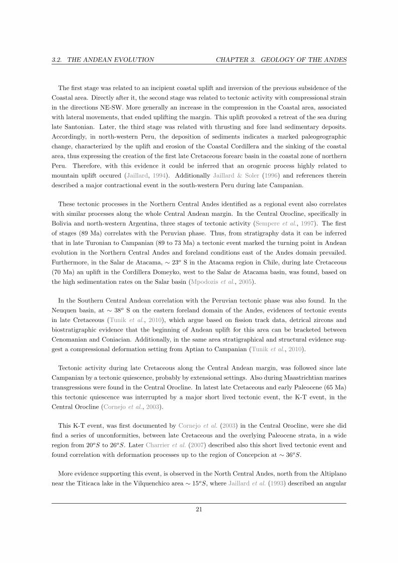
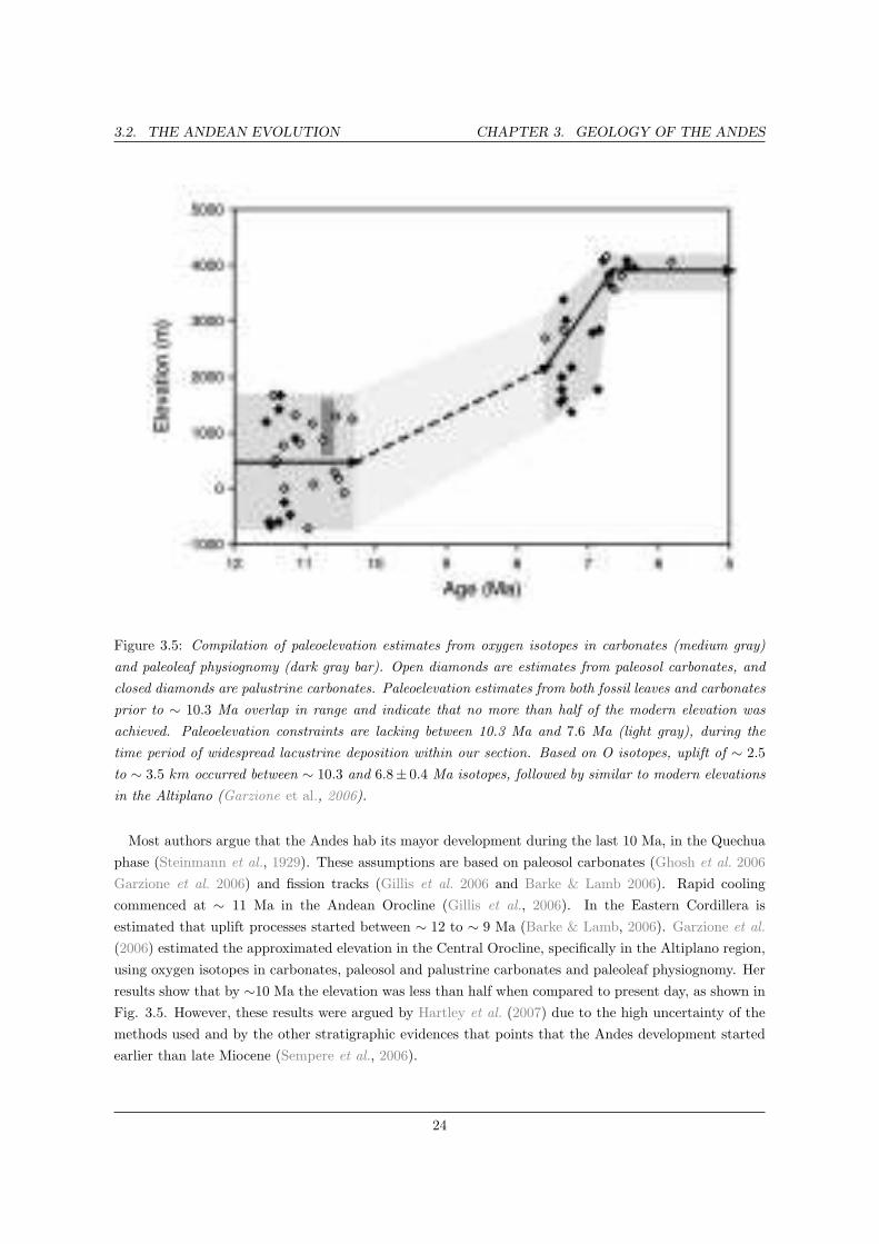
Figure 3.5: Compilation of paleoelevation estimates from oxygen isotopes in carbonates (medium gray)
and paleoleaf physiognomy (dark gray bar). Open diamonds are estimates from paleosol carbonates, and
closed diamonds are palustrine carbonates. Paleoelevation estimates from both fossil leaves and carbonates
prior to ∼ 10.3 Ma overlap in range and indicate that no more than half of the modern elevation was
achieved. Paleoelevation constraints are lacking between 10.3 Ma and 7.6 Ma (light gray), during the
time period of widespread lacustrine deposition within our section. Based on O isotopes, uplift of ∼ 2.5
to ∼ 3.5 km occurred between ∼ 10.3 and 6.8± 0.4 Ma isotopes, followed by similar to modern elevations
in the Altiplano (Garzione et al., 2006).
Most authors argue that the Andes hab its mayor development during the last 10 Ma, in the Quechua
phase (Steinmann et al., 1929). These assumptions are based on paleosol carbonates (Ghosh et al. 2006
Garzione et al. 2006) and fission tracks (Gillis et al. 2006 and Barke & Lamb 2006). Rapid cooling
commenced at ∼ 11 Ma in the Andean Orocline (Gillis et al., 2006). In the Eastern Cordillera is
estimated that uplift processes started between ∼ 12 to ∼ 9 Ma (Barke & Lamb, 2006). Garzione et al.
(2006) estimated the approximated elevation in the Central Orocline, specifically in the Altiplano region,
using oxygen isotopes in carbonates, paleosol and palustrine carbonates and paleoleaf physiognomy. Her
results show that by ∼10 Ma the elevation was less than half when compared to present day, as shown in
Fig. 3.5. However, these results were argued by Hartley et al. (2007) due to the high uncertainty of the
methods used and by the other stratigraphic evidences that points that the Andes development started
earlier than late Miocene (Sempere et al., 2006).
24

3.2. THE ANDEAN EVOLUTION CHAPTER 3. GEOLOGY OF THE ANDES
Thus, as reviewed above, there is a strong body of information supporting the development of the Andes
in 3 stages. A first periods in late Cretaceous to early Paleocene, where tectonic activity commenced
in the Northern Central Andes by late Cretaceous and propagated south to the Central Orocline, place
where a major tectonic event closed this first stage by early Paleocene. However, elevation of the Andes
by this time in these regions was presumable low, in an opposite scenario more prominent geological
features related to uplift processes should be expected. Later, in middle Eocene the second stage of
Andean orogeny started slowly to develop in the Central Andes, until it reached its maximum during
late Oligocene even early Miocene. And the later orogenic stage started in late Miocene to present and
appears to be more vigorous.
25

Chapter 4
Force balance for South America
The South American plate is moving westward since the split of the Gondwana continent ∼140 Ma
ago. The forces acting on the plate are the friction along the convergent margin, the Andean forcing, the
ridge push and the basal shear tractions. The first two forces resist the movement of the South American
plate to the west, while the last two drive the plate westward. All the forces are illustrated in the Fig.
4.1.
The force balance equation will consider the four forces mentioned above and since the Earth is round
we will use the torque instead of the force, ~M = R× ~F , where R is the radius of the Earth. Thus,
~Mfr + ~Mmb + ~Mrp + ~Mbd = 0 (4.1)
Where ~Mfr states for frictional torque at the convergent boundary of the plate, ~Mmb is the Andean
forcing torque, ~Mrp is the ridge push and ~Mbd is the basal shear torque related to the asthenospheric
flow.
Figure 4.1: A sketch of the South Atlantic region, displaying the driving (arrow pointing to the left) and
resisting (arrow pointing to the right) forces. The forces are the ridge push ~Mrp, basal shear traction~Mbd, friction force ~Mfr, Andean forcing ~Mmb.
26

4.1. DRIVING FORCES CHAPTER 4. FORCE BALANCE FOR SOUTH AMERICA
Figure 4.2: Sketch of the pressure driven (Poiseuille) flow in the asthenosphere (Hoeink et al., 2011).
4.1 Forces that drive plate motions
The driving forces are the forces that promote plate movements. This two are the basal shear tractions
and the ridge push. The first one is a force that is caused by the shear traction done below the lithosphere
due to a high velocity flow (faster than the plate velocity) in a low viscosity asthenospheric channel
(Hoeink et al., 2012). The second is the force at the mid-ocean ridge on the edge of the plate, due to the
pushing by the upwelling mantle material and the tendency of newly formed plate to slide down the sides
of the ridge (Fowler, 2009). Our calculation will be done under the assumption of the existence of a thin
low viscosity asthenospheric channel beneath the lithosphere (Hoeink & Lenardic, 2008), see Fig. 4.2.
The basal shear traction strongly depends on the characteristics of the asthenospheric flow, viscosity
and the thickness of the channel. The shear stress τ is define as a force per unit of area, which equals
the viscosity µ times the deformation ε over a time interval. This, at the same time, is equivalent to a
velocity change over distance ∆v∆x
. Since, the shear stress is a force per unit of area, we can integrate over
the area to obtain the force, as can be seen below,
τ = µ∆v
∆x
~Fbd =
∫
τdA =
∫
µ∆v
∆xdA
∆v = ~R×∆~w
Where ∆x = D is the depth to the maximum velocity, see Fig. 4.2, of the asthenospheric flow and ~w is
the euler vector of the velocity. Now to obtain the Torque, force to unit length, we just need to make the
cross product of this force with respect to the centre of the Earth ~R, which leads to,
~Mbd =
∫
~R×µ
D
(
∆~w × ~R)
dA
∆~w = wast − wplate
27

4.1. DRIVING FORCES CHAPTER 4. FORCE BALANCE FOR SOUTH AMERICA
Figure 4.3: Sketch of the ridge push force.
~Rb and ~Rd are defined as the distance from the centre of the Earth to the base of the lithosphere and
to the surface of the lithosphere, respectively. With a lithospheric thickness depending on the age of the
oceanic plate, which varies between 30 km to 100 km, approximately.
~Mbd =
∫
~Rd ×µ
D
(
(wast ×~Rb)− (wplate ×
~Rd))
dA Nm (4.2)
The equation 4.2 represents the shear traction done by the asthenospheric flow at the base of the
lithosphere, this traction drives the plate into the same direction of the flow in the asthenosphere. Where
wplate is the observed plate velocity and wast is the flow velocity in the asthenosphere and A is the size
of the plate, which is know from present and past times.
As an example, Hoeink and Lenardic (2008,2010) showed successfully that the basal shear tractions
done by the asthenosphere can drive plate motions using values of thickness and viscosity on the order
of 100 km and 1019 Pa s, respectively.
The ridge push is the force at the mid-ocean ridge on the edge of the plate, due to the pushing by the
upwelling mantle material and the tendency of newly formed plate to slide down to the sides of the ridge
(Fowler, 2009), see Fig. 4.3.
~Frp = ge(ρm − ρw)(L
3−
e
2) N/m (4.3)
Where ρm = 3.3× 10³ Kg/m3 is the density of the asthenosphere, ρw = 1× 10³ Kg/m3 density of the
water, g = 9.8 m/s2, e = 3 km is the elevation at the ridge and L = 8.5× 10⁴ m is the Plate thickness,
for present day conditions. But, we are interested on the torque related to the Ridge Push force, which
is the force times the radius of the earth, as follows
~Mrp = ~R×
[
ge(ρm − ρw)(L
3−
e
2)Wrn
]
Nm (4.4)
28
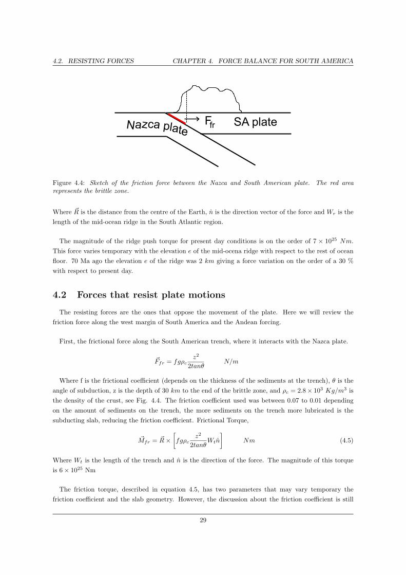
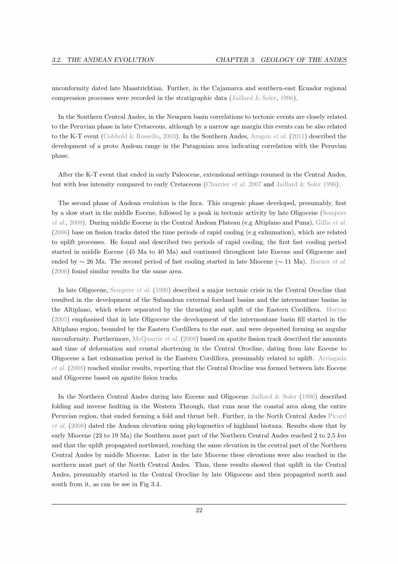
4.2. RESISTING FORCES CHAPTER 4. FORCE BALANCE FOR SOUTH AMERICA
Figure 4.4: Sketch of the friction force between the Nazca and South American plate. The red arearepresents the brittle zone.
Where ~R is the distance from the centre of the Earth, n is the direction vector of the force and Wr is the
length of the mid-ocean ridge in the South Atlantic region.
The magnitude of the ridge push torque for present day conditions is on the order of 7 × 1025 Nm.
This force varies temporary with the elevation e of the mid-ocena ridge with respect to the rest of ocean
floor. 70 Ma ago the elevation e of the ridge was 2 km giving a force variation on the order of a 30 %
with respect to present day.
4.2 Forces that resist plate motions
The resisting forces are the ones that oppose the movement of the plate. Here we will review the
friction force along the west margin of South America and the Andean forcing.
First, the frictional force along the South American trench, where it interacts with the Nazca plate.
~Ffr = fgρcz2
2tanθN/m
Where f is the frictional coefficient (depends on the thickness of the sediments at the trench), θ is the
angle of subduction, z is the depth of 30 km to the end of the brittle zone, and ρc = 2.8× 10³ Kg/m3 is
the density of the crust, see Fig. 4.4. The friction coefficient used was between 0.07 to 0.01 depending
on the amount of sediments on the trench, the more sediments on the trench more lubricated is the
subducting slab, reducing the friction coefficient. Frictional Torque,
~Mfr = ~R×
[
fgρcz2
2tanθWtn
]
Nm (4.5)
Where Wt is the length of the trench and n is the direction of the force. The magnitude of this torque
is 6× 1025 Nm
The friction torque, described in equation 4.5, has two parameters that may vary temporary the
friction coefficient and the slab geometry. However, the discussion about the friction coefficient is still
29

4.3. ASTHENOSPHERE FLOW CHAPTER 4. FORCE BALANCE FOR SOUTH AMERICA
Figure 4.5: Sketch of the Andean forcing.
under debate, and additionally it is hard to constrain then for the past. In the case of the slab geometry
its the same, because it is hard to know how much could it change during the past.
The magnitude of the Andean forcing done by the Andes for the present days was already estimated by
Iaffaldano et al. in 2006 and is on the order of 1.4×1026 Nm. See Fig. 4.5 for a sketch of how vertical load
of the topographic elevation of the Andes is balanced laterally. For what concerns on our calculations we
are not interested in the magnitude of the Andean forcing in the past, but on the elevation of the Andes.
Therefore, we will assume that the Andean force estimated by Iaffaldano et al. in 2006 only depends on
the elevation of the Andes.~Mmb = ζ(h) (4.6)
Where ζ is any function that depends only on the elevation h.
4.3 Flow velocity in the asthenosphere
At present day we can estimate three torques, the ridge push, Andean forcing and the friction force. It
means that we can estimate the basal shear tractions necessary to maintain the balance on the system,
see equation 4.1. However, for the basal shear equation 4.2 three parameters are unknown, the viscosity
and thickness of the asthenospheric channel, and the flow velocity. To solve this problem, we will solve
the torque balance equation 4.1 for a variety of combinations of viscosity and thickness of the channel.
In order to obtain a viscosity-thickness-dependent flow velocity needed to maintain balance.
30

4.3. ASTHENOSPHERE FLOW CHAPTER 4. FORCE BALANCE FOR SOUTH AMERICA
To start we separate the basal drag torque equation 4.2 in two components,
~Mbd =
∫
~Rd ×µ
D
(
(wast ×~Rb)− (wplate ×
~Rd))
dA
~Mbd =
∫
~Rd ×µ
D
(
wast ×~Rb
)
dA−
∫
~Rd ×µ
D
(
wplate ×~Rd
)
dA
~Mbd = ~Mastbd − ~Mplate
bd (4.7)
If we replace 4.7 in 4.1 and use 4.5, 4.4 and the value for the mountain building force estimated by
Iaffaldano et al. (2006) 4.6 we get,
~Mfr + ~Mmb + ~Mrp + ~Mastbd − ~Mplate
bd = 0
~Mastbd = − ~Mfr −
~Mmb −~Mrp + ~Mplate
bd
~Mastbd = ~Mt (4.8)
The right hand side of equation 4.8 can be estimated from observations. The magnitudes of this forces
are for ~Mmb = −1.4 × 1026 Nm, ~Mfr = −6 × 1025 Nm, ~Mrp = 7 × 1025 Nm and ~Mplatebd = 0.4 × 1026
Nm, thus the ~Mastbd = 1.7 × 1026 Nm. After some algebraic arrangement we can solve for ~wast using a
linear system. ~Bij is a matrix that comes out after solving ~R× (~w× ~R). Since ~w does not depend on the
area and it can be taken outside of the integral.
∫
~Rd ×µ
D
(
wast ×~Rb
)
dA =
∫µ
D~Bij ~wjdA
~Mastbd =
∫µ
D~BijdA
︸ ︷︷ ︸
Gij
~wj (4.9)
Comparing equation 4.8 and 4.9 we get,
Gij ~wj = ~Mt
~wj = G−1
ij~Mt (4.10)
As a result we obtain an asthenospheric flow velocity for a variety of combinations of flow viscosity
and channel thickness (see table 4.1). The velocity obtained is proportional to the depth and inversely
to the viscosity.
~w ∼D
µ
31

4.3. ASTHENOSPHERE FLOW CHAPTER 4. FORCE BALANCE FOR SOUTH AMERICA
Channel thickness
Flow viscosity 100 km 150 km 200 km 250 km 300 km 350 km 400 km 450 km 500 km
1× 10¹⁸ Pa s 81.15 117.78 154.24 190.74 227.38 264.23 301.31 338.65 376.26
5× 10¹⁸ Pa s 18.71 26.05 33.35 40.66 48.00 55.38 62.80 70.28 77.81
1× 10¹⁹ Pa s 10.91 14.59 18.24 21.90 25.58 29.27 32.99 36.74 40.51
5× 10¹⁹ Pa s 4.69 5.43 6.17 6.91 7.65 8.40 9.15 9.91 10.68
1× 10²⁰ Pa s 3.91 4.29 4.66 5.04 5.42 5.80 6.18 6.57 6.95
Table 4.1: Values of the flow velocity in asthenosphere in cm per yr for a variety of thickness and
viscosity combinations. High flow velocities are related to low viscosity and thicker channel, while the
low velocities are related to high viscosities and a thin channel.
The results in the table 4.1 displays several combinations of thickness and viscosity of the asthenospheric
channel. It can be seen that the thicker the channel and the lower the viscosity, the faster is the flow
velocity in the asthenosphere, up to 370 cm/yr. In the opposite case where the viscosity is high but the
channel is thin, then the flow velocity in the asthenosphere is slow on the order of 4 cm/yr. For a fixed
thickness, the lower the viscosity the faster the flow velocity in the asthenosphere, for a fix viscosity the
thicker the channel the faster the flow velocity, this can be seen in the Fig. 4.6. We are interested in high
flow velocities in the asthenosphere in order to drive plate motions.
32

4.4. ANDES ELEVATION CHAPTER 4. FORCE BALANCE FOR SOUTH AMERICA
7.80868
7.80868
7.80868
7.80868
11.6981
11.6981
11.6981
15.5876
15.5876
15.5876
19.477
19.477
19.477
23.3665
23.3665
23.3665
27.256
27.256
31.1454
31.1454
35.034935.0349
38.924338.9243
42.813842.8138
46.703250.5927
Thickness [km]
Vis
cosity [P
as]
Asthenosphere velocity [cm/yr]
Resisting
Driving
150 200 250 300 350
1
2
3
4
5
6
7
8
9
10x 10
19
10
20
30
40
50
60
70
Figure 4.6: Flow velocities in the asthenospheric channel. Flow velocities lower than the plate velocity
make the basal shear tractions resist the movement instead of drive it. Higher velocities are related to a
thicker channel and a low viscosity, while low velocities are related to thinner channel and high viscosity.
Knowing the flow velocity in the asthenospheric channel and assuming it has not change trough time
we have all the necessary parameters to estimate the Andean average elevation for past times, back to
late Cretaceous (100 Ma). Our estimate of elevation, however, will depend on the combination of the
viscosity and thickness of the channel, therefore our solution will be not unique.
4.4 Estimation of the average elevation of the Andes
In order to estimate the average topography for the Andes we have to go back to the torque balance
4.1. The four main forces acting on the South American plate are the friction, mountain weight, ridge
push and basal drag. The calculations are going to be made between two time intervals, this means
that we are not interested in the total forces but in their temporal variations, thereofre the forces that
temporary varies comparatively little can be neglected. The next equation shows the time variation,
~M t1fr +
~M t1mb +
~M t1rp +
~M t1bd = 0
~M t2fr +
~M t2mb +
~M t2rp +
~M t2bd = 0
33
4.4. ANDES ELEVATION CHAPTER 4. FORCE BALANCE FOR SOUTH AMERICA
Since the order of magnitude of the ridge push and frictional forces are one order lower and their
temporal variations are no more than a 30% in the case of the ridge push and for the frictional forces the
temporal variation are complicated and not clear that to assume their constant or infer some variations
its almost the same, in the sense of uncertainties. We can assume that both forces vary significantly
little with time and for simplicity of the problem their temporal changes can be neglected. That makes~M t2rp −
~M t1rp = 0 y ~M t2
fr −~M t1fr = 0. As a consequence we obtain,
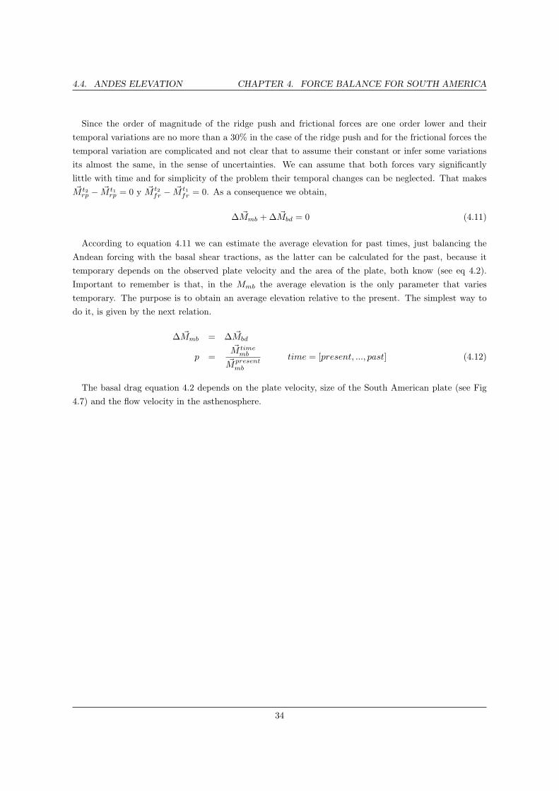
∆ ~Mmb +∆ ~Mbd = 0 (4.11)
According to equation 4.11 we can estimate the average elevation for past times, just balancing the
Andean forcing with the basal shear tractions, as the latter can be calculated for the past, because it
temporary depends on the observed plate velocity and the area of the plate, both know (see eq 4.2).
Important to remember is that, in the Mmb the average elevation is the only parameter that varies
temporary. The purpose is to obtain an average elevation relative to the present. The simplest way to
do it, is given by the next relation.
∆ ~Mmb = ∆ ~Mbd
p =~M timemb
~Mpresentmb
time = [present, ..., past] (4.12)
The basal drag equation 4.2 depends on the plate velocity, size of the South American plate (see Fig
4.7) and the flow velocity in the asthenosphere.
34

4.4. ANDES ELEVATION CHAPTER 4. FORCE BALANCE FOR SOUTH AMERICA
Figure 4.7: Top, spreading rate velocity. Middle, area of the South American plate since late Cretaceous
(100 Ma). Bottom, each grey line represent the contour of the plate area for an age, constrained from
ocean floor age.
35

4.4. ANDES ELEVATION CHAPTER 4. FORCE BALANCE FOR SOUTH AMERICA
Solving the torque balance between the basal shear tractions and the Andean forcing, using equation
4.11 and 4.12 results are as many as the data we have on the Table 4.1, it means 45 possible solutions.
All of them are displayed on the chapter D.
Not all the solutions are plausible, we can discard directly the ones with a slow flow velocity in the
asthenosphere (less than 7 cm/yr, see Fig. 4.6) and with too high flow velocity (more than 70 cm/yr),
because they probability of that fast flow velocity in the asthenosphere is highly unreal. So, the range
of solutions gets reduced by almost half. In the Fig. 4.8 are displayed all the solutions that are more
plausible.
0 10 20 30 40 50 60 70 80 90 1000.2
0.3
0.4
0.5
0.6
0.7
0 10 20 30 40 50 60 70 80 90 1000
0.2
0.4
0.6
0.8
1
Figure 4.8: Top: Average estimation of the Andean elevation with respect to present day topographic ele-
vation, black lines are all the solutions and red line is the more reasonable solution (base on seismological
data). Bottom: observed South American plate velocity. For both graphs the x-axis is the time. By 60
Ma all solutions show that the Andes have a high elevated topography (∼80 % of present day)
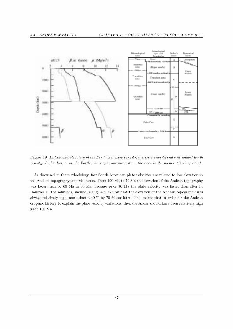
The red line in the Fig. 4.8, is the more reasonable solution base on seismic data. In the Fig. 4.9 we
can see that the Earth interior is segmented. The asthenosphere lays beneath the lithosphere and from
the Fig. 4.9 right side, it can be restricted to a depth of 350 km to 410 km. The preferable viscosity
value is on the order of 1× 10¹⁹ Pa s as discussed by Hoeink and Lenardic (2008, 2010, 2011).
36
4.4. ANDES ELEVATION CHAPTER 4. FORCE BALANCE FOR SOUTH AMERICA
Figure 4.9: Left:seismic structure of the Earth, α p-wave velocity, β s-wave velocity and ρ estimated Earth
density. Right: Layers on the Earth interior, to our interest are the ones in the mantle (Davies, 1999).
As discussed in the methodology, fast South American plate velocities are related to low elevation in
the Andean topography, and vice versa. From 100 Ma to 70 Ma the elevation of the Andean topography
was lower than by 60 Ma to 40 Ma, because prior 70 Ma the plate velocity was faster than after it.
However all the solutions, showed in Fig. 4.8, exhibit that the elevation of the Andean topography was
always relatively high, more than a 40 % by 70 Ma or later. This means that in order for the Andean
orogenic history to explain the plate velocity variations, then the Andes should have been relatively high
since 100 Ma.
37
Chapter 5
Discussion
Our force balance, as simple as it is, allows to understand key features in the relationship between
boundary and basal shear forces. Boundary forces for the South American plate are well known. These
are the ridge push, friction along the convergent margin and the tectonic force due to the Andean
elevation. Basal shear force is related to pressure driven asthenospheric flow that drives South American
plate motions. We assume a thin and low viscosity asthenosphere, with a time-independent constant flow
velocity. Through the force balance we could show that the variations of the elevation of the Andean
topography is not the main factor controlling plate motions, as other articles have suggested before (e.g.,
Husson & Ricard 2004, Norabuena et al. 1999). This was corroborated by revising the orogenic evolution
of the Andes contributed by the geological record.
The elevation of the Andes, which is needed to explain the plate motion deceleration observed, according
to our force balance, must have been on the order of 50 percent or higher in the past between 100 Ma to
60 Ma (e.g late Cretaceous to Paleocene). From the variety of results we have found the most suitable
parameter values are a viscosity on the order of 1019 Pa s and channel thickness of 250 km (350 km
depth). When analysing the data with a channel thickness of 250 km and a viscosity of 1 × 10¹⁹ Pa s,
our results displays that the elevation of the Andes by late Cretaceous and Paleocene (100 Ma to 60 Ma)
were very high, no less than 60% of present day by late Cretaceous (100 Ma to 70 Ma) and up to 80%
by Paleocene (60 Ma), see Fig. 5.1. This heigh elevated topography in the Andes resulting from our
estimates, generates doubts.
38

CHAPTER 5. DISCUSSION
0 10 20 30 40 50 60 70 80 90 100
!
"
# $# %
0.6
0.7
0.8
0.9
1
0.2
0.3
0.4
0.5
0.1
"
& &
' (
!
))
-./. -./. -./. -./. -./. -./. -./. -./. -./. -./. -./. -./. -./. -./. -./. 0 11111 .
0 10 20 30 40 50 60 70 80 90 1000.2
0.3
0.4
0.5
0.6
0.7
*+,
0 10 20 30 40 50 60 70 80 90 1000
0.2
0.4
0.6
0.8
1
Figure 5.1: Top: Estimate elevation of the Andean topography, red line in the more reasonable solution
and in grey are the other solutions. Middle: Observed South American plate velocity. Bottom: Andean
orogenic evolution since late Cretaceous. 1: oxygen isotopes is carbonates (Garzione et al. 2006 and
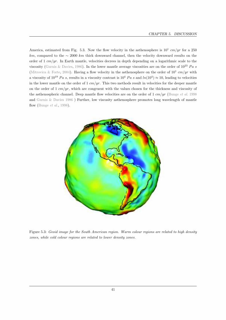
Ghosh et al. 2006), 2: leaf morphology method in the Altiplano, Western and Eastern Cordillera (Gregory-
Wodzicki, 2000), 3: AFT North Central Andes and Central Orocline (Hoorn et al., 2010), 4: AFT in the
Central Orocline (Gillis et al., 2006), 5: unconformities in the Central Orocline (Cornejo et al., 2003),
6: tectonic activity related to uplift in the Central Orocline (Sempere et al., 1997), 7: tectonic activity
related to uplift in the Northern Central Andes (Jaillard 1994 and Jaillard & Soler 1996), 8: Estimated
Andean average elevation.
The orogenic evolution of the Andes since late Cretaceous as inferred from the geological record, does
not sustain the result of our force balance. The main periods of uplift in the Andes, where developed
since middle Eocene (40 Ma) and presumably the elevation by Paleocene (60 Ma) and later was low.
39

CHAPTER 5. DISCUSSION
During, late Cretaceous to Paleocene tectonic processes were active along the Andean margin, however
no evidence exist of a high elevated Andes were present during that time period (e.g., Jaillard & Soler
1996, Sempere et al. 1997 among others). Moreover, the uplift presumably started slowly since middle
Eocene, reaching a first peak of orogeny by late Oligocene and a second during late Miocene to present
(e.g., Garzione et al. 2006 Gregory-Wodzicki 2000 Sempere et al. 1994 among others). According to this,
the plate velocity variations cannot be explained by variations in the elevation of the Andean topography.
Neither can this velocity changes be explained by a reduced size of the plate, see Fig 5.1 bottom green line,
because it does not vary more than a 20 percent for past times. Changes in the flux of the asthenosphere
can offer an alternative explanation.
The flux of the asthenosphere depends on the thickness and viscosity of the asthenospheric channel.
We assumed a channel thickness of 250 km (as the more reasonable value) and considering a lithosphere
thickness of 100 km, for a total depth of 350 km. This values could be mistaken. However, the values
used for the thickness and viscosity of the channel can be corroborated by seismic tomography images,
see Fig. 5.2. Seismic tomography allows to understand deep Earth structures. Mantle anisotropy are
normally associated with the mantle flow direction, due to elongated crystalline structure. Thus, seismic
tomography images in Figure 5.2 show low S-wave velocities related to a high material mobility (e.g.,
low viscosity on the order of 1019 Pa s), establishing that the bottom of the asthenospheric channel
lies between 350 to 400 km depth, as can be deduced for the two seismic cross sections. Thus, seismic
tomography agrees with the values we used for the channel thickness.
−90˚
−60˚
−30˚
−30˚ 0˚
30˚
30˚
60˚
−30˚
−30˚
0˚
0˚
30˚
A B
C D
4.2 4.3 4.4 4.5 4.6 4.7
Vs [km/s] at 200 km depth
−6 −4 −2 0 2 4 6
Vs anomaly [%]
100200300400 D
epth
[km
]100200300400 D
epth
[km
]
A B
C D
Figure 5.2: Full waveform tomography image for the South Atlantic region. Left: 200 km depth seismic
images for the South Atlantic. Right: Two vertical profiles(Colli et al., 2012).
The viscosity value used is corroborated by the geoid observation over the Earth. The geoid is defined
as the equipotential surface of the gravity field that is coincident with the surface of the oceans. It is
useful because it is more sensitive than gravity to deeper or larger-scale density variations. In the image
of the South America region, see Fig. 5.3, the warm coloured zone represents the high density material
flowing downward. Flowing material in the asthenosphere has to go down. Through this the geoid reveals
a thickness of this downward channel of rough ∼ 2000 km that is the wide of the red zone over South
40
CHAPTER 5. DISCUSSION
America, estimated from Fig. 5.3. Now the flow velocity in the asthenosphere is 101 cm/yr for a 250
km, compared to the ∼ 2000 km thick downward channel, then the velocity downward results on the
order of 1 cm/yr. In Earth mantle, velocities decrees in depth depending on a logarithmic scale to the
viscosity (Gurnis & Davies, 1986). In the lower mantle average viscosities are on the order of 1023 Pa s
(Mitrovica & Forte, 2004). Having a flow velocity in the asthenosphere on the order of 101 cm/yr with
a viscosity of 1019 Pa s, results in a viscosity contrast is 104 Pa s and ln(104) ≈ 10, leading to velocities
in the lower mantle on the order of 1 cm/yr. This two methods result in velocities for the deeper mantle
on the order of 1 cm/yr, which are congruent with the values chosen for the thickness and viscosity of
the asthenospheric channel. Deep mantle flow velocities are on the order of 1 cm/yr (Bunge et al. 1998
and Gurnis & Davies 1986 ) Further, low viscosity asthenosphere promotes long wavelength of mantle
flow (Bunge et al., 1998).
Figure 5.3: Geoid image for the South American region. Warm colour regions are related to high density
zones, while cold colour regions are related to lower density zones.
41

CHAPTER 5. DISCUSSION
−9
0˚
−6
0˚
−3
0˚
0˚
30
˚
−6
0˚
−3
0˚
0˚
30
˚
−9
0˚
−6
0˚
−3
0˚
0˚
30
˚−
90
˚−
60
˚−
30
˚0
˚3
0˚
−9
0˚
−6
0˚
−3
0˚
0˚
30
˚
−6
0˚
−3
0˚
0˚
30
˚
−6
0˚
−3
0˚
0˚
30
˚
−6
0˚
−3
0˚
0˚
30
˚
−9
0˚
−6
0˚
−3
0˚
0˚
30
˚
−6
0˚
−3
0˚
0˚
30
˚
−9
0˚
−6
0˚
−3
0˚
0˚
30
˚−
90
˚−
60
˚−
30
˚0
˚3
0˚
−9
0˚
−6
0˚
−3
0˚
0˚
30
˚
−6
0˚
−3
0˚
0˚
30
˚
12
0 M
a1
10
Ma
10
0 M
a9
0 M
a
80
Ma
70
Ma
60
Ma
50
Ma
40
Ma
30
Ma
20
Ma
10
Ma
Figure
5.4:
EvolutionofthePlate
configurationsince
late
Cretaceous(120Ma).
Itthefigure
canbe
appreciatedthatAfricahasremain
alm
ost
inthesameplace,whereastheSouth
Americancontinen
thasmovedwestward
andhow
hasevolved
theplatesin
thesideofthePacific(e.g.,
Farallon,Phoenix
andNazcaplates)
( Muller
etal.,2008b).
42

CHAPTER 5. DISCUSSION
The evolution on the plate configuration has undergone important changes since late Cretaceous (100
Ma) to present, as can be seen in the Figure 5.4. The more out standing change is at ∼ 60 Ma when
the Aluk ridge, in front of the South American plate, stopped and migrated far South. Previous to its
migration, the ridge was allowing material to go from the South Atlantic region in to the Pacific region.
Thus, after his close no more material was allowed to cross into the Pacific region. This correlates with
the K-T event described in the geology by ∼ 60 Ma, see Fig. 5.1. The new plate configuration allow to
the asthenosphere flux to push the trench westward, accelerating the South American plate.
In the Fig. 5.4 can be seen how the configuration of the plates (e.g., Farallon/Nazca) has change since
100 Ma. This makes hard to believe the assumption that the friction forces is constant through time.
However, the assumption taken was for simplification of the problem, its is undoubtedly that the friction
force was different in the past. But, how different was it? was it lower or higher? this questions are
almost impossible to answer, besides the friction coefficient between the overriding and subducting plate
is not well constrained and understood. Therefore, the assumption on leaving the frictional force constant
through time was the simplest and smartest option.
Flow velocity changes in the asthenosphere are affected by pressure driven mechanism connected to
lateral variation on the surface topography. The asthenosphere flow beneath the South Atlantic can be
described by a pressure driven Poiseuille flux (Hoeink et al., 2011). For this to be true, topography signals
on the plate have must be present. Japsen et al. (2012) described epeirogenic uplift periods in the north
east Brazil, specifically during late Cretaceous (80 Ma), Eocene (40 Ma) and Miocene (15 Ma). These
periods of uplift correlates with the orogenic evolution of the Andes (Steinmann et al., 1929). Further,
the African Superswell is characterized by dynamically supported topography (Nyblade & Robinson,
1994), with an estimated elevation of rough ∼ 1 km in contrast to the conjugate South American plate,
that corresponds the difference between the Argentine basin in South America with the Cape Basin in
Africa, see Fig. 1.4. Janssen et al. (1995) argued a temporal and spatial correlation between phase
of subsidence in African basins and variations in plate motions during tertiary. Furthermore, Burke &
Gunnell (2008) described that Africa started to be flexed upward when the Afar plume erupted ca. 31
Ma. The pronounced dynamic topography gradient across the South Atlantic region, implies significant
westward flow in the asthenosphere, as suggested by Behn et al. (2004).
~v = −h2
8η
∆P
∆x(5.1)
To assess the dynamical feasibility of westward fluxing asthenosphere across the South Atlantic re-
gion from a simple fluid dynamic model for pressure driven flow in a low viscosity channel, where the
asthenosphere channel is approximated as a viscous fluid confined between two fixed, horizontal infinite
planes separated by a distance h. The excess of velocity due to the horizontal pressure gradient ∆P∆x
that arises in the channel varies parabolically with depth, see equation 5.1. Thus, taking ∼ 1 km of
topography difference over a distance of 7000 km, leads to a pressure gradient of 300 bars and assuming
an asthenosphere viscosity of 1 × 10¹⁹ Pas and a channel thickness 250 km, this yields to a velocity of
∼ 10 cm/yr. This results is on the same order of magnitude as the estimation for the flow velocity in the
asthenosphere in order to maintain balance with present day boundary forces.
43

CHAPTER 5. DISCUSSION
0 10 20 30 40 50 60 70 80 90 100
!
"
# $# %
0.6
0.7
0.8
0.9
1
0.2
0.3
0.4
0.5
0.1
"
& &
' (
!
))
-./. -./. -./. -./. -./. -./. -./. -./. -./. -./. -./. -./. -./. -./. 0 11111 .
0 10 20 30 40 50 60 70 80 90 1000.2
0.3
0.4
0.5
0.6
0.7
*+,
0 10 20 30 40 50 60 70 80 90 1000
0.2
0.4
0.6
0.8
1
Figure 5.5: Top: Estimate elevation of the Andean topography, red line is the more reasonable solution
and in grey are the other solutions and blue line is the new estimation of the elevation of the Andes
considering a pressure driven (Poiseuille) flux from Africa to South America. Middle: Observed South
American plate velocity. Bottom: Andean orogenic evolution since late Cretaceous. 1: oxygen isotopes
is carbonates (Garzione et al. 2006 and Ghosh et al. 2006), 2: leaf morphology method in the Altiplano,
Western and Eastern Cordillera (Gregory-Wodzicki, 2000), 3: AFT North Central Andes and Central
Orocline (Hoorn et al., 2010), 4: AFT in the Central Orocline (Gillis et al., 2006), 5: unconformities in
the Central Orocline (Cornejo et al., 2003), 6: tectonic activity related to uplift in the Central Orocline
(Sempere et al., 1997), 7: tectonic activity related to uplift in the Northern Central Andes (Jaillard 1994
and Jaillard & Soler 1996), 8: Estimated Andean average elevation.
44

CHAPTER 5. DISCUSSION
Repeating the calculations done previously, but this time taking into account a contribution on the flux
in the asthenosphere due to a pressure driven (Poiseuille) flow from the African into the South American
plate since early Oligocene (35 Ma) (Burke & Gunnell, 2008). The new results displayed in the Fig. 5.5
blue line match in an excellent manner with the geological information.
Thus, dynamic topography variations plays a important role in plate motions, through a thin low
viscosity asthenosphere influenced by pressure gradients. Our novel approach contributes to a more
integral understanding of plate motion, not only due to boundary forces, but also by basal shear forces
and the influence of dynamic topography.
45
Chapter 6
Conclusion
By simple calculations of a force balance between the boundary and the basal shear forces, temporal
plate motions variations can be explained. South American plate motions describes a velocity decrease
in late Cretaceous (70 Ma) follow by a speed up and a final deceleration since early Oligocene (35 Ma).
This is the first time that somebody has try to explain plate motions for a long time period 100 Ma.
Our assumption is base on that plate motions are driven by basal shear forces related to pressure driven
(Poiseuille) low viscosity asthenosphere flow beneath the lithosphere. Boundary forces cannot fully ex-
plain plate motions, because high elevation on the Andean topography will be needed for past times in
order to explain the velocity decelerations. The geological record of the Andes has shown that the more
prominent uplift phases occurred since the middle Eocene (40 Ma). Our assumption on a thin astheno-
spheric layer is tested by comparing it with full waveform seismic topography images, thus validating
our choice on the more reasonable solutions. We used the geoid observation, accompanied by convec-
tion studies (Gurnis & Davies, 1986), to test the feasibility of a low viscosity asthenosphere. Further,
a low viscosity asthenosphere promotes long wavelength mantle circulation (Bunge et al., 1998). Pres-
sure gradients affects asthenospheric flow velocities, due to lateral topographic variations (e.g., Dynamic
topography). The African plateau has experienced several epeirogenic changes during the tertiary, that
are in temporal and spatially correlation with South American plate motions. The pronounced dynamic
topography gradient across the South Atlantic region, implies significant westward flow in the astheno-
sphere. This hypothesis is tested by assuming a pressure driven (Poiseuille) flow in the asthenosphere,
resulting in flow velocity magnitude on the order of 10 cm/yr, due to pressure gradients of 300 bars,
done by a topography contrast of 1 km. Repeating the calculation on the estimation of the elevation of
the Andean topography, but considering the contribution of a pressure driven flow from Africa to South
America, results are in better correlation with the geological evolution of the Andes.
We have reviewed forces that acts on the South American plate, but also have accounted for all the
other external aspects that can play a role into affecting South American plate motions, such as dynamic
topography and the plate configuration on the Pacific side. As a matter of fact, this work is the first one
attempting to explain plate velocity variations for a long time period (100 Ma), integrating simple but
robust mechanism. Our novel approach contributes to a more integral understanding of plate motion,
not only due to boundary forces, but also by basal shear forces and the influence of far field effects, such
46

CHAPTER 6. CONCLUSION
as dynamic topography in the adjacent plates.
47
Bibliography
Amante, C. & Eakins, B. W. (2009). ETOPO1 Arc-Minute Global Relief Model: Procedures, Data
Sources and Analysis .
Anderson, D. L. (1982). Hotspots, polar wander, Mesozoic convection and the geoid. Nature 297,
391–393.
Aragon, E., Goin, F. J., Aguilera, Y. E., Woodburne, M. O., Carlini, A. A. & Roggiero,
M. F. (2011). Palaeogeography and palaeoenvironments of northern Patagonia from the late Creta-
ceous to the Miocene: the Palaeogene Andean gap and the rise of the North Patagonian High Plateau.
Biological Journal of the Linnean Society 103(2), 305–315.
Arriagada, C., Roperch, P., Mpodozis, C. & Cobbold, P. R. (2008). Paleogene building of the
Bolivian orocline: Tectonic restoration of the central andes in 2-d map view. Tectonics 27(6).
Barke, R. & Lamb, S. (2006). Late cenozoic uplift of the eastern cordillera, bolivian andes. Earth and
Planetary Science Letters 249(3-4), 350–367.
Barnes, J., Ehlers, T., McQuarrie, N., O’Sullivan, P. & Pelletier, J. (2006). Eocene to
recent variations in erosion across the central Andean fold-thrust belt, northern Bolivia: Implications
for plateau evolution. Earth and Planetary Science Letters 248(1–2), 118 – 133. URL http://www.
sciencedirect.com/science/article/pii/S0012821X06003712.
Behn, M., Conrad, C. & Silver, P. (2004). Detection of upper mantle flow associated with the
african superplume. Earth and Planetary Science Letters 224(3-4), 259–274.
Bianchi, M. C., Sabadini, R. & Bunge, H.-P. (2011). Analysing the variations in plate motions in
the south Atlantic. Universita‘ degli studi di Milano Master’s thesis.
Buck, W. R., Small, C. & Ryan, W. B. F. (2009). Constraints on asthenospheric flow from the
depths of oceanic spreading centers: The east pacific rise and the australian-antarctic discordance.
Geochemistry Geophysics Geosystems 10.
Bullard, E., Everett, J. E. & Smith, A. G. (1965). The fit of the continents around the atlantic.
Philosophical Transactions of the Royal Society of London. Series A, Mathematical and Physical Sci-
ences 258(1088), 41–51. A Symposium on Continental Drift.
Bunge, H., Ricard, Y. & Matas, J. (2001). Non-adiabaticity in mantle convection. Geophysical
Research Letters 28(5), 879–882.
48

BIBLIOGRAPHY BIBLIOGRAPHY
Bunge, H., Richards, M. & Baumgardner, J. (1996). Effect of depth-dependent viscosity on the
planform of mantle convection. Nature 379(6564), 436–438.
Bunge, H., Richards, M., Lithgow-Bertelloni, C., Baumgardner, J., Grand, S. & Ro-
manowicz, B. (1998). Time scales and heterogeneous structure in geodynamic earth models. Science
280(5360), 91–95.
Burke, K. & Gunnell, Y. (2008). The african erosion surface: A continental-scale synthesis of
geomorphology, tectonics, and environmental change over the past 180 million years. The Geological
Society of America, Memoirs 201, 21.
Cande, S., Labrecque, J. & Haxby, W. (1988). Plate kinematics of the south-atlantic-chron c34 to
present. Journal of Geophysical Research-Solid Earth and Planets 93(B11), 13479–13492.
Charrier, R., Pinto, L. & Rodriguez, M. P. (2007). Tectonostratigraphic evolution of the Andean
orogen in Chile. The Geology of Chile, The Geological Society of London , 221.
Cobbold, P. & Rossello, E. (2003). Aptian to recent compressional deformation, foothills of the
Neuquen basin, Argentina. Marine and Petroleum Geology 20(5), 429 – 443. URL http://www.
sciencedirect.com/science/article/pii/S0264817203000771.
Colli, L., Fichtner, A. & Bunge, H.-P. (2012). Full waveform tomography of the upper mantle
in the South Atlantic region: evidence for pressure-driven westward flow in a shallow asthenosphere.
Tectonophysics In press.
Cornejo, P., Matthews, S. & de Arce, C. P. (2003). The K-T compressive deformation event in
northern Chile 24-27 s. 10 Geological Congress in Concepcion Chile .
Crosby, A. G., McKenzie, D. & Sclater, J. G. (2006). The relationship between depth, age and
gravity in the oceans. Geophys. J. Int. 166(2), 553–573.
Davies, G. (1988). Ocean bathymetry and mantle convection large-scale flow and hotspots. Journal of
Geophysical Research-Solid Earth and Planets 93(B9), 10467–10480.
Davies, G. F. (1999). Dynamic Earth: Plates, Plumes and Mantle Convection. Cambridge, First Edition
ed.
Debayle, E., Kennett, B. & Priestley, K. (2005). Global azimuthal seismic anisotropy and the
unique plate-motion deformation of australia. Nature 433(7025), 509–512.
Ege, H., Sobel, E. R., Scheuber, E. & Jacobshagen, V. (2007). Exhumation history of the
southern altiplano plateau (southern bolivia) constrained by apatite fission track thermochronology.
Tectonics 26(1).
Farıas, R., M., Charrier, S., Carretier, J., Martinod, A., Fock, D., Campbell, J., Caceres
& Comte, D. (2008). Late miocene high and rapid surface uplift and its erosional response in the
Andes of central Chile (33–35 s). Tectonics 27.
49
BIBLIOGRAPHY BIBLIOGRAPHY
Folguera, A., Orts, D., Spagnuolo, M., Rojas Vera, E., Litvak, V., Sagripanti, L., Ramos,
M. E. & Ramos, V. A. (2011). A review of Late Cretaceous to Quaternary palaeogeography of the
southern andes. Biological Journal of the Linnean Society 103(2), 250–268.
Fowler, C. (2009). The Solid Earth: An Introduction to Global Geophysics. Cambridge, Second Edition
ed.
Gansser, A. (1973). Factsand theories on the andes. Journal of the Geological Society of London. (129),
93–131.
Garzione, C. N., Molnar, P., Libarkin, J. C. & MacFadden, B. J. (2006). Rapid late Miocene
rise of the Bolivian Altiplano: Evidence for removal of mantle lithosphere. Earth and Planetary Science
Letters 241(3–4), 543 – 556.
Ghosh, P., Garzione, C. & Eiler, J. (2006). Rapid uplift of the altiplano revealed through c-13-o-18
bonds in paleosol carbonates. Science 311(5760), 511–515.
Gillis, R. J., Horton, B. K. & Grove, M. (2006). Thermochronology, geochronology, and upper
crustal structure of the cordillera real: Implications for cenozoic exhumation of the central andean
plateau. Tectonics 25(6).
Gregory-Wodzicki, K. (2000). Uplift history of the central and northern Andes: A review. Geological
Society of America Bulletin 112(7), 1091–1105.
Gurnis, M. & Davies, G. (1986). Mixing in numerical models of mantle convection incorporating plate
kinematics. Journal of Geophysical Research 6, 375–395.
Hager, B. & Richards, M. (1989). Long-wavelength variations in earths geoid - physical models
and dynamical implications. Philosophical Transactions of the Royal Society of London Series A-
Mathematical Physical and Engineering Science 328(1599), 309–327.
Hartley, A. (2003). Andean uplift and climate change. Journal of the Geological Society 160(Part 1),
7–10.
Hartley, A. J., Sempere, T. & Woerner, G. (2007). A comment on rapid late miocene rise of the
Bolivian Altiplano: Evidence for removal of mantle lithosphere by C.N. Garzione et al. Earth Planet.
sci. lett. 241 (2006) 543-556. Earth and Planetary Science Letters 259(3-4), 625–629.
Hoeink, T., Jellinek, A. M. & Lenardic, A. (2011). Viscous coupling at the lithosphere-
asthenosphere boundary. Geochemistry Geophysics Geosystems 12.
Hoeink, T. & Lenardic, A. (2008). Three-dimensional mantle convection simulations with a low-
viscosity asthenosphere and the relationship between heat flow and the horizontal length scale of
convection. Geophysical Research Letters 35(10).
Hoeink, T. & Lenardic, A. (2010). Long wavelength convection, poiseuille-couette flow in the low-
viscosity asthenosphere and the strength of plate margins. Geophysical Journal International 180(1),
23–33.
50
BIBLIOGRAPHY BIBLIOGRAPHY
Hoeink, T., Lenardic, A. & Richards, M. (2012). Depth-dependent viscosity and mantle stress
amplification: implications for the role of the asthenosphere in maintaining plate tectonics. Geophysical
Journal International 191(1), 30–41.
Hoorn, C., Wesselingh, F. P., ter Steege, H., Bermudez, M. A., Mora, A., Sevink, J.,
Sanmartin, I., Sanchez-Meseguer, A., Anderson, C. L., Figueiredo, J. P., Jaramillo, C.,
Riff, D., Negri, F. R., Hooghiemstra, H., Lundberg, J., Stadler, T., Saerkinen, T. &
Antonelli, A. (2010). Amazonia through time: Andean uplift, climate change, landscape evolution,
and biodiversity. Science 330(6006), 927–931.
Horton, B. (2005). Revised deformation history of the central Andes: Inferences from Cenozoic foredeep
and intermontane basins of the Eastern cordillera, Bolivia. Tectonics 24(3).
Husson, L., Conrad, C. P. & Faccenna, C. (2012). Plate motions, Andean orogeny, and volcanism
above the South Atlantic convection cell. Earth and Planetary Science Letters 317, 126–135.
Husson, L. & Ricard, Y. (2004). Stress balance above subduction: application to the andes. Earth
and Planetary Science Letters 222(3-4), 1037–1050.
Iaffaldano, G., Bunge, H.-P. & Dixon, T. H. (2006). Feedback between mountain belt growth and
plate convergence. Geology 34(10), 893–896.
Jaillard, E. (1994). Kimmeridgian to Paleocene tectonic and geodynamic evolution of the Peruvian
(and Ecuadorian) margin. In: Cretaceous tectonics of the Andes, Earth Evolution Sciences. Vieweg,
pp. 101–167. URL http://www.documentation.ird.fr/hor/fdi:010019764.
Jaillard, E., Cappertta, H., Ellenberger, P. & Feist, M. (1993). Sedimentology, paleontology,
biostratigraphy and correlation of the late Cretaceous vilquenchico group of southern Peru. Cretaceous
Research 14(6), 623–661.
Jaillard, E. & Soler, P. (1996). Cretaceous to early Paleogene tectonic evolution of the northern
central Andes (0-18 s) and its relations to geodynamics. Tectonophysics 259(1-3), 41–53.
Janssen, M., Stephenson, R. & Cloetingh, S. (1995). Temporal and spatial correlations between
changes in plate motions and the evolution of rifted basins in Africa. Geological Society of America
Bulletin 107(11), 1317–1332.
Japsen, P., Bonow, J. M., Green, P. F., Cobbold, P. R., Chiossi, D., Lilletveit, R., Mag-
navita, L. P. & Pedreira, A. (2012). Episodic burial and exhumation in ne brazil after opening of
the south atlantic. Geological Society of America Bulletin 124(5-6), 800–816.
Karato, S. & Jung, H. (1998). Water, partial melting and the origin of the seismic low velocity and
high attenuation zone in the upper mantle. Earth and Planetary Science Letters 157(3-4), 193–207.
McQuarrie, N., Barnes, J. B. & Ehlers, T. A. (2008). Geometric, kinematic, and erosional history
of the central Andean plateau, Bolivia (15-17 s). Tectonics 27(3).
51

BIBLIOGRAPHY BIBLIOGRAPHY
Mitrovica, J. & Forte, A. (2004). A new inference of mantle viscosity based upon joint inversion
of convection and glacial isostatic adjustment data. Earth and Planetary Science Letters 225(1-2),
177–189.
Morgan, J., Morgan, W., Zhang, Y. & Smith, W. (1995). Observational hints for a plume-
fed,suboceanic asthenosphere and its role in mantle convection. Journal of Geophysical Research-Solid
Earth 100(B7), 12753–12767.
Mpodozis, C., Arriagada, C., Basso, M., Roperch, P., Cobbold, P. & Reich, M. (2005).
Late mesozoic to paleogene stratigraphy of the salar de atacama basin, antofagasta, northern chile:
Implications for the tectonic evolution of the central andes. Tectonophysics 399(1-4, SI).
Muller, R., Roest, W., Royer, J., Gahagan, L. & Sclater, J. (1997). Digital isochrons of the
world’s ocean floor. Journal of Geophysical Research-Solid Earth 102(B2), 3211–3214.
Muller, R. D., Sdrolias, M., Gaina, C. & Roest, W. R. (2008a). Age, spreading rates, and
spreading asymmetry of the world’s ocean crust. Geochem. Geophy. Geosy. 9(4).
Muller, R. D., Sdrolias, M., Gaina, C. & Roest, W. R. (2008b). Age, spreading rates, and
spreading asymmetry of the world’s ocean crust. Geochemistry Geophysics Geosystems 9.
Norabuena, E., Dixon, T., Stein, S. & Harrison, C. (1999). Decelerating nazca-south america
and nazca-pacific plate motions. Geophysical Research Letters 26(22), 3405–3408.
Nurnberg, D. & Muller, R. (1991). The tectonic evolution of the south-atlantic from late Jurassic
to present. Tectonophysics 191(1-2), 27–53.
Nyblade, A. & Robinson, S. (1994). The african superswell. Geophysical Research Letters 21(9),
765–768.
Picard, D., Sempere, T. & Plantard, O. (2008). Direction and timing of uplift propagation in
the Peruvian Andes deduced from molecular phylogenetics of highland biotaxa. Earth and Planetary
Science Letters 271(1–4), 326 – 336. URL http://www.sciencedirect.com/science/article/pii/
S0012821X08002628.
Rapela, C., Pankhurst, R., Casquet, C., Baldo, E., Saavedra, J. & Galindo, C. (1998).
Early evolution of the Proto-Andean margin of South America. Geology 26(8), 707–710.
Schuberth, B. S. A., Bunge, H. P. & Ritsema, J. (2009). Tomographic filtering of high-resolution
mantle circulation models: Can seismic heterogeneity be explained by temperature alone? Geochem-
istry Geophysics Geosystems 10.
Sempere, T., Butler, R., Richards, D., Marshall, L., Sharp, W. & Swisher, C. (1997).
Stratigraphy and chronology of upper cretaceous lower paleogene strata in bolivia and northwest ar-
gentina. Geological Society of America Bulletin 109(6), 709–727.
Sempere, T., Folguera, A. & Gerbault, M. (2008). New insights into andean evolution: An
introduction to contributions from the 6th isag symposium (barcelona, 2005). Tectonophysics, in the
press .
52

BIBLIOGRAPHY BIBLIOGRAPHY
Sempere, T., Hartley, A. & Roperch, P. (2006). Comment on “rapid uplift of the altiplano revealed
through c-13-o-18 bonds in paleosol carbonates. Science 314(5800).
Sempere, T., Herail, G., Oller, J. & Bonhonmme, M. (1990). Late Oligecene early Miocene major
tectonic crisis and related basins in Bolivia. Geology 18(10), 946–949.
Sempere, T., Marshall, L., Rivano, S. & Godoy, E. (1994). Late Oligocene early Miocene com-
presional tectosedimentary episode and associated land-mammal faunas in the Andes of central Chile
and adjacent Argentina (32-37 s). Tectonophysics 229(3-4), 251–264.
Simmons, N. & Grand, S. (2002). Partial melting in the deepest mantle. Geophysical Research Letters
29(11).
Simmons, N. A., Forte, A. M. & Grand, S. P. (2007). Thermochemical structure and dynamics of
the african superplume. Geophysical Research Letters 34(2).
Steinmann, G., Lisson, C. I., Sieberg, A. & Stappenbeck, R. (1929). Geologie von Peru .
Tassara, A. & Yanez, G. (2003). Relationship between elastic thickness and the tectonic segmentation
of the Andean margin. Revista Geologica de Chile 30(2), 159–186.
Thomson, S. (2002). Late cenozoic geomorphic and tectonic evolution of the patagonian andes between
latitudes 42 degrees s and 46 degrees s: An appraisal based on fission-track results from the transpres-
sional intra-arc liquine-ofqui fault zone. Geological Society of America Bulletin 114(9), 1159–1173.
Tkalcic, H. & Romanowicz, B. (2002). Short scale heterogeneity in the lowermost mantle: insights
from pcp-p and scs-s data. Earth and Planetary Science Letters 201(1), 57–68.
Tunik, M., Folguera, A., Naipauer, M., Pimentel, M. & Ramos, V. A. (2010). Early uplift and
orogenic deformation in the Neuquen basin: Constraints on the Andean uplift from u–pb and hf isotopic
data of detrital zircons. Tectonophysics 489(1–4), 258 – 273. URL http://www.sciencedirect.com/
science/article/pii/S0040195110001642.
Wiens, D. A. & Stein, S. (1985). Implications of oceanic intraplate seismicity for plate stresses,
driving forces and rheology. Tectonophysics 116(1-2), 143 – 162. URL http://www.sciencedirect.
com/science/article/pii/0040195185902276.
Zhong, S. & Leng, W. (2006). Dynamics of mantle plumes and their implications for the heat budget
and composition of the mantle. Geochimica et cosmochimica acta 70(18, S), A749.
53

Appendix A
Geologic time scale
54

APPENDIX A. GEOLOGIC TIME SCALE
Walk
er, J
.D., a
nd G
eis
sm
an, J.W
., c
om
pile
rs, 2009, G
eolo
gic
Tim
e S
cale
: G
eolo
gic
al S
ocie
ty o
f A
merica, doi: 1
0.1
130/2
009.C
TS
004R
2C
. ©
2009 T
he G
eolo
gic
al S
ocie
ty o
f A
merica.
23
5
70
80
90
10
0
11
0
12
0
13
0
14
0
15
0
16
0
17
0
18
0
19
0
21
0
20
0
22
0
23
0
24
0
25
0
5
10
15
20
25
30
35
40
45
50
55
60
65
75
0
10
00
12
50
15
00
17
50
20
00
22
50
25
00
27
50
30
00
32
50
35
00
37
50
26
0
28
0
30
0
32
0
34
0
38
0
36
0
40
0
42
0
44
0
46
0
48
0
50
0
52
0
54
0
2009 G
EO
LO
GIC
TIM
E S
CA
LE
PA
LE
OZ
OIC
PERMIAN DEVONIAN ORDOVICIANSILURIAN
MIS
SIS
-
SIP
PIA
N
PE
NN
SY
L-
VA
NIA
N
CAMBRIAN*CARBONIFEROUS
AG
E(M
a)
EP
OC
HA
GE
PIC
KS
(Ma
)P
ER
IOD
25
1
26
0
25
4
26
62
68
27
12
76
28
4
29
7
30
43
06
29
9.0
31
8
32
6
34
5
35
9
37
4
38
5
39
2
39
8
40
74
11
41
64
19
42
1
42
84
26
43
64
39
42
3
44
44
46
45
5
46
1
47
24
68
47
9
48
8
49
65
01
50
35
07
49
2
51
0
51
75
21
53
5
54
2
GZ
EL
IAN
KA
SIM
OV
IAN
MO
SC
OV
IAN
BA
SH
KIR
IAN
SE
RP
UK
HO
VIA
N
VIS
EA
N
TO
UR
NA
ISIA
N
FA
ME
NN
IAN
FR
AS
NIA
N
GIV
ET
IAN
EIF
ELIA
N
EM
SIA
N
PR
AG
HIA
NL
OC
KH
OV
IAN
31
2
PR
EC
AM
BR
IAN
PROTEROZOIC ARCHEAN
AG
E(M
a)
EO
NE
RA
BD
Y.
AG
ES
(Ma
)
10
00
12
00
18
00
20
50
23
00
14
00
16
00
25
00
28
00
32
00
36
00
38
50
L MM E EE E
Furo
n-
gia
n
Series 3
Series 2
Terr
e-
neuvia
n
L L L MM
54
2
63
0
85
0
ME
SO
ZO
IC
TRIASSICJURASSICCRETACEOUS
AG
E(M
a)
EP
OC
HA
GE
PIC
KS
(Ma
)
MA
GN
ET
ICP
OLA
RIT
YP
ER
IOD
PE
RIO
D
HIST.
ANOM.
CHRON.
LA
TE
EA
RLY
LA
TE
EA
RLY
MID
DL
E
LA
TE
EA
RLY
MID
DL
E
MA
AS
TR
ICH
TIA
N65.5
70.6
83.5
85.8
89.3
93.5
99.6
112
125
130
136
140
145.5
151
156
165
161
CA
MP
AN
IAN
SA
NT
ON
IAN
CO
NIA
CIA
N
TU
RO
NIA
N
CE
NO
MA
NIA
N
ALB
IAN
AP
TIA
N
BA
RR
EM
IAN
HA
UT
ER
IVIA
N
VA
LA
NG
INIA
N
BE
RR
IAS
IAN
TIT
HO
NIA
N
KIM
ME
RID
GIA
N
OX
FO
RD
IAN
CA
LLO
VIA
N
BA
TH
ON
IAN
BA
JO
CIA
N
AA
LE
NIA
N
TO
AR
CIA
N
PLIE
NS
BA
CH
IAN
SIN
EM
UR
IAN
HE
TTA
NG
IAN
NO
RIA
N
RH
AE
TIA
N
CA
RN
IAN
LA
DIN
IAN
AN
ISIA
N
OLE
NE
KIA
N
IND
UA
N
C3
1
C3
2
C3
3
31 32
33
M0r
M1
M5
M10
M12
M14
M16
M18
M20
M22
M25
M29
M3
168
172
176
197
190
201.
6
204
241
228
251.0
25
0
245
RAPID POLARITY CHANGES
30
C3
0
C3
434
CE
NO
ZO
ICA
GE
(Ma
)E
PO
CH
AG
EP
ICK
S(M
a)
MA
GN
ET
ICP
OLA
RIT
YP
ER
IOD
HIST.
ANOM.
CHRON.
QU
AT
ER
-N
AR
YP
LE
IST
OC
EN
E
MIOCENE OLIGOCENE EOCENE PALEOCENE
PLIO
CE
NE
PIA
CE
NZ
IAN
0.0
11
.8
3.6
5.3
7.2
11
.6
13
.8
16
.0
20
.4
23
.0
28
.4
33
.9
37
.2
40
.4
48
.6
55
.8
58
.7
61
.7
65
.5
L EL M E L M ME EL
ZA
NC
LE
AN
ME
SS
INIA
N
TO
RT
ON
IAN
SE
RR
AV
ALLIA
N
LA
NG
HIA
N
BU
RD
IGA
LIA
N
AQ
UIT
AN
IAN
CH
AT
TIA
N
RU
PE
LIA
N
PR
IAB
ON
IAN
BA
RT
ON
IAN
LU
TE
TIA
N
YP
RE
SIA
N
DA
NIA
N
TH
AN
ET
IAN
SE
LA
ND
IAN
CA
LA
BR
IAN
HO
LO
CE
NE
TERTIARYPALEOGENENEOGENE
1C
1
C2
C2
A
C3
C3
A
C4
C4
A
C6
C6
A
C6
B
C6
C
C7
C8
C9
C1
0
C11
C1
2
C1
3
C1
5
C1
6
C1
7
C1
8
C1
9
C2
0
C2
1
C2
2
C2
3
C2
4
C2
5
C2
6
C2
7
C2
8
C2
9
C7
A
C5
C5
A
C5
B
C5
C
C5
D
C5
E
2
2A 3 3A 4 4A 5 5B
5A
5C 6
6A
6B 7 8 9
10
11
12
13 15 16
17
18
19
20 21
22 23
24
25
28
29
26 27
7A
6C
5D
5E 30
C3
0
GE
LA
SIA
N2
.6
183
CH
AN
GH
SIN
GIA
N
WO
RD
IAN
RO
AD
IAN
WU
CH
IAP
ING
IAN
CA
PIT
AN
IAN
KU
NG
UR
IAN
AS
SE
LIA
N
SA
KM
AR
IAN
AR
TIN
SK
IAN
PR
IDO
LIA
NL
UD
FO
RD
IAN
GO
RS
TIA
NH
OM
ER
IAN
RH
UD
DA
NIA
N
TE
LY
CH
IAN
AE
RO
NIA
N
SH
EIN
WO
OD
IAN
HIR
NA
NT
IAN
SA
ND
BIA
N
KA
TIA
N
DA
RR
IWIL
IAN
DA
PIN
GIA
N
STA
GE
10
STA
GE
9P
AIB
IAN
GU
ZH
AN
GIA
ND
RU
MIA
NS
TA
GE
5S
TA
GE
4
STA
GE
3
STA
GE
2
FO
RT
UN
IAN
FLO
IAN
TR
EM
AD
OC
IAN
ED
IAC
AR
AN
CR
YO
GE
NIA
N
TO
NIA
N
ST
EN
IAN
EC
TA
SIA
N
CA
LY
MM
IAN
STA
TH
ER
IAN
OR
OS
IRIA
N
RH
YA
CIA
N
SID
ER
IAN
NE
OP
RO
-
TE
RO
ZO
IC
ME
SO
PR
O-
TE
RO
ZO
IC
PA
LE
OP
RO
-
TE
RO
ZO
IC
NE
OA
RC
HE
AN
ME
SO
-
AR
CH
EA
N
PA
LE
O-
AR
CH
EA
N
EO
AR
CH
EA
N
HAD
EAN
*Inte
rnational ages h
ave n
ot been fully
esta
blis
hed. T
hese a
re c
urr
ent nam
es a
s r
eport
ed b
y the Inte
rnational C
om
mis
sio
n o
n S
tratigra
phy.
Sourc
es for
nom
encla
ture
and a
ges a
re p
rim
arily
fro
m G
radste
in, F., O
gg, J., S
mith, A
., e
t al., 2004, A
Geolo
gic
Tim
e S
cale
200
4: C
am
bridge U
niv
ers
ity P
ress, 589 p
. M
odific
ations to
the T
riassic
after:
Furin, S
., P
reto
, N
., R
igo, M
., R
oghi, G
., G
ianolla
, P., C
row
ley,
J.L
., a
nd B
ow
ring, S
.A., 2
006, H
igh-p
recis
ion U
-Pb z
ircon a
ge fro
m the T
riassic
of Italy
: Im
plic
ations for
the T
riassic
tim
e s
cale
and the C
arn
ian o
rigin
of calc
are
ous n
annopla
nkto
n a
nd d
inosaurs
: G
eolo
gy,
v. 34, p. 1009–1012, doi: 1
0.1
130/G
22967A
.1; and K
ent, D
.V., a
nd O
lsen, P.E
.,
2008, E
arly J
ura
ssic
magneto
str
atigra
phy a
nd p
ale
ola
titu
des fro
m the H
art
ford
continenta
l rift b
asin
(easte
rn N
ort
h A
merica):
Testing for
pola
rity
bia
s a
nd a
bru
pt pola
r w
ander
in
associa
tion w
ith the c
entr
al A
tlantic m
agm
atic p
rovin
ce: Journ
al of G
eophysic
al R
esearc
h, v.
113, B
06105, doi: 1
0.1
029/2
007JB
00
5407.
55
Appendix B
Mantle convection
We will look at the equations that governs mantle convection in order to see the maximum change
in the velocity rate that mantle convection can explain. A starting point for describing the physics of
a continuum are the conservation equations. For what concerns, the momentum conservation equation.
The changes of momentum can be easily deduced by balancing it with the body forces acting in a volume
Ω and the surface force acting on its surface Σ, that is, Newton’s second law. The total momentum is,
∫
Ω
ρ~vdV
and its variations are due to advective transport of momentum across the surface, forces acting on this
surface and internal body forces. The momentum conservation of an open, fixed volume, can therefore
be expressed in integral form as
∫
Ω
∂(ρ~v)
∂tdV = −
∫
Σ
ρ~v(~v· d~S) +
∫
Σ
σ· d~S +
∫
Ω
~FdV (B.1)
The tensor ~σ corresponds to the total stresses applied on the surface Σ. Our convention is that σij
is the i component of the force per unit area across a plane normal to the j-direction. The term ~F
represents the sum of all body forces, and in particular the gravitational forces ρg.
Using the divergence theorem for the first term on the right-hand side, ρ~v(~v· d~S) can also be written
ρ(~v ⊗ d~S) and knowing the mass conservation equations for any vector field ~A,
∂ ~A
∂t+∇· (ρ ~A⊗ ~v) = ρ
D ~A
Dt
The differential form the momentum conservations equation becomes,
ρD~v
Dt= ∇·σ + ~F
56
APPENDIX B. MANTLE CONVECTION
It is common to divide the total stress tensor into a thermodynamic pressure −PI where I is the
identity stress tensor, and a velocity-dependent stress tensor τ . Without motion, the total stress tensor
is thus isotropic and equal to the usual pressure.
In most geophysical literature, it has been assumed that the velocity-dependent tensor has no isotropic
component, which means it is traceless. In this case the thermodynamic pressure P is the average isotropic
stress, tr(σ) = −3P , which is not the hydrostatic pressure. The velocity-dependent stress tensor τ is thus
also the deviatoric stress tensor. As ∇· (PI) = ∇P , momentum conservation B.1 , in terms of pressure
and deviatoric stresses, is
ρD~v
Dt= −∇P +∇· τ + ~F
This equation is called Navier-Stokes equation with velocity-dependent stress tensor τ
τ = σ −1
3Tr(σ)
Where,
σ = −PI + 2ηǫ
with the assumption of incompressibility and null bulk viscosity.
When the equations governing the dynamics of the problem at hand are known, a method of dimensional
analysis becomes available: nondimensionalisazion. It is usually the best choice as the relevant physical
parameters appear explicitly in the equations.
We can nondimensionalize the Navier-Stokes equation multiplying byU
2Leach member of the equation.
In this way we arrived to explicit the Reynolds number Re that is at the denominator of the viscous
forces term in the next equation.
ρD~v′
Dt= −∇P ′ +∇
2~v′
Re+ ~F ′ (B.2)
The Reynolds number gives a measure of the ratio of inertial forces to viscous forces and consequently
quantifies the relative importance of these two types of forces for the mantle, it is
Re =ρUL
µ
where taking some characteristic numbers for these parameters we have ρ = 4000 kg/m3 , U = 1
cm/yr, L = 6000000 m and µ = 1021 P as, the Reynolds number for the Earth results very small, thus
the term of the inertia forces in equation B.2 (D~v′
Dt) is negligible and we arrive to the Stokes equation for
a laminar flow.
0 = −∇P ′ +∇2~v′
Re+ ~F ′
57
APPENDIX B. MANTLE CONVECTION
If we solve for ~v we see that the solution for this equation is a stationary one. It is stationary because
the parameters are not time-dependent.
We speculated to solve the Stokes equation for the motion of a spherical anomaly of temperature in an
uniform, infinite and homogeneous space. The fluid sphere has radius a and viscosity η1 in an unbounded
fluid with viscosity η0 =η1γ
(where γ is the ratio of the viscosity of the sphere to that of the surrounding
fluid) and velocity U~ez far from the sphere. The drag on the sphere is
~F = 4παη0U1 + 3γ/2
1 + γ~ez
If the densities of the two fluids differ such that ρ1 = ρ0 +∆ρ, the steady velocity of the sphere ~V as
it moves freely under gravity is obtained by equating ~F to the Archimedean buoyancy force,
~V =a2~g∆ρ
3η0
1 + γ
1 + 3γ/2(B.3)
The speed of an effectively inviscid sphere (γ = 0) is only 50 percent greater than that of a rigid sphere
(γ → ∞).
Equation B.3 has been widely used to estimate the ascent speed of plume heads in the mantle. Con-
sidering a = 500000 m that is a typical dimension of a mass anomaly, a density variation around 1 since
we consider α = 10−5 1/K and ∇T = 102 K in ρ = ρ0(1 + α∇T ), and a viscosity µ = 1021 P as. As
a result we obtain a velocity of 1 cm/yr, this means that material in the mantle is flowing at around 1
order of magnitude lower than observed plate motions.
So far we considered the paramaters in the equations as constant parameters and so the velocity we
found is a stationary solution. But we know that the temperature gradient causes a density variation
and so the gravitational forcing is time-dependent.
Thus, to have an estimate of the rate with which the speeds in the mantle change, we must not look
only at the Stokes equation, but we must look at Stokes equation coupled with the Energy equation
that rules the evolution of the temperature anomalies. We want to investigate on what time-scale, from
an Eulerian point of view, the temperature anomalies change sensibly. For what concerns the energy
conservation, the total energy per unit mass of a fluid is the sum of its internal energy U and its kinetic
energy. In the fixed volume Ω, the total energy is thus
∫
ρ
(
U +~v2
2
)
dV
A change of the energy content can be caused by: advection of energy across the boundary σ by
macroscopic flow, transfer of energy through the same surface without mass transport, by say diffusion
or conduction, work of body forces, work of surface forces and volumetrically distributed radioactive heat
production. Using the divergence theorem, the balance of energy can therefore be written as
58
APPENDIX B. MANTLE CONVECTION
∂
∂t
(
ρ
(
U +v2
2
))
= −∇·
(
ρ
(
u+v2
2
)
~v + ~q + P~v − τ ·~v
)
+ ~F ·~v + ρH
where ~q is the diffusive flux, H the rate of energy production per unit mass, and where the stresses
are divided into thermodynamic pressure and velocity dependent stresses. This expression can be de-
veloped and simplified by using the equation of mass conservation for any scalar vector and momentum
conservation equation, the concept of lagrangian derivative, in this way we reach the form
ρDU
Dt= ∇· ~q − P∇·~v + τ : ∇v + ρH
The viscous dissipation term τ : ∇v is the contraction of two tensors ~τ ∆V and V (of components ∂vi
∂xj).
Its expression is Σijτij∂vi/∂xj . Through some thermodynamic considerations, we arrive to the relation
DU
Dt= Cp
DT
Dt−
αT
ρ
DP
Dt−
∇·~v
ρ
Where Cp is the specific heat capacity and measures the capacity of the material to hold heat at
constant pressure. We can employ this thermodynamic relation, in our conservation equations for fluid
mechanics, to express the conservation of energy in terms of temperature variations.
ρCp
DT
Dt= −∇· ~q + αT
DP
Dt+ ~τ : ∇v + ρH
We observe that the Lagrangian variation of temperature in time is due to four elements: the four ele-
ments in the right side of the equation. They are respectively heat conduction, adiabatic transformation,
viscous friction and radioactive heat generation. If we explicit the Eulerian and Lagrangian derivative
D
Dt=
∂
∂t+ (~v· ∇)
We find another term that is the advective term (~v· ∇)T
ρCp
DT
Dt= ρCp
(∂T
∂t+ (~v· ∇)T
)
so,
ρCp
(∂T
∂t+ (~v· ∇)T
)
= −∇· ~q + αTDP
Dt+ ~τ : ∇v + ρH (B.4)
If we estimate the order of magnitude of all the terms in the equation B.4 we see that the most
impactive term is the advective one. In the heat conduction term ~q is k∇T and knowing that we have a
change in temperature of 3000 K in 3000 km (from the CMB to the upper mantle) we see that this term
is of the order of 10−15, in the adiabatic transformation term we take the temperature around 2000 K
and we know that in average in 100 Ma we have a 40 GPa of change in pressure if we consider 1000 km,
this term is of the order of magnitude of 10−8. The viscous friction term is of the order of magnitude of
10−11 since ~τ = µ∇v and we see that ∇v ≈ 105. The radioactive heat generation term is of the order of
magnitude of 10−10 since the rate of energy production per unit mass is 10−13 and ρ ≈ 4000kg/m3 . The
59
APPENDIX B. MANTLE CONVECTION
advective one is of the order of magnitude of 10−4, since v ≈ 10−10m/s and the temperature variation
was already discussed. The variation in time of gravitational forcing is principally due to advection of the
very gravity from convection, only secondly it is due to its creation/dissipation through heat conduction
or radioactive heating.
The advective term is given by the scalar multiplication between velocity and temperature gradient.
Since diffusion and heat generation are secondary phenomena, the temperature gradient remains basically
unchanged in intensity, it is simply shifted from one side to the other in the mantle by the macroscopic
shift of material. Now, if we want to understand which change in velocity mantle convection can explain,
we must find how fast this temperature gradient is brought up. Since a typical mass anomaly in the
mantle is around 500km wide and it moves 1 cm/yr, as calculated previously, it would be needed a time
of 100 Ma to have ∆v = 1 cm/yr.
60

Appendix C
Andean geology table
61

APPENDIX C. ANDEAN GEOLOGY TABLETab
leC.1:Tab
lecontainingthegeolog
ical
inform
ation
Article
Data
type
Place
Tim
eDescription
Aragon
etal.
(201
1)
-Southern
Andes,
Patago
nia
Late
Cret.
to
Dan
ian
Develop
mentof
theProto-A
ndeanrange.
M.Eoceneto
M.
Oligo
cene
Delop
mented
theNorthernPatag
onianHighPlateau
.
L.Oligo
ceneto
E.Miocene
Proto-A
ndeanunderwentmajorerosion.
Arriaga
da
etal.
(200
8)
Shorten
ing
BolivianOroclines
Eocene-
Oligecene
Formed
asa
consequen
ceof
differential
horizon
tal
shortening.
Barnes
etal.(200
6)
AFT,
ZFT
and
(U–T
h)/He
E.Cordillera
s40
-25
Ma
Accelerated
erosion.
since
15Ma
Distributederosionacross
theentire
thrust
belt.
Charrier
etal.
(200
7)
Stratigraphic
data
Arc
dom
ain
be-
tween
Antofaga
sta
andIllapel
Early
toLate
Cretaceou
s
Extension
alregimen
.
Late
Cret.
Early
Paleocene
K-T
tecton
icevent.
During
Pale-
ocene
Extension
resumed
,butwithless
intensity.
Cobbold&
Rossello
(200
3)
AFT
andVolcanism
Southern
Andes,
Neu
quen
basin
Aptian
to
present
Foldingan
dThrustingscrrelates
toPeruvian
Incaic
andQuechuaphases.
Egeet
al.(2007)
AFT
andZFT
Central
Orocline
33-27
Ma
Plateau
exhumation
.
Farıas
etal.(2008
)AFT,seefig.10
and2
from
thearticle
Central
Andes,33
to35S,
8.5-4Ma
Theprincipal
andEastern
Coa
stal
Cordillera
wereup-
lifted
.
4to
present
Thecoastalcordillera
andtheoff
shore
zonewereup-
lifted
.
Garzione
etal.
(200
6)
Oxygen
isotopePaleo-
geography
Central
Andes,Al-
tiplano
10-7Ma
Uplifted
2.5to
3.5
km.
Con
tinued
onnextpag
e
62
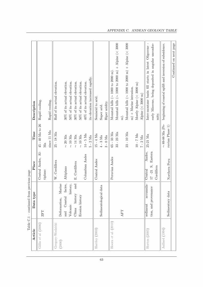
APPENDIX C. ANDEAN GEOLOGY TABLETab
leC.1
–continued
from
previouspag
e
Article
Data
type
Place
Tim
eDescription
Gilliset
al.(200
6)ZFT
Central
Andes,Al-
tiplano
45-40
Mato
26
Ma
Rap
idcooling.
since
11Ma
Rap
idcooling.
Grego
ry-W
odzicki
(200
0)
Deform
ation,
Marine
and
Coa
stal
facies,
Volcanic
history,
Clima
history
and
Erosion
history
W.Cordillera
25-18
Ma
Halfof
itsactualelevation.
Altiplano
∼20
Ma
30%
ofitsactualelevation.
∼10
Ma
50%
ofitsactualelevation.
E.Cordillera
∼14
Ma
30%
ofitsactualelevation.
∼10
Ma
50%
ofitsactualelevation.
ColumbianAndes
14-5Ma
40%
ofitsactualelevation.
5-2Ma
itselevationincreasedrapidly.
Hartley(200
3)
Sed
imentological
data
Central
Andes
15-4Ma
Sem
iaridto
arid.
4-3Ma
Super
arid.
3-0Ma
Hiper
aridity.
Hoorn
etal.(201
0)
AFT
PeruvianAndes
65-33
Ma
Mou
ntailhills
(∼10
00to
2000
m).
33-23
Ma
Mou
ntailhills
(∼10
00to
2000
m)+
Alpine(<
3000
m).
23-10
Ma
Mou
ntailhills
(∼10
00to
2000
m)+
Alpine(<
3000
m)+
Marineintrusion
.
10-7Ma
MostlyAlpine(<
3000
m)
7-2Ma
Alpine(<
3000
m)
Horton(200
5)sedim
ent
accu
mula-
tion
,an
dprovenance
Central
Andes,
17-21
S,Eastern
Cordillera
25-21Ma
Inter-mon
tanebasin
fill
starts
inlatest
Oligo
cene-
earlyMiocene,
beingdep
osited
inangu
larunconfor-
mity.
Jaillard
(199
4)
Sed
imentary
data
NorthernPeru
∼89
-88Ma(P
e-
ruvianPhase1)
beginningof
coastal
upliftan
dinversionof
subsiden
ce.
Con
tinued
onnextpag
e
63

APPENDIX C. ANDEAN GEOLOGY TABLETab
leC.1
–continued
from
previouspag
e
Article
Data
type
Place
Tim
eDescription
∼87
-86
Ma
(PeruvianPhase
2)
Incipientthrustingan
dtecton
icactivityarerelatedto
aNE-SW
compressional
strain.
∼76
-73Ma(P
e-
ruvianPhase3)
Uplift
anderosionof
theCoa
stal
Cordillera
andsub-
siden
ceof
thecoastalArea.
Jaillard
&Soler
(199
6)
Sed
imentary
data
NorthernPeru
Late
Cam
pa-
nian
Majorcontraction
alphase.
See
fig1in
thearti-
cle.
LateEocene(∼
35Ma)
folding
and
reverse
faulting
intheform
erWestern
Trough
,form
edafold
andthrust
belt.
McQ
uarrie
etal.
(200
8)
apatiteand
zircon
fis-
siontrackcoolingag
es
Central
Andes
15-
17S
40-25
Ma
Fastexhumationrate
intheEastern
Cordillera.
15(8)-0Ma
Rap
idexhumationin
theentire
fold-thrust
belt.
25-15
(8)Ma
pau
seor
adramatic
decelerationin
therate
ofdefor-
mationan
dpropag
ationof
thefold-thrust
belt.
Mpodozis
etal.
(200
5)
-Atacamabasin
LateCretaceou
sUplift
intheCordillera
deDom
eyko,reflectedin
the
sedim
entation
intheSalar
deAtacama.
Ped
ernales
basin
Uplift
and
unroofi
ngof
theCordillera
deDom
eyko,
dueto
highsedim
entation
rates.
Picardet
al.(2008
)Biotaxa
(wild
potato
andtomato)
SouthernPeru
23-19
Ma
whereab
ove2-2.5
km
high.
Central
Peru
16-13
Ma
Uplifted
above2-2.5
km
NorthernPeru
since
6Ma
Uplifted
above2km
Sem
pere
etal.
(199
0)
-Bolivia
Orocline
late
Oligo
cene
Mayor
tecton
iccrisis.
Sem
pere
etal.
(199
4)
-
32oS-37
oS
27Ma
Initiation
ofamajordeformationin
theVolcanic
and
Principal
Cordillera.
20Ma
Volcanic
inform
ationsugg
estaquiescentstate.
Con
tinued
onnextpag
e
64

APPENDIX C. ANDEAN GEOLOGY TABLETab
leC.1
–continued
from
previouspag
e
Article
Data
type
Place
Tim
eDescription
since
10Ma
2km
ofuplift
intheAconcagu
aregion.
Sem
pere
etal.
(199
7)
stratigrap
hy,
mag
-
netostratigraphy,
Ar/Ar
dating,
and
paleontology
Bolivia
and
north-
westArgentina
∼89
Ma
tecton
iceventmarkedaturningpointin
Andeanevo-
lution
.
∼59
.5–58.2Ma
Tectoniceventmarkstheinitiation
ofcontinentalfore-
landsedim
entation
inAndeanBolivia.
Thomson(2002
)Fission
track
ther-
mochronology
Patago
nian
Andes
42-46S
16-10
Ma
Initiation
ofdenudation.
7-2Ma
Fastdenudation.
Tunik
etal.(201
0)Fission
trackandU-P
b
detricalzircons
Neu
quen
Basin
98-88
Ma
Began
AndeanUplift.
65
Appendix D
Force balance results
66
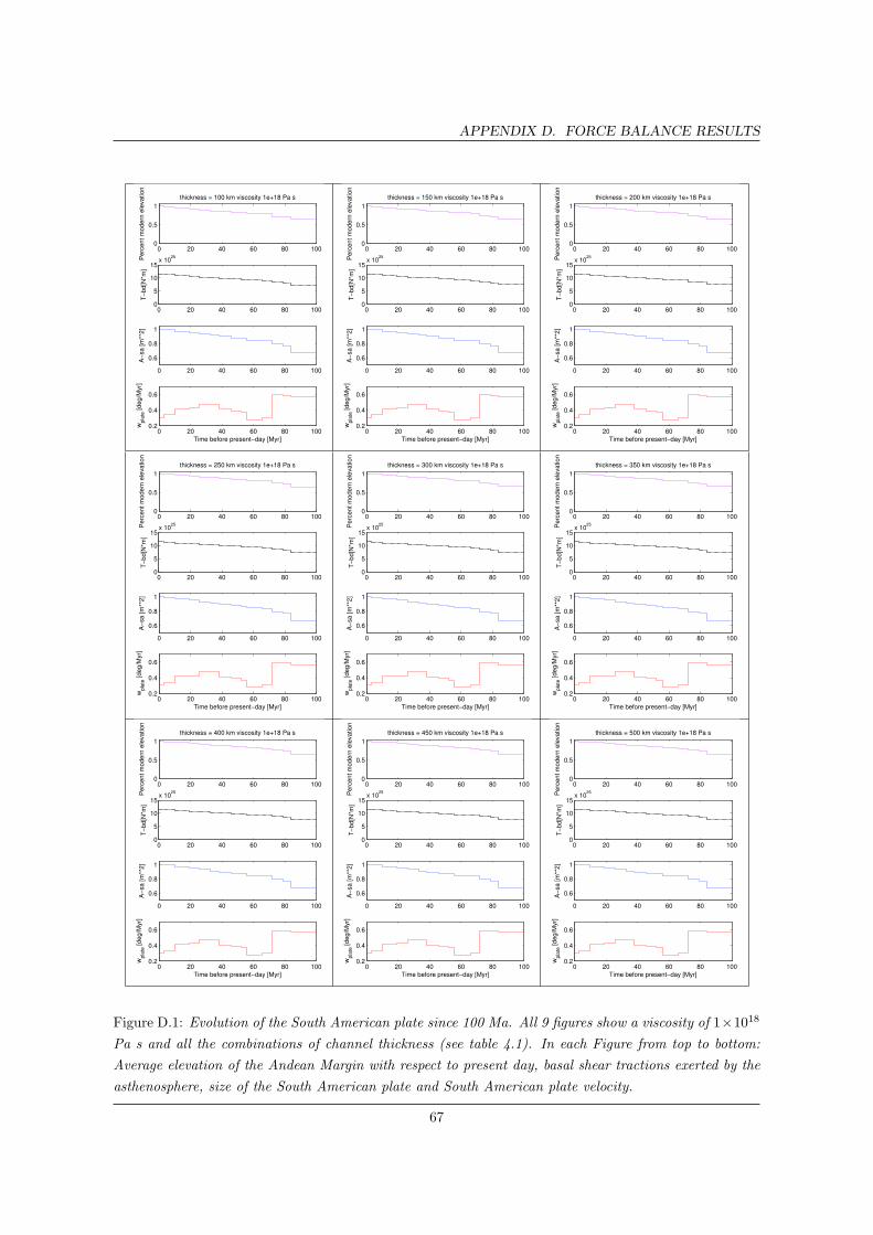
APPENDIX D. FORCE BALANCE RESULTS
0 20 40 60 80 1000
0.5
1
Pe
rce
nt
mo
de
rn e
leva
tio
n
thickness = 100 km viscosity 1e+18 Pa s
0 20 40 60 80 1000
5
10
15x 10
25
T−
bd
[N*m
]
0 20 40 60 80 100
0.6
0.8
1
A−
sa
[m
**2
]
0 20 40 60 80 1000.2
0.4
0.6
Time before present−day [Myr]
wpla
te [
de
g/M
yr]
0 20 40 60 80 1000
0.5
1
Pe
rce
nt
mo
de
rn e
leva
tio
n
thickness = 150 km viscosity 1e+18 Pa s
0 20 40 60 80 1000
5
10
15x 10
25
T−
bd
[N*m
]
0 20 40 60 80 100
0.6
0.8
1
A−
sa
[m
**2
]
0 20 40 60 80 1000.2
0.4
0.6
Time before present−day [Myr]
wpla
te [
de
g/M
yr]
0 20 40 60 80 1000
0.5
1
Pe
rce
nt
mo
de
rn e
leva
tio
n
thickness = 200 km viscosity 1e+18 Pa s
0 20 40 60 80 1000
5
10
15x 10
25
T−
bd
[N*m
]
0 20 40 60 80 100
0.6
0.8
1
A−
sa
[m
**2
]
0 20 40 60 80 1000.2
0.4
0.6
Time before present−day [Myr]
wpla
te [
de
g/M
yr]
0 20 40 60 80 1000
0.5
1
Pe
rce
nt
mo
de
rn e
leva
tio
n
thickness = 250 km viscosity 1e+18 Pa s
0 20 40 60 80 1000
5
10
15x 10
25
T−
bd
[N*m
]
0 20 40 60 80 100
0.6
0.8
1
A−
sa
[m
**2
]
0 20 40 60 80 1000.2
0.4
0.6
Time before present−day [Myr]
wpla
te [
de
g/M
yr]
0 20 40 60 80 1000
0.5
1
Pe
rce
nt
mo
de
rn e
leva
tio
n
thickness = 300 km viscosity 1e+18 Pa s
0 20 40 60 80 1000
5
10
15x 10
25
T−
bd
[N*m
]
0 20 40 60 80 100
0.6
0.8
1
A−
sa
[m
**2
]
0 20 40 60 80 1000.2
0.4
0.6
Time before present−day [Myr]
wpla
te [
de
g/M
yr]
0 20 40 60 80 1000
0.5
1
Pe
rce
nt
mo
de
rn e
leva
tio
n
thickness = 350 km viscosity 1e+18 Pa s
0 20 40 60 80 1000
5
10
15x 10
25
T−
bd
[N*m
]
0 20 40 60 80 100
0.6
0.8
1
A−
sa
[m
**2
]
0 20 40 60 80 1000.2
0.4
0.6
Time before present−day [Myr]
wpla
te [
de
g/M
yr]
0 20 40 60 80 1000
0.5
1
Pe
rce
nt
mo
de
rn e
leva
tio
n
thickness = 400 km viscosity 1e+18 Pa s
0 20 40 60 80 1000
5
10
15x 10
25
T−
bd
[N*m
]
0 20 40 60 80 100
0.6
0.8
1
A−
sa
[m
**2
]
0 20 40 60 80 1000.2
0.4
0.6
Time before present−day [Myr]
wpla
te [
de
g/M
yr]
0 20 40 60 80 1000
0.5
1
Pe
rce
nt
mo
de
rn e
leva
tio
n
thickness = 450 km viscosity 1e+18 Pa s
0 20 40 60 80 1000
5
10
15x 10
25
T−
bd
[N*m
]
0 20 40 60 80 100
0.6
0.8
1
A−
sa
[m
**2
]
0 20 40 60 80 1000.2
0.4
0.6
Time before present−day [Myr]
wpla
te [
de
g/M
yr]
0 20 40 60 80 1000
0.5
1
Pe
rce
nt
mo
de
rn e
leva
tio
n
thickness = 500 km viscosity 1e+18 Pa s
0 20 40 60 80 1000
5
10
15x 10
25
T−
bd
[N*m
]
0 20 40 60 80 100
0.6
0.8
1
A−
sa
[m
**2
]
0 20 40 60 80 1000.2
0.4
0.6
Time before present−day [Myr]
wpla
te [
de
g/M
yr]
Figure D.1: Evolution of the South American plate since 100 Ma. All 9 figures show a viscosity of 1×10¹⁸
Pa s and all the combinations of channel thickness (see table 4.1). In each Figure from top to bottom:
Average elevation of the Andean Margin with respect to present day, basal shear tractions exerted by the
asthenosphere, size of the South American plate and South American plate velocity.
67
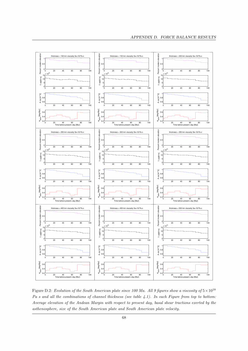
APPENDIX D. FORCE BALANCE RESULTS
0 20 40 60 80 1000
0.5
1
Pe
rce
nt
mo
de
rn e
leva
tio
n
thickness = 100 km viscosity 5e+18 Pa s
0 20 40 60 80 1000
5
10
15x 10
25
T−
bd
[N*m
]
0 20 40 60 80 100
0.6
0.8
1
A−
sa
[m
**2
]
0 20 40 60 80 1000.2
0.4
0.6
Time before present−day [Myr]
wpla
te [
de
g/M
yr]
0 20 40 60 80 1000
0.5
1
Pe
rce
nt
mo
de
rn e
leva
tio
n
thickness = 150 km viscosity 5e+18 Pa s
0 20 40 60 80 1000
5
10
15x 10
25
T−
bd
[N*m
]
0 20 40 60 80 100
0.6
0.8
1
A−
sa
[m
**2
]
0 20 40 60 80 1000.2
0.4
0.6
Time before present−day [Myr]
wpla
te [
de
g/M
yr]
0 20 40 60 80 1000
0.5
1
Pe
rce
nt
mo
de
rn e
leva
tio
n
thickness = 200 km viscosity 5e+18 Pa s
0 20 40 60 80 1000
5
10
15x 10
25
T−
bd
[N*m
]
0 20 40 60 80 100
0.6
0.8
1
A−
sa
[m
**2
]
0 20 40 60 80 1000.2
0.4
0.6
Time before present−day [Myr]
wpla
te [
de
g/M
yr]
0 20 40 60 80 1000
0.5
1
Pe
rce
nt
mo
de
rn e
leva
tio
n
thickness = 250 km viscosity 5e+18 Pa s
0 20 40 60 80 1000
5
10
15x 10
25
T−
bd
[N*m
]
0 20 40 60 80 100
0.6
0.8
1
A−
sa
[m
**2
]
0 20 40 60 80 1000.2
0.4
0.6
Time before present−day [Myr]
wpla
te [
de
g/M
yr]
0 20 40 60 80 1000
0.5
1
Pe
rce
nt
mo
de
rn e
leva
tio
n
thickness = 300 km viscosity 5e+18 Pa s
0 20 40 60 80 1000
5
10
15x 10
25
T−
bd
[N*m
]
0 20 40 60 80 100
0.6
0.8
1
A−
sa
[m
**2
]
0 20 40 60 80 1000.2
0.4
0.6
Time before present−day [Myr]
wpla
te [
de
g/M
yr]
0 20 40 60 80 1000
0.5
1
Pe
rce
nt
mo
de
rn e
leva
tio
n
thickness = 350 km viscosity 5e+18 Pa s
0 20 40 60 80 1000
5
10
15x 10
25
T−
bd
[N*m
]
0 20 40 60 80 100
0.6
0.8
1
A−
sa
[m
**2
]
0 20 40 60 80 1000.2
0.4
0.6
Time before present−day [Myr]
wpla
te [
de
g/M
yr]
0 20 40 60 80 1000
0.5
1
Pe
rce
nt
mo
de
rn e
leva
tio
n
thickness = 400 km viscosity 5e+18 Pa s
0 20 40 60 80 1000
5
10
15x 10
25
T−
bd
[N*m
]
0 20 40 60 80 100
0.6
0.8
1
A−
sa
[m
**2
]
0 20 40 60 80 1000.2
0.4
0.6
Time before present−day [Myr]
wpla
te [
de
g/M
yr]
0 20 40 60 80 1000
0.5
1
Pe
rce
nt
mo
de
rn e
leva
tio
n
thickness = 450 km viscosity 5e+18 Pa s
0 20 40 60 80 1000
5
10
15x 10
25
T−
bd
[N*m
]
0 20 40 60 80 100
0.6
0.8
1
A−
sa
[m
**2
]
0 20 40 60 80 1000.2
0.4
0.6
Time before present−day [Myr]
wpla
te [
de
g/M
yr]
0 20 40 60 80 1000
0.5
1
Pe
rce
nt
mo
de
rn e
leva
tio
n
thickness = 500 km viscosity 5e+18 Pa s
0 20 40 60 80 1000
5
10
15x 10
25
T−
bd
[N*m
]
0 20 40 60 80 100
0.6
0.8
1
A−
sa
[m
**2
]
0 20 40 60 80 1000.2
0.4
0.6
Time before present−day [Myr]
wpla
te [
de
g/M
yr]
Figure D.2: Evolution of the South American plate since 100 Ma. All 9 figures show a viscosity of 5×10¹⁸
Pa s and all the combinations of channel thickness (see table 4.1). In each Figure from top to bottom:
Average elevation of the Andean Margin with respect to present day, basal shear tractions exerted by the
asthenosphere, size of the South American plate and South American plate velocity.
68
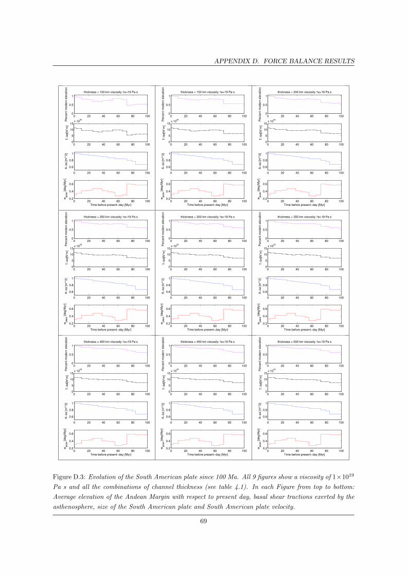
APPENDIX D. FORCE BALANCE RESULTS
0 20 40 60 80 1000
0.5
1
Pe
rce
nt
mo
de
rn e
leva
tio
n
thickness = 100 km viscosity 1e+19 Pa s
0 20 40 60 80 1000
5
10
15x 10
25
T−
bd
[N*m
]
0 20 40 60 80 100
0.6
0.8
1
A−
sa
[m
**2
]
0 20 40 60 80 1000.2
0.4
0.6
Time before present−day [Myr]
wpla
te [
de
g/M
yr]
0 20 40 60 80 1000
0.5
1
Pe
rce
nt
mo
de
rn e
leva
tio
n
thickness = 150 km viscosity 1e+19 Pa s
0 20 40 60 80 1000
5
10
15x 10
25
T−
bd
[N*m
]
0 20 40 60 80 100
0.6
0.8
1
A−
sa
[m
**2
]
0 20 40 60 80 1000.2
0.4
0.6
Time before present−day [Myr]
wpla
te [
de
g/M
yr]
0 20 40 60 80 1000
0.5
1
Pe
rce
nt
mo
de
rn e
leva
tio
n
thickness = 200 km viscosity 1e+19 Pa s
0 20 40 60 80 1000
5
10
15x 10
25
T−
bd
[N*m
]
0 20 40 60 80 100
0.6
0.8
1
A−
sa
[m
**2
]
0 20 40 60 80 1000.2
0.4
0.6
Time before present−day [Myr]
wpla
te [
de
g/M
yr]
0 20 40 60 80 1000
0.5
1
Pe
rce
nt
mo
de
rn e
leva
tio
n
thickness = 250 km viscosity 1e+19 Pa s
0 20 40 60 80 1000
5
10
15x 10
25
T−
bd
[N*m
]
0 20 40 60 80 100
0.6
0.8
1
A−
sa
[m
**2
]
0 20 40 60 80 1000.2
0.4
0.6
Time before present−day [Myr]
wpla
te [
de
g/M
yr]
0 20 40 60 80 1000
0.5
1
Pe
rce
nt
mo
de
rn e
leva
tio
n
thickness = 300 km viscosity 1e+19 Pa s
0 20 40 60 80 1000
5
10
15x 10
25
T−
bd
[N*m
]
0 20 40 60 80 100
0.6
0.8
1
A−
sa
[m
**2
]
0 20 40 60 80 1000.2
0.4
0.6
Time before present−day [Myr]
wpla
te [
de
g/M
yr]
0 20 40 60 80 1000
0.5
1
Pe
rce
nt
mo
de
rn e
leva
tio
n
thickness = 350 km viscosity 1e+19 Pa s
0 20 40 60 80 1000
5
10
15x 10
25
T−
bd
[N*m
]
0 20 40 60 80 100
0.6
0.8
1
A−
sa
[m
**2
]
0 20 40 60 80 1000.2
0.4
0.6
Time before present−day [Myr]
wpla
te [
de
g/M
yr]
0 20 40 60 80 1000
0.5
1
Pe
rce
nt
mo
de
rn e
leva
tio
n
thickness = 400 km viscosity 1e+19 Pa s
0 20 40 60 80 1000
5
10
15x 10
25
T−
bd
[N*m
]
0 20 40 60 80 100
0.6
0.8
1
A−
sa
[m
**2
]
0 20 40 60 80 1000.2
0.4
0.6
Time before present−day [Myr]
wpla
te [
de
g/M
yr]
0 20 40 60 80 1000
0.5
1
Pe
rce
nt
mo
de
rn e
leva
tio
n
thickness = 450 km viscosity 1e+19 Pa s
0 20 40 60 80 1000
5
10
15x 10
25
T−
bd
[N*m
]
0 20 40 60 80 100
0.6
0.8
1
A−
sa
[m
**2
]
0 20 40 60 80 1000.2
0.4
0.6
Time before present−day [Myr]
wpla
te [
de
g/M
yr]
0 20 40 60 80 1000
0.5
1
Pe
rce
nt
mo
de
rn e
leva
tio
n
thickness = 500 km viscosity 1e+19 Pa s
0 20 40 60 80 1000
5
10
15x 10
25
T−
bd
[N*m
]
0 20 40 60 80 100
0.6
0.8
1
A−
sa
[m
**2
]
0 20 40 60 80 1000.2
0.4
0.6
Time before present−day [Myr]
wpla
te [
de
g/M
yr]
Figure D.3: Evolution of the South American plate since 100 Ma. All 9 figures show a viscosity of 1×10¹⁹
Pa s and all the combinations of channel thickness (see table 4.1). In each Figure from top to bottom:
Average elevation of the Andean Margin with respect to present day, basal shear tractions exerted by the
asthenosphere, size of the South American plate and South American plate velocity.
69

APPENDIX D. FORCE BALANCE RESULTS
0 20 40 60 80 1000
0.5
1
Pe
rce
nt
mo
de
rn e
leva
tio
n
thickness = 100 km viscosity 5e+19 Pa s
0 20 40 60 80 1000
5
10
15x 10
25
T−
bd
[N*m
]
0 20 40 60 80 100
0.6
0.8
1
A−
sa
[m
**2
]
0 20 40 60 80 1000.2
0.4
0.6
Time before present−day [Myr]
wpla
te [
de
g/M
yr]
0 20 40 60 80 1000
0.5
1
Pe
rce
nt
mo
de
rn e
leva
tio
n
thickness = 150 km viscosity 5e+19 Pa s
0 20 40 60 80 1000
5
10
15x 10
25
T−
bd
[N*m
]
0 20 40 60 80 100
0.6
0.8
1
A−
sa
[m
**2
]
0 20 40 60 80 1000.2
0.4
0.6
Time before present−day [Myr]
wpla
te [
de
g/M
yr]
0 20 40 60 80 1000
0.5
1
Pe
rce
nt
mo
de
rn e
leva
tio
n
thickness = 200 km viscosity 5e+19 Pa s
0 20 40 60 80 1000
5
10
15x 10
25
T−
bd
[N*m
]
0 20 40 60 80 100
0.6
0.8
1
A−
sa
[m
**2
]
0 20 40 60 80 1000.2
0.4
0.6
Time before present−day [Myr]
wpla
te [
de
g/M
yr]
0 20 40 60 80 1000
0.5
1
Pe
rce
nt
mo
de
rn e
leva
tio
n
thickness = 250 km viscosity 5e+19 Pa s
0 20 40 60 80 1000
5
10
15x 10
25
T−
bd
[N*m
]
0 20 40 60 80 100
0.6
0.8
1
A−
sa
[m
**2
]
0 20 40 60 80 1000.2
0.4
0.6
Time before present−day [Myr]
wpla
te [
de
g/M
yr]
0 20 40 60 80 1000
0.5
1
Pe
rce
nt
mo
de
rn e
leva
tio
n
thickness = 300 km viscosity 5e+19 Pa s
0 20 40 60 80 1000
5
10
15x 10
25
T−
bd
[N*m
]
0 20 40 60 80 100
0.6
0.8
1
A−
sa
[m
**2
]
0 20 40 60 80 1000.2
0.4
0.6
Time before present−day [Myr]
wpla
te [
de
g/M
yr]
0 20 40 60 80 1000
0.5
1
Pe
rce
nt
mo
de
rn e
leva
tio
n
thickness = 350 km viscosity 5e+19 Pa s
0 20 40 60 80 1000
5
10
15x 10
25
T−
bd
[N*m
]
0 20 40 60 80 100
0.6
0.8
1
A−
sa
[m
**2
]
0 20 40 60 80 1000.2
0.4
0.6
Time before present−day [Myr]
wpla
te [
de
g/M
yr]
0 20 40 60 80 1000
0.5
1
Pe
rce
nt
mo
de
rn e
leva
tio
n
thickness = 400 km viscosity 5e+19 Pa s
0 20 40 60 80 1000
5
10
15x 10
25
T−
bd
[N*m
]
0 20 40 60 80 100
0.6
0.8
1
A−
sa
[m
**2
]
0 20 40 60 80 1000.2
0.4
0.6
Time before present−day [Myr]
wpla
te [
de
g/M
yr]
0 20 40 60 80 1000
0.5
1
Pe
rce
nt
mo
de
rn e
leva
tio
n
thickness = 450 km viscosity 5e+19 Pa s
0 20 40 60 80 1000
5
10
15x 10
25
T−
bd
[N*m
]
0 20 40 60 80 100
0.6
0.8
1
A−
sa
[m
**2
]
0 20 40 60 80 1000.2
0.4
0.6
Time before present−day [Myr]
wpla
te [
de
g/M
yr]
0 20 40 60 80 1000
0.5
1
Pe
rce
nt
mo
de
rn e
leva
tio
n
thickness = 500 km viscosity 5e+19 Pa s
0 20 40 60 80 1000
5
10
15x 10
25
T−
bd
[N*m
]
0 20 40 60 80 100
0.6
0.8
1
A−
sa
[m
**2
]
0 20 40 60 80 1000.2
0.4
0.6
Time before present−day [Myr]
wpla
te [
de
g/M
yr]
Figure D.4: Evolution of the South American plate since 100 Ma. All 9 figures show a viscosity of 5×10¹⁹
Pa s and all the combinations of channel thickness (see table 4.1). In each Figure from top to bottom:
Average elevation of the Andean Margin with respect to present day, basal drag shear tractions by the
asthenosphere, size of the South American plate and South American plate velocity.
70

APPENDIX D. FORCE BALANCE RESULTS
0 20 40 60 80 1000
0.5
1
Pe
rce
nt
mo
de
rn e
leva
tio
n
thickness = 100 km viscosity 1e+20 Pa s
0 20 40 60 80 1000
5
10
15x 10
25
T−
bd
[N*m
]
0 20 40 60 80 100
0.6
0.8
1
A−
sa
[m
**2
]
0 20 40 60 80 1000.2
0.4
0.6
Time before present−day [Myr]
wpla
te [
de
g/M
yr]
0 20 40 60 80 1000
0.5
1
Pe
rce
nt
mo
de
rn e
leva
tio
n
thickness = 150 km viscosity 1e+20 Pa s
0 20 40 60 80 1000
5
10
15x 10
25
T−
bd
[N*m
]
0 20 40 60 80 100
0.6
0.8
1
A−
sa
[m
**2
]
0 20 40 60 80 1000.2
0.4
0.6
Time before present−day [Myr]
wpla
te [
de
g/M
yr]
0 20 40 60 80 1000
0.5
1
Pe
rce
nt
mo
de
rn e
leva
tio
n
thickness = 200 km viscosity 1e+20 Pa s
0 20 40 60 80 1000
5
10
15x 10
25
T−
bd
[N*m
]
0 20 40 60 80 100
0.6
0.8
1
A−
sa
[m
**2
]
0 20 40 60 80 1000.2
0.4
0.6
Time before present−day [Myr]
wpla
te [
de
g/M
yr]
0 20 40 60 80 1000
0.5
1
Pe
rce
nt
mo
de
rn e
leva
tio
n
thickness = 250 km viscosity 1e+20 Pa s
0 20 40 60 80 1000
5
10
15x 10
25
T−
bd
[N*m
]
0 20 40 60 80 100
0.6
0.8
1
A−
sa
[m
**2
]
0 20 40 60 80 1000.2
0.4
0.6
Time before present−day [Myr]
wpla
te [
de
g/M
yr]
0 20 40 60 80 1000
0.5
1
Pe
rce
nt
mo
de
rn e
leva
tio
n
thickness = 300 km viscosity 1e+20 Pa s
0 20 40 60 80 1000
5
10
15x 10
25
T−
bd
[N*m
]
0 20 40 60 80 100
0.6
0.8
1
A−
sa
[m
**2
]
0 20 40 60 80 1000.2
0.4
0.6
Time before present−day [Myr]
wpla
te [
de
g/M
yr]
0 20 40 60 80 1000
0.5
1
Pe
rce
nt
mo
de
rn e
leva
tio
n
thickness = 350 km viscosity 1e+20 Pa s
0 20 40 60 80 1000
5
10
15x 10
25
T−
bd
[N*m
]
0 20 40 60 80 100
0.6
0.8
1
A−
sa
[m
**2
]
0 20 40 60 80 1000.2
0.4
0.6
Time before present−day [Myr]
wpla
te [
de
g/M
yr]
0 20 40 60 80 1000
0.5
1
Pe
rce
nt
mo
de
rn e
leva
tio
n
thickness = 400 km viscosity 1e+20 Pa s
0 20 40 60 80 1000
5
10
15x 10
25
T−
bd
[N*m
]
0 20 40 60 80 100
0.6
0.8
1
A−
sa
[m
**2
]
0 20 40 60 80 1000.2
0.4
0.6
Time before present−day [Myr]
wpla
te [
de
g/M
yr]
0 20 40 60 80 1000
0.5
1
Pe
rce
nt
mo
de
rn e
leva
tio
n
thickness = 450 km viscosity 1e+20 Pa s
0 20 40 60 80 1000
5
10
15x 10
25
T−
bd
[N*m
]
0 20 40 60 80 100
0.6
0.8
1
A−
sa
[m
**2
]
0 20 40 60 80 1000.2
0.4
0.6
Time before present−day [Myr]
wpla
te [
de
g/M
yr]
0 20 40 60 80 1000
0.5
1
Pe
rce
nt
mo
de
rn e
leva
tio
n
thickness = 500 km viscosity 1e+20 Pa s
0 20 40 60 80 1000
5
10
15x 10
25
T−
bd
[N*m
]
0 20 40 60 80 100
0.6
0.8
1
A−
sa
[m
**2
]
0 20 40 60 80 1000.2
0.4
0.6
Time before present−day [Myr]
wpla
te [
de
g/M
yr]
Figure D.5: Evolution of the South American plate since 100 Ma. All 9 figures show a viscosity of 1×10²⁰
Pa s and all the combinations of channel thickness (see table 4.1). In each Figure from top to bottom:
Average elevation of the Andean Margin with respect to present day, basal shear tractions exerted by the
asthenosphere, size of the South American plate and South American plate velocity.
71