Faculteit der Exacte Wetenschappen

TNO Defensie en veiligheid

Bachelorproject verslag Natuur- en Sterrenkunde, omvang 12 EC,uitgevoerd als stage bij TNO defensie en veiligheid in de periode

26-04-2010 tot 01-07-2010

Solid propellant grain geometrydesign, a model for the evolution

of star shaped interfaces

Auteur:Arnon Lesage,5795656

Begeleiders:Ir. Francois Bouquet

Dr. Rudolf Sprik

August 9, 2010

Contents

1 Introduction 5

2 Solid rocket motors 62.1 Passive regulation . . . . . . . . . . . . . . . . . . . . . . . . . . 62.2 Thrust and mass flow . . . . . . . . . . . . . . . . . . . . . . . . 82.3 Burn rate . . . . . . . . . . . . . . . . . . . . . . . . . . . . . . . 9

2.3.1 Pressure and burn rate . . . . . . . . . . . . . . . . . . . . 102.3.2 Temperature and burn rate . . . . . . . . . . . . . . . . . 102.3.3 Erosive burning . . . . . . . . . . . . . . . . . . . . . . . . 112.3.4 Other effects . . . . . . . . . . . . . . . . . . . . . . . . . 11

2.4 Mass flow and pressure . . . . . . . . . . . . . . . . . . . . . . . . 11

3 Grain geometry 133.1 Propagating interface . . . . . . . . . . . . . . . . . . . . . . . . . 143.2 Interface propagation methods . . . . . . . . . . . . . . . . . . . 153.3 Cellular automaton . . . . . . . . . . . . . . . . . . . . . . . . . . 153.4 Fast marching algorithm . . . . . . . . . . . . . . . . . . . . . . . 183.5 Geometric solution of a parametric star . . . . . . . . . . . . . . 183.6 The chosen method . . . . . . . . . . . . . . . . . . . . . . . . . . 19

4 Geometric evolution of a parametric star - Building the model 214.1 The parameters . . . . . . . . . . . . . . . . . . . . . . . . . . . . 214.2 Initial shape . . . . . . . . . . . . . . . . . . . . . . . . . . . . . . 234.3 Evolution of the shape . . . . . . . . . . . . . . . . . . . . . . . . 274.4 Intersection points . . . . . . . . . . . . . . . . . . . . . . . . . . 294.5 Burn area . . . . . . . . . . . . . . . . . . . . . . . . . . . . . . . 304.6 Achievements and Limitations of the algorithm . . . . . . . . . . 314.7 Results and comparison with the current software, GDP[1] . . . . 324.8 Improvements and beyond . . . . . . . . . . . . . . . . . . . . . . 32

5 Conclusion 36

1

Nomenclature

m Mass flow

r Burn rate

πK Temperature sensitivity of pressure

ρc Chamber gas density

ρe Exhaust gas density

ρp Propellant mass density

θ(θ∗) The angle from the origin to a point on the off-center circle

θ∗ The angle from the origin of the off-center circle to a point on the off-center circle

θi Angles representing the limits of the angular range over which the piece-wise functions of r(θ) work

θi(bd) Angles representing the limits of the angular range over which the piece-wise functions of r(θ, bd) work

a angle used in geometry,= πN

At Nozzle throat area

a0 Propellant constant that depends on initial grain temperature

Ab Burn Area

Ae Nozzle exit Area

At Throat Area

b angle used in geometry,= k1πN

bd Burn Depth

c Angle used in geometry,= k2πN

F Thrust

Fr1 The initial Radius of the first fillet

Fr2 The initial Radius of the second fillet

IR Inner radius

k Specific heat ratio

k1 Fraction of angles, = ba

2

k2 Fraction of angles, = ca

N Number of star points

n Combustion index

OR Outer radius

Pa Outer pressure

Pc Combustion chamber pressure

Pe Exit pressure

Pa Point angle

R Gas constant, or later on circle radius

r(θ) Radial function describing the initial interface

Rc The radius function of an off-center circle

ri(θ) Radial function describing a single piece of the geometry

ri(θ, bd) Radial function describing a single piece of the geometry as it evolvesas a function of burn depth

rfi(θ) Radial function describing the fillet piece of the geometry

rfi(θ, bd) Radial function describing the fillet piece of the geometry as it evolvesas a function of burn depth

Tc Combustion temperature

Vc Grain cavity volume

Ve Exit gas velocity

3

Samenvatting

Vaste stuwstof motoren bieden geen mogelijkheid om zich actief te reguleren.Actief reguleren houdt in dat het mogelijk is om tijdens het vliegen de stuwkrachtte veranderen naar wensen. Na het ontsteken, verbrandt de stuwstof en leverthet een bepaalde stuwkracht. De stuwkracht is afhankelijk van de hoeveelheidverbrandingsoppervlak van de stuwstof. Door de stuwstof een bepaalde ge-ometrische vorm te geven, is het mogelijk de hoeveelheid stuwkracht toch passiefte kunnen reguleren. In tegenstelling tot actief reguleren, houdt passief regulerenin dat de stuwkracht veranderingen vantevoren, dus voor het ontsteken wordenbepaald. Tijdens het verbranden van de stuwstof, zet de vaste stuwstof zich omin gas, en verandert de geometrische vorm van de stuwstof massa. De stuwstofgeometrie moet dan ook na het veranderen nog steeds aan de stuwkrachteisenvoldoen. Hiervoor is een model nodig dat de manier waarop de geometrie veran-dert kan simuleren. Hiermee kan het model berekenen wat de stuwkracht is vaneen bepaald geometrie ontwerp tijdens zijn gehele verbranding. Het model dathier wordt bestudeerd zal de eerste stap zetten naar een optimalisatie model.Het optimalisatiemodel, het einddoel, is een model dat een stuwstof geometrieberekent die aan bepaalde prestatie-eisen voldoet. De stap die in dit onder-zoek wordt bestudeerd is niet de optimalisatie, maar het berekenen van deprestaties van cilindrische geometrie, gebaseerd op twee dimensionale sterge-ometrie. Het model is uitgewerkt in MatLab, in opdracht van TNO Defensieen Veiligheid. Het model berekent de prestaties op een manier die optimal-isatie mogelijk maakt. Dit was nog niet mogelijk met de bekende methodes, endaarom werd het huidige model ontwikkeld.

4

1 Introduction

TNO Defence Security and safety provides many solutions to the overall safetyand security as a strategic partner of the Ministry of Defence. TNO has a longhistory in researching propellants. The research began in the middle of the1980’s, with the design of igniters and starter engines for the Ariane 5 mainengine (Vulcain). The Ariane 5 is a civilian rocket used as a carrier of satellitesinto orbit.

Over the years, development provided detailed methods by which the per-formance of a given propellant and propellant-geometry can be determined.The currently used software, GDP[1], is able to calculate the performance andburn behavior in detail. Yet, it does not provide fast analysis or a basis foroptimizations of the propellant geometry, also known as the grain geometry.Optimization is an essential ingredient for the development of grain geometry.The grain, which is the propellant bulk, is developed when the requirements ofthe rocket are known. It is therefore needed to have a method that calculatesa grain-geometry based on the given performance requirements. Further cal-culations and fine tuning of the geometry can then be done using the currentsoftware models.

The project is split into two separate projects. The first is the developmentand implementation of a model that provides fast performance calculations ofa given propellant and propellant-geometry. Different approaches are availablewhich will be discussed. The chosen approach is implemented in MATLAB.Fast analysis of the grain is the key ingredient of the chosen approach. Speed isimportant because in the next step, optimization, simulation of many differentgrains takes place. It is therefore desired to have an approach that minimizesthe time of a single analysis to under a second. The second part of the projectis the optimization phase. A grain geometry will be calculated that providesthe requirements for the mission at hand. The subject discussed is the first partof the project, the analysis of a grain geometry. In (4.8) a discussion followsthat provides some points of thought for the second part of the project, theoptimization.

The model produced will concentrate on burn area evolution, as a functionof burn depth. This means it will not take into account all factors affectingthe burn rate, and with that the production of thrust. These factors will bediscussed though in order to understand, why these can be examined separatelyand how future implementation is possible.

5

2 Solid rocket motors

A solid rocket motor (SRM) is a machine that provides thrust. Every SRMprovides a different amount of thrust depending on payload, destination andother factors. But thrust is not the only performance variable of a SRM. Forexample the mass of the propellant is also a major factor. As the propellantburns, it’s mass decreases, allowing higher acceleration. Therefore performanceassessment models also look at specific impulse, mass flow and other variables.This model will only examine a few aspects of the performance of a SRM,although many others can also be examined.

The solid rocket motor is one of two major classes of motors, where liquidpropellant is the other kind. What makes solid unique versus the liquid propel-lant, is the simplicity of the motor. The solid propellant contains the fuel andoxidizer. It is therefore enough to ignite the propellant and no other chemicalhas to be added for combustion to take place. There are different propellantcompositions, usually double base or composite, that all have different proper-ties. Burn rate, ignition temperature, flame temperature and other propertiesthat can all be found using experimentation and modeling.

The simplicity of the solid propellant is also it’s drawback. Requiring nothingexternal to burn, the SRM’s burning cannot be regulated in-flight by providingmore or less fuel, as in engines. A form of active, real time, control of the SRM’sthrust is not possible. Once ignited it will continue to burn until combustionstops. Combustion stops when the propellant has depleted or when it is notpossible to sustain combustion conditions (temperature and pressure). Theonly form of active thrust control is a thrust termination system. A thrusttermination system allows shutdown of the motor, but this usually destroysthe motor, and does not allow re-ignition. These systems are usually used asa failsafe to stop failing rockets, or when a stage rocket is separated from themain rocket.

Active control of an SRM is not possible and therefore interest lies in a formof passive control. It is possible to determine in advance at which phase of theSRM’s burning it will provide more or less thrust. A model that calculates whena rocket provides more or less thrust is able to predict a way of passive controlof the thrust of an SRM.

2.1 Passive regulation

The ultimate goal of the project is the optimization of a propellant grain. Re-quirements will be provided in the form of a thrust profile (a gabarit curve),with an allowed margin of error (Fig. 1). The thrust profile is a thrust vs. timediagram. Different missions require different thrust profiles, either rising thrust,neutral or more complex profiles (Fig. 2). The goal is to provide a grain config-uration that meets the specified thrust profile requirements, and falls within theallowed margins of thrust. In the first part of the project we need to be able toproduce a thrust diagram of a certain grain geometry. We will mostly be ableto simulate burn area and burn rate though, so how these exactly provide the

6

Figure 1: A thrust profile. It shows the way performance requirements areexpressed, the white area is the area where within it’s margin we wish to havethe thrust profile. The red profile fulfills the requirement.

Figure 2: A selection of thrust profiles, showing progressive, neutral, regressiveand more exotic burning profiles.

thrust is a subject that will be discussed in a later section (2.2). With passivecontrol as a goal, all factors that affect thrust are examined. Narrowing downthe factors to those important variable factors that can be modeled and allowfor easy passive control. After ignition of the motor, the pressure first builds upuntil it stabilizes. The assumption of the model is a quasi steady state wherethe pressure is stable. The transient states describing ignition and extinction,are then best described by the current, and more detailed software GDP.

The thrust provided by an SRM is a function of several factors. Amongthem the propellant, the geometry of the propellant and design of the motorand rocket. The rocket and motor design is basically the design of the nozzle andthe rocket hull, the materials used and so on. The design is predetermined anddoes not change flight performance in-flight. Moreover other factors supply therequirements for the rocket hull and nozzle. We are then left with an accelerationthat is a function of the composition of the propellant and the geometry of the

7

Figure 3: SRM definitions showing:Combustion pressure Pc, Combus-tion temperature Tc, Outer pressurePa, Throat Area At, Nozzle exitArea Ae, Exit pressure Pe and Exitgas speed Ve providing the thrust F .

propellant. In the following sections these are discussed, narrowing them downto the most important effects.

Although thrust is described as the main performance variable of an SRM,this is not entirely true for igniters. Igniters are special kind of SRM that have toignite the main rocket motor. This is done by exhausting hot gas into the mainmotor’s combustion chamber. What makes igniters unique is then that thrustis of lesser importance and mass flow, and thermal energy is where interest lies.

2.2 Thrust and mass flow

The model developed specializes in determining the burn area vs. burn depth ofa certain propellant geometry. To calculate a thrust diagram, the burn rate, thenozzle, the propellant and other factors are taken into account. I will attemptto explain briefly how these factors come into play. A few definitions can beseen in (Fig. 3), which are at play in a typical SRM.

A few assumptions are made to make matters simple. The first is the as-sumption of isentropic flow, which translates to an ideal rocket with adiabaticgas expansion, and no thermal losses. This is not entirely true but the effectsare small for SRM’s. Moreover, the assumption is made of a quasi steady state,where mass flow through the nozzle is constant with min = mout. The lastassumption is not wrong, but it is not correct for the entire duration of com-bustion, at ignition and extiction we are not at a quasi steady state. Thereforethese stages will be modeled with other software.

The thrust F contains two terms, The first is called ”Momentum thrust”,and the second ”Pressure thrust”.

F = mVe + (Pe − Pa)Ae (1)

8

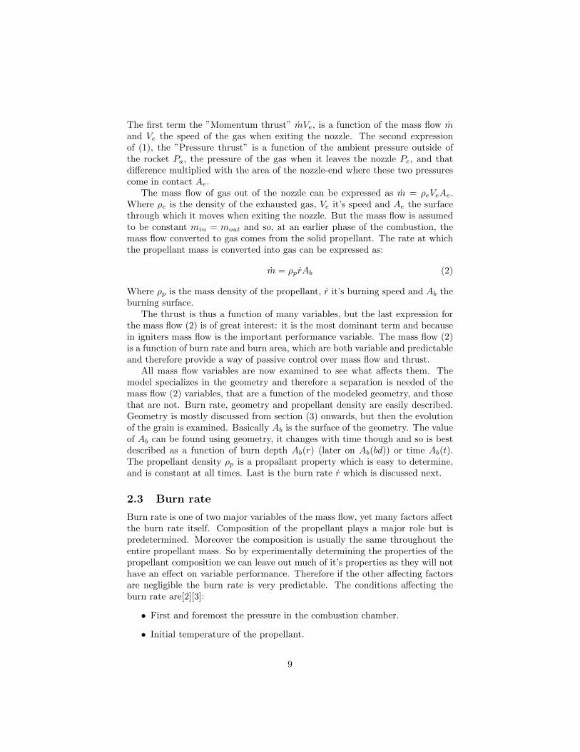
The first term the ”Momentum thrust” mVe, is a function of the mass flow mand Ve the speed of the gas when exiting the nozzle. The second expressionof (1), the ”Pressure thrust” is a function of the ambient pressure outside ofthe rocket Pa, the pressure of the gas when it leaves the nozzle Pe, and thatdifference multiplied with the area of the nozzle-end where these two pressurescome in contact Ae.

The mass flow of gas out of the nozzle can be expressed as m = ρeVeAe.Where ρe is the density of the exhausted gas, Ve it’s speed and Ae the surfacethrough which it moves when exiting the nozzle. But the mass flow is assumedto be constant min = mout and so, at an earlier phase of the combustion, themass flow converted to gas comes from the solid propellant. The rate at whichthe propellant mass is converted into gas can be expressed as:

m = ρprAb (2)

Where ρp is the mass density of the propellant, r it’s burning speed and Ab theburning surface.

The thrust is thus a function of many variables, but the last expression forthe mass flow (2) is of great interest: it is the most dominant term and becausein igniters mass flow is the important performance variable. The mass flow (2)is a function of burn rate and burn area, which are both variable and predictableand therefore provide a way of passive control over mass flow and thrust.

All mass flow variables are now examined to see what affects them. Themodel specializes in the geometry and therefore a separation is needed of themass flow (2) variables, that are a function of the modeled geometry, and thosethat are not. Burn rate, geometry and propellant density are easily described.Geometry is mostly discussed from section (3) onwards, but then the evolutionof the grain is examined. Basically Ab is the surface of the geometry. The valueof Ab can be found using geometry, it changes with time though and so is bestdescribed as a function of burn depth Ab(r) (later on Ab(bd)) or time Ab(t).The propellant density ρp is a propallant property which is easy to determine,and is constant at all times. Last is the burn rate r which is discussed next.

2.3 Burn rate

Burn rate is one of two major variables of the mass flow, yet many factors affectthe burn rate itself. Composition of the propellant plays a major role but ispredetermined. Moreover the composition is usually the same throughout theentire propellant mass. So by experimentally determining the properties of thepropellant composition we can leave out much of it’s properties as they will nothave an effect on variable performance. Therefore if the other affecting factorsare negligible the burn rate is very predictable. The conditions affecting theburn rate are[2][3]:

• First and foremost the pressure in the combustion chamber.

• Initial temperature of the propellant.

9

• Gas flow along burning surface.

• Motion of the rocket (fast spinning for example).

The research towards the effects of these conditions, is not yet able to providean analytic prediction. But the effects of each of the conditions separately havebeen studied, and provides empirical predictions[2][3]. Following is a deeperexamination of these conditions as a background to why none are taken intoaccount by the model, and how they could be implemented. These are not thepoint of focus in this model, as they have already been modeled using othermodels. Our focus still lies in the geometry evolution, but it is still necessaryto understand what their effect might be.

2.3.1 Pressure and burn rate

Experimental testing of propellants provides burn rate’s dependence on pressure.Quick examination of such experimental measurements[2] provides the followingexpression[4] for the relation

r = a0Pnc + b (3)

Where r is the burn rate, Pc is the pressure, a0 and b are functions of theinitial temperature of the propellant and n is known as the combustion index.This relation can be simplified though, for the case of rockets where b is usuallyvery small[3]. The simplified result

r = a0Pnc (4)

This is known as the Saint-Robert’s or Vieille’s law. Where a0 and n arefound empirically for a certain propellant. They usually apply for a certainrange of pressures. A set of different values for a0 and n can provide the neededrelations between burning rate and pressure throughout the combustion.

2.3.2 Temperature and burn rate

Temperature affects the rate at which chemical reactions take place. There-fore the initial propellant temperature affects the burning rate. It is there-fore common to place the rocket in a temperature controlled space, or at leastprotect from the sun prior to ignition. Moreover initial temperature require-ments are determined, so that if conditions exceed the conditions, launch isdelayed. As a rocket in-flight is exposed to extreme temperatures, from 220Kup-to 344K, it is important to see how the propellant performs in these extremevariations. A typical composite propellant experiences a variation of up-to 20%to 35% in chamber pressure Pc[2]. Moreover, for such temperature variationsthe thrust operation time varies with the same percentage. Nonuniform temper-ature within the grain may have an even more disastrous effect as the pressuremay not be symmetric and the thrust vector alters. The effect of grain temper-ature on pressure is expressed as ∆P = Pπk∆T

0 . Where ∆P is the variation of

10

pressure from the reference pressure P0, at a temperature variation of ∆T withπk an experimentally measured coefficient known as the temperature sensitivityof pressure at a constant burning area (K). By determining the a0 parame-ter for the correct reference temperature, and giving the entire propellant thatuniform temperature, we can neglect the effect of a temperature difference.

2.3.3 Erosive burning

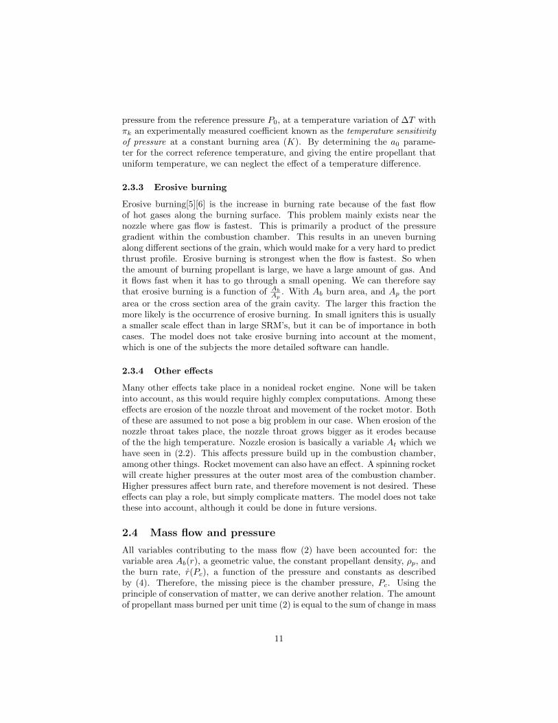
Erosive burning[5][6] is the increase in burning rate because of the fast flowof hot gases along the burning surface. This problem mainly exists near thenozzle where gas flow is fastest. This is primarily a product of the pressuregradient within the combustion chamber. This results in an uneven burningalong different sections of the grain, which would make for a very hard to predictthrust profile. Erosive burning is strongest when the flow is fastest. So whenthe amount of burning propellant is large, we have a large amount of gas. Andit flows fast when it has to go through a small opening. We can therefore saythat erosive burning is a function of Ab

Ap. With Ab burn area, and Ap the port

area or the cross section area of the grain cavity. The larger this fraction themore likely is the occurrence of erosive burning. In small igniters this is usuallya smaller scale effect than in large SRM’s, but it can be of importance in bothcases. The model does not take erosive burning into account at the moment,which is one of the subjects the more detailed software can handle.

2.3.4 Other effects

Many other effects take place in a nonideal rocket engine. None will be takeninto account, as this would require highly complex computations. Among theseeffects are erosion of the nozzle throat and movement of the rocket motor. Bothof these are assumed to not pose a big problem in our case. When erosion of thenozzle throat takes place, the nozzle throat grows bigger as it erodes becauseof the the high temperature. Nozzle erosion is basically a variable At which wehave seen in (2.2). This affects pressure build up in the combustion chamber,among other things. Rocket movement can also have an effect. A spinning rocketwill create higher pressures at the outer most area of the combustion chamber.Higher pressures affect burn rate, and therefore movement is not desired. Theseeffects can play a role, but simply complicate matters. The model does not takethese into account, although it could be done in future versions.

2.4 Mass flow and pressure

All variables contributing to the mass flow (2) have been accounted for: thevariable area Ab(r), a geometric value, the constant propellant density, ρp, andthe burn rate, r(Pc), a function of the pressure and constants as describedby (4). Therefore, the missing piece is the chamber pressure, Pc. Using theprinciple of conservation of matter, we can derive another relation. The amountof propellant mass burned per unit time (2) is equal to the sum of change in mass

11

within the combustion chamber, and the mass flowing out of the chamber[2].

m =∂

∂t(ρcVc) +AtPcCd

√k

RTc(

2

k + 1)

k+1k−1 (5)

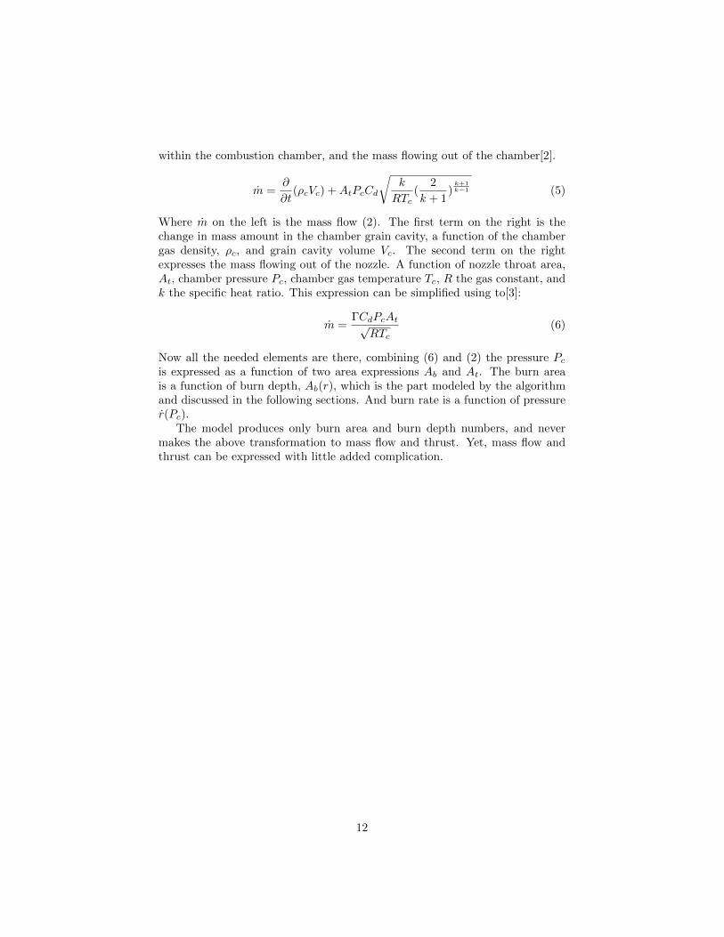
Where m on the left is the mass flow (2). The first term on the right is thechange in mass amount in the chamber grain cavity, a function of the chambergas density, ρc, and grain cavity volume Vc. The second term on the rightexpresses the mass flowing out of the nozzle. A function of nozzle throat area,At, chamber pressure Pc, chamber gas temperature Tc, R the gas constant, andk the specific heat ratio. This expression can be simplified using to[3]:

m =ΓCdPcAt√

RTc(6)

Now all the needed elements are there, combining (6) and (2) the pressure Pcis expressed as a function of two area expressions Ab and At. The burn areais a function of burn depth, Ab(r), which is the part modeled by the algorithmand discussed in the following sections. And burn rate is a function of pressurer(Pc).

The model produces only burn area and burn depth numbers, and nevermakes the above transformation to mass flow and thrust. Yet, mass flow andthrust can be expressed with little added complication.

12

3 Grain geometry

Burn rate determines how fast a propellant burns. The amount of propellantactually available for burning at that burn rate is determined by the shape ofthe propellant mass, the grain geometry. The burning takes place at the surface,and the amount of surface a certain shape has is determined by it’s geometry.The propellant mass is distributed on the inside of the combustion chamber.The mass is usually extruded or molded in a certain shape within the cylinder.In most cases the shape forms a cavity within the propellant mass, which isconnected to the nozzle. This space is where hot gases move towards the nozzle.On ignition all exposed surfaces around this space will burn. When burning,the surface recedes as solid propellant turns to gas. The receding takes place ina direction that is normal to the surface.

The configuration of the grain or the shape of it defines how it behavesin time. The grain is in most cases cylindrically symmetric. In that case itis sufficient to examine a two dimensional cross section of the grain. Rocketmodels with variations along their length axis do exist but these require morecomplex calculations. While a complexer configuration does not necessarilyprovide a performance that is not achievable in a simpler constant 2D crosssection model. This study will only focus on grain geometries that can bedescribed by a two dimensional cross section. Another symmetry often found inthe grain is a rotational symmetry. This is often the case because it is importantto get a rotationally symmetric exhaust out of the nozzle, or else the rocket netthrust vector will not be straight.

Performance of a grain is usually measured in a thrust vs time diagram.Alternatively when neglecting burn rate effects, burn area vs burn depth, isused instead of the thrust/time. These diagrams can easily display if a grain isprogressive or regressive, which translates to growing or diminishing thrust(Fig.2). But these can be easily described with cylindrical grains burning in or out.More complex grain are required for more complex performances. A combina-tion of progressive followed by regressive, or constant burn, usually require moreexotic shapes, like a stars or fynocyls. (Fig. 2)

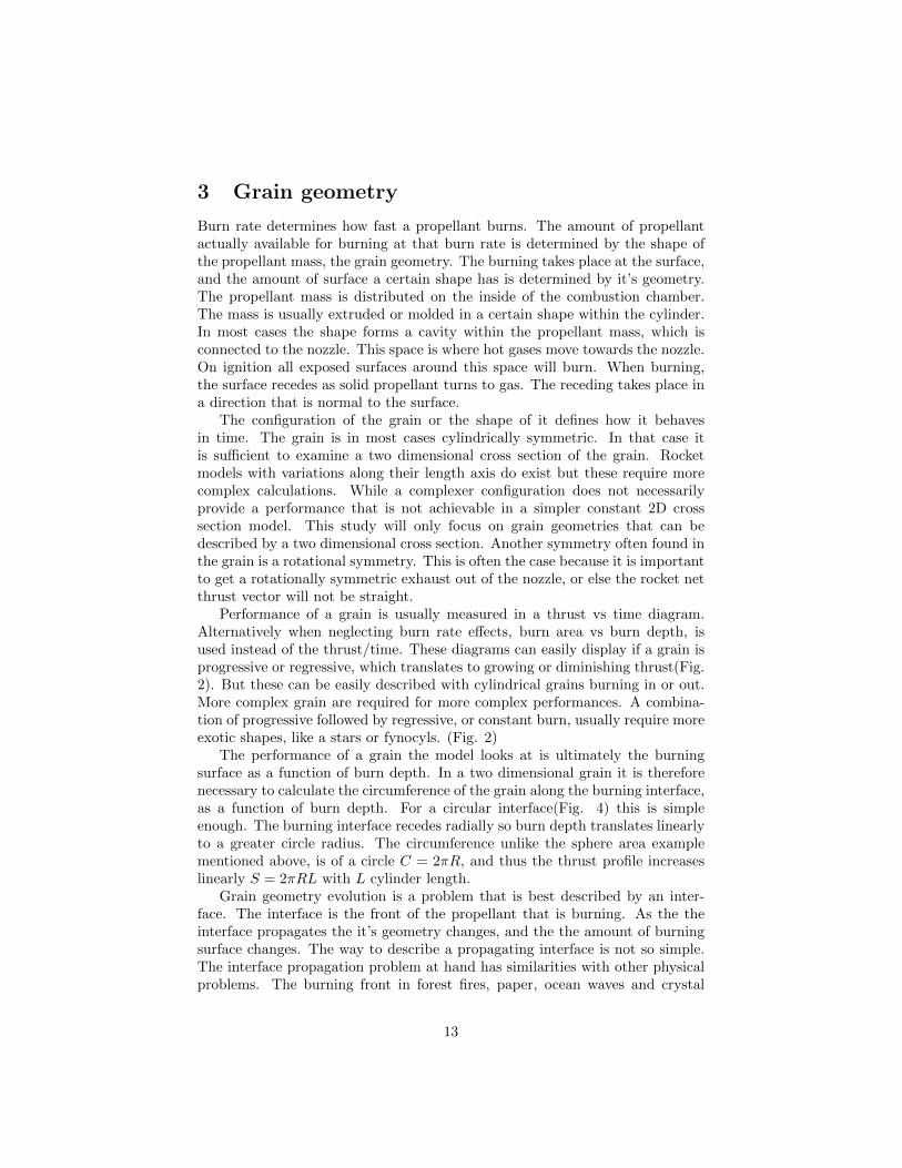
The performance of a grain the model looks at is ultimately the burningsurface as a function of burn depth. In a two dimensional grain it is thereforenecessary to calculate the circumference of the grain along the burning interface,as a function of burn depth. For a circular interface(Fig. 4) this is simpleenough. The burning interface recedes radially so burn depth translates linearlyto a greater circle radius. The circumference unlike the sphere area examplementioned above, is of a circle C = 2πR, and thus the thrust profile increaseslinearly S = 2πRL with L cylinder length.

Grain geometry evolution is a problem that is best described by an inter-face. The interface is the front of the propellant that is burning. As the theinterface propagates the it’s geometry changes, and the the amount of burningsurface changes. The way to describe a propagating interface is not so simple.The interface propagation problem at hand has similarities with other physicalproblems. The burning front in forest fires, paper, ocean waves and crystal

13

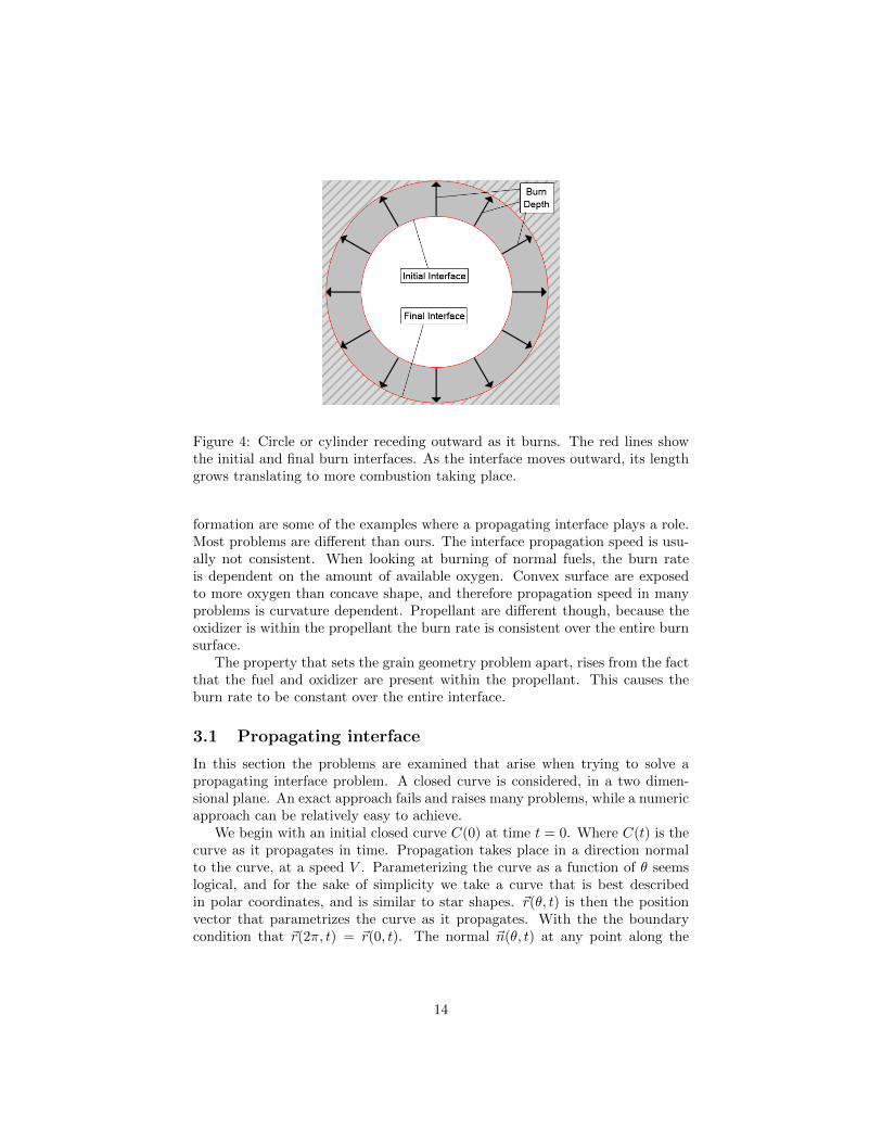
Figure 4: Circle or cylinder receding outward as it burns. The red lines showthe initial and final burn interfaces. As the interface moves outward, its lengthgrows translating to more combustion taking place.

formation are some of the examples where a propagating interface plays a role.Most problems are different than ours. The interface propagation speed is usu-ally not consistent. When looking at burning of normal fuels, the burn rateis dependent on the amount of available oxygen. Convex surface are exposedto more oxygen than concave shape, and therefore propagation speed in manyproblems is curvature dependent. Propellant are different though, because theoxidizer is within the propellant the burn rate is consistent over the entire burnsurface.

The property that sets the grain geometry problem apart, rises from the factthat the fuel and oxidizer are present within the propellant. This causes theburn rate to be constant over the entire interface.

3.1 Propagating interface

In this section the problems are examined that arise when trying to solve apropagating interface problem. A closed curve is considered, in a two dimen-sional plane. An exact approach fails and raises many problems, while a numericapproach can be relatively easy to achieve.

We begin with an initial closed curve C(0) at time t = 0. Where C(t) is thecurve as it propagates in time. Propagation takes place in a direction normalto the curve, at a speed V . Parameterizing the curve as a function of θ seemslogical, and for the sake of simplicity we take a curve that is best describedin polar coordinates, and is similar to star shapes. ~r(θ, t) is then the positionvector that parametrizes the curve as it propagates. With the the boundarycondition that ~r(2π, t) = ~r(0, t). The normal ~n(θ, t) at any point along the

14

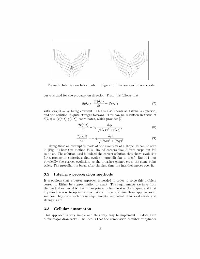
Figure 5: Interface evolution fails. Figure 6: Interface evolution succesful.

curve is used for the propagation direction. From this follows that

~n(θ, t) · ∂~r(θ, t)∂t

= V (θ, t) (7)

with V (θ, t) = V0 being constant. This is also known as Eikonal’s equation,and the solution is quite straight forward. This can be rewritten in terms of~r(θ, t) = (x(θ, t), y(θ, t)) coordinates, which provides [7]

∂x(θ, t)

∂t= V0

∂θy√(∂θx)2 + (∂θy)2

(8)

∂y(θ, t)

∂t= −V0

∂θx√(∂θx)2 + (∂θy)2

(9)

Using these an attempt is made at the evolution of a shape. It can be seenin (Fig. 5) how this method fails. Round corners should form cusps but failto do so. The solution used is indeed the correct solution that shows evolutionfor a propagating interface that evolves perpendicular to itself. But it is notphysically the correct evolution, as the interface cannot cross the same pointtwice. The propellant is burnt after the first time the interface moves over it.

3.2 Interface propagation methods

It is obvious that a better approach is needed in order to solve this problemcorrectly. Either by approximation or exact. The requirements we have fromthe method or model is that it can primarily handle star like shapes, and thatit paves the way to optimizations. We will now examine three approaches tosee how they cope with those requirements, and what their weaknesses andstrengths are.

3.3 Cellular automaton

This approach is very simple and thus very easy to implement. It does havea few major drawbacks. The idea is that the combustion chamber or cylinder

15

is converted into a grid of cells, which visually are pixels. Each cell is thenassigned a value describing it’s state. The initial values are initially determinedby the grain configuration we examine. The states are for example ”Burning”,”Propellant” and ”No propellant”. Then we define rules that help evolve thegrid. Every iteration the algorithm scans all cells and changes states accordingto the rules.

The strength of this method is that any shape or grain can be examined.Two methods were examined of inputting the initial grain configuration. Oneoption is the use of an image file where the grain is visually sketched. This canbe converted into a matrix where each pixel in the image is a cell in the matrix.The color of the pixel defines the value or state of the cell. Using images allowsfor the greatest possible versatility in grain design. Another option is based onparameters that define functions. These functions are then used to input thevalues within the matrix. This is not very versatile and not fast.

So we start with a grid of N by N cells. Using one of the methods above theinitial state of each cell is determined. The possible cell states are as describedabove, ”Burning”, ”Non-burning, Contains propellant” and ”Non-burning, Nopropellant”. After the construction of the initial grid or matrix, a loop code isused to evolve the grain. Every iteration the rules are used and the states ofcertain cells change. The rules used to evolve the grain are:

• If cell state is ”Burning” and neighboring cell state is ”Non-burning, Con-tains propellant”, then change neighboring cell to ”Burning”.

• If cell state is ”Burning”, then change to ”Non-burning, No propellant”.

• Count the amount of burning cell to determine circumference or burningarea.

The definition of a neighboring cell to a burning cell has a strong influence onthe evolution. A neighboring cell is a cell that is a maximum distance from theburning cell. Lets call this maximum distance ”neighbor distance”. We thenhave a situation where a circle or radius ”neighbor distance” of cells aroundthe burning cells should start burning. But in a simple model this maximumdistance of neighboring cells is small, approximately 1 or 2 cells. In that casethe circle will not appear as circle but appear very ”pixelated” (Fig. 7). Theconsequences of this for small values of neighbor distance can be seen in (Fig.8). To make this work better the ”neighbor distance” must be large, to form anice circle. But then the grid would also need to be large, so N has to be large.This raises the biggest drawback of this method. The algorithm scans every cellof the N2 cells, at every iteration. This makes for a calculation heavy algorithm.Moreover to know the state of the grid after a certain time all iteration stepsbefore that have to take place as well. Both of these factors do not work wellwith future optimization steps.

This method is good if one wants to examine an eccentric shape that doesn’thave any symmetries, or a shape that cannot be easily described, and thereforehas to be sketched. Nevertheless this method is not suitable for optimizationmainly because of the long calculation times.

16

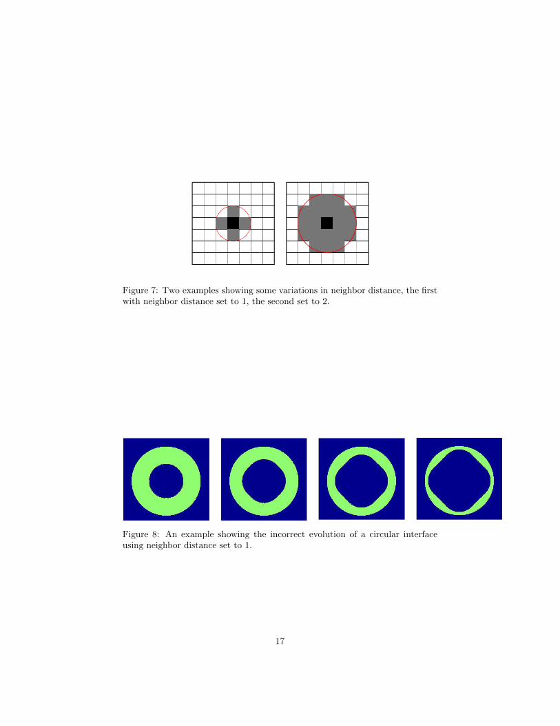
Figure 7: Two examples showing some variations in neighbor distance, the firstwith neighbor distance set to 1, the second set to 2.

Figure 8: An example showing the incorrect evolution of a circular interfaceusing neighbor distance set to 1.

17

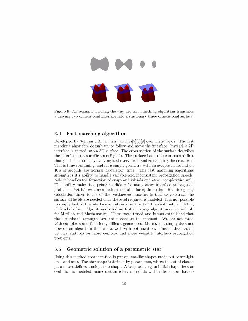
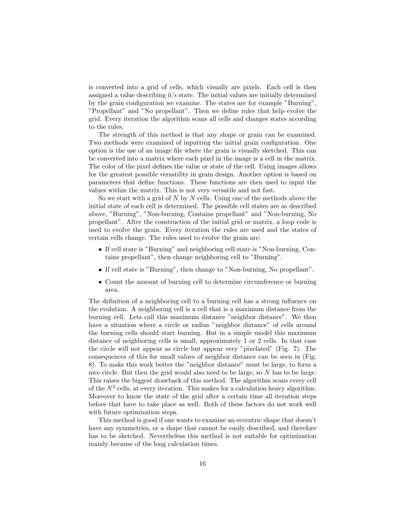
Figure 9: An example showing the way the fast marching algorithm translatesa moving two dimensional interface into a stationary three dimensional surface.

3.4 Fast marching algorithm

Developed by Sethian J.A. in many articles[7][8][9] over many years. The fastmarching algorithm doesn’t try to follow and move the interface. Instead, a 2Dinterface is turned into a 3D surface. The cross section of the surface describesthe interface at a specific time(Fig. 9). The surface has to be constructed firstthough. This is done by evolving it at every level, and contructing the next level.This is time consuming, and for a simple geometry with an acceptable resolution10’s of seconds are normal calculation time. The fast marching algorithmsstrength is it’s ability to handle variable and inconsistent propagation speeds.Aslo it handles the formation of cusps and islands and other complexities well.This ability makes it a prime candidate for many other interface propagationproblems. Yet it’s weakness make unsuitable for optimization. Requiring longcalculation times is one of the weaknesses, another is that to construct thesurface all levels are needed until the level required is modeled. It is not possibleto simply look at the interface evolution after a certain time without calculatingall levels before. Algorithms based on fast marching algorithms are availablefor MatLab and Mathematica. These were tested and it was established thatthese method’s strengths are not needed at the moment. We are not facedwith complex speed functions, difficult geometries. Moreover it simply does notprovide an algorithm that works well with optimization. This method wouldbe very suitable for more complex and more versatile interface propagationproblems.

3.5 Geometric solution of a parametric star

Using this method concentration is put on star-like shapes made out of straightlines and arcs. The star shape is defined by parameters, where the set of chosenparameters defines a unique star shape. After producing an initial shape the starevolution is modeled, using certain reference points within the shape that do

18

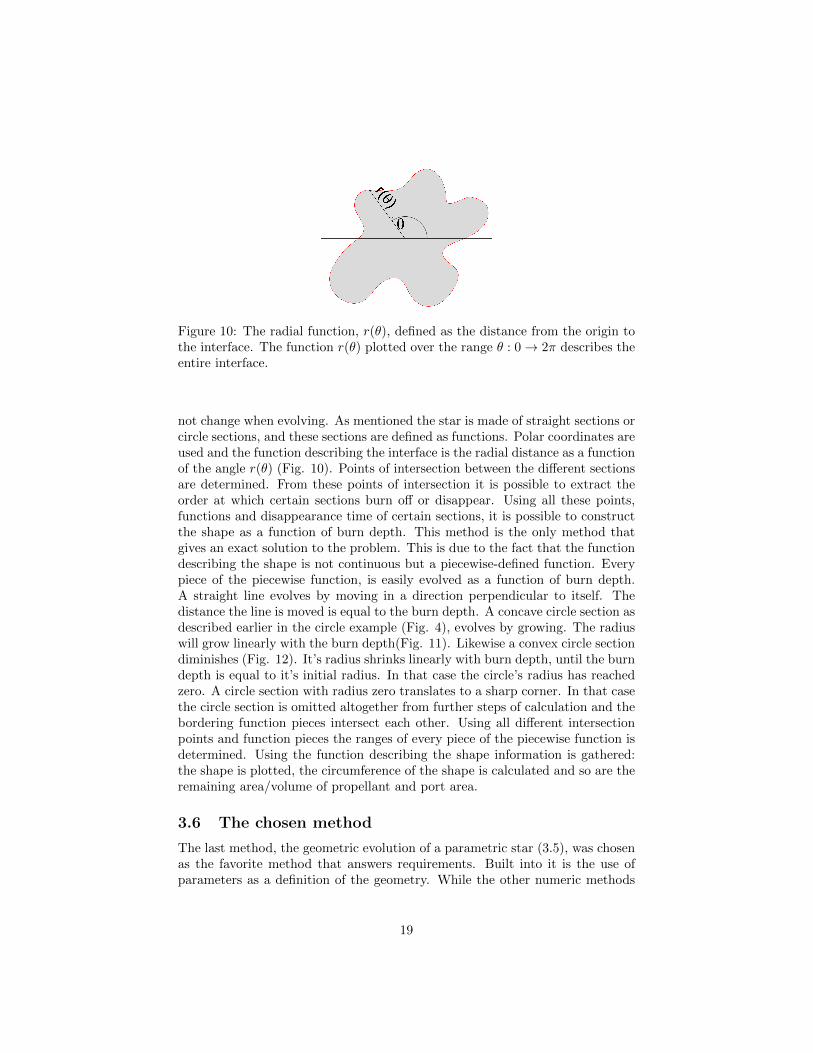
Figure 10: The radial function, r(θ), defined as the distance from the origin tothe interface. The function r(θ) plotted over the range θ : 0→ 2π describes theentire interface.

not change when evolving. As mentioned the star is made of straight sections orcircle sections, and these sections are defined as functions. Polar coordinates areused and the function describing the interface is the radial distance as a functionof the angle r(θ) (Fig. 10). Points of intersection between the different sectionsare determined. From these points of intersection it is possible to extract theorder at which certain sections burn off or disappear. Using all these points,functions and disappearance time of certain sections, it is possible to constructthe shape as a function of burn depth. This method is the only method thatgives an exact solution to the problem. This is due to the fact that the functiondescribing the shape is not continuous but a piecewise-defined function. Everypiece of the piecewise function, is easily evolved as a function of burn depth.A straight line evolves by moving in a direction perpendicular to itself. Thedistance the line is moved is equal to the burn depth. A concave circle section asdescribed earlier in the circle example (Fig. 4), evolves by growing. The radiuswill grow linearly with the burn depth(Fig. 11). Likewise a convex circle sectiondiminishes (Fig. 12). It’s radius shrinks linearly with burn depth, until the burndepth is equal to it’s initial radius. In that case the circle’s radius has reachedzero. A circle section with radius zero translates to a sharp corner. In that casethe circle section is omitted altogether from further steps of calculation and thebordering function pieces intersect each other. Using all different intersectionpoints and function pieces the ranges of every piece of the piecewise function isdetermined. Using the function describing the shape information is gathered:the shape is plotted, the circumference of the shape is calculated and so are theremaining area/volume of propellant and port area.

3.6 The chosen method

The last method, the geometric evolution of a parametric star (3.5), was chosenas the favorite method that answers requirements. Built into it is the use ofparameters as a definition of the geometry. While the other numeric methods

19

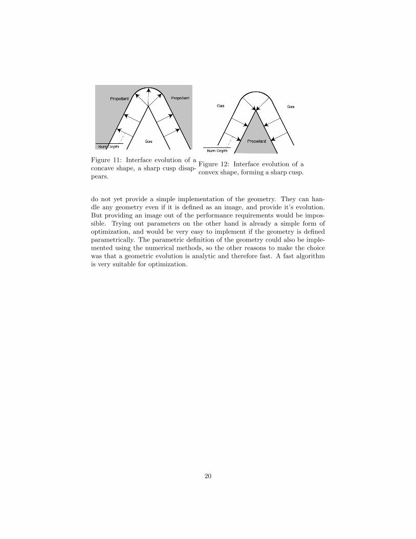
Figure 11: Interface evolution of aconcave shape, a sharp cusp disap-pears.

Figure 12: Interface evolution of aconvex shape, forming a sharp cusp.

do not yet provide a simple implementation of the geometry. They can han-dle any geometry even if it is defined as an image, and provide it’s evolution.But providing an image out of the performance requirements would be impos-sible. Trying out parameters on the other hand is already a simple form ofoptimization, and would be very easy to implement if the geometry is definedparametrically. The parametric definition of the geometry could also be imple-mented using the numerical methods, so the other reasons to make the choicewas that a geometric evolution is analytic and therefore fast. A fast algorithmis very suitable for optimization.

20

4 Geometric evolution of a parametric star -Building the model

Examination of several models for interface propagation, has resulted in thechosen geometric evolution model. It is the fastest and provides the best per-formance for optimization. An examination of the inner workings of the modelwill now follow. First defining how the geometry’s initial shape is constructedand then it’s evolution.

A parametric star is defined by a number of parameters. Each parametersdefines a key aspect of the star geometry, it could be a length of a line, or anangle. After the definition of the parameters, the initial shape and therefore it’sevolution are determined. It is important to keep in mind that the model weare developing should be able to provide initial optimization steps. The grain isthoroughly examined and fine tuned using the current grain modeling softwareGDP. It is therefore recommended to use parameters that are compatible withthe parameters used by the current software. After constructing the initialshape, we can continue and see how this shape evolves as a function of burndepth.

4.1 The parameters

Defining a star can be done relatively simple, with only a few parameters. Inthis case a star like shape extruded out of a cylinder. The parameters defining asimple star would be(Fig. 15): the star point opening angle or Point Angle(Pa),the number of star points(N), and the outer and inner radius (OR) and (IR)respectively(Fig. 13a). Adding more complexity to the star is done by definingthat the star points are spaced apart (Fig. 13b). The spacing is achieved bydefining two angles a and b, that specify at what angle θ a few key points areplaced. The angle a is deduced using the N parameter, a = π

N . The parameter

k1 specifies an angular fraction k1 ≡ ba . With the parameter k1 and the angle a,

the angle b is expressed. This is easier to work with than defining b explicitly.A b angle defined explicitly would mean that any time we change N we have toredefine b while in this way b is derived from other parameters N and k1. As afunction of parameters only the definition is b = k1a = k1π

N .A higher order of complexity within the star is achieved by defining a star

whose point are ”cut off”. It was chosen that the cut is a circular arc with it’scenter at the center of the star (Fig. 13c). The fraction of the star point thatis cut off is defined using another angle c, which is deduced from the parameterk2, defined as k2 ≡ c

a . This definition is similar to the fraction we saw beforeas k1, it defines the angular fraction of the cut off section c compared to theentire star point section a. As a function of parameters only the definition isc = k2a = k2π

N .Another adjustment made to the simple star geometry is the introduction

of rounding fillets. The fillets make the grain stronger, allowing it to withstandthe vibrations and forces it is exposed to. Two fillets are defined, one concave,

21

(a) Simple Star (b) Added spacing between starpoints

(c) Added point cut-off

Figure 13: How the parameters affect a star geometry

(a) Without the rounding fillet (b) With the rounding fillet

Figure 14: The effect of a rounding fillet.

and one convex. For each of these a radius is defined which is the fillet radius,named Fr1 and Fr2. The radius expresses the radius of the circle section thatis the fillet. The fillet is tangential to both sections that it connects, which ishow the center of the fillet circle is found.

Figure 15 shows the way the parameters of the star geometry are defined. Intotal eight parameter values have to be specified. The parameters shown in redin figure 15 are not directly defined. Rather indirectly by another parameter.The eight parameters are:

• N is the number of star points, which corresponds to a = πN .

• k1 is the fraction of angles, k1 = ba .

• k2 is the fraction of angles, k2 = ca .

22

Figure 15: The parameters defining the star geometry.

• Pa is the point angle.

• OR is the outer radius where the propellant reaches the outer casing.

• IR is the inner radius defining at what outer radius the star points begin.

• Fr1 is the radius of the rounding fillet section rf1(θ, bd).

• Fr2 is the radius of the rounding fillet section rf2(θ, bd).

4.2 Initial shape

Well chosen parameters are very important for an easy calculation of the initialshape. Having just defined all the necessary parameters, it is now necessaryto be able to construct the shape right. Visually it is easy to confirm that theinitial grain description is right. When the function describing it is withouterrors the model can go on and calculate the circumference.

23

Figure 16: The 5 different piecewise functions, that describe the entire shape.r1(θ) in black, rf1(θ) in purple, r2(θ) in green, rf2(θ) in cyan and r3(θ) in blue.

The function describing the shape is a polar function r(θ). For simplicitywe would like to describe the smallest part of the star possible. It is obviousthat symmetries are present, rotational symmetry means that we only needto describe an angular fraction of the star circular cross section. An angularfraction of 2π

N = 2a, which translates to a cyclic permutation of r(θ) = r(θ+2a).But an angular fraction of 2a of the star is also describing too much. An angularfraction a of the star is sufficient. The shape is mirrored along the a angle sothat r(θ) = r(2a − θ). So based on symmetry of the shape alone, we havenarrowed down the part we have to describe to the function r(θ) in the range0→ a.

The polar function r(θ) is thus our main interest. Because r(θ) containssharp corners it’s derivative cannot be continuous. It is therefore necessary todefine it by way of piecewise functions. I use r1(θ), r2(θ), r3(θ) for the differentsections(Fig. 16). Where r1(θ) and r3(θ) are circle sections and r2(θ) is astraight section. rf1(θ) and rf2(θ) describe r(θ) at the fillets. Eventually fivedifferent functions contribute to r(θ).

24

r(θ) =

r1(θ) for 0 ≤ θ < θ1

rf1(θ) for θ1 ≤ θ < θ2

r2(θ) for θ2 ≤ θ < θ3

rf2(θ) for θ3 ≤ θ < θ4

r3(θ) for θ4 ≤ θ < a

(10)

Here the angular range borders θi are the angles to the intersection pointsbetween the bordering sections. These angles define the range of angles overwhich each of the section functions is used.

Using the different parameter definitions an in-depth look is made into thefunction r(θ). To show the calculations involved more detailed focus is put r2(θ)and later as a function of the burn depth, r2(θ, bd).The function r1(θ) is the simplest function expression, it describes a circle arcwith circle center at the star center. Therefore r1(θ) is constant, which createsa circle section. Initially it’s value is r1(θ) = IR, as defined by the parameters.The functions r2(θ) and r3(θ) are more complicated. We now first assume thatfillet radius 1 (Fr1) and fillet radius 2 (Fr2) parameters are equal to 0, so thecorners are not rounded. In that case we know that r2 passes through the points(r, θ): (r1(b), b) and (r3(c), c).r3(θ) can be found geometrically to be

r3(θ) = IRsin(Pa

2 − b)sin(Pa

2 − c)for Fr1 = Fr2 = 0 (11)

r3(θ) is shown to be constant as r3(θ) is a circle section around the center of thestar, similar to r1(θ). So now we have two points, where through the straightline r2(θ) goes (r, θ):

(IR, b) and (IRsin(pa

2 − b)sin(pa

2 − c), c) (12)

Using two points it is easy to find the line gradient being equal to

m =y2 − y1

x2 − x1=

IR sin( pa2 −b)

sin(−c+ pa2 ) sin(c)− IR sin(b)

IR sin( pa2 −b)

sin(−c+ pa2 ) cos(c)− IR cos(b)

(13)

The gradient in use is a Cartesian gradient, so the two polar points are convertedto Cartesian coordinate points where after the line is determined. The linefunction which is defined in Cartesian coordinates is then converted again topolar coordinates.

When the fillet radii are greater than zero we are faced with a slightly morecomplex situation. Each of the fillets is also defined differently. Fr2 is purelya rounding fillet and adapts itself to the corner it rounds. On the other hand,Fr1 whose center point is defined by the angle b. So when Fr1 is formed othersections have to move. First we examine the effect of Fr1, which are seen in

25

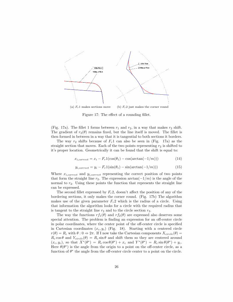
(a) Fr1 makes sections move (b) Fr2 just makes the corner round

Figure 17: The effect of a rounding fillet.

(Fig. 17a). The fillet 1 forms between r1 and r2, in a way that makes r2 shift.The gradient of r2(θ) remains fixed, but the line itself is moved. The fillet isthen formed in between in a way that it is tangential to both sections it borders.

The way r2 shifts because of Fr1 can also be seen in (Fig. 17a) as thestraight section that moves. Each of the two points representing r2 is shifted toit’s proper location. Geometrically it can be found that the shift is equal to:

xi,correct = xi − Fr1(cos(θ1)− cos(arctan(−1/m))) (14)

yi,correct = yi − Fr1(sin(θ1)− sin(arctan(−1/m))) (15)

Where xi,correct and yi,correct representing the correct position of two pointsthat form the straight line r2. The expression arctan(−1/m) is the angle of thenormal to r2. Using these points the function that represents the straight linecan be expressed.

The second fillet expressed by Fr2, doesn’t affect the position of any of thebordering sections, it only makes the corner round. (Fig. 17b) The algorithmmakes use of the given parameter Fr2 which is the radius of a circle. Usingthat information the algorithm looks for a circle with the required radius thatis tangent to the straight line r2 and to the circle section r3.

The way the functions rf1(θ) and rf2(θ) are expressed also deserves somespecial attention. The problem is finding an expression for an off-center circlein polar coordinates, where the center point of the off-center circle is specifiedin Cartesian coordinates (xc, yc) (Fig. 18). Starting with a centered circler(θ) = Rc with θ : 0⇒ 2π. If I now take the Cartesian components Xcircle(θ) =Rc cos θ and Ycircle(θ) = Rc sin θ and shift them so they are centered around(xc, yc), so that X∗(θ∗) = Rc cos θ(θ∗) + xc and Y ∗(θ∗) = Rc sin θ(θ∗) + yc.Here θ(θ∗) is the angle from the origin to a point on the off-center circle, as afunction of θ∗ the angle from the off-center circle center to a point on the circle.

26

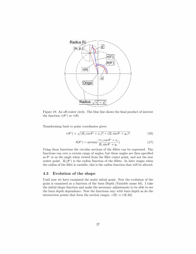
Figure 18: An off-center circle. The blue line shows the final product of interestthe function r(θ∗) or r(θ).

Transforming back to polar coordinates gives:

r(θ∗) =√

(Rc cos θ∗ + xc)2 + (Rc sin θ∗ + yc)2 (16)

θ(θ∗) = arctan(‘rrc cos θ∗ + xcRc sin θ∗ + yc

) (17)

Using these functions the circular sections of the fillets can be expressed. Thefunctions run over a certain range of angles, but these angles are then specifiedas θ∗ or as the angle when viewed from the fillet center point, and not the starcenter point. Rc(θ

∗) is the radius function of the fillets. In later stages whenthe radius of the fillet is variable, this is the radius function that will be altered.

4.3 Evolution of the shape

Until now we have examined the static initial grain. Now the evolution of thegrain is examined as a function of the burn Depth (Variable name bd). I takethe initial shape function and make the necessary adjustments to be able to seethe burn depth dependence. Now the functions vary with burn depth as do theintersection points that form the section ranges. r(θ)⇒ r(θ, bd)

27

r(θ, bd) =

r1(θ, bd) for 0 ≤ θ < θ1(bd)

rf1(θ, bd) for θ1(bd) ≤ θ < θ2(bd)

r2(θ, bd) for θ2(bd) ≤ θ < θ3(bd)

rf2(θ, bd) for θ3(bd) ≤ θ < θ4(bd)

r3(θ, bd) for θ4(bd) ≤ θ < a

(18)

First participating shapes’ evolution in general is examined. The participat-ing shapes are (1) a concave circle section,(2) a convex circle section and (3)a straight line. (1) When burned a concave circle’s radius will grow with burndepth. Any concave circle section with initial radius Ri will have a burn depthdependent radius Ri(bd) = Ri + bd. (2) Likewise to the concave case a convexcircle section will have it’s radius affected, unlike the concave case it’s radiuswill shrink. An initial convex circle section with initial radius Ri will have aburn depth dependent radius Ri(bd) = Ri − bd. (3) Straight lines move in adirection perpendicular to themselves. So the straight line (x) = mx + y0 willmove perpendicular to itself in the direction − 1

m . It will move a distance of bdin that direction.

In more detail it can be seen how the front described by r2(θ, bd) evolves.It was already discussed how it shifts due to rounding of fillet radius Fr1. Andit was just remarked that straight lines move a distance of bd in the directionperpendicular to themselves. So as before when r2(θ) was handled, actuallynot the line is handled but two points on the line. The points are moved andthrough them the line described by r2(θ, bd) is formed. The amount of shiftis bd and the direction is perpendicular to the line. As before the gradient ofthe line described by r2(θ, bd) is m, and the normal gradient is − 1

m . The angleof that normal arctan(− 1

m ). Taking the x and y component the points can bealtered easily.

xi,evo = xi,correct + bd cos(arctan(− 1

m)) (19)

yi,evo = yi,correct + bd sin(arctan(− 1

m)) (20)

The rest of the shapes are circular with a certain radius. For the concavesections r1(θ, bd), r3(θ, bd) and fr1(θ, bd). The radius is adjusted in the sameway as described before to Ri(bd) = Ri + bd. For r1(θ, bd) and r3(θ, bd) this issimple as their defining function is their radius. So their adjustment are:

r1(θ, bd) = r1(θ) + bd (21)

r3(θ, bd) = r3(θ) + bd (22)

The fillet Fr1 is not centered around the star center, therefore the positionfunction rf1(θ, bd) does not represent it’s radius, but it’s distance from the cen-ter of the star (Fig. 16). The radius function has to be adjusted to have the bdaddition. For the second fillet Fr2, the same applies. The burn depth adjust-ment applies to the radius function and not to the position function rf2(θ, bd).

28

The adjustment in this case is negative. The radius function of rf2(θ, bd) di-minishes as Ri(bd) = Ri − bd. So in equations 21 and 22 the radius constantR would be exchanged with a radius function R(bd) = R ± bd. Using all thesecalculation methods the expressions for all different sections are found. Thegoal now is to see at what range of angles each of these functions is used.

4.4 Intersection points

The functions r1(θ, bd), r2(θ, bd), r3(θ, bd), rf1(θ, bd) and rf2(θ, bd) are known.But it is important to find the range over which each of these is used. Theangles θ1−4(bd) express the boundaries of the piecewise function ranges. Somerequire more complex calculations than others, which rely on the intersectionpoints between certain sections. Not only bordering sections have intersectionpoints. Sometimes sections burn off and their neighbors start to intersect eachother. An analytic solution was used in the calculation of these intersections,and so it requires some algorithms. Two different algorithms are being used inall these cases, which describe the intersection between all different sections. (1)The intersection between two circles, (2) the intersection between a circle anda straight line.

At this point of the evolution care has to be taken in how the grain evolves.For almost any initial geometry design, some sections disappear during it’sevolution. When a section disappears the bordering sections start to intersecteach other. It is necessary to find a set of rules that know at what point whichsections disappear. Five different cases have been identified, and separated usinga set of rules. Each of these cases is like a burn phase where the total burningsurface stays linear within the phase, the only factor breaking the linearity is ifthe grain is starting to reach it’s outside border.

1. This phase takes place in most grains. It happens when both fillet radiiare non zero. The phase describes a shape where all sections are presentand burning. Usually this will end with the fillet section described byrf2(θ, bd) disappearing. The interface in this phase is described by all fivefunctions.

2. In many cases the second burn phase, after grain section fillet 2 has dis-appeared. all the other sections are still burning and present. The shapeis then described using the four remaining section functions r1(θ, bd),rf1(θ, bd), r2(θ, bd) and r3(θ, bd). In this case the intersection betweenr2(θ, bd) and r3(θ, bd) provides the boundary to both of these functions.

3. The grain section described by r2(θ, bd) has disappeared, yet the sectiondescribed by r3(θ, bd) has not. Therefore the fillet section rf1(θ, bd) isintersecting r3(θ, bd). And the intersection point provides the boundaryto these functions.

4. The grain section described by r3(θ, bd) has disappeared, yet the sectiondescribed by r2(θ, bd) has not. r2(θ, bd) goes up-to the boundary of ourshape, a.

29

5. The grain sections described by r2(θ, bd) and r3(θ, bd) have both disap-peared. Now the section of the first fillet rf1(θ, bd) continues up-to theboundary of our shape, a.

A grain always loses sections, never develops new, so a shape evolves only into ahigher number phase never to a lower number. Also, a shape can only undergoone of the phases (3) or (4). The algorithm does not climb or drop downthe ladder. For every value of bd it determines which phase the grain is in.This means that the history of the grain is not important, the algorithm knowsimmediately what the grain geometry is at a specific burn depth, without ithaving to know what it was in earlier burn steps.

Using this set of rules coupled with the intersection points, and combiningall this with functions describing each section, the model is able to describe thegrain evolution.

4.5 Burn area

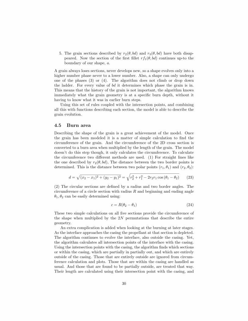
Describing the shape of the grain is a great achievement of the model. Oncethe grain has been modeled it is a matter of simple calculation to find thecircumference of the grain. And the circumference of the 2D cross section isconverted to a burn area when multiplied by the length of the grain. The modeldoesn’t do this step though, it only calculates the circumference. To calculatethe circumference two different methods are used. (1) For straight lines likethe one described by r2(θ, bd), The distance between the two border points isdetermined. This is the distance between two polar points (r1, θ1) and (r2, θ2):

d =√

(x2 − x1)2 + (y2 − y1)2 =√r22 + r2

1 − 2r2r1 cos (θ1 − θ2) (23)

(2) The circular sections are defined by a radius and two border angles. Thecircumference of a circle section with radius R and beginning and ending angleθ1, θ2 can be easily determined using:

c = R(θ2 − θ1) (24)

These two simple calculations on all five sections provide the circumference ofthe shape when multiplied by the 2N permutations that describe the entiregeometry.

An extra complication is added when looking at the burning at later stages.As the interface approaches the casing the propellant at that section is depleted.The algorithm continues to evolve the interface, also outside the casing. Yet,the algorithm calculates all intersection points of the interface with the casing.Using the intersection points with the casing, the algorithm finds which sectionsor within the casing, which are partially in partially out, and which are entirelyoutside of the casing. Those that are entirely outside are ignored from circum-ference calculation and plots. Those that are within the casing are handled asusual. And those that are found to be partially outside, are treated that way.Their length are calculated using their intersection point with the casing, and

30

they are plotted up to the casing. The circumference only calculates burningpropellant interface, and although the casing closes the interface shape in thelate stages, it is not counted as burn area.

4.6 Achievements and Limitations of the algorithm

The algorithm is able to provide an analytical description of the grain. Followingthis the algorithm provides an analytic description of the grain’s evolution. Itis able to do so for a given set of parameters, for any given burn depth. Thecorrectness of the evolution is examined visually, an incorrect evolution can beeasily observed. An error in the evolution shows up as sections that overlap, orparts of the shape that are missing.

Many examples exist of when the algorithm fails, but the main limitation isprobably when the Pa angle is too small. When the angle Pa reaches smallervalues the star point goes beyond the origin into negative r(θ) values. In thiscase the entire algorithm breaks down, and we are left with odd results. Oddis what is troublesome because a grain is formed, but not a correct one, andone that also evolves incorrectly. If the algorithm is called to provide only theburning area(like intended) then there is no clear indication that the algorithmfailed. So this leaves us with a two options. Either one has to always examinethe grain’s evolution visually, or we need to determine the parameter limits atwhich the algorithm fails.

The second option would be most ideal, and would fit well with an optimiza-tion algorithm, providing boundaries for parameters search. A third solutionalso exists and it is to alter the algorithm so it can handle the case of star pointsgoing beyond the origin. This would solve the problem but unlike the formersolution it would not solve further problems. All the parameters used havecertain limitations as a function of the other parameters, and the point goingbeyond the origin, is only one example of these failures. The fillet radii may notbe too large, N cannot be zero, OR has to be set larger than IR, and in thesame way there are many more limits that arise when the parameter definitionsare examined. At no point does the algorithm check for any of these limits.

I will now summarize the problems that might make an invalid grain.

1. The number of star points, N , has to be larger than 1.

2. The outer radius, OR, has to be larger than the inner radius, IR.

3. The fillets 1 and 2 may not be too big so that they do not intersect.

4. Fillet 2 may not be too big so that it cannot go beyond the shape border,the line at an angle θ = a.

5. Star point may not go beyond the origin into a negative radius range.

31

4.7 Results and comparison with the current software,GDP[1]

The developed software is able to construct star geometries based on parameters,evolve them and calculate burn area profiles. Eventually two different programsdeveloped use the developed algorithm. The first is a function that acceptsgeometry parameters and a single burn depth value, as input. The outputproduced is the burn area, at the particular stage in the geometry evolution,defined by the given burn depth. This function could prove to be very usefulin future optimization steps. The second program that uses the algorithm alsoaccepts the parameters as input, as well as a range of burn depths, and a numberof calculation steps. It produces two figures(Fig. 19), a burn area vs. depthprofile for a geometry, and figure showing the evolution of the geometry atdifferent burn stages or burn depths.

The current software, GDP[1], allows for grain modeling and combines nu-merical and analytic methods depending on grain geometry. A star like shapelike ours is done analytically. But the software also allows for more complexgrains, which are analyzed with a numeric algorithm which is not fast, and couldtake a several minutes to complete a geometry evolution.

A comparison of the grains and their evolution is shown in (Fig. 20). Itcan be clearly seen that the currently developed algorithm provides the exactsame results. moreover the way the parameters in our algorithm were definedthe parameters can be plugged into the old software package instantly. Thedifferences one should keep in mind are that in the old software package adiameter is used while in ours a radius. And that we have two extra parameters(k2, Fr2)that need to be set to zero in order to compare the results.

4.8 Improvements and beyond

The algorithm provides exactly what it was meant to do. It can provide ananalytic evolution of a star like grain geometry. Optimization of the grain andimplementation of limits is the following step. But other improvements thatcan be implemented are also possible. Some of these are discussed next.

The algorithm can model the evolution of a star like shape, and produce theburn area profile, yet that is not the thrust or mass flow the rocket provides.To be able to provide other performance variables we will need to take the burnrate into account. Overlaying the burn area vs. burn depth with the burn rate isbasically making the burn depth a function of time. This means stretching outor compressing the profile at different times. In section (2.3) the burn rate wasexamined, and it was found to be a function of pressure or burn area, dependingon the expression used. And pressure is a function of burn area, port area andother factors. A model that takes into account all these factors is complicatedand is probably done numerically. It was chosen that our model will concentrateon the burn area vs. burn depth, while the complicated calculations are doneusing GDP. But in order to optimize a grain for specific thrust or mass flowrequirements and not for specific burn area requirements, this will have to be

32

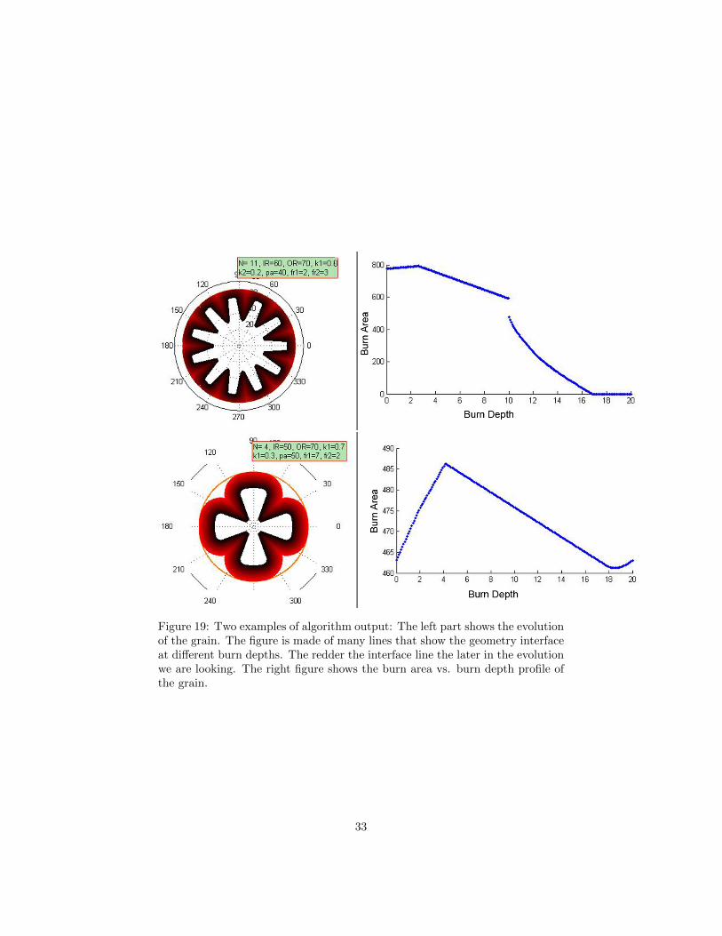
Figure 19: Two examples of algorithm output: The left part shows the evolutionof the grain. The figure is made of many lines that show the geometry interfaceat different burn depths. The redder the interface line the later in the evolutionwe are looking. The right figure shows the burn area vs. burn depth profile ofthe grain.

33

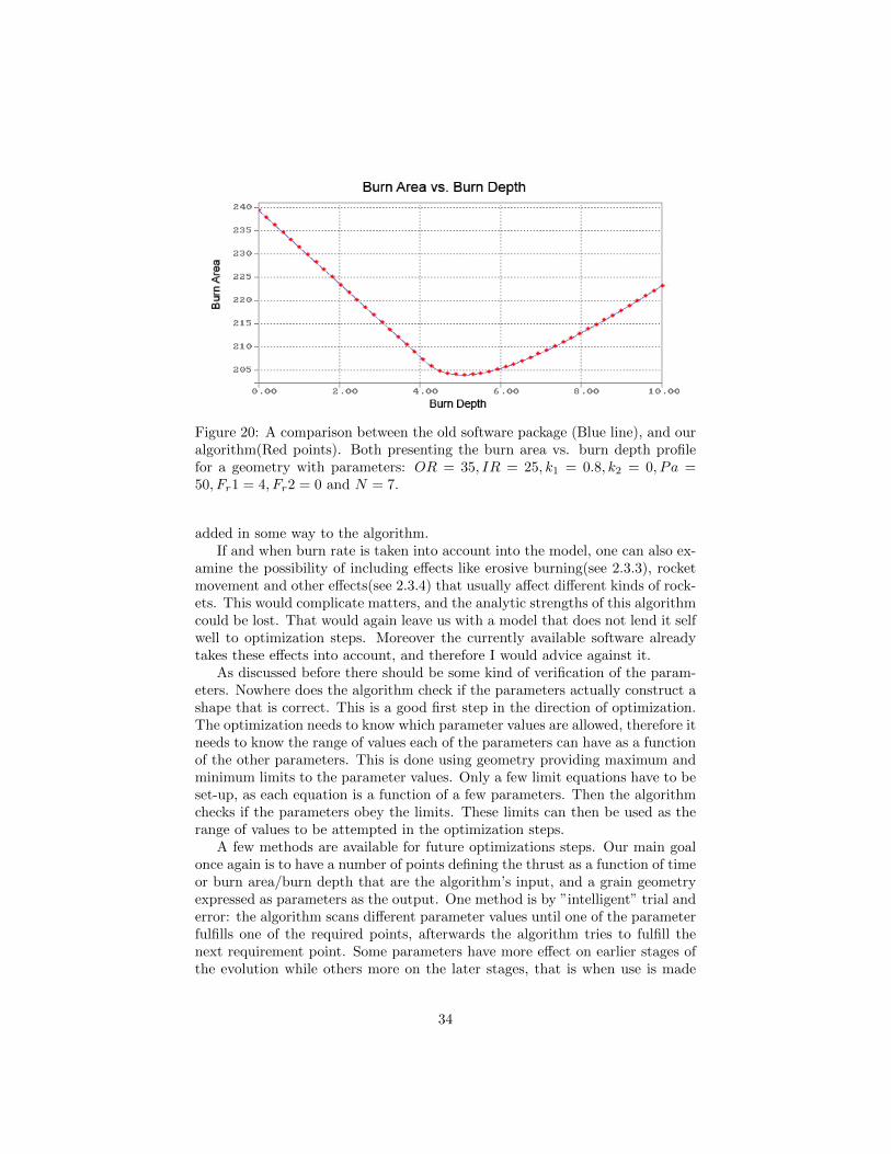
Figure 20: A comparison between the old software package (Blue line), and ouralgorithm(Red points). Both presenting the burn area vs. burn depth profilefor a geometry with parameters: OR = 35, IR = 25, k1 = 0.8, k2 = 0, Pa =50, Fr1 = 4, Fr2 = 0 and N = 7.

added in some way to the algorithm.If and when burn rate is taken into account into the model, one can also ex-

amine the possibility of including effects like erosive burning(see 2.3.3), rocketmovement and other effects(see 2.3.4) that usually affect different kinds of rock-ets. This would complicate matters, and the analytic strengths of this algorithmcould be lost. That would again leave us with a model that does not lend it selfwell to optimization steps. Moreover the currently available software alreadytakes these effects into account, and therefore I would advice against it.

As discussed before there should be some kind of verification of the param-eters. Nowhere does the algorithm check if the parameters actually construct ashape that is correct. This is a good first step in the direction of optimization.The optimization needs to know which parameter values are allowed, therefore itneeds to know the range of values each of the parameters can have as a functionof the other parameters. This is done using geometry providing maximum andminimum limits to the parameter values. Only a few limit equations have to beset-up, as each equation is a function of a few parameters. Then the algorithmchecks if the parameters obey the limits. These limits can then be used as therange of values to be attempted in the optimization steps.

A few methods are available for future optimizations steps. Our main goalonce again is to have a number of points defining the thrust as a function of timeor burn area/burn depth that are the algorithm’s input, and a grain geometryexpressed as parameters as the output. One method is by ”intelligent” trial anderror: the algorithm scans different parameter values until one of the parameterfulfills one of the required points, afterwards the algorithm tries to fulfill thenext requirement point. Some parameters have more effect on earlier stages ofthe evolution while others more on the later stages, that is when use is made

34

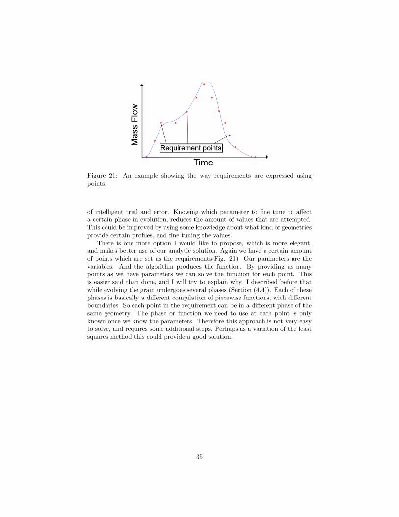
Figure 21: An example showing the way requirements are expressed usingpoints.

of intelligent trial and error. Knowing which parameter to fine tune to affecta certain phase in evolution, reduces the amount of values that are attempted.This could be improved by using some knowledge about what kind of geometriesprovide certain profiles, and fine tuning the values.

There is one more option I would like to propose, which is more elegant,and makes better use of our analytic solution. Again we have a certain amountof points which are set as the requirements(Fig. 21). Our parameters are thevariables. And the algorithm produces the function. By providing as manypoints as we have parameters we can solve the function for each point. Thisis easier said than done, and I will try to explain why. I described before thatwhile evolving the grain undergoes several phases (Section (4.4)). Each of thesephases is basically a different compilation of piecewise functions, with differentboundaries. So each point in the requirement can be in a different phase of thesame geometry. The phase or function we need to use at each point is onlyknown once we know the parameters. Therefore this approach is not very easyto solve, and requires some additional steps. Perhaps as a variation of the leastsquares method this could provide a good solution.

35

5 Conclusion

The problem examined is the burning and thrust function of star-like graingeometries. Several different methods have been examined that can simulatethe burning of the grain geometry. Eventually the method we have based iton is a geometric parametric approach. It is based initially on defining a starusing parameters. The star is built out of sections, which all change and burnindependently. This model is able to describe the shape of the propellant grainat all different burn steps, and does so at great speed and accuracy. A single stepcalculation time is approximately 0.1 to 0.01 sec. Moreover the model is verysuitable for future steps that optimize the geometry according to performancerequirements. The performance delivered is the burn area vs. burn depth, whileultimately it should deliver the mass flow vs. time profile. It was examined howthe burn area profile should be translated into a thrust profile. The modelalgorithm is compatible with the current software, GDP.

References

[1] Grain Design Program, AED Electronics,http://www.aedelectronics.nl/gdp/gdp.htm.

[2] Sutton G.P., Wiley Interscience, Rocket Propulsion Elements, 1992.

[3] Barrere M. and Jaumotte A. and de Veubeke B. F. and VandenkerckhoveJ., Elsevier, Rocket Propulsion, 1960.

[4] Geckler R., Butterworths scientific publications, The mechanism of combus-tion of solid propellants, 1954.

[5] J. C. Godon, J. Duterque, and G. Lengellet, JOURNAL OF PROPULSIONAND POWER, Vol. 9, No. 6, Erosive Burning in Solid Propellant Motors,1993.

[6] H. S. Mukunda and P. J. Paul, COMBUSTIONAND FLAME, 109:224-236,Universal Behaviour in Erosive Burning of Solid Propellants, 1997.

[7] Sethian J.A., Comm. in Math. Phys., 101, 487-499, Curvature and the Evo-lution of Fronts, 1985.

[8] Sethian J.A., J. Differential Geometry, 31, 131-161, Numerical Algorithm forpropagating Interfaces: Hamilton-Jacobi Equations and Conservation Laws,1990.

[9] Sethian J.A., Cambridge Monograph on Applied and Computational Math-ematics, Level Set Methods and Fast Marching Methods Evolving Interfacesin Computational Geometry, Fluid Mechanics, Computer Vision, and Ma-terials Science, Cambridge University Press, 1999.

36