Risk Avers

8/3/2019 Risk Avers

http://slidepdf.com/reader/full/risk-avers 1/39

Risk Aversion and Expected Utility Theory:

Coherence for Small- and Large-Stakes Gambles

James C. Cox

University of Arizona

[email protected]

Vjollca Sadiraj

University of [email protected]

January 2001; revised July 2002

8/3/2019 Risk Avers


Risk Aversion and Expected Utility Theory:

Coherence for Small- and Large-Stakes Gambles∗

There is a sizable literature reporting the conclusion that expected utility theory cannot provide acoherent positive theory of risk averse behavior. Recently-published articles have sharpened thecriticism with calibrations based on assumed concavity and additivity of initial wealth to income.We demonstrate that the negative conclusions in this literature are valid for only one expected

utility model not, as claimed, for expected utility theory. The conclusions are not valid for theexpected utility model commonly used in bidding theory nor for a more general expected utilitymodel that we develop by extending the Arrow-Pratt characterization of agents’ comparative risk aversion. Clarification of the distinction between expected utility theory and expected utility

models also makes it clear that loss aversion is consistent with expected utility theory.

Key Words: expected utility theory, risk aversion, loss aversion

JEL Classification Number: D81

1. Introduction

A central objective in developing an empirical science is coherence in the application of theory to

data from different sources. Thus, Rabin (2000a, 2000b) and Rabin and Thaler (2001) address an

important question concerning coherence of the application of concave expected utility theory to

explain risk-averse behavior for both small-stakes gambles used in laboratory experiments and

large-stakes gambles observed in everyday life. Although Rabin (2000b) singles out the work of

experimental economists for special criticism, his “calibration theorem” focuses one’s attention

on the central issue in a sizable literature that questions the usefulness of expected utility theory

for modeling risk-averse behavior.1

This criticism has been quite influential, in part because strongly-worded conclusions

have been repeated so many times. Thus, Rabin (2000a) tells readers that: “Within the expected-

utility framework, the concavity of the utility-of-wealth function is not only sufficient to explain

risk aversion – it is also necessary: Diminishing marginal utility of wealth is the sole explanation

for risk aversion …” (p. 202) Rabin also states that: “The inability of expected utility theory to

provide a plausible account of risk aversion over modest stakes has been illustrated in writing in a

8/3/2019 Risk Avers


2

variety of different contexts …” (pp. 202-203) He continues by stating: “Within the expected-

utility framework, for any concave utility function, even very little risk aversion over modest

stakes implies an absurd degree of risk aversion over large stakes.” (p. 203)

Rabin (2000b) proves a calibration theorem and corollary for a concave expected-utility

model that he interprets as bringing the following to one’s attention: “…this theory implies that

people are approximately risk neutral when stakes are small…While not broadly appreciated, the

inability of expected-utility theory to provide a plausible account of risk aversion over modest

stakes has become oral tradition among some subsets of researchers…” (p. 1281) In addition to

proof of the theorem, Rabin discusses at some length its purported implications for empirical

methods in economics. He is particularly critical of the use by experimental economists of

concave expected-utility theory to explain systematic, one-sided deviations from the predictions

of risk-neutral models because of his belief that “…expected-utility theory is manifestly not close

to the right explanation of risk attitudes over modest stakes…” (p. 1282) and “…if we think that

subjects in experiments are risk averse, then we know they are not expected-utility maximizers.”

(p. 1286) He states that the right explanation is loss aversion, which is said to be inconsistent

with expected-utility theory: “…loss aversion, is a departure from expected-utility theory that

provides a direct explanation for modest scale risk aversion.” (p. 1288)

The conclusions about expected-utility theory are stated most forcefully by Rabin and

Thaler (2001), as follows: “We are arguing that when people decline gambles with positive

expected value for modest stakes, they are violating expected utility theory.” (p. 227) They

conclude their paper as follows: “…it is time for economists to recognize that expected utility

theory is an ex-hypothesis, so that we can concentrate our energies on the important task of

developing better descriptive models of choice under uncertainty.” (p. 230) This conclusion is

immediately preceded by the following: “What should expected utility theory be replaced with?

We think it is clear that loss aversion and the tendency to isolate each risky choice must both be

key components of a good descriptive theory of risk attitudes.” (p. 230)

8/3/2019 Risk Avers


3

These criticisms of expected utility theory, and the related discussions of loss aversion,

involve some issues for which there is a marked absence of clarity in the literature on decision

theory. In order to help clarify the fundamental differences between expected utility theory and

alternative decision theories, we draw attention to the distinction between expected utility theory

and expected utility models. We address the coherence question for both of the commonly-used

expected utility models, the expected utility of terminal wealth model and the expected utility of

income model, and for a more general model that we develop, the expected utility of income and

initial wealth model.

We explain that the calibration theorem has no implication for the expected utility of

income (EUI) model because of its fixed reference point of zero income. The expected utility of

income and initial wealth (EUI&IW) model includes initial wealth as a reference point but the

calibration theorem has no implication for this model because initial wealth is not additive to

income in the utility function for this model. In contrast, if there is empirical support for the

pattern of small-stakes risk aversion hypothesized in Rabin (2000a, 2000b) and Rabin and Thaler

(2001), then the calibration theorem has implications for applicability of the expected utility of

terminal wealth (EUTW) model.

Since modeling risk aversion with the EUTW model is called into question by Rabin’s

calibration theorem, and since the calibration theorem has no implication for the EUI&IW model,

it is important to ascertain whether central analytical results in the economics of uncertainty that

have been derived with the EUTW model have analogues that can be derived with the EUI&IW

model. We begin the study of this question by extending the Arrow (1971) and Pratt (1964)

characterization of comparative risk aversion to the EUI&IW model. Subsequently, we use the

EUI&IW model to derive an analogue of Arrow’s (1971) classic two-asset portfolio allocation

proposition.

Clarification of the distinction between expected utility theory and specific expected

utility models also helps to clarify the implications of loss aversion (Kahneman and Tversky,

8/3/2019 Risk Avers


4

1979) for decision theory. We explain that loss aversion is consistent with some expected utility

models, hence it is consistent with expected utility theory. Thus, if a researcher observes loss-

averse behavior, he should not, ipso facto, be motivated to reject expected utility theory in favor

of some alternative such as prospect theory (Kahneman and Tversky, 1979), although loss

aversion is inconsistent with the expected utility of terminal wealth model.

We mention a small part of the literature that reports data showing risk-averse behavior in

laboratory experiments. The common features of these experiments are: (1) consistent one-sided

deviations of subjects’ choices from the predictions of risk neutrality, in the direction consistent

with risk aversion; (2) no relevance of loss aversion; and (3) researchers’ use of expected utility

models for which the calibration theorem has no implication. Clarification of these issues is

important to decision theory and to proper review for journals of papers reporting empirical

applications of expected utility theory.2

2. Expected Utility Theory vs. Expected Utility Models

We define “expected utility theory” as the theory of decision-making under risk based on a set of

axioms for a preference ordering that includes the independence axiom or an alternative that

implies that the (expected) utility function that represents the ordering is linear in probabilities.

Linearity in probabilities implies that indifference curves in the Machina (1982) triangle diagram

and the probability simplex are parallel straight lines. Thus, we include within expected utility

theory any model of decision-making under risk that has parallel straight-line indifference curves

in the Machina triangle diagram.

Expected utility theory and alternative decision theories are concerned with the properties

of preference orderings of probability distributions of “prizes.” The identity of the prizes depends

on the decision context that is modeled and on assumptions made by the theorist. We shall

confine our discussion to decision contexts in which the prizes are amounts of money. Within this

context, we identify two expected utility models that are commonly used, the expected utility of

8/3/2019 Risk Avers


5

terminal wealth model and the expected utility of income model. We also discuss a third model,

the expected utility of income and initial wealth model. The distinctions among the models are in

the assumed identity of the prizes. All of the models have parallel straight-line indifference

curves in the Machina triangle, hence are included within expected utility theory.

2.1 The EUTW Model

The expected utility of terminal wealth (EUTW) model is based on the assumption that the prizes

are amounts of terminal wealth. This model was used in the seminal work of Arrow (1971) and

Pratt (1964) in which they developed the measures for comparing agents’ risk attitudes. This

model is commonly used in theoretical and empirical papers on various topics.

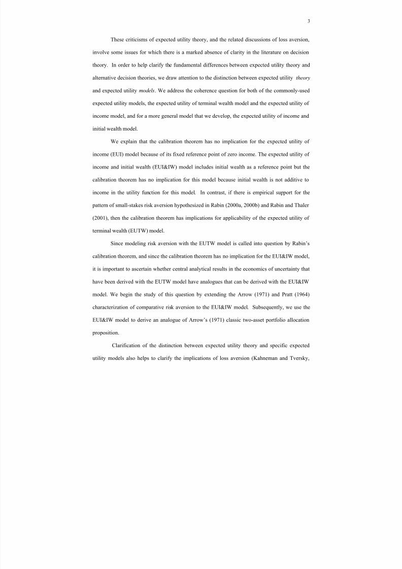
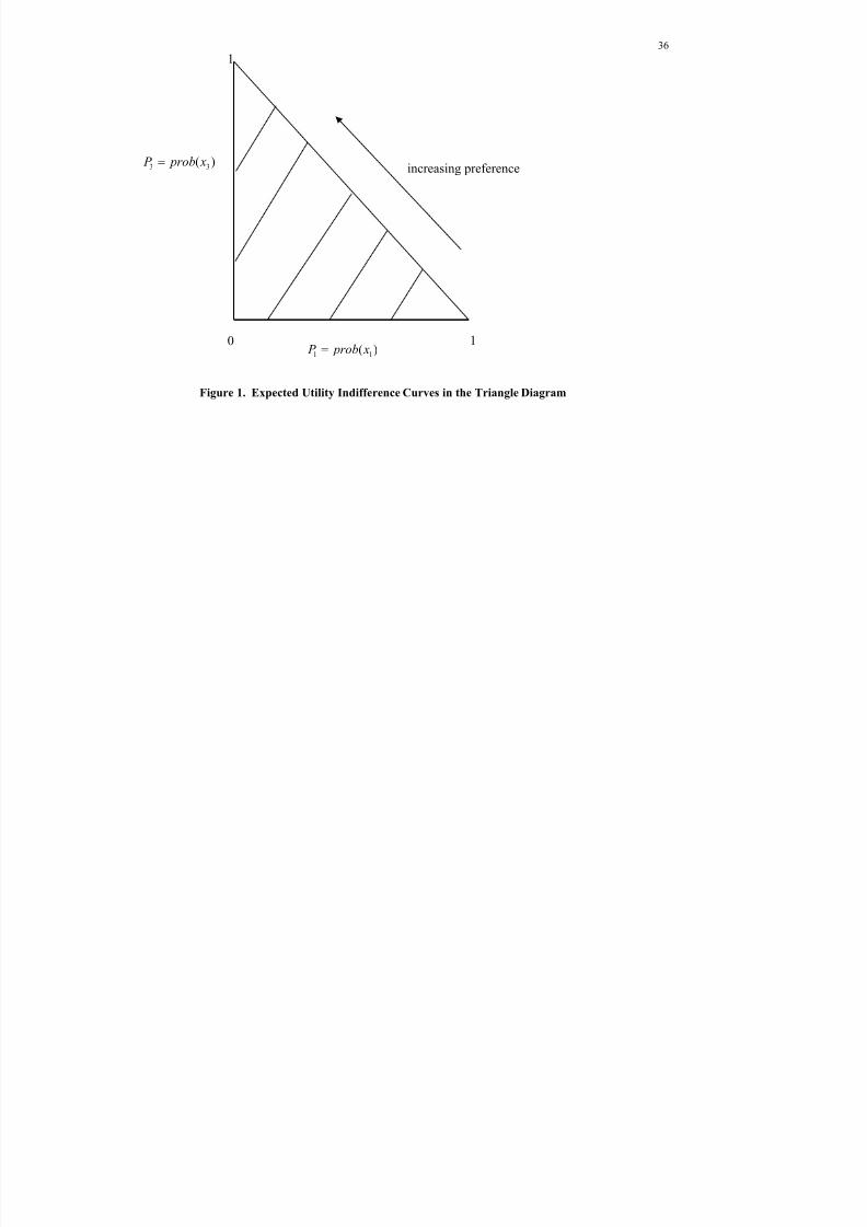
It will help explain some essential distinctions between models to briefly review the

familiar triangle-diagram representation of indifference curves for simple gambles (Machina,

1987). Consider three amounts of monetary gains (or amounts of income), i y , i = 1,2,3 such that

321 y y y << . Assume that the i y occur with probabilities, i p , i = 1,2,3 such that

1321 =++ p p p . If w is the decision-maker’s initial wealth, then the expected utility function

for the EUTW model is written as

(1) ∑=

+=3

1

)(i

iiW ywu pU .

Since 312 1 p p p −−= , indifference curves for expected utility function (1) can be represented

in the triangle diagram in Figure 1. Indifference curves are parallel straight lines because

expected utility function (1) is linear in probabilities. Higher (respectively lower) Arrow-Pratt

absolute risk aversion implies steeper (respectively flatter) slope of the indifference curves. Thus

if expected utility function (1) exhibits non-constant absolute risk aversion then the slopes of the

indifference curves in Figure 1 depend on the amount of initial wealth, w . In the special cases in

8/3/2019 Risk Avers


6

which expected utility function (1) exhibits constant absolute risk aversion or the agent is risk

neutral, the slope of the indifference curves in Figure 1 is invariant to changes in w .

2.2 The EUI Model

The expected utility of income (EUI) model is based on the assumption that the prizes are

amounts of income (or, equivalently, changes in wealth or gains and loses). The EUI model is

commonly used in theoretical modeling, most notably in the theory of auctions. Thus, most

bidding models are based on the expected utility axioms, the assumption that the prizes are

amounts of income, and the assumption of Bayesian-Nash equilibrium.3

Considering the same three-outcome lottery as above, the expected utility function for the

EUI model is written as

(2) ∑=

=3

1

)(i

ii I yv pU .

Obviously, indifference curves for this model are parallel straight lines whose slope is

independent of initial wealth.

2.3 The EUI&IW Model

We here discuss a more general model, the expected utility of income and initial wealth

(EUI&IW) model. Assume that the prizes are ordered pairs of amounts of initial wealth and

income, ),( i yw , i = 1,2,3. Then the expected utility function can be written as

(3) ∑=

=3

1

),(

i

ii IW yw pU υ .

Indifference curves for this model are parallel straight lines; therefore it is an expected utility

model. Because it appears that the properties of the EUI&IW model have not previously been

developed, we extend the Arrow-Pratt theory of comparative risk aversion to this model, as

follows.

8/3/2019 Risk Avers


7

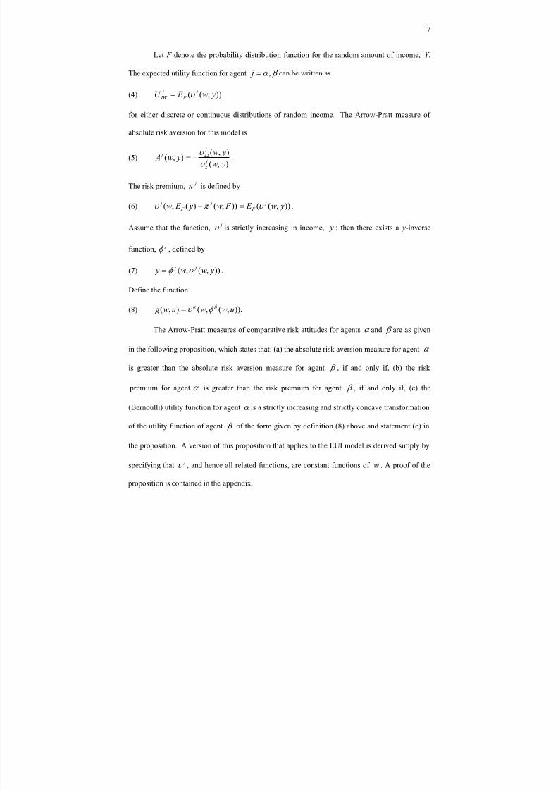
Let F denote the probability distribution function for the random amount of income, Y .

The expected utility function for agent β α ,= j can be written as

(4) )),(( yw E U j

F

j

IW υ =

for either discrete or continuous distributions of random income. The Arrow-Pratt measure of

absolute risk aversion for this model is

(5) ),(

),(),(

2

22

yw

yw yw A

j

j j

υ

υ −= .

The risk premium, jπ is defined by

(6) )),(()),()(,( yw E F w y E w j

F

j

F

j υ π υ =− .

Assume that the function, jυ is strictly increasing in income, y ; then there exists a y-inverse

function, jφ , defined by

(7) )),(,( yww y j j υ φ = .

Define the function

(8) )).,(,(),( uwwuw g β α φ υ =

The Arrow-Pratt measures of comparative risk attitudes for agents α and β are as given

in the following proposition, which states that: (a) the absolute risk aversion measure for agent α

is greater than the absolute risk aversion measure for agent β , if and only if, (b) the risk

premium for agent α is greater than the risk premium for agent β , if and only if, (c) the

(Bernoulli) utility function for agent α is a strictly increasing and strictly concave transformation

of the utility function of agent β of the form given by definition (8) above and statement (c) in

the proposition. A version of this proposition that applies to the EUI model is derived simply by

specifying that jυ , and hence all related functions, are constant functions of w . A proof of the

proposition is contained in the appendix.

8/3/2019 Risk Avers


8

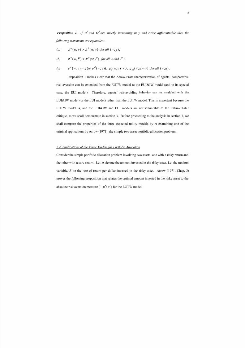
Proposition 1. If aυ and

β υ are strictly increasing in y and twice differentiable then the

following statements are equivalent:

(a) ),(),( yw A yw Aβ α > , for all ),( yw ;

(b) ),(),( F w F wβ α π π > , for all w and F ;

(c) )),(,(),( yww g yw β α υ υ = , 0),(2 >uw g , 0),(22 <uw g , for all ),( uw .

Proposition 1 makes clear that the Arrow-Pratt characterization of agents’ comparative

risk aversion can be extended from the EUTW model to the EUI&IW model (and to its special

case, the EUI model). Therefore, agents’ risk-avoiding behavior can be modeled with the

EUI&IW model (or the EUI model) rather than the EUTW model. This is important because the

EUTW model is, and the EUI&IW and EUI models are not vulnerable to the Rabin-Thaler

critique, as we shall demonstrate in section 3. Before proceeding to the analysis in section 3, we

shall compare the properties of the three expected utility models by re-examining one of the

original applications by Arrow (1971), the simple two-asset portfolio allocation problem.

2.4 Implications of the Three Models for Portfolio Allocation

Consider the simple portfolio allocation problem involving two assets, one with a risky return and

the other with a sure return. Let a denote the amount invested in the risky asset. Let the random

variable, R be the rate of return per dollar invested in the risky asset. Arrow (1971, Chap. 3)

proves the following proposition that relates the optimal amount invested in the risky asset to the

absolute risk aversion measure ( uu′′′−) for the EUTW model.

8/3/2019 Risk Avers


9

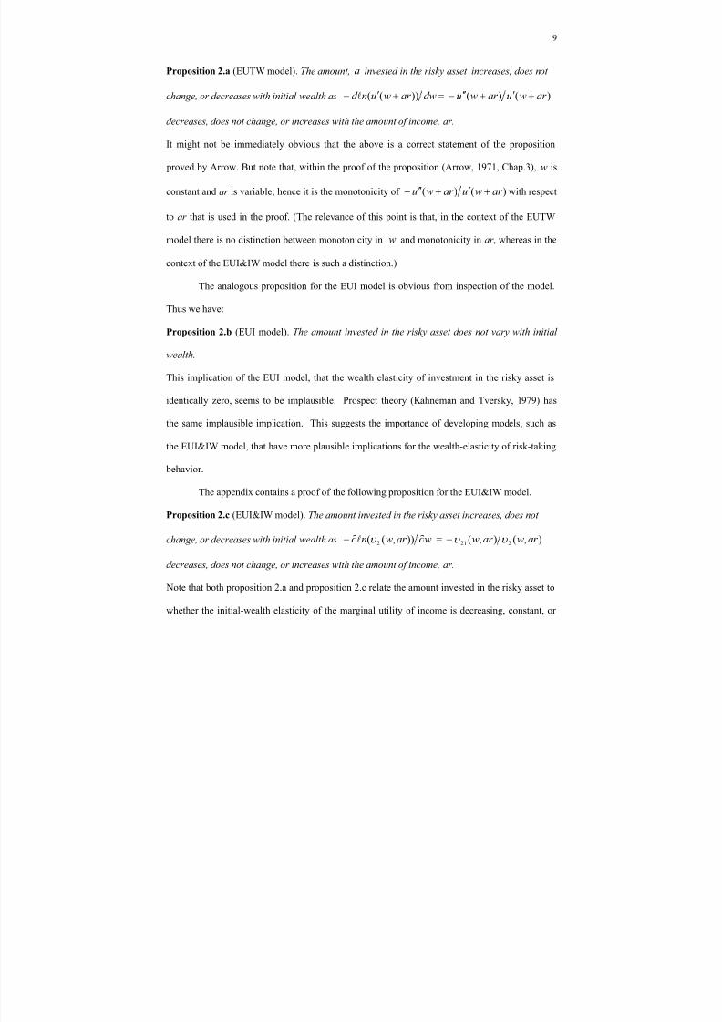
Proposition 2.a (EUTW model). The amount, a invested in the risky asset increases, does not

change, or decreases with initial wealth as dwar wund ))(( +′− l = )()( ar wuar wu +′+′′−

decreases, does not change, or increases with the amount of income, ar.

It might not be immediately obvious that the above is a correct statement of the proposition

proved by Arrow. But note that, within the proof of the proposition (Arrow, 1971, Chap.3), w is

constant and ar is variable; hence it is the monotonicity of )()( ar wuar wu +′+′′− with respect

to ar that is used in the proof. (The relevance of this point is that, in the context of the EUTW

model there is no distinction between monotonicity in w and monotonicity in ar , whereas in the

context of the EUI&IW model there is such a distinction.)

The analogous proposition for the EUI model is obvious from inspection of the model.

Thus we have:

Proposition 2.b (EUI model). The amount invested in the risky asset does not vary with initial

wealth.

This implication of the EUI model, that the wealth elasticity of investment in the risky asset is

identically zero, seems to be implausible. Prospect theory (Kahneman and Tversky, 1979) has

the same implausible implication. This suggests the importance of developing models, such as

the EUI&IW model, that have more plausible implications for the wealth-elasticity of risk-taking

behavior.

The appendix contains a proof of the following proposition for the EUI&IW model.

Proposition 2.c (EUI&IW model). The amount invested in the risky asset increases, does not

change, or decreases with initial wealth as war wn ∂∂− )),(( 2υ l = ),(),( 221 ar war w υ υ −

decreases, does not change, or increases with the amount of income, ar.

Note that both proposition 2.a and proposition 2.c relate the amount invested in the risky asset to

whether the initial-wealth elasticity of the marginal utility of income is decreasing, constant, or

8/3/2019 Risk Avers


10

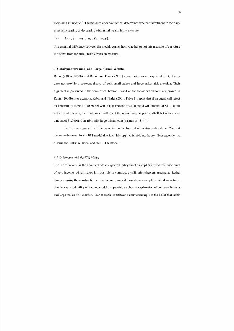
increasing in income.4 The measure of curvature that determines whether investment in the risky

asset is increasing or decreasing with initial wealth is the measure,

(9) =),( ywC ),(),( 221 yw yw υ υ − .

The essential difference between the models comes from whether or not this measure of curvature

is distinct from the absolute risk aversion measure.

3. Coherence for Small- and Large-Stakes Gambles

Rabin (2000a, 2000b) and Rabin and Thaler (2001) argue that concave expected utility theory

does not provide a coherent theory of both small-stakes and large-stakes risk aversion. Their

argument is presented in the form of calibrations based on the theorem and corollary proved in

Rabin (2000b). For example, Rabin and Thaler (2001, Table 1) report that if an agent will reject

an opportunity to play a 50-50 bet with a loss amount of $100 and a win amount of $110, at all

initial wealth levels, then that agent will reject the opportunity to play a 50-50 bet with a loss

amount of $1,000 and an arbitrarily large win amount (written as “$∞ ”).

Part of our argument will be presented in the form of alternative calibrations. We first

discuss coherence for the EUI model that is widely applied in bidding theory. Subsequently, we

discuss the EUI&IW model and the EUTW model.

3.1 Coherence with the EUI Model

The use of income as the argument of the expected utility function implies a fixed reference point

of zero income, which makes it impossible to construct a calibration-theorem argument. Rather

than reviewing the construction of the theorem, we will provide an example which demonstrates

that the expected utility of income model can provide a coherent explanation of both small-stakes

and large-stakes risk aversion. Our example constitutes a counterexample to the belief that Rabin

8/3/2019 Risk Avers


11

and Thaler’s conclusions about incoherence of small-stakes and large-stakes risk aversion hold

for the EUI model.

Consider the example used by Rabin (2000b) in which it is assumed that a decision-

maker would reject a gamble that yields a gain of $110 and a loss of $100 with equal probability.

We will compare implied levels of risk aversion for the EUI model with the levels given in

Rabin’s Tables I and II for the EUTW model. The second and third columns of our Table I

reproduce some results reported in Rabin’s Table I and Table II. The “Table I Rejections” we

reproduce are implied by the corollary to the calibration theorem if the agent is assumed to reject

the 50-50, lose $100/ gain $110 gamble for all initial wealth levels. Such an agent would also

reject a gamble in which he would, with equal probability, lose $1000 or gain any arbitrarily large

amount. The “Table II Rejections” we reproduce are derived from the assumption that the agent

will reject the 50-50, lose $100/ gain $110 gamble for all initial wealth levels no greater than

$300,000. In that case, the agent would also reject a gamble in which he would, with equal

probability, lose $20,000 or gain $160,000,000,000 when his initial wealth is $290,000.

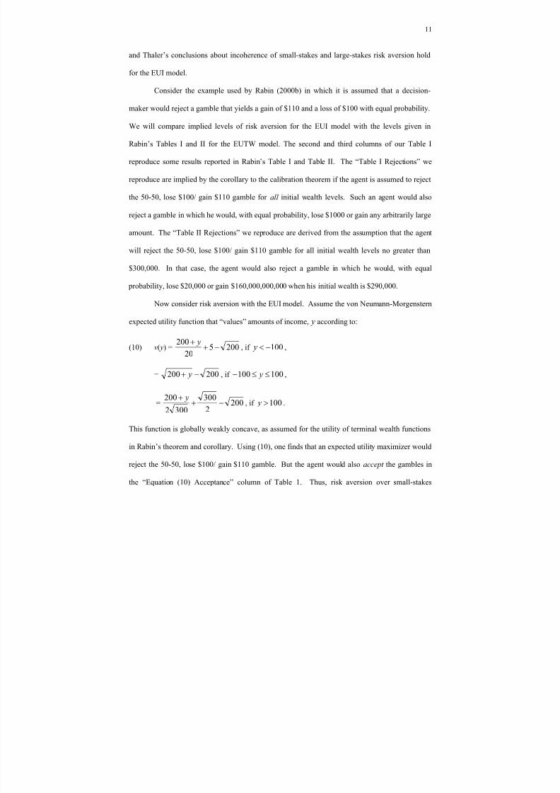
Now consider risk aversion with the EUI model. Assume the von Neumann-Morgenstern

expected utility function that “values” amounts of income, y according to:

(10) v( y) = 200520

200−+

+ y, if 100−< y ,

= 200200 −+ y , if 100100 ≤≤− y ,

= 2002

300

3002

200−+

+ y, if 100> y .

This function is globally weakly concave, as assumed for the utility of terminal wealth functions

in Rabin’s theorem and corollary. Using (10), one finds that an expected utility maximizer would

reject the 50-50, lose $100/ gain $110 gamble. But the agent would also accept the gambles in

the “Equation (10) Acceptance” column of Table 1. Thus, risk aversion over small-stakes

8/3/2019 Risk Avers


8/3/2019 Risk Avers


13

0.5 v (-100) < v (0). Assuming that v (y) is given by equation (10), one finds that the decision-

maker would reject the 50-50, lose $100/ gain $110 gamble for all initial wealth levels, w . But

the agent would also accept the gambles in the “Equation (10) Acceptance” column of Table 1,

for all initial wealth levels, w .

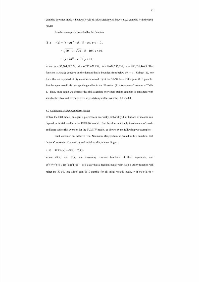
Next consider a multiplicative function that values amounts of income, y and initial

wealth, w according to

(13) )()(),( yvw yw mm ϕ υ = ,

where )(wmϕ > 0 and )( yv are concave functions of their arguments. Again assuming that v (y)

is given by equation (10), one finds that the decision-maker would reject the 50-50, lose $100/

gain $110 gamble for all initial wealth levels, w . Once again, the agent would also accept the

gambles in the “Equation (10) Acceptance” column of Table 1, for all initial wealth levels, w .

Thus, risk aversion over small-stakes gambles does not imply ridiculous levels of risk aversion

over large-stakes gambles with the EUI&IW Model.

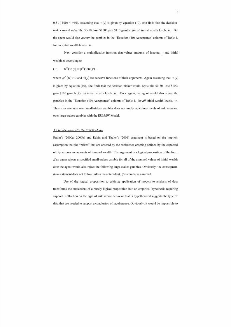
3.3 Incoherence with the EUTW Model

Rabin’s (2000a, 2000b) and Rabin and Thaler’s (2001) argument is based on the implicit

assumption that the “prizes” that are ordered by the preference ordering defined by the expected

utility axioms are amounts of terminal wealth. The argument is a logical proposition of the form:

If an agent rejects a specified small-stakes gamble for all of the assumed values of initial wealth

then the agent would also reject the following large-stakes gambles. Obviously, the consequent,

then statement does not follow unless the antecedent, if statement is assumed.

Use of the logical proposition to criticize application of models to analysis of data

transforms the antecedent of a purely logical proposition into an empirical hypothesis requiring

support. Reflection on the type of risk averse behavior that is hypothesized suggests the type of

data that are needed to support a conclusion of incoherence. Obviously, it would be impossible to

8/3/2019 Risk Avers


14

conduct money payoff experiments with subjects whose actual personal wealth varied over the

whole real line. Therefore, it is impossible that empirical support for the assumptions in Rabin’s

(2000a) Table 11.1 or Rabin’s (2000b) Table I or Rabin and Thaler’s (2001) Table 1 calibrations

could ever be provided. Furthermore, it would be virtually impossible to conduct experiments

with individual subjects whose actual personal wealth took on all values up to $300,000. In

contrast, one could recruit subjects from a subject pool consisting of distinct individuals with

wealth levels varying over a range large enough to make use of the logic of the calibration

theorem. In that case, the data would confound heterogeneity in subjects’ risk attitudes with

variability in their individual wealth levels. But such an across-subjects experimental design

would be a reasonable approach to providing empirical support for the type of small-stakes risk

aversion assumed in Rabin’s (2000b) Table II calibration. Furthermore, it is a reasonable

conjecture that the (typically-unobserved) variability in wealth across subjects in earlier

experiments on risk attitudes may have sufficient variability for this purpose. Therefore, Rabin

and Thaler’s argument does make questionable the coherence of applications of the EUTW model

to small-stakes and large-stakes gambles.

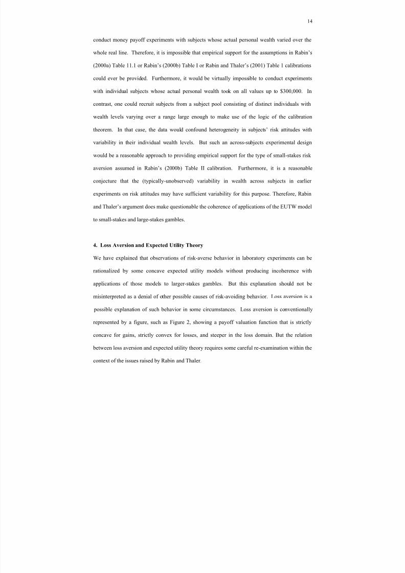
4. Loss Aversion and Expected Utility Theory

We have explained that observations of risk-averse behavior in laboratory experiments can be

rationalized by some concave expected utility models without producing incoherence with

applications of those models to larger-stakes gambles. But this explanation should not be

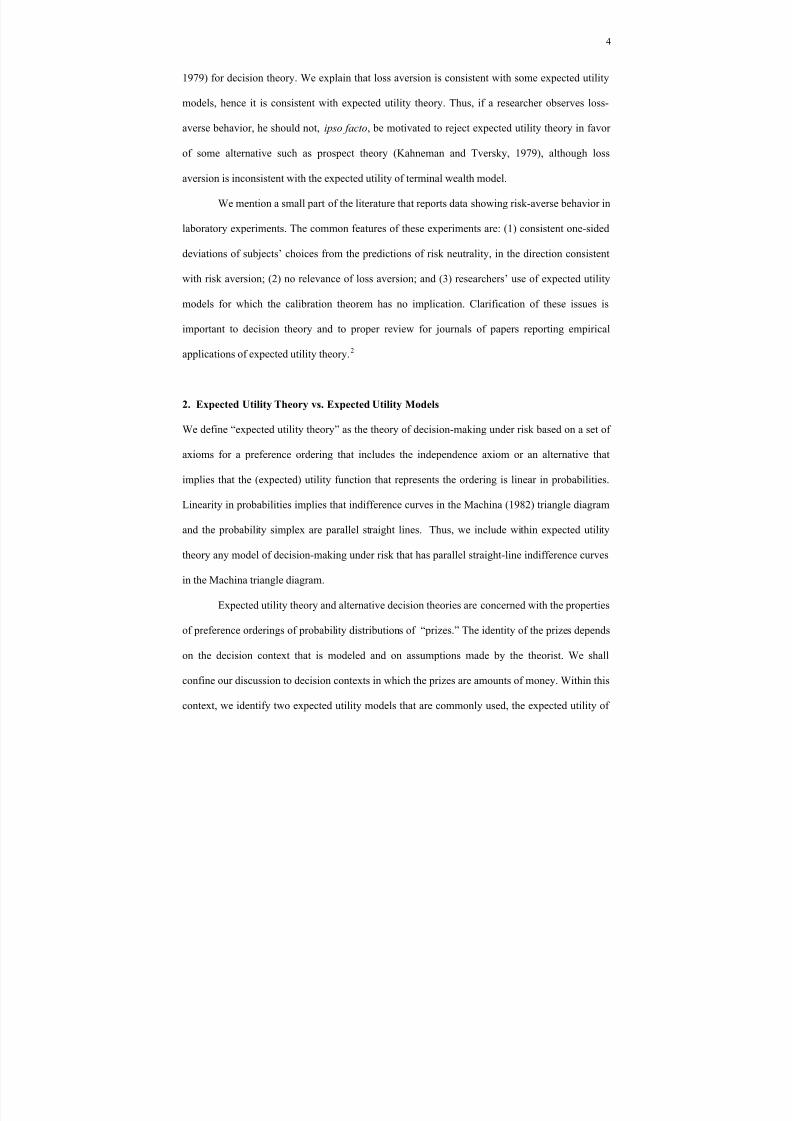
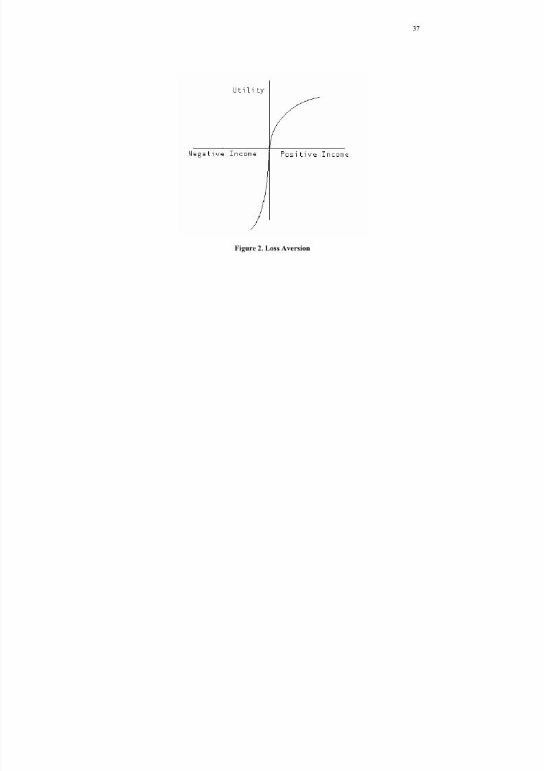
misinterpreted as a denial of other possible causes of risk-avoiding behavior. Loss aversion is a

possible explanation of such behavior in some circumstances. Loss aversion is conventionally

represented by a figure, such as Figure 2, showing a payoff valuation function that is strictly

concave for gains, strictly convex for losses, and steeper in the loss domain. But the relation

between loss aversion and expected utility theory requires some careful re-examination within the

context of the issues raised by Rabin and Thaler.

8/3/2019 Risk Avers


15

Observing that expected utility theory contains more than the EUTW model helps one to

understand the essential differences between that theory and its alternatives. Some researchers,

such as Kahneman and Tversky (1979), Rabin (2000b), and Rabin and Thaler (2001), believe that

loss aversion distinguishes expected utility theory from alternatives such as prospect theory. But

loss aversion is consistent with the EUI and EUI&IW models, hence it is consistent with expected

utility theory. Empirical tests that can discriminate on a fundamental level between expected

utility theory and its alternatives must be based on differences between the implications of

alternative sets of axioms, not different subsidiary assumptions about what the prizes are to which

the axioms are applied. Thus, observations of Allais paradox behavior are empirical

inconsistencies with expected utility theory because they are inconsistent with the Machina-

triangle indifference curves being parallel straight lines (Machina, 1982, 1987). In contrast,

observations of loss-averse behavior are consistent with the indifference curves being parallel

straight lines, hence they are consistent with expected utility theory.

Explicit integration of loss aversion into expected utility theory has just begun to produce

interesting extensions of decision theory. Thus, Nielson (2002) develops an analogue of the

characterization of comparative risk aversion (“more risk averse than”) stated as one agent’s

preferences being “more S-shaped than” another agent’s preferences over probability

distributions of payoffs.

5. Lottery Payoffs in Experiments

Rabin and Thaler (2001, p. 224) criticize the use of lottery payoffs in experiments: “This lottery

procedure either isn’t necessary, or doesn’t work. If subjects are expected utility maximizers then

the procedure is unnecessary, since expected utility theory tells us that people will be virtually

risk neutral in decisions on the scale of laboratory stakes. If subjects are not expected utility

maximizers, then the procedure cannot be relied upon to work, since subjects may not have

8/3/2019 Risk Avers


16

preferences that are linear in probabilities.” Similar assertions are contained in Rabin (2000a)

and Rabin (2000b).

Lottery payoffs were introduced into decision theory by Smith (1961). They were used

in experiments first by Roth and Malouf (1979) and, subsequently, by Roth and Murnigham

(1982), Roth and Schoumaker (1983), and many others. Neither Smith’s theoretical argument nor

most applications in experiments requires use of the EUTW model rather than the EUI model or

the EUI&IW model. Therefore, Rabin and Thaler’s argument has no general implication for

applicability of lottery payoffs in experiments.

The problem with lottery payoffs does not derive from the calibration theorem but rather

from experimental studies that conclude that they do not successfully induce risk attitudes on

subjects. Thus, Walker, Smith, and Cox (1990) and Cox and Oaxaca (1995) report that lottery

payoffs do not successfully control subjects’ risk attitudes in bidding (market) experiments.

Selten, Sadrieh, and Abbink (1999) report that lottery payoffs fail to induce risk neutral behavior

in non-market experiments. Berg, Dickhaut, and Rietz (2001) report somewhat greater success

from using lottery payoffs to induce risk-averse and risk-loving preferences in preference reversal

experiments.

It is clear that the empirical failure of lottery payoffs is a failure of expected utility theory.

But alternative decision theories have not been subjected to similar tests with types of lottery

payoffs that are appropriate in the absence of linearity in probabilities, hence it is unknown

whether any of them would fare any better.

6. Exogenous Risky Income

Subjects in experiments may have risky incomes that are exogenous to experimental treatments.

Any such risky income would not ordinarily be observed by experimenters. The existence of

exogenous risky income raises some questions about rational behavior, and the modeling of

rational behavior, that are well beyond the scope of the present paper. These questions revolve

8/3/2019 Risk Avers


17

around the implications of integration, or non-integration, of risky incomes from different

decision contexts. But it is germane to discussion of the issues we are examining to ask whether

integration of exogenous large-stakes risks with endogenous small-stakes risks has implications

for applicability of concave expected utility theory.

Consider the following example. Assume that an experimental subject rejects the 50-50,

lose $100, gain $110 gamble. Also assume that this subject has exogenous risky income with a

mean value of $10,000. If the subject does not integrate the endogenous and exogenous risks

then the argument in subsection 3.1 tells us that there is no implication of ridiculous large-stakes

risk aversion. Thus we will here focus on the case where the subject is assumed to integrate the

endogenous and exogenous risky incomes. If the risky incomes are integrated by addition, does

concavity necessarily have an untenable implication? In other words, does small-stakes risk

aversion that is endogenous to an experiment, together with exogenous large-stakes risky income,

have calibration-theorem-like implications for large-stakes risk aversion?

Let the random variables, X and Y denote the exogenous and endogenous risky incomes.

The risky income that is assumed to be endogenous to an experiment is the 50-50, lose $100, gain

$110 gamble. The exogenous income is assumed to have a log-normal distribution with mean of

$10,000 and variance of $90,000. Assume the von Neumann-Morgenstern utility function that

values sums of amounts of income, y+ according to:

(14) 200520

800,9)( −+

++−=+

y x y xv , if 900,9<+ y x

= 200800,9 −++− y x , if 100,10900,9 ≤+≤ y x

= 2002

300

3002

800,9−+

++− y x, if 100,10>+ y x .

It is straightforward to show that equation (14) and the assumed log-normal distribution of X

imply that the agent will reject the 50-50, lose $100, gain $110 gamble. Does the agent have

8/3/2019 Risk Avers


18

reasonable large-stakes risk aversion? Yes, the minimum gain that would be required to get a

decision-maker with expected utility function including (14) and the assumed log-concave

distribution of exogenous income to accept a gamble with 0.5 probability of losing $20,000, and

0.5 probability of receiving the gain, is a gain of $44,000.

7. Exogenous Risk-Free Income

Rabin’s (2000b) calibration theorem is based on the assumption that an agent will reject an

opportunity to play a 50-50 bet, such as one with a loss amount of $100 and a win amount of

$110, for all initial wealth levels. This suggests the question of whether an alternative

assumption about behavior could support a calibration theorem that would apply to the EUI and

EUI&IW models.

Consider the alternative assumption that an agent prefers the certain amount of money, x

to playing a 50-50 bet with payoffs 100$− x and 110$+ x , for all values of x . Does this

assumption imply a calibration-theorem result that applies to the EUI and EUI&IW models? The

answer turns on the interpretation of “initial wealth.” Amounts of money that are risk-free, and

exogenous to decisions about risky propositions, would seem to be included in any natural

interpretation of what is meant by initial wealth In the context of these models. The following

example explicates this point.

Consider the EUI&IW model. Suppose that an agent has wealth in the amount, w .

Santa Claus then offers the agent a choice between the certain amount of money, x and playing a

50-50 bet with money payoffs 100$− x and 110$+ x . Since the amount is not at risk, and

is invariant with the agent’s choice between alternative decisions about the risky proposition, it is

included in the agent’s risk-free purchasing power, that is, his initial wealth. The natural

representation with the EUI&IW model is that Santa Claus has posed the question of whether

)0,( xw +υ is or is not greater than )110,()100,(21

21 xw xw ++−+ υ υ ; that is, Santa Claus

8/3/2019 Risk Avers


19

increased the agent’s initial wealth from w to xw + and offered the choice between playing or

not playing the 50-50 bet with payoffs of 100$− and 110$+ . The assumption that the agent

declines to play the bet for all amounts, x has no calibration-theorem implications, as shown by

examples like those in subsection 3.2 above.

8. Data Supporting Risk Aversion Over Small Stakes

Central elements in the discussion are whether there are data that support decision-makers’ risk

avoidance with small-stakes gambles and whether, as maintained by Rabin (2000a, pp. 207-8)

and Rabin (2000b, pp. 1288-9) and Rabin and Thaler (2001, pp. 226-7), this risk-avoiding

behavior can be explained by loss aversion. There is a large literature of experimental economics

papers that report behavior which is consistent with concave expected utility models but

inconsistent with their risk-neutral special cases. The risk aversion interpretation of much of this

data requires maintained hypotheses about Nash equilibrium, rational expectations, etc. Thus,

recent experiments by Holt and Laury (forthcoming) are very informative because they do not

require complicated maintained hypotheses to interpret the data.

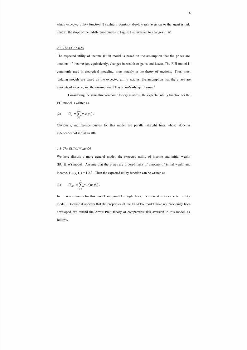
8.1 Risk Aversion in Choices Between Binary Lotteries

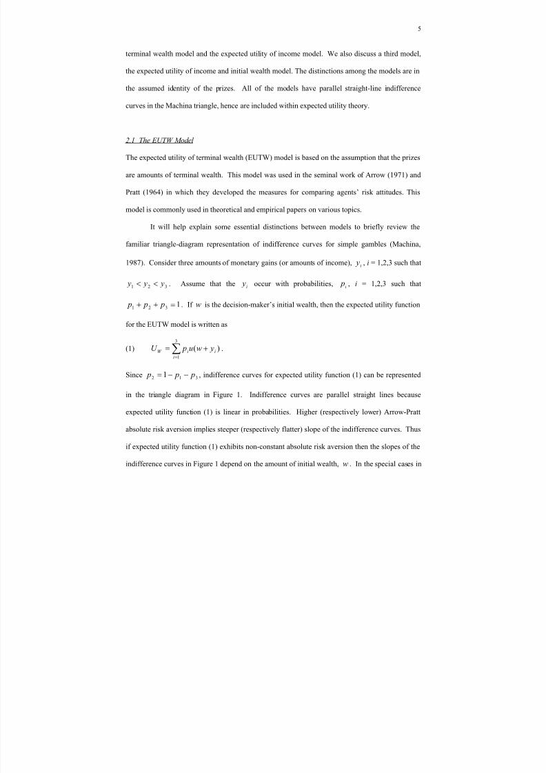
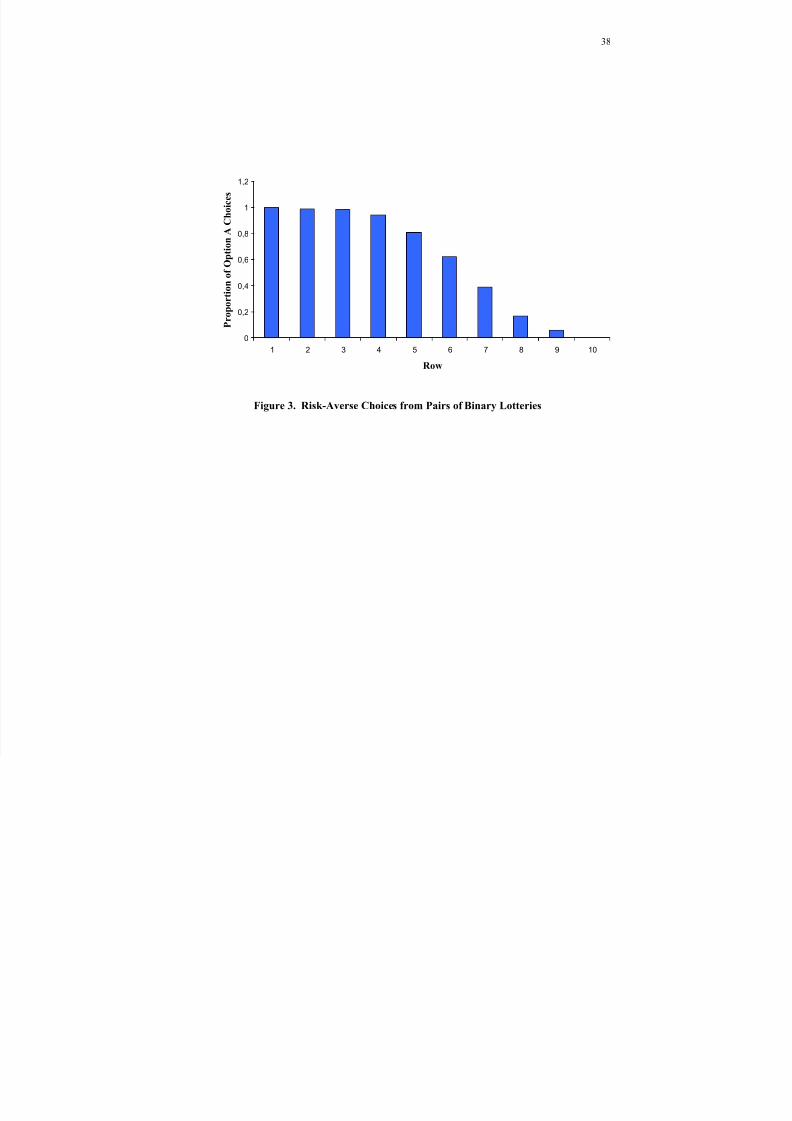
In one of their several treatments, Holt and Laury asked subjects to choose one lottery from each

of the 10 pairs of binary lotteries in Table 2. First, note that none of the lotteries involves losses,

hence loss aversion is irrelevant to interpreting the data. Secondly, note that a risk-neutral

expected utility maximizer will choose option A in the first four rows of Table 2 and choose

option B in rows five through ten. A risk-preferring expected utility maximizer will “cross over”

from choosing option A to choosing option B at some row weakly between row one and row five.

And a risk-averse expected utility maximizer will cross over from choosing option A to choosing

option B at some row weakly between row five and row ten. Choice of option A in row five and

below is consistent only with risk aversion. Results from this experimental treatment involving

8/3/2019 Risk Avers


20

175 subjects are reported in Figure 3. Note that 81% of the subjects are still choosing option A in

row 5; that is, 81% of the subjects are risk averse. Thus the data clearly provide strong support for

risk aversion for small-stakes payoffs.5

There is a large literature of experimental economics papers that report risk-averse

behavior in contexts that are more complicated than choice between binary lotteries. Because

more complicated hypotheses are required to interpret the data in these alternative environments,

the conclusion that decision-makers’ risk aversion explains one-sided deviations from the

predictions of risk-neutral models has been more controversial than for choice over binary

lotteries. Private value auctions are one context in which there is a large amount of data that are

inconsistent with risk neutrality.

8.2 Risk Aversion in Private Value Auctions

Vickrey (1961) developed a theory of bidding in first-price sealed-bid auctions based on the

expected utility axioms, the income assumption about the identity of the prizes, and the

assumption of Bayesian-Nash equilibrium. For the case in which private values for the auctioned

item are drawn independently from the uniform distribution on [0, v h], the risk-neutral

equilibrium bid function for single-unit auctions with n bidders is

(15) ii vn

nb

1−= .

As explained by Vickrey, risk-averse bidders will bid higher amounts than those given by

equation (15).

There is a large literature on experiments with first-price private-value auctions that

reports data that are inconsistent with bid function (15) because virtually all of the bids are higher

than (n-1)vi/n. Bidding more than (n-1)vi/n cannot be a way to avoid losses; hence such

apparently risk-averse bidding behavior cannot be explained by loss aversion. Tests of bidding

theory have used both market prices and individual-subject data. For example, Cox, Roberson,

8/3/2019 Risk Avers


21

and Smith (1982), Cox, Smith, and Walker (1988), and Cox and Oaxaca (1996a) report tests

based on auction market prices, individual bids and values, and decision-makers’ expected money

payoffs from bidding that support the conclusion that almost all subjects in laboratory first-price

sealed-bid auctions submit bids that are consistent with risk aversion but inconsistent with risk

neutrality. The auction literature does contain some controversy (Kagel, 1995) but the issues are

posed within the context of the EUI model, not the EUTW model.

8.3 Risk Aversion in Search Experiments

Sequential job search experiments provide another context in which there are data supporting

risk-averse behavior over small stakes. The theory is based on the expected utility axioms,

amounts of income as the prizes, and solution of the dynamic search problem by backwards

recursion. Subjects cannot lose money in most of these search experiments, hence loss aversion

cannot explain the observed behavior.

In search from known distributions without recall opportunities, 77% of 600 search

terminations were consistent with the varying predictions of the risk-neutral model over several

treatments, whereas 94% were consistent with the weakly risk-averse version of the theory (Cox

and Oaxaca, 1989). In search from known distributions with perfect or stochastic recall of past

offers, 61% of search terminations were consistent with the risk-neutral model whereas 96% were

consistent with the weakly risk-averse model (Cox and Oaxaca, 1996b). In tests with reservation

wage data for search from known distributions, the risk-neutral reservation wage path was

rejected with data from all of the experimental treatments whereas the weakly risk-averse

reservation wage path was not rejected with data for any of the three treatments (Cox and Oaxaca,

1992a, 1992b). In search from unknown distributions, 70% of search terminations were

consistent with risk-neutral predictions whereas 88% were consistent with the weakly risk-averse

model (Cox and Oaxaca, 2000).

8/3/2019 Risk Avers


22

Of course, it is impossible to “prove” that many decision-makers stop searching earlier

than predicted by risk-neutral search theory, or that their reservation wages are higher than risk-

neutral reservation wages, because of risk aversion. But alternative explanations embodied in

models have not been developed and tested. There are some anomalous data (Sonnemans, 1998,

2000).

9. Concluding Remarks

A central issue in developing an empirical science is coherence in the application of theory to

data from different sources. While such coherence is not always possible, it remains a central

objective. The principal of parallelism, that the same laws apply inside and outside the laboratory,

is a hallmark of an experimental science whether it be natural science (Shapley, 1964) or

economics (Smith, 1982). Thus, Rabin (2000a, 2000b), Rabin and Thaler (2001), and the several

other authors listed in footnote 1 raise an important question concerning coherence of the

application of concave expected utility theory to explain risk-averse behavior for both small-

stakes gambles used in laboratory experiments and large-stakes gambles encountered in everyday

life. But the central conclusion stated repeatedly by Rabin and Thaler is demonstrably wrong:

Calibration-theorem calculations do not imply that expected utility theory cannot provide a

coherent explanation of both small-stakes and large-stakes risk aversion.

We have addressed the coherence question for both of the commonly-used expected

utility models, the expected utility of terminal wealth (EUTW) model and the expected utility of

income (EUI) model, and for a more general model, the expected utility of income and initial

wealth (EUI&IW) model. We have explained that calibration-theorem arguments based on

varying initial wealth levels have no implication for the EUI model because of its fixed reference

point of zero income. The EUI&IW model includes initial wealth as a reference point but

calibration-theorem arguments based on varying initial wealth levels have no implication for this

model because initial wealth is not additive to income in the utility function. In contrast, with

8/3/2019 Risk Avers


23

empirical support for the hypothesized type of small-stakes risk aversion, the calibration-theorem

arguments do have implications for applicability of the EUTW model.

Let us suppose that the across-subjects comparisons that can be made with existing data

provide empirical support for Rabin’s (2000a, 2000b) and Rabin and Thaler’s (2001) assumed

pattern of risk-avoiding behavior. What experimental studies are then called into question? We

have already explained that typical experimental papers on auctions and search are immune to

criticisms based on the calibration theorem because they test hypotheses derived with the EUI

model. But what about other experiments involving decisions in risky environments? If the

authors used the EUTW model and strict concavity to derive the tested hypotheses then their

papers are subject to the criticisms stated by Rabin and Thaler. This brings up the question of

whether similar hypotheses could be derived from the EUI&IW model, and tested with the same

data. Key insights into answering this question are provided by our extension of the Arrow

(1971) and Pratt (1964) characterization of agents’ comparative risk aversion to the EUI&IW

model and the use of this model to derive an analogue of Arrow’s (1971) classic two-asset

portfolio allocation proposition. Proposition 1, in section 2.3, informs us that hypotheses based on

agents’ comparative risk aversion that were derived from the EUTW model have analogues that

can be derived from the EUI&IW model. Proposition 2.c, in section 2.4, provides the EUI&IW-

model analogue of Arrow’s proposition relating the amount invested in the risky asset to changes

in initial wealth.

The calibration theorem does not provide a general critique of lottery payoffs designed to

control subjects’ risk attitudes. The reason is that the theoretical basis for lottery payoffs is

linearity in probabilities; it does not require terminal wealth to be the assumed argument of an

expected utility function. The main critique of lottery payoffs is provided by experimental data

that support conclusions that they do not succeed in inducing predicted behavior. These data are,

of course, inconsistent with expected utility theory. But the data appear to be inconsistent with

the compound lottery axiom (Walker, Smith, and Cox, 1990; Cox and Oaxaca, 1995), not the

8/3/2019 Risk Avers


24

independence axiom that gives expected utility functions their defining characteristic of linearity

in probabilities. Alternative decision theories must include analogues of the compound lottery

axiom if they are to be applicable to compound lotteries. Thus there is no valid presumption that

the data from experiments designed to test the effectiveness of lottery payoffs for controlling

subjects’ risk-avoiding behavior are consistent with alternatives to expected utility theory.

Rabin and Thaler attribute risk-avoiding behavior in experiments to loss aversion. While

loss aversion may be empirically significant in some contexts, it cannot explain choices between

binary lotteries when the possible payoffs for the lotteries exclude losses. Experiments with such

lotteries provide unambiguous support for risk aversion. Bids in first-price private-value auctions

that exceed risk-neutral theoretical bids cannot be explained by loss aversion because such bids

do not avoid or minimize any possible losses. Search terminations earlier than predicted by risk-

neutral search theory and reservation wages that exceed risk-neutral reservation wages cannot be

explained by loss aversion because no losses are possible in most of the sequential search

experiments.

Both loss aversion and risk aversion are consistent with expected utility theory. Loss

aversion is inconsistent with the EUTW model but it is consistent with the EUI and EUI&IW

models. The common view that loss aversion is inconsistent with expected utility theory

confuses an inconsistency with a secondary assumption about the identity of “prizes” with an

inconsistency with a set of axioms. The Allais paradox is inconsistent with the axioms, loss

aversion is not.

Observations of risk-averse behavior in laboratory experiments can be rationalized by

concave expected utility theory without producing incoherence with applications of that theory to

large-stakes gambles. Thus, expected utility theory can provide a coherent explanation of risk

aversion in both laboratory and field environments. Then the decision about whether to apply

expected utility theory in both environments or neither environment can be based upon whether

or not known inconsistencies with the axioms, such as the Allais paradox, are judged to be of

8/3/2019 Risk Avers


25

sufficient importance to justify sacrificing the simplicity of the theory. There is a substantial

literature that reports data from experiments that are inconsistent with parallel straight-line

indifference curves in the Machina triangle. But that, in itself, does not imply that expected utility

theory should be rejected. The relevant question is whether there is an alternative theory that

performs so much better in predicting data that it justifies paying the cost of abandoning the

parsimony of expected utility theory. Papers reporting direct tests of the implications of expected

utility theory’s linear indifference curves, and the implications of the alternative indifference

maps provided by other theories, typically conclude that the data are significantly inconsistent

with all of the decision theories (see, for example, Harless and Camerer, 1994; Hey and Orme,

1994; Hey, 2001).

8/3/2019 Risk Avers


26

Endnotes

∗ We are grateful for research support from the Decision Risk and Management Science

Program of the National Science Foundation (grant number SES9818561). Helpful

comments and suggestions were provided by Matthew Rabin and Peter P. Wakker.

1. See, for examples, Hansson (1988), Segal and Spivak (1990), Epstein and Zin (1990), Kandel

and Stambaugh (1991), Epstein (1992), and Loomes and Segal (1994).

2. In just one three-week period the following was observed. A colleague of one of the authors

received a referee report stating that the concave expected utility model he was using to

explain systematic one-sided deviations from the predictions of expected value maximization

could not be correct, “… as shown by Rabin (2000).” Friends of the authors had a paper

reporting experiments with matching pennies games involving more and less risky

alternatives rejected because the referees claimed that Rabin (2000b) had shown that risk

aversion could not explain the one-sided deviations from risk neutral predictions. The

authors received in the mail a working paper reporting experiments with private value

auctions in which is was stated that the higher-than-risk-neutral bids that were observed

could not be explained by subjects’ risk aversion because “…if we take the implied estimates

of risk aversion seriously, they imply pathologically risk-averse behavior over larger sums of

money (Rabin, 2000).” Friends of the authors had a paper reporting auction experiments

rejected by a journal in large part because a referee stated that their use of risk aversion had

been shown to be incorrect by Rabin (2000b).

3. See, for examples: Vickrey (1961); Riley and Samuelson (1981); Milgrom and Weber (1982);

McAfee and McMillan (1987), and Milgrom (1989).

8/3/2019 Risk Avers


27

4. The statement in terms of elasticity is correct because one can multiply

)()( ar wuar wu +′+′′− by w in Arrow’s proof on proposition 2.a, and still derive his

conclusion, and one can multiply ),(),( 221 ar war w υ υ − by w in our proof of proposition

2.c and still derive our conclusion.

5. Holt and Laury (forthcoming) also report results from several other treatments, including

ones involving lower and higher money payoffs and others involving small and large

hypothetical payoffs.

8/3/2019 Risk Avers


28

References

Arrow, Kenneth (1971): Essays in the Theory of Risk-Bearing . Chicago: Markham Publishing Co.

Berg, Joyce E., John W. Dickhaut, and Thomas A. Rietz (2001): “Diminishing Preference

Reversals by Inducing Risk Preferences,” working paper, University of Iowa and University of Minnesota.

Cox, James C. and Ronald L. Oaxaca (1989): “Laboratory Experiments with a Finite Horizon JobSearch Model,” Journal of Risk and Uncertainty, 2, 301-29.

Cox, James C. and Ronald L. Oaxaca (1992a): “Tests for a Reservation Wage Effect,” in J.Geweke, (ed.), Decision-Making Under Risk and Uncertainty: New Models and Empirical Findings. Dordrecht: Kluwer Academic Publishers.

Cox, James C. and Ronald L. Oaxaca (1992b): “Direct tests of the Reservation Wage Property,” Economic Journal , 102, 1423-32.

Cox, James C. and Ronald L. Oaxaca (1995): “Inducing Risk-Neutral Preferences: Further Analysis of the Data,” Journal of Risk and Uncertainty, 11, 65-79.

Cox, James C. and Ronald L. Oaxaca (1996a): “Is Bidding Behavior Consistent with BiddingTheory for Private Value Auctions?”, in R. Mark Isaac (ed.), Research in Experimental Economics, vol.6. Greenwich: JAI Press.

Cox, James C. and Ronald L. Oaxaca (1996b): “Testing Job Search Models: The LaboratoryApproach,” in S. Polachek (ed.), Research in Labor Economics, vol. 15. Greenwich: JAI Press.

Cox, James C. and Ronald L. Oaxaca (2000): “Good News and Bad News: Search from

Unknown Wage Offer Distributions,” Experimental Economics , 2, 197-225.

Cox, James C., Bruce Roberson, and Vernon L. Smith (1982): “Theory and Behavior of SingleObject Auctions,” in Vernon L. Smith (ed.), Research in Experimental Economics, vol. 2.Greenwich: JAI Press.

Cox, James C., Vernon L. Smith, and James M. Walker (1982): “Auction Market Theory of Heterogeneous Bidders” Economics Letters, 9, 319-25.

Cox, James C., Vernon L. Smith, and James M. Walker (1988): “Theory and Individual Behavior of First-Price Auctions,” Journal of Risk and Uncertainty, 1, 61-99.

Epstein, L. G. (1992): Behavior Under Risk: Recent Developments in Theory and Applications,”in Advances in Economic Theory, vol. II, Jean-Jacques Laffont, ed., Cambridge University Press.

Epstein, L. G. and S. E. Zin (1990): “‘First-Order’ Risk Aversion and the Equity PremiumPuzzle,” Journal of Monetary Economics, 26, 387-407.

Hansson, B. (1988): “Risk Aversion as a Problem of Conjoint Measurement,” in Decision, Probability, and Utility, P. Gardenfors and N. E. Sahlin, eds., Cambridge University Press.

8/3/2019 Risk Avers


29

Harless, David W. and Colin F. Camerer (1994): “The Predictive Utility of Generalized ExpectedUtility Theories, Econometrica, 62, 1251-89.

Hey, John D. (2001): “Does Repetition Improve Consistency?”, Experimental Economics , 4, 5-54.

Hey, John D. and Chris Orme (1994): “Investigating Generalizations of Expected Utility TheoryUsing Experimental Data,” Econometrica, 62, 1291-326.

Holt, Charles A. and Susan K. Laury (forthcoming): “Risk Aversion and Incentive Effects,” toappear in the American Economic Review.

Kahneman, Daniel, Jack L. Knetsch, and Richard H. Thaler (1991): “Anomalies: The EndowmentEffect, Loss Aversion, and Status Quo Bias,” Journal of Economic Perspectives, 5, 193-206.

Kahneman, Daniel and Amos Tversky (1979): “Prospect Theory: An Analysis of Decision Under Risk,” Econometrica, 47, 263-91.

Kagel, John H. (1995): “Auctions: A Survey of Experimental Research,” in John H. Kagel andAlvin E. Roth, eds., The Handbook of Experimental Economics, Princeton: Princeton UniversityPress.

Kagel, John H. and Dan Levin (1993): “Independent Private Value Auctions: Bidder Behavior inFirst, Second and Third Price Auctions with Varying Numbers of Bidders,” Economic Journal ,103, 868-79.

Kandel, S. and R. F. Stambaugh (1991): “Asset Returns, Investment Horizons, and IntemporalPreferences,” Journal of Monetary Economics, February, 39-71.

Loomes, Graham and Uzi Segal (1994): “Observing Different Orders of Risk Aversion,” Journal

of Risk and Uncertainty, 9, 239-56.

Machina, Mark J. (1982), “‘Expected Utility’ Analysis Without the Independence Axiom,” Econometrica, 50, 121-54.

Machina, Mark J. (1987): “Choice under Uncertainty: Problems Solved and Unsolved,” Journal of Economic Perspectives, 1, 121-54.

McAfee, R. Preston and John McMillan (1987): “Auctions and Bidding,” Journal of Economic

Literature, 25, 699-738.

Milgrom, Paul R. (1989). “Auctions and Bidding: A Primer,” Journal of Economic Perspectives

3(3): 3-22.

Milgrom, Paul R. and Robert J. Weber (1982): “A Theory of Auctions and Competitive Bidding,” Econometrica, 50, 1089-122.

Nielson, William S. (2002). “Comparative Risk Sensitivity with Reference-DependentPreferences,” Journal of Risk and Uncertainty, 24 (2), 131-142.

Pratt, John W. (1964): “Risk Aversion in the Small and in the Large,” Econometrica, 32, 123-36.

8/3/2019 Risk Avers


30

Rabin, Matthew (2000a): “Diminishing Marginal Utility of Wealth Cannot Explain Risk Aversion,” in Daniel Kahneman and Amos Tversky (eds.), Choices, Values, and Frames, RussellSage Foundation, Cambridge University Press, Cambridge, UK.

Rabin, Matthew (2000b): “Risk Aversion and Expected Utility Theory: A Calibration Theorem,”

Econometrica, 68, 1281-92.

Rabin, Matthew and Richard Thaler (2001): “Anomalies: Risk Aversion,” Journal of Economic Perspectives, 15, 219-32.

Riley, John G. and William F. Samuelson (1981): “Optimal Auctions,” American Economic Review, 71, 381-92.

Roth, Alvin E. and Michael W. K.Malouf (1979): “The Role of Information in Bargaining,” Psychological Review, 86, 574-94.

Roth, Alvin E. and J. Keith Murnigham (1982): “The Role of Information in Bargaining: An

Experimental Study,” Econometrica, 50, 1123-42.

Roth, Alvin E.Roth and Schoumaker (1983): “Expectations and Reputations in Bargaining: AnExperimental Study, American Economic Review, 73, 362-72.

Segal, U. and A. Spivak (1990): “First Order Versus Second Order Risk Aversion,” Journal of

Economic Theory, 51, 111-25.

Selten, Reinhard, Abdolkarim Sadrieh, and Klaus Abbink (1999): “Money Does not Induce Risk Neutral Behavior, but Binary Lotteries Do Even Worse,” Theory and Decision, 46, 231-52.

Shapley, Harlow (1964): O f Stars and Men. Boston.

Smith, Cedric A. B. (1961): “Consistency in Statistical Inference and Decisions,” Journal of the Royal Statistical Society, Ser. B, 23, 1-25.

Smith, Vernon L. (1982): “Microeconomic Systems as an Experimental Science,” American Economic Review, 72, 923-55.

Sonnemans, Joep (1998): “Strategies of Search,” Journal of Economic Behavior and Organization, 35, 309-32.

Sonnemans, Joep (2000): “Decisions and Strategies in a Sequential Search Environment,” Journal of Economic Psychology, 21, 91-102.

Walker, James M., Vernon L. Smith, and James C. Cox (1990): “Inducing Risk-NeutralPreferences: An Examination in a Controlled Market Environment,” Journal of Risk and Uncertainty, 3, 5-24.

Vickrey, William (1961): “Counterspeculation, Auctions, and Competitive Sealed Tenders,” Journal of Finance, 16, 8-37.

8/3/2019 Risk Avers


31

Appendix: Proofs of the Propositions

Proof of Proposition 1.

We first show that (a) ↔ (c). Differentiation of (c) with respect to y yields

(a.1) β α υ υ 222 g =

and

(a.2) β β α υ υ υ 222

222222 )( g g += .

The definition of ),( yw A jand statements (a.1) and (a.2) imply

(a.3)( ) ( )

[ ]( )

. A 2

2

2

2

2

2

2

22

2

22

2

2

2222222

β

α α β

β

α

β

β

α

α

β

β α

υ

υ

υ

υ

υ

υ

υ

υ

υ

υ υ A

g g −=

−=

−=

Statement (a.1) implies that ),,(,0),(2 uwuw g ∀> because 0),(2 > ywα υ and 0),(2 > yw β υ ,

),( yw∀ . Statement (a.3) implies that ),,(,0),(22 uwuw g ∀< if and only if

).,(),,(),( yw yw A yw A ∀> β α

We next show that (c) → (b). One has

(a.4))).,(())),(,(,(())),(,((

))),((,()))),((,(,(

yw E ywww E yww g E

yw E w g yw E ww F F

α β β α β

β β β α

υ υ φ υ υ

υ υ φ υ

==>

=

Therefore

(a.5)).,()())),((,(

)))),((,(,(,())),((,(),()(

F w y E yw E w

yw E www yw E w F w y E

F F

F F F

α α α

β β α α β β β

π υ φ

υ φ υ φ υ φ π

−=>

==−

Therefore (c) → (b).

We next show that (b) → (c). One has

(a.6))).,(()))),((,(,()),()(,(

)),()(,()))),((,(,(

yw E yw E ww F w y E w

F w y E w yw E ww

F F F

F F

α α α α α α

β α β β α

υ υ φ υ π υ

π υ υ φ υ

==−>

−=

Therefore

8/3/2019 Risk Avers


32

(a.7)))).,(,(()))),(,(,(()),((

)))),((,(,())),((,(

yww g E ywww E yw E

yw E ww yw E w g

F F F

F F

β β β α α

β β α β

υ υ φ υ υ

υ φ υ υ

==>

=

Therefore, g is strictly concave in ).,(,0),( : 22 uwuw g u ∀<

Proof of Proposition 2.c.

Let V(a) denote the expected utility of investing an amount, a in the risky asset with cumulative

distribution function, F for the random rate of return per dollar invested, R ; that is.

(a.8) )),(()( ar w E aV F υ = .

Assume that 0)( >r E F and hence 0>a . Let a(w) be the optimal choice of a as a function of

the initial wealth, w; this will satisfy the first-order condition as an identity:

(a.9) 0)),(()( 2 ≡=′ r ar w E aV F υ .

Differentiating with respect to w gives

(a.10))),((

)),((2

22

21

r ar w E

r ar w E

dw

da

F

F

υ

υ −= .

Since 0),(22

<ar wυ , one has

(a.11) ( ))),(( 21 r ar w E signdw

da sign F υ =

.

We show that if ),(),( 221 yw yw υ υ − decreases in y then ( ) 0)),(( 21 >r ar w E sign F υ , and

hence from (a.11) the amount, a invested in the risky asset increases. The other cases can be

derived by similar arguments.

Consider first the case where r > 0. Since ),(),( 221 yw yw υ υ − decreases in y, one has

(a.12))0,(

)0,(

),(

),(

2

21

2

21

w

w

ar w

ar w

υ

υ

υ

υ −<− ,

which can be rewritten as

8/3/2019 Risk Avers


33

(a.13) ),()0,(

)0,(),( 2

2

2121 ar w

w

war w υ

υ

υ υ > .

Multiplying both sides by r > 0, one has

(a.14) r ar wwwr ar w ),(

)0,()0,(),( 2

2

2121 υ

υ υ υ > .

A similar argument shows that the inequality in (a.14) is satisfied for 0<r as well. Therefore,

taking expectations over all values of the random rate of return, and using (a.9), gives one

(a.15) 0)),(()0,(

)0,()),(( 2

2

2121 => r ar w E

w

wr ar w E F F υ

υ

υ υ .

8/3/2019 Risk Avers


Table 1. If Averse to 50-50 Lose $100 / Gain $110, Will Reject or Accept 50-50 $Lose /$Gain Bets

$ Lose $ GainTable I Rejections Table II Rejections Eq. (10) Acceptances Eq. (11) Acc

400 550 550 655 690

600 990 990 1,000 1,040

800 2,090 2,090 1,350 1,385

1,000 ∞ 718,190 1,695 1,730

2,000 ∞ 12,210,880 3,425 3,460

4,000 ∞ 60,528,930 6,890 6,925

6,000 ∞ 180,000,000 10,355 10,39

8,000 ∞ 510,000,000 13,820 13,85

10,000 ∞ 1,300,000,000 17,285 17,32

20,000 ∞ 160,000,000,000 34,605 34,64

8/3/2019 Risk Avers


35

Table 2. Ten Paired Lottery-Choice Decisions

Option A Option B Expected Payoff

Difference

1/10 of $40.00, 9/10 of $32.002/10 of $40.00, 8/10 of $32.003/10 of $40.00, 7/10 of $32.004/10 of $40.00, 6/10 of $32.005/10 of $40.00, 5/10 of $32.006/10 of $40.00, 4/10 of $32.007/10 of $40.00, 3/10 of $32.00

8/10 of $40.00, 2/10 of $32.009/10 of $40.00, 1/10 of $32.0010/10 of $40.00, 0/10 of $32.00

1/10 of $77.00, 9/10 of $2.002/10 of $77.00, 8/10 of $2.003/10 of $77.00, 7/10 of $2.004/10 of $77.00, 6/10 of $2.005/10 of $77.00, 5/10 of $2.006/10 of $77.00, 4/10 of $2.007/10 of $77.00, 3/10 of $2.00

8/10 of $77.00, 2/10 of $2.009/10 of $77.00, 1/10 of $2.0010/10 of $77.00, 0/10 of $2.00

$23.30$16.60$9.90$3.20-$3.50-$10.20-$16.90

-$23.60-$30.30-$37.00

8/3/2019 Risk Avers


36

Figure 1. Expected Utility Indifference Curves in the Triangle Diagram

increasing preference

1

10)( 11 x prob P =

)( 33 x prob P =

8/3/2019 Risk Avers


37

Figure 2. Loss Aversion

8/3/2019 Risk Avers


38

Figure 3. Risk-Averse Choices from Pairs of Binary Lotteries

0

0,2

0,4

0,6

0,8

1

1,2

1 2 3 4 5 6 7 8 9 10

Row

P r o p o r t i o n o f O p t i o n A

C h o i c e s

Risk Avers

Documents

Transcript of Risk Avers