Reverse engineering recurrent networks for sentimentclassification reveals line attractor dynamics

Niru Maheswaranathan∗Google Brain, Google Inc.

Mountain View, CAnirum@google.com

Alex H. Williams∗Stanford University

Stanford, CAahwillia@stanford.edu

Matthew D. GolubStanford University

Stanford, CAmgolub@stanford.edu

Surya GanguliStanford and Google Brain, Google Inc.

Stanford, CAsganguli@stanford.edu

David SussilloGoogle Brain, Google Inc.

Mountain View, CAsussillo@google.com

Abstract

Recurrent neural networks (RNNs) are a widely used tool for modeling sequentialdata, yet they are often treated as inscrutable black boxes. Given a trained recurrentnetwork, we would like to reverse engineer it–to obtain a quantitative, interpretabledescription of how it solves a particular task. Even for simple tasks, a detailedunderstanding of how recurrent networks work, or a prescription for how to developsuch an understanding, remains elusive. In this work, we use tools from dynam-ical systems analysis to reverse engineer recurrent networks trained to performsentiment classification, a foundational natural language processing task. Given atrained network, we find fixed points of the recurrent dynamics and linearize thenonlinear system around these fixed points. Despite their theoretical capacity toimplement complex, high-dimensional computations, we find that trained networksconverge to highly interpretable, low-dimensional representations. In particular,the topological structure of the fixed points and corresponding linearized dynamicsreveal an approximate line attractor within the RNN, which we can use to quanti-tatively understand how the RNN solves the sentiment analysis task. Finally, wefind this mechanism present across RNN architectures (including LSTMs, GRUs,and vanilla RNNs) trained on multiple datasets, suggesting that our findings arenot unique to a particular architecture or dataset. Overall, these results demonstratethat surprisingly universal and human interpretable computations can arise across arange of recurrent networks.

1 Introduction

Recurrent neural networks (RNNs) are a popular tool for sequence modelling tasks. These architec-tures are thought to learn complex relationships in input sequences, and exploit this structure in anonlinear fashion. However, RNNs are typically viewed as black boxes, despite considerable interestin better understanding how they function.

Here, we focus on studying how recurrent networks solve document-level sentiment analysis—asimple, but longstanding benchmark task for language modeling [7, 19]. Simple models, suchas logistic regression trained on a bag-of-words representation, can achieve good performance inthis setting [17]. Nonetheless, baseline models without bi-gram features miss obviously important

∗equal contribution

33rd Conference on Neural Information Processing Systems (NeurIPS 2019), Vancouver, Canada.

0 150Timestep (t)

1

0

1

LSTM

acti

vity,

h(t)

0 150Timestep (t)

1

0

1

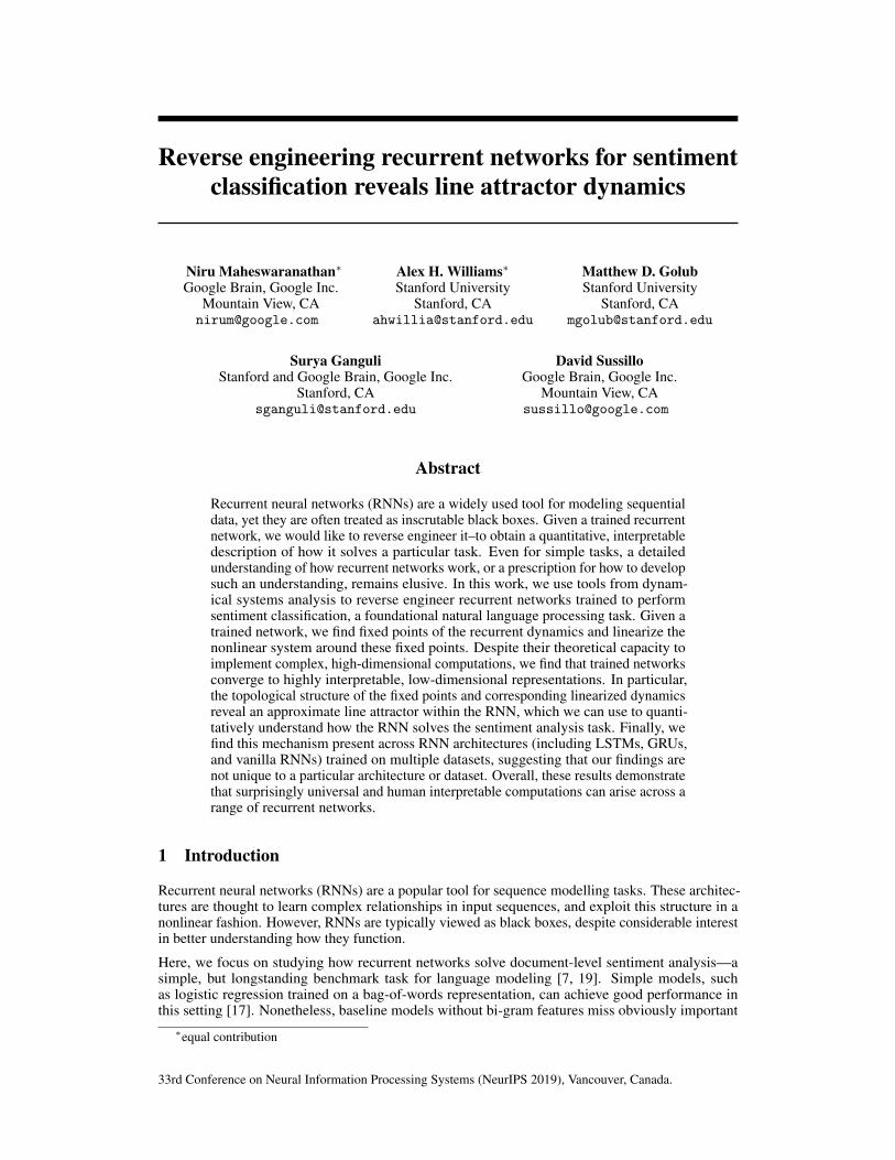
Figure 1: Example LSTM hidden state activity for a network trained on sentiment classification. Eachpanel shows the evolution of the hidden state for all of the units in the network for positive (left) andnegative (right) example documents over the first 150 tokens. At a glance, the activation time seriesfor individual units appear inscrutable.

syntactic relations, such as negation clauses [18]. To capture complex structure in text, especiallyover long distances, many recent works have investigated a wide variety of feed-forward and recurrentneural network architectures for this task (for a review, see [19]).

We demonstrate that popular RNN architectures, despite having the capacity to implement high-dimensional and nonlinear computations, in practice converge to low-dimensional representationswhen trained on this task. Moreover, using analysis techniques from dynamical systems theory, weshow that locally linear approximations to the nonlinear RNN dynamics are highly interpretable.In particular, they all involve approximate low-dimensional line attractor dynamics–a useful dy-namical feature that can be implemented by linear dynamics and can used to store an analog value[13]. Furthermore, we show that this mechanism is surprisingly consistent across a range of RNNarchitectures. Taken together, these results demonstrate how a remarkably simple operation—linearintegration—arises as a universal mechanism in disparate, nonlinear recurrent architectures that solvea real world task.

2 Related Work

Several studies have tried to interpret recurrent networks by visualizing the activity of individualRNN units and memory gates during NLP tasks [5, 15]. While some individual RNN state variablesappear to encode semantically meaningful features, most units do not have clear interpretations. Forexample, the hidden states of an LSTM appear extremely complex when performing a task (Fig.1). Other work has suggested that network units with human interpretable behaviors (e.g. classselectivity) are not more important for network performance [10], and thus our understanding ofRNN function may be misled by focusing only on single interpretable units. Instead, this work aimsto interpret the entire hidden state to infer computational mechanisms underlying trained RNNs.

Another line of work has developed quantitative methods to identify important words or phrases inan input sequence that influenced the model’s ultimate prediction [8, 11]. These approaches canidentify interesting salient features in subsets of the inputs, but do not directly shed light into thecomputational mechanism of RNNs.

3 Methods

3.1 Preliminaries

We denote the hidden state of a recurrent network at time t as a vector, ht. Similarly, the input to thenetwork at time t is given by a vector xt. We use F to denote a function that applies any recurrentnetwork update, i.e. ht+1 = F (ht,xt).

3.2 Training

We trained four RNN architectures–LSTM [4], GRU [1], Update Gate RNN (UGRNN) [2], andstandard (vanilla) RNNs–on binary sentiment classifcation tasks. We trained each network type oneach of three datasets: the IMDB movie review dataset, which contains 50,000 highly polarized

2

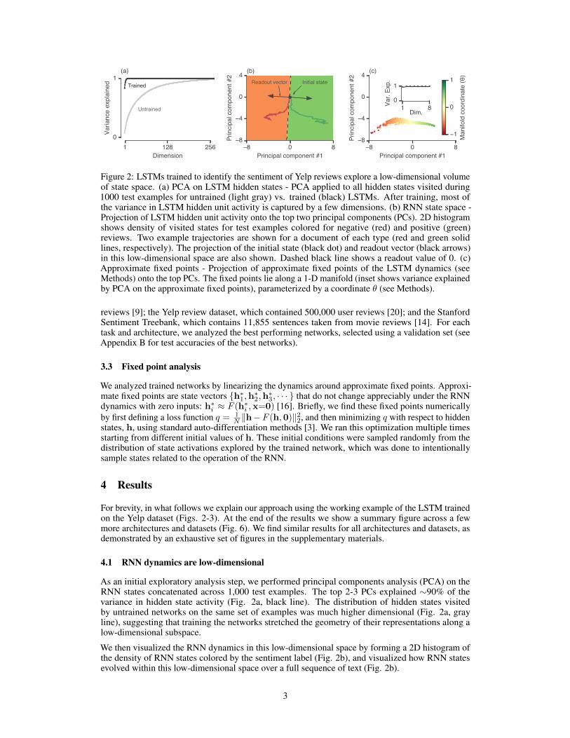
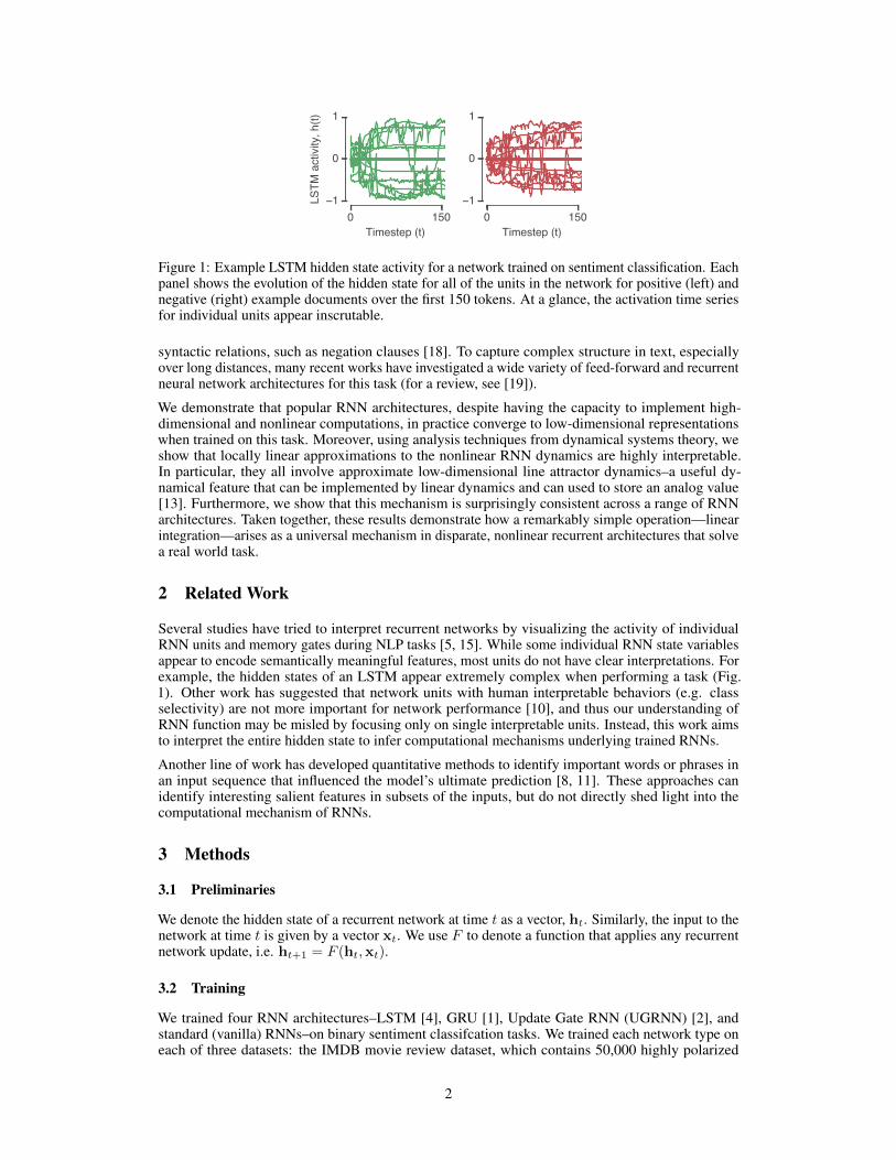
Figure 2: LSTMs trained to identify the sentiment of Yelp reviews explore a low-dimensional volumeof state space. (a) PCA on LSTM hidden states - PCA applied to all hidden states visited during1000 test examples for untrained (light gray) vs. trained (black) LSTMs. After training, most ofthe variance in LSTM hidden unit activity is captured by a few dimensions. (b) RNN state space -Projection of LSTM hidden unit activity onto the top two principal components (PCs). 2D histogramshows density of visited states for test examples colored for negative (red) and positive (green)reviews. Two example trajectories are shown for a document of each type (red and green solidlines, respectively). The projection of the initial state (black dot) and readout vector (black arrows)in this low-dimensional space are also shown. Dashed black line shows a readout value of 0. (c)Approximate fixed points - Projection of approximate fixed points of the LSTM dynamics (seeMethods) onto the top PCs. The fixed points lie along a 1-D manifold (inset shows variance explainedby PCA on the approximate fixed points), parameterized by a coordinate θ (see Methods).

reviews [9]; the Yelp review dataset, which contained 500,000 user reviews [20]; and the StanfordSentiment Treebank, which contains 11,855 sentences taken from movie reviews [14]. For eachtask and architecture, we analyzed the best performing networks, selected using a validation set (seeAppendix B for test accuracies of the best networks).

3.3 Fixed point analysis

We analyzed trained networks by linearizing the dynamics around approximate fixed points. Approxi-mate fixed points are state vectors {h∗1,h∗2,h∗3, · · · } that do not change appreciably under the RNNdynamics with zero inputs: h∗i ≈ F (h∗i ,x=0) [16]. Briefly, we find these fixed points numericallyby first defining a loss function q = 1

N ‖h−F (h,0)‖22, and then minimizing q with respect to hiddenstates, h, using standard auto-differentiation methods [3]. We ran this optimization multiple timesstarting from different initial values of h. These initial conditions were sampled randomly from thedistribution of state activations explored by the trained network, which was done to intentionallysample states related to the operation of the RNN.

4 Results

For brevity, in what follows we explain our approach using the working example of the LSTM trainedon the Yelp dataset (Figs. 2-3). At the end of the results we show a summary figure across a fewmore architectures and datasets (Fig. 6). We find similar results for all architectures and datasets, asdemonstrated by an exhaustive set of figures in the supplementary materials.

4.1 RNN dynamics are low-dimensional

As an initial exploratory analysis step, we performed principal components analysis (PCA) on theRNN states concatenated across 1,000 test examples. The top 2-3 PCs explained ∼90% of thevariance in hidden state activity (Fig. 2a, black line). The distribution of hidden states visitedby untrained networks on the same set of examples was much higher dimensional (Fig. 2a, grayline), suggesting that training the networks stretched the geometry of their representations along alow-dimensional subspace.

We then visualized the RNN dynamics in this low-dimensional space by forming a 2D histogram ofthe density of RNN states colored by the sentiment label (Fig. 2b), and visualized how RNN statesevolved within this low-dimensional space over a full sequence of text (Fig. 2b).

3

8 0 8PC #1

8404

PC #

2

(a)

0.4 1.0( )

0.3

0.0

0.3

()

(b)

0.4 1.0( )

0.3

0.0

0.3

()

0.4 1.0( )

0.3

0.0

0.3

()

0.8 0.0 0.8Manifold coordinate ( )

100101102103104

Tim

e co

nsta

nt (

) (c)

0 128Eigenvalue (index)

100101102103104

Tim

e co

nsta

nt (

) (d)

0 128Eigenvalue (index)

100101102103104

Tim

e co

nsta

nt (

)

0 128Eigenvalue (index)

100101102103104

Tim

e co

nsta

nt (

)

Figure 3: Characterizing the top eigenmodes of each fixed point. (a) Same plot as in Fig. 2c (fixedpoints are grey), with three example fixed points highlighted. (b) For each of these fixed points,we compute the LSTM Jacobian (see Methods) and show the distribution of eigenvalues (coloredcircles) in the complex plane (black line is the unit circle). (c-d) The time constants (τ in terms of #of input tokens, see Appendix C) associated with the eigenvalues. (c) The time constant for the topthree modes for all fixed points as function of the position along the line attractor (parameterizedby a manifold coordinate, θ). (d) All time constants for all eigenvalues associated with the threehighlighted fixed points. The top eigenmode across fixed points has a time constant on the order ofhundreds to thousands of tokens.

We observed that the state vector incrementally moved from a central position towards one or anotherend of the PC-plane, with the direction corresponding either to a positive or negative sentimentprediction. Input words with positive valence (“amazing”, “great”, etc.) incremented the hidden statetowards a positive sentiment prediction, while words with negative valence (“bad”, “horrible”, etc.)pushed the hidden state in the opposite direction. Neutral words and phrases did not typically exertlarge effects on the RNN state vector.

These observations are reminiscent of line attractor dynamics. That is, the RNN state vector evolvesalong a 1D manifold of marginally stable fixed points. Movement along the line is negligible whenevernon-informative inputs (i.e. neutral words) are input to the network, whereas when an informativeword or phrase (e.g. “delicious” or “mediocre”) is encountered, the state vector is pushed towards oneor the other end of the manifold. Thus, the model’s representation of positive and negative documentsgradually separates as evidence is incrementally accumulated.

The hypothesis that RNNs approximate line attractor dynamics makes four specific predictions, whichwe investigate and confirm in subsequent sections. First, the fixed points form an approximately 1Dmanifold that is aligned with the readout weights (Section 4.2). Second, all fixed points are attractingand marginally stable. That is, in the absence of input (or, perhaps, if a string of neutral/uninformativewords are encountered) the RNN state should rapidly converge to the closest fixed point and thenshould not change appreciably (Section 4.4). Third, locally around each fixed point, inputs represent-ing positive vs. negative evidence should produce linearly separable effects on the RNN state vectoralong some dimension (Section 4.5). Finally, these instantaneous effects should be integrated by therecurrent dynamics along the direction of the 1D fixed point manifold (Section 4.5).

4.2 RNNs follow a 1D manifold of stable fixed points

The line attractor hypothesis predicts that RNN state vector should rapidly approach a fixed point ifno input is delivered to the network. To test this, we initialized the RNN to a random state (chosenuniformly from the distribution of states observed on the test set) and simulated the RNN without anyinput. In all cases, the normalized velocity of the state vector (‖ht+1 − ht‖/‖ht‖) approached zerowithin a few steps, and often the initial velocity was small. From this we conclude that the RNN isvery often in close proximity to a fixed point during the task.

We numerically identified the location of ∼500 RNN fixed points using previously establishedmethods [16, 3]. Briefly, we minimized the quantity q = 1

N ‖h− F (h,0)‖22 over the RNN hidden

4

state vector, h, from many initial conditions drawn to match the distribution of hidden states duringtraining. Critical points of this loss function satisfying q < 10−8 were consider fixed points (similarresults were observed for different choices of this threshold). For each architecture, we found ∼500(approximate) fixed points.

We then projected these fixed points into the same low-dimensional space used in Fig. 2b. Althoughthe PCA projection was fit to the RNN hidden states, and not the fixed points, a very high percentageof variance in fixed points was captured by this projection (Fig. 2c, inset), suggesting that the RNNstates remain close to the manifold of fixed points. We call the vector that describes the main axisof variation of the 1D manifold m. Consistent with the line attractor hypothesis, the fixed pointsappeared to be spread along a 1D curve when visualized in PC space, and furthermore the principaldirection of this curve was aligned with the readout weights (Fig. 2c).

We further verified that this low-dimensional approximation was accurate by using locally linearembedding (LLE) [12] to parameterize a 1D manifold of fixed points in the raw, high-dimensionaldata. This provided a scalar coordinate, θi ∈ [−1, 1], for each fixed point, which was well-matchedto the position of the fixed point manifold in PC space (coloring of points in Fig. 2c).

4.3 Linear approximations of RNN dynamics

We next aimed to demonstrate that the identified fixed points were marginally stable, and thus could beused to preserve accumulated information from the inputs. To do this, we used a standard linearizationprocedure [6] to obtain an approximate, but highly interpretable, description of the RNN dynamicsnear the fixed point manifold. Briefly, given the last state ht−1 and the current input xt, the approachis to locally approximate the update rule with a first-order Taylor expansion:

ht = F (h∗ + ∆ht−1,x∗ + ∆xt)

≈ F (h∗,x∗) + Jrec∆ht−1 + Jinp∆xt (1)

where ∆ht−1 = ht−1−h∗ and ∆xt = xt−x∗, and {Jrec,Jinp} are Jacobian matrices of the system:J recij (h∗,x∗) = ∂F (h∗,x∗)i

∂h∗j

and J inpij (h∗,x∗) = ∂F (h∗,x∗)i

∂x∗j

.

We choose h∗ to be a numerically identified fixed point and x∗ = 02, thus we have F (h∗,x∗) ≈ h∗

and ∆xt = xt. Under this choice, equation (1) reduces to a discrete-time linear dynamical system:

∆ht = Jrec∆ht−1 + Jinpxt. (2)

It is important to note that both Jacobians depend on which fixed point we choose to linearize around,and should thus be thought of as functions of h∗; for notational simplicity we do not denote thisdependence explicitly.

By reducing the nonlinear RNN to a linear system, we can analytically estimate the network’sresponse to a sequence of T inputs. In this approximation, the effect of each input xt is decoupledfrom all others; that is, the final state is given by the sum of all individual effects3.

We can restrict our focus to the effect of a single input, xt. Let k = T − t be the number of timesteps between xt and the end of the document. The total effect of xt on the final RNN state is(Jrec)

kJinpxt. After substituting the eigendecomposition Jrec = RΛL for a non-normal matrix, this

becomes:

RΛkLJinpxt =

N∑a=1

λkara`>a Jinpxt, (3)

where L = R−1, the columns of R (denoted ra) contain the right eigenvectors of Jrec, the rowsof L (denoted `>a ) contain the left eigenvectors of Jrec, and Λ is a diagonal matrix containingcomplex-valued eigenvalues, λ1 > λ2 > . . . > λN , which are sorted based on their magnitude.

2We also tried linearizing around the average embedding over all words; this did not change the results. Theaverage embedding is very close to the zeros vector (the norm of the difference between the two is less than8 × 10−3), so it is not surprising that using that as the linearization point yields similar results.

3We consider the case where the network has closely converged to a fixed point, so that h0 = h∗ and thus∆h0 = 0.

5

8 0 8PC #1

840

PC #

2

(b)

0.3 0.0 0.3 PC #1

0.3

0.0

0.3

PC

#2Positivewords

Negativewords

(a)

0.3 0.0 0.3 PC #1

0.3

0.0

0.3

PC

#2

0.3 0.0 0.3 PC #1

0.3

0.0

0.3

PC

#2

0 1Manifold projection (mTr1)

0

15

Freq

uenc

y

Null

Observed

(d)

0.3 0.0 0.3Input projection (` T

1 Jinpx)

0

30Fr

eque

ncy

Negative words Positive words

Neutral words(c)

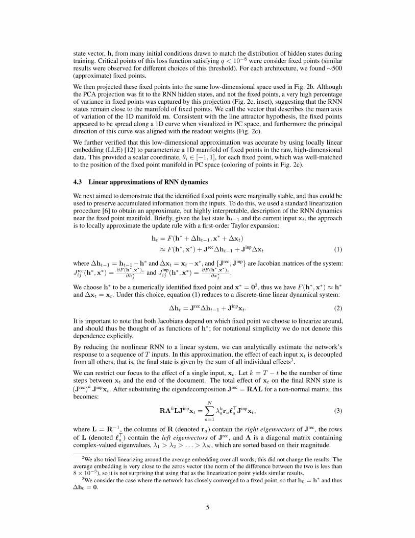
Figure 4: Effect of different word inputs on the LSTM state vector. (a) Effect of word inputs, Jinpx,for positive, negative, and neutral words (green, red, cyan dots). The green and red arrows point to thecenter of mass for the positive and negative words, respectively. Blue arrows denote `1, the top lefteigenvector. The PCA projection is the same as Fig. 2c, but centered around each fixed point. Eachplot denotes a separate fixed point (labeled in panel b). (b) Same plot as in Fig. 2c, with the threeexample fixed points in (a) highlighted (the rest of the approximate fixed points are shown in grey).Blue arrows denote r1, the top right eigenvector. In all cases r1 is aligned with the orientation of themanifold, m, consistent with an approximate line attractor. (c) Average of the projection of inputswith the left eigenvector (`>1 Jinpx) over 100 positive (green), negative (red), or neutral (cyan) words.Histogram displays the distribution of this input projection over all fixed points. (d) Distribution ofr>1 m (overlap of the top right eigenvector with the fixed point manifold) over all fixed points. Nulldistribution consists of randomly generated unit vectors of the same dimension as the hidden state.

4.4 An analysis of integration eigenmodes.

Each mode of the system either reduces to zero or diverges exponentially fast, with a time constantgiven by: τa =

∣∣∣ 1log(|λa|)

∣∣∣ (see Appendix C for derivation). This time constant has units of tokens(or, roughly, words) and yields an interpretable number for the effective memory of the system. Inpractice we find, with high consistency, that nearly all eigenmodes are stable and only a small numbercluster around |λa| ≈ 1.

Fig. 3 plots the eigenvalues and associated time constants and shows the distribution of all eigenvaluesat three representative fixed points along the fixed point manifold (Fig. 3a). In Fig. 3c, we plot thedecay time constant of the top three modes; the slowest decaying mode persists after ∼1000 timesteps, while the next two modes persist after ∼100 time steps, with lower modes decaying even faster.Since the average review length for the Yelp dataset is ∼175 words, only a small number of modescan retain information from the beginning of the document.

Overall, these eigenvalue spectra are consistent with our observation that RNN states only explore alow-dimensional subspace when performing sentiment classification. RNN activity along the majorityof dimensions is associated with fast time constants and is therefore quickly forgotten. While multipleeigenmodes likely contribute to the performance of the network, we restrict this initial study to theslowest mode, for which λ1 ≈ 1.

4.5 Left and right eigenvectors

Restricting our focus to the top eigenmode for simplicity (there may be a few slow modes ofintegration), the effect of a single input, xt, on the network activity (eq. 3) becomes: r1`

>1 Jinpx. We

have dropped the dependence on t since λ1 ≈ 1, so the effect of x is largely insensitive to the exacttime it was input to system. Using this expression, we separately analyzed the effects of specificwords with positive, negative and neutral valences. We defined positive, negative, and neutral wordsbased on the magnitude and sign of the logistic regression coefficients of a bag-of-words classifier.

6

9 0 9Principal component #1

8

4

0

4

Princ

ipal c

ompo

nent

#2

(a)

0.0 0.5 1.0Fractional error

0

5

10

Freq

uenc

y

(b)

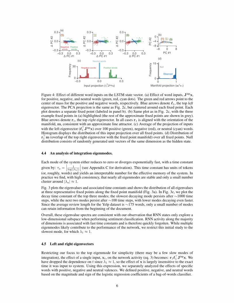
Figure 5: Linearized LSTM dynamics display low fractional error. (a) At every step along a trajectory,we compute the next state using either the full nonlinear system (solid, black) or the linearized system(dashed, red). Inset shows a zoomed in version of the dynamics. (b) Histogram of fractional error ofthe linearized system over many test examples, evaluated in the high-dimensional state space.

We first examined the term Jinpx for various choices of x (i.e. various word tokens). This quantityrepresents the instantaneous linear effect of x on the RNN state vector. We projected the resultingvectors onto the same low-dimensional subspace shown in Fig. 2c. We see that positive and negativevalence words push the hidden state in opposite directions. Neutral words, in contrast, exert muchsmaller effects on the RNN state (Fig 4).

While Jinpx represents the instantaneous effect of a word, only the features of this input that overlapwith the top few eigenmodes are reliably remembered by the network. The scalar quantity `>1 Jinpx,which we call the input projection, captures the magnitude of change induced by x along theeigenmode associated with the longest timescale. Again we observe that the valence of x stronglycorrelates with this quantity: neutral words have an input projection near zero while positive andnegative words produced larger magnitude responses of opposite sign. Furthermore, this is reliablyobserved across all fixed points. Fig. 4c shows the average input projection for positive, negative, andneutral words; the histogram summarizes these effects across all fixed points along the line attractor.

Finally, if the input projection onto the top eigenmode is non-negligible, then the right eigenvectorr1 (which is normalized to unit length) represents the direction along which x is integrated. If theRNN implements an approximate line attractor, then r1 (and potentially other slow modes) shouldalign with the principal direction of the manifold of fixed points, m. In essence, this prediction statesthat an informative input pushes the current RNN state along the fixed point manifold and towards aneighboring fixed point, with the direction of this movement determined by word or phrase valence.We indeed observe a high degree of overlap between r1 and m both visually in PC space (Fig. 4b)and quantitatively across all fixed points (Fig. 4d).

4.6 Linearized dynamics approximate the nonlinear system

To verify that the linearized dynamics (2) well approximate the nonlinear system, we compared hiddenstate trajectories of the full, nonlinear RNN to the linearized dynamics. That is, at each step, wecomputed the next hidden state using the nonlinear LSTM update equations (hLSTM

t+1 = F (ht,xt)), andthe linear approximation of the dynamics at the nearest fixed point (hlin

t+1 = h∗+Jrec (h∗) (ht − h∗)+

Jinp (h∗) xt). Fig. 5a shows the true, nonlinear trajectory (solid black line) as well as the linearapproximations at every point along the trajectory (red dashed line). To summarize the error acrossmany examples, we computed the relative error ‖hLSTM

t+1 − hlint+1‖2/‖hLSTM

t+1 ‖2. Fig. 5b shows thatthis error is small (around 10%) across many test examples.

Note that this error is the single-step error, computed by running either the nonlinear or lineardynamics forward for one time step. If we run the dynamics for many time steps, we find that smallerrors in the linearized system accumulate thus causing the trajectories to diverge. This suggests thatwe cannot, in practice, replace the full nonlinear LSTM with a single linearized version.

4.7 Universal mechanisms across architectures and datasets

Empirically, we investigated whether the mechanisms identified in the LSTM (line attractor dynamics)were present not only for other network architectures but also for networks trained on other datasets

7

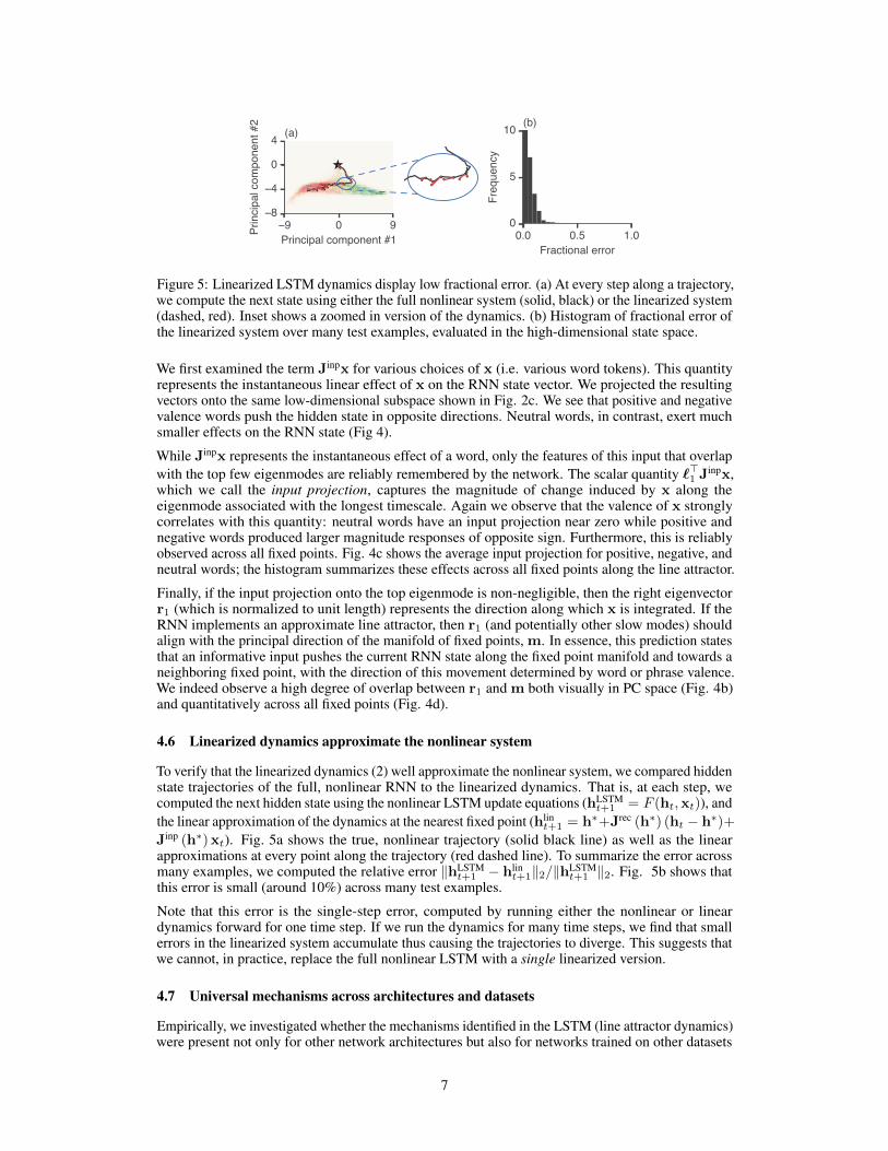
Figure 6: Universal mechanisms across architectures and datasets (see Appendix A for all otherarchitecture-dataset combinations). Top row: comparison of left eigenvector (blue) against instan-taneous effect of word input Jinpx by valence (green and red dots are positive and negative words,compare to Fig. 4a) for an example fixed point. Second row: Histogram of input projections summa-rizing the effect of input across fixed points (average of `>1 Jinpx, compare to Fig. 4c). Third row:Example fixed point (blue) shown on top of the manifold of fixed points (gray) projected into theprincipal components of hidden state activity, along with the corresponding top right eigenvector(compare to Fig. 4b). Bottom row: Distribution of projections of the top right eigenvector onto themanifold across fixed points (distribution of r>1 m, compare to Fig. 4d).

used for sentiment classification. Remarkably, we see a surprising near-universality across networks(but see Supp. Mat. for another solution for the VRNN). Fig. 6 shows, for different architectures anddatasets, the correlation of the the top left eigenvectors with the instantaneous input for a given fixedpoint (first row), as well as a histogram over the same quantity over fixed points (second row). Weobserve the same configuration of a line attractor of approximate fixed points, and show an examplefixed point and right eigenvector highlighted (third row) along with a summary of the projection ofthe top right eigenvector along the manifold across fixed points (bottom row). We see that regardlessof architecture or dataset, each network approximately solves the task using the same mechanism.

5 Discussion

In this work we applied dynamical systems analysis to understand how RNNs solve sentiment analysis.We found a simple mechanism—integration along a line attractor—present in multiple architecturestrained to different sentiment analysis tasks. Overall, this work provides preliminary, but optimistic,evidence that different, highly intricate network models can converge to similar solutions that may bereduced and understood by human practitioners.

In summary, we found that in nearly all cases the key activity performed by the RNN for sentimentanalysis is simply counting the number of positive and negative words used. More precisely, a slowmode of a local linear system aligns its left eigenvector with the current effective input, which itself

8

nicely separates positive and negative word tokens. The associated right eigenvector then representsthat input in a direction aligned to a line attractor, which in turn is aligned to the readout vector. Asthe RNN iterates over a document, integration of negative and positive words moves the system statealong this line attractor, corresponding to accumulation of evidence by the RNN towards a prediction.

Such a mechanism is consistent with a solution that does not make use of word order when making adecision. As such, it is likely that we have not understood all the dynamics relevant in the computationof sentiment analysis. For example, we speculate there may be some yet unknown mechanism thatdetects simple bi-gram negations of one word by another, e.g. “not bad,” since the gated RNNsperformed a few percentage points better than the bag-of-words model. Nonetheless, it appears thatapproximate line attractor dynamics represent a fundamental computational mechanism in theseRNNs, which can be built upon by future investigations.

When we compare the overall classification accuracy of the Jacobian linearized version of the LSTMwith the full nonlinear LSTM, we find that the linearized version is much worse, presumably due tosmall errors in the linear approximation that accrue as the network processes a document. Note thatif we directly train a linear model (as opposed to linearizing a nonlinear model), the performanceis quite high (only around 3% worse than the LSTM), which suggests that the error of the Jacobianlinearized model has to do with errors in the approximation, not from having less expressive power.

We showed that similar dynamical features occur in 4 different architectures, the LSTM, GRU,UGRNN and vanilla RNNs (Fig. 6 and Supp. Mat.) and across three datasets. These rather differentarchitectures all implemented the solution to sentiment analysis in a highly similar way. This hints ata surprising notion of universality of mechanism in disparate RNN architectures.

While our results pertain to a specific task, sentiment analysis is nevertheless representative of alarger set of modeling tasks that require integrating both relevant and irrelevant information over longsequences of symbols. Thus, it is possible that the uncovered mechanisms—namely, approximateline attractor dynamics—will arise in other practical settings, though perhaps employed in differentways on a per-task basis.

Acknowledgments

The authors would like to thank Peter Liu, Been Kim, and Michael C. Mozer for helpful feedbackand discussions.

References

[1] Kyunghyun Cho, Bart van Merrienboer, Caglar Gulcehre, Fethi Bougares, Holger Schwenk,and Yoshua Bengio. Learning Phrase Representations using RNN Encoder-Decoder for Statis-tical Machine Translation. In Proc. Conference on Empirical Methods in Natural LanguageProcessing, Unknown, Unknown Region, 2014.

[2] Jasmine Collins, Jascha Sohl-Dickstein, and David Sussillo. Capacity and trainability inrecurrent neural networks. arXiv preprint arXiv:1611.09913, 2016.

[3] Matthew Golub and David Sussillo. FixedPointFinder: A tensorflow toolbox for identifyingand characterizing fixed points in recurrent neural networks. Journal of Open Source Software,3(31):1003, 2018.

[4] Sepp Hochreiter and Jürgen Schmidhuber. Long short-term memory. Neural computation,9(8):1735–1780, 1997.

[5] Andrej Karpathy, Justin Johnson, and Li Fei-Fei. Visualizing and understanding recurrentnetworks. arXiv preprint arXiv:1506.02078, 2015.

[6] Hassan K. Khalil. Nonlinear Systems. Pearson, 2001.

[7] Bing Liu. Sentiment analysis: Mining opinions, sentiments, and emotions. Cambridge UniversityPress, 2015.

[8] Scott M Lundberg and Su-In Lee. A unified approach to interpreting model predictions. InI. Guyon, U. V. Luxburg, S. Bengio, H. Wallach, R. Fergus, S. Vishwanathan, and R. Garnett,editors, Advances in Neural Information Processing Systems 30, pages 4765–4774. CurranAssociates, Inc., 2017.

9

[9] Andrew L. Maas, Raymond E. Daly, Peter T. Pham, Dan Huang, Andrew Y. Ng, and ChristopherPotts. Learning word vectors for sentiment analysis. In Proceedings of the 49th Annual Meetingof the Association for Computational Linguistics: Human Language Technologies - Volume1, HLT ’11, pages 142–150, Stroudsburg, PA, USA, 2011. Association for ComputationalLinguistics.

[10] Ari S. Morcos, David G.T. Barrett, Neil C. Rabinowitz, and Matthew Botvinick. On theimportance of single directions for generalization. In International Conference on LearningRepresentations, 2018.

[11] W. James Murdoch, Peter J. Liu, and Bin Yu. Beyond word importance: Contextual de-composition to extract interactions from LSTMs. In International Conference on LearningRepresentations, 2018.

[12] Sam T. Roweis and Lawrence K. Saul. Nonlinear dimensionality reduction by locally linearembedding. Science, 290(5500):2323–2326, 2000.

[13] H. S. Seung. How the brain keeps the eyes still. Proceedings of the National Academy ofSciences, 93(23):13339–13344, 1996.

[14] Richard Socher, Alex Perelygin, Jean Wu, Jason Chuang, Christopher D Manning, Andrew Ng,and Christopher Potts. Recursive deep models for semantic compositionality over a sentimenttreebank. In Proceedings of the 2013 conference on empirical methods in natural languageprocessing, pages 1631–1642, 2013.

[15] Hendrik Strobelt, Sebastian Gehrmann, Bernd Huber, Hanspeter Pfister, Alexander M Rush, et al.Visual analysis of hidden state dynamics in recurrent neural networks. CoRR, abs/1606.07461,2016.

[16] David Sussillo and Omri Barak. Opening the black box: low-dimensional dynamics in high-dimensional recurrent neural networks. Neural computation, 25(3):626–649, 2013.

[17] Sida Wang and Christopher D. Manning. Baselines and bigrams: Simple, good sentimentand topic classification. In Proceedings of the 50th Annual Meeting of the Association forComputational Linguistics: Short Papers - Volume 2, ACL ’12, pages 90–94, Stroudsburg, PA,USA, 2012. Association for Computational Linguistics.

[18] Michael Wiegand, Alexandra Balahur, Benjamin Roth, Dietrich Klakow, and Andrés Montoyo.A survey on the role of negation in sentiment analysis. In Proceedings of the Workshop onNegation and Speculation in Natural Language Processing, NeSp-NLP ’10, pages 60–68,Stroudsburg, PA, USA, 2010. Association for Computational Linguistics.

[19] Lei Zhang, Shuai Wang, and Bing Liu. Deep learning for sentiment analysis: A survey. WileyInterdisciplinary Reviews: Data Mining and Knowledge Discovery, 8(4):e1253, 2018.

[20] Xiang Zhang, Junbo Zhao, and Yann LeCun. Character-level convolutional networks for textclassification. In C. Cortes, N. D. Lawrence, D. D. Lee, M. Sugiyama, and R. Garnett, editors,Advances in Neural Information Processing Systems 28, pages 649–657. Curran Associates,Inc., 2015.

10