Remote Sens. OPEN ACCESS remote sensing - TU … · Unité de Recherche Hydrologie-Hydraulique, 5...

Remote Sens. 2014, 6, 8718-8738; doi:10.3390/rs6098718OPEN ACCESS

remote sensingISSN 2072-4292

www.mdpi.com/journal/remotesensing

Article

Assessing Seasonal Backscatter Variations with Respect toUncertainties in Soil Moisture Retrieval in SiberianTundra RegionsElin Högström 1,2,*, Anna Maria Trofaier 1,2,3, Isabelle Gouttevin 4,5 and Annett Bartsch 1,2,6,7

1 Research Group Remote Sensing, Department of Geodesy and Geoinformation (GEO),Vienna University of Technology, Gußhausstraße 27-29, A-1040 Vienna, Austria;E-Mails: [email protected] (A.M.T.); [email protected] (A.B.)

2 Research Group Remote Sensing, Austrian Polar Research Institute, Vienna University,Althanstraße 14, A-1090 Vienna, Austria

3 Scott Polar Research Institute, University of Cambridge, Lensfield Road, Cambridge, CB2 1ER, UK4 Institut National de Recherche en Sciences et Technologies pour l’Environnement et l’Agriculture,

Unité de Recherche Hydrologie-Hydraulique, 5 rue de la Doua, CS 70077, F-69626 VilleurbanneCedex, France; E-Mail: [email protected]

5 CRYOS School of Architecture, Civil and Environmental Engineering, Ecole Polytechnique Federalede Lausanne, Batiment GR, Station 2, CH-1015 Lausanne, Switzerland

6 Department of Geography, Ludwig-Maximilians-Universität München, Luisenstraße 37,D-80333 Munich, Germany

7 IFFB Geoinformatik-Z GIS, Universität Salzburg, Hellbrunner Str, 35, A-5020 Salzburg, Austria

* Author to whom correspondence should be addressed; E-Mail: [email protected];Tel.: +43-1-58801-12266; Fax: +43-1-58801-12299.

Received: 30 June 2014; in revised form: 26 August 2014 / Accepted: 2 September 2014 /Published: 17 September 2014

Abstract: Knowledge of surface hydrology is essential for many applications, includingstudies that aim to understand permafrost response to changing climate and the associatedfeedback mechanisms. Advanced remote sensing techniques make it possible to retrievea range of land-surface variables, including radar retrieved soil moisture (SSM). It hasbeen pointed out before that soil moisture retrieval from satellite data can be challengingat high latitudes, which correspond to remote areas where ground data are scarce and theapplicability of satellite data of this type is essential. This study investigates backscattervariability other than associated with changing soil moisture in order to examine the possibleimpact on soil moisture retrieval. It focuses on issues specific to SSM retrieval in the Arctic,

Remote Sens. 2014, 6 8719

notably variations related to tundra lakes. ENVISAT Advanced Synthetic Aperture Radar(ASAR) Wide Swath (WS, 120 m) data are used to understand and quantify impacts onMetop (AAdvanced Scatterometer (ASCAT, 25 km) soil moisture retrieval during the snowfree period. Sites of interest are chosen according to ASAR WS availability, high or lowagreement between output from the land surface model ORCHIDEE and ASCAT derivedSSM. Backscatter variations are analyzed with respect to the ASCAT footprint area. Itcan be shown that the low model agreement is related to water fraction in most cases.No difference could be detected between periods with floating ice (in snow off situation) andice free periods at the chosen sites. The mean footprint backscatter is however impacted bypartial short term surface roughness change. The water fraction correlates with backscatterdeviations (relative to a smooth water surface reference image) within the ASCAT footprintareas (R = 0.91−0.97). Backscatter deviations of up to 5 dB can occur in areas with lessthan 50% water fraction and an assumed soil moisture related range (sensitivity) of 7 dB inthe ASCAT data. The sensitivity is also positively correlated with water fraction in regionswith low land-surface model agreement (R = 0.68). A precise quantification of the impacton soil moisture retrieval would, however, need to consider actual soil moisture changes andsensor differences. The study demonstrates that the usage of higher spatial resolution datathan currently available for SSM is required in lowland permafrost environments.

Keywords: permafrost; soil moisture; Arctic; high latitudes; water bodies; radar;remote sensing; land surface model

1. Introduction

The pan-Arctic tundra lowlands are underlain by perennially frozen ground known as permafrost.Permafrost warming is ongoing and predicted to increase in magnitude over the course of the 21stcentury [1]. The potential impact that thawing permafrost may have on the global climate systemthrough the release of greenhouse gases has been a concern and a research focus since many years(e.g., [2,3]). Changes to the thermal state of permafrost are linked to rising air temperatures andvariations in the precipitation. These changes to the ground thermal regime are also modifyinghydrological and biogeochemical dynamics [4] which are closely coupled with active layer processes [5].The soil water content (SWC) of the active layer is a driving factor of ecosystem respiration [6] andtherefore soil moisture may be seen as a control parameter for carbon exchange with the atmosphere [7].Soil moisture is highly variable in space and time, controlled by precipitation, redistribution andevapotranspiration. Attempts to address this spatio-temporal variability have led to the developmentof remote sensing techniques employing surface soil moisture (SSM) retrieval algorithms (e.g., [8–11]).The availability and applicability of satellite data in the Arctic is in addition crucial because of theremote nature of this region. Both passive and active microwave sensors are used to produce SSMdata, including global coarse resolution (25–50 km) datasets [12]. Past studies have often focused on


developing methods using active microwave sensors. Scatterometer data have become central to SSMretrieval studies. The ERS scatterometer derived SSM datasets have been used in a number of studies(e.g., [13,14]). More recently the Advanced Scatterometer (ASCAT) data (e.g., [15,16]), includingan operational retrieval method implemented by the European Organization for the Exploitation ofMeteorological Satellites (EUMETSAT), is used for the same purpose. The ASCAT sensor, whichis onboard the polar-orbiting meteorological satellite MetOp (A and B), is well suited for continuousmonitoring, providing 80% daily global coverage [17,18] undertook a validation study that comparessoil moisture products from ASCAT as well as from the passive microwave Soil Moisture Ocean Salinity(SMOS) radiometer with in situ observations. They found that the remotely-sensed SSM products showa significant correlation with the in situ data, capturing the annual cycle as well as trends in short termfluctuations in SSM.

Furthermore, the feasibility of using synthetic aperture radar (SAR) data to extract soil moisturepatterns at higher spatial resolution (1 km) have been investigated (e.g., [19,20]). There are limitations toSSM retrieval from active microwave sensors in cold regions where frozen ground conditions, landscapeheterogeneity and seasonal land cover variations all contribute to the radar’s return signal [21]. Each ofthese factors impacts on the radar scattering mechanism and hence complicates the SSM retrievalmethods that rely on relating differences in the ground’s dielectric properties to soil moisture levelsaccording to the empirical relationship established by [22]. Particularly challenging for the SSM retrievalprocedure are frozen ground conditions. In fact, the soil water index (SWI) method entirely relies onunfrozen and snow-free ground conditions [23]. Phase changes between the liquid and solid states ofwater have a significant effect on its dielectric properties [24–26]. Freezing of the ground usually resultsin low backscatter values that are similar to those attributed to dry soils, which in turn may lead tomisinterpretation [27]. Furthermore, snow scattering processes are even more complex, depending ondepth, density and grain size of the snowpack, as well as wet or dry snow conditions [28]. Information onsnowmelt timings and duration, as well as freeze/thaw cycles can be extracted from the radar signalitself [27,29]. However, they still pose a considerable problem for SSM retrieval in cold regions.The future Soil Moisture Active Passive (SMAP) mission, due to launch in late 2014, will try to addressall of the aforementioned limitations by combining both radar and radiometer measurements [30].

Precipitation records from the field are sparse in remote areas such as the Arctic. Satellite data provideinput data with high temporal and spatial coverage, which in addition can be obtained considerably morefrequently than the field measurements can be collected, which makes it valuable for e.g., real-timeflood forecasting. Thus, to predict precipitation runoff and infiltration, remotely-sensed SSM dataare used as input and/or as validation data for hydrological models [31,32]. In cold regions, thehydrological system is interconnected to the frozen ground, as it hampers the infiltration capacityand percolation. Therefore, permafrost hydrology and active layer processes need to be taken intoaccount for accurate modeling [33]. While permafrost models primarily consider the extent of snowcover and land surface temperatures, simulations of active layer processes rely on soil compositionincluding the active layer’s water retention capability [4]. Permafrost models are either developedas stand-alone algorithms or as modules that are incorporated into Land Surface Models (LSMs) andGeneral Circulation Model (GCMs) [34]. One such LSM is ORCHIDEE (ORganizing Carbon andHydrology in Dynamic EcosystEms). This model is designed to represent terrestrial fluxes (carbon,


water and energy budget). As such, it is a physically-based model that simulates the soil hydrologicaland thermal dynamics, incorporating a soil freezing scheme necessary for appropriately modelinghigh-latitude processes [35]. This present study comes in support of a comparison study betweenmodeling results and satellite-derived surface soil moisture [36], by putting effort in the evaluation ofthe limitations associated with the radar backscatter behavior. In [36] ORCHIDEE output is comparedto an ASCAT SSM product, derived using the algorithm put forward by [17], aggregated on weekly timesteps and adjusted to polar regions [27].

In the present study, we take advantage of the higher spatial resolution data from the European SpaceAgency’s Envisat Advanced Synthetic Aperture Radar (ASAR) operating in Wide Swath (WS, 120 m)mode, to investigate how seasonal dynamics other than surface soil moisture changes can affect the radarbackscatter within proportions of the ASCAT footprints. The focus is on open water surfaces, whosebackscatter signal will be altered by winter lake ice covers and weather conditions, e.g., rain or wind.The open water surfaces are defined by supervised classification (see methods). Previous studies ofcoarse scale scatterometer data from Siberia have concluded that the contribution of lakes and rivers tothe overall normalized radar backscatter is negligible [37]. However, weather induced changes on theopen water surface and seasonal changes of its extent may be impacting on the dry and wet referenceswhich are used as input for relative surface soil moisture retrieval [38] and the impact on coarse resolutionbackscatter has so far not been quantified with respect to water fraction and water body size.

Gouttevin [36] formulates several hypotheses to explain the low agreement between ORCHIDEEand ASCAT SSM, including the topographical impact (for which both the modeling and the SSMretrieval algorithm are not suited), surface ponding (coarsely represented in ORCHIDEE) and unreliablemeteorological forcing data for land-surface modelling in remote, Arctic regions like North-EasternSiberia. The present study examines whether the presence of permanent open water surfaces may be anadditional source of disagreement between the SSM product and the model output.

2. Data and Methods

2.1. Study Sites

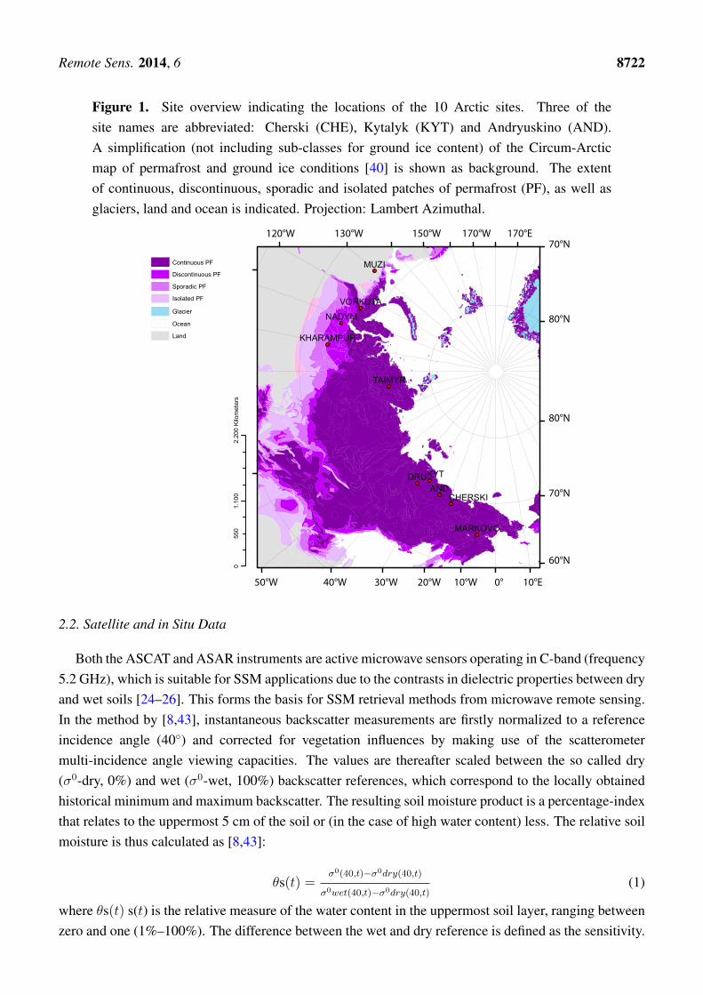
Across Siberia, 10 sites were selected (Figure 1). These sites were chosen in order to representthe diversity of landscapes in the Arctic region and because of their proximity to meteorologicalstations. Furthermore, among the sites, Kytalyk, Cherski, Vorkuta and Nadym are long-term permafrostmonitoring sites [39]. Lastly, an essential criterion for choosing the sites was the ASAR data availability(several acquisitions per month). Kharampur and Vorkuta are underlain by sporadic permafrost andNadym by discontinuous permafrost, whereas all other sites are underlain by continuous permafrost, withthe exception of Muzi, which is not underlain by permafrost [40]. The site locations include lake-richas well as lake-poor areas. The flat and low altitude areas where the sites are located are generally wet.The Western Siberian Lowlands, the coastal plains and the Taimyr Peninsula largely consist of tundralandscapes with predominating wet conditions (e.g., [41,42]).


Figure 1. Site overview indicating the locations of the 10 Arctic sites. Three of thesite names are abbreviated: Cherski (CHE), Kytalyk (KYT) and Andryuskino (AND).A simplification (not including sub-classes for ground ice content) of the Circum-Arcticmap of permafrost and ground ice conditions [40] is shown as background. The extentof continuous, discontinuous, sporadic and isolated patches of permafrost (PF), as well asglaciers, land and ocean is indicated. Projection: Lambert Azimuthal.

ANDDRUKYT

MUZI

NADYM

TAIMYR

MARKOVO

CHERSKI

VORKUTA

KHARAMPUR

Continuous PF

Discontinuous PF

Sporadic PF

Isolated PF

Glacier

Ocean

Land

01.

100

2.20

055

0Ki

lom

eter

s120°W 130°W 150°W 170°W 170°E

70°N

80°N

80°N

70°N

60°N

50°W 40°W 30°W 20°W 10°W 0° 10°E

2.2. Satellite and in Situ Data

Both the ASCAT and ASAR instruments are active microwave sensors operating in C-band (frequency5.2 GHz), which is suitable for SSM applications due to the contrasts in dielectric properties between dryand wet soils [24–26]. This forms the basis for SSM retrieval methods from microwave remote sensing.In the method by [8,43], instantaneous backscatter measurements are firstly normalized to a referenceincidence angle (40◦) and corrected for vegetation influences by making use of the scatterometermulti-incidence angle viewing capacities. The values are thereafter scaled between the so called dry(σ0-dry, 0%) and wet (σ0-wet, 100%) backscatter references, which correspond to the locally obtainedhistorical minimum and maximum backscatter. The resulting soil moisture product is a percentage-indexthat relates to the uppermost 5 cm of the soil or (in the case of high water content) less. The relative soilmoisture is thus calculated as [8,43]:

θs(t) =σ0(40,t)−σ0dry(40,t)

σ0wet(40,t)−σ0dry(40,t)(1)

where θs(t) s(t) is the relative measure of the water content in the uppermost soil layer, ranging betweenzero and one (1%–100%). The difference between the wet and dry reference is defined as the sensitivity.


MetOp-A ASCAT (launched 2006, C-Band, VV polarization) together with its predecessors onboardERS1 and ERS2 (European Remote Sensing Satellite) allows to obtain such references over a time periodreaching back to 1991 [9]. The ASCAT incidence angle ranges from 25◦ to 65◦ and the backscatter isnormalized to a standard incidence angle of 40◦ [44]. The MetOp ASCAT derived dataset which hasbeen used for this study is available globally from TU Wien [8,9,27,43]. The high global coverage(approximately 2 days for mapping the entire globe) and coarse spatial resolution (25 km) makes itappropriate for comparison with global models, such as the ORCHIDEE land surface model.

Since the retrieval algorithm makes use of a change detection technique [12,19] it may be sensitiveto other dynamics than those truly related to soil moisture, such as seasonal water body dynamics.In addition, the SSM values can only be derived under unfrozen conditions. Therefore, an algorithmfor detecting the surface status and if necessary masking frozen surfaces (creating a surface status flag)has already been implemented for high-latitude applications [17,27]. The ASCAT time series data areavailable for a predefined discrete global grid (DGG; for definition see [17]). The grid format is basedon the assumption that the Earth can be modeled as a rotated ellipsoid. Each grid cell over land isattributed a timeseries of backscatter values which are spatially resampled with an equal spacing of12.5 km in latitude and longitude. The cells are identified by a unique grid cell index (GPI) [17]. For thisstudy the global original dataset (without temporal aggregation) has been used, except for the modelto remotely-sensed data comparison, where a weekly composite of the ASCAT data was used [45].This specific dataset was developed as requested by users from the global modeling community withinthe DUE-permafrost project. The weekly composite consists in daily records where the retrieved SSMvalues from the preceding week are averaged.

The ASAR WS (C-band) dataset has a higher spatial resolution than ASCAT. ASAR was a ScanSARinstrument on board ENVISAT. Its spatial resolution in wide swath (WS) mode is 120 m for allsub-swaths [46]. ASAR had a revisit period of 35 days. Data availability is considerably constraintcompared to scatterometer data. Suitable time series can be obtained for a range of locations acrossSiberia for selected years [47]. For this study, an ASAR WS dataset which was pre-processed overNorthern Eurasia for the time period 2007–2008 within the framework of the European Space Agency(ESA) Support To Science Element (STSE) project ALANIS Methane [47–49] was used. Since thebackscatter signal decreases with increasing incidence angle of the radar beam relative to the surface, thebackscatter measurements are normalized to a common reference angle (30◦) using the SAR GeophysicalRetrieval Toolbox (SGRT), which is a scripting chain developed by the Institute of Photogrammetry andRemote Sensing (IPF). The scripting chain calls the commercial SARscape or the free NEST software,allowing for the automatization of the entire preprocessing procedure [47,50]. Single images are split upinto predefined subsets and stored as time series stacks. In addition, the surface status flag developed forASCAT [27] is used for masking the frozen ground condition and melting snow from the ASAR data.Point-station data measurements of maximum- and minimum temperature, precipitation and wind speedwas obtained from the harmonized Global Summary of the Day and Month Observations dataset fromthe Global Precipitation Climatology Center [51].


2.3. Land Surface Model

The land surface model ORCHIDEE combines a multi-layer hydrological scheme recently improvedfor high-latitude processes [35], with a detailed representation of the energy and carbon cycles and theinterface between soil and atmosphere. Of more relevance here is the hydrological scheme, which relieson a vertical discretization of the Richards equation allowing for physically-based diffusion of liquidwater within the soil, up to a depth of 2 m. Soil freezing, vertical soil compaction and the effect of rootwater uptake, are also accounted for [52]. When rainfall of meltwater exceed the infiltration capacityof the uppermost soil layers, exceeding water either ponds or flows as surface runoff, depending on thelocal topography. The model uses as input standard meteorological data (precipitation, air humidity,pressure, temperature, and thermal and solar radiations), which are usually referred to as “forcingdata”. It produces several hydrological outputs, including vertically discretized soil moisture content,subsurface and surface runoff and evapotranspiration. The ORCHIDEE land surface model has provenable to reproduce observed hydrological features even in high-latitude regions [36].

The present study uses the model’s output for vertically discretized volumetric SSM of dailyresolution. In order to compare the average volumetric soil moisture calculated by the model to theweekly aggregated ASCAT SSM data, a number of adaptations were made. The modeled soil moisturefrom the uppermost 5 cm of the soil was masked out for frozen conditions and snow cover. For eachmodel grid cell, the local historical maximum and minimum references were found so that the SWI ofthe model output could be established, rescaling between 0% and 100%. A weekly composite of themodel output from the second step was then produced on a daily basis for consistent comparison withthe ASCAT high-latitudes product from the DUE-permafrost project (see Sections 2.1 and 2.2) [36].On average, the agreement between ORCHIDEE SSM and ASCAT SSM, as measured by the dailycorrelation coefficient of the model and ASCAT weekly composites, is however quite low over our studyareas. Possible reasons for this outcome have been mentioned in the introduction.

2.4. Methodology

ASCAT SSM time series were retrieved for each DGG cell. For comparability, these DGG extentswere used to define regions of interest (ROI) within each ASAR grid stack. For each study site,a 3100 km2 large area was divided into meshes of hexagons using the GPI as center points. This resultedin 9–11 hexagonal ROI within each of the ten sites (Figure 2 shows the 11 ROI in Cherski).

A supervised classification (minimum distance) was performed on ice free ASAR acquisitionswith summer maximal lake expansion and water/land contrasts, to separate land from water. Higherbackscatter than the typical C-band backscatter for smooth water surfaces may be caused by (1) icecovers on water surfaces and (2) wind and rain action. Wave ripples on the water body surface due towind and rain increase the surface roughness and hence lead to diffuse scattering and high backscattervalues [47,53]. The persistence of lake ice on large lakes well into the summer and the associated waterbody classification issues have already been pointed out by [47]. To identify any water surface effects, thewater areas identified by the classification were replaced by the value −20 dB, which is a typical C-bandbackscatter value for smooth water surfaces in the used dataset [47,54]. This builds the reference dataset.


Figure 2. ASAR acquisitions from Cherski, 2008. (A) shows a time with high wind speedand precipitation (11 August 2007); (B) shows a time with prevailing ice cover (17 June2007); (C) illustrates an acquisition from 6 July 2007 when there is no disturbances on thewater surface. The overlain hexagon mesh shows the ROI and their grid point index number.

The mean backscatter result of the masking and replacement by a reference value, henceforth referredto as refilling, was calculated for each ROI and for each available acquisition. This average from thereference datasets was plotted against the original dataset. The mask effect, ∆σ0, is the differencebetween the original and the reference ROI average for each available acquisition. The acquisitions werealso visually interpreted together with meteorological data in order to identify any rain, ice and windconditions. In addition to the above described specific examination of the surface effects (potentiallyfrom ice, rain and/or wind) it was investigated whether the level of agreement between the ASCATand ORCHIDEE SSM results could be related to the abundance of lakes. For this purpose, open waterfraction and lake size were calculated for each ROI from the ASAR WS data by converting the previouslydescribed water classification to polygons. Criteria related to total water cover and lake size were definedand used to separate ROI into three categories:

(A) More than 20% lake area per total area including only lakes larger than 10 km2

(B) More than 20% lake area per total area including only lakes smaller than 10 km2

(C) Less than 20% lake area per total area.

The fractional area of lake, lake count, ∆σ0, ASCAT sensitivity and ASCAT-ORCHIDEE agreementand the correlation thereof, were computed and analysed for each category. Here, the correlation is


meant to determine whether significant relationships exist between lake characteristics, identified lakeeffect on backscatter (∆σ0) and ASCAT SSM retrieval characteristics (sensitivity) or performance (hereassessed by the ASCAT-ORCHIDEE agreement). Since ice is assumed more likely to be present in earlysummer than the high summer months, the ∆σ0 during June was calculated separately from that duringJuly-August, to isolate eventual impacts of prevailing ice cover. For the same reason, a two sampledt-test of the ∆σ0 from June in relation to that in July-August was done in order to know if there wasa significant difference between these two time periods. Analyses of higher temporal resolution thanmonthly could not be done due to the irregular acquisition intervals by ENVISAT ASAR WS [47].

3. Results

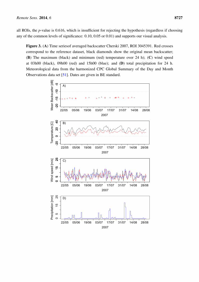
The original mean backscatter for the ROIs is always higher than or equal to the mean backscatterfrom the reference image since frozen ground conditions and spring snowmelt events have beenexcluded. Figure 3A shows the backscatter for one of the ROI in Cherski during 2007, including themean unmasked backscatter (black diamonds) and the mean of the backscatter after having applied thewater mask and replaced the backscatter values with the smooth water surface reference value (−20 dB)(red crosses). It can be seen in Figure 3A and that the difference is in the order of more than 2 dB duringseveral occasions during the warm months of the year. Note that the winter months are excluded sinceASCAT soil moisture is derived only under unfrozen conditions (see Section 2.2). Figure 3B–D showsthe temperature, wind speed and precipitation for the same site and time period.

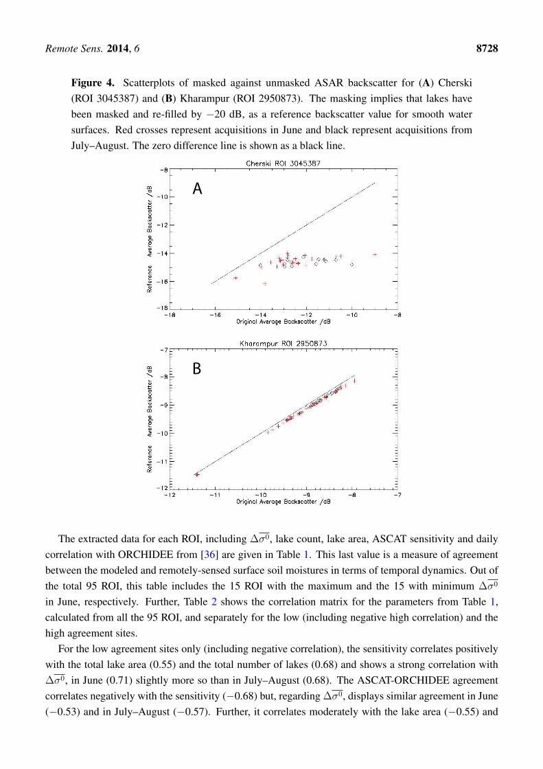
In three of the acquisitions from Cherski in 2007 where ∆σ0 was found to be high, either precipitationor high wind speed was identified by visual interpretation of the ASAR data and in the meteorologicalrecord. One example is the acquisition from 11 August 2007, illustrated in Figure 2A (see Figure 3Dfor precipitation data). Figure 2B shows the same area but an acquisition with presumed ice cover.One occasion with presumed prevailing ice cover (17 June 2007) was visually identified for this siteduring 2007, but strong effects were not recognized compared to the reference (smooth surface).Figure 2C shows relatively smooth water surface conditions for Cherski (6 July 2007), as well as thelimits of the hexagonal ROI for this site and their GPI numbers. For Kytalyk, Andryuskino and partlyfor Druzhina, the results were similar to those from Cherski. In Kharampur, Muzi, Nadym, Taimyr andVorkuta, ∆σ0 is generally low and no significant backscatter change that could be related to weatherconditions was observed in the ASAR data. Scatterplots of the reference values as a function of theoriginal data for one of the ROI in Cherski (subject to high ∆σ0 ) and one of the ROI in Kharampur (notsubject to a high ∆σ0 ) are shown in the left and right panel of Figure 4, respectively.

To isolate the potential effect from prevailing ice cover the early summer months are separated fromthe late summer months: the acquisitions from June are plotted as black diamonds whereas those fromJuly and August as red crosses. Figure 4B shows that the mean from the unmasked backscatter in the caseof Kharampur is similar to that of the masked (reference dataset). A clear difference between ∆σ0 in thelow agreement sites compared to the high agreement sites can be seen. It can not be concluded that ∆σ0

is different during the early summer months from the later summer months. When statistically testing thenull hypothesis that the ∆σ0 is not significantly different in June compared to that in July–August over


all ROIs, the p-value is 0.616, which is insufficient for rejecting the hypothesis (regardless if choosingany of the common levels of significance: 0.10, 0.05 or 0.01) and supports our visual analysis.

Figure 3. (A) Time seriesof averaged backscatter Cherski 2007, ROI 3045391. Red crossescorrespond to the reference dataset, black diamonds show the original mean backscatter;(B) The maximum (black) and minimum (red) temperature over 24 h); (C) wind speedat 03h00 (black), 09h00 (red) and 15h00 (blue); and (D) total precipitation for 24 h.Meteorological data from the harmonized CPC Global Summary of the Day and MonthObservations data set [51]. Dates are given in BE standard.

-20-15-10

-5

Mea

n B

acks

catte

r [dB

]-20-15-10

-5

2007

22/05 05/06 19/06 03/07 17/07 31/07 14/08 28/08

A)

-20

020

40

2007

Tem

pera

ture

[C]

-20

020

40

22/05 05/06 19/06 03/07 17/07 31/07 14/08 28/08

B)

05

1525

2007

Win

d sp

eed

[m/s

]05

1525

05

1525

22/05 05/06 19/06 03/07 17/07 31/07 14/08 28/08

C)

05

1525

2007

Pre

cipi

tatio

n [m

m]

22/05 05/06 19/06 03/07 17/07 31/07 14/08 28/08

D)


Figure 4. Scatterplots of masked against unmasked ASAR backscatter for (A) Cherski(ROI 3045387) and (B) Kharampur (ROI 2950873). The masking implies that lakes havebeen masked and re-filled by −20 dB, as a reference backscatter value for smooth watersurfaces. Red crosses represent acquisitions in June and black represent acquisitions fromJuly–August. The zero difference line is shown as a black line.

A

B

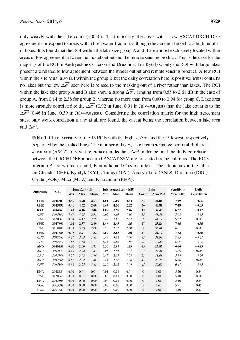
The extracted data for each ROI, including ∆σ0, lake count, lake area, ASCAT sensitivity and dailycorrelation with ORCHIDEE from [36] are given in Table 1. This last value is a measure of agreementbetween the modeled and remotely-sensed surface soil moistures in terms of temporal dynamics. Out ofthe total 95 ROI, this table includes the 15 ROI with the maximum and the 15 with minimum ∆σ0

in June, respectively. Further, Table 2 shows the correlation matrix for the parameters from Table 1,calculated from all the 95 ROI, and separately for the low (including negative high correlation) and thehigh agreement sites.

For the low agreement sites only (including negative correlation), the sensitivity correlates positivelywith the total lake area (0.55) and the total number of lakes (0.68) and shows a strong correlation with∆σ0, in June (0.71) slightly more so than in July–August (0.68). The ASCAT-ORCHIDEE agreementcorrelates negatively with the sensitivity (−0.68) but, regarding ∆σ0, displays similar agreement in June(−0.53) and in July–August (−0.57). Further, it correlates moderately with the lake area (−0.55) and


only weakly with the lake count (−0.30). That is to say, the areas with a low ASCAT-ORCHIDEEagreement correspond to areas with a high water fraction, although they are not linked to a high numberof lakes. It is found that the ROI within the lake size group A and B are almost exclusively located withinareas of low agreement between the model output and the remote sensing product. This is the case for themajority of the ROI in Andryuskino, Cherski and Druzhina. For Kytalyk, only the ROI with large lakespresent are related to low agreement between the model output and remote sensing product. A few ROIwithin the site Muzi also fall within the group B but the daily correlation here is positive. Muzi containsno lakes but the low ∆σ0 seen here is related to the masking out of a river rather than lakes. The ROIwithin the lake size group A and B also show a strong ∆σ0, ranging from 0.55 to 2.61 dB in the case ofgroup A, from 0.14 to 2.38 for group B, whereas no more than from 0.00 to 0.94 for group C. Lake areais more strongly correlated to the ∆σ0 (0.92 in June, 0.91 in July–August) than the lake count is to the∆σ0 (0.46 in June, 0.39 in July–August). Considering the correlation matrix for the high agreementsites, only weak correlation if any at all are found, the caveat being the correlation between lake areaand ∆σ0.

Table 1. Characteristics of the 15 ROIs with the highest ∆σ0 and the 15 lowest, respectively(separated by the dashed line). The number of lakes, lake area percentage per total ROI area,sensitivity (ASCAT dry-wet reference) in decibel, ∆σ0 in decibel and the daily correlationbetween the ORCHIDEE model and ASCAT SSM are presented in the columns. The ROIsin group A are written in bold, B in italic and C as plain text. The site names in the tableare Cherski (CHE), Kytalyk (KYT), Taimyr (TAI), Andryuskino (AND), Druzhina (DRU),Voruta (VOR), Muzi (MUZ) and Kharampur (KHA).

Site Name GPIJune ∆σ0 (dB) July–August ∆σ0 (dB) Lake Sensitivity

Mean (dB)Daily

CorrelationMin Max Mean Min Max Mean Count Area (%)

CHE 3045387 0.85 4.78 2.61 1.01 5.09 2.44 34 44.84 7.29 −0.35CHE 3045391 0.41 4.62 2.60 0.67 4.50 2.22 36 40.82 7.49 −0.35KYT 3084867 1.43 4.16 2.46 1.09 3.98 2.46 12 39.48 6.27 −0.17CHE 3045395 0.69 4.25 2.38 0.02 4.05 1.80 35 41.83 7.08 −0.35TAI 3120067 0.94 4.12 2.25 0.42 3.85 2.97 3 41.17 5.22 0.10

CHE 3047693 1.96 2.37 2.19 1.46 2.45 1.95 27 23.84 7.65 −0.35TAI 3118181 0.83 3.53 2.08 0.38 3.33 2.70 1 32.44 6.01 0.10

CHE 3047689 0.49 3.21 1.82 0.59 3.53 1.66 41 32.19 7.73 −0.35CHE 3047685 0.21 3.33 1.81 0.49 4.01 1.70 42 31.99 7.85 −0.21CHE 3047697 1.54 1.88 1.74 1.31 2.06 1.59 35 17.26 6.89 −0.35AND 3049899 0.62 2.60 1.72 0.36 2.05 1.19 43 23.83 6.06 −0.13AND 3052177 0.49 2.24 1.47 0.05 1.91 1.01 27 23.44 5.89 0.00DRU 3033509 0.21 2.92 1.46 0.47 2.85 1.28 22 18.91 5.74 −0.26AND 3047609 0.61 2.32 1.46 0.41 1.86 1.08 45 22.26 6.36 0.00CHE 3045399 0.38 2.25 1.42 0.20 2.35 1.04 45 30.09 6.41 −0.35

KHA 2948131 0.00 0.01 0.01 0.01 0.01 0.01 0 0.00 5.26 0.34TAI 3120063 0.00 0.01 0.00 0.00 0.01 0.00 0 0.00 5.18 0.10

KHA 2945369 0.00 0.00 0.00 0.00 0.01 0.00 0 0.00 5.40 0.34VOR 3013089 0.00 0.00 0.00 0.00 0.00 0.00 5 0.61 5.91 0.45MUZ 2961321 0.00 0.00 0.00 0.00 0.00 0.00 0 0.00 4.50 0.23


Table 2. Correlation matrix including the number of lakes, lake area percentage per totalROI area, sensitivity (ASCAT dry-wet reference) in decibel, ∆σ0 in decibel and the dailycorrelation between the ORCHIDEE model and ASCAT SSM. The correlation is retrievedfor all the 95 ROI in total. The correlations for ROI with lower agreement than or equal tozero (47 ROI) are presented separated from those with higher agreement than zero (48 ROI).See legend below the table for explanation of bold, italic and asterisk.

Low Agreement Sites

Lake count Lake area Sensitivity June ∆σ0 July–August ∆σ0 Daily correlation

Lake count *** *** *** **Lake area *** *** *** ***Sensitivity 0.55 0.68 *** *** ***June ∆σ0 0.46 0.92 0.71 ***

July–August ∆σ0 0.39 0.91 0.68 ***Daily correlation −0.30 −0.55 −0.68 −0.53 −0.57

High Agreement Sites

Lake count Lake area Sensitivity June ∆σ0 July–August ∆σ0 Daily correlation

Lake count | | | |Lake area | *** *** |Sensitivity 0.03 −0.04 | | |June ∆σ0 0.16 0.97 0.00 |

July–August ∆σ0 0.10 0.96 0.00 |Daily correlation 0.01 −0.25 0.38 −0.25 −0.30

| = p-value insufficient; bold = strong correlation; italic = moderate correlation; ** = p-value < 0.01;*** = p-value < 0.001.

Figure 5 shows ∆σ0 from June in dB plotted against the ASCAT-ORCHIDEE agreement. It can beseen that the ∆σ0 increases with daily correlation, notably so for group A and B. The R2 can not besaid to be strong for any of the groups. However, R2 for group A is notably stronger than both B and C.Results are similar for the two investigated time periods, e.g., June as well as July–August.


Figure 5. Spatially (within each ROI) and temporally (June only) averaged backscatter(∆σ0) in dB plotted against the ASCAT-ORCHIDEE agreement. The regions of interestwith high total lake area percentage and notably large lakes (group A) are shown as bluediamonds and those with high lake area including small lakes (group B) are shown as redsquares. Regions with generally little lake area (group C) are shown as green triangles.This plot includes all the 95 ROI.

4. Discussion

The results confirm that open water surfaces of tundra lakes are typically rough with respect tothe used wavelength (C-band). Indeed, authors have previously estimated an on average −4.9 dBhigher backscatter (same preprocessing) than under calm conditions [50]. Spatially averaged backscatterdeviations for the ROIs which represent the ASCAT cells and include both water and land area reach upto 5 dB. High ∆σ0 correspond with times of high wind speed or precipitation. It is here hypothesizedthat locations with low (including negative) agreement between the ASCAT and ORCHIDEE SSMcorrespond to areas that have many and/or large lakes and that the ∆σ0 at the same locations is high.At sites with positive correlation between ASCAT and the landsurface model SSM (Kharampur, Muzi,Nadym, Taimyr and Vorkuta), ∆σ0 is generally low (<0.71 dB). There are two exceptions in Taimyr,where the mask effect is as large as 2.08 and 2.25 dB. These cases correspond to the only ROI in Taimyrwith a large total water area (32.44% and 41.17%, respectively). This is however not reflected in thethe daily correlation between ASCAT and ORCHIDEE, which is 0.10 for all of the ROI in Taimyr.This could thus be explained by reasons other than water bodies but related to the model, brought up inthe Section 2.3.

At Markovo (eastern Siberia), the model-SSM retrieval agreement is low (−0.06). Here, the ∆σ0

is less pronounced. It is in fact comparable to the high agreement sites, although the site is located inan area of low agreement. For Markovo, the low agreement between the model output and the ASCATdata could be explained by other reasons than water bodies; it is more likely due to the exceptionallyscarce forcing weather data from this part of Siberia [36].


Figure 5 further confirms that there is a difference between the water fraction and lake size classes(groups A, B and C) regarding the dependency of the ASCAT-ORCHIDEE agreement and ∆σ0.Results are similar for the two investigated time periods (June, July-Aug). Although there is some scatteramong the categories and the R2 value is moderate, it is found that the magnitude of ∆σ0 for group Cappears to be independent from the ASCAT-ORCHIDEE correlation whereas it explains 16%–44 % ofthe variation for group A and B.

At sites with an ASCAT-ORCHIDEE correlation lower than −0.21, the average June ∆σ0 rangesfrom 0.56–2.26 dB. This corresponds to 10%–35% of the overall ASCAT sensitivity to soil moisture,which in turn would translate into as much as 35% higher relative soil moisture value if the difference inASAR backscatter (∆σ0) would be directly comparable to the ASCAT soil moisture product. For singleacquisitions it amounts to 60%–70% in areas of 40%–45% water fraction. A direct comparison toASCAT backscatter and quantification of impact on soil moisture retrieval is however limited. One wouldneed to make the assumption that the averaged ASAR WS backscatter over the ROI corresponds to theASCAT backscatter. The hexagonal grid of ROI generated in this study is merely an approximationof the ASCAT grid cells. Furthermore, the absolute backscatter values may deviate due to incidenceangle differences (ranging from 25◦ to 65◦) and differences in signal contribution over the footprintfor ASCAT [44] as well as actual soil moisture changes. In the cases when the high backscatter eventscoincide with precipitation events, the impact of dielectric properties changes would need to be taken intoaccount.In the cases when the high backscatter events coincide with precipitation events, the impact ofdielectric properties changes would need to be taken into account: it is difficult to separate the backscattervariations due to the actual increase in soil moisture from the action that the rain causes on the surface.Furthermore, it should be considered that the ASCAT dataset which has been used for comparison withORCHIDEE has been aggregated to weekly time steps. One can expect a smoothing of the backscattervariations in this case, so the actual disagreement with the model may be higher when compared ona daily basis.

For soil moisture retrieval the signal is impacted if the area covered by open water surface withinthe footprint is large [38]. A surface water fraction flag, derived from the Global Lakes and WetlandsDatabase [55], exists but it does not take wetland dynamics, temporary inundation and small lakes intoaccount [54]. An improved flag of this kind could be derived from ASAR data [13,56]. Tundra lakescan be considerably smaller than the ASAR WS resolution [57]. The impact of these small lakes wouldneed to be analyzed in addition for the development of a correction algorithm of the scatterometer soilmoisture datasets, e.g., by taking into account subpixel-scale fraction of water cover [57].

5. Conclusions

This study examines backscatter variabilities other than related to soil moisture in order to addresschallenges in radar soil moisture retrieval that are specific for in the Arctic. The impact on the soilmoisture retrieval is investigated for sites across Siberia, including permafrost longterm monitoringsites. Satellite derived surface soil moisture datasets would provide valuable additional informationto point measurements in these regions. Envisat ASAR WS imaging radar data are investigated in orderto identify seasonal variations in backscatter that are not related to SSM but to lake cover surface status.


This gives an indication for the magnitude of the impact of such features on the coarser spatial resolutionASCAT SSM retrieval, and cast some light on the model-to-ASCAT low agreement in SSM, highlightedby a previously published study [36]. Different techniques and sensors can be used for SSM retrievalfrom satellites [7,8,10]. The findings of this study can be applied to systems relying on similar principles:change detection approach in a backscattered signal that is impacted by surface soil moisture but also bysurface conditions, e.g., water surface roughness or frozen conditions. Most importantly, these specificfindings are applicable to C-band sensors.

Identified backscatter difference is in the order of 2 dB on the mean backscatter over several weeksand up to 5 dB on specific acquisitions in the areas with low ORCHIDEE-ASCAT agreement (no ornegative correlation). In comparison, the assumed ASCAT sensitivity for soil moisture changes reachesapproximately 7 dB in these areas. A direct translation of the identified difference to deviations of thesoil moisture values from the actual values would need to take sensor and data processing differencesinto account.

Regions with high backscatter deviations (averaged over ASCAT grid cell) from the reference datasetrepresenting smooth water surfaces (∆σ0) are however evidently characterized by a high percentage oftotal lake area, i.e., many of the ROI in eastern Siberia: Cherski, Andryuskio, Druzhina and Kytalyk.The sites Kharampur, Taimyr, Nadym, Vorkuta and Muzi (western and central Siberia), show low ∆σ0

and are areas with few lakes. In the case of Markovo (far eastern Siberia) the low agreement betweenthe model output and the SSM product is more likely explained by the exceptionally scarce weather datafrom this area used to force the model [36]. Although events of wind and precipitation identified bythe meteorological data only occurred infrequently for each site, the correlation between the backscatterdeviation and the ASCAT-ORCHIDEE agreement together with the lake size distribution lead to theconclusion that water body fraction and water body size is one explanation for the disagreement betweenthe ASCAT and ORCHIDEE SSM. In this context, it should be considered that the ORCHIDEE modeldoes not represent ephemeral lakes (i.e., normally dry lakes that fills with water for short periods), whichare an additional source of error for ORCHIDEE in lake-rich areas.

The low and negative correlation sites compared to the high agreement sites clearly show differentresults for the ∆σ0 in relation to the total lake expansion and size distribution. However, no significantdifference was shown between the early and late summer months. The presence of ice cover on lakesdoes not give strong effect on the ∆σ0 in this study.

In addition to the above and other model-related issues as discussed by [36], the low agreementbetween ORCHIDEE and ASCAT SSM in the Siberian lowlands is likely related to the existence ofwater bodies. Therefore, it should be noted that in circumpolar lowland permafrost areas, where pondsand lakes are common features, the presence of water bodies has an impact on the ASCAT SSM retrieval.This supports what has previously been pointed out about open water having a disturbing influence onthe signal and thus for the surface soil moisture retrieval if the area covered by open water surface withinthe footprint is large [38]. In Siberia, an improved surface flag product that takes into account wetlanddynamics could be derived from Synthetic Aperture Radar (SAR) imagery [32,53]. The usage of higherspatial resolution data for SSM retrieval as available from Sentinel-1 is required in regions with largewater fractions, including lowland permafrost environments.


Acknowledgments

The authors acknowledge financial support by the European Union FP7-ENV project PAGE21(Changing Permafrost in the Arctic and its Global effects in the 21st century) under contractNo. GA282700. The ALANIS project was funded by the European Space Agency (ESA) Support toScience Element (STSE) program (ESRIN Contr. No. 4000100647/10/I-LG).

Author Contributions

All co-authors have substantially contributed to the writing of the manuscript. In addition,Elin Högström has carried out all analyses and prepared the first draft. Anna Maria Trofaier has set thestudy into a wider context including SAR applications, took care of layout and provided native Englishediting. All items related to land surface modelling have been prepared by Isabella Gouttevin. AnnettBartsch developed the concept for the study and provided expertise in EO data handling.

Conflicts of Interest

The authors declare no conflict of interest.

References

1. IPCC. Observations: Cryosphere. In Proceedings of the Climate Change 2013: The PhysicalScience Basis. Contribution of Working Group I to the Fifth Assessment Report of theIntergovernmental Panel on Climate Change, Stockholm, Sweden, 23–26 September 2013;pp. 362–364.

2. Friborg, T.; Soegaard, H.; Christensen, T.; Lloyd, C.; Panikov, N. Siberian wetlands: Where asink is a source. Geophys. Res. Lett. 2004, 30, doi:10.1029/2003GL017797

3. Christensen, T.R.; Johansson, T.R.; Akerman, H.J.; Mastepanov, M.; Malmer, N.; Friborg, T.;Crill, P.; Svensson, B H. Thawing sub-arctic permafrost: Effects on vegetation and methaneemissions. Geophys. Res. Lett. 2004, 31, doi:10.1029/2003GL018680

4. Langer, M.; Westermann, S.; Heikenfeld, M.; Dorn, W.; Boike, J. Satellite-based modeling ofpermafrost temperatures in a tundra lowland landscape. Remote Sens. Environ. 2013, 135, 12–24.

5. Swenson, S.; Lawrence, D.; Lee, H. Improved simulation of the terrestrial hydrological cyclein permafrost regions by the Community Land Model. J. Adv. Model. Earth Syst. 2012, 4,doi:10.1029/2012MS000165.

6. Lupascu, M.; Welker, J.; Seibt, U.; Maseyk, K.; Xu, X.; Czimczik, C. High Arctic wetting reducespermafrost carbon feedbacks to climate warming. Nat. Clim. Chang. 2013, 4, 51–55.

7. Kimball, J.S.; Jones, L.A.; Zhang, K.; Heinsch, F.A.; McDonald, K.C.; Oechel, W.C. A satelliteapproach to estimate land—Atmosphere exchange for boreal and arctic biomes using MODIS andAMSR-E. IEEE Trans. Geosci. Remote Sens. 2009, 47, 569–587.

8. Wagner, W.; Noll, J.; Borgeaud, M.; Rott, H. Monitoring soil moisture over the Canadian prairieswith the ERS scatterometer. IEEE Trans. Geosci. Remote Sens. 1999, 37, 206–216.


9. Naeimi, V.; Bartalis, Z.; Wagner, W. ASCAT soil moisture: An assessment of the data quality andconsistency with the ERS scatterometer heritage. J. Hydrometeorol. 2009, 10, 555–563.

10. Njoku, E.G.; Jackson, T.J.; Lakshmi, V.; Chan, T.K.; Nghiem, S.V. Soil moisture retrieval fromAMSR-E. IEEE Trans. Geosci. Remote Sens. 2003, 41, 215–229.

11. Koike, T.; Nakamura, Y.; Kaihotsu, I.; Davva, G.; Matsuura, N.; Tamagawa, K.; Fujii, H.Development of an Advanced Microwave Scanning Radiometer (AMSR-E) algorithm of soilmoisture and vegetation water content. Annu. J. Hydraul. Eng. JSCE 2004, 48, 217–222.

12. Wagner, W.; Bloschl, G.; Pampaloni, P.; Calvet, J.C.; Bizzarri, B.; Wigneron, J.P.; Kerr, Y.Operational readiness of microwave remote sensing of soil moisture for hydrologic applications.Nord. Hydrol. 2007, 38, 1–20.

13. Bartsch, A.; Balzter, H.; George, C. The influence of regional surface soil moisture anomalieson forest fires in Siberia observed from satellites. Environ. Res. Lett. 2009, 4.doi:10.1088/1748-9326/4/4/045021.

14. Künzer, C.; Zhao, D.; Scipal, K.; Sabel, D.; Naeimi, V.; Bartalis, Z.; Hasenauer, S.; Mehl, H.;Dech, S.; Wagner, W. El Niño influences represented in ERS scatterometer derived soil moisturedata. Appl. Geogr. 2009, 29, 463–477.

15. Paulik, C.; Dorigo, W.; Wagner, W.; Kidd, R. Validation of the ASCAT soil water index usingin situ datafrom the international soil moisture network. Int. J. Appl. Earth Obs. Geoinf.2014, 30, 1–8.

16. Brocca, L.; Melone, F.; Moramarco, T.; Wagner, W.; Hasenauer, S. ASCAT soil wetness indexvalidation through in situ and modeled soil moisture data in central Italy. Remote Sens. Environ.2010, 114, 2745–2755.

17. Naeimi, V.; Scipal, K.; Bartalis, Z.; Hasenauer, S.; Wagner, W. An improved soil moisture retrievalalgorithm for ERS and METOP scatterometer observations. IEEE Trans. Geosci. Remote Sens.2009, 47, 1999–2013.

18. Albergel, C.; de Rosnay, P.; Gruhier, C.; Muñoz-Sabater, J.; Hasenauer, S.; Isaksen, L.; Kerr, Y.;Wagner, W. Evaluation of remotely sensed and modelled soil moisture products using globalground-based in situ observations. Remote Sens. Environ. 2012, 118, 215–226.

19. Wagner, W.; Pathe, C.; Doubkova, M.; Sabel, D.; Bartsch, A.; Hasenauer, S.; Blöschl, G.;Scipal, K.; Martínez-Fernández, J.; Löw, A. Temporal stability of soil moisture and radarbackscatter observed by the Advanced Synthetic Aperture Radar (ASAR). Sensors 2008, 8,1174–1197.

20. Doubkova, M.; van Dijk, A.I.J.M.; Sabel, D.; Wagner, W.; Blöschl, G. Evaluation of thepredicted error of the soil moisture retrieval from C-band SAR by comparison against modelledsoil moisture estimates over Australia. Remote Sens. Environ. 2012, 120, 188–196.

21. Bartsch, A.; Sabel, D.; Wagner, W.; Park, S.E. Considerations for derivation and use of soilmoisture data from active microwave satellites at high latitudes. In Proceedings of the 2011 IEEEInternational Geoscience and Remote Sensing Symposium (IGARSS), Vancouver, BC, Canada,24–29 July 2011; pp. 3132–3135.


22. Ulaby, F.T.; Moore, R.K.; Fung, A.K. Microwave Remote Sensing, Active and Passive, III, RadarRemote Sensing and Surface Scattering and Emission Theory; Artech House Publishers: London,UK/Boston, MA, USA, 1986.

23. Scipal, K.; Drusch, M.; Wagner, W. Assimilation of a ERS scatterometer derived soil moistureindex in the ECMWF numerical weather prediction system. Adv. Water Resour. 2008, 31,1101–1112.

24. Ulaby, F.T.; Moore, R.K.; Fung, A.K. Microwave Remote Sensing, Active and Passive, II, RadarRemote Sensing and Surface Scattering and Emission Theory; Artech House Publishers: London,UK/Boston, MA, USA, 1982.

25. Way, J.; Zimmermann, R.; Rignot, E.; McDonald, K.; Oren, R. Winter and spring thaw asobserved with imaging radar at BOREAS. J. Geophys. Res. Atmos. (1984–2012) 1997, 102,29673–29684.

26. Wegmüller, U. The effect of freezing and thawing on the microwave signatures of bare soil.Remote Sens. Environ. 1990, 33, 123–135.

27. Naeimi, V.; Paulik, C.; Bartsch, A.; Wagner, W.; Kidd, R.; Park, S.E.; Elger, K.; Boike, J.ASCAT Surface State Flag (SSF): Extracting information on surface freeze/thaw conditions frombackscatter data using an empirical threshold-analysis algorithm. IEEE Trans. Geosci. RemoteSens. 2012, 50, 2566–2582.

28. Bartsch, A. Ten years of SeaWinds on QuikSCAT for snow applications. Remote Sens. 2010, 2,1142–1156.

29. Bartsch, A.; Kidd, R.A.; Wagner, W.; Bartalis, Z. Temporal and spatial variability of the beginningand end of daily spring freeze/thaw cycles derived from scatterometer data. Remote Sens. Environ.2007, 106, 360–374.

30. Entekhabi, D.; Njoku, E.G.; O’Neill, P.E.; Kellogg, K.H.; Crow, W.T.; Edelstein, W.N.;Entin, J.K.; Goodman, S.D.; Jackson, T.J.; Johnson, J.; et al. The soil moisture active passive(SMAP) mission. IEEE Proc. 2010, 98, 704–716.

31. Brocca, L.; Moramarco, T.; Melone, F.; Wagner, W.; Hasenauer, S.; Hahn, S. Assimilation ofsurface- and root-zone ASCAT soil moisture products into rainfall-runoff modeling. IEEE Trans.Geosci. Remote Sens. 2012, 50, 2542–2555.

32. Schumann, G.; Bates, P.D.; Horritt, M.S.; Matgen, P.; Pappenberger, F. Progress in integration ofremote sensing—Derived flood extent and stage data and hydraulic models. Rev. Geophys. 2009,47, doi:10.1029/2008RG000274.

33. Woo, M.K.; Kane, D.L.; Carey, S.K.; Yang, D. Progress in permafrost hydrology in the newmillennium. Permafr. Periglac. Process. 2008, 19, 237–254.

34. Marchenko, S.; Romanovsky, V.; Tipenko, G. Numerical modeling of spatial permafrost dynamicsin Alaska. In Proceedings of the Ninth International Conference on Permafrost, Institute ofNorthern Engineering, University of Alaska Fairbanks, Fairbanks, AK, USA, 29 June–3 July2008; Volume 29, pp. 1125–1130.

35. Gouttevin, I.; Krinner, G.; Ciais, P.; Polcher, J.; Legout, C. Multi-scale validation of a new soilfreezing scheme for a land-surface model with physically-based hydrology. Cryosphere 2012, 6,407–430.


36. Gouttevin, I.; Bartsch, A.; Krinner, G.; Naeimi, V. A comparison between remotely-sensed andmodelled surface soil moisture (and frozen status) at high latitudes. Hydrol. Earth Syst. Sci.Discuss. 2013, 10, doi:10.5194/hessd-10-11241-2013.

37. Wismann, V. Monitoring of seasonal thawing in Siberia with ERS scatterometer data. IEEETrans. Geosci. Remote Sens. 2000, 38, 1804–1809.

38. Wagner, W.; Hahn, S.; Kidd, R.; Melzer, T.; Bartalis, Z.; Hasenauer, S.; Figa-Saldaña, J.;de Rosnay, P.; Jann, A.; Schneider, S.; et al. The ASCAT soil moisture product: A review ofits specifications, validation results, and emerging applications. Meteorol. Z. 2013, 22, 5–33.

39. Romanovsky, V.E.; Smith, S.L.; Christiansen, H.H. Permafrost thermal state in the polar NorthernHemisphere during the international polar year 2007–2009: A synthesis. Permafr. Periglac.Process. 2010, 21, 106–116.

40. Brown, J.; Ferrians, O.J.; Heginbottom, J.; Melnikov, E. Circum-Arctic Map of Permafrost andGround-Ice Conditions; National Snow and Ice Data Center; Digital Media. Available online:http://nsidc.org/data/docs/fgdc/ggd318_map_circumarctic/ (accessed on 17 September 2014).

41. Serreze, M.C.; Etringer, A.J. Precipitation characteristics of the Eurasian Arctic drainage system.Int. J. Climatol. 2003, 23, 1267–1291.

42. Boike, J.; Wille, C.; Abnizova, A. Climatology and summer energy and water balance ofpolygonal tundra in the Lena River Delta, Siberia. J. Geophys. Res. Biogeosci. (2005–2012)2008, 113, doi:10.1029/2007JG000540.

43. Wagner, W.; Lemoine, G.; Borgeaud, M.; Rott, H. A study of vegetation cover effects on ERSscatterometer data. IEEE Trans. Geosci. Remote Sens. 1999, 37, 938–948.

44. Bartalis, Z.; Wagner, W.; Naeimi, V.; Hasenauer, S.; Scipal, K.; Bonekamp, H.; Figa, J.;Anderson, C. Initial soil moisture retrieval from the METOP—A Advanced Scatterometer(ASCAT). Geophys. Res. Lett. 2007, 34, doi:10.1029/2007GL031088.

45. Paulik, C.; Melzer, T.; Hahn, S.; Bartsch, A.; Heim, B.; Elger, K.; Wagner, W. CircumpolarSurface Soil Moisture and Freeze/Thaw Surface Status Remote Sensing Products (Version 2)with Links to Geotiff Images and NetCDF Files (2007-01 to 2010-09); TU Vienna: Vienna,Austria, 2012.

46. Closa, J.; Rosich, B.; Monti-Guarnieri, A. The ASAR wide swath mode products. In Proceedingsof the 2003 IEEE International Geoscience and Remote Sensing Symposium (IGARSS’03),Toulouse, France, 21–25 July 2003; Volume 2, pp. 1118–1120.

47. Bartsch, A.; Trofaier, A.; Hayman, G.; Sabel, D.; Schlaffer, S.; Clark, D.; Blyth, E. Detection ofopen water dynamics with ENVISAT ASAR in support of land surface modelling at high latitudes.Biogeosciences 2012, 9, 703–714.

48. Reschke, J.; Bartsch, A.; Schlaffer, S.; Schepaschenko, D. Capability of C-Band SAR foroperational wetland monitoring at high latitudes. Remote Sens. 2012, 4, 2923–2943.

49. Trofaier, A.; Bartsch, A.; Rees, W.; Leibman, M. Assessment of spring floods and surfacewater extent over the Yamalo-Nenets Autonomous District. Environ. Res. Lett. 2013, 8,doi:10.1088/1748-9326/8/4/045026.

http://nsidc.org/data/docs/fgdc/ggd318_map_circumarctic/


50. Sabel, D.; Bartsch, A.; Schlaffer, S.; Klein, J.P.; Wagner, W. Soil moisture mapping inpermafrost regions—An outlook to Sentinel-1. In Proceedings of the 2012 IEEE InternationalGeoscience and Remote Sensing Symposium (IGARSS), Munich, Germany, 22–27 July 2012;pp. 1216–1219.

51. Climate Prediction Center/National Centers for Environmental Prediction/National WeatherService/NOAA/U.S. Dpt. of Commerce. 1987, Updated Half-Yearly. CPC Global Summaryof Day/Month Observations, 1979-Continuing. Research Data Archive at the National Center forAtmospheric Research, Computational and Information Systems Laboratory. Dataset. Availableonline: http://rda.ucar.edu/datasets/ds512.0/ (accessed on 27 July 2011).

52. de Rosney, P.; Polcher, J. Modelling root water uptake in a complex land surface scheme coupledto a GCM. Hydrol. Earth Syst. Sci. 1998, 2, 239–255.

53. Bartsch, A.; Wagner, W.; Scipal, K.; Pathe, C.; Sabel, D.; Wolski, P. Global monitoring ofwetlands—The value of ENVISAT ASAR Global mode. J. Environ. Manag. 2009, 90,2226–2233.

54. Bartsch, A.; Pathe, C.; Wagner, W.; Scipal, K. Detection of permanent open water surfaces incentral Siberia with ENVISAT ASAR wide swath data with special emphasis on the estimation ofmethane fluxes from tundra wetlands. Hydrol. Res. 2008, 39, 89–100.

55. Lehner, B.; Döll, P. Development and validation of a global database of lakes, reservoirs andwetlands. J. Hydrol. 2004, 296, 1–22.

56. Schumann, G.; Lunt, D.; Valdes, P.; de Jeu, R.; Scipal, K.; Bates, P. Assessment of soil moisturefields from imperfect climate models with uncertain satellite observations. Hydrol. Earth Syst.Sci. 2009, 13, 1545–1553.

57. Muster, S.; Langer, M.; Heim, B.; Westermann, S.; Boike, J. Subpixel heterogeneity of ice-wedgepolygonal tundra: A multi-scale analysis of land cover and evapotranspiration in the Lena RiverDelta, Siberia. Tellus B 2012, 64, doi:10.3402/tellusb.v64i0.17301.

c© 2014 by the authors; licensee MDPI, Basel, Switzerland. This article is an open access articledistributed under the terms and conditions of the Creative Commons Attribution license(http://creativecommons.org/licenses/by/3.0/).

http://rda.ucar.edu/datasets/ds512.0/

Remote Sens. OPEN ACCESS remote sensing - TU … · Unité de Recherche Hydrologie-Hydraulique, 5...

Documents

Transcript of Remote Sens. OPEN ACCESS remote sensing - TU … · Unité de Recherche Hydrologie-Hydraulique, 5...