
Random graphs and complex networksrhofstad/NotesRGCNII.pdf1.2 Random graphs and real-world networks9...
359
RANDOM GRAPHS AND COMPLEX NETWORKS Volume 2 Remco van der Hofstad January 31, 2020
Transcript of Random graphs and complex networksrhofstad/NotesRGCNII.pdf1.2 Random graphs and real-world networks9...

RANDOM GRAPHS AND COMPLEX NETWORKS
Volume 2
Remco van der Hofstad
January 31, 2020


Aan Mad, Max en Larshet licht in mijn leven
Ter nagedachtenis aan mijn oudersdie me altijd aangemoedigd hebben

Contents
List of illustrations ix
List of tables xi
Preface xiii
Course outline xvii
Part I Preliminaries 1
1 Introduction and preliminaries 31.1 Motivation: Real-world networks 41.2 Random graphs and real-world networks 91.3 Random graph models 11
1.3.1 Erdos-Renyi random graph 111.3.2 Inhomogeneous random graphs 131.3.3 Configuration model 171.3.4 Switching algorithms for uniform random graphs 221.3.5 Preferential attachment models 271.3.6 A Bernoulli preferential attachment model 301.3.7 Universality of random graphs 31
1.4 Power-laws and their properties 321.5 Notation 331.6 Notes and discussion 341.7 Exercises for Chapter 1 35
2 Local weak convergence of random graphs 372.1 The metric space of rooted graphs 372.2 Local weak convergence of graphs 392.3 Local weak convergence of random graphs 42
2.3.1 Local weak convergence and completeness of the limit 452.4 Consequences of local weak convergence: local functionals 46
2.4.1 Local weak convergence and convergence of neighborhoods 462.4.2 Local weak convergence and clustering coefficients 472.4.3 Neighborhoods of edges and degree-degree dependencies 47
2.5 The giant component is almost local 472.6 Notes and discussion 502.7 Exercises for Chapter 2 51
Part II Connected components in random graphs 55
3 Phase transition in general inhomogeneous random graphs 593.1 Motivation 593.2 Definition of the model 61
3.2.1 Examples of inhomogeneous random graphs 643.3 Degree sequence of inhomogeneous random graphs 66
v
vi Contents
3.3.1 Degree sequence of finitely-types case 673.3.2 Finite-type approximations of bounded kernels 673.3.3 Degree sequences of general inhomogeneous random graphs 69
3.4 Multitype branching processes 713.4.1 Multitype branching processes with finitely many types 713.4.2 Survival vs. extinction of multitype branching processes 723.4.3 Poisson multitype branching processes 74
3.5 Local weak convergence for inhomogeneous random graphs 783.5.1 Local weak convergence: finitely many types 793.5.2 Local weak convergence: infinitely many types 833.5.3 Comparison to branching processes 843.5.4 Local weak convergence to unimodular trees for GRGn(w) 87
3.6 The phase transition for inhomogeneous random graphs 873.7 Related results for inhomogeneous random graphs 923.8 Notes and discussion 943.9 Exercises for Chapter 3 95
4 The phase transition in the configuration model 1014.1 Local weak convergence to unimodular trees for CMn(d) 1024.2 Phase transition in the configuration model 107
4.2.1 Finding the largest component 1114.2.2 Analysis of the algorithm for CMn(d) 1134.2.3 Proof of Theorem 4.4 1184.2.4 The giant component of related random graphs 122
4.3 Connectivity of CMn(d) 1244.4 Related results for the configuration model 1304.5 Notes and discussion 1334.6 Exercises for Chapter 4 134
5 Connected components in preferential attachment models 1395.1 Exchangeable random variables and Polya urn schemes 1395.2 Local weak convergence of preferential attachment models 148
5.2.1 Local weak convergence of PAMs with fixed number of edges 1485.2.2 Local weak convergence Bernoulli preferential attachment 166
5.3 Connectivity of preferential attachment models 1675.3.1 Giant component for Bernoulli preferential attachment 168
5.4 Further results for preferential attachment models 1705.5 Notes and discussion 1705.6 Exercises for Chapter 5 171
Part III Small-world properties of random graphs 175
6 Small-world phenomena in inhomogeneous random graphs 1796.1 Small-world effect in inhomogeneous random graphs 1796.2 Lower bounds on typical distances in IRGs 183
6.2.1 Logarithmic lower bound distances for finite-variance degrees 1836.2.2 log log lower bound on distances for infinite-variance degrees 188
6.3 The log log upper bound 193
Contents vii
6.4 Path counting and log upper bound for finite-variance weights 1986.4.1 Path-counting techniques 1996.4.2 Logarithmic distance bounds for finite-variance weights 2056.4.3 Distances for IRGn(κ): Proofs of Theorems 3.16 and 6.1(ii) 211
6.5 Related results on distances for inhomogeneous random graphs 2146.5.1 The diameter in inhomogeneous random graphs 2146.5.2 Distance fluctuations for GRGn(w) with finite-variance degrees 215
6.6 Notes and discussion 2166.7 Exercises for Chapter 6 217
7 Small-world phenomena in the configuration model 2217.1 The small-world phenomenon in CMn(d) 2227.2 Proofs of small-world results CMn(d) 223
7.2.1 Branching process approximation 2237.2.2 Path-counting techniques 2247.2.3 A log log upper bound on the diameter core τ ∈ (2, 3) 229
7.3 Branching processes with infinite mean 2337.4 The diameter of the configuration model 239
7.4.1 The diameter of the configuration model: logarithmic case 2397.4.2 Diameter of the configuration model for τ ∈ (2, 3): log log case 241
7.5 Related results for the configuration model 2467.5.1 Distances for infinite-mean degrees 2467.5.2 Fluctuation of distances for finite-variance degrees 2487.5.3 Fluctuation of distances for infinite-variance degrees 249
7.6 Notes and discussion 2517.7 Exercises for Chapter 7 253
8 Small-world phenomena in preferential attachment models 2558.1 Logarithmic distances in preferential attachment trees 2568.2 Small-world effect in preferential attachment models 2658.3 Path counting in preferential attachment models 2678.4 Small-world effect in PA models: lower bounds 274
8.4.1 Logarithmic lower bounds on distances for δ > 0 2748.4.2 Lower bounds on distances for δ = 0 and m ≥ 2 2768.4.3 Typical distance in PA-models: log log-lower bound 277
8.5 Small-world effect in PA models: upper bounds 2838.5.1 Logarithmic upper bounds for δ > 0 2838.5.2 The diameter of the core 284
8.6 Diameters in preferential attachment models 2888.7 Further results on distances in preferential attachment models 2898.8 Notes and discussion 2898.9 Exercises for Chapter 8 289
Part IV Related models and problems 291
9 Related Models 2959.1 Directed random graphs 295
9.1.1 Directed inhomogeneous random graphs 296
viii Contents
9.1.2 The directed configuration model 2989.1.3 Directed preferential attachment models 300
9.2 Random graphs with community structure 3019.2.1 Stochastic block model 3019.2.2 Inhomogeneous random graphs with communities 3019.2.3 Configuration models with community structure 3069.2.4 Configuration model with clustering 3079.2.5 Random intersection graphs 3089.2.6 Exponential random graphs and maximal entropy 309
9.3 Spatial random graphs 3099.3.1 Small-world model 3099.3.2 Geometric inhomogeneous random graphs 3119.3.3 Scale-free percolation 3119.3.4 Hyperbolic random graphs 3169.3.5 Spatial configuration models 3189.3.6 Spatial preferential attachment models 318
9.4 Notes and discussion 3209.5 Exercises for Chapter 9 321
Appendix Some facts about metric spaces 323
References 329
Index 337
Todo list 341
Illustrations
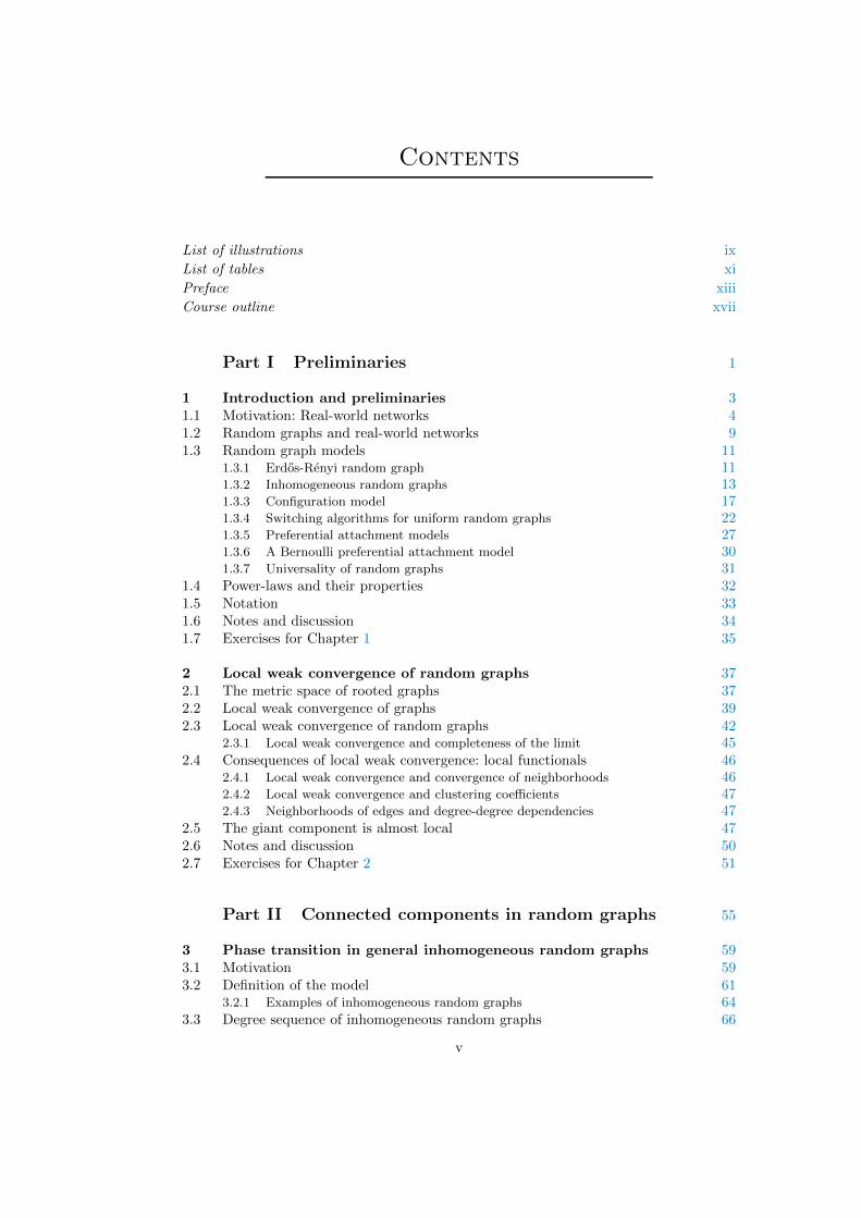
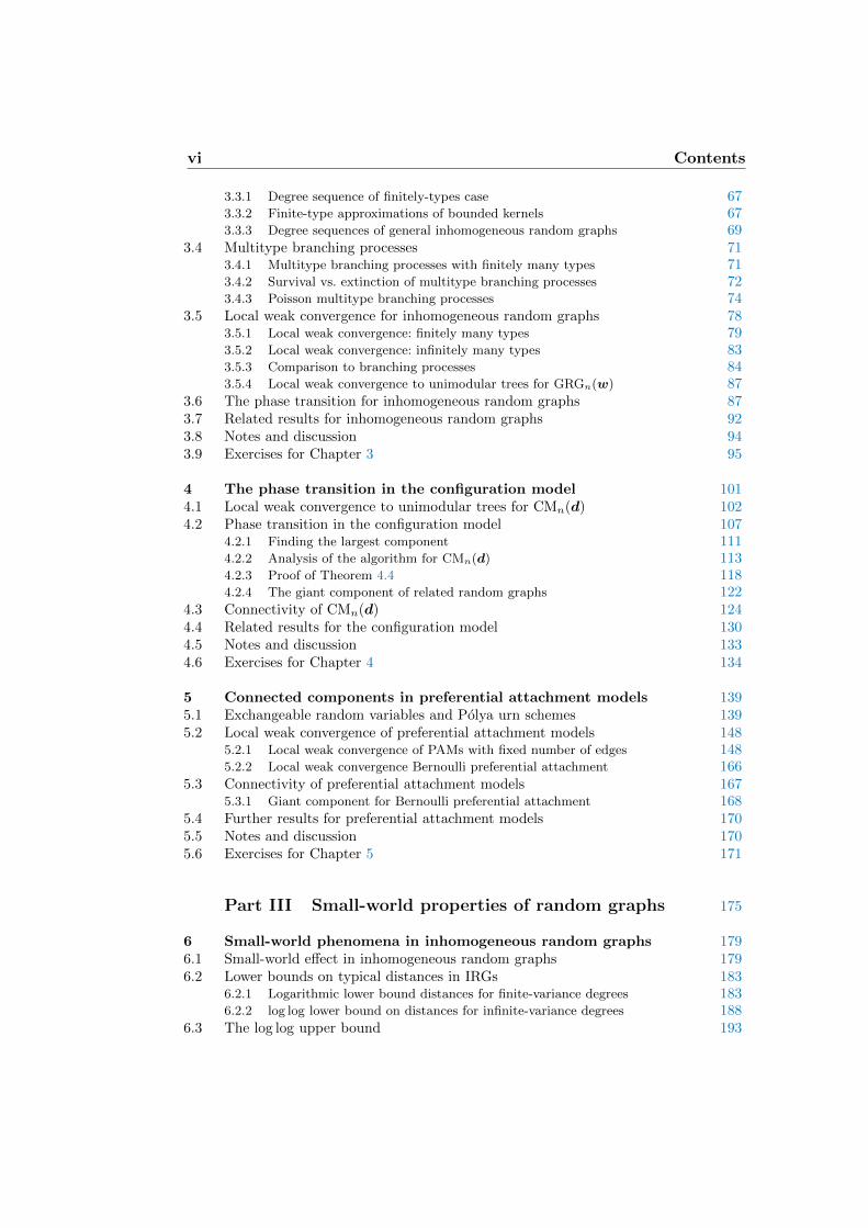
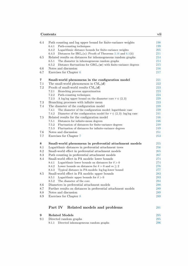
1.1 Degree sequence of the Autonomous Systems graph in 2014 61.2 log-log plot of the degree sequence in the Internet Movie Data base 71.3 The probability mass functions of the in- and out-degree sequence in the
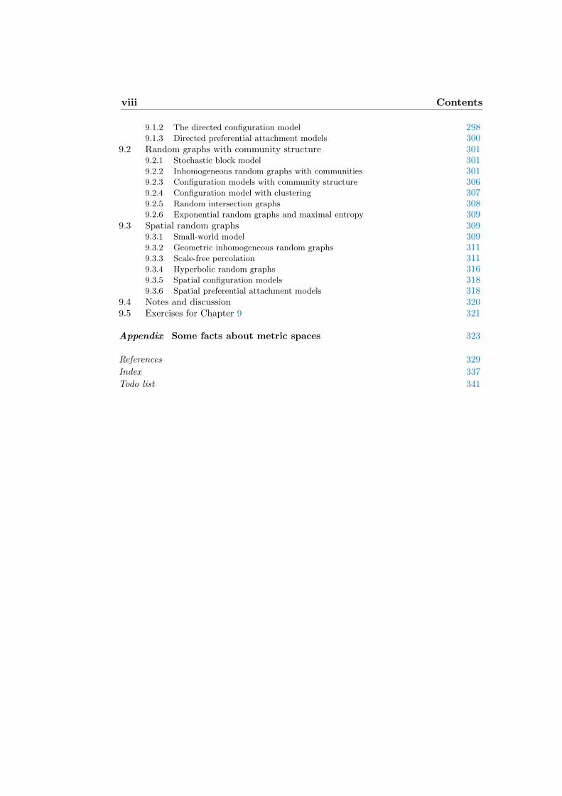
WWW from various data sets 71.4 AS and Internet hopcount 81.5 Typical distances in the Internet Movie Data base 81.6 Forward and backward switchings 256.1 A 12-step self-avoiding path connecting vertices i and j. 1856.2 A 10-step good path connecting i and j and the upper bounds on the weight
of its vertices. The height of a vertex is high for vertices with large weights. 1896.3 An example of a pair of paths (π, ρ) and its corresponding shape. 2027.1 Number of AS traversed in hopcount data (blue) compared to the model
(purple) with τ = 2.25, n = 10, 940. 2217.2 Empirical probability mass function of the distCMn(d)(U1, U2) for τ = 1.8 and
n = 103, 104, 105. 2479.1 The WWW according to Broder et al. 296
ix

Tables
3.1 The five rows correspond to the following real-life networks: (1) Model of theprotein-protein connections in blood of people with Alzheimer-disease. (2)Model of the protein-protein connections in blood of people with MultipleSclerosis. (3) Network of actors in 2011 in the Internet Movie Data base(IMDb), where actors are linked if they appeared in the same movie. (4)Collaboration network based on DBLP. Two scientist are connected if theyever collaborated on a paper. (5) Network where nodes represent zebras.There is a connection between two zebras if they ever interacted with eachother during the observation phase. 59
4.1 The rows in the above table represent the following real-world networks:The California road network consists of nodes, which represent intersectionsor endpoints of roads. In the Facebook network nodes represent the usersand they are connected if they are friends on the social media platformHyves was a Dutch social media platform. Nodes represent the users, and anedge between nodes represents a friendship. The arXiv astro-physics networkrepresents authors of papers within the astro-physics section of arXiv. Thereis an edge between authors if they have ever been co-authors. Models thehigh voltage power network in western USA. The nodes denote transformerssubstations, and generators and the edges represent transmission cables. Thedata set consists of jazz-musicians and there exists a connected if they evercollaborated. 101
xi


Preface
In this book, we study connected components and small-world properties of ran-dom graph models for complex networks. This is Volume 2 of a sequel of twobooks. Volume 1 describes the preliminary topics of random graphs as models forreal-world networks. Since 1999, many real-world networks have been investigated.These networks turned out to have rather different properties than classical ran-dom graph models, for example in the number of connections that the elementsin the network make. As a result, a wealth of new models was invented to capturethese properties. Volume 1 studies the models as well as their degree structure.This book summarizes the insights developed in this exciting period that focuson the connected components and small-world properties of the proposed randomgraph models.
While Volume 1 is intended to be used for a master level course where stu-dents have a limited prior knowledge of special topics in probability, Volume 2describes more involved notions that have been the focus of attention in the pasttwo decades. Volume 2 is intended to be used for a PhD level course, readingseminars, or for researchers wishing to obtain a consistent and extended overviewof the results and methodology that has been developed in this area. Volume1 includes many of the preliminaries, such as convergence of random variables,probabilistic bounds, coupling, martingales and branching processes, and we fre-quently refer to these results. The series of Volumes 1 and 2 aims to be self-contained. In Volume 2 we do briefly repeat some of the preliminaries on randomgraphs, including the introduction of some of the models and the key results ontheir degree distributions as discussed in great length in Volume 1. In Volume 2,we give the results concerning connected components, connectivity transitions, aswell as the small-world nature of the random graph models introduced in Volume1. We aim to give detailed and complete proofs. When we do not give proofs ofour results, we provide pointers to the literature. We further discuss several morerecent random graph models that aim to provide for more realistic models forreal-world networks, as they incorporate their directed nature, their communitystructure or their spatial embedding.
The field of random graphs was pioneered in 1959-1960 by Erdos and Renyi(1959; 1960; 1961a; 1961b), in the context of the Probabilistic Method. The initialwork by Erdos and Renyi on random graphs has incited a great amount of followup in the field, initially mainly in the combinatorics community. See the standardreferences on the subject by Bollobas (2001) and Janson, Luczak and Rucinski(2000) for the state of the art. Erdos and Renyi (1960) give a rather completepicture of the various phase transitions that occur in the Erdos-Renyi randomgraph. This initial work did not aim to realistically model real-world networks. Inthe period after 1999, due to the fact that data sets of real-world networks becameabundantly available, their structure has attracted enormous attention in mathe-matics as well as various applied domains. This is for example reflected in the factthat one of the first articles in the field Albert and Barabasi (2002) has attracted
xiii
xiv Preface
over 27000 citations. One of the main conclusions from this overwhelming bodyof work is that many real-world networks share two fundamental properties. Thefirst is that they are highly inhomogeneous, in the sense that vertices play ratherdifferent roles in the networks. This property is exemplified by the degree struc-ture of the real-world networks obeying power laws: these networks are scale-free.The scale-free nature of real-world networks prompted the community to comeup with many novel random graph models that, unlike the Erdos-Renyi randomgraph, do have power-law degree sequences. This was the key focus in Volume 1,where three models were presented that can have power-law degree sequences.
In this book, we pick up on the trail left in Volume 1, and we now focus onthe connectivity structure between vertices. Connectivity can be summarized intwo key aspects of real-world networks: the fact that they are highly connected,as exemplified by the fact that they tend to have one giant component containinga large proportion of the vertices (if not all of them), and their small-worldnature, quantifying the fact that most pairs of vertices are separated by shortpaths. We discuss the available methods for these proofs, including path countingtechniques, branching process approximations, exchangeable random variablesand De Finetti’s theorems. We pay particular attention to a recent technique,called local weak convergence, that makes the statement that random graphs‘locally look like trees’ precise. This technique is extremely powerful, and webelieve that its full potential has not yet been reached.
This book consists of four parts. In Part I, consisting of Chapter 1, we repeatsome definitions from Volume 1, including the random graph models studied inthis book, which are inhomogeneous random graphs, the configuration modeland preferential attachment models. We also discuss general techniques such aslocal-weak convergence. In Part II, consisting of Chapters 3–5, we discuss largeconnected components in random graph models. In Chapter 3, we further ex-tend the definition of the generalized random graph to general inhomogeneousrandom graphs. In Chapter 4 we discuss the large connected components in theconfiguration model, and in Chapter 5, we discuss the connected components inpreferential attachment models. In Part III, consisting of Chapters 3–5, we studythe small-world nature in random graphs, starting with inhomogeneous randomgraphs, continuing with the configuration model and ending with the preferentialattachment model. In Part IV, consisting of Chapter 9, we study related randomgraph models and their structure. Along the way, we give many exercises thathelp the reader to obtain a deeper understanding of the material by working ontheir solutions. These exercises appear in the last section of each of the chapters,and when applicable, we refer to them at the appropriate place in the text.
I have tried to give as many references to the literature as possible. However, thenumber of papers on random graphs is currently exploding. In MathSciNet (seehttp://www.ams.org/mathscinet), there were, on December 21, 2006, a totalof 1,428 papers that contain the phrase ‘random graphs’ in the review text, onSeptember 29, 2008, this number increased to 1614, on April 9, 2013, to 2346 and,
Preface xv
on April 21, 2016, to 2986. These are merely the papers on the topic in the mathcommunity. What is special about random graph theory is that it is extremelymultidisciplinary, and many papers using random graphs are currently writtenin economics, biology, theoretical physics and computer science. For example,in Scopus (see http://www.scopus.com/scopus/home.url), again on December21, 2006, there were 5,403 papers that contain the phrase ‘random graph’ in thetitle, abstract or keywords, on September 29, 2008, this increased to 7,928, onApril 9, 2013, to 13,987 and, on April 21, 2016, to 19,841. It can be expected thatthese numbers will continue to increase, rendering it impossible to review all theliterature.
In June 2014, I decided to split the preliminary version of this book up into twobooks. This has several reasons and advantages, particularly since Volume 2 ismore tuned towards a research audience, while the first part is more tuned towardsan audience of master students with varying backgrounds. The pdf-versions ofboth Volumes 1 and 2 can be obtained from
http://www.win.tue.nl/∼rhofstad/NotesRGCN.html
For further results on random graphs, or for solutions to some of the exercises inthis book, readers are encouraged to look there. Also, for a more playful approachto networks for a broad audience, including articles, videos, and demos of manyof the models treated in this book, we refer all readers to the Network Pages athttp://www.networkspages.nl. The Network Pages are an interactive websitedeveloped by and for all those that are interested in networks. One can finddemos for some of the models discussed here, as well as of network algorithmsand processes on networks.
This book, as well as Volume 1 of it, would not have been possible withoutthe help and encouragement of many people. I thank Gerard Hooghiemstra forthe encouragement to write it, and for using it at Delft University of Technologyalmost simultaneously while I used it at Eindhoven University of Technology inthe Spring of 2006 and again in the Fall of 2008. I particularly thank Gerard formany useful comments, solutions to exercises and suggestions for improvementsof the presentation throughout the book. Together with Piet Van Mieghem, weentered the world of random graphs in 2001, and I have tremendously enjoyedexploring this field together with you, as well as with Henri van den Esker, DmitriZnamenski, Mia Deijfen and Shankar Bhamidi, Johan van Leeuwaarden, JuliaKomjathy, Nelly Litvak and many others.
I thank Christian Borgs, Jennifer Chayes, Gordon Slade and Joel Spencer forjoint work on random graphs that are alike the Erdos-Renyi random graph, butdo have geometry. Special thanks go to Gordon Slade, who has introduced me tothe world of percolation, which is closely linked to the world of random graphs(see also the classic on percolation by Grimmett (1999)). It is peculiar to see thattwo communities work on two so closely related topics with different methods andeven different terminology, and that it has taken such a long time to build bridges
xvi Preface
between the subjects. I am very happy that these bridges are now rapidly appear-ing, and the level of communication between different communities has increasedsignificantly. I hope that this book helps to further enhance this communication.Frank den Hollander deserves a special mention. Frank, you have been importantas a driving force throughout my career, and I am very happy now to be workingwith you on fascinating random graph problems!
Further I thank Marie Albenque, Gianmarco Bet, Shankar Bhamidi, FinbarBogerd, Marko Boon, Francesco Caravenna, Rui Castro, Kota Chisaki, Mia Dei-jfen, Michel Dekking, Henri van den Esker, Lorenzo Federico, Lucas Gerin, JesseGoodman, Rajat Hazra, Markus Heydenreich, Frank den Hollander, Yusuke Ide,Lancelot James, Martin van Jole, Willemien Kets, Julia Komjathy, John Lapeyre,Lasse Leskela, Nelly Litvak, Norio Konno, Abbas Mehrabian, Mislav Miskovic,Mirko Moscatelli, Jan Nagel, Sidharthan Nair, Alex Olssen, Mariana Olvera-Cravioto, Helena Pena, Nathan Ross, Karoly Simon, Dominik Tomecki, NicolaTurchi, Viktoria Vadon, Thomas Vallier, Xiaotin Yu for remarks and ideas thathave improved the content and presentation of these notes substantially. WouterKager has entirely read the February 2007 version of this book, giving many ideasfor improvements of the arguments and of the methodology. Artem Sapozhnikov,Maren Eckhoff and Gerard Hooghiemstra read and commented the October 2011version. Sandor Kolumban read large parts of the October 2015 version, andspotted many errors, typos and inconsistencies.
I especially thank Dennis Timmers, Eefje van den Dungen, Joop van de Pol andRowel Gundlach, who, as, my student assistants, have been a great help in thedevelopment of this book, in making figures, providing solutions to the exercises,checking the proofs and keeping the references up to date. Maren Eckhoff andGerard Hooghiemstra also provided many solutions to the exercises, for which Iam grateful! Sandor Kolumban and Robert Fitzner helped me to turn all picturesof real-world networks as well as simulations of network models into a unifiedstyle, a feat that is beyond my LATEX skills. A big thanks for that! Also my thanksfor suggestions and help with figures to Marko Boon, Alessandro Garavaglia,Dimitri Krioukov, Vincent Kusters, Clara Stegehuis, Piet Van Mieghem and YanaVolkovich.
This work would not have been possible without the generous support of theNetherlands Organisation for Scientific Research (NWO) through VIDI grant639.032.304, VICI grant 639.033.806 and the Gravitation Networks grant024.002.003.
Remco van der Hofstad Eindhoven

Course outline
The relation between the chapters in Volumes 1 and 2 of this book is as follows:
Random Graphsand Complex
NetworksBranchingProcesses[Volume 1,Chapter 3]
Probabilis-tic Methods[Volume 1,Chapter 2]
Intro-duction
[Volume 1,Chapter 1]
Erdos-Renyirandom graph
Phasetransition[Volume 1,Chapter 4]
Revisited[Volume 1,Chapter 5]
Inhomogeneousrandom graphs
Intro-duction
[Volume 1,Chapter 6]
Con-nectivity
[Volume 2,Chapter 2]
Small world[Volume 2,Chapter 5]
Configura-tion model
Intro-duction
[Volume 1,Chapter 7]
Con-nectivity
[Volume 2,Chapter 3]
Small world[Volume 2,Chapter 6]
Preferentialattachment model
Intro-duction
[Volume 1,Chapter 8]
Con-nectivity
[Volume 2,Chapter 4]
Small world[Volume 2,Chapter 7]
Related models[Vol. 2, Chapter 8]
xvii
xviii Course outline
Here is some more explanation as well as a possible itinerary of a master or PhDcourse on random graphs, including both Volumes 1 and 2, in a course outline:
B Start with the introduction to real-world networks in [Volume 1, Chapter 1],which forms the inspiration for what follows. Continue with [Volume 1, Chapter2], which gives the necessary probabilistic tools used in all later chapters, and pickthose topics that your students are not familiar with and that are used in thelater chapters that you wish to treat. [Volume 1, Chapter 3] introduces branchingprocesses, and is used in [Volume 1, Chapters 4, 5], as well as in most of Volume2.
B After these preliminaries, you can start with the classical Erdos-Renyi ran-dom graph as covered in [Volume 1, Chapters 4–5]. Here you can choose the levelof detail, and decide whether you wish to do the entire phase transition or wouldrather move on to the random graphs models for complex networks. It is possibleto omit [Volume 1, Chapter 5] before moving on.
B Having discussed the Erdos-Renyi random graph, you can make your ownchoice of topics from the world of random graphs. There are three classes of mod-els for complex networks that are treated in quite some detail in this book. Youcan choose how much to treat in each of these models. You can either treat fewmodels and discuss many aspects, or instead discuss many models at a less deeplevel. The introductory chapters about the three models, [Volume 1, Chapter 6]for inhomogeneous random graphs, [Volume 1, Chapter 7] for the configurationmodel, and [Volume 1, Chapter 8] for preferential attachment models, provide abasic introduction to them, focussing on their degree structure. These introduc-tory chapters need to be read in order to understand the later chapters aboutthese models (particularly the ones in Volume 2). The parts on the differentmodels can be read independently.
B For readers that are interested in more advanced topics, one can eithertake one of the models and discuss the different chapters in Volume 2 focussingon them. [Volume 2, Chapters 3 and 6] discuss inhomogeneous random graphs,[Volume 2, Chapters 4 and 7] discuss the configuration model, while [Volume 2,Chapters 5 and 8] focus on preferential attachment models. The alternative isto take one of the topics, and work through them in detail. [Volume 2, Part II]discusses the largest connected components or phase transition in our randomgraph models, while [Volume 2, Part III] treats their small-world nature.
When you have further questions and/or suggestions about course outlines,then feel free to contact me.

Part I
Preliminaries
1

Chapter 1
Introduction and preliminaries
Abstract
In this chapter, we draw motivation from real-world networks, and for-mulate random graph models for them. We focus on some of the mod-els that have received the most attention in the literature, namely, theErdos-Renyi random graph, Inhomogeneous random graphs, the con-figuration model and preferential attachment models. We also discusssome of their extensions that have the potential to yield more realis-tic models for real-world networks. We follow van der Hofstad (2017),which we refer to as [Volume 1], both for the motivation as well as forthe introduction of the random graph models involved. We then con-tinue to discuss an important technique in this book, called local-weakconvergence.
Looking back, and ahead
In Volume 1 of this pair of books, we have discussed various models having flexibledegree sequences. The generalized random graph and the configuration modelgive us static flexible models for random graphs with various degree sequences.Preferential attachment models give us a convincing explanation of the abundanceof power-law degree sequences in various applications. In [Volume 1, Chapters 6–8], we have focussed on the properties of the degrees of such graphs. However,we have noted in [Volume 1, Chapter 1] that many real-world networks not onlyhave degree sequences that are rather different from the ones of the Erdos-Renyirandom graph, also many examples are small worlds and have a giant connectedcomponent.
In Chapters 3–8, we shall return to the models discussed in [Volume 1, Chapters6–8], and focus on their connected components as well as on the distances in theserandom graph models. Interestingly, a large chunk of the non-rigorous physicsliterature suggests that the behavior in various different random graph modelscan be described by only a few essential parameters. The key parameter of eachof these models in the power-law degree exponent, and the physics literaturepredicts that the behavior in random graph models with similar degree sequencesis similar. This is an example of the notion of universality, a notion which iscentral in statistical physics. Despite its importance, there are only few exampleof universality that can be rigorously proved. In Chapters 3–8, we investigate thelevel of universality present in random graph models.
We will often refer to Volume 1. When we do, we write [Volume 1, Theorem2.17] to mean that we refer to Theorem 2.17 in van der Hofstad (2017).
Organisation of this chapter
This chapter is organised as follows. In Section 1.1, we discuss real-world networksthe inspiration that they provide. In Section 1.2, we then discuss how graph
3
4 Introduction and preliminaries
sequences, where the size of the involved graphs tends to infinity, aim at describinglarge complex networks. In Section 1.3, we recall the definition of several randomgraph models, as introduced in Volume 1. In Section 1.5, we recall some of thestandard notion used in this pair of books. We close this chapter with notes anddiscussion in Section 1.6, and with exercises in Section 1.7.
1.1 Motivation: Real-world networks
In the past two decades, an enormous research effort has been performed onmodeling of various real-world phenomena using networks.
Networks arise in various applications, from the connections between friendsin friendship networks, the connectivity of neurons in the brain, to the relationsbetween companies and countries in economics and the hyperlinks between web-pages in the World-Wide web. The advent of the computer era has made manynetwork data sets available, and around 1999-2000, various groups started to in-vestigate network data from an empirical perspective. See Barabasi (2002) andWatts (2003) for expository accounts of the discovery of network properties byBarabasi, Watts and co-authors. Newman et al. (2006) bundle some of the origi-nal papers detailing the empirical findings of real-world networks and the networkmodels invented for them. The introductory book by Newman (2010) lists manyof the empirical properties of, and scientific methods for, networks. See also [Vol-ume 1, Chapter 1] for many examples of real-world networks and the empiricalfindings for them. Here we just give some basics.
Graphs
A graph G = (V,E) consists of a collection V of vertices, also called vertex set,and a collection of edges E, often called edge set. The vertices correspond tothe objects that we model, the edges indicate some relation between pairs ofthese objects. In our settings, graphs are usually undirected. Thus, an edge is anunordered pair u, v ∈ E indicating that u and v are directly connected. WhenG is undirected, if u is directly connected to v, then also v is directly connectedto u. Thus, an edge can be seen as a pair of vertices. When dealing with socialnetworks, the vertices represent the individuals in the population, while the edgesrepresent the friendships among them. We mainly deal with finite graphs, andthen, for simplicity, we take V = [n] := 1, . . . , n. The degree du of a vertex u isequal to the number of edges containing u, i.e.,
du = #v ∈ V : u, v ∈ E. (1.1.1)
Often, we deal with the degree of a random vertex in G. Let U ∈ [n] be a vertexchosen uniformly at random in [n], then the typical degree is the random variableDn given by
Dn = dU . (1.1.2)
1.1 Motivation: Real-world networks 5
It is not hard to see that the probability mass function of Dn is given by
P(Dn = k) =1
n
∑i∈[n]
1di=k. (1.1.3)
Exercise 1.1 asks you to prove (1.1.3).
We next discuss some of the common features that many real-world networksturn out to have, starting with the high variability of the degree distribution:
Scale-free phenomenon
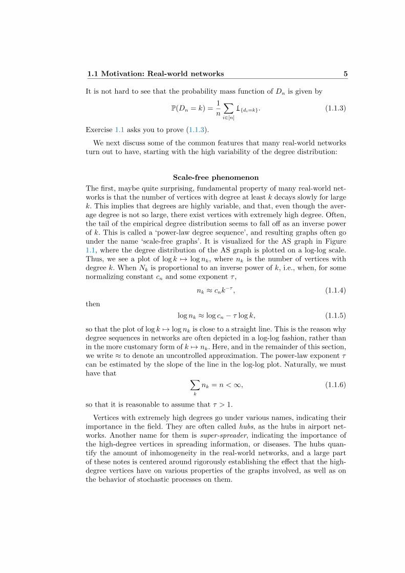
The first, maybe quite surprising, fundamental property of many real-world net-works is that the number of vertices with degree at least k decays slowly for largek. This implies that degrees are highly variable, and that, even though the aver-age degree is not so large, there exist vertices with extremely high degree. Often,the tail of the empirical degree distribution seems to fall off as an inverse powerof k. This is called a ‘power-law degree sequence’, and resulting graphs often gounder the name ‘scale-free graphs’. It is visualized for the AS graph in Figure1.1, where the degree distribution of the AS graph is plotted on a log-log scale.Thus, we see a plot of log k 7→ log nk, where nk is the number of vertices withdegree k. When Nk is proportional to an inverse power of k, i.e., when, for somenormalizing constant cn and some exponent τ ,
nk ≈ cnk−τ , (1.1.4)
then
log nk ≈ log cn − τ log k, (1.1.5)
so that the plot of log k 7→ log nk is close to a straight line. This is the reason whydegree sequences in networks are often depicted in a log-log fashion, rather thanin the more customary form of k 7→ nk. Here, and in the remainder of this section,we write ≈ to denote an uncontrolled approximation. The power-law exponent τcan be estimated by the slope of the line in the log-log plot. Naturally, we musthave that ∑
k
nk = n <∞, (1.1.6)
so that it is reasonable to assume that τ > 1.
Vertices with extremely high degrees go under various names, indicating theirimportance in the field. They are often called hubs, as the hubs in airport net-works. Another name for them is super-spreader, indicating the importance ofthe high-degree vertices in spreading information, or diseases. The hubs quan-tify the amount of inhomogeneity in the real-world networks, and a large partof these notes is centered around rigorously establishing the effect that the high-degree vertices have on various properties of the graphs involved, as well as onthe behavior of stochastic processes on them.
6 Introduction and preliminaries
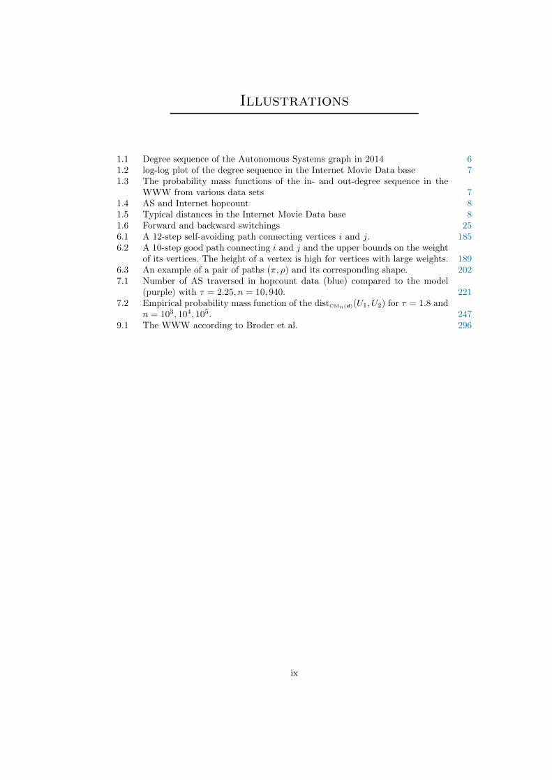
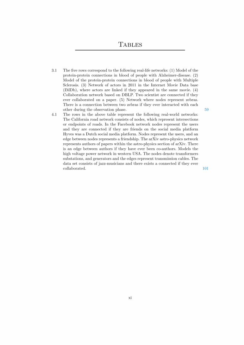
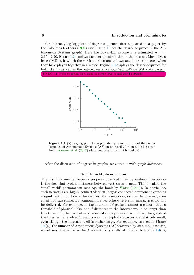
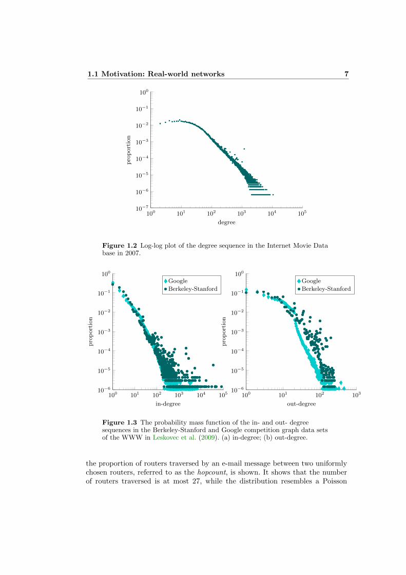
For Internet, log-log plots of degree sequences first appeared in a paper bythe Faloutsos brothers (1999) (see Figure 1.1 for the degree sequence in the Au-tonomous Systems graph). Here the power-law exponent is estimated as τ ≈2.15−2.20. Figure 1.2 displays the degree distribution in the Internet Movie Database (IMDb), in which the vertices are actors and two actors are connected whenthey have played together in a movie. Figure 1.3 displays the degree-sequence forboth the in- as well as the out-degrees in various World-Wide Web data bases.TO DO 1.1: Refer to recent discussion on power-laws in real-world networks.
100 101 102 103 104
10−7
10−5
10−3
10−1
degree
pro
port
ion
Figure 1.1 (a) Log-log plot of the probability mass function of the degreesequence of Autonomous Systems (AS) on on April 2014 on a log-log scalefrom Krioukov et al. (2012) (data courtesy of Dmitri Krioukov).
After the discussion of degrees in graphs, we continue with graph distances.
Small-world phenomenon
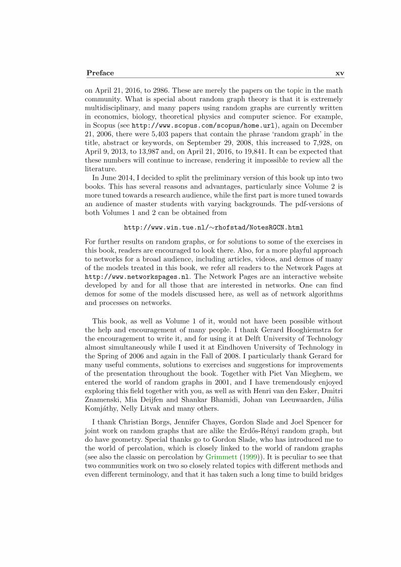
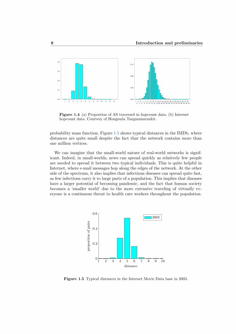
The first fundamental network property observed in many real-world networksis the fact that typical distances between vertices are small. This is called the‘small-world’ phenomenon (see e.g. the book by Watts (1999)). In particular,such networks are highly connected: their largest connected component containsa significant proportion of the vertices. Many networks, such as the Internet, evenconsist of one connected component, since otherwise e-mail messages could notbe delivered. For example, in the Internet, IP-packets cannot use more than athreshold of physical links, and if distances in the Internet would be larger thanthis threshold, then e-mail service would simply break down. Thus, the graph ofthe Internet has evolved in such a way that typical distances are relatively small,even though the Internet itself is rather large. For example, as seen in Figure1.4(a), the number of Autonomous Systems (AS) traversed by an e-mail data set,sometimes referred to as the AS-count, is typically at most 7. In Figure 1.4(b),
1.1 Motivation: Real-world networks 7
100 101 102 103 104 10510−7
10−6
10−5
10−4
10−3
10−2
10−1
100
degree
pro
port
ion
Figure 1.2 Log-log plot of the degree sequence in the Internet Movie Database in 2007.
100 101 102 103 104 10510−6
10−5
10−4
10−3
10−2
10−1
100
in-degree
pro
port
ion
Berkeley-Stanford
100 101 102 10310−6
10−5
10−4
10−3
10−2
10−1
100
out-degree
pro
port
ion
Berkeley-Stanford
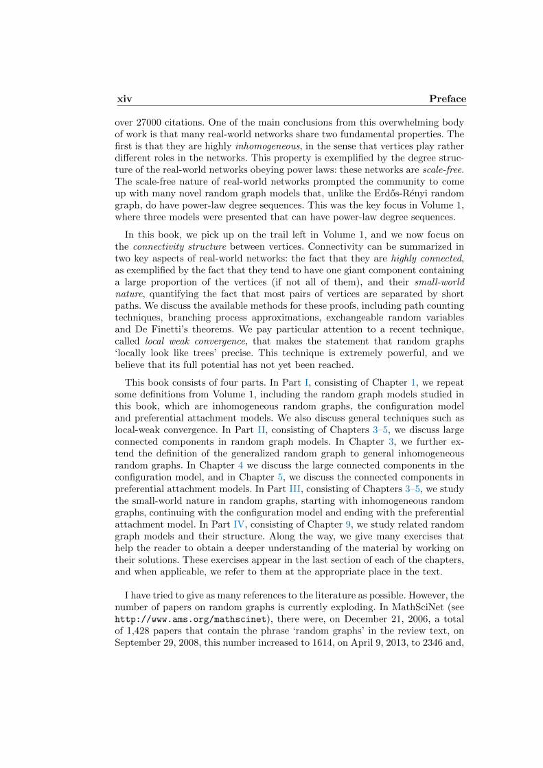
Figure 1.3 The probability mass function of the in- and out- degreesequences in the Berkeley-Stanford and Google competition graph data setsof the WWW in Leskovec et al. (2009). (a) in-degree; (b) out-degree.
the proportion of routers traversed by an e-mail message between two uniformlychosen routers, referred to as the hopcount, is shown. It shows that the numberof routers traversed is at most 27, while the distribution resembles a Poisson
8 Introduction and preliminaries
1 2 3 4 5 6 7 8 9 10 11 12 130.0
0.1
0.2
0.3
0.4
12
34
56
78
910
1112
1314
1516
1718
1920
2122
2324
2526
2728
2930
3132
3334
3536
3738
3940
4142
4344
0.00
0.04
0.08
0.12
Figure 1.4 (a) Proportion of AS traversed in hopcount data. (b) Internethopcount data. Courtesy of Hongsuda Tangmunarunkit.
probability mass function. Figure 1.5 shows typical distances in the IMDb, wheredistances are quite small despite the fact that the network contains more thanone million vertices.
We can imagine that the small-world nature of real-world networks is signif-icant. Indeed, in small-worlds, news can spread quickly as relatively few peopleare needed to spread it between two typical individuals. This is quite helpful inInternet, where e-mail messages hop along the edges of the network. At the otherside of the spectrum, it also implies that infectious diseases can spread quite fast,as few infections carry it to large parts of a population. This implies that diseaseshave a larger potential of becoming pandemic, and the fact that human societybecomes a ‘smaller world’ due to the more extensive traveling of virtually ev-eryone is a continuous threat to health care workers throughout the population.
1 2 3 4 5 6 7 8 9 100
0.2
0.4
0.6
distance
pro
port
ion
of
pair
s
2003
Figure 1.5 Typical distances in the Internet Movie Data base in 2003.
1.2 Random graphs and real-world networks 9
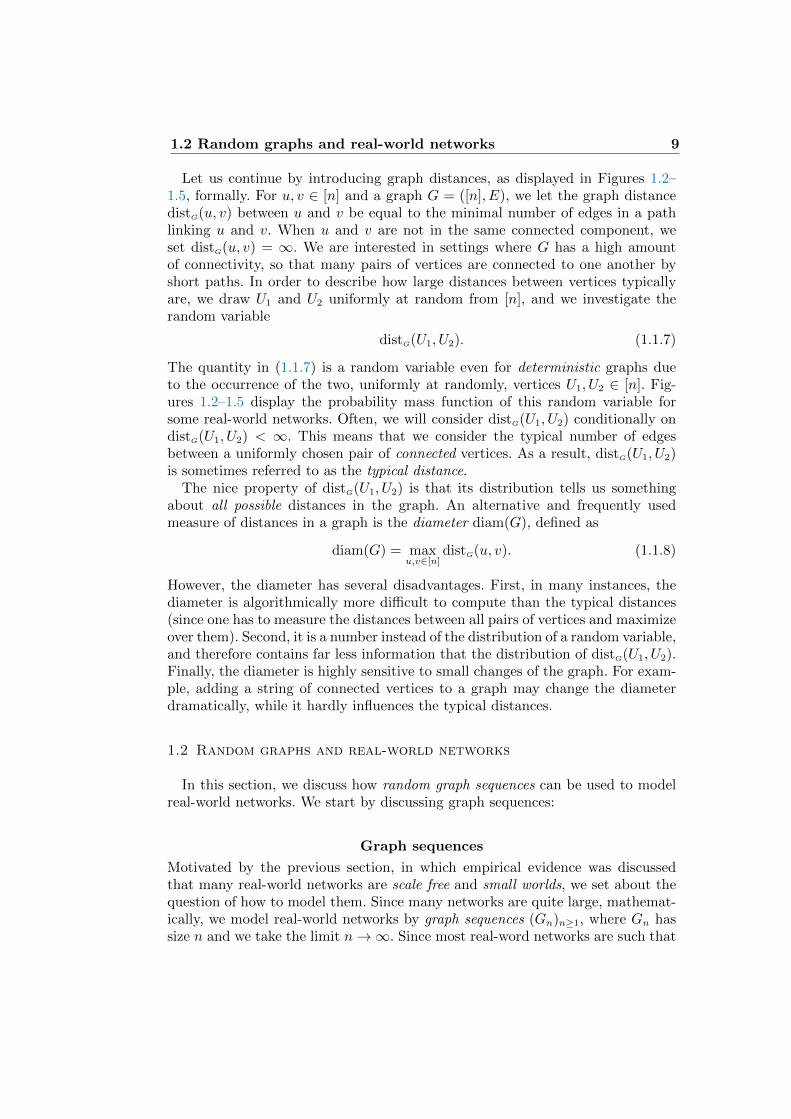
Let us continue by introducing graph distances, as displayed in Figures 1.2–1.5, formally. For u, v ∈ [n] and a graph G = ([n], E), we let the graph distancedistG(u, v) between u and v be equal to the minimal number of edges in a pathlinking u and v. When u and v are not in the same connected component, weset distG(u, v) = ∞. We are interested in settings where G has a high amountof connectivity, so that many pairs of vertices are connected to one another byshort paths. In order to describe how large distances between vertices typicallyare, we draw U1 and U2 uniformly at random from [n], and we investigate therandom variable
distG(U1, U2). (1.1.7)
The quantity in (1.1.7) is a random variable even for deterministic graphs dueto the occurrence of the two, uniformly at randomly, vertices U1, U2 ∈ [n]. Fig-ures 1.2–1.5 display the probability mass function of this random variable forsome real-world networks. Often, we will consider distG(U1, U2) conditionally ondistG(U1, U2) < ∞. This means that we consider the typical number of edgesbetween a uniformly chosen pair of connected vertices. As a result, distG(U1, U2)is sometimes referred to as the typical distance.
The nice property of distG(U1, U2) is that its distribution tells us somethingabout all possible distances in the graph. An alternative and frequently usedmeasure of distances in a graph is the diameter diam(G), defined as
diam(G) = maxu,v∈[n]
distG(u, v). (1.1.8)
However, the diameter has several disadvantages. First, in many instances, thediameter is algorithmically more difficult to compute than the typical distances(since one has to measure the distances between all pairs of vertices and maximizeover them). Second, it is a number instead of the distribution of a random variable,and therefore contains far less information that the distribution of distG(U1, U2).Finally, the diameter is highly sensitive to small changes of the graph. For exam-ple, adding a string of connected vertices to a graph may change the diameterdramatically, while it hardly influences the typical distances.
1.2 Random graphs and real-world networks
In this section, we discuss how random graph sequences can be used to modelreal-world networks. We start by discussing graph sequences:
Graph sequences
Motivated by the previous section, in which empirical evidence was discussedthat many real-world networks are scale free and small worlds, we set about thequestion of how to model them. Since many networks are quite large, mathemat-ically, we model real-world networks by graph sequences (Gn)n≥1, where Gn hassize n and we take the limit n→∞. Since most real-word networks are such that
10 Introduction and preliminaries
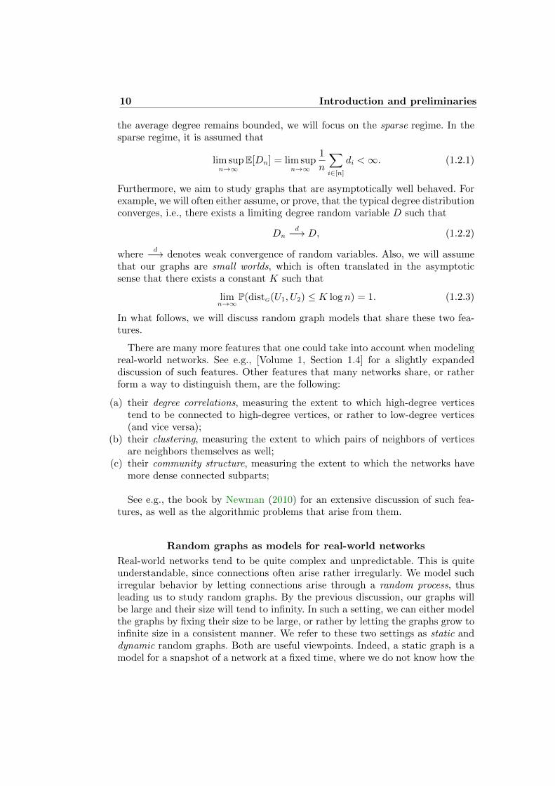
the average degree remains bounded, we will focus on the sparse regime. In thesparse regime, it is assumed that
lim supn→∞
E[Dn] = lim supn→∞
1
n
∑i∈[n]
di <∞. (1.2.1)
Furthermore, we aim to study graphs that are asymptotically well behaved. Forexample, we will often either assume, or prove, that the typical degree distributionconverges, i.e., there exists a limiting degree random variable D such that
Dnd−→ D, (1.2.2)
whered−→ denotes weak convergence of random variables. Also, we will assume
that our graphs are small worlds, which is often translated in the asymptoticsense that there exists a constant K such that
limn→∞
P(distG(U1, U2) ≤ K log n) = 1. (1.2.3)
In what follows, we will discuss random graph models that share these two fea-tures.
There are many more features that one could take into account when modelingreal-world networks. See e.g., [Volume 1, Section 1.4] for a slightly expandeddiscussion of such features. Other features that many networks share, or ratherform a way to distinguish them, are the following:
(a) their degree correlations, measuring the extent to which high-degree verticestend to be connected to high-degree vertices, or rather to low-degree vertices(and vice versa);
(b) their clustering, measuring the extent to which pairs of neighbors of verticesare neighbors themselves as well;
(c) their community structure, measuring the extent to which the networks havemore dense connected subparts;
See e.g., the book by Newman (2010) for an extensive discussion of such fea-tures, as well as the algorithmic problems that arise from them.
Random graphs as models for real-world networks
Real-world networks tend to be quite complex and unpredictable. This is quiteunderstandable, since connections often arise rather irregularly. We model suchirregular behavior by letting connections arise through a random process, thusleading us to study random graphs. By the previous discussion, our graphs willbe large and their size will tend to infinity. In such a setting, we can either modelthe graphs by fixing their size to be large, or rather by letting the graphs grow toinfinite size in a consistent manner. We refer to these two settings as static anddynamic random graphs. Both are useful viewpoints. Indeed, a static graph is amodel for a snapshot of a network at a fixed time, where we do not know how the

1.3 Random graph models 11
connections arose in time. Many network data sets are of this form. A dynamicsetting, however, may be more appropriate when we know how the network cameto be as it is. In the static setting, we can make model assumptions on the degreesso that they are scale free. In the dynamic setting, we can let the evolution of thegraph be such that they give rise to power-law degree sequences, so that thesesettings may provide explanations for the frequent occurrence of power-laws inreal-world networks.
Most of the random graph models that have been investigated in the (extensive)literature are caricatures of reality, in the sense that one cannot with dry eyes ar-gue that they describe any real-world network quantitatively correctly. However,these random graph models do provide insight into how any of the above featurescan influence the global behavior of networks, and thus provide for possible ex-planations of the empirical properties of real-world networks that are observed.Also, random graph models can be used as null models, where certain aspectsof real-world networks are taken into account, while others are not. This gives aqualitative way of investigating the importance of such empirical features in thereal world. Often, real-world networks are compared to uniform random graphswith certain specified properties, such as their number of edges or even their de-gree sequence. We will come back to how to generate random graphs uniformlyat random from the collection of all graphs with these properties below.
In the next section, we describe four models of random graphs, three of whichare static and one of which is dynamic.
1.3 Random graph models
We start with the most basic and simple random graph model, which has provedto be a source of tremendous inspiration, both for its mathematical beauty, aswell as providing a starting point for the analysis of random graphs.
1.3.1 Erdos-Renyi random graph
The Erdos-Renyi random graph is the simplest possible random graph. In it,we make every possible edge between a collection of n vertices open or closedwith equal probability. Thus, Erdos-Renyi random graph has vertex set [n] =1, . . . , n, and, denoting the edge between vertices s, t ∈ [n] by st, st is occupiedor present with probability p, and vacant or absent otherwise, independently ofall the other edges. The parameter p is called the edge probability. The aboverandom graph is denoted by ERn(p).
The model is named after Erdos and Renyi, since they have made profoundcontributions in the study of this model. See, in particular, Erdos and Renyi(1959, 1960, 1961a,b), where Erdos and Renyi investigate a related model inwhich a collection of m edges is chosen uniformly at random from te collection of(n2
)possible edges. The model just defined was first introduced though by Gilbert
(1959), and was already investigated heuristically by Solomonoff and Rapoport
12 Introduction and preliminaries
(1951). Informally, when m = p(n2
), the two models behave very similarly. We
remark in more detail on the relation between these two models at the end ofthis section. Exercise 1.2 investigates the uniform nature of ERn(p) with p =1/2. Alternatively speaking, the null model where we take no properties of thenetwork into account is the ERn(p) with p = 1/2. This model has expected degree(n− 1)/2, which is quite large. As a result, this model is not sparse at all. Thus,we next make this model sparser by making p smaller.
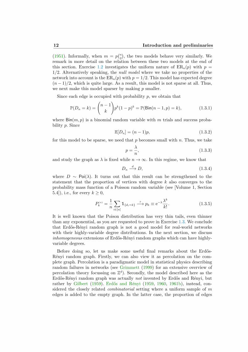
Since each edge is occupied with probability p, we obtain that
P(Dn = k) =
(n− 1
k
)pk(1− p)k = P(Bin(n− 1, p) = k), (1.3.1)
where Bin(m, p) is a binomial random variable with m trials and success proba-bility p. Since
E[Dn] = (n− 1)p, (1.3.2)
for this model to be sparse, we need that p becomes small with n. Thus, we take
p =λ
n, (1.3.3)
and study the graph as λ is fixed while n→∞. In this regime, we know that
Dnd−→ D, (1.3.4)
where D ∼ Poi(λ). It turns out that this result can be strengthened to thestatement that the proportion of vertices with degree k also converges to theprobability mass function of a Poisson random variable (see [Volume 1, Section5.4]), i.e., for every k ≥ 0,
P (n)
k =1
n
∑i∈[n]
1di=kP−→ pk ≡ e−λ
λk
k!. (1.3.5)
It is well known that the Poison distribution has very thin tails, even thinnerthan any exponential, as you are requested to prove in Exercise 1.3. We concludethat Erdos-Renyi random graph is not a good model for real-world networkswith their highly-variable degree distributions. In the next section, we discussinhomogeneous extensions of Erdos-Renyi random graphs which can have highly-variable degrees.
Before doing so, let us make some useful final remarks about the Erdos-Renyi random graph. Firstly, we can also view it as percolation on the com-plete graph. Percolation is a paradigmatic model in statistical physics describingrandom failures in networks (see Grimmett (1999) for an extensive overview ofpercolation theory focussing on Zd). Secondly, the model described here as theErdos-Renyi random graph was actually not invented by Erdos and Renyi, butrather by Gilbert (1959). Erdos and Renyi (1959, 1960, 1961b), instead, con-sidered the closely related combinatorial setting where a uniform sample of medges is added to the empty graph. In the latter case, the proportion of edges
1.3 Random graph models 13
is 2m/n(n − 1) ≈ 2m/n2, so we should think of m ≈ 2λn for a fair comparison.Note that when we condition the total number of edges to be equal to m, thelaw of the Erdos-Renyi random graphis equal to the model where a collectionof m uniformly chosen edges is added, explaining the close relation between thetwo models. Due to the concentration of the total number of edges, we can in-deed roughly exchange the binomial model with p = λ/m with the combinatorialmodel with m = 2λn. The combinatorial model has the nice feature that it pro-duces a uniform graph from the collection of all graphs with m edges, and thuscould serve as a null model for a real-world network in which only the number ofedges is fixed.
1.3.2 Inhomogeneous random graphs
In inhomogeneous random graphs, we keep the independence of the edges, butmake the edge probabilities different for different edges. A general format forsuch models is in the seminal work of Bollobas et al. (2007). We will discuss suchgeneral inhomogeneous random graphs in Chapter 3 below. We start with onekey example, that has attracted the most attention in the literature so far, andis also discussed in great detail in [Volume 1, Chapter 6].
Rank-1 inhomogeneous random graphs
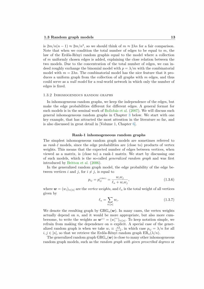
The simplest inhomogeneous random graph models are sometimes referred toas rank-1 models, since the edge probabilities are (close to) products of vertexweights. This means that the expected number of edges between vertices, whenviewed as a matrix, is (close to) a rank-1 matrix. We start by discussing oneof such models, which is the so-called generalized random graph and was firstintroduced by Britton et al. (2006).
In the generalized random graph model, the edge probability of the edge be-tween vertices i and j, for i 6= j, is equal to
pij = p(GRG)
ij =wiwj
`n + wiwj, (1.3.6)
wherew = (wi)i∈[n] are the vertex weights, and `n is the total weight of all verticesgiven by
`n =∑i∈[n]
wi. (1.3.7)
We denote the resulting graph by GRGn(w). In many cases, the vertex weightsactually depend on n, and it would be more appropriate, but also more cum-bersome, to write the weights as w(n) = (w(n)
i )i∈[n]. To keep notation simple, werefrain from making the dependence on n explicit. A special case of the gener-alized random graph is when we take wi ≡ nλ
n−λ , in which case pij = λ/n for alli, j ∈ [n], so that we retrieve the Erdos-Renyi random graph ERn(λ/n).
The generalized random graph GRGn(w) is close to many other inhomogeneousrandom graph models, such as the random graph with given prescribed degrees or
14 Introduction and preliminaries
Chung-Lu model, where instead
pij = p(CL)
ij = min(wiwj/`n, 1), (1.3.8)
and which has been studied intensively by Chung and Lu (2002a,b, 2003, 2006a,b).A further adaptation is the so-called Poissonian random graph or Norros-Reittumodel (introduced by Norros and Reittu (2006)), for which
pij = p(NR)
ij = 1− exp (−wiwj/`n) . (1.3.9)
See Janson (2010a) or [Volume 1, Sections 6.7 and 6.8] for conditions under whichthese random graphs are asymptotically equivalent, meaning that all events haveequal asymptotic probabilities.
Naturally, the topology of the generalized random graph depends sensitivelyupon the choice of the vertex weights w = (wi)i∈[n]. These vertex weights canbe rather general, and we both investigate settings where the weights are deter-ministic, as well as where they are random. In order to describe the empiricalproportions of the weights, we define their empirical distribution function to be
Fn(x) =1
n
∑i∈[n]
1wi≤x, x ≥ 0. (1.3.10)
We can interpret Fn as the distribution of the weight of a uniformly chosen vertexin [n] (see Exercise 1.4). We denote the weight of a uniformly chosen vertex U in[n] by Wn = wU , so that, by Exercise 1.4, Wn has distribution function Fn.
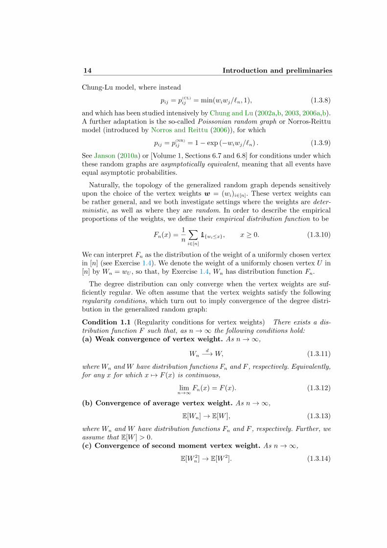
The degree distribution can only converge when the vertex weights are suf-ficiently regular. We often assume that the vertex weights satisfy the followingregularity conditions, which turn out to imply convergence of the degree distri-bution in the generalized random graph:
Condition 1.1 (Regularity conditions for vertex weights) There exists a dis-tribution function F such that, as n→∞ the following conditions hold:(a) Weak convergence of vertex weight. As n→∞,
Wnd−→W, (1.3.11)
where Wn and W have distribution functions Fn and F , respectively. Equivalently,for any x for which x 7→ F (x) is continuous,
limn→∞
Fn(x) = F (x). (1.3.12)
(b) Convergence of average vertex weight. As n→∞,
E[Wn]→ E[W ], (1.3.13)
where Wn and W have distribution functions Fn and F , respectively. Further, weassume that E[W ] > 0.(c) Convergence of second moment vertex weight. As n→∞,
E[W 2n ]→ E[W 2]. (1.3.14)
1.3 Random graph models 15
Condition 1.1(a) guarantees that the weight of a ‘typical’ vertex is close to arandom variable W that is independent of n. Condition 1.1(b) implies that theaverage weight of the vertices in GRGn(w) converges to the expectation of thelimiting weight variable. In turn, this implies that the average degree in GRGn(w)converges to the expectation of the limit random variable of the vertex weights.Condition 1.1(c) ensures the convergence of the second moment of the weights tothe second moment of the limiting weight variable.
Remark 1.2 (Regularity for random weights) Sometimes we will be interestedin cases where the weights of the vertices are random themselves. For example,this arises when the weights w = (wi)i∈[n] are realizations of i.i.d. random vari-ables. When the weights are random variables themselves, also the function Fnis a random distribution function. Indeed, in this case Fn is the empirical dis-tribution function of the random weights (wi)i∈[n]. We stress that E[Wn] is thento be interpreted as 1
n
∑i∈[n]wi, which is itself random. Therefore, in Condition
1.1, we require random variables to converge, and there are several notions ofconvergence that may be used. As it turns out, the most convenient notion ofconvergence is convergence in probability.
Let us now discuss some canonical examples of weight distributions that satisfythe Regularity Condition 1.1.
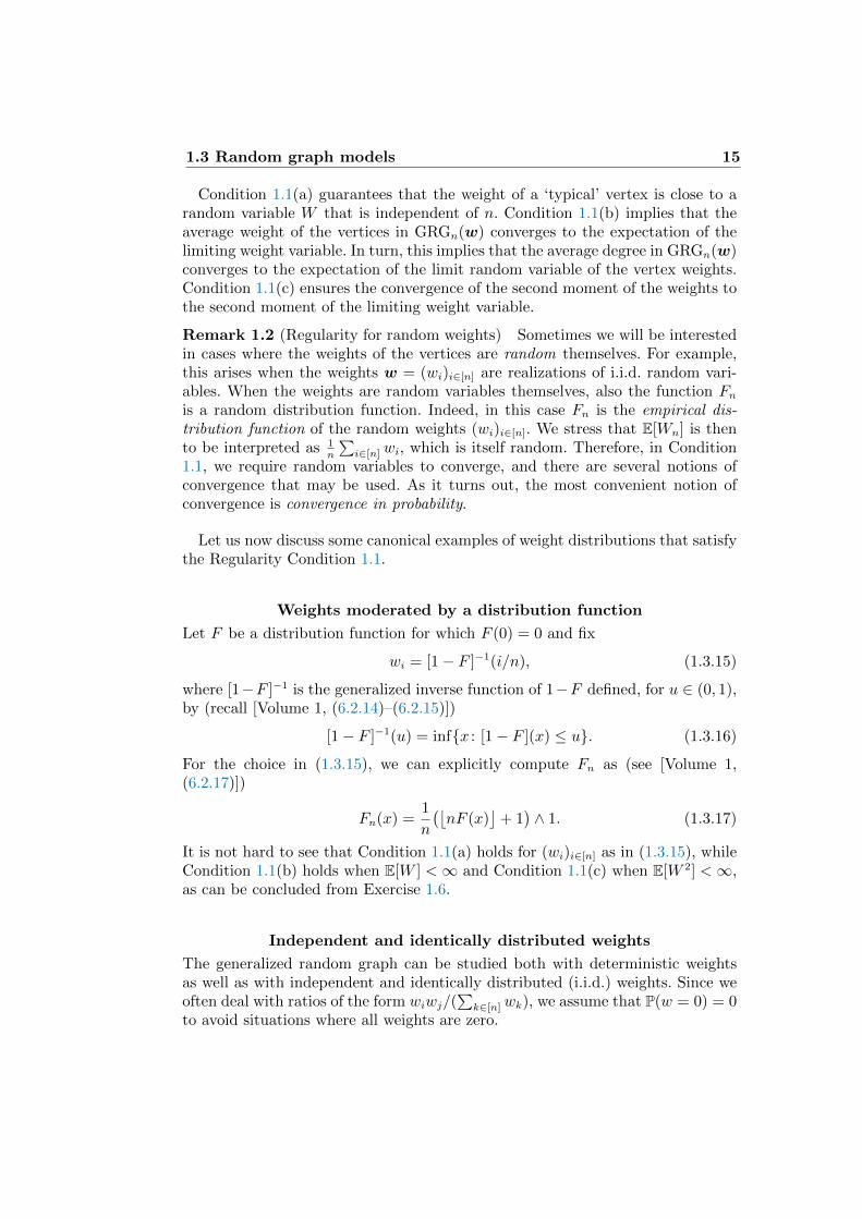
Weights moderated by a distribution function
Let F be a distribution function for which F (0) = 0 and fix
wi = [1− F ]−1(i/n), (1.3.15)
where [1−F ]−1 is the generalized inverse function of 1−F defined, for u ∈ (0, 1),by (recall [Volume 1, (6.2.14)–(6.2.15)])
[1− F ]−1(u) = infx : [1− F ](x) ≤ u. (1.3.16)
For the choice in (1.3.15), we can explicitly compute Fn as (see [Volume 1,(6.2.17)])
Fn(x) =1
n
(⌊nF (x)
⌋+ 1)∧ 1. (1.3.17)
It is not hard to see that Condition 1.1(a) holds for (wi)i∈[n] as in (1.3.15), whileCondition 1.1(b) holds when E[W ] <∞ and Condition 1.1(c) when E[W 2] <∞,as can be concluded from Exercise 1.6.
Independent and identically distributed weights
The generalized random graph can be studied both with deterministic weightsas well as with independent and identically distributed (i.i.d.) weights. Since weoften deal with ratios of the form wiwj/(
∑k∈[n]wk), we assume that P(w = 0) = 0
to avoid situations where all weights are zero.
16 Introduction and preliminaries
Both models, i.e., with weights (wi)i∈[n] as in (1.3.15), and with i.i.d. weights(wi)i∈[n], have their own merits. The great advantage of i.i.d. weights is thatthe vertices in the resulting graph are, in distribution, the same. More precisely,the vertices are completely exchangeable, like in the Erdos-Renyi random graphERn(p). Unfortunately, when we take the weights to be i.i.d., then in the resultinggraph the edges are no longer independent (despite the fact that they are con-ditionally independent given the weights). In the sequel, we focus on the settingwhere the weights are prescribed. When the weights are deterministic, this changesnothing, when the weights are i.i.d., this means that we work conditionally onthe weights.
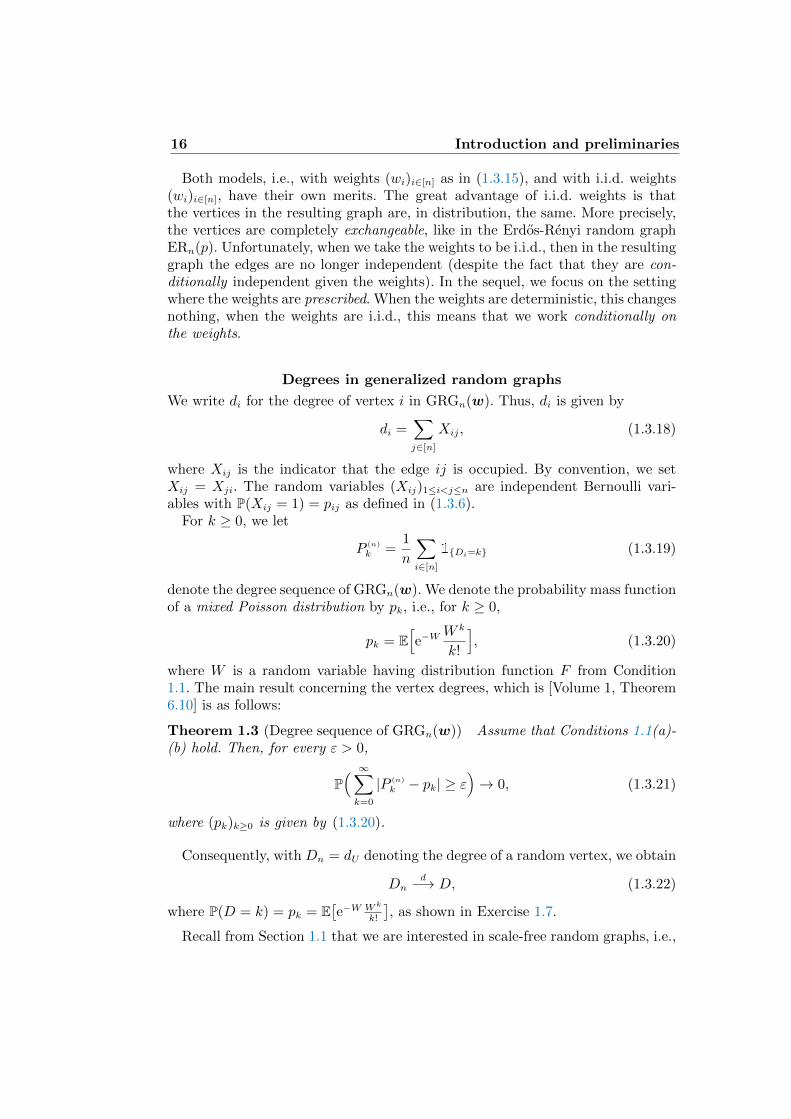
Degrees in generalized random graphs
We write di for the degree of vertex i in GRGn(w). Thus, di is given by
di =∑j∈[n]
Xij, (1.3.18)
where Xij is the indicator that the edge ij is occupied. By convention, we setXij = Xji. The random variables (Xij)1≤i<j≤n are independent Bernoulli vari-ables with P(Xij = 1) = pij as defined in (1.3.6).
For k ≥ 0, we let
P (n)
k =1
n
∑i∈[n]
1Di=k (1.3.19)
denote the degree sequence of GRGn(w). We denote the probability mass functionof a mixed Poisson distribution by pk, i.e., for k ≥ 0,
pk = E[e−W
W k
k!
], (1.3.20)
where W is a random variable having distribution function F from Condition1.1. The main result concerning the vertex degrees, which is [Volume 1, Theorem6.10] is as follows:
Theorem 1.3 (Degree sequence of GRGn(w)) Assume that Conditions 1.1(a)-(b) hold. Then, for every ε > 0,
P( ∞∑k=0
|P (n)
k − pk| ≥ ε)→ 0, (1.3.21)
where (pk)k≥0 is given by (1.3.20).
Consequently, with Dn = dU denoting the degree of a random vertex, we obtain
Dnd−→ D, (1.3.22)
where P(D = k) = pk = E[e−W Wk
k!
], as shown in Exercise 1.7.
Recall from Section 1.1 that we are interested in scale-free random graphs, i.e.,
1.3 Random graph models 17
random graphs for which the degree distribution obeys a power law. We see fromTheorem 1.3 that this is true precisely when D obeys a power law. This, in turn,occurs precisely when W obeys a power law, i.e., when, for w large,
P(W > w) =c
wτ−1(1 + o(1)), (1.3.23)
and then also, for w large,
P(D > w) =c
wτ−1(1 + o(1)). (1.3.24)
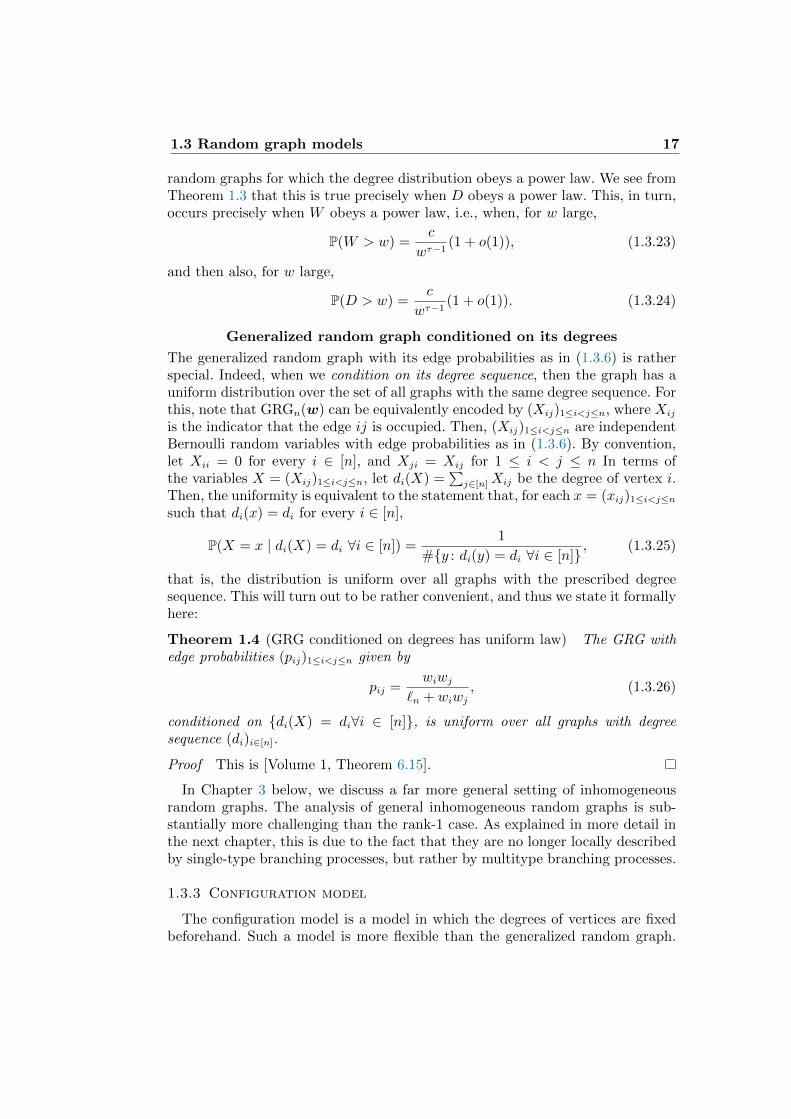
Generalized random graph conditioned on its degrees
The generalized random graph with its edge probabilities as in (1.3.6) is ratherspecial. Indeed, when we condition on its degree sequence, then the graph has auniform distribution over the set of all graphs with the same degree sequence. Forthis, note that GRGn(w) can be equivalently encoded by (Xij)1≤i<j≤n, where Xij
is the indicator that the edge ij is occupied. Then, (Xij)1≤i<j≤n are independentBernoulli random variables with edge probabilities as in (1.3.6). By convention,let Xii = 0 for every i ∈ [n], and Xji = Xij for 1 ≤ i < j ≤ n In terms ofthe variables X = (Xij)1≤i<j≤n, let di(X) =
∑j∈[n]Xij be the degree of vertex i.
Then, the uniformity is equivalent to the statement that, for each x = (xij)1≤i<j≤nsuch that di(x) = di for every i ∈ [n],
P(X = x | di(X) = di ∀i ∈ [n]) =1
#y : di(y) = di ∀i ∈ [n] , (1.3.25)
that is, the distribution is uniform over all graphs with the prescribed degreesequence. This will turn out to be rather convenient, and thus we state it formallyhere:
Theorem 1.4 (GRG conditioned on degrees has uniform law) The GRG withedge probabilities (pij)1≤i<j≤n given by
pij =wiwj
`n + wiwj, (1.3.26)
conditioned on di(X) = di∀i ∈ [n], is uniform over all graphs with degreesequence (di)i∈[n].
Proof This is [Volume 1, Theorem 6.15].
In Chapter 3 below, we discuss a far more general setting of inhomogeneousrandom graphs. The analysis of general inhomogeneous random graphs is sub-stantially more challenging than the rank-1 case. As explained in more detail inthe next chapter, this is due to the fact that they are no longer locally describedby single-type branching processes, but rather by multitype branching processes.
1.3.3 Configuration model
The configuration model is a model in which the degrees of vertices are fixedbeforehand. Such a model is more flexible than the generalized random graph.
18 Introduction and preliminaries
For example, the generalized random graph always has a positive proportion ofvertices of degree 0, 1, 2, etc, as easily follows from Theorem 1.3.
Fix an integer n that will denote the number of vertices in the random graph.Consider a sequence of degrees d = (di)i∈[n]. The aim is to construct an undi-rected (multi)graph with n vertices, where vertex j has degree dj. Without lossof generality, we assume throughout this chapter that dj ≥ 1 for all j ∈ [n],since when dj = 0, vertex j is isolated and can be removed from the graph.One possible random graph model is then to take the uniform measure over suchundirected and simple graphs. Here, we call a multigraph simple when it has noself-loops, and no multiple edges between any pair of vertices. However, the setof undirected simple graphs with n vertices where vertex j has degree dj may beempty. For example, in order for such a graph to exist, we must assume that thetotal degree
`n =∑j∈[n]
dj (1.3.27)
is even. We wish to construct a simple graph such that d = (di)i∈[n] are thedegrees of the n vertices. However, even when `n =
∑j∈[n] dj is even, this is not
always possible.
Since it is not always possible to construct a simple graph with a given degreesequence, instead, we construct a multigraph, that is, a graph possibly having self-loops and multiple edges between pairs of vertices. One way of obtaining such amultigraph with the given degree sequence is to pair the half-edges attached tothe different vertices in a uniform way. Two half-edges together form an edge,thus creating the edges in the graph. Let us explain this in more detail.
To construct the multigraph where vertex j has degree dj for all j ∈ [n], wehave n separate vertices and incident to vertex j, we have dj half-edges. Everyhalf-edge needs to be connected to another half-edge to form an edge, and byforming all edges we build the graph. For this, the half-edges are numbered in anarbitrary order from 1 to `n. We start by randomly connecting the first half-edgewith one of the `n − 1 remaining half-edges. Once paired, two half-edges forma single edge of the multigraph, and the half-edges are removed from the list ofhalf-edges that need to be paired. Hence, a half-edge can be seen as the left orthe right half of an edge. We continue the procedure of randomly choosing andpairing the half-edges until all half-edges are connected, and call the resultinggraph the configuration model with degree sequence d, abbreviated as CMn(d).
A careful reader may worry about the order in which the half-edges are be-ing paired. In fact, this ordering turns out to be completely irrelevant since therandom pairing of half-edges is completely exchangeable. It can even be done ina random fashion, which will be useful when investigating neighborhoods in theconfiguration model. See e.g., [Volume 1, Definition 7.5 and Lemma 7.6] for moredetails on this exchangeability.
Interestingly, one can compute rather explicitly what the distribution of CMn(d)is. To do so, note that CMn(d) is characterized by the random vector (Xij)1≤i≤j≤n,
1.3 Random graph models 19
where Xij is the number of edges between vertex i and j. Here Xii is the numberof self-loops incident to vertex i, and
di = Xii +∑j∈[n]
Xij (1.3.28)
In terms of this notation, and writing G = (xij)i,j∈[n] to denote a multigraph onthe vertices [n],
P(CMn(d) = G) =1
(`n − 1)!!
∏i∈[n] di!∏
i∈[n] 2xii∏
1≤i≤j≤n xij!. (1.3.29)
See e.g., [Volume 1, Proposition 7.7] for this result. In particular, P(CMn(d) = G)is the same for each simple G, where G is simple when xii = 0 for every i ∈ [n] andxij ∈ 0, 1 for every 1 ≤ i < j ≤ n. Thus, the configuration model conditionedon simplicity is a uniform random graph with the prescribed degree distribution.This is quite relevant, as it gives a convenient way to obtain such a uniform graph,which is a highly non-trivial fact.
Interestingly, the configuration model was invented by Bollobas (1980) to studyuniform random regular graphs (see also (Bollobas, 2001, Section 2.4)). The in-troduction was inspired by, and generalized the results in, the work of Benderand Canfield (1978). The original work allowed for a careful computation of thenumber of regular graphs, using a probabilistic argument. This is the probabilisticmethod at its best, and also explains the emphasis on the study of the probabilityfor the graph to be simple as we will see below. The configuration model, as wellas uniform random graphs with a prescribed degree sequence, were further stud-ied in greater generality by Molloy and Reed (1995, 1998). This extension is quiterelevant to us, as the scale-free nature of many real-world applications encouragesus to investigate configuration models with power-law degree sequences.
The uniform nature of the configuration model partly explains its popularity,and it has become one of the most highly studied random graph models. It alsoimplies that, conditioned on simplicity, the configuration model is the null modelfor a real-world network where all the degrees are fixed. It thus allows one todistinguish the relevance of the degree inhomogeneity and other features of thenetwork, such as its community structure, clustering, etc.
As for the GRGn(w), we again impose regularity conditions on the degreesequence d. In order to state these assumptions, we introduce some notation. Wedenote the degree of a uniformly chosen vertex U in [n] by Dn = dU . The randomvariable Dn has distribution function Fn given by
Fn(x) =1
n
∑j∈[n]
1dj≤x, (1.3.30)
which is the empirical distribution of the degrees. We assume that the vertexdegrees satisfy the following regularity conditions:
20 Introduction and preliminaries
Condition 1.5 (Regularity conditions for vertex degrees)(a) Weak convergence of vertex weight. There exists a distribution functionF such that, as n→∞,
Dnd−→ D, (1.3.31)
where Dn and D have distribution functions Fn and F , respectively.Equivalently, for any x,
limn→∞
Fn(x) = F (x). (1.3.32)
Further, we assume that F (0) = 0, i.e., P(D ≥ 1) = 1.(b) Convergence of average vertex degrees. As n→∞,
E[Dn]→ E[D], (1.3.33)
where Dn and D have distribution functions Fn and F from part (a), respectively.(c) Convergence of second moment vertex degrees. As n→∞,
E[D2n]→ E[D2], (1.3.34)
where again Dn and D have distribution functions Fn and F from part (a), re-spectively.
The possibility to obtain a non-simple graph is a major disadvantage of theconfiguration model. There are two ways of dealing with this complication:
(a) Erased configuration model
The first way of dealing with multiple edges is to erase the problems. Thismeans that we replace CMn(d) = (Xij)1≤i≤j≤n by its erased version ECMn(d) =
(X(er)ij )1≤i≤j≤n, where X
(er)ii ≡ 0, while X
(er)ij = 1 precisely when Xij ≥ 1. In words,
we remove the self-loops and merge all multiple edges to a single edge. Of course,this changes the precise degree distribution. However, [Volume 1, Theorem 7.10]shows that only a small proportion of the edges is erased, so that the erasing doesnot change the degree distribution. See [Volume 1, Section 7.3] for more details.Of course, the downside of this approach is that the degrees are changed by theprocedure, while we would like to keep the degrees precisely as specified.
Let us describe the degree distribution in the erased configuration model inmore detail, to study the effect of the erasure of self-loops and multiple edges.We denote the degrees in the erased configuration model by D(er) = (D(er)
i )i∈[n],so that
D(er)
i = di − 2si −mi, (1.3.35)
where (di)i∈[n] are the degrees in CMn(d), si = xii is the number of self-loops ofvertex i in CMn(d), and
mi =∑j 6=i
(xij − 1)1xij≥2 (1.3.36)
1.3 Random graph models 21
is the number of multiple edges removed from i.Denote the empirical degree sequence (p(n)
k )k≥1 in CMn(d) by
p(n)
k = P(Dn = k) =1
n
∑i∈[n]
1di=k, (1.3.37)
and denote the related degree sequence in the erased configuration model (P (er)
k )k≥1
by
P (er)
k =1
n
∑i∈[n]
1D(er)i =k. (1.3.38)
From the notation it is clear that (p(n)
k )k≥1 is a deterministic sequence when d =(di)i∈[n] is deterministic, while (P (er)
k )k≥1 is a random sequence, since the eraseddegrees (D(er)
i )i∈[n] form a random vector even when d = (di)i∈[n] is deterministic.
Now we are ready to state the main result concerning the degree sequence ofthe erased configuration model:
Theorem 1.6 (Degree sequence of erased configuration model with fixed degrees)For fixed degrees d satisfying Conditions 1.5(a)-(b), the degree sequence of theerased configuration model (P (er)
k )k≥1 converges in probability to (pk)k≥1. Moreprecisely, for every ε > 0,
P( ∞∑k=1
|P (er)
k − pk| ≥ ε)→ 0, (1.3.39)
where pk = P(D = k) as in Condition 1.5(a).
Theorem 1.6 indeed shows that most of the edges are kept in the erasureprocedure, see Exercise 1.9.
(b) Configuration model conditioned on simplicity
The second solution to the multigraph problem of the configuration model is tothrow away the result when it is not simple, and to try again. Therefore, this con-struction is sometimes called the repeated configuration model (see Britton et al.(2006)). It turns out that, when Conditions 1.5(a)-(c) hold, then (see [Volume 1,Theorem 7.12])
limn→∞
P(CMn(d) is a simple graph) = e−ν/2−ν2/4, (1.3.40)
where
ν =E[D(D − 1)]
E[D](1.3.41)
is the expected forward degree. Thus, this is a realistic option when E[D2] <∞.Unfortunately, this is not an option when the degrees obey an asymptotic powerlaw with τ ∈ (2, 3), since then E[D2] = ∞. Note that, by (1.3.29), CMn(d)
22 Introduction and preliminaries
conditioned on simplicity is a uniform random graph with the prescribed degreesequence. We denote this random graph by UGn(d). We will return to the dif-ficulty of generating simple graphs with infinite-variance degrees later in thischapter.
Relation GRG and CM
Since CMn(d) conditioned on simplicity yields a uniform (simple) random graphwith these degrees, and by (1.3.25), also GRGn(w) conditioned on its degrees isa uniform (simple) random graph with the given degree distribution, the laws ofthese random graph models are the same. As a result, one can prove results forGRGn(w) by proving them for CMn(d) under the appropriate degree conditions,and then proving that GRGn(w) satisfies these conditions in probability. See[Volume 1, Section 7.5], where this is worked out in great detail. We summarizethe results in Theorem 1.7 below, as it will be frequently convenient to deriveresults for GRGn(w) through those for appropriate CMn(d)’s.
A further useful result in this direction is that the weight regularity condi-tions in Conditions 1.1(a)-(c) imply the degree regularity conditions in Conditions1.5(a)-(c):
Theorem 1.7 (Regularity conditions weights and degrees) Let di be the degreeof vertex i in GRGn(w), and let d = (di)i∈[n]. Then, d satisfies Conditions 1.5(a)-(b) in probability when w satisfies Conditions 1.1(a)-(b), where
P(D = k) = E[W k
k!e−W
](1.3.42)
denotes the mixed-Poisson distribution with mixing distribution W having distri-bution function F in Condition 1.1(a). Further, d satisfies Conditions 1.5(a)-(c)in probability when w satisfies Conditions 1.1(a)-(c).
Proof This is [Volume 1, Theorem 7.19]. The weak convergence in Condition1.5(a) is Theorem 1.3.
Theorem 1.7 allows us to prove many results for the generalized random graphby first proving them for the configuration model, and then extending them tothe generalized random graph. See [Volume 1, Sections 6.6 and 7.5] for moredetails. This will prove to be a convenient proof strategy to deduce results for thegeneralized random graph from those for the configuration model that will alsobe frequently used in this book.
1.3.4 Switching algorithms for uniform random graphs
So far, we have focussed on obtaining a uniform random graph with a prescribeddegree sequence by conditioning the configuration model on being simple. As ex-plained above, this does not work so well when the degrees have infinite variance.Another setting where this method fails to deliver is when the average degree islarge rather than bounded, so that the graph is no longer sparse strict sense. An
1.3 Random graph models 23
alternative method to produce a sample from the uniform distribution is by usinga switching algorithm. A switching algorithm is a Markov chain on the space ofsimple graphs, where, in each step, some edges in the graph are rewired. The uni-form distribution is the stationary distribution of this Markov chain, so lettingthe switching algorithm run infinitely long, we obtain a perfect sample from theuniform distribution. Let us now describe in some more detail how this algorithmworks. Switching algorithms can also be used rather effectively to compute prob-abilities of certain events for uniform random graphs with specified degrees, aswe explain afterwards. As such, switching methods form an indispensable tool instudying uniform random graphs with prescribed degrees. We start by explainingthe basic switching algorithms and its relation to uniform sampling.
The switch Markov chain
The switch Markov chain is a Markov chain on the space of simple graphs withprescribed degrees given by d. Fix a simple graph G = ([n], E(G)) for which thedegree of vertex i equals di for all i ∈ [n]. We assume that such a simple exists. Inorder to describe the dynamics of the switch chain, choose two edges u, v andx, y uniformly at random from E(G). The possible switches of these two edgesare (1) u, x and v, y; (2) v, x and u, y; and (3) u, v and x, y (so thatno change is made). Choose each of these three options with probability equalto 1
3, and write the chosen edges as e1, e2. Accept the switch when the resulting
graph with edges e1, ee∪(E(G)\u, v, x, y
is simple, and reject the switch
otherwise (so that the graph remains unchanged under the dynamics).It is not very hard to see that the resulting Markov chain is aperiodic and
irreducible. Further, the switch chain is doubly stochastic, since it is reversible. Asa result, its stationary distribution is the uniform random graph with prescribeddegree sequence d which we denoted by UGn(d).
The above method works rather generally, and will, in the limit of infinitelymany switches, produce a sample from UGn(d). As a result, this chain is themethod of choice to produce a sample of UGn(d) when the probability of sim-plicity of the configuration model vanishes. However, it is unclear how often oneneeds to switch in oder for the Markov chain to be sufficiently close to the uni-form (and thus stationary) distribution. See Section 1.6 for a discussion of thehistory of the problem, as well as the available results about its convergence tothe stationary distribution.
Switching methods for random graphs with prescribed degrees
Switching algorithms can also be used to prove properties about uniform ran-dom graphs with prescribed degrees. Here, we explain how switching can be useto estimate the connection probability between vertices of specific degrees in auniform random graph. Recall that `n =
∑i∈[n] di. We write u ∼ v for the
event that vertex u is connected to v. In UGn(d), there can be at most one edgebetween two vertices. Then, the edge probabilities for UGn(d) are given in thefollowing theorem:
24 Introduction and preliminaries
Theorem 1.8 (Edge probabilities for uniform random graphs with prescribeddegrees) Assume that the empirical distribution Fn of d satisfies
[1− Fn](x) ≤ CFx−(τ−1), (1.3.43)
for some CF > 0 and τ ∈ (2, 3). Assume further that `n/n 9 0. Let U denote aset of unordered pairs of vertices and let EU denote the event that x, y is anedge for every x, y ∈ U . Then, assuming that |U | = O(1), for every u, v /∈ U ,
P(u ∼ v | EU) = (1 + o(1))(du − |Uu|)(dv − |Uv|)
`n + (du − |Uu|)(dv − |Uv|), (1.3.44)
where Ux denote the set of pairs in U that contain x.
Remark 1.9 (Relation to ECMn(d) and GRGn(w)) Theorem 1.8 shows thatwhen dudv `n, then
1− P(u ∼ v) = (1 + o(1))`ndudv
. (1.3.45)
In the erased configuration model, on the other hand,
1− P(u ∼ v) ≤ e−dudv/`n . (1.3.46)
Thus, the probability that two high-degree vertices are not connected is muchsmaller for ECMn(d) than for UGn(d). Instead, P(u ∼ v) ≈ dudv
`n+dudv, as it would
be for GRGn(w) when w = d, which indicated once more that GRGn(w) andUGn(d) are closely related.
We now proceed to prove Theorem 1.8. We first prove a useful lemma aboutthe number of two-paths starting from a specified vertex.
Lemma 1.10 (The number of two-paths) Assume that d satisfies (1.3.43) forsome C > 0 and τ ∈ (2, 3). For any graph G whose degree sequence is d, thenumber of two-paths starting from any specified vertex is o(n).
Proof Without loss of generality we may assume that d1 ≥ d2 ≥ · · · ≥ dn. Forevery 1 ≤ i ≤ n, the number of vertices with degree at least di is at least i. By(1.3.43), we then have
CFnd1−τi ≥ n[1− Fn](di) ≥ i (1.3.47)
for every i ∈ [n]. Thus, di ≤ (CFn/i)1/(τ−1)
. Then the number of two-paths from
any vertex is bounded by∑d1
i=1 di, which is at most
d1∑i≥1
(CFn
i
)1/(τ−1)
= (CFn)1/(τ−1)
d1∑i=1
i−1/(τ−1) (1.3.48)
= O(n1/(τ−1)
)dτ−2τ−1
1 = O(n(2τ−3)/(τ−1)2
),
since d1 ≤ (CFn)1/(τ−1). Since τ ∈ (2, 3), the above is o(n).
1.3 Random graph models 25
y
vu
x
a b
y
vu
x
a b
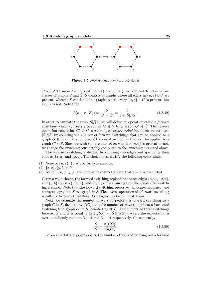
Figure 1.6 Forward and backward switchings
Proof of Theorem 1.8. To estimate P(u ∼ v | EU), we will switch between twoclasses of graphs S and S. S consists of graphs where all edges in u, v ∪ U arepresent, whereas S consists of all graphs where every x, y ∈ U is present, butu, v is not. Note that
P(u ∼ v | EU) =|S|
|S|+ |S| =1
1 + |S|/|S| . (1.3.49)
In order to estimate the ratio |S|/|S|, we will define an operation called a forwardswitching which converts a graph in G ∈ S to a graph G′ ∈ S. The reverseoperation converting G′ to G is called a backward switching. Then we estimate|S|/|S| by counting the number of forward switchings that can be applied to agraph G ∈ S, and the number of backward switchings that can be applied to agraph G′ ∈ S. Since we wish to have control on whether u, v is present or not,we change the switching considerably compared to the switching discussed above.
The forward switching is defined by choosing two edges and specifying theirends as x, a and y, b. The choice must satisfy the following constraints:
(1) None of u, x, v, y, or a, b is an edge;(2) x, a, y, b 6∈ U ;(3) All of u, v, x, y, a, and b must be distinct except that x = y is permitted.
Given a valid choice, the forward switching replaces the three edges u, v, x, a,and y, b by u, x, v, y, and a, b, while ensuring that the graph after switch-ing is simple. Note that the forward switching preserves the degree sequence, andconverts a graph in S to a graph in S. The inverse operation of a forward switchingis called a backward switching. See Figure 1.6 for an illustration.
Next, we estimate the number of ways to perform a forward switching to agraph G in S, denoted by f(G), and the number of ways to perform a backwardswitching to a graph G′ in S, denoted by b(G). The number of total switchingsbetween S and S is equal to |S|E[f(G)] = |S|E[b(G′)], where the expectation isover a uniformly random G ∈ S and G′ ∈ S respectively. Consequently,
|S||S| =
E[f(G)]
E[b(G′)]. (1.3.50)
Given an arbitrary graph G ∈ S, the number of ways of carrying out a forward
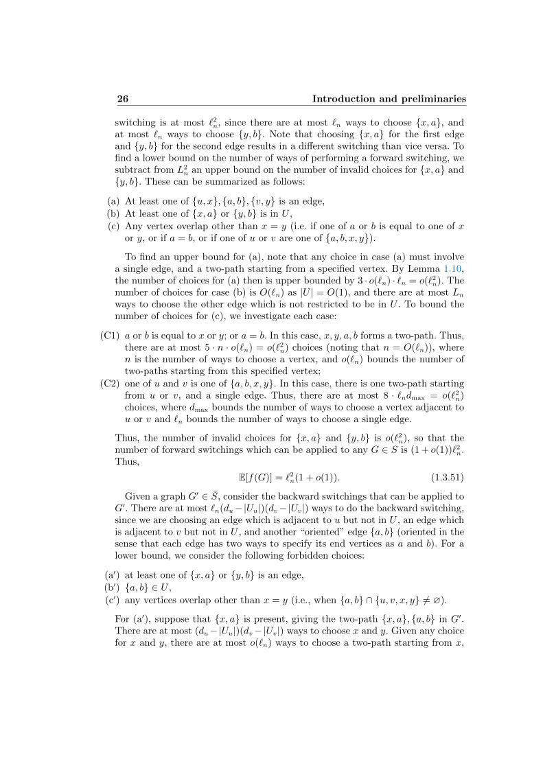
26 Introduction and preliminaries
switching is at most `2n, since there are at most `n ways to choose x, a, andat most `n ways to choose y, b. Note that choosing x, a for the first edgeand y, b for the second edge results in a different switching than vice versa. Tofind a lower bound on the number of ways of performing a forward switching, wesubtract from L2
n an upper bound on the number of invalid choices for x, a andy, b. These can be summarized as follows:
(a) At least one of u, x, a, b, v, y is an edge,
(b) At least one of x, a or y, b is in U ,
(c) Any vertex overlap other than x = y (i.e. if one of a or b is equal to one of xor y, or if a = b, or if one of u or v are one of a, b, x, y).To find an upper bound for (a), note that any choice in case (a) must involve
a single edge, and a two-path starting from a specified vertex. By Lemma 1.10,the number of choices for (a) then is upper bounded by 3 · o(`n) · `n = o(`2n). Thenumber of choices for case (b) is O(`n) as |U | = O(1), and there are at most Lnways to choose the other edge which is not restricted to be in U . To bound thenumber of choices for (c), we investigate each case:
(C1) a or b is equal to x or y; or a = b. In this case, x, y, a, b forms a two-path. Thus,there are at most 5 · n · o(`n) = o(`2n) choices (noting that n = O(`n)), wheren is the number of ways to choose a vertex, and o(`n) bounds the number oftwo-paths starting from this specified vertex;
(C2) one of u and v is one of a, b, x, y. In this case, there is one two-path startingfrom u or v, and a single edge. Thus, there are at most 8 · `ndmax = o(`2n)choices, where dmax bounds the number of ways to choose a vertex adjacent tou or v and `n bounds the number of ways to choose a single edge.
Thus, the number of invalid choices for x, a and y, b is o(`2n), so that thenumber of forward switchings which can be applied to any G ∈ S is (1 + o(1))`2n.Thus,
E[f(G)] = `2n(1 + o(1)). (1.3.51)
Given a graph G′ ∈ S, consider the backward switchings that can be applied toG′. There are at most `n(du−|Uu|)(dv−|Uv|) ways to do the backward switching,since we are choosing an edge which is adjacent to u but not in U , an edge whichis adjacent to v but not in U , and another “oriented” edge a, b (oriented in thesense that each edge has two ways to specify its end vertices as a and b). For alower bound, we consider the following forbidden choices:
(a′) at least one of x, a or y, b is an edge,
(b′) a, b ∈ U ,
(c′) any vertices overlap other than x = y (i.e., when a, b ∩ u, v, x, y 6= ∅).
For (a′), suppose that x, a is present, giving the two-path x, a, a, b in G′.There are at most (du−|Uu|)(dv−|Uv|) ways to choose x and y. Given any choicefor x and y, there are at most o(`n) ways to choose a two-path starting from x,
1.3 Random graph models 27
and hence o(`n) ways to choose a, b. Thus, the total number of choices is at mosto((du − |Uu|)(dv − |Uv|)`n). The case that y, b is an edge is symmetric.
For (b′), there are O(1) choices for choosing a, b since |U | = O(1), and atmost (du− |Uu|)(dv − |Uv|) choices x and y. Thus, the number of choices for case(b′) is O((du − |Uu|)(dv − |Uv|)) = o((du − |Uu|)(dv − |Uv|)`n).
For (c′), the case that a or b is equal to x or y corresponds to a two-path startingfrom u or v together with a single edge from u or v. Since o(`n) bounds the numberof two-paths starting from u or v and du− |Uu|+ dv− |Uv| bounds the number ofways to choose the single edge, there are o(`n(dv− |Uv|)) + o(Ln(du− |Uu|)) totalchoices. If a or b is equal to u or v, there are (du−|Uu|)(dv−|Uv|) ways to choosex and y, and at most du + dv ways to choose the last vertex as a neighbor of uor v. Thus, there are O((du − |Uu|)(dv − |Uv|)dmax) = o((du − |Uu|)(dv − |Uv|)`n)total choices, since dmax = O(n1/(τ−1)) = o(n) = o(Ln). This concludes that thenumber of backward switchings that can be applied to any graph G′ ∈ S′ is(du − |Uu|)(dv − |Uv|)`n(1 + o(1)), so that also
E[b(G′)] = (du − |Uu|)(dv − |Uv|)`n(1 + o(1)). (1.3.52)
Combining (1.3.50), (1.3.51) and (1.3.52) results in
|S|/|S| = (1 + o(1))`2n
(du − |Uu|)(dv − |Uv|)`n, (1.3.53)
and thus (1.3.49) yields
P(u ∼ v | EU) =1
1 + |S|/|S| = (1 + o(1))(du − |Uu|)(dv − |Uv|)
`n + (du − |Uu|)(dv − |Uv|). (1.3.54)
1.3.5 Preferential attachment models
Most networks grow in time. Preferential attachment models describe growingnetworks, where the numbers of edges and vertices grow linearly with time. Pref-erential attachment models were first introduced by Barabasi and Albert (1999),whose model we will generalize. Bollobas, Riordan, Spencer and Tusnady (2001)studied the model by Barabasi and Albert (1999), and later many other papersfollowed on this, and related, models. See [Volume 1, Chapter 8] for details. Herewe give a brief introduction.
The model that we investigate produces a graph sequence that we denote by(PA(m,δ)
t )t≥1 and which, for every time t, yields a graph of t vertices and mt edgesfor some m = 1, 2, . . . We start by defining the model for m = 1 when the graphconsists of a collection of trees. In this case, PA(1,δ)
1 consists of a single vertex witha single self-loop. We denote the vertices of PA(1,δ)
t by v(1)
1 , . . . , v(1)
t . We denote thedegree of vertex v(1)
i in PA(1,δ)
t by Di(t), where, by convention, a self-loop increasesthe degree by 2.
We next describe the evolution of the graph. Conditionally on PA(1,δ)
t , thegrowth rule to obtain PA(1,δ)
t+1 is as follows. We add a single vertex v(1)
t+1 having
28 Introduction and preliminaries
a single edge. This edge is connected to a second end point, which is equal tov(1)
t+1 with probability (1 + δ)/(t(2 + δ) + (1 + δ)), and to vertex v(1)
i ∈ PA(1,δ)
t withprobability (Di(t) + δ)/(t(2 + δ) + (1 + δ)) for each i ∈ [t], where δ ≥ −1 is aparameter of the model. Thus,
P(v(1)
t+1 → v(1)
i | PA(1,δ)
t
)=
1 + δ
t(2 + δ) + (1 + δ)for i = t+ 1,
Di(t) + δ
t(2 + δ) + (1 + δ)for i ∈ [t].
(1.3.55)
The above preferential attachment mechanism is called affine, since the attach-ment probabilities in (1.3.55) depend in an affine way on the degrees of therandom graph PA(1,δ)
t .
The model with m > 1 is defined in terms of the model for m = 1 as follows.Fix δ ≥ −m. We start with PA(1,δ/m)
mt , and denote the vertices in PA(1,δ/m)
mt byv(1)
1 , . . . , v(1)
mt. Then we identify or collapse the m vertices v(1)
1 , . . . , v(1)
m in PA(1,δ/m)
mt
to become vertex v(m)
1 in PA(m,δ)
t . In doing so, we let all the edges that are incidentto any of the vertices in v(1)
1 , . . . , v(1)
m be incident to the new vertex v(m)
1 in PA(m,δ)
t .Then, we collapse the m vertices v(1)
m+1, . . . , v(1)
2m in PA(1,δ/m)
mt to become vertex v(m)
2
in PA(m,δ)
t , etc. More generally, we collapse the m vertices v(1)
(j−1)m+1, . . . , v(1)
jm in
PA(1,δ/m)
mt to become vertex v(m)
j in PA(m,δ)
t . This defines the model for generalm ≥ 1. The resulting graph PA(m,δ)
t is a multigraph with precisely t vertices andmt edges, so that the total degree is equal to 2mt. The original model by Barabasiand Albert (1999) focused on the case δ = 0 only, which is sometimes called theproportional model. The inclusion of the extra parameter δ > −1 is relevantthough, as we will see later.
The preferential attachment model (PA(m,δ)
t )t≥1 is increasing in time, in thesense that vertices and edges, once they have appeared, remain there forever.Thus, the degrees are monotonically increasing in time. Moreover, vertices witha high degree have a higher chance of attracting further edges of later vertices.Therefore, the model is sometimes called the rich-get-richer model. It is not hardto see that Di(t)
a.s.−→ ∞ (see Exercise 1.10). As a result, one could also callthe preferential attachment model the old-get-richer model, which may be moreappropriate.
Let us continue to discuss the degree structure in (PA(m,δ)
t )t≥1.
Degrees of fixed vertices
We start by investigating the degrees of fixed vertices as t → ∞, i.e., we studyDi(t) for fixed i as t → ∞. To formulate our results, we define the Gamma-function t 7→ Γ(t) for t > 0 by
Γ(t) =
∫ ∞0
xt−1e−xdx. (1.3.56)
The following theorem describes the evolution of the degree of fixed vertices (see[Volume 1, Theorem 8.2 and (8.3.11)]):
1.3 Random graph models 29
Theorem 1.11 (Degrees of fixed vertices) Fix m ≥ 1 and δ > −m. Then,Di(t)/t
1/(2+δ/m) converges almost surely to a random variable ξi as t→∞.
It turns out that also t−1/(2+δ/m) maxi∈[t]Di(t)a.s.−→M for some limiting positive
and finite random variable M (see [Volume 1, Section 8.7]). In analogy to i.i.d.random variables, the fact that t−1/(2+δ/m) maxi∈[t]Di(t)
a.s.−→ M suggests thatthe degree of a random vertex satisfies a power law with power-law exponentτ = 3 + τ/m, and that is our next item on the agenda.
The degree sequence of the preferential attachment model
The main result in this section establishes the scale-free nature of preferentialattachment graphs. In order to state it, we need some notation. We write
Pk(t) =1
t
t∑i=1
1Di(t)=k (1.3.57)
for the (random) proportion of vertices with degree k at time t. For m ≥ 1 andδ > −m, we define (pk)k≥0 by pk = 0 for k = 0, . . . ,m− 1 and, for k ≥ m,
pk = (2 + δ/m)Γ(k + δ)Γ(m+ 2 + δ + δ/m)
Γ(m+ δ)Γ(k + 3 + δ + δ/m)(1.3.58)
It turns out that (pk)k≥0 is a probability mass function (see [Volume 1, Section8.3]). The probability mass function (pk)k≥0 arises as the limiting degree distri-bution for PA(m,δ)
t , as shown in the following theorem:
Theorem 1.12 (Degree sequence in preferential attachment model) Fix m ≥ 1and δ > −m. There exists a constant C = C(m, δ) > 0 such that, as t→∞,
P(
maxk|Pk(t)− pk| ≥ C
√log t
t
)= o(1). (1.3.59)
We next investigate the scale-free properties of (pk)k≥0 by investigating theasymptotics of pk for k large. By (1.3.58) and Stirling’s formula, as k →∞,
pk = cm,δk−τ (1 +O(1/k)), (1.3.60)
where
τ = 3 + δ/m > 2, and cm,δ = (2 + δ/m)Γ(m+ 2 + δ + δ/m)
Γ(m+ δ). (1.3.61)
Therefore, by Theorem 1.12 and (1.3.60), the asymptotic degree sequence ofPA(m,δ)
t is close to a power law with exponent τ = 3 + δ/m. We note that anyexponent τ > 2 is possible by choosing δ > −m and m ≥ 1 appropriately.
30 Introduction and preliminaries
Extensions to the preferential attachment rule
In this book, we also sometimes investigate the related (PA(m,δ)
t (b))t≥1 model, inwhich the self-loops for m = 1 in (1.3.55) are not allowed, so that
P(v(1)
t+1 → v(1)
i | PA(1,δ)
t (b))
=Di(t) + δ
t(2 + δ)for i ∈ [t]. (1.3.62)
The model for m ≥ 2 is again defined in terms of the model (PA(1,δ)
t (b))t≥1 for m =1 by collapsing blocks of m vertices. The advantage of (PA(m,δ)
t (b))t≥1 compared to(PA(m,δ)
t )t≥1 is that (PA(m,δ)
t (b))t≥1 is naturally connected, while (PA(m,δ)
t )t≥1 maynot be.
Another adaptation of the preferential attachment rule is when no self-loopsare ever allowed while the degrees are updated when the m edges incident to thenew vertex is being attached. We denote this model by (PA(m,δ)
t (c))t≥1. In thiscase, the model for m = 1 is the same as (PA(1,δ)
t (b))t≥1, while for m ≥ 2 andj ∈ 0, . . . ,m− 1, we attach the (j + 1)st edge of vertex v(m)
t+1 to vertex v(m)
i fori ∈ [t] with probability
P(v(m)
t+1,j+1 → v(m)
i | PA(m,δ)
t,j (c))
=Di(t, j) + δ
t(2m+ δ)for i ∈ [t]. (1.3.63)
Here, Di(t, j) is the degree of vertex v(m)
i after the connection of the edges incidentto the first t vertices, as well as the first j edges incident to vertex v(m)
t+1. Manyother adaptations are possible, and have been investigated in the literature, suchas settings where the m edges incident to v(m)
t+1 are independently connected as in(1.3.63) when j = 0, but we refrain from discussing these. It is not hard to verifythat Theorem 1.12 remains to hold for all these adaptations, which explains whyauthors have often opted for the version of the model that is most convenientfor them. On the other hand, in Theorem 1.11 there will be minor adaptations,particularly since the limiting random variables (ξi)i≥1 do depend on the precisemodel.
1.3.6 A Bernoulli preferential attachment model
In this section, we discuss a model that is quite a bit different from the otherpreferential attachment models discussed above. The main difference is that inthis model, the number of edges is not fixed, but instead there is much moreindependence in the edge attachments. A preferential attachment models withconditionally independent edges is investigated by Dereich and Morters (2009,2011, 2013). We call this model the Bernoulli preferential attachment model, asthe attachment indicators are all conditionally independent Bernoulli variables.Let us now give the details.
Fix a preferential attachment function f : N0 7→ (0,∞). Then, the graph evolvesas follows. Start with BPA(f)
1 ) being a graph containing one vertex v1 and noedges. At each time t ≥ 2, we add a vertex vt. Conditionally on G(t − 1), and
1.3 Random graph models 31
independently for every i ∈ [t− 1], we connect this vertex to i by a directed edgewith probability
f(Di(t− 1))
t− 1, (1.3.64)
where Di(t − 1) is the in-degree of vertex i at time t − 1. This creates the ran-dom graph BPA(f)
t . Note that the number of edges in the random graph process(BPA(f)
t )t≥1 is not fixed, and equal a random variable. In particular, it makes adifference whether we use the in-degree in (1.3.64).
We consider functions f : N 7→ (0,∞) that satisfy that f(k + 1)− f(k) < 1 forevery k ≥ 0. Under this assumption and when f(0) ≤ 1, Morters and Dereichshow that the empirical degree sequence converges as t→∞, i.e.,
Pk(t) ≡1
t
∑i∈[t]
1Di(t)=kP−→ pk, where pk =
1
1 + f(k)
k−1∏l=0
f(l)
1 + f(l).
(1.3.65)In particular, log(1/pk)/ log(k)→ 1+1/γ when f(k)/k → γ ∈ (0, 1) (see Exercise1.12). Remarkably, when f(k) = γk + β, the power-law exponent of the degreedistribution does not depend on β. The restriction that f(k + 1) − f(k) < 1 isneeded to prevent the degrees from exploding. Further, log(1/pk) ∼ k1−α/(γ(1−α)) when f(k) ∼ γkα for some α ∈ (0, 1) (see Exercise 1.13). Interestingly,Morters and Dereich also show that when
∑k≥1 1/f(k)2 < ∞, then there exists
a persistent hub, i.e., a vertex that has maximal degree for all but finitely manytimes. When
∑k≥1 1/f(k)2 =∞, this does not happen.
1.3.7 Universality of random graphs
There are tons of other graph topologies where one can expect similar resultsas in the random graphs discussed above. We will discuss a few related models inChapter 9 below, where we include several aspects that are relevant in practice,such as directed graphs, adding community structure to random graphs, and ge-ometry. The random graph models that we investigate are inhomogeneous, andone can expect that the results depend sensitively on the amount of inhomogene-ity present. This is reflected in the results that we will prove, where the preciseasymptotics is different when the vertices have heavy-tailed degrees rather thanlight-tailed degrees. However, interestingly, what is ‘heavy tailed’ and what is‘light tailed’ depends on the precise model at hand. Often, as we will see, thedistinction depends on how many moments the degree distribution has.
We have proposed many random graph models for real-world networks. Sincethese models are aiming at describing similar real-world networks, one wouldhope that they also give similar answers. Indeed, for a real-world network withpower-law degree sequences, we could model its static structure by the configu-ration model with the same degree sequence, and its dynamical properties by thepreferential attachment model with similar scale-free degrees. How to interpretthe modeling when these attempts give completely different predictions?
32 Introduction and preliminaries
Universality is the phrase physicists use when different models display similarbehavior. Models that show similar behavior are then in the same universalityclass. Enormous effort is going into decided whether various random graph mod-els are in the same universality class, or rather in different ones, and why. We willsee that for some features the degree distribution decides the universality classfor a wide range of models, as one might possibly hope. This also explains whythe degree distribution plays such a dominant role in the investigation of randomgraphs. Let us discuss some related graphs that have attracted substantial at-tention in the literature as models for networks. In Chapter 9, we discuss severalrelated random graph models that have attracted the attention in the literature.
1.4 Power-laws and their properties
In this text, we frequently deal with random variables having an (asymptotic)power-law distribution. For such random variables, we often need to investigatetruncated moments. We study two of such truncated moment bounds here. Westart with the tail of the mean:
Lemma 1.13 (Truncated moments) Let X be a non-negative random variablewhose distribution function satisfies that for every x ≥ 1,
1− FX(x) ≤ CXx−(τ−1). (1.4.1)
Then, there exists a constant C = CX(a) such that, for a < τ − 1 and all ` ≥ 1,
E[Xa1X>`] ≤ C`a−(τ−1), (1.4.2)
while, for for a > τ − 1 and all ` ≥ 1,
E[Xa1X≤`] ≤ C`a−(τ−1). (1.4.3)
Proof We note that for any cumulative distribution function x 7→ F (x) on thenon-negative reals, we have the partial integration identity∫ ∞
u
f(x)F (dx) = f(u)[1− F (u)] +
∫ ∞u
[f(x)− f(u)]F (dx) (1.4.4)
= f(u)[1− F (u)] +
∫ ∞u
∫ x
0
f ′(y)dyF (dx)
= f(u)[1− F (u)] +
∫ ∞u
f ′(y)
∫ ∞y
F (dx)dy
= f(u)[1− F (u)] +
∫ ∞u
f ′(y)[1− F (y)]dy.
provided that either y 7→ f ′(y)[1− F (y)] is absolutely integrable, or x 7→ f(x) iseither non-decreasing or non-increasing. Here, the interchange of the summationorder is allowed by Fubini’s Theorem for non-negative functions (see (Halmos,1950, Section 3.6, Theorem B)) when x 7→ f(x) is non-decreasing, and by Fubini’s
1.5 Notation 33
Theorem (Halmos, 1950, Section 3.6, Theorem C) when y 7→ f ′(y)[1 − F (y)] isabsolutely integrable.
When D ≥ 0, using (1.4.1) and (1.4.4), for a < τ − 1 and ` > 0,
E[Xa
1X>`]
= xaP(X > `) +
∫ ∞`
axa−1P(X > x)dx (1.4.5)
≤ CXxa−(τ−1) + aCX
∫ ∞`
xa−1x−(τ−1) ≤ Ca,τ`a−(τ−1).
as required.
An important notion in many graphs is the size-biased version X? of a non-negative random variable X that is given by
P(X? ≤ x) =E[X1X≤x]
E[X]. (1.4.6)
Let F ?X
denote the distribution function of X?. The following lemma gives boundson the tail of the distribution function F ?
X:
Lemma 1.14 (Size-biased tail distribution) Let X be a non-negative randomvariable whose distribution function satisfies that for every x ≥ 1,
1− FX(x) ≤ CXx−(τ−1). (1.4.7)
Assume that τ > 2, so that E[X] < ∞. Further, assume that E[X] > 0. Then,there exists a constant C such that
1− F ?X
(x) ≤ C?Xx−(τ−2). (1.4.8)
Proof This follows immediately from (1.4.6), by using (1.4.2) with a = 1.
1.5 Notation
Let us introduce some standard notation used throughout this book.
Random variables
We use special notation for certain random variables. We write X ∼ Ber(p)when X has a Bernoulli distribution with success probability p, i.e., P(X = 1) =1 − P(X = 0) = p. We write X ∼ Bin(n, p) when the random variable X has abinomial distribution with parameters n and p, and we write X ∼ Poi(λ) whenX has a Poisson distribution with parameter λ. We write X ∼ Exp(λ) when Xhas an exponential distribution with mean 1/λ. We write X ∼ Gam(λ, r) when Xhas a Gamma distribution with density fX(x) = λrxr−1e−λr/Γ(r), where r, λ > 0.The random variable Gam(λ, r) has mean r/λ and variance r/λ2. Finally, we writeX ∼ Beta(a, b) when X has a Beta distribution with parameters a, b > 0, so that
X has density fX(x) = xa−1(1− x)b−1 Γ(a+b)
Γ(a)Γ(b).
We sometimes abuse notation, and write e.g., P(Bin(n, p) = k) to denoteP(X = k) when X ∼ Bin(n, p). We call a sequence of random variables (Xi)i≥1
34 Introduction and preliminaries
independent and identically distributed (i.i.d.) when they are independent, andXi has the same distribution as X1 for every i ≥ 1.
Convergence of random variables
We say that a sequence of events (En)n≥1 occurs with high probability (whp)when limn→∞ P(En) = 1. We further write f(n) = O(g(n)) if |f(n)|/|g(n)| isuniformly bounded from above by a positive constant as n→∞, f(n) = Θ(g(n))if f(n) = O(g(n)) and g(n) = O(f(n)), f(n) = Ω(g(n)) if 1/f(n) = O(1/g(n))and f(n) = o(g(n)) if f(n)/g(n) tends to 0 as n→∞. We say that f(n) g(n)when g(n) = o(f(n)).
For sequences of random variables (Xn)n≥1, we let Xnd−→ X denote that Xn
converges in distribution to X, while XnP−→ X denotes that Xn converges in
probability to X and Xna.s.−→ X denotes that Xn converges almost surely to X.
We write that Xn = OP(Yn) when |Xn|/Yn is a tight sequence of random variables
and Xn = OP(Yn) when |Xn|/Yn P−→ 0. Finally, we write that Xn = oP(Yn) when
Xn/YnP−→ 0.
Trees
In this book, we will often deal with trees, and then it is important to be clearabout what we mean exactly with a tree. It will be convenient to think of atree T with root ∅ as being labelled in the Ulam-Harris way, so that a vertex vin generation k has a label ∅a1 · · · ak, where ai ∈ N. Naturally, there are somerestrictions in that if ∅v1 · · · vk ∈ V (T ), then also ∅a1 · · · ak−1 ∈ T and also∅a1 · · · (ak − 1) ∈ T when ak ≥ 2. We refer to [Volume 1, Chapter 3] for details.It will sometimes also be useful to explore the branching process tree in a breadth-first exploration. This corresponds to the lexicographical ordering in the Ulam-Harris encoding of the tree. Ulam-Harris trees are also sometimes called planetrees (see e.g., (Drmota, 2009, Chapter 1)).
1.6 Notes and discussion
Notes on Sections 1.1–1.3
These sections are summaries of chapters in Volume 1, to which we refer for notesand discussion. The exception is Section 1.3.4 on switching algorithms for uniformrandom graphs with prescribed degrees, which is novel. Switching algorithmshave a long history, dating back at least to McKay (1981), see also Gao andWormald (2016); McKay and Wormald (1990), as well as McKay (2011) and thereferences therein for an overview. The material in Section 1.3.4 is an adaptationof some of the material in Gao et al. (2018), where Theorem 1.8 was used tocompute the number of triangles in uniform random graphs with power-law degreedistributions of infinite variance.
1.7 Exercises for Chapter 1 35
Notes on Section 1.4
1.7 Exercises for Chapter 1
Exercise 1.1 (Probability mass function typical degree) Prove (1.1.3).
Exercise 1.2 (Uniform random graph) Consider ERn(p) with p = 1/2. Showthat the result is a uniform graph, i.e., it has the same distribution as a uniformchoice from all the graphs on n vertices.
Exercise 1.3 (Thin tails Poisson) Show that, for every α > 0, and with pk =
e−λ λk
k!the Poisson probability mass function,
limk→∞
eαkpk = 0. (1.7.1)
Exercise 1.4 (Weight of uniformly chosen vertex) Let U be a vertex chosenuniformly at random from [n]. Show that the weight wU of U has distributionfunction Fn.
Exercise 1.5 (Maximal weight bound) Assume that Conditions 1.1(a)-(b) hold.Show that maxi∈[n]wi = o(n). Further, show that maxi∈[n]wi = o(
√n) when
Conditions 1.1(a)-(c) hold.
Exercise 1.6 (Domination weights) Let Wn have distribution function Fn from(1.3.17). Show that Wn is stochastically dominated by the random variable Whaving distribution function F .
Exercise 1.7 (Degree of uniformly chosen vertex in GRGn(w)) Prove that,under the conditions of Theorem 1.3, (1.3.22) holds.
Exercise 1.8 (Power-law degrees in generalized random graphs) Prove that,under the conditions of Theorem 1.3, (1.3.24) follows from (1.3.23). Does theconverse also hold?
Exercise 1.9 (Number of erased edges) Assume that Conditions 1.5(a)-(b)hold. Show that Theorem 1.6 implies that the number of erased edges is oP(n).
Exercise 1.10 (Degrees grow to infinity a.s.) Fix m = 1 and i ≥ 1. Provethat Di(t)
a.s.−→ ∞, by using that∑t
s=i Is Di(t), where (It)t≥i is a sequence ofindependent Bernoulli random variables with P(It = 1) = (1+δ)/(t(2+δ)+1+δ).What does this imply for m > 1?
Exercise 1.11 (Degrees of fixed vertices) Prove Theorem 1.11 for m = 1 andδ > −1 using the martingale convergence theorem and the fact that
Mi(t) =Di(t) + δ
1 + δ
t−1∏s=i−1
(2 + δ)s+ 1 + δ
(2 + δ)(s+ 1)(1.7.2)
is a martingale.
Exercise 1.12 (Degrees distribution of affine Bernoulli PAM) Show that pk ∼cγ,βk
−(1+1/γ) when f(k) = γk + β. What is cγ,β?
36 Introduction and preliminaries
Exercise 1.13 (Degrees distribution of sublinear Bernoulli PAM) Show thatlog(1/pk) ∼ k1−α/(γ(1− α)) when f(k) ∼ γkα for some α ∈ (0, 1).
Exercise 1.14 (Power-law degree sequence) Prove (1.3.61) by using Stirling’sformula.
Chapter 2
Local weak convergenceof random graphs
Abstract
In this chapter, we discuss local weak convergence, as introduced byBenjamini and Schramm (2001) and independently by Aldous andSteele (2004). Local weak convergence described the intuitive notionthat a finite graph, seen from the perspective of a typical vertex, lookslike a certain limiting graph. This is already useful to make the notionthat a finite cube in Zd is locally much alike Zd itself when the sidelength is large. However, it plays an even more profound role in randomgraph theory. For example, local weak convergence to some limitingtree, which often occurs in random graphs as we will see throughoutthis book, is referred to as locally tree-like behavior. We discuss localweak convergence in general, as it has proven to be an extremely usefulnotion in general.
Organisation of this chapter
This chapter is organised as follows. In Section 2.2, we start by discussing themetric space of rooted graphs, that will play a crucial role in local weak conver-gence. There, we think of our graphs as being deterministic and we discuss theirconvergence to some (possibly random) limit. Here, the randomness originatesfrom the fact that we consider the graph rooted at a random vertex, and thisrandomness may persist in the limit. In Section 2.3, we then extend the notionof local weak convergence to random graphs, for which there are several notionsof convergence like for real-valued random variables. In Section 2.4, we discussconsequences of local weak convergence to local functionals. In Section 2.5, wediscuss the consequences of local weak convergence on the existence of the giantcomponent. While the proportion of vertices in the giant is not necessarily a con-tinuous functional, one could argue that it is ‘almost local’. We close this chapterwith notes and discussion in Section 2.6, and with exercises in Section 2.7.
2.1 The metric space of rooted graphs
Let us start by discussing the notion of local weak convergence in more detail.We follow Aldous and Steele (2004), using results from Benjamini et al. (2015)as well. We start with some definitions:
Definition 2.1 (Locally finite and rooted graphs) A rooted graph is a pair(G, o), where G = (V (G), E(G)) is a graph with vertex set V (G) and edge setE(G), and o ∈ V (G) is a vertex. Further, a rooted or non-rooted graph is called
37
38 Local weak convergence of random graphs
locally finite when each of its vertices has finite degree (though not necessarilyuniformly bounded).
In Definition 2.1, graphs can be finite or infinite, but we will always havegraphs that are locally finite in mind. Also, in the definitions below, the graphsare deterministic and we will clearly indicate when we move to random graphsinstead.
For a rooted graph (G, o), we let Bo(r) denote the subgraph of G of all verticesat graph distance at most r away from o. Formally, this means that Bo(r) =(V (Bo(r)), E(Bo(r))), where
V (Bo(r)) = u : dG(o, u) ≤ r, (2.1.1)
E(Bo(r)) = u, v ∈ E(G) : u, v ∈ Bo(r).We continue by introducing the notion of isomorphism between graphs, whichbasically describes that graphs ‘look the same’. Here is the formal definition:
Definition 2.2 (Graph isomorphism) Two (finite or infinite) graphs G1 =(V (G1), E(G1)) and G2 = (V (G2), E(G2)) are called isomorphic, which we writeas G1 ' G2, when there exists a map φ : V (G1) 7→ V (G2) such that u, v ∈E(G1) precisely when φ(u), φ(v) ∈ E(G2). Similarly, two rooted (finite or in-finite) graphs (G1, o1) and (G2, o2) where Gi = (V (Gi), E(Gi)) for i ∈ 1, 2 arecalled isomorphic, which we write as (G1, o1) ' (G2, o2), when there exists a mapφ : V (G1) 7→ V (G2) such that φ(o1) = φ(o2) and u, v ∈ E(G1) precisely whenφ(u), φ(v) ∈ E(G2).
Exercises 2.1 and 2.2 below investigate the notion of graph isomorphism. Welet G? denote the space of rooted graphs modulo isomorphisms, as introducedby Aldous and Steele (2004). This means that G? contains the set of equivalenceclasses of rooted graphs. We often omit the equivalence classes, and write (G, o) ∈G?, bearing in mind that all (G′, o′) such that (G′, o′) ' (G, o) are considered tobe the same.
These notions allow us to turn the space of connected rooted graphs into ametric space:
Definition 2.3 (Metric on rooted graphs) Let (G1, o1) and (G2, o2) be tworooted connected graphs, and write Bi,vi(r) for the neighborhood of vertex vi inGi. Let
R? = supr : B1,o1(r) ' B2,o2(r). (2.1.2)
Define
dG?
((G1, o1), (G2, o2)
)= 1/(R? + 1). (2.1.3)
The space G? of rooted graphs is a nice metric space under the metric dG?in
(2.1.3), in that it is separable and thus Polish. Here we recall that a metric spaceis called separable when there exists a countable dense subset of elements. Wewill see later on that such a countable dense set can be created by looking at
2.2 Local weak convergence of graphs 39
finite rooted graphs. Since graphs that agree up to distance r are at distance atmost 1/(r+1) from each other (see Exercise 2.3), this is indeed a dense countablesubset. See Exercises 2.4 and 2.5 below for two exercises that study such aspects.
The valueR? is the largest value of r for whichB1,o1(r) is isomorphic toB2,o2(r).When R? =∞, then B1,o1(r) is isomorphic to B2,o2(r) for every r ≥ 1, and thenthe rooted graphs G1 and G2 are the same.
2.2 Local weak convergence of graphs
We next define local weak convergence of finite graphs:
Definition 2.4 (Local weak convergence) Let Gn = ([n], E(Gn)) denote a finite(possibly disconnected) graph. Let (Gn, on) be the rooted graph obtained by lettingon ∈ [n] be chosen uniformly at random and restricting Gn to the connectedcomponent of on in Gn. We say that Gn converges in the local weak sense to(G, o), which is a (possibly) random element of G? having law µ, when
En[h(Gn, on
)]→ E
[h(G, o
)], (2.2.1)
where the expectation on the right-hand side of (2.2.1) is w.r.t. (G, o) having lawµ, for every bounded and continuous function h : G? 7→ R, while the expectationEn is w.r.t. the random vertex on only.
Since we will later apply local weak convergence ideas to random graphs, westrive to be absolutely clear about what we take the expectation with. Indeed,the expectation in (2.2.1) is equal to
En[h(Gn, on
)]=
1
n
∑u∈[n]
h(Gn, u). (2.2.2)
The notion of local weak convergence is hard to grasp, and it also may appear tobe rather weak. In the sequel, we discuss examples of graphs that converge locallyweakly Further, see Section 1.6 for some examples of how local weak convergencemay be used. The notion will also be crucially used in this book. We continue bydiscussing a convenient criterion for proving local weak convergence.
Criterion for local weak convergence
While the notion of local weak convergence may seem somewhat weak, it actuallyturns out to be quite convenient, as we will see in the remainder of this book. Wenext provide a criterion for local weak convergence:
Theorem 2.5 (Criterion for local weak convergence) The sequence of finitegraphs (Gn)n≥1 converges in the local weak sense to (G, o) precisely when, forevery rooted graph (H, v),
p(n)(H) =1
n
∑u∈[n]
1(B(n)u (r),u)'(H,v) → P((Bo(r), o) ' (H, v)), (2.2.3)
40 Local weak convergence of random graphs
where B(n)
u (r) is the k-neighborhood of u in Gn, and Bo(k) is the k-neighborhoodof o in the limiting graph (G, o).
Proof First of all, local weak convergence implies that (2.2.3) holds, since wecan take h
(G, o
)= 1(G,o)'(H,v). For the other side, we need to prove that if
(2.2.3) holds, then, En[h(Gn, on
)]→ E
[h(G, o
)]for every bounded and continu-
ous function h : G? 7→ R. Fix ε. Take r = r(δ) so large that
dG?
((G, o), (Bo(r), o)
)≤ δ. (2.2.4)
Next, by continuity of h, we can take δ > 0 so small that, for every rooted graph(G, o), ∣∣h(G, o)− h(Bo(r), o)∣∣ ≤ ε/4. (2.2.5)
We conclude that∣∣∣En[h(Gn, on)]− E
[h(G, o
)]∣∣∣ (2.2.6)
≤∣∣∣En[h(B(n)
on(r), on
)]− E
[h(Bo(r), o
)]∣∣∣+ ε/2.
Fix k large. Let Er,k(G, o) be the event that there exists a vertex v at distanceat most r from o in G such that dv(G) > k. Since the limiting graph (G, o) islocally finite, for every η > 0, we can take k so large that
P(Er,k(G, o)) ≤ η. (2.2.7)
Further, we can write
P(Er,k(Gn, on)) = 1− P(Er,k(Gn, on)c). (2.2.8)
Now, there is just a finite number of rooted (G, o) graphs that Er,k(G, o)c holds
(see Exercise 2.6). Thus, by (2.2.3),
P(Er,k(Gn, on)c)→ P(Er,k(G, o)c). (2.2.9)
Take n0 so large that, for all n ≥ n0,
|P(Er,k(Gn, on)c)− P(Er,k(G, o)c)| ≤ η. (2.2.10)
Then, also P(Er,k(Gn, on)) ≤ 2η. We conclude that∣∣∣En[h(Gn, on)]− E
[h(G, o
)]∣∣∣ (2.2.11)
≤∣∣∣En[h(B(n)
on(r), on
)1Er,k(Gn,on)c
]− E
[h(Bo(r), o
)1Er,k(G,o)c
]∣∣∣+ ε/2 + 2η‖h‖∞,
where ‖h‖∞ = sup(H,v)∈G?|h(H, v)| < ∞, since h is a bounded function. Again,
since there is just a finite number of rooted (G, o) graphs that Er,k(G, o)c holds,
by (2.2.3),
En[h(B(n)
on(r), on
)1Er,k(Gn,on)c
]→ E
[h(Bo(r), o
)1Er,k(G,o)c
]. (2.2.12)
Then, pick n1 ≥ 1 so large that, for all n ≥ n1,∣∣∣En[h(B(n)
on(r), on
)1Er,k(Gn,on)c
]− E
[h(Bo(r), o
)1Er,k(G,o)c
]∣∣∣ ≤ ε/4. (2.2.13)
2.2 Local weak convergence of graphs 41
Taking η = ε/(8‖h‖∞) then shows that, for all n ≥ n0 ∨ n1,∣∣∣En[h(Gn, on)]− E
[h(G, o
)]∣∣∣ ≤ ε, (2.2.14)
which proves the claim.
Theorem 2.5 shows that the proportion of vertices in Gn whose neighborhoodlooks like (H, v) converges to a (possibly random) limit. You are asked to provelocal weak convergence for some examples in Exercises 2.8 and 2.9. See alsoExercise 2.7, where you are asked to construct an example where the local weaklimit of a sequence of deterministic graphs actually is random.
We continue by giving a tightness criterium for local weak convergence:
Theorem 2.6 (Tightness criterion for local weak convergence) Let (Gn)n≥1 bea sequence of marked graphs. Let d(n)
ondenote the degree of on in Gn, where on.
Then (Gn, on)n≥1 is tight when (d(n)
on)n≥1 forms a uniformly integrable sequence
of random variables.
Proof Let A be a family of finite graphs such that the random variables. For agraph G, let UG denote a random vertex and let U(G) = (G,UG) be the rootedgraph obtained by rooting G at UG. We need to show that if
degG(UG) : G ∈ A
is a uniformly integrable sequence of random variables, then the family A is tight.Let
f(d) = supG∈A
E[degG(UG)1degG(UG)>d
]. (2.2.15)
By assumption, limd→∞ f(d) = 0. Write m(G) = E[degG(UG). Thus, 1 ≤ m(G) ≤
f(0) <∞. Write D(G) for the degree-biased probability measure on (G, x) : x ∈V (G), that is,
D(G)[(G, x)] =degG(x)
m(G)· U(G)[(G, x)], (2.2.16)
and DG for the corresponding root. Since U(G) ≤ m(G)D(G) ≤ f(0)D(G), itsuffices to show that D(G) : G ∈ A is tight. Note that degG(DG) : G ∈ A istight.
For r ∈ N, let FM
r (x) be the event such that there is some vertex at distanceat most r from x whose degree is larger than M . Let X be a uniform randomneighbor of DG. Because D(G) is a stationary measure for a simple random walk,FM
r (DG) and FM
r (X) have the same probability. Also,
P(FM
r+1(DG) | degG(DG))≤ degG(DG)P
(FM
r (X) | degG(DG)). (2.2.17)
We claim that for all r ∈ N and ε > 0, there exists M <∞ such that
P(FM
r (X))≤ ε (2.2.18)
for all G ∈ A. This clearly implies that D(G) : G ∈ A is tight. We prove theclaim by induction on r.
42 Local weak convergence of random graphs
The statement for r = 0 is trivial. Given that the property holds for r, let us nowshow it for r+ 1. Given ε > 0, choose d so large that P(degG(DG) > d) ≤ ε/2 forall G ∈ A. Also, choose M so large that P(FM
r (DG)) ≤ ε/(2d) for all G ∈ A. WriteF for the event such that degG(DG) > d. Then, by conditioning on degG(DG),we see that
P(FM
r+1(DG))≤ P(F ) + E
[1F cP
(FM
r+1(DG) | degG(DG))]
(2.2.19)
≤ ε/2 + E[1F cdegG(DG)P
(FM
r (DG) | degG(DG))]
≤ ε/2 + E[1F cdP
(FM
r (DG) | degG(DG))]
≤ ε/2 + dP(FM
r (DG))
≤ ε/2 + dε/(2d) = ε,
for all G ∈ A, which proves the claim.
The needed uniform integrability in Theorem 2.6 is quite suggestive. Indeed,in many random graph models, such as for example the configuration model, thedegree of a random neighbor of a vertex has the size-biased degree distribution.Previously, we have often written Dn = d(n)
onfor the degree of a uniform vertex
in our graph. When (d(n)
on)n≥1 forms a uniformly integrable sequence of random
variables, there exists a subsequence along which D?n, the size-biased version of
Dn = d(n)
on, converges in distribution (see Exercise 2.10 below). Further, Condi-
tions 1.5(a)-(b) imply that (don)n≥1 is a tight sequence of random variables (seeExercise 2.11). Thus, at least for the configuration model, we can fully understandwhy the uniform integrability of (d(n)
on)n≥1 is needed.
Having discussed the notion of local weak convergence for deterministic graphs,we now move on to random graphs. Here the situation becomes even more delicate,as now we have double randomness, both in the random root as well as the randomgraph.
2.3 Local weak convergence of random graphs
We next discuss settings of random graphs. Even for random variables, thereare different notions of convergence tat are relevant, such as convergence in distri-bution and in probability. Also for local weak convergence, there are two relatednotions of convergence that we may consider. We start with convergence in dis-tribution:
Definition 2.7 (Local weak convergence of random graphs) Let Gn = ([n], E(Gn))denote a finite (possibly disconnected) random graph. Let (G, o) be a random vari-able on G? having law µ. Then,
(a) We say that Gn converges in in distribution in the local weak sense to (G, o)
2.3 Local weak convergence of random graphs 43
when
E[h(Gn, on
)]→ E
[h(G, o
)], (2.3.1)
where the expectation on the right-hand side of (2.3.1) is w.r.t. (G, o) hav-ing law µ, for every bounded and continuous function h : G? 7→ R, while theexpectation E is w.r.t. the random vertex on and the random graph Gn.
(b) We say that Gn converges in probability in the local weak sense to (G, o) when
En[h(Gn, on
)] P−→ E[h(G, o
)], (2.3.2)
where the expectation on the right-hand side of (2.3.2) is w.r.t. (G, o) hav-ing law µ, for every bounded and continuous function h : G? 7→ R, while theexpectation En is w.r.t. the random vertex on only.
(c) We say that Gn converges almost surely in the local weak sense to (G, o) when
En[h(Gn, on
)] a.s.−→ E[h(G, o
)], (2.3.3)
where the expectation on the right-hand side of (2.3.2) is w.r.t. (G, o) hav-ing law µ, for every bounded and continuous function h : G? 7→ R, while theexpectation En is w.r.t. the random vertex on only.
As usual in convergence of random variables, the difference between theseclosely related definitions lies in what can be concluded from it. Indeed, when wehave convergence in probability in the local weak sense, then En
[h(Gn, on
)], which
is a random variable due to the dependence on the random graph Gn, converges inprobability. Thus, this is sometimes called a quenched result. When we have con-vergence in distribution in the local weak sense, instead, then only expectationsw.r.t. the random graph of the form E
[h(Gn, on
)]converge. This corresponds
to an annealed result. Certainly when considering complicated functionals of therandom graph, we would prefer the limit not to depend on the specific randomgraph, and be deterministic instead. For this, one needs the stronger notion ofconvergence in probability in the local weak sense.
We have added the notion of local weak convergence in the almost sure sense,even though for random graphs this notion often is not highly useful. Indeed,almost sure convergence for random graphs is often already tricky, as for staticmodels such as Erdos-Renyi random graph and the configuration model, there isno obvious relation between the graphs of size n and those of size n+ 1. This ofcourse is different for the preferential attachment model, which is a (consistent)graph process. However, even here, local weak convergence is all about the neigh-borhood of a uniform vertex, and it is not obvious to relate the uniform choicesfor graphs of different sizes.
Exercise 2.13 shows a consequence of local weak convergence in probabilitythat can be quite useful, as it shows that the neighborhoods of two independentlychosen uniform vertices are independent.
We next discuss a convenient criterion for local weak convergence, inspired byTheorem 2.5:
44 Local weak convergence of random graphs
Theorem 2.8 (Criterion for local weak convergence of random graphs) Let(Gn)n≥1 be a sequence of rooted graphs. Let (G, o) be a random variable on G?having law µ. Then,
(a) Gn converges in distribution in the local weak sense to (G, o) when, for everyrooted graph (H, v) ∈ G?,
E[p(n)(H, v)] =1
n
∑u∈[n]
P(B(n)
u (k) ' (H, v))→ P((Bo(k), o) ' (H, v)), (2.3.4)
where Bo(k) is the k-neighborhood of o in (G, o) and we view B(n)
u (k) as a rootedgraph with root u in Gn.
(b) Gn converges in probability in the local weak sense to (G, o) when for everyrooted graph (H, v) ∈ G?,
p(n)(H, v) =1
n
∑u∈[n]
1B(n)u (k)'(H,v)
P−→ P((Bo(k), o) ' (H, v)), (2.3.5)
where Bo(k) is the k-neighborhood of o in (G, o) and we view B(n)
u (k) as a rootedgraph with root u in Gn.
(c) Gn converges almost surely in the local weak sense to (G, o) when for everyrooted graph (H, v) ∈ G?,
p(n)(H, v) =1
n
∑u∈[n]
1B(n)u (k)'(H,v)
a.s.−→ P((Bo(k), o) ' (H, v)), (2.3.6)
where Bo(k) is the k-neighborhood of o in (G, o) and we view B(n)
u (k) as a rootedgraph with root u in Gn.
Proof This follows directly from Theorem 2.5.
In what follows, we will be mainly interested in convergence in probability inthe local weak sense, since this is the notion that is the most powerful in thesetting of random graphs.
Local weak convergence of marked graphs
Benjamini, Lyons and Schramm (2015) allow for more general marks, a notionthat will also be convenient for us, for example when dealing with general inho-mogeneous graphs. Let us explain this in some more detail.
A marked graph is a (multi-)graph G = (V (G), E(G)) together with a completeseparable metric space Ξ, called the mark space. Here Ξ maps from V (G) andE(G) to Ξ. Images in Ξ are called marks. Each edge is given two marks, oneassociated to (‘at’) each of its endpoints. The only assumption on degrees is thatthey are finite. We omit the mark maps from our notation for networks. We nextextend the metric to the above setting of marked graphs. Let the distance between(G1, o1) and (G2, o2) be 1/1 + α), where α is the supremum of those r > 0 suchthat there is some rooted isomorphism of the balls of (graph-distance) radius brcaround the roots of Gi, such that each pair of corresponding marks has distance
2.3 Local weak convergence of random graphs 45
less than 1/r. For probability measures µn, µ on G?, we write µnd−→ µ as n→∞
when µn converges weakly to µ with respect to this metric. See Exercise 2.14 foran application of marked graphs to directed graphs.
2.3.1 Local weak convergence and completeness of the limit
For many random graph models, the local weak limit is almost surely containedin a smaller set of rooted graphs. The most common example is when the randomgraph converges in the local weak sense to a tree, but it can apply more generally.In this case, it turns out to be enough to prove the convergence in Definition 2.7only for elements that the limit (G, o) takes values in. Let us explain this in moredetail.
Let T? ⊂ G? be a subset of the space of rooted graphs. Let T?(k) ⊆ T? be thesubset of T? of graphs for which the distance between any vertex and the root isat most k. Then, we have the following result:
Theorem 2.9 (Local weak convergence and subsets) Let (Gn)n≥1 be a sequenceof rooted graphs. Let (G, o) be a random variable on G? having law µ. Let T? ⊂ G?be a subset of the space of rooted graphs. Let T?(k) ⊆ T? be the subset of T?
of graphs for which the distance between any vertex and the root is at most k.Assume that µ
((G, o) ∈ T?
)= 1. Then, Gn converges in distribution in the local
weak sense to (G, o) when (2.3.4) holds for all (H, y) ∈ T?(k), where T?(k) ⊆ T?
be the subset of T? of graphs for which the distance between any vertex and theroot is at most k. Similar extensions hold for (2.3.5) and (2.3.6).
We will apply Theorem 2.9 in particular when the limit is a.s. a tree. Then,Theorem 2.9 implies that we only have to investigate (H, y) that are trees them-selves.
Proof The set T?(k) is countable. Therefore, since µ((G, o) ∈ T?
)= 1, for every
ε > 0, there exists an m = m(ε) and a subset T?(k,m) of size m such thatµ((Bo(k), o) ∈ T?(k,m)
)≥ 1− ε. Fix this set. Then we bound
P((B(n)
o (k), o) 6∈ T?(k))
= 1− P((B(n)
o (k), o) ∈ T?(k))
(2.3.7)
≤ 1− P((B(n)
o (k), o) ∈ T?(k,m)).
Therefore,
lim supn→∞
P((B(n)
o (k), o) 6∈ T?(k))≤ 1− lim inf
n→∞P((B(n)
o (k), o) ∈ T?(k,m))
(2.3.8)
= 1− µ((Bo(k), o) ∈ T?(k,m)
)≤ 1− (1− ε) = ε.
Since ε > 0 is arbitrary, we conclude that P((B(n)
o (k), o) 6∈ T?(k))→ 0. In partic-
ular, this means that, for any (H, y) 6∈ T?(k),
P((B(n)
o (k), o) ' (H, y))→ 0 = µ
((Bo(k), o) ' (H, y)
). (2.3.9)
Thus, when the required convergence holds for every (H, y) ∈ T?(k), it followsfor every (H, y) 6∈ T?(k) when µ
((G, o) ∈ T?
)= 1.
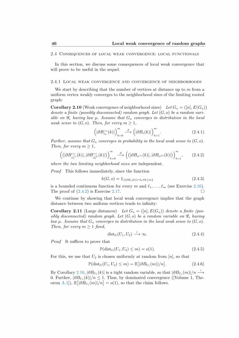
46 Local weak convergence of random graphs
2.4 Consequences of local weak convergence: local functionals
In this section, we discuss some consequences of local weak convergence thatwill prove to be useful in the sequel.
2.4.1 Local weak convergence and convergence of neighborhoods
We start by describing that the number of vertices at distance up to m from auniform vertex weakly converges to the neighborhood sizes of the limiting rootedgraph:
Corollary 2.10 (Weak convergence of neighborhood sizes) Let Gn = ([n], E(Gn))denote a finite (possibly disconnected) random graph. Let (G, o) be a random vari-able on G? having law µ. Assume that Gn converges in distribution in the localweak sense to (G, o). Then, for every m ≥ 1,(
|∂B(n)
on(k)|
)mk=0
d−→(|∂Bo(k)|
)mk=1
. (2.4.1)
Further, assume that Gn converges in probability in the local weak sense to (G, o).Then, for every m ≥ 1,((
|∂B(n)
o(1)n
(k)|, |∂B(n)
o(2)n
(k)|))m
k=0
d−→((|∂Bo(1)(k)|, |∂Bo(2)(k)|
))mk=1
, (2.4.2)
where the two limiting neighborhood sizes are independent.
Proof This follows immediately, since the function
h(G, o) = 1|∂Bo(k)|=`k∀k≤m (2.4.3)
is a bounded continuous function for every m and `1, . . . , `m (see Exercise 2.16).The proof of (2.4.2) is Exercise 2.17.
We continue by showing that local weak convergence implies that the graphdistance between two uniform vertices tends to infinity:
Corollary 2.11 (Large distances) Let Gn = ([n], E(Gn)) denote a finite (pos-sibly disconnected) random graph. Let (G, o) be a random variable on G? havinglaw µ. Assume that Gn converges in distribution in the local weak sense to (G, o).Then, for every m ≥ 1 fixed,
distG(U1, U2)P−→∞. (2.4.4)
Proof It suffices to prove that
P(distG(U1, U2) ≤ m) = o(1). (2.4.5)
For this, we use that U2 is chosen uniformly at random from [n], so that
P(distG(U1, U2) ≤ m) = E[|∂BU1
(m)|/n]. (2.4.6)
By Corollary 2.10, |∂BU1(k)| is a tight random variable, so that |∂BU1
(m)|/n P−→0. Further, |∂BU1
(k)|/n ≤ 1. Thus, by dominated convergence ([Volume 1, The-orem A.1]), E
[|∂BU1
(m)|/n]
= o(1), so that the claim follows.
2.5 The giant component is almost local 47
2.4.2 Local weak convergence and clustering coefficients
In this section, we discuss the convergence of various local and global clusteringcoefficients when a random graph converges locally weakly.TO DO 2.1: Add convergence of various clustering coefficients!
2.4.3 Neighborhoods of edges and degree-degree dependencies
In this section, we discuss the convergence of degree-degree dependencies whena random graph converges locally weakly. For this, it is crucial to also discussthe convergence of the local neighborhood of a uniformly chosen edge. We willsee that we need an extra uniform integrability condition for the assortativitycoefficient to converge.TO DO 2.2: Add convergence of neighborhoods of edges.
TO DO 2.3: Use this to show convergence of assortativity coefficient. How about otherdegree-degree dependency measures?
2.5 The giant component is almost local
We continue by investigating the size of the giant component when the graphconverges in the local weak sense. Clearly, the size of the largest connected com-ponent |Cmax| is not continuous in the local weak convergence sense (see Exercise2.18), as it is a global object. However, local weak convergence still tells us auseful story about the existence of a giant.
Corollary 2.12 (Upper bound on the giant) Let Gn = ([n], E(Gn)) denote afinite (possibly disconnected) random graph. Let (G, o) be a random variable onG? having law µ. Assume that Gn converges in probability in the local weak senseto (G, o) and write ζ = P(|C (o)| =∞) for the survival probability of the limitinggraph (G, o). Then, for every ε > 0 fixed,
P(|Cmax| ≤ n(ζ + ε))→ 1. (2.5.1)
In particular, Corollary 2.12 implies that |Cmax|/n P−→ 0 when ζ = 0 (seeExercise 2.19).
Proof Define
Z≥k =∑v∈[n]
1|C (v)|≥k. (2.5.2)
Assume that Gn converges in probability in the local weak sense to (G, o). Then,we conclude that with ζ≥k = P(|C (o)| ≥ k) (see Exercise 2.20),
Z≥kn
P−→ ζ≥k. (2.5.3)
48 Local weak convergence of random graphs
It is not hard to see that, for every k ≥ 1,
|Cmax| ≥ k = Z≥k ≥ k. (2.5.4)
Thus, if ζk > 0 for every k, we obtain that, for every k ≥ 1 and every ε > 0,
P(|Cmax| ≥ n(ζ≥k + ε/2)) = o(1). (2.5.5)
Therefore, with ζ = limk→∞ ζ≥k = P(|C (o)| =∞) and for every ε > 0,
P(|Cmax| ≥ n(ζ + ε)) = o(1). (2.5.6)
We conclude that while local weak convergence cannot determine the size ofthe largest connected component, it can prove an upper bound on |Cmax|. In
this book, we will often extend this to |Cmax|/n P−→ ζ, but this is no longer aconsequence of local weak convergence directly, and more involved argumentsmust be used. We next prove that one, relatively simple, condition suffices:
Theorem 2.13 (The giant is almost local) Let Gn = ([n], E(Gn)) denote afinite (possibly disconnected) random graph. Let (G, o) be a random variable onG? having law µ. Assume that Gn converges in probability in the local weak senseto (G, o) and write ζ = P(|C (o)| =∞) for the survival probability of the limitinggraph (G, o). Assume that ζ > 0 and that
limk→∞
lim supn→∞
1
n2E[#x, y ∈ [n] : |C (x)|, |C (y)| ≥ k, x←→/ y
]= 0. (2.5.7)
Then, with Cmax and C(2) denoting the largest and second largest connected com-ponents (with ties broken arbitrarily),
|Cmax|n
P−→ ζ,|C(2)|n
P−→ 0. (2.5.8)
Theorem 2.13 shows that a relatively mild condition as in (2.5.7) suffices forthe giant to have the expected limit. In fact, it is necessary and sufficient, as youcan see in Exercise 2.22. Theorem 2.13 will be useful when we can easily showthat vertices with large clusters are likely to be connected. There are many almostequivalent choices for the condition in (2.5.7), at least when the local weak limit(G, o) is a (homogeneous) branching process. Indeed, we may also consider x, yfor which the diameters of C (x) and C (y) exceed k, or |∂Bx(k)|, |∂By(k)| ≥ k.See Exercise 2.24.
We recall that the vector (|C(i)|)i≥1 denotes the clusters ordered in size, fromlarge to small with ties broken arbitrarily, so that C(1) = Cmax. The followinggives a useful estimate on the sum of squares of these ordered cluster sizes. In itsstatement, we write Xn,k = ok,P(1) when
limk→∞
lim supn→∞
P(|Xn,k| > ε) = 0. (2.5.9)
2.5 The giant component is almost local 49
Lemma 2.14 (Convergence of sum of squares of cluster sizes) Under the con-ditions of Theorem 2.13,
1
n2
∑i≥1
|C(i)|2 P−→ ζ2, (2.5.10)
and1
n2
∑i≥1
|C(i)|21|C(i)|≥k = ζ2 + ok,P(1). (2.5.11)
Proof We use that, by local weak convergence in probability and for any k ≥ 1fixed (recall (2.5.3))
1
n
∑i≥1
|C(i)|1|C(i)|≥k =1
n
∑v∈[n]
1|C (v)|≥k =1
nZ≥k
P−→ ζ≥k, (2.5.12)
where we recall that ζ≥k = P(|C (o)| ≥ k). Then we obtain that
1
n
∑i≥1
|C(i)|1|C(i)|≥k = ζ + ok,P(1). (2.5.13)
Further,
1
n2#x, y ∈ [n] : |C (x)|, |C (y)| ≥ k, x←→/ y
(2.5.14)
=1
n2
∑i,j≥1
i 6=j
|C(i)||C(j)|1|C(i)|,|C(j)|≥k = ok,P(1),
by the Markov inequality and our main assumption in (2.5.7). We conclude that
1
n2
∑i≥1
|C(i)|2|1|C(i)|≥k =( 1
n
∑i≥1
|C(i)|1|C(i)|≥k
)2
+ ok,P(1) (2.5.15)
= ζ2 + ok,P(1),
by (2.5.12). This proves (2.5.11) Finally,
1
n2
∑i≥1
|C(i)|2 =1
n2
∑i≥1
|C(i)|2|1|C(i)|≥k +O(k/m), (2.5.16)
which completes the proof of (2.5.10).
We are now ready to complete the proof of Theorem 2.13, and we start byexplaining the ideas behind this. Define the probability measure (qi,n)i≥1 by
qi,n =|C(i)||1|C(i)|≥k∑j≥1 |C(j)||1|C(j)|≥k
. (2.5.17)
By (2.5.12),∑
j≥1 |C(j)||1|C(j)|≥k/nP−→ ζ, and thus, by (2.5.11),
∑i≥1 q
2i,n =
1 + ok,P(1). We conclude that we have a probability mass function such that itssum of squares is close to 1. This is only possible when maxi≥1 qi,n = 1 + ok,P(1).
50 Local weak convergence of random graphs
Since i 7→ qi,n is non-increasing, this means that q1,n = |Cmax|1|Cmax|≥k = ζn(1+ok,P(1)), while q2,n = ok,P(1), which is what we aim to prove. We now fill in thedetails:
Proof of Theorem 2.13. By Lemma 2.14,
1
n2
∑i≥1
|C(i)|2|1|C(i)|≥k = ζ2 + ok,P(1). (2.5.18)
Denote xi = |C(i)|1|C(i)|≥k/n. Then, by (2.5.12) and (2.5.18), for every ε > 0and whp, ∑
i≥1
xi ≤ ζ + ε/4,∑i≥1
x2i ≥ ζ2 − ε2. (2.5.19)
Now suppose by contradiction that x1,n = |C(1)|1|C(1)|≥k/n ≤ ζ − ε for someε > 0. Then
max∑i≥1
x2i ≤ (ζ − ε)2 + (5ε/4)2 < ζ(1− ε), (2.5.20)
where the maximum is taken over all vectors (xi)i≥1 such that x1 ≤ ζ − ε and∑i≥1 xi ≤ ζ + ε/4, and where ε > 0 is taken sufficiently small. However, (2.5.20)
contradicts (2.5.19) when ζ > 0 and ε > 0 is sufficiently small. We concludethat, whp, x1,n = |Cmax|1|Cmax|≥k/n = |Cmax|/n ≥ ζ − ε. Combining this with
Corollary 2.12, we obtain that |Cmax|/n P−→ ζ, as required.Similarly, suppose that x2,n = |C(2)|1|C(2)|≥k/n ≥ ε. Then, since
∑i≥1 xi ≤
ζ + ε/4 by (2.5.19), we must have that x1 ≤ ζ − 3ε/4. However, by the previousargument, the probability that x1 = |Cmax|/n ≤ ζ − 3ε/4 vanishes.
2.6 Notes and discussion
Notes on Section 2.1
Notes on Section 2.2
Various generalizations of local weak convergence are possible. For example, Al-dous and Steele (2004) introduce the notion of geometric rooted graphs, whichare rooted graphs where each edge e receives a weight `(e), turning the rootedgraph into a metric space itself. Benjamini, Lyons and Schramm (2015) allow formore general marks. These marks are associated to the vertices as well as theedges, and can take values in a general complete separable metric space, whichare called marked graphs. Such more general set ups are highly relevant in manyapplications. Aldous and Lyons (2007) also study the implications for stochasticprocesses, such as percolation and random walks, on unimodular graphs.
The tightness statement in Theorem 2.6 is (Benjamini et al., 2015, Theorem3.1). Benjamini et al. (2015) use the term network instead of a marked graph.We avoid the term networks here, as it may cause confusion with the complexnetworks in the real world that form inspiration for this book.
2.7 Exercises for Chapter 2 51
Notes on Section 2.3
Notes on Section 2.4
Notes on Section 2.5
2.7 Exercises for Chapter 2
Exercise 2.1 (Graph isomorphisms fix vertex and edge numbers) Assume thatG1 ' G2. Show that G1 and G2 have the same number of vertices and edges.
Exercise 2.2 (Graph isomorphisms fix degree sequence) Let G1 and G2 be twofinite graphs. Assume that G1 ' G2. Show that G1 and G2 have the same degreesequences. Here, for a graph G, we let the degree sequence be (pk(G))k≥0, where
pk(G) =1
|V (G)|∑
v∈V (G)
1dv(G)=k, (2.7.1)
where dv(G) is the degree of v in G.
Exercise 2.3 (Distance to rooted graph ball) Let the ball Br(o) around o inthe graph G be defines as in (2.1.1). Show that dG?
((Br(o), o), (G, o)
)≤ 1/(r+1).
When does equality hold?
Exercise 2.4 (Countable number of graphs with bounded radius) Fix k. Showthat there is a countable number of isomorphism classes of rooted graphs (G, o)with radius at most r. Here, we let the radius rad(G, o) of a rooted graph (G, o)be equal to rad(G, o) = maxv∈V (G) dG(v, o).
Exercise 2.5 (Graph isomorphisms fix degree sequence) Use Exercise 2.4 aboveto show that the set of rooted graphs G? has a countable dense set, and is thusseparable.
Exercise 2.6 (Bounded number of graphs with bounded radius and degrees)Show that there are only a bounded number of isomorphism classes of rootedgraphs (G, o) with radius at most r for which the degree of every vertex is at mostk.
Exercise 2.7 (Random local weak limit) Construct the simplest (in your opin-ion) possible example where the local weak limit of a sequence of deterministicgraphs is random.
Exercise 2.8 (Local weak limit of line and cycle) Let Gn be given by V (Gn) =[n], E(Gn) =
i, i + 1 : i ∈ [n − 1]
be the line. Show that Gn converges to Z.
Show that the same is true for the cycle, for which E(Gn) =i, i + 1 : i ∈
[n− 1]∪1, n
.
Exercise 2.9 (Local weak limit of finite tree) Let Gn be the tree of depth k, inwhich every vertex except the 3× 2k−1 leaves have degree 3. Here n = 3(2k − 1).What is the local weak limit of Gn? Show that it is random, despite the fact thatthe graphs Gn are deterministic.
52 Local weak convergence of random graphs
Exercise 2.10 (Uniform integrability and convergence of size-biased degrees)Show that when (d(n)
on)n≥1 forms a uniformly integrable sequence of random vari-
ables, there exists a subsequence along which D?n, the size-biased version of Dn =
d(n)
on, converges in distribution.
Exercise 2.11 (Uniform integrability and degree regularity condition) ForCMn(d), show that Conditions 1.5(a)-(b) imply that (don)n≥1 is a tight sequenceof random variables.
Exercise 2.12 (Local weak limit of random 2-regular graph) Show that theconfiguration model CMn(d) with di = 2 for all i ∈ [n] converges in the local weaksense in probability to Z. Conclude that the same applies to the random 2-regulargraph.
Exercise 2.13 (Independent neighborhoods of different vertices) Let Gn con-verge in probability in the local weak sense to (G, o). Let (o(1)
n , o(2)
n ) be two indepen-dent uniformly chosen vertices in [n]. Show that (Gn, o
(1)
n ) and (Gn, o(2)
n ) jointlyconverge to two independent copies of (G, o).
Exercise 2.14 (Directed graphs as marked graphs) There are several ways todescribe directed graphs as marked graphs. Give one.
Exercise 2.15 (Example of weak convergence where convergence in probabilityfails) Construct an example where Gn converges in distribution in the local weaksense to (G, o), but not in probability.
Exercise 2.16 (Continuity of neighborhood functions) Fix m ≥ 1 and `1, . . . , `m.Show that
h(G, o) = 1|∂Bo(k)|=`k∀k≤m (2.7.2)
is a bounded continuous function.
Exercise 2.17 (Proof of (2.4.2)) Let Gn converge in probability in the localweak sense to (G, o). Prove (2.4.2) using Exercise 2.13.
Exercise 2.18 (|Cmax| is not a continuous functional) Show that |Cmax| is nota continuous functional in G?.
Exercise 2.19 (Upper bound on |Cmax| using LWC) Let Gn = ([n], E(Gn))denote a finite (possibly disconnected) random graph. Let (G, o) be a randomvariable on G? having law µ. Assume that Gn converges in probability in the localweak sense to (G, o), and assume that the survival probability of the limiting graph
(G, o) satisfies ζ = P(|C (o)| =∞) = 0. Show that |Cmax|/n P−→ 0.
Exercise 2.20 (Convergence of the proportion of vertices in clusters of size atleast k) Let Gn converge in probability in the local weak sense to (G, o). Show
that Zk in (2.5.2) satisfies that Zk/nP−→ ζk = P(|C (o)| ≥ k) for every k ≥ 1.
Exercise 2.21 (Local weak convergence with a subcritical limit) Let Gn con-verge in probability in the local weak sense to (G, o). Assume that ζ = P(|C (o)| =∞) = 0. Use (2.5.6) to prove that |Cmax|/n P−→ 0.
2.7 Exercises for Chapter 2 53
Exercise 2.22 (Sufficiency of (2.5.7) for almost locality giant) Let Gn =([n], E(Gn)) denote a finite (possibly disconnected) random graph. Let (G, o) bea random variable on G? having law µ. Assume that Gn converges in probabilityin the local weak sense to (G, o) and write ζ = P(|C (o)| = ∞) for the survivalprobability of the limiting graph (G, o). Assume that
lim supk→∞
lim supn→∞
E[#x, y ∈ [n] : |C (x)|, |C (y)| ≥ k, x←→/ y
]> 0. (2.7.3)
Then, prove that for some ε > 0,
lim supn→∞
P(|Cmax| ≤ n(ζ − ε)) > 0. (2.7.4)
Exercise 2.23 (Sufficiency of (2.5.7) for uniqueness giant) Under the conditionsin Exercise 2.22, show that
lim supn→∞
P(|C(2)| > εn) > 0. (2.7.5)
Exercise 2.24 (Alternative condition for (2.5.7)) Let Gn = ([n], E(Gn)) de-note a finite (possibly disconnected) random graph. Assume that Gn converges inprobability in the local weak sense to the homogeneous branching process (G, o)and write ζ = P(|C (o)| = ∞) > 0 for the branching process survival probability.Reprove Theorem 2.13 when the condition in (2.5.7) is replaced by
lim supk→∞
lim supn→∞
E[#x, y ∈ [n] : |∂Bx(k)|, |∂By(k)| ≥ k, x←→/ y
]> 0. (2.7.6)


Part II
Connected componentsin random graphs
55

57
Overview of Part II.
In this part, we study connected components in random graphs. In more detail,we investigate the connected components of uniform vertices, thus describing thelocal weak limits of these random graphs. Further, we study the structure of thelargest connected component, sometimes also called the giant component, whichcontains a positive proportion of the graph. In many random graphs, such a giantcomponent exists when there are sufficiently many connections, while the largestconnected component is much smaller than the number of vertices when thereare few connections. Thus, these random graphs satisfy a phase transition. Weidentify the size of the giant component, as well as its structure in terms of thedegrees of its vertices. We also investigate when the graph is fully connected, thusestablishing the connectivity threshold for the random graphs in question.
In more detail, this part is organised as follows. We study general inhomo-geneous random graphs in Chapter 3, and the configuration model, as well theclosely related uniform random graph with prescribed degrees, in Chapter 4. Inthe last chapter of this part, Chapter 5, we study the connected components andlocal weak convergence of the preferential attachment model.

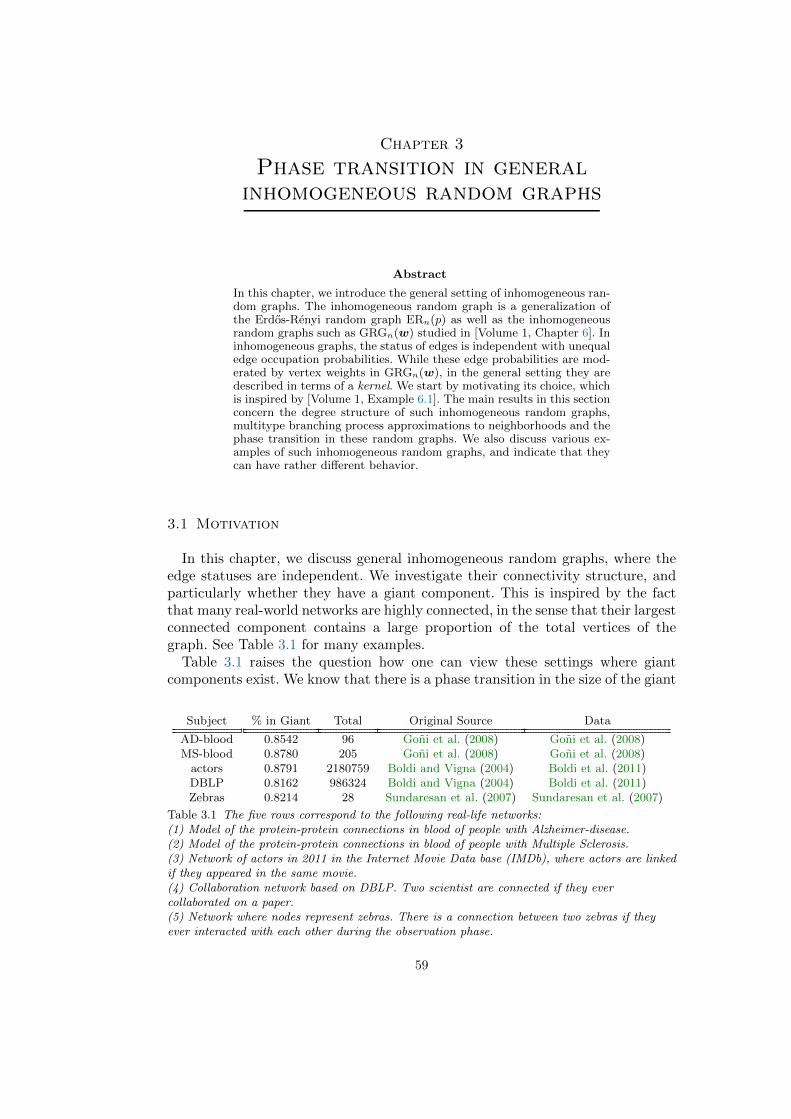
Chapter 3
Phase transition in generalinhomogeneous random graphs
Abstract
In this chapter, we introduce the general setting of inhomogeneous ran-dom graphs. The inhomogeneous random graph is a generalization ofthe Erdos-Renyi random graph ERn(p) as well as the inhomogeneousrandom graphs such as GRGn(w) studied in [Volume 1, Chapter 6]. Ininhomogeneous graphs, the status of edges is independent with unequaledge occupation probabilities. While these edge probabilities are mod-erated by vertex weights in GRGn(w), in the general setting they aredescribed in terms of a kernel. We start by motivating its choice, whichis inspired by [Volume 1, Example 6.1]. The main results in this sectionconcern the degree structure of such inhomogeneous random graphs,multitype branching process approximations to neighborhoods and thephase transition in these random graphs. We also discuss various ex-amples of such inhomogeneous random graphs, and indicate that theycan have rather different behavior.
3.1 Motivation
In this chapter, we discuss general inhomogeneous random graphs, where theedge statuses are independent. We investigate their connectivity structure, andparticularly whether they have a giant component. This is inspired by the factthat many real-world networks are highly connected, in the sense that their largestconnected component contains a large proportion of the total vertices of thegraph. See Table 3.1 for many examples.
Table 3.1 raises the question how one can view these settings where giantcomponents exist. We know that there is a phase transition in the size of the giant
Subject % in Giant Total Original Source Data
AD-blood 0.8542 96 Goni et al. (2008) Goni et al. (2008)MS-blood 0.8780 205 Goni et al. (2008) Goni et al. (2008)
actors 0.8791 2180759 Boldi and Vigna (2004) Boldi et al. (2011)DBLP 0.8162 986324 Boldi and Vigna (2004) Boldi et al. (2011)Zebras 0.8214 28 Sundaresan et al. (2007) Sundaresan et al. (2007)
Table 3.1 The five rows correspond to the following real-life networks:(1) Model of the protein-protein connections in blood of people with Alzheimer-disease.(2) Model of the protein-protein connections in blood of people with Multiple Sclerosis.(3) Network of actors in 2011 in the Internet Movie Data base (IMDb), where actors are linkedif they appeared in the same movie.(4) Collaboration network based on DBLP. Two scientist are connected if they evercollaborated on a paper.(5) Network where nodes represent zebras. There is a connection between two zebras if theyever interacted with each other during the observation phase.
59
60 Phase transition in general inhomogeneous random graphs
component in the ERn(λ/n), recall [Volume 1, Chapter 4]. A main ingredient willbe to investigate when a giant component is present in general inhomogeneousrandom graphs. This will occur precisely when the local weak limit has a positiveprobability of surviving (recall Section 2.5). Therefore, we also investigate localweak convergence in this chapter.
We will study much more general models where edges are present indepen-dently than we have done so far (recall the generalized random graph in [Volume1, Chapter 6], see also Section 1.3.2). In the generalized random graph, verticeshave weights associated to them, and the edge occupation probabilities are pro-portional to the product of the weights of the vertices that the edge connects. Thismeans that vertices with high weights have relatively large occupation probabili-ties to all other vertices, a property that may not be always be appropriate. Letus illustrate this by an example, which is a continuation of [Volume 1, Example6.1]:
Example 3.1 (Population of two types: general setting) Suppose that we havea complex network in which there are n1 vertices of type 1 and n2 of type 2.Type 1 individuals have on average m1 neighbors, type 2 individuals m2, wherem1 6= m2. Further, suppose that the probability that a type 1 individual is afriend of a type 2 individual is quite different from the probability that a type 1individual is a friend of a type 1 individual.
In the model proposed in [Volume 1, Example 6.3], the probability that a typei individual is a friend of a type j individual (where i, j,∈ 1, 2) is equal tomimj/(`n +mimj), where `n = n1m1 +n2m2. Approximating this probability bymimj/`n, we see that the probability that a type 1 individual is friend of a type 2individual is highly related to the probability that a type 1 individual is friend ofa type 1 individual. Indeed, take two type 1 and two type 2 individuals. Then, theprobability that the type 1 individuals are friends and the type 2 individuals arefriends is almost the same as the probability that first type 1 individual is friendwith the first type 2 individual, and the second type 1 individual is friend of thesecond type 2 individual. Thus, there is some, possibly unwanted and artificial,symmetry in the model. How can one create instances where the edge probabilitiesbetween vertices of the same type are much larger, or alternatively much smaller,than they would be for the generalized random graph? In the two extremes, weeither have a bipartite graph where vertices are only connected to vertices of theother type, or a disjoint union of two Erdos-Renyi random graphs , consistingof the vertices of the two types and no edges between them. We aim to be ableto obtain anything in between. In particular, the problem with the generalizedrandom graph originates in the product structure of the edge probabilities. In thischapter, we will deviate from such a product structure.
As explained above, we wish to be quite flexible in our choices of edge proba-bilities. However, we also wish for settings where the random graph is sufficiently‘regular’, as for example exemplified by its degree sequences converging to somedeterministic distribution. In particular, we aim for settings where the random
3.2 Definition of the model 61
graphs are sparse. As a result, we need to build this regularity into the precisestructure of the edge probabilities. This will be achieved by introducing an ap-propriate kernel that moderates the edge probabilities, and that is sufficientlyregular. Let us introduce the model in detail in the next section.
Organization of this chapter
This chapter is organised as follows. In Section 3.2, we introduce general inhomo-geneous random graphs. In Section 3.3, we study the degree distribution in gen-eral inhomogeneous random graphs. In Section 3.4, we treat multitype branchingprocesses, the natural generalization of branching processes for inhomogeneousrandom graphs. In Section 3.5, we use multitype branching processes to identifythe local weak limit of inhomogeneous random graphs. In Section 3.6, we studythe phase transition of inhomogeneous random graphs. In Section 3.7, we statesome recent related results. We close this chapter with notes and discussion inSection 3.8, and exercises in Section 3.9.
3.2 Definition of the model
We assume that our individuals have types which are in a certain type spaceS. When there are individuals of just 2 types, as in Example 3.1, then it sufficesto take S = 1, 2. However, the model allows for rather general sets of typesof the individuals, both finite as well as (countably or uncountably) infinite. Anexample of an uncountably infinite type space could be types related to the agesof the individuals in the population. Also the setting of the generalized randomgraph with wi satisfying (1.3.15) correponds to the uncountable type-space settingwhen the distribution function F is that of a continuous random variable W . Wetherefore also need to know how many individuals there are of a given type. Thisis described in terms of a measure µn, where, for A ⊆ S, µn(A) denotes theproportion of individuals having a type in A.
In our general model, instead of vertex weights, the edge probabilities aremoderated by a kernel κ : S2 → [0,∞). The probability that two vertices oftypes x1 and x2 are connected is approximately κ(x1, x2)/n, and different edgesare present independently. Since there are many choices for κ, we arrive at arather flexible model, where vertices have types and connection probabilities arerelated to the types of the vertices involved.
We start by making the above definitions formal, by defining what our groundspace is and what a kernel is:
Definition 3.2 (Setting: ground space and kernel) (i) A ground space is a pair(S, µ), where S is a separable metric space and µ is a Borel probability measureon S.
(ii) A vertex space V is a triple (S, µ, (xn)n≥1), where (S, µ) is a ground space and,for each n ≥ 1, xn is a random sequence (x1, x2, . . . , xn) of n points of S, such
62 Phase transition in general inhomogeneous random graphs
that
µn(A) = #i : xi ∈ A/n→ µ(A) (3.2.1)
for every µ-continuity set A ⊆ S. The convergence in (3.2.1) is denoted by
µnp−→ µ.
(iii) A kernel κ is a symmetric non-negative (Borel) measurable function on S2. Bya kernel on a vertex space (S, µ, (xn)n≥1) we mean a kernel on (S, µ).
Before defining the precise random graph model, we state the necessary con-ditions on our kernels. We write E(G) for the number of edges in a graph G.Note that for an inhomogeneous random graph with edge probabilities p =(pij)1≤i<j≤n,
E[E(IRGn(p))] =∑i<j
pij, (3.2.2)
so that our model has bounded degree in expectation precisely when 1n
∑i<j pij
remains bounded. In our applications, we wish that the average degree per vertexin fact converges, as this corresponds to the random graph model being sparse(recall [Volume 1, Definition 1.3]). Further, we do not wish the vertex set tobe subdivided into two sets of vertices where the probability to have an edgebetween them is zero, as this implies that the graph can be divided into twoentirely disjoint graphs. This explains the main conditions we pose on the kernelκ in the following definition:
Definition 3.3 (Setting: graphical and irreducible kernels) (i) A kernel κ is graph-ical if the following conditions hold:
(a) κ is continuous a.e. on S2;(b) ∫∫
S2
κ(x, y)µ(dx)µ(dy) <∞; (3.2.3)
(c)
1
nE[E(IRGn(κ))]→ 1
2
∫∫S2
κ(x, y)µ(dx)µ(dy). (3.2.4)
Similarly, a sequence (κn)n≥1 of kernels is called graphical with limit κ when
yn → y and zn → z imply that κn(yn, zn)→ κ(y, z), (3.2.5)
where κ satisfies conditions (a) and (b) above, and
1
nE[E(IRGn(κn))]→ 1
2
∫∫S2
κ(x, y)µ(dx)µ(dy). (3.2.6)
(ii) A kernel κ is called reducible if
∃A ⊆ S with 0 < µ(A) < 1 such that κ = 0 a.e. on A× (S\A);
otherwise κ is irreducible.
3.2 Definition of the model 63
We now discuss the above definitions. The assumptions in (3.2.3), (3.2.4),(3.2.6) imply that the expected number of edges is proportional to n, and thatthe proportionality constant is precisely equal to
∫∫S2 κ(x, y)µ(dx)µ(dy). Thus,
in the terminology of [Volume 1, Chapter 1], IRGn(κ) is sparse. This sparsityalso allows us to approximate graphical kernels by bounded ones in such a waythat the number of removed edges is oP(n), a fact that will be crucially used inthe sequel. Indeed, bounded graphical kernels can be well approximated by stepfunctions in a similar way as continuous functions on R can be well approximatedby step functions. In turn, such step functions on S × S correspond to randomgraphs with finitely many different types.
We extend the setting to n-dependent sequences (κn)n≥1 of kernels in (3.2.5), asin many natural cases the kernels do indeed depend on n. In particular, it allows usto deal with several closely related and natural notions of the edge probabilities atthe same time (see e.g., (3.2.7), (3.2.8) and (3.2.9) below), showing that identicalresults hold in each of these cases.
Roughly speaking, κ is reducible if the vertex set of IRGn(κ) can be split in twoparts so that the probability of an edge from one part to the other is zero, andirreducible otherwise. When κ is reducible, then the random graph splits into twoindependent random graphs on the two disjoint subsets A and S \A. Therefore,we could have equally well started with each of them separately, explaining whythe notion of irreducibility is quite natural.
In many cases, we shall take S = [0, 1], xi = i/n and µ the Lebesgue-measureon [0, 1]. Then, clearly, (3.2.1) is satisfied. In fact, Janson (2009b) shows thatwe can always restrict to S = [0, 1] by suitably adapting the other choices ofour model. However, for notational purposes, it is more convenient to work withgeneral S. For example, where S = 1 is just a single type, the model reducesto the Erdos-Renyi random graph, and in the setting where S = [0, 1], this isslightly more cumbersome, as worked out in detail in Exercise 3.1.
Now we come to the definition of our random graph. Given a kernel κ, forn ∈ N, we let IRGn(κ) be the random graph on [n], each possible edge ij, wherei, j ∈ [n], is present with probability
pij(κ) = pij =1
n[κ(xi, xj) ∧ n], (3.2.7)
and the events that different edges are present are independent. Similarly, IRGn(κn)is defined with κn replacing κ in (3.2.7). Exercise 3.2 shows that the lower boundin (3.2.4) always holds for IRGn(κ) when κ is continuous. Further, Exercise 3.3shows that (3.2.4) holds for IRGn(κ) when κ is bounded and continuous.
Bollobas et al. (2007) also allow for the choices
p(NR)
ij (κn) = 1− e−κn(xi,xj)/n, (3.2.8)
and
p(GRG)
ij (κn) = pij =κ(xi, xj)
n+ κ(xi, xj). (3.2.9)
64 Phase transition in general inhomogeneous random graphs
All results in Bollobas et al. (2007) remain valid for the choices in (3.2.8) and(3.2.9). When ∑
i,j∈[n]
κn(xi, xj)3 = o(n3/2), (3.2.10)
this follows immediately from [Volume 1, Theorem 6.18], see Exercise 3.6.
For CLn(w) with w = (wi)i∈[n] as in (1.3.15), we take S = [0, 1], xi = i/n and,with ψ(x) = [1− F ]−1(x),
κn(x, y) = ψ(x)ψ(y)n/`n. (3.2.11)
For CLn(w) with w = (wi)i∈[n] satisfying Condition 1.1, instead, we take S =[0, 1], xi = i/n and
κn(i/n, j/n) = wiwj/E[Wn]. (3.2.12)
Exercises 3.4–3.5 study the Chung-Lu random graph in the present framework.
In the next section, we discuss some examples of inhomogeneous random graphs.
3.2.1 Examples of inhomogeneous random graphs
The Erdos-Renyi random graph
If S is general and κ(x, y) = λ for every x, y ∈ S, then the edge probabilities pijgiven by (3.2.7) are all equal to λ/n (for n > λ). Then IRGn(κ) = ERn(λ/n).The simplest choice here is to take S = 1.
The homogeneous bipartite random graph
Let n be even, ket S = 0, 1, let xi = 0 for i ∈ [n/2] and xi = 1 for i ∈ [n]\ [n/2].Further, let κ be defined by κ(x, y) = 0 when x 6= y and κ(x, y) = λ when x = y.Then IRGn(κ) is the random bipartite graph with n/2 vertices in each class, whereeach possible edge between classes is present with probability λ/n, independentlyof the other edges. Exercise 3.7 investigates the validity of Definitions 3.2-3.3 forhomogeneous bipartite graphs.
The stochastic block model
The stochastic block model generalizes the above setting. Let n be even, ketS = 0, 1, let xi = 0 for i ∈ [n/2] and xi = 1 for i ∈ [n] \ [n/2]. Further, let κ bedefined by κ(x, y) = b when x 6= y and κ(x, y) = b when x = y. This means thatvertices of the same type are connected with probability a/n, while vertices withdifferent types are connected with probabilities a/n. A major research effort hasbeen devoted to studying when it can be statistically detected that a 6= b.
Homogeneous random graphs
We call an inhomogeneous random graph homogeneous when λ(x) =∫S κ(x, y)µ(dy) ≡
λ. Thus, despite the inhomogeneity that is present, every vertex in the graph has(asymptotically) the same number of expected offspring. Exercise 3.8 shows that

3.2 Definition of the model 65
the Erdos-Renyi random graph, the homogeneous bipartite random graph andthe stochastic block model are all homogeneous random graphs. In such settings,however, the level of inhomogeneity is limited.
Inhomogeneous random graphs with finitely many types
Fix r ≥ 2 and suppose we have a graph with r different types of vertices. LetS = 1, . . . , r. Let ni denote the number of vertices of type i, and let µn(i) =ni/n. Let IRGn(κ) be the random graph where two vertices of types i and j,respectively, joined by an edge with probability n−1κ(i, j) (for n ≥ maxκ). Thenκ is equivalent to an r× r matrix, and the random graph IRGn(κ) has vertices ofr different types (or colors). The finite-types case has been studied by Soderberg(2002, 2003a,b,c). We conclude that our general inhomogeneous random graphcovers the cases of a finite (or even countably infinite) number of types. Exercises3.9–3.11 study the setting of inhomogeneous random graphs with finitely manytypes.
It will turn out that this case is particularly important, as many of the othersettings can be arbitrarily well approximated by inhomogeneous random graphswith finitely many types. As such, this model will be the building block uponwhich most of the results are built.
Uniformly grown random graph
The uniformly grown random graph was proposed by Callaway, Hopcroft, Klein-berg, Newman, and Strogatz (2001). In their model, the graph grows dynamicallyas follows. At each time step, a new vertex is added. Further, with probability δ,two vertices are chosen uniformly at random and joined by an undirected edge.This process is repeated for n time steps, where n describes the number of ver-tices in the graph. Callaway et al. predict, based in physical reasonings, that inthe limit of large n, the resulting graph has a giant component precisely whenδ > 1/8, and the proportion of vertices in the giant component is of the ordere−Θ(1/(
√8δ−1). Such behavior is sometimes called an infinite order phase transi-
tion. Durrett (2003) discusses this model. We will discuss a variant of this modelproposed and analyzed by Bollobas, Janson and Riordan (2005). Their modelis an example of the general inhomogeneous random graphs as discussed in theprevious section. We take as a vertex space [n], and the edge ij is present withprobability
pij =c
maxi, j , (3.2.13)
all edge statuses being independent random variables. Equivalently, we can viewthis random graph as arising dynamically, where vertex t connects to a vertexs < t with probability 1/t independently for all s ∈ [t− 1].
Sum kernels
We have already seen that product kernels are special, as they give rise to theChung-Lu model or its close brothers, the generalized random graph or the
66 Phase transition in general inhomogeneous random graphs
Norros-Reittu model. For sum kernels, instead, we take κ(x, y) = ψ(x) +ψ(y), sothat pij = min(ψ(i/n) + ψ(j/n))/n, 1.
We see that there are tons of examples of random graphs with independentedges that fall into the general class of inhomogeneous random graphs. In thesequel, we will investigate them in general. We start by investigating their degreestructure.
3.3 Degree sequence of inhomogeneous random graphs
We now start by investigating the degrees of the vertices of IRGn(κn). As weshall see, the degree of a vertex of a given type x is asymptotically Poisson witha mean
λ(x) =
∫Sκ(x, y)µ(dy) (3.3.1)
that depends on x. This leads to a mixed Poisson distribution for the degree D ofa (uniformly chosen) random vertex of IRGn(κ). We recall that Nk denotes thenumber of vertices of IRGn(κ) with degree k. Our main result is as follows:
Theorem 3.4 (The degree sequence of IRGn(κ)) Let (κn) be a graphical se-quence of kernels with limit κ as described in Definition 3.3(i). For any fixedk ≥ 0,
Nk/nP−→∫S
λ(x)k
k!e−λ(x)µ(dx) (3.3.2)
where x 7→ λ(x) is defined by
λ(x) =
∫Sκ(x, y)µ(dy). (3.3.3)
Equivalently,
Nk/nP−→ P(D = k), (3.3.4)
where D has the mixed Poisson distribution with distribution Wλ given by
P(Wλ ≤ x) =
∫ x
0
λ(y)µ(dy). (3.3.5)
In the remainder of this section, we prove Theorem 3.4. This proof is also agood example of how such proofs will be carried out in the sequel. Indeed, westart by proving Theorem 3.4 for the finite-types case, which is substantially eas-ier. After this, we give a proof in the general case, for which we shall need toprove results on approximations of sequences of graphical kernels. These approx-imations will apply for bounded kernels, and thus we will also need to show thatunbounded kernels can be well-approximated by bounded kernels. It is here thatthe assumption (3.2.4) will be crucially used.
3.3 Degree sequence of inhomogeneous random graphs 67
3.3.1 Degree sequence of finitely-types case
We start by proving Theorem 3.4 in the finite-types case. Take a vertex v oftype i, let Dv be its degree, and let Dv,j be the number of edges from v to verticesof type j ∈ [r]. Then, clearly, Dv =
∑j Dv,j.
Recall that, in the finite-types case, the edge probability between vertices oftypes i and j is denoted by (κn(i, j)∧n)/n. Further, (3.2.5) implies that κn(i, j)→κ(i, j) for every i, j ∈ [r], while (3.2.1) implies that the number ni of vertices oftype i satisfies ni/n→ µi for some probability distribution (µi)i∈[r].
Assume that n ≥ maxκ. The random variables (Dv,j)j∈[r] are independent,
and Dv,j ∼ Bin(nj − δij, κ(i, j)/n)d−→ Poi(µjκ(i, j)), where nj are the number of
vertices with type j and µj = limn→∞ nj/n. Hence,
Dvd−→ Poi
(∑j
µjκ(i, j))
= Poi(λ(i)), (3.3.6)
where λ(i) =∫κ(i, j)dµ(j) =
∑j κ(i, j)µj. Consequently,
P(Dv = k)→ P(Poi(λ(i)) = k) =λ(i)k
k!e−λ(i). (3.3.7)
Let Nk,i be the number of vertices in IRGn(κn) of type i with degree k. Then,for fixed n1, . . . , nr,
1
nE[Nk,i] =
1
nniP(Dv = k)→ µiP(Poi(λ(i)) = k). (3.3.8)
It is easily checked that Var(Nk,i) = O(n) (see Exercise 3.12). Hence,
1
nNk,i
P−→ P(Poi(λ(i)) = k)µi = P(Ξ = k), (3.3.9)
and thus, summing over i,
1
nNk =
∑i
1
nNk,i
P−→∑i
P(Poi(λ(i)) = k)µi = P(D = k). (3.3.10)
This proves Theorem 3.4 in the finite-type case.
In order to prove Theorem 3.4 in the general case, we shall be approximatinga sequence of graphical kernels (κn) by appropriate regular finite kernels.
3.3.2 Finite-type approximations of bounded kernels
Recall that S is a separable metric space, and that µ is a Borel measure on Swith µ(S) = 1. Here the metric and topological structure of S will be important.We refer to Appendix A for more details on metric spaces that will be assumedthroughout this section.
In this section, we assume that (κn) is a graphical sequence of bounded kernelswith limit κ as described in Definition 3.3(i). Thus, we assume that
supn≥1
supx,y∈S
κn(x, y) <∞. (3.3.11)
68 Phase transition in general inhomogeneous random graphs
Our aim is to find finite-type approximations of κn that bound κn from aboveand below. It is here that the metric structure of S, as well as the continuity of(x, y) 7→ κn(x, y), is crucially used. This is the content of the next lemma:
Lemma 3.5 (Finite-type approximations of general kernels) If (κn)n≥1 is agraphical sequence of kernels on a vertex space V with limit κ, then there existsa sequence (κ−m)m≥1 of finite-type kernels on V with the following properties:
(i) If κ is irreducible, then so is κ−m for all large enough m;(ii) κ−m(x, y) κ(x, y) for every x, y ∈ S.
Let us now give some details. We find these finite-type approximations bygiving a partition Pm of S on which κn(x, y) is almost constant when x and y areinside cells of the partition. Fix m ≥ 1 which will indicate the number of cells inthe partition of S. Given a sequence of finite partitions Pm = Am1, . . . , AmMm
,m ≥ 1, of S and an x ∈ S, we define the function x 7→ im(x) by requiring that
x ∈ Am,im(x). (3.3.12)
Thus, im(x) indicates the cell in Pm that x is in. For A ⊂ S we write diam(A)for sup|x− y| : x, y ∈ A. By taking Pm as the dyadic partition into intervals oflength 2−m in S, we easily see the following:
Lemma 3.6 (Approximating partition) Fix m ≥ 1. There exists a sequence offinite partitions Pm = Am1, . . . , AmMm
of S such that
(i) each Ami is measurable and µ(∂Ami) = 0;(ii) for each m, Pm+1 refines Pm, i.e., each Ami is a union
⋃j∈Jmi Am+1,j for some
set Jmi;(iii) for a.e. x ∈ S, diam(Am,im(x)) → 0 as m → ∞, where im(x) is defined by
(3.3.12).
Recall that a kernel κ is a symmetric measurable function on S × S. Fixing asequence of partitions with the properties described in Lemma 3.6, we can definesequences of lower and upper approximations to κ by
κ−m(x, y) = infκ(x′, y′) : x′ ∈ Am,im(x), y′ ∈ Am,im(y), (3.3.13)
κ+m(x, y) = supκ(x′, y′) : x′ ∈ Am,im(x), y
′ ∈ Am,im(y). (3.3.14)
We thus replace κ by its infimum or supremum on each Ami×Amj. As κ+m might
be +∞, we only use it for bounded κn as in (3.3.11). Obviously, κ−m and κ+m are
constant on Am,i×Am,j for every i, j, so that κ−m and κ+m correspond to finite-type
kernels (see Exercise 3.14).By Lemma 3.6(ii),
κ−m ≤ κ−m+1 and κ+m ≥ κ+
m+1. (3.3.15)
Furthermore, if κ is continuous a.e. then, by Lemma 3.6(iii),
κ−m(x, y)→ κ(x, y) and κ+m(x, y)→ κ(x, y) for a.e. (x, y) ∈ S2. (3.3.16)
3.3 Degree sequence of inhomogeneous random graphs 69
If (κn) is a graphical sequence of kernels with limit κ, we define instead
κ−m(x, y) := inf(κ ∧ κn)(x′, y′) : x′ ∈ Am,im(x), y′ ∈ Am,im(y), n ≥ m, (3.3.17)
κ+m(x, y) := sup(κ ∨ κn)(x′, y′) : x′ ∈ Am,im(x), y
′ ∈ Am,im(y), n ≥ m. (3.3.18)
Again, by Lemma 3.6, we have κ−m ≤ κ−m+1, and, by Lemma 3.6(iii) and 3.3(ii),
κ−m(x, y) κ(x, y) as m→∞, for a.e. (x, y) ∈ S2. (3.3.19)
Since κ−m ≤ κ, we can obviously construct our random graph so that IRGn(κ−m) ⊆IRGn(κn), and in the sequel we assume this. See also Exercise 3.15. Similarly,we shall assume that IRGn(κ+
m) ⊇ IRGn(κn) when κn is bounded as in (3.3.11).Moreover, when n ≥ m,
κn ≥ κ−m, (3.3.20)
and we may assume that IRGn(κ−m) ⊆ IRGn(κn). By the convergence of the se-quence of kernels (κn), we further obtain that also the number of edges converges.Thus, in bounding κn, we do not create or destroy too many edges. This providesthe starting point of our analysis, which we provide in the following section.
3.3.3 Degree sequences of general inhomogeneous random graphs
Now we are ready to complete the proof of Theorem 3.4 for general sequencesof graphical kernels (κn). Define κ−m by (3.3.17). Since we only use the lowerbounding kernel κ−m (which always exists), we need not assume that κn is bounded.
Let ε > 0 be given. From (3.2.6) and monotone convergence, there is an msuch that∫∫
S2
κ−m(x, y)µ(dx)µ(dy) >
∫∫S2
κ(x, y)µ(dx)µ(dy)− ε. (3.3.21)
For n ≥ m, we have κ−m ≤ κn by (3.3.20), so we may assume that IRGn(κ−m) ⊆IRGn(κn). Then, by (3.2.6) and (3.3.21),
1
nE(IRGn(κn) \ IRGn(κ−m)) (3.3.22)
=1
nE(G(n, κn))− 1
nE(IRGn(κ−m))
P−→ 1
2
∫∫S2
κ(x, y)µ(dx)µ(dy)− 1
2
∫∫S2
κ−m(x, y)µ(dx)µ(dy) <ε
2,
so that, whp E(IRGn(κn) \ IRGn(κ−m)) < εn. Let us write N (m)
k for the numberof vertices of degree k in IRGn(κ−m). It follows that, whp,
|N (m)
k −Nk| < 2εn. (3.3.23)
Writing Ξ(m) for the equivalent of Ξ defined using κ−m in place of κ, by the proof
for the finite-type case, N (m)
k /nP−→ P(D(m) = k). Thus, whp,
|N (m)
k /n− P(D(m) = k)| < ε. (3.3.24)
70 Phase transition in general inhomogeneous random graphs
Finally, we have E[Ξ] =∫S λ(x)µ(dx) =
∫∫S2 κ(x, y)µ(dx)µ(dy). Since λ(m)(x) ≤
λ(x), we can couple the branching processes such that Ξ(m) ≤ Ξ, and thus
P(D 6= D(m)) = P(Ξ− Ξ(m) ≥ 1) ≤ E[Ξ− Ξ(m)]
=
∫∫S2
κ(x, y)µ(dx)µ(dy)−∫∫S2
κ−m(x, y)µ(dx)µ(dy) < ε.
(3.3.25)
Combining (3.3.23), (3.3.24) and (3.3.25), we see that |Nk/n − P(Ξ = k))| < 4εwhp.
Now that we have identified the limit of the degree distribution, let us discussits proof as well as some of the properties of the limiting degree distribution.
Bounded kernels
First of all, the proof above will be exemplary of several proofs that we will use inthis chapter, as well as Chapter 6. The current proof is particularly simple, as itonly makes use of the lower bounding finite-type inhomogeneous random graph,while in many settings we also need the upper bound. This upper bound can onlyapply to bounded kernels κn as in (3.3.11). As a result, we will need to study theeffect of bounding κn, for example by approximating it by κn(x, y) ∧K.
Tail properties of the degree distribution
Let W = Wλ be the random variable λ(U), where U is a random variable on Shaving distribution µ. Then we can also describe the mixed Poisson distributionof D as Poi(W ). Under mild conditions, the tail probabilities P(D > t) andP(W > t) agree for large t. We state this for the case of power-law tails; manyof these result generalizes to regularly-varying tails. Let N≥k be the number ofvertices with degree at least k.
Corollary 3.7 (Power-law tails for the degree sequence) Let (κn) be a graphicalsequence of kernels with limit κ. Suppose that P(W > t) = µ
(x : λ(x) > t
)=
at−(τ−1)(1 + o(1)) as t→∞, for some a > 0 and τ > 2. Then
N≥k/nP−→ P(D ≥ k) ∼ ak−(τ−1), (3.3.26)
where the first limit is for k fixed and n → ∞, and the second for k → ∞. Inparticular, limn→∞ P(D ≥ k) ∼ ak−(τ−1) as k →∞.
Proof It suffices to show that P(D ≥ k) ∼ ak−(τ−1); the remaining conclusionsthen follow from Theorem 3.4. For any ε > 0, as t→∞,
P(Poi(W ) > t | Λ > (1 + ε)t)→ 1,
and P(Poi(W ) > t |W < (1− ε)t) = o(t−(τ−1)).
It follows that P(D > t) = P(Poi(W ) > t) = at−(τ−1)(1+o(1)) as t→∞. Exercise3.16 asks you to fill the details on this argument.
This result shows that the general inhomogeneous random graph does include
3.4 Multitype branching processes 71
natural cases with power-law degree distributions. Recall that we have alreadyobserved in [Volume 1, Theorem 6.7] that this is the case for the GRGn(w) whenthe weights sequence w is chosen appropriately.
3.4 Multitype branching processes
In order to study further properties of IRGn(κn), we need to understand theneighborhood structure of vertices. This will be crucially used in the next section,where we study the local weak convergence properties of IRGn(κn)For simplicity,let us restrict ourselves to the finite-types case. As we have seen, nice kernelscan be arbitrarily well approximated by finite-type kernels, so this should be agood start. Then, for a vertex of type i, the number of neighbors of type j isclose to Poisson distributed with approximate mean κ(i, j)µ(j). Even when weassume independence of the neighborhood structures of different vertices, we stilldo not arrive at a classical branching process as discussed in [Volume 1, Chapter3]. Instead, we can describe the neighborhood structure with a branching processin which we keep track of the type of each of the vertices. For general κ andµ, we can even have a continuum of types. Such branching processes are calledmultitype branching processes. In this section, we discuss some of the basics andwe shall quickly go to the special case of multitype branching processes whereevery offspring has a Poisson distribution.
3.4.1 Multitype branching processes with finitely many types
Multitype branching process can be analyzed using linear algebra. In order todo so, we first introduce some notation. We first assume that we are in the finitetypes case, and denote the number of types by r. We let j = (j1, . . . , jr) ∈ Nr0be a vector of non-negative integers, and denote by p(i)
j the probability that anindividual of type i gives rise to an offspring j, i.e., j1 children of type 1, j2children of type 2, etc. The offsprings of the different individuals are all mutuallyindependent. Denote by Z(i)
n,j the number of individuals of type j in generationn when starting from a single particle of type i and Z(i)
n = (Z(i)
n,1, . . . , Z(i)
n,j). Weare interested in the survival or extinction of multitype branching processes, andin the growth of the generation sizes. In the multitype case, we are naturallylead to a matrix setup. We now discuss the survival versus extinction of mul-titype branching processes. We denote the survival probability of the multitypebranching process when starting from a single individual of type i by
ζ(i) = P(Z(i)
n 6= 0 for all n), (3.4.1)
and we let ζ = (ζ(1), . . . , ζ(r)). Our first aim is to investigate when ζ = 0.
72 Phase transition in general inhomogeneous random graphs
Multitype branching processes and generating functions
We write p(j) = (p(1)
j , . . . , p(r)
j ) and we let
G(i)(s) =∑j
p(i)
j
r∏a=1
sjaa (3.4.2)
be the joint moment generating function of the offspring of an individual of type i.We write G(s) = (G(1)(s), . . . , G(r)(s)) for the vector of generating functions. Wenow generalize Theorem 3.1 to the multitype case. Let ζ satisfy ζ = 1−G(1−ζ).By convexity of s 7→ G(s), there is at most one non-zero solution to the equations = G(s) which is not equal to 0. Define
G(i)
n (s) = E[ r∏a=1
sZ(i)n,a
a
], (3.4.3)
and Gn(s) = (G(1)
n (s), . . . , G(r)
n (s). Then, we have that Gn+1(s) = Gn(G(s)) =G(Gn(s)) and ζ = 1 − limn→∞Gn(0). Naturally, the extinction probability de-pends sensitively on the type of the ancestor of the branching process. On theother hand, under reasonable assumptions, the positivity of the survival prob-ability is independent of the initial type. A necessary and sufficient conditionfor this property is that, with positive probability, an individual of type i arisesas a descendent of an individual of type j for each type i and j. See Exercise3.18. Exercise 3.19 relates this to the lth power of the mean offspring matrixTκ = (κijµ(j))ri,j=1.
We note that when G(s) = Ms for some matrix M, then each individualin the Markov chain has precisely one offspring, and we call this case singular(see Exercise 3.20). When each particle has precisely one offspring, the multitypebranching process is equivalent to a Markov chain, and the process a.s. survives.Thus, in this case, there is no survival vs. extinction phase transition. We shallassume throughout the remainder that the multitype branching process is non-singular.
3.4.2 Survival vs. extinction of multitype branching processes
We continue to describe the survival versus extinction of multitype branchingprocesses in terms of the mean offspring. Let κij denote the expected offspring oftype j of a single individual of type i, and let Tκ = (κijµ(j))ri,j=1 be the matrix ofexpected offsprings. We shall assume that there exists an l such that the matrixTlκ has only strictly positive entries. This is sometimes called irreducibility, as it
implies that the Markov chain of the number of individuals of the various typesis an irreducible Markov chain. By the Perron-Frobenius theorem, the matrix Tκ
has a unique largest eigenvalue ‖Tκ‖ with non-negative left-eigenvector xκ, andthe eigenvalue ‖Tκ‖ can be computed as
‖Tκ‖ = supx : ‖x‖2≤1
‖Tκx‖2, where ‖x‖2 =
√√√√ r∑i=1
x2i . (3.4.4)

3.4 Multitype branching processes 73
We note that
E[Z(i)
n+1 | Z(i)
n = z] = Tκz, (3.4.5)
so that
E[Z(i)
n+1] = Tnκe
(i). (3.4.6)
where Tnκ denotes the n-fold application of the matrix Tκ, and e(i) is the vector
which has on the ith position a 1, and further only zeroes. The identificationsin (3.4.5) and (3.4.6) have several important consequences concerning the phasetransition of multitype branching processes, as we shall now discuss in moredetail.
First, when ‖Tκ‖ < 1,
E[Z(i)
n+1] ≤ ‖Tκ‖n‖e(i)‖2, (3.4.7)
which converges to 0 exponentially fast. Therefore, by the Markov inequality([Volume 1, Theorem 2.17]), the multitype branching process dies out a.s. When‖Tκ‖ > 1, on the other hand, the sequence
Mn = xκZ(i)
n+1‖Tκ‖−n (3.4.8)
is a non-negative martingale, by (3.4.5) and the fact that xκ is a left-eigenvectorwith eigenvalue ‖Tκ‖, since xκTκ = ‖Tκ‖xκ. By the Martingale convergence the-orem (Theorem 2.24), the martingale Mn converges a.s. When we further assumesome further restrictions on Mn, for example that Mn has finite second moment,then we obtain that Mn
a.s.−→ M∞ and E[Mn] → E[M∞]. More precisely, there isa multitype analog of the Kesten-Stigum Theorem ([Volume 1, Theorem 3.10]).Since E[Mn] = E[M0] = xκe
(i) > 0, we thus have that Z(i)
n+1 grows exponentiallywith a strictly positive probability, which implies that the survival probabilityis positive. [Volume 1, Theorem 3.1] can be adapted to show that Z(i)
n+1P−→ 0
when ‖Tκ‖ = 1. See e.g. (Harris, 1963, Sections II.6-II.7). We conclude that, fornon-singular and irreducible multitype branching processes, we have that ζ > 0precisely when ‖Tκ‖ > 1. This is the content of the following theorem:
Theorem 3.8 (Survival vs. extinction of finite-type branching processes) sec-MulBP Let (Z(i)
n )n≥0 be a multitype branching process with offspring matrix Tκ
on the type space [r]. Assume that there exists an l such that the matrix Tlκ
has only strictly positive entries, and that∑
j κijµj 6= 1 for every j ∈ [r]. Thenthe following holds: (a) The survival probability ζ is the largest solution to ζ =1−G(1− ζ), and ζ > 0 precisely when ‖Tκ‖ > 1.(b) Assume that ‖Tκ‖ > 1. Let xκ be the unique positive left-eigenvector of Tκ.Then, the martingale Mn = xκZ
(i)
n+1‖Tκ‖−n converges to a.s. to a non-negativelimit on the event of survival precisely when E[Z(i)
1 log (Z(i)
1 )] <∞ for all i ∈ [r],where Z(i)
1 = ‖Z(i)
1 ‖1 is the total offspring of a type i individual.
74 Phase transition in general inhomogeneous random graphs
3.4.3 Poisson multitype branching processes
We now specialize to Poisson multitype branching processes as these turn out tobe the most relevant in the random graph setting. We call a multitype branchingprocesses Poisson when all the number of children of each type are independentPoisson random variables. Thus, Z(i) = (Z(i)
1,1, . . . , Z(i)
1,r) is a vector of independentPoisson random variables with means (κ1,i, . . . , κr,i). As we see later, Poissonmultitype branching processes arise naturally when exploring a component ofIRGn(κ) starting at a vertex of type x. This is directly analogous to the useof the single-type Poisson branching process in the analysis of the Erdos-Renyigraph ERn(λ/n) as discussed in detail in [Volume 1, Chapters 4 and 5].
Poisson multitype branching processes with finitely many types
For Poisson multitype branching processes with finitely many types, we obtainthat
G(i)(s) = E[r∏a=1
sZ
(i)1,a
a ] = e∑ra=1 κa,iµ(i)(sa−1) = e(Tκ(s−1))i . (3.4.9)
Thus, the vector of survival probabilities ζ satisfies
ζ = 1− e−Tκζ, (3.4.10)
where, for a matrix M, we recall that eM =∑
n≥0 Mn/n! denotes the matrixexponential. This leads us to the investigation of eigenfunctions of non-linearoperators of the form f 7→ 1− e−Tκf .
There is a beautiful property of Poisson random variables that allows us toconstruct a Poisson multitype branching process in a particularly convenient way.This property follows from the following Poisson thinning property:
Lemma 3.9 (A Poisson number of multinomial trials) Let X have a Pois-son distribution with parameter λ. Perform X multinomial trials, where the ith
outcome appears with probability pi for some probabilities (pi)ki=1. Let (Xi)
ki=1,
where Xi denotes the total number of outcomes i. Then (Xi)ki=1 is a sequence of
independent Poisson random variables with parameters (λpi)ki=1.
Proof Let (xi)ki=1 denote a sequence of non-negative integers, denote x =
∑ki=1 xi
and compute
P((Xi)ki=1 = (xi)
ki=1) = P(X = x)P((Xi)
ki=1 = (xi)
ki=1 | X = x) (3.4.11)
= e−λλx
x!
(x
x1, x2, . . . , xk
)px1
1 · · · pxkk =k∏i=1
e−λxiλxi
(xi)!.
By Lemma 3.9, we can alternatively construct a Poisson branching process asfollows. For an individual of type i, let its total number of offspring Zi have aPoisson distribution with parameter
∑j∈[r] κijµ(j). Then give each of the chil-
dren a type j with probability κijµ(j)/λ(i). Let Zij denote the total number of
3.4 Multitype branching processes 75
individuals of type j thus obtained. Then, the offspring distribution Z(i) has thesame distribution as (Zij)j∈[r].
We now extend the above setting of finite-type Poisson multitype branchingprocesses to the infinite-type case. Again, we prove results in the infinite-typescase by reducing to the finite-type case.
Poisson multitype branching processes with infinitely many types
Let κ be a kernel. We define the Poisson multitype branching processes withkernel κ as follows. Each individual of type x ∈ S is replaced in the next genera-tion by a set of individuals distributed as a Poisson process on S with intensityκ(x, y)µ(dy). Thus, the number of children with types in a subset A ⊆ S has aPoisson distribution with mean
∫Aκ(x, y)µ(dy), and these numbers are indepen-
dent for disjoint sets A and for different particles; see e.g., Kallenberg (2002).
Let ζκ(x) be the survival probability of the Poisson multitype branching processwith kernel κ, starting from an ancestor of type x ∈ S. Set
ζκ =
∫Sζκ(x)µ(dx). (3.4.12)
Again, it can be seen in a similar way as above that ζκ > 0 if and only if ‖Tκ‖ > 1,where now the linear operator Tκ is defined, for f : S → R,
(Tκf)(x) =
∫Sκ(x, y)f(y)µ(dy), (3.4.13)
for any (measurable) function f such that this integral is defined (finite or +∞)for a.e. x ∈ S.
Note that Tκf is defined for every f ≥ 0, with 0 ≤ Tκf ≤ ∞. If κ ∈ L1(S×S),as we shall assume throughout, then Tκf is also defined for every bounded f . Inthis case Tκf ∈ L1(S) and thus Tκf is finite a.e.
As we shall see, the analysis of multitype branching processes with a possiblyuncountable number of types is a bit more functional analytic. Similarly to thefinite-type case in (3.4.4), we define
‖Tκ‖ = sup‖Tκf‖2 : f ≥ 0, ‖f‖2 ≤ 1
≤ ∞. (3.4.14)
When finite, ‖Tκ‖ is the norm of Tκ as an operator on L2(S); it is infinite ifTκ does not define a bounded operator on L2. The norm ‖Tκ‖ is at most theHilbert-Schmidt norm of Tκ:
‖Tκ‖ ≤ ‖Tκ‖HS = ‖κ‖L2(S×S) =
(∫∫S2
κ(x, y)2µ(dx)µ(dy)
)1/2
. (3.4.15)
We also define the non-linear operator Φκ by(Φκf
)(x) = 1− e−(Tκf)(x), x ∈ S, (3.4.16)
for f ≥ 0. Note that for such f we have 0 ≤ Tκf ≤ ∞, and thus 0 ≤ Φκf ≤ 1.
76 Phase transition in general inhomogeneous random graphs
We shall characterize the survival probability ζκ(x), and thus ζκ, in terms of thenon-linear operator Φκ, showing essentially that the function x 7→ ζκ(x) is themaximal fixed point of the non-linear operator Φκ (recall (3.4.10)). Again, thesurvival probability satisfies that ζκ > 0 precisely when ‖Tκ‖ > 1, recall thefinite-types case discussed in detail above.
We call a multitype branching process supercritical when ‖Tκ‖ > 1, criticalwhen ‖Tκ‖ < 1, and subcritical when ‖Tκ‖ < 1. Then, the above discussioncan be summarized by saying that a multitype branching process survives withpositive probability precisely when it is supercritical.
Poisson branching processes and product kernels: the rank-1 case
We continue by studying the rank-1 case, where the kernel is of product structure.Let κ(x, y) = ψ(x)ψ(y), so that Tκ(x, y) = ψ(x)ψ(y)µ(y). In this case, we see thatψ is an eigenvector with eigenvalue
‖Tκ‖ =
∫Sψ(y)2µ(dy) = ‖ψ‖2L2(µ). (3.4.17)
Further, the left eigenvector equals µ(x)ψ(x). Thus, the rank-1 multitype branch-ing process is supercritical when ‖ψ‖2L2(µ) > 1, critical when ‖ψ‖2L2(µ) < 1, and
subcritical when ‖ψ‖2L2(µ) < 1.The rank-1 case is rather special, and not only since we can explicitly compute
the eigenvectors of the operator Tκ. It also turns out that the rank-1 multitypecase reduces to a single type branching process with mixed Poisson offspringdistribution. For this, we recall the construction right below Lemma 3.9. Wecompute that
λ(x) =
∫Sψ(x)ψ(y)µ(dy) = ψ(x)
∫Sψ(y)µ(y), (3.4.18)
so that an offspring of an individual of type x receives mark y with probability
p(x, y) =Tκ(x, y)µ(y)
λ(x)=
ψ(x)ψ(y)µ(y)
ψ(x)∫S ψ(z)µ(dz)
=ψ(y)µ(y)∫S ψ(z)µ(dz)
. (3.4.19)
We conclude that every individual chooses its type independently of the type ofits parent. This means that this multitype branching process reduces to a singletype branching process with offspring distribution that is Poi(Wλ), where
P(Wλ ∈ A) =
∫Aψ(y)µ(dy)∫S ψ(z)µ(dz)
. (3.4.20)
This makes the rank-1 setting particularly appealing.
Poisson branching processes and sum kernels
For the sum kernel, the analysis becomes slightly more involved, but can still besolved. Recall that κ(x, y) = α(x) + α(y) for the sum kernel. Anticipating a nice
3.4 Multitype branching processes 77
shape of the eigenvalues and -vectors, we let φ(x) = aα(x) + b, and verify theeigenvalue relation. This leads to
(Tκφ)(x) =
∫Sκ(x, y)φ(y)µ(dy) =
∫S[α(x) + α(y)](aα(y) + b))µ(dy) (3.4.21)
= α(x)(a‖α‖L1(µ) + b
)+(a‖α‖L2(µ) + b‖α‖L1(µ)) = λ(aα(x) + b).
Solving for a, b, λ leads to a‖α‖L1(µ) + b = aλ, a‖α‖2L2(µ) + b‖α‖L1(µ) = λb, so that
the vector (a, b)T is the eigenvector with eigenvalue λ of the matrix[‖α‖L1(µ) 1‖α‖2L2(µ) ‖α‖L1(µ)
](3.4.22)
Solving this equation leads to eigenvalues
λ = ‖α‖L1(µ) ± ‖α‖L2(µ), (3.4.23)
and the corresponding eigenvectors (1,±‖α‖L2(µ))T . Clearly, the maximal eigen-
value equals λ = ‖α‖L2(µ) +‖α‖L1(µ), with corresponding L2(µ)-normalized eigen-vector
φ(x) =α(x) + ‖α‖L2(µ)
2(‖α‖2L2(µ) + ‖α‖L1(µ)‖α‖L2(µ)
) . (3.4.24)
All other eigenvectors can be chosen to be orthogonal to α and 1, so that thiscorresponds to a rank-2 setting.
Unimodular Poisson branching processes
In our results, we will be interested in multitype Poisson branching processesthat start from the type distribution µ. Thus, we fix the root ∅ in the branchingprocess tree, and give it a random type Q satisfying that P(Q ∈ A) = µ(A),for any measurable A ⊆ X . This corresponds to the unimodular setting that isimportant in random graph settings. The idea is that the total number of verticeswith types in A is close to nµ(A), so that if we pick a vertex uniformly at random,it will have a type in A with asymptotic probability equal to µ(A).
Branching process notation
We now introduce some notation that will be helpful. We let BP≤k denote thebranching process up to and including generation k, where of each individual v inthe kth generation, we record its type as Q(v). It will be convenient to think ofT as being labelled in the Ulam-Harris way (recall Section 1.9), so that a vertexv in generation k has a label ∅a1 · · · ak, where ai ∈ N. When applied to BP, wewill denote this process by (BP(t))t≥1, where BP(t) consists of precisely t vertices(with BP(1) equal to the root ∅, as well as its type Q(∅).
Monotone approximations of kernels
In what follows, we will often approximate general kernels by kernels with finitelymany types, as described in Lemma 3.5. For monotone sequences, we can provethe following convergence result:
78 Phase transition in general inhomogeneous random graphs
Theorem 3.10 (Monotone approximations of multitype Poisson branching pro-cesses) Let (κn) be a sequence of kernels such that κn(x, y) κ(x, y). Let BP(n)
≤kdenote the first k generations of the Poisson multitype branching process withkernel κn and BP≤k that of the Poisson multitype branching process with ker-
nel κ. Then BP(n)
≤kd−→ BP≤k. Further, let ζ(n)
≥k(x) denote the probability that anindividual of type x has at least k descendants. Then, ζ(n)
≥k(x) ζ≥k(x).
Proof Since κn(x, y) κ(x, y), we can write
κ(x, y) =∑n≥1
∆κn(x, y), where ∆κn(x, y) = κn−1(x, y)− κn−1(x, y).
(3.4.25)We can represent this by a sum of independent Poisson multitype processes withintensities ∆κn(x, y) and associate a label n to each particle that arises from∆κn(x, y). Then, the branching process BP(n)
≤k is obtained by keeping all verticeswith labels at most n, while BP≤k is obtained by keeping all vertices. Conse-
quently, BP(n)
≤kd−→ BP≤k follows. Further, 1 − ζ(n)
≥k(x) = ζ(n)
<k(x) is a continuousfunction of BP(n)
≤k and thus also converges.
3.5 Local weak convergence for inhomogeneous random graphs
In this section, we prove the local weak convergence of IRGn(κn) in general.Our main result is as follows:
Theorem 3.11 (Locally tree-like nature IRGn(κn)) Assume that κn is an irre-ducible graphical kernel converging to some limiting kernel κ. Then IRGn(κn) con-verges in probability in the local weak sense to the unimodular multitype markedGalton-Watson tree, where
B the root has offspring distribution Poi(Wλ) and type Q with distribution
P(Q ∈ A) = µ(A); (3.5.1)
B a vertex of type x has offspring distribution Poi(λ(x)), with
λ(x) =
∫Sκ(x, y)µ(dy), (3.5.2)
and each of its offspring receives an independent type with distribution Q(x)given by
P(Q(x) ∈ A) =
∫Aκ(x, y)µ(dy)∫
S κ(x, y)µ(dy). (3.5.3)
The proof of Theorem 3.11 follows a usual pattern. We start by proving The-orem 3.11 for the finite-type case, and then use finite-type approximations toextend the proof to the infinite-type case.
3.5 Local weak convergence for inhomogeneous random graphs 79
3.5.1 Local weak convergence: finitely many types
In order to get started for the proof of (2.3.5) for Theorem 3.11 in the finite-type case, we introduce some notation. Fix a rooted tree (T, y, q) of k generationsfor which y ∈ V (T ) denotes the root, and where the vertex v ∈ V (T ) has typeq(v) for all v ∈ V (T ). It will again be convenient to think of T as being labelledin the Ulam-Harris way, so that a vertex v in generation k has a label ∅a1 · · · ak,where ai ∈ N.
Let
Nn(T, y, q) =∑v∈[n]
1B(n;Q)v (k)'(T,y,q) (3.5.4)
denote the number of vertices whose local neighborhood up to generation t equals(T, y, q), where. Here, in B(n;Q)
v (k), we record of the types of the vertices in B(n)
v (k).Theorem 2.8 implies that in order to prove Theorem 4.1, we need to show that
Nn(T, y, q)
nP−→ P(BP≤k ' (T, y, q)). (3.5.5)
Indeed, since there are only a finite number of types, (3.5.5) also implies that
Nn(T, y)/nP−→ ρ(T, y), where
ρ(T, y) =∑q
P(BP≤k ' (T, y, q)) (3.5.6)
is the probability that the branching process produces a certain tree (and ignoringthe types). To this, we can then apply Theorem 2.8. Alternatively, we can consider(3.5.5) as convergence of marked graphs as discussed in Section 1.6, which isstronger, but we do not pursue this direction here further.
To prove (3.5.5) , we will use a second moment method. We first prove thatthe first moment E[Nn(T, y, q)]/n → P(BP≤k ' (T, y, q)), after which we provethat Var(Nn(T, y, q)) = o(n2). Then, by the Chebychev inequality ([Volume 1,Theorem 2.18]), (4.1.5) follows.
Local weak convergence: first moment
We start by noting that
1
nE[Nn(T, y)] = P(B(n;Q)
U (k) ' (T, y, q)), (3.5.7)
where U ∈ [n] is a vertex chosen uniformly at random. Our aim is to prove thatP(B(n;Q)
U (k) ' (T, y, q))→ P(BP≤k ' (T, y, q)).
Let us start with the branching process and analyze P(BP≤k ' (T, y, q)). Fixa vertex v ∈ T of type q(v). The probability of seeing a sequence of dv childrenof (ordered) types (q(v1), . . . , q(vd)) equals
e−λ(q(v))λ(q(v))dv
dv!
dv∏j=1
κ(q(v), q(vj))
λ(q(v)= e−λ(q(v)) 1
dv!
dv∏j=1
κ(q(v), q(vj))µ(vj),
(3.5.8)
80 Phase transition in general inhomogeneous random graphs
since we first draw a Poisson λ(q(v)) number of children, assign an order to themand then assign a type q to each of them with probability κ(q(v), q/λ(q(v). Thisis true independently for all v ∈ T with |v| ≤ k − 1, so that
P(BP≤k ' (T, y, q)) =∏
v∈T : |v|≤k−1
e−λ(q(v)) 1
dv!
dv∏j=1
κ(q(v), q(vj))µ(vj). (3.5.9)
For a comparison to the graph exploration, it will turn out to be convenient torewrite this probability slightly. Let T≤k−1 = v : |v| ≤ k− 1 denote the verticesin the first k−1 generations of T and let |T≤k−1| denote its size. We can order the
elements of T≤k−1 in their lexicographic ordering as (vi)|T≤k−1|i=1 . The lexicographic
ordering it the ordering in which the vertices are explored in the breadth-firstexploration. Then we can rewrite
P(BP≤k ' (T, y, q)) =
|T≤k−1|∏i=1
e−λ(q(vi))1
dvi !
dvi∏j=1
κ(q(vi), q(vij))µ(vij). (3.5.10)
Let us now turn to IRGn(κn). Fix a vertex v ∈ [n] of type q(v). The probabilityof seeing a sequence of dv neighbors of (ordered) types (q(v1), . . . , q(vd)) equals
1
dv!
∏q∈S
(1− κn(q(v), q))nq−mqdv∏j=1
κn(q(v), q(vj))
n[nqj −mq(vj)(j − 1)], (3.5.11)
where mq = #i : q(vi) = q is the number of type q vertices in (q(v1), . . . , q(vd))and mq(vj)(j) = #i ≤ j : q(vi) = q is the number of type q vertices in(q(v1), . . . , q(vj)). Here, the first factor is since we assign an ordering uniformlyat random, the second since all other edges (except for the specified ones) needto be absent, and the third specifies that the edges to vertices of the (ordered) se-quence of types are present. When n→∞, and since nq/n→ µ(q), κn(q(v), q)→κ(q(v), q) for every q ∈ S,
1
dv!
∏q∈S
(1− κn(q(v), q)
n
)nq−mq dv∏j=1
κn(q(v), q(vij))[nqj −mq(vj)(j − 1)]
n
→ e−λ(q(v)) 1
dv!
dv∏i=1
κ(q(v), q(vj))µ(q(vj)), (3.5.12)
as required. The above computation, however, ignores the depletion-of-pointseffect that fewer vertices participate in the course of the exploration. To describe
this, recall the lexicographic ordering of the elements in T≤k−1 as (vi)|T≤k−1|i=1 , and,
for a type q, let mq(i) = #j ∈ [i] : q(vi) = q denote the number of typeq individuals in (T, y, q) encountered up to and including the ith exploration.
3.5 Local weak convergence for inhomogeneous random graphs 81
Then,
P(B(n;Q)
U (k) ' (T, y, q)) =
|T≤k−1|∏i=1
1
dvi !
∏q∈S
(1− κn(q(vi), q)
n
)nq−mq(i−1)
(3.5.13)
×dvi∏j=1
κn(q(vi), q(vij))
n[nqj −mq(vj)(i+ j − 1)].
As n → ∞, this converges to the right hand side of (3.5.10), as required. Thiscompletes the proof of (3.5.7), and thus the convergence of the first moment.
Local weak convergence: second moment
Here, we study the second moment of Nn(T, y, q), and show that it is close to thefirst moment squared:
Lemma 3.12 (Concentration of the number of trees) As n→∞,
Var(Nn(T, y, q)2)
n2→ 0. (3.5.14)
Consequently, Nn(T, y, q)/nP−→ P(BP≤k ' (T, y, q)).
Proof We start by computing
E[Nn(T, y, q)2]
n2= P(B(n,Q)
U1(k) = B(n,Q)
U2(k) = (T, y, q)), (3.5.15)
where U1, U2 ∈ [n] are two vertices chosen uniformly at random from [n], inde-pendently.
We first claim that with high probability and any k fixed, distIRGn(κn)(U1, U2) >2k. For this, we take the expectation with respect to U2 to obtain that
P(distIRGn(κn)(U1, U2) ≤ 2k) =1
nE[|B(n;Q)
U1(2k)|]. (3.5.16)
By (3.5.13),
P(B(n;Q)
U1(2k) ' (T, y, q)) ≤
|T≤k−1|∏i=1
1
dvi !
dvi∏j=1
κn(q(vi), q(vij))nqjn. (3.5.17)
Denote the mean-offspring matrix M(n) by M(n)
ij = κn(q(vi), q(vij))nqj/n, andwrite µ(n)
i = ni/n. Then,
P(distIRGn(κn)(U1, U2) ≤ 2k) ≤ 1
n
∑`≤2k
(µ(n))T (M(n))`1. (3.5.18)
82 Phase transition in general inhomogeneous random graphs
Let λn denote the largest eigenvalue of M(n), so that
P(distIRGn(κn)(U1, U2) ≤ 2k) ≤ 1
n
∑`≤2k
‖µ(n)‖2λ`n‖1‖2 (3.5.19)
=‖µ(n)‖2‖1‖2
n
∑`≤2k
λ`n
=‖µ(n)‖2‖1‖2
n
λ2k+1n − 1
λn − 1.
As n → ∞, M(n)
ij → (Tκ)ij for every i, j ∈ [m], so that also λn → λ = ‖Tκ‖.We conclude that, for every k ∈ N fixed, P(distIRGn(κn)(U1, U2) ≤ 2k) = o(1). SeeExercises 3.23–3.24 for extensions of this result for distances in inhomogeneousrandom graphs with finitely many types.
We conclude that
E[Nn(T, y, q)2]
n2= P(B(n;Q)
U1(k) = B(n;Q)
U2(k) ' (T, y, q), U2 /∈ B(n)
U1(2k)) + o(1).
(3.5.20)We now condition on B(n)
U1(k) = (T, y, q), and write
P(B(n;Q)
U1(k) ' B(n;Q)
U2(k) ' (T, y, q), U2 /∈ B(n)
U1(2k)) (3.5.21)
= P(B(n;Q)
U2(k) = (T, y), q | B(n)
U1(k) ' (T, y, q), U2 /∈ B(n)
U1(2k))
× P(B(n;Q)
U1(k) ' (T, y, q), U2 /∈ B(n)
U1(2k)).
We already know that P(B(n;Q)
U1(k) = (T, y, q))→ P(BP≤k ' (T, y, q)), so that also
P(B(n)
U1(k) = (T, y), U2 /∈ B(n)
U1(2k))→ P(BP≤k ' (T, y, q)). (3.5.22)
In Exercise 3.25, you prove that indeed (3.5.22) holds.We next investigate the conditional probability, by noting that, conditionally on
B(n;Q)
U1(k) ' (T, y, q) and U2 /∈ B(n)
U1(2k), the probability that B(n;Q)
U2(k) = (T, y, q)
is the same as the probability that B(n;Q)
U2(k) ' (T, y, q) in IRGn′(κn′) which is
obtained by removing the vertices in B(n;Q)
U1(k) as well as the edges from them.
We conclude that the resulting random graph has n′ = n − |T | vertices, andn′q = nq −mq vertices of type q ∈ [m], where mq is the number of type q verticesin (T, y, q). Further, κn′(i, j) = κn(i, j)n′/n. The whole point is that κn′(i, j) →κ(i, j) and n′q/n→ µ(q) still hold. Therefore, also
P(B(n;Q)
U2(k) ' (T, y, q) | B(n;Q)
U1(k) = (T, y, q), U2 /∈ B(n)
U1(2k)
)(3.5.23)
→ P(BP≤k ' (T, y, q)).
and we have proved that E[Nn(T, y, q)2]/n2 → P(BP≤k ' (T, y, q))2. From this,(3.5.14) follows directly since E[Nn(T, y, q)]/n→ P(BP≤k ' (T, y, q)). As a result,
E[Nn(T, y, q)]/n is concentrated and thus Nn(T, y, q)/nP−→ P(BP≤k ' (T, y, q)),
as required.
Lemma 3.12 completes the proof of Theorem 3.11 in the finite-types case.
3.5 Local weak convergence for inhomogeneous random graphs 83
3.5.2 Local weak convergence: infinitely many types
We next extend the proof of Theorem 3.11 to the infinite-types case. We followthe strategy in Section 3.3.3.
Fix a general sequence of graphical kernels (κn). Again define κ−m by (3.3.17),so that κn ≥ κ−m. Couple IRGn(κ−m) and IRGn(κn) such that E(IRGn(κ−m)) ⊆E(IRGn(κn)). Let ε′ > 0 be given. Recall (3.3.22), which shows that, whp, wecan take m so large that the bound
E(IRGn(κ−m)) ⊆ E(IRGn(κn)) =∑u∈[n]
(Du −D(m)
u ) ≤ ε′n (3.5.24)
holds whp We let K denote the maximal degree in T . Let N (m)
n (T, y, q) denoteNn(T, y, q) for the kernel κ−m (and keep Nn(T, y, q) for (3.5.4) for the kernel κn).If a vertex v is such that B(n;Q)
v (k) ' (T, y, q) in IRGn(κ−m), but not in IRGn(κn),or vice versa, then one of the vertices in B(n;Q)
v (k − 1) needs to have a differentdegree in IRGn(κ−m) than in IRGn(κn). Thus,
|N (m)
n (T, y, q)−Nn(T, y, q)| (3.5.25)
≤∑u,v
1u∈B(n;Q)v (k−1),B
(n;Q)v (k)'(T,y,q) in IRGn(κ−m)1Du 6=D(m)
u
+∑u,v
1u∈B(n;Q)v (k−1),B
(n;Q)v (k)'(T,y,q) in IRGn(κn)1D(m)
u 6=Du.
Recall that the maximal degree of any vertex in T is K. Further, if B(n;Q)
v (k) '(T, y, q) and u ∈ B(n;Q)
v (k − 1), then all the vertices on the path between u and vhave degree at most K. Therefore,∑
v
1u∈B(n;Q)v (k−1),B
(n;Q)v (k)'(T,y,q) in IRGn(κ−m) ≤
∑`≤k−1
K` ≤ Kk − 1
K − 1, (3.5.26)
and in the same way,∑v
1u∈B(n;Q)v (k−1),B
(n;Q)v (k)'(T,y,q) in IRGn(κn) ≤
Kk − 1
K − 1. (3.5.27)
We thus conclude that whp
|N (m)
n (T, y, q)−Nn(T, y, q)| ≤ 2Kk − 1
K − 1
∑u∈[n]
1D(m)u 6=Du (3.5.28)
≤ 2Kk − 1
K − 1
∑u∈[n]
(D(m)
u −Du) ≤ 2Kk − 1
K − 1ε′n.
Taking ε′ = ε(K − 1)/[2(Kk − 1)], we thus obtain that
|N (m)
n (T, y, q)−Nn(T, y, q)| ≤ εn, (3.5.29)
as required.
84 Phase transition in general inhomogeneous random graphs
For N (m)
n (T, y, q), we can use Theorem 3.11 in the finite-types case to obtainthat
1
nN (m)
n (T, y, q)P−→ P(BP(m)
≤k ' (T, y, q)). (3.5.30)
The fact that m can be taken so large that |P(BP(m)
≤k ' (T, y, q)) − P(BP≤k '(T, y, q))| ≤ ε follows from Theorem 3.10.
3.5.3 Comparison to branching processes
In this section, we describe a beautiful comparison of the neighborhoods of auniformly chosen vertex in rank-1 inhomogeneous random graphs, such as thegeneralized random graph, the Chung-Lu model and the Norros-Reittu model,and a marked branching process. This comparison is particularly pretty whenconsidering the Norros-Reittu model, where there is an explicit stochastic dom-ination result of these neighborhoods are bounded by a unimodular branchingprocess with a mixed Poisson offspring distribution. 1 We start by describing theresult for the rank-1 setting, after which we extend it to kernels with finitelymany types.
Stochastic domination of clusters by a branching process
We shall dominate the cluster of a vertex in the Norros-Reittu model by the totalprogeny of a two-stage branching processes with mixed Poisson offspring. Thisdomination is such that we also control the difference, and makes the heuristicargument below Theorem 3.17 precise.
We now describe the cluster exploration of a uniformly chosen vertex U ∈ [n].Define the mark distribution to be the random variable M with distribution
P(M = m) = wm/`n, m ∈ [n]. (3.5.31)
Let (Xw)w be a collection of independent random variables, where
(a) the number of children of the root X∅ has a mixed Poisson distribution withrandom parameter wM∅ , where M∅ is uniformly chosen in [n];
(b) Xw has a mixed Poisson distribution with random parameter wMw, where
(Mw)w 6=∅ are i.i.d. random marks with distribution (3.5.31) independently ofM∅.
We call (Xw,Mw)w a marked mixed-Poisson branching process (MMPBP).Clearly, wU = wM∅ has distribution Wn defined in (1.3.10), while the distribu-
tion of wMwfor each w with |w| ≥ 1 is i.i.d. with distribution wM given by
P(wM ≤ x) =n∑
m=1
1wm≤xP(M = m) =1
`n
n∑m=1
wm1wm≤x (3.5.32)
= P(W ?n ≤ x) = F ?
n(x),
1 In van den Esker et al. (2008), the unimodular branching process is called a delayed branching
process, and also the term two-stage branchign process has been used.
3.5 Local weak convergence for inhomogeneous random graphs 85
where W ?n is the size-biased distribution of Wn and F ?
n is given by
F ?n(x) =
1
`n
n∑m=1
wm1wm≤x. (3.5.33)
When we are only interested in numbers of individuals, then we obtain a uni-modular branching process since the random variables (Xw)w are independent,and the random variables (Xw)w 6=∅ are i.i.d. However, in the sequel, we makeexplicit use of the marks (Mw)w 6=∅, as the complete information (Xw,Mw)w givesus a way to retrieve the cluster of the vertex M∅, something that would not bepossible on the basis of (Xw)w only.
In order to define the cluster exploration in NRn(w), we introduce a thinningthat guarantees that we only inspect a vertex once. We think of Mw as being thevertex label in NRn(w) of the tree vertex w, and Xw = Poi(wMw
) as its potentialnumber of children. These potential children effectively become children whentheir marks correspond to vertices in NRn(w) that have not yet appeared. Thethinning ensures this. To describe the thinning, we set ∅ unthinned, and, for wwith w 6= ∅, we thin w when either (i) one of the tree vertices on the (unique)path between the root ∅ and w has been thinned, or (ii) when Mw = Mw′ forsome unthinned vertex w′ < w. We now make the connection between the thinnedmarked mixed Poisson branching process and the cluster exploration precise:
Proposition 3.13 (Clusters as thinned marked branching processes) The clus-ter of a uniformly chosen vertex C (U) is equal in distribution to Mw : w unthinned,the marks of unthinned vertices encountered in the marked mixed Poisson branch-ing process up to the end of the exploration. Similarly, the set of vertices at graphdistance k from U has the same distribution as(
Mw : w unthinned, |w| = k)k≥0
. (3.5.34)
Proof We prove the two statements simultaneously. By construction, the dis-tribution of U is the same as that of M∅, the mark of the root of the markedmixed Poisson branching process. We continue by proving that the direct neigh-bors of the root ∅ agree in both constructions. In NRn(w), the direct neighborsare equal to j ∈ [n] \ l : Ilj = 1, where (Ilj)j∈[n]\l are independent Be(plj)random variables with plj = 1− e−wlwk/`n .
We now prove that the same is true for the marked mixed Poisson branchingprocess. Conditionally on M∅ = l, the root has a Poi(wl) number of children,where these Poi(wl) offspring receive i.i.d. marks. We make use of the fundamental‘thinning’ property of the Poisson distribution in Lemma 3.9. By Lemma 3.9, therandom vector (X∅,j)j∈[n], where X∅,j is the number of offspring of the rootthat receive mark j, is a vector of independent Poisson random variables withparameters wlwj/`n. Due to the thinning, a mark occurs precisely when X∅,j ≥ 1.Therefore, the mark j occurs, independently for all j ∈ [n], with probability1 − e−wlwj/`n = p(NR)
jk . This proves that the set of marks of children of the root
86 Phase transition in general inhomogeneous random graphs
in the MMPBD has the same distribution as the set of neighbors of the chosenvertex in NRn(w).
Next, we look at the number of new elements of C (U) neighboring the vertexwhich has received word w. First, condition on Mw = l, and assume that w is notthinned. Conditionally on Mw = l, the number of children of w in the MMPBPhas distribution Poi(wl). Each of these Poi(wl) children receives an i.i.d. mark.Let Xw,j denote the number of children of w that receive mark j.
By Lemma 3.9, (Xw,j)j∈[n] is again a vector of independent Poisson randomvariables with parameters wlwj/`n. Due to the thinning, a mark appears withinthe offspring of individual w precisely when Xw,j ≥ 1, and these events areindependent. In particular, for each j that has not appeared as the mark of anunthinned vertex, the probability that it occurs equals 1 − e−wjwk/`n = p(NR)
jk , asrequired.
Stochastic domination by branching processes: finite-type case
The rank-1 setting described above is special, since the marks of vertices in thetree are independent random variables in that they do not depend on the type oftheir parent. This is in general not true. We next describe how the result can begeneralized. We restrict to the finite-type case.
Let us introduce some notation. Recall that ni denotes the number of verticesof type i ∈ [m], and write n≤i =
∑j≤i nj. Define the intervals Ii = [n≤i] \ [n≤i]
(where, by convention, I1 = [n1]. We note that all vertices in the intervals Ii playthe same role, and this will be used crucially in our coupling.
We now describe the cluster exploration of a uniformly chosen vertex U ∈ [n]of type i. Define the mark distribution to be the random variable M(j) withdistribution
P(M(j) = `) =1
ni, ` ∈ Ij. (3.5.35)
Let (Xw)w be a collection of independent random variables, where
(a) the number of children of the root X∅ has a mixed Poisson distribution withrandom parameter λn(i) =
∑j κn(i, j), and each of the children of ∅ receives
a type Tw, where Tw = j with probability κn(i, j)/λn(i);(b) given that a vertex w has type j, it receives a mark Mw(j) with distribution
in (3.5.35).(b) Xw has a mixed Poisson distribution with random parameter wMw
, where(Mw)w 6=∅ are i.i.d. random marks with distribution (3.5.31) independently ofM∅.
We call (Xw, Tw,Mw)w a marked multitype Poisson branching process. Then, thefollowing extension of Proposition 3.13 holds:
Proposition 3.14 (Clusters as thinned marked multiype branching processes)The cluster of a vertex C (v) of type i is equal in distribution to Mw : w unthinned,the marks of unthinned vertices encountered in the marked multitype Poisson
3.6 The phase transition for inhomogeneous random graphs 87
branching process up to the end of the exploration. Similarly, the set of verticesat graph distance k from U has the same distribution as(
Mw : w unthinned, |w| = k)k≥0
. (3.5.36)
You are asked to prove Proposition 3.14 in Exercise 3.28.
3.5.4 Local weak convergence to unimodular trees for GRGn(w)
We close this section by investigating the locally tree-like nature of the gener-alized random graph. Our main result is as follows:
Theorem 3.15 (Locally tree-like nature GRGn(w)) Assume that Condition1.1(a)-(b) holds. Then GRGn(w) converges locally-weakly in probability to theunimodular Galton-Watson tree with offspring distribution (pk)k≥0 given by
pk = P(D = k) = E[e−W
W k
k!
]. (3.5.37)
This result also applies to NRn(w) and CLn(w) under the same conditions.
Theorem 3.15 follows directly from Theorem 3.11. However, we will also givean alternative proof by following a different route, by relying on the local tree-likenature of CMn(d) proved in Theorem 4.1, and the relation between GRGn(w)and CMn(d) discussed in Section 1.3 and using Theorem 1.7. This approach isinteresting in itself, since it allows for general proofs for GRGn(w) by provingthe result first for CMn(d), and then merely extending it to GRGn(w). We willfrequently rely on such a proof.
3.6 The phase transition for inhomogeneous random graphs
In this section, we discuss the phase transition in IRGn(κ). The main resultshows that there is a giant component when the associated multitype branchingprocess is supercritical, while otherwise there is not:
Theorem 3.16 (Giant component of IRG) Let (κn) be a sequence of irreduciblegraphical kernels with limit κ, and let Cmax denote the largest connected compo-nent of IRGn(κn). Then,
|Cmax|/n P−→ ζκ. (3.6.1)
In all cases ζκ < 1, while ζκ > 0 precisely when ‖Tκ‖ > 1.
Theorem 3.16 is a generalization of the law of large numbers for the largestconnected component in [Volume 1, Theorem 4.8] for ERn(λ/n) (see Exercise3.31).
We do not give a complete proof of Theorem 4.8 in this chapter. The upperbound follows directly from Theorem 3.11, together with the realization in (2.5.6).
88 Phase transition in general inhomogeneous random graphs
For the lower bound, it suffices to prove this for kernels with finitely-many types,by Lemma 3.5. This will be done in Chapter 6. We close this section by discussinga few examples of Theorem 3.16:
The bipartite random graph
We let n be even and take S = 1, 2 and
κn(x, y) = κ(x, y) = λ1x 6=y/2. (3.6.2)
Thus, for i < j, the edge probabilities pij given by (3.2.7) are equal to λ/(2n)(for 2n > λ) when i ∈ [n/2] and j ∈ [n] \ [n/2].
In this case, ‖Tκ‖ = λ with corresponding eigenfunction f(x) = 1 for all x ∈ S.Thus, Theorem 3.16 proves that there is a phase transition at λ = 2. Furthermore,the function ζλ(x) reduces to the single value ζλ/2, which is the survival probabilityof a Poisson branching process with mean offspring λ/2. This is not surprising,since the degree of each vertex is Bin(n/2, λ/n), so the bipartite random graphof size n is quite closely related the Erdos-Renyi random graph of size n/2.
The finite-type case
The bipartite random graph can also be viewed as a random graph with two typesof vertices (i.e., the vertices [n/2] and [n]\[n/2]). We now generalize the results tothe finite-type case, in which we have seen that κn is equivalent to an r×r-matrix(κn(i, j))i,j∈[r], where r denotes the number of types. In this case, IRGn(κ) hasvertices of r different types (or colors), say ni vertices of type i, with two verticesof type i and j joined by an edge with probability n−1κn(i, j) (for n ≥ maxκn).This case has been studied by Soderberg Soderberg (2002, 2003a,c,b), who notedTheorem 3.16 in this case. Exercises 3.29–3.30 investigate the phase transition inthe finite-type case.
The random graph with prescribed expected degrees
We next consider the Chung-Lu model or expected degree random graph, whereκn is given by (3.2.12), i.e., κn(i/n, j/n) = wiwj/E[Wn].
We first assume that Condition 1.1(a)-(c) holds, so that in particular E[W 2] <∞, where W has distribution function F . A particular instance of this case is thechoice wi = [1 − F ]−1(i/n) in (1.3.15). In this case, the sequence (κn) convergesto κ, where the limit κ is given by (recall (3.9.2))
κ(x, y) = ψ(x)ψ(y)/E[W ], (3.6.3)
where ψ(x) = [1− F ]−1(x) Then, we note that for each f ≥ 0 with ‖f‖2 = 1,
(Tκf)(x) = ψ(x)
∫S ψ(x)f(x)µ(dx)∫S ψ(x)µ(dx)
, (3.6.4)
so that ‖Tκf‖2 =∫S ψ(x)f(x)µ(dx)/
∫S ψ(x)µ(dx), which is maximal when f(x) =
ψ(x)/‖ψ‖2. We conclude that ‖Tκ‖ = ‖ψ‖22/∫S ψ(x)µ(dx) = E[W 2]/E[W ]. Thus,
‖Tκ‖ = E[W 2]/E[W ], (3.6.5)
3.6 The phase transition for inhomogeneous random graphs 89
and we recover the results in Chung and Lu (2004, 2006b) in the case whereE[W 2] < ∞. In the case where E[W 2] = ∞, on the other hand, we see that‖Tκf‖2 =∞ for every f with ‖f‖2 = 1 such that
∫S ψ(x)f(x)µ(dx) 6= 0, so that
‖Tκ‖ =∞, so that CLn(w) is always supercritical in this regime.While Theorem 3.16 identifies the phase transition in IRGn(κn), for the rank-
1 setting, we will prove quite some stronger results as we discuss now. In itsstatement, we denote the complexity of a component C to be equal to E(C ) −V (C ) + 1, which equals the maximal number of edges that need to be removedto turn C into a tree. The main result is as follows:
Theorem 3.17 (Phase transition in generalized random graphs) Suppose thatCondition 1.1(a)-(b) hold and consider the random graphs GRGn(w),CLn(w) orNRn(w), letting n → ∞. Denote pk = P(Poi(W ) = k) as defined below (1.3.22).Let Cmax and C(2) be the largest and second largest components of GRGn(w),CLn(w)or NRn(w).
(a) If ν = E[W 2]/E[W ] > 1, then there exist ξ ∈ (0, 1), ζ ∈ (0, 1) such that
|Cmax|/n P−→ ζ,
vk(Cmax)/nP−→ pk(1− ξk), for every k ≥ 0,
|E(Cmax)|/n P−→ 12E[W ](1− ξ2).
while |C(2)|/n P−→ 0 and |E(C(2))|/n P−→ 0. Further, 12E[W ](1− ξ2) < ζ, so that
the complexity of the giant is linear.
(b) If ν = E[W 2]/E[W ] ≤ 1, then |Cmax|/n P−→ 0 and |E(Cmax)|/n P−→ 0.
The above results apply to GRGn(w) and CLn(w) under the same conditions.
The proof of Theorem 3.17 is deferred to Section 4.2.2 in Chapter 4, wherea similar result is proved for the configuration model. By the strong relationbetween the configuration model and the generalized random graph, this resultcan be seen to imply Theorem 3.17.
Let us discuss some implications of Theorem 3.17, focussing on the supercriticalcase where ν = E[W 2]/E[W ] > 1. In this case, the parameter ξ is the extinctionprobability of a branching process with offspring distribution p?k = P(Poi(W ?) =k), where W ? is the size-biased version of W . Thus,
ξ = GPoi(W?)(ξ) = E[eW?(ξ−1)], (3.6.6)
where GPoi(W?)(s) = E[sPoi(W?)] is the probability generating function of a mixed
Poisson random variable with mixing distribution W ?.Further, since vk(Cmax)/n
P−→ pk(1− ξk) and |Cmax|/n P−→ ζ, it must be that
ζ =∑k≥0
pk(1− ξk) = 1−GD(ξ), (3.6.7)
where GD(s) = E[sD] is the probability generating function of D = Poi(W ). We
90 Phase transition in general inhomogeneous random graphs
also note that |E(Cmax)|/n P−→ η with η = 12E[W ](1− ξ2), so that
η = 12
∑k≥0
kpk(1− ξk) = 12E[W ]
∑k≥0
kpkE[W ]
(1− ξk) (3.6.8)
= 12E[W ]
(1− ξGPoi(W?)(ξ)
)= 1
2E[W ]
(1− ξ2),
as required.We now compare the limiting total number of edges to the limiting total size
of Cmax. We note that since f(k) = k and g(k) = 1− ξk are both increasing,∑k≥0
kpk(1− ξk) >∑k≥0
kpk∑k≥0
(1− ξk)pk = E[W ]ζ. (3.6.9)
As a result,
η > 12E[W ]ζ. (3.6.10)
Thus, the average degree η/ζ in the giant component is strictly larger than theaverage degree in the entire graph E[W ]/2.
We finally show that η > ζ, so that the giant has linear complexity. By con-vexity of x 7→ xk−1 and the fact that ξ < 1, for k ≥ 1,
k−1∑i=0
ξi ≤ k(1 + ξk−1)/2 (3.6.11)
with strict inequality for k ≥ 3. Multiply by 1− ξ to obtain
1− ξk ≤ k(1− ξ)(1 + ξk−1)/2, (3.6.12)
again for every k ≥ 1, again with strict inequality for k ≥ 3. Now multiply by pkand sum to get ∑
k
pk(1− ξk) ≤ (1− ξ)∑k
kpk(1 + ξk−1)/2. (3.6.13)
The lhs of (3.6.13) equals ζ by (3.6.7). We next investigate the rhs of (3.6.13).Recall that ∑
k
kpk = E[W ], (3.6.14)
and ∑k
kpkE[W ]
ξk−1 = ξ. (3.6.15)
Hence, the rhs of (3.6.13) is
(1− ξ)(E[W ] + E[W ]ξ)/2 = E[W ](1− ξ2)/2, (3.6.16)
which is the limit in probability of |E(Cmax)|/n.
We close this section by discussing the consequences of the phase transition forthe attack vulnerability of CLn(w):
3.6 The phase transition for inhomogeneous random graphs 91
Attack vulnerability of CLn(w)
Suppose an adversary attacks a network by removing some of its vertices. A cleveradversary would remove the vertices in a clever way, this is often referred to asa deliberate attack. On the other hand, the vertices might also be exposed torandom failures, which is often referred to as a random attack. The results asstated above do not specifically apply to these settings, but do= have intuitiveconsequences. We model a deliberate attack as the removal of a proportion of thevertices with highest weights, whereas a random attack is modeled by randomremoval of the vertices with a given probability. One of the aims is to quantify theeffect of such attacks, and in particular the difference in random and deliberateattacks. We denote the proportion of removed vertices by p. We shall alwaysassume that ν > 1, so that a giant component exists, and we investigate underwhat conditions on p and the graph CLn(w), the giant component remains toexist.
We start by addressing the case of random attack for the CLn(w) model un-der Condition 1.1(a)-(c), where E[W 2] < ∞. One of the difficulties of the aboveset-up is that we remove vertices rather than edges, so that the resulting graphis no longer an IRG. In percolation jargon, we deal with site percolation ratherthan with edge percolation. We start by relating the obtained graph to an inho-mogeneous random graph.
Note that when we explore a cluster of a vertex after an attack, then the vertexmay not have been affected by the attack, which has probability p. After this, inthe exploration, we always inspect an edge between a vertex which is unaffectedby the attack and a vertex of which we do not yet know whether it has beenattacked or not. As a result, for random attacks, the probability that it is affectedis precisely equal to p. Therefore, it is similar to the random graph where pij isreplaced with (1−p)×pij. For a branching process, this identification is exact, andwe have that ζκ,p = (1−p)ζ(1−p)κ, where ζκ,p denotes the survival probability of thebranching process where each individual is killed with probability p independentlyof all other randomness. For CLn(w), this equality is only asymptotic. In thecase where E[W 2] < ∞, so that ν < ∞, this means that there exists a criticalvalue pc = 1 − 1/ν, such that if p < pc, the CLn(w) where vertices are removedwith probability p, the giant component persists, while if p > pc, then the giantcomponent is destroyed. Thus, when E[W 2] < ∞, the CLn(w) is sensitive torandom attacks. When E[W 2] =∞, on the other hand, ν =∞, so that the giantcomponent persists for every p ∈ [0, 1), and the graph is called robust to randomattacks. Here we must note that the size of the giant component does decrease,since ζκ,p < pζκ!
For a deliberate attack, we remove the proportion p of vertices with highestweight. This means that w is replaced with w(p), which is equal to wi(p) =wi1i>np, and we denote the resulting edge probabilities by
pij(p) = max1, wi(p)wj(p)/`n. (3.6.17)
In this case, the resulting graph on [n]\ [np] is again a Chung-Lu model, for which
92 Phase transition in general inhomogeneous random graphs
ν is replaced with ν(p) given by
ν(p) = E[ψ(U)21U>p]/E[W ], (3.6.18)
where U is uniform on [0, 1] and we recall that we denote ψ(u) = [1 − F ]−1(u).Now, for any distribution function F , E[[1 − F ]−1(U)2
1U>p] < ∞, so that, forp sufficiently close to 1, ν(p) < 1 (see Exercise 3.38). Thus, the CLn(w) model isalways sensitive to deliberate attacks.
3.7 Related results for inhomogeneous random graphs
In this section, we discuss some related results for inhomogeneous randomgraphs. While we give intuition about their proofs, we do not include them in fulldetail.
The largest subcritical cluster
For the classical random graph ERn(λ/n), it is well known that in the subcriticalcase for which λ < 1, the stronger bound |Cmax| = Θ(log n) holds (see [Vol-ume 1, Theorems 4.4–4.5]), and that in the supercritical case for which λ > 1,|C(2)| = Θ(log n). These bounds do not always hold in the general framework weare considering here, but if we add some conditions, then we can improve theestimates in Theorem 3.16 for the subcritical case to O(log n):
Theorem 3.18 (Subcritical phase and duality principle of inhomogeneous ran-dom graphs) Consider the inhomogeneous random graph IRGn(κn), where (κn)is a graphical sequence of kernels with limit κ. Then,
(i) if κ is subcritical and supx,y,n κn(x, y) <∞, then |Cmax| = OP(log n).
(ii) if κ is supercritical, κ is irreducible, and either infx,y,n κn(x, y) > 0 or supx,y,n κn(x, y) <∞, then |C(2)| = OP(log n).
When limn→∞ supx,y κn(x, y) = ∞, the largest subcritical clusters can haverather different behavior, as we now show for the rank-1 case. Note that, byTheorem 3.16 as well as the fact that ‖Tκ‖ = ν = E[W 2]/E[W ], a rank-1 modelcan only be subcritical when E[W 2] < ∞, i.e., in the case of finite variancedegrees. However, when W has a power-law tail, i.e., when P(W ≥ w) ∼ w−(τ−1),then the highest weight can be much larger than log n. When this is the case,then also the largest subcritical cluster is much larger than log n, as proved inthe following theorem:
Theorem 3.19 (Subcritical phase for rank-1 inhomogeneous random graphs)Let w satisfy Condition 1.1(a)-(c) with ν = E[W 2]/E[W ] < 1, and, further, thatthere exist τ > 3 and c2 > 0 such that
[1− Fn](x) ≤ c2x−(τ−1). (3.7.1)
3.7 Related results for inhomogeneous random graphs 93
Then, for NRn(w) with ∆ = maxj∈[n]wj,
|Cmax| =∆
1− ν + oP(n1/(τ−1)). (3.7.2)
Theorem 3.19 is most interesting in the case where the limiting distributionfunction F in Condition 1.1 has a power-law tail. For example, forw as in (1.3.15),let F satisfy
[1− F ](x) = cx−(τ−1)(1 + o(1)). (3.7.3)
Then, ∆ = w1 = [1− F ]−1(1/n) = (cn)1/(τ−1)(1 + o(1)). Therefore,
|Cmax| = (cn)1/(τ−1)/(1− ν) + o(n1/(τ−1). (3.7.4)
Thus, the largest connected component is much larger than for ERn(λ/n) withλ < 1.
Theorem 3.19 can be intuitively understood as follows. The connected com-ponent of a typical vertex is close to a branching process, so that it is withhigh probability bounded since the expected value of its cluster will be close to1/(1− ν). Thus, the best way to obtain a large connected component is to startwith a vertex with high weight wi, and let all of its roughly wi children be in-dependent branching processes. Therefore, in expectation, each of these childrenis connected to another 1/(1 − ν) different vertices, leading to a cluster size ofroughly wi/(1− ν). This is clearly largest when wi = maxj∈[n]wj = ∆, leading toan intuitive explanation of Theorem 3.19.
Theorems 3.18 and 3.19 raise the question what the precise conditions for |Cmax|to be of order log n are. Intuitively, when ∆ log n, then |Cmax| = ∆/(1−ν)(1+oP(1)), whereas if ∆ = Θ(log n), then |Cmax| = ΘP(log n) as well. In Turova (2011),it was proved that |Cmax|/ log n converges in probability to a finite constant whenν < 1 and the weights are i.i.d. with distribution function F with E[eαW ] < ∞for some α > 0, i.e., exponential tails are sufficient.
The critical behavior of rank-1 random graphs
We next discuss the effect of inhomogeneity on the size of the largest connectedcomponents in the critical case. As it turns out, the behavior is rather differentdepending on whether E[W 3] <∞ or not.
Theorem 3.20 (The critical behavior with finite third moments) Fix the Norros-Reittu random graph with weights w(t) = w(1+ tn(τ−3)(τ−1)). Assume that ν = 1,that the weight sequence w satisfies Condition 1.1(a)-(c), and further assume that
E[Wn] = E[W ]+o(n−1/3), E[W 2n ] = E[W 2]+o(n−1/3), E[W 3
n ] = E[W 3]+o(1)(3.7.5)
Let (|C(i)(t)|)i≥1 denote the clusters of NRn(w(t)) with w(t) = (1 + tn−1/3)w,ordered in size. Then, as n→∞, for all t ∈ R,(
n−2/3|C(i)(t)|)i≥1
d−→(γ?i (t)
)i≥1, (3.7.6)
in the product topology, for some limiting random variables(γ?i (t)
)i≥1
.
94 Phase transition in general inhomogeneous random graphs
The limiting random variables(γ?i (t)
)i≥1
are, apart from a multiplication by a
constant and a time-rescaling, equal to those for ERn(λ/n) in the scaling window(see Theorem 5.7).
When E[W 3−ε] =∞ for some ε > 0, it turns out that the scaling of the largestcritical cluster is rather different:
Theorem 3.21 (Weak convergence of the ordered critical clusters for τ ∈ (3, 4))Fix the Norros-Reittu random graph with weights w(t) = w(1 + tn(τ−3)(τ−1))defined in (1.3.15). Assume that ν = 1 and that there exists a τ ∈ (3, 4) and0 < cF <∞ such that
limx→∞
xτ−1[1− F (x)] = cF . (3.7.7)
Let (|C(i)(t)|)i≥1 denote the clusters of NRn(w(t)), ordered in size. Then, as n→∞, for all t ∈ R, (
n−(τ−2)/(τ−1)|C(i)(t)|)i≥1
d−→ (γi(t))i≥1, (3.7.8)
in the product topology, for some non-degenerate limit (γi(t))i≥1.
In this chapter, we have already seen that distances depend sensitively on thefiniteness of E[W 2]. Now we see that the critical behavior is rather different whenE[W 3] < ∞ or E[W 3] = ∞. Interestingly, in the power-law case as describedin (3.7.7), the size of the largest clusters grows like n(τ−2)/(τ−1), which is muchsmaller than the n2/3 scaling when E[W 3] < ∞. The proof of Theorems 3.20and 3.21 also reveals that the structure of large critical clusters is quite different.When E[W 3] < ∞, then the vertex with largest weight is in the largest con-nected component with vanishing probability. Therefore, the largest connectedcomponent arises by many attempts to create a large cluster, and each trial hasroughly the same probability. This can be formulated as power to the masses. Inthe other hand, for weights w as in (1.3.15) for which (3.7.7) holds, the verticeswith largest weight are with probability bounded away from 0 and 1 in the largestcluster, while a vertex with small weight is in the largest cluster with vanishingprobability. Thus, to find the largest clusters, it suffices to explore the clusters ofthe high-weight vertices: power to the wealthy!
3.8 Notes and discussion
Notes on Section 3.1.
Notes on Section 3.2.
The seminal paper Bollobas et al. (2007) studies inhomogeneous random graph inan even more general setting, where the number of vertices in the graph need notbe equal to n. In this case, the vertex space is called a generalized vertex space.We simplify the discussion here by assuming that the number of vertices is alwaysequal to n. An example where the extension to a random number of vertices is
3.9 Exercises for Chapter 3 95
crucially used is in Turova and Vallier (2010), which studies an interpolationbetween percolation and ERn(p).
Notes on Section 3.3.
Theorem 3.4 is a special case of (Bollobas et al., 2007, Theorem 3.13).
Notes on Section 3.4.
See (Athreya and Ney, 1972, Chapter V) or (Harris, 1963, Chapter III) for morebackground on multitype branching processes.
Notes on Section 3.5.
Theorem 3.11 is novel to the best of our knowledge, even though Bollobas et al.(2007) prove various relations between inhomogeneous random graphs and branch-ing processes. Proposition 3.13 appears first as (Norros and Reittu, 2006, Proposi-tion 3.1), where the connection between NRn(w) and Poisson branching processeswere first exploited to prove versions of Theorem 6.3.
Notes on Section 3.6.
Theorem 3.17 is taken from Janson and Luczak (2009), where the giant compo-nent is investigated for the configuration model. We explain its proof in detail inSection 4.2, where we also prove how the result for the configuration model inTheorem 4.4 can be used to prove Theorem 3.17. Theorem 3.16 is a special caseof (Bollobas et al., 2007, Theorem 3.1). Earlier versions for random graphs withgiven expected degrees or Chung-Lu model appeared in Chung and Lu (2002b,2006b) (see also the monograph Chung and Lu (2006a)). I have learned the proofof the linear complexity of the giant in Theorem 3.17 from Svante Janson.
Bollobas et al. (2007) prove various other results concerning the giant compo-nent of IRGn(κ). For example, (Bollobas et al., 2007, Theorem 3.9) proves thatthe giant component of IRGn(κ) is stable in the sense that its size does not changemuch if we add or delete a few edges. Note that the edges added or deleted donot have to be random or independent of the existing graph, rather, they can bechosen by an adversary after inspecting the whole of IRGn(κ). More precisely,(Bollobas et al., 2007, Theorem 3.9) shows that, for small enough δ > 0, the giantcomponent of IRGn(κ) in the supercritical regime does change by more than εnvertices if we remove any collection of δn edges.
Notes on Section 3.7.
Theorem 3.19 is (Janson, 2008, Corollary 4.4). Theorem 3.20 is proved in Bhamidiet al. (2010b), a related version with a different proof can be found in Turova(2013). Theorem 3.21 is proved in Bhamidi et al. (2012).
3.9 Exercises for Chapter 3
Exercise 3.1 (Erdos-Renyi random graph) Show that when S = [0, 1] andpij = κ(i/n, j/n)/n with κ : [0, 1]2 → [0,∞) being continuous, then the model is
96 Phase transition in general inhomogeneous random graphs
the Erdos-Renyi random graph with edge probability λ/n precisely when κ(x, y) =λ. Is this also true when κ : [0, 1]2 → [0,∞) is not continuous?
Exercise 3.2 (Lower bound on expected number of edges) Show that whenκ : S × S is continuous, then
lim infn→∞
1
nE[E(IRGn(κ))] ≥ 1
2
∫∫S2
κ(x, y)µ(dx)µ(dy), (3.9.1)
so that the lower bound in (3.2.4) generally holds.
Exercise 3.3 (Expected number of edges) Show that when κ : S ×S is boundedand continuous, then (3.2.4) holds.
Exercise 3.4 (The Chung-Lu model) Prove that when κ is given by
κ(x, y) = [1− F ]−1(x)[1− F ]−1(y)/E[W ], (3.9.2)
then κ is graphical precisely when E[W ] <∞, where W has distribution functionF . Further, κ is always irreducible.
Exercise 3.5 (The Chung-Lu model repeated) Let wi = [1−F ]−1(i/n)√nE[W ]/`n
and wi = [1 − F ]−1(i/n) as in [Volume 1, (6.2.14)]. Then CLn(w) and CLn(w)
are asymptotically equivalent whenever (E[Wn]
`n− 1)2 = o(n).
Exercise 3.6 (Asymptotic equivalence for general IRGs) Prove that the randomgraphs IRGn(p) with pij as in (3.2.7) is asymptotically equivalent to IRGn(p) withpij = p(NR)
ij (κn) and to IRGn(p) with pij = p(GRG)
ij (κn) when (3.2.10) holds.
Exercise 3.7 (Definitions 3.2-3.3 for homogeneous bipartite graph) Prove thatDefinitions 3.2-3.3 hold for the homogeneous bipartite graph.
Exercise 3.8 (Examples of homogeneous random graphs) Show that the Erdos-Renyi random graph, the homogeneous bipartite random graph and the stochasticblock model are all homogeneous random graphs.
Exercise 3.9 (Homogeneous bipartite graph) Prove that the homogeneous bi-partite random graph is a special case of the finite-types case.
Exercise 3.10 (Irreducibility for the finite-types case) Prove that, in the finite-type case, irreducibility follows when there exists an m such that the mth powerof the matrix (κ(i, j)µ(j))i,j∈[r] contains no zeros.
Exercise 3.11 (Graphical limit in the finite-types case) Prove that, in thefinite-type case, (3.2.1) holds precisely when
limn→∞
ni/n = µi. (3.9.3)
Exercise 3.12 (Variance of number of vertices of type i and degree k) LetIRGn(κn) be a finite-type inhomogeneous random graph with graphical sequenceof kernels κn. Let Ni,k be equal to the number of vertices of type i and degree k.Show that Var(Ni,k) = O(n).
3.9 Exercises for Chapter 3 97
Exercise 3.13 (Proportion of isolated vertices in inhomogeneous random graphs)Let IRGn(κn) be an inhomogeneous random graph with graphical sequence of ker-nels κn that converge to κ. Show that the proportion of isolated vertices convergesto
1
nN0(n)
P−→ p0 =
∫e−λ(x)µ(dx). (3.9.4)
Conclude that p0 > 0 when∫λ(x)µ(dx) <∞.
Exercise 3.14 (Upper and lower bounding finite-type kernels) Prove that thekernels κ−m and κ+
m in (3.3.13) and (3.3.14) are of finite type.
Exercise 3.15 (Inclusion of graphs for larger κ) Let κ′ ≤ κ hold a.e. Show thatwe can couple IRGn(κ) and IRGn(κ) such that IRGn(κ) ⊆ IRGn(κ).
Exercise 3.16 (Tails of Poisson variables) Use stochastic domination of Poissonrandom variables with different variables, as well as concentration properties ofPoisson variables, to complete the proof of (??).
Exercise 3.17 (Power-laws for sum kernels) Let κ(x, y) = α(x) + α(y) for acontinuous function α : [0, 1] 7→ [0,∞). Use Corollary 3.7 to identify when thedegree distribution satisfies a power law. How is the tail behavior of D related tothat of α?
Exercise 3.18 (Irreducibility of multitype branching process) Show that thepositivity of the survival probability ζ(i) of an individual of type i is independentof the type i when the probability that an individual of type j to have a type idescendent is strictly positive.
Exercise 3.19 (Irreducibility of multitype branching process (Cont.)) Provethat the probability that an individual of type j to have a type i descendent isstrictly positive precisely when there exists an l such that T lκ(i, j) > 0, whereTκ(i, j) = κijµj is the mean offspring matrix.
Exercise 3.20 (Singularity of multitype branching process) Prove that G(s) =Ms for some matrix M precisely when each individual in the Markov chain hasexactly one offspring.
Exercise 3.21 (Erdos-Renyi random graph) Prove that NRn(w) = ERn(λ/n)when w is constant with wi = −n log (1− λ/n).
Exercise 3.22 (Homogeneous Poisson multitype branching processes) Considera homogeneous Poisson multitype branching process with parameter λ. Show thatthe function φ(x) = 1 is an eigenvector of Tκ with eigenvalue λ. Conclude that(Zj)j≥0 is a martingale, where (Zj)j≥0 denotes the number of individuals in thejth generation.
Exercise 3.23 (Bounds on distances in the case where ‖Tκ‖ > 1) Fix ε > 0.Use (3.5.19) to show that distIRGn(κn)(U1, U2) ≥ (1 − ε) log‖Tκ‖(n) whp when‖Tκ‖ > 1.
98 Phase transition in general inhomogeneous random graphs
Exercise 3.24 (No large component when ‖Tκ‖ < 1) Use (3.5.19) to show thatdistIRGn(κn)(U1, U2) =∞ whp when ‖Tκ‖ < 1.
Exercise 3.25 (Proof of no-overlap property in (3.5.22)) Prove that P(B(n;Q)
U1(k) =
(T, y, q), U2 ∈ B(n)
U1(2k))→ 0, and conclude that (3.5.22) holds.
Exercise 3.26 (Branching process domination of Erdos-Renyi random graph)Show that Exercise 3.21 together with Proposition 3.13 imply that |C (U)| T ?, where T ? is the total progeny of a Poisson branching process with mean−n log (1− λ/n) offspring.
Exercise 3.27 (Local weak convergence of ERn(λ/n)) Use Theorem 3.15 toshow that also ERn(λ/n) converges locally weakly in probability to the Galton-Watson tree with Poisson offspring distribution with parameter λ.
Exercise 3.28 (Coupling to a multitype Poisson branching process) ProveProposition 3.14 by adapting the proof of Proposition 3.13.
Exercise 3.29 (Phase transition for r = 2) Let ζκ denote the survival probabilityof a two-types multitype branching process. Compute ζκ and give necessary andsufficient conditions for ζκ > 0 to hold.
Exercise 3.30 (The size of small components in the finite-types case) Provethat, in the finite-types case, when (κn) converges, then supx,y,n κn(x, y) < ∞holds, so that the results of Theorem 3.18 apply in the sub- and supercriticalcases.
Exercise 3.31 (Law of large numbers for Cmax for ERn(λ/n)) Prove that, for
the Erdos-Renyi random graph, Theorem 3.16 implies that |Cmax|/n P−→ ζλ, whereζλ is the survival probability of a Poisson branching process with mean λ offspring.
Exercise 3.32 (Connectivity of uniformly chosen vertices) Suppose we drawtwo vertices uniformly at random from [n] in IRGn(κn). Prove that Theorem3.17 implies that the probability that the vertices are connected converges to ζ2.
Exercise 3.33 (The size of small components for CLn(w)) Use Theorem 3.18to prove that, for CLn(w) with weights given by (1.3.15) and with 1 < ν < ∞,the second largest cluster has size |C(2)| = OP(log n) when W has bounded supportor is a.s. bounded below by ε > 0, while if ν < 1, |Cmax| = O(log n) when W hasbounded support. Here W is a random variable with distribution function F .
Exercise 3.34 (Average degree in two populations) Show that the averagedegree is close to pm1 + (1− p)m2 in the setting of Example 3.1.
Exercise 3.35 (The phase transition for two populations) Show that the ζ > 0precisely when [pm2
1 + (1−p)m22]/[pm1 + (1−p)m2] > 1 in the setting of Example
3.1. Find an example of p,m1,m2 where the average degree is less than one, yetthere exists a giant component.
Exercise 3.36 (Degree sequence of giant component) Consider GRGn(w) as
3.9 Exercises for Chapter 3 99
in Theorem 3.17. Show that the proportion of vertices of the giant componentCmax having degree k is close to pk(1− ξk)/ζ.
Exercise 3.37 (Degree sequence of complement of giant component) ConsiderGRGn(w) as in Theorem 3.17. Show that when ξ < 1, the proportion of verticesoutside the giant component Cmax having degree k is close to pkξ
k/(1− ζ). Con-clude that the degree sequence of the complement of the giant component neversatisfies a power law. Can you give an intuitive explanation for this?
Exercise 3.38 (Finiteness of ν(p)) Prove that ν(p) in (3.6.18) satisfies thatν(p) <∞ for every p ∈ (0, 1] and any distribution function F .

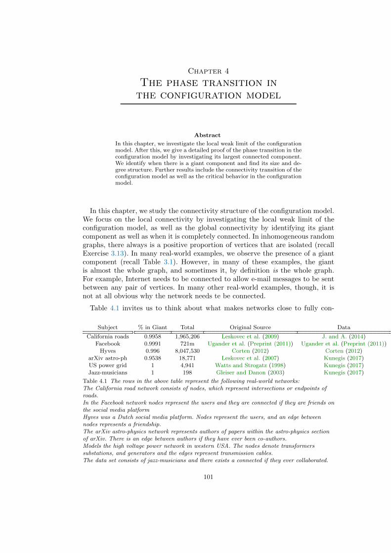
Chapter 4
The phase transition inthe configuration model
Abstract
In this chapter, we investigate the local weak limit of the configurationmodel. After this, we give a detailed proof of the phase transition in theconfiguration model by investigating its largest connected component.We identify when there is a giant component and find its size and de-gree structure. Further results include the connectivity transition of theconfiguration model as well as the critical behavior in the configurationmodel.
In this chapter, we study the connectivity structure of the configuration model.We focus on the local connectivity by investigating the local weak limit of theconfiguration model, as well as the global connectivity by identifying its giantcomponent as well as when it is completely connected. In inhomogeneous randomgraphs, there always is a positive proportion of vertices that are isolated (recallExercise 3.13). In many real-world examples, we observe the presence of a giantcomponent (recall Table 3.1). However, in many of these examples, the giantis almost the whole graph, and sometimes it, by definition is the whole graph.For example, Internet needs to be connected to allow e-mail messages to be sentbetween any pair of vertices. In many other real-world examples, though, it isnot at all obvious why the network needs te be connected.
Table 4.1 invites us to think about what makes networks close to fully con-
Subject % in Giant Total Original Source Data
California roads 0.9958 1,965,206 Leskovec et al. (2009) J. and A. (2014)Facebook 0.9991 721m Ugander et al. (Preprint (2011)) Ugander et al. (Preprint (2011))
Hyves 0.996 8,047,530 Corten (2012) Corten (2012)arXiv astro-ph 0.9538 18,771 Leskovec et al. (2007) Kunegis (2017)US power grid 1 4,941 Watts and Strogatz (1998) Kunegis (2017)Jazz-musicians 1 198 Gleiser and Danon (2003) Kunegis (2017)
Table 4.1 The rows in the above table represent the following real-world networks:The California road network consists of nodes, which represent intersections or endpoints ofroads.In the Facebook network nodes represent the users and they are connected if they are friends onthe social media platformHyves was a Dutch social media platform. Nodes represent the users, and an edge betweennodes represents a friendship.The arXiv astro-physics network represents authors of papers within the astro-physics sectionof arXiv. There is an edge between authors if they have ever been co-authors.Models the high voltage power network in western USA. The nodes denote transformerssubstations, and generators and the edges represent transmission cables.The data set consists of jazz-musicians and there exists a connected if they ever collaborated.
101
102 The phase transition in the configuration model
nected. We investigate this question here in the context of the configurationmodel. The advantage of the configuration model is that it highly flexible in itsdegree structure, making it possible for all degrees to be at least a certain value.We will see that this allows the random graph to be connected, while at the sametime remaining sparse, as is the case in many real-world networks.
Organization of this chapter
This chapter is organized as follows. In Section 4.1, we study the local weak limitof the configuration model. In Section 4.2, we state and prove the law of largenumbers for the giant component in the configuration model, thus establishingthe phase transition. In Section 4.3, we study when the configuration model isconnected. In Section 4.4, we state further results in the configuration model. Weclose this chapter in Section 4.5 with notes and discussion and with exercises inSection 4.6.
4.1 Local weak convergence to unimodular trees for CMn(d)
We start by investigating the locally tree-like nature of the configuration model.Our main result is as follows:
Theorem 4.1 (Locally tree-like nature configuration model) Assume that Con-ditions 1.5(a)-(b) hold. Then CMn(d) converges locally-weakly in probability tothe unimodular Galton-Watson tree with root offspring distribution (pk)k≥0 givenby pk = P(D = k).
Before starting with the proof of Theorem 4.1, let us explain the above con-nection between local neighborhoods and branching processes. We note that theasymptotic offspring distribution at the root is equal to (pk)k≥0, where pk =P(D = k) is the asymptotic degree distribution, since the probability that a ran-dom vertex has degree k is equal to p(n)
k = P(Dn = k) = nk/n, where nk denotesthe number of vertices with degree k, which, by Condition 1.5(a), converges topk = P(D = k), for every k ≥ 1. This explains the offspring of the root of ourbranching process approximation.
The offspring distribution of the individuals in the first and later generationsis given by
p?k =(k + 1)pk+1
E[D]. (4.1.1)
We now heuristically explain this relation to branching processes by intuitivelydescribing the exploration of a vertex chosen uniformly from the vertex set [n].To describe the offspring of the direct neighbors of the root, we examine thedegree of the vertex to which the first half-edge incident to the root is paired.By the uniform matching of half-edges, the probability that a vertex of degree kis chosen is proportional to k. Ignoring the fact that the root and one half-edgehave already been chosen (which does have an effect on the number of available or
4.1 Local weak convergence to unimodular trees for CMn(d) 103
free half-edges), the degree of the vertex incident to the chosen half-edge equalsk with probability equal to kp(n)
k /E[Dn], where again p(n)
k = nk/n denotes theproportion of vertices with degree k, and
E[Dn] =1
n
∑i∈[n]
di =1
n
∑i∈[n]
∞∑k=0
k1di=k =∞∑k=0
kp(n)
k (4.1.2)
is the average degree in CMn(d). Thus, (kp(n)
k /E[Dn])k≥0 is a probability massfunction. However, one of the half-edges is used up to connect to the root, sothat, for a vertex incident to the root to have k offspring, it needs to connectits half-edge to a vertex having degree k + 1. Therefore, the probability that theoffspring of any of the direct neighbors of the root is equal to k equals
p?(n)
k =(k + 1)p(n)
k+1
E[Dn]. (4.1.3)
Thus, (p?(n)
k )k≥0 can be interpreted as the forward degree of vertices in the clusterexploration. When Condition 1.5(a)-(b) hold, also p?(n)
k → p?k, where (p?k)k≥0 isdefined in (4.1.1). As a result, we often refer to (p?k)k≥0 as the asymptotic forwarddegree distribution.
The above heuristically argues that the number of vertices unequal to the rootconnected to any direct neighbor of the root has asymptotic law (p?k)k≥0. How-ever, every time we pair two half-edges, the number of free or available half-edgesdecreases by 2. Similarly to the depletion-of-points effect in the exploration ofclusters for the Erdos-Renyi random graph ERn(λ/n), the configuration modelCMn(d) suffers from a depletion-of-points-and-half-edges effect. Thus, by iter-atively connecting half-edges in a breadth-first way, the offspring distributionchanges along the way, which gives potential trouble. Luckily, the number ofavailable half-edges that we start with equals `n − 1, which is very large whenCondition 1.5(a)-(b) hold, since then `n/n = E[Dn]/n→ E[D] > 0. Thus, we canpair many half-edges before we start noticing that their number decreases. As aresult, the degrees of different vertices in the exploration process is close to beingi.i.d., leading to a branching process approximation. In order to prove Theorem4.1, we will only need to pair a bounded number of edges.
In order to get started for the proof of (2.3.5) for Theorem 4.1, we introducesome notation. Fix a rooted tree (T, y) with k generations, and let
Nn(T, y) =∑v∈[n]
1B(n)v (k)'(T,y) (4.1.4)
denote the number of vertices whose local neighborhood up to generation t equals(T, y). By Theorem 2.8, in order to prove Theorem 4.1, we need to show that
Nn(T, y)
nP−→ P(BP≤k ' (T, y)). (4.1.5)
Here, we also rely on Theorem 2.9 to see that it suffices to prove (4.1.5) fortrees, since the unimodular Galton-Watson tree is a tree with probability 1. For
104 The phase transition in the configuration model
this, we will use a second moment method. We first prove that the first momentE[Nn(T, y)]/n→ P(T (p, k) ' (T, y)), after which we prove that Var(Nn(T, y)) =o(n2). Then, by the Chebychev inequality, (4.1.5) follows.
Local weak convergence for configuration model: first moment
We next relate the neighborhood in a random graph to a branching process wherethe root has offspring distribution Dn, while all other individuals have offspringdistribution D?
n − 1, where
P(D?n = k) =
k
E[Dn]P(Dn = k), k ∈ N, (4.1.6)
is the size-biased distribution ofDn. Denote this branching process by (BPn(t))t∈N0.
Here, BPn(t) denotes the branching process when it contains precisely t vertices,and we explore it in the breadth-first order. Clearly, by Conditions 7.8(a)-(b),
Dnd−→ D and D?
n
d−→ D?, which implies that BPn(t)d−→ BP(t) for every t fi-
nite, where BP(t) is the restriction of the unimodular branching process BP withoffspring distribution (pk)k≥1 fo which pk = P(D = k) to its first t individuals(see Exercise 4.1). For future reference, denote the offspring distribution of theabove branching process by
p?k = P(D? − 1 = k) (4.1.7)
Note that, when (T, y) is a fixed rooted tree of k generations, then BP≤k '(T, y) precisely when BP(tk) ' (T, y), where tk denotes the number of vertices in(T, y).
We let (Gn(t))t∈N0denote the graph exploration process from a uniformly
chosen vertex U ∈ [n]. Here Gn(t) is the exploration up to t vertices, in thebreadth-first manner. In particular, from (Gn(t))t∈N0
we can retrieve (BU(t))t∈N0
for every t ≥ 0. The following lemma proves that we can couple the graph ex-ploration to the branching process in such a way that (Gn(t))0≤t≤mn is equal to(BPn(t))0≤t≤mn whenever mn →∞ arbitrarily slowly. In the statement, we write
(Gn(t), BPn(t))t∈N0for the coupling of (Gn(t))0≤t≤mn and (BPn(t))0≤t≤mn :
Lemma 4.2 (Coupling graph exploration and branching process) Subject to
Conditions 1.5(a)-(b), there exists a coupling (Gn(t), BPn(t))t∈N0of (Gn(t))0≤t≤mn
and (BPn(t))0≤t≤mn such that
P(
(Gn(t))0≤t≤mn 6= (BPn(t))0≤t≤mn
)= o(1), (4.1.8)
whenever mn → ∞ arbitrarily slowly. Consequently, E[Nn(T )]/n → P(BP≤k 'T ).
In the proof, we will see that any mn = o(√n/dmax) is allowed. Here dmax =
maxi∈[n] di is the maximal vertex degree in the graph, which is o(n) when Condi-tions 7.8(a)-(b) hold.
4.1 Local weak convergence to unimodular trees for CMn(d) 105
Proof We let the offspring of the root of the branching process Dn be equalto dU , which is the number of neighbors of the vertex U ∈ [n] that is chosen
uniformly at random. By construction, Dn = dU , so that also Gn(1) = BPn(1).
We next explain how to jointly construct (Gn(t), BPn(t))0≤t≤m given that we have
already constructed (Gn(t), BPn(t))0≤t≤m−1.
To obtain (Gn(t)0≤t≤m, we take the first unpaired half-edge xm. This half-edgeneeds to be paired to a uniform half-edge that has not been paired so far. Wedraw a uniform half-edge ym from the collection of all half-edges, independently
of the past, and we let the (m−1)st individual in (BPn(t))0≤t≤m−1 have preciselydUm − 1 children. Note that dUm − 1 has the same distribution as D?
n − 1 and, byconstruction, the collection
(dUt −1
)t≥0
is i.i.d. When ym is still free, i.e., has not
yet been paired in (Gn(t))0≤t≤m−1, then we also let xm be paired to ym, and we
have constructed (Gn(t))0≤t≤m. However, a problem arises when ym has already
been paired in (Gn(t))0≤t≤m−1, in which case we draw a uniform unpaired half-edgey′m and pair xm to y′m instead. Clearly, this might give rise to a difference between
(Gn(t))t≤m and (BPn(t))0≤t≤m. We now provide bounds on the probability thatan error occurs before time mn.
There are two sources of differences between (Gn(t))t≥0 and (BPn(t))t≥0:
Half-edge re-use In the above coupling ym had already been paired and is beingre-used in the branching process, and we need to redraw y′m;
Vertex re-use In the above coupling, this means that ym is a half-edge that hasnot yet been paired in (Gn(t))0≤t≤m−1, but it is incident to a half-edge that has
already been paired in (Gn(t))0≤t≤m−1. In particular, the vertex to which it is
incident has already appeared in (Gn(t))0≤t≤m−1 and it is being re-used in the
branching process. In this case, a copy of the vertex appears in (BPn(t))0≤t≤m,
while a cycle appears in (Gn(t))0≤t≤m.
We now provide a bound on both contributions:
Half-edge re-use
Up to timem−1, at most 2m−1 half-edges are forbidden to be used by (Gn(t)t≤m).The probability that the half-edge qm equals one of these two half-edges is at most
2m− 1
`n. (4.1.9)
Hence the probability that a half-edge is being re-used before time mn is at most
mn∑m=1
2m− 1
`n=m2n
`n= o(1), (4.1.10)
when mn = o(√n).
106 The phase transition in the configuration model
Vertex re-use
The probability that vertex i is chosen in the mth draw is equal to di/`n. Theprobability that vertex i is drawn twice before time mn is at most
mn(mn − 1)
2
d2i
`2n. (4.1.11)
By the union bound, the probability that there exists a vertex that is chosentwice up to time mn is at most
mn(mn − 1)
2`n
∑i∈[n]
d2i
`n≤ m2
n
dmax
`n= o(1), (4.1.12)
by Condition 7.8 when mn = o(√n/dmax).
Completion of the proof
In order to show that E[Nn(T, y)]/n → P(T (p, k) ' (T, y)), we let tk denote thenumber of individuals in the first k − 1 generations in (T, y), and let (T (t))t∈[tk]
be its breadth-first exploration. Then,
E[Nn(T, y)]/n = P((Gn(t))t∈[tk] = (T (t))t∈[tk]), (4.1.13)
so that
P((Gn(t))t∈[tk] = (T (t))t∈[tk]) = P((BPn(t))t∈[tk] = (T (t))t∈[tk]) + o(1) (4.1.14)
= P((BP(t))t∈[tk] = (T (t))t∈[tk]) + o(1)
= P(BP≤k ' (T, y)) + o(1),
where the first equality is (4.1.8), while the second is the statement that BPn(t)d−→
BP(t) for every t finite from Exercise 4.1. This proves the claim.
Local weak convergence for the configuration model: second moment
Here, we study the second moment of Nn(T, y), and show that it is close to thefirst moment squared:
Lemma 4.3 (Concentration of the number of trees) Assume that Conditions1.5(a)-(b) hold. Then,
E[Nn(T, y)2]
n2→ P(BP≤k ' (T, y))2. (4.1.15)
Consequently, Nn(T, y)/nP−→ P(BP≤k ' (T, y)).
Proof We start by computing
E[Nn(T, y)2]
n2= P(B(n)
U1(k), B(n)
U2(k) ' (T, y)), (4.1.16)
4.2 Phase transition in the configuration model 107
where U1, U2 ∈ [n] are two vertices chosen uniformly at random from [n], indepen-
dently. Since |B(n)
U1(k)| d−→ |BP≤k|, which is a tight random variable, U2 /∈ B(n)
U1(2k)
with high probability, so that also
E[Nn(T, y)2]
n2= P(B(n)
U1(k), B(n)
U2(k) ' (T, y), U2 /∈ B(n)
U1(2k)) + o(1). (4.1.17)
We now condition on B(n)
U1(k) = (T, y), and write
P(B(n)
U1(k), B(n)
U2(k) ' (T, y), U2 /∈ B(n)
U1(2k)) (4.1.18)
= P(B(n)
U2(k) ' (T, y) | B(n)
U1(k) ' (T, y), U2 /∈ B(n)
U1(2k))
× P(B(n)
U1(k) ' (T, y), U2 /∈ B(n)
U1(2k)).
We already know that P(B(n)
U1(k) ' (T, y))→ P(BP≤k ' (T, y)), so that also
P(B(n)
U1(k) ' (T, y), U2 /∈ B(n)
U1(2k))→ P(BP≤k ' (T, y)). (4.1.19)
In Exercise 4.2, you prove that indeed (4.1.19) holds.
We note that, conditionally on B(n)
U1(k) ' (T, y), U2 /∈ B(n)
U1(k), the probabil-
ity that B(n)
U2(k) ' (T, y) is the same as the probability that B(n)
U2(k) ' (T, y)
in CMn′(d′) which is obtained by removing all vertices in B(n)
U1(k). Thus, since
B(n)
U1(k) ' (T, y), we have that n′ = n − |V (T )| and d′ is the corresponding de-
gree sequence. The whole point is that the degree distribution d′ still satisfiesConditions 7.8(a)-(b). Therefore, also
P(B(n)
U2(k) ' (T, y) | B(n)
U1(k) ' (T, y), U2 /∈ B(n)
U1(k)) (4.1.20)
→ P(BP≤k ' (T, y)),
and we have proved (4.1.15). Since E[Nn(T, y)]/n → P(BP≤k ' (T, y)) andE[Nn(T, y)2]/n2 → P(BP≤k ' (T, y))2, it follows that Var(Nn(T, y)/n) → 0, sothat Nn(T, y)/n is concentrated. Since also E[Nn(T, y)]/n → P(BP≤k ' (T, y)),
we obtain that Nn(T, y)/nP−→ P(BP≤k ' (T, y)), as required.
Lemma 4.3 completes the proof of Theorem 4.1.
4.2 Phase transition in the configuration model
In this section, we investigate the connected components in the configurationmodel. Alike for the Erdos-Renyi random graph, we identify when the configura-tion model whp has a giant component. Again, this condition has the interpreta-tion that an underlying branching process describing the exploration of a clusterhas a strictly positive survival probability.
We start by recalling some notation from [Volume 1, Chapter 7]. We investigatethe configuration model CMn(d), where in most cases, the degrees d = (di)i∈[n]
are assumed to satisfy Condition 1.5(a)-(b), and sometimes also Condition 1.5(c).We recall that Dn is the degree of a uniformly chosen vertex in [n], i.e., Dn = dU ,
108 The phase transition in the configuration model
where U is uniformly chosen from [n]. Equivalently,
P(Dn = k) = nk/n, (4.2.1)
where nk denotes the number of vertices of degree k. For a graph G, we writevk(G) for the number of vertices of degree k in G, and |E(G)| for the number ofedges. The main result concerning the size and structure of the largest connectedcomponents of CMn(d) is the following:
Theorem 4.4 (Phase transition in CMn(d)) Suppose that Condition 1.5(a)-(b) hold and consider the random graph CMn(d), letting n → ∞. Assume thatp2 = P(D = 2) < 1. Let Cmax and C(2) be the largest and second largest componentsof CMn(d).
(a) If ν = E[D(D − 1)]/E[D] > 1, then there exist ξ ∈ [0, 1), ζ ∈ (0, 1] such that
|Cmax|/n P−→ ζ,
vk(Cmax)/nP−→ pk(1− ξk) for every k ≥ 0,
|E(Cmax)|/n P−→ 1
2E[D](1− ξ2).
while |C(2)|/n P−→ 0 and |E(C(2))|/n P−→ 0.
(b) If ν = E[D(D − 1)]/E[D] ≤ 1, then |Cmax|/n P−→ 0 and |E(Cmax)|/n P−→ 0.
Consequently, the same result holds for the uniform random graph with degree se-quence d satisfying Condition 1.5(a)-(b), under the extra assumption that
∑i∈[n] d
2i =
O(n).
Reformulation in terms of branching processes
We start by interpreting the results in Theorem 4.4 in terms of branching pro-cesses as also arising in Section 4.1. As it turns out, we can interpret ξ as theextinction probability of a branching process, and ζ as the survival probabilityof the unimodular Galton-Watson tree that appears in Theorem 4.1. Thus, ζsatisfies
ζ =∑k≥1
pk(1− ξk), (4.2.2)
where ξ is the extinction probability of the branching process with offspringdistribution (p?k)k≥0, which satisfies
ξ =∑k≥0
p?kξk. (4.2.3)
Clearly, ξ = 1 precisely when
ν =∑k≥0
kp?k ≤ 1. (4.2.4)
4.2 Phase transition in the configuration model 109
By (4.1.1), we can rewrite
ν =1
E[D]
∑k≥0
k(k + 1)pk+1 = E[D(D − 1)]/E[D], (4.2.5)
which explains the condition on ν in Theorem 4.4(a). Further, to understandthe asymptotics of vk(Cmax), we note that there are nk = np(n)
k ≈ npk verticeswith degree k. Each of the k direct neighbors of a vertex of degree k surviveswith probability close to 1− ξ, so that the probability that at least one of themsurvives is close to 1 − ξk. When one of the neighbors of the vertex of degreek survives, the vertex itself is part of the giant component, which explains whyvk(Cmax)/n
P−→ pk(1 − ξk). Finally, an edge consists of two half-edges, and anedge is part of the giant component precisely when one of the vertices incident toit is, which occurs with probability 1− ξ2. There are in total `n/2 = nE[Dn]/2 ≈nE[D]/2 edges, which explains why |E(Cmax)|/n P−→ 1
2E[D](1 − ξ2). Therefore,
all results in Theorem 4.4 have a simple explanation in terms of the branchingprocess approximation of the connected component for CMn(d) of a uniformvertex in [n].
Reformulation in terms of generating functions
We next reformulate the results in terms of generating functions, which play acrucial role throughout our proof. Let
GD(x) =∞∑k=0
pkxk = E[xD] (4.2.6)
be the probability generating function of the probability distribution (pk)k≥1. Re-call that, for a non-negative random variable D, the random variable D? denotesits size-biased distribution. Define further
G?D
(x) = E[xD?
] =∞∑k=1
p?kxk = G′
D(x)/G′
D(1), (4.2.7)
H(x) = E[D]x(x−G?
D(x)). (4.2.8)
Note that G?D
(1) = 1, and thus H(0) = H(1) = 0. Note also that
H ′(1) = 2E[D]−∑k
k2pk = E[2D −D2] = −E[D(D − 2)] (4.2.9)
For further properties of x 7→ H(x), see Lemma 4.9 below. We conclude that ifE[D(D − 2)] =
∑k k(k − 2)pk > 0 and if p?1 > 0, then there is a unique ξ ∈ (0, 1)
such that H(ξ) = 0, or equivalently G?D
(ξ) = ξ, so that indeed ξ is the extinctionprobability of the branching process with offspring distribution (p?k)k≥0. Whenp?1 = 0, instead, ξ = 0 is the unique solution in [0, 1) of H(ξ) = 0. The functionsx 7→ H(x) and x 7→ G?
D(x) play a central role in our analysis of the problem.
We prove Theorem 4.4 in Section 4.2.2 below. We now remark upon the resultand on the conditions arising in it.
110 The phase transition in the configuration model
The condition P(D = 2) = p2 < 1
Because isolated vertices do not matter, without loss of generality, we may assumethat p0 = 0. The case p2 = 1, for which ν = 1 is quite exceptional. In this case,H(x) = 0 for all x. We give three examples showing that then quite differentbehaviors are possible.
Our first example is when di = 2 for all i ∈ [n], so we are studying a random2-regular graph. In this case, the components are cycles and the distribution ofcycle lengths in CMn(d) is given by the Ewen’s sampling formula ESF(1/2), seee.g. Arratia et al. (2003). This implies that |Cmax|/n converges in distribution toa non-degenerate distribution on [0, 1] and not to any constant (Arratia et al.,2003, Lemma 5.7). Moreover, the same is true for |C(2)|/n (and for |C(3)|/n,...),so in this case there are several large components. To intuitively see this result,we note that in the exploration of a cluster we start with one vertex with twohalf-edges. When pairing a half-edge, it connects to a vertex that again has twohalf-edges. Therefore, the number of half-edges to be paired is always equal to 2,up to the moment when the cycle is closed, and the cluster is completed. Whenthere are m = αn free half-edges left, the probability of closing up the cycle equals1/m = 1/(αn), and, thus, the time this takes is of order n. A slight extensionof this reasoning shows that the time it takes to close a cycle is nTn, where Tnconverges to a limiting non-degenerate random variable (see Exercise 4.3).
Our second example with p2 = 1 is obtained by adding a small number ofvertices of degree 1. More precisely, we let n1 →∞ be such that n1/n→ 0, andn2 = n− n1. In this case, components can either be cycles, or strings of verticeswith degree 2 terminated with two vertices with degree 1. When n1 → ∞, itis more likely to terminate a long string of vertices of degree 2 by a vertex ofdegree 1 than by closing the cycle, as for the latter we need to pair to a uniquehalf-edge, while for the former, we have n1 choices. Therefore, it is easy to seethat this implies that |Cmax| = oP(n) (see Exercise 4.4 for details).
Our third example with p2 = 1 is obtained by instead adding a small numberof vertices of degree 4 (i.e., n4 → ∞ such that n4/n → 0, and n2 = n − n4.)We can regard each vertex of degree 4 as two vertices of degree 2 that have beenidentified. Therefore, to obtain CMn(d) with this degree distribution, we can startfrom a configuration model having N = n+n4 vertices, and uniformly identifyingn4 pairs of vertices of degree 2. Since the configuration model with N = n + n4
vertices of degree 2 has many components having size of order n, most of thesewill merge into one giant component. As a result, |Cmax| = n − oP(n), so thereis a giant component containing almost everything, as you will prove yourself inExercise 4.5.
We conclude that the case where p2 = P(D = 2) = 1 is quite sensitive to theprecise properties of the degree structure that are not captured by the limitingdistribution (pk)k≥1 only. In the sequel, we ignore the case where p2 = 1.
4.2 Phase transition in the configuration model 111
Reduction to the case where P(D = 1) = p1 > 0
In our proof, it is convenient to assume that p1 = P(D = 1) > 0. The extinctionprobability ξ = 0 and the survival probability ζ = 1 when p1 = 0, which causestechnical difficulties in the proof. We now explain how we can reduce the casewhere p1 = 0 to the case where p1 > 0.
Let dmin = mink : pk > 0 be the minimum of the support of the asymptoticdegree distribution D. Fix ε > 0, and assume that ε < pdmin
. Consider the con-figuration model with n = n + 2dminεn, and degree sequence d = (di)i∈[n] withnk = nk for all k > dmin, ndmin
= ndmin− εn, n1 = 2dminεn. This configuration
model can be obtained from CMn(d) by replacing εn vertices of degree dmin bydmin vertices having degree 1, as if we have ‘forgotten’ that these vertices areactually equal.
Clearly, CMn(d) can be retrieved by identifying εn collections of dmin verticesof degree 1 to a single vertex of degree dmin. When d satisfies Condition 1.5(a)-(b),then so does d with limiting degree distribution p1 = 2dminε/, pdmin
= (pdmin−
ε)/(1+2dminε), pk = pk/(1+2dminε) for all k > dmin. The above procedure clearlymakes |Cmax| smaller. Further, with ζε denoting the limit of |Cmax|/n for d, wehave that ζε → 1 as ε ↓ 0. As a result, Theorem 4.4 for ζ = 1, ξ = 0 follows fromTheorem 4.4 with p1 > 0, for which ζ < 1 and ξ > 0. In the remainder of theproof, we therefore without loss of generality assume that ξ > 0 and ζ < 1.
Organization of the proof of Theorem 4.4
Theorem 4.4 is proved using a clever randomization scheme to explore the con-nected components one by one. This construction is explained terms of a simplecontinuous-time algorithm in Section 4.2.1 below. The algorithm describes thenumber of vertices of given degrees that have been found, as well as the totalnumber of unpaired half-edges, at time t > 0. It is proved that, when n → ∞,these quantities all converge in probability to deterministic functions describedin terms of the functions x 7→ H(x) and x 7→ G?
D(x) above. In particular, the
number of unpaired half-edges is given in terms of x 7→ H(x), so that the firstzero of this function gives the size of the giant component. In Section 4.2.2, thealgorithm is analyzed by showing that when ζ > 0, after a short initial period ofexploring small clusters, the giant component is found, and the exploration ex-plores it completely, after which no large component is left. When ζ = 0, instead,only small clusters are found. A crucial aspect in the proof resides in how to dealwith the depletion-of-points-and-half-edges effect.
4.2.1 Finding the largest component
The components of an arbitrary finite graph or multigraph can be found bythe following standard procedure. Pick an arbitrary vertex v and determine thecomponent of v as follows: include all the neighbors of v in an arbitrary order;then add in the neighbors of the neighbors, and so on, until no more verticescan be added. The vertices included until this moment form the component ofv. If there are still vertices left in the graph, then pick any such vertex w, and
112 The phase transition in the configuration model
repeat the above to determine the second component (the component of vertexw). Carry on in this manner until all the components have been found.
The same result can be obtained in the following way, which turns out to bemore convenient for the exploration of the giant component in the configurationmodel. Regard each edge as consisting of two half-edges, each half-edge havingone endpoint. We will label the vertices as sleeping or awake (= used) and thehalf-edges as sleeping, active or dead; the sleeping and active half-edges are alsocalled living. We start with all vertices and half-edges sleeping. Pick a vertexand label its half-edges as active. Then take any active half-edge, say x and findits partner y in the graph; label these two half-edges as dead. Further, if theendpoint of y is sleeping, label it as awake and all other half-edges of the vertexincident to y as active. Repeat as long as there are active half-edge. When thereis no active half-edge left, we have obtained the first component. Then start againwith another vertex until all components are found.
We apply this algorithm to CMn(d) with a given degree sequence, revealing itsedges during the process. We thus initially only observe the vertex degrees andthe half-edges, but not how they are joined to form edges. Hence, each time weneed a partner of an half-edge, it is uniformly distributed over all other livinghalf-edges, with the understanding that the dead half-edges are the ones that arealready paired into edges.It is here that we are using the specific structure of theconfiguration model, which simplifies the analysis substantially.
We make the random choices of finding a partner to the edges by associatingi.i.d. random maximal lifetimes τx to the half-edge x, where τx has an Exp(1)distribution. We interpret these lifetimes as clocks, and changes in our explorationprocess only occur when a clock of a half-edge rings. In other words, each half-edge dies spontaneously at rate 1 (unless killed earlier). Each time we need tofind the partner of a half-edge x, we then wait until the next living half-edge 6= xdies and take that one. This process in continuous-time can be formulated as analgorithm, constructing CMn(d) and exploring its components simultaneously,as follows. Recall that we start with all vertices and half-edges sleeping. Theexploration is then formalized in the following three steps:
Step 1 When there is no active half-edge (as in the beginning), select a sleeping vertexand declare it awake and all its half-edges active. For definiteness, we choosethe vertex by choosing a half-edge uniformly at random among all sleeping half-edges. When there is no sleeping half-edge left, the process stops; the remainingsleeping vertices are all isolated and we have explored all other components.
Step 2 Pick an active half-edge (which one does not matter) and kill it, i.e., changeits status to dead.
Step 3 Wait until the next half-edge dies (spontaneously, as a result of its clock ring-ing). This half-edge is joined to the one killed in the previous step Step 2 toform an edge of the graph. When the vertex incident to it is sleeping, we changethis vertex to awake and all other half-edges incident to it to active. Repeatfrom Step 1.
The above randomized algorithm is such that components are created between
4.2 Phase transition in the configuration model 113
the successive times Step 1 is performed, where we say that Step 1 is performedwhen there is no active half-edge and, as a result, a new vertex is chosen.
The vertices in the component created during one of these intervals betweenthe successive times Step 1 is performed are the vertices that are awakened duringthe interval. Note also that a component is completed and Step 1 is performedexactly when the number of active half-edges is 0 and a half-edge dies at a vertexwhere all other half-edges (if any) are dead. In the next section, we investigatethe behavior of the key characteristics of the algorithm, such as the number ofsleeping half-edges and the number of sleeping vertices of a given degree.
4.2.2 Analysis of the algorithm for CMn(d)
We start by introducing the key characteristics of the exploration algorithm.Let S(t) and A(t) be the numbers of sleeping and active half-edges, respectively,at time t, and let
L(t) = S(t) +A(t) (4.2.10)
be the number of living half-edges. For definiteness, we define these random func-tions to be right-continuous.
Let us first look at L(t). We start with `n =∑
i∈[n] di half-edges, all sleepingand thus living, but we immediately perform Step 1 and Step 2 and kill one ofthem. Thus, L(0) = `n − 1. In the sequel, as soon as a living half-edge dies, weperform Step 3 and then (instantly) either Step 2 or both Step 1 and Step 2.Since Step 1 does not change the number of living half-edges while Step 2 andStep 3 each decrease it by 1, the total result is that L(t) is decreased by 2 eachtime one of the living half-edges dies, except when the last living one dies andthe process terminates. Because of this simple dynamics of t 7→ L(t), we can givesharp asymptotics of L(t) when n→∞:
Proposition 4.5 (Number of living half-edges) As n → ∞, for any t0 ≥ 0fixed,
sup0≤t≤t0
|n−1L(t)− E[Dn]e−2t| P−→ 0. (4.2.11)
Proof The process t 7→ L(t) satisfies L(0) = `n−1, and it degreases by 2 at rateL(t). As a result, it is closely related to a death process. We study such processesin the following lemma:
Lemma 4.6 (Asymptotics of death processes) Let d, γ > 0 be given and let(N (x)(t))t≥0 be a Markov process such that N (x)(t) = x a.s., and the dynamics oft 7→ (N (x)(t))t≥0 is such that when it is in position y, then it jumps down by d atrate γy. In other words, the waiting time until the next event is Exp(1/γy) andeach jump is of size d downwards. Then, for every t0 ≥ 0,
E[
supt≤t0
∣∣N (x)(t)− e−γdtx∣∣2] ≤ 8d(eγdt0 − 1)x+ 8d2. (4.2.12)
Proof The proof follows by distinguishing several cases. First assume that d = 1
114 The phase transition in the configuration model
and that x is an integer. In this case, the process is a standard pure death processtaking the values x, x − 1, x − 2, . . . , 0, describing the number of particles alivewhen the particles die independently at rate γ > 0. As is well known, and easilyseen by regarding N (x)(t) as the sum of x independent copies of the processN (1)(t), the process (eγtN (x)(t))t≥0, is a martingale starting in x. Furthermore,for every t ≥ 0, the random variable N (x)(t) has a Bin(x, e−γt) distribution, sinceeach of the x particles has a probability of dying before time t of e−γt, and thedifferent particles die independently.
We rely on Doob’s martingale inequality, which states that for a martingale(Mn)n≥0,
E[
supm≤n
∣∣Mm − E[Mm]∣∣2] ≤ Var(Mn). (4.2.13)
Application of Doob’s martingale inequality yields
E[
supt≤t0
∣∣N (x)(t)− e−γtx∣∣2] ≤ E
[supt≤t0
∣∣eγtN (x)(t)− x∣∣2] ≤ 4E
[(eγtN (x)(t0)− x
)2]= 4e2γtVar(N (x)(t0)) ≤ 4(eγt0 − 1)x. (4.2.14)
This proves the claim for x being integer.Next, we still assume d = 1, but let x > 0 be arbitrary. We can couple the
two processes(N (x)(t)
)t≥0
and(N (bxc)(t))t≥0 with different initial values such that
whenever the smaller one jumps by 1, so does the other. This coupling keeps
|N (x)(t)−N (bxc)(t)| < 1 (4.2.15)
for all t ≥ 0, and thus,
supt≤t0
∣∣N (bxc)(t)− e−γtbxc∣∣ ≤ sup
t≤t0
∣∣N (x)(t)− e−γtx∣∣+ 2, (4.2.16)
so that by (4.2.14), in turn,
E[
supt≤t0
∣∣N (x)(t)− e−γtx∣∣2] ≤ 8(eγt0 − 1)x+ 8. (4.2.17)
Finally, for a general d > 0, we observe that N (x)(t)/d is a process of the sametype with the parameters (γ, d, x) replaced by (γd, 1, x/d), and the general resultfollows from (4.2.17) and (4.2.14).
The proof of Proposition 4.5 follows from Lemma 4.6 with d = 2, x = (`n−1) =nE[Dn]− 1 and γ = 1.
We continue by considering the sleeping half-edges S(t). Let Vk(t) be the num-ber of sleeping vertices of degree k at time t, so that
S(t) =∞∑k=1
kVk(t). (4.2.18)
Note that Step 2 does not affect sleeping half-edges, and that Step 3 implies thateach sleeping vertex of degree k is eliminated (i.e., awakened) with intensity k,
4.2 Phase transition in the configuration model 115
independently of all other vertices. There are also some sleeping vertices elim-inated by Step 1, though, which complicates the dynamics of t 7→ Vk(t). It ishere that the depletion-of-points-and-half-edges effect enters the analysis of thecomponent structure of CMn(d). This effect is complicated, but we will see itis quite harmless. This can be understood by noting that we only apply Step 1when we have completed exploring an entire component. Since we will be mainlyinterested in settings where the giant component is large, we will see that wewill not be using Step 1 very often before having completely explored the giantcomponent. After having completed the exploration of the giant component, westart using Step 1 again quite frequently, but it will turn out that then it is veryunlikely to be exploring any particularly large connected components. Thus, wecan have a setting in mind where the number of applications of Step 1 is quitesmall.
With this intuition in mind, we first ignore the effect of Step 1 by letting Vk(t)be the number of vertices of degree k such that all its half-edges have maximallifetimes τx > t. Thus, none of its k half-edges would have died spontaneouslyup to time t, assuming they all escaped Step 1. Let us now explain in somemore detail why it is reasonable to ignore the effect of Step 1 in the leadingorder when there exists a giant component. Indeed, we perform Step 1 until wehit the giant component, and then it takes a long time to find the entire giantcomponent. When ζ > 0, the number of times we perform Step 1 until we findthe giant component will be small (probably a tight random variable), as eachtime we have a strictly positive probability of choosing a vertex in the giantcomponent. Thus, intuitively, we expect the difference between Vk(t) and Vk(t)
to be insignificant. Thus, we start by focussing on the dynamics of (Vk(t))t≥0,ignoring the effect of Step 1, and later adapt for this omission.
For a given half-edge, we call the half-edges incident to the same vertex itssibling half-edges. Let further
S(t) =∑k
kVk(t) (4.2.19)
denote the number of half-edges whose sibling half-edges have escaped sponta-neous death up to time t. Comparing with (4.2.18), we see that the process S(t)
ignores the effect of Step 1 in an identical way as Vk(t).Recall the functions GD, G?
Dfrom (4.2.6)–(4.2.7), and define
h(x) = xE[D]G?D
(x). (4.2.20)
Then, we can identify the asymptotics of (Vk(t))t≥0 in a similar way as in Propo-sition 4.5:
Lemma 4.7 (Number of living vertices of degree k) Assume that Conditions1.5(a)-(b) hold. Then, as n→∞, for any t0 ≥ 0 fixed
supt≤t0|n−1Vk(t)− pke−kt| P−→ 0 (4.2.21)
116 The phase transition in the configuration model
for every k ≥ 0 and
supt≤t0|n−1
∞∑k=0
Vk(t)−GD(e−t)| P−→ 0, (4.2.22)
supt≤t0|n−1S(t)− h(e−t)| P−→ 0. (4.2.23)
Proof The statement (4.2.21) again follows from Lemma 4.6, now with γ = k,
x = nk and d = 1. The case k = 0 is trivial, with V0(t) = n0 for all t. We canreplace p(n)
k = nk/n by pk by Condition 1.5(a).By Condition 1.5(b), the sequence of random variables (Dn)n≥1 is uniformly
integrable, which means that for every ε > 0 there exists K <∞ such that for alln,∑
k>K knk/n = E[Dn|Dn > k] < ε. We may further assume (or deduce fromFatou’s inequality) that
∑k>K kpk < ε, and obtain by (4.2.21) that, whp,
supt≤t0|n−1S(t)− h(e−t)| = sup
t≤t0
∣∣∣∣∣∞∑k=1
k(n−1Vk(t)− pke−kt)∣∣∣∣∣
≤K∑k=1
k supt≤t0|n−1Vk(t)− pke−kt|+
∑k>K
k(nkn
+ pk)
≤ ε+ ε+ ε,
proving (4.2.23). An almost identical argument yields (4.2.22).
Remarkably, the difference between S(t) and S(t) is easily estimated. The fol-lowing result can be viewed as the key to why this approach works. Indeed, itgives a uniform upper bound on the difference due to the application of Step 1:
Lemma 4.8 (Effect of Step 1) Let dmax := maxi∈[n] di be the maximum degreeof CMn(d). Then
0 ≤ S(t)− S(t) < sup0≤s≤t
(S(s)− L(s)) + dmax. (4.2.24)
The process (S(t))t≥0 runs on scale n (see e.g., the related statement for(L(t))t≥0 in Proposition 4.5). Further, dmax = o(n) when Conditions 1.5(a)-(b)
hold. Finally, one can expect that S(s) ≤ L(s) holds, since the difference is re-
lated to the number of active half-edges. Thus, intuitively, sup0≤s≤t(S(s)−L(s)) =
S(0)−L(0) = 0. We will make that argument precise after we have proved Lemma
4.8. We then conclude that S(t)− S(t) = oP(n), and so they have the same limitafter rescaling by n. Let us now prove Lemma 4.8:
Proof Clearly, Vk(t) ≤ Vk(t), and thus S(t) ≤ S(t). Furthermore, S(t) − S(t)increases only as a result of Step 1. Indeed, Step 1 acts to guarantee that A(t) =L(t)− S(t) ≥ 0, and is only performed when A(t) = 0.
If Step 1 is performed at time t and a vertex of degree j > 0 is awakened, then
4.2 Phase transition in the configuration model 117
Step 2 applies instantly and we have A(t) = j − 1 < dmax, and consequently
S(t)− S(t) = S(t)− L(t) +A(t) < S(t)− L(t) + dmax. (4.2.25)
Furthermore, S(t) − S(t) is never changed by Step 2 and either unchanged or
decreased by Step 3. Hence, S(t)−S(t) does not increase until the next time Step1 is performed. Consequently, for any time t, if s was the last time before (or
equal to) t that Step 1 was performed, then S(t) − S(t) ≤ S(s) − S(s), and theresult follows by (4.2.25).
Let us now set the stage for taking the limits of n → ∞. Recall that A(t) =L(t)− S(t) denotes the number of awakened vertices and let
A(t) = L(t)− S(t) = A(t)− (S(t)− S(t)) (4.2.26)
denote the number of awakened vertices ignoring the effect of Step 1. Thus,A(t) ≤ A(t) since S(t) ≤ S(t). We will use A(t) as a proxy for A(t) in s similar
way as S(t) is used a a proxy for S(t).
Recall the definition of H(x) in (4.2.8). By Lemmas 4.5 and 4.7 and the defi-
nition that A(t) = L(t)− S(t), for any t0 ≥ 0,
supt≤t0|n−1A(t)−H(e−t)| P−→ 0. (4.2.27)
Lemma 4.8 can be rewritten as
0 ≤ S(t)− S(t) < − infs≤t
A(s) + dmax. (4.2.28)
By (4.2.26) and (4.2.28),
A(t) ≤ A(t) < A(t)− infs≤t
A(s) + dmax, (4.2.29)
which, perhaps, illuminates the relation between A(t) and A(t). Recall that con-nected components are explored between subsequent zeros of the process t 7→A(t). The function t 7→ H(e−t), which acts as the limit of A(t) (and thus hope-fully also of A(t)), is strictly positive in (0,− log ξ) and H(1) = H(ξ) = 0. There-
fore, we expect A(t) to be positive for t ∈ (0,− log ξ), and, if so, infs≤t A(s) = 0.
This would prove that indeed A(t) and A(t) are close on this entire interval, andthe exploration on the interval t ∈ (0,− log ξ) will turn out to correspond to theexploration of the giant component.
The idea is to continue our algorithm in Step 1-Step 3 until the giant compo-nent has been found, which implies that A(t) > 0 for the time of exploration ofthe giant component, and A(t) = 0 for the first time when we have completedthe exploration of the giant component, which is t = − log ξ. Thus, the terminfs≤t A(s) in (4.2.29) ought to be negligible. When Conditions 1.5(a)-(b) hold,
we further have that dmax = o(n), so that one can expect A(t) to be a goodapproximation of A(t). The remainder of the proof makes this intuition precise.
118 The phase transition in the configuration model
We start by summarizing some useful analytical properties of x 7→ H(x) that werely upon in the sequel:
Lemma 4.9 (Properties of x 7→ H(x)) Suppose that Conditions 1.5(a)-(b) holdand let H(x) be given by (4.2.8). Suppose also that p2 < 1.
(i) If ν = E[D(D − 1)]/E[D] > 1 and p1 > 0, then there is a unique ξ ∈ (0, 1)such that H(ξ) = 0. Moreover, H(x) < 0 for all x ∈ (0, ξ) and H(x) > 0 forall x ∈ (ξ, 1).
(ii) If ν = E[D(D − 1)]/E[D] ≤ 1, then H(x) < 0 for all x ∈ (0, 1).
Proof As remarked earlier, H(0) = H(1) = 0 and H ′(1) = −E[D(D − 2)].Furthermore, if we define φ(x) := H(x)/x, then φ(x) = E[D](x − G?
D(x)) is a
concave function on (0, 1], and it is strictly concave unless pk = 0 for all k ≥ 3, inwhich case H ′(1) = −E[D(D− 2)] = p1 > 0. Indeed, p1 + p2 = 1 when pk = 0 forall k ≥ 3. Since we assume that p2 < 1, we thus obtain that p1 > 0 in this case.
In case (ii), we thus have that φ is concave and φ′(1) = H ′(1)−H(1) ≥ 0, witheither the concavity or the inequality strict, and thus φ′(x) > 0 for all x ∈ (0, 1),whence φ(x) < φ(1) = 0 for x ∈ (0, 1).
In case (i), H ′(1) < 0, and thus H(x) > 0 for x close to 1. Further, when p1 > 0,H ′(0) = −h′(0) = −p1 < 0, and thus H(x) ≤ 0 for x close to 0. Hence, there isat least one ξ ∈ (0, 1) with H(ξ) = 0, and since H(x)/x is strictly concave andalso H(1) = 0, there is at most one such ξ and the result follows.
Now we are in the position to complete the proof of Theorem 4.4 in the followingsection.
4.2.3 Proof of Theorem 4.4
We start with the proof of Theorem 4.4(i). Let ξ be the zero of H given byLemma 4.9(i) and let θ = − log ξ. Then, by Lemma 4.9, H(e−t) > 0 for 0 < t < θ,and thus inft≤θH(e−t) = 0. Consequently, (4.2.27) implies
n−1 inft≤θ
A(t) = inft≤θ
n−1A(t)− inft≤θ
H(e−t)P−→ 0. (4.2.30)
Further, by Condition 1.5(b), dmax = o(n), and thus n−1dmax → 0. Conse-quently, (4.2.28) and (4.2.30) yield
supt≤θ
n−1|A(t)− A(t)| = supt≤θ
n−1|S(t)− S(t)| P−→ 0. (4.2.31)
Thus, by (4.2.27),
supt≤θ|n−1A(t)−H(e−t)| P−→ 0. (4.2.32)
This will be the work horse of our argument. By Lemma 4.9, we know thatt 7→ H(e−t) is positive on (0,− log ξ) when ν > 1. Thus, the exploration in theinterval (0,− log ξ) will find the giant component. We now make this intuitionprecise. In particular, we need to show that no large connected component is found
4.2 Phase transition in the configuration model 119
before or after this interval (showing that the giant is unique), and we need toinvestigate the properties of the giant, in terms of number of edges, vertices ofdegree k etc. We now provide these details.
Let 0 < ε < θ/2. Since H(e−t) > 0 on the compact interval [ε, θ − ε], (4.2.32)implies that A(t) remains whp positive on [ε, θ− ε], and thus no new componentis started during this interval.
On the other hand, again by Lemma 4.9(i), H(e−(θ+ε)) < 0 and (4.2.27) im-
plies that n−1A(θ + ε)P−→ H(e−(θ+ε)), while A(θ + ε) ≥ 0. Thus, with ∆ =
|H(e−θ−ε)|/2 > 0, whp
S(θ + ε)− S(θ + ε) = A(θ + ε)− A(θ + ε) ≥ −A(θ + ε) > n∆, (4.2.33)
while (4.2.31) yields that S(θ)− S(θ) < n∆ whp. Consequently, whp S(θ + ε)−S(θ+ε) > S(θ)−S(θ), so whp Step 1 is performed between the times θ and θ+ε.
Let T1 be the last time Step 1 was performed before time θ/2. Let T2 be the nexttime Step 1 is performed (by convention, T2 =∞ if such a time does not exist).We have shown that for any ε > 0, and whp 0 ≤ T1 ≤ ε and θ − ε ≤ T2 ≤ θ + ε.In other words, T1
P−→ 0 and T2P−→ θ. We conclude that we have found one
component that is explored between time T1P−→ 0 and time T2
P−→ θ. This isour candidate for the giant component, and we continue to study its properties,i.e., its size, its number of edges and its number of vertices of degree k. Theseproperties are stated separately in the next proposition, so that we are able toreuse them later on:
Proposition 4.10 (Connected component properties) Let T ?1 and T ?2 be two
random times when Step 1 is performed, with T ?1 ≤ T ?2 , and assume that T ?1P−→ t1
and T ?2P−→ t2 where 0 ≤ t1 ≤ t2 ≤ θ < ∞. If C ? is the union of all components
explored between T ?1 and T ?2 , then
vk(C?)/n
P−→ pk(e−kt1 − e−kt2), k ≥ 0, (4.2.34)
|C ?|/n P−→ GD(e−t1)−GD(e−t2), (4.2.35)
|E(C ?)|/n P−→ 1
2h(e−t1)− 1
2h(e−t2). (4.2.36)
In particular, if t1 = t2, then |C ?|/n P−→ 0 and |E(C ?)| P−→ 0.
Below, we apply Proposition 4.10 to T1 = oP(1) and T2, where T2 = θ + oP(1).We can identify the values of the above constants for t1 = 0 and t2 = θ as e−kt1 =1, e−kt2 = ξ, GD(e−t1) = 1, GD(e−t2) = 1− ζ, h(e−t1) = 2E[D], h(e−t2) = 2E[D]ξ2
(see Exercise 4.6).By Proposition 4.10 and Exercise 4.6, Theorem 4.4(i) follows when we prove
that the connected component found between times T1 and T2 is indeed the giantcomponent. This is proved after we complete the proof of Proposition 4.10:
120 The phase transition in the configuration model
Proof The set of vertices C ? contains all vertices awakened in the interval[T ?1 , T
?2 ) and no others, and thus (writing Vk(t−) = limst Vk(s))
vk(C?) = Vk(T
?1−)− Vk(T ?2−), k ≥ 1. (4.2.37)
Since T ?2P−→ t2 ≤ θ and H is continuous, we obtain that inft≤T?2 H(e−t)
P−→inft≤t2 H(e−t) = 0, where the latter equality follows since H(1) = 0. Now, (4.2.27)
and (4.2.28) imply, in analogy with (4.2.30) and (4.2.31), that n−1 inft≤T?2 A(t)P−→
0 and thus also
supt≤T?2
n−1|S(t)− S(t)| P−→ 0. (4.2.38)
Since Vj(t) ≥ Vj(t) for every j and t ≥ 0,
Vk(t)− Vk(t) ≤ k−1∞∑j=1
j(Vj(t)− Vj(t)) = k−1(S(t)− S(t)), k ≥ 1. (4.2.39)
Hence (4.2.38) implies, for every k ≥ 1, supt≤T?2 |Vk(t) − Vk(t)| = oP(n). Conse-quently, using Lemma 4.7, for j = 1, 2,
Vk(T?j −) = Vk(T
?j −) + oP(n) = npke
−kT?j + oP(n) = npke−ktj + oP(n), (4.2.40)
and (4.2.34) follows by (4.2.37). Similarly, using∑∞
k=0(Vk(t)−Vk(t)) ≤ S(t)−S(t),
|C ?| =∞∑k=1
(Vk(T?1−)− Vk(T ?2−)) =
∞∑k=1
(Vk(T?1−)− Vk(T ?2 )) + oP(n) (4.2.41)
= nGD(e−T?1 )− nGD(e−T
?2 ) + oP(n),
and
2|E(C ?)| =∞∑k=1
k(Vk(T?1−)− Vk(T ?2 )) =
∞∑k=1
k(Vk(T?1−)− Vk(T ?2 )) + oP(n)
(4.2.42)
= nh(e−T?1 )− nh(e−T
?2 ) + oP(n),
and (4.2.35) and (4.2.36) follow from the convergence T ?iP−→ ti and the continuity
of t 7→ GD(e−t) and t 7→ h(e−t).
We are now ready to complete the proof of Theorem 4.4:
Proof of Theorem 4.4. Let C ′max be the component created at time T1 and exploreduntil time T2, where we recall that T1 is the last time Step 1 was performed beforetime θ/2 and let T2 be the next time it is performed if this occurs and T2 = ∞otherwise. Then, T1
P−→ 0 and T2P−→ θ. The cluster C ′max is our candidate for
the giant component Cmax, and we next prove that indeed it is, whp, the largestconnected component.
4.2 Phase transition in the configuration model 121
By Proposition 4.10, with t1 = 0 and t2 = θ,
|vk(C ′max)|/n P−→ pk(1− e−kt), (4.2.43)
|C ′max|/nP−→ GD(1)−GD(e−θ) = 1−GD(ξ), (4.2.44)
|E(C ′max)|/n P−→ 1
2(h(1)− h(e−θ)) =
1
2(h(1)− h(ξ)) =
E[D]
2(1− ξ2), (4.2.45)
using Exercise 4.6. We have found one large component C ′max with the claimednumbers of vertices and edges. It remains to show that whp there is no other largecomponent. The basic idea is that if there exists another component that has atleast η`nhalf-edges in it, then it should have a reasonable chance of actuallybeing found quickly. Since we can show that the probability of finding a largecomponent before T1 or after T2 is small, there just cannot be any other largeconnected component. Let us now make this intuition precise.
No early large component
Here we first show that it is unlikely that a large component different from C ′max
is found before time T1. For this, let η > 0, and apply Proposition 4.10 to T0 = 0and T1, where T1 was defined to be the last time Step 1 was performed beforetime θ/2. Then, since T1
P−→ 0, the total number of vertices and edges in allcomponents found before C ′max, i.e., before time T1, is oP(n). Hence, recalling that`n = Θ(n) by Condition 1.5(b),
P(a component C with |E(C )| ≥ η`n is found before C ′max)→ 0. (4.2.46)
We conclude that whp no component containing at least η`n half-edges is foundbefore C ′max is found.
No late large component
In order to study the probability of finding a component containing at least η`nedges after C ′max is found, we start by letting T3 be the first time after time T2
that Step 1 is performed. Since S(t)−S(t) increases by at most dmax = o(n) eachtime Step 1 is performed, we obtain from (4.2.38) that
supt≤T3
(S(t)− S(t)) ≤ supt≤T2
(S(t)− S(t)) + dmax = oP(n). (4.2.47)
Comparing this to (4.2.33), for every ε > 0 and whp, we have that θ + ε > T3.
Since also T3 > T2P−→ θ, it follows that T3
P−→ θ. If C ′ is the component createdbetween T2 and T3, then Proposition 4.10 applied to T2 and T3 yields |C ′|/n P−→ 0
and |E(C ′)| P−→ 0.On the other hand, if there would exist a component C 6= C ′max in CMn(d) with
at least η`n edges that has not been found before C ′max, then with probability atleast η, the vertex chosen at random by Step 1 at time T2 starting the compo-nent C ′ would belong to C . When this occurs, we clearly have that C = C ′.
122 The phase transition in the configuration model
Consequently,
P(a component C with |E(C )| ≥ η`n is found after C ′max) (4.2.48)
≤ η−1P(|E(C ′)| ≥ η`n)→ 0,
since |E(C ′)| P−→ 0.
Completion of the proof of Theorem 4.4(i)
Combining (4.2.46) and (4.2.48), we see that whp there is no component exceptC ′max that has at least η`n edges. As a result, we must have that C ′max = Cmax,where Cmax is the largest component. Further, again whp, |E(C(2))| < η`n. Conse-quently, the results for Cmax follow from (4.2.43)-(4.2.45). We have further shown
that |E(C(2))|/`n P−→ 0, which implies that |E(C(2))|/n P−→ 0 and |C(2)|/n P−→ 0because `n = Θ(n) and |C(2)| ≤ |E(C(2))|+1. This completes the proof of Theorem4.4(i).
Proof of Theorem 4.4(ii)
The proof of Theorem 4.4(ii) is similar to the last step in the proof for Theorem4.4(i). Indeed, let T1 = 0 and let T2 be the next time Step 1 is performed, orT2 =∞ when this does not occur. Then,
supt≤T2
|A(t)− A(t)| = supt≤T2
|S(t)− S(t)| ≤ 2dmax = o(n). (4.2.49)
For every ε > 0, n−1A(ε)P−→ H(e−ε) < 0 by (4.2.27) and Lemma 4.9(ii), while
A(ε) ≥ 0, and it follows from (4.2.49) that whp T2 < ε. Hence, T2P−→ 0. We
apply Proposition 4.10 (which holds in this case too, with θ = 0) and find that if
C is the first component found, then |E(C )|/n P−→ 0.Let η > 0. If |E(Cmax)| ≥ η`n, then the probability that the first half-edge
chosen by Step 1 belongs to Cmax, and thus C = Cmax, is 2|E(Cmax)|/(2`n) ≥ η,and hence,
P(|E(Cmax)| ≥ η`n) ≤ η−1P(|E(C )| ≥ η`n)→ 0. (4.2.50)
The results follows since `n = Θ(n) by Condition 1.5(b) and |Cmax| ≤ |E(Cmax)|+1. This completes the proof of Theorem 4.4(ii), and thus that of Theorem 4.4.
4.2.4 The giant component of related random graphs
In this section, we extend the results of Theorem 4.4 to some related models,such as uniform simple random graphs with a given degree sequence, as well asgeneralized random graphs.
Recall that UGn(d) denotes a uniform simple random graph with degrees d(see [Volume 1, Section 7.5]). The results in Theorem 4.4 also hold for UGn(d)when we assume that Conditions 1.5(a)-(c) hold:
4.2 Phase transition in the configuration model 123
Theorem 4.11 (Phase transition in UGn(d)) Let d satisfy Conditions 1.5(a)-(c). Then, the results in Theorem 4.4 also hold for a uniform simple graph withdegree sequence d.
Proof By [Volume 1, Corollary 7.17], and since d = (di)i∈[n] satisfies Condition1.5(a)-(c), any event En that occurs whp for CMn(d), also occurs whp for UGn(d).By Theorem 4.4, the event En that
∣∣|Cmax|/n− ζ∣∣ ≤ ε occurs whp for CMn(d),
so it also holds whp for UGn(d). The proof for the other limits is identical.
Note that it is not obvious how to extend Theorem 4.11 to the case whereν =∞, which we discuss now:
Theorem 4.12 (Phase transition in UGn(d) for ν = ∞) Let d satisfy Condi-tions 1.5(a)-(b), and assume that there exists p > 1 such that
E[Dpn]→ E[Dp]. (4.2.51)
Then, the results in Theorem 4.4 also hold for a uniform simple graph with degreesequence d.
Proof We do not present the entire proof, but rather sketch a route towards itfollowing Bollobas and Riordan (2015). Bollobas and Riordan (2015) show thatfor every ε > 0, there exists δ = δ(ε) > 0 such that
P(||Cmax| − ζn| > εn) ≤ e−δn, (4.2.52)
and
P(|vk(Cmax)− pk(1− ξk)n| > εn) ≤ e−δn. (4.2.53)
This exponential concentration is quite convenient, as it allows us to extend theresult to the setting of uniform random graphs by conditioning CMn(d) to besimple. Indeed, since Conditions 1.5(a)-(b) imply that
P(CMn(d) simple) = e−o(n), (4.2.54)
it follows that the results also hold for the uniform simple random graph UGn(d)when Conditions 1.5(a)-(b) hold. See Exercise 4.9 below.
We next prove Theorem 3.16 for rank-1 inhomogeneous random graphs, asalready stated in Theorem 3.17, and restated here for convenience:
Theorem 4.13 (Phase transition in GRGn(w)) Let w satisfy Condition 1.1(a)-(c). Then, the results in Theorem 4.4 also hold for GRGn(w), CLn(w) andNRn(w).
Proof Let di be the degree of vertex i in GRGn(w) defined in [Volume 1,(1.3.18)], where we use a small letter to avoid confusion with Dn, which is the de-gree of a uniform vertex in [n]. By [Volume 1, Theorem 7.18], the law of GRGn(w)conditionally on the degrees d and CMn(d) conditionally on being simple agree.Assume that (di)i∈[n] satisfies that Conditions 1.5(a)-(c) hold in probability. Then,by [Volume 1, Theorem 7.18] and Theorem 4.4, the results in Theorem 4.4 alsohold for GRGn(w). By [Volume 1, Theorem 6.20], the same result applies to
124 The phase transition in the configuration model
CLn(w), and by [Volume 1, Exercise 6.39], also to NRn(w). The fact that Con-ditions 1.1(a)-(c) imply that Conditions 1.5(a)-(c) hold for GRGn(w) is stated inTheorem 1.7.
Unfortunately, when ν = ∞, we cannot rely on the fact that by [Volume 1,Theorem 7.18], the law of GRGn(w) conditionally on the degrees d and CMn(d)conditionally on being simple agree. Indeed, when ν = ∞, the probability thatCMn(d) is simple vanishes. Therefore, we instead rely on a truncation argumentto extend Theorem 4.13 to the case where ν =∞. It is here that the monotonicityof GRGn(w) in terms of the edge probabilities can be used rather conveniently:
Theorem 4.14 (Phase transition in GRGn(w)) Let w satisfy Conditions 1.1(a)-(b). Then, the results in Theorem 4.4 also hold for GRGn(w), CLn(w) andNRn(w).
Proof We only prove that |Cmax|/n P−→ ζ, the other statements in Theorem 4.4can be proved in a similar fashion (see Exercise 4.7 below). We prove Theorem4.14 only for NRn(w), the proof for GRGn(w) and CLn(w) being similar. Therequired upper bound |Cmax|/n ≤ ζm+oP(1) follows by the local weak convergencein Theorem 3.11 and (2.5.6).
For the lower bound, we bound NRn(w) from below by a random graph withedge probabilities
p(K)
ij = 1− e−(wi∧K)(wj∧K)/`n . (4.2.55)
Therefore, also |Cmax| |C (K)
max|, where C (K)
max is the largest connected componentin the inhomogeneous random graph with edge probabilities (p(K)
ij )i,j∈[n]. Let
w(K)
i = (wi ∧K)1
`n
∑j∈[n]
(wj ∧K), (4.2.56)
so that the edge probabilities in (4.2.55) correspond to the Norros-Reittu modelwith weights (w(K)
i )i∈[n]. It is not hard to see that when Condition 1.1(a) holds for(wi)i∈[n], then Conditions 1.1(a)-(c) hold for (w(K)
i )i∈[n], where the limiting randomvariable equals (W∧K). Therefore, Theorem 4.13 applies to (w(K)
i )i∈[n]. We deduce
that |C (K)
max|/nP−→ ζ(K), which is the survival probability of the two-stage mixed-
Poisson branching process with mixing variable (W ∧K). Since ζ(K) → ζ when
K →∞, we conclude that |Cmax|/n P−→ ζ.
4.3 Connectivity of CMn(d)
Assume that P(D = 2) < 1. By Theorem 4.4, we see that |Cmax|/n P−→ 1 whenP(D ≥ 2) = 1, as in this case the survival probability equals 1. In this section,we investigate conditions under which CMn(d) is whpconnected, i.e., Cmax = [n]and |Cmax| = n.
Our main result shows that CMn(d) is whp connected when dmin−mini∈[n] di ≥
4.3 Connectivity of CMn(d) 125
3. Interestingly enough, we need very few conditions for this result, and do noteven need Conditions 1.5(a)-(b):
Theorem 4.15 (Connectivity of CMn(d)) Assume that di ≥ 3 for every i ∈ [n].Then CMn(d) is connected whp. More precisely,
P(CMn(d) disconnected) = o(1). (4.3.1)
TO DO 4.1: Fix this proof!
When Condition 1.5(a) holds with p1 = p2 = 0, then ν ≥ 2 > 1 is immediate,so we are always in the supercritical regime. Also, ζ = 1 when p1 = p2 = 0,since survival of the unimodular Galton-Watson tree occurs with probability 1.Therefore, Theorem 4.4 implies that the largest connected component has sizen(1 + oP(1)) when Condition 1.5(a)-(b) hold. Theorem 4.15 extends this to thestatement that CMn(d) is with high probability connected. However, we do notassume that Condition 1.5 holds here.
We note that Theorem 4.15 yields an important difference between the gener-alized random graph and the configuration model, also from a practical point ofview. Indeed, for the generalized random graph to be whp connected, the degreesmust tend to infinity. This has already been observed for ERn(p) in [Volume1, Theorem 5.8]. For the configuration model, it is possible that the graph isconnected while the average degree is bounded. Many real-world networks areconnected, which makes the configuration model often more suitable than inho-mogeneous random graphs.
Proof The proof is based on a simple counting argument. We recall that a con-figuration denotes a pairing of all the half-edges. We note that the probability ofa configuration equals 1/(`n − 1)!!. On the event that CMn(d) is disconnected,there exists a set of indices I ⊂ [n] with |I| ≤ bn/2c such that all half-edges inci-dent to vertices in I are only paired to other half-edges incident to other verticesin I. For I ⊆ [n], we let
`n(I) =∑i∈I
di. (4.3.2)
Clearly, in order for the half-edges incident to vertices in I to be paired only toother half-edges incident to vertices in I, `n(I) needs to be even. The number ofconfigurations for which this happens is bounded above by
(`n(I)− 1)!!(`n(Ic)− 1)!!. (4.3.3)
As a result,
P(CMn(d) disconnected) ≤∑I⊂[n]
(`n(I)− 1)!!(`n(Ic)− 1)!!
(`n − 1)!!(4.3.4)
=∑I⊂[n]
`n(I)/2∏j=1
`n(I)− 2j + 1
`n − 2j + 1,
126 The phase transition in the configuration model
where the sum over I ⊂ [n] is restricted to I for which |I| ≤ bn/2c. In Exercise4.12, you will use (4.3.4) to give a bound on the probability of the existence ofan isolated vertex (i.e., a vertex with only self-loops)
Define
f(x) =x∏j=1
2x− 2j + 1
`n − 2j + 1. (4.3.5)
We can rewrite
f(x) =
∏xj=1(2x− 2j + 1)∏xj=1(`n − 2j − 1)
=
∏x−1i=0 (2i+ 1)∏x−1
k=0(`n − 2k + 1)=
x−1∏j=0
2i+ 1
`n − 2i− 1, (4.3.6)
where we write i = x−j and k = j−1 in the second equality. Thus, for x ≤ `n/4,x 7→ f(x) is decreasing, since
f(x+ 1)
f(x)=
2x+ 1
`n − 2x− 1≤ 1. (4.3.7)
Now, for every I, since di ≥ 3 for every i ∈ [n] and since `n(I) is even,
`n(I) ≥ 2d3|I|/2e, (4.3.8)
which only depends on the number of vertices in I. Since there are precisely(nm
)ways of choosing m vertices out of [n], we conclude that
P(CMn(d) disconnected) ≤∑I⊂[n]
f(d3|I|/2e) =
bn/2c∑m=1
(n
m
)f(d3m/2e), (4.3.9)
with m = |I|.Note that, for m odd,
f(2d3(m+ 1)/2e)f(2d3m/2e) =
f((3m+ 1)/2 + 1)
f((3m+ 1)/2)=
3m+ 3
`n − 3m− 2. (4.3.10)
while, for m even,
f(d3(m+ 1)/2e)f(d3m/2e) =
f(3m/2 + 2)
f(3m/2)=
3m+ 5
`n − 3m− 5
3m+ 3
`n − 3m− 3, (4.3.11)
Define
hn(m) =
(n
m
)f(d3m/2e), (4.3.12)
so that
P(CMn(d) disconnected) ≤bn/2c∑m=1
hn(m). (4.3.13)
Then,
hn(m+ 1)
hn(m)=n−mm+ 1
f(d3(m+ 1)/2e)f(d3m/2e) , (4.3.14)
4.3 Connectivity of CMn(d) 127
so that, for m odd and using `n ≥ 3n,
hn(m+ 1)
hn(m)=
3(n−m)
`n − 3m− 3≤ n−mn−m− 1
, (4.3.15)
while, for m even and using `n ≥ 3n,
hn(m+ 1)
hn(m)=
3(n−m)
`n − 3m− 5
3m+ 5
`n − 3m− 3≤ n−mn−m− 1
m+ 2
n−m− 2. (4.3.16)
Thus, we obtain that, for m ≤ n/2, there exists a c > 0 such that
hn(m+ 1)
hn(m)≤ 1 +
c
n. (4.3.17)
We conclude that, for m ≤ n/2 such that m ≥ 3,
hn(m) = hn(3)m∏j=3
hn(j + 1)
hn(j)≤ hn(3)
bn/2c∏j=3
(1 + c/n) (4.3.18)
≤ hn(3)(1 + c/n)bn/2c ≤ hn(3)ec/2,
so that
P(CMn(d) disconnected) ≤εn∑m=1
hn(m) ≤ hn(1) + hn(2) +
bn/2c∑m=3
hn(m) (4.3.19)
≤ hn(1) + hn(2) + nhn(3)ec/2/2.
By Exercises 4.12 and 4.14, hn(1), hn(2) = O(1/n), so we are left to computehn(3). For this, we note that d3m/2e = 5 when m = 3, so that
hn(3) =
(n
3
)f(5) =
9!!n(n− 1)(n− 2)
6(`n − 1)(`n − 3)(`n − 5)(`n − 7)(`n − 9)= O(1/n2),
(4.3.20)so that nhn(3) = O(1/n). We conclude that
P(CMn(d) disconnected) = O(1/n), (4.3.21)
as required.
The above proof is remarkably simple, and requires very little of the precisedegree distribution except for dmin ≥ 3. In the sequel, we investigate what happenswhen this condition fails.
We continue by showing that CMn(d) is with positive probability disconnectedwhen either n1 n1/2:
Proposition 4.16 (Disconnectivity of CMn(d) when n1 n1/2) Let Condition1.5(a)-(b) hold, and assume that n1 n1/2. Then,
limn→∞
P(CMn(d) connected) = 0. (4.3.22)
128 The phase transition in the configuration model
Proof We note that CMn(d) is disconnected when there are two vertices ofdegree 1 whose half-edges are paired to each other. When the half-edges of twovertices of degree 1 are paired to each other, we say that a 2-pair is created.Then, since after i pairings of degree-1 vertices to higher-degree vertices, thereare `n − n1 − i+ 1 half-edges incident to higher-degree vertices, out of a total of`n − 2i+ 1 unpaired half-edges,
P(CMn(d) contains no 2-pair) =n1∏i=1
`n − n1 − i+ 1
`n − 2i+ 1(4.3.23)
=n1∏i=1
(1− n1 − i
`n − 2i+ 1
).
Since, for each i ≥ 1,
1− n1 − i`n − 2i+ 1
≤ 1− n1 − i`n
≤ e−(n1−i)/`n , (4.3.24)
we arrive at
P(CMn(d) contains no 2-pair) ≤n1∏i=1
e−(n1−i)/`n (4.3.25)
= e−n1(n1−1)/[2`n] = o(1),
since `n = Θ(n) and n1 n1/2.
Proposition 4.17 (Disconnectivity of CMn(d) when p2 > 0) Let Conditions1.5(a)-(b) hold, and assume that p2 > 0. Then,
lim supn→∞
P(CMn(d) connected) < 1. (4.3.26)
Proof We perform a second moment method on the number P (2) of connectedcomponents consisting of two vertices of degree 2. The expected number of suchcomponents equals
E[P (2)] =2n2(n2 − 1)
2(`n − 1)(`n − 3), (4.3.27)
since there are n2(n2 − 1)/2 pairs of vertices of degree 2, and the probabilitythat a fixed pair forms a connected component is equal to 2/(`n − 1)(`n − 3). ByCondition 1.5(a)-(b), which implies that n2/n→ p2,
E[P (2)]→ p22/E[D]2 ≡ λ2. (4.3.28)
By assumption, p2 > 0, so that also λ2 > 0. We can use Theorem 2.6 to show
that P (2)d−→ Poi(λ2), so that
P(CMn(d) disconnected) ≥ P(P (2) > 0)→ 1− e−λ2 > 0, (4.3.29)
as required. The proof that Theorem 2.6 can be applied is left as Exercise 4.11below.
4.3 Connectivity of CMn(d) 129
We close this section with a detailed result on the size of the giant componentwhen dmin ≥ 2:
Theorem 4.18 (Connectivity of CMn(d) when p1 = 0) Let Conditions 1.5(a)-(b) hold, and assume that p2 ∈ (0, 1). Assume that di ≥ 2 for every i ∈ [n].Then
n− |Cmax| d−→∑k≥2
kXk, (4.3.30)
where (Xk)k≥2 are independent Poisson random variables with parameters λk2/(2k)with λ2 = 2p2/E[D]. Consequently,
P(CMn(d) connected)→ e−∑k≥2 λ
k2/(2k) ∈ (0, 1). (4.3.31)
Rather than giving the complete proof of Theorem 4.18, we give a sketch of it:
Sketch of proof of Theorem 4.18. Let P (k) denote the number of k-cycles consist-ing of degree 2 vertices, for k ≥ 2. Obviously, every vertex in such a cycle is notpart of the giant component, so that
n− |Cmax| ≥∑k≥2
kP (k). (4.3.32)
A multivariate moment method allows one to prove that (P (k))k≥2d−→ (Xk)k≥2,
where (Xk)k≥2 are independent Poisson random variables with parameters λk2/(2k) =limn E[P (k)]. See also Exercise 4.15, where you are asked to prove this.
In order to complete the argument, two approaches are possible (and have beenused in the literature). First, Federico and van der Hofstad (2017) use countingarguments to show that as soon as a connected component has at least one vertexv of degree dv ≥ 3, then it is whp part of the giant component Cmax. This thenproves that (4.3.32) is whp an equality. See also Exercise 4.16.
Alternatively, and more in the style of Luczak (1992), one can pair up allthe half-edges incident to vertices of degree 2, and realize that the graph, afterpairing of all the vertices of degree 2 is again a configuration model with anchanged degree distribution. The cycles consisting of only degree 2 vertices willbe removed, so that we only need to consider the contribution of pairing stringsof degree 2 vertices to vertices of degrees at least 3. If both ends of the string areeach connected to two distinct vertices of degrees ds, dt at least 3, then we canimagine this string to correspond to a single vertex of degree ds+dt−2 ≥ 4, whichis sufficiently large. Unfortunately, it is also possible that the string of degree 2vertices is connected to the same vertex u of degree du ≥ 3. When du ≥ 5, thenthere will still be at least 3 remaining half-edges of u, which is fine. Thus, weonly need to care about the case where we create a cycle of vertices of degree 2with one vertex u in it of degree du = 3 or du = 4, which will then correspond tovertices of degree 1 and 2. In Exercise 4.17, you are asked to prove that there is abounded number of such cycles. Thus, it suffices to extend the proof of Theorem4.15 to the setting where there are a bounded number of vertices of degrees 1 and
130 The phase transition in the configuration model
2. We can deal with the degree 2 vertices in the same way. Pairing the degree 1vertices again leads to vertices of (extra) degree at least 3-1=2, which are finewhen the extra degree is at least 4, and otherwise can be dealt with as with theother degree 2 vertices. We refrain from giving more details.
4.4 Related results for the configuration model
In this section, we discuss related results on connected components for theconfiguration model. We start by discussing the subcritical behavior of the con-figuration model.
The largest subcritical cluster
When ν < 1, so that in particular E[D2] <∞, the largest connected componentfor CMn(d) is closely related to the largest degree:
Theorem 4.19 (Subcritical phase for CMn(d)) Let d satisfy Condition 1.5(a)-(c) with ν = E[D(D − 1)]/E[D] < 1. Suppose further that there exists τ > 3 andc2 > 0 such that
[1− Fn](x) ≤ c2x−(τ−1). (4.4.1)
Then, for CMn(d) with dmax = maxj∈[n] dj,
|Cmax| =dmax
1− ν + oP(n1/(τ−1)). (4.4.2)
Theorem 4.19 is closely related to Theorem 3.19. In fact, we can use Theorem4.19 to prove Theorem 3.19, see Exercise 4.18. Note that the result in (4.4.2) ismost interesting when dmax = Θ(n1/(τ−1)), as it would be in the case when thedegrees obey a power law with exponent τ (for example, in the case where thedegrees are i.i.d.). When dmax = o(n1/(τ−1)), instead, Theorem 4.19 implies that|Cmax| = oP(n
1/(τ−1)), a less precise result. Bear in mind that Theorem 4.19 onlygives sharp asymptotics of |Cmax| when dmax = Θ(n1/(τ−1)) (see Exercise 4.19).
The intuition behind Theorem 4.19 is that from the vertex of maximal degree,there are dmax half-edges that can reach more vertices. Since the random graph issubcritical, one can use Theorem 4.1 to prove that the tree rooted at any half-edgeincident to the vertex of maximal degree converges in distribution to a subcriticalbranching process. Further, the trees rooted at different half-edges are close tobeing independent. Thus, by the law of large numbers, one can expect that thetotal number of vertices in these dmax trees are close to dmax times the expectedsize of a single tree, which is 1/(1− ν). This explains the result in Theorem 4.19.Part of this intuition is made precise in Exercises 4.21 and 4.22. Exercises 4.23and 4.24 investigate conditions under which |Cmax| = dmax/(1 − ν)(1 + oP(1))might or might not hold.
4.4 Related results for the configuration model 131
The near-critical supercritical behavior in the configuration model
Janson and Luczak (2009) also prove partial results on the near-critical behaviorof CMn(d), and these are further extended in van der Hofstad et al. (Preprint2016). We distinguish between the degrees having finite third-moment degrees,and the case where the degrees obey a power law with power-law exponent τ ∈(3, 4):
Theorem 4.20 (Near-critical behavior CMn(d) with finite third moments) Letd satisfy Condition 1.5(a)-(c) with ν = E[D(D − 1)]/E[D] = 1.(a) Assume further that αn = νn − 1 = E[Dn(Dn − 2)]/E[Dn] > 0 is such thatαn n−1/3, and that
E[D3+εn ] = O(1) (4.4.3)
for some ε > 0. Let β = E[D(D − 1)(D − 2)]/E[D] > 0. Then, CMn(d) satisfies
|Cmax| =2
E[D]βnαn + oP(nαn),
|vk(Cmax)| = 2E[D]
βkpknαn + oP(nαn), for every k ≥ 0,
|E(Cmax)| = 2E[D]2
βnαn + oP(nαn),
while |C(2)| = oP(nαn) and |E(C(2))| = oP(nαn).
We next investigate the setting where the degrees do not have finite third-moments, which turns out to be quite different:
Theorem 4.21 (Near-critical behavior CMn(d) with infinite third moments)Let d satisfy Condition 1.5(a)-(c) with ν = E[D(D−1)]/E[D] = 1. Let ζ?n denotethe survival probability of a branching process with offspring distribution D?
n − 1.Assume further that αn = νn − 1 = E[Dn(Dn − 2)]/E[Dn] > 0 is such thatαn n−1/3(E[D3
n])2/3. Then, CMn(d) satisfies
|Cmax| = E[D]ζ?nn(1 + oP(1)),
|vk(Cmax)| = kpkζ?nn(1 + oP(1)), for every k ≥ 0,
|E(Cmax)| = E[D]ζ?nn(1 + oP(1)),
while |C(2)| = oP(nζ?n) and |E(C(2))| = oP(nζ
?n).
The asymptotics of |Cmax| in Theorem 4.20 can be understood by the fact that,for a branching process with offspring distribution X having mean E[X] = 1 + εwhere ε is small, the survival probability ζ satisfies ζ = 2ε/Var(X)(1 + o(1)) (seeExercise 4.25). Therefore, the survival probability ζ? of the branching processwith offspring distribution D? − 1 is close to 2ε/β, where we note that β =Var(D? − 1) = Var(D?). Since the limit of |Cmax|/n ζ satisfies
ζ =∞∑k=1
pk(1− (1− ζ?)k), (4.4.4)
132 The phase transition in the configuration model
we further obtain that
ζ = ζ?E[D](1 + o(1)). (4.4.5)
The results on |vk(Cmax)| and |E(Cmax)| can be understood in a similar way.Exercises 4.25–4.26 investigate the asymptotics of survival probabilities undervarious tail and moment assumptions. The results in Theorem 4.21 are far moregeneral, and Theorem 4.21 implies Theorem 4.20 (see Exercise 4.27).
In the case where the degrees obey a power law, for example when 1−Fn(x) =Θ(x−(τ−1)) for all x ≤ n1/(τ−1), it can be seen that ζ?n = Θ(α1/(τ−3)
n ) (recall alsoExercise 4.26), and the restriction on αn becomes αn n−(τ−3)/(τ−1) (see Exercise4.28).
The critical behavior in the configuration model
In this section, we study the critical behavior of the configuration model. Thecritical phase can be characterized by the largest connected components beingrandom, and often scaling limits are taken to identify their limiting distribution.We focus on the critical case of CMn(d) for i.i.d. degrees:
Theorem 4.22 (Weak convergence of the ordered critical clusters: finite thirdmoments) Let d = (di)i∈[n] be a sequence of i.i.d. random variables having thesame distribution as D satisfying ν = E[D(D−1)]/E[D] = 1. Let (|C(i)|)i≥1 denotethe clusters of CMn(d), ordered in size. Let E[D3] <∞. Then, as n→∞,(
n−2/3|C(i)|)i≥1
d−→ (γi)i≥1, (4.4.6)
in the product topology, for some non-degenerate limit (γi)i≥1.
Theorem 4.22 is reminiscent of [Volume 1, Theorem 5.7] for the Erdos-R’enyirandom graph. In fact, it even turns out that the scaling limits (γi)i≥1 are closelyrelated to the scaling limits of critical connected components in Erdos-R’enyirandom graph. Thus, one can say that Theorem 4.22 describes the setting ofweak inhomogeneity. We next study the case of strong inhomogeneity, which cor-responds to degrees having infinite third moment:
Theorem 4.23 (Weak convergence of the ordered critical clusters) Let d =(di)i∈[n] be a sequence of i.i.d. random variables having the same distribution asD satisfying ν = E[D(D − 1)]/E[D] = 1. Let (|C(i)|)i≥1 denote the clusters ofCMn(d), ordered in size. Let the distribution function F of D satisfy that thereexists a τ ∈ (3, 4) and 0 < cF <∞ such that
limx→∞
xτ−1[1− F (x)] = cF . (4.4.7)
Then, as n→∞, (n−(τ−2)/(τ−1)|C(i)|
)i≥1
d−→ (γi)i≥1, (4.4.8)
in the product topology, for some non-degenerate limit (γi)i≥1.
4.5 Notes and discussion 133
As mentioned before, Theorem 4.22 describes the setting where the effect oflarge degrees is negligible. When E[D3] = ∞, on the other hand, the criticalscaling changes rather dramatically, and the largest critical cluster has size nρ,where ρ = (τ − 2)/(τ − 1) ∈ (1/2, 2/3). Thus, in the presence of high-degreevertices, critical connected components become smaller. This is similar to thefact that the near-critical branching process survival probability becomes smallerfor heavy-tailed offspring distributions compared to light-tailed offspring distri-butions (compare Exercises 4.25 and 4.26).
There are many results extending Theorems 4.22–4.23 to fixed degrees, undersimilar (but stronger) assumptions as in Condition 1.5(a)-(c). We refer to Section4.5 for an extensive overview of the literature.
4.5 Notes and discussion
Notes on Section 4.1
Theorem 4.1 is a classical result for the configuration model, and has appearedin various guises throughout the literature. For example, Dembo and Montanari(2010) crucially rely on it in order to identify the limiting pressure for the Isingmodel on the configuration model.
Notes on Section 4.2
This section is adapted from Janson and Luczak (2009), which, in turn, gener-alizes the results by Molloy and Reed (1995, 1998). The results by Molloy andReed (1995, 1998) are not phrased in terms of branching processes, which makesthem a bit more difficult to grasp. We have chosen to reformulate the results us-ing branching process terminology. We also refer to Bollobas and Riordan (2015),who give an alternative proof using branching process approximations on the ex-ploration of the giant component. They also provide the extension of Theorem4.11 that we explain there, by showing that the probability of a deviation of or-der εn of vk(Cmax) is exponentially small for the configuration model. Since theprobability of simplicity in CMn(d) for power-law degrees with infinite varianceis not exponentially small, this implies the stated extension in Theorem 4.12.
Notes on Section 4.3
These results are folklore. A version of Theorem 4.15 can be found in (Chatterjeeand Durrett, 2009, Lemma 1.2). We could not find the precise version stated inTheorem 4.15. Theorem 4.18 is proved by Federico and van der Hofstad (2017).This paper also allows for a number of vertices n1 of degree 1 satisfying n1 = ρ
√n.
Earlier versions include the results by Luczak (1992) for dmin ≥ 2 and Wormald(1981), who proved r-connectivity when dmin = r.
Notes on Section 4.4
Theorem 4.19 is proved by Janson (2008). (Janson, 2008, Theorem 1.1) showsthat |Cmax| ≤ An1/(τ−1) when the power-law upper bound in (4.4.1) holds, while
134 The phase transition in the configuration model
(Janson, 2008, Theorem 1.1) gives the asymptotic statement. Further, Janson(2008) remarks that the jth largest cluster has size d(j)/(1− ν) + oP(n
1/(τ−1)).Theorem 4.20 was first proved under a finite (4 + ε)-moment condition in
Janson and Luczak (2009). It is improved to the case where E[D3n] → E[D3] by
van der Hofstad et al. (Preprint 2016). Interestingly, the behavior is differentwhen Conditions 1.5(a)-(b) hold, but E[D3
n]→∞ sufficiently fast. Also this caseis studied by van der Hofstad et al. (Preprint 2016).
Theorems 4.22–4.23 are proved by Joseph (2014), who focuses on configurationmodels with i.i.d. degrees. For related (weaker but more robust) results in thecase of fixed degrees satisfying an assumption as in Condition 1.5, see Hatami andMolloy (2010). There is a lot of work on scaling limits for critical configurationmodels (or the related problem of critical percolation on configuration models,which can be related to critical configuration models, see Janson (2009a)), andwe now give some links to the literature. Nachmias and Peres (2010) studiescritical percolation on random regular graphs. Riordan (2012) studies the criticalbehavior of configuration models with bounded degrees, while Dhara et al. (2017)extends these results to the (necessary) finite third-moment assumption. Dharaet al. (Preprint (2016)) shows that different scaling arises when the degrees havepower-law tails with infinite third-moment degrees. Interestingly, these resultsare quite different from those in the setting of i.i.d. degrees studied by Joseph(2014). For an extensive overview of the literature, we refer to van der (Hofstad,2018+, Chapter 4).
4.6 Exercises for Chapter 4
Exercise 4.1 (Convergence of n-dependent branching process) Assume that
Conditions 1.5(a)-(b) hold. Prove that D?n
d−→ D?, and conclude that BPn(t)d−→
BP(t) for every t finite.
Exercise 4.2 (Proof of no-overlap property in (4.1.19)) Assume that the con-ditions in Theorem 4.1 hold. Prove that P(B(n)
U1(k) = (T, y), U2 ∈ B(n)
U1(2k)) → 0,
and conclude that (4.1.19) holds.
Exercise 4.3 (Cluster size of vertex 1 in a 2-regular graph) Let n2 = n, andlet C (1) denote the cluster size of vertex 1. Show that
|C (1)|/n d−→ T, (4.6.1)
where P(T ≤ x) = 1−√
1− x.
Exercise 4.4 (Cluster size in a 2-regular graph with some degree-1 vertices)Let n1 →∞ with n1/n→ 0, and n2 = n−n1. Let C (1) denote the cluster size ofvertex 1. Show that
|C (1)|/n P−→ 0. (4.6.2)
Exercise 4.5 (Cluster size in a 2-regular graph with some degree-4 vertices)
4.6 Exercises for Chapter 4 135
Let n4 →∞ with n4/n→ 0, and n2 = n−n4. Let C (1) denote the cluster size ofvertex 1. Show that
|C (1)|/n P−→ 1. (4.6.3)
Exercise 4.6 (Limiting constants) Prove that for t1 = 0 and t2 = θ, e−kt1 =1, e−kt2 = ξ, GD(e−t1) = 1, GD(e−t2) = 1−ζ, h(e−t1) = 2E[D], h(e−t2) = 2E[D]ξ2.
Exercise 4.7 (Theorem 4.4 for GRGn(w) with ν = ∞) Prove that all state-ments in Theorem 4.4 hold for the GRGn(w) in Theorem 4.14 when ν =∞.
Exercise 4.8 (Number of vertices with degree k) Let w satisfy Conditions
1.1(a)-(b). Adapt the proof of |Cmax|/n P−→ ζ to show that also vk(Cmax)/nP−→
pk(1− ξk) for NRn(w).
Exercise 4.9 (Phase transition in UGn(d) for ν = ∞) Combine (4.2.54) and(4.2.52)–(4.2.53) to complete the proof of Theorem 4.12.
Exercise 4.10 (A lower bound on the probability of simplicity) Prove (4.2.54)under the assumption that Conditions 1.5(a)-(b) hold, or look the proof up in(Bollobas and Riordan, 2015, Lemma 21).
Exercise 4.11 (Factorial moments of P (2)) Let Conditions 1.5(a)-(b) hold,and assume that p2 > 0. Prove that, for every k ≥ 1 and with λ2 = 2p2
2/E[D]2,
E[(P (2))k]→ λk2 . (4.6.4)
Conclude that P (2)d−→ Poi(λ2).
Exercise 4.12 (Isolated vertex) Use (4.3.4) to show that, when di ≥ 3 for alli ∈ [n],
P(there exists an isolated vertex) ≤ 3n
(2`n − 1)(2`n − 3). (4.6.5)
Exercise 4.13 (Isolated vertex (Cont.)) Use (4.3.9) to reprove Exercise 4.12.Hence, the above bound is quite sharp.
Exercise 4.14 (A cluster of size two) Use (4.3.9) to prove that, when di ≥ 3for all i ∈ [n],
P(there exists a cluster of size 2) ≤ 15n(n− 1)
(2`n − 1)(2`n − 3)(2`n − 5). (4.6.6)
Exercise 4.15 (Cycles in CMn(d)) Let P (k) denote the number of k-cyclesconsisting of degree 2 vertices, for k ≥ 2. Let λ2 = 2p2/E[D]. Use the multi-
variate moment method to prove that (P (k))k≥2d−→ (Xk)k≥2, where (Xk)k≥2 are
independent Poisson random variables with parameters λk2/(2k) = limn E[P (k)].
Exercise 4.16 (Cmax when dmin = 2) Consider CMn(d) with dmin = 2 andassume that P(D ≥ 3) > 0. Show that Theorem 4.18 holds if P(∃v : dv ≥ 3 and v 6∈Cmax) = o(1).
136 The phase transition in the configuration model
Exercise 4.17 (Cycles of degree 2 vertices with one other vertex) Let Condi-tions 1.5(a)-(b) hold, and suppose that dmin ≥ 2. Show that the expected number ofcycles consisting of vertices of degree 2 except for one vertex of degree k convergesto k(k−1)
2E[D]2
∑`≥1(2p2/E[D])`.
Exercise 4.18 (Proof of Theorem 3.19) Use Theorem 4.19 and Theorem 1.7to prove Theorem 3.19.
Exercise 4.19 (Sharp asymptotics in Theorem 4.19) Prove that |Cmax| =dmax/(1− ν)(1 + oP(1)) precisely when dmax = Θ(n1/(τ−1)).
Exercise 4.20 (Sub-polynomial subcritical clusters) Use Theorem 4.19 to provethat |Cmax| = oP(n
ε) for every ε > 0 when (4.4.1) holds for every τ > 1 (wherethe constant c2 is allowed to depend on τ). Thus, when the maximal degree issub-polynomial, then also the maximal connected component is.
Exercise 4.21 (Single tree asymptotics in Theorem 4.19) Assume that theconditions in Theorem 4.19 hold. Use Theorem 4.1 to prove that the tree rootedat any half-edge incident to the vertex of maximal degree converges in distributionto a subcritical branching process with expected total progeny 1/(1− ν).
Exercise 4.22 (Two-tree asymptotics in Theorem 4.19) Assume that the con-ditions in Theorem 4.19 hold. Use the local weak convergence in Theorem 4.1 toprove that the two trees rooted at any pair of half-edges incident to the vertexof maximal degree jointly converge in distribution to two independent subcriticalbranching processes with expected total progeny 1/(1− ν).
Exercise 4.23 (Theorem 4.19 when dmax = o(log n)) Assume that the condi-tions in Theorem 4.19 hold, so that ν < 1. Suppose that dmax = o(log n). Do youexpect |Cmax| = dmax/(1− ν)(1 + oP(1)) to hold?
Exercise 4.24 (Theorem 4.19 when dmax log n) Assume that the conditionsin Theorem 4.19 hold, so that ν < 1. Suppose that dmax log n. Do you expect|Cmax| = dmax/(1− ν)(1 + oP(1)) to hold?
Exercise 4.25 (Survival probability of finite-variance branching process) LetX be the offspring distribution of a branching process with finite variance. Showthat its survival probability ζ = ζ(ε) satisfies ζ(ε) = 2ε/Var(X)(1 + o(1)). Whatdoes this imply for a unimodular branching process with finite third-moment rootoffspring distribution?
Exercise 4.26 (Survival probability of infinite-variance branching process) LetX be the offspring distribution of a branching process with infinite variance andtail asymptotics P(X > x) = cx−(τ−2)(1 + o(1)) for some τ ∈ (2, 3). Show that itssurvival probability ζ = ζ(ε) satisfies ζ(ε) = Θ(ε1/(τ−3)). What does this imply fora unimodular branching process with root offspring distribution X that satisfiesP(X > x) = cx−(τ−1)(1 + o(1)) for some τ ∈ (2, 3)?
Exercise 4.27 (Relation Theorems 4.20 and 4.21) Show that Theorem 4.21implies Theorem 4.20 when E[D3
n]→ E[D3].
4.6 Exercises for Chapter 4 137
Exercise 4.28 (Near-critical configuration model with infinite third momentpower-law degrees) Let the conditions in Theorem 4.21 hold. Assume that 1 −Fn(x) = Θ(x−(τ−1)) for all x ≤ n1/(τ−1). Recall that ζ?n is the survival prob-ability of the branching process with offspring distribution D?
n − 1. Show thatζ?n = Θ(α1/(τ−3)
n ) and thus that |Cmax| = Θ(α1/(τ−3)n n). Show further that αn
n−1/3(E[D3n])2/3 is equivalent to αn n−(τ−3)/(τ−1).

Chapter 5
Connected components inpreferential attachment models
Abstract
In this chapter, we further investigate preferential attachment models.In Section 5.1 we start by discussing an important tool in this chapter:exchangeable random variables and their distribution described in DeFinetti’s Theorem. We apply these results to Polya urn schemes, which,in turn, we use to describe the distribution of the degrees in preferentialattachment models. It turns out that Polya urn schemes can also beused to describe the local weak limit of preferential attachment models.
Organization of this chapter
We start in Section 5.1 to discuss exchangeable random variables, and their fas-cinating properties. We continue in Section 5.2 with local weak convergence forpreferential attachment models. In Section 5.3, we investigate the connectivityof PA(m,δ)
t . Section 5.4 highlights some further results for preferential attachmentmodels. We close this chapter in Section 5.5 with notes and discussion, and inSection 5.6 with exercises.
Throughout this chapter, we work with the preferential attachment model de-fined in Section 1.3.5 (and discussed in detail in [Volume 1, Chapter 8]) anddenoted by (PA(m,δ)
t )t≥1, unless stated otherwise. We recall that, for m = 1, thismodel starts with a single vertex with 1 self-loops at time t = 1 and at each timea vertex is added with 1 edges which are attached to the vertices in the graphwith probabilities given in (1.3.55) for m = 1. The model with m ≥ 2 is obtainedby identifying blocks of m vertices in (PA1,δ/m(t))t≥1. We sometimes also discussother variants of the model, such as (PA(b)
m,δ(t))t≥1, in which the m = 1 modeldoes not have any self-loops (recall (1.3.62)), so that the model is by defaultconnected.
5.1 Exchangeable random variables and Polya urn schemes
In this section, we discuss the distribution of infinite sequences of exchange-able random variables and their applications to Polya urn schemes. We start bydiscussing De Finetti’s Theorem.
De Finetti’s Theorem for exchangeable random variables
A finite sequence of random variables (Xi)ni=1 is called exchangeable when the
distribution of (Xi)ni=1 is the same as the one of (Xσ(i))
ni=1 for any permutation
σ : [n] → [n]. An infinite sequence (Xi)i≥1 is called exchangeable when (Xi)ni=1
is exchangeable for every n ≥ 1. The notion of exchangeability is rather strong,
139
140 Connected components in preferential attachment models
and implies for example that the distribution of Xi is the same for every i (seeExercise 5.1).
Clearly, when a sequence of random variables is i.i.d., then it is also exchange-able (see Exercise 5.2). Remarkably, however, the distribution of an infinite se-quence of random variables is always a mixture of independent and identicallydistributed random variables. This is the content of De Finetti’s Theorem, whichwe state and prove here in the case where (Xi)i≥1 are indicator variables, whichis the most relevant setting for our purposes:
Theorem 5.1 (De Finetti’s Theorem) Let (Xi)i≥1 be an infinite sequence ofexchangeable random variables, and assume that Xi ∈ 0, 1. Then there exists arandom variable U with P(U ∈ [0, 1]) = 1 such that, for all 1 ≤ k ≤ n
P(X1 = · · · = Xk = 1, Xk+1 = · · · = Xn = 0) = E[Uk(1− U)n−k]. (5.1.1)
De Finetti’s Theorem (Theorem 5.1) states that an infinite exchangeable se-quence of indicators has the same distribution as an independent Bernoulli se-quence with a random success probability U . Thus, the different elements of thesequence are not independent, but their dependence enters only through the ran-dom success probability U .
In the proof we see that Theorem 5.1 in fact holds more generally, for example,when Xi takes on at most a finite number of values. Since we only rely on Theorem5.1 for indicator variables, we refrain from stating this more general version.
Define Sn to be the number of ones in (Xi)ni=1, i.e.,
Sn =n∑k=1
Xk. (5.1.2)
Then Theorem 5.1 is equivalent to the statement that
P(Sn = k) = E[P(Bin(n,U) = k
)]. (5.1.3)
You are asked to prove (5.1.3) in Exercise 5.4. Equation (5.1.3) also allows us tocompute the distribution of U . Indeed, when we would have that
limn→∞
P(Sn ∈ (an, bn)) =
∫ b
a
f(u)du, (5.1.4)
where f is a density, then (5.1.3) implies that f is in fact the density of the randomvariable U . This is useful in applications of De Finetti’s Theorem (Theorem 5.1).Equation (5.1.4) follows by noting that Sn/n
a.s.−→ U by the strong law of largenumbers applied to the conditional law given U . In Exercise 5.3, you are askedto fill in the details.Proof of Theorem 5.1. The proof makes use of Helly’s Theorem, which states thatany sequence of bounded random variables has a weakly converging subsequence.
5.1 Exchangeable random variables and Polya urn schemes 141
We fix m ≥ n and condition on Sm to write
P(X1 = · · · = Xk = 1, Xk+1 = · · · = Xn = 0) (5.1.5)
=m∑j=k
P(X1 = · · · = Xk = 1, Xk+1 = · · · = Xn = 0 | Sm = j
)P(Sm = j).
By exchangeability and conditionally on Sm = j, each sequence (Xi)mi=1 containing
precisely j ones is equally likely. Since there are precisely(mj
)such sequences, and
precisely(m−nj−k
)of them start with k ones and n− k zeros, we obtain
P(X1 = · · · = Xk = 1, Xk+1 = · · · = Xn = 0 | Sm = j
)=
(m−nj−k
)(mj
) . (5.1.6)
Writing (m)k = m · (m− 1) · · · (m− k+ 1) for the kth factorial moment of m, wetherefore arrive at
P(X1 = · · · = Xk = 1, Xk+1 = · · · = Xn = 0)
=m∑j=k
(j)k(m− n)j(m)j
P(Sm = j). (5.1.7)
When m→∞ and for k and n with k ≤ n fixed,
(j)k(m− n)j(m)j
=( jm
)k(1− j
m
)n−k+ o(1), (5.1.8)
which can be seen by splitting between j > εm and j ≤ εm for ε > 0 arbitrarilysmall. On the former, [j]k = jk(1 + o(1)), while on the latter, [j]k ≤ (εm)k.
Recall that Sm = j, so that
P(X1 = · · · = Xk = 1, Xk+1 = · · · = Xn = 0) (5.1.9)
= limm→∞
E[Y km(1− Ym)n−k
],
where Ym = Sm/m. Note that it is here that we make use of the fact that (Xi)i≥1
is an infinite exchangeable sequence of random variables. Equation (5.1.9) is thepoint of departure for the completion of the proof.
We have that 0 ≤ Ym ≤ 1 since 0 ≤ Sm ≤ m, so that the sequence of randomvariables (Ym)m≥1 is a bounded sequence. By Helly’s Theorem, it contains aweakly converging subsequence, i.e., there exists a (Yml)l≥1 with liml→∞ml =∞and a random variable U such that Yml
d−→ U . Since the random variable Y km(1−
Ym)n−k is uniformly bounded for each k, n, Lebeque’s Dominated ConvergenceTheorem ([Volume 1, Theorem A.1]) gives that
limm→∞
E[Y km(1− Ym)n−k
]= lim
l→∞E[Y kml
(1− Yml)n−k]
(5.1.10)
= E[Uk(1− U)n−k
].
This completes the proof.
A careful reader may wonder about whether the above proof on the basis of
142 Connected components in preferential attachment models
subsequences indeed is enough. Indeed, it is possible that another subsequence(Ym′l)l≥1 with liml→∞m
′l =∞ has another limiting random variable V such that
Ym′ld−→ V. However, from (5.1.9) we then conclude that E
[V k(1 − V )n−k
]=
E[Uk(1−U)n−k
]for every k, n. In particular, E[V k] = E[Uk] for every k ≥ 0. Since
the random variables U, V are a.s. bounded by 1, and have the same moments,
they also have the same distribution. We conclude that Ymld−→ U for every
subsequence along which Yml converges, and this is equivalent to Ymd−→ U .
De Finetti’s Theorem implies that when Xk and Xn are coordinates of an infiniteexchangeable sequence of indicators, then they are positively correlated, see Ex-ercise 5.5. Thus, it is impossible for infinite exchangeable sequences of indicatorvariables to be negatively correlated, which is somewhat surprising.
In the proof of De Finetti’s Theorem, it is imperative that the sequence (Xi)i≥1
is infinite. This is not mere a technicality of the proof. Rather, there are finiteexchangeable sequences of random variables for which the equality (5.1.1) doesnot hold. Indeed, take an urn filled with b blue and r red balls and draw ballssuccessively without replacement. Let Xi denote the indicator that the ith balldrawn is blue. Then, clearly, the sequence (Xi)
r+bi=1 is exchangeable. However,
P(X1 = X2 = 1) =b(b− 1)
(b+ r)(b+ r − 1)(5.1.11)
<( b
b+ r)2 = P(X1 = 1)P(X2 = 1),
so that X1 and X2 are negatively correlated. As a result, (5.1.1) fails.
Polya urn schemes
An important application of De Finetti’s Theorem (Theorem 5.1) arises in so-called Polya urn schemes. An urn consists of a number of balls, and we succes-sively draw balls and replace them in the urn. We start with B0 = b0 blue ballsand R0 = r0 red balls at time n = 0. Let Wb,Wr : N → (0,∞) be two weightfunctions. Then, at time n+ 1, the probability of drawing a blue ball, condition-ally on the number Bn of blue balls at time n, is proportional to the weight ofthe blue balls at time n, i.e., the conditional probability of drawing a blue ball isequal to
Wb(Bn)
Wb(Bn) +Wr(Rn). (5.1.12)
After drawing a ball, it is replaced together with a second ball of the same color.We denote this Polya urn scheme by ((Bn, Rn))∞n=1. Naturally, since we alwaysreplace one ball by two balls, the total number of balls is deterministic and satisfiesBn +Rn = b0 + r0 + n.
In this section, we restrict to the case where there exist ar, ab > 0 such that
Wb(k) = ab + k, Wr(k) = ar + k, (5.1.13)
5.1 Exchangeable random variables and Polya urn schemes 143
i.e., both weight functions are linear with the same slope, but possibly a differentintercept. Our main result concerning Polya urn schemes is the following theorem:
Theorem 5.2 (Limit theorem for linear Polya urn schemes) Let ((Bn, Rn))∞n=1
be a Polya urn scheme with linear weight functions Wb and Wr as in (5.1.13) forsome ar, ab > 0. Then, as n→∞,
BnBn +Rn
a.s.−→ U, (5.1.14)
where U has a Beta-distribution with parameters a = b0 +ab and b = r0 +ar, and
P(Bn = B0 + k) = E[P(Bin(n,U) = k
)]. (5.1.15)
Before proving Theorem 5.2, let us comment on its remarkable content. Clearly,the number of blue balls Bn is not a binomial random variable, as early drawsof blue balls reinforce the proportion of blue balls in the end. However, (5.1.15)states that we can first draw a random variable, and then conditionally on thatrandom variable, the number of blue balls is binomial. Thus, we can insteadthink of the Polya urn as first drawing the limiting random variable U , and,conditionally on its value, after this having a binomial experiment. This is anextremely useful perspective, as we will see later on. The urn conditioned on thelimiting variable U is sometimes called a Polya urn with strength U , and Theorem5.2 implies that this is a mere binomial experiment.
Proof of Theorem 5.2. Let Xn denote the indicator that the nth ball drawn isblue. We first show that (Xn)n≥1 is an infinite exchangeable sequence. For this,we note that
Bn = b0 +n∑j=1
Xj, Rn = r0 +n∑j=1
(1−Xj) = r0 − b0 + n−Bn. (5.1.16)
Now, for any sequence (xt)nt=1,
P((Xt)
nt=1 = (xt)
nt=1
)=
n∏t=1
Wb(bt)xtWr(rt)
1−xt
Wb(bt) +Wr(rt), (5.1.17)
where bt = b0 +∑t
j=1 xj and rt = R0 − B0 + t − bt. Denote k =∑n
t=1 xt. Then,by (5.1.13) and (5.1.16),
n∏t=1
(Wb(bt) +Wr(rt)) =n−1∏t=0
(b0 + r0 + ab + ar + t), (5.1.18)
while
n∏t=1
Wb(bt)xt =
k−1∏m=0
(b0 +ab+m),n∏t=1
Wr(rt)1−xt =
n−k−1∏j=0
(r0 +ar+j). (5.1.19)
144 Connected components in preferential attachment models
Thus, we arrive at
P((Xt)
nt=1 = (xt)
nt=1
)=
∏k−1m=0(b+m)
∏n−k−1j=0 (r + j)∏n−1
t=0 (b+ r + t), (5.1.20)
where b = b0 + ab and r = r0 + ar. In particular, (5.1.20) does not depend on theorder in which the elements of (xt)
nt=1 appear, so that the sequence (Xn)n≥1 is an
infinite exchangeable sequence. Thus, by De Finetti’s Theorem (Theorem 5.1),the sequence (Xn)n≥1 is a mixture of Bernoulli random variables with a randomsuccess probability U , and we are left to compute the distribution of U . We alsoobserve that the distribution of depends only on b0, r0, ab, ar through b = b0 + aband r = r0 + ar.
We next verify (5.1.4). For fixed 0 ≤ k ≤ n, there are(nk
)sequences of k ones
and n−k zeros. Each sequence has the same probability given by (5.1.20). Thus,
P(Sn = k) =
(n
k
)∏k−1m=0(b+m)
∏n−k−1j=0 (r + j)∏n−1
t=0 (b+ r + t)
=Γ(n+ 1)
Γ(k + 1)Γ(n− k + 1)× Γ(k + b)
Γ(b)× Γ(n− k + r)
Γ(r)× Γ(b+ r)
Γ(n+ b+ r)
=Γ(b+ r)
Γ(r)Γ(b)× Γ(k + b)
Γ(k + 1)× Γ(n− k + r)
Γ(n− k + 1)× Γ(n+ 1)
Γ(n+ b+ r). (5.1.21)
For k and n− k large, by [Volume 1, (8.3.9)],
P(Sn = k) =Γ(b+ r)
Γ(r)Γ(b)
kb−1(n− k)r−1
nb+r−1(1 + o(1)). (5.1.22)
Taking k = dune (recall (5.1.4))
limn→∞
nP(Sn = dune) =Γ(b+ r)
Γ(r)Γ(b)ub−1(1− u)r−1, (5.1.23)
which is the density of a Beta-distribution with parameters b and r. It is not hardto show from (5.1.23) that (5.1.4) holds with f(u) the right-hand side of (5.1.23)(see Exercise 5.6).
Multiple urn extensions
We next explain how Theorem 5.2 can be inductively extended to urns with sev-eral colors of balls. This will be essential in the analysis of preferential attachmentmodels, where we will need a large number of urns. Assume that we have an urnwith several colors (Ci(n))i∈[`],n≥0. Again, we restrict to the setting where theweight functions in the urn are affine, i.e., there exist (ai)i∈[`] such that
Wi(k) = ai + k. (5.1.24)
We assume that the Polya urn starts with ki balls of color i, and that a ballis drawn according to the weights Wi(Ci(n)) for i ∈ [`], and then replaced by
two balls of the same color. For j ∈ [`], we let a[j,`] =∑`
j=i ai and C[j,`](n) =
5.1 Exchangeable random variables and Polya urn schemes 145∑`j=iCi(n). We first view the balls of color 1 and the other colors as a two type
urn. Thus,
C1(n)
na.s.−→ U1, (5.1.25)
where U1 has a Beta distribution with parameters a = k1+a1 and b = k[2,`]+a[2,`].This highlights what the proportion of balls of color 1 is, but it groups all otherballs together as one ‘combined’ color. This combined color takes a proportion1 − U1 of the balls. Now, the times that a ‘combined’ color ball is being drawnagain forms a (multitype) Polya urn scheme, now with the colors 2, . . . , `. Thisimplies that
C2(n)
na.s.−→ U2(1− U1), (5.1.26)
where U2 is independent of U1 and has a Beta distribution with parametersa = k2 + a2 and b = k[3,`] + a[3,`]. Repeating gives that
Ci(n)
na.s.−→ Ui
i−1∏j=1
(1− Uj), (5.1.27)
where Ui is independent of (U1, . . . , Ui−1) and has a Beta distribution with pa-rameters a = ki + ai and b = k[i,`] + a[i,`]. This not only gives an extension ofTheorem 5.2 to urns with multiple colors, but also gives an appealing indepen-dence structure of the various limits.
Applications to scale-free trees
We close this section by discussing applications of Polya urn schemes to scale-freetrees. We start at time t = 2 with two vertices of which vertex 1 has degree d1
and vertex 2 has degree d2. After this, we successively attach vertices to oldervertices with probability proportional to the degree plus δ > −1. We do notallow for self-loops, so that indeed we obtain a tree. This is a generalization of(PA(1,δ)
t (b))∞t=2, in which we are are more flexible in choosing the initial graph.The model for (PA(1,δ)
t (b))t≥1 arises when d1 = 3 and d2 = 1 (see Exercise 5.8).
We decompose the growing tree in two trees. For i = 1, 2, we let Ti(t) be thetree of vertices that are closer to i than to 3− i. Thus, the tree T2(t) consists ofthose vertices for which the path in the tree from the vertex to the root passesthrough vertex 2, and T1(t) consists of the remainder of the scale-free tree. LetSi(t) = |Ti(t)| denote the number of vertices in Ti(t). Clearly, S1(t) + S2(t) = t,which is the total number of vertices of the tree at time t. We can apply Theorem5.2 to describe the relative sizes of T1(t) and T2(t):
Theorem 5.3 (Tree decomposition for scale-free trees) As t→∞,
S1(t)
S1(t) + S2(t)a.s.−→ U, (5.1.28)
146 Connected components in preferential attachment models
where U has a Beta-distribution with parameters a = (d1 + δ)/(2 + δ) and b =(d2 + δ)/(2 + δ), and
P(S1(t) = k) = E[P(Bin(t− 1, U) = k − 1
)]. (5.1.29)
By Theorem 5.3, we can decompose a scale-free tree into two disjoint scale-freetrees each of which contains a positive proportion of the vertices that convergesalmost surely to a Beta-distribution with parameters a = (d1 + δ)/(2 + δ) andb = (d2 + δ)/(2 + δ).
Proof of Theorem 5.3. The evolution of (S1(t))t≥2 can be viewed as a Polya urnscheme. Indeed, when S1(t) = s1(t), then the probability of attaching the (t+1)stvertex to T1(t) is equal to
(2s1(t) + d1 − 2) + δs1(t)
(2s1(t) + d1 − 2) + δs1(t) + 2(s2(t) + d2) + δs2(t), (5.1.30)
since the number of vertices in Ti(t) equals Si(t), while the total degree of Ti(t)equals (2Si(t) + di − 2). We can rewrite this as
s1(t) + (d1 − 2)/(2 + δ)
s1(t) + s2(t) + (d1 + d2 − 4)/(2 + δ), (5.1.31)
which is equal to (5.1.12) in the case (5.1.13) when r0 = b0 = 1 and ab =(d1−2)/(2+δ), ar = (d2−2)/(2+δ). Therefore, the proof of Theorem 5.3 followsdirectly from Theorem 5.2.
We continue by discussing an application of Polya urn schemes to the relativesizes of the initial degrees. For this, we fix an integer k ≥ 2, and only regardtimes t ≥ k at which an edge is attached to one of the k initial vertices. We workwith (PA(1,δ)
t )t≥1, so that we start at time t = 1 with one vertices with one self-loop, after which we successively attach vertices to older vertices with probabilityproportional to the degree plus δ > −1, allowing for self-loops. The main resultis as follows:
Theorem 5.4 (Relative degrees in scale-free trees) For (PA(1,δ)
t )t≥1, as t→∞,
Dk(t)
D1(t) + · · ·+Dk(t)a.s.−→ Bk, (5.1.32)
where Bk has a Beta-distribution with parameters a = 1+δ and b = (k−1)(2+δ).
By Theorem 1.11, Dk(t)t−1/(2+δ) a.s.−→ ξk, where ξk is positive almost surely
by the argument in the proof of [Volume 1, Theorem 8.14]. It thus follows fromTheorem 5.4 that Bk = ξk/(ξ1 + · · ·+ ξk). We conclude that Theorem 5.4 allowsto identify properties of the law of the limiting degrees.
Proof of Theorem 5.4. Denote the sequence of stopping times (τk(n))n≥2k−1, byτk(2k − 1) = k − 1, and
τk(n) = inft : D1(t) + · · ·+Dk(t) = n, (5.1.33)
5.1 Exchangeable random variables and Polya urn schemes 147
i.e., τk(n) is the time where the total degree of vertices 1, . . . , k equals n. SinceDj(t)
a.s.−→∞ for every j, τk(n) <∞ for every n. Moreover, since τk(n)a.s.−→∞,
limt→∞
Dk(t)
D1(t) + · · ·+Dk(t)= lim
n→∞
Dk(τk(n))
D1(τk(n)) + · · ·+Dk(τk(n))(5.1.34)
= limn→∞
Dk(τk(n))
n.
Now, the random variables((Dk(τk(n)), D1(τk(n)) + · · · + Dk−1(τk(n)))
)n≥2k−1
form a Polya urn scheme, with Dk(τk(2k − 1)) = 1, and D1(τk(2k − 1)) + · · · +Dk−1(τk(2k − 1)) = 2k − 2. The edge at time τk(n) is attached to vertex k withprobability
Dk(τk(n)) + δ
n+ kδ, (5.1.35)
which are the probabilities of a Polya urn scheme in the linear weight case in(5.1.13) when ab = δ, ar = (k − 1)δ, b0 = 1, r0 = 2(k − 1). Thus, the statementfollows from Theorem 5.2.
Theorem 5.4 is easily extended to (PA(1,δ)
t (b))t≥1:
Theorem 5.5 (Relative degrees in scale-free trees) For (PA(1,δ)
t (b))t≥1, as t →∞,
Dk(t)
D1(t) + · · ·+Dk(t)a.s.−→ Bk, (5.1.36)
where Bk has a Beta-distribution with parameters a = 1 + δ and b = (2k − 1) +(k − 1)δ.
Of course, the dynamics for (PA(1,δ)
t (b))t≥1 are slightly different. Indeed, now therandom variables
((Dk(τk(n)), D1(τk(n))+· · ·+Dk−1(τk(n)))
)n≥2k−1
form a Polya
urn scheme, with Dk(τk(2k)) = 1, and D1(τk(2k)) + · · ·+Dk−1(τk(2k)) = 2k− 1.The edge at time τk(n) is attached to vertex k with probability
Dk(τk(n)) + δ
n+ kδ, (5.1.37)
which are the probabilities of a Polya urn scheme in the linear weight case in(5.1.13) when ab = δ, ar = (k − 1)δ, b0 = 1, r0 = 2k − 1. Thus, again the state-ment follows from Theorem 5.2. See Exercise 5.10 for the complete proof. Re-markably, even though (PA(1,δ)
t )t≥1 and (PA(1,δ)
t (b))t≥1 have the same asymptoticdegree distribution, the limiting degrees in Theorems 5.4 and 5.5 are different.
In the following section, we bring the above discussion substantially forwardand study the local weak limit of preferential attachment models.
148 Connected components in preferential attachment models
5.2 Local weak convergence of preferential attachment models
In this section, we study the local weak convergence of preferential attachmentmodels, which is a much more difficult subject. Indeed, it turns out that the localweak limit is not described by a homogeneous Galton-Watson tree, but rather byan inhomogeneous one, leading to multiype branching processes.
5.2.1 Local weak convergence of PAMs with fixed number of edges
In this section, we study local weak limits of preferential attachment models,using Polya urn schemes. We start with (PA(m,δ)
t (c))t≥1, as this model turns outto be the simplest for local weak limits due to its close relation to Polya urnschemes.
Recall that the graph start at time t with two vertices with m edges betweenthem. Let τk be the kth time that an edge is added to either vertex 1 or 2. Therelation to Polya urn schemes can be informally explained by noting that therandom variable k 7→ D1(τk)/(D1(τk) +D2(τk)) can be viewed as the proportionof type 1 vertices in a Polya urn starting with m balls of type 1 and type 2,respectively. Application of a De Finetti Theorem, which relies on exchangeabil-ity, shows that D1(τk)/(D1(τk) + D2(τk)) converges almost surely to a certainBeta-distribution, which we denote by β. What is particularly nice about thisdescription is that the random variable D1(τk) has exactly the same distributionas m plus a Bin(k, β) distribution, i.e., conditionally on β, D1(τk) is a sum of i.i.d.random variables.
In the graph context, the Polya urn description becomes more daunting. How-ever, the description again is in terms of Beta random variables, and the ex-changeable version of the model PA(m,δ)
n (c) can again be gives rather explicitly interms of the arising random variables. Let us now give some details.
We continue by introducing the limiting graph. Let
u =δ
2m, (5.2.1)
and write
χ =1 + 2u
1 + u=
2(m+ δ)
2m+ δ, ψ =
1− χχ
=1
1 + 2u=
m
m+ δ. (5.2.2)
The exponent ψ equals ψ = 1/(τ − 2), where τ = 3 + δ/m equals the power-lawexponent of the graph. We will show that asymptotically, the branching processobtained by exploring the neighborhood of a random vertex on in PA(m,δ)
t (c) isgiven by a multitype branching process, in which every vertex has a type that isclosely related to the age of the vertex. To state our main theorem, we introducethis tree.
As for inhomogeneous random graphs and the configuration model, we will seethat the local weak limit of PA(m,δ)
n (c) is again a tree, but it is not homogeneous.
5.2 Local weak convergence of preferential attachment models 149
Further, each vertex has two different types of children, labelled L and R. Thechildren labeled with L are the older neighbors that one of the m edges that thevertex entered with is connected to, while children labeled R are younger verticesthat used one of their m edges to connect to the vertex. The distinction betweenthe different kind of vertices can be determined by giving each vertex an agevariable. Since we are interested in the asymptotic neighborhood of a uniformvertex, the age of the root, which corresponds to the limit of on/n, is a uniformrandom variable on [0, 1]. In order to describe its immediate neighbors, we haveto describe how many older vertices of type L is in connected to, as well as thenumber of older vertices of type R. After this, we again have to describe thenumber of R and L type children its children has, etc.
Let us now describe these constructs in detail. Let the random rooted tree(T, o) be defined by its vertices labeled by finite words, as in the Ulam-Harrislabelling of trees,
w = w1w2 · · ·wl, (5.2.3)
each carrying a label R or L, which are defined recursively as follows: The root ∅has a position X∅ = Uχ
∅, where U∅ is chosen uniformly at random in [0, 1]. Herethe uniform random variable U∅ corresponds to the uniform vertex from whichwe start exploring the graph. Thus, we can think of the uniform random variableU∅ as corresponding to the age of the vertex. The ‘location’ of a vertex in thetree will correspond to the age to the power χ, and will be a more convenientparametrization of the ages of the vertices involved.
In the recursion step, we assume that w and the corresponding variable xw ∈[0, 1] have been chosen in a previous step. For j ≥ 1, let wj be the jth child ofw, i.e., wj = ∅w1w2 · · ·wlj, and set
m−(w) =
m if w is the root or of type L,
m− 1 if w is of type R.(5.2.4)
Recall that a Gamma distribution Y with parameters r and λ has density fY (x) =xr−1λre−λx/Γ(r) for x ≥ 0 and 0 otherwise. Let Y have a Gamma distributionwith parameters r = m + δ and λ = 1, and let Y ? be the size-biased version ofY , which has a Gamma distribution with parameters r = m + δ + 1 and λ = 1(see Exercise 5.11). We then take
Γw ∼Y if w is the root or of type R,
Y ? if w is of type L,(5.2.5)
independently of everything else.Let w1, . . . , wm−(w) be the children of w type L, and let their locations
Xw1, . . . , Xwm−(w) be sampled i.i.d. and uniformly at random from [0, Xa] (wherewe recall that the locations correspond to the age raised to the power χ). Fur-ther, let (Xw(m−(w))+j))j≥1 be the (ordered) points of a Poisson point process with
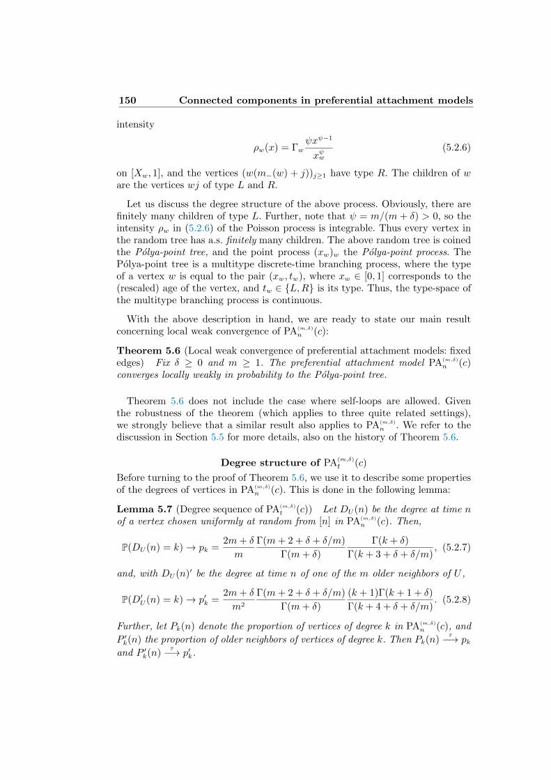
150 Connected components in preferential attachment models
intensity
ρw(x) = Γwψxψ−1
xψw(5.2.6)
on [Xw, 1], and the vertices (w(m−(w) + j))j≥1 have type R. The children of ware the vertices wj of type L and R.
Let us discuss the degree structure of the above process. Obviously, there arefinitely many children of type L. Further, note that ψ = m/(m + δ) > 0, so theintensity ρw in (5.2.6) of the Poisson process is integrable. Thus every vertex inthe random tree has a.s. finitely many children. The above random tree is coinedthe Polya-point tree, and the point process (xw)w the Polya-point process. ThePolya-point tree is a multitype discrete-time branching process, where the typeof a vertex w is equal to the pair (xw, tw), where xw ∈ [0, 1] corresponds to the(rescaled) age of the vertex, and tw ∈ L,R is its type. Thus, the type-space ofthe multitype branching process is continuous.
With the above description in hand, we are ready to state our main resultconcerning local weak convergence of PA(m,δ)
n (c):
Theorem 5.6 (Local weak convergence of preferential attachment models: fixededges) Fix δ ≥ 0 and m ≥ 1. The preferential attachment model PA(m,δ)
n (c)converges locally weakly in probability to the Polya-point tree.
Theorem 5.6 does not include the case where self-loops are allowed. Giventhe robustness of the theorem (which applies to three quite related settings),we strongly believe that a similar result also applies to PA(m,δ)
n . We refer to thediscussion in Section 5.5 for more details, also on the history of Theorem 5.6.
Degree structure of PA(m,δ)
t (c)
Before turning to the proof of Theorem 5.6, we use it to describe some propertiesof the degrees of vertices in PA(m,δ)
n (c). This is done in the following lemma:
Lemma 5.7 (Degree sequence of PA(m,δ)
t (c)) Let DU(n) be the degree at time nof a vertex chosen uniformly at random from [n] in PA(m,δ)
n (c). Then,
P(DU(n) = k)→ pk =2m+ δ
m
Γ(m+ 2 + δ + δ/m)
Γ(m+ δ)
Γ(k + δ)
Γ(k + 3 + δ + δ/m), (5.2.7)
and, with DU(n)′ be the degree at time n of one of the m older neighbors of U ,
P(D′U(n) = k)→ p′k =2m+ δ
m2
Γ(m+ 2 + δ + δ/m)
Γ(m+ δ)
(k + 1)Γ(k + 1 + δ)
Γ(k + 4 + δ + δ/m). (5.2.8)
Further, let Pk(n) denote the proportion of vertices of degree k in PA(m,δ)
n (c), and
P ′k(n) the proportion of older neighbors of vertices of degree k. Then Pk(n)P−→ pk
and P ′k(n)P−→ p′k.
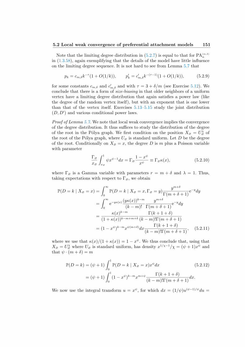
5.2 Local weak convergence of preferential attachment models 151
Note that the limiting degree distribution in (5.2.7) is equal to that for PA(m,δ)
n
in (1.3.58), again exemplifying that the details of the model have little influenceon the limiting degree sequence. It is not hard to see from Lemma 5.7 that
pk = cm,δk−τ (1 +O(1/k)), p′k = c′m,δk
−(τ−1)(1 +O(1/k)), (5.2.9)
for some constants cm,δ and c′m,δ and with τ = 3 + δ/m (see Exercise 5.12). Weconclude that there is a form of size-biasing in that older neighbors of a uniformvertex have a limiting degree distribution that again satisfies a power law (likethe degree of the random vertex itself), but with an exponent that is one lowerthan that of the vertex itself. Exercises 5.13–5.15 study the joint distribution(D,D′) and various conditional power laws.
Proof of Lemma 5.7. We note that local weak convergence implies the convergenceof the degree distribution. It thus suffices to study the distribution of the degreeof the root in the Polya graph. We first condition on the position X∅ = Uχ
∅ ofthe root of the Polya graph, where U∅ is standard uniform. Let D be the degreeof the root. Conditionally on X∅ = x, the degree D is m plus a Poisson variablewith parameter
Γ∅
x∅
∫ 1
x∅
ψxψ−1dx = Γ∅1− xψxψ
≡ Γ∅κ(x), (5.2.10)
where Γ∅ is a Gamma variable with parameters r = m + δ and λ = 1. Thus,taking expectations with respect to Γ∅, we obtain
P(D = k | X∅ = x) =
∫ ∞0
P(D = k | X∅ = x,Γ∅ = y)ym+δ
Γ(m+ δ + 1)e−ydy
=
∫ ∞0
e−yκ(x) (yκ(x))k−m
(k −m)!
ym+δ
Γ(m+ δ + 1)e−ydy
=κ(x)k−m
(1 + κ(x))k−m+m+δ
Γ(k + 1 + δ)
(k −m)!Γ(m+ δ + 1)
= (1− xψ)k−mxψ(m+δ)dxΓ(k + 1 + δ)
(k −m)!Γ(m+ δ + 1), (5.2.11)
where we use that κ(x)/(1 + κ(x)) = 1− xψ. We thus conclude that, using thatX∅ = Uχ
∅ where U∅ is standard uniform, has density x1/χ−1/χ = (ψ + 1)xψ andthat ψ · (m+ δ) = m
P(D = k) = (ψ + 1)
∫ 1
0
P(D = k | X∅ = x)xψdx (5.2.12)
= (ψ + 1)
∫ 1
0
(1− xψ)k−mxm+ψ Γ(k + 1 + δ)
(k −m)!Γ(m+ δ + 1)dx.
We now use the integral transform u = xψ, for which dx = (1/ψ)u(ψ−1)/ψdu =
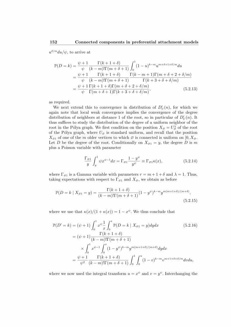
152 Connected components in preferential attachment models
uδ/mdu/ψ, to arrive at
P(D = k) =ψ + 1
ψ
Γ(k + 1 + δ)
(k −m)!Γ(m+ δ + 1)
∫ 1
0
(1− u)k−mum+δ+1+δ/mdu
=ψ + 1
ψ
Γ(k + 1 + δ)
(k −m)!Γ(m+ δ + 1)
Γ(k −m+ 1)Γ(m+ δ + 2 + δ/m)
Γ(k + 3 + δ + δ/m)
=ψ + 1
ψ
Γ(k + 1 + δ)Γ(m+ δ + 2 + δ/m)
Γ(m+ δ + 1)Γ(k + 3 + δ + δ/m), (5.2.13)
as required.We next extend this to convergence in distribution of D′U(n), for which we
again note that local weak convergence implies the convergence of the degreedistribution of neighbors at distance 1 of the root, so in particular of D′U(n). Itthus suffices to study the distribution of the degree of a uniform neighbor of theroot in the Polya graph. We first condition on the position X∅ = Uχ
∅ of the rootof the Polya graph, where U∅ is standard uniform, and recall that the positionX∅1 of one of the m older vertices to which ∅ is connected is uniform on [0, X∅.Let D be the degree of the root. Conditionally on X∅1 = y, the degree D is mplus a Poisson variable with parameter
Γ∅1
y
∫ 1
y
ψxψ−1dx = Γ∅1
1− yψyψ
≡ Γ∅1κ(x), (5.2.14)
where Γ∅1 is a Gamma variable with parameters r = m+ 1 + δ and λ = 1. Thus,taking expectations with respect to Γ∅1 and X∅, we obtain as before
P(D = k | X∅1 = y) =Γ(k + 1 + δ)
(k −m)!Γ(m+ δ + 1)(1− yψ)k−mym(m+1+δ)/(m+δ),
(5.2.15)
where we use that κ(x)/(1 + κ(x)) = 1− xψ. We thus conclude that
P(D′ = k) = (ψ + 1)
∫ 1
0
xψ1
x
∫ x
0
P(D = k | X∅1 = y)dydx (5.2.16)
= (ψ + 1)Γ(k + 1 + δ)
(k −m)!Γ(m+ δ + 1)
×∫ 1
0
xψ−1
∫ x
0
(1− yψ)k−mym(m+1+δ)/(m+δ)dydx
=ψ + 1
ψ2
Γ(k + 1 + δ)
(k −m)!Γ(m+ δ + 1)
∫ 1
0
∫ u
0
(1− v)k−mvm+1+δ+δ/mdvdu,
where we now used the integral transform u = xψ and v = yψ. Interchanging the
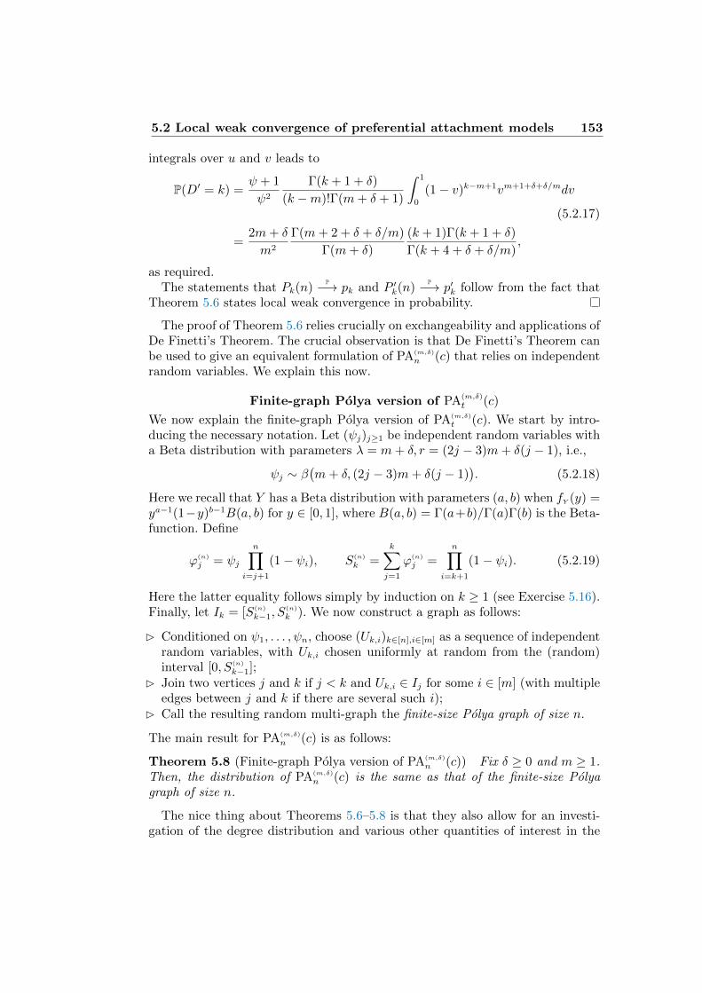
5.2 Local weak convergence of preferential attachment models 153
integrals over u and v leads to
P(D′ = k) =ψ + 1
ψ2
Γ(k + 1 + δ)
(k −m)!Γ(m+ δ + 1)
∫ 1
0
(1− v)k−m+1vm+1+δ+δ/mdv
(5.2.17)
=2m+ δ
m2
Γ(m+ 2 + δ + δ/m)
Γ(m+ δ)
(k + 1)Γ(k + 1 + δ)
Γ(k + 4 + δ + δ/m),
as required.The statements that Pk(n)
P−→ pk and P ′k(n)P−→ p′k follow from the fact that
Theorem 5.6 states local weak convergence in probability.
The proof of Theorem 5.6 relies crucially on exchangeability and applications ofDe Finetti’s Theorem. The crucial observation is that De Finetti’s Theorem canbe used to give an equivalent formulation of PA(m,δ)
n (c) that relies on independentrandom variables. We explain this now.
Finite-graph Polya version of PA(m,δ)
t (c)
We now explain the finite-graph Polya version of PA(m,δ)
t (c). We start by intro-ducing the necessary notation. Let (ψj)j≥1 be independent random variables witha Beta distribution with parameters λ = m+ δ, r = (2j − 3)m+ δ(j − 1), i.e.,
ψj ∼ β(m+ δ, (2j − 3)m+ δ(j − 1)
). (5.2.18)
Here we recall that Y has a Beta distribution with parameters (a, b) when fY (y) =ya−1(1−y)b−1B(a, b) for y ∈ [0, 1], where B(a, b) = Γ(a+b)/Γ(a)Γ(b) is the Beta-function. Define
ϕ(n)
j = ψj
n∏i=j+1
(1− ψi), S(n)
k =k∑j=1
ϕ(n)
j =n∏
i=k+1
(1− ψi). (5.2.19)
Here the latter equality follows simply by induction on k ≥ 1 (see Exercise 5.16).Finally, let Ik = [S(n)
k−1, S(n)
k ). We now construct a graph as follows:
B Conditioned on ψ1, . . . , ψn, choose (Uk,i)k∈[n],i∈[m] as a sequence of independentrandom variables, with Uk,i chosen uniformly at random from the (random)interval [0, S(n)
k−1];B Join two vertices j and k if j < k and Uk,i ∈ Ij for some i ∈ [m] (with multiple
edges between j and k if there are several such i);B Call the resulting random multi-graph the finite-size Polya graph of size n.
The main result for PA(m,δ)
n (c) is as follows:
Theorem 5.8 (Finite-graph Polya version of PA(m,δ)
n (c)) Fix δ ≥ 0 and m ≥ 1.Then, the distribution of PA(m,δ)
n (c) is the same as that of the finite-size Polyagraph of size n.
The nice thing about Theorems 5.6–5.8 is that they also allow for an investi-gation of the degree distribution and various other quantities of interest in the
154 Connected components in preferential attachment models
preferential attachment model. Exercises 5.17–5.19 use Theorem 5.8 to deriveproperties of the number of multiple edges in PA(m,δ)
n (c) for m = 2.
In terms of the above Polya-point tree, the proof will show that the Gammavariables Y that define the “strength” Γw are inherited from the Beta randomvariables (ψk)k∈[n], while the “position” variables Xw are inherited from the ran-dom variables (S(n)
k )k∈[n] (see Lemmas 5.10 and 5.11 below).
Before moving to the proof of Theorem 5.8, we use it to identify the almost surelimit of degrees of fixed vertices. For this, we recall that χ = (m + δ)/(2m + δ)and we define the following random variable:
Fk = limn→∞
(nk
)χ ∏j=k+1
(1− ψj). (5.2.20)
In Exercise 5.20 you are asked to prove that the almost sure limit in (5.2.20)exists. Then, the limiting distribution of fixed vertices is as follows:
Lemma 5.9 (Degree structure of PA(m,δ)
t (c): fixed vertices) Consider PA(m,δ)
t (c)with m ≥ 1 and δ > −m. Then,
n−(1−χ)Dk(n)d−→ (2m+ δ)kχψkFk. (5.2.21)
We prove Lemma 5.9 below.
Let us give some insight into the proof of Theorem 5.8, after which we givethe full proof. There is a close connection between the preferential attachmentmodel and the Polya urn model in the following sense: every new connection thata vertex gains can be represented by a new ball added in the urn correspondingto that vertex. The initial number of balls in each urn is equal to m. Indeed,recall the discussion above about D1(τk)/(D1(τk) + D2(τk)) converging almostsurely to a Beta-distribution. What is particularly nice about this description isthat the random variable D1(τk) has exactly the same distribution as m plus aBin(k, β) distribution, i.e., conditionally on β, D1(τk) is a sum of i.i.d. randomvariables, this equality in distribution being valid for all k. This observation canbe extended to give a probabilistic description of (D1(τ ′k), D2(τ ′k), . . . , Dn(τ ′k))k≥1
that is valid for all k, n ≥ 1 fixed. Here τ ′k =∫t : D1(t) + . . . , Dn(t) = k is
the first time where the total degree of the vertices in [n] is equal to k. Notethat τ ′2mn = n. Further, the random variables (D1(τ ′k), D2(τ ′k), . . . , Dn(τ ′k))
2mnk=1
determine the law of (PA(m,δ)
t (b))t∈[n] uniquely. This explains why PA(m,δ)
n (b) canbe described in terms of independent random variables. The precise description interms of ψj in (5.2.18) follows from tracing back the graph construction obtainedin this way. We next use this to complete the proof of Theorem 5.8:
Let us now make this intuition more precise. Let us consider first a two-urnmodel, with the number of balls in one urn representing the degree of a particularvertex k, and the number of balls in the other representing the sum of the degreesof the vertices 1, . . . , k−1. We will start this process at the point when n = k and
5.2 Local weak convergence of preferential attachment models 155
k has connected to precisely m vertices in [k−1]. Note that at this point, the urnrepresenting the degree of k has m balls, while the other one has (2k−3)m balls.Consider a time in the evolution of the preferential attachment model when wehave n−1 ≥ k old vertices, and i−1 edges between the new vertex n and [k−1].Assume that at this point the degree of k is dk, and the sum of the degrees ofvertices in [k − 1] is d<k. At this point, the probability that the ith edge from nto [n− 1] is attached to k is
dk + δ
2m(n− 1) + (1 + δ)(i− 1), (5.2.22)
while the probability that it is connected to a vertex in [k − 1] is equal to
d<k + δ(k − 1)
2m(n− 1) + (1 + δ)(i− 1). (5.2.23)
Thus, conditioned on connecting to [k], the probability that the ith edge from nto [n−1] is attached to k is (dk+δ)/Z, while the probability that the ith edge fromn to [n−1] is attached to [k−1] is (d<k+δ(k−1))/Z, where Z = kδ+d<k+1 is thenormalization constant. Taking into account that the two urns start with m and(2k− 3)m balls, respectively, we see that the evolution of the two bins is a Polyaurn with strengths ψk and 1−ψk, where ψk has the β(m+δ, (2k−3)m+δ(k−1))distribution. We next use this to complete the proof of Theorem 5.8:
Completion of the proof of Theorem 5.8. Using the two-urn process as an inductiveinput, we can now construct the Polya graph defined in Theorem 5.8 in a similarway as it was done for Polya urns with multiple colors in (5.1.27).
Let Xt ∈ 1, 2, . . . , dt/me be the vertex receiving the tth edge in the sequentialmodel (the other endpoint of this edge being the vertex dt/me + 1). For t ≤ m,Xt is deterministic (and equal to 1), but starting at t = m+1, we have a two-urnmodel, starting with m balls in each urn. As shown above, the two urns can bedescribed as Polya urns with strengths 1−ψ2 and ψ2. Once t > 2m, Xt can takethree values, but conditioned on Xt ≤ 2, the process continues to be a two-urnmodel with strengths 1 − ψ2 and ψ2. To determine the probability of the eventthat Xt ≤ 2, we now use the above two-urn model with k = 3, which gives thatthe probability of the event Xt ≤ 2 is 1−ψ3, at least as long as t ≤ 3m. Combiningthese two-urn models, we get a three-urn model with strengths (1− ψ2)(1− ψ3),ψ2(1 − ψ3) and ψ3. Again, this model remains valid for t > 3m, as long as wecondition on Xt ≤ 3. Continuing inductively, we see that the sequence Xt evolvesin stages:
B For t ∈ [m], the variable Xt is deterministic: Xt = 1.
B For t = m+1, . . . , 2m, the distribution of Xt ∈ 1, 2 is described by a two-urnmodel with strengths 1− ψ2 and ψ2, where ψ2 ∼ B2.
B In general, for t = m(k−1)+1, . . . , km, the distribution of Xt ∈ [k] is described
156 Connected components in preferential attachment models
by a k-urn model with strengths
ϕ(k)
j = ψj
k∏i=j+1
(1− ψi), j = 1, . . . , k. (5.2.24)
Here ψk is chosen at the beginning of the kth stage, independently of thepreviously chosen strengths ψ1, . . . , ψk−1 (for convenience, we set ψ1 = 1).
Note that the random variables ϕ(k)
j can be expressed in terms of the randomvariables introduced in Theorem 5.8 as follows. By (5.2.19), Sk =
∏nj=k+1(1−ψj).
This implies that φ(n)
j = ψj/S(n)
j , which relates the strengths φ(n)
j to the randomvariables defined right before Theorem 5.8, and shows that the process derivedabove is indeed the process given in the theorem.
Asymptotics of (ψk)k∈[n] and (S(n)
k )k∈[n]
We next continue to analyse the random variables in Theorem 5.8 to prepare usfor proving local weak convergence in Theorem 5.6. We start by analyzing ψk fork large:
Lemma 5.10 (Gamma asymptotics of Beta variables) As k →∞, kψkd−→ Y ,
where Y has a Gamma distribution with r = m+ δ and λ = 2m+ δ.More precisely, take fk(x) such that P(ψk ≤ fk(x)) = P(χk ≤ x), where χk has a
Gamma distribution with r = m + δ and λ = 1 (so that Yd= X/(2m + δ). For
every ε > 0, there exists K = Kε ≥ 1 sufficiently large. Then, for all k ≥ K andx ≤ (log k)2,
1− εk(2m+ δ)
x ≤ fk(x) ≤ 1 + ε
k(2m+ δ)x. (5.2.25)
Further, χk ≤ (log k)2 for all k ≥ K and with probability at least 1− ε.Proof Fix x ≥ 0. We compute that
P(kψk ≤ x) =Γ(m+ δ + (2k − 3)m+ δ(k − 1)
)Γ(m+ δ
)Γ((2k − 3)m+ δ(k − 1)
) (5.2.26)
×∫ x/k
0
um+δ−1(1− u)(2k−3)m+δ(k−1)−1du
= (1 + o(1))km+δ
Γ(m+ δ
)k−(m+δ)
∫ x
0
um+δ−1(1− u/k)(2k−3)m+δ(k−1)−1du.
For every u > 0, (1 − u/k)(2k−3)m+δ(k−1)−1 → e−u(2m+δ), so that dominated con-vergence implies that
P(kψk ≤ x)→∫ x
0
um+δ−1
Γ(m+ δ
)e−u(2m+δ)du, (5.2.27)
as required. We refrain from proving the other statements, that are more technicalversions of the above argument.
5.2 Local weak convergence of preferential attachment models 157
By Lemma 5.10, we see that indeed the Beta random variables (ψk)k∈[n] giverise to the Gamma random variables in (5.2.5). This explains the relevance of theGamma random variables in the Polya-point graph.
We continue by analyzing the asymptotics for the random variables (S(n)
k )k∈[n]:
Lemma 5.11 (Asymptotics of S(n)
k ) Recall that χ = (m + δ)/(2m + δ). Forevery ε > 0, there exists η > 0 and K < ∞ such that for all n ≥ K and withprobability at least 1− ε,
maxk∈[n]
∣∣∣S(n)
k −(kn
)χ∣∣∣ ≤ η, (5.2.28)
and
maxk∈[n]\[K]
∣∣∣S(n)
k −(kn
)χ∣∣∣ ≤ ε(kn
)χ. (5.2.29)
Proof We give the intuition behind Lemma 5.11. We recall from (5.2.19) thatS(n)
k =∏ni=k+1(1 − ψi), where (ψk)k∈[n] are independent random variables. We
start by investigating S′n =∏ni=1(1− ψi), so that S(n)
k = S′k/S′n. We write
logS′n =n∑i=1
log(1− ψi). (5.2.30)
Thus, using Lemma 5.10 and with (χi)i≥1 an i.i.d. sequence of Gamma random
variables with parameters r = m+ δ and using that kψkd−→ χk/(2m+ 1),
logS′n ≈ −n∑i=1
ψi ≈ −1
2m+ δ
n∑i=1
χi/i (5.2.31)
≈ − 1
2m+ δ
n∑i=1
E[χi]
i=
m+ δ
2m+ δlog n = χ log n.
Thus, Sk = S′k/S′n ≈
(kn
)χ, as required. The proof can be completed using mar-
tingale techniques and is omitted here.
We use the above analysis to complete the proof of Lemma 5.9:Proof of Lemma 5.9. We use a conditional second moment method on Dk(n),conditionally on (ψk)k∈[n]. Denote
F (n)
k =(nk
)χ ∏j=k+1
(1− ψj). (5.2.32)
Then,
E[Dk(n) | (ψk)k∈[n]
]= m
n∑`=k+1
ϕ(`)
k , (5.2.33)
and
Var(Dk(n) | (ψk)k∈[n]
)≤ m
n∑`=k+1
ϕ(`)
k . (5.2.34)
158 Connected components in preferential attachment models
It thus suffices to show that n1−χm∑n
`=k+1 ϕ(`)
k
a.s.−→ m1−χk
χψkFk. For this, we note
that since ϕ(`)
k = ψk∏`j=k+1(1− ψj), we arrive at
mn∑
`=k+1
ϕ(`)
k = mψk
n∑`=k+1
(k`
)χF (`)
k = mkχψk
n∑`=k+1
`−χF (`)
k . (5.2.35)
Since χ ∈ (0, 1) and F (`)
k
a.s.−→ Fk as `→∞, we obtain that
n1−χn∑
`=k+1
`−χF (`)
k
a.s.−→ Fk/(1− χ). (5.2.36)
This completes the proof.
Regularity properties of the Polya-point tree and overview
We next discuss some properties of the Polya-point tree, showing that the tree(T ,∅) is well defined and, within the r-neighborhood of the root, all randomvariables used in its description are uniformly bounded:
Lemma 5.12 (Regularity Polya-point tree) Fix r ≥ 1 and ε > 0. Then thereexist constants η > 0 and K < ∞ such that, with probability at least 1 − ε,Br(∅) ≤ K, Xw ≥ η for all w ∈ Br(∅), and further Γw ≤ K, ρw(·) ≤ K for allw ∈ Br(∅), while finally, minw,w′∈Br(∅) |Xw −Xw′ | ≥ η.
Proof The proof of this lemma is standard, and can, for example, be obtained byinduction on r. The last bound follows from the continuous nature of the randomvariables Xw, which implies that Xw 6= Xw′ for all distinct pairs w,w′, whichimplies that any finite number will be with probability at least 1 − ε separatedby at least δ.
Let us describe how the proof of Theorem 5.6 is organised. Similarly to theproofs of Theorems 3.11 and 4.1, we will investigate the number of r-neighborhoodsof a specific shape (H, y), using a second moment method. Let
Nn,r(H, y) =∑v∈[n]
1B(n)r (v)'(H,y), (5.2.37)
where B(n)
r (vn) is the r-neighborhood of v in PA(m,δ)
n (c). With Br(∅) the r-neighborhood of ∅ in the Polya-point graph (T ,∅), we will show that
Nn,r(H, y)
nP−→ P(Br(∅) ' (H, y)). (5.2.38)
Proving convergence of is much harder than for Theorems 3.11 and 4.1, as thetype of a vertex is crucial in determining the number and types of its children,and the type space is continuous. Thus, we need to take the types of vertices intoaccount, so as to make an inductive analysis in r possible in which we couple
5.2 Local weak convergence of preferential attachment models 159
both the neighborhoods as well as their types. We start with the first moment,for which we note that
E[Nn,r(H, y)/n] = P(B(n)
r (on) ' (H, y)). (5.2.39)
We do this using a coupling approach, by showing that we can couple B(n)
r (on),together with the types of the vertices involved, with Br(∅) such that the differ-ences are quite small. After that, we use this as the starting point of a recursiveanalysis in r, which is the second step in the analysis. We complete the proof bystudying the second moment of the number of r-neighborhoods of a specific shape(H, y). Let us now give the details of the convergence of the expected number ofone-neighborhoods of a uniform point.
Exploration of PA(m,δ)n (c): one-neighborhood
In this step, we discuss how we can couple the one-neighborhood of a uniformlychosen vertex to that in (T ,∅), so as to prove Theorem 5.6 for r = 1. This willserve as the starting point for an inductive analysis, and will give insight into themethod of proof. The main result states that we can couple B(n)
1 (on) in PA(m,δ)
n (c)and B1(∅) in (T ,∅) in such a way that all the variables involved are close:
Lemma 5.13 (Coupling one-neighborhood of uniform vertex in PA(m,δ)
n (c) andPolya-point tree) Fix ε > 0. Let on be chosen uniformly at random from [n].Let
von1, . . . , von(m+qon )
be the neighbors of on, ordered such that the edge on, voni was created beforethe edge on, von(i+1). Then, there exist η > 0 and N = N(ε) < ∞ such that,with probability at least 1−ε, B(n)
1 (on), where on = v∅, together with the variables(S(n)
v∅i)i≥1, and B1(∅), together with its positions (X∅i)i≥1, can be coupled such
that
(i) B(n)
1 (on) ' B1(∅) and |B1(∅)| ≤ K;(ii) |X∅k − S(n)
v∅k| ≤ η for all k for which ok ∈ B1(∅);
(iii) v∅1, . . . , v∅(m+q∅) are all distinct and v∅k ≥ ηn for all v∅k ∈ B(n)
1 (on);(iv) Γ∅k ≤ K for all k such that ∅k ∈ B1(∅).
Consequently, P(B(n)
1 (on) ' (H, y))→ P(B1(∅) ' (H, y)).
We start with Lemma 5.13, as this proof will share many ingredients with theproof for the general r ≥ 1, while its notation is relatively simple. Below, we willextend it to general r ≥ 1.
Proof We start by proving (i)–(ii). Choose U∅ uniform in [0, 1], let X∅ = Uχ∅,
and let X∅1, . . . , X∅(m+q∅) be the positions of the children of ∅ in (T ,∅). Defineon = dnU∅e, and define v∅i for i ∈ [m] by
S(n)
v∅i−1 ≤X∅i
X∅S(n)
v∅≤ S(n)
v∅i. (5.2.40)
By Theorem 5.8 and the observation that Uv∅i = X∅i/X∅ is a collection of i.i.d.
160 Connected components in preferential attachment models
uniform random variables on [0, 1], it follows that whp v∅i ∈ n[X∅i− δ,X∅i + δ],as required. In more detail, given ε > 0, choose δ > 0 and K > 0 such that theregularity properties in Lemma 5.12 hold for r = 1. By Lemma 5.11, for n largeenough,
|S(n)
v∅−X∅| ≤ η, and |S(n)
v∅i−X∅i| ≤ η ∀i ∈ [m], (5.2.41)
with probability at least 1− 2ε.We continue by investigating the limiting distribution of the remaining neigh-
bors v∅1, . . . , v∅(m+q(n)∅ )
. Along the way, we will prove that q(n)
∅ = q∅ whp. Note
that by Theorem 5.8 and conditionally on (ψk)k∈[n], each vertex v > v∅ has mindependent chances of being connected to v∅. Let Xv,i be the vertex to whichthe ith edge of v is attached. Then, the events Xv,i = v∅ for i ∈ [m] are,conditionally on (ψk)k∈[n], independent events with success probability
Pv→v∅ =ϕ(v−1)
v∅
S(v−1)
v−1
=S(n)
v∅
S(n)
v−1
ψv∅ , (5.2.42)
where the latter equality follows by (5.2.19).Denote
Nv∅(y) =ny∑
v=v∅+1
m∑i=1
1Xv,i=v∅. (5.2.43)
Our aim is to show that, conditionally on U∅,(Nv∅(y)
)y∈v∅/n
converges to a
Poisson process on [U∅, 1]. For this, we first analyze the asymptotics of the successprobabilities Pv→v∅ . By Lemma 5.12, v∅ ≥ nη with probability at least 1 − ε.Recall that ψk = fk(χk), where χk has a Gamma distribution with parametersλ = 1 and r = m+ δ. Thus, we may apply Lemmas 5.10 and 5.11, which yield
(1− η)Pv→v∅ ≤ Pv→v∅ ≤ (1 + η)Pv→v∅ , (5.2.44)
where
Pv→v∅ =χv∅
(2m+ δ)n
n
v∅
(v∅v
)χ. (5.2.45)
Letting Nv∅(y) =∑ny
v=v∅+1
∑mi=1 1Xv,i=v∅, where (Xv,i)v,i are conditionally in-
dependent given (ψk)k≥1 (or, equivalently, given (χk)k≥1, we can couple Nv∅(y)to a Poisson random variable with parameter
χv∅2(1 + δ/m)U∅
∫ y
0
(U∅
s
)χds (5.2.46)
on [U∅, 1] such that the random variables are distinct with vanishing probability.
Using that χv∅ = Γv∅/(2m + δ) proves that Nv∅(xχ) converges to a Poissonrandom variable with parameter
χv∅
Uψ∅
∫ x
0
ψsψ−1ds =Γ∅
Uψ∅
∫ x
0
ψsψ−1ds, (5.2.47)
5.2 Local weak convergence of preferential attachment models 161
on [U∅, 1]. It is not hard to extend this result to the statement that(Nv∅(xχ)
)x∈[U∅,1]
converges in distribution to an inhomogeneous Poisson process with intensityΓ∅ψx
ψ−1/Uψ∅ = ρ∅(x), as required. In particular, this shows that q(n)
∅ = q∅ withprobability at least 1− ε.
We conclude the proof of (i)–(ii) by investigating the differences between X∅iand S(n)
v∅iusing Lemma 5.11 to bound the difference between S(n)
v∅iand (v∅i/n)χ,
which yields that for n large enough and with probability at least 1−3ε, q(n)
∅ = q∅and the bounds q0 +m ≤ N , χv∅ = Γv∅ ≤ K and
|X∅k − S(n)
v∅k| ≤ η for all i ∈ [m+ q0] \ [q] (5.2.48)
hold, as required. This completes the proof of parts (i)–(ii).
For (iii), we note that by (5.2.41) and (5.2.48), and another application ofLemma 5.11, there exists an η > 0 such that v∅k ≥ ηn with probability at least1− 4ε and |v∅k − v∅l ≥ ηn for all k, l ≤ m+ q∅. As a result, (v∅k)k∈[m+q∅] are alldistinct. This completes the proof of (iii).
For (iv), we note that the claimed bounds are obviously true when the sequence(χv∅k)k∈[m+q0] would be independent. However, this is not true, since the fact thatv∅k is a neighbor of v∅ ‘tilts’ the distribution of the above random variables. Wewill provide a coupling between (χv∅k)k∈[m+q0] and a collection of independentrandom variables. Let us now provide the details.
We assume that Γ∅ = χv∅ ≤ K, that q(n)
∅ = q∅ and that (v∅k)k∈[m+q0] areall distinct with mink∈[m+q0] v∅k ≥ ηn. Let E denote the event that v∅ is theuniform random vertex and that the neighbors of v∅ are (v∅k)k∈[m+q0]. Let χE,γ∅
denote the conditional distribution of (χk)k∈[n]\v∅ conditioned on Γ∅ = γ∅ andE . Further, let (χk)k∈[n] denote an independent collection of random variableswith distribution
χv∅k ∼ Y ?v∅k∀k ∈ [m], χk ∼ Yk ∀k ∈ [n] \ [m]. (5.2.49)
Let ρ(· | E , χv∅ = γ∅) denote the density of the (multi-dimensional) randomvariable (χk)k∈[n], and let P be the joint distribution of PA(m,δ)
n (c) and the randomvariables (χk)k∈[n]. By Bayes’ Theorem,
ρ(· | E , χv∅ = γ∅) =P(E | ·, χv∅ = γ∅)
P(E | χv∅ = γ∅)ρ∅(·), (5.2.50)
where ρ∅(·) is the original density of the random variables (χk)k∈[n]\v∅. Wedenote the corresponding probability distributions and expectations as P∅ andE∅, respectively. We conclude that we have to compare P(E | ·, χv∅) to P(E |·, χv∅). Since we are interested in the distribution of (χk)k∈[n], this amounts tocomparing P(E | (χk)k∈[n]) to P(E | χv∅). For this, we need to compute P(E |(χk)k∈[n]) (and note that P(E | χv∅) = E∅[P(E | (χk)k∈[n])]). This is our next step.
162 Connected components in preferential attachment models
By Theorem 5.8, we can explicitly compute
P(E | (χk)k∈[n]) = m!m∏i=1
Pv∅→v∅i
q∅∏j=1
mPv∅j→v∅(1− Pv∅j→v∅
)m−1(5.2.51)
×∏
v>v∅ : v 6∈v∅(m+1),...v∅(m+q)
(1− Pv→v∅
)m,
by the conditional independence given (ψk)k∈[n], which is equivalent to conditionalindependence given (χk)k∈[n]. We rewrite
P(E | (χk)k∈[n]) = m!m∏i=1
Pv∅→v∅i
q∅∏j=1
mPv∅j→v∅1− Pv∅j→v∅
∏v>v∅
(1− Pv→v∅
)m, (5.2.52)
where Pv→v′ is given, and using (5.2.19), by
Pv→v′ =ϕ(v−1)
v′
S(v−1)
v−1
=S(n)
v′
S(n)
v−1
ψv′ . (5.2.53)
We now perform asymptotics of this formula. We use Lemma 5.11 to show that wecan for every η > 0, there exists n0 sufficiently large, such that, with probabilityat least 1− ε,
(1− η)P(E | (χk)k∈[n]) (5.2.54)
≤ m!m∏i=1
ψv∅( v∅v∅i
)χ q∅∏j=1
mψv∅(v∅jv∅
)χe−mψv∅
∑v>v∅
(v∅v
)χ≤ (1 + η)P(E | (χk)k∈[n]).
To bound P(E | χv∅) = E∅[P(E | (χk)k∈[n])], we also need a good bound on“bad” event, for which we use the deterministic upper bound
P(E | (χk)k∈[n]) ≤ m!m∏i=1
Pv∅→v∅i
q∅∏j=1
mPv∅j→v∅ ≤ m!(mψv∅)qm∏i=1
ψv∅i (5.2.55)
≤ C ′m!m∏i=1
ψv∅( v∅v∅i
)χ q∅∏j=1
mψv∅(v∅jv∅
)χe−mψv∅
∑v>v∅
(v∅v
)χ,
where C ′ = η−(m+N) supn≥1 emnfδn(K) <∞.We conclude that with probability at least 1− ε/2 with respect to P∅,√
1− ηm∏i=1
ψv∅iE∅[ψv∅i ]
≤ P(E | (χk)k∈[n]
P(E | χ∅)≤√
1 + ηm∏i=1
ψv∅iE∅[ψv∅i ]
. (5.2.56)
With the help of Lemma 5.10, with probability at least 1− ε,
(1− η)m∏i=1
χv∅iE∅[χv∅i ]
≤ P(E | (χk)k∈[n]
P(E | χ∅)≤ (1 + η)
m∏i=1
χv∅iE∅[χv∅i ]
. (5.2.57)
The factors χv∅i/E∅[χv∅i ] correspond to the size-biasing of χv∅k for k ∈ [m] as
5.2 Local weak convergence of preferential attachment models 163
indicated in (5.2.49). Since this is of product structure, asymptotic independenceof (χv∅k)k∈[n]\v∅ remains.
We conclude that with probability at least 1− ε with respect to P∅,
(1− η)ρ(·) ≤ ρ(· | E , χv∅ = γ∅) ≤ (1 + η)ρ(·), (5.2.58)
where ρ is the density of (χv∅k)k∈[n]\v∅, whose law we denote by P.To complete the proof, we use [Volume 1, (2.2.8)] to compute that
dTV(ρ(· | E , χv∅), ρ(·)) = 1−∫ρ(~χ | E , χv∅) ∧ ρ(~χ)d~χ. (5.2.59)
Let Ω∅ denote the where (5.2.58) holds, so that P∅(Ω | E , χv∅) ≥ 1 − η. Then,we bound
dTV(ρ(· | E , χv∅), ρ(·)) ≤ 1−∫
Ω∅
ρ(~χ | E , χv∅) ∧ ρ(~χ)d~χ. (5.2.60)
On Ω∅, (5.2.58) holds, so that ρ(~χ) ≥ ρ(~χ | E , χv∅)/(1 + η). Thus,
dTV(ρ(· | E , χv∅), ρ(·)) ≤ 1− 1
1 + η
∫Ω∅
ρ(~χ | E , χv∅) (5.2.61)
= 1− 1
1 + ηP∅(Ω | E , χv∅) ≤ 1− 1− η
1 + η=
2η
1 + η≤ 2η.
We conclude that
dTV(ρ(· | A,χv∅), ρ(·)) ≤ 2η. (5.2.62)
Choosing η so small that 2η ≤ ε, this shows that we can couple (χE,γ∅k )k∈[n]\v∅
and (χk)k∈[n]\v∅ such that they are equal with probability at least 1 − ε, asrequired. It is straightforward to show that (iv) holds for the random variables(χk)k∈[n]\v∅ as these are independent Gamma distributions. This completes theproof of (iv).
The fact that P(B(n)
1 (on) ' (H, y)) → P(B1(∅) ' (H, y)) follows directly fromthe fact that we have coupled such that q(n)
∅ = q∅, and this occurs with probabilityat least 1− ε. Since ε > 0 is arbitrary, the statement follows.
Exploration of PA(m,δ)n (c): general neighborhood
In this step, we discuss how we can explore the one-neighborhood of a uniformlychosen vertex, so as to prove Theorem 5.6.
Proposition 5.14 (Coupling general neighborhood of uniform vertex in PA(m,δ)
n (c)and Polya-point tree) Fix ε > 0 and r ≥ 1. Let on be chosen uniformly at ran-dom from [n]. Let vw be the vertices that are within distance r from on, orderedsuch that the edge vw, vwi was created before the edge vw, vw(i+1). Then, thereexist η > 0 and N = N(ε) <∞ such that, with probability at least 1−ε, B(n)
r (on),where on = v∅, together with the variables (S(n)
vw)|w|≤r, and Br(∅), together with
its positions (Xw)i≥1, can be coupled such that
(1) B(n)
r (on) ' Br(∅) and |Br(∅)| ≤ K;
164 Connected components in preferential attachment models
(2) |Xw − S(n)
vw| ≤ η for all k for which w ∈ Br(∅);
(3) (vw)w∈Br(∅) are all distinct and vw ≥ ηn for all vw ∈ B(n)
r (on);(4) Γw ≤ K for all w ∈ Br(∅).
Consequently, P(B(n)
r (on) ' (H, y))→ P(Br(∅) ' (H, y)).
Proposition 5.14 is the natural extension to r ≥ 1 of Lemma 5.13, and we willsee that its proof runs accordingly.
Proof For r = 1, this follows from Lemma 5.13. This initiates the inductionargument.
Assume by induction that the statement holds for r − 1, and fix Br−1(∅),(Xw)w∈Br−1(∅) (Γw)w∈Br−1(∅), (χw)w∈Br−1(∅) and (vw)w∈Br(∅) such that Proposi-tion 5.14 holds for them (a statement that holds with probability at least 1 − εaccording to the induction hypothesis). We now wish to extend these statementsto r.
For this, fix a vertex w ∈ ∂Br−1(∅) = Br−1(∅) \ Br−2(∅). We explore theneighborhood of vw in much the same way as exploring the neighborhood of v∅in the proof of Lemma 5.13, but we have much more information already thatwe need to keep in check. To this end, we note that for all w′ ∈ Br−1(∅), theneighborhood of vw′ is already determined by our conditioning on (vw)w∈Br−1(∅).This implies in particular that none of the edges sent out of vw′ can be attachedto a vertex v ∈ B(n)
r−1(on), except when w′ is of type R and vw′ happend to bethe parent of vw, in which case the edge between vw′ and vw is already present.To determine the children of type L of vw, we therefore have to condition onnot hitting the set B(n)
r−1(on). Apart from this, the process of determining thechildren of vw is exactly the same as that for v∅ in the proof of Lemma 5.13.Since |B(n)
r−1(on)| ≤ N , vw′ ≥ ηn and χvw′ ≤ K for all w′ ∈ B(n)
r−1(on), it followsthat ∑
vw′∈B(n)r−1(on)
ϕ(vw)
vw′≤ C
n(5.2.63)
for some C > 0. This implies that conditioning on vw′ 6∈ B(n)
r−1(on) has only anegligible effect on the distribution of the children of vw. We thus proceed asin the proof of Lemma 5.13 to obtain a coupling between a sequence of i.i.d.values (Xwi)i∈[m] of type L and the children (vwi)i∈[m]. As before, we have that|S(n)
vwi−Xwi| ≤ η, for n large enough, with probability at least 1− ε.
We can continue with this process for all vw ∈ ∂B(n)
r−1(on) = B(n)
r−1(on)\B(n)
r−2(on),thus producing the set Lr consisting of all the type L children of vertex vw ∈B(n)
r (on) \ B(n)
r−1(on). It is not hard to see that with probability tending to 1 asn → ∞, the set Lr has no intersection with B(n)
r−1(on), so we will assume this inthe remainder of the proof.
Next, we continue with the children of type R of vertices in ∂Br(∅). As-sume that we have already determined the children of type R of the vertices
5.2 Local weak convergence of preferential attachment models 165
in Ur−1 ⊆ B(n)
r−1(on) \ B(n)
r−2(on). Denote the set of children obtained so far byR(Ur−1). We decompose this set as R(Ur−1r) =
⋃mi=1R
(i)(Ur), where R(i)(Ur) =v ∈ Rr : Xv,i ∈ Ur−1. Now consider a vertex vw ∈ ∂B(n)
r−1(on) \Ur−1. Condition-ing on the graph obtained so far is again not difficult, and now amounts to twoconditions:
(1) Xv,i 6= vw if v ∈ B(n)
r−1(on)∪Ur−1, since all the edges coming out of this set havealready been determined;
(2) For v 6∈ B(n)
r−1(on) ∪ Ur−1, the probability that vw receives the ith edge fromk is different from the probability given in (5.2.53), since the random variableXv,i has been probed or checked before. Indeed, we know that Xv,i 6∈ B(n)
r−2(on),since otherwise v would have sent out an edge to a vertex in B(n)
r−2(on), whichwould mean that v would have been a child of type R in B(n)
r−1(on), which givesa contradiction. We also know that Xv,i 6∈ Ur−1, since otherwise v ∈ R(i)(Ur).
Instead of (5.2.53), (2) means that we have to use the modified probability
Pv→v′ =ϕ(v−1)
v′
S(v−1)
v−1
, (5.2.64)
where
S(v−1)
v−1 =∑
u>v−1: u 6∈B(n)r−1(on)∪Ur
ϕ(v−1)
u . (5.2.65)
Since, by the induction hypothesis, S(v−1)
v−1 ≤ S(v−1)
v−1 ≤ S(v−1)
v−1 +C/n, for some C > 0,
we can still infer Lemma 5.11 to approximate Pv→v′ by Pv→v′ , which equals
Pv→v′ =1
n
χv′
2m+ δ
n
v′
(v′v
)χ. (5.2.66)
From here onwards, the proof is a straightforward adaptation of the proof ofLemma 5.13, and we omit further details.
The fact that P(B(n)
r (on) ' (H, y))→ P(Br(∅) ' (H, y)) follows since we havecoupled the neighborhoods such that with probability at least 1− ε, q(n)
w = qw forall |w| ≤ r. Since ε > 0 is arbitrary, the statement follows.
Exploration of PA(m,δ)n (c): two neighborhoods
In this part, we argue that
P(B(n)
r (o(1)
n ), B(n)
r (o(2)
n ) ' (H, y))→ P(Br(∅) ' (H, y))2, (5.2.67)
where o(1)
n , o(2)
n are two vertices chosen uniformly at random and independentlyfrom [n].
A second moment method then immediately shows that, for every rooted tree(H, y),
1
n
∑v∈[n]
B(n)
1 (v) ' (H, y))P−→ P(Br(∅) ' (H, y)), (5.2.68)
166 Connected components in preferential attachment models
which completes the proof of the local weak convergence in probability in Theo-rem 5.6.
We note that
P(B(n)
r (o(1)
n ) ∩B(n)
r (o(2)
n ) 6= ∅) = P(o(2)
n /∈ B(n)
2r (o(1)
n ) = 1− o(1), (5.2.69)
since |B(n)
2r (o(1)
n | is a tight sequence of random variables. Thus, it suffices to showthat
P(B(n)
r (o(1)
n ), B(n)
r (o(2)
n ) ' (H, y), B(n)
r (o(1)
n ) ∩B(n)
r (o(2)
n ) = ∅)→ P(Br(∅) ' (H, y))2.(5.2.70)
To see (5.2.67), we condition onB(n)
r (o(1)
n ), which is such thatBr(∅(1)), (Xw)w∈Br(∅(1))
(Γw)w∈Br(∅), (χw)w∈Br(∅) and (vw)w∈Br(∅) such that Proposition 5.14 holds. Thisoccurs whp, as Proposition 5.14. Consider
P(B(n)
r (o(2)
n ) ' (H, y) | B(n)
r (o(1)
n ), o(2)
n 6∈ B(n)
2r (o(1)
n )). (5.2.71)
We adapt the proof of Proposition 5.14. Conditioning on B(n)
r (o(1)
n ), o(2)
n 6∈ B(n)
2r (o(1)
n )has the effect that (5.2.64) is now modified to
Pv→v′ =ϕ(v−1)
v′
S(v−1)
v−1,2
, (5.2.72)
where now
S(v−1)
v−1 =∑
u>v−1: u 6∈B(n)r−1(on)∪Ur∪B(n)
2r (o(1)n )
ϕ(v−1)
u . (5.2.73)
This again makes very little difference, so that indeed, for B(n)
r (o(1)
n ), which is suchthat Br(∅(1)), (Xw)w∈Br(∅(1)) (Γw)w∈Br(∅), (χw)w∈Br(∅) and (vw)w∈Br(∅) such thatProposition 5.14 holds,
P(B(n)
r (o(2)
n ) ' (H, y) | B(n)
r (o(1)
n ), o(2)
n 6∈ B(n)
2r (o(1)
n ))
(5.2.74)
P−→ P(Br(∅) ' (H, y)),
as required.
5.2.2 Local weak convergence Bernoulli preferential attachment
Recall the Bernoulli preferential attachment model (BPA(f)
t )t≥1 in Section 1.3.6.A special case is the (BPA(f)
t )t≥1 with an affine attachment function f , i.e., thesetting where there exist γ, β > 0 such that
f(k) = γk + β. (5.2.75)
Due to the attachment rules in (1.3.64), the model does not satisfy the rescalingproperty that the model with cf has the same law as the model with f , for anyc > 0. In fact, it turns out that the parameter γ > 0 (which is, by conventionalways taken to be 1 for (PA(m,δ)
t )t≥1) is now the parameter that determines the

5.3 Connectivity of preferential attachment models 167
tail behavior of the degree distribution (recall Exercise 1.12). In Exercises 5.21-5.22, you are asked to compute the average degree of this affine model, as well asthe number of edges added at time t for large t.
In this section, we investigate the local weak limit of Bernoulli preferentialattachment models, as introduced in Section 1.3.6. The main result is as follows:
Theorem 5.15 (Local weak convergence of preferential attachment models: con-ditionally independent edges) Fix δ ≥ 0. The preferential attachment modelwith conditionally independent edges converges locally weakly in probability to thePolya-point graph with mixed Poisson distributions.
TO DO 5.1: Add local weak convergence for BPAM
5.3 Connectivity of preferential attachment models
In this section we investigate the connectivity of (PA(m,δ)
t )t≥1. We start bydescribing the connectivity when m = 1, which is special. For m = 1, the numberof connected components of PA(1,δ)
t Nt has distribution given by
Nt = I1 + I2 + · · ·+ It, (5.3.1)
where Ii is the indicator that the ith edge connects to itself, so that (Ii)i≥1 areindependent indicator variables with
P(Ii = 1) =1 + δ
(2 + δ)(i− 1) + 1 + δ. (5.3.2)
It is not hard to see that this implies that Nt/ log t converges in probability to(1+δ)/(2+δ) < 1, so that whpthere exists a largest connected component of sizeat least t/ log t. As a result, whp PA(1,δ)
t is not connected, but has few connectedcomponents which are almost all quite large. We do not elaborate more on theconnectivity properties form = 1 and instead leave the asymptotics of the numberof connected components as Exercise 5.23.
For m ≥ 2, the situation is entirely different since then PA(m,δ)
t is connectedwhpat sufficiently large times:
Theorem 5.16 (Connectivity of PA(m,δ)
t for m ≥ 2) Fix m ≥ 2. Then, withhigh probability for T large, PA(m,δ)
t is connected for all t ≥ T .
Proof of Theorem 5.16. Again, we let Nt denote the number of connected com-ponents of PA(m,δ)
t . We note that, It = Nt −Nt−1 = 1 precisely when all m edgesof vertex t are attached to vertex t. Thus
P(It = 1) =m∏e=1
2e− 1 + δ
(2m+ δ)t+ (2e− 1 + δ). (5.3.3)
168 Connected components in preferential attachment models
For m ≥ 2,∞∑t=2
P(It = 1) <∞, (5.3.4)
so that, almost surely, It = 1 only occurs finitely often. As a result, limt→∞Nt <∞ almost surely since Nt ≤ 1 +
∑∞t=2 It. This implies that, for m ≥ 2, PA(m,δ)
t al-most surely contains only finitely many connected components. However, PA(m,δ)
t
has a positive probability of being disconnected at a certain time t ≥ 2 (see Exer-cise 5.27 below). However, for m ≥ 2, It = Nt −Nt−1 can also be negative, sincethe edges of the vertex vt can be attached to two distinct connected components.We will see that this happens with high probability, which explains why Nt = 1whp for t large, as we next show.
We first fix K ≥ 1 large. Then, with probability converging to 1 as K → ∞,∑∞t=K 1Nt>Nt−1 = 0. We condition on
∑∞t=K 1Nt>Nt−1 = 0, so that no new
connected components are formed after time K, and the number of connectedcomponents can only decrease in time. Let Fs denote the σ-algebra generatedby (PA(m,δ)
t )st=1. We are left to prove that for t sufficiently large, the vertices1, . . . ,K are whp all connected in PA(m,δ)
t . This proof proceeds in two steps. Weshow that, if Nt ≥ 2 and t is large, then P(N2t − Nt ≤ −1 | FK , Nt ≥ 2) isuniformly bounded from below. Indeed, conditionally on FK , Nt ≥ 2, and usingNt ≤ K, PA(m,δ)
t must have one connected component of size at least t/K. Everyother component has at least one vertex in it, and its degree is at least m. Fixs ∈ [2t] \ [t]. This means that the probability that the first edge of v(m)
s connectsto the connected component of size at least t/K, while the second connects tothe connected component of size at least 1, conditionally on Ft is at least
m+ δ
2(2m+ δ)t
(m+ δ)t/K
2(2m+ δ)t≥ ε
t, (5.3.5)
for some ε > 0. Thus, the probability that this happens for at least one s ∈ [2t]\[t]is at least
1−(
1− ε
t
)t, (5.3.6)
which is uniformly positive for every t. Thus, P(N2t − Nt ≤ −1 | FK , Nt ≥2) is uniformly bounded from below. As a result, Nt
a.s.−→ 1, so that NT = 1for some T < ∞ a.s. Without loss of generality, we can take T ≥ K. When∑∞
t=K 1Nt>Nt−1 = 0, if NT = 1 for some T , then Nt = 1 for all t ≥ T . Thisproves that PA(m,δ)
2t is whp connected for all t ≥ T , where T is large, whichimplies Theorem 5.16.
This proves that PA(m,δ)
2t is whp connected for all t ≥ T , where T is large, whichimplies Theorem 5.16.
5.3.1 Giant component for Bernoulli preferential attachment
The preferential attachment model PA(m,δ)
n turns out to be connected whp, aswe discuss in more detail in the next section. This, however, is not true for the
5.3 Connectivity of preferential attachment models 169
preferential attachment model with conditionally independent edges as definedin Section 1.3.6. Here, we describe the existence of the giant component in thismodel:
Theorem 5.17 (Existence of a giant component: linear case) If f(k) = γk+ βfor some 0 ≤ γ < 1 and 0 < β ≤ 1, then there exists a giant component if andonly if
γ ≥ 1
2or β >
(1/2− γ)2
1− γ . (5.3.7)
The notation used by Dereich and Morters (2013) is slightly different from ours.Dereich and Morters (2009) prove that their model obeys an asymptotic power-law with exponent τ = 1 + 1/γ = 3 + δ/m, so that γ intuitively corresponds toγ = m/(2m+ δ). As a result, γ ≥ 1
2corresponds to δ ≤ 0, which is also precisely
the setting where the configuration model always has a giant component (recallTheorem 4.4).
The more involved case of more general attachment functions k 7→ f(k) is moredelicate to describe. We start by introducing some notation, following Dereichand Morters (2013). We call a preferential attachment function f : 0, 1, 2, . . . 7→(0,∞) concave when
f(0) ≤ 1 and ∆f(k) := f(k + 1)− f(k) < 1 forall k ≥ 0. (5.3.8)
By concavity the limit
γ := limn→∞
f(n)
n= min
k≥0∆f(k) (5.3.9)
exists. γ plays a crucial role in the analysis, as can already be observed in Theorem5.17.
Let (Zt)t≥0 be a pure birth Markov process started with birth rate f(k) whenit is in state k. Let S := ` ∪ [0,∞] be a type space. Given a α ∈ (0, 1), definethe increasing functions M , respectively, M τ , by
M(t) =
∫ t
0
e−sE[f(Zs)]ds, M(t) = E[Zt], M τ (t) = E[Zt | ∆Zτ = 1]−1[τ,∞)(t),
(5.3.10)Next, define a linear operator Aα on the Banach space C(S) of continuous,bounded functions on S := ` ∪ [0,∞] with ` being a (non-numerical) sym-bol, by
(Aαg)(τ) =
∫ ∞0
g(t)eαtdM(t) +
∫ ∞0
g(t)e−αtdM τ (t). (5.3.11)
The operator Aα should be thought of as describing the expected offspring ofvertices of different types, as explained in more detail below. The main resulton the existence of a giant component in the preferential attachment model withconditionally independent edges is the following theorem:
170 Connected components in preferential attachment models
Theorem 5.18 (Existence of a giant component) No giant component existsif and only if there exists 0 < α < 1 such that Aα is a compact operator withspectral radius ρ(Aα) ≤ 1.
It turns out that Aα is a well-defined compact operator (Dereich and Morters,2013, Lemma 3.1) if and only if (Aα1)(0) < ∞. When thinking of Aα as thereproduction operator, the spectral radius ρ(Aα) describes whether the multi-type branching process has a positive survival probability. Thus, ρ(Aα) shouldbe thought of as the equivalent of the usual condition E[X] ≤ 1 for extinction ofa discrete single-type branching process.TO DO 5.2: Extend the discussion of the phase transition for BPAM
5.4 Further results for preferential attachment models
TO DO 5.3: Add further results!
5.5 Notes and discussion
Notes on Section 5.1
The proof of Theorem 5.1 is adapted from Ross (1996). More recent discussionson exchangeable random variables and their properties can be found in Aldous(1985) and Pemantle (2007), the latter focussing on random walks with self-interaction, where exchangeability is a crucial tool. There is a lot of work on urnschemes, also in cases where the weight functions are not linear with equal slope,in which case the limits can be seen to obey rather different characteristics. Seee.g., (Athreya and Ney, 1972, Chapter 9).
Notes on Section 5.2
The multitype branching process local weak limit in Theorem 5.6 has been es-tablished by Berger, Borgs, Chayes and Saberi (2014) for preferential attachmentmodels with a fixed number of outgoing edges per vertex. Berger et al. (2014)only treat the case where δ ≥ 0, the more recent extension to δ > −m is novel.This is due to the fact that Berger et al. (2014) view the attachment probabili-ties as a mixture between attaching uniformly and according to the degree. We,instead, rely on the Polya urn description that works for all δ > −m. In thiscase, Theorem 5.6 is (Berger et al., 2014, Theorem 2.2). Theorem 5.6 states lo-cal weak convergence in probability to the Polya-point tree, while (Berger et al.,2014, Theorem 2.2) states local weak convergence in distribution. Local weakconvergence in probability can be deduced from the convergence in probability ofsubgraph counts in (Berger et al., 2014, Lemma 2.4). We refrain from discussingthis issue further.
The proof of Theorem 5.8 follows (Berger et al., 2014, Section 3.1) closely,
5.6 Exercises for Chapter 5 171
apart from the fact that we do not rely on the relation to a mixture of choosinga vertex uniformly and according to degree.
Berger et al. (2014) also study two related settings, one where the edges areattached independently (i.e., without the intermediate update of the degrees whileattaching the m edges incident to the newest vertex), and the conditional modelin which the edges are attached to distinct vertices. This shows that the resultis quite robust, and hopefully also applies to the related settings of PA(m,δ)
n andPA(m,δ)
n (b).A related version of Theorem 5.8 for δ = 0 was proved by Bollobas and Riordan
(2004a) in terms of a pairing representation. This applies to the model PA(m,δ)
n
with δ = 0. Another related version of Theorem 5.8 is proved by Rudas et al.(2007), which applies to general preferential attachment functions with m = 1and relies on a continuous-time embedding in terms of continuous-time branchingprocesses. We refer to Section 5.4 for more details.
Theorem 5.15 is proved by Dereich and Morters (2009, 2011, 2013) for theBernoulli preferential attachment model.
Notes on Section 5.3
The result on the giant component for preferential attachment models with con-ditionally independent edges in Theorem 5.18 is proved by Dereich and Morters(2009, 2011, 2013).
Notes on Section 5.4
The embedding results in terms of continuous-time branching processes can befound in Rudas et al. (2007), as well as Athreya (2007); Athreya et al. (2008).
5.6 Exercises for Chapter 5
Exercise 5.1 (Stationarity of exchangeable sequences) Show that when (Xi)ni=1
are exchangeable, then the marginal distribution of Xi is the same as that of X1.Show also that the distribution of (Xi, Xj), for j 6= i, is the same as that of(X1, X2).
Exercise 5.2 (I.i.d. sequences are exchangeable) Show that when (Xi)i≥1 arei.i.d., they form an infinite sequence of exchangeable random variables.
Exercise 5.3 (Limiting density in De Finetti’s Theorem (Theorem 5.1)) UseDe Finetti’s Theorem (Theorem 5.1) to prove that Sn/n
a.s.−→ U . Use this to prove(5.1.4).
Exercise 5.4 (The number of ones in (Xi)ni=1) Prove (5.1.3).
Exercise 5.5 (Positive correlation of exchangeable random variables) Let (Xi)i≥1
be an infinite sequence of exchangeable random variables. Prove that
P(Xk = Xn = 1) ≥ P(Xk = 1)P(Xn = 1). (5.6.1)
172 Connected components in preferential attachment models
Prove that equality holds if and only if there exists a p such that P(U = p) = 1.
Exercise 5.6 (Limiting density of mixing distribution for Polya urn schemes)Prove that (5.1.23) proves (5.1.4).
Exercise 5.7 (Uniform recursive trees) A uniform recursive tree is obtained bystarting with a single vertex, and successively attaching the (n + 1)st vertex toa uniformly chosen vertex in [n]. Prove that for uniform recursive trees the treedecomposition in Theorem 5.3 is such that
S1(n)
S1(n) + S2(n)a.s.−→ U, (5.6.2)
where U is uniform on [0, 1]. Use this to prove that P(S1(n) = k) = 1/n for eachk ∈ [n].
Exercise 5.8 (Scale-free trees) Recall the model studied in Theorem 5.3, whereat time t = 2, we start with two vertices of which vertex 1 has degree d1 andvertex 2 has degree d2. After this, we successively attach vertices to older verticeswith probability proportional to the degree plus δ > −1 as in (1.3.62). Show thatthe model for (PA(1,δ)
t (b))t≥1 arises when d1 = 3 and d2 = 1. What does Theorem5.3 imply for (PA(1,δ)
t (b))t≥1?
Exercise 5.9 (Relative degrees of vertices 1 and 2) Use Theorem 5.4 to computelimt→∞ P(D2(t) ≥ xD1(t)) for (PA(1,δ)
t )t≥1.
Exercise 5.10 (Proof of Theorem 5.5) Complete the proof of Theorem 5.5.
Exercise 5.11 (Size-biased version of Gamma) Let X have a Gamma dis-tribution with parameter r. Show that its size-biased version X? has a Gammadistribution with parameter r + 1.
Exercise 5.12 (Power-law exponents in PA(m,δ)
t (c)) Prove the power-law rela-tions in (5.2.9) and identify cm,δ and c′m,δ.
Exercise 5.13 (Joint law (D,D′) for PA(m,δ)
t (c) (Berger et al., 2014, Lemma 5.3))Adapt the proof of Lemma 5.7 to show that, for j ≥ m and k ≥ m+ 1,
P(D = j,D′ = k) (5.6.3)
=2m+ δ
m2
Γ(k + 1 + δ)
k!Γ(m+ 1 + δ)
Γ(j + δ)
j!Γ(m+ δ)
×∫ 1
0
∫ 1
v
(1− v)kvm+1+δ+δ/m(1− u)jum+δdudv.
Exercise 5.14 (Joint law (D,D′) for PA(m,δ)
t (c) (Berger et al., 2014, Lemma 5.3))Use Lemma 5.7 and Exercise 5.13 to show that, for fixed j ≥ m and as k →∞,
P(D′ = k | D = j) = Cjk−(2+δ/m)(1 +O(1/k)). (5.6.4)
Exercise 5.15 (Joint law (D,D′) for PA(m,δ)
t (c) (Berger et al., 2014, Lemma
5.6 Exercises for Chapter 5 173
5.3)) Use Lemma 5.7 and Exercise 5.13 to show that, for fixed k ≥ m + 1 andas j →∞,
P(D = j | D′ = k) = Cjj−(m+4+δ+δ/m)(1 +O(1/j)). (5.6.5)
Exercise 5.16 (Simple form of Sk in (5.2.19)) Prove, using induction on k,that S(n)
k =∏ni=k+1(1− ψi) in (5.2.19) holds.
Exercise 5.17 (Multiple edges and Theorem 5.8) Fix m = 2. Let Mt denotethe number of multiple edges in PA(m,δ)
t (c). Use Theorem 5.8 to show that
E[Mt+1 −Mt] =t∑
k=1
E[( ϕkS(n)
t−1
)2]. (5.6.6)
Exercise 5.18 (Multiple edges and Theorem 5.8 (cont.)) Fix m = 2. Let Mt
denote the number of multiple edges in PA(m,δ)
t (c). Compute E[(
ϕk
S(n)t−1
)2]and use
this to show that E[Mt]/ log t→ c, and identify c > 0.
Exercise 5.19 (Multiple edges and Theorem 5.8 (cont.)) Fix m = 2. Let Mt
denote the number of multiple edges in PA(m,δ)
t (c). Use Theorem 5.8 to show that,conditionally on (ψk)k≥1, the sequence (Mt+1−Mt)t≥2 is an independent sequencewith
P(Mt+1 −Mt = 1 | (ψk)k≥1
)=
t−1∑k=1
( ϕkS(n)
t−1
)2
. (5.6.7)
Exercise 5.20 (Almost sure limit of Fk in (5.2.20)) Fix k ≥ 1. Prove that(Mn(k))n≥k+1, where
Mn(k) =n∏
j=k+1
1− ψjE[1− ψj]
, (5.6.8)
is a multiplicative positive martingale and using the Martingale Convergence The-orem ([Volume 1, Theorem 2.24]) and thus converges. Conclude that (5.2.20)holds by showing that
∏nj=k+1 E[1− ψj] = (k/n)χ(1 + o(1)).
Exercise 5.21 (Recursion formula for total edges in affine BPA(f)
t ) Consider theaffine BPA(f)
t with f(k) = γk+β. Derive a recursion formula for E[|E(BPA(f)
t )|],where we recall that |E(BPA(f)
t )| is the total number of edges in BPA(f)
t . Identifyµ such that E[|E(BPA(f)
t )|]/t→ µ.
Exercise 5.22 (Number of edges per vertex in affine BPA(f)
t ) Consider the
affine BPA(f)
t with f(k) = γk + β. Assume that |E(BPA(f)
t )|]/t P−→ µ. Show that
Dt(t)d−→ Poi(µ).
Exercise 5.23 (CLT for number of connected components for m = 1) Showthat the number of connected components Nt in PA(1,δ)
t satisfies a central limittheorem with equal asymptotic mean and variance given by
E[Nt] =1 + δ
2 + δlog t(1 + o(1)), Var(Nt) =
1 + δ
2 + δlog t(1 + o(1)). (5.6.9)
174 Connected components in preferential attachment models
Exercise 5.24 (Number of connected components for m = 1) Use Exercise5.23 to show that the number of connected components Nt in PA(1,δ)
t satisfies
Nt/ log tP−→ (1 + δ)/(2 + δ).
Exercise 5.25 (Number of self-loops in PA(m,δ)
t ) Fix m ≥ 1 and δ > −m. Usea similar analysis as in Exercise 5.23 to show that the number of self-loops St inPA(m,δ)
t satisfies St/ log tP−→ m(m+ 1 + 2δ)/[2(2m+ δ)].
Exercise 5.26 (Number of self-loops in PA(m,δ)
t (b)) Fix m ≥ 1 and δ > −m.Use a similar analysis as in Exercise 5.25 to show that the number of self-loopsSt in PA(m,δ)
t (b) satisfies St/ log tP−→ (m− 1)(m+ 2δ)/[2(2m+ δ)].
Exercise 5.27 (All-time connectivity for (PA(m,δ)
t )t≥1) Fix m ≥ 2. Compute theprobability that (PA(m,δ)
t )t≥1 is connected for all times t ≥ 1, and show that thisprobability is in (0, 1).

Part III
Small-world propertiesof random graphs
175

177
Summary of Part II.
So far, we have considered the simplest connectivity properties possible. We havefocused on the degrees in Volume 1, and the existence and uniqueness of a macro-scopic connected component in Part II of this book. We can summarize the resultsobtained in the following meta theorem:
Meta Theorem A. (Existence and uniqueness of giant component) In a ran-dom graph model with power-law degrees having power-law exponent τ , there is aunique giant component when τ ∈ (2, 3) and there is a unique giant componentwhen the graph has average degree that exceeds a certain precise threshold whenτ > 3.
The above means, informally, that the giant component is quite robust torandom removal of edges when τ ∈ (2, 3), while it is not when τ > 3. Theseresults make the general philosophy that ‘random graphs with similar degreecharacteristics should behave alike’ precise, at least at the level of the existenceof a giant component.
Overview of Part III.
In this part, we aim to extend the discussion of similarity of random graphsto their small-world characteristics, by investigating distances within the giantcomponent. We focus both on their typical distances, which means the graphdistances between most pair of vertices as characterized by the graph distancebetween two uniformly chosen vertices conditioned on being connected, as wellas on their maximal distances as characterized by their diameters.
In more detail, this part is organised as follows. We study distances in gen-eral inhomogeneous random graphs in Chapter 6, and those in the configurationmodel, as well the closely related uniform random graph with prescribed degrees,in Chapter 7. In the last chapter of this part, Chapter 8, we study distances inthe preferential attachment model.

Chapter 6
Small-world phenomena ininhomogeneous random graphs
Abstract
In this chapter, we investigate the small-world structure in rank-1 in-homogeneous random graphs. For this, we develop path-counting tech-niques that are interesting in their own right.
TO DO 6.1: Add case of distances in real-world network...
In this chapter, we investigate the small-world properties of inhomogeneousrandom graphs.
Organization of this chapter
We start in Section 6.1 by discussing results on the small-world phenomenon ininhomogeneous random graphs. We state results for general inhomogeneous ran-dom graphs, and then specialize to rank-1 inhomogeneous random graphs. Onlyfor the rank-1 case, we provide complete proofs. For the general case, we insteadexplain the intuition and give proofs in special cases. In Section 6.2, we provelower bounds on typical distances. In Section 6.3, we prove the correspondingupper bounds in the log log regime, and in Section 6.4, we discuss path-countingtechniques to show the log upper bound for τ > 3. In Section 6.5.1, we discussthe diameter of inhomogeneous random graphs. In Section 6.5, we discuss relatedresults for distances in inhomogeneous random graphs. We close this chapter withnotes and discussion in Section 6.6, and with exercises in Section 6.7.
6.1 Small-world effect in inhomogeneous random graphs
In this section, we consider the distances between vertices of IRGn(κn) where,as usual, (κn) is a graphical sequence of kernels with limit κ.
Recall that we write distG(i, j) for the graph distance between the verticesi, j ∈ [n] in a graph G, where the graph distance is the minimum number ofedges in the graph G that form a path from i to j, and where, by convention,we let distG(i, j) =∞ when i, j are in different connected components. We definethe typical graph distance to be distG(U1, U2), where U1, U2 are two vertices thatare chosen uniformly at random from the vertex set [n].
It is possible that no path connecting U1 and U2 exists, in which case wedefine distIRGn(κn)(U1, U2) =∞. By Theorem 3.16, P(distIRGn(κn)(U1, U2) =∞)→1 − ζ2 > 0, since ζ < 1 (see Exercise 3.32). In particular, when ζ = 0, whichis equivalent to ν ≤ 1, P(distIRGn(κn)(U1, U2) = ∞) → 1. Therefore, in our main
179
180 Small-world phenomena in inhomogeneous random graphs
results, we shall condition on U1 and U2 to be connected, and only consider caseswhere ζ > 0.
Logarithmic asymptotics of typical graph distance in IRGn(κn)
We start by discussing logarithmic asymptotics of the typical graph distance inthe case where ν = ‖Tκ‖ ∈ (1,∞). When ‖Tκ‖ = ∞, instead, then our resultsalso prove that distIRGn(κn)(U1, U2) = oP(log n), but they do not tell us much abouttheir exact asymptotics.
The main result on typical graph distances in IRGn(κn) is as follows:
Theorem 6.1 (Typical distances in IRGn(κn)) Let (κn) be graphical sequenceof kernels with limit κ, and with ν = ‖Tκ‖ ∈ (1,∞). Let ε > 0 be fixed. Then,for IRGn(κn),
(i) If supx,y,n κn(x, y) <∞, then
P(distIRGn(κn)(U1, U2) ≤ (1− ε) logν n) = o(1). (6.1.1)
(ii) If κ is irreducible, then
P(distIRGn(κn)(U1, U2) ≤ (1 + ε) logν n) = ζ2κ + o(1). (6.1.2)
In the terminology of [Volume 1, Section 1.4], Theorem 6.1(ii) implies thatIRGn(κ) is a small world when κ is irreducible and ν = ‖Tκ‖ <∞. Theorem 6.1(i)shows that the graph distances are of order Θ(log n) when supx,y,n κn(x, y) <∞,so that IRGn(κn) is not an ultra-small world.
The intuition behind Theorem 6.1 is that, by (3.4.6) and (3.4.8), a Poissonmultitype branching process with kernel κ has neighborhoods that grow expo-nentially, i.e., the number of vertices at distance k grows like ‖Tκ‖k. Thus, ifwe examine the distance between two vertices U1 and U2 chosen uniformly atrandom from [n], then we need to explore the neighborhood of vertex U1 up tothe moment that it ‘catches’ vertex U2. In this case, the neighborhood must be ofsize of order n, so that we need that ‖Tκ‖k = νk ∼ n, i.e., k = kn ∼ logν n. How-ever, proving such a fact is quite tricky, since there are far fewer possible furthervertices to explore when the neighborhood has size proportional to n. The proofovercomes this fact by exploring from the two vertices U1 and U2 simultaneouslyup to the first moment that these neighborhoods share a common vertex. At thismoment, we have found the shortest path.
We next specialize to rank-1 inhomogeneous random graphs, where we alsoinvestigate in more detail what happens when ν = ∞ in the case where thedegree power-law exponent τ satisfies τ ∈ (2, 3).
Distances in rank-1 IRGs with finite-variance weights
We continue by investigating the behavior of distNRn(w)(U1, U2) for NRn(w) in thecase where the weights have finite variance:
Theorem 6.2 (Typical distances in NRn(w) for finite-variance weights) In the
6.1 Small-world effect in inhomogeneous random graphs 181
Norros-Reittu model NRn(w), where the weights w = (wi)i∈[n] satisfy Condition1.1(a)-(c) and where ν > 1, conditionally on distNRn(w)(U1, U2) <∞,
distNRn(w)(U1, U2)
log nP−→ 1/ log ν. (6.1.3)
The same result applies, under the same conditions, to GRGn(w) and CLn(w).
Theorem 6.2 can be seen as a special case of Theorem 6.1. However, in Theorem6.1(i), we require that κn is a bounded kernel. In the setting of Theorem 6.2, thiswould imply that maxiwi is uniformly bounded in n. Theorem 6.2 does notrequire this.
We give a complete proof of Theorem 6.2 in Sections 6.2 and 6.4 below. There,we will also use the ideas in the proof of Theorem 6.2 to give a proof of Theorem6.1.
The intuition behind Theorem 6.2 is as follows. In Section 3.5, we have arguedthat the neighborhood of a uniform vertex in NRn(w) is well-approximated bya two-stage branching process, where the second and all later generations haveoffspring distribution (p?k)k≥0, which is the probability mass function of the size-biased version minus one of the degree distribution D, where D has probabilitymass function (pk)k≥0 as in (3.5.37). When ν =
∑k≥0 kp
?k < ∞, the number of
vertices at distance k is close to Mνk, where M is the martingale limit of Zk/νk.
To know what distNRn(w)(U1, U2) is, we need to grow the neighborhoods from thefirst uniform vertex until we find the second uniform vertex. The latter happenswith reasonable probability when Zk ≈ n, which suggests that the relevant k issuch that νk ≈ n, so that k ≈ logν n.
While the above heuristic is quite convincing, the argument is fatally flawed.Indeed, as already argued in Section 3.5, the neighborhoods of a uniform vertexare well-approximated by a branching process as long as the number of verticesfound is much smaller than n. When the number of vertices found becomes oforder n, the depletion-of-points effect has already started to kick in. Therefore,the above approach is doomed to fail. Our proof instead, is divided in a lowerand and upper bound on the typical distance distNRn(w)(U1, U2). For the proof ofthe lower bound in Section 6.2.1, we show that the expected number of paths of kedges between two uniform vertices is approximately νk/`n, so that such a pathwhp does not exist when k ≤ (1 − ε) logν n. For the proof of the upper boundin Section 6.4, we use a second moment method to show that, conditionally onthe two uniformly chosen vertices being in the giant component, whp there existsa path of (1 + ε) logν n edges. This requires novel path-counting techniques inrandom graphs that are interesting in their own right. Exercise 6.1 investigatetypical distance for the Erdos-Renyi random graph, as well as in the case whereν =∞.
Theorem 6.2 leaves open what happens when ν = ∞. We can use Theorem6.2 to show that distNRn(w)(U1, U2) = oP(log n), see Exercise 6.2 below. We next
182 Small-world phenomena in inhomogeneous random graphs
study the case where the weights have an asymptotic power-law distribution withτ ∈ (2, 3).
Distances in rank-1 IRGs with infinite-variance weights
We continue to study typical distances in the Norros-Reittu random graph NRn(w),in the case where the degrees obey a power-law with degree exponent τ satisfyingthat τ ∈ (2, 3). In this case, ν = ∞, so that distNRn(w)(U1, U2) = oP(log n) (recallExercise 6.2). In turns out that the precise scaling of distNRn(w)(U1, U2) dependssensitively on the precise way how νn →∞. Below, we assume that they obey apower-law with exponent τ satisfying that τ ∈ (2, 3). We will later discuss whathappens in related settings, for example when τ = 3.
Many of our arguments also apply to the generalized random graph GRGn(w)and the Chung-Lu model CLn(w). In this section, we discuss the setting where theweights w are heavy tailed. Recall that Fn(x) denotes the proportion of verticesi for which wi ≤ x. Then, we assume that there exists a τ ∈ (2, 3) such that forall δ > 0, there exists c1 = c1(δ) and c2 = c2(δ) such that, uniformly in n,
c1x−(τ−1+δ) ≤ [1− Fn](x) ≤ c2x
−(τ−1−δ), (6.1.4)
where the upper bound is expected to hold for every x ≥ 1, while the lower boundis only required to hold for 1 ≤ x ≤ nα for some α > 1/2.
The assumption in (6.1.4) is what we need precisely, and it states that [1 −Fn](x) obeys power-law bounds for appropriate values of x. Note that the lowerbound in (6.1.4) cannot be valid for all x, since Fn(x) > 0 implies that Fn(x) ≥1/n, so that the lower and upper bound in (6.1.4) are contradicting when x n1/(τ−1). Thus, the lower bound can hold only for x = O(n1/(τ−1)). When τ ∈(2, 3), we have that 1/(τ − 1) ∈ (1/2, 1), and we only need the lower boundto hold for x ≤ nα for some α ∈ (1/2, 1). Exercises 6.3 and 6.4 give simplerconditions for (6.1.4) in special cases, such as i.i.d. weights.
The main result on graph distances in the case of infinite-variance weights isas follows:
Theorem 6.3 (Typical distances in NRn(w) for τ ∈ (2, 3)) Fix the Norros-Reittu model NRn(w), where the weights w = (wi)i∈[n] satisfy Conditions 1.1(a)-(b) and (6.1.4). Then, conditionally on distNRn(w)(U1, U2) <∞,
distNRn(w)(U1, U2)
log log nP−→ 2
| log (τ − 2)| . (6.1.5)
The same results apply, under the same conditions, to CLn(w) and GRGn(w).
Theorem 6.3 implies that NRn(w) with w as in (1.3.15), for τ ∈ (2, 3), is anultra-small world when (6.2.23) is satisfied.
The main tool to study distances in NRn(w) is a comparison to branchingprocesses, which is particularly pretty for NRn(w). In the next two sections, weprove Theorems 6.2–6.3. When τ > 3, then the branching process approximation
6.2 Lower bounds on typical distances in IRGs 183
has finite mean, and we can make use of the martingale limit results of the num-ber of individuals in generation k as k →∞. When τ ∈ (2, 3), on the other hand,the branching process has infinite mean. In this case, the number of individualsin generation k, conditionally on survival, grows super-exponentially, which ex-plains why distances grow doubly logarithmically. See Section 7.3, where this isexplained in more detail in the context of the configuration model.
The super-exponential growth implies that a path between two vertices typ-ically passes through vertices with larger and larger weights as we move awayfrom the two vertices. Thus, starting from the first vertex U1 ∈ [n], the pathconnecting U1 to U2 uses vertices that first grow until the midpoint of the path isreached, and then decrease again to reach U2. This can be understood by notingthat the probability that a vertex with weight w is not connected to any vertexwith weight larger than y > w in NRn(w) is
e−∑i : wi>y
wwi/`n = e−w[1−F?n ](y), (6.1.6)
where F ?n(y) =
∑i : wi≤y wi/`n is the distribution function of W ?
n introduced in
(6.2.33). When (6.1.4) holds, it follows that [1 − F ?n ](y) is close to y−(τ−2), the
size-biasing increasing the power by one.Therefore, the probability that a vertexwith weight w is not connected to any vertex with weight larger than y > w inNRn(w) is approximately e−wy
−(τ−2)
. Take w large, then this probability is smallwhen y w1/(τ−2). Thus, a vertex of weight w is whp connected to a vertex ofweight w1/(τ−2). Since 1/(τ −2) > 1 when τ ∈ (2, 3), we obtain that vertices withlarge weights w are whp connected to vertices with weight at least w1/(τ−2).
The proof of Theorems 6.2–6.3 are organized as follows. In Section 6.2, weprove the lower bounds on the typical distance in NRn(w), both when τ > 3 andwhen τ ∈ (2, 3). In Section 6.3, we prove the log log n upper bound for τ ∈ (2, 3).In Section 6.4, we investigate the number of paths between sets of vertices inNRn(w), and use this to prove the log n upper bound when τ > 3. In eachof our proofs, we formulate the precise results as separate theorems, and provethem under conditions that are slightly weaker than those in Theorems 6.2–6.3.Further, in Section 6.2 we also give the proof of Theorem 6.1(i), and in Section6.4 we also give the proof of Theorem 6.1(ii).
6.2 Lower bounds on typical distances in IRGs
In this section, we prove lower bounds on typical graph distances. In Section6.2.1, we prove the lower bound in Theorem 6.1(i) in the setting of Theorem 6.2.
6.2.1 Logarithmic lower bound distances for finite-variance degrees
In this section, we prove a logarithmic lower bound on the graph distance inNRn(w). The main result is as follows:
Theorem 6.4 (Logarithmic lower bound graph distances NRn(w)) Assume
184 Small-world phenomena in inhomogeneous random graphs
that
lim supn→∞
νn = ν, (6.2.1)
where ν ∈ (1,∞) and
νn = E[W 2n ]/E[Wn] =
∑i∈[n]
w2i /∑i∈[n]
wi. (6.2.2)
Then, for any ε > 0,
P(distNRn(w)(U1, U2) ≤ (1− ε) logν n) = o(1). (6.2.3)
The same results hold for CLn(w) and GRGn(w) under the same conditions.
Proof The idea behind the proof of Theorem 6.4 is that it is quite unlikely thata path exists that is much shorter than logν n edges. In order to show this, weuse a first moment bound and show that the expected number of occupied pathsconnecting the two vertices chosen uniformly at random from [n] having lengthat most k is o(1). We now fill in the details.
We abbreviate kn = d(1−ε) logν ne. Then, conditioning on the uniform verticeschosen gives
P(distNRn(w)(U1, U2) ≤ kn) =1
n2
∑i,j∈[n]
P(distNRn(w)(i, j) ≤ kn)
=1
n2
∑i,j∈[n]
kn∑k=0
P(distNRn(w)(i, j) = k). (6.2.4)
In this section and in Section 6.4, we make use of path-counting techniques (seein particular Section 6.4.1). Here, we show that short paths are unlikely by givingupper bounds on the expected number of paths of various types. In Section 6.4.1,we give bounds on the variance of the number of paths of various types, so as toshow that long paths are quite likely to exist. Such bounds on the variance of thenumber of paths are quite challenging, and here we give some basics to highlightthe main ideas in a much simpler setting.
A path π = (π0, . . . , πk) of length k between vertices i and j is a sequence ofvertices connecting π0 = i to πk = j. We call a path π self-avoiding when it visitsevery vertex at most once, i.e., πi 6= πj for every i 6= j. Let Pk(i, j) denote theset of k-step self-avoiding paths between vertices i and j. See Figure 6.1 for anexample of a 12-step self-avoiding path between i and j.
When distNRn(w)(i, j) = k, there must be path of length k such that all edges(πl, πl+1) are occupied in NRn(w), for l = 0, . . . , k−1. The probability in NRn(w)that the edge (πl, πl+1) is occupied is equal to
1− e−wπlwπl+1/`n ≤ wπlwπl+1
/`n. (6.2.5)
For CLn(w) and GRGn(w), an identical upper bound holds, which explains whythe proof of Theorem 6.4 for NRn(w) applies verbatim to those models .
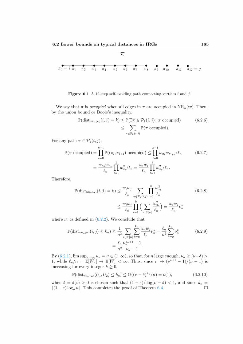
6.2 Lower bounds on typical distances in IRGs 185
π0 = i π1 π2 π3 π4 π5 π6 π7 π8 π9 π10 π11 π12 = j
π
Figure 6.1 A 12-step self-avoiding path connecting vertices i and j.
We say that π is occupied when all edges in π are occupied in NRn(w). Then,by the union bound or Boole’s inequality,
P(distNRn(w)(i, j) = k) ≤ P(∃π ∈ Pk(i, j) : π occupied) (6.2.6)
≤∑
π∈Pk(i,j)
P(π occupied).
For any path π ∈ Pk(i, j),
P(π occupied) =k−1∏s=0
P((πl, πl+1) occupied) ≤k−1∏l=0
wπlwπl+1/`n (6.2.7)
=wπ0
wπk`n
k∏l=1
w2πl/`n =
wiwj`n
k∏l=1
w2πl/`n.
Therefore,
P(distNRn(w)(i, j) = k) ≤ wiwj`n
∑π∈Pk(i,j)
k∏l=1
w2πl
`n(6.2.8)
≤ wiwj`n
k∏l=1
( ∑πl∈[n]
w2πl
`n
)=wiwj`n
νkn,
where νn is defined in (6.2.2). We conclude that
P(distNRn(w)(i, j) ≤ kn) ≤ 1
n2
∑i,j∈[n]
kn∑k=0
wiwj`n
νkn =`nn2
kn∑k=0
νkn (6.2.9)
=`nn2
νkn+1n − 1
νn − 1.
By (6.2.1), lim supn→∞ νn = ν ∈ (1,∞), so that, for n large enough, νn ≥ (ν−δ) >1, while `n/n = E[Wn] → E[W ] < ∞. Thus, since ν 7→ (νk+1 − 1)/(ν − 1) isincreasing for every integer k ≥ 0,
P(distNRn(w)(U1, U2) ≤ kn) ≤ O((ν − δ)kn/n) = o(1), (6.2.10)
when δ = δ(ε) > 0 is chosen such that (1 − ε)/ log(ν − δ) < 1, and since kn =d(1− ε) logν ne. This completes the proof of Theorem 6.4.
186 Small-world phenomena in inhomogeneous random graphs
The condition (6.2.1) is slightly weaker than Condition 1.1(c), which is assumed inTheorem 6.2, as shown in Exercise 6.6. Exercise 6.7 extends the proof of Theorem6.4 to show that (distNRn(w)(U1, U2) ≤ logn
log νn)− is tight.
We close this section by extending the above result to settings where νn is notnecessarily bounded, the most interesting case being τ = 3:
Corollary 6.5 (Lower bound graph distances NRn(w) for τ = 3) Let νn begiven in (6.2.2). Then, for any ε > 0,
P(
distNRn(w)(U1, U2) ≤ (1− ε) logνn n)
= o(1). (6.2.11)
The same results hold for CLn(w) and GRGn(w) under the same conditions.
The proof of Corollary 6.5 is left as Exercise 6.8. In the case where τ = 3 and[1 − Fn](x) is, for a large range of x values, of the order x−2 (which is strongerthan τ = 3), it can be expected that νn = Θ(log n), so that in that case
P(
distNRn(w)(U1, U2) ≤ (1− ε) log n
log logn
)= o(1). (6.2.12)
Exercise 6.9 investigates the situation where τ = 3. Exercise 6.10 the case whereτ ∈ (2, 3), where Corollary 6.5 unfortunately does not give highly interestingresults.
Proof of Theorem 6.1(i)
The proof of the upper bound in Theorem 6.1(i) is closely related to that inTheorem 6.4. Note that
P(distIRGn(κn)(i, j) = k) ≤∑
i1,...,ik−1∈[n]
k−1∏l=0
κn(xil , xil+1)
n, (6.2.13)
where i0 = i, ik = j and we can restrict the vertices to be distinct, so that
P(distIRGn(κn)(i, j) = k) ≤ 1
nk
∑i0,i1,...,ik−1,ik∈[n]
k−1∏l=0
κn(xil , xil+1). (6.2.14)
If the above (k + 1)-dimensional discrete integrals could be replaced by the con-tinuous integral, then we would arrive at
1
n
∫S· · ·∫S
k∏l=0
κ(xl, xl+1)k∏i=0
µ(dxi) =1
n‖Tk+1
κ 1‖1, (6.2.15)
which is bounded from above by 1n‖Tκ‖k+1. Repeating the bound in (6.2.10)
would then prove that, when ν = ‖Tκ‖ > 1,
P(distIRGn(κn)(i, j) ≤ (1− ε) logν n) = o(1). (6.2.16)
However, in the general case, it is not so easy to replace the (k+ 1)-fold discretesum in (6.2.14) by a (k+ 1)-fold integral. We next explain how this can be done,starting with the finite-types case.
6.2 Lower bounds on typical distances in IRGs 187
In the finite-type case, (6.2.13) turns into
P(distIRGn(κ)(i, j) = k) ≤ 1
n2
∑v1,...,vk−1∈[n]
k−1∏l=0
κn(xvl , xvl+1)
n(6.2.17)
≤ 1
n2
∑i1,...,ik−1∈[n]
k−1∏l=0
κ(n)(il, il+1)nil+1
n,
where the number of vertices of type i is denoted by ni, and where the probabilitythat there exists an edge between vertices of type i and j is equal to κ(n)(i, j)/n.Under the conditions in Theorem 6.1(i), we have that ni/n → pi and thatκ(n)(i, j) → κij. This also implies that ‖Tκn‖ → ν, where ν is largest eigenvalueof the matrix (mij)i,j∈[r] with mij = κijpj. Denoting m(n)
ij = κ(n)(i, j)nj/n→ mij,we obtain
P(distIRGn(κ)(i, j) = k) ≤ 1
n2
∑v1,...,vk−1∈[n]
k−1∏l=0
κn(xvl , xvl+1)
n(6.2.18)
≤ 1
n〈µT , [M (n)]k1〉,
where 1 is the all-one vector, µi = ni/n→ pi, and M (n)
ij = m(n)
ij . Obviously, wherethere are N <∞ types,
〈µT , [M (n)]k1〉 ≤ ‖M (n)‖k‖µ‖‖1‖ ≤ ‖M (n)‖k√N. (6.2.19)
Thus,
P(distIRGn(κ)(i, j) = k) ≤√N
n‖M (n)‖k. (6.2.20)
We conclude that
P(dIRGn(κn)(U1, U2) ≤ (1− ε) logνn n) = o(1), (6.2.21)
where νn = ‖M (n)‖ → ν. This proves the claim of Theorem 6.1(i) in the finite-typesetting.
We next extend the proof of Theorem 6.1(i) to the infinite-type setting. Assumethat the conditions in Theorem 6.1(i) hold. Recall the bound in (3.3.18), whichbounds κn from above by κ+
m, which is of finite-type. Then, use the fact that‖Tκ+
m‖ ↓ ‖Tκ‖ = ν > 1 to conclude that P(dIRGn(κn)(U1, U2) ≤ (1 − ε) logν n) =
o(1) holds under the conditions of Theorem 6.1(i). This completes the proof ofTheorem 6.1(i).
Theorem 6.1 leaves open the case when ‖Tκ‖ = ∞, which, for example forCLn(w), is the case when F has infinite second moment. (Bollobas et al., 2007,Theorem 3.14(iv)) states that when ‖Tκ‖ = ∞, the typical graph distance issmaller than log n. More precisely, (Bollobas et al., 2007, Theorem 3.14(iv)) states
188 Small-world phenomena in inhomogeneous random graphs
that if κ is irreducible and ‖Tκ‖ = ∞, then there is a function f(n) = o(log n)such that
P(distIRGn(κ)(i, j) ≤ f(n)) = ζ2κ + o(1). (6.2.22)
Exercise 6.12 shows that one can take f(n) = o(log n).
6.2.2 log log lower bound on distances for infinite-variance degrees
In this section, we prove a log log-lower bound on the typical distances ofNRn(w) for τ ∈ (2, 3). The main result we prove is the following theorem:
Theorem 6.6 (Loglog lower bound on typical distances in NRn(w)) Supposethat the weights w = (wi)i∈[n] satisfy Condition 1.1(a) and that there exists aτ ∈ (2, 3) and c2 such that, for all x ≥ 1,
[1− Fn](x) ≤ c2x−(τ−1), (6.2.23)
Then, for every ε > 0,
P(
distNRn(w)(i, j) ≤ (1− ε) 2 log log n
| log (τ − 2)|)
= o(1). (6.2.24)
The same results hold for CLn(w) and GRGn(w) under the same conditions.
We follow the proof of Theorem 6.4 as closely as possible. The problem withthat proof is that, under the condition in (6.2.23), νn is too large. Indeed, Exercise6.10 shows that the lower bound obtained in Corollary 6.5 is a constant, whichis not very useful. What goes wrong in that argument is that there are too manyvertices with too high weight, and they provide the main contribution to νn andhence to the upper bound as in (6.2.9). However, this argument completely ignoresthe fact that it is quite unlikely that a vertex with a high weight is chosen.
Indeed, as argued in (6.1.6), when starting from a vertex with weight w, say,the probability that it is directly connected to a vertex having weight an is atmost ∑
j : wj≥y
wwj`n
= w[1− F ?n ](y), (6.2.25)
which is small when y is too large. On the other hand, the main contribution toνn comes from vertices having maximal weight of the order n1/(τ−1). This problemis resolved by a suitable truncation argument on the weights of the vertices in theoccupied paths, which effectively removes these high-weight vertices. Therefore,instead of obtaining νn =
∑s∈[n]w
2s/`n, we obtain a partial sum of this restricted
to vertices having a relatively small weight. Effectively, this means that we splitthe space of all paths into good paths, i.e., paths that avoid vertices with toolarge weight, and bad paths, which are paths that jump to vertices with too highweight.
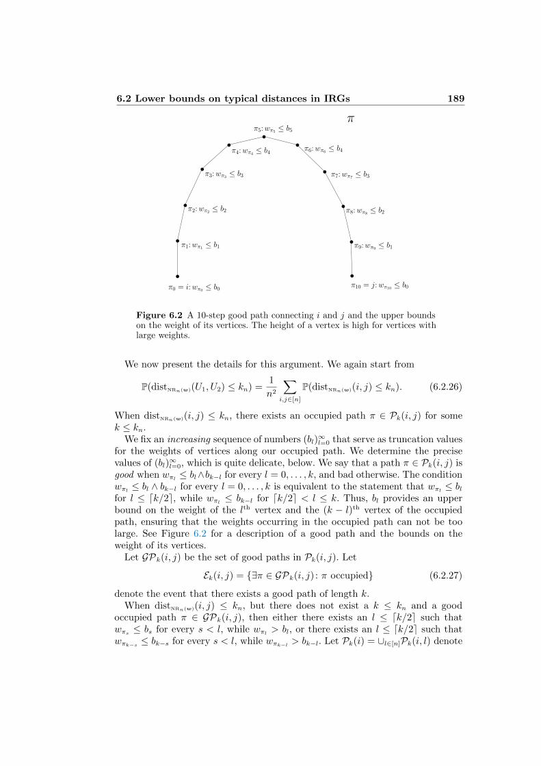
6.2 Lower bounds on typical distances in IRGs 189
π0 = i:wπ0 ≤ b0
π1:wπ1 ≤ b1 π9:wπ9 ≤ b1
π10 = j:wπ10 ≤ b0
π2:wπ2 ≤ b2 π8:wπ8 ≤ b2
π3:wπ3 ≤ b3 π7:wπ7 ≤ b3
π4:wπ4 ≤ b4π6:wπ6 ≤ b4
π5:wπ5 ≤ b5
π
Figure 6.2 A 10-step good path connecting i and j and the upper boundson the weight of its vertices. The height of a vertex is high for vertices withlarge weights.
We now present the details for this argument. We again start from
P(distNRn(w)(U1, U2) ≤ kn) =1
n2
∑i,j∈[n]
P(distNRn(w)(i, j) ≤ kn). (6.2.26)
When distNRn(w)(i, j) ≤ kn, there exists an occupied path π ∈ Pk(i, j) for somek ≤ kn.
We fix an increasing sequence of numbers (bl)∞l=0 that serve as truncation values
for the weights of vertices along our occupied path. We determine the precisevalues of (bl)
∞l=0, which is quite delicate, below. We say that a path π ∈ Pk(i, j) is
good when wπl ≤ bl∧bk−l for every l = 0, . . . , k, and bad otherwise. The conditionwπl ≤ bl ∧ bk−l for every l = 0, . . . , k is equivalent to the statement that wπl ≤ blfor l ≤ dk/2e, while wπl ≤ bk−l for dk/2e < l ≤ k. Thus, bl provides an upperbound on the weight of the lth vertex and the (k − l)th vertex of the occupiedpath, ensuring that the weights occurring in the occupied path can not be toolarge. See Figure 6.2 for a description of a good path and the bounds on theweight of its vertices.
Let GPk(i, j) be the set of good paths in Pk(i, j). Let
Ek(i, j) = ∃π ∈ GPk(i, j) : π occupied (6.2.27)
denote the event that there exists a good path of length k.When distNRn(w)(i, j) ≤ kn, but there does not exist a k ≤ kn and a good
occupied path π ∈ GPk(i, j), then either there exists an l ≤ dk/2e such thatwπs ≤ bs for every s < l, while wπl > bl, or there exists an l ≤ dk/2e such thatwπk−s ≤ bk−s for every s < l, while wπk−l > bk−l. Let Pk(i) = ∪l∈[n]Pk(i, l) denote
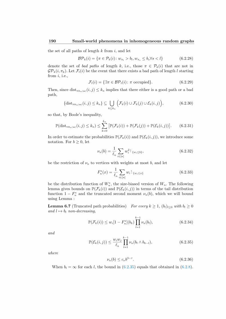
190 Small-world phenomena in inhomogeneous random graphs
the set of all paths of length k from i, and let
BPk(i) = π ∈ Pk(i) : wπl > bl, wπs ≤ bs∀s < l (6.2.28)
denote the set of bad paths of length k, i.e., those π ∈ Pk(i) that are not inGPk(i, πk). Let Fl(i) be the event that there exists a bad path of length l startingfrom i, i.e.,
Fl(i) = ∃π ∈ BP l(i) : π occupied. (6.2.29)
Then, since distNRn(w)(i, j) ≤ kn implies that there either is a good path or a badpath,
distNRn(w)(i, j) ≤ kn ⊆⋃k≤kn
(Fk(i) ∪ Fk(j) ∪ Ek(i, j)
), (6.2.30)
so that, by Boole’s inequality,
P(distNRn(w)(i, j) ≤ kn) ≤kn∑k=0
[P(Fk(i)) + P(Fk(j)) + P(Ek(i, j))
]. (6.2.31)
In order to estimate the probabilities P(Fk(i)) and P(Ek(i, j)), we introduce somenotation. For b ≥ 0, let
νn(b) =1
`n
∑i∈[n]
w2i1wi≤b, (6.2.32)
be the restriction of νn to vertices with weights at most b, and let
F ?n(x) =
1
`n
∑i∈[n]
wi1wi≤x (6.2.33)
be the distribution function of W ?n , the size-biased version of Wn. The following
lemma gives bounds on P(Fk(i)) and P(Ek(i, j)) in terms of the tail distributionfunction 1 − F ?
n and the truncated second moment νn(b), which we will boundusing Lemma :
Lemma 6.7 (Truncated path probabilities) For every k ≥ 1, (bl)l≥0 with bl ≥ 0and l 7→ bl non-decreasing,
P(Fk(i)) ≤ wi[1− F ?n ](bk)
k−1∏l=1
νn(bl), (6.2.34)
and
P(Ek(i, j)) ≤wiwj`n
k−1∏l=1
νn(bl ∧ bk−l), (6.2.35)
where
νn(b) ≤ cνb3−τ . (6.2.36)
When bl =∞ for each l, the bound in (6.2.35) equals that obtained in (6.2.8).
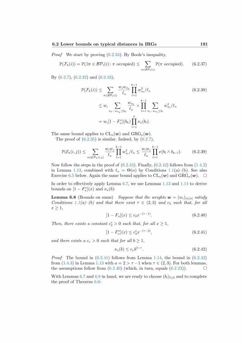
6.2 Lower bounds on typical distances in IRGs 191
Proof We start by proving (6.2.34). By Boole’s inequality,
P(Fk(i)) = P(∃π ∈ BP l(i) : π occupied) ≤∑
π∈BPl(i)
P(π occupied). (6.2.37)
By (6.2.7), (6.2.32) and (6.2.33),
P(Fk(i)) ≤∑
π∈BPl(i)
wiwπk`n
k−1∏l=1
w2πl/`n (6.2.38)
≤ wi∑
πk : wπk≥bk
wπk`n×
k−1∏l=1
∑πl : wπl≤bl
w2πl/`n
= wi[1− F ?n ](bk)
k∏l=1
νn(bl).
The same bound applies to CLn(w) and GRGn(w).The proof of (6.2.35) is similar. Indeed, by (6.2.7),
P(Ek(i, j)) ≤∑
π∈GPk(i,j)
wiwj`n
k−1∏l=1
w2πl/`n ≤
wiwj`n
k−1∏l=1
ν(bl ∧ bk−l). (6.2.39)
Now follow the steps in the proof of (6.2.34). Finally, (6.2.42) follows from (1.4.2)in Lemma 1.13, combined with `n = Θ(n) by Conditions 1.1(a)–(b). See alsoExercise 6.5 below. Again the same bound applies to CLn(w) and GRGn(w).
In order to effectively apply Lemma 6.7, we use Lemmas 1.13 and 1.14 to derivebounds on [1− F ?
n ](x) and νn(b):
Lemma 6.8 (Bounds on sums) Suppose that the weights w = (wi)i∈[n] satisfyConditions 1.1(a)–(b) and that there exist τ ∈ (2, 3) and c2 such that, for allx ≥ 1,
[1− Fn](x) ≤ c2x−(τ−1). (6.2.40)
Then, there exists a constant c∗2 > 0 such that, for all x ≥ 1,
[1− F ?n ](x) ≤ c?2x−(τ−2), (6.2.41)
and there exists a cν > 0 such that for all b ≥ 1,
νn(b) ≤ cνb3−τ . (6.2.42)
Proof The bound in (6.2.41) follows from Lemma 1.14, the bound in (6.2.42)from (1.4.3) in Lemma 1.13 with a = 2 > τ−1 when τ ∈ (2, 3). For both lemmas,the assumptions follow from (6.2.40) (which, in turn, equals (6.2.23)).
With Lemmas 6.7 and 6.8 in hand, we are ready to choose (bl)l≥0 and to completethe proof of Theorem 6.6:
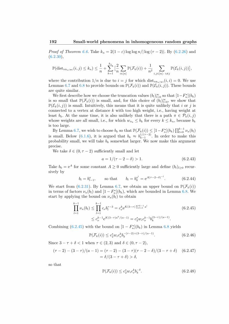
192 Small-world phenomena in inhomogeneous random graphs
Proof of Theorem 6.6. Take kn = 2(1− ε) log log n/| log (τ − 2)|. By (6.2.26) and(6.2.30),
P(distNRn(w)(i, j) ≤ kn) ≤ 1
n+
kn∑k=1
[ 2
n
∑i∈[n]
P(Fk(i)) +1
n2
∑i,j∈[n] : i 6=j
P(Ek(i, j))],
where the contribution 1/n is due to i = j for which distNRn(w)(i, i) = 0. We useLemmas 6.7 and 6.8 to provide bounds on P(Fk(i)) and P(Ek(i, j)). These boundsare quite similar.
We first describe how we choose the truncation values (bl)∞l=0 so that [1−F ?
n ](bk)is so small that P(Fk(i)) is small, and, for this choice of (bl)
∞l=0, we show that
P(Ek(i, j)) is small. Intuitively, this means that it is quite unlikely that i or j isconnected to a vertex at distance k with too high weight, i.e., having weight atleast bk. At the same time, it is also unlikely that there is a path π ∈ Pk(i, j)whose weights are all small, i.e., for which wπk ≤ bk for every k ≤ kn, because bkis too large.
By Lemma 6.7, we wish to choose bk so that P(Fk(i)) ≤ [1−F ?n ](bk)
∏k−1l=0 νn(bl)
is small. Below (6.1.6), it is argued that bk ≈ b1/(τ−2)k−1 . In order to make this
probability small, we will take bk somewhat larger. We now make this argumentprecise.
We take δ ∈ (0, τ − 2) sufficiently small and let
a = 1/(τ − 2− δ) > 1. (6.2.43)
Take b0 = eA for some constant A ≥ 0 sufficiently large and define (bl)l≥0 recur-sively by
bl = bal−1, so that bl = bal
0 = eA(τ−2−δ)−l . (6.2.44)
We start from (6.2.31). By Lemma 6.7, we obtain an upper bound on P(Fk(i))in terms of factors νn(bl) and [1−F ?
n ](bk), which are bounded in Lemma 6.8. Westart by applying the bound on νn(bl) to obtain
k−1∏l=1
νn(bl) ≤k−1∏l=1
cνbτ−3l = ckνe
K(3−τ)∑k−1l=1 a
l
(6.2.45)
≤ ck−1ν eK(3−τ)ak/(a−1) = c?2wic
k−1ν b
(3−τ)/(a−1)k .
Combining (6.2.45) with the bound on [1− F ?n ](bk) in Lemma 6.8 yields
P(Fk(i)) ≤ c?2wickνb−(τ−2)+(3−τ)/(a−1)k . (6.2.46)
Since 3− τ + δ < 1 when τ ∈ (2, 3) and δ ∈ (0, τ − 2),
(τ − 2)− (3− τ)/(a− 1) = (τ − 2)− (3− τ)(τ − 2− δ)/(3− τ + δ) (6.2.47)
= δ/(3− τ + δ) > δ,
so that
P(Fk(i)) ≤ c?2wickνb−δk . (6.2.48)
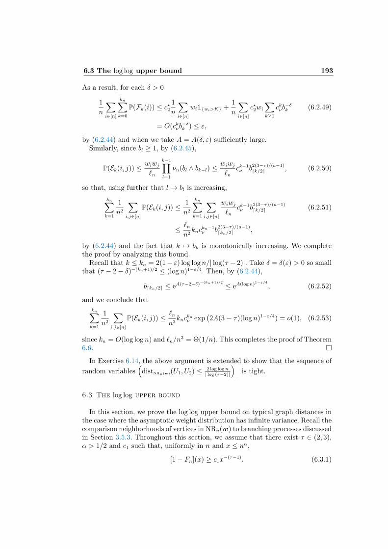
6.3 The log log upper bound 193
As a result, for each δ > 0
1
n
∑i∈[n]
kn∑k=0
P(Fk(i)) ≤ c?21
n
∑i∈[n]
wi1wi>K +1
n
∑i∈[n]
c?2wi∑k≥1
ckνb−δk (6.2.49)
= O(ckνb−δk ) ≤ ε,
by (6.2.44) and when we take A = A(δ, ε) sufficiently large.Similarly, since bl ≥ 1, by (6.2.45),
P(Ek(i, j)) ≤wiwj`n
k−1∏l=1
νn(bl ∧ bk−l) ≤wiwj`n
ck−1ν b
2(3−τ)/(a−1)dk/2e , (6.2.50)
so that, using further that l 7→ bl is increasing,
kn∑k=1
1
n2
∑i,j∈[n]
P(Ek(i, j)) ≤1
n2
kn∑k=1
∑i,j∈[n]
wiwj`n
ck−1ν b
2(3−τ)/(a−1)dk/2e (6.2.51)
≤ `nn2knc
kn−1ν b
2(3−τ)/(a−1)dkn/2e ,
by (6.2.44) and the fact that k 7→ bk is monotonically increasing. We completethe proof by analyzing this bound.
Recall that k ≤ kn = 2(1− ε) log log n/| log(τ − 2)|. Take δ = δ(ε) > 0 so smallthat (τ − 2− δ)−(kn+1)/2 ≤ (log n)1−ε/4. Then, by (6.2.44),
bdkn/2e ≤ eA(τ−2−δ)−(kn+1)/2 ≤ eA(logn)1−ε/4 , (6.2.52)
and we conclude that
kn∑k=1
1
n2
∑i,j∈[n]
P(Ek(i, j)) ≤`nn2knc
knν exp
(2A(3− τ)(log n)1−ε/4) = o(1), (6.2.53)
since kn = O(log log n) and `n/n2 = Θ(1/n). This completes the proof of Theorem
6.6.
In Exercise 6.14, the above argument is extended to show that the sequence of
random variables(
distNRn(w)(U1, U2) ≤ 2 log logn| log (τ−2)|
)−
is tight.
6.3 The log log upper bound
In this section, we prove the log log upper bound on typical graph distances inthe case where the asymptotic weight distribution has infinite variance. Recall thecomparison neighborhoods of vertices in NRn(w) to branching processes discussedin Section 3.5.3. Throughout this section, we assume that there exist τ ∈ (2, 3),α > 1/2 and c1 such that, uniformly in n and x ≤ nα,
[1− Fn](x) ≥ c1x−(τ−1). (6.3.1)
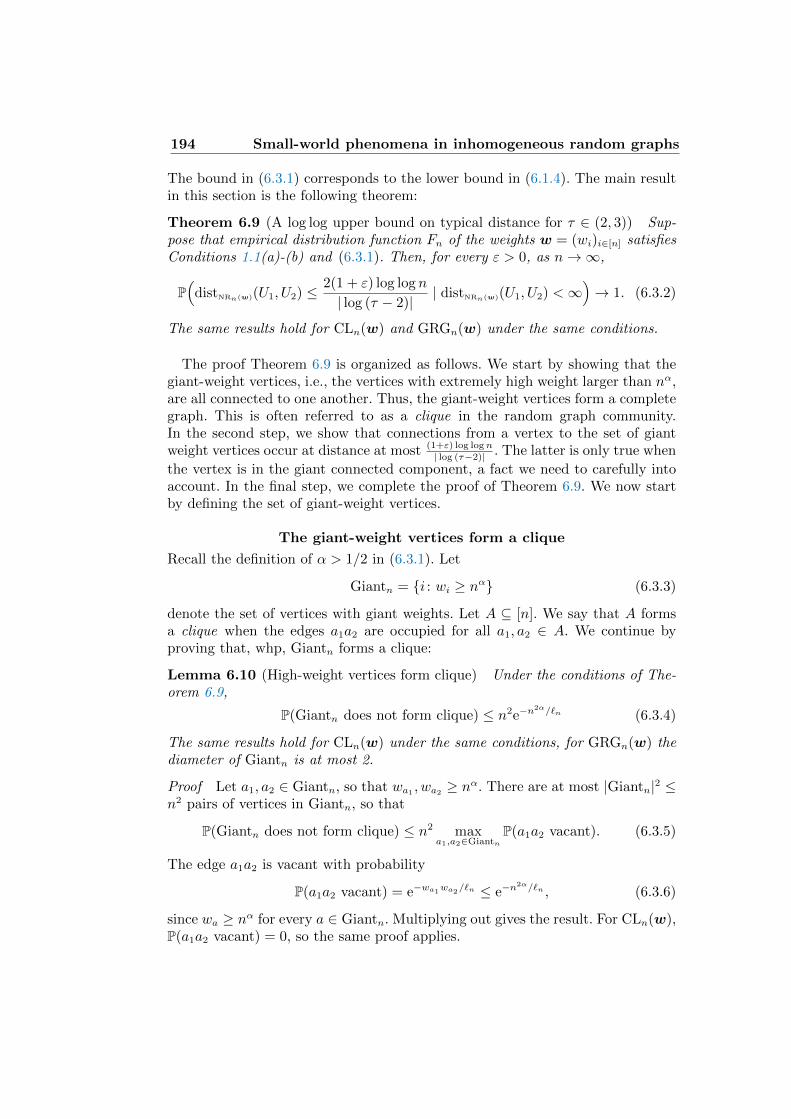
194 Small-world phenomena in inhomogeneous random graphs
The bound in (6.3.1) corresponds to the lower bound in (6.1.4). The main resultin this section is the following theorem:
Theorem 6.9 (A log log upper bound on typical distance for τ ∈ (2, 3)) Sup-pose that empirical distribution function Fn of the weights w = (wi)i∈[n] satisfiesConditions 1.1(a)-(b) and (6.3.1). Then, for every ε > 0, as n→∞,
P(
distNRn(w)(U1, U2) ≤ 2(1 + ε) log log n
| log (τ − 2)| | distNRn(w)(U1, U2) <∞)→ 1. (6.3.2)
The same results hold for CLn(w) and GRGn(w) under the same conditions.
The proof Theorem 6.9 is organized as follows. We start by showing that thegiant-weight vertices, i.e., the vertices with extremely high weight larger than nα,are all connected to one another. Thus, the giant-weight vertices form a completegraph. This is often referred to as a clique in the random graph community.In the second step, we show that connections from a vertex to the set of giantweight vertices occur at distance at most (1+ε) log logn
| log (τ−2)| . The latter is only true when
the vertex is in the giant connected component, a fact we need to carefully intoaccount. In the final step, we complete the proof of Theorem 6.9. We now startby defining the set of giant-weight vertices.
The giant-weight vertices form a clique
Recall the definition of α > 1/2 in (6.3.1). Let
Giantn = i : wi ≥ nα (6.3.3)
denote the set of vertices with giant weights. Let A ⊆ [n]. We say that A formsa clique when the edges a1a2 are occupied for all a1, a2 ∈ A. We continue byproving that, whp, Giantn forms a clique:
Lemma 6.10 (High-weight vertices form clique) Under the conditions of The-orem 6.9,
P(Giantn does not form clique) ≤ n2e−n2α/`n (6.3.4)
The same results hold for CLn(w) under the same conditions, for GRGn(w) thediameter of Giantn is at most 2.
Proof Let a1, a2 ∈ Giantn, so that wa1 , wa2 ≥ nα. There are at most |Giantn|2 ≤n2 pairs of vertices in Giantn, so that
P(Giantn does not form clique) ≤ n2 maxa1,a2∈Giantn
P(a1a2 vacant). (6.3.5)
The edge a1a2 is vacant with probability
P(a1a2 vacant) = e−wa1wa2/`n ≤ e−n2α/`n , (6.3.6)
since wa ≥ nα for every a ∈ Giantn. Multiplying out gives the result. For CLn(w),P(a1a2 vacant) = 0, so the same proof applies.
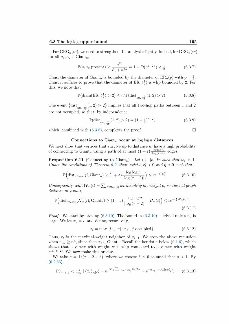
6.3 The log log upper bound 195
For GRGn(w), we need to strengthen this analysis slightly. Indeed, for GRGn(w),for all a1, a2 ∈ Giantn,
P(a1a2 present) ≥ n2α
`n + n2α= 1−Θ(n1−2α) ≥ 1
2. (6.3.7)
Thus, the diameter of Giantn is bounded by the diameter of ERn(p) with p = 12.
Thus, it suffices to prove that the diameter of ERn( 12) is whp bounded by 2. For
this, we note that
P(diam(ERn( 12) > 2) ≤ n2P(dist
ERn(12
)(1, 2) > 2). (6.3.8)
The event distERn(
12
)(1, 2) > 2 implies that all two-hop paths between 1 and 2
are not occupied, so that, by independence
P(distERn(
12
)(1, 2) > 2) = (1− 1
4)n−2, (6.3.9)
which, combined with (6.3.8), completes the proof.
Connections to Giantn occur at log log n distances
We next show that vertices that survive up to distance m have a high probabilityof connecting to Giantn using a path of at most (1 + ε) log logn
| log (τ−2)| edges:
Proposition 6.11 (Connecting to Giantn) Let i ∈ [n] be such that wi > 1.Under the conditions of Theorem 6.9, there exist c, c?1 > 0 and η > 0 such that
P(
distNRn(w)(i,Giantn) ≥ (1 + ε)log logn
| log (τ − 2)|)≤ ce−c?1wηi . (6.3.10)
Consequently, withWm(i) =∑
k∈∂Bm(i)wk denoting the weight of vertices at graphdistance m from i,
P(
distNRn(w)(Nm(i),Giantn) ≥ (1 + ε)log log n
| log (τ − 2)| | Bm(i))≤ ce−c?1Wm(i)η .
(6.3.11)
Proof We start by proving (6.3.10). The bound in (6.3.10) is trivial unless wi islarge. We let x0 = i, and define, recursively,
x` = maxj ∈ [n] : x`−1j occupied. (6.3.12)
Thus, x` is the maximal-weight neighbor of x`−1. We stop the above recursionwhen wx` ≥ nα, since then x` ∈ Giantn. Recall the heuristic below (6.1.6), whichshows that a vertex with weight w is whp connected to a vertex with weightw1/(τ−2). We now make this precise.
We take a = 1/(τ − 2 + δ), where we choose δ > 0 so small that a > 1. By(6.2.33),
P(wx`+1< wax` | (xs)s≤`) = e
−wx`∑l : wl≥wax`
wl/`n= e−wx` [1−F
?n ](wax`
). (6.3.13)
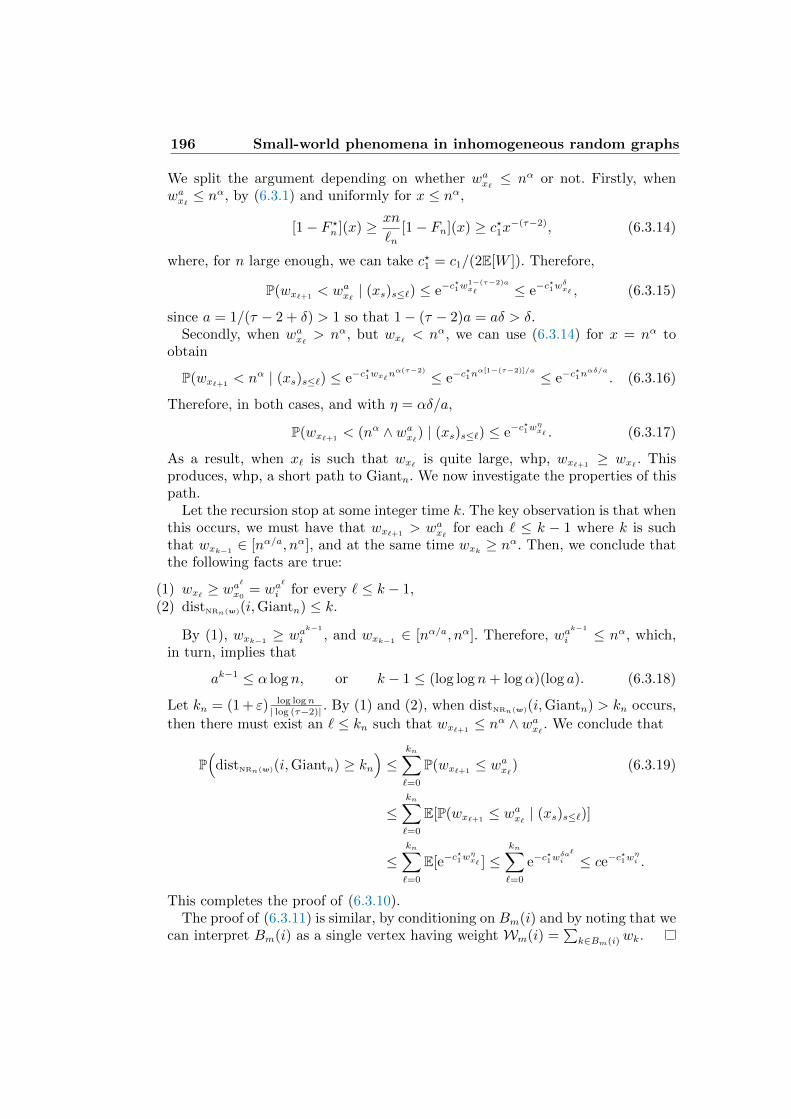
196 Small-world phenomena in inhomogeneous random graphs
We split the argument depending on whether wax` ≤ nα or not. Firstly, whenwax` ≤ nα, by (6.3.1) and uniformly for x ≤ nα,
[1− F ?n ](x) ≥ xn
`n[1− Fn](x) ≥ c?1x−(τ−2), (6.3.14)
where, for n large enough, we can take c?1 = c1/(2E[W ]). Therefore,
P(wx`+1< wax` | (xs)s≤`) ≤ e−c
?1w
1−(τ−2)ax` ≤ e−c
?1w
δx` , (6.3.15)
since a = 1/(τ − 2 + δ) > 1 so that 1− (τ − 2)a = aδ > δ.Secondly, when wax` > nα, but wx` < nα, we can use (6.3.14) for x = nα to
obtain
P(wx`+1< nα | (xs)s≤`) ≤ e−c
?1wx`n
α(τ−2) ≤ e−c?1nα[1−(τ−2)]/a ≤ e−c
?1nαδ/a
. (6.3.16)
Therefore, in both cases, and with η = αδ/a,
P(wx`+1< (nα ∧ wax`) | (xs)s≤`) ≤ e−c
?1w
ηx` . (6.3.17)
As a result, when x` is such that wx` is quite large, whp, wx`+1≥ wx` . This
produces, whp, a short path to Giantn. We now investigate the properties of thispath.
Let the recursion stop at some integer time k. The key observation is that whenthis occurs, we must have that wx`+1
> wax` for each ` ≤ k − 1 where k is suchthat wxk−1
∈ [nα/a, nα], and at the same time wxk ≥ nα. Then, we conclude thatthe following facts are true:
(1) wx` ≥ wa`
x0= wa
`
i for every ` ≤ k − 1,(2) distNRn(w)(i,Giantn) ≤ k.
By (1), wxk−1≥ wa
k−1
i , and wxk−1∈ [nα/a, nα]. Therefore, wa
k−1
i ≤ nα, which,in turn, implies that
ak−1 ≤ α log n, or k − 1 ≤ (log log n+ logα)(log a). (6.3.18)
Let kn = (1 + ε) log logn| log (τ−2)| . By (1) and (2), when distNRn(w)(i,Giantn) > kn occurs,
then there must exist an ` ≤ kn such that wx`+1≤ nα ∧ wax` . We conclude that
P(
distNRn(w)(i,Giantn) ≥ kn)≤
kn∑`=0
P(wx`+1≤ wax`) (6.3.19)
≤kn∑`=0
E[P(wx`+1≤ wax` | (xs)s≤`)]
≤kn∑`=0
E[e−c?1w
ηx` ] ≤
kn∑`=0
e−c?1w
δa`
i ≤ ce−c?1wηi .
This completes the proof of (6.3.10).The proof of (6.3.11) is similar, by conditioning on Bm(i) and by noting that we
can interpret Bm(i) as a single vertex having weight Wm(i) =∑
k∈Bm(i)wk.
6.3 The log log upper bound 197
Completion of the proof of Theorem 6.9
To prove the upper bound in Theorem 6.9, for ε ∈ (0, 1), we take
kn = (1 + ε)log log n
| log (τ − 2)| , (6.3.20)
so that it suffices to show, for every ε > 0,
limn→∞
P(distNRn(w)(U1, U2) ≤ 2kn| distNRn(w)(U1, U2) <∞) = 1. (6.3.21)
Since
P(distNRn(w)(U1, U2) ≤ 2kn| distNRn(w)(U1, U2) <∞) (6.3.22)
=P(distNRn(w)(U1, U2) ≤ 2kn)
P(distNRn(w)(U1, U2) <∞),
this follows from the two bounds
lim infn→∞
P(distNRn(w)(U1, U2) <∞) ≤ ζ2, (6.3.23)
lim supn→∞
P(distNRn(w)(U1, U2) ≤ 2kn) ≥ ζ2, (6.3.24)
with ζ > 0 the survival probability of the underlying branching process approxi-mation to the neighborhoods of NRn(w) identified in Theorem 3.15. For (6.3.23),we split, for some m ≥ 1,
P(distNRn(w)(U1, U2) <∞) (6.3.25)
≤ P(distNRn(w)(U1, U2) ≤ 2m)
+ P(|∂Bm(U1)| > 0, |∂Bm(U1)| > 0, distNRn(w)(U1, U2) > 2m).
By Corollary 2.11, P(distNRn(w)(U1, U2) ≤ 2m) = o(1), and, by (2.4.2) in Corollary2.10,
P(|∂Bm(U1)| > 0, |∂Bm(U1)| > 0,distNRn(w)(U1, U2) > 2m) (6.3.26)
= P(|∂Bm(o)| > 0)2 + o(1),
where ∂Bm(o) is the set of vertices at distance m in the local weak limit ofNRn(w) identified in Theorem 3.15. The right-hand side of (6.3.26) converges toζ2 when m→∞. This proves (6.3.23).
To prove (6.3.24), we fix m ≥ 1 and write
P(2m < distNRn(w)(U1, U2) ≤ 2kn) (6.3.27)
≥ P(distNRn(w)(Ui,Giantn) ≤ kn, i = 1, 2,distNRn(w)(U1, U2) > 2m
)≥ P(|∂Bm(U1)| > 0, |∂Bm(U1)| > 0,distNRn(w)(U1, U2) > 2m)
− 2P(distNRn(w)(U1,Giantn) < kn, |∂Bm(U1)| > 0
).
By (6.3.26), the first term converges to ζ2m, which in turn converges to ζ2 when
m→∞.

198 Small-world phenomena in inhomogeneous random graphs
For the second term, we condition on Bm(U1), Bm(U2), and use that ∂Bm(U1)is measurable w.r.t. Bm(U1) to obtain
P(distNRn(w)(U1,Giantn) < kn, |Bm(U1)| > 0
)(6.3.28)
= E[P(distNRn(w)(U1,Giantn) > kn | Bm(U1)
)1|∂Bm(U1)|>0
].
By Proposition 6.11,
P(distNRn(w)(U1,Giantn) > kn | Bm(U1)
)≤ ce−c?1Wm(U1)η . (6.3.29)
By Theorem 3.15 and Conditions 1.1(a)-(b), we obtain that
Wm(U1)ηd−→|∂Bm(o)|∑i=1
W ?i , (6.3.30)
where(W ?i
)i≥1
are i.i.d. copies of random variables with distribution function F ?.
Therefore,
Wm(U1)P−→∞ (6.3.31)
when first n → ∞ followed by m → ∞, and we use that |∂Bm(o)| P−→ ∞ since|∂Bm(o)| > 0. As a result,
P(distNRn(w)(U1,Giantn) > kn | Bm(U1)
)1|∂Bm(U1)|>0
P−→ 0, (6.3.32)
which by Lebesgues Dominated Convergence Theorem [Volume 1, Theorem A.1]implies that
E[e−c
?1Wm(V1)η
1|∂Bm(U1)|>0
]→ 0, (6.3.33)
when first n→∞ followed by m→∞. This proves (6.3.24), and thus completesthe proof of the upper bound in Theorem 6.3.
6.4 Path counting and log upper bound for finite-variance weights
In this section, we give the proof of the log upper bound for finite-varianceweights. For this, we use the second moment method to show that whp there existsa path of at most (1 + ε) logν n edges between U1 and U2. To apply the second-moment method, we give a bound on the variance of the number of paths ofgiven lengths using path-counting techniques. This section is organised as follows.In Section 6.4.1, we highlight the path-counting techniques. In Section 6.4.2, weapply these methods to give upper bounds on distances for finite-variance weights.We also investigate the case where τ = 3, and prove that typical distances arebounded by log n/ log logn under appropriate conditions as well. We close inSection 6.4.3 by proving Theorems 3.16 and 6.1(ii).
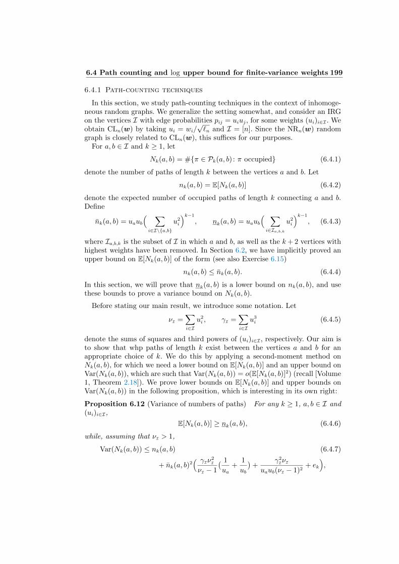
6.4 Path counting and log upper bound for finite-variance weights 199
6.4.1 Path-counting techniques
In this section, we study path-counting techniques in the context of inhomoge-neous random graphs. We generalize the setting somewhat, and consider an IRGon the vertices I with edge probabilities pij = uiuj, for some weights (ui)i∈I . Weobtain CLn(w) by taking ui = wi/
√`n and I = [n]. Since the NRn(w) random
graph is closely related to CLn(w), this suffices for our purposes.For a, b ∈ I and k ≥ 1, let
Nk(a, b) = #π ∈ Pk(a, b) : π occupied (6.4.1)
denote the number of paths of length k between the vertices a and b. Let
nk(a, b) = E[Nk(a, b)] (6.4.2)
denote the expected number of occupied paths of length k connecting a and b.Define
nk(a, b) = uaub( ∑i∈I\a,b
u2i
)k−1
, nk(a, b) = uaub( ∑i∈Ia,b,k
u2i
)k−1
, (6.4.3)
where Ia,b,k is the subset of I in which a and b, as well as the k+ 2 vertices withhighest weights have been removed. In Section 6.2, we have implicitly proved anupper bound on E[Nk(a, b)] of the form (see also Exercise 6.15)
nk(a, b) ≤ nk(a, b). (6.4.4)
In this section, we will prove that nk(a, b) is a lower bound on nk(a, b), and usethese bounds to prove a variance bound on Nk(a, b).
Before stating our main result, we introduce some notation. Let
νI =∑i∈I
u2i , γI =
∑i∈I
u3i (6.4.5)
denote the sums of squares and third powers of (ui)i∈I , respectively. Our aim isto show that whp paths of length k exist between the vertices a and b for anappropriate choice of k. We do this by applying a second-moment method onNk(a, b), for which we need a lower bound on E[Nk(a, b)] and an upper bound onVar(Nk(a, b)), which are such that Var(Nk(a, b)) = o(E[Nk(a, b)]
2) (recall [Volume1, Theorem 2.18]). We prove lower bounds on E[Nk(a, b)] and upper bounds onVar(Nk(a, b)) in the following proposition, which is interesting in its own right:
Proposition 6.12 (Variance of numbers of paths) For any k ≥ 1, a, b ∈ I and(ui)i∈I,
E[Nk(a, b)] ≥ nk(a, b), (6.4.6)
while, assuming that νI > 1,
Var(Nk(a, b)) ≤ nk(a, b) (6.4.7)
+ nk(a, b)2( γIν
2I
νI − 1
( 1
ua+
1
ub
)+
γ2IνI
uaub(νI − 1)2+ ek
),
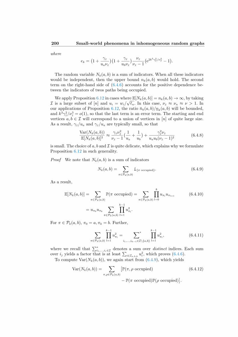
200 Small-world phenomena in inhomogeneous random graphs
where
ek =(1 +
γIuaνI
)(1 +
γIubνI
) νIνI − 1
(e2k3γ2
I/ν3I − 1
).
The random variable Nk(a, b) is a sum of indicators. When all these indicatorswould be independent, then the upper bound nk(a, b) would hold. The secondterm on the right-hand side of (6.4.6) accounts for the positive dependence be-tween the indicators of twos paths being occupied.
We apply Proposition 6.12 in cases where E[Nk(a, b)] = nk(a, b)→∞, by takingI is a large subset of [n] and ui = wi/
√`n. In this case, νI ≈ νn ≈ ν > 1. In
our applications of Proposition 6.12, the ratio nk(a, b)/nk(a, b) will be bounded,and k3γ2
I/ν3I = o(1), so that the last term is an error term. The starting and end
vertices a, b ∈ I will correspond to a union of vertices in [n] of quite large size.As a result, γI/ua and γI/ua are typically small, so that
Var(Nk(a, b))
E[Nk(a, b)]2≈ γIν
2I
νI − 1
( 1
ua+
1
ub
)+
γ2IνI
uaub(νI − 1)2(6.4.8)
is small. The choice of a, b and I is quite delicate, which explains why we formulateProposition 6.12 in such generality.
Proof We note that Nk(a, b) is a sum of indicators
Nk(a, b) =∑
π∈Pk(a,b)
1π occupied. (6.4.9)
As a result,
E[Nk(a, b)] =∑
π∈Pk(a,b)
P(π occupied) =∑
π∈Pk(a,b)
k∏l=0
uπluπl+1(6.4.10)
= uπ0uπk
∑π∈Pk(a,b)
k−1∏l=1
u2πl.
For π ∈ Pk(a, b), π0 = a, πk = b. Further,
∑π∈Pk(a,b)
k−1∏l=1
u2πl
=∑∗
i1,...,ik−1∈I\a,b
k−1∏l=1
u2πl, (6.4.11)
where we recall that∑∗
i1,...,ir∈I denotes a sum over distinct indices. Each sumover ij yields a factor that is at least
∑i∈Ia,b,k u
2i , which proves (6.4.6).
To compute Var(Nk(a, b)), we again start from (6.4.9), which yields
Var(Nk(a, b)) =∑
π,ρ∈Pk(a,b)
[P(π, ρ occupied) (6.4.12)
− P(π occupied)P(ρ occupied)].
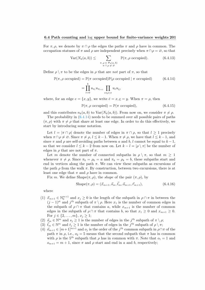
6.4 Path counting and log upper bound for finite-variance weights 201
For π, ρ, we denote by π ∩ ρ the edges the paths π and ρ have in common. Theoccupation statuses of π and ρ are independent precisely when π∩ρ = ∅, so that
Var(Nk(a, b)) ≤∑
π, ρ ∈ Pk(a, b)π ∩ ρ 6= ∅
P(π, ρ occupied). (6.4.13)
Define ρ \ π to be the edges in ρ that are not part of π, so that
P(π, ρ occupied) = P(π occupied)P(ρ occupied | π occupied) (6.4.14)
=k∏l=0
uπluπl+1
∏e∈ρ\π
ueue,
where, for an edge e = x, y, we write e = x, e = y. When π = ρ, then
P(π, ρ occupied) = P(π occupied), (6.4.15)
and this contributes nk(a, b) to Var(Nk(a, b)). From now on, we consider π 6= ρ.The probability in (6.4.14) needs to be summed over all possible pairs of paths
(π, ρ) with π 6= ρ that share at least one edge. In order to do this effectively, westart by introducing some notation.
Let l = |π ∩ ρ| denote the number of edges in π ∩ ρ, so that l ≥ 1 preciselywhen π∩ ρ 6= ∅. Since π 6= ρ, l ≤ k− 1. When π 6= ρ, we have that l ≤ k− 1, andsince π and ρ are self-avoiding paths between a and b, l cannot be equal to k− 1,so that we consider l ≤ k − 2 from now on. Let k − l = |ρ \ π| be the number ofedges in ρ that are not part of π.
Let m denote the number of connected subpaths in ρ \ π, so that m ≥ 1whenever π 6= ρ. Since π0 = ρ0 = a and πk = ρk = b, these subpaths start andend in vertices along the path π. We can view these subpaths as excursions ofthe path ρ from the walk π. By construction, between two excursions, there is atleast one edge that π and ρ have in common.
Fix m. We define Shape(π, ρ), the shape of the pair (π, ρ), by
Shape(π, ρ) = (~xm+1, ~sm,~tm, ~om+1, ~rm+1), (6.4.16)
where
(1) ~xm+1 ∈ Nm+10 and xj ≥ 0 is the length of the subpath in ρ ∩ π in between the
(j − 1)st and jth subpath of π \ ρ. Here x1 is the number of common edges inthe subpath of ρ ∩ π that contains a, while xm+1 is the number of commonedges in the subpath of ρ ∩ π that contains b, so that x1 ≥ 0 and xm+1 ≥ 0.For j ∈ 2, . . . ,m, xj ≥ 1;
(2) ~sm ∈ Nm and sj ≥ 1 is the number of edges in the jth subpath of π \ ρ;(3) ~tm ∈ Nm and tj ≥ 1 is the number of edges in the jth subpath of ρ \ π;(4) ~om+1 ∈ [m+1]m+1 and oj is the order of the jth common subpath in ρ∩π of the
path π in ρ, i.e., o2 = 5 means that the second subpath that π has in commonwith ρ is the 5th subpath that ρ has in common with π. Note that o1 = 1 andom+1 = m+ 1, since π and ρ start and end in a and b, respectively;
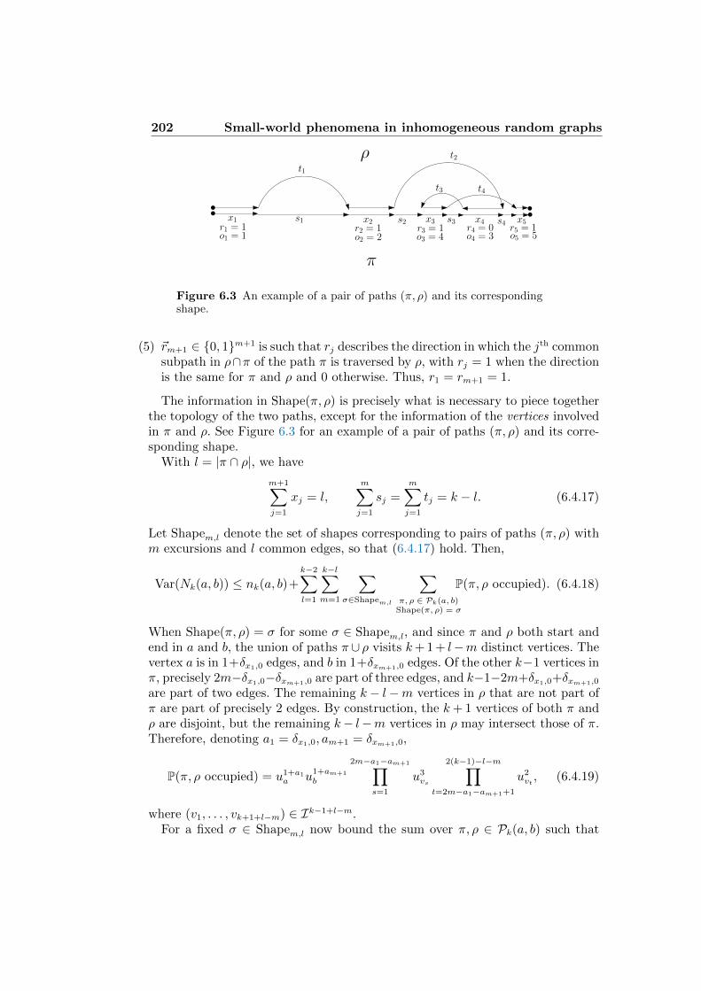
202 Small-world phenomena in inhomogeneous random graphs
π
ρ
x1 x2 x3 x4 x5r1 = 1 r2 = 1 r3 = 1 r4 = 0 r5 = 1
s1 s2 s3 s4
t1
t2
t3 t4
o1 = 1 o2 = 2 o3 = 4 o4 = 3 o5 = 5
Figure 6.3 An example of a pair of paths (π, ρ) and its correspondingshape.
(5) ~rm+1 ∈ 0, 1m+1 is such that rj describes the direction in which the jth commonsubpath in ρ∩π of the path π is traversed by ρ, with rj = 1 when the directionis the same for π and ρ and 0 otherwise. Thus, r1 = rm+1 = 1.
The information in Shape(π, ρ) is precisely what is necessary to piece togetherthe topology of the two paths, except for the information of the vertices involvedin π and ρ. See Figure 6.3 for an example of a pair of paths (π, ρ) and its corre-sponding shape.
With l = |π ∩ ρ|, we have
m+1∑j=1
xj = l,m∑j=1
sj =m∑j=1
tj = k − l. (6.4.17)
Let Shapem,l denote the set of shapes corresponding to pairs of paths (π, ρ) withm excursions and l common edges, so that (6.4.17) hold. Then,
Var(Nk(a, b)) ≤ nk(a, b)+k−2∑l=1
k−l∑m=1
∑σ∈Shapem,l
∑π, ρ ∈ Pk(a, b)
Shape(π, ρ) = σ
P(π, ρ occupied). (6.4.18)
When Shape(π, ρ) = σ for some σ ∈ Shapem,l, and since π and ρ both start andend in a and b, the union of paths π ∪ ρ visits k+ 1 + l−m distinct vertices. Thevertex a is in 1+δx1,0 edges, and b in 1+δxm+1,0 edges. Of the other k−1 vertices inπ, precisely 2m−δx1,0−δxm+1,0 are part of three edges, and k−1−2m+δx1,0+δxm+1,0
are part of two edges. The remaining k − l−m vertices in ρ that are not part ofπ are part of precisely 2 edges. By construction, the k+ 1 vertices of both π andρ are disjoint, but the remaining k− l−m vertices in ρ may intersect those of π.Therefore, denoting a1 = δx1,0, am+1 = δxm+1,0,
P(π, ρ occupied) = u1+a1a u
1+am+1
b
2m−a1−am+1∏s=1
u3vs
2(k−1)−l−m∏t=2m−a1−am+1+1
u2vt, (6.4.19)
where (v1, . . . , vk+1+l−m) ∈ Ik−1+l−m.For a fixed σ ∈ Shapem,l now bound the sum over π, ρ ∈ Pk(a, b) such that
6.4 Path counting and log upper bound for finite-variance weights 203
Shape(π, ρ) = σ from above by summing (6.4.19) over all (v1, . . . , vk−1+l−m) ∈Ik−1+l−m, to obtain for any σ ∈ Shapem,l,∑
π, ρ ∈ Pk(a, b)Shape(π, ρ) = σ
P(π, ρ occupied) (6.4.20)
≤ uaubγ2mI ν2k−1−3m−l
I
(uaνIγI
)δx1,0(ubνIγI
)δxm+1,0
= nk(a, b)2γ2(m+1)I ν−3(m−1)−l
I
( γIuaνI
)1−δx1,0( γIubνI
)1−δxm+1,0 .
Therefore, we arrive at
Var(Nk(a, b)) ≤ nk(a, b) + nk(a, b)2k−2∑l=1
k−l∑m=1
γ2(m−1)I ν−3(m−1)−l
I (6.4.21)
×∑
σ∈Shapem,l
( γIuaνI
)1−δx1,0( γIubνI
)1−δxm+1,0 .
We continue to compute the number of shapes in the following lemma:
Lemma 6.13 (The number of shapes) Fix m ≥ 1 and l ≤ k−2. For m = 1, thenumber of shapes in Shapem,l with fixed a1 = δx1,0, am+1 = δxm+1,0 equals l whena1 = am+1 = 0, 1 when a1 + am+1 = 1 and 0 when a1 = am+1 = 1. For m ≥ 2,the number of shapes in Shapem,l with fixed a1 = δx1,0, am+1 = δxm+1,0 is boundedby
2m−1(m− 1)!
(k − l − 1
m− 1
)2(l
m− a1 − am+1
). (6.4.22)
Proof Since r1 = rm+1 = 1, there are 2m−1 directions in which the commonparts can be traversed. Since there are m distinct parts, there are m+ 1 commonparts. The first part contains vertex a, the last part contains vertex b. Thus, thereare (m− 1)! orders ~om+1 of the common parts when we have fixed the directionsthe paths can be traversed.
In counting the number of ~xm+1, ~sm,~tm, we repeatedly use the fact that thereare
(a−1b−1
)possible sequences (y1, . . . , yb) ∈ Nb0 such that
∑bj=1 yj = a. This can be
seen by representing a as a sequence of a ones, separated by a−1 zeros. We drawb zeros, which we can do in
(a−1b−1
)possible ways. Then, we note that a sequence
(y1, . . . , yb) ∈ Nb0 such that∑b
j=1 yj = a can be obtained uniquely by letting yi be
the number of ones in between the (i− 1)st and ith chosen zero. Similarly, there
are(a+b−1b−1
)possible sequences (y1, . . . , yb) ∈ Nb such that
∑bj=1 yj = a, since we
can apply the previous equality to (y1 + 1, . . . , yb + 1) ∈ Nb.Using the above, we continue to count the number of shapes. The number of
(s1, . . . , sm) ∈ Nm such that sj ≥ 1 and∑m
j=1 sj = k − l equals(k − l − 1
m− 1
). (6.4.23)
204 Small-world phenomena in inhomogeneous random graphs
The same applies to (t1, . . . , tm) ∈ Nm such that tj ≥ 1 and∑m
j=1 tj = l. In
counting the number of possible ~xm+1 such that∑m+1
j=1 xj = l, we need to counttheir numbers separately for x1 = 0 and x1 ≥ 1, and for xm+1 = 0 and xm+1 ≥ 1.When m = 1, the number is zero when x1 = x2 = 0, since x1 = x2 = 0 impliesthat the paths share no edges. Denote a1 = δx1,0, am+1 = δxm+1,0, and supposethat m− a1 − am+1 ≥ 0. Then, there are(
l
m− a1 − am+1
)(6.4.24)
possible choice of ~xm+1 with fixed a1 = δx1,0, am+1 = δxm+1,0. The claim follows
by multiplying these bounds on the number of choices for ~rm+1, ~om+1, ~sm, ~tm and~xm+1.
We are now ready to complete the proof of Proposition 6.12:
Proof of Proposition 6.12. By (6.4.21) and applying Lemma 6.13, it suffices tosum
2m−1(m− 1)!
(k − l − 1
m− 1
)2(l
m− a1 − am+1
)(6.4.25)
×(2γ2
I
ν3I
)m−1ν−lI( γIuaνI
)1−a1( γIubνI
)1−am+1
over l ∈ [k−2], m ∈ [k− l] and a1, am+1 ∈ 0, 1, where, by convention,(l−1
)= 0.
We start with m = 1, for which we obtain that the sum of (6.4.25) over theother variables equals
γI( 1
ua+
1
ub
) ∞∑l=1
ν−(l−1)I +
γ2I
uaubνI
∞∑l=1
lν−(l−1)I
=γIν
2I
νI − 1
( 1
ua+
1
ub
)+
γ2IνI
uaub(νI − 1)2, (6.4.26)
where we use that, for a ∈ [0, 1),∞∑l=0
a−l = a/(1− a),∞∑l=0
la−(l−1) = a2/(1− a)2. (6.4.27)
The terms in (6.4.26) are the first two terms appearing on the right-hand side of(6.4.7).
This leaves us to bound the contribution whenm ≥ 2. We continue by bounding(k − l − 1
m− 1
)(m− 1)! =
1
(m− 1)!
( (k − l − 1)!
(k − l −m)!
)2
≤ k2(m−1)
(m− 1)!, (6.4.28)
and, using that(ab
)≤ ab/b! and l ≤ k,(
l
m− a1 − am+1
)≤ lm−a1−am+1
(m− a1 − am+1)!≤ km. (6.4.29)
6.4 Path counting and log upper bound for finite-variance weights 205
Therefore, the number of shapes in Shapem,l is, for each l ≥ 1 and m ≥ 2,bounded by
2m−1 k2(m−1)
(m− 1)!km = k
(2k3)m−1
(m− 1)!. (6.4.30)
Since the above is independent of l, we can start by summing (6.4.25) over l ≥ 1,and over a1, am+1 ∈ 0, 1 to obtain a bound of the form
k(1 +
γIuaνI
)(1 +
γIubνI
) νIνI − 1
∑m≥2
(2k3)m−1
(m− 1)!
(γ2I
ν3I
)m−1
(6.4.31)
= k(1 +
γIuaνI
)(1 +
γIubνI
) νIνI − 1
(e2k3γ2
I/ν3I − 1
).
The term in (6.4.31) is the last term appearing on the right-hand side of (6.4.7).Summing the bounds in (6.4.26) and (6.4.31) proves (6.4.7).
Exercises 6.16–6.18 study various consequences of our path-counting tech-niques. In the next section, we use Proposition 6.12 to prove lower bounds ongraph distances.
6.4.2 Logarithmic distance bounds for finite-variance weights
In this section, we prove that two uniformly chosen vertices that are condi-tioned to be connected are with high probability within distance (1 + ε) logν n,as formulated in the following theorem:
Theorem 6.14 (Logarithmic upper bound graph distances NRn(w)) Assumethat Conditions 1.1(a)-(c) hold, where ν = E[W 2]/E[W ] ∈ (1,∞). Then, for anyε > 0,
P(distNRn(w)(U1, U2) ≤ (1+ε) logν n | distNRn(w)(U1, U2) <∞) = 1+o(1). (6.4.32)
The same results hold for CLn(w) and GRGn(w) under the same conditions.
Organization of the proof of Theorem 6.14
We prove Theorem 6.14 by combining the branching process comparison to asecond moment method using Proposition 6.12 on the number of paths of a givenlength. More precisely, we fix m ≥ 1 large, and recall that Bm(U1) and Bm(U2)denote the vertices at distance at most m from U1 and U2 respectively, and let∂Bm(U1) and ∂Bm(U2) denote the vertices at distance precisely equal to m. Wecondition on Bm(U1) and Bm(U2) such that ∂Bm(U1) 6= ∅ and ∂Bm(U2) 6= ∅. Bythe local weak convergence in Theorem 3.11, the probabilities of the latter eventis close to ζ2
m, where ζm = P(∂Bm(o) 6= ∅) is the probability that the branchingprocess that is the local weak limit of NRn(w) survives to generation m. See alsoCorollary 2.10 that proves the asymptotic independence of the neighborhoods ofU1 and U2. Then, ζm → ζ when m → ∞, and, conditionally on |∂Bm(o)| > 0,|∂Bm(o)| ≥ M whp, for any M and as m → ∞. This explains the branching-process approximation.
206 Small-world phenomena in inhomogeneous random graphs
We now state the precise branching-process approximation result that we willrely upon. We take ui = wi/
√`n,
a = ∂Bm(U1), b = ∂Bm(U2), (6.4.33)
so that
ua =1√`n
∑i∈∂Bm(U1)
wi =Wm(U1)/√`n, (6.4.34)
ub =1√`n
∑i∈∂Bm(U2)
wi =Wm(U2)/√`n.
We formalize the above ideas in the following lemma:
Lemma 6.15 (Branching process approximation) As n→∞,
(Wm(U1),Wm(U2))d−→( Z(1)
m∑j=1
W ?(1)(j),
Z(2)m∑j=1
W ?(2)(j)), (6.4.35)
where (Z(1)
m , Z(2)
m )m≥0 are the generation sizes of two independent branching pro-cesses, and (W ?(1)(j))j≥1 and (W ?(2)(j))j≥1 are two independent sequences of i.i.d.random variables with distribution F ?.
Proof By Corollary 2.10, |∂Bm(U1)| and |∂Bm(U2)| jointly converge in distri-bution to (Z(1)
m , Z(2)
m ), which are independent generation sizes of the local weaklimit of NRn(w) as in Theorem 3.15. Each of the individuals in ∂Bm(U1) and∂Bm(U2) receives a mark Mi, and its weight is wMi
. By Proposition 3.13, thesemarks are i.i.d. random variables conditioned to be unthinned. Whp no ver-tex in Bm(U1) ∪ Bm(U2) is thinned. Then, Wm(Ui) =
∑|∂Bm(Ui)|j=1 W ?
n(j), where
(W ?n(j))j≥1 are i.i.d. copies of W ?
n . By Condition 1.1(a), W ?n
d−→ W ?, so that
Wm(Ui)d−→∑|∂Bm(Ui)|
j=1 W?(i)(j). The joint convergence follows in a similar fash-
ion, now using local weak convergence in probability.
Second moment method and path counting
Fix k = kn = (1 + ε) logν n − 2m. We next present the details of the secondmoment method that shows that whp, on the event that ∂Bm(U1) 6= ∅ and∂Bm(U2) 6= ∅, there exist a path of length kn − 2m connecting ∂Bm(U1) and∂Bm(U2). This ensures that, on the event that ∂Bm(U1) 6= ∅ and ∂Bm(U2) 6= ∅,the event distNRn(w)(U1, U2) ≤ kn−2m occurs whp. For this, we take ui = wi/
√`n.
We aim to apply Proposition 6.12, for which we fix K ≥ 1 sufficiently large andtake a = ∂Bm(U1), b = ∂Bm(U2) and
Ia,b = i ∈ [n] : wi ≤ K \ (Bm(U1) ∪Bm(U2)). (6.4.36)
In order to apply Proposition 6.12, we start by investigating the constantsappearing in it:
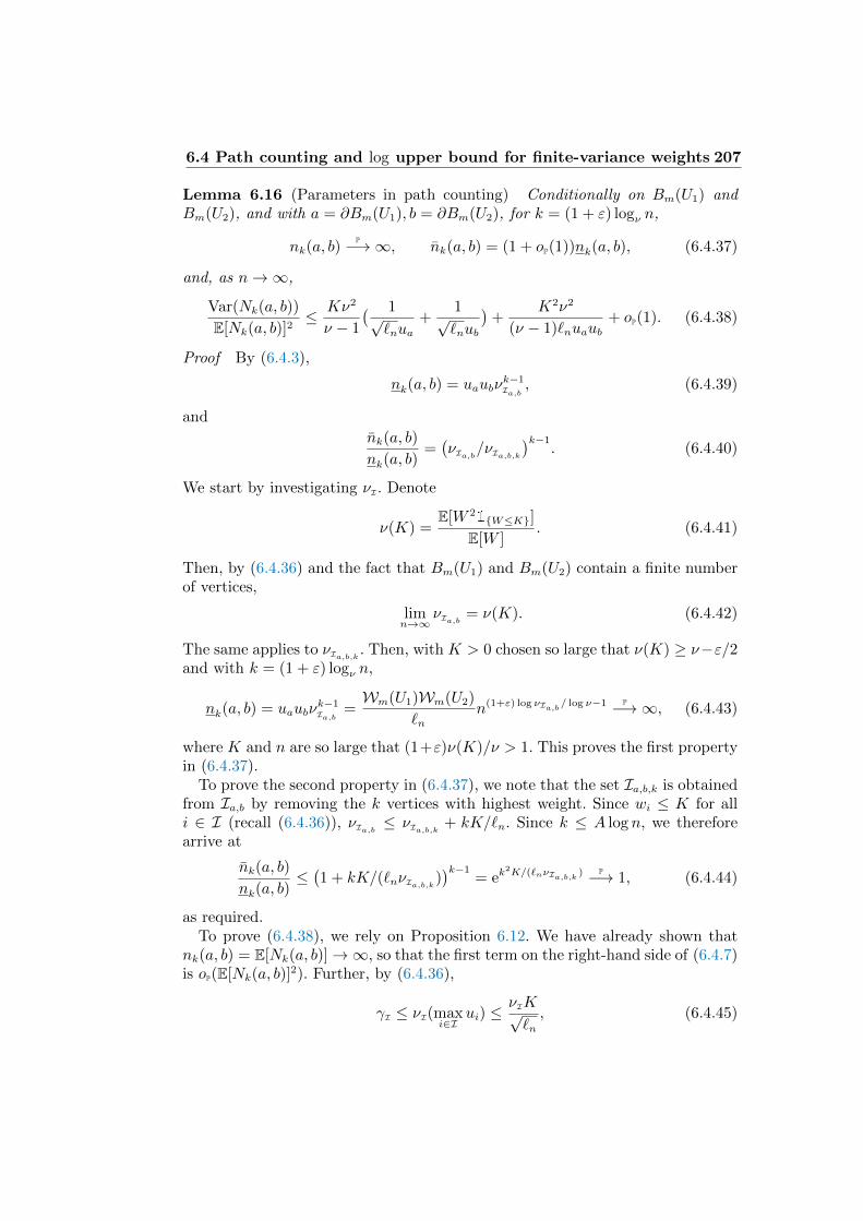
6.4 Path counting and log upper bound for finite-variance weights 207
Lemma 6.16 (Parameters in path counting) Conditionally on Bm(U1) andBm(U2), and with a = ∂Bm(U1), b = ∂Bm(U2), for k = (1 + ε) logν n,
nk(a, b)P−→∞, nk(a, b) = (1 + oP(1))nk(a, b), (6.4.37)
and, as n→∞,
Var(Nk(a, b))
E[Nk(a, b)]2≤ Kν2
ν − 1
( 1√`nua
+1√`nub
)+
K2ν2
(ν − 1)`nuaub+ oP(1). (6.4.38)
Proof By (6.4.3),
nk(a, b) = uaubνk−1Ia,b
, (6.4.39)
and
nk(a, b)
nk(a, b)=(νIa,b/νIa,b,k
)k−1. (6.4.40)
We start by investigating νI. Denote
ν(K) =E[W 2
1W≤K]
E[W ]. (6.4.41)
Then, by (6.4.36) and the fact that Bm(U1) and Bm(U2) contain a finite numberof vertices,
limn→∞
νIa,b = ν(K). (6.4.42)
The same applies to νIa,b,k . Then, with K > 0 chosen so large that ν(K) ≥ ν−ε/2and with k = (1 + ε) logν n,
nk(a, b) = uaubνk−1Ia,b
=Wm(U1)Wm(U2)
`nn(1+ε) log νIa,b/ log ν−1 P−→∞, (6.4.43)
where K and n are so large that (1+ε)ν(K)/ν > 1. This proves the first propertyin (6.4.37).
To prove the second property in (6.4.37), we note that the set Ia,b,k is obtainedfrom Ia,b by removing the k vertices with highest weight. Since wi ≤ K for alli ∈ I (recall (6.4.36)), νIa,b ≤ νIa,b,k + kK/`n. Since k ≤ A log n, we thereforearrive at
nk(a, b)
nk(a, b)≤(1 + kK/(`nνIa,b,k)
)k−1= ek
2K/(`nνIa,b,k ) P−→ 1, (6.4.44)
as required.To prove (6.4.38), we rely on Proposition 6.12. We have already shown that
nk(a, b) = E[Nk(a, b)]→∞, so that the first term on the right-hand side of (6.4.7)is oP(E[Nk(a, b)]
2). Further, by (6.4.36),
γI ≤ νI(maxi∈I
ui) ≤νIK√`n, (6.4.45)
208 Small-world phenomena in inhomogeneous random graphs
so that, for k ≤ A log n with A > 1 fixed,
(1 +γIuaνI
)(1 +γIubνI
)k(e2k3γ2I/ν
3I − 1) = oP(1). (6.4.46)
Substituting these bounds into (6.4.38) and using (6.4.37) yields the claim.
Completion of the proof of Theorem 6.14
Now we are are ready to complete the proof of Theorem 6.14. We must show that
P(kn < distNRn(w)(U1, U2) <∞) = o(1). (6.4.47)
Indeed, then P(distNRn(w)(U1, U2) > kn | distNRn(w)(U1, U2) < ∞) = o(1) since,P(distNRn(w)(U1, U2) <∞)→ ζ2 > 0 by Theorem 3.17. We rewrite
P(kn < distNRn(w)(U1, U2) <∞) (6.4.48)
= P(kn < distNRn(w)(U1, U2) <∞, ∂Bm(U1) 6= ∅, ∂Bm(U2) 6= ∅)
≤ P(Nkn−2m(∂Bm(U1), ∂Bm(U2)) = 0, ∂Bm(U1) 6= ∅, ∂Bm(U2) 6= ∅).
Recall that k = kn = (1 + ε) logν n. By the Chebychev inequality [Volume 1,Theorem 2.18], the conditional probability of distNRn(w)(U1, U2) > kn givenBm(U1), Bm(U2) is at most
Var(Nk−2m(a, b))
E[Nk−2m(a, b)]2≤ Kν2
ν − 1
( 1√`nua
+1√`nub
)+
K2ν2
(ν − 1)`nuaub+ oP(1). (6.4.49)
When ∂Bm(U1) 6= ∅ and ∂Bm(U2) 6= ∅, by (6.4.34),
1√`nua
+1√`nub
P−→( Z(1)
m∑j=1
W ?(1)(j))−1
+( Z(2)
m∑j=1
W ?(2)(j))−1
P−→ 0, (6.4.50)
when m→∞. Therefore,
P(Nk−2m(a, b) = 0 | ∂Bm(U1) 6= ∅, ∂Bm(U2) 6= ∅
)P−→ 0, (6.4.51)
and, by Lebesgues’ Dominated Convergence Theorem [Volume 1, Theorem A.1],
P(distNRn(w)(U1, U2) > kn, ∂Bm(U1) 6= ∅, ∂Bm(U2) 6= ∅)→ 0, (6.4.52)
when first n→∞ followed by m→∞, which completes the proof.
We close this section by describing what happens when τ = 3, and there areno slowly-varying functions.
Distances for the critical case τ = 3
When τ = 3, wi is approximately c(n/i)1/2. It turns our that this changes thedistances only by a doubly logarithmic factor:
6.4 Path counting and log upper bound for finite-variance weights 209
Theorem 6.17 (Graph distances NRn(w) in critical τ = 3 case) Assume thatCondition 1.1(a)-(b) hold, and that there exists constants c2 > c1 > 0 and α > 0such that for all x ≤ nα,
[1− Fn](x) ≥ c1/x2, (6.4.53)
and for all x ≥ 0,
[1− Fn](x) ≤ c2/x2. (6.4.54)
Then, conditionally on distNRn(w)(U1, U2) <∞,
distNRn(w)(U1, U2) log log n
log nP−→ 1. (6.4.55)
The same results hold for CLn(w) and GRGn(w) under the same conditions.
The lower bound in Theorem 6.17 is already stated in Corollary 6.5. The upperbound can be proved using the path-counting techniques in Proposition 6.12 andadaptations of it. We now sketch the proof.
Let η > 0 and let
αn = eν1−ηn . (6.4.56)
Define the core of NRn(w) to be
Coren = i : wi ≥ αn. (6.4.57)
The proof of Theorem 6.17 follows from the following two propositions:
Proposition 6.18 (Typical distances in the core) Under the conditions of The-orem 6.17, let V ′1 , V
′2 ∈ Coren be chosen with probability proportional to their
weight, i.e.,
P(V ′i = j) =wj∑
v∈Corenwv, (6.4.58)
and let H ′n be the graph distance between V ′1 , V′
2 in Coren. Then, for any ε > 0,there exists an η > 0 such that
P(H ′n ≤
(1 + ε) log n
log logn
)→ 1. (6.4.59)
Proposition 6.19 (From the periphery to the core) Under the conditions ofTheorem 6.17, let U1, U2 be two vertices chosen uniformly at random from [n].Then, for any η > 0,
P(dNRn(w)(U1,Coren) ≤ ν1−ηn , dNRn(w)(U2,Coren) ≤ ν1−η
n )→ ζ2. (6.4.60)
Proof of Theorem 6.17 subject to Propositions 6.18–6.19. To see that Propositions6.18–6.19 imply Theorem 6.17, we note that
dNRn(w)(U1, U2) ≤ dNRn(w)(U1,Coren) + dNRn(w)(U2,Coren) (6.4.61)
+ dNRn(w)(V′
1 , V′
2),
210 Small-world phenomena in inhomogeneous random graphs
where V ′1 , V′
2 ∈ Coren are the vertices in Coren found first in the breadth-firstsearch from U1 and U2, respectively. Then, by Proposition 3.13, V ′1 , V
′2 ∈ Coren
are chosen with probability proportional to their weight. Fix kn = log n/ log logn.We conclude that, when n is so large that ν1−η
n ≤ εkn/4,
P(dNRn(w)(U1, U2) ≤ (1 + ε)kn) (6.4.62)
≥ P(dNRn(w)(Ui,Coren) ≤ ν1−η
n , i = 1, 2)
× P(dNRn(w)(V
′1 , V
′2) ≤ (1 + ε/2)kn | dNRn(w)(Ui,Coren) ≤ ν1−η
n , i = 1, 2).
By Proposition 6.19, the first probability converges to ζ2, and by Proposition6.18, the second probability converges to 1. We conclude that
P(dNRn(w)(U1, U2) ≤ (1 + ε)
log n
log logn
)→ ζ2.
Since also P(dNRn(w)(U1, U2) <∞)→ ζ2, this completes the proof.
The proofs of Propositions 6.18–6.19 follow from path-counting techniques sim-ilar to the ones carried out above. We now sketch their proofs, starting withProposition 6.18:
Proof of Proposition 6.18. We take
a = V ′1 , b = V ′2 , I = wi : wi ∈ [K,√αn]. (6.4.63)
The whole point is that there exists a constant c > 0 such that
νI ≥ c logαn = cν1−ηn , (6.4.64)
while ua ≥ αn/√`n, ub ≥ αn/
√`n, so that
E[Nk(a, b)] ≈ α2nckνk(1−η)n /`n →∞ (6.4.65)
for k = log n/((1− η) log νn) ≤ (1 + ε/2) log n/ log νn when η is such that 1/(1−η) ≤ 1 + ε/2. Further,
γI ≤√αn/
√`n, (6.4.66)
so that Var(Nk(a, b))/E[Nk(a, b)]2 → 0 by Proposition 6.12. Since νn = Θ(log n)
when τ = 3 (see (6.4.53)–(6.4.54) in Theorem 6.17), this completes the proof.
See Exercises 6.19–6.21 for some further properties of paths within the core.
Proof of Proposition 6.19. We again condition on ∂Bm(U1) 6= ∅, ∂Bm(U2) 6= ∅,the probability of which converges to ζ2 when first n→∞ followed by m→∞.Then, we perform a second moment method on the number of paths between∂Bm(Ui) and Coren. For this, we take k = ν1−η
n and
a = ∂Bm(U1), b = Coren, I = i : wi ≤ K \ (Bm(U1) ∪Bm(U2)).(6.4.67)
Then we follow the proof in (6.4.49)–(6.4.52) to show that
P(dNRn(w)(U1,Coren) > ν1−ηn , ∂Bm(U1) 6= ∅, ∂Bm(U2) 6= ∅)→ 0, (6.4.68)
6.4 Path counting and log upper bound for finite-variance weights 211
as required. Note, for this, that, conditionally on Bm(U1), Bm(U2)
E[Nk(a, b)] ≈ ν(K)kWm(U1)1
`n
∑i∈Coren
wi, (6.4.69)
where ν(K)→∞ as K →∞, and where, by (6.4.53),
1
n
∑i∈Coren
wi ≥ αn[1− Fn](αn) ≥ c/αn. (6.4.70)
Therefore, E[Nk(a, b)] → ∞ as soon as k ≥ 2 logαn/ log ν(K), which is satisfiedfor K sufficiently large and k = ν1−η
n . Exercise 6.22 asks you to complete theabove proof.
6.4.3 Distances for IRGn(κ): Proofs of Theorems 3.16 and 6.1(ii)
In this section, we use the path-counting techniques in Section 6.4.1 to givesome missing proofs for general inhomogeneous random graphs. We assume that(κn) is graphical sequence of kernels with limit irreducible κ, and with ν = ‖Tκ‖ ∈(1,∞). We start by proving Theorem 6.1(ii), and then we use it to prove Theorem3.16.
Logarithmic upper bound on distances in Theorem 6.1(ii)
Without loss of generality, we may assume that κ is bounded, i.e., supx,y κ(x, y) <∞. Indeed, we can always stochastically dominate v with an unbounded κn frombelow by IRGn(κn) with a bounded kernel that approximates it arbitrarily well.Since graph distances increase by decreasing κn, if we prove Theorem 6.1(ii) inthe bounded case, the unbounded case will follow immediately. Further, we canapproximate a bounded κn from above by a finite-type kernel. Therefore, it nowsuffices to prove Theorem 6.1(ii) for a kernel of finite type.
Let us set up the notation for the finite-types case. For u, v ∈ [n], we letκn(u, v) = κn;iu,iv , where iu ∈ [k] denotes the type of vertex u ∈ [n]. We assumethat, for all i, j ∈ [k],
limn→∞
κn;i,j = κi,j, (6.4.71)
and
limn→∞
µn(i) =1
n#v ∈ [n] : iv = i = µ(i). (6.4.72)
In this case, ‖Tκn‖ is the largest eigenvalue of the matrix M(n)
i,j = κn;i,jµn(j),which converges to the largest eigenvalue of the matrix Mi,j = κn;i,jµ(j), whichequals ν = ‖Tκ‖ ∈ (1,∞), by assumption. This factor arises due to the depletion-of-points effect, which guarantees that the paths used are self-avoiding. Withoutloss of generality, we assume that µ(i) > 0 for all i ∈ [k]. This sets the stage ofour analysis.
We fix m ≥ 1, and assume that ∂Bm(U1), ∂Bm(U2) 6= ∅. We will prove that
P(dIRGn(κn)(U1, U2) ≤ (1 + ε) logν n | Bm(U1), Bm(U2)
)= 1 + oP(1). (6.4.73)
212 Small-world phenomena in inhomogeneous random graphs
We follow the proof of Theorem 6.14, and rely on path-counting techniques. Weagain take
a = ∂Bm(U1), b = ∂Bm(U2), (6.4.74)
and
Ia,b = [n] \ (Bm(U1) ∪Bm(U2)). (6.4.75)
Recall that
Nk(a, b) = #π ∈ Pk(a, b) : π occupied. (6.4.76)
We aim to use the second moment method for Nk(a, b), for which we investigatethe mean and variance of Nk(a, b). We compute
E[Nk(a, b)] =∑
π∈Pk(a,b)
P(π occupied) =∑
π∈Pk(a,b)
k∏l=0
κn(πl, πl+1)
n(6.4.77)
≤ 1
n〈x, T kκny〉,
where x = (xi)ki=1,y = (yi)
ki=1 with xi the number of type i vertices in ∂Bm(U1)
and yi the number of type i vertices in ∂Bm(U2), respectively. An identical lowerbound holds with an extra factor (µ
n− k)/µ
n, where µ
n= minj∈[k] µn(j) →
minj∈[k] µ(j) > 0, by assumption.Recall the notation and results in Section 3.4, and in particular Theorem 3.8(b).
The types of U1 and U2 are asymptotically independent, and the probability thatU1 has type j is equal to µn(j), which converges to µ(j). On the event thatthe type of U1 equals j1, the vector of the numbers of individuals in ∂Bm(U1)converges in distribution to (Z(1,j1)
m (i))i∈[k], which, by Theorem 3.8(b), is close toM∞xκ(i) for some strictly positive random variable M∞. We conclude that
xd−→ Z(1,j1)
m (i), xd−→ Z(2,j2)
m (i), (6.4.78)
where the limiting branching processes are independent. Equation (6.4.78) re-places the convergence in Lemma 6.15 for GRGn(w).
We conclude that, for k = kn = (1 + ε) logν n, and conditionally on a =∂Bm(U1), b = ∂Bm(U2) such that ∂Bm(U1), ∂Bm(U2) 6= ∅,
E[Nk(a, b)]P−→∞. (6.4.79)
This completes the analysis of the first moment.
We next analyse Var(Nk(a, b)) and prove that Var(Nk(a, b))/E[Nk(a, b)]2 P−→
∞. Here our proof will be slightly more sketchy.Recall (6.4.18). In this case, we compute, to replace (6.4.19),
P(π, ρ occupied) = P(π occupied)P(ρ occupied | π occupied). (6.4.80)
Recall the definition of a shape in (6.4.16). Fix σ ∈ Shapem,l and ρ ∈ Pk(a, b)with Shape(π, ρ) = σ. The factor P(ρ occupied | π occupied), summed out overthe free vertices of ρ (i.e., the ones that are not also vertices in π) gives rise to
6.4 Path counting and log upper bound for finite-variance weights 213
m factors of the form T tiκn(iπui , iπvi )/n for i ∈ [m + 1] and some vertices πui and
πvi in the path (πi)ki=0. We use that, uniformly in t ≥ 1,
k2
nmaxi,j∈[k]
T tκn(i, j) ≤ Ck2
n‖Tκn‖t, (6.4.81)
where k2 is an upper bound on the number of choices for πui and πvi . Thus, for
every of the m subpaths of length ti we obtain a factor Ck2
n‖Tκn‖ti . We arrive at∑
π, ρ ∈ Pk(a, b)Shape(π, ρ) = σ
P(π, ρ occupied) (6.4.82)
≤ E[Nk(a, b)]m∏i=1
Ck2
n‖Tκn‖ti ≤ E[Nk(a, b)]‖Tκn‖k−l
(Ck2
n
)m.
This replaces (6.4.20), and the proof can now be completed in an identical way asthe proof of (6.4.7) combined with the proof of (6.4.47) in the proof of Theorem6.14. We omit further details.
Concentration of the giant in Theorem 3.16
By Theorem 3.11, we know that IRGn(κn) converges in probability in the localweak sense. Therefore, we aim to apply Theorem 2.13, for which we need to verifythat(2.5.7) holds.
We rewrite the expectation appearing in (2.5.7) as
1
n2E[#x, y ∈ [n] : |C (x)|, |C (y)| ≥ k, x←→/ y
]= P
(|C (U1)|, |C (U2)| ≥ k, U1 ←→/ U2
). (6.4.83)
We condition on Bk(U1) and Bk(U2), and note that the events that |C (U1)| ≥ kand |C (U2)| ≥ k are measurable with respect to Bk(U1) and Bk(U2) to obtain
P(|C (U1)|, |C (U2)| ≥ k, U1 ←→/ U2
)= E
[1|C (U1)|,|C (U2)|≥kP
(U1 ←→/ U2 | Bk(U1), Bk(U2)
)]. (6.4.84)
By Exercise 6.23, together with Theorem 3.11,
limk→∞
limn→∞
P(∂Bk(U1) = ∅, |C (U1)| ≥ k
)= 0. (6.4.85)
Therefore,
P(|C (U1)|, |C (U2)| ≥ k, U1 ←→/ U2
)= E
[1|C (U1)|,|C (U2)|≥k,∂Bk(U1),∂Bk(U2)6=∅P
(U1 ←→/ U2 | Bk(U1), Bk(U2)
)].
(6.4.86)
When ∂Bk(U1), ∂Bk(U2) 6= ∅, it immediately follows that |C (U1)|, |C (U2)| ≥ k.
214 Small-world phenomena in inhomogeneous random graphs
Thus,
P(|C (U1)|, |C (U2)| ≥ k, U1 ←→/ U2
)= E
[1∂Bk(U1),∂Bk(U2)6=∅P
(U1 ←→/ U2 | Bk(U1), Bk(U2)
)]+ ok(1), (6.4.87)
where ok(1) denotes a quantity that tends to zero when first n→∞ followed byk →∞.
In the proof of Theorem 6.1(ii), we have shown that, on ∂Bk(U1), ∂Bk(U2) 6=∅,
P(dIRGn(κn)(U1, U2) ≤ (1 + ε) logν n | Bk(U1), Bk(U2)
)= 1 + oP(1). (6.4.88)
In particular, on ∂Bk(U1), ∂Bk(U2) 6= ∅,
P(U1 ←→/ U2 | Bk(U1), Bk(U2)
)= oP(1). (6.4.89)
Since also P(U1 ←→/ U2 | Bk(U1), Bk(U2)
)≤ 1, the Dominated Convergence
Theorem [Volume 1, Theorem A.1] completes the proof of (2.5.7) for IRGn(κn),as required.
6.5 Related results on distances for inhomogeneous random graphs
In this section, we discuss some related results for inhomogeneous randomgraphs. While we give intuition about their proofs, we shall not include them infull detail.
6.5.1 The diameter in inhomogeneous random graphs
In this section, we investigate the diameter of IRGn(κn), which is defined to bethe maximal finite graph distance between any pair of vertices, i.e., the diameterdiam(G) of the graph G equals
diam(G) = maxu,v : distG(u,v)<∞
distG(u, v). (6.5.1)
We shall see that for IRGn(κ), the diameter tends to be much larger than thetypical graph distances, which is due to long thin lines which are distributedas subcritical IRGn(κ) with a subcritical κ by a duality principle for IRGn(κ).Before we state the results, we introduce the notion of the dual kernel :
Definition 6.20 (Dual kernel for IRGn(κ)) Let (κn) be a sequence of super-critical kernels with limit κ. The dual kernel is the kernel κ defined by κ(x, y) =κ(x, y), with reference measure dµ(x) = (1− ζκ(x))µ(dx).
The dual kernel shall describe the graph after the removal of the giant compo-nent. Here, the reference measure µ measures the size of the graph. In this case,a vertex x is in the giant component with probability 1 − ζκ(x), in which caseit must be removed. Thus, µ describes the proportion of vertices of the various
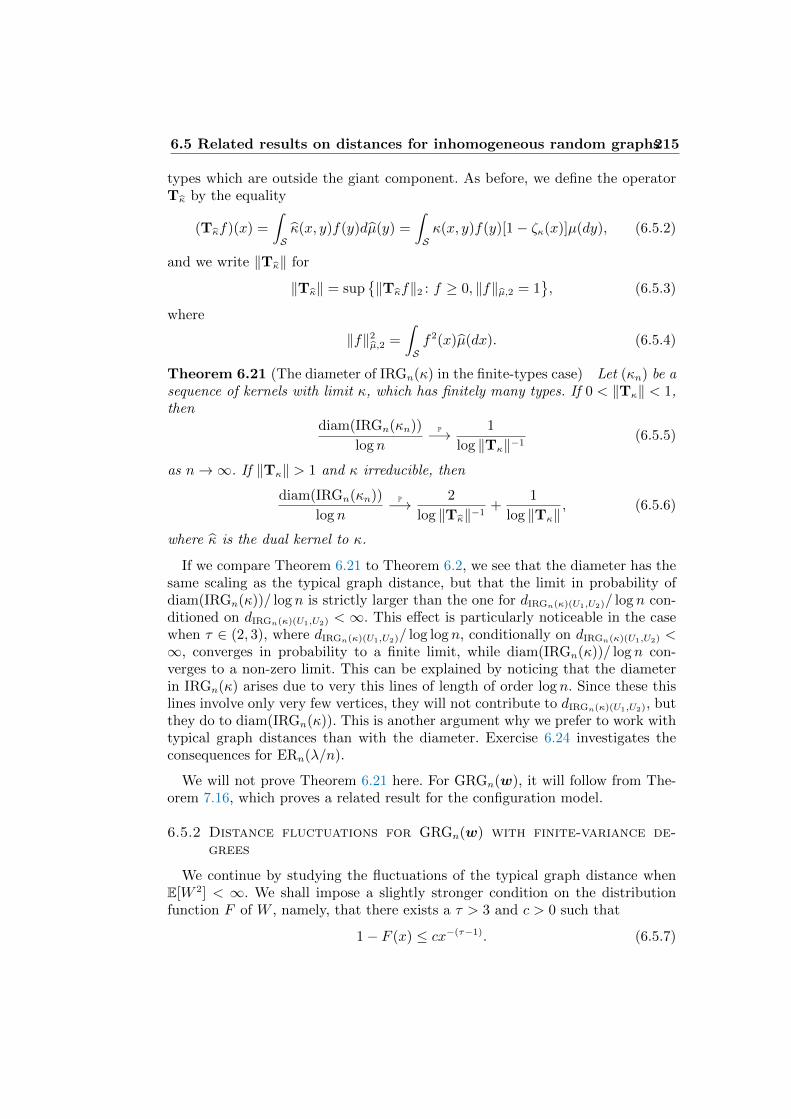
6.5 Related results on distances for inhomogeneous random graphs215
types which are outside the giant component. As before, we define the operatorTκ by the equality
(Tκf)(x) =
∫Sκ(x, y)f(y)dµ(y) =
∫Sκ(x, y)f(y)[1− ζκ(x)]µ(dy), (6.5.2)
and we write ‖Tκ‖ for
‖Tκ‖ = sup‖Tκf‖2 : f ≥ 0, ‖f‖µ,2 = 1
, (6.5.3)
where
‖f‖2µ,2 =
∫Sf2(x)µ(dx). (6.5.4)
Theorem 6.21 (The diameter of IRGn(κ) in the finite-types case) Let (κn) be asequence of kernels with limit κ, which has finitely many types. If 0 < ‖Tκ‖ < 1,then
diam(IRGn(κn))
log nP−→ 1
log ‖Tκ‖−1(6.5.5)
as n→∞. If ‖Tκ‖ > 1 and κ irreducible, then
diam(IRGn(κn))
log nP−→ 2
log ‖Tκ‖−1+
1
log ‖Tκ‖, (6.5.6)
where κ is the dual kernel to κ.
If we compare Theorem 6.21 to Theorem 6.2, we see that the diameter has thesame scaling as the typical graph distance, but that the limit in probability ofdiam(IRGn(κ))/ log n is strictly larger than the one for dIRGn(κ)(U1,U2)/ log n con-ditioned on dIRGn(κ)(U1,U2) < ∞. This effect is particularly noticeable in the casewhen τ ∈ (2, 3), where dIRGn(κ)(U1,U2)/ log logn, conditionally on dIRGn(κ)(U1,U2) <∞, converges in probability to a finite limit, while diam(IRGn(κ))/ log n con-verges to a non-zero limit. This can be explained by noticing that the diameterin IRGn(κ) arises due to very this lines of length of order log n. Since these thislines involve only very few vertices, they will not contribute to dIRGn(κ)(U1,U2), butthey do to diam(IRGn(κ)). This is another argument why we prefer to work withtypical graph distances than with the diameter. Exercise 6.24 investigates theconsequences for ERn(λ/n).
We will not prove Theorem 6.21 here. For GRGn(w), it will follow from The-orem 7.16, which proves a related result for the configuration model.
6.5.2 Distance fluctuations for GRGn(w) with finite-variance de-grees
We continue by studying the fluctuations of the typical graph distance whenE[W 2] < ∞. We shall impose a slightly stronger condition on the distributionfunction F of W , namely, that there exists a τ > 3 and c > 0 such that
1− F (x) ≤ cx−(τ−1). (6.5.7)
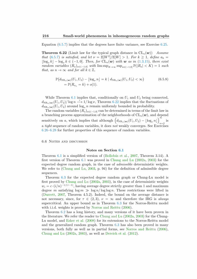
216 Small-world phenomena in inhomogeneous random graphs
Equation (6.5.7) implies that the degrees have finite variance, see Exercise 6.25.
Theorem 6.22 (Limit law for the typical graph distance in CLn(w)) Assumethat (6.5.7) is satisfied, and let ν = E[W 2]/E[W ] > 1. For k ≥ 1, define ak =blogν kc − logν k ∈ (−1, 0]. Then, for CLn(w) with w as in (1.3.15), there existrandom variables (Ra)a∈(−1,0] with lim supK→∞ supa∈(−1,0] P(|Ra| < K) = 1 suchthat, as n→∞ and for all k ∈ Z,
P(dNRn(w)(U1, U2)− blogν nc = k | dNRn(w)(U1, U2) <∞
)(6.5.8)
= P(Ran = k) + o(1).
While Theorem 6.1 implies that, conditionally on U1 and U2 being connected,dNRn(w)(U1, U2)/ log n
P−→ 1/ log ν, Theorem 6.22 implies that the fluctuations ofdNRn(w)(U1, U2) around logν n remain uniformly bounded in probability.
The random variables (Ra)a∈(−1,0] can be determined in terms of the limit law ina branching process approximation of the neighborhoods of CLn(w), and depend
sensitively on a, which implies that although(dNRn(w)(U1, U2) − blogν nc
)∞n=2
is
a tight sequence of random variables, it does not weakly converges. See Exercises6.26–6.28 for further properties of this sequence of random variables.
6.6 Notes and discussion
Notes on Section 6.1
Theorem 6.1 is a simplified version of (Bollobas et al., 2007, Theorem 3.14). Afirst version of Theorem 6.1 was proved in Chung and Lu (2002a, 2003) for theexpected degree random graph, in the case of admissible deterministic weights.We refer to (Chung and Lu, 2003, p. 94) for the definition of admissible degreesequences.
Theorem 6.3 for the expected degree random graph or Chung-Lu model isfirst proved by Chung and Lu (2002a, 2003), in the case of deterministic weightswi = c ·(i/n)−1/(τ−1), having average degree strictly greater than 1 and maximumdegree m satisfying logm log n/ log log n. These restrictions were lifted in(Durrett, 2007, Theorem 4.5.2). Indeed, the bound on the average distance isnot necessary, since, for τ ∈ (2, 3), ν = ∞ and therefore the IRG is alwayssupercritical. An upper bound as in Theorem 6.3 for the Norros-Reittu modelwith i.i.d. weights is proved by Norros and Reittu (2006).
Theorem 6.2 has a long history, and many versions of it have been proven inthe literature. We refer the reader to Chung and Lu (2002a, 2003) for the Chung-Lu model, and Esker et al. (2008) for its extensions to the Norros-Reittu modeland the generalized random graph. Theorem 6.3 has also been proved in manyversions, both fully as well as in partial forms, see Norros and Reittu (2006),Chung and Lu (2002a, 2003), as well as Dereich et al. (2012).
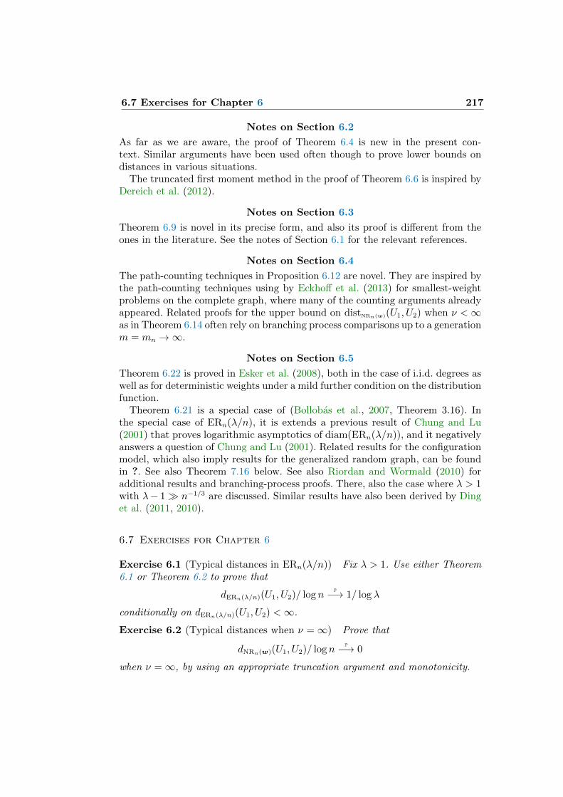
6.7 Exercises for Chapter 6 217
Notes on Section 6.2
As far as we are aware, the proof of Theorem 6.4 is new in the present con-text. Similar arguments have been used often though to prove lower bounds ondistances in various situations.
The truncated first moment method in the proof of Theorem 6.6 is inspired byDereich et al. (2012).
Notes on Section 6.3
Theorem 6.9 is novel in its precise form, and also its proof is different from theones in the literature. See the notes of Section 6.1 for the relevant references.
Notes on Section 6.4
The path-counting techniques in Proposition 6.12 are novel. They are inspired bythe path-counting techniques using by Eckhoff et al. (2013) for smallest-weightproblems on the complete graph, where many of the counting arguments alreadyappeared. Related proofs for the upper bound on distNRn(w)(U1, U2) when ν <∞as in Theorem 6.14 often rely on branching process comparisons up to a generationm = mn →∞.
Notes on Section 6.5
Theorem 6.22 is proved in Esker et al. (2008), both in the case of i.i.d. degrees aswell as for deterministic weights under a mild further condition on the distributionfunction.
Theorem 6.21 is a special case of (Bollobas et al., 2007, Theorem 3.16). Inthe special case of ERn(λ/n), it is extends a previous result of Chung and Lu(2001) that proves logarithmic asymptotics of diam(ERn(λ/n)), and it negativelyanswers a question of Chung and Lu (2001). Related results for the configurationmodel, which also imply results for the generalized random graph, can be foundin ?. See also Theorem 7.16 below. See also Riordan and Wormald (2010) foradditional results and branching-process proofs. There, also the case where λ > 1with λ− 1 n−1/3 are discussed. Similar results have also been derived by Dinget al. (2011, 2010).
6.7 Exercises for Chapter 6
Exercise 6.1 (Typical distances in ERn(λ/n)) Fix λ > 1. Use either Theorem6.1 or Theorem 6.2 to prove that
dERn(λ/n)(U1, U2)/ log nP−→ 1/ log λ
conditionally on dERn(λ/n)(U1, U2) <∞.
Exercise 6.2 (Typical distances when ν =∞) Prove that
dNRn(w)(U1, U2)/ log nP−→ 0
when ν =∞, by using an appropriate truncation argument and monotonicity.
218 Small-world phenomena in inhomogeneous random graphs
Exercise 6.3 (Power-law tails in key example of deterministic weights) Let wbe defined as in (1.3.15), and assume that F satisfies
1− F (x) = x−(τ−1)L(x), (6.7.1)
where the exponent satisfies τ ∈ (2, 3), and where x 7→ L(x) is slowly varying.Prove that (6.1.4) holds.
Exercise 6.4 (Power-law tails for i.i.d. weights) For i.i.d. weights w = (wi)i∈[n]
with distribution F satisfying that (6.7.1) with τ ∈ (2, 3), and where x 7→ L(x) isslowly varying. Prove that (6.1.4) holds with probability converging to 1.
Exercise 6.5 (Bound on truncated forward degree νn(b)) Prove (6.2.42) bycombining (1.4.2) in Lemma 1.13 with `n = Θ(n) by Conditions 1.1(a)–(b).
Exercise 6.6 (Conditions (6.2.1) and Condition 6.4) Show that when there isprecisely one vertex with weight w1 =
√n, whereas wi = λ > 1, then (6.2.1) holds,
but Condition 6.4 does not. Argue that the upper bound derived in Theorem 6.4is not sharp, since the vertex 1 can occur at most once in a self-avoiding path.
Exercise 6.7 (Lower bound on fluctuations) Adapt the proof of Theorem 6.4to show that for every ε, we can find a constant K = K(ε) > 0 such that
P(dNRn(w)(U1, U2) ≤ logνn n−K
)≤ ε. (6.7.2)
Conclude that if log νn = log ν + o(1/ log n), then the same statement holds withlogν n replacing logνn n.
Exercise 6.8 (Proof Corollary 6.5) Adapt the proof to Theorem 6.4 to proveCorollary 6.5.
Exercise 6.9 (Lower bound on typical distances for τ = 3) Let wi = c√
(n/i),so that τ = 3. Prove that νn/ log n→ c. Use Corollary 6.5 to obtain that for anyε > 0,
P(dNRn(w)(U1, U2) ≤ (1− ε) log n
log logn
)= o(1). (6.7.3)
Exercise 6.10 (Lower bound on typical distances for τ ∈ (2, 3)) Let wi =c/i1/(τ−1) with τ ∈ (2, 3). Prove that there exists a constant c′ > 0 such thatνn ≥ c′n(3−τ)/(τ−1). Show that Corollary 6.5 implies that dNRn(w)(U1, U2) ≥ (τ −1)/(τ − 3) in this case. How useful is this bound?
Exercise 6.11 (Convergence in probability of typical distance in IRGn(κn))Suppose that the graphical sequence of kernels (κn) satisfies supx,y,n κn(x, y) <∞,where the limit κ is irreducible and ν = ‖Tκ‖ > 1. Prove that Theorem 3.16together with Theorem 6.1(i–ii) imply that, conditionally on dIRGn(κn)(U1, U2) <∞,
dIRGn(κn)(U1, U2)/ log nP−→ 1/ log ν. (6.7.4)
Exercise 6.12 (Convergence in probability of typical distance in IRGn(κn))
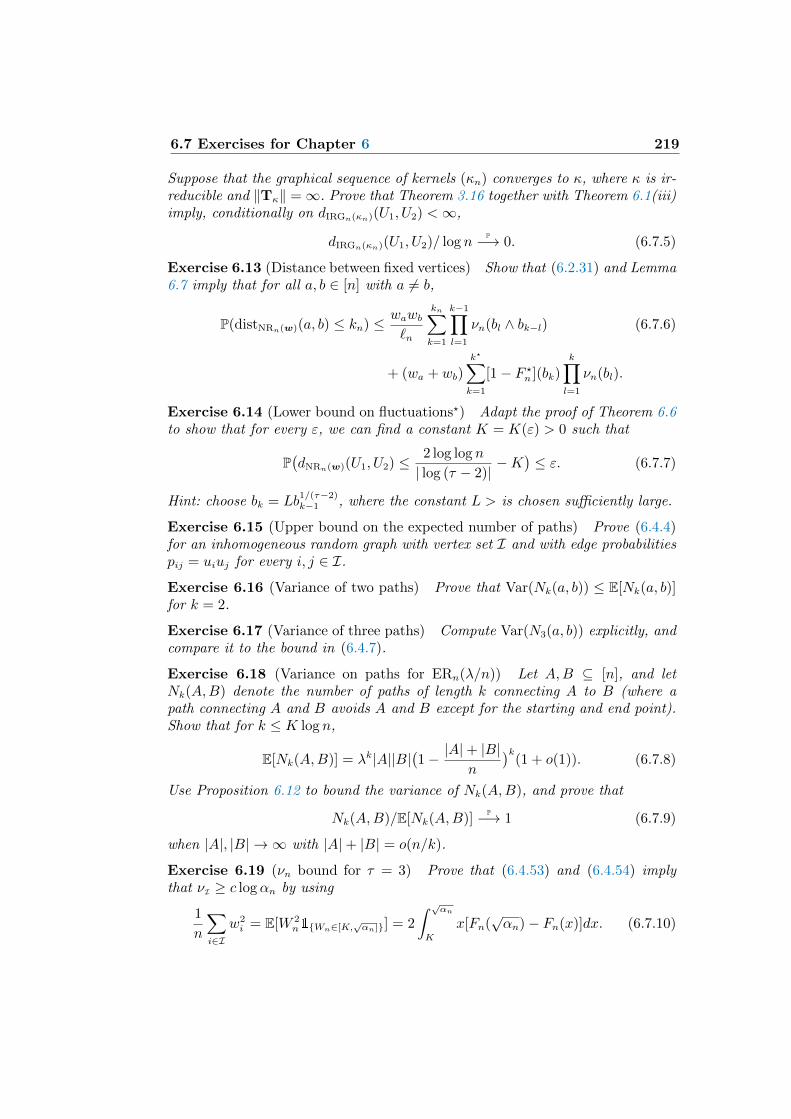
6.7 Exercises for Chapter 6 219
Suppose that the graphical sequence of kernels (κn) converges to κ, where κ is ir-reducible and ‖Tκ‖ =∞. Prove that Theorem 3.16 together with Theorem 6.1(iii)imply, conditionally on dIRGn(κn)(U1, U2) <∞,
dIRGn(κn)(U1, U2)/ log nP−→ 0. (6.7.5)
Exercise 6.13 (Distance between fixed vertices) Show that (6.2.31) and Lemma6.7 imply that for all a, b ∈ [n] with a 6= b,
P(distNRn(w)(a, b) ≤ kn) ≤ wawb`n
kn∑k=1
k−1∏l=1
νn(bl ∧ bk−l) (6.7.6)
+ (wa + wb)k?∑k=1
[1− F ?n ](bk)
k∏l=1
νn(bl).
Exercise 6.14 (Lower bound on fluctuations?) Adapt the proof of Theorem 6.6to show that for every ε, we can find a constant K = K(ε) > 0 such that
P(dNRn(w)(U1, U2) ≤ 2 log log n
| log (τ − 2)| −K)≤ ε. (6.7.7)
Hint: choose bk = Lb1/(τ−2)k−1 , where the constant L > is chosen sufficiently large.
Exercise 6.15 (Upper bound on the expected number of paths) Prove (6.4.4)for an inhomogeneous random graph with vertex set I and with edge probabilitiespij = uiuj for every i, j ∈ I.
Exercise 6.16 (Variance of two paths) Prove that Var(Nk(a, b)) ≤ E[Nk(a, b)]for k = 2.
Exercise 6.17 (Variance of three paths) Compute Var(N3(a, b)) explicitly, andcompare it to the bound in (6.4.7).
Exercise 6.18 (Variance on paths for ERn(λ/n)) Let A,B ⊆ [n], and letNk(A,B) denote the number of paths of length k connecting A to B (where apath connecting A and B avoids A and B except for the starting and end point).Show that for k ≤ K log n,
E[Nk(A,B)] = λk|A||B|(1− |A|+ |B|
n
)k(1 + o(1)). (6.7.8)
Use Proposition 6.12 to bound the variance of Nk(A,B), and prove that
Nk(A,B)/E[Nk(A,B)]P−→ 1 (6.7.9)
when |A|, |B| → ∞ with |A|+ |B| = o(n/k).
Exercise 6.19 (νn bound for τ = 3) Prove that (6.4.53) and (6.4.54) implythat νI ≥ c logαn by using
1
n
∑i∈I
w2i = E[W 2
n1Wn∈[K,√αn]] = 2
∫ √αnK
x[Fn(√αn)− Fn(x)]dx. (6.7.10)
220 Small-world phenomena in inhomogeneous random graphs
Exercise 6.20 (Expected number of paths within Coren diverges) Prove that
E[Nk(a, b)]→∞for a = V ′1 , b = V ′2 and k = log n/((1− η) log νn).
Exercise 6.21 (Concentration of number of paths within Coren) Prove that
Var(Nk(a, b))/E[Nk(a, b)]2 → 0
for a = V ′1 , b = V ′2 and k = log n/((1− η) log νn).
Exercise 6.22 (Completion proof Proposition 6.18) Complete the proof ofProposition 6.18 by adapting the arguments in (6.4.49)–(6.4.52).
Exercise 6.23 (Size versus boundary of large clusters) Let the graph G = (V,E)converge locally weakly in probability. Prove that
limk→∞
limn→∞
P(∂Bk(U1) = ∅, |C (U1)| ≥ k
)= 0. (6.7.11)
Exercise 6.24 (Diameter of ERn(λ/n)) Recall Theorem 6.21. For ERn(λ/n),show that ‖Tκ‖ = λ and ‖Tκ‖ = µλ, where µλ is the dual parameter in [Volume1, (3.6.6)], so that Theorem 6.21 becomes
diam(ERn(λ/n))
log nP−→ 2
logµ−1λ
+1
log λ. (6.7.12)
Exercise 6.25 (Finite variance degrees when (6.5.7) holds) Prove that (6.5.7)implies that E[W 2] < ∞. Use this to prove that the degrees have uniformlybounded variance when (6.5.7) holds.
Exercise 6.26 (Tightness of centered typical graph distances in CLn(w)) Provethat, under the conditions of Theorem 6.22, and conditionally on dNRn(w)(U1, U2) <
∞, the sequence(dNRn(w)(U1, U2)− blogν nc
)∞n=2
is tight.
Exercise 6.27 (Non-convergence of centered typical graph distances in CLn(w))Prove that, under the conditions of Theorem 6.22, and conditionally on dNRn(w)(U1, U2) <∞, the sequence dNRn(w)(U1, U2)−blogν nc does not weakly converge when the dis-tribution of Ra depends continuously on a and when there are a, b ∈ (−1, 0] suchthat the distribution of Ra is not equal to the one of Rb.
Exercise 6.28 (Extension Theorem 6.22 to GRGn(w) and NRn(w)) Use [Vol-ume 1, Theorem 6.18] to prove that Theorem 6.22 holds verbatim for GRGn(w)and NRn(w) when (6.5.7) holds.
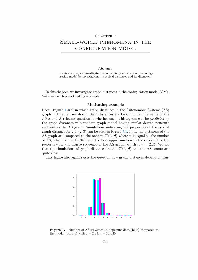
Chapter 7
Small-world phenomena in theconfiguration model
Abstract
In this chapter, we investigate the connectivity structure of the config-uration model by investigating its typical distances and its diameter.
In this chapter, we investigate graph distances in the configuration model (CM).We start with a motivating example.
Motivating example
Recall Figure 1.4(a) in which graph distances in the Autonomous Systems (AS)graph in Internet are shown. Such distances are known under the name of theAS-count. A relevant question is whether such a histogram can be predicted bythe graph distances in a random graph model having similar degree structureand size as the AS graph. Simulations indicating the properties of the typicalgraph distance for τ ∈ (2, 3) can be seen in Figure 7.1. In it, the distances of theAS-graph are compared to the ones in CMn(d) where n is equal to the numberof AS, which is n = 10, 940, and the best approximation to the exponent of thepower-law for the degree sequence of the AS-graph, which is τ = 2.25. We seethat the simulations of graph distances in this CMn(d) and the AS-counts arequite close.
This figure also again raises the question how graph distances depend on ran-
0 1 2 3 4 5 6 7 8 9 10 110.0
0.1
0.2
0.3
0.4
Figure 7.1 Number of AS traversed in hopcount data (blue) compared tothe model (purple) with τ = 2.25, n = 10, 940.
221
222 Small-world phenomena in the configuration model
dom graph properties, such as n, but also the structure of the random graph inquestion. The configuration model is a highly flexible model, in the sense that itallows to choose the degree distribution in a highly general way. Thus, we canuse the CM to single out the relation between the graph distances and the degreestructure, in a similar way as that it allows to investigate the size of the giantcomponent and the connectivity as a function of the degree distribution as inChapter 4. Finally, we can verify whether the graph distances are closely relatedto those in inhomogeneous random graphs, as discussed in Chapter 6, so as tospot another sign of the wanted universality of structural properties of randomgraphs with similar degree distributions.
Organization of this chapter
This chapter is organized as follows. In Section 7.1, we study the typical graphdistance in the configuration model. In Section 7.2, we prove these distance re-sults, using path counting techniques and comparisons to branching processes.In Section 7.3, we study infinite-mean branching processes, as these arise in theconfiguration model with infinite-variance degrees. In Section 7.4, we study thediameter of the configuration model. In Section 7.5, we state further results in theconfiguration model. We close this chapter with notes and discussion in Section7.6, and with exercises in Section 7.7.
7.1 The small-world phenomenon in CMn(d)
In this section, we describe the main results on distances in the configurationmodel, both in the case of finite-variance degrees as well as in the case of infinite-variance degrees. These results will be proved in the following sections.
Distances in configuration models with finite-variance degrees
We start by analyzing the typical graph distance in the case where the configu-ration model CMn(d) when Conditions 1.5(a)-(c) hold:
Theorem 7.1 (Typical distances in CMn(d) for finite-variance degrees) In theconfiguration model CMn(d), where the degrees d = (di)i∈[n] satisfy Conditions1.5(a)-(c) and where ν > 1, conditionally on distCMn(d)(U1, U2) <∞,
distCMn(d)(U1, U2)/ log nP−→ 1/ log ν. (7.1.1)
Theorem 7.1 shows that the typical distances in CMn(d) are of order logν n,and is thus similar in spirit as Theorem 6.2. We shall see that also its proof isquite similar.
Finite mean, infinite variance degrees
We next study the typical distance of the configuration model with degrees havingfinite mean and infinite variance. We start by formulating the precise condition onthe degrees that we shall work with. This condition is identical to the condition
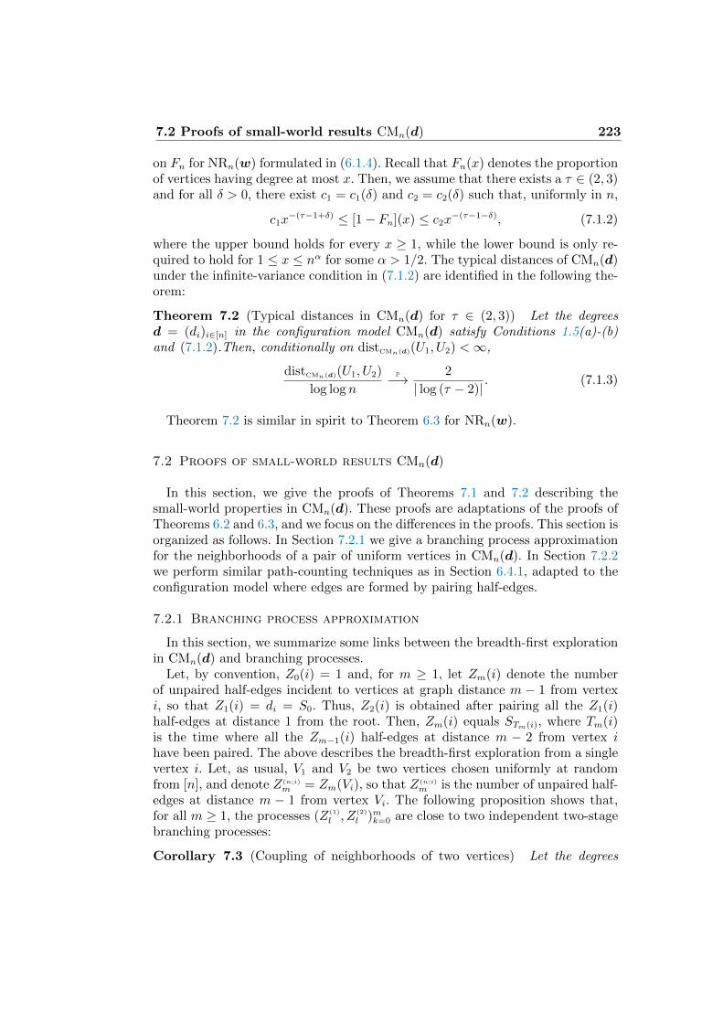
7.2 Proofs of small-world results CMn(d) 223
on Fn for NRn(w) formulated in (6.1.4). Recall that Fn(x) denotes the proportionof vertices having degree at most x. Then, we assume that there exists a τ ∈ (2, 3)and for all δ > 0, there exist c1 = c1(δ) and c2 = c2(δ) such that, uniformly in n,
c1x−(τ−1+δ) ≤ [1− Fn](x) ≤ c2x
−(τ−1−δ), (7.1.2)
where the upper bound holds for every x ≥ 1, while the lower bound is only re-quired to hold for 1 ≤ x ≤ nα for some α > 1/2. The typical distances of CMn(d)under the infinite-variance condition in (7.1.2) are identified in the following the-orem:
Theorem 7.2 (Typical distances in CMn(d) for τ ∈ (2, 3)) Let the degreesd = (di)i∈[n] in the configuration model CMn(d) satisfy Conditions 1.5(a)-(b)and (7.1.2).Then, conditionally on distCMn(d)(U1, U2) <∞,
distCMn(d)(U1, U2)
log log nP−→ 2
| log (τ − 2)| . (7.1.3)
Theorem 7.2 is similar in spirit to Theorem 6.3 for NRn(w).
7.2 Proofs of small-world results CMn(d)
In this section, we give the proofs of Theorems 7.1 and 7.2 describing thesmall-world properties in CMn(d). These proofs are adaptations of the proofs ofTheorems 6.2 and 6.3, and we focus on the differences in the proofs. This section isorganized as follows. In Section 7.2.1 we give a branching process approximationfor the neighborhoods of a pair of uniform vertices in CMn(d). In Section 7.2.2we perform similar path-counting techniques as in Section 6.4.1, adapted to theconfiguration model where edges are formed by pairing half-edges.
7.2.1 Branching process approximation
In this section, we summarize some links between the breadth-first explorationin CMn(d) and branching processes.
Let, by convention, Z0(i) = 1 and, for m ≥ 1, let Zm(i) denote the numberof unpaired half-edges incident to vertices at graph distance m − 1 from vertexi, so that Z1(i) = di = S0. Thus, Z2(i) is obtained after pairing all the Z1(i)half-edges at distance 1 from the root. Then, Zm(i) equals STm(i), where Tm(i)is the time where all the Zm−1(i) half-edges at distance m − 2 from vertex ihave been paired. The above describes the breadth-first exploration from a singlevertex i. Let, as usual, V1 and V2 be two vertices chosen uniformly at randomfrom [n], and denote Z(n;i)
m = Zm(Vi), so that Z(n;i)
m is the number of unpaired half-edges at distance m − 1 from vertex Vi. The following proposition shows that,for all m ≥ 1, the processes (Z(1)
l , Z(2)
l )mk=0 are close to two independent two-stagebranching processes:
Corollary 7.3 (Coupling of neighborhoods of two vertices) Let the degrees
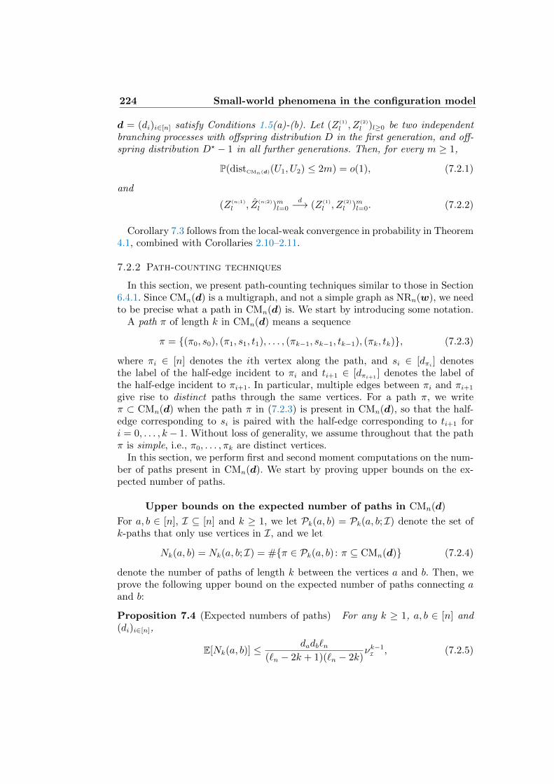
224 Small-world phenomena in the configuration model
d = (di)i∈[n] satisfy Conditions 1.5(a)-(b). Let (Z(1)
l , Z(2)
l )l≥0 be two independentbranching processes with offspring distribution D in the first generation, and off-spring distribution D? − 1 in all further generations. Then, for every m ≥ 1,
P(distCMn(d)(U1, U2) ≤ 2m) = o(1), (7.2.1)
and
(Z(n;1)
l , Z(n;2)
l )ml=0
d−→ (Z(1)
l , Z(2)
l )ml=0. (7.2.2)
Corollary 7.3 follows from the local-weak convergence in probability in Theorem4.1, combined with Corollaries 2.10–2.11.
7.2.2 Path-counting techniques
In this section, we present path-counting techniques similar to those in Section6.4.1. Since CMn(d) is a multigraph, and not a simple graph as NRn(w), we needto be precise what a path in CMn(d) is. We start by introducing some notation.
A path π of length k in CMn(d) means a sequence
π = (π0, s0), (π1, s1, t1), . . . , (πk−1, sk−1, tk−1), (πk, tk), (7.2.3)
where πi ∈ [n] denotes the ith vertex along the path, and si ∈ [dπi ] denotesthe label of the half-edge incident to πi and ti+1 ∈ [dπi+1
] denotes the label ofthe half-edge incident to πi+1. In particular, multiple edges between πi and πi+1
give rise to distinct paths through the same vertices. For a path π, we writeπ ⊂ CMn(d) when the path π in (7.2.3) is present in CMn(d), so that the half-edge corresponding to si is paired with the half-edge corresponding to ti+1 fori = 0, . . . , k − 1. Without loss of generality, we assume throughout that the pathπ is simple, i.e., π0, . . . , πk are distinct vertices.
In this section, we perform first and second moment computations on the num-ber of paths present in CMn(d). We start by proving upper bounds on the ex-pected number of paths.
Upper bounds on the expected number of paths in CMn(d)
For a, b ∈ [n], I ⊆ [n] and k ≥ 1, we let Pk(a, b) = Pk(a, b; I) denote the set ofk-paths that only use vertices in I, and we let
Nk(a, b) = Nk(a, b; I) = #π ∈ Pk(a, b) : π ⊆ CMn(d) (7.2.4)
denote the number of paths of length k between the vertices a and b. Then, weprove the following upper bound on the expected number of paths connecting aand b:
Proposition 7.4 (Expected numbers of paths) For any k ≥ 1, a, b ∈ [n] and(di)i∈[n],
E[Nk(a, b)] ≤dadb`n
(`n − 2k + 1)(`n − 2k)νk−1I , (7.2.5)
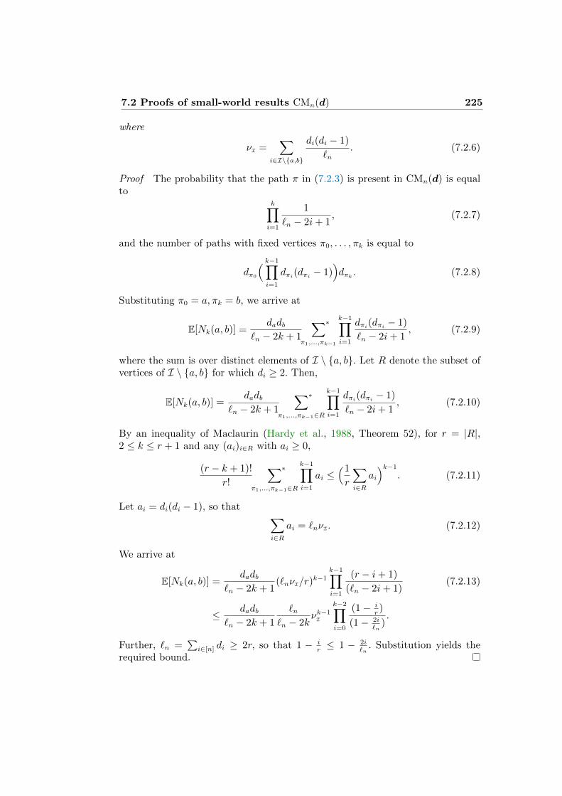
7.2 Proofs of small-world results CMn(d) 225
where
νI =∑
i∈I\a,b
di(di − 1)
`n. (7.2.6)
Proof The probability that the path π in (7.2.3) is present in CMn(d) is equalto
k∏i=1
1
`n − 2i+ 1, (7.2.7)
and the number of paths with fixed vertices π0, . . . , πk is equal to
dπ0
( k−1∏i=1
dπi(dπi − 1))dπk . (7.2.8)
Substituting π0 = a, πk = b, we arrive at
E[Nk(a, b)] =dadb
`n − 2k + 1
∑∗
π1,...,πk−1
k−1∏i=1
dπi(dπi − 1)
`n − 2i+ 1, (7.2.9)
where the sum is over distinct elements of I \ a, b. Let R denote the subset ofvertices of I \ a, b for which di ≥ 2. Then,
E[Nk(a, b)] =dadb
`n − 2k + 1
∑∗
π1,...,πk−1∈R
k−1∏i=1
dπi(dπi − 1)
`n − 2i+ 1, (7.2.10)
By an inequality of Maclaurin (Hardy et al., 1988, Theorem 52), for r = |R|,2 ≤ k ≤ r + 1 and any (ai)i∈R with ai ≥ 0,
(r − k + 1)!
r!
∑∗
π1,...,πk−1∈R
k−1∏i=1
ai ≤(1
r
∑i∈R
ai)k−1
. (7.2.11)
Let ai = di(di − 1), so that ∑i∈R
ai = `nνI. (7.2.12)
We arrive at
E[Nk(a, b)] =dadb
`n − 2k + 1(`nνI/r)
k−1k−1∏i=1
(r − i+ 1)
(`n − 2i+ 1)(7.2.13)
≤ dadb`n − 2k + 1
`n`n − 2k
νk−1I
k−2∏i=0
(1− ir)
(1− 2i`n
).
Further, `n =∑
i∈[n] di ≥ 2r, so that 1 − ir≤ 1 − 2i
`n. Substitution yields the
required bound.
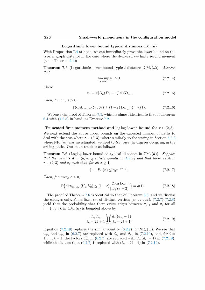
226 Small-world phenomena in the configuration model
Logarithmic lower bound typical distances CMn(d)
With Proposition 7.4 at hand, we can immediately prove the lower bound on thetypical graph distance in the case where the degrees have finite second moment(as in Theorem 6.4):
Theorem 7.5 (Logarithmic lower bound typical distances CMn(d)) Assumethat
lim supn→∞
νn > 1, (7.2.14)
where
νn = E[Dn(Dn − 1)]/E[Dn]. (7.2.15)
Then, for any ε > 0,
P(distCMn(d)(U1, U2) ≤ (1− ε) logνn n) = o(1). (7.2.16)
We leave the proof of Theorem 7.5, which is almost identical to that of Theorem6.4 with (7.2.5) in hand, as Exercise 7.2.
Truncated first moment method and log log lower bound for τ ∈ (2, 3)
We next extend the above upper bounds on the expected number of paths todeal with the case where τ ∈ (2, 3), where similarly to the setting in Section 6.2.2where NRn(w) was investigated, we need to truncate the degrees occurring in thearising paths. Our main result is as follows:
Theorem 7.6 (Loglog lower bound on typical distances in CMn(d)) Supposethat the weights d = (di)i∈[n] satisfy Condition 1.5(a) and that there exists aτ ∈ (2, 3) and c2 such that, for all x ≥ 1,
[1− Fn](x) ≤ c2x−(τ−1), (7.2.17)
Then, for every ε > 0,
P(
distCMn(d)(U1, U2) ≤ (1− ε) 2 log log n
| log (τ − 2)|)
= o(1). (7.2.18)
The proof of Theorem 7.6 is identical to that of Theorem 6.6, and we discussthe changes only. For a fixed set of distinct vertices (π0, . . . , πk), (7.2.7)-(7.2.8)yield that the probability that there exists edges between πi−1 and πi for alli = 1, . . . , k in CMn(d) is bounded above by
dπ0dπk
`n − 2k + 1
k−1∏i=1
dπi(dπi − 1)
`n − 2i+ 1. (7.2.19)
Equation (7.2.19) replaces the similar identity (6.2.7) for NRn(w). We see thatwπ0
and wπk in (6.2.7) are replaced with dπ0and dπk in (7.2.19), and, for i =
1, . . . , k − 1, the factors w2πi
in (6.2.7) are replaced with dπi(dπi − 1) in (7.2.19),while the factors `n in (6.2.7) is replaced with (`n − 2i+ 1) in (7.2.19).
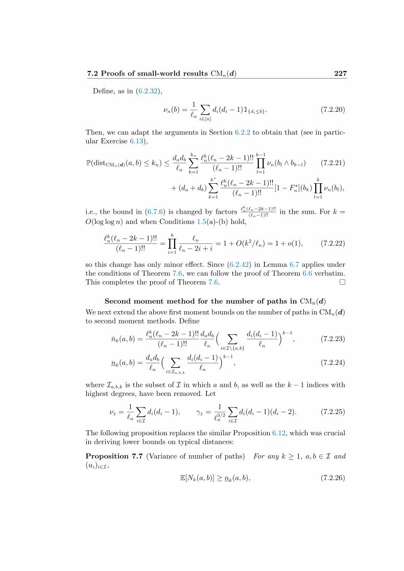
7.2 Proofs of small-world results CMn(d) 227
Define, as in (6.2.32),
νn(b) =1
`n
∑i∈[n]
di(di − 1)1di≤b. (7.2.20)
Then, we can adapt the arguments in Section 6.2.2 to obtain that (see in partic-ular Exercise 6.13),
P(distCMn(d)(a, b) ≤ kn) ≤ dadb`n
kn∑k=1
`kn(`n − 2k − 1)!!
(`n − 1)!!
k−1∏l=1
νn(bl ∧ bk−l) (7.2.21)
+ (da + db)k?∑k=1
`kn(`n − 2k − 1)!!
(`n − 1)!k∏l=1
νn(bl),
i.e., the bound in (6.7.6) is changed by factors `kn(`n−2k−1)!!
(`n−1)!!in the sum. For k =
O(log log n) and when Conditions 1.5(a)-(b) hold,
`kn(`n − 2k − 1)!!
(`n − 1)!!=
k∏i=1
`n`n − 2i+ i
= 1 +O(k2/`n) = 1 + o(1), (7.2.22)
so this change has only minor effect. Since (6.2.42) in Lemma 6.7 applies underthe conditions of Theorem 7.6, we can follow the proof of Theorem 6.6 verbatim.This completes the proof of Theorem 7.6.
Second moment method for the number of paths in CMn(d)
We next extend the above first moment bounds on the number of paths in CMn(d)to second moment methods. Define
nk(a, b) =`kn(`n − 2k − 1)!!
(`n − 1)!!
dadb`n
( ∑i∈I\a,b
di(di − 1)
`n
)k−1
, (7.2.23)
nk(a, b) =dadb`n
( ∑i∈Ia,b,k
di(di − 1)
`n
)k−1
, (7.2.24)
where Ia,b,k is the subset of I in which a and b, as well as the k − 1 indices withhighest degrees, have been removed. Let
νI =1
`n
∑i∈I
di(di − 1), γI =1
`3/2n
∑i∈I
di(di − 1)(di − 2). (7.2.25)
The following proposition replaces the similar Proposition 6.12, which was crucialin deriving lower bounds on typical distances:
Proposition 7.7 (Variance of number of paths) For any k ≥ 1, a, b ∈ I and(ui)i∈I,
E[Nk(a, b)] ≥ nk(a, b), (7.2.26)
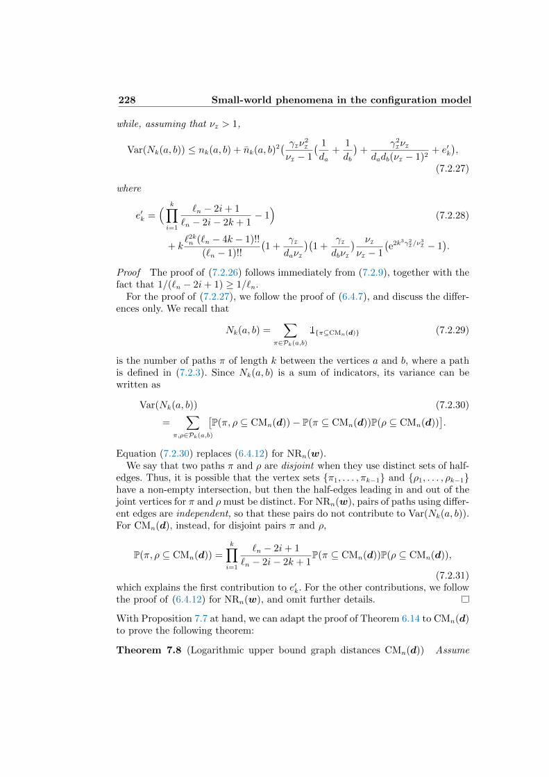
228 Small-world phenomena in the configuration model
while, assuming that νI > 1,
Var(Nk(a, b)) ≤ nk(a, b) + nk(a, b)2( γIν2
I
νI − 1
( 1
da+
1
db
)+
γ2IνI
dadb(νI − 1)2+ e′k
),
(7.2.27)
where
e′k =( k∏i=1
`n − 2i+ 1
`n − 2i− 2k + 1− 1)
(7.2.28)
+ k`2kn (`n − 4k − 1)!!
(`n − 1)!!
(1 +
γIdaνI
)(1 +
γIdbνI
) νIνI − 1
(e2k3γ2
I/ν3I − 1
).
Proof The proof of (7.2.26) follows immediately from (7.2.9), together with thefact that 1/(`n − 2i+ 1) ≥ 1/`n.
For the proof of (7.2.27), we follow the proof of (6.4.7), and discuss the differ-ences only. We recall that
Nk(a, b) =∑
π∈Pk(a,b)
1π⊆CMn(d) (7.2.29)
is the number of paths π of length k between the vertices a and b, where a pathis defined in (7.2.3). Since Nk(a, b) is a sum of indicators, its variance can bewritten as
Var(Nk(a, b)) (7.2.30)
=∑
π,ρ∈Pk(a,b)
[P(π, ρ ⊆ CMn(d))− P(π ⊆ CMn(d))P(ρ ⊆ CMn(d))
].
Equation (7.2.30) replaces (6.4.12) for NRn(w).We say that two paths π and ρ are disjoint when they use distinct sets of half-
edges. Thus, it is possible that the vertex sets π1, . . . , πk−1 and ρ1, . . . , ρk−1have a non-empty intersection, but then the half-edges leading in and out of thejoint vertices for π and ρ must be distinct. For NRn(w), pairs of paths using differ-ent edges are independent, so that these pairs do not contribute to Var(Nk(a, b)).For CMn(d), instead, for disjoint pairs π and ρ,
P(π, ρ ⊆ CMn(d)) =k∏i=1
`n − 2i+ 1
`n − 2i− 2k + 1P(π ⊆ CMn(d))P(ρ ⊆ CMn(d)),
(7.2.31)which explains the first contribution to e′k. For the other contributions, we followthe proof of (6.4.12) for NRn(w), and omit further details.
With Proposition 7.7 at hand, we can adapt the proof of Theorem 6.14 to CMn(d)to prove the following theorem:
Theorem 7.8 (Logarithmic upper bound graph distances CMn(d)) Assume
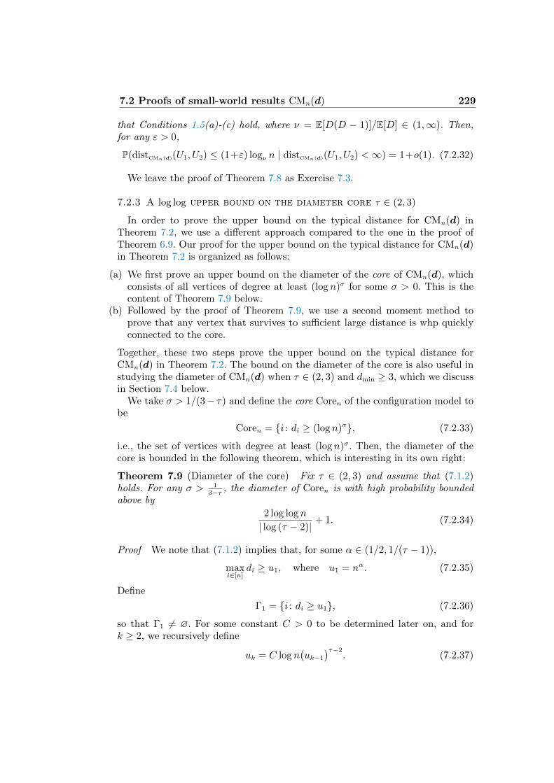
7.2 Proofs of small-world results CMn(d) 229
that Conditions 1.5(a)-(c) hold, where ν = E[D(D − 1)]/E[D] ∈ (1,∞). Then,for any ε > 0,
P(distCMn(d)(U1, U2) ≤ (1+ε) logν n | distCMn(d)(U1, U2) <∞) = 1+o(1). (7.2.32)
We leave the proof of Theorem 7.8 as Exercise 7.3.
7.2.3 A log log upper bound on the diameter core τ ∈ (2, 3)
In order to prove the upper bound on the typical distance for CMn(d) inTheorem 7.2, we use a different approach compared to the one in the proof ofTheorem 6.9. Our proof for the upper bound on the typical distance for CMn(d)in Theorem 7.2 is organized as follows:
(a) We first prove an upper bound on the diameter of the core of CMn(d), whichconsists of all vertices of degree at least (log n)σ for some σ > 0. This is thecontent of Theorem 7.9 below.
(b) Followed by the proof of Theorem 7.9, we use a second moment method toprove that any vertex that survives to sufficient large distance is whp quicklyconnected to the core.
Together, these two steps prove the upper bound on the typical distance forCMn(d) in Theorem 7.2. The bound on the diameter of the core is also useful instudying the diameter of CMn(d) when τ ∈ (2, 3) and dmin ≥ 3, which we discussin Section 7.4 below.
We take σ > 1/(3− τ) and define the core Coren of the configuration model tobe
Coren = i : di ≥ (log n)σ, (7.2.33)
i.e., the set of vertices with degree at least (log n)σ. Then, the diameter of thecore is bounded in the following theorem, which is interesting in its own right:
Theorem 7.9 (Diameter of the core) Fix τ ∈ (2, 3) and assume that (7.1.2)holds. For any σ > 1
3−τ , the diameter of Coren is with high probability boundedabove by
2 log log n
| log (τ − 2)| + 1. (7.2.34)
Proof We note that (7.1.2) implies that, for some α ∈ (1/2, 1/(τ − 1)),
maxi∈[n]
di ≥ u1, where u1 = nα. (7.2.35)
Define
Γ1 = i : di ≥ u1, (7.2.36)
so that Γ1 6= ∅. For some constant C > 0 to be determined later on, and fork ≥ 2, we recursively define
uk = C log n(uk−1
)τ−2. (7.2.37)
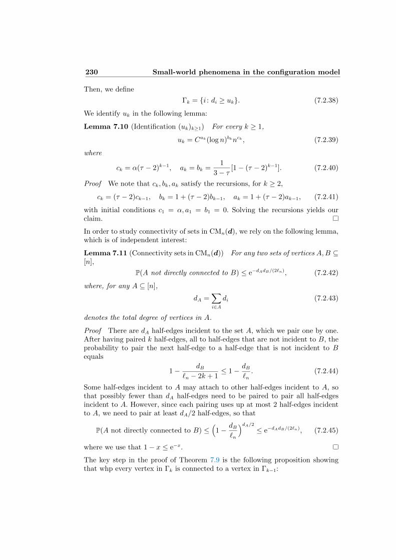
230 Small-world phenomena in the configuration model
Then, we define
Γk = i : di ≥ uk. (7.2.38)
We identify uk in the following lemma:
Lemma 7.10 (Identification (uk)k≥1) For every k ≥ 1,
uk = Cak(log n)bknck , (7.2.39)
where
ck = α(τ − 2)k−1, ak = bk =1
3− τ [1− (τ − 2)k−1]. (7.2.40)
Proof We note that ck, bk, ak satisfy the recursions, for k ≥ 2,
ck = (τ − 2)ck−1, bk = 1 + (τ − 2)bk−1, ak = 1 + (τ − 2)ak−1, (7.2.41)
with initial conditions c1 = α, a1 = b1 = 0. Solving the recursions yields ourclaim.
In order to study connectivity of sets in CMn(d), we rely on the following lemma,which is of independent interest:
Lemma 7.11 (Connectivity sets in CMn(d)) For any two sets of vertices A,B ⊆[n],
P(A not directly connected to B) ≤ e−dAdB/(2`n), (7.2.42)
where, for any A ⊆ [n],
dA =∑i∈A
di (7.2.43)
denotes the total degree of vertices in A.
Proof There are dA half-edges incident to the set A, which we pair one by one.After having paired k half-edges, all to half-edges that are not incident to B, theprobability to pair the next half-edge to a half-edge that is not incident to Bequals
1− dB`n − 2k + 1
≤ 1− dB`n. (7.2.44)
Some half-edges incident to A may attach to other half-edges incident to A, sothat possibly fewer than dA half-edges need to be paired to pair all half-edgesincident to A. However, since each pairing uses up at most 2 half-edges incidentto A, we need to pair at least dA/2 half-edges, so that
P(A not directly connected to B) ≤(
1− dB`n
)dA/2≤ e−dAdB/(2`n), (7.2.45)
where we use that 1− x ≤ e−x.
The key step in the proof of Theorem 7.9 is the following proposition showingthat whp every vertex in Γk is connected to a vertex in Γk−1:
7.2 Proofs of small-world results CMn(d) 231
Proposition 7.12 (Connectivity between Γk−1 and Γk) Fix τ ∈ (2, 3) andassume that Conditions 1.5(a)-(b) and (7.1.2) hold. Fix k ≥ 2, and take C >2E[D]/c. Then, the probability that there exists an i ∈ Γk that is not directlyconnected to Γk−1 is o(n−δ), for some δ > 0 that is independent of k.
Proof We note that, by definition,∑i∈Γk−1
di ≥ uk−1|Γk−1| = uk−1n[1− Fn](uk−1). (7.2.46)
By (7.1.2), and since k 7→ uk is decreasing with u1 = nα,
[1− Fn](uk−1) ≥ c(uk−1)1−τ . (7.2.47)
As a result, we obtain that for every k ≥ 2,∑i∈Γk−1
di ≥ cn(uk−1)2−τ . (7.2.48)
By (7.2.48) and Lemma 7.11, using Boole’s inequality, the probability that thereexists an i ∈ Γk that is not directly connected to Γk−1 is bounded by
ne−uknuk−1[1−F (uk−1)]
2`n ≤ ne−cuk(uk−1)2−τ
2E[Dn] = n1− cC2E[Dn] . (7.2.49)
By Conditions 1.5(a)-(b), E[Dn] → E[D], so that, as n → ∞ and taking C >2E[D]/c, we obtain the claim for any δ < cC
2E[D]− 1.
We now complete the proof of Theorem 7.9:Proof of Theorem 7.9. Fix
k? =log log n
| log (τ − 2)| . (7.2.50)
As a result of Proposition 7.12, whp, the diameter of Γk? is at most 2k? + 1,because the distance between any vertex in Γk? and Γ1 is at most k?, while, byExercise 7.4, Γ1 forms a complete graph. Therefore, it suffices to prove that
Coren ⊆ Γk? . (7.2.51)
By (7.2.37), in turn, this is equivalent to uk? ≥ (log n)σ, for any σ > 1/(3 − τ).According to Lemma 7.10,
uk? = Cak? (log n)bk?nck? . (7.2.52)
We note that nck? = elogn(τ−2)k?
. Since, for 2 < τ < 3,
x(τ − 2)log x
| log (τ−2)| = x · x−1 = 1, (7.2.53)
we find with x = log n that nck? = e. Further, bk → 1/(τ − 3) as k →∞, so that(log n)bk? = (log n)1/(3−τ)+o(1), and ak = bk, so that also Cak? = C1/(τ−3)+o(1). Weconclude that
uk? = (log n)1/(3−τ)+o(1), (7.2.54)
232 Small-world phenomena in the configuration model
so that, by picking n sufficiently large, we can make 1/(3 − τ) + o(1) ≤ σ. Thiscompletes the proof of Theorem 7.9.
We continue to use Theorem 7.9 to prove a log log n upper bound on the typicaldistance distCMn(d)(U1, U2) in the case where τ ∈ (2, 3). We start by describingthe setting. We assume that there exist τ ∈ (2, 3), α > 1/2 and c1 such that,uniformly in n and x ≤ nα,
[1− Fn](x) ≥ c1x−(τ−1). (7.2.55)
Theorem 7.13 (A log log upper bound on typical distance for τ ∈ (2, 3)) Sup-pose that the empirical distribution function Fn of the degrees d = (di)i∈[n] satis-fies Conditions 1.5(a)-(b) and (7.2.55). Then, for every ε > 0,
limn→∞
P(
distCMn(d)(U1, U2) ≤ 2(1 + ε) log log n
| log (τ − 2)| | distCMn(d)(U1, U2) <∞)
= 1.
(7.2.56)
Proof We make crucial use of the branching process approximation in Section7.2.1. We let U1, U2 denote two vertices chosen uniformly at random from [n], andwe recall that Z(i)
m denote the number of unpaired or free half edges incident tovertices in Nm(Ui). By Corollary 7.3, (Z(1)
l , Z(2)
l )ml=0 can be whp perfectly coupledto (Z(1)
l , Z(2)
l )ml=0, which are two independent unimodular or two-stage branch-ing processes where the root has offspring distribution D, and individuals in allfurther generations have offspring distribution D? − 1.
We condition on Bm(U1), Bmn(U2) which are such that Z(n;1)
m ≥ 1, Z(n;2)
m ≥ 1.We couple these to (Z(1)
m , Z(2)
m ). We note that, conditionally on Z(1)
m ≥ 1, Z(2)
m ≥ 1,
Z(1)
m
P−→∞, Z(2)
m
P−→∞ when m→∞.We will condition on (Bm(U1), Bmn(U2)), and denote the conditional distribu-
tion by Pmn , and the expectation and variance under the measure Pmn by Emnand Varmn , respectively. We collapse the vertices in Bm(U1) to a single vertexa1 and Bmn(U2) to a single vertex a2. The distribution of the resulting randomgraph is again a configuration model, with degrees da1 = Z(n;1)
m , da2 = Z(n;2)
m andvertex set R = [n] ∪ a1, a2 \ (Bm(U1) ∪Bm(U2)).
We apply Proposition 7.7 with k = ε log log n, a1, b = Coren and with I = i ∈R : di ≤ K. Then, Proposition 7.7 gives that, conditionally on (Bm(U1), Bmn(U2))such that Z(n;1)
m ≥ 1, Z(n;2)
m ≥ 1,
Pmn(Nk(ai, b) = 0) ≤ Varmn(Nk(ai, b))/Emn [Nk(ai, b)]2 (7.2.57)
≤ O(K)(1/Z(n;1)
m + 1/Z(n;2)
m
) P−→ 0,
in the iterated limit where first n → ∞, followed by m → ∞. As a result, con-ditionally on (Bm(U1), Bmn(U2)) such that Z(n;1)
m ≥ 1, Z(n;2)
m ≥ 1, with probabilityat least 1− o(1), Nk(ai, b) ≥ 1, so that, on this event,
distCMn(d)(U1, U2) ≤ diamCMn(d)(Coren) + 2k ≤ 2(1 + ε) log log n
| log (τ − 2)| . (7.2.58)
7.3 Branching processes with infinite mean 233
We further use that, by Theorem 4.4,
P(distCMn(d)(U1, U2) <∞)→ ζ2, (7.2.59)
while
P(Z(n;1)
m ≥ 1, Z(n;2)
m ≥ 1)→ ζ2 (7.2.60)
in the iterated limit where first n → ∞, followed by m → ∞. As a result, withkn = 2(1+ε) log logn
| log (τ−2)| ,
P(distCMn(d)(U1, U2) ≤ kn | distCMn(d)(U1, U2) <∞
)(7.2.61)
≥ P(distCMn(d)(U1, U2) ≤ kn, Z(n;1)
m ≥ 1, Z(n;2)
m ≥ 1)
P(distCMn(d)(U1, U2) <∞)
=P(Z(n;1)
m ≥ 1, Z(n;2)
m ≥ 1)− o(1)
P(distCMn(d)(U1, U2) <∞)= 1− o(1),
as required. This completes the proof of Theorem 7.13.
Exercise 7.5 explores an alternative proof of Theorem 7.13.
7.3 Branching processes with infinite mean
When τ ∈ (2, 3), the branching processes (Z(1)
j )j≥0 and (Z(2)
j )j≥0 are well-defined, but have infinite mean in generations 2, 3, etc. This leads us to considerbranching processes with infinite mean. In this section, we give a scaling resultfor the generation sizes for such branching processes. This result will be crucialto describe the fluctuations of the typical distances in CMn(d), and also allowus to understand how the ultrasmall distances of order log log n arise. The mainresult in this section is the following theorem:
Theorem 7.14 (Branching processes with infinite mean) Let (Zn)n≥0 be abranching process with offspring distribution Z1 = X having distribution func-tion FX. Assume that there exist α ∈ (0, 1) and a non-negative, non-increasingfunction x 7→ γ(x), such that
x−α−γ(x) ≤ 1− FX(x) ≤ x−α+γ(x), for large x, (7.3.1)
where x 7→ γ(x) satisfies
(i) x 7→ xγ(x) is non-decreasing,
(ii)∫∞
0γ(eex) dx <∞, or, equivalently,
∫∞e
γ(y)
y log ydy <∞.
Then αn log(Zn ∨ 1)a.s.−→ Y , with P(Y = 0) equal to the extinction probability of
(Zn)n≥0.
In the analysis for the configuration model, α = τ − 2, as α corresponds tothe tail exponent of the size-biased random variable D? (recall Lemma 1.14).Theorem 7.14 covers the case where the branching process has an offspring which
234 Small-world phenomena in the configuration model
has very thick tails. Indeed, it is not hard to show that Theorem 7.14 impliesthat E[Xs] =∞ for every s > α ∈ (0, 1) (see Exercise 7.7 below).
We do not prove Theorem 7.14 in full generality. Rather, we prove it in asimpler, yet still quite general case, in which γ(x) = (log x)γ−1 for some γ ∈ [0, 1).See Exercise 7.6 to see that this case indeed satisfies the assumptions in Theorem7.14.
Proof of Theorem 7.14 for γ(x) = (log x)γ−1. The proof is divided into four mainsteps. Define
Mn = αn log(Zn ∨ 1). (7.3.2)
We shall first assume that P(Z1 ≥ 1) = 1, so that η = 1. We start by splittingMn in a suitable way.
The split
For i ≥ 1, we define
Yi = αi log( (Zi ∨ 1)
(Zi−1 ∨ 1)1/α
). (7.3.3)
We can write
Mn = Y1 + Y2 + · · ·+ Yn. (7.3.4)
From this split, it is clear that almost sure convergence of Mn follows when thesum
∑∞i=0 Yi converges, which, in turn, is the case when
∞∑i=1
E[∣∣Yi∣∣] <∞. (7.3.5)
This is what we prove in the following three steps.
Inserting normalization sequences
We next investigate E[∣∣Yi∣∣]. We prove by induction on i that there exist constants
κ < 1 and C > 0 such that
E[∣∣Yi∣∣] ≤ Kκi. (7.3.6)
For i = 0, this follows from the fact that, when (7.3.1) holds, the random variableY1 = α log(Z1∨1) has a bounded absolute expectation. This initializes the induc-tion hypothesis. We next turn to the advancement of the induction hypothesis.For this, we recall the definition of un in [Volume 1, (2.6.7)], which states that
un = infx : 1− FX(x) ≤ 1/n. (7.3.7)
The interpretation of un is that it indicates the order of magnitude of maxni=1Xi,where (Xi)
ni=1 are i.i.d. random variables with distribution function FX.
Then we define
Ui = αi log( uZi−1∨1
(Zi−1 ∨ 1)1/α
), Vi = αi log
( Zi ∨ 1
uZi−1∨1
). (7.3.8)
7.3 Branching processes with infinite mean 235
Then, Yi = Ui + Vi, so that
E[∣∣Yi∣∣] ≤ E
[∣∣Ui∣∣]+ E[∣∣Vi∣∣]. (7.3.9)
We bound each of these terms separately.
Bounding the normalizing constants
In this step, we analyse the normalizing constants n 7→ un, assuming(7.3.1), anduse this, as well as theinduction hypothesis, to bound E
[∣∣Ui∣∣].When (7.3.1) holds and since limx→∞ γ(x) = 0, there exists a constant Cε ≥ 1
such that, for all n ≥ 1,
un ≤ Cεn1/α+ε, (7.3.10)
This gives a first bound on n 7→ un. We next substitute this bound into (7.3.1)and use that x 7→ xγ(x) is non-decreasing together with γ(x) = (log x)γ−1, toobtain that
1 + o(1) = n[1−FX(un)] ≥ n[u−(τ−1)−γ(un)n
]≥ n
[u−(τ−1)n elog
(Cεn
1α
+ε)γ]
, (7.3.11)
which, in turn, implies that there exists a constant c > 0 such that
un ≤ n1/αec(logn)γ . (7.3.12)
In a similar way, we can show the matching lower bound un ≥ n1/αe−c(logn)γ . Asa result,
E[∣∣Ui∣∣] ≤ cαiE[(log (Zi−1 ∨ 1))γ
]. (7.3.13)
Using the concavity of x 7→ xγ for γ ∈ [0, 1), as well as Jensen’s Inequality, wearrive at
E[∣∣Ui∣∣] ≤ cαi(E[(log (Zi−1 ∨ 1))
])γ= αi(1−γ)E[Mi−1]γ . (7.3.14)
By (7.3.4) and (7.3.6), which implies that E[Mi−1] ≤ Kκ/(1− κ), we arrive at
E[∣∣Ui∣∣] ≤ αi(1−γ)c
( Kκ
1− κ)γ. (7.3.15)
Logarithmic moment of an asymptotically stable random variable
In this step, we bound E[∣∣Vi∣∣]. We note that by [Volume 1, Theorem 2.33] and
for Zi quite large, the random variable (Zi ∨ 1)/(uZi−1∨1) should be close to astable random variable. We make use of this fact by bounding
E[∣∣Vi∣∣] ≤ αi sup
m≥1E[∣∣ log
(Sm/um
)∣∣], (7.3.16)
where Sm = X1+· · ·+Xm, and (Xi)mi=1 are i.i.d. copies of the offspring distribution
X. We shall prove that there exists a constant C > 0 such that, for all m ≥ 1,
E[∣∣ log
(Sm/um
)∣∣] ≤ C. (7.3.17)
In order to prove (7.3.17), we note that it suffices to bound
E[(
log(Sm/um
))+
]≤ C+, E
[(log(Sm/um
))−
]≤ C−, (7.3.18)
236 Small-world phenomena in the configuration model
where, for x ∈ R, x+ = maxx, 0 and x− = max−x, 0. Since |x| = x+ +x−, wethen obtain (7.3.17) with C = C+ + C−. In order to prove (7.3.17), we start byinvestigating E
[(log(Sm/um
))−
]. We note that (log x)− = log (x−1 ∨ 1), so that
E[(
log(Sm/um
))−
]= E
[log(um/(Sm ∧ um)
)], (7.3.19)
where x∧ y = minx, y. The function x 7→ log((um/(x∧um)
)is non-increasing,
and, since Sm ≥ X(m), where X(m) = max1≤i≤mXi, we arrive at
E[
log(um/(Sm ∧ um)
)]≤ E
[log(um/(X(m) ∧ um)
)]. (7.3.20)
We next use that, for x ≥ 1, x 7→ log(x) is concave, so that, for every s,
E[
log(um/(X(m) ∧ um)
)]=
1
sE[
log((um/(X(m) ∧ um))s
)](7.3.21)
≤ 1
slog(E[(um/(X(m) ∧ um)
)s])≤ 1
s+
1
slog(usmE
[X−s
(m)
]),
where, in the last step, we made us of the fact that um/(x∧um) ≤ 1+um/x. Nowrewrite X−s
(m)= (−Y(m))
s, where Yj = −X−1j and Y(m) = max1≤j≤m Yj. Clearly,
Yj ∈ [−1, 0] since Xi ≥ 1, so that E[(−Y1)s] < ∞. Also, umY(m) = −um/X(m)
converges in distribution to −E−1/α, where E is exponential with mean 1, so itfollows from (Pickands III, 1968, Theorem 2.1) that, as m→∞,
E [(umY(m))p]→ E[E−1/α] <∞. (7.3.22)
We proceed with E[(
log(Sm/um
))+
], for which the proof is a slight adaptation
of the above argument. Now we make use of the fact that (log x)+ = log (x ∨ 1) ≤1 + x for x ≥ 0, so that we must bound
E[
log(Sm ∨ um/um
)]=
1
sE[
log((Sm ∨ um/um))s
)]≤ 1
s+ log
(E[(Sm/um
)s].
(7.3.23)The discussion on (Hall, 1981, Page 565 and Corollary 1) yields, for s < α,E[Ssm] = E[|Sm|s] ≤ 2s/2λs(t), for some function λs(m) depending on s, m andFX. Using the discussion on (Hall, 1981, Page 564), we have that λs(m) ≤Csm
s/αl(m1/α)s, where l( · ) is a slowly-varying function. With some more effort,it can be shown that we can replace l(m1/α) by `(m), which gives
E[
log(Sm ∨um/um
)]≤ 1
s+ logE
[(Smum
)s] ≤ 1
s+Cssms/α`(m)su−sm =
1
s+ 2s/2
Css,
(7.3.24)and which proves the first bound in (7.3.18) with C+ = 1
s+ 2s/2Cs
s.
Completion of the proof of Theorem 7.14 when X ≥ 1
Combining (7.3.9) with (7.3.15) and (7.3.16)–(7.3.17), we arrive at
E[∣∣Yi∣∣] ≤ αi(1−γ)c
( Kκ
1− κ)γ
+ Cαi ≤ Kκi, (7.3.25)
7.3 Branching processes with infinite mean 237
when we take κ = α1−γ and we take K to be sufficiently large, for example K ≥2C and K ≥ 2c
(Kκ1−κ
)γ. This completes the proof when the offspring distribution
X satisfies X ≥ 1.
Completion of the proof of Theorem 7.14
We finally extend the result to the setting where X = 0 with positive probability.Since E[X] = ∞, the survival probability ζ = P(Zn ≥ 1∀n ≥ 0) satisfies ζ > 0.Conditionally on extinction, clearly Zn
a.s.−→ 0, so that, on the survival event,αn log(Zn ∨ 1)
a.s.−→ Y , where, conditionally on extinction, Y = 0.It remains to prove that αn log(Zn∨1)
a.s.−→ Y on the survival event. By [Volume1, Theorem 3.12], we have that, conditionally on survival,
Z(∞)
n
Zn
a.s.−→ ξ > 0, (7.3.26)
where we recall that Z(∞)
n are the individuals in the nth generation which havean infinite line of descent. By [Volume 1, Theorem 3.11] and conditionally onsurvival, (Z(∞)
n )n≥0 is again a branching process, now with offspring distributionp(∞) given in [Volume 1, (3.4.2)]. Note that, in particular, P(Z(∞)
1 ≥ 1) = 1, andwe wish to apply Theorem 7.14 to Z(∞)
n instead of Zn. It is not hard to show thatalso p(∞) in [Volume 1, (3.4.2)] satisfies the conditions in Theorem 7.14 with thefunction x 7→ γ?(x), given by γ?(x) = γ(x) + c/ log x . Thus, conditionally onsurvival,
αn log(Z(∞)
n ∨ 1)a.s.−→ Y (∞), (7.3.27)
and combining (7.3.26) and (7.3.27), it immediately follows that, conditionallyon survival,
αn log(Zn ∨ 1)a.s.−→ Y (∞). (7.3.28)
We conclude that Theorem 7.14 holds, where Y = 0 with probability η = 1 − ζand Y = Y (∞) with probability ζ.
We finally state some properties of the a.s. limit Y of (αn log(Zn∨1))n≥0, of whichwe omit a proof:
Theorem 7.15 (Limiting variable for infinite-mean branching processes) Underthe conditions of Theorem 7.14,
limx→∞
log P(Y > x)
x= −1, (7.3.29)
where is the a.s. limit of αn log(Zn ∧ 1).
Theorem 7.15 can be understood from the fact that, by (7.3.2)–(7.3.3),
Y =∞∑n=1
Yi, (7.3.30)
238 Small-world phenomena in the configuration model
where
Y1 = α log(Z1 ∨ 1
). (7.3.31)
By (7.3.1),
P(Y1 > x) = P(Z1 > ex1/α
) = e−x(1+o(1)), (7.3.32)
which shows that Y1 satisfies (7.3.29). The equality in (7.3.30) together with(7.3.3) suggests that the tails of Y1 are equal to those of Y , which heuristicallyexplains (7.3.29).
Intuition behind ultrasmall distances using Theorem 7.14
We now use the results in Theorem 7.14 to explain how we can understand theultrasmall distances in the configuration model. First, note that
P(distCMn(d)(U1, U2) = k) =1
nE[|Bk(U1)|]. (7.3.33)
This suggests that distCMn(d)(U1, U2) should be closely related to the value ofk (if any exists) such that E[|Bk(U1)|] = Θ(n). Using the branching processapproximation that
|Bk(U1)| = Z(n;1)
k ≈ Z(1)
k ≈ e(τ−2)−kY1(1+oP(1)) (7.3.34)
(the first approximation being true for smallish k, but not necessarily for largek), this suggest that distCMn(d)(U1, U2) ≈ kn, where, by Theorem 7.14,
Θ(n) = Z(1)
kn= e(τ−2)−knY1(1+oP(1)), (7.3.35)
which suggests that distCMn(d)(U1, U2) ≈ log log n/| log(τ −2)|. Of course, for suchvalues, the branching process approximation may fail miserably, and in fact itdoes. This is exemplified the fact that e(τ−2)−knY (1+oP(1)) can become much largerthan n, which is clearly impossible for |Bkn(U1)|.
More intriguingly, comparing with we see that the proposed typical distancesare a factor 2 too small compared to Theorem 7.2. The reason is that the double-exponential growth can clearly no longer be valid when Z(n;1)
k becomes too large,and thus, Z(n;1)
k must be far away from Z(1)
k in this regime. The whole problem isthat we are using the branching-process approximation well beyond its expirationdate.
So, let us try this again, but rather than using it for one neighborhood, letus use the branching process approximation from two sides. Now we rely on thestatement that
P(distCMn(d)(U1, U2) ≤ 2k) = P(Bk(U1) ∩Bk(U2) 6= ∅). (7.3.36)
Again using (7.3.35), we see that |Bk(U1)| ≈ e(τ−2)−kY1(1+oP(1)) and |Bk(U1)| ≈e(τ−2)−kY2(1+oP(1)), where Y1 and Y2 are independent. These grow roughly at thesame pace, and in particular, |Bk(U1)| = nΘ(1) roughly at the same time, namely,when k ≈ log log n/| log(τ − 2)|. Thus, we conclude that distCMn(d)(U1, U2) ≈2 log log n/| log(τ − 2)|, as rigorously proved in Theorem 7.2. We will see that the
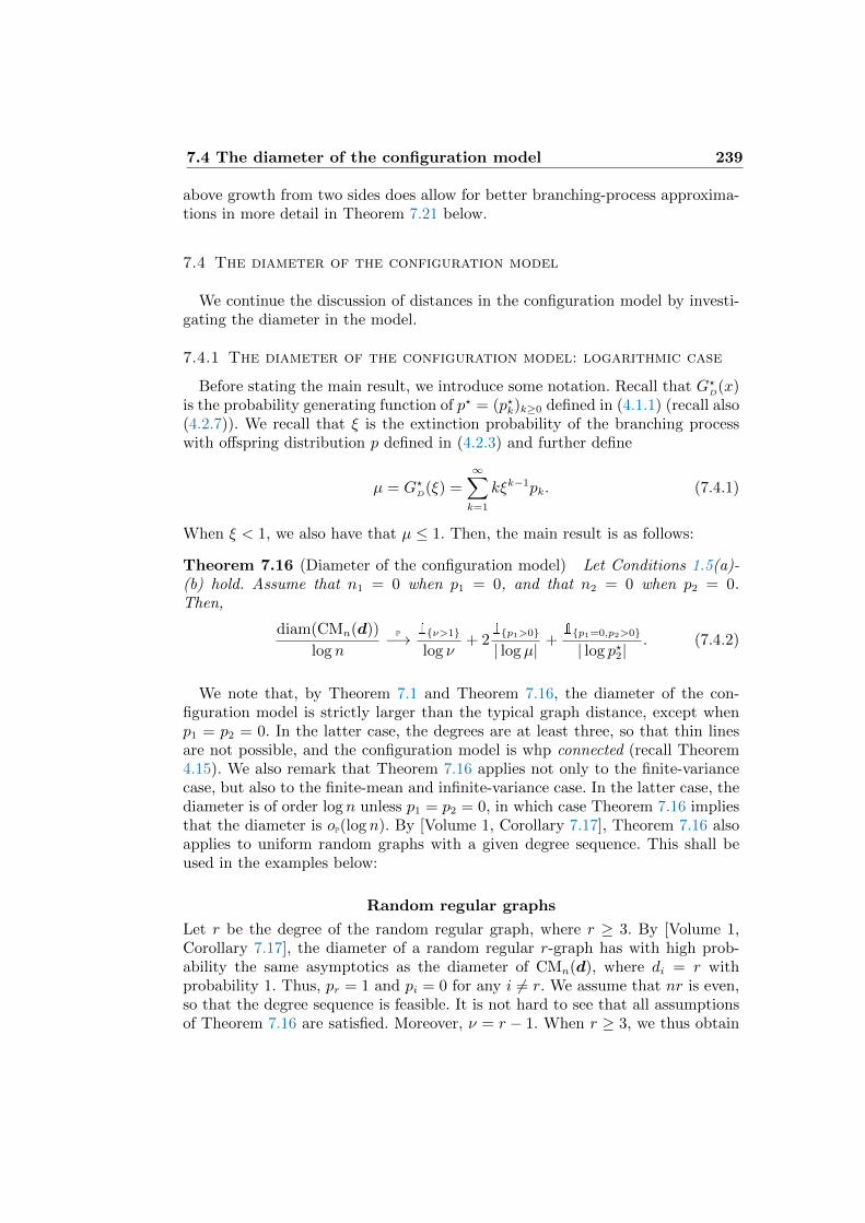
7.4 The diameter of the configuration model 239
above growth from two sides does allow for better branching-process approxima-tions in more detail in Theorem 7.21 below.
7.4 The diameter of the configuration model
We continue the discussion of distances in the configuration model by investi-gating the diameter in the model.
7.4.1 The diameter of the configuration model: logarithmic case
Before stating the main result, we introduce some notation. Recall that G?D
(x)is the probability generating function of p? = (p?k)k≥0 defined in (4.1.1) (recall also(4.2.7)). We recall that ξ is the extinction probability of the branching processwith offspring distribution p defined in (4.2.3) and further define
µ = G?D
(ξ) =∞∑k=1
kξk−1pk. (7.4.1)
When ξ < 1, we also have that µ ≤ 1. Then, the main result is as follows:
Theorem 7.16 (Diameter of the configuration model) Let Conditions 1.5(a)-(b) hold. Assume that n1 = 0 when p1 = 0, and that n2 = 0 when p2 = 0.Then,
diam(CMn(d))
log nP−→ 1ν>1
log ν+ 2
1p1>0
| logµ| +1p1=0,p2>0
| log p?2|. (7.4.2)
We note that, by Theorem 7.1 and Theorem 7.16, the diameter of the con-figuration model is strictly larger than the typical graph distance, except whenp1 = p2 = 0. In the latter case, the degrees are at least three, so that thin linesare not possible, and the configuration model is whp connected (recall Theorem4.15). We also remark that Theorem 7.16 applies not only to the finite-variancecase, but also to the finite-mean and infinite-variance case. In the latter case, thediameter is of order log n unless p1 = p2 = 0, in which case Theorem 7.16 impliesthat the diameter is oP(log n). By [Volume 1, Corollary 7.17], Theorem 7.16 alsoapplies to uniform random graphs with a given degree sequence. This shall beused in the examples below:
Random regular graphs
Let r be the degree of the random regular graph, where r ≥ 3. By [Volume 1,Corollary 7.17], the diameter of a random regular r-graph has with high prob-ability the same asymptotics as the diameter of CMn(d), where di = r withprobability 1. Thus, pr = 1 and pi = 0 for any i 6= r. We assume that nr is even,so that the degree sequence is feasible. It is not hard to see that all assumptionsof Theorem 7.16 are satisfied. Moreover, ν = r − 1. When r ≥ 3, we thus obtain
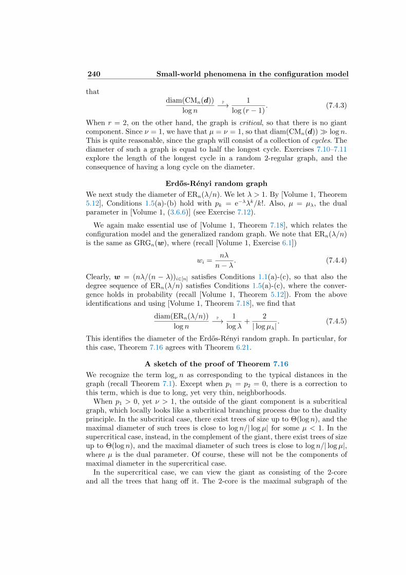
240 Small-world phenomena in the configuration model
thatdiam(CMn(d))
log nP−→ 1
log (r − 1). (7.4.3)
When r = 2, on the other hand, the graph is critical, so that there is no giantcomponent. Since ν = 1, we have that µ = ν = 1, so that diam(CMn(d)) log n.This is quite reasonable, since the graph will consist of a collection of cycles. Thediameter of such a graph is equal to half the longest cycle. Exercises 7.10–7.11explore the length of the longest cycle in a random 2-regular graph, and theconsequence of having a long cycle on the diameter.
Erdos-Renyi random graph
We next study the diameter of ERn(λ/n). We let λ > 1. By [Volume 1, Theorem5.12], Conditions 1.5(a)-(b) hold with pk = e−λλk/k!. Also, µ = µλ, the dualparameter in [Volume 1, (3.6.6)] (see Exercise 7.12).
We again make essential use of [Volume 1, Theorem 7.18], which relates theconfiguration model and the generalized random graph. We note that ERn(λ/n)is the same as GRGn(w), where (recall [Volume 1, Exercise 6.1])
wi =nλ
n− λ. (7.4.4)
Clearly, w = (nλ/(n − λ))i∈[n] satisfies Conditions 1.1(a)-(c), so that also thedegree sequence of ERn(λ/n) satisfies Conditions 1.5(a)-(c), where the conver-gence holds in probability (recall [Volume 1, Theorem 5.12]). From the aboveidentifications and using [Volume 1, Theorem 7.18], we find that
diam(ERn(λ/n))
log nP−→ 1
log λ+
2
| logµλ|. (7.4.5)
This identifies the diameter of the Erdos-Renyi random graph. In particular, forthis case, Theorem 7.16 agrees with Theorem 6.21.
A sketch of the proof of Theorem 7.16
We recognize the term logν n as corresponding to the typical distances in thegraph (recall Theorem 7.1). Except when p1 = p2 = 0, there is a correction tothis term, which is due to long, yet very thin, neighborhoods.
When p1 > 0, yet ν > 1, the outside of the giant component is a subcriticalgraph, which locally looks like a subcritical branching process due to the dualityprinciple. In the subcritical case, there exist trees of size up to Θ(log n), and themaximal diameter of such trees is close to log n/| logµ| for some µ < 1. In thesupercritical case, instead, in the complement of the giant, there exist trees of sizeup to Θ(log n), and the maximal diameter of such trees is close to log n/| logµ|,where µ is the dual parameter. Of course, these will not be the components ofmaximal diameter in the supercritical case.
In the supercritical case, we can view the giant as consisting of the 2-coreand all the trees that hang off it. The 2-core is the maximal subgraph of the
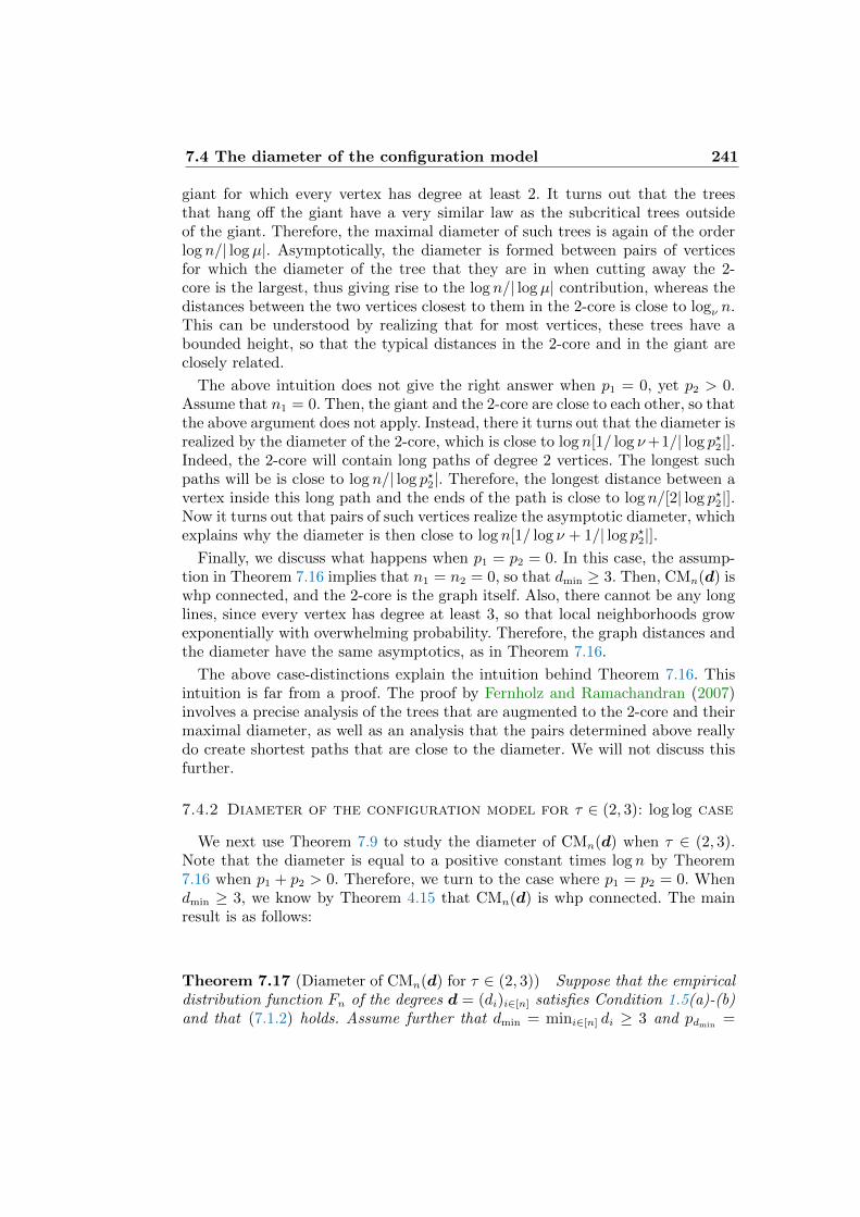
7.4 The diameter of the configuration model 241
giant for which every vertex has degree at least 2. It turns out that the treesthat hang off the giant have a very similar law as the subcritical trees outsideof the giant. Therefore, the maximal diameter of such trees is again of the orderlog n/| logµ|. Asymptotically, the diameter is formed between pairs of verticesfor which the diameter of the tree that they are in when cutting away the 2-core is the largest, thus giving rise to the logn/| logµ| contribution, whereas thedistances between the two vertices closest to them in the 2-core is close to logν n.This can be understood by realizing that for most vertices, these trees have abounded height, so that the typical distances in the 2-core and in the giant areclosely related.
The above intuition does not give the right answer when p1 = 0, yet p2 > 0.Assume that n1 = 0. Then, the giant and the 2-core are close to each other, so thatthe above argument does not apply. Instead, there it turns out that the diameter isrealized by the diameter of the 2-core, which is close to log n[1/ log ν+1/| log p?2|].Indeed, the 2-core will contain long paths of degree 2 vertices. The longest suchpaths will be is close to log n/| log p?2|. Therefore, the longest distance between avertex inside this long path and the ends of the path is close to log n/[2| log p?2|].Now it turns out that pairs of such vertices realize the asymptotic diameter, whichexplains why the diameter is then close to log n[1/ log ν + 1/| log p?2|].
Finally, we discuss what happens when p1 = p2 = 0. In this case, the assump-tion in Theorem 7.16 implies that n1 = n2 = 0, so that dmin ≥ 3. Then, CMn(d) iswhp connected, and the 2-core is the graph itself. Also, there cannot be any longlines, since every vertex has degree at least 3, so that local neighborhoods growexponentially with overwhelming probability. Therefore, the graph distances andthe diameter have the same asymptotics, as in Theorem 7.16.
The above case-distinctions explain the intuition behind Theorem 7.16. Thisintuition is far from a proof. The proof by Fernholz and Ramachandran (2007)involves a precise analysis of the trees that are augmented to the 2-core and theirmaximal diameter, as well as an analysis that the pairs determined above reallydo create shortest paths that are close to the diameter. We will not discuss thisfurther.
7.4.2 Diameter of the configuration model for τ ∈ (2, 3): log log case
We next use Theorem 7.9 to study the diameter of CMn(d) when τ ∈ (2, 3).Note that the diameter is equal to a positive constant times log n by Theorem7.16 when p1 + p2 > 0. Therefore, we turn to the case where p1 = p2 = 0. Whendmin ≥ 3, we know by Theorem 4.15 that CMn(d) is whp connected. The mainresult is as follows:
Theorem 7.17 (Diameter of CMn(d) for τ ∈ (2, 3)) Suppose that the empiricaldistribution function Fn of the degrees d = (di)i∈[n] satisfies Condition 1.5(a)-(b)and that (7.1.2) holds. Assume further that dmin = mini∈[n] di ≥ 3 and pdmin
=
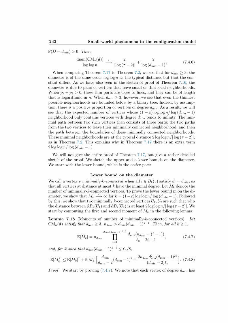
242 Small-world phenomena in the configuration model
P(D = dmin) > 0. Then,
diam(CMn(d))
log log nP−→ 2
| log (τ − 2)| +2
log (dmin − 1). (7.4.6)
When comparing Theorem 7.17 to Theorem 7.2, we see that for dmin ≥ 3, thediameter is of the same order log log n as the typical distance, but that the con-stant differs. As we have also seen in the sketch of proof of Theorem 7.16, thediameter is due to pairs of vertices that have small or thin local neighborhoods.When p1 + p2 > 0, these thin parts are close to lines, and they can be of lengththat is logarithmic in n. When dmin ≥ 3, however, we see that even the thinnestpossible neighborhoods are bounded below by a binary tree. Indeed, by assump-tion, there is a positive proportion of vertices of degree dmin. As a result, we willsee that the expected number of vertices whose (1 − ε) log log n/ log (dmin − 1)neighborhood only contains vertices with degree dmin tends to infinity. The min-imal path between two such vertices then consists of three parts: the two pathsfrom the two vertices to leave their minimally connected neighborhood, and thenthe path between the boundaries of these minimally connected neighborhoods.These minimal neighborhoods are at the typical distance 2 log log n/| log (τ − 2)|,as in Theorem 7.2. This explains why in Theorem 7.17 there is an extra term2 log log n/ log (dmin − 1).
We will not give the entire proof of Theorem 7.17, but give a rather detailedsketch of the proof. We sketch the upper and a lower bounds on the diameter.We start with the lower bound, which is the easier part:
Lower bound on the diameter
We call a vertex v minimally-k-connected when all i ∈ Bk(v) satisfy di = dmin, sothat all vertices at distance at most k have the minimal degree. Let Mk denote thenumber of minimally-k-connected vertices. To prove the lower bound in on the di-ameter, we show that Mk
P−→∞ for k = (1− ε) log log n/ log (dmin − 1). Followedby this, we show that two minimally k-connected vertices U1, U2 are such that whpthe distance between ∂Bk(U1) and ∂Bk(U2) is at least 2 log log n/| log (τ − 2)|. Westart by computing the first and second moment of Mk in the following lemma:
Lemma 7.18 (Moments of number of minimally-k-connected vertices) LetCMn(d) satisfy that dmin ≥ 3, ndmin
> dmin(dmin − 1)k−1. Then, for all k ≥ 1,
E[Mk] = ndmin
dmin(dmin−1)k−1∏i=1
dmin(ndmin− (i− 1))
`n − 2i+ 1, (7.4.7)
and, for k such that dmin(dmin − 1)k−1 ≤ `n/8,
E[M2k ] ≤ E[Mk]
2 + E[Mk][ dmin
dmin − 2(dmin − 1)k +
2ndmind2
min(dmin − 1)2k
(dmin − 2)`n
]. (7.4.8)
Proof We start by proving (7.4.7). We note that each vertex of degree dmin has
7.4 The diameter of the configuration model 243
the same probability of being minimally-k connected, and that there are preciselyndmin
vertices of degree dmin, so that
E[Mk] = ndminP(v is minimally-k-connected). (7.4.9)
Vertex v with dv = dmin is minimally-k-connected when all its half-edges atdistance at most k are paired to half-edges incident to a distinct vertex havingminimal degree dmin, and no cycles occur in Bk(v). When i − 1 half-edges arepaired to distinct vertices of degree dmin, then the probability that the ith half-edge is again paired to a distinct vertex of degree dmin equals
dmin(ndmin− (i− 1))
`n − 2i+ 1. (7.4.10)
Since for v to be minimally-k-connected, there are dmin(dmin − 1)k−1 half-edgesthat need to be paired to distinct vertices of degree dmin, this proves (7.4.7).
To prove (7.4.8), we note that
E[M2k ] =
∑v1,v2∈[n]
P(v1, v2 are minimally-k-connected). (7.4.11)
We split the above probability depending on whether Bk(U1) ∩ Bk(U2) = ∅ ornot. The contribution to E[M2
k ] due to Bk(U1) ∩ Bk(U2) = ∅ is, similarly to theproof of (7.4.7), equal to
ndmin(ndmin
− ik−1)2ik∏i=1
dmin(ndmin− (i− 1))
`n − 2i+ 1, (7.4.12)
where we abbreviate ik = dmin(dmin− 1)k−1 and note that ndmin− ik−1 > 0, since,
by assumption, ndmin> dmin(dmin − 1)k−1.
We use that i 7→ dmin(ndmin− (i− 1))/(`n − 2i+ 1) is decreasing since
(ndmin− (i− 1))
`n − 2i+ 1≥ ndmin
− i`n − 2i− 1
(7.4.13)
precisely when `n ≥ 2ndmin+ 1, and which is true since `n ≥ dminndmin
≥ 3ndmin.
Therefore, the contribution to E[M2k ] from v1 and v2 satisfying Bk(v1)∩Bk(v2) =
∅ is at most
n2dmin
( ik∏i=1
dmin(ndmin− (i− 1))
`n − 2i+ 1
)2
= E[M2k ], (7.4.14)
which is the first contribution to the r.h.s. of (7.4.8).We are left to deal with the contribution to E[M2
k ] from v1 and v2 such thatBk(v1) ∩Bk(v2) 6= ∅. When v1 is k-minimally connected,
|Bk(v1)| = 1 +k∑l=1
dmin(dmin − 1)l−1 (7.4.15)
= 1 + dmin
(dmin − 1)k − 1
dmin − 2≤ dmin
(dmin − 1)k
dmin − 2.
244 Small-world phenomena in the configuration model
Therefore, the contribution due to v2 ∈ Bk(v1) is bounded by
E[Mk]dmin
dmin − 2(dmin − 1)k, (7.4.16)
which is the second contribution to the r.h.s. of (7.4.8). Finally, we study thecase where Bk(v1) ∩ Bk(v2) 6= ∅, but v2 6∈ Bk(v1). When Bk(v1) ∩ Bk(v2) 6= ∅,but v2 6∈ Bk(v1), then one of the dmin(dmin − 1)k half-edges in Bk(v1) needsto be connected to one of the dmin(dmin − 1)l−k half-edges in Bl−k(v2), wherel = distCMn(d)(v1, v2) ∈ [2k]\[k]. Conditionally on v1 being k-minimally connectedand v2 being l−k-minimally connected, the probability that this occurs is at most
dmin(dmin − 1)kdmin(dmin − 1)l−k
`n − 2ik − 2il−k + 1≤ 2dmin(dmin − 1)kdmin(dmin − 1)l−k−1
`n,
(7.4.17)where, in the last inequality, we used that dmin(dmin − 1)k−1 ≤ `n/8. Therefore,this contribution is bounded by
E[Mk]2k∑
l=k+1
E[Ml−k]2dmin(dmin − 1)kdmin(dmin − 1)l−k−1
`n. (7.4.18)
We bound E[Ml−k] ≤ ndminand sum
2k∑l=k+1
(dmin − 1)l−k−1 ≤ (dmin − 1)2k
dmin − 2, (7.4.19)
to arrive at the third and final contribution to the r.h.s. of (7.4.8).
To complete the proof of the lower bound on the diameter, we fix ε > 0 suffi-ciently small, and take k? = (1− ε) log logn
log (dmin−1). Clearly,
dmin(dmin − 1)k?−1 ≤ (log n)1−ε ≤ `n/8, (7.4.20)
so that, in particular, we may use Lemma 7.18.We note that ndmin
/n → pdminby Condition 1.5(a) and pdmin
> 0 by assump-tion. Therefore, by Conditions 1.5(a)-(b), dminndmin
/`n → λdmin, where we define
λdmin= dminpdmin
/E[D]. By (7.4.7) in Lemma 7.18,
E[Mk] ≥ n(pdmin− δ)(λdmin
− δ)dmin(dmin−1)k−1
. (7.4.21)
As a result, E[Mk? ] ≥ n(pdmin−δ)(λdmin
−δ)(logn)1−ε . Further, by (7.4.8) in Lemma7.18,
Var(Mk?) = o(E[Mk? ]2), (7.4.22)
so that
Mk?/E[Mk? ]P−→ 1. (7.4.23)
We conclude that, whp, Mk? ≥ n1−o(1). Since each minimally-k?-connected vertex
7.4 The diameter of the configuration model 245
uses up at most
1 +k?∑l=1
dmin(dmin − 1)l−1 = no(1) (7.4.24)
vertices of degree dmin, whp there must be at least two minimally-k?-connectedvertices whose k?-neighborhoods are disjoint. We fix two such vertices and denotethem by v1 and v2. We note that v1 and v2 have precisely dmin(dmin − 1)k
?−1
unpaired half-edges in ∂Bk?(v1) and ∂Bk?(v2). Let A12 denote the event thatv1, v2 are minimally-k?-connected with their k?-neighborhoods being disjoint.
Conditionally on A12, the random graph obtained by collapsing the half-edgesin ∂Bk?(v1) to a single vertex a and the half-edges in ∂Bk?(v1) to a single vertexb is a configuration model on the vertex set a, b ∪ [n] \ (Bk?(v1) ∪ Bk?(v2)),having degrees d given by da = db = dmin(dmin − 1)k
?−1 and di = di for everyi ∈ [n] \ (Bk?(v1) ∪Bk?(v2)).
By the truncated first moment method on paths, performed in the proof ofTheorem 7.6 (recall (7.2.21)), it follows that, for any ε > 0,
P(
distCMn(d)(∂Bk?(v1), ∂Bk?(v2)) ≤ (1− ε) 2 log log n
| log (τ − 2)| | A12
)= o(1). (7.4.25)
Therefore, whp,
diam(CMn(d)) ≥ (1− ε) 2 log log n
| log (τ − 2)| + 2k? (7.4.26)
= (1− ε) log log n[ 2
| log (τ − 2)| +2
log (dmin − 1)
].
Since ε > 0 is arbitrary, this proves the lower bound on diam(CMn(d)) in Theo-rem 7.17.
Sketch of the upper bound on the diameter
We now sketch the proof of the upper bound on the diameter. We aim to provethat, with kn = log log n[2/| log(τ − 2)|+ 2/ log (dmin − 1)],
P(∃v1, v2 ∈ [n] : distCMn(d)(v1, v2) ≥ (1 + ε)kn) = o(1). (7.4.27)
We already know that whp diam(Coren) ≤ 2 log log n/| log (τ − 2)| + 1, and wewill assume this from now on. Fix v1, v2 ∈ [n]. Then (7.4.27) follows when we canshow that
P(∃v : distCMn(d)(v,Coren) ≥ (1 + ε) log log n/ log (dmin − 1)) = o(1), (7.4.28)
and we will argue that, uniformly in v ∈ [n],
P(distCMn(d)(v,Coren) ≥ (1 + ε) log log n/ log (dmin − 1)) = o(1/n), (7.4.29)
which would prove (7.4.27).To prove (7.4.29), it is convenient to explore the neighborhood of the vertex
v by only pairing up the first dmin half-edges incident to v and the dmin − 1half-edges incident to any other vertex appearing in the neighborhood. We call
246 Small-world phenomena in the configuration model
this exploration graph the k-exploration graph. One can show that it is quiteunlikely that there are many cycles within this exploration graph, so that it isactually close to a tree. Therefore, the number of vertices on the boundary of thisk-exploration graph with k? = (1 + ε/2) log log n/ log (dmin − 1) is close to
(dmin − 1)k ≈ (log n)1+ε/2. (7.4.30)
This is large, but not extremely large. However, one of these vertices is boundto have quite large degree, and thus, from this vertex, it is quite likely that weconnect to Coren quickly, meaning in o(log log n) steps. More precisely, the mainingredient in the upper bound is the statement that, for
k? = (1 + ε/2) log log n/ log (dmin − 1)
and whp, the k-exploration tree connects to Coren whp in less than k?. We omitfurther details.
7.5 Related results for the configuration model
In this section, we discuss related results for the configuration model. We startby discussing the distances in infinite-mean configuration models.
7.5.1 Distances for infinite-mean degrees
In this section, we assume that there exist τ ∈ (1, 2) and c > 0 such that
limx→∞
xτ−1[1− F ](x) = c. (7.5.1)
We study the configuration model CMn(d) where the degrees d = (di)i∈[n] are ani.i.d. sequence of random variables with distribution F satisfying (7.5.1).
We make heavy use of the notation used in [Volume 1, Theorem 7.23], whichwe first recall. Recall that the random probability distribution P = (Pi)i≥1 isgiven by
Pi = Zi/Z, (7.5.2)
where Zi = Γ−1/(τ−1)i and Γi =
∑ij=1Ei with (Ei)i≥1 an i.i.d. sequence of ex-
ponential random variables with parameter 1, and where Z =∑
i≥1 Γi. Recallfurther that MP,k is a multinomial distribution with parameters k and probabili-ties P = (Pi)i≥1. Thus, MP,k = (B1, B2, . . .),where, conditionally on P = (Pi)i≥1,Bi is the number of outcomes i in k independent trials such that each outcome isequal to i with probability Pi. In [Volume 1, Theorem 7.23], the random variableMP,D1
appears, where D1 is independent of P = (Pi)i≥1. We let M (1)
P,D1and M (2)
P,D2
be two random variables which are conditionally independent given P = (Pi)i≥1.In terms of this notation, the main result on distances in CMn(d) when thedegrees have infinite mean is the following:
Theorem 7.19 (Distances in CMn(d) with i.i.d. infinite mean degrees) Fix
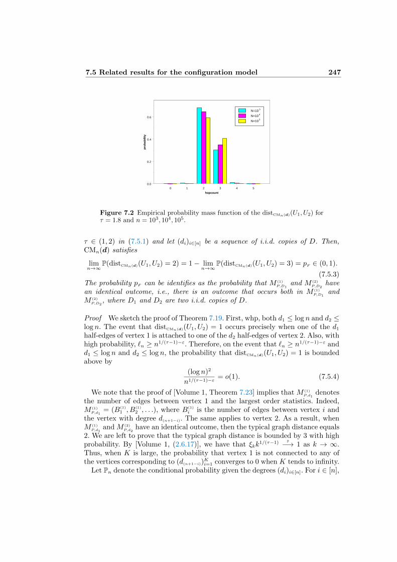
7.5 Related results for the configuration model 247
0 1 2 3 4 5
hopcount
0.0
0.2
0.4
0.6
pro
bab
ility
N=10
5
N=10
N=10
3
4
Figure 7.2 Empirical probability mass function of the distCMn(d)(U1, U2) forτ = 1.8 and n = 103, 104, 105.
τ ∈ (1, 2) in (7.5.1) and let (di)i∈[n] be a sequence of i.i.d. copies of D. Then,CMn(d) satisfies
limn→∞
P(distCMn(d)(U1, U2) = 2) = 1− limn→∞
P(distCMn(d)(U1, U2) = 3) = pF ∈ (0, 1).
(7.5.3)The probability pF can be identifies as the probability that M (1)
P,D1and M (2)
P,D2have
an identical outcome, i.e., there is an outcome that occurs both in M (1)
P,D1and
M (2)
P,D2, where D1 and D2 are two i.i.d. copies of D.
Proof We sketch the proof of Theorem 7.19. First, whp, both d1 ≤ log n and d2 ≤log n. The event that distCMn(d)(U1, U2) = 1 occurs precisely when one of the d1
half-edges of vertex 1 is attached to one of the d2 half-edges of vertex 2. Also, withhigh probability, `n ≥ n1/(τ−1)−ε. Therefore, on the event that `n ≥ n1/(τ−1)−ε andd1 ≤ log n and d2 ≤ log n, the probability that distCMn(d)(U1, U2) = 1 is boundedabove by
(log n)2
n1/(τ−1)−ε = o(1). (7.5.4)
We note that the proof of [Volume 1, Theorem 7.23] implies that M (1)
P,d1denotes
the number of edges between vertex 1 and the largest order statistics. Indeed,M (1)
P,d1= (B(1)
1 , B(1)
2 , . . .), where B(1)
i is the number of edges between vertex i andthe vertex with degree d(n+1−i). The same applies to vertex 2. As a result, whenM (1)
P,d1and M (2)
P,d2have an identical outcome, then the typical graph distance equals
2. We are left to prove that the typical graph distance is bounded by 3 with highprobability. By [Volume 1, (2.6.17)], we have that ξkk
1/(τ−1) P−→ 1 as k → ∞.Thus, when K is large, the probability that vertex 1 is not connected to any ofthe vertices corresponding to (d(n+1−i))
Ki=1 converges to 0 when K tends to infinity.
Let Pn denote the conditional probability given the degrees (di)i∈[n]. For i ∈ [n],
248 Small-world phenomena in the configuration model
we let vi be the vertex corresponding to the ith order statistic d(n+1−i). By Lemma7.11,
Pn(vi not directly connected to vj) ≤ e−d(n+1−i)d(n+1−j)
2`n . (7.5.5)
Moreover, d(n+1−i), d(n+1−j) ≥ n1/(τ−1)−ε with high probability for n sufficientlylarge and any ε > 0, while whp `n ≤ n1/(τ−1)+ε. As a result, whp,
Pn(vi not directly connected to vj) ≤ e−n1/(τ−1)−3ε
. (7.5.6)
Therefore, for fixed K and for every i, j ∈ [K], the vertices vi and vj are whpneighbors. This implies that the vertices corresponding to the high order statisticsform a complete graph. We have already concluded that 1 is connected to vi forsome i ≤ K. In the same way, we conclude that vertex 2 is connected to vj forsome j ≤ K. Since vi is whp connected to vj, we conclude that
Pn(distCMn(d)(U1, U2) ≤ 3
)= 1− o(1). (7.5.7)
This completes the proof.
7.5.2 Fluctuation of distances for finite-variance degrees
We continue to study the fluctuations of the distances in the configurationmodel, starting with the case where the degrees have finite variance. We needa limit result from branching process theory before we can identify the limitingrandom variables (Ra)a∈(−1,0].
Recall that (Zk)k≥0 denotes the unimodular branching process where in thefirst generation, the offspring has distribution D with distribution function Fand in the second and further generations, the offspring has distribution D? − 1,where D? is the size-biased distribution of D. The process (Zk/E[D]νk−1)k≥1 isa martingale with uniformly bounded expectation and consequently convergesalmost surely to a limit (see e.g., [Volume 1, Theorem 2.24 and Exercise 2.26]):
limn→∞
ZnE[D]νn−1
=W a.s. (7.5.8)
In the theorem below we need two independent copies W1 and W1 of W.
Theorem 7.20 (Limit law for typical distance in CMn(d)) Let (di)i∈[n] be asequence of i.i.d. copies of a random variable D, and assume that there existτ > 3 and c <∞ such that, for all x ≥ 1,
[1− F ](x) ≤ cx−(τ−1), (7.5.9)
and let ν > 1. For k ≥ 1, let ak = blogν kc − logν k ∈ (−1, 0]. Then, CMn(d)satisfies that there exist random variables (Ra)a∈(−1,0] such that as n → ∞ andfor all k ∈ Z,
P(distCMn(d)(U1, U2)− blogν nc = k | distCMn(d)(U1, U2) <∞
)(7.5.10)
= P(Ran = k) + o(1).
7.5 Related results for the configuration model 249
The random variables (Ra)a∈(−1,0] can be identified as
P(Ra > k) = E[
exp−κνa+kW1W2∣∣W1W2 > 0,
], (7.5.11)
where W1 and W2 are independent limit copies of W in (7.5.8) and where κ =E[D](ν − 1)−1.
In words, Theorem 7.20 states that for τ > 3, the graph distance distCMn(d)(U1, U2)between two randomly chosen connected vertices grows like the logν n, where nis the size of the graph, and that the fluctuations around this mean remain uni-formly bounded in n.
The law of Ra is involved, and can in most cases not be computed exactly.The reason for this is the fact that the random variables W that appear in itsstatement are hard to compute explicitly (see also [Volume 1, Chapter 3]).
There are two examples where the law of W is known. The first example iswhen all degrees in the graph are equal to some r ≥ 3, and we obtain the r-regular graph. In this case, E[D] = r, ν = r − 1, and W = 1 a.s. In particular,P(distCMn(d)(U1, U2) <∞) = 1 + o(1). Therefore,
P(Ra > k) = exp− r
r − 2(r − 1)a+k, (7.5.12)
and distCMn(d)(U1, U2) is asymptotically equal to logr−1 n. The second example iswhen p? is the probability mass function of a geometric random variable, in whichcase the branching process with offspring p? conditioned to be positive convergesto an exponential random variable with parameter 1. This example correspondsto
p?j = p(1− p)j−1, so that pj =1
jcpp(1− p)j−2, ∀j ≥ 1, (7.5.13)
and cp is a normalization constant. For p > 12, the law of W has the same law as
the sum of D1 copies of a random variable Y, where Y = 0 with probability 1−pp
and equal to an exponential random variable with parameter 1 with probability2p−1p
. Even in this simple case, the computation of the exact law of Ra is non-trivial.
7.5.3 Fluctuation of distances for infinite-variance degrees
We next study the fluctuations of typical distances in CMn(d) in the settingwhere the degrees are i.i.d. and satisfy that there exist τ ∈ (2, 3), γ ∈ [0, 1) andC <∞ such that
x−τ+1−C(log x)γ−1 ≤ 1− F (x) ≤ x−τ+1+C(log x)γ−1
, for large x. (7.5.14)
The condition in (7.5.14) is such that the results in Theorem 7.14 apply. Then, wecan identify the fluctuations of the typical graph distance in CMn(d) as follows:
Theorem 7.21 (Fluctuations graph distance CMn(d) for infinite-variance de-grees) Let (di)i∈[n] be a sequence of i.i.d. copies of a random variable D. Fix
250 Small-world phenomena in the configuration model
τ ∈ (2, 3) and assume that (7.5.14) holds. Then, CMn(d) satisfies that there existrandom variables (Ra)a∈(−1,0] such that, as n→∞ and for all l ∈ Z,
P(
distCMn(d)(U1, U2) = 2⌊ log logn
| log(τ − 2)|⌋
+ l∣∣∣ distCMn(d)(U1, U2) <∞
)(7.5.15)
= P(Ran = l) + o(1),
where an = b log logn| log(τ−2)|c−
log logn| log(τ−2)| ∈ (−1, 0]. Here, the random variables (Ra)a∈(−1,0]
are given by
P(Ra > l) = P(
mins∈Z
[(τ − 2)−sY1 + (τ − 2)s−clY2
]≤ (τ − 2)dl/2e+a
∣∣Y1Y2 > 0),
where cl = 1 if l is even, and zero otherwise, and Y1, Y2 are two independentcopies of the limit random variable in Theorem 7.14.
In words, Theorem 7.2 states that for τ ∈ (2, 3), the graph distance distCMn(d)(U1, U2)between two randomly chosen connected vertices grows proportional to log log ofthe size of the graph, and that the fluctuations around this mean remain uni-formly bounded in n.
We next discuss an extension, obtained by possibly truncating the degree dis-tribution. In order to state the result, we make the following assumption:
Condition 7.22 (Truncated infinite-variance degrees) There exists a βn ∈(1, 1/(τ − 1)] such that Fn(x) = 1 for x ≥ nβn(1+ε) for all ε > 0, while forall x ≤ nβn(1−ε),
1− Fn(x) =Ln(x)
xτ−1, (7.5.16)
with τ ∈ (2, 3), and a function Ln(x) that satisfies that, for some constant C1 > 0and η ∈ (0, 1), that
e−C1(log x)η ≤ Ln(x) ≤ eC1(log x)η . (7.5.17)
Theorem 7.23 (Fluctuations distances CMn(d) for truncated infinite-variancedegrees) Let (di)i∈[n] satisfy Condition 7.22 for some τ ∈ (2, 3). Assume thatdmin ≥ 2, and that there exists κ > 0 such that
maxdTV(Fn, F ), dTV(F ?n , F
?) ≤ n−κβn . (7.5.18)
When βn → 1/(τ − 1), we further require that the limit random variable Y inTheorem 7.14 has no pointmass on (0,∞). Then,
distCMn(d)(U1, U2)− 2log log(nβn)
| log(τ − 2)| −1
βn(τ − 3)(7.5.19)
is a tight sequence of random variables.
Which of the two terms in (7.5.19) dominates depends sensitively on the choiceof βn. When βn → β ∈ (0, 1/(τ − 1)], the first term dominates. When βn =(log n)−γ for some γ ∈ (0, 1), the second term dominates. Both terms are of the
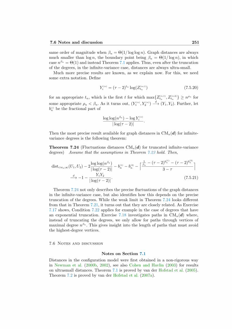
7.6 Notes and discussion 251
same order of magnitude when βn = Θ(1/ log logn). Graph distances are alwaysmuch smaller than log n, the boundary point being βn = Θ(1/ log n), in whichcase nβn = Θ(1) and instead Theorem 7.1 applies. Thus, even after the truncationof the degrees, in the infinite-variance case, distances are always ultra-small.
Much more precise results are known, as we explain now. For this, we needsome extra notation. Define
Y (n)
i = (τ − 2)tn log(Z(n;i)
tn ) (7.5.20)
for an appropriate tn, which is the first t for which maxZ(n;1)
tn , Z(n;2)
tn ≥ nρn for
some appropriate ρn < βn. As it turns out, (Y (n)
1 , Y (n)
2 )d−→ (Y1, Y2). Further, let
b(i)n be the fractional part of
log log(nβn)− log Y (n)
i
| log(τ − 2)| .
Then the most precise result available for graph distances in CMn(d) for infinite-variance degrees is the following theorem:
Theorem 7.24 (Fluctuations distances CMn(d) for truncated infinite-variancedegrees) Assume that the assumptions in Theorem 7.23 hold. Then,
distCMn(d)(U1, U2)− 2log log(nβn)
| log(τ − 2)| − b(1)
n − b(2)n −⌈ 1βn− (τ − 2)b
(1)n − (τ − 2)b
(2)n
3− τ⌉
d−→ −1− Y1Y2
| log(τ − 2)| . (7.5.21)
Theorem 7.24 not only describes the precise fluctuations of the graph distancesin the infinite-variance case, but also identifies how this depends on the precisetruncation of the degrees. While the weak limit in Theorem 7.24 looks differentfrom that in Theorem 7.21, it turns out that they are closely related. As Exercise7.17 shows, Condition 7.22 applies for example in the case of degrees that havean exponential truncation. Exercise 7.18 investigates paths in CMn(d) where,instead of truncating the degrees, we only allow for paths through vertices ofmaximal degree nβn . This gives insight into the length of paths that must avoidthe highest-degree vertices.
7.6 Notes and discussion
Notes on Section 7.1
Distances in the configuration model were first obtained in a non-rigorous wayin Newman et al. (2000b, 2002), see also Cohen and Havlin (2003) for resultson ultrasmall distances. Theorem 7.1 is proved by van der Hofstad et al. (2005).Theorem 7.2 is proved by van der Hofstad et al. (2007a).
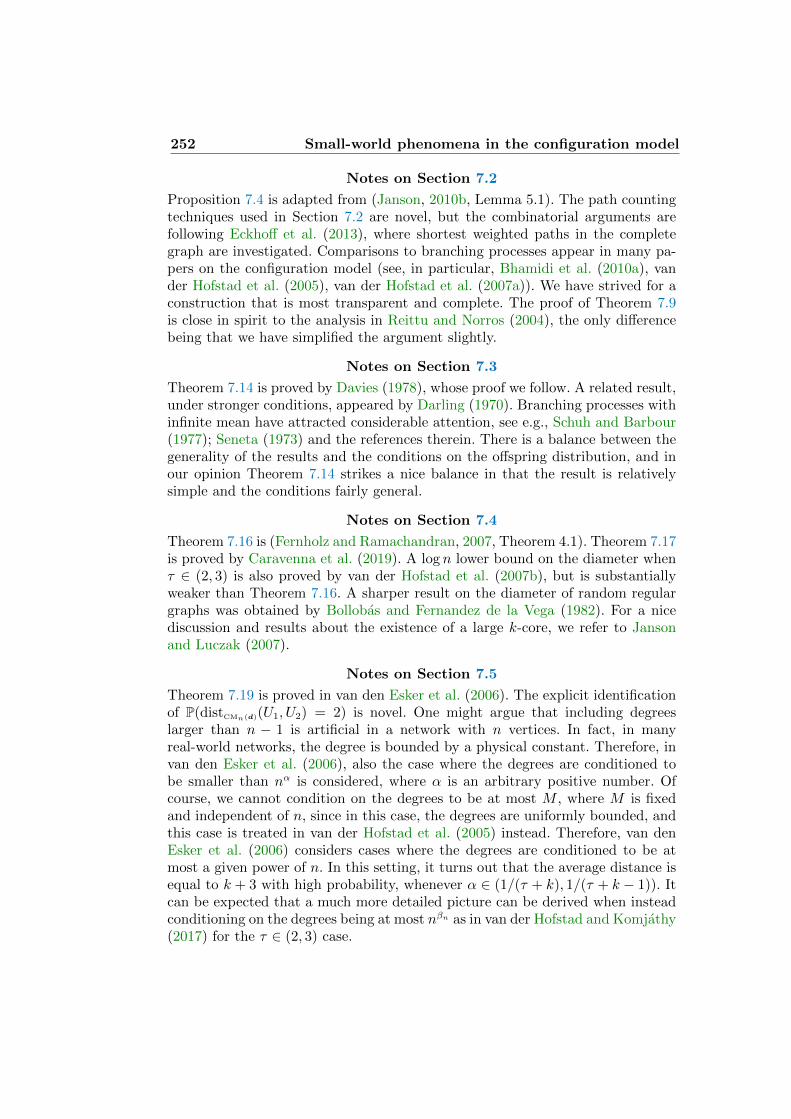
252 Small-world phenomena in the configuration model
Notes on Section 7.2
Proposition 7.4 is adapted from (Janson, 2010b, Lemma 5.1). The path countingtechniques used in Section 7.2 are novel, but the combinatorial arguments arefollowing Eckhoff et al. (2013), where shortest weighted paths in the completegraph are investigated. Comparisons to branching processes appear in many pa-pers on the configuration model (see, in particular, Bhamidi et al. (2010a), vander Hofstad et al. (2005), van der Hofstad et al. (2007a)). We have strived for aconstruction that is most transparent and complete. The proof of Theorem 7.9is close in spirit to the analysis in Reittu and Norros (2004), the only differencebeing that we have simplified the argument slightly.
Notes on Section 7.3
Theorem 7.14 is proved by Davies (1978), whose proof we follow. A related result,under stronger conditions, appeared by Darling (1970). Branching processes withinfinite mean have attracted considerable attention, see e.g., Schuh and Barbour(1977); Seneta (1973) and the references therein. There is a balance between thegenerality of the results and the conditions on the offspring distribution, and inour opinion Theorem 7.14 strikes a nice balance in that the result is relativelysimple and the conditions fairly general.
Notes on Section 7.4
Theorem 7.16 is (Fernholz and Ramachandran, 2007, Theorem 4.1). Theorem 7.17is proved by Caravenna et al. (2019). A log n lower bound on the diameter whenτ ∈ (2, 3) is also proved by van der Hofstad et al. (2007b), but is substantiallyweaker than Theorem 7.16. A sharper result on the diameter of random regulargraphs was obtained by Bollobas and Fernandez de la Vega (1982). For a nicediscussion and results about the existence of a large k-core, we refer to Jansonand Luczak (2007).
Notes on Section 7.5
Theorem 7.19 is proved in van den Esker et al. (2006). The explicit identificationof P(distCMn(d)(U1, U2) = 2) is novel. One might argue that including degreeslarger than n − 1 is artificial in a network with n vertices. In fact, in manyreal-world networks, the degree is bounded by a physical constant. Therefore, invan den Esker et al. (2006), also the case where the degrees are conditioned tobe smaller than nα is considered, where α is an arbitrary positive number. Ofcourse, we cannot condition on the degrees to be at most M , where M is fixedand independent of n, since in this case, the degrees are uniformly bounded, andthis case is treated in van der Hofstad et al. (2005) instead. Therefore, van denEsker et al. (2006) considers cases where the degrees are conditioned to be atmost a given power of n. In this setting, it turns out that the average distance isequal to k + 3 with high probability, whenever α ∈ (1/(τ + k), 1/(τ + k − 1)). Itcan be expected that a much more detailed picture can be derived when insteadconditioning on the degrees being at most nβn as in van der Hofstad and Komjathy(2017) for the τ ∈ (2, 3) case.
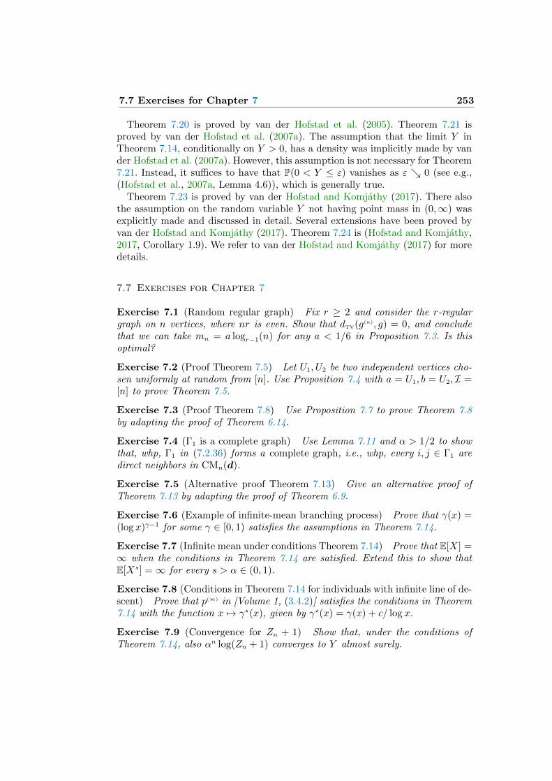
7.7 Exercises for Chapter 7 253
Theorem 7.20 is proved by van der Hofstad et al. (2005). Theorem 7.21 isproved by van der Hofstad et al. (2007a). The assumption that the limit Y inTheorem 7.14, conditionally on Y > 0, has a density was implicitly made by vander Hofstad et al. (2007a). However, this assumption is not necessary for Theorem7.21. Instead, it suffices to have that P(0 < Y ≤ ε) vanishes as ε 0 (see e.g.,(Hofstad et al., 2007a, Lemma 4.6)), which is generally true.
Theorem 7.23 is proved by van der Hofstad and Komjathy (2017). There alsothe assumption on the random variable Y not having point mass in (0,∞) wasexplicitly made and discussed in detail. Several extensions have been proved byvan der Hofstad and Komjathy (2017). Theorem 7.24 is (Hofstad and Komjathy,2017, Corollary 1.9). We refer to van der Hofstad and Komjathy (2017) for moredetails.
7.7 Exercises for Chapter 7
Exercise 7.1 (Random regular graph) Fix r ≥ 2 and consider the r-regulargraph on n vertices, where nr is even. Show that dTV(g(n), g) = 0, and concludethat we can take mn = a logr−1(n) for any a < 1/6 in Proposition 7.3. Is thisoptimal?
Exercise 7.2 (Proof Theorem 7.5) Let U1, U2 be two independent vertices cho-sen uniformly at random from [n]. Use Proposition 7.4 with a = U1, b = U2, I =[n] to prove Theorem 7.5.
Exercise 7.3 (Proof Theorem 7.8) Use Proposition 7.7 to prove Theorem 7.8by adapting the proof of Theorem 6.14.
Exercise 7.4 (Γ1 is a complete graph) Use Lemma 7.11 and α > 1/2 to showthat, whp, Γ1 in (7.2.36) forms a complete graph, i.e., whp, every i, j ∈ Γ1 aredirect neighbors in CMn(d).
Exercise 7.5 (Alternative proof Theorem 7.13) Give an alternative proof ofTheorem 7.13 by adapting the proof of Theorem 6.9.
Exercise 7.6 (Example of infinite-mean branching process) Prove that γ(x) =(log x)γ−1 for some γ ∈ [0, 1) satisfies the assumptions in Theorem 7.14.
Exercise 7.7 (Infinite mean under conditions Theorem 7.14) Prove that E[X] =∞ when the conditions in Theorem 7.14 are satisfied. Extend this to show thatE[Xs] =∞ for every s > α ∈ (0, 1).
Exercise 7.8 (Conditions in Theorem 7.14 for individuals with infinite line of de-scent) Prove that p(∞) in [Volume 1, (3.4.2)] satisfies the conditions in Theorem7.14 with the function x 7→ γ?(x), given by γ?(x) = γ(x) + c/ log x.
Exercise 7.9 (Convergence for Zn + 1) Show that, under the conditions ofTheorem 7.14, also αn log(Zn + 1) converges to Y almost surely.
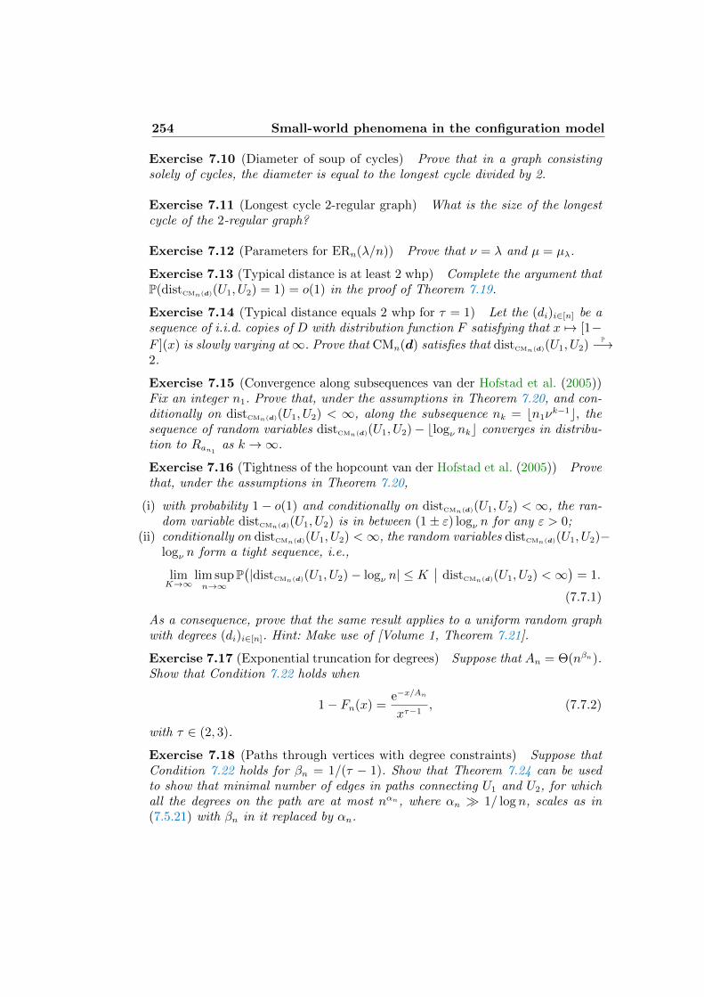
254 Small-world phenomena in the configuration model
Exercise 7.10 (Diameter of soup of cycles) Prove that in a graph consistingsolely of cycles, the diameter is equal to the longest cycle divided by 2.
Exercise 7.11 (Longest cycle 2-regular graph) What is the size of the longestcycle of the 2-regular graph?
Exercise 7.12 (Parameters for ERn(λ/n)) Prove that ν = λ and µ = µλ.
Exercise 7.13 (Typical distance is at least 2 whp) Complete the argument thatP(distCMn(d)(U1, U2) = 1) = o(1) in the proof of Theorem 7.19.
Exercise 7.14 (Typical distance equals 2 whp for τ = 1) Let the (di)i∈[n] be asequence of i.i.d. copies of D with distribution function F satisfying that x 7→ [1−F ](x) is slowly varying at∞. Prove that CMn(d) satisfies that distCMn(d)(U1, U2)
P−→2.
Exercise 7.15 (Convergence along subsequences van der Hofstad et al. (2005))Fix an integer n1. Prove that, under the assumptions in Theorem 7.20, and con-ditionally on distCMn(d)(U1, U2) < ∞, along the subsequence nk = bn1ν
k−1c, thesequence of random variables distCMn(d)(U1, U2)− blogν nkc converges in distribu-tion to Ran1
as k →∞.
Exercise 7.16 (Tightness of the hopcount van der Hofstad et al. (2005)) Provethat, under the assumptions in Theorem 7.20,
(i) with probability 1− o(1) and conditionally on distCMn(d)(U1, U2) <∞, the ran-dom variable distCMn(d)(U1, U2) is in between (1± ε) logν n for any ε > 0;
(ii) conditionally on distCMn(d)(U1, U2) <∞, the random variables distCMn(d)(U1, U2)−logν n form a tight sequence, i.e.,
limK→∞
lim supn→∞
P(|distCMn(d)(U1, U2)− logν n| ≤ K
∣∣ distCMn(d)(U1, U2) <∞)
= 1.
(7.7.1)
As a consequence, prove that the same result applies to a uniform random graphwith degrees (di)i∈[n]. Hint: Make use of [Volume 1, Theorem 7.21].
Exercise 7.17 (Exponential truncation for degrees) Suppose that An = Θ(nβn).Show that Condition 7.22 holds when
1− Fn(x) =e−x/An
xτ−1, (7.7.2)
with τ ∈ (2, 3).
Exercise 7.18 (Paths through vertices with degree constraints) Suppose thatCondition 7.22 holds for βn = 1/(τ − 1). Show that Theorem 7.24 can be usedto show that minimal number of edges in paths connecting U1 and U2, for whichall the degrees on the path are at most nαn, where αn 1/ log n, scales as in(7.5.21) with βn in it replaced by αn.
Chapter 8
Small-world phenomena inpreferential attachment models
Abstract
In this chapter, we investigate graph distances in preferential attach-ment models. We focus on typical distances as well as the diameter ofpreferential attachment models. We again rely on path-counting tech-niques. Remarkably, the setting where τ ∈ (2, 3) (corresponding toδ ∈ (−m, 0) is better understood than the setting where τ > 3.
Motivation: local structure versus small-world properties
In Chapters 6–7, we have seen that random graphs with infinite-variance degreesare ultra-small worlds. This can be understood informally by two effects. First,we note that such random graph models contain super-hubs, whose degrees aremuch larger than n1/2 and that form a complete graph of connections, as wellas that these super-hubs are often part of shortest paths between two typicalvertices; and (b) vertices of large degree d 1 are typically connected to verticesof much larger degree, more precisely, of degree roughly d1/(τ−2). Combined, thesetwo effects mean that it takes roughly log log n/| log(τ − 2)| steps from a typicalvertex to reach one of the super-hubs, and thus roughly 2 log log n/| log(τ − 2)|steps to connect two typical vertices to each other. Of course, the proofs are moretechnical, but this is the bottom line.
The above explanation depends crucially on the local structure of the general-ized random graph as well as the configuration model, in which indeed vertices ofhigh degree are whp connected to vertices of much high degree. In this chapter,we will see that for the preferential attachment model, such consideration need tobe subtly adapted. Indeed, fix δ ∈ (−m, 0) and m ≥ 2, so that the degree distri-bution has infinite variance. Then, in preferential attachment models, vertices oflarge degree d tend to be the old vertices, but old vertices are not necessarily con-nected to much older vertices, which would be necessary to increase their degreefrom d to d1/(τ−2). However, vertices of degree d 1 do tend to be connected totypical vertices that in turn tend to be connected to vertices of degree roughlyd1/(τ−2). We conclude that distances seem about twice as high in preferential at-tachment models than they are in the corresponding generalized random graphsand configuration models, and that this can be explained by the differences inthe local connectivity structure. Unfortunately, due to its dynamic nature, theresults for preferential attachment models are harder to prove, and they are lesscomplete.
Throughout this chapter, we work with the preferential attachment model de-fined in [Volume 1, Section 8.2], which we denote by (PA(m,δ)
n )n≥1, unless statedotherwise. We recall that this model starts with a single vertex with m self-loops
255
256 Small-world phenomena in preferential attachment models
at time t = 1 and at each time a vertex is added with m edges which are at-tached to the vertices in the graph with probabilities given in [Volume 1, (??)]for m = 1, and as described on page [Volume 1, 282] for m ≥ 2. This modelcan also be obtained by identifying blocks of m vertices in (PA(1,δ/m)
n )n≥1. Wesometimes also discuss other variants of the model, such as (PA(m,δ)
n (b)(n))n≥1, inwhich the m = 1 model does not have any self-loops.
Organization of this chapter
In Section 8.1, we start by showing that preferential attachment trees (where ev-ery vertex comes in with one edge to earlier vertices and m = 1) have logarithmicheight. In Section 8.2 we investigate graph distances in PA(m,δ)
n and formulateour main results. In Section 8.3, we investigate path counting techniques in pref-erential attachment models, which we use in Section 8.4 to prove lower boundson distances. In Section 8.5, we prove the matching upper bounds on graph dis-tances. In Section 8.6, we discuss the diameter of preferential attachment modelsfor m ≥ 2. In Section 8.7, we discuss further results about distances in preferentialattachment models. We close this chapter with notes and discussion in Section8.8, and with exercises in Section 8.9.
8.1 Logarithmic distances in preferential attachment trees
In this section, we investigate distances in scale-free trees, arising for m = 1.We start by studying the height of the tree PA(1,δ)
n , where the height of a tree Tis defined as
height(T ) = maxv∈[n]
distT (1, v), (8.1.1)
followed by its diameter:
Theorem 8.1 (Typical distance in scale-free trees) Fix m = 1 and δ > −1.Then, as n→∞,
distPA
(1,δ)n
(1, U)
log nP−→ 1 + δ
2 + δ,
height(PA(1,δ)
n )
log nP−→ 2(1 + δ)
(2 + δ). (8.1.2)
Theorem 8.2 (Diameter of scale-free trees) Fix m = 1 and δ > −1. Let γ bethe non-negative solution of
γ + (1 + δ)(1 + log γ) = 0. (8.1.3)
Then
distPA
(1,δ)n
(U1, U2)
log nP−→ 2(1 + δ)
(2 + δ)γ,
diam(PA(1,δ)
n )
log nP−→ 2(1 + δ)
(2 + δ)γ. (8.1.4)
The proof of Theorems 8.1–8.2 rely on the fact that PA(1,δ)
n consists of a collec-tion of trees with precisely one self-loop. There is a close analogy between thesetrees and so-called uniform recursive trees. In uniform recursive trees, we grow a
8.1 Logarithmic distances in preferential attachment trees 257
tree such that at time 1, we have a unique vertex called the root, with label 1.At time n, we add a vertex and connect it to a uniformly chosen vertex in thetree. See Smythe and Mahmoud (1994) for a survey of recursive trees.
A variant of a uniform recursive tree is the case where the probability thata newly added vertex is attached to a vertex is proportional to the degree ofthe vertices (and, for the root, the degree of the root plus one). This processis called a random plane-oriented recursive tree. For a uniform recursive tree ofsize t, it is proved by Pittel (1994) that the maximal distance between the rootand any other vertex is with high probability equal to 1
2γlog n(1 + o(1)), where
γ satisfies (8.1.3) with δ = 0. It is not hard to see that this implies that themaximal graph distance between any two vertices in the uniform recursive tree isequal to 1
γlog n(1 +o(1)). We shall make use of similar arguments below to prove
Theorem 8.2. Exercises 8.1–8.3 explore properties of the constant γ.In the proof of Theorem 8.2 it will be useful to work with PA(1,δ)
n (b) instead ofPA(1,δ)
n , for which a similar result holds:
Theorem 8.3 (Distances in scale-free trees PA(1,δ)
n (b)) Fix m = 1 and δ > −1,and let γ be the solution of (8.1.3). Then
distPA
(1,δ)n (b)
(1, U)
log nP−→ 1 + δ
2 + δ,
height(PA(1,δ)
n (b))
log na.s.−→ 2(1 + δ)
(2 + δ). (8.1.5)
and
distPA
(1,δ)n (b)
(U1, U2)
log nP−→ 2(1 + δ)
(2 + δ)γ,
diam(PA(1,δ)
n (b))
log nP−→ 2(1 + δ)
(2 + δ)γ. (8.1.6)
We start by proving the upper bound in Theorem 8.3. We remark that thealmost sure limit of the height in Theorem 8.3 does not depend on the precisestarting configuration of the graph PA(1,δ)
2 (b).
In the proof of the upper bound, we make use of the following result whichcomputes the probability mass function of the distance between vertex t and theroot 1. Before stating the result, we need some more notation. We write t −→ swhen in (PA(1,δ)
n (b))n≥1 one of the edges of vertex t is connected to vertex s. Notethat for this to happen, we need that t > s. For s1 = t > s2 > · · · > sk = 1, anddenoting ~sk = (s1, s2, . . . , sk), we write
E~sk =k−1⋂i=1
si −→ si+1. (8.1.7)
For a configuration of PA(1,δ)
n (b), we let dist(t, s) denote the unique value of ksuch that t = s1 −→ s2 −→ · · · −→ sk−1 −→ sk = s. Then the probability massfunction of dist(t, s) can be explicitly identified as follows:
Proposition 8.4 (Distribution of dist(t, s) in PA(1,δ)
n (b)) Fix m = 1 and δ > −1.
258 Small-world phenomena in preferential attachment models
Then, for all t > s,
P(dist(t, s) = k) =(1 + δ
2 + δ
)k Γ(t+ 12+δ
)Γ(s)
Γ(s+ 12+δ
)Γ(t+ 1)
∑~sk
k−1∏i=1
1
si, (8.1.8)
where the sum is over ordered vectors ~sk = (s0, . . . , sk) of length k+ 1 with s0 = tand sk = s. Further,
P(t −→ s1 −→ · · · −→ sk−1 −→ s) =(1 + δ
2 + δ
)k Γ(t+ 12+δ
)Γ(s)
Γ(s+ 12+δ
)Γ(t+ 1)
k−1∏i=1
1
si,
(8.1.9)
Proof of Proposition 8.4. Since the path between vertex t and s is unique, weobtain
P(dist(t, s) = k) =∑~sk
P( k−1⋂i=0
si −→ si+1), (8.1.10)
where again the sum is over all ordered vectors ~sk = (s0, . . . , sk) of length k + 1with s0 = t and sk = s. Therefore, (8.1.8) follows immediately from (8.1.9).
We claim that the events si −→ si+1 are independent, i.e., for every sequence~sk = (s0, . . . , sk)
P( k−1⋂i=0
si −→ si+1)
=k−1∏i=0
P(si −→ si+1). (8.1.11)
We prove the independence in (8.1.11) by induction on k. For k = 0, there isnothing to prove, and this initializes the induction hypothesis. To advance theinduction hypothesis in (8.1.11), we condition on PA(1,δ)
s0−1(b) to obtain
P( k−1⋂i=0
si −→ si+1)
= E[P( k−1⋂i=0
si −→ si+1∣∣∣PA(1,δ)
s1−1(b))]
= E[1⋂k−1
i=1 si−→si+1P(s0 −→ s1 | PA(1,δ)
s0−1(b))], (8.1.12)
since the event⋂l−1i=1si −→ si+1 is measurable with respect to PA(1,δ)
s0−1(b). Fur-thermore, from [Volume 1, (8.2.2)],
P(s0 −→ s1 | PA(1,δ)
s0−1(b))
=Ds1(s0 − 1) + δ
(2 + δ)(s0 − 1). (8.1.13)
In particular,
P(s0 −→ s1
)= E
[Ds1(s0 − 1) + δ
(2 + δ)(s0 − 1)
]. (8.1.14)
8.1 Logarithmic distances in preferential attachment trees 259
Therefore,
P( k−1⋂i=0
si −→ si+1)
= E[1⋂k−1
i=1 si−→si+1Ds2(s1 − 1) + δ
(2 + δ)(s1 − 1)
]= P
( k−1⋂i=1
si −→ si+1)E[Ds1(s0 − 1) + δ
(2 + δ)(s0 − 1)
], (8.1.15)
since the random variable Ds1(s0 − 1) only depends on how many edges are
connected to s1 after time s1, and is thus independent of the event⋂l−1i=1si −→
si+1, which only depends on the attachment of the edges up to and includingtime s1. We conclude that
P( k−1⋂i=0
si −→ si+1)
= P(s1 −→ s2
)P( k−1⋂i=0
si −→ si+1). (8.1.16)
The claim in (8.1.11) for k follows from the induction hypothesis.Combining (8.1.10) with (8.1.11) and (8.1.14), we obtain that
P(t −→ s1 −→ · · · −→ sk−1 −→ s) =k−1∏i=0
E[Dsi+1
(si − 1) + δ
(2 + δ)(si − 1)
]. (8.1.17)
By [Volume 1, (8.11.3)],
E[Di(t) + δ
(2 + δ)t
]= (1 + δ)
Γ(t+ 12+δ
)Γ(i)
(2 + δ)tΓ(t)Γ(i+ 12+δ
)
=1 + δ
2 + δ
Γ(t+ 12+δ
)Γ(i)
Γ(t+ 1)Γ(i+ 12+δ
), (8.1.18)
so that
P(t −→ s1 −→ · · · −→ sk−1 −→ s) (8.1.19)
=(1 + δ
2 + δ
)k k−1∏i=0
Γ(si + 12+δ
)Γ(si+1)
Γ(si + 1)Γ(si+1 + 12+δ
)
=(1 + δ
2 + δ
)kΓ(s0 + 12+δ
)Γ(sk + 1)
Γ(sk + 12+δ
)Γ(s0)
k−1∏i=1
1
si
=(1 + δ
2 + δ
)k Γ(t+ 12+δ
)Γ(s)
Γ(1 + 12+δ
)Γ(t+ 1)
k−1∏i=1
1
si. (8.1.20)
This completes the proof of Proposition 8.4.
Proof of the upper bounds in Theorem 8.3. We first use Proposition 8.3 to provethat, for U chosen uniformly at random from [n],
dist(1, U)
log n≤ (1 + oP(1))
1 + δ
2 + δ. (8.1.21)
260 Small-world phenomena in preferential attachment models
and, almost surely for large enough n,
dist(1, n)
log n≤ (1 + ε)
(1 + δ)
(2 + δ)γ. (8.1.22)
We start by noting that (8.1.21)–(8.1.22) immediately prove (8.1.5). Further,(8.1.22) implies that, almost surely for large enough n,
height(PA(1,δ)
n (b)) ≤ (1 + ε)(1 + δ)
(2 + δ)γ. (8.1.23)
By the triangle inequality,
distPA
(1,δ)n (b)
(U1, U2) ≤ dist(1, U1) + dist(1, U2), (8.1.24)
diam(PA(1,δ)
n (b)) ≤ 2height(PA(1,δ)
n (b)), (8.1.25)
so that (8.1.21)–(8.1.22) imply the upper bounds in Theorem 8.3.We proceed to prove (8.1.21) and (8.1.22), and start with some preparations.
We use (8.1.8) and symmetry to obtain
P(dist(1, n) = k) =(1 + δ
2 + δ
)k Γ(n+ 12+δ
)
Γ(1 + 12+δ
)Γ(n+ 1)
∑∗
~tk−1
1
(k − 1)!
k−1∏i=1
1
ti, (8.1.26)
where the sum now is over all vectors ~tk−1 = (t1, . . . , tk−1) with 1 < ti < n withdistinct coordinates. We can upper bound this sum by leaving out the restrictionthat the coordinates of ~tk−1 are distinct, so that
P(dist(1, n) = k) ≤(1 + δ
2 + δ
)k Γ(n+ 12+δ
)
Γ(1 + 12+δ
)Γ(n+ 1)
1
(k − 1)!
( n−1∑s=2
1
s
)k−1
. (8.1.27)
Since x 7→ 1/x is monotonically decreasing
n−1∑s=2
1
s≤∫ n
1
1
xdx = log n. (8.1.28)
Also, we use [Volume 1, (8.3.9)] to bound, for some constant Cδ > 0,
P(dist(1, n) = k) ≤ Cδn−1+δ2+δ
(1+δ2+δ
log n)k−1
(k − 1)!(8.1.29)
= CP(Poi(1 + δ
2 + δlog n
)= k − 1
).
Now we are ready to prove (8.1.21). We note that U is chosen uniformly in [n],
8.1 Logarithmic distances in preferential attachment trees 261
so that
P(dist(1, U) = k) =1
n
n∑s=1
P(dist(vs, v1) = k) ≤ 1
n
n∑s=1
Cδs− 1+δ
2+δ
(1+δ2+δ
log s)k−1
(k − 1)!
≤
(1+δ2+δ
log n)k−1
t(k − 1)!
n∑s=1
Cδs− 1+δ
2+δ ≤ C
(1+δ2+δ
log n)k−1
(k − 1)!n−
1+δ2+δ
= CP(Poi(1 + δ
2 + δlog n
)= k − 1
). (8.1.30)
Therefore,
P(dist(1, U) > k) ≤ CP(Poi(1 + δ
2 + δlog n
)≥ k
). (8.1.31)
Now we fix ε > 0 and take k = kn = (1+ε)(1+δ)
(2+δ)log n, to arrive at
P(dist(1, U) > kn) ≤ CP(Poi(1 + δ
2 + δlog n
)≥ (1 + ε)(1 + δ)
(2 + δ)log n
)= o(1),
(8.1.32)
by the law of large numbers and for any ε > 0, as required.We continue to prove (8.1.22). By (8.1.29),
P(dist(1, n) > k) ≤ CδP(Poi(1 + δ
2 + δlog n
)≥ k
). (8.1.33)
Now take kn = a log n with a > (1+δ)/(2+δ). We use the Borel-Cantelli lemmasto see that dist(1, n) > kn will occur only finitely often when (8.1.33) is summable.We then use the large deviation bounds for Poisson random variables in [Volume1, Exercise 2.20] with λ = (1 + δ)/(2 + δ) to obtain that
P(dist(1, n) > a log n) ≤ Cδn−[a(log (a(2+δ)/(1+δ))−1)+ 1+δ2+δ ]. (8.1.34)
Let x be the solution of
x(log (x(2 + δ)/(1 + δ))− 1) +1 + δ
2 + δ= 1, (8.1.35)
so that x = (1+δ)
(2+δ)γ. Then, for every a > x,
P(dist(1, n) > a log n) = O(n−p), (8.1.36)
where
p = [a(log (a(2 + δ)/(1 + δ))− 1) + (1 + δ)(2 + δ)] > 1. (8.1.37)
As a result, by the Borel-Cantelli Lemma, the event dist(1, n) > kn occurs onlyfinitely often, and we conclude that (8.1.22) holds.
262 Small-world phenomena in preferential attachment models
Proof of the lower bound on distPA
(1,δ)n (b)
(1, U) in Theorem 8.3. We use (8.1.30) toobtain that
P(distPA
(1,δ)n (b)
(1, U) ≤ k) ≤ CP(Poi(1 + δ
2 + δlog n
)≤ k
). (8.1.38)
Fix kn = (1+δ)(1−ε)(2+δ)
log n, and note that P(distPA
(1,δ)n (b)
(1, U) ≤ kn) = o(1) by the
law of large numbers.
To complete the proof of height(PA(1,δ)
n (b))/ log n
a.s.−→ (1+δ)(1−ε)(2+δ)γ
in Theorem 8.3,
we use the second moment method to prove that height(PA(1,δ)
n (b))≤ (1+δ)(1−ε)
(2+δ)γlog n
has vanishing probability. Together with (8.1.23), this certainly proves that
height(PA(1,δ)
n (b))/ log n
P−→ (1 + δ)(1− ε)(2 + δ)γ
.
However, since height(PA(1,δ)
n (b))
is a non-decreasing sequence of random vari-ables, this also implies that this convergence even holds almost surely, as weargue in more detail below Proposition 8.5.
We formalize the statement that height(PA(1,δ)
n (b))≤ (1+δ)(1−ε)
(2+δ)γlog n in the
following proposition:
Proposition 8.5 (Height of PA(1,δ)
n (b) converges in probability) For every ε > 0there exists a η = η(ε) > 0 such that
P(
height(PA(1,δ)
n (b))≤ (1 + δ)(1− ε)
(2 + δ)γlog n
)≤ O(n−η). (8.1.39)
Proof of lower bound on height(PA(1,δ)
n (b))
in Theorem 8.3 subject to Proposition8.5. Fix α > 0, and take tk = tk(α) = eαk. For any α > 0, by Proposition 8.5 and
the fact that t−ηk is summable, almost surely, height(PA(1,δ)
tk(b))≥ (1+δ)(1−ε)
(2+δ)γlog tk.
This proves the almost sure lower bound on height(PA(1,δ)
n (b))
along the subse-quence (tk)k≥0. To extend this to an almost sure lower bound when n → ∞, weuse that t 7→ height
(PA(1,δ)
n (b))
is non-decreasing, so that, for every t ∈ [tk−1, tk],
height(PA(1,δ)
n (b))≥ height
(PA(1,δ)
tk−1(b))
(8.1.40)
≥ (1 + δ)(1− ε)(2 + δ)γ
log tk−1
≥ (1− ε)(1− α)(1 + δ)
(2 + δ)γlog n,
where the third inequality follows from the almost sure lower bound on height(PA(1,δ)
tk−1(b)).
The above bound holds for all ε, α > 0, so that letting ε, α ↓ 0 proves ourclaim.
Proof of Proposition 8.5. We perform a path counting argument. We fix T ∈ [n]and k ∈ N. Recall that a path π = (π0, . . . , πk) is a sequence of vertices. In thissection we assume that πi > πi+1, since our paths will be part of the scale-free
8.1 Logarithmic distances in preferential attachment trees 263
tree PA(1,δ)
n (b). We write π ∈ PA(1,δ)
n (b) for the event that the edge from πi isconnected to πi+1 for all i = 0, . . . , k − 1. We let
Nk(n) = #π ⊆ PA(1,δ)
n (b) : πk ∈ [n] (8.1.41)
denote the number of k-step paths in PA(1,δ)
n (b) with an endpoint in [n]. By Propo-sition 8.4,
E[Nk(n)] =(1 + δ
2 + δ
)k n∑sk=1
n∑s0=sk
Γ(s0 + 12+δ
)Γ(sk)
Γ(sk + 12+δ
)Γ(s0 + 1)
∑~sk
k−1∏i=1
1
si(8.1.42)
≥(1 + δ
2 + δ
)k n∑sk=1
Γ(sk)
Γ(sk + 12+δ
)
n∑s0=sk
Γ(s0 + 12+δ
)
Γ(s0 + 1)
∑~sk
k−1∏i=1
1
si,
where again the sum is over all ordered ~sk = (s0, . . . , sk) with sk ∈ [n] ands0 ∈ [n]. We can bound this from below by
E[Nk(n)] ≥(1 + δ
2 + δ
)k n∑sk=1
Γ(sk)
Γ(sk + 12+δ
)
n∑s0=sk
Γ(s0 + 12+δ
)
Γ(s0 + 1)
1
(k − 1)!
∑~tk
k−1∏i=1
1
ti,
(8.1.43)
where now the sum is over all vectors ~tk = (t1, . . . , tk−1) with distinct coordinateswith ti ∈ [sk + 1, s0 − 1]. For fixed s0, sk,∑
~tk
k−1∏i=1
1
ti≥( s0−1∑s=sk+k
1
s
)k−1
. (8.1.44)
We can lower bound
s0−1∑s=sk+k
1
s≥∫ s0
sk+k
1
xdx = log(s0/(sk + k)) ≥ (1− ε) log n (8.1.45)
when s0 ≥ n/2, sk ≤ T and log[2(T + k)] ≤ ε log n. Thus, we conclude that
E[Nk(n)] ≥(1 + δ
2 + δ
)k n∑sk=1
Γ(sk)
Γ(sk + 12+δ
)
n∑s0=t/2
Γ(s0 + 12+δ
)
Γ(s0 + 1)
1
(k − 1)![(1− ε) log n]k−1.
(8.1.46)Using [Volume 1, (8.3.9)], we therefore arrive at
E[Nk(n)] ≥ (1 + o(1))(1 + δ
2 + δ
)k n∑sk=1
s−1/(2+δ)k
n∑s0=t/2
s−(1+δ)/(2+δ)0
1
(k − 1)![(1− ε) log n]k
≥ c(1 + δ
2 + δ
)kn(1+δ)/(2+δ)n1/(2+δ) 1
(k − 1)![(1− ε) log n]k−1
= cn(1+δ)/(2+δ)n[1+(1−ε)(1+δ)]/(2+δ)P(Poi(1 + δ
2 + δ(1− ε) log n
)= k − 1
).
(8.1.47)
264 Small-world phenomena in preferential attachment models
When we take k = kn = (1+δ)(1−ε)(2+δ)γ
log n, then
P(Poi(1 + δ
2 + δ(1− ε) log n
)= k − 1
)≥ cn−(1−ε)/
√log n, (8.1.48)
so that
E[Nk(n)] ≥ n(1+δ)/(2+δ)nε/(2+δ)+o(1). (8.1.49)
We next take T = nε to arrive at
E[Nk(n)] ≥ nε+o(1). (8.1.50)
This provides the required lower bound on E[Nk(n)]. We defer the proof of anupper bound on Var(Nk(n)) to Section 8.3, where we prove that there exist C > 0and η = η(ε) > 0 such that Var(Nk(n)) ≤ CE[Nk(n)]2n−η (see Lemma 8.12below). As a result, by the Chebychev inequality ([Volume 1, Theorem 2.18])
P(Nk(n) = 0) ≤ Var(Nk(n))
E[Nk(n)]2≤ Cn−η. (8.1.51)
Since height(PA(1,δ)
n (b)) ≥ k when Nk(n) ≥ 1, this proves the claim in Proposition8.5.
We complete this section by proving Theorems 8.2–8.3:Proof of Theorems 8.2 and 8.3. We first prove the upper bound on the diameterof PA(1,δ)
n (b) in Theorem 8.3, for which we use that
diam(PA(1,δ)
n (b)) ≤ 2 · height(PA(1,δ)
n (b)). (8.1.52)
Equation (8.1.52) together with the upper bound in Theorem 8.3 imply that
lim supn→∞
diam(PA(1,δ)
n (b))
log n≤ 2(1 + δ)
γ(2 + δ). (8.1.53)
For the lower bound, we use the lower bound on diam(PA(1,δ)
n (b)) in Theo-rem 8.3 and the decomposition of scale-free trees in Theorem 5.3. Theorem 5.3states that the scale-free tree PA(1,δ)
n (b) can be decomposed into two scale-freetrees, having a similar distribution as copies PA(b1)
S1(t)(1, δ) and PA(1,δ)
t−S1(t)(b2), where
(PA(1,δ)
n (b1))n≥1 and (PA(1,δ)
n (b2))n≥1 are independent scale-free tree processes, andthe law of S1(t) is described in (5.1.29). By this tree decomposition
diam(PA(1,δ)
n (b))≥ height
(PA(1,δ)
S1(n)(b1))
+ height(PA(1,δ)
n−S1(n)(b2)). (8.1.54)
The two trees (PA(1,δ)
n (b1))n≥1 and (PA(1,δ)
n (b2))n≥1 are not exactly equal indistribution to (PA(1,δ)
n (b))n≥1, because the initial degree of the starting verticesat time n = 2 is different. However, the precise almost sure scaling in Theorem5.3 does not depend in a sensitive way on d1 and d2, and also the height of thescale-free tree in Theorem 8.3 does not depend on the starting graphs PA(1,δ)
2 (b1)and PA(1,δ)
2 (b1) (see the remark below Theorem 8.3).
Exercise??
8.2 Small-world effect in preferential attachment models 265
Since S1(n)/na.s.−→ U , with U having a Beta-distribution with parameters
a = 3+δ2+δ
and b = 1+δ2+δ
, we obtain that height(PA(1,δ)
S1(n)(b1))/ log n
a.s.−→ (1+δ)
(2+δ)γand
height(PA(1,δ)
n−S1(n)(b2))/ log n
a.s.−→ (1+δ)
(2+δ)γ. Thus, we conclude that, almost surely
for large enough n,
diam(PA(1,δ)
n (b))
log n≥ (1− ε) 2(1 + δ)
(2 + δ)γ. (8.1.55)
Combining (8.1.53) and (8.1.55) proves the convergence of diam(PA(1,δ)
n (b))/ log n
in Theorem 8.3.We proceed with the proof of the convergence of dist
PA(1,δ)n (b)
(U1, U2)/ log n inTheorem 8.3. We write
distPA
(1,δ)n (b)
(U1, U2) = distPA
(1,δ)n (b)
(1, U1) + distPA
(1,δ)n (b)
(1, U2) (8.1.56)
− distPA
(1,δ)n (b)
(1, V ),
where V is the last vertex that is on both paths from 1 → U1 as well as from1→ U2. The asymptotics of the first two terms are identified in (8.1.5) in Theorem8.3, so that it suffices to show that dist
PA(1,δ)n (b)
(1, V ) = oP(log n).
Update from here!
To prove Theorem 8.2, we note that the connected components of PA(1,δ)
n aresimilar in distribution to single scale-free tree PA(1,δ)
t1(b1), . . . ,PA(1,δ)
tNn(bNn), apart
from the initial degree of the root. Here ti denotes the size of the ith tree attime n, and we recall that Nt denotes the total number of trees at time n. Since
Nn/ log nd−→ (1 + δ)/(2 + δ) (recall Exercise 5.23), whp the largest connected
component has size at least εn/ log n. Since
log(εn/ log n
)= log n(1 + o(1)), (8.1.57)
the result follows along the same lines as in the proof of Theorem 8.3.
8.2 Small-world effect in preferential attachment models
In the next sections we investigate distances in preferential attachment modelsfor m ≥ 2. These results are not as complete as those for inhomogeneous randomgraphs or the configuration model as discussed in Chapters 6 and 7, respectively.We investigate both the diameter as well as typical distances. By Theorem 5.16,PA(m,δ)
n is whp connected when m ≥ 2. Recall that in a connected graph, thetypical distance or hopcount dist
PA(m,δ)n
(U1, U2) is the graph distance between twovertices chosen uniformly at random from [n]. Recall further that the power-lawdegree exponent for PA(m,δ)
n is equal to τ = 3 + δ/m. Therefore, τ > 3 preciselywhen δ > 0. For the generalized random graph and the configuration model, wehave seen that distaces are logarithmic in the size of the graph when τ > 3, anddoubly logarithmic when τ ∈ (2, 3). We will see that similar behavior is true forPA(m,δ)
n . We start by analyzing the case where δ > 0.
266 Small-world phenomena in preferential attachment models
Logarithmic distances in PA models with m ≥ 2 and δ > 0.
We start by investigating the case where δ > 0 so that also the power-law degreeexponent τ satisfies τ > 3. In this case, both the diameter as well as typicaldistances are logarithmic in the size of the graph:
Theorem 8.6 (A log n bound for typical distances in PAMs) Fix m ≥ 2 andδ > 0. There exist 0 < a1 < a2 <∞ such that, as n→∞,
P(a1 log n ≤ distPA
(m,δ)n
(U1, U2) ≤ a2 log n) = 1− o(1). (8.2.1)
While we believe that there are constants a and b with a < b such that
distPA
(m,δ)n
(U1, U2)/ log nP−→ a, diam(PA(m,δ)
n )/ log nP−→ b, (8.2.2)
currently, a proof for this fact is still missing.
Distances in PA models with m ≥ 2 and δ = 0.
For δ = 0, τ = 3. For NRn(w), distances grow as log n/ log log n in this case(recall Theorem 6.17). The same turns out to be true for PA(m,δ)
n :
Theorem 8.7 (Typical distances of PA(m,δ)
n for δ = 0) Fix m ≥ 2 and δ = 0.As n→∞,
distPA
(m,δ)n
(U1, U2)log log n
log nP−→ 1. (8.2.3)
Theorem 8.7 shows that distances for τ = 3 are similar in PA(m,δ)
n as in NRn(w).Interestingly, for PA(m,δ)
n with δ = 0, the diameter and the typical distances areclose to being equal. For NRn(w) and CMn(d) with power-law exponent τ = 3,this fact is not known.
log log distances in PA models with m ≥ 2 and δ < 0.
We close this section by discussing the case where δ ∈ (−m, 0), so that τ ∈ (2, 3).In this case, it turns out that distances again grow doubly logarithmically in thesize of the graph:
Theorem 8.8 (log log n asymptotics for the diameter for δ < 0) Fix m ≥ 2 andassume that δ ∈ (−m, 0). As n→∞,
distPA
(m,δ)n
(U1, U2)
log log nP−→ 4
| log (τ − 2)| . (8.2.4)
Interestingly, the term 4/| log (τ − 2)| appearing in Theorems 8.8 replaces theterm 2/| log (τ − 2)| in Theorems 7.2 and 7.17 for the configuration model CMn(d)with power-law exponent τ ∈ (2, 3). Thus, typical distances are twice as big forPA(m,δ)
n compared to CMn(d) with the same power-law exponent. This can beintuitively explained as follows. For the configuration model CMn(d), verticeswith high degrees are likely to be directly connected (see e.g. Lemma 7.11). ForPA(m,δ)
n , this is not the case. However, vertices with high degrees are likely to be
8.3 Path counting in preferential attachment models 267
at distance two. This makes distances in PA(m,δ)
n about twice as big as those forCMn(d) with the same degree sequence. This effect is special for δ < 0 and isstudied in more detail in Exercises 8.4–8.5.
Universality in distances for scale-free graphs
The available results are all consistent with the prediction that distances in pref-erential attachment models have the same asymptotics as distances in the con-figuration model with the same degree sequence. This suggest a strong form ofuniversality, which is interesting in its own right.
8.3 Path counting in preferential attachment models
In this section we study the probability that a certain path is present in PA(m,δ)
n .Recall that we call a path π = (s0, s1, . . . , sl) self-avoiding when si 6= sj for all1 ≤ i < j ≤ l. The following proposition studies the probability that a path ispresent in PA(m,δ)
n :
Proposition 8.9 (Path counting in PA(m,δ)
n ) Denote γ = m2m+δ
. Let π = (π0, π1, . . . , πl)be a self-avoiding path of length l consisting of the l + 1 unordered verticesπ0, π1, . . . , πl. Then
P(π ⊆ PA(m,δ)
n ) ≤ (Cm2)ll−1∏i=0
1
(πi ∧ πi+1)γ(πi ∨ πi+1)1−γ . (8.3.1)
Paths are formed by repeatedly forming edges. When m = 1, paths go fromlater vertices to older vertices. When m ≥ 2, this monotonicity property of pathsis lost, which makes the proof harder. We start by investigating intersections ofevents that specify which edges are present in PA(m,δ)
n . We start by introducingsome notation. Denote by
g(t, j) = s, 1 ≤ j ≤ m, (8.3.2)
the event that the jth edge of vertex t is attached to the earlier vertex s. ForPA(m,δ)
n , this event means that in PAmt(1, δ) the edge from vertex m(t− 1) + jis attached to one of the vertices m(s− 1) + 1, . . . ,ms.
It is a direct consequence of the definition of PA-models that the event (8.3.2)increases the preference for vertex s, and hence decreases (in a relative way) thepreference for the vertices u, 1 ≤ u ≤ t, u 6= s. It should be intuitively clearthat another way of expressing this effect is to say that, for different s1 6= s2,the events g(t1, j1) = s1 and g(t2, j2) = s2 are negatively correlated. We nowformalize this result For integer ns ≥ 1, we denote by
Es =ns⋂i=1
g(t(s)i , j
(s)
i ) = s, (8.3.3)
the event that the jith edge of vertex ti is attached to the earlier vertex s, for
268 Small-world phenomena in preferential attachment models
i = 1, . . . , ns. We start by proving that the events Es, for different s, are negativelycorrelated for each choice of k ≥ 1 and all possible choices of t(s)i , j
(s)
i .
Lemma 8.10 (Negative correlation for connection of edges) For distinct s1, s2, . . . , sk,both for PA(m,δ)
n and for PA(m,δ)
t (b),
P( k⋂i=1
Esi
)≤
k∏i=1
P(Esi). (8.3.4)
Proof We only prove the statement for PA(m,δ)
n , the proof for PA(m,δ)
t (b) is identi-cal. We use induction on the largest edge number present in the events Es1 , . . . , Esk .Here, we define the edge number of the event g(t, j) = s to be m(t − 1) + j,which is the order of the edge when we consider the edges as being attached insequence in PAmt(1, δ/m).
The induction hypothesis is that (8.3.4) holds for all k and all choices of t(s)i , j(s)
i
such that maxi,sm(t(s)i − 1) + j(s)
i ≤ e, where induction is performed with respectto e.
To initialize the induction, we note that for e = 1, the induction hypothesisholds trivially, since
⋂ki=1Esi can be empty or consist of exactly one event, and
in the latter case there is nothing to prove. This initializes the induction.To advance the induction, we assume that (8.3.4) holds for all k and all choices
of t(s)i , j(s)
i such that maxi,sm(t(s)i −1)+j(s)
i ≤ e−1, and we extend it to all k and allchoices of t(s)i , j
(s)
i such that maxi,sm(t(s)i − 1) + j(s)
i ≤ e. Clearly, for k and t(s)i , j(s)
i
such that maxi,sm(t(s)i − 1) + j(s)
i ≤ e− 1, the bound follows from the inductionhypothesis, so we may restrict attention to the case that maxi,sm(t(s)i −1)+j(s)
i =e. We note that there is a unique choice of t, j such that m(t− 1) + j = e. Thereare two possibilities: (1) Either there is exactly one choice of s and t(s)i , j
(s)
i suchthat t(s)i = t, j(s)
i = j, or (2) there are at least two of such choices. In the latter
case,⋂ks=1Es = ∅, since the eth edge is connected to a unique vertex. Hence,
there is nothing to prove.We are left to investigate the case where there exists a unique s and t(s)i , j
(s)
i
such that t(s)i = t, j(s)
i = j. Denote by
E′s =ns⋂
i=1:(t(s)i ,j
(s)i )6=(t,j)
g(t(s)i , j
(s)
i ) = s
(8.3.5)
the restriction of Es to all other edges. Then we can write
k⋂i=1
Esi =g(t, j) = s
∩ E′s ∩
k⋂i=1: si 6=s
Esi . (8.3.6)
By construction, all the edge numbers of the events in E′s ∩⋂ki=1: si 6=sEsi are at
most e− 1. Thus we obtain
P( k⋂i=1
Esi
)≤ E
[1E′s∩
⋂ki=1: si 6=s
EsiPe−1(g(t, j) = s)
], (8.3.7)
8.3 Path counting in preferential attachment models 269
where Pe−1 denotes the conditional probability given the edge attachments upto the (e − 1)st edge connection, or, equivalently, given PAe−1(1, δ/m), and
we have used that the event E′s ∩⋂ki=1: si 6=sEsi is measurable with respect to
PAe−1(1, δ/m).We compute
Pe−1(g(t, j) = s) =Ds(t− 1, j − 1) + δ
(2m+ δ)(t− 1) + (j − 1)(2 + δ/m) + 1 + δ, (8.3.8)
where we recall that Ds(t− 1, j − 1) is the degree of vertex s after j − 1 edges ofvertex t have been attached. We wish to use the induction hypothesis. For this,we note that
Ds(t− 1, j − 1) = m+∑
(t′,j′) : mt′+j′≤e−1
1g(t′,j′)=s, (8.3.9)
where we recall that e− 1 = m(t− 1) + j− 1. Each of the events g(t′, j′) = s in(8.3.9) has edge number strictly smaller than e and occurs with a non-negativemultiplicative constant. As a result, we may use the induction hypothesis for eachof these terms. Thus, we obtain, using also m+ δ ≥ 0, that,
P( k⋂i=1
Esi
)≤ m+ δ
(2m+ δ)(t− 1) + (j − 1)(2 + δ/m) + 1 + δP(E′s)
k∏i=1: si 6=s
P(Esi)
(8.3.10)
+∑
(t′,j′) : mt′+j′≤e−1
P(E′s ∩ g(t′, j′) = s)(2m+ δ)(t− 1) + (j − 1)(2 + δ/m) + 1 + δ
k∏i=1: si 6=s
P(Esi).
We use (8.3.9) to recombine the above as
P( k⋂i=1
Esi
)≤ E
[1E′s
Ds(t− 1, j − 1) + δ
(2m+ δ)(t− 1) + (j − 1)(2 + δ/m) + 1 + δ
] k∏i=1:si 6=s
P(Esi),
(8.3.11)and the advancement is completed when we note that
E[1E′s
Ds(t− 1, j − 1) + δ
(2m+ δ)(t− 1) + (j − 1)(2 + δ/m) + 1 + δ
]= P(Es). (8.3.12)
The claim in Lemma 8.10 follows by induction.
We next study the probabilities of the events Es when ns ≤ 2:
Lemma 8.11 (Edge connection events for at most two edges) Denote γ = m2m+δ
.There exist absolute constants M1 = M1(δ,m),M2 = M2(δ,m), such that(i) for m = 1 and any n > s,
P(g(n, 1) = s) = (1 + δ)Γ(t)Γ(s+ 1+δ
2+δ)
Γ(t+ 1+δ2+δ
)Γ(s+ 1)≤ M1
n1−γsγ. (8.3.13)
270 Small-world phenomena in preferential attachment models
Consequently, for each 1 ≤ j ≤ m and n > s,
P(g(n, j) = s
)≤ M1
n1−γsγ. (8.3.14)
(ii) for m = 1 and any t2 > t1 > s,
P(g(t1, 1) = s, g(t2, 1) = s
)=
Γ(t2)Γ(t1 + 12+δ
)Γ(s+ 1+δ2+δ
)
Γ(t2 + 1+δ2+δ
)Γ(t1 + 1)Γ(s+ 3+δ2+δ
)(1 + δ). (8.3.15)
Consequently, for any 1 ≤ j1, j2 ≤ m and t2 > t1 > s,
P(g(t1, j1) = s, g(t2, j2) = s
)≤ M2
(t1t2)1−γs2γ. (8.3.16)
Proof We only prove (8.3.13) and (8.3.15), (8.3.14) and (8.3.16) follow immedi-ately from [Volume 1, (8.3.9)].
Throughout this proof, we abbreviate g(t) = g(t, 1). By the definition of(PA(m,δ)
n )n≥1 in terms of (PAn(1, δ/m))n≥1, this implies the result for generalm ≥ 1, where the factors of m follow from the fact that vertex s in PA(m,δ)
n
corresponds to vertices ms, . . . ,m(s + 1) − 1 in PAmt(1, δ/m), which are all atleast ms. Note, in particular, that g(t, j) = s for m ≥ 2 in PA(m,δ)
n is equivalentto g(m(t− 1) + j) ∈ m(s− 1) + 1, . . . ,ms in PAmt(1, δ/m).
For (8.3.13), we use [Volume 1, Theorem 8.2] to compute
P(g(t) = s
)= E
[E[1g(t)=s |PAt−1(1, δ)]
]= E
[ Ds(t− 1) + δ
(2 + δ)(t− 1) + 1 + δ
]= (1 + δ)
Γ(t)Γ(s+ 1+δ2+δ
)
Γ(t+ 1+δ2+δ
)Γ(s+ 1). (8.3.17)
Take t2 > t1. We proceed with the proof of (8.3.15) by computing
P(g(t1) = s, g(t2) = s
)(8.3.18)
= E[P(g(t1) = s, g(t2) = s
∣∣PAt2−1(m, δ))]
= E[1g(t1)=s
(Ds(t2 − 1) + δ
(t2 − 1)(2 + δ) + 1 + δ
)]=
1
(t2 − 1)(2 + δ) + 1 + δ
Γ(t2)Γ(t1 + 1+δ2+δ
)
Γ(t2 − 1 + 1+δ2+δ
)Γ(t1 + 1)E[1g(t1)=s (Ds(t1) + δ)
]=
Γ(t2)Γ(t1 + 1+δ2+δ
)
Γ(t2 + 1+δ2+δ
)Γ(t1 + 1)E[1g(t1)=s (Ds(t1) + δ)
](8.3.19)
where we use the iteration, for t1 < u ≤ t2 − 1,
E[1g(t1)=s (Ds(u) + δ)
](8.3.20)
=(
1 +1
(2 + δ)(u− 1) + 1 + δ
)E[1g(t1)=s (Ds(u− 1) + δ)
].
8.3 Path counting in preferential attachment models 271
We are lead to compute E[1g(t1)=s (Ds(t1) + δ)
]. We use recursion to obtain
E[1g(t1)=s (Ds(t1) + δ)
∣∣PAt1−1(m, δ)]
(8.3.21)
= E[1g(t1)=s (Ds(t1)−Ds(t1 − 1))
∣∣PAt1−1(m, δ)]
+ E[1g(t1)=s (Ds(t1 − 1) + δ)
∣∣PAt1−1(m, δ)]
=(Ds(t1 − 1) + δ)(Ds(t1 − 1) + 1 + δ)
(t1 − 1)(2 + δ) + 1 + δ.
By [Volume 1, Proposition 8.15],
E[(Ds(t) + δ)(Ds(t) + 1 + δ)] =2
c2(t)E[Zs,2(t)] =
c2(s)
c2(t)(2 + δ)(1 + δ). (8.3.22)
Recalling that ck(j) = Γ(j + 1+δ2+δ
)/Γ(j + k+1+δ2+δ
), this brings us to
E[(Ds(t) + δ)(Ds(t) + 1 + δ)] =Γ(t+ 3+δ
2+δ)Γ(s+ 1+δ
2+δ)
Γ(t+ 1+δ2+δ
)Γ(s+ 3+δ2+δ
)(2 + δ)(1 + δ). (8.3.23)
where M4 is a uniform constant. Consequently,
E[1g(t1)=s (Ds(t1) + δ)
](8.3.24)
=Γ(t1 + 1
2+δ)Γ(s+ 1+δ
2+δ)
[(t1 − 1)(2 + δ) + 1 + δ]Γ(t1 − 12+δ
)Γ(s+ 3+δ2+δ
)(2 + δ)(1 + δ)
=Γ(t1 + 1
2+δ)Γ(s+ 1+δ
2+δ)
Γ(t1 + 1+δ2+δ
)Γ(s+ 3+δ2+δ
)(1 + δ).
Combining (8.3.19), (8.3.21) and (8.3.22), we arrive at
P(g(t1) = s, g(t2) = s
)(8.3.25)
=Γ(t2)Γ(t1 + 1+δ
2+δ)
Γ(t2 + 1+δ2+δ
)Γ(t1 + 1)×
Γ(t1 + 12+δ
)Γ(s+ 1+δ2+δ
)
Γ(t1 + 1+δ2+δ
)Γ(s+ 3+δ2+δ
)(1 + δ)
=Γ(t2)Γ(t1 + 1
2+δ)Γ(s+ 1+δ
2+δ)
Γ(t2 + 1+δ2+δ
)Γ(t1 + 1)Γ(s+ 3+δ2+δ
)(1 + δ),
as required.
With Lemmas 8.10 and 8.11 at hand, we are ready to prove Proposition 8.9:
Proof of Proposition 8.9. Since π is self-avoiding, we can write π ⊆ PA(m,δ)
n =∩ki=1Esi , where either
Es = g(t, j) = s (8.3.26)
for some t > s and some 1 ≤ j ≤ m, or
Es = g(t1, j1) = g(t2, j2) = s, (8.3.27)
272 Small-world phenomena in preferential attachment models
for some t1, t2 > s and some 1 ≤ j1, j2 ≤ m. In the first case, by (8.3.13),
P(Es) = P(g(n, j) = s
)≤ M1
n1−γsγ, (8.3.28)
whereas in the second case, according to (8.3.15),
P(Es) = P(g(t1, j1) = s, g(t2, j2) = s) ≤ M2
(t1t2)1−γs2γ=
M2
t1−γ1 sγt1−γ2 sγ. (8.3.29)
In both cases Mi, i = 1, 2, is an absolute constant. Lemma 8.10 then yields (8.3.1),where the factor m2l originates from the number of possible choices of ji ∈ [m]for i = 1, . . . , k and the possible si that are collapsed to the same vertex.
Lemma 8.12 (A variance estimate on Nk(n)) Recall the definition of Nk(n) in(8.1.41) and let T = nε for some ε > 0. Then there exists constants C > 0 andη = η(ε) > 0 such that
Var(Nk(n)) ≤ CE[Nk(n)]2n−η. (8.3.30)
Proof By Exercise 8.6, when the path (π0, . . . , πk) is completely disjoint from(ρ0, . . . , ρk),
P( k−1⋂i=0
πi −→ πi+1 ∩k−1⋂i=0
ρi −→ ρi+1)
(8.3.31)
≤ P( k−1⋂i=0
πi −→ πi+1)P( k−1⋂i=0
ρi −→ ρi+1).
Therefore, the indicators of disjoint paths are negatively correlated. As a result,we can bound
Var(Nk(n)) ≤∑
π,ρ : π∩ρ6=∅
P(π, ρ ⊆ PA(1,δ)
n (b)). (8.3.32)
Since m = 1, the paths π, ρ of length k must merge at some point, before movingoff to their common end point in [n]. When ρ = π, then we obtain a contributionE[Nk(n)], so that from now on we assume that π 6= ρ.
Write π = (π0, . . . , πk) and ρ = (ρ0, . . . , ρk) and π 6= ρ. Then there must be anl ∈ [k − 1] such that πj = ρj for all j = l, . . . , k. For two fixed paths π and ρ forwhich πj = ρj for all j = l, . . . , k, while πl−1 6= ρl−1. By Lemma 8.10, for suchpaths π, ρ,
P(π, ρ ⊆ PA(1,δ)
n (b)) ≤( l−1∏i=1
P(πi−1 −→ πi)P(ρi−1 −→ ρi))
(8.3.33)
× P(πl−1, ρl−1 −→ πl)( k∏j=l+1
P(πj−1 −→ πj)).
8.3 Path counting in preferential attachment models 273
By (8.1.9) in Proposition 8.4,
l−1∏i=1
P(πi−1 −→ πi) =(1 + δ
2 + δ
)l−1 Γ(π0 + 12+δ
)Γ(πl−1)
Γ(πl−1 + 12+δ
)Γ(π0 + 1)
l−2∏i=1
1
πi(8.3.34)
By symmetry, we may assume without loss of generality that πl−1 > ρl−1. Then,by (8.3.15),
P(πl−1, ρl−1 −→ πl) = (1 + δ)Γ(ρl−1 − δ
2+δ)Γ(πl−1 − 1+δ
2+δ)Γ(πl)
Γ(ρl−1 + 12+δ
)Γ(πl−1)Γ(πl + 22+δ
). (8.3.35)
As a result,
P(π, ρ ⊆ PA(1,δ)
n (b)) ≤(1 + δ
2 + δ
)l+k−3 Γ(π0 + 12+δ
)Γ(πl−1)
Γ(πl−1 + 12+δ
)Γ(π0 + 1)
Γ(ρ0 + 12+δ
)Γ(ρl−1)
Γ(ρl−1 + 12+δ
)Γ(ρ0 + 1)
(8.3.36)
× (1 + δ)Γ(ρl−1 − δ
2+δ)Γ(πl−1 − 1+δ
2+δ)Γ(πl)
Γ(ρl−1 + 12+δ
)Γ(πl−1)Γ(πl + 22+δ
)
l−2∏i=1
1
πiρi
×Γ(πl + 1
2+δ)Γ(πk)
Γ(πk + 12+δ
)Γ(πl + 1)
k−1∏i=l+1
1
πi
= (1 + δ)(1 + δ
2 + δ
)l+k−3 Γ(π0 + 12+δ
)
Γ(π0 + 1)
Γ(ρ0 + 12+δ
)
Γ(ρ0 + 1)
Γ(ρl−1)Γ(ρl−1 − δ2+δ
)
Γ(ρl−1 + 12+δ
)Γ(ρl−1 + 12+δ
))
×Γ(πl + 1
2+δ)
Γ(πl + 22+δ
)
Γ(πk)
Γ(πk + 12+δ
)
1
(πl−1 + 12+δ
)
l−2∏i=1
1
πiρi
k−1∏i=l
1
πi.
By (??), this can be bounded by
C(1 + δ
2 + δ
)l+k(π0ρ0)−(1+δ)/(2+δ)(πlπk)
−1/(2+δ)l−1∏i=1
1
ρi
k−1∏i=1
1
πi, (8.3.37)
where C is a uniform constant. We need to sum the above over l < k, all decreasingπ = (π0, . . . , πk) with πk ∈ [n] and all decreasing (ρ0, . . . , ρl−1) with ρl−1 > πl. Thesum can be bounded from above by summing over all decreasing (ρ0, . . . , ρl−1)
and bounding π−1/(2+δ)l ≤ 1 to obtain an upper bound as in (8.1.43)
E[Nk(n)](1 + δ
2 + δ
)l (log n)l
l!
∑s∈[n]
s−(1+δ)/(2+δ). (8.3.38)
Therefore,
Var(Nk(n)) ≤ E[Nk(n)] + E[Nk(n)]k−1∑l=1
(1 + δ
2 + δ
)l (log n)l
l!
∑s∈[n]
s−(1+δ)/(2+δ).
(8.3.39)When T = nε, it is not hard to adapt the arguments in (8.1.43)–(8.1.49) to showthat this is at most E[Nk(n)]2n−η for some η = η(ε) > 0.
274 Small-world phenomena in preferential attachment models
Add Discussion of distPA
(1,δ)n (b)
(1, V ) = oP(logn) here! Or exercise?
8.4 Small-world effect in PA models: lower bounds
In this section we prove lower bounds on distances in PA(m,δ)
n with m ≥ 2. InSection 8.3 we start by proving an upper bound on the probability that a pathexists in PA(m,δ)
n , which is our main tool in this section. After this we prove thelower bounds on distances for δ > 0 in Section 8.4.1, for δ = 0 in Section 8.4.2,and for δ < 0 in Section 8.4.3.
8.4.1 Logarithmic lower bounds on distances for δ > 0
In this section we investigate lower bounds on the distances when δ > 0, inwhich case γ = m/(2m+ δ) < 1/2. By Proposition 8.9,
P(
distPA
(m,δ)n
(1, t) = k)≤ ck
∑π
k−1∏j=0
1
(πj ∧ πj+1)γ(πj ∨ πj+1)1−γ , (8.4.1)
where c = m2C, and where the sum is over all self-avoiding paths π = (π0, . . . , πk)with πk = t, π0 = 1. Define
fk(i, t) =∑~s
k−1∏j=0
1
(πj ∧ πj+1)γ(πj ∨ πj+1)1−γ , (8.4.2)
where now the sum is over all self-avoinding π = (π0, . . . , πk) with pik = t, π0 = i,so that
P(
distPA
(m,δ)n
(i, t) = k)≤ ckfk(i, t). (8.4.3)
We study the function fk(i, t) in the following lemma:
Lemma 8.13 (A bound on fk) Fix γ < 1/2. Then, for every b > γ such thatγ + b < 1, there exists a Cγ,b > 0 such that, for every 1 ≤ i < t and all k ≥ 1,
fk(i, t) ≤Ckγ,b
ibn1−b . (8.4.4)
Proof We prove the lemma using induction on k ≥ 1. To initialize the inductionhypothesis, we note that, for 1 ≤ i < t and every b ≥ a,
f1(i, t) =1
(i ∧ t)γ(i ∨ t)1−γ =1
iγn1−γ =1
n
( ti
)γ≤ 1
n
( ti
)b=
1
ibn1−b . (8.4.5)
This initializes the induction hypothesis when Cγ,b ≥ 1. To advance the inductionhypothesis, note that
fk(i, t)≤i−1∑s=1
1
sγi1−γfk−1(s, t) +
∞∑s=i+1
1
iγs1−γ fk−1(s, t). (8.4.6)
8.4 Small-world effect in PA models: lower bounds 275
We now bound each of these two contributions, making use of the inductionhypothesis. We bound the first sum by
i−1∑s=1
1
sγi1−γfk−1(s, t) ≤ Ck−1
γ,b
i−1∑s=1
1
sγi1−γ1
sbn1−b =Ck−1γ,b
i1−γn1−b
i−1∑s=1
1
sγ+b(8.4.7)
≤ 1
1− γ − bCk−1γ,b
ibn1−b ,
since γ + b < 1. We bound the second sum by
∞∑s=i+1
1
iγs1−γ fk−1(s, t) ≤ Ck−1γ,b
t−1∑s=i+1
1
iγs1−γ1
sbn1−b + Ck−1γ,b
∞∑s=t+1
1
iγs1−γ1
tbs1−b
=Ck−1γ,b
iγn1−b
t−1∑s=i+1
1
s1−γ+b+Ck−1γ,b
iγtb
∞∑s=t+1
1
s2−γ−b
≤ 1
b− γCk−1γ,b
ibn1−b +1
1− γ − bCk−1γ,b
ibn1−b , (8.4.8)
since 1 + b− a > 1, 2− γ − b > 1, b > γ and (t/i)γ ≤ (t/i)b. We conclude that
fk(i, t) ≤Ck−1γ,b
ibn1−b
( 1
b− γ +2
1− γ − b)≤ Ck
γ,b
ibn1−b , (8.4.9)
when
Cγ,b =1
b− γ +2
1− γ − b ≥ 1. (8.4.10)
This advances the induction hypothesis, and completes the proof of Lemma 8.13.
We next prove the upper bound on the diameter of PA(m,δ)
n . By Lemma 8.13and (8.4.3),
P(
distPA
(m,δ)n
(1, t) = k)≤ (cCγ,b)
k
n1−b . (8.4.11)
As a result,
P(diam(PA(m,δ)
n ) ≤ k)≤ P
(dist
PA(m,δ)n
(1, t) ≤ k)≤ (cCγ,b)
k+1
n1−b(cCγ,b − 1)= o(1),
(8.4.12)whenever k ≤ 1−b
log (cCγ,b)log n. We conclude that there exists c2 = c2(m, δ) such
that diam(PA(m,δ)
n ) ≥ c2 log n whp.
We next extend the above discussion to typical distances:
Lemma 8.14 (Typical distances for δ > 0) Fix m ≥ 1 and δ > 0. Letdist
PA(m,δ)n
(U1, U2) = distPA
(m,δ)n
(V1, V2) be the distance between two uniformly cho-sen vertices in [n]. Then, whp, for c2 = c2(m, δ) > 0 sufficiently small, dist
PA(m,δ)n
(U1, U2) ≥c2 log n.
276 Small-world phenomena in preferential attachment models
Proof By Lemma 8.13, with K = log (cCa,b ∨ 2) and γ < b < 1− γ, and for all1 ≤ i < j ≤ t,
P(
distPA
(m,δ)n
(i, j) = k)≤ ckfk(i, j) ≤
eKk
ibj1−b . (8.4.13)
As a result,
P(
distPA
(m,δ)n
(i, j) ≤ c2 log n)≤ nKc2
ibj1−beK
eK − 1, (8.4.14)
and thus, using also∑j−1
i=1 i−b ≤ j1−b/(1− b),
P(distPA
(m,δ)n
(U1, U2) ≤ c2 log n) =1
t2P(
distPA
(m,δ)n
(i, j) ≤ c2 log n)
(8.4.15)
≤ 2∑
1≤i<j≤n
nKc2
ibj1−b = O(nKc2−1) = o(1),
for every c2 > 0 such that Kc2 + 1 < 2.
8.4.2 Lower bounds on distances for δ = 0 and m ≥ 2
In this section we investigate lower bounds on the distances in PA(m,δ)
n whenm ≥ 2 and δ = 0 and prove the lower bound in Theorem 8.24.
We again start from Proposition 8.9, which as we will show implies that forδ = 0,
k =log(t− 1)
log(3Cm2 log n)(8.4.16)
is a lower bound for the diameter of PA(m,δ)
n . Consider a path π of length l con-sisting of the vertices π0, π1, . . . , πl, then (??) implies that
P(π ⊆ PA(m,δ)
n ) ≤ (Cm2)ll−1∏j=0
1√πjπj+1
=(Cm2)l√π0πl
l−1∏j=1
1
πj. (8.4.17)
Thus, the expected number of paths π of length l between π0 = t and πl = t− 1is bounded by
(Cm2)l√t(t− 1)
∑1≤π1,...,πl−1≤t−2
l−1∏j=1
1
πj=
(Cm2)l√t(t− 1)
(t−2∑s=1
1
s
)l−1
≤ (Cm2)l
t− 1(log n)l−1 ≤ (1/2)l(log n)−1 → 0
precisely when (2Cm2 log n)l ≤ t− 1, or, equivalently,
l ≤ log(t− 1)
log((2Cm2) log n). (8.4.18)
Equality in (8.4.18) holds for k in (8.4.16). This implies that the diameter is atleast L in (8.4.16), and completes the proof of Theorem 8.24.
8.4 Small-world effect in PA models: lower bounds 277
8.4.3 Typical distance in PA-models: log log-lower bound
In this section we prove the lower bound in Theorem 8.8. We do so in a moregeneral setting assuming an upper bound on the existence of paths in the model:
Assumption 8.15 There exist κ and γ such that, for all t and pairwise distinctvertices π0, . . . , πl ∈ [n],
P(π0 ↔ π1 ↔ . . .↔ πl) ≤l∏i=1
κ(πi−1 ∧ πi)−γ(πi ∨ πi−1)γ−1. (8.4.19)
By Proposition 8.9, Assumption 8.15 is satisfied for PA(m,δ)
n with γ = m/(2m+δ). We expect log log-distances in such networks if and only if δ ∈ (−m, 0), sothat 1
2< γ < 1. Theorem 8.16, which is the main result in this section, gives a
lower bound on the typical distance in this case:
Theorem 8.16 (Doubly logarithmic lower bound on distances PAMs) Let(PAn)t∈N be a random graph model that satisfies Assumption 8.15 for some γsatisfying 1
2< γ < 1. Then, for random vertices V1 and V2 chosen independently
and uniformly from [n] and whp as K grows large,
distPAn(V1, V2) ≥ 4 log log n
log(γ/(1− γ))−K. (8.4.20)
For PA(m,δ)
n , γ = m/(2m+ δ), so that
γ
1− γ =m
m+ δ=
1
τ − 2, (8.4.21)
where we recall that τ = 3 + δ/m. Therefore, Theorem 8.16 proves the lowerbound in Theorem 8.8.TO DO 8.2: Adapt this argument as in ?!
The proof of Theorem 8.16 is based on a constrained or truncated first ordermethod, similar to the ones used for NRn(w) in Theorem 6.6 and for CMn(d) inTheorem 7.6. Due to the fact that the probability for existence of paths satisfiesa rather different bound compared to the bounds for NRn(w) and CMn(d), thistruncated first order method looks rather different compared to the ones presentedin the proof of Theorems 6.6 and 7.6.
Let us now briefly explain the truncated first moment method. We start withan explanation of the (unconstrained) first moment bound and its shortcomings.Let v, w be distinct vertices of PAn. Then for kn ∈ N
P(distPA
(m,δ)n
(v, w) ≤ 2kn) = P
(2kn⋃k=1
⋃π
v ↔ π1 ↔ π2 ↔ . . .↔ πk−1 ↔ w)
≤2kn∑k=1
∑π
k∏j=1
p(πj−1, πj), (8.4.22)
278 Small-world phenomena in preferential attachment models
where π = (π0, . . . , πk) is any collection of pairwise distinct vertices in PAn withπ0 = v and πk = w and, for n, m ∈ N, we define
p(n,m) = κ(n ∧m)−γ(n ∨m)γ−1. (8.4.23)
We assign to each path π = (π0, . . . , πk) the weight
p(π) =k∏j=1
p(πj−1, πj), (8.4.24)
and the upper bound is just the sum over the weights of all paths from v to w oflength no more than 2kn. The shortcoming of this bound is that the paths thatcontribute most to the total weight are those that connect v, resp. w, quickly tovertices with extremely small indices and thus extremely high degree. Since suchpaths are quite unlikely, they have to be removed in order to get a reasonableestimate.
To this end we define a decreasing sequence ` = (`k)k=0,...,k of positive integersand consider a tuple of vertices π = (π0, . . . , πk) as good if vl ∧ vk−l ≥ `l forall l ∈ 0, . . . , k. We denote the probability that there exists a good path oflength k between v and w by Ek(v, w). We further denote by Fk(v) the eventthat there exists a bad path of length k in the network starting at v, i.e., a pathv = π0 ↔ . . . ↔ πl such that π0 ≥ `0, . . . , πl−1 ≥ `l−1, but πl < `l, i.e., a paththat traverses the threshold after exactly l steps. For fixed vertices v, w ≥ `0, thetruncated first moment estimate is the estimate that
P(distPAt(v, w) ≤ 2k) ≤k∑l=1
P(Fl(v)) +k∑l=1
P(Fl(w)) +2k∑k=1
P(El(v, w)) (8.4.25)
where the good paths in the last sum start with v0 = v and end with vk =w. Equation (8.4.25) is identical to the inequality (6.2.31) used in the proof ofTheorem 6.6. However, the notion of good has changed due to the fact that verticesno longer have a weight, but rather an age, and vertices that have appeared earlyin PAn are the most likely to have large degrees. This explains why good verticeshave high indices for PAn, while good vertices have high weights for NRn(w).
By assumption,
P(π0 ↔ . . .↔ πk) ≤ p(π0, . . . , πk) (8.4.26)
so that for v ≥ `0 and l = 1, . . . , k, and with π = (π0, . . . , π) with π0 = v,
P(Fl(v)) ≤n∑
π1=`1
. . .n∑
πl−1=`l−1
`l−1∑πl=1
p(π). (8.4.27)
Given ε > 0 we choose `0 = dεte and (`j)j=0,...,k decreasing fast enough so thatthe first two summands on the right hand side of (8.4.25) together are no largerthan 2ε. For l ∈ [k], we set
fl,t(v, u) := 1v≥`0
n∑π1=`1
. . .n∑
πl−1=`l−1
p(v, π1, . . . , πl−1, u), (8.4.28)
8.4 Small-world effect in PA models: lower bounds 279
and set f0,t(v, u) = 1v=u1u≤n. To rephrase the truncated moment estimate interms of f , note that p is symmetric so that for all l ≤ 2k
P(El(v, w)) ≤n∑
π1=`1
. . .n∑
πbl/2c=`bl/2c
. . .n∑
πl−1=`1
p(v, π1, . . . , πbl/2c)p(πbl/2c, . . . , πl−1, w)
=n∑
πbl/2c=`bl/2c
fbl/2c,t(v, πbl/2c)fdl/2e,t(w, πbl/2c). (8.4.29)
Using the recursive representation
fk+1,t(v, n) =n∑
m=`k
fk,t(v,m)p(m,n), (8.4.30)
we establish upper bounds for fk,t(v, u) and use these to show that the rightmostterm in (8.4.25) remains small if k = kn is chosen sufficiently small. This leadsto the lower bounds for the typical distance in Theorem 8.16. Let us now makethese ideas precise:
Proof of Theorem 8.16. We assume that Assumption 8.15 holds for a γ ∈ ( 12, 1)
with a fixed constant κ. Recall the definition of fk,t and the key estimates (8.4.25),(8.4.27) and (8.4.29), which combined give
P(distPAn(v, w) ≤ 2kn) ≤kn∑k=1
`k−1∑l=1
fk,t(v, l) +kn∑k=1
`k−1∑l=1
fk,t(w, l) (8.4.31)
+2kn∑k=1
n∑vbk/2c=`bn/2c
fbn/2c,t(v, vbn/2c)fdn/2e,t(w, vbn/2c).
The remaining task of the proof is to choose kn ∈ N and 2 ≤ `kn ≤ . . . ≤ `0 ≤ twhich allow the required estimates for the right-hand side. Denote the truncatedversion of fk,t(v,m) by fk,t(v,m) = 1m≥`kfk,t(v,m). Our aim is to provide amajorant of the form
fk,t(v,m) ≤ αkm−γ + 1m>`k−1βkmγ−1 (8.4.32)
for suitably chosen parameters αk, βk ≥ 0. Key to this choice is the followinglemma:
Lemma 8.17 (A recursive bound on fk,t(v,m) for γ ∈ (1/2, 1)) Let γ ∈ (1/2, 1)and suppose that 2 ≤ ` ≤ t, α, β ≥ 0 and q : [n]→ [0,∞) satisfies
q(m) ≤ 1m≥`(αm−γ + βmγ−1) for all m ∈ [n]. (8.4.33)
Then there exists a constant c > 1 depending only on γ and κ such that
n∑k=1
q(k)p(k,m) ≤ c(α log (t/`) + βn2γ−1
)m−γ+c1m>`
(α`1−2γ + β log (t/`)
)mγ−1
(8.4.34)for all m ∈ [n].
280 Small-world phenomena in preferential attachment models
Proof We use (8.4.23) to rewrite
n∑k=1
q(k)p(k,m) =n∑
k=m∨`
q(k)p(k,m) + 1m>`
m−1∑k=`
q(k)p(k,m)
=n∑
k=m∨`
κ(αk−γ + βkγ−1)kγ−1m−γ + 1m>`
m−1∑k=`
κ(αk−γ + βkγ−1)k−γmγ−1.
Simplifying the sums leads ton∑k=1
q(k)p(k,m) ≤ κ(α
n∑k=m∨`
k−1 + βn∑
k=m∨`
k2γ−2)m−γ
+ κ1m>`(αm−1∑k=`
k−2γ + βm−1∑k=`
k−1)mγ−1
≤ κ(α log
(m
`− 1
)+
β
2γ − 1n2γ−1
)m−γ
+ κ1m>`( α
1− 2γ(`− 1)1−2γ + β log
(m
`− 1
))mγ−1.
(8.4.35)
This immediately implies the assertion since ` ≥ 2 by assumption.
We apply Lemma 8.17 iteratively. We use induction to prove that there exist(`k)k≥0, (αk)k≥1 and (βk)k≥1 such that
fk,t(v,m) ≤ αkm−γ + βkmγ−1 for all m ∈ [n]. (8.4.36)
The sequences (`k)k≥0, (αk)k≥1 and (βk)k≥1 are chosen as follows. We let `0, α1, β1
be determined by
`0 = dεte, α1 = κ(εt)γ−1 and β1 = κ(εt)−γ , (8.4.37)
where ε > 0 is small.For higher values of k, αk+1, βk+1 and `k satisfy the recursions
6ε
π2k2≥ 1
1− γαk`1−γk , (8.4.38)
where we let `k be the largest integer satisfying the above inequality under theassumption that `k ≥ 2, and
αk+1 = c(αk log
(t/`k
)+ βkn
2γ−1), βk+1 = c
(αk`
1−2γk + βk log
(t/`k
)),
(8.4.39)
TO DO 8.3: Check whether equality is okay??
where c is the constant in Lemma 8.17.We start by initializing the induction. Fix v ≥ `0. Then, for all m ∈ [n],
f1,t(v,m) = p(v,m) ≤ k`γ−10 m−γ + 1m>`0κ`
−γ0 mγ−1
≤ α1m−γ + 1m>`0β1m
γ−1. (8.4.40)
8.4 Small-world effect in PA models: lower bounds 281
Now suppose, for some k ∈ N, that we have chosen αk, βk and an integer `k−1
such that
fk,t(v,m) ≤ αkm−γ + βkmγ−1 for all m ∈ [n]. (8.4.41)
By the induction hypothesis we can apply Lemma 8.17 with ` = `k and q(m) =fk,t(v,m) = 1m≥`kfk,t(v,m). Then Lemma 8.17 yields that
fk+1,t(v,m) ≤ αk+1m−γ + 1m>`kβk+1m
γ−1 for all m ∈ [n], (8.4.42)
showing that the induction can be advanced up to the point where `k < 2. Havingadvanced the induction hypothesis, we obtain that (8.4.36) holds with the givenchoices of (`k)k≥0, (αk)k≥1 and (βk)k≥1 .
We next use (8.4.36) to prove Theorem 8.16. Summing over (8.4.42) and using(8.4.36) and (8.4.38) we obtain
`k−1∑l=1
fk,t(v, l) ≤1
1− γαk`1−γk ≤ 6ε
π2k2, (8.4.43)
which, when summed over all k ≥ 1 is bounded by ε. Hence the first two sum-mands on the right-hand side in (8.4.31) together are smaller than 2ε. It remainsto choose kn = kn(t) as large as possible while ensuring that `kn ≥ 2 and
limt→∞
2kn∑k=1
n∑πbk/2c=`bk/2c
fbk/2c,t(v, πbk/2c)fdk/2e,t(w, πbk/2c) = 0. (8.4.44)
To this end recall that `k is the largest integer satisfying (8.4.38) and the pa-rameters αk, βk are defined via equalities in (8.4.39). To establish lower boundsfor the decay of `k we investigate the growth of ηk = t/`k > 0. Going backwardsthrough the definitions yields, for k ≥ 1, that there exists a constant C > 0 suchthat
η1−γk+2 ≤ C
[(k + 2)2
k2ηγk +
(k + 2)2
(k + 1)2η1−γk+1 log ηk+1
], (8.4.45)
with η1, η2 ≤ C0 for some constant C0 > 0 (which, as all constants in this para-graph, may depend on ε). Indeed, writing C for a constant that may change fromline to line, using first the relation for `k+2 in (8.4.38), followed by the equalityfor αk+2 in (8.4.39),
η1−γk+2 = n1−γ`γ−1
k+2 = Cn1−γαk+2(k+2)2 = Cn1−γ(k+2)2(αk+1 log(ηk+1)+βk+1n2γ−1).
(8.4.46)
The first term on the right-hand side of (8.4.46) equals C (k+2)2
(k+1)2η1−γk+1 log(ηk+1),
which is the second term on the right-hand side of (8.4.45). For the second termon the right-hand side of (8.4.46), we use the equality for βk+1 in (8.4.39) to writeit as
Cnγ(k + 2)2βk+1 = Cnγ(k + 2)2(αk`
1−2γk + βk log(ηk)
). (8.4.47)
Now the first term is equal to C (k+2)2
k2ηγk+1, which is the first term in (8.4.45). We
282 Small-world phenomena in preferential attachment models
are left with Cnγ(k + 2)2βk log(ηk). Since cβkn2γ−1 ≤ αk+1,
Cnγ(k + 2)2βk log(ηk) ≤ Cn1−γ(k + 2)2αk+1 log(ηk) ≤ Cn1−γ (k + 2)2
(k + 1)2`−(1−γ)k+1
(8.4.48)
= Cη1−γk+1 log(ηk) ≤ Cη1−γ
k+1 log(ηk+1),
since k 7→ `k is degreasing, so that k 7→ ηk is increasing. This completes the proofof (8.4.45).
Lemma 8.18 (Inductive bounds on ηk) Let (ηk)k≥1 satisfy η0 = 1/ε and η1 =,and (8.4.45) holds for k ≥ 2. Then there exist constants b, B > 0 such that
ηk ≤ b exp(B( γ
1− γ)k/2)
. (8.4.49)
Proof By assumption, (8.4.49) follows for k = 0 by the fact that η0 = t/`0 ≤ 1/ε.By (8.4.45), we can obtain similar bounds for ηk with k ≤ 2, Suppose that weknow that (8.4.49) holds for all l ≤ k − 1 where k ≥ 3. Then (8.4.45) togetherwith the fact that k/(k − 1) and k/(k − 2) are bounded yields that there existsa constant C > 0 such that
η1−γk ≤ Cηγk−2 + Cη1−γ
k−1 log ηk−1, (8.4.50)
and using that (x+ y)1/(1−γ) ≤ 21/(1−γ)(x1/(1−γ) + y1/(1−γ)) leads us to
ηk ≤ Cηγ/(1−γ)k−2 + Cηk−1(log ηk−1)1/(1−γ). (8.4.51)
Iterating the above inequality once more yields
ηk ≤ C(2C)γ/(1−γ)η(γ/(1−γ))2
k−4 +C(2C)γ/(1−γ)ηγ/(1−γ)k−3 (log ηk−3)γ/(1−γ)2+Cηk−1(log ηk−1)1/(1−γ).
(8.4.52)Iterating indefinitely yields
ηk ≤ C(2C)∑k/2l=1(γ/(1−γ))lη
(γ/(1−γ))k/2
0 +C
k/2∑i=1
(2C)∑i−1l=1 (γ/(1−γ))lη
(γ/(1−γ))i−1
k−2i+1 (log ηk−2i+1)γi−1/(1−γ)i .
(8.4.53)We now prove by induction that there exists constants b, B such that
ηk ≤ b exp(B( γ
1− γ)k/2)
. (8.4.54)
Using the induction hypothesis, we can bound ηk byTO DO 8.4: Continue from here!
η1−γk ≤ CAγ(k−1) exp
(B(1−γ)
( γ
1− γ)k/2)
+Cb1−γ exp(B√
(1− γ)3/γ( γ
1− γ)k/2)
B( γ
1− γ)(k−1)/2
.
(8.4.55)Since γ > 1/2, we have that (1 − γ)/γ < 1, so that for large k the second termis negligible compared to the first term for every k ≥ 2 when B is sufficiently
8.5 Small-world effect in PA models: upper bounds 283
large. For γ > 1/2... Taking b large enough, we can bound the right-hand side of
(8.4.55) by b1−γ exp(B(1− γ)
(γ
1−γ
)k/2)We now use (8.4.42) and (8.4.49) to estimate
2kn∑n=1
n∑u=`k
µ(v)
n∗(u)µ(w)
n−n∗(u) ≤ 2kn∑k=1
n∑u=`k
(αku−γ + βku
γ−1)2
≤ 4
2γ − 1
kn∑k=1
(α2k`
1−2γk + β2
kn2γ−1)
≤ 4
2γ − 1kn(α2
kn`1−2γkn
+ β2knn2γ−1). (8.4.56)
Using (8.4.38) and (8.4.49) the first summand in the bracket can be estimated by
α2kn`1−2γkn
≤(k−2n
6ε
π2(1− γ)
)2
`−1kn≤(
6ε
bπ2(1− γ)
)2 1
tk4n
exp
(B
(γ
1− γ
)kn/2).
(8.4.57)Using equality in (8.4.39) we get βkn ≤ c(αkn`1−2γ
kn+αknn
1−2γ log(t/`kn)). Notingthat the second summand on the right-hand side is bounded by a multiple of thefirst, we find a constant C1 > 0 such that β2
knn2γ−1 ≤ C1α
2kn`1−2γkn
, and thus, fora suitable constant C2 > 0,
2kn∑n=1
n∑u=`k
µ(v)
n∗(u)µ(w)
n−n∗(u) ≤ C2
1
tkn3 exp
(B
(γ
1− γ
)kn/2). (8.4.58)
Hence, for a suitable constant C > 0, choosing
kn ≤log logn
log√
γ1−γ
−K, (8.4.59)
we obtain that the term we consider goes to zero of order O((log log n)−3). Notefrom (8.4.49) that this choice also ensures that `kn ≥ 2. We have thus shown that
P(distPA
(m,δ)n
(v, w) ≤ 2kn) ≤ 2ε+O((log log n)−3
), (8.4.60)
whenever v, w ≥ `0 = dεte, which implies the statement of Theorem 8.16.
8.5 Small-world effect in PA models: upper bounds
8.5.1 Logarithmic upper bounds for δ > 0
In this section we prove lower bounds on distances in PA(m,δ)
n . We start byproving that the logarithmic bounds on the diameter for (PA(m,δ)
n )n≥1:
Proof of Theorem 8.6. We start by proving the claim for (PA(b)
m,δ(t))n≥1. Since(PA(b)
m,δ(t))n≥1 is obtained from (PA(b)
1,δ/m(mt))n≥1 by collapsing m successive ver-
tices, diam(PA(b)
m,δ(t)) diam(PA(b)
1,δ/m(mt)), and the result follows from Theorem8.3.
284 Small-world phenomena in preferential attachment models
8.5.2 The diameter of the core
In this section we investigate PA(m,δ)
n with m ≥ 2 and δ ∈ (−m, 0) and provethe upper bounds in Theorem 8.8.
The proof of Theorem 8.25 is divided into two key steps. In the first, in Theorem8.19, we give a bound on the diameter of the core which consists of the verticeswith degree at least a certain power of log n. This argument is close in spirit tothe argument in Reittu and Norros (2004) used to prove bounds on the averagedistance for the configuration model, but substantial adaptations are necessaryto deal with preferential attachment. After this, in Theorem ??, we derive abound on the distance between vertices with a small degree and the core. Westart by defining and investigating the core of the preferential attachment model.In the sequel, it will be convenient to prove Theorem 8.25 for 2t rather than fort. Clearly, this does not make any difference for the results.
We adapt the proof of Theorem 7.9 to PA(m,δ)
n . We recall that
τ = 3 +δ
m, (8.5.1)
so that −m < δ < 0 corresponds to τ ∈ (2, 3). Throughout this section, we fixm ≥ 2.
We take σ > 13−τ = −m
δ> 1 and define the core Coret of the PA-model
PAm,δ(2t) to be
Coret =i ∈ [n] : Di(t) ≥ (log n)σ
, (8.5.2)
i.e., all the vertices which at time n have degree at least (log n)σ.For a graph G with vertex set [n] and a given edge set, we write distG(i, j) for
the shortest-path distance between i and j in the graph G. Also, for A ⊆ [n], wewrite
diamt(A) = maxi,j∈A
distPA
(m,δ)n
(i, j). (8.5.3)
Then, the diameter of the core in the graph PAm,δ(2t), which we denote bydiam2t(Coret), is bounded in the following theorem:
Theorem 8.19 (The diameter of the core) Fix m ≥ 2. For every σ > 13−τ ,
whp,
diam2t(Coret) ≤ (1 + o(1))4 log log n
| log (τ − 2)| . (8.5.4)
The proof of Theorem 8.19 is divided into several smaller steps. We start byproving that the diameter of the inner core Innert, which is defined by
Innert =i ∈ 1, 2, . . . , t : Di(t) ≥ n
12(τ−1) (log n)−
12
, (8.5.5)
is, whpbounded by Cδ <∞. After this, we will show that the distance from theouter core, which is defined to be equal to Outert = Coren\Innert, to the inner
8.5 Small-world effect in PA models: upper bounds 285
core can be bounded by a fixed constant times log log n. This also shows that thediameter of the outer core is bounded by a different constant times log log n. Wenow give the details.
Proposition 8.20 (The diameter of the inner core) Fix m ≥ 2 and δ ∈ (−m, 0).Then, whp,
diam2t(Innert) < Cδ. (8.5.6)
Proof We first introduce the important notion of a t-connector between a vertexi ∈ 1, 2, . . . , t and a set of vertices A ⊆ 1, 2, . . . , t, which plays a crucial rolethroughout the proof. Fix a set of vertices A and a vertex i. We say that thevertex j ∈ t + 1, t + 2, . . . , 2t is a t-connector between i and A if one of theedges incident to j connects to i and another edge incident to j connects to avertex in A. Thus, when there exists a t-connector between i and A, the distancebetween i and A in PAm,δ(2t) is at most 2.
We note that for a set of vertices A and a vertex i with degree at time nequal to Di(t), we have that, conditionally on PA(m,δ)
n , the probability that j ∈t+ 1, t+ 2, . . . , 2t is a t-connector for i and A is at least
(DA(t) + δ|A|)(Di(t) + δ)
[2t(2m+ δ)]2, (8.5.7)
independently of the fact whether the other vertices are t-connectors or not, andwhere, for any A ⊆ 1, 2, . . . , t, we write
DA(t) =∑i∈A
Di(t). (8.5.8)
Since di(t) + δ ≥ m+ δ > 0 for every i ≤ t, and δ < 0, we have that
Di(t) + δ = Di(t)(
1 +δ
Di(t)
)≥ Di(t)(1 +
δ
m) = Di(t)
m+ δ
m, (8.5.9)
and, thus, also DA(t)+δ|A| ≥ DA(t)m+δm
. As a result, for η = (m+δ)2/(2m(2m+δ))2 > 0, the probability that j ∈ t + 1, t + 2, . . . , 2t is a t-connector for i and
A is at least ηDA(t)Di(t)
t2, independently of the fact whether the other vertices are
t-connectors or not. Therefore, the probability that there is no t-connector for iand A is, conditionally on PA(m,δ)
n , bounded above by(1− ηDA(t)Di(t)
t2
)t≤ exp
−ηDA(t)Di(t)
t
. (8.5.10)
We shall make use of (8.5.10) in several places throughout the proof.From [Volume 1, Theorem 8.3] whp, Innert contains at least
√t vertices and
denote the first√t vertices of Innert by I. Observe that for τ > 2 we have
n(τ−1)−1−1 ↓ 0 so that, for any i, j ∈ I, the probability that there exists a t-connector for i and j is bounded below by
1− exp−ηn 1τ−1−1(log n)−1 ≥ pt ≡ n
1τ−1−1(log n)−2, (8.5.11)
for t sufficiently large.
286 Small-world phenomena in preferential attachment models
We wish to couple Innert with an Erdos-Renyi random graph with nt =√t
vertices and edge probability pt, which we denote by ER(nt, pt). For this, fori, j ∈ 1, 2, . . . , nt, we say that an edge between i and j is present when thereexists a t-connector connecting the ith and jth vertex in I. We now prove thatthis graph is bounded below by ER(nt, pt). Note that (8.5.11) does not guaranteethis coupling, instead we should prove that the lower bound holds uniformly,when i and j belong to I.
For this, we order the nt(nt − 1)/2 edges in an arbitrary way, and bound theconditional probability that the lth edge is present conditionally on the previousedges from below by pt, for every l. This would prove the claimed stochasticdomination by ER(nt, pt).
Indeed, the lth edge is present precisely when there exists a t-connector con-necting the corresponding vertices which we call i and j in I. Moreover, we shallnot make use of the first vertices which were used to t-connect the previous edges.This removes at most nt(nt − 1)/2 ≤ t/2 possible t-connectors, after which atleast another t/2 remain. The probability that one of them is a t-connector forthe ith and jth vertex in I is bounded below by, for t sufficiently large,
1−exp−ηn 1τ−1−2(log n)−1t/2 = 1−exp−ηn 1
τ−1−1(log n)−1/2 ≥ pt ≡ n1
τ−1−1(log n)−2,(8.5.12)
using 1− e−x ≥ x/2 for x ∈ [0, 1] and η/2 ≥ log n−1 for t sufficiently large.This proves the claimed stochastic domination of the random graph on the
vertices I and ER(nt, pt). Next, we show that diam(ER(nt, pt)) is, whp, boundedby a uniform constant.
For this we use the result in (Bollobas, 2001, Corollary 10.12), which givessharp bounds on the diameter of an Erdos-Renyi random graph. Indeed, thisresult implies that if pdnd−1 − 2 log n → ∞, while pd−1nd−2 − 2 log n → −∞,then diam(ER(n, p)) = d, whp. In our case, n = nt = n1/2 and p = pt =
n1
τ−1−1(log n)−2, which implies that, whp, τ−13−τ < d ≤ τ−1
3−τ + 1. Thus, we obtain
that the diameter of I in PAm,δ(2t) is whp bounded by 2( τ−13−τ + 1) in this case.
We finally show that for any i ∈ Innert \ I, the probability that there doesnot exist a t-connector connecting i and I is small. Indeed, this probability is,since DI(t) ≥
√tn
1τ−1 (log n)−1/2, and Di(t) ≥ n
12(τ−1) (log n)−1/2, the probability
of there not existing a t-connector is bounded above by e−ηn1/(τ−1)−1/2(logn)−1
,which is tiny since τ < 3. This proves that whpthe distance between any vertexi ∈ Innert \I and I is bounded by 2, and, together with the fact that diam2t(I) ≤2( τ−1
3−τ + 1) thus implies that diam2t(Innert) ≤ 2( τ−13−τ + 2).
Proposition 8.21 (Distance between outer and inner core) Fix m ≥ 2. Withhigh probability, the inner core Innert can be reached from any vertex in the outercore Outert using no more than 2 log logn
| log (τ−2)| edges in PAm,δ(2t). More precisely, whp
maxi∈Outert
minj∈Innert
distPAm,δ(2t)(i, j) ≤ 2 log log n
| log (τ − 2)| . (8.5.13)
8.5 Small-world effect in PA models: upper bounds 287
Proof Recall that
Outert = Coret \ Innert. (8.5.14)
and define
N1 = Innert = i : Di(t) ≥ W1, (8.5.15)
where
W1 = lt = n1
2(τ−1) (log n)−12 . (8.5.16)
We now recursively define a sequence uk, for k ≥ 2, so that for any vertex i ∈1, 2, . . . , t with degree at least uk, the probability that there is no t-connectorfor the vertex i and the set
Nk−1 = j : Dj(t) ≥ Wk−1, (8.5.17)
conditionally on PA(m,δ)
n is tiny. According to (8.5.10) and [Volume 1, Exercise8.20], this probability is at most
exp− ηBt[uk−1]2−τuk
t
= o(n−1), (8.5.18)
where we define
Wk = D log n(Wk−1
)τ−2, (8.5.19)
with D exceeding (ηB)−1. By Lemma 7.10 we have
Wk = Dak(log n)bknck , (8.5.20)
where
ck =(τ − 2)k−1
2(τ − 1), bk =
1− (τ − 2)k−1
3− τ − 1
2(τ−2)k−1, ak =
1− (τ − 2)k−1
3− τ .
(8.5.21)Then, the key step in the proof of Proposition 8.21 is the following lemma:
Lemma 8.22 (Connectivity between Nk−1 and Nk) Fix m, k ≥ 2. Then theprobability that there exists an i ∈ Nk that is not at distance two from Nk−1 inPAm,δ(2t) is o(n−1).
Proof We note that, by [Volume 1, Exercise 8.20], with probability exceeding1− o(n−1), for all k, ∑
i∈Nk−1
Di(t) ≥ Bt[Wk−1]2−τ . (8.5.22)
On the event that the bounds in (8.5.22) hold, we obtain by (8.5.10) that theconditional probability, given PAm, δ(t), that there exists an i ∈ Nk such thatthere is no t-connector between i and Nk−1 is bounded, using Boole’s inequality,by
te−ηB[Wk−1]2−τWk = te−ηBD logn = o(n−1), (8.5.23)
where we have used (8.5.19) and we have taken D > 2(ηB)−1.
288 Small-world phenomena in preferential attachment models
We now complete the proof of Proposition 8.21. Fix
k∗ =⌊ log log n
| log (τ − 2)|⌋. (8.5.24)
As a result of Lemma 8.22, we have that the distance between Nk∗ and Innert isat most 2k∗. Therefore, we are done when we can show that
Outert ⊆ i : Di(t) ≥ (log n)σ ⊆ Nk∗ = i : Di(t) ≥ Wk∗, (8.5.25)
so that it suffices to prove that (log n)σ ≥ Wk∗ , for any σ > 13−τ . For this, we
note that, by Lemma 7.10, we have that
Wk∗ = Dak∗ (log n)bk∗nck∗ . (8.5.26)
We have that nck∗ = O(1) = (log n)o(1), (log n)bk∗ = (log n)1
3−τ +o(1), and Dak∗ =(log n)o(1). Thus,
Wk∗ = (log n)1
3−τ +o(1), (8.5.27)
so that, by picking t sufficiently large, we can make σ ≥ 13−τ +o(1). This completes
the proof of Proposition 8.21.
Proof of Theorem 8.19. We note that whp diam2t(Coret) ≤ Cδ + 2k∗, where k∗
is the upper bound on maxi∈Outert minj∈Innert dPAm,δ(2t)(i, j) in Proposition 8.21,and we have made use of Proposition 8.20. This proves Theorem 8.19.
Proof of the upper bound in Theorem 8.8.TO DO 8.5: Add proof!
8.6 Diameters in preferential attachment models
In this section, we investigate the diameter in preferential attachment models.
Theorem 8.23 (A log n bound for the diameter in PAMs) Fix m ≥ 1 andδ > 0. For PA(m,δ)
n there exist 0 < b1 < b2 <∞ such that, as n→∞,
P(b1 log n ≤ diam(PA(m,δ)
n ) ≤ b2 log n) = 1− o(1). (8.6.1)
Theorem 8.24 (Diameter of PA(m,δ)
n for δ = 0) Fix m ≥ 2 and δ = 0. ForPA(m,δ)
n , as n→∞,
diam(PA(m,δ)
n )log log n
log nP−→ 1. (8.6.2)
Theorem 8.25 (Diameter of PA(m,δ)
n for δ < 0) Fix m ≥ 2 and δ ∈ (−m, 0).For PA(m,δ)
n , as n→∞,
diam(PA(m,δ)
n )
log lognP−→ 4
| log (τ − 2)| +2
logm. (8.6.3)
8.7 Further results on distances in preferential attachment models289
TO DO 8.6: Extend the discussion in this section.
TO DO 8.7: Explain that Theorem 8.23 is already proved
8.7 Further results on distances in preferential attachment models
TO DO 8.9: Add further result, such as the ones in the BPAM
8.8 Notes and discussion
TO DO 8.10: Extend notes and discussion
Notes on Section 8.1
Scale-free trees have received substantial attention in the literature, we refer toBollobas and Riordan (2004b); Pittel (1994) and the references therein. Theorem8.2 is one of the main results in Pittel (1994).
There is a beautiful result on the height of trees using branching processes dueto Kingman (1975), which Pittel (1994) makes crucial use of. This approach isbased on exponential martingales, and allows for a relatively short proof of thelower bound on the height of the tree.
Notes on Section 8.2.
A weaker version of Theorem 8.8 is proved in Dommers et al. (2010). The currenttheorem is inspired by Dereich et al. (2012).
Notes on Section 8.3.
Notes on Section 8.4.
Notes on Section 8.5.
Notes on Section 8.6.
Notes on Section 8.7.
8.9 Exercises for Chapter 8
TO DO 8.11: Design more exercises
Exercise 8.1 (Bound on γ) Prove that the solution γ of (8.1.3) satisfies γ < 1.What does this imply for the diameter and typical distances in scale-free trees?
Exercise 8.2 (Bound on γ) Prove that the solution γ of (8.1.3) satisfies γ ∈(0, e−1).
Exercise 8.3 (Typical distances in scale-free trees) Use rove that
distPA
(1,δ)n (b)
(U1, U2)
log nP−→ 2(1 + δ)
(2 + δ)γ.
290 Small-world phenomena in preferential attachment models
Exercise 8.4 (Early vertices are whp at distance 2 for δ < 0) Let δ ∈ (−m, 0)and m ≥ 2. Show that for i, j fixed
limt→∞
P(distPA
(m,δ)n
(vi, vj) ≤ 2) = 1. (8.9.1)
Exercise 8.5 (Early vertices are not at distance 2 when δ > 0) Let δ > 0 andm ≥ 2. Show that for i, j fixed
limt→∞
P(distPA
(m,δ)n
(vi, vj) = 2) = 0. (8.9.2)
Exercise 8.6 (Negative correlations for m = 1) Show that when m = 1, Lemma8.10 implies that when (π0, . . . , πk) contains different coordinates as (ρ0, . . . , ρk),then
P( k−1⋂i=0
πi −→ πi+1∩k−1⋂i=0
ρi −→ ρi+1)≤ P
( k−1⋂i=0
πi −→ πi+1)P( k−1⋂i=0
ρi −→ ρi+1).
(8.9.3)
Exercise 8.7 (Extension of (8.3.15) to PA(1,δ)
n (b)) Prove that for PA(1,δ)
n (b),(8.3.15) is replaced with
P(g(t1) = s, g(t2) = s
)= (1 + δ)
Γ(t1 − δ/(2 + δ))Γ(t2 − (1 + δ)/(2 + δ))Γ(s)
Γ(t1 + 1/(2 + δ))Γ(t2)Γ(s+ 2/(2 + δ)).
(8.9.4)

Part IV
Related models and problems
291

293
Summary of Part III.
In Part III, we have investigated the small-world behavior of random graphs,extending the results on the existence and uniqueness of the giant component asinformally described in Meta Theorem A on Page III. It turns out that the resultsare all quite similar, even though the details of the description of the models aresubstantially different. We can summarize the results obtained in the followingmeta theorem:Meta Theorem B. (Small- and ultra-small-world characteristics) In a randomgraph model with power-law degrees having power-law exponent τ , the typicaldistances of the giant component in a graph of size n are order log log n whenτ ∈ (2, 3), while they are of order log n when τ > 3.
Informally, these results quantify the ‘six-degrees of separation’ paradigm inrandom graphs, where we see that random graphs with very heavy-tailed degreeshave really small distances in them, as could perhaps be expected. The linesof proof of these results are even often similar, relying on clever path countingtechniques. In particular, the results show that in generalized random graphs andconfiguration models alike, in the τ ∈ (2, 3) regime, vertices of high degrees, say k,are typically connected to vertices of even higher degree or order k1/(τ−2). In thepreferential attachment model, on the other hand, this is not true, yet vertices ofdegree k tend to be connected te vertices of degree k1/(τ−2) in two steps, makingtypical distances roughly twice as large.
Overview of Part IV.
In this part, we study several related random graph models that can be seen asextensions of the simple models studied so far. They incorporate features thatwe have not seen yet, such as direction of the edges, existence of clustering,communities and/or geometry. The red line through this part will be the studyto which extent the main results informally described in Meta Theorems A (seepage 177) and B (see above) remain valid, and if not, to which extent they needto be adapted.

Chapter 9
Related Models
Abstract
In this chapter, we discuss some related random graph models thathave been studied in the literature. We explain their relevance, as wellas some of the properties in them. We discuss directed random graphs,random graphs with community structure, as well as spatial randomgraphs.
Organization of this chapter
We start in Section 9.1 by discussing directed versions of the random graphsstudied in this book. In Section 9.2, we introduce several random graph modelsthat have a community structure in them, so as to model the communities occur-ring in many (maybe even most?) real-world networks. In Section 9.3, we discussrandom graph models that have a spatial component to them, and explain howthe spatial structure gives rise to high clustering. We close this chapter with notesand discussion in Section 9.4, and with exercises in Section 9.5.
9.1 Directed random graphs
TO DO 9.1: Explain directed networks from a practical setting (WWW?)
Many real-world networks are directed, in the sense that edges are oriented.For example, in the World-Wide Web, the vertices are web pages, and the edgesare the hyperlinks between them, which are clearly oriented. One could naturallyforget about these directions, but that would discard a wealth of information.For example, in citation networks, it makes a substantial difference whether mypaper links to a paper, or that paper links to mine.
A digraph D = (V (D), E(D)) on the vertex set V (D) = [n] han an edge setthat is a subset of the set E(D) ⊆ [n]2 = (u, v) : u, v ∈ [n] of all ordered pairs ofelements of [n]. Elements of D are called directed edges or arcs. In many cases, adirection in the edges is natural. For example, citation networks and the World-Wide Web are naturally directed. The orientation in the edges causes substantialdifferences in the connectivity structure of the graphs involved. Indeed, a givenvertex v has both a forward connected component consisting of all the verticesthat it is connected to, as well as a backward connected component. Finally,every vertex has a strongly connected component (SCC), which consists of thosevertices to which there exists a forward and a backwards path. See Exercise 9.1for a description of the topology of di-graphs that ensures that the SCC of avertex is well defined, in that it does not depend on the vertex chosen.
The different notions of connectivity divide the graph up into several disjointparts. Often, there is a unique largest strongly connected component (SSC) that
295
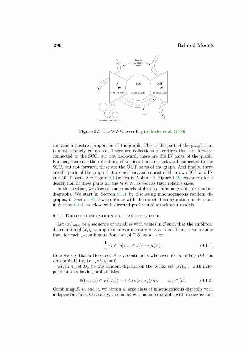
296 Related Models
Tendrils44 Million
nodes
SCC OUTIN
56 Million nodes44 Million nodes 44 Million nodes
Disconnected components
Tubes
Figure 9.1 The WWW according to Broder et al. (2000).
contains a positive proportion of the graph. This is the part of the graph thatis most strongly connected. There are collections of vertices that are forwardconnected to the SCC, but not backward, these are the IN parts of the graph.Further, there are the collections of vertices that are backward connected to theSCC, but not forward, these are the OUT parts of the graph. And finally, thereare the parts of the graph that are neither, and consist of their own SCC and INand OUT parts. See Figure 9.1 (which is [Volume 1, Figure 1.19] repeated) for adescription of these parts for the WWW, as well as their relative sizes.
In this section, we discuss some models of directed random graphs or randomdi-graphs. We start in Section 9.1.1 by discussing inhomogeneous random di-graphs, in Section 9.1.2 we continue with the directed configuration model, andin Section 9.1.3, we close with directed preferential attachment models.
9.1.1 Directed inhomogeneous random graphs
Let (xi)i∈[n] be a sequence of variables with values in S such that the empiricaldistribution of (xi)i∈[n] approximates a measure µ as n→∞. That is, we assumethat, for each µ-continuous Borel set A ⊆ S, as n→∞,
1
n|i ∈ [n] : xi ∈ A| → µ(A). (9.1.1)
Here we say that a Borel set A is µ-continuous whenever its boundary ∂A haszero probability, i.e., µ(∂A) = 0.
Given n, let Dn be the random digraph on the vertex set (xi)i∈[n] with inde-pendent arcs having probabilities
P((xi, xj) ∈ E(Dn)) = 1 ∧ (κ(xi, xj)/n), i, j ∈ [n]. (9.1.2)
Combining S, µ, and κ, we obtain a large class of inhomogeneous digraphs withindependent arcs. Obviously, the model will include digraphs with in-degree and
9.1 Directed random graphs 297
out-degree distributions which have power laws. This general model was studiedin detail in Chapter 3. Note that in the case of random graphs it is necessary toassume, in addition, that the kernel κ is symmetric. In the definition of digraphsDn for n ≥ 2, we do not require the symmetry of the kernel.
For large n, the phase transition in the digraph Dn can be described in terms ofthe survival probabilities of the related multitype Galton-Watson branching pro-cesses with type space S. Let us introduce the necessary mixed-Poisson branchingprocesses now. Given s ∈ S, let X (s) and Y(s) denote the Galton-Watson pro-cesses starting at a particle of type s ∈ S such that the number of children oftypes in a subset A ⊆ S of a particle of type t ∈ S has a Poisson distributionwith means ∫
Aκ(t, u)µ(du), and
∫Aκ(u, t)µ(du), (9.1.3)
respectively. These numbers are independent for disjoint subsets A and for differ-ent particles. The critical point of the emergence of the giant SCC is determinedby the averaged joint survival probability
ζ =
∫SζX (s)ζY(s)µ(ds) (9.1.4)
being positive. Here ζX (s) and ζY(s) denote the non-extinction probabilities ofX (s) and Y(s), respectively.
In order to establish Theorem 9.1, we need to impose further conditions on thekernel κ, like those in Chapter 3. Namely, we need to assume that the kernel κ isirreducible (µ × µ)-almost everywhere. That is, for any measurable A ⊆ S withµ(A) 6= 1 or µ(A) 6= 0, the identity (µ×µ)((s, t) ∈ A×(S \A) : κ(s, t) = 0) = 0implies that either µ(A) = 0 or µ(S \ A) = 0. In addition, we assume that κ iscontinuous almost everywhere on (S × S, µ × µ), and the number of arcs inDIRGn(κ), denoted by |E(DIRGn(κ))|, satisfies that, as n→∞,
1
n|E(DIRGn(κ))| P−→
∫S×S
κ(s, t)µ(ds)µ(dt) <∞. (9.1.5)
Note that here we implicitly assume that κ is integrable.This gives rise to the following theorem:
Theorem 9.1 (Phase transition in DIRGn(κ)) Suppose that
(a) When ν > 1, ζ in (9.1.4) satisfies ζ ∈ (0, 1] and
|Cmax|/n P−→ ζ, (9.1.6)
while |C(2)|/n P−→ 0 and |E(C(2))|/n P−→ 0.
(b) When ν < 1, ζ in (9.1.4) satisfies ζ = 0 and |Cmax|/n P−→ 0 and |E(Cmax)|/n P−→0.
TO DO 9.3: Add discussion directed inhomogeneous random graphs
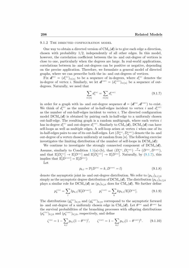
298 Related Models
9.1.2 The directed configuration model
One way to obtain a directed version of CMn(d) is to give each edge a direction,chosen with probability 1/2, independently of all other edges. In this model,however, the correlation coefficient between the in- and out-degree of vertices isclose to one, particularly when the degrees are large. In real-world applications,correlations between in- and out-degrees can be positive or negative, dependingon the precise application. Therefore, we formulate a general model of directedgraphs, where we can prescribe both the in- and out-degrees of vertices.
Fix d(in) = (d(in)
i )i∈[n] to be a sequence of in-degrees, where d(in)
i denotes thein-degree of vertex i. Similarly, we let d(out) = (d(out)
i )i∈[n] be a sequence of out-degrees. Naturally, we need that∑
i∈[n]
d(in)
i =∑i∈[n]
d(out)
i (9.1.7)
in order for a graph with in- and out-degree sequence d = (d(in),d(out)) to exist.We think of d(in)
i as the number of in-half-edges incident to vertex i and d(out)
i
as the number of out-half-edges incident to vertex i. The directed configurationmodel DCMn(d) is obtained by pairing each in-half-edge to a uniformly chosenout-half-edge. The resulting graph is a random multigraph, where each vertex ihas in-degree d(in)
i and out-degree d(out)
i . Similarly to CMn(d), DCMn(d) can haveself-loops as well as multiple edges. A self-loop arises at vertex i when one of itsin-half-edges pairs to one of its out-half-edges. Let (D(in)
n , D(out)
n ) denote the in- andout-degree of a vertex chosen uniformly at random from [n]. The following exerciseinvestigates the limiting distribution of the number of self-loops in DCMn(d):
We continue to investigate the strongly connected component of DCMn(d).
Assume, similarly to Condition 1.5(a)-(b), that (D(in)
n , D(out)
n )d−→ (D(in), D(out)),
and that E[D(in)
n ] → E[D(in)] and E[D(out)
n ] → E[D(in)]. Naturally, by (9.1.7), thisimplies that E[D(out)] = E[D(in)]:
Let
pk,l = P(D(in) = k,D(out) = l) (9.1.8)
denote the asymptotic joint in- and out-degree distribution. We refer to (pk,l)k,l≥0
simply as the asymptotic degree distribution of DCMn(d). The distribution (pk,l)k,l≥0
plays a similar role for DCMn(d) as (pk)k≥0 does for CMn(d). We further define
p?(in)
k =∑l
lpk,l/E[D(out)], p?(out)l =∑k
kpk,l/E[D(in)]. (9.1.9)
The distributions (g(in)
k )k≥0 and (g(out)
k )k≥0 correspond to the asymptotic forwardin- and out-degree of a uniformly chosen edge in CMn(d). Let θ(in) and θ(out) bethe survival probabilities of the branching processes with offspring distributions(p?(in)
k )k≥0 and (p?(out)
k )k≥0, respectively, and define
ζ(in) = 1−∑k,l
pk,l(1− θ(in))l, ζ(out) = 1−∑k,l
pk,l(1− θ(out))k. (9.1.10)
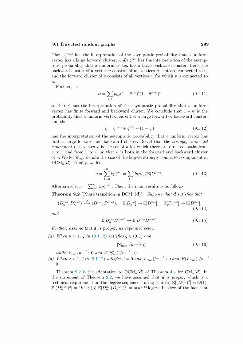
9.1 Directed random graphs 299
Then, ζ(out) has the interpretation of the asymptotic probability that a uniformvertex has a large forward cluster, while ζ(in) has the interpretation of the asymp-totic probability that a uniform vertex has a large backward cluster. Here, thebackward cluster of a vertex v consists of all vertices u that are connected to v,and the forward cluster of v consists of all vertices u for which v is connected tou.
Further, let
ψ =∑k,l
pk,l(1− θ(in))l(1− θ(out))k (9.1.11)
so that ψ has the interpretation of the asymptotic probability that a uniformvertex has finite forward and backward cluster. We conclude that 1 − ψ is theprobability that a uniform vertex has either a large forward or backward cluster,and thus
ζ = ζ(out) + ζ(in) − (1− ψ) (9.1.12)
has the interpretation of the asymptotic probability that a uniform vertex hasboth a large forward and backward cluster. Recall that the strongly connectedcomponent of a vertex v is the set of u for which there are directed paths fromv to u and from u to v, so that u is both in the forward and backward clusterof v. We let Cmax denote the size of the largest strongly connected component inDCMn(d). Finally, we let
ν =∞∑k=0
kp?(in)k =∑k,l
klpk,l/E[D(out)], (9.1.13)
Alternatively, ν =∑∞
k=0 kp?(out)
k . Then, the main results is as follows:
Theorem 9.2 (Phase transition in DCMn(d)) Suppose that d satisfies that
(D(in)
n , D(out)
n )d−→ (D(in), D(out)), E[D(in)
n ]→ E[D(in)], E[D(out)
n ]→ E[D(in)],(9.1.14)
and
E[D(in)
n D(out)
n ]→ E[D(in)D(out)]. (9.1.15)
Further, assume that d is proper, as explained below.
(a) When ν > 1, ζ in (9.1.12) satisfies ζ ∈ (0, 1] and
|Cmax|/n P−→ ζ, (9.1.16)
while |C(2)|/n P−→ 0 and |E(C(2))|/n P−→ 0.
(b) When ν < 1, ζ in (9.1.12) satisfies ζ = 0 and |Cmax|/n P−→ 0 and |E(Cmax)|/n P−→0.
Theorem 9.2 is the adaptation to DCMn(d) of Theorem 4.4 for CMn(d). Inthe statement of Theorem 9.2, we have assumed that d is proper, which is atechnical requirement on the degree sequence stating that (a) E[(D(in)
n )2] = O(1),E[(D(out)
n )2] = O(1); (b) E[D(in)
n (D(out)
n )2] = o(n1/12 log n). In view of the fact that
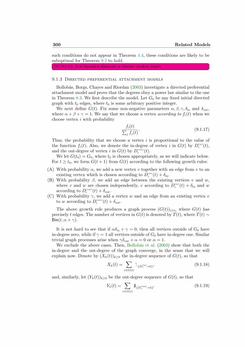
300 Related Models
such conditions do not appear in Theorem 4.4, these conditions are likely to besuboptimal for Theorem 9.2 to hold.TO DO 9.3: Add discussion distances in directed random graphs
9.1.3 Directed preferential attachment models
Bollobas, Borgs, Chayes and Riordan (2003) investigate a directed preferentialattachment model and prove that the degrees obey a power law similar to the onein Theorem 8.3. We first describe the model. Let G0 be any fixed initial directedgraph with t0 edges, where t0 is some arbitrary positive integer.
We next define G(t). Fix some non-negative parameters α, β, γ, δin and δout,where α+ β + γ = 1. We say that we choose a vertex according to fi(t) when wechoose vertex i with probability
fi(t)∑j fj(t)
. (9.1.17)
Thus, the probability that we choose a vertex i is proportional to the value ofthe function fi(t). Also, we denote the in-degree of vertex i in G(t) by D(in)
i (t),and the out-degree of vertex i in G(t) by D(out)
i (t).We let G(t0) = G0, where t0 is chosen appropriately, as we will indicate below.
For t ≥ t0, we form G(t+ 1) from G(t) according to the following growth rules:
(A) With probability α, we add a new vertex v together with an edge from v to anexisting vertex which is chosen according to D(in)
i (t) + δin.(B) With probability β, we add an edge between the existing vertices v and w,
where v and w are chosen independently, v according to D(in)
i (t) + δin and waccording to D(out)
i (t) + δout.(C) With probability γ, we add a vertex w and an edge from an existing vertex v
to w according to D(out)
i (t) + δout.
The above growth rule produces a graph process (G(t))t≥t0 where G(t) hasprecisely t edges. The number of vertices in G(t) is denoted by T (t), where T (t) ∼Bin(t, α+ γ).
It is not hard to see that if αδin + γ = 0, then all vertices outside of G0 havein-degree zero, while if γ = 1 all vertices outside of G0 have in-degree one. Similartrivial graph processes arise when γδout + α = 0 or α = 1.
We exclude the above cases. Then, Bollobas et al. (2003) show that both thein-degree and the out-degree of the graph converge, in the sense that we willexplain now. Denote by (Xk(t))k≥0 the in-degree sequence of G(t), so that
Xk(t) =∑v∈G(t)
1D(in)v =k, (9.1.18)
and, similarly, let (Yk(t))k≥0 be the out-degree sequence of G(t), so that
Yk(t) =∑v∈G(t)
1D(out)v =k. (9.1.19)
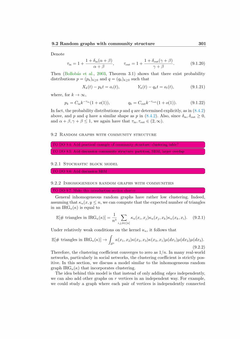
9.2 Random graphs with community structure 301
Denote
τin = 1 +1 + δin(α+ β)
α+ β, τout = 1 +
1 + δout(γ + β)
γ + β. (9.1.20)
Then (Bollobas et al., 2003, Theorem 3.1) shows that there exist probabilitydistributions p = (pk)k≥0 and q = (qk)k≥0 such that
Xk(t)− pkt = oP(t), Yk(t)− qkt = oP(t), (9.1.21)
where, for k →∞,
pk = Cink−τin(1 + o(1)), qk = Coutk
−τout(1 + o(1)). (9.1.22)
In fact, the probability distributions p and q are determined explicitly, as in (8.4.2)above, and p and q have a similar shape as p in (8.4.2). Also, since δin, δout ≥ 0,and α+ β, γ + β ≤ 1, we again have that τin, τout ∈ (2,∞).
9.2 Random graphs with community structure
TO DO 9.4: Add practical example of community structure: clustering table?
TO DO 9.5: Add discussion community structure: partition, SBM, larger overlap
9.2.1 Stochastic block model
TO DO 9.6: Add discussion SBM
9.2.2 Inhomogeneous random graphs with communities
TO DO 9.7: Make this introduction section shorter
General inhomogeneous random graphs have rather low clustering. Indeed,assuming that κn(x, y ≤ n, we can compute that the expected number of trianglesin an IRGn(κ) is equal to
E[# triangles in IRGn(κ)] =1
n3
∑i,j,k∈[n]
κn(xi, xj)κn(xj, xk)κn(xk, xi). (9.2.1)
Under relatively weak conditions on the kernel κn, it follows that
E[# triangles in IRGn(κ)]→∫S3
κ(x1, x2)κ(x2, x3)κ(x3, x1)µ(dx1)µ(dx2)µ(dx3).
(9.2.2)Therefore, the clustering coefficient converges to zero as 1/n. In many real-worldnetworks, particularly in social networks, the clustering coefficient is strictly pos-itive. In this section, we discuss a model similar to the inhomogeneous randomgraph IRGn(κ) that incorporates clustering.
The idea behind this model is that instead of only adding edges independently,we can also add other graphs on r vertices in an independent way. For example,we could study a graph where each pair of vertices is independently connected
302 Related Models
with probability λ/n, as for ERn(λ/n), but also each collection of triples forms atriangle with probability µ/n2, independently for all triplets and independentlyof the status of the edges. Here the exponent n−2 is chosen to as to make theexpected number of triangles containing a vertex bounded.
In social networks, also complete graphs of size four, five, etc., are presentmore often than in usual random graph. Therefore, we also wish to add thoseindependently. In order to formulate this general version of the model, we startby introducing some notation.
Let F consist of one representative of each isomorphism class of finite connectedgraphs, chosen so that if F ∈ F has r vertices then V (F ) = [r] = 1, 2, . . . , r.Simple examples of such F are the complete graphs on r vertices, but also otherexamples are possible. Recall that S denotes the type space. Given F ∈ F withr vertices, let κF be a measurable function from Sr to [0,∞). The function κF iscalled the kernel corresponding to F . A sequence κ = (κF )F∈F is a kernel family.
Let κ be a kernel family and n an integer. We define a random graph IRGn(κ)with vertex set [n] = 1, . . . , n. First let x1, x2, . . . , xn ∈ S be i.i.d. (independentand identically distributed) with the distribution µ. Given x = (x1, . . . , xn), con-struct IRGn(κ) as follows, starting with the empty graph. For each r and eachF ∈ F with |F | = r, and for every r-tuple of distinct vertices (v1, . . . , vr) ∈ [n]r,add a copy of F on the vertices v1, . . . , vr (with vertex i of F mapped to vi) withprobability
p = p(v1, . . . , vr;F ) =κF (xv1 , . . . , xvr)
nr−1, (9.2.3)
all these choices being independent. Here, if p > 1, by convention we simply adda copy with probability 1. We shall often call the added copies of the various Fthat together form IRGn(κ) atoms as they may be viewed as indivisible buildingblocks. Sometimes we refer to them as small graphs, although there is in generalno bound on their sizes.
The reason for dividing by nr−1 in (9.2.3) is that we wish to consider sparsegraphs; indeed, our main interest is the case when IRGn(κ) has O(n) edges. Asit turns out, we can be slightly more general; however, when κF is integrable(which we shall always assume), the expected number of added copies of eachgraph F is O(n). Note that all incompletely specified integrals are with respectto the appropriate r-fold product measure µr on Sr.
There are several plausible choices for the normalization in (9.2.3). The one wehave chosen means that if κF = c is constant, then (asymptotically) there are onaverage cn copies of F in total, and each vertex is on average in rc copies of F .An alternative is to divide the expression in (9.2.3) by r; then (asymptotically)each vertex would on average be in c copies of F . Another alternative, naturalwhen adding cliques only but less so in the general case, would be to divide by r!;this is equivalent to considering unordered sets of r vertices instead of ordered r-tuples. When there is only one kernel, corresponding to adding edges, this wouldcorrespond to the normalization used in Bollobas et al. (2007), and in particular
9.2 Random graphs with community structure 303
to that of the classical model ERn(λ/n); the normalization we use here differsfrom this by a factor of 2.
In the special case where all κF are zero apart from κK2, the kernel correspond-
ing to an edge, we recover (essentially) a special case of the model of Bollobaset al. (2007); we call this the edge-only case, since we add only edges, not largergraphs. We write κ2 for κK2
. Note that in the edge-only case, given x, two verticesi and j are joined with probability
κ2(xi, xj) + κ2(xj, xj)
n+O
((κ2(xi, xj) + κ2(xj, xi))
2
n2
). (9.2.4)
The correction term will never matter, so we may as well replace κ2 by its sym-metrized version. In fact, we shall always assume that κF is invariant underpermutations of the vertices of the graph F .
For any kernel family κ, let κe be the corresponding edge kernel, defined by
κe(x, y) =∑F
∑ij∈E(F )
∫SV (F )\i,j
κF (x1, . . . , xi−1, x, xi+1, . . . , xj−1, y, xj+1, . . . , x|F |),
(9.2.5)where the second sum runs over all 2E(F ) ordered pairs (i, j) with ij ∈ Edges(F ),and we integrate over all variables apart from x and y. Note that the sum neednot always converge; since every term is positive this causes no problems: wesimply allow κe(x, y) =∞ for some x, y. Given xi and xj, the probability that iand j are joined in G(n, κ) is at most κe(xi, xj)/n+O(1/n2). In other words, κecaptures the edge probabilities in G(n, κ), but not the correlations.
Before proceeding to deeper properties, let us note that the expected numberof added copies of F is (1 +O(n−1))n
∫S|F | κF . Unsurprisingly, the actual number
turns out to be concentrated about this mean. Let
ξ(κ) =∑F∈F
E(F )
∫S|F |
κF =1
2
∫S2
κe ≤ ∞ (9.2.6)
be the asymptotic edge density of κ. Since every copy of F contributes E(F ) edges,the following theorem is almost obvious, provided we can ignore overlappingedges.
Theorem 9.3 (The edge density in IRGn(κ)) As n→∞, E[E(IRGn(κ))/n]→ξ(κ) ≤ ∞ Moreover, E(IRGn(κ))/n converges in probability to the asymptoticedge density ξ(κ). In other words, if ξ(κ) <∞ then E(IRGn(κ)) = ξ(κ)n+op(n),and if ξ(κ) =∞ then E(IRGn(κ)) > Cn for every constant C, whp.
The main focus is the emergence of the giant component. By the componentstructure of a graph G, we mean the set of vertex sets of its components, i.e.,the structure encoding only which vertices are in the same component, not theinternal structure of the components themselves. When studying the componentstructure of IRGn(κ), the model can be simplified somewhat. Recalling that theatoms F ∈ F are connected by definition, when we add an atom F to a graphG, the effect on the component structure is simply to unite all components of
304 Related Models
G that meet the vertex set of F , so only the vertex set of F matters, not itsgraph structure. We say that κ is a clique kernel family if the only non-zerokernels are those corresponding to complete graphs; the corresponding randomgraph model IRGn(κ) is a clique model. For questions corresponding componentstructure, it suffices to study clique models. For clique kernels we write κr forκKr ; as above, we always assume that κr is symmetric, here meaning invariantunder all permutations of the coordinates of Sr. Given a general kernel familyκ, the corresponding (symmetrized) clique kernel family is given by κ = (κr)r≥2
with
κr(x1, . . . , xr) =∑
F∈F : |F |=r
1
r!
∑π∈Gr
κF (xπ(1), . . . , xπ(r)), (9.2.7)
where Gr denotes the symmetric group of permutations of [r]. (This is consistentwith our notation κ2 = κKr .) When considering the size (meaning number ofvertices) of the giant component in IRGn(κ), we may always replace κ by thecorresponding clique kernel family.
It is often convenient to think of a clique model as a random hypergraph, withthe cliques as the hyperedges; for this reason we call a clique kernel family a hyper-kernel. Note that each unordered set of r vertices corresponds to r! r-tuples, so theprobability that we add a Kr on a given set of r vertices is r!κr(xv1 , . . . , xvr)/n
r−1.(More precisely, this is the expected number of Krs added with this vertex set.)
In our analysis we also consider the linear operator Tκe defined by
Tκe(f)(x) =
∫Sκe(x, y)f(y)dµ(y), (9.2.8)
where κe is defined by (9.2.5). We need to impose some sort of integrabilitycondition on our kernel family:
Definition 9.4 (i) A kernel family κ = (κF )F∈F is integrable if∫κ =
∑F∈F
|F |∫S|F |
κF <∞. (9.2.9)
This means that the expected number of atoms containing a given vertex is bounded.
(ii) A kernel family κ = (κF )F∈F is edge integrable if∑F∈F
E(F )
∫S|F |
κF <∞; (9.2.10)
equivalently, ξ(κ) < ∞ or∫S2 κe < ∞. This means that the expected number of
edges in G(n, κ) is O(n), see Theorem 9.3, and thus the expected degree of a givenvertex is bounded.
Note that a hyperkernel (κr) is integrable if and only if∑
r≥2 r∫Sr κr < ∞,
and edge integrableThe main results concerning the phase transition on IRGn(κ) is that if κ is an
9.2 Random graphs with community structure 305
integrable kernel family satisfying a certain extra assumption, then the normal-ized size of the giant component in IRGn(κ) is simply ζ(κ) + op(1). The extraassumption is an irreducibility assumption similar to Definition 3.3(ii) that es-sentially guarantees that the graph does not split into two pieces: we say that asymmetric kernel κe : S2 → [0,∞) is reducible if
∃A ⊂ S with 0 < µ(A) < 1 such that κe = 0 a.e. on A× (S \A);
otherwise κe is irreducible. Thus, κe is irreducible if
A ⊆ S and κe = 0 a.e. on A× (S \A) implies µ(A) = 0 or µ(S \A) = 0.
We are now ready to formulate the main result in this section involving thephase transition in IRGn(κ). Recall that |Cmax| denotes the number of vertices inthe largest connected component of the graph under consideration, and |C(2)| thenumber of vertices in its second largest component.
Theorem 9.5 (The phase transition on clustered inhomogeneous random graphs)Let κ′ = (κ′F )F∈F be an irreducible, integrable kernel family, and let κ = (κr)r≥2 bethe corresponding hyperkernel, given by (9.2.7). Then, there exists a ζ(κ) ∈ [0, 1)such that
|Cmax| = ζ(κ)n+ op(n), (9.2.11)
and |C(2)| = op(n).
Theorem 9.5 is proved by showing that (in the hyperkernel case) the branchingprocess that captures the ‘local structure’ of IRGn(κ). For Theorem 9.5 to beuseful we would like to know something about ζ(κ), which can be calculatedfrom ζκ, which is in turn the largest solution to the functional equation:
f = 1− e−Sκ(f)(x). (9.2.12)
The question when ζ(κ) > 0 is settled in the following theorem:
Theorem 9.6 (Condition for existence giant component) Let κ be an integrablehyperkernel. Then, ζ(κ) > 0 if and only if ||Tκe || > 1. Furthermore, if κ isirreducible and ||Tκe || > 1, then ζκ(x) is the unique non-zero solution to thefunctional equation (9.2.12), and ζκ(x) > 0 holds for a.e. x.
In general, ||Tκe || may be rather hard to calculate. When we suppose thateach κr is constant, however, this can be done. Indeed, say that κr = cr. Thenκe(x, y) =
∑r r(r − 1)cr = 2ξ(κ) for all x and y, so
||Tκe || = 2ξ(κ). (9.2.13)
This is perhaps surprising: it tells us that for such uniform hyperkernels, thecritical point where a giant component emerges is determined only by the totalnumber of edges added; it does not matter what size cliques they lie in, eventhough, for example, the third edge in every triangle is ‘wasted’. This turns outnot to be true for arbitrary kernel families, where, rather each atom needs to bereplaced by a clique.
306 Related Models
9.2.3 Configuration models with community structure
Hierarchical configuration model
TO DO 9.8: Present results HCM: connectivity and graph distances
The configuration model has low clustering, which often makes it inappropri-ate in applied contexts. Indeed, many real-world networks, in particular socialnetworks, have a high amount of clustering instead. A possible solution to over-come this low clustering is by introducing a community or household structure.Consider the configuration model CMn(d) with a degree sequence d = (di)i∈[n]
satisfying Condition 1.5(a)-(b). Now we replace each of the vertices by a smallgraph. Thus, vertex i is replaced by a local graph Gi. We assign each of the dihalf-edges incident to vertex i to a vertex in Gi in an arbitrary way. Thus, vertexi is replaced by the pair of the community graph Gi = (Vi, Ei) and the inter-community degrees d(b) = (d(b)
u )u∈Vi satisfying that∑
u∈Vi d(b)
u = di. Naturally, thesize of the graph becomes N =
∑i∈[n] |Vi|.
As a result, we obtain a graph with two levels of hierarchy, whose local structureis described by the local graphs (Gi)i∈[n], whereas its global structure is describedby the configuration model CMn(d). This model is called the hierarchical con-figuration model. A natural assumption is that the degree sequence d = (di)i∈[n]
satisfies Condition 7.8(a)-(b), while the empirical distribution of the graphs
µn(H, ~d) =1
n
∑i∈[n]
1Gi=H,(d(b)u )u∈Vi=~d (9.2.14)
converges as n → ∞ to some probability distribution on graphs with integermarks associated to the vertices. See Stegehuis et al. (2016a,b) for power-lawrelations in hierarchical configuration models and epidemic spread in them, re-spectively, and Hofstad et al. (Preprint 2015) for its topological properties, suchas its connectivity, its clustering, etc.
The configuration model with household structure
TO DO 9.9: Adapt this discussion: special case of HCM
The configuration model has low clustering, which often makes it inappropriatein applied contexts. Indeed, in Chapter 1, we have seen that many real-worldnetworks have a high amount of clustering instead. For example, in modeling asocial network, one can expect a large amount of clustering. A possible solutionto overcome this low clustering, is by introducing a community or householdstructure. Consider the configuration model CMn(d) with a degree sequence d =(di)i∈[n] satisfying Condition 1.5(a)-(b). Now we replace each of the vertices bya small graph. Thus, vertex i is replaced by a local graph Gi. We assign each ofthe di half-edges incident to vertex i to a uniform vertex in Gi. As a result, weobtain a graph with two levels of hierarchy, whose local structure is described bythe local graphs Gi, whereas its global structure is described by the configurationmodel CMn(d).
9.2 Random graphs with community structure 307
The number of vertices in the configuration model with household structure isgiven by
N =n∑i=1
ni, (9.2.15)
where ni denotes the number of vertices in Gi. Further, assume that the empiricaldistribution of the graph sizes converges, i.e., there exists a distribution functionFH such that, for every x ∈ R,
FH,n(x) =1
n
∑i∈[n]
1ni≤x → FH(x), (9.2.16)
and N/n → E[H], where H has distribution function FH. Assume further thatthe local graphs Gi are all connected. Then, assuming (9.2.16) and N/n→ E[H],the size of the largest connected component |Cmax| of the configuration modelwith household structure satisfies
|Cmax|/N P−→ ζ, (9.2.17)
where ζ is the asymptotic proportion of vertices in the giant component ofCMn(d).
It would be of interest to investigate typical distances within the configurationmodel with household structure. It seems reasonable to predict that HN/ logNconverges to a limit when [Volume 1, Condition 7.8(a)-(c)] holds, where the limitequals α/ log ν, where α denotes the typical distance in a household drawn uni-formly at random. Similar results should hold for infinite variance degrees, whereit can be expected that HN/ log logN
P−→ 2α/| log(τ − 2)|.Due to the fact that a vertex in the configuration model is a household, which
in itself is a small subgraph, it seems plausible that the fluctuations of the typicaldistances within the different households give rise to larger fluctuations of thetypical distances for the configuration model with household structure than forCMn(d) as presented in Theorem 7.20–7.21. In particular, one might expect that(HN − α logν N)/
√logN converges to a normal random variable when [Volume
1, Condition 7.8(a)-(c)] holds, while (Hn − 2α log logN/| log(τ − 2)|)/√log logNconverges to a normal random variable when a condition as in (7.1.2) holds withδ = 0.
9.2.4 Configuration model with clustering
The low clustering of CMn(d) can be resolved by introducing households asdescribed above. Alternatively, and in the spirit of clustered inhomogeneous ran-dom graphs as described in Section 9.2.2, we can also introduce clustering directly.In the configuration model with clustering, we assign two numbers to a vertexi ∈ [n]. We let d(si)
i denote the number of simple half-edges incident to vertex i,and we let d(tr)
i denote the number of triangles that vertex i is part of. We saythat there are d(si)
i half-edges incident to vertex i, and d(tr)
i third-triangles.
308 Related Models
The graph is built by (a) recursively choosing two half-edges uniformly at ran-dom without replacement, and pairing them into edges (as for CMn(d)); and (b)choosing triples of third-triangles uniformly at random and without replacement,and drawing edges between the three vertices incident to the third-triangles thatare chosen.
Let (D(si)
n , D(tr)
n ) denote the number of simple edges and triangles incident to
a uniform vertex in [n], and assume that (D(si)
n , D(tr)
n )d−→ (D(si), D(tr)) for some
limiting distribution (D(si), D(tr)). Newman (2009) performs a generating functionanalysis of when a giant component is expected to exist. The criterion Newmanfinds is that(E[(D(si))2]
E[D(si)]− 2)(2E[(D(tr))2]
E[D(tr)]− 3)<
2E[D(si)D(tr)]
E[D(si)]E[D(tr)]. (9.2.18)
When D(tr) = 0 a.s., so that there are no triangles, this reduces to
E[(D(si))2]
E[D(si)]− 2 > 0, (9.2.19)
which is equivalent to ν = E[D(si)(D(si) − 1)]/E[D(si)] > 1. It would be of interestto analyze this model mathematically.
9.2.5 Random intersection graphs
TO DO 9.10: Extend discussion of intersection graphs
Random intersection graphs with independent group-memberships
The most studied model is when there are n vertices, m = m(n) groups and eachvertex is independently connected to each group with probability p(n) (oftenm = nα and p = cn−(1+α)/2 which gives different behavior depending on thevalue of α). This model was introduced by Singer (1996) and further studied inFill et al. (2000); Karonski et al. (1999); Stark (2004).
Deijfen and Kets (2009) studied a version where the vertices have randomweights and the edge probabilities are determined by these weights (which givesa graph where both the degree distribution and the clustering can be controlled).In the above model the number of groups that a vertex belongs to is Bin(m,p)-distributed. The model has also been investigated for more general distributionsof groups per vertex by Godehardt and Jaworski (2003) and Jaworski et al. (2006).
Mindaugas Bloznelis has studied this more general model in quite a few papers,including distances and component sizes Bloznelis (n.d., 2010a,b).
Random intersection graphs with prescribed degrees and groups
Above we have studied random intersection graphs, where connections are ran-domly and independently formed between individuals and groups. We now de-scribe a model in which vertex v ∈ [n] belongs to d(ve)
v groups, while group g ∈ [m]has size d(gr)
g . Here n is the number of individuals, while m is the number of groups.
9.3 Spatial random graphs 309
Naturally, in order for the model to be well defined, we need that∑v∈[n]
d(ve)
v =∑g∈[m]
d(gr)
g . (9.2.20)
We call two vertices v1 and v2 neighbors when they are connected to the samegroup, so that the degree of a vertex v is the total number of other vertices u forwhich there exists a group of which both u and v are members. This model mightbe appropriate as a simple model for collaboration graphs such as the IMDb andthe collaboration graph among mathematicians. In the above setting, this modelhas not received much attention in the mathematical community.
Random intersection graphs with communities
9.2.6 Exponential random graphs and maximal entropy
TO DO 9.11: Add discussion of exponential random graphs, and show that GRG is specialcase
9.3 Spatial random graphs
TO DO 9.12: Add discussion why geometry may be useful in random graphs
9.3.1 Small-world model
The models described so far do not incorporate geometry at all. An alternativeapproach of explaining the small-world phenomenon is to start with a finite torus,and to add random long range connections to them, independently for each pairof vertices. This gives rise to a graph which is a small perturbation of the originallattice, but has occasional long-range connections that are crucial in order toshrink distances. From a practical point of view, we can think of the originalgraph as being the local description of acquaintances in a social network, whilethe shortcuts describe the occasional acquaintances in the population living farapart. The main idea is that, even though the shortcuts only form a tiny part ofthe connections in the graph, they are crucial in order to make it a small world.
There are various ways of adding long-range connections (for example byrewiring the existing edges), and we shall focus on the models in Barbour andReinert (2001, 2004, 2006), for which the strongest mathematical results havebeen obtained. Small-world models were first introduced and analyzed in Mooreand Newman (2000); Newman et al. (2000a); Newman and Watts (1999), anda non-rigorous mean-field analysis of distances in small-world models was per-formed in Newman et al. (2000a). See Barbour and Reinert (2001) for a discussionof the differences between the exact and mean-field analyses.
The simplest version of the model studied in Barbour and Reinert (2001) isobtained by taking the circle of circumference n, and adding a Poisson number ofshortcuts with parameter nρ/2, where the starting and endpoints of the shortcutsare chosen uniformly at random independently of each other. This model is called
310 Related Models
the continuous circle model in Barbour and Reinert (2001). Distance is measuredas usual along the circle, and the shortcuts have, by convention, length zero.Thus, one can think of this model as the circle where the points along the randomshortcut are identified, thus creating a puncture in the circle. Multiple shortcutsthen lead to multiple puncturing of the circle, and the distance is then the usualdistance along the punctured graph. Denote by Dn the distance between twouniformly chosen points along the punctured circle. Then, (Barbour and Reinert,2001, Theorem 3.9) states that as n→∞, Dn(2ρ)/ log ρn converges in probabilityto 1 when nρ → ∞, and that ρ(Dn − log ρn/2) converges in distribution to arandom variable T satisfying
P(T > t) =
∫ ∞0
e−ydy
1 + e2t. (9.3.1)
The random variable T can also be described by
P(T > t) = E[e−e2tW (1)W (2)
], (9.3.2)
where W (1), W (2) are two independent exponential random variables with param-eter 1. Alternatively, it can be see that T = (G1 +G2 −G3)/2, where G1, G2, G3
are three independent Gumbel distributions (see (Barbour and Reinert, 2006,Page 1242)).
Interestingly, the method of proof of (Barbour and Reinert, 2001, Theorem 3.9)is quite close to the method of proof for Theorem 7.20. Indeed, again the partsof the graph that can be reached in distance at most t are analyzed. Let P1 andP2 be two uniform points along the circle, so that Dn has the same distributionas the distance between P1 and P2. Denote by R(1)(t) and R(2)(t) the parts of thegraph that can be reached within distance t. Then, Dn = 2Tn, where Tn is thefirst time that R(1)(t) and R(2)(t) have a non-zero intersection. The proof thenconsists of showing that, up to time Tn, the processes R(1)(t) and R(2)(t) are closeto certain continuous-time branching processes, primarily due to the fact that theprobability that there are two intervals that are overlapping in quite small. Then,W (1) and W (2) can be viewed as appropriate martingale limits of these branchingprocesses. In (Barbour and Reinert, 2001, Theorem 4.2), also an extension tohigher dimensions is given.
The proof was extended by Barbour and Reinert (2006) to deal with discretetori where the shortcuts also contribute one to the graphs distance, so that dis-tances are the usual distances on discrete graphs. For this, it was necessary thatthe average number of shortcuts per vertex ρ ↓ 0, a restriction that does not ap-pear in Barbour and Reinert (2001). It would be of interest to extend the resultsto the case of fixed ρ as well in the discrete setting.
A related model was considered by Turova and Vallier (2010). Indeed, Turovaand Vallier (2010) study a mixture between subcritical percolation on a finitecube and the Erdos-Renyi random graph. Using the methodology of Bollobaset al. (2007), it is shown that the phase transition is similar to the one describedin Theorem ??. It would be of interest to verify whether the distance results
9.3 Spatial random graphs 311
in Bollobas et al. (2007) can also be used to prove that the distances grow likelogν n, where n is the size of the graph, and ν > 1 an appropriate constant.
9.3.2 Geometric inhomogeneous random graphs
TO DO 9.13: Introduce the GIRG
9.3.3 Scale-free percolation
In this section, we define a percolation model that interpolates between long-range percolation and the scale-free rank-1 inhomogeneous random graphs asdiscussed in Chapter 3. This model, termed scale-free percolation in Deijfen et al.(2013), provides a percolation model in which the degree of a vertex can havefinite mean but infinite variance. Mind that this phenomenon is impossible forindependent percolation models, since the independence of the edge variablesimplies that the variance of the degrees is always bounded by their mean.
Scale-free percolation is defined on the lattice Zd. Let each vertex x ∈ Zd beequipped with an i.i.d. weight Wx. Conditionally on the weights (Wx)x∈Zd , theedges in the graph are independent and the probability that there is an edgebetween x and y is defined by
pxy = 1− e−λWxWy/|x−y|α , (9.3.3)
for α, λ ∈ (0,∞). We say that the edge x, y is occupied with probability pxyand vacant otherwise.
Let us discuss the role of the different parameters in the scale-free percolationmodel. The parameter α > 0 describes the long-range nature of the model, whilewe think of λ > 0 as the percolation parameter. The weight distribution is the lastparameter that describes the model. We are mainly interested in settings wherethe Wx have unbounded support in [0,∞), and then particularly when they varysubstantially.
Naturally, the model for fixed λ > 0 and weights (Wx)x∈Zd is the same asthe one for λ = 1 and weights (
√λWx)x∈Zd , so there is some redundancy in the
parameters of the model. However, we view the weights (Wx)x∈Zd as creating arandom environment in which we study the percolative properties of the model.Thus, we think of the random variables (Wx)x∈Zd as fixed once and for all andwe change the percolation configuration by varying λ. We can thus view ourmodel as percolation in a random environment given by the weights (Wx)x∈Zd .The downside of scale-free percolation is that the edge statuses are no longerindependent random variables, but are rather positively correlated (see Exercise9.5).
Scale-free percolation interpolates between long-range percolation and rank-1inhomogeneous random graphs. Indeed, we retrieve long-range percolation whenwe take Wx ≡ 1. We retrieve the Norros-Reittu model in (3.2.8) with i.i.d. edgeweights when we take α = 0, λ = 1/
∑i∈[n]Wi and consider the model on [n]
312 Related Models
instead of Zd. Thus, this model can be considered to be an interpolation betweenlong-range percolation and rank-1 inhomogeneous random graphs.
Choice of edge weights.
We assume that the distribution FW of the weights (Wx)x∈Zd has a regularly-varying tail with exponent τ − 1, that is, denoting by W a random variable withthe same distribution as W0 and by FW its distribution function, we assume that
1− FW (w) = P(W > w) = w−(τ−1)L(w), (9.3.4)
where w 7→ L(w) is a function that varies slowly at infinity. Here we recall thata function L varies slowly at infinity when, for every x > 0,
limt→∞
L(tx)
L(x)= 1. (9.3.5)
Examples of slowly-varying functions are powers of logarithms. See the classicalwork by Bingham, Goldie and Teugels Bingham et al. (1989) for more informationabout regularly-varying functions. We interpret τ > 1 as the final parameter ofour model, next to α, λ (and the dimension d). Of course, there may be manyvertex-weight distributions having the asymptotics in (9.3.4) with the same τ ,but the role of τ is so important in the sequel that we separate it out.
Write Dx for the degree of x ∈ Zd and note that, by translation invariance, Dx
has the same distribution as D0. The name scale-free percolation is justified bythe following theorem:
Theorem 9.7 (Power-law degrees for power-law weights Deijfen et al. (2013))Fix d ≥ 1.
(a) Assume that the weight distribution satisfies (??) with α ≤ d or γ = α(τ −1)/d ≤ 1. Then P(D0 =∞ |W0 > 0) = 1.
(b) Assume that the weight distribution satisfies (??) with α > d and γ = α(τ −1)/d > 1. Then there exists s 7→ `(s) that is slowly varying at infinity such that
P(D0 > s) = s−γ`(s). (9.3.6)
The fact that the degrees have a power-law distribution is why this model iscalled scale-free percolation. The parameter γ measures how many momentsof the degree distribution are finite. In general, when edges are present indepen-dently, but not with the same probability, it is impossible to have infinite-variancedegrees in the long-range setting (see Exercise 9.4). We continue by studying thepercolative properties of scale-free percolation. As before, we denote by λc theinfimum of all λ ≥ 0 with the property P(|C (0)| =∞) > 0. It is a priori unclearwhether λc < ∞ or not. Deijfen et al. (Deijfen et al., 2013, Theorem 3.1) provethat λc < ∞ holds in most cases. Indeed, if P(W = 0) < 1, then λc < ∞ in alld ≥ 2. Naturally, d = 1 again is special and the results in (Deijfen et al., 2013,Theorem 3.1) are not optimal. It is shown that if α ∈ (1, 2] and P(W = 0) < 1,
9.3 Spatial random graphs 313
then λc <∞ in d = 1, while if α > 2 and τ > 1 is such that γ = α(τ − 1)/d > 2,then λc =∞ in d = 1.
More interesting is whether λc = 0 or not. The following theorem shows thatthis depends on whether the degrees have infinite variance or not:
Theorem 9.8 (Positivity of the critical value Deijfen et al. (2013)) Assumethat the weight distribution satisfies (??) with τ > 1 and that α > d.
(a) Assume that γ = α(τ − 1)/d > 2. Then, θ(λ) = 0 for small λ > 0, that is,λc > 0.
(b) Assume that γ = α(τ − 1)/d < 2. Then, θ(λ) > 0 for every λ > 0, that is,λc = 0.
In ordinary percolation, instantaneous percolation in the form λc = 0 canonly occur when the degree of the graph is infinite. The randomness in the ver-tex weights facilitates instantaneous percolation in scale-free percolation. We seea similar phenomenon for rank-1 inhomogeneous random graphs, such as theNorros-Reittu model. The instantaneous percolation is related to robustness ofthe random network under consideration. Graph distances in scale-free percola-tion have been investigated in Deijfen et al. (2013); Heydenreich et al. ((2016))by identifying the number of edges between x and y as a function of |x − y| forx, y in the infinite component. Again we see that graph distances are rather smallif γ ∈ (1, 2), whereas graph distances are much larger for γ > 2.
There is some follow-up work on scale-free percolation. Hirsch (Preprint (2014))proposes a continuum model for scale-free percolation. Deprez et al. (2015) arguethat scale-free percolation can be used to model real-life networks. Bringmannet al. ((2015),6) study this model on a torus and in continuuum space and cointhe name geometric inhomogeneous random graphs. Heydenreich et al. ((2016))establish recurrence and transience criteria. Deprez et al. Deprez et al. (2015)show that when α ∈ (d, 2d), then the percolation function is continuous. For long-range percolation this was proved by Berger (2002). However, in full generality,continuity of the percolation function as λ = λc when λc > 0 is unknown.
We see that γ ∈ (1, 2), where the variance of the degrees is infinite, is specialin the sense that instantaneous percolation occurs as for rank-1 random graphs.This raises the questions to which extent the analogy extends. For example, inrank-1 random graphs, the scaling limits within the scaling window are differentfor random graphs having infinite third moments of the degrees than for thosefor which the third moment is finite. This indicates that the critical behavior ofscale-free percolation might be different for γ ∈ (2, 3), where the degrees haveinfinite third moment, compared to γ > 3 where the degrees have finite thirdmoment, particularly in high dimensions. Indeed, we can think of the Norros-Reittu as a kind of mean-field model for this setting, certainly when we restrictscale-free percolation to the torus. It would be of great interest to investigatethese models in more detail.
314 Related Models
Another scale-free percolation model by Yukich
In this section, we discuss the results in Yukich (2006) on an infinite scale-freepercolation model. Note that, for a transitive graph with fixed degree r andpercolation with a fixed percolation parameter p, the degree of each vertex hasa binomial distribution with parameters r and p. Since r is fixed, this does notallow for a power-law degree sequence. As a result, it is impossible to have a scale-free random graph when dealing with independent percolation, so that we shallabandon the assumption of independence of the different edges, while keeping theassumption of translation invariance.
The model considered in Yukich (2006) is on Zd, and, thus, the definition ofa scale-free graph process does not apply so literally. We adapt the definitionslightly by saying that an infinite random graph is scale-free when
pk = P(Do = k), (9.3.7)
where Dx is the degree of vertex x ∈ Zd and o ∈ Zd is the origin, satisfies (1.4.4).This is a reasonable definition, since if let Br = [−r, r]d ∩ Zd be a cube of widthr around the origin, and denote n = (2r + 1)d, then, for each k ≥ 0,
P (n)
k =1
n
∑x∈Br
1Dx=k, (9.3.8)
which, assuming translation invariance and ergodicity, converges to pk.We next describe the model in Yukich (2006). We start by taking an i.i.d.
sequence Uxx∈Zd of uniform random variables on [0, 1]. Fix δ ∈ (0, 1] and q ∈(1/d,∞). The edge x, y ∈ Zd×Zd appears in the random graph precisely when
|x− y| ≤ δminU−qx , U−qy . (9.3.9)
We can think of the ball of radius δU−qx as being the region of influence of x,and two vertices are connected precisely when each of them lies into the region ofinfluence of the other. This motivates the choice in (9.3.9). The parameter δ canbe interpreted as the probability that nearest-neighbors are connected, and in thesequel we shall restrict ourselves to δ = 1, in which case the infinite connectedcomponent equals Zd. We denote the resulting (infinite) random graph by Gq.
We next discuss the properties of this model, starting with its scale-free nature.In (Yukich, 2006, Theorem 1.1), it is shown that, with τ = qd/(qd− 1) ∈ (1,∞),the limit
limk→∞
kτ−1P(Do ≥ k) (9.3.10)
exists, so that the model is scale free with degree power-law exponent τ (recall(1.4.3)). The intuitive explanation of (9.3.10) is as follows. Suppose we conditionon the value of Uo = u. Then, the conditional distribution of Do given that Uo = uis equal to
Do =∑x∈Zd
1|x|≤minU−qo ,U−qx =∑
x : |x|≤u−q1|x|≤U−qx . (9.3.11)
9.3 Spatial random graphs 315
Note that the random variables 1|x|≤U−qx x∈Zd are independent Bernoulli ran-dom variables with probability of success equal to
P(1|x|≤U−qx = 1) = P(U ≤ |x|−1/q) = |x|−1/q. (9.3.12)
In order for Do ≥ k to occur, for k large, we must have that Uo = u is quite small,and, in this case, a central limit theorem should hold for Do, with mean equal to
E[Do | Uo = u] =∑
x : |x|≤u−q|x|−1/q = cu−(qd−1)(1 + o(1)), (9.3.13)
for some explicit constant c = c(q, d). Furthermore, the conditional variance ofDo given that Uo = u is bounded above by its conditional expectation, so thatthe conditional distribution of Do given that Uo = u is highly concentrated. Weomit the detail, and merely note that this can be made precise by using standardlarge deviations result. Assuming sufficient concentration, we obtain that theprobability that Do ≥ k is asymptotically equal to the probability that U ≤ uk,where uk is determined by the equation that
E[Do | Uo = uk] = cu−(qd−1)k (1 + o(1)) = k, (9.3.14)
so that uk = (k/c)−1/(qd−1). This suggests that
P(Do ≥ k) = P(U ≤ uk)(1 + o(1)) = (ck)−1/(qd−1)(1 + o(1)), (9.3.15)
which explains (9.3.10).We next turn to distances in this scale-free percolation model. For x, y ∈ Zd, we
denote by dGq(x, y) the graph distance (or chemical distance) between the verticesx and y, i.e., the minimal number of edges in Gq connecting x and y. The mainresult in Yukich (2006) is the following theorem:
Theorem 9.9 (Ultra-small distances for scale-free percolation) For all d ≥ 1and all q ∈ (1/d,∞), whp as |x| → ∞,
dGq(o, x) ≤ 8 + 4 log log |x|. (9.3.16)
The result in Theorem 9.9 shows that distances in the scale-free percolationmodel are much smaller than those in normal percolation models. It would beof interest to investigate whether the limit dGq(o, x)/ log log |x| exists, and, if so,what this limit is.
While Theorem 9.9 resembles the results in Theorem 7.21, there are a fewessential differences. First of all, Gq is an infinite graph, whereas the models con-sidered in Theorem 7.21 are all finite. It would be of interest to extend Theorem9.9 to the setting on finite tori, where the Euclidean norm |x − y| in (9.3.9) isreplaced by the Euclidean norm on the torus, and the typical distance Hn is con-sidered. This result is not immediate from the proof of Theorem 9.9. Secondly,in Theorems 7.20 and 7.21, it is apparent that the behavior for τ > 3 is ratherdifferent compared to the behavior for τ ∈ (2, 3). This feature is missing in The-orem 9.9. It would be of interest to find a geometric random graph model wherethe difference in behavior between τ > 3 and τ ∈ (2, 3) also appears.
316 Related Models
The result in Theorem 9.9 can be compared to similar results for long-rangepercolation, where edges are present independently, and the probability that theedge x, y is present equals |x − y|−s+o(1) for some s > 0. In this case, detailedresults exist for the limiting behavior of d(o, x) depending on the value of s. Forexample, in Benjamini et al. (2004), it is shown that the diameter of this infinitepercolation model is equal to dd/(d − s)e a.s. See also Biskup (2004) and thereferences therein.
9.3.4 Hyperbolic random graphs
Here we consider the hyperbolic random graph where nodes are in a disk ofradius R, and connected if their hyperbolic distance is at most R Krioukov et al.(2010). These graphs are very different from general inhomogeneous randomgraphs, because their geometry creates more clustered random graphs. Let usnow describe the random graph model in more detail. The model samples n ver-tices on a disk of radius R = 2 log(n/ν), where the density of the radial coordinater of a vertex p = (r, φ) is
ρ(r) = βsinh(βr)
cosh(βR)− 1, (9.3.17)
with β = (τ − 1)/2. Here ν parametrizes the average degree of the generatednetworks and −β the negative curvature of the space. The angle of p is sampleduniformly from [0, 2π], so that the points have a spherically symmetric distribu-tion. Then, two vertices are connected when their hyperbolic distance is at mostR. Here, the hyperbolic distance x between two points at polar coordinates (r, φ)and (r′, φ′) is given by the hyperbolic law of cosines
cosh(βx) = cosh(βr) cosh(βr′)− sinh(βr) sinh(βr′) cos(∆(φ, φ′)), (9.3.18)
where ∆(φ, φ′) = π − |π − |φ− φ′|| is the angle between the two angles.For a point i with radial coordinate ri, we define its type ti as
ti = e(R−ri)/2. (9.3.19)
Then, the degree of vertex i can be approximated by a Poisson random variablewith mean ti Bode et al. (2015). Thus, with high probability
ti = Θ(Di), (9.3.20)
where Di denotes the degree of vertex i. Furthermore, ti are distributed as apower-law with exponent τ Bode et al. (2015), so that the degrees have a power-law distribution as well. The ti’s can be interpreted as the weights in a rank-1inhomogeneous random graph Bode et al. (2015). Let us now explain the degreestructure in more detail.
We now study c(k) for the hyperbolic random graph. We need to compute theprobability that a triangle is formed between a vertex of degree k, a vertex i withti ∝ nα1 and a vertex j with tj ∝ nα2 with α1 ≤ α2. We can write this probability
9.3 Spatial random graphs 317
as
P(4 on types k, nα1 , nα2) = P(k ↔ nα1)P(k ↔ nα2)P(nα1 and nα2 neighbor connect).(9.3.21)
Two vertices with types ti and tj connect with probability Bode et al. (2015)
P(i↔ j | ti, tj) = min
(2νtitjπn
, 1
)(1 + oP(1)). (9.3.22)
Therefore, the probability that a vertex of degree k connects with a randomlychosen vertex of type nα1 can be approximated by
P(k ↔ nα1) ∝ min(knα1−1, 1
)(9.3.23)
with high probability. The third term in (9.3.21) equals the probability that thetwo neighbors of a vertex of degree k connect to one another, which is moreinvolved. Two neighbors of a vertex are likely to be close to one another, whichmakes the probability that they connect larger. We now compute the order ofmagnitude of the third term in (9.3.21). Let i and j be neighbors of a vertexwith degree k, with ti ∝ nα1 and tj ∝ nα2 . Two vertices with types ti and tjand angular coordinates φi and φj connect to one another if the relative anglebetween φi and φj, ∆θ, satisfies Bode et al. (2015)
∆θ ≤ 2νtitjn
. (9.3.24)
W.l.o.g., let the angular coordinate of the vertex with degree k be 0. Then,by (9.3.24) φi and φj satisfy
−Θ(min(knα1−1, 1)) ≤ φi ≤ Θ(min(knα1−1, 1)),
−Θ(min(knα2−1, 1)) ≤ φj ≤ Θ(min(knα2−1, 1)). (9.3.25)
Because the angular coordinates in the hyperbolic random graph are uniformlydistributed, φi and φj are uniformly distributed in the above ranges. By (9.3.24),vertices i and j are connected if their relative angle is at most
2νnα1+α2−1. (9.3.26)
Thus, the probability that i and j connect, is the probability that two randomlychosen points in the intervals (9.3.25) differ in their angles by at most (9.3.26).Assume α2 ≥ α1. Then, the probability that i and j are connected is proportionalto
P(nα1 and nα2 neighbor connect) ∝ min
(nα1+α2−1
min(nα2−1, 1), 1
)= min(nα1 max(nα2−1, k−1), 1).
(9.3.27)Thus, (??) reduces to
maxα1,α2
n(α1+α2)(1−τ) min(knα1−1, 1) min(knα2−1, 1) min(nα1 max(nα2−1, k−1), 1).
(9.3.28)
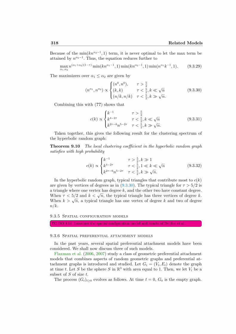
318 Related Models
Because of the min(knα2−1, 1) term, it is never optimal to let the max term beattained by nα2−1. Thus, the equation reduces further to
maxα1,α2
n(α1+α2)(1−τ) min(knα1−1, 1) min(knα2−1, 1) min(nα1k−1, 1). (9.3.29)
The maximizers over α1 ≤ α2 are given by
(nα1 , nα2) ∝
(n0, n0), τ > 5
2
(k, k) τ < 52, k √n
(n/k, n/k) τ < 52, k √n.
(9.3.30)
Combining this with (??) shows that
c(k) ∝
k−1 τ > 5
2
k4−2τ τ < 52, k √n
k2τ−6n5−2τ τ < 52, k √n.
(9.3.31)
Taken together, this gives the following result for the clustering spectrum ofthe hyperbolic random graph:
Theorem 9.10 The local clustering coefficient in the hyperbolic random graphsatisfies with high probability
c(k) ∝
k−1 τ > 5
2, k 1
k4−2τ τ < 52, 1 k √n
k2τ−6n5−2τ τ < 52, k √n.
(9.3.32)
In the hyperbolic random graph, typical triangles that contribute most to c(k)are given by vertices of degrees as in (9.3.30). The typical triangle for τ > 5/2 isa triangle where one vertex has degree k, and the other two have constant degree.When τ < 5/2 and k <
√n, the typical triangle has three vertices of degree k.
When k >√n, a typical triangle has one vertex of degree k and two of degree
n/k.
9.3.5 Spatial configuration models
TO DO 9.14: Introduce the spatial configuration model and results of Deijfen et al.
9.3.6 Spatial preferential attachment models
In the past years, several spatial preferential attachment models have beenconsidered. We shall now discuss three of such models.
Flaxman et al. (2006, 2007) study a class of geometric preferential attachmentmodels that combines aspects of random geometric graphs and preferential at-tachment graphs is introduced and studied. Let Gt = (Vt, Et) denote the graphat time t. Let S be the sphere S in R3 with area equal to 1. Then, we let Vt be asubset of S of size t.
The process (Gt)t≥0 evolves as follows. At time t = 0, G0 is the empty graph.
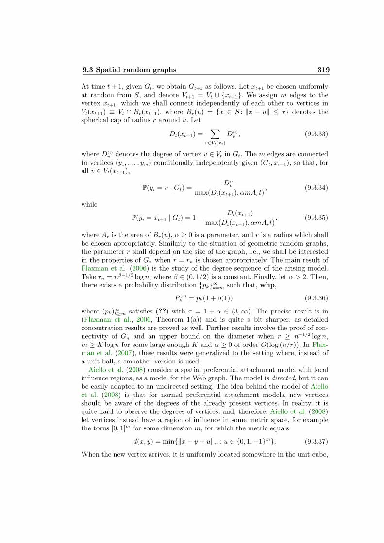
9.3 Spatial random graphs 319
At time t+ 1, given Gt, we obtain Gt+1 as follows. Let xt+1 be chosen uniformlyat random from S, and denote Vt+1 = Vt ∪ xt+1. We assign m edges to thevertex xt+1, which we shall connect independently of each other to vertices inVt(xt+1) ≡ Vt ∩ Br(xt+1), where Br(u) = x ∈ S : ‖x − u‖ ≤ r denotes thespherical cap of radius r around u. Let
Dt(xt+1) =∑
v∈Vt(xt)
D(t)
v , (9.3.33)
where D(t)
v denotes the degree of vertex v ∈ Vt in Gt. The m edges are connectedto vertices (y1, . . . , ym) conditionally independently given (Gt, xt+1), so that, forall v ∈ Vt(xt+1),
P(yi = v | Gt) =D(t)
v
max(Dt(xt+1), αmArt), (9.3.34)
while
P(yi = xt+1 | Gt) = 1− Dt(xt+1)
max(Dt(xt+1), αmArt), (9.3.35)
where Ar is the area of Br(u), α ≥ 0 is a parameter, and r is a radius which shallbe chosen appropriately. Similarly to the situation of geometric random graphs,the parameter r shall depend on the size of the graph, i.e., we shall be interestedin the properties of Gn when r = rn is chosen appropriately. The main result ofFlaxman et al. (2006) is the study of the degree sequence of the arising model.Take rn = nβ−1/2 log n, where β ∈ (0, 1/2) is a constant. Finally, let α > 2. Then,there exists a probability distribution pk∞k=m such that, whp,
P (n)
k = pk(1 + o(1)), (9.3.36)
where (pk)∞k≥m satisfies (??) with τ = 1 + α ∈ (3,∞). The precise result is in
(Flaxman et al., 2006, Theorem 1(a)) and is quite a bit sharper, as detailedconcentration results are proved as well. Further results involve the proof of con-nectivity of Gn and an upper bound on the diameter when r ≥ n−1/2 log n,m ≥ K log n for some large enough K and α ≥ 0 of order O(log (n/r)). In Flax-man et al. (2007), these results were generalized to the setting where, instead ofa unit ball, a smoother version is used.
Aiello et al. (2008) consider a spatial preferential attachment model with localinfluence regions, as a model for the Web graph. The model is directed, but it canbe easily adapted to an undirected setting. The idea behind the model of Aielloet al. (2008) is that for normal preferential attachment models, new verticesshould be aware of the degrees of the already present vertices. In reality, it isquite hard to observe the degrees of vertices, and, therefore, Aiello et al. (2008)let vertices instead have a region of influence in some metric space, for examplethe torus [0, 1]m for some dimension m, for which the metric equals
d(x, y) = min‖x− y + u‖∞ : u ∈ 0, 1,−1m. (9.3.37)
When the new vertex arrives, it is uniformly located somewhere in the unit cube,
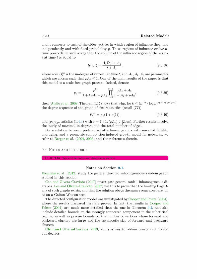
320 Related Models
and it connects to each of the older vertices in which region of influence they landindependently and with fixed probability p. These regions of influence evolve astime proceeds, in such a way that the volume of the influence region of the vertexi at time t is equal to
R(i, t) =A1D
(t)
i +A2
t+A3
, (9.3.38)
where now D(t)
i is the in-degree of vertex i at time t, and A1, A2, A3 are parameterswhich are chosen such that pA1 ≤ 1. One of the main results of the paper is thatthis model is a scale-free graph process. Indeed, denote
pk =pk
1 + kpA1 + pA2
k−1∏j=0
jA1 +A2
1 +A2 + pA2
, (9.3.39)
then (Aiello et al., 2008, Theorem 1.1) shows that whp, for k ≤ (n1/8/ log n)4pA1/(2pA1+1),the degree sequence of the graph of size n satisfies (recall (??))
P (n)
k = pk(1 + o(1)), (9.3.40)
and (pk)k≥0 satisfies (1.4.4) with τ = 1+1/(pA1) ∈ [2,∞). Further results involvethe study of maximal in-degrees and the total number of edges.
For a relation between preferential attachment graphs with so-called fertilityand aging, and a geometric competition-induced growth model for networks, werefer to Berger et al. (2004, 2005) and the references therein.
9.4 Notes and discussion
TO DO 9.16: Extend the notes and discussion section.
Notes on Section 9.1.
Bloznelis et al. (2012) study the general directed inhomogeneous random graphstudied in this section.
Cao and Olvera-Cravioto (2017) investigate general rank-1 inhomogeneous di-graphs. Lee and Olvera-Cravioto (2017) use this to prove that the limiting PageR-ank of such graphs exists, and that the solution obeys the same recurrence relationas on a Galton-Watson tree.
The directed configuration model was investigated by Cooper and Frieze (2004),where the results discussed here are proved. In fact, the results in Cooper andFrieze (2004) are much more detailed than the one in Theorem 9.2, and alsoinclude detailed bounds on the strongly connected component in the subcriticalregime, as well as precise bounds on the number of vertices whose forward andbackward clusters are large and the asymptotic size of forward and backwardclusters.
Chen and Olvera-Cravioto (2013) study a way to obtain nearly i.i.d. in-andout-degrees.
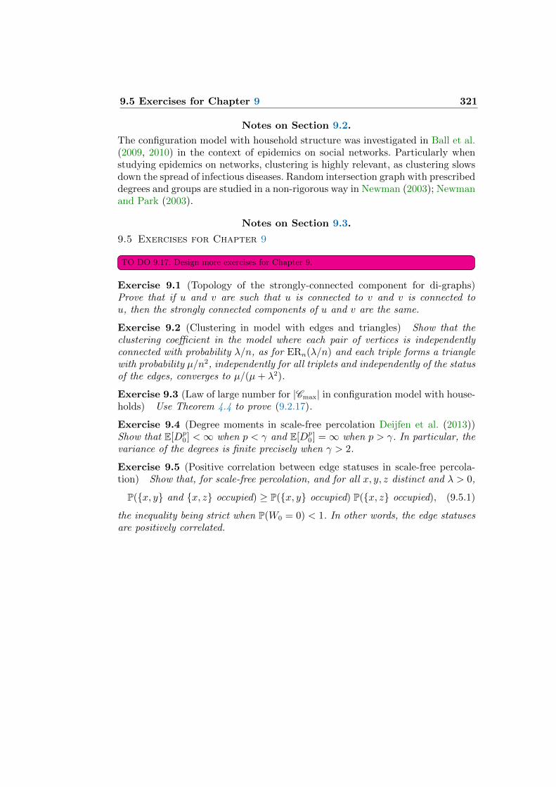
9.5 Exercises for Chapter 9 321
Notes on Section 9.2.
The configuration model with household structure was investigated in Ball et al.(2009, 2010) in the context of epidemics on social networks. Particularly whenstudying epidemics on networks, clustering is highly relevant, as clustering slowsdown the spread of infectious diseases. Random intersection graph with prescribeddegrees and groups are studied in a non-rigorous way in Newman (2003); Newmanand Park (2003).
Notes on Section 9.3.
9.5 Exercises for Chapter 9
TO DO 9.17: Design more exercises for Chapter 9.
Exercise 9.1 (Topology of the strongly-connected component for di-graphs)Prove that if u and v are such that u is connected to v and v is connected tou, then the strongly connected components of u and v are the same.
Exercise 9.2 (Clustering in model with edges and triangles) Show that theclustering coefficient in the model where each pair of vertices is independentlyconnected with probability λ/n, as for ERn(λ/n) and each triple forms a trianglewith probability µ/n2, independently for all triplets and independently of the statusof the edges, converges to µ/(µ+ λ2).
Exercise 9.3 (Law of large number for |Cmax| in configuration model with house-holds) Use Theorem 4.4 to prove (9.2.17).
Exercise 9.4 (Degree moments in scale-free percolation Deijfen et al. (2013))Show that E[Dp
0 ] <∞ when p < γ and E[Dp0 ] =∞ when p > γ. In particular, the
variance of the degrees is finite precisely when γ > 2.
Exercise 9.5 (Positive correlation between edge statuses in scale-free percola-tion) Show that, for scale-free percolation, and for all x, y, z distinct and λ > 0,
P(x, y and x, z occupied) ≥ P(x, y occupied) P(x, z occupied), (9.5.1)
the inequality being strict when P(W0 = 0) < 1. In other words, the edge statusesare positively correlated.


Appendix A
Some facts aboutmetric spaces
.
Abstract
In this section, we highlight some properties and results about metricspaces, including separable metric spaces and Borel measures on them.These results are used throughout Chapters 1– 3. We also present someof the missing details in the proof that the space of rooted graphs is aseparable metric space, or a Polish space.
A.1 Metric spaces
In this section, we discuss metric spaces. We start by defining what a metricis:
Definition A.1 (Distance metric) Let X be a space. A distance on X is afunction d : X 2 7→ [0,∞) such that
(a) 0 ≤ d(x, y) <∞ for all x, y ∈ X ;
(b) d(x, y) = d(y, x) for all x, y ∈ X ;
(c) d(x, z) ≤ d(x, y) + d(y, z) for all x, y, z ∈ X .
Definition A.2 (Metric space) Let X be a space and d a metric on it. Then(X , d) is called a metric space.
We next discuss some desirable properties of metric spaces:
Definition A.3 (Complete metric space) Let (X , d) be a metric space. We saythat (X , d) is complete when every Cauchy sequence has a limit. Here, a Cauchysequence is a sequence (xn)n≥1 with xn ∈ X such that for every ε > 0 there existsan N = N(ε) such that d(xn, xm) ≤ ε for all n,m ≥ N .
Definition A.4 (Separable metric space) Let (X , d) be a metric space. We saythat (X , d) is separable if it contains a countable subset that is dense in (X , d).This means that there exists a countable set A ⊆ X such that, for every x ∈ Xthere exists a sequence (an)n≥1 with an ∈ A such that d(an, x)→ 0.
Definition A.5 (Polish space) The metric space (X , d) is called Polish when itis separable and complete.
323
324 Some facts about metric spaces
A.2 Properties of the metric dG? on rooted graphs
For (G, o) ∈ G?, let
[G, o] = (G′, o′) : (G′, o′) ' (G, o) (A.2.1)
denote the equivalence class in G? corresponding to (G, o). We further let
[G?] = (G, o) : (G, o) ∈ G? (A.2.2)
denote the set of equivalence class in G?. This will be the set on which the distancedG?
actsIn this section, we prove that ([G?],dG?
) is a Polish space:
Theorem A.6 (Rooted graphs form a Polish space) dG?is a well-defined metric
on [G?]. Further, the metric space ([G?],dG?) is a Polish space.
The proof of Theorem A.6 will be divided into several steps. We start in Propo-sition A.8 by showing that dG?
is an ultrametric, which is a slightly strongerproperty than being a metric, and which also implies that (G?, dG?
) is a metricspace. In Proposition A.10, we show that the metric space (G?,dG?
) is complete,and in Proposition A.12, we show that it is separable. After that, we completethe proof of Theorem A.6.
A.2.1 Ultrametric property of dG?
In this section, we prove that dG?: G? × G? → [0, 1] is an ultrametric. One
of the problems that we have to resolve is that the space of rooted graphs isonly defined up to isomorphisms, which means that we have to make sure thatdG?
((G1, o1), (G2, o2)) is independent of the exact representative we choose in theequivalence classes of (G1, o1) and (G2, o2). That is the content of the followingproposition:
Proposition A.7 (dG?is well-defined on [G?]) The equality dG?
((G1, o1), (G2, o2)) =
dG?((G1, o1), (G2, o2)) holds whenever (G1, o1) ' (G1, o1) and (G2, o2) ' (G2, o2).
Consequently, dG?: [G?]× [G?] is well-defined.
Proposition A.8 (Ultrametricity) The map dG?: G? × G? → [0, 1] is an ultra-
metric, meaning that
(a) dG?((G1, o1), (G2, o2)) = 0 precisely when (G1, o1) ' (G2, o2);
(b) dG?((G1, o1), (G2, o2)) = dG?
((G2, o2), (G1, o1)) for all (G1, o1), (G2, o2) ∈ G?;(c) dG?
((G1, o1), (G3, o3)) ≤ maxdG?((G1, o1), (G2, o2)),dG?
((G2, o2), (G3, o3)) forall (G1, o1), (G2, o2), (G3, o3) ∈ G?.
Before giving the proof of Propositions A.7–A.8, we state and prove an impor-tant ingredient in them:
Lemma A.9 (Local neighborhoods determine the graph) Let (G1, o1) and(G2, o2) be two connected locally finite rooted graphs such that (B(G1)
r (o1), o1) '(B(G2)
r (o2), o2) for all r ≥ 0. Then (G1, o1) ' (G2, o2).
A.2 Properties of the metric dG?on rooted graphs 325
Proof We use a subsequence argument. Fix r ≥ 0, and consider the isomorphismφr : (B(G1)
r (o1), o1) → (B(G2)
r (o2), o2), which exists by assumption. Extend φr to(G1, o1) by defining
ψr(v) =
φr(v) for v ∈ V (B(G1)
r (o1));
o2 otherwise.(A.2.3)
Our aim is to use (ψr)r≥0 to construct an isomorphism between (G1, o1) and(G2, o2).
Abbreviate V (G1)
r = V (B(G1)
r (o1)). Let ψr|V (G1)0
be the restriction of ψr to V (G1)
0 =
o1. Then we know that ψr(v) = o2 for every v ∈ V (G1)
0 and r ≥ 0. We next letψr|V (G1)
1be the restriction of ψr to V (G1)
1 . Then, ψr|V (G1)1
is an isomorphism between
(B(G1)
1 (o1), o1) and (B(G2)
1 (o2), o2) for every r. Since there are only finitely manysuch isomorphisms, the same isomorphism φ′1 needs to be repeated infinitely manytimes in the sequence (ψr|V (G1)
1)r≥1. Let N1 denote the values of r for which
ψr|V (G1)1
= φ′1 ∀r ∈ N1. (A.2.4)
Now we repeat this argument to k = 2. Let ψr|V (G1)2
be the restriction of ψr to
V (G1)
2 . Again, ψr|V (G1)2
is an isomorphism between (B(G1)
2 (o1), o1) and (B(G2)
2 (o2), o2)
for every r. Since there are again only finitely many such isomorphisms, thesame isomorphism φ′2 needs to be repeated infinitely many times in the sequence(ψr|V (G1)
2)r∈N1
. Let N2 denote the values of r ∈ N1 for which
ψr|V (G1)2
= φ′2 ∀r ∈ N2. (A.2.5)
We now generalize this argument to general k ≥ 2. Let ψr|V (G1)
k
be the restric-
tion of ψr to V (G1)
k . Again, ψr|V (G1)
k
is an isomorphism between (B(G1)
k (o1), o1) and
(B(G2)
k (o2), o2) for every r. Since there are again only finitely many such isomor-phisms, the same isomorphism φ′k needs to be repeated infinitely many times inthe sequence (ψr|V (G1)
k
)r∈Nk−1. Let Nk denote the values of r ∈ Nk−1 for which
ψr|V (G1)
k
= φ′k ∀r ∈ Nk. (A.2.6)
Then, we see that Nk is a decreasing infinite set.Let us define ψ′` to be the first element of the sequence (ψr)r∈N` . Then, it
follows that ψ′`(v) = φ′k(v) for all ` ≥ k and all v ∈ V (G1)
k . Denote U0 = o1and Uk = V (G1)
k \ V (G1)
k−1 . Since we assume that V (G1) is connected, we have that∪k≥0Uk = V (G1).
It follows that the functions (ψ′`)`≥1 converge pointwise to
ψ(v) = ψ′∞(v) =∑k≥1
φ′k(v)1v∈Uk. (A.2.7)
We claim that ψ is the desired isomorphism between (G1, o1) and (G2, o2).The map ψ is clearly bijective, since φ′k : Uk → φ′k(Uk) is bijective. Further,
326 Some facts about metric spaces
let u, v ∈ V (G1). Denote k = maxdG1(o1, u), dG1
(o1, v). Then u, v ∈ Vk. Be-cause φ′k is an isomorphism between (B(G1)
k (o1), o1) and (B(G2)
k (o2), o2), it followsthat φ′k(u), φ′k(v) ∈ V (B(G2)
k (o2)) and φ′k(u), φ′k(v) ∈ E(B(G2)
k (o2)) preciselywhen u, v ∈ E(B(G1)
k (o1). Since ψ = φ′k on V (G1)
k , it then also follows thatψ(u), ψ(v) ∈ E(B(G2)
k (o2)) precisely when u, v ∈ E(B(G1)
k (o1), as required.Finally, ψ(o1) = φk(o1) and φk(o1) = o2 for every k ≥ 0. This completes theproof.
Proof of Proposition A.7. We note that if (G1, o1) ' (G1, o1) and (G2, o2) '(G2, o2), then (B(G1)
r , o1) ' (B(G2)
r , o2) if and only if (B(G1)
r , o1) ' (B(G2)
r , o2). There-fore, dG?
((G1, o1), (G2, o2)) is independent of the exact choice of the representativein the equivalence class of (G1, o1) and (G2, o2), so that dG?
((G1, o1), (G2, o2)) isconstant on such equivalence classes. This makes the metric dG?
([G1, o1], [G2, o2])well-defined for [G1, o1], [G2, o2] ∈ [G?].
Proof of Proposition A.8. (a) Assume that dG?((G1, o1), (G2, o2)) = 0. Then we
have (B(G1)
r (o1), o1) ' (B(G2)
r (o2), o2) for all r ≥ 0, so that, by Lemma A.9, also(G1, o1) ' (G2, o2), as required.
The proof of (b) is trivial and omitted.For (c), let rij = supr : (B(Gi)
r (oi), oi) ' (B(Gj)
r (oj), oj). Then (B(G1)
r (o1), o1) '(B(G3)
r (o3), o3) for all r ≤ minr13, r23 and (B(G1)
r (o2), o2) ' (B(G3)
r (o3), o3) forall r ≤ minr13, r23. We conclude that (B(G1)
r (o1), o1) ' (B(G2)
r (o2), o2) for allr ≤ minr13, r23, so that r12 ≥ minr13, r23. This implies that 1/(r13 + 1) ≤max1/(r13 + 1), 1/(r23 + 1), which implies the claim (recall (2.1.2)).
A.2.2 Completeness of ([G?], dG?)
In this section, we prove that ([G?],dG?) is complete:
Proposition A.10 (Completeness) The metric space ([G?],dG?) is complete.
Before giving the proof of Proposition A.10, we state and prove an importantingredient in it:
Lemma A.11 (Compatible rooted graph sequences have a limit) Let ((Gr, or))r≥0
be connected locally finite rooted graphs that are compatible, meaning that (B(Gs)
r , os) '(B(Gr)
r , or) for all r ≤ s. Then there exists a connected locally finite rooted graph(G, o) such that (Gr(or), or) ' (B(G)
r , o). Moreover, (G, o) is unique up to isomor-phisms.
Proof The point is that (Gr, or) may not live on the same vertex sets. Therefore,we first create a version (G′r, o
′r) that does live on the same vertex set. For this,
we will first construct isomorphic copies of (Gr, or) on a common node set, ina compatible way. To do this, denote Vr = v ∈ N : r ≤ Nr, where Nr =|V (Br(or))|. We define a sequence of bijections φr : V (Br(or)) → Vr recursivelyas follows. Let φ0 be the unique isomorphism from V (B0(o0)) = o0 to V0 = 1.
Let ψr be an isomorphism between (Gr−1, or−1) and (B(Gr)
r−1 , or), and ηr an
A.2 Properties of the metric dG?on rooted graphs 327
arbitrary bijection between V (Gr−1) \ V (B(Gr)
r−1 ) to Vr \ Vr−1. Define
φr(v) =
φr−1(ψ−1
r (v)) for v ∈ V (B(Gr)
r−1 ),
ηr(v) for v ∈ V (Gr−1) \ V (B(Gr)
r−1 ).(A.2.8)
Then we define (G′r, o′r) = (φr(Gr), φr(or)), where φr(Gr) is the graph consisting
of the vertex set φr(v) : v ∈ V (Gr) and edge set φr(u), φr(v) : u, v ∈E(Gr). Let us derive some properties of (G′r, o
′r). First of all, we see that o′r = 1
for every r ≥ 0, by construction. Further, φr is a bijection, so that (B(G′r)r (o′r), o
′r) '
(B(Gr)
r (or), or) = (Gr, or).Now we are ready to define (G, o). We define the root as o = 1, the vertex
set of G by V (G) =⋃r≥1 V (G′r), and the edge set E(G) =
⋃r≥1E(G′r). Then it
follows that (B(G)
r (o), o) = (B(G′r)r (o′r), o
′r) ' (B(Gr)
r (or), or) = (Gr, or), as required.Further, (G, o) is locally finite and connected, since (Gr, or) is for every r ≥ 0.Finally, to verify uniqueness, note that if (G′, o′) also satisfies that (B(G′)
r (o′), o′) '(B(Gr)
r (or), or) = (Gr, or) for every r ≥ 0, then (B(G′)r (o′), o′) ' (B(G)
r (o), o) forevery r ≥ 0, so that (G, o) ' (G′, o′), as required.
Proof of Proposition A.10. To verify completeness, fix a Cauchy sequence ([Gn, on])n≥1
with representative rooted graphs ((Gn, on))n≥1. Then, for every ε > 0, there ex-ists an N = N(ε) ≥ 0 such that, for every n,m ≥ N ,
dG?([Gn, on], [Gm, om]) ≤ ε. (A.2.9)
We note that, by Proposition A.7,
dG?([Gn, on], [Gm, om]) = dG?
((Gn, on), (Gm, om)), (A.2.10)
so from now on, we can work with the representatives instead. Since
dG?((Gn, on), (Gm, om)) ≤ ε, (A.2.11)
we obtain that for all r ≤ 1/ε−1 and n,m ≥ N , (B(Gn)
r (on), on) ' (B(Gm)
r (om), om).Equivalently, this implies that for every r ≥ 1, there exists an nr such that, forall n ≥ nr,
(B(Gn)
r (on), on) ' (B(Gnr )
r (onr), onr). (A.2.12)
Clearly, we may select nr such that nr is strictly increasing. Define (G′r, o′r) =
(B(Gnr )
r (onr), onr). Then ((G′r, o′r))r≥0 forms a compatible sequence. By Lemma
A.11, there exists a locally finite rooted graph (G, o) such that (B(G)
r , o) ' (G′r(o′r), o
′r).
But then also
(B(Gn)
r , on) ' (B(Gnr )
r (onr), onr = (G′r(o′r), o
′r). (A.2.13)
This, in turn, implies that, for all n ≥ nr,dG?
([G, o], [Gn, on]) = dG?((G, o), (Gn, on)) ≤ 1/(r + 1). (A.2.14)
Since r ≥ 1 is arbitrary, we conclude that [Gn, on] converges to [G, o], which is in[G?], so that ([G?], dG?
) is complete.
328 Some facts about metric spaces
A.2.3 Separability of ([G?], dG?)
In this section, we prove that ([G?],dG?) is separable:
Proposition A.12 (Separability) The metric space (G?,dG?) is separable.
Proof We need to show that there exists a countable dense subset in (G?, dG?).
Consider the set of all finite rooted graphs, which is certainly countable. Also,(B(G)
r (o), o) is a finite rooted graph for all r ≥ 0. Finally, dG?((B(G)
r (o), o), (G, o)) ≤1/(r + 1), so that (B(G)
r (o), o) converges to (G, o) when r → ∞. Thus, the spaceof finite rooted graphs is dense and countable. This completes the proof that(G?,dG?
) is separable.
A.2.4 ([G?],dG?) is Polish: Proof of Theorem A.6
In this section, we use the above results to complete the proof of Theorem A.6:
Proof of Theorem A.6. The function dG?is well-defined on [G?]× [G?] by Propo-
sition A.7. Proposition A.8 implies that dG?is an (ultra)metric on [G?]. Finally,
Proposition A.10 proves that ([G?], dG?) is complete, while Proposition A.12 proves
that ([G?],dG?) is separable. Thus, ([G?], dG?
) is a Polish space.
A.3 Notes and discussion
Notes on Section A.1
We draw inspiration from Howes (1995) and Rudin (1987, 1991).
Notes on Section A.2
This section is based to a large extent on (Leskela, 2019, Appendix B), some partsof the presented material is copied almost verbatim from there. I am grateful toLasse Leskela for making me aware of the subtleties of the proof, as well as sharinghis preliminary version of these notes.
References
Aiello, W., Bonato, A., Cooper, C., Janssen, J., and Pralat, P. 2008. A spatial web graph modelwith local influence regions. Internet Math., 5(1-2), 175–196.
Albert, R., and Barabasi, A.-L. 2002. Statistical mechanics of complex networks. Rev. ModernPhys., 74(1), 47–97.
Aldous, D. 1985. Exchangeability and related topics. Pages 1–198 of: Ecole d’ete de probabilitesde Saint-Flour, XIII—1983. Lecture Notes in Math., vol. 1117. Berlin: Springer.
Aldous, D., and Lyons, R. 2007. Processes on unimodular random networks. Electron. J. Probab.,12, no. 54, 1454–1508.
Aldous, D., and Steele, J. M. 2004. The objective method: probabilistic combinatorial optimiza-tion and local weak convergence. 110, 1–72.
Arratia, R., Barbour, AD, and Tavare, S. 2003. Logarithmic combinatorial structures: a proba-bilistic approach. European Mathematical Society.
Athreya, K., and Ney, P. 1972. Branching processes. New York: Springer-Verlag. DieGrundlehren der mathematischen Wissenschaften, Band 196.
Athreya, K. B., Ghosh, A. P., and Sethuraman, S. 2008. Growth of preferential attachmentrandom graphs via continuous-time branching processes. Proc. Indian Acad. Sci. Math. Sci.,118(3), 473–494.
Athreya, K.B. 2007. Preferential attachment random graphs with general weight function.Internet Math., 4(4), 401–418.
Ball, F., Sirl, D., and Trapman, P. 2009. Threshold behaviour and final outcome of an epidemicon a random network with household structure. Adv. in Appl. Probab., 41(3), 765–796.
Ball, F., Sirl, D., and Trapman, P. 2010. Analysis of a stochastic SIR epidemic on a randomnetwork incorporating household structure. Math. Biosci., 224(2), 53–73.
Barabasi, A.-L. 2002. Linked: The New Science of Networks. Cambridge, Massachusetts: PerseusPublishing.
Barabasi, A.-L., and Albert, R. 1999. Emergence of scaling in random networks. Science,286(5439), 509–512.
Barbour, A. D., and Reinert, G. 2001. Small worlds. Random Structures Algorithms, 19(1),54–74.
Barbour, A. D., and Reinert, G. 2004. Correction: “Small worlds” [Random Structures Algo-rithms 19 (2001), no. 1, 54–74; MR1848027]. Random Structures Algorithms, 25(1), 115.
Barbour, A. D., and Reinert, G. 2006. Discrete small world networks. Electron. J. Probab., 11,no. 47, 1234–1283 (electronic).
Bender, E.A., and Canfield, E.R. 1978. The asymptotic number of labelled graphs with givendegree sequences. Journal of Combinatorial Theory (A), 24, 296–307.
Benjamini, I., and Schramm, O. 2001. Recurrence of distributional limits of finite planar graphs.Electron. J. Probab., 6, no. 23, 13 pp. (electronic).
Benjamini, I., Kesten, H., Peres, Y., and Schramm, O. 2004. Geometry of the uniform spanningforest: transitions in dimensions 4, 8, 12, . . . . Ann. of Math. (2), 160(2), 465–491.
Benjamini, I., Lyons, R., and Schramm, O. 2015. Unimodular random trees. Ergodic TheoryDynam. Systems, 35(2), 359–373.
Berger, N. 2002. Transience, recurrence and critical behavior for long-range percolation. Comm.Math. Phys., 226(3), 531–558.
Berger, N., Borgs, C., Chayes, J. T., D’Souza, R. M., and Kleinberg, R. D. 2004. Competition-induced preferential attachment. Pages 208–221 of: Automata, languages and programming.Lecture Notes in Comput. Sci., vol. 3142. Berlin: Springer.
Berger, N., Borgs, C., Chayes, J. T., D’Souza, R. M., and Kleinberg, R. D. 2005. Degree dis-tribution of competition-induced preferential attachment graphs. Combin. Probab. Comput.,14(5-6), 697–721.
329
330 References
Berger, N., Borgs, C., Chayes, J., and Saberi, A. 2014. Asymptotic behavior and distributionallimits of preferential attachment graphs. Ann. Probab., 42(1), 1–40.
Bhamidi, S., Hofstad, R. van der, and Hooghiemstra, G. 2010a. First passage percolation onrandom graphs with finite mean degrees. Ann. Appl. Probab., 20(5), 1907–1965.
Bhamidi, S., Hofstad, R. van der, and Leeuwaarden, J. van. 2010b. Scaling limits for criticalinhomogeneous random graphs with finite third moments. Electronic Journal of Probability,15, 1682–1702.
Bhamidi, S., Hofstad, R. van der, and Leeuwaarden, J. van. 2012. Novel scaling limits for criticalinhomogeneous random graphs. Ann. Probab., 40(6), 2299–2361.
Bingham, N. H., Goldie, C. M., and Teugels, J. L. 1989. Regular variation. Encyclopedia ofMathematics and its Applications, vol. 27. Cambridge: Cambridge University Press.
Biskup, M. 2004. On the scaling of the chemical distance in long-range percolation models. Ann.Probab., 32(4), 2938–2977.
Bloznelis, M. Loglog distances in a power law random intersection graph. Preprint (2008).Bloznelis, M. 2010a. Component evolution in general random intersection graphs. SIAM J.
Discrete Math., 24(2), 639–654.Bloznelis, M. 2010b. The largest component in an inhomogeneous random intersection graph
with clustering. Electron. J. Combin., 17(1), Research Papr 110, 17.Bloznelis, M., Gotze, F., and Jaworski, J. 2012. Birth of a strongly connected giant in an
inhomogeneous random digraph. J. Appl. Probab., 49(3), 601–611.Bode, M., Fountoulakis, N., and Muller, T. 2015. On the largest component of a hyperbolic
model of complex networks. Electron. J. Combin., 22(3), Paper 3.24, 46.Boldi, P., and Vigna, S. 2004. The WebGraph Framework I: Compression Techniques. Pages
595–601 of: Proc. of the Thirteenth International World Wide Web Conference (WWW 2004).Manhattan, USA: ACM Press.
Boldi, P., Rosa, M., Santini, M., and Vigna, S. 2011. Layered Label Propagation: A Mul-tiResolution Coordinate-Free Ordering for Compressing Social Networks. Pages 587–596 of:Srinivasan, Sadagopan, Ramamritham, Krithi, Kumar, Arun, Ravindra, M. P., Bertino, Elisa,and Kumar, Ravi (eds), Proceedings of the 20th international conference on World Wide Web.ACM Press.
Bollobas, B. 1980. A probabilistic proof of an asymptotic formula for the number of labelledregular graphs. European J. Combin., 1(4), 311–316.
Bollobas, B. 2001. Random graphs. Second edn. Cambridge Studies in Advanced Mathematics,vol. 73. Cambridge: Cambridge University Press.
Bollobas, B., and Fernandez de la Vega, W. 1982. The diameter of random regular graphs.Combinatorica, 2(2), 125–134.
Bollobas, B., and Riordan, O. 2004a. The diameter of a scale-free random graph. Combinatorica,24(1), 5–34.
Bollobas, B., and Riordan, O. 2004b. Shortest paths and load scaling in scale-free trees. Phys.Rev. E., 69, 036114.
Bollobas, B., and Riordan, O. 2015. An old approach to the giant component problem. J.Combin. Theory Ser. B, 113, 236–260.
Bollobas, B., Riordan, O., Spencer, J., and Tusnady, G. 2001. The degree sequence of a scale-freerandom graph process. Random Structures Algorithms, 18(3), 279–290.
Bollobas, B., Borgs, C., Chayes, J., and Riordan, O. 2003. Directed scale-free graphs. Pages 132–139 of: Proceedings of the Fourteenth Annual ACM-SIAM Symposium on Discrete Algorithms(Baltimore, MD, 2003). New York: ACM.
Bollobas, B., Janson, S., and Riordan, O. 2005. The phase transition in the uniformly grownrandom graph has infinite order. Random Structures Algorithms, 26(1-2), 1–36.
Bollobas, B., Janson, S., and Riordan, O. 2007. The phase transition in inhomogeneous randomgraphs. Random Structures Algorithms, 31(1), 3–122.
Bringmann, K., Keusch, R., and Lengler, J. (2015). Geometric Inhomogeneous Random Graphs.Preprint arXiv:1511.00576 [cs.SI].
References 331
Bringmann, K., Keusch, R., and Lengler, J. (2016). Average Distance in a General Class ofScale-Free Networks with Underlying Geometry. Preprint arXiv:1602.05712 [cs.DM].
Britton, T., Deijfen, M., and Martin-Lof, A. 2006. Generating simple random graphs withprescribed degree distribution. J. Stat. Phys., 124(6), 1377–1397.
Broder, A., Kumar, R., Maghoul, F., Raghavan, P., Rajagopalan, S., Stata, R., Tomkins, A.,and Wiener, J. 2000. Graph Structure in the Web. Computer Networks, 33, 309–320.
Callaway, D.S., Hopcroft, J.E., Kleinberg, J. M., Newman, M. E. J., and Strogatz, S.H. 2001.Are randomly grown graphs really random? Physical Review E, 64, 041902.
Cao, J., and Olvera-Cravioto, M. 2017. On a general class of inhomogeneous random digraphs.Preprint arXiv:1712.03319 [math.PR].
Caravenna, F., Garavaglia, A., and van der Hofstad, R. 2019. Diameter in ultra-small scale-freerandom graphs. Random Structures Algorithms, 54(3), 444–498.
Chatterjee, S., and Durrett, R. 2009. Contact processes on random graphs with power lawdegree distributions have critical value 0. Ann. Probab., 37(6), 2332–2356.
Chen, N., and Olvera-Cravioto, M. 2013. Directed random graphs with given degree distribu-tions. Stoch. Syst., 3(1), 147–186.
Chung, F., and Lu, L. 2001. The diameter of sparse random graphs. Adv. in Appl. Math., 26(4),257–279.
Chung, F., and Lu, L. 2002a. The average distances in random graphs with given expecteddegrees. Proc. Natl. Acad. Sci. USA, 99(25), 15879–15882 (electronic).
Chung, F., and Lu, L. 2002b. Connected components in random graphs with given expecteddegree sequences. Ann. Comb., 6(2), 125–145.
Chung, F., and Lu, L. 2003. The average distance in a random graph with given expecteddegrees. Internet Math., 1(1), 91–113.
Chung, F., and Lu, L. 2004. Coupling online and offline analyses for random power law graphs.Internet Math., 1(4), 409–461.
Chung, F., and Lu, L. 2006a. Complex graphs and networks. CBMS Regional Conference Seriesin Mathematics, vol. 107. Published for the Conference Board of the Mathematical Sciences,Washington, DC.
Chung, F., and Lu, L. 2006b. The volume of the giant component of a random graph with givenexpected degrees. SIAM J. Discrete Math., 20, 395–411.
Cohen, R., and Havlin, S. 2003. Scale-free networks are ultrasmall. Phys. Rev. Lett., 90, 058701,1–4.
Cooper, C., and Frieze, A. 2004. The size of the largest strongly connected component of arandom digraph with a given degree sequence. Combin. Probab. Comput., 13(3), 319–337.
Corten, R. 2012. Composition and Structure of a Large Online Social Network in the Nether-lands. PLOS ONE, 7(4), 1–8.
Darling, D. A. 1970. The Galton-Watson process with infinite mean. J. Appl. Probability, 7,455–456.
Davies, P. L. 1978. The simple branching process: a note on convergence when the mean isinfinite. J. Appl. Probab., 15(3), 466–480.
Deijfen, M., and Kets, W. 2009. Random intersection graphs with tunable degree distributionand clustering. Probab. Engrg. Inform. Sci., 23(4), 661–674.
Deijfen, M., Hofstad, R. van der, and Hooghiemstra, G. 2013. Scale-free percolation. Annalesde l’institut Henri Poincare (B) Probability and Statistics, 49(3), 817–838. cited By (since1996)0.
Dembo, A., and Montanari, A. 2010. Ising models on locally tree-like graphs. The Annals ofApplied Probability, 20(2), 565–592.
Deprez, P, Hazra, R., and Wuthrich, M. 2015. Inhomogeneous Long-Range Percolation forReal-Life Network Modeling.
Dereich, S., and Morters, P. 2009. Random networks with sublinear preferential attachment:Degree evolutions. Electronic Journal of Probability, 14, 122–1267.
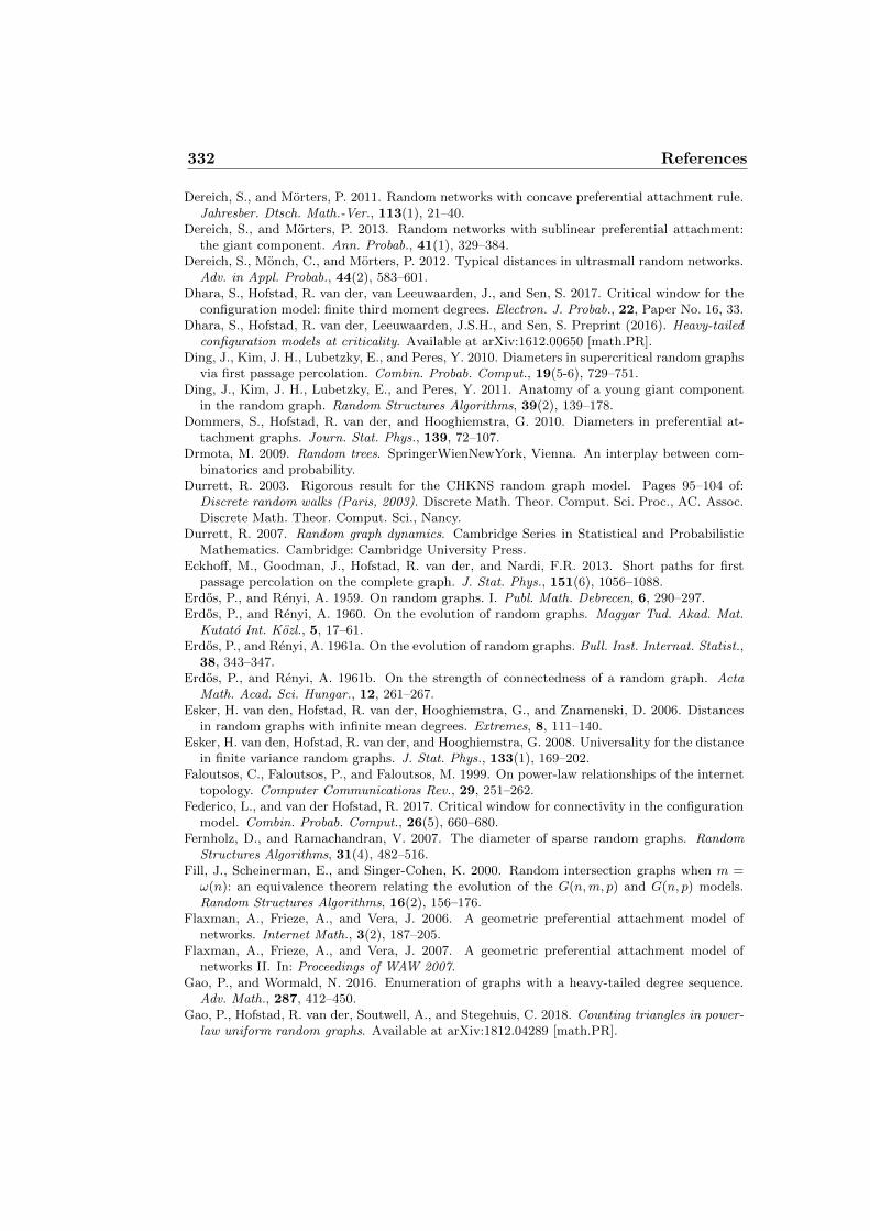
332 References
Dereich, S., and Morters, P. 2011. Random networks with concave preferential attachment rule.Jahresber. Dtsch. Math.-Ver., 113(1), 21–40.
Dereich, S., and Morters, P. 2013. Random networks with sublinear preferential attachment:the giant component. Ann. Probab., 41(1), 329–384.
Dereich, S., Monch, C., and Morters, P. 2012. Typical distances in ultrasmall random networks.Adv. in Appl. Probab., 44(2), 583–601.
Dhara, S., Hofstad, R. van der, van Leeuwaarden, J., and Sen, S. 2017. Critical window for theconfiguration model: finite third moment degrees. Electron. J. Probab., 22, Paper No. 16, 33.
Dhara, S., Hofstad, R. van der, Leeuwaarden, J.S.H., and Sen, S. Preprint (2016). Heavy-tailedconfiguration models at criticality. Available at arXiv:1612.00650 [math.PR].
Ding, J., Kim, J. H., Lubetzky, E., and Peres, Y. 2010. Diameters in supercritical random graphsvia first passage percolation. Combin. Probab. Comput., 19(5-6), 729–751.
Ding, J., Kim, J. H., Lubetzky, E., and Peres, Y. 2011. Anatomy of a young giant componentin the random graph. Random Structures Algorithms, 39(2), 139–178.
Dommers, S., Hofstad, R. van der, and Hooghiemstra, G. 2010. Diameters in preferential at-tachment graphs. Journ. Stat. Phys., 139, 72–107.
Drmota, M. 2009. Random trees. SpringerWienNewYork, Vienna. An interplay between com-binatorics and probability.
Durrett, R. 2003. Rigorous result for the CHKNS random graph model. Pages 95–104 of:Discrete random walks (Paris, 2003). Discrete Math. Theor. Comput. Sci. Proc., AC. Assoc.Discrete Math. Theor. Comput. Sci., Nancy.
Durrett, R. 2007. Random graph dynamics. Cambridge Series in Statistical and ProbabilisticMathematics. Cambridge: Cambridge University Press.
Eckhoff, M., Goodman, J., Hofstad, R. van der, and Nardi, F.R. 2013. Short paths for firstpassage percolation on the complete graph. J. Stat. Phys., 151(6), 1056–1088.
Erdos, P., and Renyi, A. 1959. On random graphs. I. Publ. Math. Debrecen, 6, 290–297.Erdos, P., and Renyi, A. 1960. On the evolution of random graphs. Magyar Tud. Akad. Mat.
Kutato Int. Kozl., 5, 17–61.Erdos, P., and Renyi, A. 1961a. On the evolution of random graphs. Bull. Inst. Internat. Statist.,
38, 343–347.Erdos, P., and Renyi, A. 1961b. On the strength of connectedness of a random graph. Acta
Math. Acad. Sci. Hungar., 12, 261–267.Esker, H. van den, Hofstad, R. van der, Hooghiemstra, G., and Znamenski, D. 2006. Distances
in random graphs with infinite mean degrees. Extremes, 8, 111–140.Esker, H. van den, Hofstad, R. van der, and Hooghiemstra, G. 2008. Universality for the distance
in finite variance random graphs. J. Stat. Phys., 133(1), 169–202.Faloutsos, C., Faloutsos, P., and Faloutsos, M. 1999. On power-law relationships of the internet
topology. Computer Communications Rev., 29, 251–262.Federico, L., and van der Hofstad, R. 2017. Critical window for connectivity in the configuration
model. Combin. Probab. Comput., 26(5), 660–680.Fernholz, D., and Ramachandran, V. 2007. The diameter of sparse random graphs. Random
Structures Algorithms, 31(4), 482–516.Fill, J., Scheinerman, E., and Singer-Cohen, K. 2000. Random intersection graphs when m =ω(n): an equivalence theorem relating the evolution of the G(n,m, p) and G(n, p) models.Random Structures Algorithms, 16(2), 156–176.
Flaxman, A., Frieze, A., and Vera, J. 2006. A geometric preferential attachment model ofnetworks. Internet Math., 3(2), 187–205.
Flaxman, A., Frieze, A., and Vera, J. 2007. A geometric preferential attachment model ofnetworks II. In: Proceedings of WAW 2007.
Gao, P., and Wormald, N. 2016. Enumeration of graphs with a heavy-tailed degree sequence.Adv. Math., 287, 412–450.
Gao, P., Hofstad, R. van der, Soutwell, A., and Stegehuis, C. 2018. Counting triangles in power-law uniform random graphs. Available at arXiv:1812.04289 [math.PR].
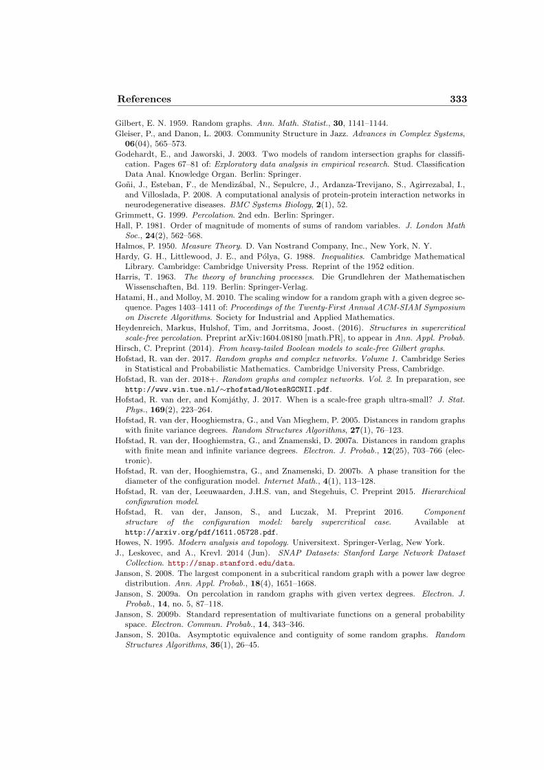
References 333
Gilbert, E. N. 1959. Random graphs. Ann. Math. Statist., 30, 1141–1144.
Gleiser, P., and Danon, L. 2003. Community Structure in Jazz. Advances in Complex Systems,06(04), 565–573.
Godehardt, E., and Jaworski, J. 2003. Two models of random intersection graphs for classifi-cation. Pages 67–81 of: Exploratory data analysis in empirical research. Stud. ClassificationData Anal. Knowledge Organ. Berlin: Springer.
Goni, J., Esteban, F., de Mendizabal, N., Sepulcre, J., Ardanza-Trevijano, S., Agirrezabal, I.,and Villoslada, P. 2008. A computational analysis of protein-protein interaction networks inneurodegenerative diseases. BMC Systems Biology, 2(1), 52.
Grimmett, G. 1999. Percolation. 2nd edn. Berlin: Springer.
Hall, P. 1981. Order of magnitude of moments of sums of random variables. J. London MathSoc., 24(2), 562–568.
Halmos, P. 1950. Measure Theory. D. Van Nostrand Company, Inc., New York, N. Y.
Hardy, G. H., Littlewood, J. E., and Polya, G. 1988. Inequalities. Cambridge MathematicalLibrary. Cambridge: Cambridge University Press. Reprint of the 1952 edition.
Harris, T. 1963. The theory of branching processes. Die Grundlehren der MathematischenWissenschaften, Bd. 119. Berlin: Springer-Verlag.
Hatami, H., and Molloy, M. 2010. The scaling window for a random graph with a given degree se-quence. Pages 1403–1411 of: Proceedings of the Twenty-First Annual ACM-SIAM Symposiumon Discrete Algorithms. Society for Industrial and Applied Mathematics.
Heydenreich, Markus, Hulshof, Tim, and Jorritsma, Joost. (2016). Structures in supercriticalscale-free percolation. Preprint arXiv:1604.08180 [math.PR], to appear in Ann. Appl. Probab.
Hirsch, C. Preprint (2014). From heavy-tailed Boolean models to scale-free Gilbert graphs.
Hofstad, R. van der. 2017. Random graphs and complex networks. Volume 1. Cambridge Seriesin Statistical and Probabilistic Mathematics. Cambridge University Press, Cambridge.
Hofstad, R. van der. 2018+. Random graphs and complex networks. Vol. 2. In preparation, seehttp://www.win.tue.nl/∼rhofstad/NotesRGCNII.pdf.
Hofstad, R. van der, and Komjathy, J. 2017. When is a scale-free graph ultra-small? J. Stat.Phys., 169(2), 223–264.
Hofstad, R. van der, Hooghiemstra, G., and Van Mieghem, P. 2005. Distances in random graphswith finite variance degrees. Random Structures Algorithms, 27(1), 76–123.
Hofstad, R. van der, Hooghiemstra, G., and Znamenski, D. 2007a. Distances in random graphswith finite mean and infinite variance degrees. Electron. J. Probab., 12(25), 703–766 (elec-tronic).
Hofstad, R. van der, Hooghiemstra, G., and Znamenski, D. 2007b. A phase transition for thediameter of the configuration model. Internet Math., 4(1), 113–128.
Hofstad, R. van der, Leeuwaarden, J.H.S. van, and Stegehuis, C. Preprint 2015. Hierarchicalconfiguration model.
Hofstad, R. van der, Janson, S., and Luczak, M. Preprint 2016. Componentstructure of the configuration model: barely supercritical case. Available athttp://arxiv.org/pdf/1611.05728.pdf.
Howes, N. 1995. Modern analysis and topology. Universitext. Springer-Verlag, New York.
J., Leskovec, and A., Krevl. 2014 (Jun). SNAP Datasets: Stanford Large Network DatasetCollection. http://snap.stanford.edu/data.
Janson, S. 2008. The largest component in a subcritical random graph with a power law degreedistribution. Ann. Appl. Probab., 18(4), 1651–1668.
Janson, S. 2009a. On percolation in random graphs with given vertex degrees. Electron. J.Probab., 14, no. 5, 87–118.
Janson, S. 2009b. Standard representation of multivariate functions on a general probabilityspace. Electron. Commun. Probab., 14, 343–346.
Janson, S. 2010a. Asymptotic equivalence and contiguity of some random graphs. RandomStructures Algorithms, 36(1), 26–45.

334 References
Janson, S. 2010b. Susceptibility of random graphs with given vertex degrees. J. Comb., 1(3-4),357–387.
Janson, S., and Luczak, M. 2007. A simple solution to the k-core problem. Random StructuresAlgorithms, 30(1-2), 50–62.
Janson, S., and Luczak, M. 2009. A new approach to the giant component problem. RandomStructures Algorithms, 34(2), 197–216.
Janson, S., Luczak, T., and Rucinski, A. 2000. Random graphs. Wiley-Interscience Series inDiscrete Mathematics and Optimization. Wiley-Interscience, New York.
Jaworski, J., Karonski, M., and Stark, D. 2006. The degree of a typical vertex in generalizedrandom intersection graph models. Discrete Math., 306(18), 2152–2165.
Joseph, Adrien. 2014. The component sizes of a critical random graph with given degree se-quence. Ann. Appl. Probab., 24(6), 2560–2594.
Kallenberg, O. 2002. Foundations of modern probability. Second edn. Probability and its Ap-plications (New York). New York: Springer-Verlag.
Karonski, M., Scheinerman, E., and Singer-Cohen, K. 1999. On random intersection graphs: thesubgraph problem. Combin. Probab. Comput., 8(1-2), 131–159. Recent trends in combina-torics (Matrahaza, 1995).
Kingman, J. F. C. 1975. The first birth problem for an age-dependent branching process. Ann.Probability, 3(5), 790–801.
Krioukov, D., Papadopoulos, F., Kitsak, M., Vahdat, A., and Boguna, M. 2010. Hyperbolicgeometry of complex networks. Phys. Rev. E (3), 82(3), 036106, 18.
Krioukov, D., Kitsak, M., Sinkovits, R., Rideout, D., Meyer, D., and Boguna, M. 2012. Networkcosmology. Scientific reports, 2.
Kunegis, J. 2017. The Koblenz Network Collection.Lee, J., and Olvera-Cravioto, M. 2017. PageRank on inhomogeneous random digraphs. Preprint
arXiv:1707.02492 [math.PR].Leskela, L. 2019. Random graphs and network statistics. Available at
http://math.aalto.fi/∼lleskela/LectureNotes004.html.Leskovec, J., Kleinberg, J., and Faloutsos, C. 2007. Graph evolution: Densification and shrinking
diameters. ACM Transactions on Knowledge Discovery from Data (TKDD), 1(1), 2.Leskovec, J., Lang, K., Dasgupta, A., and Mahoney, M. 2009. Community structure in large
networks: Natural cluster sizes and the absence of large well-defined clusters. Internet Math-ematics, 6(1), 29–123.
Luczak, T. 1992. Sparse random graphs with a given degree sequence. Pages 165–182 of: Randomgraphs, Vol. 2 (Poznan, 1989). Wiley-Intersci. Publ. Wiley, New York.
McKay, B.D. 1981. Subgraphs of random graphs with specified degrees. Congressus Numeran-tium, 33, 213–223.
McKay, B.D. 2011. Subgraphs of Random Graphs with Specified Degrees. In: Proceedings of theInternational Congress of Mathematicians 2010 (ICM 2010). Published by Hindustan BookAgency (HBA), India. WSPC Distribute for All Markets Except in India.
McKay, Brendan D, and Wormald, Nicholas C. 1990. Asymptotic enumeration by degree se-quence of graphs of high degree. European Journal of Combinatorics, 11(6), 565–580.
Molloy, M., and Reed, B. 1995. A critical point for random graphs with a given degree sequence.Random Structures Algorithms, 6(2-3), 161–179.
Molloy, M., and Reed, B. 1998. The size of the giant component of a random graph with a givendegree sequence. Combin. Probab. Comput., 7(3), 295–305.
Moore, C., and Newman, M. E. J. 2000. Epidemics and percolation in small-world networks.Phys. Rev. E, 61, 5678–5682.
Nachmias, A., and Peres, Y. 2010. Critical percolation on random regular graphs. RandomStructures Algorithms, 36(2), 111–148.
Newman, M. E. J. 2003. Properties of highly clustered networks. Physical Review E, 68(2),026121.
Newman, M. E. J. 2009. Random Graphs with Clustering. Phys. Rev. Lett., 103(Jul), 058701.
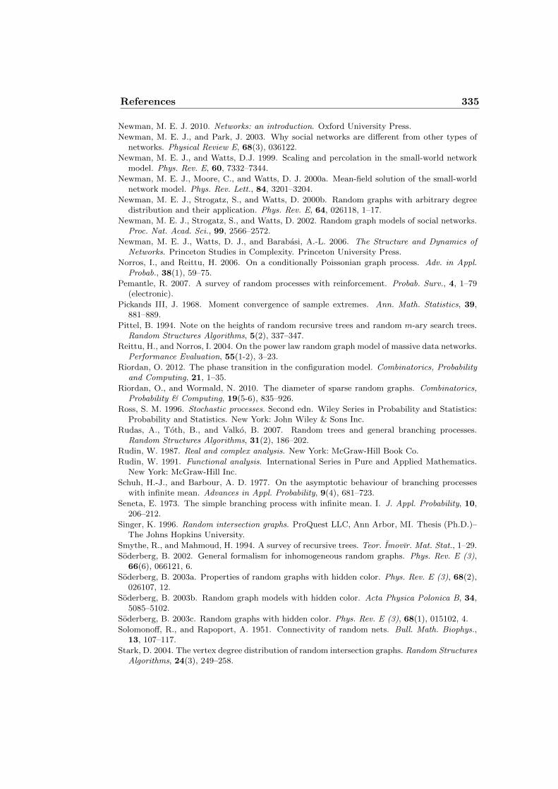
References 335
Newman, M. E. J. 2010. Networks: an introduction. Oxford University Press.
Newman, M. E. J., and Park, J. 2003. Why social networks are different from other types ofnetworks. Physical Review E, 68(3), 036122.
Newman, M. E. J., and Watts, D.J. 1999. Scaling and percolation in the small-world networkmodel. Phys. Rev. E, 60, 7332–7344.
Newman, M. E. J., Moore, C., and Watts, D. J. 2000a. Mean-field solution of the small-worldnetwork model. Phys. Rev. Lett., 84, 3201–3204.
Newman, M. E. J., Strogatz, S., and Watts, D. 2000b. Random graphs with arbitrary degreedistribution and their application. Phys. Rev. E, 64, 026118, 1–17.
Newman, M. E. J., Strogatz, S., and Watts, D. 2002. Random graph models of social networks.Proc. Nat. Acad. Sci., 99, 2566–2572.
Newman, M. E. J., Watts, D. J., and Barabasi, A.-L. 2006. The Structure and Dynamics ofNetworks. Princeton Studies in Complexity. Princeton University Press.
Norros, I., and Reittu, H. 2006. On a conditionally Poissonian graph process. Adv. in Appl.Probab., 38(1), 59–75.
Pemantle, R. 2007. A survey of random processes with reinforcement. Probab. Surv., 4, 1–79(electronic).
Pickands III, J. 1968. Moment convergence of sample extremes. Ann. Math. Statistics, 39,881–889.
Pittel, B. 1994. Note on the heights of random recursive trees and random m-ary search trees.Random Structures Algorithms, 5(2), 337–347.
Reittu, H., and Norros, I. 2004. On the power law random graph model of massive data networks.Performance Evaluation, 55(1-2), 3–23.
Riordan, O. 2012. The phase transition in the configuration model. Combinatorics, Probabilityand Computing, 21, 1–35.
Riordan, O., and Wormald, N. 2010. The diameter of sparse random graphs. Combinatorics,Probability & Computing, 19(5-6), 835–926.
Ross, S. M. 1996. Stochastic processes. Second edn. Wiley Series in Probability and Statistics:Probability and Statistics. New York: John Wiley & Sons Inc.
Rudas, A., Toth, B., and Valko, B. 2007. Random trees and general branching processes.Random Structures Algorithms, 31(2), 186–202.
Rudin, W. 1987. Real and complex analysis. New York: McGraw-Hill Book Co.
Rudin, W. 1991. Functional analysis. International Series in Pure and Applied Mathematics.New York: McGraw-Hill Inc.
Schuh, H.-J., and Barbour, A. D. 1977. On the asymptotic behaviour of branching processeswith infinite mean. Advances in Appl. Probability, 9(4), 681–723.
Seneta, E. 1973. The simple branching process with infinite mean. I. J. Appl. Probability, 10,206–212.
Singer, K. 1996. Random intersection graphs. ProQuest LLC, Ann Arbor, MI. Thesis (Ph.D.)–The Johns Hopkins University.
Smythe, R., and Mahmoud, H. 1994. A survey of recursive trees. Teor. Imovır. Mat. Stat., 1–29.
Soderberg, B. 2002. General formalism for inhomogeneous random graphs. Phys. Rev. E (3),66(6), 066121, 6.
Soderberg, B. 2003a. Properties of random graphs with hidden color. Phys. Rev. E (3), 68(2),026107, 12.
Soderberg, B. 2003b. Random graph models with hidden color. Acta Physica Polonica B, 34,5085–5102.
Soderberg, B. 2003c. Random graphs with hidden color. Phys. Rev. E (3), 68(1), 015102, 4.
Solomonoff, R., and Rapoport, A. 1951. Connectivity of random nets. Bull. Math. Biophys.,13, 107–117.
Stark, D. 2004. The vertex degree distribution of random intersection graphs. Random StructuresAlgorithms, 24(3), 249–258.
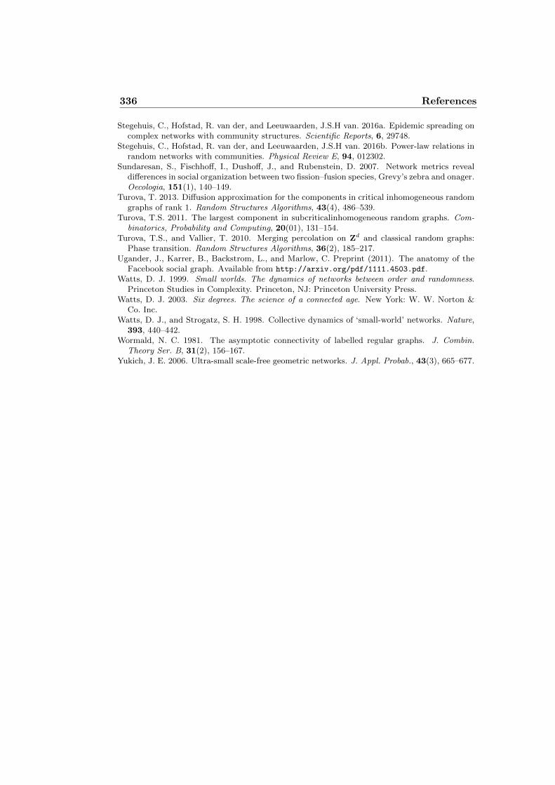
336 References
Stegehuis, C., Hofstad, R. van der, and Leeuwaarden, J.S.H van. 2016a. Epidemic spreading oncomplex networks with community structures. Scientific Reports, 6, 29748.
Stegehuis, C., Hofstad, R. van der, and Leeuwaarden, J.S.H van. 2016b. Power-law relations inrandom networks with communities. Physical Review E, 94, 012302.
Sundaresan, S., Fischhoff, I., Dushoff, J., and Rubenstein, D. 2007. Network metrics revealdifferences in social organization between two fission–fusion species, Grevy’s zebra and onager.Oecologia, 151(1), 140–149.
Turova, T. 2013. Diffusion approximation for the components in critical inhomogeneous randomgraphs of rank 1. Random Structures Algorithms, 43(4), 486–539.
Turova, T.S. 2011. The largest component in subcriticalinhomogeneous random graphs. Com-binatorics, Probability and Computing, 20(01), 131–154.
Turova, T.S., and Vallier, T. 2010. Merging percolation on Zd and classical random graphs:Phase transition. Random Structures Algorithms, 36(2), 185–217.
Ugander, J., Karrer, B., Backstrom, L., and Marlow, C. Preprint (2011). The anatomy of theFacebook social graph. Available from http://arxiv.org/pdf/1111.4503.pdf.
Watts, D. J. 1999. Small worlds. The dynamics of networks between order and randomness.Princeton Studies in Complexity. Princeton, NJ: Princeton University Press.
Watts, D. J. 2003. Six degrees. The science of a connected age. New York: W. W. Norton &Co. Inc.
Watts, D. J., and Strogatz, S. H. 1998. Collective dynamics of ‘small-world’ networks. Nature,393, 440–442.
Wormald, N. C. 1981. The asymptotic connectivity of labelled regular graphs. J. Combin.Theory Ser. B, 31(2), 156–167.
Yukich, J. E. 2006. Ultra-small scale-free geometric networks. J. Appl. Probab., 43(3), 665–677.
Index
Albert-Barabasi model, 161
Branching processdelayed, 229infinite mean, 220marked, 81multitype, 69two-stage, 81
Central limit theorem, 168Chung-Lu model
attack vulnerability, 88fluctuations of typical distance, 203
Clique, 187Collaboration graph
random intersection graph, 289Complexity, 86Configuration model, 97, 209
average distance, 209clustering, 286, 287connectivity, 120core, 216diameter, 225diameter core, 216directed, 278distance, 209forward degree distribution, 98household structure, 286near-critical behavior, 126path counting, 211phase transition, 103
Connected componentcomplexity, 86
Connectivityconfiguration model, 120
De Finetti’s Theorem, 134Death process, 108Distribution
Bernoulli, 134Mixed Poisson, 64
Erdos-Renyi random graphdiameter, 226
Exchangeable random variables, 134
Helly’s Theorem, 136Hopcount, 8Household model, 286
Inhomogeneous random graph, 59diameter, 202fluctuations of typical distance, 203graphical, 60irreducible, 60small world, 174sparsity, 60
typical graph distance, 174, 203Ultra-small world, 176
Inhomogeneous random graphsdual kernel, 202duality principle, 202
Internet, 8hopcount, 8
Internet Movie Data baserandom intersection graph, 289
Maclaurin inequality, 213Mixed marked Poisson branching process, 82Mixed Poisson distribution, 64Multitype branching process, 69
irreducible, 70Markov chain, 70singular, 70
Polya urn schemelimit theorem, 136, 137
Pathself-avoiding, 178
Path countingconfiguration model, 211
Paths, 178self-avoiding, 178
percolationlong-range, 296
Perron-Frobenius theorem, 70Phase transition
configuration model, 103Preferential attachment model, 133, 235
diameter, 244typical distances, 244
Random graphtypical graph distance, 174
Random intersection graph, 288Random intersection graphs, 288Random variables
exchangeable, 134Real-world network, 3
scale-free percolation network, 294Scale-free trees, 235Self-avoiding path, 178Size-biased distribution, 82Small world, 174spatial preferential attachment models, 298Stochastic domination, 82
TheoremDe Finetti, 134Helly, 136Perron-Frobenius, 70
Treeheight, 236
337

338 Index
Two-regular graphdiameter, 233longest cycle, 233
Ultra-small world, 174, 176Uniform recursive trees, 236Universality, 245

Glossary 339

Todo list
TO DO 1.1: Refer to recent discussion on power-laws in real-world networks. 6TO DO 2.1: Add convergence of various clustering coefficients! 47TO DO 2.2: Add convergence of neighborhoods of edges. 47TO DO 2.3: Use this to show convergence of assortativity coefficient. How about
other degree-degree dependency measures? 47TO DO 4.1: Fix this proof! 125TO DO 5.1: Add local weak convergence for BPAM 167TO DO 5.2: Extend the discussion of the phase transition for BPAM 170TO DO 5.3: Add further results! 170TO DO 6.1: Add case of distances in real-world network... 179Update from here! 265Add Discussion of dist
PA(1,δ)n (b)
(1, V ) = oP(log n) here! Or exercise? 274TO DO 8.2: Adapt this argument as in ?! 277TO DO 8.3: Check whether equality is okay?? 280TO DO 8.4: Continue from here! 282TO DO 8.5: Add proof! 288TO DO 8.6: Extend the discussion in this section. 289TO DO 8.7: Explain that Theorem 8.23 is already proved 289TO DO 8.9: Add further result, such as the ones in the BPAM 289TO DO 8.10: Extend notes and discussion 289TO DO 8.11: Design more exercises 289TO DO 9.1: Explain directed networks from a practical setting (WWW?) 295TO DO 9.3: Add discussion directed inhomogeneous random graphs 297TO DO 9.3: Add discussion distances in directed random graphs 300TO DO 9.4: Add practical example of community structure: clustering table? 301TO DO 9.5: Add discussion community structure: partition, SBM, larger overlap 301TO DO 9.6: Add discussion SBM 301TO DO 9.7: Make this introduction section shorter 301TO DO 9.8: Present results HCM: connectivity and graph distances 306TO DO 9.9: Adapt this discussion: special case of HCM 306TO DO 9.10: Extend discussion of intersection graphs 308TO DO 9.11: Add discussion of exponential random graphs, and show that GRG
is special case 309TO DO 9.12: Add discussion why geometry may be useful in random graphs 309TO DO 9.13: Introduce the GIRG 311TO DO 9.14: Introduce the spatial configuration model and results of Deijfen et
al. 318TO DO 9.16: Extend the notes and discussion section. 320TO DO 9.17: Design more exercises for Chapter 9. 321
341