Quantum Mechanics: From Realism to Intuitionismlandsman/scriptieRonnie.pdf · Quantum Mechanics:...
128
Transcript of Quantum Mechanics: From Realism to Intuitionismlandsman/scriptieRonnie.pdf · Quantum Mechanics:...
Quantum Mechanics:
From Realism to IntuitionismA mathematical and philosophical investigation
Master's Thesis Mathematical Physics
Author:
Ronnie Hermens
Supervisor:
Prof. Dr. N. P. Landsman
Second Reader:
Dr. H. Maassen
ii
Aan de hoge blauwe hemel
zweeft een dapper wolkje,
in tegen de wind.
Hij komt niet ver,
maar probeert het tenminste.
Jaap Robben
iii
Preface
As a student of physics I always felt that the diculties I had with comprehending the ex-plained theories were mostly due to my incapability. Pondering on questions like What is anelectric eld? somehow prevented me from actually solving Maxwell's equations, which is infact the thing that you have to do to pass your exam. But then working out the details of theactual solving leads to various diculties again. Indeed, quite often in physics one encountersmathematical problems which one must march over to obtain the desired answer. Sometimesthis results in peculiarities that seemed paradoxical to me like a discontinuous solution to adierential equation. As it turns out, I'm one of those persons who in many cases can't seethe bigger picture until he's worked out a lot of the details. Fortunately, working out detailsis an activity praised in mathematics (the unfortunate thing for me was that it took me overfour years to discover this).
When I rst came with the idea for this thesis I didn't know very much about the funda-ments of quantum mechanics. Discussions on topics like hidden variables, contextuality orlocality always seemed gladly avoid by the teachers during the lectures on quantum theory.It was kind of a revelation (and a relief) for me to nd out that the incomprehensibility ofquantum mechanics is not easily stepped over. This became clearer to me when I followed acourse on quantum probability taught by Dr. Maassen. One of the rst topics discussed, wasthe violation of Bell inequalities by quantum mechanics, which demonstrates directly that theprobability measures obtained in quantum mechanics are fundamentally dierent from thosedescribed by Kolmogorov's theory. This is interesting in particular for probability theoristsbut it wasn't the aim of Bell to advocate for a revision of probability theory. Rather, it was hisaim to show that any hidden-variable theory that reproduces the predictions obtained fromquantum mechanics must be non-local, i.e. it requires action at a distance.
Roughly, a hidden-variable theory is a theory that allows a realist interpretation i.e., atheory in which observables can be interpreted to correspond to properties of systems thatactually exist. Personally, I never considered that this should be taken as a demand forphysical theories. Not because I have a strong opinion considering the realist/idealist questionin philosophy, but more because I never considered it the task of physics to be judgmentalabout such philosophical problems. However, there were enough questions raised in my headto form a starting point for this thesis and luckily, none of them have been answered properly.These questions include the following. How can mathematics play a role in nding answersto metaphysical questions? How reliable is mathematics in this role? Why does quantummechanics not allow (certain) realist interpretations?
As it goes with such questions, trying out answers immediately leads to new questions. Inparticular it becomes of interest what the role of mathematics is in physics and even broader,what the nature of mathematics is in itself, i.e. what is mathematics actually about? Con-cerning this rst problem I became particularly interested in probability theory, which, inmy opinion, is one of the purest forms of physics.1 I remember a lecture during a course onstatistical physics taught by Prof. Vertogen during which he gave a derivation of the notionof entropy from a Bayesian point of view making only use of philosophical and logical con-siderations (i.e., without resorting to the measure-theoretic approach). At that time I didn't
1This view doesn't seem very popular, but it is in fact in correspondence with Hilbert's vision who explainedhis sixth problem as follows: To treat in the same manner, by means of axioms, those physical sciences inwhich mathematics plays an important part; in the rst rank are the theory of probabilities and mechanics[Hil2].
iv
recognize it as such, but it did make me realize how important logic is for the constructionof physical theories. Unfortunately for me, at the same time I also followed a course on logicthought by Dr. Veldman. The unfortunate coincidence was that while Prof. Vertogen madeextensive use of the logical law ¬(¬X) = X (it was actually the rst formula in the accompa-nying reader), Dr. Veldman was advocating against the use of this law, which is abandonedin intuitionistic logic. Needless to say, I had my logical conceptions all mixed up and I endedup failing the exams for both the courses.
Ever since I've had a sort of love-hate relationship with intuitionism. At rst I didn't likeit all and I tried to nd a motivation for myself to see why the law of excluded middle shouldbe true. From a physics point of view, all the motivations I could nd were based on realism,which seemed to me to be a too strong assumption. On the other hand, it seemed to me thatif one can doubt one specic logical law, one might as well doubt all of logic. This is also whatBrouwer advocated and roughly, he proposed that not logic should be our guide to truth, butintuition. It never became clear to me why this approach would be more reliable when it comesto truth. But at least logic enables us to compare notes in an (almost) unambiguous way. Icame to except logic as a tool for reasoning not because I believe it is true, but because I don'tsee a better alternative. Then what about the law of excluded middle? I think from a realist(or Platonist when it comes to mathematics) point of view it may be mandatory. Others maywant to learn to use it with care. For me, sometimes its truth seems almost evident2 while onother occasions it seems very suspicious (and the same holds for the axiom of choice for thatmatter). And as for truth, perhaps truth is overrated.
I wouldn't have found a personally satisfactory view on physics and mathematics if itweren't for the aforementioned persons. In fact, I probably would have quit my study withinthe rst three years without the down toned visions on physics Prof. Vertogen presented inhis lectures and I would like to thank him for that. I also would like to thank Prof. Landsmanand Dr. Maassen for making me enthusiastic about mathematical physics and Dr. Veldmanfor teaching me about the philosophy of mathematics and intuitionism in particular. Withoutthese people I would never have guessed it to be possible to write a philosophical thesis onphysics with the use of mathematical rigor that still makes sense. For this I must also thankDr. Seevinck who taught me a lot about the foundations of physics and who was often willingto listen to my own ideas. Finally I'd like to thank my girlfriend Femke for supporting me inevery step the past ten years and for being my philosophical sparring partner from time totime and above all for being my best friend.
Nijmegen, October 2009
2I think this also must have been the case for Brouwer for I see no better way to motivate his continuityprinciple.

v
Contents
Preface iii
1 Introduction 1
2 Introduction to the Foundations of Quantum Mechanics 4
2.1 Postulates of Quantum Mechanics . . . . . . . . . . . . . . . . . . . . . . . . . 42.2 The (In)completeness of Quantum Mechanics (Part I) . . . . . . . . . . . . . . 92.3 Impossibility Proofs for Hidden Variables . . . . . . . . . . . . . . . . . . . . . 12
2.3.1 Von Neumann's Theorem . . . . . . . . . . . . . . . . . . . . . . . . . . 132.3.2 A Counterexample . . . . . . . . . . . . . . . . . . . . . . . . . . . . . . 192.3.3 The Kochen-Specker Theorem . . . . . . . . . . . . . . . . . . . . . . . . 222.3.4 The Bell Inequality . . . . . . . . . . . . . . . . . . . . . . . . . . . . . . 31
3 The Alleged Nullication of the Kochen-Specker Theorem 43
3.1 Introduction . . . . . . . . . . . . . . . . . . . . . . . . . . . . . . . . . . . . . . 433.2 The Nullication . . . . . . . . . . . . . . . . . . . . . . . . . . . . . . . . . . . 433.3 First Critics . . . . . . . . . . . . . . . . . . . . . . . . . . . . . . . . . . . . . . 46
3.3.1 Non-Linearity of the MK-Models . . . . . . . . . . . . . . . . . . . . . . 463.3.2 Contextuality of the MK-Models . . . . . . . . . . . . . . . . . . . . . . 47
3.4 The Statistics of MKC-Models . . . . . . . . . . . . . . . . . . . . . . . . . . . 493.5 Further Criticism . . . . . . . . . . . . . . . . . . . . . . . . . . . . . . . . . . . 54
3.5.1 An Empirical Discrepancy with Quantum Mechanics (Part I) . . . . . . 543.5.2 Non-Classicality . . . . . . . . . . . . . . . . . . . . . . . . . . . . . . . 563.5.3 An Empirical Discrepancy with Quantum Mechanics (Part II) . . . . . . 59
3.6 A Modication of the MKC-Models for Imprecise Measurements . . . . . . . . . 623.7 Non-Locality of the MKC-Models . . . . . . . . . . . . . . . . . . . . . . . . . . 673.8 Conclusion . . . . . . . . . . . . . . . . . . . . . . . . . . . . . . . . . . . . . . . 69
4 The Free Will Theorem Stripped Down 71
4.1 Introduction . . . . . . . . . . . . . . . . . . . . . . . . . . . . . . . . . . . . . . 714.2 The Axioms . . . . . . . . . . . . . . . . . . . . . . . . . . . . . . . . . . . . . . 714.3 The Theorem . . . . . . . . . . . . . . . . . . . . . . . . . . . . . . . . . . . . . 734.4 Discussion . . . . . . . . . . . . . . . . . . . . . . . . . . . . . . . . . . . . . . . 76
4.4.1 Free Will and Determinism . . . . . . . . . . . . . . . . . . . . . . . . . 764.4.2 The Possibility of Absolute Determinism . . . . . . . . . . . . . . . . . . 794.4.3 Robustness . . . . . . . . . . . . . . . . . . . . . . . . . . . . . . . . . . 814.4.4 What does the Free Will Theorem add to the Story? . . . . . . . . . . . 84
5 The Strangeness and Logic of Quantum Mechanics 90
5.1 The (In)completeness of Quantum Mechanics (Part II) . . . . . . . . . . . . . . 905.2 Quantum Mechanics as a Hidden-Variable Theory . . . . . . . . . . . . . . . . . 925.3 Quantum Logic and the Violation of the Bell Inequality . . . . . . . . . . . . . 955.4 Intuitionism and Complementarity . . . . . . . . . . . . . . . . . . . . . . . . . 1005.5 Towards Intuitionistic Quantum Logic . . . . . . . . . . . . . . . . . . . . . . . 1045.6 Epilogue . . . . . . . . . . . . . . . . . . . . . . . . . . . . . . . . . . . . . . . . 111

vi
References 114
Introduction 1
1 Introduction
Theoretical physicists live in a classical world, looking
into a quantummechanical world.
- J. S. Bell
Quantum mechanics started as a counter-intuitive theory and has succeeded in preservingthis status ever since. Most introductions to quantum mechanics start with Planck's radiationformula. This was the rst formula that relied on the quantization of energy, which is adeparture from the Natura non facit saltus-principle. Proposing the theoretical interpretationof this radiation formula was described by Planck himself as an act of despair:
Kurz zusammengefasst kann ich die ganze Tat als einen Akt der Verzweiungbezeichnen, denn von Natur bin ich friedlich und bedenklichen Abenteuern ab-geneigt ..., aber eine Deutung musste um jeden Preis gefunden werden, und wäreer noch so hoch. ... Im übrigen war ich zu jedem Opfer an meinen bisherigenphysikalischen Überzeugungen bereit. [Pla]
The act of despair in question was actually not the concept of allowing discontinuity in Nature(although this was related) but the reliance on Boltzmann's theory of statistical physics, whichis based on atomism; i.e. the idea that all matter is made up of some smallest particles calledatoms. Nowadays, the concept of atomism is part of the doctrine of natural science and nobodywould question the existence of atoms. However, around 1900 there was no real consensusabout the issue, and in fact Planck originally opposed it.
In his later years, Planck came to accept the concept of atomism and thus conquered one ofthe (to him) counter-intuitive aspects of his radiation formula, and thus quantum mechanics.However, this acceptance took a large revision on what is to be expected of Nature and onwhat is to be expected of a physical theory. It seems that this has been characteristic forthe discussion on the foundations of quantum mechanics ever since. Some of the revisionsthat have been proposed throughout the years will be discussed in this thesis. These includerevisions of our view on: reality, causality, locality, free will, determinism and logic. Notthe lightest of subjects, and it seems mind-boggling enough that quantum mechanics has ledpeople to such considerations.
An important motivation for the entire discussion is the search for an answer to the ques-tion: What is actually being measured when a measurement is performed? In classicalphysics there seemed to be an easy answer to this question; a measurement reveals some prop-erty possessed by the system under consideration. This is, roughly, the realist interpretationof physics. However, as it turns out, such an interpretation is not possible in quantum me-chanics without making compromises. The proof of this statement is usually attributed to theKochen-Specker Theorem and the violation of the Bell inequalities by quantum mechanics,which will be discussed in Chapter 2. Both imply a compromise that has to be made if onewishes to maintain realism. The Kochen-Specker Theorem implies that one has to resort tocontextuality3, and the Bell inequality argument implies that one has to resort to non-locality.
3Of all the philosophical concepts that play a role in this thesis, this is probably the most peculiar one.Roughly, it states that what is actually measured depends in a very strong sense on how it is measured i.e., itdepends on the measuring context. Of course, each of these concepts will be explained more carefully in thecourse of this thesis.
2 Introduction
Most people do not wish to make such compromises, and therefore these proofs are also knownas `impossibility proofs' or `no-go theorems'.
There is a natural problem that arises in this situation. The statements derived are allof a philosophical nature, but on the other hand, rigorous proofs can only be made withinmathematics. This is because when it comes to mathematical objects, most people agree onhow these objects may be manipulated to obtain new objects.4 However, this also means thatphilosophical and mathematical concepts have to be linked to one another, and there is ofcourse no rigorous way to do this. In fact, there is not even much consensus about what termslike reality, locality and free will mean and what role they should play in a physical theory.This leaves a lot of room for discussion on what actually can be proven about Nature andabout physical theories in particular.
In Chapter 3 it will be shown that the Kochen-Specker Theorem is quite unstable consid-ering speculations on what realism should entail. More specically, it turns out that if onerelaxes the view on what constitutes a physical observable, one may retain non-contextuality.The discussion becomes more philosophical in Chapter 4, where the Free Will Theorem ofConway and Kochen is discussed. This is also the rst point where it becomes more clear thatthe strangeness of quantum mechanics does not just aect the realist interpretation of physics;the indeterminacy introduced by quantum mechanics seems unavoidable in any other proceed-ing theory (consistent with current experimental knowledge), irrespective of whether one hasa realist or an anti-realist view. This leads to the question whether the earlier arguments usedto point out problems in the realist interpretation can be extended to also point out problemsthat arise in other interpretations. In Chapter 5 it is argued that this does indeed seem to bethe case.
Hoping to acquire a better understanding of these problems, I take on a short re-investigationof the Copenhagen interpretation. It seems that the Copenhagen interpretation does pro-vide certain conceptual tools to overcome some philosophical problems concerning quantummechanics. However, most people, like myself, cannot help to feel some unease about thisinterpretation. This feeling is similar to the one sometimes encountered when studying amathematical theorem; although the proof may convince one that the theorem should betrue, it doesn't always provide the feeling that one understands what the theorem actuallystates. Often, a clarication is needed to explain why a theorem is stated the way it is, andwhat the idea behind the theorem is.
Such a clarication appears to be missing for the Copenhagen interpretation. Bohr onlyrecites some facts about the strangeness of quantum mechanics (at least, the facts as he seesthem) and suggests how one should cope with them. The impossibility proofs show that thesefacts cannot easily be sidestepped and so indeed it seems that one must cope with them.However, structural philosophical arguments about what accounts for this strangeness aremissing. There is no clear motivation for coping with the problems in the way suggested by
Bohr. In Chapter 5 I will attempt to provide this motivation, by linking the philosophy ofBohr to some of the philosophical ideas behind intuitionistic logic. More precisely, my hope isthat an abuse of language in the sense meant by Bohr, may be avoided by adopting a dierentform of logic. In particular, it seems that the law of excluded middle provides a devious wayto introduce sentences that speak of phenomena that cannot be compared with one another.
4It may be noted that there is no general consensus on what these objects are. However, in many casesthis doesn't inuence what is considered a proof and what is not.

Introduction 3
It is clear that Bohr wanted to avoid such sentences5, and should have argued against thislaw, hence embracing intuitionistic logic. However, he insisted on the use of classical logic.
5In the words of Wittgenstein: Wovon man nicht reden kann, darüber muss man schweigen.
4 Introduction to the Foundations of Quantum Mechanics
2 Introduction to the Foundations of Quantum Mechanics
There is a theory which states that if ever anyone discov-
ers exactly what the Universe is for and why it is here,
it will instantly disappear and be replaced by something
even more bizarre and inexplicable. There is another
which states that this has already happened.
D. Adams
2.1 Postulates of Quantum Mechanics
The goal of this section is to give a brief introduction to (some of) the counter-intuitiveaspects of quantum theory and to show why they can't be resolved as easily as one mighthope (namely, due to the impossibility proofs for hidden-variable theories). First, (a versionof) the postulates of quantum mechanics, as originally introduced by von Neumann [vN], isformulated. The version I use here is the one that was presented to me by Michael Seevinckin a course on the foundations of quantum mechanics [See2]. Although probably most readersalready know these postulates in some form, I think it is good to restate them to give a morecomplete overview. Moreover, it will make the discussion more precise, since there will nowbe less ambiguity on what I mean when I refer to a particular postulate.6 More than onceI found myself in a situation when I had an objection to some argument used in a text onfoundations of quantum mechanics, only to nd out that I was actually objecting to one ofthe postulates in a dierent form. Also, it seems a good occasion to introduce the notationused throughout this thesis.
1. State Postulate: Every physical system can be associated with a (complex) Hilbertspace7 H. Every nonzero vector ψ ∈ H gives a complete description of the state of thesystem. For each λ ∈ C, λ 6= 0, the two vectors ψ and λψ describe the same state. If twosystems are associated with spaces H1 and H2, then the composite system is describedby the space H1⊗H2.
A more generalized notion of the state of a system is given by the language of density operators.The states in the form of vectors in a Hilbert space are then called pure states. Notice thateach pure state in fact corresponds with an entire `line' (λψ)λ∈C\0 in H, called a ray. Toeach ray one associates the projection Pψ : H → H on this line, given by
Pψ(φ) :=〈ψ, φ〉〈ψ,ψ〉
ψ, ∀φ ∈ H . (1)
With a mixture of pure states one can then associate a convex combination of one-dimensionalprojection operators.8 More formally, a mixed state is a positive trace-class operator with trace1. The set of mixed states will be denoted by S(H), and the set of pure states by P1(H) (which
6This also holds more generally; a lot of confusion may be avoided if more authors took the time to restateimportant terms in their discussion.
7In our denition of a Hilbert space, the inner product will be linear in the second term and anti-linear inthe rst.
8The interpretation of mixed states as an actual mixture of pure states is not entirely without problems.For example, two mixtures of dierent pure states may constitute the same mixed stated. Therefore, a mixedstate doesn't give complete information about the pure states of which it is a mixture. Moreover, interpreting
Postulates of Quantum Mechanics 5
stands for the set of one-dimensional projections). The set S(H) is a convex set. One mayshow that the set P1(H) corresponds to the set of all extreme points of S(H) (i.e., the one-dimensional projections are precisely all the elements of S(H) that cannot be written as aproper convex combination of other elements).
2. Observable Postulate: With each physical observable A, there is associated a self-adjoint operator A : D(A)→ H with domain D(A) dense in H.
The theory of self-adjoint operators is noticeably more complex than most physics literaturewould lead one to believe, as is made clear in the following example.
Example 2.1. Consider the Hilbert space H = L2(R), the space of all square integrablefunctions. The position operator dened by (Xψ)(x) := xψ(x) does not map every ψ ∈ Hto an element of H. Therefore, the set H cannot be taken as its domain but instead,one must take some dense subset D(X). Its adjoint operator X∗ is dened as the uniqueoperator that satises
〈ψ,Xφ〉 = 〈X∗ψ, φ〉, ∀ψ ∈ D(X∗), φ ∈ D(X), (2)
where the domain of X∗ is dened as
D(X∗) := ψ ∈ H ; φ 7→ 〈ψ,Xφ〉 is a bounded linear functional ∀φ ∈ D(X). (3)
Intuitively, the larger one chooses D(X), the smaller D(X∗) becomes. It is therefore adelicate matter to choose D(X) in such a way that X is self-adjoint, i.e., (X,D(X)) =(X∗, D(X∗)). It turns out that X is self-adjoint on the domain D(X) = ψ ∈ H ; Xψ ∈H.
Note that for the specication of this domain it is necessary that Xψ is actuallydened for all ψ. For X this causes no problems, but for the momentum operator P ,the expression (Pψ)(x) = −i~ d
dxψ(x) is not well-dened for most elements of H withoutintroducing the notion of a generalized function (also called a distribution). First oneintroduces an injection ψ 7→ Lψ of H into the set of all linear functionals on the vectorspace C∞c (R) (i.e. the set of all innitely dierentiable function with compact support):
Lψ(φ) := 〈ψ, φ〉, ∀φ ∈ C∞c (R). (4)
On this sspace of linear functionals, one denes the derivative as
ddx
Lψ(φ) := −⟨ψ,
ddx
φ
⟩, ∀φ ∈ C∞c (R). (5)
Now for any ψ ∈ H one takes the condition ddxψ ∈ H to mean that there exists a χ ∈ H
such that ddxLψ = Lχ. In this case, one denes d
dxψ = χ. In particular, if ψ is dierentiable(in the usual sense) with derivative in H one has
ddx
Lψ(φ) := −⟨ψ,
ddx
φ
⟩=⟨
ddx
ψ, φ
⟩= L d
d xψ(φ), ∀φ ∈ C∞c (R), (6)
the mixed states as `not actually knowing what the pure state is' leads to problems when considering compositestates, since a mixed state is in general a convex combination of pure states of the form Pψ1⊗ψ2 . Such statesare known as proper mixtures, other mixtures are called improper. This terminology is due to d'Espagnat.See also [d'E].

6 Introduction to the Foundations of Quantum Mechanics
so that this new notion of a derivative is a proper extension of the usual one. It then turnsout that the momentum operator P is self-adjoint on the domain
D(P ) := ψ ∈ AC(R) ; Pψ ∈ H, (7)
where AC(R) is the set of all functions that are absolutely continuous9 on each niteinterval of R. A proof can be found in [Yos, p. 198]. In this book one can also nd a proofof the peculiar fact that there is no self-adjoint momentum operator on the Hilbert spaceL2[0,∞) (p. 353). A friendly text on these problems that also emphasizes the relevancefor physics and chemistry is [BFV].
These are examples of self-adjoint operators that play a large role in the theory of quantummechanics. However, most self-adjoint operators don't play any role in quantum theory. Onemay, for example, consider the operator X +P on the Hilbert space L2[0, 1]. In this case, theoperator X is self-adjoint on the domain D(X) = H. The momentum operator is self-adjointon the domain
D(P ) =ψ ∈ H ; ψ is absolutely continuous,−i~ d
dxψ ∈ H, ψ(0) = ψ(1)
. (8)
It follows from the Kato-Rellich theorem (see for example [dO, Ch. 6]) that X + P is self--adjoint on the domain D(X + P ) = D(P ).
Though self-adjoint, the operator X + P has no direct physical meaning. But even anindirect meaning (e.g. by adding the measuring results of position and momentum) is am-biguous, since one cannot measure both observables at the same time (because X and P donot commute). This leads one to question the converse of the observable postulate, i.e. theclaim that every self-adjoint operator corresponds with an observable. It seems reasonableto deny this claim. On the other hand, it seems premature to exclude some operators (likeX + P ) a priori, since it cannot be excluded that a meaning for such an observable will befound in the future.
For a bounded operator A on a Hilbert space H its spectrum is dened as the set
σ(A) := a ∈ C ; A− a1 is invertible. (9)
For an unbounded operator A with domain D(A) dense in H the spectrum σ(A) can still bedened. In this case a ∈ σ(A) if and only if there exists a bounded operator B such that(A − a1)B = 1 and B(A − a1)ψ = ψ for all ψ ∈ D(A). The spectrum is a generalizationof the notion of the set of eigenvalues of a matrix. As with matrices, the spectrum of a self-adjoint operator is always a subset of the real numbers. This physically justies the followingpostulate.10
9A function ψ is called absolutely continuous on the interval I if for each ε > 0 there exists a δ > 0 suchthat for each nite sequence (an, bn) of pairwise disjoint open sub-intervals of I, one has
∑n |ψ(bn)−ψ(an)| < ε
whenever∑n |bn − an| < δ.
10This postulate is often seen as a part of the Born postulate. Indeed, the Born postulate implies thata measurement result almost surely (i.e., with probability one) is a value in the spectrum of A. The valuepostulate sharpens this by stating that measurement results outside σ(A) can actually never be obtained.

Postulates of Quantum Mechanics 7
3. Value Postulate: A measurement of a physical observable A yields a real number inthe spectrum of the associated self-adjoint operator A.
The value postulate does not make any statement about the actual result of a specicmeasurement. To elaborate on this postulate, one of the wonderful results of functionalanalysis is needed: the spectral theorem.11
Theorem 2.1. For each densely-dened self-adjoint operator A, there is a spectral measure12
µA such that
(i) A =∫
R z dµA(z) (as a Stieltjes integral).
(ii) If ∆ ∩ σ(A) = ∅, then µA(∆) = 0 for each Borel set ∆.
(iii) For each open subset U ⊂ R with U ∩ σ(A) 6= ∅, one has µA(U) 6= 0.
(iv) If B is a bounded operator such that BA ⊂ AB13, then B also commutes with µA(∆)for every Borel set ∆.
This mathematically justies the following postulate.
4. Born Postulate: The probability of nding a result a ∈ ∆ upon measurement of theobservable A on a system in the state ψ for a Borel set ∆ is given by
Pψ[A ∈ ∆] =1‖ψ‖2
〈ψ, µA(∆)ψ〉. (10)
The notation Pψ[A ∈ ∆] is probably more familiar to probability theorists than to physicists,but I think it is a convenient one. It is to be read as the probability for the event A ∈ ∆,given the state ψ. Similarly, I write
Eψ(A) =∫
RzPψ[A ∈ d z] =
∫R
1‖ψ‖2
〈ψ, zµA(d z)ψ〉 =〈ψ,Aψ〉〈ψ,ψ〉
(11)
for the expectation value, instead of the often seen notation 〈A〉ψ. Note that it is more commonto take the right-hand side of (11) as the denition of the quantum-mechanical expectationvalue. Its relation with the probabilities for measurement results (the left hand side of (11))may then be seen to be a consequence of the spectral theorem (i.e., according to this theorem(11) is equivalent to (10)).
In the generalized case where mixed states are considered, the Born rule generalizes to
Pρ[A ∈ ∆] = Tr(ρµA(∆)) (12)
for the mixed state ρ, where Tr denotes the trace operation. One easily checks that this resultsin (10) in case that ρ = Pψ (i.e., whenever ρ is a pure state).
11See for example [Con2] or [Rud] for proofs.12A spectral measure is a map µ from the Borel subsets B of R to the projection operators P(H) such that
µ(∅) = 0, µ(R) = 1, µ(∆1 ∩ ∆2) = µ(∆1)µ(∆2) ∀∆1,∆2 ∈ B and for each countable set of disjoint subsets(∆i)
∞i=1 in B one has µ(∪∞i=1∆i) =
∑∞i=1 µ(∆i).
13This means that D(BA) ⊂ D(AB) and ABψ = BAψ for all ψ ∈ D(BA).
8 Introduction to the Foundations of Quantum Mechanics
Remark 2.1. Observables associated with projection operators (in particular, those of theform µA(∆)) are usually regarded as the yes-no-questions. Since their spectrum is 0, 1,a measurement of such an observable always yields one of these numbers. For an observableP associated with the operator P , the number 1 corresponds to the answer The state ofthe system after the measurement lies in the space P H. and the number 0 corresponds tothe answer The state of the system after the measurement lies in the space (1−P )H. Inparticular, a measurement of the observable associated with an operator of the form µA(∆)can be associated with the question Does the value of A lie in the set ∆? The precisemeaning of these questions (and their answers) will play an underlying role in this thesis.
Many physicists may nd this use of mathematics overwhelming and maybe even unneces-sary. In most physics literature one simply refers to the spectral decomposition of an operatorwithout explicitly dening what this means. Operators are often treated as if they are matricesand their spectra are then referred to as the set of eigenvalues with corresponding eigenstatesand eigenspaces. As a student of physics I became confused when rst realizing that, forexample, the position operator X does not have any eigenstates. Moreover, it didn't becomeclear to me why the probability of nding a particle in some (Borel) subset ∆ was given by
Pψ[X ∈ ∆] =1‖ψ‖2
∫∆|ψ(x)|2 dx, (13)
until I learned (in a mathematics course) that the spectral measure for the position operatoris simply given by14 µX(∆)ψ = 1∆ψ (because σ(X) = R), so that (13) is a special case of(10).
Finally, it has to be specied how the state of the system changes in time. Actually, twopostulates are needed for this.
5. Schrödinger Postulate: When no measurement is performed on the system, thechange of the state in time is described by a unitary transformation. That is,
ψ(t) = U(t)ψ(0)
for some strongly continuous unitary one-parameter group15 t 7→ U(t).
Note that no distinction in notation is made between the map ψ : R → H, t 7→ ψ(t) and thevector ψ in H as is standard in most literature. This postulate is in fact equivalent to the onefound in more standard physics literature. Namely, because of Stone's Theorem there existsa self-adjoint operator H such that U(t) = e−iHt ∀t, which brings one back to the originalSchrödinger equation
idd tψ(t) = Hψ(t), ∀ψ ∈ D(H).
For a mixed state ρ the time evolution is given by ρ(t) = U(t)ρU∗(t), or id ρ(t)d t = [H, ρ(t)].
6. Von Neumann Postulate (Projection Postulate): When an observable A cor-responding to an operator A with discrete spectrum is measured and the measure-ment yields some a ∈ σ(A), the state of the system changes discontinuously from ψ toµA(a)ψ.
14Here, 1∆ denotes the indicator function for the set ∆.15This means that the set U(t) ; t ∈ R forms a group of unitary operators satisfying U(t+ s) = U(t)U(s)
∀s, t, where the map t 7→ U(t) is continuous in the sense that lims→t U(s)ψ = U(t)ψ for all t ∈ R, ψ ∈ H.

The (In)completeness of Quantum Mechanics 9
Note that the state of the system after measurement is indeed always a state (i.e. µA(a)ψ 6=0) because of the Born postulate.
The motivation for introducing this postulate is that it ensures that if a measurement ofan observable yields some value a, an immediate second measurement of the same observablewill yield exactly the same result. It is founded on experimental experience (von Neumannbased it on the Compton-Simons experiment [vN]) and therefore seems a necessary claim.However, the postulate as stated here only applies for discrete observables (i.e., those whosecorresponding operators have a discrete spectrum). It has, in fact, been shown that a similarpostulate for continuous spectra cannot be formulated: repeatable measurements are onlypossible for discrete observables [Oza]. A more extensive discussion can be found in [BLM].
The von Neumann postulate is probably the most controversial postulate of quantum me-chanics. Because the time evolution of the state of a system depends so greatly on whetheror not there is a measurement being performed on the system, one is tempted to ask whatexactly constitutes a measurement. No satisfactory answer to this question exists in my opin-ion, and it is one of the underlying questions of what is known as the measurement problem(see also [Bel5]). Compared to the diculty of this problem, the problem of repeatability forobservables with a continuous spectrum seems a rather small one. It seems likely to me thata philosophically satisfying solution of the measurement problem may also solve the latter.16
Although it certainly is an interesting topic for research, the measurement problem willnot be the focus of this paper. My problem is rather related to one of the earliest objectionsagainst quantum mechanics made clear for the rst time by Einstein, namely its possibleincompleteness.
2.2 The (In)completeness of Quantum Mechanics (Part I)
It follows from the Born postulate that, in general, the state of the system does not determinewhat the result of the outcome of a measurement is. This in itself was not the only problemEinstein had with quantum theory. An even more serious problem for him was that certainobservables like energy and momentum, which are even supposed to be conserved, are notattributed a particular value at all in quantum mechanics. That is, if one knows the state ofthe system, one cannot in general say what the momentum of a particle in the system is. In[EPR] Einstein, Podolsky and Rosen also gave a seemingly convincing reason why a completetheory should attribute a value to such observables at all times. Below, an experiment isdiscussed that is quite similar to the one discussed in [EPR], but has the advantage that thereare no unbounded operators involved. It was rst introduced by Bohm [BA] and has playeda central role in many discussions ever since.
Example 2.2 (The EPRB-experiment). Consider a system of two spin-12 particles (say,
two electrons). Each particle taken by itself can be described in a Hilbert space C2, wherea basis is choosen such that (1, 0) stands for spin up and (0, 1) for spin down. Physicists
16There have been proposals for introducing generalizations of the von Neumann postulate that are richenough to incorporate observables with a continuous spectrum. However, there are great consequences involved.In the scenario described in [Sri] it requires a generalization of the state postulate to a point where the originalstates (the density operators) are only associated with the probability functions they generate through theBorn postulate. The generalized states also allow probability functions that are no longer of the form (12) andare no longer σ-additive in general.
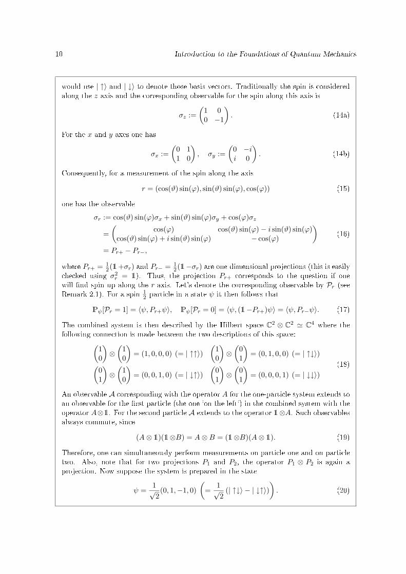
10 Introduction to the Foundations of Quantum Mechanics
would use | ↑〉 and | ↓〉 to denote those basis vectors. Traditionally the spin is consideredalong the z-axis and the corresponding observable for the spin along this axis is
σz :=(
1 00 −1
). (14a)
For the x and y axes one has
σx :=(
0 11 0
), σy :=
(0 −ii 0
). (14b)
Consequently, for a measurement of the spin along the axis
r = (cos(ϑ) sin(ϕ), sin(ϑ) sin(ϕ), cos(ϕ)) (15)
one has the observable
σr := cos(ϑ) sin(ϕ)σx + sin(ϑ) sin(ϕ)σy + cos(ϕ)σz
=(
cos(ϕ) cos(ϑ) sin(ϕ)− i sin(ϑ) sin(ϕ)cos(ϑ) sin(ϕ) + i sin(ϑ) sin(ϕ) − cos(ϕ)
)= Pr+ − Pr−,
(16)
where Pr+ = 12(1+σr) and Pr− = 1
2(1−σr) are one-dimensional projections (this is easilychecked using σ2
r = 1). Thus, the projection Pr+ corresponds to the question if onewill nd spin up along the r-axis. Let's denote the corresponding observable by Pr (seeRemark 2.1). For a spin-1
2 particle in a state ψ it then follows that
Pψ[Pr = 1] = 〈ψ, Pr+ψ〉, Pψ[Pr = 0] = 〈ψ, (1−Pr+)ψ〉 = 〈ψ, Pr−ψ〉. (17)
The combined system is then described by the Hilbert space C2 ⊗ C2 ' C4 where thefollowing connection is made between the two descriptions of this space:(
10
)⊗(
10
)= (1, 0, 0, 0) (= | ↑↑〉)
(10
)⊗(
01
)= (0, 1, 0, 0) (= | ↑↓〉)(
01
)⊗(
10
)= (0, 0, 1, 0) (= | ↓↑〉)
(01
)⊗(
01
)= (0, 0, 0, 1) (= | ↓↓〉)
(18)
An observable A corresponding with the operator A for the one-particle system extends toan observable for the rst particle (the one `on the left') in the combined system with theoperator A⊗1. For the second particle A extends to the operator 1⊗A. Such observablesalways commute, since
(A⊗ 1)(1⊗B) = A⊗B = (1⊗B)(A⊗ 1). (19)
Therefore, one can simultaneously perform measurements on particle one and on particletwo. Also, note that for two projections P1 and P2, the operator P1 ⊗ P2 is again aprojection. Now suppose the system is prepared in the state
ψ =1√2
(0, 1,−1, 0)(
=1√2
(| ↑↓〉 − | ↓↑〉)). (20)

The (In)completeness of Quantum Mechanics 11
If the spin along the z-axis for the rst particle is measured one nds that the probabilitiesfor nding spin up or spin down are respectively
Pψ[Pz = 1] = 〈ψ, Pz+ ⊗ 1ψ〉 =12〈(1, 0), Pz+(1, 0)〉 =
12
;
Pψ[Pz = 0] = 〈ψ, Pz− ⊗ 1ψ〉 =12〈(0, 1), Pz−(0, 1)〉 =
12.
(21)
The reasoning of Einstein, Podolsky and Rosen now is as follows. According to the vonNeumann postulate, after the measurement the state of the system will be (0, 1, 0, 0) uponnding spin up and (0, 0, 1, 0) upon nding spin down. In either case, a measurement ofthe spin along the z-axis on the second particle will yield a particular result (the oppositeof the spin of the rst particle) with absolute certainty. Since one can make a predictionof the spin of the second particle without in any way disturbing this particle (the distancebetween the two particles may be arbitrarily large) one may state that the spin along thez-axis has a real meaning. That is, the spin along the z-axis appears to be an observablethat is actually meaningful for the observed system. Einstein, Podolsky and Rosen wouldsay that there exists an element of physical reality that corresponds to this observable.
Now, if one would measure the spin along the y-axis on particle one instead, the stateof the system would be projected to the state (−1, 1,−1, 1) if one would nd spin up, andto the state (1, 1,−1,−1) if one would nd spin down. Each happens with probability 1
2 .In either case, a measurement of the spin along the y-axis on the second particle yieldsa particular result (the opposite of the spin of the rst particle) with absolute certainty.Following the same reasoning, one concludes that also the spin along the y-axis of thesecond particle should correspond to an element of physical reality.
Now the problem is the following: in the states (0, 1, 0, 0) and (0, 0, 1, 0) one can assigna value to the spin along the z-axis for the second particle, but the spin along the y-axisdoes not have a denite value. Vice versa for the states (−1, 1,−1, 1) and (1, 1,−1,−1). Itturns out that there is no state that can assign a denite value to both the observables atthe same time and hence there is no state in quantum mechanics that can give a completedescription of the system, because there is always at least one observable that has nodenite value in that state.
The standard literature uses the terminology of Einstein, Podolsky and Rosen, which ismore formal. The crucial terms they use are (quotations are taken from [EPR]):
EOPR: If, without in any way disturbing a system, we can predict with certainty (i.e.,with probability equal to unity) the value of a physical quantity, then there exists anelement of physical reality [EOPR] corresponding to this physical quantity.
Comp: A necessary condition for the completeness of a physical theory is that everyelement of the physical reality must have a counterpart in the physical theory.
Loc: The performance of a measurement on a physical system does not have an instan-taneous inuence on elements of the physical reality that are located at some distanceof this system.
12 Introduction to the Foundations of Quantum Mechanics
In these terms the example above now reads as follows. Since without in any way disturbingthe second particle (because of Loc) either its spin along the y-axis or along the z-axis can bepredicted, both these observables must correspond to elements of the physical reality (EOPR).Since no state of the system can describe simultaneously the values of both these observables,the theory of quantum mechanics is not complete (because of Comp).
These terms may sound a bit metaphysical, if only because they hinge upon a particulardenition of physical reality. However, the argument still holds if one takes the criteria ofcompleteness not to be about physical reality, but about possible observations, eliminatingthe objections that instrumentalists (or idealists) may have against this argument. One couldargue that a physical theory should be local in the sense that, if one can make predictionsabout observables of system 1 by performing measurements on some system 2 separated fromsystem 1, the theory should be able to make those predictions also without the use of system 2.In addition, the theory is complete if, in this situation, it actually does make these predictions.This seems at least sensible.
Bohr, as the great defender of the completeness of quantum mechanics, published his ownresponse to this experiment [Boh2]. His main objection is undoubtedly to be sought in thefollowing passage.
From our point of view we now see that the wording of the above-mentionedcriterion of physical reality proposed by Einstein, Podolsky and Rosen contains anambiguity as regards the meaning of the expression without in any way disturbingthe system. Of course there is in a case like that just considered no question of amechanical disturbance of the system under investigation during the last criticalstage of the measuring procedure. But even at this stage there is essentially thequestion of an inuence on the very conditions which dene the possible types of
predictions regarding the future behavior of the system. Since these conditionsconstitute an inherent element of the description of any phenomenon to which theterm physical reality can properly be attached, we see that the argumentationof the above-mentioned authors [Einstein, Podolsky and Rosen] does not justifytheir conclusion that the quantum-mechanical description is incomplete. [Boh2]
In terms of example 2.2, it seems that Bohr nds an ambiguity in the reasoning used to obtainthe conclusion that both the spin along the z-axis, as the spin along the y-axis correspondto elements of physical reality. Apparently, some form of disturbance must be at hand. Inmy understanding, there is an ambiguity in the fact that in [EPR] it is demanded that thetheory gives a simultaneous description of a pair of observables that cannot be measuredsimultaneously. Bohr declares such observables to be complementary. No doubt, I do thinkthat Bohr's reply might tell us that we may consider quantum mechanics a complete theoryin a certain sense (although I think more clarication is needed), but it doesn't really tell uswhy we cannot consider it to be incomplete in a dierent sense. Thus a search for a theorythat is complete in the sense of Einstein, Podolsky and Rosen (i.e., a so-called hidden-variabletheory) seems to me justied, certainly back in 1935, but even today. However, it appearsthat attempts to nd such a theory that is also local are doomed to fail.
2.3 Impossibility Proofs for Hidden Variables
What constitutes a hidden-variable theory? Thus far, it has only been argued that quantummechanics does not satisfy the criteria because of its alleged incompleteness (that is, according
Impossibility Proofs for Hidden Variables 13
to Einstein, Podolsky and Rosen). Let's make some seemingly reasonable assumptions on thestructure of a theory that is supposedly complete (or at least, more complete than quantummechanics).
As in any contemporary approach to physics, suppose there is a set Λ called the state-space.The completeness claim now implies that there exist states λ ∈ Λ that, for each observable A,determine the value λ(A) of that observable. Such a state will be called a pure state and it issupposed that Λ only consists of pure states. As a result, for each observable A, a function fA :Λ→ VA can be constructed, assigning to each state the value of the observable in that state:
fA(λ) := λ(A) (22)
Here VA denotes the set of all possible values that A may have. It is common belief that onecan take this to be the set of real numbers (or an n-tuple of real numbers, e.g. in the case ofposition or momentum).17
Now, the interpretation of (22) is that if a system in a state λ is considered, and theobservable A is measured, then one will nd the value fA(λ) with probability one. This impliesthat measurements reveal properties possessed by the system prior to the measurement. Inparticular, the outcomes of experiments are pre-determined (unlike in quantum mechanics).Furthermore, if one assumes that a measurement does not disturb the state of the system, oneautomatically gains repeatability of measurements (i.e., successive measurements of the sameobservable will yield the same result). There is no need for a discontinuous state change likethe one introduced by the von Neumann postulate.
The statistics of quantum mechanics should be recovered by the hidden-variable model byintroducing appropriate probability measures P on the set Λ (which should be turned into ameasurable space by an appropriate choice of some σ-algebra). The expectation value of theobservable A for the ensemble P would then be given by
E(A) =∫
ΛfA(λ) dP(λ). (23)
2.3.1 Von Neumann's Theorem
The impossibility proof of von Neumann as presented in [vN] is quite extensive and complex(it spans about ten pages, preceded by about fteen pages of introductory discussion). In fact,a good understanding of the proof is hard to acquire and even in recent years explanations ofit have been put online [Ros], [Sin], [Dmi].18
It is not surprising that the original proof appears to be somewhat vague at rst sight. It isconcerned with the question whether or not the stochastic behavior of quantum mechanics canbe reproduced by a classical theory. However, von Neumann's book (from 1932) dates frombefore the time the mathematical axioms of classical probability were properly introduced byKolmogorov [Kol3] in 1933. The clear structure as presented above therefore wasn't availableto von Neumann at that time.19 In fact, von Neumann doesn't explicitly speak about assigning
17It is a remarkable accomplishment of modern science that everything is described by numbers; evenphenomena like colors. However, it seems good to point out that we are holding on to a dogma here, and thatone day it may appear that using numbers isn't an appropriate way to describe all phenomena.
18This last article actually originates from 1974, but has only been published recently.19Most likely, von Neumann was acquainted with the recent developments made in probability theory, since
he himself was also working on measure theory. Still, even Kolmogorov's work seems sometimes less formalfrom a modern perspective.
14 Introduction to the Foundations of Quantum Mechanics
denite values to observables at all and doesn't make use of the notion of a probability space(like Λ). Instead, the focus is on ensembles of systems and properties of the expectation valuesfor observables. Von Neumann investigates what kind of properties ensembles do have fromthe point of view of quantum mechanics, and should have from the point of view of hidden-variable theories. A discrepancy between these two leads von Neumann to conclude that nocompletion of quantum mechanics in terms of hidden variables is possible.
In terms of the above described structure, one may think of an ensemble as a functionE : O → R on the set O of all observables, dened by equation (23). Although this is agood concept to keep in mind when von Neumann talks about an expectation-value function,it should be emphasized that von Neumann actually refers to a broader notion. In fact,von Neumann almost proves that the expectation-value functions that appear in quantummechanics cannot be of the form (23) (this is proven more explicitly by the violation of theBell inequalities, see Section 2.3.4).
To accomplish this, von Neumann relies on four axioms for a hidden-variable theory:
vN1 For each observable A corresponding to the operator A, and for each polynomial f : R→R, the observable f(A) (corresponding to applying the function f to each measurementresult of A) corresponds to the operator f(A).
vN2 If A is an observable that only takes positive values, then for each ensemble of systemsone has E(A) ≥ 0.
vN3 For each sequence of observables A1,A2, . . . corresponding to operators A1, A2, . . ., thereis an observable A1 +A2 + . . . corresponding to the operator A1 +A2 + . . ..
vN4 For each sequence of observables A1,A2, . . ., each sequence of real numbers c1, c2, . . .and each ensemble of systems it should hold that
E(c1A1 +c2A2 + . . .) = c1E(A1) + c2E(A2) + . . . . (24)
Axiom vN3 is a bit ambiguous. At rst sight, it is not clear if von Neumann allows the sums tobe innite. It turns out in the proof that this assumption is indeed necessary. In that case, thefollowing diculty arises. In general, a sequence of operators
∑ni=1Ai will not converge to any
operator (neither uniformly, nor strongly, nor weakly). In fact, it is not even clear that if A1
and A2 are self-adjoint, that their sum is too (since it is not clear how to choose D(A1 +A2)).For sake of simplicity, one may consider only observables whose corresponding operators arebounded. Also, von Neumann nowhere uses vN3 in this form in his proof. Instead, one mayintroduce the following modied axiom.
vN3' If A is an observable corresponding to the bounded operator A and A1, A2, . . . is asequence of bounded self-adjoint operators such that
∑ni=1Ai converges strongly to A
(as n→∞), then each of the operators Ai corresponds to a certain observable Ai.
For the same reasons, vN4 will also be modied:
vN4' If A is an observable corresponding to the bounded operator A, and A1, A2, . . . is asequence of bounded self-adjoint operators and c1, c2, . . . a sequence of real numberssuch that
∑ni=1 ciAi converges strongly to A (as n→∞), then
E(A) = E(c1A1 +c2A2 + . . .) = c1E(A1) + c2E(A2) + . . . . (25)

Impossibility Proofs for Hidden Variables 15
Note that vN3' and vN4' are in a sense the axioms vN3 and vN4 reversed. Indeed, vN3postulates the existence of a single observable given the existence of an entire sequence ofobservables, whereas vN3' postulates the existence of an entire sequence of observables, giventhe existence of a single observable. From the axioms presented in this way, it follows thateach bounded self-adjoint operator should correspond to an observable. Also, it follows fromvN4' that E(cA) = cE(A). For this reason, one can always normalize any expectation-valuefunction E such that E(1) = 1 (except for the pathological case where E(A) = 0 for all A, orE(1) =∞). Therefore, mainly normalized ensembles will be considered.
Besides these axioms, von Neumann introduces two denitions.
Denition 2.1. An expectation-value function E : O → R is called dispersion free if
E(A2) = E(A)2, ∀A . (26)
This denition expresses the idea that for every observable A, its variance in a dispersion-free state is zero. That is, in such an ensemble a measurement of any observable A will yielda particular result almost surely. A hidden-variable state, then, would have to be dispersionfree.
Denition 2.2. An expectation-value function E : O → R is called pure or homogeneous iffor all expectation-value functions E′,E′′ the condition
E(A) = E′(A) + E′′(A), ∀A, (27)
implies that there exist positive constants c′, c′′ (independent of A, with c′ + c′′ = 1), suchthat
E′(A) = c′E(A) and E′′(A) = c′′E(A), ∀A . (28)
This denition expresses that a homogeneous ensemble is not the mixture of two otherensembles. That is, every split made in the ensemble only gives two versions of the originalensemble.
The main mathematical result by von Neumann may now be formulated as follows:
Theorem 2.2. If vN3' holds, then for every expectation-value function E that satises vN2,
vN4' and E(1) <∞, there exists a positive trace-class operator U such that
E(A) = Tr(UA), ∀A ∈ O. (29)
Conversely, if U is a positive trace-class operator U , then the expectation-value function
E(A) = Tr(UA) satises vN2 and vN4'.
Proof:
For a unit vector e, let Pe denote the projection on the ray spanned by e, and let Pe denotethe corresponding observable (which exists according to vN3'). For any pair of unit vectorse1, e2, the operators Fe1,e2 and Ge1,e2 are dened to be
Fe1,e2ψ := 〈e2, ψ〉e1 + 〈e1, ψ〉e2, Ge1,e2ψ := i〈e2, ψ〉e1 − i〈e1, ψ〉e2 = Fie1,e2 , (30)
or, equivalently,
Fe1,e2 = P(e1+e2)/√
2 − P(e1−e2)/√
2, Ge1,e2 = P(ie1+e2)/√
2 − P(ie1−e2)/√
2. (31)
16 Introduction to the Foundations of Quantum Mechanics
One easily checks that, if e1 and e2 are either orthogonal or identical (i.e., if Pe1 and Pe2commute), then these operators are self-adjoint. The corresponding observables are denotedby Fe1,e2 and Ge1,e2 . Note that one has Fe,e = 2Pe and Ge,e = 0 for all unit vectors e.
Let E : O → R be given. The operator U can now be dened in the following way. Let ebe an arbitrary unit vector and let (en)∞n=1 be an orthonormal basis of the Hilbert space suchthat there is an i with e = ei (note that Hilbert spaces are by denition separable in [vN]).Now consider the functional
fe : ψ 7→∞∑n=1
〈ψ, en〉(
12E(Fen,e) +
i
2E(Gen,e)
). (32)
It must be checked that this limit indeed exists for each ψ. Note that projection operatorscorrespond to positive observables. From vN2 and vN4' it then follows that
E(Fe1,e2) = E(P(e1+e2)/√
2)− E(P(e1−e2)/√
2)
≤ E(P(e1+e2)/√
2) = E(1)− E(1− P(e1+e2)/√
2)
≤ E(1) <∞,
(33)
and similarly, E(Ge1,e2) ≤ E(1) <∞ for all unit vectors e1, e2. Therefore,
limN→∞
∣∣∣∣∣N∑n=1
〈ψ, en〉(
12E(Fen,e) +
i
2E(Gen,e)
)∣∣∣∣∣ ≤ E(1) limN→∞
∣∣∣∣∣N∑n=1
〈ψ, en〉
∣∣∣∣∣ = ‖ψ‖E(1) <∞. (34)
It is straightforward, though tedious, to show that the value of fe(ψ) does not depend on thechoice of the basis in which e appears. I will omit this part of the proof here. From (34) itfollows that the functional fe is in fact bounded and hence, according to Riesz' representationtheorem, there is a unique vector in H, which will be denoted by Ue, such that
fe(ψ) = 〈ψ,Ue〉, ∀ψ ∈ H . (35)
This denes the operator U . From this denition it follows that
〈e1, Ue2〉 :=12E(Fe1,e2) +
i
2E(Ge1,e2), whenever Pe1 and Pe2 commute. (36)
In particular, one has
〈e, Ue〉 =12E(Fe,e) +
i
2E(Ge,e) = E(Pe). (37)
It is now easy to show that U is self-adjoint. For each pair of unit vectors e1, e2 with [Pe1 , Pe2 ] =0 one has
〈Ue1, e2〉 =〈e2, Ue1〉∗ =12E(Fe2,e1)− i
2E(Ge2,e1)
=12E(Fe1,e2) +
i
2E(Ge1,e2) = 〈e1, Ue2〉.
(38)
The general result〈ψ,Uφ〉 = 〈Uψ, φ〉, ∀ψ, φ ∈ H, (39)
Impossibility Proofs for Hidden Variables 17
then follows by expanding both vectors with respect to the same basis.Now let A be an arbitrary observable and let A be its corresponding bounded self-adjoint
operator. For any orthonormal basis (en)∞n=1 of H, write anm := 〈en, Aem〉. Then
A =∞∑n=1
n−1∑m=1
(annPen + Re(anm)Fen,em + Im(anm)Gen,em) , (40)
where the right hand side converges strongly to A. Indeed, for ψ ∈ H one has
limN→∞
N∑n=1
n−1∑m=1
(annPen + Re(anm)Fen,em + Im(anm)Gen,em)ψ
= limN→∞
N∑n=1
n−1∑m=1
∞∑j=1
(annPen + Re(anm)Fen,em + Im(anm)Gen,em) 〈ej , ψ〉ej
= limN→∞
N∑n=1
n−1∑m=1
(〈en, ψ〉annen + Re(anm) (〈em, ψ〉en + 〈en, ψ〉em)
+ iIm(anm) (〈em, ψ〉en − 〈en, ψ〉em))
= limN→∞
N∑n=1
n−1∑m=1
〈en, Aen〉〈en, ψ〉en + 〈en, Aem〉〈em, ψ〉en + 〈em, Aen〉〈en, ψ〉em
= limN→∞
N∑n,m=1
〈en, Aem〉〈em, ψ〉en = Aψ.
(41)
Finally, using vN4', it follows that
E(A) =∞∑n=1
n−1∑m=1
(annE(Pen) + Re(anm)E(Fen,em) + Im(anm)E(Gen,em))
=∞∑n=1
n−1∑m=1
(ann Tr(UPen) + Re(anm) Tr(UFen,em) + Im(anm) Tr(UGen,em))
=∞∑n=1
n−1∑m=1
Tr (U (annPen + Re(anm)Fen,em + Im(anm)Gen,em))
= Tr(UA),
(42)
where the second step almost immediately follows from the denition of U . The positivity ofU follows from equation (37) together with vN2. From the same equation together with vN4'it also follows that U is trace-class. Indeed, for any orthonormal basis (ei)∞i=1 one nds
∞∑i=1
〈ei, Uei〉 =∞∑i=1
E(Pei) = E(1) <∞. (43)
The proof of the converse statement is straightforward and is omited here.
From this theorem, the following corollaries are obtained.

18 Introduction to the Foundations of Quantum Mechanics
Corollary 2.3. If in addition to the conditions of Theorem 2.2 the ensemble E is pure and
U 6= 0, there is a unit vector e and real number λ such that U = λPe. Conversely, for each
unit vector e, the expectation-value function E(A) = Tr(PeA) = 〈e,Ae〉 is pure.
Proof:
To prove the rst statement, let ψ0 ∈ H such that Uψ0 6= 0. Then dene the operators
U ′ : ψ 7→ 〈Uψ0, ψ〉〈ψ0, Uψ0〉
Uψ0, U ′′ : ψ 7→ Uψ − U ′ψ. (44)
It follows from the self-adjointness of U that these are both self-adjoint too. Moreover, theyare positive20:
〈ψ,U ′ψ〉 =|〈ψ,Uψ0〉|2
〈ψ0, Uψ0〉≥ 0, 〈ψ,U ′′ψ〉 =
〈ψ,Uψ〉〈ψ0, Uψ0〉 − |〈ψ,Uψ0〉|2
〈ψ0, Uψ0〉≥ 0. (45)
Therefore, the expectation-value functions E′ and E′′ associated with U ′ and U ′′ satisfy E(A) =E′(A) + E′′(A). Then, because E is pure, it follows that there are c′, c′′ such that U ′ = c′U ,U ′′ = c′′U and c′, c′′ > 0. Because U ′′ψ0 = 0, it follows that c′ = 1 and c′′ = 0.
Now set e := 1‖Uψ0‖Uψ0. For every ψ ∈ H, it then holds that
Uψ = U ′ψ =〈Uψ0, ψ〉〈ψ0, Uψ0〉
Uψ0 =〈e, ψ〉‖Uψ0‖2
〈ψ0, Uψ0〉e =
‖Uψ0‖2
〈ψ0, Uψ0〉Peψ. (46)
For the converse, let U = Pe for some unit vector e and let E denote the expectation-value function associated with U . Suppose E′ and E′′ satisfy (27), and let U ′ and U ′′ be thepositive semi-denite self-adjoint operators associated with these ensembles. It follows thatU = U ′ + U ′′. Now let ψ ∈ H be any vector and set ψ‖ = Peψ and ψ⊥ = (1−Pe)ψ. Then
0 ≤ 〈ψ⊥, U ′ψ⊥〉 ≤ 〈ψ⊥, U ′ψ⊥〉+ 〈ψ⊥, U ′′ψ⊥〉 = 〈ψ⊥, Uψ⊥〉 = 0. (47)
Thus, U ′ψ⊥ = 0 and also U ′′ψ⊥ = 0. Furthermore,
〈(1−Pe)U ′ψ, (1−Pe)U ′ψ〉 = 〈(1−Pe)U ′ψ,U ′ψ〉 = 〈U ′(1−Pe)U ′ψ,ψ〉 = 〈0, ψ〉 = 0. (48)
That is, U ′ψ ∈ PeH ∀ψ ∈ H (and similarly for U ′′). Now set c′ = 〈e, U ′e〉. Then U ′e = c′eand
U ′ψ = U ′ψ‖ = 〈e, ψ〉c′e = c′Uψ, ∀ψ ∈ H . (49)
In the same way set c′′ = 〈e, U ′′e〉, and it follows that c′+c′′ = 1. This shows that U is pure.
In other words, this corollary states that the only possible pure states, as dened inDenition 2.2, are in fact the ones already given by quantum mechanics. The other corollaryis the following.
Corollary 2.4. If the axioms vN1 and vN3' are satised, there are no normalisable dispersion-
free expectation-value functions that satisfy vN2 and vN4'.
20These inequalities follow from using the Cauchy-Schwartz inequality for the mapping (ψ, φ) 7→ 〈ψ,Uφ〉,which is an inner product because U is positive. This also shows that 〈ψ0, Uψ0〉 > 0.
Impossibility Proofs for Hidden Variables 19
Proof:
Let E be an expectation-value function that satises vN2 and vN4' and let U be the self-adjoint operator dened by this function according to the previous theorem. Let e be any unitvector. Because E is dispersion free, and because of vN1 one has
Tr(UPe)2 = E(Pe)2 = E(P2e ) = Tr(UP 2
e ) = Tr(UPe). (50)
Since E(Pe) ≤ E(1) <∞, it follows that Tr(UPe) ∈ 0, 1 for all e. Then, since e 7→ Tr(UPe)is a continuous function on the unit vectors, it must be constant. Consequently, either U = O
or U = 1 (where O denotes the zero operator and 1 the unit operator). But if U = O onehas E(A) = Tr(O ·A) = 0 for every observable A and the function is not normalisable21. Onthe other hand, if U = 1, for each pair of orthonormal vectors e1, e2 the operator Pe1 + Pe2 isagain a projection, and
2 = Tr(U(Pe1 + Pe2)) = Tr(U(Pe1 + Pe2)2)
= E((Pe1 + Pe2)2) = E(Pe1 + Pe2)2 = Tr(U(Pe1 + Pe2))2 = 4,(51)
which is again a contradiction. Therefore, there are no normalisable dispersion-free ensembles.
The conclusion drawn by von Neumann is the following. Since there are no states thatare dispersion free, there are no hidden-variable states that can counter the indeterminismof quantum mechanics. In fact, since all pure states are given by unit vectors in the Hilbertspace, no extension of quantum mechanics is possible. In his own words:
There would still be the question [. . . ] as to whether the dispersions of the ho-mogeneous ensembles characterized by the wave functions [. . . ] are not due to thefact that these are not the real states, but only mixtures of several states [. . . ]which together would determine everything causally, i.e., lead to dispersion freeensembles. The statistics of the homogeneous ensemble [the ones given by the unitvectors] would then have resulted from the averaging over that region of values ofthe hidden parameters which is involved in those states. But this is impossiblefor two reasons: First, because then the homogeneous ensemble in question couldbe represented as a mixture of two dierent ensembles, contrary to its denition.Second, because the dispersion free ensembles, which would have to correspond tothe actual states [. . . ], do not exist. It should be noted that we need not go anyfurther into the mechanism of the hidden parameters, since we now know thatthe established results of quantum mechanics can never be re-derived with theirhelp. [vN]
So, if I understand von Neumann correctly, any search for a hidden-variable model will bedoomed to fail. However, the general rule that the more complex an argument becomes, themore likely it will be that it is awed, turns out to apply once again.
2.3.2 A Counterexample
Despite von Neumann's proof it turns out to be easy to show that hidden-variable theoriesthat reproduce the quantum-mechanical statistics do exist. The simplest way of accomplishing
21This is also physically unacceptable. Using the words of von Neumann: U = O furnishes no information.
20 Introduction to the Foundations of Quantum Mechanics
this will be called the catalog theory (for reasons made clear later on). Let O denote the set ofall self-adjoint operators on the Hilbert space H associated with the system in question. Sincequantum mechanics has proven to be very accurate in describing phenomena, and because atheory is desired that completes quantum mechanics and doesn't replace it, take VA = σ(A)for the set of possible values of A, where A is the self-adjoint operator associated with theobservable A in quantum mechanics. Now the set of hidden variables is dend to be
Λcat := λ : O → R ; λ(A) ∈ σ(A) ∀A ∈ O. (52)
A σ-algebra on this set can be formed in the following way. For each Borel subset ∆ ⊂ R andobservable A, let [A ∈ ∆] denote the set of all states for which the value of A lies in ∆:
[A ∈ ∆] = λ ∈ Λcat ; λ(A) ∈ ∆. (53)
Then Σcat will be the σ-algebra generated by all these sets. For each quantum-mechanicalstate ψ, dene the probability measure22 Pψ to be
Pψ[A ∈ ∆] = Tr(PψµA(∆)), (54)
which ensures that (23) holds. It follows from Kolmogorov's extension theorem that this denesa probability measure on (Λcat,Σcat) (I omit the details to keep the argument clear). It followsfrom von Neumann's proof that this probability measure is not dispersion free. However, itis a mixture of ensembles that are dispersion free (each of the λ may be associated with adispersion free ensemble). And although it was shown that this ensemble is homogeneous, itstill is a mixture of ensembles. So, accepting the validity of von Neumann's proof, there mustbe a conict with his assumptions.
In the proof of the second part of Corollary 2.3 it was stated that if the ensemble given byPψ can be written as the mixture of two ensembles, these ensembles can again be associatedwith a positive trace-class operator. However, this step uses Theorem 2.2, which only holds ifthese ensembles satisfy vN2 and vN4'. And although vN2 is satised in this model (positiveobservables can indeed only have positive values), vN4' is not. In fact, if one considers anensemble that picks out λ almost surely, the axiom reads
λ(A) = E(A) = c1E(A1) + c2E(A2) + . . . = c1λ(A1) + c2λ(A2) + . . . , (55)
whenever A = c1A1 + c2A2 + . . ..Obviously, this property doesn't hold for any of the λ ∈ Λcat. It is, in a certain sense, the
absence of such a property that makes the theory (Λcat,Σcat) meaningless. It is indeed just abig catalog of all possible measurement results, and a state is only determined if one measuresall observables. If this is done, then one can look in the catalog to nd what the state is.There are no laws in this theory. That is, having measured some observables, together withthis theory, one cannot make a prediction about measurement results of any other observablethat is any more precise then the prediction that can be made in case the earlier measurementshadn't been performed. For example, measuring the momentum p of a particle does not helpto predict its kinetic energy p2/2m. Thus such a theory is completely meaningless, for thereis no causal structure. We want a theory that at least says that a ball will move if we kick it.However, the importance of the catalog theory lies in the fact that it exposes the assumption(55) made by von Neumann as a rather dubious one.
22No distinction in notation is made between this measure and the probability function in (10).

Impossibility Proofs for Hidden Variables 21
The realization that the proof of von Neumann doesn't exclude all possible hidden-variabletheories has resulted in heavy critique on the theorem (see for example [Mer3]). I think thisis unreasonable. As a proof for the non-existence of hidden-variable theories it may perhapsdepend on unnecessarily strong assumptions, but as an investigation of the possible existenceof hidden-variable theories it remains valuable.
How strong is, in fact, assumption vN4'? It is a natural assumption that any hidden-variable theory should be empirically equivalent to quantum mechanics. Now the two postu-lates of quantum mechanics that relate the mathematical structure to empirical statementsare the value postulate and the Born postulate. In a hidden-variable theory the rst couldeasily be accounted for by demanding that VA = σ(A) for all observables. The second oneis harder to pinpoint. The Born postulate does in fact imply that for any three observablesA,A1,A2 corresponding to self-adjoint operators A,A1, A2 such that A = c1A1 + c2A2 onehas
E(A) = c1E(A1) + c2E(A2) (56)
for every empirically admissible ensemble (i.e., for every quantum-mechanical ensemble). Is itthen necessary that this relation should also hold for all sub-ensembles? In other words, is aviolation of A = c1A1 +c2A2 in a sub-ensemble susceptible to empirical investigation?
To test the relation A = c1A1+c2A2 empirically, one simply measures the three observablesA, A1 and A2 and checks if the relation holds. If the operators A1 and A2 commute23, thenaccording to (property (iv) of) Theorem 2.1, all the projection operators they generate by theirspectral measure also commute. Together with the von Neumann postulate, this implies thata measurement of one of the observables alters the probability distribution over the possibleoutcomes of the other observables in such a way that the relation A = c1A1 + c2A2 will besatised. The procedure to test the relation A = c1A1 + c2A2 described above is therefore ameaningful one, and it seems a reasonable assumption that equation (56) should hold for allsub-ensembles. However, in the case that A1 and A2 do not commute, a measurement of oneobservable in general does not alter the probability distribution over the possible outcomesin such a way that A = c1A1 + c2A2 is satised. In that case, a measurement of A1 and A2
may best be performed by again splitting a set of systems in the same state in two parts andmeasuring A1 on one part and A2 on the second. But this is not expressed by the relationA = c1A1 +c2A2. In fact, Bell [Bel2] pointed out that if one considers the observablesassociated with the operators σz, σy and σr from example 2.2 with r = 1
2
√2(1, 0, 1), one has
σr =12
√2 (σz + σy) . (57)
However, this relation can never be satised empirically if each of the observables is onlyallowed to take the values -1 or 1 upon measurement (i.e., eigenvalues are not linear fornon-commuting operators24).
The conclusion is now drawn that (56) may only seem a reasonable demand if the cor-responding self-adjoint operators commute. The arguments used to come to this conclusionappear to me to be reasonably involved and I therefore disagree with Bell and Mermin whostated that assumption vN4' (and even von Neumann's proof in general) is silly.25 Further-
23In that case they automatically also commute with A.24Already in 1935 a related objection was made by Grete Hermann [Her1] which, however, remained ignored
for many years. The interested reader may consult [See1] and [Her2] for more information.25In [Mer3], Mermin uses this term and defends it referring to a quote from Bell in an interview. Ever since,
vN4' has become known as von Neumann's silly assumption.
22 Introduction to the Foundations of Quantum Mechanics
more, the question is left open of what would be a reasonable relation between observablesfor which the corresponding self-adjoint operators do not commute. Certainly, the classicalrelation between energy, momentum and position,
H =p2
2m+ V (x), (58)
should have some meaning in a hidden-variable theory, especially since it plays an importantrole in quantum physics (as an operator equation). Should the assumption that, in a hidden-variable theory, (56) only holds for quantum-mechanical ensembles (i.e. those described by apositive trace-class operator) really be the remnant of this (once so fundamental) equation?
At this point, it is not at all clear that a weakening of vN4', e.g., by stating that it only hasto hold for observables whose corresponding operators commute, enables one to nd a possiblehidden-variable theory that is satisfactory. The catalog theory presented above is of courseunsatisfactory, if only because it is empirically in violation with quantum mechanics (e.g.most states will violate a relation like A = c1A1 +c2A2 even if the corresponding operatorscommute). The catalog theory may only be saved by introducing an ad hoc state change uponthe performance of a measurement to ensure the preservation of physical laws. Bell showedin [Bel2] that a hidden-variable model that is completely consistent with quantum mechanicsis in fact possible for the system of a single spin 1
2 -particle; in his a model equation (56) issatised for all commuting observables in all states. In that case, the dimension of the Hilbertspace is 2. The question then arises if such a model can be extended to cover systems describedby Hilbert spaces of arbitrary dimension. The next theorem will show that this cannot bedone.
2.3.3 The Kochen-Specker Theorem
For a hidden-variable theory, it is demanded that there exists a set Λ consisting of all purestates. Appealing to the completeness condition of Einstein, Podolsky and Rosen, it is de-manded that for each observable A, there must be a map fA : Λ→ VA, assigning to each statethe value of the observable A in that state. To obtain empirical equivalence with quantummechanics, the set of possible values for A is taken to be VA = σ(A), where σ(A) is thespectrum of the self-adjoint operator A associated to the observable A in quantum mechanics.
Thus far, the set Λ resembles the state space of the catalog theory in the sense that it iscompletely lawless. From the proof by von Neumann it follows that demanding
λ(A) = c1λ(A1) + c2λ(A2), ∀λ whenever A = c1A1 + c2A2, (59)
is too strict, and in fact not even necessary to obtain empirical equivalence when A1 and A2
do not commute.It seems good to point out again that von Neumann never explicitly required (59) to hold
for the hidden-variable states. In fact, von Neumann explicitly appealed only to the statisticalform of this law (i.e., requiring it only to hold for the expectation values), as explainedearlier. Because it follows from the Born postulate, this is in fact a necessary requirementfor the quantum-mechanical ensembles. In my opinion, the only aw in the reasoning ofvon Neumann is to be found in the proof of the homogeneousity of the quantum-mechanicalensembles described by the unit vectors in the Hilbert space (Corollary 2.3). It was herethat the unreasonable assumption was made that if the quantum-mechanical ensemble was amixture of two ensembles, then these sub-ensembles should also satisfy vN4'.
Impossibility Proofs for Hidden Variables 23
In contrast with von Neumann, Kochen and Specker do explicitly work with pure statesλ. Of course, linear laws like (59) (for commuting observables) are not the only ones to besatised in the hidden-variable model. For any Borel function f and every observable Aone can introduce the observable f(A) which coincides with applying the function f to themeasurement result of A. Kochen and Specker made the following assumption in [KS]:
FUNC': If the observable A is associated with the self-adjoint operator A, thenthe observable f(A) is associated with the self-adjoint operator f(A) (if it exists).
Note that this is a generalization of vN1. In the precise form given here, this assumptionis somewhat implicit in [KS]. There, it automatically results since there is no distinction innotation between observables and self-adjoint operators. The denition of the operator f(A)is then given by the Borel functional calculus.26 It follows that A and f(A) commute, andhence their corresponding observables can be measured simultaneously (their measurementresults are always related by f , no matter in what order they are measured). This motivatesthe following assumption.
FUNC: For each observable A and each Borel function f , any hidden-variablestate λ satises
λ(f(A)) = f(λ(A)), (60)
where f(A) is dened as stated above.
Note that vN2 is a special case of this assumption. From FUNC and FUNC' together italso follows that (59) holds whenever A1 and A2 commute. Now, if for a certain physicalsystem Obs denotes the set of observables27, the set of hidden variables that satisfy the criteriaimposed by Kochen and Specker is given by
ΛKS := λ : Obs → R ; λ(A) ∈ σ(A), λ(f(A)) = f(λ(A)), ∀ Borel functions f. (61)
An element of this set is often also called a valuation function. Using this denition, thetheorem Kochen & Specker can now be formulated in the following way:
Theorem 2.5 (Kochen-Specker Theorem). If the Hilbert space associated with the system has
dimension greater than 2, then the set ΛKS is empty.
The proof is actually fairly long and I'll try to present it here in the form of a story,discussing the technical details along the way. The story focuses on special observables only,namely those corresponding to projection operators P in quantum mechanics, which are re-garded as the yes-no-questions (see Remark 2.1). For such operators, the following lemmacan be proven in a very direct way.28
26See for example [Con2].27Each observable may be associated with a self-adjoint operator according to the observable postulate.
The set Obs can thus be viewed as a subset of all self-adjoint operators.28In their article [KS], Kochen & Specker refer to theorem 6 in [Neu] to state that whenever two operators
A1, A2 commute, there exists an operator A and functions f1, f2 such that fi(A) = Ai for i = 1, 2. This resultappears also in a lot of textbooks. See for example proposition 1.21 in [Tak], which states that every Abelianvon Neumann algebra is generated by a single self-adjoint operator. In a lot of literature, one simply refers tothis as a well known mathematical fact without specifying exactly what this fact is (it took me quite sometime to gure out what it was). To clarify the discussion, I have chosen to only prove the part that is necessaryfor this discussion.
24 Introduction to the Foundations of Quantum Mechanics
Lemma 2.6. For any n-tuple P1, . . . , Pn of mutually orthogonal (and hence commuting) pro-
jection operators, there exists a self-adjoint operator An and functions fn,1, . . . , fn,n such that
Pi = fn,i(An), for i = 1, . . . , n.
Proof:
With induction in n. For n = 1 the assertion is trivial, just take A1 = P1. For arbitrary n,take
An = α1P1 + α2P2 + . . .+ αnPn, with α1 = 1, αk =12
(1−
√1− αk−1
). (62)
Consider the function h : C→ C, h : x 7→ 4(x− x2). One then has
h(An) = 4(An −A2n) = 4(α1 − α2
1)P1 + 4(α2 − α22)P2 + . . .+ 4(αn − α2
n)Pn= α1P2 + α2P3 + . . .+ αn−1Pn.
(63)
Therefore, applying h n−1 times to An gives hn−1(An) = Pn. Now suppose the lemma is truefor certain n, for the case n+ 1, take fn+1,n+1 = hn (applying h n times) and for k = 1, . . . , ndene
fn+1,k : C→ C;fn+1,k(x) := fn,k(x− αn+1fn+1,n+1(x)).
(64)
This proves the lemma since
fn+1,k(An+1) = fn,k(An+1 − αn+1fn+1,n+1(An+1))= fn,k(An+1 − αn+1Pn+1) = fn,k(An) = Pk.
(65)
Corollary 2.7 (Finite Sum Rule). For any n-tuple P1, . . . , Pn of mutually orthogonal projec-
tion operators, every λ ∈ ΛKS must satisfy
λ(P1 + . . .+ Pn) = λ(P1) + . . .+ λ(Pn), (66)
where Pi is the observable associated with the operator Pi.
Proof:
Let P1, . . . , Pn be an n-tuple of orthogonal projection operators. Take An and fn,1, . . . , fn,nas constructed in Lemma 2.6 and take g = fn,1 + . . . + fn,n. Let An denote the observableassociated with the operator An. One then has for every λ ∈ ΛKS
λ(P1 + . . .+ Pn) = λ(g(An)) = g(λ(An)= fn,1(λ(An)) + . . .+ fn,n(λ(An)) = λ(fn,1(An)) + . . .+ λ(fn,n(An))= λ(P1) + . . .+ λ(Pn).
(67)
Here it shows that the apparently innocent FUNC rule has serious consequences. In fact,the nite sum rule enables one to prove the following lemma, which, together with its corollary,already almost proves the Kochen-Specker Theorem. The following lemma is about four-dimensional Hilbert spaces. Later on, I will present a similar result for the three-dimensionalcase (Lemma 2.12). Lemma 2.8 may be seen as an appetizer for the one presented later.
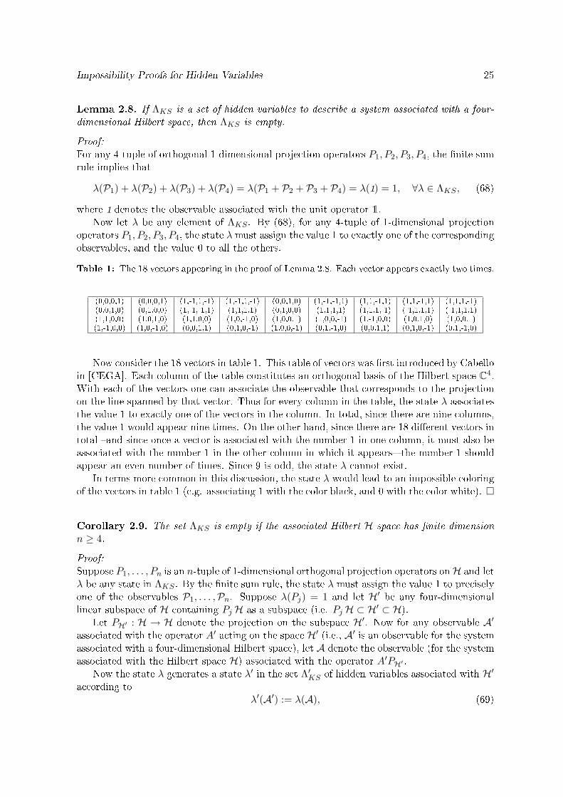
Impossibility Proofs for Hidden Variables 25
Lemma 2.8. If ΛKS is a set of hidden variables to describe a system associated with a four-
dimensional Hilbert space, then ΛKS is empty.
Proof:
For any 4-tuple of orthogonal 1-dimensional projection operators P1, P2, P3, P4, the nite sumrule implies that
λ(P1) + λ(P2) + λ(P3) + λ(P4) = λ(P1 + P2 + P3 + P4) = λ(1) = 1, ∀λ ∈ ΛKS , (68)
where 1 denotes the observable associated with the unit operator 1.Now let λ be any element of ΛKS . By (68), for any 4-tuple of 1-dimensional projection
operators P1, P2, P3, P4, the state λ must assign the value 1 to exactly one of the correspondingobservables, and the value 0 to all the others.
Table 1: The 18 vectors appearing in the proof of Lemma 2.8. Each vector appears exactly two times.
(0,0,0,1) (0,0,0,1) (1,-1,1,-1) (1,-1,1,-1) (0,0,1,0) (1,-1,-1,1) (1,1,-1,1) (1,1,-1,1) (1,1,1,-1)(0,0,1,0) (0,1,0,0) (1,-1,-1,1) (1,1,1,1) (0,1,0,0) (1,1,1,1) (1,1,1,-1) (-1,1,1,1) (-1,1,1,1)(1,1,0,0) (1,0,1,0) (1,1,0,0) (1,0,-1,0) (1,0,0,1) (1,0,0,-1) (1,-1,0,0) (1,0,1,0) (1,0,0,1)(1,-1,0,0) (1,0,-1,0) (0,0,1,1) (0,1,0,-1) (1,0,0,-1) (0,1,-1,0) (0,0,1,1) (0,1,0,-1) (0,1,-1,0)
Now consider the 18 vectors in table 1. This table of vectors was rst introduced by Cabelloin [CEGA]. Each column of the table constitutes an orthogonal basis of the Hilbert space C4.With each of the vectors one can associate the observable that corresponds to the projectionon the line spanned by that vector. Thus for every column in the table, the state λ associatesthe value 1 to exactly one of the vectors in the column. In total, since there are nine columns,the value 1 would appear nine times. On the other hand, since there are 18 dierent vectors intotal and since once a vector is associated with the number 1 in one column, it must also beassociated with the number 1 in the other column in which it appears the number 1 shouldappear an even number of times. Since 9 is odd, the state λ cannot exist.
In terms more common in this discussion, the state λ would lead to an impossible coloringof the vectors in table 1 (e.g. associating 1 with the color black, and 0 with the color white).
Corollary 2.9. The set ΛKS is empty if the associated Hilbert H space has nite dimension
n ≥ 4.
Proof:
Suppose P1, . . . , Pn is an n-tuple of 1-dimensional orthogonal projection operators onH and letλ be any state in ΛKS . By the nite sum rule, the state λ must assign the value 1 to preciselyone of the observables P1, . . . ,Pn. Suppose λ(Pj) = 1 and let H′ be any four-dimensionallinear subspace of H containing Pj H as a subspace (i.e. Pj H ⊂ H′ ⊂ H).
Let PH′ : H → H denote the projection on the subspace H′. Now for any observable A′associated with the operator A′ acting on the space H′ (i.e., A′ is an observable for the systemassociated with a four-dimensional Hilbert space), let A denote the observable (for the systemassociated with the Hilbert space H) associated with the operator A′PH′ .
Now the state λ generates a state λ′ in the set Λ′KS of hidden variables associated with H′according to
λ′(A′) := λ(A), (69)
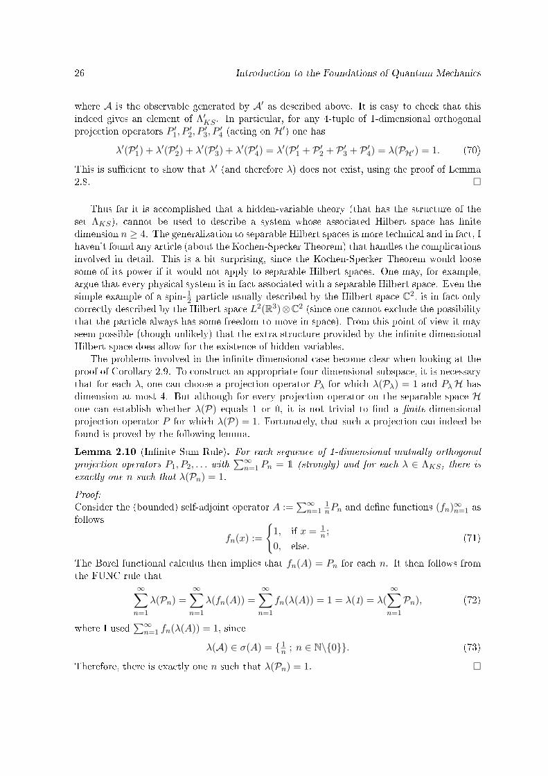
26 Introduction to the Foundations of Quantum Mechanics
where A is the observable generated by A′ as described above. It is easy to check that thisindeed gives an element of Λ′KS . In particular, for any 4-tuple of 1-dimensional orthogonalprojection operators P ′1, P
′2, P
′3, P
′4 (acting on H′) one has
λ′(P ′1) + λ′(P ′2) + λ′(P ′3) + λ′(P ′4) = λ′(P ′1 + P ′2 + P ′3 + P ′4) = λ(PH′) = 1. (70)
This is sucient to show that λ′ (and therefore λ) does not exist, using the proof of Lemma2.8.
Thus far it is accomplished that a hidden-variable theory (that has the structure of theset ΛKS), cannot be used to describe a system whose associated Hilbert space has nitedimension n ≥ 4. The generalization to separable Hilbert spaces is more technical and in fact, Ihaven't found any article (about the Kochen-Specker Theorem) that handles the complicationsinvolved in detail. This is a bit surprising, since the Kochen-Specker Theorem would loosesome of its power if it would not apply to separable Hilbert spaces. One may, for example,argue that every physical system is in fact associated with a separable Hilbert space. Even thesimple example of a spin-1
2 particle usually described by the Hilbert space C2, is in fact onlycorrectly described by the Hilbert space L2(R3)⊗C2 (since one cannot exclude the possibilitythat the particle always has some freedom to move in space). From this point of view it mayseem possible (though unlikely) that the extra structure provided by the innite-dimensionalHilbert space does allow for the existence of hidden variables.
The problems involved in the innite-dimensional case become clear when looking at theproof of Corollary 2.9. To construct an appropriate four-dimensional subspace, it is necessarythat for each λ, one can choose a projection operator Pλ for which λ(Pλ) = 1 and PλH hasdimension at most 4. But although for every projection operator on the separable space Hone can establish whether λ(P) equals 1 or 0, it is not trivial to nd a nite-dimensionalprojection operator P for which λ(P) = 1. Fortunately, that such a projection can indeed befound is proved by the following lemma.
Lemma 2.10 (Innite Sum Rule). For each sequence of 1-dimensional mutually orthogonal
projection operators P1, P2, . . . with∑∞
n=1 Pn = 1 (strongly) and for each λ ∈ ΛKS, there is
exactly one n such that λ(Pn) = 1.
Proof:
Consider the (bounded) self-adjoint operator A :=∑∞
n=11nPn and dene functions (fn)∞n=1 as
follows
fn(x) :=
1, if x = 1
n ;0, else.
(71)
The Borel functional calculus then implies that fn(A) = Pn for each n. It then follows fromthe FUNC rule that
∞∑n=1
λ(Pn) =∞∑n=1
λ(fn(A)) =∞∑n=1
fn(λ(A)) = 1 = λ(1) = λ(∞∑n=1
Pn), (72)
where I used∑∞
n=1 fn(λ(A)) = 1, since
λ(A) ∈ σ(A) = 1n ; n ∈ N\0. (73)
Therefore, there is exactly one n such that λ(Pn) = 1.
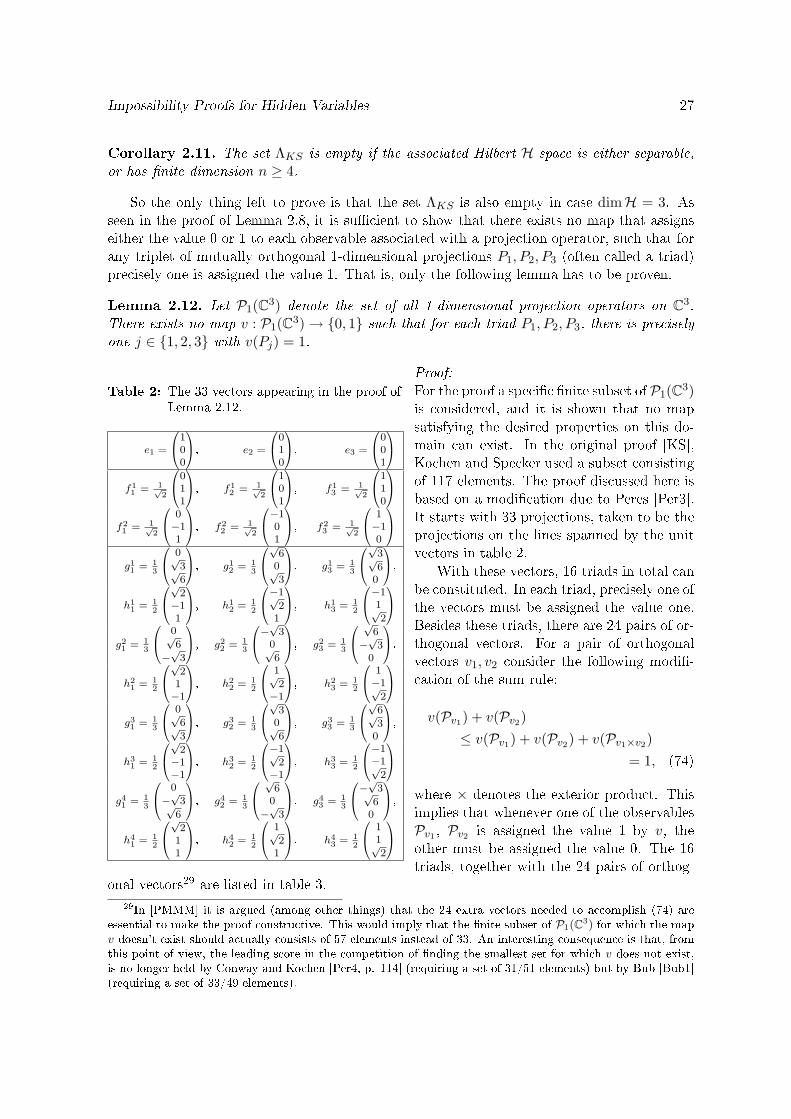
Impossibility Proofs for Hidden Variables 27
Corollary 2.11. The set ΛKS is empty if the associated Hilbert H space is either separable,
or has nite dimension n ≥ 4.
So the only thing left to prove is that the set ΛKS is also empty in case dimH = 3. Asseen in the proof of Lemma 2.8, it is sucient to show that there exists no map that assignseither the value 0 or 1 to each observable associated with a projection operator, such that forany triplet of mutually orthogonal 1-dimensional projections P1, P2, P3 (often called a triad)precisely one is assigned the value 1. That is, only the following lemma has to be proven.
Lemma 2.12. Let P1(C3) denote the set of all 1-dimensional projection operators on C3.
There exists no map v : P1(C3)→ 0, 1 such that for each triad P1, P2, P3, there is precisely
one j ∈ 1, 2, 3 with v(Pj) = 1.
Table 2: The 33 vectors appearing in the proof ofLemma 2.12.
e1 =
100
, e2 =
010
, e3 =
001
f11 = 1√
2
011
, f12 = 1√
2
101
, f13 = 1√
2
110
f21 = 1√
2
0−11
, f22 = 1√
2
−101
, f23 = 1√
2
1−10
g11 = 1
3
0√3√6
, g12 = 1
3
√60√3
, g13 = 1
3
√3√6
0
,
h11 = 1
2
√2−11
, h12 = 1
2
−1√2
1
, h13 = 1
2
−11√2
g21 = 1
3
0√6
−√
3
, g22 = 1
3
−√30√6
, g23 = 1
3
√6
−√
30
,
h21 = 1
2
√21−1
, h22 = 1
2
1√2−1
, h23 = 1
2
1−1√
2
g31 = 1
3
0√6√3
, g32 = 1
3
√30√6
, g33 = 1
3
√6√3
0
,
h31 = 1
2
√2−1−1
, h32 = 1
2
−1√2−1
, h33 = 1
2
−1−1√
2
g41 = 1
3
0
−√
3√6
, g42 = 1
3
√60
−√
3
, g43 = 1
3
−√3√6
0
,
h41 = 1
2
√211
, h42 = 1
2
1√2
1
, h43 = 1
2
11√2
Proof:
For the proof a specic nite subset of P1(C3)is considered, and it is shown that no mapsatisfying the desired properties on this do-main can exist. In the original proof [KS],Kochen and Specker used a subset consistingof 117 elements. The proof discussed here isbased on a modication due to Peres [Per3].It starts with 33 projections, taken to be theprojections on the lines spanned by the unitvectors in table 2.
With these vectors, 16 triads in total canbe constituted. In each triad, precisely one ofthe vectors must be assigned the value one.Besides these triads, there are 24 pairs of or-thogonal vectors. For a pair of orthogonalvectors v1, v2 consider the following modi-cation of the sum rule:
v(Pv1) + v(Pv2)≤ v(Pv1) + v(Pv2) + v(Pv1×v2)
= 1, (74)
where × denotes the exterior product. Thisimplies that whenever one of the observablesPv1 , Pv2 is assigned the value 1 by v, theother must be assigned the value 0. The 16triads, together with the 24 pairs of orthog-
onal vectors29 are listed in table 3.29In [PMMM] it is argued (among other things) that the 24 extra vectors needed to accomplish (74) are
essential to make the proof constructive. This would imply that the nite subset of P1(C3) for which the mapv doesn't exist should actually consists of 57 elements instead of 33. An interesting consequence is that, fromthis point of view, the leading score in the competition of nding the smallest set for which v does not exist,is no longer held by Conway and Kochen [Per4, p. 114] (requiring a set of 31/51 elements) but by Bub [Bub1](requiring a set of 33/49 elements).
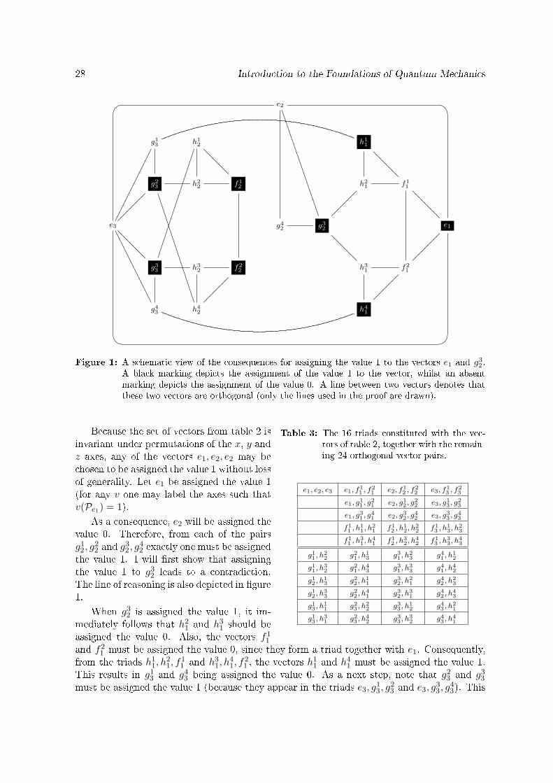
28 Introduction to the Foundations of Quantum Mechanics
e2
************************* EDGF
g13 h1
2
????????h1
1
????????
g23
*************************h2
2 f12 h2
1 f11
?????????
e3
@A BC
?????????
////////////////// g42 g3
2
????????e1
g33
h3
2 f22 h3
1 f21
g43 h4
2
h4
1
Figure 1: A schematic view of the consequences for assigning the value 1 to the vectors e1 and g32 .
A black marking depicts the assignment of the value 1 to the vector, whilst an absentmarking depicts the assignment of the value 0. A line between two vectors denotes thatthese two vectors are orthogonal (only the lines used in the proof are drawn).
Table 3: The 16 triads constituted with the vec-tors of table 2, together with the remain-ing 24 orthogonal vector pairs.
e1, e2, e3 e1, f11 , f
21 e2, f1
2 , f22 e3, f1
3 , f23
e1, g11 , g
21 e2, g1
2 , g22 e3, g1
3 , g23
e1, g31 , g
41 e2, g3
2 , g42 e3, g3
3 , g43
f11 , h
11, h
21 f1
2 , h12, h
22 f1
3 , h13, h
23
f11 , h
31, h
41 f1
2 , h32, h
42 f1
3 , h33, h
43
g11 , h
22 g2
1 , h13 g3
1 , h23 g4
1 , h12
g11 , h
32 g2
1 , h43 g3
1 , h33 g4
1 , h42
g12 , h
13 g2
2 , h11 g3
2 , h21 g4
2 , h23
g12 , h
33 g2
2 , h41 g3
2 , h31 g4
2 , h43
g13 , h
11 g2
3 , h22 g3
3 , h12 g4
3 , h21
g13 , h
31 g2
3 , h42 g3
3 , h32 g4
3 , h41
Because the set of vectors from table 2 isinvariant under permutations of the x, y andz axes, any of the vectors e1, e2, e2 may bechosen to be assigned the value 1 without lossof generality. Let e1 be assigned the value 1(for any v one may label the axes such thatv(Pe1) = 1).
As a consequence, e2 will be assigned thevalue 0. Therefore, from each of the pairsg1
2, g22 and g
32, g
42 exactly one must be assigned
the value 1. I will rst show that assigningthe value 1 to g3
2 leads to a contradiction.The line of reasoning is also depicted in gure1.
When g32 is assigned the value 1, it im-
mediately follows that h21 and h3
1 should beassigned the value 0. Also, the vectors f1
1
and f21 must be assigned the value 0, since they form a triad together with e1. Consequently,
from the triads h11, h
21, f
11 and h3
1, h41, f
21 , the vectors h
11 and h4
1 must be assigned the value 1.This results in g1
3 and g43 being assigned the value 0. As a next step, note that g2
3 and g33
must be assigned the value 1 (because they appear in the triads e3, g13, g
23 and e3, g
33, g
43). This
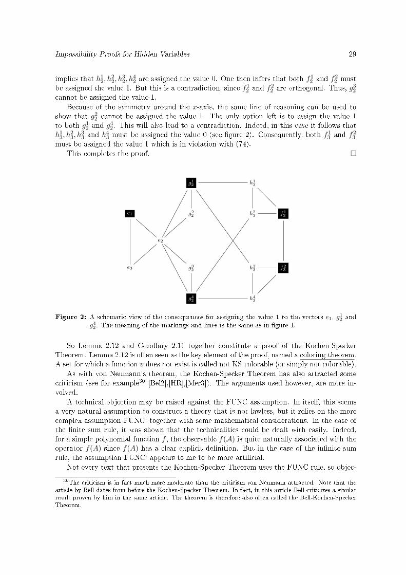
Impossibility Proofs for Hidden Variables 29
implies that h12, h
22, h
32, h
42 are assigned the value 0. One then infers that both f1
2 and f22 must
be assigned the value 1. But this is a contradiction, since f12 and f2
2 are orthogonal. Thus, g32
cannot be assigned the value 1.Because of the symmetry around the x-axis, the same line of reasoning can be used to
show that g22 cannot be assigned the value 1. The only option left is to assign the value 1
to both g12 and g4
2. This will also lead to a contradiction. Indeed, in this case it follows thath1
3, h23, h
33 and h4
3 must be assigned the value 0 (see gure 2). Consequently, both f13 and f2
3
must be assigned the value 1 which is in violation with (74).This completes the proof.
g12
666666666666666666666666666h1
3
????????
e1
CCCCCCCCg22 h2
3 f13
e2
CCCCCCCCC
0000000000000000
e3
g32 h3
3 f23
g42
h4
3
Figure 2: A schematic view of the consequences for assigning the value 1 to the vectors e1, g12 and
g42 . The meaning of the markings and lines is the same as in gure 1.
So Lemma 2.12 and Corollary 2.11 together constitute a proof of the Kochen-SpeckerTheorem. Lemma 2.12 is often seen as the key element of the proof, named a coloring theorem.A set for which a function v does not exist is called not KS-colorable (or simply not colorable).
As with von Neumann's theorem, the Kochen-Specker Theorem has also attracted somecriticism (see for example30 [Bel2],[HR],[Mer3]). The arguments used however, are more in-volved.
A technical objection may be raised against the FUNC assumption. In itself, this seemsa very natural assumption to construct a theory that is not lawless, but it relies on the morecomplex assumption FUNC' together with some mathematical considerations. In the case ofthe nite sum rule, it was shown that the technicalities could be dealt with easily. Indeed,for a simple polynomial function f , the observable f(A) is quite naturally associated with theoperator f(A) since f(A) has a clear explicit denition. But in the case of the innite sumrule, the assumption FUNC' appears to me to be more articial.
Not every text that presents the Kochen-Specker Theorem uses the FUNC rule, so objec-
30The criticism is in fact much more moderate than the criticism von Neumann attracted. Note that thearticle by Bell dates from before the Kochen-Specker Theorem. In fact, in this article Bell criticizes a similarresult proven by him in the same article. The theorem is therefore also often called the Bell-Kochen-SpeckerTheorem.

30 Introduction to the Foundations of Quantum Mechanics
tions related to precisely this rule aren't very strong. For example, in [CEGA] one simplystarts with the assumption of the innite sum rule. I will now present a possible (though notvery strong) direct motivation for this rule.31
Consider an observable A corresponding to the operator A. A measurement of A can beinterpreted as asking the system the question: What is the value of A? This formulationis a bit sloppy, since the discussion is exactly about whether or not a value can be assignedto the system at all times. One may, instead, read this question as What is the value of Aafter the measurement?, at least, in case one accepts that the value of A has a meaning ifthe system is in an eigenstate of the operator A. Otherwise, one may read this question asWhat will be the value yielded when I perform a measurement of A? or, if one rejects thepossibility of innite precise measurements: What subset of σ(A) will emerge when I performa measurement that I associate with the measurement of A? Whatever question the readermay prefer, let's agree to abbreviate it with What is the value of A?
Conversely, it seems reasonable that similar, physical meaningful, questions could be as-sociated with operators. Suppose ∆ ⊂ σ(A). One may ask the question Does the value ofA lie in ∆? In fact, one can associate an operator with this question, namely the projectionoperator µA(∆) from Theorem 2.1. Now let (∆i)i∈I be any partition of σ(A). A measurementof A may then be interpreted as simultaneously asking all the yes-no questions32 Does thevalue of A lie in ∆i? for i ∈ I. Since a measurement will yield only one result, preciselyone of the questions must be answered yes, and all the others must be answered no. Thismotivates the (innite) sum rule.
A possible objection against this line of reasoning is that it is in general not clear whetheror not a sequence of mutually orthogonal projection operators (Pi)i∈I can be associated witha single observable such that Pi = µA(∆i) for all i for some partition (∆i)i∈I of σ(A). Thisexposes a second problem: Why should the self-adjoint operators mentioned in the proofindeed correspond to observables33?
A short investigation of this problem will reveal yet another objection when consideringthe proof of Lemma 2.8. In this setting, for each column of table 1 one would have to nd anobservable Ai and a partition (∆k
i )4k=1 of σ(Ai) , i = 1, . . . , 9 (since there are nine columns)
such that each vector in the ith column is associated with the observable corresponding toµAi(∆
ki ) for some k. However, from this point of view, it is not at all clear why, whenever
µAi(∆ki ) = µAj (∆
lj) = P (i 6= j), they should both be associated with the same observable
P and why they should be assigned the same value. One may argue that the observableassociated with µAi(∆
ki ) is in fact not the same as the one associated with µAj (∆
lj), especially
since the observables Ai and Aj cannot be measured at the same time. This leads to thefollowing denition.
Denition 2.3. A theory is called contextual if the value of an observable may depend onthe measuring context. That is, it may depend on what other observables are being measured.
In the terms of the observables Ai,Aj and P, contextuality states that the value of P maydepend upon whether it is measured simultaneously with Ai or with Aj . This seems a natural
31A more extensive investigation of possible starting assumptions and how they are related can be found in[FT].
32See also Remark 2.1.33In the von Neumann proof, it was simply postulated (though implicitly) that the converse of the observable
postulate should hold. One may, of course, postulate the same for the Kochen-Specker Theorem, but that seemsunreasonable to me (see earlier considerations when introducing the observable postulate on page 5).
Impossibility Proofs for Hidden Variables 31
assumption if P is considered to be the observable corresponding to µAi(∆ki ) in one measuring
context, whilst corresponding to µAj (∆lj) in the other. But what if P has a meaning all of
its own, independently of the observables Ai and Aj? In that case, contextuality becomesa stronger assumption. It then states that the value of P may depend on the way we (asexperimenters look) at it.
It turns out that if one wishes to use the contextuality argument to criticize the Kochen-Specker Theorem, one necessarily has to adopt this stronger form. This is because the opera-tors that play a role in the proof of Lemma 2.12 can each be associated with a single observablethat has a clear physical meaning independently of its measuring context. Indeed, every vectorcan be associated with the squared spin of a spin-1 particle along that axis. The operatorsassociated with these observables commute if and only if the associated axes are orthogonal.Thus ever triad can be associated with a set of three observables that can be measured atthe same time. It is predicted by quantum mechanics that such triplet measurements alwaysyield twice the value 1, and once the value 0. The proof of Lemma 2.12 thus also shows thata (non-contextual) denite value assignment to these observables is impossible.
Bell [Bel2] argued that the value assigned to any observable may well depend on whichother observables are to be measured. This is because dierent sets of observables must bemeasured using dierent measuring devices. This is, in fact, in line with (and partly inspiredby) the philosophy of Bohr, who thought that observables have no real meaning at all withoutspecifying the measuring context. But, for me, the idea that this may be so, i.e. that the valueof an observable depends on the way we measure it, is a substantial compromise to what isto be expected from a hidden-variable theory. It parts from the idea that observables shouldhave a denite value independent of the observer. Quite a step for someone who was `against`measurement [Bel5].
2.3.4 The Bell Inequality
Instead of studying the possibility of hidden-variable theories in a broad sense34, the argumentof Bell focuses on one specic physical system: that of a pair of spin-1
2 particles. The originalrst paper [Bel1] does in fact not account for contextual theories (i.e., it assumes denite valuesfor observables independent of the measuring context). The argument was improved in [Bel3],where Bell incorporated the possibility that the actual value obtained when measuring anobservable may also depend on the setting of the measurement device. Later, Bell's argumenthas also been extended to incorporate stochastic hidden-variable theories (i.e. theories inwhich measurement results are not necessarily pre-determined, but do obey certain otherrequirements). To make the argument for stochastic theories more comprehensible, I willrst discuss a Bell-type argument for deterministic theories. A more extensive account of thevariety of Bell arguments can be found in [CS] and [See3].
Deterministic Hidden Variables
I will present the argument here in a way that is slightly dierent from what is common in mostliterature. The dierences will become more apparent along the way. The main dierence isthat I start from the hidden state of the system λ that is supposed to determine all outcomes
34The proof by von Neumann focuses on ensembles for arbitrary physical systems and also the Kochen-Specker Theorem is a statement about all physical statements that are described by a Hilbert space of dimensiongreater than 2.
32 Introduction to the Foundations of Quantum Mechanics
of all possible experiments for all possible contexts, whereas one usually argues from the valueof a specic observable as a function of several hidden variables, which may then be `local' or`non-local'.
The system under consideration is again that of the two spin-12 particles of Example 2.2.
The question will be whether or not a hidden-variable theory can reproduce the statistics thatquantum mechanics dictates if the system is prepared in the state
ψ =1√2
(0, 1,−1, 0). (75)
First, an examination of the structure of a contextual hidden-variable theory is necessary.Since it is now allowed that values of observables may depend on measuring contexts, oneshould reconsider the notion of a state in a hidden-variable theory. Now a state λ shouldassign a value in σ(A) to each observable A, for each measuring context C in which it ispossible to measure A. To give a precise meaning to this requirement, the following denitionis helpful.
Denition 2.4. A measuring context C is a set Ai ; i ∈ I of observables for which allcorresponding self-adjoint operators Ai ; i ∈ I commute.
By an appeal to the FUNC' rule, each measuring context Ai ; i ∈ I might be representedby the commutative W*-algebra35 of operators generated by the set Ai ; i ∈ I. Indeed, thisconstruction exactly adds all the observables A to the measuring context for which there existsan i ∈ I and a Borel function f such that A = f(Ai) for some i. However, since no specialstructure (like that of a W*-algebra) is required to make the argument of this paragraphwork, it seems redundant to demand it. In fact, the FUNC' rule may better be avoided (inorder not to make unnecessary assumptions) and an observable of the form f(A) may onlybe interpreted as applying the function f to the measurement result of A (that is, it is notrequired that it is associated with a self-adjoint operator).
Denition 2.5. A contextual pure state λ is a rule that to each measuring context C assignsa function λC : C → R such that λC(A) ∈ σ(A) for all A ∈ C.
It turns out that the set of all contextual pure states is large enough to avoid a conict withquantum mechanics. In fact, contextual hidden-variable theories do exist, Bohmian mechanicsprobably being the most popular one ([Boh1], see [Tum1] for a friendly introduction). Themain objection against Bohmian mechanics is that it is non-local i.e., it allows action at adistance. This is what inspired Bell to write his article [Bel1]; he wanted to investigate whetherthis non-local behavior is a necessary property of any hidden-variable theory. It turns out thatit is, at least if one adopts the following denition of locality.36
Denition 2.6. A contextual pure state is called local if for any pair of observables A1,A2
corresponding to commuting operators A1, A2 that can be measured using measuring devices
35AW*-algebra (or von Neumann algebra) is a set of bounded operators that is closed under taking adjointsand that is equal to its double commutant, where the commutant of a set of bounded operators V is the set ofall bounded operators that commute with every element of V . There are also more abstract denitions thatdo not require the notion of an operator on a Hilbert space (see for example [Dav].
36One may easily check that also the catalog theory of Section 2.3.2 must indeed be non-local if it is modiedto be empirically equivalent with quantum mechanics.
Impossibility Proofs for Hidden Variables 33
that may be separated at an arbitrary distance from each other, and for every measuringcontext C containing A1 and A2, one has
λC(A1) = λC\A2(A1) and λC(A2) = λC\A1(A2). (76)
Such a pair of observables will be called separable. The set of all local contextual pure statesis called ΛBell.
One may think of separable observables as observables of separated systems that are nowcombined into one system. That is, the system is described by a Hilbert space of the formH1⊗H2. Two observables may then be called separable if their corresponding operatorsare of the form A1 ⊗ 1 and 1⊗A2. Thus A1 is an observable of the separate subsystemdescribed by the space H1 and A2 is an observable of the subsystem described by the spaceH2. Consequently, a local pure state must assign a value to the observable A1 in the contextC independently of any observable in C associated with a spatially separated subsystem. Inother words, equation (76) may be itterated an arbitrary number of times until the context Cno longer contains any observables associated with a spatially separated subsystem.
The theorem due to Bell may now be formulated as follows.
Theorem 2.13. There is no local, contextual hidden-variable theory (and consequently no
non-contextual one) that can reproduce the statistics of the system of two spin-12 particles
prepared in the state ψ = 1√2(0, 1,−1, 0) (that are space-like separated). Therefore, any such
theory is empirically in disagreement with quantum mechanics.
Due to the extra structure acquired (compared to Λcat or ΛKS) by introducing contex-tuality, an examination of how the statistics of quantum mechanics are to be reproduced isrequired before the theorem can be proven. This is done in the same way as in classicalstatistical physics (as was also roughly sketched in the beginning of paragraph 2.3).
A macro state in the hidden-variable theory is a probability distribution µ over the setΛBell.37 One usually thinks of the system as an ensemble of systems, or one can think of asystem whose pure state uctuates rapidly in time.38 To talk sensibly about a probabilitymeasure on the set ΛBell, a σ-algebra ΣBell of subsets of ΛBell is required.
This σ-algebra is constructed as follows. For each observable A corresponding to someoperator A, for each measuring context C such that A ∈ C and for each Borel set ∆ ⊂ σ(A),consider the event that the measurement of A yields a result in ∆ in the context C. This eventis identied with the set
[AC ∈ ∆] := λ ∈ ΛBell ; λC(A) ∈ ∆. (77)
For xed C, let ΣC be the σ-algebra generated by all such sets. Then take ΣBell to be theσ-algebra generated by all these σ-algebras. For a xed measuring context C, the followingequivalence relation on ΛBell is introduced:
λ ∼C λ′ <==> λC(A) = λ′C(A),∀A ∈ C. (78)
37The term `macro state' is taken from statistical physics where it is also used to describe probabilitydistributions over pure states (also called micro states). The term may seem a bit awkward, since it describeswhat may be called a micro state in quantum mechanics. However, it is precisely this viewpoint (i.e., that thequantum states are micro states) that is criticized by Einstein, Podolsky and Rosen.
38The philosophy of the interpretation of statistical mechanics is a topic of its own [Skl].

34 Introduction to the Foundations of Quantum Mechanics
This denes a set of equivalence classes
ΛC := ΛBell/ ∼C , [λ]C := λ′ ∈ ΛBell ; λ′ ∼C λ. (79)
For any S ∈ ΣC , it follows that if λ ∈ S, then [λ]C ⊂ S. Therefore, the σ-algebra ΣC extendsin a natural way to a σ-algebra on ΛC by taking
[λ]C ; λ ∈ S ; S ∈ ΣC. (80)
For notational convenience, both σ-algebras will be denoted by the same symbol. Also, nodistinction in notation will be made for their elements. Any macro state µ now extends to aprobability measure PC on (ΛC ,ΣC) for any measuring context C by taking
PC(S) := µ(S) =∫
ΛBell
1S(λ) dµ(λ), ∀S ∈ ΣC . (81)
These restricted probability spaces (ΛC ,ΣC ,PC) have the advantage that any observable A ∈ Ccan be viewed as a stochastic variable on ΛC by taking
A([λ]C) := λC(A), λ ∈ [λ]C , (82)
which is well dened (i.e. independent of the choice of λ).Here one nds a relation between the usual way in which the argument is presented with
A as a function of the hidden parameters on the left-hand side, and the way I present theargument on the right-hand side. From this equation, the dierence between the two ap-proaches can also be explained. In the more common discussions, A is seen as a function ofthe state of the system and the measurement context separately. One would write somethinglike A(λ,mC) where λ is a hidden parameter associated with the preparation of the systemand mC is a hidden parameter associated with the preparation of the measurement device.Both elements are here incorporated in the use of the state λ, which may of course depend onmuch more than only the system preparation and measurement preparation.
Now consider two separable observables A1,A2. Because of the locality assumption (76),it follows that
A1([λ]A1,A2) = λA1,A2(A1) = λA1(A1) = A1([λ]A1);
A2([λ]A1,A2) = λA1,A2(A2) = λA2(A2) = A2([λ]A2).(83)
Now return to the example of the two spin-12 particles. Let σr1 be the spin of the rst
particle along the r1-axis (one should actually write σr1 ⊗ 1) and σr2 the spin of the secondparticle along the r2-axis. Clearly, these are separable observables. Viewing them as stochasticvariables in the measuring context σr1 , σr2, the expectation value of their product39 for axed macro state µ is given by
Eσr1 ,σr2(σr1σr2) =∫
ΛBell
σr1([λ]σr1 ,σr2)σr2([λ]σr1 ,σr2) dµ(λ)
=∫
ΛBell
λσr1(σr1)λσr2(σr2) dµ(λ).(84)
This equation is the key to the proof of the following lemma.
39Sometimes this is called a correlation, but I will refrain from using that term so as to avoid confusionwith the mathematical term.

Impossibility Proofs for Hidden Variables 35
Lemma 2.14. Let σr1 and σr′1 denote the spin along the r1 and r′1 axes of the rst particle
and let σr2 and σr′2 denote the spin along the r2 and r′2 axes of the second particle. Then
any macro state µ of the local, contextual hidden-variable theory satises the following Bell
inequality:∣∣∣Eσr1 ,σr2(σr1σr2)− Eσr1 ,σr′2(σr1σr′2)
∣∣∣+∣∣∣Eσr′1 ,σr2(σr′1σr2) + Eσr′1 ,σr′2
(σr′1σr′2)∣∣∣ ≤ 2. (85)
Proof:
The rst term in the inequality can be estimated in the following way:∣∣∣Eσr1 ,σr2(σr1σr2)− Eσr1 ,σr′2(σr1σr′2)
∣∣∣ = · · ·
· · · =∣∣∣∣∫
ΛBell
λσr1(σr1)(λσr2(σr2)− λσr′2
(σr′2))
dµ(λ)∣∣∣∣
≤∫
ΛBell
∣∣∣λσr1(σr1)∣∣∣ ∣∣∣λσr2(σr2)− λσr′2
(σr′2)∣∣∣dµ(λ)
=∫
ΛBell
∣∣∣λσr2(σr2)− λσr′2(σr′2)
∣∣∣ dµ(λ).
(86)
Similarly,∣∣∣Eσr′1 ,σr2(σr′1σr2) + Eσr′1 ,σr′2(σr′1σr′2)
∣∣∣ = · · ·
· · · =∣∣∣∣∫
ΛBell
λσr′1(σr′1)
(λσr2(σr2) + λσr′2
(σr′2))
dµ(λ)∣∣∣∣
≤∫
ΛBell
∣∣∣λσr′1(σr′1)∣∣∣ ∣∣∣λσr2(σr2) + λσr′2
(σr′2)∣∣∣dµ(λ)
=∫
ΛBell
∣∣∣λσr2(σr2) + λσr′2(σr′2)
∣∣∣ dµ(λ).
(87)
Next, note that ΛBell can be split to four disjoint pieces
Λ++ = λ ∈ ΛBell ; λσr2(σr2) = λσr′2(σr′2) = 1;
Λ+− = λ ∈ ΛBell ; λσr2(σr2) = −λσr′2(σr′2) = 1;
Λ−+ = λ ∈ ΛBell ; λσr2(σr2) = −λσr′2(σr′2) = −1;
Λ−− = λ ∈ ΛBell ; λσr2(σr2) = λσr′2(σr′2) = −1,
(88)
so that ΛBell = Λ++ ∪ Λ+− ∪ Λ−+ ∪ Λ−−. One easily checks that on each of these pieces onehas ∣∣∣λσr2(σr2)− λσr′2
(σr′2)∣∣∣+∣∣∣λσr2(σr2) + λσr′2
(σr′2)∣∣∣ = 2. (89)
This leads to the estimate∣∣∣Eσr1 ,σr2(σr1σr2)− Eσr1 ,σr′2(σr1σr′2)
∣∣∣+∣∣∣Eσr′1 ,σr2(σr′1σr2) + Eσr′1 ,σr′2
(σr′1σr′2)∣∣∣
≤∫
ΛBell
2 dµ(λ) = 2, (90)
36 Introduction to the Foundations of Quantum Mechanics
which proves the lemma.
With the use of this lemma, Theorem 2.13 can now be proven.Proof of Theorem 2.13:
All that has to be shown, is that the inequality (85), can be violated in quantum mechanics.Using the notation of Example 2.2, setting e1 = (1, 0) and e2 = (0, 1) and taking ψ as in (75),the quantum-mechanical equivalent of (84) can be calculated:
Eψ(σr1σr2) =〈ψ, σr1 ⊗ σr2ψ〉
=12〈e1 ⊗ e2 − e2 ⊗ e1, σr1 ⊗ σr2 (e1 ⊗ e2 − e2 ⊗ e1)〉
=12〈e1 ⊗ e2, σr1 ⊗ σr2e1 ⊗ e2〉 −
12〈e1 ⊗ e2, σr1 ⊗ σr2e2 ⊗ e1〉
+12〈e2 ⊗ e1, σr1 ⊗ σr2e2 ⊗ e1〉 −
12〈e2 ⊗ e1, σr1 ⊗ σr2e1 ⊗ e2〉 .
(91)
Writing out these inner products and using some trigonometry leads to the following relation:
Eψ(σr1σr2) =− 12
cos(ϕ1) cos(ϕ2)
− 12
(cos(ϑ1) sin(ϕ1)− i sin(ϑ1) sin(ϕ1))(cos(ϑ2) sin(ϕ2) + i sin(ϑ2) sin(ϕ2))
− 12
cos(ϕ1) cos(ϕ2)
− 12
(cos(ϑ1) sin(ϕ1) + i sin(ϑ1) sin(ϕ1))(cos(ϑ2) sin(ϕ2)− i sin(ϑ2) sin(ϕ2))
=− cos(ϕ1) cos(ϕ2)− (cos(ϑ1) cos(ϑ2) + sin(ϑ1) sin(ϑ2)) sin(ϕ1) sin(ϕ2)=− cos(ϕ1) cos(ϕ2)− cos(ϑ1 − ϑ2) sin(ϕ1) sin(ϕ2).
(92)
To simplify, take ϕ1 = ϕ2 = π/2, so that Eψ(σr1σr2) = − cos(ϑ1 − ϑ2). With this expression,(85) becomes ∣∣cos(ϑ1 − ϑ2)− cos(ϑ1 − ϑ′2)
∣∣+∣∣cos(ϑ′1 − ϑ2) + cos(ϑ′1 − ϑ′2)
∣∣ ≤ 2. (93)
It is not hard to see that this inequality can be violated. For example, if one takes
ϑ1 = 0, ϑ′1 = π2 , ϑ2 = 7
4π, ϑ′2 = 5
4π, (94)
this inequality would result in
2√
2 = 412
√2 =
∣∣cos(ϑ1 − ϑ2)− cos(ϑ1 − ϑ′2)∣∣+∣∣cos(ϑ′1 − ϑ2) + cos(ϑ′1 − ϑ′2)
∣∣ ≤ 2, (95)
which is a contradiction. This completes the proof.
Stochastic Hidden Variables
The starting point for a stochastic hidden-variable theory is again a set Λ of pure states thatmay be contextual in nature. However, instead of assigning a value to each observable, a
Impossibility Proofs for Hidden Variables 37
pure state λ assigns to each observable A a probability measure on the space (σ(A),ΣA) foreach measuring context C with A ∈ C, where ΣA is the σ-algebra of Borel-sets in σ(A). Thismeasure will be denoted by
∆ 7→ PC [A ∈ ∆|λ]. (96)
It is further assumed that there is a way to conditionalize. That is, if the measurementof the observable A1 yields some subset ∆1 ∈ ΣA1 as a measurement result, the pure state ofthe system may be altered going from λ to λ′. Instead of introducing some notation for thealtered state, I introduce the following notation to denote that the state may be altered by aprevious measurement:
PC [A2 ∈ ∆2| A1 ∈ ∆1, λ] := PC [A2 ∈ ∆2|λ′], (97)
for any A2 ∈ C, ∆2 ∈ ΣA2 .The reader may notice an ambiguity in this notation. If the state λ changes into the state
λ′, all probability distributions may be altered. That is, (97) is supposed to hold for arbitraryobservables A2 in arbitrary contexts C that do not necessarily contain A1. It then seemsnatural to assume that the new state may depend on the context in which the result A1 ∈ ∆1
was obtained. To incorporate this possibility, the notation should in fact look something like
PC [A2 ∈ ∆2| A1 ∈C1 ∆1, λ], (98)
where A1 ∈C1 ∆1 denotes that the result A1 ∈ ∆1 was obtained in the measuring context C1.However, in waht follows it will be the case that, once a context is chosen, it remains xed forall subsequent measurements and one may think of PC [A2 ∈ ∆2| A1 ∈ ∆1, λ] as shorthand forPC [A2 ∈ ∆2| A1 ∈C ∆1, λ]. It may also be noted that this way of conditionalizing is dierentfrom the one in standard probability theory. For example, in general it is not to be expectedthat, whenever A1,A2 ∈ C, the equality
PC [A2 ∈ ∆2| A1 ∈ ∆1, λ]PC [A1 ∈ ∆1|λ] = PC [A1 ∈ ∆1| A2 ∈ ∆2, λ]PC [A2 ∈ ∆2|λ] (99)
will hold for all λ.A macro state of the system will again correspond to a probability distribution over the
pure states. At rst glance this may look like a distribution over distributions. However, thepure states are not probability distributions themselves but rather collections of distributions.Also, one is encouraged to think of the pure states as complete descriptions of the system(in the sense that they contain maximal information about the system), and to interpret themacro states as descriptions of the system based on incomplete information (hence as notexactly knowing what the pure state is). Strictly speaking, this denition only makes senseif the space Λ is endowed with a σ-algebra Σ of subsets. This is introduced in the followingway. For a xed context C, observable A ∈ C and Borel set ∆ ∈ ΣA there is a map Λ→ [0, 1]given by λ 7→ PC [A ∈ ∆|λ]. Σ is taken to be the smallest σ-algebra that makes all these mapsmeasurable.
A macro state µ can be used to assign probabilities to actual events by means of thestochastic variables λ 7→ PC [A ∈ ∆|λ] by taking
PC [A ∈ ∆|µ] :=∫
ΛPC [A ∈ ∆|λ] dµ(λ). (100)
This is to be read as the probability to nd a value in ∆ if one measures the observable A inthe context C, given that the state is µ. It is good to note that this is not the probability of

38 Introduction to the Foundations of Quantum Mechanics
an event, that is, it is not the measure of some subset of Λ, but rather the expectation valueof the variable λ 7→ PC [A ∈ ∆|λ]. This does indeed seem the only natural way to make senseof probabilities of experimental events in this abstract mathematical context in such a waythat
PC [A ∈ ∆|δλ] :=∫
ΛPC [A ∈ ∆|λ′] d δλ(λ′) = PC [A ∈ ∆|λ], (101)
where δλ is the macro state given by
δλ(S) =
1, λ ∈ S;0, λ /∈ S,
∀S ∈ Σ. (102)
In the same way, conditionalized probabilities may be introduced by taking
PC [A2 ∈ ∆2| A1 ∈ ∆1, µ] :=∫
ΛPC [A2 ∈ ∆2| A1 ∈ ∆1, λ] dµ(λ), (103)
and the expectation value of the observable A in the context C given the state µ is dened tobe
EC [A |µ] :=∫
ΛEC [A |λ] dµ(λ)
=∫
Λ
∫σ(A)
xPC [A ∈ dx|λ] dµ(λ).(104)
As was done for deterministic theories, a condition of locality is now introduced. For thedeterministic models it was implicitly assumed that measurements do not disturb the state ofthe system, whereas here disturbances are allowed. However, in order to proceed one needsto assume that such disturbances may only have a local eect. Consequently, to obtain aBell-inequality, two locality assumptions are made for the stochastic model.
Denition 2.7.
(i) A state µ is called outcome independent (OILOC) if for any pair of separable observablesA1,A2, corresponding to commuting operators A1, A2, for every measuring context Ccontaining A1 and A2, and for every pair of measurable sets ∆1 ⊂ σ(A1) and ∆2 ⊂σ(A2), one has
PC [A1 ∈ ∆1| A2 ∈ ∆2, µ] = PC [A1 ∈ ∆|µ]. (105)
(ii) A state µ is called context independent (CILOC) if for any pair of separable observablesA1,A2, corresponding to commuting operators A1, A2, for every measuring context Ccontaining A1 and A2, and for every measurable set ∆ ⊂ σ(A1), one has
PC [A1 ∈ ∆|µ] = PC\A2[A1 ∈ ∆|µ]. (106)
These two locality criteria are due to Jarrett [Jar] (similar criteria are also discussed in[vF2]). The rst condition states that the measurement result is not allowed to depend onthe result of a (simultaneous) measurement made far away. That is, measurement results maynot inuence future measurement results instantaneously. The second condition expresses theidea that the measurement result of an observable may not depend on the experimental setup

Impossibility Proofs for Hidden Variables 39
used far away. Note that for OILOC states and separable observables, relation (99) holds. Forsuch observables one can thus sensibly talk about a joint probability distribution by taking
PC [(A1 ∈ ∆1) ∧ (A2 ∈ ∆2)|λ] := PC [A2 ∈ ∆2| A1 ∈ ∆1, λ]PC [A1 ∈ ∆1|λ]. (107)
To nally obtain a Bell-type inequality, a third implicit assumption is made, namely, thatthe state µ of the system does not depend on the measuring context C. The idea is that thestate may have been prepared long before the choice of the measuring context was made. Thisis not so much an assumption of locality, but an assumption of free choice: the experimenteris free to choose the experimental set-up, independent of the history of the system. A truelydeterministic theory may deny this assumption (although advocates of such a theory wouldprobably not hope to nd a solution in stochastic hidden variables anyway). This leads to thefollowing formulation of the Bell inequality, again in terms of the experiment of Example 2.2:
Lemma 2.15. Let σr1 and σr′1 denote the spin of the rst particle along the r1 and r′1 axes
and let σr2 and σr′2 denote the spin of the second particle along the r2 and r′2 axes. Consider
the measuring contexts
C12 = σr1 , σr2, C12′ = σr1 , σr′2, C1′2 = σr′1 , σr2, C1′2′ = σr′1 , σr′2. (108)
Then any macro state µ of the contextual stochastic hidden-variables theory that satises the
locality claims (i) and (ii) of Denition 2.7 satises the following Bell-inequality:∣∣∣EC12 [σr1σr2 |µ]− EC12′ [σr1σr′2 |µ]∣∣∣+∣∣∣EC1′2 [σr′1σr2 |µ] + EC1′2′ [σr′1σr′2 |µ]
∣∣∣ ≤ 2. (109)
Proof:
First, an expression for the expectation values is obtained using both locality assumptions:
EC12 [σr1σr2 |µ] =∫
ΛEC12 [σr1σr2 |λ] dµ(λ)
=∫
ΛPC12 [σr1 = 1 ∧ σr2 = 1|λ] + PC12 [σr1 = −1 ∧ σr2 = −1|λ] dµ(λ)
−∫
ΛPC12 [σr1 = 1 ∧ σr2 = −1|λ] + PC12 [σr1 = −1 ∧ σr2 = 1|λ] dµ(λ)
=PC12 [σr1 = 1 ∧ σr2 = 1|µ] + PC12 [σr1 = −1 ∧ σr2 = −1|µ]− PC12 [σr1 = 1 ∧ σr2 = −1|µ]− PC12 [σr1 = −1 ∧ σr2 = 1|µ]
=PC12 [σr1 = 1|σr2 = 1, µ]PC12 [σr2 = 1|µ] + PC12 [σr1 = −1|σr2 = −1, µ]PC12 [σr2 = −1|µ]− PC12 [σr1 = 1|σr2 = −1, µ]PC12 [σr2 = −1|µ]− PC12 [σr1 = −1|σr2 = 1, µ]PC12 [σr2 = 1|µ]
(105)= PC12 [σr1 = 1|µ]PC12 [σr2 = 1|µ] + PC12 [σr1 = −1|µ]PC12 [σr2 = −1|µ]− PC12 [σr1 = 1|µ]PC12 [σr2 = −1|µ]− PC12 [σr1 = −1|µ]PC12 [σr2 = 1|µ]
(106)= Pσr1[σr1 = 1|µ]Pσr2[σr2 = 1|µ] + Pσr1[σr1 = −1|µ]Pσr2[σr2 = −1|µ]
− Pσr1[σr1 = 1|µ]Pσr2[σr2 = −1|µ]− Pσr1[σr1 = −1|µ]Pσr2[σr2 = 1|µ]
=(Pσr1[σr1 = 1|µ]− Pσr1[σr1 = −1|µ]
)(Pσr2[σr2 = 1|µ]− Pσr2[σr2 = −1|µ]
).
(110)
40 Introduction to the Foundations of Quantum Mechanics
Similar relations hold for the other expectation values. Next, introduce the functions
fi(µ) := Pσri[σri = 1|µ]− Pσri[σri = −1|µ];
f ′i(µ) := Pσr′i[σr′i = 1|µ]− Pσr′
i[σr′i = −1|µ],
(111)
for i = 1, 2. In terms of these functions, the inequality (109) reads∣∣f1(µ)f2(µ)− f1(µ)f ′2(µ)∣∣+∣∣f ′1(µ)f2(µ) + f ′1(µ)f ′2(µ)
∣∣ ≤ 2. (112)
That this inequality is satised follows almost immediately from |fi(µ)| ≤ 1 and |f ′i(µ)| ≤ 1for i = 1, 2. Indeed, one has∣∣f1(µ)f2(µ)− f1(µ)f ′2(µ)
∣∣+∣∣f ′1(µ)f2(µ) + f ′1(µ)f ′2(µ)
∣∣≤∣∣f2(µ)− f ′2(µ)
∣∣+∣∣f2(µ) + f ′2(µ)
∣∣ ≤ 2. (113)
This completes the proof.
Corollary 2.16. There is no local, contextual stochastic hidden-variable theory that can repro-
duce the statistics of the system of two spin-12 particles prepared in the state ψ = 1√
2(0, 1,−1, 0)
(that are space-like separated). Therefore, any such theory is empirically in violation with
quantum mechanics.
Remark 2.2. It has been shown (see for instance [Cir], [Lan1]) that the maximal violationof the Bell-inequality is with a factor
√2 (like in equation (95)). That is, for any 4-tuple
of operators A1, A2, A3, A4 each of the form Ai = 2Pi − 1 with Pi a projection, such that[P1, P3] = [P2, P4] = 0 and [P1, P2] 6= 0 and [P3, P4] 6= 0, it holds for every state ψ that
|Eψ(A1A3)− Eψ(A1A4)|+ |Eψ(A2A3) + Eψ(A2A4)| ≤ 2√
2. (114)
Thus quantum mechanics itself satises an inequality similar to the Bell inequality.
Discussion
Theorem 2.13 and Corollary 2.16 are remarkable results. Whereas the theorems of von Neu-mann and Kochen & Specker prove the incompatibility of hidden variables with quantummechanics at an abstract level, the Bell inequality provides a distinction between local re-alist theories and quantum mechanics that is susceptible to experimental investigation. Nowonder Shimony coined the term experimental metaphysics to describe related experimentalresearch. The rst experimental tests were performed by Freedman and Clauser40 [FC], butoften the ones performed by Aspect [ADR] are seen as the decisive ones (in favor of quantummechanics).
Although it is the general consensus that the violation of the Bell inequality excludes thepossibility of local realism, there are possible objections against this claim. For example, be-sides expressing a certain notion of locality, equation (76) may also be viewed as a consequenceof free will. Indeed, it expresses the idea that the measurement result of A1 does not depend
40In fact, this experiment tested a modication of the Bell inequality that is due to Clauser, Horne, Shimonyand Holt (known as the CHSH inequality) [CHSH].
Impossibility Proofs for Hidden Variables 41
on whether or not one chooses to use a measuring context in which A2 can be measured. Thischoice may therefore be considered to be free. Conversely, if one denies this form of free will,a violation of (76) is possible without allowing action at a distance. This is because from thispoint of view, the actual measuring context was already determined before the experimentwas even thought of.41 There is therefore no need to demand certain relations between dif-ferent measuring contexts, since only one measuring context is actual. In particular, for theequation λC(A1) = λC\A2(A1) there is no reason to assume that both sides of (76) shouldbe dened from the determinist point of view i.e., λC need only be dened for the actualmeasuring context that is determined to be chosen. Some recent development made followingthis philosophy can be found in [tH1] and [BJS]. However, most scientists nd this viewpoint`conspirational' and don't wish to abandon free will for the sake of local realism. I will comeback to this discussion in Chapter 4.
Certain other explicit and implicit assumptions made in the derivation of the Bell in-equality have also been subjected to criticism42; see for example [HB], [But], [Gis] and [Shi2].The experimental tests that show the violation of Bell inequalities in Nature have also beencriticized (c.f. [FR], [Gil], [San]). Furtermore, for an investigation and criticism of the Bellinequalities from a probability theoretic point of view, one may refer to [Khr]. The entirecriticism may perhaps best be summarized in the following way.
Between the metaphysical statement a local realistic theory is impossible andthe actual experimental set-up there is a huge gap, which can only be bridgedwith the aid of many auxiliary hypotheses. Any one of these could be wrong.Proceeding from the experimental side, we can, for example, point out that thereare experimental loopholes [. . . ] in Aspect's experiments, which, if investigatedfurther, might turn out to be responsible for the result. We can also suspect theexistence of some selection eect which inuences the detection probabilities,so that Aspect's experiments do not actually test Bell's inequality [. . . ]. We canaccept the possibility that some additional implicit assumption has entered intothe mathematical derivation of Bell's inequality, or doubt that the mathemati-cal criteria used in this derivation are accurate and complete translations of themetaphysical concepts realism and locality. And surely, there are many morepossibilities, which we cannot see from within the network of present-day physicalconcepts. [BD]
Indeed, one must always be careful about what conclusions are drawn from mathematicaltheorems. As will be shown in the next chapter, there may be creative ways to escape plausibleassumptions, thereby rendering them implausible. And in Chapter 4 it will also be arguedthat no mathematical theorem at all can ever decide on the true nature of reality.
However, as long as we are stuck with these present-day physical concepts, it seems that theonly way to maintain the possibility of a hidden-variable theory is to accept either non-localityor absolute determinism (thereby denying free will). These two options are also unacceptablefor me (as for most people) and the only remaining option seems to be to accept the strangenessof quantum mechanics, and try to make sense of the Copenhagen interpretation, or to nd abetter interpretation. In the end, it will turn out that a choice has to be made on what is
41See also the implicit assumption made just above the formulation of Lemma 2.15.42Some of them are not directly translatable to the notation used in this paper. It might be interesting to
investigate whether or not they still apply here or if the notation used here leads to other possible objections.
42 Introduction to the Foundations of Quantum Mechanics
to be expected from a physical theory and what is to be demanded from it. I will argue thatif one wishes to make as few metaphysical assumptions as possible, a view must be adoptedthat explicitly incorporates the idea that not everything can be known.
Introduction 43
3 The Alleged Nullication of the Kochen-Specker
Theorem
What is proved by impossibility proofs is lack of imagi-
nation.
J. S. Bell
3.1 Introduction
It is a common phenomenon in any discussion on the foundations of some subject that thestronger a statement, the more creative the theories that oppose this statement. This is nodierent in the hidden-variable discussion. In 1999 Meyer [Mey] unleashed a discussion onthe alleged `nullication' of the Kochen-Specker Theorem, which seems to have resulted in astalemate between Appleby on one side [App4] and Barrett and Kent on the other [BK]. Theaim of this chapter is to give an overview of this discussion and assess whether or not theKochen-Specker Theorem has been `nullied'. Although [BK] already gives an overview of thediscussion, this overview is obviously prejudiced, and hence it seems worthwhile to presentthe story from the perspective of an outsider.
3.2 The Nullication
The loophole in the Kochen-Specker Theorem that Meyer found lies neither in the mathe-matical proof of the theorem, nor in the somewhat abstract FUNC rule, but in its use of theobservable postulate. All proofs of the Kochen-Specker Theorem are based on nding a setof self-adjoint operators that cannot all be assigned a denite value in such a way that theFUNC rule is satised. A contradiction with quantum mechanics then arises if one assumesthat these operators correspond to actual observables. This dubious assumption is the reversalof the observable postulate (Section 2.1). In fact, it is not clear at all why every self-adjointoperator (or any specic self-adjoint operator) should correspond to an observable. On theother hand, the operators that appear in the proof of Lemma 2.12 are generally accepted tocorrespond to observables (see also the discussion at the end of Section 2.3.3).
But is it really necessary to consider these operators to be observables? More precisely,are all operators corresponding to squared spins along some axis empirically distinguishable?Meyer thinks they are not. According to him, no experimental arrangement could be alignedto measure spin projections along coordinate axes specied within more than nite precision[Mey]. I tend to agree with this. For small enough ε, the squared spin along some axis r maywell be indistinguishable from the squared spin along the r + ε axis. Then Meyer continuesto argue that all that has to be done to `nullify' the Kochen-Specker Theorem is to nd a setof observables that can be assigned values in accordance with the FUNC rule, such that thesquared spin along any axis is indistinguishable from some observable in this set.
The choice of the squared spin along some axis r is commonly identied with the point onthe unit sphere S2 in R3 where the axis intersects with this sphere.43 The most natural subsetof S2 that results in a set of observables that are empirically indistinguishable from the set ofobservables when taking the entire S2, is S2 ∩ Q3. Note that this is not the same as the setof all points in S2 whose corresponding axes go through a point in Q3. For example, the axisthrough (1, 1, 0) enters the sphere in the points ±1/
√2(1, 1, 0) /∈ S2 ∩Q3. It is, however, true
43In fact, for each axis there are two points on the sphere. Such points are considered to be equivalent.
44 The Alleged Nullication of the Kochen-Specker Theorem
that S2∩Q3 is indeed dense in S2. It is in fact also true for higher dimensions (i.e. Sn∩Qn+1
is dense in Sn, see for example [Sch]).To complete the argument of Meyer, the following proposition must be proven.
Proposition 3.1. The set ObsFP of all squared spin observables along axes that intersect the
set S2∩Q3 can be assigned denite values in accordance with the FUNC rule. More explicitly,
there exists a map f : S2 ∩Q3 → 0, 1 such that for all x, x′, x′′ ∈ S2 ∩Q3 one has
f(x) = f(−x); (115a)
if x⊥x′, then f(x) + f(x′) ≥ 1; (115b)
if x⊥x′⊥x′′⊥x, then f(x) + f(x′) + f(x′′) = 2. (115c)
The proof I will present here is based on the one given by Havlicek, Krenn, Summhammerand Svozil in [HKSS]. It is based on the following lemma, which is also proven in [HKSS].
Lemma 3.2. An axis intersects S2 ∩ Q3 if and only if it intersects the set of all triples of
integers that satisfy the Pythagorean property;
Z3Pyth := (x, y, z) ∈ Z3\0 ; x2 + y2 + z2 = n2, n ∈ N. (116)
Proof:
For the `only if', suppose(n1m1, n2m2, n3m3
)∈ S2 ∩Q3. Let n ∈ N be the least common multiple
(lcm) of m1,m2,m3. Then n ·(n1m1, n2m2, n3m3
)∈ Z3 lies on the same axis as
(n1m1, n2m2, n3m3
)and
(nn1
m1
)2
+(nn2
m2
)2
+(nn3
m3
)2
= n2
((n1
m1
)2
+(n2
m2
)2
+(n3
m3
)2)
= n2 (117)
For the `if', suppose (x, y, z) ∈ Z3Pyth. Then
1n(x, y, z) ∈ S2 ∩ Q3, and it lies on the same
axis as (x, y, z).
Proof of Proposition 3.1:
For any point (x, y, z) ∈ Z3Pyth, let (x′, y′, z′) =
(x
gcd(x,y,z) ,y
gcd(x,y,z) ,z
gcd(x,y,z)
)where gcd
stands for greatest common divisor. This is again a point in Z3Pyth. It follows that precisely
one of the numbers x′, y′ or z′ must be odd. This can be seen as follows. Let n2 = x′2+y′2+z′2.If n is even, then n2 = 0[mod4]. Because not all x′, y′ and z′ can be even (since then theirgreatest common divisor would equal 1), precisely two must be odd. Suppose y′ and z′ areodd. Since y′2 − 1 = (y′ − 1)(y′ + 1) is the product of two even numbers, y′2 = 1[mod4], andsimilarly z′2 = 1[mod4]. But this implies that
2 = n2 − x′2 − (y′2 − 1)− (z′2 − 1) = 0[mod4], (118)
which is a contradiction. Therefore, n cannot be even. If n is odd, then either x′, y′, z′ are allodd, or precisely one of them is odd. If they are all odd, then x′2 + y′2 + z′2 = 3[mod4], whichleads to a contradiction, since n2 = 1[mod4]. Therefore, precisely one of the x′, y′, z′ must beodd.
The Nullication 45
This leads to the denition of the function
f : S2 ∩Q3 → 0, 1, f
(n1
m1,n2
m2,n3
m3
):=
0, lcm(m1,m2,m3)
gcd(n1,n2,n3)n3m3
is odd;
1, lcm(m1,m2,m3)gcd(n1,n2,n3)
n3m3
is even.(119)
To show that this function satises (115), note that the map
S :(n1
m1,n2
m2,n3
m3
)7→ lcm(m1,m2,m3)
gcd(n1, n2, n3)
(n1
m1,n2
m2,n3
m3
)(120)
takes elements of S2∩Q3 to elements (x, y, z) ∈ Z3Pyth, with gcd(x, y, z) = 1. Condition (115a)
immediately follows from the denition of f . Condition (115b) will follow from (115c), sinceif x, x′ ∈ S2 ∩ Q3 with x⊥x′, then x × x′ ∈ S2 ∩ Q3, where × denotes the exterior product.So the only thing left to show is (115c).
Suppose x, x′, x′′ is a triple of mutually orthogonal vectors in S2∩Q3. If f(x) = 0, it mustbe shown that f(x′) = f(x′′) = 1. For this, set
x =(n1
m1,n2
m2,n3
m3
), x′ =
(n′1m′1
,n′2m′2
,n′3m′3
), x′′ =
(n′′1m′′1
,n′′2m′′2
,n′′3m′′3
), (121)
andS(x) = (x1, x2, x3), S(x′) = (x′1, x
′2, x′3), S(x′′) = (x′′1, x
′′2, x′′3). (122)
If f(x) = 0, then x3 is odd and x1 and x2 are both even. Furthermore, since x1x′1 + x2x
′2 +
x3x′3 = 0, the number
x′3 = −x1x′1 + y1y
′1
x3(123)
must be even too, and so f(x′) = 1. Similarly, f(x′′) = 1.Secondly, it must be shown that if f(x) = f(x′) = 1, then f(x′′) = 0. Note that
f(x′′) =
0, x′′3 is odd;1, x′′3 is even.
(124)
However, because f(x) = f(x′) = 1, x3 and x′3 are even and x1, x2, x′1 andx
′2 are odd. Suppose
now that x′′3 is even. If x′′1 is even, it follows that x′′2 = −1x2
(x1x′′1 + x3x
′′3) is also even. Similarly,
if x′′2 is even, x′′1 must be even. Thus if x′′3 is even, x′′1, x′′2, x′′3 must all be even which is a
contradiction. Therefore, x′′3 must be odd and hence f(x′′) = 0.This completes the proof.
Meyer suggests that any measurement of a squared spin along some axis r eventuallyresults in the measurement of the squared spin along some axis r′, close to r, that intersectswith S2 ∩Q3. Also, the selection of the direction r′ occurs in such a way that if one measuresthe squared spin along three orthogonal axes x, y, z, actually the spin along some orthogonalaxes x′, y′, z′ are measured, where x′, y′, z′ intersect with S2 ∩ Q3 and are close to the axesx, y, z. This makes the actual measurement empirically indistinguishable from the intendedmeasurement, and (115c) ensures that the measurement result is in agreement with predictionsmade by quantum mechanics. This is Meyer's alleged `nullication' of the Kochen-SpeckerTheorem.

46 The Alleged Nullication of the Kochen-Specker Theorem
Of course, the fact that only rational vectors are considered in the discussion above isnot that relevant. The same arguments can be used for any other dense, so-called colorablesubset of S2. Not much later, Kent [Ken] showed that dense colorable sets not only existin the three-dimensional case, but in fact for any nite-dimensional Hilbert space. He alsogeneralized the scheme to so-called positive operator valued measurements. These modelshave become known as MK-models. For the present discussion it is enough for the time beingto simply know that these extensions exist; in any case, the main discussion can be focusedon the three-dimensional case.
3.3 First Critics
The number of articles that criticize Meyer's paper is substantial. Apparently, new hope forhidden variables is not warmly welcomed. This came as a bit of a surprise to me, since manyof these critics do agree that there are fundamental problems with quantum mechanics. Itseems as though some people are afraid that some problems actually might have a possiblesolution. I will only discuss a selection of these articles, hoping not to leave out too manyinteresting comments.
The claim of Meyer that the Kochen-Specker Theorem has been nullied leads to thequestion what it is exactly that the Kochen-Specker Theorem states. A common notion isthat the theorem states that (at any given time) not all observables can be assigned denitevalues that are independent of the measuring context. The necessary assumption to arriveat this conclusion is that observables obey natural functional relationships. The way this isproved, is by selecting a specic set of observables and showing that any assignment of valuesto those observables contradicts the functional relationships between those observables; seeSection 2.3.3.
3.3.1 Non-Linearity of the MK-Models
Cabello's rst comment [Cab1] is quite straightforward, but seems to rely on a misinterpre-tation of the MK-models. In his view, each self-adjoint operator or each projection operatorcorresponds with a possible measurement. The Kochen-Specker Theorem then states that itis impossible to conceive a hidden variable model in which the outcomes of all measurementsare pre-determined.
From this point of view, Cabello is right. But clearly, the whole point of the nite precisiondiscussion is that the 1-to-1 correspondence between observables and self-adjoint operatorsis not a necessary one. Cabello only focuses briey on this viewpoint, but arrives at theconclusion that this cannot be what is meant in the MK-models since this loophole wouldhave very weird consequences. For one, it would imply that the superposition principle is nolonger valid. Indeed, in the three-dimensional case (in the Meyer model) the operators σ2
x andσ2y correspond to observables. But the operator σ2
x+y doesn't, since the x + y-axis intersectsS2 in the points ± 1√
2(1, 1, 0) /∈ S2 ∩ Q3. However, the superposition principle44, although
a noticable aspect of quantum theory, cannot be a necessary criterion for a hidden variables
44Usually the superposition principle is only postulated for states. However, each of these observablescan be associated with a one-dimensional projection 1−σ2
r . Since there is a one-to-one correspondence be-tween (equivalence classes of pure) states and one-dimensional projections, one may therefore argue that thesuperposition principle should also hold for these operators.

First Critics 47
theory (as is also noted in [BK]). One may even argue that it is a rather vague aspect ofquantum mechanics altogether.
3.3.2 Contextuality of the MK-Models
Also Mermin [Mer2] recognizes that a good understanding of the Kochen-Specker Theoremis necessary in order to get the discussion going. To relate this theorem to nite precisionmeasurements, he restates it in the following way.45
Suppose ΩKS = A1, . . . ,An is a nite uncolorable set of observables (each correspondingto an operator with nite spectrum) and let CKS be the set of all subsets of ΩKS whose elementscorrespond to mutually commuting observables. That is, for each set Ai1 , . . . ,Aik ∈ CKSthe observables Ai1 , . . . ,Aik can be measured simultaneously according to quantum theory.The set of all denite value assignments is again given by
Λ = λ : ΩKS → R ; λ(Ai) ∈ σ(Ai), i = 1, . . . , n. (125)
Mermin then argues that the Kochen-Specker Theorem implies that for each probability mea-sure P on this space46 there is a subset CKS of mutually measurable observables and a valueassignment λ such that P(λ) > 0 and such that λ restricted to the set CKS gives a valuationthat is in conict with the supposed functional relationships between these observables. Interms of the three-dimensional case: there is always a nite probability to measure the squaredspin in three orthogonal directions and not nd one of the outcomes (1,1,0), (1,0,1) or (0,1,1)(for a particular choice of the three directions).
Certainly, this is a legitimate restatement of the Kochen-Specker Theorem, but already itsopening assumption is susceptible to the criticism of Meyer and Kent, who would deny ΩKS
to be a set of observables. However, there are sets of observables that are arbitrarily close (insome sense) to the objects in the set ΩKS , and this is where Mermin seeks a loophole in theargument of Meyer and Kent. In his own words:
. . . the KS theorem is not nullied by the nite precision of real experimentalsetups because of the fundamental physical requirement that probabilities of out-comes of real experiments vary only slightly under slight variations in the congu-ration of the experimental apparatus, and because the import of the theorem canbe stated in terms of whether certain outcomes never occur, or occur a denitenonzero fraction of the time in a set of randomly chosen ideal experiments. [Mer2,p. 3]
Here Mermin has smuggled in a new assumption that was not part of the original Kochen-Specker Theorem, namely, that the probability of nding a certain measurement result dependscontinuously on the experimental setup. Thus, if anything, Mermin has only showed that givenhis continuity assumption the Kochen en Specker theorem is not nullied by Meyer and Kent.In the case of the spin-1 particle, this condition would probably look something like this:
Assumption 3.1. Let σ2r denote the squared spin along the r-axis, with ‖r‖ = 1. Then
Mermin's continuity assumption implies that for each state of the system (characterized bythe probability measure P), and for each r ∈ S2, for each ε > 0, there is a δ > 0 such that∣∣P[σ2
r = 1]− P[σ2r′ = 1]
∣∣ < ε (126)
45Here, somewhat more mathematical terms are used than in [Mer2] in order to obtain a better view.46For a σ-algebra one may take the power set.

48 The Alleged Nullication of the Kochen-Specker Theorem
for all r′ ∈ S2 with ‖r′ − r‖ < δ.
This assumption is indeed satised in quantum mechanics. It remains to be investigatedif the Meyer and Kent models can satisfy this assumption and whether or not this is a `silly'assumption.
Mermin states that without his continuity assumption, any physical theory capable ofdealing with nite-precision measurements would be quite useless. It should be noted, however,that the assumption as stated in equation (126) is of a purely theoretical nature, which is notsusceptible to any experimental investigation. Indeed, when trying to determine whether thecontinuity criterion is satised, r and r′ have to be chosen arbitrarily close to each other. Ameasurement of σ2
r then becomes indistinguishable from a measurement of σ2r′ and there is no
way to compare the frequencies with which [σ2r = 1] or [σ2
r′ = 1] occur. Certainly, pragmaticallyspeaking, any investigation of this condition leads to a verication of this condition andtherefore one may consider it to be an a priori condition of scientic theories. But it is ametaphysical question if this experimental verication is a result of the condition actuallybeing true (since the condition does not satisfy the falsication principle).
It follows that outcomes of measurements of observables arbitrarily close to those in anuncolorable set must statistically resemble the outcomes predicted for the uncolorable observ-ables predicted by quantum mechanics. But one does not need this assumption, since quantummechanics already predicts certain probabilities for the colorable observables. The only as-sumption needed is that the hidden variables theory reproduces those statistics, in which casethe continuity criterion will automatically follow for the observables in the MK-models. Inthis sense the Meyer-Kent models are incomplete, since no statistical behavior is specied inthese models.47 However, incomplete as they are, Mermin claims that is in principle impos-sible for the Meyer-Kent models to reproduce the statistics of quantum mechanics withoutre-introducing contextuality.
To state his argument for this claim, consider again an uncolorable set ΩKS = A1, . . . ,An.For each observable Ai in this set, there is an observable A′i in the colorable set that is em-pirically indistinguishable from Ai. This gives a set Ω′KS = A′1, . . . ,A′n. Mermin cor-rectly notices that it is impossible to construct this set in such a way that for each setC = Ai1 , . . . ,Aik ∈ CKS , the set C ′ = A′i1 , . . . ,A
′ik is again a set of observables cor-
responding to mutually commuting operators. Indeed, if this were possible, any coloring of C ′
would automatically yield a coloring of C, which is assumed to be impossible. His conclusionis the following:
[This] deciency makes the MK set [Ω′KS ] useless for specifying preassigned non-contextual values agreeing with quantum mechanics for the outcomes of every oneof the slightly imperfect experiments that corresponds to measuring a mutuallycommuting subset [some C ∈ CKS ] of observables from the ideal KS uncolorableset [ΩKS ]. [Mer2, p. 2]
It seems a strange assumption that each time one intends to measure the observable Ai, infact the same observable A′i is actually measured. Within the nite precision of measurement,however, there are countably many observables A′i that may be measured if one intends to
47At this point, notice that the discussion is diverting from the possible existence of non-contextual hiddenvariables (which is claimed to be impossible by the Kochen-Specker Theorem) to the question if such a hiddenvariables theory can reproduce the statistics of quantum mechanics (about which the Kochen-Specker Theoremper se is silent).

The Statistics of MKC-Models 49
measure Ai. The hidden assumption that Mermin makes is that the Meyer-Kent models havethe property that whenever one attempts to measure Ai, the observable actually measured isalways the same A′i. But it is very likely that the measurement of A′i that is actually performedwill uctuate in time within the boundaries of the nite precision with which the measurementis set up. However, against this line of reasoning Mermin brings forth the following objection:
If one tries to bridge this gap in the argument by associating more than a singlenearby MK colorable observable with some of the observables in the ideal uncol-orable set, one sacrices the non-contextuality of the value assignments. [Mer2,p. 2]
From a quantum-mechanical perspective, this is indeed true. If A appears in two measurementcontexts C1 and C2, in the MK-model it may be associated with several dierent observablesA′1 ∈ C ′1 and A′2 ∈ C ′2, depending on the context in which one wishes to measure A. However,from the point of view of the MK-model, A′1 and A′2 are two distinct observables and there isno reason why they should be assigned the same value, or even values close to each other. Noteven an appeal to Mermin's continuity assumption helps at this point, for the only requirementis that the distributions over the value assignments for these two observables resemble eachother.
3.4 The Statistics of MKC-Models
As noted, the critique of Mermin focuses on the question whether or not the statistics of quan-tum mechanics can be reproduced by an MK-model. Clifton and Kent [CK1] recognized thisshortcoming and presented a modied non-contextual hidden-variable theory that is supposedto be able to reproduce the right statistical behavior. These modied models are known asMKC-models.
The purpose of Clifton and Kent is to nd a subset PCK(H) ⊂ P(H) that is colorable (i.e.there exists a valuation function) and dense in P(H), where H is a nite-dimensional Hilbertspace. That is, for each P ∈ P(H) and for each ε > 0, there is a P ′ ∈ PCK(H) such that‖P − P ′‖ < ε, where ‖.‖ denotes the operator norm. Furthermore, it is required that the setof resolutions of the identity48 generated by PCK(H) is dense in the set of all resolutions ofthe identity. That is, for each resolution P1, . . . , Pn of the identity and each ε > 0, there is aresolution of the identity P ′1, . . . , P ′n ⊂ PCK(H) such that ‖Pi−P ′i‖ < ε for all i = 1, . . . , n.
This is sucient to ensure that for any self-adjoint operator A, an observable in theMKC-model can be found that is empirically indistinguishable from A. Indeed, for a nite-dimensional Hilbert space H of dimension n, each self-adjoint operator A has a spectraldecomposition of the form
A =∑
a∈σ(A)
aPa, (127)
where #σ(A) ≤ n and (Pa)a∈σ(A) is a set of pairwise orthogonal projection operators thatsum up to the unit operator 1. Then, for each ε > 0, there are pairwise orthogonal projectionoperators P ′a ∈ PCK(H), a ∈ σ(A) such that ‖Pa − P ′a‖ < ε/n sup|a| ; a ∈ σ(A). The
48A resolution of the identity is a sequence (Pi) of pairwise orthogonal projection operators such that∑i Pi = 1.
50 The Alleged Nullication of the Kochen-Specker Theorem
operator49 A′ :=∑
a∈σ(A) aP′a may then be seen as an observable50 in the MKC-model, and
it satises ‖A′ −A‖ < ε.In order to dene statistical behavior, it is not enough that the set PCK(H) is colorable;
in order to reproduce the predictions of quantum mechanics, it also needs to allow sucientlymany dierent colorings. To explain this, some notation will be introduced.
For an orthonormal basis 〈ei〉ni=1, let
P1 (〈ei〉) = Pe1 , . . . , Pen (128)
denote the set of one-dimensional projections on the basis vectors and let P (〈ei〉) be theset of all projections that project on subspaces of H spanned by some subset of e1, . . . , en(i.e. P (〈ei〉) is the Boolean algebra generated by P1 (〈ei〉)). Note that #P1 (〈ei〉) = n and#P (〈ei〉) = 2n. A valuation function on P (〈ei〉) is completely determined by assigning thevalue 1 to precisely one of the Pei (and hence, it always exists).
Denition 3.1. Two (orthonormal) bases 〈ei〉ni=1 and 〈e′i〉ni=1 are called totally incompatibleif [P, P ′] 6= 0 for all P ∈ P (〈ei〉) and P ′ ∈ P (〈e′i〉) with P, P ′ /∈ O,1. That is, for allP ∈ P (〈ei〉) and P ′ ∈ P (〈e′i〉), P H ⊂ P ′H implies P = O or P ′ = 1.
The central theorem of Clifton and Kent [CK1] can then be formulated as follows.
Theorem 3.3. For each nite-dimensional Hilbert space H, there is a countable set of or-
thonormal bases 〈e(1)i 〉ni=1, 〈e
(2)i 〉ni=1, 〈e
(3)i 〉ni=1, . . . that are pairwise totally incompatible, such
that
PCK(H) =∞⋃m=1
P(〈e(m)i 〉
)(129)
is dense in P(H) and such that the set of resolutions of the identity generated by PCK(H) is
dense in the set of all resolutions of the identity.
The proof given by Clifton and Kent is not very illuminating and therefore I omit it.51
The following lemma states that this set is in fact colorable.52
Lemma 3.4. For each f : N→ 1, . . . , n, the function λf : PCK(H)→ 0, 1 given by
λf (P ) =
1, if Pe(m)f(m)
≤ P ;
0, otherwisefor P ∈ P
(〈e(m)i 〉
), m ∈ N (130)
is well-dened and denes a valuation function. Moreover, all valuation functions on PCK(H)are of this form and the correspondence is bijective.
Proof:
To see that the function is well-dened, note that for each P ∈ PCK(H) (unequal to O and
1) there is exactly one m such that P ∈ P(〈e(m)i 〉
)because the bases are pairwise totally
incompatible.
49If sup|a| ; a ∈ σ(A) = 0, then A = O and one may simply take A′ = εP ′ for any P ′ ∈ PCK(H).50Throughout the remainder of this section, no distinction in notation between observables and their cor-
responding operators will be made.51Especially because they do not construct PCK(H) explicitely but rely on an existence proof.52The set of natural numbers N is here taken to exclude 0, i.e., N = 1, 2, 3, . . ..
The Statistics of MKC-Models 51
Recall that a valuation function satises the nite sum rule53 for all projection operatorsin PCK(H). In fact, it is sucient to only show the the nite sum rule is satised in orderto show that λf is a valuation function (see also [FT]). Now suppose P1, . . . , Pk is a subsetof PCK(H)\O,1 such that
∑ki=1 Pi = 1. Then all these projection operators commute. To
see this, let Pi and Pj be any two projections in this set and let Ph =∑k
l=1l 6=i,j
Pl. Then
Ph + Pi + Pj = 1 = 12 = (Ph + Pi + Pj)2
= P 2h + P 2
i + P 2j + Ph(Pi + Pj) + (Pi + Pj)Ph + PiPj + PjPi
= Ph + Pi + Pj + Ph(Pi + Pj) + (Pi + Pj)Ph + PiPj + PjPi.
(131)
Subtracting Ph + Pi + Pj from both sides leads to
Ph(Pi + Pj) + (Pi + Pj)Ph + PiPj + PjPi = O . (132)
Because Pi + Pj = 1−Ph, this results in PiPj = −PjPi. Finally, it follows that
PiPj = PiPjPj = −PjPiPj = PjPjPi = PjPi. (133)
Therefore, since all bases are totally incompatible, there is a unique m ∈ N such that
P1, . . . , Pk ⊂ P(〈e(m)i 〉
). Then, since λf restricted to each P
(〈e(m)i 〉
)is a valuation func-
tion, it follows that the nite sum rule holds. This shows that λf is indeed a valuation functionon PCK(H).
To show that all valuation functions are of this form and the correspondence is one-to-one,let λ be an arbitrary valuation function. For each basis 〈e(m)
i 〉ni=1 it holds that∑n
i=1 Pe(m)i
= 1.
Therefore, because of the nite sum rule, fλ(m) may be dened to be the unique element k of
1, . . . , n with λ(Pe(m)k
)= 1. Because of the nite sum rule, one must have that if P ≤ P ′,
then λ(P ) ≤ λ(P ′). Therefore, (130) is automatically satised and λ = λfλ .
In the corresponding hidden-variable theory, the set of pure states Λ, is the set of allvaluation functions on PCK(H). The above lemma establishes that Λ ' 1, . . . , nN. Thesepure states, the hidden variables, are suspected not to be empirically accessible. Instead, thesystem is described by selected probability distributions on the pure states. Each projectionoperator P ∈ PCK(H) reappears in the hidden-variable theory as a stochastic variable P :Λ→ 0, 1 given by
P (λ) := λ(P ). (134)
To show that the hidden-variable model can reproduce the statistical behavior of quantumtheory, the following theorem must be proven.54
Theorem 3.5. For each density operator ρ on the Hilbert space H, there is a probability
measure Pρ on Λ such that
Pρ[P = 1] = Tr(ρP ) (135)
for each P ∈ PCK(H), where [P = 1] = λ ∈ Λ ; λ(P ) = 1 = P−1(1).53See Corollary 2.7.54The claim of this theorem is not stated very clearly in [CK1] and an actual proof is lacking. Possibly it
is one of the sources of confusion in the later criticisms on the MKC-models.
52 The Alleged Nullication of the Kochen-Specker Theorem
Proof:
In order to prove the existence of the probability measure, Λ ' 1, . . . , nN has to be turnedinto a measurable space rst. For a nite sequence t1, . . . , tk of natural numbers (not neces-sarily in increasing order) and a sequence B1, . . . , Bk of subsets of 1, . . . , n, dene
S(t1, . . . , tk;B1, . . . , Bk) := λf ∈ Λ ; f(t1) ∈ B1, . . . , f(tk) ∈ Bk. (136)
For a xed sequence t1, . . . , tk, let Σ(t1, . . . , tk) be the σ-algebra generated by all these so-called cylinder sets. Further, let Σ be the smallest σ-algebra that contains all these σ-algebras,i.e.
Σ = σ (Σ(t1, . . . , tk) ; t1, . . . , tk ⊂ N) . (137)
Note that Σ(t1, . . . , tk) has in fact only nite many elements and that it is isomorphic (asa set) to the power set of 1, . . . , nt1,...,tk. Therefore, a probability measure on the space(Λ,Σ(t1, . . . , tk)) is completely dened by its action on the sets that are equivalent to a sin-gleton subset of 1, . . . , nt1,...,tk, i.e. the sets of the form
s(t1, . . . , tk; j1, . . . , jk) := λf ∈ Λ ; f(ti) = ji for i = 1, . . . , k. (138)
Now let a density operator ρ be given. For each nite sequence t1, . . . , tk dene a proba-bility measure Pρ,t1,...,tk on the space (Λ,Σ(t1, . . . , tk)) by
Pρ,t1,...,tk [s(t1, . . . , tk; j1, . . . , jk)] :=k∏i=1
Tr(ρP (ti)
eji
), (139)
for each sequence j1, . . . , jk in 1, . . . , n.It is easy to see that these probability measures satisfy the following consistency criteria:
(i) For any nite sequence t1, . . . , tk and all permutations (t′1, . . . , t′k) = (tπ(1), . . . , tπ(k)) one
has
Pρ,t′1,...,t′k[s(t′1, . . . , t
′k; jπ(1), . . . , jπ(k))] = Pρ,t1,...,tk [s(t1, . . . , tk; j1, . . . , jk)]. (140)
(ii) For each nite sequence t1, . . . , tk, tk+1, the measure Pρ,t1,...,tk,tk+1acts as Pρ,t1,...,tk on
every set in Σ(t1, . . . , tk), i.e. Pρ,t1,...,tk,tk+1(S) = Pρ,t1,...,tk(S) for all S ∈ Σ(t1, . . . , tk).
Then, according to the Kolmogorov's extension theorem (see for example Theorem 10.1 in[BW]), there exists a probability measure Pρ on the space (Λ,Σ) such that Pρ acts as Pρ,t1,...,tkon the sets in Σ(t1, . . . , tk), for each nite sequence t1, . . . , tk.
The only thing left to show is that Pρ satises (135). For one-dimensional projection thisfollows almost immediately:
Pρ[Pe(m)l
= 1] = Pρ(λf ∈ Λ ; f(l) = m) = Pρ,l(λf ∈ Λ ; f(l) = m) = Tr(ρPe(m)l
). (141)
And also for the zero and unit operator (135) follows immediately since
Pρ[O = 1] = Pρ(∅) = 0 and Pρ[1 = 1] = Pρ(Λ) = 1. (142)

Further Criticism 53
For all the other P ∈ PCK(H), there is exactly one m ∈ N with P ∈ P(〈e(m)i 〉
). Therefore,
[P = 1] = λ ∈ Λ ; λ(P ) = 1 =∞⋃i=1
n⋃k=1
λ ∈ Λ ; λ(P
e(i)k
) = 1, Pe(i)k
≤ P
=n⋃k=1
λ ∈ Λ ; λ(P
e(m)k
) = 1, Pe(m)k
≤ P
=n⋃k=1
Pe(m)k
≤P
[Pe(m)k
= 1],(143)
where in the third step I used the property that all the bases are totally incompatible. Sincethis is a union of disjoint sets, it follows that
Pρ[P = 1] =n∑k=1
Pe(m)k
≤P
Pρ[Pe(m)k
= 1] =n∑k=1
Pe(m)k
≤P
Tr(ρP
e(m)k
)= Tr
(ρ
n∑k=1
Pe(m)k
≤P
Pe(m)k
)
= Tr (ρP ) .
(144)
This completes the proof.
Putting the result of Theorem 3.5 back into the denition of the measure Pρ, it followsthat
Pρ[Pe(i)f(i)
= 1 ∀i = 1, . . . ,∞] = Pρ(λf) =∞∏i=1
Pρ[Pe(i)f(i)
= 1]. (145)
Consequently,
Corollary 3.6. With repsect to any of the probability measures Pρ, two projection operators
P1, P2 ∈ PCK(H) are independent as stochastic variables P1, P2 if and only if they do notcommute.
It follows from Theorem 3.5 that the non-contextual hidden-variable theory dened byLemma 3.4 can indeed reproduce the statistical predictions of quantum theory with arbitraryprecision. To see this, consider a quantum system in the state ρ and let A be a self-adjointoperator with spectral decomposition A =
∑a∈σ(A) aPa. The quantum-mechanical probability
for nding the value a is then given by Tr(ρPa).It may be that not all the Pa lie in PCK(H). But for every ε > 0 there exists a
(nonunique55) A′ =∑
a∈σ(A) aP′a such that P ′a ∈ PCK(H),
∑a∈σ(A) P
′a = 1 and ‖A−A′‖ < ε
(see the discussion just above Denition 3.1). Then, if one argues that a measurement ofA in fact comes down to the measurement of A′, one nds the value a with a probabilityPρ[P ′a = 1] = Tr(ρP ′a) that is close to the probability predicted by quantum mechanics:∣∣Tr(ρP ′a)− Tr(ρPa)
∣∣ =∣∣Tr(ρ(P ′a − Pa))
∣∣ ≤ ‖P ′a − Pa‖Tr(ρ) < ε. (146)
In fact, the more precise the measurements become (i.e., the smaller ε becomes), the more theprobabilities obtained will resemble those predicted by quantum mechanics. This establishes,in particular, that the continuity criterion of Mermin (Section 3.3.2) is in fact satised by theMKC-models.
55It is of course not necessary to take a ∈ σ(A). One may also take an other set σ(A)′ such that a′ is closeto a whenever P ′a is close to Pa. However, this is not very convenient notation-wise and it is already sucientto only consider taking a ∈ σ(A).
54 The Alleged Nullication of the Kochen-Specker Theorem
3.5 Further Criticism
3.5.1 An Empirical Discrepancy with Quantum Mechanics (Part I)
In [Cab2], Cabello claims exactly the opposite of Clifton and Kent. Namely, he states thatneither the model of Meyer, nor the models of Clifton and Kent can reproduce the statisticsof quantum mechanics. It is not surprising that Meyer's model does not posses this property,for in the proof of Proposition 3.1 only one possible coloring of the set S2 ∩Q3 was described.Without much use of imagination, this result can be extended to obtain three dierent col-orings, but surely the richness of quantum stochastics cannot be reproduced by a probabilityspace with only three elements. Also, it seems to me pointless to falsify a claim that was nevermade, certainly since the absence of a statistical part of the models of Meyer and Kent wasone of the main motivations for Clifton and Kent to construct their models.
The proof Clifton and Kent gave to show that their models can reproduce the statistics ofquantum theory seems convincing, and it is a shame that Cabello did not point out what hethought was wrong with this proof. It seems that Cabello was probably puzzled when Cliftonand Kent stated that
. . . it should already be clear that the set of truth valuations [. . . ] will be su-ciently rich to recover the statistics of any quantum state by averaging over thevalues of the hidden variables that determine the various truth valuations. [CK1,p. 6]
This seemed indeed a puzzling statement, but I think it should have been claried now byTheorem 3.5.
Instead, Cabello focuses on the statistical behavior of two specic observables. Consideragain the sphere S2 and let D be a dense subset for the MKC-model. That is, D is associatedwith the one-dimensional projections in PCK(C3). Let Pe denote the projection on the linespanned by some vector e and consider e1 = 1√
3(1, 1, 1) and e2 = 1√
3(1, 1,−1). Cabello now
argues that for each probability measure P on the set Λ of pure states (i.e., colorings of theset PCK(C3)), the probability P[Pe′1 = Pe′2 = 1] can be made arbitrary small as long as e′1and e′2 are taken close enough to e1 and e2. In more precise terms:
Lemma 3.7. For each ε > 0, there exists a δ > 0, such that for all Pe′1 , Pe′2 ∈ PCK(R3) with
‖ei − e′i‖ < δ (i = 1, 2) one hasP[Pe′1 = Pe′2 = 1] < ε (147)
for all probability measures P on Λ.
Before turning to the proof, it is useful to ask why this property is supposed to be inconict with quantum mechanics. In the usual interpretation, the observables associated withthe operators Pe1 and Pe2 cannot be measured simultaneously (since the operators do notcommute). The empirical result of nding the result 1 for both measurements observablesmust therefore be obtained by performing the experiments after each other, which calls forthe use of the von Neumann postulate or some other postulate that describes the dynamicsof measurements. To avoid this discussion, consider a system that is already described by thestate e1. If one then rst measures Pe1 and then Pe2 , the probability of nding for both thevalue 1 is given by the transition probability
PQM [Pe1 = Pe2 = 1] = 〈e1, Pe2e1〉 = |〈e1, e2〉|2 = 19 . (148)

Further Criticism 55
So if Lemma 3.7 holds, this does seem a reasonable proof for the incapability of the MKC-models to reproduce quantum predictions. Hence a careful investigation of Cabello's proof iscalled for.Proof of Lemma 3.7:
Consider the following two orthonormal bases of C3:
f1 =12
√2(0, 1,−1), f2 =
12
√2(0, 1, 1), f3 = (1, 0, 0);
g1 =12
√2(1, 0,−1), g2 =
12
√2(1, 0, 1), g3 = (0, 1, 0).
(149)
These satisfy f1 ⊥ e1 ⊥ g1, f2 ⊥ e2 ⊥ g2 and f3 ⊥ g3. Consequently, for every ε′, ε′′ > 0 twoorthonormal bases (f ′1, f
′2, f′3), (g′1, g
′2, g′3) can be chosen that satisfy the following criteria:
Pf ′i , Pg′i ∈ PCK(R3) for i = 1, 2, 3.
‖Pf ′1Pe1‖ < ε′, ‖Pg′1Pe1‖ < ε′, ‖Pf ′2Pe2‖ < ε′, ‖Pg′2Pe2‖ < ε′.
‖Pf ′3Pg′3‖ < ε′′.
Indeed, this is done by choosing the bases close enough to the bases (f1, f2, f3) and (g1, g2, g3).
Now, in the MKC-model, an attempted measurement of Pe1 leads to an actual measure-ment of Pe′1 and similarly, an attempted measurement of Pe2 leads to an actual measurementof Pe′2 with ‖ei − e′i‖ < δ, where δ > 0 denotes the precision of the measurement. Since δ iscontrolled by the experimenter, it can be taken arbitrarily small.
Consider now the set of all λ ∈ Λ that satisfy λ(Pe′1) = λ(Pe′2) = 1. Cabello argues that ε′
and δ can be taken small enough such that for any probability measure P that is supposed todescribe a quantum state, one has
P[Pf ′1 = 1|Pe′1 = Pe′2 = 1] <18ε; P[Pg′1 = 1|Pe′1 = Pe′2 = 1] <
18ε;
P[Pf ′2 = 1|Pe′1 = Pe′2 = 1] <18ε; P[Pg′2 = 1|Pe′1 = Pe′2 = 1] <
18ε,
(150)
because each of the pairs (f ′1, e′1), (g′1, e
′1), (f ′2, e
′2) and (g′2, e
′2) are arbitrarily close to being
orthogonal (by choosing ε′ and δ suciently small). Therefore, for `almost all'56 λ ∈ Λwith λ(Pe′1) = λ(Pe′2) = 1, one should have λ(Pf ′1) = λ(Pf ′2) = λ(Pg′1) = λ(Pg′2) = 0. Forthese λ one has λ(Pf ′3) = λ(Pg′3) = 1. But, if ε′′ is taken small enough, one should haveP[Pf ′3 = Pg′3 = 1] < ε/2, because f ′3, g
′3 are almost orthogonal.
To recapitulate, one has
P[Pe′1 = Pe′2 = 1] =P[Pe′1 = Pe′2 = 1, Pf ′3 = Pg′3 = 1]
+ P[Pe′1 = Pe′2 = 1, Pf ′3 = 0 or Pg′3 = 0]
≤P[Pf ′3 = Pg′3 = 1] + P[Pf ′3 = 0 or Pg′3 = 0|Pe′1 = Pe′2 = 1]
≤12ε+ P[Pf ′1 = 1|Pe′1 = Pe′2 = 1] + P[Pg′1 = 1|Pe′1 = Pe′2 = 1]
+ P[Pf ′2 = 1|Pe′1 = Pe′2 = 1] + P[Pg′2 = 1|Pe′1 = Pe′2 = 1]
≤12ε+
18ε+
18ε+
18ε+
18ε = ε.
(151)
56This is to be considered with respect to P, but not in the usual measure-theoretic sense. Cabello'sargument becomes a bit obscure at this point.
56 The Alleged Nullication of the Kochen-Specker Theorem
This proof however, relies on an implicit assumption of continuity. Although the allowedprobability distributions in the MKC-models (i.e. the ones of Theorem 3.5) are continuous ina certain sense, the pure states are not. Indeed, in the previous section it was shown that forevery Pe ∈ PCK(H), for every ε > 0 there is a δ > 0 such that
|P[Pe = 1]− P[Pe′ = 1]| < ε (152)
for all e′ with ‖e− e′‖ < δ (this resembles the continuity criterion of Mermin). However, thisdoes not imply that
|P[Pe = Pe′ = 1]− P[Pe = 1]| (153)
becomes small as e′ approaches e. To be more explicit, in Cabello's proof it is assumed thatif (en) is a sequence that approaches a vector e that is orthonormal to f , then
limn→∞
P[Pen = Pf = 1] = P[Pe = Pf = 1] = 0 (154)
for allowed probability distributions. This is simply not true. In fact, the discontinuity of thepure states is an essential part of the MKC-models (see below).
Cabello's argument (although implicitly) does point out a feature of the MKC-modelsthat is not understood clearly yet, namely, the possible measurement of observables whosecorresponding operators do not commute. It is no wonder that the models are silent aboutthis topic, since it is also an unclear point in quantum theory itself. However, in the caseconsidered in Lemma 3.7, it can easily be seen that the MKC-model does reproduce equation(148) because of Theorem 3.5. Indeed, in this case one has ρ = Pe1 and using Corollary 3.6one nds
Pρ[Pe′1 = Pe′2 = 1] = Pρ[Pe′1 = 1]Pρ[Pe′2 = 1] = Tr(Pe1Pe′2) Tr(Pe1Pe′1)
' Tr(Pe1Pe2) Tr(Pe1Pe1) = 19 .
(155)
So, not only does the proof of Cabello contain a aw, the asserted lemma isn't true either.However, implicitly Cabello has shown that it is a necessary condition for the MKC-modelsthat they violate (154).
3.5.2 Non-Classicality
The most extended criticism the MKC-models have attracted is due to Appleby [App1],[App2], [App3] and [App4]. From Appleby's investigation, three main objections againstthe MKC-models may be distinguished:
(i) The MKC-models are not classical in some sense.
(ii) The MKC-models are contextual in some sense.
(iii) The MKC-models are not robust with regard to the nite precision of measurements.
I chose to use the expression in some sense, because in my opinion the validity of the rst twoclaims is partly a matter of taste. That is, they depend on what one is supposed to expect froma hidden-variable theory. Appleby states that, although the MKC-models, strictly speaking,
Further Criticism 57
do nullify the Kochen-Specker Theorem57, they do not nullify the essential point made by theKochen-Specker Theorem, which, according to Appleby, is that
. . . quantum mechanics (whether relativistic or not) is inconsistent with classicalnotions of physical reality. [App1, p. 1]
This is, of course, nothing new. It was already clear in the founding days of quantum mechanicsthat this new theory was inconsistent with classical notions due to the wave-particle dualityand the superposition principle. So naturally, the question arises what is meant with theseclassical notions in this case. In [App1] three criteria are introduced:
1) To each observable quantity characterizing a system there corresponds an objectivephysical quantity, which has a determinate value at every instant.
2) An ideal, perfectly precise measurement gives, with certainty, a value which exactly
coincides with the value which the quantity being measured objectively did possess,immediately before the measurement process was initiated.
3) A non-ideal, approximate measurement gives, with high probability, a value which is closeto the value which the quantity being measured objectively did possess, immediatelybefore the measurement process was initiated.
Criterion 1) is the only one on which the original Kochen-Specker Theorem focuses. The factthat the MKC-models do satisfy it brings the alleged nullication. It may be good to disposeof a possible misconception as to why this criterion is satised. For each nite-dimensionalHilbert space, the MKC-models provide a function that assigns to each self-adjoint operatorin a dense subset of all the self-adjoint operators a value in its spectrum in such a way thatthe FUNC-rule is satised. By the nite precision of measurement, it is then argued thatevery time one intends to measure an observable, actually an observable corresponding to aself-adjoint operator in the colorable set is being measured. The other self-adjoint operatorssimply do not correspond to any observable at all. I regard this as one of the few nice featuresof these models, since it implies that there are only (at most) countably many observables.
It may also be noted that the MKC-models are in fact models about innitely precise
measurements. Each of the observables in the theory can be measured with arbitrary precisionand a measurement of an observable gives precisely the result it possesses. The only reason forintroducing the notion of imprecise measurements is for arguing that the theory of quantummechanics and the theory of MKC (both theories about precise measurements) are empiricallyindistinguishable. Theoretically, however, they are fundamentally dierent (as they must beaccording to the Kochen-Specker Theorem). In fact, if one were able to perform innitelyprecise measurements, one would be able to distinguish the MKC-models from quantum theorysimply by trying to measure one of the observables that are supposed to exist according toquantum theory, but which is non-existent according to the MKC-models. It follows that theMKC-models do in fact satisfy the criteria 1) and 2) (as is also acknowledged by Appleby).
The rest of the article [App1] is devoted to proving that the MKC-models cannot satisfycriterion 3). However, a similar conclusion can already be drawn from the previous section.Indeed, if it is held that 3) should imply (154), it follows from Lemma 3.7 that the MKC-modelscannot satisfy 3) (this is also noted in [App2] and [App4]).
57In the later two articles [App2] and [App4] (the rst version of [App3] was written before [App2]) Applebyseems to doubt this earlier claim. I will return to this point in the next section.

58 The Alleged Nullication of the Kochen-Specker Theorem
In [App4] a more direct proof of the violation of 3) is given, motivated by looking at thecoloring of Meyer (Proposition 3.1). The function f introduced there is densely discontinuous,i.e., every non-empty open subset of S2∩Q3 contains both elements that are assigned the value1 by f , as elements that are assigned the value 0. Appleby calls this feature patholologicallydiscontinuous. It is taken to imply that any imprecise measurement of an observable Pe (forsome e ∈ S2∩Q3) might just as well yield the value 1−f(e) instead of the value f(e) (since animprecise measurement of Pe will result in revealing the value of some Pe′ with e′ close to e).It is not a priori clear that the pure states in the MKC-models should also exhibit such denselydiscontinuous features. However, Appleby has proven that for any valuation function f onany dense subset of P(C3), there is a non-empty open set on which f is densely discontinuous.It therefore turns out that 3) is indeed necessarily violated by the MKC-models.
Is criterion 3) actually necessary for a hidden-variable theory? I don't see why this shouldbe the case, and neither do Barrett and Kent [BK].58 Appleby also seems to have somedoubts about whether or not 3) should be a necessary condition, since a great deal of thepapers [App2] and [App4] are devoted to arguing that the MKC-models in fact violate acriterion that is stronger than 3), namely, that measurements in the MKC-models do notfurnish any information about the system at hand:
MKC focus on the point that, in their models, a measurement does always re-veal the pre-existing value of something. [. . . ] What they overlook is that, [. . . ]although the experimenter learns a value, s/he has no idea what it is a value of.Consequently, the experimenter does not acquire any actual knowledge. [App4,p. 4]
This line of reasoning is of course true, but the conclusion drawn from it isn't. Although theexperimenter doesn't know of which observable he/she has required the value, he/she doesknow approximately of which observable it is the value. Thus an (imprecise) measurementdoesn't provide an imprecise result of the observable one intended to measure but, instead,provides a precise result of an imprecise observable. In my opinion, this counts as actualknowledge. Moreover, performing the same measurement on an ensemble of systems, anexperimenter does acquire knowledge about the macro state of the system. In that setting, itis no longer of importance what the actual observable being measured is (by the continuity ofthe probability distributions).
Appleby goes on to argue that
What emerges from this is that PMKC59 have been asking the wrong question.The important question is not: How much of S2 [. . . ] can be coloured at all?But rather: How much of S2 can be coloured in such a way that the colours areempirically knowable? [App4, p. 4]
It seems to me that here it is Appleby who is asking the wrong question. By demanding that`the colors' should be empirically knowable, Appleby implicitly demands that the hidden vari-ables λ of the MKC-models should be empirically knowable. That is, the hidden variables arenot allowed to be hidden. From a realist point of view this misses the point. The investigation
58It should be noted that [BK] was written after [App4], despite its earlier publication in the same journal.59The P here stands for Pitowsky who was, in fact, the rst to show that a densely dened valuation
function on S2 exists [Pit]. This model is non-constructive and relies on an unorthodox view on probabilitytheory. However, the main reason for omitting it here, is that I didn't nd that it contributed much to thestory.

Further Criticism 59
of hidden-variable theories is based on the question whether or not quantum mechanics couldbe completed. That is, the question is if it is in principle possible to assign denite values toall observables.60
In conclusion, I would say that it is a matter of taste whether one considers the MKC-models to be suciently classical or not and to what extent one requires a hidden-variabletheory to be classical. The only hard fact is that the models violate Appleby's criterion 3).However, as it turns out, this is not the end of the story.
3.5.3 An Empirical Discrepancy with Quantum Mechanics (Part II)
In another attempt to prove that the MKC-models do not satisfy 3) (and that they arecontextual in some sense), Appleby (in [App1]) proved a more disturbing feature of the MKC-models: if one takes into account the nite precision of measurement correctly, the MKC-models empirically violate the predictions made by quantum mechanics. This is what ismeant with the non-robustness of (iii).
Recall that (as argued above) neither the MKC-models, nor quantum mechanics denetheories that incorporate the nite precision of measurements explicitly. So one has to keepin mind that what Appleby in fact shows is that a certain modication of the MKC-models isincompatible with a certain modication of quantum theory. Indeed, a great deal of the paper[App1] is devoted to presenting a modication of quantum theory that does allow one tocompare measurement results of imprecisely measured (and therefore possibly incompatible)observables. Although of interesting nature, I will not discuss it here; the results of thismodication that are necessary for this discussion will be presented along the way.
The argument takes place in the setting of the spin-1 particle. Consider, again, the mea-surement of the squared spin along some axis r. Although only the operators σ2
r ∈ PCKcorrespond to actual observables, in an actual experiment one may of course also intend tomeasure σ2
r′ for some σ2r′ /∈ PCK (especially since it may not be known to the experimentalist
what the set PCK exactly is). So which values of r′ are acceptable? Appleby assumes thatall values of r′ are acceptable as long as they are nitely speciable. One may think ofcomputable real numbers.61 It doesn't actually matter much which set is taken, as long asthree criteria are satised:
The set contains all the r for which σ2r ∈ PCK (let's denote this set SCK2 ).
The set contains a subset r1, . . . , rn that is uncolorable.
The set is countable.
Let SA2 be a set that satises the above three criteria. An object σ2r′ for r
′ ∈ SA2 \SCK2 may becalled a pseudo-observable.
Now, the intended measurement of a pseudo-observable σ2r′ necessarily results in the ex-
posure of the value of σ2r for some r ∈ SCK2 . Appleby assumes that this direction r is selected
by some probability measure µr′ on the set SCK2 . For given λ, dene
pλ(r′) := µr′r ∈ SCK2 ; λ(σ2r ) = 1, (156)
60Where it remains a topic of discussion what should be considered to be the set of all observables.61Roughly stated, this is the set of numbers that can be estimated up to arbitrary precision using an
algorithm on a Turing machine. It is a countable set that not only incorporates all rationals, but also numberslike√
2.
60 The Alleged Nullication of the Kochen-Specker Theorem
the probability of nding the value 1 if one intends to measure σ2r′ , given that the particle is
in the state λ. Of course, such a measure µr′ may be assumed to exist for all r′ ∈ SA2 (onemay even take µr′ to be the Dirac measure for the set r′ whenever r′ ∈ SCK2 ). Then eachstate λ induces a generalized state λ : σ2
r′ ; r′ ∈ SA2 → 0, 1 by
λ(σ2r′) :=
0, if pλ(r′) < 1
2 ;1, if pλ(r′) ≥ 1
2 .(157)
It is not easy to give a clear interpretation of these generalized states. They don't containany more information than that λ(σ2
r′) gives the most probable outcome of the measurementof σ2
r′ , given that the state is λ. Any extra information given by the measure µr′ is thrownaway. Also, note that in general for r ∈ SCK2 one does not have λ(σ2
r ) = λ(σ2r ).
Since SA2 is uncolorable, there exists a set of orthonormal directions e1, e2, e3 ∈ SA2 suchthat
λ(σ2e1) + λ(σ2
e2) + λ(σ2e3) 6= 2. (158)
Next, consider an experiment in which one actually intends to measure these pseudo-observablesand letM1,M2,M3 denote the corresponding measurement results. In this setting, the fol-lowing lemma can be proven.62
Lemma 3.8. Consider a spin-1 particle in the state λ and let σ2e1 , σ
2e2 , σ
2e3 be a triple of pseudo-
observables such that e1, e2, e3 is an orthonormal basis and the relation (158) holds. Assume
that the measures µe1 , µe2 , µe3 are independent. Then the probability thatM1 +M2 +M3 6= 2is greater than 1
2 .
Proof:
Consider the eventM1 +M2 +M3 = 2. Since the measures µe1 , µe2 , µe3 are independent, theprobability of this event can simply be calculated by using the product measure µe1×µe2×µe3on the space SCK2 × SCK2 × SCK2 . One then has
P [M1 +M2 +M3 = 2] =P [M1 = 0,M2 =M3 = 1] + P [M2 = 0,M1 =M3 = 1]+ P [M3 = 0,M1 =M2 = 1]
=(1− pλ(e1))pλ(e2)pλ(e3) + pλ(e1)(1− pλ(e2))pλ(e3)+ pλ(e1)pλ(e2)(1− pλ(e3)).
(159)
For the sake of notational convenience, set pi = pλ(ei) for i = 1, 2, 3. By symmetry, one mayassume that p1 ≤ p2 ≤ p3. Using relation (158), the following cases can be distinguished.Either 1) p1 ≥ 1
2 , or 2) p3 <12 or 3) p2 <
12 and p3 ≥ 1
2 . For the remainder of the proof, recallthat for any p ∈ [0, 1], one has p(1− p) ≤ 1
4 .Case 2) is easy. One has
P [M1 +M2 +M3 = 2] =(1− p1)p2p3 + p1(1− p2)p3 + p1p2(1− p3)
<12p2 + p1(1− p3)p3 + p1p3(1− p3)
≤12p2 + p1
14
+ p114≤ p2 <
12.
(160)
62In [App1] this result is only stated and a proof is omited.

Further Criticism 61
For case 1), set f(p2, p3) = (1− p2)p3 + p2(1− p3). It follows that
P [M1 +M2 +M3 = 2] = (1− p1)p2p3 + p1(1− p2)p3 + p1p2(1− p3)
=(1− p1) (p2p3 − f(p2, p3)) + f(p2, p3)
≤ sup
12
(p2p3 − f(p2, p3)) + f(p2, p3) ; p2p3 − f(p2, p3) ≥ 0, p2, p3 ∈ [12, 1]
∨ supf(p2, p3) ; p2p3 − f(p2, p3) < 0, p2, p3 ∈ [
12, 1]
≤ sup
12
(p2p3 + f(p2, p3)) ; p2, p3 ∈ [12, 1]∨ sup
f(p2, p3) ; p2, p3 ∈ [
12, 1]
=12∨ 1
2=
12.
(161)
Finally, for case 3) one has
P [M1 +M2 +M3 = 2] =(1− p1)p2p3 + p1(1− p2)p3 + p1p2(1− p3)=p2 (p1(1− p3) + (1− 2p1)p3) + p1p3.
(162)
Note that both (1− p3) ≥ 0 as (1− 2p1) ≥ 0 so the factor for p2 is always positive. Therefore
P [M1 +M2 +M3 = 2] <12
(p1(1− p3) + (1− 2p1)p3) + p1p3
=12
(p1 + p3 − p1p3) ≤ 12.
(163)
So for each of the three possible cases one has
P [M1 +M2 +M3 6= 2] = 1− P [M1 +M2 +M3 = 2] ≥ 12. (164)
Appleby then concludes that if the nite precision of measurement is taken into accountcorrectly (namely by introducing the measures µr), the MKC-models provide a non-negligibleprobability (≥ 1
2) to nd a measurement result that contradicts the FUNC-rule, no matterhow precise the measurement becomes (i.e., no matter how much the measures µr approachthe appropriate Dirac measures). On the other hand, Appleby's theory of imprecise measure-ments for quantum mechanics predicts that in that theory this probability goes to zero asmeasurements become more precise. He then reaches his conclusion:
This establishes that, if the alignment errors are random, and statistically in-dependent, then the model must exhibit a form of contextuality: for it meansthat the probable outcome of an approximate measurement must, in general, bestrongly dependent, not only on the observable which is being measured, but alsoon the particular way in which the measurement is carried out. It follows that, ifthe stated assumptions are true, the model fails to satisfy clause 3). . . [App1, p.17]
62 The Alleged Nullication of the Kochen-Specker Theorem
Although Appleby focuses his objections on the statement that the MKC-models cannotsatisfy clause 3), I think the direct consequence of Lemma 3.8, stating that the MKC-modelsmake predictions that are empirically dierent from the predictions made by quantum theory,is the strongest objection that can be made against these models. It is indeed a bit strangethat Appleby doesn't come back to this point extensively in any of his later articles.
The reply of Barrett and Kent to this objection isn't very extensive either. They simplystate that the assumption that imprecise measurements may lead to simultaneous measure-ments of observables that do not correspond to commuting observables is wrong. In their ownwords:
. . . in a CK model for projective measurements, the projectors actually measuredare always commuting (assuming that they are measured simultaneously)this isone of the axioms of the theory that relate its mathematical structure to theworld. . . [BK, p. 163]
This defense works only as long as the pseudo-observables σ2e1 , σ
2e2 and σ2
e3 are measuredsimultaneously, for then the entire procedure can be regarded as the measurement of a singlepseudo-observable (which then results in the measurement of a single real observable). In thiscase, the measures µe1 , µe2 , µe3 in Lemma 3.8 are not independent.
However, quantum mechanics predicts the same results irrespective of whether the pseudo-observables are measured simultaneously or sequentially. Appleby argues that in the case ofsequential measurements, requiring that the measures µe1 , µe2 , µe3 are dependent leads tocomplications. He thinks of a measurement where one selects three directions e1, e2, e3 thatare very close to being orthogonal but with the property that one is still able to measure thatthey are not. That is, he tries to trick nature by acting as if the precision of measurementis not as good as it actually is. Then, since the observables that are actually measured mustcommute, either it must be physically impossible to set up this experiment, or, when themeasurement is performed, there is some force that actually changes the alignment of theset up (in a way noticeable for the experimenter). Either way, the model provides a deniteempirical prediction (which is distinguishable from predictions made by quantum mechanics).
As they stand, the MKC-models do not provide an obvious way to escape these diculties.It therefore seems that they are indeed not robust with regard to the nite precision of mea-surements, in a very drastic way. But, as noted earlier, the only thing proven is that a certainmodication of the MKC-models is in conict with predictions made by quantum mechanics.The question is left open of whether every modication should posses this property. I willshow in the next section that this is not the case, by constructing an explicit counterexample.
3.6 A Modication of the MKC-Models for ImpreciseMeasurements
To examine the behavior of the MKC-models for sequential measurements, it is good to lookat the way quantum mechanics deals with this. Considering the situation of Lemma 3.8,after the rst measurement of σ2
e1 , the von Neumann postulate implies that the state of thesystem changes instantaneously in such a (discontinuous) way that the measurement resultswill satisfyM1 +M2 +M3 = 2 with high probability.63 The new state also makes the system
63Other mechanisms that preserve the empirical relations likeM1 +M2 +M3 = 2 have been suggested toprevent the use of the von Neumann postulate. However, that is not important for this discussion.
A Modication of the MKC-Models for Imprecise Measurements 63
robust with regard to the nite precision of measurements. It may be possible to introduce asimilar postulate in the MKC-models. Barrett and Kent state that this is indeed the case:
If the projectors are measured sequentially, then the rules of the model stip-ulate that the hidden state changes discontinuously after the measurement andAppleby's analysis no longer applies. [BK, p. 163]
This discontinuous change is supposed to take place in such a way
that the probability distribution of the post-measurement hidden variables corre-spond to that dened by the post-measurement quantummechanical state vectors.[BK, p. 160]
However, it is not clear how this discontinuous change should eect the pure state (of thehidden variable model) of a single system and if this can be done in such a way that Lemma3.8 can no longer be applied. Indeed, the following comment by Appleby still seems to apply:
The models discussed by MKC are incomplete, since they do not include a spec-ication of the dynamics. It is a highly non-trivial question, as to whether thereexists a dynamics which, in every situation, gives rise to the probability distri-bution having the desired propertiesnot only in situations where the alignmenterrors arise naturally, but also in situations where the errors are adjusted byhand (in the manner described in the last paragraph) [i.e., Appleby's procedureto trick nature] [App1, p. 17]
The diculty that arises when trying to consider a possible modication is that an im-mediate change of the pure state λ is required to ensure robustness, whilst the pure statesthemselves have no direct relation with quantum mechanics. In line with Appleby, one mayassume that for each (imprecise) measurement of the (pseudo-)observable P , there is a proba-bility measure µP on PCK(H) that selects the actual observable of which the value is revealedupon measurement. To investigate what properties the immediate state change should obey,the following denition is introduced.
Denition 3.2. For ε > 0, an imprecise measurement of the pseudo-observable P is calledε-precise if
µP P ′ ∈ PCK(H) ; ‖P ′ − P‖ > ε < ε. (165)
Now consider the sequential measurement of two pseudo-observables P1, P2 with ‖P2P1‖ <δ for some δ > 0. Suppose the rst measurement of P1 yielded the result 1 and let λ′ denotethe state of the system after the measurement. If all measurements are ε-precise, λ′ is requiredto satisfy the following relations:
µP1P ′ ∈ PCK(H) ; λ′(P ′) = 1 → 1, as ε, δ → 0;µP2P ′ ∈ PCK(H) ; λ′(P ′) = 1 → 0, as ε, δ → 0.
(166)
Equivalently, if the measurement of P1 yielded the result 0:
µP1P ′ ∈ PCK(H) ; λ′(P ′) = 1 → 0, as ε, δ → 0. (167)
The most natural way to establish this would be to require that after the measurement of P1
yielded the result 1, the state changes to a state λ′ that assigns the value 1 to all P ∈ PCK(H)
64 The Alleged Nullication of the Kochen-Specker Theorem
in some neighborhood of P1 and the value 0 to all P ∈ PCK(H) that are in the neighborhoodof some P ′ perpendicular to P1. Similarly if the measurement yielded the result 0.
This seems an impossible task, since it was shown by Appleby that every λ is denselydiscontinuous in a certain region Dλ. However, Appleby made no specic claim about theregions where λ can be continuous. Indeed, Appleby did not (extensively) answer his ownquestion about how much of S2 can be colored in such a way that the colors are empiricallyknowable. It turns out that the MKC-models are suciently exible to allow colorings thatare empirically knowable.
Proposition 3.9. For every nite-dimensional Hilbert space H, for every unit vector e ∈ Hwith Pe ∈ PCK(H), there are open subsets U,U ′ of P(H) (with respect to the norm on B(H))and a non-empty subset Λe ⊂ Λ such that
(i) Pe ∈ U and Pe′ ∈ U ′ for all e′ ⊥ e.
(ii) For all λ ∈ Λe λ(P ) = 1 for all P ∈ U∩PCK(H) and λ(P ) = 0 for all P ∈ U ′∩PCK(H).
Proof:
Let e be given and dene U and U ′ as follows:
U :=P ∈ P(H) ; ‖PPe‖ >
12
,
U ′ :=P ∈ P(H) ; ‖PPe‖ <
1n
,
(168)
where n is the dimension of H. It is easy to see that these sets are open.64
Recall that each λ is completely dened by its action on the one-dimensional projections(by Lemma 3.4). Now, dene
Λe :=
λf ∈ Λ ;
f(m)=j whenever Pe(m)j
∈U,
f(m) 6=j whenever Pe(m)j
∈U ′
. (169)
It follows directly from this denition that Λe satises criterion (ii). To show that it is notempty, the following two statements have to be proven for every orthonormal basis e1, . . . , enof H:
1) If Pe1 ∈ U , then Pej /∈ U for all j > 1 (i.e., at most one of the Pei lies in U).
2) If Pe1 , . . . , Pen−1 ∈ U ′, then Pen /∈ U ′.
To prove 1) and 2), it is useful to note that for every projection P one has
‖PPe‖ = sup‖PPeψ‖ ; ψ ∈ H, ‖ψ‖ = 1 = supψ ; ‖ψ‖=1
√〈PPeψ, PPeψ〉
= supψ ; ‖ψ‖=1
√〈Peψ, PPeψ〉 = sup
ψ ; ‖ψ‖=1
√〈ψ, e〉〈e, Pe〉〈e, ψ〉 = ‖Pe‖.
(170)
64Indeed, if P ∈ U choose 0 < ε < ‖PPe‖ − 12. Then P ′ ∈ U whenever ‖P ′ − P‖ < ε (for all P ′ ∈ P(H)):
‖PPe‖ ≤ ‖P − P ′‖‖Pe‖+ ‖P ′Pe‖ < ε+ ‖P ′Pe‖,
thus ‖P ′Pe‖ > ‖PPe‖ − ε > 12. A similar argument shows that U ′ is open.

A Modication of the MKC-Models for Imprecise Measurements 65
Consequently, whenever P and P ′ are orthogonal projections, one has
‖(P + P ′)Pe‖ = ‖PPe‖+ ‖P ′Pe‖. (171)
Now let e1, . . . , en be any orthonormal basis. Suppose Pe1 ∈ U . Then for all j > 1
1 ≥ ‖(Pe1 + Pej )Pe‖ = ‖Pe1Pe‖+ ‖PejPe‖ >12
+ ‖PejPe‖, (172)
hence ‖PejPe‖ < 12 . Thus Pej /∈ U .
To prove the second statement, suppose Pei ∈ U ′ for all i = 1, . . . , n − 1. Using (171), itfollows that
‖PenPe‖ = ‖1Pe‖ − ‖n−1∑i=1
PeiPe‖ = 1−n−1∑i=1
‖PeiPe‖ > 1− (n− 1)1n
=1n. (173)
This proves the proposition.
Using this proposition, it may be argued that after the measurement of any (pseudo-)observable P , the following procedure takes place: let λ denote the state of the system beforethe measurement and let P ′ be the observable whose value was actually displayed by themeasurement. If λ(P ′) = 1, the state changes to some λ′ ∈ Λe for some unit vector e withPe ≤ P ′. If λ(P ′) = 0, the state changes to some λ′ ∈ Λe for some unit vector e with Pe ≤ P ′⊥.This procedure ensures that the MKC-models are robust with regard to sequential imprecisemeasurements of almost commuting pseudo-observables. As a consequence, Appleby's Lemma3.8 no longer applies to this modication.
The above-described procedure is a very drastic one to ensure robustness. For example,the sets U and U⊥ of Proposition 3.9 could have been taken a lot smaller. But there is alsoa more natural way to select a new λ′. Consider a system in the macro state Pρ. If themeasurement of the (pseudo-)observable P on an individual system yielded the result 1, anew state λ′ may be selected at random in accordance with the measure PPρP . Equivalently,if the result was 0, a new state may be selected in accordance with the measure PP⊥ρP⊥ .
This scheme enables one to dene the entire dynamics for the models. Indeed, one mayconsider that the actual state of an individual system λ(t) changes rapidly and stochasticallyin time, precisely in such a way that for every t one has
P[λ(t) ∈ ∆] = Pρ(t)[∆], ∀∆ ⊂ Λ, (174)
where ρ(t) is given by the Schrödinger postulate (when no measurement is performed) and thevon Neumann postulate (when a measurement is performed). More formally, the structure ofthe non-contextual hidden variable theory may be dened by the following postulates:
1. State Postulate: For every physical system there is a set of pure states Λ, denedas the set of valuation functions on PCK(H) (which is well-dened by Theorem 3.3and Lemma 3.4) , where H denotes the nite-dimensional Hilbert space associated withthe system in quantum mechanics. The evolution of the state is given by a functionω ∈ Ω = ΛR. At each time t the pure state ω(t) ∈ Λ gives a complete description of thesystem.

66 The Alleged Nullication of the Kochen-Specker Theorem
2. Observable Postulate: With each physical observable A, there is associated a functionA : Λ → R that assigns to each state the value possessed by the observable A in thatstate. A measurement of the observable A at the time t yields the value A(ω(t)).
3. Dynamics Postulate: The evolution of the state of a single system is described by astochastic process (Xt)t∈R with ltration (Ft)t∈R on the space (Ω,Σ,P) where
Xt(ω) := ω(t), (175)
and Ft is the smallest σ-algebra generated by (Xt′)t′≤t and Σ is the smallest σ-algebracontaining ∪t∈RFt. At each time t, the probability that λ ∈ ∆ for any subset ∆ ⊂ Λ isgiven by P[X−1
t (∆)].
These three postulates indeed imply that the theory at hand is a stochastic non-contextualtheory, which in principle admits a realist interpretation. The following postulates only serveto ensure empirical equivalence with quantum mechanics.
4. Extended Observable Postulate: With each physical observable A, there is also as-sociated a self-adjoint operator A for which the spectral decomposition A =
∑a∈σ(A) aPa
satises Pa ∈ PCK(H) ∀a ∈ σ(A). The relation between A and A is given by
A(λ) =∑
a∈σ(A)
aλ(Pa). (176)
5. Extended Dynamics Postulate: The probability measure P on the space (Ω,Σ)satises
P[X−1t (∆)] = Pρ(t)[∆], ∀∆ ⊂ Λ, (177)
where the right-hand side is dened by Theorem 3.5 and ρ(t) is the quantum-mechanicalstate of the system whose time-evolution is given by the Schrödinger and von Neumannpostulates.
This last axiom ensures that the probability of nding a value in ∆ upon measurement of theobservable A at the time t is given by
P[X−1t
(A−1(∆)
)]= P
[X−1t (∪a∈∆λ ; λ(Pa) = 1)
]= Pρ(t) [∪a∈∆λ ; λ(Pa) = 1]
=∑a∈∆
Pρ(t) [λ ; λ(Pa) = 1]
=∑a∈∆
Tr(ρ(t)Pa) = Tr(ρ(t)µA(∆)),
(178)
where equation (144) is used to arrive at the last line. As noted earlier, the continuity propertyof the probability measures ensures that an imprecise measurement of an observable A yields,with approximately the same probability, approximately the same result (see (146)). Thisis the sincerest form of robustness one may expect for a stochastic theory and in this sense,Appleby's objection (iii) (Section 3.5.2) no longer applies.
As a nal remark it may be noted that the theory dened by the above ve postulatesis in fact fundamentally indeterministic. Indeed, the actual probability measure P is onlydetermined up to the time t since ρ(t) is not determined for all t. That is, unless one arguesthat it is also actually determined which experiments will be performed by experimenters, thevon Neumann postulate implies that ρ actually evolves indeterministically.
Non-Locality of the MKC-Models 67
3.7 Non-Locality of the MKC-Models
An interesting light may be shed on the MKC-Models when studying them in the contextof the EPRB-experiment (Example 2.2) and the Bell inequality for this experiment (Section2.3.4). The original MKC-model is extremely non-local for this system: it turns out thatalmost every measurement on the rst particle also interacts with the second particle andvice versa. This can be seen as follows. The Hilbert space associated with the pair of spin-1
2particles is C4. In quantum mechanics, an observable for the rst particle corresponds withan operator of the form A⊗ 1, where A is some self-adjoint operator acting on the space C2.But even if A corresponds to an observable in the MKC-model, A ⊗ 1 will most likely be apseudo-observable. For suppose A⊗ 1 and 1⊗A′ are two observables with A = a1P1 + a2P2,A′ = a′1P
′1 + a′2P
′2. Then
P1 ⊗ P ′1, P1 ⊗ P ′2, P2 ⊗ P ′1, P2 ⊗ P ′2 (179)
forms a resolution of the identity. Since each projection operator is only allowed to appear inone resolution of the identity, there can be no other observables of the form B ⊗ 1 or 1⊗B′unless [A,B] = 0 or [A′, B′] = 0. Consequently, a measurement of a (pseudo-)observable A⊗1will result in the measurement of some observable (A⊗1)′ close to A⊗1, which is most likelynot of the form A′ ⊗ 1 (and probably not even of the form A′ ⊗ 1′).65 In general, it is noteasy to nd an interpretation of an observable that is not factorizable (like (A ⊗ 1)′), but itis generally agreed that it is a non-local observable, that is, a measurement of the observablerequires an interaction with both particles.66
Despite this extreme non-local property, it does not automatically follow that the MKC-model should actually violate the Bell inequality. This is because the EPRB-experiment isgenerally expected to involve two subsequent measurements (which procedure is not yet well-understood in the original MKC-models). In fact, if one would use an approach similar to theone used by Appleby in Section 3.5.3, it would follow that the MKC-model does satisfy theBell inequality. That is, unless it is assumed that the spins of the two particles are measuredsimultaneously every time. In this case the Bell inequality is violated in a somewhat peculiarway. Each measurement reveals the value of some observable (σr1 ⊗σr2)′ in the neighborhoodof σr1 ⊗ σr2 . But whereas in quantum mechanics σr1 ⊗ σr2 can be viewed as the productof two observables σr1 ⊗ 1 and 1⊗σr2 , it is in general not the case that (σr1 ⊗ σr2)′ canbe seen as the product of two observables in the neighborhood of σr1 ⊗ 1 and 1⊗σr2 . Thisfactorizability is indeed a necessary condition to derive a Bell inequality (see for example[Bub2]). Consequently, the estimates made in (86) and (87) no longer hold. In other words,the measurement of σr1 ⊗ σr2 can no longer be viewed as measuring the two spins and thentaking their product in the MKC-model.
The modied MKC-models introduced in the previous section can violate the Bell inequal-ity by the discontinuous state change upon measurement. It is easy to see that this entitlesa violation of OILOC (while CILOC is left intact). But although a new form of non-localityappears, one may argue that the extreme form of non-locality can be dropped in the modiedmodels.
65The exact form of these observables depends, of course, on how one exactly constructs PCK(C4). It is anopen question if it can be constructed in such a way that it respects the structure of C2 ⊗ C2.
66A similar sort of reasoning can be found in [App3] to argue for a certain form of contextuality. But evenif the (in my opinion somewhat vague) argument presented there appeals to the reader, it may be disposed ofby the modied MKC-models as I will indicate later.
68 The Alleged Nullication of the Kochen-Specker Theorem
The question is actually how a system consisting of several subsystems should be describedin the context of the MKC-model. In a straightforward approach, for a system consisting oftwo subsystems, the set of states would be given by the set of all valuation functions onPCK(H1⊗H2), where H1 and H2 are the two Hilbert spaces associated with the subsystemsin quantum mechanics. This approach leads to the extreme non-locality discussed above.However, instead of rst trying to dene the states, it is better to rst look for a denitionof appropriate observables. It seems reasonable to assume that any measurement on thecomposite system rst requires an interaction with one subsystem and then with the other. Forexample, a measurement of A⊗B consists of a measurement of A on system 1, a measurementof B on system 2, and nally of taking the product of the results. Since quantum mechanicspredicts that the result will be independent of the order in which A and B are measured,one can unambiguously speak of the measurement of A ⊗ B. It therefore seems reasonablethat each observable for the composite system should be a function of observables for theindividual systems. The set of observables obtained in this way will in general no longer becolorable. Consider for example the following set of observables for the pair of two spin-1
2particles, which is uncolorable67:
σx ⊗ 1 1⊗σx σx ⊗ σx
1⊗σy σy ⊗ 1 σy ⊗ σy
σx ⊗ σy σy ⊗ σx σz ⊗ σz
It is plausible that there exists an orthonormal basis x, y, z such that all these operatorswould actually correspond to observables in this theory. However, in the scheme illustratedabove the only way to measure σy ⊗ σy is by a measurement of σy ⊗ 1 and a measurementof 1⊗σy. A measurement of the pair σy ⊗ σy, σx ⊗ σx would actually involve measurementsof all four of the `local' observables that appear in the square. A disturbance due to the vonNeumann postulate would therefore render this example meaningless. Indeed, for the purestates the functional relations (i.e., the FUNC rule) are only required to be satised locally,whereas the von Neumann postulate ensures that the relations are also satised for non-localmeasurements.
The above discussion can be summarized as follows: for a composite system, consisting oftwo subsystems, the set of pure states is given by Λ1×Λ2, where Λi is the set of all valuationfunctions on PCK(Hi). The evolution of the state of the composite system (ω : R→ Λ1×Λ2)may now be viewed as described by two coupled stochastic processes guided by the densityoperators ρ1 and ρ2 that are derived from the density operator ρ on the space H1⊗H2 andthe use of the partial trace, i.e. ρ1 = Tr2(ρ) where Tr2 : B(H1⊗H2)→ B(H1) is the uniquelinear operator that satises
Tr2(A1 ⊗A2) = Tr(A2)A1, ∀A1 ∈ B(H1), A2 ∈ B(H2), (180)
and similarely ρ2 = Tr1(ρ). The procedure to cope with these partial traces becomes clearerin an example.
67This example is taken from [Mer3].

Conclusion 69
Let A be an observable for the rst subsystem and B an observable for the second system,and suppose one wants to measure their product AB. The self-adjoint operator associatedwith this observable is denoted by A⊗ B, and the corresponding stochastic variable is givenby
AB : Λ1 × Λ2 → R, AB(λ1, λ2) := A(λ1)B(λ2). (181)
Suppose a measurement of AB rst entails an interaction with subsystem 2 and then withsubsystem 1. Let t be the time at which the measurement was initiated and let t′ be the timeat which the interaction with subsystem 2 has taken place (t and t′ may be assumed arbitrarilyclose to each other). The probability that the measurement yields the result x may then becalculated as follows:
P[AB ∈ x] =∑
b∈σ(B)
Pρ1(t′)
[A ∈ x/b|B ∈ b
]Pρ2(t)
[B ∈ b
]=
∑b∈σ(B)
1σ(A)(x/b)Tr((1⊗Pbρ(t)1⊗Pb)Px/b ⊗ 1
)Tr (1⊗Pbρ(t)1⊗Pb)
Tr(ρ(t)1⊗Pb)
=∑
b∈σ(B)
1σ(A)(x/b) Tr(ρ(t)Px/b ⊗ Pb
)=
∑(a,b)∈σ(A)×σ(B)
ab=c
Tr (ρ(t)Pa ⊗ Pb) ,
(182)
which is exactly the probability predicted by quantum mechanics. It follows that this proba-bility is independent of whether the measurement apparatus rst interacts with subsystem 1or with subsystem 2. The requirement that this interaction between the two subsystems (i.e.the conditionalizing of the probabilities) must take place no matter how close t′ is to t, in factleads to a violation of OILOC. This violation thus comes as a blessing for this theory since itenables one to avoid the extreme non-locality discussed at the beginning of this section.
3.8 Conclusion
In my opinion, the modied version of the MKC-models is a non-contextual hidden-variabletheory. If it is taken to be the sole statement of the Kochen-Specker Theorem that theoriesthat assign denite values to all observables in a non-contextual way (consistent with thealgebraic relations holding in quantum mechanics) are impossible to construct, one might saythat the theorem has indeed been `nullied'. However, the term `nullication' seems to implythat the entire theorem may be rendered useless. With this statement I disagree, and insteadI tend to agree with Appleby that
The PMKC models do not nullify the Bell-KS theorem. Instead, they give us adeeper and more accurate insight into what the theorem is telling us. [App4, p.22]
Appleby states that what the Kochen-Specker Theorem is telling us, is actually a deeperstatement than the one that there are no non-contextual hidden-variable theories. He adoptsBell's view on the theorem that the main conclusion to be drawn is that
. . . the result of the measurement does not actually tell us about some propertypreviously possessed by the system. . . [Bel3]

70 The Alleged Nullication of the Kochen-Specker Theorem
But, as argued before, I think this statement is too strong and does not apply to the MKC-models. Instead, the main statement may be taken that point 3) of Section 3.5.2 must beviolated by any hidden-variable theory, and it is a matter of taste if one is willing to allowthis. It may also be emphasized that the full scope of the Kochen-Specker Theorem is restoredas soon as there appears to be a method to perform innitely precise measurements (if onlyfor a nite uncolorable set of observables). Although unlikely and unimaginable, this may bea possibility.
But even if the Kochen-Specker Theorem happens to have been nullied, there are stilltheorems stating that every hidden-variable theory must be non-local. Indeed, the MKC-models turn out to be no exception (I will also come back to this point in the next Chapter).For me, this is enough to rule out the possibility of acceptable hidden-variable theories.
For a closing comment, I concur with the one made by Barrett and Kent:
We would like to emphasize that neither the preceding discussion nor earlier con-tributions to this debate [. . . ] are or were intended to cast doubt on the essentialimportance and interest of the Kochen-Specker Theorem. As we have stressedthroughout, our interest in examining the logical possibility of non-contextual hid-den variables simulating quantum mechanics is simply that it is a logicalif scien-tically highly implausiblepossibility, which demonstrates interesting limitationson what we can rigorously infer about fundamental physics. [BK, p. 174]

Introduction 71
4 The Free Will Theorem Stripped Down
There is no eective scientic test for free will. You can't
run the universe again, with everything exactly as it was,
and see if a dierent choice can be made the second time
round.
T. Pratchett, I. Stewart & J. Cohen
4.1 Introduction
In [CK2] and [CK4] Conway and Kochen present a very remarkable theorem. In their ownwords
[i]t asserts, roughly, that if indeed we humans have free will, then elementaryparticles already have their own small share of this valuable commodity. [CK4]
This is a very strong and strange statement, and it seems unlikely that such a strong philo-sophical statement can be proven by means of mathematics alone (along with some physicalaxioms). While discussing the theorem, I'll try to lay bare where the philosophical assump-tions turn into mathematical ones and where the mathematical conclusions are transformedback to philosophical conclusions. The stronger the claim of a theorem, the more importantsuch transformations become. But of course, it is easy to criticize such transformations. Thesimplest argument will be that philosophical notions simply have a dierent nature from math-ematical ones and therefore, any translation from the one into the other cannot be awless(see also the discussion at the end of Section 2.3.4). But I will also try to give some critiquewhile accepting these transformations, weakening the so-called free will theorem even for thebelievers.
The theorem that will be discussed here is in fact the The Strong Free Will Theorem[CK4], which seems a bit more transparent than the original Free Will Theorem [CK2]. I willtry to explain the theorem in such a way that it becomes clear that it doesn't so much dependon either quantum mechanics or relativity. At best, the theorem can be understood by anyonewith a decent knowledge of mathematics and philosophy, with the hope that also people fromthese disciplines can enter the discussion. This should certainly be the aim of any theoremthat is supposed to make a statement about free will.
4.2 The Axioms
Three axioms are introduced named SPIN, TWIN and MIN. I will state them here in the formas they appear verbatim in [CK4].
SPIN: Measurements of the squared (components of) spin of a spin-1 particle inthree orthogonal directions always give the answers 1,0,1 in some order.
This axiom is of course derived from quantum theory. But this theory is not necessarilyneeded to make it an acceptable axiom. It is in fact an experimentally testable prediction.The term `squared spin of a spin-1 particle along some axis' may be directly associated withsome associated procedure to measure this observable. Such a procedure (or an appropriate
72 The Free Will Theorem Stripped Down
equivalence class thereof) may even be taken as the denition of the observable.68 That is,once the axiom has been experimentally veried69, it becomes an axiom that must be derivablefrom any theory that describes the associated experiment.
From this point of view, the axiom can be explained in the following way: for each choice ofthree orthogonal directions e1, e2, e3, one can construct a measuring context that always givesthree numbers x1, x2, x3 with the special property that two of these numbers are equal to 1,and the other is equal to 0. It is also possible to unambiguously associate each of the obtainednumbers xi with exactly one of the chosen directions ei. The exact procedure involved isirrelevant for the argument made by the Free Will Theorem.
Explained in this way, the SPIN axiom is a very modest one. There are, of course, manyother procedures to obtain three numbers x1, x2, x3 with the special property that two of thesenumbers equal 1 and the other equals 0. One may, for example, put three balls in a bag, oneof them blue and the other two red, then take out the balls one at the time and take a numberfor each ball; 0 if the ball is blue and 1 if it is red.70 The reason for taking spin-1 particlesonly becomes clear in the second axiom.
TWIN: For twinned spin-1 particles, suppose experimenter A performs a tripleexperiment of measuring the squared spin component of particle a in three or-thogonal directions x, y, z, while experimenter B measures the twinned particleb in one direction, w. Then if w happens to be in the same direction as one ofx, y, z, experimenter B's measurement will necessarily yield the same answer asthe corresponding measurement by A.
The above formulation of this axiom by Conway and Kochen is a bit unfortunate. In fact,it is not an axiom at all, but rather a denition of the term twinned spin-1 particles. Theaxiom should then be taken to be the statement that twinned spin-1 particles exist. Or, moreprecisely, that it is possible to set up two systems, conveniently named particles a and b, suchthat a measurement on system b necessarily yields the same value as one of the obtained valuesfrom a measurement on system a if certain criteria are met. My point becomes clearer in astory.
The TWIN axiom states that two experimenters A (Alice) and B (Bob) can come togetherto set up part of an experiment. Then they split the experiment into two and each of themtakes one part to his/her own home laboratory. Once at home, each of the experimenters canchoose to perform a measurement on their part of the experiment at any time they like. Inadvance, Alice and Bob have agreed on two sets of possible measurements from which theyare allowed to pick one. The experiments Bob is allowed to perform are parameterized by athree-dimensional direction w. Suppose that he is allowed to choose one of the 33 directionsfrom the Peres proof of the Kochen-Specker Theorem (see table 2). Each of the possibleexperiments has 0 and 1 as the only possible outcomes i.e., with each of the 33 directions
68The thesis that observables only have meaning with reference to the way they are measured is commonin Copenhagen interpretations of quantum mechanics. See for example [Hei, Ch. III].
69This can of course only be done up to certain precision; I will come back to this point in Section 4.4.3.It may also be noted that the known elementary spin-1 particles (the W± or Z0 boson) aren't the easiestones to manipulate for experimental testing. However, properties similar to the ones assumed in SPIN may beaccomplished by working with coupled spin- 1
2particles. For example, something similar was done in [HLLB].
That is, one doesn't necessarily need elementary spin-1 particles to test SPIN.70Of course, the statistical behavior of spin-1 particles is much richer, as predicted by quantum mechanics.
But it is not demanded here that quantum mechanics is true.

The Theorem 73
there is associated a physical quantity with possible values 0 and 1. The experiments canbe thought of as the ones appearing in the SPIN axiom, with the extra procedure that twoof the three results are thrown away. Alice, on the other hand, is allowed to choose from 40experiments, each of them associated with one of the triads that appear in the Peres proof(table 3) and corresponding to the experiment from the SPIN axiom.
Thus far, this story is merely a consequence of the SPIN axiom. The new assumption isthat when Alice and Bob are still together, they can arrange their experiment in such a waythat if the direction Bob chooses at home coincides with one of the directions in the triad thatAlice chooses, then their associated measurement results will also coincide no matter at what
time either of the experimenters chooses to do their experiment. In short, they can prepare apair of twinned spin-1 particles. Again, this is an experimentally testable axiom; the fact thatquantum mechanics predicts this behavior is remarkable, though, of secondary importance.
The third axiom actually incorporates two dierent axioms. One of these declares the freewill of the experimenters and the other states a certain notion of locality.
MIN: Assume that the experiments performed by A and B are space-like sep-arated. Then experimenter B can freely choose any one of the 33 particulardirections w, and a's response is independent of this choice. Similarly and in-dependently, A can freely choose any one of the 40 triples x, y, z, and b's responseis independent of that choice.
The axiom rstly states that both Alice and Bob have a form a free will that allows themthe ability of free choice. In particular, they both have the ability to choose whether or notthey let their choice depend on the choice of the other. Their choices are free in the sense thattheir history (up to the point of the experiment) does not determine the settings.
Secondly, the notion of locality used in the axiom, is that the choice of the experiment ofany experimenter does not inuence the outcome of the experiment performed by the other.Since the experimenters themselves choose the time at which they perform their experiment,it may be arranged that neither does Alice's experiment lie in the causal future of Bob, nordoes Bob's experiment lie in the causal future of Alice. This is possible under the assumptionthat instantaneous inuences are prohibited and that there is no absolute frame of reference.
4.3 The Theorem
Conway and Kochen stated their Strong Free Will Theorem as follows [CK4]:
Theorem 4.1. The axioms SPIN, TWIN and MIN imply that the response of a spin 1 particle
to a triple experiment is free that is to say, is not a function of properties of that part of the
universe that is earlier than this response with respect to any given inertial frame.
Obviously, the second part of the statement makes the rst part even more mystifying.Being mathematicians, Conway and Kochen focus their proof of the theorem primarily onmathematical considerations. As a result, the philosophical considerations have become ob-scured. In an attempt to give both sides of the story the attention they deserve, I'll rstpresent the main mathematical reasoning in a lemma.
Lemma 4.2. It is not possible to simultaneously assign denite values to the outcomes of all
possible experiments on twinned spin-1 particles, without violating the SPIN or TWIN axiom.

74 The Free Will Theorem Stripped Down
Proof:
The assignment of `denite values to the outcomes of all possible experiments' means thatwith each experiment, one associates a unique number (or set of numbers) that denotes theoutcome of the experiment. Let EB denote the set of the 33 possible experiments for Bob andlet EA denote the set of the 40 possible experiments for Alice. A denite value assignment thatmeets the SPIN axiom then consists of two parts, namely a function θB : EB → 0, 1 and afunction θA : EA → (0, 1, 1), (1, 0, 1), (1, 1, 0). At this point there are still 233 · 340 ' 1029
possible assignments.For any triad (x1, x2, x3) ∈ EA, let θjA(x1, x2, x3) denote the j-th component of the triplet
θA(x1, x2, x3) for j = 1, 2, 3. For any xed θB, the TWIN axiom implies that for every x ∈ EBthe following condition should hold: if x also appears as the j-th component in the triad(x1, x2, x3) ∈ EA, then
θB(x) = θjA(x1, x2, x3). (183)
Note that EB and EA have been constructed in such a way that if x appears both as the j-thcomponent in (x1, x2, x3) ∈ EA and as the k-th component in (x′1, x
′2, x′3) ∈ EA, then x ∈ EB.
Consequently, if x appears both as the j-th component in (x1, x2, x3) ∈ EA and as the k-thcomponent in (x′1, x
′2, x′3) ∈ EA, then
θjA(x1, x2, x3) = θkA(x′1, x′2, x′3). (184)
This allows one to construct a function θ : EB → 0, 1 in the following way:
θ(x) := θjA(x1, x2, x3) if x is the j-th component in the triad (x1, x2, x3). (185)
Since each element x ∈ EB appears in at least one triad in EA, this function is actuallydened for all x ∈ EB, and because of (184) it is also well-dened, i.e., the value assignmentis independent of the choice of the triad in which x appears. Furthermore, the function θsatises the special property that for each orthogonal triple x, y, z ∈ EB one has
θ(x) + θ(y) + θ(z) = 2. (186)
But according to Lemma 2.12, such a function does not exist. Since each choice of θB togetherwith the TWIN axiom leads to the construction of an impossible function, the assignment ofa denite value to the outcomes of all possible experiments is not possible without violatingeither the SPIN or the TWIN axiom (or both).
Proof of Theorem 4.1:
The structure of the proof is as follows. First, it will be shown that the assumption of MIN,SPIN and TWIN together with the assumption that the responses of spin-1 particles to atriple experiment is not free implies the existence of an assignment of denite values to theoutcomes of all possible experiments. It then follows from Lemma 4.2 that the axioms SPINand TWIN cannot both hold. Since all three the axioms SPIN, TWIN and MIN are assumedto hold, a contradiction is established, leading to the conclusion that the response of a spin-1particle to a triple experiment cannot be free. It then follows that its response must indeedbe free.
From a logical point of view, Conway and Kochen avoid (possibly improper) use of thedouble negation elimination by giving free will a negative denition:
Discussion 75
Denition 4.1. The response of the particle is said to be free if it is not determined by whathas happened at earlier times (in any inertial frame).
This is an adaption of Conway and Kochen's dention of the free choice of the experi-menter:
To say that A's choice of x, y, z is free means more precisely that it is not deter-mined by (i.e., it is not a function of) what has happened at earlier times (in anyinertial frame). [CK4]
There is no mentioning in their articles of how their denition exactly corresponds to thedenition of the free response of the particles, but I think Denition 4.1 is the most obviousone.
Now rst consider particle b. Since the response of the particle is assumed to be determin-istic, a denite value can be assigned to the outcome of the measurement that is actually beingperformed by Bob.71 Since Bob (by the MIN axiom) has a free choice which experiment hewishes to perform (i.e. the actual measurement he will perform is not determined), the particlemust have a deterministic response for each possible choice of Bob. Thus at any time point tB(dened in the reference frame of Bob) there is a denite value assignment θtBB : Eb → 0, 1,where θtBB (x) denotes the pre-determined measurement result if Bob chooses to perform themeasurement x at time tB (here, the SPIN axiom has been used). Using the same sort ofreasoning, at any time point tA (dened in the reference frame of Alice) there is a denitevalue assignment θtAA : EA → (0, 1, 1), (1, 0, 1), (1, 1, 0), where θtAA (x1, x2, x3) denotes thepre-determined measurement result if Alice chooses to perform the measurement (x1, x2, x3)at time tA.
In principle, the TWIN axiom only has to be satised for the actual pair of experimentsperformed by Alice and Bob. If tB < tA in all inertial frames72, θtAA can be arranged to satisfythe TWIN axiom for the specic outcome θtBB (x) for the specic choice of x made by Bob. Viceversa, θtBB can be arranged to satisfy the TWIN axiom for the specic outcome θtAA (x1, x2, x3)for the specic choice of (x1, x2, x3) made by Alice if tA < tB in all inertial frames.
However, tA and tB may be chosen in such a way that neither θtAA is allowed to inuenceθtBB , nor is θtBB allowed to inuence θtAA , that is, they are independent in the sense of the MINaxiom. Therefore, since all possible choices for experiments are allowed for both Alice andBob, the TWIN axiom must actually be satised for all these possible choices. But this isimpossible according to Lemma 4.2.
It then follows that if one maintains the axioms SPIN, TWIN and MIN, the responses of theparticles a and b to a triple experiment are not both determined. By De Morgan's law, it thenfollows that at least one of the particles must have a `free will' in the sense of Denition 4.1.
71Here, one may raise the question whether the (mathematical) notion of value deniteness is a necessarycondition for the (philosophical) concept of determinism to hold. I think it is.
72This is a fancy way of saying that events happening at the time tB are allowed to have a causal inuenceon the events happening at time tA.

76 The Free Will Theorem Stripped Down
4.4 Discussion
4.4.1 Free Will and Determinism
Most readers will nd the Free Will Theorem disturbing when they encounter it the rsttime. Indeed, most people have a certain notion of free will that is unlikely to be ascribableto particles. This notion will most likely also divert from the one given by Conway andKochen (quoted just below Denition 4.1), because having free will is usually seen as a positivestatement; it is a property someone may possess. Conway and Kochen however, dene freewill as a negative statement (and not even as a property): it is dened as the absence of someproperty that someone's actions may have. The reason why they use this denition is ratherstrange. In their own words:
Our provocative ascription of free will to elementary particles is deliberate, sinceour freedom asserts that if experimenters have a certain freedom, then particlesmust have exactly the same kind of freedom. Indeed, it is natural to suppose thatthis latter freedom is the ultimate explanation of our own. [CK4]
I think it's questionable to state that this sort of freedom explains what free will is, because theassumption that they actually use in the proof of their theorem (under the guise of free will)is not that experimenters have free will, but that some of their choices are not pre-determined.Their denition also allows other forms of free will that are not explored in their paper.
It seems natural that the freedom of choice possessed by the experimenter entails a certainform of indeterminism in the world, i.e. it is a common notion that some of our actual choicesare not determined. However, the reasoning the other way around does seem to be a problem.Typically, our freedom of choice is accompanied by the feeling of being in control of thesituation. Making a choice is an actual act, whereas indeterminism can be entirely passive.The notion of free will to which Conway and Kochen appeal in the MIN axiom is appealing,not because the choices made by Alice and Bob are not pre-determined, as they claim, but, inmy opinion, because they can actually make these choices.73 It seems unreasonable to me toassume that the indeterministic behavior of the particles is similarly due to an active `choice'made by these particles.
But even within the context of the free will theorem, one may argue that the freedomof the particles cannot be exactly the same kind of freedom that experimenters have. Itis clearly assumed by Conway and Kochen that Alice and Bob have an independent form offree will. However, the particles in the story certainly do not. Once one particle has decidedwhat value it wishes to bring about at the performance of a measurement, the other particle isimmediately robbed of its free will. In fact, adopting the term `free will' to the behavior of theparticles seems to introduce a new form of non-locality into the story, since the particles haveto agree on what choice they make, using communicating skills that violate the law of causality.Secondly, it is plausible that the freedom to choose which experiment to perform is not theonly freedom experimenters have. Besides being experimenters, most experimenters are alsoknown to be normal human beings who sometimes choose not to perform a measurement andrather have a cup of coee.74 This is also a freedom particles do not have. If the experimenter
73Indeed, if the choices made by the experimenters were only due to some stochastic process, there wouldbe no motivation to assign denite values to the outcomes of all possible experiments, since in that case onemay argue that the stochastic process that selects the experiment also selects the outcome of the experiment(and thus doesn't have to select outcomes for all possible experiments).
74Some may even consider throwing it across the room [Con1].

Discussion 77
chooses to perform a measurement, the particle is forced to produce a measurement result. Itseems that experimenters have an active form of free will, whereas particles (if indeed theyhave some sort of free will) merely have a passive form of free will.
Thus far I have only argued that the term `free will' is an unfortunate one to describe thepeculiar behavior of the particles in the Free Will Theorem. It seems more natural to describethis behavior as indeterministic, which is usually dened as the denial of determinism. Oneoften nds the following description of determinism by Laplace:
We ought then to regard the present state of the universe as the eect of its ante-rior state and as the cause of the one which is to follow. Given for one instant anintelligence which could comprehend all the forces by which nature is animated andthe respective situation of the beings who compose itan intelligence sucientlyvast to submit these data to analysisit would embrace in the same formula themovements of the greatest bodies of the universe and those of the lightest atom;for it, nothing would be uncertain and the future, as the past, would be presentto its eyes. [Lap]
More loosely put, given a complete account of the current situation of the entire universe,there is only one possible future.
But one does not need the Free Will Theorem to recognize that this form of determinismis excluded if experimenters have free will. One only needs to think of the following insipidexample. If I hold a ball, I can choose to do with it whatever I want, making the path of theball indeterministic. In more general terms, if there are indeterministic events present in atheory that have a causal inuence on other events (which seems a necessary consequence ofthe form of free will of experimenters introduced by Conway and Kochen), these other eventswill necessarily also have indeterministic aspects.
In Newtonian mechanics, the situation may be considered to be even worse. Here, one doesnot even have to assume the free will of experimenters to encounter a form of indeterminism.75
Consider a particle with mass 1 in one dimension. Supposing it is subjected to the forceF (x, t) = 6sgn(x)|x|
13 with initial position x(0) = 0 and initial momentum p(0) = 0, the
equation of motiond2 x
d t2= 6sgn(x)|x|
13 (187)
does not have a unique solution, i.e. the motion of the particle is not determined.76 Theexample is even robust against a more general denition of determinism that allows that anentire account of the present state alone may not be enough to determine the future:
Determinism is the thesis that the past and the laws of nature together determine,at every moment a unique future. [vI]
For suppose it is known that x(t) = 0 and p(t) = 0 for all t ≤ 0, then still x(t) = t3, x(t) = −t3and x(t) = 0 for t > 0 are possible solutions.
The denition of determinism given by van Inwagen has my preference over the denitionby Laplace. It has always puzzled me why determinism is often presented with the extra
75The following example is taken from [Lan3], which is in turn inspired by [Ear].76Possible solutions are for example x(t) = t3 or x(t) = −t3. It should be noted that this indeterminacy
can only occur when the force does not satisfy the Lipschitz condition. Sometimes this condition is added asan axiom for Newtonian mechanics to ensure that the equation of motion always has a unique solution.
78 The Free Will Theorem Stripped Down
condition that the present renders the past as irrelevant for determining future events; whichmay perhaps conveniently be named the deterministic Markov property.77
The above examples point out that value deniteness for all observables (a property ofclassical physics) does not necessarily imply determinism. Indeed, determinism does not onlyrequire that certain observables have a denite value, but also that the way these values changein time is uniquely given. If the Free Will Theorem is not to be rendered trivial, it must beshown that there is a crucial dierence between indeterminism with value deniteness andindeterminism without value deniteness (and not only from a realist point of view).
I don't believe it was the main intention of Conway and Kochen to show that determinismand free will are incompatible. Presumably, they did assume some form of compatibilism thatis possible in classical physics, but is necessarily violated by quantum mechanics. AlthoughI am by no means an expert on the philosophical problems involved78, I will try to give adenition of determinism that might appeal to Conway and Kochen:79
Denition 4.2. The response of a particle to an experiment is called locally deterministic ifit is completely determined by its past, given the choice of the actual experiment performed,for all possible choices of the experiment.
In a certain sense this is a milder form of determinism than the ones given earlier, since itonly requires that the immediate future is determined rather than the entire future. This iswhat the term `locally' in the denition expresses; it refers to locality in time, rather than inspace. Indeed, it is a form of determinism that is obeyed in the classical examples just given,80
but it also seems that it is exactly a violation of this form of determinism that appears in theproof of the Free Will Theorem. A possible objection against this denition of determinism isthat it's also a more vague one, since it relies on the notion of `experiment'. However, the useof this notion in the denition seems necessary if Conway and Kochen's Denition 4.1 is tomake any sense, since that in turn relies on the notion of `response'. At least, the denition isuseful in the present discussion and it can be used to propose a new formulation of the FreeWill Theorem that is sharper and emphasizes what is really proven:
Theorem 4.3. The axioms SPIN, TWIN and MIN imply that the response of a spin-1 particle
to a triple experiment is not locally deterministic.
Or, even more precisely,81
77The term may be even more appropriately related to this discussion than it seems at rst sight. In[BLN] it is argued that Markov came up with the idea of Markov chains partly to show that it is not truethat independence is a necessary condition for the law of large numbers to hold. This erroneous assumptionwas used by Nekrasov to argue in favor of Christianity and the existence of free will, which was a source ofannoyance for Markov (being an atheist).
78[vI] provides a clear presentation of the problem with free will in philosophy. Roughly stated, the problemis that free will is incompatible both with determinism and indeterminism, but nonetheless seems to exist.
79I do not dare to claim that this denition makes free will compatible with determinism, but I do thinkthat if compatibility is possible, this may be a possible step in the right direction. It is at least an attempt toalter our view on determinism instead of our view on free will, which seems the more customary approach tocompatibilism.
80More generally, it is obeyed in any theory in which observables have denite values at all times thatchange continuously in time. In that case, the value assigned to some observable A at time t is given by thelimit limt′→tA(t′) which is completely determined by what happened at earlier times.
81This last formulation avoids the use of the de Morgan law at the end of the proof of the Free WillTheorem, which is not generally accepted (e.g. in intuitionistic logic). Indeed, what is actually proven is that
Discussion 79
Theorem 4.4. The axioms SPIN, TWIN and MIN imply that the response of a spin-1 particle
to a triple experiment cannot be locally deterministic for all particles.
Regardless if one accepts the radical denition of free will for particles introduced byConway and Kochen, I think the new formulation gives a more precise formulation of what isreally stated by the theorem (or rather, by its proof).
Overall, I think it is a pity that Conway and Kochen presented their theorem in the waythey did. If it had been formulated in the proposed way of Theorems 4.3 or 4.4, probablymore people would appreciate what is really accomplished by the theorem. Of course, theextension of free will to elementary particles is a witty notion, but I was surprised to see thateven in [CK3] Conway states that the Free Will Theorem says that if we human beings doindeed have free will, then so do elementary particles have their own very small quantity offree will. Einstein's valuable lesson that a good joke should not be repeated too often seemsto apply here.
4.4.2 The Possibility of Absolute Determinism
In my reformulation of the Free Will Theorem (Theorems 4.3 and 4.4), the whole term `freewill' has been eliminated. However, the term `Free Will Theorem' of course still applies,since it assumes the MIN axiom. For a true determinist (i.e. one who believes in a form ofdeterminism à la van Inwagen or Laplace), the notion of free will as imposed by the MINaxiom is, obviously, appalling. Indeed, if one accepts this form of determinism, the choicesmade by Alice and Bob are of course also pre-determined, i.e., they don't have an actualchoice. It is a shame that there do not seem to be a lot of philosophers who are deterministsthat mingle in the discussion. Fortunately, 't Hooft is both a respectable physicist and anoutspoken determinist. In [tH2] he argues in favor of determinism and against the notions offree will proposed in the articles on determinism and quantum mechanics. In fact, he easilydisposes of the motivations for free will. About Tumulka's argument that
[w]e should require a physical theory to be non-conspirational, which means herethat it can cope with arbitrary choices of the experimenters, as if they had freewill [. . . ]. A theory seems unsatisfactory if somehow the initial conditions of theuniverse are so contrived that EPR pairs [e.g. the correlated pairs of particleswhich are postulate by the TWIN axiom] always know in advance which magneticelds the experimenters will choose. [Tum2],
't Hooft states that this form of conspirational aspects, like any conspirational aspects, aredicult to object to from a deterministic point of view. Indeed, the feeling of a conspiracyseems unavoidable if one accepts determinism, since in that case one may always answer thequestion why things happen in a certain way by saying that it was simply determined to bethat way.82
Besides disposing of the arguments in favor of free will, 't Hooft also argues against thenotion of free will meaning a modication of our actions without corresponding modicationsof our past [tH2]. From a deterministic point of view this is obvious, since every possible
the assumption that the responses of both particles are locally deterministic leads to a contradiction. So, for atleast one of the particles the assumption isn't true. However, the proof doesn't provide a way for us to decidefor which particle this is the case.
82One may, for instance, think that it is conspirational that the sun comes up every day. From a deterministpoint of view, what seems conspirational or not is just a matter of opinion.

80 The Free Will Theorem Stripped Down
past implies a unique present, a modication of the present must imply a modication of thepast. Remarkably, 't Hooft also states that this sort of free will is already prohibited in thestructure of quantum mechanics:
Suppose we let an [annihilation] operator ai(~x, t) act on a state, which means,more or less, that we remove a particle at the point ~x, at time t. A dierent stateis then obtained, in which both the future and the past development of operators
look dierent from what they were in the old state! [tH2]
That is, any modication made in the present inuences the past also in the structure ofquantum mechanics. Or, put more strongly, according to 't Hooft quantum mechanics itselfis in conict with the MIN axiom. This is a dubious argument in my opinion. In the axiomsof orthodox quantum mechanics, the role of the observer is described explicitly and the onlyalteration to the wave function that, according to these axioms, can be made by observersis its collapse. The act of annihilating particles is one that is not directly related to theaxioms, and the question if the mathematical description of this act (about which 't Hooftspeaks) has a direct relation to performing the act in real life (I do not know what thismeans exactly) is not easy to answer. But, to turn things around, if acts performed in thepresent by means of free will (e.g. turning on some magnetic eld) do retroactively inuencethe probabilities of nding certain measurement results in the past, it would be possible toperform measurements that conict with these probabilities in the present, since the wrongwave function would be used to describe the experiment (because one does not know if it willbe altered by some act performed in the future). I am not sure if I am meeting the objectionsmade by 't Hooft, since his arguments are often clouded by the use of mathematical symbolsand technical terminology. But hopefully, I have given some hint about why I think thatquantum mechanics is not incompatible with free will in principle, just like classical mechanicsdoesn't seem incompatible with free will in principle.
Despite 't Hooft's determinism, he doesn't entirely reject the idea of free will. Instead, heproposes a modied axiom of free will. To understand this modication, one rst needs tounderstand what is expected from a deterministic theory. In his own words:
All we should demand is that the model in question obeys the most rigid require-ments of internal logic. Our model should consist of a complete description of itsphysical variables, the values they can take, and the laws they obey while evolving.The notion of time has to be introduced if only to distinguish cause from eect :cause must always precede eect. If we would not have such a notion of time, wewould not know in which order the `laws of nature' that we might have postulated,should be applied. [tH2]
The notion of completeness used here is presumably the same as the one required byEinstein, Podolsky and Rosen. Being a deterministic model, it predicts what will happen inthe future with certainty. However, exact calculations are assumed to be of such a complexnature that one will be forced to make crude approximations. On the other hand, to explainthe present situation, numerous guesses concerning the past have to be made. This is wherethe free will of 't Hooft enters the discussion; that, although the model is about only onepossible development of events, it should also describe other possible developments. In hisown words, the modied axiom of free will states that
we must demand that our model gives credible scenarios for a universe for any
choice of the initial conditions! [tH2]

Discussion 81
Thus, although one is not allowed to freely choose the experiment to perform, one is allowed tochoose several initial conditions to check the theory. In particular, the theory should be denedand make predictions for any such choice. Of course, this choice is not entirely free since anactual free performance of calculations using pen and paper will eect the entire past. In fact,one is only allowed to check the theory for the initial conditions one is determined to check bythis same theory. In other words, there is no real notion of `any choice of the initial conditions'in the deterministic world. Another possible objection to this axiom is that it presumes thenotion of `initial state of the universe', which, in general, cannot be given a sensible meaningbut perhaps only in the supposed deterministic model. Although I don't think that 't Hooftsucceeds in showing that a sense of free will is still possible in a deterministic world, he doesmake an important point83: absolute determinism is a logical possibility.
But 't Hooft claims more than just the logical possibility of determinism; he also considersit possible that a deterministic theory of the universe might actually exist. I have reasonabledoubts about this claim. Since such a theory would predict every action performed, a way tofalsify it would be to nd some of the experiments Alice and Bob are prohibited to performand let them try to perform these experiments. This implies that the deterministic theorywould actually make people aware of choices they are prohibited to make, which seems tome a very dubious situation (but indeed a logical possibility). A possible way out is that itis predetermined that such calculations (to determine prohibited experiments) will never beperformed, but this seems unlikely because we've already come this far to discuss plans ofperforming these calculations (i.e., it will lead to a similarly dubious form of self-awareness).The other option is that the calculations are simply too dicult to perform. In fact, thelaws of nature must be of such a character that there doesn't exist any numerical method tocalculate the directions of choice for Alice and Bob even within some reasonable precision.This appears to be the situation as 't Hooft envisages it. It therefore seems that 't Hooft hastaken it to be his task to construct a theory that nobody understands and nobody can use. I'dlike to note that this remark is not intended as a sneer but rather as a warning. I do believethat research on a possible deterministic theory is a noble cause, but I just don't see how itcan succeed without ending in vague ambiguous technical terms. Hopefully, determinists willbe aware of these lurking dangers.
Finally, it should be noted that the Free Will Theorem in this case does establish that apotential determinist theory cannot possibly improve on the predictions of quantum mechanicsfor the experiments concerning spin-1 particles. The choice between free will and determinismtherefore doesn't aect the way these experiments are described. But at least quantum theorytakes the notion of experiment seriously, whereas from the deterministic point of view I can'thelp feeling a sense of defeat if possible experiments that would falsify the theory are prohibitedeven if these experiments can be performed in principle (i.e., they are not explicitly prohibitedby the theory itself).
4.4.3 Robustness
The free will theorem may be seen as a modication of the Kochen-Specker Theorem. Boththeorems use an argumentation of the form:
`A certain type of theory should have certain properties. If these properties aresatised, then one can construct a certain function on the unit sphere S2 in R3.
83Although it is by no means a new point.
82 The Free Will Theorem Stripped Down
Since such a function does not exist, a theory of such a type cannot exist.'
As seen in Chapter 3, the Kochen-Specker Theorem is susceptible to loopholes if one takesthe nite precision of measurement into account. Basically, the argument of Meyer [Mey] wasthat for that `certain type of theory' the `certain function' doesn't need to be dened on theentire set S2. Since both the Kochen-Specker Theorem and the Free Will Theorem are basedon the non-existence of the same function, it seems likely that Meyer's argument can also beused in this case. Although Conway and Kochen provide some discussion on the robustness84
of their theorem [CK2], they do not explicitly go into the argument of Meyer (in fact, theydon't even mention the MKC models). I will argue here that Meyer's argument in fact doesnot apply to the free will theorem.
The original Kochen-Specker argument is set up so as to render realist theories that repro-duce quantum-mechanical predictions impossible. From a realist point of view, each observablemust be assigned a denite value such that one can unambiguously speak about actual prop-erties possessed by a single system. The argument then runs that with each point on the unitsphere S2 in R3 (more precisely, to each ray in R3) there must be an observable associated withthis point. Given that the denite value assignment should satisfy certain rules to reproducethe quantum-mechanical predictions, one obtains a contradiction. In fact, it is sucient toconsider only a nite subset of points in S2 to obtain a contradiction. The loophole in this ar-gument is that if one takes into account the nite precision of measurement, one can no longermaintain the argument that indeed every point in S2 should coincide with an observable. Infact, it is enough to consider some dense countable subset.
The Free Will Theorem is dierent in spirit from the Kochen-Specker Theorem in that itdoes not start from the assumption of a realist approach toward nature. Instead, it focuseson the possibility of determinism and only assumes that measurements have outcomes. Sono assignment of denite values to observables is required, but instead an assignment ofdenite values to measurement results is called for. Then, although not every point in theuncolorable subset S′ of S2 may correspond to an actual observable, such points do denotepossible experiments that can be performed, and hence a denite value assignment to them isrequired.
As seen, the MKC models respond to this situation in a peculiar way. Each time ameasurement is performed, corresponding to a triad in the uncolorable subset, they claimthat what in fact is measured are the values of some observables that together correspondto a triad close to the original triad one set out to measure. The indeterminacy of quantummechanics is then retrieved by a probability distribution on the hidden states and hence onthe values possessed by the actual observables. For an uncolorable subset S′, there are triadsx, y, z and x, y′, z′ such that the observable actually measured if one wishes to measure σ2
x
is necessarily a dierent one in each of the triads possessing a dierent value. This is howthe MKC-models satisfy the SPIN axiom. However, to satisfy the TWIN axiom, the modelsintroduce a form of non-locality. Indeed, after Bob has performed his measurement, the stateof the entire system changes in such a way that Alice's measurement will automatically satisfythe TWIN and MIN axioms. At least, this is the case for the modied MKC-models proposedin Section 3.6. In the original models, a discrepancy arises similar to the ones encountered inSection 3.5.3 and Section 3.7.
This form of non-locality cannot be sidestepped, since the TWIN axiom requires that thevalue obtained upon measurement of σ2
x is the same for both triads x, y, z and x, y′, z′. That
84Robust under taking the nite precision of measurements into account.
Discussion 83
is, in the view of the MKC-models, it is required that dierent observables, which are closeto each other, must be assigned the same denite value. Since the denite value assignmentsare highly discontinuous at certain (non-negligible) regions (as they must be, as proven in[App4]), the MKC-models cannot satisfy this criterion.
This result is not surprising. Clifton and Kent [CK1] already noticed that their modelsshould be non-local. The ensuing action at a distance allows nature to select a triad thatsatises the quantum-mechanical predictions. It is, however, interesting to see that the ar-gument of non-locality turns from the requirement that `each observable must be assigned adenite value independent of the measuring context' to the requirement that `dierent observ-ables must be assigned the same denite value'. In a certain sense this also explains why theFree Will Theorem is robust. If locality is taken into account, the SPIN and TWIN axiomsrequire that most observables close to each other are assigned the same value, which entailsrobustness.
A more extensive treatment of why the free will theorem is robust is also made in [CK2].However, the argumentation used there appears to be a bit vague. The starting assump-tion is that it may of course be the case that the axioms SPIN and TWIN are in fact onlyapproximately true and are more likely to be of the form:
SPINFP : Measurements of the squared (components of) spin of a spin-1 particlein three nominally orthogonal directions give the answers85 1,0,1 in some orderwith a frequency of at least 1− εS .
TWINFP : For twinned spin-1 particles, suppose experimenter A performs a tripleexperiment of measuring the squared spin component of particle a in three nom-inally orthogonal directions x, y, z, while experimenter B measures the twinnedparticle b in one direction, w. Then if w happens to be nominally in the same di-rection as one of x, y, z, experimenter B's measurement will yield the same answeras the corresponding measurement by A with a frequency of at least 1− εT .
Then, assuming an upper bound for the nite precision of measurement, an upper bound isderived for 3εT + εS using quantum theory. This confuses me, for why would one want toderive an upper bound for 3εT + εS using an assumption (quantum mechanics) that alreadystates that 3εT + εS = 0? However, the upper bound derived by Conway and Kochen will stillbe useful for the following discussion.
Experimental investigations of the SPIN and TWIN axiom will provide upper bounds forthe parameters εS and εT . These upper bounds in turn provide an upper bound fmax for thefrequency with which the conjunction of SPIN and TWIN will be violated. On the other hand,for deterministic theories an estimate for the lower bound fmin of the frequency with whichexperimental violations of SPIN and TWIN will appear can be made. Then, if fmax < fmin,the Free Will Theorem shows that a deterministic theory is not possible, even if the weakenedversions SPINFP and TWINFP of SPIN and TWIN are assumed to be true.
As to the bound fmin, note that there are in fact 1320 = #(EA×EB) possible experimentsthat Alice and Bob together can choose from. If each of these experiments is assigned a deniteoutcome, at least one of these assignments must conict with either the SPIN or the TWIN
85One may assume that there are intervals I1, I0 containing 1 resp. 0 such that a measurement result in I1(resp. I0) may be interpreted as the result 1 (resp. 0).
84 The Free Will Theorem Stripped Down
axiom. Consequently,86
fmin ≥1
1320. (188)
The estimate for fmax is a bit more tricky; here, an assumption on the frequency with whichAlice and Bob choose their experiments is required. For the sake of simplicity, it is assumedthat each of them independently chooses an experiment at random. Let x, y, z denote thetriad selected by Alice an m the direction chosen by Bob. The corresponding measurementresults will be denoted by Mx,My,Mz and Mm. Whenever m ∈ x, y, z (nominally),87
MmA denotes the measurement result obtained by Alice for the direction m. Furthermore,let [101] denote the set (0, 1, 1), (1, 0, 1), (1, 1, 0). Using this notation, one nds
fmax =P[¬TWIN ∨ ¬MIN]=P [((Mx,My,Mz) /∈ [101]) ∨ (Mm 6=MmA ∧m ∈ x, y, z)]≤P [(Mx,My,Mz) /∈ [101]] + P [Mm 6=MmA |m ∈ x, y, z]P [m ∈ x, y, z]≤εS + εT P [m ∈ x, y, z]
=εS + εT
(333
1640
+233
2440
)= εS +
455εT ,
(189)
where I used (implementing the randomness of the settings) that 16 of the 40 triads contain3 directions that may be chosen by Bob, and the other 24 only contain 2 directions that maybe chosen by Bob. It follows that, if it can be derived from experiment that εS and εT areactually so small that
εS +455εT <
11320
, (190)
the Free Will Theorem holds. Here, the calculation of Conway and Kochen comes in. Theyderived (assuming the quantum mechanics is true) that it is reasonable to assume that actualexperimental tests of SPIN and TWIN will yield
3εT + εS ≤1
2900000, (191)
which is clearly suciently small to entail (190). But of course this is all just theoreticalsophistry, which only becomes relevant when actual experimental tests of SPIN and TWINwill be performed.
4.4.4 What does the Free Will Theorem add to the Story?
The Bell Inequality
Roughly stated, the claim made by the Free Will Theorem seems to be that determinism isa logical impossibility if one accepts certain forms of free will, locality, and some quantum-mechanical predictions. This claim strongly resembles the main conclusion of Bell's impossi-bility proof for contextual hidden variables. At rst sight, the conclusions drawn from Bell'sinequalities seem to be much stronger, since also certain types of indeterministic hidden-variable theories appear to be excluded. However, the assumptions made to derive a Bell-type
86Conway and Kochen derive here the frequency 1/40. Somehow, they come to the conclusion that aviolation of SPIN∧TWIN necessarily results in a violation of SPIN. I don't see why this should be true.
87It is reasonable to assume that Alice and Bob have agreed upon when this conclusion may be drawn andwhen not.
Discussion 85
inequality turn out to be stronger too (or at least dierent). A comparison may be made bytranslating the Bell-type argument in the language of the Free Will Theorem.
In the derivation of the Bell inequality for coupled spin-12 particles, certain analogues of
the following axioms may be recognized:
SPIN':Measurements of the spin of a spin-12 particle in any direction always gives
one of the answers -1 or 1.
TWIN': For twinned spin-12 particles, suppose experimenter A performs an exper-
iment of measuring the spin of particle a in the direction xa, while experimenterB measures the spin of the twinned particle b in one direction, xb. Then if xb hap-pens to be the same direction as xa, experimenter B's measurement will necessarilyyield the opposite answer from the corresponding measurement by A.
The MIN-axiom for this system would read as follows:
MIN': Assume that the experiments performed by A and B are space-like sepa-rated. Then experimenter B can freely choose any direction xb, and a's response isindependent of this choice. Similarly and independently, A can freely choose anydirection xa, and b's response is independent of that choice.
However, it should be noted that this doesn't directly translate to the notions of localityCILOC and OILOC and the notion of free will assumed to derive the Bell inequality (see thediscussion at the end of Section 2.3.4). This is partly because MIN (and therefore MIN') usesvery general terms like `independent' and `freely' whose meaning only becomes apparent by itsuse in the proof. On the other hand, the axioms CILOC and OILOC are of such a mathematicalnature that it isn't quite apparent what they express exactly. In fact, their meaning is onlymathematically evident within the framework of Kolmogorov's probability theory. Indeed, itseems to be necessary for the derivation of the Bell inequality to assume that the measure-theoretic approach towards probability theory is suitable for describing actual probabilitiesof events in the real world. Among physicists this has become widely accepted, but manylogicians would beg to dier.88 In fact, one may even consider the violation of Bell inequalitiesby quantum mechanics as an indication that the measure-theoretic approach is indeed awed.
Overall, I think that the physical meaning of the various assumptions in the derivationof the Bell inequality is somewhat clouded by mathematical terms. For example, as seen inSection 3.7, the notion of factorizability plays a crucial role, but it is not easily motivatedwithout the use of the mathematical framework of quantum mechanics. However, it shouldbe mentioned that the passage of time has given people the opportunity to nd implicitassumptions in the derivation of the Bell inequality. It is likely that in the future similarhidden assumptions will be found for the Free Will Theorem.
Coupled Spin-1 Particles
The main thrust of Lemma 4.2 was known long before Conway and Kochen came with theirtheorem [HR], [Sta], [BS2], and it has even been stated that the Free Will Theorem indeedexpresses nothing that wasn't already known [GTTZ]. At rst glance, this does indeed seem to
88[Háj] gives a nice overview of logical probability. It also notes some of the axioms made by Kolmogorovthat may be relaxed.
86 The Free Will Theorem Stripped Down
be the case. However, a closer inspection shows that there are important dierences betweenthe Free Will Theorem and these earlier articles.
To obtain a clear view of these dierences, it is good to rst consider the similarities. Inall articles one may distinguish three assumptions AS1, AS2, AS3. The argument may thenbe arranged to have the following abstract form.
(i) Because of AS1, all 40× 33 = 1320 experiments must be assigned a denite outcome.
(ii) Because of AS2, each of the 1320 individual outcomes must be in accordance withquantum-mechanical predictions.
(iii) Because of AS3, the assignments must be non-contextual.
(iv) Because of the Kochen-Specker Theorem, this is not possible and therefore, the threeassumptions AS1, AS2 and AS3 cannot all be true.
In the Free Will Theorem, the assumptions are as follows:
AS1: MIN and (local) determinism.
AS2: MIN, SPIN and TWIN.
AS3: MIN.
In the articles [HR], [Sta] and [BS2] the assumptions are not formulated in this form, andit takes some more work to recover this line of reasoning from these articles. Also, none ofthe articles refer to any specic set of experiments, which makes it harder to construct actualexperiments to test the theorems. In [HR] and [Sta], (i) is partly motivated by an appeal torealism:
We shall be concerned with the sort of realism which asserts at least that at alltimes and in all states every physical magnitude which pertains to the system hassome value [HR, p. 482]
And also in [Sta] it is noted that value deniteness is motivated by `classical realism'.89 It isassumed that the correlation between possessed (existential) values and outcomes of experi-ments is given through the rule of Faithful Measurement:
FM: Any measurement of a physical magnitude Q reveals the value which Q hadimmediately prior to the measurement [HR, p. 483]
Without such a rule, a theorem can only exclude certain existential behavior for a theory,which is of course of not much interest if it is not related to any empirical behavior. Stairsis mainly concerned with existential behavior and therefore doesn't address the notion ofexperimental outcomes. Brown and Svetlichny have a more direct approach to (i), which issimilar to the one followed by Conway and Kochen:
In a deterministic h.v. theory, once all the values of the relevant parameters arexed at t, the predicted outcome of a measurement of any observable Awe shalldenote it by [A]t is uniquely determined. [BS2, p. 1380]
89Part of the investigation of Stairs concerns the question whether or nor value deniteness is a necessarycondition for realism. A form of realism in which this condition may be relaxed is termed `quantum realism'by Stairs.
Discussion 87
However, Brown and Svetlichny are not very clear about their motivation for stating that theoutcome for any observable should be determined. In fact, in a deterministic theory this isonly required to hold for the observables that are determined to be measured. The only tworeasons I can think of for requiring that the claim should also hold for other observables, isan appeal to either realism, or free will.90 Since Brown and Svetlichny state that
it is not required that [A]t, for every observable A, be interpreted to representan objective element of reality [. . . ] associated with A, which the measurementprocess somehow faithfully reveals at t. [BS2, p. 1384],
I take it that they implicitly rely on a notion of free will.For step (ii), it is necessary to make assumptions on what constitutes (a part of) the set
of observables if it is assumed that measurements reveal the values of observables. In allthree articles [HR, Sta, BS2] it is assumed that observables can be associated with self-adjointoperators on a Hilbert space, at least, for the particular system of two spin-1 particles. Brownand Svetlichny actually (implicitly) require that all self-adjoint operators can be associatedwith an observable by relying on Gleason's lemma in their proof. The other proofs rely on theKochen-Specker Theorem and therefore only require a nite subset of self-adjoint operatorsto correspond to observables.
In [HR], (ii) is motivated by assuming functional relationships between the observablesand the Value Rule:
VR: If for a quantum-mechanical state ψ it holds that
〈ψ, µA(a)ψ〉 = 0, (192)
then λC(A) 6= a for all measuring contexts C, for all λ that are supposed to occurin the state determined by ψ.
Together with FM this implies that individual outcomes of the 1320 experiments are in ac-cordance with quantum-mechanical predictions. This seems trivial at rst sight, but it shouldbe noted that actually a modied version of FUNC is assumed to hold for the observables,which allows contextuality. I will formulate this here in terms that concur with the ones Iused throughout this thesis (see Section 2.3.4).
FUNC*: Let A1,A2 and A3 be three observables corresponding to operatorsA1, A2 and A3 such that
A1 = f1(A3), A2 = f2(A3) and A1 = g(A2) (193)
for certain functions f1, f2 and g. Assume that A3 is a maximal operator (i.e., itsspectral decomposition consists only of 1-dimensional projections), then
λA1,A3(A1) = g(λA2,A3(A2)
)(194)
should hold for all λ.90Sometimes, a more direct assumption is used called `counterfactual deniteness', which simply means that
unperformed measurements also have (potential) outcomes. However, on its own, counterfactual denitenessdoesn't seem a convincing assumption to me if it isn't motivated by either realism or free will.
88 The Free Will Theorem Stripped Down
For a single spin-1 particle, the operator
S = s1σ2x + s2σ
2y + s3σ
2z (195)
is maximal for any triple of distinct real numbers s1, s2, s3. Consequently, FUNC* impliesthat in a context in which S can be measured, the observables σ2
x, σ2y , σ
2z should be assigned
values in accordance with the FUNC rule. However, for the system of two spin-1 particles, Sis no longer maximal, but the functional relationship can still be derived under the followingextra assumption91:
Local Contextuality (LOCC): If H and H′ are the Hilbert spaces for twospatially separated systems and S is an observable associated with the operatorS ⊗ 1, where S is a maximal operator on H, then
λS,A1(S) = λS,A2(S) (196)
should hold for all hidden states λ and for all observables A1,A2 corresponding tomaximal operators A1, A2.
This LOCC assumption92 can also be read in the MIN axiom of the Free Will Theorem.The FUNC* assumption, however, has no direct counterpart. In fact, one may argue thatit is not well motivated at all in [HR] or [Sta]. Surely, if the FUNC relation is not satisedfor observables that can be measured simultaneously, the hidden-variable theory will lead toconicting predictions whenever these observables are being measured. But this only motivatesthe idea that FUNC should hold for the observables that will actually be measured. Extendingthis to all observables may, again, only be motivated by appealing to the free choice of theexperimenters. Indeed, realism can only motivate the requirement that the observables havean actual value, but cannot imply that these values should satisfy the FUNC rule (unless oneadopts a many worlds interpretation).
In any case, Brown and Svetlichny replace the FUNC* assumption with the followingone93:
Excluded Joint Events (EJE): If, for a system described by the quantum-mechanical state ψt, one has
〈ψt, µA1⊗1(a1)µ1⊗A2(a2)ψt〉 = 0, (197)
i.e., the probability of nding the value a1 when measuring A1 ⊗ 1 and the valuea2 when measuring 1⊗A2 is zero, where A1 and A2 are maximal operators on theindividual Hilbert spaces, then either [A1 ⊗ 1]t 6= a1 or [1⊗A2]t 6= a2, or both.
It is sucient for them to only consider observables that are locally maximal, because theyview the triple experiments of Alice as the measurement of a single observable of the form of(195), which indeed is maximal. The measurements performed by Bob are not taken to be
91The assumption stated here is not entirely the same as the one used by Heywood and Redhead, whichis known as ontological locality. However, the dierences are extremely minor and irrelevant for the presentdiscussion.
92It is here stated as a notion of locality, but it may also be viewed as a notion of global non-contextualityi.e., it states that contextuality is only allowed locally.
93A similar approach is followed by Stairs.

Discussion 89
measurements of the squared spin but of the spin itself (i.e. σw in stead of σ2w), which is also
associated with a maximal operator. Besides this assumption, they also rely on a notion oflocality that is similar to the notion of LOCC. However, as with the FUNC* assumption, theEJE assumption for all A1 and A2 may only be motivated with the aid of the assumption offree choice of the experimenters. Indeed, events that are assigned probability zero in quantummechanics may be determined never to occur in a hidden-variable theory. But this doesn'timply that either [A1 ⊗ 1]t 6= a1 or [1⊗A2]t 6= a2, or both. It would be sucient to requirethat A1⊗1 and 1⊗A2 will not both be measured whenever [A1⊗1]t = a1 and [1⊗A2]t = a2
(and this would indeed imply EJE if free will is assumed).In [BS2], the third step (iii) now follows almost immediately. Indeed, using EJE it fol-
lows that the values assigned to the measurement outcomes for Bob do not depend on theexperiment performed by Alice. It also is derived from EJE that the value assignments forBob should satisfy the FUNC rule (which is excluded by the Kochen-Specker Theorem andby Gleason's lemma). The argument by Heywood and Redhead is quite lengthy and relies onyet another assumption of locality, called Environmental Locality. It is not very interestingto discuss the details here.
From the above discussion, several conclusions may be drawn about the dierences betweenthe Free Will Theorem and the earlier articles mentioned above.
(i) Heywood and Redhead and Stairs rely on a notion of realism to motivate value denite-ness for outcomes of experiments, whereas Brown and Svetlichny don't motivate valuedeniteness that well at all. The Free Will Theorem relies on a strong notion of freewill and the idea that measurements have outcomes to motivate value deniteness forall possible experiments.
(ii) All earlier articles rely on the theoretical structure of quantum mechanics. That is, thetheorems are all formulated and proven in terms of the mathematics of Hilbert spaces,the tensor direct product of Hilbert spaces, local maximal self-adjoint operators, etc. Bythe use of this language it isn't very clear if the proven statements actually apply to all
possible hidden-variable theories.
(iii) The earlier articles rely on strong abstract assumptions like FUNC* and EJE, whichactually imply the clearer and weaker assumptions SPIN and TWIN.
(iv) The abstract assumptions FUNC* and EJE are not well motivated and may perhapsonly be well motivated by the same strong notion of free will assumed by Conway andKochen.94
Even if the above conclusions don't convince the reader that the Free Will Theorem actuallystates something new and adds something to the foundations of quantum mechanics, I thinkthat the Free Will Theorem does present a clearer argument. In each of the articles [HR, Sta,BS2], either the starting assumptions are not stated very clearly, or it is not very clear fromthe proof in which steps these assumptions are used or why the other steps are not basedon extra implicit assumptions. It should be noted, however, that on this point a lot of workremains to be done for the Free Will Theorem as well, especially for the ways it was formulatedand proven in [CK2] and [CK4] (as also noted throughout this chapter).
94Actually, an appeal to this form of free will may already be found in [EPR] where Einstein, Podolsky andRosen use it to motivate the incompleteness of quantum mechanics. However, there is no real consensus if thisnotion of free will is necessary to run their argument [Fin2].

90 The Strangeness and Logic of Quantum Mechanics
5 The Strangeness and Logic of Quantum Mechanics
De kwantumtheorie leidt tot een logica waarin plaats is
voor niet-weten.
G. Vertogen
5.1 The (In)completeness of Quantum Mechanics (Part II)
The discussion in the previous chapters was rather about hidden variables than about quantummechanics itself. The main conclusion that can be drawn from this discussion is that itseems impossible to resolve the Einstein-Podolsky-Rosen paradox (of Example 2.2) in the wayenvisaged by those same people without the use of dubious assumptions (i.e. either non-locality or absolute determinism). The appropriate marginal note should always be that thisconclusion is based on abstract mathematical considerations making use of numerous explicitand implicit assumptions. However, as it stands it seems to me that even after more thanseventy years since [EPR], the standard realist approach has provided no satisfactory way forunderstanding quantum mechanics. To use a metaphor; it is raining in the realist quantumworld. And as long as this is the case, one might as well go for a stroll in the Copenhagenquantum garden. Indeed, throughout the development of quantum mechanics Bohr maintainedthat the theory is in fact complete. Perhaps the conict between Bohr and Einstein can beresolved by reaching an understanding of why Bohr came to this conclusion.
Bohr's rst response to the Einstein-Podolsky-Rosen paradox quoted in Section 2.2 haspuzzled many minds over the years. In terms of Example 2.2, it seems that Bohr is sayingthat the phenomenon spin along the z-axis of the second particle before the measurementon the rst particle is a phenomenon dierent from the one after that measurement, since theexperimental context has changed. This seems somewhat reasonable, since the prediction ofthe value of the spin along the z-axis of the second particle requires the measurement on therst particle. Note that this does not have to be seen as altering the observed system. Thatis, one may still think that the second particle remains undisturbed under the measurementof the rst particle. What merely changes is the measuring context. But then, if the systemremains unchanged, why is it described as being in a dierent state (as a consequence of thevon Neumann postulate)? What is the notion of a `state of a system' according to Bohr?Bohr answers these considerations in the following way:
In fact the paradox nds it complete solution within the frame of the quantum-mechanical formalism, according to which no well-dened use of the concept ofstate can be made as referring to the object separate from the body with whichit has been in contact, until the external conditions involved in the denition ofthis concept are unambiguously xed by a further suitable control of the auxiliarybody. [Boh3, p. 21]
Hence it seems that according to Bohr the quantum-mechanical state of a system only hasa meaning within a specied measuring context. In the quantum-mechanical formalism oneshould therefore not speak of the state of a system, but instead, of the state ψ relative to eachpossible measuring context. But isn't this bluntly accepting that the quantum-mechanicaldescription is incomplete? If the quantum-mechanical formalism does not provide one withthe state of a system, shouldn't one search for a theory that does? But according to Bohr,this would be asking the wrong question. To say that there would be such a thing as the state
The (In)completeness of Quantum Mechanics (Part II) 91
of the system would be to say that dierent measuring contexts could be compared with eachother in an unambiguous way. The impossibility of doing so may be seen as the core lessonBohr draws from quantum mechanics. In his own words:
[T]he impossibility of subdividing the individual quantum eects and of separatinga behavior of the objects from their interaction with the measuring instrumentsserving to dene the conditions under which the phenomena appear implies anambiguity in assigning conventional attributes to atomic objects which calls fora reconsideration of our attitude toward the problem of physical explanation.[Boh4, p. 317]
Thus phenomena are only well-dened within a specied measuring context. Bohr consid-ers this peculiarity of quantum mechanics to be fundamental, and this leads him to introducea new philosophical concept: phenomena that require dierent experimental setups may bedened as complementary. Bohr states that information about the same object obtained bydierent experimental arrangements is complementary. It should be noted that Bohr placesthis philosophical concept prior to empirical experience. For Bohr, the fact that dierent mea-suring devices are required to measure dierent aspects of the same object is only consideredempirical evidence for complementarity:
Such empirical evidence exhibits a novel type of relationship, which has no ana-logue in classical physics and which may conveniently be termed complementarityin order to stress that in the contrasting phenomena we have to do with equallyessential aspects of all well-dened knowledge about the objects. [Boh4, p. 314]
But as a philosophical concept it stands on its own:
[C]omplementarity presents itself as a rational generalization of the very ideal ofcausality. [Boh4, p. 317]
However, Bohr does not explain why the notion of complementarity is obvious and nec-essary. The vagueness of this notion also doesn't help much to see why quantum mechanicsis complete and if so, in what sense. Especially the necessity of complementarity remainsunclear, and at rst sight it just seems yet another strange aspect of quantum mechanics thatmay be removed in a possible succeeding theory. In the end, it seems as if Bohr just tries toresolve the strangeness of quantum mechanics by conveniently terming it complementarity.This unsatised feeling is not new, of course. In 1963 even Bohr's ally Rosenfeld had thefollowing to say:
Complementarity is no system, no doctrine with ready-made precepts. There isno via regia to it; no formal denition of it can even be found in Bohr's writings,and this worries many people. [WZ, p. 85]
Personally, I think that it is only after the search for a hidden-variable theory has failedthat some more meaning can be found in the notion of complementarity, though not necessarilyin favor of Bohr's interpretation. The principle of complementarity may only shed some lighton the matter if one could nd a philosophical argument for this principle, preferably basedon considerations outside quantum mechanics. If this can be done, it will be most likely that afound notion of complementarity will dier from what Bohr had in mind. In the remainder ofthis Chapter, I will undertake a short investigation of the strangeness of quantum mechanicsto nally come to a proposal for a philosophical foundation of complementarity.

92 The Strangeness and Logic of Quantum Mechanics
5.2 Quantum Mechanics as a Hidden-Variable Theory
It remains fascinating that science works in such a way that a theory like quantum mechanicsmay emerge, diering fundamentally from a priori notions of what a theory should be. Thestructure and requirements imposed on a hidden-variable theory that lead to impossibilityproofs seem so reasonable that it is remarkable that they cannot be met. In the words of Bell[Bel2]: That so much follows from such apparently innocent assumptions leads us to questiontheir innocence. In fact, one may wonder if quantum mechanics avoids the objections raisedagainst possible hidden-variable theories (and if so, how). Can quantum mechanics itself beinterpreted as a hidden-variable theory?95
In quantum mechanics the pure states are given by vectors ψ in a Hilbert space H. Thesestates do not determine the value of all observables, but instead they assign a probability topossible measurement outcomes for each observable in such a way that with each observableone can associate a probability space in the following way:
Lemma 5.1. For every observable A corresponding to the operator A with spectrum σ(A) andevery state ψ, the triple (σ(A),ΣA,Pψ,A) is a probability space, where ΣA is the σ-algebra of
all Borel subsets of σ(A) and Pψ,A is dened by the Born postulate:
Pψ,A(∆) =1‖ψ‖2
〈ψ, µA(∆)ψ〉, ∀∆ ∈ ΣA. (198)
The proof is straightforward and well-known and therefore I omit it here. Although thismay be an unsurprising result, it is signicant for the present discussion. Apparently, foreach observable separately, quantum mechanics behaves like a hidden variable-theory. That is,one may choose one observable (or, more generally, a set of observables whose correspondingoperators mutually commute) and implement it as corresponding to an element of physicalreality in the sense of Einstein-Podolsky-Rosen. One may then adopt the view that thisspecic observable does have a denite value at all times and adopt an ignorance interpretationtowards the quantum-mechanical state of the system. This view plays an important role inso-called modal interpretations of quantum mechanics [DD]. As far as I know, none of theseinterpretations solve all the problems encountered in the earlier Chapters in a satisfactoryway. For example, (the modal interpretation of) Bohmian mechanics (in which position is thespecial selected observable) is still non-local.
The Kochen-Specker Theorem shows that it is impossible to embed all the probabilityspaces in Lemma 5.1 for all A into one all-embracing classical probability space in a satisfactoryway.96 At least, not without resorting to contextuality. Surprisingly enough, even thoughthe Bohrian interpretation emphasizes the incompatibility of dierent measuring contexts,quantum mechanics itself is not contextual in a certain sense. As seen in Lemma 5.1, for axed observable the probabilities assigned to dierent events do not depend on the measuringcontext. More specically, if A1,A2 and A3 are three observables, corresponding to theoperators A1, A2, A3, such that [A1, A3] = [A2, A3] = 0 but [A1, A2] 6= 0, then (using the
95The idea of this section was inspired by a small paragraph in [See2], a more formal investigation of thisquestion was carried out in [BB]. My discussion on contextuality is based on some remarks made in [Mer3].
96It was shown in Chapter 3 that this is possible if one restricts to a certain dense subset of all self-adjointoperators. However, the present discussion focusses on quantum mechanics itself and from this point of viewthere is no motivation to deny the reversal of the observable postulate and the Kochen-Specker Theoremapplies.
Quantum Mechanics as a Hidden-Variable Theory 93
notation of Section 2.3.4) one has
PA1,A3(∆) = PA2,A3(∆), ∀∆ ∈ ΣA3 . (199)
This is a consequence of the fact that probabilities assigned to events in quantum mechanicsare in a certain sense blind to the actual observable considered: that is, for any pair ofobservables A1,A2 corresponding to the operators A1, A2 with ∆1 ∈ ΣA1 and ∆2 ∈ ΣA2 suchthat µA1(∆1) = µA2(∆2), for any state ψ one has
Pψ[A1 ∈ ∆1] = Pψ[A2 ∈ ∆2], (200)
irrespective of whether or notA1 andA2 commute. Indeed, in quantummechanics propositionsof the form A ∈ ∆ fall into equivalence classes:
(A1 ∈ ∆1) ∼ (A2 ∈ ∆2)<==>µA1(∆1) = µA2(∆2). (201)
Of course, this non-contextuality cannot be extended to the actual results of a measurementsif A1 and A2 are incompatible. However, this cannot be considered a contextual aspect of thetheory, but is rather a consequence of the indeterministic character of the theory.
Thus far, quantum mechanics seems to behave pretty decently as a stochastic hidden-variable theory. But certainly quantum mechanics violates the Bell inequality and it musttherefore be non-local. To investigate this, quantum theory has to be translated further intothe language of stochastic hidden variables (Section 2.3.4). Although usually the pure statesare given by the one-dimensional projections, in this setting the pure states are given by thedensity operators. Indeed, to each observable A a density operator ρ assigns a probabilitymeasure on the space (σ(A),ΣA) for each measuring context C with A ∈ C in the followingway:
ΣA 3 ∆ 7→ PC [A ∈ ∆|ρ] = Tr(ρµA(∆)), (202)
which is indeed a probability measure (this follows from Lemma 5.1). The rule for condition-alizing is given by the von Neumann postulate. In this case, equation (97) becomes
PC [A2 ∈ ∆2| A1 ∈ ∆1, ρ] = PC[A2 ∈ ∆2|ρ′
], (203)
where97
ρ′ =1
Tr(ρµA1(∆1))
∑a∈∆1
µA1(a)ρµA1(a). (204)
The macro states for this hidden-variable theory may be considered all to be of the formµ = δρ in the sense of equation (101).
The notation introduced here allows one to check if quantum mechanics satises the localityconditions OILOC and CILOC. CILOC is clearly satised, since quantum mechanics is non-contextual, as seen above. Therefore, since quantum mechanics does violate the Bell inequality,it must violate OILOC. This is indeed the case. Consider again the state ψ = 1√
2(0, 1,−1, 0)
in the Hilbert space C2 ⊗ C2 as in Example 2.2 and the measuring context C12 from Lemma2.15. One then has
PC12 [σr1 = 1|Pψ] = Tr(Pψ(Pr+ ⊗ 1)) =12, (205)
97In case it worries the reader that Tr(ρµA1(∆1)) may equal zero, note that in that case the probabilityof nding the result A1 ∈ ∆1 given the state ρ is zero, too. If one interprets events with probability zero asevents that cannot occur, the situation where Tr(ρµA1(∆1)) = 0 will never occur. In other cases, one may ndit satisfactory to assign the value zero to PC[A2 ∈ ∆2| A1 ∈ ∆1, ρ].
94 The Strangeness and Logic of Quantum Mechanics
but
PC12 [σr1 = 1|σr2 = 1, Pψ] = Tr(
(1⊗Pr+)Pψ(1⊗Pr+)Tr(Pψ(1⊗Pr+))
(Pr+ ⊗ 1))
= 0
= 2 Tr(Pψ(Pr+ ⊗ Pr+)) = 0.(206)
It would therefore seem that quantum mechanics is indeed non-local in this specic sense. Butthat conclusion seems be a bit rash. What does a violation of OILOC imply? There is in factmuch discussion on the issue whether or not a violation of OILOC implies non-locality, whichI will not discuss here.98 Instead, I will only make a few remarks.
From an information-theoretic point of view it would seem logical that new informationalters the probabilities one should assign to events. However, according to the state postulate,the state ψ should already contain all the information necessary to describe the system, sinceit is supposed a complete description of the system. It can only be maintained that both thestates before the measurement and after the measurement provide a complete description of thesystem if the system at hand has been changed under the inuence of the measurement. Sincethe description of both subsystems has been altered after the measurement, both subsystemsmust have been inuenced by the measurement, which implies an action at a distance. It isin this sense that a violation of OILOC implies non-locality.
This line of reasoning is appears to be completely satisfactory, but there are a few loopholes.In fact, the Copenhagen interpretation provides a way out. One may consider the wavefunction to be a complete description of the system and maintain that the second particleremains undisturbed under the inuence of a measurement, provided one no longer considers
the wave function as a property possessed by the system, but as a description of the system.Then, after the rst measurement, what changes is not the system but our knowledge aboutthe system.99 Indeed, after the rst measurement the observer has gained new informationabout the system, but this new information did not have any ontological value before themeasurement.
This may sound like a dispute of the reality of the system and an encouragement of theview that the measurement brings into being certain properties of the system. This is indeeda form of the Copenhagen interpretation often heard, but it is not a necessary conclusion. Allthat is maintained is that certain notions used to describe a system (i.e. the wave function,but also observables like spin, position and momentum) are not to be considered possessed
properties of the system but rather aspects of the way the system is described. That is, incontrast with Einstein's view, these aspects are not supposed to correspond to elements ofreality. In the words of Bohr:
The entire formalism [quantum mechanics] is to be considered as a tool for derivingpredictions, of denite or statistical character, as regards information obtainableunder experimental conditions described in classical terms and specied by meansof parameters entering into the algebraic or dierential equations of which the ma-trices or the wave-functions, respectively, are solutions. These symbols themselves[. . . ] are not susceptible to pictorial interpretation; and even derived real functionslike densities and currents are only to be regarded as expressing the probabilitiesfor the occurrence of individual events observable under well-dened experimentalconditions. [Boh4, p. 314]
98[Fin1], [Jar], [vF3, Ch. 4], [Shi1], [Mau1, Ch. 4] is a (too) short list of relevant publications.99I will later return to the question of what is actually meant with `the knowledge about the system'.

Quantum Logic and the Violation of the Bell Inequality 95
There are some naturally appealing features to this viewpoint. What is being questionedhere is not so much the existence of reality but rather the direct correspondence betweenreality and the way we humans perceive reality. This correspondence is assumed explicitly in[EPR] by introducing a sucient condition for the existence of an element of physical reality(EOPR). However, such an assumption is of a metaphysical nature and naturally a physicaltheory may only describe the way we humans perceive reality.
A few remarks are in place. First, the viewpoint sketched here may be termed `the real-ist interpretation of Bohr' which is also promoted by Folse in [Fol]. However, there are alsoanalyses of the philosophy of Bohr that portray Bohr as an anti-realist. In [Lan2] both theseviewpoints are considered. Second, from the viewpoint sketched above, the notion of com-pleteness in [EPR] no longer makes sense. Instead, there may be other notions of completenesssuch that quantum mechanics may be considered complete. In fact, Bohr maintained through-out the development of quantum mechanics that it is a complete theory. However, there is noconsensus about what he meant by that. At least, the impossibility proofs establish that it isa non-trivial matter to extend quantum mechanics to a theory that would be `more complete'in a satisfactory way. If one accepts the impossibility of extending quantum theory, then thetheory may be considered complete. In [EBF] the notion of completeness is discussed in moredetail.
Finally, I'd like to make a remark that is perhaps somewhat controversial. In the experi-ment, after Alice has performed her experiment, her description of the entire system has beenaltered by the von Neumann postulate. However, Bob still uses the `old' description. It seemsthat it is natural to assume that Bob's description is `awed'. However, this conclusion seemsto rely on the assumption that Alice actually describes the state of the system. There are (atleast) two ways out of this dilemma. The rst is to state that, although Alice's description isnot the state of the system, it is the objective description of the system. From this point ofview, Bob's description is indeed awed. The other way out is to assume that both Alice andBob are right and there is no such thing as the objective description of a system, but onlysubjective descriptions. Indeed, from Bob's perspective, his state gives a complete descriptionof the system, in the sense that it contains all the information available to him.100
5.3 Quantum Logic and the Violation of the Bell Inequality
In the previous section it was established that, if one views quantum mechanics as a stochastichidden-variable theory, the violation of the Bell inequality by quantum mechanics may beattributed to a violation of OILOC. If OILOC is considered as a notion of locality, it is clearwhat a violation of it means and that it is disturbing. But, as I argued, this viewpoint isnot necessary. On the other hand, it is not clear what OILOC means precisely if it is notinterpreted as a notion of locality and it is not at all clear how one should understand aviolation of OILOC in that case. This problem is not easily solved, and I will not make anattempt here. What I will do is establish another proof of the Bell inequality based on logicalconsideration instead of philosophical ones. From this proof I will explain how I think Bohr
100These two viewpoints are not necessarily mutually exclusive. In [Myr] a modication of the quantum-mechanical state is introduced in such a way that its behavior is somewhat like that of the electromagneticeld in special relativity; the notion of the state is objective, but the way it should be interpreted depends onthe reference frame of the observer (as does its time-evolution). Roughly, the collapse of the state propagateswith the speed of light. So directly after the rst measurement, both Alice's and Bob's description of thesystem are correct descriptions.
96 The Strangeness and Logic of Quantum Mechanics
would consider it to be possible to violate the inequality, how orthodox quantum mechanicsviolates this inequality, and how I think the violation should be interpreted.
Before I continue, there is an important remark to be made. The Bell inequality derivedin the following lemma is one of probabilistic logic and not one of probability theory. Therst is a branch of logic, whereas the second is a branch of mathematics. The mathematicaltools used in probability theory are therefore not used and hence are not necessarily assumedto be true. For example, it is not assumed that all probability functions can be associatedwith nite measures on some measurable space. Instead, in probabilistic logic a probabilityfunction P is a rule that to each proposition A assigns a value P(A) ∈ [0, 1] that denotes theprobability that the proposition is true. There are many forms of probabilistic logic, eachassuming dierent rules that should hold for the function P. I will assume the following rules:
1) If A→ B, then P(A) ≤ P(B)2) If A and B are mutually exclusive, i.e., A ∧ B→ ⊥,
then P(A ∨ B) = P(A) + P(B)(207)
It is further assumed that the propositions obey all the relations of classical logic.
Lemma 5.2. For each probability function P that satises (207), and for all propositions A1,
B1, A2 and B2 one has
P(A1 ∧ B1) ≤ P(A1 ∧ B2) + P(A2 ∧ B1) + P(¬A2 ∧ ¬B2) (208)
Proof:
Using the rules assumed earlier, the inequality follows by simply expanding:
P(A1 ∧ B1) = P(A1 ∧ B1 ∧ (B2 ∨ ¬B2))= P((A1 ∧ B1 ∧ B2) ∨ (A1 ∧ B1 ∧ ¬B2))= P(A1 ∧ B1 ∧ B2) + P(A1 ∧ B1 ∧ ¬B2) ≤ P(A1 ∧ B2) + P(B1 ∧ ¬B2)= P(A1 ∧ B2) + P(B1 ∧ ¬B2 ∧ (A2 ∨ ¬A2))= P(A1 ∧ B2) + P((B1 ∧ ¬B2 ∧ A2) ∨ (B1 ∧ ¬B2 ∧ ¬A2))= P(A1 ∧ B2) + P(B1 ∧ ¬B2 ∧ A2) + P(B1 ∧ ¬B2 ∧ ¬A2)≤ P(A1 ∧ B2) + P(A2 ∧ B1) + P(¬A2 ∧ ¬B2)
(209)
Typical propositions that play a role in physics are of the form [A ∈ ∆], where A is anobservable and ∆ some subset of R (preferably Borel). Here, [A ∈ ∆], may be understood asa shorthand notation of the statement: The answer to the question Does the value of A liein ∆? is yes (see also the discussion just after the proof of Lemma 2.12 in Section 2.3.3).
By considering such propositions, it is not hard to show that quantum mechanics violatesthe inequality (208). It is again sucient to look at the pair of spin-1
2 particles in the stateψ = 1
2
√2(0, 1,−1, 0). Note that every spin operator along some axis r in the xy-plane is of
the form
σr =(
0 cos(θr)− i sin(θr)cos(θr) + i sin(θr) 0
). (210)

Quantum Logic and the Violation of the Bell Inequality 97
Now let σ(1)a be the spin along the axis a for one particle and σ(2)
b the spin along the axis b forthe second particle. Using the notation of Example 2.2 one nds
Pψ[σ(1)a ∈ 1 ∧ σ
(2)b ∈ 1] =〈ψ, Pa+ ⊗ Pb+ψ〉
=〈e1 ⊗ e2 − e2 ⊗ e1, (Pa+ ⊗ Pb+)e1 ⊗ e2 − e2 ⊗ e1〉
2
=Pa+11Pb+22 − Pa+12Pb+21 + Pa+22Pb+11 − Pa+21Pb+12
2
=18
(1− (cos(θa)− i sin(θa))(cos(θb) + i sin(θb))
+ 1− (cos(θa) + i sin(θa))(cos(θb)− i sin(θb))
=14
(1− cos(θa − θb)) .
(211)
Similarely, one nds
Pψ[σ(1)a ∈ −1 ∧ σ(2)
b ∈ −1] =14
(1− cos(θa − θb)) . (212)
Now take
θa1 = 0, θa2 =2π3, θb1 = π, θb2 =
π
3, (213)
and set
Aj = [σ(1)aj ∈ 1], ¬Aj = [σ(1)
aj ∈ −1], Bj = [σ(2)bj∈ 1], ¬Bj = [σ(2)
bj∈ −1], (214)
for j = 1, 2. With these identications and the expressions (211) and (212), the inequality(208) would now read
12
= P(A1 ∧ B1) ≤ P(A1 ∧ B2) + P(A2 ∧ B1) + P(¬A2 ∧ ¬B2) =18
+18
+18, (215)
which is of course false.The derivation of the Bell inequality (208) is not based on philosophical concepts like re-
alism, causality and locality, but on purely classically logical considerations. Of course, thesame inequality can also be derived assuming the structure of a classical probability space andassociating with each proposition some subset of this space. However, since such assumptionswere not made, the usual objections made against the derivation of the Bell inequality, orexplanations of its violation, can no longer be applied in a direct manner. The easiest objec-tion against the logical derivation is that it implicitly assumes non-contextuality. Indeed, it isassumed that the proposition A1 is the same in both the contexts σ(1)
a1 , σ(2)b1 and σ(1)
a1 , σ(2)b2,
which is denied in viable hidden-variable theories. But, as argued in Section 5.2, quantum me-chanics is in a certain sense a non-contextual theory, at least in such a way that the argumentof contextuality cannot be applied without making additional assumptions. Bohr's answer tothe paradox would probably be of a more philosophical nature. The derivation of the inequal-ity relies on introducing propositions which involve speaking about both observables σ(1)
a1 and
σ(1)a2 or both σ(2)
b1and σ(2)
b2. However, such observables are complementary. A proposition like
A1 ∧ B1 ∧ B2 relies on an abuse of language and is therefore ambiguous. This makes the wholederivation ambiguous and hence incorrect. However, although this Bohrian line of reasoning
98 The Strangeness and Logic of Quantum Mechanics
may sound appealing, it is not based on quantum mechanics as it is. There is no mentioningof the notion of complementarity in any of the axioms of this theory and also, there exists noderivation of this notion from the axioms. In fact, orthodox quantum mechanics can violatethe inequality without resorting to any philosophical considerations. Each proposition in thederivation of (208) can be associated with a mathematical object in the theory in a consistentway. This association was rst conceived in 1936 by Birkho and von Neumann [BvN]. Inthis article it is shown that quantum mechanics can be viewed so as to obey a form of logicnoticeably dierent from the logic that is customary held to be true (i.e. classical logic). Thisnew form of logic is usually termed quantum logic. I will give a short derivation of this logicbased on the one given in [Ish].
As noted earlier, typical propositions in physics are of the form [A ∈ ∆]. In quantummechanics, each such proposition can be associated with a projection operator, namely, µA(∆).By (201), propositions fall into equivalence classes and there is a 1-1 correspondence betweenthe set of equivalence classes and the set of projection operators P(H). Following Isham in[Ish], the following meaning is given to the statement that P is true, for some P ∈ P(H):
Denition 5.1. For a quantum system in the state ψ each proposition associated with theprojection P is true if 〈ψ, Pψ〉 = 1, i.e., a proposition [A ∈ ∆] is true if the probability ofnding a value in ∆ upon measurement of A is one.
Naturally, with each proposition one can associate the set of all states for which thisproposition is true. For a proposition associated with the projection P this set is preciselygiven by P H. Notice that P H is a closed linear subspace of H and that in fact all closedlinear subspaces are of this form. This identication can be used to introduce the logicalconnectives.
Disjunction: The statement [A ∈ ∆ or A ∈ ∆′] is associated with the set of all stateswith the property that a measurement of A will yield an element of ∆ or an elementof ∆′ with probability one. This corresponding set of states will then be the closure ofthe set Sp(µA(∆)H, µA(∆′)H), where Sp denotes the linear span. This closed linearsubspace is in fact equal to µA(∆∪∆′)H. Generalizing this result for dierent operatorsyields the identication
[A1 ∈ ∆1]∨QL
[A2 ∈ ∆2] = Sp(µA1(∆1)H, µA2(∆2)H), (216)
where the overlining denotes the closure of the set.
Conjunction: The statement [A ∈ ∆ and A ∈ ∆′] is associated with the set of all stateswith the property that a measurement of A will yield a result that is both an element of∆ and an element of ∆′ with probability one. This corresponding set of states will thenbe µA(∆)H∩µA(∆′)H. This is again a closed linear subspace given by µA(∆ ∩∆′)H.Generalizing this result for dierent operators yields the identication
[A1 ∈ ∆1]∧QL
[A2 ∈ ∆2] = µA1(∆1)H∩µA2(∆2)H . (217)
This is the set of states with the property that a measurement of A1 will yield anelement of ∆1 with probability 1 and a measurement of A2 will yield an element of ∆2
with probability 1.

Quantum Logic and the Violation of the Bell Inequality 99
Negation: The statement [A /∈ ∆A] is associated with the set of all states with theproperty that a measurement of A will yield a result that is not an element of ∆A withprobability one. This corresponding set of states is given by (µA(∆)H)⊥. This is againa closed linear subspace, given by µA(∆c)H, where ∆c denotes the complement in theset σ(A). So
¬QL
[A ∈ ∆] = µA(∆c)H . (218)
With these identications, one sees that every proposition can be associated with a unique pro-jection, irrespective of whether it concerns an elementary proposition101 of the form [A ∈ ∆],or a proposition that is formed using several elementary propositions together with the con-nectives. The propositional calculus then inherits the lattice structure of the set of projectionoperators. The partial ordering is given by
P1 ≤ P2<==>P1H ⊂ P2H . (219)
The top element > is given by the unit operator 1. This is taken to correspond with `absolutetruth'. Indeed, the set H corresponds with the set of states for which all propositions are true.Similarly, the bottom element ⊥ is given by the zero operator O. Within this structure, thefollowing rules hold for all propositions A1, A2 and A3:
A1 ∨ (A2 ∨ A3) = (A1 ∨ A2) ∨ A3
A1 ∨ A2 = A2 ∨ A1
A1 ∨ (A1 ∧ A2) = A1
A1 ∨ ¬A1 = >
Associativity
Commutativity
Absorption
Complements
A1 ∧ (A2 ∧ A3) = (A1 ∧ A2) ∧ A3
A1 ∧ A2 = A2 ∧ A1
A1 ∧ (A1 ∨ A2) = A1
A1 ∧ ¬A1 = ⊥
(220)
However, the relations
A1∨(A2∧A3) = (A1∨A2)∧(A1∨A3) Distributivity A1∧(A2∨A3) = (A1∧A2)∨(A1∧A3) (221)
no longer hold in general. In particular, the second and the sixth step in the proof of Lemma5.2 do not hold for the particular case of the two spin-1
2 particles considered.There has been some discussion through the years about the question how signicant
the discovery of this so-called quantum logic is for the interpretation of quantum mechanics.Probably one of the most progressive views was advocated by Putnam in [Put]. In this article,it is argued that most of the problems concerning quantum mechanics would cease to exist ifone adopts the viewpoint that quantum logic is in fact the only `true' logic. Classical logicthen re-emerges as a certain limit similar to the way Euclidean geometry appears as a specialcase of non-Euclidean geometry. In particular, Putnam argued that one could easily adopt a(non-classical) realist point of view towards systems, observables and measurements.
It seems to me that history wasn't very kind to this viewpoint. There were many morepeople willing to criticize this viewpoint than willing to endorse it.102 However, one of themost interesting articles due to Stairs [Sta], exposes some of the diculties that in light of
101In logic, one may probably use the term `atomic formula'.102This simply seems to be the faith of controversial ideas as also seen earlier in the `nullication' discussion
in Chapter 3. Consequently, it seems to me that such ideas have a tendency to be forgotten before they arewell understood. Indeed, Maudlin's Tale of Qunatum Logic [Mau2] has a beginning and an end. It shouldbe noted that one of the factors that may have played a role is that Putnam later distanced himself from hisown ideas.
100 The Strangeness and Logic of Quantum Mechanics
Putnam's thesis may be formulated as follows. Although quantum logic allows one to seewhy the Bell inequality (208) may be violated, it does not help much in understanding whythe Bell inequality in Section 2.3.4 can be violated without engaging in the philosophicaldiscussion involving realism and locality. But even so, what quantum logic does is replacethe mystery of Why can the Bell inequality be violated? with the mystery of Why can thelaw of distributivity be violated? This last mystery is extensively discussed in [Dum] and itseems that there is no solution at hand.
The quantum logical approach to the explanation of the violation of the Bell inequality(208) appears to be more precise than the Bohrian approach, since it exactly indicates whichsteps of the proof of Lemma 5.2 are awed. But this approach also seems to immediatelyarrive at a philosophical dead end: the violation of distributivity. Indeed, from a philosophicalpoint of view the Bohrian approach seems more appealing, even though it relies on the vaguenotion of complementarity. It does seem to be the case that the proof of Lemma 5.2 relieson ambiguous manipulations of the propositions. In fact, I believe that this discussion mayprovide us with a way to turn the situation around. Indeed, one should not search for anunderstanding of the notion of complementarity to explain why the proof of Lemma 5.2 isawed, but instead, one should search for an understanding of the aw of the proof to reachan explanation of the notion of complementarity.
Approaches similar to this have been carried out several times, of course. For example,in [Hee] an explanation of complementarity is explored from a quantum-logical point of view.However, this is of course again replacing a mystery by another mystery. In the same way,one also sometimes hears explanations based on non-commutativity, which plays a role in themathematical structure of quantum mechanics. But this idea is of course circular. For Bohr,position and momentum are identied with non-commuting operators because the observablesare of a complementary nature, not the other way around. In fact, one may argue thatexplanations based on mathematical structures are hardly explanations at all, ever. It alsoseems to me that the quantum-logical approach doesn't capture the ideas of Bohr at all. Therst abuse of language in the proof of Lemma 5.2 already appears in the rst step, wherethe incompatible statements about the observables σ(2)
b1and σ(2)
b2are introduced by appealing
to the innocent looking law of excluded middle. However, this logical law has been accusedearlier of being applied `recklessly' by Brouwer (the founder of Intuitionism), and it's worth aninvestigation to nd out whether or not something similar is going on in quantum mechanics.
5.4 Intuitionism and Complementarity
To see if intuitionism can play a possible role in the interpretation of quantum mechanics itis better to rst have a small look at the philosophy behind intuitionism. Intuitionism is aphilosophy of mathematics, which opposes the Platonic idea that mathematical objects existindependently of the mathematician. Consequently, for Brouwer, there is no independentmathematical truth; propositions only become true when one experiences its truth i.e., if onehas found a proof for them. For Brouwer, this is also what a proof is; a construction thatone rehearses in one's head. It seems he never saw any reason to formalize this notion muchfurther, but fortunately, his student Heyting did, thereby introducing intuitionistic logic [Hey].Independently, a few years earlier Kolmogorov also had come up with a formalization of someof Brouwer's ideas [Kol1]. These works have led to what is now known as the Brouwer-Heyting-Kolmogorov (BHK) interpretation of logical connectives. These are as follows:
A proof of A ∧ B consists of a proof of A and a proof of B.

Intuitionism and Complementarity 101
A proof of A∨B consists of a proof of A or a proof of B together with a rule that tells oneof which statement one has the proof i.e., one can decide whether A is true or B is true.
A proof of A→ B consists of a rule that converts every proof of A to a proof of B.
A proof of ¬A consists of a rule that converts every proof of A to a proof of 0 = 1 i.e., aproof of ¬A is a proof of A→ ⊥.
In particular, a proof of A ∨ ¬A consists of showing that either A is true, or showing that A
leads to a contradiction, and it is therefore not a triviality (as it is in the Platonic view).Brouwer himself was not that impressed by the introduction of intuitionistic logic. He
viewed logic merely as the study of regularities that appear in the use of language [Bro].But for him, performing mathematics is a language-free act. The only role language plays inmathematics is in communication, where one may only hope that expressing a proof in wordsleads to a similar construction in the mind of the person to whom you are explaining the proof.So for both Brouwer and Bohr, language may be seen as a necessary evil for communication.However, whereas for Bohr communication is seen as a necessary ingredient of science, forBrouwer communication wasn't that important.
Of course, the BHK interpretation does not yet establish what an actual proof is,103 butonly states how one should read the logical connectives. However, what counts as a proof isirrelevant to the present discussion. What is interesting, is to see if these interpretations ofconnectives can be adopted to apply to physical statements, instead of mathematical ones. Inparticular, I'll rst take a closer look at the inequality of the previous section.
The abuse of language involved in Lemma 5.2 actually already appears in the inequality(208) itself. The four statements A1 ∧ B1, A1 ∧ B2, A2 ∧ B1 and ¬A2 ∧ ¬B2 all refer to dierentexperimental situations, in each of which only two observables are being measured. At least,this is the assumption one must make if one wishes to apply equations (211) and (212).However, in practice, only one of these experimental situations can be actual, the others arehypothetical. This means that inequality (208) expresses a counterfactual statement, whichmay indeed be considered an abuse of language.104
In the proof of Lemma 5.2, counterfactual reasoning already enters in the rst step. Thereasoning is:
If instead of measuring σ(1)a1 and σ(2)
b1one would measure σ(2)
b2, one would nd either
the result 1 or -1 i.e., one would be able to conclude B2 or ¬B2.
However, in the exact situation where one is measuring σ(1)a1 and σ(2)
b1, one can neither draw the
conclusion B2, nor the conclusion ¬B2. Consequently, one cannot draw the conclusion B2∨¬B2
either, that is (using the terminology of Brouwer), the statement B2 ∨ ¬B2 is reckless, unless
one actually measures σ(2)b2
. So, the physical `proof' of a statement may be regarded to be theactual appearance of a measurement result.
The obvious way out would seem to be to also measure σb2 . Then, if one also assumesthat σa2 will be measured, every step in the proof of Lemma 5.2 is intuitionisticaly justied.But surely the inequality would still be violated by quantum mechanics? However, it turnsout that this is no longer the case, since in this experimental setup, where on one side rst
103What actually counts as a proof and what does not is one of the general questions in the philosophy ofmathematics. A friendly book that looks at this question from a historic perspective is [Kra].
104This may be compared to the counterfactual reasoning that appears in Example 2.2.
102 The Strangeness and Logic of Quantum Mechanics
σ(1)a1 is measured and then σ(1)
a2 , and on the other side rst σ(2)b1
is measured and then σ(2)b2
, theequations (211) and (212) will no longer hold in general. Although in the special case of (213)one may still show that
P(A1 ∧ B2) = P(A2 ∧ B1) =18, (222)
one now nds that
P(¬A2 ∧ ¬B2)
=P(¬A2 ∧ ¬B2 ∧ A1 ∧ B1) + P(¬A2 ∧ ¬B2 ∧ ¬A1 ∧ B1)+ P(¬A2 ∧ ¬B2 ∧ A1 ∧ ¬B1) + P(¬A2 ∧ ¬B2 ∧ ¬A1 ∧ ¬B1)
=〈ψ, (Pa1+Pa2−Pa1+ ⊗ Pb1+Pb2−Pb1+)ψ〉+ 〈ψ, (Pa1−Pa2−Pa1− ⊗ Pb1+Pb2−Pb1+)ψ〉+ 〈ψ, (Pa1+Pa2−Pa1+ ⊗ Pb1−Pb2−Pb1−)ψ〉+ 〈ψ, (Pa1−Pa2−Pa1− ⊗ Pb1−Pb2−Pb1−)ψ〉
=932
+ 0 + 0 +132
=516. (223)
So in this case, the inequality (208) reads 12 ≤
18 + 1
8 + 516 , which is actually true.
This example strengthens the believe that, in quantum mechanics, a statement of the formA∨¬A may only be considered to be true if an actual experiment is performed that will decidewhether A or ¬A is true i.e., if one can nd a `physics proof' of A ∨ ¬A. In this light, Peres'statement that unperformed experiments have no result105 may be explained by saying thatany statement A is neither true nor false unless one has a proof of one or the other i.e., unprovenstatements are not true (nor are they not true). Now, two statements A and B may be calledcomplementary if one cannot simultaneously prove A∨¬A and B∨¬B. That is, two statementsare complementary if they are not simultaneously decidable, ever. In quantum mechanics,this is for example the case if A is a statement about some observable A, and B a statementof some observable B whose corresponding operators A and B do not commute. This seems atriviality, but notice that in this way complementarity is dened in logical terms. Its intuitiveuse in quantum mechanics is merely a consequence of this denition. To make things clearer,let me give a more intuitive example.
Consider the double slit experiment. The analysis given by Putnam in [Put] provides aclear view from a logician's perspective. Consider a photon that went through the barrier andlet R be the statement the photon is detected within a certain region R on the photographicplate. Further, let S1 be the statement the photon went through slit 1 and S2 the statementthe photon went through slit 2. Classically, one would expect that the probability of ndingthe photon at a certain region R given that both slits are open is given by
P(R|S1 ∨ S2) =12P(R|S1) +
12P(R|S2). (224)
105This is the title of Peres' article [Per1] in which he advocates against the use of counterfactual reasoning.This opinion is also reected in [Per2] and [Per4].
Intuitionism and Complementarity 103
This expression is easily derived if one assumes that one may arrange that P(S1) = P(S2) andthat photons cannot go through both slits at the same time. Indeed, one then nds
P(R|S1 ∨ S2) =P(R ∧ (S1 ∨ S2))P(S1 ∨ S2)
=P((R ∧ S1) ∨ (R ∧ S2))
P(S1 ∨ S2)
=P(R ∧ S1)P(S1 ∨ S2)
+P(R ∧ S2)P(S1 ∨ S2)
=P(R ∧ S1)2P(S1)
+P(R ∧ S2)2P(S2)
=12P(R|S1) +
12P(R|S2).
(225)
However, it is well known that with both slits open an interference pattern emerges on thephotographic plate, which is not what is obtained if one takes the sum of the patterns thatemerge with one slit closed. Putnam tries to adopt a realist point of view and therefore statesthat each photon that goes through the barrier, goes through exactly one slit. He blames theuse of the law of distributivity in the second step, which is not generally true in quantumlogic.
Another often-heard conclusion is that the particular photon behaves as a wave insteadof a particle in case both slits are open, and can therefore go through both slits at the sametime. Both views are rather mystifying. From the intuitionistic point of view the derivationmay in fact be considered to be correct. However, in this case the condition S1∨S2 means thatone can actually decide whether S1 is the case, or S2. Experiments have shown that in caseswhere one actually can make this decision, the interference pattern dissolves and equation(224) holds. Indeed, Putnam makes the starting assumption that in cases where a photonactually goes through the barrier, the statement S1 ∨ S2 is always true. Feynman actually gotit right from this point of view. About a similar experiment for electrons he concludes:
What we must say (to avoid making wrong predictions) is the following. If onelooks at the holes or, more accurately, if one has a piece of apparatus which iscapable of determining whether the electrons go through hole 1 or hole 2, then onecan say that it goes either through hole 1 or hole 2. But, when one does not tryto tell which way the electron goes, when there is nothing in the experiment todisturb the electrons, then one may not say that an electron goes either throughhole 1 or hole 2. If one does say that, and starts to make any deductions fromthe statement, he will make errors in the analysis. This is the logical tightrope onwhich we must walk if we wish to describe nature successfully. [FLS, p. 37-9]
Indeed, in experiments in which an interference pattern is found, nothing can be said aboutthe path of the photons, whereas in experiments where the path of the photons is detected,the interference pattern dissolves. These two possible views on the behavior of photons arethus complementary. In connection with the logical denition of complementarity, one can saythat statements about the specic slit through which a photon passes and statements aboutthe wavelength of the photons (which can be derived from studying the interference pattern)are complementary; they are not simultaneously decidable.
It is likely that the given logical denition of complementarity doesn't coincide with Bohr'sideas about complementarity and I do not dare to claim that this denition serves as a mag-ical key to a better understanding of the ideas of Bohr. However, the given denition doesprovide a way to take a new look at quantum mechanics based on considerations that do notdepend on quantum mechanics. In this light, quantum mechanics presents itself as a theory
104 The Strangeness and Logic of Quantum Mechanics
in which complementary statements naturally and necessarily arise (e.g. statement about theposition and statements about the momentum of a particle are complementary). But quan-tum mechanics is only a specic example in which complementarity arises and other examplesoutside physics are quite likely to be possible, as also envisaged by Bohr. The present notionof complementarity also shows what care should be taken in counterfactual reasoning. Indeed,although one can envisage that in a certain situation A may be decidable and in another B maybe decidable, one should be careful to note that one cannot, in general, draw the conclusionthat both are decidable at the same time. That is, there is no problem with counterfactual rea-soning as such, but one should take care not to confuse counterfactual reasoning with factualreasoning.
5.5 Towards Intuitionistic Quantum Logic
In the previous sections some motivation was given to adopt an intuitionistic point of viewtowards quantum mechanics, and it was argued that this approach seems to be in line withparts of the Copenhagen interpretation. However, all these considerations only seem to oataround quantum mechanics, but nowhere do they appear in the mathematical formulationof the theory. This is in strong contrast with, for example, the Bohmian interpretation ofquantum mechanics or the MKC-models and the proposed axioms for these models discussedin Chapter 3. In fact, as it stands the mathematical structure of quantum mechanics ratheradvocates the adoption of quantum logic than of intuitionistic logic. It is not at all clear thata consistent intuitionistic interpretation of quantum mechanics is possible. Unfortunately, Icannot present a solution to this problem, but I will discuss some possible ideas that may leadto possible consistent interpretations in the future. The reader more familiar with intuitionismmay be warned. The reasonings I use sometimes borrow ideas from intuitionism, but notconsistently so. The mathematics used is primarily classical, but the interpretation of it is notalways.
Formally, the task is to nd a new correspondence between propositions and mathematicalobjects in the theory such that these mathematical objects together form the structure of aHeyting algebra, which is the formal algebraic structure of intuitionistic logic.106 A naturalapproach is to take a closer look at quantum logic. The rst step taken by Birkho and vonNeumann, where they associate propositions of the form [A ∈ ∆] with closed linear subspaces(or the projections on these spaces), seems a very natural one to hang on to, so the focus ison the derivation of the logical connectives. It seems plausible that their derivation containssome conceptual aws, since a non-classical logic is derived using considerations based onclassical logic. Indeed, the same approach when applied to classical physics leads to theconstruction of a classical propositional lattice (in the form of a Boolean algebra).107 Thederivation of quantum logic has of course been criticized several times over the years. Aninteresting contribution is due to Popper, who concludes:
It is of interest that the kind of change in classical logic which would t whatBirkho and von Neumann suggest [. . . ] would be the rejection of the law of
106A Heyting algebra is a bounded lattice L such that for all l1, l2 ∈ L there is an element denoted l1 → l2that is the greatest element that satises (l1 → l2)∧ l1 ≤ l2. Negation (often named the pseudo-complement inthis context) may then be dened by ¬l := l→ ⊥. A Heyting algebra is a proper generalization of the notionof a Boolean algebra: every Boolean algebra is a Heyting algebra and a Heyting algebra is Boolean if and onlyif ¬¬l = l for all l ∈ L.
107See for example [Ish, Ch. 4].

Towards Intuitionistic Quantum Logic 105
excluded middle [. . . ], as proposed by Brouwer, but rejected by Birkho and vonNeumann. [Pop]
This conclusion is based on the following consideration. It is not hard to nd two statementsA and B (both of the form [A ∈ ∆]) such that in certain states one has
P(B ∧ (A ∨ ¬A)) = P(B) > 0 = P(B ∧ A) + P(B ∧ ¬A) = P((B ∧ A) ∨ (B ∧ ¬A)). (226)
The right-hand side of this inequality may be interpreted as stating that B is incompatibleboth with A and ¬A. On the other hand, P(B) > 0 can be interpreted to imply that B is notan absurdity and therefore is a third possibility (besides the possibilities A and ¬A).
From this point of view, it does indeed seem strange that A∨¬A is associated with triviality.From an intuitionistic point of view, the peculiarity doesn't seem to arise from the denitionof negation. This deserves some explanation. In the BHK interpretation each mathematicalproposition is associated with a project, namely, that of nding a proof. In particular, Kol-mogorov associated propositions with problems of which it is the task of the mathematicianto solve them ([Kol2] see also [Coq]). Indeed, the negation of a proposition is not just simplythe absence of a proof, but actually requires a proof on its own. The notion of proof, however,is quite an ambiguous one in physics. Indeed, in mathematics one often considers `truth' tomean `provability', but in physics the best one can do is falsify a proposition. That is, forany acceptable physical proposition one must be able to construct an experiment that mayhave as an outcome that the proposition is not true. The statement [A ∈ ∆] is falsied if ameasurement of A yields a result outside ∆ and similarly, ¬[A ∈ ∆] can be falsied if it isassociated with the statement [A ∈ ∆c] (note that this wouldn't be the case if ¬[A ∈ ∆] wereassociated with the set H\µA(∆)H).
On the other hand, in quantum logic the disjunction of two propositions seems to includemuch more than the truth of either one the individual propositions. Indeed, consider thesituation of equation (226) and consider a state for which B is true. Quantum logic states thatfor this state the proposition A∨¬A is true. However, one cannot decide which of the two (A and¬A) is true and even worse: assuming either option leads to a contradiction. Thus it seems morenatural to associate the set µA(∆)H∪µA(∆c)H with the statement [A ∈ ∆]∨¬[A ∈ ∆]. Thisleads to an extension of the set of propositions that not only includes closed linear subspacesof the Hilbert space, but at least also incorporates nite unions of closed linear subspaces:
L1 :=
n⋃j=1
Kj ; n ∈ N,Kj ⊂ H is a closed linear subspace ∀j
. (227)
This set forms a partially ordered set under inclusion i.e.,
n⋃j=1
Kj ≤m⋃j=1
K ′j <==>n⋃j=1
Kj ⊂m⋃j=1
K ′j . (228)
The top element > is given by H and the bottom element ⊥ is the empty set ∅, taking anempty inclusion. The bottom element may be identied with the zero-dimensional subspace0, since the zero vector is not a state. This leads to a small adjustment of the set L1 byintroducing the equivalence relation
l1 ∼ l2 <==> l1\l2 ∪ l2\l1 ⊂ 0, l1, l2 ∈ L1, (229)
106 The Strangeness and Logic of Quantum Mechanics
and then taking L1/ ∼. I will treat L1 as if it is in fact L1/ ∼. A disjunction and a conjunctioncan be dened as follows:
n⋃j=1
Kj ∨m⋃k=1
K ′j =n⋃j=1
m⋃k=1
(Kj ∪K ′k) ∈ L1,
n⋃j=1
Kj ∧m⋃k=1
K ′j =n⋃j=1
m⋃k=1
(Kj ∩K ′k) ∈ L1.
(230)
The denition of the disjunction is a straight forward generalization of the ideas that led tothe denition of L1. The denition of the conjunction is inspired by its use in quantum logic.It is easy to see that these denitions in fact coincide with the join and the meet that turn L1
into a lattice.In L1, the denition of negation generalizes to
¬n⋃j=1
Kj :=
ψ ∈ H ; 〈ψ, φ〉 = 0, ∀φ ∈n⋃j=1
Kj
, (231)
which is a closed linear subspace and thus again an element of L1. This negation has someinteresting properties. For example, for any element l ∈ L1, its double negation ¬¬l is thesmallest closed linear subspace that contains l. Consequently, the closed linear subspaces areprecisely the regular elements of L1 i.e., the elements for which the relation ¬¬l = l holds.The negation also behaves non-classically, since one has
l ∨ ¬l 6= > and ¬l ∨ ¬¬l 6= >, ∀l ∈ L1\>,⊥. (232)
However, this negation is not a pseudo-complement (which is required for L1 to be a Heytingalgebra), since although one does have l∧¬l = ⊥ for all l ∈ L1, ¬l is not the greatest elementthat satises this property. In fact, there is no greatest element in L1 that satises thiscriterion for any l ∈ L1\>,⊥, and a pseudo-complement can therefore not be dened at all.To see this, consider the two-dimensional Hilbert space with orthonormal basis e1, e2. Thenany element l ∈ L1 that satises Pe1 H l satises Pe1 H∧l = ⊥, but the supremum over allthese elements does not exist (unless one also allows arbitrary unions in L1, in which case thepseudo-complement simply becomes the set-theoretic complement). From the impossibility todene a pseudo-complement it does not only follow that L1 cannot be given the structure ofa Heyting algebra, but also that it cannot conform to a broader class of algebras (such as thepseudo-complemented lattices).
In conclusion, one cannot embed the quantum-logical structure in a Heyting algebra simplyby redening conjunction. But redening negation is also not an option. Indeed, it is easy toshow that one cannot dene an implication on the lattice of projections with disjunction andconjunction dened as in Section 5.3. To see this, consider again the two-dimensional Hilbertspace and let f := 1
2
√2(e1 + e2). The proposition Pf → Pe1 should be the supremum of all
elements that satisfy P ∧ Pf ≤ Pe1 . Thus Pf → Pe1 should be the supremum over all P thatsatisfy Pe1 P , which does not exist. These considerations exclude every acceptable Heytingalgebra in terms of subsets of the Hilbert space.108
108Remaining options are to nd yet an other denition of the join, or to nd an other denition of thepartial order. Both options are not likely to result in any structure that also allows an interpretation.

Towards Intuitionistic Quantum Logic 107
A way to break out of the structure of subsets of the Hilbert space may be found whenlooking once more at the particular proposition [A ∈ ∆] ∨ ¬[A ∈ ∆], where ¬[A ∈ ∆] isinterpreted as [A ∈ ∆c]. According to quantum mechanics, a measurement of A will withcertainty yield a result in the set ∆∪∆c. Does this also mean that one can say that the resultlies either in ∆ or in ∆c? From an intuitionistic point of view the answer is not clear, sincefor an intuitionist the equality ∆ ∪∆c = R does not hold in general. There may be numbersx ∈ R for which one cannot make this decision. However, in practice one may imagine thatthe set ∆ is well-behaved and the set of all numbers x ∈ R for which one cannot decide x ∈ ∆or x ∈ ∆c is most likely to be assigned probability zero in any quantum-mechanical state.What I want to get at, is that in the event of an actual measurement of A, it is natural toassume that [A ∈ ∆] ∨ ¬[A ∈ ∆] is true. However, in the case of a measurement of an otherobservable, the proposition [A ∈ ∆]∨¬[A ∈ ∆] is not likely to make any sense. What may beconsidered true and what may not, may depend on the measurement context. The informationabout measuring contexts is thrown away when propositions are identied with closed linearsubspaces, and this may be seen as an explanation of why it is not possible to unambiguouslyassociate propositions with subsets of the Hilbert space from an intuitionistic point of view.
It was shown in [CHLS] that if one adopts a richer structure that also accounts for measur-ing contexts, it is possible to construct a Heyting algebra to obtain an intuitionistic quantumlogic for systems associated with a nite-dimensional Hilbert space. Their results are obtainedby looking at quantum mechanics from a topos-theoretic point of view. This may be seen as adicult way of taking the easy way out. The easy part is that Heyting algebras arise naturallyin topos theory. The dicult part is that the approach is very abstract from a mathematicalpoint of view. It is not easy to nd physical interpretations for the results obtained in thisway, which is also my main concern with the Heyting algebra obtained in [CHLS]. To discussthese concerns, I'll rst introduce the Heyting algebra under consideration.
Each nite-dimensional Hilbert space over C is isomorphic with Cn. The set of operatorsthen corresponds with the set of all n × n matrices A = Mn(C). Measuring contexts areassociated with Abelian unital sub-C*-algebras of A. The motivation for this is based onthe FUNC' rule of Section 2.3.3. For any observable A and any Borel function f , one canintroduce the observable f(A) by applying f to the result of a measurement of A. So in anymeasurement context in which one can measure A, one can also measure all observables ofthe form f(A). Then, if A is associated with the operator A, one may associate f(A) withf(A). So the measurement context in which one can measure A may be associated with theset f(A) ; f Borel. These are precisely all the self-adjoint operators in the smallest unitalsub-C*-algebra that contains A. This algebra is automatically Abelian. Furthermore, allAbelian unital sub-C*-algebras of A are of this form. The set of all these sub-algebras will bedenoted by C(A).
As argued earlier, it is a problem in quantum logic that propositions are specied withoutreferring to a measurement context. For example, the statement [A ∈ ∆] ∨ ¬[A ∈ ∆] may beconsidered to be true in any context in which one can measureA and not true in other contexts.The question is, of course, how these notions should be linked together. One suggestion is toassociate propositions with functions
S : C(A)→ P(A), (233)
where P(A) is the set of all projection operators in A. The idea is that for each measuringcontext a function S species what is actually being measured in that context. In [CHLS],

108 The Strangeness and Logic of Quantum Mechanics
the following restrictions are derived for these functions:
L2 := S : C(A)→ P(A) ; S(C) ∈ P(C), S(C) ≤ S(D) if C ⊂ D, ∀C,D ∈ C(A), (234)
where the partial order refers to the one from quantum logic. This set becomes a boundedlattice under the denition
S1 ≤ S2 <==> S1(C) ≤ S2(C), ∀C ∈ C(A), (235a)
such that its top and bottom element are given by
>(C) = 1, ⊥(C) = O, ∀C ∈ C(A), (235b)
and the join and meet are given by
(S1 ∨ S2)(C) = S1(C) ∨ S2(C), ∀C ∈ C(A); (235c)
(S1 ∧ S2)(C) = S1(C) ∧ S2(C), ∀C ∈ C(A). (235d)
Note that the lattice operations on the right-hand side are those from quantum logic. As itturns out, with the denition of implication given by
(S1 → S2)(C) :=∨P ∈ P(C) ; P ≤ S1(D)⊥ ∨ S2(D), ∀D ⊃ C, (235e)
the lattice becomes a Heyting algebra, which in general is non-Boolean (i.e., if one denes¬S := S → ⊥, there are elements S for which S∨¬S 6= >). From a mathematical point of viewthis is enough to speak of an intuitionistic logic ofMn(C). However, without an interpretationthis logic is meaningless from a physical point of view. In [CHLS], any indication for apossible interpretation is missing. The question therefore becomes: What does a propositionS actually state? And: What is the signicance of the restrictions in (234)? The ideabehind the rst restriction may be that statements in a certain measuring context shouldmake sense in that specic measuring context. The idea behind the second condition may bethat in a larger measuring context more may be true. But these notions are, of course, a bitvague and so it may be better to investigate them in an explicit example.
Consider the system of a single spin-12 particle with associated Hilbert space C2. More
specically, consider a measurement of the spin along the z-axis. The associated operator andcorresponding minimal measuring context are given by
σz =(
1 00 −1
), Cz =
(λ1 00 λ2
); λ1, λ2 ∈ C
. (236)
The algebra Cz is the only measuring context in which σz can be measured and the only mea-suring context properly contained in this one is C1. Now consider the proposition [Pz+ = 1],which is generally read as the spin along the z-axis is up and which in quantum logic is asso-ciated with the projection operator Pz+. It is a fundamental proposition, since it may be theoutcome of a measurement; any physical theory should at least incorporate such propositions.So it becomes the task to associate an element S[Pz+=1] of L with this proposition. For itsvalue in Cz two possibilities come to mind:
S[Pz+=1](Cz) = Pz + or S[Pz+=1](Cz) = 1 . (237)
Towards Intuitionistic Quantum Logic 109
The second option immediately leads to problems because it would imply S[Pz−=1](Cz) = 1,which consequently results in S[Pz+=1] = S[Pz−=1]. The rst option implies S[Pz+=1](C1) = O
because S[Pz+=1] must be an element of L. Thus the proposition S[Pz+=1] seems to statethat in the measurement context in which one can only measure trivialities (C1), one ndsa contradiction (which is the standard interpretation of the zero operator). This seems verypuzzling to me to say the least, and I think the problem arises from the restriction S(C) ≤ S(D)whenever C ⊂ D.
Consider the following interpretation of a function S : C(A)→ P(A): given the propositionS, then S(C) gives all the available information that is relevant for predictions concerningmeasurements in the measuring context C. Now consider the given information [Pz+ = 1]. Anassociated proposition S[Pz+=1] should state that in the measuring context Cz one will onlynd results compatible with [Pz+ = 1] i.e., S[Pz+=1](Cz) should be equal to Pz+. However,in the measuring context C1, the information [Pz+ = 1] is completely useless; it is as goodas no information at all. Without information one can only hang on to trivialities, whichmay best be associated with the projection 1. Opposite to trivialities, a contradiction may beinterpreted as an excess of information, associated with the projection O. Indeed, the mostnatural contradiction arises from A∧¬A for any proposition A. Note that this line of reasoningmay be applied to any measuring context that doesn't contain σz. Therefore, it seems naturalto dene
S[Pz+=1](C) :=
Pz+, Pz+ ∈ C;1, Pz+ /∈ C,
∀C ∈ C(A), (238)
which is no longer an element of L2, since it violates the second condition.From this point of view, it seems natural to introduce the set
L3 := S : C(A)→ P(A) ; S(C) ∈ P(C), S(C) ≤ S(D) if C ⊃ D, ∀C,D ∈ C(A). (239)
The new restriction, i.e. S(C) ≤ S(D) whenever D ⊂ C, may be motivated by the interpreta-tion that the available information S can be further specied in a broader measuring context.The quantum propositional lattice P(H) may be embedded into this set by taking
SP (C) :=
P, P ∈ C;1, P /∈ C,
∀C ∈ C(A), ∀P ∈ P(H). (240)
This embedding may also be used to motivate the operations (235a), (235b), (235c) and(235d) to turn L3 into a lattice.109 Information S1 may be considered to be more precisethen S2 (S1 ≤ S2) if and only if the information is more precise in every measuring context(S1(C) ≤ S2(C) ∀C). The top element corresponds with no information at all (> = S1) andthe bottom element corresponds with contradictory information (⊥ = SO). Now considerthe information SP1 or SP2 . In a measurement context containing both P1 and P2, one canthen conclude that P1 ∨ P2 in this context. However, in any other context, one can draw noconclusion at all, since one doesn't know which information P1 or P2 is true.110 One then
109It is easy to see that L3 with these operations is in fact a bounded lattice, and I will omit the proof here.110This is a peculiarity even in the BHK interpretation. To prove A ∨ B one must prove at least one of the
statements. Thus having obtained a proof of A ∨ B, one has obtained a proof of A or a proof of B. However,once the conclusion is converted from either A is true to A ∨ B is true, or from B is true to A ∨ B is true, onecannot recover which of the two is true from the proposition A ∨ B. This is only recovered by looking at theproof of A ∨ B, in which case one would rather have one of the propositions A, B or A ∧ B. The same reasoningmay be applied when thinking of SP1 ∨ Sp2 .
110 The Strangeness and Logic of Quantum Mechanics
nds (SP1 ∨ SP2)(C) = SP1(C) ∨ SP2(C) for all C. This may be compared to the propositionSP1∨P2 , which contains more information from this perspective, since SP1∨P2 ≤ SP1 ∨ SP2 .Finally, consider the information SP1 and SP2 . In a measurement context containing bothP1 and P2, both pieces of information can be applied to obtain P1 ∧ P2. In a measurementcontext containing only one of the P1, P2, only one part of information is applicable and onemay only obtain the relevant P1 or P2. One therefore nds (SP1 ∧ SP2)(C) = SP1(C) ∧ SP2(C)for all C.
The lattice L3 is turned into a Heyting algebra by taking
(S1 → S2)(C) :=∧S1(D)⊥ ∨ S2(D) ; D ⊂ C. (241)
Indeed, for each C, the maximal element of P(C) that can be assigned to S1 → S2 such that(S1 → S2)(C) ∧ S1(C) ≤ S2(C) is S1(C)⊥ ∨ S2(C). However, since S1 → S2 also has to satisfy(S1 → S2)(C) ≤ (S1 → S2)(D) whenever D ⊂ C, the maximal element that can be assignedto (S1 → S2)(C) such that S1 → S2 ∈ L3 is precisely the one given in (241). This alsoshows that L3 is indeed a Heyting algebra. The negation is then dened in the usual way by¬S := S → ⊥. This negation has some interesting features. Suppose S(C1) = 1. Then, bydenition,
¬S(C1) = (S → ⊥)(C1) = S(C1)⊥ ∨ ⊥(C1) = O . (242)
This implies that ¬S = ⊥. On the other hand, if S(C1) = O, then S = ⊥ and one has
¬S(C1) =(S → ⊥)(C1) =∧S(D)⊥ ∨ ⊥(D) ; D ⊂ C
=∧O⊥ ∨O ; D ⊂ C = 1 .
(243)
In conclusion
¬S =
>, S = ⊥;⊥, S 6= ⊥,
∀S ∈ L3. (244)
So the only regular elements of L3 are ⊥ and >, which makes L3 extremely non-Boolean.It seems to me that the Heyting algebra L3 comes closer to describing an intuitionistic logic
forMn(C) then L2. But there is still a lot of work to be done if intuitionistic logic is to play anexplicit role in the interpretation of quantum mechanics and it is not clear if L3 is a step in theright direction. A signicant feature of quantum mechanics is that propositions about futuremeasurements can be assigned a probability of turning out to be true in the case of actualmeasurements. It is not clear what role these probabilities should play in the intuitionisticapproach. Moreover, there is no generally accepted theory of intuitionistic probability, thoughthere have been some interesting suggestions (see for example [vF1], [ML1], [ML2] and [Wea]).It is an open question if any of these suggestions can be applied to L3 in a way that is consistentwith the interpretation of the propositions.
A question that may play an important role is: What is the meaning of these probabilitiesin the Copenhagen interpretation? In the realist approach probabilities arise from lack ofinformation about the actual state of the system, but from the Copenhagen point of view, thestate of the system may be considered to be nothing but these probabilities. The information-theoretic approach I have used to discuss some problems in this thesis seems to advocate aBayesian approach, in which the probability of an event expresses the degree of faith someone(usually called an agent in this context) has in that the event will actually occur based on theinformation available to that person.

Epilogue 111
Investigations in a Bayesian approach to quantum mechanics are being carried out ([FS]is one of the latest works and also refers to a lot of earlier work). One of the obstacles is tond a philosophical motivation for the Born axiom or rather an answer to the question: Whyare the only admissible probabilities those that obey the structure postulated by the Bornaxiom? This is indeed a natural question. In orthodox quantum mechanics the probabilitiesare simply derived from the objective quantum state. But, as argued at the end of Section5.2, the objective state does not make much sense from an information theoretic point ofview. A diculty that arises when trying to nd an answer to the above question is that theBorn axiom allows one to have connections between probabilities that apply to counterfactualsituations, whereas the Copenhagen interpretation advocates the idea that one should notcompare counterfactual situations. It seems to me quite possible that these diculties mayhave more natural solutions if one adopts an intuitionistic point of view, since the intuitionisticpoint of view provides a way of dealing with counterfactual propositions, as shown in Section5.4.
The nal problem that I want to discuss, which arises if one wants to adopt an intuitionistpoint of view on quantum mechanics, is the following. The theory of Hilbert spaces, being themathematical foundation of quantum mechanics, is based on classical mathematics and relieson theorems that may not be true from an intuitionistic point of view. Attempts have beenmade to nd a constructive foundation for quantum mechanics in [Bri], [RB] and [BS1] butit has never come so far as to nd a constructive approach in which the axioms of quantummechanics can be reformulated (at least, not as far as I know). However, one may also raise thequestion to what extent the Hilbert space formalism is truly necessary for quantum mechanics.Approaches have become more algebraic over the years and it may be possible to obtain aformulation in which it is easier to obtain an intuitionistic mathematical approach. But theproblem may also nd an other resolution. One may have an intuitionistic point of viewtowards physics while maintaining a classical point of view towards mathematics. However,it is a deep philosophical question if this view can be self-consistent.
5.6 Epilogue
The ideas expressed in Chapter 5 may seem premature and perhaps even a bit farfetched.Although I do believe that intuitionistic ideas may play a possible role in understandingquantum mechanics, I should stress that I don't think that their role will ever be strictlynecessary; this depends on what one expects from a physical theory.
In [Bel5], Bell expressed his dislike for the standard interpretation of quantum mechanics(which is roughly quantum mechanics as presented by the six postulates in Section 2.1). Forexample, he states that
the idea that quantum mechanics [. . . ] is exclusively about the results of experi-ments would remain disappointing. [Bel5, p. 34]
But, like many physicists, Bell not only opposes the instrumentalist view on science, but healso advocates that a physical theory should actually be about Nature itself rather than aboutmerely our observations of Nature. In other words, Bell argues that a satisfactory realistinterpretation should be a necessary criterion for any physical theory.
The impossibility proofs discussed in this thesis are taken to imply some unsatisfactoryfeatures every realist interpretation of quantum mechanics necessarily possesses. However,none of these proofs seem loophole-free to me and I don't think they can be. The reason
112 The Strangeness and Logic of Quantum Mechanics
is quite simple: one never knows for sure if one has considered all possible loopholes. Thediscovery of the `nite precision'-loophole in the Kochen-Specker Theorem, which leads to theMKC-models, is a striking example, in my opinion.
No matter what exactly is proven by any of the impossibility proofs, it has been estab-lished that a realist interpretation is not possible without adding, removing or modifyingany of the postulates. Indeed, both the von Neumann proof and the Kochen-Specker Theo-rem imply that any realist interpretation will encounter diculties incorporating the notionof non-commutativity of observables,111 whereas the Bell-type arguments and the Free WillTheorem show that any realist interpretation will meet diculties incorporating the notion ofentanglement.
It is a peculiar aspect of quantum mechanics that the choice between realism and instru-mentalism seems to strongly inuence the way the theory should be formulated. But it maybe even more peculiar thatmost of the realist interpretations known to date (the best-knownprobably being Bohmian mechanics, the GRW theory and Everett's many worlds interpreta-tion) describe a signicantly dierent reality. This may cast even more doubt on the realistview than the introduction of non-locality. The most noticeabe advantage some of the presentrealist interpretations of quantum mechanics have is that they are easy to understand; theystate what is actually being measured when a measurement is performed, and sometimes evendescribe what constitutes a measurement. In other words, they only seem compelling due tothe vagueness and diculty of the standard interpretation.
But when comprehension rather than truth becomes the decisive criterion for physicaltheories, there is no reason to adopt a realist view per se. Comprehension may also be foundusing other approaches, and Bohr's views seem a good starting point to me. The Copenhageninterpretation is a departure from the materialist paradise upheld by classical physics.112 Theemphasis is on the subject (the experimenter) and how the subject interacts with the object(through experiments) without making any statements about the object by itself. In a certainsense, it is an anti-Copernican revolution; the Copenhagen interpretation puts the observerback into the center of the universe.
It should be noted that the Bohrian approach is not really an instrumentalist approach.A true instrumentalist would be content with just the mathematical formulation of a theoryalong with some rules how to apply it. In fact, I think Bohr would agree with Bell that there'smore to physics than just measurement results. It is the aim to acquire some understandingof Nature. The dierence is that realists start by making assumptions about Nature itselfwhereas Bohr starts from the point of view of the observer, accepting the (likely) possibilitythat in this approach one may never come to a complete understanding of Nature itself.
This is roughly the point of view I had when I rst came up with the idea of a possible rolefor intuitionistic logic in quantum mechanics. It was only later that I found some resemblanceswith the ideas expressed by Bohr.113 In a realist interpretation the law of excluded middle
111It is usually understood to imply the notion of contextuality but as discussed in this thesis, this conclusionis not a necessary one. In the MKC-models, non-commutativity leads to statistical independence (see Corollary3.6). Either way, it seems unlikely that the notion of non-commutativity will vanish completely in a realistinterpretation.
112This departure somewhat resembles the departure from Cantor's paradise that took place in mathematicsfrom around 1900. Hilbert would have nothing of it: Aus dem Paradies, das Cantor uns geschaen, soll unsniemand vertreiben können. [Hil1, p. 170]. And many mathematicians still agree with this view to someextent.
113Although Bohr stressed the necessity of the use of classical logic in physics: all well-dened experimentaldata [. . . ] must be expressed in ordinary language making use of common logic. [Boh4, p. 317].

Epilogue 113
seems necessary; every statement about something that is, is either true or false. But from thepoint of view of the observer this is not obvious. For example, a statement like `the particlewent either through slit one or slit two' has no signicant meaning if one does not perform anexperiment that decides through which slit the particle went.
Intuitionistic logic also seems the natural logic that is used when deriving theories fromexperimental data, since such theories naturally do not talk about unperformed measurements.From this point of view it may not be all that surprising that a theory (i.e. quantum mechanics)could have emerged at the beginning of the twentieth century that seemed to defy the notionsof logic itself, since the methods used to construct the theory use a logic that diers from theone demanded for the theory itself.

114
References
[ADR] Alain Aspect, Jean Dalibard, and Gérard Roger. Experimental test of Bell's in-equalities using time-varying analyzers. Phys. Rev. Lett., 49(25):18041807, Dec1982.
[App1] D. M. Appleby. Contextuality of approximate measurements, May 2000.
[App2] D. M. Appleby. Nullication of the nullication, September 2001.
[App3] D. M. Appleby. Existential contextuality and the models of Meyer, Kent and Clifton,October 2002.
[App4] D. M. Appleby. The Bell-Kochen-Specker theorem. Studies in History and Philos-
ophy of Modern Physics, 36:128, 2005.
[BA] D. Bohm and Y. Aharonov. Discussion of experimental proof for the paradox ofEinstein, Rosen, and Podolsky. Phys. Rev., 108(4):10701076, Nov 1957.
[BB] E. G. Beltrametti and S. Bugajski. A classical extension of quantum mechanics. J.Phys. A: Math. Gen., 28:33293343, 1995.
[BD] Yoav Ben-Dov. Local realism and the crucial experiment. Frontiers of FundamentalPhysics, 1994.
[BE] Jeremy Buttereld and John Earman, editors. Philosophy of Physics Part B. Else-vier, 2007.
[Bel1] John S. Bell. On the Einstein Podolsky Rosen paradox. Physics, 1(3):195200,1964.
[Bel2] John S. Bell. On the problem of hidden variables in quantum mechanics. Rev. Mod.
Phys., 38(3):447452, Jul 1966. Reprinted in [Bel4].
[Bel3] John S. Bell. Introduction to the hidden-variable question. Foundations of QuantumMechanics, pages 171181, 1971. Reprinted in [Bel4].
[Bel4] John S. Bell. Speakable and Unspeakable in Quantum Mechanics. Cambridge Uni-versity Press, Cambridge, 1987.
[Bel5] John S. Bell. Against `measurement'. Physics World, pages 3340, August 1990.
[BFV] Guy Bonneau, Jacques Faraut, and Galliano Valent. Self-adjoint extensions ofoperators and the teaching of quantum mechanics. Am. J. Phys., 69(3), 2001.
[BJS] Massimo Blasone, Petr Jizba, and Fabio Scardigli. Can quantum mechanics be anemergent phenomenon? 2009.
[BK] L. Barrett and A. Kent. Non-contextuality, nite precision measurement and theKochen-Specker theorem. Studies in History and Philosophy of Modern Physics,35:151176, 2004.

115
[BLM] P. Busch, P.J. Lahti, and P. Mittelstaedt. The Quantum Theory of Measurement.Springer-Verlag, Berlin, 1991.
[BLN] G. P. Basharin, A. N. Langville, and V. A. Naumov. The life and work of A.A.Markov. Linear Algebra and its Applications, 386:326, 2004.
[Boh1] David Bohm. A suggested interpretation of the quantum theory in terms of hiddenvariables I & II. Physical Review, 85(2):166193, 1952.
[Boh2] Niels Bohr. Can quantum-mechanical description of physical reality be consideredcomplete? Physical Review, 48:696702, 1935.
[Boh3] Niels Bohr. The causality problem in atomic physics. New Theories in Physics,pages 1145, 1939.
[Boh4] Niels Bohr. On the notions of causality and complementarity. Dialectica, 2(3-4):312319, 1948.
[Bri] Douglas S. Bridges. Can constructive mathematics be applied in physics? Journal
of Philosophical Logic, 28:439453, 1999.
[Bro] L.E.J. Brouwer. De onbetrouwbaarheid der logische principes. Tijdschrift voor
wijsbegeerte, 2:152158, 1908.
[BS1] Douglas Bridges and Karl Svozil. constructive mathematics in quantum physics.International Journal of Theoretical Physics, 39(3):503515, 2000.
[BS2] H. R. Brown and G. Svetlichny. Nonlocality and Gleason's lemma. Part 1. Deter-ministic theories. Foundations of Physics, 20(11):13791387, 1990.
[Bub1] Jerey Bub. Schütte's tautology and the Kochen-Specker theorem. Foundations ofPhysics, 26(6):787806, June 1996.
[Bub2] Jerey Bub. Interpreting the Quantum World. Cambridge University Press, 1997.
[But] Jeremy Buttereld. Stochastic Einstein locality revisited. British Journal for the
Philosophy of Science, 58(4):805867, 2007.
[BvN] Garrett Birkho and John von Neumann. The logic of quantum mechanics. Annalsof Mathematics, 37(4):823843, October 1936. (Reprinted in [Hoo1], pp. 126.).
[BW] Rabi Bhattacharya and Edward C. Waymire. A Basic Course in Probability Theory.Springer New York, 2007.
[Cab1] Adán Cabello. Comment on non-contextual hidden variables and physical mea-surements, November 1999.
[Cab2] Adán Cabello. Finite-precision measurement does not nullify the Kochen-Speckertheorem, April 2002.
[CEGA] Adán Cabello, José M. Estebaranz, and Guillermo García-Alcaine. Bell-Kochen-Specker theorem: A proof with 18 vectors. Physics Letters, A 212:183187, 1996.
116
[CHLS] Martijn Caspers, Chris Heunen, Nicolaas P. Landsman, and Bas Spitters. Intu-itionistic quantum logic of an n-level system. Foundations of Physics, 39:731759,2009.
[CHSH] John F. Clauser, Michael A. Horne, Abner Shimony, and Richard A. Holt. Proposedexperiment to test local hidden-variable theories. Phys. Rev. Lett., 23(15):880884,October 1969.
[Cir] B. S. Cirel'son. Quantum generalizations of Bell's inequality. Letters in Mathemat-
ical Physics, 4:93100, 1980.
[CK1] R. Clifton and A. Kent. Simulating quantum mechanics by non-contextual hid-den variables. Proceedings: Mathematical, Physical and Engineering Sciences,456(2001):21012114, September 2001.
[CK2] J. Conway and S. Kochen. The free will theorem. Foundations of Physics,36(10):14411473, 2006.
[CK3] J. Conway and S. Kochen. The free will theorem, 2009. Series of 6 public lecturesdelivered by J. Conway at Princeton University, March 23April 27. Available onlineat http://www.math.princeton.edu/facultypapers/Conway/.
[CK4] J. H. Conway and S. Kochen. The strong free will theorem. Notices of the AMS,56(2):226232, 2009. Also available at arXiv:quant-ph/0807.3286.
[Con1] J. Conway, 2006. In an interview quoted in [Mer1].
[Con2] John B. Conway. A Course in Functional Analysis. Springer-Verlag, second edition,1990.
[Coq] Thierry Coquand. Kolmogorov's contribution to intuitionistic logic. In Éric Char-pentier, Annick Lesne, and Nikolaï K. Nikolski, editors, Kolmogorov's Heritage in
Mathematics, pages 1940. Springer, 2007. Translated from the French by Em-manuel Kowalski.
[CS] John F. Clauser and Abner Shimony. Bell's theorem: experimental tests and impli-cations. Rep. Prog. Phys., 41:18811927, 1978.
[Dav] K. R. Davidson. C*-Algebras by Example. American Mathematical Society, Provi-dence, 1996.
[DD] Michael Dickson and Dennis Dieks. Modal interpretations of quantum mechanics.In Edward N. Zalta, editor, The Stanford Encyclopedia of Philosophy. Spring 2009edition, 2009.
[d'E] B. d'Espagnat. Conceptual Foundations of Quantum Mechanics. W. A. Benjamin,Menlo Park, CA, second edition, 1976.
[Dmi] N. A. Dmitriev. Von Neumann's theorem and the impossibility of introducinghidden parameters in quantum mechanics. Theoretical and Mathematical Physics,143(3):848853, 2005.

117
[dO] César R. de Oliveira. Intermediate Spectral Theory and Quantum Dynamics.Birkhäuser, 2009.
[Dum] M. Dummett. Is logic empirical? In H. D. Lewis, editor, Contemporary British
Philosophy Volume IV, pages 4568. George Allen and Unwin, 1976.
[Ear] John Earman. Aspects of determinism in modern physics, 2007. pp. 13691429 in[BE].
[EBF] Andrew Elby, Harvey R. Brown, and Sara Foster. What makes a theory physicallycomplete? Foundations of Physics, 23(7):971985, 1993.
[EPR] A. Einstein, B. Podolsky, and N. Rosen. Can quantum-mechanical description ofphysical reality be considered complete? Physical Review, 47:777780, 1935.
[FC] Stuart J. Freedman and John F. Clauser. Experimental test of local hidden-variabletheories. Phys. Rev. Lett., 28(14):938941, April 1972.
[Fin1] Arthur Fine. Hidden variables, joint probability and the Bell inequalities. PhysicalReview Letters, 48:291295, 1982.
[Fin2] Arthur Fine. The Einstein-Podolsky-Rosen argument in quantum theory. In Ed-ward N. Zalta, editor, The Stanford Encyclopedia of Philosophy. Fall 2009 edition,2009.
[FLS] Richard P. Feynman, Robert B. Leighton, and Matthew Sands. The Feynman
Lectures on Physics, volume 1. Addison-Wesley, 1963.
[Fol] Henry J. Folse. The Philosophy of Niels Bohr. Elsevier Science Pub Co, 1985.
[FR] A. Feoli and S. Rampone. Some remarks on Bell's inequality tests. Europhysics
Letters, 62(2):154160, 2003.
[FS] Christopher A. Fuchs and Rüdiger Schack. Quantum-Bayesian coherence, June2009.
[FT] Arthur Fine and Paul Teller. Algebraic constraints on hidden variables. Foundationsof Physics, 8(7-8):629636, August 1978.
[Gil] R. D. Gill. Time, nite statistics, and Bell's fth position. Foundations of Probabilityand Physics 2 (Växjö, 2002). Math. Model. Phys. Eng. Cogn. Sci., 5:179206, 2003.
[Gis] Nicolas Gisin. Bell inequalities: many questions, a few answers, 2007.
[GTTZ] S. Goldstein, D. V. Tausk, R. Tumulka, and N. Zanghì. On the free-will postulatein quantum mechanics. 2009.
[Háj] Alan Hájek. The Blackwell guide to philosophical logic, chapter 16. Probability,Logic and Probability Logic, pages 362384. WileyBlackwell, 2001.
[HB] Alan Hájek and Jerey Bub. Epr. Foundations of Physics, 22(3):313332, March1992.
118
[Hee] Patrick A. Heelan. Complementarity, context dependence, and quantum logic.Foundations of Physics, 1(2):95110, 1970.
[Hei] Werner Heisenberg. Physics and Philosophy. Harper & Brothers, New York, 1958.
[Her1] Grete Hermann. Die naturphilosophischen Grundlagen der Quantenmechanik. Ver-lag, Berlin, 1935.
[Her2] C. L. Herzenberg. Grete hermann: An early contributor to quantum theory, 2008.
[Hey] A. Heyting. Die formalen Regeln der intuitionistischen Logik, I, II, III. Sitzungs-
berichte Akad. Berlin, pages 4256, 5771, 158169, 1930.
[Hil1] David Hilbert. Über das Unendliche. Math. Annalen, 95:161190, 1926.
[Hil2] David Hilbert. Mathematical problems. Bulletin (New Series) of the American
Mathematical Society, 37:407436, 2000. Reprinted from Bull. Amer. Math. Soc.8 (July 1902), 437479. Originally published as Mathematische Probleme. Vor-
trag, gehalten auf dem internationalen Mathematike-Congress zu Paris 1900, Gött.Nachr. 1900, 253-297, Vandenhoeck & Ruprecht, Göttingen. Translated for the Bul-letin, with the author's permission, by Dr. Mary Winston Newson, 1902.
[HKSS] Hans Havlicek, Guenther Krenn, Johann Summhammer, and Karl Svozil. Color-ing the rational quantum sphere and the kochen-specker theorem. MATH.GEN.,34:3071, 1999.
[HLLB] John C. Howell, Anita Lamas-Linares, and Dik Bouwmeester. Experimental vi-olation of a spin-1 Bell inequality using maximally entangled four-photon states.Physical Review Letters, 88(3):030401, 2002.
[Hoo1] C. A. Hooker, editor. The Logico-Algebraic Approach to Quantum Mechanics, Vol-
ume I. D. Reidel, 1975.
[Hoo2] C. A. Hooker, editor. The Logico-Algebraic Approach to Quantum Mechanics, Vol-
ume II. D. Reidel, 1979.
[HR] P. Heywood and M. L. G. Redhead. Nonlocality and the Kochen-Specker paradox.Foundations of Physics, 13(5):481499, 1983.
[Ish] Chris J. Isham. Lectures on Quantum Theory. Imperial College Press, London,1995.
[Jar] Jon P. Jarrett. On the physical signicance of the locality conditions in the Bellarguments. Noûs, 18(4):569589, 1984.
[Ken] Adrian Kent. Noncontextual hidden variables and physical measurements. Phys.
Rev. Lett., 83(19):37553757, Nov 1999.
[Khr] A. Yu. Khrennikov. EPR-Bohm experiment and Bell's inequality: Quantum physicsmeets probability theory. Theoretical and Mathematical Physics, 157(1):14481460,2008.
119
[Kol1] A. N. Kolmogorov. O principe tertium non datur. Matematiceskij Sbornik, 32:646667, 1925. English translation in [vH], pp. 416437.
[Kol2] A. N. Kolmogorov. Zur Deutung der intuitionistischen Logik. Mathematische
Zeitschrift, 35:5865, 1932.
[Kol3] A. N. Kolmogorov. Foundations of the Theory of Probability. Chelsea Publish-ing Company, 1956. Translated from the German by N. Morrison. Original title:Grundbegrie der Wahrscheinlichkeitrechnung, Berlin 1933.
[Kra] Steven G. Krantz. The proof is in the pudding: A look at the changing nature ofmathematical proof, 2007. Early manuscript of the forthcoming book The Proof
is in the Pudding: The Changing Nature of Mathematical Proof, Springer 2010.Available online at http://www.math.wustl.edu/~sk/books/proof.pdf.
[KS] S. Kochen and E. P. Specker. The problem of hidden variables in quantum mechan-ics. Journal of Mathematics and Mechanics, 17:5967, 1967. (Reprinted in [Hoo1],pp. 293328.).
[Lan1] Lawrence J. Landau. On the violation of Bell's inequality in quantum theory.Physics Letters A, 120(2):54 56, 1987.
[Lan2] N. P. Landsman. When champions meet: Rethinking the Bohr-Einstein debate.Studies in History and Philosophy of Modern Physics, 37:212242, 2006.
[Lan3] N. P. Landsman. Wanneer ga ik dood? Nederlands Tijdschrift voor Natuurkunde,March 2008. Article written as an introduction to the talks given by D. Dieks,G. 't Hooft and H. Maassen at the FYSICA 2008 symposium hosted by the Rad-boud University Nijmegen. Online version available at http://www.math.ru.nl/
~landsman/NTvN_determinisme.pdf.
[Lap] Pierre Simon Marquis de Laplace. A Philosophical Essay on Probabilities. JohnWiley & Sons, New York, rst edition, 1902. Translated from the French by F. W.Truscott and F. L. Emory.
[Mau1] Tim Maudlin. Quantum Non-Locality and Relativity. Blackwell, second edition,2002.
[Mau2] Tim Maudlin. The tale of quantum logic. In Yemima Ben-Menahem, editor, HilaryPutnam (Contemporary Philosophy in Focus), pages 156187. Cambridge UniversityPress, 2005.
[Mer1] Zeeya Merali. Free will - you only think you have it. New Scientist, 6, May 2006.
[Mer2] N. D. Mermin. A Kochen-Specker theorem for imprecisely specied measurement,December 1999.
[Mer3] N. David Mermin. Hidden variables and the two theorems of John Bell. Rev. Mod.
Phys., 65(3):803815, Jul 1993.
[Mey] D. A. Meyer. Finitie precision measurement nullies the Kochen-Specker theorem.Physical Review Letters, 83(19):37513754, November 1999.
120
[ML1] C. G. Morgan and H. Leblanc. Probabilistic semantics for intuitionistic logic. NotreDame Journal of Formal Logic, 24(2):161180, 1983.
[ML2] C. G. Morgan and H. Leblanc. Probability theory, intuitionism, semantics and theDutch Book argument. Notre Dame Journal of Formal Logic, 24(3):289304, 1983.
[Myr] Wayne C. Myrvold. On peaceful coexistence: is the collapse postulate incompatiblewith relativity? Studies in History and Philosophy of Modern Physics, 33:435466,2002.
[Neu] M. A. Neumark. Operatorenalgebren im Hilbertschen Raum. Sowjetische Arbeitenzur Funktionalen Analyse, 1954.
[Oza] Masanao Ozawa. Quantum measuring processes of continuous observables. Journalof Mathematical Physics, 25(1):7987, 1984.
[Per1] A. Peres. Unperformed experiments have no results. Am. J. Phys., 46(7):745747,1978.
[Per2] A. Peres. The classic paradoxes of quantum theory. Foundations of Physics,14(11):11311145, 1984.
[Per3] A. Peres. Two simple proofs of the Kochen-Specker theorem. Journal of Physics A:Mathematical and General, 24(4):L175L178, 1991.
[Per4] Asher Peres. Quantum Theory: Concepts and Methods. KLUWER ACADEMIC,2002.
[Pit] Itamar Pitowsky. Deterministic model of spin and statistics. Phys. Rev. D,27(10):23162326, May 1983.
[Pla] Max Planck. Letter to Robert Williams Wood, 1931. Printed in Frühgeschichteder Quantentheorie, p. 31, by A. Hermann (Physik Verlag, Mosbach 1969).
[PMMM] Mladen Pavi£i¢, Jean-Pierre Merlet, Brendan McKay, and Norman D Megill.Kochen-Specker vectors. Journal of Physics A: Mathematical and General,38(7):15771592, 2005.
[Pop] Karl R. Popper. Birkho and von Neumann's interpretation of quantum mechanics.Nature, 219:682685, 1968.
[Put] H. Putnam. Is logic empirical? Boston Studies in the Philosophy of Science, V,1969. (Reprinted in [Hoo2], pp. 181206.).
[RB] Fred Richman and Douglas Bridges. A constructive proof of Gleason's theorem.Journal of Functional Analysis, 162:287312, 1999.
[Ros] Elemer E. Rosinger. What is wrong with von Neumann's theorem on "no hiddenvariables", 2004.
[Rud] Walter Rudin. Functional Analysis. McGraw-Hill, 1973.

121
[San] Emilio Santos. Bell's theorem and the experiments: Increasing empirical supportfor local realism? Studies In History and Philosophy of Science Part B: Studies In
History and Philosophy of Modern Physics, 36(3):544565, 2005.
[Sch] Eric Schmutz. Rational points on the unit sphere. Cent. Eur. J. Math., 6(3):482487, 2008.
[See1] M. P. Seevinck. Conceptual and historical aspects of von Neumann's no hiddenvariables proof. Available online at htt://www.phys.uu.nl/igg/seevinck/von_
neumann_utrecht.ps, 2004.
[See2] M. P. Seevinck. Grondslagen van de quantummechanica. Lecture notes, 2008.
[See3] M. P. Seevinck. Parts and Wholes, An Inquiry into Quantum and Classical Corre-
lations. PhD thesis, Utrecht University, 2008.
[Shi1] Abner Shimony. Search for a Naturalistic World View. Cambridge University Press,1993.
[Shi2] Abner Shimony. Bell's theorem. In Edward N. Zalta, editor, The Stanford Ency-
clopedia of Philosophy. Summer 2009 edition, 2009.
[Sin] Virendra Singh. Hidden variables, non contextuality and Einstein-locality in quan-tum mechanics, 2005.
[Skl] Lawrence Sklar. Philosophy of statistical mechanics. In Edward N. Zalta, editor,The Stanford Encyclopedia of Philosophy. Summer 2009 edition, 2009.
[Sri] M. D. Srinivas. Collapse postulate for observables with continuous spectra. Com-munications in Mathematical Physics, 71:131158, 1980.
[Sta] A. Stairs. Quantum logic, realism, and value deniteness. Philosophy of Science,50:578602, 1983.
[Tak] M. Takesaki. Theory of Operator Algebras I. Springer-Verlag, Berlin, 1979.
[tH1] Gerard 't Hooft. Determinism beneath quantum mechanics. 2002.
[tH2] Gerard 't Hooft. On the free-will postulate in quantum mechanics. 2007.
[Tum1] Roderich Tumulka. Understanding Bohmian mechanics: A dialogue. American
Journal of Physics, 72(9):12201226, 2004.
[Tum2] Roderich Tumulka. Comment on the free will theorem. 2006.
[vF1] Bas C. van Fraassen. Probabilistic semantics objectied: I. postulates and logics.Journal of Philosophical Logic, 10(3):371394, 1981.
[vF2] Bas C. van Fraassen. The charybdis of realism: Epistemological implicaltions ofBell's inequality. Synthese, 52(1):2538, July 1982.
[vF3] Bas C. van Fraassen. Quantum Mechanics, An Empiricist View. Clarendon, 1991.

122
[vH] J. van Heijenoort, editor. From Frege to Gödel: a source book in mathematical logic.Harvard University Press, 1967.
[vI] Peter van Inwagen. How to think about the problem of free will. The
Journal of Ethics, 12(34):327341, September 2008. Online version avail-able at http://philosophy.nd.edu/people/all/profiles/van-inwagen-peter/documents/Orwell0.doc.
[vN] John von Neumann. Mathematical Foundations of Quantum Mechanics. PrincetonUniversity Press, 1955. Translated from the German by R. T. Beyer. Original title:Mathematische Grundlagen der Quantenmechanik, Berlin 1932.
[Wea] Brian Weatherson. From classical to intuitionistic probability. Notre Dame Journalof Formal Logic, 44(2):111123, 2003.
[WZ] J. A. Wheeler andW. H. Zurek, editors. Quantum Theory and Measurement. Prince-ton University Press, New Jersey, 1983.
[Yos] Kôsaku Yosida. Functional Analysis. Springer-Verlag, sixth edition, 1980.