Shan Gong

Quality of Service Aware Routing Protocols for

Mobile Ad Hoc Networks This submitted in partial fulfillment of the requirements for the degree of Master of Science in Engineering Espoo, 2006 Supervisor: Sven-Gustav Häggman

i

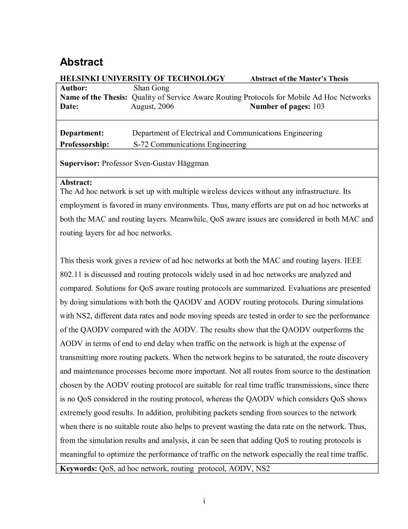
Abstract HELSINKI UNIVERSITY OF TECHNOLOGY Abstract of the Master�s Thesis Author: Shan Gong Name of the Thesis: Quality of Service Aware Routing Protocols for Mobile Ad Hoc Networks Date: August, 2006 Number of pages: 103

Department: Department of Electrical and Communications Engineering Professorship: S-72 Communications Engineering Supervisor: Professor Sven-Gustav Häggman Abstract: The Ad hoc network is set up with multiple wireless devices without any infrastructure. Its

employment is favored in many environments. Thus, many efforts are put on ad hoc networks at

both the MAC and routing layers. Meanwhile, QoS aware issues are considered in both MAC and

routing layers for ad hoc networks.

This thesis work gives a review of ad hoc networks at both the MAC and routing layers. IEEE

802.11 is discussed and routing protocols widely used in ad hoc networks are analyzed and

compared. Solutions for QoS aware routing protocols are summarized. Evaluations are presented

by doing simulations with both the QAODV and AODV routing protocols. During simulations

with NS2, different data rates and node moving speeds are tested in order to see the performance

of the QAODV compared with the AODV. The results show that the QAODV outperforms the

AODV in terms of end to end delay when traffic on the network is high at the expense of

transmitting more routing packets. When the network begins to be saturated, the route discovery

and maintenance processes become more important. Not all routes from source to the destination

chosen by the AODV routing protocol are suitable for real time traffic transmissions, since there

is no QoS considered in the routing protocol, whereas the QAODV which considers QoS shows

extremely good results. In addition, prohibiting packets sending from sources to the network

when there is no suitable route also helps to prevent wasting the data rate on the network. Thus,

from the simulation results and analysis, it can be seen that adding QoS to routing protocols is

meaningful to optimize the performance of traffic on the network especially the real time traffic.

Keywords: QoS, ad hoc network, routing protocol, AODV, NS2

ii

Acknowledgement This thesis work is done in Communications Laboratory at Helsinki University of Technology. I would like to express my gratitude to the supervisor of this thesis, Professor Sven-Gustav Häggman who gave me lots of valuable guidance and comments for this work. Special thanks to my parents for their supporting of my studying in Finland. Without their support, I could not finish my Master degree studies. In addition, many thanks to the Communications Laboratory of Helsinki University of Technology for providing me a place to do this thesis work. Last but not least, I would like to show my warm thanks to my friends Hao Zhou and Cheng Luo and all my other friends both in Finland and in China. The time spent with them makes my life in Finland colourful. Espoo, Finland, August 7th, 2006 Shan Gong

iii

Table of Contents ABSTRACT................................................................................................................... I

ACKNOWLEDGEMENT............................................................................................II

TABLE OF CONTENTS ........................................................................................... III

LIST OF ABBREVIATIONS .....................................................................................VI

LIST OF SYMBOLS...................................................................................................IX

LIST OF FIGURES...................................................................................................... X

LIST OF TABLES.......................................................................................................XI

1. INTRODUCTION .................................................................................................1

1.1. Scope of the thesis ...........................................................................................1 1.2. Aim and objectives ..........................................................................................2 1.3. Research methods ............................................................................................2 1.4. Thesis outline...................................................................................................2

2. OVERVIEW OF MOBILE AD HOC NETWORKS ...........................................4

2.1. History of Mobile Ad Hoc Networks................................................................4 2.2. Applications of Mobile Ad Hoc Networks........................................................4

2.2.1. Military applications.................................................................................4 2.2.2. Emergency operations ..............................................................................4 2.2.3. Wireless mesh networks ...........................................................................5 2.2.4. Wireless sensor networks .........................................................................5

2.3. IEEE 802.11 standard.......................................................................................6 2.3.1. IEEE 802 family.......................................................................................6 2.3.2. IEEE 802.11 family..................................................................................6 2.3.3. Basic service set in IEEE 802.11 ..............................................................7 2.3.4. Physical layer of IEEE 802.11..................................................................8 2.3.5. MAC layer of IEEE 802.11 ......................................................................9

2.3.5.1. Basic concepts in IEEE 802.11 .........................................................9 2.3.5.2. CSMA/CA mechanism in DCF.......................................................13 2.3.5.3. Medium access control with PCF....................................................15

2.3.6. CSMA/CD and IEEE 802.3 Standard .....................................................15 2.3.7. CSMA/CA in comparison with CSMA/CD ............................................16 2.3.8. IEEE 802.11e .........................................................................................17

2.4. Routing protocols in ad hoc wireless networks ...............................................18 2.4.1. Proactive routing protocols.....................................................................19

2.4.1.1. Open Shortest Path First routing protocol in Internet.......................19 2.4.1.2. Optimized Link State Routing Protocol...........................................20

iv

2.4.1.3. Comparisons between OSPF and OLSR routing protocol................22 2.4.2. Reactive routing protocols ......................................................................22

2.4.2.1. Dynamic Source Routing Protocol..................................................23 2.4.2.2. Ad Hoc On-Demand Distance Vector Routing Protocol..................24 2.4.2.3. Comparison between DSR and AODV routing protocols ................27

2.4.3. Hybrid routing protocol-Zone Routing Protocol .....................................28 2.4.4. Power-aware routing protocols ...............................................................28 2.4.5. Load-Aware Routing Protocols ..............................................................29

2.5. Chapter summary...........................................................................................30

3. QOS-AWARE ROUTING PROTOCOLS IN AD HOC NETWORKS ............32

3.1. Definition of QoS...........................................................................................32 3.2. QoS parameters..............................................................................................32 3.3. Real time traffic vs. non real time traffic ........................................................33 3.4. QoS in different layers ...................................................................................33 3.5. QoS models ...................................................................................................34 3.6. Challenge of QoS routing in ad hoc networks.................................................34 3.7. Classification of generally used metrics..........................................................35 3.8. Delay calculations..........................................................................................36 3.9. Available data rate calculations ......................................................................37

3.9.1. Transmission range and carrier sensing range .........................................37 3.9.2. Locally available data rate ......................................................................37 3.9.3. Listen Mode and Hello Mode .................................................................42 3.9.4. Real available data rate of one node........................................................43 3.9.5. Summary of the process for calculating data rate ....................................44 3.9.6. Admission control mechanisms ..............................................................45

3.10. QoS-aware routing schemes ...........................................................................48 3.10.1. Quality of Service Optimized Link State Routing Protocol .....................48 3.10.2. Quality of Service for Ad hoc On-Demand Distance Vector Routing......51

3.11. Chapter summary...........................................................................................52

4. IMPLEMENTATION OF THE QAODV ROUTING PROTOCOL IN NETWORK SIMULATOR 2......................................................................................53

4.1. Simulation tools .............................................................................................53 4.1.1. Introduction to NS2................................................................................53

4.1.1.1. History of NS .................................................................................53 4.1.1.2. Operation system and installation of NS .........................................53 4.1.1.3. Use of NS2 .....................................................................................54

4.1.2. Mobile networking in NS2 .....................................................................55 4.1.2.1. Basic wireless models in NS2 .........................................................55 4.1.2.2. Creating mobile nodes ....................................................................55 4.1.2.3. Trace file formats in wireless networks...........................................56

4.1.3. Tools used in NS2 ..................................................................................57 4.1.3.1. Generation of node movement ........................................................57 4.1.3.2. Traffic generation ...........................................................................58

v

4.1.4. Relevant tools used for data analysis ......................................................58 4.1.4.1. GAWK ...........................................................................................58 4.1.4.2. BASH.............................................................................................59

4.2. Details of the QAODV in NS2 .......................................................................59 4.2.1. General idea of the QAODV routing protocol.........................................59 4.2.2. QAODV relevant source code analysis ...................................................61

4.3. Chapter summary...........................................................................................70

5. SIMULATIONS ON AODV AND QAODV ROUTING PROTOCOLS...........71

5.1. Simulation environment .................................................................................71 5.2. Simulation models .........................................................................................71 5.3. A simple case.................................................................................................73 5.4. Simulation scenarios ......................................................................................74 5.5. Simulation traffic pattern................................................................................75 5.6. Performance metrics ......................................................................................75 5.7. Simulation results and analysis.......................................................................76

5.7.1. Data rate.................................................................................................76 5.7.2. Maximum node moving speed................................................................83

5.8. Summary of the simulations ...........................................................................88 5.9. Simulation problems ......................................................................................89 5.10. Chapter summary...........................................................................................89

6. SUMMARY AND CONCLUSIONS ...................................................................90

6.1. Summary .......................................................................................................90 6.2. Conclusions ...................................................................................................90 6.3. Discussion......................................................................................................91 6.4. Further work ..................................................................................................91

REFERENCES............................................................................................................92

APPENDIX A ..............................................................................................................95

APPENDIX B ..............................................................................................................96

APPENDIX C ............................................................................................................ 101

APPENDIX D ............................................................................................................ 103

vi

List of Abbreviations AAC Access Admission Control AC Access Categories ACK Acknowledgement AIFS Arbitration IFS ARP Address Resolution Protocol BcastID Broadcast IDentifier BASH Bourne-Again SHell BF Bellman-Ford BPSK Binary Phase Shift Keying BSS Basic Service Set CAC Call Admission Control CBR Constant Bit Rate CCK Complementary Code Keying CFP Contention Free Period CMU Carnegie Mellon University CONSER Collaborative Simulation for Education and Research CP Contention period CSMA/CA Carrier Sensing Multiple Access/Collision Avoidance CSMA/CD Carrier Sensing Multiple Access with Collision Avoidance CTS Clear To Send CW Contention Window CWmax maximum contention window size CWmin minimum contention window size DARPA Defense Advanced Research Projects Agency DBPSK Differential Quaternary Phase Shift Keying DCF Distributed Coordinate Function DestID Destination IDentifier DestSeqNum Destination Sequence Number DiffServ Differentiated Services DIFS DCF inter-frame spacing D-LAOR Delay-based Load aware on demand routing DLAR Dynamic Load-Aware Routing DLP Direct link protocol DOSPR Delay-Oriented Shortest Path Routing DQPSK Differential Quaternary Phase Shift Keying DSCP Differentiated Services Code Points DSDV Destination Sequenced Distance-Vector routing protocol DSR Dynamic Source Routing DSSS Direct-Sequence Spread-Spectrum EDCF Enhanced DCF EIFS Extended inter-frame spacing FHSS Frequency-Hopping Spread-Spectrum GNU A recursive acronym for �GNU's Not UNIX�

vii

NSF National Science Foundation HCCA HCF Controlled Channel Access HCF Hybrid Coordination Function HR/DSSS High-Rate Direct-Sequence Spread Spectrum ICIR ICSI Center for Internet Research ICSI International Computer Science Institute IFS Inter-frame Spacing IntServ Integrated Service IP Internet Protocol ISM Industrial, Scientific and Medical ISP Internet Service Provider LAN Local Area Network LBAR Load-Balanced Ad hoc Routing LR-WPAN Low Rate-Wireless Personal Area Network LSAs Link State Advertisements LSR Load-Sensitive Routing MAC Medium Access Control MANET Mobile Ad hoc NETwork MBWA Mobile Broadband Wireless Access MIT Massachusetts Institute of Technology MPRs Multi Point Relays MTPR Minimum Total Transmission Power Routing NAM Network Animator NAV Network Allocation Vector NOL Normalized Overhead Load NS2 Network Simulator 2 OFDM Orthogonal Frequency Division Multiplexing OLSR Optimized Link State Routing protocol OSI Open System Interconnection OSPF Open Shortest Path First routing protocol PARC Palo Alto Research Center PCF Point Coordinate Function PDA Personal Digital Assistant PDR Packet Delivery Ratio PHB Per-Hop Behavior PHY Physical Layer PIFS PCF inter-frame spacing QAM Quadrature amplitude modulation

QAODV Quality of Service On-Demand Distance Vector Routing Protocol

QOLSR Quality of Service Optimized Link State Routing Protocol QoS Quality of Service QOSPF Quality of Service Open Shortest Path First QPSK Quadrature Phase-shift Keying RAM Random Access Memory

viii

RERR Route ERRor RREP Route REPly RREQ Route REQuest RSVP Resource Reservation Protocol RTS Request To Send RTT Round Trip Time

SAMAN Simulation Augmented by Measurement and Analysis for Networks

SIFS Short inter-frame spacing SPF Shortest-Path-First SrcID Source IDentifier SrcSeqNum Source Sequence Number TC Topology Control Tcl Tool command language TORA Temporally ordered Routing Algorithm ToS Type of Service TTL Time To Live TXOPs Transmission OPportunities

USC/ISI University of Southern California�s Information Sciences Institute

UDP User Datagram Protocol UP User Priority VINT Virtual InterNetwork Testbed WIDENS Wireless Deployable Network System WLAN Wireless Local Area Network WMAN Wireless Metropolitan Area Network WPAN Wireless Personal Area Network WRP Wireless Routing Protocol

ix

LIST OF SYMBOLS AverageDelay(t) The average delay of round t AverageDelay(t-1) The average delay of round (t-1) Cij The cumulative power value from node i to node j. Cost(ni) The minimum cost in term of power from node i to node j Cost(nj) The power cost from source node to node j. CC The Contention count Ei The residual energy at nodes EstRTT(t) The estimated RTT of round t EstRTT(t-1) The estimated RTT of round t-1. eij The energy cost for unit flow transmission over the link. is the

initial energy and hrep The hop count of route reply hreq The hop count of route request MeasuredDelay(t) The measured RTT of round t. N The number of packets the node sent and received and sensed. NH(i) The neighbor node of node i Ni The neighbor of node i Ptransceiver(nj) The signal processing power at the transceiver j, Ptransmit(ni,nj) The transmission power needed from node i to node j (here node i

and node j are neighbor), R The retransmission times r The data rate requirement S The size of the packets. SampleRTT(t) The measured RTT of round t SWAN Stateless Wireless Ad Hoc Networks TB The Back-off time tCA The collision avoidance phase time. toverehead The control overhead time tq The L2 queuing time ts The reransmission time of S bits x1 The non-negative factor x2 The non-negative factors x3 The non-negative factors xjk The data rate used by neighbors of node i to send traffic Zi The data rate used by node i for receiving data Zj The data rate used by neighbor of node i: node j to receive traffic α The weighted factor µ Link utilization factor The initial energy at nodes

iE

x

List of Figures Figure 2-1 WIDENS system structure......................................................................5 Figure 2-2 Two configuration modes in IEEE 802.11 ..............................................8 Figure 2-3 IEEE 802.11b frame structure.................................................................9 Figure 2-4 PCF and DCF .......................................................................................10 Figure 2-5 RTS/CTS problem (1)...........................................................................13 Figure 2-6 RTS/CTS problem (2)...........................................................................13 Figure 2-7 CSMA/CA (1) ......................................................................................14 Figure 2-8 CSMA/CA (2) ......................................................................................14 Figure 2-9 CSMA/CA (3) ......................................................................................15 Figure 2-10 Point Coordinate Function ..................................................................15 Figure 2-11 Categorization of ad hoc routing protocols..........................................18 Figure 2-12 OLSR MPR set ...................................................................................22 Figure 2-13 Building of route record during route discovery .................................23 Figure 2-14 Propagation of RREP with route record .............................................24 Figure 2-15 AODV route discovery .......................................................................27 Figure 3-1 Example of local available data rate calculation (1)...............................40 Figure 3-2 Example of local available data rate calculation (2)...............................42 Figure 3-3 Example of real available data rate calculation......................................44 Figure 3-4 Example of QoS with admission control (1)..........................................46 Figure 3-5 Example of QoS with admission control (2)..........................................47 Figure 3-6 Example of MPRs calculation...............................................................50 Figure 4-1 Simplified user's view of NS.................................................................54 Figure 4-2 Changes in AODV to achieve QAODV with data rate restriction..........61 Figure 4-3 Flow char for RREQ in QAODV ..........................................................68 Figure 4-4 Flow char for RREP in QAODV...........................................................69 Figure 5-1 Maximum data rate with different hop counts .......................................73 Figure 5-2 A network topology of a simple case ....................................................73 Figure 5-3 Average end to end delay with different data rates ................................77 Figure 5-4 PDR with different data rates................................................................78 Figure 5-5 NOL with different data rates................................................................80 Figure 5-6 Time used to find the first route�First traffic flow...............................83 Figure 5-7 Time used to find the first route�Second traffic flow...........................83 Figure 5-8 Average end to end delay with different node Max. moving speeds ......84 Figure 5-9 PDR with different node Max. moving speeds ......................................86 Figure 5-10 NOL with different node Max. moving speeds....................................87

xi

List of Tables Table 2-1 IEEE 802 Family .....................................................................................6 Table 2-2 IEEE 802.11 Family.................................................................................7 Table 2-3 IEEE 802.11e priority to access category mappings ...............................17 Table 2-4 IEEE 802.11e typical QoS parameters....................................................17 Table 3-1 Example of local available data rate calculation (1)................................40 Table 3-2 Example of local available data rate calculation (2)................................41 Table 3-3 Example of real available data rate calculation.......................................44 Table 3-4 Example of QoS with admission control (1) ...........................................46 Table 3-5 Example of QoS with admission control (2) ...........................................48 Table 3-6 Example of MPRs calculation (1)...........................................................50 Table 3-7 Example of MPRs calculation (2)...........................................................50 Table 3-8 Example of MPRs calculation (3)...........................................................51 Table 3-9 Example of MPRs calculation (4)...........................................................51 Table 4-1 Part of the Tcl script for setting of parameters ........................................55 Table 4-2 Part of the Tcl script for configuration of nodes .....................................55 Table 4-3 Part of the Tcl script for creating mobile nodes ......................................56 Table 4-4 Mobile node components .......................................................................56 Table 4-5 Setdest sub-command explanation..........................................................58 Table 4-6 cbrgen sub-command explanation ..........................................................58 Table 4-7 Functions and timers in adov.cc in NS2..................................................62 Table 5-1 Throughputs between two nodes ............................................................72 Table 5-2 Case 2 scenario descriptions...................................................................74 Table 5-3 Simulation traffic pattern .......................................................................75 Table 5-4 Values obtained from the simulations with the AODV routing protocols

for different data rates ....................................................................................81 Table 5-5 Values obtained from the simulations with QAODV routing protocols for

different data rates..........................................................................................82 Table 5-6 Number of packets dropped in QAODV and AODV ..............................85 Table 5-7 Values obtained from the simulations with the AODV and the QAODV

routing protocols for different maximum node moving speed .........................88

1

1. Introduction

1.1. Scope of the thesis

In ad hoc networks, communications are done over wireless media between stations directly in a peer to peer fashion without the help of wired base station or access points. Lots of efforts have been done on ad hoc networks. One of the important and famous groups developing ad hoc networks is Mobile Ad-hoc network Group (MANET). With the popularity of ad hoc networks, many routing protocols have been designed for route discovery and route maintenance. They are mostly designed for best effort transmission without any guarantee of quality of transmissions. Some of the most famous routing protocols are Dynamic Source Routing (DSR) Ad hoc On Demand Vector (AODV) Optimized Link State Routing protocol (OLSR), and Zone Routing Protocol (ZRP). In MAC layer, one of the most popular solutions is IEEE 802.11. At the same time, Quality of Service (QoS) models in ad hoc networks become more and more required because more and more real time applications are implemented on the network. In MAC layer, IEEE 802.11e is a very popular issue discussed to set the priority to users. In routing layer, QoS are guaranteed in terms of data rate, delay, and jitter and so on. By considering QoS in terms of data rate and delay will help to ensure the quality of the transmission of real time media. For real time media transmission, if not enough data rate is obtained on the network, only part of the traffic will be transmitted on time. There would be no meaning to receiving the left part at a later time because real time media is sensitive to delay. Data that arrive late can be useless. As a result, it is essential for real time transmission to have a QoS aware routing protocol to ensure QoS of transmissions. In addition, network optimization can also be improved by setting requirements to transmissions. That is to say, prohibit the transmission of data which will be useless when it arrive the destination to the network. From the routing protocol point of view, it should be interpreted as that route which cannot satisfy the QoS requirement should not be considered as the suitable route in order to save the data rate on the network. The term �bandwidth� used by people who discussed the topic in the field of QoS aware routing protocols means �data rate� but not the physical bandwidth with the unit of Hertz. People always used it not right. In this paper the term �bandwidth� that people usually misused is modified to �data rate� with the unit of bits per second.

2

1.2. Aim and objectives

The aim of this thesis work is to give an overview of the popular MAC and routing layer solutions for ad hoc networks and take a look at of how QoS can be added to ad hoc networks especially in the network layer. Various methods for calculation of QoS metrics are discussed. Simulations will be done by using Network Simulator 2 (NS2) to see how a concrete QoS aware routing protocol performes. In the simulations, QoS is implemented on Ad hoc On-Demand Distance Vector (AODV) protocol with data rate as the QoS requirement metric. Comparisons will be done between AODV and QoS for Ad hoc On-Demand Distance Vector (QAODV) routing protocols. By doing the simulations, how much improvement can be achieved by this QAODV protocol can be seen and what kind of scenario can get benefit from this QAODV protocol will be analyzed. People who are going to do researches on QoS aware routing protocols in ad hoc networks can get benefits from reading this paper. In addition, reader can also get a clear idea of how an ad hoc network as a system works both from the theoretical part review and simulation part.

1.3. Research methods

This thesis work is based on the literature research method relying on the materials listed in the references. In addition, the approach used in case study is to do simulations. The simulations are done with NS2.

1.4. Thesis outline

Chapter 1 gives the scope and the aim of this thesis work. The outline of the thesis is described. Chapter 2 introduces the physical and MAC layer standards and routing layer protocols that are used in ad hoc networks. Firstly it simply explains mobile ad hoc networks and the applications of mobile ad hoc network. Then IEEE 802.11 standard for the physical and MAC layers are reviewed in detail. After that, some of the most popular routing protocols used in mobile ad hoc networks are introduced and compared. Chapter 3 presents what QoS is and how QoS aware routing protocols can be achieved by adding metrics to already exist routing protocols. Various methods for calculating QoS metrics are discussed. Two QoS aware routing protocols are discussed based on the existing drafts In chapter 4, the simulation tool called NS2 is introduced. A QoS aware AODV routing protocol implemented on NS2 is analyzed.

3

In chapter 5, the author will simulate some scenarios based on both the AODV and the QODV routing protocols. The performance results in AODV and QAODV are compared and analyzed. Chapter 6 concludes the thesis and gives some suggestions for further works.

4

2. Overview of Mobile Ad Hoc Networks

This chapter will give an overview of mobile ad hoc networks. The history and the applications will be summarized first. After that, IEEE 802.11 protocol will be discussed in detail. Finally, various routing protocols developed for ad hoc networks are discussed and compared.

2.1. History of Mobile Ad Hoc Networks

In early 1970s, the Mobile Ad hoc Network (MANET) was called packet radio network which was sponsored by Defense Advanced Research Projects Agency (DARPA). They had a project named packet radio having several wireless terminals that could communication with each other on battlefields. �It is interesting to note that these early packet radio systems predate the Internet, and indeed were part of the motivation of the original Internet Protocol suite.� [25]

2.2. Applications of Mobile Ad Hoc Networks

A MANET is a dynamic multi-hop wireless network that is established by a group of mobile nodes on a shared wireless channel. Mobile ad hoc networks can be in military use, emergency use, wireless sensor networks and also can have mesh wireless network architecture. [1, pp. 196-201]

2.2.1. Military applications

Use of ad hoc networks in military becomes more and more popular. Using ad hoc networks makes the setting up of communications between soldiers easy. In such applications, the used ad hoc networks need to be reliable and secure. The ability of multi-cast is required when the group leader in the army want to give order to all his soldiers.

2.2.2. Emergency operations

In emergency situation such as earthquakes, the wired networks could be destroyed. There will be a need of wireless network which could be deployed quickly for coordination of rescue.

5

An example is the design for future public safety communications. A European project called Wireless Deployable Network System (WIDENS) concentrated their work on this field. WIDENS have an idea that using ad hoc network to interoperate with existing TETRA network which is used for public safety. The system structure is shown in Figure 2-1 [2].

Figure 2-1 WIDENS system structure

2.2.3. Wireless mesh networks

Wireless mesh networks are ad hoc wireless networks which are formed to provide communication infrastructure using mobile or fixed nodes/users. The mesh topology provides alternative path for data transmission from the source to the destination. It gives quick re-configuration when the firstly chosen path fails. Wireless mesh network should be capable of self-organization and self-maintenance. The main advantages of wireless mesh networks are high speed, low cost, quick deployment, high scalability, and high availability. It works on 2.4 GHz and 5 GHz frequency bands, depending on the physical layer used. For example, if IEEE 802.11a is used, the speed can be up to 54 Mbps. An application example of wireless mesh network could be a wireless mesh networks in a residential zone, which the radio relay devices are built on top of the rooftops. In this situation, once one of the nodes in this residential area is equipped with the wired link to the internet, this node could be the gateway node. Others could connect to the internet from this node. Other possible deployments are highways, business zones, and university campus.

2.2.4. Wireless sensor networks

Wireless sensor networks use sensors to provide a wireless communication infrastructure. Sensor nodes are tiny devices used for sensing physical parameters, processing data, and communicating over the networks to the monitoring station. The application areas are

IP backbone

TETRA

Data replication

WIDENS ad-hoc network

Polic

Ambulance

Fire fighters

Co.ordinated Command Post Data Centre

Public Authorities

Head Quarters

6

military, health care, home security and environmental monitoring. There are some special characteristics which make sensor network different from other ad hoc networks. In the sensor network, nodes could be assumed to be static, that is, sensor networks need not to be in all cases designed to support the mobility. In addition, power constraint is one of the most important factors that have to be considered carefully. The limitation of power is mainly caused by the working environment of sensor network which is often harsh. As a result, it is impossible to recharge a sensor node battery, so effective protocols are required. For example, in the network layer, people need to design a low power consumption routing protocol, and power consumption will give the first priority to be considered during the route selection phase.

2.3. IEEE 802.11 standard

IEEE 802.11 standard provides physical (PHY) and MAC layer solutions for wireless local area networks. With the popularity of IEEE 802.11 standard family used in laptops, and Personal Digital Assistants (PDAs), this standard is considered to be one of the solutions used in ad hoc networks. Especially in the simulations, IEEE 802.11 standard is used in ad hoc networks by most of the people. The main references used in this part are [1, pp. 69-75] and [3].

2.3.1. IEEE 802 family

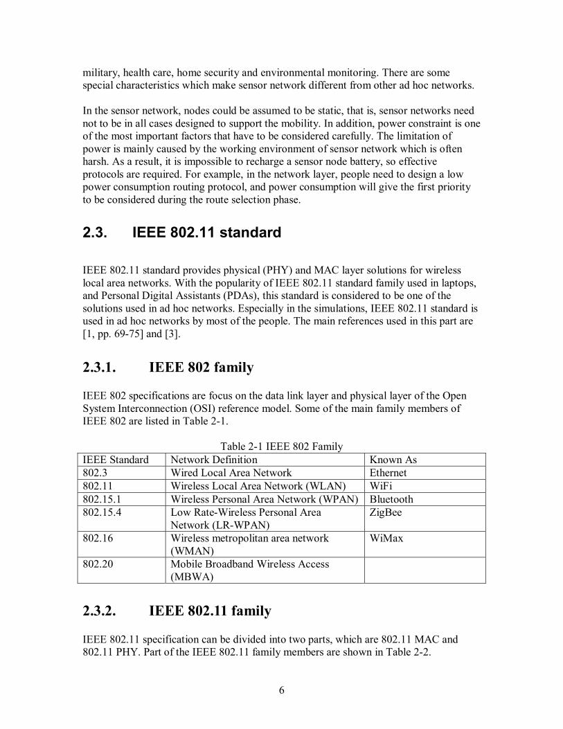
IEEE 802 specifications are focus on the data link layer and physical layer of the Open System Interconnection (OSI) reference model. Some of the main family members of IEEE 802 are listed in Table 2-1.

Table 2-1 IEEE 802 Family IEEE Standard Network Definition Known As 802.3 Wired Local Area Network Ethernet 802.11 Wireless Local Area Network (WLAN) WiFi 802.15.1 Wireless Personal Area Network (WPAN) Bluetooth 802.15.4 Low Rate-Wireless Personal Area

Network (LR-WPAN) ZigBee

802.16 Wireless metropolitan area network (WMAN)

WiMax

802.20 Mobile Broadband Wireless Access (MBWA)

2.3.2. IEEE 802.11 family

IEEE 802.11 specification can be divided into two parts, which are 802.11 MAC and 802.11 PHY. Part of the IEEE 802.11 family members are shown in Table 2-2.

7

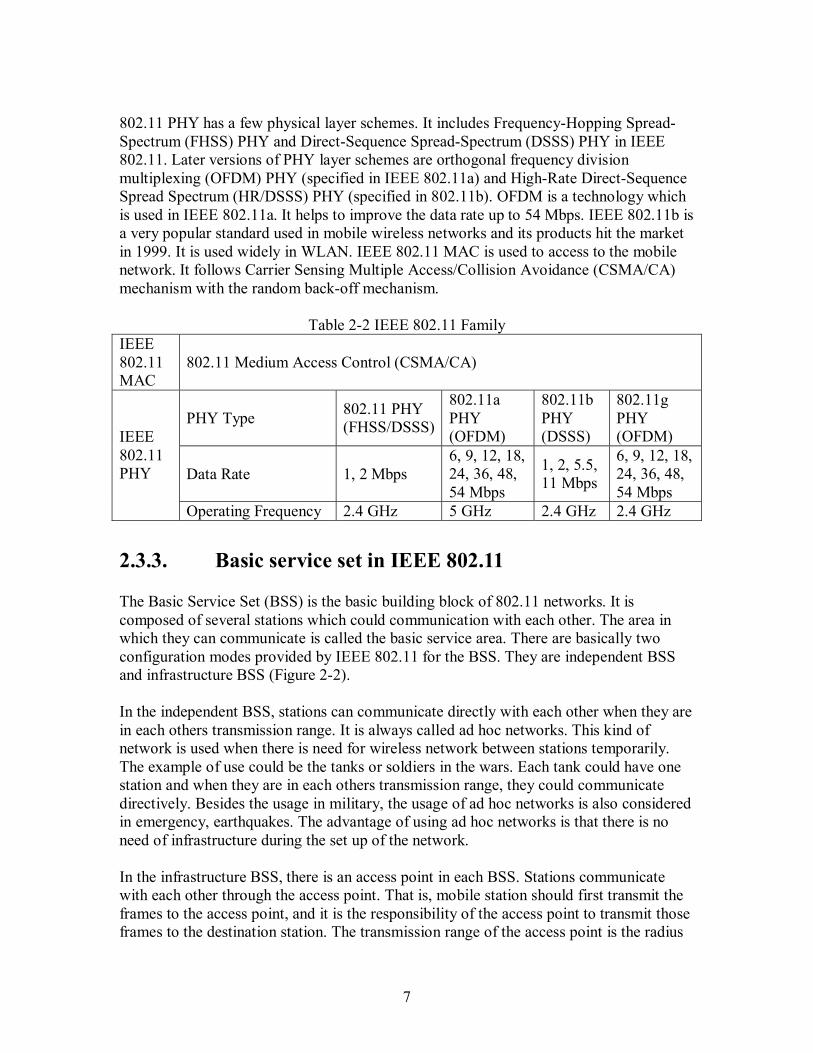
802.11 PHY has a few physical layer schemes. It includes Frequency-Hopping Spread-Spectrum (FHSS) PHY and Direct-Sequence Spread-Spectrum (DSSS) PHY in IEEE 802.11. Later versions of PHY layer schemes are orthogonal frequency division multiplexing (OFDM) PHY (specified in IEEE 802.11a) and High-Rate Direct-Sequence Spread Spectrum (HR/DSSS) PHY (specified in 802.11b). OFDM is a technology which is used in IEEE 802.11a. It helps to improve the data rate up to 54 Mbps. IEEE 802.11b is a very popular standard used in mobile wireless networks and its products hit the market in 1999. It is used widely in WLAN. IEEE 802.11 MAC is used to access to the mobile network. It follows Carrier Sensing Multiple Access/Collision Avoidance (CSMA/CA) mechanism with the random back-off mechanism.

Table 2-2 IEEE 802.11 Family IEEE 802.11 MAC

802.11 Medium Access Control (CSMA/CA)

PHY Type 802.11 PHY (FHSS/DSSS)

802.11a PHY (OFDM)

802.11b PHY (DSSS)

802.11g PHY (OFDM)

Data Rate 1, 2 Mbps 6, 9, 12, 18, 24, 36, 48, 54 Mbps

1, 2, 5.5, 11 Mbps

6, 9, 12, 18, 24, 36, 48, 54 Mbps

IEEE 802.11 PHY

Operating Frequency 2.4 GHz 5 GHz 2.4 GHz 2.4 GHz

2.3.3. Basic service set in IEEE 802.11

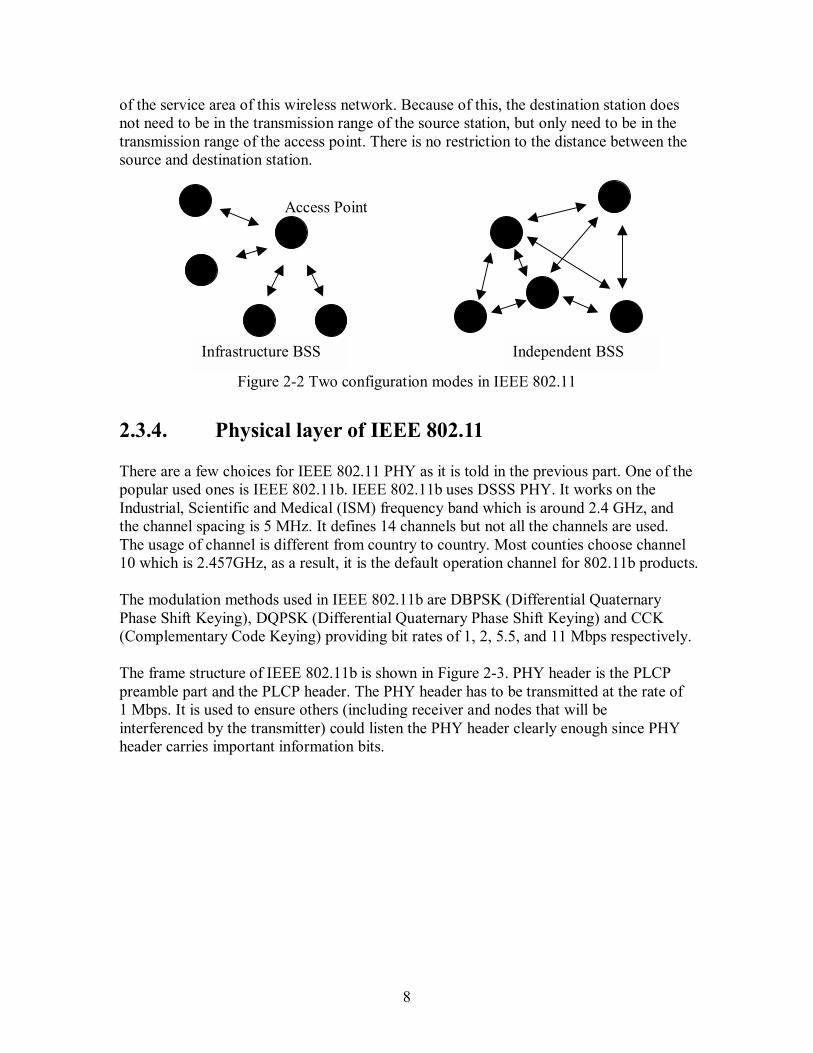
The Basic Service Set (BSS) is the basic building block of 802.11 networks. It is composed of several stations which could communication with each other. The area in which they can communicate is called the basic service area. There are basically two configuration modes provided by IEEE 802.11 for the BSS. They are independent BSS and infrastructure BSS (Figure 2-2). In the independent BSS, stations can communicate directly with each other when they are in each others transmission range. It is always called ad hoc networks. This kind of network is used when there is need for wireless network between stations temporarily. The example of use could be the tanks or soldiers in the wars. Each tank could have one station and when they are in each others transmission range, they could communicate directively. Besides the usage in military, the usage of ad hoc networks is also considered in emergency, earthquakes. The advantage of using ad hoc networks is that there is no need of infrastructure during the set up of the network. In the infrastructure BSS, there is an access point in each BSS. Stations communicate with each other through the access point. That is, mobile station should first transmit the frames to the access point, and it is the responsibility of the access point to transmit those frames to the destination station. The transmission range of the access point is the radius

8

of the service area of this wireless network. Because of this, the destination station does not need to be in the transmission range of the source station, but only need to be in the transmission range of the access point. There is no restriction to the distance between the source and destination station.

Figure 2-2 Two configuration modes in IEEE 802.11

2.3.4. Physical layer of IEEE 802.11

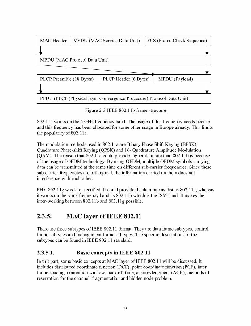
There are a few choices for IEEE 802.11 PHY as it is told in the previous part. One of the popular used ones is IEEE 802.11b. IEEE 802.11b uses DSSS PHY. It works on the Industrial, Scientific and Medical (ISM) frequency band which is around 2.4 GHz, and the channel spacing is 5 MHz. It defines 14 channels but not all the channels are used. The usage of channel is different from country to country. Most counties choose channel 10 which is 2.457GHz, as a result, it is the default operation channel for 802.11b products. The modulation methods used in IEEE 802.11b are DBPSK (Differential Quaternary Phase Shift Keying), DQPSK (Differential Quaternary Phase Shift Keying) and CCK (Complementary Code Keying) providing bit rates of 1, 2, 5.5, and 11 Mbps respectively. The frame structure of IEEE 802.11b is shown in Figure 2-3. PHY header is the PLCP preamble part and the PLCP header. The PHY header has to be transmitted at the rate of 1 Mbps. It is used to ensure others (including receiver and nodes that will be interferenced by the transmitter) could listen the PHY header clearly enough since PHY header carries important information bits.

Infrastructure BSS

Access Point

Independent BSS

9

Figure 2-3 IEEE 802.11b frame structure

802.11a works on the 5 GHz frequency band. The usage of this frequency needs license and this frequency has been allocated for some other usage in Europe already. This limits the popularity of 802.11a. The modulation methods used in 802.11a are Binary Phase Shift Keying (BPSK), Quadrature Phase-shift Keying (QPSK) and 16- Quadrature Amplitude Modulation (QAM). The reason that 802.11a could provide higher data rate than 802.11b is because of the usage of OFDM technology. By using OFDM, multiple OFDM symbols carrying data can be transmitted at the same time on different sub-carrier frequencies. Since these sub-carrier frequencies are orthogonal, the information carried on them does not interference with each other. PHY 802.11g was later rectified. It could provide the data rate as fast as 802.11a, whereas it works on the same frequency band as 802.11b which is the ISM band. It makes the inter-working between 802.11b and 802.11g possible.

2.3.5. MAC layer of IEEE 802.11

There are three subtypes of IEEE 802.11 format. They are data frame subtypes, control frame subtypes and management frame subtypes. The specific descriptions of the subtypes can be found in IEEE 802.11 standard.

2.3.5.1. Basic concepts in IEEE 802.11 In this part, some basic concepts at MAC layer of IEEE 802.11 will be discussed. It includes distributed coordinate function (DCF), point coordinate function (PCF), inter frame spacing, contention window, back off time, acknowledgment (ACK), methods of reservation for the channel, fragmentation and hidden node problem.

MAC Header MSDU (MAC Service Data Unit)

MPDU (MAC Protocol Data Unit)

PLCP Preamble (18 Bytes) PLCP Header (6 Bytes) MPDU (Payload)

PPDU (PLCP (Physical layer Convergence Procedure) Protocol Data Unit)

FCS (Frame Check Sequence)

10

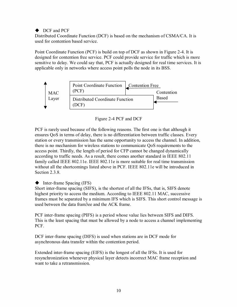
! DCF and PCF Distributed Coordinate Function (DCF) is based on the mechanism of CSMA/CA. It is used for contention based service. Point Coordinate Function (PCF) is build on top of DCF as shown in Figure 2-4. It is designed for contention free service. PCF could provide service for traffic which is more sensitive to delay. We could say that, PCF is actually designed for real time services. It is applicable only in networks where access point polls the node in its BSS.

Figure 2-4 PCF and DCF

PCF is rarely used because of the following reasons. The first one is that although it ensures QoS in terms of delay, there is no differentiation between traffic classes. Every station or every transmission has the same opportunity to access the channel. In addition, there is no mechanism for wireless stations to communicate QoS requirements to the access point. Thirdly, the length of period for CFP cannot be changed dynamically according to traffic needs. As a result, there comes another standard in IEEE 802.11 family called IEEE 802.11e. IEEE 802.11e is more suitable for real time transmission without all the shortcomings listed above in PCF. IEEE 802.11e will be introduced in Section 2.3.8. ! Inter-frame Spacing (IFS) Short inter-frame spacing (SIFS), is the shortest of all the IFSs, that is, SIFS denote highest priority to access the medium. According to IEEE 802.11 MAC, successive frames must be separated by a minimum IFS which is SIFS. This short control message is used between the data fram3ee and the ACK frame. PCF inter-frame spacing (PIFS) is a period whose value lies between SIFS and DIFS. This is the least spacing that must be allowed by a node to access a channel implementing PCF. DCF inter-frame spacing (DIFS) is used when stations are in DCF mode for asynchronous data transfer within the contention period. Extended inter-frame spacing (EIFS) is the longest of all the IFSs. It is used for resynchronization whenever physical layer detects incorrect MAC frame reception and want to take a retransmission.

Contention Based

Contention Free MAC Layer

Point Coordinate Function(PCF)

Distributed Coordinate Function (DCF)

11

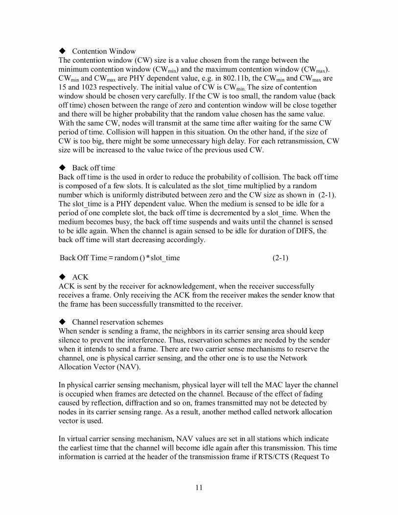
! Contention Window The contention window (CW) size is a value chosen from the range between the minimum contention window (CWmin) and the maximum contention window (CWmax). CWmin and CWmax are PHY dependent value, e.g. in 802.11b, the CWmin and CWmax are 15 and 1023 respectively. The initial value of CW is CWmin. The size of contention window should be chosen very carefully. If the CW is too small, the random value (back off time) chosen between the range of zero and contention window will be close together and there will be higher probability that the random value chosen has the same value. With the same CW, nodes will transmit at the same time after waiting for the same CW period of time. Collision will happen in this situation. On the other hand, if the size of CW is too big, there might be some unnecessary high delay. For each retransmission, CW size will be increased to the value twice of the previous used CW. ! Back off time Back off time is the used in order to reduce the probability of collision. The back off time is composed of a few slots. It is calculated as the slot_time multiplied by a random number which is uniformly distributed between zero and the CW size as shown in (2-1). The slot_time is a PHY dependent value. When the medium is sensed to be idle for a period of one complete slot, the back off time is decremented by a slot_time. When the medium becomes busy, the back off time suspends and waits until the channel is sensed to be idle again. When the channel is again sensed to be idle for duration of DIFS, the back off time will start decreasing accordingly.

slot_time * () random Time OffBack = (2-1) ! ACK ACK is sent by the receiver for acknowledgement, when the receiver successfully receives a frame. Only receiving the ACK from the receiver makes the sender know that the frame has been successfully transmitted to the receiver. ! Channel reservation schemes When sender is sending a frame, the neighbors in its carrier sensing area should keep silence to prevent the interference. Thus, reservation schemes are needed by the sender when it intends to send a frame. There are two carrier sense mechanisms to reserve the channel, one is physical carrier sensing, and the other one is to use the Network Allocation Vector (NAV). In physical carrier sensing mechanism, physical layer will tell the MAC layer the channel is occupied when frames are detected on the channel. Because of the effect of fading caused by reflection, diffraction and so on, frames transmitted may not be detected by nodes in its carrier sensing range. As a result, another method called network allocation vector is used. In virtual carrier sensing mechanism, NAV values are set in all stations which indicate the earliest time that the channel will become idle again after this transmission. This time information is carried at the header of the transmission frame if RTS/CTS (Request To

12

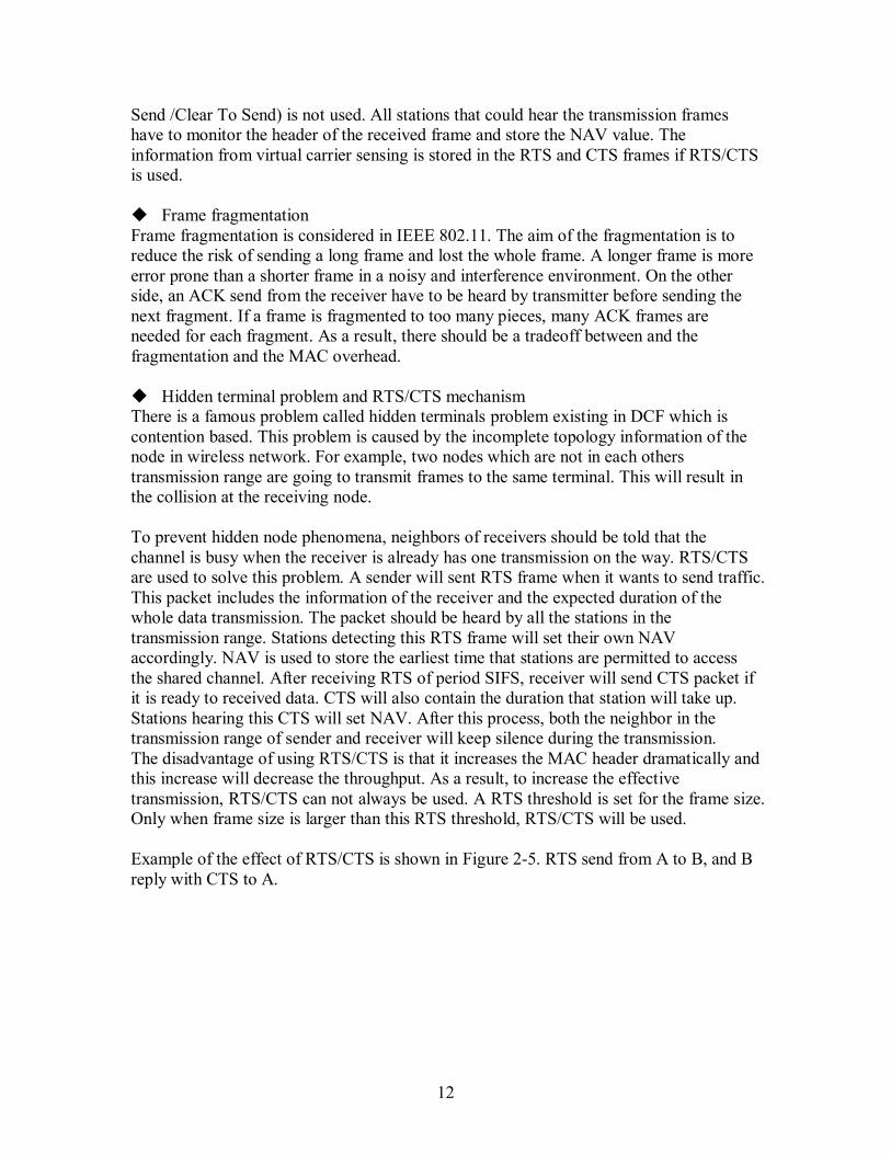
Send /Clear To Send) is not used. All stations that could hear the transmission frames have to monitor the header of the received frame and store the NAV value. The information from virtual carrier sensing is stored in the RTS and CTS frames if RTS/CTS is used. ! Frame fragmentation Frame fragmentation is considered in IEEE 802.11. The aim of the fragmentation is to reduce the risk of sending a long frame and lost the whole frame. A longer frame is more error prone than a shorter frame in a noisy and interference environment. On the other side, an ACK send from the receiver have to be heard by transmitter before sending the next fragment. If a frame is fragmented to too many pieces, many ACK frames are needed for each fragment. As a result, there should be a tradeoff between and the fragmentation and the MAC overhead. ! Hidden terminal problem and RTS/CTS mechanism There is a famous problem called hidden terminals problem existing in DCF which is contention based. This problem is caused by the incomplete topology information of the node in wireless network. For example, two nodes which are not in each others transmission range are going to transmit frames to the same terminal. This will result in the collision at the receiving node. To prevent hidden node phenomena, neighbors of receivers should be told that the channel is busy when the receiver is already has one transmission on the way. RTS/CTS are used to solve this problem. A sender will sent RTS frame when it wants to send traffic. This packet includes the information of the receiver and the expected duration of the whole data transmission. The packet should be heard by all the stations in the transmission range. Stations detecting this RTS frame will set their own NAV accordingly. NAV is used to store the earliest time that stations are permitted to access the shared channel. After receiving RTS of period SIFS, receiver will send CTS packet if it is ready to received data. CTS will also contain the duration that station will take up. Stations hearing this CTS will set NAV. After this process, both the neighbor in the transmission range of sender and receiver will keep silence during the transmission. The disadvantage of using RTS/CTS is that it increases the MAC header dramatically and this increase will decrease the throughput. As a result, to increase the effective transmission, RTS/CTS can not always be used. A RTS threshold is set for the frame size. Only when frame size is larger than this RTS threshold, RTS/CTS will be used. Example of the effect of RTS/CTS is shown in Figure 2-5. RTS send from A to B, and B reply with CTS to A.

13

Figure 2-5 RTS/CTS problem (1)

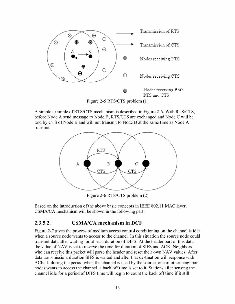
A simple example of RTS/CTS mechanism is described in Figure 2-6. With RTS/CTS, before Node A send message to Node B, RTS/CTS are exchanged and Node C will be told by CTS of Node B and will not transmit to Node B at the same time as Node A transmit.

Figure 2-6 RTS/CTS problem (2)

Based on the introduction of the above basic concepts in IEEE 802.11 MAC layer, CSMA/CA mechanism will be shown in the following part.

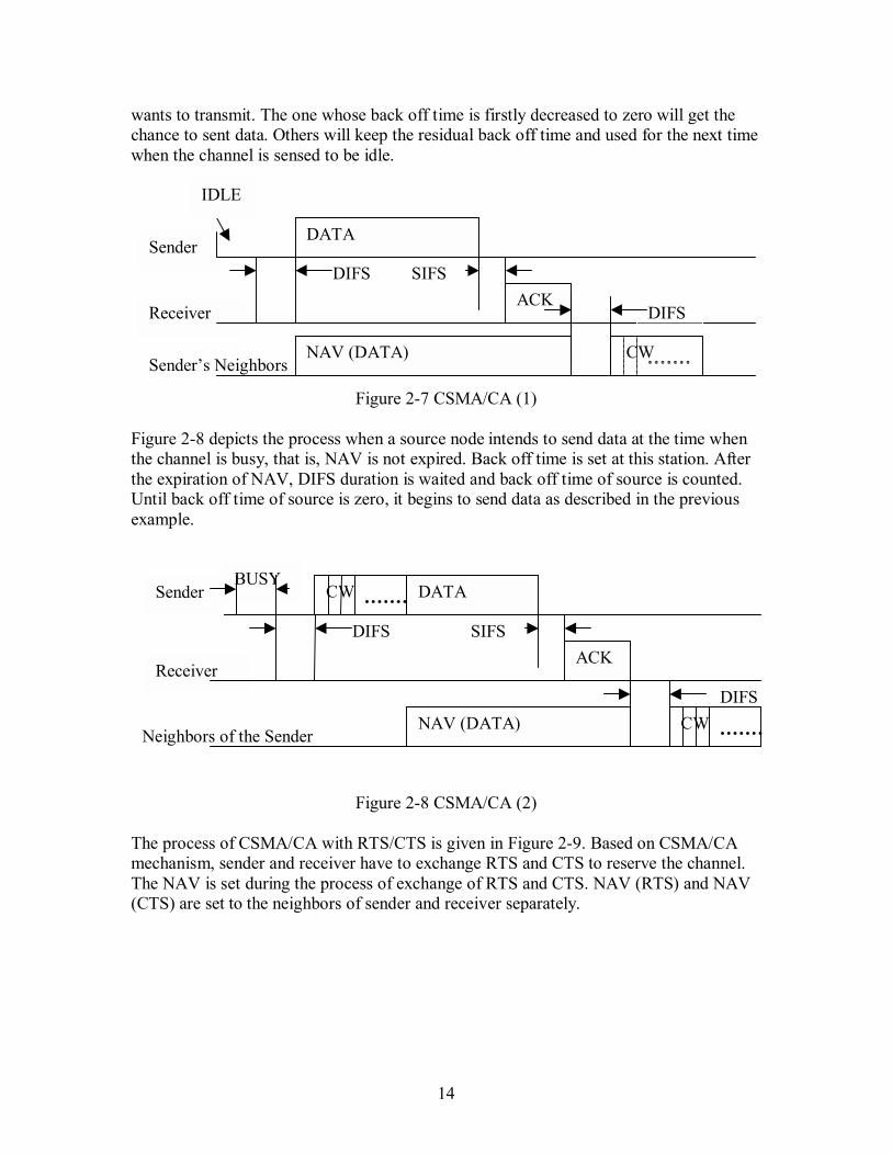
2.3.5.2. CSMA/CA mechanism in DCF Figure 2-7 gives the process of medium access control conditioning on the channel is idle when a source node wants to access to the channel. In this situation the source node could transmit data after waiting for at least duration of DIFS. At the header part of this data, the value of NAV is set to reserve the time for duration of SIFS and ACK. Neighbors who can receive this packet will parse the header and reset their own NAV values. After data transmission, duration SIFS is waited and after that destination will response with ACK. If during the period when the channel is used by the source, one of other neighbor nodes wants to access the channel, a back off time is set to it. Stations after sensing the channel idle for a period of DIFS time will begin to count the back off time if it still

14

wants to transmit. The one whose back off time is firstly decreased to zero will get the chance to sent data. Others will keep the residual back off time and used for the next time when the channel is sensed to be idle.

Figure 2-7 CSMA/CA (1)

Figure 2-8 depicts the process when a source node intends to send data at the time when the channel is busy, that is, NAV is not expired. Back off time is set at this station. After the expiration of NAV, DIFS duration is waited and back off time of source is counted. Until back off time of source is zero, it begins to send data as described in the previous example.

Figure 2-8 CSMA/CA (2)

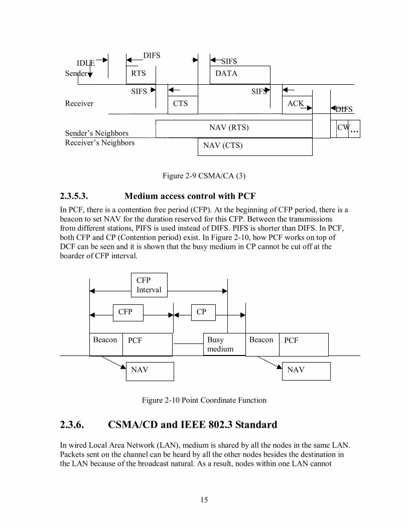
The process of CSMA/CA with RTS/CTS is given in Figure 2-9. Based on CSMA/CA mechanism, sender and receiver have to exchange RTS and CTS to reserve the channel. The NAV is set during the process of exchange of RTS and CTS. NAV (RTS) and NAV (CTS) are set to the neighbors of sender and receiver separately.

Sender

ACKReceiver

Sender�s Neighbors NAV (DATA)

IDLE

DIFS SIFS

DIFS

CW

DATA

Receiver ACK

BUSY Sender

Neighbors of the Sender NAV (DATA)

SIFS

DIFS

DIFS

CW

CW

DATA

15

Figure 2-9 CSMA/CA (3)

2.3.5.3. Medium access control with PCF In PCF, there is a contention free period (CFP). At the beginning of CFP period, there is a beacon to set NAV for the duration reserved for this CFP. Between the transmissions from different stations, PIFS is used instead of DIFS. PIFS is shorter than DIFS. In PCF, both CFP and CP (Contention period) exist. In Figure 2-10, how PCF works on top of DCF can be seen and it is shown that the busy medium in CP cannot be cut off at the boarder of CFP interval.

Figure 2-10 Point Coordinate Function

2.3.6. CSMA/CD and IEEE 802.3 Standard

In wired Local Area Network (LAN), medium is shared by all the nodes in the same LAN. Packets sent on the channel can be heard by all the other nodes besides the destination in the LAN because of the broadcast natural. As a result, nodes within one LAN cannot

IDLE

DIFS

SIFS

SIFS

SIFS

Sender

CW NAV (RTS)

ACK

DATA

Receiver

Sender�s Neighbors Receiver�s Neighbors

RTS

CTS

NAV (CTS)

DIFS

NAV

PCF Beacon

Busy medium

PCF Beacon

CFP CP

CFP Interval

NAV

16

transmit at the same time and medium access control is used to nodes to control their accesses to the medium. One of the famous used mechanisms is CSMA/CD. In CSMA mechanism, nodes first listen for a carrier on the channel before transmitting. It will decide whether to transmit signal based on the result of sensing. If the channel is sensed to be free, packets will be transmitted at once. Otherwise the channel will keep sensing until the channel is free and after that node sends the packet at once. There is problem if two nodes sense the channel to be idle and begin to transmit the packets at the same time. Then packets sending from both nodes will collide. [1, pp. 48-55] This is solved with Carrier Sensing Multiple Access with Collision Avoidance (CSMA/CD). In CSMA/CD, nodes not only sense the channel before transmission, but can also detect collision in the channel after transmission. With this additional mechanism, node can know the collision and stop transmitting immediately. For example, when there are two nodes happen to transmit at the same time, both nodes will detect the collision and will immediately stop the packet sending. In addition, node will send jamming signal which will be listened by all the other nodes. Then the nodes which are also transmitting but have not detected this collision will stop their transmissions also. Nodes will wait for a random period of time and try to send again. The collision is detected by a node by comparing the power or the pulse width of the received signal with the one it puts onto the channel. If there is difference between them, it can conclude that its packet is collided. IEEE 802.3 is the standard for CSMA/CD networks. This is widely used in Ethernet. It specifies both the physical layer and MAC sub-layer. In physical layer, four types of cabling are specified and the physical transmission media can be one of the follows: thick coaxial cable, thin coaxial cable, twisted pair and optic fiber. The provided data rate of these cables range from 10 Mbps up to 1,000 Mbps. In MAC sub-layer, CSMA/CD technology is used as it is already mentioned. A frame format is defined also. Data arrived this layer from the upper layer will be encapsulated according to the frame format. In this process, source and destination MAC address will be added. In addition, some checksum bits are added for error correction.

2.3.7. CSMA/CA in comparison with CSMA/CD

Both CSMA/CA and CSMA/CD are mechanisms for MAC layer helping with stations to access to the channel. For wireless network in IEEE 802.11, node can only know the failure of transmission with the absence of ACK message, since it is difficult for mobile node to detect packet collision in the network. Whereas the ACK is send only after the whole frame is received successfully by the receiver, but cannot be sent during the transmission of one frame. As a result, in CSMA/CA, stations have to wait a random period of time after it senses that

17

the channel is idle in order to decrease the probability of collision. In comparison, CSMA/CD will send frame at once when it detect the idle of the channel because of the ability to detect packet collision, the transmission will stop at once when the collision occurs. To sum up, CSMA/CD cannot be used in mobile wireless networks because of the difficulty of detecting the collision in mobile wireless networks.

2.3.8. IEEE 802.11e

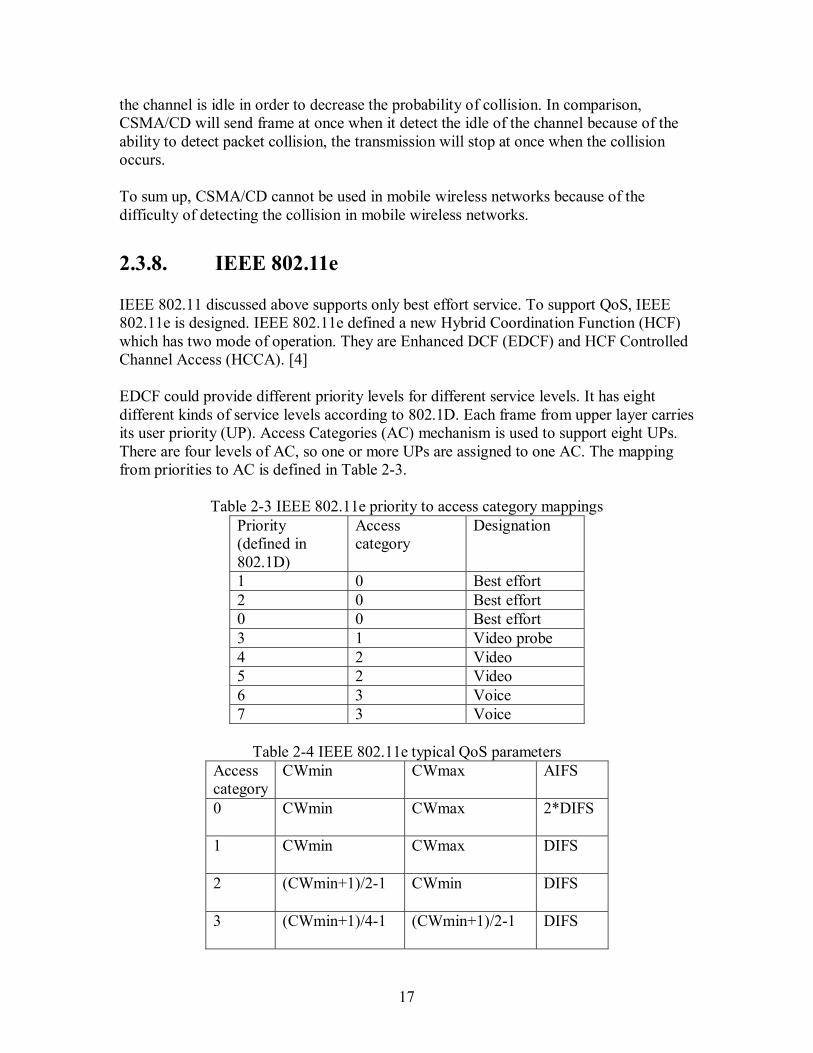
IEEE 802.11 discussed above supports only best effort service. To support QoS, IEEE 802.11e is designed. IEEE 802.11e defined a new Hybrid Coordination Function (HCF) which has two mode of operation. They are Enhanced DCF (EDCF) and HCF Controlled Channel Access (HCCA). [4] EDCF could provide different priority levels for different service levels. It has eight different kinds of service levels according to 802.1D. Each frame from upper layer carries its user priority (UP). Access Categories (AC) mechanism is used to support eight UPs. There are four levels of AC, so one or more UPs are assigned to one AC. The mapping from priorities to AC is defined in Table 2-3.

Table 2-3 IEEE 802.11e priority to access category mappingsPriority (defined in 802.1D)

Access category

Designation

1 0 Best effort 2 0 Best effort 0 0 Best effort 3 1 Video probe 4 2 Video 5 2 Video 6 3 Voice 7 3 Voice

Table 2-4 IEEE 802.11e typical QoS parameters

Access category

CWmin CWmax AIFS

0 CWmin CWmax 2*DIFS

1 CWmin CWmax DIFS

2 (CWmin+1)/2-1 CWmin DIFS

3 (CWmin+1)/4-1 (CWmin+1)/2-1 DIFS

Like in DCF, each AC is given a set of parameters, such as Arbitration IFS (AIFS), CWmin, and CWmax. AIFS is used as DIFS in DCF. The parameters assigned to each AC are shown in Table 2-4. Transmission opportunities (TXOPs) specified the time (maximum duration) which a wireless station can transmit a series of frames. By having different values in each AC, the TXOPs are differentiated. HCCA is like PCF. It is based on CFP which the access point polls every station in its BSS. Stations can communicate with access point about their QoS requirements. This is what PCF cannot achieve. In the IEEE 802.11e standard, there is a new rule for ACK. That is, the ACK need not to be used. The reason that ACK is used is for telling the source whether the transmitted packet is received successfully, if not, packet will be retransmitted. But since IEEE 802.11e is designed for real time applications with QoS, and the delay of retransmission make the retransmitted information useless, it sometimes do not need retransmission at all. As a result, ACK is not needed. Direct link protocol (DLP) is designed in IEEE 802.11e. It makes the stations to communicate directly to each other without going through the access point.

2.4. Routing protocols in ad hoc wireless networks

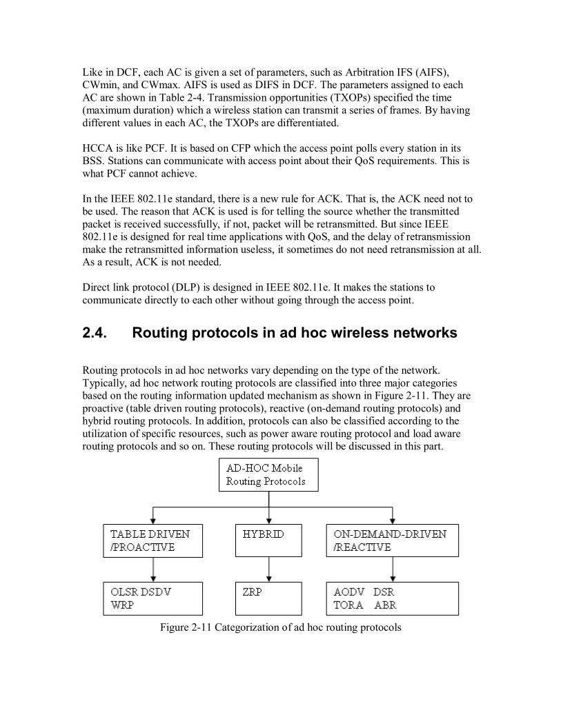
Routing protocols in ad hoc networks vary depending on the type of the network. Typically, ad hoc network routing protocols are classified into three major categories based on the routing information updated mechanism as shown in Figure 2-11. They are proactive (table driven routing protocols), reactive (on-demand routing protocols) and hybrid routing protocols. In addition, protocols can also be classified according to the utilization of specific resources, such as power aware routing protocol and load aware routing protocols and so on. These routing protocols will be discussed in this part.

Figure 2-11 Categorization of ad hoc routing protocols

19

2.4.1. Proactive routing protocols

In proactive routing protocols, routes are calculated independent of intended traffic. All the routes from one station to other stations in the network are calculated and saved in the routing table of each node. Once, there is a need of transmission, source node could check from the routing table, the route will be get immediately. Some of the used proactive routing protocols used in ad hoc networks are Optimized Link State Routing protocol (OLSR), Destination Sequenced Distance-Vector routing protocol (DSDV), and Wireless Routing Protocol (WRP). In this part, one of the most the famous Internet routing protocol which is also a proactive routing protocol called Open Shortest Path First Routing Protocol (OSPF) is discussed first. After that, representative ad hoc proactive routing protocol OLSR is described.

2.4.1.1. Open Shortest Path First routing protocol in Internet Open Shortest Path First (OSPF) routing protocol is an IETF specified link state routing protocol for the Internet. It is based on Dijkstra�s Shortest-Path-First (SPF) algorithm. Routers in the interior network send Link State Advertisements (LSAs) to all the other routers within the same hierarchical area. LSAs received from other routers are saved in a link state database. That is, the link state database of the router includes all the link information received from others. Routing table is calculated by using the information in the link state database. As a result, it converges faster than Bellman-Ford algorithm which is used in RIP. Since in RIP, routers only can exchange distance vectors with their neighbor routers, which means that routers can only get updated information from their neighbor routers. OSPF has three sub-protocols named Hello protocol, Exchange protocol and Flooding protocol. The Hello protocol ensures links working by exchange Hello messages with its neighbors during the last Hello interval. The designated router (used in broadcasting) and backup designated router are also selected by Hello protocol. The exchange protocol initially synchronizes link database with the designated router. Flooding protocol continuously maintains the link database integrity of the area [5]. Extended protocol for OSPF is QOSPF (Quality of Service Open Shortest Path First) In order to increase the QoS to satisfy the need of real-time traffic, e.g. video conference, streaming video/audio, QoS aware routing protocols are considered for Internet. Additional metrics are added to LSAs. The first considered metric is available data rate. Later, people find that it is not enough for only taking data rate and hop count to be the metric when searching for the best route. The reason is that links such as satellite links which have large data rate might be chosen, but using route including satellite links will give large delay. As a result, hop count, data rate and delay are metrics used in QOSPF. [6] The link metrics e.g. data rate and delay are advertised through the network in LSAs. The question is how often the metric information should be updated (exchange information

20

between nodes). One method could be the periodic updates, but the disadvantage of this is some big changes of available data rate happen right after one updating could be unknown before the next periodic update; it will lead to incorrect routing decision. On the other hand, too frequent update is not good as well since the amount of traffic is increased. All in all, there should be a tradeoff between the protocol overhead update frequency and accuracy of network state information that are used to select the path. When there is a significant change of metric, we need to trigger the link state advertisement. The significance could be defined as absolute or relative. The absolute scale will divide the range of metric value to different classes, if the metric in the link increases one level, its LSA will be triggered. Trigger updating could be used with periodic updates. Generally speaking, the routing algorithm is to find a path which could use the minimum hop-count with satisfaction of the data rate and delay requirements. In other words, the aim is to find the feasible path with the cost of minimal amount of recourse. Two alternatives could be used. One is on-demand computation; the other is Pre-computing. There is one algorithm especially used in QOSPF. The complexity of this algorithm is comparable to that of a standard is Bellman-Ford (BF) shortest path algorithm. The algorithm pre-computes for any destination a minimum hop count path with a maximum data rate. For each interaction, with the same number of hop-count, it will choose the route with maximum available data rate. As a result, data rate and hop-counts are all considered in one routing algorithm. OSPF is a protocol widely used in the internet. It shows basic principles of a routing protocol when trying to find a route in the network. There are some similarities between the routing protocols in different networks, whereas protocols for sure have differences because of the different characteristics of networks. After seeing another popular proactive protocol OLSR in Ad hoc network in the next part, comparisons will be done between OLSR and OSPF routing protocols. In addition, although QoS aware routing protocol is not widely used in Internet, QOSPF protocol developed based on OSPF protocols also give some basic idea of how QoS aware routing protocol could be achieved based on the existing routing protocol.

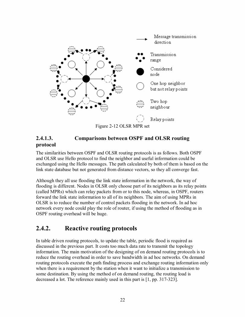
2.4.1.2. Optimized Link State Routing Protocol OLSR protocol is a proactive routing protocol. Due to its proactive nature, it has a low setup time when a route is asked. In addition, it employs an efficient link state packet forwarding mechanism called multipoint relaying, so this protocol is an optimization of the pure link state protocol. The optimization is achieved by reducing the size of the control packets and by reducing the number of links that are used to forward the link state packets. [1, pp. 349-352] The reduction of number of links is achieved by announcing only a subset of neighbours of a node that will be used for forwarding the packets for this node. This subset of neighbours which has the responsibility to forward packets is called Multi Point Relays (MPRs). MPR is a key point in OLSR protocol. Each node selects its own MPRset. With

21

this MPRset, the node should cover all the nodes which are two hops away. Link state packets generated by a node will be forward by its MPRs to all its two hop neighbours. The neighbours that are not the member of MPRs of the considered node can only process the link state packet but cannot forward it. This idea is shown in Figure 2-12. The considered node will calculate the route to all destinations through the members of MPR set. The smaller the MPR set, the more efficient the protocol is, compared with the pure link state protocol. Similarly, each node has a set of MPR selectors. The MPR selector set includes those who have selected this node as MPR. When the node receives link state packets from its neighbours, it will check whether the originator of this link state packet is in the set of MPR selectors. If yes, link state packets will be forwarded. Otherwise link state packets will only be processed. The member of MPR set and MPR selectors keep changing (updating) over time. The selection of MPR is one of the most important issues in OLSR, since only the selected node can be the relay point. The requirement for this MPR set is that node, through the neighbours in the MPR set, can read all symmetric strict 2-hop neighbours. When there is any change detected in the symmetric neighbourhood or in a symmetric strict 2-hop neighbourhood, MPR set of the node should be recalculated. Every node periodically originates Topology Control (TC) packets that contain the topology information. This TC information contains the list of neighbors which have selected the sender node as a multipoint relay and will be flooded throughout the network by using the MPR mechanism. The MPRs have the responsibility to broadcast the TC messaged to all the nodes in the network. Nodes will use TCs received from others to calculate routing table. An entry in a routing table includes the MPR selector (the destination) and a last hop node to that destination (the node who originates the TC packet for this destination). What is more, each node periodically originates Hello message to its neighbours to declare the neighbour nodes that it hears. The MPR set selected by this node will also be included in this Hello message. To use the network more efficiently, data rate should be considered during the selection of MPRs. If nodes with low data rate are selected, there will be higher possibility of overloading at this node. The link with larger data rate should have more probability to be involved in the MPR set. The selection of the optimal MPRset is NP-complete. It is what QoS based OLSR routing protocol considered.

22

Figure 2-12 OLSR MPR set

2.4.1.3. Comparisons between OSPF and OLSR routing protocol The similarities between OSPF and OLSR routing protocols is as follows. Both OSPF and OLSR use Hello protocol to find the neighbor and useful information could be exchanged using the Hello messages. The path calculated by both of them is based on the link state database but not generated from distance vectors, so they all converge fast. Although they all use flooding the link state information in the network, the way of flooding is different. Nodes in OLSR only choose part of its neighbors as its relay points (called MPRs) which can relay packets from or to this node, whereas, in OSPF, routers forward the link state information to all of its neighbors. The aim of using MPRs in OLSR is to reduce the number of control packets flooding in the network. In ad hoc network every node could play the role of router, if using the method of flooding as in OSPF routing overhead will be huge.

2.4.2. Reactive routing protocols

In table driven routing protocols, to update the table, periodic flood is required as discussed in the previous part. It costs too much data rate to transmit the topology information. The main motivation of the designing of on demand routing protocols is to reduce the routing overhead in order to save bandwidth in ad hoc networks. On demand routing protocols execute the path finding process and exchange routing information only when there is a requirement by the station when it want to initialize a transmission to some destination. By using the method of on demand routing, the routing load is decreased a lot. The reference mainly used in this part is [1, pp. 317-323].

23

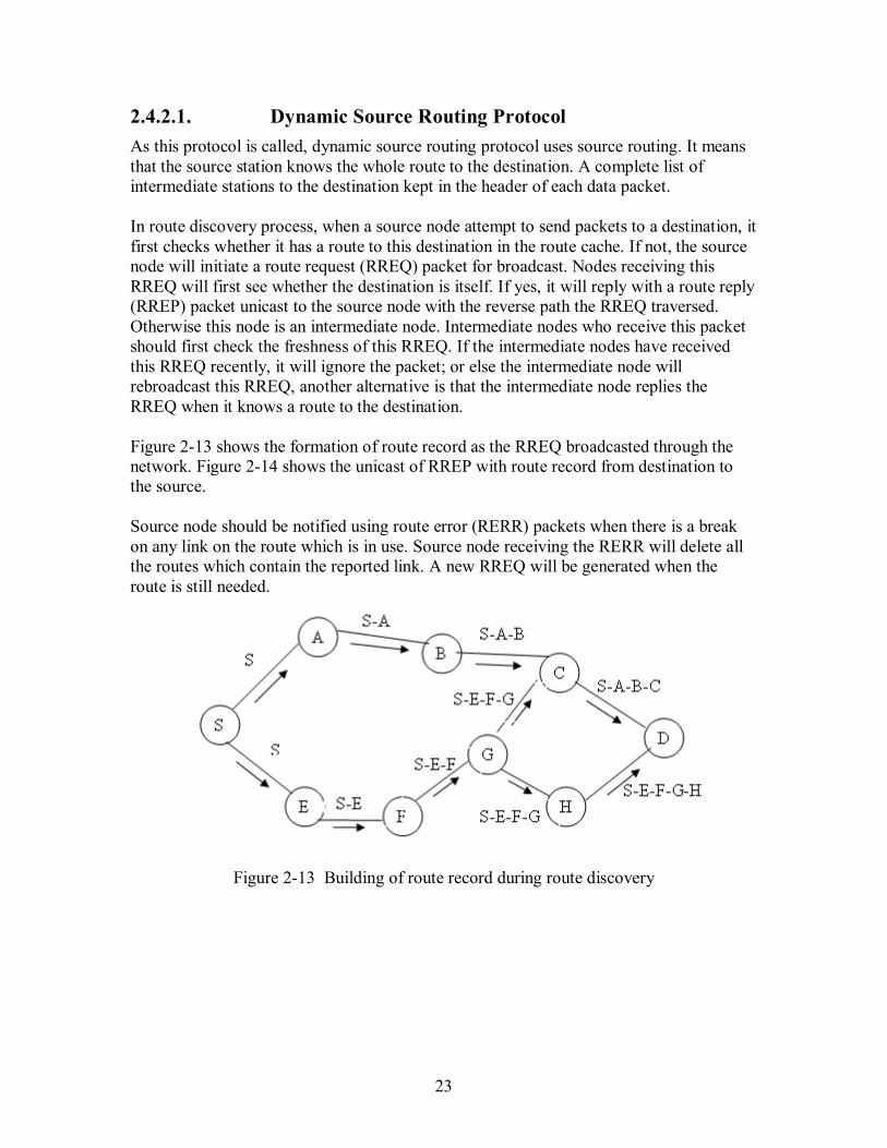
2.4.2.1. Dynamic Source Routing Protocol As this protocol is called, dynamic source routing protocol uses source routing. It means that the source station knows the whole route to the destination. A complete list of intermediate stations to the destination kept in the header of each data packet. In route discovery process, when a source node attempt to send packets to a destination, it first checks whether it has a route to this destination in the route cache. If not, the source node will initiate a route request (RREQ) packet for broadcast. Nodes receiving this RREQ will first see whether the destination is itself. If yes, it will reply with a route reply (RREP) packet unicast to the source node with the reverse path the RREQ traversed. Otherwise this node is an intermediate node. Intermediate nodes who receive this packet should first check the freshness of this RREQ. If the intermediate nodes have received this RREQ recently, it will ignore the packet; or else the intermediate node will rebroadcast this RREQ, another alternative is that the intermediate node replies the RREQ when it knows a route to the destination. Figure 2-13 shows the formation of route record as the RREQ broadcasted through the network. Figure 2-14 shows the unicast of RREP with route record from destination to the source. Source node should be notified using route error (RERR) packets when there is a break on any link on the route which is in use. Source node receiving the RERR will delete all the routes which contain the reported link. A new RREQ will be generated when the route is still needed.

Figure 2-13 Building of route record during route discovery

24

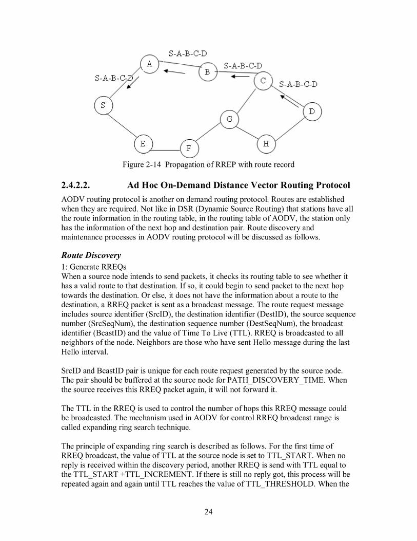
Figure 2-14 Propagation of RREP with route record

2.4.2.2. Ad Hoc On-Demand Distance Vector Routing Protocol AODV routing protocol is another on demand routing protocol. Routes are established when they are required. Not like in DSR (Dynamic Source Routing) that stations have all the route information in the routing table, in the routing table of AODV, the station only has the information of the next hop and destination pair. Route discovery and maintenance processes in AODV routing protocol will be discussed as follows.

Route Discovery 1: Generate RREQs When a source node intends to send packets, it checks its routing table to see whether it has a valid route to that destination. If so, it could begin to send packet to the next hop towards the destination. Or else, it does not have the information about a route to the destination, a RREQ packet is sent as a broadcast message. The route request message includes source identifier (SrcID), the destination identifier (DestID), the source sequence number (SrcSeqNum), the destination sequence number (DestSeqNum), the broadcast identifier (BcastID) and the value of Time To Live (TTL). RREQ is broadcasted to all neighbors of the node. Neighbors are those who have sent Hello message during the last Hello interval. SrcID and BcastID pair is unique for each route request generated by the source node. The pair should be buffered at the source node for PATH_DISCOVERY_TIME. When the source receives this RREQ packet again, it will not forward it. The TTL in the RREQ is used to control the number of hops this RREQ message could be broadcasted. The mechanism used in AODV for control RREQ broadcast range is called expanding ring search technique. The principle of expanding ring search is described as follows. For the first time of RREQ broadcast, the value of TTL at the source node is set to TTL_START. When no reply is received within the discovery period, another RREQ is send with TTL equal to the TTL_START +TTL_INCREMENT. If there is still no reply got, this process will be repeated again and again until TTL reaches the value of TTL_THRESHOLD. When the

25

incremented value TTL is equal or larger than TTL_THRESHOLD, the value of TTL will be set to the value of NETWORK_DIAMETER. RREQ will be broadcasted at a maximum of RREQ_RETRIES times with the value of NETWORK_DIAMETER. If there is still no reply got, all the packets that destine for this destination will be dropped. The advantage of this technique is to control the flooding of RREQ in the whole network. This will help to save more data rate especially when the network is large. 2: Nodes receive RREQs Nodes receiving RREQ will first check whether it is the source that sends this RREQ or whether the node has recently heard (during the last PATH_DISCOVERY_TIME) this RREQ. If one of these holds true, the newer RREQ will be droppped silently to prevent the flood of RREQ in the network. RREQ is identified by the unique SrcID and BcastID pair which will store in the nodes for PATH_DISCOVERY_TIME after nodes first received this RREQ. If the node receiving the RREQ has not heard this previously and it is not originated by itself, it will be preceded by this node further on which will be described in the following paragraphs. The node will set up a reverse route entry for the source node in its routing table. By storing this reverse route in the routing table, the node knows how to forward the RREP to the source if it received a RREP for this source node at a later time. If the entry for this source node already exists, this entry will be updated by refreshing the sequence number of the record. The sequence number is decided by choosing a larger one between the sequence number in RREQ and the one in the already existing route record. Lifetime of this route entry should be updated. When this route entry is not used until the end of lifetime, it will be deleted from the routing table. After processing with the reverse path, the node checks whether it is the destination node. If the node is an intermediate node and it may rebroadcast RREQ when it does not have a fresh enough route. In this case, see 4: Intermediate node forwards RREQ. Otherwise, if the intermediate node has a fresh enough route and it could send RREP (�D� in RREQ is set to 0), see 3: Intermediate node sends RREP. If the node is the destination node, see 4: Destination node sends RREP. 3: Intermediate node sends RREP Intermediate node could send RREP to the source node when two of the following conditions are satisfied. The first one is that the node has a fresh enough route to the destination. The second condition is the bit �D� in RREQ is not set to 0. For the first condition, the DestSeqNum of the intermediate node will be compared with the corresponding one in RREQ message. The route is valid only when DestSeqNum of the intermediate node is bigger than the corresponding one in RREQ message. The DestSeqNum is used to help find the latest route. The bit �D� in RREQ is a destination only flag. It tells whether the intermediate node could reply the RREP. When this is set to 0, intermediate node could send RREP.

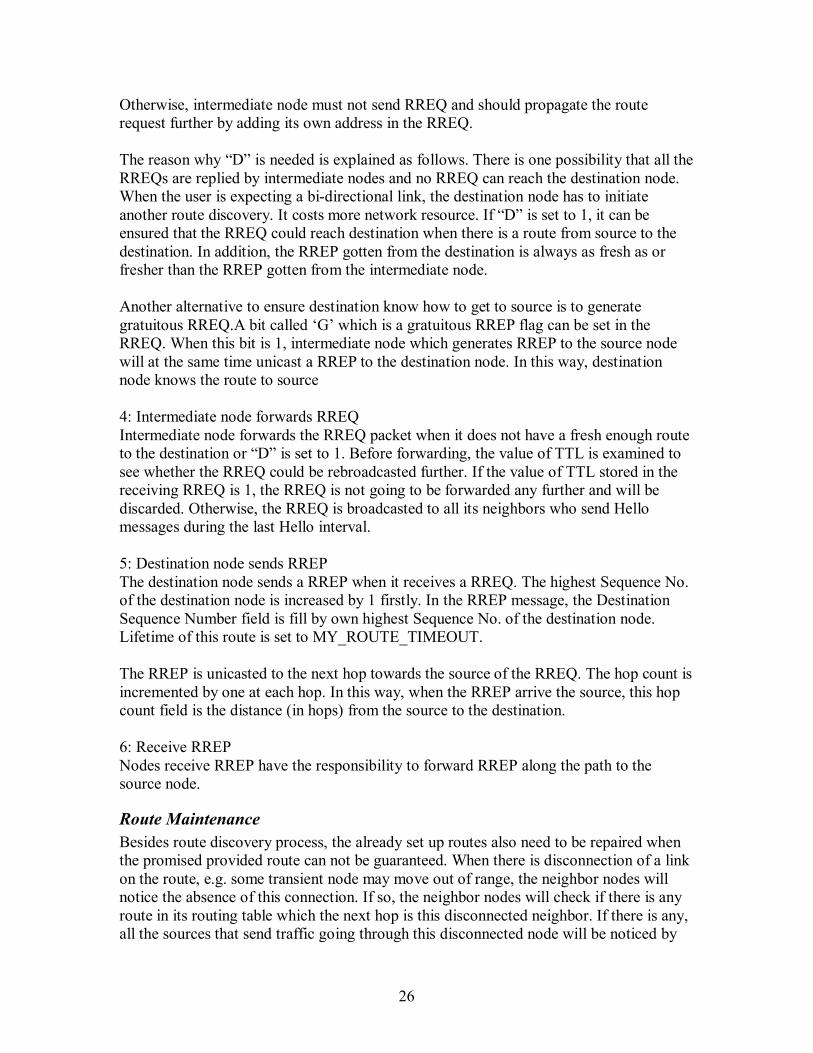
26

Otherwise, intermediate node must not send RREQ and should propagate the route request further by adding its own address in the RREQ. The reason why �D� is needed is explained as follows. There is one possibility that all the RREQs are replied by intermediate nodes and no RREQ can reach the destination node. When the user is expecting a bi-directional link, the destination node has to initiate another route discovery. It costs more network resource. If �D� is set to 1, it can be ensured that the RREQ could reach destination when there is a route from source to the destination. In addition, the RREP gotten from the destination is always as fresh as or fresher than the RREP gotten from the intermediate node. Another alternative to ensure destination know how to get to source is to generate gratuitous RREQ.A bit called �G� which is a gratuitous RREP flag can be set in the RREQ. When this bit is 1, intermediate node which generates RREP to the source node will at the same time unicast a RREP to the destination node. In this way, destination node knows the route to source 4: Intermediate node forwards RREQ Intermediate node forwards the RREQ packet when it does not have a fresh enough route to the destination or �D� is set to 1. Before forwarding, the value of TTL is examined to see whether the RREQ could be rebroadcasted further. If the value of TTL stored in the receiving RREQ is 1, the RREQ is not going to be forwarded any further and will be discarded. Otherwise, the RREQ is broadcasted to all its neighbors who send Hello messages during the last Hello interval. 5: Destination node sends RREP The destination node sends a RREP when it receives a RREQ. The highest Sequence No. of the destination node is increased by 1 firstly. In the RREP message, the Destination Sequence Number field is fill by own highest Sequence No. of the destination node. Lifetime of this route is set to MY_ROUTE_TIMEOUT. The RREP is unicasted to the next hop towards the source of the RREQ. The hop count is incremented by one at each hop. In this way, when the RREP arrive the source, this hop count field is the distance (in hops) from the source to the destination. 6: Receive RREP Nodes receive RREP have the responsibility to forward RREP along the path to the source node.

Route Maintenance Besides route discovery process, the already set up routes also need to be repaired when the promised provided route can not be guaranteed. When there is disconnection of a link on the route, e.g. some transient node may move out of range, the neighbor nodes will notice the absence of this connection. If so, the neighbor nodes will check if there is any route in its routing table which the next hop is this disconnected neighbor. If there is any, all the sources that send traffic going through this disconnected node will be noticed by

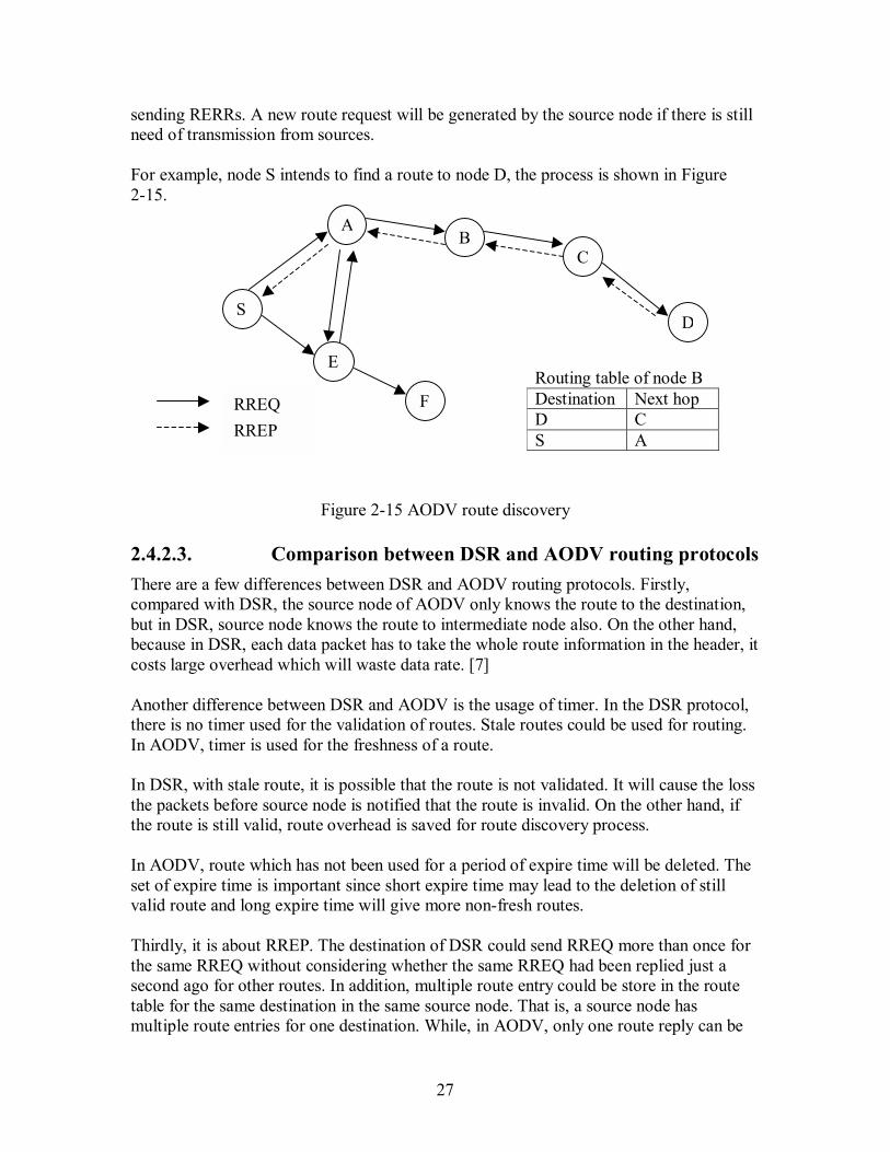
27

sending RERRs. A new route request will be generated by the source node if there is still need of transmission from sources. For example, node S intends to find a route to node D, the process is shown in Figure 2-15.

Figure 2-15 AODV route discovery

2.4.2.3. Comparison between DSR and AODV routing protocols There are a few differences between DSR and AODV routing protocols. Firstly, compared with DSR, the source node of AODV only knows the route to the destination, but in DSR, source node knows the route to intermediate node also. On the other hand, because in DSR, each data packet has to take the whole route information in the header, it costs large overhead which will waste data rate. [7] Another difference between DSR and AODV is the usage of timer. In the DSR protocol, there is no timer used for the validation of routes. Stale routes could be used for routing. In AODV, timer is used for the freshness of a route. In DSR, with stale route, it is possible that the route is not validated. It will cause the loss the packets before source node is notified that the route is invalid. On the other hand, if the route is still valid, route overhead is saved for route discovery process. In AODV, route which has not been used for a period of expire time will be deleted. The set of expire time is important since short expire time may lead to the deletion of still valid route and long expire time will give more non-fresh routes. Thirdly, it is about RREP. The destination of DSR could send RREQ more than once for the same RREQ without considering whether the same RREQ had been replied just a second ago for other routes. In addition, multiple route entry could be store in the route table for the same destination in the same source node. That is, a source node has multiple route entries for one destination. While, in AODV, only one route reply can be

A

RREQ RREP

DS

B

E

C

FRouting table of node B Destination Next hop D C S A

28

sent by the destination and only one route entry per destination is stored in the route table. The advantage of having more than one route entry per destination is that it can provide backup routes when there is a break on the current route. It means that there is no need to send a RREQ again to search for the route. On the other side, if the network has high mobility, the freshness of the back up route could be a problem and reinitiate a new RREQ should be a better choice. With the above analysis, it is found that AODV protocol should perform better in high mobility ad hoc network.

2.4.3. Hybrid routing protocol-Zone Routing Protocol

Zone Routing Protocol (ZRP) is a hybrid routing protocol. It effectively combines the advantages of both proactive and reactive routing protocols. The key concept used in this protocol is to use a proactive routing within a zone in the r-hop neighborhood of every node and use a reactive routing for nodes outside this zone. The table driven scope is limited within a zone and when a destination is out of the table driven scope, on demand routing search is initiated. In this situation, control overhead is reduced, compared to both the route request flooding mechanism employed in on demand protocols and periodic flooding of routing information packet in table driven protocol. [1, pp. 336]

2.4.4. Power-aware routing protocols

Power aware routing protocols aim at minimizing the consumption of an important resource in ad hoc network: battery power. To achieve that, the routing decisions are made based on the consumption of power. That is during the design of routing protocols, route cost less power will have more possibility to be chosen. Energy needed to transmit a signal is proportional to the square of the distance between transmitter and receiver. Transmitting a signal with half of the distance requires one fourth of the energy and if there is a node in the middle willing spend another fourth of its energy for the second half distance, data would be transmitted for half of the energy compared with the one going through a direct transmission. This however may introduce a delay, but this is the basic way that energy is saved. In the following part, two of the most effective power routing algorithms are discussed as follows Method 1: Minimum Total Transmission Power Routing (MTPR) [8]

)Cost(n)(nP)n,(nPC jjrtransceivejitransmitji ++= (2-2) The above formula calculates the power cost from source to destination. Cij is a cumulative power value from the source node to node I through node j who is the neighbour of node i, that is the cost from node i to node j. Ptransmit(ni,nj) is the transmission power consumed from node i to node j (here node i and node j are neighbor), Ptransceiver(nj)

29

is signal processing the power consumed at the transceiver j, Cost(nj) is the power cost from source node to node j. The following formula is used to choose the lowest power consumption route from source to node i.

ji,NH(i)ji Cmin )Cost(n ∈= , where NH(i) = {j; nj is a neighbor node of ni} (2-3) It is actually to choose a neighbour node of node i through whom the source could cost the minimum power to node i. With this method, the source could find a route to other nodes on the network with minimum consumption power. Method 2: Flow Augmentation algorithm [9]

x3i

x2i

xiijij )(E)E()(eC −= (2-4)

This method introduces a different method to calculate the cost consumed for a link. The cost include not only the cost for consuming power at the link but also the cost of running the energy out at node, that is, how much energy left on the node is considered by taking the initial energy and the residual energy as shown in the above formula. In the above formula, Cij is the cost of link (i,j), eij is the energy cost for unit flow transmission over the link. iE is the initial energy at nodes and Ei is the residual energy at node i. x1, x2, x3 are three non-negative factors. By giving the value of these three values, we could define the weights of link unit flow transmission, initial energy and residual energy in the algorithm. For example when {x1, x2, x3} = {0, 0, 0}, it means that Cij is one and hop count become the only route metric. {x1, x2, x3} should be selected properly to maximize the transmissions in the ad hoc network. The above two methods give a basic idea of how power aware routing protocols are designed. That is, to take energy consumption as the most important path selection metric. Power saving and maximizing the use of power in order to transmit more traffic on the network are the aim. In the next part, in load aware routing protocols will be introduced, and the aim becomes to balance the load on the network.

2.4.5. Load-Aware Routing Protocols

In load aware routing protocols, load information is utilized as the path selection metric for routing in MANETs. There are multiple schemes which are load-aware, and the ways of calculating the load at nodes are different. They are shown in the following paragraphs. [10] The first one is Dynamic Load-Aware Routing (DLAR) protocol. In DLAR, network load is defined as the number of on going traffic in its interface queue. The routing decisions

30

will be made by comparing the queuing length of the node. That is, only the delay that caused by queuing is considered. In Load-Balanced Ad hoc Routing (LBAR) protocol, the network load is defined as the total number of routes passing through the node and its neighbors. The Load-Sensitive Routing (LSR) protocol defines network load in a node as the summation of the number of packets being queued in the interface of the mobile host and its neighboring hosts. LSR protocol is more accurate than DLAR and LBAR since it considers both the traffic queuing at the current considering node and the traffic condition at the neighbor node, whereas it does not consider the effect of access contentions in the MAC layer (e.g. using IEEE 802.11). For example, we consider Node A and Node A� each of which has one queued packet. Node A has three neighbors, and number of packet queued in each neighbors is one. Node A� has only one neighbor having 3 queued packets. The total load for Node A and Node A� are equal if calculated using LSR protocol, but Node A will have higher potential contention delay than Node A�. By taking the contention delay into account, Delay-Oriented Shortest Path Routing (DOSPR) is proposed by analyzing the medium access delay in IEEE 802.11 wireless network. The last load aware routing protocol discussed here is Delay-based Load aware on demand routing (D-LAOR) protocol utilizes both the estimated total path delay and hop count as the route selection criterion. A time stamp is placed on each packet header. The average total node delay is calculated from the previous average total node delay and successful transmission delay of this time at this node. This averaged total delay includes the queuing, contention and transmission delays. The total path delay will be the summation of average total delay of the nodes that it went through. This D-LOAR is implemented on AODV protocol with some modifications during the path discovery. If the duplicated RREQ packet has a smaller total path delay and hop count than the previous one, the destination will send RREP packet again to the source node to change the route immediately, since the route with smaller delay should be chosen. In conclusion, the above routing schemes are designed based on the load at nodes of the network. Nodes with smaller load which might cause lower delay are preferred to be chosen and this method also balances the load on the network.

2.5. Chapter summary

In this chapter, an overview of mobile ad hoc networks is given. The history of ad hoc networks is outlined. Many applications in ad hoc networks are discussed. The principles of PHY and MAC layers in IEEE 802.11 are discussed in detail. Routing protocols including proactive, reactive, and many other kind of routing protocols are discussed. In

31

addition, routing protocols are compared to see differences. In the next chapter, QoS aware routing protocols will be introduced.

32

3. QoS-aware routing protocols in Ad Hoc networks

In this chapter, general concepts of QoS are introduced first. It includes the QoS definition, QoS parameters, the aim of QoS in different layers and systems, and the existing model for QoS. Since, in this thesis, the QoS is mainly discussed aiming at real time traffics, the difference between real time traffic and non-real time traffic are compared to show the need of QoS for real time services. After that, challenges of achieving QoS in ad hoc networks are presented. The generally used parameters in the routing layer of ad hoc network are shown. The mort important part in this chapter is the summarization of the calculation of metrics, including delay and data rate. The detailed steps of computing the available data rate of nodes with different methods are given. Finally, two QoS aware routing protocols for ad hoc network are introduced.

3.1. Definition of QoS

�Quality of Service is the performance level of a service offered by the network to the user�. [1, pp. 505] In the originally used network model, traffic is transmitted only with best-effort. It means that there is no quality guarantee for each transmission. When with the real-time traffic is transmitted in the network, QoS becomes demanding. In addition, because of the limitation of network resources especially in wireless networks, real time traffic need to be given higher priority to ensure that the real time traffic arrives the destination on time.

3.2. QoS parameters

QoS parameters differ from application to application. For example, for multimedia applications, the data rate and delay are the key factors, whereas, in military use, security and reliability become more important. If considering QoS required by emergency cases such as rescue, the key factor should be the availability. In sensor networks, battery life and energy conservation would be the prime QoS parameters. The QoS parameter considered here is aimed to real time applications. In real time applications, QoS requests can be expressed in term of many metrics in routing protocols. The most popular metrics are data rate and delay. To satisfy QoS requirements, the corresponding available data rate and delay that could be provided by the network of each route should be calculated in order to see which route could be used

33

with satisfying QoS. As a result, we will see how available data rate and delay are calculated.

3.3. Real time traffic vs. non real time traffic

Why does real-time traffic require QoS? It is because there are some essential differences between the non-real time data and real-time data. [11] For the transmission of non-real time data, timing is not a critical issue, the data is elastic. As a result, the non-real time network could work well without guarantee of timely delivery of data. But it always has high requirement for packet loss. Retransmissions are used if there are some lost packets. The applications of non real time data transmissions are Telnet, FTP, E-mail and web browsing. For real time transmission like telephone, video conference, streaming video and audio, the basic requirement is to transmit packets to the destination on time. People cannot tolerate large delay for example on the phone. As a result, some QoS mechanisms are badly needed to ensure the required quality of the connection.

3.4. QoS in different layers

QoS of a network can be considered at different layers. QoS considered in physical layer means the quality in terms of transmission performance. For example, through transmission power control both the stations that are near the sender or far away from the sender could hear the signal clearly with different transmission power. Power control is used both to ensure the quality of reception and to optimize the capacity. QoS implemented in MAC layer is also important. It could provide high probability of access with low delay when stations with higher user priority want to access the wireless medium. For example, in wireless LANs shorter back off time is set to achieve it, as described in Section 2.3.8 based on IEEE 802.11e. QoS implemented in the routing layer aims to find a route which provides the required quality. The metric which helps to choose the route is not only the number of needed hops along the route but also some other metrics like maximum delay and minimum data rate, e.g. QAODV described in Section 0. There are also some QoS frameworks, e.g. Stateless Wireless Ad Hoc Networks (SWAN) framework.

34

3.5. QoS models

The existing QoS models can be classified into two types based on their fundamental operations. The QoS models are Integrated Service (IntServ) and Differentiated Services (DiffServ). [11] IntServ is a fine grained approach which provides QoS to individual applications or flows. It uses Resource Reservation Protocol (RSVP) to provide a circuit switched service in packet switched network. IntServ decides whether the desired service could be provided with the current available network resource. Admission control is performed to new flows. The admission of each new flow might cause interference to the already existing flows. One of the responsibilities of admission control is that the interference caused by adding a new flow should not make QoS of old flows get worse than it has required. The drawback of IntServ is the scalability problem. This is caused by the need of storing every flow state in the routes. DiffServ provides QoS to large classes of data or aggregated traffic. It is a coarse grained approach. It maps flows into a set of service levels. In DiffServ, routers are divided into two types: edge routers and core routers. Edge routers are at the boundary of the networks. In edge routers, traffic will be classified, conditioned and assigned to different behavior aggregate when it traverse between different networks. The word �different networks� means for example networks that belong to different Internet Service Providers (ISP). Differentiated Services Code Points (DSCP) bits are reformatted which represent the Type of Service (ToS) in Internet Protocol (IP) header. Core routers forward packets based on this ToS field. In addition, core routes also need to follow the per-hope behavior (PHB) which takes charge of scheduling of packets. IntServ eliminated the need of keeping the flow state information somewhere in the network.

3.6. Challenge of QoS routing in ad hoc networks

Mobile ad hoc networks differ from the traditional wired networks. They have certain unique characteristics which cause difficulties for providing QoS in such networks. The unique characteristics are dynamically varying network topology, lack of precise state information, shared radio channel, limited resource availability, hidden terminal problem and insecure medium. [1, pp. 508-509] These characteristics and their effects on ad hoc networks will be discussed in this part one by one. # Dynamically varying network topology In mobile ad hoc networks, nodes are mobile and network topology is changing dynamically. Consequently, the route which is already set up with required QoS could not satisfy QoS anymore if one of the nodes on this established route moves. For example, a node could move to an area with more interference to it. The node whose data rate has been overused should take some actions. The information about loss of QoS should be sent by this node to all sources whose transmission is going through the overloaded node.

35

Sources who receive this message have to find another possible route by using QoS aware routing protocol again. This procedure will cause delay which may not be acceptable. # Lack of precise state information Due to the dynamic characteristic, information of nodes transmitted to other nodes may change right after this information is transmitted to its neighbors. The information here can be the data rate available at the neighboring node, since available data rate of nodes is affected by the data rate of its neighbors as will be discussed in Section 3.9.4. As a result, this information which is already transmitted may have been out of date and it may lead to a wrong routing decision. # Shared radio channel Data transmitted on the radio channel can be received by stations which are in the carrier sensing range of the transmitter. This broadcast characteristic will cause interference to other stations when traffic is transmitted over the air interface. Thus, stations have to share channel with neighbors in their carrier sensing range. This is very different from the wired channel which will not cause that much interference between each other because of proper construction of lines that attenuates crosstalk interference significantly. # Limited resource availability The resources such as data rate, battery life, and storage space are all very limited in ad hoc networks. The battery life in a sensor network is a very good example. In a sensor network, each sensor has very limited battery life, so routing based on power consumption is widely considered. The data rate is very limited for wireless links if we compared it with the data rate available in wired network. In addition, the basic characteristics of the wireless channel e.g. fading, noise, and shared data rate between neighbor nodes (neighbor nodes have to keep silent when it senses some node is transmitting) will also degrade the wireless data rate The actual radio data rate becomes much smaller. As a result, it is hard for a wireless network to provide too high data rate which could be provided by the wired network. It also brings problem of cooperation between wireless network and wired network.

3.7. Classification of generally used metrics

The QoS metrics can be classified into three categories. They are additive metrics, concave metrics, and multiplicative metrics. Additive metrics is defined as sum of the value of the metric on all links along the path. Delay and jitter are additive metrics. Delay along the path is the sum of the delay at every link along the path. A concave metric means the minimum metric value over a path. Metric value on every link along the path is taken into account. The minimum metric value stands for the metric value of the whole path. Data rate is a concave metric. The minimum data rate of all the links along the path

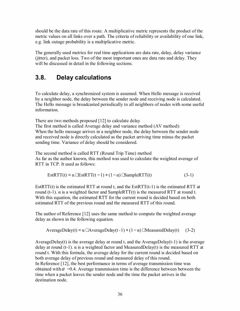
36

should be the data rate of this route. A multiplicative metric represents the product of the metric values on all links over a path. The criteria of reliability or availability of one link, e.g. link outage probability is a multiplicative metric. The generally used metrics for real time applications are data rate, delay, delay variance (jitter), and packet loss. Two of the most important ones are data rate and delay. They will be discussed in detail in the following sections.

3.8. Delay calculations

To calculate delay, a synchronized system is assumed. When Hello message is received by a neighbor node, the delay between the sender node and receiving node is calculated. The Hello message is broadcasted periodically to all neighbors of nodes with some useful information. There are two methods proposed [12] to calculate delay The first method is called Average delay and variance method (AV method): When the hello message arrives in a neighbor node, the delay between the sender node and received node is directly calculated as the packet arriving time minus the packet sending time. Variance of delay should be considered. The second method is called RTT (Round Trip Time) method As far as the author known, this method was used to calculate the weighted average of RTT in TCP. It used as follows:

t)SampleRTT(α)(11)EstRTT(tαEstRTT(t) ∗−+−∗= (3-1) EstRTT(t) is the estimated RTT at round t, and the EstRTT(t-1) is the estimated RTT at round (t-1). α is a weighted factor and SampleRTT(t) is the measured RTT at round t. With this equation, the estimated RTT for the current round is decided based on both estimated RTT of the previous round and the measured RTT of this round. The author of Reference [12] uses the same method to compute the weighted average delay as shown in the following equation.

lay(t)MeasuredDeα)(11)-ay(tAverageDelαay(t)AverageDel ∗−+∗= (3-2) AverageDelay(t) is the average delay at round t, and the AverageDelay(t-1) is the average delay at round (t-1). α is a weighted factor and MeasuredDelay(t) is the measured RTT at round t. With this formula, the average delay for the current round is decided based on both average delay of previous round and measured delay of this round. In Reference [12], the best performance in terms of average transmission time was obtained withα =0.4. Average transmission time is the difference between between the time when a packet leaves the sender node and the time the packet arrives in the destination node.

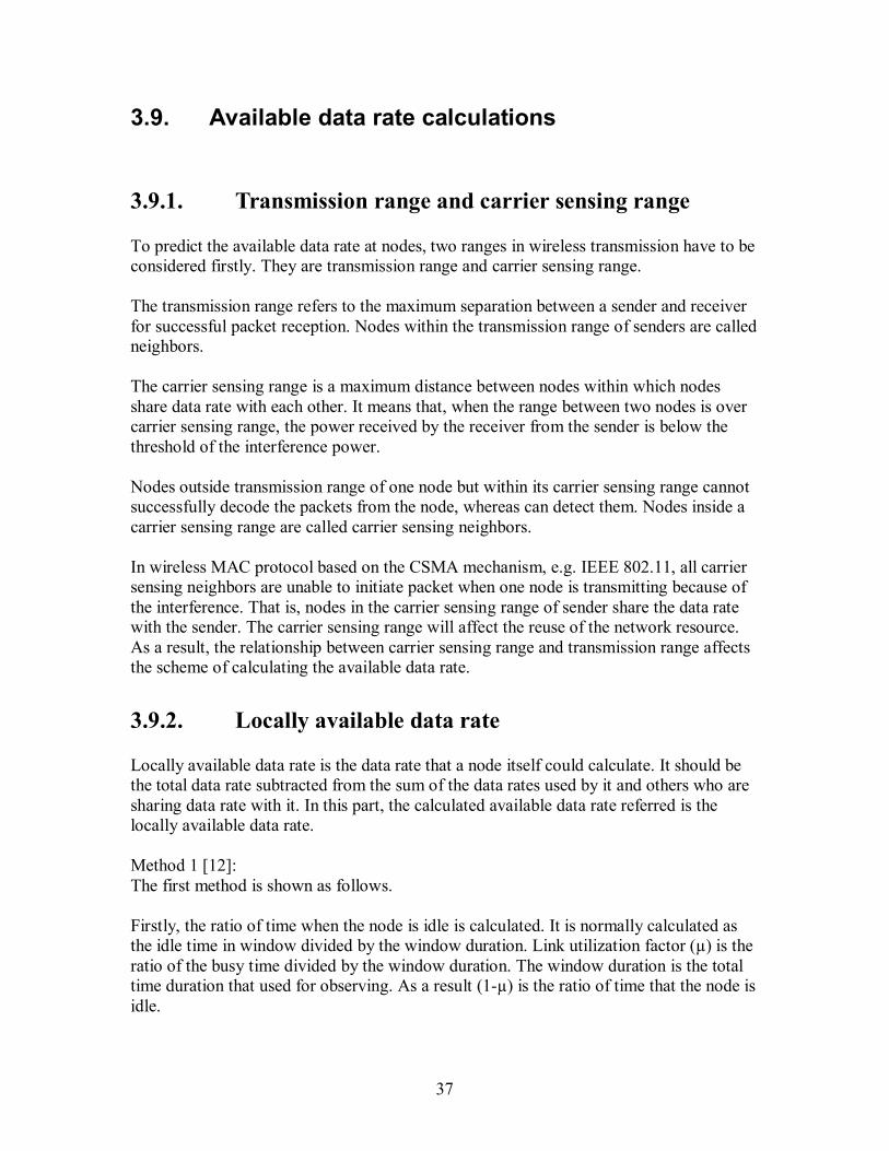
37

3.9. Available data rate calculations

3.9.1. Transmission range and carrier sensing range

To predict the available data rate at nodes, two ranges in wireless transmission have to be considered firstly. They are transmission range and carrier sensing range. The transmission range refers to the maximum separation between a sender and receiver for successful packet reception. Nodes within the transmission range of senders are called neighbors. The carrier sensing range is a maximum distance between nodes within which nodes share data rate with each other. It means that, when the range between two nodes is over carrier sensing range, the power received by the receiver from the sender is below the threshold of the interference power. Nodes outside transmission range of one node but within its carrier sensing range cannot successfully decode the packets from the node, whereas can detect them. Nodes inside a carrier sensing range are called carrier sensing neighbors. In wireless MAC protocol based on the CSMA mechanism, e.g. IEEE 802.11, all carrier sensing neighbors are unable to initiate packet when one node is transmitting because of the interference. That is, nodes in the carrier sensing range of sender share the data rate with the sender. The carrier sensing range will affect the reuse of the network resource. As a result, the relationship between carrier sensing range and transmission range affects the scheme of calculating the available data rate.

3.9.2. Locally available data rate

Locally available data rate is the data rate that a node itself could calculate. It should be the total data rate subtracted from the sum of the data rates used by it and others who are sharing data rate with it. In this part, the calculated available data rate referred is the locally available data rate. Method 1 [12]: The first method is shown as follows. Firstly, the ratio of time when the node is idle is calculated. It is normally calculated as the idle time in window divided by the window duration. Link utilization factor (µ) is the ratio of the busy time divided by the window duration. The window duration is the total time duration that used for observing. As a result (1-µ) is the ratio of time that the node is idle.

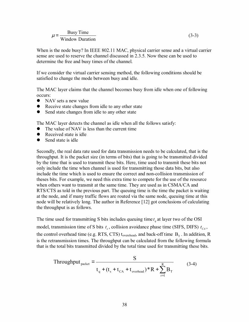
38

Duration WindowTimeBusy =µ (3-3)

When is the node busy? In IEEE 802.11 MAC, physical carrier sense and a virtual carrier sense are used to reserve the channel discussed in 2.3.5. Now these can be used to determine the free and busy times of the channel. If we consider the virtual carrier sensing method, the following conditions should be satisfied to change the mode between busy and idle. The MAC layer claims that the channel becomes busy from idle when one of following occurs: # NAV sets a new value # Receive state changes from idle to any other state # Send state changes from idle to any other state The MAC layer detects the channel as idle when all the follows satisfy: # The value of NAV is less than the current time # Received state is idle # Send state is idle Secondly, the real data rate used for data transmission needs to be calculated, that is the throughput. It is the packet size (in terms of bits) that is going to be transmitted divided by the time that is used to transmit these bits. Here, time used to transmit these bits not only include the time when channel is used for transmitting those data bits, but also include the time which is used to ensure the correct and non-collision transmission of theses bits. For example, we need this extra time to compete for the use of the resource when others want to transmit at the same time. They are used as in CSMA/CA and RTS/CTS as told in the previous part. The queuing time is the time the packet is waiting at the node, and if many traffic flows are routed via the same node, queuing time at this node will be relatively long. The author in Reference [12] got conclusions of calculating the throughput is as follows. The time used for transmitting S bits includes queuing time qt at layer two of the OSI model, transmission time of S bits st , collision avoidance phase time (SIFS, DIFS) CAt , the control overhead time (e.g. RTS, CTS) toverehead, and back-off time TB . In addition, R is the retransmission times. The throughput can be calculated from the following formula that is the total bits transmitted divided by the total time used for transmitting these bits.

∑=

++++= R

1rToverheadCAsq

packet

BR*)tt(tt

SThroughput (3-4)

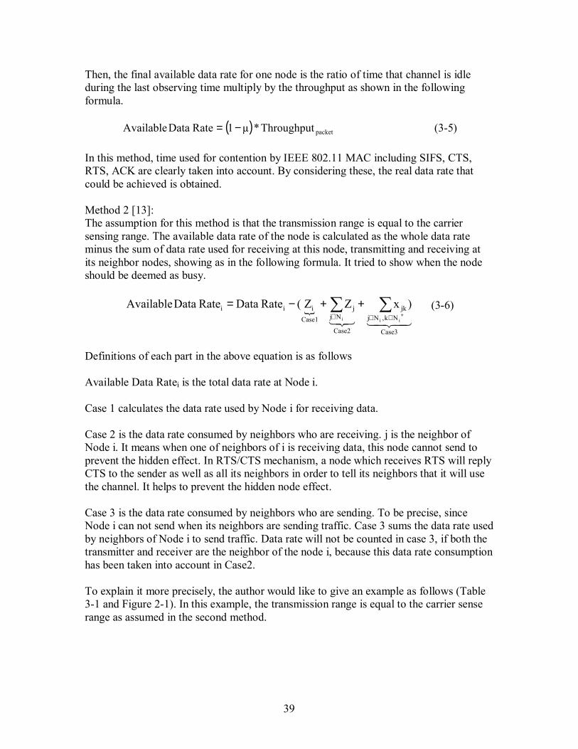
39

Then, the final available data rate for one node is the ratio of time that channel is idle during the last observing time multiply by the throughput as shown in the following formula.

( ) packetThroughput*µ1Rate Data Available −= (3-5) In this method, time used for contention by IEEE 802.11 MAC including SIFS, CTS, RTS, ACK are clearly taken into account. By considering these, the real data rate that could be achieved is obtained. Method 2 [13]: The assumption for this method is that the transmission range is equal to the carrier sensing range. The available data rate of the node is calculated as the whole data rate minus the sum of data rate used for receiving at this node, transmitting and receiving at its neighbor nodes, showing as in the following formula. It tried to show when the node should be deemed as busy.

{43421321

Case3

Nk,Njjk

Case2

Njj

Case1iii

iii

)xZZ(Rate DataRate Data Available ∑∑+∉∈∈

++−= (3-6)

Definitions of each part in the above equation is as follows Available Data Ratei is the total data rate at Node i. Case 1 calculates the data rate used by Node i for receiving data. Case 2 is the data rate consumed by neighbors who are receiving. j is the neighbor of Node i. It means when one of neighbors of i is receiving data, this node cannot send to prevent the hidden effect. In RTS/CTS mechanism, a node which receives RTS will reply CTS to the sender as well as all its neighbors in order to tell its neighbors that it will use the channel. It helps to prevent the hidden node effect. Case 3 is the data rate consumed by neighbors who are sending. To be precise, since Node i can not send when its neighbors are sending traffic. Case 3 sums the data rate used by neighbors of Node i to send traffic. Data rate will not be counted in case 3, if both the transmitter and receiver are the neighbor of the node i, because this data rate consumption has been taken into account in Case2. To explain it more precisely, the author would like to give an example as follows (Table 3-1 and Figure 2-1). In this example, the transmission range is equal to the carrier sense range as assumed in the second method.

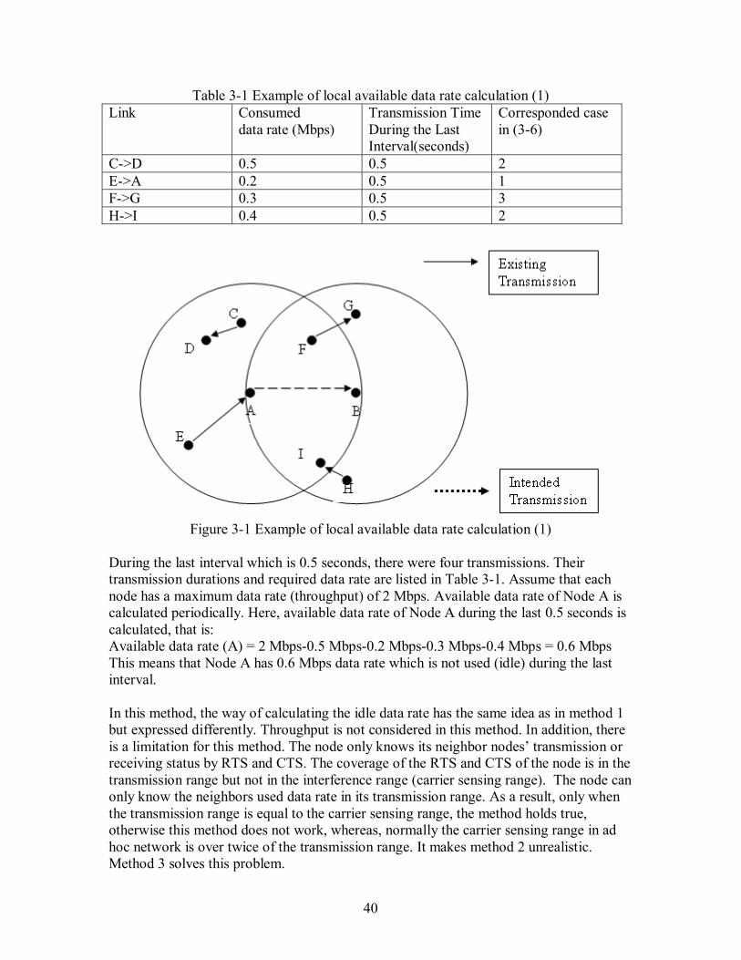
40

Table 3-1 Example of local available data rate calculation (1) Link Consumed

data rate (Mbps) Transmission Time During the Last Interval(seconds)

Corresponded case in (3-6)

C->D 0.5 0.5 2 E->A 0.2 0.5 1 F->G 0.3 0.5 3 H->I 0.4 0.5 2

Figure 3-1 Example of local available data rate calculation (1)

During the last interval which is 0.5 seconds, there were four transmissions. Their transmission durations and required data rate are listed in Table 3-1. Assume that each node has a maximum data rate (throughput) of 2 Mbps. Available data rate of Node A is calculated periodically. Here, available data rate of Node A during the last 0.5 seconds is calculated, that is: Available data rate (A) = 2 Mbps-0.5 Mbps-0.2 Mbps-0.3 Mbps-0.4 Mbps = 0.6 Mbps This means that Node A has 0.6 Mbps data rate which is not used (idle) during the last interval. In this method, the way of calculating the idle data rate has the same idea as in method 1 but expressed differently. Throughput is not considered in this method. In addition, there is a limitation for this method. The node only knows its neighbor nodes� transmission or receiving status by RTS and CTS. The coverage of the RTS and CTS of the node is in the transmission range but not in the interference range (carrier sensing range). The node can only know the neighbors used data rate in its transmission range. As a result, only when the transmission range is equal to the carrier sensing range, the method holds true, otherwise this method does not work, whereas, normally the carrier sensing range in ad hoc network is over twice of the transmission range. It makes method 2 unrealistic. Method 3 solves this problem.

41

Method 3 [14]: The third method has been implemented by people using Network Simulator 2. In this method, the sum of the size of sent, received and sensed packets during the last duration T is calculated. This method considers all the packets which are sensed and since the carrier sensing range is the actual interference range, it makes this method more realistic. As shown in the following formula the used data rate is the sum of the sent, received and sensed bits divided by the duration T. N is the number of packets the node has sent, received and sensed. S is the size of the packets. Since the packet is originally expressed with the unit of Byte, the total number of bytes is multiplied by 8 to get the unit in bits.

Τ8SΝ bps Rate Data )/∗∗(=)( (3-7) There is a tradeoff in the length of data rate calculation interval T. The longer the value of T, the more accurate the BW is. On the other hand, if people take smaller value for T, then the response for available data rate is faster. That is, data rate is updated more frequently, and the actions taken by node adaptive more quickly. In the simulation that will be done in Section 5, T is set to be 0.5s. In this method, the available data rate is calculated by subtracting the used data rate in the carrier sense range. It is more realistic compared to Method 2. Example for Method 3: The carrier sense range is 550m and the transmission range is 250m. According to Table 3-2 and Figure 3-2, Nodes B, C, D, E, F, I, are all in the transmission range of Node A, Nodes G, H, J, K are in the carrier sense range of Node A but do not in the transmission range of Node A. As a result, according to Method 3, all the data rates that consumed in these neighbors should be taken into account. The available data rate of Node A Available Data rate (Node A) = 2 � (0.2/0.5)*0.5-(0.4/0.5)*0.2-(0.5/0.5)*0.3-(0.3/0.5)*0.4-(0.3/0.5)*0.5= 0.8 Mbps

Table 3-2 Example of local available data rate calculation (2) Link Consumed

Data rate (Mbps) Transmission Time During the Last Interval(seconds)

C->D 0.5 0.2 E->A 0.2 0.4 F->G 0.3 0.5 H->I 0.4 0.3 J->K 0.5 0.3

42

Figure 3-2 Example of local available data rate calculation (2)

Data rate consumption and available data rate for nodes calculation are considered in MAC layer. The required data rate at the application layer is multiplied by some factor to predict the consumed bandwidth in MAC layer in NS2 by showing the consideration of MAC header for RTS-CTS-ACK packets. The factor that will be used in the simulation in Section 5 is 1.4.

3.9.3. Listen Mode and Hello Mode

In the above three methods, the consumed data rate of one node is always considered to be calculated by the node itself. That is, nodes by listening to the channel judge how much data rate is used by others who are in its interference (carrier sensing) range. Another method is to estimate the residual data rate by getting information from exchanging Hello messages. The current data rate of the sender as well as the current data rate usage of the one-hop neighbors of the sender is piggybacked onto the standard �Hello� message. Through Hello message, nodes could know the data rate that is used by its carrier sensing neighbors. [19]

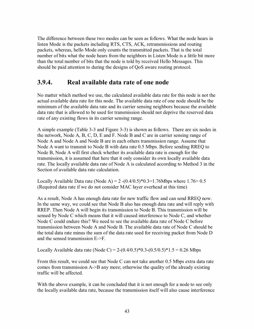
43

The difference between these two modes can be seen as follows. What the node hears in listen Mode is the packets including RTS, CTS, ACK, retransmissions and routing packets, whereas, hello Mode only counts the transmitted packets. That is the total number of bits what the node hears from the neighbors in Listen Mode is a little bit more than the total number of bits that the node is told by received Hello Messages. This should be paid attention to during the designs of QoS aware routing protocol.

3.9.4. Real available data rate of one node

No matter which method we use, the calculated available data rate for this node is not the actual available data rate for this node. The available data rate of one node should be the minimum of the available data rate and its carrier sensing neighbors because the available data rate that is allowed to be used for transmission should not deprive the reserved data rate of any existing flows in its carrier sensing range. A simple example (Table 3-3 and Figure 3-3) is shown as follows. There are six nodes in the network, Node A, B, C, D, E and F. Node B and C are in carrier sensing range of Node A and Node A and Node B are in each others transmission range. Assume that Node A want to transmit to Node B with data rate 0.5 Mbps. Before sending RREQ to Node B, Node A will first check whether its available data rate is enough for the transmission, it is assumed that here that it only consider its own locally available data rate. The locally available data rate of Node A is calculated according to Method 3 in the Section of available data rate calculation. Locally Available Data rate (Node A) = 2 -(0.4/0.5)*0.3=1.76Mbps where 1.76> 0.5 (Required data rate if we do not consider MAC layer overhead at this time) As a result, Node A has enough data rate for new traffic flow and can send RREQ now. In the same way, we could see that Node B also has enough data rate and will reply with RREP. Then Node A will begin its transmission to Node B. This transmission will be sensed by Node C which means that it will caused interference to Node C, and whether Node C could endure this? We need to see the available data rate of Node C before transmission between Node A and Node B. The available data rate of Node C should be the total data rate minus the sum of the data rate used for receiving packet from Node D and the sensed transmission E->F. Locally Available data rate (Node C) = 2-(0.4/0.5)*0.3-(0.5/0.5)*1.5 = 0.26 Mbps From this result, we could see that Node C can not take another 0.5 Mbps extra data rate comes from transmission A->B any more; otherwise the quality of the already existing traffic will be affected. With the above example, it can be concluded that it is not enough for a node to see only the locally available data rate, because the transmission itself will also cause interference

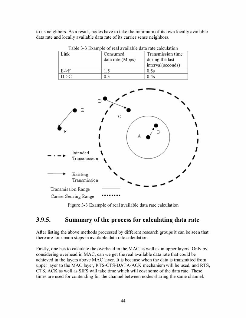
44

to its neighbors. As a result, nodes have to take the minimum of its own locally available data rate and locally available data rate of its carrier sense neighbors.

Table 3-3 Example of real available data rate calculation Link Consumed

data rate (Mbps) Transmission time during the last interval(seconds)

E->F 1.5 0.5s D->C 0.3 0.4s

Figure 3-3 Example of real available data rate calculation

3.9.5. Summary of the process for calculating data rate

After listing the above methods processed by different research groups it can be seen that there are four main steps in available data rate calculation. Firstly, one has to calculate the overhead in the MAC as well as in upper layers. Only by considering overhead in MAC, can we get the real available data rate that could be achieved in the layers above MAC layer. It is because when the data is transmitted from upper layer to the MAC layer, RTS-CTS-DATA-ACK mechanism will be used, and RTS, CTS, ACK as well as SIFS will take time which will cost some of the data rate. These times are used for contending for the channel between nodes sharing the same channel.

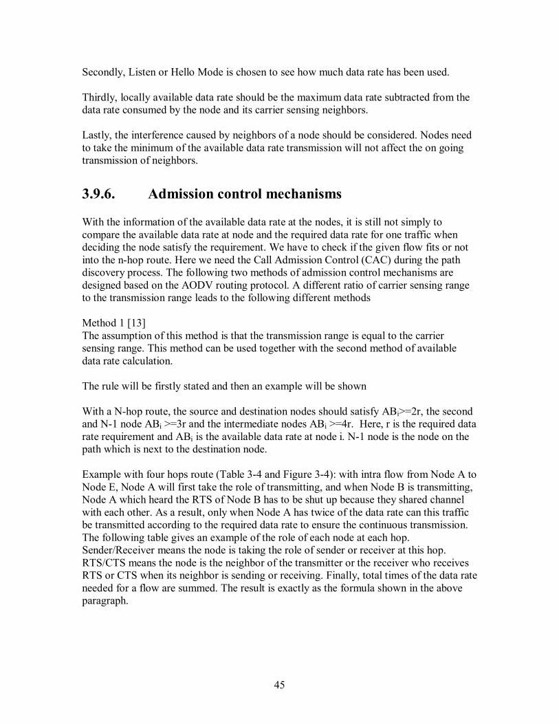
45

Secondly, Listen or Hello Mode is chosen to see how much data rate has been used. Thirdly, locally available data rate should be the maximum data rate subtracted from the data rate consumed by the node and its carrier sensing neighbors. Lastly, the interference caused by neighbors of a node should be considered. Nodes need to take the minimum of the available data rate transmission will not affect the on going transmission of neighbors.

3.9.6. Admission control mechanisms

With the information of the available data rate at the nodes, it is still not simply to compare the available data rate at node and the required data rate for one traffic when deciding the node satisfy the requirement. We have to check if the given flow fits or not into the n-hop route. Here we need the Call Admission Control (CAC) during the path discovery process. The following two methods of admission control mechanisms are designed based on the AODV routing protocol. A different ratio of carrier sensing range to the transmission range leads to the following different methods Method 1 [13] The assumption of this method is that the transmission range is equal to the carrier sensing range. This method can be used together with the second method of available data rate calculation. The rule will be firstly stated and then an example will be shown With a N-hop route, the source and destination nodes should satisfy ABi>=2r, the second and N-1 node ABi >=3r and the intermediate nodes ABi >=4r. Here, r is the required data rate requirement and ABi is the available data rate at node i. N-1 node is the node on the path which is next to the destination node. Example with four hops route (Table 3-4 and Figure 3-4): with intra flow from Node A to Node E, Node A will first take the role of transmitting, and when Node B is transmitting, Node A which heard the RTS of Node B has to be shut up because they shared channel with each other. As a result, only when Node A has twice of the data rate can this traffic be transmitted according to the required data rate to ensure the continuous transmission. The following table gives an example of the role of each node at each hop. Sender/Receiver means the node is taking the role of sender or receiver at this hop. RTS/CTS means the node is the neighbor of the transmitter or the receiver who receives RTS or CTS when its neighbor is sending or receiving. Finally, total times of the data rate needed for a flow are summed. The result is exactly as the formula shown in the above paragraph.

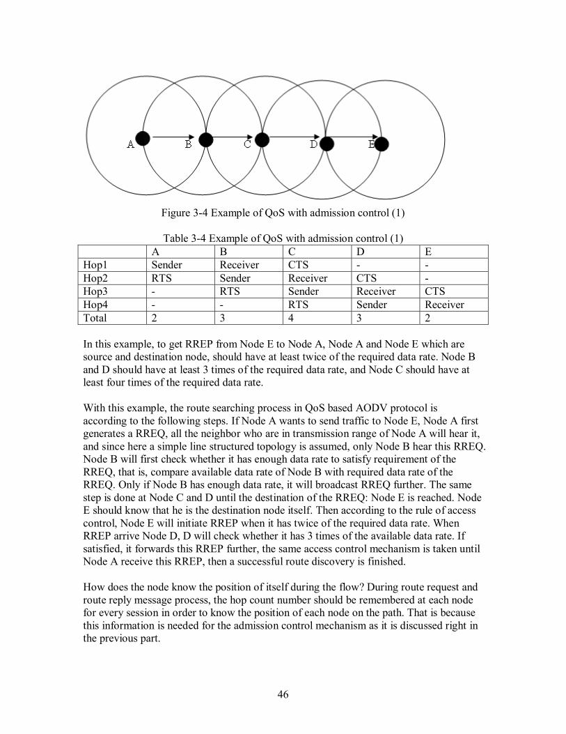
46

Figure 3-4 Example of QoS with admission control (1)

Table 3-4 Example of QoS with admission control (1)

A B C D E Hop1 Sender Receiver CTS - - Hop2 RTS Sender Receiver CTS - Hop3 - RTS Sender Receiver CTS Hop4 - - RTS Sender Receiver Total 2 3 4 3 2 In this example, to get RREP from Node E to Node A, Node A and Node E which are source and destination node, should have at least twice of the required data rate. Node B and D should have at least 3 times of the required data rate, and Node C should have at least four times of the required data rate. With this example, the route searching process in QoS based AODV protocol is according to the following steps. If Node A wants to send traffic to Node E, Node A first generates a RREQ, all the neighbor who are in transmission range of Node A will hear it, and since here a simple line structured topology is assumed, only Node B hear this RREQ. Node B will first check whether it has enough data rate to satisfy requirement of the RREQ, that is, compare available data rate of Node B with required data rate of the RREQ. Only if Node B has enough data rate, it will broadcast RREQ further. The same step is done at Node C and D until the destination of the RREQ: Node E is reached. Node E should know that he is the destination node itself. Then according to the rule of access control, Node E will initiate RREP when it has twice of the required data rate. When RREP arrive Node D, D will check whether it has 3 times of the available data rate. If satisfied, it forwards this RREP further, the same access control mechanism is taken until Node A receive this RREP, then a successful route discovery is finished. How does the node know the position of itself during the flow? During route request and route reply message process, the hop count number should be remembered at each node for every session in order to know the position of each node on the path. That is because this information is needed for the admission control mechanism as it is discussed right in the previous part.

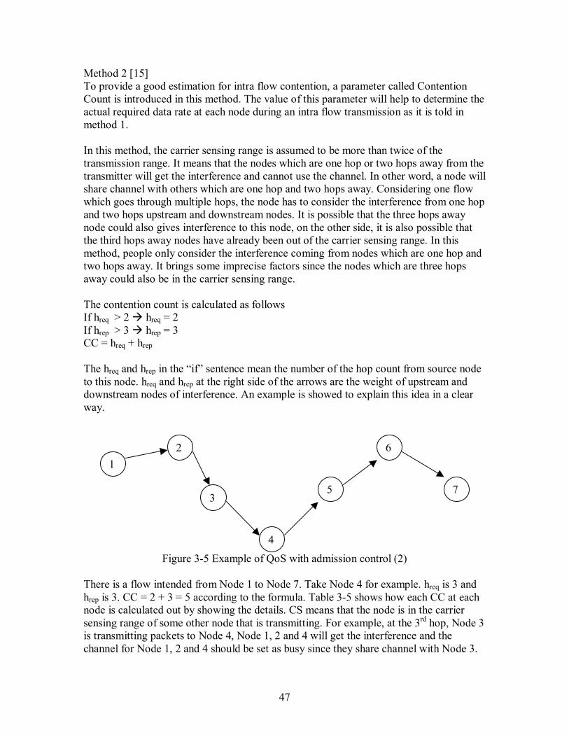
47

Method 2 [15] To provide a good estimation for intra flow contention, a parameter called Contention Count is introduced in this method. The value of this parameter will help to determine the actual required data rate at each node during an intra flow transmission as it is told in method 1. In this method, the carrier sensing range is assumed to be more than twice of the transmission range. It means that the nodes which are one hop or two hops away from the transmitter will get the interference and cannot use the channel. In other word, a node will share channel with others which are one hop and two hops away. Considering one flow which goes through multiple hops, the node has to consider the interference from one hop and two hops upstream and downstream nodes. It is possible that the three hops away node could also gives interference to this node, on the other side, it is also possible that the third hops away nodes have already been out of the carrier sensing range. In this method, people only consider the interference coming from nodes which are one hop and two hops away. It brings some imprecise factors since the nodes which are three hops away could also be in the carrier sensing range. The contention count is calculated as follows If hreq > 2 $ hreq = 2 If hrep > 3 $ hrep = 3 CC = hreq + hrep

The hreq and hrep in the �if� sentence mean the number of the hop count from source node to this node. hreq and hrep at the right side of the arrows are the weight of upstream and downstream nodes of interference. An example is showed to explain this idea in a clear way.

Figure 3-5 Example of QoS with admission control (2)

There is a flow intended from Node 1 to Node 7. Take Node 4 for example. hreq is 3 and hrep is 3. CC = 2 + 3 = 5 according to the formula. Table 3-5 shows how each CC at each node is calculated out by showing the details. CS means that the node is in the carrier sensing range of some other node that is transmitting. For example, at the 3rd hop, Node 3 is transmitting packets to Node 4, Node 1, 2 and 4 will get the interference and the channel for Node 1, 2 and 4 should be set as busy since they share channel with Node 3.

1 2

3

4

5

6

7

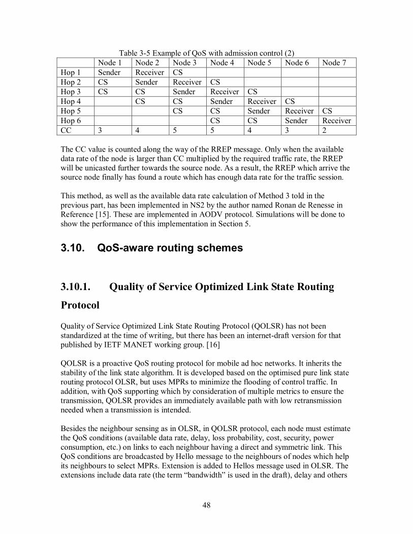
48

Table 3-5 Example of QoS with admission control (2) Node 1 Node 2 Node 3 Node 4 Node 5 Node 6 Node 7 Hop 1 Sender Receiver CS Hop 2 CS Sender Receiver CS Hop 3 CS CS Sender Receiver CS Hop 4 CS CS Sender Receiver CS Hop 5 CS CS Sender Receiver CS Hop 6 CS CS Sender Receiver CC 3 4 5 5 4 3 2 The CC value is counted along the way of the RREP message. Only when the available data rate of the node is larger than CC multiplied by the required traffic rate, the RREP will be unicasted further towards the source node. As a result, the RREP which arrive the source node finally has found a route which has enough data rate for the traffic session. This method, as well as the available data rate calculation of Method 3 told in the previous part, has been implemented in NS2 by the author named Ronan de Renesse in Reference [15]. These are implemented in AODV protocol. Simulations will be done to show the performance of this implementation in Section 5.

3.10. QoS-aware routing schemes

3.10.1. Quality of Service Optimized Link State Routing

Protocol

Quality of Service Optimized Link State Routing Protocol (QOLSR) has not been standardized at the time of writing, but there has been an internet-draft version for that published by IETF MANET working group. [16] QOLSR is a proactive QoS routing protocol for mobile ad hoc networks. It inherits the stability of the link state algorithm. It is developed based on the optimised pure link state routing protocol OLSR, but uses MPRs to minimize the flooding of control traffic. In addition, with QoS supporting which by consideration of multiple metrics to ensure the transmission, QOLSR provides an immediately available path with low retransmission needed when a transmission is intended. Besides the neighbour sensing as in OLSR, in QOLSR protocol, each node must estimate the QoS conditions (available data rate, delay, loss probability, cost, security, power consumption, etc.) on links to each neighbour having a direct and symmetric link. This QoS conditions are broadcasted by Hello message to the neighbours of nodes which help its neighbours to select MPRs. Extension is added to Hellos message used in OLSR. The extensions include data rate (the term �bandwidth� is used in the draft), delay and others

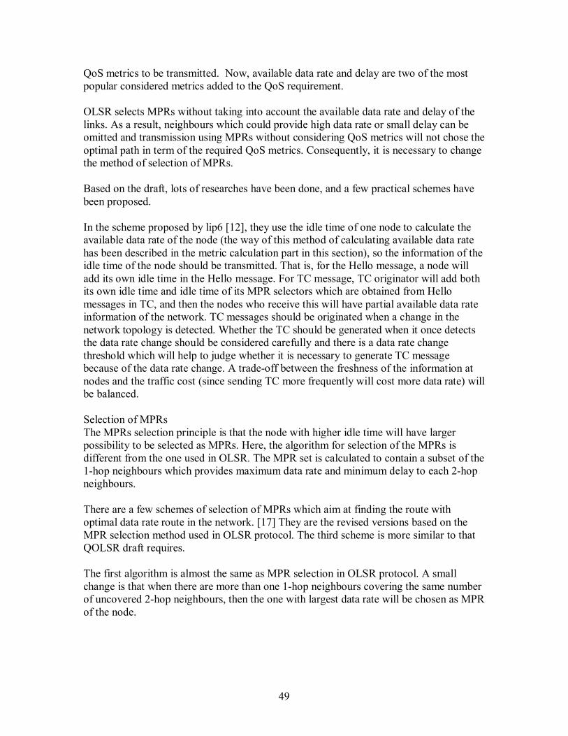
49

QoS metrics to be transmitted. Now, available data rate and delay are two of the most popular considered metrics added to the QoS requirement. OLSR selects MPRs without taking into account the available data rate and delay of the links. As a result, neighbours which could provide high data rate or small delay can be omitted and transmission using MPRs without considering QoS metrics will not chose the optimal path in term of the required QoS metrics. Consequently, it is necessary to change the method of selection of MPRs. Based on the draft, lots of researches have been done, and a few practical schemes have been proposed. In the scheme proposed by lip6 [12], they use the idle time of one node to calculate the available data rate of the node (the way of this method of calculating available data rate has been described in the metric calculation part in this section), so the information of the idle time of the node should be transmitted. That is, for the Hello message, a node will add its own idle time in the Hello message. For TC message, TC originator will add both its own idle time and idle time of its MPR selectors which are obtained from Hello messages in TC, and then the nodes who receive this will have partial available data rate information of the network. TC messages should be originated when a change in the network topology is detected. Whether the TC should be generated when it once detects the data rate change should be considered carefully and there is a data rate change threshold which will help to judge whether it is necessary to generate TC message because of the data rate change. A trade-off between the freshness of the information at nodes and the traffic cost (since sending TC more frequently will cost more data rate) will be balanced. Selection of MPRs The MPRs selection principle is that the node with higher idle time will have larger possibility to be selected as MPRs. Here, the algorithm for selection of the MPRs is different from the one used in OLSR. The MPR set is calculated to contain a subset of the 1-hop neighbours which provides maximum data rate and minimum delay to each 2-hop neighbours. There are a few schemes of selection of MPRs which aim at finding the route with optimal data rate route in the network. [17] They are the revised versions based on the MPR selection method used in OLSR protocol. The third scheme is more similar to that QOLSR draft requires. The first algorithm is almost the same as MPR selection in OLSR protocol. A small change is that when there are more than one 1-hop neighbours covering the same number of uncovered 2-hop neighbours, then the one with largest data rate will be chosen as MPR of the node.

50

Figure 3-6 Example of MPRs calculation

With the network topology shown in Figure 3-6, Node B can reach the 2-hop neighbours Node D and E through 1-hop neighbours Node C and F. Node B will select Node F as the MPR, because the data rate between Node B to Node C is smaller than the data rate from Node B to Node D.

Table 3-6 Example of MPRs calculation (1) Node 1 Hop Neighbours 2 Hop neighbours MPRs B A, C, F, G D, E F In the second algorithm, the neighbours with best data rate are selected as MPRs until all the neighbours are covered. That is, the link with highest data rate will be selected first no matter how many 2-hop neighbours it connects to. Thus more MPRs might be selected for one node in QOLSR than in OLSR, because in OLSR, the 1-hop neighbour who reaches maximum number of 2-hop neighbours will be selected first. If considering the MPR of Node B according to Figure 3-6, Nodes A and F will be selected. Among neighbours of Node B, Node A, C and F have connection to its 2-hop neighbours. Node A which has the highest connection with Node B among these three will be firstly selected and with the selection of Node A, Node D is covered. Next, Node F is selected which has the second highest data rate, and Node E is covered.

Table 3-7 Example of MPRs calculation (2) Node 1 Hop Neighbours 2 Hop neighbours MPRs B A, C, F, G D, E A, F In the third algorithm, all the 2-hop neighbours will get the optimal data rate path through MPRs to the node. It is more close to what QOLSR requires. That is, among the entire possible path from the node to its 2-hop neighbours, the path with the highest bandwidth will be chosen, and the corresponding used 1-hop neighbour will be chosen as MPR.

50 110

5

6

2

4

3

61

1

100

A

D

B

C

F

E

G

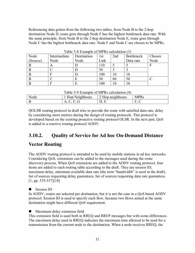
51

Referencing data gotten from the following two tables, from Node B to the 2-hop destination Node D, route goes through Node F has the highest bottleneck data rate. With the same principle, from Node B to the 2-hop destination Node E, route goes through Node C has the highest bottleneck data rate. Node F and Node C are chosen to be MPRs.

Table 3-8 Example of MPRs calculation (3) Node (Source)

Intermediate Node

Destination Node

1st Link

2nd Bottleneck Data rate

Chosen Node

B A D 110 5 5 B C D 50 3 3 B F D 100 10 10

F

B C E 50 60 50 B F E 100 10 10

C

Table 3-9 Example of MPRs calculation (4)

Node 1 Hop Neighbours 2 Hop neighbours MPRs B A, C, F, G D, E F, C QOLSR routing protocol in draft tries to provide the route with satisfied data rate, delay by considering more metrics during the design of routing protocols. This protocol is developed based on the existing proactive routing protocol OLSR. In the next part, QoS is added to a reactive routing protocol AODV.

3.10.2. Quality of Service for Ad hoc On-Demand Distance

Vector Routing

The AODV routing protocol is intended to be used by mobile stations in ad hoc networks. Considering QoS, extensions can be added to the messages used during the route discovery process. When QoS extensions are added to the AODV routing protocol, four items are added to each routing table according to the draft. They are session ID, maximum delay, minimum available data rate (the term �bandwidth� is used in the draft), list of sources requesting delay guarantees, list of sources requesting data rate guarantees. [1, pp. 535-537][18] % Session ID In AODV, routes are selected per destination, but it is not the case in a QoS based AODV protocol. Session ID is used to specify each flow, because two flows aimed at the same destination might have different QoS requirement. % Maximum delay extension field This extension field is used both in RREQ and RREP messages but with some differences. The maximum delay used in RREQ indicates the maximum time allowed to be used for a transmission from the current node to the destination. When a node receives RREQ, the

52

maximum delay will be compared with the node traversal time (should include queuing delays, interrupt processing times and transfer times). If the maximum allowable delay is smaller than the node traversal time, the RREQ will not be broadcasted further, otherwise, the RREQ will be broadcasted and before the broadcasting, traversal time of this node must be subtracted from the maximum delay field in RREQ message. In RREP message, the maximum delay extension field will be filled with zeroes, and delays are cumulative from the destination along the route that the RREP come from to the source node, and the source node will choose the one satisfying the delay requirement. % Minimum data rate extension field When the node receives a RREQ, it will compare the available data rate with the one required in this extension field and only the one that satisfies certain condition could forward the RREQ further. % List of sources requesting QoS guarantees A QoS_Lost message is generated when the QoS could not be satisfied (node traversal time increase or available data rate decrease. It needs a list of sources whose traffic is affected by this change. Comparing with AODV, in QoS based ADOV, we have RREQ, including the QoS requirement, and only the node satisfying this request could broadcast the RREQ further. In addition, the intermediate node cannot give the RREP even if it knows how to get to the destination, since data rate should be tested at each hop until to the destination. What�s more, the network should have periodic mechanisms for checking the available data rate at each node. Because of the mobility of the node, the available data rate of one node is changing with the changing of its neighbors who are sharing data rate with it. If the available data rate of a node becomes smaller than zero, it means that the node cannot afford the current traffic any more. Source of the traffic going through this node should be noticed.

3.11. Chapter summary

This chapter gave an overview of the basic concepts about QoS including the definition, parameters, and models of QoS. It also summarized some existing schemes for QoS aware routing protocols. The methods of calculating QoS parameter including data rate and delay are shown and analyzed. Finally, QoS aware AODV protocol and QoS aware OLSR routing protocol are discussed according to the references of the existing drafts.

53

4. Implementation of the QAODV routing protocol in

Network Simulator 2

This chapter is divided into two parts. The first part will describe the simulation tools. Since NS2 is very difficult for beginners, it might be useful to know the beginner�s experience of using NS2. Many relevant tools used to analyze trace files will be introduced at a beginner level. The second part will analyze the code from Ronan de Renesse about QAODV routing protocol. With this simulation code, comparisons will be shown in Section 5 between the AODV and the QAODV routing protocols.

4.1. Simulation tools

4.1.1. Introduction to NS2

�NS is a discrete event simulator targeted at networking research. NS provides substantial support for simulation of TCP, routing, and multicast protocols over wired and wireless (local and satellite) networks.� [22]

4.1.1.1. History of NS NS started as a variant of the original network simulator made in 1989 and many modifications are made during the past years. In 1995, the development of NS became supported by The Defense Advanced Research Projects Agency (DARPA) through the Virtual InterNetwork Testbed (VINT) project at Xerox Palo Alto research Center (PARC), and at the Information Sciences Institute (USC/ISI) of the University of Southern California, etc. Currently, NS development is supported through DARPA with Simulation Augmented by Measurement and Analysis for Networks (SAMAN) and National Science Foundation (NSF) with Collaborative Simulation for Education and Research (CONSER), in collaboration with other researchers including The ICSI (International Computer Science Institute) Center for Internet Research (ICIR). [22]

4.1.1.2. Operation system and installation of NS NS can run under both UNIX and Windows operating systems. There are many components needed to be installed before running NS. The user can choose to install it partly or completely. For beginners it is suggested to make a complete installation which automatically installs all necessary components at once and it requires 320 MB disk space. Installing it partly could save some disk space.

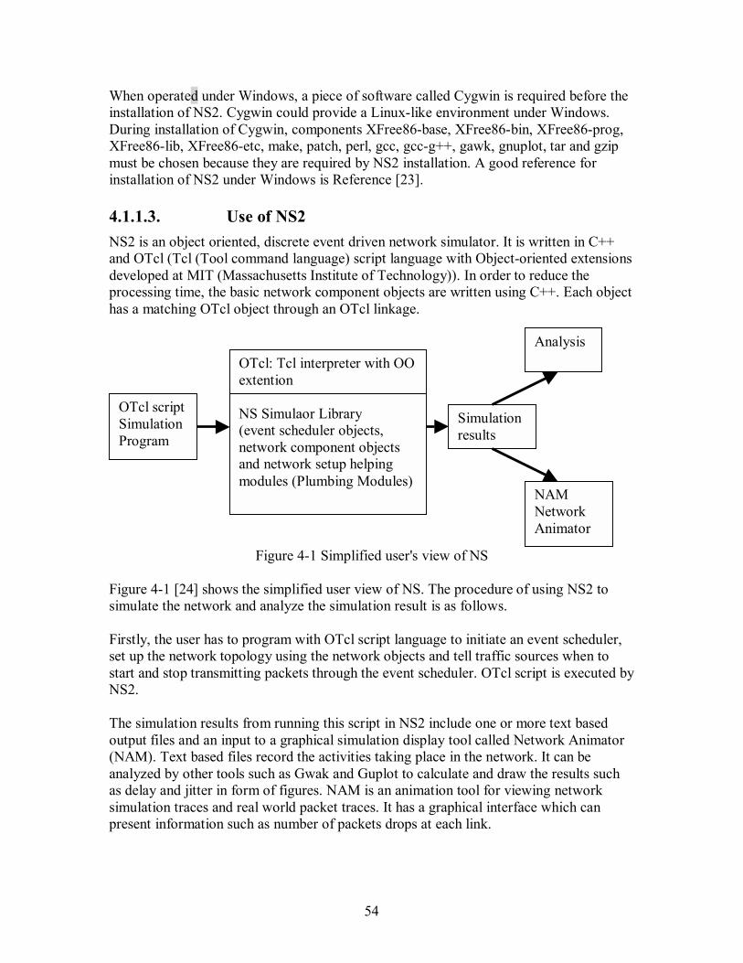
54

When operated under Windows, a piece of software called Cygwin is required before the installation of NS2. Cygwin could provide a Linux-like environment under Windows. During installation of Cygwin, components XFree86-base, XFree86-bin, XFree86-prog, XFree86-lib, XFree86-etc, make, patch, perl, gcc, gcc-g++, gawk, gnuplot, tar and gzip must be chosen because they are required by NS2 installation. A good reference for installation of NS2 under Windows is Reference [23].

4.1.1.3. Use of NS2 NS2 is an object oriented, discrete event driven network simulator. It is written in C++ and OTcl (Tcl (Tool command language) script language with Object-oriented extensions developed at MIT (Massachusetts Institute of Technology)). In order to reduce the processing time, the basic network component objects are written using C++. Each object has a matching OTcl object through an OTcl linkage.

Figure 4-1 Simplified user's view of NS

Figure 4-1 [24] shows the simplified user view of NS. The procedure of using NS2 to simulate the network and analyze the simulation result is as follows. Firstly, the user has to program with OTcl script language to initiate an event scheduler, set up the network topology using the network objects and tell traffic sources when to start and stop transmitting packets through the event scheduler. OTcl script is executed by NS2. The simulation results from running this script in NS2 include one or more text based output files and an input to a graphical simulation display tool called Network Animator (NAM). Text based files record the activities taking place in the network. It can be analyzed by other tools such as Gwak and Guplot to calculate and draw the results such as delay and jitter in form of figures. NAM is an animation tool for viewing network simulation traces and real world packet traces. It has a graphical interface which can present information such as number of packets drops at each link.

OTcl: Tcl interpreter with OO extention NS Simulaor Library (event scheduler objects, network component objects and network setup helping modules (Plumbing Modules)

OTcl script Simulation Program

Simulation results

Analysis

NAM Network Animator

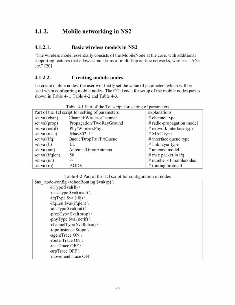
55

4.1.2. Mobile networking in NS2

4.1.2.1. Basic wireless models in NS2 �The wireless model essentially consists of the MobileNode at the core, with additional supporting features that allows simulations of multi-hop ad-hoc networks, wireless LANs etc.� [20]

4.1.2.2. Creating mobile nodes To create mobile nodes, the user will firstly set the value of parameters which will be used when configuring mobile nodes. The OTcl code for setup of the mobile nodes part is shown in Table 4-1, Table 4-2 and Table 4-3.

Table 4-1 Part of the Tcl script for setting of parameters Part of the Tcl script for setting of parameters Explanations set val(chan) Channel/WirelessChannel set val(prop) Propagation/TwoRayGround set val(netif) Phy/WirelessPhy set val(mac) Mac/802_11 set val(ifq) Queue/DropTail/PriQueue set val(ll) LL set val(ant) Antenna/OmniAntenna set val(ifqlen) 50 set val(nn) 6 set val(rp) AODV

;# channel type ;# radio-propagation model ;# network interface type ;# MAC type ;# interface queue type ;# link layer type ;# antenna model ;# max packet in ifq ;# number of mobilenodes ;# routing protocol

Table 4-2 Part of the Tcl script for configuration of nodes

$ns_ node-config -adhocRouting $val(rp) \ -llType $val(ll) \ -macType $val(mac) \ -ifqType $val(ifq) \ -ifqLen $val(ifqlen) \ -antType $val(ant) \ -propType $val(prop) \ -phyType $val(netif) \ -channelType $val(chan) \ -topoInstance $topo \ -agentTrace ON \ -routerTrace ON \ -macTrace OFF \ -arpTrace OFF \ -movementTrace OFF

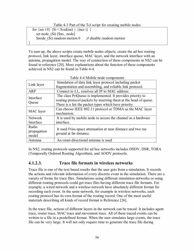
56

Table 4-3 Part of the Tcl script for creating mobile nodes for {set i 0} {$i < $val(nn) } {incr i} { set node_($i) [$ns_ node] $node_($i) random-motion 0 ;# disable random motion } To sum up, the above scripts create mobile nodes objects; create the ad hoc routing protocol, link layer, interface queue, MAC layer, and the network interface with an antenna, propagation model. The way of connection of these components in NS2 can be found in reference [20]. More explanations about the function of these components achieved in NS2 can be found in Table 4-4.

Table 4-4 Mobile node components

Link layer Simulation of data link layer protocol including packet fragmentation and assembling, and reliable link protocol.

ARP Connect to LL, resolves all IP to MAC address.

Interface Queue

The class PriQueue is implemented. It provides priority to routing protocol packets by inserting them at the head of queue. There is a list the packet types which have priority.

MAC layer Can choose IEEE 802.11 protocol or TDMA as the MAC layer mechanism.

Network Interface

It is used by mobile node to access the channel as a hardware interface.

Radio propagation model

It used Friss-space attenuation at near distance and two ray ground at far distance.

Antenna An omni-directional antenna is used In NS2, routing protocols supported for ad hoc networks includes DSDV, DSR, TORA (Temporally Ordered Routing Algorithm), and AODV protocols.

4.1.2.3. Trace file formats in wireless networks Trace file is one of the text based results that the user gets from a simulation. It records the actions and relevant information of every discrete event in the simulation. There are a variety of forms for trace files. Simulations using different simulation networks or using different routing protocols could get trace files having different trace file formats. For example, a wired network and a wireless network have absolutely different format for recording each event. In the same network, for example in wireless networks, each routing protocol has its own format of the routing record. One of the most useful materials describing all kinds of record format is Reference [26]. In the trace file, actions of different layers in the network can be traced. It includes agent trace, router trace, MAC trace and movement trace. All of these traced events can be written to a file in a predefined format. When the user simulates large events, the trace file can be very large. It will not only require time to generate the trace file during

57

simulation but also need space to store it. As a result, user should always choose part of the choices to trace. For example, in simulation of Section 5, the author would always take the agent trace and the router trace on, and MAC trace and movement trace off, since what the author interested in is the actions of nodes in the routing layer. An example of one record in the wireless trace file is listed as follows: r 5.000000000 _3_ RTR --- 2 cbr 512 [0 0 0 0] ------- [3:1 4:0 32 0] [0] 0 0 The word �field� which will be used to explain the above record means a component which is separated by spaces. The first field can be r, s, f and D for received, send, forward and drop. The second field gives occurring times for the event. The third field is the node number. The fourth field is the trace name that can be AGT, RTR, MAC, and IFQ. AGT, RTR and MAC represent transport, routing and MAC layer separately. IFQ indicate events related to the interface priority queue. The number after the dashes is a globally unique sequence number of a packet. The letters after the number give the traffic type. Traffic types can be CBR (Constant Bit Rate), TCP (Transport Control Protocol) and ACK. The number right after the packet type is the packet size in bytes. The following two square brackets separated by the dashes are MAC and routing layer information such as source and destination addresses. With the information recorded in each event, performance metrics such as packet delivery ratio, throughput, packet loss, and end-to-end delay can be calculated with the help of some additional programs, e.g. Gawk, Perl, Gnuplot and Tracegraph.

4.1.3. Tools used in NS2

4.1.3.1. Generation of node movement A tool called �setdest� is developed by CMU (Carnegie Mellon University) for generating random movements of nodes in the wireless network. It defines node movements with specific moving speed toward a random or specified location within a fixed area. When the node arrives to the movement location, it could be set to stop for a period of time. After that, the node keeps on moving towards the next location. The location setdest is at the directory of ~ns/indep-utils/cmu-scen-gen/setdest/. Users need to run �make� before they use setdest. The format of the command of setdest is as follows and explanations of each option are shown in Table 4-5. ./setdest [-n num_of_nodes] [-p pausetime] [-s maxspeed] [-t simtime] [-x maxx] [-y maxy] > [outdir/movement-file]

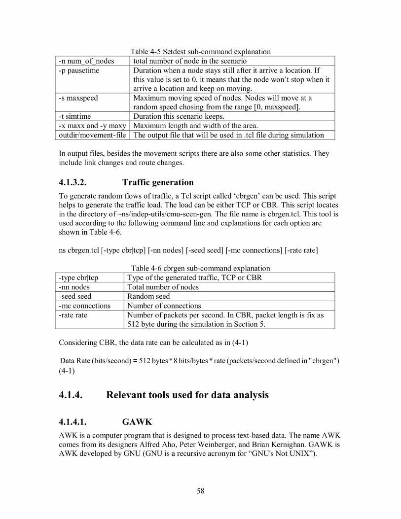
58

Table 4-5 Setdest sub-command explanation -n num_of_nodes total number of node in the scenario -p pausetime Duration when a node stays still after it arrive a location. If

this value is set to 0, it means that the node won�t stop when it arrive a location and keep on moving.

-s maxspeed Maximum moving speed of nodes. Nodes will move at a random speed chosing from the range [0, maxspeed].

-t simtime Duration this scenario keeps. -x maxx and -y maxy Maximum length and width of the area. outdir/movement-file The output file that will be used in .tcl file during simulation In output files, besides the movement scripts there are also some other statistics. They include link changes and route changes.

4.1.3.2. Traffic generation To generate random flows of traffic, a Tcl script called �cbrgen� can be used. This script helps to generate the traffic load. The load can be either TCP or CBR. This script locates in the directory of ~ns/indep-utils/cmu-scen-gen. The file name is cbrgen.tcl. This tool is used according to the following command line and explanations for each option are shown in Table 4-6. ns cbrgen.tcl [-type cbr|tcp] [-nn nodes] [-seed seed] [-mc connections] [-rate rate]

Table 4-6 cbrgen sub-command explanation -type cbr|tcp Type of the generated traffic, TCP or CBR -nn nodes Total number of nodes -seed seed Random seed -mc connections Number of connections -rate rate Number of packets per second. In CBR, packet length is fix as

512 byte during the simulation in Section 5. Considering CBR, the data rate can be calculated as in (4-1)

)cbrgen""in defined econd(packets/s rate*bits/bytes 8*bytes 512 nd)(bits/seco Rate Data = (4-1)

4.1.4. Relevant tools used for data analysis

4.1.4.1. GAWK AWK is a computer program that is designed to process text-based data. The name AWK comes from its designers Alfred Aho, Peter Weinberger, and Brian Kernighan. GAWK is AWK developed by GNU (GNU is a recursive acronym for �GNU's Not UNIX�).

59

Using AWK, a command file and an input file should be given. A command file can be a file or a command line input. The command file would tell AWK how to deal with the input file. It is composed of patterns and actions. For an input file, every line of the input file will be examined to judge whether this line matches the pattern. If this is the case, this line will be processed by the corresponding action. During the processing of the input file, GAWK will first separate the input file into pieces of records. The record separator is �\n� by default. That is why AWK normally parses the file line by line. Each record is composed of several fields; different fields are separated by white space by default. In the command file, �$1� represents the first field of a record. In actions, GAWK uses �printf� to print out the processing result. BEGIN and END are two special patterns in GAWK. Their corresponding actions are executed only at the beginning and the ending of the execution of a command file. An example of using GAWK can be seen in Appendix C.

4.1.4.2. BASH BASH (Bourne-Again SHell) is developed by Brian Fox and Chet Ramey. It is the most common shell in Linux. In this thesis work, it is used to generate loops when simulations with the same scenario requirements are needed to be done many times to get the average results. The scenarios referred are generated by tools in NS2 randomly but with the same scenario requirements. An example of using GAWK can be seen in Appendix A.

4.2. Details of the QAODV in NS2

4.2.1. General idea of the QAODV routing protocol

An idea of the QAODV protocol with Access Admission Control (AAC) is implemented on an existing AODV protocol in NS2. The method of calculating the available data rate and AAC has been shown in Section 3.9.2 Method 3 and Section 3.9.6 Method 2 respectively. This work is done by a PhD student named Ronan de Renesse. In this section, the idea of how QoS is added to the AODV is analyzed based on the code written by Ronan de Renesse. The main point is to introduce what are added to the AODV in order to achieve the QAODV. Figure 4-2 shows the main changes that the author did to modify the routing protocol from the AODV to the QAODV routing protocol. Some data rate restrictions are added during the transmission of the AODV routing packets. The frames with dot lines mean the changes based on the AODV routing protocol. In QAODV, only when the node has enough available data rate, it can forward the AODV routing packets (e.g. RREQ, and RREP). In addition, the available data rate of each node is defined as a fixed number in advance. The maximum available data rate is

60

decided by doing trials in NS2 in AODV with the same environment when simulating the QAODV. With this experiment, the maximum accumulative throughput is tried to get between nodes who are sharing the same data rate. The way of estimating the maximum data rate with trials will be described in Section 5.1. All the nodes in the network will be checked in with periodical intervals, since the usage of the data rate of nodes might change with time caused by e.g. movement of nodes. Nodes with available data rate below zero means that the node is overloaded. Traffic going through this node cannot be guaranteed any more. Source nodes generating these traffics will be noticed by ICMP_QoS_Lost messages and the corresponding traffic will be stopped at the source node. Two new parameters, route request session ID and request data rate are added in the routing protocol. This is because each session requesting different data rate may choose a different route; the route is not per destinations but per session in QAODV, The mechanism of admission control for intra flow is added. It uses Method 2 as admission control mechanism in Section. 3.9.6.

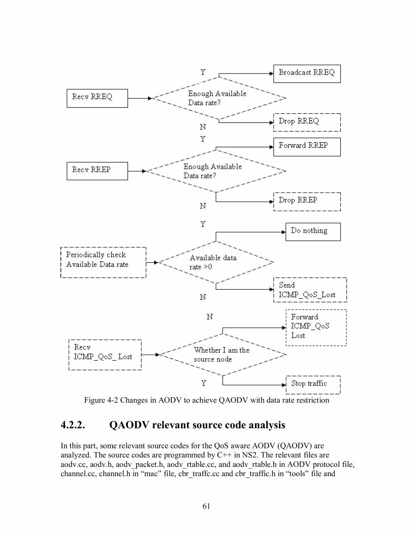
61

Figure 4-2 Changes in AODV to achieve QAODV with data rate restriction

4.2.2. QAODV relevant source code analysis

In this part, some relevant source codes for the QoS aware AODV (QAODV) are analyzed. The source codes are programmed by C++ in NS2. The relevant files are aodv.cc, aodv.h, aodv_packet.h, aodv_rtable.cc, and aodv_rtable.h in AODV protocol file, channel.cc, channel.h in �mac� file, cbr_traffc.cc and cbr_traffic.h in �tools� file and

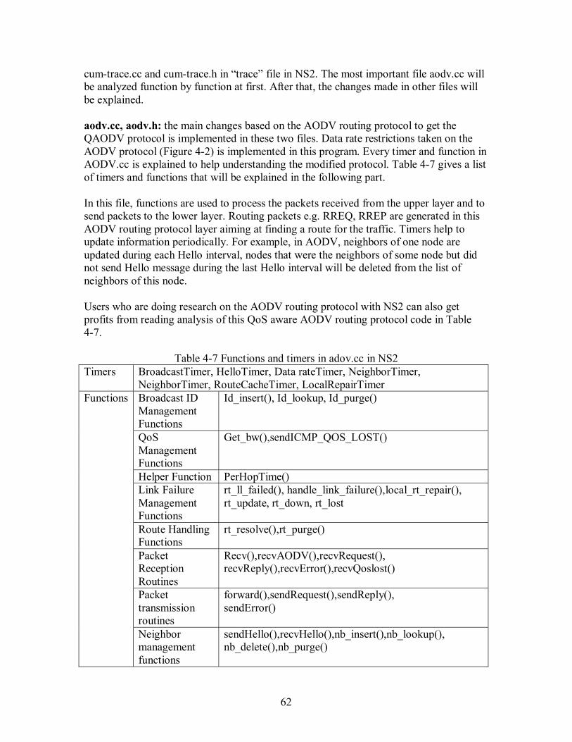
62

cum-trace.cc and cum-trace.h in �trace� file in NS2. The most important file aodv.cc will be analyzed function by function at first. After that, the changes made in other files will be explained. aodv.cc, aodv.h: the main changes based on the AODV routing protocol to get the QAODV protocol is implemented in these two files. Data rate restrictions taken on the AODV protocol (Figure 4-2) is implemented in this program. Every timer and function in AODV.cc is explained to help understanding the modified protocol. Table 4-7 gives a list of timers and functions that will be explained in the following part. In this file, functions are used to process the packets received from the upper layer and to send packets to the lower layer. Routing packets e.g. RREQ, RREP are generated in this AODV routing protocol layer aiming at finding a route for the traffic. Timers help to update information periodically. For example, in AODV, neighbors of one node are updated during each Hello interval, nodes that were the neighbors of some node but did not send Hello message during the last Hello interval will be deleted from the list of neighbors of this node. Users who are doing research on the AODV routing protocol with NS2 can also get profits from reading analysis of this QoS aware AODV routing protocol code in Table 4-7.

Table 4-7 Functions and timers in adov.cc in NS2 Timers BroadcastTimer, HelloTimer, Data rateTimer, NeighborTimer,

NeighborTimer, RouteCacheTimer, LocalRepairTimer Broadcast ID Management Functions

Id_insert(), Id_lookup, Id_purge()

QoS Management Functions

Get_bw(),sendICMP_QOS_LOST()

Helper Function PerHopTime() Link Failure Management Functions

rt_ll_failed(), handle_link_failure(),local_rt_repair(), rt_update, rt_down, rt_lost

Route Handling Functions

rt_resolve(),rt_purge()

Packet Reception Routines

Recv(),recvAODV(),recvRequest(), recvReply(),recvError(),recvQoslost()

Packet transmission routines

forward(),sendRequest(),sendReply(), sendError()

Functions

Neighbor management functions

sendHello(),recvHello(),nb_insert(),nb_lookup(), nb_delete(),nb_purge()

63

& Timers: BroadcastTimer: This timer periodically checks in each node the validation of broadcast messages. The broadcast messages are identified by the sourceID and broadcastID pairs which uniquely express the RREQ identity. Nodes receiving the RREQ for the first time have to save this RREQ for a period of time. During this period, if duplicated RREQs are received, they will be dropped. After this period, the broadcast message RREQ expires. BroadcastTimer deletes the expired RREQs from the list of each node. HelloTimer: Hello messages are periodically send to neighbors� node during every Hello Interval. This timer helps to send Hello messages from each node by invoking sendHello() function. Hello Interval is calculated for each round randomly according to some rules. Data rateTimer: This timer is a new timer for the QAODV routing protocol. It calls the function get_bw() to check each residual data rate of nodes. When the residual data rate is smaller than the minimum data rate which is always set as zero at some node, this node has to send ICMP_QOS_LOST message to tell sources who are sending packets through this node to stop transmitting. NeighborTimer: this timer calls the function nb_purge() periodically. Nb_purge() is used to purge all timeout neighbor entries. The period of this timer is the same as the interval in HelloTimer. RouteCacheTimer: this timer calls the function rt_purge() periodically to purge the expired route. LocalRepairTimer: this timer is invoked after the timeout in a local repair attempt (according to the explanation in NS2) & Functions Broadcast ID Management Functions id_insert(): this function is used to insert a new broadcast id and node id pair to the current node and to set the expiration time. Id_lookup: this function is used to search for a broadcastID and nodeID pair in the current node. It returns a Boolean value to express the existence of this pair in the current node broadcast ID list. For example, it can be called by the recvRequest() function. Only when the id_lookup returns true, the received message in recvRequest() can be processed further on. id_purge(): this function removes the expired sourceID and broadcast ID pair from nodes. QoS Management Functions (It is a new set of functions added to the AODV routing protocol)

64

get_bw(): this function is called by Data rateTimer to check the available data rate of nodes. A negative available data rate means that the nodes cannot provide the guaranteed QoS and sendICMP_QOS_LOST will be called. sendICMP_QOS_LOST(): this sends ICMP_QOS_LOST messages to all the sources that transmit packets going through the current node. When the current node is the source node, this route will be set as lost by calling rt_lost() and the source node will send RREQ again if needed. Helper Function PerHopTime(): this function helps to calculate the node traversal time. Link Failure Management Functions rt_ll_failed(): this routine is invoked when the link layer reports a route failure. In this function, when AODV_LINK_LAYER_DETECTION is not defined, packet is dropped directly. Otherwise, non-data packets and broadcast packets are dropped; and when AODV_LOCAL_REPAIR is set, the route can be repaired locally. The condition of local repair in AODV routing protocol is that, the broken link is closer to the destination than to the source. When this condition is satisfied, local_rt_repair() will be called. Then packets in the queue will be retrieved when the route functions again. Otherwise, packets in the queue will be dropped. handle_link_failure(): this function is called by nb_delete() to remove lost neighbors from the precursor list. local_rt_repair(): this function is called by rt_ll_failed(). The task of this function is to buffer the packets, mark the route as under repair and send the route request to the destination to search for a new route. The node that sends route request is the node which has a link failure. In addition, a route request timer is set to time the RREQ. rt_update(): this function is used to update the route information. The updated route information includes sequence number, number of hops, validity, next hop, and expiration time. rt_down(): when the route is found unreachable, the route is labeled as RTF_DOWN by using this function. rt_lost(): this is a new function in the QAODV routing protocol. It can be called by send_ICMP_QOS_LOST() and recvQoslost(). In this function, the route is labeled as RTF_LOST when the QoS requirement is not satisfied. Route Handling Functions rt_resolve(): this function is called by recv() when receives a data packet. The packet in processing can not be a broadcast message. In rt_resolve(), the aim is to find whether there is a route (or to establish a route) to transmit this data packet to the destination.

65

rt_purge(): this function is called only by RouteCacheTimer periodically. There are three situations in this function. The first one is when the route has expired. In this situation, the route will be labeled as invalid and the packets in the buffer of the sender are dropped. The second is that the route is not expired and there is still packets buffered. Then the buffered packets are all forwarded. The last situation is when there are still packets in the buffer, but the route is down. A RREQ will be sent for route discovery to the destination in this situation. Packet Reception Routines Recv(): every packet going through the AODV routing protocol layer will first be processed by this function. The packets are first divided into different types. The packet with type AODV will invoke recvAODV() for further processing. For data packets, there are more detailed divisions. If the paket is generated by this node and has not been forwarded, the IP header will be added. On the other side, if the packet generated by this node has been forwarded, the packet is dropped. When the node is not a source node which generates this packet, the packet will be tried to be forwarded by invoking rt_putge() to firstly find a route. Broadcast packets are broadcasted directly without searching for a route. recvAODV(): This function is called by recv() when the received packet is of AODV message type e.g. RREQ, RREP. In this function, different AODV packet types will call different functions to keep on processing the packet. AODV packet type includes RREQ, RREP, RERR, HELLO and QOSLOST packets. recvRequest() and recvReply(): these are two of the most important functions in the AODV routing protocol. To give more details of this function, flow charts are drawn as shown in Figure 4-3 and Figure 4-4. recvError():the RERR message is sent when a link is broken. The recvError() function will set all the routes to the unreachable destinations down. recvQoslost(): nodes receiving QoS lost packets have three conditions. The first one is that the node is the destination of this packet, and the node has not yet found that the QoS is lost. In this condition, rt_lost() will be called. In addition, the node will send RREQ to find a new route. The second option is composed of four terms that need to be all satisfied. Firstly the node is not the destination of this packet. Secondly, the node has not found that the QoS is lost. Thirdly, the node knows how to forward this packet to the destination. Fourthly, rt_hops is not infinite. With the above four terms fulfilled, rt_lost() is called and the packet is forwarded. Lastly, the packet that is not belonging to the above two options, is dropped. Packet transmission routines The following functions precede sending or forwarding packets. Packets are events in NS2. As a result, they need to be scheduled. Sending a packet equals to schedule the packet at a certain time. The following function will all use

66

Scheduler::instance().schedule() to schedule the packet after filling in all the fields in messages. forward():this function is used to forward the packet. The packet could be unicasted to next hop toward the destination or packets with broadcast IP will be broadcasted. The route expiration time should be updated when the packet is forwarded through this route. sendRequest(): sources generate and broadcast request messages for route discovery. Each value in RREQ messaged will be filled up in this function. Importantly, required data rate for QoS is set in the RREQ messages. Expanding ring search is used to set the TTL value. sendReply(): all fields in RREP messages are filled up in this function, and sent. sendError():all fields in RERR message are filled up in this function, and sent. Neighbor management functions sendHello(): node broadcasts Hello messages to neighbors aiming at telling the neighbors who receive this message that the node is in its neighbors transmission range. Another aim of sending Hello messages in this QoS aware routing protocol is to tell its neighbors about the available data rate of the node. recvHello(): this function is called when node receive Hello message from its neighbors. If the node is the first time receiving Hello message from this neighbor, it will add this neighbor to is neighbor list by invoking nb_insert(). nb_insert(): this function is used to insert new neighbor to the neighbor list and to set the expiration time for this entry. nb_lookup(): this function is used to check whether a node is in the neighbor list of the current node. nb_delete(): this function removes the neighbor from the neighbor list. It will call handle_link_failure(), since neighbor deleting will cause the route to be unreachable to the neighbors. nb_purge(): this function is called by the neighbor timer to purge all time out neighbor entries periodically. channel.cc, channel.h: the available data rate is calculated in this file. Each packet transmitted using the channel should be taken into account when the available data rate of the node is calculated. For each packet transmitted, every node will be examined to see whether the transmission of the packet will decrease its available data rate. Nodes whose available data rate should be subtracted by the data rate used for the transmiting packets are those who are the transmitter or who are the carrier sensing neighbors of the transmitter.

67

cbr_traffic.h: this file creates general access to CBR traffic. This function could return the required data rate from the application layer. aodv_packet.h: new parameters like requested data rate and requested session ID are defined in this header file. aodv_rtable.h and aodv_rtable.cc: route entry is changed from per destination to per session.

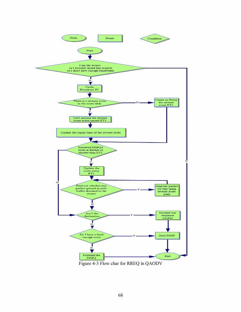
68

Figure 4-3 Flow char for RREQ in QAODV

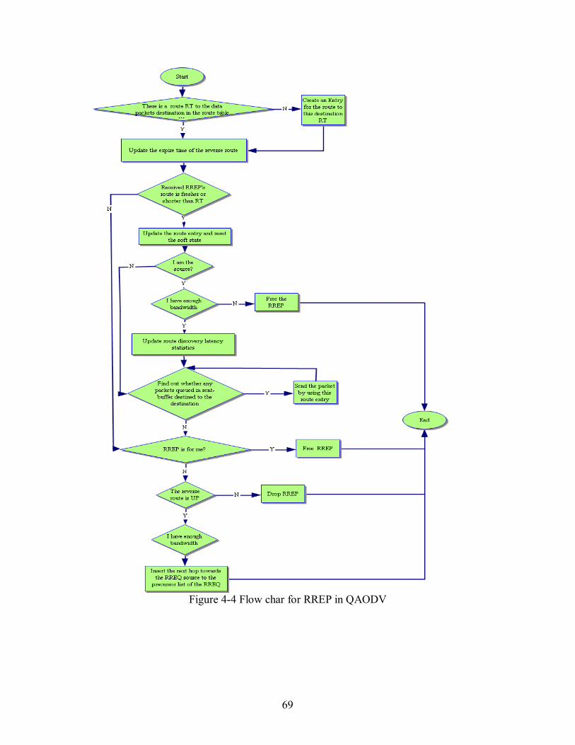
69

Figure 4-4 Flow char for RREP in QAODV

70

4.3. Chapter summary

In this chapter, NS2 is introduced and relevant tools used for analyzing trace files are discussed. The QoS aware AODV routing protocol which is implemented in Reference [15] in NS2 is analyzed in detail.

71

5. Simulations on AODV and QAODV routing protocols

5.1. Simulation environment

Simulations will be done with NS 2.27. The author installed the NS 2.27 on an Intel Pentium III /500 Personal Computer (PC) with Microsoft Windows XP Professional operation system. The computer has 256 MB of RAM (Random Access Memory). The simulation parameters used in NS 2.27 during the ad hoc network simulation are configured as follows. The channel type is �wireless channel� and the radio propagation model is �two ray ground�. MAC layer based on CSMA/CA as in IEEE 802.11 is used with RTS/CTS mechanism. The data rate at physical layer is 11 Mbps. Queue type is �drop tail� and the maximum queue length is 50. Routing protocols are the AODV and the QAODV. The transmission range and carrier sensing range are 250 m and 550 m respectively.

5.2. Simulation models

There are two routing protocols used in the following simulations. They are the AODV and the QAODV routing protocols. The AODV routing protocol used is the already existing AODV routing protocol in NS 2.27. Based on the AODV routing protocol, changes are made in reference [15] to get the QAODV routing protocol. This protocol is implemented in NS 2.27. The QAODV routing protocol used the technique discussed in the previous section including: Method 3 in Section 3.9.2 (locally available data rate calculation) and the idea in Section 3.9.4 (use Hello messages to exchange the local data rate of neighbours), as well as Method 2 in Section 3.9.6 (Access Admission Control). In the QAODV routing protocol, the data rate interval which is the interval for nodes to calculate the available data rate is 0.5 s and the Hello interval which is the interval for nodes to send Hello messages is 1 s. The maximum data rate should be tested based on the above environment. This parameter is needed by this QAODV routing protocol. In practice in NS2, in Reference [15], three files are set with this value (The three files are aodv.h, channel.cc, channel.h).

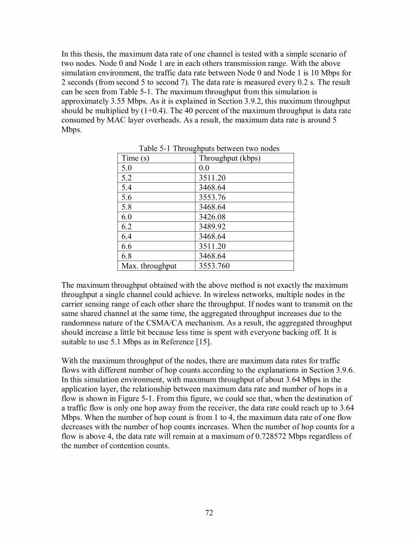
72

In this thesis, the maximum data rate of one channel is tested with a simple scenario of two nodes. Node 0 and Node 1 are in each others transmission range. With the above simulation environment, the traffic data rate between Node 0 and Node 1 is 10 Mbps for 2 seconds (from second 5 to second 7). The data rate is measured every 0.2 s. The result can be seen from Table 5-1. The maximum throughput from this simulation is approximately 3.55 Mbps. As it is explained in Section 3.9.2, this maximum throughput should be multiplied by (1+0.4). The 40 percent of the maximum throughput is data rate consumed by MAC layer overheads. As a result, the maximum data rate is around 5 Mbps.

Table 5-1 Throughputs between two nodes Time (s) Throughput (kbps) 5.0 0.0 5.2 3511.20 5.4 3468.64 5.6 3553.76 5.8 3468.64 6.0 3426.08 6.2 3489.92 6.4 3468.64 6.6 3511.20 6.8 3468.64 Max. throughput 3553.760

The maximum throughput obtained with the above method is not exactly the maximum throughput a single channel could achieve. In wireless networks, multiple nodes in the carrier sensing range of each other share the throughput. If nodes want to transmit on the same shared channel at the same time, the aggregated throughput increases due to the randomness nature of the CSMA/CA mechanism. As a result, the aggregated throughput should increase a little bit because less time is spent with everyone backing off. It is suitable to use 5.1 Mbps as in Reference [15]. With the maximum throughput of the nodes, there are maximum data rates for traffic flows with different number of hop counts according to the explanations in Section 3.9.6. In this simulation environment, with maximum throughput of about 3.64 Mbps in the application layer, the relationship between maximum data rate and number of hops in a flow is shown in Figure 5-1. From this figure, we could see that, when the destination of a traffic flow is only one hop away from the receiver, the data rate could reach up to 3.64 Mbps. When the number of hop count is from 1 to 4, the maximum data rate of one flow decreases with the number of hop counts increases. When the number of hop counts for a flow is above 4, the data rate will remain at a maximum of 0.728572 Mbps regardless of the number of contention counts.

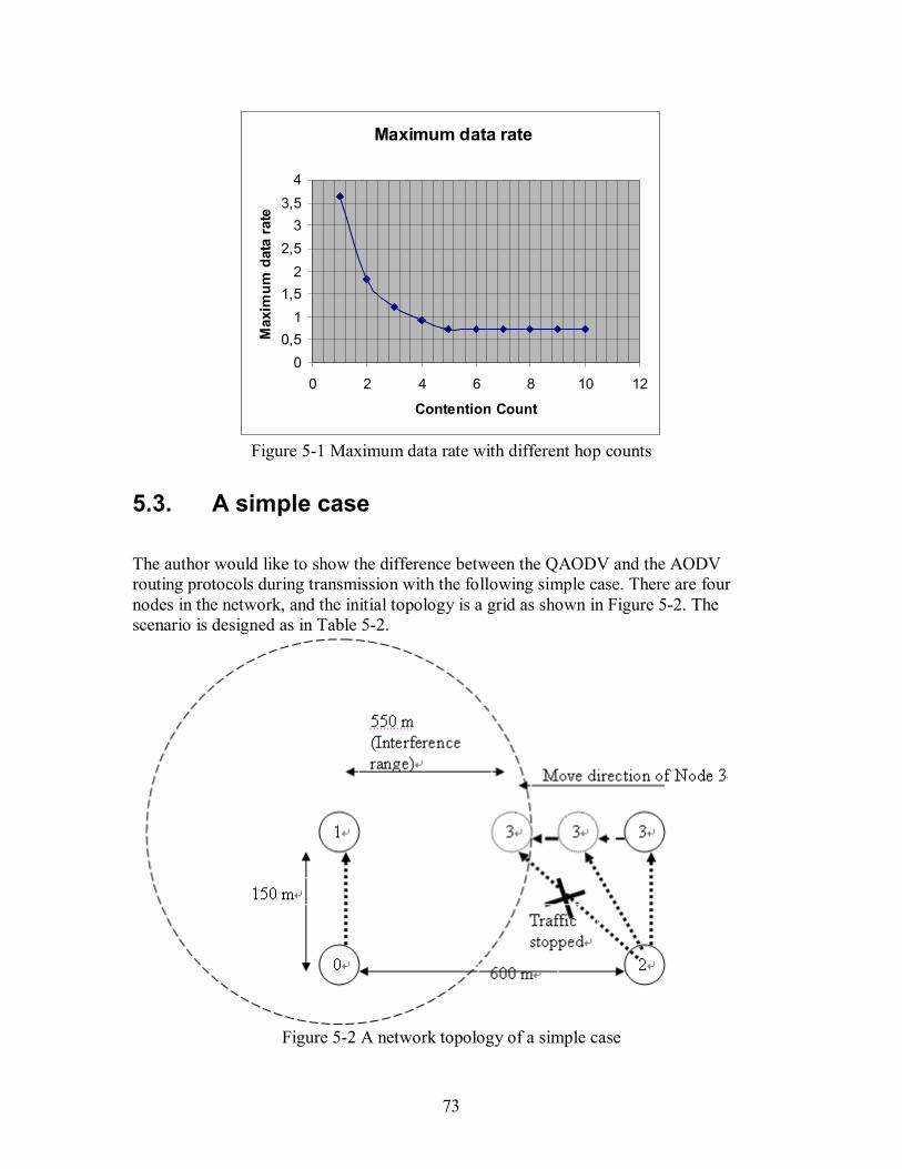
73

Maximum data rate

00,5

11,5

22,5

33,5

4

0 2 4 6 8 10 12

Contention Count

Max

imum

dat

a ra

te

Figure 5-1 Maximum data rate with different hop counts

5.3. A simple case

The author would like to show the difference between the QAODV and the AODV routing protocols during transmission with the following simple case. There are four nodes in the network, and the initial topology is a grid as shown in Figure 5-2. The scenario is designed as in Table 5-2.

Figure 5-2 A network topology of a simple case

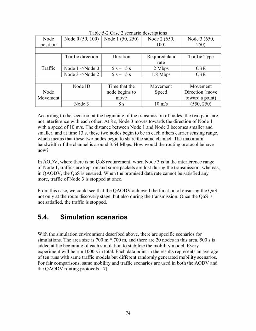
74

Table 5-2 Case 2 scenario descriptions Node

position Node 0 (50, 100) Node 1 (50, 250) Node 2 (650,

100) Node 3 (650,

250)

Traffic direction Duration Required data rate

Traffic Type

Node 1 ->Node 0 5 s � 15 s 2 Mbps CBR

Traffic Node 3 ->Node 2 5 s � 15 s 1.8 Mbps CBR

Node ID Time that the

node begins to move

Movement Speed

Movement Direction (move toward a point)

Node

Movement Node 3 8 s 10 m/s (550, 250)

According to the scenario, at the beginning of the transmission of nodes, the two pairs are not interference with each other. At 8 s, Node 3 moves towards the direction of Node 1 with a speed of 10 m/s. The distance between Node 1 and Node 3 becomes smaller and smaller, and at time 13 s, these two nodes begin to be in each others carrier sensing range, which means that these two nodes begin to share the same channel. The maximum bandwidth of the channel is around 3.64 Mbps. How would the routing protocol behave now? In AODV, where there is no QoS requirement, when Node 3 is in the interference range of Node 1, traffics are kept on and some packets are lost during the transmission, whereas, in QAODV, the QoS is ensured. When the promised data rate cannot be satisfied any more, traffic of Node 3 is stopped at once. From this case, we could see that the QAODV achieved the function of ensuring the QoS not only at the route discovery stage, but also during the transmission. Once the QoS is not satisfied, the traffic is stopped.

5.4. Simulation scenarios

With the simulation environment described above, there are specific scenarios for simulations. The area size is 700 m * 700 m, and there are 20 nodes in this area. 500 s is added at the beginning of each simulation to stabilize the mobility model. Every experiment will be run 1000 s in total. Each data point in the results represents an average of ten runs with same traffic models but different randomly generated mobility scenarios. For fair comparisons, same mobility and traffic scenarios are used in both the AODV and the QAODV routing protocols. [7]

75

5.5. Simulation traffic pattern

The Random Waypoint model provided by NS2 is used as the mobility model. The traffic type in the application layer is CBR with packet size of 512 bytes and in transport layer User Datagram Protocol (UDP) is used. The traffic pattern that will be used in the simulation is shown in Table 5-3. It is the same as what the Reference [15] uses. Setting the traffic flow in such a manner aims at greater interference impact when the sessions overlap. The source node and the destination node of each traffic flow are chosen by using function cbrgen.tcl randomly. Although the source nodes and destination nodes are fixed according the second column in Table 5-3 in the simulations, the position of each node will be put randomly for each experiment, since the topology of the network is generated randomly; the route for each traffic flow will be different for each simulation.

Table 5-3 Simulation traffic pattern Traffic flow

Source and destination node

Start time (s)

End time (s)

Session 1 3 -> 4 553 774 Session 2 7 -> 8 680 780 Session 3 4 -> 5 793 915 Session 4 5 -> 7 802 971 Session 5 5 -> 6 945 963

5.6. Performance metrics

Four performance metrics will be used to judge the performance of the AODV and the QAODV routing protocols. The explanation for each performance metric will be given in this part. # Average end to end delay: the end-to-end delay calculates the delay of the packet

which is successfully transmitted from the source to the destination. This end-to-end delay includes all possible delays caused by buffering during route discovery latency, queuing in the interface queue, retransmission delays at the MAC, propagation and transfer times. [7] It is the duration of the time a packet travels from the application layer of the source to the destination. End-to-end delay is one of the most important metrics when analysing the performance in QoS aware routing protocols. The average end-to-end delay is averaged out of all the end to end delay of successfully transmitted packets.

# Packet Delivery Ratio (PDR) is the ratio of the successfully delivered packets to

those generated by CBR sources as shown in the formula of the following part. The higher the PDR, the lower the packet loss rate, the more efficient the routing protocol from the data delivery point of view. In real time communications, the routing protocol with higher PDR may not be considered better than the one with lower PDR,

76

since packets which arrive late could be useless although they reach the destination successfully. Real time traffic is delay sensitive.

PacketsdTransmitteofNumber TotalPackets Deliveredly Successful ofNumber PDR = (5-1)

# Normalized Overhead Load (NOL) is the ratio between the total number of routing

packets and the total number of successfully delivered packets. The overhead packets in the routing layer include packets both for route discovery and route maintenance e.g. Hello messages, RREQs, RREPs and RERRs. Each hop-wise transmission of a routing packet is counted as one transmission.

Packets Deliveredly Successful ofNumber Packets Routing ofNumber TotalNOL = (5-2)

# Route finding time of the first route is the time duration which is used for finding the

first route. It is counted as the time of receiving the first RREP minus the traffic beginning time. When the source receives the first RREP, it could start to send packets immediately through the network by first contending for the channel in MAC layer with the CSMA/CA mechanism. When the criteria for the transmission channel are strict, the finding time for the first route is more likely to be large as in the QoS aware routing protocol, especially when the maximum data rate provided by the network is low.

5.7. Simulation results and analysis

5.7.1. Data rate

In this set of simulations, a group of data rates ranging from 50 kbps to 1800 kbps is applied. The mobility scenario is with a pause time of 10 seconds and the maximum node speed is 1 m/s. Four parameters defined above are calculated. The results are shown in the following figures.

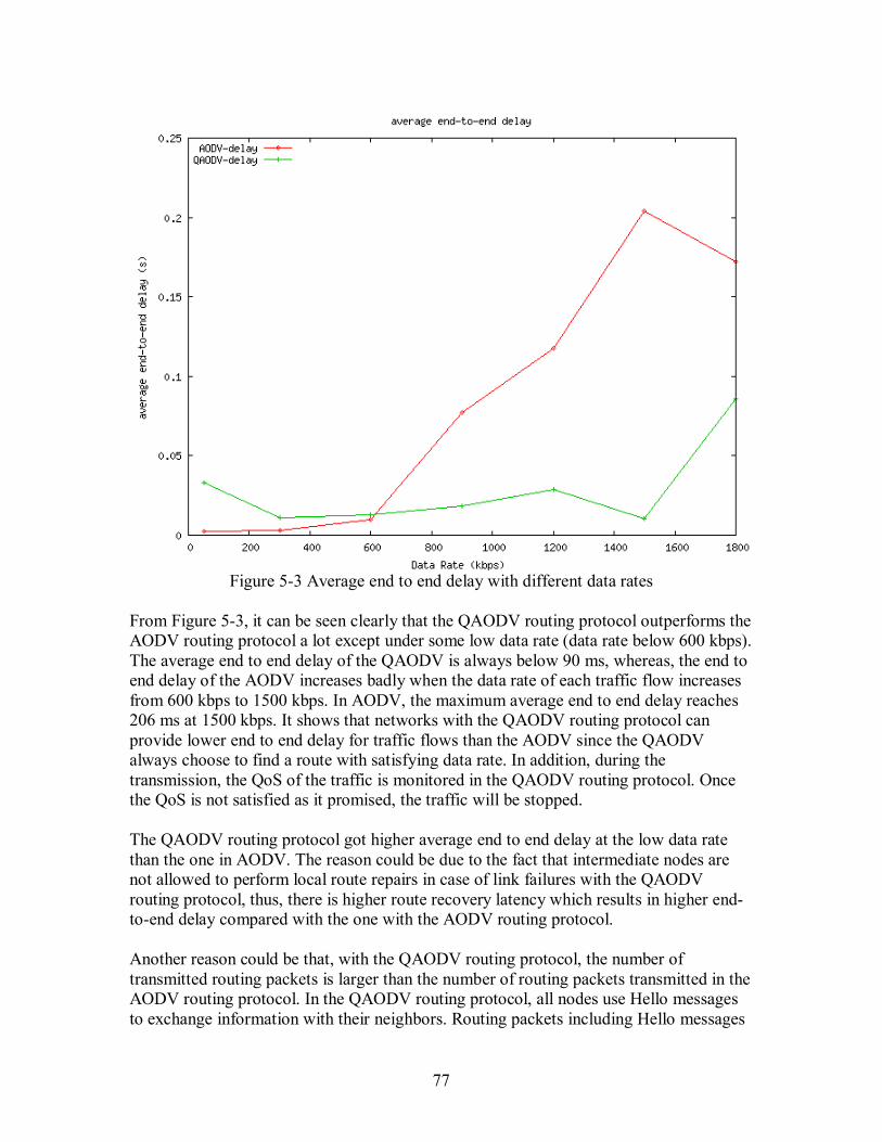
77

Figure 5-3 Average end to end delay with different data rates

From Figure 5-3, it can be seen clearly that the QAODV routing protocol outperforms the AODV routing protocol a lot except under some low data rate (data rate below 600 kbps). The average end to end delay of the QAODV is always below 90 ms, whereas, the end to end delay of the AODV increases badly when the data rate of each traffic flow increases from 600 kbps to 1500 kbps. In AODV, the maximum average end to end delay reaches 206 ms at 1500 kbps. It shows that networks with the QAODV routing protocol can provide lower end to end delay for traffic flows than the AODV since the QAODV always choose to find a route with satisfying data rate. In addition, during the transmission, the QoS of the traffic is monitored in the QAODV routing protocol. Once the QoS is not satisfied as it promised, the traffic will be stopped. The QAODV routing protocol got higher average end to end delay at the low data rate than the one in AODV. The reason could be due to the fact that intermediate nodes are not allowed to perform local route repairs in case of link failures with the QAODV routing protocol, thus, there is higher route recovery latency which results in higher end-to-end delay compared with the one with the AODV routing protocol. Another reason could be that, with the QAODV routing protocol, the number of transmitted routing packets is larger than the number of routing packets transmitted in the AODV routing protocol. In the QAODV routing protocol, all nodes use Hello messages to exchange information with their neighbors. Routing packets including Hello messages

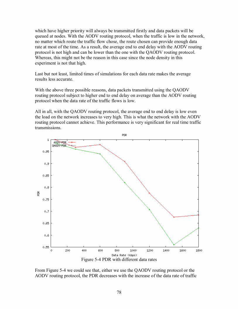
78

which have higher priority will always be transmitted firstly and data packets will be queued at nodes. With the AODV routing protocol, when the traffic is low in the network, no matter which route the traffic flow chose, the route chosen can provide enough data rate at most of the time. As a result, the average end to end delay with the AODV routing protocol is not high and can be lower than the one with the QAODV routing protocol. Whereas, this might not be the reason in this case since the node density in this experiment is not that high. Last but not least, limited times of simulations for each data rate makes the average results less accurate. With the above three possible reasons, data packets transmitted using the QAODV routing protocol subject to higher end to end delay on average than the AODV routing protocol when the data rate of the traffic flows is low. All in all, with the QAODV routing protocol, the average end to end delay is low even the load on the network increases to very high. This is what the network with the AODV routing protocol cannot achieve. This performance is very significant for real time traffic transmissions.

Figure 5-4 PDR with different data rates

From Figure 5-4 we could see that, either we use the QAODV routing protocol or the AODV routing protocol, the PDR decreases with the increase of the data rate of traffic

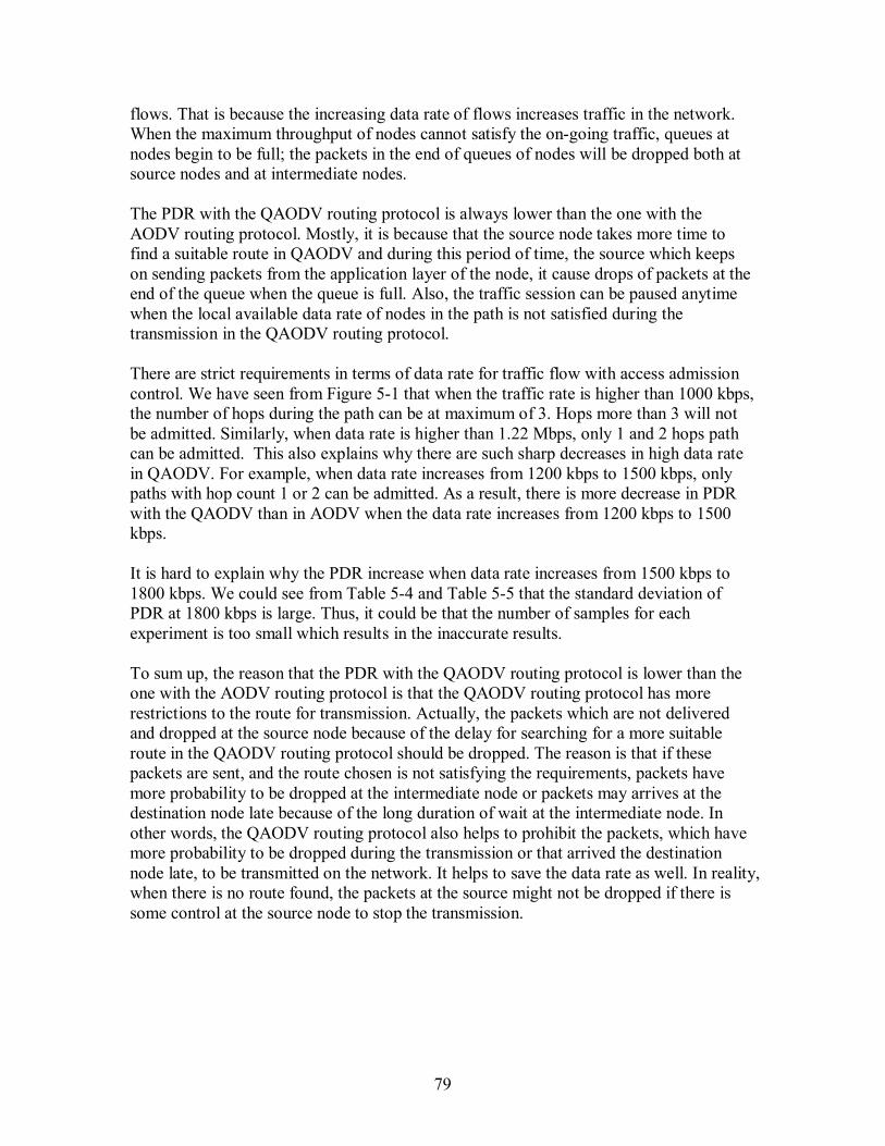
79

flows. That is because the increasing data rate of flows increases traffic in the network. When the maximum throughput of nodes cannot satisfy the on-going traffic, queues at nodes begin to be full; the packets in the end of queues of nodes will be dropped both at source nodes and at intermediate nodes. The PDR with the QAODV routing protocol is always lower than the one with the AODV routing protocol. Mostly, it is because that the source node takes more time to find a suitable route in QAODV and during this period of time, the source which keeps on sending packets from the application layer of the node, it cause drops of packets at the end of the queue when the queue is full. Also, the traffic session can be paused anytime when the local available data rate of nodes in the path is not satisfied during the transmission in the QAODV routing protocol. There are strict requirements in terms of data rate for traffic flow with access admission control. We have seen from Figure 5-1 that when the traffic rate is higher than 1000 kbps, the number of hops during the path can be at maximum of 3. Hops more than 3 will not be admitted. Similarly, when data rate is higher than 1.22 Mbps, only 1 and 2 hops path can be admitted. This also explains why there are such sharp decreases in high data rate in QAODV. For example, when data rate increases from 1200 kbps to 1500 kbps, only paths with hop count 1 or 2 can be admitted. As a result, there is more decrease in PDR with the QAODV than in AODV when the data rate increases from 1200 kbps to 1500 kbps. It is hard to explain why the PDR increase when data rate increases from 1500 kbps to 1800 kbps. We could see from Table 5-4 and Table 5-5 that the standard deviation of PDR at 1800 kbps is large. Thus, it could be that the number of samples for each experiment is too small which results in the inaccurate results. To sum up, the reason that the PDR with the QAODV routing protocol is lower than the one with the AODV routing protocol is that the QAODV routing protocol has more restrictions to the route for transmission. Actually, the packets which are not delivered and dropped at the source node because of the delay for searching for a more suitable route in the QAODV routing protocol should be dropped. The reason is that if these packets are sent, and the route chosen is not satisfying the requirements, packets have more probability to be dropped at the intermediate node or packets may arrives at the destination node late because of the long duration of wait at the intermediate node. In other words, the QAODV routing protocol also helps to prohibit the packets, which have more probability to be dropped during the transmission or that arrived the destination node late, to be transmitted on the network. It helps to save the data rate as well. In reality, when there is no route found, the packets at the source might not be dropped if there is some control at the source node to stop the transmission.

80

Figure 5-5 NOL with different data rates

In Figure 5-5, with the increase of data rate, NOL decreases in QAODV. In QAODV, Hello messages are sent periodically, that is, the number of Hello messages sent independent of the load on the network. In addition, with the increase of data rate, the total number of packets sent increases. As a result, when the data rate is low, NOL is relatively high in QAODV. In AODV, the NOL in AODV is always low since the AODV routing packets are only sent during the routing searching and maintenance periods without exchanging Hello messages. It results in the low NOL with the AODV routing protocol. The Hello messages are needed in the QAODV routing protocol in order to exchange the precisely consumed data rate information of nodes who are sharing the same channel. From this figure we could conclude that the use of the QAODV routing protocol in networks with low traffic will cost relatively more data rate than the use of the AODV routing protocol to send routing packets. A network with high traffic load has lower NOL.

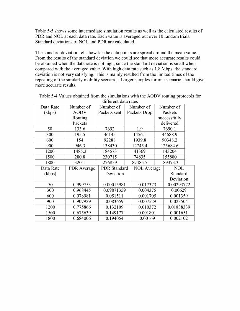
Table 5-5 shows some intermediate simulation results as well as the calculated results of PDR and NOL at each data rate. Each value is averaged out over 10 random trials. Standard deviations of NOL and PDR are calculated. The standard deviation tells how far the data points are spread around the mean value. From the results of the standard deviation we could see that more accurate results could be obtained when the data rate is not high, since the standard deviation is small when compared with the averaged value. With high data rate such as 1.8 Mbps, the standard deviation is not very satisfying. This is mainly resulted from the limited times of the repeating of the similarly mobility scenarios. Larger samples for one scenario should give more accurate results.

Table 5-4 Values obtained from the simulations with the AODV routing protocols for different data rates

Data Rate (kbps)

Number of AODV Routing Packets

Number of Packets sent

Number of Packets Drop

Number of Packets

successfully delivered

50 133.6 7692 1.9 7690.1 300 195.5 46145 1456.1 44688.9 600 154 92288 1939.8 90348.2 900 946.3 138430 12745.4 125684.6

1200 1485.3 184573 41369 143204 1500 280.8 230715 74835 155880 1800 320.1 276859 87485.7 189373.3

Data Rate (kbps)

PDR Average PDR Standard Deviation

NOL Average NOL Standard Deviation

50 0.999753 0.00015981 0.017373 0.00293772 300 0.968445 0.09871359 0.004375 0.00629 600 0.978981 0.051511 0.001705 0.001359 900 0.907929 0.083659 0.007529 0.023504 1200 0.775866 0.132109 0.010372 0.01838339 1500 0.675639 0.149177 0.001801 0.001651 1800 0.684006 0.194054 0.00169 0.002102

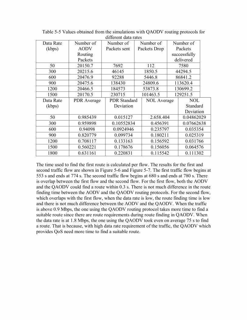
Table 5-5 Values obtained from the simulations with QAODV routing protocols for different data rates

Data Rate (kbps)

Number of AODV Routing Packets

Number of Packets sent

Number of Packets Drop

Number of Packets

successfully delivered

50 20150.7 7692 112 7580 300 20215.6 46145 1850.5 44294.5 600 20476.9 92288 5446.8 86841.2 900 20475.6 138430 24809.6 113620.4

1200 20466.5 184573 53873.8 130699.2 1500 20170.5 230715 101463.5 129251.5

Data Rate (kbps)

PDR Average PDR Standard Deviation

NOL Average NOL Standard Deviation

50 0.985439 0.015127 2.658.404 0.04862029 300 0.959898 0.10552834 0.456391 0.07662638 600 0.94098 0.0924946 0.235797 0.035354 900 0.820779 0.099734 0.180211 0.025319 1200 0.708117 0.133163 0.156592 0.031766 1500 0.560221 0.178676 0.156056 0.064576 1800 0.631161 0.220831 0.115542 0.111302

The time used to find the first route is calculated per flow. The results for the first and second traffic flow are shown in Figure 5-6 and Figure 5-7. The first traffic flow begins at 553 s and ends at 774 s. The second traffic flow begins at 680 s and ends at 780 s. There is overlap between the first flow and the second flow. For the first flow, both the AODV and the QAODV could find a route within 0.3 s. There is not much difference in the route finding time between the AODV and the QAODV routing protocols. For the second flow, which overlaps with the first flow, when the data rate is low, the route finding time is low and there is not much difference between the AODV and the QAODV. When the traffic is above 0.9 Mbps, the one using the QAODV routing protocol takes more time to find a suitable route since there are route requirements during route finding in QAODV. When the data rate is at 1.8 Mbps, the one using the QAODV took even on average 75 s to find a route. That is because, with high data rate requirement of the traffic, the QAODV which provides QoS need more time to find a suitable route.

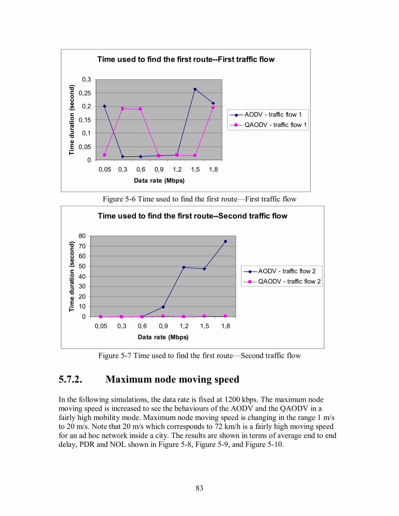
83

Time used to find the first route--First traffic flow

0

0,05

0,1

0,15

0,2

0,25

0,3

0,05 0,3 0,6 0,9 1,2 1,5 1,8

Data rate (Mbps)

Tim

e du

ratio

n (s

econ

d)

AODV - traffic flow 1QAODV - traffic flow 1

Figure 5-6 Time used to find the first route�First traffic flow

Time used to find the first route--Second traffic flow

01020304050607080

0,05 0,3 0,6 0,9 1,2 1,5 1,8

Data rate (Mbps)

Tim

e du

ratio

n (s

econ

d)

AODV - traffic flow 2QAODV - traffic flow 2

Figure 5-7 Time used to find the first route�Second traffic flow

5.7.2. Maximum node moving speed

In the following simulations, the data rate is fixed at 1200 kbps. The maximum node moving speed is increased to see the behaviours of the AODV and the QAODV in a fairly high mobility mode. Maximum node moving speed is changing in the range 1 m/s to 20 m/s. Note that 20 m/s which corresponds to 72 km/h is a fairly high moving speed for an ad hoc network inside a city. The results are shown in terms of average end to end delay, PDR and NOL shown in Figure 5-8, Figure 5-9, and Figure 5-10.

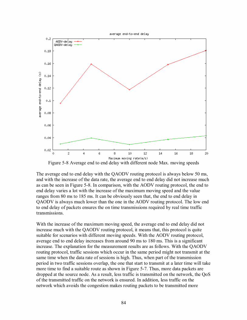
84

Figure 5-8 Average end to end delay with different node Max. moving speeds

The average end to end delay with the QAODV routing protocol is always below 50 ms, and with the increase of the data rate, the average end to end delay did not increase much as can be seen in Figure 5-8. In comparison, with the AODV routing protocol, the end to end delay varies a lot with the increase of the maximum moving speed and the value ranges from 80 ms to 185 ms. It can be obviously seen that, the end to end delay in QAODV is always much lower than the one in the AODV routing protocol. The low end to end delay of packets ensures the on time transmissions required by real time traffic transmissions. With the increase of the maximum moving speed, the average end to end delay did not increase much with the QAODV routing protocol, it means that, this protocol is quite suitable for scenarios with different moving speeds. With the AODV routing protocol, average end to end delay increases from around 90 ms to 180 ms. This is a significant increase. The explanation for the measurement results are as follows. With the QAODV routing protocol, traffic sessions which occur in the same period might not transmit at the same time when the data rate of sessions is high. Thus, when part of the transmission period in two traffic sessions overlap, the one that start to transmit at a later time will take more time to find a suitable route as shown in Figure 5-7. Thus, more data packets are dropped at the source node. As a result, less traffic is transmitted on the network, the QoS of the transmitted traffic on the network is ensured. In addition, less traffic on the network which avoids the congestion makes routing packets to be transmitted more

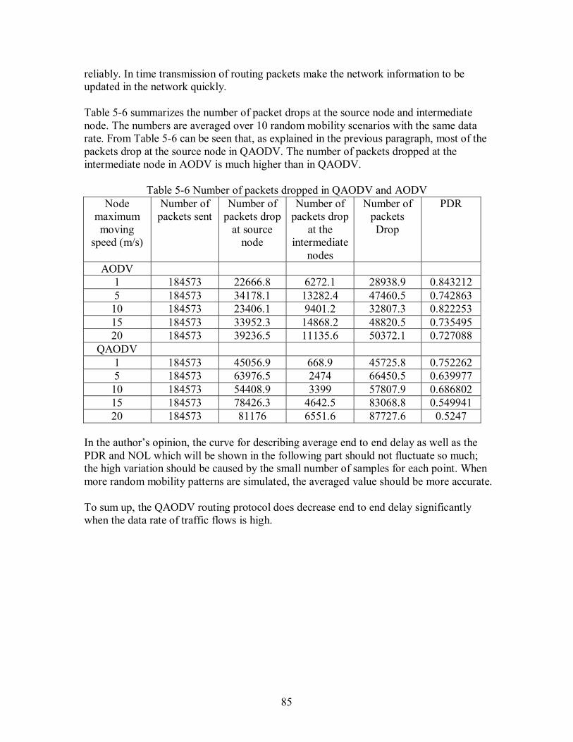
85

reliably. In time transmission of routing packets make the network information to be updated in the network quickly. Table 5-6 summarizes the number of packet drops at the source node and intermediate node. The numbers are averaged over 10 random mobility scenarios with the same data rate. From Table 5-6 can be seen that, as explained in the previous paragraph, most of the packets drop at the source node in QAODV. The number of packets dropped at the intermediate node in AODV is much higher than in QAODV.

Table 5-6 Number of packets dropped in QAODV and AODV Node

maximum moving

speed (m/s)

Number of packets sent

Number of packets drop

at source node

Number of packets drop

at the intermediate

nodes

Number of packets Drop

PDR

AODV 1 184573 22666.8 6272.1 28938.9 0.843212 5 184573 34178.1 13282.4 47460.5 0.742863

10 184573 23406.1 9401.2 32807.3 0.822253 15 184573 33952.3 14868.2 48820.5 0.735495 20 184573 39236.5 11135.6 50372.1 0.727088

QAODV 1 184573 45056.9 668.9 45725.8 0.752262 5 184573 63976.5 2474 66450.5 0.639977

10 184573 54408.9 3399 57807.9 0.686802 15 184573 78426.3 4642.5 83068.8 0.549941 20 184573 81176 6551.6 87727.6 0.5247

In the author�s opinion, the curve for describing average end to end delay as well as the PDR and NOL which will be shown in the following part should not fluctuate so much; the high variation should be caused by the small number of samples for each point. When more random mobility patterns are simulated, the averaged value should be more accurate. To sum up, the QAODV routing protocol does decrease end to end delay significantly when the data rate of traffic flows is high.

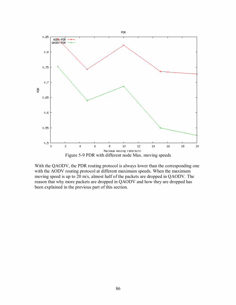
86

Figure 5-9 PDR with different node Max. moving speeds

With the QAODV, the PDR routing protocol is always lower than the corresponding one with the AODV routing protocol at different maximum speeds. When the maximum moving speed is up to 20 m/s, almost half of the packets are dropped in QAODV. The reason that why more packets are dropped in QAODV and how they are dropped has been explained in the previous part of this section.

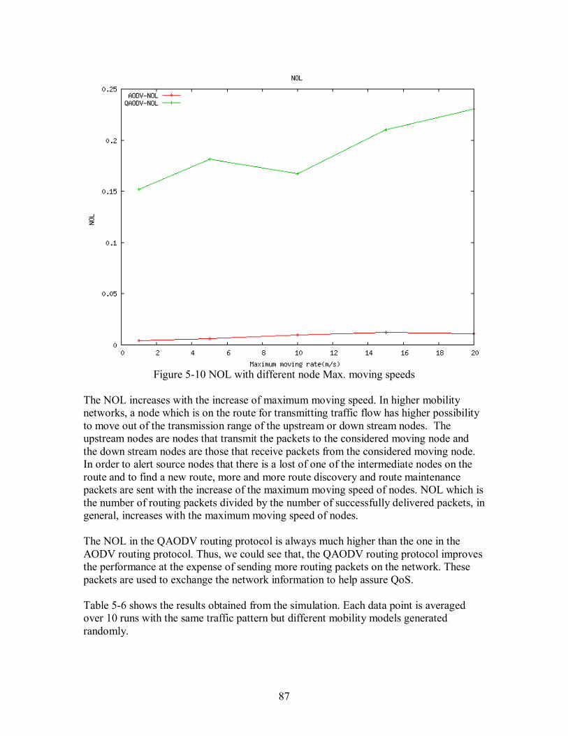
87

Figure 5-10 NOL with different node Max. moving speeds

The NOL increases with the increase of maximum moving speed. In higher mobility networks, a node which is on the route for transmitting traffic flow has higher possibility to move out of the transmission range of the upstream or down stream nodes. The upstream nodes are nodes that transmit the packets to the considered moving node and the down stream nodes are those that receive packets from the considered moving node. In order to alert source nodes that there is a lost of one of the intermediate nodes on the route and to find a new route, more and more route discovery and route maintenance packets are sent with the increase of the maximum moving speed of nodes. NOL which is the number of routing packets divided by the number of successfully delivered packets, in general, increases with the maximum moving speed of nodes. The NOL in the QAODV routing protocol is always much higher than the one in the AODV routing protocol. Thus, we could see that, the QAODV routing protocol improves the performance at the expense of sending more routing packets on the network. These packets are used to exchange the network information to help assure QoS. Table 5-6 shows the results obtained from the simulation. Each data point is averaged over 10 runs with the same traffic pattern but different mobility models generated randomly.

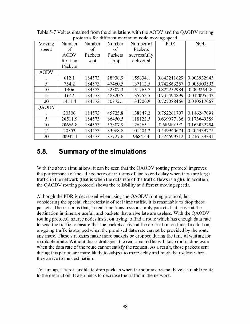
88

Table 5-7 Values obtained from the simulations with the AODV and the QAODV routing protocols for different maximum node moving speed

Moving speed

Number of

AODV Routing Packets

Number of

Packets sent

Number of

Packets Drop

Number of Packets

successfully delivered

PDR NOL

AODV 1 612.1 184573 28938.9 155634.1 0.843211629 0.0039329435 754.2 184573 47460.5 137112.5 0.742863257 0.00550059310 1406 184573 32807.3 151765.7 0.822252984 0.00926428 15 1642 184573 48820.5 135752.5 0.735494899 0.01209554220 1411.4 184573 50372.1 134200.9 0.727088469 0.010517068

QAODV 1 20306 184573 45725.8 138847.2 0.752261707 0.1462470985 20511.9 184573 66450.5 118122.5 0.639977136 0.17364938910 20666.8 184573 57807.9 126765.1 0.68680197 0.16303225415 20853 184573 83068.8 101504.2 0.549940674 0.20543977520 20932.1 184573 87727.6 96845.4 0.524699712 0.216139331

5.8. Summary of the simulations

With the above simulations, it can be seen that the QAODV routing protocol improves the performance of the ad hoc network in terms of end to end delay when there are large traffic in the network (that is when the data rate of the traffic flows is high). In addition, the QAODV routing protocol shows the reliability at different moving speeds. Although the PDR is decreased when using the QAODV routing protocol, but considering the special characteristic of real time traffic, it is reasonable to drop those packets. The reason is that, in real time transmissions, only packets that arrive at the destination in time are useful, and packets that arrive late are useless. With the QAODV routing protocol, source nodes insist on trying to find a route which has enough data rate to send the traffic to ensure that the packets arrive at the destination on time. In addition, on-going traffic is stopped when the promised data rate cannot be provided by the route any more. These strategies make more packets be dropped during the time of waiting for a suitable route. Without these strategies, the real time traffic will keep on sending even when the data rate of the route cannot satisfy the request. As a result, those packets sent during this period are more likely to subject to more delay and might be useless when they arrive to the destination. To sum up, it is reasonable to drop packets when the source does not have a suitable route to the destination. It also helps to decrease the traffic in the network.

89

The good performance with the QAODV routing protocol is achieved at the expense of sending more routing packets. This can be seen from the value of NOL. To conclude, with real time traffic, the QAODV is suitable when the traffic of the network is high. It could help to ensure the transmission as well as constrain the useless transmissions in the network.

5.9. Simulation problems

It is scientifically more appropriate to take more random mobility models for one scenario to take the average value of each point in the results, but due to the limitation of time and resource, it is hard to achieve. This results in large variation of the average results over only 10 random mobility models, so each point in the figures is not very accurate. In addition, limited scenarios are simulated. A network with large scenarios and large number of nodes is difficult to simulate because of the limitation of time and resource, so only limited scenarios can be concluded. On the other hand, author tried to give reasonable explanations in general for the evaluation of the performance of the QAODV routing protocol compared with the AODV routing protocol.

5.10. Chapter summary

In this chapter, the simulation environment is described and several simulations are done with different parameters with both the AODV and the QAODV routing protocols. Finally, results are analyzed and compared.

90

6. Summary and conclusions

6.1. Summary

This thesis work gives an introduction of mobile ad hoc networks especially the solutions for the MAC layer and the routing layer. The IEEE 802.11 standard which is widely used in ad hoc networks is discussed and a variety of routing protocols are introduced and compared. After that, because of the necessity of QoS in ad hoc networks, a few QoS relevant works are described. Challenges of implementing QoS in ad hoc networks are listed. The way of calculating two of the most important metrics: data rate and delay are summarized. Two QoS aware routing protocols are discussed. Finally, a simulation tool, NS2, is introduced and some simulations are done to compare the performance of the AODV and the QAODV routing protocol. From the simulations, it is found that, the QoS aware reactive routing protocol named the QAODV routing protocol could improve the QoS of transmissions in terms of end to end delay at the expense of sending more routing packets in the network. This QAODV routing protocol is more significant to be sent especially when the traffic on the network is high (corresponding to a situation where the data rate of the traffic flow is high in the simulations), since that improves the performance of the network remarkably.

6.2. Conclusions

Based on the simulation, it is found that packets could get less end to end delay with a QoS aware routing protocol when the traffic on the network is high. This low end to end delay is meaningful for real time transmissions. When the traffic is relatively high on the network, not all the routes that are found by the AODV routing protocol have enough free data rate for sending packets ensuring the low end to end delay of each packet. As a result, the QAODV protocol works well and shows its effects when the traffic on the network is relatively high. People who work on the area of ad hoc networks with the aim of improving the QoS for ad hoc networks can get benefit from reading this thesis. For this QAODV routing protocol, problems would rise when the node density of the network is high. The reason is that the QAODV routing protocol uses the Hello message to exchange information between neighbours. When the node density is too high, the sending of Hello messages will cost much available data rate. As a result, the network will be ruined and traffic will be delayed more since Hello messages have higher priority

91

than data packets. To conclude, it is predicted that the QAODV will not work well in high density ad hoc networks.

6.3. Discussion

In order to get more interference impact to show the merits of QoS aware routing protocols, the traffic flows overlap in terms of time; the traffic pattern is decided manually. As a result, the simulations are not fully random. Because of the limitation of time and resources, in this thesis work, only limited scenarios are simulated, and each result is taken from an average of 10 random mobility models. Thus, if more accurate performance results are expected, more random mobility models should be taken. Giving higher maximum moving speed in the networks can cause that nodes are more easily to lose the connection with their first hop neighbours. In the simulation, the QAODV routing protocol used Hello message for neighbour detection without using link layer detection. In AODV, link layer feedback for neighbour detection is used. Link layer feedback mechanism for neighbour detection makes the node response quicker to the changes of the network than the use of Hello messages to detect link failures. Thus, the link layer feedback for neighbour detection is advised to be used in the QAODV routing protocol along with using Hello messages.

6.4. Further work

In terms of metrics in the QoS aware routing protocols, only data rate metric is considered in the simulations. End to end delay metric could be an additional metric during the route discovery and maintenance in the routing protocol. Thus, end to end delay can be added to the AODV routing protocol. In the implemented QoS aware routing protocol, traffic is assumed to be all real time traffic and having the same priority, whereas in reality traffic should be differentiated to have different priorities. Traffic differentiation should be considered in the future design of routing protocols. Networks which provide higher data rate in physical layer should be considered in future simulations, since for real time transmissions when higher data rate for one flow is required, both the number of hops and the number of simultaneous flows are very limited as it can be seen from the simulation results.

92

References [1] C.Siva Ram Nurthy and B.S. Manoj �Ad hoc wireless networks Architectures and Protocols,� Prentice Hall, 2004. [2] Wireless Deployable Network System: www.widens.org, visited 2006-07-22 [3] Handouts of Helsinki University of Technology�s course: Wireless Personal, Local, Metropolitan, and Wide Area Networks http://www.comlab.hut.fi/studies/3240/index.html, visited 2006-07-22 [4] Gu, D; Zhang, J., "QoS Enhancement in IEEE802.11 Wireless Local Area Networks", IEEE Communications Magazine, ISSN: 0163-6804, Vol. 41, Issue 6, pp. 120-124, June 2003 [5] OSPF relevant lecture slides from Helsinki University of Technology: http://keskus.hut.fi/opetus/s382121/s05/Slides/S2121-04-LS-e.pdf, visited 2006-07-22 [6] R. Guerin, A. Orda, D. Williams �QoS Routing Mechanisms and OSPF Extensions,� August, 1999, Network Working Group, Rrequest for Comments: 2676. [7] S. R. Das, C. E. Perkins, E. M. Royer, and M. K. Marina. Performance Comparison of Two On-demand Routing Protocols for Ad Hoc Networks. INFOCOM 2000. Nineteenth Annual Joint Conference of the IEEE Computer and Communications Societies. Proceedings. IEEE, Volume 1, 26-30 March 2000 pp. 3 - 12. [8] C. Toh, H. Cobb, and D. Scott. �Performance evaluation of battery-life-aware routing schemes for wireless ad hoc networks,� Communications, 2001. ICC 2001. IEEE International Conference on Volume 9, 11-14 June 2001 pp. 2824 - 2829. [9] Chang JH, Tassiulas L. �Energy conserving routing in wireless ad-hoc networks,� INFOCOM 2000. Nineteenth Annual Joint Conference of the IEEE Computer and Communications Societies. Proceedings. IEEE, Volume 1, 26-30 March 2000 pp. 22 - 31. [10] Song J-H,Wong V, Leung V C M. Load-aware on-demand routing (LAOR) protocol for mobile ad hoc networks[C]. Vehicular Technology Conference, 2003. VTC 2003-Spring. The 57th IEEE Semiannual, Volume 3, 22-25 April 2003 pp. 1753 - 1757. [11] QoS relevant lecture slides from Helsinki University of Technology: http://keskus.hut.fi/opetus/s382121/s05/Slides, visited 2006-07-22 [12] H. Badis, A. Munaretto, K. Al Agha, and G. Pujolle. "QoS for Ad hoc Networking Based on Multiple Metrics: Data rate and Delay," In the proceedings of IEEE MWCN2003, Singapore, October 2003.

93

[13] Rafael Paoliello Guimar�aes and Llorenc¸ Cerd �Data rate Reservation On Wireless Networks,� Barcelona, Spain May 24, 2005 [14] Ronan de Renesse, Mona Ghassemian, Vasilis Friderikos, A. Hamid Aghvami, "QoS Enabled Routing in Mobile Ad Hoc Networks," 3G Mobile Communication Technologies, 2004. 3G 2004. Fifth IEE International Conference on 2004 pp. 678 � 682. [15] Ronan de Renesse, Mona Ghassemian, Vasilis Friderikos, A. Hamid Aghvami, "Adaptive Admission Control for Ad Hoc and Sensor Networks Providing Quality of Service," Technical Report, Center for Telecommunications Research, King�s College London, UK, May 2005. [16] Quality of Service for Ad hoc Optimized Link State Routing Protocol (QOLSR) H. Badis and K. Al Agha IETF-63 Meeting : Internet Engineering Task Force, draft-badis-manet-qolsr-02.txt, Vancouver, Canada, November 2005. Draft IETF [17] Ying Ge, Louise Lamont, Luis Villasenor, "Hierarchical OLSR -- A Scalable Proactive Routing Protocol for Heterogeneous Ad Hoc Networks", WiMob 2005 Wireless and Mobile Computing, Montreal, Canada, August 22-24, 2005. [18] C. E. Perkins, E. M. Royer, S. R. Das, �Quality of Service for Ad hoc On-Demand Distance Vector Routing,� draft-perkins-manet-aodvqos-02.txt, IETF Internet Draft, work in progress, October 2003. [19] L. Chen and W. B. Heinzelmann, �QoS-Aware Routing Based on Data rate Estimation for Mobile Ad Hoc Networks,� Selected Areas in Communications, IEEE Journal on Volume 23, Issue 3, March 2005 pp. 561 � 572. [20] NS manual http://www.isi.edu/nsnam/ns/ns-documentation.html, visited 2006-07-22 [21] Leiming Xu, Bo Pang, Yao Zhao, �NS and network simulation� POST&TELECOM PRESS, 2003 [22]Network Simulation 2 official website: http://www.isi.edu/nsnam/ns/, visited 2006-07-22 [23] NS2 installation instruction under windows operating system: http://140.116.72.80/~smallko/ns2/setup_en.htm, visited 2006-07-22 [24] A tutorial named �NS by example�: http://nile.wpi.edu/NS/, visited 2006-07-22 [25] Mobile ad hoc network described in wiki http://en.wikipedia.org/wiki/Ad_Hoc_Routing_Protocol, visited 2006-07-22

94

[26] Trace file record format http://wcc.iiita.ac.in/ns/ns2-trace-formats.html, visited 2006-07-22 [27] Explanation of the term: data rate, http://en.wikipedia.org/wiki/Data rate, visited 2006-07-22

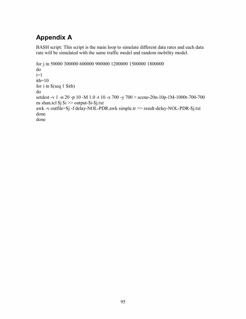
95

Appendix A BASH script: This script is the main loop to simulate different data rates and each data rate will be simulated with the same traffic model and random mobility model. for j in 50000 300000 600000 900000 1200000 1500000 1800000 do i=1 ith=10 for i in $(seq 1 $ith) do setdest -v 1 -n 20 -p 10 -M 1.0 -t 10 -x 700 -y 700 > scene-20n-10p-1M-1000t-700-700 ns shan.tcl $j $i >> output-$i-$j.txt awk -v outfile=$j -f delay-NOL-PDR.awk simple.tr >> result-delay-NOL-PDR-$j.txt done done

96

Appendix B TCL script: This script is run for each simulation

# Copyright (c) 1997 Regents of the University of California. # All rights reserved. # # Redistribution and use in source and binary forms, with or without # modification, are permitted provided that the following conditions # are met: # 1. Redistributions of source code must retain the above copyright # notice, this list of conditions and the following disclaimer. # 2. Redistributions in binary form must reproduce the above copyright # notice, this list of conditions and the following disclaimer in the # documentation and/or other materials provided with the distribution. # 3. All advertising materials mentioning features or use of this software # must display the following acknowledgement: # This product includes software developed by the Computer Systems # Engineering Group at Lawrence Berkeley Laboratory. # 4. Neither the name of the University nor of the Laboratory may be used # to endorse or promote products derived from this software without # specific prior written permission. # # THIS SOFTWARE IS PROVIDED BY THE REGENTS AND CONTRIBUTORS ``AS IS'' AND # ANY EXPRESS OR IMPLIED WARRANTIES, INCLUDING, BUT NOT LIMITED TO, THE # IMPLIED WARRANTIES OF MERCHANTABILITY AND FITNESS FOR A PARTICULAR PURPOSE # ARE DISCLAIMED. IN NO EVENT SHALL THE REGENTS OR CONTRIBUTORS BE LIABLE # FOR ANY DIRECT, INDIRECT, INCIDENTAL, SPECIAL, EXEMPLARY, OR CONSEQUENTIAL # DAMAGES (INCLUDING, BUT NOT LIMITED TO, PROCUREMENT OF SUBSTITUTE GOODS # OR SERVICES; LOSS OF USE, DATA, OR PROFITS; OR BUSINESS INTERRUPTION) # HOWEVER CAUSED AND ON ANY THEORY OF LIABILITY, WHETHER IN CONTRACT, STRICT # LIABILITY, OR TORT (INCLUDING NEGLIGENCE OR OTHERWISE) ARISING IN ANY WAY # OUT OF THE USE OF THIS SOFTWARE, EVEN IF ADVISED OF THE POSSIBILITY OF # SUCH DAMAGE. # # simple-wireless.tcl

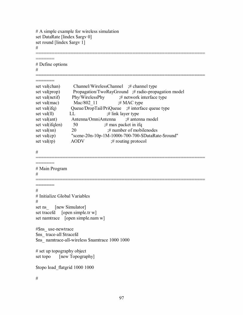
97

# A simple example for wireless simulation set DataRate [lindex $argv 0] set round [lindex $argv 1] # ====================================================================== # Define options # ====================================================================== set val(chan) Channel/WirelessChannel ;# channel type set val(prop) Propagation/TwoRayGround ;# radio-propagation model set val(netif) Phy/WirelessPhy ;# network interface type set val(mac) Mac/802_11 ;# MAC type set val(ifq) Queue/DropTail/PriQueue ;# interface queue type set val(ll) LL ;# link layer type set val(ant) Antenna/OmniAntenna ;# antenna model set val(ifqlen) 50 ;# max packet in ifq set val(nn) 20 ;# number of mobilenodes set val(cp) "scene-20n-10p-1M-1000t-700-700-$DataRate-$round" set val(rp) AODV ;# routing protocol # ====================================================================== # Main Program # ====================================================================== # # Initialize Global Variables # set ns_ [new Simulator] set tracefd [open simple.tr w] set namtrace [open simple.nam w] #$ns_ use-newtrace $ns_ trace-all $tracefd $ns_ namtrace-all-wireless $namtrace 1000 1000 # set up topography object set topo [new Topography] $topo load_flatgrid 1000 1000 #

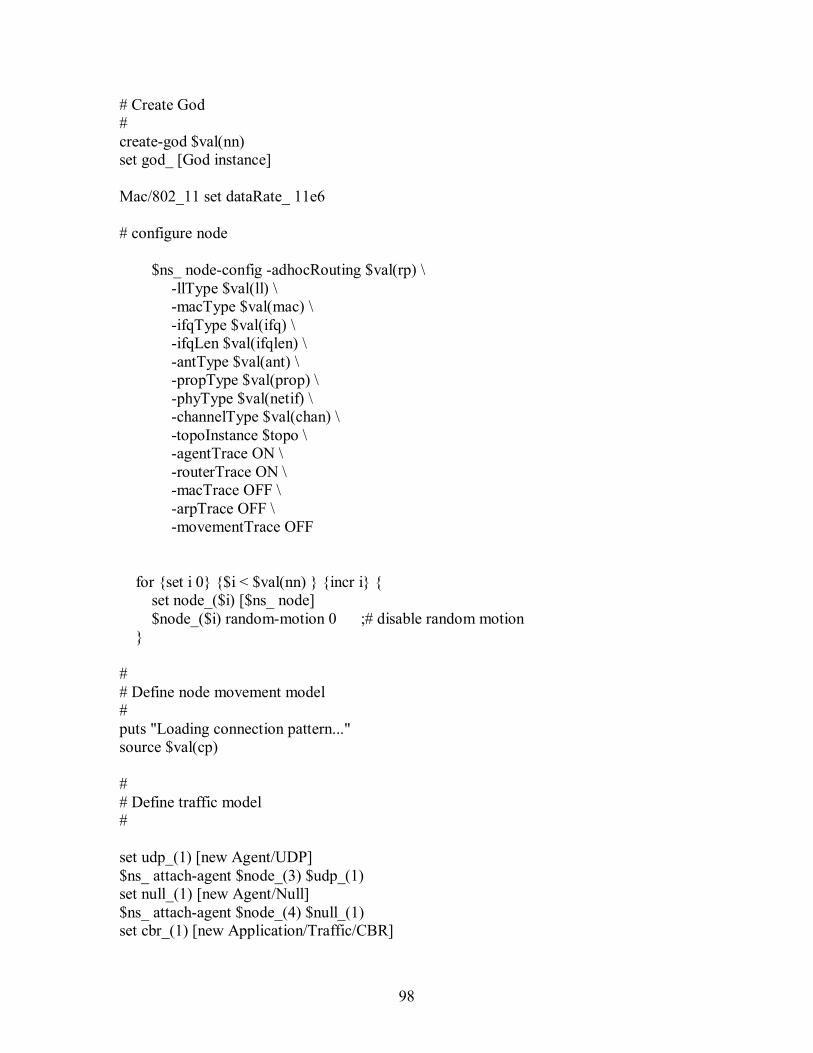
98

# Create God # create-god $val(nn) set god_ [God instance] Mac/802_11 set dataRate_ 11e6 # configure node $ns_ node-config -adhocRouting $val(rp) \ -llType $val(ll) \ -macType $val(mac) \ -ifqType $val(ifq) \ -ifqLen $val(ifqlen) \ -antType $val(ant) \ -propType $val(prop) \ -phyType $val(netif) \ -channelType $val(chan) \ -topoInstance $topo \ -agentTrace ON \ -routerTrace ON \ -macTrace OFF \ -arpTrace OFF \ -movementTrace OFF for {set i 0} {$i < $val(nn) } {incr i} { set node_($i) [$ns_ node] $node_($i) random-motion 0 ;# disable random motion } # # Define node movement model # puts "Loading connection pattern..." source $val(cp) # # Define traffic model # set udp_(1) [new Agent/UDP] $ns_ attach-agent $node_(3) $udp_(1) set null_(1) [new Agent/Null] $ns_ attach-agent $node_(4) $null_(1) set cbr_(1) [new Application/Traffic/CBR]

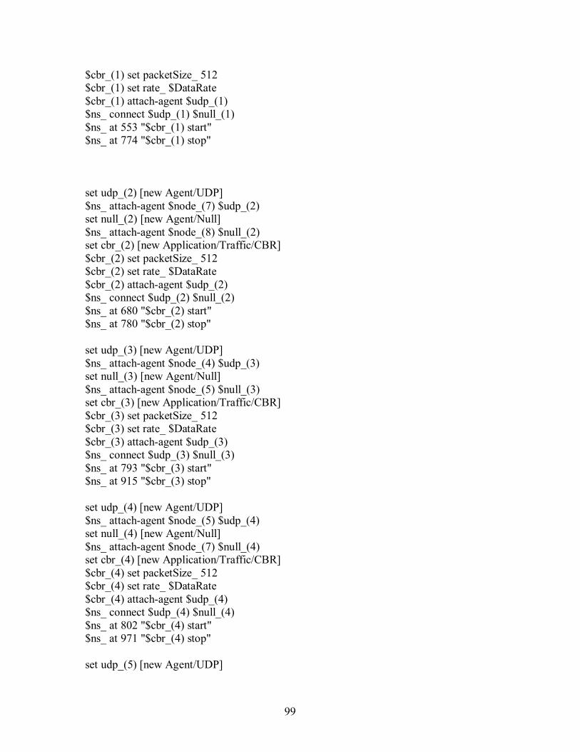
99

$cbr_(1) set packetSize_ 512 $cbr_(1) set rate_ $DataRate $cbr_(1) attach-agent $udp_(1) $ns_ connect $udp_(1) $null_(1) $ns_ at 553 "$cbr_(1) start" $ns_ at 774 "$cbr_(1) stop" set udp_(2) [new Agent/UDP] $ns_ attach-agent $node_(7) $udp_(2) set null_(2) [new Agent/Null] $ns_ attach-agent $node_(8) $null_(2) set cbr_(2) [new Application/Traffic/CBR] $cbr_(2) set packetSize_ 512 $cbr_(2) set rate_ $DataRate $cbr_(2) attach-agent $udp_(2) $ns_ connect $udp_(2) $null_(2) $ns_ at 680 "$cbr_(2) start" $ns_ at 780 "$cbr_(2) stop" set udp_(3) [new Agent/UDP] $ns_ attach-agent $node_(4) $udp_(3) set null_(3) [new Agent/Null] $ns_ attach-agent $node_(5) $null_(3) set cbr_(3) [new Application/Traffic/CBR] $cbr_(3) set packetSize_ 512 $cbr_(3) set rate_ $DataRate $cbr_(3) attach-agent $udp_(3) $ns_ connect $udp_(3) $null_(3) $ns_ at 793 "$cbr_(3) start" $ns_ at 915 "$cbr_(3) stop" set udp_(4) [new Agent/UDP] $ns_ attach-agent $node_(5) $udp_(4) set null_(4) [new Agent/Null] $ns_ attach-agent $node_(7) $null_(4) set cbr_(4) [new Application/Traffic/CBR] $cbr_(4) set packetSize_ 512 $cbr_(4) set rate_ $DataRate $cbr_(4) attach-agent $udp_(4) $ns_ connect $udp_(4) $null_(4) $ns_ at 802 "$cbr_(4) start" $ns_ at 971 "$cbr_(4) stop" set udp_(5) [new Agent/UDP]

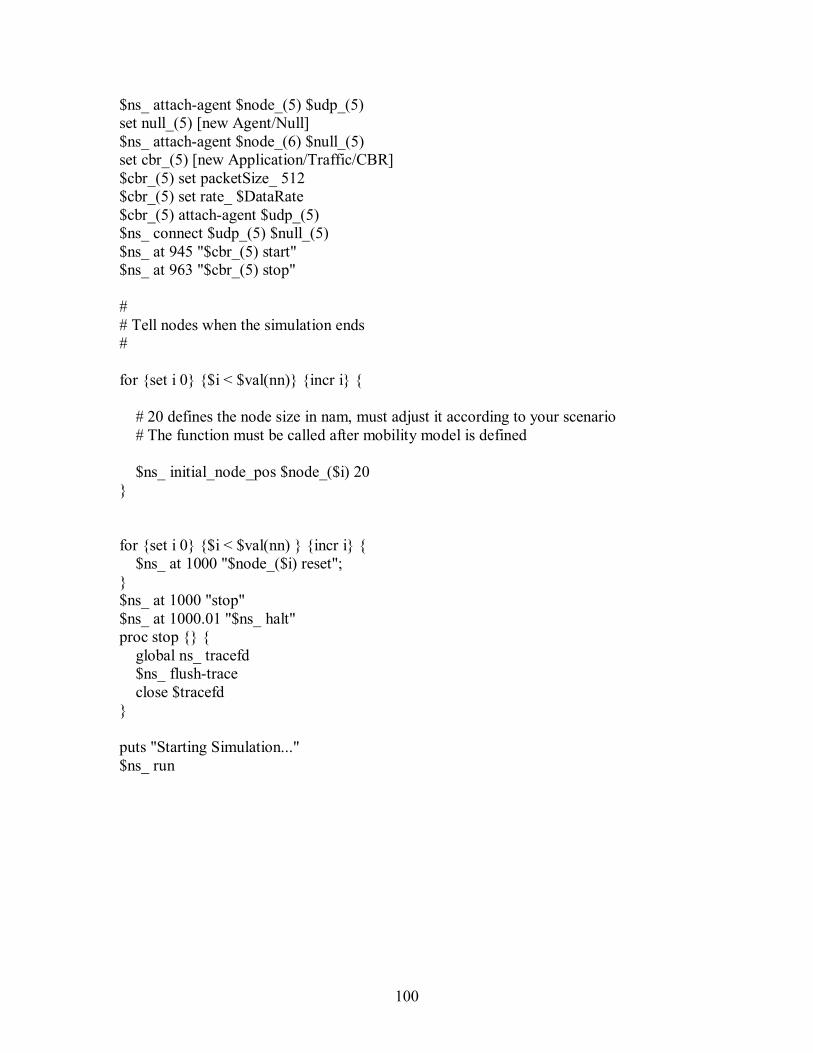
100

$ns_ attach-agent $node_(5) $udp_(5) set null_(5) [new Agent/Null] $ns_ attach-agent $node_(6) $null_(5) set cbr_(5) [new Application/Traffic/CBR] $cbr_(5) set packetSize_ 512 $cbr_(5) set rate_ $DataRate $cbr_(5) attach-agent $udp_(5) $ns_ connect $udp_(5) $null_(5) $ns_ at 945 "$cbr_(5) start" $ns_ at 963 "$cbr_(5) stop" # # Tell nodes when the simulation ends # for {set i 0} {$i < $val(nn)} {incr i} { # 20 defines the node size in nam, must adjust it according to your scenario # The function must be called after mobility model is defined $ns_ initial_node_pos $node_($i) 20 } for {set i 0} {$i < $val(nn) } {incr i} { $ns_ at 1000 "$node_($i) reset"; } $ns_ at 1000 "stop" $ns_ at 1000.01 "$ns_ halt" proc stop {} { global ns_ tracefd $ns_ flush-trace close $tracefd } puts "Starting Simulation..." $ns_ run

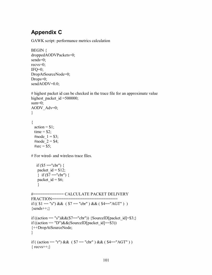
101

Appendix C GAWK script: performance metrics calculation BEGIN { droppedAODVPackets=0; sends=0; recvs=0; IFQ=0; DropAtSourceNode=0; Drops=0; sendAODV=0.0; # highest packet id can be checked in the trace file for an approximate value highest_packet_id =500000; sum=0; AODV_Adv=0; } { action = $1; time = $2; #node_1 = $3; #node_2 = $4; #src = $5; # For wired- and wireless trace files. if ($5 =="cbr") { packet_id = $12; } if ($7 =="cbr") { packet_id = $6; } #============= CALCULATE PACKET DELIVERY FRACTION============================ if (( $1 == "s") && ( $7 == "cbr" ) && ( $4=="AGT" ) ) {sends++;} if ((action == "s")&&($7=="cbr")) {SourceID[packet_id]=$3;} if ((action == "D")&&(SourceID[packet_id]==$3)) {++DropAtSourceNode; } if ( (action == "r") && ( $7 == "cbr" ) && ( $4=="AGT" ) ) { recvs++;}

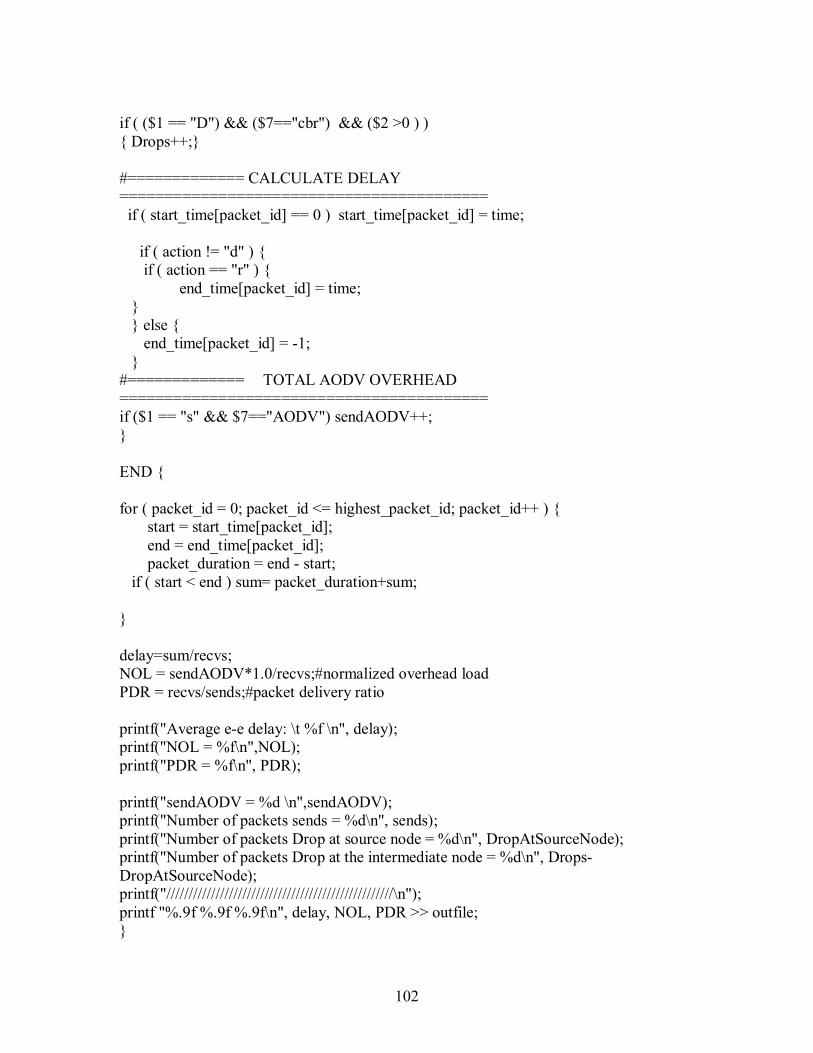
102

if ( ($1 == "D") && ($7=="cbr") && ($2 >0 ) ) { Drops++;} #============= CALCULATE DELAY ========================================= if ( start_time[packet_id] == 0 ) start_time[packet_id] = time; if ( action != "d" ) { if ( action == "r" ) { end_time[packet_id] = time; } } else { end_time[packet_id] = -1; } #============= TOTAL AODV OVERHEAD ========================================= if ($1 == "s" && $7=="AODV") sendAODV++; } END { for ( packet_id = 0; packet_id <= highest_packet_id; packet_id++ ) { start = start_time[packet_id]; end = end_time[packet_id]; packet_duration = end - start; if ( start < end ) sum= packet_duration+sum; } delay=sum/recvs; NOL = sendAODV*1.0/recvs;#normalized overhead load PDR = recvs/sends;#packet delivery ratio printf("Average e-e delay: \t %f \n", delay); printf("NOL = %f\n",NOL); printf("PDR = %f\n", PDR); printf("sendAODV = %d \n",sendAODV); printf("Number of packets sends = %d\n", sends); printf("Number of packets Drop at source node = %d\n", DropAtSourceNode); printf("Number of packets Drop at the intermediate node = %d\n", Drops-DropAtSourceNode); printf("///////////////////////////////////////////////////\n"); printf "%.9f %.9f %.9f\n", delay, NOL, PDR >> outfile; }

103

Appendix D GNUPLOT script: draw figures with the simulation results set term gif set output "average-end-to-end-delay-datarate.gif" set ylabel "average end-to-end delay (s)" set xlabel "Data Rate (kbps) " set key left top set title "average end-to-end delay" plot "aodv-delay" title 'AODV-delay' with linespoints , \ "qaodv-delay" title 'QAODV-delay' with linespoints set term gif set output "PDR-datarate.gif" set ylabel "PDR" set xlabel "Data Rate (kbps)" set key left top set title "PDR" plot "aodv-PDR" title 'AODV-PDR' with linespoints , \ "qaodv-PDR" title 'QAODV-PDR' with linespoints set term gif set output "NOL-datarate.gif" set ylabel "NOL " set xlabel "Data Rate (kbps) " set key left top set title "NOL" plot "aodv-NOL" title 'AODV-NOL' with linespoints , \ "qaodv-NOL" title 'QAODV-NOL' with linespoints