Punctuality of Railway Operations and Timetable Stability Analysis
310
Punctuality of Railway Operations and Timetable Stability Analysis Rob M.P. Goverde
Transcript of Punctuality of Railway Operations and Timetable Stability Analysis
Punctuality of Railway Operations and
Timetable Stability Analysis
Rob M.P. Goverde

Cover design: Rob M.P. Goverde
Punctuality of Railway Operations andTimetable Stability Analysis
Proefschrift
ter verkrijging van de graad van doctor
aan de Technische Universiteit Delft,
op gezag van de Rector Magnificus prof.dr.ir. J.T. Fokkema,
voorzitter van het College voor Promoties,
in het openbaar te verdedigen op maandag 3 oktober 2005 om 10:30 uur
door
Robert Michael Petrus GOVERDE
doctorandus in de wiskunde
geboren te Arnhem
Dit proefschrift is goedgekeurd door de promotor:
Prof.Dr.-Ing. I.A. Hansen
Samenstelling Promotiecommissie:
Rector Magnificus voorzitter
Prof.Dr.-Ing. I.A. Hansen Technische Universiteit Delft, promotor
Prof.dr. G.J. Olsder Technische Universiteit Delft
Prof.dr. M. Carey Queen’s University Belfast
Prof.Dr.-Ing. E. Hohnecker Universitat Karlsruhe
Prof.dr. L.G. Kroon Erasmus Universiteit Rotterdam
Dr. J.W. van der Woude Technische Universiteit Delft
Prof.dr. H.J. van Zuylen Technische Universiteit Delft, reservelid
This publication is a result of the research programme Seamless Multimodal Mobility, carried
out within the Netherlands TRAIL Research School for Transport, Infrastructure and Logistics,
and financed by Delft University of Technology.
TRAIL Thesis Series no. T2005/10, The Netherlands TRAIL Research School
TRAIL
P.O. Box 5017
2600 GA Delft
The NetherlandsPhone: +31 (0) 15 27 86046
Fax: +31 (0) 15 27 84333
E-mail: [email protected]
ISBN 90-5584-068-8
Keywords: railway timetable, max-plus algebra, railway operations
Copyright c© 2005 by Rob M.P. Goverde
All rights reserved. No part of the material protected by this copyright notice may be reproduced
or utilized in any form or by any means, electronic or mechanical, including photocopying,
recording or by any information storage and retrieval system, without written permission from
the author.
Printed in The Netherlands
PREFACE
This PhD thesis is the result of research work carried out at the Transport & Planning Depart-
ment of Delft University of Technology. I started working at this department in 1996 on several
R&D projects of Railned Innovation on “Capacity Utilization and Synchronization Manage-
ment,” including a project on the applicability of max-plus algebra to railway capacity manage-
ment based on the PhD thesis of Hans Braker. The follow-up of these projects was embedded
in the DIOC research programme Seamless Multimodal Mobility (SMM) financed by Delft
University of Technology and supported by Railned, Railinfrabeheer, Railverkeersleiding, and
Holland Railconsult. This enabled a more fundamental research approach finally resulting in
this thesis.
I hereby want to thank the members in the user committee of the SMM rail research projects for
their enthusiasm, feedback, and provision of data: Alfons Schaafsma, Laurens Berger & Jurjen
Hooghiemstra (Railned), Dick Tersteeg (Railverkeersleiding), F. Koster & J. Lodder (Railin-
frabeheer), and Ello Weits & Lieuwe Zigterman (Holland Railconsult). Over the last few years
I am indebted to Dick Middelkoop (ProRail/Railned) for his support and provision of data.
In addition, I thank anyone from the railway organizations who in any way helped me in my
understanding of the railway field.
I also like to thank the other PhD researchers in the SMM rail research projects for their collab-
oration: Antoine de Kort, Robert-Jan van Egmond, Gerardo Soto y Koelemeijer, and Subiono.
I regret that the first two decided to quit their PhD research before the end. I also wish to
express my gratitude to the post-docs and senior researchers who participated in these SMM
projects: Gerard Hooghiemstra, Rik Lopuhaa, and Bernd Heidergott, as well as my colleagues
from the TRAIL research school and the Transport & Planning Department, and in particular:
Paul Wiggenraad, Theo Muller, and prof. Piet Bovy.
My sincere gratitude goes to Remco Johanns (BIN Bedrijfsadviezen) for his work on TNV-
Prepare, and Michiel Odijk and Paul Goldman (ORTEC) for their work on PETER. Their co-
operation and programming skills made these software tools as they are now.
Special thanks go to Jurjen Hooghiemstra for giving me the opportunity to work at ProRail/
Railned in the project PRRING (Planning en Realizatie van RailINfraGebruik). I learned a lot
from his experience and our discussions. I hope that his valuable idea(l)s for improving the
railways will find their way into the railway practice. I wish him all the best in his new carreer
as an independent consultant under the name Kwaliteit in Verbinding.
I am very grateful to my promotor prof. Ingo Hansen for trusting my mathematical opinions
whilst guiding me to the world of transport, traffic and railways over all these years. His door
was always open to me and I highly appreciate our cooperation. I also thank prof. Geert Jan
Olsder for his everlasting support. I owed my PhD-position to his contacts with the Transport
& Planning Department for which I am enormously thankful.
I sincerely thank my promotion committee for reading the entire manuscript and especially prof.
Leo Kroon for his detailed comments.
v

vi Punctuality of Railway Operations and Timetable Stability Analysis
Finally, I thank my parents for their support and all my friends who never stopped believing,
and in particular: Patrick Timmers, Joke van den Bogert, and Wies Hendriks.
Rob Goverde
September 2005
CONTENTS
1 INTRODUCTION 1
1.1 Background . . . . . . . . . . . . . . . . . . . . . . . . . . . . . . . . . . . . 1
1.1.1 The Railways in the Netherlands at the Start of the 21st Century . . . . 1
1.1.2 Railway Operations and Timetable Stability . . . . . . . . . . . . . . . 2
1.2 Setting the Scene . . . . . . . . . . . . . . . . . . . . . . . . . . . . . . . . . 4
1.2.1 The Railway Timetable . . . . . . . . . . . . . . . . . . . . . . . . . . 4
1.2.2 Infrastructure Capacity Utilization and Timetable Performance . . . . . 5
1.2.3 Social Relevance . . . . . . . . . . . . . . . . . . . . . . . . . . . . . 7
1.3 Research Objectives . . . . . . . . . . . . . . . . . . . . . . . . . . . . . . . . 8
1.3.1 Ex-Post Traffic Analysis: Punctuality of Railway Operations . . . . . . 8
1.3.2 Ex-Ante Traffic Analysis: Railway Timetable Stability . . . . . . . . . 9
1.4 Contributions . . . . . . . . . . . . . . . . . . . . . . . . . . . . . . . . . . . 10
1.5 Thesis Outline . . . . . . . . . . . . . . . . . . . . . . . . . . . . . . . . . . . 12
2 FUNDAMENTALS OF RAILWAY OPERATIONS 15
2.1 Introduction . . . . . . . . . . . . . . . . . . . . . . . . . . . . . . . . . . . . 15
2.2 The Hierarchical Railway Planning Process . . . . . . . . . . . . . . . . . . . 16
2.2.1 Transport Demand . . . . . . . . . . . . . . . . . . . . . . . . . . . . 17
2.2.2 Railway Network Design . . . . . . . . . . . . . . . . . . . . . . . . . 17
2.2.3 Line Systems . . . . . . . . . . . . . . . . . . . . . . . . . . . . . . . 18
2.2.4 Railway Timetabling . . . . . . . . . . . . . . . . . . . . . . . . . . . 20
2.2.5 Rolling Stock Circulations . . . . . . . . . . . . . . . . . . . . . . . . 22
2.2.6 Crew Schedules and Rosters . . . . . . . . . . . . . . . . . . . . . . . 23
2.3 Safety and Signalling Systems . . . . . . . . . . . . . . . . . . . . . . . . . . 24
2.3.1 Train Detection . . . . . . . . . . . . . . . . . . . . . . . . . . . . . . 24
2.3.2 Fixed Block Signalling . . . . . . . . . . . . . . . . . . . . . . . . . . 25
2.3.3 Automatic Train Protection . . . . . . . . . . . . . . . . . . . . . . . . 27
2.3.4 Train Describer Systems (TNV) . . . . . . . . . . . . . . . . . . . . . 28
2.3.5 Interlocking . . . . . . . . . . . . . . . . . . . . . . . . . . . . . . . . 29
2.3.6 Dispatching . . . . . . . . . . . . . . . . . . . . . . . . . . . . . . . . 31
2.3.7 Traffic Control . . . . . . . . . . . . . . . . . . . . . . . . . . . . . . 32
2.4 Train Delays . . . . . . . . . . . . . . . . . . . . . . . . . . . . . . . . . . . . 33
2.4.1 Primary Delays . . . . . . . . . . . . . . . . . . . . . . . . . . . . . . 33
2.4.2 Secondary Delays . . . . . . . . . . . . . . . . . . . . . . . . . . . . . 34
2.5 Conclusions . . . . . . . . . . . . . . . . . . . . . . . . . . . . . . . . . . . . 35
3 RAILWAY TIMETABLES 37
3.1 Introduction . . . . . . . . . . . . . . . . . . . . . . . . . . . . . . . . . . . . 37
3.2 Running Time . . . . . . . . . . . . . . . . . . . . . . . . . . . . . . . . . . . 38
3.2.1 Running Time Calculations . . . . . . . . . . . . . . . . . . . . . . . 38
3.2.2 Running Time Margin . . . . . . . . . . . . . . . . . . . . . . . . . . 39
3.3 Blocking times and Minimum Headway . . . . . . . . . . . . . . . . . . . . . 41
vii
viii Punctuality of Railway Operations and Timetable Stability Analysis
3.4 Dwell Time . . . . . . . . . . . . . . . . . . . . . . . . . . . . . . . . . . . . 45
3.5 Transfer Time . . . . . . . . . . . . . . . . . . . . . . . . . . . . . . . . . . . 46
3.6 Layover Time . . . . . . . . . . . . . . . . . . . . . . . . . . . . . . . . . . . 47
3.7 Synchronization Time . . . . . . . . . . . . . . . . . . . . . . . . . . . . . . . 47
3.8 Buffer Time versus Scheduled Waiting Time . . . . . . . . . . . . . . . . . . . 48
3.8.1 Buffer Time . . . . . . . . . . . . . . . . . . . . . . . . . . . . . . . . 48
3.8.2 Scheduled Waiting Time . . . . . . . . . . . . . . . . . . . . . . . . . 49
3.9 Literature Review of Railway Timetabling . . . . . . . . . . . . . . . . . . . . 50
3.9.1 Timetable Feasibility . . . . . . . . . . . . . . . . . . . . . . . . . . . 50
3.9.2 Timetable Optimization . . . . . . . . . . . . . . . . . . . . . . . . . 53
3.9.3 Deterministic Timetable Performance Evaluation Models . . . . . . . . 56
3.9.4 Stochastic Models of Railway Operations . . . . . . . . . . . . . . . . 58
3.9.5 Network Simulation . . . . . . . . . . . . . . . . . . . . . . . . . . . 62
3.10 Conclusions . . . . . . . . . . . . . . . . . . . . . . . . . . . . . . . . . . . . 64
4 TRAIN DETECTION DATA AND TNV-PREPARE 67
4.1 Introduction . . . . . . . . . . . . . . . . . . . . . . . . . . . . . . . . . . . . 67
4.2 TNV-Logfiles . . . . . . . . . . . . . . . . . . . . . . . . . . . . . . . . . . . 68
4.2.1 Train Number Events . . . . . . . . . . . . . . . . . . . . . . . . . . . 69
4.2.2 Infrastructure Events . . . . . . . . . . . . . . . . . . . . . . . . . . . 70
4.3 TNV-Prepare . . . . . . . . . . . . . . . . . . . . . . . . . . . . . . . . . . . 71
4.3.1 The Internal Database . . . . . . . . . . . . . . . . . . . . . . . . . . 71
4.3.2 Generation of TNV-Tables . . . . . . . . . . . . . . . . . . . . . . . . 73
4.3.3 TNV-Tables . . . . . . . . . . . . . . . . . . . . . . . . . . . . . . . . 78
4.3.4 Accuracy and Reliability of TNV-Tables . . . . . . . . . . . . . . . . . 80
4.4 TNV-Filter . . . . . . . . . . . . . . . . . . . . . . . . . . . . . . . . . . . . 81
4.4.1 Filtering of Train Paths through Stations . . . . . . . . . . . . . . . . . 81
4.4.2 Speed Profile Estimation . . . . . . . . . . . . . . . . . . . . . . . . . 82
4.4.3 Train Length Estimation . . . . . . . . . . . . . . . . . . . . . . . . . 87
4.4.4 Running Time on Platform Tracks . . . . . . . . . . . . . . . . . . . . 88
4.4.5 Arrival and Departure Delays . . . . . . . . . . . . . . . . . . . . . . 94
4.5 Conclusions and Recommendations . . . . . . . . . . . . . . . . . . . . . . . 95
5 STATISTICAL ANALYSIS: THE EINDHOVEN CASE 97
5.1 Introduction . . . . . . . . . . . . . . . . . . . . . . . . . . . . . . . . . . . . 97
5.2 Railway station Eindhoven . . . . . . . . . . . . . . . . . . . . . . . . . . . . 98
5.3 Punctuality Analysis . . . . . . . . . . . . . . . . . . . . . . . . . . . . . . . 100
5.3.1 Arrival Delay . . . . . . . . . . . . . . . . . . . . . . . . . . . . . . . 100
5.3.2 Departure Delay . . . . . . . . . . . . . . . . . . . . . . . . . . . . . 102
5.3.3 Dwell Time . . . . . . . . . . . . . . . . . . . . . . . . . . . . . . . . 104
5.3.4 Transfer Time . . . . . . . . . . . . . . . . . . . . . . . . . . . . . . . 105
5.4 Regression Analysis . . . . . . . . . . . . . . . . . . . . . . . . . . . . . . . . 107
5.4.1 Introduction . . . . . . . . . . . . . . . . . . . . . . . . . . . . . . . . 107
5.4.2 Robust LTS Regression . . . . . . . . . . . . . . . . . . . . . . . . . . 108
5.4.3 Transfers between IC800 Hlm-Mt and IR1900 Rtd-Vl . . . . . . . . . 110
5.4.4 Transfers between IC800 Mt-Hlm and IR1900 Vl-Rtd . . . . . . . . . 111
5.4.5 Transfer IC900 Hlm-Ehv to IC1500 Gvc-Hrl . . . . . . . . . . . . . . 112
Contents ix
5.4.6 Transfer IC1500 Hrl-Gvc to IC900 Ehv-Hlm . . . . . . . . . . . . . . 113
5.4.7 Stability . . . . . . . . . . . . . . . . . . . . . . . . . . . . . . . . . . 114
5.5 Probability Distributions . . . . . . . . . . . . . . . . . . . . . . . . . . . . . 115
5.5.1 Arrival Delay . . . . . . . . . . . . . . . . . . . . . . . . . . . . . . . 115
5.5.2 Departure Delay . . . . . . . . . . . . . . . . . . . . . . . . . . . . . 117
5.5.3 Dwell Time . . . . . . . . . . . . . . . . . . . . . . . . . . . . . . . . 118
5.5.4 Transfer Time . . . . . . . . . . . . . . . . . . . . . . . . . . . . . . . 120
5.6 Conclusions . . . . . . . . . . . . . . . . . . . . . . . . . . . . . . . . . . . . 120
6 TIMED EVENT GRAPHS 123
6.1 Introduction . . . . . . . . . . . . . . . . . . . . . . . . . . . . . . . . . . . . 123
6.2 Petri Nets and Timed Event Graphs . . . . . . . . . . . . . . . . . . . . . . . . 124
6.2.1 Basic Definitions . . . . . . . . . . . . . . . . . . . . . . . . . . . . . 124
6.2.2 Building Blocks of Timed Event Graphs . . . . . . . . . . . . . . . . . 126
6.3 Basic Modelling Approach of Railway Systems . . . . . . . . . . . . . . . . . 128
6.3.1 Train Circulations . . . . . . . . . . . . . . . . . . . . . . . . . . . . 128
6.3.2 Train Synchronizations . . . . . . . . . . . . . . . . . . . . . . . . . . 129
6.3.3 Headway Constraints . . . . . . . . . . . . . . . . . . . . . . . . . . . 130
6.4 Behavioural Properties . . . . . . . . . . . . . . . . . . . . . . . . . . . . . . 132
6.4.1 Liveness . . . . . . . . . . . . . . . . . . . . . . . . . . . . . . . . . 132
6.4.2 Reachability . . . . . . . . . . . . . . . . . . . . . . . . . . . . . . . 134
6.4.3 Periodicity . . . . . . . . . . . . . . . . . . . . . . . . . . . . . . . . 138
6.4.4 Boundedness . . . . . . . . . . . . . . . . . . . . . . . . . . . . . . . 139
6.5 Synthesis of Scheduled Railway Systems . . . . . . . . . . . . . . . . . . . . 140
6.5.1 Input Data . . . . . . . . . . . . . . . . . . . . . . . . . . . . . . . . . 140
6.5.2 Timed Event Graph Construction . . . . . . . . . . . . . . . . . . . . 143
6.5.3 Event Domain Description . . . . . . . . . . . . . . . . . . . . . . . . 148
6.6 Conclusions . . . . . . . . . . . . . . . . . . . . . . . . . . . . . . . . . . . . 150
7 MAX-PLUS ALGEBRA 153
7.1 Introduction . . . . . . . . . . . . . . . . . . . . . . . . . . . . . . . . . . . . 153
7.2 Max-Plus Semirings . . . . . . . . . . . . . . . . . . . . . . . . . . . . . . . . 154
7.2.1 Basic Definitions: Semirings, Semifields, Dioids . . . . . . . . . . . . 154
7.2.2 The (max,+)-Semifield . . . . . . . . . . . . . . . . . . . . . . . . . . 156
7.2.3 Max-Plus Polynomials . . . . . . . . . . . . . . . . . . . . . . . . . . 157
7.2.4 Max-Plus Matrices . . . . . . . . . . . . . . . . . . . . . . . . . . . . 159
7.2.5 Precedence Graphs and Path Matrices . . . . . . . . . . . . . . . . . . 163
7.2.6 Polynomial Matrices and Timed Event Graphs . . . . . . . . . . . . . 167
7.2.7 Partially Ordered Semirings . . . . . . . . . . . . . . . . . . . . . . . 171
7.3 Max-Plus Semimodules . . . . . . . . . . . . . . . . . . . . . . . . . . . . . . 173
7.3.1 Semimodules over the (max,+)-Semiring . . . . . . . . . . . . . . . . 173
7.3.2 Linear and Weak Independence . . . . . . . . . . . . . . . . . . . . . 174
7.3.3 Linear Mappings . . . . . . . . . . . . . . . . . . . . . . . . . . . . . 178
7.4 Max-Plus (Generalized) Eigenproblems . . . . . . . . . . . . . . . . . . . . . 179
7.4.1 Introduction . . . . . . . . . . . . . . . . . . . . . . . . . . . . . . . . 179
7.4.2 Eigenstructure of Irreducible Matrices . . . . . . . . . . . . . . . . . . 180
7.4.3 State Classification and the Reduced Graph . . . . . . . . . . . . . . . 185
x Punctuality of Railway Operations and Timetable Stability Analysis
7.4.4 Eigenstructure of Reducible Matrices . . . . . . . . . . . . . . . . . . 188
7.4.5 The Cycle Time Vector . . . . . . . . . . . . . . . . . . . . . . . . . . 194
7.4.6 The Policy Iteration Algorithm . . . . . . . . . . . . . . . . . . . . . . 196
7.4.7 Alternative Eigenproblem Algorithms . . . . . . . . . . . . . . . . . . 205
7.5 Longest Path Algorithms . . . . . . . . . . . . . . . . . . . . . . . . . . . . . 208
7.5.1 All-Pair Longest Paths . . . . . . . . . . . . . . . . . . . . . . . . . . 208
7.5.2 Single-Origin Longest Paths . . . . . . . . . . . . . . . . . . . . . . . 209
7.5.3 All Critical Circuits . . . . . . . . . . . . . . . . . . . . . . . . . . . . 212
7.6 Conclusions . . . . . . . . . . . . . . . . . . . . . . . . . . . . . . . . . . . . 215
8 RAILWAY TIMETABLE STABILITY ANALYSIS 217
8.1 Introduction . . . . . . . . . . . . . . . . . . . . . . . . . . . . . . . . . . . . 217
8.2 Max-Plus Linear Systems . . . . . . . . . . . . . . . . . . . . . . . . . . . . . 218
8.2.1 First-Order State-Space Equations . . . . . . . . . . . . . . . . . . . . 218
8.2.2 Higher-Order State-Space Equations . . . . . . . . . . . . . . . . . . . 220
8.2.3 Polynomial Matrix Representation . . . . . . . . . . . . . . . . . . . . 221
8.2.4 Autonomous Max-Plus Linear Systems . . . . . . . . . . . . . . . . . 222
8.2.5 First-Order Representations . . . . . . . . . . . . . . . . . . . . . . . 223
8.3 Max-Plus Spectral Analysis . . . . . . . . . . . . . . . . . . . . . . . . . . . . 226
8.3.1 Timetable Stability and Critical Circuits . . . . . . . . . . . . . . . . . 226
8.3.2 Network Throughput . . . . . . . . . . . . . . . . . . . . . . . . . . . 228
8.3.3 Stability Margin . . . . . . . . . . . . . . . . . . . . . . . . . . . . . 228
8.4 Timetable Realizability . . . . . . . . . . . . . . . . . . . . . . . . . . . . . . 229
8.5 Timetable Robustness . . . . . . . . . . . . . . . . . . . . . . . . . . . . . . . 231
8.5.1 The Recovery Matrix . . . . . . . . . . . . . . . . . . . . . . . . . . . 231
8.5.2 Delay Impact Vectors . . . . . . . . . . . . . . . . . . . . . . . . . . . 234
8.5.3 Delay Sensitivity Vectors . . . . . . . . . . . . . . . . . . . . . . . . . 234
8.5.4 Circulation Recovery Times . . . . . . . . . . . . . . . . . . . . . . . 235
8.6 Delay Propagation . . . . . . . . . . . . . . . . . . . . . . . . . . . . . . . . 236
8.6.1 Introduction . . . . . . . . . . . . . . . . . . . . . . . . . . . . . . . . 236
8.6.2 The Delay Propagation Model . . . . . . . . . . . . . . . . . . . . . . 236
8.6.3 A Bucket-Based Delay Propagation Algorithm . . . . . . . . . . . . . 239
8.7 PETER . . . . . . . . . . . . . . . . . . . . . . . . . . . . . . . . . . . . . . 244
8.7.1 Introduction . . . . . . . . . . . . . . . . . . . . . . . . . . . . . . . . 244
8.7.2 Input Data . . . . . . . . . . . . . . . . . . . . . . . . . . . . . . . . . 245
8.7.3 Functionalities . . . . . . . . . . . . . . . . . . . . . . . . . . . . . . 246
8.8 Case Study: The Dutch National Railway Timetable . . . . . . . . . . . . . . . 251
8.8.1 Model Variants . . . . . . . . . . . . . . . . . . . . . . . . . . . . . . 251
8.8.2 Critical Circuit Analysis . . . . . . . . . . . . . . . . . . . . . . . . . 252
8.8.3 Delay Propagation and Recovery Time Analysis . . . . . . . . . . . . 254
8.9 Conclusions . . . . . . . . . . . . . . . . . . . . . . . . . . . . . . . . . . . . 256
9 CONCLUSIONS 257
9.1 Main Conclusions . . . . . . . . . . . . . . . . . . . . . . . . . . . . . . . . . 257
9.1.1 Analysis of Train Detection Data . . . . . . . . . . . . . . . . . . . . . 257
9.1.2 Timetable Stability Analysis . . . . . . . . . . . . . . . . . . . . . . . 259
9.2 Recommendations and Future Research . . . . . . . . . . . . . . . . . . . . . 260
Contents xi
9.2.1 Train Detection Data and Railway Operations Quality Management . . 260
9.2.2 Max-Plus Algebra . . . . . . . . . . . . . . . . . . . . . . . . . . . . 262
BIBLIOGRAPHY 265
A GLOSSARY 279
A.1 General Abbreviations . . . . . . . . . . . . . . . . . . . . . . . . . . . . . . 279
A.2 Station Abbreviations . . . . . . . . . . . . . . . . . . . . . . . . . . . . . . . 279
A.3 Mathematical Symbols and Variables . . . . . . . . . . . . . . . . . . . . . . . 280
SUMMARY 283
NEDERLANDSE SAMENVATTING (DUTCH SUMMARY) 287
ABOUT THE AUTHOR 293

xii Punctuality of Railway Operations and Timetable Stability Analysis

Chapter 1
INTRODUCTION
1.1 Background
1.1.1 The Railways in the Netherlands at the Start of the 21st Century
Punctuality and reliability of public (rail) transport are vital components of quality of service
and passenger satisfaction. In the Netherlands, an increasing number of disruptive incidents
in conjunction with an increasingly saturated railway capacity has led to a decline of reliability
and punctuality over the last decade. In contrast to the growing national mobility and increasing
congestion on the Dutch motorways, the railways in the Netherlands hardly attract new passen-
gers. Nevertheless, the railways have a responsibility to significantly contribute to the mobility
of persons to keep the heavily populated and industrialized Randstad — the conurbation in the
western Netherlands — reachable. Reliability and capacity utilization must therefore be im-
proved considerably to accommodate this increase in train traffic volume. The Dutch railway
infrastructure is already one of the most intensely utilized national railway networks in the world
with 50,000 train kilometres per track kilometre per year [163, 179]. On an average working
day 5,000 passenger trains carry 1 million passengers, and additional freight trains carry about
100,000 ton of goods. Freight trains have currently only a small share of 7% of total railway
traffic, but at least a doubling of freight traffic is expected after opening the international railway
market for freight transport in 2008 [149].
Punctuality of railway services depends heavily on reliability of resources (railway infrastruc-
ture, safety and signalling systems, rolling stock, and personnel). Since 1995, the number of
infrastructure malfunctions increased considerably in the Netherlands [78], mainly due to in-
sufficient maintenance. Moreover, rolling stock breakdown and scarcity, as well as distress
amongst train personnel further contributed to a considerable decrease in punctuality. The dis-
astrous leaves on the railway tracks in the autumn of 2001 accumulated to a decline of annual
punctuality (percentage of trains less than 3 minutes late) to below 80%. The annual passenger
kilometres also began to show a negative trend since 2001, after years of growth during the sec-
ond half of the 1990s [148]. Many of these problems can be traced back to the Dutch railway
reform in 1995 [120, 179, 203] conform to the European Directive 91/440/EEC on the devel-
opment of the Community’s railways. In this directive and the subsequent rail infrastructure
package — directives 2001/12/EC, 2001/13/EC and 2001/14/EC — the European Union com-
misioned the decoupling of railway infrastructure ownership from train operators and opening
the national railway markets for competition between train operators [61]. This led to radical
changes in the European railway markets, where national railways used to be organized in state
monopolies.
In the Netherlands, the railway reform suffered from political uncertainty. On January 1, 1995,
the Dutch monopolist NS (Nederlandse Spoorwegen) was separated into several organizations.
1
2 Punctuality of Railway Operations and Timetable Stability Analysis
Management of the Dutch railway infrastructure was transferred to three newly founded task
organizations which were responsible on behalf of the government for maintenance (Railin-
frabeheer), traffic control (Railverkeersleiding), and capacity management (Railned). NS was
furthermore split into several divisions, including the passenger train operator NS Reizigers
(NSR), the freight train operator NS Cargo, and the rolling stock maintenance division Ned-
Train. The freight division was discharged in 1999, after a fusion of NS Cargo and the German
DB Cargo under the name Railion. Furthermore, new train operators were introduced in the
regional passenger markets (NoordNed, Syntus) and especially in the rail freight market (e.g.
ACTS, ShortLines, ERS Railways). During 1996–1999 the Ministry of Transport allowed com-
petition between NSR and the new passenger train operator Lovers Rail for running concur-
rent train services on shared tracks. The experiment drastically failed and was discontinued in
1999 [203]. The new policy of the Ministry of Transport was a concession of all main passen-
ger lines — the core network — to one operator under a performance regime, and tendering of
regional lines by regional transport authorities. In the mean time NS hesitated to invest in new
rolling stock due to the uncertainty of future operation rights. In 2001, NS finally ordered new
passenger coaches which however became only gradually available in 2002 and 2003. As a re-
sult, NSR suffered from a rolling stock shortage for several years, also because of an increasing
passenger volume in 1999–2000. On January 1, 2003, the three task organizations were again
united into the single rail infrastructure manager ProRail. The Ministry of Transport finally
granted NSR a concession for 2003–2015 to operate all passenger train lines on the core Dutch
railway network [203].
In 2003, the Dutch railway sector presented their vision in the report Benutten en Bouwen [149],
including the ambition to achieve a punctuality level of 95% in 2015, with punctuality measured
as the percentage of trains less than 3 minutes late at 32 major stations. However, the highest
measured punctuality up to date was 86.5% in 1999, and a significant increase of traffic inten-
sity is expected for 2015. Hence, such a high performance can only be achieved if the timetable
is robust to regular process time variations and stable to propagation of delays. Obviously, reli-
ability of resources is a strict requirement for punctual railway operations. The Dutch railway
sector therefore gives high priority to the improvement of the current infrastructure condition
and an incentive to preventive maintenance [149]. Still, even on a perfectly reliable infrastruc-
ture and with ditto rolling stock railway traffic will experience variations from hour-to-hour and
day-to-day that prevents the theoretical capacity from being fully used. For example, fluctuat-
ing numbers of passengers boarding and alighting at stations cause variations in station dwell
times or seasonal variations in wheel-rail adhesion due to weather conditions cause variations
in running times.
1.1.2 Railway Operations and Timetable Stability
Train operations are typically exposed to disruptions in train running times and dwell times
which result in primary delays. Moreover, once a train is delayed this may produce severe delay
propagation over the network when trains are highly interconnected. The Netherlands have a
dense railway network that is heavily operated based on an integrated periodic timetable with
highly synchronized train services at transfer stations all over the network. Interdependencies
between train services are generated from passenger connections, headway separation through
the safety and signalling systems, rolling stock connections and circulations, and train crew
transfers. Moreover, an increasing saturation of railway infrastructure capacity increases the
Chapter 1. Introduction 3
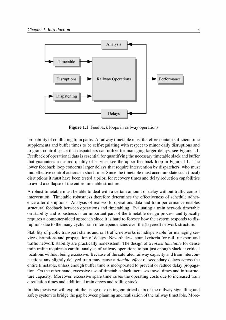
Figure 1.1 Feedback loops in railway operations
probability of conflicting train paths. A railway timetable must therefore contain sufficient time
supplements and buffer times to be self-regulating with respect to minor daily disruptions and
to grant control space that dispatchers can utilize for managing larger delays, see Figure 1.1.
Feedback of operational data is essential for quantifying the necessary timetable slack and buffer
that guarantees a desired quality of service, see the upper feedback loop in Figure 1.1. The
lower feedback loop concerns larger delays that require intervention by dispatchers, who must
find effective control actions in short-time. Since the timetable must accommodate such (local)
disruptions it must have been tested a priori for recovery times and delay reduction capabilities
to avoid a collapse of the entire timetable structure.
A robust timetable must be able to deal with a certain amount of delay without traffic control
intervention. Timetable robustness therefore determines the effectiveness of schedule adher-
ence after disruptions. Analysis of real-world operations data and train performance enables
structural feedback between operations and timetabling. Evaluating a train network timetable
on stability and robustness is an important part of the timetable design process and typically
requires a computer-aided approach since it is hard to foresee how the system responds to dis-
ruptions due to the many cyclic train interdependencies over the (layered) network structure.
Stability of public transport chains and rail traffic networks is indispensable for managing ser-
vice disruptions and propagation of delays. Nevertheless, sound criteria for rail transport and
traffic network stability are practically nonexistent. The design of a robust timetable for dense
train traffic requires a careful analysis of railway operations to put just enough slack at critical
locations without being excessive. Because of the saturated railway capacity and train intercon-
nections any slightly delayed train may cause a domino effect of secondary delays across the
entire timetable, unless enough buffer time is incorporated to prevent or reduce delay propaga-
tion. On the other hand, excessive use of timetable slack increases travel times and infrastruc-
ture capacity. Moreover, excessive spare time raises the operating costs due to increased train
circulation times and additional train crews and rolling stock.
In this thesis we will exploit the usage of existing empirical data of the railway signalling and
safety system to bridge the gap between planning and realization of the railway timetable. More-
4 Punctuality of Railway Operations and Timetable Stability Analysis
over we will develop a mathematical model that effectively describes the network structure and
system behaviour, derive transparent stability criteria, and present an implementation of the ap-
proach in a computer application. The proposed methodology quantifies network performance
and identifies the critical services in the railway transport and traffic network, and thus gives
insight in the dynamic system behaviour, which can be utilized for improving timetable designs
and supporting disruption management.
1.2 Setting the Scene
1.2.1 The Railway Timetable
A master timetable is the backbone of scheduled railway systems and determines directly or
indirectly effective railway capacity, traffic performance, quality of transport service, passenger
satisfaction, train circulations, and schedules for railway personnel. As such the timetable con-
cerns many actors including (potential) passengers, (passenger and freight) train operators, train
personnel, dispatchers, traffic controllers, infrastructure maintenance planners, and connecting
public transport providers.
European passenger railways are typically based on a periodic railway timetable, where train
lines are operated with regular intervals throughout a day and consistent transfers are provided
at transfer stations between train lines of different type or directions. The basic cycle time is
typically one hour, which means that the same pattern of train services repeats each hour. Train
lines may have a higher service frequency and still fit the overall timetable cycle time. The line
cycle time is then simply the overall cycle time divided by the line frequency, e.g., a train line
with 4 trains per hour has a regular interval of 15 minutes. A periodic timetable is popular and
effective to transport networks with diffused origin-destination demand matrices, where train
lines are synchronized at transfer stations to offer seamless connections between many different
origins and destinations.
The annual published timetable made available to travellers gives an overview of the planned ar-
rival and departure times of all trains on the railway network for a year ahead and thus presents
the transport service supply to (potential) travellers. Apart from the scheduled departure and
arrival times, this timetable also implicitly provides information on service frequency and thus
flexibility of departure time choice, (planned) travel times, and availability of direct trips or
alternatively the number of transfers and associated transfer time. A main advantage of peri-
odic timetables is that transport chains are fixed throughout the day and travellers only have to
remember the departure time of their (first) train in a basic hour, e.g. ‘departure at 05 and 35
minutes of each hour’. Depending on transport demand the periodic timetable may be made
more (or less) dense by adding (removing) train services in peak (off-peak) periods.
The published timetable is based on a much more detailed working timetable for railway per-
sonnel and traffic management systems. The working timetable specifies for each active train
number on each day:
• Origin and destination station;
• Running tracks and stops, including station routes and platform tracks;
• Scheduled arrival and departure time at each stop;
Chapter 1. Introduction 5
• Passage times at certain locations (through stations);
• Timetable speed and sometimes overtaking speed (maximum speed in case of punctual
and delayed running, respectively);
• Passenger connections at transfer stations;
• Rolling stock connections at main stations and terminals.
The working timetable may be adjusted up to the day of operation to include short-term train
path requests, such as freight trains and trains for special events (football match, pop concert).
Moreover, during operation the timetable may be adjusted in real-time by dispatchers and traffic
controllers to react on operational conditions and disruptive incidents in the train traffic system.
Because the annual passenger timetable is published a year in advance it may differ from the
actual daily working timetable.
Conventional railway timetables are in general conflict-free and allocate trains to the available
railway infrastructure in so-called train paths or time-distance graphs. If all trains adhere to their
schedule then the timetable guarantees a safe and smooth train traffic without mutual hindrance
on conflicting routes. Hence, the timetable represents a green wave of signal aspects to all trains
running according to schedule. On conventional railway lines equipped with block signals the
train driver relies completely on the trackside signals and the timetable, and has no information
nor visual clues about the progress of the preceding train due to the large headway distances
imposed by long braking distances and fixed block lengths. If a train is forced to stop at the
open track before a red signal aspect this results in a large time loss as the acceleration time of
a train from standstill to full speed is a matter of one to several minutes depending on train and
track characteristics. In particular freight trains may suffer a time loss of more than 5 minutes
when forced to an unscheduled stop.
The timetable is also the basis for dispatchers or automatic route setting (ARS) systems to set
the routes for each approaching and ready-to-depart train according to the scheduled route and
arrival/departure/through time. Also duty rosters of train crews (drivers, conductors) depend on
the timetable, and so do rolling stock circulations, including shunting at stations, deadheading
(empty running), cleaning at terminals, and periodic maintenance at depots. Hence, in case
of disruptions timetable perturbations may cause wide-spread logistic problems. Train units,
locomotives, coaches, and train crews may be in the wrong place at the wrong time resulting in
altered train compositions and an increasingly distorted rolling stock and crew allocation.
1.2.2 Infrastructure Capacity Utilization and Timetable Performance
The theoretical capacity of railway lines and station layouts is defined as the maximum number
of trains per unit of time that can be run, i.e., the reciprocal of the average minimum headway.
Theoretical capacity is determined by both infrastructure and rolling stock characteristics. In-
frastructure is characterized by the railway layout (single-track, double-track, sidings, junctions,
number of platform tracks), track speed limits (depending on e.g. curves, grades, switches), and
the signalling system (block lengths, number of signalling aspects, train protection). Rolling
stock characteristics of interest are e.g. braking and acceleration capacity, maximum speed,
train composition, and door widths.
Capacity also depends on how the traffic is organized in e.g. a timetable. The effective capacity
of railway infrastructure is therefore defined as the maximal number of trains per unit of time
6 Punctuality of Railway Operations and Timetable Stability Analysis
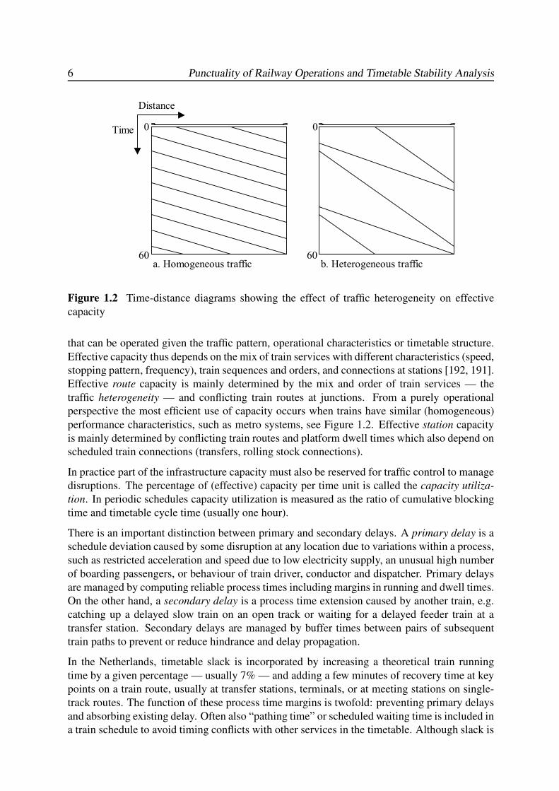
Figure 1.2 Time-distance diagrams showing the effect of traffic heterogeneity on effective
capacity
that can be operated given the traffic pattern, operational characteristics or timetable structure.
Effective capacity thus depends on the mix of train services with different characteristics (speed,
stopping pattern, frequency), train sequences and orders, and connections at stations [192, 191].
Effective route capacity is mainly determined by the mix and order of train services — the
traffic heterogeneity — and conflicting train routes at junctions. From a purely operational
perspective the most efficient use of capacity occurs when trains have similar (homogeneous)
performance characteristics, such as metro systems, see Figure 1.2. Effective station capacity
is mainly determined by conflicting train routes and platform dwell times which also depend on
scheduled train connections (transfers, rolling stock connections).
In practice part of the infrastructure capacity must also be reserved for traffic control to manage
disruptions. The percentage of (effective) capacity per time unit is called the capacity utiliza-
tion. In periodic schedules capacity utilization is measured as the ratio of cumulative blocking
time and timetable cycle time (usually one hour).
There is an important distinction between primary and secondary delays. A primary delay is a
schedule deviation caused by some disruption at any location due to variations within a process,
such as restricted acceleration and speed due to low electricity supply, an unusual high number
of boarding passengers, or behaviour of train driver, conductor and dispatcher. Primary delays
are managed by computing reliable process times including margins in running and dwell times.
On the other hand, a secondary delay is a process time extension caused by another train, e.g.
catching up a delayed slow train on an open track or waiting for a delayed feeder train at a
transfer station. Secondary delays are managed by buffer times between pairs of subsequent
train paths to prevent or reduce hindrance and delay propagation.
In the Netherlands, timetable slack is incorporated by increasing a theoretical train running
time by a given percentage — usually 7% — and adding a few minutes of recovery time at key
points on a train route, usually at transfer stations, terminals, or at meeting stations on single-
track routes. The function of these process time margins is twofold: preventing primary delays
and absorbing existing delay. Often also “pathing time” or scheduled waiting time is included in
a train schedule to avoid timing conflicts with other services in the timetable. Although slack is
Chapter 1. Introduction 7
important for reliable train operations, and should be retained in some form, it should be limited
to avoid a significant reduction of capacity and speed. A satisfactory level of capacity utilization
depends on the desired level of service quality, defined as a maximum total or average amount
of primary and secondary delay over a given time period.
When the infrastructure manager and train operators together achieve a high standard of opera-
tional performance, timetable slack can be reduced and capacity utilization may be increased by
scheduling additional train paths, increasing operating speed, or providing an improved market
oriented timetable. High capacity utilization thus requires process times with small variance
and scheduled values that are highly reliable corresponding to a high percentile of the realized
process time distributions. However, there must still be sufficient spare capacity in the form of
timetable slack to accommodate a certain lateness of trains and to recover from traffic disrup-
tions.
Persistent poor performance reduces the effective capacity and thus prevents increasing the
quality of service or performing engineering work within tightly designated slots. Punctuality
and reliability are necessary prerequisites for increasing capacity utilization. Operating more
trains on a given infrastructure network reduces the amount of “white space” (eventually unused
train slots) in the timetable, which means less ability to recover from service irregularities and
smaller time windows for engineering work and infrastructure inspection between trains.
1.2.3 Social Relevance
Dispunctuality and unreliability in public (rail) transport has a disastrous effect on passenger
satisfaction. Delayed trains, missed connections and train cancellations are particularly annoy-
ing because they cause unexpected waiting time and introduce travel time uncertainty. Absence
of reliable passenger information magnifies impatience and distress even more. Most vulnerable
are transport chains where travellers have to change trains or transfer between different modes of
transport (e.g. train–bus). A small train delay of a few minutes may cause a missed connection
and thus lead to a large passenger delay of 30 or 60 minutes, depending on the frequency of the
connecting service [173]. When repeatedly confronted with delays, travellers even anticipate on
larger travel times than published and adjust their departure time choice accordingly, especially
when the arrival time at the destination is important, e.g. to attend a business meeting. Thus,
short but unrealistic scheduled running or transfer times lead to large travel time expectations of
travellers, after a transient period of annoying travel experiences [178]. Moreover, unreliability
generates negative word-of-mouth publicity, a deteriorating image of public transport and loss
of public transport travellers.
Reducing passenger waiting time is an effective means to increase the quality of service. Un-
acceptable waiting times lead to a low perception of service and in addition generates negative
word-of-mouth publicity. Whether a waiting time is judged as excessive depends on the dis-
crepancy between perceived waiting time and expected waiting time [146]. Expectation may be
distinguished in a desired/anticipated level and a tolerable level. The desired/anticipated level of
expected waiting time is based on the published timetable and past experience. The timetable
should therefore be a close reflection of the realized services. Nevertheless, passengers are
willing to accept a larger tolerable waiting time expectation in recognition of the uncertainties
involved in railway transport and traffic operations. Waiting may not be a critical issue as long
as the discrepancy between perception and expectation is within an acceptable region. When
8 Punctuality of Railway Operations and Timetable Stability Analysis
expectations are confirmed, cognitive assimilation occurs and the difference in perception and
expectation is reduced. For moderate levels of discrepancy in either direction, passengers ad-
just their perception of waiting time to be more consistent with their expectation. However,
when the discrepancy is beyond the region of acceptance, the contrast between perception and
expectation magnifies passenger dissatisfaction.
Reliable passenger information helps passengers to set realistic expectations of waiting time
and thus reduces the discrepancy between expected and perceived waiting time. Hence, if
actual waiting time can not be avoided train operators can still reduce passenger dissatisfaction
by providing passenger information on waiting time in case of delays. Although this has little
effect on perceived waiting time it affects judgment on the quality of service indirectly through
acceptability of waiting time [146]. Informed passengers are mentally prepared for the wait and
have control over how to spend the waiting time. This way, passengers are likely to be more
understanding and tolerant to waiting. However, if the information turns out to be unreliable
passenger satisfaction is worsened even more.
1.3 Research Objectives
1.3.1 Ex-Post Traffic Analysis: Punctuality of Railway Operations
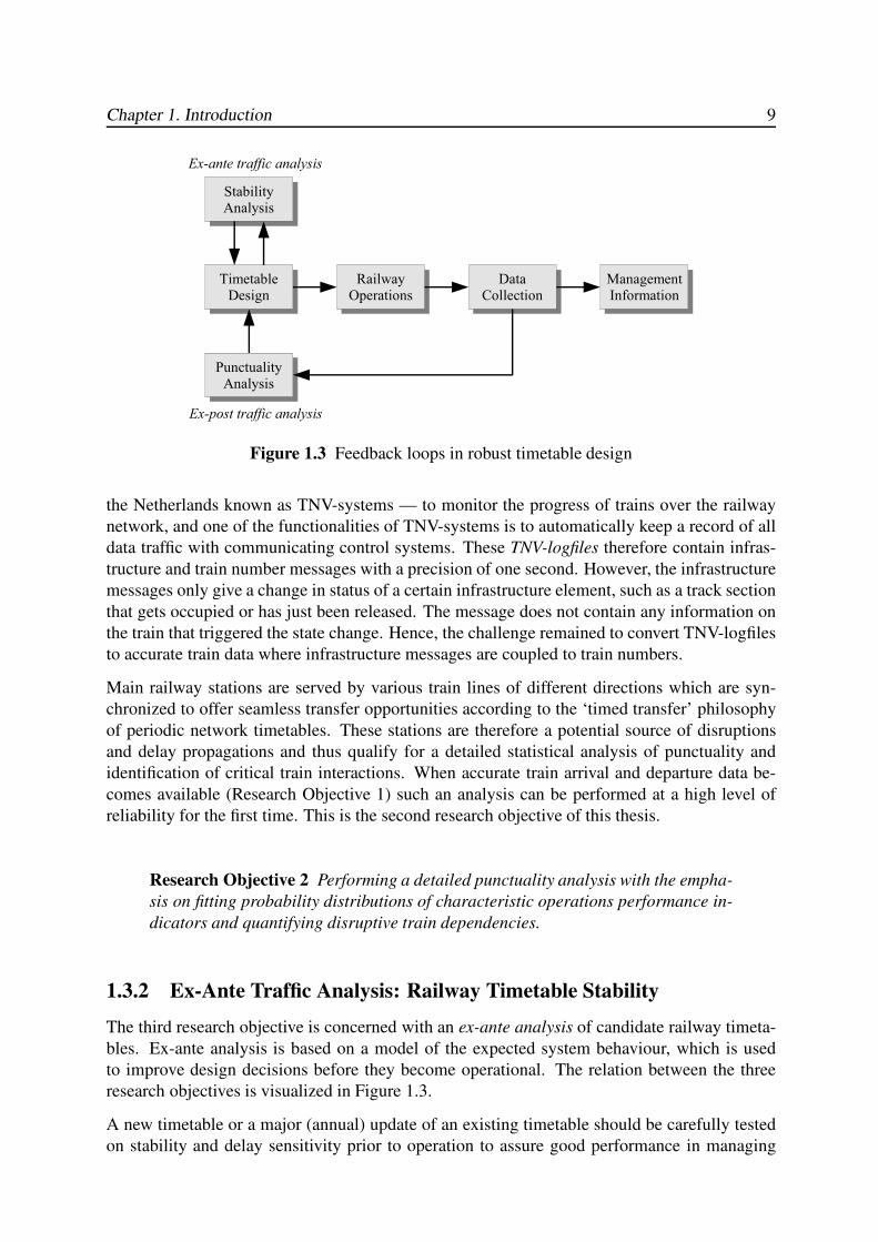
The first research objective of this PhD Thesis concerns the ex-post analysis of railway oper-
ations to obtain reliable process times and close the feedback-loop between planning and op-
erations, see Figure 1.3. Ex-post analysis is retrospective and tries to decide what (design and
control) decisions would have been optimal given the information on what actually happened.
The results can then be utilized to improve the consistency of plan and realization.
A crucial aspect in achieving and maintaining reliable timetables is the availability of accurate
empirical data to compare the timetable design and its realization. In the construction of a new
(annual) timetable historical data may be used, but also during operation of a timetable regular
empirical evaluation should be applied to detect and manage discrepancies between plan and
realization. However, the data collection and registration method via the traffic control systems
used by (ProRail) Railverkeersleiding for punctuality analysis reports does not meet scientific
requirements on precision and accuracy. The registered arrival and departure delays are only
indicative with an absolute error up to several minutes, and moreover delays below 3 minutes
are not registered at all1 [46, 80]. A detailed punctuality analysis of train traffic requires data
with an accuracy of several seconds in order to determine small delays and even early arrivals at
a precision of at least a tenth of a minute. This leads to the first research objective of this thesis.
Research Objective 1 Developing a data mining tool to retrieve accurate and re-
liable realizations of train movements from data records of the signalling and safety
system.
A potential source of traffic data is given by train detection devices, which act as sensors of
the safety and signalling systems. This train detection data is utilized by train describers — in
1Situation in 1997
Chapter 1. Introduction 9
Figure 1.3 Feedback loops in robust timetable design
the Netherlands known as TNV-systems — to monitor the progress of trains over the railway
network, and one of the functionalities of TNV-systems is to automatically keep a record of all
data traffic with communicating control systems. These TNV-logfiles therefore contain infras-
tructure and train number messages with a precision of one second. However, the infrastructure
messages only give a change in status of a certain infrastructure element, such as a track section
that gets occupied or has just been released. The message does not contain any information on
the train that triggered the state change. Hence, the challenge remained to convert TNV-logfiles
to accurate train data where infrastructure messages are coupled to train numbers.
Main railway stations are served by various train lines of different directions which are syn-
chronized to offer seamless transfer opportunities according to the ‘timed transfer’ philosophy
of periodic network timetables. These stations are therefore a potential source of disruptions
and delay propagations and thus qualify for a detailed statistical analysis of punctuality and
identification of critical train interactions. When accurate train arrival and departure data be-
comes available (Research Objective 1) such an analysis can be performed at a high level of
reliability for the first time. This is the second research objective of this thesis.
Research Objective 2 Performing a detailed punctuality analysis with the empha-
sis on fitting probability distributions of characteristic operations performance in-
dicators and quantifying disruptive train dependencies.
1.3.2 Ex-Ante Traffic Analysis: Railway Timetable Stability
The third research objective is concerned with an ex-ante analysis of candidate railway timeta-
bles. Ex-ante analysis is based on a model of the expected system behaviour, which is used
to improve design decisions before they become operational. The relation between the three
research objectives is visualized in Figure 1.3.
A new timetable or a major (annual) update of an existing timetable should be carefully tested
on stability and delay sensitivity prior to operation to assure good performance in managing
10 Punctuality of Railway Operations and Timetable Stability Analysis
secondary delays. In fact, a timetable should only be authorized if the planners or inframan-
agers are confident about its robust performance. However, an objective means of performance
evaluation is not yet available other than simulation, which is typically very involved and time
consuming for large networks. Hence, there is a need for an efficient and effective analytical
approach to evaluate network timetables on stability and network performance, which gives the
third research objective of this thesis:
Research Objective 3 Developing an analytical approach to evaluate and quan-
tify critical network dependencies on capacity utilization and timetable stability.
In this thesis we propose an analytical method based on max-plus algebra. Braker [21] and
Subiono [196] showed how the essential network timetable structure can be modelled as a
discrete-event dynamic system that is linear in the max-plus algebra. However, the efficiency of
a railway timetable is typically limited by the railway infrastructure (including signalling sys-
tem), which has a major effect on the train traffic dynamics. We therefore extend the modelling
approach by incorporating infrastructure constraints. Using this model we may then identify
and efficiently compute the most critical circuits — the closed paths in a periodic network with
the least average slack — and the (not necessarily cyclic) paths without any buffer time whatso-
ever, with respect to the scheduled process times, the timetable structure, and the infrastructure
constraints. The underlying idea being that in a highly-synchronized periodic railway timetable
delays initiated at some point in the network are likely to spread throughout the entire network
unless enough time reserves are built in at strategic places. We thus want to find the most
sensitive links in the network, i.e., the train paths containing the least slack to recover from
delays. The max-plus algebra framework enables us to use available and develop new highly
efficient algorithms that compute the critical circuits/paths for large-scale networks within some
seconds.
1.4 Contributions
This thesis contributes to the understanding of railway operations and timetable design aspects
that are important to construct robust timetables for reliable railway operations.
The first research objective led to the development of the software application TNV-Prepare
based on train description messages and messages from the safety and signalling systems as
recorded in TNV-logfiles. TNV-Prepare is able to match the infrastructure messages to train
numbers by which train paths through stations can be traced offline on track-circuit (or section)
level to and from the platform tracks. As a result, station arrival and departure times can be
derived with a precision and accuracy in the order of a second.
• This thesis shows that standard train describer records can be utilized to obtain accurate
data of infrastructure utilization and train punctuality by means of the developed software
TNV-Prepare.
Chapter 1. Introduction 11
The developed software TNV-Prepare enabled detailed analyses of train traffic and infrastruc-
ture utilization in railway stations. A punctuality analysis of the railway traffic at station Eind-
hoven has been realized conform the second research objective.
• The tool TNV-Prepare has been applied to train detection data of station Eindhoven. This
allowed an extensive statistical analysis of punctuality revealing a structural increase of
delays due to tight train interdependencies despite long scheduled dwell times.
• Probability distributions of train events and station process times have been derived and
statistically confirmed based on the empirical train detection data.
The third research objective has been realized by extending the modelling and analysis of
railway timetables in max-plus algebra. Moreover, the algorithms described in this thesis
have led to the development of the software application PETER (Performance Evaluation of
Timed Events in Railways). PETER facilitates the accessibility of the max-plus system analy-
sis method to the railway community.
• The modelling of railway timetables in max-plus algebra is generalized and extended with
infrastructure constraints.
• Key performance indicators are defined to assess railway timetables on stability and ro-
bustness.
• Efficient algorithms have been developed that enable fast evaluation of large-scale railway
timetables on stability and effective capacity utilization.
• The understanding of the max-plus modelling and analysis approach is enhanced by mod-
elling a railway traffic system as a timed event graph in conjunction with its max-plus
state-space representation.
Significant theoretical contributions have also been accomplished in the field of max-plus alge-
bra in the following directions.
• Max-plus polynomial matrices are shown to be a key element in the performance analysis
of timed event graphs and higher-order max-plus linear systems.
• The generalized eigenstructure of any irreducible and reducible max-plus polynomial ma-
trix has been completely described.
The findings of this thesis led to the development of several software products, which facilitate
understanding and direct usage in the rail traffic management practice:
• TNV-Prepare c©: this software application enables accurate analysis of infrastructure uti-
lization by matching information from safety & signalling systems to train numbers.
TNV-Prepare may encourage feedback of realization data into the planning practice and
enables an empirical foundation to performance evaluation of railway timetables and ca-
pacity assessment of railway infrastructure.
• TNV-Filter: this MATLAB program computes accurate estimates of arrival and departure
delays at platform tracks in complex railway stations based on tables generated by TNV-
Prepare and additional information on infrastructure section lengths.
• PETER c©: this software application implements the max-plus stability analysis approach
with graphical views of computational results, which includes critical circuit analysis,
recovery time analysis, and delay propagation. A special import functionality makes
PETER compatible with DONS, the timetable design system used at NSR and ProRail.
12 Punctuality of Railway Operations and Timetable Stability Analysis
Figure 1.4 Thesis outline
The software applications TNV-Prepare and PETER have both been extensively evaluated at
ProRail (Railned) during their development. TNV-Prepare is fully licensed to ProRail since
2001. ProRail also has a license to PETER since the beginning of 2005.
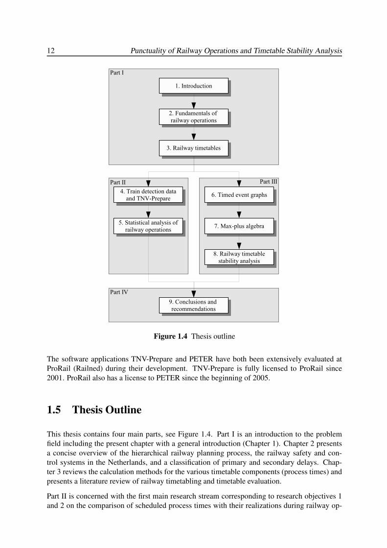
1.5 Thesis Outline
This thesis contains four main parts, see Figure 1.4. Part I is an introduction to the problem
field including the present chapter with a general introduction (Chapter 1). Chapter 2 presents
a concise overview of the hierarchical railway planning process, the railway safety and con-
trol systems in the Netherlands, and a classification of primary and secondary delays. Chap-
ter 3 reviews the calculation methods for the various timetable components (process times) and
presents a literature review of railway timetabling and timetable evaluation.
Part II is concerned with the first main research stream corresponding to research objectives 1
and 2 on the comparison of scheduled process times with their realizations during railway op-
Chapter 1. Introduction 13
erations. Chapter 4 shows that the information contained in the logfiles of TNV-systems can
be used to match infrastructure utilization to train numbers, and describes the developed tools
TNV-Prepare and TNV-Filter. In Chapter 5 the application of these tools are demonstrated in a
case study of the railway station Eindhoven. This chapter gives a detailed punctuality analysis
and shows by means of simple linear regression analysis the strong dependencies between train
services with a transfer connection and the impact of the bottleneck Eindhoven-Boxtel before
its upgrade to four tracks.
Part III deals with stability analysis on a network level conform research objective 3. Chapter 6
considers timed event graphs, a special class of Petri nets that provides a graphical modelling
approach for max-plus linear systems. A timed event graph models the interconnection structure
of events (nodes) and processes between events (arcs), and moreover denotes active processes
(e.g. train runs, transferring passengers) by assigning a token to the active processes. The to-
kens move over the graph governed by the occurrence of events, which describes the dynamic
behaviour of the modelled system. Basic building blocks and behavioural properties are pre-
sented that can be used for the synthesis of complex timed event graphs. Chapter 7 introduces
the theory of max-plus algebra and explains the relations to other mathematical disciplines
such as graph theory, Petri nets (timed event graphs), dynamic programming, Markov decision
processes, and the theory of nonnegative matrices, from which efficient algorithms have been
derived to compute characteristics of max-plus matrices and the associated graphs. Chapter 8
explains the principles of max-plus linear system theory and describes the system analysis ap-
proach to large-scale timetabled train traffic systems, as implemented in the developed software
application PETER. The software PETER is briefly described and the analysis capabilities are
demonstrated by a case study of an (hourly) periodic timetable based on the Dutch national
railway timetable of 2000/2001.
Finally, Part IV (Chapter 9) summarizes the main conclusions based on the own research con-
tributions and the recommendations for future practice and research.

14 Punctuality of Railway Operations and Timetable Stability Analysis
Chapter 2
FUNDAMENTALS OF RAILWAY
OPERATIONS
2.1 Introduction
This chapter gives an overview of passenger railway planning and railway safety and signalling
systems. In particular, we introduce trains lines and connections between train lines which
together with the railway network is important input to the timetabling process. The safety
and signalling systems are also of main importance to derive minimum headway constraints
that must be incorporated in the timetable design to compute a feasible timetable that coor-
dinates the train traffic with respect to train route conflicts and safe train distances. Rolling
stock circulations are another important aspect that must be taken into account in the timetable
design because the various rolling stock types have different characteristics (maximum speed,
acceleration/deceleration rate) that influence the realizability of the running times. Moreover,
(de-)coupling of rolling stock and turns at terminals are also important parameters that influence
minimum layover times and dwell times.
This chapter gives a review of the Dutch railway systems architecture including train detection,
train description, interlocking and traffic control. We emphasize the data flows between the
various safety and control systems and show that all information on infrastructure elements is
collected by the train describer systems (TNV-systems in Dutch) which is used to monitor the
movements of all trains on the network using their train descriptions (train numbers). A crucial
observation is that all infrastructure and train description events are recorded by the Dutch
train describer systems into TNV-logfiles, which will be used in the sequel of this thesis as an
essential data collection device.
We furthermore consider the capacity allocation process in the Netherlands in which the train
path requests of various train operators are coordinated by the infrastructure manager. This
capacity allocation has been initiated in Europe to grant competition between different (freight
and passenger) train operators according to directive 2001/14/EC on railway capacity allocation
of the European Union [60]. These European regulations have led to a drastic change from the
traditional monopolistic state railway companies to privatized train operators.
The outline of this chapter is as follows. Section 2.2 considers the various stages of (passenger)
railway planning, including line system planning (§2.2.3) and railway timetabling (§2.2.4). Sec-
tion 2.3 is concerned with the railway safety, signalling and control systems with an emphasis
on the architecture in the Netherlands. Section 2.4 classifies delays and considers a wide range
of sources of delays.
15
16 Punctuality of Railway Operations and Timetable Stability Analysis
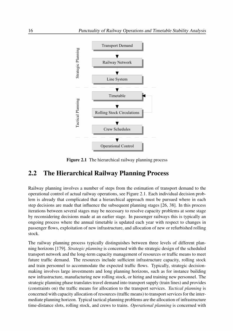
Figure 2.1 The hierarchical railway planning process
2.2 The Hierarchical Railway Planning Process
Railway planning involves a number of steps from the estimation of transport demand to the
operational control of actual railway operations, see Figure 2.1. Each individual decision prob-
lem is already that complicated that a hierarchical approach must be pursued where in each
step decisions are made that influence the subsequent planning stages [26, 38]. In this process
iterations between several stages may be necessary to resolve capacity problems at some stage
by reconsidering decisions made at an earlier stage. In passenger railways this is typically an
ongoing process where the annual timetable is updated each year with respect to changes in
passenger flows, exploitation of new infrastructure, and allocation of new or refurbished rolling
stock.
The railway planning process typically distinguishes between three levels of different plan-
ning horizons [179]. Strategic planning is concerned with the strategic design of the scheduled
transport network and the long-term capacity management of resources or traffic means to meet
future traffic demand. The resources include sufficient infrastructure capacity, rolling stock
and train personnel to accommodate the expected traffic flows. Typically, strategic decision-
making involves large investments and long planning horizons, such as for instance building
new infrastructure, manufacturing new rolling stock, or hiring and training new personnel. The
strategic planning phase translates travel demand into transport supply (train lines) and provides
(constraints on) the traffic means for allocation to the transport services. Tactical planning is
concerned with capacity allocation of resources (traffic means) to transport services for the inter-
mediate planning horizon. Typical tactical planning problems are the allocation of infrastructure
time-distance slots, rolling stock, and crews to trains. Operational planning is concerned with
Chapter 2. Fundamentals of Railway Operations 17
rescheduling during operations in face of unforeseen events, disruptive incidents or accidents.
In this thesis we are mainly concerned with the analysis of timetables, which is part of the tac-
tical planning phase. We therefore assume strategic decisions as given, that is, infrastructure
and train lines are fixed. Furthermore, rolling stock circulations and crew schedules must be
consistent with the timetable and may define additional interdependencies. In the next subsec-
tions we briefly consider the successive railway planning stages with the focus on their impact
to the timetable. For alternative reviews, see e.g. Bussieck et al. [26], Cordeau et al. [38] and
Kroon [124].
2.2.1 Transport Demand
The first step of strategic planning is demand estimation. Forecasting future travel demand is an
econometric problem directed towards the determination of origin-destination (OD) matrices
partitioned by transport mode according to travel choice behaviour [157]. In particular the
modal split between individual car and public transport is of strategic demographical importance
and depends on the available infrastructure and quality of service of public (rail) transport,
which can be influenced by strategic political decisions. Each entry in a (rail transport) OD-
matrix gives (an estimate of) the number of passengers travelling from one station in the railway
network to another. The passenger transport demand in the form of an OD-matrix is the basis of
each following stage in the railway planning process and in particular to the design of network
structure and the train lines.
2.2.2 Railway Network Design
The railway network design problem aims at the determination of railway tracks and stations
given the railway transport and traffic demand. Building new railway infrastructure is very
costly and has a severe environmental, economical, and social impact for many decades. Long-
term infrastructure investments are therefore subject to political debate and based on strategic
studies that estimate future demand for and utilization of railway infrastructure. Railway infras-
tructure issues can also be considered as part of the railway network design, such as electrifica-
tion of railway lines and the choice of safety and signalling systems.
The existing railway infrastructure is a product of historically made strategic decisions. In the
Netherlands the main part of the railway lines originate from the large railway construction
projects at the end of the 19th century [62]. In the late 21th century a number of suburban
railway lines were built, such as the Zoetermeerlijn and the Flevolijn from Weesp to Almere
and Lelystad, and a large number of new suburban stations were opened at existing lines. Also
a number of rural railway lines were closed in the 21th century as they were superseded by road
traffic. Nowadays, railway engineering projects mainly focus on capacity expansions of satu-
rated infrastructure such as upgrading single-track to double-track or double-track to four-track
lines, eliminating crossings by fly-overs and extending station layouts. International develop-
ments have also led to two major recent railway infrastructure projects of the Betuweroute, a
dedicated freight route from the Rotterdam harbour to Germany, and the HSL-Zuid, the high-
speed line from Amsterdam to Belgium [102]. Current network design issues also involve
extending or replacing conventional (heavy) railway lines by light-rail lines.
18 Punctuality of Railway Operations and Timetable Stability Analysis
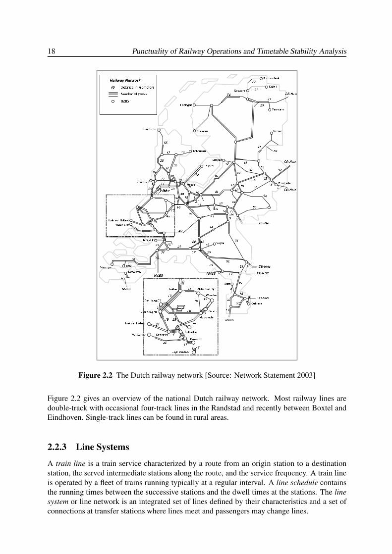
Figure 2.2 The Dutch railway network [Source: Network Statement 2003]
Figure 2.2 gives an overview of the national Dutch railway network. Most railway lines are
double-track with occasional four-track lines in the Randstad and recently between Boxtel and
Eindhoven. Single-track lines can be found in rural areas.
2.2.3 Line Systems
A train line is a train service characterized by a route from an origin station to a destination
station, the served intermediate stations along the route, and the service frequency. A train line
is operated by a fleet of trains running typically at a regular interval. A line schedule contains
the running times between the successive stations and the dwell times at the stations. The line
system or line network is an integrated set of lines defined by their characteristics and a set of
connections at transfer stations where lines meet and passengers may change lines.
Chapter 2. Fundamentals of Railway Operations 19
A railway network is usually operated by heterogeneous train types serving different transport
markets, such as long-distance trains and regional trains. This leads to a natural decomposition
of the line system into subsystems or supply networks according to train type. Generally, the
subsystems concurrently use the same tracks although some decisive train type features may
rule out certain parts of the railway network, e.g. electric multiple units (EMUs) require electri-
fied tracks and high-speed lines have restrictions on track curvature. Common passenger train
services in Europe are
(i) High-speed trains (HST): international passenger train services connecting major cities at
top speeds over 200 km/h.
(ii) Intercity (IC) trains: long-distance passenger trains connecting the major national stations
only.
(iii) Interregional (IR) trains: intermediate-distance passenger trains connecting major and
large stations,
(iv) Agglo/regional (AR) trains: local passenger trains serving all stations on their route.
The agglo/regional train lines are also called regional (R) train lines.
Passenger demand is usually specified in an origin-destination matrix for the complete train
service network. However, the passenger flows are distributed over the different subsystems.
Oltrogge [20] proposed a procedure for splitting the OD-matrix into separate OD-matrices for
the subsystems, the so-called system split. The method assumes a hierarchy of the subsystems
where the lowest level network has the finest grid of stops served by slow trains (as a result of the
stopping pattern), and the highest level subsystem connects only main stations with high speed.
For example, the three national passenger train subsystems in the Netherlands are arranged as IC
⊂ IR⊂ AR, i.e., the IC stations are a subset of the IR stations and the IR stations are a subset of
the AR stations. An admissible journey is then a transport chain with transfers to a higher level
network near the origin and transfers to a lower level network near the destination. The problem
then reduces to finding the shortest path over a supernetwork consisting of the supply networks
with additional transfer arcs at the stations where passengers may change to another subsystem.
Oltrogge [20] proposed a sophisticated valuation of the travel paths based on travel time, price,
level of comfort, and the number of system changes. Note that at this stage the transfer waiting
times are still unknown since a timetable is not yet available. The valuation differs with trip
purpose (e.g. business, leisure) and accordingly provides an assignment of traffic volume to the
different travel routes. The distribution of passengers over the supernetwork gives the number
of passengers or traffic load for each link in the supply networks. Aggregating over all assigned
routes and all OD-pairs gives the OD-matrix estimates for each subsystem.
Given passenger demand and railway network, the line optimization problem aims at finding
feasible lines (routes and frequencies) satisfying a set of constraints and optimizing some ob-
jective function. Constraints specify e.g. that all travellers are transported, passenger loads do
not exceed train capacities, and track capacities are not exceeded. Typical objectives are max-
imization of the number of direct trips (or minimization of transfers)[20] and minimization of
operating costs [25, 76, 77, 230]. The optimization problem is a mixed-integer programming
(MIP) problem, which is NP-complete. Branch-and-bound and heuristic algorithms have been
developed for solving practical instances of this problem [20, 24, 25, 76, 77, 230].
Based on the approach of Oltrogge [20] the program PROLOP (PROgram for Line OPtimiza-
tion) was developed for the analysis of passenger flows over a line system, which was used in the
20 Punctuality of Railway Operations and Timetable Stability Analysis
Netherlands by NSR and Railned [45]. PROLOP contains three modules: the line optimization
model, an assignment model, and a comparison model. NSR and Railned used mainly the last
two models to evaluate passenger flows. Input to the assignment model is the railway network,
the train lines, an OD-matrix, and optionally a timetable. The assignment model assigns trav-
ellers to train lines based on a generalized travel time utility function, as described above. The
output includes passenger loads, track load, and passenger flows at stations. The comparison
model evaluates the differences between two line systems. In 2000, NSR and Railned decided
to develop a new program with an improved interface, called TRANS (Toedelen Reizigers Aan
Netwerk Systemen). Nevertheless, the assignment method developed in PROLOP has been pre-
served in TRANS.
2.2.4 Railway Timetabling
Timetabling is the problem of matching the train line system to the available infrastructure, i.e.,
finding for each train line a feasible schedule of arrival and departure times at the consecutive
served stations taking into account constraints with respect to e.g. the safety and signalling
system, transfer connections, and regularity requirements. In this section we consider the main
timetable aspects and the timetabling process within the railway planning process. Section 3.9
gives a review of mathematical approaches of railway timetabling.
The basis of the Dutch railway timetable is a basic hour pattern (BHP)1 over the corridors
and a basic platform occupation (BPO)2 in stations. All train lines operate with a cycle time
of one hour or at regular intervals within a cycle of one hour (e.g. 30 or 15 minutes). Hence,
the arrival and departure times at all stations are essentially the same for each hour over a
day, and moreover the connections and transfer times between train lines at transfer stations
are equal over the day. This periodic timetable implies that travellers can take the same trains
and connections with equal (scheduled) travel times for each period of the day and day of the
week without consulting the timetable, which offers a great quality of service for regular train
travellers. A BHP thus consists of all arrival, departure and through times scheduled in a basic
hour. BHPs are visualized by time-distance diagrams or train path diagrams. In addition, a
BPO shows the dwell times (and arrival and departure times) and through times at the station
platform tracks during a basic hour. BPOs are visualized by platform occupation diagrams.
From a timetabling point-of-view this periodicity imposes additional restrictions to the train
schedules and their synchronization at transfer stations, since the round-trip time of each train
must be a multiple of an hour which bounds the amount of slack and buffer time that can be
built into the line schedule. Moreover, this generally holds for each closed sequence of train
runs (circuits) in the timetable (modulo the cycle time), see e.g. Odijk [154], Goverde [81] and
Peeters [159]. In the Netherlands, the system DONS is used to interactively determine a set
of feasible constraints for which then a network timetable is computed, see e.g. Hooghiem-
stra [101].
A strictly periodic daily timetable can be obtained by concatenating 24 BHPs. However, in
practice traffic demand fluctuates over a day and over the week. In a strictly periodic timetable
this would lead to crowded trains in peak periods and almost empty trains in the off-peak.
1In Dutch: basisuurpatroon (BUP)2In Dutch: basisspooropstelling (BSO)
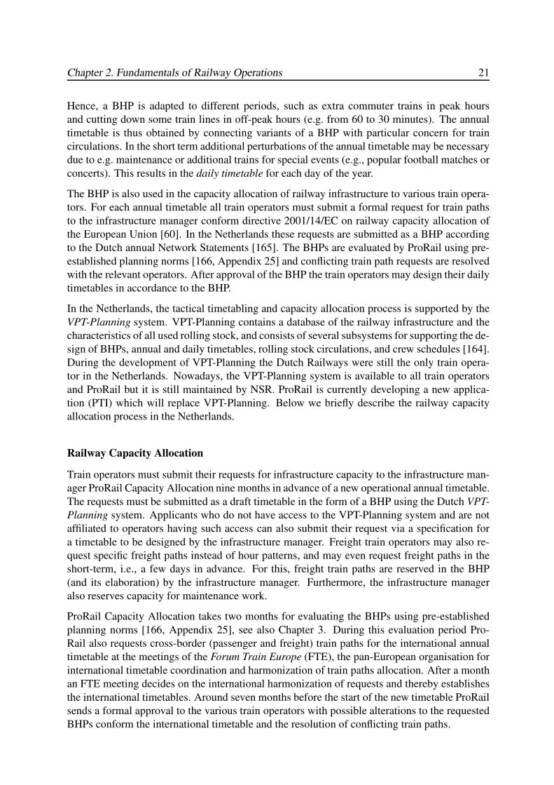
Chapter 2. Fundamentals of Railway Operations 21
Hence, a BHP is adapted to different periods, such as extra commuter trains in peak hours
and cutting down some train lines in off-peak hours (e.g. from 60 to 30 minutes). The annual
timetable is thus obtained by connecting variants of a BHP with particular concern for train
circulations. In the short term additional perturbations of the annual timetable may be necessary
due to e.g. maintenance or additional trains for special events (e.g., popular football matches or
concerts). This results in the daily timetable for each day of the year.
The BHP is also used in the capacity allocation of railway infrastructure to various train opera-
tors. For each annual timetable all train operators must submit a formal request for train paths
to the infrastructure manager conform directive 2001/14/EC on railway capacity allocation of
the European Union [60]. In the Netherlands these requests are submitted as a BHP according
to the Dutch annual Network Statements [165]. The BHPs are evaluated by ProRail using pre-
established planning norms [166, Appendix 25] and conflicting train path requests are resolved
with the relevant operators. After approval of the BHP the train operators may design their daily
timetables in accordance to the BHP.
In the Netherlands, the tactical timetabling and capacity allocation process is supported by the
VPT-Planning system. VPT-Planning contains a database of the railway infrastructure and the
characteristics of all used rolling stock, and consists of several subsystems for supporting the de-
sign of BHPs, annual and daily timetables, rolling stock circulations, and crew schedules [164].
During the development of VPT-Planning the Dutch Railways were still the only train opera-
tor in the Netherlands. Nowadays, the VPT-Planning system is available to all train operators
and ProRail but it is still maintained by NSR. ProRail is currently developing a new applica-
tion (PTI) which will replace VPT-Planning. Below we briefly describe the railway capacity
allocation process in the Netherlands.
Railway Capacity Allocation
Train operators must submit their requests for infrastructure capacity to the infrastructure man-
ager ProRail Capacity Allocation nine months in advance of a new operational annual timetable.
The requests must be submitted as a draft timetable in the form of a BHP using the Dutch VPT-
Planning system. Applicants who do not have access to the VPT-Planning system and are not
affiliated to operators having such access can also submit their request via a specification for
a timetable to be designed by the infrastructure manager. Freight train operators may also re-
quest specific freight paths instead of hour patterns, and may even request freight paths in the
short-term, i.e., a few days in advance. For this, freight train paths are reserved in the BHP
(and its elaboration) by the infrastructure manager. Furthermore, the infrastructure manager
also reserves capacity for maintenance work.
ProRail Capacity Allocation takes two months for evaluating the BHPs using pre-established
planning norms [166, Appendix 25], see also Chapter 3. During this evaluation period Pro-
Rail also requests cross-border (passenger and freight) train paths for the international annual
timetable at the meetings of the Forum Train Europe (FTE), the pan-European organisation for
international timetable coordination and harmonization of train paths allocation. After a month
an FTE meeting decides on the international harmonization of requests and thereby establishes
the international timetables. Around seven months before the start of the new timetable ProRail
sends a formal approval to the various train operators with possible alterations to the requested
BHPs conform the international timetable and the resolution of conflicting train paths.
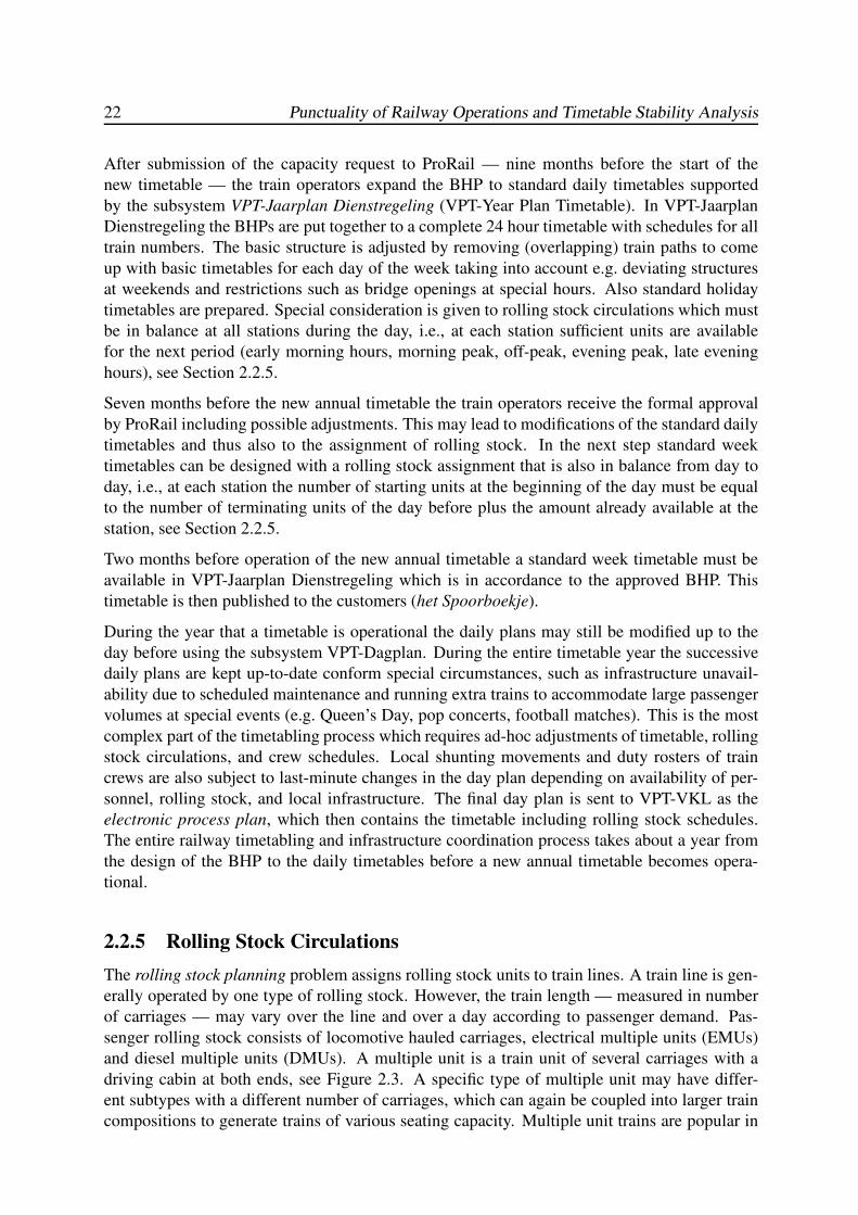
22 Punctuality of Railway Operations and Timetable Stability Analysis
After submission of the capacity request to ProRail — nine months before the start of the
new timetable — the train operators expand the BHP to standard daily timetables supported
by the subsystem VPT-Jaarplan Dienstregeling (VPT-Year Plan Timetable). In VPT-Jaarplan
Dienstregeling the BHPs are put together to a complete 24 hour timetable with schedules for all
train numbers. The basic structure is adjusted by removing (overlapping) train paths to come
up with basic timetables for each day of the week taking into account e.g. deviating structures
at weekends and restrictions such as bridge openings at special hours. Also standard holiday
timetables are prepared. Special consideration is given to rolling stock circulations which must
be in balance at all stations during the day, i.e., at each station sufficient units are available
for the next period (early morning hours, morning peak, off-peak, evening peak, late evening
hours), see Section 2.2.5.
Seven months before the new annual timetable the train operators receive the formal approval
by ProRail including possible adjustments. This may lead to modifications of the standard daily
timetables and thus also to the assignment of rolling stock. In the next step standard week
timetables can be designed with a rolling stock assignment that is also in balance from day to
day, i.e., at each station the number of starting units at the beginning of the day must be equal
to the number of terminating units of the day before plus the amount already available at the
station, see Section 2.2.5.
Two months before operation of the new annual timetable a standard week timetable must be
available in VPT-Jaarplan Dienstregeling which is in accordance to the approved BHP. This
timetable is then published to the customers (het Spoorboekje).
During the year that a timetable is operational the daily plans may still be modified up to the
day before using the subsystem VPT-Dagplan. During the entire timetable year the successive
daily plans are kept up-to-date conform special circumstances, such as infrastructure unavail-
ability due to scheduled maintenance and running extra trains to accommodate large passenger
volumes at special events (e.g. Queen’s Day, pop concerts, football matches). This is the most
complex part of the timetabling process which requires ad-hoc adjustments of timetable, rolling
stock circulations, and crew schedules. Local shunting movements and duty rosters of train
crews are also subject to last-minute changes in the day plan depending on availability of per-
sonnel, rolling stock, and local infrastructure. The final day plan is sent to VPT-VKL as the
electronic process plan, which then contains the timetable including rolling stock schedules.
The entire railway timetabling and infrastructure coordination process takes about a year from
the design of the BHP to the daily timetables before a new annual timetable becomes opera-
tional.
2.2.5 Rolling Stock Circulations
The rolling stock planning problem assigns rolling stock units to train lines. A train line is gen-
erally operated by one type of rolling stock. However, the train length — measured in number
of carriages — may vary over the line and over a day according to passenger demand. Pas-
senger rolling stock consists of locomotive hauled carriages, electrical multiple units (EMUs)
and diesel multiple units (DMUs). A multiple unit is a train unit of several carriages with a
driving cabin at both ends, see Figure 2.3. A specific type of multiple unit may have differ-
ent subtypes with a different number of carriages, which can again be coupled into larger train
compositions to generate trains of various seating capacity. Multiple unit trains are popular in
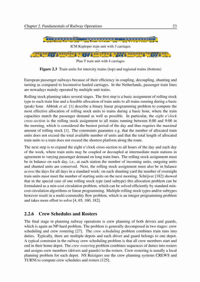
Chapter 2. Fundamentals of Railway Operations 23
ICM Koploper train unit with 3 carriages
Plan T train unit with 4 carriages
Figure 2.3 Train units for intercity trains (top) and regional trains (bottom)
European passenger railways because of their efficiency in coupling, decoupling, shunting and
turning as compared to locomotive hauled carriages. In the Netherlands, passenger train lines
are nowadays mainly operated by multiple unit trains.
Rolling stock planning takes several stages. The first step is a basic assignment of rolling stock
type to each train line and a feasible allocation of train units to all trains running during a basic
(peak) hour. Abbink et al. [1] describe a binary linear programming problem to compute the
most effective allocation of rolling stock units to trains during a basic hour, where the train
capacities match the passenger demand as well as possible. In particular, the eight o’clock
cross-section is the rolling stock assignment to all trains running between 8:00 and 9:00 in
the morning, which is considered the busiest period of the day and thus requires the maximal
amount of rolling stock [1]. The constraints guarantee e.g. that the number of allocated train
units does not exceed the total available number of units and that the total length of allocated
train units to a train does not exceed the shortest platform along the route.
The next step is to expand the eight o’clock cross-section to all hours of the day and each day
of the week, where train units may be coupled or decoupled at intermediate main stations in
agreement to varying passenger demand on long train lines. The rolling stock assignment must
be in balance on each day, i.e., at each station the number of incoming units, outgoing units
and shunted units are conserved. Next, the rolling stock assignment must also be in balance
across the days for all days in a standard week: on each shunting yard the number of overnight
train units must meet the number of starting units on the next morning. Schrijver [182] showed
that in the special case of one rolling stock type (and subtype) this allocation problem can be
formulated as a min-cost circulation problem, which can be solved efficiently by standard min-
cost circulation algorithms or linear programming. Multiple rolling stock types and/or subtypes
however result in a multi-commodity flow problem, which is an integer programming problem
and takes more effort to solve [4, 65, 160, 182].
2.2.6 Crew Schedules and Rosters
The final stage in planning railway operations is crew planning of both drivers and guards,
which is again an NP-hard problem. The problem is generally decomposed in two stages: crew
scheduling and crew rostering [27]. The crew scheduling problem combines train runs into
duties. Typically, there are multiple depots and each driver and guard belongs to one depot.
A typical constraint in the railway crew scheduling problem is that all crew members start and
end in their home depot. The crew rostering problem combines sequences of duties into rosters
and assigns crew members (drivers and guards) to the rosters. Crew rostering is usually a local
planning problem for each depot. NS Reizigers use the crew planning systems CREWS and
TURNI to compute crew schedules and rosters [125].
24 Punctuality of Railway Operations and Timetable Stability Analysis
Crew schedules obviously generate dependencies between trains because a crew must be avail-
able before a train can depart. Rosters contain at least two duties (because of a lunch break in
between) and so drivers and guards must transfer from one train unit to another in their duty
roster. To prevent delay propagation, crew transfer times must contain buffer time. It may also
be effective to combine driver/guard pairs into rosters to prevent dependencies from multiple
‘feeder’ trains. For a wide range of practical considerations of railway crew planning in the
Netherlands, see Kroon & Fischetti [125].
2.3 Safety and Signalling Systems
Railways have unique characteristics that result in potential risks: heavy vehicles run at consid-
erable speed over fixed rails while braking capacity is small due to minimal friction between
metal wheels and rails. These characteristics generally prevent that trains can be brought to a
standstill within the distance that can safely be observed by the driver and neither is a driver able
to steer away to avoid conflicts. Therefore, railway networks are equipped with safety systems
for excluding risks of derailments (by e.g. a broken rail, open movable bridge, unlocked switch),
collisions between trains, collisions between trains and road vehicles on level-crossings, and ac-
cidents with maintenance workers.
The main interface between the safety system and the trains are the trackside signals which can
be partitioned into automatic and controlled signals. Train separation on open tracks is guarded
by automatic block systems in conjunction with automatic train protection (in the Netherlands).
Block signals protect block sections and operate completely automatically based on train de-
tection and interlinked signals. Block systems are complemented by train protection systems to
further avoid human errors or failure (of the train driver). Signals also protect routes through
station layouts to avoid head-on, end-on, and flank collisions. These signals are controlled by
dispatchers and the interlocking system. Safety and signalling systems rely on train detection
systems for track occupancy and track-free detection.
The next subsections give a concise overview of the various railway safety and signalling sys-
tems with an emphasis on the current situation in the Netherlands. More background on railway
systems can be found in e.g. Bailey [12], Fenner et al. [63], Hall [92] and Pachl [158]. Van der
Werff et al. [206] give a historical survey of the signalling systems in the Netherlands.
This section subsequently considers the following topics: train detection (§2.3.1), fixed block
systems (§2.3.2), automatic train protection (§2.3.3), train describer systems (§2.3.4), interlock-
ing systems (§2.3.5), dispatching systems (§2.3.6) and traffic control systems (§2.3.7).
2.3.1 Train Detection
In modern railways the presence of a train on a track section is automatically detected by train
detection systems, which act as the sensors to the railway safety and signalling systems. The
most common train detection devices are track circuits and axle counters. More precisely, track
circuits and axle counters are track-free detection systems. This means that they either detect
that
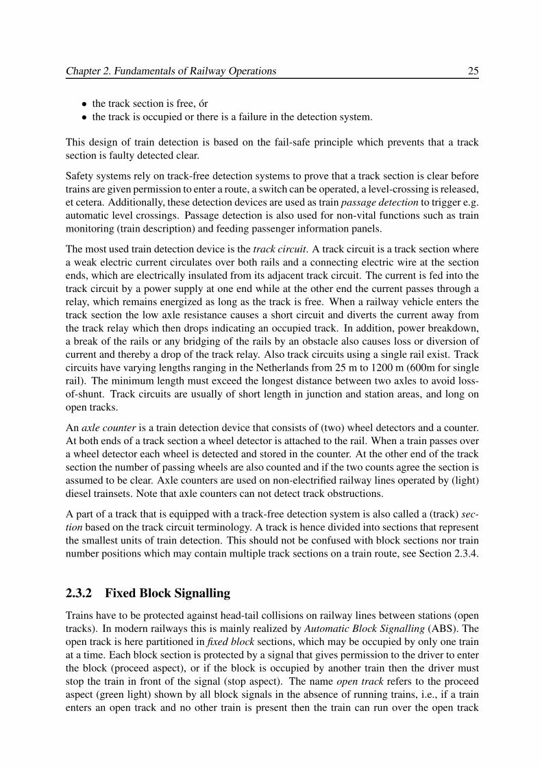
Chapter 2. Fundamentals of Railway Operations 25
• the track section is free, or
• the track is occupied or there is a failure in the detection system.
This design of train detection is based on the fail-safe principle which prevents that a track
section is faulty detected clear.
Safety systems rely on track-free detection systems to prove that a track section is clear before
trains are given permission to enter a route, a switch can be operated, a level-crossing is released,
et cetera. Additionally, these detection devices are used as train passage detection to trigger e.g.
automatic level crossings. Passage detection is also used for non-vital functions such as train
monitoring (train description) and feeding passenger information panels.
The most used train detection device is the track circuit. A track circuit is a track section where
a weak electric current circulates over both rails and a connecting electric wire at the section
ends, which are electrically insulated from its adjacent track circuit. The current is fed into the
track circuit by a power supply at one end while at the other end the current passes through a
relay, which remains energized as long as the track is free. When a railway vehicle enters the
track section the low axle resistance causes a short circuit and diverts the current away from
the track relay which then drops indicating an occupied track. In addition, power breakdown,
a break of the rails or any bridging of the rails by an obstacle also causes loss or diversion of
current and thereby a drop of the track relay. Also track circuits using a single rail exist. Track
circuits have varying lengths ranging in the Netherlands from 25 m to 1200 m (600m for single
rail). The minimum length must exceed the longest distance between two axles to avoid loss-
of-shunt. Track circuits are usually of short length in junction and station areas, and long on
open tracks.
An axle counter is a train detection device that consists of (two) wheel detectors and a counter.
At both ends of a track section a wheel detector is attached to the rail. When a train passes over
a wheel detector each wheel is detected and stored in the counter. At the other end of the track
section the number of passing wheels are also counted and if the two counts agree the section is
assumed to be clear. Axle counters are used on non-electrified railway lines operated by (light)
diesel trainsets. Note that axle counters can not detect track obstructions.
A part of a track that is equipped with a track-free detection system is also called a (track) sec-
tion based on the track circuit terminology. A track is hence divided into sections that represent
the smallest units of train detection. This should not be confused with block sections nor train
number positions which may contain multiple track sections on a train route, see Section 2.3.4.
2.3.2 Fixed Block Signalling
Trains have to be protected against head-tail collisions on railway lines between stations (open
tracks). In modern railways this is mainly realized by Automatic Block Signalling (ABS). The
open track is here partitioned in fixed block sections, which may be occupied by only one train
at a time. Each block section is protected by a signal that gives permission to the driver to enter
the block (proceed aspect), or if the block is occupied by another train then the driver must
stop the train in front of the signal (stop aspect). The name open track refers to the proceed
aspect (green light) shown by all block signals in the absence of running trains, i.e., if a train
enters an open track and no other train is present then the train can run over the open track
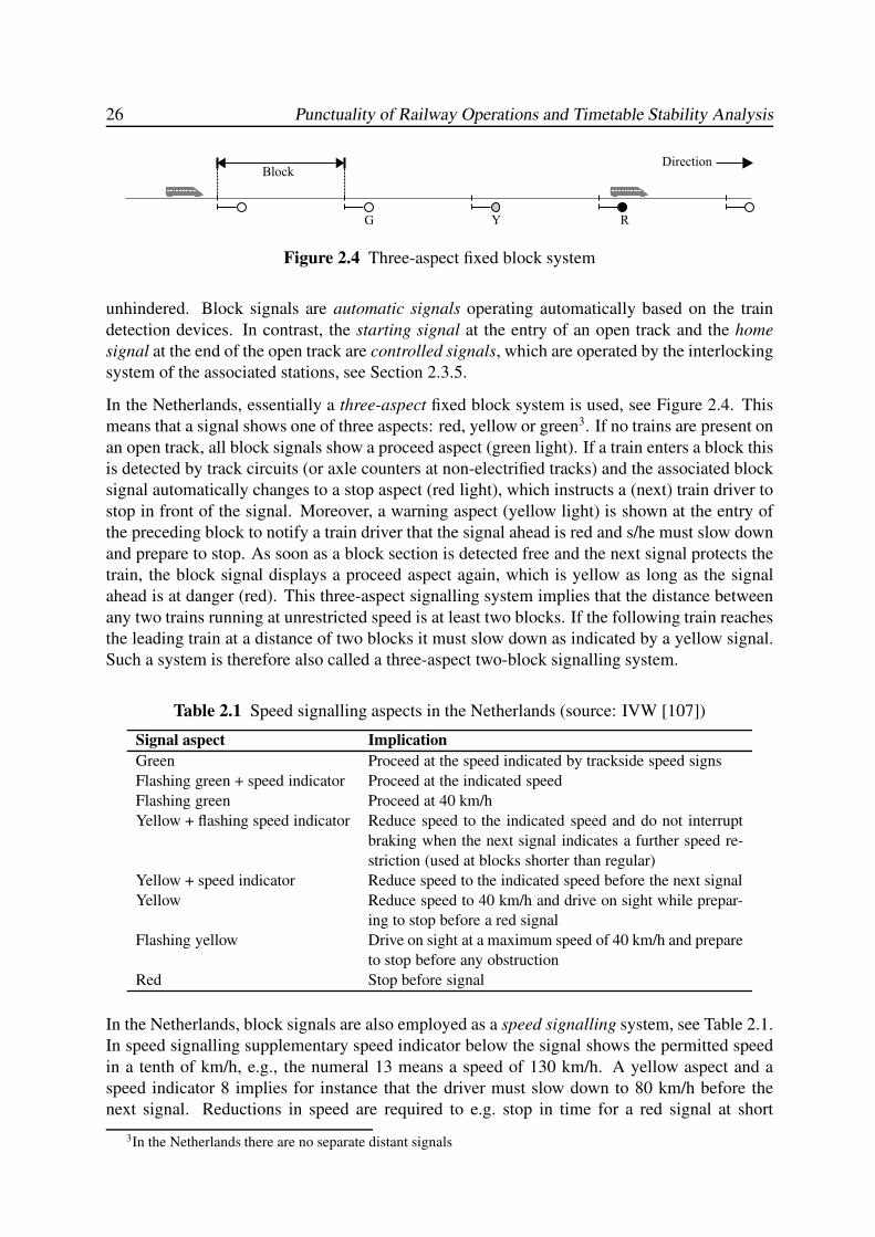
26 Punctuality of Railway Operations and Timetable Stability Analysis
RYG
BlockDirection
Figure 2.4 Three-aspect fixed block system
unhindered. Block signals are automatic signals operating automatically based on the train
detection devices. In contrast, the starting signal at the entry of an open track and the home
signal at the end of the open track are controlled signals, which are operated by the interlocking
system of the associated stations, see Section 2.3.5.
In the Netherlands, essentially a three-aspect fixed block system is used, see Figure 2.4. This
means that a signal shows one of three aspects: red, yellow or green3. If no trains are present on
an open track, all block signals show a proceed aspect (green light). If a train enters a block this
is detected by track circuits (or axle counters at non-electrified tracks) and the associated block
signal automatically changes to a stop aspect (red light), which instructs a (next) train driver to
stop in front of the signal. Moreover, a warning aspect (yellow light) is shown at the entry of
the preceding block to notify a train driver that the signal ahead is red and s/he must slow down
and prepare to stop. As soon as a block section is detected free and the next signal protects the
train, the block signal displays a proceed aspect again, which is yellow as long as the signal
ahead is at danger (red). This three-aspect signalling system implies that the distance between
any two trains running at unrestricted speed is at least two blocks. If the following train reaches
the leading train at a distance of two blocks it must slow down as indicated by a yellow signal.
Such a system is therefore also called a three-aspect two-block signalling system.
Table 2.1 Speed signalling aspects in the Netherlands (source: IVW [107])
Signal aspect Implication
Green Proceed at the speed indicated by trackside speed signs
Flashing green + speed indicator Proceed at the indicated speed
Flashing green Proceed at 40 km/h
Yellow + flashing speed indicator Reduce speed to the indicated speed and do not interrupt
braking when the next signal indicates a further speed re-
striction (used at blocks shorter than regular)
Yellow + speed indicator Reduce speed to the indicated speed before the next signal
Yellow Reduce speed to 40 km/h and drive on sight while prepar-
ing to stop before a red signal
Flashing yellow Drive on sight at a maximum speed of 40 km/h and prepare
to stop before any obstruction
Red Stop before signal
In the Netherlands, block signals are also employed as a speed signalling system, see Table 2.1.
In speed signalling supplementary speed indicator below the signal shows the permitted speed
in a tenth of km/h, e.g., the numeral 13 means a speed of 130 km/h. A yellow aspect and a
speed indicator 8 implies for instance that the driver must slow down to 80 km/h before the
next signal. Reductions in speed are required to e.g. stop in time for a red signal at short
3In the Netherlands there are no separate distant signals
Chapter 2. Fundamentals of Railway Operations 27
blocks, for permanent speed restrictions of line sections (by e.g. track curvature, switch speed
limits at station areas), or for temporary speed restrictions (e.g. maintenance sites). We refer to
Bailey [12] for an overview of the different signalling aspects used throughout Europe.
2.3.3 Automatic Train Protection
Automatic train protection (ATP) systems have been developed to support train drivers and
avoid human errors or failure. ATP shows signal information in the cabin (cab signalling),
checks whether the driver respects the signalling commands, and intervenes when necessary.
In the Netherlands, ATP is used as an additional safety layer above the automatic block system
with trackside (block) signals.
In the Netherlands, the ATB (Automatische Trein Beınvloeding) system is used on all electrified
railway lines [12, 212]. ATB invokes an emergency braking up to standstill when overspeed is
detected without braking activity from the driver within two seconds. ATB supervises five speed
limits (40, 60, 80, 130, and 140 km/h) based on track-to-train transmission through a (pulse)
code in the track circuits generated by the trackside speed signalling system. The on-board ATB
system includes a cab signalling display that shows the allowed speed. However, because of
the limitation in available speed levels, the cab signal may display a higher speed than the local
maximum speed as shown by fixed trackside speed signs and signals. Therefore, the trackside
signalling is still decisive while the cab signalling is only supportive. Audible information is
given when the speed level changes (gong) and when overspeed is detected without braking
activation from the driver (continuous bell). If the brakes are activated the bell signal stops,
and when the speed is sufficiently reduced this is indicated by an intermittent bell signal. ATB
does not work for speeds below 40 km/h; in this case the driver must follow the instructions of
the trackside signals. The 40 km/h speed limit applies when no ATB-code is received. So in
the event of signalling failure and absence of ATB-code, the train driver has to rely on driving
on sight with a 40 km/h speed limit. ATB is a continuous ATP system because of the coded
track circuits, implying that a change in aspect of the next signal is immediately transmitted to
the train. A driver may therefore increase speed as soon as the cab signalling indicates a less
restrictive speed limit. Note that ATB can only be used on electrified tracks with (coded) track
circuits.
ATB-NG (ATB-New Generation) [212] is used in the Netherlands on non-electrified railway
lines and for light trainsets that are not detected well by track circuits. ATB-NG relies on axle
counters for train detection and separate beacons between the rails for data transmission. ATB-
NG applies a speed supervision in steps of 10 km/h and in particular also supervises speeds
below 40 km/h. The information received from a beacon contains the distance to the next signal
(beacon) and the maximum speed allowed at this point. Using additional static information on
the train characteristics the onboard equipment computes a braking curve that must be respected
by the driver. Hence, a train operating with ATB-NG does not have to slow down immediately
when passing a (yellow) warning signal — as in ATB — but according to a train-specific brak-
ing curve. However, ATB-NG is an intermittent ATP system, implying that track-to-train data
transmission only occurs at discrete points on the track. Intermediate aspect changes of the next
signal are therefore only received at the next beacon.
Most Dutch railway lines are equipped with conventional ATB which is nowadays also known
as ATB-EG (ATB-first generation) to distinguish from ATB-NG. ATB-NG is implemented on
28 Punctuality of Railway Operations and Timetable Stability Analysis
several railway lines in (mostly) the east and north-east of the Netherlands. A few local Dutch
railway lines still have no ATP-system installed [165].
2.3.4 Train Describer Systems (TNV)
Each running train is assigned a unique number by which it is recognized by the control systems
and railway personnel. The train number or train description describes the train line and starting
time: the first part denotes the train line number (characterizing the train type, terminal stations,
route, and served stations) and the last two digits represent a counter for the successive trains
over the day. As an example, consider the regional train line 5600 Utrecht-Zwolle. The first
train departs from Utrecht at 6:02 with train number 5615, the next train departs at 6:32 with
number 5617, et cetera, until the last train of 0:02 with number 5687. The even numbers are
used for the trains in the opposite direction. These numbers are also shown in the published
timetable [152] and the online train travel planner.
A train describer is a system that identifies a train at a particular position and keeps track of
its progress at discrete steps over its route. In the Netherlands, train describers are known as
TNV-systems (Treinnummervolgsystemen). The position of a train number is based on TNV-
windows. A TNV-window is a route between two (not necessarily adjacent) signals. At the
start of a train journey the assigned train number is inserted into the TNV-system at the TNV-
window of the departure platform. This insertion is either done manually by a dispatcher or
automatically (e.g. at line ends). The TNV-window in which a train number is located is called
its train number position or TNV-position. The movement and direction of a train is deduced
from received safety and signalling information of signal controls, switch detection, and track
circuits. The next TNV-position is determined by the set route after the destination signal of the
current TNV-position. A TNV-step of the train number to the next TNV-position is triggered
when the train enters the first associated track section. Hence, the TNV-position of a train
corresponds with the track circuit occupancy but moves in larger steps. See Bailey [12] for
more background on train describers.
The Dutch railway network has been partitioned into 13 TNV traffic control areas, each having
a separate TNV-system. If a train approaches an adjacent traffic control area, its number is
transmitted to the associated TNV-system. When the train enters the next traffic control area
the train number is cleared from the current TNV-system and inserted into the next.
A TNV-system must be continuously aware of the state of all relevant signalling controls and
monitoring information, including track, signal, switch, and route relays. It therefore scans and
records messages received from signalling control systems (EBP and EBS, see §2.3.5), other
TNV-systems, and manual instructions from operators. Based on this information it keeps track
of the TNV-positions of all train numbers in the system, determines TNV-steps, and inserts and
deletes train numbers. Finally, the TNV-system communicates TNV-steps to the corresponding
train traffic control system (VPT-VKL) and passenger information systems (BEPAC). Figure 2.5
shows the data flows between a TNV-system and its control environment.
A TNV-system keeps a real-time record of received inputs and TNV-events. These TNV-logfiles
contain chronological information about all signalling and interlocking events in a traffic control
area. TNV-logfiles thus contain invaluable realization data of railway operations, although quite
inaccessible by their size (about 25 MB ASCII-format per day per TNV-system). Therefore, the
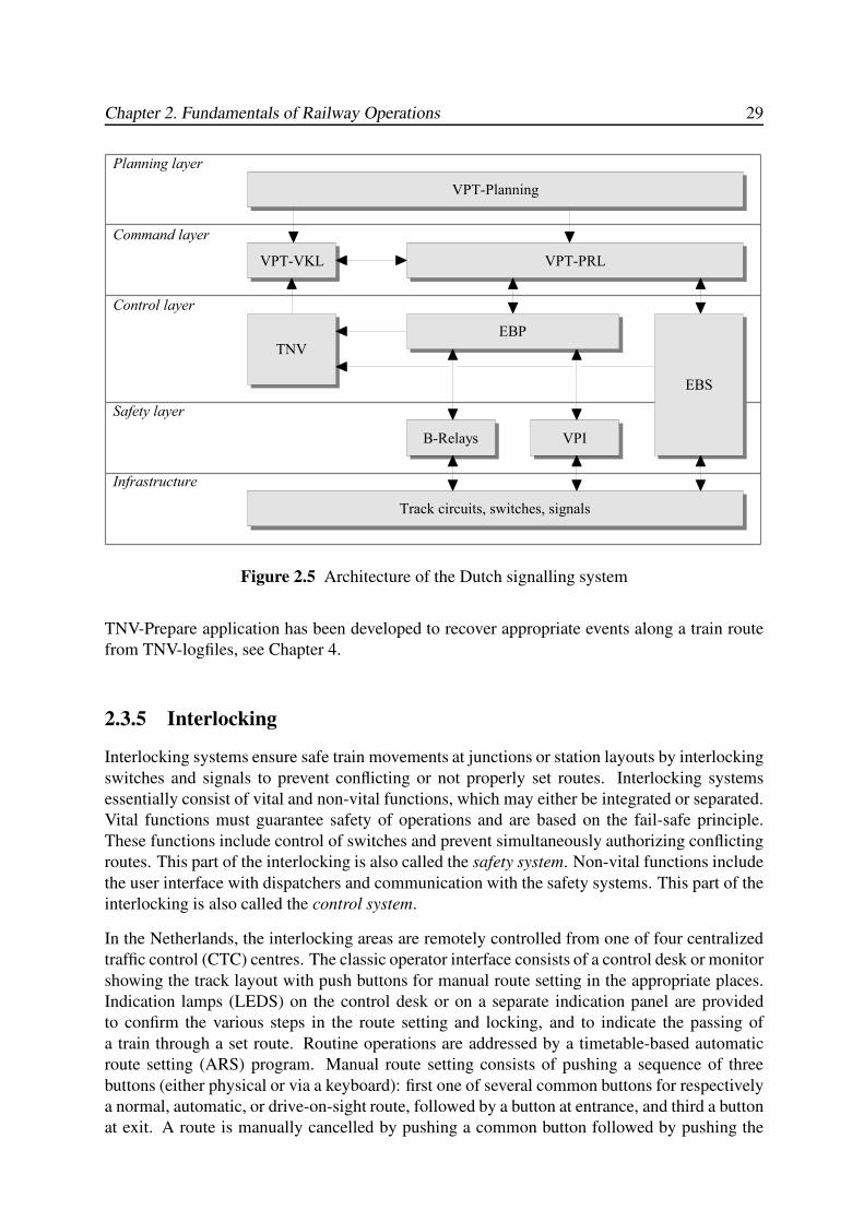
Chapter 2. Fundamentals of Railway Operations 29
Figure 2.5 Architecture of the Dutch signalling system
TNV-Prepare application has been developed to recover appropriate events along a train route
from TNV-logfiles, see Chapter 4.
2.3.5 Interlocking
Interlocking systems ensure safe train movements at junctions or station layouts by interlocking
switches and signals to prevent conflicting or not properly set routes. Interlocking systems
essentially consist of vital and non-vital functions, which may either be integrated or separated.
Vital functions must guarantee safety of operations and are based on the fail-safe principle.
These functions include control of switches and prevent simultaneously authorizing conflicting
routes. This part of the interlocking is also called the safety system. Non-vital functions include
the user interface with dispatchers and communication with the safety systems. This part of the
interlocking is also called the control system.
In the Netherlands, the interlocking areas are remotely controlled from one of four centralized
traffic control (CTC) centres. The classic operator interface consists of a control desk or monitor
showing the track layout with push buttons for manual route setting in the appropriate places.
Indication lamps (LEDS) on the control desk or on a separate indication panel are provided
to confirm the various steps in the route setting and locking, and to indicate the passing of
a train through a set route. Routine operations are addressed by a timetable-based automatic
route setting (ARS) program. Manual route setting consists of pushing a sequence of three
buttons (either physical or via a keyboard): first one of several common buttons for respectively
a normal, automatic, or drive-on-sight route, followed by a button at entrance, and third a button
at exit. A route is manually cancelled by pushing a common button followed by pushing the
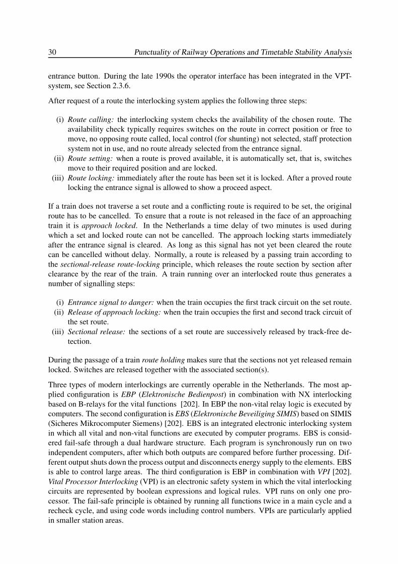
30 Punctuality of Railway Operations and Timetable Stability Analysis
entrance button. During the late 1990s the operator interface has been integrated in the VPT-
system, see Section 2.3.6.
After request of a route the interlocking system applies the following three steps:
(i) Route calling: the interlocking system checks the availability of the chosen route. The
availability check typically requires switches on the route in correct position or free to
move, no opposing route called, local control (for shunting) not selected, staff protection
system not in use, and no route already selected from the entrance signal.
(ii) Route setting: when a route is proved available, it is automatically set, that is, switches
move to their required position and are locked.
(iii) Route locking: immediately after the route has been set it is locked. After a proved route
locking the entrance signal is allowed to show a proceed aspect.
If a train does not traverse a set route and a conflicting route is required to be set, the original
route has to be cancelled. To ensure that a route is not released in the face of an approaching
train it is approach locked. In the Netherlands a time delay of two minutes is used during
which a set and locked route can not be cancelled. The approach locking starts immediately
after the entrance signal is cleared. As long as this signal has not yet been cleared the route
can be cancelled without delay. Normally, a route is released by a passing train according to
the sectional-release route-locking principle, which releases the route section by section after
clearance by the rear of the train. A train running over an interlocked route thus generates a
number of signalling steps:
(i) Entrance signal to danger: when the train occupies the first track circuit on the set route.
(ii) Release of approach locking: when the train occupies the first and second track circuit of
the set route.
(iii) Sectional release: the sections of a set route are successively released by track-free de-
tection.
During the passage of a train route holding makes sure that the sections not yet released remain
locked. Switches are released together with the associated section(s).
Three types of modern interlockings are currently operable in the Netherlands. The most ap-
plied configuration is EBP (Elektronische Bedienpost) in combination with NX interlocking
based on B-relays for the vital functions [202]. In EBP the non-vital relay logic is executed by
computers. The second configuration is EBS (Elektronische Beveiliging SIMIS) based on SIMIS
(Sicheres Mikrocomputer Siemens) [202]. EBS is an integrated electronic interlocking system
in which all vital and non-vital functions are executed by computer programs. EBS is consid-
ered fail-safe through a dual hardware structure. Each program is synchronously run on two
independent computers, after which both outputs are compared before further processing. Dif-
ferent output shuts down the process output and disconnects energy supply to the elements. EBS
is able to control large areas. The third configuration is EBP in combination with VPI [202].
Vital Processor Interlocking (VPI) is an electronic safety system in which the vital interlocking
circuits are represented by boolean expressions and logical rules. VPI runs on only one pro-
cessor. The fail-safe principle is obtained by running all functions twice in a main cycle and a
recheck cycle, and using code words including control numbers. VPIs are particularly applied
in smaller station areas.
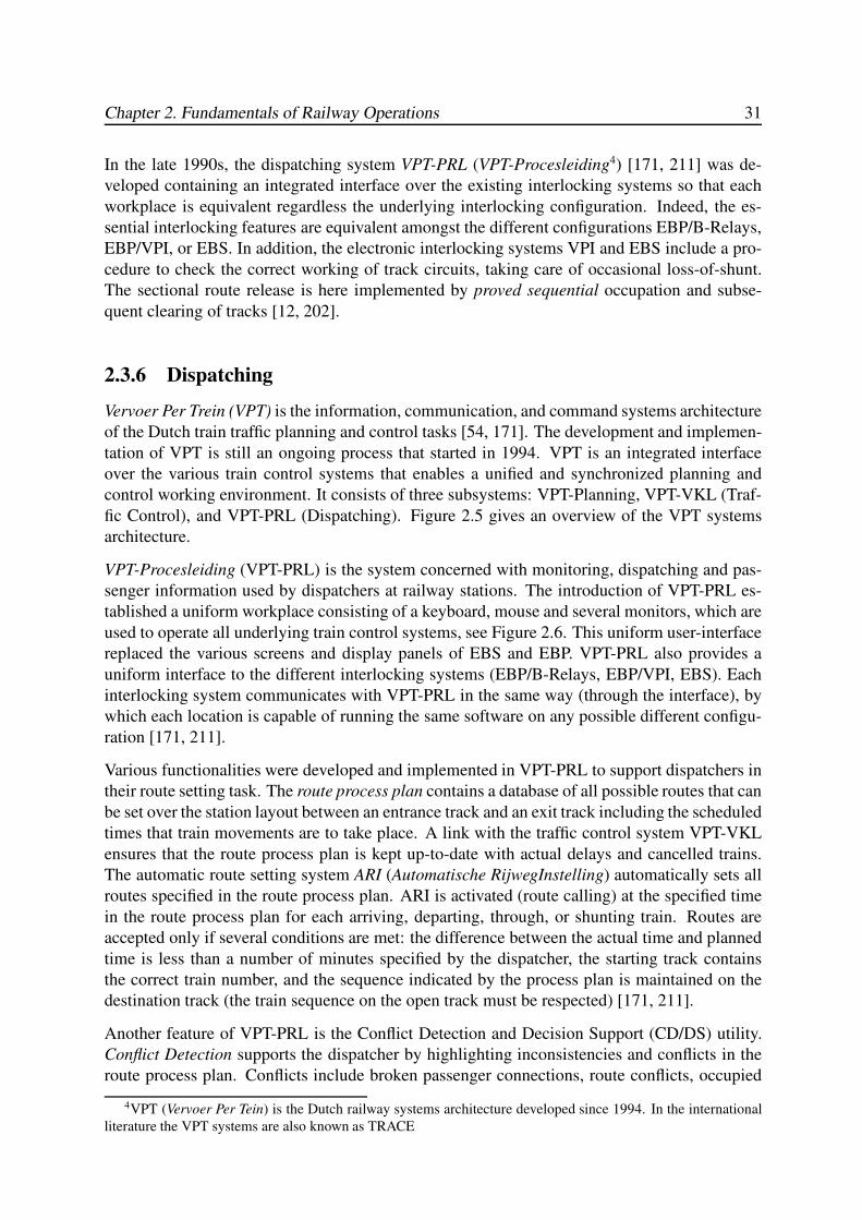
Chapter 2. Fundamentals of Railway Operations 31
In the late 1990s, the dispatching system VPT-PRL (VPT-Procesleiding4) [171, 211] was de-
veloped containing an integrated interface over the existing interlocking systems so that each
workplace is equivalent regardless the underlying interlocking configuration. Indeed, the es-
sential interlocking features are equivalent amongst the different configurations EBP/B-Relays,
EBP/VPI, or EBS. In addition, the electronic interlocking systems VPI and EBS include a pro-
cedure to check the correct working of track circuits, taking care of occasional loss-of-shunt.
The sectional route release is here implemented by proved sequential occupation and subse-
quent clearing of tracks [12, 202].
2.3.6 Dispatching
Vervoer Per Trein (VPT) is the information, communication, and command systems architecture
of the Dutch train traffic planning and control tasks [54, 171]. The development and implemen-
tation of VPT is still an ongoing process that started in 1994. VPT is an integrated interface
over the various train control systems that enables a unified and synchronized planning and
control working environment. It consists of three subsystems: VPT-Planning, VPT-VKL (Traf-
fic Control), and VPT-PRL (Dispatching). Figure 2.5 gives an overview of the VPT systems
architecture.
VPT-Procesleiding (VPT-PRL) is the system concerned with monitoring, dispatching and pas-
senger information used by dispatchers at railway stations. The introduction of VPT-PRL es-
tablished a uniform workplace consisting of a keyboard, mouse and several monitors, which are
used to operate all underlying train control systems, see Figure 2.6. This uniform user-interface
replaced the various screens and display panels of EBS and EBP. VPT-PRL also provides a
uniform interface to the different interlocking systems (EBP/B-Relays, EBP/VPI, EBS). Each
interlocking system communicates with VPT-PRL in the same way (through the interface), by
which each location is capable of running the same software on any possible different configu-
ration [171, 211].
Various functionalities were developed and implemented in VPT-PRL to support dispatchers in
their route setting task. The route process plan contains a database of all possible routes that can
be set over the station layout between an entrance track and an exit track including the scheduled
times that train movements are to take place. A link with the traffic control system VPT-VKL
ensures that the route process plan is kept up-to-date with actual delays and cancelled trains.
The automatic route setting system ARI (Automatische RijwegInstelling) automatically sets all
routes specified in the route process plan. ARI is activated (route calling) at the specified time
in the route process plan for each arriving, departing, through, or shunting train. Routes are
accepted only if several conditions are met: the difference between the actual time and planned
time is less than a number of minutes specified by the dispatcher, the starting track contains
the correct train number, and the sequence indicated by the process plan is maintained on the
destination track (the train sequence on the open track must be respected) [171, 211].
Another feature of VPT-PRL is the Conflict Detection and Decision Support (CD/DS) utility.
Conflict Detection supports the dispatcher by highlighting inconsistencies and conflicts in the
route process plan. Conflicts include broken passenger connections, route conflicts, occupied
4VPT (Vervoer Per Tein) is the Dutch railway systems architecture developed since 1994. In the international
literature the VPT systems are also known as TRACE
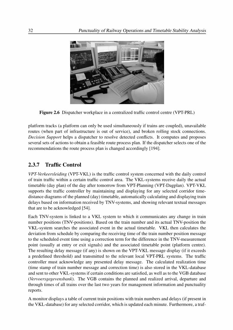
32 Punctuality of Railway Operations and Timetable Stability Analysis
Figure 2.6 Dispatcher workplace in a centralized traffic control centre (VPT-PRL)
platform tracks (a platform can only be used simultaneously if trains are coupled), unavailable
routes (when part of infrastructure is out of service), and broken rolling stock connections.
Decision Support helps a dispatcher to resolve detected conflicts. It computes and proposes
several sets of actions to obtain a feasible route process plan. If the dispatcher selects one of the
recommendations the route process plan is changed accordingly [194].
2.3.7 Traffic Control
VPT-Verkeersleiding (VPT-VKL) is the traffic control system concerned with the daily control
of train traffic within a certain traffic control area. The VKL-systems receive daily the actual
timetable (day plan) of the day after tomorrow from VPT-Planning (VPT-Dagplan). VPT-VKL
supports the traffic controller by maintaining and displaying for any selected corridor time-
distance diagrams of the planned (day) timetable, automatically calculating and displaying train
delays based on information received by TNV-systems, and showing relevant textual messages
that are to be acknowledged [54].
Each TNV-system is linked to a VKL system to which it communicates any change in train
number positions (TNV-positions). Based on the train number and its actual TNV-position the
VKL-system searches the associated event in the actual timetable. VKL then calculates the
deviation from schedule by comparing the receiving time of the train number position message
to the scheduled event time using a correction term for the difference in the TNV-measurement
point (usually at entry or exit signals) and the associated timetable point (platform centre).
The resulting delay message (if any) is shown on the VPT-VKL message display (if it exceeds
a predefined threshold) and transmitted to the relevant local VPT-PRL systems. The traffic
controller must acknowledge any presented delay message. The calculated realization time
(time stamp of train number message and correction time) is also stored in the VKL-database
and sent to other VKL-systems if certain conditions are satisfied, as well as to the VGB database
(Vervoersgegevensbank). The VGB contains the planned and realized arrival, departure and
through times of all trains over the last two years for management information and punctuality
reports.
A monitor displays a table of current train positions with train numbers and delays (if present in
the VKL-database) for any selected corridor, which is updated each minute. Furthermore, a traf-
Chapter 2. Fundamentals of Railway Operations 33
fic controller can switch between (scheduled) time-distance diagrams for any route, check the
timetable of any individual train, and modify the timetable. Mutations in the timetable are au-
tomatically transmitted to all involved traffic controllers and dispatchers. The traffic controllers
are responsible for controlling the traffic at incidents (e.g. signal malfunctioning, accidents with
road vehicles at level crossings, and catenary breakdown), which results in mutations to the
timetable. The changes in the actual timetable may also necessitate modifications in train and
crew circulations. Since the split of train operators and traffic control this is the responsibility
of separate transport controllers from the relevant train operators. These transport controllers
are located separately in the traffic control centre and also have access to the VPT-VKL system.
2.4 Train Delays
2.4.1 Primary Delays
Modern railways consist of many interacting processes on a railway network that depend on a
wide range of technical devices such as rolling stock, electrification, and safety installations.
This leads to potential risks of disruptions to the traffic processes by technical malfunctions and
deterioration, e.g. failing moving parts of the infrastructure (switches), damaged door locks,
temporary speed limits due to maintenance work, problematic coupling or decoupling, failing
braking-test, ATP-application, and engine breakdown.
Train running time between stations and dwell time at stations (slightly) varies for each trip de-
pending on a wide range of factors from within the railway system and from exogenous sources.
Internal sources of process time variation are technical malfunctions but also human-related fac-
tors such as nonpaying passengers, delay by catering, and large passenger flows (alighting and
boarding times). In addition the environment presents exogenous sources of randomness like
weather conditions. These sources of random variations are difficult to forecast and form a
fundamental part of the practice of railway operations. Therefore there will always be a certain
amount of trips that exceed a scheduled process time leading to primary delays, although sched-
uled running times and dwell times usually contain some margin or slack time to compensate
for small variations.
Definition 2.4.1 (Primary delay) A primary delay is the deviation from a scheduled process
time caused by disruption within the process.
Table 2.2 gives an overview of disruptions resulting in primary delays.
Other sources of delay are major incidents such as train engine breakdown and damage to the
overhead catenary system, which result in large delays. However, these delays are not structural
and (should) occur only seldom. Trains affected by an uncommon event experience delays that
are clearly not representative to the usual stochastic behaviour. These situations are the subject
of incidence management rather than daily operations practice. From a statistical analysis point
of view these delays are usually identified as outliers.
The fluctuations in technical and environmental conditions, and behaviour of personnel and
travellers make the process times random variables. The main objective of railway traffic man-
agement is to keep variations in the process times as small as possible. Therefore, the planned
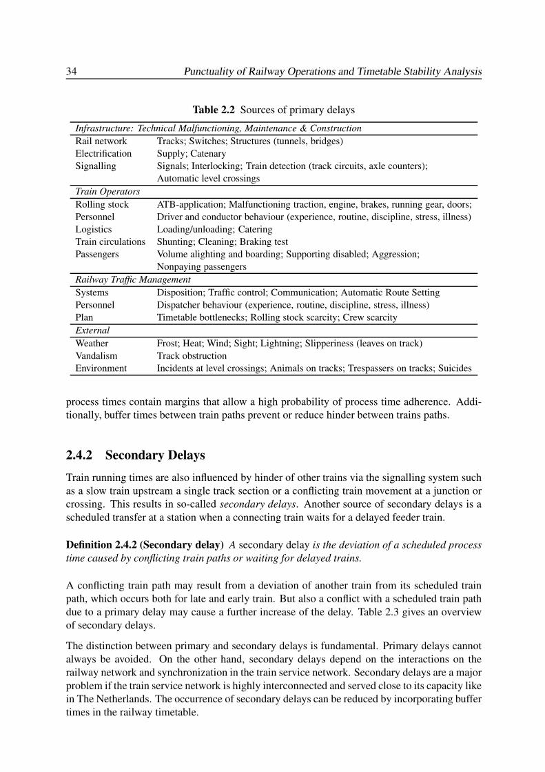
34 Punctuality of Railway Operations and Timetable Stability Analysis
Table 2.2 Sources of primary delays
Infrastructure: Technical Malfunctioning, Maintenance & Construction
Rail network Tracks; Switches; Structures (tunnels, bridges)
Electrification Supply; Catenary
Signalling Signals; Interlocking; Train detection (track circuits, axle counters);
Automatic level crossings
Train Operators
Rolling stock ATB-application; Malfunctioning traction, engine, brakes, running gear, doors;
Personnel Driver and conductor behaviour (experience, routine, discipline, stress, illness)
Logistics Loading/unloading; Catering
Train circulations Shunting; Cleaning; Braking test
Passengers Volume alighting and boarding; Supporting disabled; Aggression;
Nonpaying passengers
Railway Traffic Management
Systems Disposition; Traffic control; Communication; Automatic Route Setting
Personnel Dispatcher behaviour (experience, routine, discipline, stress, illness)
Plan Timetable bottlenecks; Rolling stock scarcity; Crew scarcity
External
Weather Frost; Heat; Wind; Sight; Lightning; Slipperiness (leaves on track)
Vandalism Track obstruction
Environment Incidents at level crossings; Animals on tracks; Trespassers on tracks; Suicides
process times contain margins that allow a high probability of process time adherence. Addi-
tionally, buffer times between train paths prevent or reduce hinder between trains paths.
2.4.2 Secondary Delays
Train running times are also influenced by hinder of other trains via the signalling system such
as a slow train upstream a single track section or a conflicting train movement at a junction or
crossing. This results in so-called secondary delays. Another source of secondary delays is a
scheduled transfer at a station when a connecting train waits for a delayed feeder train.
Definition 2.4.2 (Secondary delay) A secondary delay is the deviation of a scheduled process
time caused by conflicting train paths or waiting for delayed trains.
A conflicting train path may result from a deviation of another train from its scheduled train
path, which occurs both for late and early train. But also a conflict with a scheduled train path
due to a primary delay may cause a further increase of the delay. Table 2.3 gives an overview
of secondary delays.
The distinction between primary and secondary delays is fundamental. Primary delays cannot
always be avoided. On the other hand, secondary delays depend on the interactions on the
railway network and synchronization in the train service network. Secondary delays are a major
problem if the train service network is highly interconnected and served close to its capacity like
in The Netherlands. The occurrence of secondary delays can be reduced by incorporating buffer
times in the railway timetable.
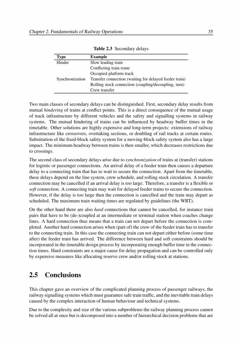
Chapter 2. Fundamentals of Railway Operations 35
Table 2.3 Secondary delays
Type Example
Hinder Slow leading train
Conflicting train route
Occupied platform track
Synchronization Transfer connection (waiting for delayed feeder train)
Rolling stock connection (coupling/decoupling, turn)
Crew transfer
Two main classes of secondary delays can be distinguished. First, secondary delay results from
mutual hindering of trains at conflict points. This is a direct consequence of the mutual usage
of track infrastructure by different vehicles and the safety and signalling systems in railway
systems. The mutual hindering of trains can be influenced by headway buffer times in the
timetable. Other solutions are highly expensive and long-term projects: extensions of railway
infrastructure like crossovers, overtaking sections, or doubling of rail tracks at certain routes.
Substitution of the fixed-block safety system for a moving-block safety system also has a large
impact. The minimum headway between trains is then smaller, which decreases restrictions due
to crossings.
The second class of secondary delays arise due to synchronization of trains at (transfer) stations
for logistic or passenger connections. An arrival delay of a feeder train then causes a departure
delay to a connecting train that has to wait to secure the connection. Apart from the timetable,
these delays depend on the line system, crew schedule, and rolling stock circulation. A transfer
connection may be cancelled if an arrival delay is too large. Therefore, a transfer is a flexible or
soft connection. A connecting train may wait for delayed feeder trains to secure the connection.
However, if the delay is too large then the connection is cancelled and the train may depart as
scheduled. The maximum train waiting times are regulated by guidelines (the WRT).
On the other hand there are also hard connections that cannot be cancelled, for instance train
pairs that have to be (de-)coupled at an intermediate or terminal station when coaches change
lines. A hard connection thus means that a train can not depart before the connection is com-
pleted. Another hard connection arises when (part of) the crew of the feeder train has to transfer
to the connecting train. In this case the connecting train can not depart either before (some time
after) the feeder train has arrived. The difference between hard and soft constraints should be
incorporated in the timetable design process by incorporating enough buffer time in the connec-
tion times. Hard constraints are a major cause for delay propagation and can be controlled only
by expensive measures like allocating reserve crew and/or rolling stock at stations.
2.5 Conclusions
This chapter gave an overview of the complicated planning process of passenger railways, the
railway signalling systems which must guarantee safe train traffic, and the inevitable train delays
caused by the complex interaction of human behaviour and technical systems.
Due to the complexity and size of the various subproblems the railway planning process cannot
be solved all at once but is decomposed into a number of hierarchical decision problems that are
36 Punctuality of Railway Operations and Timetable Stability Analysis
solved sequentially where each stage is based on the decisions made earlier. The hierarchical
approach enables an iterative solution procedure where previous decisions must be adjusted to
find a feasible or optimal solution in a later stage, although each stage typically takes several
months to complete. The railway planning process is however repeated annually by which
solutions of the previous year can be evaluated and reused or improved in the current designs.
The characteristics of railway transport are well-known: the rail-wheel contact allows a minimal
friction between vehicle and track which implies an energy-efficient way of transport. However,
at the same time the braking distances of heavy vehicles running at high speed require a sophis-
ticated safety and signalling system that protects trains from collisions. We have seen examples
of such systems as used in the Netherlands, and in particular saw how trains are automatically
detected and monitored. The train description or TNV-system is an important element in the
railway systems architecture: TNV-systems inform the dispatcher and traffic control systems
on the progress of trains as they run over the network using detailed information received from
safety and signalling systems. Both received and generated information is recorded in real-
time by the TNV-systems into so-called TNV-logfiles. In Chapter 4 we will see how we can
exploit the TNV-logfiles as a reliable and accurate source for analysing the railway traffic and
infrastructure utilization.
Railway traffic relies on both human behaviour and a large amount of technical equipment
such as the infrastructure, rolling stock and control systems, which are all sources of highly
unpredictable fluctuations in performance and more severe disruptions causing primary delays.
In addition, because of the interdependencies in the timetable and shared use of infrastructure,
existing delays may propagate and thus generate secondary delays. In the next chapter we will
see how railway timetables are designed to compensate for delays and reduce or prevent delay
propagation.
Chapter 3
RAILWAY TIMETABLES
3.1 Introduction
The quality of a timetable is in first instance determined by realistic scheduled process times for
the separate processes. In practice, the individual process times will hardly be exactly the same
from hour-to-hour or day-to-day because of variations in internal and environmental conditions.
This is accounted for by the inclusion of some time supplement so that the process time can be
realized with high probability. A scheduled process time typically consists of the following
components:
• a nominal process time for ideal or average traffic conditions;
• a margin to compensate for less favourable traffic conditions; and
• scheduled waiting time to fit the process conflict-free in the timetable.
An example of scheduled waiting time is when the time-distance trajectory of a train run is
slightly bended to fit in between other reserved train paths. Another typical occurrence of
scheduled waiting time is at a station stop when a train is overtaken by a faster train. The
process time margin is usually specified as a fixed percentage of the nominal process time, e.g.,
7%. Obviously, the variation in process time realizations should be reflected in the amount
of applied margin. A timetable contains various traffic processes: running time refers to a
train run from one station to the next, dwell time relates to alighting and boarding passengers,
transfer time corresponds to transferring passengers, etc. The expression minimum process time
is generally used for the sum of the nominal process time and a margin that must be maintained
to guarantee a reliable process time. For instance, a minimum transfer time relates to the amount
of time that is necessary for a large group of passengers to transfer from the feeder train to the
connecting train including e.g. crowding effects at stairways and in pedestrian tunnels on the
route from the arrival to the departure platform, and not to the time needed by a single fast
traveller. The terminology related to running time slightly differs from all other process times:
in this case the minimum running time usually equals the nominal running time whilst the
running time margin can be used to reduce delays.
To reduce delay propagation an additional amount of slack may be provided between two pro-
cesses. This buffer time is not part of the process time but can be used to even out minor delays.
In the case of station dwell time some buffer time may be added before the next train run to
compensate for possible arrival delays. In this case the distinction between dwell time margin
and buffer time is not that clear. Often a scheduled process time is rounded up to minutes so that
the associated events are given in whole minutes. This time supplement may also be interpreted
as either margin or buffer time.
37
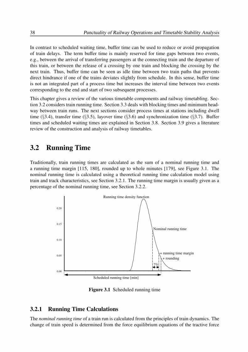
38 Punctuality of Railway Operations and Timetable Stability Analysis
In contrast to scheduled waiting time, buffer time can be used to reduce or avoid propagation
of train delays. The term buffer time is mainly reserved for time gaps between two events,
e.g., between the arrival of transferring passengers at the connecting train and the departure of
this train, or between the release of a crossing by one train and blocking the crossing by the
next train. Thus, buffer time can be seen as idle time between two train paths that prevents
direct hindrance if one of the trains deviates slightly from schedule. In this sense, buffer time
is not an integrated part of a process time but increases the interval time between two events
corresponding to the end and start of two subsequent processes.
This chapter gives a review of the various timetable components and railway timetabling. Sec-
tion 3.2 considers train running time. Section 3.3 deals with blocking times and minimum head-
way between train runs. The next sections consider process times at stations including dwell
time (§3.4), transfer time (§3.5), layover time (§3.6) and synchronization time (§3.7). Buffer
times and scheduled waiting times are explained in Section 3.8. Section 3.9 gives a literature
review of the construction and analysis of railway timetables.
3.2 Running Time
Traditionally, train running times are calculated as the sum of a nominal running time and
a running time margin [115, 180], rounded up to whole minutes [179], see Figure 3.1. The
nominal running time is calculated using a theoretical running time calculation model using
train and track characteristics, see Section 3.2.1. The running time margin is usually given as a
percentage of the nominal running time, see Section 3.2.2.
0.00
0.05
0.10
0.15
0.20
Nominal running time
+ running time margin
+ rounding
Scheduled running time [min]
7%
Running time density function
Figure 3.1 Scheduled running time
3.2.1 Running Time Calculations
The nominal running time of a train run is calculated from the principles of train dynamics. The
change of train speed is determined from the force equilibrium equations of the tractive force
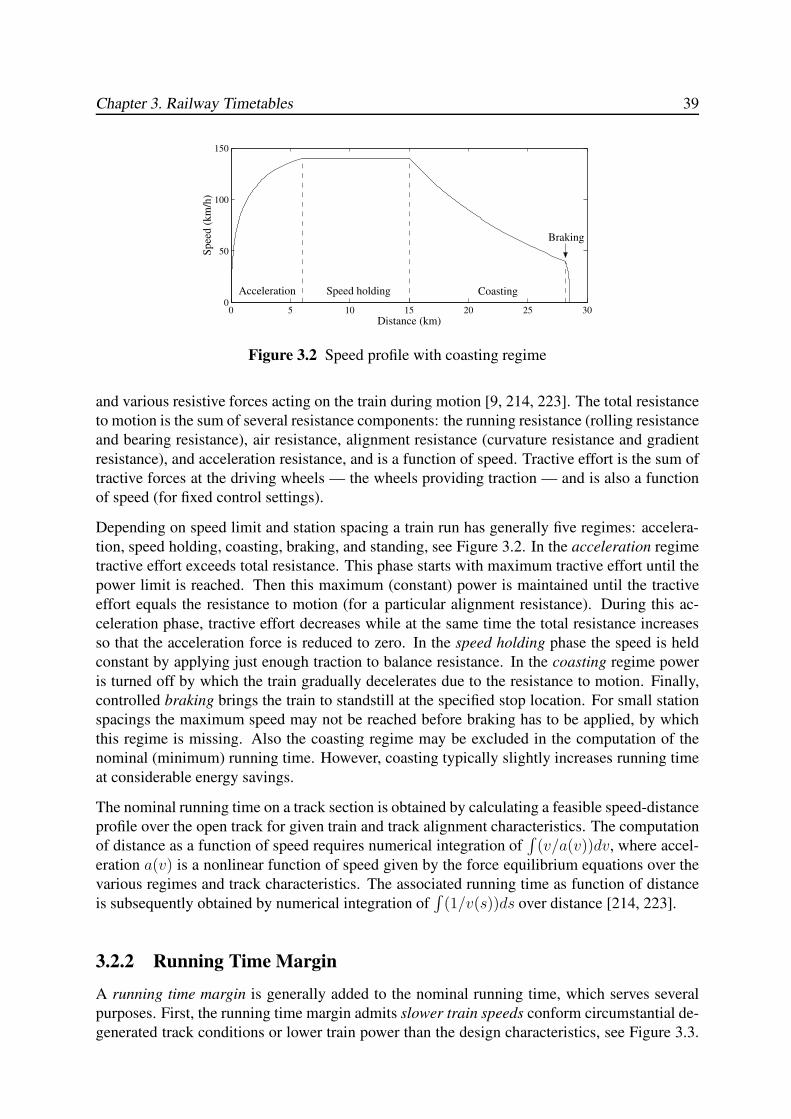
Chapter 3. Railway Timetables 39
0 5 10 15 20 25 300
50
100
150
Sp
eed
(k
m/h
)
Distance (km)
Acceleration Speed holding Coasting
Braking
Figure 3.2 Speed profile with coasting regime
and various resistive forces acting on the train during motion [9, 214, 223]. The total resistance
to motion is the sum of several resistance components: the running resistance (rolling resistance
and bearing resistance), air resistance, alignment resistance (curvature resistance and gradient
resistance), and acceleration resistance, and is a function of speed. Tractive effort is the sum of
tractive forces at the driving wheels — the wheels providing traction — and is also a function
of speed (for fixed control settings).
Depending on speed limit and station spacing a train run has generally five regimes: accelera-
tion, speed holding, coasting, braking, and standing, see Figure 3.2. In the acceleration regime
tractive effort exceeds total resistance. This phase starts with maximum tractive effort until the
power limit is reached. Then this maximum (constant) power is maintained until the tractive
effort equals the resistance to motion (for a particular alignment resistance). During this ac-
celeration phase, tractive effort decreases while at the same time the total resistance increases
so that the acceleration force is reduced to zero. In the speed holding phase the speed is held
constant by applying just enough traction to balance resistance. In the coasting regime power
is turned off by which the train gradually decelerates due to the resistance to motion. Finally,
controlled braking brings the train to standstill at the specified stop location. For small station
spacings the maximum speed may not be reached before braking has to be applied, by which
this regime is missing. Also the coasting regime may be excluded in the computation of the
nominal (minimum) running time. However, coasting typically slightly increases running time
at considerable energy savings.
The nominal running time on a track section is obtained by calculating a feasible speed-distance
profile over the open track for given train and track alignment characteristics. The computation
of distance as a function of speed requires numerical integration of∫
(v/a(v))dv, where accel-
eration a(v) is a nonlinear function of speed given by the force equilibrium equations over the
various regimes and track characteristics. The associated running time as function of distance
is subsequently obtained by numerical integration of∫
(1/v(s))ds over distance [214, 223].
3.2.2 Running Time Margin
A running time margin is generally added to the nominal running time, which serves several
purposes. First, the running time margin admits slower train speeds conform circumstantial de-
generated track conditions or lower train power than the design characteristics, see Figure 3.3.
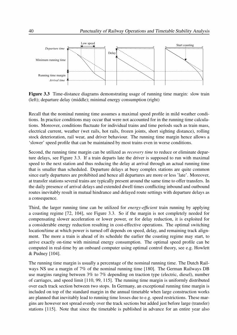
40 Punctuality of Railway Operations and Timetable Stability Analysis
Departure time
Minimum running time
Running time margin
Arrival time
Delay
Low speedStart coasting
Figure 3.3 Time-distance diagrams demonstrating usage of running time margin: slow train
(left); departure delay (middle); minimal energy consumption (right)
Recall that the nominal running time assumes a maximal speed profile in mild weather condi-
tions. In practice conditions may occur that were not accounted for in the running time calcula-
tions. Moreover, conditions fluctuate for individual trains and time periods such as train mass,
electrical current, weather (wet rails, hot rails, frozen joints, short sighting distance), rolling
stock deterioration, rail wear, and driver behaviour. The running time margin hence allows a
‘slower’ speed profile that can be maintained by most trains even in worse conditions.
Second, the running time margin can be utilized as recovery time to reduce or eliminate depar-
ture delays, see Figure 3.3. If a train departs late the driver is supposed to run with maximal
speed to the next station and thus reducing the delay at arrival through an actual running time
that is smaller than scheduled. Departure delays at busy complex stations are quite common
since early departures are prohibited and hence all departures are more or less ’late’. Moreover,
at transfer stations several trains are typically present around the same time to offer transfers. In
the daily presence of arrival delays and extended dwell times conflicting inbound and outbound
routes inevitably result in mutual hindrance and delayed route settings with departure delays as
a consequence.
Third, the larger running time can be utilized for energy-efficient train running by applying
a coasting regime [72, 104], see Figure 3.3. So if the margin is not completely needed for
compensating slower acceleration or lower power, or for delay reduction, it is exploited for
a considerable energy reduction resulting in cost-effective operations. The optimal switching
location/time at which power is turned off depends on speed, delay, and remaining track align-
ment. The more a train is ahead of its schedule the earlier the coasting regime may start, to
arrive exactly on-time with minimal energy consumption. The optimal speed profile can be
computed in real-time by an onboard computer using optimal control theory, see e.g. Howlett
& Pudney [104].
The running time margin is usually a percentage of the nominal running time. The Dutch Rail-
ways NS use a margin of 7% of the nominal running time [180]. The German Railways DB
use margins ranging between 3% to 7% depending on traction type (electric, diesel), number
of carriages, and speed limit [110, 99, 115]. The running time margin is uniformly distributed
over each track section between two stops. In Germany, an exceptional running time margin is
included on top of the standard margin in the annual timetable when large construction works
are planned that inevitably lead to running time losses due to e.g. speed restrictions. These mar-
gins are however not spread evenly over the track sections but added just before large (transfer)
stations [115]. Note that since the timetable is published in advance for an entire year also
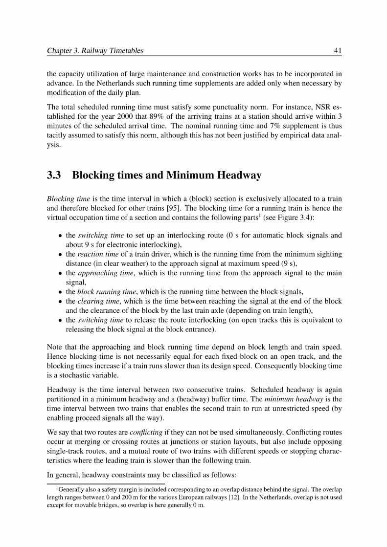
Chapter 3. Railway Timetables 41
the capacity utilization of large maintenance and construction works has to be incorporated in
advance. In the Netherlands such running time supplements are added only when necessary by
modification of the daily plan.
The total scheduled running time must satisfy some punctuality norm. For instance, NSR es-
tablished for the year 2000 that 89% of the arriving trains at a station should arrive within 3
minutes of the scheduled arrival time. The nominal running time and 7% supplement is thus
tacitly assumed to satisfy this norm, although this has not been justified by empirical data anal-
ysis.
3.3 Blocking times and Minimum Headway
Blocking time is the time interval in which a (block) section is exclusively allocated to a train
and therefore blocked for other trains [95]. The blocking time for a running train is hence the
virtual occupation time of a section and contains the following parts1 (see Figure 3.4):
• the switching time to set up an interlocking route (0 s for automatic block signals and
about 9 s for electronic interlocking),
• the reaction time of a train driver, which is the running time from the minimum sighting
distance (in clear weather) to the approach signal at maximum speed (9 s),
• the approaching time, which is the running time from the approach signal to the main
signal,
• the block running time, which is the running time between the block signals,
• the clearing time, which is the time between reaching the signal at the end of the block
and the clearance of the block by the last train axle (depending on train length),
• the switching time to release the route interlocking (on open tracks this is equivalent to
releasing the block signal at the block entrance).
Note that the approaching and block running time depend on block length and train speed.
Hence blocking time is not necessarily equal for each fixed block on an open track, and the
blocking times increase if a train runs slower than its design speed. Consequently blocking time
is a stochastic variable.
Headway is the time interval between two consecutive trains. Scheduled headway is again
partitioned in a minimum headway and a (headway) buffer time. The minimum headway is the
time interval between two trains that enables the second train to run at unrestricted speed (by
enabling proceed signals all the way).
We say that two routes are conflicting if they can not be used simultaneously. Conflicting routes
occur at merging or crossing routes at junctions or station layouts, but also include opposing
single-track routes, and a mutual route of two trains with different speeds or stopping charac-
teristics where the leading train is slower than the following train.
In general, headway constraints may be classified as follows:
1Generally also a safety margin is included corresponding to an overlap distance behind the signal. The overlap
length ranges between 0 and 200 m for the various European railways [12]. In the Netherlands, overlap is not used
except for movable bridges, so overlap is here generally 0 m.
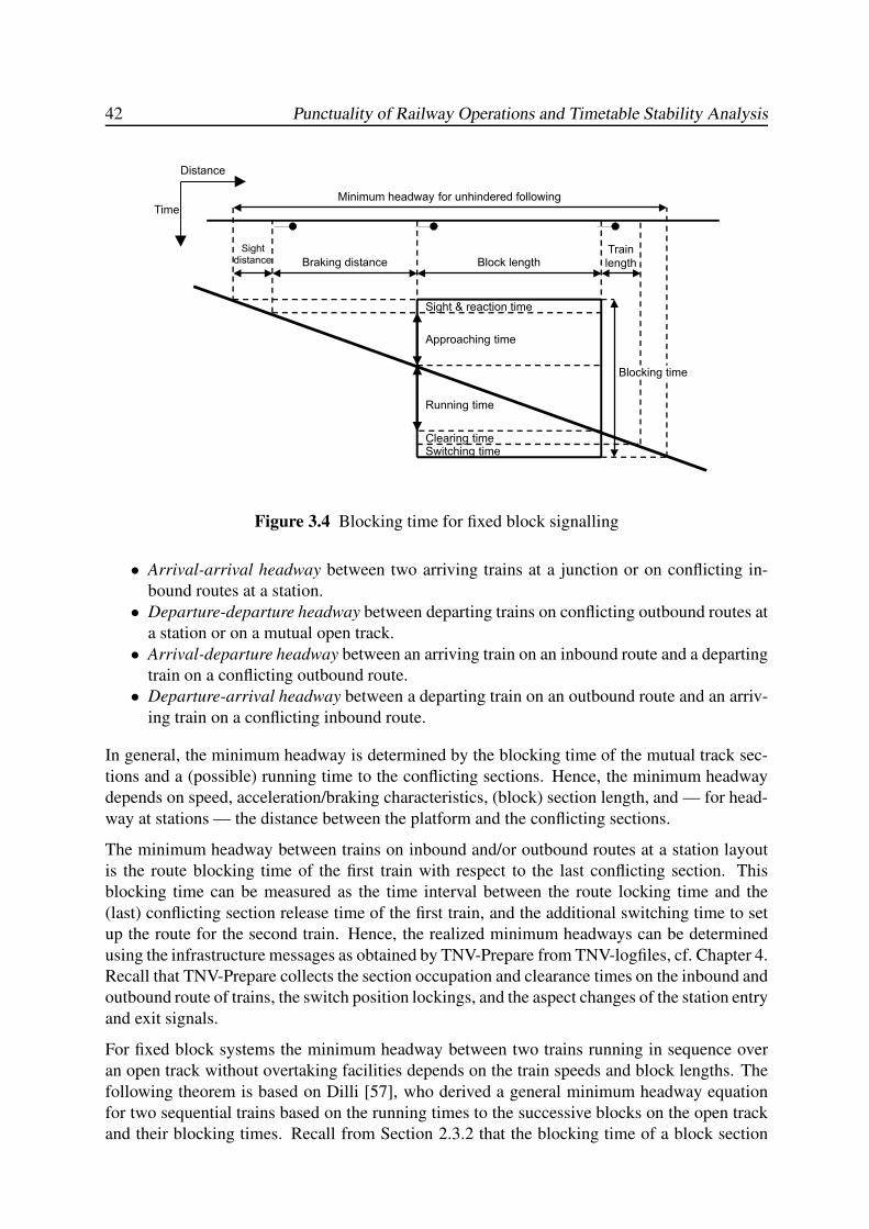
42 Punctuality of Railway Operations and Timetable Stability Analysis
Sight & reaction time
Approaching time
Running time
Clearing timeSwitching time
Sightdistance Braking distance Block length
Train
length
Minimum headway for unhindered following
Blocking time
Distance
Time
Figure 3.4 Blocking time for fixed block signalling
• Arrival-arrival headway between two arriving trains at a junction or on conflicting in-
bound routes at a station.
• Departure-departure headway between departing trains on conflicting outbound routes at
a station or on a mutual open track.
• Arrival-departure headway between an arriving train on an inbound route and a departing
train on a conflicting outbound route.
• Departure-arrival headway between a departing train on an outbound route and an arriv-
ing train on a conflicting inbound route.
In general, the minimum headway is determined by the blocking time of the mutual track sec-
tions and a (possible) running time to the conflicting sections. Hence, the minimum headway
depends on speed, acceleration/braking characteristics, (block) section length, and — for head-
way at stations — the distance between the platform and the conflicting sections.
The minimum headway between trains on inbound and/or outbound routes at a station layout
is the route blocking time of the first train with respect to the last conflicting section. This
blocking time can be measured as the time interval between the route locking time and the
(last) conflicting section release time of the first train, and the additional switching time to set
up the route for the second train. Hence, the realized minimum headways can be determined
using the infrastructure messages as obtained by TNV-Prepare from TNV-logfiles, cf. Chapter 4.
Recall that TNV-Prepare collects the section occupation and clearance times on the inbound and
outbound route of trains, the switch position lockings, and the aspect changes of the station entry
and exit signals.
For fixed block systems the minimum headway between two trains running in sequence over
an open track without overtaking facilities depends on the train speeds and block lengths. The
following theorem is based on Dilli [57], who derived a general minimum headway equation
for two sequential trains based on the running times to the successive blocks on the open track
and their blocking times. Recall from Section 2.3.2 that the blocking time of a block section
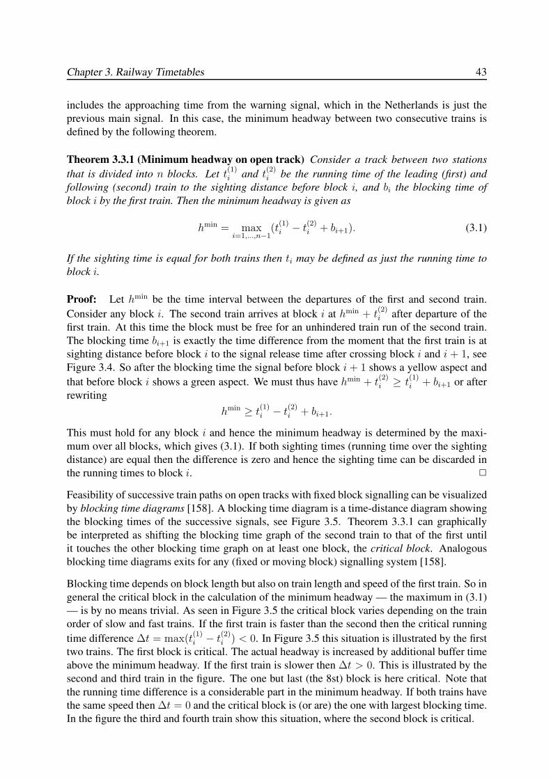
Chapter 3. Railway Timetables 43
includes the approaching time from the warning signal, which in the Netherlands is just the
previous main signal. In this case, the minimum headway between two consecutive trains is
defined by the following theorem.
Theorem 3.3.1 (Minimum headway on open track) Consider a track between two stations
that is divided into n blocks. Let t(1)i and t
(2)i be the running time of the leading (first) and
following (second) train to the sighting distance before block i, and bi the blocking time of
block i by the first train. Then the minimum headway is given as
hmin = maxi=1,...,n−1
(t(1)i − t(2)i + bi+1). (3.1)
If the sighting time is equal for both trains then ti may be defined as just the running time to
block i.
Proof: Let hmin be the time interval between the departures of the first and second train.
Consider any block i. The second train arrives at block i at hmin + t(2)i after departure of the
first train. At this time the block must be free for an unhindered train run of the second train.
The blocking time bi+1 is exactly the time difference from the moment that the first train is at
sighting distance before block i to the signal release time after crossing block i and i + 1, see
Figure 3.4. So after the blocking time the signal before block i + 1 shows a yellow aspect and
that before block i shows a green aspect. We must thus have hmin + t(2)i ≥ t
(1)i + bi+1 or after
rewriting
hmin ≥ t(1)i − t(2)i + bi+1.
This must hold for any block i and hence the minimum headway is determined by the maxi-
mum over all blocks, which gives (3.1). If both sighting times (running time over the sighting
distance) are equal then the difference is zero and hence the sighting time can be discarded in
the running times to block i. 2
Feasibility of successive train paths on open tracks with fixed block signalling can be visualized
by blocking time diagrams [158]. A blocking time diagram is a time-distance diagram showing
the blocking times of the successive signals, see Figure 3.5. Theorem 3.3.1 can graphically
be interpreted as shifting the blocking time graph of the second train to that of the first until
it touches the other blocking time graph on at least one block, the critical block. Analogous
blocking time diagrams exits for any (fixed or moving block) signalling system [158].
Blocking time depends on block length but also on train length and speed of the first train. So in
general the critical block in the calculation of the minimum headway — the maximum in (3.1)
— is by no means trivial. As seen in Figure 3.5 the critical block varies depending on the train
order of slow and fast trains. If the first train is faster than the second then the critical running
time difference ∆t = max(t(1)i − t(2)i ) < 0. In Figure 3.5 this situation is illustrated by the first
two trains. The first block is critical. The actual headway is increased by additional buffer time
above the minimum headway. If the first train is slower then ∆t > 0. This is illustrated by the
second and third train in the figure. The one but last (the 8st) block is here critical. Note that
the running time difference is a considerable part in the minimum headway. If both trains have
the same speed then ∆t = 0 and the critical block is (or are) the one with largest blocking time.
In the figure the third and fourth train show this situation, where the second block is critical.
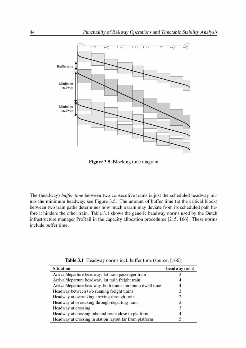
44 Punctuality of Railway Operations and Timetable Stability Analysis
Buffer time
Minimumheadway
Minimumheadway
Figure 3.5 Blocking time diagram
The (headway) buffer time between two consecutive trains is just the scheduled headway mi-
nus the minimum headway, see Figure 3.5. The amount of buffer time (at the critical block)
between two train paths determines how much a train may deviate from its scheduled path be-
fore it hinders the other train. Table 3.1 shows the generic headway norms used by the Dutch
infrastructure manager ProRail in the capacity allocation procedures [215, 166]. These norms
include buffer time.
Table 3.1 Headway norms incl. buffer time (source: [166])
Situation headway (min)
Arrival/departure headway, 1st train passenger train 3
Arrival/departure headway, 1st train freight train 4
Arrival/departure headway, both trains minimum dwell time 4
Headway between two running freight trains 3
Headway at overtaking arriving-through train 2
Headway at overtaking through-departing train 2
Headway at crossing 3
Headway at crossing inbound route close to platform 4
Headway at crossing in station layout far from platform 5
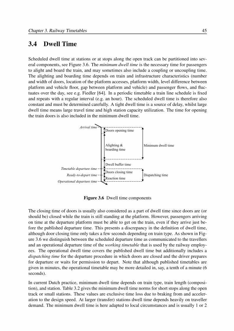
Chapter 3. Railway Timetables 45
3.4 Dwell Time
Scheduled dwell time at stations or at stops along the open track can be partitioned into sev-
eral components, see Figure 3.6. The minimum dwell time is the necessary time for passengers
to alight and board the train, and may sometimes also include a coupling or uncoupling time.
The alighting and boarding time depends on train and infrastructure characteristics (number
and width of doors, location of the platform accesses, platform width, level difference between
platform and vehicle floor, gap between platform and vehicle) and passenger flows, and fluc-
tuates over the day, see e.g. Fiedler [64]. In a periodic timetable a train line schedule is fixed
and repeats with a regular interval (e.g. an hour). The scheduled dwell time is therefore also
constant and must be determined carefully. A tight dwell time is a source of delay, whilst large
dwell time means large travel time and high station capacity utilization. The time for opening
the train doors is also included in the minimum dwell time.
Arrival time
Operational departure time
Doors opening time
Doors closing time
Alighting &
boarding time
Reaction time
Timetable departure time
Ready-to-depart time
Minimum dwell time
Dispatching time
Dwell buffer time
Figure 3.6 Dwell time components
The closing time of doors is usually also considered as a part of dwell time since doors are (or
should be) closed while the train is still standing at the platform. However, passengers arriving
on time at the departure platform must be able to get on the train, even if they arrive just be-
fore the published departure time. This presents a discrepancy in the definition of dwell time,
although door closing time only takes a few seconds depending on train type. As shown in Fig-
ure 3.6 we distinguish between the scheduled departure time as communicated to the travellers
and an operational departure time of the working timetable that is used by the railway employ-
ees. The operational dwell time covers the published dwell time but additionally includes a
dispatching time for the departure procedure in which doors are closed and the driver prepares
for departure or waits for permission to depart. Note that although published timetables are
given in minutes, the operational timetable may be more detailed in, say, a tenth of a minute (6
seconds).
In current Dutch practice, minimum dwell time depends on train type, train length (composi-
tion), and station. Table 3.2 gives the minimum dwell time norms for short stops along the open
track or small stations. These values are exclusive time loss due to braking from and acceler-
ation to the design speed. At larger (transfer) stations dwell time depends heavily on traveller
demand. The minimum dwell time is here adapted to local circumstances and is usually 1 or 2
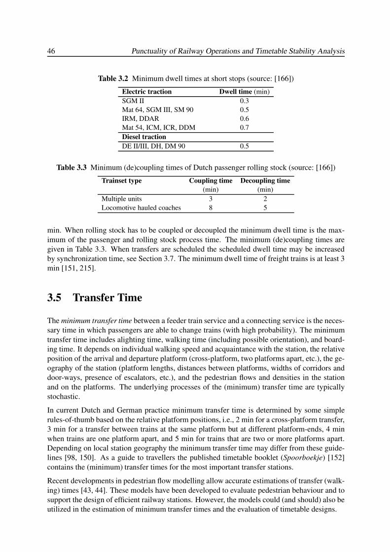
46 Punctuality of Railway Operations and Timetable Stability Analysis
Table 3.2 Minimum dwell times at short stops (source: [166])
Electric traction Dwell time (min)
SGM II 0.3
Mat 64, SGM III, SM 90 0.5
IRM, DDAR 0.6
Mat 54, ICM, ICR, DDM 0.7
Diesel traction
DE II/III, DH, DM 90 0.5
Table 3.3 Minimum (de)coupling times of Dutch passenger rolling stock (source: [166])
Trainset type Coupling time Decoupling time
(min) (min)
Multiple units 3 2
Locomotive hauled coaches 8 5
min. When rolling stock has to be coupled or decoupled the minimum dwell time is the max-
imum of the passenger and rolling stock process time. The minimum (de)coupling times are
given in Table 3.3. When transfers are scheduled the scheduled dwell time may be increased
by synchronization time, see Section 3.7. The minimum dwell time of freight trains is at least 3
min [151, 215].
3.5 Transfer Time
The minimum transfer time between a feeder train service and a connecting service is the neces-
sary time in which passengers are able to change trains (with high probability). The minimum
transfer time includes alighting time, walking time (including possible orientation), and board-
ing time. It depends on individual walking speed and acquaintance with the station, the relative
position of the arrival and departure platform (cross-platform, two platforms apart, etc.), the ge-
ography of the station (platform lengths, distances between platforms, widths of corridors and
door-ways, presence of escalators, etc.), and the pedestrian flows and densities in the station
and on the platforms. The underlying processes of the (minimum) transfer time are typically
stochastic.
In current Dutch and German practice minimum transfer time is determined by some simple
rules-of-thumb based on the relative platform positions, i.e., 2 min for a cross-platform transfer,
3 min for a transfer between trains at the same platform but at different platform-ends, 4 min
when trains are one platform apart, and 5 min for trains that are two or more platforms apart.
Depending on local station geography the minimum transfer time may differ from these guide-
lines [98, 150]. As a guide to travellers the published timetable booklet (Spoorboekje) [152]
contains the (minimum) transfer times for the most important transfer stations.
Recent developments in pedestrian flow modelling allow accurate estimations of transfer (walk-
ing) times [43, 44]. These models have been developed to evaluate pedestrian behaviour and to
support the design of efficient railway stations. However, the models could (and should) also be
utilized in the estimation of minimum transfer times and the evaluation of timetable designs.
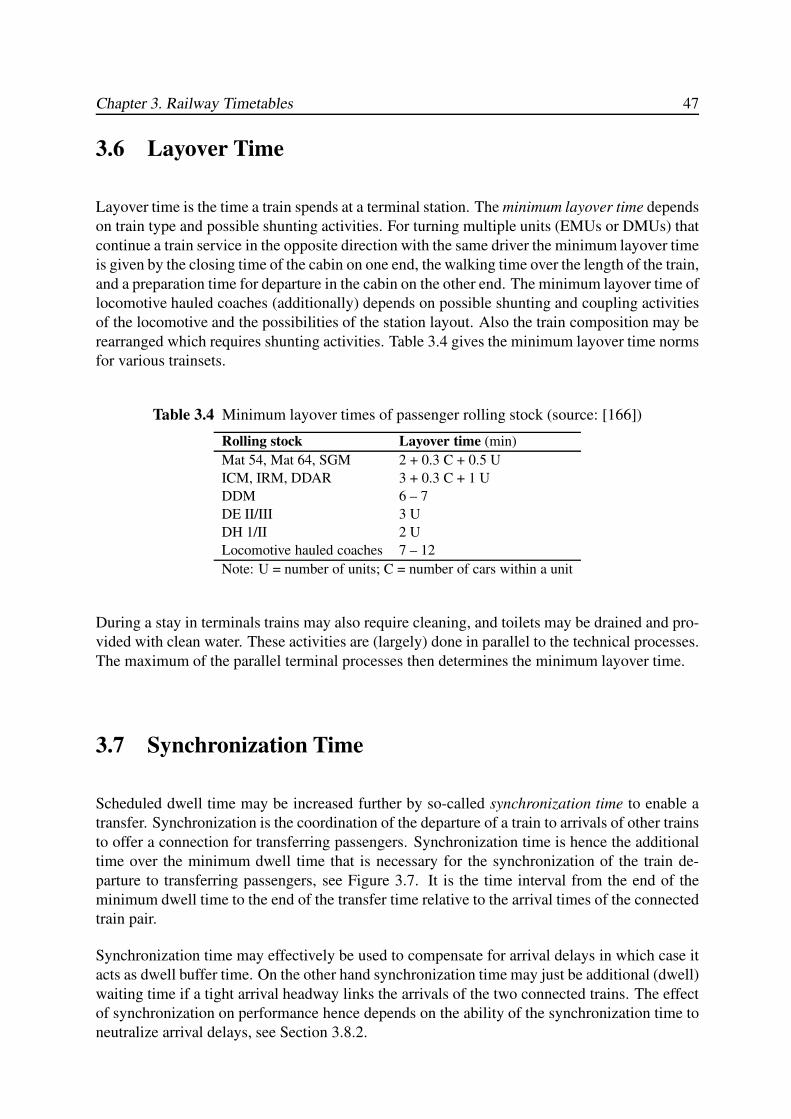
Chapter 3. Railway Timetables 47
3.6 Layover Time
Layover time is the time a train spends at a terminal station. The minimum layover time depends
on train type and possible shunting activities. For turning multiple units (EMUs or DMUs) that
continue a train service in the opposite direction with the same driver the minimum layover time
is given by the closing time of the cabin on one end, the walking time over the length of the train,
and a preparation time for departure in the cabin on the other end. The minimum layover time of
locomotive hauled coaches (additionally) depends on possible shunting and coupling activities
of the locomotive and the possibilities of the station layout. Also the train composition may be
rearranged which requires shunting activities. Table 3.4 gives the minimum layover time norms
for various trainsets.
Table 3.4 Minimum layover times of passenger rolling stock (source: [166])
Rolling stock Layover time (min)
Mat 54, Mat 64, SGM 2 + 0.3 C + 0.5 U
ICM, IRM, DDAR 3 + 0.3 C + 1 U
DDM 6 – 7
DE II/III 3 U
DH 1/II 2 U
Locomotive hauled coaches 7 – 12
Note: U = number of units; C = number of cars within a unit
During a stay in terminals trains may also require cleaning, and toilets may be drained and pro-
vided with clean water. These activities are (largely) done in parallel to the technical processes.
The maximum of the parallel terminal processes then determines the minimum layover time.
3.7 Synchronization Time
Scheduled dwell time may be increased further by so-called synchronization time to enable a
transfer. Synchronization is the coordination of the departure of a train to arrivals of other trains
to offer a connection for transferring passengers. Synchronization time is hence the additional
time over the minimum dwell time that is necessary for the synchronization of the train de-
parture to transferring passengers, see Figure 3.7. It is the time interval from the end of the
minimum dwell time to the end of the transfer time relative to the arrival times of the connected
train pair.
Synchronization time may effectively be used to compensate for arrival delays in which case it
acts as dwell buffer time. On the other hand synchronization time may just be additional (dwell)
waiting time if a tight arrival headway links the arrivals of the two connected trains. The effect
of synchronization on performance hence depends on the ability of the synchronization time to
neutralize arrival delays, see Section 3.8.2.
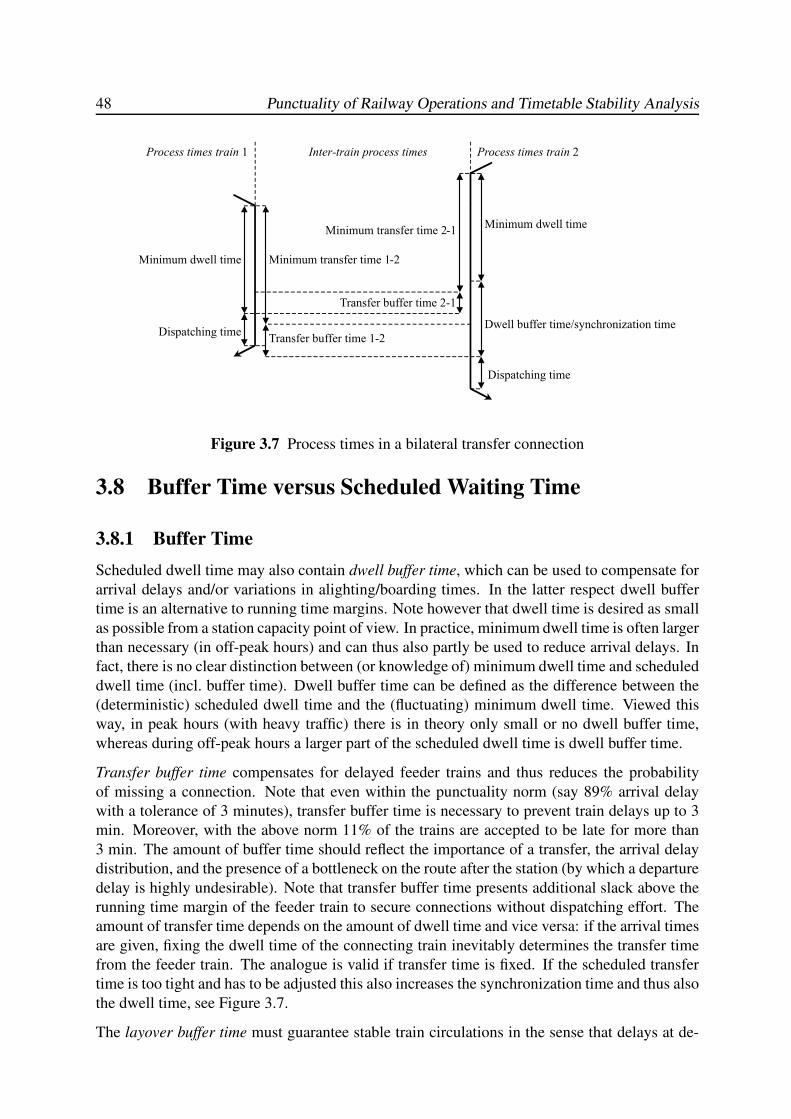
48 Punctuality of Railway Operations and Timetable Stability Analysis
Minimum dwell time Minimum transfer time 1-2
Transfer buffer time 1-2
Minimum dwell time
Dispatching time
Dwell buffer time/synchronization time
Minimum transfer time 2-1
Dispatching time
Transfer buffer time 2-1
Process times train 1 Process times train 2Inter-train process times
Figure 3.7 Process times in a bilateral transfer connection
3.8 Buffer Time versus Scheduled Waiting Time
3.8.1 Buffer Time
Scheduled dwell time may also contain dwell buffer time, which can be used to compensate for
arrival delays and/or variations in alighting/boarding times. In the latter respect dwell buffer
time is an alternative to running time margins. Note however that dwell time is desired as small
as possible from a station capacity point of view. In practice, minimum dwell time is often larger
than necessary (in off-peak hours) and can thus also partly be used to reduce arrival delays. In
fact, there is no clear distinction between (or knowledge of) minimum dwell time and scheduled
dwell time (incl. buffer time). Dwell buffer time can be defined as the difference between the
(deterministic) scheduled dwell time and the (fluctuating) minimum dwell time. Viewed this
way, in peak hours (with heavy traffic) there is in theory only small or no dwell buffer time,
whereas during off-peak hours a larger part of the scheduled dwell time is dwell buffer time.
Transfer buffer time compensates for delayed feeder trains and thus reduces the probability
of missing a connection. Note that even within the punctuality norm (say 89% arrival delay
with a tolerance of 3 minutes), transfer buffer time is necessary to prevent train delays up to 3
min. Moreover, with the above norm 11% of the trains are accepted to be late for more than
3 min. The amount of buffer time should reflect the importance of a transfer, the arrival delay
distribution, and the presence of a bottleneck on the route after the station (by which a departure
delay is highly undesirable). Note that transfer buffer time presents additional slack above the
running time margin of the feeder train to secure connections without dispatching effort. The
amount of transfer time depends on the amount of dwell time and vice versa: if the arrival times
are given, fixing the dwell time of the connecting train inevitably determines the transfer time
from the feeder train. The analogue is valid if transfer time is fixed. If the scheduled transfer
time is too tight and has to be adjusted this also increases the synchronization time and thus also
the dwell time, see Figure 3.7.
The layover buffer time must guarantee stable train circulations in the sense that delays at de-
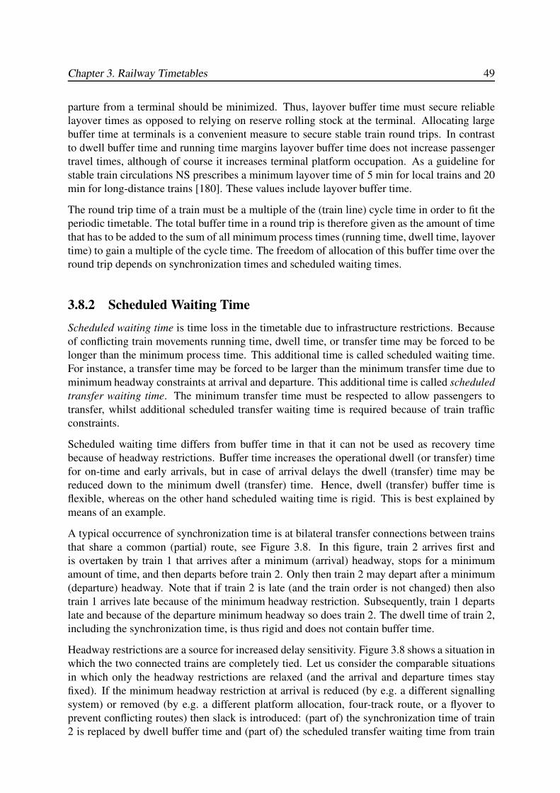
Chapter 3. Railway Timetables 49
parture from a terminal should be minimized. Thus, layover buffer time must secure reliable
layover times as opposed to relying on reserve rolling stock at the terminal. Allocating large
buffer time at terminals is a convenient measure to secure stable train round trips. In contrast
to dwell buffer time and running time margins layover buffer time does not increase passenger
travel times, although of course it increases terminal platform occupation. As a guideline for
stable train circulations NS prescribes a minimum layover time of 5 min for local trains and 20
min for long-distance trains [180]. These values include layover buffer time.
The round trip time of a train must be a multiple of the (train line) cycle time in order to fit the
periodic timetable. The total buffer time in a round trip is therefore given as the amount of time
that has to be added to the sum of all minimum process times (running time, dwell time, layover
time) to gain a multiple of the cycle time. The freedom of allocation of this buffer time over the
round trip depends on synchronization times and scheduled waiting times.
3.8.2 Scheduled Waiting Time
Scheduled waiting time is time loss in the timetable due to infrastructure restrictions. Because
of conflicting train movements running time, dwell time, or transfer time may be forced to be
longer than the minimum process time. This additional time is called scheduled waiting time.
For instance, a transfer time may be forced to be larger than the minimum transfer time due to
minimum headway constraints at arrival and departure. This additional time is called scheduled
transfer waiting time. The minimum transfer time must be respected to allow passengers to
transfer, whilst additional scheduled transfer waiting time is required because of train traffic
constraints.
Scheduled waiting time differs from buffer time in that it can not be used as recovery time
because of headway restrictions. Buffer time increases the operational dwell (or transfer) time
for on-time and early arrivals, but in case of arrival delays the dwell (transfer) time may be
reduced down to the minimum dwell (transfer) time. Hence, dwell (transfer) buffer time is
flexible, whereas on the other hand scheduled waiting time is rigid. This is best explained by
means of an example.
A typical occurrence of synchronization time is at bilateral transfer connections between trains
that share a common (partial) route, see Figure 3.8. In this figure, train 2 arrives first and
is overtaken by train 1 that arrives after a minimum (arrival) headway, stops for a minimum
amount of time, and then departs before train 2. Only then train 2 may depart after a minimum
(departure) headway. Note that if train 2 is late (and the train order is not changed) then also
train 1 arrives late because of the minimum headway restriction. Subsequently, train 1 departs
late and because of the departure minimum headway so does train 2. The dwell time of train 2,
including the synchronization time, is thus rigid and does not contain buffer time.
Headway restrictions are a source for increased delay sensitivity. Figure 3.8 shows a situation in
which the two connected trains are completely tied. Let us consider the comparable situations
in which only the headway restrictions are relaxed (and the arrival and departure times stay
fixed). If the minimum headway restriction at arrival is reduced (by e.g. a different signalling
system) or removed (by e.g. a different platform allocation, four-track route, or a flyover to
prevent conflicting routes) then slack is introduced: (part of) the synchronization time of train
2 is replaced by dwell buffer time and (part of) the scheduled transfer waiting time from train
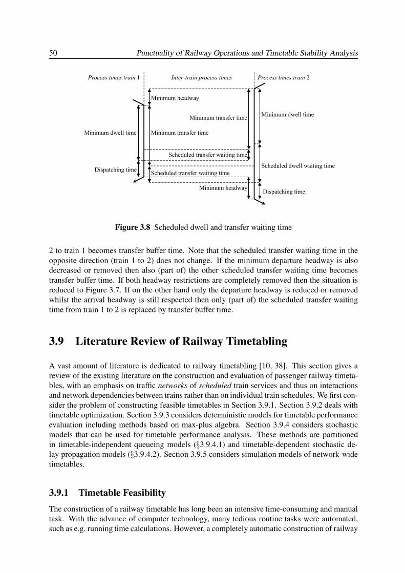
50 Punctuality of Railway Operations and Timetable Stability Analysis
Minimum dwell time Minimum transfer time
Scheduled transfer waiting time
Minimum dwell time
Dispatching time
Scheduled dwell waiting time
Minimum transfer time
Dispatching time
Scheduled transfer waiting time
Minimum headway
Minimum headway
Process times train 1 Process times train 2Inter-train process times
Figure 3.8 Scheduled dwell and transfer waiting time
2 to train 1 becomes transfer buffer time. Note that the scheduled transfer waiting time in the
opposite direction (train 1 to 2) does not change. If the minimum departure headway is also
decreased or removed then also (part of) the other scheduled transfer waiting time becomes
transfer buffer time. If both headway restrictions are completely removed then the situation is
reduced to Figure 3.7. If on the other hand only the departure headway is reduced or removed
whilst the arrival headway is still respected then only (part of) the scheduled transfer waiting
time from train 1 to 2 is replaced by transfer buffer time.
3.9 Literature Review of Railway Timetabling
A vast amount of literature is dedicated to railway timetabling [10, 38]. This section gives a
review of the existing literature on the construction and evaluation of passenger railway timeta-
bles, with an emphasis on traffic networks of scheduled train services and thus on interactions
and network dependencies between trains rather than on individual train schedules. We first con-
sider the problem of constructing feasible timetables in Section 3.9.1. Section 3.9.2 deals with
timetable optimization. Section 3.9.3 considers deterministic models for timetable performance
evaluation including methods based on max-plus algebra. Section 3.9.4 considers stochastic
models that can be used for timetable performance analysis. These methods are partitioned
in timetable-independent queueing models (§3.9.4.1) and timetable-dependent stochastic de-
lay propagation models (§3.9.4.2). Section 3.9.5 considers simulation models of network-wide
timetables.
3.9.1 Timetable Feasibility
The construction of a railway timetable has long been an intensive time-consuming and manual
task. With the advance of computer technology, many tedious routine tasks were automated,
such as e.g. running time calculations. However, a completely automatic construction of railway
Chapter 3. Railway Timetables 51
timetables is not as easy as it may seem. Scheduling trains involves sequencing of trains on open
tracks and synchronizing trains at stations, which are combinatorial difficult problems. In fact,
train scheduling belongs to the class of NP-complete problems [69], and so are related problems
as line optimization, rolling stock assignment and crew scheduling. Hence, railway planning is
still a computer-aided interactive affair that requires skills of experienced planners.
One of the main challenges in railway timetabling is the resolution of conflicting train paths.
The basic philosophy in railway planning is that a timetable is conflict-free, or feasible, in the
sense that train traffic is unhindered if each train adheres to the timetable. Feasibility of a
timetable is visualized by time-distance diagrams, where the horizontal axis corresponds to a
route of successive stations and the vertical axis corresponds to time (or vice versa). A train path
is then drawn by connecting the scheduled arrival, departure and through times at successive
stations. In this way the slope of a line between two points represents the average speed on
the associated track. The slope of a fast train is less steep than that of a slow train, and a
vertical line represents a stop. Two trains are conflicting if their paths intersect on a single-track
section. Many timetable characteristics are clearly represented by time-distance diagrams, such
as track occupancy, speed differences (different slopes), train intensity (number of trains), and
distribution of scheduled headway at timetable points. Time-distance diagrams are the main
tool in manual and computer-aided timetabling and still in use by planners and dispatchers.
Nowadays, running time calculations and drawing of time-distance diagrams are typically sup-
ported by computer software based on databases of rolling stock characteristics and the railway
infrastructure. An example is the Dutch VPT-Planning system, see Chapter 2. More advanced
computerized timetabling support systems are also able to automatically detect and interactively
resolve conflicts. An example is the system SCAN (SChedule ANalysis) [113] for scheduling
train traffic over single-track rail lines with partial double-track sections where trains can pass
(opposite trains) or overtake.
Time-distance diagrams indicate train paths based on timetable points (junctions and stations)
and scheduled event times (arrival, departure or through times), and as such do not accurately
show the infrastructure occupation times. Hence, buffer times can only be roughly estimated,
and conflicting routes in stations or critical blocks on open tracks may not be identified exactly.
The traditional time-distance diagrams are therefore no longer sufficient to represent the infras-
tructure utilization in dense network timetables, where various rail lines meet at complex station
layouts.
Brunger [23] developed the interactive scheduling system FAKTUS (FAhrplanKonstrukTion
und -UnterSuchung), in which the relation between timetable and infrastructure utilization is
captured by explicitly computing the blocking times of successive block sections at open tracks
and routes in stations. In brief, a blocking time is the time interval that a track section is exclu-
sively reserved for one train [95]. Assuming a fixed block system, the time-distance diagrams
are enhanced by showing the blocking times associated to each train path. The distance axis
now also specifies the trackside signals and route release points, and the blocking times of the
successive sections takes the form of a block step function, cf. Figure 3.5. A conflict is now
clearly visualized by overlapping blocks, which implies that a track section would be occupied
by two trains simultaneously. Hence, in a feasible timetable the time-distance blocks do never
overlap. The minimum headway between two departing or through trains is given by the min-
imum time interval between the two departures so that the block step function of the second
train just touches that of the first train. Any additional time gap at this critical block is buffer
52 Punctuality of Railway Operations and Timetable Stability Analysis
time. FAKTUS requires a detailed modelling of railway infrastructure, for which a separate
module SPURPLAN was developed by Deutsche Bahn (DB) [23]. In SPURPLAN the railway
infrastructure is modelled as a directed graph with node weights. The modules SPURPLAN
and FAKTUS are integrated in the system RUT (RechnerUnterstutztes Trassenmanagement),
which is now the standard timetable design tool of the German Railways (DB).
Schrijver & Steenbeek [184] use a combinatorial model for the computation of a feasible pe-
riodic timetable. Their feasibility problem is based on the Periodic Event Scheduling Problem
(PESP) introduced by Serafini & Ukovich [188]. PESP is the problem to find a feasible so-
lution to a system of periodic time window constraints. In this model the time differences
between two periodic departure times xi, xj ∈ [0, T ) are constrained by time windows, i.e.,
(xj − xi) mod T ∈ [lij , uij], where T is the period length (usually T = 60). The modulo
operation represents that the periodic (departure) events repeat each T minutes. The modular
constraints can be lifted to mixed-integer constraints by explicitly modelling the modulo oper-
ation as an integer multiple of the cycle time [183, 188]. Then the constraints take the form
xj − xi + zijT ∈ [lij , uij] with zij ∈ Z. Using these integral variables PESP is reformulated
as a mixed-integer programming (MIP) problem. Serafini & Ukovich [188] proved that PESP
is NP-complete, see also Odijk [154] in the context of the timetable feasibility problem. Char-
acteristic to the timetable feasibility problem is the large number of constraints with “wide”
time windows, i.e., [lij, uij] with 0 � uij − lij ≤ T corresponding to minimum headway con-
straints. The constraint propagation algorithm developed in Serafini & Ukovich [188] does not
perform well for these instances. Schrijver & Steenbeek [184] developed an alternative pow-
erful constraint propagation algorithm, called CADANS (Combinatorisch-Algebraısch Dien-
stregelingAlgoritme voor de Nederlandse Spoorwegen), which is capable of computing feasible
timetables (if they exist) for the national Dutch railway network in reasonable time (several
seconds to 15 minutes depending on the constraints). Also several other algorithms have been
developed. Odijk [153] developed a cutting plane algorithm, which was successfully applied to
small instances (large stations). Wezel et al. [225] developed a genetic algorithm for quickly
finding suboptimal solutions.
The performance of CADANS led to the development of the Dutch timetable design system
DONS (Designer Of Network Schedules) by NSR and Railned (ProRail) to support railway
planners in the construction of feasible timetables [101, 102]. The time window model is con-
sistent with the practice of railway planners, who use guidelines for e.g. a minimum dwell time
or transfer time and maximum waiting times that should not be exceeded. In the DONS interface
planners give minimum and maximum values for all process times between train runs, such as
dwell time, transfer time, coupling time, and layover time, as well as minimum (time) headway
between two train arrivals, departures, or through times at conflict points. DONS transforms the
specifications into periodic time window constraints and sends them to the solver CADANS. If
CADANS finds a feasible timetable satisfying all the constraints the timetable is returned as a
list of successive arrival and departure times for all train lines. If on the other hand no feasible
timetable exists then CADANS gives a minimal set of conflicting constraints, which should be
relaxed by the planner before a feasible solution can be found. These conflicting constraints
also indicate bottlenecks in the timetable or infrastructure.
In CADANS complex station layouts are modelled as black boxes. Hence, local feasibility
within station layouts is not taken into account. Therefore, a second module was developed to
check whether the computed network timetable is feasible with respect to local infrastructure.
Chapter 3. Railway Timetables 53
Zwaneveld [230] defined the problem of routing trains through a railway station as finding a
feasible (or optimal) assignment of trains to station routes and platforms given the station layout
and the arrival and departure times of trains. Typical constraints include capacity, interlocking
system, and cross-platform connections. Zwaneveld et al. [231] show that this station routing
problem can be modelled as a weighted node packing problem and present a branch-and-cut
algorithm, combined with efficient preprocessing and valid inequalities techniques, that is able
to solve the problem for all Dutch station instances. This algorithm is implemented in the
system STATIONS as part of DONS [230].
3.9.2 Timetable Optimization
An optimal network timetable is a feasible timetable that optimizes some objective function.
Hence, the timetable optimization problem can be seen as an extension to the timetable feasi-
bility problem. Obviously, an optimal solution to the optimization problem is also a solution to
the associated feasibility problem, but the reverse is generally not true. If the feasibility prob-
lem is NP-complete then so is the associated optimization problem. An added difficulty in the
formulation of the optimization problem is the choice of an appropriate objective function. A
typical objective is the minimization of passenger waiting time resulting in short transfer times
at transfer stations.
Weigand [220, 222] considered the problem of minimizing passenger waiting time in periodic
railway timetables. He used a graph-theoretic modelling approach by defining a directed (trans-
port chain) graph from the train line data as follows: a node is defined for each train service
between two (transfer) stations, and an arc between two nodes represents a station stop or pas-
senger transfer. A weight is assigned to each node corresponding to the associated (fixed)
running time, and arc weights correspond to minimum dwell/transfer times, which are inter-
preted as minimum waiting times. The variables are the additional “network caused” waiting
times (buffer times) on the arcs. Weigand observed that in acyclic graphs network caused wait-
ing time does not occur. However, if the graph contains cycles then at least one arc in each
cycle must contain buffer time. The total buffer time on any cycle is determined by a cycle
constraint: in a periodic timetable the oriented sum of running times (node weights), minimum
waiting times (arc weights), and buffer times (variables) on the cycle must be a multiple of the
timetable cycle time. Note that without loss of generality the node weights can be included in
the arc weights, which transforms the transport chain graph to a traditional weighted digraph
with arc weights only [81].
From graph theory it is well-known that a finite graph has a fundamental cycle basis of ν =m − n + c linear independent cycles, where m is the number of arcs, n the number of nodes,
and c the number of strongly-connected components [16]. Any cycle can be generated by a com-
bination of cycles from this basis, and if each fundamental cycle satisfies the cycle constraint
then any cycle does. Hence, the (minimum) number of constraints on the buffer times in a pe-
riodic timetable is equal to this cyclomatic number ν. The resulting problem is a mixed integer
program (MIP) with m continuous variables (the buffer times) and ν integers corresponding to
the ν cycle constraints. The cost function is a weighted sum of buffer times, where the weights
correspond to passenger volumes. Weigand [220, 222] described a heuristic in which all buffer
time in each fundamental cycle is assigned to the cycle arc with minimal weight. This problem
is equivalent to finding a maximum spanning tree, i.e., a spanning tree that maximizes the sum
54 Punctuality of Railway Operations and Timetable Stability Analysis
of its arc weights (passenger flows). The arcs of this maximum spanning tree are then assigned
zero buffer time and the nontree arcs get all buffer time. Since this solution is suboptimal, the
algorithm proceeds by successively trying to improve the solution using a simplex method and
exchanging basis variables for nonbasis variables until no more (one-step) improvement can be
obtained. The heuristic performs well for small networks, but the computation time increases
exponentially with the size of the network [220] and also the error relative to the optimal solu-
tion increases with network size [193].
Stemme [193] extended Weigand’s MIP model with maximum waiting times on each arc of the
(transport chain) graph. The cost function is again the weighted sum of buffer times over all
arcs. Stemme also used the arc lower and upper bounds to compute a lower and upper bound
on the integer variable associated to each fundamental cycle. Stemme [193] describes a branch-
and-bound algorithm for solving this MIP problem to optimality. The method is applied to the
Berlin underground network giving the optimal solution in 59 CPU minutes.
Nachtigall [141, 142] formalizes the MIP with cycle constraints and proves that the problem
is NP-complete. A branch-and-bound procedure becomes more effective when inequalities are
added to the constraint system that tighten the feasible (integer) region. Therefore, Nachti-
gall [142] derived two classes of facet-defining valid inequalities and developed two polyno-
mial separation algorithms for generating strong cutting planes. These inequalities can be com-
puted in a pre-processing step and added to the constraint system to tighten the feasible region.
Nachtigall & Voget [143] also developed a genetic algorithm to find suboptimal solutions to the
MIP-problem.
An alternative MIP-formulation is the time window constraint system of PESP and CADANS.
Krista [122, 123] used this constraint formulation including minimum headway constraints as
in CADANS. The linear cost function is the weighted sum of synchronization times (dwell
and transfer waiting times) in the network timetable. The weights are defined as the number
of through (transfer) travellers at the stop (transfer), which are obtained from the traveller as-
signment model PROLOP [20] (cf. Section 2.2.3). Since the passenger flows depend on the
waiting times in the timetable, Krista proposes an iterative method of passenger assignment
and timetable optimization. However, convergence of this iterative approach is not guaran-
teed. Krista uses the commercial optimization software CPLEX to solve the MIP directly.
Lindner [128] combined the PESP formulation of timetable constraints with line optimization
constraints with the objective of minimizing the operational costs. For practical instances from
the railways in the Netherlands (NS) and Germany (DB) the resulting MIP could not be solved
directly by a commercial solver (CPLEX) within a day. Lindner therefore described several
preprocessing techniques, valid inequalities and relaxations, and developed a branch-and-bound
procedure to tackle the problem. In particular, reduction of the number of transfer constraints
is necessary to solve practical instances within a few hours. For instance, the NS-intercity net-
work and the DB-intercity network with 40 transfer constraints could only be solved in about
10 hours.
It is remarkable that the authors using the time window formulation include infrastructure
constraints, whilst in the cycle constraint formulation infraconstraints are neglected. Nachti-
gall [142] proposed to indirectly include PESP-constraints in the problem formulation using
a penalty term in the objective function. However, the MIP problems with cycle constraints
and time window constraints are mathematically equivalent and correspond to different matrix
representations of the same underlying digraph, as shown in Goverde [81]. In the time window
Chapter 3. Railway Timetables 55
constraint system the (node) event times are the decision variables and the problem is formu-
lated using the arc-node incidence matrix M ∈ {0,±1}m×n of the digraph as
l ≤Mx+ zT ≤ u, z ∈ Zm,
where x is an n-dimensional vector of (departure) event times associated to the n nodes, l, u are
m-dimensional vectors corresponding to the time-window bounds, and z is an m-dimensional
integral vector. On the other hand, the cycle constraint system is defined in the arc tension
vector y ∈ [l, u] as decision variable and using the cycle-arc incidence matrix (or cycle matrix)
Γ ∈ {0,±1}m−n+c as
Γy + zT = 0, y ∈ [l, u], z ∈ Zm−n+c.
In graph theory the event times x correspond to node potentials and the arc variables y to
potential differences or tensions [174]. For fixed integers the problem relaxes to the optimal
or feasible differential problem, which is a network programming problem solvable in O(n3)time [174]. Odijk [153] used this relaxation of PESP in a cutting plane algorithm. The equiva-
lence between both formulations imply that solution algorithms and preprocessing approaches
developed for one problem can also be applied to the other. The cycle constraint formulation
contains less integer variables (m versusm−n+c) and is therefore favourable in direct solution
approaches such as branch and bound. Peeters [159] developed an additional class of cutting
planes for the MIP problem and did computational experiments to compare the window formu-
lation and the cycle constraint formulation, which confirmed the latter as the best formulation
from a solution algorithm point of view.
Most authors of the timetable optimization problem used a linear cost function to minimize
the dwell and transfer times in the timetable [122, 136, 141, 193, 222]. This objective gives
optimal timetables with minimal transfer times for high priority connections with large transfer
flows in case of punctual railway operations. However, in case of delays this timetable is far
from optimal: since high priority connections obtain tight transfer times arrival delays result in
either missed connections for large amounts of passengers or in many secondary delays when
trains wait for important connections. Goverde [81] therefore proposed an alternative objective
of a weighted sum of separate convex cost functions of the buffer times. For instance, a cost
measuring the risk of buffer time failure, depending on arrival delay parameters, can be used for
connections where reliability is important to guarantee e.g. stable train circulations. The cost of
a transfer connection is the mean transfer time, which depends on several parameters including
mean arrival delay, frequency, and waiting time regulations. For punctual operation the convex
functions reduce to the usual linear objective of the weighted sum of all buffer times. With
respect to arrival delays, the risk and significance of missing connections are also measured.
The distribution of buffer times in the resulting network timetable reflects the priorities between
the individual buffer time performance costs. The convexity of the cost functions guarantees
that a local optimal solution is also the global optimum. In general, optimization problems
with nonlinear objective functions are harder to solve than linear optimization problems. On
the other hand, the proposed cost functions penalize large buffer times at stops, connections,
and turns, making upper bounds on these buffer times superfluous, which relaxes the feasibility
problem [81].
Vromans [213] developed an interesting two-stage stochastic optimization model that combines
timetable optimization and simulation. The timetable constraints are based on the MIP formu-
lation of the periodic time-window constraints (see §3.9.1) with fixed integer vector (fixed train
56 Punctuality of Railway Operations and Timetable Stability Analysis
orders), whereas (max,+)-recursive equations (written as linear inequalities) are used to simu-
late the timetable with respect to sampled process times. The method starts with a feasible peri-
odic timetable and aims at optimally redistributing margins and buffer times over the timetable
without changing the essential timetable structure (fixed train orders). In a first step random
disturbances are assigned to the process times representing the process time realizations in con-
secutive timetable simulation periods. The process time realizations are used in the formulation
of a (large-scale) linear programming problem including both the timetable constraints and the
timetable simulation model; the event times are the decision variables and the objective is to
minimize the (weighted) average delay. The solution to the LP problem is an improved peri-
odic timetable that is optimized with respect to the sampled process times. Convergence with
respect to the number of realizations has not been addressed (except for a simple special case).
The model has been applied to a corridor of the Dutch Railways (in one direction).
A related model is the schedule synchronization problem in which the line schedules (running
and dwell times) are fixed. The problem is to determine the optimal departure times of all lines
at their starting station such that the costs of the resulting transfer times at stations where the
lines meet are minimized. This optimization problem can be formulated as a binary integer pro-
gram (BIP) [118] or an integer program (IP) [19]. However, infrastructure constraints can not be
handled trivially in these formulations. Domschke [58] proved that the problem is NP-complete.
Note that this problem can also be modelled using the time window (or PESP) constraints as a
special case with fixed dwell times, which then also allows infrastructure constraints. In fact,
Migom & Valaert [136] already developed a model resembling the time window constraints for
the Belgian intercity network but were unable to solve it. They then fixed all dwell times and
solved the remaining problem of finding the optimal departure times at the starting stations. The
schedule synchronization formulation is mainly applied to road public transport networks (bus
systems).
3.9.3 Deterministic Timetable Performance Evaluation Models
Braker [21] modelled the periodic timetable of the Dutch intercity network as a recursive system
in max-plus algebra and analysed its periodic behaviour by solving an eigenvalue problem in
max-plus algebra. The max-plus model is essentially given by precedence relations between
departure events that model running times, dwell times and transfer times. The variables are
the departure times which depend on preceding departures times and the scheduled departure
times. The model can be described as a linear system in max-plus algebra of the form x(k) =Ax(k − 1)⊕ d(k), where x(k) and d(k) are vectors of the kth actual and scheduled departure
times, respectively, and A is a matrix of transportation times corresponding to the precedence
relations. The maximum eigenvalue can be interpreted as the minimal cycle time where all
trains depart as early as possible and the associated eigenvector gives the earliest departure
times. A necessary condition for a stable timetable is therefore that the timetable period length
T exceeds the maximum eigenvalue λ, where the difference T − λ is the available slack on a
critical circuit. Van Egmond [207] used the max-plus model to compute the delay propagation
of an initial delay. Subiono [196] extended Braker’s approach to railway timetables of mixed
train types (AR, IR, and IC), see also Olsder et al. [156].
The max-plus models of Braker and Subiono captured the essential interconnection structure of
a periodic railway timetable and enabled the analysis of network performance and delay propa-
gation over train synchronizations due to passenger transfers and logistic connections of rolling
Chapter 3. Railway Timetables 57
stock and train crews. However, these max-plus models neglect headway restrictions imposed
by the railway infrastructure and safety and signalling systems. Hence, the model results only
give a lower bound to the system performance assuming that all timetable slack time acts as
buffer time, i.e., the differences between scheduled and minimum station dwell/transfer times
can be fully utilized for compensating delays. Note that additional constraints corresponding to
infrastructure limitations may limit buffer times and show scheduled waiting times instead, cf.
§3.8.
Van Egmond [208, 209] showed that blocking time diagrams can be described by a max-plus
heap model and that the determination of capacity consumption of a given timetable (com-
pressed sequence of blocking time graphs) equals an eigenvalue problem of the associated ma-
trix. Van Egmond [208, 209] described a heaps of pieces [71] model as an automaton [71]
over the max-plus algebra. The heap model consists of a finite set of fixed-blocks (resources,
machines) and a set of train runs (tasks, jobs) specified by their time slots over the blocks cor-
responding to a blocking time diagram. More specifically, each train run between two stations
is represented by the lower and upper contour of the associated blocking time graph, i.e., the
lower (upper) contour of a train run is a vector with the i-th entry given by the start (end) of the
blocking time of block i in the railway network. The contours define a block pattern called a
piece. A schedule of an ordered sequence of pieces then corresponds to a heap obtained from
piling up the pieces starting with a zero ground (all blocks are initially available), similar to a
tetris game. The contour of a heap of pieces can be described by matrix multiplication over
the max-plus algebra. A square matrix M(a) is assigned to each piece a as follows: if the
piece (train run) uses both block i and j thenM(a)ij is the time interval from the start of the
blocking time of block i (element i of the lower contour vector) to the end of block j (element
j of the upper contour vector); if i = j is not a block on the train route thenM(a)ii = 0; and
M(a)ij = −∞ otherwise (i or j is not on the route). Reversely, a given matrix M(a) also
uniquely defines the lower and upper contour vector of a piece a (up to a vertical shift). The
matrix associated to a heap of pieces is given by max-plus multiplication of the matrices of
the pieces in given sequence order. This matrix thus corresponds to the tightest schedule with
zero buffer time between the train runs at the critical blocks. The upper contour is given by
multiplying the heap matrix with the initial vector, and the height of the heap is the maximum
of these vector elements, which corresponds to the minimum cycle time of the schedule of the
trains in the specified order. The evolution of the upper contour of a heap of pieces by piling
up pieces to the heap is given by multiplying the upper contour of the heap by the matrix of
the new piece. For periodic schedules the minimum cycle time can be computed by solving the
eigenvalue problem of matrixM(w) where w is the heap (schedule) obtained by concatenating
the pieces in the schedule (of one period). The eigenvalue gives the minimum cycle time in the
periodic regime. Van Egmond [208] also shows how buffer times can be incorporated in the
heap model and how delays propagate over the trains in the schedule.
The max-plus heap model [208, 209] explicitly models the scheduled infrastructure utilization.
However, this requires a detailed (microscopic) modelling of the signal locations at open tracks
and routes over station layouts, and the determination of the associated running times. On
the other hand, the recursive max-plus model [21] gives a macroscopic dynamic description of
departure events at stations with only precedence relations between events that model running
times, dwell times and transfer times, which are easily obtained from the railway timetable. An
interesting question is whether it is possible to combine the two model approaches to obtain a
model that describes a scheduled railway system over large networks including infrastructure
58 Punctuality of Railway Operations and Timetable Stability Analysis
utilization but without the extensive input data and model dimension requirements of the heap
model. This challenge is addressed in this thesis in the chapters 6–8.
A different approach to capacity assessment of periodic timetables is presented in the Swiss
deterministic analytical system CAPRES (CAPacite de RESeaux ferroviaires) [42, 129]. Ca-
pacity utilization of a basic periodic timetable is here analysed by saturating the timetable with
additional trains, while respecting all timetable constraints. Running times and dwell times are
specified by a minimum and maximum value, which allows some flexibility in the saturation
process. The saturated timetable depends on a list of extra trains and a saturation strategy that
determines the order in which trains are added to the timetable during the saturation process.
This approach is useful in assessing unused capacity (possible number of extra trains) and de-
tecting bottlenecks (critical constraints that prevent addition of a train). CAPRES is used at
SBB, RFF, and SNCF.
3.9.4 Stochastic Models of Railway Operations
A timetable that is feasible for punctual train services may still be sensitive to variations in
running times and dwell times, and thus perform inadequately in daily practice where running
and dwell times vary from trip to trip. Evaluating the performance of a railway timetable in
the presence of process time variations is therefore an essential aspect in timetable design. Of
particular interest is the propagation of delays over the scheduled train services and the ability
of a timetable to reduce delays by built-in running time margins and buffer times.
3.9.4.1 Queueing Models
Queueing models can be used to estimate waiting times in railway operations given a random
interarrival process. These models are capable of giving a (rough) prediction of bottlenecks
and waiting times which can be translated to the amount of buffer time needed in a timetable
with corresponding traffic intensity. Queueing models are mainly applied in strategic capacity
assessment studies when details of the future timetable are still uncertain.
Schwanhaußer and co-workers developed several queueing models to assess the capacity of
railway infrastructure in terms of train mix, frequency of different train types, and mean interar-
rival times [186]. Schwanhaußer [185] derived analytical solutions to the required mean buffer
time on open-tracks such that an acceptable level of total delay is not exceeded. He modelled
all possible delay propagations between train pairs assuming heterogeneous train traffic with
random train orders, exponential interarrival times, and priority rules between different train
types. The approach was implemented in the mid 1980s in the MS-DOS application STRELE
(Streckenleistungsfahigkeit) [186].
Wakob [217] extended Schwanhaußer’s method to the assessment of scheduled waiting time at
railway stations and adjacent open-tracks. The approach is based on a decomposition of the
station layout into separate route sections, called TFKs (TeilFahrstraßenKnoten), that can only
be claimed by one train at a time. The TFKs are modelled as single-server queues where the
minimum headway acts as service time. The model assumes random train orders, Gamma-
distributed interarrival times, and priorities between different train types. Moreover, Wakob
assumes that the TFKs are independent and therefore neglects the interaction between train
Chapter 3. Railway Timetables 59
movements over a sequence of TFKs, see also De Kort et al. [51]. Wakob’s approach has been
implemented in the MS-DOS software ALFA (Analytische Leistungsfahigkeitsermittlung der
FAhrstraßenknoten) [186], and more recently in the tool ANKE (Analytische NetzKapazitatsEr-
mittlung) [201], which is compatible to the infrastructure database SPURPLAN.
Wendler [224] developed several extensions to the queueing models of Schwanhaußer and
Wakob based on conflicts between train triples and new approximation algorithms, which im-
prove the modelling of TFKs and their interactions. However, the method again assumes ran-
dom train orders and is thus still not valid for estimating delay propagation in periodic timeta-
bles, cf. Wendler [224, §5.3].
Meng [133] extended Schwanhaußer’s delay propagation model to train connections in stations
and derived analytical solutions for the required mean (dwell and transfer) buffer time at a
railway station for Gamma-distributed interarrival times. Train arrival orders are again assumed
random and the probability that two trains are connected is proportional to the relative train type
combinations over all possibilities. Hence, Meng calculates the mean required buffer time over
all trains in a station with respect to all possible future timetables and combinations of train
connections. The method is therefore not valid for periodic timetables with fixed train orders.
Huisman et al. [105] developed a product form queueing network for (large-scale) railway net-
works. Instead of a detailed modelling of the infrastructure, the model mimics the service
and waiting times from the traffic interconnection structure with three separate components:
stations, junctions, and connecting open tracks. Only double-track (or multi-track) lines are
considered, where each direction has its own tracks. Each track is modelled by two First-
Come-First-Serve (FCFS) single-server queues connected by a tandem queue, which represent
the train runs corresponding to a given train mix on the open track. The service time of the first
and last FCFS queue corresponds to the minimum headway at departure and arrival, respec-
tively, and the total service time of the tandem queue represents the free running time on the
open track. The number of queues in the tandem and their service times are chosen such that the
mean and variance of the total service time equals that of the free running time corresponding to
the train mix. Stations are modelled by FCFS multi-server queues, where the number of servers
corresponds to the number of platform tracks and the service time corresponds to the occupa-
tion time of a platform track. Hence, it is assumed that each train may use each platform track.
Finally, junctions are modelled by either two FCFS single-server queues in case of a fly-over or
by an order-independent single-server queue for level-crossings. All service times are assumed
exponential and the arrivals into the network occur according to a Poisson process. Huisman
et al. [105] proved that the steady-state distribution of this network is given by the product of
the steady-state distributions of all isolated queues. For practical computations explicit expres-
sions are derived for the mean waiting time of each component. This queueing approach again
assumes random train orders independent of a periodic timetable.
3.9.4.2 Stochastic Delay Propagation Models
Kraft [121] developed a model for the knock-on delays on a main railway line with several
merging and diverging lines operating under a periodic timetable. He considers various cases
of headway distributions, including fixed headway, mixed headway, and stochastic headway
(shifted exponential and Erlang). The first case corresponds to a railway line with one-way
traffic running at a fixed regular interval. The second case occurs naturally when trains on
60 Punctuality of Railway Operations and Timetable Stability Analysis
two or more railway lines merge. For instance, when two lines with equal frequency merge
then traffic with twice this frequency results after the merging section, where the headway after
merging equals the interarrival times at the merging section. If these interarrival times are equal,
i.e., the arrival times of both lines have an offset of half their headway, then a regular headway
results after merging. If a train is delayed before the merging section then the order of merging
may be changed to minimize total delay propagation. The delay propagation depends on the
location of a primary delay: at a merging line, on the main line, or at a diverging line. For
railway networks with up to three merging routes and exponential primary delays Kraft derives
analytical expressions for the mean total delay associated to the optimal merging orders. The
model does not include opposing trains on single-track routes nor cyclic networks.
Weigand [220, 221] considers propagation of delays in scheduled (cyclic) train service networks
with a periodic timetable. He assumes exponential delays characterized by two parameters: the
mean delay and the fraction of delayed trains, the delay probability. Weigand considers one train
run at a time between the departure from one station to that of the next, and iteratively derives
analytical expressions of the change in the two delay (mean and probability) parameters. The
delay evolution is subsequently derived as the sum of an initial departure delay, a primary delay
at the open track corrected by a deterministic running time margin, and secondary connection
delays at the next station due to waiting for delayed feeder trains corrected by buffer times. All
these delays are assumed independent. The connection delay depends on the number of feeder
trains and their arrival delays. If the resulting departure delay is positive then it is used as the
initial delay in the calculation of the delay evolution of the next train run. This way the delay
propagation of all trains in the network is iteratively calculated. Weigand [220] showed that if
on the average the buffer times (including running time margins) exceed the individual primary
delays then the system reaches a stable state with a constant mean level-of-delay. For cyclic
networks this means that a stable state exists if on each circuit in the network the average buffer
time exceeds the average primary delay.
Muhlhans [137] generalized the analytical stochastic model of Weigand by using general proba-
bility distributions for the primary delays and recursively deriving cumulative distribution func-
tions (CDFs) for the evolution of delays. The delay evolution is the convolution of the initial
departure delay and independent primary delays at several locations of a train run: running
time extension at the open track, hindrance at the entrance of a station, dwell time extension,
and hindrance at departure. Running time margin is used uniformly over the track and dwell
buffer time is incorporated as a shift parameter that reduces the effect of hindrance at arrival and
dwell time extension. If the train has to wait for delayed feeder trains then the convolution up
to the departure hindrance is multiplied with the product of the individual arrival delay CDFs
(shifted by the transfer buffer times) of the feeder trains. This corresponds to the assumption
that all arrival delays are independent, in which case the CDF of the maximum delay is the
product of the individual CDFs. Finally, the departure delay at the next segment is obtained
by convolution with the CDF of the departure hindrance. The CDFs for each train run can be
computed numerically, and in the special case of exponential primary delays Muhlhans [137]
derived explicit solutions. The approaches of Weigand and Muhlhans only consider secondary
delays due to waiting for connections at transfer stations. Delays due to hinder at conflict points
or to following trains are implicitly modelled as part of the primary delay on the open track.
Carey [28] considers multiple train services on (unidirectional) single-track lines with stochastic
running and dwell times defined by general probability density functions (PDFs) and determin-
Chapter 3. Railway Timetables 61
istic minimum headway times at station arrivals and departures. Carey derives recursions for
the successive PDFs of arrival and departure times for each train and station. The recursions
include primary delays (incorporated in the running and dwell time distributions) and secondary
delays due to headway conflicts of following trains, which Carey calls ‘knock-on delays’. Fur-
thermore, Carey [28, 29] presents performance measures of travel time or schedule deviations
based on the arrival and departure time PDFs which can be used to compare alternative timeta-
bles, such as expected arrival lateness (of any train at any served station), the probability of
arriving x minutes late, and similar measures for departures. He also proves convexity prop-
erties of these cost measures with respect to scheduled arrival or departure times. Using these
costs Carey formulates an optimization problem to compute optimal arrival and departure times
with the restriction that train orders keep unchanged, which thus corresponds to optimizing the
distribution of buffer times over the train line schedules. Carey proposes a cyclic coordinate
method to solve the resulting unconstrained convex optimization problem. In a follow-up paper
by Carey & Kwiecinski [30] the stochastic model is extended to networks with train connec-
tions at transfer stations and two-aspect block signalling on open tracks. The latter paper also
contains a simple example problem of optimizing the buffer times in a timetable of one train
over a single line with five stops.
Higgins & Kozan [100] present an alternative numerical-analytical stochastic model of sched-
uled urban passenger train networks. The railway network is partitioned into blocks protected
by signals, which permit only one train at a time. A minimum blocking time is assigned to each
block. If a block contains a station (platform track) then its blocking time includes dwell time.
On each block a train suffers a primary delay with certain probability, and recovers with a de-
terministic scheduled slack time (running time margin and buffer time). Secondary delay may
occur due to platform conflicts, transfer connections, turns, fixed train orders (overtaking), and
headway conflicts of following trains with different speeds when no overtaking track is avail-
able (knock-on delays). The model is a sum of implicit analytical expressions for the expected
primary and secondary delay (with incorporated slack times) over all blocks and trains, and is
solved by an iterative refinement algorithm. The model was applied to a real-life suburban train
network in Brisbane, Australia, operated by Queensland Rail (QR). This network consists of
400 km track with 557 blocks operated by 6 train lines. The considered period is the morning
peak with in total 157 trains and 148 connections. The model was validated by comparison with
stochastic simulation, since historical train delay data was only limited available (percentage of
passenger trains less than 3 and 5 minutes late). Primary delays were assumed to follow an
Erlang distribution with shape parameter 3 and mean delay of 3 minutes for all blocks, whilst
the delay probabilities were estimated depending on block type: no station (0.0001), busy sta-
tion (0.08), and nonbusy station (0.002). The analytical model was solved in 1 minute and 35
seconds, whereas the simulation model (on the same PC) required 6000 iterations in 5.5 hours.
The results of the analytical and simulation model were similar with an average absolute rela-
tive error of 8%. The analytical model was applied for an analysis of scheduled slack time in
the network timetable.
Kaminsky [114] developed a pragmatic approach to compute the optimal headway (and buffer
time) between two departing trains based on the performance criterium that a given percentage
of delayed trains — Kaminsky uses 80% — does not propagate to the second train. First, the
80th-percentile of the departure delay of the first train is determined using data of the German
train monitoring system RZU (Rechnergestutzte ZugUberwachung). In fact, Kaminsky uses an
approximation by assuming exponential departure delays, which gives an explicit expression in
62 Punctuality of Railway Operations and Timetable Stability Analysis
three parameters: the percentage of delayed trains, the mean delay of the delayed trains, and
the desired quantile (0.8). Second, Kaminsky determines the critical block for the minimum
running times and subsequently the running time margin in the planned running time up to this
block, which is then subtracted from the percentile. The result gives the buffer time between
the two trains. Hence, the method takes into account the infrastructure and block lengths, train
speed difference, running time margins at each block, and empirical delay statistics, although
it neglects a possible delay of the second train. For crossing train routes the critical block
is the one containing the crossing, and for following trains it depends on the train order and
speed difference: slow-fast, fast-slow, or equal speed. After determination of the optimal buffer
time for each train pair the scheduled departure times are adjusted interactively by the timetable
designer to represent the optimal buffer times as much as possible while maintaining the original
train sequence and respecting network constraints.
3.9.5 Network Simulation
Simulation is a popular approach to analyse complex systems when no analytical tools are
available. However, simulation is typically very time-consuming, which limits its application to
scheduled railway traffic over large-scale railway networks. Hence, in practice railway planners
are forced to concentrate on stations or rail corridors and thereby discarding network interde-
pendencies. However, with the advance of computer power a number of simulation models have
been developed which simulate railway traffic networks.
FASTA (FAhrplan STAbilitat) [147] is a Swiss discrete-event macroscopic simulation system
for stability analysis of periodic network timetables. The railway network is modelled as a
directed graph where nodes correspond to stations or junctions and arcs correspond to the con-
necting tracks. Each arc is assigned an attribute specifying the number of tracks with their al-
lowed traffic direction. Train routes are modelled as paths in the graph, where the exact running
tracks are determined dynamically during simulation. Infrastructure constraints are modelled
by minimum headway restrictions between trains and the model also considers train connec-
tions at stations. Running times can be stochastic. The output consists of the delays on different
levels of aggregation.
In the Netherlands, the macroscopic simulation system SIMONE (SImulation MOdel of NEt-
works) has been developed for testing stability and robustness of railway timetables on a net-
work level [134, 135]. SIMONE is compatible with the Dutch timetable design system DONS,
by which simulation models are automatically generated from timetable and infrastructure in-
formation in the DONS-database. Additional parameters can be set for the stochastic behaviour
of dwell times and running times and simple decision rules for solving train conflicts. The
disturbances on dwell and running time create primary delays, which may cause conflicts with
other trains resulting in secondary delays. Conflicts are modelled using minimum headway at
conflict points and occupied platforms in stations. Stations are modelled as black boxes with
platform groups assigned to each train line. If the platforms are all occupied then an arriving
train has to wait before the station on the open track. The simulation output can be given in
statistics for any selection of infrastructure and trains in different levels of aggregation from the
entire network and all trains down to a specific station, track or train. Statistics include total
delay, ratio between secondary and primary delay, punctuality (percentage of trains less than xminutes late), and percentage cancelled connections. One of the disadvantages of simulation,
Chapter 3. Railway Timetables 63
in particular for large networks, is the large simulation time. A simulation experiment of the
national Dutch network takes several days: one simulation run (20 simulated hours) already
takes several hours (including warming-up), and about 50 repetitions are minimally necessary
to obtain reliable statistics [210]. SIMONE is used at NSR and ProRail.
Microscopic simulation systems are based on a detailed modelling of infrastructure (including
signalling systems), rolling stock and timetable, which enables an accurate computation of run-
ning times and blocking times. Synchronous microscopic simulation systems give a realistic
simulation of railway operations where trains run according to the timetable and react accu-
rately to the signalling system. Also dispatching rules are specified in these simulation models
to mimic dispatchers and control centres. An example of a synchronous microscopic simulation
system is the Swiss OpenTrack [106, 144].
RailSys [53, 169] is a software system that integrates a timetable and infrastructure manager
with synchronous microscopic simulation and automatic dispatching. RailSys allows interac-
tive timetable construction using visualization of blocking time diagrams like FAKTUS/RUT.
Moreover, train path conflicts throughout the network are automatically detected and timetable
simulation can be used to evaluate the impact of the timetable conflicts. In the microscopic
simulation module the effect of (primary) stochastic dwell time delays and departure time de-
lays can be simulated. The secondary delays are computed in the simulation according to the
signalling system and timetable connections between trains. This way robustness of the con-
structed timetables can be evaluated. Recently, an automatic ‘slot search’ has been added capa-
ble of conflict-free fitting a new train path in an existing timetable [169].
Groger [90, 91] developed the asynchronous microscopic simulation system BABSI (BAhnBe-
triebsSImulation) for automatic railway timetabling and timetable simulation. BABSI is based
on asynchronous scheduling algorithms adopting the blocking time and infrastructure modelling
approach of FAKTUS/SPURPLAN (RUT), see §3.9.1. In asynchronous scheduling, trains are
ordered by priority and conflicts are hierarchically solved by priority class, i.e., for all trains
of the same priority a feasible timetable is computed whilst discarding trains of lower priority
and keeping train schedules of higher priority fixed. BABSI uses the asynchronous schedul-
ing approach segmentwise, where the ends of a segment are determined for each train by a
scheduled stop with overtaking opportunity. Conflicts are then resolved by asynchronously
(re)scheduling all trains (of the same priority) segment by segment in chronological order,
which may sometimes require backtracking to earlier conflict resolutions. In the simulation
mode, BABSI assigns random delays to trains and subsequently simulates the railway opera-
tions where the automatic conflict resolution algorithms mimic the dispatchers. The simulation
thus demonstrates the stability of a timetable by comparing the timetable with the simulation
output (realized timetable in the simulation). The user can also specify an amount of buffer
time that must be considered between the blocking times of the train paths during conflict reso-
lution, which thus results in robust schedules. In the automatic timetabling mode, all train path
requests are inserted into BABSI where all conflicts are solved automatically using the internal
conflict resolution algorithms, which finally results in a feasible timetable. The behaviour of
the conflict resolution algorithms — and thus the resulting feasible timetable — depends on
parameters for priorities between the various measures to solve individual conflicts (rerouting,
dwell time extension, running time extension, relocation of overtakings or passings, etc.) and
rules for (dynamic) train priorities. The asynchronous automatic conflict resolution algorithms
in BABSI were developed by Jacobs [108, 109] for the automatic rescheduling tool ASDIS
64 Punctuality of Railway Operations and Timetable Stability Analysis
(ASynchrone DISposition) which is also based on the FAKTUS/SPURPLAN methodology.
3.10 Conclusions
Running times and dwell times are stochastic variables. Therefore, a robust timetable contains
margins and buffer times to compensate for slight variations in process times. Also buffer times
in transfer times and headway times between train pairs guarantee that small delays do not
instantaneously result in secondary delays. Intermediate delays that can not be compensated
by buffer times are the topic of operational rail traffic management. Large delays due to e.g.
track obstruction are controlled by ad-hoc planning strategies. This latter category is beyond
the scope of this thesis.
Process times in railway operations generally consist of a minimum process time and an ad-
ditional buffer time. The calculation of minimum process times is either based on calculation
models in normal conditions using mean values of parameters (running times) or by simple
experience-based norms depending on local characteristics (dwell time, transfer time, head-
way). Ex-post evaluation of process times using feedback of realization data is not (a structural)
part of the railway planning processes. Until recently the lack of accurate operations data did
not allow such an analysis.
Running time margins are computed proportionally to the running times (7%) and mainly serve
to compensate for worse (environmental) conditions than assumed in the running time calcu-
lation models. Utilization of the margins as recovery time for late departures is hence only
moderately applicable. Statistical analysis of running times may be utilized to evaluate run-
ning time performance, test dependencies on e.g. departure delay, and improve current running
times. Again, this requires availability of operations data.
This chapter furthermore gave an extensive review of existing approaches to construct feasible
timetables and to evaluate networks timetables on stability and robustness to delay propaga-
tion. The existing railway timetable and operations models can be partitioned into microscopic
and macroscopic models. Microscopic models are based on blocking times and require de-
tailed modelling of infrastructure and signalling systems. Conflicting train paths are detected
by overlapping blocking time graphs, and resolved interactively or automatically by shifting
the overlapping blocking time graphs. Sophisticated software has been developed for timetable
construction and simulation of railway operations based on these blocking time diagrams.
Macroscopic models are based on precedence relations between events using (periodic) time
window constraints. Infrastructure and signalling systems are also modelled in an abstract way
by minimum headway times between events. The resulting constraint system can be used in
(mixed-integer) mathematical programming problems to find feasible timetables or to compute
optimal timetables with respect to some given objective function. Existing mathematical pro-
gramming software can be used to compute feasible timetables of large-scale networks.
The (microscopic and macroscopic) models used for the construction of railway timetables are
deterministic. Stochastic elements are introduced for evaluation of the constructed timetables.
For the microscopic models this leads to simulation models. For the macroscopic models also
analytical approaches have been developed based on implicit recursions of distribution func-
tions. The stochastic (analytical and simulation) models obviously require input in the form of
Chapter 3. Railway Timetables 65
stochastic distributions for delays or process times. Some models assume simple (exponential)
distributions, others work for any theoretical or empirical distribution functions. Empirical re-
search on the required distributions is however rarely done, basically because of lack of data.
A major drawback of both simulation and analytical stochastic models is the extensive amount
of time needed to compute the output, even for medium-sized networks. In practice, railway
planners therefore focus on smaller subnetworks and thereby discard network dependencies.
Deterministic max-plus algebra models provide an alternative to stochastic timetable evaluation
(simulation) models. Models based on max-plus algebra compute performance properties inher-
ent to the timetable structure and identify the critical processes in large-scale networks. There
are both microscopic and macroscopic max-plus algebra models. The current macroscopic max-
plus algebra models are only based on the timetable without consideration of infrastucture con-
straints. This thesis will remedy this shortcoming and make a connection to the mathematical
programming models, i.e., the periodic time window constraints are reformulated in max-plus
algebra which gives a (max,+)-recursive system that can be used to derive timetable properties
corresponding to periodic steady-state solutions of the dynamic system and to compute delay
propagation consistent with the timetable and infrastructure constraints.
The literature review justified the research objectives stated in Chapter 1 to fill gaps in the
current knowledge and practice of railway timetabling. In particular, accurate data of railway
operations is needed to validate distributions used in stochastic models and simulation tools
(research objectives 1 & 2). Moreover, a good alternative to simulation for timetable perfor-
mance evaluation of large-scale railway networks is still missing. This thesis is concerned with
extending and improving the macroscopic max-plus algebra modelling and analysis approach
to fill this important gap in the current timetable design process (research objective 3).

66 Punctuality of Railway Operations and Timetable Stability Analysis
Chapter 4
TRAIN DETECTION DATA AND
TNV-PREPARE
4.1 Introduction
Quality management is essential for securing quality and reliability of train services and requires
regular evaluation of (railway) system performance. Although experienced planners usually
have an idea of possible flaws or shortcomings in the timetable, its significance to the actual
operations is unknown by a lack of quantitative support. Therefore, punctuality reports based
on a day-by-day collection of operations data must be available on a regular basis requiring
the automatic retrieval of operations data. Inadequate or deteriorating performance of certain
train services is then revealed right from the start, by which instant action can be undertaken to
identify and improve deficient processes.
In the Netherlands, ProRail Traffic Control maintains a database of scheduled and realized
train event times, the Vervoersgegevensbank (VGB), from which punctuality reports are gen-
erated [46]. The realization data in VGB are received daily from the Traffic Control System
VKL, see Section 2.3.7. The accuracy of these realization times is however in the order of min-
utes. This inaccuracy is mainly due to the mismatch of measurement location (at signals) and
the timetable points at which the scheduled event times are specified (the middle of platform
tracks). VKL uses correction terms to match the passage of the entry (exit) signal to the actual
arrival (departure) at the platform. The correction terms are specified for each signal/platform
pair (TNV-windows) and further depend on train activity (arrival, departure, or passage) only. A
correction term is thus a constant value for all trains without consideration of train type, rolling
stock characteristics, train length, speed at the signal, alternative routes, and stop position at
the platform track. In particular, arrival times suffer from significant estimation errors because
station entry signals are usually located far from the platform. Arrival time realizations may
have an error of several minutes depending on the local situation. The error in departure and
through realization times (which are related to exit signals) was about a minute, and since July
1, 2003 improved to about half a minute after removal of a filter in the registration process. The
change in the registration procedure did however not improve the inaccuracy of arrival times
which are dominated by the correction terms, see Goverde [83] for more details. The VGB is
mainly used for statistics of aggregated data and has not been developed for accurate details of
individual train activities.
In an international context similar problems have been revealed concerning automatic train data
collection. In Germany, Hermann [99] used train describer data from the RZU (Rechnerun-
terstutzte ZugUberwachung) Frankfurt for a statistical delay analysis. He also found a dis-
crepancy between measurement locations (at main signals) and timetable points (at platforms).
67
68 Punctuality of Railway Operations and Timetable Stability Analysis
Hermann approximated the time difference by constant interpolation. In Switzerland, the train
describer system SURF (Systeme Unifie de Regulation Ferroviaire) is used — apart from train
monitoring — for punctuality analysis and even online checking of train positions accessible to
passengers via the SBB website. Trains can be found by station or even by train number. The
website shows the actual delay (deviation from schedule) and an estimated arrival and departure
time at the desired station or at all stops on the train route. The data is also used by the timetable
analysis tool OpenTimeTable (OTT) [200]. This tool compares and visualizes scheduled and re-
alized arrival and departure times of daily train numbers in time-distance diagrams. The SBB
measurements are also taken at main signals instead of the timetable points (platforms) and cor-
rection terms are used to estimate the remaining running time. However, the realization times
of SBB have a high accuracy with an absolute error below 20 seconds, because SBB use cor-
rection terms differentiated by route, activity, and train type, and moreover locations of signals
are optimized.
Feedback of operational data to the planning process is essential for improving punctuality
and reliability of railway operations, see also Schaafsma [179]. The availability of accurate
data of process time realizations enables the fine-tuning of scheduled process times, such as
dwell times, running times, blocking times, headway at infra points, and route setting times.
In railway systems small variations in process times may cause large delays if a train has to
stop before a stop signal. Advanced statistical analysis of individual train runs and interactions
between trains thus requires operational data with an accuracy in the order of seconds. Clearly,
the accuracy of individual train event times in the VGB is too rough for such empirical analyses.
Accurate train movement and infrastructure data is available in TNV-logfiles recorded by TNV-
systems, although these logfiles are not accessible for direct analysis. This chapter considers
the developed software applications TNV-Prepare [84] and TNV-Filter [82]. TNV-Prepare has
been developed to match infrastructure events to train numbers based on TNV-logfiles. This
gives e.g. the passage times in seconds of (the front and back of) trains on section level in
addition to TNV-position level. Moreover, since TNV-Prepare generates the entire trajectory
at section level of incoming and outgoing routes, accurate speed estimates of approaching and
departing trains can be computed resulting in reliable and accurate arrival and departure time
estimates. For this latter estimation problem the accompanying TNV-Filter application has been
developed.
The outline of this chapter is as follows. Section 4.2 explains the information contained in TNV-
logfiles. The developed software application TNV-Prepare is introduced in Section 4.3 and
TNV-Filter in Section 4.4. Finally, Section 4.5 gives conclusions and further recommendations.
4.2 TNV-Logfiles
TNV-systems were already introduced in Section 2.3.4. In brief, TNV-systems are the Dutch
train describer systems that keep track of the progress of trains based on train numbers and
infrastructure messages. One of the functionalities is to keep records of received signalling
information and mutations in train number positions, which results in logfiles of about 25 MB
ASCII-code per day for each of the 13 TNV areas. Originally, these logfiles were intended for
maintenance only. In a later stadium the logfiles were used for investigation of accidents. For
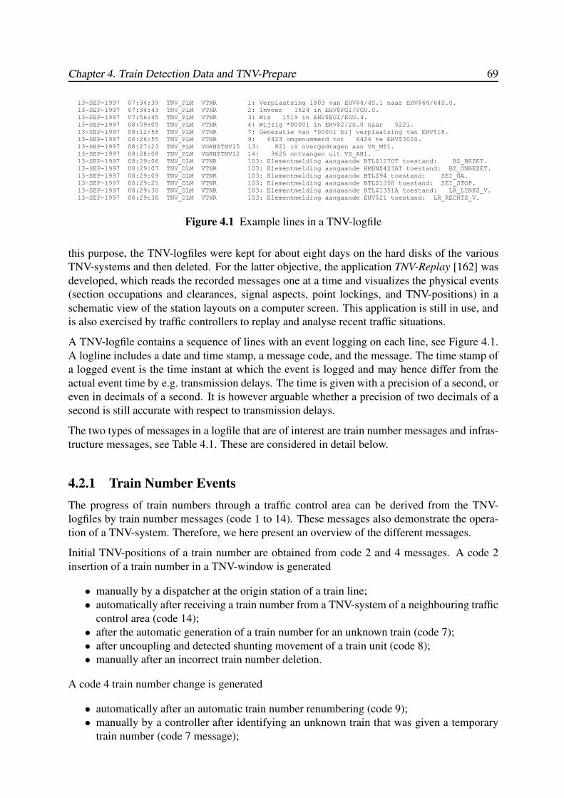
Chapter 4. Train Detection Data and TNV-Prepare 69
13-SEP-1997 07:34:39 TNV_PLM VTNR 1: Verplaatsing 1803 van EHV$4/4S.1 naar EHV$64/64S.0.13-SEP-1997 07:34:43 TNV_PLM VTNR 2: Invoer 1524 in EHV$FGI/FGU.0.13-SEP-1997 07:56:45 TNV_PLM VTNR 3: Wis 1519 in EHV$EGI/EGU.4.13-SEP-1997 08:09:05 TNV_PLM VTNR 4: Wijzig *00001 in EHV$2/2S.0 naar 5221.13-SEP-1997 08:12:58 TNV_PLM VTNR 7: Generatie van *00001 bij verplaatsing van EHV$18.13-SEP-1997 08:26:55 TNV_PLM VTNR 9: 6423 omgenummerd tot 6426 te EHV$302S.13-SEP-1997 08:27:23 TNV_PLM VGRN$TNV15 13: 821 is overgedragen aan VS_MT1.13-SEP-1997 08:28:08 TNV_PLM VGRN$TNV12 14: 3625 ontvangen uit VS_AH1.13-SEP-1997 08:29:06 TNV_DLM VTNR 103: Elementmelding aangaande BTL$1270T toestand: BZ_BEZET.13-SEP-1997 08:29:07 TNV_DLM VTNR 103: Elementmelding aangaande HMDN$423AT toestand: BZ_ONBEZET.13-SEP-1997 08:29:09 TNV_DLM VTNR 103: Elementmelding aangaande BTL$94 toestand: SEI_GA.13-SEP-1997 08:29:25 TNV_DLM VTNR 103: Elementmelding aangaande BTL$1358 toestand: SEI_STOP.13-SEP-1997 08:29:30 TNV_DLM VTNR 103: Elementmelding aangaande BTL$1351A toestand: LR_LINKS_V.13-SEP-1997 08:29:38 TNV_DLM VTNR 103: Elementmelding aangaande EHV$21 toestand: LR_RECHTS_V.
Figure 4.1 Example lines in a TNV-logfile
this purpose, the TNV-logfiles were kept for about eight days on the hard disks of the various
TNV-systems and then deleted. For the latter objective, the application TNV-Replay [162] was
developed, which reads the recorded messages one at a time and visualizes the physical events
(section occupations and clearances, signal aspects, point lockings, and TNV-positions) in a
schematic view of the station layouts on a computer screen. This application is still in use, and
is also exercised by traffic controllers to replay and analyse recent traffic situations.
A TNV-logfile contains a sequence of lines with an event logging on each line, see Figure 4.1.
A logline includes a date and time stamp, a message code, and the message. The time stamp of
a logged event is the time instant at which the event is logged and may hence differ from the
actual event time by e.g. transmission delays. The time is given with a precision of a second, or
even in decimals of a second. It is however arguable whether a precision of two decimals of a
second is still accurate with respect to transmission delays.
The two types of messages in a logfile that are of interest are train number messages and infras-
tructure messages, see Table 4.1. These are considered in detail below.
4.2.1 Train Number Events
The progress of train numbers through a traffic control area can be derived from the TNV-
logfiles by train number messages (code 1 to 14). These messages also demonstrate the opera-
tion of a TNV-system. Therefore, we here present an overview of the different messages.
Initial TNV-positions of a train number are obtained from code 2 and 4 messages. A code 2
insertion of a train number in a TNV-window is generated
• manually by a dispatcher at the origin station of a train line;
• automatically after receiving a train number from a TNV-system of a neighbouring traffic
control area (code 14);
• after the automatic generation of a train number for an unknown train (code 7);
• after uncoupling and detected shunting movement of a train unit (code 8);
• manually after an incorrect train number deletion.
A code 4 train number change is generated
• automatically after an automatic train number renumbering (code 9);
• manually by a controller after identifying an unknown train that was given a temporary
train number (code 7 message);
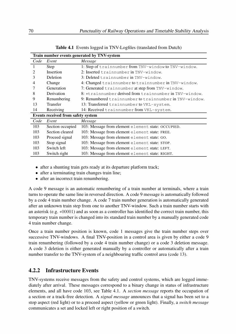
70 Punctuality of Railway Operations and Timetable Stability Analysis
Table 4.1 Events logged in TNV-Logfiles (translated from Dutch)
Train number events generated by TNV-system
Code Event Message
1 Step 1: Step of trainnumber from TNV-window to TNV-window.
2 Insertion 2: Inserted trainnumber in TNV-window.
3 Deletion 3: Deleted trainnumber in TNV-window.
4 Change 4: Changed trainnumber to trainnumber in TNV-window.
7 Generation 7: Generated trainnumber at step from TNV-window.
8 Derivation 8: ∗trainnumber derived from trainnumber in TNV-window.
9 Renumbering 9: Renumbered trainnumber to trainnumber in TNV-window.
13 Transfer 13: Transferred trainnumber to VKL-system.
14 Receiving 14: Received trainnumber from VKL-system.
Events received from safety system
Code Event Message
103 Section occupied 103: Message from element element state: OCCUPIED.
103 Section cleared 103: Message from element element state: FREE.
103 Proceed signal 103: Message from element element state: GO.
103 Stop signal 103: Message from element element state: STOP.
103 Switch left 103: Message from element element state: LEFT.
103 Switch right 103: Message from element element state: RIGHT.
• after a shunting train gets ready at its departure platform track;
• after a terminating train changes train line;
• after an incorrect train renumbering.
A code 9 message is an automatic renumbering of a train number at terminals, where a train
turns to operate the same line in reversed direction. A code 9 message is automatically followed
by a code 4 train number change. A code 7 train number generation is automatically generated
after an unknown train step from one to another TNV-window. Such a train number starts with
an asterisk (e.g. ∗00001) and as soon as a controller has identified the correct train number, this
temporary train number is changed into its standard train number by a manually generated code
4 train number change.
Once a train number position is known, code 1 messages give the train number steps over
successive TNV-windows. A final TNV-position in a control area is given by either a code 9
train renumbering (followed by a code 4 train number change) or a code 3 deletion message.
A code 3 deletion is either generated manually by a controller or automatically after a train
number transfer to the TNV-system of a neighbouring traffic control area (code 13).
4.2.2 Infrastructure Events
TNV-systems receive messages from the safety and control systems, which are logged imme-
diately after arrival. These messages correspond to a binary change in status of infrastructure
elements, and all have code 103, see Table 4.1. A section message reports the occupation of
a section or a track-free detection. A signal message announces that a signal has been set to a
stop aspect (red light) or to a proceed aspect (yellow or green light). Finally, a switch message
communicates a set and locked left or right position of a switch.
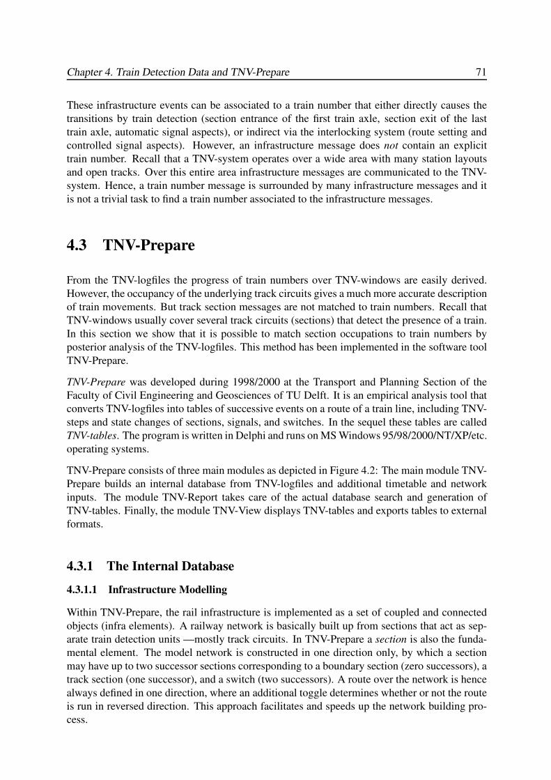
Chapter 4. Train Detection Data and TNV-Prepare 71
These infrastructure events can be associated to a train number that either directly causes the
transitions by train detection (section entrance of the first train axle, section exit of the last
train axle, automatic signal aspects), or indirect via the interlocking system (route setting and
controlled signal aspects). However, an infrastructure message does not contain an explicit
train number. Recall that a TNV-system operates over a wide area with many station layouts
and open tracks. Over this entire area infrastructure messages are communicated to the TNV-
system. Hence, a train number message is surrounded by many infrastructure messages and it
is not a trivial task to find a train number associated to the infrastructure messages.
4.3 TNV-Prepare
From the TNV-logfiles the progress of train numbers over TNV-windows are easily derived.
However, the occupancy of the underlying track circuits gives a much more accurate description
of train movements. But track section messages are not matched to train numbers. Recall that
TNV-windows usually cover several track circuits (sections) that detect the presence of a train.
In this section we show that it is possible to match section occupations to train numbers by
posterior analysis of the TNV-logfiles. This method has been implemented in the software tool
TNV-Prepare.
TNV-Prepare was developed during 1998/2000 at the Transport and Planning Section of the
Faculty of Civil Engineering and Geosciences of TU Delft. It is an empirical analysis tool that
converts TNV-logfiles into tables of successive events on a route of a train line, including TNV-
steps and state changes of sections, signals, and switches. In the sequel these tables are called
TNV-tables. The program is written in Delphi and runs on MS Windows 95/98/2000/NT/XP/etc.
operating systems.
TNV-Prepare consists of three main modules as depicted in Figure 4.2: The main module TNV-
Prepare builds an internal database from TNV-logfiles and additional timetable and network
inputs. The module TNV-Report takes care of the actual database search and generation of
TNV-tables. Finally, the module TNV-View displays TNV-tables and exports tables to external
formats.
4.3.1 The Internal Database
4.3.1.1 Infrastructure Modelling
Within TNV-Prepare, the rail infrastructure is implemented as a set of coupled and connected
objects (infra elements). A railway network is basically built up from sections that act as sep-
arate train detection units —mostly track circuits. In TNV-Prepare a section is also the funda-
mental element. The model network is constructed in one direction only, by which a section
may have up to two successor sections corresponding to a boundary section (zero successors), a
track section (one successor), and a switch (two successors). A route over the network is hence
always defined in one direction, where an additional toggle determines whether or not the route
is run in reversed direction. This approach facilitates and speeds up the network building pro-
cess.
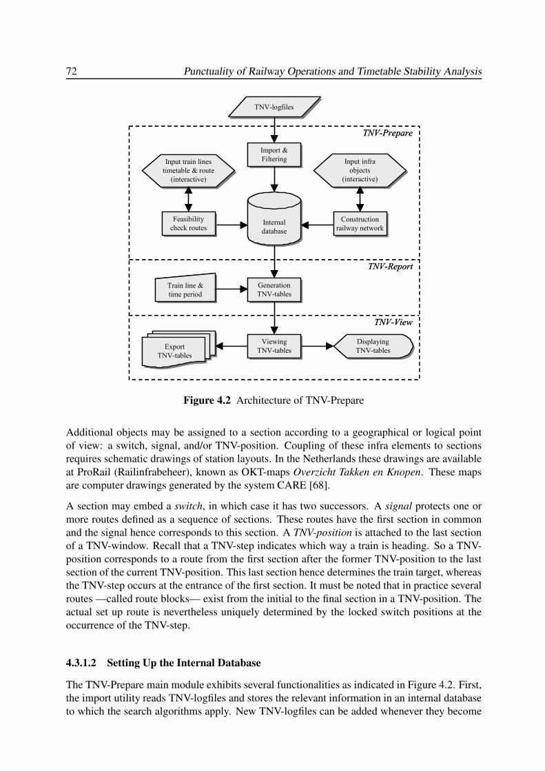
72 Punctuality of Railway Operations and Timetable Stability Analysis
TNV-logfilesTNV-logfiles
Import &
Filtering
Import &
Filtering
Internal
database
Internal
database
Input infra
objects
(interactive)
Input infra
objects
(interactive)
Input train lines
timetable & route
(interactive)
Input train lines
timetable & route
(interactive)
Train line &
time period
Train line &
time periodGeneration
TNV-tables
Generation
TNV-tables
Viewing
TNV-tables
Viewing
TNV-tablesDisplaying
TNV-tables
Displaying
TNV-tablesExport
TNV-tables
Export
TNV-tables
TNV-Prepare
TNV-Report
TNV-View
Construction
railway network
Construction
railway networkFeasibility
check routes
Feasibility
check routes
Figure 4.2 Architecture of TNV-Prepare
Additional objects may be assigned to a section according to a geographical or logical point
of view: a switch, signal, and/or TNV-position. Coupling of these infra elements to sections
requires schematic drawings of station layouts. In the Netherlands these drawings are available
at ProRail (Railinfrabeheer), known as OKT-maps Overzicht Takken en Knopen. These maps
are computer drawings generated by the system CARE [68].
A section may embed a switch, in which case it has two successors. A signal protects one or
more routes defined as a sequence of sections. These routes have the first section in common
and the signal hence corresponds to this section. A TNV-position is attached to the last section
of a TNV-window. Recall that a TNV-step indicates which way a train is heading. So a TNV-
position corresponds to a route from the first section after the former TNV-position to the last
section of the current TNV-position. This last section hence determines the train target, whereas
the TNV-step occurs at the entrance of the first section. It must be noted that in practice several
routes —called route blocks— exist from the initial to the final section in a TNV-position. The
actual set up route is nevertheless uniquely determined by the locked switch positions at the
occurrence of the TNV-step.
4.3.1.2 Setting Up the Internal Database
The TNV-Prepare main module exhibits several functionalities as indicated in Figure 4.2. First,
the import utility reads TNV-logfiles and stores the relevant information in an internal database
to which the search algorithms apply. New TNV-logfiles can be added whenever they become
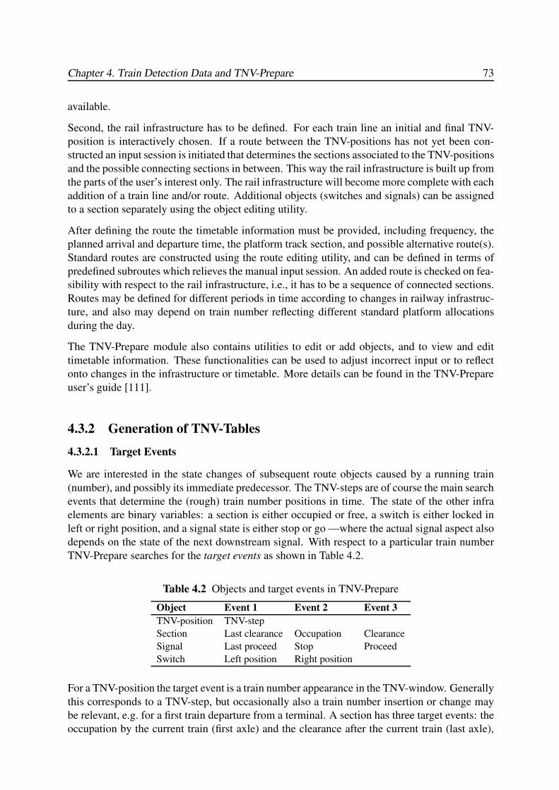
Chapter 4. Train Detection Data and TNV-Prepare 73
available.
Second, the rail infrastructure has to be defined. For each train line an initial and final TNV-
position is interactively chosen. If a route between the TNV-positions has not yet been con-
structed an input session is initiated that determines the sections associated to the TNV-positions
and the possible connecting sections in between. This way the rail infrastructure is built up from
the parts of the user’s interest only. The rail infrastructure will become more complete with each
addition of a train line and/or route. Additional objects (switches and signals) can be assigned
to a section separately using the object editing utility.
After defining the route the timetable information must be provided, including frequency, the
planned arrival and departure time, the platform track section, and possible alternative route(s).
Standard routes are constructed using the route editing utility, and can be defined in terms of
predefined subroutes which relieves the manual input session. An added route is checked on fea-
sibility with respect to the rail infrastructure, i.e., it has to be a sequence of connected sections.
Routes may be defined for different periods in time according to changes in railway infrastruc-
ture, and also may depend on train number reflecting different standard platform allocations
during the day.
The TNV-Prepare module also contains utilities to edit or add objects, and to view and edit
timetable information. These functionalities can be used to adjust incorrect input or to reflect
onto changes in the infrastructure or timetable. More details can be found in the TNV-Prepare
user’s guide [111].
4.3.2 Generation of TNV-Tables
4.3.2.1 Target Events
We are interested in the state changes of subsequent route objects caused by a running train
(number), and possibly its immediate predecessor. The TNV-steps are of course the main search
events that determine the (rough) train number positions in time. The state of the other infra
elements are binary variables: a section is either occupied or free, a switch is either locked in
left or right position, and a signal state is either stop or go —where the actual signal aspect also
depends on the state of the next downstream signal. With respect to a particular train number
TNV-Prepare searches for the target events as shown in Table 4.2.
Table 4.2 Objects and target events in TNV-Prepare
Object Event 1 Event 2 Event 3
TNV-position TNV-step
Section Last clearance Occupation Clearance
Signal Last proceed Stop Proceed
Switch Left position Right position
For a TNV-position the target event is a train number appearance in the TNV-window. Generally
this corresponds to a TNV-step, but occasionally also a train number insertion or change may
be relevant, e.g. for a first train departure from a terminal. A section has three target events: the
occupation by the current train (first axle) and the clearance after the current train (last axle),
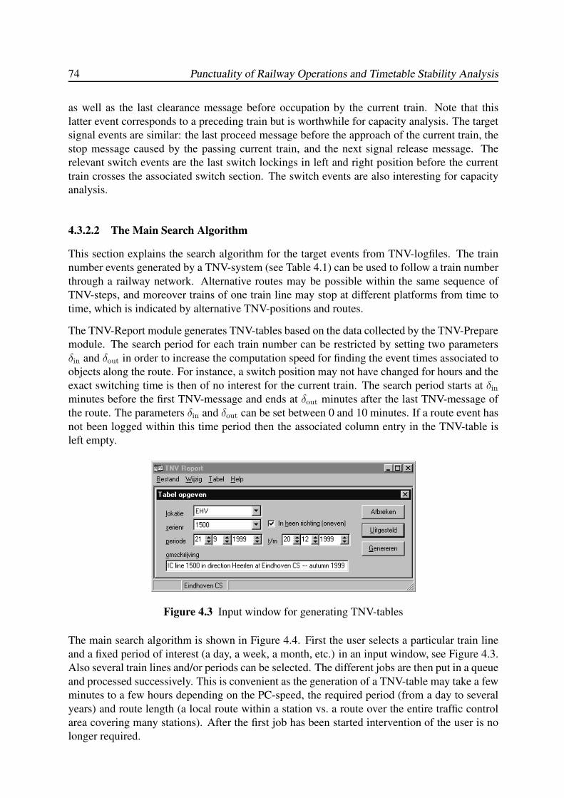
74 Punctuality of Railway Operations and Timetable Stability Analysis
as well as the last clearance message before occupation by the current train. Note that this
latter event corresponds to a preceding train but is worthwhile for capacity analysis. The target
signal events are similar: the last proceed message before the approach of the current train, the
stop message caused by the passing current train, and the next signal release message. The
relevant switch events are the last switch lockings in left and right position before the current
train crosses the associated switch section. The switch events are also interesting for capacity
analysis.
4.3.2.2 The Main Search Algorithm
This section explains the search algorithm for the target events from TNV-logfiles. The train
number events generated by a TNV-system (see Table 4.1) can be used to follow a train number
through a railway network. Alternative routes may be possible within the same sequence of
TNV-steps, and moreover trains of one train line may stop at different platforms from time to
time, which is indicated by alternative TNV-positions and routes.
The TNV-Report module generates TNV-tables based on the data collected by the TNV-Prepare
module. The search period for each train number can be restricted by setting two parameters
δin and δout in order to increase the computation speed for finding the event times associated to
objects along the route. For instance, a switch position may not have changed for hours and the
exact switching time is then of no interest for the current train. The search period starts at δinminutes before the first TNV-message and ends at δout minutes after the last TNV-message of
the route. The parameters δin and δout can be set between 0 and 10 minutes. If a route event has
not been logged within this time period then the associated column entry in the TNV-table is
left empty.
Figure 4.3 Input window for generating TNV-tables
The main search algorithm is shown in Figure 4.4. First the user selects a particular train line
and a fixed period of interest (a day, a week, a month, etc.) in an input window, see Figure 4.3.
Also several train lines and/or periods can be selected. The different jobs are then put in a queue
and processed successively. This is convenient as the generation of a TNV-table may take a few
minutes to a few hours depending on the PC-speed, the required period (from a day to several
years) and route length (a local route within a station vs. a route over the entire traffic control
area covering many stations). After the first job has been started intervention of the user is no
longer required.
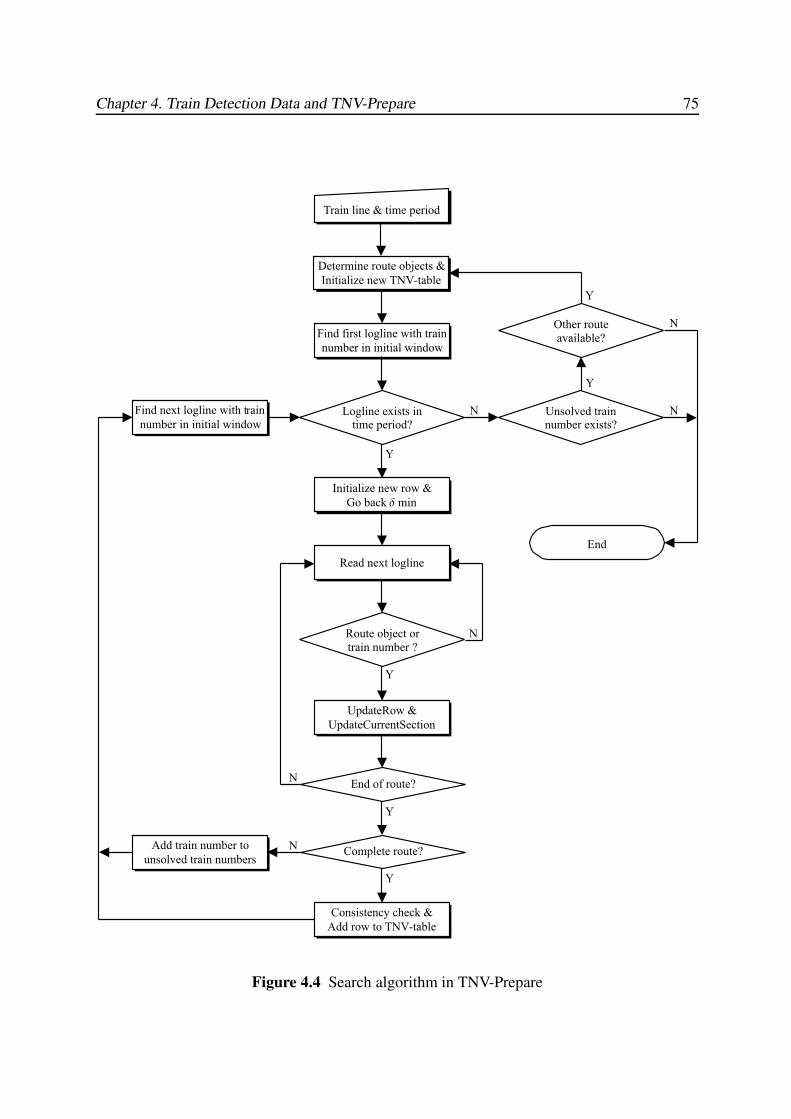
Chapter 4. Train Detection Data and TNV-Prepare 75
Train line & time period
Find first logline with train
number in initial window
Read next logline
Route object or
train number ?
UpdateRow &
UpdateCurrentSection
End of route?
Complete route?
Consistency check &
Add row to TNV-table
Add train number to
unsolved train numbers
Other route
available?
Y
Y
Y
Y
Y
Y
End
N
N
N
N N
N
Initialize new row &
Go back d min
Find next logline with train
number in initial windowLogline exists in
time period?Unsolved trainnumber exists?
Determine route objects &
Initialize new TNV-table
Figure 4.4 Search algorithm in TNV-Prepare
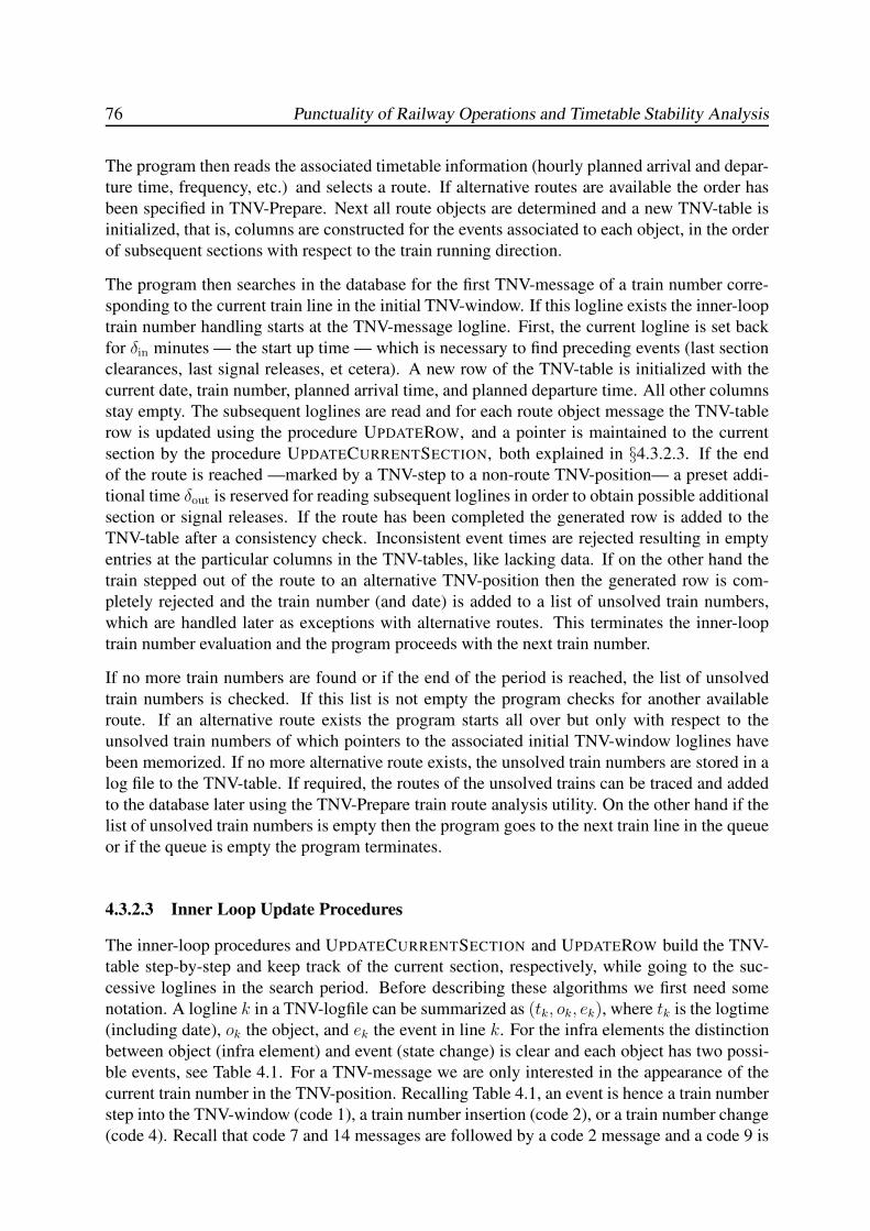
76 Punctuality of Railway Operations and Timetable Stability Analysis
The program then reads the associated timetable information (hourly planned arrival and depar-
ture time, frequency, etc.) and selects a route. If alternative routes are available the order has
been specified in TNV-Prepare. Next all route objects are determined and a new TNV-table is
initialized, that is, columns are constructed for the events associated to each object, in the order
of subsequent sections with respect to the train running direction.
The program then searches in the database for the first TNV-message of a train number corre-
sponding to the current train line in the initial TNV-window. If this logline exists the inner-loop
train number handling starts at the TNV-message logline. First, the current logline is set back
for δin minutes — the start up time — which is necessary to find preceding events (last section
clearances, last signal releases, et cetera). A new row of the TNV-table is initialized with the
current date, train number, planned arrival time, and planned departure time. All other columns
stay empty. The subsequent loglines are read and for each route object message the TNV-table
row is updated using the procedure UPDATEROW, and a pointer is maintained to the current
section by the procedure UPDATECURRENTSECTION, both explained in §4.3.2.3. If the end
of the route is reached —marked by a TNV-step to a non-route TNV-position— a preset addi-
tional time δout is reserved for reading subsequent loglines in order to obtain possible additional
section or signal releases. If the route has been completed the generated row is added to the
TNV-table after a consistency check. Inconsistent event times are rejected resulting in empty
entries at the particular columns in the TNV-tables, like lacking data. If on the other hand the
train stepped out of the route to an alternative TNV-position then the generated row is com-
pletely rejected and the train number (and date) is added to a list of unsolved train numbers,
which are handled later as exceptions with alternative routes. This terminates the inner-loop
train number evaluation and the program proceeds with the next train number.
If no more train numbers are found or if the end of the period is reached, the list of unsolved
train numbers is checked. If this list is not empty the program checks for another available
route. If an alternative route exists the program starts all over but only with respect to the
unsolved train numbers of which pointers to the associated initial TNV-window loglines have
been memorized. If no more alternative route exists, the unsolved train numbers are stored in a
log file to the TNV-table. If required, the routes of the unsolved trains can be traced and added
to the database later using the TNV-Prepare train route analysis utility. On the other hand if the
list of unsolved train numbers is empty then the program goes to the next train line in the queue
or if the queue is empty the program terminates.
4.3.2.3 Inner Loop Update Procedures
The inner-loop procedures and UPDATECURRENTSECTION and UPDATEROW build the TNV-
table step-by-step and keep track of the current section, respectively, while going to the suc-
cessive loglines in the search period. Before describing these algorithms we first need some
notation. A logline k in a TNV-logfile can be summarized as (tk, ok, ek), where tk is the logtime
(including date), ok the object, and ek the event in line k. For the infra elements the distinction
between object (infra element) and event (state change) is clear and each object has two possi-
ble events, see Table 4.1. For a TNV-message we are only interested in the appearance of the
current train number in the TNV-position. Recalling Table 4.1, an event is hence a train number
step into the TNV-window (code 1), a train number insertion (code 2), or a train number change
(code 4). Recall that code 7 and 14 messages are followed by a code 2 message and a code 9 is
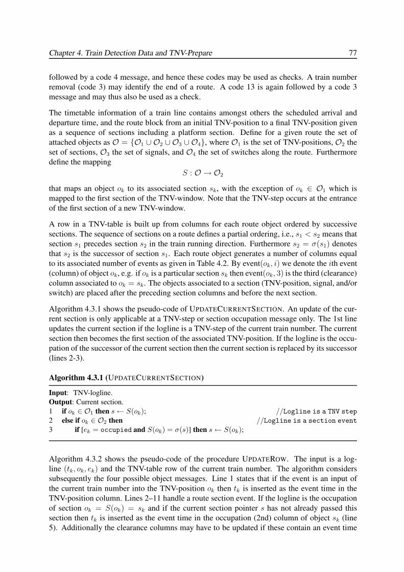
Chapter 4. Train Detection Data and TNV-Prepare 77
followed by a code 4 message, and hence these codes may be used as checks. A train number
removal (code 3) may identify the end of a route. A code 13 is again followed by a code 3
message and may thus also be used as a check.
The timetable information of a train line contains amongst others the scheduled arrival and
departure time, and the route block from an initial TNV-position to a final TNV-position given
as a sequence of sections including a platform section. Define for a given route the set of
attached objects as O = {O1 ∪ O2 ∪ O3 ∪ O4}, where O1 is the set of TNV-positions, O2 the
set of sections, O3 the set of signals, and O4 the set of switches along the route. Furthermore
define the mapping
S : O → O2
that maps an object ok to its associated section sk, with the exception of ok ∈ O1 which is
mapped to the first section of the TNV-window. Note that the TNV-step occurs at the entrance
of the first section of a new TNV-window.
A row in a TNV-table is built up from columns for each route object ordered by successive
sections. The sequence of sections on a route defines a partial ordering, i.e., s1 < s2 means that
section s1 precedes section s2 in the train running direction. Furthermore s2 = σ(s1) denotes
that s2 is the successor of section s1. Each route object generates a number of columns equal
to its associated number of events as given in Table 4.2. By event(ok, i) we denote the ith event
(column) of object ok, e.g. if ok is a particular section sk then event(ok, 3) is the third (clearance)
column associated to ok = sk. The objects associated to a section (TNV-position, signal, and/or
switch) are placed after the preceding section columns and before the next section.
Algorithm 4.3.1 shows the pseudo-code of UPDATECURRENTSECTION. An update of the cur-
rent section is only applicable at a TNV-step or section occupation message only. The 1st line
updates the current section if the logline is a TNV-step of the current train number. The current
section then becomes the first section of the associated TNV-position. If the logline is the occu-
pation of the successor of the current section then the current section is replaced by its successor
(lines 2-3).
Algorithm 4.3.1 (UPDATECURRENTSECTION)
Input: TNV-logline.
Output: Current section.
1 if ok ∈ O1 then s← S(ok); //Logline is a TNV step2 else if ok ∈ O2 then //Logline is a section event3 if [ek = occupied and S(ok) = σ(s)] then s← S(ok);
Algorithm 4.3.2 shows the pseudo-code of the procedure UPDATEROW. The input is a log-
line (tk, ok, ek) and the TNV-table row of the current train number. The algorithm considers
subsequently the four possible object messages. Line 1 states that if the event is an input of
the current train number into the TNV-position ok then tk is inserted as the event time in the
TNV-position column. Lines 2–11 handle a route section event. If the logline is the occupation
of section ok = S(ok) = sk and if the current section pointer s has not already passed this
section then tk is inserted as the event time in the occupation (2nd) column of object sk (line
5). Additionally the clearance columns may have to be updated if these contain an event time

78 Punctuality of Railway Operations and Timetable Stability Analysis
of a previous train (line 6–8). If the logline is a section clearance then tk is inserted into an
empty clearance (3rd) column of section object ok = sk (line 10) provided that the section has
already been occupied or the section lies before the current section s (line 9). If on the other
hand the section has not yet been occupied and sk precedes the current section s then the sec-
tion clearance corresponds to a previous train and tk is inserted in the 1st object column (line
11). Lines 12–21 take care of signal messages. The procedure is similar to a section message.
Finally, lines 22–24 are concerned with switch messages. A switch message is only inserted
if the switch lies after the current section (line 22), so that the final switching event is the last
before entrance of the current train. If the logline is a switch locking in the left position then tkis inserted in the 1st column of the switch object ok (line 23), and otherwise it is inserted in the
2nd column (line 24).
Algorithm 4.3.2 (UPDATEROW)
Input: Logline (tk, ok, ek) and current TNV-Table row.
Output: Updated TNV-table row with logged event.
1 if ok ∈ O1 then event(ok , 1)← tk; //Logline is a TNV step2 else if ok ∈ O2 then //Logline is a section event3 if ek = occupied then
4 if s ≤ S(ok) then
5 event(ok , 2)← tk;
6 if event(ok, 3) 6= ∅ then
7 event(ok , 1)← event(ok, 3);8 event(ok , 3)← ∅;
9 else if [event(ok, 2) 6= ∅ or S(ok) < s] then
10 if event(ok, 3) = ∅ then event(ok , 3)← tk;
11 else event(ok , 1)← tk;
12 else if ok ∈ O3 then //Logline is a signal event13 if ek = stop then
14 if s ≤ S(ok) then
15 event(ok , 2)← tk;
16 if event(ok, 3) 6= ∅ then
17 event(ok , 1)← event(ok, 3);18 event(ok , 3)← ∅;
19 else if [event(ok, 2) 6= ∅ or S(ok) < s] then
20 if event(ok, 3) = ∅ then event(ok , 3)← tk;
21 else event(ok , 1)← tk;
22 else if [ok ∈ O4 and S(ok) ≥ s] then //Logline is a switch event23 if ek = left then event(ok, 1)← tk;
24 else event(ok , 2)← tk;
4.3.3 TNV-Tables
Generated TNV-tables can be displayed in the TNV-View module. Each row of a TNV-table
corresponds to a train number at a particular day. The first four columns contain the date, train
number, scheduled arrival time, and scheduled departure time. The next columns give the event
times associated to consecutive elements on the train path.
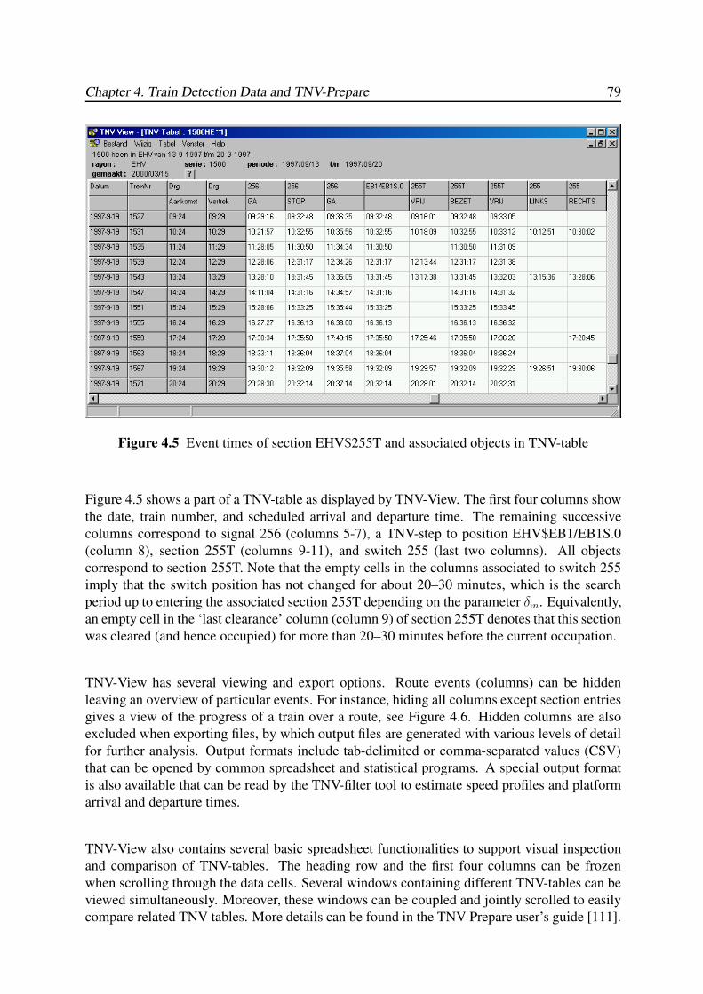
Chapter 4. Train Detection Data and TNV-Prepare 79
Figure 4.5 Event times of section EHV$255T and associated objects in TNV-table
Figure 4.5 shows a part of a TNV-table as displayed by TNV-View. The first four columns show
the date, train number, and scheduled arrival and departure time. The remaining successive
columns correspond to signal 256 (columns 5-7), a TNV-step to position EHV$EB1/EB1S.0
(column 8), section 255T (columns 9-11), and switch 255 (last two columns). All objects
correspond to section 255T. Note that the empty cells in the columns associated to switch 255
imply that the switch position has not changed for about 20–30 minutes, which is the search
period up to entering the associated section 255T depending on the parameter δin. Equivalently,
an empty cell in the ‘last clearance’ column (column 9) of section 255T denotes that this section
was cleared (and hence occupied) for more than 20–30 minutes before the current occupation.
TNV-View has several viewing and export options. Route events (columns) can be hidden
leaving an overview of particular events. For instance, hiding all columns except section entries
gives a view of the progress of a train over a route, see Figure 4.6. Hidden columns are also
excluded when exporting files, by which output files are generated with various levels of detail
for further analysis. Output formats include tab-delimited or comma-separated values (CSV)
that can be opened by common spreadsheet and statistical programs. A special output format
is also available that can be read by the TNV-filter tool to estimate speed profiles and platform
arrival and departure times.
TNV-View also contains several basic spreadsheet functionalities to support visual inspection
and comparison of TNV-tables. The heading row and the first four columns can be frozen
when scrolling through the data cells. Several windows containing different TNV-tables can be
viewed simultaneously. Moreover, these windows can be coupled and jointly scrolled to easily
compare related TNV-tables. More details can be found in the TNV-Prepare user’s guide [111].
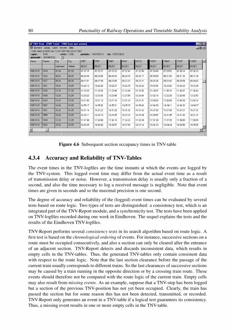
80 Punctuality of Railway Operations and Timetable Stability Analysis
Figure 4.6 Subsequent section occupancy times in TNV-table
4.3.4 Accuracy and Reliability of TNV-Tables
The event times in the TNV-logfiles are the time instants at which the events are logged by
the TNV-system. This logged event time may differ from the actual event time as a result
of transmission delay or noise. However, a transmission delay is usually only a fraction of a
second, and also the time necessary to log a received message is negligible. Note that event
times are given in seconds and so the maximal precision is one second.
The degree of accuracy and reliability of the (logged) event times can be evaluated by several
tests based on route logic. Two types of tests are distinguished: a consistency test, which is an
integrated part of the TNV-Report module, and a synchronicity test. The tests have been applied
on TNV-logfiles recorded during one week in Eindhoven. The sequel explains the tests and the
results of the Eindhoven TNV-logfiles.
TNV-Report performs several consistency tests in its search algorithm based on route logic. A
first test is based on the chronological ordering of events. For instance, successive sections on a
route must be occupied consecutively, and also a section can only be cleared after the entrance
of an adjacent section. TNV-Report detects and discards inconsistent data, which results in
empty cells in the TNV-tables. Thus, the generated TNV-tables only contain consistent data
with respect to the route logic. Note that the last section clearance before the passage of the
current train usually corresponds to different trains. So the last clearances of successive sections
may be caused by a train running in the opposite direction or by a crossing train route. These
events should therefore not be compared with the route logic of the current train. Empty cells
may also result from missing events. As an example, suppose that a TNV-step has been logged
but a section of the previous TNV-position has not yet been occupied. Clearly, the train has
passed the section but for some reason this has not been detected, transmitted, or recorded.
TNV-Report only generates an event in a TNV-table if a logical test guarantees its consistency.
Thus, a missing event results in one or more empty cells in the TNV-table.
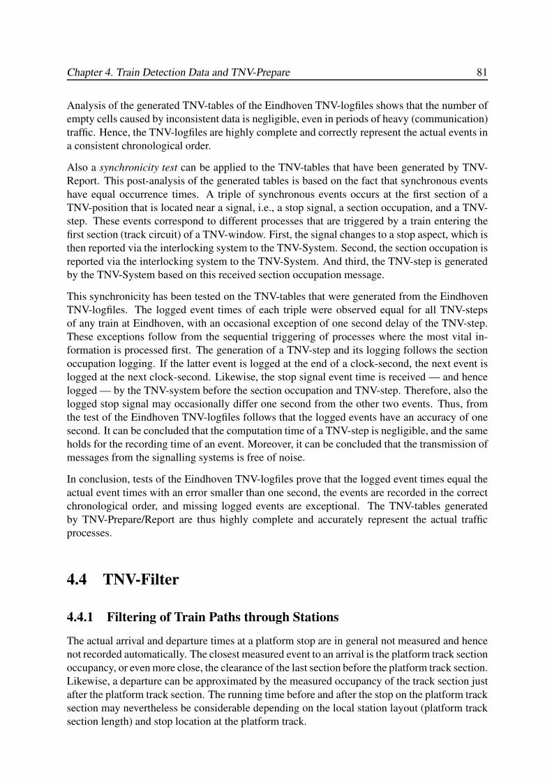
Chapter 4. Train Detection Data and TNV-Prepare 81
Analysis of the generated TNV-tables of the Eindhoven TNV-logfiles shows that the number of
empty cells caused by inconsistent data is negligible, even in periods of heavy (communication)
traffic. Hence, the TNV-logfiles are highly complete and correctly represent the actual events in
a consistent chronological order.
Also a synchronicity test can be applied to the TNV-tables that have been generated by TNV-
Report. This post-analysis of the generated tables is based on the fact that synchronous events
have equal occurrence times. A triple of synchronous events occurs at the first section of a
TNV-position that is located near a signal, i.e., a stop signal, a section occupation, and a TNV-
step. These events correspond to different processes that are triggered by a train entering the
first section (track circuit) of a TNV-window. First, the signal changes to a stop aspect, which is
then reported via the interlocking system to the TNV-System. Second, the section occupation is
reported via the interlocking system to the TNV-System. And third, the TNV-step is generated
by the TNV-System based on this received section occupation message.
This synchronicity has been tested on the TNV-tables that were generated from the Eindhoven
TNV-logfiles. The logged event times of each triple were observed equal for all TNV-steps
of any train at Eindhoven, with an occasional exception of one second delay of the TNV-step.
These exceptions follow from the sequential triggering of processes where the most vital in-
formation is processed first. The generation of a TNV-step and its logging follows the section
occupation logging. If the latter event is logged at the end of a clock-second, the next event is
logged at the next clock-second. Likewise, the stop signal event time is received — and hence
logged — by the TNV-system before the section occupation and TNV-step. Therefore, also the
logged stop signal may occasionally differ one second from the other two events. Thus, from
the test of the Eindhoven TNV-logfiles follows that the logged events have an accuracy of one
second. It can be concluded that the computation time of a TNV-step is negligible, and the same
holds for the recording time of an event. Moreover, it can be concluded that the transmission of
messages from the signalling systems is free of noise.
In conclusion, tests of the Eindhoven TNV-logfiles prove that the logged event times equal the
actual event times with an error smaller than one second, the events are recorded in the correct
chronological order, and missing logged events are exceptional. The TNV-tables generated
by TNV-Prepare/Report are thus highly complete and accurately represent the actual traffic
processes.
4.4 TNV-Filter
4.4.1 Filtering of Train Paths through Stations
The actual arrival and departure times at a platform stop are in general not measured and hence
not recorded automatically. The closest measured event to an arrival is the platform track section
occupancy, or even more close, the clearance of the last section before the platform track section.
Likewise, a departure can be approximated by the measured occupancy of the track section just
after the platform track section. The running time before and after the stop on the platform track
section may nevertheless be considerable depending on the local station layout (platform track
section length) and stop location at the platform track.
82 Punctuality of Railway Operations and Timetable Stability Analysis
Speed
Time
Dwell time AccelerationBraking ConstantConstant
Time in platform
section (train head)Occupation
platform section
Occupation
next section
Figure 4.7 Activities on a platform track section
Within the occupation time of the platform track section several activities take place: braking
until standstill at the stop location, opening of doors, boarding and alighting of passengers,
waiting at the platform track, the departure procedure, acceleration after departure, and clearing
the section after passage of the last train axle, see Figure 4.7. Let us define the arrival and
departure time as the start and end of standstill at the platform, respectively. Then the arrival
and departure time can be estimated from the platform section occupancy and the running times
before and after standstill at the platform track section.
Figure 4.8 shows the running times of equivalent trains over the same route through Eindhoven
over a distance of 435 meter from the entry signal to the platform section border. The data is
obtained using TNV-Prepare and represents a typical picture of the running time distribution
through a station. Clearly, trains run with different speeds to the platform and hence the arrival
and departure time do not only depend on the passage time at the platform section borders but
also on speed and deceleration/acceleration.
Filtering of a train path through a station therefore contains the following steps for arriving and
departing trains:
(i) Estimation of speed and acceleration/deceleration at the platform track section borders;
(ii) Estimation of the stop position at the platform track, possibly depending on train length;
(iii) Prediction of the running time at the platform track section before and after the stop
position.
Section 4.4.2 describes a least-squares estimation method for finding the speed profile and fil-
tered section passage times over the in- and outbound train route through the station, including
the average accelerations on the sections. Here the filtered passage times are feasible with re-
spect to train motion equations and correspond to the measured passage times after rounding.
The running time estimations at the platform track are considered in Section 4.4.4.
4.4.2 Speed Profile Estimation
This section presents an approach to accurately estimate the train speed profile over a route
through a station before and after the platform section. This result will then be used in the next
section to establish running times on the platform section.
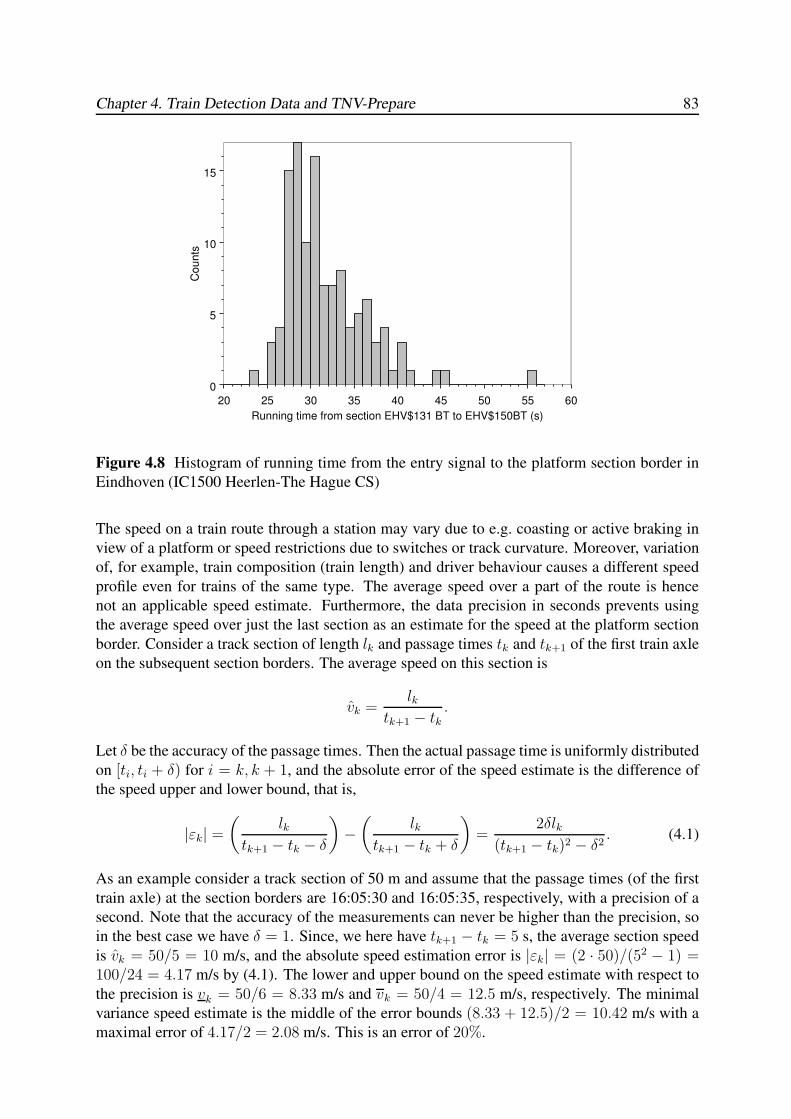
Chapter 4. Train Detection Data and TNV-Prepare 83
20 25 30 35 40 45 50 55 60
Running time from section EHV$131 BT to EHV$150BT (s)
0
5
10
15
Co
un
ts
Figure 4.8 Histogram of running time from the entry signal to the platform section border in
Eindhoven (IC1500 Heerlen-The Hague CS)
The speed on a train route through a station may vary due to e.g. coasting or active braking in
view of a platform or speed restrictions due to switches or track curvature. Moreover, variation
of, for example, train composition (train length) and driver behaviour causes a different speed
profile even for trains of the same type. The average speed over a part of the route is hence
not an applicable speed estimate. Furthermore, the data precision in seconds prevents using
the average speed over just the last section as an estimate for the speed at the platform section
border. Consider a track section of length lk and passage times tk and tk+1 of the first train axle
on the subsequent section borders. The average speed on this section is
vk =lk
tk+1 − tk.
Let δ be the accuracy of the passage times. Then the actual passage time is uniformly distributed
on [ti, ti + δ) for i = k, k + 1, and the absolute error of the speed estimate is the difference of
the speed upper and lower bound, that is,
|εk| =(
lktk+1 − tk − δ
)
−(
lktk+1 − tk + δ
)
=2δlk
(tk+1 − tk)2 − δ2. (4.1)
As an example consider a track section of 50 m and assume that the passage times (of the first
train axle) at the section borders are 16:05:30 and 16:05:35, respectively, with a precision of a
second. Note that the accuracy of the measurements can never be higher than the precision, so
in the best case we have δ = 1. Since, we here have tk+1 − tk = 5 s, the average section speed
is vk = 50/5 = 10 m/s, and the absolute speed estimation error is |εk| = (2 · 50)/(52 − 1) =100/24 = 4.17 m/s by (4.1). The lower and upper bound on the speed estimate with respect to
the precision is vk = 50/6 = 8.33 m/s and vk = 50/4 = 12.5 m/s, respectively. The minimal
variance speed estimate is the middle of the error bounds (8.33 + 12.5)/2 = 10.42 m/s with a
maximal error of 4.17/2 = 2.08 m/s. This is an error of 20%.
84 Punctuality of Railway Operations and Timetable Stability Analysis
The error bounds in (4.1) can also be used as bounds on the actual speed if the accuracy of
the measurement is known. Reversely, (4.1) can be used to determine the measurement error if
accurate speed estimates are obtained from an alternative method or if speed measurements are
available.
The motion of a train is a dynamic process with three variables that change over time: the
position of a train, its speed, and the acceleration (or deceleration for negative values). The
variables are hence functions of time. In the sequel we assume that the section passage times
and section lengths are available. The passage times of sections on a route are generated by
TNV-Prepare. The section lengths must be provided by the railway infrastructure management.
In the Netherlands the positions of insulation joints between track circuits (the section borders)
are shown on OBE-maps from Railinfrabeheer. These maps used to be drawn by hand but are
currently replaced by computer drawings using the system CARE [68].
Consider a train run over a route of n track sections and assume that the n section entrance
times are available from (track circuit occupancy) measurements. The train dynamics on this
route can be described by the discrete-time version of the Newton laws of motion
{xk+1 = xk + vk(tk+1 − tk) + 1
2ak(tk+1 − tk)2
vk+1 = vk + ak(tk+1 − tk), (4.2)
for k = 1, . . . , n − 1. Here xk is the (known) route position of the beginning of section k, vk
is the speed at this section boundary, ak is the (average) acceleration on section k, and tk is the
measured passage (entrance) time of section k. The main problem here is that the passage times
are only approximately known, i.e., the measurements are rounded to seconds and possibly have
measurement errors. Therefore, the passage times are unknowns within some bounds. Note that
if the passage times were known precisely then (4.2) is a system of 2n−2 linear equations in the
2n−1 variables (a1, . . . , an−1, v1, . . . , vn). In this case, the only variable to be determined is the
initial speed v1: for given speed v1 (4.2) is just a system of as many linear equations as variables.
The problem then reduces to finding v1 such that this linear system has a feasible solution. If
on the other hand the train positions xk are unknown instead of the passage times then (4.2) is
a standard linear filtering problem, which can be solved by the Kalman filter, see e.g. Anderson
and Moore [8]. For the specific problem at hand however a least-squares approach is pursued.
Consider the system (4.2) with known positions xk. Note that this system is nonlinear in the
passage times tk. We are now faced with the problem to find variables vk (k = 1, . . . , n), ak
(k = 1, . . . , n− 1), and τk (k = 1, . . . , n) with τk ∈ [tk, tk + 1) such that
Jk(vk, ak, τk, τk+1; xk) := xk + vk(τk+1 − τk) +1
2ak(τk+1 − τk)2
is equal to xk+1 for all k = 1, . . . , n− 1. Note that xk is a known parameter in Jk(·) and not a
variable. There is some redundancy in (4.2): we only have to find the initial speed v1 and actual
passage time τk at the first section, and then subsequently in each step k must find appropriate
variables ak and τk+1, which then also fixes speed vk+1 by the second equation in (4.2). The
decision variables can therefore be reduced to the 2n variables (τ1, . . . , τn, v1, a1, . . . , an−1).
The problem can now be defined as a least-squares optimization problem that minimizes the
sum of squared errors of xk+1 − Jk(vk, ak, τk, τk+1), while satisfying τk ∈ [tk, tk + 1) for all k.
Instead of explicitly adding the passage time constraints to the optimization problem it is more
Chapter 4. Train Detection Data and TNV-Prepare 85
convenient from an algorithmic point of view to extend the objective function with additional
terms that penalize large deviations from the actual passage times. We therefore consider the
following least-squares optimization problem
Minimize
n−1∑
k=1
(xk+1 − Jk(vk, ak, τk, τk+1))2 +
n−1∑
k=1
a2k +
n−2∑
k=1
(ak+1 − ak)2 +
n∑
k=1
(τk − tk −1
2)2
(4.3)
subject to
vk+1 = vk + ak(τk+1 − τk), k = 1, . . . , n− 1. (4.4)
The first term in the least-squares cost function penalizes the deviation of the section position
xk+1 and the estimated train position at time τk+1 given by Jk(vk, ak, τk, τk+1). The second term
minimizes the necessary acceleration or deceleration. The third term expresses the assumption
that the jumps in acceleration or deceleration are as small as possible. The fourth term penalizes
the deviation of the actual passage time τk from the expected passage time tk + 1/2. Recall that
a rounded measurement tk is in fact a uniformly distributed stochastic variable on [tk, tk + 1)with mean tk + 1/2. The constraint (4.4) implicitly determines the speeds vk (k = 2, . . . , n)
in terms of passage times and acceleration, and only serves for notational convenience. In the
actual implementation these (equality) transformations are substituted directly in the definition
of the cost function.
The terms in the cost function may also be weighted differently. Note that an absolute deviation
of 1 second of the passage time estimates τk from the measurements is allowed. However a
difference of 1 m/s2 on an acceleration estimate is unacceptable. Therefore the acceleration
terms can be multiplied by a weight of for instance 100. In this case a change in value of a
passage time τk of 1 second is in the same order as a change of 0.01 m/s2 in acceleration rate.
Nevertheless, experiments showed good performance of the least-squares estimation with cost
function (4.3) with no (or equal) weights.
If the estimated variables from the unconstrained least-squares problem exceed unrealistic limits
then constraints on the variables must be added explicitly, which results in a constrained least-
squares problem. In particular simple box constraints are applicable, i.e., where the decision
variables are bounded individually from below and above.
Passage time bounds. Assume that the passage time measurements are only subject to round-
off errors caused by the precision in seconds. Then we have the constraints
tk ≤ τk < tk + 1, k = 1, . . . , n,
where tk are the measured passage times in seconds. The bounds can be adjusted when addi-
tional measurement errors apply.
Acceleration and deceleration bounds. The acceleration and braking rates must satisfy the
train characteristics. We therefore have the constraints
a ≤ ak ≤ a, k = 1, . . . , n− 1,
where a is the maximum characteristic acceleration and a = −d is the negative maximum
characteristic braking rate d.
86 Punctuality of Railway Operations and Timetable Stability Analysis
Speed restriction. Speed can be limited by the maximum speed of the train characteristics or
by speed restrictions of the railway infrastructure (station layout or open track). We thus have
0 ≤ v1 ≤ v,
where v is the speed restriction on the first section. Recall that we do not consider all sec-
tion speeds explicitly as variables. If we want to incorporate speed restrictions on each section
separately the model must be slightly changed. A first possibility is to include all n speeds
in the decision variables instead of the n − 1 acceleration rates. An alternative is to define a
nonlinear constraint where the speed bounds are expressed in nonlinear constraints on acceler-
ation and passage times. The latter option means however that no longer efficient least-square
optimization algorithms can be used, but a nonlinear programming method must be pursued.
The solution to the speed estimation problem is now obtained as follows. First, (4.3) is solved by
an unconstrained nonlinear least-squares algorithm. If one or more of the variables do not satisfy
the above constraints then the constraints are added and the resulting problem is solved by a con-
strained nonlinear least-squares method. Unconstrained nonlinear least-squares problems are
efficiently solved by the Gauss-Newton method or the Levenberg-Marquardt method [35, 55].
Constrained nonlinear least-square problems are computationally more involved. These prob-
lems are tackled by general constrained nonlinear minimization algorithms, which are adapted
to take advantage of the special structure of the least squares cost function. In the Matlab Opti-
mization Toolbox [35] a trust region method is used as developed by Coleman & Li [36]. This
latter method requires at least as many terms in the cost function as variables. The variables
that have to be estimated are each τk and ak, and the initial speed v1. The problem thus has 2nvariables and the cost function (4.3) exhibits 4n− 4 terms. So the constrained problem can be
solved by this method for n ≥ 2, i.e., the considered route must contain at least measurements
of 2 track sections, which is necessary anyway to estimate the average speed on one section.
The 3rd term can be safely dropped but is included because it directs the (unconstrained) solu-
tion to more satisfying results by penalizing acceleration jumps. It is however only applicable
if n ≥ 3 so that at least the acceleration on two sections must be fit. Furthermore note that
if the acceleration terms in the cost function are dropped then we only have 2n − 1 terms and
the constraint problem with variable bounds can not be solved (by the above method). If only
the 2nd term (squared accelerations) is dropped then 3n − 3 terms remain and the constrained
problem can be solved if n ≥ 3 (section) measurements are available. It can hence be concluded
that for the method to really work at least 3 sections must be taken into account. Otherwise one
just takes the average speed on one section based on the passage times at both section borders.
It should be noted that if some bounds are too tight, the constrained problem may be infeasi-
ble and the problem has no solution. If for instance the measurements have an error because
of noise or transmission delays then the constraint system may be infeasible since the actual
passage times τk may deviate more than one second from tk. Note that a constant bias on all
measurements has no effect on the estimates. So infeasibility only occurs when the measure-
ments have fluctuating errors such as a transmission delay to only one or a few measurements.
Thus, the least-squares problem with above additional constraints can also be used to check for
possible measurement noise.
Chapter 4. Train Detection Data and TNV-Prepare 87
4.4.3 Train Length Estimation
The stop location on the platform tracks may depend on the train length. We therefore also want
to be able to estimate the train length from the data. Train length can be estimated using three
quantities at a fixed track position:
• passage time of the first train axle;
• passage time of the last train axle;
• (average) speed between the first and last axle passage.
Consider a section border between section k and k + 1. The passage time of the train head
(or first axle) is measured as the time that section k + 1 gets occupied. On the other hand the
passage time of the train rear (or last axle) is measured by the clearance time of section k. If
the speed is known and constant during the passage of the section border then the train length
`, approximated as the difference between the first and last axle, is given as
` = v · (sk − tk+1),
where v is the (average) speed at the section border, tk+1 is the entrance time of section k + 1,
and sk is the clearance time of section k.
The accuracy of this estimate depends on the accuracy of the three variables. If the passage
times have an accuracy of 1 second, and we assume perfect knowledge of the average speed,
then the estimation error of the train length is still 2v. Furthermore, the average speed is also
not known exactly. In the last section a method was presented to estimate the speed of the train
front at each section border. Here we need the average speed during the entire passage of a
train over a section border. As we have seen the speed profile is usually not constant during
the train trip, and in particular at the approach and departure of a station. The average speed on
the section border may be approximated by (vk+1 + uk)/2, where vk+1 is the speed of the train
front at the occupancy of section k + 1 and uk is the speed of the train back at the clearance of
section k. These two values must be estimated by e.g. the method of the last section. Still, the
error in the speed estimate is not known and hence neither is the error of train length. This error
may be decreased by taking the average of several train length estimates at subsequent sections.
The least-squares model of the last section can be extended to include train length estimation.
We now must find the speed profile of both the front and rear of the train. The speed profile
estimation of the train back is also obtained from the Newton laws of motion but with respect to
the section clearance times, which are the passage times of the last axle of a train. The average
acceleration based on track clearance times can only be obtained from the second section on-
wards since no passage time of the train back is available for the beginning of the first section.
Define
Ik(uk, bk, σk, σk+1; xk+1) := xk+1 + uk(σk+1 − σk) +1
2bk(σk+1 − σk)
2,
where σk is the filtered clearance time of section k, uk is the speed at the end of section kestimated from the clearance times, and bk is the average acceleration/deceleration at section
k + 1. Then we must have xk+2 = Ik(uk, bk, σk, σk+1) for all k = 1, . . . , n− 2.
88 Punctuality of Railway Operations and Timetable Stability Analysis
Consider again a route of n sections to which we have measurements of the occupations and
clearances. The least-squares optimization problem is now given as
Minimize
n−1∑
k=1
(xk+1 − Jk(vk, ak, τk, τk+1))2 +
n−1∑
k=1
a2k +
n−2∑
k=1
(ak+1 − ak)2 +
n∑
k=1
(τk − tk −1
2)2
+n−2∑
k=1
(xk+2 − Ik(uk, bk, σk, σk+1))2 +
n−1∑
k=1
b2k +n−2∑
k=1
(bk+1 − bk)2
+n−1∑
k=1
(σk − sk −1
2)2 +
n−1∑
k=1
(`− 1
2(vk+1 + uk) · (σk − τk+1))
2 (4.5)
subject tovk+1 = vk + ak(τk+1 − τk), k = 1, . . . , n− 1uk+1 = uk + bk(σk+1 − σk), k = 1, . . . , n− 2.
Here tk, τk, xk, vk, and ak are as before, sk is the measured clearance time of section k, σk
is the filtered clearance time, uk is the speed of the last axle at the exit of section k, bk is the
average acceleration/deceleration of the last axle at section k+1, and ` is the train length. In the
cost function the first term is the squared error of the train front motion equations. The second
term minimizes the necessary acceleration or deceleration of the train front. The third term
expresses the assumption that the jumps in acceleration or deceleration are as small as possible.
The fourth term penalizes the deviation of the actual passage time τk from the expected passage
time tk + 1/2. The fifth term is the squared error of the train back motion equations. The sixth
term minimizes the acceleration or deceleration of the train back. The seventh term expresses
the assumption that the jumps in acceleration or deceleration are as small as possible. The eighth
term penalizes the deviation of the actual passage time σk of the train back from the expected
passage time sk + 1/2. And the final term is the squared error of the train length estimate. The
two constraints are functional equations that are used in the definition of the cost function.
Problem (4.5) is an unconstrained nonlinear least-squares estimation problem. Like in the last
section, the least-squares problem can be extended by weights in the cost function and additional
bounding constraints. Observe that the last term couples the estimations based on the entrance
times and the clearance times, which otherwise are two separable problems.
4.4.4 Running Time on Platform Tracks
In this section we derive analytical estimates for the running times on the platform track. The
following information is assumed available:
• train passage time and speed at the platform section borders;
• train acceleration (deceleration) at the platform sections borders;
• train acceleration and deceleration characteristics;
• platform section length;
• stop location at the platform of the train front.
The platform section passage times are obtained by TNV-Prepare with an accuracy of one sec-
ond. The estimation of train speed and acceleration is considered in the previous section. As
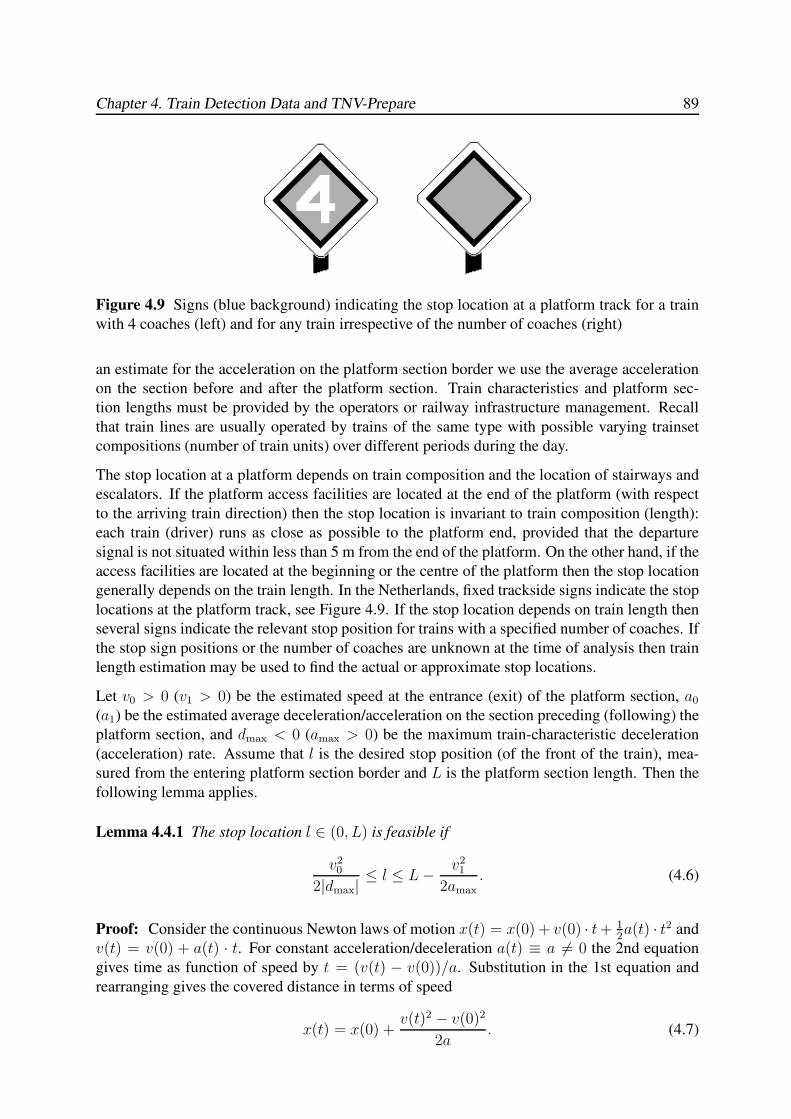
Chapter 4. Train Detection Data and TNV-Prepare 89
Figure 4.9 Signs (blue background) indicating the stop location at a platform track for a train
with 4 coaches (left) and for any train irrespective of the number of coaches (right)
an estimate for the acceleration on the platform section border we use the average acceleration
on the section before and after the platform section. Train characteristics and platform sec-
tion lengths must be provided by the operators or railway infrastructure management. Recall
that train lines are usually operated by trains of the same type with possible varying trainset
compositions (number of train units) over different periods during the day.
The stop location at a platform depends on train composition and the location of stairways and
escalators. If the platform access facilities are located at the end of the platform (with respect
to the arriving train direction) then the stop location is invariant to train composition (length):
each train (driver) runs as close as possible to the platform end, provided that the departure
signal is not situated within less than 5 m from the end of the platform. On the other hand, if the
access facilities are located at the beginning or the centre of the platform then the stop location
generally depends on the train length. In the Netherlands, fixed trackside signs indicate the stop
locations at the platform track, see Figure 4.9. If the stop location depends on train length then
several signs indicate the relevant stop position for trains with a specified number of coaches. If
the stop sign positions or the number of coaches are unknown at the time of analysis then train
length estimation may be used to find the actual or approximate stop locations.
Let v0 > 0 (v1 > 0) be the estimated speed at the entrance (exit) of the platform section, a0
(a1) be the estimated average deceleration/acceleration on the section preceding (following) the
platform section, and dmax < 0 (amax > 0) be the maximum train-characteristic deceleration
(acceleration) rate. Assume that l is the desired stop position (of the front of the train), mea-
sured from the entering platform section border and L is the platform section length. Then the
following lemma applies.
Lemma 4.4.1 The stop location l ∈ (0, L) is feasible if
v20
2|dmax|≤ l ≤ L− v2
1
2amax. (4.6)
Proof: Consider the continuous Newton laws of motion x(t) = x(0) + v(0) · t+ 12a(t) · t2 and
v(t) = v(0) + a(t) · t. For constant acceleration/deceleration a(t) ≡ a 6= 0 the 2nd equation
gives time as function of speed by t = (v(t) − v(0))/a. Substitution in the 1st equation and
rearranging gives the covered distance in terms of speed
x(t) = x(0) +v(t)2 − v(0)2
2a. (4.7)
90 Punctuality of Railway Operations and Timetable Stability Analysis
Now first consider the train arrival. The minimal braking distance is obtained by braking at
maximum capacity a = −|dmax|. Let t = 0 be the entrance time at the platform section, and
so x(0) = 0 and v(0) = v0. The minimal distance x(t) necessary for braking to zero speed
v(t) = 0 is now obtained from (4.7), which gives the lower bound on l. Now consider the train
departure. Assume that the train departs at t = 0 with maximum acceleration amax from x(0)to the platform section border x(t) = L. This strategy accelerates from v(0) = 0 to v(t) = v1
over the shortest distance (and in minimal time). Substitution in (4.7) gives the upper bound on
l. 2
In the sequel we assume that the bounds (4.6) in Lemma 4.4.1 are valid.
At the platform track section no more additional information is obtained from the safety sys-
tems. We therefore have to assume a certain braking and acceleration strategy and compute
the running time on the platform track accordingly. First we explore the feasible and maximal
speed profiles.
Let the maximum-braking speed function vmaxdec : [0, l] 7→ R+ and the maximum-acceleration
speed function vmaxacc : [l, L] 7→ R+ be defined on the platform track section as
vmaxdec (x) :=
√
2|dmax|(l − x) and vmaxacc :=
√
2amax(x− l).
The area {(x, v)|0 ≤ x ≤ l, 0 ≤ v ≤ vmaxdec (x)} is the area in the distance-speed plane from
which the destination (l, 0) can be reached. Likewise {(x, v)|l ≤ x ≤ L, 0 ≤ v ≤ vmaxacc (x)} is
the area in the distance-speed plane that is reachable from the stop location, see Figure 4.10.
The following lemma gives the speed profile over the platform track section with minimum
platform running time. Note that a straight line in the distance-speed plane from the platform
entry to the stop location and again straight to the platform exit is not the fastest speed profile.
Lemma 4.4.2 Let the bounds (4.6) in Lemma 4.4.1 be valid. The minimum platform running
time before arrival with initial speed v0 is
tminin = (umax
0 − v0)/amax + umax0 /|dmax|
and the minimum platform running time after departure with final speed v1 is
tminout = (v1 − umax
1 )/|dmax|+ umax1 /amax,
where
umax0 =
√
v20|dmax|+ 2lamax|dmax|
amax + |dmax|and umax
1 =
√
v21amax + 2(L− l)amax|dmax|
amax + |dmax|.
Proof: The speed profile with minimum running time in the distance-speed plane from (0, v0)to (l, 0) is given by accelerating with maximum acceleration until the maximum braking curve
is reached, after which this curve is followed by constant braking with maximum braking rate,
see Figure 4.10. Note that by this strategy the speed at each position is the highest possible.
The switching position l0 and associated speed can be found using (4.7). For the maximum
acceleration phase we find l0 = (v2 − v20)/2amax and for the maximum braking phase we have
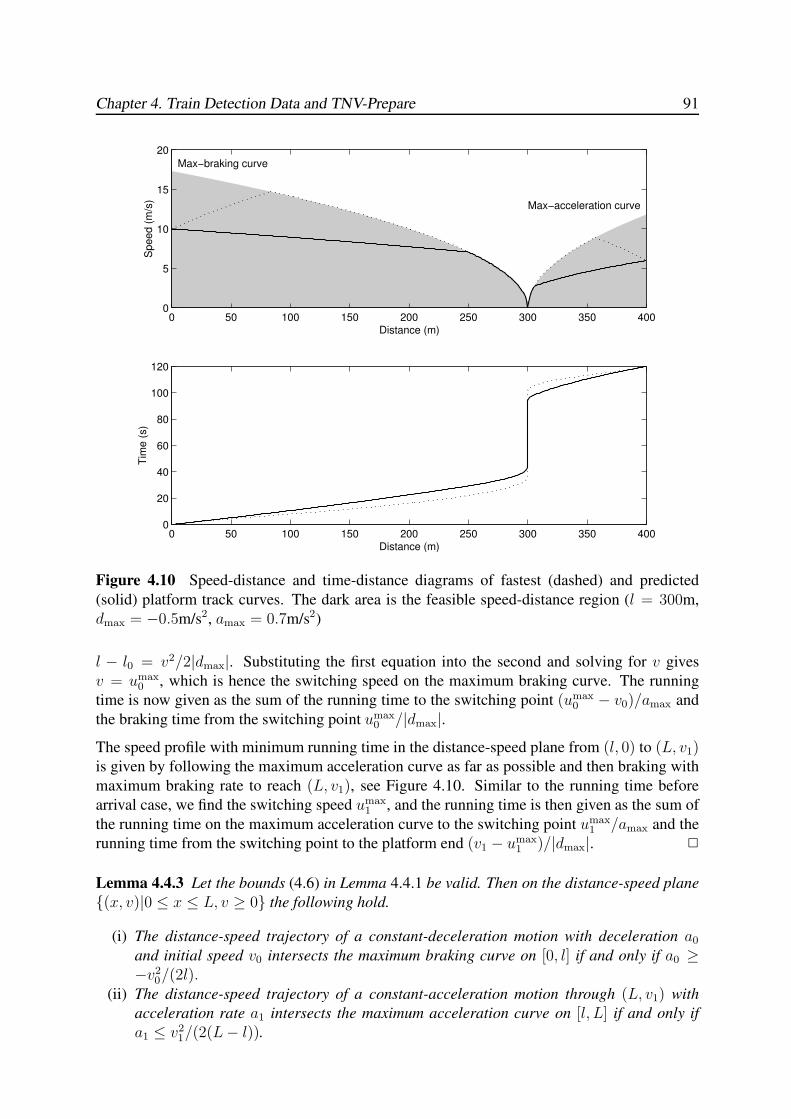
Chapter 4. Train Detection Data and TNV-Prepare 91
Distance (m)
Speed (
m/s
)
Max−braking curve
Max−acceleration curve
0 50 100 150 200 250 300 350 4000
5
10
15
20
0 50 100 150 200 250 300 350 4000
20
40
60
80
100
120
Distance (m)
Tim
e (
s)
Figure 4.10 Speed-distance and time-distance diagrams of fastest (dashed) and predicted
(solid) platform track curves. The dark area is the feasible speed-distance region (l = 300m,
dmax = −0.5m/s2, amax = 0.7m/s2)
l − l0 = v2/2|dmax|. Substituting the first equation into the second and solving for v gives
v = umax0 , which is hence the switching speed on the maximum braking curve. The running
time is now given as the sum of the running time to the switching point (umax0 − v0)/amax and
the braking time from the switching point umax0 /|dmax|.
The speed profile with minimum running time in the distance-speed plane from (l, 0) to (L, v1)is given by following the maximum acceleration curve as far as possible and then braking with
maximum braking rate to reach (L, v1), see Figure 4.10. Similar to the running time before
arrival case, we find the switching speed umax1 , and the running time is then given as the sum of
the running time on the maximum acceleration curve to the switching point umax1 /amax and the
running time from the switching point to the platform end (v1 − umax1 )/|dmax|. 2
Lemma 4.4.3 Let the bounds (4.6) in Lemma 4.4.1 be valid. Then on the distance-speed plane
{(x, v)|0 ≤ x ≤ L, v ≥ 0} the following hold.
(i) The distance-speed trajectory of a constant-deceleration motion with deceleration a0
and initial speed v0 intersects the maximum braking curve on [0, l] if and only if a0 ≥−v2
0/(2l).(ii) The distance-speed trajectory of a constant-acceleration motion through (L, v1) with
acceleration rate a1 intersects the maximum acceleration curve on [l, L] if and only if
a1 ≤ v21/(2(L− l)).
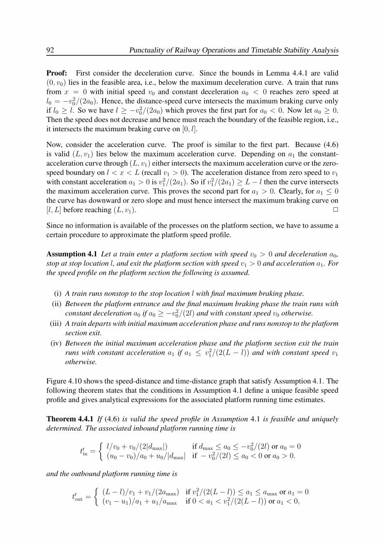
92 Punctuality of Railway Operations and Timetable Stability Analysis
Proof: First consider the deceleration curve. Since the bounds in Lemma 4.4.1 are valid
(0, v0) lies in the feasible area, i.e., below the maximum deceleration curve. A train that runs
from x = 0 with initial speed v0 and constant deceleration a0 < 0 reaches zero speed at
l0 = −v20/(2a0). Hence, the distance-speed curve intersects the maximum braking curve only
if l0 ≥ l. So we have l ≥ −v20/(2a0) which proves the first part for a0 < 0. Now let a0 ≥ 0.
Then the speed does not decrease and hence must reach the boundary of the feasible region, i.e.,
it intersects the maximum braking curve on [0, l].
Now, consider the acceleration curve. The proof is similar to the first part. Because (4.6)
is valid (L, v1) lies below the maximum acceleration curve. Depending on a1 the constant-
acceleration curve through (L, v1) either intersects the maximum acceleration curve or the zero-
speed boundary on l < x < L (recall v1 > 0). The acceleration distance from zero speed to v1
with constant acceleration a1 > 0 is v21/(2a1). So if v2
1/(2a1) ≥ L− l then the curve intersects
the maximum acceleration curve. This proves the second part for a1 > 0. Clearly, for a1 ≤ 0the curve has downward or zero slope and must hence intersect the maximum braking curve on
[l, L] before reaching (L, v1). 2
Since no information is available of the processes on the platform section, we have to assume a
certain procedure to approximate the platform speed profile.
Assumption 4.1 Let a train enter a platform section with speed v0 > 0 and deceleration a0,
stop at stop location l, and exit the platform section with speed v1 > 0 and acceleration a1. For
the speed profile on the platform section the following is assumed.
(i) A train runs nonstop to the stop location l with final maximum braking phase.
(ii) Between the platform entrance and the final maximum braking phase the train runs with
constant deceleration a0 if a0 ≥ −v20/(2l) and with constant speed v0 otherwise.
(iii) A train departs with initial maximum acceleration phase and runs nonstop to the platform
section exit.
(iv) Between the initial maximum acceleration phase and the platform section exit the train
runs with constant acceleration a1 if a1 ≤ v21/(2(L − l)) and with constant speed v1
otherwise.
Figure 4.10 shows the speed-distance and time-distance graph that satisfy Assumption 4.1. The
following theorem states that the conditions in Assumption 4.1 define a unique feasible speed
profile and gives analytical expressions for the associated platform running time estimates.
Theorem 4.4.1 If (4.6) is valid the speed profile in Assumption 4.1 is feasible and uniquely
determined. The associated inbound platform running time is
trin =
{l/v0 + v0/(2|dmax|) if dmax ≤ a0 ≤ −v2
0/(2l) or a0 = 0(u0 − v0)/a0 + u0/|dmax| if − v2
0/(2l) ≤ a0 < 0 or a0 > 0.
and the outbound platform running time is
trout =
{(L− l)/v1 + v1/(2amax) if v2
1/(2(L− l)) ≤ a1 ≤ amax or a1 = 0(v1 − u1)/a1 + u1/amax if 0 < a1 < v2
1/(2(L− l)) or a1 < 0,
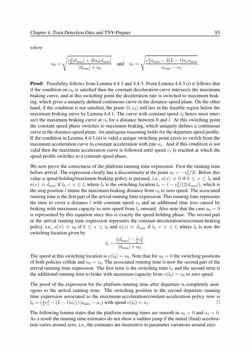
Chapter 4. Train Detection Data and TNV-Prepare 93
where
u0 =
√
v20|dmax|+ 2la0|dmax||dmax|+ a0
and u1 =
√
v21amax − 2(L− l)a1amax
amax − a1
.
Proof: Feasibility follows from Lemma 4.4.1 and 4.4.3: From Lemma 4.4.3.(i) it follows that
if the condition on a0 is satisfied then the constant deceleration curve intersects the maximum
braking curve, and at this switching point the deceleration rate is switched to maximum brak-
ing, which gives a uniquely defined continuous curve in the distance-speed plane. On the other
hand, if the condition is not satisfied, the point (0, v0) still lies in the feasible region below the
maximum braking curve by Lemma 4.4.1. The curve with constant speed v0 hence must inter-
sect the maximum braking curve at v0 for a distance between 0 and l. At this switching point
the constant speed phase switches to maximum braking, which uniquely defines a continuous
curve in the distance-speed plane. An analogous reasoning holds for the departure speed profile.
If the condition in Lemma 4.4.3.(ii) is valid a unique switching point exists to switch from the
maximum acceleration curve to constant acceleration with rate a1. And if this condition is not
valid then the maximum acceleration curve is followed until speed v1 is reached at which the
speed profile switches to a constant speed phase.
We now prove the correctness of the platform running time expression. First the running time
before arrival. The expression clearly has a discontinuity at the point a0 = −v20/2l. Below this
value a speed-holding/maximum-braking policy is pursued, i.e., a(x) ≡ 0 if 0 ≤ x ≤ l0 and
a(x) ≡ dmax if l0 < x ≤ l, where l0 is the switching location l0 = l − v20/(2|dmax|), which is
the stop position l minus the maximum braking distance from v0 to zero speed. The associated
running time is the first part of the arrival running time expression. This running time represents
the time to cover a distance l with constant speed v0 and an additional time loss caused by
braking with maximum capacity to zero speed from l0 onward. Also note that the case a0 = 0is represented by this equation since this is exactly the speed-holding phase. The second part
in the arrival running time expression represents the constant-deceleration/maximum-braking
policy, i.e., a(x) ≡ a0 if 0 ≤ x ≤ l0 and a(x) ≡ dmax if l0 < x ≤ l, where l0 is now the
switching location given by
l0 =l|dmax| − 1
2v20
|dmax|+ a0.
The speed at this switching location is v(l0) = u0. Note that for a0 = 0 the switching positions
of both policies collide and u0 = v0. The associated running time is now the second part of the
arrival running time expression. The first term is the switching time t0 and the second term is
the additional running time to brake with maximum capacity from v(l0) = u0 to zero speed.
The proof of the expression for the platform running time after departure is completely anal-
ogous to the arrival running time. The switching position in the second departure running
time expression associated to the maximum-acceleration/constant-acceleration policy now is
l0 = (12v21 − (L− l)a1)/(amax − a1) with speed v(l0) = u1. 2
The following lemma states that the platform running times are smooth in a0 = 0 and a1 = 0.
As a result the running time estimates do not show a sudden jump if the initial (final) accelera-
tion varies around zero, i.e., the estimates are insensitive to parameter variations around zero.
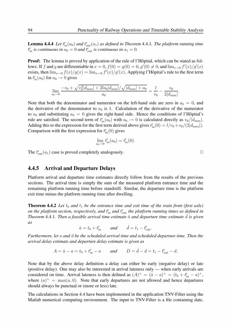
94 Punctuality of Railway Operations and Timetable Stability Analysis
Lemma 4.4.4 Let trin(a0) and trout(a1) as defined in Theorem 4.4.1. The platform running time
trin is continuous in a0 = 0 and trout is continuous in a1 = 0.
Proof: The lemma is proved by application of the rule of l’Hopital, which can be stated as fol-
lows: If f and g are differentiable in x = 0, f(0) = g(0) = 0, g′(0) 6= 0, and limx→0 f′(x)/g′(x)
exists, then limx→0 f(x)/g(x) = limx→0 f′(x)/g′(x). Applying l’Hopital’s rule to the first term
in trin(a0) for a0 → 0 gives
lima0→0
−v0 +√
v20|dmax|+ 2la0|dmax|/
√
|dmax|+ a0
a0=
l
v0− v0
2|dmax|.
Note that both the denominator and numerator on the left-hand side are zero in a0 = 0, and
the derivative of the denominator to a0 is 1. Calculation of the derivative of the numerator
to a0 and substituting a0 = 0 gives the right-hand side. Hence the conditions of l’Hopital’s
rule are satisfied. The second term of trin(a0) with a0 → 0 is calculated directly as v0/|dmax|.Adding this to the expression for the first term derived above gives trin(0) = l/v0+v0/(2|dmax|).Comparison with the first expression for trin(0) gives
lima0→0
trin(a0) = trin(0).
The trout(a1) case is proved completely analogously. 2
4.4.5 Arrival and Departure Delays
Platform arrival and departure time estimates directly follow from the results of the previous
sections. The arrival time is simply the sum of the measured platform entrance time and the
remaining platform running time before standstill. Similar, the departure time is the platform
exit time minus the platform running time after dwelling.
Theorem 4.4.2 Let t0 and t1 be the entrance time and exit time of the train front (first axle)
on the platform section, respectively, and trin and trout the platform running times as defined in
Theorem 4.4.1. Then a feasible arrival time estimate a and departure time estimate d is given
as
a = t0 + trin and d = t1 − trout.
Furthermore, let a and d be the scheduled arrival time and scheduled departure time. Then the
arrival delay estimate and departure delay estimate is given as
A = a− a = t0 + trin − a and D = d− d = t1 − trout − d.
Note that by the above delay definition a delay can either be early (negative delay) or late
(positive delay). One may also be interested in arrival lateness only — when early arrivals are
considered on time. Arrival lateness is then defined as (A)+ = (a − a)+ = (t0 + trin − a)+,
where (a)+ = max(a, 0). Note that early departures are not allowed and hence departures
should always be punctual or (more or less) late.
The calculations in Section 4.4 have been implemented in the application TNV-Filter using the
Matlab numerical computing environment. The input to TNV-Filter is a file containing date,
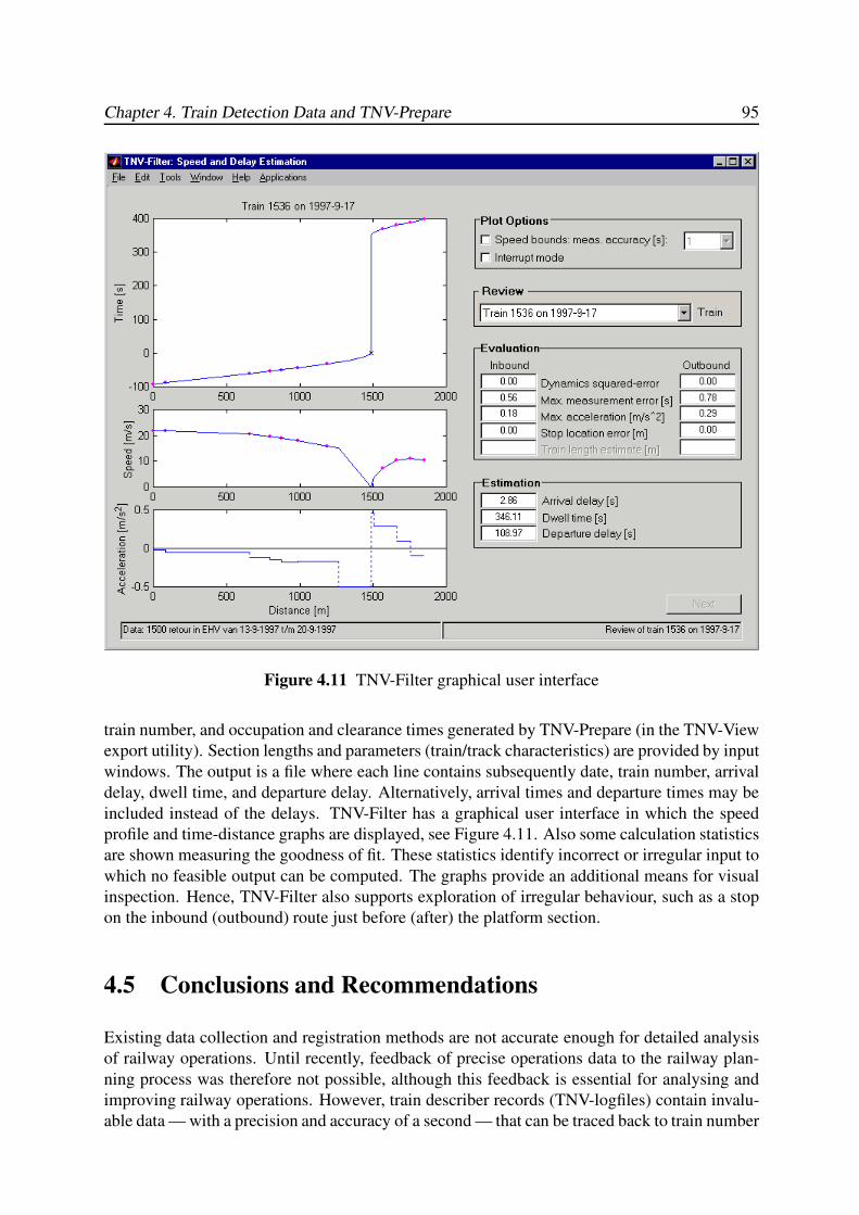
Chapter 4. Train Detection Data and TNV-Prepare 95
Figure 4.11 TNV-Filter graphical user interface
train number, and occupation and clearance times generated by TNV-Prepare (in the TNV-View
export utility). Section lengths and parameters (train/track characteristics) are provided by input
windows. The output is a file where each line contains subsequently date, train number, arrival
delay, dwell time, and departure delay. Alternatively, arrival times and departure times may be
included instead of the delays. TNV-Filter has a graphical user interface in which the speed
profile and time-distance graphs are displayed, see Figure 4.11. Also some calculation statistics
are shown measuring the goodness of fit. These statistics identify incorrect or irregular input to
which no feasible output can be computed. The graphs provide an additional means for visual
inspection. Hence, TNV-Filter also supports exploration of irregular behaviour, such as a stop
on the inbound (outbound) route just before (after) the platform section.
4.5 Conclusions and Recommendations
Existing data collection and registration methods are not accurate enough for detailed analysis
of railway operations. Until recently, feedback of precise operations data to the railway plan-
ning process was therefore not possible, although this feedback is essential for analysing and
improving railway operations. However, train describer records (TNV-logfiles) contain invalu-
able data — with a precision and accuracy of a second — that can be traced back to train number
96 Punctuality of Railway Operations and Timetable Stability Analysis
governed events using the developed software application TNV-prepare.
TNV-Prepare couples events of infra elements to train numbers, such as section occupations
and releases on open tracks and through railway stations, triggered signal changes, and switch
position lockings. From this information other interesting process times can easily be derived,
such as blocking times, running times on (block) sections, headway at infra points, route setting
times, et cetera.
The actual arrival and departure times at a platform stop are in general not recorded automat-
ically. Therefore, the tool TNV-Filter has been developed that estimates arrival and departure
times in (large) stations based on TNV-tables generated by TNV-Prepare. The speed trajectory
and train length of each train entering or departing a station is estimated on the basis of section
(track circuit) occupation and clearance times and scheduled train characteristics. Estimation er-
rors due to round-off errors (passage times are given in seconds) and deceleration (acceleration)
variations during the approach (departure) are filtered by means of a nonlinear least-squares
method taking into account possible speed limits at e.g. signals and switches. Subsequently, the
running time at the platform section before and after standstill are estimated from the filtered
inbound and outbound speed profiles, known standard deceleration and acceleration charac-
teristics per type of train, and stop location on the platform section (possibly depending on
train length). This way, the arrival and departure times of each train at the platform tracks are
determined with a precision in the order of a second.
From March 2000 the TNV-logfiles from each TNV-control area are no longer wasted after a few
days, but centrally collected each day and saved on CD-ROM for (internal) analysis purposes.
This archiving is done by AEA Technology Rail under license from ProRail, primarily for use
with TNV-Replay. The saved format is more compact and differs slightly from the raw TNV-
logfiles described in this chapter [83]. In July 2003 the import utility of TNV-Prepare was
extended to handle this format as well.
Chapter 5
STATISTICAL ANALYSIS:
THE EINDHOVEN CASE
5.1 Introduction
Until recently, empirical analysis of train delays dealt with delays of at least 3 minutes for prac-
tical reasons of operations control. However, modern train detection systems and computing
facilities now enable much more precise measurements and hence also much more accurate
data analysis opportunities, see Chapter 4. Analysis of realized process times is a crucial step
in punctuality management since operations data contain invaluable information about process
time variations – which should be small in a well-designed railway system – and train interac-
tions. Analysis of realization data reveals tight headway times or the actual amount of buffer
time at infrastructure bottlenecks and train connections.
Stations are the bottlenecks in a railway network as here trains of various lines meet and inter-
act. Delayed and/or early trains result in potential conflicting train paths — controlled by the
interlocking system — causing mutual hinder at conflict points. Delays measured at stations
represent a mixture of primary and secondary delays. Arrival delays are input delays to a sta-
tion area summarizing the train operations upstream to the station including the inbound routes.
They are a mixture of primary running time disruptions on the preceding open track and e.g.
a provoked low speed by following a slow train on the open track, and hinder at merging and
crossing inbound routes. Disruptions in the dwelling process are a source of primary delays,
e.g. extensive alighting and boarding time and a prolonged departure process. The measured de-
parture delays are the result of arrival delays, disruption in the dwelling process, and secondary
delays at departure resulting from e.g. conflicting outbound routes or waiting for delayed feeder
trains.
Statistics of process time realizations and resulting delays are a means of timetable evaluation
identifying tight process times and critical train interactions (transfer times, headway) or on
the other hand quantifying available slack and buffer times. Moreover, regression analysis can
be applied to evaluate potential dependencies between processes as a cause of delay propaga-
tion. Note that delay measurements at stations provide train delays associated to any possible
primary or secondary source. Finding the explicit source(s) of these resulting delays is hard
and requires monitoring information other than just delay measurements. Nevertheless, train
dependencies and critical process times expose possible sources of delay and give directions to
possible improvements in the timetable design.
The objective of this chapter is to find structural variations in process times caused by regular
minor disruptions and interactions. Major incidents or accidents — leading to long-term dam-
age or obstruction of rail tracks — are not structural and (should) occur only seldom, and are
97
98 Punctuality of Railway Operations and Timetable Stability Analysis
thus discarded in the analysis. Trains affected by an uncommon event experience delays that
are clearly not representative to the usual stochastic behaviour. These situations are the subject
of incidence management rather than daily operations practice. From a statistical point of view
these delays are usually identified as outliers.
In the Netherlands, passenger train services operate basically according to a periodic timetable,
repeating the same arrival and departure times each hour, with the exception of additional pas-
senger trains in rush hours and freight trains that are scheduled in between the regular train
services. It is hence anticipated that the traffic processes are mainly variations on a repetitive
pattern. This motivates an aggregation on train line level rather than analysing process times of
individual train numbers.
This chapter considers a case study of a statistical analysis applied to Eindhoven station. Parts of
this chapter have been published before in Goverde et al. [87] and Hansen & Goverde [93, 94],
and presented at several congresses including the 9th WCTR [86] and WCRR 2001 [85]. Over
the last years similar and other statistical analyses have been applied to various stations and
corridors [145, 199, 228]. The results presented in this chapter on Eindhoven have also been
found in the other studies.
TNV-logfiles in the traffic area Eindhoven were collected during one week in September 1997
and made available by Railinfrabeheer and Railverkeersleiding to TU Delft. Note that in 1997
TNV-logfiles were not maintained but could be saved on request. From the TNV-logfiles the
train line specific event times at railway station Eindhoven were generated by TNV-Prepare
and subsequently the platform arrival and departure times were obtained using the TNV-Filter
program (Chapter 4). In total, 1846 trains had been recorded, of which about 30% IC-trains,
30% IR-trains and 40% local (AR) trains. Freight trains have been discarded in the analysis.
The statistical analysis of this Eindhoven data has been done by means of the statistical software
package S-Plus [131].
The chapter is outlined as follows. Section 5.2 presents the characteristics of station Eindhoven.
Section 5.3 gives the derived punctuality statistics of Eindhoven. In Section 5.4 departure de-
lays are predicted from arrival delays using regression analysis, whereas the remaining noise
is attributed to human factors. Section 5.5 covers distribution assessment of the events and
processes in Eindhoven. In the final section some conclusions are presented.
5.2 Railway station Eindhoven
Eindhoven is the main intercity transfer station in the southern part of the Netherlands, where
train lines of four main directions meet: from Utrecht (and beyond) in the north, from Rot-
terdam in the west, Venlo in the east, and Heerlen in the south. Eindhoven has 6 platforms
for passengers and connects 3 double-track railway routes. A double-track route from Utrecht
and one from Rotterdam merge at Boxtel from which a double-track1 route leads to Eindhoven.
So the west- and northbound trains have a mutual double-track route between Eindhoven and
Boxtel, see Figure 5.1.
1In the mean time the corridor between Eindhoven and Boxtel has been upgraded to a four-track route as part
of the Rail 21 programme. The four-track route became fully operational at the end of 2002
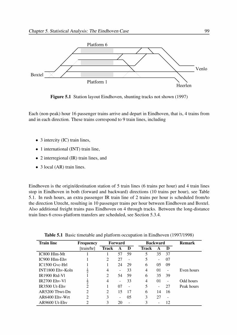
Chapter 5. Statistical Analysis: The Eindhoven Case 99
Figure 5.1 Station layout Eindhoven, shunting tracks not shown (1997)
Each (non-peak) hour 16 passenger trains arrive and depart in Eindhoven, that is, 4 trains from
and in each direction. These trains correspond to 9 train lines, including
• 3 intercity (IC) train lines,
• 1 international (INT) train line,
• 2 interregional (IR) train lines, and
• 3 local (AR) train lines.
Eindhoven is the origin/destination station of 5 train lines (6 trains per hour) and 4 train lines
stop in Eindhoven in both (forward and backward) directions (10 trains per hour), see Table
5.1. In rush hours, an extra passenger IR train line of 2 trains per hour is scheduled from/to
the direction Utrecht, resulting in 10 passenger trains per hour between Eindhoven and Boxtel.
Also additional freight trains pass Eindhoven on 4 through tracks. Between the long-distance
train lines 6 cross-platform transfers are scheduled, see Section 5.3.4.
Table 5.1 Basic timetable and platform occupation in Eindhoven (1997/1998)
Train line Frequency Forward Backward Remark
[train/hr] Track A D Track A D
IC800 Hlm-Mt 1 1 57 59 5 35 37
IC900 Hlm-Ehv 1 2 27 - 5 - 07
IC1500 Gvc-Hrl 1 1 24 29 6 05 09
INT1800 Ehv-Koln 12 4 - 33 4 01 - Even hours
IR1900 Rtd-Vl 1 2 54 59 6 35 39
IR2700 Ehv-Vl 12 4 - 33 4 01 - Odd hours
IR3500 Ut-Ehv 2 1 07 - 5 - 27 Peak hours
AR5200 Tbwt-Dn 2 2 15 17 6 14 16
AR6400 Ehv-Wrt 2 3 - 05 3 27 -
AR9600 Ut-Ehv 2 3 20 - 3 - 12
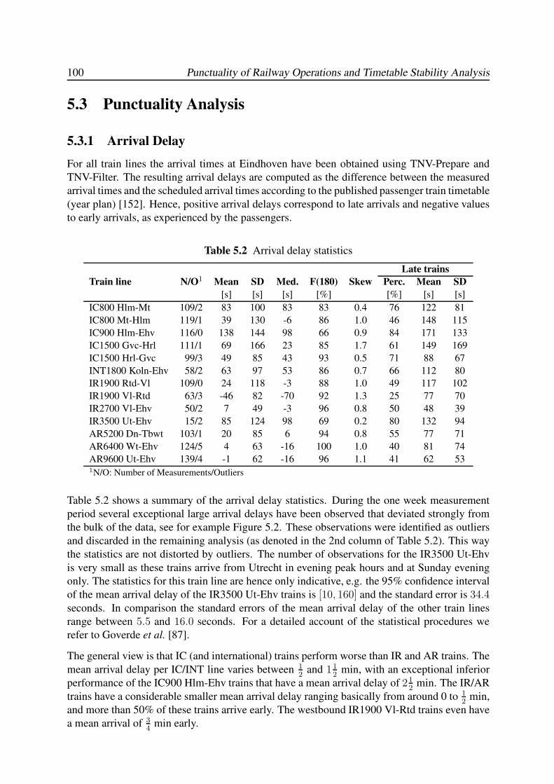
100 Punctuality of Railway Operations and Timetable Stability Analysis
5.3 Punctuality Analysis
5.3.1 Arrival Delay
For all train lines the arrival times at Eindhoven have been obtained using TNV-Prepare and
TNV-Filter. The resulting arrival delays are computed as the difference between the measured
arrival times and the scheduled arrival times according to the published passenger train timetable
(year plan) [152]. Hence, positive arrival delays correspond to late arrivals and negative values
to early arrivals, as experienced by the passengers.
Table 5.2 Arrival delay statistics
Late trains
Train line N/O1 Mean SD Med. F(180) Skew Perc. Mean SD
[s] [s] [s] [%] [%] [s] [s]
IC800 Hlm-Mt 109/2 83 100 83 83 0.4 76 122 81
IC800 Mt-Hlm 119/1 39 130 -6 86 1.0 46 148 115
IC900 Hlm-Ehv 116/0 138 144 98 66 0.9 84 171 133
IC1500 Gvc-Hrl 111/1 69 166 23 85 1.7 61 149 169
IC1500 Hrl-Gvc 99/3 49 85 43 93 0.5 71 88 67
INT1800 Koln-Ehv 58/2 63 97 53 86 0.7 66 112 80
IR1900 Rtd-Vl 109/0 24 118 -3 88 1.0 49 117 102
IR1900 Vl-Rtd 63/3 -46 82 -70 92 1.3 25 77 70
IR2700 Vl-Ehv 50/2 7 49 -3 96 0.8 50 48 39
IR3500 Ut-Ehv 15/2 85 124 98 69 0.2 80 132 94
AR5200 Dn-Tbwt 103/1 20 85 6 94 0.8 55 77 71
AR6400 Wt-Ehv 124/5 4 63 -16 100 1.0 40 81 74
AR9600 Ut-Ehv 139/4 -1 62 -16 96 1.1 41 62 531N/O: Number of Measurements/Outliers
Table 5.2 shows a summary of the arrival delay statistics. During the one week measurement
period several exceptional large arrival delays have been observed that deviated strongly from
the bulk of the data, see for example Figure 5.2. These observations were identified as outliers
and discarded in the remaining analysis (as denoted in the 2nd column of Table 5.2). This way
the statistics are not distorted by outliers. The number of observations for the IR3500 Ut-Ehv
is very small as these trains arrive from Utrecht in evening peak hours and at Sunday evening
only. The statistics for this train line are hence only indicative, e.g. the 95% confidence interval
of the mean arrival delay of the IR3500 Ut-Ehv trains is [10, 160] and the standard error is 34.4seconds. In comparison the standard errors of the mean arrival delay of the other train lines
range between 5.5 and 16.0 seconds. For a detailed account of the statistical procedures we
refer to Goverde et al. [87].
The general view is that IC (and international) trains perform worse than IR and AR trains. The
mean arrival delay per IC/INT line varies between 12
and 112
min, with an exceptional inferior
performance of the IC900 Hlm-Ehv trains that have a mean arrival delay of 212
min. The IR/AR
trains have a considerable smaller mean arrival delay ranging basically from around 0 to 12
min,
and more than 50% of these trains arrive early. The westbound IR1900 Vl-Rtd trains even have
a mean arrival of 34
min early.
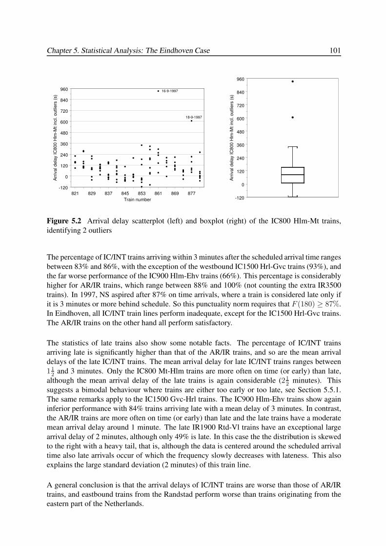
Chapter 5. Statistical Analysis: The Eindhoven Case 101
821 829 837 845 853 861 869 877
Train number
-120
0
120
240
360
480
600
720
840
960
Arr
iva
l d
ela
y IC
80
0 H
lm-M
t in
cl. o
utlie
rs (
s)
16-9-1997
18-9-1997
-120
0
120
240
360
480
600
720
840
960
Arr
iva
l d
ela
y IC
80
0 H
lm-M
t in
cl. o
utlie
rs (
s)
Figure 5.2 Arrival delay scatterplot (left) and boxplot (right) of the IC800 Hlm-Mt trains,
identifying 2 outliers
The percentage of IC/INT trains arriving within 3 minutes after the scheduled arrival time ranges
between 83% and 86%, with the exception of the westbound IC1500 Hrl-Gvc trains (93%), and
the far worse performance of the IC900 Hlm-Ehv trains (66%). This percentage is considerably
higher for AR/IR trains, which range between 88% and 100% (not counting the extra IR3500
trains). In 1997, NS aspired after 87% on time arrivals, where a train is considered late only if
it is 3 minutes or more behind schedule. So this punctuality norm requires that F (180) ≥ 87%.
In Eindhoven, all IC/INT train lines perform inadequate, except for the IC1500 Hrl-Gvc trains.
The AR/IR trains on the other hand all perform satisfactory.
The statistics of late trains also show some notable facts. The percentage of IC/INT trains
arriving late is significantly higher than that of the AR/IR trains, and so are the mean arrival
delays of the late IC/INT trains. The mean arrival delay for late IC/INT trains ranges between
112
and 3 minutes. Only the IC800 Mt-Hlm trains are more often on time (or early) than late,
although the mean arrival delay of the late trains is again considerable (212
minutes). This
suggests a bimodal behaviour where trains are either too early or too late, see Section 5.5.1.
The same remarks apply to the IC1500 Gvc-Hrl trains. The IC900 Hlm-Ehv trains show again
inferior performance with 84% trains arriving late with a mean delay of 3 minutes. In contrast,
the AR/IR trains are more often on time (or early) than late and the late trains have a moderate
mean arrival delay around 1 minute. The late IR1900 Rtd-Vl trains have an exceptional large
arrival delay of 2 minutes, although only 49% is late. In this case the the distribution is skewed
to the right with a heavy tail, that is, although the data is centered around the scheduled arrival
time also late arrivals occur of which the frequency slowly decreases with lateness. This also
explains the large standard deviation (2 minutes) of this train line.
A general conclusion is that the arrival delays of IC/INT trains are worse than those of AR/IR
trains, and eastbound trains from the Randstad perform worse than trains originating from the
eastern part of the Netherlands.
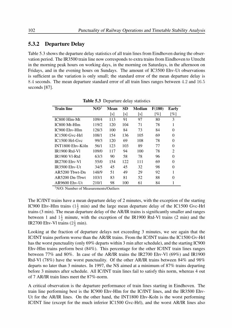
102 Punctuality of Railway Operations and Timetable Stability Analysis
5.3.2 Departure Delay
Table 5.3 shows the departure delay statistics of all train lines from Eindhoven during the obser-
vation period. The IR3500 train line now corresponds to extra trains from Eindhoven to Utrecht
in the morning peak hours on working days, in the morning on Saturdays, in the afternoon on
Fridays, and in the evening hours on Sundays. The amount of IC3500 Ehv-Ut observations
is sufficient as the variation is only small; the standard error of the mean departure delay is
8.4 seconds. The mean departure standard error of all train lines ranges between 4.2 and 16.5seconds [87].
Table 5.3 Departure delay statistics
Train line N/O1 Mean SD Median F(180) Early
[s] [s] [s] [%] [%]
IC800 Hlm-Mt 109/4 113 91 97 80 3
IC800 Mt-Hlm 119/2 120 104 71 78 1
IC900 Ehv-Hlm 128/3 100 84 73 84 0
IC1500 Gvc-Hrl 108/1 154 136 105 69 0
IC1500 Hrl-Gvc 99/3 120 69 108 78 0
INT1800 Ehv-Koln 56/1 123 103 89 77 0
IR1900 Rtd-Vl 109/0 117 94 100 78 2
IR1900 Vl-Rtd 63/3 90 58 78 96 0
IR2700 Ehv-Vl 55/0 154 122 111 69 0
IR3500 Ehv-Ut 34/5 45 45 32 98 0
AR5200 Tbwt-Dn 148/9 51 49 29 92 1
AR5200 Dn-Tbwt 103/1 83 81 52 88 0
AR9600 Ehv-Ut 210/1 98 100 61 84 11N/O: Number of Measurements/Outliers
The IC/INT trains have a mean departure delay of 2 minutes, with the exception of the starting
IC900 Ehv-Hlm trains (112
min) and the large mean departure delay of the IC1500 Gvc-Hrl
trains (3 min). The mean departure delay of the AR/IR trains is significantly smaller and ranges
between 1 and 112
minute, with the exception of the IR1900 Rtd-Vl trains (2 min) and the
IR2700 Ehv-Vl trains (212
min).
Looking at the fraction of departure delays not exceeding 3 minutes, we see again that the
IC/INT trains perform worse than the AR/IR trains. From the IC/INT trains the IC1500 Gv-Hrl
has the worst punctuality (only 69% departs within 3 min after schedule), and the starting IC900
Ehv-Hlm trains perform best (84%). This percentage for the other IC/INT train lines ranges
between 77% and 80%. In case of the AR/IR trains the IR2700 Ehv-Vl (69%) and IR1900
Rtd-Vl (78%) have the worst punctuality. Of the other AR/IR trains between 84% and 98%
departs no later than 3 minutes. In 1997, the NS aimed at a minimum of 87% trains departing
before 3 minutes after schedule. All IC/INT train lines fail to satisfy this norm, whereas 4 out
of 7 AR/IR train lines meet the 87%-norm.
A critical observation is the departure performance of train lines starting in Eindhoven. The
train line performing best is the IC900 Ehv-Hlm for the IC/INT lines, and the IR3500 Ehv-
Ut for the AR/IR lines. On the other hand, the INT1800 Ehv-Koln is the worst performing
IC/INT line (except for the much inferior IC1500 Gvc-Hrl), and the worst AR/IR lines also
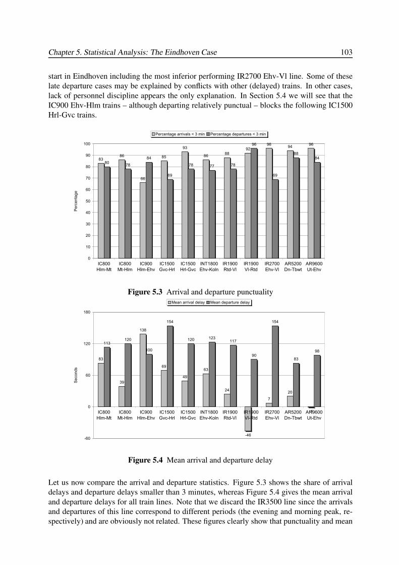
Chapter 5. Statistical Analysis: The Eindhoven Case 103
start in Eindhoven including the most inferior performing IR2700 Ehv-Vl line. Some of these
late departure cases may be explained by conflicts with other (delayed) trains. In other cases,
lack of personnel discipline appears the only explanation. In Section 5.4 we will see that the
IC900 Ehv-Hlm trains – although departing relatively punctual – blocks the following IC1500
Hrl-Gvc trains.
8386
66
85
93
8688
9296
9496
8078
84
69
78 77 78
96
69
8884
0
10
20
30
40
50
60
70
80
90
100
IC800
Hlm-Mt
IC800
Mt-Hlm
IC900
Hlm-Ehv
IC1500
Gvc-Hrl
IC1500
Hrl-Gvc
INT1800
Ehv-Koln
IR1900
Rtd-Vl
IR1900
Vl-Rtd
IR2700
Ehv-Vl
AR5200
Dn-Tbwt
AR9600
Ut-Ehv
Pe
rce
nta
ge
Percentage arrivals < 3 min Percentage departures < 3 min
Figure 5.3 Arrival and departure punctuality
83
39
138
69
49
63
24
-46
7
20
-1
113120
100
154
120 123117
90
154
83
98
-60
0
60
120
180
IC800
Hlm-Mt
IC800
Mt-Hlm
IC900
Hlm-Ehv
IC1500
Gvc-Hrl
IC1500
Hrl-Gvc
INT1800
Ehv-Koln
IR1900
Rtd-Vl
IR1900
Vl-Rtd
IR2700
Ehv-Vl
AR5200
Dn-Tbwt
AR9600
Ut-Ehv
Se
co
nd
s
Mean arrival delay Mean departure delay
Figure 5.4 Mean arrival and departure delay
Let us now compare the arrival and departure statistics. Figure 5.3 shows the share of arrival
delays and departure delays smaller than 3 minutes, whereas Figure 5.4 gives the mean arrival
and departure delays for all train lines. Note that we discard the IR3500 line since the arrivals
and departures of this line correspond to different periods (the evening and morning peak, re-
spectively) and are obviously not related. These figures clearly show that punctuality and mean
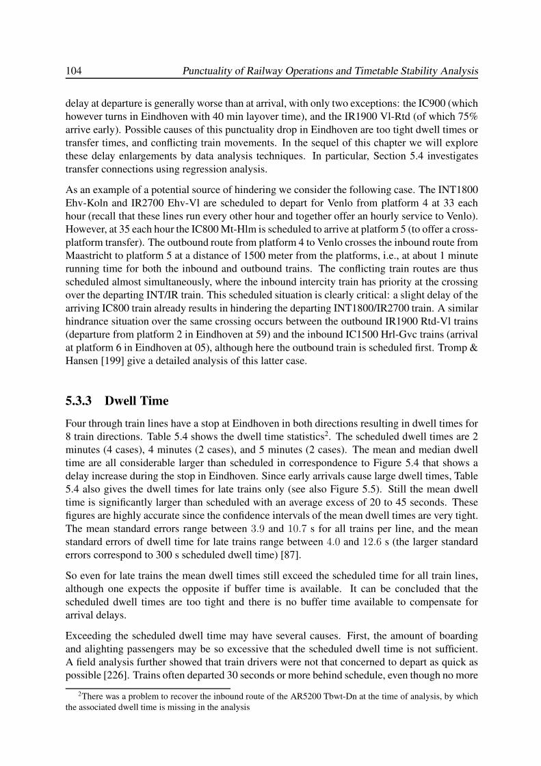
104 Punctuality of Railway Operations and Timetable Stability Analysis
delay at departure is generally worse than at arrival, with only two exceptions: the IC900 (which
however turns in Eindhoven with 40 min layover time), and the IR1900 Vl-Rtd (of which 75%
arrive early). Possible causes of this punctuality drop in Eindhoven are too tight dwell times or
transfer times, and conflicting train movements. In the sequel of this chapter we will explore
these delay enlargements by data analysis techniques. In particular, Section 5.4 investigates
transfer connections using regression analysis.
As an example of a potential source of hindering we consider the following case. The INT1800
Ehv-Koln and IR2700 Ehv-Vl are scheduled to depart for Venlo from platform 4 at 33 each
hour (recall that these lines run every other hour and together offer an hourly service to Venlo).
However, at 35 each hour the IC800 Mt-Hlm is scheduled to arrive at platform 5 (to offer a cross-
platform transfer). The outbound route from platform 4 to Venlo crosses the inbound route from
Maastricht to platform 5 at a distance of 1500 meter from the platforms, i.e., at about 1 minute
running time for both the inbound and outbound trains. The conflicting train routes are thus
scheduled almost simultaneously, where the inbound intercity train has priority at the crossing
over the departing INT/IR train. This scheduled situation is clearly critical: a slight delay of the
arriving IC800 train already results in hindering the departing INT1800/IR2700 train. A similar
hindrance situation over the same crossing occurs between the outbound IR1900 Rtd-Vl trains
(departure from platform 2 in Eindhoven at 59) and the inbound IC1500 Hrl-Gvc trains (arrival
at platform 6 in Eindhoven at 05), although here the outbound train is scheduled first. Tromp &
Hansen [199] give a detailed analysis of this latter case.
5.3.3 Dwell Time
Four through train lines have a stop at Eindhoven in both directions resulting in dwell times for
8 train directions. Table 5.4 shows the dwell time statistics2. The scheduled dwell times are 2
minutes (4 cases), 4 minutes (2 cases), and 5 minutes (2 cases). The mean and median dwell
time are all considerable larger than scheduled in correspondence to Figure 5.4 that shows a
delay increase during the stop in Eindhoven. Since early arrivals cause large dwell times, Table
5.4 also gives the dwell times for late trains only (see also Figure 5.5). Still the mean dwell
time is significantly larger than scheduled with an average excess of 20 to 45 seconds. These
figures are highly accurate since the confidence intervals of the mean dwell times are very tight.
The mean standard errors range between 3.9 and 10.7 s for all trains per line, and the mean
standard errors of dwell time for late trains range between 4.0 and 12.6 s (the larger standard
errors correspond to 300 s scheduled dwell time) [87].
So even for late trains the mean dwell times still exceed the scheduled time for all train lines,
although one expects the opposite if buffer time is available. It can be concluded that the
scheduled dwell times are too tight and there is no buffer time available to compensate for
arrival delays.
Exceeding the scheduled dwell time may have several causes. First, the amount of boarding
and alighting passengers may be so excessive that the scheduled dwell time is not sufficient.
A field analysis further showed that train drivers were not that concerned to depart as quick as
possible [226]. Trains often departed 30 seconds or more behind schedule, even though no more
2There was a problem to recover the inbound route of the AR5200 Tbwt-Dn at the time of analysis, by which
the associated dwell time is missing in the analysis
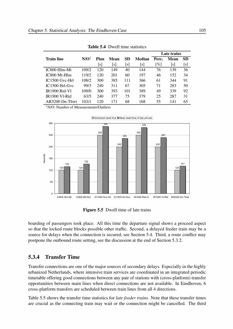
Chapter 5. Statistical Analysis: The Eindhoven Case 105
Table 5.4 Dwell time statistics
Late trains
Train line N/O1 Plan Mean SD Median Perc. Mean SD
[s] [s] [s] [s] [%] [s] [s]
IC800 Hlm-Mt 109/2 120 149 40 144 76 139 36
IC800 Mt-Hlm 119/2 120 201 60 197 46 152 34
IC1500 Gvc-Hrl 108/2 300 385 111 366 61 344 91
IC1500 Hrl-Gvc 99/3 240 311 67 305 71 283 50
IR1900 Rtd-Vl 109/0 300 393 101 389 49 339 92
IR1900 Vl-Rtd 63/5 240 377 75 379 25 287 31
AR5200 Dn-Tbwt 103/1 120 171 68 168 55 141 651N/O: Number of Measurements/Outliers
120 120
300
240
300
240
120
139152
344
283
339
287
141
0
60
120
180
240
300
360
IC800 Hlm-Mt IC800 Mt-Hlm IC1500 Gvc-Hrl IC1500 Hrl-Gvc IR1900 Rtd-Vl IR1900 Vl-Rtd AR5200 Dn-Tbwt
Se
co
nd
s
Scheduled dwell time Mean dwell time of late arrivals
Figure 5.5 Dwell time of late trains
boarding of passengers took place. All this time the departure signal shows a proceed aspect
so that the locked route blocks possible other traffic. Second, a delayed feeder train may be a
source for delays when the connection is secured, see Section 5.4. Third, a route conflict may
postpone the outbound route setting, see the discussion at the end of Section 5.3.2.
5.3.4 Transfer Time
Transfer connections are one of the major sources of secondary delays. Especially in the highly
urbanized Netherlands, where intensive train services are coordinated in an integrated periodic
timetable offering good connections between any pair of stations with (cross-platform) transfer
opportunities between main lines when direct connections are not available. In Eindhoven, 6
cross-platform transfers are scheduled between train lines from all 4 directions.
Table 5.5 shows the transfer time statistics for late feeder trains. Note that these transfer times
are crucial as the connecting train may wait or the connection might be cancelled. The third
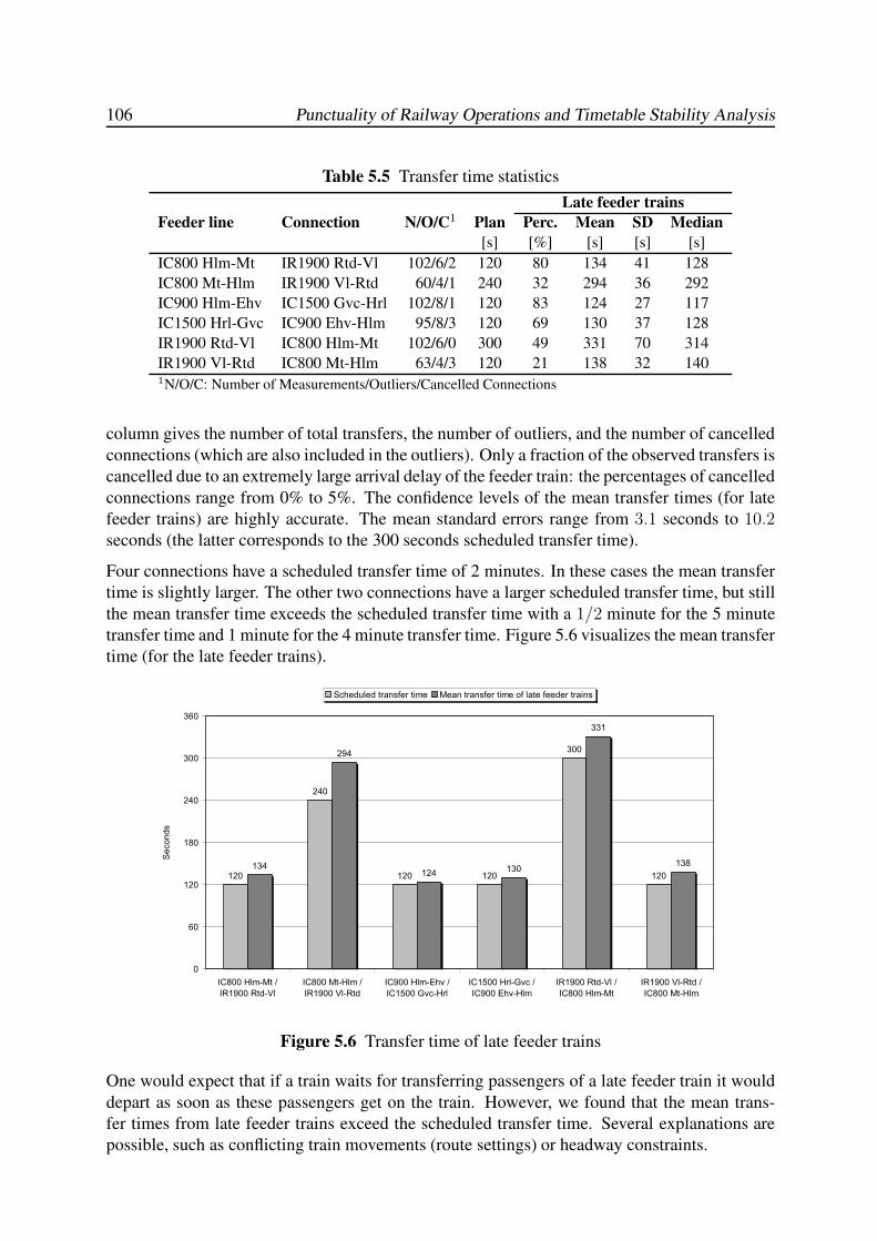
106 Punctuality of Railway Operations and Timetable Stability Analysis
Table 5.5 Transfer time statistics
Late feeder trains
Feeder line Connection N/O/C1 Plan Perc. Mean SD Median
[s] [%] [s] [s] [s]
IC800 Hlm-Mt IR1900 Rtd-Vl 102/6/2 120 80 134 41 128
IC800 Mt-Hlm IR1900 Vl-Rtd 60/4/1 240 32 294 36 292
IC900 Hlm-Ehv IC1500 Gvc-Hrl 102/8/1 120 83 124 27 117
IC1500 Hrl-Gvc IC900 Ehv-Hlm 95/8/3 120 69 130 37 128
IR1900 Rtd-Vl IC800 Hlm-Mt 102/6/0 300 49 331 70 314
IR1900 Vl-Rtd IC800 Mt-Hlm 63/4/3 120 21 138 32 1401N/O/C: Number of Measurements/Outliers/Cancelled Connections
column gives the number of total transfers, the number of outliers, and the number of cancelled
connections (which are also included in the outliers). Only a fraction of the observed transfers is
cancelled due to an extremely large arrival delay of the feeder train: the percentages of cancelled
connections range from 0% to 5%. The confidence levels of the mean transfer times (for late
feeder trains) are highly accurate. The mean standard errors range from 3.1 seconds to 10.2seconds (the latter corresponds to the 300 seconds scheduled transfer time).
Four connections have a scheduled transfer time of 2 minutes. In these cases the mean transfer
time is slightly larger. The other two connections have a larger scheduled transfer time, but still
the mean transfer time exceeds the scheduled transfer time with a 1/2 minute for the 5 minute
transfer time and 1 minute for the 4 minute transfer time. Figure 5.6 visualizes the mean transfer
time (for the late feeder trains).
120
240
120 120
300
120134
294
124130
331
138
0
60
120
180
240
300
360
IC800 Hlm-Mt /
IR1900 Rtd-Vl
IC800 Mt-Hlm /
IR1900 Vl-Rtd
IC900 Hlm-Ehv /
IC1500 Gvc-Hrl
IC1500 Hrl-Gvc /
IC900 Ehv-Hlm
IR1900 Rtd-Vl /
IC800 Hlm-Mt
IR1900 Vl-Rtd /
IC800 Mt-Hlm
Se
co
nd
s
Scheduled transfer time Mean transfer time of late feeder trains
Figure 5.6 Transfer time of late feeder trains
One would expect that if a train waits for transferring passengers of a late feeder train it would
depart as soon as these passengers get on the train. However, we found that the mean trans-
fer times from late feeder trains exceed the scheduled transfer time. Several explanations are
possible, such as conflicting train movements (route settings) or headway constraints.
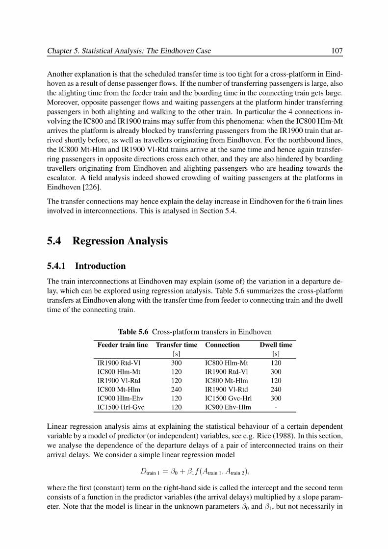
Chapter 5. Statistical Analysis: The Eindhoven Case 107
Another explanation is that the scheduled transfer time is too tight for a cross-platform in Eind-
hoven as a result of dense passenger flows. If the number of transferring passengers is large, also
the alighting time from the feeder train and the boarding time in the connecting train gets large.
Moreover, opposite passenger flows and waiting passengers at the platform hinder transferring
passengers in both alighting and walking to the other train. In particular the 4 connections in-
volving the IC800 and IR1900 trains may suffer from this phenomena: when the IC800 Hlm-Mt
arrives the platform is already blocked by transferring passengers from the IR1900 train that ar-
rived shortly before, as well as travellers originating from Eindhoven. For the northbound lines,
the IC800 Mt-Hlm and IR1900 Vl-Rtd trains arrive at the same time and hence again transfer-
ring passengers in opposite directions cross each other, and they are also hindered by boarding
travellers originating from Eindhoven and alighting passengers who are heading towards the
escalator. A field analysis indeed showed crowding of waiting passengers at the platforms in
Eindhoven [226].
The transfer connections may hence explain the delay increase in Eindhoven for the 6 train lines
involved in interconnections. This is analysed in Section 5.4.
5.4 Regression Analysis
5.4.1 Introduction
The train interconnections at Eindhoven may explain (some of) the variation in a departure de-
lay, which can be explored using regression analysis. Table 5.6 summarizes the cross-platform
transfers at Eindhoven along with the transfer time from feeder to connecting train and the dwell
time of the connecting train.
Table 5.6 Cross-platform transfers in Eindhoven
Feeder train line Transfer time Connection Dwell time
[s] [s]
IR1900 Rtd-Vl 300 IC800 Hlm-Mt 120
IC800 Hlm-Mt 120 IR1900 Rtd-Vl 300
IR1900 Vl-Rtd 120 IC800 Mt-Hlm 120
IC800 Mt-Hlm 240 IR1900 Vl-Rtd 240
IC900 Hlm-Ehv 120 IC1500 Gvc-Hrl 300
IC1500 Hrl-Gvc 120 IC900 Ehv-Hlm -
Linear regression analysis aims at explaining the statistical behaviour of a certain dependent
variable by a model of predictor (or independent) variables, see e.g. Rice (1988). In this section,
we analyse the dependence of the departure delays of a pair of interconnected trains on their
arrival delays. We consider a simple linear regression model
Dtrain 1 = β0 + β1f(Atrain 1, Atrain 2),
where the first (constant) term on the right-hand side is called the intercept and the second term
consists of a function in the predictor variables (the arrival delays) multiplied by a slope param-
eter. Note that the model is linear in the unknown parameters β0 and β1, but not necessarily in
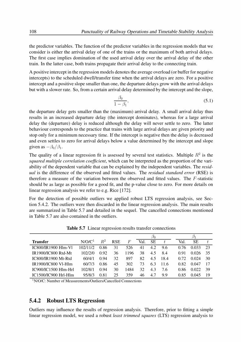
108 Punctuality of Railway Operations and Timetable Stability Analysis
the predictor variables. The function of the predictor variables in the regression models that we
consider is either the arrival delay of one of the trains or the maximum of both arrival delays.
The first case implies domination of the used arrival delay over the arrival delay of the other
train. In the latter case, both trains propagate their arrival delay to the connecting train.
A positive intercept in the regression models denotes the average overload (or buffer for negative
intercepts) to the scheduled dwell/transfer time when the arrival delays are zero. For a positive
intercept and a positive slope smaller than one, the departure delays grow with the arrival delays
but with a slower rate. So, from a certain arrival delay determined by the intercept and the slope,
β0
1− β1, (5.1)
the departure delay gets smaller than the (maximum) arrival delay. A small arrival delay thus
results in an increased departure delay (the intercept dominates), whereas for a large arrival
delay the (departure) delay is reduced although the delay will never settle to zero. The latter
behaviour corresponds to the practice that trains with large arrival delays are given priority and
stop only for a minimum necessary time. If the intercept is negative then the delay is decreased
and even settles to zero for arrival delays below a value determined by the intercept and slope
given as −β0/β1.
The quality of a linear regression fit is assessed by several test statistics. Multiple R2 is the
squared multiple correlation coefficient, which can be interpreted as the proportion of the vari-
ability of the dependent variable that can be explained by the independent variables. The resid-
ual is the difference of the observed and fitted values. The residual standard error (RSE) is
therefore a measure of the variation between the observed and fitted values. The F -statistic
should be as large as possible for a good fit, and the p-value close to zero. For more details on
linear regression analysis we refer to e.g. Rice [172].
For the detection of possible outliers we applied robust LTS regression analysis, see Sec-
tion 5.4.2. The outliers were then discarded in the linear regression analysis. The main results
are summarized in Table 5.7 and detailed in the sequel. The cancelled connections mentioned
in Table 5.7 are also contained in the outliers.
Table 5.7 Linear regression results transfer connections
β0 β1
Transfer N/O/C1 R2 RSE F Val. SE t Val. SE t
IC800/IR1900 Hlm-Vl 102/11/2 0.86 31 526 41 4.2 9.6 0.76 0.033 23
IR1900/IC800 Rtd-Mt 102/2/0 0.92 36 1196 38 4.5 8.4 0.91 0.026 35
IC800/IR1900 Mt-Rtd 60/4/1 0.94 32 897 82 4.5 18.4 0.72 0.024 30
IR1900/IC800 Vl-Hlm 60/7/3 0.86 45 302 73 6.3 11.6 0.82 0.047 17
IC900/IC1500 Hlm-Hrl 102/8/1 0.94 30 1484 32 4.3 7.6 0.86 0.022 39
IC1500/IC900 Hrl-Hlm 95/8/3 0.81 25 359 46 4.7 9.9 0.85 0.045 191N/O/C: Number of Measurements/Outliers/Cancelled Connections
5.4.2 Robust LTS Regression
Outliers may influence the results of regression analysis. Therefore, prior to fitting a simple
linear regression model, we used a robust least trimmed squares (LTS) regression analysis to
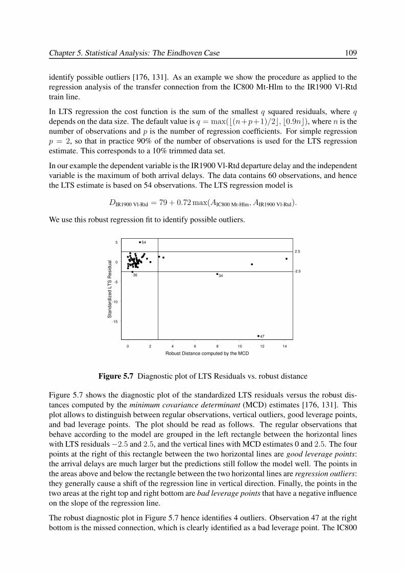
Chapter 5. Statistical Analysis: The Eindhoven Case 109
identify possible outliers [176, 131]. As an example we show the procedure as applied to the
regression analysis of the transfer connection from the IC800 Mt-Hlm to the IR1900 Vl-Rtd
train line.
In LTS regression the cost function is the sum of the smallest q squared residuals, where qdepends on the data size. The default value is q = max(b(n+p+1)/2c, b0.9nc), where n is the
number of observations and p is the number of regression coefficients. For simple regression
p = 2, so that in practice 90% of the number of observations is used for the LTS regression
estimate. This corresponds to a 10% trimmed data set.
In our example the dependent variable is the IR1900 Vl-Rtd departure delay and the independent
variable is the maximum of both arrival delays. The data contains 60 observations, and hence
the LTS estimate is based on 54 observations. The LTS regression model is
DIR1900 Vl-Rtd = 79 + 0.72 max(AIC800 Mt-Hlm, AIR1900 Vl-Rtd).
We use this robust regression fit to identify possible outliers.
0 2 4 6 8 10 12 14
Robust Distance computed by the MCD
-15
-10
-5
0
5
Sta
ndard
ized L
TS
Resid
ual
36
54
34
47
-2.5
2.5
Figure 5.7 Diagnostic plot of LTS Residuals vs. robust distance
Figure 5.7 shows the diagnostic plot of the standardized LTS residuals versus the robust dis-
tances computed by the minimum covariance determinant (MCD) estimates [176, 131]. This
plot allows to distinguish between regular observations, vertical outliers, good leverage points,
and bad leverage points. The plot should be read as follows. The regular observations that
behave according to the model are grouped in the left rectangle between the horizontal lines
with LTS residuals−2.5 and 2.5, and the vertical lines with MCD estimates 0 and 2.5. The four
points at the right of this rectangle between the two horizontal lines are good leverage points:
the arrival delays are much larger but the predictions still follow the model well. The points in
the areas above and below the rectangle between the two horizontal lines are regression outliers:
they generally cause a shift of the regression line in vertical direction. Finally, the points in the
two areas at the right top and right bottom are bad leverage points that have a negative influence
on the slope of the regression line.
The robust diagnostic plot in Figure 5.7 hence identifies 4 outliers. Observation 47 at the right
bottom is the missed connection, which is clearly identified as a bad leverage point. The IC800
110 Punctuality of Railway Operations and Timetable Stability Analysis
arrival delay is 836 s, whereas the IR1900 delay has only a small departure delay of 39 s. A
second bad leverage point is observation 34, which corresponds to 577 s arrival delay of the
IR1900 train and a departure delay of 388 s. Furthermore, two regression outliers are detected:
Observation 36 consists of a 43 s arrival delay of the IC800 train and a departure delay of 20 s.
And finally, observation 54 where both trains arrive early (63 s and 70 s, respectively) but the
departure is 200 s delayed.
The next step is to remove the 4 outliers from the data and use a simple linear regression analysis
on the remaining data to obtain a final regression fit. In Table 5.7 we see that the final regression
fit is obtained as
DIR1900 Vl-Rtd = 82 + 0.72 max(AIC800 Mt-Hlm, AIR1900 Vl-Rtd),
which differs from the LTS regression fit only in the intercept with 3 seconds. Note that these
regression coefficients may differ from the LTS regression estimate since the linear regression fit
is based on more observations, assuming that the number of outliers does not exceed 10% of the
total number of observations. Despite the relatively small number of observations (60−4 = 56)
for the above regression fit, the fit performs remarkably well with an explained variation of
R2 = 94% and a residual standard error of RSE = 32 seconds. For an interpretation of the
results see Section 5.4.4.
5.4.3 Transfers between IC800 Hlm-Mt and IR1900 Rtd-Vl
The eastbound IR1900 and IC800 trains run in this order from Boxtel to Eindhoven over the
same track. The IC800 trains are scheduled to arrive 3 minutes after the IR1900 trains after
which 2 minutes later both trains depart in their respective directions. This timing allows a
cross-platform transfer between both trains with a transfer time of 5 and 2 minutes, respectively.
The regression model that performs best in explaining the departure of the IC800 trains to
Maastricht from the arrival delays is
DIC800 Hlm-Mt = 38 + 0.91AIC800 Hlm-Mt,
where D800Hlm-Mt is the departure delay of the IC800 trains at Eindhoven in the direction
Maastricht, and A800Hlm-Mt its arrival delay, see Figure 5.8. This model explains 92% of the
variation of the departure delay with a residual standard error of 36 seconds. Detailed regression
results are presented in Table 5.7. Apparently, the departure of IC800 trains to Maastricht does
not depend on the arrival of the feeder IR1900 trains from Rotterdam. Recall however that the
IR1900 and IC800 trains approach Eindhoven in this order over the same double-track route
from Boxtel. In all observations this order is respected, and hence a large IR1900 arrival delay
also resulted in a large IC800 delay.
The regression model of the departure of the IR1900 trains to Venlo that performs best is
DIR1900 Rtd-Vl = 41 + 0.76AIC800 Hlm-Mt,
which explains 86% of the variation of the departure delay with a residual standard error of 31
seconds, see Figure 5.8. Table 5.7 contains the detailed regression results. The departure time
of the IC 1900 trains to Venlo also depends only on the arrival delay of the feeder IC 800 trains
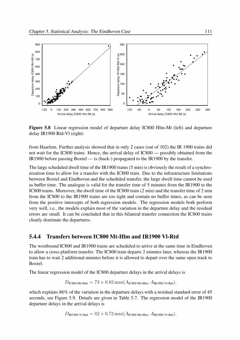
Chapter 5. Statistical Analysis: The Eindhoven Case 111
-120 0 120 240 360 480 600 720 840 960
Arrival delay IC800 Hlm-Mt (s)
0
120
240
360
480
600
720
840
960
De
pa
rtu
re d
ela
y IC
80
0 H
lm-M
t (s
)
-120 -60 0 60 120 180 240 300 360
Arrival delay IC800 Hlm-Mt (s)
0
60
120
180
240
300
360
De
pa
rtu
re d
ela
y IR
19
00
Rtd
-Vl (s
)
Figure 5.8 Linear regression model of departure delay IC800 Hlm-Mt (left) and departure
delay IR1900 Rtd-Vl (right)
from Haarlem. Further analysis showed that in only 2 cases (out of 102) the IR 1900 trains did
not wait for the IC800 trains. Hence, the arrival delay of IC800 — possibly obtained from the
IR1900 before passing Boxtel — is (back-) propagated to the IR1900 by the transfer.
The large scheduled dwell time of the IR1900 trains (5 min) is obviously the result of a synchro-
nization time to allow for a transfer with the IC800 train. Due to the infrastructure limitations
between Boxtel and Eindhoven and the scheduled transfer, the large dwell time cannot be used
as buffer time. The analogue is valid for the transfer time of 5 minutes from the IR1900 to the
IC800 trains. Moreover, the dwell time of the IC800 train (2 min) and the transfer time of 2 min
from the IC800 to the IR1900 trains are too tight and contain no buffer times, as can be seen
from the positive intercepts of both regression models. The regression models both perform
very well, i.e., the models explain most of the variation in the departure delay and the residual
errors are small. It can be concluded that in this bilateral transfer connection the IC800 trains
clearly dominate the departures.
5.4.4 Transfers between IC800 Mt-Hlm and IR1900 Vl-Rtd
The westbound IC800 and IR1900 trains are scheduled to arrive at the same time in Eindhoven
to allow a cross-platform transfer. The IC800 train departs 2 minutes later, whereas the IR1900
train has to wait 2 additional minutes before it is allowed to depart over the same open track to
Boxtel.
The linear regression model of the IC800 departure delays in the arrival delays is
DIC800 Mt-Hlm = 73 + 0.82 max(AIC800 Mt-Hlm, AIR1900 Vl-Rtd),
which explains 86% of the variation in the departure delays with a residual standard error of 45
seconds, see Figure 5.9. Details are given in Table 5.7. The regression model of the IR1900
departure delays in the arrival delays is
DIR1900 Vl-Rtd = 82 + 0.72 max(AIC800 Mt-Hlm, AIR1900 Vl-Rtd),
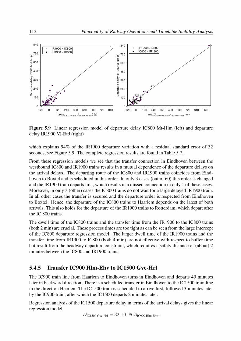
112 Punctuality of Railway Operations and Timetable Stability Analysis
-120 0 120 240 360 480 600 720 840
max(AIC800 Mt-Hlm ,AIR1900 Vl-Rtd ) (s)
0
120
240
360
480
600
720
840
De
pa
rtu
re d
ela
y IC
80
0 M
t-H
lm (
s)
IR1900 > IC800
IR1900 > IC800
-120 0 120 240 360 480 600 720 840 960
max(AIC800 Mt-Hlm ,AIR1900 Vl-Rtd ) (s)
0
120
240
360
480
600
720
840
De
pa
rtu
re d
ela
y IR
19
00
Vl-R
td (
s)
IR1900 > IC800
IC800 > IR1900
Figure 5.9 Linear regression model of departure delay IC800 Mt-Hlm (left) and departure
delay IR1900 Vl-Rtd (right)
which explains 94% of the IR1900 departure variation with a residual standard error of 32
seconds, see Figure 5.9. The complete regression results are found in Table 5.7.
From these regression models we see that the transfer connection in Eindhoven between the
westbound IC800 and IR1900 trains results in a mutual dependence of the departure delays on
the arrival delays. The departing route of the IC800 and IR1900 trains coincides from Eind-
hoven to Boxtel and is scheduled in this order. In only 3 cases (out of 60) this order is changed
and the IR1900 train departs first, which results in a missed connection in only 1 of these cases.
Moreover, in only 3 (other) cases the IC800 trains do not wait for a large delayed IR1900 train.
In all other cases the transfer is secured and the departure order is respected from Eindhoven
to Boxtel. Hence, the departure of the IC800 trains to Haarlem depends on the latest of both
arrivals. This also holds for the departure of the IR1900 trains to Rotterdam, which depart after
the IC 800 trains.
The dwell time of the IC800 trains and the transfer time from the IR1900 to the IC800 trains
(both 2 min) are crucial. These process times are too tight as can be seen from the large intercept
of the IC800 departure regression model. The larger dwell time of the IR1900 trains and the
transfer time from IR1900 to IC800 (both 4 min) are not effective with respect to buffer time
but result from the headway departure constraint, which requires a safety distance of (about) 2
minutes between the IC800 and IR1900 trains.
5.4.5 Transfer IC900 Hlm-Ehv to IC1500 Gvc-Hrl
The IC900 train line from Haarlem to Eindhoven turns in Eindhoven and departs 40 minutes
later in backward direction. There is a scheduled transfer in Eindhoven to the IC1500 train line
in the direction Heerlen. The IC1500 train is scheduled to arrive first, followed 3 minutes later
by the IC900 train, after which the IC1500 departs 2 minutes later.
Regression analysis of the IC1500 departure delay in terms of the arrival delays gives the linear
regression model
DIC1500 Gvc-Hrl = 32 + 0.86AIC900 Hlm-Ehv,
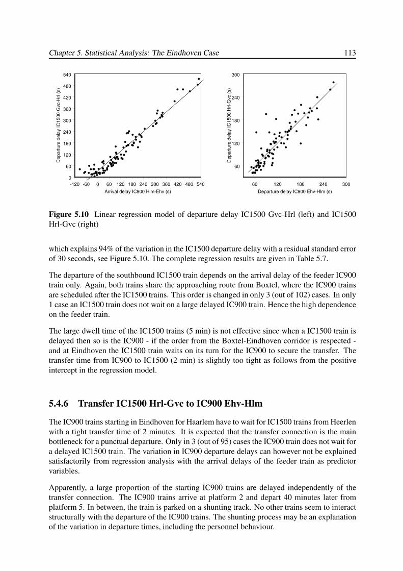
Chapter 5. Statistical Analysis: The Eindhoven Case 113
-120 -60 0 60 120 180 240 300 360 420 480 540
Arrival delay IC900 Hlm-Ehv (s)
0
60
120
180
240
300
360
420
480
540
De
pa
rtu
re d
ela
y IC
15
00
Gvc-H
rl (
s)
60 120 180 240 300
Departure delay IC900 Ehv-Hlm (s)
60
120
180
240
300
De
pa
rtu
re d
ela
y IC
15
00
Hrl-G
vc (
s)
Figure 5.10 Linear regression model of departure delay IC1500 Gvc-Hrl (left) and IC1500
Hrl-Gvc (right)
which explains 94% of the variation in the IC1500 departure delay with a residual standard error
of 30 seconds, see Figure 5.10. The complete regression results are given in Table 5.7.
The departure of the southbound IC1500 train depends on the arrival delay of the feeder IC900
train only. Again, both trains share the approaching route from Boxtel, where the IC900 trains
are scheduled after the IC1500 trains. This order is changed in only 3 (out of 102) cases. In only
1 case an IC1500 train does not wait on a large delayed IC900 train. Hence the high dependence
on the feeder train.
The large dwell time of the IC1500 trains (5 min) is not effective since when a IC1500 train is
delayed then so is the IC900 - if the order from the Boxtel-Eindhoven corridor is respected -
and at Eindhoven the IC1500 train waits on its turn for the IC900 to secure the transfer. The
transfer time from IC900 to IC1500 (2 min) is slightly too tight as follows from the positive
intercept in the regression model.
5.4.6 Transfer IC1500 Hrl-Gvc to IC900 Ehv-Hlm
The IC900 trains starting in Eindhoven for Haarlem have to wait for IC1500 trains from Heerlen
with a tight transfer time of 2 minutes. It is expected that the transfer connection is the main
bottleneck for a punctual departure. Only in 3 (out of 95) cases the IC900 train does not wait for
a delayed IC1500 train. The variation in IC900 departure delays can however not be explained
satisfactorily from regression analysis with the arrival delays of the feeder train as predictor
variables.
Apparently, a large proportion of the starting IC900 trains are delayed independently of the
transfer connection. The IC900 trains arrive at platform 2 and depart 40 minutes later from
platform 5. In between, the train is parked on a shunting track. No other trains seem to interact
structurally with the departure of the IC900 trains. The shunting process may be an explanation
of the variation in departure times, including the personnel behaviour.
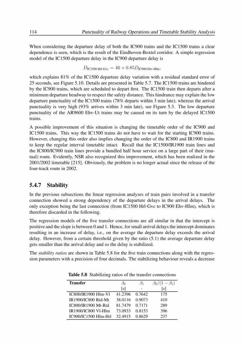
114 Punctuality of Railway Operations and Timetable Stability Analysis
When considering the departure delay of both the IC900 trains and the IC1500 trains a clear
dependence is seen, which is the result of the Eindhoven-Boxtel corridor. A simple regression
model of the IC1500 departure delay in the IC900 departure delay is
DIC1500 Hrl-Gvc = 46 + 0.85DIC900 Ehv-Hlm,
which explains 81% of the IC1500 departure delay variation with a residual standard error of
25 seconds, see Figure 5.10. Details are presented in Table 5.7. The IC1500 trains are hindered
by the IC900 trains, which are scheduled to depart first. The IC1500 train then departs after a
minimum departure headway to respect the safety distance. This hindrance may explain the low
departure punctuality of the IC1500 trains (78% departs within 3 min late), whereas the arrival
punctuality is very high (93% arrives within 3 min late), see Figure 5.3. The low departure
punctuality of the AR9600 Ehv-Ut trains may be caused on its turn by the delayed IC1500
trains.
A possible improvement of this situation is changing the timetable order of the IC900 and
IC1500 trains. This way the IC1500 trains do not have to wait for the starting IC900 trains.
However, changing this order also implies changing the order of the IC800 and IR1900 trains
to keep the regular interval timetable intact. Recall that the IC1500/IR1900 train lines and
the IC800/IC900 train lines provide a bundled half hour service on a large part of their (mu-
tual) route. Evidently, NSR also recognized this improvement, which has been realized in the
2001/2002 timetable [215]. Obviously, the problem is no longer actual since the release of the
four-track route in 2002.
5.4.7 Stability
In the previous subsections the linear regression analyses of train pairs involved in a transfer
connection showed a strong dependency of the departure delays in the arrival delays. The
only exception being the last connection (from IC1500 Hrl-Gvc to IC900 Ehv-Hlm), which is
therefore discarded in the following.
The regression models of the five transfer connections are all similar in that the intercept is
positive and the slope is between 0 and 1. Hence, for small arrival delays the intercept dominates
resulting in an increase of delay, i.e., on the average the departure delay exceeds the arrival
delay. However, from a certain threshold given by the ratio (5.1) the average departure delay
gets smaller than the arrival delay and so the delay is stabilized.
The stability ratios are shown in Table 5.8 for the five train connections along with the regres-
sion parameters with a precision of four decimals. The stabilizing behaviour reveals a decrease
Table 5.8 Stabilizing ratios of the transfer connections
Transfer β0 β1 β0/(1 − β1)[s] - [s]
IC800/IR1900 Hlm-Vl 41.2396 0.7642 175
IR1900/IC800 Rtd-Mt 38.0116 0.9073 410
IC800/IR1900 Mt-Rtd 81.7479 0.7171 289
IR1900/IC800 Vl-Hlm 73.0933 0.8153 396
IC900/IC1500 Hlm-Hrl 32.4915 0.8629 237
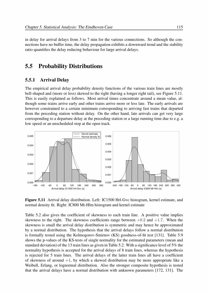
Chapter 5. Statistical Analysis: The Eindhoven Case 115
in delay for arrival delays from 3 to 7 min for the various connections. So although the con-
nections have no buffer time, the delay propagation exhibits a downward trend and the stability
ratio quantifies the delay reducing behaviour for large arrival delays.
5.5 Probability Distributions
5.5.1 Arrival Delay
The empirical arrival delay probability density functions of the various train lines are mostly
bell-shaped and (more or less) skewed to the right (having a longer right tail), see Figure 5.11.
This is easily explained as follows. Most arrival times concentrate around a mean value, al-
though some trains arrive early and other trains arrive more or less late. The early arrivals are
however constrained to a certain minimum corresponding to arriving fast trains that departed
from the preceding station without delay. On the other hand, late arrivals can get very large
corresponding to a departure delay at the preceding station or a large running time due to e.g. a
low speed or an unscheduled stop at the open track.
0.000
0.001
0.002
0.003
0.004
0.005Kernel estimate
Normal density fit
-180 -120 -60 0 60 120 180 240 300 360
Arrival delay IC1500 Hrl-Gvc (s)
0.000
0.001
0.002
0.003
0.004
0.005
0.006
-240 -180 -120 -60 0 60 120 180 240 300 360 420
Arrival delay IC800 Mt-Hlm (s)
Figure 5.11 Arrival delay distribution. Left: IC1500 Hrl-Gvc histogram, kernel estimate, and
normal density fit. Right: IC800 Mt-Hlm histogram and kernel estimate
Table 5.2 also gives the coefficient of skewness to each train line. A positive value implies
skewness to the right. The skewness coefficients range between +0.2 and +1.7. When the
skewness is small the arrival delay distribution is symmetric and may hence be approximated
by a normal distribution. The hypothesis that the arrival delays follow a normal distribution
is formally tested using the Kolmogorov-Smirnov (KS) goodness-of-fit test [131]. Table 5.9
shows the p-values of the KS-tests of single normality for the estimated parameters (mean and
standard deviation) of the 13 train lines as given in Table 5.2. With a significance level of 5% the
normality hypothesis is accepted for the arrival delays of 8 train lines, whereas the hypothesis
is rejected for 5 train lines. The arrival delays of the latter train lines all have a coefficient
of skewness of around +1, by which a skewed distribution may be more appropriate like a
Weibull, Erlang, or lognormal distribution. Also the stronger composite hypothesis is tested
that the arrival delays have a normal distribution with unknown parameters [172, 131]. The
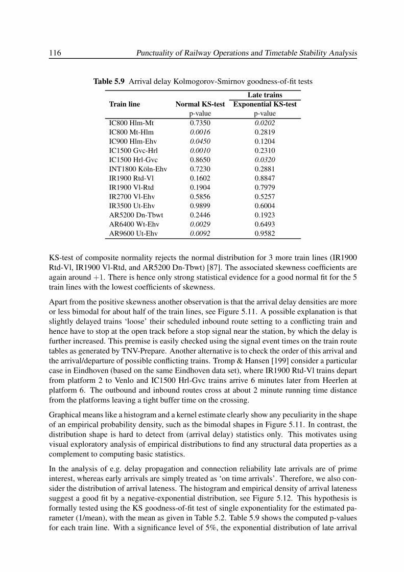
116 Punctuality of Railway Operations and Timetable Stability Analysis
Table 5.9 Arrival delay Kolmogorov-Smirnov goodness-of-fit tests
Late trains
Train line Normal KS-test Exponential KS-test
p-value p-value
IC800 Hlm-Mt 0.7350 0.0202
IC800 Mt-Hlm 0.0016 0.2819
IC900 Hlm-Ehv 0.0450 0.1204
IC1500 Gvc-Hrl 0.0010 0.2310
IC1500 Hrl-Gvc 0.8650 0.0320
INT1800 Koln-Ehv 0.7230 0.2881
IR1900 Rtd-Vl 0.1602 0.8847
IR1900 Vl-Rtd 0.1904 0.7979
IR2700 Vl-Ehv 0.5856 0.5257
IR3500 Ut-Ehv 0.9899 0.6004
AR5200 Dn-Tbwt 0.2446 0.1923
AR6400 Wt-Ehv 0.0029 0.6493
AR9600 Ut-Ehv 0.0092 0.9582
KS-test of composite normality rejects the normal distribution for 3 more train lines (IR1900
Rtd-Vl, IR1900 Vl-Rtd, and AR5200 Dn-Tbwt) [87]. The associated skewness coefficients are
again around +1. There is hence only strong statistical evidence for a good normal fit for the 5
train lines with the lowest coefficients of skewness.
Apart from the positive skewness another observation is that the arrival delay densities are more
or less bimodal for about half of the train lines, see Figure 5.11. A possible explanation is that
slightly delayed trains ‘loose’ their scheduled inbound route setting to a conflicting train and
hence have to stop at the open track before a stop signal near the station, by which the delay is
further increased. This premise is easily checked using the signal event times on the train route
tables as generated by TNV-Prepare. Another alternative is to check the order of this arrival and
the arrival/departure of possible conflicting trains. Tromp & Hansen [199] consider a particular
case in Eindhoven (based on the same Eindhoven data set), where IR1900 Rtd-Vl trains depart
from platform 2 to Venlo and IC1500 Hrl-Gvc trains arrive 6 minutes later from Heerlen at
platform 6. The outbound and inbound routes cross at about 2 minute running time distance
from the platforms leaving a tight buffer time on the crossing.
Graphical means like a histogram and a kernel estimate clearly show any peculiarity in the shape
of an empirical probability density, such as the bimodal shapes in Figure 5.11. In contrast, the
distribution shape is hard to detect from (arrival delay) statistics only. This motivates using
visual exploratory analysis of empirical distributions to find any structural data properties as a
complement to computing basic statistics.
In the analysis of e.g. delay propagation and connection reliability late arrivals are of prime
interest, whereas early arrivals are simply treated as ‘on time arrivals’. Therefore, we also con-
sider the distribution of arrival lateness. The histogram and empirical density of arrival lateness
suggest a good fit by a negative-exponential distribution, see Figure 5.12. This hypothesis is
formally tested using the KS goodness-of-fit test of single exponentiality for the estimated pa-
rameter (1/mean), with the mean as given in Table 5.2. Table 5.9 shows the computed p-values
for each train line. With a significance level of 5%, the exponential distribution of late arrival
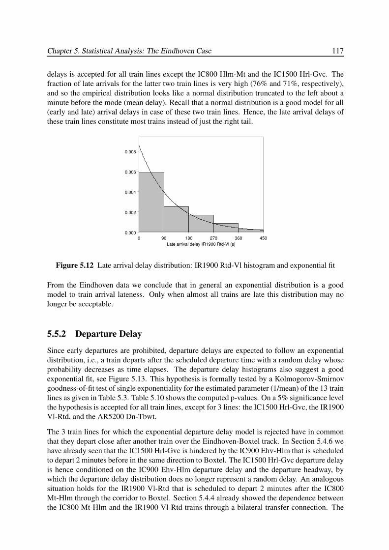
Chapter 5. Statistical Analysis: The Eindhoven Case 117
delays is accepted for all train lines except the IC800 Hlm-Mt and the IC1500 Hrl-Gvc. The
fraction of late arrivals for the latter two train lines is very high (76% and 71%, respectively),
and so the empirical distribution looks like a normal distribution truncated to the left about a
minute before the mode (mean delay). Recall that a normal distribution is a good model for all
(early and late) arrival delays in case of these two train lines. Hence, the late arrival delays of
these train lines constitute most trains instead of just the right tail.
0.000
0.002
0.004
0.006
0.008
0 90 180 270 360 450
Late arrival delay IR1900 Rtd-Vl (s)
Figure 5.12 Late arrival delay distribution: IR1900 Rtd-Vl histogram and exponential fit
From the Eindhoven data we conclude that in general an exponential distribution is a good
model to train arrival lateness. Only when almost all trains are late this distribution may no
longer be acceptable.
5.5.2 Departure Delay
Since early departures are prohibited, departure delays are expected to follow an exponential
distribution, i.e., a train departs after the scheduled departure time with a random delay whose
probability decreases as time elapses. The departure delay histograms also suggest a good
exponential fit, see Figure 5.13. This hypothesis is formally tested by a Kolmogorov-Smirnov
goodness-of-fit test of single exponentiality for the estimated parameter (1/mean) of the 13 train
lines as given in Table 5.3. Table 5.10 shows the computed p-values. On a 5% significance level
the hypothesis is accepted for all train lines, except for 3 lines: the IC1500 Hrl-Gvc, the IR1900
Vl-Rtd, and the AR5200 Dn-Tbwt.
The 3 train lines for which the exponential departure delay model is rejected have in common
that they depart close after another train over the Eindhoven-Boxtel track. In Section 5.4.6 we
have already seen that the IC1500 Hrl-Gvc is hindered by the IC900 Ehv-Hlm that is scheduled
to depart 2 minutes before in the same direction to Boxtel. The IC1500 Hrl-Gvc departure delay
is hence conditioned on the IC900 Ehv-Hlm departure delay and the departure headway, by
which the departure delay distribution does no longer represent a random delay. An analogous
situation holds for the IR1900 Vl-Rtd that is scheduled to depart 2 minutes after the IC800
Mt-Hlm through the corridor to Boxtel. Section 5.4.4 already showed the dependence between
the IC800 Mt-Hlm and the IR1900 Vl-Rtd trains through a bilateral transfer connection. The
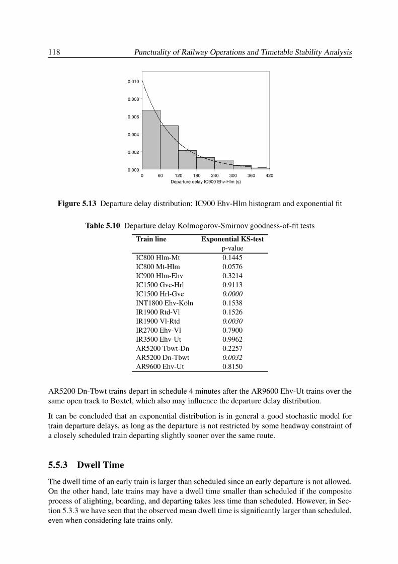
118 Punctuality of Railway Operations and Timetable Stability Analysis
0.000
0.002
0.004
0.006
0.008
0.010
0 60 120 180 240 300 360 420
Departure delay IC900 Ehv-Hlm (s)
Figure 5.13 Departure delay distribution: IC900 Ehv-Hlm histogram and exponential fit
Table 5.10 Departure delay Kolmogorov-Smirnov goodness-of-fit tests
Train line Exponential KS-test
p-value
IC800 Hlm-Mt 0.1445
IC800 Mt-Hlm 0.0576
IC900 Hlm-Ehv 0.3214
IC1500 Gvc-Hrl 0.9113
IC1500 Hrl-Gvc 0.0000
INT1800 Ehv-Koln 0.1538
IR1900 Rtd-Vl 0.1526
IR1900 Vl-Rtd 0.0030
IR2700 Ehv-Vl 0.7900
IR3500 Ehv-Ut 0.9962
AR5200 Tbwt-Dn 0.2257
AR5200 Dn-Tbwt 0.0032
AR9600 Ehv-Ut 0.8150
AR5200 Dn-Tbwt trains depart in schedule 4 minutes after the AR9600 Ehv-Ut trains over the
same open track to Boxtel, which also may influence the departure delay distribution.
It can be concluded that an exponential distribution is in general a good stochastic model for
train departure delays, as long as the departure is not restricted by some headway constraint of
a closely scheduled train departing slightly sooner over the same route.
5.5.3 Dwell Time
The dwell time of an early train is larger than scheduled since an early departure is not allowed.
On the other hand, late trains may have a dwell time smaller than scheduled if the composite
process of alighting, boarding, and departing takes less time than scheduled. However, in Sec-
tion 5.3.3 we have seen that the observed mean dwell time is significantly larger than scheduled,
even when considering late trains only.
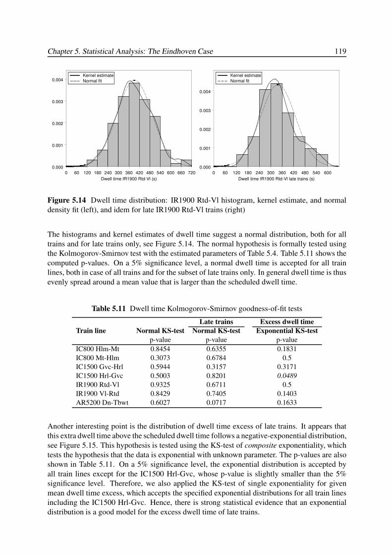
Chapter 5. Statistical Analysis: The Eindhoven Case 119
0.000
0.001
0.002
0.003
0.004Kernel estimate
Normal fit
0 60 120 180 240 300 360 420 480 540 600 660 720
Dwell time IR1900 Rtd-Vl (s)
0.000
0.001
0.002
0.003
0.004
Kernel estimate
Normal fit
0 60 120 180 240 300 360 420 480 540 600
Dwell time IR1900 Rtd-Vl late trains (s)
Figure 5.14 Dwell time distribution: IR1900 Rtd-Vl histogram, kernel estimate, and normal
density fit (left), and idem for late IR1900 Rtd-Vl trains (right)
The histograms and kernel estimates of dwell time suggest a normal distribution, both for all
trains and for late trains only, see Figure 5.14. The normal hypothesis is formally tested using
the Kolmogorov-Smirnov test with the estimated parameters of Table 5.4. Table 5.11 shows the
computed p-values. On a 5% significance level, a normal dwell time is accepted for all train
lines, both in case of all trains and for the subset of late trains only. In general dwell time is thus
evenly spread around a mean value that is larger than the scheduled dwell time.
Table 5.11 Dwell time Kolmogorov-Smirnov goodness-of-fit tests
Late trains Excess dwell time
Train line Normal KS-test Normal KS-test Exponential KS-test
p-value p-value p-value
IC800 Hlm-Mt 0.8454 0.6355 0.1831
IC800 Mt-Hlm 0.3073 0.6784 0.5
IC1500 Gvc-Hrl 0.5944 0.3157 0.3171
IC1500 Hrl-Gvc 0.5003 0.8201 0.0489
IR1900 Rtd-Vl 0.9325 0.6711 0.5
IR1900 Vl-Rtd 0.8429 0.7405 0.1403
AR5200 Dn-Tbwt 0.6027 0.0717 0.1633
Another interesting point is the distribution of dwell time excess of late trains. It appears that
this extra dwell time above the scheduled dwell time follows a negative-exponential distribution,
see Figure 5.15. This hypothesis is tested using the KS-test of composite exponentiality, which
tests the hypothesis that the data is exponential with unknown parameter. The p-values are also
shown in Table 5.11. On a 5% significance level, the exponential distribution is accepted by
all train lines except for the IC1500 Hrl-Gvc, whose p-value is slightly smaller than the 5%
significance level. Therefore, we also applied the KS-test of single exponentiality for given
mean dwell time excess, which accepts the specified exponential distributions for all train lines
including the IC1500 Hrl-Gvc. Hence, there is strong statistical evidence that an exponential
distribution is a good model for the excess dwell time of late trains.
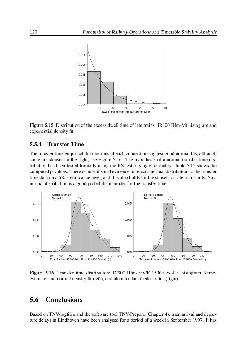
120 Punctuality of Railway Operations and Timetable Stability Analysis
0.000
0.005
0.010
0.015
0.020
0.025
0 30 60 90 120 150 180
Dwell time excess late IC800 Hlm-Mt (s)
Figure 5.15 Distribution of the excess dwell time of late trains: IR800 Hlm-Mt histogram and
exponential density fit
5.5.4 Transfer Time
The transfer time empirical distributions of each connection suggest good normal fits, although
some are skewed to the right, see Figure 5.16. The hypothesis of a normal transfer time dis-
tribution has been tested formally using the KS-test of single normality. Table 5.12 shows the
computed p-values. There is no statistical evidence to reject a normal distribution to the transfer
time data on a 5% significance level, and this also holds for the subsets of late trains only. So a
normal distribution is a good probabilistic model for the transfer time.
0.000
0.004
0.008
0.012
Kernel estimate
Normal fit
0 30 60 90 120 150 180 210 240
Transfer time IC900 Hlm-Ehv / IC1500 Gvc-Hrl (s)
0.000
0.005
0.010
0.015
Kernel estimate
Normal fit
0 30 60 90 120 150 180 210
Transfer time late IC900 Hlm-Ehv / IC1500 Gvc-Hrl (s)
Figure 5.16 Transfer time distribution: IC900 Hlm-Ehv/IC1500 Gvc-Hrl histogram, kernel
estimate, and normal density fit (left), and idem for late feeder trains (right)
5.6 Conclusions
Based on TNV-logfiles and the software tool TNV-Prepare (Chapter 4), train arrival and depar-
ture delays in Eindhoven have been analysed for a period of a week in September 1997. It has
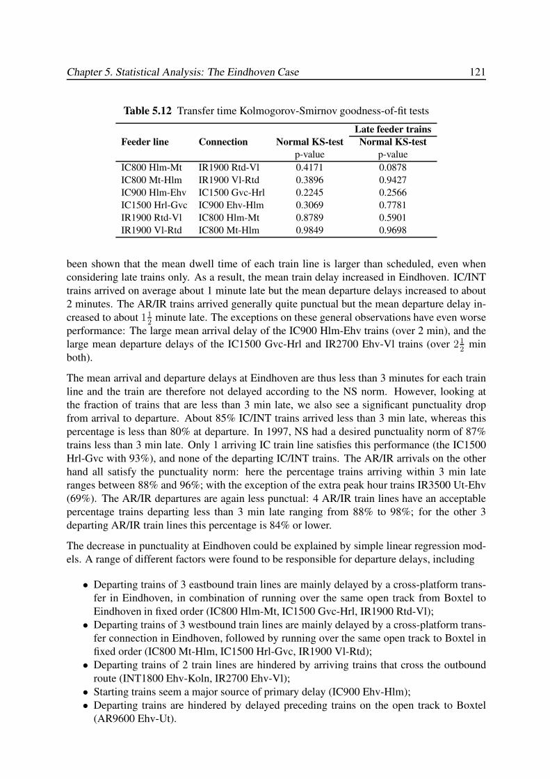
Chapter 5. Statistical Analysis: The Eindhoven Case 121
Table 5.12 Transfer time Kolmogorov-Smirnov goodness-of-fit tests
Late feeder trains
Feeder line Connection Normal KS-test Normal KS-test
p-value p-value
IC800 Hlm-Mt IR1900 Rtd-Vl 0.4171 0.0878
IC800 Mt-Hlm IR1900 Vl-Rtd 0.3896 0.9427
IC900 Hlm-Ehv IC1500 Gvc-Hrl 0.2245 0.2566
IC1500 Hrl-Gvc IC900 Ehv-Hlm 0.3069 0.7781
IR1900 Rtd-Vl IC800 Hlm-Mt 0.8789 0.5901
IR1900 Vl-Rtd IC800 Mt-Hlm 0.9849 0.9698
been shown that the mean dwell time of each train line is larger than scheduled, even when
considering late trains only. As a result, the mean train delay increased in Eindhoven. IC/INT
trains arrived on average about 1 minute late but the mean departure delays increased to about
2 minutes. The AR/IR trains arrived generally quite punctual but the mean departure delay in-
creased to about 112
minute late. The exceptions on these general observations have even worse
performance: The large mean arrival delay of the IC900 Hlm-Ehv trains (over 2 min), and the
large mean departure delays of the IC1500 Gvc-Hrl and IR2700 Ehv-Vl trains (over 212
min
both).
The mean arrival and departure delays at Eindhoven are thus less than 3 minutes for each train
line and the train are therefore not delayed according to the NS norm. However, looking at
the fraction of trains that are less than 3 min late, we also see a significant punctuality drop
from arrival to departure. About 85% IC/INT trains arrived less than 3 min late, whereas this
percentage is less than 80% at departure. In 1997, NS had a desired punctuality norm of 87%
trains less than 3 min late. Only 1 arriving IC train line satisfies this performance (the IC1500
Hrl-Gvc with 93%), and none of the departing IC/INT trains. The AR/IR arrivals on the other
hand all satisfy the punctuality norm: here the percentage trains arriving within 3 min late
ranges between 88% and 96%; with the exception of the extra peak hour trains IR3500 Ut-Ehv
(69%). The AR/IR departures are again less punctual: 4 AR/IR train lines have an acceptable
percentage trains departing less than 3 min late ranging from 88% to 98%; for the other 3
departing AR/IR train lines this percentage is 84% or lower.
The decrease in punctuality at Eindhoven could be explained by simple linear regression mod-
els. A range of different factors were found to be responsible for departure delays, including
• Departing trains of 3 eastbound train lines are mainly delayed by a cross-platform trans-
fer in Eindhoven, in combination of running over the same open track from Boxtel to
Eindhoven in fixed order (IC800 Hlm-Mt, IC1500 Gvc-Hrl, IR1900 Rtd-Vl);
• Departing trains of 3 westbound train lines are mainly delayed by a cross-platform trans-
fer connection in Eindhoven, followed by running over the same open track to Boxtel in
fixed order (IC800 Mt-Hlm, IC1500 Hrl-Gvc, IR1900 Vl-Rtd);
• Departing trains of 2 train lines are hindered by arriving trains that cross the outbound
route (INT1800 Ehv-Koln, IR2700 Ehv-Vl);
• Starting trains seem a major source of primary delay (IC900 Ehv-Hlm);
• Departing trains are hindered by delayed preceding trains on the open track to Boxtel
(AR9600 Ehv-Ut).
122 Punctuality of Railway Operations and Timetable Stability Analysis
For the scheduled dwell and transfer buffer times of the interconnected trains we moreover
obtain the following conclusions:
• A transfer connection of two trains that arrive over the same open track in fixed order
results in a large dwell time (synchronization time) for the first arriving train and also in
a large transfer time for transferring passengers of this train. However, these large dwell
and transfer times do not contain effective buffer time for arrival delay compensation.
• A transfer connection of two trains just before a common open track results in a large
dwell time (synchronization time) for the last departing train, without effective buffer
time.
A generic conclusion is that the function of Eindhoven as a transfer station in combination
with the Eindhoven-Boxtel corridor results in large scheduled dwell and transfer times that still
lack buffer time, and hence enforces a strong source of delay propagation. During the last
few years the corridor between Boxtel and Eindhoven has been upgraded to four-tracks, which
became fully operational at the end of 2002. The above results indicate that this infrastructure
construction leads to a considerable capacity improvement, shorter dwell (and travel) times, and
increased punctuality. An ex-post analysis of the new situation would be interesting to quantify
the gains of this infrastructure investment.
Chapter 6
TIMED EVENT GRAPHS
6.1 Introduction
Train arrivals at main stations initiate several concurrent activities: alighting and boarding of
passengers, passenger transfers to connecting trains departing in different directions, and exiting
passengers walking to their final destination or continuing their journey in another transport
mode. Likewise, train departures synchronize activities of through, starting and transferring
passengers. Rolling stock connections show similar structures: trains from different directions
may be coupled to continue as one combined train or a train may be decoupled after which
the front and back continue in different directions. The railway infrastructure and safety and
signalling systems cause a different kind of synchronization between trains on conflicting routes
which must run in sequence over the shared infrastructure in some decided order.
The main complexity in railway timetable design is due to settling of concurrency by choos-
ing certain priority rules such as specifying routing and/or train sequence orders [154, 231].
The theory developed in the forthcoming may then be used to evaluate the consequences of
these choices in terms of performance. When the timetable has been settled by a higher-level
scheduling policy the resulting railway traffic system is mainly characterized by trains running
concurrently over partially shared tracks and synchronization of trains at stations and junctions.
The dynamics of such traffic systems can be modelled by timed event graphs [11], a subclass in
the theory of Petri nets [139, 218]. In these discrete-event systems the state evolution depends
on causal relations between activities and discrete events in contrast to conventional dynamical
systems where dynamics are governed by difference or differential equations [189].
Various classes of Petri nets have been used for modelling and analysing railway systems, see
e.g. Ren & Zhou [170], Sakaguchi & Tomii [177], Van der Aalst & Odijk [205] and Zhu [229].
In general, simulation can be used to derive properties of highly complex Petri net models. In
the special case of timed event graphs a rich analytical theory has been developed to prove
structural and behavioural properties [139] as well as performance properties [11, 32]. In this
chapter we will be concerned with modelling timed event graphs and deriving structural and
behavioural properties. Performance evaluation is based on a state-space representation of timed
event graphs which gives a linear system description in max-plus algebra. This will be the topic
of Chapters 7 and 8.
In the sequel we assume that a basic network timetable structure has already been designed in
an earlier stage of the planning process and analyse the properties of the resulting structure.
We thus assume full knowledge of the timetable (arrival and departure times of all train lines),
minimum process times (running times and dwell times of all train lines, passenger transfer
times between train lines at transfer stations, layover times of train circulations at line termi-
nals, connection times of rolling stock connections (coupling/decoupling times), and transfer
123
124 Punctuality of Railway Operations and Timetable Stability Analysis
times of train crews or other logistic connections), and minimum headway times between train
paths. This information determines all train interconnections, infrastructure restrictions and
train orders at conflict points. The strength or vulnerability of the imposed timetable structure
furthermore depends on the amount and distribution of process time supplements and buffer
times over the timetable.
The outline of this chapter is as follows. Section 6.2 formally introduces Petri nets and the spe-
cial subclass of timed event graphs. Section 6.3 explains how timed event graphs can be used
to model typical railway system issues, including timetable and infrastructure structures. Sec-
tion 6.4 is concerned with behavioural properties of timed event graphs. Section 6.5 describes
the synthesis of a timed event graph based on the railway timetable and (global) infrastructure
data. Conclusions are given in Section 6.6.
6.2 Petri Nets and Timed Event Graphs
6.2.1 Basic Definitions
A Petri net is a special bipartite directed graph introduced by Petri [161] as a general graphical
and mathematical modelling tool for describing relations between conditions and events. Since
this pioneering work many authors contributed to the development of the Petri net theory, see
the excellent review and tutorial paper by Murata [139]. Event graphs are a subclass of Petri
nets which are able to efficiently describe synchronization structures in networks. As opposed
to general Petri nets event graphs cannot model choice or decisions, in favour of superior an-
alytical and computational power. In particular, the state representation of timed event graphs
corresponds to linear systems in max-plus algebra, which will be the topic of Chapter 7 and 8.
This section formally defines the structure of timed event graphs.
Definition 6.2.1 (Petri net) A Petri net is a tuple PN = (T ,P, E , µ), where
(i) T = {t1, . . . , tn} is a finite set of transitions;
(ii) P = {p1, . . . , pm} is a finite set of places;
(iii) P ∩ T = ∅ and P ∪ T 6= ∅;
(iv) E ⊆ T × P ∪ P × T is a set of arcs from transitions to places and vice versa;
(v) µ ∈ Nm0 is an initial marking of the places.
Graphically, places are depicted as circles and transitions as rectangles or bars. The initial
marking is represented by drawing µ(pk) = µk dots (tokens) in the circle representing place
pk, see Figure 6.1. A transition is called an input transition to a place if there is an arc from
the transition to the place and an output transition if the arc is reversed. Analogously, a place
adjacent to a transition is called an incoming place if there is an arc from the place to the
transition and an outgoing place if the arc is reversed.
Definition 6.2.2 (Event graph) An event graph is a Petri net in which each place has exactly
one input and one output transition.
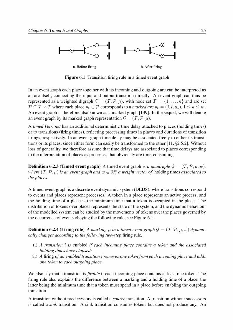
Chapter 6. Timed Event Graphs 125
a. Before firing b. After firing
i i
Figure 6.1 Transition firing rule in a timed event graph
In an event graph each place together with its incoming and outgoing arc can be interpreted as
an arc itself, connecting the input and output transition directly. An event graph can thus be
represented as a weighted digraph G = (T ,P, µ), with node set T = {1, . . . , n} and arc set
P ⊆ T × T where each place pk ∈ P corresponds to a marked arc pk = (j, i, µk), 1 ≤ k ≤ m.
An event graph is therefore also known as a marked graph [139]. In the sequel, we will denote
an event graph by its marked graph representation G = (T ,P, µ).
A timed Petri net has an additional deterministic time delay attached to places (holding times)
or to transitions (firing times), reflecting processing times in places and durations of transition
firings, respectively. In an event graph time delay may be associated freely to either its transi-
tions or its places, since either form can easily be transformed to the other [11, §2.5.2]. Without
loss of generality, we therefore assume that time delays are associated to places corresponding
to the interpretation of places as processes that obviously are time-consuming.
Definition 6.2.3 (Timed event graph) A timed event graph is a quadruple G = (T ,P, µ, w),where (T ,P, µ) is an event graph and w ∈ Rm
+ a weight vector of holding times associated to
the places.
A timed event graph is a discrete event dynamic system (DEDS), where transitions correspond
to events and places represent processes. A token in a place represents an active process, and
the holding time of a place is the minimum time that a token is occupied in the place. The
distribution of tokens over places represents the state of the system, and the dynamic behaviour
of the modelled system can be studied by the movements of tokens over the places governed by
the occurrence of events obeying the following rule, see Figure 6.1.
Definition 6.2.4 (Firing rule) A marking µ in a timed event graph G = (T ,P, µ, w) dynami-
cally changes according to the following two-step firing rule:
(i) A transition i is enabled if each incoming place contains a token and the associated
holding times have elapsed;
(ii) A firing of an enabled transition i removes one token from each incoming place and adds
one token to each outgoing place.
We also say that a transition is firable if each incoming place contains at least one token. The
firing rule also explains the difference between a marking and a holding time of a place, the
latter being the minimum time that a token must spend in a place before enabling the outgoing
transition.
A transition without predecessors is called a source transition. A transition without successors
is called a sink transition. A sink transition consumes tokens but does not produce any. An
126 Punctuality of Railway Operations and Timetable Stability Analysis
autonomous event graph is an event graph without sources. A loop is a place pj = (i, i), where
i is both input and output transition to the place pj. In a loop a token is simultaneously removed
and added to pj , but the new token becomes available to the output transition only after again
the holding time has elapsed.
Remark The first four properties in Definition 6.2.1 define a net N = (T ,P, E), which is a
bipartite directed graph (V,E) with node set V = T ∪ P that is partitioned in two kinds of
elements called transitions and places, respectively. The marking defined by the 5th property
together with the firing rule extends the net to a place/transition net or Petri net PN = (N , µ).An event graph is also called a decision-free Petri net or marked graph [139]. It is decision-free
in the sense that the flow of tokens through a place is generated by only one input transition and
there is no choice between more than one output transition. Note that if a place has two output
transitions then a decision must be made about which transition is fired. If one of the transitions
fires, the token is removed from the place and the other transition is no longer enabled. In an
event graph this situation is not applicable since each place has exactly one input and output
transition. 2
A timed event graph may also be thought of as a bivalued directed multigraph G = (T ,P, µ, w),where both weights are associated to the arcs. In this digraph, the nodes correspond to transi-
tions, the arcs to places, the first arc weight to the initial marking, and the second arc weight to
the holding time. This means that a timed event graph can be stored in a computer using effi-
cient weighted digraph representations and manipulated by standard data structures. For small
dense networks a (weighted) adjacency or incidence matrix representation can be used, whereas
for large-scale sparse networks an arc list, adjacency list or forward/reverse star representation
may be used [3, 39]. We will generally represent a timed event graph G = (T ,P, µ, w) as a
(marked) arc list
pk = (in(pk), out(pk), µ(pk), w(pk)), 1 ≤ k ≤ m,
where in(pk) is the input transition of pk, out(pk) the output transition, µ(pk) = µk the initial
marking, and w(pk) = wk the holding time. The transitions are just numbered from 1, . . . , n.
This representation takes onlyO(m) storage place. The adjacency list representation of a timed
event graph is a list (or array) of the transitions, where each transition points to a list of all its
outgoing places. This representation takesO(n+m) storage place and is useful when traversing
the timed event graph. In general, there may be multiple places between a pair of transitions.
Nevertheless, without loss of generality we may assume that parallel places with the same input
and output transition have different markings. Indeed, if two or more parallel places have the
same initial marking then the one with the highest holding time dominates the others and so the
places can be combined to a single place with the maximum holding time. In Chapter 7 we will
also introduce a matrix representation of a timed event graph that will be useful for algebraic
manipulations.
6.2.2 Building Blocks of Timed Event Graphs
The topology of event graphs allows sequential and parallel processes that are connected by
three primitive transitions:
(i) Sequential transitions model a succession of processes or stages of processes, which
each consume some holding time before the next stage is enabled, see Figure 6.2.a. An
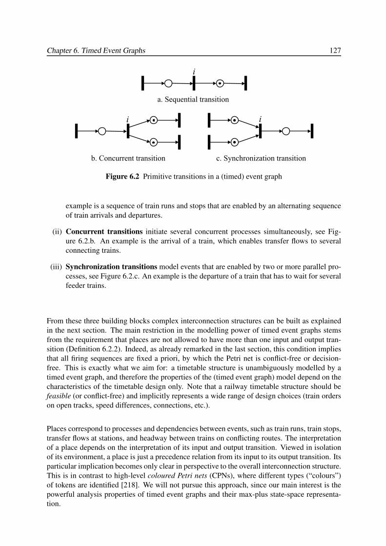
Chapter 6. Timed Event Graphs 127
a. Sequential transition
b. Concurrent transition c. Synchronization transition
i
i i
Figure 6.2 Primitive transitions in a (timed) event graph
example is a sequence of train runs and stops that are enabled by an alternating sequence
of train arrivals and departures.
(ii) Concurrent transitions initiate several concurrent processes simultaneously, see Fig-
ure 6.2.b. An example is the arrival of a train, which enables transfer flows to several
connecting trains.
(iii) Synchronization transitions model events that are enabled by two or more parallel pro-
cesses, see Figure 6.2.c. An example is the departure of a train that has to wait for several
feeder trains.
From these three building blocks complex interconnection structures can be built as explained
in the next section. The main restriction in the modelling power of timed event graphs stems
from the requirement that places are not allowed to have more than one input and output tran-
sition (Definition 6.2.2). Indeed, as already remarked in the last section, this condition implies
that all firing sequences are fixed a priori, by which the Petri net is conflict-free or decision-
free. This is exactly what we aim for: a timetable structure is unambiguously modelled by a
timed event graph, and therefore the properties of the (timed event graph) model depend on the
characteristics of the timetable design only. Note that a railway timetable structure should be
feasible (or conflict-free) and implicitly represents a wide range of design choices (train orders
on open tracks, speed differences, connections, etc.).
Places correspond to processes and dependencies between events, such as train runs, train stops,
transfer flows at stations, and headway between trains on conflicting routes. The interpretation
of a place depends on the interpretation of its input and output transition. Viewed in isolation
of its environment, a place is just a precedence relation from its input to its output transition. Its
particular implication becomes only clear in perspective to the overall interconnection structure.
This is in contrast to high-level coloured Petri nets (CPNs), where different types (“colours”)
of tokens are identified [218]. We will not pursue this approach, since our main interest is the
powerful analysis properties of timed event graphs and their max-plus state-space representa-
tion.
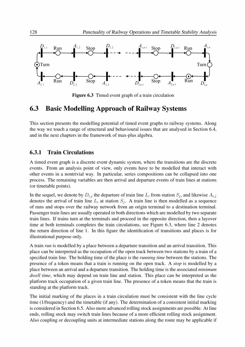
128 Punctuality of Railway Operations and Timetable Stability Analysis
A1, -1n D1, -1nA1,n
D2, -1nA2, -1n D2,n
Stop
Stop
D1, 1A1, 2
A2, 1 D2, 2
D1, 2
A2, 2
StopRun Run
RunStopRun
TurnTurn
Figure 6.3 Timed event graph of a train circulation
6.3 Basic Modelling Approach of Railway Systems
This section presents the modelling potential of timed event graphs to railway systems. Along
the way we touch a range of structural and behavioural issues that are analysed in Section 6.4,
and in the next chapters in the framework of max-plus algebra.
6.3.1 Train Circulations
A timed event graph is a discrete event dynamic system, where the transitions are the discrete
events. From an analysis point of view, only events have to be modelled that interact with
other events in a nontrivial way. In particular, series compositions can be collapsed into one
process. The remaining variables are then arrival and departure events of train lines at stations
(or timetable points).
In the sequel, we denote by Di,j the departure of train line Li from station Sj , and likewise Ai,j
denotes the arrival of train line Li at station Sj . A train line is then modelled as a sequence
of runs and stops over the railway network from an origin terminal to a destination terminal.
Passenger train lines are usually operated in both directions which are modelled by two separate
train lines. If trains turn at the terminals and proceed in the opposite direction, then a layover
time at both terminals completes the train circulations, see Figure 6.3, where line 2 denotes
the return direction of line 1. In this figure the identification of transitions and places is for
illustrational purpose only.
A train run is modelled by a place between a departure transition and an arrival transition. This
place can be interpreted as the occupation of the open track between two stations by a train of a
specified train line. The holding time of the place is the running time between the stations. The
presence of a token means that a train is running on the open track. A stop is modelled by a
place between an arrival and a departure transition. The holding time is the associated minimum
dwell time, which may depend on train line and station. This place can be interpreted as the
platform track occupation of a given train line. The presence of a token means that the train is
standing at the platform track.
The initial marking of the places in a train circulation must be consistent with the line cycle
time (1/frequency) and the timetable (if any). The determination of a consistent initial marking
is considered in Section 6.5. Also more advanced rolling stock assignments are possible. At line
ends, rolling stock may switch train lines because of a more efficient rolling stock assignment.
Also coupling or decoupling units at intermediate stations along the route may be applicable if
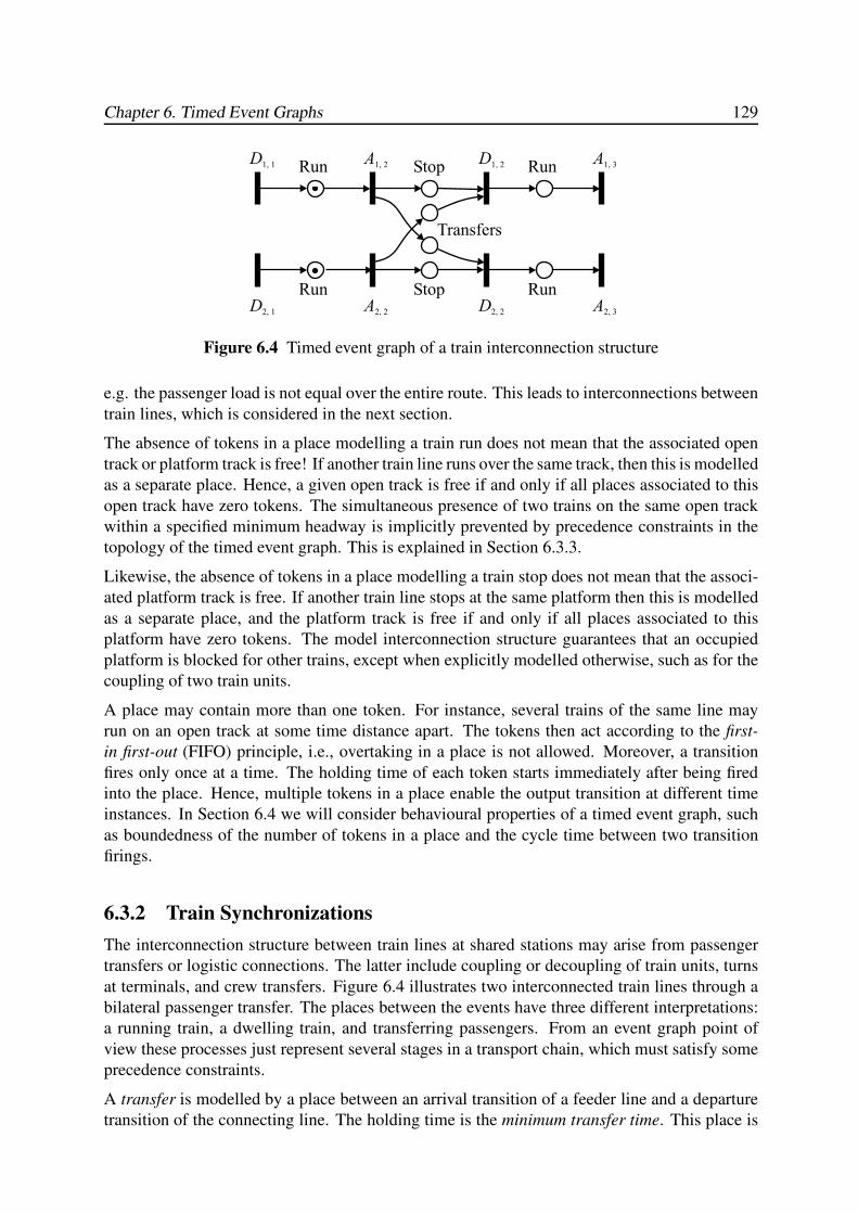
Chapter 6. Timed Event Graphs 129
D1, 1 A1, 2 D1, 2 A1, 3
D2, 1 A2, 2 D2, 2 A2, 3
Run Stop Run
Run RunStop
Transfers
Figure 6.4 Timed event graph of a train interconnection structure
e.g. the passenger load is not equal over the entire route. This leads to interconnections between
train lines, which is considered in the next section.
The absence of tokens in a place modelling a train run does not mean that the associated open
track or platform track is free! If another train line runs over the same track, then this is modelled
as a separate place. Hence, a given open track is free if and only if all places associated to this
open track have zero tokens. The simultaneous presence of two trains on the same open track
within a specified minimum headway is implicitly prevented by precedence constraints in the
topology of the timed event graph. This is explained in Section 6.3.3.
Likewise, the absence of tokens in a place modelling a train stop does not mean that the associ-
ated platform track is free. If another train line stops at the same platform then this is modelled
as a separate place, and the platform track is free if and only if all places associated to this
platform have zero tokens. The model interconnection structure guarantees that an occupied
platform is blocked for other trains, except when explicitly modelled otherwise, such as for the
coupling of two train units.
A place may contain more than one token. For instance, several trains of the same line may
run on an open track at some time distance apart. The tokens then act according to the first-
in first-out (FIFO) principle, i.e., overtaking in a place is not allowed. Moreover, a transition
fires only once at a time. The holding time of each token starts immediately after being fired
into the place. Hence, multiple tokens in a place enable the output transition at different time
instances. In Section 6.4 we will consider behavioural properties of a timed event graph, such
as boundedness of the number of tokens in a place and the cycle time between two transition
firings.
6.3.2 Train Synchronizations
The interconnection structure between train lines at shared stations may arise from passenger
transfers or logistic connections. The latter include coupling or decoupling of train units, turns
at terminals, and crew transfers. Figure 6.4 illustrates two interconnected train lines through a
bilateral passenger transfer. The places between the events have three different interpretations:
a running train, a dwelling train, and transferring passengers. From an event graph point of
view these processes just represent several stages in a transport chain, which must satisfy some
precedence constraints.
A transfer is modelled by a place between an arrival transition of a feeder line and a departure
transition of the connecting line. The holding time is the minimum transfer time. This place is
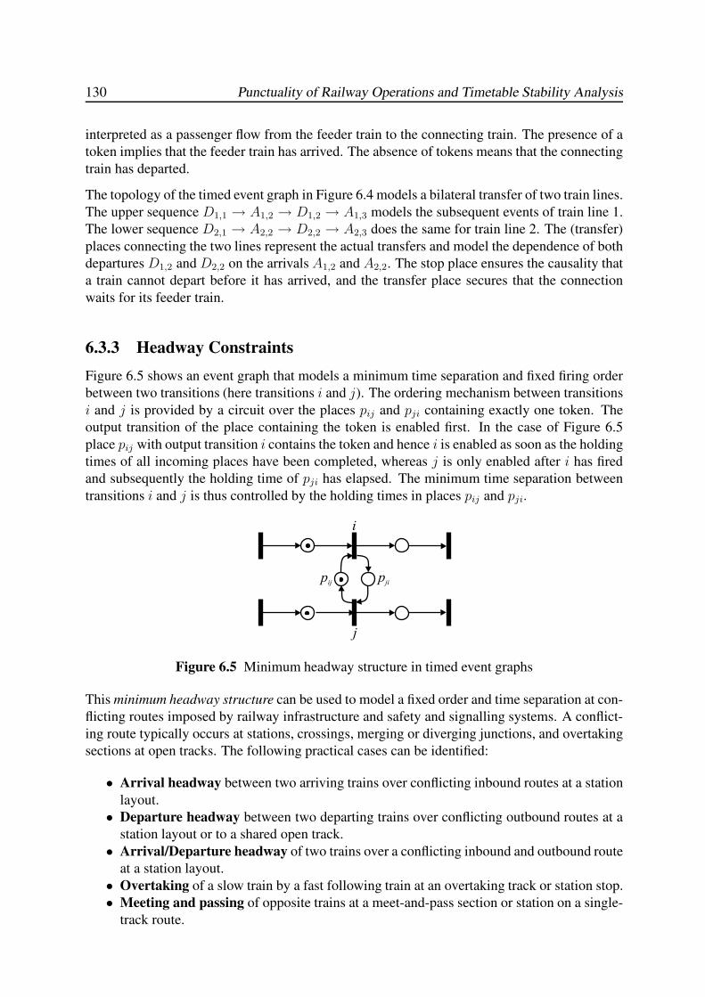
130 Punctuality of Railway Operations and Timetable Stability Analysis
interpreted as a passenger flow from the feeder train to the connecting train. The presence of a
token implies that the feeder train has arrived. The absence of tokens means that the connecting
train has departed.
The topology of the timed event graph in Figure 6.4 models a bilateral transfer of two train lines.
The upper sequence D1,1 → A1,2 → D1,2 → A1,3 models the subsequent events of train line 1.
The lower sequence D2,1 → A2,2 → D2,2 → A2,3 does the same for train line 2. The (transfer)
places connecting the two lines represent the actual transfers and model the dependence of both
departures D1,2 and D2,2 on the arrivals A1,2 and A2,2. The stop place ensures the causality that
a train cannot depart before it has arrived, and the transfer place secures that the connection
waits for its feeder train.
6.3.3 Headway Constraints
Figure 6.5 shows an event graph that models a minimum time separation and fixed firing order
between two transitions (here transitions i and j). The ordering mechanism between transitions
i and j is provided by a circuit over the places pij and pji containing exactly one token. The
output transition of the place containing the token is enabled first. In the case of Figure 6.5
place pij with output transition i contains the token and hence i is enabled as soon as the holding
times of all incoming places have been completed, whereas j is only enabled after i has fired
and subsequently the holding time of pji has elapsed. The minimum time separation between
transitions i and j is thus controlled by the holding times in places pij and pji.
i
j
pij pji
Figure 6.5 Minimum headway structure in timed event graphs
This minimum headway structure can be used to model a fixed order and time separation at con-
flicting routes imposed by railway infrastructure and safety and signalling systems. A conflict-
ing route typically occurs at stations, crossings, merging or diverging junctions, and overtaking
sections at open tracks. The following practical cases can be identified:
• Arrival headway between two arriving trains over conflicting inbound routes at a station
layout.
• Departure headway between two departing trains over conflicting outbound routes at a
station layout or to a shared open track.
• Arrival/Departure headway of two trains over a conflicting inbound and outbound route
at a station layout.
• Overtaking of a slow train by a fast following train at an overtaking track or station stop.
• Meeting and passing of opposite trains at a meet-and-pass section or station on a single-
track route.
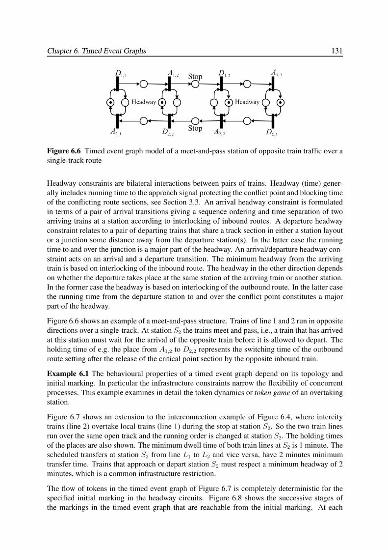
Chapter 6. Timed Event Graphs 131
D1, 1A1, 2 D1, 2
A1, 3
A2, 1 D2, 2A2, 2 D2, 3
Stop
Stop
Headway Headway
Figure 6.6 Timed event graph model of a meet-and-pass station of opposite train traffic over a
single-track route
Headway constraints are bilateral interactions between pairs of trains. Headway (time) gener-
ally includes running time to the approach signal protecting the conflict point and blocking time
of the conflicting route sections, see Section 3.3. An arrival headway constraint is formulated
in terms of a pair of arrival transitions giving a sequence ordering and time separation of two
arriving trains at a station according to interlocking of inbound routes. A departure headway
constraint relates to a pair of departing trains that share a track section in either a station layout
or a junction some distance away from the departure station(s). In the latter case the running
time to and over the junction is a major part of the headway. An arrival/departure headway con-
straint acts on an arrival and a departure transition. The minimum headway from the arriving
train is based on interlocking of the inbound route. The headway in the other direction depends
on whether the departure takes place at the same station of the arriving train or another station.
In the former case the headway is based on interlocking of the outbound route. In the latter case
the running time from the departure station to and over the conflict point constitutes a major
part of the headway.
Figure 6.6 shows an example of a meet-and-pass structure. Trains of line 1 and 2 run in opposite
directions over a single-track. At station S2 the trains meet and pass, i.e., a train that has arrived
at this station must wait for the arrival of the opposite train before it is allowed to depart. The
holding time of e.g. the place from A1,2 to D2,2 represents the switching time of the outbound
route setting after the release of the critical point section by the opposite inbound train.
Example 6.1 The behavioural properties of a timed event graph depend on its topology and
initial marking. In particular the infrastructure constraints narrow the flexibility of concurrent
processes. This example examines in detail the token dynamics or token game of an overtaking
station.
Figure 6.7 shows an extension to the interconnection example of Figure 6.4, where intercity
trains (line 2) overtake local trains (line 1) during the stop at station S2. So the two train lines
run over the same open track and the running order is changed at station S2. The holding times
of the places are also shown. The minimum dwell time of both train lines at S2 is 1 minute. The
scheduled transfers at station S2 from line L1 to L2 and vice versa, have 2 minutes minimum
transfer time. Trains that approach or depart station S2 must respect a minimum headway of 2
minutes, which is a common infrastructure restriction.
The flow of tokens in the timed event graph of Figure 6.7 is completely deterministic for the
specified initial marking in the headway circuits. Figure 6.8 shows the successive stages of
the markings in the timed event graph that are reachable from the initial marking. At each
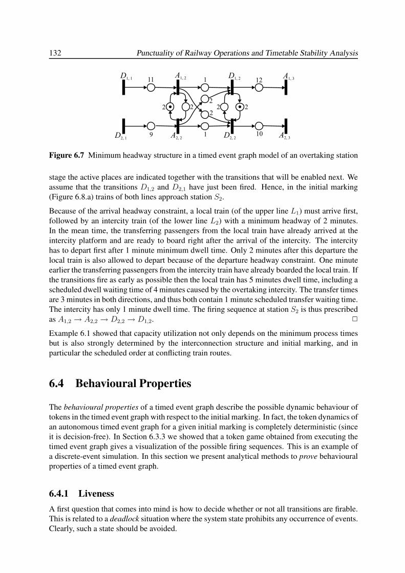
132 Punctuality of Railway Operations and Timetable Stability Analysis
D1, 1A1, 2 D1, 2 A1, 3
D2, 1 A2, 2 D2, 2 A2, 3
1
1
2 22
22 2
1211
9 10
Figure 6.7 Minimum headway structure in a timed event graph model of an overtaking station
stage the active places are indicated together with the transitions that will be enabled next. We
assume that the transitions D1,2 and D2,1 have just been fired. Hence, in the initial marking
(Figure 6.8.a) trains of both lines approach station S2.
Because of the arrival headway constraint, a local train (of the upper line L1) must arrive first,
followed by an intercity train (of the lower line L2) with a minimum headway of 2 minutes.
In the mean time, the transferring passengers from the local train have already arrived at the
intercity platform and are ready to board right after the arrival of the intercity. The intercity
has to depart first after 1 minute minimum dwell time. Only 2 minutes after this departure the
local train is also allowed to depart because of the departure headway constraint. One minute
earlier the transferring passengers from the intercity train have already boarded the local train. If
the transitions fire as early as possible then the local train has 5 minutes dwell time, including a
scheduled dwell waiting time of 4 minutes caused by the overtaking intercity. The transfer times
are 3 minutes in both directions, and thus both contain 1 minute scheduled transfer waiting time.
The intercity has only 1 minute dwell time. The firing sequence at station S2 is thus prescribed
as A1,2 → A2,2 → D2,2 → D1,2. 2
Example 6.1 showed that capacity utilization not only depends on the minimum process times
but is also strongly determined by the interconnection structure and initial marking, and in
particular the scheduled order at conflicting train routes.
6.4 Behavioural Properties
The behavioural properties of a timed event graph describe the possible dynamic behaviour of
tokens in the timed event graph with respect to the initial marking. In fact, the token dynamics of
an autonomous timed event graph for a given initial marking is completely deterministic (since
it is decision-free). In Section 6.3.3 we showed that a token game obtained from executing the
timed event graph gives a visualization of the possible firing sequences. This is an example of
a discrete-event simulation. In this section we present analytical methods to prove behavioural
properties of a timed event graph.
6.4.1 Liveness
A first question that comes into mind is how to decide whether or not all transitions are firable.
This is related to a deadlock situation where the system state prohibits any occurrence of events.
Clearly, such a state should be avoided.
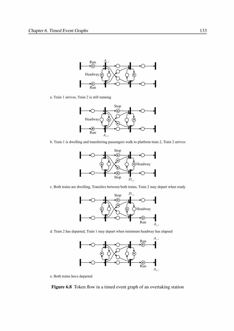
Chapter 6. Timed Event Graphs 133
A1, 2
Headway
Run
Run
A2, 2
Stop
Headway
Run
D2, 2
Stop
Stop
Headway
D1, 2
A2, 3
Stop
Headway
Run
A1, 3
A2, 3
Run
Run
a. Train 1 arrives, Train 2 is still running
b. Train 1 is dwelling and transferring passengers walk to platform train 2, Train 2 arrives
c. Both trains are dwelling, Transfers between both trains, Train 2 may depart when ready
d. Train 2 has departed, Train 1 may depart when minimum headway has elapsed
e. Both trains have departed
Figure 6.8 Token flow in a timed event graph of an overtaking station
134 Punctuality of Railway Operations and Timetable Stability Analysis
Definition 6.4.1 (Liveness) A transition is live if it is firable at the initial marking or can get
firable through some firing sequence from the initial marking. An event graph is live for an
initial marking if all its transitions are live. An event graph that is not live is called deadlocked.
The most well-known example of deadlock is a single-track route occupied by a train heading
for a meet-and-pass station of which all platforms are occupied by opposite trains. Another
example of a deadlocked scheduled railway system occurs when a train waits for a feeder train
that never arrives. Note that if this train also has connections at following stations these con-
necting trains eventually also keep on waiting, and so on. Finally, no train in the railway system
(or a strongly connected subsystem) will ever be able to depart.
A circuit in an event graph is a directed path of transitions and places where the first and last
transition coincides. The following basic lemma states that the number of tokens on a circuit in
an event graph does not change by firing [37].
Lemma 6.4.1 The number of tokens in any circuit of an event graph G is invariant to any firing
sequence.
Proof: Consider any circuit in an event graph. A token in a place on the circuit can only be
generated and consumed by transitions that also belong to the circuit since in an event graph
each place has only one input and one output transition. Moreover, if a transition in the circuit is
fired then a token is removed from the incoming place but simultaneously added to the outgoing
place in the circuit, by which the number of tokens in the circuit does not change after firing. 2
Commoner et al. [37, Th. 1] proved the following necessary and sufficient condition for an
event graph to be live, which provides a simple liveness test of an event graph.
Theorem 6.4.1 (Liveness) An event graph G = (T ,P, µ0) is live if and only if each circuit
contains at least one token in the initial marking µ0.
Proof: If a circuit of an event graph has zero tokens in the initial marking then this circuit
remains free of tokens by Lemma 6.4.1. But then the transitions on this circuit will never be
enabled. Therefore, each circuit in the initial marking should have at least one token to be live.
Conversely, assume there exists a transition i that is not live. Then i must have an incoming
place without tokens and this place must be restrained from tokens by any firing sequence. This
means that the input transition of this incoming place may never be enabled. Since the number
of places in an event graph is finite, backtracking on token-free incoming places either ends in
a source (which is firable by convention), or at a circuit which contains a marked place by the
condition in the theorem. This contradicts that i is not live. 2
Note that a live marking remains live after firing as a consequence of Theorem 6.4.1 and
Lemma 6.4.1
6.4.2 Reachability
Firing an enabled transition changes the distribution of tokens (marking) in an event graph
according to the firing rule in Definition 6.2.4. A sequence of firings thus results in a sequence
Chapter 6. Timed Event Graphs 135
of markings. We are now interested in determining whether a certain desired or undesired
marking can be reached, or more general, in determining the possible markings that can be
reached from an initial marking.
Definition 6.4.2 (Reachability, reachable set) A marking µ is reachable from a marking µ0
if there exists a firing sequence transforming µ0 to µ. The reachable set of an event graph
G = (T ,P, µ0) is the set of all possible markings reachable from the initial marking µ0, and is
denoted as R(µ0).
The topological structure of a timed event graph can be characterized in terms of its inci-
dence matrix. Let G = (T ,P, µ0, w) be a timed event graph. A matrix representation G is
the transition-place incidence matrix M ∈ {0,±1}n×m defined as
[M ]ij =
1 if out(pj) = i−1 if in(pj) = i
0 otherwise.
From the firing rule immediately follows that the negative entries in row i correspond to the
incoming places from which a token is removed if transition i fires, and the positive entries
correspond to the outgoing places to which a token is added. Each column j has two nonzeros
corresponding to the input and output transition of place pj . The incidence matrix M equals the
node-arc incidence matrix of the underlying digraph where each place pj is identified with an
arc from transition in(pj) to out(pj).
The marking evolution over an event graph can be described by a dynamic equation of succes-
sive markings. Let µ(k) be the marking after k transition firings in an event graph (T ,P, µ0)with incidence matrix M ∈ {0,±1}n×m. The firing vector σ(k) ∈ {0, 1}n denotes the enabled
transitions that fire simultaneously at the kth firing, i.e., σi(·) = 1 if i fires and σi(·) = 0otherwise. A necessary and sufficient condition for transition i to be enabled at marking
µ = (µ1, . . . , µm)> ∈ Nm0 is
µj ≥ (−M)ij for all j = 1, . . . , m.
In particular this inequality must be valid for all j associated to predecessor places pj of transi-
tion i for which (M)ij = −1. The inequality is trivially satisfied for all other pj . The marking
dynamic equation in an event graph is given by
µ(k) = µ(k − 1) +M>σ(k), k ∈ N,
where µ(0) = µ0 and M> is the transposed incidence matrix. Now suppose that a marking µ is
reachable from the initial marking µ0 through a feasible firing sequence {σ(1), σ(2), . . . , σ(l)}.Then marking µ = µ(l) is determined by
µ = µ0 +M>y, (6.1)
where y =∑l
k=1 σ(k) ∈ Nn0 is the firing count vector, i.e., yi is the number of times that i
must fire to reach µ from µ0. Hence, a necessary condition for a marking µ to be reachable is
that there exists a valid firing count vector y satisfying (6.1). However, (6.1) is not a sufficient
condition, since y may not correspond to a legal firing sequence, i.e., a firing sequence that
136 Punctuality of Railway Operations and Timetable Stability Analysis
satisfies the firing rule. In particular, both µ and y are constrained to be nonnegative integral
vectors.
A necessary and sufficient condition for a reachable marking is obtained in terms of the fun-
damental cycle matrix of an event graph. The following is a straightforward generalization of
graph theoretic concepts to event graphs. Basic references on graph theory are Berge [16] and
Bollobas [18]. A cycle in an event graph is a sequence of transitions and places, where the first
and last transition coincide. In a cycle the orientation of places may be arbitrary. Recall that a
circuit is a cycle in which all places are oriented in the same direction. An elementary cycle is
a cycle where each transition occurs only once, i.e., a cycle having no subcycles. In the sequel,
we will always assume that a cycle is elementary. A cycle is represented by its place incidence
vector γ = (γ1, . . . , γm)> ∈ {0,±1}m, defined as γk = 1 if pk is a forward place w.r.t. the cycle
orientation, γk = −1 if pk is a backward place, and γk = 0 otherwise. The sum of two cycles is
again a cycle and indeed the set of all cycles is a subspace of Rm with dimension ν = m−n+c,where c is the number of strongly-connected components of the event graph.
A cycle basis is a set of independent cycles that spans the cycle space, i.e., each cycle in the
event graph can be obtained by a linear combination of the cycles in the cycle basis. A cycle
basis is obtained by the following graph algorithm. First, assume that G = (T ,P) is strongly
connected, i.e., c = 1. Then there exists a spanning tree S = (T ,PS) over the transitions of Gwith PS ⊆ P . By definition, a spanning tree does not contain cycles and adding a nontree place
pk ∈ P \ PS generates a cycle in G with a path on the spanning tree from the output transition
of the nontree place to its input transition. The number of places in a spanning tree is n − 1as any additional place gives a cycle. Hence, the number of nontree places is m − (n − 1) =m − n + 1. Each cycle generated by a nontree place and a path on a spanning tree is called
a fundamental cycle. The orientation of a fundamental cycle is defined by the direction of the
nontree place. The set of m− n + 1 fundamental cycles form a fundamental cycle basis. Note
that a fundamental cycle basis is not unique but depends on the choice of the spanning tree.
Now consider the general case of an event graph with c components. Then we may consider
each strongly-connected component separately, or equivalently, find a spanning forest F with
n − c places. The number of places in G − F is the cyclomatic number ν = m − n + c, and
each of these places generates a fundamental cycle associated to the spanning forest F . From
this algorithm follows that the dimension of the cycle space is ν since each fundamental cycle
contains exactly one unique place that is not contained in any other fundamental cycle.
Above we presented an algorithm for finding a fundamental cycle basis. By definition each cy-
cle can be represented by a linear combination of these fundamental cycles. The (fundamental)
cycle matrix of an event graph is now the cycle-place incidence matrix Γ ∈ {0,±1}ν×m, where
each row is the incidence vector of a fundamental cycle,
[Γ]ij =
1 if pj is a forward place in fundamental cycle i−1 if pj is a backward place in fundamental cycle i
0 otherwise.
Recall that the direction of a place on a cycle depends on the orientation of the cycle.
Murata [138] proved a necessary and sufficient condition for a reachable marking using a circuit
theoretic analogy. We give a new simple proof based on polyhedral theory [181]. We need the
following important definition. A matrix A is called totally unimodular if the determinant of
Chapter 6. Timed Event Graphs 137
each square submatrix of A takes values in {0,±1}. The following lemma is a basic result in
polyhedral theory [181, §19.1].
Lemma 6.4.2 Let A ∈ {0,±1}m×n be a totally unimodular matrix and b ∈ Zn an integral
vector. Then the polyhedron {x ∈ Rm | x ≥ 0, Ax = b} is integral, that is, all of its extreme
points are integral vectors.
We can now prove the following theorem.
Theorem 6.4.2 (Reachability) Let G = (T ,P, µ0) be a live (timed) event graph. Then a mark-
ing µ is reachable from the initial marking µ0 if and only if
Γµ = Γµ0, (6.2)
where Γ is the fundamental cycle matrix of G.
Proof: If µ is reachable from µ0 then there must be a legal firing sequence with firing count
vector y satisfying (6.1), or equivalently
M>y = ∆µ (6.3)
where ∆µ = µ − µ0. This means that the vector ∆µ is a linear combination of the columns of
M> (or rows of M), or equivalently, ∆µ is an element in the range of M>. From linear algebra
it is well-known [195] that (6.3) has a solution y iff ∆µ is orthogonal to the kernel of M , i.e.,
ξ>∆µ = 0 for all ξ ∈ {ξ ∈ {0,±1}m |Mξ = 0}. From graph theory it is known that the rank of
an incidence matrix M is n−c, where c is the number of strongly-connected components of the
(event) graph, and the dimension of its kernel is the cyclomatic number ν = m− n+ c. In fact
the kernel of an incidence matrix is the cycle space spanned by ν independent cycles [16, Ch. 4].
Now, the cycle matrix Γ is the matrix where each row corresponds to an independent cycle from
a cycle basis of the graph G. Hence, the rows of Γ span the kernel ofM , and therefore Γ∆µ = 0is a necessary condition for the existence of a solution y to (6.3).
Conversely, let µ ∈ {µ ∈ Rm | µ ≥ 0,Γµ = Γµ0}. It is well-known that a cycle matrix Γis totally unimodular. Moreover, since both µ0 and Γ are integral, also Γµ0 is integral. From
Lemma 6.4.2 then follows that there is an integral vector µ such that Γµ = Γµ0. Therefore,
∆µ = µ − µ0 is integral. It is also well-known that an incidence matrix M (and its transpose
M>) is totally unimodular. Then again by Lemma 6.4.2 {y ∈ Rn | y ≥ 0,M>y = ∆µ} is an
integral polyhedron. Hence, the condition Γµ = Γµ0 is sufficient for the existence of an integral
vector y ≥ 0 satisfying (6.3). 2
The roles of µ0 and µ in (the proof of) Theorem 6.4.2 can be interchanged. Hence we obtain
the following.
Corollary 6.4.1 Let G = (T ,P, µ0) be a live (timed) event graph. Two markings µ0 and µ are
mutually reachable if and only if (6.2) holds.
Commoner et al. [37] proved a necessary and sufficient condition for a reachable marking µ in
the case of a live and strongly-connected event graph. In a strongly-connected (event) graph
138 Punctuality of Railway Operations and Timetable Stability Analysis
(a basis of) the set of all cycles can be generated from (a basis of) the set of all circuits and
vice versa [16]. Therefore the following result of Commoner et al. [37, Th.11] is a corollary to
Theorem 6.4.2.
Corollary 6.4.2 Let G = (T ,P, µ0) be a live and strongly-connected (timed) event graph.
Then a marking µ is reachable from the initial marking µ0 if and only if the token count on each
(directed) circuit in G = (T ,P, µ) is equal to that of G = (T ,P, µ0).
The reachable set of an event graph is now completely described by the following corollary to
Theorem 6.4.2.
Corollary 6.4.3 (Reachable set) The reachable set of a live event graph G = (T ,P, µ0) is
R(µ0) = {µ ∈ Nm0 | Γµ = Γµ0},
where Γ is a fundamental cycle matrix of G.
Thus, for any marking µ0 all timed event graphs G = (T ,P, µ, w) with initial marking µ ∈R(µ0) are equivalent in the sense that they are interchangeable by some legal firing sequence.
Hence, all behavioural properties of a timed event graph G = (T ,P, µ0, w) are invariant to
changing the initial marking in any marking µ ∈ R(µ0).
6.4.3 Periodicity
A (timed) event graph G = (T ,P, µ0) is consistent if there exists a finite firing sequence from
µ0 back to µ0 in which each transition fires at least once. Formally, this is defined as follows.
Definition 6.4.3 (Consistency) A (timed) event graph G = (T ,P, µ0) is consistent if there
exists a positive firing count vector y ∈ Nn such that M>y = 0, where M is the incidence
matrix of G.
Consistency is indifferent to loops in the event graph since any firing of the associated transition
both removes and adds a token to the place in the loop. Hence, consistency can be defined
without loss of generality in terms of incidence matrices although they do not represent loops.
Definition 6.4.4 (Synchronousness) A consistent event graph is called synchronous if the tran-
sitions of any firing sequence transforming µ0 back to itself are fired the same (nonzero) number
of times.
Lemma 6.4.3 (Synchronousness) A strongly-connected (timed) event graph G = (T ,P, µ0)is synchronous.
Proof: If marking µ0 is reachable from µ0 then (6.1) with µ = µ0 gives M>y = 0. The
rows of M> have exactly two nonzeros 1 and −1, and so y = (1, . . . , 1)> ∈ Nn is a solution
to M>y = 0. Moreover, the (transposed) incidence matrix M (M>) of a strongly-connected
digraph has rank n − 1, and therefore the kernel of M> has dimension 1. Hence, the only
vectors satisfying M>y = 0 are multiples of y = (1, . . . , 1)> ∈ Nn, which spans the kernel. 2
Chapter 6. Timed Event Graphs 139
Synchronousness is more restrictive than consistency: the latter requires the existence of a firing
sequence returning to the initial marking, whereas synchronousness assumes that in such a firing
sequence all transitions have fired the same time. A consistent timed event graph exhibits a
periodic behaviour if a suitable sequence of firings is repeated. This is the basis of a periodic
timetable which in fact determines such a suitable order of train departures.
The cycle time of an event is the asymptotic steady-state interval between two successive oc-
currences of the event. Formally, this is defined as follows.
Definition 6.4.5 (Cycle time) Consider a timed event graph G = (T ,P, µ0, w). Let xi(k) be
the time at which transition i ∈ T fires for the k-th time. Then the cycle time χi is defined for
each transition i ∈ T by
χi = limk→∞
xi(k)
k.
If all transitions have the same cycle time then we say that the timed event graph is periodic. For
any (closed) path ξ denote by w(ξ) and µ(ξ) the weight and marking of the path, respectively.
Hence,
w(ξ) =∑
pk∈ξ
wk and µ(ξ) =∑
pk∈ξ
µk.
Theorem 6.4.3 (Periodicity) A live strongly-connected timed event graph G = (T ,P, µ0, w)is periodic and the common cycle time equals the maximum cycle mean η defined as
η = maxξ∈C
w(ξ)
µ(ξ), (6.4)
where C is the set of all elementary circuits in G.
Proof: By liveness of G each transition is firable by some firing sequence from the initial
marking. Moreover, because G is strongly connected it is synchronous by Lemma 6.4.3 and
therefore each transition has fired the same number of times before a next cycle of firings starts.
Hence, G is periodic and the cycle time is determined by the transitions on a circuit with the
largest mean weight, which is given by (6.4). 2
If a (departure) transition in a strongly-connected event graph is deadlocked then the entire
system is deadlocked, i.e., the cycle time is undefined. On the other hand if the strongly-
connected event graph is live then the system is periodic. In the next chapter we will give an
efficient algorithm to compute the minimum cycle time as the solution of an eigenvalue problem
in the max-plus algebra.
6.4.4 Boundedness
A synchronous timed event graph also implies that the event graph is bounded.
Definition 6.4.6 (Boundedness) A place p is said to be k-bounded, with k ∈ Z+, if the number
of tokens in p never exceeds k for any marking reachable from the initial marking µ0. A (timed)
event graph is called k-bounded if each of its places is k-bounded. A place (or event graph) is
said to be bounded if it is k-bounded for some integer k > 0.
140 Punctuality of Railway Operations and Timetable Stability Analysis
In a strongly-connected timed event graph each place is by definition contained in a circuit
and by Lemma 6.4.1 the number of tokens in a place can never exceed the minimum number of
tokens in any circuit over this place. Hence, a strongly-connected timed event graph is bounded.
However, a stronger result is valid when the timed event graph is in its periodic steady-state.
Theorem 6.4.4 Let G = (T ,P, µ0) be a live strongly-connected (timed) event graph, and k =maxi(µ0i
) the maximum initial marking of any place. Then G is asymptotically (k+1)-bounded.
Proof: Since G is strongly connected by definition each place belongs to at least one circuit.
Moreover, by Theorem 6.4.3 each transition has the same cycle time. Therefore, in each period
a place obtains one token from its input transition and passes one token to its output transition.
So the number of tokens in a place can be at most the initial number plus one. Hence, the
number of tokens in each place is at most k + 1, and so G is (k + 1)-bounded. 2
6.5 Synthesis of Scheduled Railway Systems
The basic modelling approach has already been introduced in Section 6.3. Here we give an
algorithm to construct a timed event graph associated to a periodic network timetable, and
prove the behavioural properties of the constructed timed event graph.
6.5.1 Input Data
To model a train service network as a timed event graph input data must be available on the
timetable, train lines, connections between train lines, and headway constraints. The timetable
contains the arrival and departure times of each train line at the stations they serve. Train line
information includes routes, served stations, frequency, running times, minimum dwell times,
and minimum layover times (if applicable). Information on connections includes train pairs
and station and the minimum transfer or connection times. The data of headway constraints
contains pairs of train events and conflict point, and the minimum headway in both directions
that has to be respected at the conflict point.
In Section 6.3 we considered both arrival and departure events. However, since we are con-
cerned with deterministic running times, the arrival times of train runs are trivially expressed
in their departure times. Therefore we may concentrate on departure times only without loss of
generality. Note that this reduces the number of modelled transitions by a factor two.
Timetable Points
We adopt a macroscopic view of a railway network consisting of timetable points and tracks
between these points. A timetable point is a location on the railway network where interacting
or conflicting events may occur. Examples of timetable points are main railway stations, inter-
mediate stops on the open track, crossings, merging and diverging junctions, shunting yards,
freight yards, and movable bridges. Timetable points are denoted by variables Si and can be in-
terpreted as (virtual) stations. The set of all timetable points is denoted by S = {S1, . . . , S|S|}.The timetable points can be defined in a file TimetablePointData where each row char-
acterizes a timetable point as
TimetablePointData(i) = (Si, xi, yi, typei),
Chapter 6. Timed Event Graphs 141
where Si is the station name, xi and yi are the coordinates with respect to a map of the railway
network, and typei is the type of the timetable point. We distinguish between the following
types: intercity station (IC), interregional station (IR), regional station (AR), freight or shunting
yard (F), junctions (J), and movable bridges (BR). Like the coordinates, the timetable point
types are essentially only used for visualizing the railway network. Different types of timetable
points may be visualized by different objects or objects of different size. In the PETER software
(see Chapter 8) passenger stations are visualized by circles of varying size (IC>IR>AR), freight
and shunting yards by squares, and junctions/bridges by dots.
By definition all events on a railway network occur at timetable points. Routes over timetable
points are implicitly determined by line constraints as considered below. Conflicting routes and
platform capacity within railway stations are also implicitly modelled by headway constraints
as considered below. Headway conflicts on the open tracks are only considered at timetable
points. Signals and blocks on open tracks are thus not explicitly included in the model. Never-
theless, because we assume deterministic running times feasibility at the open track is ensured
by headway constraints at the beginning and end of the open track (departure and arrival head-
way constraints) and possible headway constraints at intermediate timetable points.
This macroscopic modelling of the railway network by headway constraints has the advantage
that the timed event graph is independent of particular safety and signalling systems. Hence,
the modelling approach is applicable for hybrid railway networks with a mixture of any fixed
block and moving block signalling systems.
Line Data
A train line is determined by a sequence of line segments between successive timetable points
on the line route. Timetable points are either stations where the train line stops or intermedi-
ate passing points. The former generates arrival and departure events, whilst the latter gives
passage or through events. The through events are included to define possible headway con-
straints. For instance, an intercity train may have a scheduled overtake of a regional train at a
local station without stopping. The minimum headway constraints between the dwelling train
and through train are then defined between the arrival and departure event of the regional train
and the passage event of the intercity train. If for instance the intercity train is delayed then the
minimum headway constraint between the intercity passage event and the local departure event
guarantees that the regional train waits for the passage of the intercity train.
Train lines with a frequency f > 1 per timetable cycle time are modelled by f separate train
lines. Likewise, train lines operated in both forward and return direction are modelled by two
different train lines. For instance, consider the Dutch railway timetable with cycle time T = 60minutes and the regional train line 6300 from The Hague CS to Haarlem and vice versa that is
operated twice per hour in both directions. We model this by 4 train lines named 63xy using
a digit x ∈ {0, 1} for the forward (0) or return (1) direction and a digit y ∈ {1, . . . , f} for the
subsequent trains starting from the terminals within one timetable period. Hence, 6301 is the
train line from The Hague CS to Haarlem corresponding to the first departure from The Hague
CS at 06 each hour, 6302 is the train line departing from The Hague CS 30 minutes later at 36
each hour, 6311 is the train line from Haarlem to The Hague CS departing from Haarlem at 03
each hour, and 6312 is the train line Haarlem–The Hague departing from Haarlem at 33 each
hour.
The train lines are defined in a file LineData. The rows in this file contain the successive train
142 Punctuality of Railway Operations and Timetable Stability Analysis
line segments of the train lines, where each row i contains the following objects:
LineData(i) = (Li, S1i , S
2i , Ai, di, t
runi , tmin
i ),
with Li the train line number, S1i the origin station of the line segment, S2
i the destination station
of the line segment,Ai ∈ {S, P,E} the activity type at the destination S2i being either a stop (S),
a passage (P) or an ending E, di ∈ [0, T ) the scheduled event time at the origin S1i , trun
i ≥ 0 the
running time from S1i to S2
i , and tmini ≥ 0 the minimum process time at S2
i . For a stop activity
the minimum process time tmini corresponds to the minimum dwell time at S2
i . For a passage
activity tmini = 0. The event at the destination station is either an arrival or passage depending
on the activity Ai. Likewise, the scheduled event time di at the origin is either a departure time
or a through time depending on the activity at S1i .
By definition the successive rows in LineData satisfy the following continuity assumption:
if Li = Li+1 then S2i = S1
i+1.
So, if two successive rows i and i + 1 correspond to the same train line then the destination
station of row i is the origin station of row i+ 1. Hence, LineData consists of blocks of subse-
quent rows corresponding to a train line route from one terminal to the other. We furthermore
assume that all train lines start with a departure from a terminal and the last line segment of
each train line is an end. Hence,
if Li 6= Li+1 then Ai = E.
Turns are assumed to be part of the synchronization constraints, which facilitates the description
of complex train circulations over different train lines.
Synchronization Data
At transfer stations train lines may be synchronized to allow passenger or crew transfers or
rolling stock connections. Likewise, at terminal stations trains may turn to continue in the
opposite direction or switch to another train line. These synchronization constraints are defined
in a file SynchData, where each row k corresponds to a single transfer, connection or turn
from one train line to another characterized by the following objects:
SynchData(k) = (L1k, L
2k, Sk, t
mink ),
with L1k the feeder train line number, L2
k the connecting train line number, Sk the shared con-
nection station, and tmink ≥ 0 the minimum transfer, connection or layover time at Sk.
Each synchronization constraints is defined from an arrival event of the feeder train to the de-
parture event of the connecting train, both at the same station Sk. Hence, there is no need to
further specify the event types of the train lines in a synchronization constraint.
Headway Data
Finally, HeadwayData contains a list of minimum headway constraints between train lines.
Each row k corresponds to a minimum headway constraint and contains the following objects:
HeadwayData(k) = (L1k, S
1k, L
2k, S
2k , hk, E
1k , E
2k),
where L1k and L2
k are the conflicting train line numbers with origin station S1k and S2
k , respec-
tively, hk ≥ 0 is the minimum headway time from the first train to the second train, and the
Chapter 6. Timed Event Graphs 143
event types E1k , E
2k ∈ {D,A} denote whether the headway constraint must be evaluated at the
outbound route of a departure (D) from the origin station or at the inbound route of an arrival
(A) at the destination station of each line segment. For example, (L11, S
11 , L
21, S
21 , 2,A,D) is
an AD-headway constraint, where the departure of train 2 must respect a 2 minute minimum
headway after the arrival of train 1 (in a periodic pattern). For through trains the arrival and
departure time are equivalent and combined in the passage time. However, note that an arrival
over the incoming route of a through train refers to the destination station at the end of a line
segment and therefore equals the departure over the outbound route at the origin station of the
next line segment.
6.5.2 Timed Event Graph Construction
Based on the input data defined in the previous section we construct the timed event graph in
three steps. First, the train line sequences are generated. Second, train lines are connected by
events with synchronization constraints, and third, train lines are interconnected between event
pairs with headway constraints. We first define the data structure of the timed event graph.
Transitions are stored as a list with four elements
T (i) = (Li, Si, Ei, di) (6.5)
where Li is the train line of event i, Si is the timetable point, Ei ∈ {A,D, P,E} the event type,
and di the scheduled event time. The event type is either an arrival (A), departure (D), passage
(P), or termination/ending (E), and depending on the event type the event time is an arrival,
departure, through or termination time. Furthermore, a line end corresponds to one of three
situations: a turn to operate a train line in the opposite direction, a switch to operate on another
train line or a run out of the modelled area. Note that the triple (Li, Si, Ei) uniquely identifies
an event whilst the event time di gives additional information about the timetable. Moreover,
if two distinct transitions (Li, Si, Ei) and (Lj , Sj, Ej) satisfy Li = Lj and Si = Sj then either
Ei = A and Ej = D or vice versa.
Places are stored as a list of four elements
pk = (in(pk), out(pk), µ(pk), w(pk)) (6.6)
corresponding to the input transition, output transition, initial marking, and holding time of
place pk. The input and output transition in(pk) and out(pk) are represented by an integer
corresponding to an index of the transition list. So, in(pk) = i implies a link to transition
T (i) = (Li, Si, Ei, di). The data structure (6.6) is a simple arc list representation of a timed
event graph. We may also obtain an adjacency list representation by extending the transition
list (6.5) with one more object corresponding to (a link to) a list of all places pk with in(pk) = i.For more information on data structures we refer to e.g. Aho et al. [2] or Cormen et al. [39].
We use the notation di ∈ [0, T ) for the scheduled event time associated with transition i, and Tis the cycle time (or period length) of the timetable (usually T = 60 minutes). If the scheduled
event times are given in whole minutes then obviously di ∈ {0, 1, . . . , T − 1}.Algorithm 6.5.1 gives the basic algorithm for constructing the timed event graph. Here we used
the ceiling function dae giving the least integer larger than or equal to a real number a. Line 1
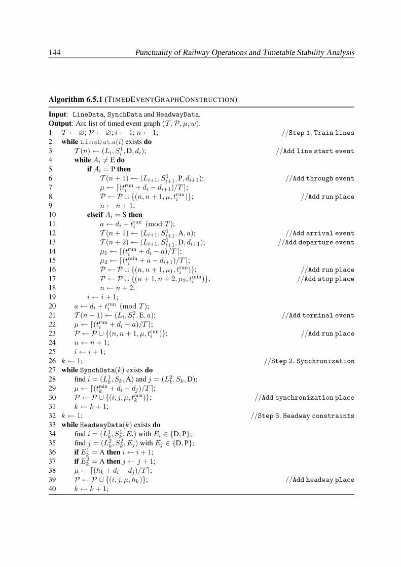
144 Punctuality of Railway Operations and Timetable Stability Analysis
Algorithm 6.5.1 (TIMEDEVENTGRAPHCONSTRUCTION)
Input: LineData, SynchData and HeadwayData.
Output: Arc list of timed event graph (T ,P, µ, w).1 T ← ∅; P ← ∅; i← 1; n← 1; //Step 1. Train lines2 while LineData(i) exists do
3 T (n)← (Li, S1i , D, di); //Add line start event
4 while Ai 6= E do
5 if Ai = P then
6 T (n + 1)← (Li+1, S1i+1, P, di+1); //Add through event
7 µ← d(truni + di − di+1)/T e;
8 P ← P ∪ {(n, n + 1, µ, truni )}; //Add run place
9 n← n + 1;
10 elseif Ai = S then
11 a← di + truni (mod T );
12 T (n + 1)← (Li+1, S1i+1, A, a); //Add arrival event
13 T (n + 2)← (Li+1, S1i+1, D, di+1); //Add departure event
14 µ1 ← d(truni + di − a)/T e;
15 µ2 ← d(tmini + a− di+1)/T e;
16 P ← P ∪ {(n, n + 1, µ1, truni )}; //Add run place
17 P ← P ∪ {(n + 1, n + 2, µ2, tmini )}; //Add stop place
18 n← n + 2;
19 i← i + 1;
20 a← di + truni (mod T );
21 T (n + 1)← (Li, S2i , E, a); //Add terminal event
22 µ← d(truni + di − a)/T e;
23 P ← P ∪ {(n, n + 1, µ, truni )}; //Add run place
24 n← n + 1;
25 i← i + 1;
26 k ← 1; //Step 2. Synchronization27 while SynchData(k) exists do
28 find i = (L1k, Sk, A) and j = (L2
k, Sk, D);29 µ← d(tmin
k + di − dj)/T e;30 P ← P ∪ {(i, j, µ, tmin
k )}; //Add synchronization place31 k ← k + 1;
32 k ← 1; //Step 3. Headway constraints33 while HeadwayData(k) exists do
34 find i = (L1k, S
1k , Ei) with Ei ∈ {D, P};
35 find j = (L2k, S
2k , Ej) with Ej ∈ {D, P};
36 if E1k = A then i← i + 1;
37 if E2k = A then j ← j + 1;
38 µ← d(hk + di − dj)/T e;39 P ← P ∪ {(i, j, µ, hk)}; //Add headway place40 k ← k + 1;
Chapter 6. Timed Event Graphs 145
initializes the lists T and P of transitions and places, respectively, as well as the two counters iand n. The counter i points at the current row in LineData and n denotes the current size of the
transition list. Lines 2–25 generate all transitions and places corresponding to a train line from
terminal to terminal. Each train line starts with a departure event from a terminal (line 3). For
a passage activity lines 5–9 generate a through event and a place from the previous transition
to this new transition corresponding to a train run. Likewise, for a stop activity lines 10–18
generate an arrival and a departure event and two cascade places from the previous transition
over the two new transitions corresponding to a train run and stop, respectively. The algorithm
iterates over the inner loop of line 5–19 until the current input row contains an end activity.
Lines 20–24 generate a terminal event and a place corresponding to the train run on the final
line segment of the current line. The algorithm then proceeds with the next train line in the
outer loop (line 2), and this procedure repeats until the last row of LineData has been reached.
The synchronization constraints are considered in lines 26–31. For each row k in SynchData
the corresponding arrival and departure transitions are connected by a place with holding time
equal to the minimum transfer/connection/layover time.
Finally, lines 32–40 generate the places corresponding to minimum headway constraints. Some
explanation is in order to the procedure of finding the correct transitions in lines 34–37. If the
event type isE1k = D then the associated transition may either be a departure or through event at
station S1k . Note that either (L1
k, S1k ,D) or (L1
k, S1k , P) may exist but not both since an (outbound)
event is either a departure or a passage. On the other hand, if the event type is E1k = A then the
associated transition is either an arrival, through or terminal event at the next timetable point
after S1k on the route of line L1
k. To locate the corresponding transition in the transition list Tobserve that an arrival, passage or terminal event at the destination station of a line segment in
the transition list T is the successor of the departure or passage at the origin station of this line
segment, i.e., if the latter transition is located in T (i) then the former transition is located in
T (i+ 1). The analogue holds for event E2k .
We assume that the input data is such that the timed event graph generated by Algorithm 6.5.1
satisfies the following condition.
Assumption 6.1 On any circuit ξ with weight w(ξ) = 0 there is at least one place pk =(j, i, l, 0) ∈ ξ such that di 6= dj.
This assumption is no limitation in practice but guarantees that each circuit has at least one
proper precedence relation that determines a firing sequence order. Given this assumption the
timed event graph constructed by Algorithm 6.5.1 satisfies the following basic behavioural prop-
erties.
Theorem 6.5.1 (Initial marking) Let (T ,P, µ, w) be the timed event graph constructed by
Algorithm 6.5.1, where the initial marking in each place pk = (i, j, µk, wk) ∈ P is defined by
µk =
⌈wk + di − dj
T
⌉
, (6.7)
with d ∈ [0, T )n the scheduled departure time vector (modulo T ). Then G = (T ,P, µ, w) is
live and µ is the minimal marking such that each event i is firable at time di with cycle time T .
146 Punctuality of Railway Operations and Timetable Stability Analysis
Proof: First note that the initial marking equation (6.7) defines nonnegative markings µk =d(wk + di − dj)/T e ≥ 0 only, since (wk + di − dj)/T > (wk − T )/T ≥ −T/T = −1. We
next prove that each circuit of the constructed timed event graph contains at least one token and
therefore by Theorem 6.4.1 the timed event graph is live. Consider first any circuit ξ with at
least one place pk ∈ ξ with wk > 0 and thus w(ξ) > 0. Then
∑
pk∈ξ
µk =∑
pk∈ξ
⌈(wk + din(pk) − dout(pk))/T
⌉
≥⌈∑
pk∈ξ
(wk + din(pk) − dout(pk))/T
⌉
=
⌈
1
T
∑
pk∈ξ
wk
⌉
> 0. (6.8)
Now consider the case w(ξ) = 0, i.e., wk = 0 for all pk ∈ ξ. Then
∑
pk∈ξ
µk =∑
pk∈ξ
⌈(wk + din(pk) − dout(pk))/T
⌉=∑
pk∈ξ
⌈(din(pk) − dout(pk))/T
⌉≥ 1
by Assumption 6.1. We next prove that (6.7) is the minimal marking for which the timed event
graph is executable with a cycle time T and firing instants di (mod T ). Consider any place
pk = (i, j). If transition i fires at time instant di ∈ [0, T ) then the token added to pk is available
to j at time instant di +wk. The timetable requires that j fires at time instants dj + l ·T (l ∈ N0)
and so at these time instants a token should be available in pk. The token fired by i is only
available after a number of cycles given by
µk = min{l ∈ N0 | dj + lT ≥ di + wk}= min{l ∈ N0 | l ≥ (di + wk − dj)/T}. (6.9)
Thus, the initial marking of pk must contain at least this amount of tokens to be able to fire at the
scheduled time instants before the first token from transition i becomes available. The minimal
marking l ∈ N0 in (6.9) is exactly the right-hand side of (6.7). 2
It is interesting to look at the strongly-connected components in the timed event graph con-
structed by Algorithm 6.5.1. Rolling stock is often exclusively allocated to one train line in both
directions, i.e., trains turn at the terminal stations and continue in the opposite direction. In other
cases rolling stock alternates between train lines at a common terminal station. Hence, rolling
stock circulations ‘close’ the train lines by which each complete train line is contained in at
least one strongly-connected component. Moreover, bidirectional transfers between train lines
at a mutual transfer station connect two components into one larger component, and likewise
headway constraints between two train lines in both directions also combine strongly-connected
components. It is therefore not surprising that the timed event graph may be largely strongly
connected with separate components only at some disconnected regional railway lines. The
strongly-connected components have several behavioural properties as stated in the following
theorem.
Theorem 6.5.2 Let (T ,P, µ, w) be the timed event graph constructed by Algorithm 6.5.1 and
let p be the maximum initial marking in any place, p = maxk µk. If G = (T ,P, µ, w) is
strongly connected then it is autonomous, live, (p+ 1)-bounded and periodic with a cycle time
smaller than or equal to T .
Chapter 6. Timed Event Graphs 147
Proof: By definition of strongly connectedness each transition in the event graph is contained
in a circuit and thus has an incoming place, which implies that G is autonomous. Liveness
follows directly from Theorem 6.5.1. By Theorem 6.4.3 and strongly connectedness, G is pe-
riodic and the cycle time equals the maximum cycle mean η. Let ξ be an arbitrary circuit. If
w(ξ) = 0 for all circuits ξ then trivially T ≥ η = 0. On the other hand, if w(ξ) > 0 then
T ≥ (∑
pk∈ξ wk)/(∑
pk∈ξ µk) by (6.8) and therefore also T ≥ η. Finally, G is p + 1-bounded
by Theorem 6.4.4. 2
In the timed event graph of Algorithm 6.5.1 the timetable is implicitly incorporated in the de-
termination of the initial marking, cf. (6.7) and the timed event graph is executable with respect
to the timetable d, although the transitions do not wait for the scheduled departure times before
firing. Instead the transitions fire as early as the initial marking and holding times allow. By
Theorem 6.5.2 the strongly-connected components then operate periodically with cycle time
smaller than T after possibly some transient behaviour. This will be detailed in Chapter 8.
The timed event graph can be forced into a periodic behaviour in accordance with the peri-
odic timetable by explicitly including the latter into the model. This essentially means that the
transitions do not fire as early as possible but wait for their scheduled event time. Hence, the
timetable realizes additional buffer times between successive departures. Moreover, if the timed
event graph is not connected then inclusion of the timetable also has a coordinating function be-
tween the various strongly-connected components.
The periodic timetable with cycle time T can be implemented in the timed event graph as
follows. First, add a loop to the timed event graph consisting of transition n + 1 which is both
input and output transition to a place pn+1,n+1 = (n+1, n+1) with one initial token and holding
time wn+1 = T . Hence, transition n + 1 fires with a cycle time T and may be interpreted as
a clock that synchronizes the start of the next period for all transitions. Second, add a place
pi,n+1 = (n+ 1, i) for all i = 1, . . . , n. The place pi,n+1 has zero initial tokens and the holding
time is defined as wi,n+1 = di, where di ∈ [0, T ) is the timetable event time of transition i. If
transition n + 1 fires at time instant t = 0 then each i in the timed event graph is enabled at
xi(k) = di + k · T for k ∈ N0. Thus, the resulting (autonomous) scheduled timed event graph
G is given in arc list representation as
G = G ∪ {(n+ 1, n+ 1, 1, T )} ∪ {(n+ 1, i, 0, di)|i = 1, . . . , n}. (6.10)
This corresponds to the timed event graph G = (T , P, µ, w), where
T .= T ∪ {n+ 1},
P .= P ∪ {(n+ 1, n+ 1)} ∪ {(n+ 1, i)|i = 1, . . . , n},
µ.= (µ>, 1, 0, . . . , 0)> ∈ Zm+1+n
+ ,
w.= (w>, T, d>)> ∈ Rm+1+n
+ .
Theorem 6.5.3 (Scheduled timed event graph) Let G = (T , P, µ, w) be the scheduled timed
event graph defined in (6.10) and let p be the maximum initial marking in any place, p =maxk µk. Then G is autonomous, live, (p+ 1)-bounded, and periodic with cycle time T .
Proof: By construction transition n+1 is a predecessor to all transitions, including n+1 itself,
and therefore G is autonomous. The original timed event graph G is live by Theorem 6.5.1. The
148 Punctuality of Railway Operations and Timetable Stability Analysis
event graph G differs from G by one additional transition n + 1, a place (n + 1, n + 1), and
places from the new transition n + 1 to each other transition. The loop (n + 1, n + 1) contains
one token and transition n+ 1 has no other incoming places, by which the new transition n+ 1is live. Furthermore, the loop (n+1, n+1) is the only new circuit generated by the new places.
Hence, G is live. By Theorem 6.5.2 all strongly-connected subgraphs of G are periodic with
cycle time not exceeding T . The added places from n + 1 to all original transitions do not
change the strongly-connected components. Hence, the components in G are those of G plus
the additional loop (n + 1, n+ 1). Moreover, transition n + 1 has cycle time T and has access
to all other transitions. Therefore, any transition in G is slowed down to the cycle time of n+1,
i.e., the complete timed event graph is synchronous with cycle time T . Finally, G is (p + 1)-
bounded since each transition in G has the same cycle time and so each place receives at most
one token before again consuming a token during one period. Note that the loop (n+ 1, n+ 1)is 1-bounded and p > 0 since G is live. 2
In the scheduled event graph (6.10) we incorporated the timetable integrally over all transitions.
However, in general only departures must be strictly adhered to, whilst arrivals and passages
are also allowed to be early. Hence, we can alternatively add the timetable places to departure
events only, i.e.,
G′ = G ∪ {(n+ 1, n+ 1, 1, T )} ∪ {(n+ 1, i, 0, di)|i ∈ D}, (6.11)
where
D .= {i ∈ T | Ei = D}.
Each arrival, through or terminal event at the destination station of a line segment has a pre-
decessor in T corresponding to the departure event at the origin station of this line segment.
Therefore, the proof of Theorem 6.5.3 is also valid for the timed event graph G′ and so Theo-
rem 6.5.3 also holds for G′ instead of G.
Comparing Theorem 6.5.2 and 6.5.3, we see that an integrated periodic timetable has an impact
on the properties of a timed event graph comparable to strongly connectedness. In Chapter 8 we
will study the performance properties of a timed event graph — including the dependence on
the internal structure of strongly-connected components — in terms of its max-plus state-space
realization using the max-plus algebraic eigenvalue theory that will be introduced in Chapter 7.
6.5.3 Event Domain Description
The timed event graph can alternatively be described in the event domain, where the variables
are the event times associated to the transitions i ∈ T . Let xi(k) denote the kth occurrence
time of event i (e.g. departure i of train line Li from station Si). We assume that all trains run
at an integrated regular interval T (usually T = 60 minutes). If the discrete event system is
synchronous, the counter k represents the period (hour) in which the event occurs. If a train line
has a frequency f > 1 trains per cycle time T then the f trains in a basic period are modelled by
separate train lines with a cycle time T each. Without loss of generality we furthermore assume
that the first timetable period is [0, T ), the 2nd period is [T, 2 · T ), and in general the kth period
is [(k − 1) · T, k · T ).
Consider a timed event graph G = (T ,P, µ, w). Then each place p ∈ P with out(p) = igenerates a constraint on the event time xi(k) given by
xi(k) ≥ xin(p)(k − µ(p)) + w(p),
Chapter 6. Timed Event Graphs 149
since i may only fire for the kth time if the activity initiated by event in(p) in µ(p) periods
before has been completed. Denote by Πi the set of incoming places to transition i, so
Πi.= {p ∈ P | out(p) = i}.
Then if transitions fire as soon as they are enabled, we obtain the following equation for the
event times
xi(k) = maxp∈Πi
(xin(p) (k − µ(p)) + w(p)
)for all i ∈ T . (6.12)
If events are not allowed to occur before their scheduled event times then additional timetable
constraints must be taken into account defined as
xi(k) ≥ di(k) for all i ∈ T ,
where di(k) is the scheduled event time of event i in period k. In a periodic timetable with
cycle time T the scheduled event time of event i over successive periods k ∈ N is given by
di(k) = di(0) + k · T , where di(0) is an initial scheduled departure time. The general dynamic
event time equations of the scheduled timed event graph then becomes
xi(k) = max
(
maxp∈Πi
(xin(p)(k − µ(p)) + w(p)
), di(k)
)
for all i ∈ T . (6.13)
The dynamic equations (6.12) and (6.13) are the state-space realizations of the (homogeneous)
timed event graph and scheduled timed event graph, respectively. This description is used in
the performance evaluation of timed event graphs, see Chapter 8. It is interesting to note that
the discrete-event dynamic equations (6.12) and (6.13) are nonlinear because of the maximum
operation. Nevertheless, the equations become linear when evaluated in the appropriate algebra,
the so-called max-plus algebra, where the fundamental operations are the maximum and sum,
see Chapter 7.
Example 6.2 Consider the timed event graph of Figure 6.7. The line constraints are
A1,2(k) ≥ D1,1(k) + 11
D1,2(k) ≥ A1,2(k) + 1
A1,3(k) ≥ D1,2(k) + 12
A2,2(k) ≥ D2,1(k) + 9
D2,2(k) ≥ A2,2(k) + 1
A2,3(k) ≥ D2,2(k) + 10,
the transfer constraints are
D1,2(k) ≥ A2,2(k) + 2
D2,2(k) ≥ A1,2(k) + 2
and the headway constraints are given by
A1,2(k) ≥ A2,2(k − 1) + 2
A2,2(k) ≥ A1,2(k) + 2
D1,2(k) ≥ D2,2(k) + 2
D2,2(k) ≥ D1,2(k − 1) + 2.
150 Punctuality of Railway Operations and Timetable Stability Analysis
From these constraints we obtain the following discrete-event dynamic system description in
the event domain:
A1,2(k) = max (D1,1(k) + 11, A2,2(k − 1) + 2)
D1,2(k) = max (A1,2(k) + 1, A2,2(k) + 2, D2,2(k) + 2)
A1,3(k) = D1,2(k) + 12
A2,2(k) = max (D2,1(k) + 9, A1,2(k) + 2)
D2,2(k) = max (A2,2(k) + 1, A1,2(k) + 2, D1,2(k − 1) + 2)
A2,3(k) = D2,2(k) + 10.
Now suppose that a train on line L1 departs from station S1 at 0 and a train of line L2 follows
after 5 minutes, i.e., D1,1(1) = 0 and D2,1(1) = 5. Moreover, assume that these are the first two
trains of a day and therefore no events have occurred for k < 1 which can be modelled by taking
the event times x(0) sufficiently small, or in particular we may take initiallyA2,2(0) = −∞ and
D1,2(0) = −∞. Then we can simply compute the event times from the recursions above,
evaluated in the appropriate order, giving
A1,2(1) = max (D1,1(1) + 11, A2,2(0) + 2) = max (0 + 11,−∞+ 2) = 11
A2,2(1) = max (D2,1(1) + 9, A1,2(1) + 2) = max (5 + 9, 11 + 2) = 14
D2,2(1) = max (A2,2(1) + 1, A1,2(1) + 2, D1,2(0) + 2) = max (14 + 1, 11 + 2,−∞+ 2) = 15
D1,2(1) = max (A1,2(1) + 1, A2,2(1) + 2, D2,2(1) + 2) = max (11 + 1, 14 + 2, 15 + 2) = 17
A2,3(1) = D2,2(1) + 10 = 15 + 10 = 25
A1,3(1) = D1,2(1) + 12 = 17 + 12 = 29.
If the successive departure times D1,1(k) and D2,1(k) from station S1 are given for each k ≥ 1then we can analogously compute the successive event times for each period k ∈ N. 2
6.6 Conclusions
A railway timetable and the shared infrastructure utilization generate train interdependencies
that leads to scheduled waiting times and delay propagation during operations. In general,
a timetable represents a (cyclic) network structure of train circulations and synchronization
of trains at main railway stations imposed by passenger transfers, rolling stock connections
or crew transfers, and in addition the railway infrastructure and safety and signalling systems
cause headway restrictions between successive trains. This intrinsic network structure and the
train traffic dynamics within this structure can be modelled and analysed by a graphical and
mathematical structure called timed event graphs.
Structural properties of timed event graphs concern the topology or interconnection structure.
We showed how the primitive structures of timed event graphs (sequential, concurrent and syn-
chronization transitions) can be connected to model typical timetable structures and infrastruc-
ture restrictions. Structural properties are independent of the initial marking. On the other hand,
behavioural properties of timed event graphs are those characteristics that depend on the initial
marking. We showed that timed event graphs have a tendency of becoming periodic driven by
the circulation of tokens over circuits in the timed event graph.
Chapter 6. Timed Event Graphs 151
This chapter also described the input data necessary for the synthesis of a timed event graph that
models the essential features of a scheduled railway system. Line data contains the line sched-
ules and train process times, synchronization data contains passenger and logistic connections
between train lines, and headway data consists of all headway restrictions between event pairs
corresponding to conflicting train routes. An algorithm has been presented for systematically
constructing a timed event graph based on this input data. The timetable and process times
contained in the timetable, synchronization data and headway data have been used to derive a
consistent initial marking. So far, the analysis of the timetable structure has been mainly struc-
tural and behavioural. The next step is performance related issues which will be considered in
Chapter 8 after explaining the fundamental mathematics in Chapter 7.

152 Punctuality of Railway Operations and Timetable Stability Analysis
Chapter 7
MAX-PLUS ALGEBRA
7.1 Introduction
This chapter deals with max-plus algebra. Max-plus algebra is a particular example of an idem-
potent semiring, or dioid, originating from the 1960s as a formal algebraic structure for solving a
range of path problems in graph theory. Many graph algorithms are equivalent to classical algo-
rithms for solving linear systems of equations when formulated in the appropriate algebra [75].
Cuninghame-Green [40] gave a first systematic treatment of max-plus algebra showing many
counterparts to linear algebra with interpretations in path problems over graphs. In 1985, Co-
hen et al. [32] showed that timed event graphs can be represented by (recursive) linear systems
in max-plus algebra and explained how the periodic steady-state behaviour of these discrete-
event systems are characterized by solving an eigenproblem in max-plus algebra. This led to
a renewed interest in max-plus algebra accumulating to a max-plus linear system theory of
discrete-event dynamic systems as presented in Baccelli et al. [11], in analogy to linear system
theory of dynamic systems governed by differential and difference equations. Current research
issues include the geometric description of max-plus semimodules, see e.g. Cohen et al. [34].
This chapter introduces max-plus algebra, its connection to path problems, and the eigen-
problem of max-plus matrices. The eigenstructure of irreducible max-plus matrices is well-
known [11, 40]. Gaubert [70] developed a full description of the eigenstructure of reducible
max-plus matrices. Cochet-Terrasson et al. [31] introduced a generalized eigenproblem of max-
plus polynomial matrices and described the max-plus policy iteration algorithm for solving this
problem. A max-plus polynomial matrix can be viewed as a formal representation of a timed
event graph. The paper of Cochet-Terrasson et al. [31] therefore motivated the approach in this
chapter to develop a complete description of the generalized eigenstructure of reducible max-
plus polynomial matrices. In Chapter 8 we will use the polynomial matrix in the state-space
description of the timed event graph. Hence, a polynomial matrix is not only a formal represen-
tation of timed event graphs but can also be used to describe the firing dynamics of the timed
event graph.
The outline of this chapter is as follows. Section 7.2 defines the max-plus semiring as well
as polynomials and matrices over this semiring, which are themselves also semirings. The
relation between max-plus matrices and precedence graphs is explained, as well as that of max-
plus polynomial matrices and timed event graphs. Section 7.3 is concerned with max-plus
semimodules, which represent the counterpart of vector spaces in max-plus algebra. Section 7.4
considers the eigenproblem of max-plus matrices and extends this theory to the generalized
eigenproblem of max-plus polynomial matrices. This section also explains the max-plus policy
iteration algorithm. Longest path algorithms are considered in Section 7.5. Finally, Section 7.6
presents some conclusions.
153
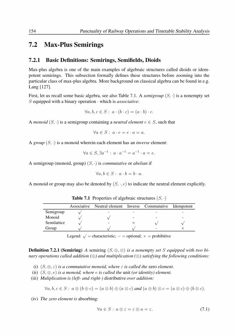
154 Punctuality of Railway Operations and Timetable Stability Analysis
7.2 Max-Plus Semirings
7.2.1 Basic Definitions: Semirings, Semifields, Dioids
Max-plus algebra is one of the main examples of algebraic structures called dioids or idem-
potent semirings. This subsection formally defines these structures before zooming into the
particular class of max-plus algebra. More background on classical algebra can be found in e.g.
Lang [127].
First, let us recall some basic algebra, see also Table 7.1. A semigroup (S, ·) is a nonempty set
S equipped with a binary operation · which is associative:
∀a, b, c ∈ S : a · (b · c) = (a · b) · c.
A monoid (S, ·) is a semigroup containing a neutral element e ∈ S, such that
∀a ∈ S : a · e = e · a = a.
A group (S, ·) is a monoid wherein each element has an inverse element:
∀a ∈ S, ∃a−1 : a · a−1 = a−1 · a = e.
A semigroup (monoid, group) (S, ·) is commutative or abelian if
∀a, b ∈ S : a · b = b · a.
A monoid or group may also be denoted by (S, ·, e) to indicate the neutral element explicitly.
Table 7.1 Properties of algebraic structures (S, ·)Associative Neutral element Inverse Commutative Idempotent
Semigroup√
- - - -
Monoid√ √
- - -
Semilattice√
- × √ √
Group√ √ √
- ×Legend:
√= characteristic; − = optional; × = prohibitive
Definition 7.2.1 (Semiring) A semiring (S,⊕,⊗) is a nonempty set S equipped with two bi-
nary operations called addition (⊕) and multiplication (⊗) satisfying the following conditions:
(i) (S,⊕, ε) is a commutative monoid, where ε is called the zero element.
(ii) (S,⊗, e) is a monoid, where e is called the unit (or identity) element.
(iii) Muliplication is (left- and right-) distributive over addition:
∀a, b, c ∈ S : a⊗ (b⊕ c) = (a⊗ b)⊕ (a⊗ c) and (a⊕ b)⊗ c = (a⊗ c)⊕ (b⊗ c).
(iv) The zero element is absorbing:
∀a ∈ S : a⊗ ε = ε⊗ a = ε. (7.1)
Chapter 7. Max-Plus Algebra 155
A semiring may also be denoted by (S,⊕,⊗, ε, e) to indicate the zero and unit element explic-
itly.
If (S,⊗) is also commutative then (S,⊕,⊗) is a commutative semiring. From the definition
directly follows that any semiring has at least one element, namely the zero element ε. More-
over, if a semiring (S,⊕,⊗) has more than one element, |S| > 1, then it contains both a zero
and unit element and e 6= ε by the absorption law. Indeed, for all a ∈ S we have a ⊗ e = a (eis the identity) and a ⊗ ε = ε (ε is absorbing), whence if e = ε then we must have a = ε or
equivalently S = {ε}. This proves that e = ε if and only if |S| = 1. Furthermore, the neutral
elements are unique, since if both e and e′ are a zero element then e = e⊕ e′ = e′. Likewise, if
ε and ε′ are both a unit element, then ε = ε⊗ ε′ = ε′.
Definition 7.2.2 (Semifield) A semifield (S,⊕,⊗, ε, e) is a semiring in which (S \ {ε},⊗, e)is a group.
In a commutative semifield (S,⊕,⊗, ε, e) each nonzero element has a (multiplicative) inverse,
i.e., ∀a ∈ S\{ε}, ∃a−1 : a⊗a−1 = a−1⊗a = e. In general we may distinguish between a right-
and left-inverse, but in a commutative semifield they coincide. Obviously, ε is not invertible
since the zero element ε in a semiring is absorbing. This is similar to the ordinary field of real
numbers, where 0 has no multiplicative inverse. The inverse multiplicative operation is called
division and is denoted by �.
Definition 7.2.3 (Idempotency, dioid) Let (S,⊕,⊗) be a semiring. An element a ∈ S is called
(additively) idempotent if a⊕a = a. A semiring (S,⊕,⊗) is idempotent if ∀a ∈ S : a⊕a = a.
An idempotent semiring is also called a dioid.
A commutative idempotent semigroup (S,⊕) is also called a semilattice [40], cf. Section 7.2.7.
Hence, addition in an idempotent semiring (or dioid) can also be characterized as a semilatice
with zero element. An example of an idempotent operation is the pairwise maximum operation,
since max(a, a) = a for any a ∈ R.
Proposition 7.2.1 An idempotent semiring (semigroup, monoid) has exactly one additive in-
vertible element, which is the zero element ε.
Proof: Assume that a has an additive inverse b such that a ⊕ b = ε. Then a = a ⊕ ε =a⊕ a⊕ b = a⊕ b = ε and likewise b = ε⊕ b = a⊕ b⊕ b = a⊕ b = ε. Thus, a = b = ε. 2
Idempotency thus prevents the existence of (additive) inverse elements, and therefore an idem-
potent semiring (semifield) can not be embedded in a ring (field), wherein addition is a group.
Semirings may therefore be classified into two essentially different classes according to whether
or not addition is idempotent. An example of a semiring (in fact, a semifield) that is not idem-
potent is R+ = ([0,∞),+, ·, 0, 1), the nonnegative real numbers with conventional addition and
multiplication. Clearly, this semiring can be extended to a ring (or field) by adding the negative
real numbers. Such semirings therefore correspond to the nonnegative elements of a ring, which
can be symmetrized with negative elements. In contrast, addition in idempotent semirings (or
dioids) is neither invertible nor can be made invertible in the classic sense, since idempotent
addition simply does not allow the existence of inverse elements (other than the trivial zero
156 Punctuality of Railway Operations and Timetable Stability Analysis
element) because of Proposition 7.2.1. Therefore, alternative notions of inversion have been
developed for solving linear equations (and monotone functional equations) over a dioid based
on residuation theory of (semi)lattices [11, 40]. We will not deliberate this here any further, but
refer to Cuninghame-Green [40] and Baccelli et al. [11] for details.
Definition 7.2.4 (Subsemiring) Let (S,⊕,⊗, ε, e) be an (idempotent) semiring. A subset T ⊆S is a subsemiring of (S,⊕,⊗, ε, e) if
(i) ε ∈ T and e ∈ T .
(ii) T is closed under addition and multiplication, i.e., ∀a, b ∈ T : a⊕ b ∈ T and a⊗ b ∈ T .
A subsemiring T of a semiring (S,⊕,⊗, ε, e) inherits the addition and multiplication of the
latter and (T,⊕,⊗, ε, e) is itself a semiring. If (S,⊕,⊗, ε, e) is idempotent (or commutative)
then so are its subsemirings.
7.2.2 The (max,+)-Semifield
Max-plus algebra is the study of the algebraic structure Rmax.= (R ∪ {−∞},⊕,⊗) of the set
R ∪ {−∞} equipped with two binary operations called addition (⊕) and multiplication (⊗),
which are defined for all a, b ∈ R ∪ {−∞} by
a⊕ b .= max(a, b), a⊗ b .= a+ b. (7.2)
The algebraic structure Rmax = (R∪{−∞},⊕,⊗) is a semifield. In the forthcoming, the scalar
operations ⊕ and ⊗ will always mean the (max,+) operations defined by (7.2).
Proposition 7.2.2 Rmax = (R ∪ {−∞},⊕,⊗, ε, e), with ⊕ = max, ⊗ = +, zero element
ε = −∞ and unit element e = 0 is a commutative idempotent semifield.
Proof: The proposition is easily verified by checking the axioms. 2
Rmax = (R ∪ {−∞},max,+) is known as the (max,+)-semiring or (max,+)-semifield. In
literature also the names path algebra [75] and schedule algebra [73] are used corresponding
to applications to path and schedule problems over directed graphs. In the sequel, we will
use the notation ε = −∞ and e = 0 to emphasize the special meaning of these elements in
Rmax. We also denote by Rε.= R ∪ {ε} the set of real numbers extended by ε. Because of
distributivity, ⊗ has priority over ⊕ and so we also just write ab instead of a ⊗ b, as is also
common in conventional algebra. Since the zero element in Rmax is ε we will also refer to a
nonzero element as a finite element. Division in Rmax is defined for all a ∈ Rε and b ∈ R by
a� b .= a− b.
A power a⊗l in max-plus algebra is defined by repeated multiplication of l factors, i.e., for all
a ∈ Rmax and l ∈ N
a⊗l .= a⊗ · · · ⊗ a︸ ︷︷ ︸
l times
= l · a,
Chapter 7. Max-Plus Algebra 157
where · is the conventional multiplication. The superscript ⊗ may be omitted if there is no
confusion that the power must be evaluated in max-plus algebra. Powers of a ∈ Rmax are not
restricted to integers but can more generally defined by a⊗l .= l · a for any real number l ∈ R,
and by convention ε⊗0 = e. Products of powers satisfy ak⊗al = ak⊗l, since akal = k ·a+l ·a =(k + l) · a = ak⊗l. A (positive) power of a sum satisfies (a⊕ b)k = ak ⊕ bk for all k ∈ N, since
(a ⊕ b)k = k · max(a, b) = max(k · a, k · b) = ak ⊕ bk. By induction this identity is easily
generalized to a power of a finite series of elements ai ∈ Rmax as
(n⊕
i=1
ai
)k
=
n⊕
i=1
aki for all k ∈ N.
The notation of the inverse a−1 should not be confused with the power of a to −1, although
incidentally a⊗−1 = −a is the inverse of a 6= ε.
The following examples illustrate the arithmetics in Rmax.
2.4⊕ 3 = 3 2.4⊗ 3 = 5.4 4⊕ 8⊗−3 = 52⊕−3 = 2 2⊗−3 = −1 3−8 = −24e⊕ 3 = 3 e� 3 = −3 2⊗ 4−3 ⊗ 5 = −5
−2⊕−3 = −2 −2⊗−3 = −5 (2⊕ 3)2 = 6ε⊕ 3 = 3 ε⊗ 3 = ε (−1⊕−4)3 = −3.
If we are interested in integers only we may also work in the dioid Zmax = (Z ∪ {ε},⊕,⊗).Zmax is a subsemiring of Rmax and therefore itself an idempotent semiring (see Definition 7.2.4),
which is easily proved as follows. Clearly, ε, e ∈ Zmax and for any two integers a, b ∈ Z also
a ⊕ b = max(a, b) and a ⊗ b = a + b is an integer. Furthermore, a ⊕ ε = a and a ⊗ ε = ε.The multiplicative inverses a−1 = −a of all nonzero elements are also contained in Z. Hence,
Zmax is a commutative idempotent semifield. Another subsemiring of Rmax (and of Zmax) is
(N ∪ {0, ε},⊕,⊗), which is a commutative idempotent semiring, but not a semifield.
7.2.3 Max-Plus Polynomials
In this section we look at polynomials over the (max,+)-Semiring.
Definition 7.2.5 (Max-plus polynomial) A (formal) max-plus polynomial in an indeterminate
X is a finite sum⊕p
l=0 alXl for some integer p ∈ N and al ∈ Rmax. The set of max-plus
polynomials is denoted as Rmax[X].
The elements al of a polynomial f =⊕p
l=0 alXl ∈ Rmax[X] are called the coefficients of
f . The support of a polynomial f is the index set of the finite coefficients of f , denoted as
supp(f) = {0 ≤ l ≤ p | al > ε}. The degree of a polynomial f ∈ Rmax[X] is the highest
power of X (or highest index) with al > ε, and denoted as deg(f) =⊕
l∈supp(f) l. Two
polynomials⊕p
l=0 alXl and
⊕pl=0 blX
l are equal if and only if al = bl for all l = 0, . . . , p.
On the set of formal max-plus polynomials Rmax[X] we define addition and multiplication as
follows. Let f =⊕p
l=0 alXl and g =
⊕ql=0 blX
l. The sum ⊕ of two polynomials is defined
158 Punctuality of Railway Operations and Timetable Stability Analysis
componentwise, i.e.,
f ⊕ g =
deg(f)⊕deg(g)⊕
l=0
(al ⊕ bl)X l. (7.3)
If the support of the polynomials f and g differs then we treat the missing coefficients as ε. Note
that the degree of h = f ⊕ g ∈ Rmax[X] is the maximal degree of f and g, deg(h) = deg(f)⊕deg(g) = max(deg(f), deg(g)). The product ⊗ of two polynomials is defined according to the
sup-convolution rule:
f ⊗ g =
deg(f)⊗deg(g)⊕
l=0
(⊕
i⊗j=l
ai ⊗ bj)
X l. (7.4)
The degree of the product of two polynomials is the product of the degree of its factors, deg(f⊗g) = deg(f)⊗ deg(g) = deg(f) + deg(g).
It is easily verified that the set of polynomials Rmax[X] with addition and multiplication as
defined in (7.3) and (7.4), respectively, satisfies the axioms of a semiring with the constant
polynomials ε and e acting as zero and unit, respectively. Note that the neutral elements can be
understood as the polynomials of degree 0, i.e., ε = εX0 and e = eX0. More generally, we
define the set S[X] of polynomials in the indeterminate X over a semiring (S,⊕,⊗) with addi-
tion and multiplication defined by (7.3) and (7.4) evaluated over S. The proof of the following
theorem is a straightforward exercise in checking the axioms of a semiring.
Theorem 7.2.1 Let (S,⊕,⊗, ε, e) be an (idempotent) semiring. Then the algebraic structure
(S[X],⊕,⊗, ε, e) of polynomials over S with addition ⊕ and multiplication ⊗ as defined in
(7.3) and (7.4), respectively, is an (idempotent) semiring.
In particular, the sets of max-plus polynomials Rmax[X] and Zmax[X] are idempotent semirings.
The definition of polynomial addition and multiplication is consistent with algebraic manipu-
lations in Rmax when considering the indeterminate as a variable in Rmax. By the following
proposition we may substitute an element x ∈ Rmax for the indeterminate X . Hence, to each
polynomial f ∈ Rmax[X] we can associate a polynomial function f : Rmax → Rmax defined by
f(x) =⊕p
l=0 alxl.
Theorem 7.2.2 Let (S[X],⊕,⊗, ε, e) be a polynomial semiring over a commutative semiring
S. Then for any x ∈ S the valuation mapping ϕ : f 7→ f(x) is a homomorphism from S[X]into S.
Proof: We must prove that ϕ(f ⊕ g) = ϕ(f)⊕ ϕ(g) and ϕ(f ⊗ g) = ϕ(f)⊗ ϕ(g). We may
assume without loss of generality that two polynomials have the same degree by taking any
missing coefficients equal to ε. So let f(X) =⊕p
i=0 aiXi and g(X) =
⊕pj=0 bjX
j . Then for
Chapter 7. Max-Plus Algebra 159
addition we have
ϕ(f)⊕ ϕ(g) = f(x)⊕ g(x)= (
⊕pi=0 aix
i)⊕(⊕p
j=0 bjxj)
= a0 ⊕ a1x⊕ . . .⊕ apxp ⊕ b0 ⊕ b1x⊕ · · · ⊕ bpxp
= (a0 ⊕ b0)⊕ (a1x⊕ b1x)⊕ · · · ⊕ (apxp ⊕ bpxp) (by associativity)
= (a0 ⊕ b0)⊕ (a1 ⊕ b1)x⊕ · · · ⊕ (ap ⊕ bp)xp (by distributivity)
=⊕p
l=0(al ⊕ bl)xl
= (f ⊕ g)(x) (by(7.3))
= ϕ(f ⊕ g).For multiplication we have
ϕ(f)⊗ ϕ(g) = f(x)⊗ g(x)= (
⊕pi=0 aix
i)⊗(⊕p
j=0 bjxj)
distr.= a0
(⊕p
j=0 bjxj)
⊕ a1x(⊕p
j=0 bjxj)
⊕ · · · ⊕ apxp(⊕p
j=0 bjxj)
comm.= a0
(⊕p
j=0 bjxj)
⊕ a1
(⊕p
j=0 bjxj+1)
⊕ · · · ⊕ ap
(⊕p
j=0 bjxj+p)
=⊕p
i=0
(
ai ⊗(⊕p
j=0 bjxi+j))
=⊕p
i=0
⊕pj=0(ai ⊗ bj)xi+j
=⊕p⊗p
l=0
⊕
i⊗j=l(ai ⊗ bj)xi⊗j
(7.4)= (f ⊗ g)(x)= ϕ(f ⊗ g).
Here the third equality follows from distributivity of multiplication over addition and in the
fourth equality we used the multiplicative commutativity assumption of S. 2
The valuation homomorphism ϕ : Rmax[X] → Rmax is not an isomorphism, since e.g. the two
polynomialsX2⊕X⊕e andX2⊕e are different by definition, but for the associated polynomial
functions we have x2 ⊕ x⊕ e = max(2x, x, 0) = max(2x, 0) = x2 ⊕ e for all x ∈ Rmax.
7.2.4 Max-Plus Matrices
In this section we consider matrices over the (max,+)-semiring. The scalar max-plus opera-
tions are extended to matrices in a standard way. Let Rm×nmax be the set of m × n matrices with
entries in Rmax. Then matrix addition⊕ is defined componentwise for A,B ∈ Rm×nmax as
[A⊕B]ij = aij ⊕ bij = max(aij, bij), (7.5)
and matrix multiplication⊗ is defined for matrices A ∈ Rm×nmax and B ∈ Rn×r
max as
[A⊗ B]ij =
n⊕
k=1
aik ⊗ bkj = maxk=1,...,n
(aik + bkj), (7.6)
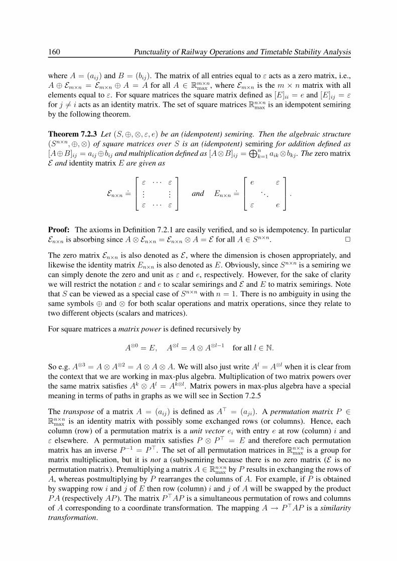
160 Punctuality of Railway Operations and Timetable Stability Analysis
where A = (aij) and B = (bij). The matrix of all entries equal to ε acts as a zero matrix, i.e.,
A ⊕ Em×n = Em×n ⊕ A = A for all A ∈ Rm×nmax , where Em×n is the m × n matrix with all
elements equal to ε. For square matrices the square matrix defined as [E]ii = e and [E]ij = εfor j 6= i acts as an identity matrix. The set of square matrices Rn×n
max is an idempotent semiring
by the following theorem.
Theorem 7.2.3 Let (S,⊕,⊗, ε, e) be an (idempotent) semiring. Then the algebraic structure
(Sn×n,⊕,⊗) of square matrices over S is an (idempotent) semiring for addition defined as
[A⊕B]ij = aij⊕bij and multiplication defined as [A⊗B]ij =⊕n
k=1 aik⊗bkj . The zero matrix
E and identity matrix E are given as
En×n.=
ε · · · ε...
...
ε · · · ε
and En×n
.=
e ε. . .
ε e
.
Proof: The axioms in Definition 7.2.1 are easily verified, and so is idempotency. In particular
En×n is absorbing since A⊗ En×n = En×n ⊗A = E for all A ∈ Sn×n. 2
The zero matrix En×n is also denoted as E , where the dimension is chosen appropriately, and
likewise the identity matrix En×n is also denoted as E. Obviously, since Sn×n is a semiring we
can simply denote the zero and unit as ε and e, respectively. However, for the sake of clarity
we will restrict the notation ε and e to scalar semirings and E and E to matrix semirings. Note
that S can be viewed as a special case of Sn×n with n = 1. There is no ambiguity in using the
same symbols ⊕ and ⊗ for both scalar operations and matrix operations, since they relate to
two different objects (scalars and matrices).
For square matrices a matrix power is defined recursively by
A⊗0 = E, A⊗l = A⊗ A⊗l−1 for all l ∈ N.
So e.g. A⊗3 = A⊗ A⊗2 = A⊗ A⊗ A. We will also just write Al = A⊗l when it is clear from
the context that we are working in max-plus algebra. Multiplication of two matrix powers over
the same matrix satisfies Ak ⊗ Al = Ak⊗l. Matrix powers in max-plus algebra have a special
meaning in terms of paths in graphs as we will see in Section 7.2.5
The transpose of a matrix A = (aij) is defined as A> = (aji). A permutation matrix P ∈Rn×n
max is an identity matrix with possibly some exchanged rows (or columns). Hence, each
column (row) of a permutation matrix is a unit vector ei with entry e at row (column) i and
ε elsewhere. A permutation matrix satisfies P ⊗ P> = E and therefore each permutation
matrix has an inverse P−1 = P>. The set of all permutation matrices in Rn×nmax is a group for
matrix multiplication, but it is not a (sub)semiring because there is no zero matrix (E is no
permutation matrix). Premultiplying a matrix A ∈ Rn×nmax by P results in exchanging the rows of
A, whereas postmultiplying by P rearranges the columns of A. For example, if P is obtained
by swapping row i and j of E then row (column) i and j of A will be swapped by the product
PA (respectively AP ). The matrix P>AP is a simultaneous permutation of rows and columns
of A corresponding to a coordinate transformation. The mapping A → P>AP is a similarity
transformation.
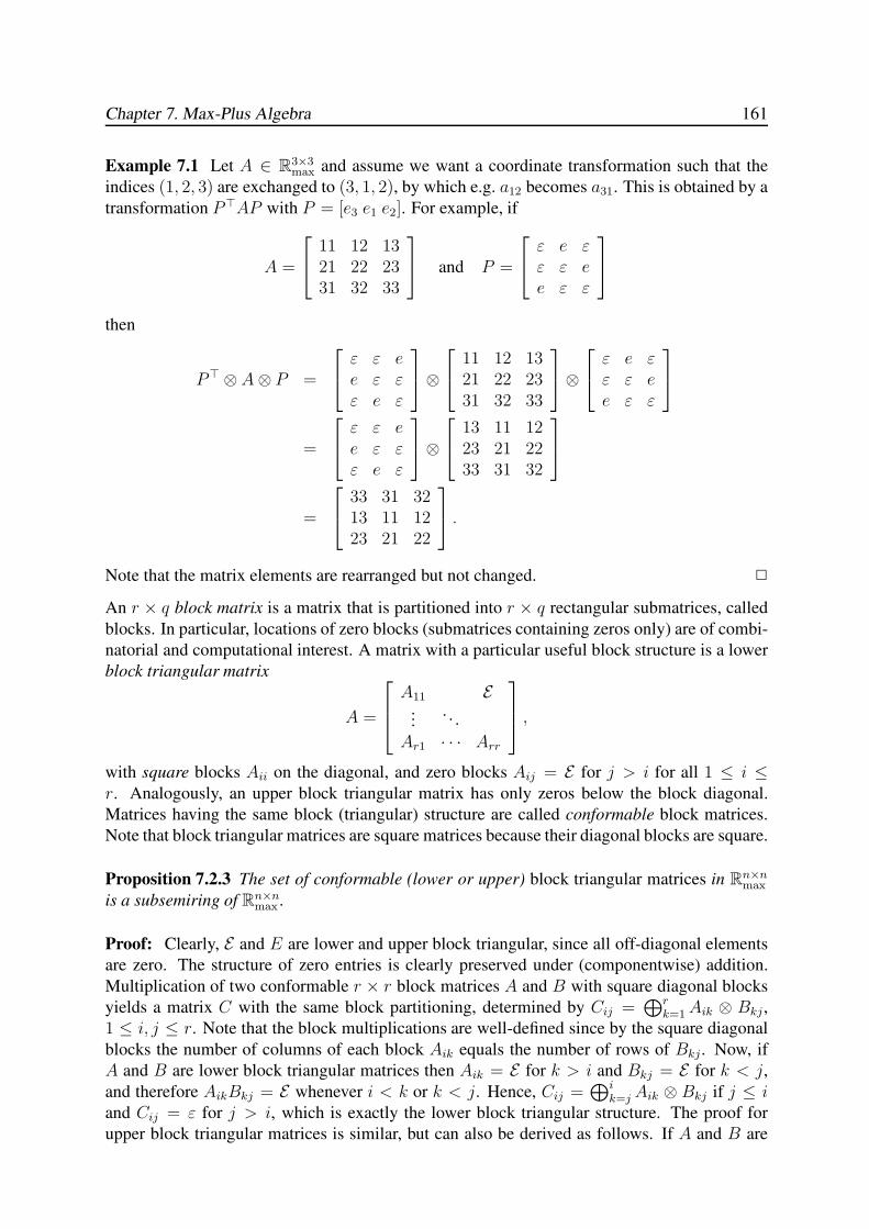
Chapter 7. Max-Plus Algebra 161
Example 7.1 Let A ∈ R3×3max and assume we want a coordinate transformation such that the
indices (1, 2, 3) are exchanged to (3, 1, 2), by which e.g. a12 becomes a31. This is obtained by a
transformation P>AP with P = [e3 e1 e2]. For example, if
A =
11 12 1321 22 2331 32 33
and P =
ε e εε ε ee ε ε
then
P> ⊗ A⊗ P =
ε ε ee ε εε e ε
⊗
11 12 1321 22 2331 32 33
⊗
ε e εε ε ee ε ε
=
ε ε ee ε εε e ε
⊗
13 11 1223 21 2233 31 32
=
33 31 3213 11 1223 21 22
.
Note that the matrix elements are rearranged but not changed. 2
An r × q block matrix is a matrix that is partitioned into r × q rectangular submatrices, called
blocks. In particular, locations of zero blocks (submatrices containing zeros only) are of combi-
natorial and computational interest. A matrix with a particular useful block structure is a lower
block triangular matrix
A =
A11 E...
. . .
Ar1 · · · Arr
,
with square blocks Aii on the diagonal, and zero blocks Aij = E for j > i for all 1 ≤ i ≤r. Analogously, an upper block triangular matrix has only zeros below the block diagonal.
Matrices having the same block (triangular) structure are called conformable block matrices.
Note that block triangular matrices are square matrices because their diagonal blocks are square.
Proposition 7.2.3 The set of conformable (lower or upper) block triangular matrices in Rn×nmax
is a subsemiring of Rn×nmax .
Proof: Clearly, E and E are lower and upper block triangular, since all off-diagonal elements
are zero. The structure of zero entries is clearly preserved under (componentwise) addition.
Multiplication of two conformable r × r block matrices A and B with square diagonal blocks
yields a matrix C with the same block partitioning, determined by Cij =⊕r
k=1Aik ⊗ Bkj ,
1 ≤ i, j ≤ r. Note that the block multiplications are well-defined since by the square diagonal
blocks the number of columns of each block Aik equals the number of rows of Bkj. Now, if
A and B are lower block triangular matrices then Aik = E for k > i and Bkj = E for k < j,and therefore AikBkj = E whenever i < k or k < j. Hence, Cij =
⊕ik=j Aik ⊗ Bkj if j ≤ i
and Cij = ε for j > i, which is exactly the lower block triangular structure. The proof for
upper block triangular matrices is similar, but can also be derived as follows. If A and B are
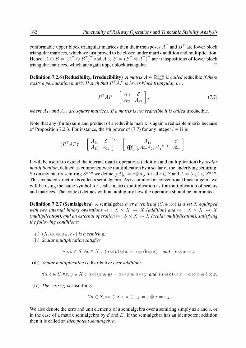
162 Punctuality of Railway Operations and Timetable Stability Analysis
conformable upper block triangular matrices then their transposes A> and B> are lower block
triangular matrices, which we just proved to be closed under matrix addition and multiplication.
Hence, A ⊕ B = (A> ⊕ B>)> and A ⊗ B = (B> ⊗ A>)> are transpositions of lower block
triangular matrices, which are again upper block triangular. 2
Definition 7.2.6 (Reducibility, Irreducibility) A matrix A ∈ Rn×nmax is called reducible if there
exists a permutation matrix P such that P>AP is lower block triangular, i.e.,
P>AP =
[A11 EA21 A22
]
, (7.7)
where A11 and A22 are square matrices. If a matrix is not reducible it is called irreducible.
Note that any (finite) sum and product of a reducible matrix is again a reducible matrix because
of Proposition 7.2.3. For instance, the lth power of (7.7) for any integer l ∈ N is
(P>AP )l =
[A11 EA21 A22
]l
=
[Al
11 E⊕l−1
k=0Ak22A21A
l−k−111 Al
22
]
.
It will be useful to extend the internal matrix operations (addition and multiplication) by scalar
multiplication, defined as componentwise multiplication by a scalar of the underlying semiring.
So on any matrix semiring Sn×n we define [cA]ij = c⊗aij for all c ∈ S and A = (aij) ∈ Sn×n.
This extended structure is called a semialgebra. As is common in conventional linear algebra we
will be using the same symbol for scalar-matrix multiplication as for multiplication of scalars
and matrices. The context defines without ambiguity how the operation should be interpreted.
Definition 7.2.7 (Semialgebra) A semialgebra over a semiring (S,⊕,⊗) is a set X equipped
with two internal binary operations ⊕ : X × X → X (addition) and ⊗ : X × X → X(multiplication), and an external operation⊗ : S ×X → X (scalar multiplication), satisfying
the following conditions:
(i) (X,⊕,⊗, εX , eX) is a semiring;
(ii) Scalar multiplication satisfies
∀a, b ∈ S, ∀x ∈ X : (a⊗ b)⊗ x = a⊗ (b⊗ x) and e⊗ x = x.
(iii) Scalar multiplication is distributive over addition:
∀a, b ∈ S, ∀x, y ∈ X : a⊗ (x⊕ y) = a⊗ x⊕ a⊗ y and (a⊕ b)⊗ x = a⊗ x⊕ b⊗ x.
(iv) The zero εX is absorbing:
∀a ∈ S, ∀x ∈ X : a⊗ εX = ε⊗ x = εX .
We also denote the zero and unit elements of a semialgebra over a semiring simply as ε and e, or
in the case of a matrix semialgebra by E and E. If the semialgebra has an idempotent addition
then it is called an idempotent semialgebra.
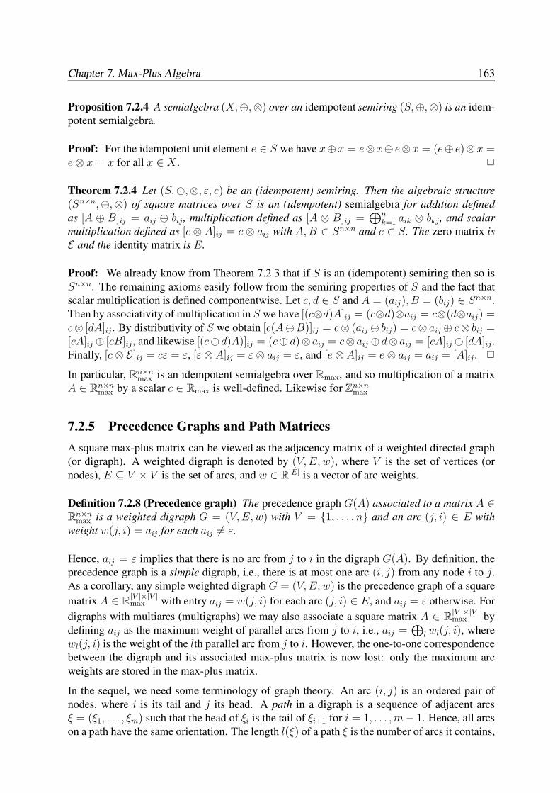
Chapter 7. Max-Plus Algebra 163
Proposition 7.2.4 A semialgebra (X,⊕,⊗) over an idempotent semiring (S,⊕,⊗) is an idem-
potent semialgebra.
Proof: For the idempotent unit element e ∈ S we have x⊕x = e⊗x⊕ e⊗x = (e⊕ e)⊗x =e⊗ x = x for all x ∈ X . 2
Theorem 7.2.4 Let (S,⊕,⊗, ε, e) be an (idempotent) semiring. Then the algebraic structure
(Sn×n,⊕,⊗) of square matrices over S is an (idempotent) semialgebra for addition defined
as [A ⊕ B]ij = aij ⊕ bij , multiplication defined as [A ⊗ B]ij =⊕n
k=1 aik ⊗ bkj, and scalar
multiplication defined as [c ⊗ A]ij = c ⊗ aij with A,B ∈ Sn×n and c ∈ S. The zero matrix is
E and the identity matrix is E.
Proof: We already know from Theorem 7.2.3 that if S is an (idempotent) semiring then so is
Sn×n. The remaining axioms easily follow from the semiring properties of S and the fact that
scalar multiplication is defined componentwise. Let c, d ∈ S and A = (aij), B = (bij) ∈ Sn×n.
Then by associativity of multiplication in S we have [(c⊗d)A]ij = (c⊗d)⊗aij = c⊗(d⊗aij) =c⊗ [dA]ij. By distributivity of S we obtain [c(A⊕B)]ij = c⊗ (aij ⊕ bij) = c⊗ aij ⊕ c⊗ bij =[cA]ij ⊕ [cB]ij , and likewise [(c⊕ d)A)]ij = (c⊕ d)⊗ aij = c⊗ aij ⊕ d⊗ aij = [cA]ij ⊕ [dA]ij .
Finally, [c⊗ E ]ij = cε = ε, [ε⊗ A]ij = ε⊗ aij = ε, and [e⊗A]ij = e⊗ aij = aij = [A]ij . 2
In particular, Rn×nmax is an idempotent semialgebra over Rmax, and so multiplication of a matrix
A ∈ Rn×nmax by a scalar c ∈ Rmax is well-defined. Likewise for Zn×n
max
7.2.5 Precedence Graphs and Path Matrices
A square max-plus matrix can be viewed as the adjacency matrix of a weighted directed graph
(or digraph). A weighted digraph is denoted by (V,E, w), where V is the set of vertices (or
nodes), E ⊆ V × V is the set of arcs, and w ∈ R|E| is a vector of arc weights.
Definition 7.2.8 (Precedence graph) The precedence graph G(A) associated to a matrix A ∈Rn×n
max is a weighted digraph G = (V,E, w) with V = {1, . . . , n} and an arc (j, i) ∈ E with
weight w(j, i) = aij for each aij 6= ε.
Hence, aij = ε implies that there is no arc from j to i in the digraph G(A). By definition, the
precedence graph is a simple digraph, i.e., there is at most one arc (i, j) from any node i to j.As a corollary, any simple weighted digraph G = (V,E, w) is the precedence graph of a square
matrix A ∈ R|V |×|V |max with entry aij = w(j, i) for each arc (j, i) ∈ E, and aij = ε otherwise. For
digraphs with multiarcs (multigraphs) we may also associate a square matrix A ∈ R|V |×|V |max by
defining aij as the maximum weight of parallel arcs from j to i, i.e., aij =⊕
l wl(j, i), where
wl(j, i) is the weight of the lth parallel arc from j to i. However, the one-to-one correspondence
between the digraph and its associated max-plus matrix is now lost: only the maximum arc
weights are stored in the max-plus matrix.
In the sequel, we need some terminology of graph theory. An arc (i, j) is an ordered pair of
nodes, where i is its tail and j its head. A path in a digraph is a sequence of adjacent arcs
ξ = (ξ1, . . . , ξm) such that the head of ξi is the tail of ξi+1 for i = 1, . . . , m− 1. Hence, all arcs
on a path have the same orientation. The length l(ξ) of a path ξ is the number of arcs it contains,
164 Punctuality of Railway Operations and Timetable Stability Analysis
so if ξ = (ξ1, . . . , ξm) then l(ξ) = m. In a weighted digraph the path weight is the product of
arc weights, i.e., w(ξ) =⊗
ξi∈ξ wi, where wi is the weight of arc ξi. Note that this corresponds
to the conventional sum of arc weights. By convention, a path of length 0 has weight 0. A path
of length 0 corresponds to staying at a node, and should not be confused with a loop from a
node to itself, which has length 1.
A matrix power in max-plus algebra has a special meaning in terms of paths in digraphs. By
definition (7.6) of matrix multiplication, we have [A2]ij = maxk=1,...,n(aik + akj), which equals
the largest weight of all paths with exactly two arcs from j to i. In general, Am is the matrix of
the maximum weights of all paths with length m, i.e.,
[Am]ij is the maximum weight of all paths from j to i with m arcs.
Now, letA(m) .=⊕m
l=0Al be the matrix of the maximum weights of all paths with length smaller
than or equal to m, i.e.,
[A(m)]ij is the maximum weight of all paths from j to i with at most m arcs.
The following proposition shows that the matrices A(m) can also be determined by a max-plus
matrix power.
Proposition 7.2.5 For any A ∈ Rn×nmax and any m ∈ N
m⊕
l=0
Al = (E ⊕ A)m. (7.8)
Proof: Clearly, for m = 1 we have E⊕A = A0⊕A1. Now assume that (7.8) holds for m = kthen it also holds for m = k + 1, since
(E ⊕ A)k+1 = (E ⊕A)⊗ (E ⊕ A)k
= (E ⊕A)⊗⊕kl=0A
l (induction step)
=⊕k
l=0(Al)⊕⊕k
l=0(AAl) (by distributivity)
=⊕k
l=0(Al)⊕⊕k+1
l=1 (Al)
= E ⊕⊕kl=1(A
l)⊕⊕kl=1(A
l)⊕ Ak+1
= E ⊕⊕kl=1(A
l)⊕ Ak+1 (by idempotency)
=⊕k+1
l=0 Al.
Hence, by induction (7.8) is valid for all m ∈ N. 2
Let
A+ .=
∞⊕
l=1
Al = A⊕A2 ⊕ A3 ⊕ . . . . (7.9)
Then [A+]ij is the maximum path weight from j to i over all paths of any length (> 0). There-
fore, A+ is also called the (longest) path matrix1. The entry [A+]ii is the maximum path weight
1In the min-plus semiring (Rn×n ∪ {∞}, min, +) this matrix is known as the shortest path matrix
Chapter 7. Max-Plus Algebra 165
from i back to i over paths with length at least one. A related matrix sum is the (Kleene) star of
A, defined as
A∗ .=
∞⊕
l=0
Al = E ⊕ A⊕A2 ⊕ . . . . (7.10)
The matrix A∗ is also known as the quasi-inverse or matrix closure of A [73]. The matrices
A∗ and A+ are equal except possibly for the diagonal elements. Consider a node i in the
precedence graph G(A). If i is not contained in any circuit then [A+]ii = ε. If on the other hand
i is contained in circuits with negative weight only then [A+]ii < e. In both cases [A∗]ii = e.
The closure A∗ for any matrix A ∈ Rn×nmax satisfies a range of properties that follow immediately
from its definition. In particular, A+ = AA∗ and A∗ = E ⊕ A+ = E ⊕ AA∗. Furthermore,
from (7.10) and (additive) idempotency of Rn×nmax follows A∗A∗ = A∗, which means that A∗ is
both additive and multiplicative idempotent.
In general, the infinite sums in (7.9) and (7.10) do not have to converge. However, the following
proposition gives a necessary and sufficient condition for finite convergence of these infinite
sums.
Proposition 7.2.6 Let A ∈ Rn×nmax be such that the associated precedence graph G(A) has no
circuits with positive weight. Then the limitsA∗ and A+ exist and are reached by the finite sums
A∗ =
n−1⊕
l=0
Al and A+ =
n⊕
l=1
Al. (7.11)
Proof: In a digraph with n nodes, any path from node j to i, j 6= i, of length n or more
necessarily consists of an elementary path with length strictly less than n and one or more
circuits. Since by assumption any circuit has nonpositive weight, the inclusion of a circuit to
an elementary path will never increase the path weight, by which follows that the maximum-
weight path between any two distinct nodes has length at most n − 1. Moreover, a path from
any node i to itself is by definition a circuit and thus has nonpositive weight by assumption.
Therefore, for all i, j there is an integer l ∈ {0, . . . , n − 1} such that [Al]ij ≥ [Am]ij for all
integers m ≥ n. Hence,n−1⊕
l=0
Al ≥ Am for all m ≥ n, (7.12)
proving the finite convergence of A∗. Note that by the assumption on the circuit weights the
diagonal entries of A∗ are all e. In the case of A+, a diagonal entry [A+]ii corresponds to
the maximum-weight circuit over i. Clearly this must be an elementary circuit by the same
reasoning as above. An elementary circuit in a digraph of n nodes has at most n nodes, whence⊕n
l=1Al ≥ Am for all m ≥ n+ 1. 2
If A ∈ Rn×nmax satisfies the condition of Proposition 7.2.6, i.e., G(A) has no positive-weight
circuits, then in particular A∗ = (E ⊕ A)m for any m ≥ n − 1 because of (7.12) and Proposi-
tion 7.2.5.
By definition an acyclic graph has no circuits and we therefore obtain the following corollary
to Proposition 7.2.6.
166 Punctuality of Railway Operations and Timetable Stability Analysis
Corollary 7.2.1 If A ∈ Rn×nmax has an acyclic precedence graphG(A) then A∗ and A+ exist and
are defined by (7.11).
The matrices A+ and A∗ can be computed by efficient graph algorithms due to the equiva-
lence to the all-pairs longest (or shortest) path problem. The well-known Floyd-Warshall al-
gorithm [66, 39] computes A+ in O(n3) time using a special implementation of the repeated
max-plus matrix multiplication, see Section 7.5.1. For large sparse matrices the repeated short-
est path algorithm of Johnson [112, 39] is even more efficient, see Section 7.5 for more details.
If we have computed A+ then we also have A∗ = E ⊕ A∗, by simply setting each negative
diagonal entry to 0, since [A∗]ii = e⊕ [A+]ii = max(0, a+ii).
Lemma 7.2.1 Let A,P ∈ Rn×nmax , where P is a permutation matrix. Then
(P>AP )+ = P>A+P and (P>AP )∗ = P>A∗P.
Proof: A permutation matrix P satisfies PP> = P>P = E and therefore (P>AP )2 =P>APP>AP = P>A2P . By induction we obtain (P>AP )l = P>AlP for any integer l ≥ 1,
and thus
(P>AP )+ =∞⊕
l=1
(P>AP )l =∞⊕
l=1
P>AlP = P> ⊗(
∞⊕
l=1
Al
)
⊗ P = P>A+P.
The proof of (P>AP )∗ = P>A∗P is similar, with the additional term (P>AP )0 = E =P>P = P>EP = P>A0P . 2
A directed graph G(A) is strongly connected if there is a path from any node j to any node
i in G(A). In terms of the matrix A this means that for all indices 1 ≤ i, j ≤ n there exists
an integer l ∈ N such that [Al]ij > ε, or using the path matrix we simply have A+ > ε. The
following proposition gives a graph interpretation of an irreducible matrix A. We assume that
n ≥ 2.
Proposition 7.2.7 Let A ∈ Rn×nmax with associated precedence graph G(A). Then A is irre-
ducible if and only if G(A) is strongly connected.
Proof: We prove the contraposition that A is reducible if and only if G(A) is not strongly
connected. First, assume that G(A) = (V,E) is not strongly connected. Then there exists a
nonempty subset of nodes W ⊂ V , such that no arcs go from W to V \W . Without loss of
generality, we may assume that the nodes are numbered such that the last |W | nodes correspond
to W . But then A has the block triangular form (7.7), where A11 corresponds to the arcs in the
component (V \W ), A22 to the arcs between nodes in W , and the block A12 = E corresponds
to aij = ε for (j, i) ∈W × (V \W ).
Conversely, assume that A is reducible. Then there exists a permutation matrix P , such that
P>AP has block triangular form (7.7). By Proposition 7.2.3 this block triangular structure is
preserved for any sum and power, whence (P>AP )+ =⊕∞
l=1(P>AP )l is also block triangular
and so is P>A+P by Lemma 7.2.1. Thus, A+ ≯ ε and so G(A) is not strongly connected. 2
Chapter 7. Max-Plus Algebra 167
7.2.6 Polynomial Matrices and Timed Event Graphs
Since Rmax[X] and Rn×nmax are idempotent semirings we can also consider square matrices with
entries in Rmax[X], or polynomials with square matrices as coefficients. This leads to the idem-
potent semiring Rn×nmax [X] of max-plus polynomial matrices, which will play a central role in the
theory of max-plus linear systems of Chapter 8.
Definition 7.2.9 (Polynomial matrix) A polynomial matrix in an indeterminateX over a semi-
ring S is a finite sum
A =
p⊕
l=0
Al ⊗X l (7.13)
for some integer p ∈ N and matrix coefficientsAl ∈ Sn×n. The set of n×n polynomial matrices
is denoted as Sn×n[X].
In particular, Rn×nmax [X] is the set of max-plus polynomial matrices in an indeterminate X over
the semiring Rmax with elements⊕p
l=0Al ⊗X l, where Al ∈ Rn×nmax .
Theorem 7.2.5 Let (S,⊕,⊗) be an (idempotent) semiring. Then the set Sn×n[X] of square
polynomial matrices over S is an (idempotent) semiring for addition defined as
A⊕ B =
deg(A)⊕deg(B)⊕
l=0
(Al ⊕ Bl)Xl (7.14)
and multiplication defined as
A⊗ B =
deg(A)⊗deg(B)⊕
l=0
⊕
r⊗s=l
(Ar ⊗ Bs)Xl. (7.15)
The zero and unit elements in Sn×n[X] are the zero matrix E and identity matrix E.
Proof: If S is an (idempotent) semiring then Sn×n is an (idempotent) semiring by Theo-
rem 7.2.3. The addition defined in (7.14) is simply the polynomial addition over the (idempo-
tent) matrix semiring Sn×n and the multiplication (7.15) is just polynomial multiplication over
Sn×n. Hence, Theorem 7.2.1 can be applied, by which Sn×n[X] is an (idempotent) semiring.
The zero and identity matrix can be interpreted as the constant polynomial matrices EX0 and
EX0. 2
In Definition 7.2.9 a polynomial matrix is defined as a polynomial with matrix coefficients. An
alternative definition of a polynomial matrix is a matrix A ∈ (Rmax[X])n×n with polynomial
entries Aij =⊕p
l=0 a(l)ij X
l, where a(l)ij ∈ Rmax for all 1 ≤ i, j ≤ n and 0 ≤ l ≤ p. In fact,
we will show that the algebraic structures Rn×nmax [X] and (Rmax[X])n×n are indistinguishable or
isomorphic, by which it is mathematically justified to interpret a polynomial matrix either as a
polynomial with matrix coefficients or as a matrix with polynomial entries. For example,
A =
[ε e3 e
]
⊕[ε ee 2
]
X =
[ε e⊕X
3⊕X e⊕ 2X
]
.
168 Punctuality of Railway Operations and Timetable Stability Analysis
Theorem 7.2.6 Let (S,⊕,⊗) be an (idempotent) semiring. Then the set (S[X])n×n of square
matrices A with polynomial entries Aij =⊕p
l=0 a(l)ij X
l in an indeterminate X over S is an
(idempotent) semiring for addition defined as
(A⊕B)ij = Aij ⊕ Bij =
deg(Aij)⊕deg(Bij )⊕
l=0
(
a(l)ij ⊕ b(l)ij
)
X l, (7.16)
and multiplication as
(A⊗ B)ij =
n⊕
k=1
(Aik ⊗ Bkj) =
n⊕
k=1
deg(Aik)⊗deg(Bkj)⊕
l=0
⊕
r⊗s=l
(
a(r)ik ⊗ b
(s)kj
)
X l. (7.17)
The zero and unit elements in (S[X])n×n are the zero matrix E and identity matrix E.
Proof: If S is an (idempotent) semiring then S[X] is also an (idempotent) semiring by Theo-
rem 7.2.1. The addition defined in (7.16) is simply the (componentwise) matrix addition over
the (idempotent) semiring S[X] and the multiplication (7.17) is just matrix multiplication over
S[X]. Hence, Theorem 7.2.3 can be applied, by which Sn×n[X] is an (idempotent) semiring. 2
Note the similarity between the proof of Theorem 7.2.6 and that of Theorem 7.2.5. Sn×n[X]is the semiring of polynomials with matrix coefficients and (S[X])n×n is the semiring of ma-
trices with polynomial entries. The resulting semiring structure is algebraically equivalent as
presented in the following theorem.
Theorem 7.2.7 Let (S,⊕,⊗) be an (idempotent) semiring. Then the (idempotent) semirings
Sn×n[X] and (S[X])n×n are isomorphic.
Proof: Define the mapping ψ : Sn×n[X]→ (S[X])n×n as
ψ
(p⊕
l=0
AlXl
)
= A with Aij =
p⊕
l=0
[Al]ijXl for all 1 ≤ i, j ≤ n.
It is easily seen that ψ is bijective and maps each entry of a matrix coefficient uniquely onto a
coefficient of a polynomial matrix entry, i.e., [Al]ij = a(l)ij for all 1 ≤ i, j ≤ n and 0 ≤ l ≤ p.
Hence, the inverse mapping ψ−1 : (S[X])n×n → Sn×n[X] is well-defined. Addition (7.14) on
(S[X])n×n is exactly (7.16) by identifying [Al]ij = a(l)ij , i.e., A ⊕ B = ψ(ψ−1(A) ⊕ ψ−1(B)).
Likewise, multiplication (7.17) is just the elementwise formulation of (7.17) with [Al]ij = a(l)ij ,
that is, A ⊗ B = ψ(ψ−1(A) ⊗ ψ−1(B)). Then clearly ψ is an isomorphism from Sn×n[X]to (S[X])n×n and so (S[X])n×n is isomorphic to Sn×n[X]. Moreover, this isomorphism also
implies that (S[X])n×n is an (idempotent) semiring if and only if Sn×n[X] is. 2
Because of Theorem 7.2.7 we may identify by both Sn×n[X] ∼= (S[X])n×n the n×n polynomial
matrix semiring in an indeterminate X over the semiring S.
In particular, Rn×nmax [X] and Zn×n
max [X] are idempotent semirings, with addition and multiplication
understood as matrix addition and multiplication over the semiring Rmax[X]. As an example in
R2×2max[X] we have
[2 X
e⊕ 1X X2
]
⊕[
3X 1X3 1⊕ 2X
]
=
[2⊕ 3X 1X3⊕ 1X 1⊕ 2X ⊕X2
]
Chapter 7. Max-Plus Algebra 169
and
[2 X
e⊕ 1X X2
]
⊗[
3X 1X3 1⊕ 2X
]
=
[5X 3X ⊕ 2X2
3X ⊕ 4X2 1X ⊕ 2X2 ⊕ 2X3
]
.
Analogous to a max-plus polynomial function associated to a max-plus polynomial, we asso-
ciate a matrix polynomial function A : Rmax → Rn×nmax to each matrix polynomialA ∈ Rn×n
max [X]by substituting an element x ∈ Rmax for the indeterminate X .
Theorem 7.2.8 Let (Sn×n[X],⊕,⊗, E , E) be the semiring of polynomial matrices over a com-
mutative semiring S. Then for any x ∈ S the valuation mapping ϕ : A 7→ A(x) is a homomor-
phism from Sn×n[X] into Sn×n.
Proof: The proof is analogous to that of Theorem 7.2.2 by showing that ϕ(A⊕B) = ϕ(A)⊕ϕ(B) and ϕ(A⊗B) = ϕ(A)⊗ϕ(B) hold entrywise. Without loss of generality we assume that
all polynomial entries have the same degree by taking any missing coefficients equal to ε. So
let Aij =⊕p
l=0 a(l)ij X
l and Bij =⊕p
l=0 b(l)ij X
l. Then for addition we have
ϕ(A)⊕ ϕ(B) = A(x)⊕ B(x)
= (⊕p
i=0Aixi)⊕
(⊕p
j=0Bjxj)
= A0 ⊕ A1x⊕ . . .⊕ Apxp ⊕ B0 ⊕ B1x⊕ · · · ⊕ Bpx
p
= (A0 ⊕ B0)⊕ (A1x⊕ B1x)⊕ · · · ⊕ (Apxp ⊕Bpx
p) (by associativity)
= (A0 ⊕ B0)⊕ (A1 ⊕ B1)x⊕ · · · ⊕ (Ap ⊕ Bp)xp (by distributivity)
=⊕p
l=0(Al ⊕Bl)xl
= (A⊕ B)(x)
= ϕ(A⊕ B).
For multiplication we have
ϕ(A)⊗ ϕ(B) = A(x)⊗B(x)
= (⊕p
i=0Aixi)⊗
(⊕p
j=0Bjxj)
distr.= A0
(⊕p
j=0Bjxj)
⊕ A1x(⊕p
j=0Bjxj)
⊕ · · · ⊕ Apxp(⊕p
j=0Bjxj)
comm.= A0
(⊕p
j=0Bjxj)
⊕ A1
(⊕p
j=0Bjx1+j)
⊕ · · · ⊕Ap
(⊕p
j=0Bjxp+j)
=⊕p
i=0
(
Ai ⊗(⊕p
j=0Bjxi+j))
=⊕p
i=0
⊕pj=0(Ai ⊗Bj)x
i⊗j
=⊕p⊗p
l=0
⊕
i⊗j=l(Ai ⊗Bj)xl
= (A⊗ B)(x)
= ϕ(A⊗B).
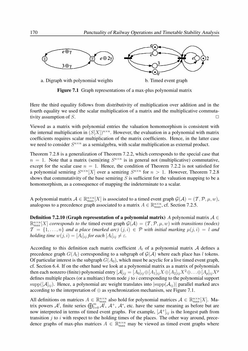
170 Punctuality of Railway Operations and Timetable Stability Analysis
1 2 g2Åe
gÅe
gÅ3
1 2 g2Åe
gÅe
gÅ3
·
2
e
3
·
·e
e
e
·
2
e
3
·
·e
e
e
a. Digraph with polynomial weights b. Timed event graph
Figure 7.1 Graph representations of a max-plus polynomial matrix
Here the third equality follows from distributivity of multiplication over addition and in the
fourth equality we used the scalar multiplication of a matrix and the multiplicative commuta-
tivity assumption of S. 2
Viewed as a matrix with polynomial entries the valuation homomorphism is consistent with
the internal multiplication in (S[X])n×n. However, the evaluation in a polynomial with matrix
coefficients requires scalar multiplication of the matrix coefficients. Hence, in the latter case
we need to consider Sn×n as a semialgebra, with scalar multiplication as external product.
Theorem 7.2.8 is a generalization of Theorem 7.2.2, which corresponds to the special case that
n = 1. Note that a matrix (semi)ring Sn×n is in general not (multiplicative) commutative,
except for the scalar case n = 1. Hence, the condition of Theorem 7.2.2 is not satisfied for
a polynomial semiring Sn×n[X] over a semiring Sn×n for n > 1. However, Theorem 7.2.8
shows that commutativity of the base semiring S is sufficient for the valuation mapping to be a
homomorphism, as a consequence of mapping the indeterminate to a scalar.
A polynomial matrix A ∈ Rn×nmax [X] is associated to a timed event graph G(A) = (T ,P, µ, w),
analogous to a precedence graph associated to a matrix A ∈ Rn×nmax , cf. Section 7.2.5.
Definition 7.2.10 (Graph representation of a polynomial matrix) A polynomial matrix A ∈Rn×n
max [X] corresponds to the timed event graph G(A) = (T ,P, µ, w) with transitions (nodes)
T = {1, . . . , n} and a place (marked arc) (j, i) ∈ P with initial marking µ(j, i) = l and
holding time w(j, i) = [Al]ij for each [Al]ij 6= ε.
According to this definition each matrix coefficient Al of a polynomial matrix A defines a
precedence graph G(Al) corresponding to a subgraph of G(A) where each place has l tokens.
Of particular interest is the subgraphG(A0), which must be acyclic for a live timed event graph,
cf. Section 6.4. If on the other hand we look at a polynomial matrix as a matrix of polynomials
then each nonzero (finite) polynomial entry [A]ij = [A0]ij⊕[A1]ijX⊕[A2]ijX2⊕. . .⊕[Ap]ijX
p
defines multiple places (or a multiarc) from node j to i corresponding to the polynomial support
supp([A]ij). Hence, a polynomial arc weight translates into |supp(Aij)| parallel marked arcs
according to the interpretation of ⊕ as synchronization mechanism, see Figure 7.1.
All definitions on matrices A ∈ Rn×nmax also hold for polynomial matrices A ∈ Rn×n
max [X]. Ma-
trix powers Al, finite series⊕m
l=0Al, A+, A∗, etc. have the same meaning as before but are
now interpreted in terms of timed event graphs. For example, [A+]ij is the longest path from
transition j to i with respect to the holding times of the places. The other way around, prece-
dence graphs of max-plus matrices A ∈ Rn×nmax may be viewed as timed event graphs where
Chapter 7. Max-Plus Algebra 171
all arcs have the same marking. Permutation matrices P ∈ Rn×nmax [X] are the same as in Rn×n
max
(like the identity matrix), and P>AP is just a coordinate transformation of the indices of the
matrix A. A reducible polynomial matrix is defined analogous to Definition 7.2.6 as a polyno-
mial matrix A that can be written in lower block triangular form by an appropriate coordinate
transformation, where now of course blocks are rectangular polynomial submatrices. In fact,
(ir)reducibility is a combinatorial matrix property that only depends on the support of the matrix,
supp(A) = {(j, i) | [A]ij 6= ε}, that is, the pattern of nonzero entries. The support is preserved
by the valuation homomorphism for finite values of the variable X . Hence, A ∈ Rn×nmax [X] is
(ir)reducible if and only if A(e) ∈ Rn×nmax is, or any A(x) with fixed x ∈ Rmax \{ε} for that
matter, where A(x) is the valuation homomorphism of A in x. In particular, G(A) is strongly
connected if and only if A(e) is irreducible. Indeed, for fixed x = e the polynomial matrix
function reduces to a max-plus matrix, where the associated precedence graph is obtained from
the timed event graph by replacing the multiple places from a transition j to i by a single arc
from node j to i with weight aij = maxl=0,...,p[Al]ij . Note that strongly connectedness is invari-
ant to (the weights of) parallel places. An algebraic characterization of an irreducible square
polynomial matrix A ∈ Rn×nmax [X] is that for all i, j there exists an integer m ∈ N, such that
[Am]ij 6= ε, or such that [Am(e)]ij 6= ε. This corresponds to strongly connectedness of the
associated timed event graph, i.e., a path exists between any two transitions.
7.2.7 Partially Ordered Semirings
Definition 7.2.11 (Partial order, total order) A binary relation ≤ on a set S 6= ∅ is called a
partial order on S if the following axioms are satisfied for all a, b, c ∈ S:
(i) Reflexivity: a ≤ a.
(ii) Antisymmetry: if a ≤ b and b ≤ a then a = b.
(iii) Transitivity: if a ≤ b and b ≤ c then a ≤ c.
A partial order is called a total order if it additionally satisfies
• Comparability: for all a, b ∈ S, either a ≤ b or b ≤ a.
If ≤ is a partial order on S then (S,≤) is called a partially ordered set. Likewise, if ≤ is a total
order on S then (S,≤) is called a totally ordered set.
Given a partially ordered set (S,≤), we define a ≥ b as the equivalence of b ≤ a. If a ≤ b and
a 6= b we also write a < b, and similarly a > b⇔ (b ≤ a ∧ a 6= b).
Definition 7.2.12 (Partially ordered semiring) Let (S,⊕,⊗, ε, e) be a semiring and (S,≤) a
partially ordered set. Then (S,⊕,⊗,≤) is called a partially ordered semiring if the following
monotony laws are satisfied for all a, b, c ∈ S:
(i) Additive monotony: if a ≤ b then a⊕ c ≤ b⊕ c.(ii) Multiplicative monotony: if a ≤ b and ε ≤ c then a⊗ c ≤ b⊗ c and c⊗ a ≤ c⊗ b.
If moreover ≤ is a total order on S then (S,⊕,⊗,≤) is called a totally ordered semiring.
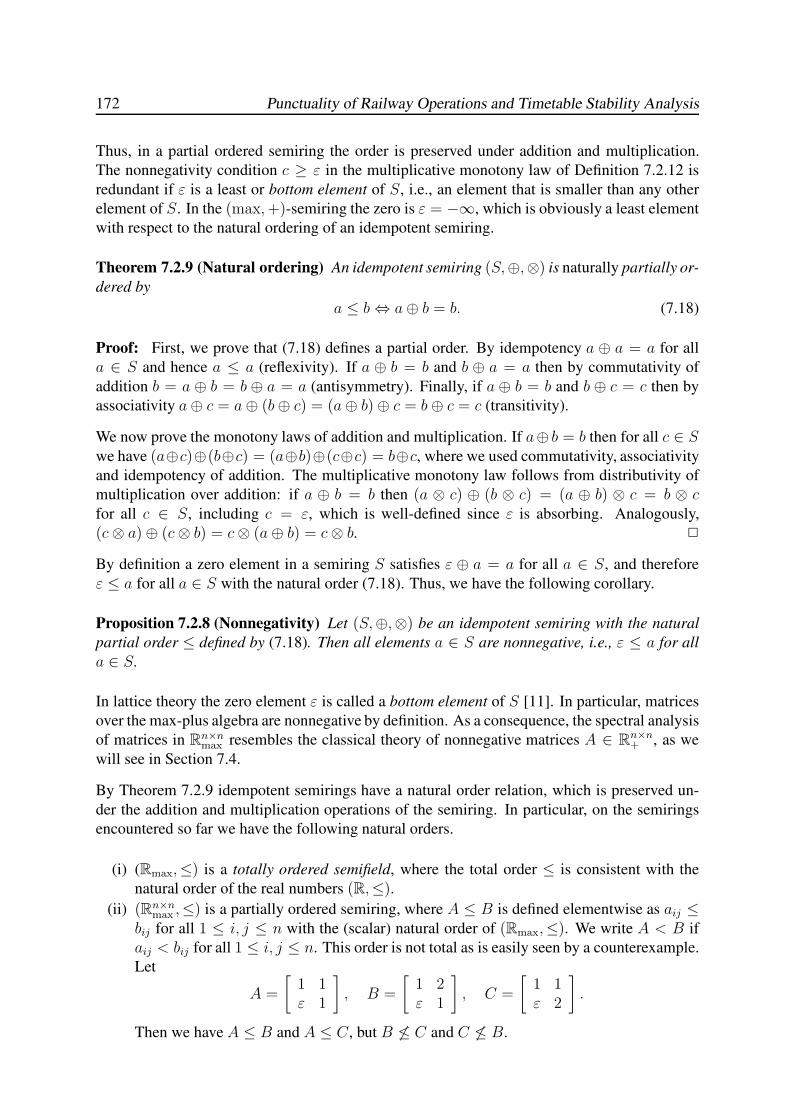
172 Punctuality of Railway Operations and Timetable Stability Analysis
Thus, in a partial ordered semiring the order is preserved under addition and multiplication.
The nonnegativity condition c ≥ ε in the multiplicative monotony law of Definition 7.2.12 is
redundant if ε is a least or bottom element of S, i.e., an element that is smaller than any other
element of S. In the (max,+)-semiring the zero is ε = −∞, which is obviously a least element
with respect to the natural ordering of an idempotent semiring.
Theorem 7.2.9 (Natural ordering) An idempotent semiring (S,⊕,⊗) is naturally partially or-
dered by
a ≤ b⇔ a⊕ b = b. (7.18)
Proof: First, we prove that (7.18) defines a partial order. By idempotency a ⊕ a = a for all
a ∈ S and hence a ≤ a (reflexivity). If a ⊕ b = b and b ⊕ a = a then by commutativity of
addition b = a ⊕ b = b ⊕ a = a (antisymmetry). Finally, if a ⊕ b = b and b ⊕ c = c then by
associativity a⊕ c = a⊕ (b⊕ c) = (a⊕ b)⊕ c = b⊕ c = c (transitivity).
We now prove the monotony laws of addition and multiplication. If a⊕ b = b then for all c ∈ Swe have (a⊕c)⊕(b⊕c) = (a⊕b)⊕(c⊕c) = b⊕c, where we used commutativity, associativity
and idempotency of addition. The multiplicative monotony law follows from distributivity of
multiplication over addition: if a ⊕ b = b then (a ⊗ c) ⊕ (b ⊗ c) = (a ⊕ b) ⊗ c = b ⊗ cfor all c ∈ S, including c = ε, which is well-defined since ε is absorbing. Analogously,
(c⊗ a)⊕ (c⊗ b) = c⊗ (a⊕ b) = c⊗ b. 2
By definition a zero element in a semiring S satisfies ε ⊕ a = a for all a ∈ S, and therefore
ε ≤ a for all a ∈ S with the natural order (7.18). Thus, we have the following corollary.
Proposition 7.2.8 (Nonnegativity) Let (S,⊕,⊗) be an idempotent semiring with the natural
partial order ≤ defined by (7.18). Then all elements a ∈ S are nonnegative, i.e., ε ≤ a for all
a ∈ S.
In lattice theory the zero element ε is called a bottom element of S [11]. In particular, matrices
over the max-plus algebra are nonnegative by definition. As a consequence, the spectral analysis
of matrices in Rn×nmax resembles the classical theory of nonnegative matrices A ∈ Rn×n
+ , as we
will see in Section 7.4.
By Theorem 7.2.9 idempotent semirings have a natural order relation, which is preserved un-
der the addition and multiplication operations of the semiring. In particular, on the semirings
encountered so far we have the following natural orders.
(i) (Rmax,≤) is a totally ordered semifield, where the total order ≤ is consistent with the
natural order of the real numbers (R,≤).
(ii) (Rn×nmax ,≤) is a partially ordered semiring, where A ≤ B is defined elementwise as aij ≤
bij for all 1 ≤ i, j ≤ n with the (scalar) natural order of (Rmax,≤). We write A < B if
aij < bij for all 1 ≤ i, j ≤ n. This order is not total as is easily seen by a counterexample.
Let
A =
[1 1ε 1
]
, B =
[1 2ε 1
]
, C =
[1 1ε 2
]
.
Then we have A ≤ B and A ≤ C, but B 6≤ C and C 6≤ B.
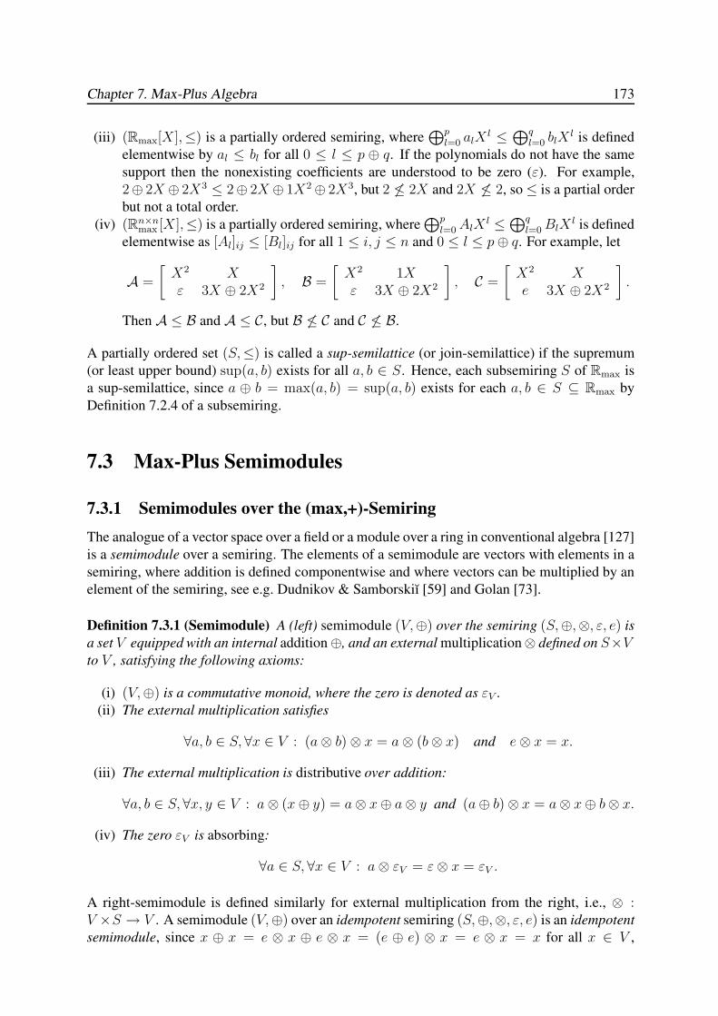
Chapter 7. Max-Plus Algebra 173
(iii) (Rmax[X],≤) is a partially ordered semiring, where⊕p
l=0 alXl ≤ ⊕q
l=0 blXl is defined
elementwise by al ≤ bl for all 0 ≤ l ≤ p ⊕ q. If the polynomials do not have the same
support then the nonexisting coefficients are understood to be zero (ε). For example,
2⊕ 2X ⊕ 2X3 ≤ 2⊕ 2X ⊕ 1X2⊕ 2X3, but 2 6≤ 2X and 2X 6≤ 2, so≤ is a partial order
but not a total order.
(iv) (Rn×nmax [X],≤) is a partially ordered semiring, where
⊕pl=0AlX
l ≤⊕ql=0BlX
l is defined
elementwise as [Al]ij ≤ [Bl]ij for all 1 ≤ i, j ≤ n and 0 ≤ l ≤ p⊕ q. For example, let
A =
[X2 Xε 3X ⊕ 2X2
]
, B =
[X2 1Xε 3X ⊕ 2X2
]
, C =
[X2 Xe 3X ⊕ 2X2
]
.
Then A ≤ B and A ≤ C, but B 6≤ C and C 6≤ B.
A partially ordered set (S,≤) is called a sup-semilattice (or join-semilattice) if the supremum
(or least upper bound) sup(a, b) exists for all a, b ∈ S. Hence, each subsemiring S of Rmax is
a sup-semilattice, since a ⊕ b = max(a, b) = sup(a, b) exists for each a, b ∈ S ⊆ Rmax by
Definition 7.2.4 of a subsemiring.
7.3 Max-Plus Semimodules
7.3.1 Semimodules over the (max,+)-Semiring
The analogue of a vector space over a field or a module over a ring in conventional algebra [127]
is a semimodule over a semiring. The elements of a semimodule are vectors with elements in a
semiring, where addition is defined componentwise and where vectors can be multiplied by an
element of the semiring, see e.g. Dudnikov & Samborskiı [59] and Golan [73].
Definition 7.3.1 (Semimodule) A (left) semimodule (V,⊕) over the semiring (S,⊕,⊗, ε, e) is
a set V equipped with an internal addition⊕, and an external multiplication⊗ defined on S×Vto V , satisfying the following axioms:
(i) (V,⊕) is a commutative monoid, where the zero is denoted as εV .
(ii) The external multiplication satisfies
∀a, b ∈ S, ∀x ∈ V : (a⊗ b)⊗ x = a⊗ (b⊗ x) and e⊗ x = x.
(iii) The external multiplication is distributive over addition:
∀a, b ∈ S, ∀x, y ∈ V : a⊗ (x⊕ y) = a⊗ x⊕ a⊗ y and (a⊕ b)⊗ x = a⊗ x⊕ b⊗ x.
(iv) The zero εV is absorbing:
∀a ∈ S, ∀x ∈ V : a⊗ εV = ε⊗ x = εV .
A right-semimodule is defined similarly for external multiplication from the right, i.e., ⊗ :V ×S → V . A semimodule (V,⊕) over an idempotent semiring (S,⊕,⊗, ε, e) is an idempotent
semimodule, since x ⊕ x = e ⊗ x ⊕ e ⊗ x = (e ⊕ e) ⊗ x = e ⊗ x = x for all x ∈ V ,
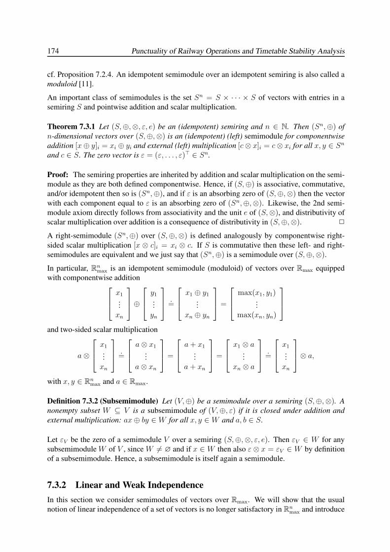
174 Punctuality of Railway Operations and Timetable Stability Analysis
cf. Proposition 7.2.4. An idempotent semimodule over an idempotent semiring is also called a
moduloid [11].
An important class of semimodules is the set Sn = S × · · · × S of vectors with entries in a
semiring S and pointwise addition and scalar multiplication.
Theorem 7.3.1 Let (S,⊕,⊗, ε, e) be an (idempotent) semiring and n ∈ N. Then (Sn,⊕) of
n-dimensional vectors over (S,⊕,⊗) is an (idempotent) (left) semimodule for componentwise
addition [x⊕ y]i = xi ⊕ yi and external (left) multiplication [c⊗ x]i = c⊗ xi for all x, y ∈ Sn
and c ∈ S. The zero vector is ε = (ε, . . . , ε)> ∈ Sn.
Proof: The semiring properties are inherited by addition and scalar multiplication on the semi-
module as they are both defined componentwise. Hence, if (S,⊕) is associative, commutative,
and/or idempotent then so is (Sn,⊕), and if ε is an absorbing zero of (S,⊕,⊗) then the vector
with each component equal to ε is an absorbing zero of (Sn,⊕,⊗). Likewise, the 2nd semi-
module axiom directly follows from associativity and the unit e of (S,⊗), and distributivity of
scalar multiplication over addition is a consequence of distributivity in (S,⊕,⊗). 2
A right-semimodule (Sn,⊕) over (S,⊕,⊗) is defined analogously by componentwise right-
sided scalar multiplication [x ⊗ c]i = xi ⊗ c. If S is commutative then these left- and right-
semimodules are equivalent and we just say that (Sn,⊕) is a semimodule over (S,⊕,⊗).
In particular, Rnmax is an idempotent semimodule (moduloid) of vectors over Rmax equipped
with componentwise addition
x1...
xn
⊕
y1...
yn
.=
x1 ⊕ y1...
xn ⊕ yn
=
max(x1, y1)...
max(xn, yn)
and two-sided scalar multiplication
a⊗
x1...
xn
.=
a⊗ x1...
a⊗ xn
=
a+ x1...
a + xn
=
x1 ⊗ a...
xn ⊗ a
.=
x1...
xn
⊗ a,
with x, y ∈ Rnmax and a ∈ Rmax.
Definition 7.3.2 (Subsemimodule) Let (V,⊕) be a semimodule over a semiring (S,⊕,⊗). A
nonempty subset W ⊆ V is a subsemimodule of (V,⊕, ε) if it is closed under addition and
external multiplication: ax⊕ by ∈W for all x, y ∈W and a, b ∈ S.
Let εV be the zero of a semimodule V over a semiring (S,⊕,⊗, ε, e). Then εV ∈ W for any
subsemimodule W of V , since W 6= ∅ and if x ∈ W then also ε ⊗ x = εV ∈ W by definition
of a subsemimodule. Hence, a subsemimodule is itself again a semimodule.
7.3.2 Linear and Weak Independence
In this section we consider semimodules of vectors over Rmax. We will show that the usual
notion of linear independence of a set of vectors is no longer satisfactory in Rnmax and introduce
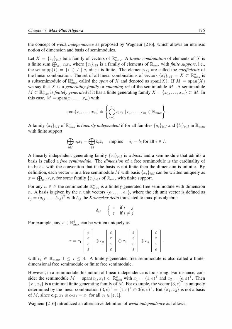
Chapter 7. Max-Plus Algebra 175
the concept of weak independence as proposed by Wagneur [216], which allows an intrinsic
notion of dimension and basis of semimodules.
Let X = {xi}i∈I be a family of vectors of Rnmax. A linear combination of elements of X is
a finite sum⊕
i∈I cixi, where {ci}i∈I is a family of elements of Rmax with finite support, i.e.,
the set supp(I) = {i ∈ I | ci 6= ε} is finite. The elements ci are called the coefficients of
the linear combination. The set of all linear combinations of vectors {xi}i∈I = X ⊂ Rnmax is
a subsemimodule of Rnmax called the span of X and denoted as span(X). If M = span(X)
we say that X is a generating family or spanning set of the semimodule M . A semimodule
M ⊂ Rnmax is finitely generated if it has a finite generating family X = {x1, . . . , xm} ⊂ M . In
this case, M = span(x1, . . . , xm) with
span(x1, . . . , xm).=
{m⊕
i=1
cixi | c1, . . . , cm ∈ Rmax
}
.
A family {xi}i∈I of Rnmax is linearly independent if for all families {ai}i∈I and {bi}i∈I in Rmax
with finite support
⊕
i∈I
aixi =⊕
i∈I
bixi implies ai = bi for all i ∈ I.
A linearly independent generating family {xi}i∈I is a basis and a semimodule that admits a
basis is called a free semimodule. The dimension of a free semimodule is the cardinality of
its basis, with the convention that if the basis is not finite then the dimension is infinite. By
definition, each vector x in a free semimodule M with basis {xi}i∈I can be written uniquely as
x =⊕
i∈I cixi for some family {ci}i∈I of Rmax with finite support.
For any n ∈ N the semimodule Rnmax is a finitely-generated free semimodule with dimension
n. A basis is given by the n unit vectors {e1, . . . , en}, where the jth unit vector is defined as
ej = (δ1j , . . . , δnj)> with δij the Kronecker delta translated to max-plus algebra:
δij =
{e if i = jε if i 6= j.
For example, any x ∈ R4max can be written uniquely as
x = c1
eεεε
⊕ c2
εeεε
⊕ c3
εεeε
⊕ c4
εεεe
.
with ci ∈ Rmax, 1 ≤ i ≤ 4. A finitely-generated free semimodule is also called a finite-
dimensional free semimodule or finite free semimodule.
However, in a semimodule this notion of linear independence is too strong. For instance, con-
sider the semimodule M = span(x1, x2) ⊂ R2max with x1 = (1, e)> and x2 = (e, ε)>. Then
{x1, x2} is a minimal finite generating family of M . For example, the vector (3, e)> is uniquely
determined by the linear combination (3, e)> = (1, e)> ⊕ 3(e, ε)>. But {x1, x2} is not a basis
of M , since e.g. x1 ⊕ c2x2 = x1 for all c2 ∈ [ε, 1].
Wagneur [216] introduced an alternative definition of weak independence as follows.
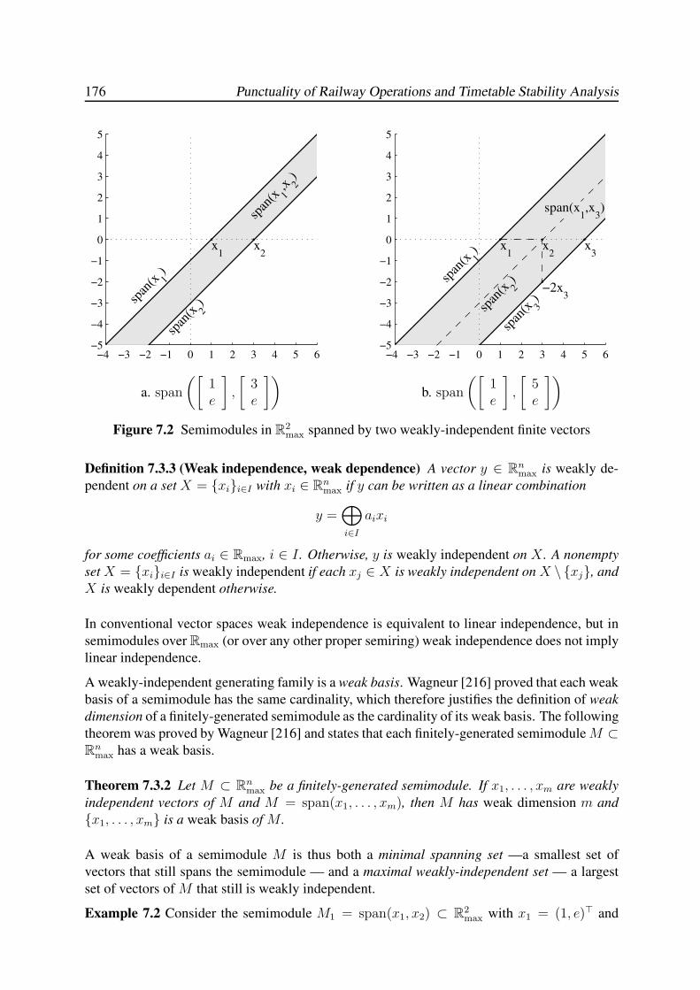
176 Punctuality of Railway Operations and Timetable Stability Analysis
−4 −3 −2 −1 0 1 2 3 4 5 6−5
−4
−3
−2
−1
0
1
2
3
4
5
x1
x2
span
(x 1)
span
(x 2)
span
(x 1,x 2
)
−4 −3 −2 −1 0 1 2 3 4 5 6−5
−4
−3
−2
−1
0
1
2
3
4
5
x1
x2
x3
−2x3
span
(x 1)
span
(x 2)
span
(x 3)
span(x1,x
3)
a. span
([1e
]
,
[3e
])
b. span
([1e
]
,
[5e
])
Figure 7.2 Semimodules in R2max spanned by two weakly-independent finite vectors
Definition 7.3.3 (Weak independence, weak dependence) A vector y ∈ Rnmax is weakly de-
pendent on a set X = {xi}i∈I with xi ∈ Rnmax if y can be written as a linear combination
y =⊕
i∈I
aixi
for some coefficients ai ∈ Rmax, i ∈ I . Otherwise, y is weakly independent on X . A nonempty
set X = {xi}i∈I is weakly independent if each xj ∈ X is weakly independent on X \ {xj}, and
X is weakly dependent otherwise.
In conventional vector spaces weak independence is equivalent to linear independence, but in
semimodules over Rmax (or over any other proper semiring) weak independence does not imply
linear independence.
A weakly-independent generating family is a weak basis. Wagneur [216] proved that each weak
basis of a semimodule has the same cardinality, which therefore justifies the definition of weak
dimension of a finitely-generated semimodule as the cardinality of its weak basis. The following
theorem was proved by Wagneur [216] and states that each finitely-generated semimoduleM ⊂Rn
max has a weak basis.
Theorem 7.3.2 Let M ⊂ Rnmax be a finitely-generated semimodule. If x1, . . . , xm are weakly
independent vectors of M and M = span(x1, . . . , xm), then M has weak dimension m and
{x1, . . . , xm} is a weak basis of M .
A weak basis of a semimodule M is thus both a minimal spanning set —a smallest set of
vectors that still spans the semimodule — and a maximal weakly-independent set — a largest
set of vectors of M that still is weakly independent.
Example 7.2 Consider the semimodule M1 = span(x1, x2) ⊂ R2max with x1 = (1, e)> and
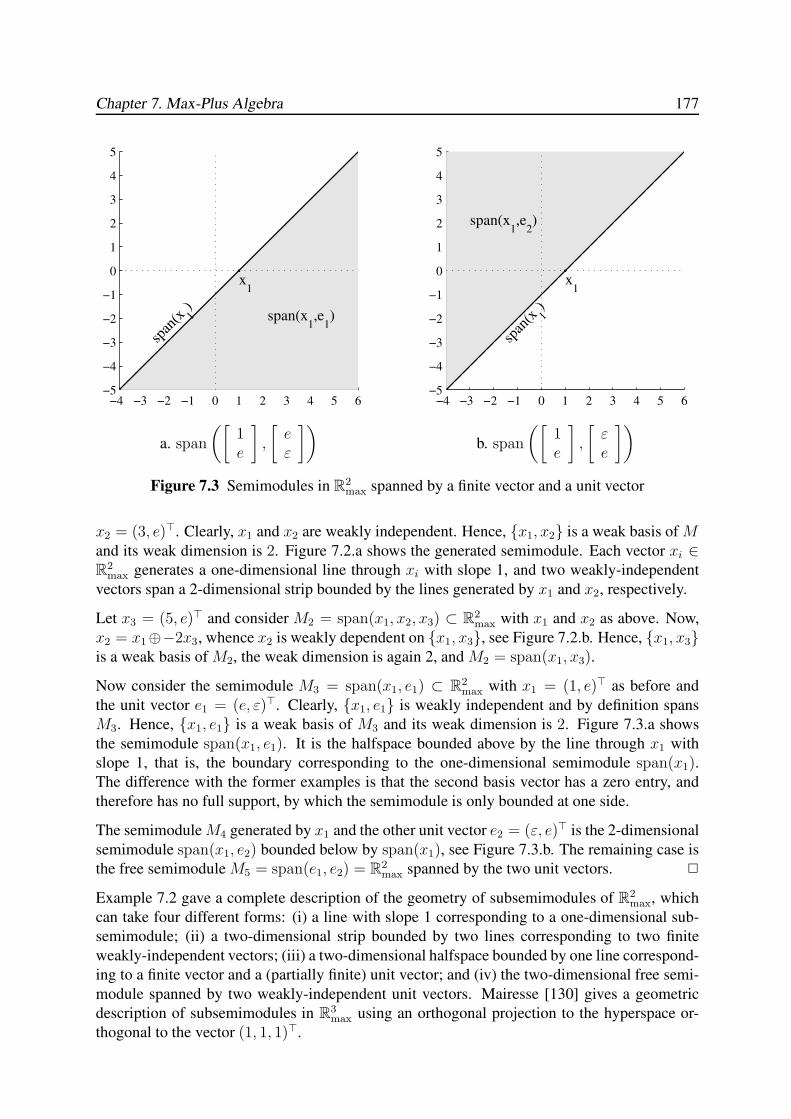
Chapter 7. Max-Plus Algebra 177
−4 −3 −2 −1 0 1 2 3 4 5 6−5
−4
−3
−2
−1
0
1
2
3
4
5
x1
span
(x 1)
span(x1,e
1)
−4 −3 −2 −1 0 1 2 3 4 5 6−5
−4
−3
−2
−1
0
1
2
3
4
5
x1
span
(x 1)
span(x1,e
2)
a. span
([1e
]
,
[eε
])
b. span
([1e
]
,
[εe
])
Figure 7.3 Semimodules in R2max spanned by a finite vector and a unit vector
x2 = (3, e)>. Clearly, x1 and x2 are weakly independent. Hence, {x1, x2} is a weak basis of Mand its weak dimension is 2. Figure 7.2.a shows the generated semimodule. Each vector xi ∈R2
max generates a one-dimensional line through xi with slope 1, and two weakly-independent
vectors span a 2-dimensional strip bounded by the lines generated by x1 and x2, respectively.
Let x3 = (5, e)> and consider M2 = span(x1, x2, x3) ⊂ R2max with x1 and x2 as above. Now,
x2 = x1⊕−2x3, whence x2 is weakly dependent on {x1, x3}, see Figure 7.2.b. Hence, {x1, x3}is a weak basis of M2, the weak dimension is again 2, and M2 = span(x1, x3).
Now consider the semimodule M3 = span(x1, e1) ⊂ R2max with x1 = (1, e)> as before and
the unit vector e1 = (e, ε)>. Clearly, {x1, e1} is weakly independent and by definition spans
M3. Hence, {x1, e1} is a weak basis of M3 and its weak dimension is 2. Figure 7.3.a shows
the semimodule span(x1, e1). It is the halfspace bounded above by the line through x1 with
slope 1, that is, the boundary corresponding to the one-dimensional semimodule span(x1).The difference with the former examples is that the second basis vector has a zero entry, and
therefore has no full support, by which the semimodule is only bounded at one side.
The semimoduleM4 generated by x1 and the other unit vector e2 = (ε, e)> is the 2-dimensional
semimodule span(x1, e2) bounded below by span(x1), see Figure 7.3.b. The remaining case is
the free semimodule M5 = span(e1, e2) = R2max spanned by the two unit vectors. 2
Example 7.2 gave a complete description of the geometry of subsemimodules of R2max, which
can take four different forms: (i) a line with slope 1 corresponding to a one-dimensional sub-
semimodule; (ii) a two-dimensional strip bounded by two lines corresponding to two finite
weakly-independent vectors; (iii) a two-dimensional halfspace bounded by one line correspond-
ing to a finite vector and a (partially finite) unit vector; and (iv) the two-dimensional free semi-
module spanned by two weakly-independent unit vectors. Mairesse [130] gives a geometric
description of subsemimodules in R3max using an orthogonal projection to the hyperspace or-
thogonal to the vector (1, 1, 1)>.

178 Punctuality of Railway Operations and Timetable Stability Analysis
7.3.3 Linear Mappings
Any max-plus matrix A ∈ Rm×nmax can be identified with a linear map A : Rn
max → Rmmax defined
by A : x 7→ Ax. These linear maps will be the main topic in the remainder of this thesis.
Definition 7.3.4 (Linear map) Let V,W be two idempotent semimodules over Rmax. Then a
mapping f : V → W is called a linear map from V to W if for all x, y ∈ V and for all
c ∈ Rmax, we have
• Additivity: f(x⊕ y) = f(x)⊕ f(y),• Homogeneity: f(cx) = cf(x).
Because of homogeneity a linear map f maps the origin to the origin: with c = ε we have
for all x ∈ V : f(ε ⊗ x) = f(εn) = ε ⊗ f(x) = εm. If V and W are finitely-generated free
semimodules over Rmax with dimension n and m, i.e., V = Rnmax and W = Rm
max, then the
linear map f : V → W can be represented by a matrix A ∈ Rm×nmax as f(x) = Ax. Conversely,
any matrix A ∈ Rm×nmax can be identified with a linear map A : Rn
max → Rmmax defined by
A : x 7→ Ax. Note that A(x ⊕ y) = Ax ⊕ Ay and A(cx) = cAx for all x, y ∈ Rnmax and
c ∈ Rmax.
The image of a matrix (map) A : Rmmax → Rn
max is defined as
im(A) = {Ax | x ∈ Rnmax} ⊆ Rm
max.
Hence, the image of a matrix map is the subsemimodule generated by the columns of A, also
called the column space or range of A. Indeed, we may write Ax =⊕n
i=1[A]· ix(i) where [A]· i
is the ith column of A and x = (x(1), . . . , x(n))>. The number of weakly-independent columns
of A is called the weak column rank of A and thus im(A) is a finitely-generated semimodule
with weak dimension equal to the weak column rank.
The image of a given matrix A ∈ Rm×nmax consists of m-dimensional vectors and so im(A) is a
subsemimodule of Rmmax. However, the weak dimension of im(A) may exceed m if n > m ≥ 3,
which is distinct from conventional linear algebra. In general, there are max-plus semimodules
V ⊂ Rmmax of arbitrary large weak dimension as a result of the following theorem. For a proof
see Cuninghame-Green [40, Theorem 16.4] or Cuninghame-Green & Butkovic [41].
Theorem 7.3.3 (Cuninghame-Green [40]) Let m ≥ 3. Then for any n ∈ N there exist n finite
(weakly) independent vectors v1, . . . , vn ∈ Rmmax.
In their proof of this theorem Cuninghame-Green & Butkovic [41] show that the vectors vi =(e, ci, c
−1i )> = (e, ci,−ci)> ∈ R3
max with distinct ci ∈ R, i = 1, . . . , n, are (weakly) indepen-
dent. In particular, we may take ci = i for i ∈ N. Then for all n ∈ N the max-plus matrix
A ∈ R3×nmax defined as
A =
e e · · · ee 1 · · · n− 1e −1 · · · −(n− 1)
,
has weak column rank n. This generalizes to matrices with row dimension m ≥ 3, by simply
adding rows with value e (like the first row above). The above also implies that the weak
Chapter 7. Max-Plus Algebra 179
column rank of a max-plus matrix may differ from its weak row rank — the weak dimension of
the semimodule generated by the (independent) rows of A — including square matrices.
The kernel of a matrix A ∈ Rm×nmax may be defined as ker(A) = {x ∈ Rn
max| Ax = ε} ⊆ Rnmax,
see Golan [73]. However, this generally gives a trivial kernel: if A has no zero columns then
ker(A) = {ε}. Cohen et al. [33] give an alternative definition of the kernel, see also Cohen et
al. [34]. Nevertheless, the dimension theory of max-plus matrices is still an open research topic
and far from the elegant fundamental dimension theorem of conventional linear algebra [195].
In the next section we will consider invariant subsemimodules of square matrices A ∈ Rn×nmax ,
that is, vectors v ∈ im(A) satisfying Av = v or more generally vectors v ∈ im(A) satisfying
A ⊗ v = λ ⊗ v for some λ ∈ Rmax. Finding all such vectors is the max-plus eigenproblem
which is well-understood and considered in detail in the next section.
7.4 Max-Plus (Generalized) Eigenproblems
7.4.1 Introduction
The eigenproblem associated to a square matrix A ∈ Rn×nmax is the problem of finding a scalar
λ ∈ Rmax and a nonzero vector v ∈ Rnmax\{ε}, such that
A⊗ v = λ⊗ v. (7.19)
If a solution (λ, v) exists then λ = λ(A) is called an eigenvalue, v is a (right) eigenvector of Aassociated to the eigenvalue λ, and (λ, v) is an eigenpair of A. The set of all eigenvalues is the
spectrum of A, denoted as spec(A) = {λ ∈ Rmax | ∃v 6= ε : Av = λv}. The eigenstructure of
a square matrix is the spectrum and the associated eigenvectors.
The case that λ = ε is an eigenvalue of a matrix A ∈ Rn×nmax is the least interesting and is dealt
with in the following lemma.
Lemma 7.4.1 A max-plus matrix A ∈ Rn×nmax has a zero eigenvalue λ = ε if and only if A has a
zero column.
Proof: If the ith column of A is zero, [A]· i = ε, then [A]· iei = ε, where ei ∈ Rnmax is the ith
unit vector. Thus, λ = ε is an eigenvalue of A with eigenvector ei 6= ε. Conversely, suppose
λ = ε is an eigenvalue of A with associated eigenvector v 6= ε. Then there is an entry vi > εand because v must satisfy Av = ε it follows that [A]· i = ε. 2
In the sequel assume that λ > ε. Then the inverse λ−1 exists since Rmax is a semifield, and we
may multiply both sides of (7.19) by λ−1 to obtain the reformulation λ−1 ⊗ A⊗ v = v. Using
the polynomial matrix A = AX ∈ Rn×nmax [X] evaluated at x = λ−1, the eigenproblem can be
rewritten as the fixed-point problem A(λ−1) ⊗ v = v. This motivates the following definition
of the generalized eigenproblem of square max-plus polynomial matrices A =⊕p
l=0AlXl ∈
Rn×nmax [X]: find a nonzero scalar λ ∈ Rmax\{ε} and a nonzero vector v ∈ Rn
max\{ε}, such that
A(λ−1)⊗ v = v. (7.20)
180 Punctuality of Railway Operations and Timetable Stability Analysis
Clearly, for A = AX we retain the original eigenproblem (7.19) with the extra condition λ >ε. Another way to interpret (7.20) is that (e, v) is an eigenpair of A(λ−1). For A = AXthis interpretation reads (Aλ−1)v = λ−1Av = λ−1λv = ev. In the forthcoming, we will
consider the generalized eigenproblem for square max-plus polynomial matrices, which embeds
the eigenproblem of square matrices as a special case.
In max-plus algebra any (polynomial) matrix is nonnegative, cf. Section 7.2.7. As a result,
many concepts from the Perron-Frobenius theory of nonnegative matrices [14, 17] also ap-
ply to matrices in max-plus algebra, see e.g. Cuninghame-Green [40], Baccelli et al. [11] and
Bapat [13]. The max-plus (generalized) eigenproblem is fundamental to the max-plus linear
system theory to be developed in Chapter 8. Therefore, this section gives an in-depth account
of the (generalized) eigenproblem, which cumulates in the celebrated policy iteration algorithm
of Cochet-Terrasson et al. [31] that solves max-plus generalized eigenproblems in ‘no time’
even for large-scale matrices.
7.4.2 Eigenstructure of Irreducible Matrices
We start this section with a fundamental theorem that states that an irreducible max-plus poly-
nomial matrices has a unique eigenvalue which has a nice interpretation in terms of the cycle
time of the associated timed event graph. An alternative proof is given in Baccelli et al. [11,
Theorem 3.28].
Theorem 7.4.1 (Generalized eigenvalue) Let A =⊕p
l=0AlXl ∈ Rn×n
max [X] be an irreducible
polynomial matrix with acyclic G(A0). Then A has a unique generalized eigenvalue λ > ε and
finite eigenvectors v > ε such that A(λ−1)⊗ v = v, and λ is equal to the maximum cycle mean
of the associated timed event graph G(A),
η = maxξ∈C
w(ξ)
µ(ξ), (7.21)
where C is the set of all elementary circuits in G(A), w(ξ) is the weight of circuit ξ, and µ(ξ)is the number of tokens in circuit ξ.
Proof: The irreducibility of A implies that G(A) is strongly connected and so by definition
contains circuits, and the acyclic assumption on G(A0) implies that each circuit in G(A) con-
tains at least one token, µ(ξ) ≥ 1 for all ξ ∈ C. Hence, the maximum cycle mean η defined
in (7.21) is well-defined and finite. We next prove that this means that also any eigenvector
v ∈ Rnmax is finite. Assume v is only partially finite and let v = (ε, u)> be a partitioning of v
with u > ε. PartitioningA accordingly gives[A11(λ
−1) A12(λ−1)
A21(λ−1) A22(λ
−1)
]
⊗[εu
]
=
[εu
]
,
and therefore A12(λ−1) ⊗ u = ε, which implies A12(λ
−1) = ε since by assumption u > ε.However, this contradicts the irreducibility of A and we conclude that v must be finite.
It remains to prove that λ equals the maximum cycle mean η. In conventional notation the
generalized eigenproblem becomes
maxj=1,...,n
(wij − µijλ+ vj) = vi for all i = 1, . . . , n, (7.22)
Chapter 7. Max-Plus Algebra 181
where
µij = µij(λ) = arg maxl=0,...,p
([Al]ij − lλ) and wij = [Aµij]ij.
Note that the maximal polynomial term (or marked arc) depends on λ. From (7.22) we obtain
wij + vj − vi ≤ µijλ for all 1 ≤ i, j ≤ n,
where equality holds for at least one pair (j, i) for each 1 ≤ i ≤ n. The terms vj − vi vanish by
summation over any circuit ξ and therefore
λ ≥∑
(j,i)∈ξ(wij + vj − vi)∑
(j,i)∈ξ µij
=
∑
(j,i)∈ξ wij∑
(j,i)∈ξ µij
=w(ξ)
µ(ξ)for all ξ ∈ C. (7.23)
Now consider the (saturation) graph Gs(A(λ−1)) = (V s, Es) with node set V s = {1, . . . , n}and arc setEs = {(j, i) | wij−µijλ+vj = vi}. This graph contains a circuit because each node
i has at least one incoming arc by (7.22). Furthermore, each circuit ξ0 in Gs(A(λ−1)) satisfies
w(ξ0)/µ(ξ0) = λ and by (7.23) it follows that λ is the maximum cycle mean, and therefore
unique. 2
In the special case of A = AX the condition on A0 is redundant and the token count on any
circuit is just the circuit length. Hence, we obtain the following corollary to Theorem 7.4.1.
Corollary 7.4.1 (Eigenvalue) Let A ∈ Rn×nmax be an irreducible matrix. Then A has a unique
eigenvalue λ > ε and finite eigenvectors v > ε such that A⊗ v = λ⊗ v, and λ is equal to the
maximum cycle mean of the associated precedence graph G(A),
η = maxξ∈C
w(ξ)
l(ξ), (7.24)
where C is the set of all elementary circuits in G(A), w(ξ) is the weight of circuit ξ, and l(ξ) is
the length of circuit ξ.
The theorem presented here as corollary 7.4.1 is the analogue in max-plus algebra of the Perron-
Frobenius theorem for nonnegative matrices [17, 187]. It is one of the classical results in max-
plus algebra, see Gondran & Minoux [74], Cuninghame-Green [40, Chapter 25], Baccelli et
al. [11, Theorem 3.23] and Bapat [13]. Theorem 7.4.1 is a generalization of this result to max-
plus polynomial matrices.
In the first-order case A = AX the maximum cycle mean (7.24) can alternatively be written in
matrix notation as
λ =
n⊕
k=1
(tr(Ak)
)1/k,
where the trace of a matrix A = (aij) ∈ Rn×nmax is defined as
tr(A) =
n⊕
i=1
aii.
A critical circuit is a circuit with maximum cycle mean. By Theorem 7.4.1 and Corollary 7.4.1
the (generalized) eigenvalue depends on the critical circuits in the underlying (timed event)
182 Punctuality of Railway Operations and Timetable Stability Analysis
graph. A graph may contain several critical circuits, which by definition have the same (maxi-
mum) cycle mean. The nodes of a critical circuit are called critical nodes. Of course, a critical
node may be contained in many circuits but at least one of them has a cycle mean equal to the
maximum cycle mean.
In the sequel our main concern is the polynomial function A(x) valuated at a fixed scalar ν−1 ∈Rmax. The resulting matrix will henceforth be denoted as
Aν.= A(ν−1) =
p⊕
l=0
Alν−l,
where ν ∈ Rmax is a fixed scalar. We also write A+ν = [A(ν−1)]+, A∗
ν = [A(ν−1)]∗, et cetera.
Note thatAν ∈ Rn×nmax and if ν = λ is a generalized eigenvalue ofA ∈ Rn×n
max [X] with eigenvector
v then (e, v) is an eigenpair of Aλ, since Aλ ⊗ v = A(λ−1)⊗ v = v.
Lemma 7.4.2 Let A ∈ Rn×nmax [X] be an irreducible polynomial matrix with generalized eigen-
value λ(A), ν ∈ Rmax\{ε} a finite scalar, and Aν = A(ν−1) =⊕p
l=0Alν−l ∈ Rn×n
max . Then
λ(Aν) ≤ e if and only if ν ≥ λ(A).
Proof: First note that since λ(A) exists, A0 must be acyclic by Theorem 7.4.1. We next prove
that λ(Aν) is a decreasing function of ν. Let ν1 ≥ ν2. Then c⊗ ν−l1 < c⊗ ν−l
2 for any c > ε and
l ∈ N, and so we have [A(ν−11 )]ij =
⊕pl=0[Al]ij⊗ν−l
1 ≤⊕p
l=0[Al]ij⊗ν−l2 = [A(ν−1
2 )]ij, where
equality holds iff [A0]ij ≥⊕p
l=1[Al]ij ⊗ ν−l2 (which includes the trivial case [A(ν−1)]ij = ε).
Hence, each polynomial entry [A(ν−1)]ij is a nonincreasing function of ν, and moreover each
polynomial entry [A(ν−1)]ij with degree 1 or higher is decreasing in ν. Because A0 is acyclic,
each circuit inG(Aν) contains at least one arc with a polynomial weight of degree one or higher,
and therefore all circuit weights and cycle means inG(Aν) are decreasing in ν. The generalized
eigenvalue λ(Aν) is then a (strictly) decreasing function of ν by Theorem 7.4.1.
For ν = λ(A) we have Aλv = A(λ−1)v = v for some (generalized) eigenvector v and so Aλ
has eigenvalue e. Hence, for any ν ≥ λ we have λ(Aν) ≤ λ(Aλ) = e, and so ν ≥ λ is a
sufficient condition. Moreover, if λ(Aν) > e = λ(Aλ) then ν < λ, and therefore ν ≥ λ(A) is
also a necessary condition. 2
Theorem 7.4.2 (Generalized eigenvectors) Let A ∈ Rn×nmax [X] be an irreducible polynomial
matrix with generalized eigenvalue λ. Then any column i of A+λ such that [A+
λ ]ii = e is a
generalized eigenvector of A associated to λ.
Proof: Let (λ, v) be a generalized eigenpair of A. Then (e, v) is an eigenpair of Aλ and
the precedence graph G(Aλ) is strongly connected with maximum cycle mean equal to e. The
longest path matrix A+λ =
⊕nl=1A
lλ is well-defined by Proposition 7.2.6, and by irreducibility
A+λ > ε. Let ξ0 be a critical circuit of G(Aλ) and i be any node on ξ0. Then any path from i to
itself in G(Aλ) has weight at most e, and since i belongs to ξ0, there is at least one such path
with weight e. Hence, [A+λ ]ii = e and therefore the i-th column of A+
λ is equal to that of A∗λ.
Let v = [A+λ ]· i = [A∗
λ]· i, where A· i denotes the i-th column of matrix A. Then
Aλ ⊗ v = Aλ ⊗ [A+λ ]· i = Aλ ⊗ [A∗
λ]· i = [Aλ ⊗A∗λ]· i = [A+
λ ]· i = v,
which proves that (λ, [A+λ ]·i) is a generalized eigenpair of A. 2
Chapter 7. Max-Plus Algebra 183
The indices i satisfying the condition in Theorem 7.4.2 are exactly the critical nodes of the
precedence graph G(Aλ), i.e., the nodes on a critical circuit of G(Aλ).
In the case of a square max-plus matrix A ∈ Rn×nmax with eigenvalue λ ∈ Rmax\{ε} we have
[Aλ]ij = [A ⊗ λ−1]ij = aij − λ. Clearly, the support of A, supp(A) = {(j, i) | aij > ε, 1 ≤i, j ≤ n}, is preserved in Aλ. Furthermore, the precedence graphs G(A) and G(Aλ) are equal
except for the arc weights, and in particular the critical circuits in both graphs are the same, with
the maximum cycle means η(A) = λ and η(Aλ) = e. Hence, we have the following corollary
to Theorem 7.4.2.
Corollary 7.4.2 (Eigenvectors) Let A ∈ Rn×nmax be an irreducible matrix with eigenvalue λ.
Then any column i of [λ−1A]+ such that [λ−1A]+ii = e is an eigenvector of A associated to λ.
If v1, v2 ∈ Rnmax are two generalized eigenvectors of A corresponding to the generalized eigen-
value λ ∈ Rmax then for any c1, c2 ∈ Rmax also c1v1 ⊕ c2v2 is a generalized eigenvector ofAcorresponding to λ, since
A(λ−1)⊗ (c1v1 ⊕ c2v2) = A(λ−1)⊗ (c1v1)⊕A(λ−1)⊗ (c2v2)
= c1(A(λ−1)⊗ v1)⊕ c2(A(λ−1)⊗ v2)
= c1v1 ⊕ c2v2.
This argument is easily expanded to any linear combination of generalized eigenvectors. In gen-
eral, the generalized eigenvectors corresponding to a generalized eigenvalue λ of a polynomial
matrix A ∈ Rn×nmax [X] span a subsemimodule of Rn
max:
V(λ) = {v ∈ Rnmax | A(λ−1)v = v} =
⊕
i∈I
ci[A+λ ]· i
with ci ∈ Rmax and I = {1 ≤ i ≤ n | [A+λ ]ii = e}. This semimodule is called the eigensemi-
module of A corresponding to the generalized eigenvalue λ or also simply the eigenspace of
λ(A). Unlike the classical Perron-Frobenius theory where an irreducible nonnegative matrix
has a unique eigenvector (up to a constant multiple), the dimension of the eigenspace of a max-
plus (polynomial) matrix depends on the interconnection structure of the critical circuit(s) of
G(Aλ).
Lemma 7.4.3 Let A ∈ Rn×nmax [X] be an irreducible polynomial matrix with generalized eigen-
value λ. If the precedence graph G(Aλ) has a unique critical circuit then all generalized eigen-
vectors associated to λ are weakly dependent, and the one-dimensional eigenspace is given by
V(λ) = span([A+λ ]· i) for any index i ∈ {1 ≤ i ≤ n | [A+
λ ]ii = e}.
Proof: By Theorem 7.4.2 we know that the set V(λ) of generalized eigenvectors is generated by
the critical columns of A+λ . By definition [A+
λ ]· i is a critical column if and only if i is contained
in a critical circuit of G(Aλ), i.e., [A+λ ]ii = e. It remains to prove that under the condition of a
unique critical circuit all generalized eigenvectors are proportional and thus weakly dependent.
In general, [A+λ ]lj ≥ [A+
λ ]li[A+λ ]ij for each 1 ≤ l ≤ n, with strict equality only if the longest
path from j to l passes node i. If i, j are any two nodes on a critical circuit of G(Aλ) then
[A+λ ]ji[A
+λ ]ij = [A+
λ ]jj = e. Therefore, for all 1 ≤ l ≤ n
[A+λ ]li[A
+λ ]ij ≤ [A+
λ ]lj = [A+λ ]lj[A
+λ ]ji[A
+λ ]ij ≤ [A+
λ ]li[A+λ ]ij
184 Punctuality of Railway Operations and Timetable Stability Analysis
and so [A+λ ]· j = [A+
λ ]· i[A+λ ]ij = [A+
λ ]ij [A+λ ]· i, which proves that [A+
λ ]· j and [A+λ ]· i are weakly
dependent for any pair of indices i and j on the same critical circuit. 2
If there is more than one critical circuit then the eigenspace may be generated by several weakly-
independent generalized eigenvectors. The general result requires the notion of the critical
graph.
Definition 7.4.1 (Critical graph) Let A ∈ Rn×nmax [X] be a polynomial matrix with generalized
eigenvalue λ. The critical graph Gc(Aλ) = (V c, Ec) is the digraph with node set V c = {1 ≤i ≤ n | [A+
λ ]ii = e} and arc set Ec = {(j, i) | [Aλ]ij > ε, i, j ∈ V c}.
Note that the critical graph Gc(Aλ) = (V c, Ec) is a cyclic subgraph of the precedence graph
G(Aλ) = (V,E), with V c ⊆ V and Ec = E ∩ (V c × V c). If λ is known the critical graph can
be computed using Algorithm 7.5.3 of Section 7.5.3. This algorithm computes the diagonal of
the matrix A+λ . Selecting all diagonal entries equal to e gives the node set V c and subsequently
Ec is determined by selecting all arcs (j, i) corresponding to [Aλ]ij 6= ε with both j, i ∈ V c.
If Gc(Aλ) is not strongly connected then the node set can be decomposed into critical classes
Kci associated to the strongly-connected components, V c = Kc
1 ∪ . . . ∪ Kcc , where c is the
number of components, and Kci ∩ Kc
j = ∅ for i 6= j. The next theorem characterizes the
eigenspace of an irreducible max-plus (polynomial) matrix by its weak basis.
Theorem 7.4.3 (Eigenspace) LetA ∈ Rn×nmax [X] be an irreducible polynomial matrix with gen-
eralized eigenvalue λ. If the critical graph Gc(Aλ) has c connected components then the
eigenspace V(λ) ⊆ Rnmax of generalized eigenvectors associated to λ is a finitely-generated
semimodule of weak dimension c, given by
V(λ) = span([A+λ ]·i1, . . . , [A
+λ ]·ic), (7.25)
where the indices are arbitrarily selected from each critical class ik ∈ Kck for all k = 1, . . . , c.
Proof: By Theorem 7.4.2 we know that the set V(λ) of generalized eigenvectors is generated
by the critical columns of A+λ , and by Lemma 7.4.3 the generalized eigenvectors from the same
critical classes are weakly dependent. We now prove that a maximal weakly independent set
of generalized eigenvectors is obtained by selecting one critical column of A+λ for each critical
class Kc1, . . . , K
cc , which then constitutes a weak basis of V(λ). Let I = {i1, . . . , ic} be a
representative set of indices from each class Kc1, . . . , K
cc . Then we must prove that for each
i ∈ I the vector [A+λ ]· i is weakly independent on the set {[A+
λ ]· k | k ∈ I \{i}}. We argue by
contradiction. Suppose
[A+λ ]· i =
⊕
k∈I\{i}
ck ⊗ [A+λ ]· k (7.26)
for some coefficients ck ∈ Rmax, k ∈ I \ {i}. Concentrating on the ith row of (7.26) we have
[A+λ ]ii =
⊕
k∈I\{i} ck[A+λ ]ik = e, since i is a critical node. Hence, there must be at least one
index j ∈ I\{i} with cj = [A+λ ]−1
ij , such that e = cj [A+λ ]ij = [A+
λ ]−1ij [A+
λ ]ij. Then by (7.26) we
have [A+λ ]· i ≥ [A+
λ ]−1ij [A+
λ ]·j . In particular, on the jth row this gives [A+λ ]ji ≥ [A+
λ ]−1ij [A+
λ ]jj =
[A+λ ]−1
ij e = [A+λ ]−1
ij . However, in general we have [A+λ ]ij[A
+λ ]ji ≤ e or equivalently [A+
λ ]ji ≤[A+
λ ]−1ij with equality only if i and j are on the same critical circuit. But by construction i and j
correspond to distinct critical classes and we thus have a contradiction. 2
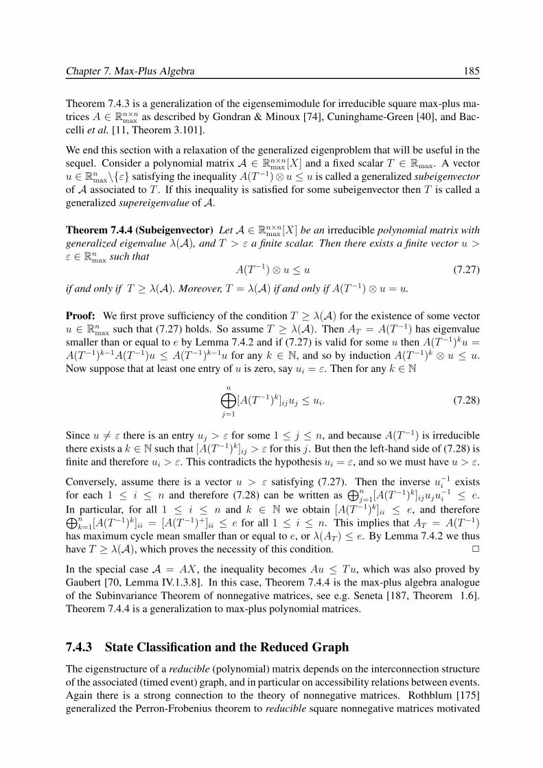
Chapter 7. Max-Plus Algebra 185
Theorem 7.4.3 is a generalization of the eigensemimodule for irreducible square max-plus ma-
trices A ∈ Rn×nmax as described by Gondran & Minoux [74], Cuninghame-Green [40], and Bac-
celli et al. [11, Theorem 3.101].
We end this section with a relaxation of the generalized eigenproblem that will be useful in the
sequel. Consider a polynomial matrix A ∈ Rn×nmax [X] and a fixed scalar T ∈ Rmax. A vector
u ∈ Rnmax\{ε} satisfying the inequality A(T−1)⊗ u ≤ u is called a generalized subeigenvector
of A associated to T . If this inequality is satisfied for some subeigenvector then T is called a
generalized supereigenvalue of A.
Theorem 7.4.4 (Subeigenvector) Let A ∈ Rn×nmax [X] be an irreducible polynomial matrix with
generalized eigenvalue λ(A), and T > ε a finite scalar. Then there exists a finite vector u >ε ∈ Rn
max such that
A(T−1)⊗ u ≤ u (7.27)
if and only if T ≥ λ(A). Moreover, T = λ(A) if and only if A(T−1)⊗ u = u.
Proof: We first prove sufficiency of the condition T ≥ λ(A) for the existence of some vector
u ∈ Rnmax such that (7.27) holds. So assume T ≥ λ(A). Then AT = A(T−1) has eigenvalue
smaller than or equal to e by Lemma 7.4.2 and if (7.27) is valid for some u then A(T−1)ku =A(T−1)k−1A(T−1)u ≤ A(T−1)k−1u for any k ∈ N, and so by induction A(T−1)k ⊗ u ≤ u.
Now suppose that at least one entry of u is zero, say ui = ε. Then for any k ∈ N
n⊕
j=1
[A(T−1)k]ijuj ≤ ui. (7.28)
Since u 6= ε there is an entry uj > ε for some 1 ≤ j ≤ n, and because A(T−1) is irreducible
there exists a k ∈ N such that [A(T−1)k]ij > ε for this j. But then the left-hand side of (7.28) is
finite and therefore ui > ε. This contradicts the hypothesis ui = ε, and so we must have u > ε.
Conversely, assume there is a vector u > ε satisfying (7.27). Then the inverse u−1i exists
for each 1 ≤ i ≤ n and therefore (7.28) can be written as⊕n
j=1[A(T−1)k]ijuju−1i ≤ e.
In particular, for all 1 ≤ i ≤ n and k ∈ N we obtain [A(T−1)k]ii ≤ e, and therefore⊕n
k=1[A(T−1)k]ii = [A(T−1)+]ii ≤ e for all 1 ≤ i ≤ n. This implies that AT = A(T−1)has maximum cycle mean smaller than or equal to e, or λ(AT ) ≤ e. By Lemma 7.4.2 we thus
have T ≥ λ(A), which proves the necessity of this condition. 2
In the special case A = AX , the inequality becomes Au ≤ Tu, which was also proved by
Gaubert [70, Lemma IV.1.3.8]. In this case, Theorem 7.4.4 is the max-plus algebra analogue
of the Subinvariance Theorem of nonnegative matrices, see e.g. Seneta [187, Theorem 1.6].
Theorem 7.4.4 is a generalization to max-plus polynomial matrices.
7.4.3 State Classification and the Reduced Graph
The eigenstructure of a reducible (polynomial) matrix depends on the interconnection structure
of the associated (timed event) graph, and in particular on accessibility relations between events.
Again there is a strong connection to the theory of nonnegative matrices. Rothblum [175]
generalized the Perron-Frobenius theorem to reducible square nonnegative matrices motivated
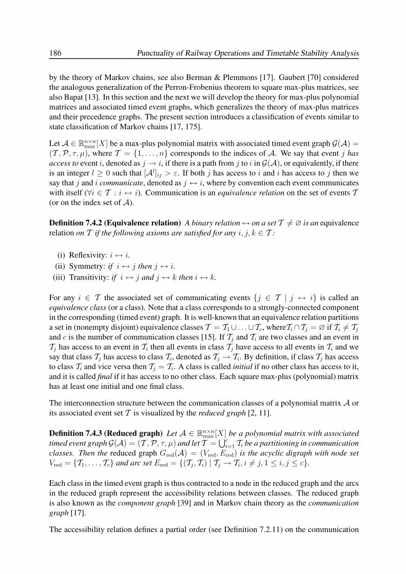
186 Punctuality of Railway Operations and Timetable Stability Analysis
by the theory of Markov chains, see also Berman & Plemmons [17]. Gaubert [70] considered
the analogous generalization of the Perron-Frobenius theorem to square max-plus matrices, see
also Bapat [13]. In this section and the next we will develop the theory for max-plus polynomial
matrices and associated timed event graphs, which generalizes the theory of max-plus matrices
and their precedence graphs. The present section introduces a classification of events similar to
state classification of Markov chains [17, 175].
Let A ∈ Rn×nmax [X] be a max-plus polynomial matrix with associated timed event graph G(A) =
(T ,P, τ, µ), where T = {1, . . . , n} corresponds to the indices of A. We say that event j has
access to event i, denoted as j → i, if there is a path from j to i in G(A), or equivalently, if there
is an integer l ≥ 0 such that [Al]ij > ε. If both j has access to i and i has access to j then we
say that j and i communicate, denoted as j ↔ i, where by convention each event communicates
with itself (∀i ∈ T : i ↔ i). Communication is an equivalence relation on the set of events T(or on the index set of A).
Definition 7.4.2 (Equivalence relation) A binary relation↔ on a set T 6= ∅ is an equivalence
relation on T if the following axioms are satisfied for any i, j, k ∈ T :
(i) Reflexivity: i↔ i.
(ii) Symmetry: if i↔ j then j ↔ i.
(iii) Transitivity: if i↔ j and j ↔ k then i↔ k.
For any i ∈ T the associated set of communicating events {j ∈ T | j ↔ i} is called an
equivalence class (or a class). Note that a class corresponds to a strongly-connected component
in the corresponding (timed event) graph. It is well-known that an equivalence relation partitions
a set in (nonempty disjoint) equivalence classes T = T1∪ . . .∪Tc, whereTi∩Tj = ∅ if Ti 6= Tj
and c is the number of communication classes [15]. If Tj and Ti are two classes and an event in
Tj has access to an event in Ti then all events in class Tj have access to all events in Ti and we
say that class Tj has access to class Ti, denoted as Tj → Ti. By definition, if class Tj has access
to class Ti and vice versa then Tj = Ti. A class is called initial if no other class has access to it,
and it is called final if it has access to no other class. Each square max-plus (polynomial) matrix
has at least one initial and one final class.
The interconnection structure between the communication classes of a polynomial matrix A or
its associated event set T is visualized by the reduced graph [2, 11].
Definition 7.4.3 (Reduced graph) Let A ∈ Rn×nmax [X] be a polynomial matrix with associated
timed event graph G(A) = (T ,P , τ, µ) and let T =⋃c
i=1 Ti be a partitioning in communication
classes. Then the reduced graph Gred(A) = (Vred, Ered) is the acyclic digraph with node set
Vred = {T1, . . . , Tc} and arc set Ered = {(Tj, Ti) | Tj → Ti, i 6= j, 1 ≤ i, j ≤ c}.
Each class in the timed event graph is thus contracted to a node in the reduced graph and the arcs
in the reduced graph represent the accessibility relations between classes. The reduced graph
is also known as the component graph [39] and in Markov chain theory as the communication
graph [17].
The accessibility relation defines a partial order (see Definition 7.2.11) on the communication
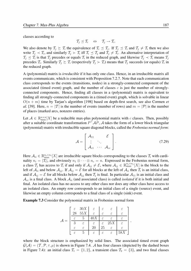
Chapter 7. Max-Plus Algebra 187
classes according to
Tj � Ti ⇔ Tj → Ti.
We also denote by Tj � Ti the equivalence of Ti � Tj . If Tj � Ti and Tj 6= Ti then we also
write Tj ≺ Ti, and similarly Tj � Ti iff Ti � Tj and Tj 6= Ti. An alternative interpretation of
Tj � Ti is that Tj precedes or equals Ti in the reduced graph, and likewise Tj ≺ Ti means Tj
precedes Ti. Similarly Tj � Ti (respectively Tj � Ti) means that Tj succeeds (or equals) Ti in
the reduced graph.
A (polynomial) matrix is irreducible if it has only one class. Hence, in an irreducible matrix all
events communicate, which is consistent with Proposition 7.2.7. Note that each communication
class corresponds to the events (transitions, nodes) in a strongly-connected component of the
associated (timed event) graph, and the number of classes c is just the number of strongly-
connected components. Hence, finding all classes in a (polynomial) matrix is equivalent to
finding all strongly-connected components in a (timed event) graph, which is solvable in linear
O(n + m) time by Tarjan’s algorithm [198] based on depth-first search, see also Cormen et
al. [39]. Here, n = |T | is the number of events (number of rows) and m = |P| is the number
of places (marked arcs, nonzero entries).
Let A ∈ Rn×nmax [X] be a reducible max-plus polynomial matrix with c classes. Then, possibly
after a suitable coordinate transformation P>AP , A takes the form of a lower block triangular
(polynomial) matrix with irreducible square diagonal blocks, called the Frobenius normal form:
A =
A11 E...
. . .
Ac1 · · · Acc
. (7.29)
Here Aii ∈ Rni×nimax [X] are irreducible square blocks corresponding to the classes Ti with cardi-
nality ni = |Ti|, and obviously n1 ⊗ · · · ⊗ nc = n. Expressed in the Frobenius normal form,
a class Tj has access to Ti if and only if Aij 6= E , where Aij ∈ Rni×njmax [X] is the block to the
left of Aii and below Ajj. If Aij = E for all blocks at the left of Aii then Ti is an initial class,
and if Aij = E for all blocks below Ajj then Tj is final. In particular A11 is an initial class and
Acc is a final class. A block Aii (and associated class) is called isolated if it is both initial and
final. An isolated class has no access to any other class nor does any other class have access to
an isolated class. An empty row corresponds to an initial class of a single (source) event, and
likewise an empty column corresponds to a final class of a single (sink) event.
Example 7.3 Consider the polynomial matrix in Frobenius normal form
A =
ε 30X ε ε ε ε28 55X ε ε ε ε
ε 5 40X ε ε ε
3 ε ε ε 25X εε ε 20 25 ε ε
ε 5 ε ε ε 58X
,
where the block structure is emphasized by solid lines. The associated timed event graph
G(A) = (T ,P, τ, µ) is shown in Figure 7.4. A has four classes (depicted by the dashed boxes
in Figure 7.4): an initial class T1 = {1, 2}, a transient class T2 = {3}, and two final classes
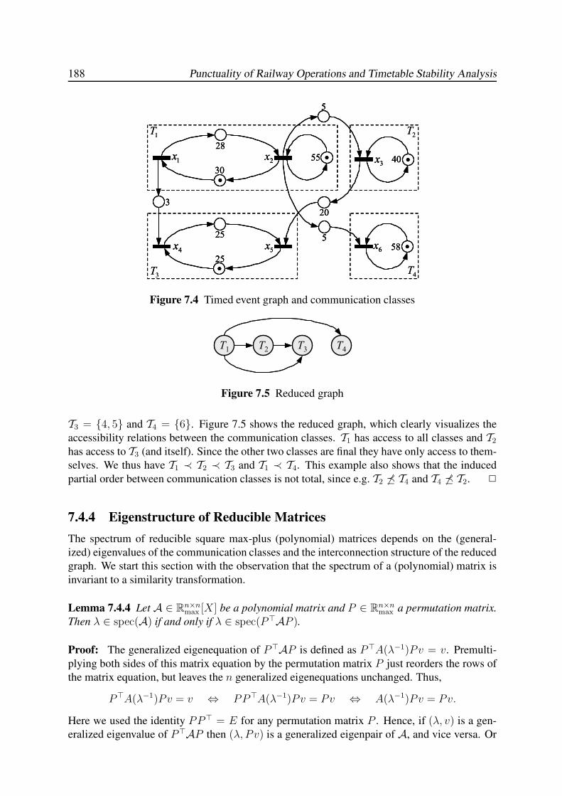
188 Punctuality of Railway Operations and Timetable Stability Analysis
5
·
·
28
55
30
·
25
25
3
·40
·
20
585
2x1x3x
4x 5x 6x
1T 2T
3T 4T
5
·
·
28
55
30
·
25
25
3
·40
·
20
585
2x1x3x
4x 5x 6x
5
·
·
28
55
30
·
25
25
3
·40
·
20
585
2x1x3x
4x 5x 6x
1T 2T
3T 4T
Figure 7.4 Timed event graph and communication classes
T1 T2 T3 T4T1 T2 T3 T4
Figure 7.5 Reduced graph
T3 = {4, 5} and T4 = {6}. Figure 7.5 shows the reduced graph, which clearly visualizes the
accessibility relations between the communication classes. T1 has access to all classes and T2has access to T3 (and itself). Since the other two classes are final they have only access to them-
selves. We thus have T1 ≺ T2 ≺ T3 and T1 ≺ T4. This example also shows that the induced
partial order between communication classes is not total, since e.g. T2 6� T4 and T4 6� T2. 2
7.4.4 Eigenstructure of Reducible Matrices
The spectrum of reducible square max-plus (polynomial) matrices depends on the (general-
ized) eigenvalues of the communication classes and the interconnection structure of the reduced
graph. We start this section with the observation that the spectrum of a (polynomial) matrix is
invariant to a similarity transformation.
Lemma 7.4.4 Let A ∈ Rn×nmax [X] be a polynomial matrix and P ∈ Rn×n
max a permutation matrix.
Then λ ∈ spec(A) if and only if λ ∈ spec(P>AP ).
Proof: The generalized eigenequation of P>AP is defined as P>A(λ−1)Pv = v. Premulti-
plying both sides of this matrix equation by the permutation matrix P just reorders the rows of
the matrix equation, but leaves the n generalized eigenequations unchanged. Thus,
P>A(λ−1)Pv = v ⇔ PP>A(λ−1)Pv = Pv ⇔ A(λ−1)Pv = Pv.
Here we used the identity PP> = E for any permutation matrix P . Hence, if (λ, v) is a gen-
eralized eigenvalue of P>AP then (λ, Pv) is a generalized eigenpair of A, and vice versa. Or
Chapter 7. Max-Plus Algebra 189
equivalently, if (λ, u) is a generalized eigenpair of A then (λ, P>u) is a generalized eigenvalue
of P>AP , and vice versa. 2
Without loss of generality we thus may assume that a reducible (polynomial) matrix is in Frobe-
nius normal form (7.29), where the event set (or index set) T = {1, . . . , n} is partitioned
into c classes T =⋃c
i=1 Ti. The number of events in class Ti is denoted as ni = |Ti|, with⊗c
i=1 ni = n.
Each class Ti corresponds to an irreducible polynomial submatrix Aii ∈ Rni×nimax [X] of A and
thus has a unique generalized eigenvalue λ(Aii) by Theorem 7.4.1. However, this class gener-
alized eigenvalue may be dominated by a preceding class with larger generalized eigenvalue.
Moreover, if the class has access to a class with larger generalized eigenvalue then its general-
ized eigenvalue is not contained in the spectrum of the full matrix A, as we will see below.
For any subset I ⊆ T let Γ(I) be the set of events that are accessible from I , i.e.,
Γ(I).= {j ∈ T | ∃i ∈ I : i→ j}.
A subset I ⊆ T is a closed set if I = Γ(I).
Lemma 7.4.5 Let A ∈ Rn×nmax [X] be a polynomial matrix and let T =
⋃ci=1 Ti be a partitioning
of the event set in communication classes. Then Ki = Γ(Ti) is a closed set for each 1 ≤ i ≤ c.
Proof: For any class Ti ⊆ T the set Γ(Ti) 6= ∅ since Ti ⊆ Γ(Ti) for all 1 ≤ i ≤ c.Furthermore, if Ti � Tj then by definition Tj ⊂ Γ(Ti). Hence, Ki = Γ(Ti) contains all classes
accessible from Ti and is thus a closed set for each 1 ≤ i ≤ c. 2
The following theorem was proved by Gaubert [70] for square max-plus matrices A ∈ Rn×nmax .
Theorem 7.4.5 (Generalized eigenpair) Let A ∈ Rn×nmax [X] be a polynomial matrix in Frobe-
nius normal form with c classes,
A =
A11 E...
. . .
Ac1 · · · Acc
.
Then λ is a generalized eigenvalue ofA if and only if there exists a class Ti such that λ = λ(Aii)and
λ(Aii) =⊕
Tj⊆Γ(Ti)
λ(Ajj). (7.30)
Moreover there exists a generalized eigenvector v = (v1, . . . , vn)> ∈ Rnmax associated to
λ(A) = λ(Aii) with support Γ(Ti), given by
vj =
{[A+
λ ]jl if j ∈ Γ(Ti)ε otherwise,
(7.31)
for any l ∈ Ti with [A+λ ]ll = e.
190 Punctuality of Railway Operations and Timetable Stability Analysis
Proof: Assume that λ = λ(Aii) is a generalized eigenvalue ofA but (7.30) is violated. Hence,
there exists a class Tk ⊂ Γ(Ti) with λ(Akk) > λ(Aii). Let the generalized eigenvector v ∈ Rnmax
associated to λ be partitioned conform the block partitioning of A, i.e., v = (v1, . . . , vc)> ∈
Rnmax with vj ∈ R
|Tj |max, 1 ≤ j ≤ c. Then the kth block row of the generalized eigenequation
A(λ−1)⊗ v = v becomes⊕
j 6=k
Akj(λ−1)⊗ vj ⊕ Akk(λ
−1)⊗ vk = vk,
and therefore in particular Akk(λ−1)vk ≤ vk, which implies that vk is a subeigenvector of
Akk associated to λ = λ(Aii). Then by Theorem 7.4.4 we must have λ ≥ λ(Akk), but this
contradicts the assumption λ(Akk) > λ(Aii). Thus, (7.30) is a necessary condition.
Conversely, assume (7.30) is valid. By Lemma 7.4.5 the set Ki = Γ(Ti) ⊆ T is closed. Hence,
possibly after a similarity transformation, A can be written in block triangular form
A =
[A[Ki|Ki] EA[Ki|Ki] A[Ki|Ki]
]
,
where Ki = T \ Ki is the complement of Ki in T , and A[I|J ] ∈ R|I|×|J |max [X] denotes the
submatrix of A corresponding to row index set I and column index set J . Assume (λ, v) is a
generalized eigenpair of the principle submatrix A[Ki|Ki] with v ∈ R|Ki|max. Then (ε, v)> ∈ Rn
max
is a generalized eigenvector of A associated to λ, since[A[Ki|Ki](λ
−1) EA[Ki|Ki](λ
−1) A[Ki|Ki](λ−1)
] [εv
]
=
[ε
A[Ki|Ki](λ−1)v
]
=
[εv
]
. (7.32)
Hence, we may restrict ourselves to the generalized eigenvalue of the principle submatrix B =
A[Ki|Ki] ∈ R|Ki|×|Ki|max [X] of A. Because of (7.30), λ is the maximum generalized eigenvalue
of B. Let Bλ = B(λ−1). Then Bλ has eigenvalue e and so the precedence graph G(Bλ) has
no circuits with positive weight. By Proposition 7.2.6 the matrices B+λ and B∗
λ are then well-
defined, and by definition Bλ[B∗λ]· l = [B+
λ ]· l for any 1 ≤ l ≤ |Ki|. If l is contained in a critical
circuit of G(B) then [B+λ ]ll = e, and so [B+
λ ]· l = [B∗λ]· l. Hence, for any critical index l the vector
[B+λ ]· l is an eigenvector of Bλ associated to the eigenvalue e, and therefore also a generalized
eigenvector of B associated to λ, since B(λ−1)[B+λ ]· l = Bλ[B
+λ ]· l = [B+
λ ]· l. This proves that
(7.30) is also a sufficient condition.
It remains to prove that (7.31) defines a generalized eigenvector v ofA. From (7.32) and the fact
that Ki = Γ(Ti) is closed it follows that a generalized eigenvector v associated to λ = λ(Aii)exists with supp(v) = Ki = Γ(Ti). Consider again the generalized eigenvector [B+
λ ]· l of B.
If A is already in the form (7.32) then we simply have v = (ε, [B+λ ]· l)
> = [A+λ ]· l. If the form
(7.32) is obtained after a similarity transformation P>AP then we have v = P>⊗ (ε, [B+λ ]· l)
>,
analogous to the proof of Lemma 7.4.4, which is exactly (7.31). 2
Corollary 7.4.3 Let A ∈ Rn×nmax [X] be a polynomial matrix in Frobenius normal form (7.29)
with c classes. Then the set of all generalized eigenvalues of A is characterized by
spec(A) =
λ(Aii) ∈ Rmax | λ(Aii) =
⊕
Tj⊆Γ(Ti)
λ(Ajj), 1 ≤ i ≤ c
. (7.33)
Chapter 7. Max-Plus Algebra 191
Classes that satisfy the condition in Theorem 7.4.5 are obviously of particular importance, and
will be called principle in the sequel. So if A ∈ Rn×nmax [X] is a polynomial matrix in Frobenius
normal form (7.29) then Ti is a principle class if λ(Aii) ≥ λ(Ajj) for all Tj ∈ Γ(Ti). A class
with (generalized) eigenvalue equal to the maximum (generalized) eigenvalue is called basic,
and any other class is nonbasic. Clearly, all basic classes are principle. Moreover, all final
classes are trivially principle. Thus, we have the following corollary to Theorem 7.4.5
Corollary 7.4.4 Let A ∈ Rn×nmax [X] be a polynomial matrix in Frobenius normal form with c
classes T1, . . . , Tc. Then
(i) λ0 =⊕c
i=1 λ(Aii) ∈ spec(A).(ii) λ(Aii) ∈ spec(A) for each final class Ti ⊆ T .
Remark Theorem 7.4.5 is formulated according to the convention in max-plus algebra that the
ij-th entry of a (polynomial) matrix corresponds to the (marked) arc (j, i) in the precedence
graph (timed event graph) [11]. In conventional graph theory an arc (j, i) corresponds to the
the ji-th entry of the adjacency matrix [16, 18]. The ‘reversed arc’ convention in max-plus
algebra enables a familiar linear system equation x(k) = Ax(k − 1) with column vectors x(·),as opposed to a dynamic equation y(k) = y(k − 1)M for row vectors y(·) (which is however
customary in Markov chain theory). The “reverse” statement of the theorem is the following:
the set of eigenvalues is determined by the maximum eigenvalue of all classes that are accessible
from a given class [13, 31]. 2
According to Theorem 7.4.5 any principle class Ti of a (polynomial) matrix, or its index set,
defines a (generalized) eigenvector with finite entry vj only if j is accessible from class Ti, in
which case it is the weight of a longest path from a selected critical node l ∈ Ti to j in the
precedence graph G(Aλ). If the critical graph Gc(A[Ti|Ti](λ−1)) restricted to the nodes of class
Ti has several disconnected critical circuits then Ti defines several weakly-independent (gener-
alized) eigenvectors associated to the generalized eigenvalue λ(A) = λ(Aii), analogous to an
irreducible (polynomial) matrix. However, these (generalized) eigenvectors have the same sup-
port. More important are (generalized) vectors resulting from distinct principle classes with the
same (generalized) eigenvalue, which have access to different classes conform the precedence
ordering in the reduced graph.
Define for each λ ∈ spec(A) the set of principle classes with eigenvalue λ as
K(λ) =
Ti | λ(Aii) = λ, λ(Aii) =
⊕
Tj⊆Γ(Ti)
λ(Ajj), 1 ≤ i ≤ c
. (7.34)
Then the events that are accessible from any principle class with generalized eigenvalue λ ∈spec(A) is
Kλ = Γ(K(λ)) =⋃
Tk∈K(λ)
Γ(Tk) = {1 ≤ j ≤ n | ∃Tk ∈ K(λ) : Tk → j}. (7.35)
Theorem 7.4.6 (Eigenspace) Let A ∈ Rn×nmax [X] be a polynomial matrix in Frobenius normal
form with c classes T1, . . . , Tc, λ ∈ spec(A), and define Aλ = A[Kλ|Kλ](λ−1) ∈ RKλ×Kλ
max . If the
192 Punctuality of Railway Operations and Timetable Stability Analysis
critical graph Gc(Aλ) has υ strongly-connected components with index sets Kc1, . . . , K
cυ then
the eigenspace V(λ) ⊆ Rnmax of generalized eigenvectors associated to λ is a finitely-generated
semimodule of weak dimension υ with weak basis {vi1 , . . . , viυ} defined as
vjik
=
{[A+
λ ]jik if j ∈ Kλ
ε otherwise,(7.36)
where the indices ik ∈ Kck are arbitrarily selected from each critical component for all k =
1, . . . , υ.
Proof: The classes in Kλ have maximum generalized eigenvalue λ corresponding to the prin-
ciple classes in K(λ). Therefore, analogous to Lemma 7.4.2 Aλ = A[Kλ|Kλ](λ−1) ∈ RKλ×Kλ
max
has maximum eigenvalue e. For all (critical) nodes i on a critical circuit of a principle class, we
then have [A+λ ]ii = [A+
λ ]ii = e and therefore the critical graph Gc(Aλ) is the union of the criti-
cal graphs of the principle classes. Moreover, the critical circuits of different principle classes
are by definition separate components in the critical graph, and so there are υ ≥ c number
of components in the critical graph. From Theorem 7.4.3 it then follows that the generalized
eigenvectors associated to the nodes in the critical graph Gc(Aλ) span the eigensemimodule
V(λ), i.e.,
V(λ) =⊕
i∈I
civi with I = V c = {1 ≤ i ≤ n | [A+λ ]ii = e},
where ci ∈ Rmax and the vectors vi are defined by (7.36). Recall that Kλ is the union of Γ(Tk)over the principle classes Tk ∈ K(λ) by (7.35), whence (7.36) coincides with (7.31). It remains
to prove that a weak basis of V(λ) is obtained by selecting an arbitrary node ik from each
component Kck in Gc(Aλ), 1 ≤ k ≤ υ.
We first prove that generalized eigenvectors of different classes are weakly independent. Con-
sider the accessibility relations between the classes T1, . . . , Tc conform the reduced graph asso-
ciated to A, see Section 7.4.3. We are interested in the principle classes Ti ∈ K(λ) and their
descendants in the reduced graph, which are exactly the classes accessible from the principle
classes in K(λ), i.e., Γ(K(λ)) = Kλ. For any sequence Tk1≺ Tk2
≺ Tk3in the reduced graph
we have Γ(Tk1) ⊃ Γ(Tk2
) ⊃ Γ(Tk3). Now, consider any principle class Tk ∈ K(λ), which
generates a generalized eigenvector vik with support Γ(Tk) by (7.36). Then there does not ex-
ist a linear combination of generalized eigenvectors associated to the other principle classes in
K(λ)\Tk with the same support, which is proved as follows. For any preceding class Tj ≺ Tk
in the reduced graph we have Γ(Tk) ⊂ Γ(Tj), and in particular Tj 6⊆ Γ(Tk). Thus, a generalized
vector associated to a preceding class has larger support than vik and a linear combination in-
cluding such a vector will also have larger support unless the associated coefficient is ε. On the
other hand, for all succeeding classes Tj � Tk in the reduced graph we have Γ(Tk) ⊃ Γ(Tj), and
in particular Tk 6⊆ Γ(Tj) for all Tj � Tk. Hence, vik cannot be written as a linear combination
of generalized eigenvectors associated to classes succeeding Ti. This proves that vik is weakly
independent of the generalized eigenvectors from other (principle) classes.
Finally, if a class has more than one component in the critical graph then the generalized eigen-
vectors associated to each component have the same support but are weakly independent, which
is proved as follows. Partition the vectors according to v = (v[Tk], v[Tk]), where Tk = T \Tk. By
Theorem 7.4.3 the partial vectors corresponding to Tk are weakly independent, and they remain
weakly independent regardless of a dimension expansion. 2
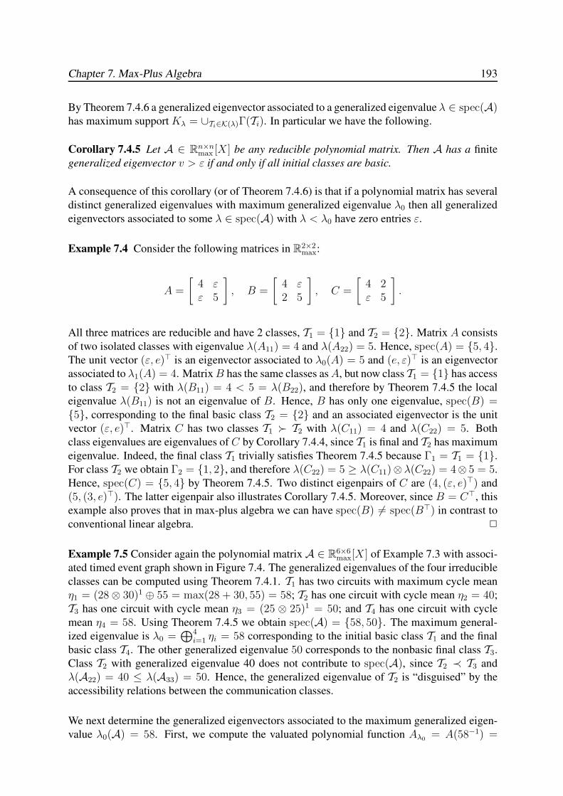
Chapter 7. Max-Plus Algebra 193
By Theorem 7.4.6 a generalized eigenvector associated to a generalized eigenvalue λ ∈ spec(A)has maximum support Kλ = ∪Ti∈K(λ)Γ(Ti). In particular we have the following.
Corollary 7.4.5 Let A ∈ Rn×nmax [X] be any reducible polynomial matrix. Then A has a finite
generalized eigenvector v > ε if and only if all initial classes are basic.
A consequence of this corollary (or of Theorem 7.4.6) is that if a polynomial matrix has several
distinct generalized eigenvalues with maximum generalized eigenvalue λ0 then all generalized
eigenvectors associated to some λ ∈ spec(A) with λ < λ0 have zero entries ε.
Example 7.4 Consider the following matrices in R2×2max:
A =
[4 εε 5
]
, B =
[4 ε2 5
]
, C =
[4 2ε 5
]
.
All three matrices are reducible and have 2 classes, T1 = {1} and T2 = {2}. Matrix A consists
of two isolated classes with eigenvalue λ(A11) = 4 and λ(A22) = 5. Hence, spec(A) = {5, 4}.The unit vector (ε, e)> is an eigenvector associated to λ0(A) = 5 and (e, ε)> is an eigenvector
associated to λ1(A) = 4. MatrixB has the same classes asA, but now class T1 = {1} has access
to class T2 = {2} with λ(B11) = 4 < 5 = λ(B22), and therefore by Theorem 7.4.5 the local
eigenvalue λ(B11) is not an eigenvalue of B. Hence, B has only one eigenvalue, spec(B) ={5}, corresponding to the final basic class T2 = {2} and an associated eigenvector is the unit
vector (ε, e)>. Matrix C has two classes T1 � T2 with λ(C11) = 4 and λ(C22) = 5. Both
class eigenvalues are eigenvalues of C by Corollary 7.4.4, since T1 is final and T2 has maximum
eigenvalue. Indeed, the final class T1 trivially satisfies Theorem 7.4.5 because Γ1 = T1 = {1}.For class T2 we obtain Γ2 = {1, 2}, and therefore λ(C22) = 5 ≥ λ(C11)⊗λ(C22) = 4⊗ 5 = 5.
Hence, spec(C) = {5, 4} by Theorem 7.4.5. Two distinct eigenpairs of C are (4, (ε, e)>) and
(5, (3, e)>). The latter eigenpair also illustrates Corollary 7.4.5. Moreover, since B = C>, this
example also proves that in max-plus algebra we can have spec(B) 6= spec(B>) in contrast to
conventional linear algebra. 2
Example 7.5 Consider again the polynomial matrix A ∈ R6×6max[X] of Example 7.3 with associ-
ated timed event graph shown in Figure 7.4. The generalized eigenvalues of the four irreducible
classes can be computed using Theorem 7.4.1. T1 has two circuits with maximum cycle mean
η1 = (28⊗ 30)1 ⊕ 55 = max(28 + 30, 55) = 58; T2 has one circuit with cycle mean η2 = 40;
T3 has one circuit with cycle mean η3 = (25 ⊗ 25)1 = 50; and T4 has one circuit with cycle
mean η4 = 58. Using Theorem 7.4.5 we obtain spec(A) = {58, 50}. The maximum general-
ized eigenvalue is λ0 =⊕4
i=1 ηi = 58 corresponding to the initial basic class T1 and the final
basic class T4. The other generalized eigenvalue 50 corresponds to the nonbasic final class T3.
Class T2 with generalized eigenvalue 40 does not contribute to spec(A), since T2 ≺ T3 and
λ(A22) = 40 ≤ λ(A33) = 50. Hence, the generalized eigenvalue of T2 is “disguised” by the
accessibility relations between the communication classes.
We next determine the generalized eigenvectors associated to the maximum generalized eigen-
value λ0(A) = 58. First, we compute the valuated polynomial function Aλ0= A(58−1) =
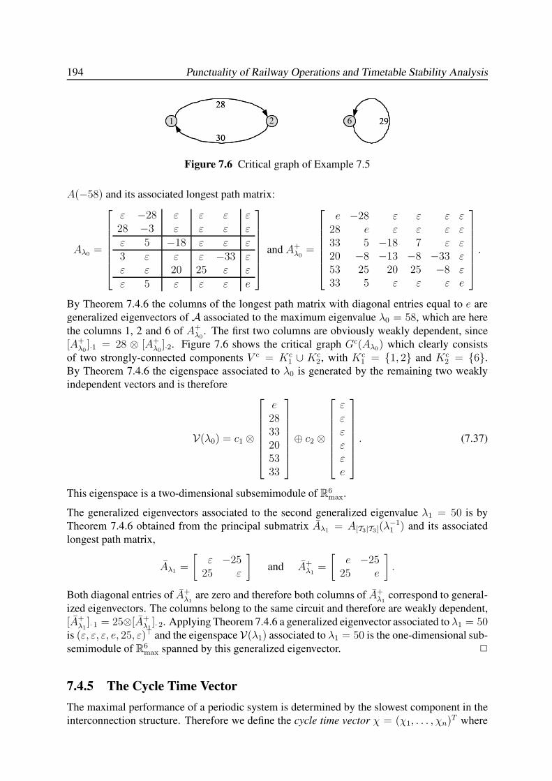
194 Punctuality of Railway Operations and Timetable Stability Analysis
1 2 6
30
28
291 2 6
30
28
29
Figure 7.6 Critical graph of Example 7.5
A(−58) and its associated longest path matrix:
Aλ0=
ε −28 ε ε ε ε28 −3 ε ε ε ε
ε 5 −18 ε ε ε
3 ε ε ε −33 εε ε 20 25 ε ε
ε 5 ε ε ε e
and A+λ0
=
e −28 ε ε ε ε28 e ε ε ε ε33 5 −18 7 ε ε20 −8 −13 −8 −33 ε53 25 20 25 −8 ε33 5 ε ε ε e
.
By Theorem 7.4.6 the columns of the longest path matrix with diagonal entries equal to e are
generalized eigenvectors of A associated to the maximum eigenvalue λ0 = 58, which are here
the columns 1, 2 and 6 of A+λ0
. The first two columns are obviously weakly dependent, since
[A+λ0
]·1 = 28 ⊗ [A+λ0
]·2. Figure 7.6 shows the critical graph Gc(Aλ0) which clearly consists
of two strongly-connected components V c = Kc1 ∪ Kc
2 , with Kc1 = {1, 2} and Kc
2 = {6}.By Theorem 7.4.6 the eigenspace associated to λ0 is generated by the remaining two weakly
independent vectors and is therefore
V(λ0) = c1 ⊗
e2833205333
⊕ c2 ⊗
εεεεεe
. (7.37)
This eigenspace is a two-dimensional subsemimodule of R6max.
The generalized eigenvectors associated to the second generalized eigenvalue λ1 = 50 is by
Theorem 7.4.6 obtained from the principal submatrix Aλ1= A[T3|T3](λ
−11 ) and its associated
longest path matrix,
Aλ1=
[ε −25
25 ε
]
and A+λ1
=
[e −25
25 e
]
.
Both diagonal entries of A+λ1
are zero and therefore both columns of A+λ1
correspond to general-
ized eigenvectors. The columns belong to the same circuit and therefore are weakly dependent,
[A+λ1
]· 1 = 25⊗[A+λ1
]· 2. Applying Theorem 7.4.6 a generalized eigenvector associated to λ1 = 50is (ε, ε, ε, e, 25, ε)> and the eigenspace V(λ1) associated to λ1 = 50 is the one-dimensional sub-
semimodule of R6max spanned by this generalized eigenvector. 2
7.4.5 The Cycle Time Vector
The maximal performance of a periodic system is determined by the slowest component in the
interconnection structure. Therefore we define the cycle time vector χ = (χ1, . . . , χn)T where
Chapter 7. Max-Plus Algebra 195
each χi equals the maximal generalized eigenvalue of the irreducible classes that have access
to event i. For a polynomial matrix A in Frobenius normal form with c classes T1, . . . , Tc this
gives
χi =⊕
Tk→i
λ(Akk) for all 1 ≤ i ≤ n. (7.38)
Moreover, we define a generalized eigenmode of a polynomial matrix A as a pair (χ, v) of a
cycle time vector χ and an associated bias vector v that satisfies for all 1 ≤ i ≤ n:
vi =n⊕
j=1
p⊕
l=0
([Al]ij ⊗ χ−l
j ⊗ vj
).
If A ∈ Rn×nmax [X] is an irreducible polynomial matrix then the bias vector is equivalent to the
eigenvector, and this is also true for reducible polynomial matrices with a constant cycle time
vector, i.e., when the initial classes are also basic. In the general reducible case however the
cycle time vector may have different entries. If the bias vector is partitioned accordingly then
the partial bias vectors augmented with zero entries are generalized eigenvectors corresponding
to the various cycle time entries. Hence, if I ⊆ {1, . . . , n} is an index set of equal cycle
time entries then this cycle time is a generalized eigenvalue of A with associated generalized
eigenvector x ∈ Rnmax given by xi = vi if i ∈ I and xi = ε if i 6∈ I . The generalized eigenmode
thus corresponds to the worst-case generalized eigenstructure of the system.
In the forthcoming we will assume that each event i has a predecessor. Hence, the timed event
graph has no source events, or equivalently, the polynomial matrix has no zero rows. Moreover,
we assume that each circuit has at least one token, i.e., G(A0) is acyclic.
Definition 7.4.4 (Nondegeneracy) A polynomial matrixA =⊕p
l=0AlXl ∈ Rn×n
max [X] is called
nondegenerate if
(i) Each row has at least one finite entry, or formally, for all 1 ≤ i ≤ n there exists 1 ≤ j ≤ nand 0 ≤ l ≤ p, such that [Al]ij 6= ε,
(ii) G(A0) is acyclic, i.e., tr(A+0 ) =
⊕ni=1[A
+0 ]ii = ε.
For the eigenproblem of a square max-plus matrix the acyclicity condition on G(A0) is super-
fluous, since this case corresponds to A = A1X , and therefore A0 = E . Hence, in this case
nondegeneracy is equivalent to the requirement that A has no empty rows.
Lemma 7.4.6 A polynomial matrix A =⊕p
l=0AlXl ∈ Rn×n
max [X] is nondegenerate if and only
if its associated timed event graph G(A) is autonomous and live.
Proof: By definition an autonomous timed event graph has no source transitions and therefore
each transition i must have an incoming place (j, i, l), or equivalently, each row i of the asso-
ciated polynomial matrix must have at least one finite entry [Al]ij 6= ε. By Theorem 6.4.1 a
timed event graph is live if and only if there are no circuits with zero tokens or equivalently iff
G(A0) has no circuits. Hence, [A`0]ii = ε for all 1 ≤ i, ` ≤ n, or equivalently, [A+
0 ]ii = ε for all
1 ≤ i ≤ n, which can be abbreviated to the condition tr(A+0 ) =
⊕ni=1[A
+0 ]ii = ε. 2
196 Punctuality of Railway Operations and Timetable Stability Analysis
The nondegeneracy condition on a polynomial matrix is a necessary and sufficient condition for
the existence of a finite cycle time vector, that is, it guarantees that each transition i has a finite
cycle time ε < χi <∞. This is formally stated in the following theorem.
Theorem 7.4.7 Let A =⊕p
l=0AlXl ∈ Rn×n
max [X] be a nondegenerate polynomial matrix. Then
A has a finite cycle time vector χ > ε, and the entry χi is equal to the maximum cycle mean
over all classes that have access to i for all 1 ≤ i ≤ n.
Proof: The timed event graph G(A) is finite with n transitions and m ≤ n ·n ·p+n−1 places,
where the worst-case bound corresponds to full matrices Al for 1 ≤ l ≤ p and |supp(A0)| =n − 1 corresponding to a maximum spanning tree with zero tokens. Recall that a maximum
spanning tree is the most dense simple graph that has no cycles. From the nondegeneracy
condition follows that each transition has an incoming place and because the event graph is
finite this means that each transition has an upstream circuit. Moreover, nondegeneracy of Aimplies thatG(A0) is acyclic and therefore by Theorem 7.4.1 the generalized eigenvalue of each
class equals the (finite) maximum cycle mean of the associated strongly connected component.
By definition (7.38) each cycle time entry χi is the maximal generalized eigenvalue over all
classes that have access to i, which is thus equivalent to the maximum of all (maximum) cycle
means of those classes. Hence, each event i has at least one upstream circuit and the maximum
cycle mean over all upstream circuits defines the cycle time entry χi for all 1 ≤ i ≤ n. 2
7.4.6 The Policy Iteration Algorithm
An efficient algorithm to compute the (generalized) eigenstructure of a max-plus (polynomial)
matrix is the policy iteration algorithm developed by Cochet-Terrasson et al. [31] based on
Howard’s multichain policy iteration algorithm for Markov decision processes with average
reward [103], which is well-known in the fields of dynamic programming and stochastic control,
see e.g. Puterman [168].
The policy iteration algorithm applies to nondegenerate irreducible and reducible polynomial
matrices. In the irreducible case it computes the generalized eigenvalue, an associated general-
ized eigenvector, and an optimal policy from which a critical circuit is easily determined. In the
reducible case the policy iteration algorithm computes for each transition the maximal gener-
alized eigenvalue that has access to it, and an associated eigenvector with maximal support.
Hence, the algorithm computes the generalized eigenmode (χ, v) of a nondegenerate poly-
nomial matrix A and moreover is generally applicable without prior knowledge on the class
structure of the polynomial matrix.
In the sequel we will utilize the adjacency list representation (6.6) of the places (or marked
arcs) pk = (j, i, l) ∈ P , 1 ≤ k ≤ m, which unambiguously identifies all places in the timed
event graph associated to the finite polynomial matrix entries [Al]ij. Recall that this is a sparse
(polynomial) matrix notation. Define for each event i ∈ T the set Πi ⊆ P of incoming places
as
Πi.= {pk ∈ P | out(pk) = i} = {(j, i, l) | [Al]ij 6= ε, 1 ≤ j ≤ n, 0 ≤ l ≤ p}.
Then the generalized eigenproblem is to find a generalized eigenmode (χ, v), such that for all
Chapter 7. Max-Plus Algebra 197
1 ≤ i ≤ n
χi =⊕
(j,i,l)∈Πi
χj = max(j,i,l)∈Πi
χj , (7.39a)
vi =⊕
(j,i,l)∈Πi
([Al]ij ⊗ χ−lj ⊗ vj) = max
(j,i,l)∈Πi
([Al]ij − l · χj + vj). (7.39b)
We will refer to (7.39a) as the first-order optimality equation and to (7.39b) as the second-order
optimality equation. The key to the policy iteration algorithm is a policy. A policy is a vector
function π : T n → Pn that maps each transition to one of its incoming places, i.e.,
πi = pk ∈ Πi for all i ∈ T .An entry πi ∈ Πi is also simply called the policy of transition i. The holding time, initial
marking, input transition, and output transition of a policy πi are denoted as w(πi), µ(πi),in(πi), and out(πi), respectively. A polynomial matrix representation of a policy π is Aπ =⊕p
l=0Aπl X
l, where each row i has exactly one finite entry [Al]ij > ε conform
[Aπl ]ij =
{w(πi) if in(πi) = j and µ(πi) = lε otherwise.
Let Pπ = {π1, . . . , πn} ⊆ P be the set of places in the policy π. A policy graph is the timed
event graph G(Aπ) = (T ,Pπ, µ(π), w(π)) associated to a policy π, which is a simple subgraph
of G(A) with each transition 1 ≤ i ≤ n having indegree one, that is, each transition has exactly
one incoming place. By the following lemma the number of circuits in a policy graph G(Aπ) is
finite.
Lemma 7.4.7 Let G(Aπ) be a timed event graph associated to a policy π. Then each connected
component of G(Aπ) contains one and only one circuit.
Proof: By definition of a policy each place has a unique output transition and therefore G(Aπ)does not contain parallel places. Hence, G(Aπ) is a simple (timed event) graph. From graph
theory it is well-known that a connected (timed event) graph with n nodes (transitions) and no
cycles has exactly n − 1 arcs (places), corresponding to a spanning tree; any additional arc
(place) will generate a circuit, and furthermore deleting any arc (place) will make the graph
no longer connected [16, Ch. 16]. As an immediate consequence, if G(Aπ) is connected and
contains n places then it has exactly 1 circuit. Now, suppose G(Aπ) has c components. Then
it contains a forest of c trees spanning the components. A straightforward extension of the
above shows that this spanning forest has n − c places: assume that the trees have n1, . . . , nc
transitions, respectively, with∑c
i=1 ni = n. Then each tree contains ni− 1 places, and together
they possess∑c
i=1(ni − 1) = n − c places. In a policy each transition must have an incoming
place, whilst a (finite) tree contains by definition a transition without predecessor. Hence, each
tree in the forest needs at least one additional place, which generates exactly one circuit in each
of the c components. 2
The proof of Lemma 7.4.7 also reveals the structure of a policy (timed event) graph G(Aπ):each component consists of a ‘base’ circuit with possibly some outgoing paths or trees. This
topology guarantees that each transition has an incoming place, and furthermore, corresponds
to the timed event graph with the least number of places with this property. This structure also
has the following consequence.
198 Punctuality of Railway Operations and Timetable Stability Analysis
Lemma 7.4.8 Let Aπ ∈ Rn×nmax [X] be a polynomial matrix associated to a policy π. Then Aπ
has a finite cycle time vector χ > ε, which is uniquely determined.
Proof: By Lemma 7.4.7 each transition i in the policy graph G(Aπ) has one and only one
upstream circuit, and therefore the cycle time χi of transition i is uniquely determined by the
cycle mean of this circuit. This holds for all transitions in the same connected component
which therefore share the same unique cycle time. Note that here a component is not strongly
connected, except for the trivial case that the circuit covers all transitions. The connected com-
ponents are a partitioning of T = {1, . . . , n} and therefore the direct sum of the cycle time
vector components gives a cycle time vector of full support. 2
Finding a generalized eigenmode of a policy polynomial matrix is called policy evaluation.
Policy evaluation involves finding the circuits and connected components, computing the cy-
cle mean of the circuits, and computing an associated generalized eigenvector. Lemma 7.4.7
suggest a simple procedure to find all circuits in the policy event graph: starting from an arbi-
trary transition just follow the associated policies backwards until an already visited transition
is revisited. This transition, say s, then obviously lies on a circuit. By Lemma 7.4.7 this is
the only circuit in the component of the policy graph containing s. Hence, the cycle mean of
this circuit is the unique generalized eigenvalue χ for all events accessible from s in G(Aπ).By Theorem 7.4.5 the associated entries of the generalized eigenvector are given by the longest
path weights inG(Aπλ) from s to all accessible events, which can efficiently be computed using a
breadth-first search (BFS) algorithm [39]. In BFS the transitions are visited in topological order
from s, by which the value of vin(π(i)) is determined before reaching transition i and therefore
vi can be computed directly by vi = w(πi)− µ(πi) · χin(πi) + vin(πi).
A given policy πk with generalized eigenmode (χk, vk) is optimal iff it satisfies the optimality
conditions (7.39a–7.39b). So a policy πk can be improved if there exists a place p = (j, i, l) ∈Πi with χk
j > χki for some transition 1 ≤ i ≤ n, conform the first-order optimality condition
(7.39a). In this case transition i can be connected to a component with higher cycle time. Let
πk+1i = arg max
(j,i,l)∈Πi
χkj .
Then if χk+1 6= χk at least one transition is improved under the new policy. However, if
χk+1 = χk then we must still check the second-order optimality condition (7.39b). If for any
transition i there is a predecessor j over a place with l tokens such that vki < [Al]ij − l ·χk
j + vkj
then πki is not optimal, and an improved policy is found by
πk+1i = arg max
(j,i,l)∈Πi
([Al]ij − l · χk
j + vkj
).
The policy iteration algorithm computes the maximum generalized eigenmode of a polynomial
matrix A ∈ Rn×nmax [X] by exploiting the efficient computation of the generalized eigenmode
of a policy graph and successively improving policies until an optimal policy has been found.
In general, the policy iteration algorithm starts with an arbitrary policy —select any incoming
place for each transition— and then iterates between a policy evaluation step which computes
a generalized eigenmode corresponding to a given policy, and a policy improvement step which
tries to improve the current policy. If no more improvement can be found, the generalized
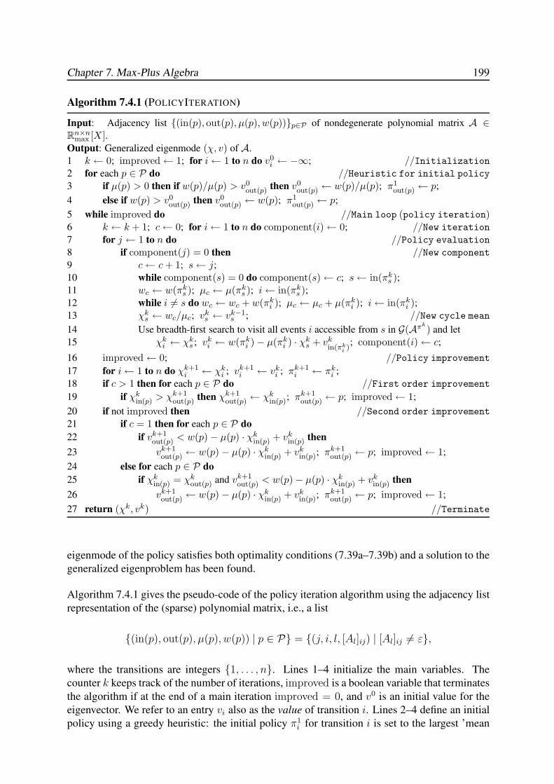
Chapter 7. Max-Plus Algebra 199
Algorithm 7.4.1 (POLICYITERATION)
Input: Adjacency list {(in(p), out(p), µ(p), w(p))}p∈P of nondegenerate polynomial matrix A ∈Rn×n
max [X].Output: Generalized eigenmode (χ, v) of A.
1 k ← 0; improved← 1; for i← 1 to n do v0i ← −∞; //Initialization
2 for each p ∈ P do //Heuristic for initial policy3 if µ(p) > 0 then if w(p)/µ(p) > v0
out(p) then v0out(p) ← w(p)/µ(p); π1
out(p) ← p;
4 else if w(p) > v0out(p) then v0
out(p) ← w(p); π1out(p) ← p;
5 while improved do //Main loop (policy iteration)6 k ← k + 1; c← 0; for i← 1 to n do component(i)← 0; //New iteration7 for j ← 1 to n do //Policy evaluation8 if component(j) = 0 then //New component9 c← c + 1; s← j;
10 while component(s) = 0 do component(s)← c; s← in(πks );
11 wc ← w(πks ); µc ← µ(πk
s ); i← in(πks );
12 while i 6= s do wc ← wc + w(πki ); µc ← µc + µ(πk
i ); i← in(πki );
13 χks ← wc/µc; vk
s ← vk−1s ; //New cycle mean
14 Use breadth-first search to visit all events i accessible from s in G(Aπk
) and let
15 χki ← χk
s ; vki ← w(πk
i )− µ(πki ) · χk
s + vkin(πk
i ); component(i)← c;
16 improved← 0; //Policy improvement
17 for i← 1 to n do χk+1i ← χk
i ; vk+1i ← vk
i ; πk+1i ← πk
i ;
18 if c > 1 then for each p ∈ P do //First order improvement
19 if χkin(p) > χk+1
out(p) then χk+1out(p) ← χk
in(p); πk+1out(p) ← p; improved← 1;
20 if not improved then //Second order improvement21 if c = 1 then for each p ∈ P do
22 if vk+1out(p) < w(p) − µ(p) · χk
in(p) + vkin(p) then
23 vk+1out(p) ← w(p) − µ(p) · χk
in(p) + vkin(p); πk+1
out(p) ← p; improved← 1;
24 else for each p ∈ P do
25 if χkin(p) = χk
out(p) and vk+1out(p) < w(p)− µ(p) · χk
in(p) + vkin(p) then
26 vk+1out(p) ← w(p) − µ(p) · χk
in(p) + vkin(p); πk+1
out(p) ← p; improved← 1;
27 return (χk, vk) //Terminate
eigenmode of the policy satisfies both optimality conditions (7.39a–7.39b) and a solution to the
generalized eigenproblem has been found.
Algorithm 7.4.1 gives the pseudo-code of the policy iteration algorithm using the adjacency list
representation of the (sparse) polynomial matrix, i.e., a list
{(in(p), out(p), µ(p), w(p)) | p ∈ P} = {(j, i, l, [Al]ij) | [Al]ij 6= ε},
where the transitions are integers {1, . . . , n}. Lines 1–4 initialize the main variables. The
counter k keeps track of the number of iterations, improved is a boolean variable that terminates
the algorithm if at the end of a main iteration improved = 0, and v0 is an initial value for the
eigenvector. We refer to an entry vi also as the value of transition i. Lines 2–4 define an initial
policy using a greedy heuristic: the initial policy π1i for transition i is set to the largest ’mean
200 Punctuality of Railway Operations and Timetable Stability Analysis
weight’ of all incoming places, i.e.,
π1i ∈ arg max
(j,i,l)∈Πi
[Al]ijmax(1, l)
,
with the convention that for the degenerate case l = 0 the ‘mean weight’ is set to [Al]ij as in
the case l = 1. This is implemented by checking for each place whether the actual value of the
output transition can be improved using the ‘mean weight’ of the current place. This choice for
the initial policy is customary but any other initial policy could be used as well.
Lines 5–27 contain the main loop of the algorithm which iterates until no more improvement
is found (line 5), in which case the optimal policy has been found and the current eigenmode
(χk, vk) is returned as output of the algorithm (line 27). Line 6 updates the iteration counter,
resets the number of found connected components c to 0, and initializes the variable componentto 0 for all transitions. At the end of the kth iteration c is the number of connected components
of policy πk and component(i) is the component of transition i.
Lines 7–15 implement the policy evaluation step, which computes the eigenmode of the policy
component by component. For each transition j if component(j) = 0 then j has not yet been
visited in iteration k and so a new component has been found (lines 7–8). Line 9 updates
the component counter and initializes transition s to the current transition. Line 10 finds a
critical transition using the policies to search the policy graph backwards starting from the
current transition and labelling all visited transitions by updating the variable component until
an already labelled transition is revisited, indicating that a circuit has been found containing the
updated transition s. Lines 11–13 compute the cycle mean of the current component. Line 11
initializes two variables wc and µc by the weight and marking of the policy of s, and line 12
walks backwards over the policies in the circuit updating the path weight and marking from suntil s is revisited. Line 13 then sets the cycle time χk
s to the cycle mean computed by dividing
the computed circuit weight by the circuit token count, and sets the value vks to the value of s
in the last iteration. The particular choice of the initial value vks is customary and useful for
analysis of the algorithm but could be set to any arbitrary value, in particular vks = 0. Lines
14–15 visit all transitions accessible from s using breadth-first search, setting the cycle time
equal to the computed cycle mean, the eigenvector value to the value of s plus the mean path
weight from s, and component to the current component. Hence, together with transition jeach transition in the same component has also been visited and evaluated before the algorithm
returns to line 7, and therefore these transitions will be skipped in line 8. So if there is only one
connected component in the kth policy then all transitions will be visited in the first iteration of
line 7, and therefore all remaining iterations in line 7 will terminate directly in line 8. On the
other hand, if there is a transition that has not yet been visited then there is at least one more
component in the policy and the first unvisited transition that satisfies the condition of line 8
starts a new policy evaluation iteration for the next component.
Lines 16–26 implement the policy improvement step. Lines 16–17 reset the boolean variable
improved to zero, and copies the current cycle time vector, eigenvector and policy. If more
than one component has been found in the policy evaluation step then a first-order improve-
ment may be found (lines 18–19). In this case for each place is checked whether the input
transition has a higher cycle time then the output transition, and if so, the output transition is
connected to the component with higher cycle time and an improved policy has been found for
this transition. Note that in the comparison of cycle times (line 19) the updated cycle time of
Chapter 7. Max-Plus Algebra 201
the output transition is used which secures that only places with higher input cycle time than
in the last improvement are accepted for a further improvement. If no first-order improvement
has been found or if all transitions are already contained in one component then lines 20–26
check whether a second-order improvement can be found. If there is only one component in
the current policy then for each place it is simply checked whether a higher value of the output
transition can be obtained using this place instead of the actual policy, and if so, the value of the
output transition is improved and a new policy has been found for this transition (lines 21–23).
In the case of more than one component under the current policy the second-order improvement
is only applicable to places with the same cycle time in both its input and output transition, in
which case the same improvement procedure is applied as in the case of one component (lines
24–26). Note that since the first-order improvement must have been passed without improve-
ment we know that if the cycle time of the input and output transition are not equal then the
output transition is accessible from a transition with higher cycle time than the input transition.
If an improved policy has been found for any of the transitions then at the end of the policy im-
provement routine improved = 1 and a new iteration starts from line 5, otherwise the algorithm
terminates and returns the current generalized eigenmode (χk, vk) as the solution.
Cochet-Terrasson et al. [31] proved the following theorem.
Theorem 7.4.8 Let A =⊕p
l=0AlXl ∈ Rn×n
max [X] be a nondegenerate polynomial matrix. Then
the policy iteration algorithm converges to the optimal policy in a finite number of iterations,
and λ0 =⊕n
i=1 χi is the maximum generalized eigenvalue of A.
Proposition 7.4.1 Let A =⊕p
l=0AlXl ∈ Rn×n
max [X] be a nondegenerate polynomial matrix.
Then the policy iteration algorithm terminates in I · O(m) computation time, where m is the
number of finite entries [Al]ij and I is the number of iterations of the algorithm.
Proof: The worst-case computational complexity of Algorithm 7.4.1 can be estimated as
follows. The initialization step takes O(n) to initialize v0 (line 1) and O(m) to compute the
initial policy by checking all m places once (lines 2–4). Hence, the initialization takes O(n) +O(m) = O(m) time. We now estimate the time complexity of one iteration of the main loop
(lines 5–26). Starting a new iteration takes O(n) time to reset the variable component for each
transition. Policy evaluation only searches the policy graph, which has n transitions and also just
n places. Consider one iteration of policy evaluation (lines 8–15). Let nj denote the number
of transitions (and places) in component 1 ≤ j ≤ c, with c the total number of connected
components in the policy. Line 10 searches the component backwards until a transition has
been encountered twice. Hence, an upper bound for the number of transitions that have been
visited before a transition is revisited is nj. In lines 11–12 all transitions in the circuit contained
in the component are visited, which can be at most nj transitions corresponding to the case that
the component is one big circuit. Lines 14–15 search all transitions in the component using BFS,
which takes O(nj) time. Evaluating one component in a policy graph thus takes 3 · O(nj) =O(nj) time. Hence, the iterations of line 7 take (n−c)·O(1)+
∑cj=1O(nj) = O(n−c)+O(n) =
O(n) time, where the first term corresponds to the n − c cases that a transition of an already
evaluated component is checked in line 8 which takes just O(1) time. The policy improvement
routine takes O(m) time, since now all places are checked. If the policy has just one connected
component then each place is checked in lines 21–23, which thus takes O(m) time. If the
policy has several components then first each place is checked for first-order improvements in
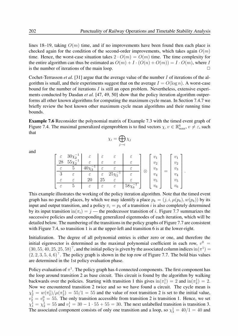
202 Punctuality of Railway Operations and Timetable Stability Analysis
lines 18–19, taking O(m) time, and if no improvements have been found then each place is
checked again for the condition of the second-order improvements, which takes again O(m)time. Hence, the worst-case situation takes 2 · O(m) = O(m) time. The time complexity for
the entire algorithm can thus be estimated as O(m) + I · (O(n) +O(m)) = I ·O(m), where Iis the number of iterations of the main loop. 2
Cochet-Terrasson et al. [31] argue that the average value of the number I of iterations of the al-
gorithm is small, and their experiments suggest that on the average I = O(logn). A worst-case
bound for the number of iterations I is still an open problem. Nevertheless, extensive experi-
ments conducted by Dasdan et al. [47, 49, 50] show that the policy iteration algorithm outper-
forms all other known algorithms for computing the maximum cycle mean. In Section 7.4.7 we
briefly review the best known other maximum cycle mean algorithms and their running time
bounds.
Example 7.6 Reconsider the polynomial matrix of Example 7.3 with the timed event graph of
Figure 7.4. The maximal generalized eigenproblem is to find vectors χ, v ∈ R6max, v 6= ε, such
that
χi =⊕
j→i
χj
and
ε 30χ−12 ε ε ε ε
28 55χ−12 ε ε ε ε
ε 5 40χ−13 ε ε ε
3 ε ε ε 25χ−15 ε
ε ε 20 25 ε ε
ε 5 ε ε ε 58χ−16
⊗
v1
v2
v3
v4
v5
v6
=
v1
v2
v3
v4
v5
v6
.
This example illustrates the working of the policy iteration algorithm. Note that the timed event
graph has no parallel places, by which we may identify a place pk = (j, i, µ(pk), w(pk)) by its
input and output transition, and a policy πi = pk of a transition i is also completely determined
by its input transition in(πi) = j — the predecessor transition of i. Figure 7.7 summarizes the
successive policies and corresponding generalized eigenmodes of each iteration, which will be
detailed below. The numbering of the transitions in the policy graphs of Figure 7.7 are consistent
with Figure 7.4, so transition 1 is at the upper-left and transition 6 is at the lower-right.
Initialization. The degree of all polynomial entries is either zero or one, and therefore the
initial eigenvector is determined as the maximal polynomial coefficient in each row, v0 =(30, 55, 40, 25, 25, 58)>, and the initial policy is given by the associated column indices in(π1) =(2, 2, 3, 5, 4, 6)>. The policy graph is shown in the top row of Figure 7.7. The bold bias values
are determined in the 1st policy evaluation phase.
Policy evaluation of π1. The policy graph has 4 connected components. The first component has
the loop around transition 2 as base circuit. This circuit is found by the algorithm by walking
backwards over the policies. Starting with transition 1 this gives in(π11) = 2 and in(π1
2) = 2.
Now we encountered transition 2 twice and so we have found a circuit. The cycle mean is
χ12 = w(π1
2)/µ(π12) = 55/1 = 55 and the value of root transition 2 is set to the initial value,
v12 = v0
2 = 55. The only transition accessible from transition 2 is transition 1. Hence, we set
χ11 = χ1
2 = 55 and v11 = 30 − 1 · 55 + 55 = 30. The next unlabelled transition is transition 3.
The associated component consists of only one transition and a loop, so χ13 = 40/1 = 40 and
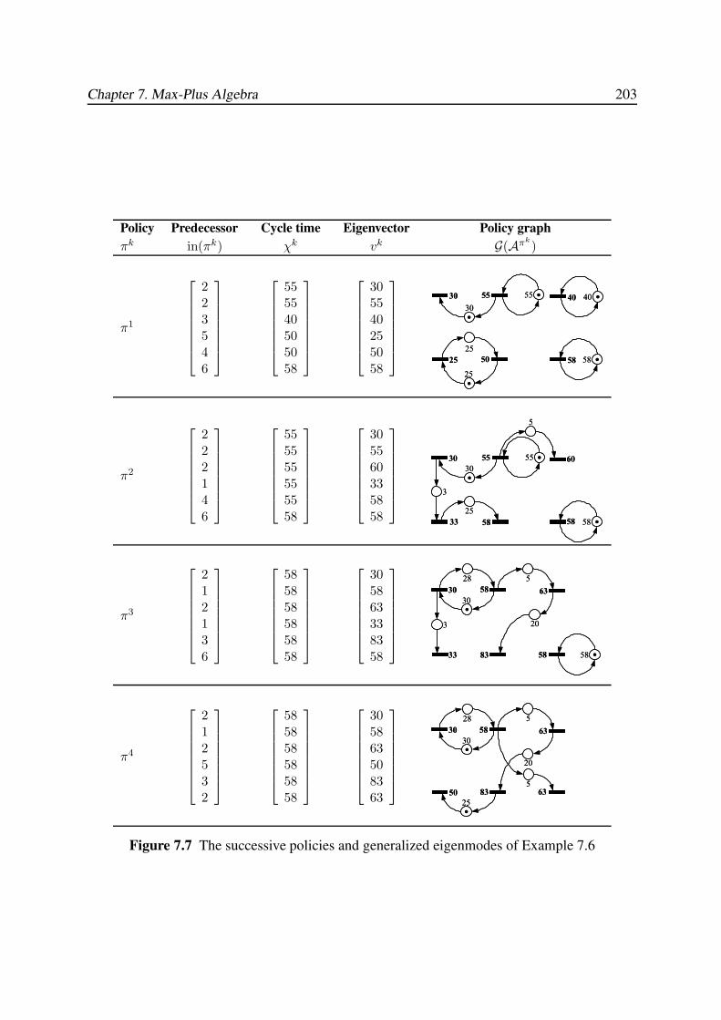
Chapter 7. Max-Plus Algebra 203
Policy Predecessor Cycle time Eigenvector Policy graph
πk in(πk) χk vk G(Aπk
)
π1
223546
555540505058
305540255058
·
·55
30
·
25
25
·40
·58
30 55 40
5825 50
·
·55
30
·
25
25
·40
·58
30 55 40
5825 50
π2
222146
555555555558
305560335858
5
·
·55
30
25
3
·5858
30 55 60
33 58
5
·
·55
30
25
3
·5858
30 55 60
33 58
π3
212136
585858585858
305863338358
5
·
28
30
3
·
20
58
30
33
58 63
83 58
5
·
28
30
3
·
20
58
30
33
58 63
83 58
π4
212532
585858585858
305863508363
5
·
28
30
·25
20
5
30 58 63
8350 63
5
·
28
30
·25
20
5
30 58 63
8350 63
Figure 7.7 The successive policies and generalized eigenmodes of Example 7.6
204 Punctuality of Railway Operations and Timetable Stability Analysis
v13 = v0
3 = 40. The next unlabelled transition is transition 4 with in(π14) = 5 and in(π1
5) = 4.
Hence, the circuit of the third component is (4, 5, 4). Starting from transition 4 the cycle mean
is computed as χ14 = (w(π1
4) + w(π15))/(µ(π1
4) + µ(π15)) = (25 + 25)/(1 + 0) = 50 and the
bias value is v14 = v0
4 = 25. Transition 5 is accessible from transition 4 and so χ15 = χ1
4 = 50and v1
5 = 25 − 0 · 50 + 25 = 50. The final unlabelled transition is transition 6 which forms a
component of its own with a loop having cycle mean χ16 = 58/1 and the bias value is simply
set as v16 = v0
6 = 58. We thus computed the generalized eigenmode (χ1, v1) of π1.
Policy improvement of π1. Two first-order improvements can be computed. Transition 3 (with
χ13 = 40) has transition 2 as a predecessor with higher cycle time and so χ2
3 = χ12 = 55.
Likewise, transition 4 (χ14 = 50) is connected to transition 1 with higher cycle time χ2
4 =χ1
1 = 55. Also transition 5 (χ15 = 50) is improved because χ2
4 = 55 > χ15 = 50, but the new
policy is just the improved old one, so the policy of transition 5 is maintained by predecessor
4 although the cycle time is updated to χ25 = χ2
4 = 55. We thus found the improved policy
in(π2) = (2, 2, 2, 1, 4, 6)>.
Policy evaluation of π2. The policy graph is shown in the 2nd row of Figure 7.7. There are 2
components. The circuit of the first component is again the loop around transition 2 with cycle
mean χ22 = 55/1 = 55 and the bias value of transition 2 is set to v2
2 = v12 = 55. Transition 2
has three successors: transition 1 and 3, and transition 2 itself which has already been labelled.
Hence, we set χ21 = 55 and v2
1 = 30−1·55+55 = 30, and χ23 = 55 and v2
3 = 5−0·55+55 = 60.
Transition 3 has no successors but transition 1 has, so we follow the path from transition 1 to
transition 4 and set χ24 = 55 and v2
4 = 3 − 0 · 55 + 30 = 33. Transition 4 has transition 5 as
successor and so we proceed setting χ25 = 55 and v2
5 = 25−0 ·55+33 = 58. Now all transition
accessible from transition 2 have been visited, and we proceed to the next unlabelled transition.
This is transition 6 which is still isolated and so again χ26 = 58 and v2
6 = v16 = 58.
Policy improvement of π2. There are no first-order improvements, but two second-order im-
provements can be found. Transition 2 has predecessor 1 with v22 = 55 < 28− 0 · 55+30 = 58
and thus an improved policy is in(π32) = 1. Likewise, for transition 5 we find the improved
policy in(π35) = 3 since v2
5 = 58 < 20 − 0 · 55 + 60 = 80. At the end of the 2nd policy
improvement we thus have the improved policy in(π3) = (2, 1, 2, 1, 3, 6)>.
Policy evaluation of π3. The policy graph is shown in the 3rd row of Figure 7.7. There are two
components. The circuit of the first component is (1, 2, 1) with cycle mean χ31 = (28+30)/(0+
1) = 58. Visiting all transition from transition 1 we find the generalized eigenmode as in the
third row of Figure 7.7. Transition 6 is still an isolated component with cycle time 58.
Policy improvement of π3. Again no first-order improvement is found, but there are two second-
order improvements. For transition 4 we find the improved policy in(π44) = 5 since v3
4 = 33 <25 − 1 · 58 + 83 = 50. For transition 6 we find the improved policy in(π4
6) = 2 because
v36 = 58 < 5− 0 · 58+58 = 63. We thus found the improved policy in(π4) = (2, 1, 2, 5, 3, 2)>.
Policy evaluation of π4. The policy graph (Figure 7.7, 4th row) is connected, with circuit
(1, 2, 1). The cycle mean is χ41 = (28 + 30)/(0 + 1) = 58 and the value for the root transition
is set to v41 = v3
1 = 30. The bias vector is obtained by adding the root value v41 to the mean path
weights of the paths from root transition 1 to all transitions giving v4 = (30, 58, 63, 50, 83, 63)>.
Since all transitions are accessible from a single root transition the cycle time vector is χ4 =(58, 58, 58, 58, 58, 58)>.
Chapter 7. Max-Plus Algebra 205
Policy improvement of π4. We can skip the first-order improvement step, since π4 consists of
only one connected component and therefore all transitions have the same cycle time. Second-
order improvements can be found neither, which means that π4 is an optimal policy and (χ4, v4)is a generalized eigenmode.
Since all transitions have the same cycle time λ0 = 58 is the maximum generalized eigenvalue
by Theorem 7.4.8. Comparing the computed generalized eigenvector v4 with the eigensemi-
module (7.37) as computed in Example 7.5, we see that v4 ∈ V(λ0) with c1 = 30. 2
The policy iteration algorithm computes the maximum generalized eigenvalue λ0 =⊕n
i=1 χi
and one particular associated generalized eigenvector given by
xi =
{vi if χi = λ0
ε otherwise.
If one is interested in determining all classes and eigenpairs of a polynomial matrix A then the
theory of Section 7.4.4 must be applied. This requires the following main steps::
1. Determine the Frobenius normal form (7.29) of A, i.e., compute the classes (strongly-
connected components) of A and the reduced graph Gred(A),2. Apply the policy iteration algorithm to each irreducible principle submatrix of A corre-
sponding to the classes,
3. Compute the principle classes (7.34) and determine the spectrum (7.33) of A,
4. Compute the critical graph and apply Theorem 7.4.6 to construct the generalized eigensemi-
module V(λ) for each λ ∈ spec(A).
7.4.7 Alternative Eigenproblem Algorithms
In the operations research literature several algorithms have been developed related to the max-
plus (generalized) eigenproblem. The problem of computing the maximum (or minimum) cycle
mean in a weighted digraph (precedence graph) is generally known as the maximum mean
cycle problem (or minimum mean cycle problem) [3], which thus corresponds to the eigenvalue
of a max-plus matrix. The more general problem of computing the maximum (or minimum)
cycle mean in a biweighted or marked graph (timed event graph) is known as the maximum
(minimum) profit-to-time ratio cycle problem or briefly the maximum ratio cycle problem [3],
which corresponds to finding the generalized eigenvalue of a max-plus polynomial matrix. Note
that the maximum mean cycle problem is a special case of the maximum ratio cycle problem
(corresponding to a unit initial marking) and hence any algorithm for the latter more general
problem also solves the former problem. Conversely, any algorithm for the maximum mean
cycle problem can also be used for the maximum ratio cycle problem after a transformation
from the (higher-order) timed event graph to a canonical precedence graph, see Section 8.2.5.
Karp’s algorithm [116] is the first and most well-known polynomial algorithm for the maximum
cycle mean problem. It is based on Karp’s theorem [116]: If A = (aij) ∈ Rn×nmax is irreducible
then the maximum cycle mean in the (strongly connected) precedence graph G(A) = (V,E) is
given by
λ = maxi=1,...,n
mink=0,...,n−1
[An]ij − [Ak]ijn− k for any 1 ≤ j ≤ n,
206 Punctuality of Railway Operations and Timetable Stability Analysis
where the matrix powers are evaluated in max-plus algebra, see also Baccelli et al. [11, Theorem
2.19]. To evaluate this expression we must compute the jth columns (for arbitrary j) of the
matrices Ak for k = 0, . . . , n, which are just the single-origin longest path weights from origin
j over paths with length k. Karp’s algorithm [116] uses the dynamic programming algorithm
[Ak]ij = max(l,i)∈Π(i)
(ail + [Ak−1]lj) for all i, k = 1, . . . , n,
with initial conditions [A0]jj = e and [A0]ij = ε for all i 6= j, and where Π(i) = {(l, i) | ail 6=ε, 1 ≤ l ≤ n} denotes the set of incoming arcs of i. The resulting algorithm runs in Θ(nm)time. Dasdan & Gupta [48] propose a breadth-first search (BFS) variant of Karp’s algorithm.
At each level k only nodes l ∈ Vk = {l ∈ V | [Ak]lj 6= ε} have to be considered in the
computation of the finite entries [Ak+1]ij , since [Ak+1]ij > ε iff i ∈ succ(l) for some l ∈ Vk.
Hence, at level k the path weight [Ak+1]ij is updated for each successor i ∈ succ(l) of the
nodes l ∈ Vk. Dasdan & Gupta’s algorithm also runs in O(nm) time for worst-case instances.
Braker [21] extended Karp’s algorithm to find the generalized eigenvalue of polynomial matri-
ces A =⊕p
l=1AlXl without zero-order terms, i.e., the maximum cycle ratio in timed event
graphs with at least one token in each place. Experiments by Braker [21] showed that the ex-
tended Karp algorithm applied to polynomial matrices (corresponding to timed event graphs)
outperforms Karp’s algorithm applied to the augmented matrix obtained by transformation of
the timed event graph to the canonical precedence graph (without considering the additional
time to compute this augmented matrix). For other variants of Karp’s algorithm, see Dasdan et
al. [49, 50].
Karp & Orlin [117] developed two parametric longest (shortest) path algorithms which essen-
tially find the generalized eigenvalue λ of an irreducible first-order max-plus polynomial matrix
A =⊕1
l=0AlXl. They define a digraph where each arc k has a parametric arc weight wk−λµk
with µk ∈ {0, 1} and parameter λ ∈ R. The problem then translates to finding the maximal
(minimal) λ such that the graph has no positive (negative) weight circuits. Karp & Orlin give
an O(nm logn) (and also an O(n3)) algorithm for solving this cycle ratio problem. Young
et al. [227] give a Fibonacci heap implementation of Karp & Orlin’s algorithm that runs in
O(nm + n2 log n) time. Moreover, the algorithm of Young et al. [227] applies to reducible
digraphs with generalized parametric arc weights wk−λµk with µk ∈ {0, p}, which thus corre-
sponds to general reducible max-plus polynomial matricesA =⊕p
l=0AlXl. Young et al. [227]
showed that in the special case of the maximum (minimum) cycle mean problem, i.e., µk = 1for all arcs k, their parametric path algorithm runs in worst-case time O(nm + n2 logn) and
expected time O(m+ n logn).
The power algorithm [22, 190, 197] computes both the eigenvalue and an eigenvector for an
irreducible matrix A ∈ Rn×nmax . For any x(0) 6= ε iterate x(k) = A ⊗ x(k − 1), k ≥ 1, until
x(p) = c⊗ x(q) for some integers p > q ≥ 0 and real c ∈ R. Then λ = c/(p− q) is the unique
eigenvalue and v =⊕p−q
j=1 λp−q−j ⊗ x(q + j − 1) is an eigenvector. The computation time of
the power algorithm depends on the length of the transient behaviour before the vector x(k)reaches the periodic regime. Soto y Koelemijer [190] shows that the power algorithms takes
O(c2An + cAm) time and O(cAn) space, where cA = c(A, x(0)) is the length of the transient
regime, which may become arbitrary large for some matrices A (with small λ0(A) − λ1(A)where λ1(A) is the second largest cycle mean) and ‘bad’ choices of x(0). Note, however, that
if x(0) happens to be an eigenvector then only p− q iterations are needed. If A is a state matrix
corresponding to a periodic timetable as in the next chapter then the timetable vector d0 is a
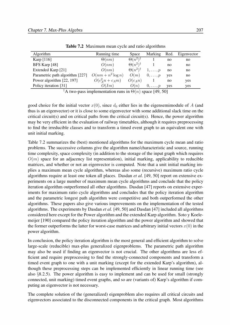
Chapter 7. Max-Plus Algebra 207
Table 7.2 Maximum mean cycle and ratio algorithms
Algorithm Running time Space Marking Red. Eigenvector
Karp [116] Θ(nm) Θ(n2)† 1 no no
BFS Karp [48] O(nm) Θ(n2)† 1 no no
Extended Karp [21] O(nm) Θ(n2)† 1, . . . , p no no
Parametric path algorithm [227] O(nm + n2 log n) O(m) 0, . . . , p yes no
Power algorithm [22, 197] O(c2An + cAm) O(cAn) 1 no yes
Policy iteration [31] O(Im) O(n) 0, . . . , p yes yes†A two-pass implementation runs in Θ(n) space [49, 50]
good choice for the initial vector x(0), since d0 either lies in the eigensemimodule of A (and
thus is an eigenvector) or it is close to some eigenvector with some additional slack time on the
critical circuit(s) and on critical paths from the critical circuit(s). Hence, the power algorithm
may be very efficient in the evaluation of railway timetables, although it requires preprocessing
to find the irreducible classes and to transform a timed event graph to an equivalent one with
unit initial marking.
Table 7.2 summarizes the (best) mentioned algorithms for the maximum cycle mean and ratio
problems. The successive columns give the algorithm name/characteristic and source, running
time complexity, space complexity (in addition to the storage of the input graph which requires
O(m) space for an adjacency list representation), initial marking, applicability to reducible
matrices, and whether or not an eigenvector is computed. Note that a unit initial marking im-
plies a maximum mean cycle algorithm, whereas also some (recursive) maximum ratio cycle
algorithms require at least one token all places. Dasdan et al. [49, 50] report on extensive ex-
periments on a large number of maximum mean cycle algorithms and conclude that the policy
iteration algorithm outperformed all other algorithms. Dasdan [47] reports on extensive exper-
iments for maximum ratio cycle algorithms and concludes that the policy iteration algorithm
and the parametric longest path algorithm were competitive and both outperformed the other
algorithms. These papers also give various improvements on the implementation of the tested
algorithms. The experiments by Dasdan et al. [49, 50] and Dasdan [47] included all algorithms
considered here except for the Power algorithm and the extended Karp algorithm. Soto y Koele-
meijer [190] compared the policy iteration algorithm and the power algorithm and showed that
the former outperforms the latter for worst-case matrices and arbitrary initial vectors x(0) in the
power algorithm.
In conclusion, the policy iteration algorithm is the most general and efficient algorithm to solve
large-scale (reducible) max-plus generalized eigenproblems. The parametric path algorithm
may also be used if finding an eigenvector is not crucial. The other algorithms are less ef-
ficient and require preprocessing to find the strongly-connected components and transform a
timed event graph to one with a unit marking (except for the extended Karp’s algorithm), al-
though these preprocessing steps can be implemented efficiently in linear running time (see
also §8.2.5). The power algorithm is easy to implement and can be used for small (strongly
connected, unit marking) timed event graphs, and so are (variants of) Karp’s algorithm if com-
puting an eigenvector is not necessary.
The complete solution of the (generalized) eigenproblem also requires all critical circuits and
eigenvectors associated to the disconnected components in the critical graph. Most algorithms
208 Punctuality of Railway Operations and Timetable Stability Analysis
can easily be extended to give one critical circuit, but finding all critical nodes requires more
effort. Olsder et al. [155] describe an algorithm for computing the maximum eigenvalue and all
critical nodes of a max-plus matrixA ∈ Rn×nmax containing at least one circuit. The algorithm uses
the Floyd-Warshall procedure (see §7.5.1) to detect positive weight circuits of the parametric
matrix Aλ = λ−1A = (aij − λ) for increasing values of λ until λ = λ0(A). Starting with a
lower bound for λ (e.g., λ = min{aij |aij > ε}) the Floyd-Warshall procedure is applied to
Aλ; if a positive diagonal entry [Akλ]ii is computed then λ is reset to the cycle mean of this
circuit (obtained by backtracking on the predecessor vector) and the Floyd-Warshall procedure
is restarted on the updated matrix Aλ. If the Floyd-Warshall procedure terminates without
detecting a positive circuit then λ = λ0(A) and the critical nodes are those i with [A+λ ]ii = 0.
Olsder et al. [155] then describe how to obtain finite eigenvectors from the longest path matrix
A+λ under the assumption that all nodes are accessible from a critical circuit (that is, the initial
classes of A are basic, see Corollary 7.4.5).
The most efficient approach to compute all critical nodes associated to the maximum general-
ized eigenvalue λ0 of a polynomial matrix A ∈ Rn×nmax [X] proceeds in two stages: first compute
the maximum generalized eigenvalue λ0 using the policy iteration algorithm (or any other fast
algorithm) and subsequently compute the diagonal of the longest path matrix [A(λ−10 )]+ using
the ALLLONGESTCIRCUITS algorithm presented in §7.5.3. If the policy iteration algorithm
returns a cycle time vector with entries χi 6= λ0 then we may restrict the computation of the
diagonal to the principle submatrix [A[K0|K0](λ−10 )]+ where K0 = {1 ≤ i ≤ n | χi = λ0}.
Finally, a basis of the eigensemimodule associated to λ0 is obtained by computing the columns
[A+λ0
]· j for a selected node j from each component in the critical graph, see Theorem 7.4.6. The
latter is a single-origin longest path problem from origin j, see §7.5.2. Note that the policy iter-
ation algorithm is more efficient to compute λ0 than repeated application of an all-pair longest
path algorithm as in Olsder et al. [155], and moreover, a repeated single-origin longest path
algorithm for the selected critical nodes is much more efficient than computing the complete
longest path matrix.
7.5 Longest Path Algorithms
7.5.1 All-Pair Longest Paths
A necessary and sufficient condition for the existence of finite longest paths in finite digraphs is
that the graph has no positive-weight circuits. In the sequel we will assume that this condition is
satisfied. In general, all path algorithms can easily be extended to detect positive-weight circuits
and return an error message if such a circuit is detected [3, 39]. Recall that a precedence graph
G(A) has a positive circuit iff the maximum eigenvalue (or maximum cycle mean) λ0(A) > e.We will only call a longest path algorithm for max-plus matrices with maximum eigenvalue not
exceeding e, for ‘normalized’ max-plus matricesAλ0= λ−1
0 A, or valuated polynomial matrices
Aν = A(ν−1) =⊕p
l=0Alν−l with ν ≥ λ0, which all satisfy the condition of nonpositive-weight
circuits.
Algorithm 7.5.1 gives the well-known Floyd-Warshall algorithm for computing the longest path
matrix A+ [66, 219, 39]. The algorithm iteratively computes the longest path weight from each
node j to i using paths over ‘internal’ nodes 1, . . . , k only. Thus, in the k-th (outer) iteration
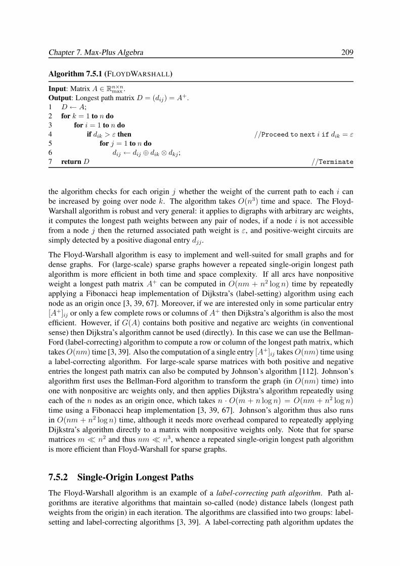
Chapter 7. Max-Plus Algebra 209
Algorithm 7.5.1 (FLOYDWARSHALL)
Input: Matrix A ∈ Rn×nmax .
Output: Longest path matrix D = (dij) = A+.
1 D ← A;
2 for k = 1 to n do
3 for i = 1 to n do
4 if dik > ε then //Proceed to next i if dik = ε5 for j = 1 to n do
6 dij ← dij ⊕ dik ⊗ dkj;
7 return D //Terminate
the algorithm checks for each origin j whether the weight of the current path to each i can
be increased by going over node k. The algorithm takes O(n3) time and space. The Floyd-
Warshall algorithm is robust and very general: it applies to digraphs with arbitrary arc weights,
it computes the longest path weights between any pair of nodes, if a node i is not accessible
from a node j then the returned associated path weight is ε, and positive-weight circuits are
simply detected by a positive diagonal entry djj.
The Floyd-Warshall algorithm is easy to implement and well-suited for small graphs and for
dense graphs. For (large-scale) sparse graphs however a repeated single-origin longest path
algorithm is more efficient in both time and space complexity. If all arcs have nonpositive
weight a longest path matrix A+ can be computed in O(nm + n2 logn) time by repeatedly
applying a Fibonacci heap implementation of Dijkstra’s (label-setting) algorithm using each
node as an origin once [3, 39, 67]. Moreover, if we are interested only in some particular entry
[A+]ij or only a few complete rows or columns of A+ then Dijkstra’s algorithm is also the most
efficient. However, if G(A) contains both positive and negative arc weights (in conventional
sense) then Dijkstra’s algorithm cannot be used (directly). In this case we can use the Bellman-
Ford (label-correcting) algorithm to compute a row or column of the longest path matrix, which
takesO(nm) time [3, 39]. Also the computation of a single entry [A+]ij takesO(nm) time using
a label-correcting algorithm. For large-scale sparse matrices with both positive and negative
entries the longest path matrix can also be computed by Johnson’s algorithm [112]. Johnson’s
algorithm first uses the Bellman-Ford algorithm to transform the graph (in O(nm) time) into
one with nonpositive arc weights only, and then applies Dijkstra’s algorithm repeatedly using
each of the n nodes as an origin once, which takes n · O(m + n log n) = O(nm + n2 logn)time using a Fibonacci heap implementation [3, 39, 67]. Johnson’s algorithm thus also runs
in O(nm + n2 logn) time, although it needs more overhead compared to repeatedly applying
Dijkstra’s algorithm directly to a matrix with nonpositive weights only. Note that for sparse
matrices m � n2 and thus nm � n3, whence a repeated single-origin longest path algorithm
is more efficient than Floyd-Warshall for sparse graphs.
7.5.2 Single-Origin Longest Paths
The Floyd-Warshall algorithm is an example of a label-correcting path algorithm. Path al-
gorithms are iterative algorithms that maintain so-called (node) distance labels (longest path
weights from the origin) in each iteration. The algorithms are classified into two groups: label-
setting and label-correcting algorithms [3, 39]. A label-correcting path algorithm updates the
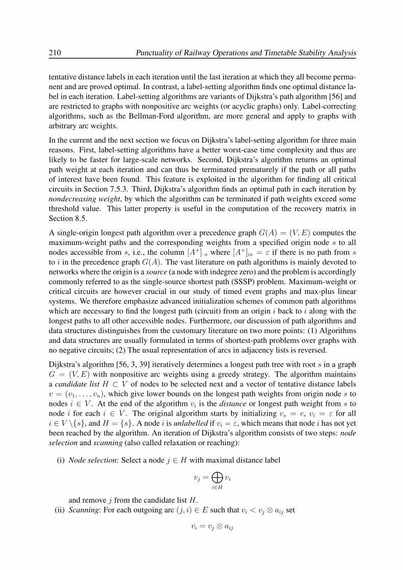
210 Punctuality of Railway Operations and Timetable Stability Analysis
tentative distance labels in each iteration until the last iteration at which they all become perma-
nent and are proved optimal. In contrast, a label-setting algorithm finds one optimal distance la-
bel in each iteration. Label-setting algorithms are variants of Dijkstra’s path algorithm [56] and
are restricted to graphs with nonpositive arc weights (or acyclic graphs) only. Label-correcting
algorithms, such as the Bellman-Ford algorithm, are more general and apply to graphs with
arbitrary arc weights.
In the current and the next section we focus on Dijkstra’s label-setting algorithm for three main
reasons. First, label-setting algorithms have a better worst-case time complexity and thus are
likely to be faster for large-scale networks. Second, Dijkstra’s algorithm returns an optimal
path weight at each iteration and can thus be terminated prematurely if the path or all paths
of interest have been found. This feature is exploited in the algorithm for finding all critical
circuits in Section 7.5.3. Third, Dijkstra’s algorithm finds an optimal path in each iteration by
nondecreasing weight, by which the algorithm can be terminated if path weights exceed some
threshold value. This latter property is useful in the computation of the recovery matrix in
Section 8.5.
A single-origin longest path algorithm over a precedence graph G(A) = (V,E) computes the
maximum-weight paths and the corresponding weights from a specified origin node s to all
nodes accessible from s, i.e., the column [A+]· s where [A+]is = ε if there is no path from sto i in the precedence graph G(A). The vast literature on path algorithms is mainly devoted to
networks where the origin is a source (a node with indegree zero) and the problem is accordingly
commonly referred to as the single-source shortest path (SSSP) problem. Maximum-weight or
critical circuits are however crucial in our study of timed event graphs and max-plus linear
systems. We therefore emphasize advanced initialization schemes of common path algorithms
which are necessary to find the longest path (circuit) from an origin i back to i along with the
longest paths to all other accessible nodes. Furthermore, our discussion of path algorithms and
data structures distinguishes from the customary literature on two more points: (1) Algorithms
and data structures are usually formulated in terms of shortest-path problems over graphs with
no negative circuits; (2) The usual representation of arcs in adjacency lists is reversed.
Dijkstra’s algorithm [56, 3, 39] iteratively determines a longest path tree with root s in a graph
G = (V,E) with nonpositive arc weights using a greedy strategy. The algorithm maintains
a candidate list H ⊂ V of nodes to be selected next and a vector of tentative distance labels
v = (v1, . . . , vn), which give lower bounds on the longest path weights from origin node s to
nodes i ∈ V . At the end of the algorithm vi is the distance or longest path weight from s to
node i for each i ∈ V . The original algorithm starts by initializing vs = e, vi = ε for all
i ∈ V \{s}, and H = {s}. A node i is unlabelled if vi = ε, which means that node i has not yet
been reached by the algorithm. An iteration of Dijkstra’s algorithm consists of two steps: node
selection and scanning (also called relaxation or reaching):
(i) Node selection: Select a node j ∈ H with maximal distance label
vj =⊕
i∈H
vi
and remove j from the candidate list H .
(ii) Scanning: For each outgoing arc (j, i) ∈ E such that vi < vj ⊗ aij set
vi = vj ⊗ aij
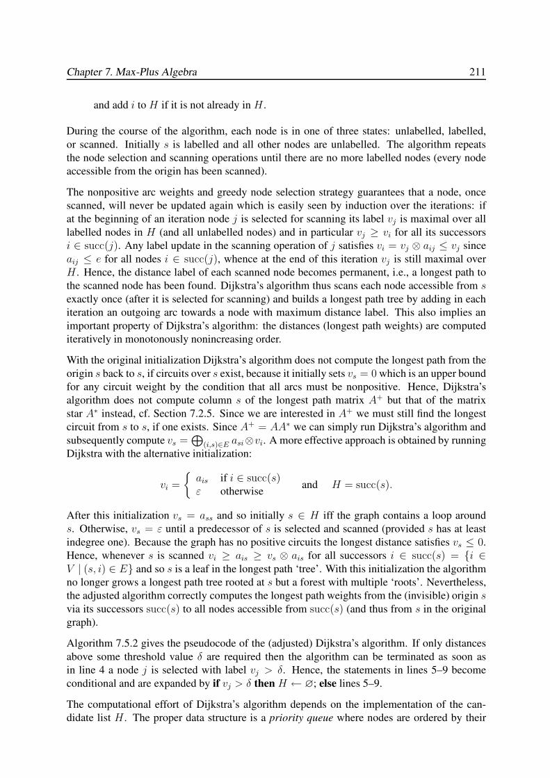
Chapter 7. Max-Plus Algebra 211
and add i to H if it is not already in H .
During the course of the algorithm, each node is in one of three states: unlabelled, labelled,
or scanned. Initially s is labelled and all other nodes are unlabelled. The algorithm repeats
the node selection and scanning operations until there are no more labelled nodes (every node
accessible from the origin has been scanned).
The nonpositive arc weights and greedy node selection strategy guarantees that a node, once
scanned, will never be updated again which is easily seen by induction over the iterations: if
at the beginning of an iteration node j is selected for scanning its label vj is maximal over all
labelled nodes in H (and all unlabelled nodes) and in particular vj ≥ vi for all its successors
i ∈ succ(j). Any label update in the scanning operation of j satisfies vi = vj ⊗ aij ≤ vj since
aij ≤ e for all nodes i ∈ succ(j), whence at the end of this iteration vj is still maximal over
H . Hence, the distance label of each scanned node becomes permanent, i.e., a longest path to
the scanned node has been found. Dijkstra’s algorithm thus scans each node accessible from sexactly once (after it is selected for scanning) and builds a longest path tree by adding in each
iteration an outgoing arc towards a node with maximum distance label. This also implies an
important property of Dijkstra’s algorithm: the distances (longest path weights) are computed
iteratively in monotonously nonincreasing order.
With the original initialization Dijkstra’s algorithm does not compute the longest path from the
origin s back to s, if circuits over s exist, because it initially sets vs = 0 which is an upper bound
for any circuit weight by the condition that all arcs must be nonpositive. Hence, Dijkstra’s
algorithm does not compute column s of the longest path matrix A+ but that of the matrix
star A∗ instead, cf. Section 7.2.5. Since we are interested in A+ we must still find the longest
circuit from s to s, if one exists. Since A+ = AA∗ we can simply run Dijkstra’s algorithm and
subsequently compute vs =⊕
(i,s)∈E asi⊗vi. A more effective approach is obtained by running
Dijkstra with the alternative initialization:
vi =
{ais if i ∈ succ(s)ε otherwise
and H = succ(s).
After this initialization vs = ass and so initially s ∈ H iff the graph contains a loop around
s. Otherwise, vs = ε until a predecessor of s is selected and scanned (provided s has at least
indegree one). Because the graph has no positive circuits the longest distance satisfies vs ≤ 0.
Hence, whenever s is scanned vi ≥ ais ≥ vs ⊗ ais for all successors i ∈ succ(s) = {i ∈V | (s, i) ∈ E} and so s is a leaf in the longest path ‘tree’. With this initialization the algorithm
no longer grows a longest path tree rooted at s but a forest with multiple ‘roots’. Nevertheless,
the adjusted algorithm correctly computes the longest path weights from the (invisible) origin svia its successors succ(s) to all nodes accessible from succ(s) (and thus from s in the original
graph).
Algorithm 7.5.2 gives the pseudocode of the (adjusted) Dijkstra’s algorithm. If only distances
above some threshold value δ are required then the algorithm can be terminated as soon as
in line 4 a node j is selected with label vj > δ. Hence, the statements in lines 5–9 become
conditional and are expanded by if vj > δ then H ← ∅; else lines 5–9.
The computational effort of Dijkstra’s algorithm depends on the implementation of the can-
didate list H . The proper data structure is a priority queue where nodes are ordered by their
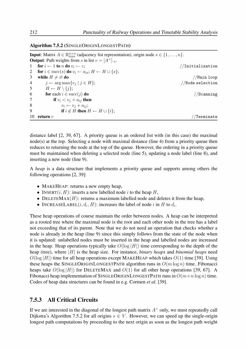
212 Punctuality of Railway Operations and Timetable Stability Analysis
Algorithm 7.5.2 (SINGLEORIGINLONGESTPATH)
Input: Matrix A ∈ Rn×nmax (adjacency list representation), origin node s ∈ {1, . . . , n}.
Output: Path weights from s in list v = [A+]· s.
1 for i← 1 to n do vi ← ε; //Initialization2 for i ∈ succ(s) do vi ← ais; H ← H ∪ {s};3 while H 6= ∅ do //Main loop4 j ← arg max{vj | j ∈ H}; //Node selection5 H ← H \ {j};6 for each i ∈ succ(j) do //Scanning7 if vi < vj + aij then
8 vi ← vj + aij;
9 if i 6∈ H then H ← H ∪ {i};10 return v //Terminate
distance label [2, 39, 67]. A priority queue is an ordered list with (in this case) the maximal
node(s) at the top. Selecting a node with maximal distance (line 4) from a priority queue then
reduces to returning the node at the top of the queue. However, the ordering in a priority queue
must be maintained when deleting a selected node (line 5), updating a node label (line 8), and
inserting a new node (line 9).
A heap is a data structure that implements a priority queue and supports among others the
following operations [2, 39]:
• MAKEHEAP: returns a new empty heap,
• INSERT(i, H): inserts a new labelled node i to the heap H ,
• DELETEMAX(H): returns a maximum labelled node and deletes it from the heap,
• INCREASELABEL(i, di , H): increases the label of node i in H to di.
These heap operations of course maintain the order between nodes. A heap can be interpreted
as a rooted tree where the maximal node is the root and each other node in the tree has a label
not exceeding that of its parent. Note that we do not need an operation that checks whether a
node is already in the heap (line 9) since this simply follows from the state of the node when
it is updated: unlabelled nodes must be inserted in the heap and labelled nodes are increased
in the heap. Heap operations typically take O(log |H|) time corresponding to the depth of the
heap (tree), where |H| is the heap size. For instance, binary heaps and binomial heaps need
O(log |H|) time for all heap operations except MAKEHEAP which takes O(1) time [39]. Using
these heaps the SINGLEORIGINLONGESTPATH algorithm runs in O(m logn) time. Fibonacci
heaps take O(log |H|) for DELETEMAX and O(1) for all other heap operations [39, 67]. A
Fibonacci heap implementation of SINGLEORIGINLONGESTPATH runs inO(m+n logn) time.
Codes of heap data structures can be found in e.g. Cormen et al. [39].
7.5.3 All Critical Circuits
If we are interested in the diagonal of the longest path matrix A+ only, we must repeatedly call
Dijkstra’s Algorithm 7.5.2 for all origins s ∈ V . However, we can speed up the single-origin
longest path computations by proceeding to the next origin as soon as the longest path weight
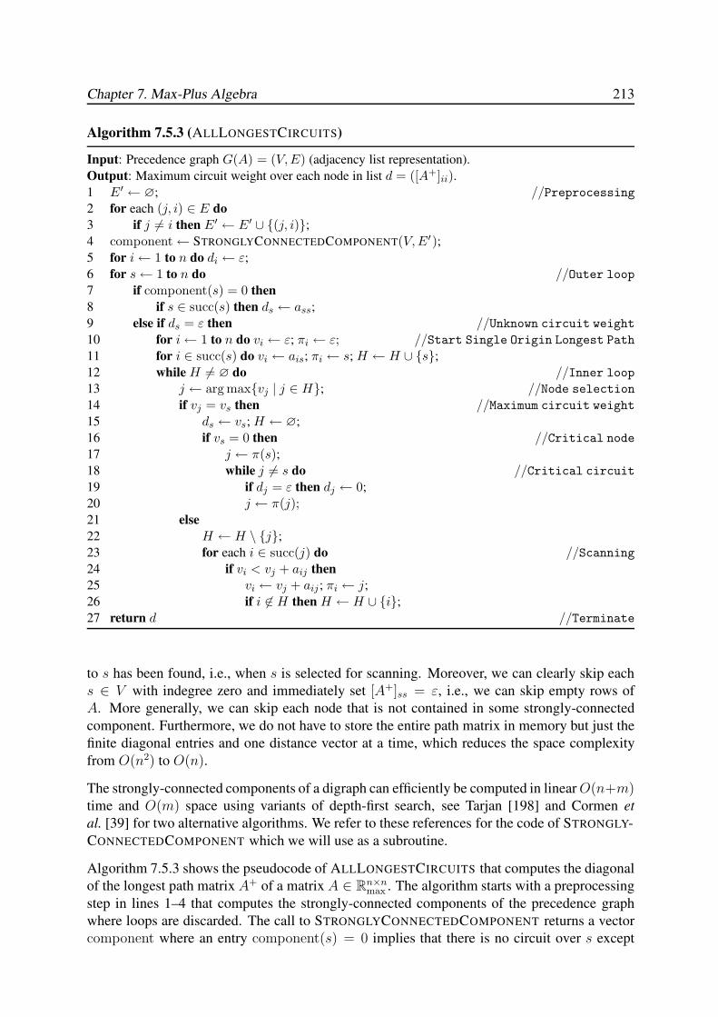
Chapter 7. Max-Plus Algebra 213
Algorithm 7.5.3 (ALLLONGESTCIRCUITS)
Input: Precedence graph G(A) = (V,E) (adjacency list representation).
Output: Maximum circuit weight over each node in list d = ([A+]ii).1 E′ ← ∅; //Preprocessing2 for each (j, i) ∈ E do
3 if j 6= i then E′ ← E′ ∪ {(j, i)};4 component← STRONGLYCONNECTEDCOMPONENT(V, E′);5 for i← 1 to n do di ← ε;
6 for s← 1 to n do //Outer loop7 if component(s) = 0 then
8 if s ∈ succ(s) then ds ← ass;
9 else if ds = ε then //Unknown circuit weight10 for i← 1 to n do vi ← ε; πi ← ε; //Start Single Origin Longest Path11 for i ∈ succ(s) do vi ← ais; πi ← s; H ← H ∪ {s};12 while H 6= ∅ do //Inner loop13 j ← arg max{vj | j ∈ H}; //Node selection14 if vj = vs then //Maximum circuit weight15 ds ← vs; H ← ∅;
16 if vs = 0 then //Critical node17 j ← π(s);18 while j 6= s do //Critical circuit19 if dj = ε then dj ← 0;
20 j ← π(j);21 else
22 H ← H \ {j};23 for each i ∈ succ(j) do //Scanning24 if vi < vj + aij then
25 vi ← vj + aij ; πi ← j;
26 if i 6∈ H then H ← H ∪ {i};27 return d //Terminate
to s has been found, i.e., when s is selected for scanning. Moreover, we can clearly skip each
s ∈ V with indegree zero and immediately set [A+]ss = ε, i.e., we can skip empty rows of
A. More generally, we can skip each node that is not contained in some strongly-connected
component. Furthermore, we do not have to store the entire path matrix in memory but just the
finite diagonal entries and one distance vector at a time, which reduces the space complexity
from O(n2) to O(n).
The strongly-connected components of a digraph can efficiently be computed in linearO(n+m)time and O(m) space using variants of depth-first search, see Tarjan [198] and Cormen et
al. [39] for two alternative algorithms. We refer to these references for the code of STRONGLY-
CONNECTEDCOMPONENT which we will use as a subroutine.
Algorithm 7.5.3 shows the pseudocode of ALLLONGESTCIRCUITS that computes the diagonal
of the longest path matrix A+ of a matrix A ∈ Rn×nmax . The algorithm starts with a preprocessing
step in lines 1–4 that computes the strongly-connected components of the precedence graph
where loops are discarded. The call to STRONGLYCONNECTEDCOMPONENT returns a vector
component where an entry component(s) = 0 implies that there is no circuit over s except
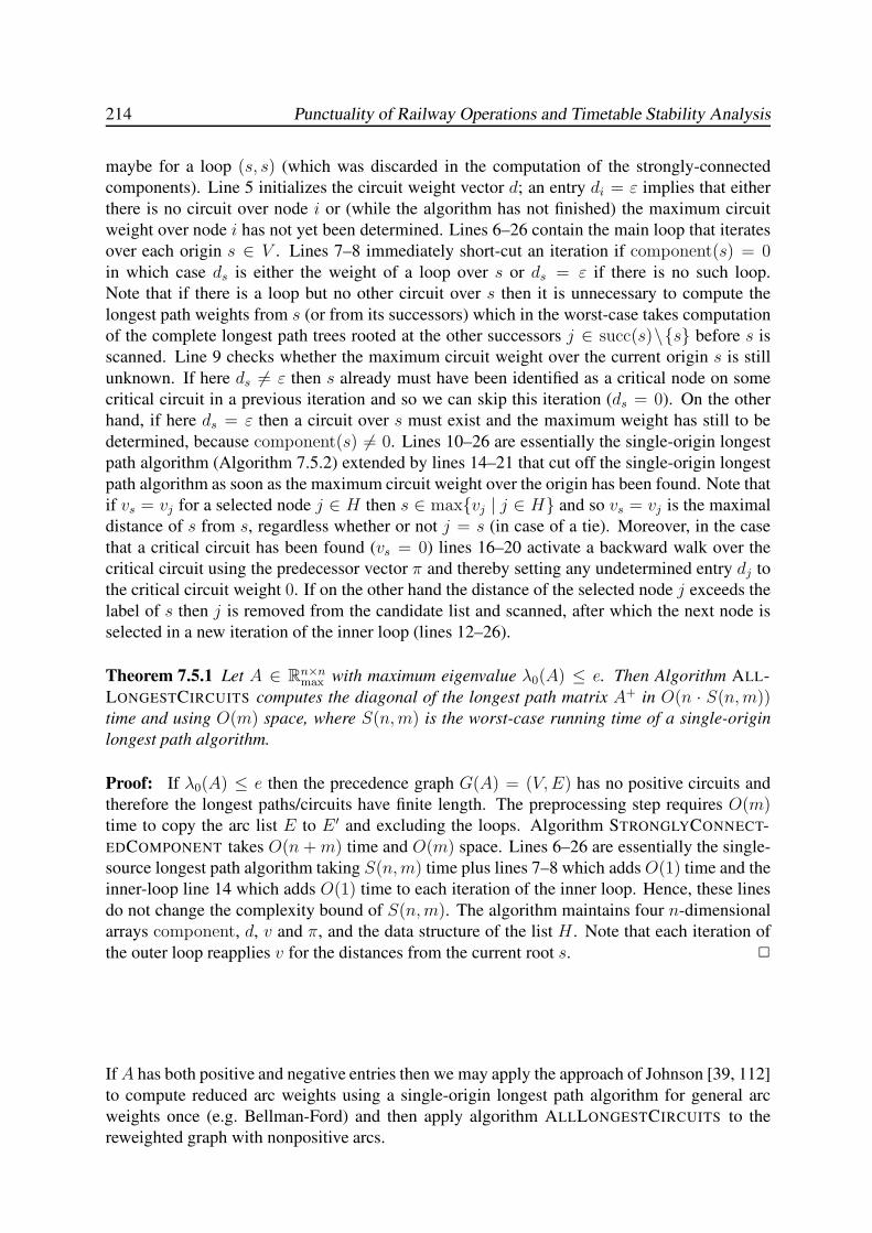
214 Punctuality of Railway Operations and Timetable Stability Analysis
maybe for a loop (s, s) (which was discarded in the computation of the strongly-connected
components). Line 5 initializes the circuit weight vector d; an entry di = ε implies that either
there is no circuit over node i or (while the algorithm has not finished) the maximum circuit
weight over node i has not yet been determined. Lines 6–26 contain the main loop that iterates
over each origin s ∈ V . Lines 7–8 immediately short-cut an iteration if component(s) = 0in which case ds is either the weight of a loop over s or ds = ε if there is no such loop.
Note that if there is a loop but no other circuit over s then it is unnecessary to compute the
longest path weights from s (or from its successors) which in the worst-case takes computation
of the complete longest path trees rooted at the other successors j ∈ succ(s)\{s} before s is
scanned. Line 9 checks whether the maximum circuit weight over the current origin s is still
unknown. If here ds 6= ε then s already must have been identified as a critical node on some
critical circuit in a previous iteration and so we can skip this iteration (ds = 0). On the other
hand, if here ds = ε then a circuit over s must exist and the maximum weight has still to be
determined, because component(s) 6= 0. Lines 10–26 are essentially the single-origin longest
path algorithm (Algorithm 7.5.2) extended by lines 14–21 that cut off the single-origin longest
path algorithm as soon as the maximum circuit weight over the origin has been found. Note that
if vs = vj for a selected node j ∈ H then s ∈ max{vj | j ∈ H} and so vs = vj is the maximal
distance of s from s, regardless whether or not j = s (in case of a tie). Moreover, in the case
that a critical circuit has been found (vs = 0) lines 16–20 activate a backward walk over the
critical circuit using the predecessor vector π and thereby setting any undetermined entry dj to
the critical circuit weight 0. If on the other hand the distance of the selected node j exceeds the
label of s then j is removed from the candidate list and scanned, after which the next node is
selected in a new iteration of the inner loop (lines 12–26).
Theorem 7.5.1 Let A ∈ Rn×nmax with maximum eigenvalue λ0(A) ≤ e. Then Algorithm ALL-
LONGESTCIRCUITS computes the diagonal of the longest path matrix A+ in O(n · S(n,m))time and using O(m) space, where S(n,m) is the worst-case running time of a single-origin
longest path algorithm.
Proof: If λ0(A) ≤ e then the precedence graph G(A) = (V,E) has no positive circuits and
therefore the longest paths/circuits have finite length. The preprocessing step requires O(m)time to copy the arc list E to E ′ and excluding the loops. Algorithm STRONGLYCONNECT-
EDCOMPONENT takes O(n +m) time and O(m) space. Lines 6–26 are essentially the single-
source longest path algorithm taking S(n,m) time plus lines 7–8 which adds O(1) time and the
inner-loop line 14 which adds O(1) time to each iteration of the inner loop. Hence, these lines
do not change the complexity bound of S(n,m). The algorithm maintains four n-dimensional
arrays component, d, v and π, and the data structure of the list H . Note that each iteration of
the outer loop reapplies v for the distances from the current root s. 2
IfA has both positive and negative entries then we may apply the approach of Johnson [39, 112]
to compute reduced arc weights using a single-origin longest path algorithm for general arc
weights once (e.g. Bellman-Ford) and then apply algorithm ALLLONGESTCIRCUITS to the
reweighted graph with nonpositive arcs.
Chapter 7. Max-Plus Algebra 215
7.6 Conclusions
In this chapter we introduced max-plus algebra and several algorithms for solving eigenprob-
lems and longest path problems in max-plus algebra. In particular, we introduced max-plus
matrices and their associated precedence graphs, as well as max-plus polynomial matrices and
their formal connection to timed event graphs. We explained linear dependence and indepen-
dent vectors in semimodules, stressed the differences with vector spaces over classical fields,
and gave a geometric description of vectors in max-plus semimodules.
We explained the (generalized) eigenproblem of max-plus (polynomial) matrices and showed
the connection with the topological structure of the associated graphs. We showed how the
nodes of the precedence (or timed event) graphs can be partitioned into classes with a unique
eigenvalue which equals the (maximum) cycle mean of the critical circuit(s), and gave a full
description of the corresponding eigenspaces (eigensemimodules). We furthermore presented
the efficient policy iteration algorithm for solving the (generalized) eigenproblem and developed
an algorithm for finding all critical circuits. Moreover, we considered efficient implementations
of single-origin longest path algorithms.
The max-plus algebra theory and numerical algorithms developed in this chapter will be used in
the next chapter on max-plus linear systems, which relates max-plus algebra to the performance
analysis of timed event graphs — and railway timetables in particular.

216 Punctuality of Railway Operations and Timetable Stability Analysis
Chapter 8
RAILWAY TIMETABLE STABILITY
ANALYSIS
8.1 Introduction
The issue of railway traffic stability is rapidly gaining attention in Europe because of the in-
creasingly saturated railway infrastructure where a slightly delayed train may cause a domino
effect of secondary delays over the entire network. European railways are typically operated
according to a predetermined (master) timetable, which represents a conflict-free coordination
of train paths and includes slack time to manage train delays. From a system point of view the
timetable can be understood as a steady state for the train traffic. Traffic stability then refers to
the possibility and effort necessary of returning to the steady state after disruptions. The system
response to disruptions is highly complicated due to complex cyclic train interdependencies
generated by infrastructure restrictions (e.g. conflicting routes or a fast train getting stuck be-
hind a leading slow train on an open track), timetable constraints (passenger connections at
transfer stations), and logistics (rolling stock circulations and train personnel schedules). In
this chapter we develop an analytical approach to analyse timetable stability based on max-plus
algebra.
In Chapter 6 we have seen how scheduled railway systems can be modelled as timed event
graphs and considered a number of structural and behavioural properties of timed event graphs.
The present chapter is devoted to the dynamic behaviour over time or performance evaluation
of timed event graphs based on the state-space representation of timed event graphs in the event
domain, which was already briefly introduced in Section 6.5.3. The state-space description of
timed event graphs is a system of (max,+)-recursive equations — recursive equations involving
maximum and sum operations — and are thus nonlinear in a classical sense. However, formu-
lated in max-plus algebra the state-space equations show a linear dynamic system and can be
analysed using the theory developed in Chapter 7.
The approach taken in this chapter concentrates on network timetable evaluation in a determin-
istic setting in accordance to the design choices of e.g. train orders at conflicting routes and
the deterministic design times (running times, dwell times, transfer times, minimum headway
times, etc.) used in the construction of the timetable. A max-plus state matrix captures this
timetable structure and the eigenstructure of this matrix reveals the interconnected components,
associated cycle times and available recovery times, which can all be computed by efficient
polynomial algorithms. Moreover, because bottlenecks of the systems are explicitly revealed
— through the notion of critical circuits — this approach provides an efficient way not only
to evaluate the performance but also to assess certain design choices made at earlier stages in
the timetable design process. We propose transparent stability and robustness criteria and as-
sociated performance indicators and are able to identify critical processes or resources in the
217
218 Punctuality of Railway Operations and Timetable Stability Analysis
timetable or infrastructure. The approach has been implemented in the computer application
PETER (Performance Evaluation of Timed Events in Railways) which is also introduced and
demonstrated in this chapter. PETER has been developed as a decision support to railway plan-
ners for evaluating and improving timetable designs and infrastructure utilization. Because of
efficient numerical algorithms and implementations PETER enables a real-time environment to
analyse large-scale periodic railway timetables.
The application oriented literature on max-plus algebra and timed event graphs typically deals
with the analysis of irreducible first-order models of the form x(k) = Ax(k − 1) ⊕ Bu(k),although in first instance the derived models contain higher-order and/or zero-order dynamics.
Hence, more general order models are first transformed to the canonical first-order representa-
tion and analysed accordingly. In particular, topological and behavioural properties are analysed
separately from performance properties. The first-order models indeed allow an elegant anal-
ysis avoiding some complications arising from especially the zero-order dynamics. In practice
however the zero-order dynamics do represent essential behavioural properties that can only be
analysed in full potential if explicitly available in the model. Moreover, the analyses usually
assume irreducibility (strongly connectedness) without consideration of accessibility relations
in general reducible systems. The first-order representations thus contain some simplifying
assumptions that do no justice to the original problem. In this chapter we deal with general
higher-order max-plus linear systems and propose a formal polynomial matrix representation
of both the higher-order state matrix and associated timed event graph. We use this approach to
model periodic railway timetables as scheduled max-plus linear systems and develop a generic
max-plus system analysis theory that has been proved valuable in evaluating railway timetables
on stability and robustness.
The chapter is outlined as follows. Section 8.2 introduces max-plus linear systems and pro-
poses a general linear state-space representation of (scheduled) timed event graphs. Section 8.3
considers a spectral analysis of the linear system and defines an appropriate notion of timetable
stability. Timetable realizability is considered in Section 8.4. Section 8.5 defines a notion of
timetable robustness based on recovery times in the timetable. Section 8.6 deals with delay
propagation and shows how any initial delay scenario may propagate over time and the network
given the timetable structure. PETER is briefly introduced in Section 8.7, and illustrated in a
case-study of the Dutch national railway timetable in Section 8.8. Section 8.9 ends this chapter
with some conclusions.
8.2 Max-Plus Linear Systems
8.2.1 First-Order State-Space Equations
A max-plus linear system is a linear system description of a discrete-event dynamic system
evaluated over the (max,+)-semiring, where the state dynamics can be described by recursive
equations in max-plus algebra. The canonical (first-order) max-plus linear system is{x(k) = Ax(k − 1)⊕Bu(k), x(0) = x0
y(k) = Cx(k).(8.1)
Here x(·) ∈ Rnmax is the state vector, u(·) ∈ Rr
max the input vector and y(·) an output vector.
The state, input, and output vectors depend on a counter k ∈ N which numbers the subsequent
Chapter 8. Railway Timetable Stability Analysis 219
occurrences of events. The system matrices (A,B,C) are the state matrix A ∈ Rn×nmax , the
input matrix B ∈ Rn×rmax, and the output matrix C ∈ Rs×n
max. We consider only constant system
matrices, soA,B, andC are invariant to k. Then for given system matrices the system evolution
{x(k)}k∈N and output sequence {y(k)}k∈N is completely determined by the initial condition x0
and the input sequence {u(k)}k∈N. If C = E, the identity matrix, then the output vector is just
the state vector. The state vector x = (x1, . . . , xn)> corresponds to events 1, . . . , n that occur
at discrete times. Hence the term discrete events. The state vector x(k) is the vector of event
times associated to the kth occurrence of the events. So, xi(k) is the time instant at which event
i takes place for the kth time.
A homogeneous max-plus linear system has no inputs, i.e., B = E . In this case the recursive
state equation is
x(k) = A⊗ x(k − 1), x(0) = x0. (8.2)
The evolution of a homogeneous first-order max-plus linear system can be calculated analyt-
ically for a given state matrix and initial condition. Substituting k = 1 in (8.2) simply gives
x(1) = Ax0, for k = 2 we obtain x(2) = Ax(1) = A ⊗ Ax0 = A2x0, and by a repeated
argument we obtain
x(k) = Ak ⊗ x0 for all k ∈ N.
The behaviour of the homogeneous system depends on the eigenvalues of A and the initial state
vector x0. Section 8.3 is devoted to this spectral analysis. It will be shown that the asymptotic
behaviour of the successive event times is periodic and independent of the initial condition,
although the initial condition determines the length of the transient behaviour before reaching
the periodic regime [11, 190].
The inhomogeneous term Bu(k) is used to control or regulate the system behaviour into a
desired state evolution. In railway systems or public transport systems the (departure) events
are generally regulated by a timetable, which specifies the earliest allowed departure times. A
regular interval or periodic timetable with cycle time T is modelled itself by the homogeneous
first-order max-plus linear system
d(k) = d(k − 1)⊗ T, d(0) = d0,
where d(·) ∈ Rnmax is the timetable vector and d0 ∈ Rn
max is an initial timetable vector. Note
that the right-hand side is a matrix multiplication of an n × 1-dimensional vector d(k − 1)and a scalar T giving the n × 1-dimensional vector d(k). Alternatively, we could express
this equation using the right-hand side diag(T, . . . , T ) ⊗ d(k − 1) with the diagonal matrix
diag(T, . . . , T ) = T ⊗ E ∈ Rn×nmax , or by the scalar-vector product T ⊗ d(k − 1). The solution
to this timetable system is
d(k) = T k ⊗ d0 for all k ∈ N. (8.3)
By defining B = E ∈ Rn×nmax , the identity matrix, and u(k) = d(k) we obtain Bu(k) = d(k)
which fits the framework (8.1). By convention we use the inhomogeneous term d(k) directly
for scheduled max-plus linear systems. An alternative representation that clearly visualizes the
periodicity of the timetable is obtained by defining B = d0 ∈ Rn×1max and u(k) = T k, which
again fits the inhomogeneous state equation (8.1). Here, the clock event u(k) gives the starting
time of the kth period with respect to the initial timetable vector d0. Nevertheless, we use the
former representation which also allows aperiodic timetables.
220 Punctuality of Railway Operations and Timetable Stability Analysis
The canonical state-space equations of a scheduled max-plus linear system with periodic timetable
are therefore
x(k) = A⊗ x(k − 1)⊕ d(k), x(0) = x0, d(k) = d0 ⊗ T k. (8.4)
Here x(k) and d(k) are the kth actual and scheduled event time vectors, respectively.
8.2.2 Higher-Order State-Space Equations
The general state-space representation of a timed event graph G = (T ,P, µ, w) is the higher-
order max-plus linear system
{x(k) =
⊕pl=0Alx(k − l)⊕Bu(k), x(1− p) = x1−p, . . . , x(0) = x0
y(k) = Cx(k).(8.5)
Here the parameter p is called the order of the system which equals the highest initial marking
of any place, p =⊕m
i=1 µi. The system matrices Al ∈ Rn×nmax correspond to the places ph =
(j, i, µh, wh) in the timed marked graph G with initial marking µh = l, i.e.,
[Al]ij =
{wh if ph = (j, i, l) ∈ Pε otherwise.
(8.6)
Note that the first-order max-plus linear system (8.1) is a special case of (8.5) with all places
having a unit initial marking, i.e, A1 = A and A0 = E . Thus, (8.1) is a pure first-order linear
system without zero-order terms. In Section 8.2.5 we will show that any pth order linear system
can be transformed into a pure first-order representation.
We now return to the timed event graph model G = (T ,P, µ, w) of a scheduled railway system
as derived in Chapter 6. Each place ph ∈ P with output transition out(ph) = i corresponds to a
constraint in the event domain
xi(k) ≥ xin(ph) (k − µh)⊗ wh,
cf. Section 6.5.3. If transitions fire as soon as they are enabled the event times are given by
xi(k) =⊕
p∈Πi
xin(ph) (k − µh)⊗ wh for all i ∈ T , (8.7)
where Πi is the set of incoming places to transition i. Defining the matrices Al by (8.6) then
(8.7) becomes
xi(k) =
p⊕
l=0
n⊕
j=1
[Al]ij ⊗ xj(k − l) for all 1 ≤ i ≤ n
which in vector notation is the pth order max-plus linear system
x(k) =
p⊕
l=0
Al ⊗ x(k − l).
Chapter 8. Railway Timetable Stability Analysis 221
where x(k) = (x1(k), . . . , xn(k))>. If the events wait for their scheduled event times then the
event times are given by the pth order inhomogeneous state-space equation
x(k) =
p⊕
l=0
Al ⊗ x(k − l)⊕ d(k), (8.8)
where d(k) = (d1(k), . . . , dn(k))> is the timetable vector in period k. For a periodic timetable
with cycle time T the timetable vectors are defined by (8.3), which equals di(k) = di(0)⊗T k =di(0) + k · T as in Section 6.5.3.
The general state-space equations of a scheduled max-plus linear system with periodic timetable
are therefore
x(k) =⊕p
l=0Alx(k − l)⊕ d(k)y(k) = Cx(k)d(k) = d0 ⊗ T k.
(8.9)
In general the events in a railway system may be partitioned in departures, arrivals, passages
and terminal events, cf. Chapter 6. Usually, only the departure events are prohibited to depart
early, whilst arrival, through and terminal events may be early, that is, these latter events do
not have to wait for their scheduled event time before arriving at or passing through a station.
The (initial) timetable vector may thus be partitioned as d0 = (d10, ε)
>, where d10 corresponds
to the departure events. Likewise, the output vector may be defined to give e.g. the departure
events only. Assuming that the events are ordered with the events of interest numbered first as
1, . . . , n1 then C = [E E ] ∈ Rn1×nmax yields the desired output vector y(·) ∈ Rn1
max.
The general pth order state-space equations (8.9) include an implicit zero-order term and appear
therefore no longer purely recursive. However, from a timed event graph perspective it is clear
that the zero-order dynamics merely correspond to transitions that fire in the same period as
the predecessor transitions and thus still satisfy some precedence order. This will be explained
in detail in Section 8.6. The system dynamics are therefore completely determined by (8.9)
when given initial states x(l) for l = 1 − p, . . . , 0. In Section 8.2.5 we also discuss a simple
transformation that removes the zero-order terms from the state-space representation.
8.2.3 Polynomial Matrix Representation
An alternative formulation of a higher-order max-plus linear system (8.9) can be obtained using
a shift operator. Let γ be the backward-shift operator defined on a discrete-event dynamic
variable x(k) as
γx(k) = x(k − 1).
A backward-shift over l ≥ 1 periods is denoted by γl and corresponds to l successive applica-
tions of the backward shift γ, that is, γlx(k) = x(k− l) for any integer l ≥ 1. This is consistent
with the recursion γlx(k) = γl−1γx(k) = γl−1x(k − 1) for all l ∈ N with the convention that
γ0 = e. Using the shift operator the scheduled max-plus linear system (8.9) can be rewritten as
x(k) =
p⊕
l=0
Alx(k − l)⊕ d(k) =
p⊕
l=0
Alγlx(k)⊕ d(k) = A(γ)x(k)⊕ d(k), (8.10)
where A(γ) =⊕p
l=0Alγl is a polynomial matrix in the shift operator γ. A polynomial matrix
may thus be used both as a formal representation of a timed event graph, see Section 7.2.6, and
222 Punctuality of Railway Operations and Timetable Stability Analysis
as a shift operator in the max-plus linear system state representation. In the sequel, we will also
denote by (j, i, l) ∈ supp(A(γ)) = {(j, i, l)|[Al]ij 6= ε} a place (j, i) ∈ P with l tokens.
A first-order max-plus linear system is one for which A(γ) = Aγ, in which case A(γ)x(k) =Aγx(k) = Ax(k − 1). Hence, a first-order system satisfies the dynamic state-space equation
x(k) = Ax(k − 1), or in the scheduled case x(k) = Ax(k − 1)⊕ d(k).
8.2.4 Autonomous Max-Plus Linear Systems
As previously defined a homogeneous higher-order max-plus linear system is a linear system
with zero input matrix B = E ,
x(k) =
p⊕
l=0
Al ⊗ x(k − l) = A(γ)⊗ x(k). (8.11)
A homogeneous linear system (8.11) is related to an autonomous linear system. An autonomous
timed event graph is one that has no source transitions, which means that the polynomial ma-
trix representation A(γ) has no zero rows. The general scheduled max-plus linear system (8.8)
however allows source events which simply fire according to the timetable. In a homogeneous
system source transitions may be defined to fire unconditionally. Nevertheless, system perfor-
mance is determined by the internal events of the cyclic interconnection structure of the timed
event graph. Here, an internal event is an event contained in some circuit or accessible from an
upstream circuit.
Definition 8.2.1 (Autonomous linear system) A homogeneous max-plus linear system x(k) =A(γ)x(k) =
⊕pl=0Alx(k − l) is called autonomous if the polynomial state matrix A(γ) has no
zero row, or formally, ∀1 ≤ i ≤ n, ∃1 ≤ j ≤ n such that [A(γ)]ij 6= ε.
An autonomous system thus corresponds to a timed event graph that has no incoming paths or
trees.
The timetable subsystem of a scheduled max-plus linear system can be interpreted as an open-
loop control system, where the periodic timetable is defined a priori. Consider the scheduled
max-plus linear system (8.9). Then, given an initial timetable vector d0 and initial state vectors
xl, 1−p ≤ l ≤ 0, this system may be viewed as an autonomous max-plus linear system defined
by
x(k) =
[A(γ) d0
ε Tγ
]
⊗ x(k), y(k) = [C ε]⊗ x(k), (8.12)
with initial conditions
x(0) =
[x0
e
]
and x(l) =
[xl
ε
]
for 1− p ≤ l ≤ −1,
where x = (x, xn+1)> ∈ Rn+1
max is an augmented state vector with xn+1(k) the starting time of the
kth period. Note that xn+1(k) = T k = k ·T . The autonomous linear system (8.12) is equivalent
to the scheduled linear system (8.9) in the sense that the output sequence {y(k)}k∈N is equal for
both system realizations. Note that (8.12) is the state-space realization of the scheduled timed
event graph (6.10) of Theorem 6.5.3.
Chapter 8. Railway Timetable Stability Analysis 223
8.2.5 First-Order Representations
The max-plus linear systems (8.8) and (8.11) are pth order systems which admit implicit (zero-
order) terms. This section shows that any pth order max-plus linear system can be transformed
into an equivalent pure first-order linear system (without zero-order terms).
A fundamental result in max-plus algebra is the solution of an implicit equation x = Ax⊕ b is
given by x = A∗b, provided A∗ exists [11, §3.2.3]. The next lemma states a special case of this
result which we will be using in the sequel at several occasions.
Lemma 8.2.1 Let A ∈ Rn×nmax be such that G(A) is an acyclic graph. Then for any vector
b ∈ Rnmax the implicit equation x = Ax⊕ b has solution x = A∗b.
Proof: Because G(A) is acyclic A∗ =⊕n−1
l=0 Al is well-defined by Corollary 7.2.1. By
recursive substitution we obtain
x = Ax⊕ b= A(Ax⊕ b)⊕ b = A2x⊕Ab⊕ b= A2(Ax⊕ b)⊕Ab⊕ b = A3x⊕ A2b⊕ Ab⊕ b...
= Anx⊕(
n−1⊕
l=0
Al
)
b
= A∗b.
The last equality follows from the acyclicity of G(A) which implies that Al = E for all l ≥ n,
since any path with length n or more includes a circuit (in a finite graph with n nodes). 2
Now consider again the higher-order linear system x(k) =⊕p
l=0Alx(k − l) ⊕ d(k). Recall
that G(A0) is the precedence graph associated to A0. If this graph has a circuit then the classes
accessible by events from this circuit are deadlocked. Hence, a necessary (and sufficient) condi-
tion for a live timed event graph associated to the max-plus system (8.8) or (8.11) is that G(A0)is acyclic. Moreover, this condition assures the existence of A∗
0. Before presenting the main
result of this section we need the following lemma.
Lemma 8.2.2 Let x(k) =⊕p
l=0Al ⊗ x(k − l)⊕ d(k) be a scheduled max-plus linear system.
If G(A0) is acyclic then
A∗0 ⊗ d(k) = d(k).
Proof: Because G(A0) is acyclic A+ and A∗ are finitely generated by Corollary 7.2.1. More-
over, since G(A0) has no circuits [A+0 ]ii = ε for all 1 ≤ i ≤ n and therefore [A∗
0]ii =[E ⊕ A+
0 ]ii = e for all 1 ≤ i ≤ n. From the marking formula (6.7) of Theorem 6.5.1 all
paths ξ ∈ Pij in G(A0) from node j to i with weight w(ξ) must satisfy di(k) ≥ w(ξ)⊗ dj(k)otherwise some arc on the path would have had a token which contradicts that the path lies on
G(A0). Hence, di(k) ≥ [A+0 ]ij ⊗ dj(k) and
n⊕
j=1
[A∗0]ij ⊗ dj(k) = e⊗ di(k)⊕
⊕
j 6=i
[A+0 ]ij ⊗ dj(k) = di(k)
224 Punctuality of Railway Operations and Timetable Stability Analysis
for each 1 ≤ i ≤ n, which proves A∗0d(k) = d(k). 2
In the sequel we say that two max-plus linear systems are equivalent if the state trajectories
{x(k)}k∈N of both systems are equal.
Theorem 8.2.1 (Elimination of implicit terms) Let x(k) =⊕p
l=0Al ⊗ x(k − l) ⊕ d(k) be a
scheduled max-plus linear system. If G(A0) is acyclic and the initial conditions are given by
x(l) = xl for 1− p ≤ l ≤ 0 then this system is equivalent to
x(k) =
p⊕
l=1
A∗0Alx(k − l)⊕ d(k). (8.13)
Proof: Rewrite the higher-order linear system equation as
x(k) =
p⊕
l=0
Alx(k − l)⊕ d(k) = A0x(k)⊕(
p⊕
l=1
Alx(k − l)⊕ d(k))
.
This is an implicit equation in x(k) and because G(A0) is acyclic we can apply Lemma 8.2.1,
which gives
x(k) = A∗0 ⊗
(p⊕
l=1
Alx(k − l)⊕ d(k))
=
p⊕
l=1
A∗0Alx(k − l)⊕ A∗
0d(k)
=
p⊕
l=1
A∗0Alx(k − l)⊕ d(k). (by Lemma 8.2.2)
With the initial conditions x1−p, . . . , x0 the recursive equations (8.13) completely determine
the state trajectory {x(k)}k∈N. Note that the original state-space equations (8.8) also allow
an additional initial vector x(1). This initial condition is excluded for the transformed system
description, see Section 8.6. 2
The interpretation of Theorem 8.2.1 is that places with zero initial tokens are contracted to
the last predecessor with a nonzero number of initial tokens, i.e., places with zero tokens are
removed from the graph and a new place is added from the input transition of the last upstream
place(s) having nonzero initial tokens. The holding time of the new place given as [Al]ij is then
the weight of the original path from transition j to i with the first place on this path having ltokens and the remaining places having zero tokens.
Removing the zero-order term using Theorem 8.2.1 may generate sinks in the associated timed
event graph, see Figure 8.1. If a transition has only zero-token outgoing places then it becomes
a sink after removal of the zero-token places. These transitions may subsequently be removed
from the graph. So for any transition i with zero-token outgoing places only the state xi is
removed from the state vector x. The resulting reduced state vector is denoted as x ∈ Rn,
where n is the number of transitions with nonzero-token outgoing places. Accordingly, the
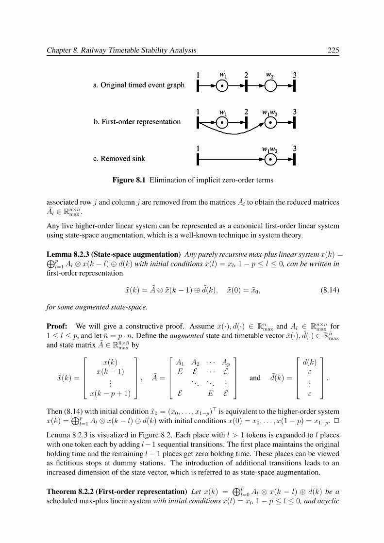
Chapter 8. Railway Timetable Stability Analysis 225
·
1 2 3w1 w2
· ·
1 2 3w1 w1w2
·
1 3w1w2
a. Original timed event graph
b. First-order representation
c. Removed sink
·
1 2 3w1 w2
·
1 2 3w1 w2
· ·
1 2 3w1 w1w2
· ·
1 2 3w1 w1w2
·
1 3w1w2
·
1 3w1w2
a. Original timed event graph
b. First-order representation
c. Removed sink
Figure 8.1 Elimination of implicit zero-order terms
associated row j and column j are removed from the matrices Al to obtain the reduced matrices
Al ∈ Rn×nmax .
Any live higher-order linear system can be represented as a canonical first-order linear system
using state-space augmentation, which is a well-known technique in system theory.
Lemma 8.2.3 (State-space augmentation) Any purely recursive max-plus linear system x(k) =⊕p
l=1Al ⊗ x(k − l)⊕ d(k) with initial conditions x(l) = xl, 1− p ≤ l ≤ 0, can be written in
first-order representation
x(k) = A⊗ x(k − 1)⊕ d(k), x(0) = x0, (8.14)
for some augmented state-space.
Proof: We will give a constructive proof. Assume x(·), d(·) ∈ Rnmax and Al ∈ Rn×n
max for
1 ≤ l ≤ p, and let n = p · n. Define the augmented state and timetable vector x(·), d(·) ∈ Rnmax
and state matrix A ∈ Rn×nmax by
x(k) =
x(k)x(k − 1)
...
x(k − p+ 1)
, A =
A1 A2 · · · Ap
E E · · · E. . .
. . ....
E E E
and d(k) =
d(k)ε...
ε
.
Then (8.14) with initial condition x0 = (x0, . . . , x1−p)> is equivalent to the higher-order system
x(k) =⊕p
l=1Al ⊗ x(k − l)⊕ d(k) with initial conditions x(0) = x0, . . . , x(1− p) = x1−p. 2
Lemma 8.2.3 is visualized in Figure 8.2. Each place with l > 1 tokens is expanded to l places
with one token each by adding l−1 sequential transitions. The first place maintains the original
holding time and the remaining l − 1 places get zero holding time. These places can be viewed
as fictitious stops at dummy stations. The introduction of additional transitions leads to an
increased dimension of the state vector, which is referred to as state-space augmentation.
Theorem 8.2.2 (First-order representation) Let x(k) =⊕p
l=0Al ⊗ x(k − l) ⊕ d(k) be a
scheduled max-plus linear system with initial conditions x(l) = xl, 1− p ≤ l ≤ 0, and acyclic
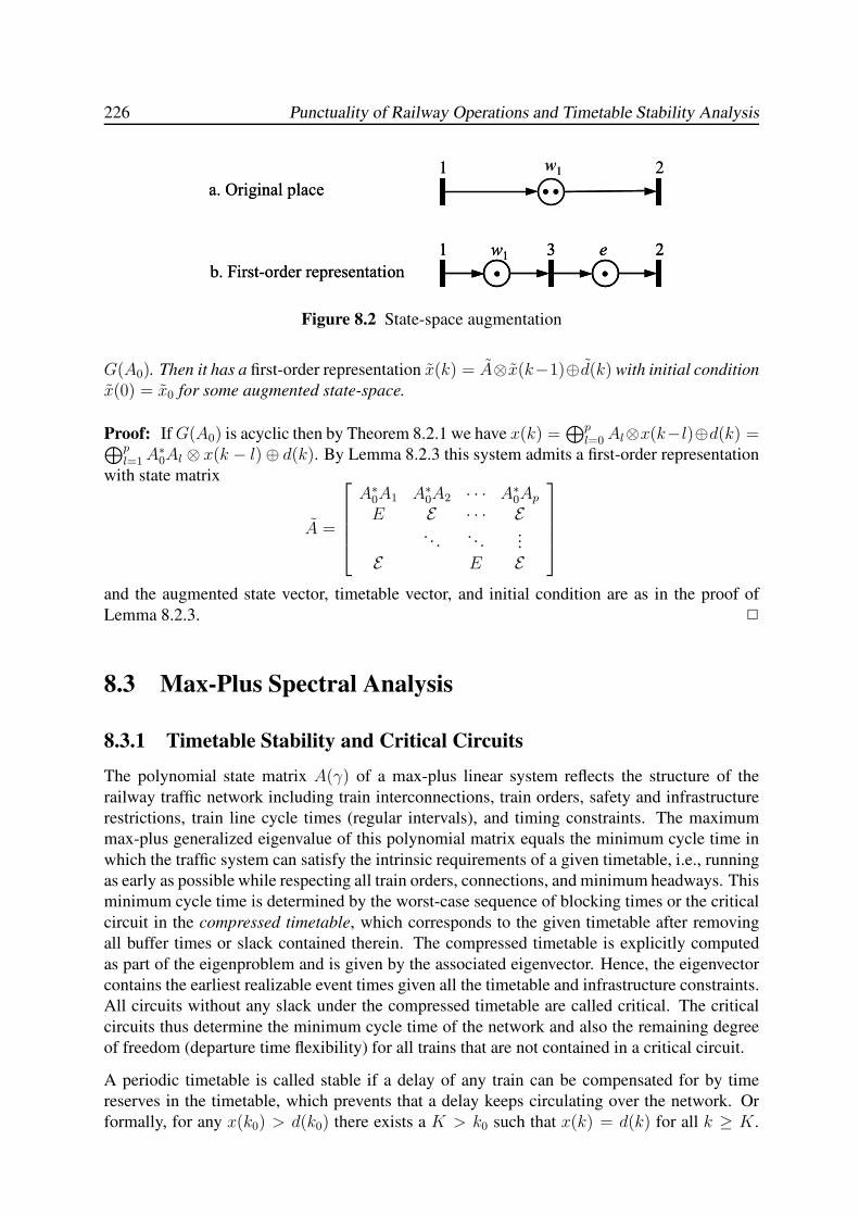
226 Punctuality of Railway Operations and Timetable Stability Analysis
· ·
1 2w1
a. Original place
b. First-order representation · ·
1 3 2w1 e
· ·
1 2w1
a. Original place
b. First-order representation · ·
1 3 2w1 e
· ·
1 3 2w1 e
Figure 8.2 State-space augmentation
G(A0). Then it has a first-order representation x(k) = A⊗x(k−1)⊕d(k) with initial condition
x(0) = x0 for some augmented state-space.
Proof: IfG(A0) is acyclic then by Theorem 8.2.1 we have x(k) =⊕p
l=0Al⊗x(k−l)⊕d(k) =⊕p
l=1A∗0Al ⊗ x(k − l)⊕ d(k). By Lemma 8.2.3 this system admits a first-order representation
with state matrix
A =
A∗0A1 A∗
0A2 · · · A∗0Ap
E E · · · E. . .
. . ....
E E E
and the augmented state vector, timetable vector, and initial condition are as in the proof of
Lemma 8.2.3. 2
8.3 Max-Plus Spectral Analysis
8.3.1 Timetable Stability and Critical Circuits
The polynomial state matrix A(γ) of a max-plus linear system reflects the structure of the
railway traffic network including train interconnections, train orders, safety and infrastructure
restrictions, train line cycle times (regular intervals), and timing constraints. The maximum
max-plus generalized eigenvalue of this polynomial matrix equals the minimum cycle time in
which the traffic system can satisfy the intrinsic requirements of a given timetable, i.e., running
as early as possible while respecting all train orders, connections, and minimum headways. This
minimum cycle time is determined by the worst-case sequence of blocking times or the critical
circuit in the compressed timetable, which corresponds to the given timetable after removing
all buffer times or slack contained therein. The compressed timetable is explicitly computed
as part of the eigenproblem and is given by the associated eigenvector. Hence, the eigenvector
contains the earliest realizable event times given all the timetable and infrastructure constraints.
All circuits without any slack under the compressed timetable are called critical. The critical
circuits thus determine the minimum cycle time of the network and also the remaining degree
of freedom (departure time flexibility) for all trains that are not contained in a critical circuit.
A periodic timetable is called stable if a delay of any train can be compensated for by time
reserves in the timetable, which prevents that a delay keeps circulating over the network. Or
formally, for any x(k0) > d(k0) there exists a K > k0 such that x(k) = d(k) for all k ≥ K.
Chapter 8. Railway Timetable Stability Analysis 227
In particular this implies that for each event i a delay zi(k0) = xi(k0) − di(k0) in some period
k0 must have been (partially) absorbed before it recurs to a next occurrence of this event xi(k)with k > k0. We thus obtain the following definition of stability.
Definition 8.3.1 (Stability) A scheduled max-plus linear system is stable if each circuit in the
associated timed event graph contains some positive buffer time.
Stability can therefore be tested by computing the maximal generalized eigenvalue as presented
in the following theorem.
Theorem 8.3.1 (Stability) Let A(γ) =⊕p
l=0Alγl ∈ Rn×n
max [γ] be a polynomial matrix with
maximum generalized eigenvalue λ0. Then the scheduled max-plus linear system (8.9) is stable
if and only if
λ0 < T.
If λ0 = T the system is called critical, and if λ0 > T the system is unstable.
Proof: By Theorem 7.4.1 the maximum eigenvalue λ0 equals the maximum cycle mean over
all circuits in the network. If λ0 < T then even the critical circuit(s) have some average buffer
time T−λ0 > e, and therefore all circuits have at least T−λ0 > e average buffer time. Note that
the total buffer time on a circuit ξ is µ(ξ) · T − w(ξ) ≤ µ(ξ) · T − µ(ξ) · λ0 = µ(ξ) · (T − λ0),which is positive only if T > λ0. Finally, notice that since λ0 exists G(A0) must be acyclic
and therefore there are no circuits with zero tokens. Hence, we only consider stability for live
systems. 2
Theorem 8.3.1 states that the timetable cycle time should exceed the minimum possible one,
that is, the maximum eigenvalue is the minimum cycle time. Hence, the maximum eigenvalue
allows a stability test: if λ0 exceeds the timetable cycle time T then the system is unstable.
Instability here means that there is no slack on the critical circuit by which delays that reach
the critical circuit can never settle, i.e., all trains on the critical circuit will get delayed and
possibly propagate this delay to other trains in the network. If λ0 < T is close to T then delays
on the critical circuit will settle only slowly and the system will become unstable in case of
(temporary) process time prolongations on the critical circuit.
Stability thus depends on the eigenstructure of the (polynomial) state matrix of the homoge-
neous max-plus linear system x(k) =⊕p
l=0Alx(k − l) = A(γ)x(k). It is insightful to revisit
and interpret the eigenproblem with respect to the dynamic system equations. Recall from
Chapter 7 (Sections 7.4.5 and 7.4.6) that the associated generalized eigenmode (χ, v) satisfies
the conditions (7.39a–7.39b) which we repeat here for convenience:
χi = max(j,i,l)∈Πi
χj and vi = max(j,i,l)∈Πi
([Al]ij − l · χj + vj) for all i = 1, . . . , n. (8.15)
Here χj is the cycle time of event j with λ0 =⊕n
j=1 χj. We now interpret v as an event time
vector. Then (8.15) implies that each event i must wait for the latest preceding activity with
process time [Al]ij that was initiated l periods of length χj ago at event time vj − l · χj . If
A(γ) is irreducible — the timed event graph G(A(γ)) is strongly-connected — all cycle times
are constant χi ≡ λ0 corresponding to the minimal cycle time of all events. The eigenvector
v then corresponds to the earliest possible event times where the events cycle at their minimal
228 Punctuality of Railway Operations and Timetable Stability Analysis
cycle time λ0. In case of delayed events the system may thus ‘accelerate’ with cycle time λ0
until the delays have settled. Note that delayed events consume timetable slack and buffer times
and fire as early as possible until they again meet their schedule. In the reducible case delayed
events of distinct classes may cycle at different cycle times in accordance to the available slack
in the different components. Thus, events of nonbasic classes (with cycle time χj < λ0, see
Section 7.4.4) settle quicker than events of basic classes, whilst critical events on a critical
circuit take longest to settle.
The (maximum) eigenvalue is a unique characteristic of the state matrices of a max-plus linear
system. Hence, the maximum eigenvalue is a performance indicator of the traffic scenario
characterized by the timetable, infrastructure, and signalling system. In particular, like the
state matrices the eigenvalue depends on the line frequencies, line schedules (running times,
minimum dwell times), traffic mix (speed differences) and train orders on the open tracks,
minimum headways, minimum layover times at terminals, minimum transfer times of passenger
connections, and minimum (de-)coupling times of rolling stock connections.
8.3.2 Network Throughput
A performance indicator related to stability is capacity utilization. An indicator for network
capacity utilization of a periodic railway system is the network throughput defined as (using
conventional division)
ρ = λ0/T,
where λ0 is the minimum cycle time and T the timetable cycle time. For a stable railway system
we have 0 < ρ ≤ 1 , where ρ = 1 corresponds to the saturated case in which the mean cycle time
of trains on the critical circuit is exactly (a multiple of) T . If ρ < 1 the system operates below its
maximum (theoretical) performance and hence contains buffer time to compensate for delays.
Clearly, the network throughput represents a trade-off between stability and capacity utilization.
The higher this measure the more effective the train circulations but the less slack is available
for delay recovery.
In current daily railway practice throughput is a more recognizable quantity than the minimum
cycle time. For instance a throughput of 70% implies that the infrastructure on the worst-case
circuit is utilized for 70% and the remaining 30% is buffer time to avoid or reduce hindrance.
Network throughput refers to the throughput of the critical circuit. A large throughput on this
circuit does not necessarily mean that the throughput on any corridor (which can be seen as a
subnetwork) is also this high. It is therefore also relevant which transportation links make up
the critical circuit, and how the critical cycle time relates to the cycle times of train lines and
corridors or other subnetworks. The cycle times, and hence throughputs, of train lines are easily
obtained when connections and headway are discarded: the circuits are then exactly the train
line circulations (assuming layover times are included).
8.3.3 Stability Margin
The difference ∆1 = T − λ0 gives the average amount of slack on the critical circuit(s) and
hence is a measure of robustness or sensitivity to delays. In particular, ∆1 is the marginal
Chapter 8. Railway Timetable Stability Analysis 229
increase of each active holding time such that the timetable becomes critical, i.e., ∆1 is the
solution to
maxξ∈C
w(ξ) + µ(ξ) ·∆1
µ(ξ)= max
ξ∈C
w(ξ)
µ(ξ)+ ∆1 = λ0 + ∆1 = T.
Another indicator of robustness is the stability margin ∆2 defined as the maximum simultaneous
increase of all process times such that the train network can still be operated with cycle time T ,
or formally, ∆2 is the solution to the problem (∆2⊗A(T−1))⊗v = v. Note the difference with
∆1 = T − λ which is defined relative to the marking in each place. Hence, ∆1 relates to the
number of trains (tokens) on each circuit whereas ∆2 takes all stops (events) into account. The
stability margin ∆2 can be computed by solving an auxiliary eigenvalue problem as presented
in the following theorem.
Theorem 8.3.2 (Stability margin) Let (8.9) be a stable scheduled max-plus linear system. Then
the stability margin ∆2 is given by ∆2 = ν−1, where ν is the solution of the eigenvalue problem
AT ⊗ v = ν ⊗ v.
Proof: The stability margin ∆2 is the implicit least solution of (∆2 ⊗ AT ) ⊗ v = e ⊗ v. The
max-plus matrix ∆2 ⊗ AT corresponds to the precedence graph G(AT ) where each arc weight
is increased by ∆2. Hence, by Theorem 7.4.1 we have
maxξ∈C
w(ξ)− µ(ξ) · T + l(ξ) ·∆2
l(ξ)= max
ξ∈C
w(ξ)− µ(ξ) · Tl(ξ)
+ ∆2 = e,
with solution ∆2 = −maxξ∈C(w(ξ)−µ(ξ)·T )/l(ξ), which is exactly the inverse of the solution
ν to the eigenvalue problem AT ⊗ v = ν ⊗ v. Hence ∆2 = ν−1 = −ν. 2
In first-order linear systems x(k) = Ax(k − 1) the number of places and tokens on each circuit
ξ is the same, l(ξ) = µ(ξ), and therefore ∆2 = ∆1. In a first-order state-space representation
the number of events is thus reduced to the number of initial tokens.
8.4 Timetable Realizability
In this section we focus on the timetable system {d(k)}k∈N. Hence, we assume that A(γ) is a
given polynomial state matrix and derive conditions on the timetable vectors d(k) such that the
scheduled max-plus linear system
x(k) = A(γ)x(k)⊕ d(k) for all k ∈ N (8.16)
is well-defined. We will concentrate on periodic timetables that satisfy the first-order state
equations d(k) = d(k − 1) ⊗ T , d(0) = d0. From Section 8.2.1 we know that the solution of
this timetable system is
d(k) = d0 ⊗ T k, k ∈ N.
The characteristic parameters of a periodic timetable are thus the initial timetable vector d0 and
the cycle time T . If required the timetable sequence may be extended to the left by allowing
periods k ∈ Z.
230 Punctuality of Railway Operations and Timetable Stability Analysis
A timetable only makes sense if the system is able to operate according to the timetable. This
means that for each marked arc (j, i, l) ∈ supp(A(γ))
di(k) ≥ [Al]ij ⊗ dj(k − l) for all k ∈ Z. (8.17)
Timetables satisfying this condition are called realizable [21].
Definition 8.4.1 (Timetable realizability) A sequence {d(k)}k∈Z is called a realizable timetable
for the scheduled max-plus linear system (8.16) if
d(k) ≥ A(γ)d(k) for all k ∈ Z. (8.18)
The scheduled system (8.16) is called realizable if it has a realizable timetable.
Theorem 8.4.1 (Realizable periodic timetable) A periodic timetable d(k) = d0 ⊗ T k, k ∈ Z,
is realizable for a scheduled max-plus linear system x(k) = A(γ)x(k) ⊕ d(k) if and only if d0
is a generalized subeigenvector of A(γ) associated to T , i.e.,
d0 ≥ A(T−1)⊗ d0. (8.19)
Proof: Assume d(·) is a realizable periodic timetable. Then for all k ∈ Z
d(k) ≥ A(γ)d(k) =
p⊕
l=0
Ald(k − l) =
p⊕
l=0
Ald0Tk−l =
p⊕
l=0
AlT−ld0T
k = A(T−1)d(k).
In particular, for k = 0 we obtain inequality (8.19). Hence, for a periodic timetable the condi-
tions (8.18) and (8.19) are equivalent. 2
By Theorem 8.4.1 any finite (sub)eigenvector of the polynomial state matrix A(γ) associated to
T is a realizable timetable to the scheduled system (8.16). Moreover, a realizable timetable is
never unstable as stated in the following Theorem.
Theorem 8.4.2 A scheduled max-plus linear system with a realizable periodic timetable d(k) =d0 ⊗ T k for k ∈ Z is either stable or critical, i.e., T ≥ λ0.
Proof: By Theorem 8.4.1 a periodic timetable is realizable iff d0 ∈ Rnmax is a subeigenvector of
A(γ) associated to T . Then by Theorem 7.4.4 we must have T ≥ λ0, where λ0 is the maximal
generalized eigenvalue ofA(γ), and finally by Theorem 8.3.1 the system is stable except for the
critical case T = λ0. 2
The inequality (8.18), or equivalently (8.17), implies that a realizable timetable contains some
nonnegative slack time in each process from one event to another. For a periodic timetable we
can rewrite (8.17) as di(k) ≥ dj(k) + [Al]ij − l · T for all k ∈ Z, or equivalently
di(k)− dj(k)− [Al]ij + l · T ≥ 0 for all k ∈ Z. (8.20)
The actual slack time from j to imay be less because of a tighter process (sequence) from event
j to i. This is the topic of Section 8.5. Also note that a realizable timetable implies that when
Chapter 8. Railway Timetable Stability Analysis 231
all trains are able to depart according to schedule at some period then this will also be realized
for any future period.
The derivation of a scheduled max-plus linear system and in particular the determination of the
initial marking typically assumes a feasible timetable, cf. Algorithm 6.5.1 and Theorem 6.5.1.
However, the (process time) input data for the timed event graph construction may differ from
the process times applied during evaluation. The construction is based on the scheduled process
times. Once the system has been generated the process times may be adjusted without changing
the initial marking. For robustness studies the running times may be decreased by their running
time margins and for capacity tests the minimum headway times can be reset to the capacity
allocation norms. Realizability of the adjusted system is then no longer trivial.
8.5 Timetable Robustness
8.5.1 The Recovery Matrix
A timetable generally contains slack to recover from delays after disruptions. Slack time can
be incorporated within scheduled process times (running time margins) or between train move-
ments (buffer times). Moreover, a sequence of train runs embraces an accumulation of slack
times. Timetable robustness against delay propagation is therefore determined by accessibility
relations between events and the amount of available slack time on paths from one event to an-
other. Since in general multiple paths exist between pairs of timetable events we are interested
in the critical path from one event to another that has the least accumulated slack time over all
possible paths. This is the topic of this section.
In this section we assume that d(·) is a periodic timetable with cycle time T and finite initial
timetable vector d0 > ε, and consider the scheduled max-plus linear system
x(k) = A(γ)x(k)⊕ d(k), d(k) = d0 ⊗ T k for all k ∈ N. (8.21)
We write d0 = (d01, . . . , d
0n)
>. By definition, if di(k) ∈ [0, T ) for some 1 ≤ i ≤ n then
dj(k) ∈ [0, T ) for all 1 ≤ j ≤ n. Moreover, each two events in a periodic timetable have a
regular interval, i.e., for all 1 ≤ i, j ≤ n event time differences satisfy d0i − d0
j = di(k)− dj(k)for all k ∈ Z. Without loss of generality, we may assume that d0 ∈ [0, T )n denotes the timetable
vector over the basic period [0, T ).
In the sequel, we refer to the slack time of two adjacent events as the sum of process time margin
and buffer time. Recovery time will be used in a more wide sense as follows [207].
Definition 8.5.1 (Recovery matrix) The recovery matrix R = (rij) is the n × n dimensional
matrix of (cumulative) recovery times, where rij is the minimum total slack time over all paths
from event j to i in the timed event graph G(A(γ)) associated to the scheduled max-plus linear
system (8.21).
An alternative interpretation of the recovery matrix is that rij is the largest delay of xj(k) in
some period k ∈ N that will not reach xi(m) for all m ≥ k. If there is no path from event jto i then delays of event j will never reach i and so rij = ∞. The recovery matrix thus takes
232 Punctuality of Railway Operations and Timetable Stability Analysis
values from the extended set Rmax.= Rmax ∪ {∞}, or from [e,∞) if the timetable is realizable,
cf. (8.20). In fact, the recovery matrix is defined as a shortest path problem which corresponds
to the so-called min-plus algebra Rmin = (R∪ {∞},min,+), which is an idempotent semiring
dual to the max-plus algebra. We will however stay within the framework of the (extended)
max-plus algebra by using the identity min(a, b) = −max(−a,−b) for all a, b ∈ Rmax, where
by convention−ε =∞.
The following theorem characterizes the entries of a recovery matrix [207, 89].
Theorem 8.5.1 Let (8.21) be a stable scheduled max-plus linear system. Then the associated
recovery matrix R = (rij) ∈ Rn×nmax is defined by
rij = d0i − d0
j − [A+T ]ij, (8.22)
where rij =∞ if there is no path from j to i in the timed event graph G(A(γ)).
Proof: By the stability assumption T > λ and therefore A+T = A+(T−1) = [
⊕pl=0AlT
−l]+ is
well-defined. By definition, the entry rij is the minimal cumulative slack over all paths from jto i in G(A(γ)). Let Pij be the set of all paths from j to i, and for any path ξ ∈ Pij denote by
w(ξ) the weight of path ξ and by µ(ξ) the initial marking on path ξ. Then for all k ∈ N
rij = minξ∈Pij
[di(k + µ(ξ))− dj(k)− w(ξ)]
= minξ∈Pij
[(d0
i + (k + µ(ξ)) · T )− (d0j + k · T )− w(ξ)
]
= minξ∈Pij
[d0
i − d0j − w(ξ) + µ(ξ) · T
]
= d0i − d0
j −maxξ∈Pij
[w(ξ)− µ(ξ) · T ]
= d0i − d0
j − [A+T ]ij .
If there is no path from j to i then [A+T ]ij = ε, and by convention rij = d0
i − d0j − [A+
T ]ij =d0
i − d0j − ε =∞. 2
Theorem 8.5.1 shows that a recovery time depends on the cycle time T ∈ R+, the polynomial
state matrix A(γ) ∈ Rn×nmax [γ], and the scheduled event times of the origin j and destination i,
but not on the exact timetable of intermediate events. In the proof of Theorem 8.5.1 we used
stability but did not need realizability. If a timetable is unrealizable then recovery times may
be negative, i.e., there exist paths j → i such that rij < 0. Nevertheless, if the timetable is
(partially) unrealizable but stable it can still be robust when the recovery times are positive for
almost all connected event pairs inG(AT ). Of course, the unrealizable arcs will always generate
a (small) delay but depending on the slack of adjacent arcs this delay may be absorbed quickly
which prevents delay propagation over large areas. Unrealizable train runs may formally oc-
cur in the timetable when infrastructure conflicts are not solved in the timetable design. This
occurs for instance in the flexible time-window philosophy of dynamic railway traffic manage-
ment [179]: route conflicts are solved by dispatchers in short-term rescheduling depending on
the actual train positions during operation, e.g. on basis of a first-come first-served (FCFS)
principle.
By Theorem 8.5.1 computation of the recovery matrix R involves solving an (all-pair) longest
path problem over the graph G(AT ). If AT is stable then G(AT ) does not contain positive
Chapter 8. Railway Timetable Stability Analysis 233
(weight) circuits, which is a necessary condition for the existence of finite longest paths. Nev-
ertheless, G(AT ) generally contains positive arc weights (in conventional sense). For example,
for each (j, i) ∈ supp(A0) we have [AT ]ij =⊕p
l=0[AlT−l]ij = [A0]ij ⊕
⊕pl=1[AlT
−l]ij ≥[A0]ij ≥ e. We can use the Floyd-Warshall algorithm to compute the longest path matrix A+
T in
O(n3) time [3, 39]. However, the matrices AT ∈ Rn×nmax are typically very large and sparse, i.e.,
m� n2, where m is the number of finite matrix entries (arcs). In this case, it is more efficient
to solve the all-pair longest path problem by a repeated single-origin (or single-destination)
longest path algorithm. Implementations of Dijkstra’s label-setting algorithm [56, 3, 39] are
particularly efficient in both running time and memory usage. However, Dijkstra’s longest path
algorithm is restricted to graphs with nonpositive arc weights only1
If d0 > ε is a realizable timetable then we can use the timetable vector d0 to compute nonpositive
reduced arc weights while leaving the longest paths invariant.
Lemma 8.5.1 (Slack Matrix) Let (8.21) be a realizable scheduled max-plus linear system and
define the slack matrix S = (sij) ∈ Rn×nmax by
sij = d0j − d0
i + [AT ]ij . (8.23)
Then S satisfies
(i) sij ≤ e for all 1 ≤ i, j ≤ n,
(ii) the precedence graph G(S) has no positive-weight circuits,
(iii) [S+]ij = d0j − d0
i + [A+T ]ij for all 1 ≤ i, j ≤ n.
Proof: The realizability assumption implies d0i ≥ d0
j + [AT ]ij and therefore sij = d0j − d0
i +[AT ]ij ≤ e for all 1 ≤ i, j ≤ n, which proves (i). By (i) the graph G(S) has nonpositive arc
weights only and therefore the weight of each path or circuit in G(S) will also be nonnegative,
which proves property (ii). From Proposition 7.2.6 and property (ii) follows that S+ exists and
is given by S+ =⊕n
l=1 Sl. Also A+
T = A(T−1)+ is well-defined which is proved as follows.
By Corollary 8.4.2 we have T ≥ λ0(A(γ)) and therefore λ0(AT ) ≤ e. Hence, the maximum
cycle mean of G(AT ) is at most e and so all circuits in G(AT ) must have nonpositive weight,
by which A+T =
⊕nl=1A
lT using Proposition 7.2.6. It remains to prove that the equality (iii)
is valid. Obviously, sij = ε iff [AT ]ij = ε. Hence, the precedence graph G(S) equals G(AT )except for an arc reweighting. Now, let Pij be the set of all paths from j to i in G(S). Then the
path weight w(ξ) of any path ξ = (j = i0, i1, . . . , il = i) ∈ Pij of some length l = l(ξ) satisfies
w(ξ) =
l(ξ)∑
k=1
sikik−1=
l(ξ)∑
k=1
(
d0ik−1− d0
ik+ [AT ]ikik−1
)
= d0j − d0
i +
l(ξ)∑
k=1
[AT ]ikik−1.
Hence, the weight of a path ξ in G(S) equals its weight in G(AT ) plus a constant term d0j − d0
i
that only depends on the initial and final node of the path. Since ξ ∈ Pij was arbitrary, this
holds for all paths from j to i of any length and in particular for the maximum-weight paths,
which proves (iii). 2
1Recall that the discussion of path algorithms and data structures in the max-plus algebra setting distinguishes
from the common literature on two points: (1) Algorithms and data structures are usually formulated in terms of
shortest-path problems over graphs with no negative circuits. (2) The usual representation of arcs in adjacency
matrices or lists is reversed
234 Punctuality of Railway Operations and Timetable Stability Analysis
Theorem 8.5.2 If the scheduled max-plus linear system (8.21) is realizable then the recovery
matrix R = (rij) is well-defined by rij = −[S+]ij .
Proof: The theorem follows immediately from Theorem 8.5.1 and Lemma 8.5.1(iii). 2
As a consequence of Theorem 8.5.2 the recovery matrix R can be computed as the solution
to a longest path problem over a graph with nonpositive arc weights only. For this problem
any longest (or shortest) path algorithm can be used. The best worst-case running time is
O(nm+n2 log n) obtained by repetitively using a Fibonacci heap implementation of Dijkstra’s
algorithm [67]. However, for large networks computing and storing the complete recovery ma-
trix takes much computing time and storage space. Note that even if the matrix AT is sparse
this will generally not be the case for the recovery matrix R. In particular if AT is irreducible
then R is a full matrix and thus needs a storage space of O(n2).
In practice we are only interested in special parts of the matrix R which can better be computed
on demand rather than precomputing and storing the full recovery matrix in advance. In par-
ticular we are interested in only a limited number of rows or columns or in the diagonal of the
recovery matrix R, which have different practical interpretations. We next have a closer look at
the interpretation of the matrix entries depending on their location in the matrix.
8.5.2 Delay Impact Vectors
Each jth column of the recovery matrix gives the recovery time from event j to all other events
in the timetable. Hence, column j represents the impact that a delay of event j will have on
future train events. An entry rij is the maximum delay of event j that can be compensated
before reaching event i. If event j has a delay zj(k) ≥ 0 in some period k then event i will be
delayed by zi(m) = max(zj(k) − rij , 0) at some period m ≥ k, i.e., if zj(k) ≤ rij then the
delay will have been absorbed before reaching event i and otherwise event i will suffer a delay
of zj(k)− rij ≥ 0.
A column j of the recovery matrix can thus be interpreted as a delay impact vector. The finite
entries of this vector correspond to the events that are accessible from j and the values represent
the impact that a delay of event j will have. Of special interest are recovery times below some
threshold value δ, which specifies an impact region at level δ:
Iδ(j).= {i | rij ≤ δ, 1 ≤ i ≤ n}.
For example, the impact region I3(j) gives a neighbourhood of less than 3 minutes recovery
time from event j.
The delay impact vector and associated impact regions give a quick insight view on the impact
of individual delayed events. Since a delay impact vector is just a column of the recovery
matrix it can be computed by the SINGLEORIGINLONGESTPATH algorithm of Section 7.5.2
for the origin j in O(nj log nj) time, where nj ≤ n is the number of events accessible from j.
8.5.3 Delay Sensitivity Vectors
Each ith row of the recovery matrix gives the recovery time to event i from all other events in
the timetable. Hence, row i represents the sensitivity of event i on delays of preceding events.
Chapter 8. Railway Timetable Stability Analysis 235
In this case, event i will receive a delay zi(m) = max(zj(k) − rij , 0) from a previous event
j that was delayed by zj(k) in some period k ≤ m. So again, if zj(k) ≤ rij then the delay
will have been absorbed before reaching event i and otherwise event i will suffer a delay of
zj(k)− rij ≥ 0.
A row i of the recovery matrix can thus be interpreted as a delay sensitivity vector. The finite
entries of this vector correspond to the events that have access to i and the values represent the
sensitivity of event i on these preceding events. A critical set of events can be defined for which
the recovery times to i are below some threshold value δ. This results in a sensitivity region at
level δ:
Sδ(i).= {j | rij ≤ δ, 1 ≤ j ≤ n}.
For example, the sensitivity region S3(i) gives a neighbourhood of less than 3 minutes recovery
time to event i.
The delay sensitivity vector and associated sensitivity regions quantify the vulnerability of an
event on preceding events. A delay sensitivity vector is a row of the recovery matrix and can
be computed by a single-destination longest path algorithm, or equivalently by a single-origin
longest path algorithm in the graph G(AT ) obtained by reversing all arcs. Hence, a sensitivity
vector can be computed by the SINGLEORIGINLONGESTPATH algorithm of Section 7.5.2 for
G(AT ) and the origin i in O(ni log ni) time, where ni ≤ n is the number of events that have
access to i.
8.5.4 Circulation Recovery Times
Each diagonal entry of the recovery matrix gives the recovery time over all possible paths from
an event i back to event i. The diagonal thus represents the circulation recovery times of all
events in the timetable. The circulation recovery time is an absolute robustness measure for each
periodic event separately and represents the maximum delay that can be absorbed by available
slack in the timetable. Any larger delay will backfire (in reduced form) over some path (circuit)
in the timetable.
The main issue in stability analysis is the circulation of delays over the network. If a delay
keeps circulating over a circuit then all trains on this circuit keep departing delayed. In the
spectral analysis of Sections 7.4 and 8.3 we considered critical circuits that have the smallest
average amount of slack. The circulation recovery time gives a second-order stability test. In
first instance an event is critical if it is part of a critical circuit with minimal stability margin.
Recall that the stability margin is an integrated measure for all events on a critical circuit. In
contrast, the circulation recovery time may vary for all critical events on the critical circuit(s).
Hence, of all critical events the events with minimal circulation recovery time are the most
jeopardizing to stability.
The circulation recovery times of all events are exactly the diagonal entries of the recovery
matrix. Thus, the circulation recovery vector can be computed by the ALLLONGESTCIRCUITS
algorithm of Section 7.5.3.
236 Punctuality of Railway Operations and Timetable Stability Analysis
8.6 Delay Propagation
8.6.1 Introduction
The recovery matrix R = (rij) consists of the maximum delays that can be recovered between
any two pairs of events in the network. So if an initial delay of a train j exceeds the recovery
time rij then the delay will propagate to train i. Nevertheless, from the recovery matrix we still
do not know when this train will be delayed and whether the train is delayed more than once by
cyclic delay propagation or by initial delays of different trains. Hence, the recovery matrix gives
a quick insight in the impact and sensitivity of delays but does not facilitate detailed propagation
of delays over time and the network.
A delay propagation model explicitly computes the propagation of initial delays over space
and time. Given any combination of initial delays a delay propagation model determines all
arrival and departure delays of each train at each station over each subsequent period and thus
also the settling time (or more precisely the settling period) after which all delays have been
absorbed by available timetable slack. The max-plus dynamic equations provide an effective
delay propagation model, which will be discussed in this section.
This delay propagation model can be applied to derive stability tests. An appropriate measure
is for instance the stability quotient defined as the number of periods needed before an initial
delay of some fixed value settles, see Pachl [158, §6.6]. For example, the German Railways rec-
ommend a stability quotient less than 2 for an initial delay of 10 minutes, which implies that any
delay of 10 minutes should be completely compensated for within two timetable periods [158].
The delay propagation model can also be used for computing the optimal train waiting times
and passenger delays [79, 96, 52]. Furthermore, several variants can be computed where for
instance all trains wait for delayed feeder trains, transfer connections are cancelled, or reserve
rolling stock can be assigned at line ends. The delay propagation is then computed for a number
of models with different state matrices corresponding to removed or adjusted connections (arcs)
which are compared with respect to some objective function.
8.6.2 The Delay Propagation Model
Assume d0 > ε and consider the scheduled max-plus linear system with a special output vector
z(k) containing the delays in period k:
x(k) = A(γ)x(k)⊕ d(k), k ∈ N
d(k) = d0 ⊗ T k, k ∈ N
z(k) = D−1(k)⊗ x(k), k ∈ N
x(1−) = x1, x(l) = xl, 1− p ≤ l ≤ 0,
(8.24)
whereD−1(k) = diag(d−11 (k), . . . , d−1
n (k)). Hence, z(k) is the delay vector of events scheduled
in period k with entries
zi(k) = d−1i (k)⊗ xi(k) = xi(k)⊗ d−1
i (k) = xi(k)− di(k).
Note that the dynamic state-space equation implies x(k) ≥ d(k) and therefore zi(k) ≥ e for all
1 ≤ i ≤ n. The inverse matrix is well-defined for any diagonal matrix D ∈ Rn×nmax with finite
Chapter 8. Railway Timetable Stability Analysis 237
diagonal entries. Hence as the notation suggests D−1(k) is the inverse matrix of the diagonal
matrix
D(k) = diag(d(k)) =
d1(k) E. . .
E dn(k)
= T k ⊗
d01 E
. . .
E d0n
.
The initial conditions may be given in terms of the initial delay vectors z1, z0, . . . , z1−p ∈ Rn+ of
delays that reach events in the first (current) timetable period or beyond. The initial state vectors
are then computed as xl = D(l)⊗zl for 1−p ≤ l ≤ 1, whereD(l) = diag(d(l)) = T l⊗diag(d0)is the left-continuation of the timetable system to the last periods l = 1, 0, . . . , 1− p. If we are
only interested in a subset of delays or if d0 ≯ ε then we may define the delay vector with
respect to a suitable output vector y(k) = C ⊗ x(k) as z(k) = D−1(k)⊗ y(k), where D(·) is a
diagonal matrix of the scheduled event times corresponding to the outputs yi(·).Particular attention must be given to the initial state vector x1. Assume that at some reference
time t0 (e.g. the current time) we know or have a prediction of the delays of all events scheduled
up to t0. Without loss of generality we assume that t0 occurs in the first period of the max-plus
model, t0 ∈ [0, T ). Then the initial conditions to the max-plus linear system (8.24) are the event
time vectors of the last p periods x1−p, . . . , x0 such that x(l) = xl for l = 1 − p, . . . , 0, and an
initial vector x1 that partially determines the state x(1) for the events scheduled up to t0. Writing
x1 = (x11, . . . , x
1n)>, we have xi(1) = x1
i for those events 1 ≤ i ≤ n that have a scheduled event
time di(1) ∈ [0, t0], since these event times are known at time t0 by assumption. The event times
of the remaining events i are still unknown at time t0 and depend on both the delayed events
of preceding processes that were initiated before time t0 as well as on the delay propagation
within (the second part of) the first period over (t0, T ). Since we have no information on the
event times scheduled after t0 they are given an initial estimate x1i = di(1), corresponding to
the scheduled event times, and we thus have xi(1) ≥ x1i for all i with di(1) > t0. Hence, we
denote by x(1−) = x1 the partially known state vector at time t0.
The general pth-order state-space equations contain (many) zero-order terms. Theoretically, we
can eliminate these implicit terms from the dynamic model and obtain a purely recursive state-
space realization, see Section 8.2.5. However, we then also loose the possibility of taking into
account initial delays in the first period. Moreover, this procedure aggregates the propagation of
delays within a timetable period. We will therefore keep the zero-order terms in the max-plus
model to correctly represent and compute the propagation of delays over all events.
The following theorem gives a recursive procedure for computing the delay propagation that
correctly incorporates the partial initial state vector x1 of the first period. Recall that the (transi-
tive closure) matrix A∗0 of a matrix A0 with acyclic precedence graph can be computed in linear
O(n+m) time using a topological ordering algorithm [3].
Theorem 8.6.1 Consider a realizable scheduled max-plus linear system (8.24) with acyclic
G(A0) and initial state vectors xl, 1 − p ≤ l ≤ 1. Then the state trajectory {x(k)}k∈N is
recursively determined by x(1− p) = x1−p, . . . , x(0) = x0,
x(1) = A∗0 ⊗
(
x1 ⊕p⊕
l=1
Alx1−l
)
⊕ d(1)
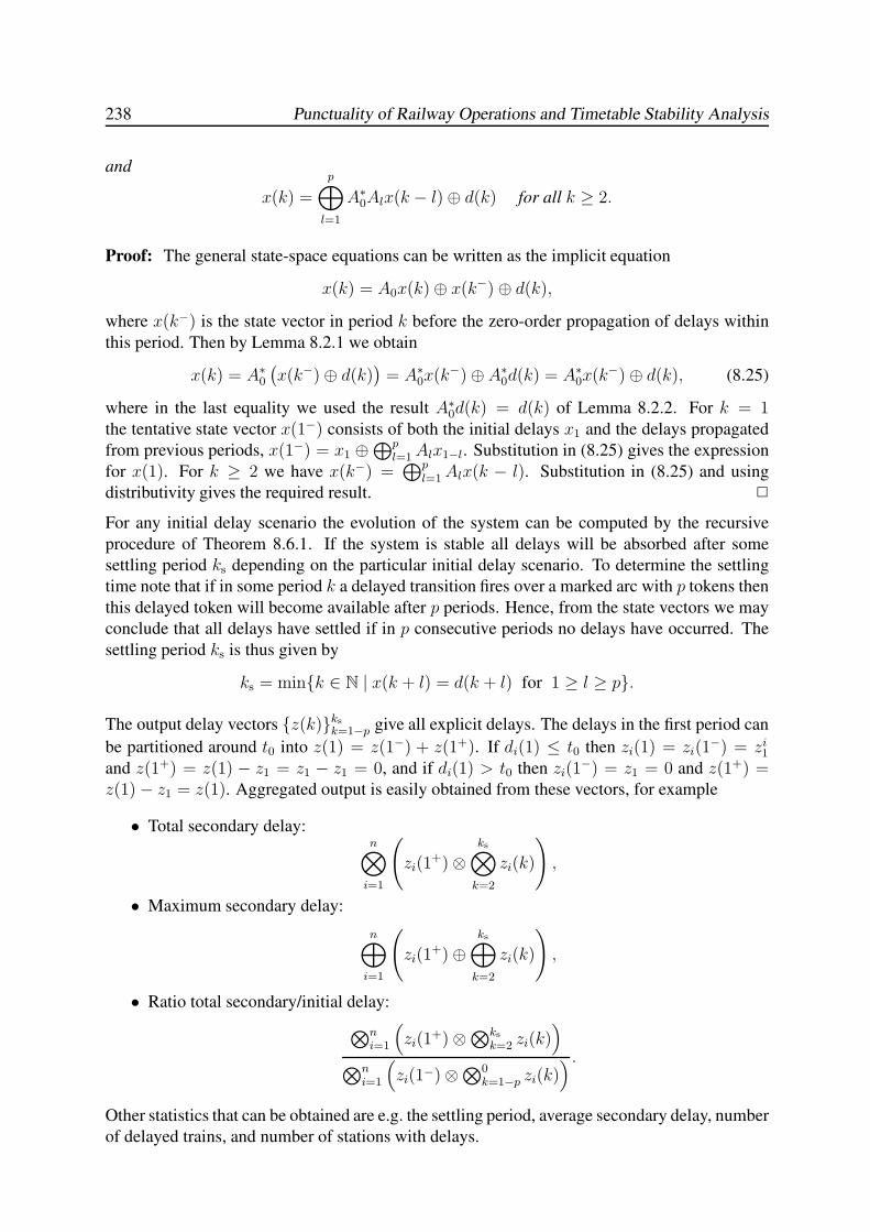
238 Punctuality of Railway Operations and Timetable Stability Analysis
and
x(k) =
p⊕
l=1
A∗0Alx(k − l)⊕ d(k) for all k ≥ 2.
Proof: The general state-space equations can be written as the implicit equation
x(k) = A0x(k)⊕ x(k−)⊕ d(k),where x(k−) is the state vector in period k before the zero-order propagation of delays within
this period. Then by Lemma 8.2.1 we obtain
x(k) = A∗0
(x(k−)⊕ d(k)
)= A∗
0x(k−)⊕A∗
0d(k) = A∗0x(k
−)⊕ d(k), (8.25)
where in the last equality we used the result A∗0d(k) = d(k) of Lemma 8.2.2. For k = 1
the tentative state vector x(1−) consists of both the initial delays x1 and the delays propagated
from previous periods, x(1−) = x1 ⊕⊕p
l=1Alx1−l. Substitution in (8.25) gives the expression
for x(1). For k ≥ 2 we have x(k−) =⊕p
l=1Alx(k − l). Substitution in (8.25) and using
distributivity gives the required result. 2
For any initial delay scenario the evolution of the system can be computed by the recursive
procedure of Theorem 8.6.1. If the system is stable all delays will be absorbed after some
settling period ks depending on the particular initial delay scenario. To determine the settling
time note that if in some period k a delayed transition fires over a marked arc with p tokens then
this delayed token will become available after p periods. Hence, from the state vectors we may
conclude that all delays have settled if in p consecutive periods no delays have occurred. The
settling period ks is thus given by
ks = min{k ∈ N | x(k + l) = d(k + l) for 1 ≥ l ≥ p}.
The output delay vectors {z(k)}ks
k=1−p give all explicit delays. The delays in the first period can
be partitioned around t0 into z(1) = z(1−) + z(1+). If di(1) ≤ t0 then zi(1) = zi(1−) = zi
1
and z(1+) = z(1) − z1 = z1 − z1 = 0, and if di(1) > t0 then zi(1−) = z1 = 0 and z(1+) =
z(1)− z1 = z(1). Aggregated output is easily obtained from these vectors, for example
• Total secondary delay:n⊗
i=1
(
zi(1+)⊗
ks⊗
k=2
zi(k)
)
,
• Maximum secondary delay:
n⊕
i=1
(
zi(1+)⊕
ks⊕
k=2
zi(k)
)
,
• Ratio total secondary/initial delay:
⊗ni=1
(
zi(1+)⊗⊗ks
k=2 zi(k))
⊗ni=1
(
zi(1−)⊗⊗0k=1−p zi(k)
) .
Other statistics that can be obtained are e.g. the settling period, average secondary delay, number
of delayed trains, and number of stations with delays.
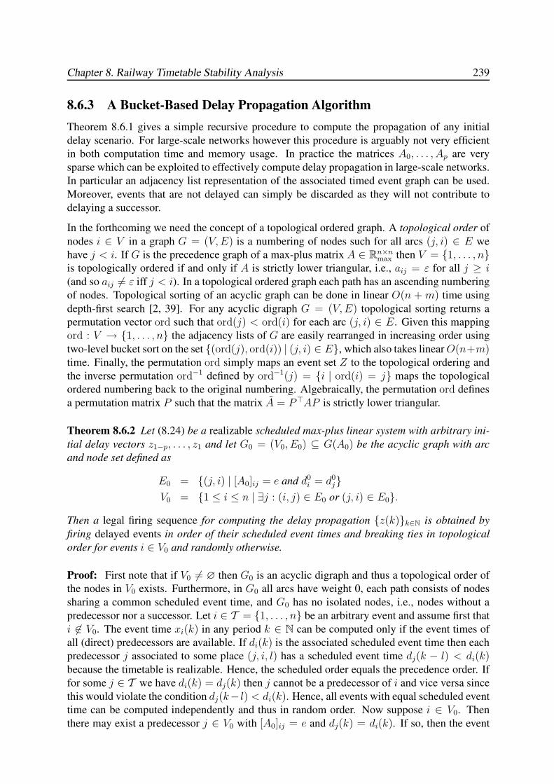
Chapter 8. Railway Timetable Stability Analysis 239
8.6.3 A Bucket-Based Delay Propagation Algorithm
Theorem 8.6.1 gives a simple recursive procedure to compute the propagation of any initial
delay scenario. For large-scale networks however this procedure is arguably not very efficient
in both computation time and memory usage. In practice the matrices A0, . . . , Ap are very
sparse which can be exploited to effectively compute delay propagation in large-scale networks.
In particular an adjacency list representation of the associated timed event graph can be used.
Moreover, events that are not delayed can simply be discarded as they will not contribute to
delaying a successor.
In the forthcoming we need the concept of a topological ordered graph. A topological order of
nodes i ∈ V in a graph G = (V,E) is a numbering of nodes such for all arcs (j, i) ∈ E we
have j < i. If G is the precedence graph of a max-plus matrix A ∈ Rn×nmax then V = {1, . . . , n}
is topologically ordered if and only if A is strictly lower triangular, i.e., aij = ε for all j ≥ i(and so aij 6= ε iff j < i). In a topological ordered graph each path has an ascending numbering
of nodes. Topological sorting of an acyclic graph can be done in linear O(n + m) time using
depth-first search [2, 39]. For any acyclic digraph G = (V,E) topological sorting returns a
permutation vector ord such that ord(j) < ord(i) for each arc (j, i) ∈ E. Given this mapping
ord : V → {1, . . . , n} the adjacency lists of G are easily rearranged in increasing order using
two-level bucket sort on the set {(ord(j), ord(i)) | (j, i) ∈ E}, which also takes linearO(n+m)time. Finally, the permutation ord simply maps an event set Z to the topological ordering and
the inverse permutation ord−1 defined by ord−1(j) = {i | ord(i) = j} maps the topological
ordered numbering back to the original numbering. Algebraically, the permutation ord defines
a permutation matrix P such that the matrix A = P>AP is strictly lower triangular.
Theorem 8.6.2 Let (8.24) be a realizable scheduled max-plus linear system with arbitrary ini-
tial delay vectors z1−p, . . . , z1 and let G0 = (V0, E0) ⊆ G(A0) be the acyclic graph with arc
and node set defined as
E0 = {(j, i) | [A0]ij = e and d0i = d0
j}V0 = {1 ≤ i ≤ n | ∃j : (i, j) ∈ E0 or (j, i) ∈ E0}.
Then a legal firing sequence for computing the delay propagation {z(k)}k∈N is obtained by
firing delayed events in order of their scheduled event times and breaking ties in topological
order for events i ∈ V0 and randomly otherwise.
Proof: First note that if V0 6= ∅ then G0 is an acyclic digraph and thus a topological order of
the nodes in V0 exists. Furthermore, in G0 all arcs have weight 0, each path consists of nodes
sharing a common scheduled event time, and G0 has no isolated nodes, i.e., nodes without a
predecessor nor a successor. Let i ∈ T = {1, . . . , n} be an arbitrary event and assume first that
i 6∈ V0. The event time xi(k) in any period k ∈ N can be computed only if the event times of
all (direct) predecessors are available. If di(k) is the associated scheduled event time then each
predecessor j associated to some place (j, i, l) has a scheduled event time dj(k − l) < di(k)because the timetable is realizable. Hence, the scheduled order equals the precedence order. If
for some j ∈ T we have di(k) = dj(k) then j cannot be a predecessor of i and vice versa since
this would violate the condition dj(k− l) < di(k). Hence, all events with equal scheduled event
time can be computed independently and thus in random order. Now suppose i ∈ V0. Then
there may exist a predecessor j ∈ V0 with [A0]ij = e and dj(k) = di(k). If so, then the event
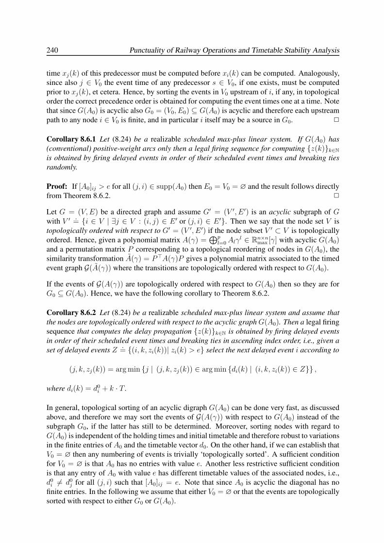
240 Punctuality of Railway Operations and Timetable Stability Analysis
time xj(k) of this predecessor must be computed before xi(k) can be computed. Analogously,
since also j ∈ V0 the event time of any predecessor s ∈ V0, if one exists, must be computed
prior to xj(k), et cetera. Hence, by sorting the events in V0 upstream of i, if any, in topological
order the correct precedence order is obtained for computing the event times one at a time. Note
that since G(A0) is acyclic also G0 = (V0, E0) ⊆ G(A0) is acyclic and therefore each upstream
path to any node i ∈ V0 is finite, and in particular i itself may be a source in G0. 2
Corollary 8.6.1 Let (8.24) be a realizable scheduled max-plus linear system. If G(A0) has
(conventional) positive-weight arcs only then a legal firing sequence for computing {z(k)}k∈N
is obtained by firing delayed events in order of their scheduled event times and breaking ties
randomly.
Proof: If [A0]ij > e for all (j, i) ∈ supp(A0) then E0 = V0 = ∅ and the result follows directly
from Theorem 8.6.2. 2
Let G = (V,E) be a directed graph and assume G′ = (V ′, E ′) is an acyclic subgraph of Gwith V ′ .= {i ∈ V | ∃j ∈ V : (i, j) ∈ E ′ or (j, i) ∈ E ′}. Then we say that the node set V is
topologically ordered with respect to G′ = (V ′, E ′) if the node subset V ′ ⊂ V is topologically
ordered. Hence, given a polynomial matrix A(γ) =⊕p
l=0Alγl ∈ Rn×n
max [γ] with acyclic G(A0)and a permutation matrix P corresponding to a topological reordering of nodes in G(A0), the
similarity transformation A(γ) = P>A(γ)P gives a polynomial matrix associated to the timed
event graph G(A(γ)) where the transitions are topologically ordered with respect to G(A0).
If the events of G(A(γ)) are topologically ordered with respect to G(A0) then so they are for
G0 ⊆ G(A0). Hence, we have the following corollary to Theorem 8.6.2.
Corollary 8.6.2 Let (8.24) be a realizable scheduled max-plus linear system and assume that
the nodes are topologically ordered with respect to the acyclic graphG(A0). Then a legal firing
sequence that computes the delay propagation {z(k)}k∈N is obtained by firing delayed events
in order of their scheduled event times and breaking ties in ascending index order, i.e., given a
set of delayed events Z.= {(i, k, zi(k))| zi(k) > e} select the next delayed event i according to
(j, k, zj(k)) = arg min {j | (j, k, zj(k)) ∈ arg min {di(k) | (i, k, zi(k)) ∈ Z}} ,
where di(k) = d0i + k · T .
In general, topological sorting of an acyclic digraph G(A0) can be done very fast, as discussed
above, and therefore we may sort the events of G(A(γ)) with respect to G(A0) instead of the
subgraph G0, if the latter has still to be determined. Moreover, sorting nodes with regard to
G(A0) is independent of the holding times and initial timetable and therefore robust to variations
in the finite entries ofA0 and the timetable vector d0. On the other hand, if we can establish that
V0 = ∅ then any numbering of events is trivially ‘topologically sorted’. A sufficient condition
for V0 = ∅ is that A0 has no entries with value e. Another less restrictive sufficient condition
is that any entry of A0 with value e has different timetable values of the associated nodes, i.e.,
d0i 6= d0
j for all (j, i) such that [A0]ij = e. Note that since A0 is acyclic the diagonal has no
finite entries. In the following we assume that either V0 = ∅ or that the events are topologically
sorted with respect to either G0 or G(A0).
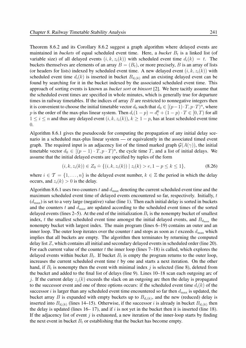
Chapter 8. Railway Timetable Stability Analysis 241
Theorem 8.6.2 and its Corollary 8.6.2 suggest a graph algorithm where delayed events are
maintained in buckets of equal scheduled event time. Here, a bucket Bt is a linked list (of
variable size) of all delayed events (i, k, zi(k)) with scheduled event time di(k) = t. The
buckets themselves are elements of an array B = (Bt), or more precisely, B is an array of lists
(or headers for lists) indexed by scheduled event time. A new delayed event (i, k, zi(k)) with
scheduled event time di(k) is inserted in bucket Bdi(k) and an existing delayed event can be
found by searching for it in the bucket indexed by the associated scheduled event time. This
approach of sorting events is known as bucket sort or binsort [2]. We here tacitly assume that
the scheduled event times are specified in whole minutes, which is generally true for departure
times in railway timetables. If the indices of array B are restricted to nonnegative integers then
it is convenient to choose the initial timetable vector d0 such that d0 ∈ [(p−1) ·T, p ·T )n, where
p is the order of the max-plus linear system. Then di(1− p) = d0i + (1− p) · T ∈ [0, T ) for all
1 ≤ i ≤ n and thus any delayed event (i, k, zi(k)), k ≥ 1− p, has at least scheduled event time
0.
Algorithm 8.6.1 gives the pseudocode for computing the propagation of any initial delay sce-
nario in a scheduled max-plus linear system — or equivalently in the associated timed event
graph. The required input is an adjacency list of the timed marked graph G(A(γ)), the initial
timetable vector d0 ∈ [(p − 1) · T, p · T )n, the cycle time T , and a list of initial delays. We
assume that the initial delayed events are specified by tuples of the form
(i, k, zi(k)) ∈ Z0.= {(i, k, zi(k)) | zi(k) > e, 1− p ≤ k ≤ 1}, (8.26)
where i ∈ T = {1, . . . , n} is the delayed event number, k ∈ Z the period in which the delay
occurs, and zi(k) > 0 is the delay.
Algorithm 8.6.1 uses two counters t and dmax denoting the current scheduled event time and the
maximum scheduled event time of delayed events encountered so far, respectively. Initially, t(dmax) is set to a very large (negative) value (line 1). Then each initial delay is sorted in buckets
and the counters t and dmax are updated according to the scheduled event times of the sorted
delayed events (lines 2–5). At the end of the initializationBt is the nonempty bucket of smallest
index, t the smallest scheduled event time amongst the initial delayed events, and Bdmaxthe
nonempty bucket with largest index. The main program (lines 6–19) contains an outer and an
inner loop. The outer loop iterates over the counter t and stops as soon as t exceeds dmax which
implies that all buckets are empty. The algorithm then terminates by returning the computed
delay listZ, which contains all initial and secondary delayed events in scheduled order (line 20).
For each current value of the counter t the inner loop (lines 7–18) is called, which explores the
delayed events within bucket Bt. If bucket Bt is empty the program returns to the outer loop,
increases the current scheduled event time t by one and starts a next iteration. On the other
hand, if Bt is nonempty then the event with minimal index j is selected (line 8), deleted from
the bucket and added to the final list of delays (line 9). Lines 10–18 scan each outgoing arc of
j. If the current delay zj(k) exceeds the slack on an outgoing arc then the delay is propagated
to the successor event and one of three options occurs: if the scheduled event time di(k) of the
successor i is larger than any scheduled event time encountered so far then dmax is updated, the
bucket array B is expanded with empty buckets up to Bdi(k), and the new (reduced) delay is
inserted into Bdi(k) (lines 14–15). Otherwise, if the successor i is already in bucket Bdi(k) then
the delay is updated (lines 16– 17), and if i is not yet in the bucket then it is inserted (line 18).
If the adjacency list of event j is exhausted, a new iteration of the inner-loop starts by finding
the next event in bucket Bt or establishing that the bucket has become empty.
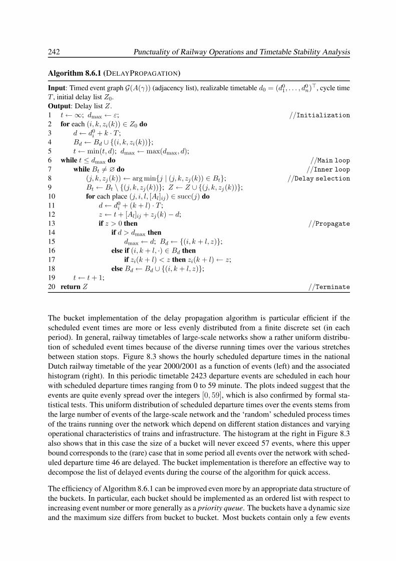
242 Punctuality of Railway Operations and Timetable Stability Analysis
Algorithm 8.6.1 (DELAYPROPAGATION)
Input: Timed event graph G(A(γ)) (adjacency list), realizable timetable d0 = (d01, . . . , d
0n)>, cycle time
T , initial delay list Z0.
Output: Delay list Z .
1 t←∞; dmax ← ε; //Initialization2 for each (i, k, zi(k)) ∈ Z0 do
3 d← d0i + k · T ;
4 Bd ← Bd ∪ {(i, k, zi(k))};5 t← min(t, d); dmax ← max(dmax, d);6 while t ≤ dmax do //Main loop7 while Bt 6= ∅ do //Inner loop8 (j, k, zj(k))← arg min{j | (j, k, zj(k)) ∈ Bt}; //Delay selection9 Bt ← Bt \ {(j, k, zj(k))}; Z ← Z ∪ {(j, k, zj (k))};10 for each place (j, i, l, [Al]ij) ∈ succ(j) do
11 d← d0i + (k + l) · T ;
12 z ← t + [Al]ij + zj(k)− d;
13 if z > 0 then //Propagate14 if d > dmax then
15 dmax ← d; Bd ← {(i, k + l, z)};16 else if (i, k + l, ·) ∈ Bd then
17 if zi(k + l) < z then zi(k + l)← z;
18 else Bd ← Bd ∪ {(i, k + l, z)};19 t← t + 1;
20 return Z //Terminate
The bucket implementation of the delay propagation algorithm is particular efficient if the
scheduled event times are more or less evenly distributed from a finite discrete set (in each
period). In general, railway timetables of large-scale networks show a rather uniform distribu-
tion of scheduled event times because of the diverse running times over the various stretches
between station stops. Figure 8.3 shows the hourly scheduled departure times in the national
Dutch railway timetable of the year 2000/2001 as a function of events (left) and the associated
histogram (right). In this periodic timetable 2423 departure events are scheduled in each hour
with scheduled departure times ranging from 0 to 59 minute. The plots indeed suggest that the
events are quite evenly spread over the integers [0, 59], which is also confirmed by formal sta-
tistical tests. This uniform distribution of scheduled departure times over the events stems from
the large number of events of the large-scale network and the ‘random’ scheduled process times
of the trains running over the network which depend on different station distances and varying
operational characteristics of trains and infrastructure. The histogram at the right in Figure 8.3
also shows that in this case the size of a bucket will never exceed 57 events, where this upper
bound corresponds to the (rare) case that in some period all events over the network with sched-
uled departure time 46 are delayed. The bucket implementation is therefore an effective way to
decompose the list of delayed events during the course of the algorithm for quick access.
The efficiency of Algorithm 8.6.1 can be improved even more by an appropriate data structure of
the buckets. In particular, each bucket should be implemented as an ordered list with respect to
increasing event number or more generally as a priority queue. The buckets have a dynamic size
and the maximum size differs from bucket to bucket. Most buckets contain only a few events
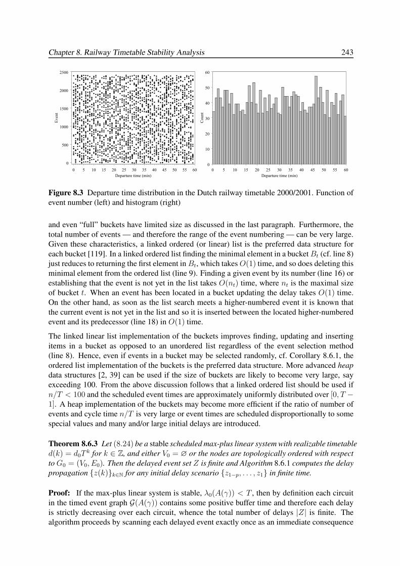
Chapter 8. Railway Timetable Stability Analysis 243
0 5 10 15 20 25 30 35 40 45 50 55 60
Departure time (min)
0
500
1000
1500
2000
2500
Even
t
••••••
••
•••••••••••
••••••••••••••
•
••••
••••
••••••
•••••••••••••••••••••••••••••
••••••••••
•••••••••••••••••••••
••••••••••••••••••
•••••••
••••••••••••••
••••••••••••••••••
••••
••••••••••
•••••••••••••••
•
•••••
•
•••••
••••••••••••••••••••••••••••
•••••••
•••••••••••••
•
•••••••
••••••••••••••••••••••••••••••••••••••••
•••••••••••••
•
••••••••••••••••••••••
•••
•••••••••••••••
••••••••••••••••••••••••••••••
•
•••
•••
•••••••
••••••
••••••
••
•••••
•
••••••••••••••
•••••••••••••••••
•••••••
••
••••••••••••
•
••••••
••••
••••••••••••••
•••••
••
••••
•••••••••••••••••
••••••
•
•••••••••••••
•••
••••••••••••••
••••
•••••••••••••••
••••
••••••••••••
•
••••••••••••••••••••••••••••••••••••••••
••••••••••••
••••
•••••••••
••••••••••••••••••••••••••
•••••••••••
•••
••••••••••••••••••••••••••
•••
•••••••••••••••••••••••••••••
•••••••••••••••••••••
••••••••
•••••••••••••••
•••
•••••
••••••••
•••••••••••
•
••••••••••••••••••••
•
••••••••••••
•••••••••••••••••••••••••••
•••••••••
••••
••
••••••••••
•••••••••••
•••••
•
•••••••••••••••••••••••••••••
•
•••••••••••••
•••••••••
••••••
••
••••
••••••••••
•••
•••••••••••••••••••••••••
•••••••••••••••
•••••
•••••••
•••••
•••••••••••••••••
•••••••
••••••••••••••••••••••
•••••••
••••••••••
•••••••••••••••••••••••
•••••••••••••••
•••••
••••••••••
•••••••
••••••••••••••
••
•
••••••
••
•••••••••••••••••
••••••
••••
•••••••••
•••••••••••••••••••••••••••••••••••••
••••••••••••••••••••••••••••••••••••••••••••
••••••••
•••••••••••••••••••••••••
••••••••
•••
•••••••
••••••••••••
•••••••••••
•••••••
••••••••••••••••••••••••••••
•••
••••
••••
•••••
•
•••••••••••••••••••••••
•••••••••••••••••••••••
••••••••••••
••••••••••••••••••••••••••••••••
•
•••••••••••••••
•••••••••••••••••••••••••••••
••••
••••••••••••••••••
•••••
•••••••
••••••
•••••••••••••••••••••••••
••••••••
•
••
•••••••••••••
•••••••
••••
•
••••
••••
•••••••••
•••••••••
••••••••••
•••••
•
••••••••••••
•••••••••••••
•••••••••••
•••••••••••••
•••••
••••
••••••••••••
•••
•••••••••••••••••
••••••••••••••••
••••••
•••••••••••
••••
••••••••••••••••••••••••••••••••••••••••••
•••••
••••••••
••••••••••••••••
•
•••••••••••••
••••••••••••••••••••••••••••••••••••••••••••••••••
•••••••••••••••••••••••••
•••
••••••
••••••
••••••••
••
••••••••••••••••••••••
••••••
••••••••••••••••••••••••••••••••••••••••••
••••
•
•••••••••
•••••••••
••••
•••
••••••••••••••••••••••••••••••••
••••••••
••••••••••••••••
•••••••
•
••••••••••••••
••••••••••••••••••••••••••••
••••••••••••••••
••
•••••
•••
•
•••••••••••••
•••
•••••
••
•••••••••••••••••
••
••••••••••••
••••••••••
•••••••••••••••••••••••
•
•••••••••••••••••••••
•••••••••
••
••
•••••••••
••••
•••••
0 5 10 15 20 25 30 35 40 45 50 55 60
Departure time (min)
0
10
20
30
40
50
60
Count
Figure 8.3 Departure time distribution in the Dutch railway timetable 2000/2001. Function of
event number (left) and histogram (right)
and even “full” buckets have limited size as discussed in the last paragraph. Furthermore, the
total number of events — and therefore the range of the event numbering — can be very large.
Given these characteristics, a linked ordered (or linear) list is the preferred data structure for
each bucket [119]. In a linked ordered list finding the minimal element in a bucketBt (cf. line 8)
just reduces to returning the first element inBt, which takesO(1) time, and so does deleting this
minimal element from the ordered list (line 9). Finding a given event by its number (line 16) or
establishing that the event is not yet in the list takes O(nt) time, where nt is the maximal size
of bucket t. When an event has been located in a bucket updating the delay takes O(1) time.
On the other hand, as soon as the list search meets a higher-numbered event it is known that
the current event is not yet in the list and so it is inserted between the located higher-numbered
event and its predecessor (line 18) in O(1) time.
The linked linear list implementation of the buckets improves finding, updating and inserting
items in a bucket as opposed to an unordered list regardless of the event selection method
(line 8). Hence, even if events in a bucket may be selected randomly, cf. Corollary 8.6.1, the
ordered list implementation of the buckets is the preferred data structure. More advanced heap
data structures [2, 39] can be used if the size of buckets are likely to become very large, say
exceeding 100. From the above discussion follows that a linked ordered list should be used if
n/T < 100 and the scheduled event times are approximately uniformly distributed over [0, T −1]. A heap implementation of the buckets may become more efficient if the ratio of number of
events and cycle time n/T is very large or event times are scheduled disproportionally to some
special values and many and/or large initial delays are introduced.
Theorem 8.6.3 Let (8.24) be a stable scheduled max-plus linear system with realizable timetable
d(k) = d0Tk for k ∈ Z, and either V0 = ∅ or the nodes are topologically ordered with respect
to G0 = (V0, E0). Then the delayed event set Z is finite and Algorithm 8.6.1 computes the delay
propagation {z(k)}k∈N for any initial delay scenario {z1−p, . . . , z1} in finite time.
Proof: If the max-plus linear system is stable, λ0(A(γ)) < T , then by definition each circuit
in the timed event graph G(A(γ)) contains some positive buffer time and therefore each delay
is strictly decreasing over each circuit, whence the total number of delays |Z| is finite. The
algorithm proceeds by scanning each delayed event exactly once as an immediate consequence
244 Punctuality of Railway Operations and Timetable Stability Analysis
of Theorem 8.6.2 and its Corollary 8.6.2 and therefore terminates after a finite number of itera-
tions. Note that a topological order of the nodes of G(A0) also implies a topological order with
respect to G0 = (V0, E0) and is thus also covered by the theorem. 2
In practice Algorithm 8.6.1 has a fast pseudolinear running time in the number of (initial and
secondary) delayed events |Z| because: (1) the algorithm only scans delayed events, (2) each
delayed event is scanned exactly once, (3) the number of successors checked for delay propa-
gation in each scan is limited by the maximum outdegree over all nodes which is typically very
small (< 10), (4) the buckets Bt are typically small (nt = |Bt| < 100) and finding an event
in an (ordered) bucket or detecting its absence takes on the average log(nt) < 10 comparisons,
whereas all other bucket operations take O(1) time.
8.7 PETER
8.7.1 Introduction
PETER is a strategic and tactical planning support system for the evaluation of periodic rail-
way timetables on network stability and effective capacity utilization. PETER is an acronym of
Performance Evaluation of Timed Events in Railways. The software PETER contains an imple-
mentation of the timed event graph and max-plus linear system theory presented in this thesis.
The core of the PETER software is the implementation of an automatic (max-plus) model build-
ing procedure and efficient state-of-the-art numerical algorithms for analysing the model, which
are well-documented in this thesis. For the programming and development of a user-friendly
human-machine interface (HMI) suitable for railway planners it was decided to cooperate with
the software firm ORTEC [88], who are specialized in planning software and, amongst others,
developed and maintain the Dutch railway timetable design system DONS for the Dutch Rail-
ways (NSR) and ProRail. PETER has a modular system architecture written in Delphi for the
operating systems MS Windows 95 and higher. The policy iteration algorithm of the critical
circuit analysis is a callable routine implemented in C. The modular design facilitates future
enhancements.
PETER has been developed to support railway professionals in their task of designing, eval-
uating and improving railway timetables. The graphical user interface (GUI) enables non-
mathematical users to apply automated advanced mathematical modelling and analysis tech-
niques while maintaining focus on timetabling decisions (input parameters) and interpretation
of computational results. The tool relieves the tedious task of ‘pencil and paper’ calculations
and allows visualization of complex (cyclic) network interdependencies which are inherently
present in the railway timetable but hard to grasp without computer-aided support.
The main strength of PETER is the analytical max-plus analysis approach which in combination
with efficient numerical graph algorithms enables a real-time computational environment for
the evaluation of large-scale network timetables. Moreover, a graphical network visualization
allows an insightful representation of results which helps users to focus on critical components
and prevents them from drowning in an overkill of output which is a serious concern when
analysing large-scale networks. PETER is also compatible with DONS. All analysis methods in
PETER are hence available to quickly evaluate timetable structures generated by DONS, which
is a further major contribution to the computer-aided timetable design in the Netherlands.
Chapter 8. Railway Timetable Stability Analysis 245
This section briefly outlines the features of PETER. In Section 8.8 the application of PETER —
and the max-plus analysis approach in general — is demonstrated in a case study of the national
Dutch railway timetable.
8.7.2 Input Data
PETER automatically builds a max-plus linear system model and the network visualization
based on the following input data:
• Timetable points: name (abbreviation), coordinates and type (intercity stations (IC), in-
terregional stations (IR), regional stops (AR), freight or shunting yards (F), junctions (J),
and movable bridges (BR)),
• Train lines: line number, route, stops, nominal running times, minimum dwell times,
frequency,
• Timetable: scheduled arrival, departure and through times,
• Connections: passenger transfers and minimum transfer times,
• Rolling stock circulations: turns or other rolling stock connections and minimum layover
or (de-)coupling times,
• Logistics: crew transfers and minimum transfer times (optional),
• Infrastructure and safety system: minimum headway times between train events.
Section 6.5 gave a description of the generic input data file format. Timetable points are given
in the TimetablePointData, train lines and timetable data are combined in the LineData,
SynchData contain the connection, rolling stock circulation and logistics data, and the infras-
tructure and safety system data are given in the HeadwayData. In PETER these data are im-
ported from a combined ASCII generic input file. Process times can be specified up to a second
using decimal or time format (min:sec), e.g. 63 minutes and 15 seconds is specified in decimals
by 63.25 and in time format by 63:15. This generic format is easily generated by standard text
editors or spreadsheets. Networks can also be created within PETER using the build-in editors
and saved in the generic format. For fast access the internal data structure of PETER and the
computed results can also be saved from computer memory to a binary file.
PETER automatically constructs the max-plus model and draws the network view based on the
input data. A build-in editor can also be used to edit data. When data has been edited it is
checked on feasibility before PETER builds a new max-plus model. The modular system ar-
chitecture of PETER enables easy extension of functionalities. As an example, a module has
been developed that directly imports data files from the Dutch timetable design tool DONS,
see Section 3.9.1. The DONS data is given in three data files: TimetablePoints contains the
data of the timetable points. Constraints is the input data file prepared via the DONS inter-
face that is used by CADANS to compute a feasible timetable (or a minimal set of conflicting
constraints). Recall from Section 3.9.1 that CADANS is the kernel of DONS that computes a
feasible timetable from a set of periodic time window constraints corresponding to the periodic
event scheduling problem (PESP). Constraints thus contains these PESP constraints in a pre-
scribed ASCII format. Finally, Timetable is an output file of CADANS containing a feasible
timetable in some prescribed ASCII format.
PETER also contains several options to quickly analyse the impact of parameter variations. By
simply selecting a toggle we may individually exclude all layover times, passenger transfers,
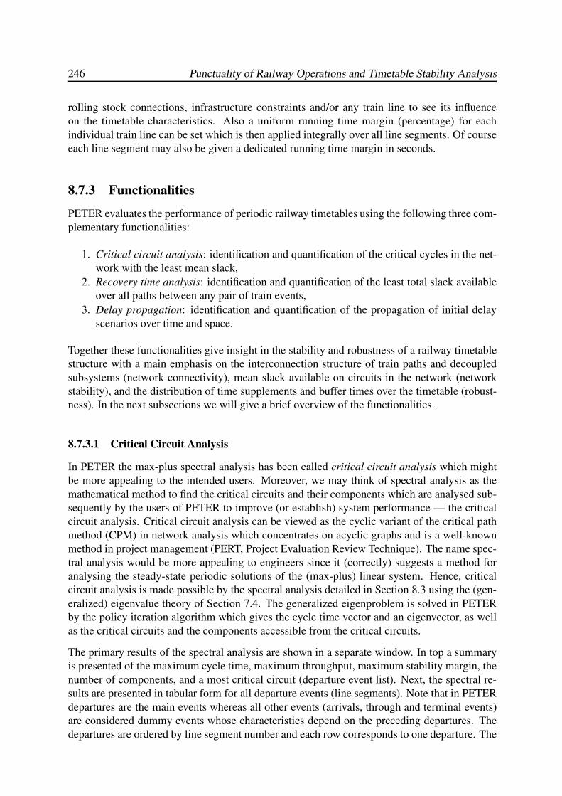
246 Punctuality of Railway Operations and Timetable Stability Analysis
rolling stock connections, infrastructure constraints and/or any train line to see its influence
on the timetable characteristics. Also a uniform running time margin (percentage) for each
individual train line can be set which is then applied integrally over all line segments. Of course
each line segment may also be given a dedicated running time margin in seconds.
8.7.3 Functionalities
PETER evaluates the performance of periodic railway timetables using the following three com-
plementary functionalities:
1. Critical circuit analysis: identification and quantification of the critical cycles in the net-
work with the least mean slack,
2. Recovery time analysis: identification and quantification of the least total slack available
over all paths between any pair of train events,
3. Delay propagation: identification and quantification of the propagation of initial delay
scenarios over time and space.
Together these functionalities give insight in the stability and robustness of a railway timetable
structure with a main emphasis on the interconnection structure of train paths and decoupled
subsystems (network connectivity), mean slack available on circuits in the network (network
stability), and the distribution of time supplements and buffer times over the timetable (robust-
ness). In the next subsections we will give a brief overview of the functionalities.
8.7.3.1 Critical Circuit Analysis
In PETER the max-plus spectral analysis has been called critical circuit analysis which might
be more appealing to the intended users. Moreover, we may think of spectral analysis as the
mathematical method to find the critical circuits and their components which are analysed sub-
sequently by the users of PETER to improve (or establish) system performance — the critical
circuit analysis. Critical circuit analysis can be viewed as the cyclic variant of the critical path
method (CPM) in network analysis which concentrates on acyclic graphs and is a well-known
method in project management (PERT, Project Evaluation Review Technique). The name spec-
tral analysis would be more appealing to engineers since it (correctly) suggests a method for
analysing the steady-state periodic solutions of the (max-plus) linear system. Hence, critical
circuit analysis is made possible by the spectral analysis detailed in Section 8.3 using the (gen-
eralized) eigenvalue theory of Section 7.4. The generalized eigenproblem is solved in PETER
by the policy iteration algorithm which gives the cycle time vector and an eigenvector, as well
as the critical circuits and the components accessible from the critical circuits.
The primary results of the spectral analysis are shown in a separate window. In top a summary
is presented of the maximum cycle time, maximum throughput, maximum stability margin, the
number of components, and a most critical circuit (departure event list). Next, the spectral re-
sults are presented in tabular form for all departure events (line segments). Note that in PETER
departures are the main events whereas all other events (arrivals, through and terminal events)
are considered dummy events whose characteristics depend on the preceding departures. The
departures are ordered by line segment number and each row corresponds to one departure. The
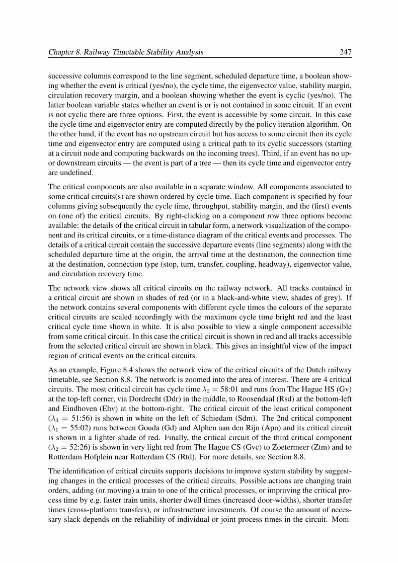
Chapter 8. Railway Timetable Stability Analysis 247
successive columns correspond to the line segment, scheduled departure time, a boolean show-
ing whether the event is critical (yes/no), the cycle time, the eigenvector value, stability margin,
circulation recovery margin, and a boolean showing whether the event is cyclic (yes/no). The
latter boolean variable states whether an event is or is not contained in some circuit. If an event
is not cyclic there are three options. First, the event is accessible by some circuit. In this case
the cycle time and eigenvector entry are computed directly by the policy iteration algorithm. On
the other hand, if the event has no upstream circuit but has access to some circuit then its cycle
time and eigenvector entry are computed using a critical path to its cyclic successors (starting
at a circuit node and computing backwards on the incoming trees). Third, if an event has no up-
or downstream circuits — the event is part of a tree — then its cycle time and eigenvector entry
are undefined.
The critical components are also available in a separate window. All components associated to
some critical circuits(s) are shown ordered by cycle time. Each component is specified by four
columns giving subsequently the cycle time, throughput, stability margin, and the (first) events
on (one of) the critical circuits. By right-clicking on a component row three options become
available: the details of the critical circuit in tabular form, a network visualization of the compo-
nent and its critical circuits, or a time-distance diagram of the critical events and processes. The
details of a critical circuit contain the successive departure events (line segments) along with the
scheduled departure time at the origin, the arrival time at the destination, the connection time
at the destination, connection type (stop, turn, transfer, coupling, headway), eigenvector value,
and circulation recovery time.
The network view shows all critical circuits on the railway network. All tracks contained in
a critical circuit are shown in shades of red (or in a black-and-white view, shades of grey). If
the network contains several components with different cycle times the colours of the separate
critical circuits are scaled accordingly with the maximum cycle time bright red and the least
critical cycle time shown in white. It is also possible to view a single component accessible
from some critical circuit. In this case the critical circuit is shown in red and all tracks accessible
from the selected critical circuit are shown in black. This gives an insightful view of the impact
region of critical events on the critical circuits.
As an example, Figure 8.4 shows the network view of the critical circuits of the Dutch railway
timetable, see Section 8.8. The network is zoomed into the area of interest. There are 4 critical
circuits. The most critical circuit has cycle time λ0 = 58:01 and runs from The Hague HS (Gv)
at the top-left corner, via Dordrecht (Ddr) in the middle, to Roosendaal (Rsd) at the bottom-left
and Eindhoven (Ehv) at the bottom-right. The critical circuit of the least critical component
(λ3 = 51:56) is shown in white on the left of Schiedam (Sdm). The 2nd critical component
(λ1 = 55:02) runs between Gouda (Gd) and Alphen aan den Rijn (Apn) and its critical circuit
is shown in a lighter shade of red. Finally, the critical circuit of the third critical component
(λ2 = 52:26) is shown in very light red from The Hague CS (Gvc) to Zoetermeer (Ztm) and to
Rotterdam Hofplein near Rotterdam CS (Rtd). For more details, see Section 8.8.
The identification of critical circuits supports decisions to improve system stability by suggest-
ing changes in the critical processes of the critical circuits. Possible actions are changing train
orders, adding (or moving) a train to one of the critical processes, or improving the critical pro-
cess time by e.g. faster train units, shorter dwell times (increased door-widths), shorter transfer
times (cross-platform transfers), or infrastructure investments. Of course the amount of neces-
sary slack depends on the reliability of individual or joint process times in the circuit. Moni-
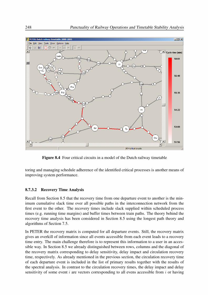
248 Punctuality of Railway Operations and Timetable Stability Analysis
Figure 8.4 Four critical circuits in a model of the Dutch railway timetable
toring and managing schedule adherence of the identified critical processes is another means of
improving system performance.
8.7.3.2 Recovery Time Analysis
Recall from Section 8.5 that the recovery time from one departure event to another is the min-
imum cumulative slack time over all possible paths in the interconnection network from the
first event to the other. The recovery times include slack supplied within scheduled process
times (e.g. running time margins) and buffer times between train paths. The theory behind the
recovery time analysis has been considered in Section 8.5 using the longest path theory and
algorithms of Section 7.5.
In PETER the recovery matrix is computed for all departure events. Still, the recovery matrix
gives an overkill of information since all events accessible from each event leads to a recovery
time entry. The main challenge therefore is to represent this information to a user in an acces-
sible way. In Section 8.5 we already distinguished between rows, columns and the diagonal of
the recovery matrix corresponding to delay sensitivity, delay impact and circulation recovery
time, respectively. As already mentioned in the previous section, the circulation recovery time
of each departure event is included in the list of primary results together with the results of
the spectral analysis. In contrast to the circulation recovery times, the delay impact and delay
sensitivity of some event i are vectors corresponding to all evens accessible from i or having
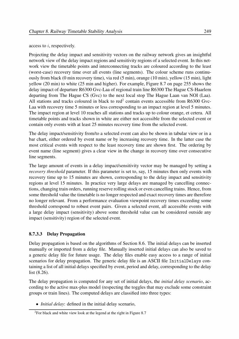
Chapter 8. Railway Timetable Stability Analysis 249
access to i, respectively.
Projecting the delay impact and sensitivity vectors on the railway network gives an insightful
network view of the delay impact regions and sensitivity regions of a selected event. In this net-
work view the timetable points and interconnecting tracks are coloured according to the least
(worst-case) recovery time over all events (line segments). The colour scheme runs continu-
ously from black (0 min recovery time), via red (5 min), orange (10 min), yellow (15 min), light
yellow (20 min) to white (25 min and higher). For example, Figure 8.7 on page 255 shows the
delay impact of departure R6300 Gvc-Laa of regional train line R6300 The Hague CS-Haarlem
departing from The Hague CS (Gvc) to the next local stop The Hague Laan van NOI (Laa).
All stations and tracks coloured in black to red2 contain events accessible from R6300 Gvc-
Laa with recovery time 5 minutes or less corresponding to an impact region at level 5 minutes.
The impact region at level 10 reaches all stations and tracks up to colour orange, et cetera. All
timetable points and tracks shown in white are either not accessible from the selected event or
contain only events with at least 25 minutes recovery time from the selected event.
The delay impact/sensitivity from/to a selected event can also be shown in tabular view or in a
bar chart, either ordered by event name or by increasing recovery time. In the latter case the
most critical events with respect to the least recovery time are shown first. The ordering by
event name (line segment) gives a clear view in the change in recovery time over consecutive
line segments.
The large amount of events in a delay impact/sensitivity vector may be managed by setting a
recovery threshold parameter. If this parameter is set to, say, 15 minutes then only events with
recovery time up to 15 minutes are shown, corresponding to the delay impact and sensitivity
regions at level 15 minutes. In practice very large delays are managed by cancelling connec-
tions, changing train orders, running reserve rolling stock or even cancelling trains. Hence, from
some threshold value the timetable is no longer respected and exact recovery times are therefore
no longer relevant. From a performance evaluation viewpoint recovery times exceeding some
threshold correspond to robust event pairs. Given a selected event, all accessible events with
a large delay impact (sensitivity) above some threshold value can be considered outside any
impact (sensitivity) region of the selected event.
8.7.3.3 Delay Propagation
Delay propagation is based on the algorithms of Section 8.6. The initial delays can be inserted
manually or imported from a delay file. Manually inserted initial delays can also be saved to
a generic delay file for future usage. The delay files enable easy access to a range of initial
scenarios for delay propagation. The generic delay file is an ASCII file InitialDelays con-
taining a list of all initial delays specified by event, period and delay, corresponding to the delay
list (8.26).
The delay propagation is computed for any set of initial delays, the initial delay scenario, ac-
cording to the active max-plus model (respecting the toggles that may exclude some constraint
groups or train lines). The computed delays are classified into three types:
• Initial delay: defined in the initial delay scenario,
2For black and white view look at the legend at the right in Figure 8.7
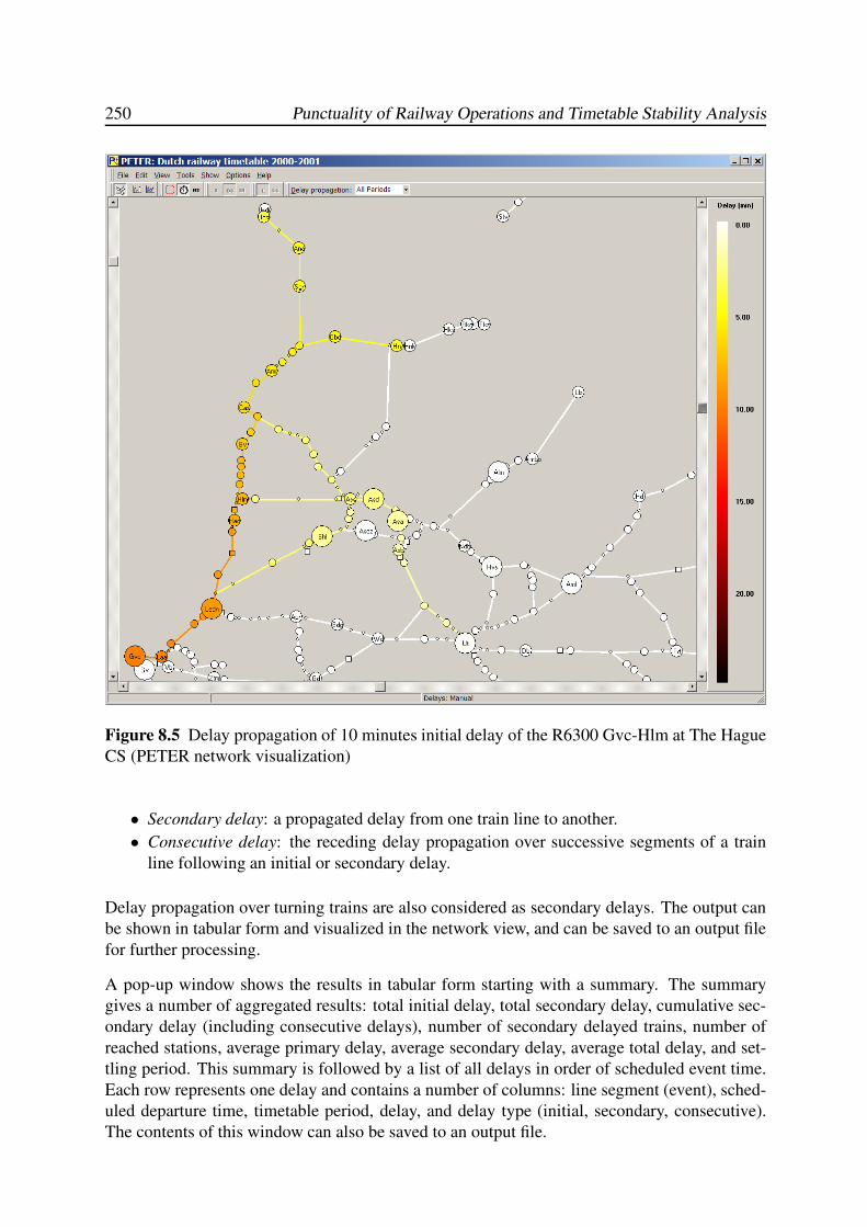
250 Punctuality of Railway Operations and Timetable Stability Analysis
Figure 8.5 Delay propagation of 10 minutes initial delay of the R6300 Gvc-Hlm at The Hague
CS (PETER network visualization)
• Secondary delay: a propagated delay from one train line to another.
• Consecutive delay: the receding delay propagation over successive segments of a train
line following an initial or secondary delay.
Delay propagation over turning trains are also considered as secondary delays. The output can
be shown in tabular form and visualized in the network view, and can be saved to an output file
for further processing.
A pop-up window shows the results in tabular form starting with a summary. The summary
gives a number of aggregated results: total initial delay, total secondary delay, cumulative sec-
ondary delay (including consecutive delays), number of secondary delayed trains, number of
reached stations, average primary delay, average secondary delay, average total delay, and set-
tling period. This summary is followed by a list of all delays in order of scheduled event time.
Each row represents one delay and contains a number of columns: line segment (event), sched-
uled departure time, timetable period, delay, and delay type (initial, secondary, consecutive).
The contents of this window can also be saved to an output file.
Chapter 8. Railway Timetable Stability Analysis 251
The network visualization consists of a projection of the delays to the network, similar to the
recovery impact. Figure 8.5 shows an example of the network visualization, see §8.8 for details..
In this network view the timetable points and interconnecting tracks are coloured with respect
to the maximum (worst-case) delay over all events (line segments). The colour scheme runs
continuously from white (0 minutes delay), via yellow (5 min), orange (10 min), red (15 min),
dark red (20 min) to black (25 min and higher). Note that the colour scheme is the reversed of
the recovery times, so that again black is critical and white is harmless. The delay propagation
can be visualized all at once, or by successive timetable periods which thus shows an animation
of the delay propagation over the consecutive periods. The latter visualization starts with the
initial delays, then the delay propagation in period zero, the first period, etc., until the settling
period.
8.8 Case Study: The Dutch National Railway Timetable
8.8.1 Model Variants
This section presents the results of a case-study of the Dutch national railway timetable. The
max-plus linear system model is based on a DONS variant of the Dutch 2000/2001 railway
timetable in the morning peak. The model contains all train lines and freight paths scheduled in
the morning peak including the intercity (IC), interregional (IR), and regional (R) lines of NS
Reizigers, the regional lines of Syntus in the east of the Netherlands, the regional lines of No-
ordNed in the north, the high-speed line (HST) from Amsterdam to Belgium, the international
(INT) lines to Germany, and the freight (F) train paths. Table 8.1 summarizes the model. The
dummy events correspond to arrival, through and terminal events.
Table 8.1 Summary of the Dutch national 2000/2001 railway timetable model
DONS timetable model
Timetable points 729 stations, stops, shunting yards, junctions, movable bridges
Train line segments 7183 2062 stops, 281 turns, 4760 runs, 80 ends
Connections 259 198 transfers, 61 rolling stock connections
Headway constraints 87776 arrivals, departures, in/outbound, crossings, meets, overtaking
Max-plus linear system
Nodes (transitions) 3536 1677 departure events, 1859 dummy events
Arcs (places) 25472 1677 line segments, 259 synchronization, 23536 infra
Tokens 12429 305 train runs, 90 connections, 105 turns, 11929 headway order
Order 2 13043 0-token places, 12193 1-token places, 236 2-token places
We consider two model variants distinguished by the amount of running time margin. In the
basic variant we consider scheduled running times and in the margins variant we assume mini-
mum running times implying that running time margins are used for delay reduction. Since the
actual running time margins were not available we approximated them by subtracting 7% of the
scheduled running times according to the capacity allocation norms, although in practice the de-
fault margins are slightly higher due to rounding running times to whole minutes. Furthermore,
the DONS model did not always specify minimum layover times of turning trains. In those
252 Punctuality of Railway Operations and Timetable Stability Analysis
Table 8.2 Spectral analysis results basic and margins timetable
Basic Margins
λ ∆2 λ ∆2 Component / critical circuit (CC)
60:00 0:00 58:01 0:11 Main network
CC: Various
58:00 0:06 55:02 0:15 Line Gouda–Alphen aan den Rijn
CC: R9500 Gouda–Boskoop–Gouda
55:00 0:22 51:56 0:35 Line Rotterdam CS–Hoek van Holland
CC: R4200 Rotterdam CS–Maassluis West–Rotterdam CS
54:48 0:21 52:26 0:31 Lines The Hague CS–Zoetermeer/Rotterdam Hofplein
CC: R13300, R13400, R13700, R13500, R13600
cases we used a default value of 5 minutes and assumed that any remaining layover time could
be utilized as buffer time in case of delays. The minimum headway times in the DONS model
utilized at infrastructure conflict points are based on the Dutch capacity allocation norms which
range between 2 and 4 minutes depending on the route conflict and train types, see Chapter 3.
8.8.2 Critical Circuit Analysis
Table 8.2 shows the results of the spectral analysis of the basic timetable. The network is al-
most entirely connected with various critical circuits of maximum cycle mean λ0 = 60. Hence,
the basic timetable is critical implying that on the critical circuits no spare time is available
other than the (unknown) process time margins and buffer times contained in the running times
and minimum headways. The network contains three additionally strongly-connected compo-
nents that are uncoupled from the main network component, see Table 8.2. The second critical
component is the regional train line R9500 running on a single-track route between Gouda and
Alphen aan den Rijn. The critical circuit has cycle mean λ1 = 58 minutes and is compiled of
the trip from Gouda to Boskoop just before Alphen where the train meets its opposite train, the
minimum headway to the opposite train, the trip from Boskoop back to Gouda, and the turn
in Gouda. The third component is the partial single-track route between Rotterdam CS and
Hoek van Holland, where the train circulation of the R4200 between Rotterdam and Maassluis
West (about 2/3 to the Hoek van Holland) is critical with cycle mean λ2 = 55. The fourth
component is a suburban subnetwork consisting of the Hofpleinlijn (The Hague CS–Rotterdam
Hofplein) and the Zoetermeerlijn (The Hague CS–Zoetermeer); the critical circuit has cycle
mean λ3 = 54:48 minutes and consists of 66 arcs representing a mixed sequence of all running
5 regional train lines including 46 stops, 4 turns and 16 infrastructure constraints (arcs).
The margins timetable differs from the basic timetable by the incorporation of running time
margins. Table 8.2 (3rd and 4th column) summarizes the results of the spectral analysis. We see
the same four components as in the basic variant but smaller maximum cycle means. The critical
circuits in the three smaller components have not changed, although the order of the cycle means
of the last two components has changed reflecting that the amount of running time in the train
line circulation of the R4200 is larger than in the critical circuit of the other component. The
effect of the 7% running time margin is also apparent in the most critical component, which
now contains 2 minutes average slack time. Moreover, this component now contains a unique
critical circuit containing 10 trains running between The Hague HS to Breda and back, see
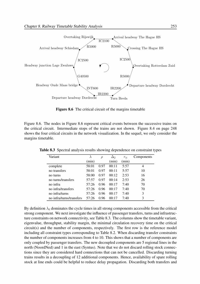
Chapter 8. Railway Timetable Stability Analysis 253
Arrival headway Schiedam
Headway Oude Maas bridge
Departure headway Dordrecht Turn Breda
Departure headway Dordrecht
Overtaking Rotterdam Zuid
Crossing The Hague HS
Arrival headway The Hague HSOvertaking Rijswijk
IC2500
G40500
INT600
IR2200
IR2200
R5000
IC2500
R5000
IC2100
R5000
Headway junction Lage Zwaluwe
Figure 8.6 The critical circuit of the margins timetable
Figure 8.6. The nodes in Figure 8.6 represent critical events between the successive trains on
the critical circuit. Intermediate stops of the trains are not shown. Figure 8.4 on page 248
shows the four critical circuits in the network visualization. In the sequel, we only consider the
margins timetable.
Table 8.3 Spectral analysis results showing dependence on constraint types
Variant λ ρ ∆2 rii Components
(min) (min) (min)
complete 58:01 0.97 00:11 5:57 4
no transfers 58:01 0.97 00:11 5:57 10
no turns 58:00 0.97 00:12 2:53 16
no turns/transfers 57:57 0.97 00:14 2:53 26
no infra 57:26 0.96 00:17 7:40 70
no infra/transfers 57:26 0.96 00:17 7:40 70
no infra/turns 57:26 0.96 00:17 7:40 3
no infra/turns/transfers 57:26 0.96 00:17 7:40 3
By definition λ0 dominates the cycle times in all strong components accessible from the critical
strong component. We next investigate the influence of passenger transfers, turns and infrastruc-
ture constraints on network connectivity, see Table 8.3. The columns show the timetable variant,
eigenvalue, throughput, stability margin, the minimal circulation recovery time on the critical
circuit(s) and the number of components, respectively. The first row is the reference model
including all constraint types corresponding to Table 8.2. When discarding transfer constraints
the number of components increases from 4 to 10. This shows that a number of components are
only coupled by passenger transfers. The new decoupled components are 5 regional lines in the
north (NoordNed) and 1 in the east (Syntus). Note that we do not discard rolling stock connec-
tions since they are considered hard connections that can not be cancelled. Discarding turning
trains results in a decoupling of 12 additional components. Hence, availability of spare rolling
stock at line ends could be helpful to reduce delay propagation. Discarding both transfers and
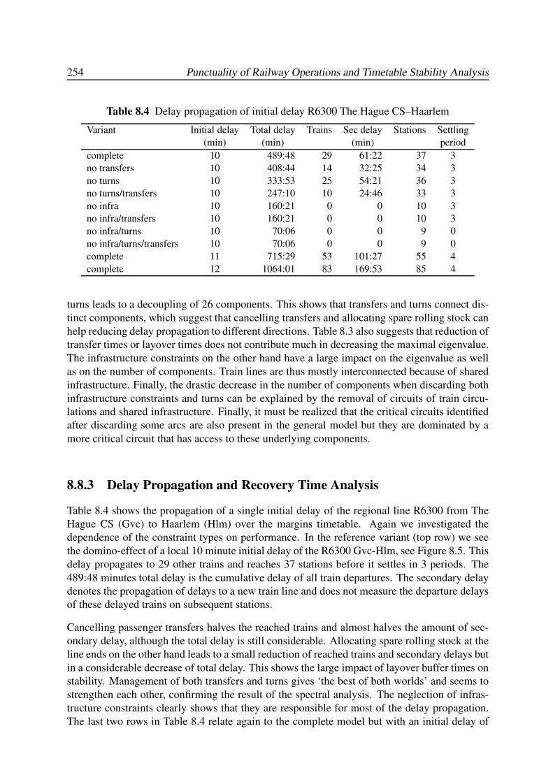
254 Punctuality of Railway Operations and Timetable Stability Analysis
Table 8.4 Delay propagation of initial delay R6300 The Hague CS–Haarlem
Variant Initial delay Total delay Trains Sec delay Stations Settling
(min) (min) (min) period
complete 10 489:48 29 61:22 37 3
no transfers 10 408:44 14 32:25 34 3
no turns 10 333:53 25 54:21 36 3
no turns/transfers 10 247:10 10 24:46 33 3
no infra 10 160:21 0 0 10 3
no infra/transfers 10 160:21 0 0 10 3
no infra/turns 10 70:06 0 0 9 0
no infra/turns/transfers 10 70:06 0 0 9 0
complete 11 715:29 53 101:27 55 4
complete 12 1064:01 83 169:53 85 4
turns leads to a decoupling of 26 components. This shows that transfers and turns connect dis-
tinct components, which suggest that cancelling transfers and allocating spare rolling stock can
help reducing delay propagation to different directions. Table 8.3 also suggests that reduction of
transfer times or layover times does not contribute much in decreasing the maximal eigenvalue.
The infrastructure constraints on the other hand have a large impact on the eigenvalue as well
as on the number of components. Train lines are thus mostly interconnected because of shared
infrastructure. Finally, the drastic decrease in the number of components when discarding both
infrastructure constraints and turns can be explained by the removal of circuits of train circu-
lations and shared infrastructure. Finally, it must be realized that the critical circuits identified
after discarding some arcs are also present in the general model but they are dominated by a
more critical circuit that has access to these underlying components.
8.8.3 Delay Propagation and Recovery Time Analysis
Table 8.4 shows the propagation of a single initial delay of the regional line R6300 from The
Hague CS (Gvc) to Haarlem (Hlm) over the margins timetable. Again we investigated the
dependence of the constraint types on performance. In the reference variant (top row) we see
the domino-effect of a local 10 minute initial delay of the R6300 Gvc-Hlm, see Figure 8.5. This
delay propagates to 29 other trains and reaches 37 stations before it settles in 3 periods. The
489:48 minutes total delay is the cumulative delay of all train departures. The secondary delay
denotes the propagation of delays to a new train line and does not measure the departure delays
of these delayed trains on subsequent stations.
Cancelling passenger transfers halves the reached trains and almost halves the amount of sec-
ondary delay, although the total delay is still considerable. Allocating spare rolling stock at the
line ends on the other hand leads to a small reduction of reached trains and secondary delays but
in a considerable decrease of total delay. This shows the large impact of layover buffer times on
stability. Management of both transfers and turns gives ‘the best of both worlds’ and seems to
strengthen each other, confirming the result of the spectral analysis. The neglection of infras-
tructure constraints clearly shows that they are responsible for most of the delay propagation.
The last two rows in Table 8.4 relate again to the complete model but with an initial delay of
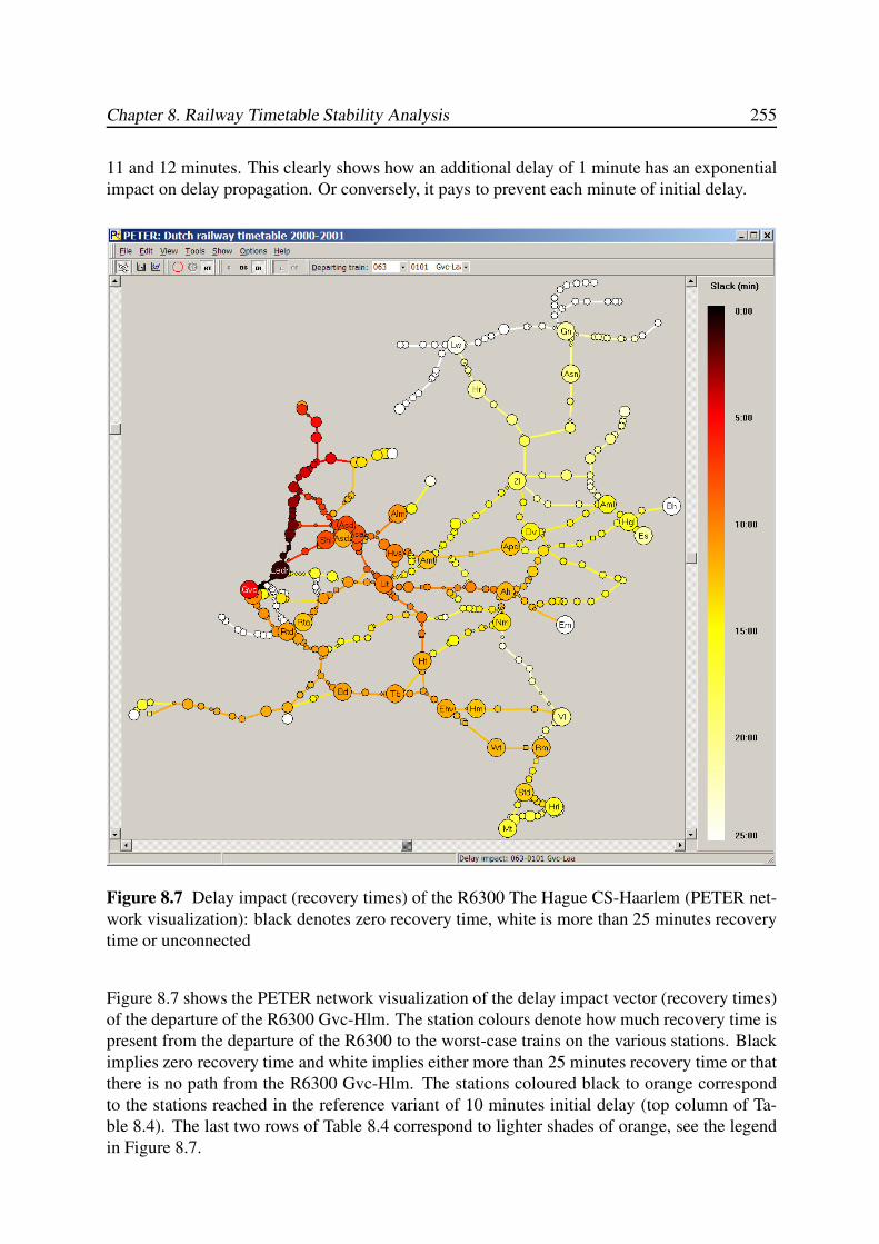
Chapter 8. Railway Timetable Stability Analysis 255
11 and 12 minutes. This clearly shows how an additional delay of 1 minute has an exponential
impact on delay propagation. Or conversely, it pays to prevent each minute of initial delay.
Figure 8.7 Delay impact (recovery times) of the R6300 The Hague CS-Haarlem (PETER net-
work visualization): black denotes zero recovery time, white is more than 25 minutes recovery
time or unconnected
Figure 8.7 shows the PETER network visualization of the delay impact vector (recovery times)
of the departure of the R6300 Gvc-Hlm. The station colours denote how much recovery time is
present from the departure of the R6300 to the worst-case trains on the various stations. Black
implies zero recovery time and white implies either more than 25 minutes recovery time or that
there is no path from the R6300 Gvc-Hlm. The stations coloured black to orange correspond
to the stations reached in the reference variant of 10 minutes initial delay (top column of Ta-
ble 8.4). The last two rows of Table 8.4 correspond to lighter shades of orange, see the legend
in Figure 8.7.
256 Punctuality of Railway Operations and Timetable Stability Analysis
The results of the delay propagation and recovery times shown here depend on the parameters
(process times) of the DONS model. In particular, the minimum headway times are given
by the headway norms, which however also include buffer time. Hence, the results are too
conservative. More realistic minimum headways can be obtained by empirical data or using
blocking time calculations. This was however beyond the scope of this case study.
8.9 Conclusions
Railway timetables have an intrinsic structure that can be conveniently modelled using max-
plus algebra. It has been shown how polynomial matrices in max-plus algebra provide a direct
link between timed event graphs and their max-plus state-space representations. A discrete-
event systems theory has been developed to analyse these max-plus linear systems on stability,
realizability, robustness, and delay propagation. The analysis methods are based on efficient
algorithms including the solution to a generalized eigenproblem, shortest (or longest) path al-
gorithms, and a dedicated delay propagation algorithm. Using these algorithms many valuable
performance indicators can be computed, including network performance indicators (minimum
cycle time, throughput, stability margin), recovery times (delay impact vectors, delay sensitiv-
ity vectors, circulation recovery times), and delay propagation statistics (total secondary delay,
number of delayed trains, average secondary delay, settling period).
The max-plus eigenproblem provides several useful quantitative and qualitative characteristics
of the railway timetable and its operational behaviour. A simple stability test is obtained by
comparing the maximum eigenvalue (minimum cycle time) to the timetable period length (e.g.
an hour). Obviously, the timetable cycle time must exceed the maximum eigenvalue otherwise
the timetable is unrealizable, that is, it cannot be operated within the intended timetable period
length. Only if the maximum eigenvalue is smaller than the basic timetable period it can be
expected that the traffic network is stable, meaning that initial delays settle within a finite num-
ber of periods. The higher the difference between the minimum and intended cycle time the
more stable the traffic network becomes. In addition, a stability margin can be computed by
an auxiliary (max-plus) eigenproblem in which the timetable slack is explicitly evaluated. This
stability margin gives the minimum slack time of each train run during a basic timetable period.
This margin corresponds to a circuit with the least mean slack time, where the mean is taken
over the number of trains (tokens) in the circuit. This circuit may differ from the critical circuit
depending on the number of trains in the circuits: the higher the train count the less the share of
slack time to each train.
The max-plus modelling and analysis algorithms have been implemented in the software tool
PETER (Performance Evaluation of Timed Events in Railways). The algebraic approach com-
bined with efficient graph theoretic algorithms allows real-time analysis of large-scale networks.
The main functionalities of PETER have been explained and demonstrated with a case study of
the Dutch railway timetable.
Chapter 9
CONCLUSIONS
9.1 Main Conclusions
9.1.1 Analysis of Train Detection Data
One of the main contributions of this PhD research conform the first research objective is the
development of the software application TNV-Prepare, which converts TNV-logfiles to tables
of train number and infrastructure events collected by train line and realized route. In these
TNV-tables each daily train number has been coupled to the occupation and release time of the
successive track sections on the realized train route, as well as relevant signal aspect changes
and switch lockings. All recorded event times have a precision of one second and are checked
on route-logic consistency by TNV-Prepare, thus guaranteeing the reliability of the information
in the TNV-tables. The coupling of infrastructure data from the safety and signalling systems to
train numbers enables an accurate quantitative analysis of train movements and station infras-
tructure utilization, including realized track occupation times, blocking times, and minimum
headway times between train pairs, which was not possible before the development of TNV-
Prepare.
Arrival and departure times at platform tracks are not detected directly by the safety and sig-
nalling systems. Nevertheless, ‘rough’ estimates of arrival times and departure times of sched-
uled events at platform tracks are available in the TNV-tables by means of the release time of
the section directly before the platform track section (last train axle enters the platform section)
and the occupation time of the successor section (first train axle leaves the platform track), re-
spectively. The error in these arrival/departure time estimates range between a few seconds to a
maximum of 30 seconds depending on the length of the platform track section, the train length,
and the stop position on the platform track. These estimates are thus rather accurate and in
particular improve the current automatic registration by the Dutch traffic control system VKL,
which is based on far measurement points (at signals) using static tables of correction times
to bridge the running time to/from the platform stop position. If additionally section lengths
(and preferably also stop positions) are available, then the supplementary tool TNV-Filter can
be used to improve the arrival/departure time estimates to a maximal error of a few seconds
by fitting speed profiles through the station route and thus obtaining the actual speed and ac-
celeration/deceleration rates at the platform section borders, which are used in estimating the
remaining running time at the platform section. Thus, TNV-Prepare — in combination with
TNV-Filter — also enables accurate estimates and analysis of dwell times, transfer times and
running times, see Figure 9.1.
The data in TNV-logfiles made accessible via application of TNV-Prepare have been shown
to be invaluable for detailed analysis of train punctuality, detection of train interdependencies,
257
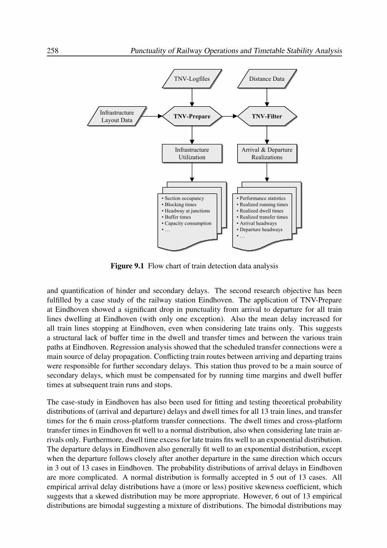
258 Punctuality of Railway Operations and Timetable Stability Analysis
Infrastructure
Utilization
Infrastructure
UtilizationArrival & Departure
Realizations
Arrival & Departure
Realizations
TNV-PrepareTNV-Prepare TNV-FilterTNV-Filter
TNV-LogfilesTNV-Logfiles Distance DataDistance Data
Infrastructure
Layout Data
Infrastructure
Layout Data
• Section occupancy
• Blocking times
• Headway at junctions
• Buffer times
• Capacity consumption
• …
• Section occupancy
• Blocking times
• Headway at junctions
• Buffer times
• Capacity consumption
• …
• Performance statistics
• Realized running times
• Realized dwell times
• Realized transfer times
• Arrival headways
• Departure headways
• …
• Performance statistics
• Realized running times
• Realized dwell times
• Realized transfer times
• Arrival headways
• Departure headways
• …
Infrastructure
Utilization
Infrastructure
UtilizationArrival & Departure
Realizations
Arrival & Departure
Realizations
TNV-PrepareTNV-Prepare TNV-FilterTNV-Filter
TNV-LogfilesTNV-Logfiles Distance DataDistance Data
Infrastructure
Layout Data
Infrastructure
Layout Data
• Section occupancy
• Blocking times
• Headway at junctions
• Buffer times
• Capacity consumption
• …
• Section occupancy
• Blocking times
• Headway at junctions
• Buffer times
• Capacity consumption
• …
• Performance statistics
• Realized running times
• Realized dwell times
• Realized transfer times
• Arrival headways
• Departure headways
• …
• Performance statistics
• Realized running times
• Realized dwell times
• Realized transfer times
• Arrival headways
• Departure headways
• …
Figure 9.1 Flow chart of train detection data analysis
and quantification of hinder and secondary delays. The second research objective has been
fulfilled by a case study of the railway station Eindhoven. The application of TNV-Prepare
at Eindhoven showed a significant drop in punctuality from arrival to departure for all train
lines dwelling at Eindhoven (with only one exception). Also the mean delay increased for
all train lines stopping at Eindhoven, even when considering late trains only. This suggests
a structural lack of buffer time in the dwell and transfer times and between the various train
paths at Eindhoven. Regression analysis showed that the scheduled transfer connections were a
main source of delay propagation. Conflicting train routes between arriving and departing trains
were responsible for further secondary delays. This station thus proved to be a main source of
secondary delays, which must be compensated for by running time margins and dwell buffer
times at subsequent train runs and stops.
The case-study in Eindhoven has also been used for fitting and testing theoretical probability
distributions of (arrival and departure) delays and dwell times for all 13 train lines, and transfer
times for the 6 main cross-platform transfer connections. The dwell times and cross-platform
transfer times in Eindhoven fit well to a normal distribution, also when considering late train ar-
rivals only. Furthermore, dwell time excess for late trains fits well to an exponential distribution.
The departure delays in Eindhoven also generally fit well to an exponential distribution, except
when the departure follows closely after another departure in the same direction which occurs
in 3 out of 13 cases in Eindhoven. The probability distributions of arrival delays in Eindhoven
are more complicated. A normal distribution is formally accepted in 5 out of 13 cases. All
empirical arrival delay distributions have a (more or less) positive skewness coefficient, which
suggests that a skewed distribution may be more appropriate. However, 6 out of 13 empirical
distributions are bimodal suggesting a mixture of distributions. The bimodal distributions may
Chapter 9. Conclusions 259
be explained by hinder of arriving trains due to conflicting train routes by which the distribution
is a mixture of hindered and unhindered arrivals. The arrivals can be partitioned into early and
late arrivals. When considering late train arrivals only an exponential distribution fits well to
the (late) arrival delays, except in 2 out of 13 cases of which the majority of trains arrive late.
These 2 cases showed a good normal fit for all (early and late) arrivals.
Identification of small but structural primary and secondary delays is essential for improving
railway operations and timetables. Structural shortcomings in a timetable often generate only
small delays (less than 60 seconds) but a cumulation of small delays leads to large delays at
possibly distant locations which become hard to explain. In the current practice where delays
below 3 minutes are not recognized as such it is impossible to find the real sources of delays by
which unnecessary drastic measures are applied to repair symptoms rather than actual problems.
A periodic assessment of railway operations at stations and corridors with potential risk of delay
propagation is therefore recommended to find and resolve sources of structural timetable con-
flicts. An important cause of timetable fragility is the quality and precision of some timetabling
base data, such as assumptions on power supply, driver behaviour, alighting/boarding time, et
cetera, used to compute e.g. running times, dwell times and minimum headway. Feedback
from operational realization data thus is a necessary means to relieve this problem and match
planning more closely to realization.
9.1.2 Timetable Stability Analysis
The third research objective was developing an analytical approach to evaluate and quantify
critical network dependencies on capacity utilization and timetable stability. To this end, we
adopted the max-plus algebra modelling approach and extended it by including headway con-
straints conform minimum headway relations imposed by the railway infrastructure. Moreover,
the resulting constraint system resembles that of DONS — the Dutch timetable design system
for computing feasible periodic timetables — which facilitates the compatibility between the
timetable construction and timetable evaluation.
We showed that a periodic railway timetable has an inherent structure that can be modelled
efficiently as a timed event graph, or equivalently, a linear system in max-plus algebra. The
max-plus linear system model contains all timetable and headway constraints of interdependent
event pairs. We emphasized the importance of the zero-order dynamics and showed that an
effective description of a general (higher-order) max-plus linear system can be obtained using
a polynomial state matrix, which yields a direct state-space representation in the event domain
of the associated timed event graph. Performance evaluation of the max-plus linear system
is achieved by computing the generalized eigenstructure of the (polynomial) state matrix for
which the remarkably fast policy iteration algorithm is available. The eigenstructure explic-
itly quantifies the decoupled components and minimal cycle times of all events and moreover
identifies the critical events and processes. The maximum generalized eigenvalue defines the
minimum cycle time attainable for the given interconnection structure, which corresponds to the
capacity consumption within a timetable period. The ratio of the maximum eigenvalue and the
timetable period length gives the network throughput, and the difference between the timetable
cycle time and the maximum eigenvalue is a measure of the stability margin within a basic
timetable period. All these measures are related to the critical circuits in the network structure,
which correspond to (closed) sequences of consecutive timetable events that are interrelated by
260 Punctuality of Railway Operations and Timetable Stability Analysis
either timetable relations or conflicting routes. The identified critical events and processes give
directions for further analysis to improve the timetable.
Supplementary to the eigenstructure analysis, the recovery times between all event pairs can be
computed in the so-called recovery matrix using any available shortest (or longest) path algo-
rithms. The diagonal entries of this recovery matrix are the circulation recovery times indicating
for each event the minimum total slack over any recurrent path, which is a clear robustness mea-
sure. Also the columns and rows of the recovery matrix show explicitly the tightness between
events over all paths in the network and thus identify the impact and sensitivity of delays in the
network. Robustness against explicit initial delay scenarios can furthermore be computed by
a very effective bucket-based delay propagation algorithm, yielding the settling period of the
initial delays or any other individual or aggregated measure of the initial and secondary delays.
The max-plus analysis approach has been implemented in the software tool PETER (Perfor-
mance Evaluation of Timed Events in Railways), which enables railway planners to use pow-
erful mathematical techniques in the evaluation of periodic timetables. One of the main ad-
vantages of PETER over other existing software for evaluating railway timetables is its com-
putational performance. Properties of large-scale timetables are computed in real-time which
makes it a perfect tool for comparing a large number of different timetable variants or studying
a timetable design in much detail using predefined initial delay scenarios. Moreover, we believe
that the deterministic model conform the timetable design (deterministic process times, fixed
train orders) is appealing to timetable designers who show a reluctant response to simulation
tools.
The compatibility of PETER to DONS enables an automatic import of data. However, the
minimum headway times used in DONS are mainly very simplified. Headway design norms
may be used for the construction of a timetable, which then consist of the minimum headway
time and some buffer time. For a realistic evaluation in PETER the amount of buffer time within
these headway times must be known to prevent conservative results. It is however unknown
how much buffer time is contained in the headway times used in DONS as this is typically
location dependent and must be calculated by hand. Realistic minimum headway times can be
obtained by either microscopic blocking time calculations or empirical train detection data. In
the Netherlands, blocking time models are (still) not used in the railway planning practice. On
the other hand, reliable empirical data on infrastructure utilization is now available by means of
the tool TNV-Prepare which can thus be applied to derive realistic minimum headway times.
9.2 Recommendations and Future Research
9.2.1 Train Detection Data and Railway Operations Quality Management
TNV-Prepare requires manual input of railway infrastructure and routes, which is an undesir-
able tedious task when the tool is applied on a wider scale. The infrastructure modelling utility
in TNV-Prepare can however be adapted to import infrastructure configuration data files from
the system CARE [68] that also provides the configuration data in the TNV-systems. Each time
the configuration data of a TNV-system is updated also the TNV-Prepare infrastructure must be
updated. This guarantees a synchronization between the configuration data in the TNV-systems
and TNV-Prepare, by which the infra elements and route blocks contained in the TNV-logfiles
Chapter 9. Conclusions 261
are automatically recognized by TNV-Prepare. The configuration data in the TNV-Replay ap-
plication [162] — also based on TNV-logfiles — is maintained in the same way. Ideally the con-
figuration files also contain section lengths by which TNV-Filter is analogously automatically
configured. ProRail is still developing an Infra-atlas that will contain up-to-date geographi-
cal data of station layouts, although it remains yet unclear whether length information of track
sections will be completely available and maintained after local infrastructure modifications.
Recent developments in the format of TNV-logfiles authorized by ProRail ICT-Services for an-
other project (monitoring of switch loads) also allow new improvements in the applicability
of TNV-Prepare in both scale and time. The recording module of TNV-systems has been cus-
tomized to include the reserved route block in each logged train number step message, where a
route block is a list of sections and switches within a TNV-position. These new TNV-logfiles are
known as VTL-files (Verbeterde TNV-Logfiles). This TNV software update has been gradually
installed over the 13 TNV-systems during 2004–2005. The extra information in combination
with the configuration files of the route blocks simplifies the search algorithm of TNV-Prepare
considerably and consequently decreases the necessary computation time to couple train num-
bers to infrastructure events drastically, hence enabling a real-time and national generation of
‘TNV-tables’ over complete train line routes from terminal to terminal. Moreover, the system
TROTS (TRain Observation and Tracking System) which is currently being developed to re-
place the TNV-systems will be able to provide accurate event time realizations. Availability of
reliable train realization data in the near future is therefore no longer an issue.
Future effort must be directed towards usage of the empirical data in daily practice. As already
discussed the data should be used for a regular comparison of planning with its realization to
improve small structural conflicts in the timetable. More specific, dwell times and transfer
times at (key) transfer stations should be evaluated and where necessary improved. Until now,
these process times are mainly based on (historical) rules of thumb which have hardly been
adjusted over the last decades although the traffic intensity changed considerably. Now we
have the data available we can set this straight. Also train running times should be evaluated
and in particular the used running time margins, which may depend on local conditions and
circumstances. Internationally, different running time supplements are advised for the various
train line types. Data analysis will reveal whether a differentiation of running time margins
is worthwhile. Moreover, the existing running time calculation methods (such as in DONS
and VPT-Planning) can be verified and possibly calibrated using the realization data, which
will improve the realizability of the timetable. Finally, accurate determination of minimum
headway times has been structurally neglected in the Netherlands, and therefore there is also
no knowledge on existing buffer time between train paths at conflict points. Data analysis will
reveal the realized minimum headways and thus buffer times between events. In combination
with blocking time theory tight headway times without any average buffer time can easily be
detected and consequently robustness of operations can be improved considerably by adding
buffer time corresponding to the local variations in headway.
Deterioration and unavailability of infrastructure (signals, switches, tracks) and other techni-
cal equipment (rolling stock, dispatching and control systems) also have a main impact on the
dispunctuality of railway operations. These primary sources of disruptions and delays can evi-
dently not be detected from TNV-data. Nevertheless, a variety of registration systems are in use
for logging incidents and equipment failures. A link between these systems and the TNV-data
via train numbers, location and time of breakdowns, will provide the necessary information
262 Punctuality of Railway Operations and Timetable Stability Analysis
to identify primary delays associated to recorded disruptions. Moreover, the secondary delays
(and cancellations) resulting from the diagnosed primary delays can subsequently be determined
from the TNV-data which thus reveals the impact of a disruption on operations. Knowing the
impact of various disruptions may help to improve accurate disruption management.
9.2.2 Max-Plus Algebra
The max-plus algebra approach — and the tool PETER — could be an effective instrument
to the capacity allocation process of infrastructure managers. In particular in the Netherlands
where capacity requests of train operators are submitted as basic hour patterns (BHPs), which
are nothing else than periodic timetables with a cycle time of one hour that can effectively be
modelled and analysed in max-plus algebra as we have seen in this thesis. The infrastructure
manager must coordinate the various BHP requests and test the resulting integrated BHP on
feasibility and stability. The current practice at ProRail Capacity Allocation is still largely
manual with the support of VPT-Planning (VPT-BUP), which however does not include conflict
detection or evaluation functionalities other than the graphical means of time-distance graphs
(no blocking times) and basic platform occupation diagrams. Possible extensions of PETER
to be even more beneficial are an interface with VPT-BUP files to read VPT-BUP files and
an automatic conflict detection mechanism. The latter implies that conflicting train paths are
detected and minimum headways between conflicting train routes are computed. To this end,
some additional data is required on the infrastructure usage. In the near future VPT-BUP will be
replaced by PTI (Planning & Toewijzing Infrastructuur) which is currently under dvelopment.
An interface to PTI is therefore also advisable.
This thesis considered deterministic max-plus linear systems for effective analysis of large-
scale railway timetables. Future extensions may be directed towards introducing stochastic
elements without sacrificing the computing time too much. This may lead to for instance sen-
sitivity analysis of the timetable parameters (process times) to further identify critical events
and processes. A more serious stochastic extension is changing the order of scheduled events,
which is typically one of the most effective actions to reduce delay propagation. The problem
of finding critical train orders is however linked to the NP-hard problems of sequencing and
scheduling. Nevertheless, we may effectively evaluate the impact on performance of changing
selected events. Another extension is the unavailability of resources by which the system must
change to a different mode (state matrix). Current research on this topic includes (max-plus)
Taylor series approximations [97] and — from a control point of view — switching max-plus
linear systems [204].
Another research direction is railway timetable optimization. The max-plus delay propagation
model may be used in a two-stage stochastic optimization model that combines timetable opti-
mization and evaluation [213]. However, this optimization problem does not change the critical
circuits but only the distribution of slack over the (critical) processes. Even more challeng-
ing is the question whether we can use the max-plus model to construct timetables in addition
to evaluation and improving. For scheduled public transport this question can be answered
confirmative: from the transportation times a max-plus model (or timed event graph) can be
constructed and the eigenvector of the state matrix gives a most effective timetable for running
regularly with a cycle time exceeding the eigenvalue. The performance of this initial timetable
can successively be improved using marking optimization [126, 167] where tokens (vehicles)
Chapter 9. Conclusions 263
can be added or redistributed over the timed event graph to optimize some objective function.
In railway systems the shared use of infrastructure causes the difficulty that decisions have to
be made on the order of trains over conflicting train routes. This ordering problem makes the
problem typically NP-hard: in the worst-case all combinations of train orders must be evalu-
ated before finding the optimal solution. The problem complexity is likely equivalent to the
NP-complete periodic event scheduling problem (PESP). However, a different problem formu-
lation may guide an efficient solution algorithm in practice. Heuristic design criteria may help
to find good solutions. The stochastic max-plus model extensions may also guide the timetable
optimization process [97].

264 Punctuality of Railway Operations and Timetable Stability Analysis
BIBLIOGRAPHY
[1] Abbink, E., Van den Berg, B., Kroon, L.G., and Salomon, M., “Allocation of Railway
Rolling Stock for Pasenger Trains”, Transportation Science, vol. 38, no. 1, pp. 33–41,
2004.
[2] Aho, A.V., Hopcroft, J.E., and Ullman, J.D., Data Structures and Algorithms, Addison-
Wesley, Reading, 1983.
[3] Ahuja, R.K., Magnanti, T.L., and Orlin, J.B., Network Flows: Theory, Algorithms, and
Applications, Prentice-Hall, New Jersey, 1993.
[4] Alfieri, A., Groot, R., Kroon, L.G., and Schrijver, A., “Efficient Circulation of Railway
Rolling Stock”, ERIM Report Series ERS-2002-110-LIS, Erasmus University Rotter-
dam, Rotterdam, 2002.
[5] Allan, J., Brebbia, C.A., Hill, R.J., Sciutto, G., and Sone, S. (eds.), Computers in Rail-
ways IX, WIT Press, Southampton, 2004.
[6] Allan, J., Hill, R.J., Brebbia, C.A., Sciutto, G., and Sone, S. (eds.), Computers in Rail-
ways VII, WIT Press, Southampton, 2000.
[7] Allan, J., Hill, R.J., Brebbia, C.A., Sciutto, G., and Sone, S. (eds.), Computers in Rail-
ways VIII, WIT Press, Southampton, 2002.
[8] Anderson, B.D.O. and Moore, J.B., Optimal Filtering, Prentice-Hall, Englewood Cliffs,
1979.
[9] Andrews, H.I., Railway Traction: The Principles of Mechanical and Electrical Railway
Traction, Studies in Mechanical Engineering, vol. 5, Elsevier, Amsterdam, 1996.
[10] Assad, A.A., “Models for Rail Transportation”, Transportation Research Part A, vol. 14,
no. 3, pp. 205–220, 1980.
[11] Baccelli, F.L., Cohen, G., Olsder, G.J., and Quadrat, J.P., Synchronization and Linearity:
An Algebra for Discrete Event Systems, Wiley, Chichester, 1992.
[12] Bailey, C. (ed.), European Railway Signalling, Institution of Railway Signal Engineers
(IRSE), A&C Black, London, 1995.
[13] Bapat, R.B., “A Max Version of the Perron-Frobenius Theorem”, Linear Algebra and its
Applications, vol. 275–276, pp. 3–18, 1998.
[14] Bapat, R.B. and Raghavan, T.E.S., Nonnegative Matrices and Applications, Cambridge
University Press, Cambridge, 1997.
[15] Berge, C., Topological Spaces, Oliver & Boyd, London, 1963. Reprint by Dover, Mine-
ola, 1997.
[16] Berge, C., The Theory of Graphs, Methuen, London, 1966. Reprint by Dover, Mineola,
2001.
[17] Berman, A. and Plemmons, R.J., Nonnegative Matrices in the Mathematical Sciences,
Classics in Applied Mathematics, vol. 9, SIAM, Philadelphia, 1994.
[18] Bollobas, B., Modern Graph Theory, Graduate Texts in Mathematics, vol. 184, Springer,
New York, 1998.
[19] Bookbinder, J.H. and Desilets, A., “Transfer Optimization in a Transit Network”, Trans-
portation Science, vol. 26, no. 2, pp. 106–118, 1992.
265
266 Punctuality of Railway Operations and Timetable Stability Analysis
[20] Bouma, A. and Oltrogge, C., “Linienplanung und Simulation fur offentliche Verkehr-
swege in Praxis und Theorie”, Eisenbahntechnische Rundschau (ETR), vol. 43, no. 6, pp.
369–378, 1994.
[21] Braker, J.G., Algorithms and Applications in Timed Discrete Event Systems, PhD thesis,
Delft University of Technology, Delft, 1993.
[22] Braker, J.G. and Olsder, G.J., “The Power Algorithm in Max Algebra”, Linear Algebra
and its Applications, vol. 182, pp. 67–89, 1993.
[23] Brunger, O., Konzeption einer Rechnerunterstutzung fur die Feinkonstruktion von Eisen-
bahnfahrplanen, Dissertation, Veroffentlichungen des Verkehrswissenschaftlichen Insti-
tutes der RWTH Aachen, Heft 51, Aachen, 1995.
[24] Bussieck, M., Optimal Lines in Public Rail Transport, PhD thesis, Technische Universitat
Braunschweig, Braunschweig, 1998.
[25] Bussieck, M.R., Kreuzer, P., and Zimmermann, U.T., “Optimal Lines for Railway Sys-
tems”, European Journal of Operational Research, vol. 96, no. 1, pp. 54–63, 1997.
[26] Bussieck, M.R., Winter, T., and Zimmermann, U.T., “Discrete Optimization in Public
Rail Transport”, Mathematical Programming, vol. 79, no. 3, pp. 415–444, 1997.
[27] Caprara, A., Fischetti, M., Toth, P., Vigo, D., and Guida, P.L., “Algorithms for Railway
Crew Management”, Mathematical Programming, vol. 79, pp. 125–141, 1997.
[28] Carey, M., “Reliability of Interconnected Scheduled Services”, European Journal of Op-
erational Research, vol. 79, no. 1, pp. 51–72, 1994.
[29] Carey, M., “Ex Ante Heuristic Measures of Schedule Reliability”, Transportation Re-
search Part B, vol. 33, no. 7, pp. 473–494, 1999.
[30] Carey, M. and Kwiecinski, A., “Properties of Expected Costs and Performance Mea-
sures in Stochastic Models of Scheduled Transport”, European Journal of operational
Research, vol. 83, no. 1, pp. 182–199, 1995.
[31] Cochet-Terrasson, J., Cohen, G., Gaubert, S., Mc Gettrick, M., and Quadrat, J.-P., “Nu-
merical Computation of Spectral Elements in Max-Plus Algebra”, In: IFAC Conference
on System Structure and Control, Nantes, France, 1998.
[32] Cohen, G., Dubois, D., Quadrat, J.-P., and Viot, M., “A Linear-System-Theoretic View
of Discrete-Event Processes and Its Use for Performance Evaluation in Manufacturing”,
IEEE Transactions on Automatic Control, vol. AC-30, no. 3, pp. 210–220, 1985.
[33] Cohen, G., Gaubert, S., and Quadrat, J.-P., “Linear Projectors in the Max-Plus Algebra”,
In: Proceedings of the 5th IEEE Mediterranean Conference on Control and Systems,
Paphos, Cyprus, 21–23 July, 1997.
[34] Cohen, G., Gaubert, S., and Quadrat, J.-P., “Max-Plus Algebra and System Theory:
Where We Are and Where to Go Now”, Annual Reviews in Control, vol. 23, pp. 207–219,
1999.
[35] Coleman, T., Branch, M.A., and Grace, A., Optimization Toolbox User’s Guide, Version
2, The MathWorks, Natick, 1999.
[36] Coleman, T.F. and Li, Y., “An Interior Trust Region Approach for Nonlinear Minimiza-
tion Subject to Bounds”, SIAM Journal on Optimization, vol. 6, pp. 418–445, 1996.
[37] Commoner, F., Holt, A.W., Even, S., and Pnueli, A., “Marked Directed Graphs”, Journal
of Computer and System Sciences, vol. 5, pp. 511–523, 1971.
[38] Cordeau, J.-F., Toth, P., and Vigo, D., “A Survey of Optimization Models for Train Rout-
ing and Scheduling”, Transportation Science, vol. 32, no. 4, pp. 380–404, 1998.
Bibliography 267
[39] Cormen, T.H., Leiserson, C.E., and Rivest, R.L, Introduction to Algorithms, MIT Press,
Cambridge, 1990.
[40] Cuninghame-Green, R.A., Minimax Algebra, Lecture Notes in Economics and Mathe-
matical Systems, vol. 166, Springer, Berlin, 1979.
[41] Cuninghame-Green, R.A. and Butkovic, P., “Bases in Max-Algebra”, Linear Algebra
and its Applications, vol. 389, pp. 107–120, 2004.
[42] Curchod, A. and Lucchini, L., “CAPRES: General Description of the Model”, Document
ITEP 788/6, Ecole Polytechnique Federale de Lausanne (EPFL), Lausanne, 2001.
[43] Daamen, W., “A Quantitative Assessment on the Design of a Railway Station”, In: Allan
et al. [7], pp. 191–200, 2002.
[44] Daamen, W., Modelling Passenger Flows in Public Transport Facilities, PhD thesis,
TRAIL Thesis Series, no. T2004/6, Delft University Press, Delft, 2004.
[45] Dam, A. and Kieft, S., Prolop, toedelings- en vergelijkingsmodel: Overzicht werking, in-
en output, NS Reizigers Marketingonderzoek & Advies, Utrecht, 1998.
[46] Damen, A., “Uitvoeringstijden treinactiviteiten in Vervoersgegevensbank VKL”, Intern
rapport, NS Verkeersleiding, Utrecht, 1997.
[47] Dasdan, A., “Experimental Analysis of the Fastest Optimum Cycle Ratio and Mean Al-
gorithms”, ACM Transactions on Design Automation of Electronic Systems, vol. 9, no. 4,
pp. 385–418, 2004.
[48] Dasdan, A. and Gupta, R.K., “Faster Maximum and Minimum Mean Cycle Algorithms
for System Performance Analysis”, IEEE Transactions on Computer-Aided Design of
Integrated Circuits and Systems, vol. 17, no. 10, pp. 889–899, 1998.
[49] Dasdan, A., Irani, S.S., and Gupta, R.K., “An Experimental Study of Minimum Mean
Cycle Algorithms”, Technical report 98-32, University of California, Irvine, 1998.
[50] Dasdan, A., Irani, S.S., and Gupta, R.K., “Efficient Algorithms for Optimum Cycle Mean
and Optimum Cost to Time Ratio Problems”, In: Proceedings of the 36th ACM/IEEE
Design Automation Conference (DAC), pp. 37–42, ACM Press, New York, 1999.
[51] De Kort, A.F., Heidergott, B., Van Egmond, R.J., and Hooghiemstra, G., Train Movement
Analysis at Railway Stations: Procedures & Evaluation of Wakob’s Approach, TRAIL
Series in Transportation Science, no. S99/1, Delft University Press, Delft, 1999.
[52] De Schutter, B., Van den Boom, T., and Hegyi, A., “A Model Predictive Control Ap-
proach for Recovery from Delays in Railway Systems”, Transportation Research Record,
vol. 1793, pp. 15–20, 2002.
[53] Demitz, J., Hubschen, C., and Albrecht, C., “Timetable Stability – Using Simulation to
Ensure Quality in a Regular Interval Timetable”, In: Allan et al. [5], pp. 549–562, 2004.
[54] Den Brok, M. and Vissers, R., “VPT, a New Systems Architecture for Planning and
Control of Train Traffic in The Netherlands”, In: Murthy et al. [140], pp. 19–26, 1994.
[55] Dennis, J.E., “Nonlinear Least Squares”, In: Jacobs, D. (ed.), State of the Art in Numeri-
cal Analysis, pp. 269–312, Academic Press, London, 1977.
[56] Dijkstra, E.W., “A Note on Two Problems in Connexion with Graphs”, Numerische Math-
ematik, vol. 1, pp. 269–271, 1959.
[57] Dilli, G., “Der Wandernde Engpaß und sein Gefolge”, Eisenbahntechnische Rundschau
(ETR), vol. 3, no. 1, pp. 1–11, 1954.
[58] Domschke, W., “Schedule Synchronization for Public Transit Networks”, OR Spektrum,
vol. 11, no. 1, pp. 17–24, 1989.
268 Punctuality of Railway Operations and Timetable Stability Analysis
[59] Dudnikov, P.I. and Samborskiı, S.N., “Endomorphisms of Finitely Generated Free Semi-
modules”, In: Maslov, V.P. and Samborskiı, S.N. (eds.), Idempotent Analysis, Advances
in Soviet Mathematics, vol. 13, pp. 65–85, American Mathematical Association (AMS),
Providence, 1992.
[60] European Commission, “Directive 2001/14/EC of the European Parliament and of the
Council of 26 February 2001 on the Allocation of Railway Infrastructure Capacity and
the Levying of Charges for the Use of Railway Infrastructure and Safety Certification”,
Official Journal of the European Communities, vol. L 75, pp. 29–46, 2001.
[61] European Commission, White Paper—European Transport Policy for 2010: Time to De-
cide, Office for Official Publications of the European Communities, Luxembourg, 2001.
[62] Faber, J.A. (ed.), Het spoor: 150 jaar spoorwegen in Nederland, Meulenhoff, Amster-
dam, 1989.
[63] Fenner, W., Naumann, P., and Trinckauf, J., Bahnsicherungstechnik, Publicis Corporate
Publishing, Erlangen, 2003.
[64] Fiedler, J., “Die Haltezeit und ihre Einflußfaktoren”, Eisenbahntechnische Rundschau
(ETR), vol. 17, no. 11, pp. 474–479, 1968.
[65] Fioole, P.J., Kroon, L.G., Maroti, G., and Schrijver, A., “A Rolling Stock Circulation
Model for Combining and Splitting of Passenger Trains”, Report PNA-E0420, CWI,
Amsterdam, 2004.
[66] Floyd, R.W., “Algorithm 97: Shortest path”, Communications of the ACM, vol. 5, no. 6,
pp. 345, 1962.
[67] Fredman, M.L. and Tarjan, R.E., “Fibonacci Heaps and Their Uses in Improved Network
Optimization Algorithms”, Journal of the Association for Computing Machinery (ACM),
vol. 34, no. 3, pp. 596–615, 1987.
[68] Fries, G.A. and Van Sprakelaar, J., “Computer Aided Railway Engineering”, In: Mellitt
et al. [132], pp. 53–59, 1998.
[69] Garey, M.R. and Johnson, D.S., Computers and Intractability: A Guide to Theory of
NP-Completeness, Freeman, New York, 1979.
[70] Gaubert, S., Theorie des Systemes Lineaires dans les Dioıdes, PhD thesis, L’ecole Na-
tionale Superieure des Mines de Paris, Paris, 1992.
[71] Gaubert, S. and Mairesse, J., “Modeling and Analysis of Timed Petri Nets using Heaps
of Pieces”, IEEE Transactions on Automatic Control, vol. 44, no. 4, pp. 683–697, 1999.
[72] Gijsen, A. and Van den Brink, R.R.M., “Het spoor in model: energieverbruik en emissies
door het railvervoer”, RIVM rapport 773002 021/2002, National Institute of Public
Health and the Environment (RIVM), Bilthoven, 2002.
[73] Golan, J.S., Semirings and Affine Equations Over Them: Theory and Applications, Math-
ematics and Its Applications, vol. 556, Kluwer, Dordrecht, 2003.
[74] Gondran, M. and Minoux, M., “Valeurs Propres et Vecteurs Propres en Theorie des
Graphes”, In: Problemes Combinatoires et Theorie des Graphes, Colloques Interna-
tionaux du Centre National de la Recherche Scientifique, no. 260, pp. 181–183, CNRS,
Paris, 1978.
[75] Gondran, M. and Minoux, M., Graphs and Algorithms, Wiley, New York, 1984.
[76] Goossens, J.H.M., Models and Algorithms for Railway Line Planning Problems, PhD
thesis, Universiteit Maastricht, Maastricht, 2004.
Bibliography 269
[77] Goossens, J.H.M., Van Hoesel, C.P.M., and Kroon, L.G., “A Branch-and-Cut Approach
for Solving Railway Line-Planning Problems”, Transportation Science, vol. 38, no. 3,
pp. 379–393, 2004.
[78] Gotz, W.W.J., “Trendanalyse 2001: Trends in veiligheid van het spoorwegsysteem in
Nederland”, Rapport RnV/02/M10.008.076, Railned Spoorwegveiligheid, Utrecht, 2002.
[79] Goverde, R.M.P., “Synchronization Control of Scheduled Train Services to Minimize
Passenger Waiting Times”, In: Proceedings of the 4th TRAIL Year Congress, part 2,
TRAIL Research School, Delft, 1998.
[80] Goverde, R.M.P., “Analyse van treinpaden in stations m.b.v. TNV-Prepare”, In: Hansen,
I.A., Olsder, G.J., and Michels, R. (eds.), Modellen voor de beheersing van treinverkeer,
Bundeling bijdragen SMM workshop 19 mei, Utrecht, TRAIL Research School, Delft,
1999.
[81] Goverde, R.M.P., “Improving Punctuality and Transfer Reliability by Railway Timetable
Optimization”, In: Proceedings of the 5th TRAIL Annual Congress, TRAIL Research
School, Delft, 1999.
[82] Goverde, R.M.P., “Delay Estimation and Filtering of Train Detection Data”, In: Pro-
ceedings TRAIL 6th Annual Congress 2000, TRAIL Conference Proceedings Series, No.
P2000/3, Part 2, TRAIL Research School, Delft, 2000.
[83] Goverde, R.M.P., “PRRING II: Inzicht in de betrouwbaarheid van realisatiegegevens
treinactiviteiten”, Rapport EXT 200307-01, versie 1.0, ProRail Strategie & Innovatie,
Utrecht, 2003.
[84] Goverde, R.M.P. and Hansen, I.A., “TNV-Prepare: Analysis of Dutch Railway Opera-
tions Based on Train Detection Data”, In: Allan et al. [6], pp. 779–788, 2000.
[85] Goverde, R.M.P. and Hansen, I.A., “Delay Propagation and Process Management at Rail-
way Stations”, In: Proceedings CD-Rom of the World Conference on Railway Research
(WCRR 2001), Koln, November 25–29, 2001.
[86] Goverde, R.M.P., Hansen, I.A., Hooghiemstra, G., and Lopuhaa, H.P., “Delay Distribu-
tions in Railway Stations”, In: Proceedings CD-Rom of the 9th World Conference on
Transport Research (WCTR), Seoul, July 22–27, 2001.
[87] Goverde, R.M.P., Hooghiemstra, G., and Lopuhaa, H.P., Statistical Analysis of Train
Traffic: The Eindhoven Case, TRAIL Series in Transportation Science, no. S2001/1,
Delft University Press, DUP Science, Delft, 2001. ISBN: 90-407-2201-3.
[88] Goverde, R.M.P. and Odijk, M.A., “Performance Evaluation of Network Timetables Us-
ing PETER”, In: Allan et al. [7], pp. 731–740, 2002.
[89] Goverde, R.M.P. and Soto y Koelemeijer, G., Performance Evaluation of Periodic Rail-
way Timetables: Theory and Algorithms, TRAIL Studies in Transportation Science,
no. S2000/2, Delft University Press, Delft, 2000.
[90] Groger, T.A., Simulation der Fahrplanerstellung auf der Basis eines hierarchischen
Trassenmanagements und Nachweis der Stabilitat der Betriebsabwicklung, PhD thesis,
RWTH Aachen, Aachen, 2002.
[91] Groger, T.A., “Timetable Simulation by Sophisticated Conflict Resolution between Train
Paths”, In: Allan et al. [5], pp. 573–582, 2004.
[92] Hall, S., Modern Signalling Handbook, Ian Allan Publishing, Hersham, 3rd ed., 2001.
[93] Hansen, I.A. and Goverde, R.M.P., “Ermittlung und Analyse von Ankunftsverspatungen
in Bahnhofen”, Verkehr und Technik, vol. 55, no. 10, pp. 447–453, 2002. (in German).
270 Punctuality of Railway Operations and Timetable Stability Analysis
[94] Hansen, I.A. and Goverde, R.M.P., “Entwicklung und Verteilung von Zugverspatungen
in Bahnhofen”, Verkehr und Technik, vol. 56, no. 2, pp. 69–74, 2003. (in German).
[95] Happel, O., “Sperrzeiten als Grundlage fur die Fahrplankonstruktion”, Eisenbahntech-
nische Rundschau (ETR), vol. 8, no. 2, pp. 79–90, 1959.
[96] Heidergott, B. and De Vries, R., “Towards a Control Theory for Transportation Net-
works”, Discrete Event Dynamic Systems, vol. 11, no. 4, pp. 371–398, 2001.
[97] Heidergott, B. and Leahu, H., “Series Expansions of Generalised Matrix Products”, In:
Proceedings of the 44th IEEE Conference on Decision and Control and European Con-
trol Conference ECC 2005, Sevilla, Spain, 2005 (to appear).
[98] Hereth, K.U., “Die Ubergangszeit bei Zuganschlussen, ein wichtiges Element bei der
Konstruktion des Personenzugfahrplans”, Die Bundesbahn, vol. 53, no. 6, pp. 407–410,
1977.
[99] Hermann, U., Untersuchung zur Verspatungsentwicklung von Fernreisezugen auf der
Datengrundlagen der Rechnerunterstutzten Zuguberwachung Frankfurt am Main, Dis-
sertation Nr. D17, Technische Hochschule Darmstadt, Darmstadt, 1996.
[100] Higgins, A. and Kozan, E., “Modelling Train Delays in Urban Networks”, Transportation
Science, vol. 32, no. 4, pp. 346–357, 1998.
[101] Hooghiemstra, J.S., “An Automatic Timetable Generator for the Dutch Railway Net-
work”, In: Murthy et al. [140], pp. 109–116, 1994.
[102] Hooghiemstra, J.S., Kroon, L.G., Odijk, M.A., Salomon, M., and Zwaneveld, P.J., “De-
cision Support Systems Support the Search for Win-Win Solutions in Railway Network
Design”, Interfaces, vol. 29, no. 2, pp. 15–32, 1999.
[103] Howard, R.A., Dynamic Programming and Markov Processes, MIT Press/Wiley, New
York, 1960.
[104] Howlett, P.G. and Pudney, P.J., Energy-Efficient Train Control, Springer, London, 1995.
[105] Huisman, T., Boucherie, R.J., and Van Dijk, N.M., “A Solvable Queueing Network
Model for Railway Networks and its Validation and Applications for the Netherlands”,
European Journal of Operational Research, vol. 142, no. 1, pp. 30–51, 2002.
[106] Hurlimann, D., Objektorientierte Modellierung von Infrastrukturelementen und Betrieb-
svorgangen im Eisenbahnwesen, Dissertation ETH Nr. 14281, IVT Schriftenreihe 125,
Eidgenossische Technische Hochschule (ETH), Zurich, 2002.
[107] IVW, Regeling Spoorverkeer, Inspectie Verkeer en Waterstaat (IVW), Divisie Rail,
Utrecht, 2005.
[108] Jacobs, J., Rechnerunterstutzte Konfliktermittlung und Entscheidungsunterstutzung bei
der Disposition des Zuglaufs, PhD thesis, RWTH Aachen, Aachen, 2003.
[109] Jacobs, J., “Reducing Delays by Means of Computer-Aided ‘on-the-Spot’ Reschedul-
ing”, In: Allan et al. [5], pp. 603–612, 2004.
[110] Jentsch, E. and Gropler, O., “Stochastische Zugfahrtsimulation: Zusammenhange
und Anwendungsmoglichkeiten”, In: Hertel, G. (ed.), 2. Eisenbahnbetriebswissen-
schaftliches Kolloquium: Taktfahrplan und Kapazitat, Schriftenreihe des Instituts fur
Verkehrssystemtheorie und Bahnverkehr, vol. 2, pp. 154–171, Technische Universitat
Dresden, Dresden, 1996.
[111] Johanns, R.D., Handleiding bij de modules van de TNV-Prepare programmatuur, Trans-
portation and Planning Section, Delft University of Technology, Delft, 2001.
[112] Johnson, D.B., “Efficient Algorithms for Shortest Paths in Sparse Networks”, Journal of
the Association for Computing Machinery (ACM), vol. 24, no. 1, pp. 1–13, 1977.
Bibliography 271
[113] Jovanovic, D. and Harker, P.T., “Tactical Scheduling of Rail Operations: The SCAN I
System”, Transportation Science, vol. 25, no. 1, pp. 46–64, 1991.
[114] Kaminsky, R., Pufferzeiten in Netzen des spurgefuhrten Verkehrs in Abhangigkeit von
Zugfolge und Infrastruktur, Dissertation, Wissenschaftliche Arbeiten Nr. 56 des Insti-
tuts fur Verkehrswesen, Eisenbahnbau und -betrieb der Universitat Hannover, Hannover,
2001.
[115] Kannengießer, F. and Wiche, B., “Einfluß der Fahrzeitenzuschlage und Pufferzeiten auf
die Punktlichkeit”, Die Bundesbahn, vol. 62, no. 11, pp. 1001–1007, 1987.
[116] Karp, R.M., “A Characterization of the Minimum Cycle Mean in a Digraph”, Discrete
Mathematics, vol. 23, no. 3, pp. 309–311, 1978.
[117] Karp, R.M. and Orlin, J.B., “Parametric Shortest Path Algorithms with an Application to
Cyclic Staffing”, Discrete Applied Mathematics, vol. 3, no. 1, pp. 37–45, 1981.
[118] Klemt, W.-D. and Stemme, W., “Schedule Synchronization for Public Transit Networks”,
In: Daduna, J.R. and Wren, A. (eds.), Computer-Aided Transit Scheduling, Proceedings
of the Fourth International Workshop on Computer-Aided Scheduling of Public Trans-
port, Lecture Notes in Economics and Mathematical Systems, vol. 308, pp. 327–335,
Springer, Berlin, 1988.
[119] Knuth, D.E., The Art of Computer Programming. Volume 3: Sorting and Searching,
Addison-Wesley, Boston, 2nd ed., 1998.
[120] Koolstra, K., “Capaciteitsmanagement in de spoorwegsector”, In: Ten Heuvelhof, E.,
Koolstra, K., and Stout, H. (eds.), Capaciteitsmanagement: Beslissen over capaciteit
van infrastructuren, pp. 95–115, Lemma, Utrecht, 2001.
[121] Kraft, K.H., Zugverspatungen und Betriebssteuerung von Stadtschnellbahnen in sys-
temtheoretischer Analyse, Dissertation, Technische Universitat Braunschweig, Braun-
schweig, 1981.
[122] Krista, M., Verfahren zur Fahrplanoptimierung dargestelt am Beispiel der Synchron-
zeiten, Dissertation, Schriftenreihe des Instituts fur Eisenbahnwesen und Verkehrs-
sicherung, Heft 56, Technische Universitat Braunschweig, Braunschweig, 1996.
[123] Krista, M., “Fahrplanoptimierung durch Minimierung der Synchronzeiten”, Signal +
Draht, vol. 91, no. 1–2, pp. 34–38, 1999.
[124] Kroon, L.G., Opsporen van sneller en beter: modelling through..., Inaugural Addresses
Research in Management Series, no. EIA-2001-03-LIS, Erasmus University Rotterdam,
Rotterdam, 2001.
[125] Kroon, L.G. and Fischetti, M., “Crew Scheduling for Netherlands Railways: “Destina-
tion: Customer””, In: Voß, S. and Daduna, J.R. (eds.), Computer-Aided Scheduling of
Public Transport, Lecture Notes in Economics and Mathematical Systems, vol. 505, pp.
181–201, Springer, Berlin, 2001.
[126] Laftit, S., Proth, J.-M., and Xie, X.L., “Optimization of Invariant Criteria for Event
Graphs”, IEEE Transactions on Automatic Control, vol. 37, no. 5, pp. 547–555, 1992.
[127] Lang, S., Algebra, Graduate Texts in Mathematics, vol. 211, Springer, New York, rev.
3rd ed., 2002.
[128] Lindner, T., Train Schedule Optimization in Public Rail Transport, PhD thesis, Technis-
che Universitat Braunschweig, Braunschweig, 2000.
[129] Lucchini, K., Rivier, R., and Emery, D., “CAPRES Network Capacity Assessment for
Swiss Nort-South Rail Freight Traffic”, In: Allan et al. [6], pp. 221–230, 2000.
272 Punctuality of Railway Operations and Timetable Stability Analysis
[130] Mairesse, J., “Graphical Approach of the Spectral Theory in the (max,+) Algebra”, IEEE
Transactions on Automatic Control, vol. 40, no. 10, pp. 1783–1789, 1995.
[131] Mathsoft, S-PLUS 2000 User’s Guide, Data Analysis Products Division, Seattle, 1999.
[132] Mellitt, B., Hill, R.J., Allan, J., Sciutto, G., and Brebbia, C.A. (eds.), Computers in
Railways VI, Computational Mechanics Publications / WIT Press, Southampton, 1998.
[133] Meng, Y., Bemessung von Pufferzeiten in Anschlussen von Reisezugen, Dissertation,
Veroffentlichen des Verkehrswissenschaftlichen Institutes der RWTH Aachen, Heft 46,
Aachen, 1991.
[134] Middelkoop, D. and Bouwman, M., “SIMONE: Large Scale Train Network Simula-
tions”, In: Peters, B.A., Smith, J.S., Medeiros, D.J., and Rohrer, M.W. (eds.), Proceed-
ings of the 2001 Winter Simulation Conference, pp. 1042–1047, IEEE, Piscataway, 2001.
[135] Middelkoop, D. and Bouwman, M., “Testing the Stability of the Rail Network”, In: Allan
et al. [7], pp. 995–1002, 2002.
[136] Migom, A. and Valaert, W., “The Optimization of a Rhythmic Intercity Train Network”,
Rail International, vol. 12, pp. 71–91, 1981.
[137] Muhlhans, E., “Berechnung der Verspatungsentwicklung bei Zugfahrten”, Eisenbahn-
technische Rundschau (ETR), vol. 39, no. 7–8, pp. 465–468, 1990.
[138] Murata, T., “Circuit Theoretic Analysis and Synthesis of Marked Graphs”, IEEE Trans-
actions on Circuits and Systems, vol. CAS-24, no. 7, pp. 400–405, 1977.
[139] Murata, T., “Petri Nets: Properties, Analysis and Applications”, Proceedings of the IEEE,
vol. 77, no. 4, pp. 541–580, 1989.
[140] Murthy, T.K.S., Mellitt, B., Brebbia, C.A., Sciutto, G., and Sone, S. (eds.), Computers in
Railways IV, vol. 2, Computational Mechanics Publications, Southampton, 1994.
[141] Nachtigall, K., “Periodic Network Optimization with Different Arc Frequencies”, Dis-
crete Applied Mathematics, vol. 69, no. 1–2, pp. 1–17, 1996.
[142] Nachtigall, K., “Cutting Planes for a Polyhedron Associated with a Periodic Network”,
Internal report IB 112-96/17, Institut fur Flugfuhrung, Deutsche Forschungsanstalt fur
Luft- und Raumfahrt (DLR), Braunschweig, 1997.
[143] Nachtigall, K. and Voget, S., “A Genetic Algorithm Approach to Periodic Railway Syn-
chronization”, Computers and Operations Research, vol. 23, no. 5, pp. 453–463, 1996.
[144] Nash, A. and Huerlimann, D., “Railroad Simulation Using OpenTrack”, In: Allan et al.
[5], pp. 45–54, 2004.
[145] Nie, L. and Hansen, I.A., “System Analysis of Train Operations and Track Occupancy at
Railway Stations”, European Journal of Transport and Infrastructure Research, vol. 5,
no. 1, pp. 31–54, 2005.
[146] Nie, W., “Waiting: Integrating Social and Psychological Perspectives in Operations Man-
agement”, Omega, vol. 28, no. 6, pp. 611–629, 2000.
[147] Nordeen, M., Stability Analysis of Cyclic Timetables for a Highly Interconnected Rail
Network, PhD thesis nr. 1435, Ecole Polytechnique Federale de Lausanne (EPFL), Lau-
sanne, 1996.
[148] NS, Jaarverslag 2004, Utrecht, 2004.
[149] NS, ProRail, Railion, V&W, “Benutten en Bouwen: Het plan van de spoorsector”, Rap-
port, Nederlandse Spoorwegen, ProRail, Railion, Ministerie van Verkeer en Waterstaat,
Utrecht, 2003.
[150] NSR, Wachttijden voor reizigerstreinen (WRT): Dienstregeling 1995/1996, NS Reizigers
Logistiek, Utrecht, 1995.
Bibliography 273
[151] NSR, Jaardienst Reizigerstreindienst 01 juni 1997 t/m 23 mei 1998, NS Reizigers,
Utrecht, 1997.
[152] NSR, Spoorboekje 97/98, NS Reizigers, Utrecht, 1997.
[153] Odijk, M.A., “A Constraint Generation Algorithm for the Construction of Periodic Rail-
way Timetables”, Transportation Research Part B, vol. 30, no. 6, pp. 455–464, 1996.
[154] Odijk, M.A., Railway Timetable Generation, PhD thesis, Delft University Press, Delft,
1997.
[155] Olsder, G.J., Roos, K., and Van Egmond, R.J., “An Efficient Algorithm for Critical Cir-
cuits and Finite Eigenvectors in the Max-Plus Algebra”, Linear Algebra and its Applica-
tions, vol. 295, no. 1–3, pp. 231–240, 1999.
[156] Olsder, G.J., Subiono, and Mc Gettrick, M., “On Timetables and Allocation of Trains”,
In: Proceedings of the Fourth Workshop on Discrete Event Systems (WODES98), pp.
463–468, Cagliari, 1998.
[157] Ortuzar, J. de D. and Willumsen, L.G., Modelling Transport, Wiley, Chichester, 3rd ed.,
2001.
[158] Pachl, J., Railway Operation and Control, VTD Rail Publishing, Mountlake Terrace,
2002.
[159] Peeters, L.W.P., Cyclic Railway Timetable Optimization, PhD thesis, Erasmus University
Rotterdam, Rotterdam, 2003.
[160] Peeters, M. and Kroon, L.G., “Circulation of Railway Rolling Stock: A Branch-and-Price
Approach”, ERIM Report Series ERS-2003-055-LIS, Erasmus University Rotterdam,
Rotterdam, 2003.
[161] Petri, C.A., Kommunikation mit Automaten, Dissertation, Universitat Bonn, Institut fur
Instrumentelle Mathematik, Schriften des IIM Nr. 2, Bonn, 1962.
[162] Pieters, M.R. and Nieuwenhuis, P., Gebruikershandleiding TNV Replay, AEA Technol-
ogy Rail, Utrecht, 2001.
[163] Poort, J.P., “Grenzen aan benutting”, Rapport, NYFER, Breukelen, 2002.
[164] Prins, M., Het vervoersproces van planning tot uitvoering, NS Verkeersleiding, Urecht,
1998.
[165] ProRail, Network Statement 2005, Utrecht, 2004.
[166] ProRail, Netwerkverklaring 2006, Utrecht, 2005.
[167] Proth, J.-M., Sauer, N., and Xie, X.L., “Optimization of the Number of Transportation
Devices in a Flexible Manufacturing System Using Event Graphs”, IEEE Transactions
on Industrial Electronics, vol. 44, no. 3, pp. 298–306, 1997.
[168] Puterman, M.L., Markov Decision Processes: Discrete Stochastic Dynamic Program-
ming, Wiley, New York, 1994.
[169] Radtke, A. and Hauptmann, D., “Automated Planning of Timetables in Large Railway
Networks Using a Microscopic Data Basis and Railway Simulation Techniques”, In:
Allan et al. [5], pp. 615–625, 2004.
[170] Ren, X. and Zhou, M., “Tactical Scheduling of Rail Operations: A Petri Net Approach”,
In: IEEE International Conference on Systems, Man and Cybernetics, vol. 4, pp. 3087–
3092, 1995.
[171] Renkema, M. and Vas Visser, H., “TRACE Supervision System for Dispatching and
Passenger Information”, In: Allan, J., Brebbia, C.A., and Hill, R.J. (eds.), Computers in
Railways V, vol. 2, pp. 247–256, Computational Mechanics Publications, Southampton,
1996.
274 Punctuality of Railway Operations and Timetable Stability Analysis
[172] Rice, J.A., Mathematical Statistics and Data Analysis, Wadsworth and Brooks/Cole, Pa-
cific Grove, 1988.
[173] Rietveld, P., Bruinsma, F.R., and Van Vuuren, D.J., “Coping with Unreliability in Pub-
lic Transport Chains: A Case Study for Netherlands”, Transportation Research Part A,
vol. 35, no. 6, pp. 539–559, 2001.
[174] Rockafellar, R.T., Network Flows and Monotropic Optimization, Wiley, New York, 1984.
[175] Rothblum, U.G., “Algebraic Eigenspaces of Nonnegative Matrices”, Linear Algebra and
its Applications, vol. 12, no. 3, pp. 281–292, 1975.
[176] Rousseeuw, P. J. and Van Zomeren, B. C., “Unmasking Multivariate Outliers and Lever-
age Points”, Journal of the American Statistical Association, vol. 85, pp. 633–639, 1990.
[177] Sakaguchi, T. and Tomii, N., “A Train Traffic Model Based on Coloured Petri Nets and its
Application to a Train Schedule Planning System”, In: Allan, J., Brebbia, C.A., and Hill,
R.J. (eds.), Computers in Railways V, vol. 1, pp. 457–466, Computational Mechanics
Publications, Southampton, 1996.
[178] Schaafsma, A.A.M., “Versnel het openbaar vervoer en verlies reizigers: het risico van
korte reistijden in het spoorboekje”, In: Mouwen, A.M.T., Kalfs, N., and Govers,
B. (eds.), Colloquium Vervoersplanologisch Speurwerk. Beheersbare mobiliteit: een
utopie?, pp. 266–279, CVS, Delft, 1996.
[179] Schaafsma, A.A.M., Dynamisch Railverkeersmanagement, PhD thesis, TRAIL Thesis
Series, no. T2001/7, Delft University Press, Delft, 2001.
[180] Schaafsma, A.A.M. and Weits, E.A.G. (eds.), Capaciteit en Belasting van het Spoorweg-
net, Railned, Utrecht, 1996.
[181] Schrijver, A., Theory of Linear and Integer Programming, Wiley, Chichester, 1986.
[182] Schrijver, A., “Minimum Circulation of Railway Stock”, CWI Quarterly, vol. 6, no. 3,
pp. 205–217, 1993.
[183] Schrijver, A., “Routing and Timetabling by Topological Search”, Documenta Mathemat-
ica Extra Volume ICM III, pp. 687–695, 1998.
[184] Schrijver, A. and Steenbeek, A., Dienstregelingontwikkeling voor Railned: Rapport
CADANS 1.0, CWI, Amsterdam, 1994.
[185] Schwanhaußer, W., Die Bemessung der Pufferzeiten im Fahrplangefuge der Eisenbahn,
Dissertation, Veroffentlichungen des Verkehrswissenschaflichen Institutes der RWTH
Aachen, Heft 20, Aachen, 1974.
[186] Schwanhaußer, W., “The Status of German Railway Operations Management in Research
and Practice”, Transportation Research Part A, vol. 28, no. 6, pp. 495–500, 1994.
[187] Seneta, E., Non-negative Matrices and Markov Chains, Springer, New York, 2nd ed.,
1981.
[188] Serafini, P. and Ukovich, W., “A Mathematical Model for Periodic Event Scheduling
Problems”, SIAM Journal on Discrete Mathematics, vol. 2, no. 4, pp. 550–581, 1989.
[189] Sontag, E.D., Mathematical Control Theory: Deterministic Finite Dimensional Systems,
Texts in Applied Mathematics, vol. 6, Springer, New York, 1990.
[190] Soto y Koelemeijer, G., On the Behaviour of Classes of Min-Max-Plus Systems, PhD
thesis, Delft University of Technology, TRAIL Thesis Series, no. T2003/6, Delft, 2003.
[191] SRA, Capacity Utilisation Policy: Network Utilisation Strategy, Strategic Rail Authority,
London, June 2003.
[192] SRA, “Capacity Utilisation Policy”, Consultation document, Strategic Rail Authority,
London, September 2002.
Bibliography 275
[193] Stemme, W., Anschlußoptimierung in Netzen des offentlichen Personennahverkehrs, Dis-
sertation D 83, Technische Universitat Berlin, Berlin, 1988.
[194] Stolk, A., “Automatic Conflict Detection and Advanced Decision Support for Optimal
Usage of Railway Infrastructure: Purpose and Concepts”, In: Mellitt et al. [132], pp.
629–638, 1998.
[195] Strang, G., Linear Algebra and its Applications, Harcourt Brace Jovanovich, Orlando,
3rd ed., 1988.
[196] Subiono, On Classes of Min-Max-Plus Systems and their Applications, PhD thesis,
TRAIL Thesis Series, no. T2000/2, Delft University Press, Delft, 2000.
[197] Subiono and Van der Woude, J., “Power Algorithms for (max,+)- and Bipartite
(min,max,+)-Systems”, Discrete Event Dynamic Systems, vol. 10, no. 4, pp. 369–389,
2000.
[198] Tarjan, R.E., “Depth First Search and Linear Graph Algorithms”, SIAM Journal on Com-
puting, vol. 1, no. 2, pp. 146–160, 1972.
[199] Tromp, J.P.M. and Hansen, I.A., “Hindrance Between Conflicting Train Movements at a
Level Crossing”, In: Allan et al. [7], pp. 985–993, 2002.
[200] Ullius, M., “Open Timetable: Tool for Analysis and Quality Control of Timetables”, OTT
Infosheet, IVT, Eidgenossische Technische Hochschule (ETH) Zurich, Zurich, 2003.
[201] Vakhtel, S., Rechnerunterstutzte analytische Ermittlung der Kapazitat von Eisenbahn-
netzen, Dissertation, Veroffentlichungen des Verkehrswissenschaftlichen Institutes der
RWTH Aachen, Heft 59, Aachen, 2002.
[202] Van Boetzelaer, M., “Elektronische beveiliging bij de NS”, Op de rails, vol. 63, no. 3,
pp. 94–100, 1995.
[203] Van de Velde, D., “Dutch and Japanese Railway Reforms and Exchanges”, Japanese
Railway & Transport Review, vol. 24, pp. 10–16, July 2000.
[204] Van den Boom, T.J.J. and De Schutter, B., “Modelling and Control of Railway Net-
works”, In: Proceedings of the American Control Conference (ACC), pp. 5728–5733,
Boston, 2004.
[205] Van der Aalst, W.M.P. and Odijk, M.A., “Analysis of Railway Stations by Means of
Interval Timed Coloured Petri Nets”, Real-Time Systems, vol. 9, no. 3, pp. 241–263,
1995.
[206] Van der Werff, M., Scholten, H., and Godziejewski, B., “Migration Stategy for Signalling
Systems in the Netherlands”, Signal + Draht, vol. 94, no. 10, pp. 43–48, 2002.
[207] Van Egmond, R.J., “Propagation of Delays in Public Transport”, Reports of the Faculty
of Technical Mathematics and Informatics, no. 98-39, Delft University of Technology,
Delft, 1998.
[208] Van Egmond, R.J., Railway Capacity Assessment: An Algebraic Approach, TRAIL Stud-
ies in Transportation Science, S99/2, Delft University Press, Delft, 1999.
[209] Van Egmond, R.J., “An Algebraic Approach for Scheduling Train Movements”, In: Voß,
S. and Daduna, J.R. (eds.), Computer-Aided Scheduling of Public Transport, Lecture
Notes in Economics and Mathematical Systems, vol. 505, Springer, Berlin, 2001.
[210] Van Harn, P., Rekenen of simuleren? Een onderzoek naar stabiliteit van dienstregelingen,
Master thesis, Vrije Universiteit Amsterdam, Amsterdam, 2003.
[211] Van Hengstum, H. and Van Delft, R., “Invoering VPT-procesleiding”, Railevant, vol. 41,
no. 3, pp. 8–11, 1995.
276 Punctuality of Railway Operations and Timetable Stability Analysis
[212] Van Leur, M., “NS Introduces a New Generation Automatic Train Protection”, In:
Murthy et al. [140], pp. 319–324, 1994.
[213] Vromans, M.J.C.M., Reliability of Railway Systems, PhD thesis, Erasmus University
Rotterdam, Rotterdam, 2005.
[214] Vuchic, V.R., Urban Public Transportation: Systems and Technology, Prentice-Hall, En-
glewood Cliffs, 1981.
[215] Wagenaar, A., “Toetsing 2001/2002: Beoordeling basisuurpatronen & 24-uursuit-
werking”, Rapport RnT/01/123, Railned, Utrecht, 2001.
[216] Wagneur, E., “Moduloıds and Pseudomodules: 1. Dimension Theory”, Discrete Mathe-
matics, vol. 98, no. 1, pp. 57–73, 1991.
[217] Wakob, H., Ableitung eines generellen Wartemodells zur Ermittlung der planmaßigen
Wartezeiten im Eisenbahnbetrieb unter besonderer Berucksichtigung der Aspekte Leis-
tungsfahigkeit und Anlagenbelastung, Dissertation, Veroffentlichungen des Verkehrswis-
senschaftlichen Institutes der RWTH Aachen, Heft 36, Aachen, 1985.
[218] Wang, J., Timed Petri Nets: Theory and Applications, Kluwer, Boston, 1998.
[219] Warshall, S., “A Theorem on Boolean Matrices”, Journal of the Association for Comput-
ing Machinery (ACM), vol. 9, no. 1, pp. 11–12, 1962.
[220] Weigand, W., Graphentheoretisches Verfahren zur Fahrplangestaltung in Transportnet-
zen unter berucksichtigung von Pufferzeiten mittels interaktiver Rechentechnik, Disser-
tation, Technische Universitat Braunschweig, Braunschweig, 1981.
[221] Weigand, W., “Verspatungsubertragungen in Fernverkehrsnetzen”, Eisenbahntechnische
Rundschau (ETR), vol. 30, no. 12, pp. 915–920, 1981.
[222] Weigand, W., “The Man-Machine Dialogue and Timetable Planning”, Rail International,
vol. 14, no. 3, pp. 8–25, 1983.
[223] Wende, D., Fahrdynamik, Transpress, Berlin, 1983.
[224] Wendler, E., Analytische Berechnung der planmaßigen Wartezeiten bei asynchroner
Fahrplankonstruktion, Dissertation, Veroffentlichungen des Verkehrswissenschaftlichen
Institutes der RWTH Aachen, Heft 55, Aachen, 1999.
[225] Wezel, M.C., Kok, J.N., Van den Berg, J., and Van Kampen, W., “Genetic Improvement
of Railway Timetables”, In: Davidor, Y., Schwefel, H.P., and Manner, R. (eds.), Proceed-
ings of the Third Conference on Parallel Problem Solving from Nature, Lecture Notes in
Computer Science, vol. 866, pp. 566–575, Springer, Berlin, 1994.
[226] Wiggenraad, P.B.L., “Alighting and Boarding of Passengers at Dutch Railway Stations”,
In: Papers of the TRAIL Workshop “Train Delays at Stations and Network Stability”,
TRAIL Research School, Delft, December 7, 2001.
[227] Young, N.E., Tarjan, R.E., and Orlin, J.B., “Faster Parametric Shortest Path and Mini-
mum Balance Algorithms”, Networks, vol. 21, no. 2, pp. 205–221, 1991.
[228] Yuan, J., Goverde, R.M.P., and Hansen, I.A., “Propagation of Train Delays in Stations”,
In: Allan et al. [7], pp. 975–984, 2002.
[229] Zhu, P., Betriebliche Leistung von Bahnsystemen unter Storungsbedingungen, Disserta-
tion, Fortschritt-Berichte VDI, Reihe 12, no. 462, VDI Verlag, Dusseldorf, 2001.
[230] Zwaneveld, P.J., Railway Planning: Routing of Trains and Allocation of Passenger Lines,
PhD thesis, Erasmus University Rotterdam/TRAIL Research School, Eburon Publishers,
Delft, 1997.

Bibliography 277
[231] Zwaneveld, P.J., Kroon, L.G., and Van Hoesel, S.P.M., “Routing Trains through a Rail-
way Station Based on a Node Packing Model”, European Journal of Operational Re-
search, vol. 128, no. 1, pp. 14–33, 2001.

278 Punctuality of Railway Operations and Timetable Stability Analysis
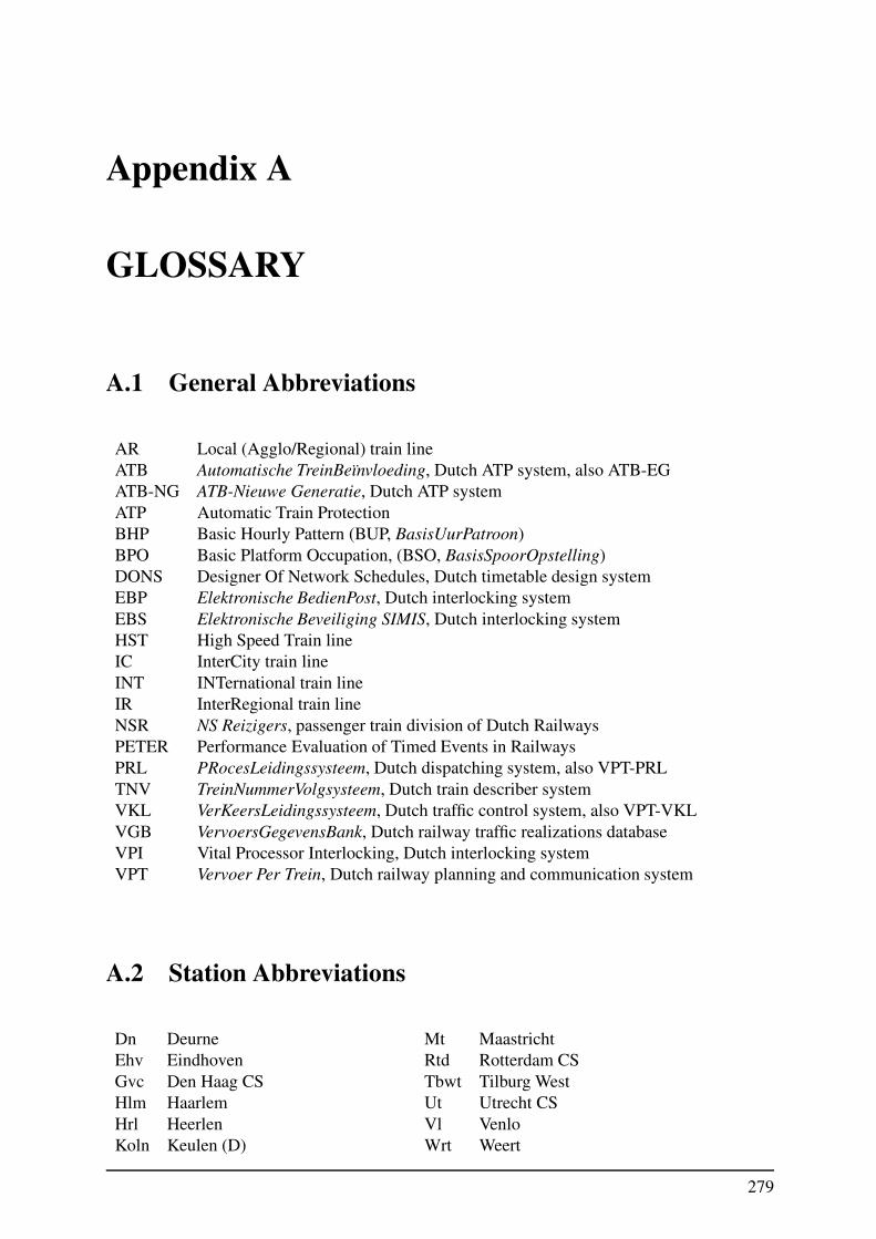
Appendix A
GLOSSARY
A.1 General Abbreviations
AR Local (Agglo/Regional) train line
ATB Automatische TreinBeınvloeding, Dutch ATP system, also ATB-EG
ATB-NG ATB-Nieuwe Generatie, Dutch ATP system
ATP Automatic Train Protection
BHP Basic Hourly Pattern (BUP, BasisUurPatroon)
BPO Basic Platform Occupation, (BSO, BasisSpoorOpstelling)
DONS Designer Of Network Schedules, Dutch timetable design system
EBP Elektronische BedienPost, Dutch interlocking system
EBS Elektronische Beveiliging SIMIS, Dutch interlocking system
HST High Speed Train line
IC InterCity train line
INT INTernational train line
IR InterRegional train line
NSR NS Reizigers, passenger train division of Dutch Railways
PETER Performance Evaluation of Timed Events in Railways
PRL PRocesLeidingssysteem, Dutch dispatching system, also VPT-PRL
TNV TreinNummerVolgsysteem, Dutch train describer system
VKL VerKeersLeidingssysteem, Dutch traffic control system, also VPT-VKL
VGB VervoersGegevensBank, Dutch railway traffic realizations database
VPI Vital Processor Interlocking, Dutch interlocking system
VPT Vervoer Per Trein, Dutch railway planning and communication system
A.2 Station Abbreviations
Dn Deurne Mt Maastricht
Ehv Eindhoven Rtd Rotterdam CS
Gvc Den Haag CS Tbwt Tilburg West
Hlm Haarlem Ut Utrecht CS
Hrl Heerlen Vl Venlo
Koln Keulen (D) Wrt Weert
279
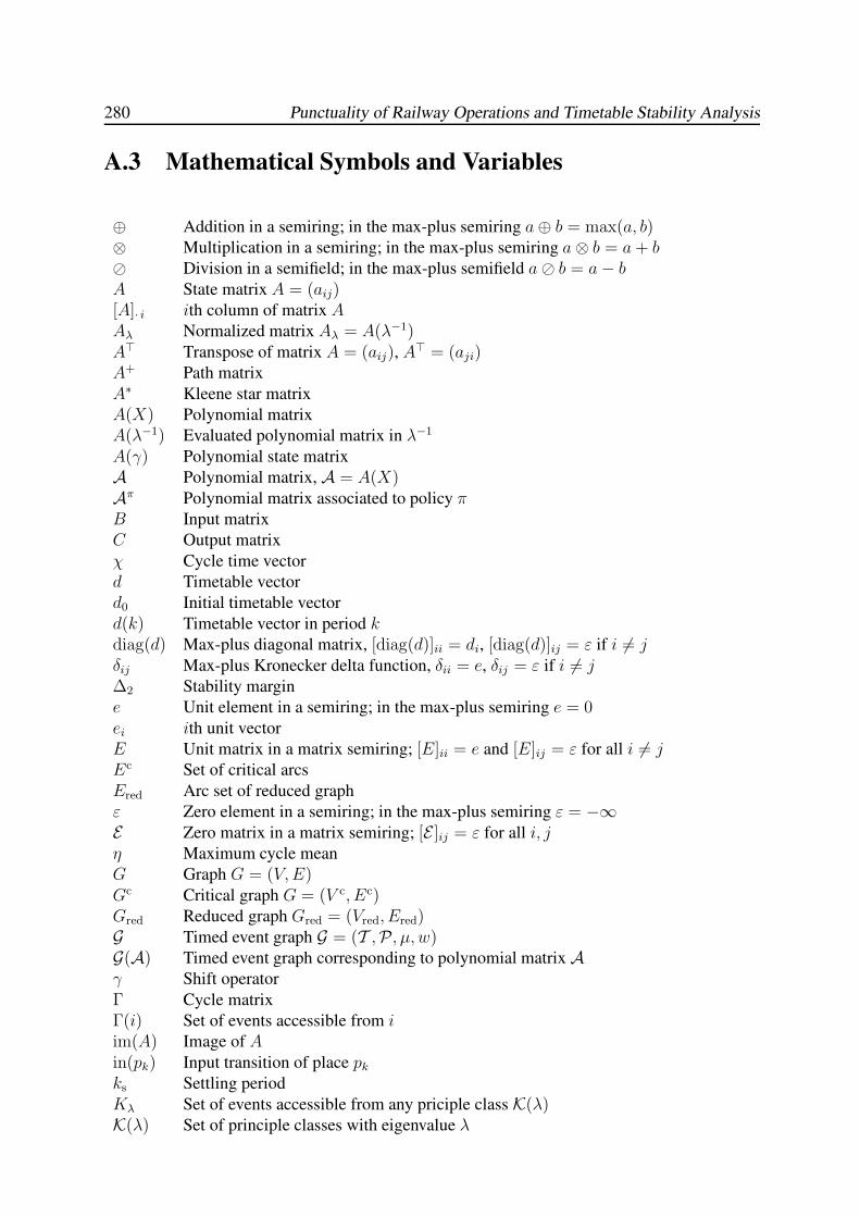
280 Punctuality of Railway Operations and Timetable Stability Analysis
A.3 Mathematical Symbols and Variables
⊕ Addition in a semiring; in the max-plus semiring a⊕ b = max(a, b)⊗ Multiplication in a semiring; in the max-plus semiring a⊗ b = a+ b� Division in a semifield; in the max-plus semifield a� b = a− bA State matrix A = (aij)[A]· i ith column of matrix AAλ Normalized matrix Aλ = A(λ−1)A> Transpose of matrix A = (aij), A
> = (aji)A+ Path matrix
A∗ Kleene star matrix
A(X) Polynomial matrix
A(λ−1) Evaluated polynomial matrix in λ−1
A(γ) Polynomial state matrix
A Polynomial matrix, A = A(X)Aπ Polynomial matrix associated to policy πB Input matrix
C Output matrix
χ Cycle time vector
d Timetable vector
d0 Initial timetable vector
d(k) Timetable vector in period kdiag(d) Max-plus diagonal matrix, [diag(d)]ii = di, [diag(d)]ij = ε if i 6= jδij Max-plus Kronecker delta function, δii = e, δij = ε if i 6= j∆2 Stability margin
e Unit element in a semiring; in the max-plus semiring e = 0ei ith unit vector
E Unit matrix in a matrix semiring; [E]ii = e and [E]ij = ε for all i 6= jEc Set of critical arcs
Ered Arc set of reduced graph
ε Zero element in a semiring; in the max-plus semiring ε = −∞E Zero matrix in a matrix semiring; [E ]ij = ε for all i, jη Maximum cycle mean
G Graph G = (V,E)Gc Critical graph G = (V c, Ec)Gred Reduced graph Gred = (Vred, Ered)G Timed event graph G = (T ,P, µ, w)G(A) Timed event graph corresponding to polynomial matrix Aγ Shift operator
Γ Cycle matrix
Γ(i) Set of events accessible from iim(A) Image of Ain(pk) Input transition of place pk
ks Settling period
Kλ Set of events accessible from any priciple class K(λ)K(λ) Set of principle classes with eigenvalue λ
Glossary 281
λ Eigenvalue
λ0 Maximum eigenvalue
m Number of arcs or places
M Incidence matrix
µ Marking vector of a timed event graph
µ0 Initial marking vector of a timed event graph
µ(pk) Marking of place pk
n Number of nodes or transitions
N Set of natural numbers, N = {1, 2, 3, . . .}N0 Set of natural numbers extended with zero, N0 = Z+ = {0, 1, 2, 3, . . .}out(pk) Output transition of place pk
p Order (maximum marking)
P Max-plus permutation matrix
P Set of places in a timed event graph
π Policy vector
Πi Set of incoming places to event iR(µ0) Reachable set of markings in a timed event graph with initial marking µ0
R Set of real numbers
Rε Set of real numbers extended with ε = −∞Rmax Max-plus semifield (Rε,max,+,−∞, 0)Rmax[X] Semiring of max-plus polynomials
Rnmax Semimodule of n-dimensional vectors over the max-plus semifield
Rm×nmax Set of m× n matrices over the max-plus semifield
Rm×nmax [X] Set of m× n max-plus polynomial matrices
span(A) Spanning set of columns of Aρ Throughput
spec(A) Spectrum of matrix Asupp(A) Support of matrix A (index set of finite entries)
S General semiring
S[γ] Polynomial semiring in the indeterminate γ over the semiring Sσ(k) Firing vector of the kth firing
tr(A) Trace of matrix A, tr(A) =⊕n
i=1 aii
T Timetable cycle time
T Set of transitions of a timed event graph
Ti Communication class Ti ⊆ Tu Input vector
v Eigenvector
V c Set of critical nodes or transitions
Vred Node set of reduced graph, communication class
V(λ) Eigensemimodule associated to eigenvalue λw Holding time (weight) vector of a timed event graph
w(pk) Holding time of place pk
x State vector
x0 Initial state vector
x(k) Event time vector in period kX An indeterminate
ξ Circuit or path
282 Punctuality of Railway Operations and Timetable Stability Analysis
y Output vector
z Delay vector
Z Set of integers, Z = {. . . ,−2,−1, 0, 1, 2, . . .}Z+ Set of nonnegative integers, Z+ = {0, 1, 2, . . .}Z− Set of nonpositive integers, Z− = {0,−1,−2, . . .}
SUMMARY
Punctuality of Railway Operations and Timetable Stability Analysis
Rob M.P. Goverde
This thesis is concerned with the analysis of railway timetables. The considered research topics
include: (1) data collection of railway operations based on train detection data; (2) statistical
analysis of empirical data to find sources of structural delays; and (3) stability analysis of large-
scale periodic railway timetables.
An essential element in the design of a reliable railway timetable is the feedback of empirical
data from realized operations. A timetable consists of deterministic process times (running
times, dwell times, transfer times, etc.), which in practice vary from hour-to-hour or day-to-
day due to e.g. varying driver behaviour, fluctuating passenger volumes, and changing weather
conditions. The stochastic distributions of realized process times and arrival/departure times
show how well the timetable can be adhered to. In the Dutch railway practice this quality
cycle is however not structurally applied. Running times are computed using advanced running
time calculation models and successively increased by a given percentage — usually 7% —
to compensate for larger running times. Dwell times and transfer times are based on rules-of-
thumb. And also minimum headway times between pairs of trains sharing some infrastructure
are based on norms, which include some (unknown) buffer time. (Chapter 3)
Empirical validation of the individual process times was not possible until recently, because
of lacking accurate realization data. The traffic control systems collect and maintain a large
amount of event time realizations (arrivals, departures and passages at timetable points), but
these realizations are derived from passage times at entrance and exit signals (via train descrip-
tion steps) which causes uncertainty about the accuracy of the individual recorded event times.
This data is therefore only suitable for statistics at an aggregated level, such as the percentage
of trains arriving within three minutes after schedule at 32 stations over a month. (Chapter 4)
This thesis shows that accurate event time realizations are available in records (TNV-logfiles)
of the train describer systems (TNV in Dutch), and describes the tool TNV-Prepare that was
especially developed to recover this information from the TNV-logfiles. Train describers keep
track of the progress of trains based on train numbers and infrastructure messages received from
the safety and signalling systems. All received infrastructure messages and all generated train
number events are recorded chronologically in TNV-logfiles. These files thus contain invaluable
information. However, the infrastructure and train number messages are logged independently
from a wide area. The Dutch railway network contains 13 TNV-systems, which each monitors
all running trains over a large area and records all train number events, as well as all received
infrastructure events related to e.g. track sections (occupation, release), signals (stop, go), and
switches (left, right). Until the year 2000 — during this PhD research — the TNV-logfiles
were kept for at most a week for investigation of accidents. In this PhD research the software
TNV-Prepare has been developed that couples train numbers to infrastructure events based on
the TNV-logfiles. This way train movements can be traced on track section occupancy level,
283
284 Punctuality of Railway Operations and Timetable Stability Analysis
including the entry and exit of platform track sections, by which realised arrival, departure, and
through times can be determined with an accuracy of a few seconds. (Chapter 4)
The potential of accurate empirical data is demonstrated in a case-study of the railway station
Eindhoven. Eindhoven is a main Dutch transfer station at which various train lines from dif-
ferent directions stop, turn, or connect. The analysis is based on TNV-logfiles from 1997 that
were specially collected and made available for this aim. The statistical analysis showed that
Eindhoven was a source of delay growth. The mean dwell time of each train line was larger
than scheduled, also when considering late trains only. The departure delays increased on the
average by one minute with respect to the arrival delays. Using regression analysis, the delay
expansion could be explained by a combination of dependencies between train lines, includ-
ing transfer connections and conflicting routes. In particular, the double-track route between
Eindhoven and Boxtel caused much hindrance, because trains with scheduled transfers in Eind-
hoven had to arrive or depart one after another. This bottleneck was removed in 2002 after
the four-track route between Eindhoven and Boxtel became available. Other findings include a
poor departure punctuality of turning trains and the resulting hindrance despite a layover time of
more then thirty minutes, and conflicting routes between in- and outbound train lines with tight
scheduled headway. Apart from the specific outcomes, this case-study clearly demonstrates the
power of a statistical analysis of accurate train data. (Chapter 5)
Another more theoretical topic of the case-study concerned the estimation and testing of theoret-
ical probability distributions to the various process times and delays. Stochastic mathematical
models and simulation models rely on given probability distributions for process times or de-
lays. By absence of empirical data, distributions are typically based on theoretical assumptions
and often also simple exponential distributions are used which are easy to work with. The
Eindhoven data has been used to fit process times and delays for each train line separately.
For this data, the excess dwell times of late trains follow an exponential distribution. Also the
departure delays follow an exponential distribution except for train lines heading in the same di-
rection with close scheduled departure times. Dwell times and transfer times of cross-platform
transfers follow a normal distribution, both for all trains and when considering late trains only.
Arrival delays do not fit well to any simple theoretical distribution in general, mainly due to
disturbances of conflicting train paths. (Chapter 5)
The second main topic of this thesis is railway timetable stability. Train traffic has to deal with a
large amount of (network) dependencies. Some of these dependencies are caused by the railway
timetable and logistics, such as passenger transfers, rolling stock circulations, and schedules of
drivers and conductors. Other dependencies relate to the shared railway infrastructure, such as
following trains on open tracks, conflicting routes at station layouts between in- and outbound
trains, and meeting trains on partial single-track routes. A timetable is usually conflict-free
in the sense that all conflicts between train paths have been solved in advance. However, if a
train deviates from its scheduled time-distance path then it may hinder other trains, which then
deviate from schedule as well, etc. Because of this domino-effect, a local primary disruption
may have condiderable consequences to the entire traffic network. Therefore, a stable timetable
contains some buffer time between train paths which compensates for small disruptions and
avoids prompt secondary delays to other trains. Testing the stability of a railway timetable
requires a network model of all train interdependcies. (Chapter 3 & 6)
A railway timetable essentially describes precedence relations between events and decisions on
the scheduled order of events. For instance, a train is ready-to-depart if it has arrived and the
Summary 285
minimum dwell time has been respected to guarantee alighting and boarding of passengers; if
the train has a transfer connection with a feeder train then it also has to wait for the arrival
of this feeder train plus a minimum transfer time to allow transferring passengers to board the
train; and finally, the train may have to wait for trains with a conflicting inbound or outbound
route before the route from the platform to the open track becomes available. Discrete-event
systems where synchronization between events is the main characteristic can be formulated as
‘timed event graphs,’ a special abstract network structure (Petri net) describing time-dependent
precedence relations and their process logic. A timed event graph model shows the implications
of the scheduled order of events and proves whether it is (im)possible that a system becomes
deadlocked. An example of this is that a train may depart to a single-track route only if all
opposite trains have left the open track. These topological and behavioural properties of a
timetable can be analysed by the ‘marked’ graph theory of timed event graphs. (Chapter 6)
Timetable performance and stability is effectively analysed in the event domain associated to
a timed event graph. The departure times of all trains are therefore collected in a state vector
and the dynamic equations describing the interactions between events are given by (max,+)-
recursions in which the departure time of any train is determined by the maximum over all
preceding departure times plus the subsequent minimum process times that have to be waited
for. These recursive equations are linear systems in the so-called max-plus algebra. In max-plus
algebra ‘addition’ of two numbers is defined as their maximum and ‘multiplication’ as conven-
tional addition, e.g. 2⊕3 = max(2, 3) = 3 and 2⊗3 = 2+3 = 5. From a systems point of view,
addition of two processes implies process synchronization (a new process may start after the last
preceding process has terminated) and multiplication corresponds to cascading processes (the
process time of the composite process is the sum of the individual successive process times).
All process times are collected in a state matrix, and the evolution of the discrete-event system
is described accordingly by matrix-vector multiplications and addition of vectors, evaluated in
max-plus algebra. (Chapter 7 & 8)
From an algorithmic point of view, the analysis of max-plus linear systems concentrates on
solving critical-path problems and eigenproblems in max-plus algebra. This thesis therefore
considers efficient algorithms to these problems given the particular application area. A timed
event graph can be represented by a polynomial matrix in max-plus algebra, i.e., a polynomial
with matrix coefficients, or equivalently, a matrix with polynomial entries. The polynomial
matrices can also be used in a formal description of higher-order linear systems, including zero-
order terms. The zero-order terms correspond to all processes that are completed within one
period, the first-order terms correspond to all processes exceeding a timetable period, et cetera.
The most common approach to tackle higher-order systems is to transform them into a purely
first-order system to which elegant algebraic solutions exist. However, this is computationally
not the most effective and also leads to practical problems, mainly because the zero-order dy-
namics have dissappeared. This thesis shows how the existing max-plus algebra theory of ma-
trices and first-order recursive systems can be extended to polynomial matrices and higher-order
implicit systems. Special attention is given to the generalized eigenproblem of (irreducible and
reducible) max-plus polynomial matrices. This theory gives the necessary background for the
complete description of the eigenspace of (polynomial) matrices, and a correct interpretation of
the max-plus policy-iteration algorithm in case of reducible max-plus (polynomial) matrices.
The max-plus policy-iteration algorithm has been developed recently based on the well-known
policy-iteration algorithm for Markov decision processes, and has proved to be very effective
in solving generalized eigenproblems in max-plus algebra with a linear practical running time.
286 Punctuality of Railway Operations and Timetable Stability Analysis
Other considered topics include efficiently computing all critical circuits and delay propagation
with respect to large-scale sparse max-plus systems. (Chapter 7)
The stability test of max-plus linear systems is based on the eigenvalues of the (polynomial)
state matrix. The maximum eigenvalue denotes the minimal cycle time of the railway timetable.
Hence, for an hourly timetable the maximum eigenvalue must be smaller than sixty minutes to
be (asymptotically) stable, in which case any initial delay will settle after a finite number of peri-
ods. The maximum eigenvalue equals the mean cycle time of a ‘critical circuit,’ which can also
be computed explicitly. A critical circuit is a cyclic sequence of events and processes with the
least slack over all circuits in the network. An eigenvector corresponds to a periodic timetable
(departure time vector) in which the critical events are scheduled directly after each other with-
out slack and thus allowing a cycle time equal to the maximum eigenvalue. The departure times
in the eigenvector correspond to the critical paths from one of the critical events. The difference
between the timetable cycle time — usually an hour — and the maximum eigenvalue gives the
mean slack on the critical circuits. All processes that do not belong to a critical circuit have
more slack available. Whether a stable timetable is also robust depends on the distribution of
slack time over the timetable. An example of a stable timetable that is not very robust is one
where the buffer time over each train line circulation is concentrated in the layover times at
the terminals, by which primary delays are propagated over the entire network before they are
reduced at the train line ends. The distribution of slack over a timetable is represented by the
‘recovery matrix,’ where each entry corresponds to the least total slack time over all paths be-
tween two events. The impact of any combination of initial delays can also be visualized by
explicitly computing the delay propagation using the max-plus state equations. (Chapter 8)
The algorithms have been implemented in the software tool PETER (Performance Evaluation
of Timed Events in Railways). Special attention has been given to the development and imple-
mentation of efficient algorithms that are capable of computing results of large-scale networks
in several seconds. Furthermore, results in PETER are graphically presented by means of a
projection to the railway network, thus clearly visualizing the locations of critical events and
processes in the network. PETER offers a systematic and transparant stability analysis of large-
scale periodic timetables and can be applied in the design process of railway timetables, for
evaluating network stability in the capacity allocation process, and for developing effective dis-
patching policies to minimize delay propagation. (Chapter 8)
NEDERLANDSE SAMENVATTING
(DUTCH SUMMARY)
Punctualiteit van railverkeer en stabiliteitsanalyse van dienstregelingen
Rob M.P. Goverde
Dit proefschrift beschrijft methoden voor de analyse van treindienstregelingen. De onderwerpen
die aan bod komen zijn: (1) dataverzameling van de dienstuitvoering gebaseerd op treindetectie
data; (2) statistische analyse van empirische data om oorzaken van structurele vertragingen op
te sporen; en (3) stabiliteitsanalyse van periodieke dienstregelingen voor grootschalige spoor-
netwerken.
Een essentieel element in het ontwerpproces van een betrouwbare dienstregeling is terugkop-
peling van empirische data van de gerealiseerde dienstuitvoering. Een dienstregeling bestaat
immers uit deterministische procestijden (rijtijden, halteringstijden, overstaptijden, etc.), terwijl
deze in de praktijk varieren van uur-tot-uur en dag-tot-dag vanwege bijvoorbeeld verschillend
rijgedrag van machinisten, fluctuerende aantallen reizigers en veranderende weersomstandighe-
den. De stochastische verdelingen van gerealiseerde procestijden en aankomst- en vertrektij-
den geven aan in welke mate de dienstregeling haalbaar blijkt te zijn. Deze kwaliteitscirkel is
echter nauwelijks aanwezig bij de spoorpraktijk in Nederland. Rijtijden worden berekend met
geavanceerde rijtijdmodellen waar vervolgens een bepaald percentage — meestal 7% — aan
toe wordt gevoegd om langere rijtijden op te vangen. Halteringstijden en overstaptijden zijn
gebaseerd op vuistregels. En ook de minimale volgtijden tussen twee treinen die (gedeeltelijk)
gebruik maken van hetzelfde spoor zijn gebaseerd op normtijden, waarin een (onbekende) spe-
ling zit verwerkt. (Hoofdstuk 3)
Empirische validatie van de afzonderlijke procestijden was tot voor kort niet mogelijk we-
gens het ontbreken van nauwkeurige realisatiegegevens. Via de verkeersleidingssystemen wordt
dagelijks een grote hoeveelheid aan gerealiseerde treinactiviteiten (aankomsten, vertrekken en
doorkomsten op dienstregelpunten) verzameld en opgeslagen, maar deze worden afgeleid van
passagetijden bij inrijseinen en vertrekseinen (via vensterverplaatsingen van het treinnummer-
volgsysteem) waardoor onzekerheid ontstaat over de nauwkeurigheid van de individuele geregi-
streerde realisatietijden. Deze gegevens zijn daarom alleen geschikt voor statistieken op geag-
gregeerd niveau, zoals het percentage treinen dat minder dan drie minuten na plan aankomt op
32 stations in een maand. (Hoofdstuk 4)
Dit proefschrift laat zien dat nauwkeurige uitvoeringstijden op individueel treinniveau wel im-
pliciet aanwezig zijn in de zogenaamde TNV-logbestanden van de treinnummervolgsystemen
(TNV), en beschrijft de tool TNV-Prepare die speciaal is ontwikkeld om deze gegevens boven
tafel te krijgen. TNV-systemen volgen de voortgang van alle treinen op het spoornet via trein-
nummers en infrastructuurmeldingen uit de beveiligings- en beheersingssystemen. Alle ele-
mentmeldingen die het TNV-systeem ontvangt vanuit de beveiligings- en beheersingssystemen
worden chronologisch opgeslagen in de TNV-logbestanden, evenals de gegenereerde trein-
nummermeldingen van het TNV-systeem zelf. Deze bestanden bevatten dus een schat aan
287
288 Punctuality of Railway Operations and Timetable Stability Analysis
informatie. Het probleem is echter dat de inframeldingen en treinnummermeldingen los van
elkaar staan. Het Nederlandse spoornet heeft 13 TNV-systemen die ieder een gebied bedienen
in grootte vergelijkbaar met een provincie. Alle treinen die in dit gebied rondrijden worden
gevolgd en gelogd, evenals o.a. alle spoorsecties die bezet en onbezet raken, seinen die op rood
springen en weer vrij komen, en wissels die omgelegd worden. Tot het jaar 2000 (tijdens dit
promotieonderzoek) werden deze TNV-logbestanden hooguit een week bewaard voor eventuele
analyse van ongelukken en vervolgens overschreven. Als onderdeel van dit promotieonderzoek
is de software TNV-Prepare ontwikkeld, die op basis van TNV-logbestanden treinnummers kop-
pelt aan inframeldingen. Hierdoor kunnen individuele treinen op spoorsectieniveau gevolgd
worden, inclusief het op- en afrijden van perronsporen, waardoor gerealiseerde aankomst-,
vertrek- en doorkomsttijden met een nauwkeurigheid van enkele seconden bepaald kunnen wor-
den. (Hoofdstuk 4)
In een case-study is het potentieel van beschikbare nauwkeurige realisatietijden aangetoond.
Als case is het station Eindhoven uitgekozen. Eindhoven is een belangrijk knooppunt waar
diverse treinseries uit verschillende richtingen stoppen, keren en op elkaar aansluiten. De
analyse is gebaseerd op TNV-logbestanden uit 1997 die destijds speciaal voor dit doel waren
aangevraagd en opgeslagen. Uit de statistische analyse kwam naar voren dat Eindhoven een
bron was van vertragingstoename. De gemiddele halteringstijden van alle treinseries waren
langer dan gepland, ook als alleen gekeken werd naar treinen die te laat aankwamen. De
vertrekvertragingen namen gemiddeld met een minuut toe ten opzichte van de aankomstver-
tragingen. Met behulp van regressieanalyse kon de vertragingstoename worden verklaard uit
een combinatie van afhankelijkheden tussen de treinseries, waaronder reizigersaansluitingen en
conflicterende rijwegen. Met name het tweesporige baanvak tussen Eindhoven en Boxtel zorgde
voor veel hinder omdat treinen die in Eindhoven op elkaar aansloten achter elkaar moesten
aankomen dan wel vertrekken. Deze bottleneck is in 2002 opgeheven na het gereedkomen van
de spoorverdubbeling tussen Eindhoven en Boxtel. Andere structurele vertragingsoorzaken die
zijn gevonden waren kruisende rijwegen van aankomende en vertrekkende treinseries met krap
geplande opvolgtijd en een slechte vertrekpunctualiteit van kerende treinen met de daardoor
ontstane hinder ondanks ruim een half uur geplande keertijd. Los van de specifieke uitkomsten
geeft deze case-study duidelijk de meerwaarde aan die een statistische analyse van nauwkeurige
data biedt. (Hoofdstuk 5)
Een ander meer theoretisch onderdeel van de case-study was het schatten en testen van theore-
tische kansverdelingen voor de diverse procestijden en vertragingen. Stochastische wiskundige
modellen en simulatiemodellen gaan uit van bepaalde kansverdelingen voor vertragingen en
procestijden. Wegens gebrek aan empirische data worden veelal aannamen gedaan omtrent de
kansverdelingen die de afzonderlijke processen goed beschrijven, en ook wordt vaak uitgegaan
van eenvoudige (exponentiele) kansverdelingen waar makkelijk mee te rekenen is. Voor de
Eindhovense data is gekeken naar procestijden en vertragingen per treinserie. Hier bleek dat
de overschrijding van halteringstijden voor vertraagde treinen voldoet aan een exponentiele
verdeling. Ook de vertrekvertraging voldoet aan een exponentiele verdeling mits de geplande
vertrektijden van treinen in dezelfde richting ver genoeg uit elkaar liggen. Halteringstijden
en overstaptijden van ‘cross-platform’ aansluitingen volgen een normale verdeling, zowel voor
alle treinen als wanneer alleen gekeken wordt naar vertraagde treinen. Aankomsttijden zijn
over het algemeen niet goed te beschrijven met enkelvoudige kansverdelingen; hindering van
aankomende treinen blijkt hier een grote verstoring te zijn. (Hoofdstuk 5)
Nederlandse Samenvatting 289
Het tweede onderwerp van dit proefschrift is de stabiliteit van dienstregelingen. Het treinverkeer
over een spoorwegnetwerk heeft te maken met een groot aantal netwerkafhankelijkheden. Een
aantal van deze afhankelijkheden ontstaat door de opzet van de dienstregeling en de logistieke
processen, zoals reizigersaansluitingen, materieelomlopen en diensten van machinisten en con-
ducteurs. Andere afhankelijkheden ontstaan doordat treinen over een gemeenschappelijke in-
frastructuur rijden. In die laatste categorie vallen achtereenvolgende treinen over baanvakken
tussen stations, conflicterende rijwegen op stations tussen binnenkomende en vertrekkende
treinen, en elkaar tegemoet komende treinen op gedeeltelijk enkelsporige trajecten. In de
dienstregeling zijn in principe alle conflicten opgelost zodat alle treinen ongehinderd over het
spoornet kunnen rijden. Zodra een trein echter van het geplande tijdwegpad afwijkt kan hinder
ontstaan voor andere treinen, die daardoor ook van hun geplande pad afwijken en zo op hun
beurt ook weer andere treinen kunnen hinderen. Vanwege dit domino-effect kan een lokale
primaire verstoring grote gevolgen hebben voor de hele treinenloop. Een goede dienstregeling
bevat daarom zogenaamde buffertijden tussen de treinpaden zodat kleine verstoringen kunnen
worden opgevangen en niet direct leiden tot secundaire vertragingen voor andere treinen. Om de
stabiliteit van een dienstregeling te kunnen toetsen is een modellering op netwerkniveau nodig.
(Hoofdstuk 3 & 6)
Een dienstregeling beschrijft de causale verbanden tussen treinactiviteiten en de geplande vol-
gorde van deze activiteiten. Zo mag een trein pas vertrekken nadat het is aangekomen en min-
stens een bepaalde minimum halteringstijd aan een perron heeft stilgestaan om reizigers de
gelegenheid te geven uit en in te stappen; als de trein een aansluitrelatie heeft met een andere
trein, dan moet ook worden gewacht totdat de andere trein is aangekomen en de overstap-
pende reizigers zijn ingestapt; en tenslotte moet mogelijk worden gewacht op het vertrek of de
binnenkomst van andere treinen met een conflicterende rijweg voordat de rijweg van het per-
ronspoor naar het baanvak vrij komt. Systemen met discrete gebeurtenissen waarbij synchro-
nisatie een belangrijke rol speelt kunnen worden beschreven met ‘timed event graphs,’ een spe-
ciaal soort abstract netwerk (Petri net) waar behalve de tijdsafhankelijke relaties tussen opeen-
volgende gebeurtenissen ook de proceslogica wordt beschreven. De beschrijving als timed
event graph geeft inzicht in de volgorde waarin gebeurtenissen plaatsvinden en of het mo-
gelijk is dat het systeem vastloopt, een zogenaamde deadlock. Een voorbeeld hiervan is dat een
trein niet eerder van een station met meerdere perronsporen naar een enkelsporig baanvak mag
vertrekken dan nadat alle tegengestelde treinen het baanvak hebben verlaten. Dit soort topolo-
gische en gedragsafhankelijke eigenschappen van een dienstregeling kunnen worden bestudeerd
met methoden uit de ‘gemarkeerde’ graaftheorie van timed event graphs. (Hoofdstuk 6)
De kwaliteit en stabiliteit van een dienstregeling kan effectief worden bestudeerd in het ‘toe-
standsdomein’ van de timed event graph. De vertrektijden van alle treinen worden daarvoor
gezien als toestandsvector en de dynamische vergelijking die de interactie tussen de vertrek-
tijden beschrijft is een recursieve vergelijking waarin de vertrektijd van een gegeven trein
wordt gegeven als het maximum over voorgaande vertrektijden plus de daarop volgende mini-
mum procestijden waarop gewacht moet worden. Dergelijke vergelijkingen kunnen worden
opgevat als lineaire systemen in de zogenaamde ‘max-plus algebra.’ In max-plus algebra is de
‘optelling’ van twee getallen gedefinieerd als het maximum en de ‘vermenigvuldiging’ als een
gewone optelling, zodat bijvoorbeeld 2⊕3 = max(2, 3) = 3 en 2⊗3 = 2+3 = 5. Systeemtech-
nisch komt de optelling van twee processen neer op de synchronisatie van processen (een
aansluitend proces kan beginnen na het voorgaande proces dat als laatste is afgerond) en ver-
menigvuldiging op het na elkaar uitvoeren van processen (de procestijd van het samengestelde
290 Punctuality of Railway Operations and Timetable Stability Analysis
proces is de som van de achtereenvolgende procestijden). Alle procestijden kunnen worden
samengevat in een toestandsmatrix, waarna het discrete-event systeem wordt beschreven door
matrix-vector vermenigvuldigingen en optellingen van vectoren, opgevat als bewerkingen in
max-plus algebra. (Hoofdstuk 7 & 8)
Algoritmisch komt de analyse van max-plus lineaire systemen neer op het oplossen van eigen-
waardeproblemen in max-plus algebra en kortste-pad of kritiekste-pad problemen. In dit proef-
schrift is daarom aandacht besteed aan efficiente algoritmen voor deze problemen met be-
trekking tot het specifieke toepassingsgebied. Een timed event graph komt direct overeen met
een ‘polynomiale matrix’ in max-plus algebra. Dit is een polynoom waarin de coefficienten
bestaan uit matrices, of, wat op hetzelfde neerkomt, een matrix waarvan de elementen bestaan
uit polynomen. Deze polynomiale matrix kan ook worden gebruikt in de beschrijving van
hogere-orde lineaire systemen, inclusief nulde-orde termen. De nulde-orde termen zijn alle pro-
cessen die binnen een periode worden afgewerkt, de eerste-orde termen alle processen die over
een periodegrens heenlopen, et cetera. De gebruikelijke methode bestaat uit een transformatie
van het hogere-orde systeem naar een puur eerste-orde systeem, waarvoor elegante algebraische
analysemethoden bestaan. Echter, vanuit algoritmisch oogpunt bezien is dit niet effectief en ook
vanuit de toepassing geredeneerd levert deze vereenvoudiging problemen op, met name door-
dat de nulde-orde dynamica is verdwenen. Dit proefschrift laat zien hoe de bekende max-plus
algebra theorie van matrices en eerste-orde recursieve systemen kan worden uitgebreid naar
polynomiale matrices en hogere-orde impliciete systemen. Speciale aandacht is besteed aan het
gegeneraliseerde eigenprobleem van max-plus polynomiale matrices, zowel voor irreducibele
als reducibele polynomiale matrices. Deze theorie geeft de noodzakelijke achtergrond die nodig
is voor een volledige beschrijving van de eigenruimte van (polynomiale) matrices en voor een
juiste interpretatie van het max-plus ‘policy’-iteratie algoritme in het geval van reducibele max-
plus (polynomiale) matrices. Het max-plus policy-iteratie algoritme is recent ontwikkeld op
basis van het welbekende policy-iteratie algoritme voor Markov beslissingsproblemen, en blijkt
voor het oplossen van het gegeneraliseerde eigenprobleem in max-plus algebra zeer effectief
te zijn met een lineaire praktische rekentijd. Andere onderwerpen die aan bod komen zijn het
efficient berekenen van alle kritieke circuits en de vertragingsvoortplanting voor grootschalige
ijle max-plus systemen. (Hoofdstuk 7)
De stabiliteitsanalyse van max-plus lineaire systemen komt neer op het berekenen van de eigen-
waarden van de (polynomiale) toestandsmatrix. De maximum eigenwaarde geeft de minimale
lengte van een dienstregelingsperiode aan waarmee de dienstregeling zich kan herhalen. Voor
een uurdienstregeling moet de maximum eigenwaarde dus kleiner zijn dan zestig minuten. In
dat geval is de dienstregeling (asymptotisch) stabiel zodat een initiele vertraging in de loop
der tijd uitdempt. De maximum eigenwaarde is gelijk aan de gemiddelde procestijd over een
‘kritiek circuit’, wat ook expliciet kan worden berekend. Een kritiek circuit is een cyclische
opeenvolging van processen en treinactiviteiten waarvoor de minste speling beschikbaar is. Een
eigenvector komt overeen met een dienstregeling (vertrektijdvector) waarin de kritieke trein-
activiteiten direct achter elkaar zijn gepland zodat een periodieke dienstuitvoering mogelijk is
met een periode gelijk aan de maximum eigenwaarde. De vertrektijden in de eigenvector komen
overeen met de kritieke paden vanaf een van de kritieke treinactiviteiten. Het verschil tussen
de echte dienstregelingsperiode (meestal een uur) en de maximum eigenwaarde geeft de gemid-
delde speling op de kritieke circuits aan. De treinactiviteiten die niet op een kritiek circuit liggen
hebben meer speling. Of een stabiele dienstregeling ook robuust is hangt af van de verdeling van
de speling over de dienstregeling. Een dienstregeling waarbij alle speling zoveel mogelijk in de
Nederlandse Samenvatting 291
keringen zit verwerkt is bijvoorbeeld niet robuust aangezien pas bij de keringen vertraging kan
worden afgebouwd. De spelingsverdeling over de dienstregeling wordt inzichtelijk gemaakt
via de spelingsmatrix, de recovery matrix, waarin ieder element aangeeft hoeveel speling op het
meeste kritieke pad tussen twee treinactiviteiten zit. De voortplanting van initiele vertragingen
kunnen ook expliciet worden berekend via de toestandsvergelijking waardoor de impact van
een combinatie van vertragingen kan worden gevisualiseerd. (Hoofdstuk 8)
De algoritmen en analysemogelijkheden zijn geımplementeerd in de software PETER (Perfor-
mance Evaluation of Timed Events in Railways). Bijzondere aandacht is besteed aan de ont-
wikkeling en implementatie van efficiente algoritmen die grootschalige netwerken in enkele
seconden kunnen doorrekenen. Daarnaast is in PETER aandacht besteed aan de grafische
presentatie van resultaten middels een projectie op het spoornetwerk, waardoor kritieke pun-
ten duidelijk zichtbaar worden. PETER voorziet in een behoefte voor een systematische en
transparante stabiliteitsanalyse van dienstregelingen voor grootschalige railverkeersnetwerken
en kan worden gebruikt in het ontwerpproces van dienstregelingen, de evaluatie van netwerksta-
biliteit bij de toedeling van railinfrastructuurcapaciteit en voor de ontwikkeling van effectieve
afhandelingsstrategieen ter beperking van vertragingsvoortplanting. (Hoofdstuk 8)

292 Punctuality of Railway Operations and Timetable Stability Analysis
ABOUT THE AUTHOR
Rob Goverde was born in Arnhem, the Netherlands, on June 22, 1968. During 1987–1993,
he studied mathematics at Utrecht University. In 1993, Rob received his MSc in Mathematics
with a specialization in optimization theory. His MSc thesis dealt with a theoretical topic in
impulsive optimal control theory.
During 1994–1995, Rob attended the two-year post-MSc mathematical design engineering pro-
gramme WBBM at Delft University of Technology, where he received the degree of Master
of Technological Design (MTD) in Mathematical Modelling and Decision Support. During
1995, in the second year design project, he worked at the Dutch National Aerospace Labora-
tory (NLR), where he designed a robust flight control system using H∞ robust control theory.
This project was part of the international Robust Flight Control Design Challenge formulated
by the Group for Aeronautical Research and Technology in Europe (GARTEUR). In 1996, Rob
also obtained the certificate of the Dutch Network on the Mathematics of Operations Research
(LNMB) for attending advanced PhD courses on mathematical programming and combinatorial
optimization.
Since 1996, Rob is affiliated with the Transport & Planning Department at Delft University of
Technology, where he worked on his PhD research within the TRAIL Research School. During
his PhD research, Rob developed mathematical models for the design and analysis of reliable
railway timetables. Based on his research, Rob presented numerous papers at both national and
international conferences. In 2002–2003, Rob was also detached to Railned/ProRail where he
worked in the project PRRING (Planning en Realizatie van RailINfraGebruik). His research
has led to two software products, TNV-Prepare and PETER, which are both presented in his
PhD thesis on ‘Punctuality of Railway Operations and Timetable Stability Analysis.’ After his
PhD defence in 2005, Rob will continue working at the Transport & Planning Department as
post-doc.
293

TRAIL Thesis Series
A series of The Netherlands TRAIL Research School for theses on transport, infrastructure and
logistics.
Nat, C.G.J.M., van der, A Knowledge-based Concept Exploration Model for Submarine Design,
T99/1, March 1999, TRAIL Thesis Series, Delft University Press, The Netherlands
Westrenen, F.C., van, The Maritime Pilot at Work: Evaluation and Use of a Time-to-boundary
Model of Mental Workload in Human-machine Systems, T99/2, May 1999, TRAIL Thesis Se-
ries, Eburon, The Netherlands
Veenstra, A.W., Quantitative Analysis of Shipping Markets, T99/3, April 1999, TRAIL Thesis
Series, Delft University Press, The Netherlands
Minderhoud, M.M., Supported Driving: Impacts on Motorway Traffic Flow, T99/4, July 1999,
TRAIL Thesis Series, Delft University Press, The Netherlands
Hoogendoorn, S.P., Multiclass Continuum Modelling of Multilane Traffic Flow, T99/5, Septem-
ber 1999, TRAIL Thesis Series, Delft University Press, The Netherlands
Hoedemaeker, M., Driving with Intelligent Vehicles: Driving Behaviour with Adaptive Cruise
Control and the Acceptance by Individual Drivers, T99/6, November 1999, TRAIL Thesis Se-
ries, Delft University Press, The Netherlands
Marchau, V.A.W.J., Technology Assessment of Automated Vehicle Guidance – Prospects for
Automated Driving Implementation, T2000/1, January 2000, TRAIL Thesis Series, Delft Uni-
versity Press, The Netherlands
Subiono, On Classes of Min-max-plus Systems and their Applications, T2000/2, June 2000,
TRAIL Thesis Series, Delft University Press, The Netherlands
Meer, J.R., van, Operational Control of Internal Transport, T2000/5, September 2000, TRAIL
Thesis Series, Delft University Press, The Netherlands
Bliemer, M.C.J., Analytical Dynamic Traffic Assignment with Interacting User-Classes: Theo-
retical Advances and Applications using a Variational Inequality Approach, T2001/1, January
2001, TRAIL Thesis Series, Delft University Press, The Netherlands
Muilerman, G.J., Time-based logistics: An analysis of the relevance, causes and impacts,
T2001/2, April 2001, TRAIL Thesis Series, Delft University Press, The Netherlands
Roodbergen, K.J., Layout and Routing Methods for Warehouses, T2001/3, May 2001, TRAIL
Thesis Series, The Netherlands
Willems, J.K.C.A.S., Bundeling van infrastructuur, theoretische en praktische waarde van een
ruimtelijk inrichtingsconcept, T2001/4, June 2001, TRAIL Thesis Series, Delft University Press,
The Netherlands
Binsbergen, A.J., van, J.G.S.N. Visser, Innovation Steps towards Efficient Goods Distribution
Systems for Urban Areas, T2001/5, May 2001, TRAIL Thesis Series, Delft University Press,
The Netherlands
Rosmuller, N., Safety analysis of Transport Corridors, T2001/6, June 2001, TRAIL Thesis
Series, Delft University Press, The Netherlands
Schaafsma, A., Dynamisch Railverkeersmanagement, besturingsconcept voor railverkeer op
basis van het Lagenmodel Verkeer en Vervoer, T2001/7, October 2001, TRAIL Thesis Series,
Delft University Press, The Netherlands
Bockstael-Blok, W., Chains and Networks in Multimodal Passenger Transport. Exploring a
design approach, T2001/8, December 2001, TRAIL Thesis Series, Delft University Press, The
Netherlands
Wolters, M.J.J., The Business of Modularity and the Modularity of Business, T2002/1, February
2002, TRAIL Thesis Series, The Netherlands
Vis, F.A., Planning and Control Concepts for Material Handling Systems, T2002/2, May 2002,
TRAIL Thesis Series, The Netherlands
Koppius, O.R., Information Architecture and Electronic Market Performance, T2002/3, May
2002, TRAIL Thesis Series, The Netherlands
Veeneman, W.W., Mind the Gap; Bridging Theories and Practice for the Organisation of
Metropolitan Public Transport, T2002/4, June 2002, TRAIL Thesis Series, Delft University
Press, The Netherlands
Nes, R. van, Design of multimodal transport networks, a hierarchical approach, T2002/5,
September 2002, TRAIL Thesis Series, Delft University Press, The Netherlands
Pol, P.M.J., A Renaissance of Stations, Railways and Cities, Economic Effects, Development
Strategies and Organisational Issues of European High-Speed-Train Stations, T2002/6, October
2002, TRAIL Thesis Series, Delft University Press, The Netherlands
Runhaar, H., Freight transport: at any price? Effects of transport costs on book and newspa-
per supply chains in the Netherlands, T2002/7, December 2002, TRAIL Thesis Series, Delft
University Press, The Netherlands
Spek, S.C., van der, Connectors. The Way beyond Transferring, T2003/1, February 2003,
TRAIL Thesis Series, Delft University Press, The Netherlands
Lindeijer, D.G., Controlling Automated Traffic Agents, T2003/2, February 2003, TRAIL Thesis
Series, Eburon, The Netherlands
Riet, O.A.W.T., van de, Policy Analysis in Multi-Actor Policy Settings. Navigating Between
Negotiated Nonsense and Useless Knowledge, T2003/3, March 2003, TRAIL Thesis Series,
Eburon, The Netherlands
Reeven, P.A., van, Competition in Scheduled Transport, T2003/4, April 2003, TRAIL Thesis
Series, Eburon, The Netherlands
Peeters, L.W.P., Cyclic Railway Timetable Optimization, T2003/5, June 2003, TRAIL Thesis
Series, The Netherlands
Soto Y Koelemeijer, G., On the behaviour of classes of min-max-plus systems, T2003/6, Septem-
ber 2003, TRAIL Thesis Series, The Netherlands
Lindveld, Ch..D.R., Dynamic O-D matrix estimation: a behavioural approach, T2003/7, Septem-
ber 2003, TRAIL Thesis Series, Eburon, The Netherlands
Weerdt, de M.M., Plan Merging in Multi-Agent Systems, T2003/8, December 2003, TRAIL
Thesis Series, The Netherlands
Langen, de P.W, The Performance of Seaport Clusters, T2004/1, January 2004, TRAIL Thesis
Series, The Netherlands
Hegyi, A., Model Predictive Control for Integrating Traffic Control Measures, T2004/2, Febru-
ary 2004, TRAIL Thesis Series, The Netherlands
Lint, van, J.W.C., Reliable Travel Time Prediction for Freeways, T2004/3, June 2004, TRAIL
Thesis Series, The Netherlands
Tabibi, M., Design and Control of Automated Truck Traffic at Motorway Ramps, T2004/4, July
2004, TRAIL Thesis Series, The Netherlands
Verduijn, T. M., Dynamism in Supply Networks: Actor switching in a turbulent business envi-
ronment, T2004/5, September 2004, TRAIL Thesis Series, The Netherlands
Daamen, W., Modelling Passenger Flows in Public Transport Facilities, T2004/6, September
2004, TRAIL Thesis Series, The Netherlands
Zoeteman, A., Railway Design and Maintenance from a Life-Cycle Cost Perspective: A Decision-
Support Approach, T2004/7, November 2004, TRAIL Thesis Series, The Netherlands
Bos, D.M., Changing Seats: A Behavioural Analysis of P&R Use, T2004/8, November 2004,
TRAIL Thesis Series, The Netherlands
Versteegt, C., Holonic Control For Large Scale Automated Logistic Systems, T2004/9, Decem-
ber 2004, TRAIL Thesis Series, The Netherlands
Wees, K.A.P.C. van, Intelligente voertuigen, veiligheidsregulering en aansprakelijkheid. Een
onderzoek naar juridische aspecten van Advanced Driver Assistance Systems in het wegverkeer,
T2004/10, December 2004, TRAIL Thesis Series, The Netherlands
Tampere, C.M.J., Human-Kinetic Multiclass Traffic Flow Theory and Modelling: With Applica-
tion to Advanced Driver Assistance Systems in Congestion, T2004/11, December 2004, TRAIL
Thesis Series, The Netherlands
Rooij, R.M., The Mobile City. The planning and design of the Network City from a mobility
point of view, T2005/1, February 2005, TRAIL Thesis Series, The Netherlands
Le-Anh, T., Intelligent Control of Vehicle-Based Internal Transport Systems, T2005/2, April
2005, TRAIL Thesis Series, The Netherlands
Zuidgeest, M.H.P., Sustainable Urban Transport Development: a Dynamic Optimization Ap-
proach, T2005/3, April 2005, TRAIL Thesis Series, The Netherlands
Hoogendoorn-Lanser, S., Modelling Travel Behaviour in Multimodal Networks, T2005/4, May
2005, TRAIL Thesis Series, The Netherlands
Dekker, S., Port Investment – Towards an integrated planning of port capacity, T2005/5, June
2005, TRAIL Thesis Series, The Netherlands
Koolstra, K., Transport Infrastructure Slot Allocation, T2005/6, June 2005, TRAIL Thesis Se-
ries, The Netherlands
Vromans, M., Reliability of Railway Systems, T2005/7, July 2005, TRAIL Thesis Series, The
Netherlands
Oosten, W., Ruimte voor een democratische rechtsstaat. Geschakelde sturing bij ruimtelijke
investeringen, T2005/8, September 2005, TRAIL Thesis Series, Sociotext, The Netherlands
Le-Duc, T., Design and control of efficient order picking, T2005/9, September 2005, TRAIL
Thesis Series, The Netherlands
Goverde, R.M.P., Punctuality of Railway Operations and Timetable Stability Analysis, T2005/10,
October 2005, TRAIL Thesis Series, The Netherlands