Performance analysis of Earned Value Management in the ... · p-factor 59 serial-parallel factor...

UNIVERSITEIT GENT

FACULTEIT ECONOMIE EN BEDRIJFSKUNDE

ACADEMIEJAAR 2009 – 2010

Performance analysis of Earned Value Management in the construction industry

Masterproef voorgedragen tot het bekomen van de graad van

Master in de Toegepaste Economische Wetenschappen: Handelsingenieur

Pieter Buyse & Tim Vandenbussche

onder leiding van

Prof. Dr. M. Vanhoucke

II

Permission

“The authors give the authorization to make this thesis available for consultation and to copy

parts of it for personal use. Any other use is subject to the limitations of copyright, in particular

with regard to the obligation to explicitly mention the source when quoting results from this

thesis.”

Date:

Pieter Buyse Tim Vandenbussche

III

Preface

Many people were involved in writing this thesis. That is why we would like to address this part

to thank them.

First of all we would like to thank our promoter, Dr. Mario Vanhoucke, for his proper guidance

while writing this thesis. His enthusiasm and personal commitment served as one of our main

motivations. At the same time did he provide us with the necessary knowledge and insights.

Secondly we would like to thank the different companies we worked with. In particular we

would like to thank the following people.

Bruno De Paepe & Joris Muylaert (Jan De Nul)

André Boelaert, Glenn Deleter & Filip Vertongen (Strabag)

Bernard Danhier and Marianne Strydonck (Fluxys)

Kris De Caluwe (Louis De Waele)

Koen Muller & Jan Landuyt (Soetaert)

We would really like to thank every one of them for their enthusiasm, patience and time. They

provided us with the necessary data and without their cooperation we would have never been

able to complete this thesis.

Last but not least we would like to thank our families and friends for their support and input. It

was a good motivation for us to know that we could always count on them.

IV

Table of contents

PREFACE III

TABLE OF CONTENTS IV

LIST OF ABBREVIATIONS VI

LIST OF FIGURES AND TABLES VII

INTRODUCTION 1

1. EVM BASICS 2

INTRODUCTION 2 EVM METRICS 2

KEY EVM PARAMETERS 2 PERFORMANCE MEASURES 3

PREDICTING THE FUTURE WITH EVM 4 COST FORECASTING 5 DURATION FORECASTING 6

EARNED SCHEDULE 9 P-FACTOR 10 RE-BASELINING 11 EVM SUMMARY 12

2 EVM STUDIES 14

CPI STABILITY 14 COST AND DURATION FORECASTING 17 RE-BASELINING 19 CHARACTERISTICS OF A PROJECT 19

CONTRACT TYPE 19 LENGTH OF THE PROJECT 20 BUDGET 21 NETWORK STRUCTURE 21

3 EVM IN THE CONSTRUCTION SECTOR 23

MANAGING CONSTRUCTION PROJECTS WITH EVM 23 THE PROBLEM OF IMPLEMENTING EVM 23

External causes 24 Internal causes 24

SOLVING THE PROBLEM 25 CONSTRUCTION PROJECT CHARACTERISTICS 27

CONTRACT TYPE 27 LENGTH OF THE PROJECT 28 BUDGET 28 NETWORK STRUCTURE 28 CONSTRUCTION TYPE 28 TYPE OF CLIENT 29 IMPORTANCE OF THE PROJECT 29 BIDDING ENVIRONMENT 29 ADDITIONAL WORK 29

FINDINGS OF EVM IN THE CONSTRUCTION SECTOR 30

V

4 RESEARCH 31

INTRODUCTION 31 METHODOLOGY 32

VARIABLES: 32 EQUATIONS 32

Cost forecasting 32 Duration forecasting 32

SPECIFIC HYPOTHESISES 33 POPULATION AND SAMPLE 35 DATA COLLECTION 35 DATA ANALYSIS 37

ProTrack 37 MS EXCEL 39 SPSS 39

5 PROJECTS 41

JAN DE NUL 42 STRABAG 43 FLUXYS 44 LOUIS DE WAELE 45 SOETAERT 46

6 RESULTS 47

INDICES STABILITY 47 FORECASTING METHODS 49

COST FORECASTING METHODS 50 DURATION FORECASTING METHODS 51

RE-BASELINING 52 INDICES STABILITY 52 FORECASTING METHODS 53

Spread between the forecasting methods 54 Comparison of the forecasting methods 55

RE-BASELINING MIGHT ALSO BE DISADVANTAGEOUS 57 PROJECT CHARACTERISTICS 59

P-FACTOR 59 SERIAL-PARALLEL FACTOR (SP) 61 LENGTH OF THE PROJECT 62 CONTRACT TYPE 63

7 CONCLUSIONS 64

INDICES STABILITY 64 FORECAST ACCURACY 64 RE-BASELINING 65 PROJECT CHARACTERISTICS 66 IMPLEMENTATION 67 SUMMARY 67

REFERENCES IX

APPENDICES XI

APPENDIX I: COST DISTRIBUTION EXAMPLE XI APPENDIX II: STABILITY RESULTS PER PROJECT XIII APPENDIX III: STATISTICAL RESULTS XIV

VI

List of Abbreviations

AC=Actual Cost (=ACWP) ACWP=Actual Cost of Work Performed (=AC) AD=Actual Duration AT=Actual Time BAC=Budgeted Actual Cost BCWP=Budgeted Cost of Work Performed BCWS=Budgeted Cost of Work Scheduled CPI=Cost Performed Index CPM=Critical Path Method CR=Critical Ratio (=CSI=SCI) CR=Cost reimbursable contract CSI=Cost Schedule Index (=CR=SCI) CV=Cost Variance DoD=Department of Defense EAC=Estimate At Completion (cost) EAC(t)=Estimate At Completion (date) ED=Earned Duration ES=Earned Schedule ETC=Estimate To Completion (cost) (=PCWR) ETC(t)=Estimate To Completion (date) EVM=Earned Value Management FP=Fixed Price contract IEAC(t)=Independent Estimate At Completion (date) P= P-factor PC=Percentage Completed PD=Planned Duration PD(t)=Planned Duration at time t PM=Project Manager PF=Performance Factor PCWR=Planned Cost of Work Remaining (=ETC) RACI= Responsible, Accountable, Consulted, Informed RB=Re-Baselined RM=Risk Management SCI=Schedule Cost Ratio (=CR=CSI) SP=Serial-Parallel indicator SPI=Schedule Performed Index SPI(t)=Schedule Performance Index at time t SV =Schedule Variance SV(t) =Schedule Variance at time t TCPI=To Complete Performance Index TV=Time Variance VM=Value Management WBS=Work Breakdown Structure

VII

List of Figures and Tables

Figure 1: Earned Value Basics (Source: Lipke W., 2003, p.2) ................................................................................................... 3 Figure 2: Cost and schedule variances (Source: Lipke W., 2003, p.3) ................................................................................... 8 Figure 3: Cost and schedule performance indicators (Source: Lipke W., 2003, p.3) ....................................................... 8 Figure 4: Earned Schedule (Source: Lipke W., 2003, p.5) .......................................................................................................... 9 Figure 5: P-factor (Source: Lipke W., 2004, p.4) ......................................................................................................................... 10 Figure 6: Project with current baseline (Source: Abba, W, 2006) ....................................................................................... 11 Figure 7: Project re-baselined (Source: Abba, W, 2006) ......................................................................................................... 11 Figure 8: Overview EVM metrics (Source: Vanhoucke Mario, 2010, p.3) ......................................................................... 13 Figure 9: Transforming data into EVM parameters ................................................................................................................. 26 Figure 10: Data collection ................................................................................................................................................................... 36 Figure 11: Cumulative stability of indices ..................................................................................................................................... 47 Figure 12: SPI versus SPI(t) ................................................................................................................................................................ 48 Figure 13: Stability of original vs. re-baselined .......................................................................................................................... 53 Figure 14: Duration forecast methods of the Fluxys project, original vs. re-baselined ............................................... 58 Figure 15: P-factor of the projects ................................................................................................................................................... 60 Figure 16: Average forecasting deviation per forecasting method .................................................................................... 62 Figure 17: CPI stability vs. Length of the project........................................................................................................................ 63 Figure 18: Cost distribution example ............................................................................................................................................... XI Figure 19: SPI stability compared to the length of the project ........................................................................................... XIX Figure 20: SPI(t) stability compared to the length of the project...................................................................................... XIX

Table 1: EAC formulas .............................................................................................................................................................................. 5 Table 2: Work rates .................................................................................................................................................................................. 6 Table 3: EAC(t) formulas ........................................................................................................................................................................ 7 Table 4: CPI stability (Source: Lipke W., 2004, p.4)................................................................................................................... 15 Table 5: CPI and SPI stability (Source: Henderson and Zwikael, 2008) ............................................................................ 16 Table 6: Cost and duration forecasting formulas ...................................................................................................................... 17 Table 7: Problems of EVM implementation .................................................................................................................................. 25 Table 8: Cost forecasting formulas .................................................................................................................................................. 32 Table 9: Duration forecasting formulas ........................................................................................................................................ 32 Table 10: Projects ................................................................................................................................................................................... 35 Tabel 11: Tracking overview ‘ProTrack’ ....................................................................................................................................... 38 Table 12: Used statistical tests .......................................................................................................................................................... 39 Table 13: Projects summary ............................................................................................................................................................... 41 Table 14: SPI(t) at 20 percent completion .................................................................................................................................... 49 Table 15: Ranking of the cost forecasting methods .................................................................................................................. 50 Tabel 16: Ranking of duration forecasting methods ................................................................................................................ 51 Table 17: Cost forecasting error of original vs. re-baselined................................................................................................. 54 Table 18: Duration forecasting error of original vs. re-baselined ....................................................................................... 54 Table 19: Cost forecasting ranking original vs. re-baselined ................................................................................................ 55 Table 20: Duration forecasting original vs. re-baselined ....................................................................................................... 56 Tabel 21: Indices stability of the Fluxys project, original vs. re-baselined ....................................................................... 57 Tabel 22: SPI(t) of the Fluxys project, a comparison ................................................................................................................ 57 Table 23: Average forecasting error vs. P-factor ....................................................................................................................... 60 Table 24: Serial-Parallel indicator .................................................................................................................................................. 61 Table 25: Cost distribution ................................................................................................................................................................. XII Table 26: Stability results .................................................................................................................................................................. XIII Table 27: Results hypothesis (7-9)a............................................................................................................................................... XIV Table 28: Results hypothesis (7-9)b............................................................................................................................................... XIV Table 29: Results hypothesis 10a ...................................................................................................................................................... XV Table 30: Results hypothesis 10b ...................................................................................................................................................... XV Table 31: Results hypothesis 10c ...................................................................................................................................................... XV Table 32: Results hypothesis 11a..........................................................................................................................................................XVI

VIII

Table 33: Results hypothesis 11b .................................................................................................................................................... XVI Table 34: Results hypothesis11c............................................................................................................................................................XVI Table 35: Results hypothesis 11d .................................................................................................................................................... XVI Table 36: Results hypothesis 11e .................................................................................................................................................... XVI Table 37: Results hypothesis 12a ...................................................................................................................................................XVII Table 38: Results hypothesis 12b ...................................................................................................................................................XVII Table 39: Results hypothesis 12c ...................................................................................................................................................XVII Table 40: Results hypothesis 14a ................................................................................................................................................. XVIII Table 41: Results hypothesis 14b ................................................................................................................................................. XVIII Table 42: Results hypothesis 14c ................................................................................................................................................. XVIII

1

Introduction

In writing this thesis it was our goal to conduct some interesting research that could be tested

against the theory. We found this possibility in the area of project management where our

promoter Dr. Mario Vanhoucke already did a lot of research in Earned Value Management

(EVM). This methodology was developed to help Project Managers (PMs) in following up their

projects and take appropriate action when the project gets out of hand.

This subject caught our specific interest as we noticed the simplicity and effectiveness of EVM in

controlling projects. We were really eager to check if this method could also proof useful in a

sector where it still had to earn its stripes. Although the construction sector is one of the

stereotype sectors when talking about projects, the implementation of EVM has not gone

smoothly. Therefore the question was asked by us “if this method would be implemented, would

it then provide some added value for PMs and companies in following up their projects?”

When we were looking for real life data we contacted several of the biggest Belgian construction

companies together with some smaller ones. Out of the large bunch of contacted companies data

was obtained concerning five projects that were already finished. This allowed us to check the

effect that the use of EVM could have had on the execution of those five construction projects.

The data and information gathered on those five projects were used to make suggestions toward

the implementation of EVM in the construction sector and to check whether similar results could

be found in the literature. For analysing the data, the recently developed software package

ProTrack was used. The results obtained from analyzing these five projects have no intention of

falsifying or validating any theory or whatsoever. Therefore the sample size is too small. It

rather aimed at providing an extensive qualitative research where all possible influencing

factors were discussed and explained based on our findings.

This thesis is constructed so that readers unfamiliar with EVM can find all necessary basics in

the first part before starting with summarizing some of the most interesting findings concerning

this method in the second part. The third part focuses on EVM implementation and efficiency in

the construction sector and hereby concludes the theoretical part. In part four an introduction is

given of our study and the methodology is explained. Because the projects in the sample all have

specific characteristics, a project overview is given in part five. The sixth part gives an overview

of the results of the research and is followed by an overall conclusion.

2

1. EVM BASICS

Introduction

The birthplace of Earned Value Management (EVM) is situated within the United States

Department of Defence (DoD). In the 1960s the DoD decided that more appropriate control was

needed to manage their huge projects and related budgets. More specific it was their intend to

obtain early warning signals and predict the outcome of their projects much earlier in the

project life.

This was realised by creating a standard method to measure and evaluate a project’s

performance based on basic measures. Since then EVM has proven to be very valuable as a

control system for project managers (PMs) who want to keep track of their projects in a

quantitative way. EVM provides an analysis of both the cost and schedule performance of a

project. This is done by analyzing on a regular basis the value of the work that was planned, that

is really executed and its actual cost. All values are expressed in monetary units, a main

characteristic of EVM.

The unique interaction of the three project management elements (scope, cost and time) that is

done by EVM provides PMs with crucial information on the performance and progress of their

project during its life cycle. This information helps PMs to identify what needs to be done to

bring the project back on track, cost and schedule wise. The following section gives an overview

of the basics of EVM, based on several books and articles including Anbari (2003), Fleming en

Koppelman (2005) and Vanhoucke (2009).

Besides the traditional EVM methods, the section also includes Earned Schedule (ES). This

recently developed extension overcomes certain pitfalls of EVM, especially in forecasting

duration. The section about ES is based on the article “Schedule is Different” (Lipke, 2003).

EVM Metrics

Key EVM Parameters

For implementing EVM/ES, a clear project scope is required together with a project budget and a

project schedule. The project budget must reflect all planned costs incurred by the activities of

which the project consists. The budget is then distributed over all the activities in the project

schedule. By cumulating these budgeted costs over time a first measure is obtained, the Planned

Value (PV). The PV is the value that was planned to have been spent according to the original

plan at a certain point in time. The Budget at Completion (BAC) is the total cost of the project as

3

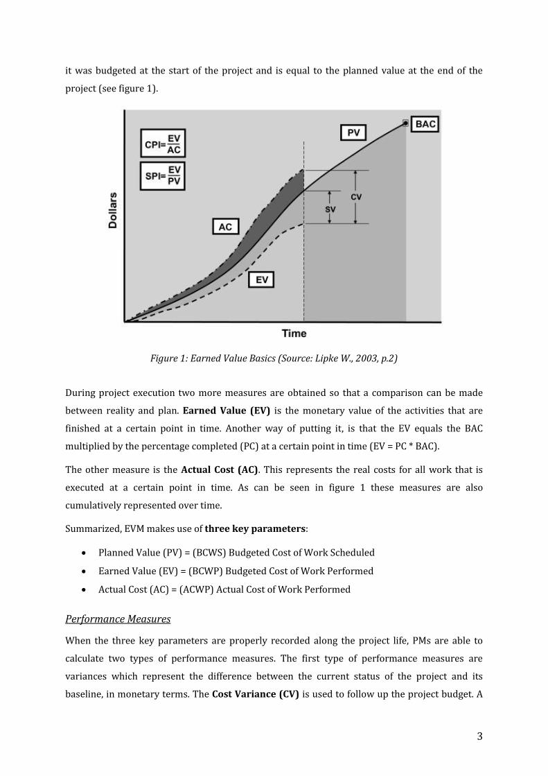
it was budgeted at the start of the project and is equal to the planned value at the end of the

project (see figure 1).

Figure 1: Earned Value Basics (Source: Lipke W., 2003, p.2)

During project execution two more measures are obtained so that a comparison can be made

between reality and plan. Earned Value (EV) is the monetary value of the activities that are

finished at a certain point in time. Another way of putting it, is that the EV equals the BAC

multiplied by the percentage completed (PC) at a certain point in time (EV = PC * BAC).

The other measure is the Actual Cost (AC). This represents the real costs for all work that is

executed at a certain point in time. As can be seen in figure 1 these measures are also

cumulatively represented over time.

Summarized, EVM makes use of three key parameters:

Planned Value (PV) = (BCWS) Budgeted Cost of Work Scheduled

Earned Value (EV) = (BCWP) Budgeted Cost of Work Performed

Actual Cost (AC) = (ACWP) Actual Cost of Work Performed

Performance Measures

When the three key parameters are properly recorded along the project life, PMs are able to

calculate two types of performance measures. The first type of performance measures are

variances which represent the difference between the current status of the project and its

baseline, in monetary terms. The Cost Variance (CV) is used to follow up the project budget. A

4

negative (positive) value points out that more (less) has been spent for the executed activities

than what was originally planned. The Schedule Variance (SV) is an indicator that provides

PMs with a value that represents whether the project is on schedule or not. A negative (positive)

value means that the project is behind (ahead of) schedule. The variances are also shown in

figure 1.

The variances can be derived as follows:

Cost Variance: CV = EV – AC

Schedule Variance: SV = EV – PV

Another type of performance measures are indices, also calculated from the three key

parameters of EVM. The indices are again used to display how well the project is performing,

now relatively in comparison with the baseline. Again two types of indices can be distinguished.

The first type of index is the Cost Performance Index (CPI), which expresses the cost efficiency

of the executed work. A CPI of less (more) than one means that the project is currently running

over (under) budget. The second index is the Schedule Performance Index (SPI). The SPI

shows whether the project is performing on schedule or not. A SPI of more (less) than one

means that the project is ahead of (behind) plan.

The indices can be derived as follows:

Cost Performance Index: CPI = EV / AC

Schedule Performance Index: SPI = EV / PV

It is clear that the variances and indices are interrelated. Still it is useful to calculate both

performance measures. The variances can give a snapshot of where the project is today

(expressed in monetary value) while the indices are rather used to represent the evolution in

performance of the project. This is of significant importance to make forecasts about the future

of the project.

Predicting the future with EVM

All of the performance measures help PMs to monitor the progress of the project both from a

cost and schedule point of view. Therefore EVM acts as an early warning system that helps PMs

to solve problems and exploit opportunities during project execution. Besides, these measures

and indicators are also used to make predictions about the future performance of the project.

The next section will describe how cost and time forecasts are made using EVM.

5

Cost forecasting

First of all the predictive power of the cost performance measures is considered. Here the focus

lies on predicting the final cost of the project. This final cost will be referred to as the Estimate at

Completion (EAC). The EAC consists of the Actual Cost (AC), the cost that has been spent so far

and an estimate of the cost of the remaining work (Estimate to Completion, ETC). In some

literature, ETC is also referred to as Planned Cost of Work Remaining (PCWR). It can be

calculated as follows:

ETC =(BAC − EV)

performance factor

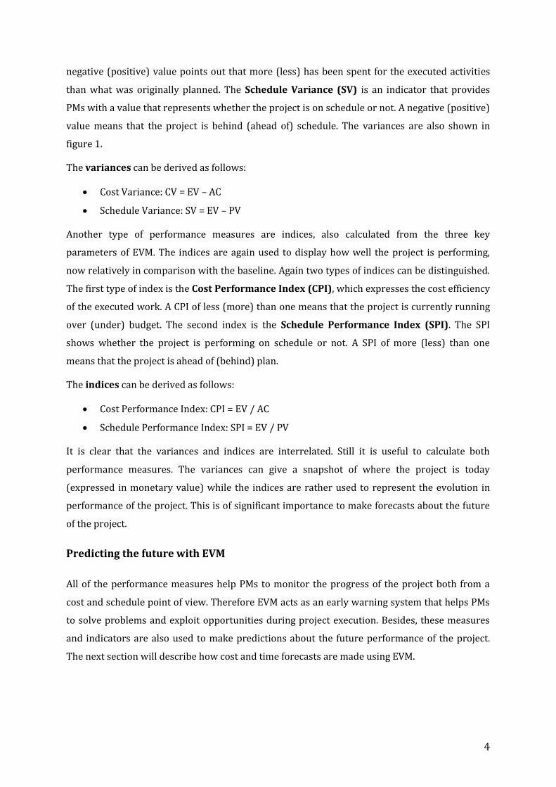
Several different formulas exist to calculate the EAC, depending on the performance factor that

is used to calculate the ETC. In general eight commonly used forecasting formulas are accepted

by project managers (see table 1).

EAC1 = AC + (BAC − EV) EAC5 = AC + BAC − EV

CR

EAC2 = AC + (BAC − EV)

CPI EAC6 = AC +

BAC − EV

CR(t)


SPI EAC7 = AC +

BAC − EV

wt1 ∗ SPI + wt2 ∗ CPI

EAC4 = AC + BAC − EV

SPI(t) EAC8 = AC +

BAC − EV

wt1 ∗ SPI(t) + wt2 ∗ CPI

Table 1: EAC formulas

EAC1 assumes a discount factor that is equal to one. This means that to estimate the remaining

cost of the project, no project performance measure is taken into account. The remaining cost is

assumed to equal the planned cost for the remaining work. The most commonly used formula

for cost forecasting is EAC2. In this formula the CPI is used as a discount factor for estimating the

remaining cost. EAC3 and EAC4 on the other hand are used in cases where the duration has a

huge impact on the final cost of the project.

In the last four EAC formulas it is supposed that both the cost and schedule performance

indicators have an impact on the cost of remaining work. The discount factor in EAC5 is called

the critical ratio (CR) (Anbari, 2001; Lewis, 2001) or cost - schedule index (CSI) (Barr, 1996;

Meredith & Mantel, 2000) or schedule - cost index (SCI) (Christensen, 1999; Vanhoucke, 2010).

It attempts to combine cost and schedule indicators into one overall project health indicator. A

CR equal to one indicates that overall project performance is on target while a lower number

indicates less than targeted performance.

6

CR is derived as follows:

CR = CPI * SPI

A performance factor equal to the CR(t) substitutes the SPI by the SPI(t). The last two equation

EAC7 and EAC8 are derivative formulas which give a weight to both the CPI (wt1) and the

SPI/SPI(t) (wt1). This way a customized formula can be obtained for the project.

Duration forecasting

EVM has also been used for more than forty years to predict the final duration of projects. This is

done analogue to forecasting the EAC. The oldest method calculated the Independent Estimate

At Completion (IEAC(t)). This estimate exists of the time that has already elapsed (Actual Time,

AT) and the duration of what the remaining work is estimated to take (Estimate To Complete,

ETC(t)). The time that is expected to complete the project is calculated by adjusting the work

remaining (Estimate To Complete, ETC) for the work rate that is expected on the remaining of

the project. ETC(t) is also referred to as Planned Duration of Work Remaining (PDWR) and can

be calculated as follows:

ETC(t) = (BAC – EV)

Work Rate

The Independent Estimate at Completion (IEAC(t)) can be derived as follows:

IEAC(t) = AT + ETC(t)

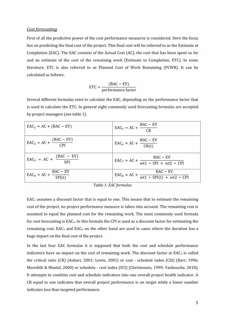
Four commonly applied work rates were used to translate a monetary value into a time value:

Average Planned Value (PVav = PVcum/n)

Average Earned Value (EVav = EVcum/n)

Current period Planned Value (PVlp)

Current period Earned Value (EVlp)

Table 2: Work rates

Although this traditional method was applied for forty years, it deals with certain mathematical

deficiencies (for more information see Lipke (2009), “Project Duration Forecasting.”). This

induces that the method doesn’t give reliable estimates for all projects and therefore adjusted

methods have been developed.

Recently three extensions to EVM were established: the Planned Value method (Anbari, 2003),

the Earned Duration method (Jacob, 2003) and the Earned Schedule method (Lipke, 2003).

Table 3 provides an overview of the duration forecasting formulas of these three methods.

Depending on the discount factor, three forecast formulas can be derived for each method.

7

Planned value method

(Anbari)

Earned duration method

(Jacob)

Earned schedule method

(Lipke)

EAC t PV 1 = PD − TV EAC t ED 1 = AD + (PD − ED) EAC t ES 1 = AD + (PD − ES)

EAC t PV 2 = PD

SPI EAC t ED 2 = AD +

(PD − ED)

SPI EAC t ES 2 = AD +

(PD − ES)

SPI(t)

EAC t PV 3 = PD

CR EAC t ED 3 = AD +

(PD − ED)

CR EAC t ES 3 = AD +

(PD − ES)

CR

Table 3: EAC(t) formulas

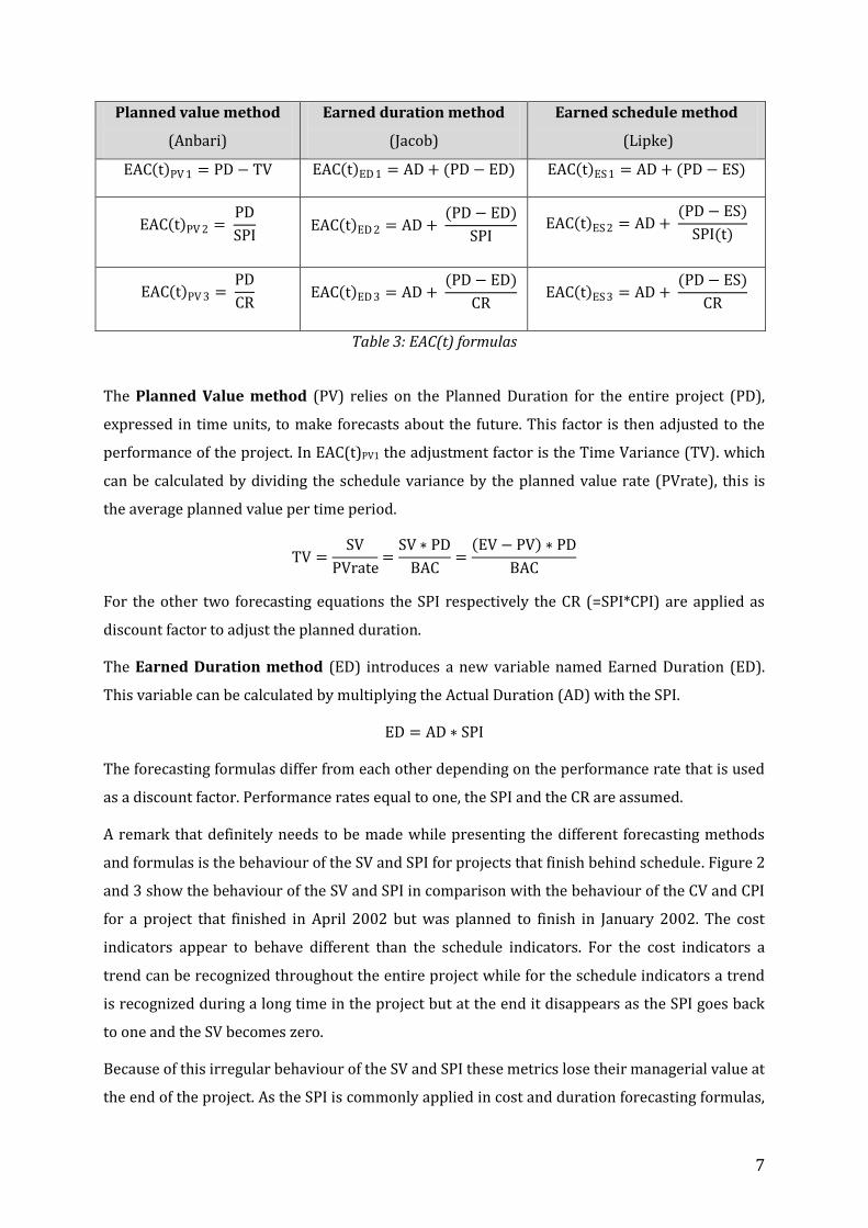
The Planned Value method (PV) relies on the Planned Duration for the entire project (PD),

expressed in time units, to make forecasts about the future. This factor is then adjusted to the

performance of the project. In EAC(t)PV1 the adjustment factor is the Time Variance (TV). which

can be calculated by dividing the schedule variance by the planned value rate (PVrate), this is

the average planned value per time period.

TV =SV

PVrate=

SV ∗ PD

BAC=

EV − PV ∗ PD

BAC

For the other two forecasting equations the SPI respectively the CR (=SPI*CPI) are applied as

discount factor to adjust the planned duration.

The Earned Duration method (ED) introduces a new variable named Earned Duration (ED).

This variable can be calculated by multiplying the Actual Duration (AD) with the SPI.

ED = AD ∗ SPI

The forecasting formulas differ from each other depending on the performance rate that is used

as a discount factor. Performance rates equal to one, the SPI and the CR are assumed.

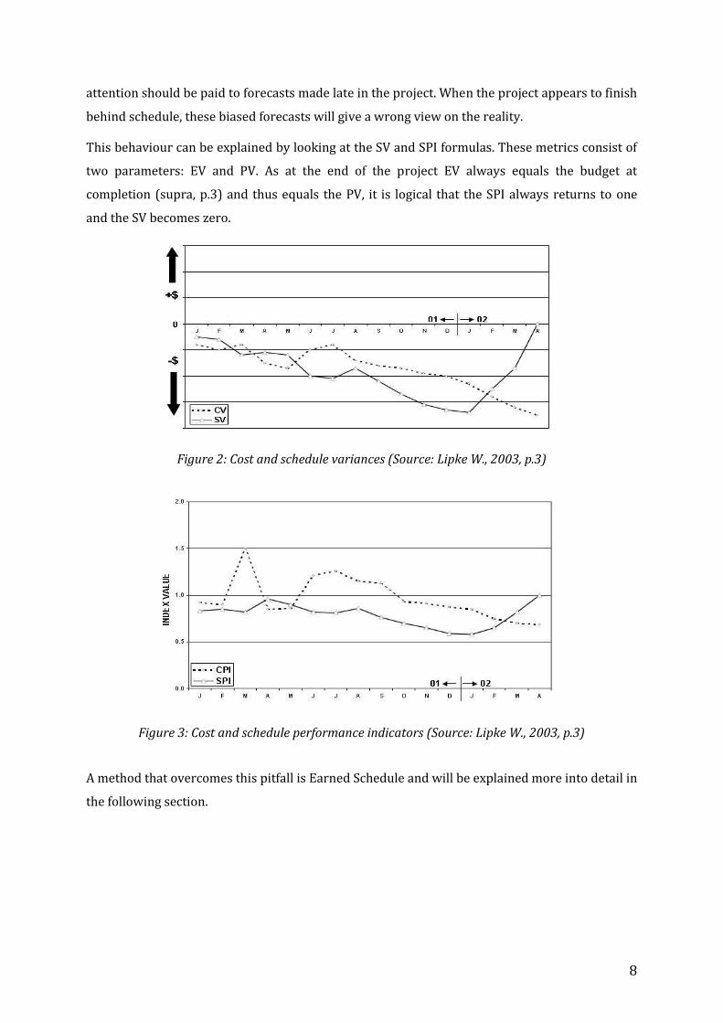
A remark that definitely needs to be made while presenting the different forecasting methods

and formulas is the behaviour of the SV and SPI for projects that finish behind schedule. Figure 2

and 3 show the behaviour of the SV and SPI in comparison with the behaviour of the CV and CPI

for a project that finished in April 2002 but was planned to finish in January 2002. The cost

indicators appear to behave different than the schedule indicators. For the cost indicators a

trend can be recognized throughout the entire project while for the schedule indicators a trend

is recognized during a long time in the project but at the end it disappears as the SPI goes back

to one and the SV becomes zero.

Because of this irregular behaviour of the SV and SPI these metrics lose their managerial value at

the end of the project. As the SPI is commonly applied in cost and duration forecasting formulas,

8

attention should be paid to forecasts made late in the project. When the project appears to finish

behind schedule, these biased forecasts will give a wrong view on the reality.

This behaviour can be explained by looking at the SV and SPI formulas. These metrics consist of

two parameters: EV and PV. As at the end of the project EV always equals the budget at

completion (supra, p.3) and thus equals the PV, it is logical that the SPI always returns to one

and the SV becomes zero.

Figure 2: Cost and schedule variances (Source: Lipke W., 2003, p.3)

Figure 3: Cost and schedule performance indicators (Source: Lipke W., 2003, p.3)

A method that overcomes this pitfall is Earned Schedule and will be explained more into detail in

the following section.

9

Earned Schedule

The Earned Schedule (ES) method can be seen as an expansion of EVM because the same basic

EVM metrics are used and the ES performance measures are similar to those for EVM. ES was

first introduced by Lipke (2003) and measures schedule performance in units of time instead of

in costs, which is done in EVM. This approach solves the problem that the EVM schedule

indicators SV and SPI encounter for late finish projects.

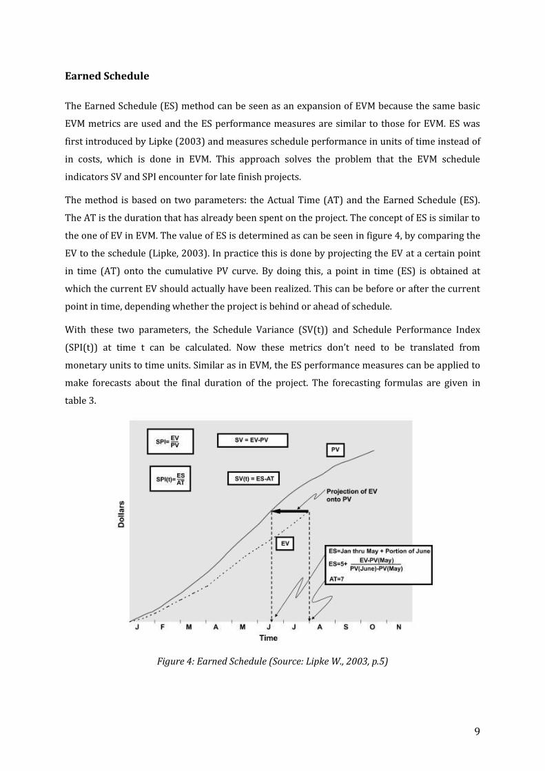
The method is based on two parameters: the Actual Time (AT) and the Earned Schedule (ES).

The AT is the duration that has already been spent on the project. The concept of ES is similar to

the one of EV in EVM. The value of ES is determined as can be seen in figure 4, by comparing the

EV to the schedule (Lipke, 2003). In practice this is done by projecting the EV at a certain point

in time (AT) onto the cumulative PV curve. By doing this, a point in time (ES) is obtained at

which the current EV should actually have been realized. This can be before or after the current

point in time, depending whether the project is behind or ahead of schedule.

With these two parameters, the Schedule Variance (SV(t)) and Schedule Performance Index

(SPI(t)) at time t can be calculated. Now these metrics don’t need to be translated from

monetary units to time units. Similar as in EVM, the ES performance measures can be applied to

make forecasts about the final duration of the project. The forecasting formulas are given in

table 3.

Figure 4: Earned Schedule (Source: Lipke W., 2003, p.5)

10

P-factor

The P-factor (Lipke, 2004) is a recently proposed Earned Value measure that makes the direct

connection between the schedule and EVM data. The P-factor is an indicator for schedule

adherence, it measures whether the project is executed according to plan or not. This is

important because projects that do not stick to the plan are mostly in trouble or might deal with

a higher risk for rework.

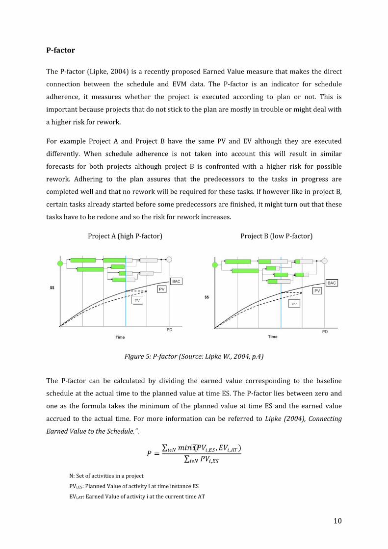
For example Project A and Project B have the same PV and EV although they are executed

differently. When schedule adherence is not taken into account this will result in similar

forecasts for both projects although project B is confronted with a higher risk for possible

rework. Adhering to the plan assures that the predecessors to the tasks in progress are

completed well and that no rework will be required for these tasks. If however like in project B,

certain tasks already started before some predecessors are finished, it might turn out that these

tasks have to be redone and so the risk for rework increases.

Project A (high P-factor) Project B (low P-factor)

Figure 5: P-factor (Source: Lipke W., 2004, p.4)

The P-factor can be calculated by dividing the earned value corresponding to the baseline

schedule at the actual time to the planned value at time ES. The P-factor lies between zero and

one as the formula takes the minimum of the planned value at time ES and the earned value

accrued to the actual time. For more information can be referred to Lipke (2004), Connecting

Earned Value to the Schedule.".

𝑃 = 𝑚𝑖𝑛(𝑃𝑉𝑖 ,𝐸𝑆 , 𝐸𝑉𝑖 ,𝐴𝑇)𝑖𝜖𝑁

𝑃𝑉𝑖,𝐸𝑆𝑖𝜖𝑁

N: Set of activities in a project

PVi,ES: Planned Value of activity i at time instance ES

EVi,AT: Earned Value of activity i at the current time AT

EV EV

11

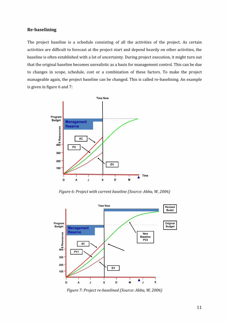
Re-baselining

The project baseline is a schedule consisting of all the activities of the project. As certain

activities are difficult to forecast at the project start and depend heavily on other activities, the

baseline is often established with a lot of uncertainty. During project execution, it might turn out

that the original baseline becomes unrealistic as a basis for management control. This can be due

to changes in scope, schedule, cost or a combination of these factors. To make the project

manageable again, the project baseline can be changed. This is called re-baselining. An example

is given in figure 6 and 7:

Figure 6: Project with current baseline (Source: Abba, W, 2006)

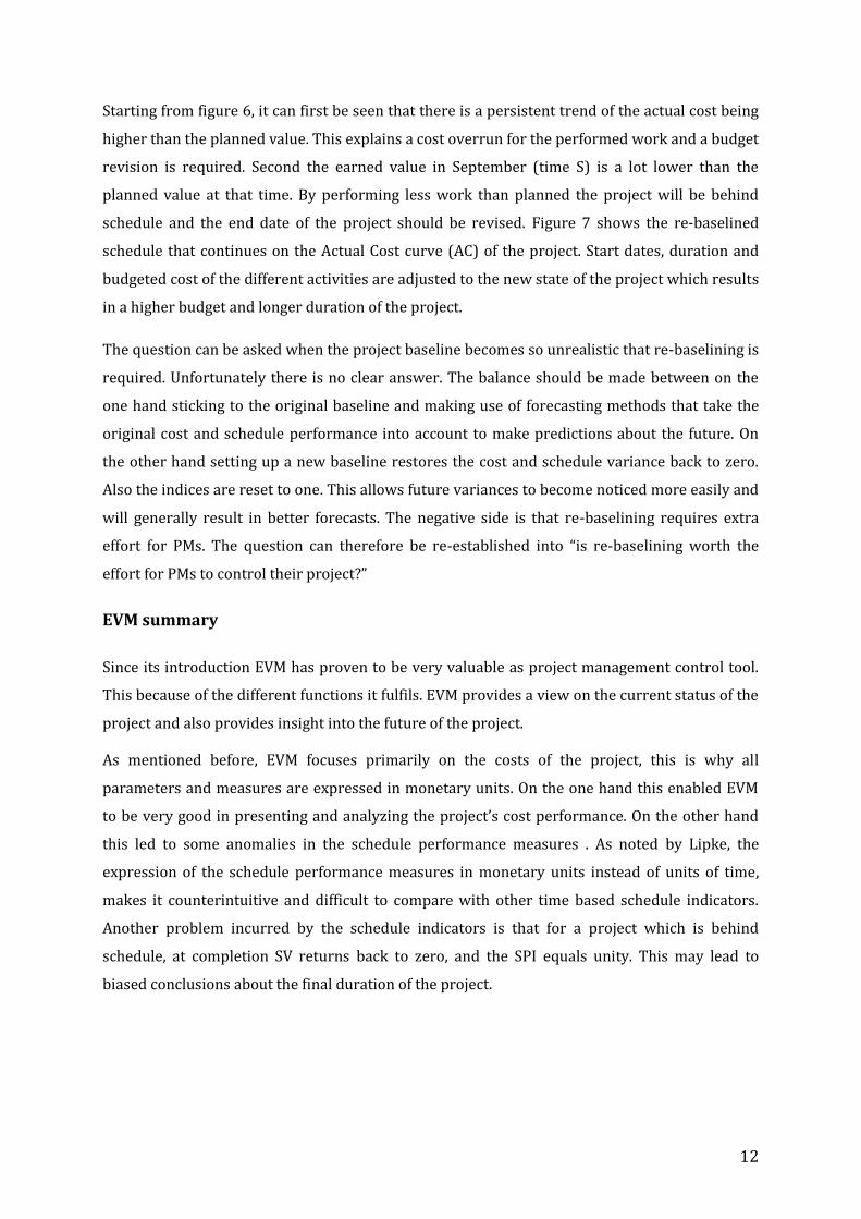
Figure 7: Project re-baselined (Source: Abba, W, 2006)

12

Starting from figure 6, it can first be seen that there is a persistent trend of the actual cost being

higher than the planned value. This explains a cost overrun for the performed work and a budget

revision is required. Second the earned value in September (time S) is a lot lower than the

planned value at that time. By performing less work than planned the project will be behind

schedule and the end date of the project should be revised. Figure 7 shows the re-baselined

schedule that continues on the Actual Cost curve (AC) of the project. Start dates, duration and

budgeted cost of the different activities are adjusted to the new state of the project which results

in a higher budget and longer duration of the project.

The question can be asked when the project baseline becomes so unrealistic that re-baselining is

required. Unfortunately there is no clear answer. The balance should be made between on the

one hand sticking to the original baseline and making use of forecasting methods that take the

original cost and schedule performance into account to make predictions about the future. On

the other hand setting up a new baseline restores the cost and schedule variance back to zero.

Also the indices are reset to one. This allows future variances to become noticed more easily and

will generally result in better forecasts. The negative side is that re-baselining requires extra

effort for PMs. The question can therefore be re-established into “is re-baselining worth the

effort for PMs to control their project?”

EVM summary

Since its introduction EVM has proven to be very valuable as project management control tool.

This because of the different functions it fulfils. EVM provides a view on the current status of the

project and also provides insight into the future of the project.

As mentioned before, EVM focuses primarily on the costs of the project, this is why all

parameters and measures are expressed in monetary units. On the one hand this enabled EVM

to be very good in presenting and analyzing the project’s cost performance. On the other hand

this led to some anomalies in the schedule performance measures . As noted by Lipke, the

expression of the schedule performance measures in monetary units instead of units of time,

makes it counterintuitive and difficult to compare with other time based schedule indicators.

Another problem incurred by the schedule indicators is that for a project which is behind

schedule, at completion SV returns back to zero, and the SPI equals unity. This may lead to

biased conclusions about the final duration of the project.

13

As the implementation of earned schedule overcomes these problems, the credibility of EVM is

only rising. Especially with the insertion of the P-factor which closes the gap between schedule

and EVM data, EVM can now control projects in a very extended way.

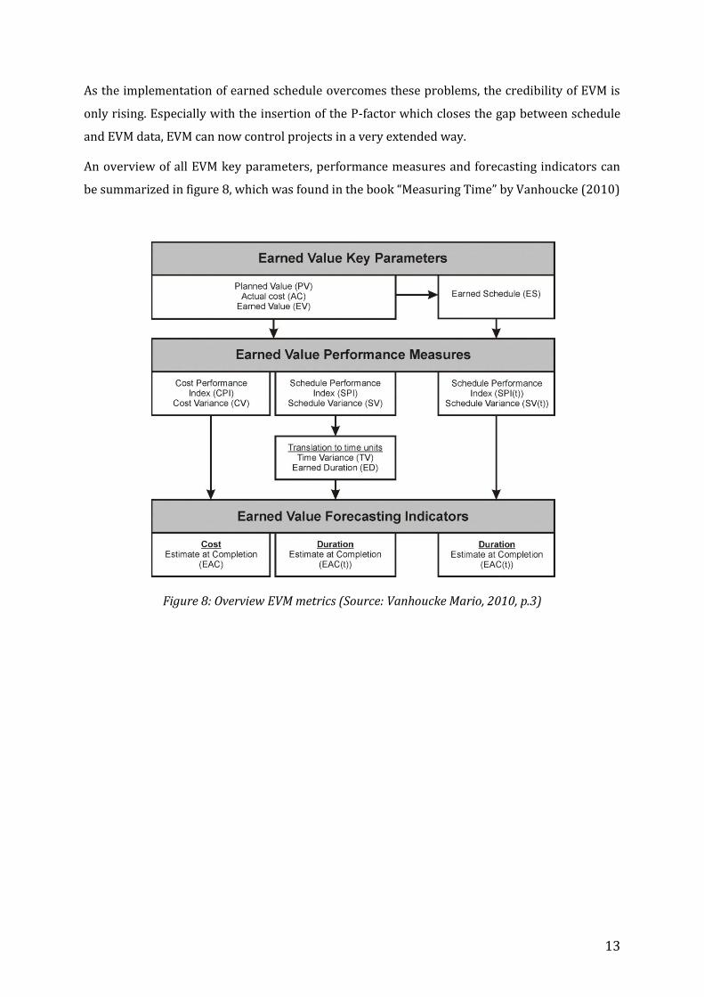
An overview of all EVM key parameters, performance measures and forecasting indicators can

be summarized in figure 8, which was found in the book “Measuring Time” by Vanhoucke (2010)

Figure 8: Overview EVM metrics (Source: Vanhoucke Mario, 2010, p.3)

14

2 EVM studies

During the years, a lot of research has been done in the Earned Value Management domain. This

section will give an overview about the most important studies, results and conclusions. The

literature will not focus specifically on construction projects but is meant to give a global insight

in the use of Earned Value Management in multiple industries. In a later section these findings

will be analyzed and criticized in relation to the construction sector. This approach is preferred

because currently there is not a lot of specific research available about the performance of the

Earned Value Method in the construction sector. First the frequently studied CPI stability

findings are presented. Subsequently studies about the different forecasting methods are

discussed and re-baselining is considered. To conclude an overview of the influencing project

characteristics is given.

CPI stability

A first study object is the stability of the CPI. The CPI is an indicator of the cost performance

efficiency of a project and its stability is important for three main reasons (Christensen and

Heise, 1993). First, the CPI is a parameter that is used in many EAC formulas which predict the

cost at completion. Second, a stable CPI might indicate that cost control is performed well

because variances are identified early and corrected in the corresponding period. Third, it can

be compared with the To Complete Performance Index (TCPI) and be used as a benchmark. For

example if the TCPI is significantly higher than the CPI, efficiency will have to be improved for

the remaining work in order to avoid cost overruns.

It was long accepted that the CPI does not change with more than ten percent after a project is

fifty percent complete, although it lasted until 1990 before empirical evidence was available. The

first study was published by Payne (1990). The study analyzed data of seven completed aircraft

programs and tested the hypothesis that the cumulative CPI is stable, meaning to have a

maximum deviation of ten percent, from the fifty percent completion point. The results

confirmed the hypothesis and further investigation on these projects even showed stability from

the twenty percent completion point. Even from the ten percent completion point the CPI was

stable, except for one project.

A more extended research was executed three years later (Christensen, Heise, 1993). Now data

from 155 defence contracts were investigated. Again the hypothesis was that the CPI is stable

from the fifty percent completion point and also sensitivity analysis was done for the forty,

thirty, twenty and ten completion point. Next to a larger sample size, this study differs from

15

Payne’s study because both the cumulative and non-cumulative CPI were now calculated. The

results were satisfying. From the 155 contracts, 153 had a stable cumulative CPI from the fifty

percent completion point which confirmed their hypothesis. Also from the twenty percent

completion point, cumulative CPI stability was achieved for a 95 percent confidence interval.

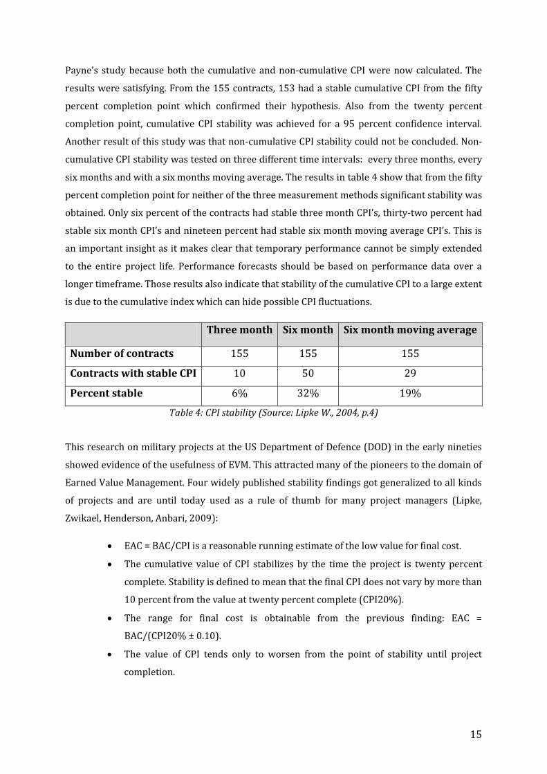
Another result of this study was that non-cumulative CPI stability could not be concluded. Non-

cumulative CPI stability was tested on three different time intervals: every three months, every

six months and with a six months moving average. The results in table 4 show that from the fifty

percent completion point for neither of the three measurement methods significant stability was

obtained. Only six percent of the contracts had stable three month CPI’s, thirty-two percent had

stable six month CPI’s and nineteen percent had stable six month moving average CPI’s. This is

an important insight as it makes clear that temporary performance cannot be simply extended

to the entire project life. Performance forecasts should be based on performance data over a

longer timeframe. Those results also indicate that stability of the cumulative CPI to a large extent

is due to the cumulative index which can hide possible CPI fluctuations.

Three month Six month Six month moving average

Number of contracts 155 155 155

Contracts with stable CPI 10 50 29

Percent stable 6% 32% 19%

Table 4: CPI stability (Source: Lipke W., 2004, p.4)

This research on military projects at the US Department of Defence (DOD) in the early nineties

showed evidence of the usefulness of EVM. This attracted many of the pioneers to the domain of

Earned Value Management. Four widely published stability findings got generalized to all kinds

of projects and are until today used as a rule of thumb for many project managers (Lipke,

Zwikael, Henderson, Anbari, 2009):

EAC = BAC/CPI is a reasonable running estimate of the low value for final cost.

The cumulative value of CPI stabilizes by the time the project is twenty percent

complete. Stability is defined to mean that the final CPI does not vary by more than

10 percent from the value at twenty percent complete (CPI20%).

The range for final cost is obtainable from the previous finding: EAC =

BAC/(CPI20% ± 0.10).

The value of CPI tends only to worsen from the point of stability until project

completion.

16

Especially Fleming and Koppelman (2000, 2005), two pioneering EVM researchers, wrote some

convincing books and articles that further dispersed the idea that CPI stability exists. Although

the latter were also a bit sceptic about the correlation of CPI stability and the size of the project.

This arose from the fact that all the projects in the DoD research program were extremely large

projects. There is a big difference between the timing of measurement between short and long

duration projects. For example the twenty percent completion point of a ten year lasting project

is after two years, while for a one-year project this is already after 2,4 months.

A first study that investigated this relation reported that the CPI stability after twenty percent

completion is only valid for large projects with a very long duration, generally longer than 6,7

years (Lipke, 2005). For smaller, short duration projects (less than two years), the CPI cannot be

evaluated as a reliable predictor for the cost at completion early in the project.

While the results of Lipke still accepted CPI stability to some extent, a study that was published

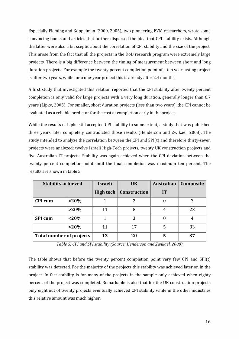
three years later completely contradicted those results (Henderson and Zwikael, 2008). The

study intended to analyze the correlation between the CPI and SPI(t) and therefore thirty-seven

projects were analyzed: twelve Israeli High-Tech projects, twenty UK construction projects and

five Australian IT projects. Stability was again achieved when the CPI deviation between the

twenty percent completion point until the final completion was maximum ten percent. The

results are shown in table 5.

Stability achieved Israeli

High tech

UK

Construction

Australian

IT

Composite

CPI cum <20% 1 2 0 3

>20% 11 8 4 23

SPI cum <20% 1 3 0 4

>20% 11 17 5 33

Total number of projects 12 20 5 37

Table 5: CPI and SPI stability (Source: Henderson and Zwikael, 2008)

The table shows that before the twenty percent completion point very few CPI and SPI(t)

stability was detected. For the majority of the projects this stability was achieved later on in the

project. In fact stability is for many of the projects in the sample only achieved when eighty

percent of the project was completed. Remarkable is also that for the UK construction projects

only eight out of twenty projects eventually achieved CPI stability while in the other industries

this relative amount was much higher.

17

This study of Henderson and Zwikael (2008) also revealed a consistent behaviour between the

CPI and SPI(t), which proved the value of the SPI(t) and Earned Schedule as a good method to

control project duration.

The question whether CPI stability can be assumed has no clear answer. Some call it a myth and

some still believe it is a general rule. The truth will probably lay somewhere in-between and is

dependent on the characteristics of the project, for example the length of the project or the

industry. In our study, it is our intention to verify CPI stability for the construction sector and to

find reasons why it would be applicable on construction projects or why not.

Cost and duration forecasting

The main reason for many project managers to apply EVM on their projects, is because forecasts

about cost and duration can be made early in the project. These forecasts, if reliable, are useful

for a project manager because then extra resources can be allocated to the project in order to

put the project back on track. During the years a lot of different formulas have been set up to

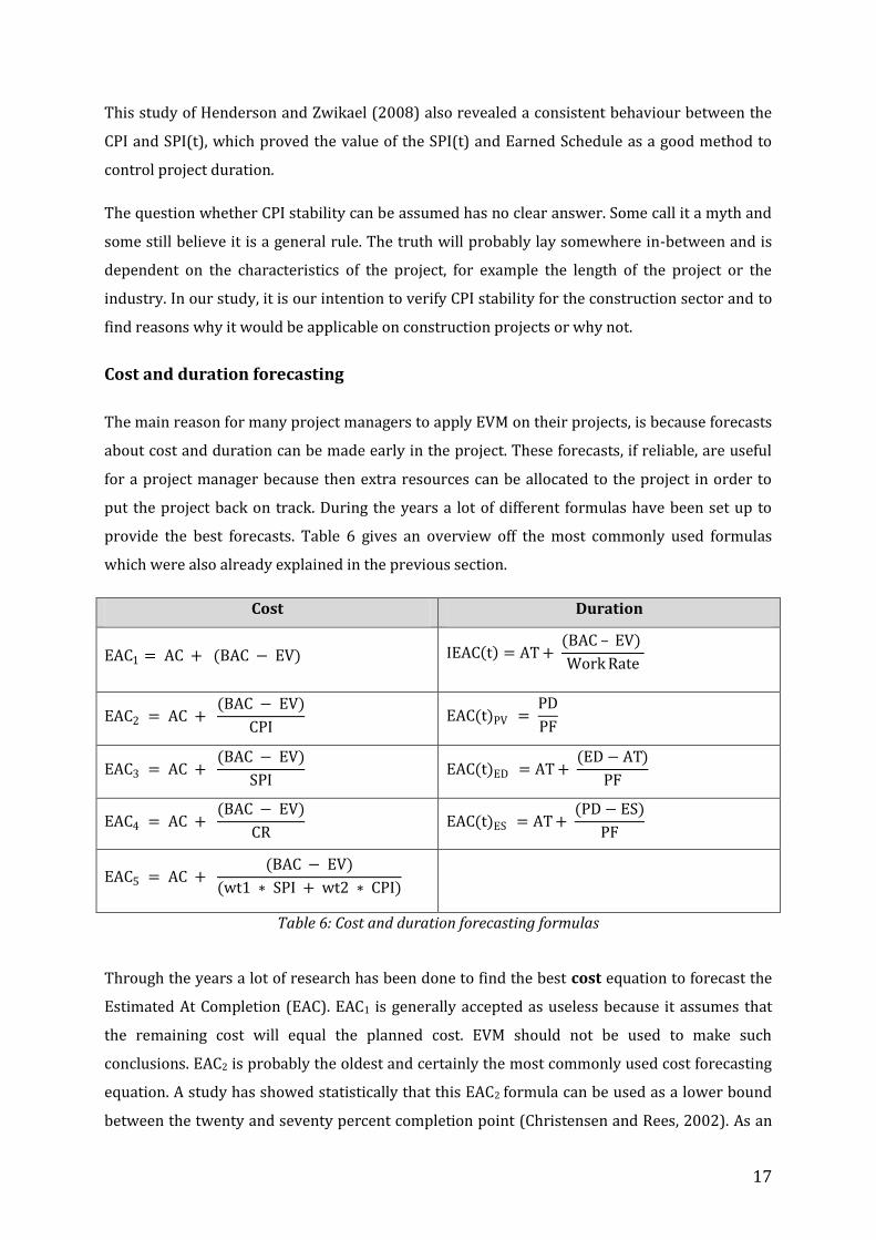
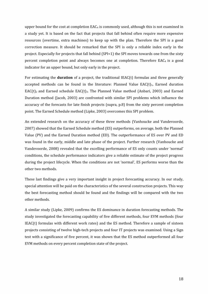
provide the best forecasts. Table 6 gives an overview off the most commonly used formulas

which were also already explained in the previous section.

Cost Duration

EAC1 = AC + (BAC − EV) IEAC t = AT + (BAC – EV)

Work Rate


CPI EAC(t)PV =

PD

PF


SPI EAC(t)ED = AT +

(ED − AT)

PF


CR EAC(t)ES = AT +

(PD − ES)

PF


(wt1 ∗ SPI + wt2 ∗ CPI)

Table 6: Cost and duration forecasting formulas

Through the years a lot of research has been done to find the best cost equation to forecast the

Estimated At Completion (EAC). EAC1 is generally accepted as useless because it assumes that

the remaining cost will equal the planned cost. EVM should not be used to make such

conclusions. EAC2 is probably the oldest and certainly the most commonly used cost forecasting

equation. A study has showed statistically that this EAC2 formula can be used as a lower bound

between the twenty and seventy percent completion point (Christensen and Rees, 2002). As an

18

upper bound for the cost at completion EAC4 is commonly used, although this is not examined in

a study yet. It is based on the fact that projects that fall behind often require more expensive

resources (overtime, extra machines) to keep up with the plan. Therefore the SPI is a good

correction measure. It should be remarked that the SPI is only a reliable index early in the

project. Especially for projects that fall behind (SPI<1) the SPI moves towards one from the sixty

percent completion point and always becomes one at completion. Therefore EAC4 is a good

indicator for an upper bound, but only early in the project.

For estimating the duration of a project, the traditional IEAC(t) formulas and three generally

accepted methods can be found in the literature: Planned Value EAC(t)1, Earned duration

EAC(t)2 and Earned schedule EAC(t)3. The Planned Value method (Anbari, 2003) and Earned

Duration method (Jacob, 2003) are confronted with similar SPI problems which influence the

accuracy of the forecasts for late finish projects (supra, p.8) from the sixty percent completion

point. The Earned Schedule method (Lipke, 2003) overcomes this SPI problem.

An extended research on the accuracy of these three methods (Vanhoucke and Vandevoorde,

2007) showed that the Earned Schedule method (ES) outperforms, on average, both the Planned

Value (PV) and the Earned Duration method (ED). The outperformance of ES over PV and ED

was found in the early, middle and late phase of the project. Further research (Vanhoucke and

Vandevoorde, 2008) revealed that the excelling performance of ES only counts under ‘normal’

conditions, the schedule performance indicators give a reliable estimate of the project progress

during the project lifecycle. When the conditions are not ‘normal’, ES performs worse than the

other two methods.

These last findings give a very important insight in project forecasting accuracy. In our study,

special attention will be paid on the characteristics of the several construction projects. This way

the best forecasting method should be found and the findings will be compared with the two

other methods.

A similar study (Lipke, 2009) confirms the ES dominance in duration forecasting methods. The

study investigated the forecasting capability of five different methods, four EVM methods (four

IEAC(t) formulas with different work rates) and the ES method. Therefore a sample of sixteen

projects consisting of twelve high-tech projects and four IT projects was examined. Using a Sign

test with a significance of five percent, it was shown that the ES method outperformed all four

EVM methods on every percent completion state of the project.

19

Re-baselining

Re-baselining the cost and schedule estimates is desirable when the original baseline is no

longer viable (Solanki, 2009). The baseline becomes unviable when the result of cost, schedule

or technical issues made it unrealistic. These issues can be triggered by either a change of plans

or by a performance level that is not in accordance with what was assumed at project initiation.

In the article ‘An Earned Value tutorial’ by Durrenberger (2003) a list of guidelines is given to

help project managers decide whether to re-baseline or not.

The project is out of money

The project is out of time

The project is out of resources

The project stakeholders approve a scope change

To give an answer to the question whether or not to re-baseline the following quote is cited. “Re-

baselining is only legitimate when it is performed in response to a stakeholder- approved scope

change.” (Durrenberger, 2003, p.10)

Characteristics of a project

A project is by definition unique and has different characteristics. Therefore an enormous

variety in projects exists. Some projects are rather similar while others will be completely

different. This logically implies that not for every project the same EVM technique will give the

best result and that EVM is even not appropriate for certain projects. In this section four project

characteristics are discussed more into detail in order to create a better understanding of their

influence on the use of EVM.

Contract type

A first characteristic is the contract type. In general two basic contract types exist: a fixed price

contract and a cost reimbursable contract. It was always believed that EVM was only useful

for cost reimbursable contracts and that for fixed price contracts EVM was rather useless. The

last decade however, this point of view has been criticized and nowadays a more mixed belief on

contract selection exists.

The traditional point of view was established by large US government departments. They made

the first large EVM studies in the Department of Defence (DoD) (supra, p.14) and because of this

their influence was huge. Besides the DoD, the National Aeronautics and Space Administration

(NASA) also shared the belief that EVM was only required for large cost reimbursable contracts.

20

The last decade a lot of evidence has been found to reject this traditional point of view and

generalize it to include also fixed price contracts. First of all, several anecdotes went around

about successful implementation of EVM on fixed price contracts. Later on this revolutionary

insight was also accepted by Fleming and Koppelman (2002), two convincing pioneers in the

Earned Value domain. Furthermore a method to transform fixed price data into key EVM

parameters was discovered (Alvorado et al., 2004). When also Marshall (2005, 2007), one of the

main investigators in this domain published his preference to include EVM on fixed price

contracts, many project managers were convinced.. Although still some proponents exist,

nowadays contract type is mostly considered not to have a huge impact on the choice whether to

apply EVM or not.

Length of the project

A second characteristic that was heavily discussed during the years is the length of the project. It

has gone through a similar process as the contract type discussion. In the early years of EVM it

was considered that EVM was only worth to be used on very long (> five years) projects. The

main reason is already discussed before: stability at the twenty percent completion point is only

achieved in projects with a long duration. This way the CPI and SPI at the twenty percent

completion point can be used to make accurate forecasts about the total cost and duration from

early on in the project. This statement was again initiated by the influencing US government

departments in the early nineties and is still considered to be correct by some project managers.

However during the last years, more and more project managers started to believe that EVM

could also be a good technique for small and medium sized projects. This belief is only

appropriate if some rules are taken into account. First it is interesting to increase the reporting

cycle from months to weeks or even days for very small projects. Secondly it might be hard and

expensive to calculate the actual cost on a daily basis. Then the compromise can be made to

adjust the actual costs for example on a weekly basis while adjusting the schedule on a daily

basis. Besides a study on projects with a cost of around $200.000 and length of only six months

revealed that EVM was very beneficial to these projects (Custers, 2008).

Another finding concerning the duration of projects is that often projects get stuck at ninety

percent completion. The last ten percent takes much longer than expected and costs much more

than ten percent of the budget. This behaviour is called the ’90 percent syndrome’ and can be

found across different types of projects and industries. This symptom can be explained by a

common archetype from System Dynamics known as ‘Shifting the Burden’ (Winston and

Maroulis, 1998). This relates to the time when activities are completed. Executing activities

before they are scheduled can create rework later on in the project life and may be accumulated

21

until the end of the project. This then causes the last ten percent to take ages. This can be seen as

one of the main reasons why the p-factor (supra, p.8) is useful in following up a project.

Budget

Projects are also characterized by a budget that is allocated to them. Although the influence of

the budget is less crucial to the usefulness of EVM than that of the duration, it is also heavily

discussed. Here the size of the budget itself doesn’t have an influence on the efficiency of EVM

but managers don’t think it is worthwhile to apply EVM on projects with a limited budget. This

prejudice is prompted by three underlying thoughts.

First of all, many project managers and people in general have the idea that EVM creates a lot of

extra work which costs money. But actually most EVM key parameters already exist on most

projects. The issue is just to find a common ground between the schedule and cost estimates of a

project. For construction projects this connection is present in the public tender that is

submitted by the company but afterwards this connection is neglected. This issue is treated

more in detail in the section about ‘Managing construction projects with EVM’ (infra, p.23).

Secondly there is the fear of having to change the organization of the company or project team

when implementing EVM. This could require serious investments if it was really necessary. But

this is not the case. EVM just requires that the functional organisational units within the

company, which have a certain responsibility over the project, also show up on the project

organisation chart.

A last thing that managers think will raise the costs of the project when implementing EVM is the

need for a new software package. Most of the time these software packages are pretty expensive

but such packages can be useful for large projects but are definitely not necessary. The

straightforward calculations that are used by EVM can be easily done in Microsoft Excel.

Network structure

A fourth indicator that was only recently investigated is the influence of the network structure. A

first publication (Lipke, 2004) described the importance of schedule adherence, measured by

the P-factor: an indicator that measures how the schedule is being accomplished according to

plan. The P-factor is used as an important early warning signal next to the CPI and SPI(t)

because the CPI and SPI(t) say nothing about whether the project is executed according to plan

or not.

22

For this recently applied indicator no empirical evidence about its value is available yet.

Although Lipke says that “when P is a high value, we can expect CPI and SPI(t) to be high as

well”. This statement is formulated by Lipke (2009) but requires further research to be verified.

Another study (Vanhoucke and Vandevoorde, 2009) found a second important network

indicator that should be taken into account when applying EVM: the serial/parallel indicator

(SP). The main conclusion was that the more the network approaches a serial configuration, the

better the forecast estimates become. In a serial network the activity criticality is very high and

when one activity is delayed, the complete project will be delayed. This makes the network very

predictable. In a more parallel network on the other hand, a delay in a certain task does not

automatically leads to a delay in the total project because most of the tasks are not critical and

have a certain flexibility. This makes accurate forecasting a lot more difficult.

23

3 EVM in the construction Sector

Now that the EVM methods have been discussed and that factors influencing the usefulness of

these method have been highlighted, it is time to take a more in depth view on the use of EVM in

the construction sector. Although this sector was one of the first to commercially adopt the use

of EVM, its inherent dynamic nature doesn’t make it easy on project managers (Prentice 2003).

To start, some general ideas about the implementation and usefulness of EVM in practice will be

discussed. Then the factors influencing the usefulness of EVM that have been discussed earlier

will be looked at from the point of view of construction projects. Finally a real life study will be

discussed to get an idea of the effect that several factors can have on EVM effectiveness in the

construction industry.

Managing construction projects with EVM

The problem of implementing EVM

“If EVM is so good, …why isn’t EVM used on all projects?” is the title of an article by the EVM

guru’s Fleming and Koppelman (2004) and can be considered – ignoring the first part - as the

problem definition of this section. Although this thesis only focuses on construction projects, the

problems encountered when trying to implement EVM are similar to those encountered on

other type of projects. This problem description can then be further divided in two parts. The

first part looks for external causes of this problem, without questioning the method itself. The

second part approaches the problem from the opposite direction and looks for causes in the

EVM method itself. Fleming and Koppelman (2004) found three main reasons why EVM isn’t

used on all projects and these will be referred to in the following two parts.

Reason 1: because EVM advocates often speak in a foreign tongue

Reason 2: because initially the DOD defined EVM to acquire "major systems"

Reason 3: because sometimes management...doesn't really want to know the full cost!

24

External causes

Starting with the external causes for not applying the EVM methodology leads to the world of

project managers where multiple project control methods exist that help perform project audits

and performance assessments. These methods are the same as the ones every effective project

manager should have at his disposal (Caletka, 2009), including:

CPM – Critical Path Method Scheduling

WBS – Work Breakdown Structure

EVM – Earned Value Management

VM/RM – Value Management / Risk Management

All of these methods have proven their usefulness in the area of project management but when

taking a closer look at the perception of project managers towards EVM, some scepticism is

encountered. Opinions like ‘EVM is only useful on large, Long-Term projects’ and ‘EVM does

nothing for construction projects’ are still floating around. This occurs nevertheless the

unremitting effort of several authors who try to dispel these views (Fleming and Koppelman,

2002; Kim et al., 2003; Marshall, 2005; Custer, 2009). The studies performed by those authors

all point in the direction of increasing acceptance of the EVM methodology by those project

managers who have used and are using EVM.

Another external cause is the unwillingness to know the full cost of the project beforehand

(Reason 3). This attitude can have several underlying reasons, for more information can be

referred to the article by Fleming and Koppelman (2004), “If EVM is so good, … why isn't it used

on all projects?”. Sound thinking immediately dispels this so called reason. Every project

manager knows this rule: “Bad news never gets better with time.” (Fleming and Koppelman,

2002, p.1).

Internal causes

Although EVM is the only methodology that combines measurements of actual, schedule and

cost performance in one measurement system, it could equally well be that the reluctance of

implementing it can be found in the method itself. Is EVM inherently difficult to implement in the

construction sector? Implementing EVM increases the administrative effort of the project

management team. If you are new to Earned Value Management and you have read the first

section of this thesis on the EVM basics you probably noticed that the terminology used by the

EVM methods differs quite a lot from the daily language used by project managers on

construction projects (Reason 1). This new terminology increases the switching costs of a

project manager wanting to implement EVM.

25

The first section of this thesis contained another pointer why EVM is not used on every project.

This time the reason relates to the birthplace of EVM (Reason 2). The Department of Defence

(DOD) developed the EVM methodology with the purpose of managing major projects with

huge budgets. Those are not the projects that are most common in the construction sector.

Construction projects are generally characterized by significant smaller budgets and shorter

project lives.

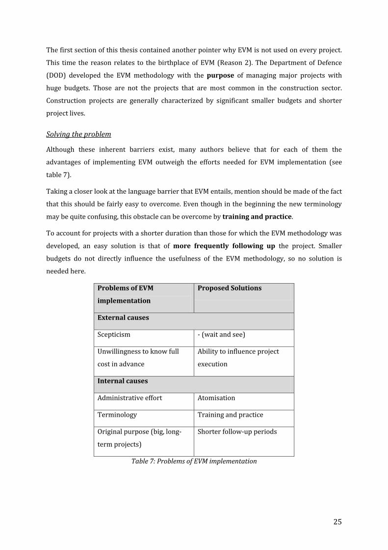
Solving the problem

Although these inherent barriers exist, many authors believe that for each of them the

advantages of implementing EVM outweigh the efforts needed for EVM implementation (see

table 7).

Taking a closer look at the language barrier that EVM entails, mention should be made of the fact

that this should be fairly easy to overcome. Even though in the beginning the new terminology

may be quite confusing, this obstacle can be overcome by training and practice.

To account for projects with a shorter duration than those for which the EVM methodology was

developed, an easy solution is that of more frequently following up the project. Smaller

budgets do not directly influence the usefulness of the EVM methodology, so no solution is

needed here.

Problems of EVM

implementation

Proposed Solutions

External causes

Scepticism - (wait and see)

Unwillingness to know full

cost in advance

Ability to influence project

execution

Internal causes

Administrative effort Atomisation

Terminology Training and practice

Original purpose (big, long-

term projects)

Shorter follow-up periods

Table 7: Problems of EVM implementation

26

Interesting is that in most construction projects managers don’t realize that they already have

most reporting systems in place to provide the needed data and measurements required by

EVM. They just don’t use the same terminology. This can significantly reduce the administrative

effort required when implementing EVM. If the project managers understand where to look for

the data required, an automated system could do the trick.

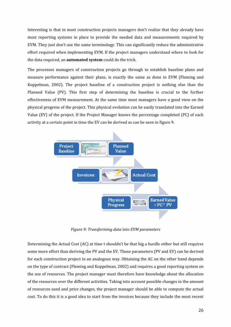
The processes managers of construction projects go through to establish baseline plans and

measure performance against their plans, is exactly the same as done in EVM (Fleming and

Koppelman, 2002). The project baseline of a construction project is nothing else than the

Planned Value (PV). This first step of determining the baseline is crucial to the further

effectiveness of EVM measurement. At the same time most managers have a good view on the

physical progress of the project. This physical evolution can be easily translated into the Earned

Value (EV) of the project. If the Project Manager knows the percentage completed (PC) of each

activity at a certain point in time the EV can be derived as can be seen in figure 9.

Figure 9: Transforming data into EVM parameters

Determining the Actual Cost (AC) at time t shouldn’t be that big a hurdle either but still requires

some more effort than deriving the PV and the EV. Those parameters (PV and EV) can be derived

for each construction project in an analogous way. Obtaining the AC on the other hand depends

on the type of contract (Fleming and Koppelman, 2002) and requires a good reporting system on

the use of resources. The project manager must therefore have knowledge about the allocation

of the resources over the different activities. Taking into account possible changes in the amount

of resources used and price changes, the project manager should be able to compute the actual

cost. To do this it is a good idea to start from the invoices because they include the most recent

27

prices. The difficulty here is that although invoices may be the most accurate source for price

information, they do not represent the actual amounts of resources used. Therefore project

managers should make registration of the team’s effort and used resources on this part of the

EVM implementation. The best practice here is to find overlap between the Organizational

Breakdown Structure (OBS) and the Work Breakdown Structure (WBS) to allocate this

responsibility. When this is done the Actual Cost of the current state of the project is known.

For the last couple of years an evolution took place in how project managers perceive the above

mentioned problems. Nowadays most of these problems are perceived as “minor” to

“insignificant”. Today the main problems encountered when implementing EVM are situated in

the organizational and cultural domain (Kim et al., 2003). This evolution is the result of the

efforts that have been put into improving the EVM processes and the increasing number of

testimonials of EVM practitioners. The organizational and cultural problems can be reduced by

clearly assigning responsibilities and by increasing the acceptance of the use of EVM throughout

the project team. The process of assigning responsibilities can be facilitated by creating a

Responsibility assignment matrix or RACI chart to assign responsibilities to persons or

organizations involved in the project (Valle and Soares, 2008). Increasing acceptance on the

other hand can be achieved by using a top-down approach which states that top management

truly believes in the EVM methodology.

Construction project characteristics

To put things into perspective with our study, an overview of the construction project

characteristics is presented in this section. Previously mentioned characteristics of projects in

general will be recapitulated and discussed from the viewpoint of construction projects. Besides

some specific characteristics of construction project will be presented.

Contract type

Having either a fixed price contract or a cost reimbursable contract is crucial to project

execution. When a contractor engages in a fixed price contract he has to make sure that all

future costs are taken into account in the baseline. For these contracts the possibility exists of

filing claims as additional expenses were required, but this is still at a risk. For cost

reimbursable contracts on the other hand the project owner is charged for all costs, shifting

the risk to the other side. So the type of contract directly influences the risk associated with the

execution. In the construction industry the most frequently applied contract type is the fixed

price contract (Fleming and Koppelman, 2002).

28


The time it takes to execute a project is another general characteristic of a project. In the

construction sector this can vary from several months to a couple of years. The longer the

duration of the project, the higher certain risks such as the ones related to the foreign exchange

rate or material prices become (Antvik, 1998).

Budget

Another general project characteristic is the budget. Every project has an according budget that

is available to the project organization to complete the project. The budget together with the

length of the project and the quality are the key performance indicators for every project in the

construction sector.

Network structure

As mentioned before, there are roughly two types of network structures (serial and parallel). In

the construction sector the most common network structure is the serial one. This is evident

because in the construction sector most projects start with the foundation and end by craftsman

finishing up the details.

While the previous characteristics were more general, the following characteristics are specific

to construction projects. This does not mean that these are not important on other types of

projects but it rather means that their importance was of less concern in the previous part

treating the findings of EVM related to project characteristics (supra, p.19).

Construction type

The first one of those characteristics is the type of construction. In general, there are three types

of construction projects:

1. Building construction

2. Heavy / civil construction

3. Industrial construction

Building construction is the most frequently executed construction type. It generally concerns

the construction and renovation of houses and other small buildings. Larger construction

projects like bridges, roads, canals, dams and huge buildings fall under the heavy/civil

construction type. These projects are also considered to create value for citizens. Finally

industrial construction projects include projects for large companies in for example the

29

petroleum, chemical, power generation or manufacturing industry and are rather aimed to make

profit.

Type of client

A second characteristic concerns the type of project owner. In the construction sector a clear

distinction can be made between three types of construction owners:

1. Public

2. Private

3. Mixed

Although it might be interesting to make a distinction between the projects based on the type of

client, evidence was found that accepted the EVM methodology in both the public and private

sectors (Kim et al., 2003).

Importance of the project

Every contractor has a portfolio of projects that are executed simultaneously. To prioritize

between these running projects the contractor is inclined to make the most important projects

perform best. This can be related to reputation, relationship between contractor and project

owner or other incentives. So this importance of the project can have a significant influence on

its performance.

Bidding environment

Most of the contracts that are related to construction projects have gone through some

evaluation and selection criteria. These criteria can also have an influence on the execution of

the project. The same can be said for the number of bidders, which were initially competing for

the contract. The most common approach toward project approval is the Design-Bid-Build

concept. In this approach first a design is approved by an architectural or design firm. Next the

different construction companies can make a bid for that design and mostly the company with

the lowest bid can execute the contract (Fleming & Koppelman, 2002).

Additional Work

The occurrence of additional work is common in the construction sector and can have a huge

influence on the eventual cost and duration. Because additional work is triggered by

unforeseeable changes made to the original plan, the project organization is mostly

compensated for it by the project owner. When additional work has to be executed, it is common

that the project suffers a delay and overruns the budget related to the original plan. This would

30

lead project managers to wrongly judge the performance of the project. Here re-baselining can

be appropriate to make sure that EVM performance measures represent the reality instead of

comparing actual cost and duration data (including additional works) to the original baseline.

Findings of EVM in the construction sector

To conclude, a real life study where EVM was used to follow up on a construction project is

discussed. In this study, mention has been made of some of the factors that are involved when

implementing EVM on construction projects. As they see it, “A major problem lies in the

determination of an appropriate accounting system to deal with scope changes.”(Valle & Soares,

2008, p.2) According to this study an appropriate Work Breakdown Structure together with a

suitable accounting plan could solve this problem. This is needed because a scope change can

have far stretching consequences for the total project. Not only the schedule and costs of the

project are affected by a scope change. resource allocation, milestones, etc. can be compromised

as well. Another study that interviewed Project Managers emphasized the influence a clearly

defined scope has on the cost-benefit ratio of influencing EVM (Vargas, 2003).

To make everything manageable Valle and Soares (2008) propose to isolate and control in detail

those activities with the greatest potential of having an impact on the project. This is an

application of Pareto’s law which states that only twenty percent of the activities determine

eighty percent of the outcome of a project. So by carefully following up on that percentile of the

activities with the highest impact on the outcome, the project becomes easier to manage while

keeping control over the project.

Another finding about the effectiveness of EVM on construction projects or projects in general is

related to responsibilities. The Project Management team should make sure that clear

responsibilities exist for each work package (Valle & Soares, 2008). This can be assured by using

a Responsibility assignment matrix (RACI chart). This tool combined with the WBS will help

project managers in following up projects accordingly.

31

4 Research

Introduction

This study aims to explore the performance of the Earned Value Method in the construction

industry. As mentioned before - although this is based on very little empirical research - it is

generally perceived that EVM and construction projects don’t fit together really well. A first

study (Henderson, Zwikael, 2008) on twenty UK construction projects showed that the generally

accepted CPI stability at twenty percent completion only applied for two projects. For twelve

projects even no CPI stability was found at all. A second study (Vargas, 2009) investigated the

impact of different construction project characteristics to the successful or unsuccessful

implementation of EVM. The results showed that EVM is a powerful tool in the control of

performance evaluation but only when the scope of the project is very well defined.

This study first aims at giving an overview of the indices stability. The CPI, SPI and SPI(t) are

included in the tests. Secondly the different EVM forecasting methods, both cost and time

related, are tested on their predictive power. Thirdly, an answer is sought on the question

whether re-baselining is worth the effort for construction projects. Finally, special attention is

paid on the in the influence of certain project characteristics. The P-factor, SP indicator, length of

the project and contract type are included.

Concluding the hypothesises of this study can be formulated in four general questions:

1. Is EVM a valuable method for following-up construction projects?

2. Which EVM forecasting methods perform generally best for construction projects?

3. When is re-baselining worth the effort in the construction industry?

4. What is the influence of project characteristics on the performance of EVM?

In this study five construction projects were examined into detail. As this sample size is small,

the results should be interpreted with care and generalizations cannot be made. Nevertheless

the value of this research lies in the combination of statistical tests with an in depth qualitative

research that aims to explain the results. This should allow the reader to get a better

understanding of EVM in all its aspects.

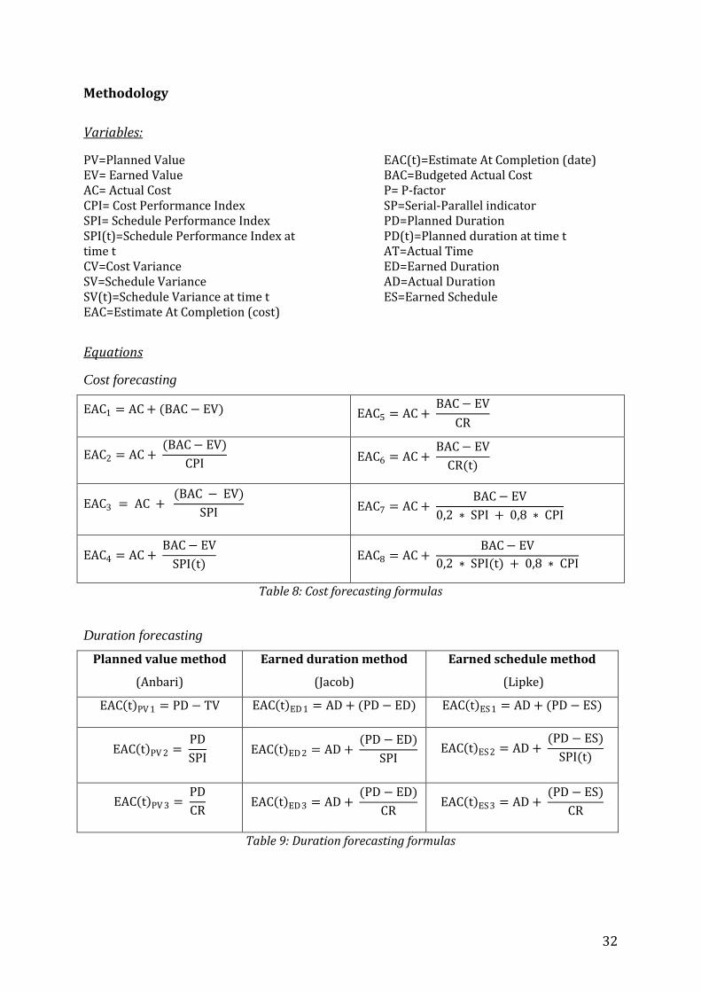
32

Methodology

Variables:

PV=Planned Value EV= Earned Value AC= Actual Cost CPI= Cost Performance Index SPI= Schedule Performance Index SPI(t)=Schedule Performance Index at time t CV=Cost Variance SV=Schedule Variance SV(t)=Schedule Variance at time t EAC=Estimate At Completion (cost)

EAC(t)=Estimate At Completion (date) BAC=Budgeted Actual Cost P= P-factor SP=Serial-Parallel indicator PD=Planned Duration PD(t)=Planned duration at time t AT=Actual Time ED=Earned Duration AD=Actual Duration ES=Earned Schedule

Equations

Cost forecasting

EAC1 = AC + (BAC − EV) EAC5 = AC + BAC − EV

CR


CPI EAC6 = AC +

BAC − EV

CR(t)


SPI EAC7 = AC +

BAC − EV

0,2 ∗ SPI + 0,8 ∗ CPI


SPI(t) EAC8 = AC +

BAC − EV

0,2 ∗ SPI(t) + 0,8 ∗ CPI

Table 8: Cost forecasting formulas

Duration forecasting

Planned value method

(Anbari)

Earned duration method

(Jacob)

Earned schedule method

(Lipke)

EAC t PV 1 = PD − TV EAC t ED 1 = AD + (PD − ED) EAC t ES 1 = AD + (PD − ES)

EAC t PV 2 = PD

SPI EAC t ED 2 = AD +

(PD − ED)

SPI EAC t ES 2 = AD +

(PD − ES)

SPI(t)

EAC t PV 3 = PD

CR EAC t ED 3 = AD +

(PD − ED)

CR EAC t ES 3 = AD +

(PD − ES)

CR

Table 9: Duration forecasting formulas

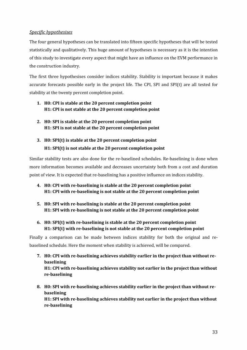
33

Specific hypothesises

The four general hypotheses can be translated into fifteen specific hypotheses that will be tested

statistically and qualitatively. This huge amount of hypotheses is necessary as it is the intention

of this study to investigate every aspect that might have an influence on the EVM performance in

the construction industry.

The first three hypothesises consider indices stability. Stability is important because it makes

accurate forecasts possible early in the project life. The CPI, SPI and SPI(t) are all tested for

stability at the twenty percent completion point.

1. H0: CPI is stable at the 20 percent completion point

H1: CPI is not stable at the 20 percent completion point

2. H0: SPI is stable at the 20 percent completion point

H1: SPI is not stable at the 20 percent completion point

3. H0: SPI(t) is stable at the 20 percent completion point

H1: SPI(t) is not stable at the 20 percent completion point

Similar stability tests are also done for the re-baselined schedules. Re-baselining is done when

more information becomes available and decreases uncertainty both from a cost and duration

point of view. It is expected that re-baselining has a positive influence on indices stability.

4. H0: CPI with re-baselining is stable at the 20 percent completion point

H1: CPI with re-baselining is not stable at the 20 percent completion point

5. H0: SPI with re-baselining is stable at the 20 percent completion point

H1: SPI with re-baselining is not stable at the 20 percent completion point

6. H0: SPI(t) with re-baselining is stable at the 20 percent completion point

H1: SPI(t) with re-baselining is not stable at the 20 percent completion point

Finally a comparison can be made between indices stability for both the original and re-

baselined schedule. Here the moment when stability is achieved, will be compared.

7. H0: CPI with re-baselining achieves stability earlier in the project than without re-

baselining

H1: CPI with re-baselining achieves stability not earlier in the project than without

re-baselining

8. H0: SPI with re-baselining achieves stability earlier in the project than without re-

baselining

H1: SPI with re-baselining achieves stability not earlier in the project than without

re-baselining

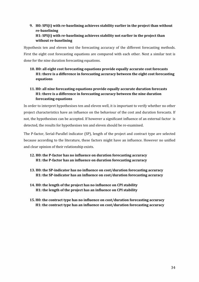
34

9. H0: SPI(t) with re-baselining achieves stability earlier in the project than without

re-baselining

H1: SPI(t) with re-baselining achieves stability not earlier in the project than

without re-baselining

Hypothesis ten and eleven test the forecasting accuracy of the different forecasting methods.

First the eight cost forecasting equations are compared with each other. Next a similar test is

done for the nine duration forecasting equations.

10. H0: all eight cost forecasting equations provide equally accurate cost forecasts

H1: there is a difference in forecasting accuracy between the eight cost forecasting

equations

11. H0: all nine forecasting equations provide equally accurate duration forecasts

H1: there is a difference in forecasting accuracy between the nine duration

forecasting equations

In order to interpret hypothesises ten and eleven well, it is important to verify whether no other

project characteristics have an influence on the behaviour of the cost and duration forecasts. If

not, the hypothesises can be accepted. If however a significant influence of an external factor is

detected, the results for hypothesises ten and eleven should be re-examined.

The P-factor, Serial-Parallel indicator (SP), length of the project and contract type are selected

because according to the literature, these factors might have an influence. However no unified

and clear opinion of their relationship exists.

12. H0: the P-factor has no influence on duration forecasting accuracy

H1: the P-factor has an influence on duration forecasting accuracy

13. H0: the SP-indicator has no influence on cost/duration forecasting accuracy

H1: the SP-indicator has an influence on cost/duration forecasting accuracy

14. H0: the length of the project has no influence on CPI stability

H1: the length of the project has an influence on CPI stability

15. H0: the contract type has no influence on cost/duration forecasting accuracy

H1: the contract type has an influence on cost/duration forecasting accuracy

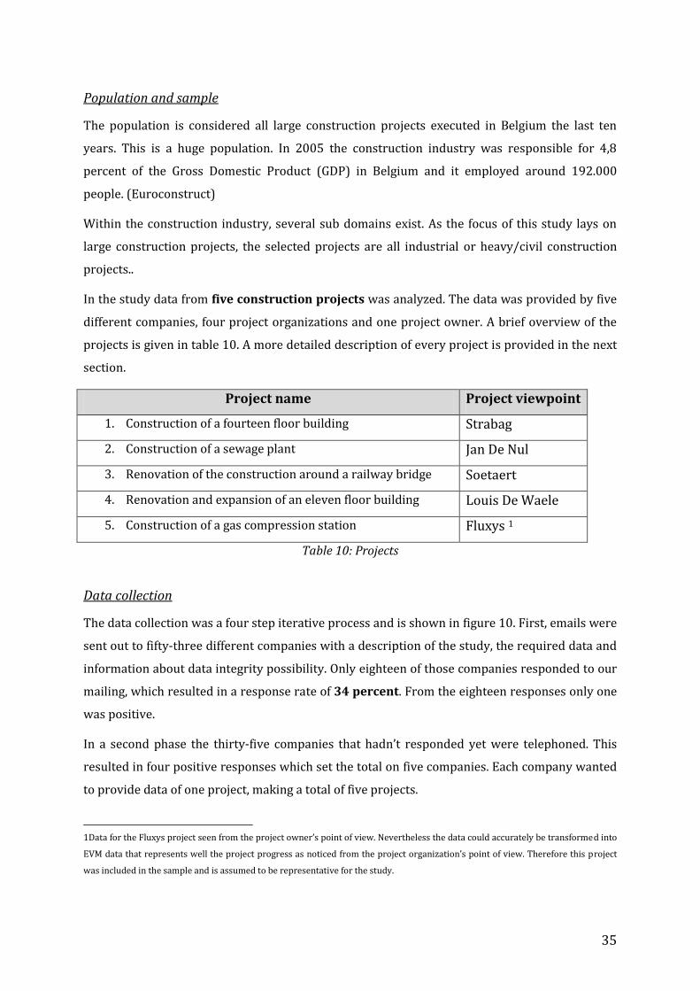
35

Population and sample

The population is considered all large construction projects executed in Belgium the last ten

years. This is a huge population. In 2005 the construction industry was responsible for 4,8

percent of the Gross Domestic Product (GDP) in Belgium and it employed around 192.000

people. (Euroconstruct)

Within the construction industry, several sub domains exist. As the focus of this study lays on

large construction projects, the selected projects are all industrial or heavy/civil construction

projects..

In the study data from five construction projects was analyzed. The data was provided by five

different companies, four project organizations and one project owner. A brief overview of the

projects is given in table 10. A more detailed description of every project is provided in the next

section.

Project name Project viewpoint

1. Construction of a fourteen floor building Strabag

2. Construction of a sewage plant Jan De Nul

3. Renovation of the construction around a railway bridge Soetaert

4. Renovation and expansion of an eleven floor building Louis De Waele

5. Construction of a gas compression station Fluxys 1

Table 10: Projects

Data collection

The data collection was a four step iterative process and is shown in figure 10. First, emails were

sent out to fifty-three different companies with a description of the study, the required data and

information about data integrity possibility. Only eighteen of those companies responded to our

mailing, which resulted in a response rate of 34 percent. From the eighteen responses only one

was positive.

In a second phase the thirty-five companies that hadn’t responded yet were telephoned. This

resulted in four positive responses which set the total on five companies. Each company wanted

to provide data of one project, making a total of five projects.

1Data for the Fluxys project seen from the project owner’s point of view. Nevertheless the data could accurately be transformed into

EVM data that represents well the project progress as noticed from the project organization’s point of view. Therefore this project

was included in the sample and is assumed to be representative for the study.

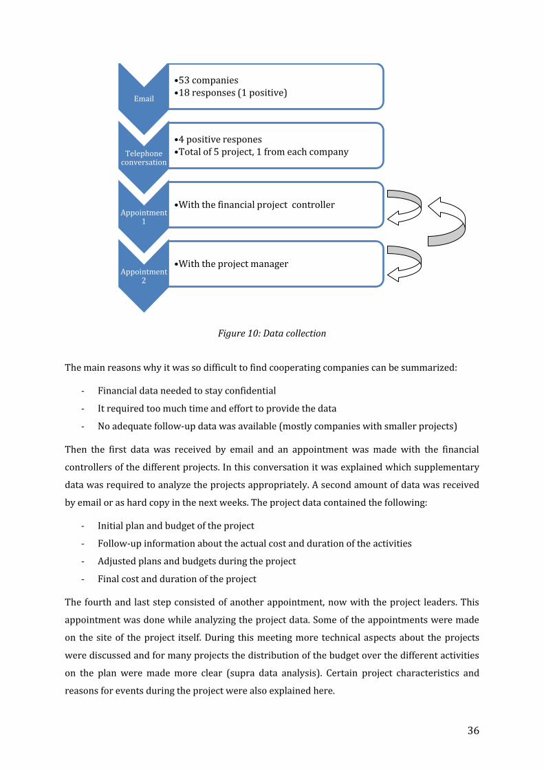
36

Figure 10: Data collection

The main reasons why it was so difficult to find cooperating companies can be summarized:

- Financial data needed to stay confidential

- It required too much time and effort to provide the data

- No adequate follow-up data was available (mostly companies with smaller projects)

Then the first data was received by email and an appointment was made with the financial

controllers of the different projects. In this conversation it was explained which supplementary

data was required to analyze the projects appropriately. A second amount of data was received

by email or as hard copy in the next weeks. The project data contained the following:

- Initial plan and budget of the project

- Follow-up information about the actual cost and duration of the activities

- Adjusted plans and budgets during the project

- Final cost and duration of the project

The fourth and last step consisted of another appointment, now with the project leaders. This

appointment was done while analyzing the project data. Some of the appointments were made

on the site of the project itself. During this meeting more technical aspects about the projects

were discussed and for many projects the distribution of the budget over the different activities

on the plan were made more clear (supra data analysis). Certain project characteristics and

reasons for events during the project were also explained here.

Email

•53 companies•18 responses (1 positive)

Telephone conversation

•4 positive respones•Total of 5 project, 1 from each company

Appointment 1

•With the financial project controller

Appointment 2

•With the project manager

37

Data analysis

ProTrack, MS Excel and SPSS are the tools that were used to analyze the data. ProTrack is a

project scheduling and tracking software tool based on the current best practices of EVM. It was

used in a first phase of the data analysis where the different projects were analyzed separately

and the necessary project metrics were calculated. In the second phase, the obtained ProTrack

results were inserted in Microsoft Excel. In this spread sheet application the data was

transformed into useful data for the study. Calculations were made and graphs were designed to

do the qualitative analysis. Finally the data was also inserted in SPSS, an analytical software tool

that was used to give statistical evidence for the proposed hypothesises.

ProTrack2

Pro Track is a software tool that was specifically designed for project managers to follow-up

their projects. All useful EVM data can be inserted in the application and useful EVM metrics are

calculated. This process will be explained first and is illustrated with an example (Appendix I).

First the project baseline is set up. In ProTrack this is done by importing the MS Project base

plan and assigning a fixed and variable cost to every activity on the plan. This is the most

difficult aspect in analyzing the data because generally construction companies don’t assign

costs to specific activities on the plan. Costs are assigned to global items like soil work, concrete

work etc. To overcome this, a method is required to assign these general costs to the specific

activities on the plan, while not giving a biased view of the project.

The cost assignment method consists of a two steps complementary process. On the one hand

data about the budgeted cost of each month was made available by the financial project

controller. On the other hand a distribution of the project cost about grouped activities on the

plan was provided by the project manager. The latter requires a lot of knowledge about the

construction project and therefore intervention of the project manager is absolutely necessary.

With these two cost distributions, one per month and one per bunch of activities, an accurate

reconstruction of the project using EVM can be established.

An example of a small project that illustrates the cost assignment method can be found in

Appendix I.

Furthermore, in ProTrack a distinction is made between fixed cost and variable cost. In this

study, the distribution is done in cooperation with the project manager and by using certain

general rules: Wages are variable costs and materials are in most cases a fixed cost. However the

rent of a tower crane is a variable cost as the rent is paid per day and not per delivery.

2 Source: www.protrack.be Accessed on 10 May 2010

http://www.protrack.be/

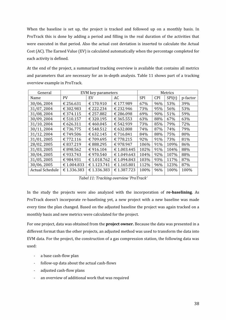
38

When the baseline is set up, the project is tracked and followed up on a monthly basis. In

ProTrack this is done by adding a period and filling in the real duration of the activities that

were executed in that period. Also the actual cost deviation is inserted to calculate the Actual

Cost (AC). The Earned Value (EV) is calculated automatically when the percentage completed for

each activity is defined.

At the end of the project, a summarized tracking overview is available that contains all metrics

and parameters that are necessary for an in-depth analysis. Table 11 shows part of a tracking

overview example in ProTrack.

General EVM key parameters Metrics Name PV EV AC SPI CPI SPI(t) p-factor

30/06, 2004 € 256.631 € 170.910 € 177.989 67% 96% 53% 39% 31/07, 2004 € 302.983 € 222.234 € 232.946 73% 95% 56% 53% 31/08, 2004 € 374.115 € 257.882 € 286.098 69% 90% 51% 59% 30/09, 2004 € 510.157 € 320.195 € 365.553 63% 88% 67% 63% 31/10, 2004 € 626.311 € 460.045 € 542.939 73% 85% 79% 72% 30/11, 2004 € 736.775 € 548.512 € 632.808 74% 87% 74% 79% 31/12, 2004 € 749.506 € 632.145 € 716.841 84% 88% 75% 80% 31/01, 2005 € 772.116 € 709.695 € 778.215 92% 91% 73% 81% 28/02, 2005 € 837.219 € 888.295 € 978.947 106% 91% 109% 86% 31/03, 2005 € 898.562 € 916.104 € 1.003.445 102% 91% 104% 88% 30/04, 2005 € 933.743 € 970.540 € 1.049.643 104% 92% 107% 88% 31/05, 2005 € 984.931 € 1.018.762 € 1.094.843 103% 93% 117% 87% 30/06, 2005 € 1.004.833 € 1.123.741 € 1.165.801 112% 96% 123% 87% Actual Schedule € 1.336.383 € 1.336.383 € 1.387.723 100% 96% 100% 100%

Tabel 11: Tracking overview ‘ProTrack’

In the study the projects were also analyzed with the incorporation of re-baselining. As

ProTrack doesn’t incorporate re-baselining yet, a new project with a new baseline was made

every time the plan changed. Based on the adjusted baseline the project was again tracked on a

monthly basis and new metrics were calculated for the project.

For one project, data was obtained from the project owner. Because the data was presented in a

different format than the other projects, an adjusted method was used to transform the data into

EVM data. For the project, the construction of a gas compression station, the following data was

used:

- a base cash-flow plan

- follow-up data about the actual cash-flows

- adjusted cash-flow plans

- an overview of additional work that was required

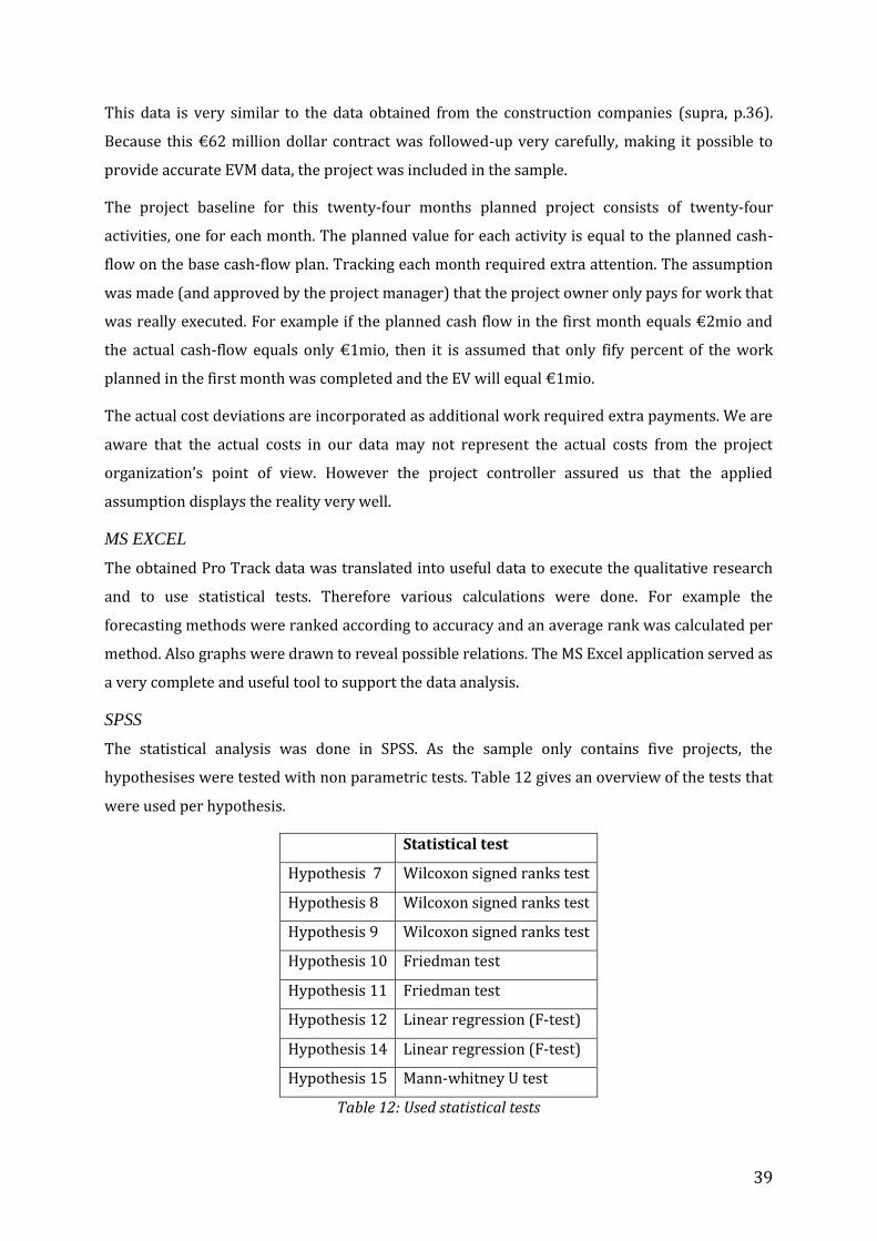
39

This data is very similar to the data obtained from the construction companies (supra, p.36).

Because this €62 million dollar contract was followed-up very carefully, making it possible to

provide accurate EVM data, the project was included in the sample.

The project baseline for this twenty-four months planned project consists of twenty-four

activities, one for each month. The planned value for each activity is equal to the planned cash-

flow on the base cash-flow plan. Tracking each month required extra attention. The assumption

was made (and approved by the project manager) that the project owner only pays for work that

was really executed. For example if the planned cash flow in the first month equals €2mio and

the actual cash-flow equals only €1mio, then it is assumed that only fify percent of the work

planned in the first month was completed and the EV will equal €1mio.

The actual cost deviations are incorporated as additional work required extra payments. We are

aware that the actual costs in our data may not represent the actual costs from the project

organization’s point of view. However the project controller assured us that the applied

assumption displays the reality very well.

MS EXCEL

The obtained Pro Track data was translated into useful data to execute the qualitative research

and to use statistical tests. Therefore various calculations were done. For example the

forecasting methods were ranked according to accuracy and an average rank was calculated per

method. Also graphs were drawn to reveal possible relations. The MS Excel application served as

a very complete and useful tool to support the data analysis.

SPSS

The statistical analysis was done in SPSS. As the sample only contains five projects, the

hypothesises were tested with non parametric tests. Table 12 gives an overview of the tests that

were used per hypothesis.

Statistical test

Hypothesis 7 Wilcoxon signed ranks test



Hypothesis 10 Friedman test

Hypothesis 11 Friedman test

Hypothesis 12 Linear regression (F-test)

Hypothesis 14 Linear regression (F-test)

Hypothesis 15 Mann-whitney U test

Table 12: Used statistical tests

40

Hypothesises one to six could not be tested statistically because due to the sample size no

distribution (normal, t, chi square, etc.) can be assumed. Therefore no confidence interval can be

set up that would be used to verify stability at the twenty percent completion point.

Hypothesises seven to nine that compare stability with and without re-baselining are tested

with a the Wilcoxon signed ranks test, a test for two related samples. The Friedman test, a test

for multiple related samples, is used to test whether the forecasting methods perform on

average equally good. If a significant difference would be detected, further post-hoc analysis is

required.

For hypothesises twelve and fourteen linear regression is used to verify the relation between

two project characteristics (P-factor and length of the project) and the forecasting

accuracy/stability. Linear regression can be used for small samples as it does not require

assumptions about the distribution of the dependent or independent variable. However it

assumes that the residuals are normally distributed. This is verified with the Kolmogorov-

Smirnof test.

No statistically appropriate test was available to test hypothesis thirteen.

Finally the Mann-Whitney U test is applied to test the influence of two independent samples,

fixed price and cost reimbursable contracts on the forecasting accuracy/stability.

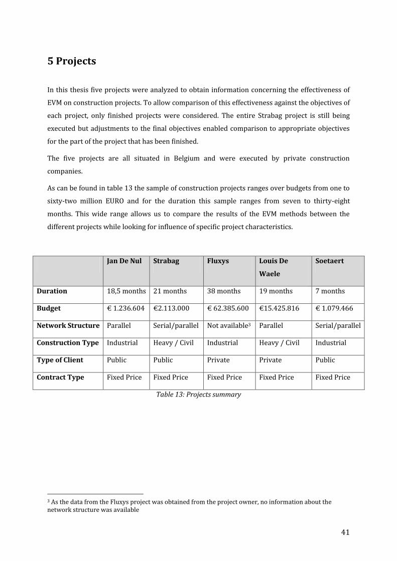
41

5 Projects

In this thesis five projects were analyzed to obtain information concerning the effectiveness of

EVM on construction projects. To allow comparison of this effectiveness against the objectives of

each project, only finished projects were considered. The entire Strabag project is still being

executed but adjustments to the final objectives enabled comparison to appropriate objectives

for the part of the project that has been finished.

The five projects are all situated in Belgium and were executed by private construction

companies.

As can be found in table 13 the sample of construction projects ranges over budgets from one to

sixty-two million EURO and for the duration this sample ranges from seven to thirty-eight

months. This wide range allows us to compare the results of the EVM methods between the

different projects while looking for influence of specific project characteristics.

Jan De Nul Strabag Fluxys Louis De

Waele

Soetaert

Duration 18,5 months 21 months 38 months 19 months 7 months

Budget € 1.236.604 €2.113.000 € 62.385.600 €15.425.816 € 1.079.466

Network Structure Parallel Serial/parallel Not available3 Parallel Serial/parallel

Construction Type Industrial Heavy / Civil Industrial Heavy / Civil Industrial

Type of Client Public Public Private Private Public

Contract Type Fixed Price Fixed Price Fixed Price Fixed Price Fixed Price

Table 13: Projects summary

3 As the data from the Fluxys project was obtained from the project owner, no information about the network structure was available

42

HOVE 2004 – THE CONSTRUCTION OF A SEWAGE PLANT

Project Owner:

Aquafin N.V.

Dijkstraat 8, 2630 Aartselaar

Project Organization:

Jan De Nul N.V.

Tragel 60, 9308 Hofstade-Aalst

Project information:

The project consists of the construction of a small sewage plant in Hove (Antwerp). The project

was finished in time and within the budget. In the beginning the project was heavily running

behind schedule. After six months this delay was recovered and the project was even performing

ahead of schedule. As the final date was easy to reach, fewer resources were allocated to the

project and the project was finished at the planned end date.

The actual cost of the project was €90.160 less than the budget. The main reason for this was

that an expected cost for pilings was not necessary anymore as the project evolved (around

€60.000). Besides, efficient work progress was the other factor that decreased the actual cost.

Start date 28/04/04 End date Planned 12/11/05 Actual 12/11/05 Delivered on time Cost Planned € 1.236.604 Actual € 1.146.444 -€90.160 # activities 220 Re-baselined 31/10/04 Contract type Fixed Price

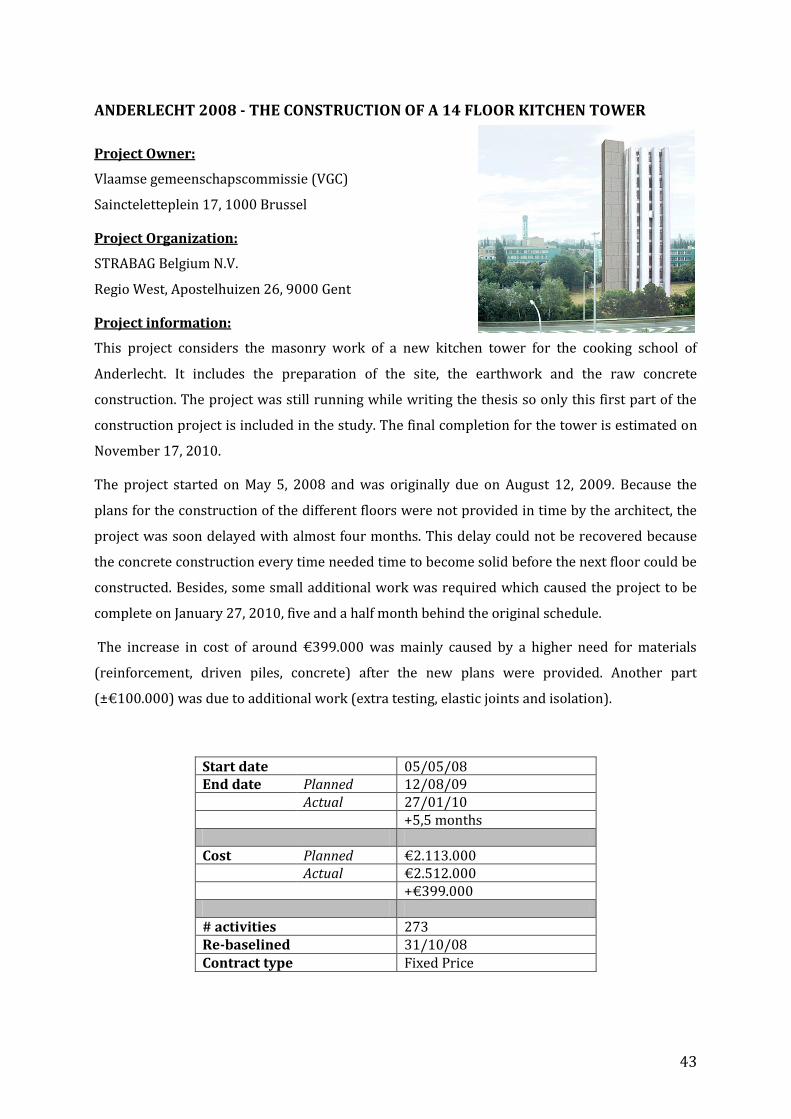
43

ANDERLECHT 2008 - THE CONSTRUCTION OF A 14 FLOOR KITCHEN TOWER

Project Owner:

Vlaamse gemeenschapscommissie (VGC)

Saincteletteplein 17, 1000 Brussel


STRABAG Belgium N.V.

Regio West, Apostelhuizen 26, 9000 Gent


This project considers the masonry work of a new kitchen tower for the cooking school of

Anderlecht. It includes the preparation of the site, the earthwork and the raw concrete

construction. The project was still running while writing the thesis so only this first part of the

construction project is included in the study. The final completion for the tower is estimated on

November 17, 2010.

The project started on May 5, 2008 and was originally due on August 12, 2009. Because the

plans for the construction of the different floors were not provided in time by the architect, the

project was soon delayed with almost four months. This delay could not be recovered because

the concrete construction every time needed time to become solid before the next floor could be

constructed. Besides, some small additional work was required which caused the project to be

complete on January 27, 2010, five and a half month behind the original schedule.

The increase in cost of around €399.000 was mainly caused by a higher need for materials

(reinforcement, driven piles, concrete) after the new plans were provided. Another part

(±€100.000) was due to additional work (extra testing, elastic joints and isolation).

Start date 05/05/08 End date Planned 12/08/09 Actual 27/01/10 +5,5 months Cost Planned €2.113.000 Actual €2.512.000 +€399.000 # activities 273 Re-baselined 31/10/08 Contract type Fixed Price

44

ZELZATE 2006 – THE CONSTRUCTION OF A NEW COMPRESSOR STATION TO

STORE NATURAL GAS

Project Owner:

Fluxys N.V.

Avenue des Arts 31

1040 Brussels


Preferred not to be published


The Fluxys project actually finished fourteen months behind schedule. This delay was caused by

two factors. First of all procurement and engineering, two activities that depended a lot on each

other, were not planned well. This resulted in a delay early in the project because materials did

not arrive in time. The delay could not be recovered because when the materials arrived, the

engineers were already working at full capacity and no additional resources could be made

available.

Secondly, later in the project a lot of additional work was required by Fluxys. The additional

work had a value of €3 million and included for example additional fire fighting protection,

additional pipelines, a new security system etc. These additional activities could not be

estimated on beforehand as these were discussed and approved during the project life. The

additional work was charged to Fluxys, the project owner.

Start date 01/06/06 End date Planned 31/05/08 Actual 31/07/09 +14 months Cost Planned € 62.385.600 Actual € 65.526.925 +€3.141.325 # activities 24 Re-baselined 31/08/07, 31/01/08,

31/08/08, 30/11/08 Contract type Fixed price

45

BRUSSELS 2006 - EXPANSION OF THE FINANCE TOWER

Project Owner:

Breevast B.V.

Jan van Rijswijcklaan 162 b11, 2020 Antwerpen


Interbuild N.V.

Heistraat 129, 2610 Wilrijk

Subcontractor:

Louis De Waele N.V.

Jean Dubrucqlaan 175, 1080 Brussel


Due to the presence of asbestos and carbonation, the Finance tower had to be renovated after a

lifespan of only 25 years. The project itself consisted of two parts. The first part concerned the

renovation of the Finance tower while the second part consisted of building a new office

building next to the tower. For this second part Interbuild N.V. formed a coalition with Louis De

Waele N.V.

The project started with a three to four weeks delay but managed to finish on time. Although it

was at a higher cost. The cost overrun of € 912.208 was on the one hand due to unforeseen extra

resources that were necessary during the project. On the other hand additional work with a

value of €423.027 was negotiated. This increase in scope was completely charged to the project

owner.

Start date 15/03/06 End date Planned 18/10/07 Actual 18/10/07 Delivered on time Cost Planned €15.425.816 Actual €16.338.024 +€ 912.208 # activities 751 Re-baselined NO Contract type Fixed Price

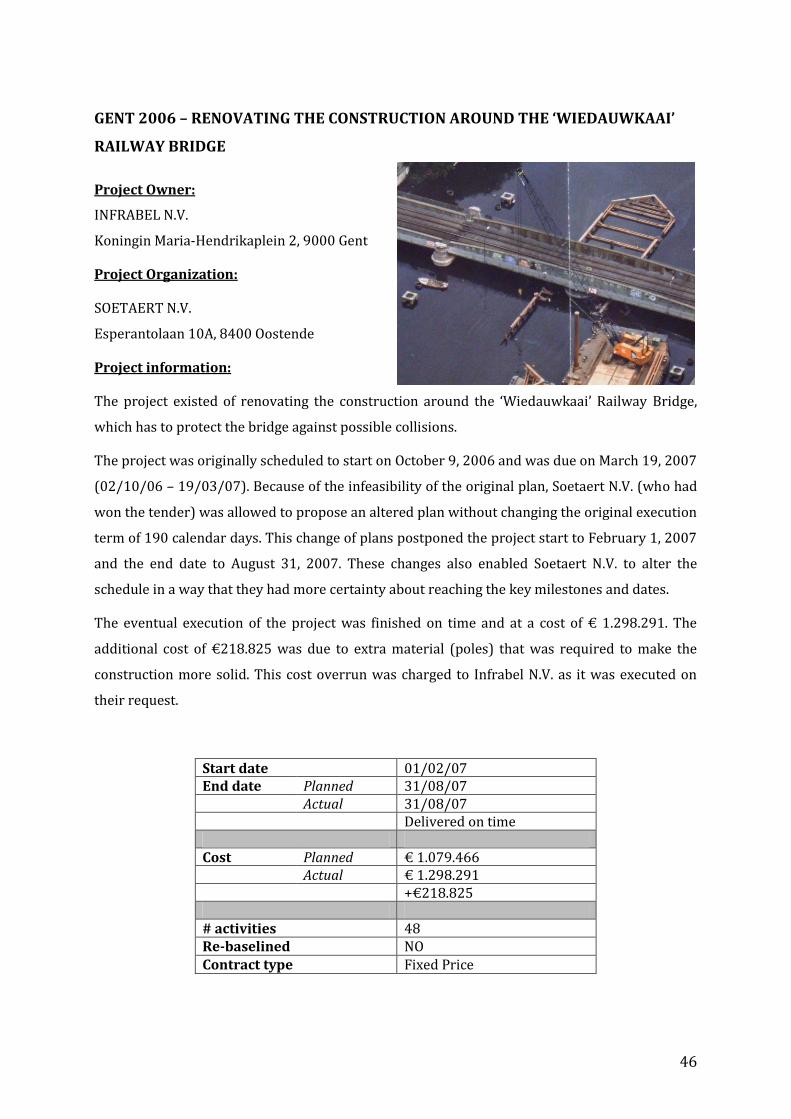
46

GENT 2006 – RENOVATING THE CONSTRUCTION AROUND THE ‘WIEDAUWKAAI’

RAILWAY BRIDGE

Project Owner:

INFRABEL N.V.

Koningin Maria-Hendrikaplein 2, 9000 Gent


SOETAERT N.V.

Esperantolaan 10A, 8400 Oostende


The project existed of renovating the construction around the ‘Wiedauwkaai’ Railway Bridge,

which has to protect the bridge against possible collisions.

The project was originally scheduled to start on October 9, 2006 and was due on March 19, 2007

(02/10/06 – 19/03/07). Because of the infeasibility of the original plan, Soetaert N.V. (who had

won the tender) was allowed to propose an altered plan without changing the original execution

term of 190 calendar days. This change of plans postponed the project start to February 1, 2007

and the end date to August 31, 2007. These changes also enabled Soetaert N.V. to alter the

schedule in a way that they had more certainty about reaching the key milestones and dates.

The eventual execution of the project was finished on time and at a cost of € 1.298.291. The

additional cost of €218.825 was due to extra material (poles) that was required to make the

construction more solid. This cost overrun was charged to Infrabel N.V. as it was executed on

their request.

Start date 01/02/07 End date Planned 31/08/07 Actual 31/08/07 Delivered on time Cost Planned € 1.079.466 Actual € 1.298.291 +€218.825 # activities 48 Re-baselined NO Contract type Fixed Price

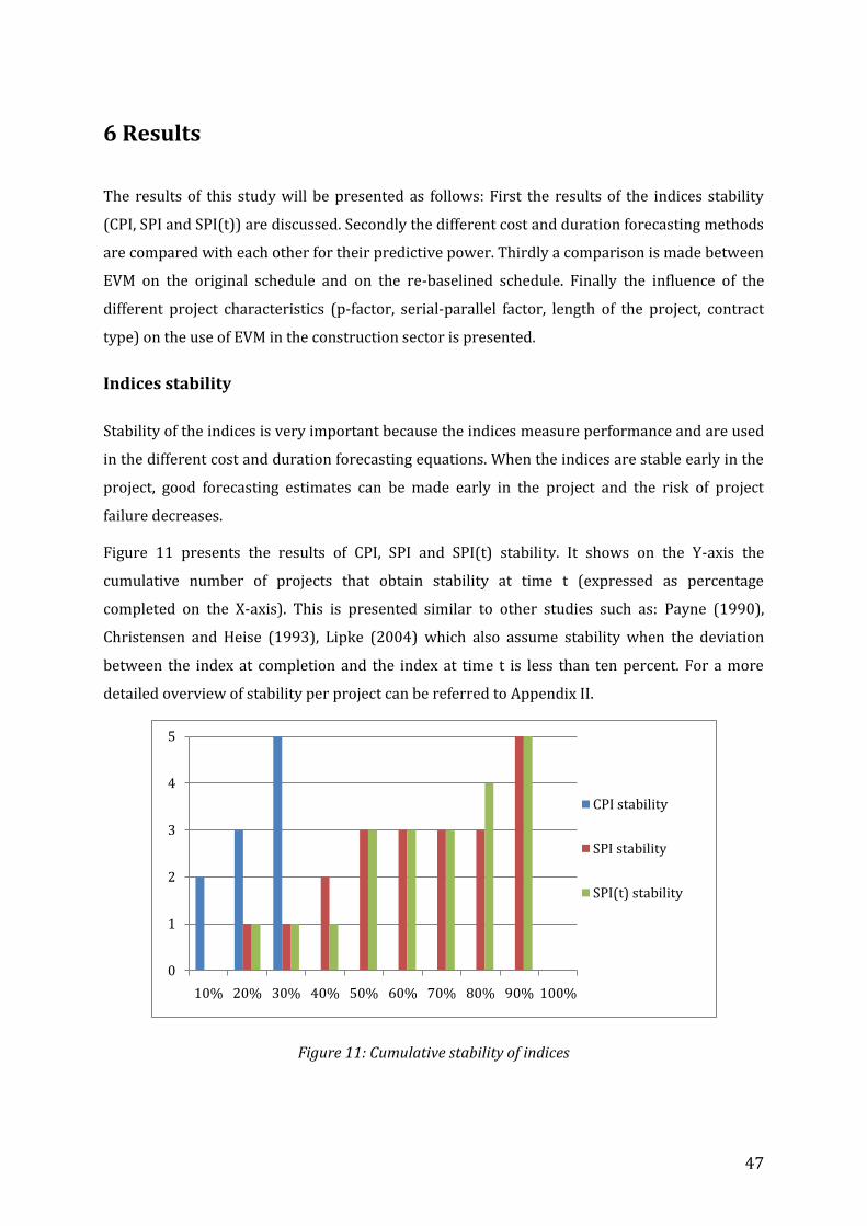
47

6 Results

The results of this study will be presented as follows: First the results of the indices stability

(CPI, SPI and SPI(t)) are discussed. Secondly the different cost and duration forecasting methods

are compared with each other for their predictive power. Thirdly a comparison is made between

EVM on the original schedule and on the re-baselined schedule. Finally the influence of the

different project characteristics (p-factor, serial-parallel factor, length of the project, contract

type) on the use of EVM in the construction sector is presented.

Indices stability

Stability of the indices is very important because the indices measure performance and are used

in the different cost and duration forecasting equations. When the indices are stable early in the

project, good forecasting estimates can be made early in the project and the risk of project

failure decreases.

Figure 11 presents the results of CPI, SPI and SPI(t) stability. It shows on the Y-axis the

cumulative number of projects that obtain stability at time t (expressed as percentage

completed on the X-axis). This is presented similar to other studies such as: Payne (1990),

Christensen and Heise (1993), Lipke (2004) which also assume stability when the deviation

between the index at completion and the index at time t is less than ten percent. For a more

detailed overview of stability per project can be referred to Appendix II.

Figure 11: Cumulative stability of indices

0

1

2

3

4

5

10% 20% 30% 40% 50% 60% 70% 80% 90% 100%

CPI stability

SPI stability

SPI(t) stability

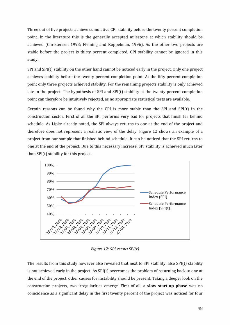
48

Three out of five projects achieve cumulative CPI stability before the twenty percent completion

point. In the literature this is the generally accepted milestone at which stability should be

achieved (Christensen 1993; Fleming and Koppelman, 1996). As the other two projects are

stable before the project is thirty percent completed, CPI stability cannot be ignored in this

study.

SPI and SPI(t) stability on the other hand cannot be noticed early in the project. Only one project

achieves stability before the twenty percent completion point. At the fifty percent completion

point only three projects achieved stability. For the remaining projects stability is only achieved

late in the project. The hypothesis of SPI and SPI(t) stability at the twenty percent completion

point can therefore be intuitively rejected, as no appropriate statistical tests are available.

Certain reasons can be found why the CPI is more stable than the SPI and SPI(t) in the

construction sector. First of all the SPI performs very bad for projects that finish far behind

schedule. As Lipke already noted, the SPI always returns to one at the end of the project and

therefore does not represent a realistic view of the delay. Figure 12 shows an example of a

project from our sample that finished behind schedule. It can be noticed that the SPI returns to

one at the end of the project. Due to this necessary increase, SPI stability is achieved much later

than SPI(t) stability for this project.

Figure 12: SPI versus SPI(t)

The results from this study however also revealed that next to SPI stability, also SPI(t) stability

is not achieved early in the project. As SPI(t) overcomes the problem of returning back to one at

the end of the project, other causes for instability should be present. Taking a deeper look on the

construction projects, two irregularities emerge. First of all, a slow start-up phase was no

coincidence as a significant delay in the first twenty percent of the project was noticed for four

40%

50%

60%

70%

80%

90%

100%

Schedule Performance Index (SPI)

Schedule Performance Index (SPI(t))

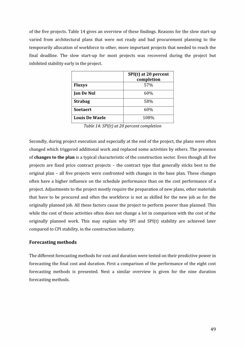
49

of the five projects. Table 14 gives an overview of these findings. Reasons for the slow start-up

varied from architectural plans that were not ready and bad procurement planning to the

temporarily allocation of workforce to other, more important projects that needed to reach the

final deadline. The slow start-up for most projects was recovered during the project but

inhibited stability early in the project.

SPI(t) at 20 percent completion

Fluxys 57%

Jan De Nul 60%

Strabag 58%

Soetaert 60%

Louis De Waele 108%

Table 14: SPI(t) at 20 percent completion

Secondly, during project execution and especially at the end of the project, the plans were often

changed which triggered additional work and replaced some activities by others. The presence

of changes to the plan is a typical characteristic of the construction sector. Even though all five

projects are fixed price contract projects – the contract type that generally sticks best to the

original plan – all five projects were confronted with changes in the base plan. These changes

often have a higher influence on the schedule performance than on the cost performance of a

project. Adjustments to the project mostly require the preparation of new plans, other materials

that have to be procured and often the workforce is not as skilled for the new job as for the

originally planned job. All these factors cause the project to perform poorer than planned. This

while the cost of these activities often does not change a lot in comparison with the cost of the

originally planned work. This may explain why SPI and SPI(t) stability are achieved later

compared to CPI stability, in the construction industry.

Forecasting methods

The different forecasting methods for cost and duration were tested on their predictive power in

forecasting the final cost and duration. First a comparison of the performance of the eight cost

forecasting methods is presented. Next a similar overview is given for the nine duration

forecasting methods.

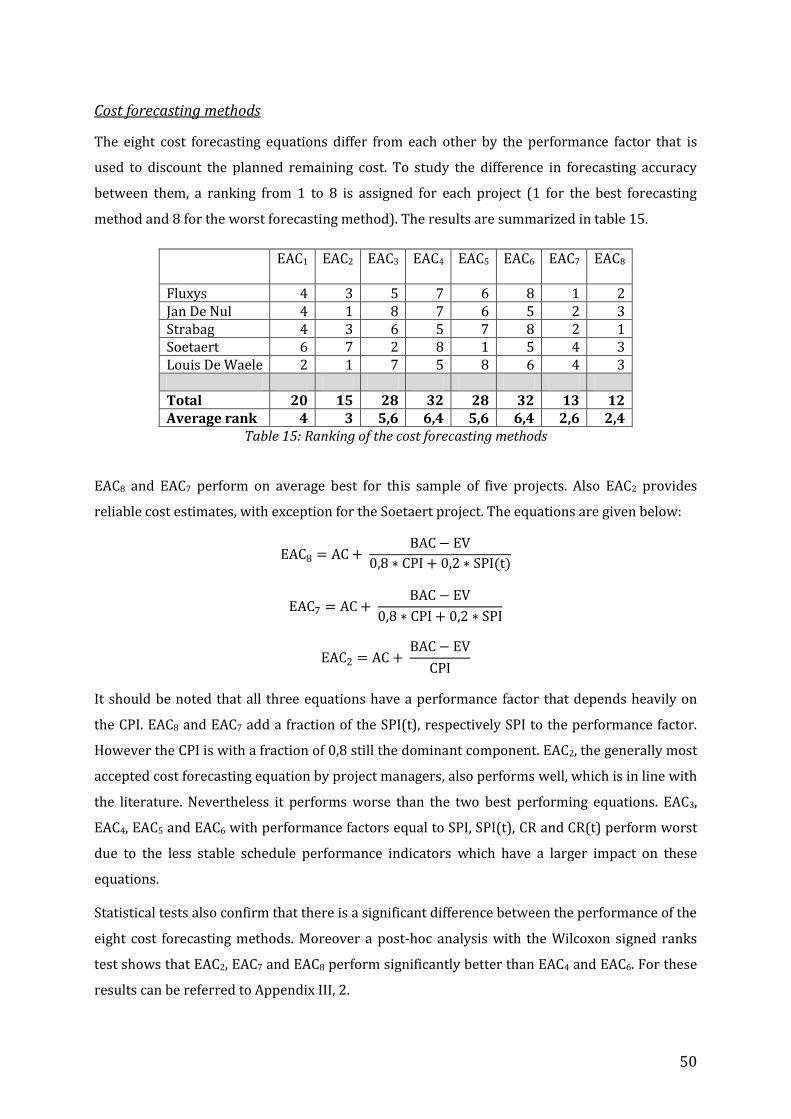
50

Cost forecasting methods

The eight cost forecasting equations differ from each other by the performance factor that is

used to discount the planned remaining cost. To study the difference in forecasting accuracy

between them, a ranking from 1 to 8 is assigned for each project (1 for the best forecasting

method and 8 for the worst forecasting method). The results are summarized in table 15.

EAC1

EAC2

EAC3 EAC4

EAC5

EAC6 EAC7

EAC8

Fluxys 4 3 5 7 6 8 1 2 Jan De Nul 4 1 8 7 6 5 2 3 Strabag 4 3 6 5 7 8 2 1 Soetaert 6 7 2 8 1 5 4 3 Louis De Waele 2 1 7 5 8 6 4 3 Total 20 15 28 32 28 32 13 12 Average rank 4 3 5,6 6,4 5,6 6,4 2,6 2,4

Table 15: Ranking of the cost forecasting methods

EAC8 and EAC7 perform on average best for this sample of five projects. Also EAC2 provides

reliable cost estimates, with exception for the Soetaert project. The equations are given below:


0,8 ∗ CPI + 0,2 ∗ SPI(t)


0,8 ∗ CPI + 0,2 ∗ SPI


CPI

It should be noted that all three equations have a performance factor that depends heavily on

the CPI. EAC8 and EAC7 add a fraction of the SPI(t), respectively SPI to the performance factor.

However the CPI is with a fraction of 0,8 still the dominant component. EAC2, the generally most

accepted cost forecasting equation by project managers, also performs well, which is in line with

the literature. Nevertheless it performs worse than the two best performing equations. EAC3,

EAC4, EAC5 and EAC6 with performance factors equal to SPI, SPI(t), CR and CR(t) perform worst

due to the less stable schedule performance indicators which have a larger impact on these

equations.

Statistical tests also confirm that there is a significant difference between the performance of the

eight cost forecasting methods. Moreover a post-hoc analysis with the Wilcoxon signed ranks

test shows that EAC2, EAC7 and EAC8 perform significantly better than EAC4 and EAC6. For these

results can be referred to Appendix III, 2.

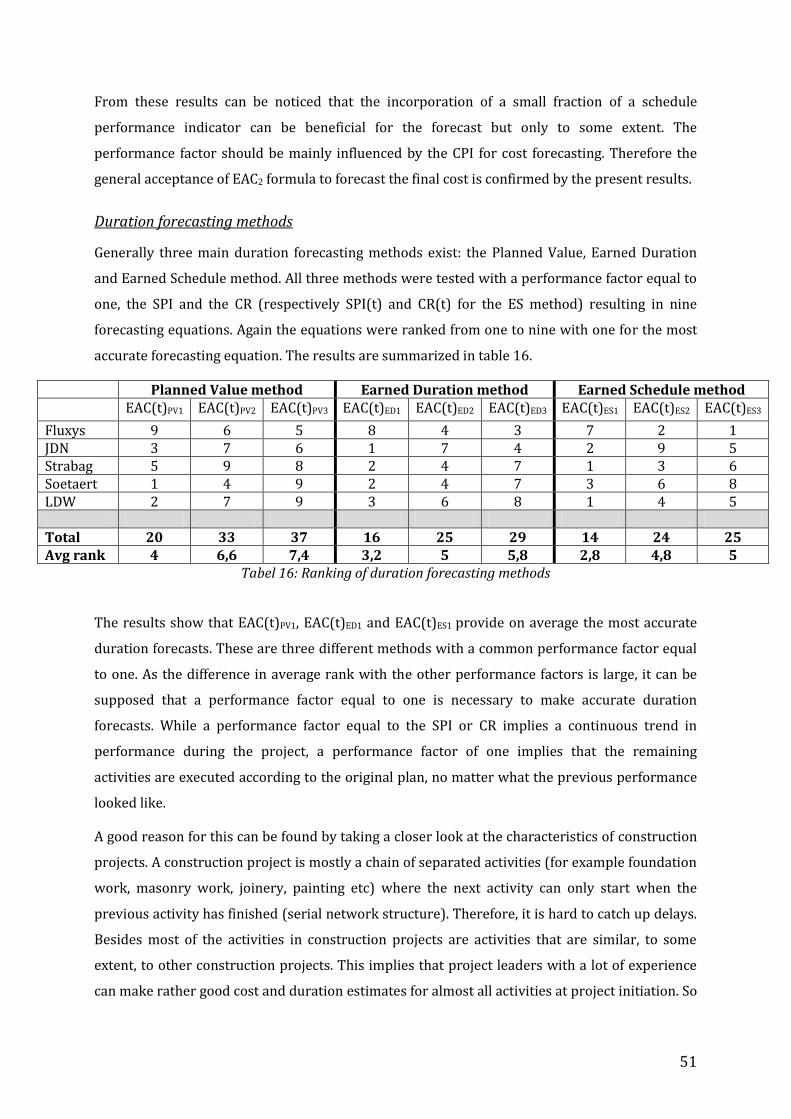
51

From these results can be noticed that the incorporation of a small fraction of a schedule

performance indicator can be beneficial for the forecast but only to some extent. The

performance factor should be mainly influenced by the CPI for cost forecasting. Therefore the

general acceptance of EAC2 formula to forecast the final cost is confirmed by the present results.

Duration forecasting methods

Generally three main duration forecasting methods exist: the Planned Value, Earned Duration

and Earned Schedule method. All three methods were tested with a performance factor equal to

one, the SPI and the CR (respectively SPI(t) and CR(t) for the ES method) resulting in nine

forecasting equations. Again the equations were ranked from one to nine with one for the most

accurate forecasting equation. The results are summarized in table 16.

Planned Value method Earned Duration method Earned Schedule method EAC(t)PV1 EAC(t)PV2 EAC(t)PV3 EAC(t)ED1 EAC(t)ED2 EAC(t)ED3 EAC(t)ES1 EAC(t)ES2 EAC(t)ES3

Fluxys 9 6 5 8 4 3 7 2 1 JDN 3 7 6 1 7 4 2 9 5 Strabag 5 9 8 2 4 7 1 3 6 Soetaert 1 4 9 2 4 7 3 6 8 LDW 2 7 9 3 6 8 1 4 5 Total 20 33 37 16 25 29 14 24 25 Avg rank 4 6,6 7,4 3,2 5 5,8 2,8 4,8 5

Tabel 16: Ranking of duration forecasting methods

The results show that EAC(t)PV1, EAC(t)ED1 and EAC(t)ES1 provide on average the most accurate

duration forecasts. These are three different methods with a common performance factor equal

to one. As the difference in average rank with the other performance factors is large, it can be

supposed that a performance factor equal to one is necessary to make accurate duration

forecasts. While a performance factor equal to the SPI or CR implies a continuous trend in

performance during the project, a performance factor of one implies that the remaining

activities are executed according to the original plan, no matter what the previous performance

looked like.

A good reason for this can be found by taking a closer look at the characteristics of construction

projects. A construction project is mostly a chain of separated activities (for example foundation

work, masonry work, joinery, painting etc) where the next activity can only start when the

previous activity has finished (serial network structure). Therefore, it is hard to catch up delays.

Besides most of the activities in construction projects are activities that are similar, to some

extent, to other construction projects. This implies that project leaders with a lot of experience

can make rather good cost and duration estimates for almost all activities at project initiation. So

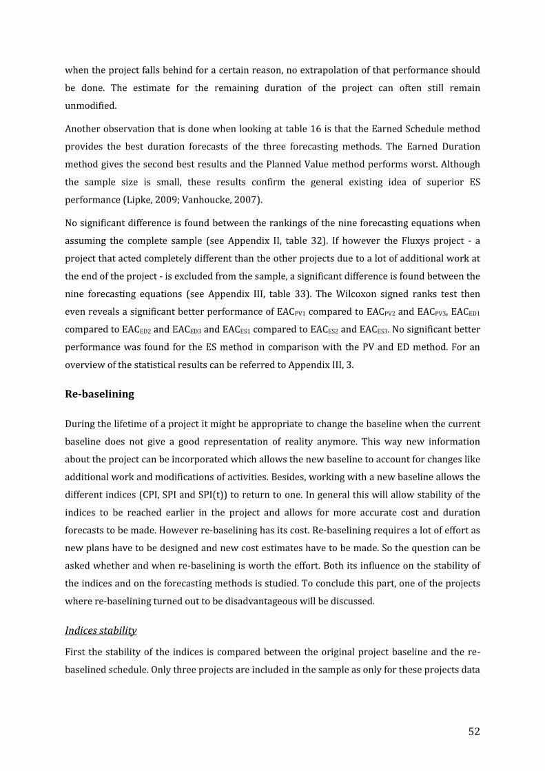
52

when the project falls behind for a certain reason, no extrapolation of that performance should

be done. The estimate for the remaining duration of the project can often still remain

unmodified.

Another observation that is done when looking at table 16 is that the Earned Schedule method

provides the best duration forecasts of the three forecasting methods. The Earned Duration

method gives the second best results and the Planned Value method performs worst. Although

the sample size is small, these results confirm the general existing idea of superior ES

performance (Lipke, 2009; Vanhoucke, 2007).

No significant difference is found between the rankings of the nine forecasting equations when

assuming the complete sample (see Appendix II, table 32). If however the Fluxys project - a

project that acted completely different than the other projects due to a lot of additional work at

the end of the project - is excluded from the sample, a significant difference is found between the

nine forecasting equations (see Appendix III, table 33). The Wilcoxon signed ranks test then

even reveals a significant better performance of EACPV1 compared to EACPV2 and EACPV3, EACED1

compared to EACED2 and EACED3 and EACES1 compared to EACES2 and EACES3. No significant better

performance was found for the ES method in comparison with the PV and ED method. For an

overview of the statistical results can be referred to Appendix III, 3.

Re-baselining

During the lifetime of a project it might be appropriate to change the baseline when the current

baseline does not give a good representation of reality anymore. This way new information

about the project can be incorporated which allows the new baseline to account for changes like

additional work and modifications of activities. Besides, working with a new baseline allows the

different indices (CPI, SPI and SPI(t)) to return to one. In general this will allow stability of the

indices to be reached earlier in the project and allows for more accurate cost and duration

forecasts to be made. However re-baselining has its cost. Re-baselining requires a lot of effort as

new plans have to be designed and new cost estimates have to be made. So the question can be

asked whether and when re-baselining is worth the effort. Both its influence on the stability of

the indices and on the forecasting methods is studied. To conclude this part, one of the projects

where re-baselining turned out to be disadvantageous will be discussed.

Indices stability

First the stability of the indices is compared between the original project baseline and the re-

baselined schedule. Only three projects are included in the sample as only for these projects data

53

was available to effect a re-baselined schedule. Figure 13 gives an overview of the average

moment in the project (expressed as percentage completed) when stability was obtained.

Figure 13: Stability of original vs. re-baselined

For all indicators stability is achieved earlier in the project when re-baselining is done. Based on

the original baseline, CPI stability was on average obtained at the 14 percent completion point.

After re-baselining this was obtained at the 10 percent completion point. SPI stability improved

from the 54 to the 29 percent completion point, a decrease of 25 percent. SPI(t) stability finally

ameliorated from the 59 percent to the 42 percent completion point. This improvement in

indices stability is a first indicator that re-baselining could be favourable.

The Wilcoxon rank sign test however does not show a significant influence of re-baselining on

indices stability. These results can be found in Appendix III, 1.

Forecasting methods

Because the indices are used in the forecasting equations, more stable indices should result in

more accurate forecasts. Therefore a comparison is made between the forecasting accuracy of

the re-baselined schedules and the original schedules, for both the cost and duration forecasts.

First the average spread of the different forecasting methods is compared per project. This will

give a general overview of the forecasting accuracy with and without re-baselining. Secondly the

different forecasting methods are ranked again and compared with each other to investigate the

influence of re-baselining on the individual forecasting methods.

0%

10%

20%

30%

40%

50%

60%

70%

80%

90%

100%

CPI stability SPI stability SPI(t) stability

Original

Re-baselined

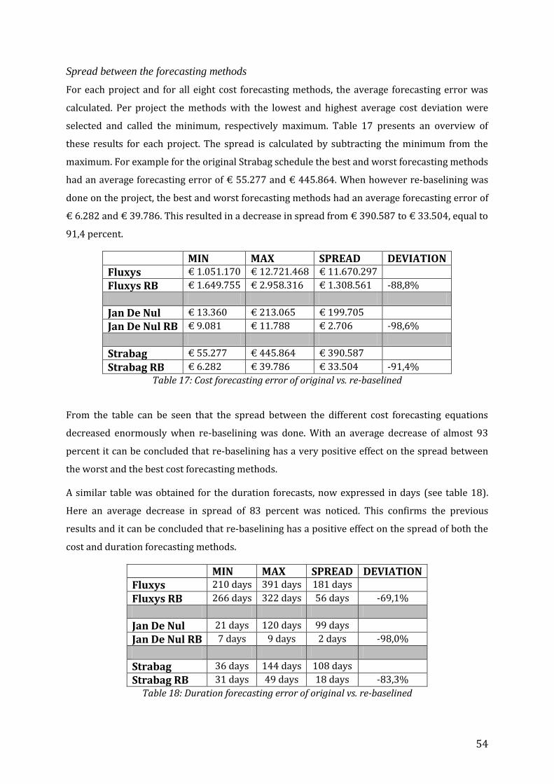
54

Spread between the forecasting methods

For each project and for all eight cost forecasting methods, the average forecasting error was

calculated. Per project the methods with the lowest and highest average cost deviation were

selected and called the minimum, respectively maximum. Table 17 presents an overview of

these results for each project. The spread is calculated by subtracting the minimum from the

maximum. For example for the original Strabag schedule the best and worst forecasting methods

had an average forecasting error of € 55.277 and € 445.864. When however re-baselining was

done on the project, the best and worst forecasting methods had an average forecasting error of

€ 6.282 and € 39.786. This resulted in a decrease in spread from € 390.587 to € 33.504, equal to

91,4 percent.

MIN MAX SPREAD DEVIATION Fluxys € 1.051.170 € 12.721.468 € 11.670.297

Fluxys RB € 1.649.755 € 2.958.316 € 1.308.561 -88,8%

Jan De Nul € 13.360 € 213.065 € 199.705

Jan De Nul RB € 9.081 € 11.788 € 2.706 -98,6%

Strabag € 55.277 € 445.864 € 390.587

Strabag RB € 6.282 € 39.786 € 33.504 -91,4%

Table 17: Cost forecasting error of original vs. re-baselined

From the table can be seen that the spread between the different cost forecasting equations

decreased enormously when re-baselining was done. With an average decrease of almost 93

percent it can be concluded that re-baselining has a very positive effect on the spread between

the worst and the best cost forecasting methods.

A similar table was obtained for the duration forecasts, now expressed in days (see table 18).

Here an average decrease in spread of 83 percent was noticed. This confirms the previous

results and it can be concluded that re-baselining has a positive effect on the spread of both the

cost and duration forecasting methods.

MIN MAX SPREAD DEVIATION Fluxys 210 days 391 days 181 days

Fluxys RB 266 days 322 days 56 days -69,1%

Jan De Nul 21 days 120 days 99 days

Jan De Nul RB 7 days 9 days 2 days -98,0%

Strabag 36 days 144 days 108 days

Strabag RB 31 days 49 days 18 days -83,3%

Table 18: Duration forecasting error of original vs. re-baselined

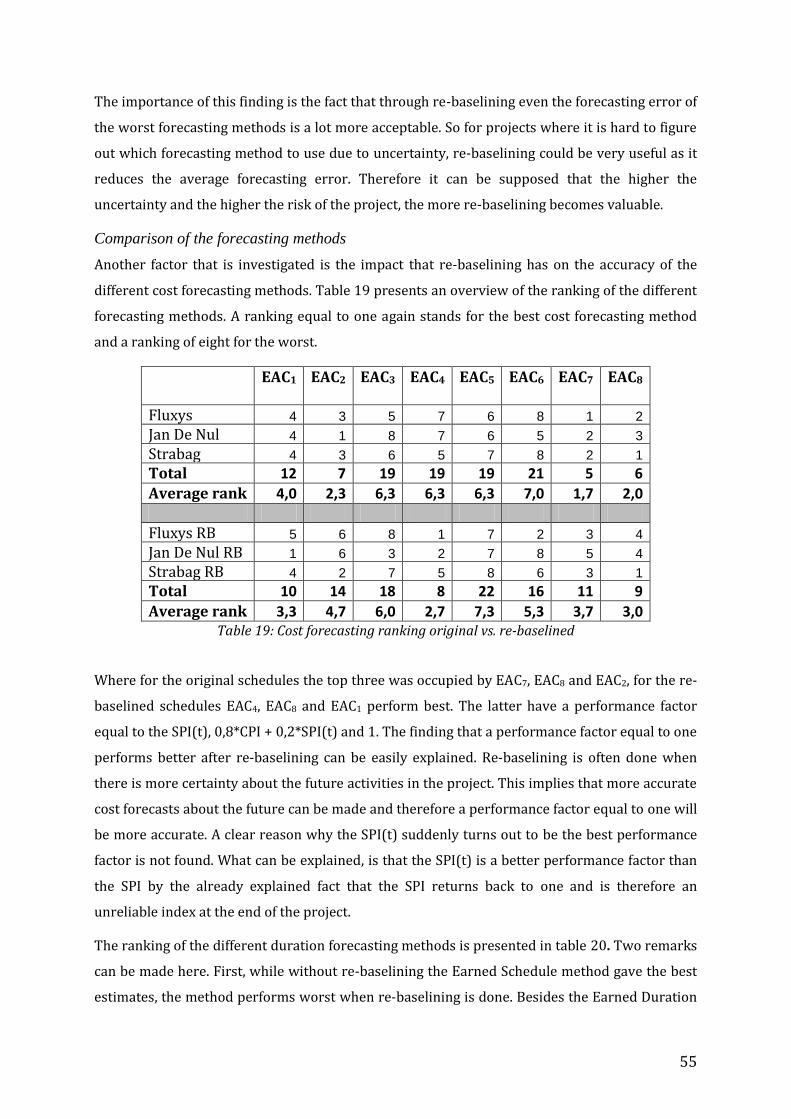
55

The importance of this finding is the fact that through re-baselining even the forecasting error of

the worst forecasting methods is a lot more acceptable. So for projects where it is hard to figure

out which forecasting method to use due to uncertainty, re-baselining could be very useful as it

reduces the average forecasting error. Therefore it can be supposed that the higher the

uncertainty and the higher the risk of the project, the more re-baselining becomes valuable.

Comparison of the forecasting methods

Another factor that is investigated is the impact that re-baselining has on the accuracy of the

different cost forecasting methods. Table 19 presents an overview of the ranking of the different

forecasting methods. A ranking equal to one again stands for the best cost forecasting method

and a ranking of eight for the worst.

EAC1

EAC2

EAC3 EAC4

EAC5

EAC6 EAC7

EAC8

Fluxys 4 3 5 7 6 8 1 2

Jan De Nul 4 1 8 7 6 5 2 3

Strabag 4 3 6 5 7 8 2 1

Total 12 7 19 19 19 21 5 6

Average rank 4,0 2,3 6,3 6,3 6,3 7,0 1,7 2,0

Fluxys RB 5 6 8 1 7 2 3 4

Jan De Nul RB 1 6 3 2 7 8 5 4

Strabag RB 4 2 7 5 8 6 3 1

Total 10 14 18 8 22 16 11 9

Average rank 3,3 4,7 6,0 2,7 7,3 5,3 3,7 3,0 Table 19: Cost forecasting ranking original vs. re-baselined

Where for the original schedules the top three was occupied by EAC7, EAC8 and EAC2, for the re-

baselined schedules EAC4, EAC8 and EAC1 perform best. The latter have a performance factor

equal to the SPI(t), 0,8*CPI + 0,2*SPI(t) and 1. The finding that a performance factor equal to one

performs better after re-baselining can be easily explained. Re-baselining is often done when

there is more certainty about the future activities in the project. This implies that more accurate

cost forecasts about the future can be made and therefore a performance factor equal to one will

be more accurate. A clear reason why the SPI(t) suddenly turns out to be the best performance

factor is not found. What can be explained, is that the SPI(t) is a better performance factor than

the SPI by the already explained fact that the SPI returns back to one and is therefore an

unreliable index at the end of the project.

The ranking of the different duration forecasting methods is presented in table 20. Two remarks

can be made here. First, while without re-baselining the Earned Schedule method gave the best

estimates, the method performs worst when re-baselining is done. Besides the Earned Duration

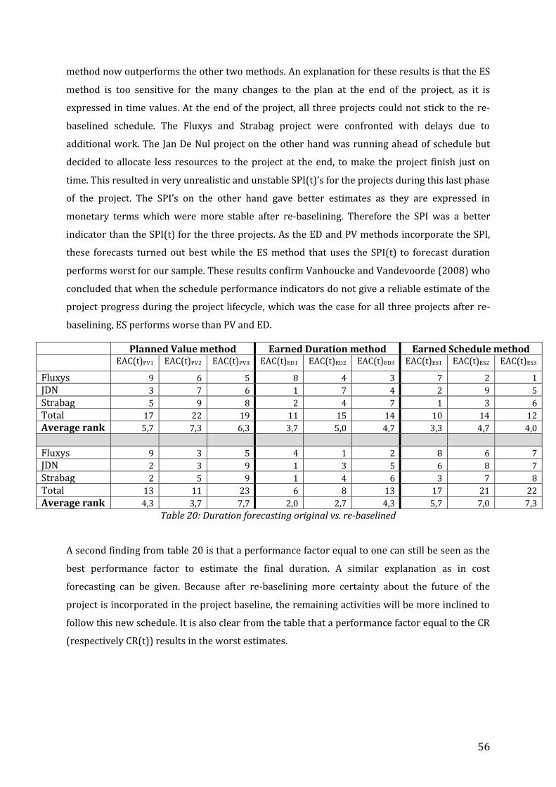
56

method now outperforms the other two methods. An explanation for these results is that the ES

method is too sensitive for the many changes to the plan at the end of the project, as it is

expressed in time values. At the end of the project, all three projects could not stick to the re-

baselined schedule. The Fluxys and Strabag project were confronted with delays due to

additional work. The Jan De Nul project on the other hand was running ahead of schedule but

decided to allocate less resources to the project at the end, to make the project finish just on

time. This resulted in very unrealistic and unstable SPI(t)’s for the projects during this last phase

of the project. The SPI’s on the other hand gave better estimates as they are expressed in

monetary terms which were more stable after re-baselining. Therefore the SPI was a better

indicator than the SPI(t) for the three projects. As the ED and PV methods incorporate the SPI,

these forecasts turned out best while the ES method that uses the SPI(t) to forecast duration

performs worst for our sample. These results confirm Vanhoucke and Vandevoorde (2008) who

concluded that when the schedule performance indicators do not give a reliable estimate of the

project progress during the project lifecycle, which was the case for all three projects after re-

baselining, ES performs worse than PV and ED.

Planned Value method Earned Duration method Earned Schedule method EAC(t)PV1 EAC(t)PV2 EAC(t)PV3 EAC(t)ED1 EAC(t)ED2 EAC(t)ED3 EAC(t)ES1 EAC(t)ES2 EAC(t)ES3

Fluxys 9 6 5 8 4 3 7 2 1

JDN 3 7 6 1 7 4 2 9 5

Strabag 5 9 8 2 4 7 1 3 6

Total 17 22 19 11 15 14 10 14 12

Average rank 5,7 7,3 6,3 3,7 5,0 4,7 3,3 4,7 4,0

Fluxys 9 3 5 4 1 2 8 6 7

JDN 2 3 9 1 3 5 6 8 7

Strabag 2 5 9 1 4 6 3 7 8

Total 13 11 23 6 8 13 17 21 22

Average rank 4,3 3,7 7,7 2,0 2,7 4,3 5,7 7,0 7,3

Table 20: Duration forecasting original vs. re-baselined

A second finding from table 20 is that a performance factor equal to one can still be seen as the

best performance factor to estimate the final duration. A similar explanation as in cost

forecasting can be given. Because after re-baselining more certainty about the future of the

project is incorporated in the project baseline, the remaining activities will be more inclined to

follow this new schedule. It is also clear from the table that a performance factor equal to the CR

(respectively CR(t)) results in the worst estimates.

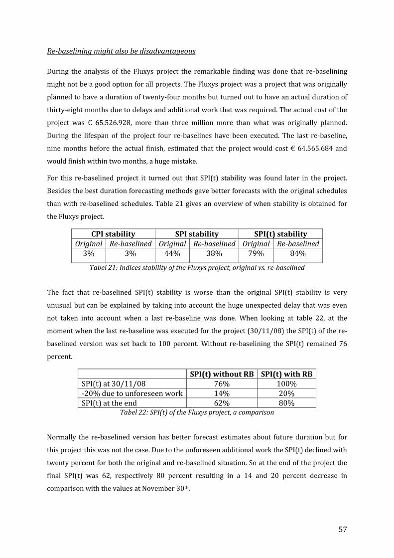
57

Re-baselining might also be disadvantageous

During the analysis of the Fluxys project the remarkable finding was done that re-baselining

might not be a good option for all projects. The Fluxys project was a project that was originally

planned to have a duration of twenty-four months but turned out to have an actual duration of

thirty-eight months due to delays and additional work that was required. The actual cost of the

project was € 65.526.928, more than three million more than what was originally planned.

During the lifespan of the project four re-baselines have been executed. The last re-baseline,

nine months before the actual finish, estimated that the project would cost € 64.565.684 and

would finish within two months, a huge mistake.

For this re-baselined project it turned out that SPI(t) stability was found later in the project.

Besides the best duration forecasting methods gave better forecasts with the original schedules

than with re-baselined schedules. Table 21 gives an overview of when stability is obtained for

the Fluxys project.

CPI stability SPI stability SPI(t) stability Original Re-baselined Original Re-baselined Original Re-baselined

3% 3% 44% 38% 79% 84%

Tabel 21: Indices stability of the Fluxys project, original vs. re-baselined

The fact that re-baselined SPI(t) stability is worse than the original SPI(t) stability is very

unusual but can be explained by taking into account the huge unexpected delay that was even

not taken into account when a last re-baseline was done. When looking at table 22, at the

moment when the last re-baseline was executed for the project (30/11/08) the SPI(t) of the re-

baselined version was set back to 100 percent. Without re-baselining the SPI(t) remained 76

percent.

SPI(t) without RB SPI(t) with RB SPI(t) at 30/11/08 76% 100% -20% due to unforeseen work 14% 20% SPI(t) at the end 62% 80%

Tabel 22: SPI(t) of the Fluxys project, a comparison

Normally the re-baselined version has better forecast estimates about future duration but for

this project this was not the case. Due to the unforeseen additional work the SPI(t) declined with

twenty percent for both the original and re-baselined situation. So at the end of the project the

final SPI(t) was 62, respectively 80 percent resulting in a 14 and 20 percent decrease in

comparison with the values at November 30th.

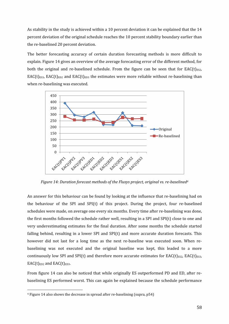
58

As stability in the study is achieved within a 10 percent deviation it can be explained that the 14

percent deviation of the original schedule reaches the 10 percent stability boundary earlier than

the re-baselined 20 percent deviation.

The better forecasting accuracy of certain duration forecasting methods is more difficult to

explain. Figure 14 gives an overview of the average forecasting error of the different method, for

both the original and re-baselined schedule. From the figure can be seen that for EAC(t)ES2,

EAC(t)ES3, EAC(t)ED2 and EAC(t)ED3 the estimates were more reliable without re-baselining than

when re-baselining was executed.

Figure 14: Duration forecast methods of the Fluxys project, original vs. re-baselined4

An answer for this behaviour can be found by looking at the influence that re-baselining had on

the behaviour of the SPI and SPI(t) of this project. During the project, four re-baselined

schedules were made, on average one every six months. Every time after re-baselining was done,

the first months followed the schedule rather well, resulting in a SPI and SPI(t) close to one and

very underestimating estimates for the final duration. After some months the schedule started

falling behind, resulting in a lower SPI and SPI(t) and more accurate duration forecasts. This

however did not last for a long time as the next re-baseline was executed soon. When re-

baselining was not executed and the original baseline was kept, this leaded to a more

continuously low SPI and SPI(t) and therefore more accurate estimates for EAC(t)ES2, EAC(t)ES3,

EAC(t)ED2 and EAC(t)ED3.

From figure 14 can also be noticed that while originally ES outperformed PD and ED, after re-

baselining ES performed worst. This can again be explained because the schedule performance

4 Figure 14 also shows the decrease in spread after re-baselining (supra, p54)

0

50

100

150

200

250

300

350

400

450

Original

Re-baselined

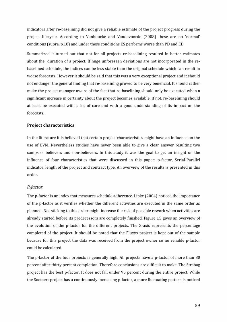
59

indicators after re-baselining did not give a reliable estimate of the project progress during the

project lifecycle. According to Vanhoucke and Vandevoorde (2008) these are no ‘normal’

conditions (supra, p.18) and under these conditions ES performs worse than PD and ED

Summarized it turned out that not for all projects re-baselining resulted in better estimates

about the duration of a project. If huge unforeseen deviations are not incorporated in the re-

baselined schedule, the indices can be less stable than the original schedule which can result in

worse forecasts. However it should be said that this was a very exceptional project and it should

not endanger the general finding that re-baselining proved to be very beneficial. It should rather

make the project manager aware of the fact that re-baselining should only be executed when a

significant increase in certainty about the project becomes available. If not, re-baselining should

at least be executed with a lot of care and with a good understanding of its impact on the

forecasts.

Project characteristics

In the literature it is believed that certain project characteristics might have an influence on the

use of EVM. Nevertheless studies have never been able to give a clear answer resulting two

camps of believers and non-believers. In this study it was the goal to get an insight on the

influence of four characteristics that were discussed in this paper: p-factor, Serial-Parallel

indicator, length of the project and contract type. An overview of the results is presented in this

order.

P-factor

The p-factor is an index that measures schedule adherence. Lipke (2004) noticed the importance

of the p-factor as it verifies whether the different activities are executed in the same order as

planned. Not sticking to this order might increase the risk of possible rework when activities are

already started before its predecessors are completely finished. Figure 15 gives an overview of

the evolution of the p-factor for the different projects. The X-axis represents the percentage

completed of the project. It should be noted that the Fluxys project is kept out of the sample

because for this project the data was received from the project owner so no reliable p-factor

could be calculated.

The p-factor of the four projects is generally high. All projects have a p-factor of more than 80

percent after thirty percent completion. Therefore conclusions are difficult to make. The Strabag

project has the best p-factor. It does not fall under 95 percent during the entire project. While

the Soetaert project has a continuously increasing p-factor, a more fluctuating pattern is noticed

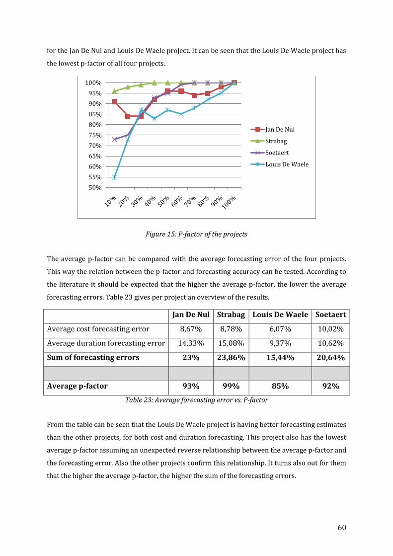
60

for the Jan De Nul and Louis De Waele project. It can be seen that the Louis De Waele project has

the lowest p-factor of all four projects.

Figure 15: P-factor of the projects

The average p-factor can be compared with the average forecasting error of the four projects.

This way the relation between the p-factor and forecasting accuracy can be tested. According to

the literature it should be expected that the higher the average p-factor, the lower the average

forecasting errors. Table 23 gives per project an overview of the results.

Jan De Nul Strabag Louis De Waele Soetaert

Average cost forecasting error 8,67% 8,78% 6,07% 10,02%

Average duration forecasting error 14,33% 15,08% 9,37% 10,62%

Sum of forecasting errors 23% 23,86% 15,44% 20,64%

Average p-factor 93% 99% 85% 92%

Table 23: Average forecasting error vs. P-factor

From the table can be seen that the Louis De Waele project is having better forecasting estimates

than the other projects, for both cost and duration forecasting. This project also has the lowest

average p-factor assuming an unexpected reverse relationship between the average p-factor and

the forecasting error. Also the other projects confirm this relationship. It turns also out for them

that the higher the average p-factor, the higher the sum of the forecasting errors.

50%

55%

60%

65%

70%

75%

80%

85%

90%

95%

100%

Jan De Nul

Strabag

Soetaert

Louis De Waele

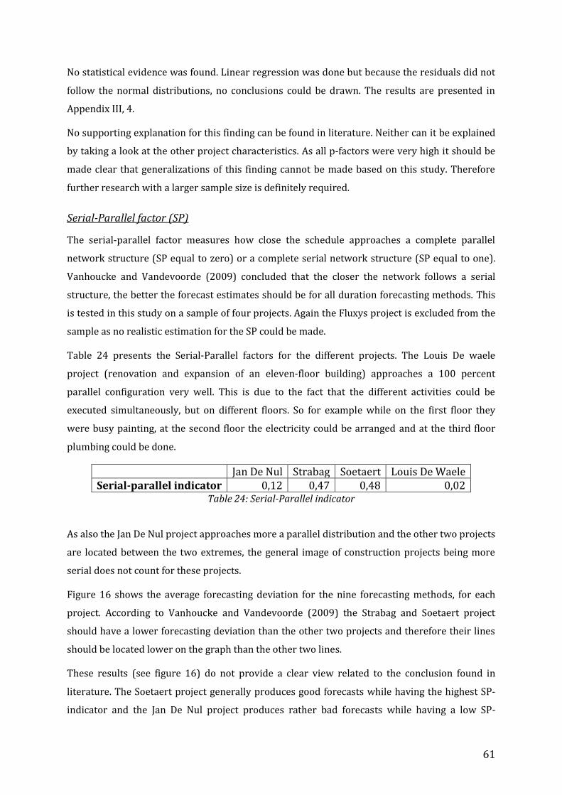
61

No statistical evidence was found. Linear regression was done but because the residuals did not

follow the normal distributions, no conclusions could be drawn. The results are presented in

Appendix III, 4.

No supporting explanation for this finding can be found in literature. Neither can it be explained

by taking a look at the other project characteristics. As all p-factors were very high it should be

made clear that generalizations of this finding cannot be made based on this study. Therefore

further research with a larger sample size is definitely required.

Serial-Parallel factor (SP)

The serial-parallel factor measures how close the schedule approaches a complete parallel

network structure (SP equal to zero) or a complete serial network structure (SP equal to one).

Vanhoucke and Vandevoorde (2009) concluded that the closer the network follows a serial

structure, the better the forecast estimates should be for all duration forecasting methods. This

is tested in this study on a sample of four projects. Again the Fluxys project is excluded from the

sample as no realistic estimation for the SP could be made.

Table 24 presents the Serial-Parallel factors for the different projects. The Louis De waele

project (renovation and expansion of an eleven-floor building) approaches a 100 percent

parallel configuration very well. This is due to the fact that the different activities could be

executed simultaneously, but on different floors. So for example while on the first floor they

were busy painting, at the second floor the electricity could be arranged and at the third floor

plumbing could be done.

Jan De Nul Strabag Soetaert Louis De Waele Serial-parallel indicator 0,12 0,47 0,48 0,02

Table 24: Serial-Parallel indicator

As also the Jan De Nul project approaches more a parallel distribution and the other two projects

are located between the two extremes, the general image of construction projects being more

serial does not count for these projects.

Figure 16 shows the average forecasting deviation for the nine forecasting methods, for each

project. According to Vanhoucke and Vandevoorde (2009) the Strabag and Soetaert project

should have a lower forecasting deviation than the other two projects and therefore their lines

should be located lower on the graph than the other two lines.

These results (see figure 16) do not provide a clear view related to the conclusion found in

literature. The Soetaert project generally produces good forecasts while having the highest SP-

indicator and the Jan De Nul project produces rather bad forecasts while having a low SP-

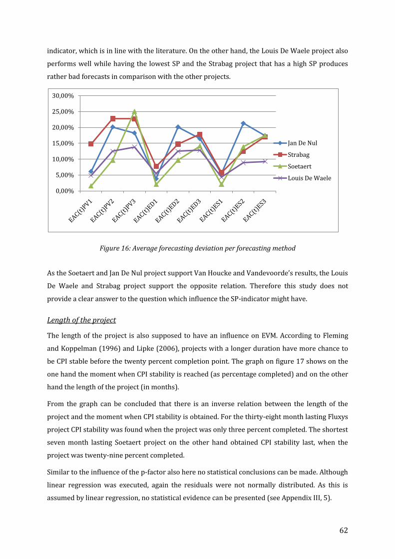
62

indicator, which is in line with the literature. On the other hand, the Louis De Waele project also

performs well while having the lowest SP and the Strabag project that has a high SP produces

rather bad forecasts in comparison with the other projects.

Figure 16: Average forecasting deviation per forecasting method

As the Soetaert and Jan De Nul project support Van Houcke and Vandevoorde’s results, the Louis

De Waele and Strabag project support the opposite relation. Therefore this study does not

provide a clear answer to the question which influence the SP-indicator might have.


The length of the project is also supposed to have an influence on EVM. According to Fleming

and Koppelman (1996) and Lipke (2006), projects with a longer duration have more chance to

be CPI stable before the twenty percent completion point. The graph on figure 17 shows on the

one hand the moment when CPI stability is reached (as percentage completed) and on the other

hand the length of the project (in months).

From the graph can be concluded that there is an inverse relation between the length of the

project and the moment when CPI stability is obtained. For the thirty-eight month lasting Fluxys

project CPI stability was found when the project was only three percent completed. The shortest

seven month lasting Soetaert project on the other hand obtained CPI stability last, when the

project was twenty-nine percent completed.

Similar to the influence of the p-factor also here no statistical conclusions can be made. Although

linear regression was executed, again the residuals were not normally distributed. As this is

assumed by linear regression, no statistical evidence can be presented (see Appendix III, 5).

0,00%

5,00%

10,00%

15,00%

20,00%

25,00%

30,00%

Jan De Nul

Strabag

Soetaert

Louis De Waele

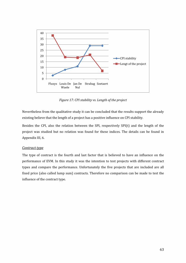
63

Figure 17: CPI stability vs. Length of the project

Nevertheless from the qualitative study it can be concluded that the results support the already

existing believe that the length of a project has a positive influence on CPI stability.

Besides the CPI, also the relation between the SPI, respectively SPI(t) and the length of the

project was studied but no relation was found for these indices. The details can be found in

Appendix III, 6.

Contract type

The type of contract is the fourth and last factor that is believed to have an influence on the

performance of EVM. In this study it was the intention to test projects with different contract

types and compare the performance. Unfortunately the five projects that are included are all

fixed price (also called lump sum) contracts. Therefore no comparison can be made to test the

influence of the contract type.

0

5

10

15

20

25

30

35

40

Fluxys Louis De Waele

Jan De Nul

Strabag Soetaert

CPI stability

Lengt of the project

64

7 Conclusions

The present thesis which studied a sample of five Belgian construction projects, provided

valuable information on different aspects related to the EVM methodology. Although the sample

size may be small, it is believed that these five projects give a rather reliable overview of

construction projects in Belgium. First, the results with respect to indices stability and

forecasting accuracy obtained from testing will be highlighted. Secondly, time was spent on the

potential influence re-baselining and project characteristics may exert on EVM effectiveness. At

last, the EVM implementation in the construction industry and the associated requirements are

studied.

Indices stability

CPI stability in this sample was achieved in three out of five projects before the twenty percent

completion point and all five projects achieved CPI stability before the thirty percent completion

point. This is in line with the suggestions in the literature and is important for the forecasting

methods using this indicator.

No stability could be found early in the project life after analyzing the stability for the other

indicators (SPI and SPI(t)). A remarkable result in the present study was the different

trajectories both indicators follow. As SPI always equals one at the end of the project, it explains

that for projects which run far behind (or ahead of) schedule, the ten percent stability

boundaries are reached late in the project life. SPI(t) does not encounter this problem of

convergence which enables it to achieve stability earlier if consistent schedule performance is

present. However, a consequence for the more realistic representation is that SPI(t) is also much

more subject to changes and therefore will not achieve stability earlier if the performance level

is not consistent.

Forecast accuracy

This study suggests that when EVM methodology is used at project initiation, cost forecasting

methods where the performance factor is mostly determined by the CPI, will provide best

estimates for the actual cost at completion. These methods perform well since the CPI gives a

good representation for future cost performance and stability is achieved early in the project. At

the same time it could prove useful to let SPI or SPI(t) influence the performance factor - for just

a small fraction. This is the case when the project shows a significant delay which most likely has

a small impact on the actual cost.

65

In order to forecast the duration of the project, a performance factor equal to one outperforms

the other performance factors, which confirms the value of the original schedule in the

construction industry. Generally, the duration of the different activities, also including those at

the end of the project, may be estimated very well at project initiation.

In addition, this study confirms the literature where it is suggested that the Earned Schedule

duration forecasting method performs generally better than the Earned Duration and Planned

Value method.

Re-baselining

The method of re-baselining has been the subject of serious discussions among EVM

practitioners. The key questions are whether it is worth the effort to re-baseline and if this

would provide better estimates. Although literature has attempted to give an answer when re-

baselining is allowed by providing some rules and recommendations, not much empirical testing

has been done until now. The present study did some innovative research by comparing the

results of the EVM methodology on both the original and the re-baselined version of the same

projects. By doing so, the added value of re-baselining could be assessed. Although the method of

re-baselining was only executed on three projects, its influence on the forecasting was

unanimous. For both the cost and duration forecasting methods re-baselining triggered a serious

decrease in the forecasting error. This finding may be of great importance to EVM

practitioners. Not only does this mean that the forecasting methods converge towards the final

result, it also enables project managers who are confronted with uncertainty regarding which

forecasting method to use, to achieve reliable forecasts.

It can be assumed that when experienced EVM practitioners have a good view on the future

course of the project and the uncertainty induced, they might be able to differentiate between

more and less suitable forecasting methods. Hence, this will result in even more accurate

forecasts for the specific project. In order to achieve this goal, a thorough training on when to

use which method is recommended.

When re-baselining is done, the use of appropriate forecasting methods is less clear compared to

the performance based on the original baseline. Here the input of the project manager is crucial.

The results concerning cost forecasting after re-baselining are rather ambiguous. Although the

CPI on average achieves stability earlier on in the project, the forecasting methods which rely on

the CPI as performance factor, have to give in on performance. The performance factors relying

on SPI(t) on the other hand, achieve better results when combined with a performance factor

equal to one.

66

Regarding the performance of duration forecasting methods, re-baselining does not affect the

preference for a performance factor of one, although it does create a notable difference in the

performance of the earned schedule method in favor to the earned duration method.

In summary, it can be stated that re-baselining has a positive impact on forecasting in general.

After re-baselining a significant decrease in forecasting error was observed for both cost and

duration forecasting methods. This is good news for projects which have to cope with huge risks

and uncertainties. In this kind of situations, it is important to have converging results from the

sensitivity analysis, which results in more reliable forecasts. Although this convergence takes

place, it may occur that re-baselining makes the best forecasting methods deviate more from the

final outcome than prior to re-baselining. Therefore, re-baselining should be applied with

caution because re-baselining will prevent the performance indicators to reflect the

performance that was achieved before a new baseline was compiled. Hence, crucial data on past

performance is lost.

Project characteristics

The present research investigated the impact of different project characteristics in relation to

their influence on earned value predictors and EVM in general.

One of these characteristics is the p-factor, a dynamic schedule adherence measure, which is

supposed to improve forecasts by taking the increase in risk of rework into account due to not

following the schedule. The sample that was studied here had an overall high p-factor.

Therefore, it was impossible to draw any strong conclusion related to this characteristic.

Another factor which was recently found to influence the duration forecast accuracy is the

Serial-Parallel indicator. This indicator is supposed to influence the forecast effectiveness of

duration forecast. Projects containing more serial activities are supposed to provide more

accurate results. However, in this study no difference was found between the projects more

resembling the serial and projects which are characterized by a rather parallel structure.

A third project characteristic, the length of the project, was also checked for its influence on CPI

stability. In this study, a clear inverse relationship was found between both parameters. The

longer a project lasts, the sooner (in percentage completed) CPI stability is achieved. This is in

accordance with the suggested relationship in literature.

67

Implementation

While processing the data needed to evaluate the projects, some key insights were obtained

which are useful for further implementation of the EVM methodology on construction projects.

The four projects, which were approached from the project organizational point of view of four

different construction companies, revealed a lot of similarities on how data was gathered. The

most important findings are those related to how data could be collected in order to be valuable

for the EVM methodology.

To join a tender, an estimate of the budget and schedule has to be set up. Therefore, calculations

have to be made concerning the cost of the different activities which are scheduled. Once the

public tender is won, a general observation was done that the information that is inherent in this

original estimate is soon abandoned. Once the project starts, two separate systems are active to

follow up on schedule and costs. This is done because both dimensions have a different Work

Breakdown Structure (WBS). Although it might seem easier to follow up costs based on a

separate WBS, this only leads to incapability of intervening in the course of the project. Besides,

the information that can integrate both systems is present in the original estimates by which the

tender was won. Using this information can therefore enable following up through an integrated

system easily. This system requires both the schedule and the costs to use one and the same

WBS.

To make the implementation of EVM a complete success, responsibilities should be clearly

assigned to the members of the project team / organization. This can be done by composing an

Organizational Breakdown Structure (OBS) and a Responsibility assignment matrix (RACI

chart). Furthermore, looking for overlap between both WBS and OBS can help the process of

composing the RACI chart.

Summary

In this study, empirical evidence is presented for most of the theories treated in literature

concerning the EVM methodology. In addition, the study reached interesting findings concerning

whether or not project managers should re-baseline. Given that no similar studies were found in

literature, further research in both the domain of re-baselining and the performance of EVM in

the construction sector is strongly encouraged.

Furthermore, it can be concluded that the EVM methodology definitely helps project managers

control construction projects by providing accurate forecasts and early warning signals. All

necessary information to implement this methodology is available in most construction projects.

This information just has to be employed to integrate both schedule and costs in one WBS. Other

68

requirements for using EVM are to have a clearly defined scope and to have the support of the

organization which enables allocation of responsibilities.

The implementation of the EVM methodology on construction projects demands some effort and

short-term yield is not obvious. However, this effort only needs to be done at the beginning of

the project and will eventually prove valuable throughout the course of the project. This added

value consists of providing early warning signals for project managers and in the long run,

employing EVM will help to a gain better view on the progress of the project’s performance. EVM

provides project managers with quantifiable and tangible data on whether the project is

performing according to plan or not. This quantifiable data can subsequently be extrapolated

throughout the portfolio of projects and will allow better estimates for new projects. The

experience, gained by implementing EVM will also enable PMs to apply the most appropriate

forecasting methods which will eventually lead to even better results. Nevertheless, appropriate

training, and organizational support is required to reach these objectives.

Conclusively, we strongly believe that the EVM methodology could have helped the studied

projects in achieving a better understanding of the project performance. Moreover, when EVM

would be incorporated as a general project management tool by construction companies and its

methodology would be understood well by project managers, it could definitely serve as a

powerful tool to follow up all types of construction projects.

IX

References

Abba W. (2006). “Understanding program resource management through Earned Value Analysi.” PMI WDC Tool Time, July 18

Alvarado, Carlos M., Robert P. Silverman, and David S. Wilson (2004, June). “Assessing the Performance of Construction Projects: Implementing Earned Value Management at the General Services Administration.” Journal of Facilities Management 3/1: 92-105.

Anbari, Frank T. (2001). “Applications and Extensions to the Earned Value Analysis Method.” Proceedings of the Project Management Institute 2001 Seminars & Symposium.

Anbari, Frank T. (2003, December). “Earned Value Project Management Method and Extensions.”Project Management Journal 34.4: 12-23.

Antvik, Sven (1998, October). "Earned Value Management (EVM) - A 200Year Perspective." Proceedings. Project Management Institute.

Barr, Zeev (1996, December). "Earned Value Analysis: A Cast Study." PM Network, pp. 31-37.

Caletka, Anthony F., CCM (2009) “Managing Construction Projects: Have you taken your project's pulse lately? Project Health Checks.” Lorman Education Services, Rochester, NY.

Christensen, David S. and Scott Heise (1993, Spring). Cost Performance Index Stability National Contract Management Journal 25: 7-15.

Christensen, David S. and David Rees (2002, Winter). Is the Cumulative CPI-based EAC a Lower Bound to Final Cost on Post-A12 Contracts? Journal of Cost Analysis and Management, pp. 55-65.

Custer, Keith, PE (2008, December). “Ten Things You Need to know About Earned Value Management.” Custer Consultants Inc.

Custer, Keith, PE (2009). “The Seven Deadly Myths of Earned Value Methods in Project Management.” Custer Consultants Inc.

Durrenberger, Mark (2003). “An Earned Value Tutorial.” Oak Associates, Inc.

Fleming, Quentin W. and Joel M. Koppelman (1996). "Earned Value Project Management." Project. Association for Project Management. United Kingdom.

Fleming, Quentin W. and Joel M. Koppelman (2002, March-April). "Earned Value Management: Mitigating the Risks Associated with Construction Projects." Program Manager: 90-95.

Fleming, Quentin W. and Joel M. Koppelman (2004, Spring). If EVM is so Good, Why Isn't it used on all Projects? The Measurable News, 5 pages.

Fleming, Quentin W. and Joel M. Koppelman (2005). Earned Value Project Management, 3rd edition. Newton Square, PA: Project Management Institute (PMI). ISBN 1-93069989-1.

Henderson, Kym and O. Zwikael. (2008, April). "Does Project Performance Exist? A Re-examination of CPI and Evaluation of SPI (t) stability." CrossTalk - The Journal of Defense Software Engineering21:7-13.

Jacob, D. S. (2003, March). "Forecasting Project Schedule Completion With Earned Value Metrics." The Measurable News: p. 1,7-9.

Kim, EunHong, Wells Jr., William G. and Duffey, Michael R. (2003). “A model for effective implementation of Earned Value Management methodology.” International Journal of Project Management 21:375-382

Lewis, J. P. (2001). “Project Planning, Scheduling and Control: A hands-on guide to bringing projects in on time and on budget. 3rd Edition. New York, NY: McGraw-Hill.

http://www.suu.edu/faculty/christensend/evms/CPIstabilityNCMJ.pdf

X

Lipke, Walter H (2003, Summer). "Schedule is Different." The Measurable News.

Lipke, Walter H. (2004, Winter). "Connecting Earned Value to the Schedule." The Measurable News, pp. 1,6-16 and Cross Talk, the Journal of Defense Software Engineering (Jun 2005).

Lipke, Walter H. (2005, Summer). "A Re-Examination of Project Outcome Prediction ...Using Earned Value Management Methods." The Measurable News, pp. 14 - 26.

Lipke, Walt (2009). "Project Duration Forecasting." Cross Talk.

Lipke, Walt, Dr. Zwikael, K. Henderson and Dr. Anbari (2009, May). "Prediction of project outcome - The application of statistical methods to earned value management and earned schedule performance indexes," International Journal of Project Management 27/4: 400-407.

Marshall, Robert A (2005, October). "The Case for Earned Value Management with Fixed-Price Contracts." Contract Management, pp. 30-34.

Marshall, Robert A. (2007, September). "The contribution of earned value management to project success on contracted efforts: A quantitative statistics approach within the population of experienced practitioners." Journal of Contract Management.

Meredith, J. R. and Mantel, S. J. (2000). “Project Management: A Managerial Approach. Wiley New York.

Payne, Kirk I (1990, September). An Investigation of the Stability of the Cost Performance Index. MS Thesis, Air Force Institute of Technology, Wright Patterson AFB, Ohio.

Prentice, J.-P., CCE. (2003). “Earned Value in the Construction and Facilities Maintenance Environments.” In Transactions of AACE International: Vol. 2003. CSC.17,pp. 1-4. Solanki, Piyush (2009). “Earned Value Management: Integrated View of Cost and Schedule Performance.” Global India Publications. pp. 65

Valle, Jose Angelo and Soares, Carlos Alberto Pereira. (2008) "The Use of Earned Value Analysis (EVA) in the Cost Management of Construction Projects." IBEC, Rio de Janiero, Brazil

Vanhoucke Mario, Vandevoorde Stephan (2007). "A Simulation and Evaluation of Earned Value Metrics to Forecast Project Duration." Journal of the Operational Research Society.

Vanhoucke Mario, Vandevoorde Stephan (2008, Winter) "Measuring the Accuracy of Earned Value/ Earned Schedule Forecasting Predictors." The Measurable News: 26-30.

Vanhoucke Mario, Vandevoorde Stephan (2009, February) "Forecasting a Project's Duration under Various Topological Structures." The Measurable News 1 :26-30.

Vanhoucke Mario. (2010). "Measuring Time, Improving Project Performance Using Earned Value Management." Springer. ISBN: 978-1-4419-1013-4.

Vargas, Ricardo Viana (2003). “Earned Value Analysis in the Control of Projects: Success of Failure?” The Measurable News and Transactions of AACE International.

Winston, J. Ledet and Maroulis, Spiro J. (1998, Ocotober) “Improving Project Performance with Simulation and Practice.” Project Management Institute, 1998 Seminars & Symposium.

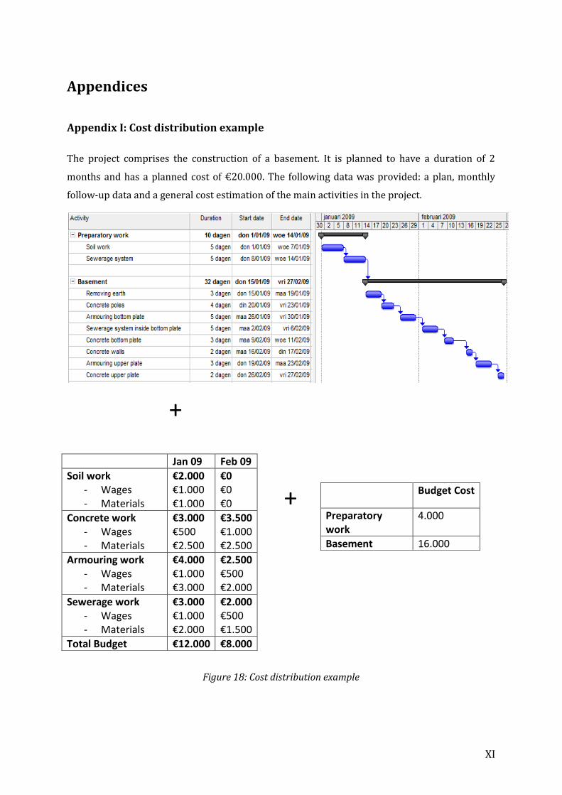
http://www.icoste.org/ICMJ%20Papers/Valle%20-%20EVA.pdf

http://www.icoste.org/ICMJ%20Papers/Valle%20-%20EVA.pdf

XI

Appendices

Appendix I: Cost distribution example

The project comprises the construction of a basement. It is planned to have a duration of 2

months and has a planned cost of €20.000. The following data was provided: a plan, monthly

follow-up data and a general cost estimation of the main activities in the project.

+

+

Figure 18: Cost distribution example

Jan 09 Feb 09

Soil work - Wages - Materials

€2.000 €1.000 €1.000

€0 €0 €0

Concrete work - Wages - Materials

€3.000 €500 €2.500

€3.500 €1.000 €2.500

Armouring work - Wages - Materials

€4.000 €1.000 €3.000

€2.500 €500 €2.000

Sewerage work - Wages - Materials

€3.000 €1.000 €2.000

€2.000 €500 €1.500

Total Budget €12.000 €8.000

Budget Cost

Preparatory work

4.000

Basement 16.000

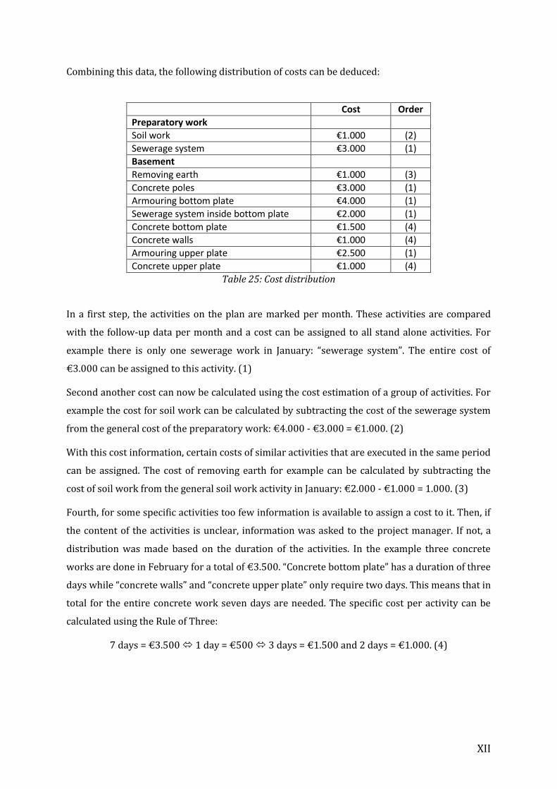
XII

Combining this data, the following distribution of costs can be deduced:

Cost Order

Preparatory work

Soil work €1.000 (2)

Sewerage system €3.000 (1)

Basement

Removing earth €1.000 (3)

Concrete poles €3.000 (1)

Armouring bottom plate €4.000 (1)

Sewerage system inside bottom plate €2.000 (1)

Concrete bottom plate €1.500 (4)

Concrete walls €1.000 (4)

Armouring upper plate €2.500 (1)

Concrete upper plate €1.000 (4)

Table 25: Cost distribution

In a first step, the activities on the plan are marked per month. These activities are compared

with the follow-up data per month and a cost can be assigned to all stand alone activities. For

example there is only one sewerage work in January: “sewerage system”. The entire cost of

€3.000 can be assigned to this activity. (1)

Second another cost can now be calculated using the cost estimation of a group of activities. For

example the cost for soil work can be calculated by subtracting the cost of the sewerage system

from the general cost of the preparatory work: €4.000 - €3.000 = €1.000. (2)

With this cost information, certain costs of similar activities that are executed in the same period

can be assigned. The cost of removing earth for example can be calculated by subtracting the

cost of soil work from the general soil work activity in January: €2.000 - €1.000 = 1.000. (3)

Fourth, for some specific activities too few information is available to assign a cost to it. Then, if

the content of the activities is unclear, information was asked to the project manager. If not, a

distribution was made based on the duration of the activities. In the example three concrete

works are done in February for a total of €3.500. “Concrete bottom plate” has a duration of three

days while “concrete walls” and “concrete upper plate” only require two days. This means that in

total for the entire concrete work seven days are needed. The specific cost per activity can be

calculated using the Rule of Three:

7 days = €3.500 1 day = €500 3 days = €1.500 and 2 days = €1.000. (4)

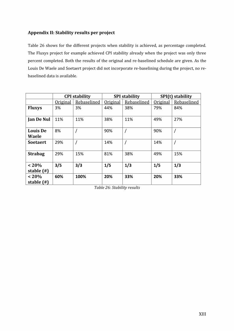
XIII

Appendix II: Stability results per project

Table 26 shows for the different projects when stability is achieved, as percentage completed.

The Fluxys project for example achieved CPI stability already when the project was only three

percent completed. Both the results of the original and re-baselined schedule are given. As the

Louis De Waele and Soetaert project did not incorporate re-baselining during the project, no re-

baselined data is available.

CPI stability SPI stability SPI(t) stability Original Rebaselined Original Rebaselined Original Rebaselined Fluxys 3%

3%

44%

38%

79%

84%

Jan De Nul 11%

11%

38%

11%

49%

27%

Louis De Waele

8%

/

90%

/

90%

/

Soetaert 29%

/

14%

/

14%

/

Strabag 29%

15%

81%

38%

49%

15%

< 20% stable (#)

3/5 3/3 1/5 1/3 1/5 1/3

< 20% stable (#)

60% 100% 20% 33% 20% 33%

Table 26: Stability results

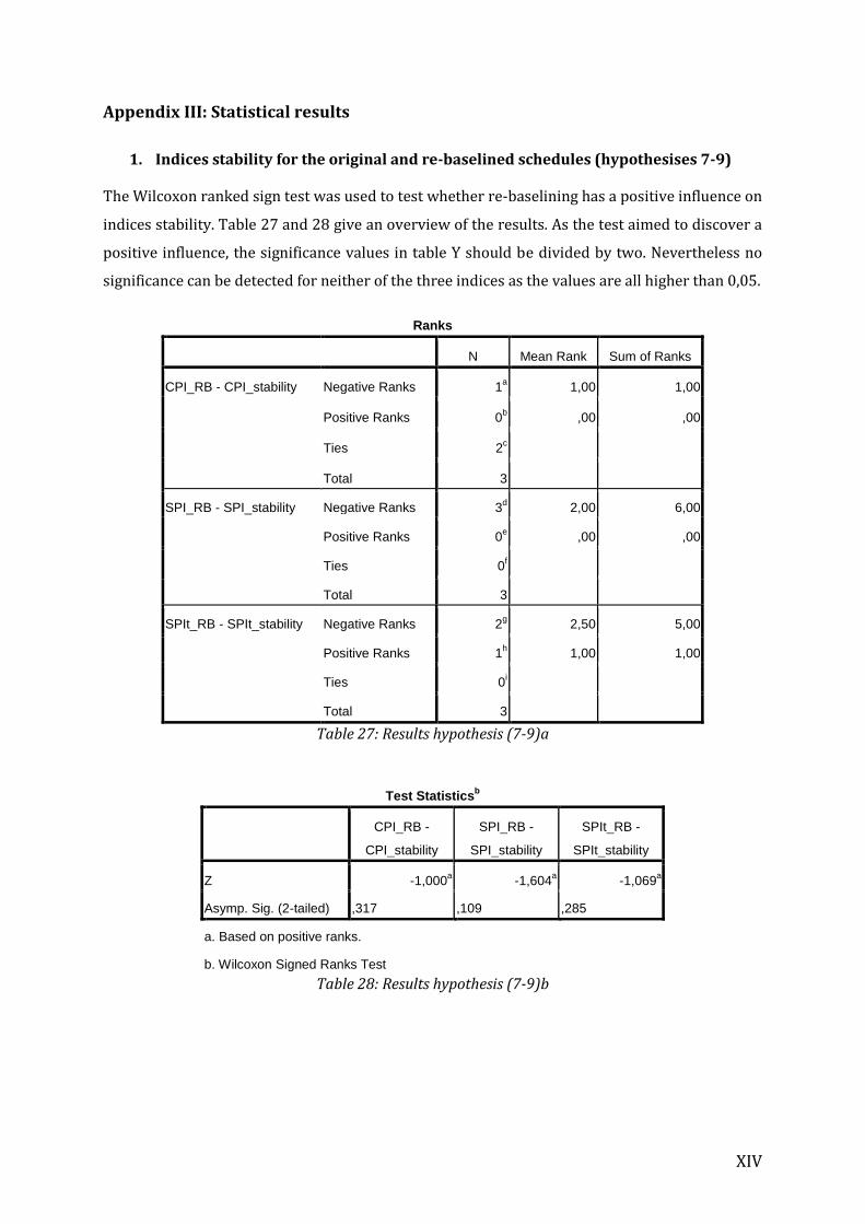
XIV

Appendix III: Statistical results

1. Indices stability for the original and re-baselined schedules (hypothesises 7-9)

The Wilcoxon ranked sign test was used to test whether re-baselining has a positive influence on

indices stability. Table 27 and 28 give an overview of the results. As the test aimed to discover a

positive influence, the significance values in table Y should be divided by two. Nevertheless no

significance can be detected for neither of the three indices as the values are all higher than 0,05.

Ranks

N Mean Rank Sum of Ranks

CPI_RB - CPI_stability Negative Ranks 1a 1,00 1,00

Positive Ranks 0b ,00 ,00

Ties 2c

Total 3

SPI_RB - SPI_stability Negative Ranks 3d 2,00 6,00

Positive Ranks 0e ,00 ,00

Ties 0f

Total 3

SPIt_RB - SPIt_stability Negative Ranks 2g 2,50 5,00

Positive Ranks 1h 1,00 1,00

Ties 0i

Total 3

Table 27: Results hypothesis (7-9)a

Test Statisticsb

CPI_RB -

CPI_stability

SPI_RB -

SPI_stability

SPIt_RB -

SPIt_stability

Z -1,000a -1,604

a -1,069

a

Asymp. Sig. (2-tailed) ,317 ,109 ,285

a. Based on positive ranks.

b. Wilcoxon Signed Ranks Test

Table 28: Results hypothesis (7-9)b

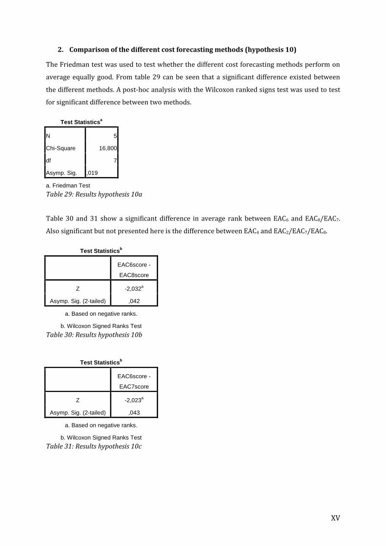
XV

2. Comparison of the different cost forecasting methods (hypothesis 10)

The Friedman test was used to test whether the different cost forecasting methods perform on

average equally good. From table 29 can be seen that a significant difference existed between

the different methods. A post-hoc analysis with the Wilcoxon ranked signs test was used to test

for significant difference between two methods.

Test Statisticsa

N 5

Chi-Square 16,800

df 7

Asymp. Sig. ,019

a. Friedman Test

Table 29: Results hypothesis 10a

Table 30 and 31 show a significant difference in average rank between EAC6 and EAC8/EAC7.

Also significant but not presented here is the difference between EAC4 and EAC2/EAC7/EAC8.

Test Statisticsb

EAC6score -

EAC8score

Z -2,032a

Asymp. Sig. (2-tailed) ,042

a. Based on negative ranks.


Table 30: Results hypothesis 10b

Test Statisticsb

EAC6score -

EAC7score

Z -2,023a




Table 31: Results hypothesis 10c

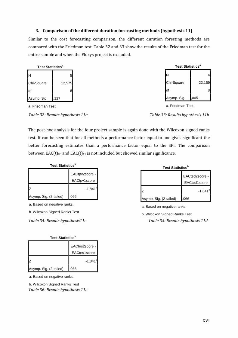
XVI

3. Comparison of the different duration forecasting methods (hypothesis 11)

Similar to the cost forecasting comparison, the different duration foresting methods are

compared with the Friedman test. Table 32 and 33 show the results of the Friedman test for the

entire sample and when the Fluxys project is excluded.

Test Statisticsa

N 5

Chi-Square 12,575

df 8

Asymp. Sig. ,127

a. Friedman Test

Table 32: Results hypothesis 11a Table 33: Results hypothesis 11b

The post-hoc analysis for the four project sample is again done with the Wilcoxon signed ranks

test. It can be seen that for all methods a performance factor equal to one gives significant the

better forecasting estimates than a performance factor equal to the SPI. The comparison

between EAC(t)X3 and EAC(t)X1 is not included but showed similar significance.

Test Statisticsb

EACtpv2score -

EACtpv1score

Z -1,841a




Table 34: Results hypothesis11c Table 35: Results hypothesis 11d

Test Statisticsb

EACtes2score -

EACtes1score

Z -1,841a




Table 36: Results hypothesis 11e

Test Statisticsa

N 4

Chi-Square 22,159

df 8

Asymp. Sig. ,005

a. Friedman Test

Test Statisticsb

EACted2score -

EACted1score

Z -1,841a




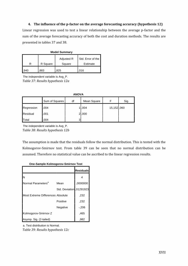
XVII

4. The influence of the p-factor on the average forecasting accuracy (hypothesis 12)

Linear regression was used to test a linear relationship between the average p-factor and the

sum of the average forecasting accuracy of both the cost and duration methods. The results are

presented in tables 37 and 38.

Model Summary

R R Square

Adjusted R

Square

Std. Error of the

Estimate

,940 ,883 ,825 ,016

The independent variable is Avg_P.


ANOVA

Sum of Squares df Mean Square F Sig.

Regression ,004 1 ,004 15,152 ,060

Residual ,001 2 ,000

Total ,004 3

The independent variable is Avg_P.


The assumption is made that the residuals follow the normal distribution. This is tested with the

Kolmogorov-Smirnov test. From table 39 can be seen that no normal distribution can be

assumed. Therefore no statistical value can be ascribed to the linear regression results.

One-Sample Kolmogorov-Smirnov Test

Residuals

N 4

Normal Parametersa Mean ,0000000

Std. Deviation ,01291923

Most Extreme Differences Absolute ,232

Positive ,232

Negative -,206

Kolmogorov-Smirnov Z ,465


a. Test distribution is Normal.


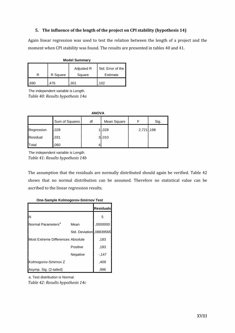
XVIII

5. The influence of the length of the project on CPI stability (hypothesis 14)

Again linear regression was used to test the relation between the length of a project and the

moment when CPI stability was found. The results are presented in tables 40 and 41.

Model Summary

R R Square

Adjusted R

Square

Std. Error of the

Estimate

,690 ,476 ,301 ,102

The independent variable is Length.


ANOVA

Sum of Squares df Mean Square F Sig.

Regression ,028 1 ,028 2,721 ,198

Residual ,031 3 ,010

Total ,060 4

The independent variable is Length.


The assumption that the residuals are normally distributed should again be verified. Table 42

shows that no normal distribution can be assumed. Therefore no statistical value can be

ascribed to the linear regression results.

One-Sample Kolmogorov-Smirnov Test

Residuals

N 5

Normal Parametersa Mean ,0000000

Std. Deviation ,08839565

Most Extreme Differences Absolute ,183

Positive ,183

Negative -,147

Kolmogorov-Smirnov Z ,409


a. Test distribution is Normal.


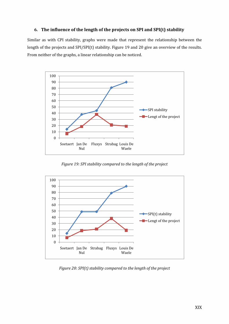
XIX

6. The influence of the length of the projects on SPI and SPI(t) stability

Similar as with CPI stability, graphs were made that represent the relationship between the

length of the projects and SPI/SPI(t) stability. Figure 19 and 20 give an overview of the results.

From neither of the graphs, a linear relationship can be noticed.

Figure 19: SPI stability compared to the length of the project

Figure 20: SPI(t) stability compared to the length of the project

0

10

20

30

40

50

60

70

80

90

100

Soetaert Jan De Nul

Fluxys Strabag Louis De Waele

SPI stability


0

10

20

30

40

50

60

70

80

90

100

Soetaert Jan De Nul

Strabag Fluxys Louis De Waele

SPI(t) stability


Performance analysis of Earned Value Management in the ... · p-factor 59 serial-parallel factor...

Documents

Transcript of Performance analysis of Earned Value Management in the ... · p-factor 59 serial-parallel factor...