Paula Medina Mac¸aira , Fernando Luiz Cyrino Oliveira ... · Paula Medina Mac¸aira1*, Fernando...

�

�

“main” — 2017/5/2 — 20:06 — page 107 — #1�

�

�

�

�

�

Pesquisa Operacional (2017) 37(1): 107-128© 2017 Brazilian Operations Research SocietyPrinted version ISSN 0101-7438 / Online version ISSN 1678-5142www.scielo.br/popedoi: 10.1590/0101-7438.2017.037.01.0107

INTRODUCING A CAUSAL PAR(p) MODEL TO EVALUATE THE INFLUENCEOF CLIMATE VARIABLES IN RESERVOIR INFLOWS: A BRAZILIAN CASE

Paula Medina Macaira1*, Fernando Luiz Cyrino Oliveira1,Pedro Guilherme Costa Ferreira2, Fernanda Villa Nova de Almeida1

and Reinaldo Castro Souza3

Received June 10, 2016 / Accepted March 16, 2017

ABSTRACT. The Brazilian electricity energy matrix is essentially formed by hydraulic sources which

currently account for 70% of the installed capacity. One of the most important characteristics of a generation

system with hydro predominance is the strong dependence on the inflow regimes. Nowadays, the Brazilian

power sector uses the PAR(p) model to generate scenarios for hydrological inflows. This approach does not

consider any exogenous information that may affect hydrological regimes. The main objective of this paper

is to infer on the influence of climatic events in water inflows as a way to improve the model’s performance.

The proposed model is called “causal PAR(p)” and considers exogenous variables, such as El Nino and

Sunspots, to generate scenarios for some Brazilian reservoirs. The result shows that the error measures

decrease approximately 3%. This improvement indicates that the inclusion of climate variables to model

and simulate the inflows time series is a valid exercise and should be taken into consideration.

Keywords: Reservoir inflow modelling, Periodic models, Climate predictors.

1 INTRODUCTION

The Brazilian electricity generation is mainly composed by hydroelectric plants owned by multi-

ple players; the Brazilian National Interconnected System (NIS) integrate power and trasmissionlines from the South, Southeast, Midwest, Northeast and part of the North region. Only 1.7%of the country’s electricity production capacity relies outside the NIS, in small isolated systems

located mainly in the Amazon region [21].

Planning the Brazilian energy sector means, basically, making decisions about the dispatch ofhydroelectric and thermoelectric plants, with the risk of financial losses or energy rationing, ashappened such strong in 2001 [25], affecting almost all Brazilian regions.

*Corresponding author.1Departamento de Engenharia Industrial, Pontifıcia Universidade Catolica do Rio de Janeiro (PUC-Rio), 22451-900 Riode Janeiro, RJ, Brasil. E-mails: [email protected]; [email protected]; [email protected] Getulio Vargas (FGV), 22231-000 Rio de Janeiro, RJ, Brasil. E-mail: [email protected] de Engenharia Eletrica, Pontifıcia Universidade Catolica do Rio de Janeiro (PUC-Rio), 22451-900 Riode Janeiro, RJ, Brasil. E-mail: [email protected]

�

�

“main” — 2017/5/2 — 20:06 — page 108 — #2�

�

�

�

�

�

108 INTRODUCING A CAUSAL PAR(p) MODEL TO EVALUATE THE INFLUENCE OF CLIMATE VARIABLES

One of the main characteristics of the hydraulic generation system is its strong dependence on

hydrological regimes. Thus, the dispatch operation planning has to define generation goals forboth hydroelectric and thermal plants along the study horizon, considering the electricity de-mand, the plants and electrical operating constraints [24].

Considering the dependence on the hydrological regimes, the existing uncertainty of the Brazil-

ian power planning requires an appropriate and consistent stochastic modelling of hydrologi-cal series. Therefore, it is possible to identify how important it is to build models to generatehydrological scenarios, in order to optimize the system operation performance, adding reliability

to the system and reducing its costs [18]. This optimization process has a stochastic variable:natural inflow.

There are, basically, two approaches to predict the natural inflow: physical and statistical mod-els, where the first one includes the rainfall-runoff hydrological model and the second covers

data-driven methods such as time series. To perform monthly forecasts and simulation the clas-sical Periodic Autoregressive (p) model [29], has been widely used. This type of model adjuststhe series using the estimated parameters of the historical data [13], and does not consider any

exogenous information that could affect the hydrological regimes and, consequently, the elec-tricity generation. Several examples of the application of PAR( p) can be found in the literature,see for example [16] who generate and forecast monthly inflows of the Ganges River with the

PAR model. A quick literature search also returns an extensive set of univariate models appliedto reservoir inflows (e.g. [27]).

However, models that incorporate explanatory variables, specifically climate variables, havebeen only recently developed. Some examples of these works in chronological order, are: [32]

studied the relation between the Sea Surface Temperature (SST) pattern over the Atlantic andthe Pacific Oceans and the variability of water availability in the Amazon Basin; [8] introduced aprocedure for further conditioning the inflow probability distributions by considering the recent

measurements of climatic variables, [28] developed a semiparametric approach for forecastinginflow at multiple gaging locations on climate precursors; [14] applied Artificial Neural Networkto model the complex relationship between inflow and climatic phenomenon; [10] investigatedthe potential of the Bayesian dynamic modelling approach through an application to forecast

a hydrologic time series using relevant climate index information; [11] included climate infor-mation in a periodic auto-regressive model in order to provide monthly inflow forecasts for 54hydropower sites in Brazil; and [12] applied Bayesian Dynamic Models to model and forecast

the water inflow for Brazilian hydropower reservoirs, and concluded that the incorporation ofclimate variables such as rainfall precipitation and El Nino variables, increased the accuracy ofboth modelling and prediction.

Considering the context and the relevance of the subject, this paper aims to investigate and pro-

pose methodological advances in time series modelling and stochastic simulation to generatesynthetical hydrological scenarios to model the Brazilian hydrothermal dispatch.

Pesquisa Operacional, Vol. 37(1), 2017

�

�

“main” — 2017/5/2 — 20:06 — page 109 — #3�

�

�

�

�

�

PAULA MEDINA MACAIRA et al. 109

The proposed method, called causal PAR(p), intends to include, exogenously, the meteoro-

logical phenomena influence by adjusting a Dynamic Regression (Autoregressive DistributedLags Model) to the traditional PAR(p) residuals and climate series, incorporating the regressioncoefficient in the traditional modelling. Several preliminary analyses will be concieved in order

to obtain a greater understanding of the involved series and its applicability into the proposedmethod.

Besides this main goal, which is to present a new approach to model the inflow series, this workalso intends to generate synthetical scenarios that better represent the original historical series as

well as confidence intervals for out-of-sample forecasts.

The paper is organized as follows: section 2 presents the theoretical background, with a briefdescription of the Periodic Autoregressive model, the mathematical details of the proposed ap-proach (causal PAR(p)), and a short description of the Bootstrap technique, used to generate

synthetical scenarios. Section 3 describes the input variables, their connection with reservoirinflows the underlying system and the Brazilian case study; section 4 presents a exploratoryanalysis of the available variables. The results from the traditional model and the proposed ap-

proach are shown on section 5, and section 6 sums up the work and summarizes its conclusionand final remarks.

2 THEORETICAL BACKGROUND

The proposed framework to include the climate series behaviour in the PAR(p) modelling,

named as causal PAR(p), is composed using two main techniques: PAR(p) and Dynamic Re-gression Model. These techniques are briefly presented in what follows.

2.1 Traditional PAR(p)

Periodic Autoregressive models can also be referred to PAR(p), where p corresponds to the

order of the model, in other words, the number of autoregressive terms identified in the model.The PAR(p) model fits to each series period an AR(p) model. Generally, p is a vector, p =[p1, p2, . . . , p12], where each element provides the order for each period (month, in case of

monthly series). For more details about the PAR(p) model see [7].

PAR(p) model is mathematically described as follows:(Zt − μm

σm

)= ϕm

1

(Z1 − μm−1

σm−1

)+ ϕm

2

(Z2 − μm−2

σm−2

)+ . . . +

· · · + ϕmpm

(Zt−pm − μm−pm

σm−pm

)+ at

(1)

where,

Zt is the seasonal series of period S.

S is the number of periods (S = 12 to monthly series).


�

�

“main” — 2017/5/2 — 20:06 — page 110 — #4�

�

�

�

�

�


T is the time index, t = 1, 2, . . . , S N , function of the T year (T = 1, 2, . . . , N) and the m

period (m = 1, 2, . . . , S).

N is the number of years.

μm is the seasonal average of the period m.

σm is the seasonal standard deviation of the period m.

ϕm is the i-th autoregressive coefficient of the period m.

pm is the order of the autoregressive operator of the period m.

at is the series of independent noises with average zero and variance σ2(m)a .

2.2 Dynamic Regression Model

A Dynamic Regression model can be described by the following general equation:

at =k∑

i=1

βi (L)Xi,t + 1

a(L)εt (2)

Where at is the dependent (or output) variable; Xi,t are the explanatory (or inputs) variables;βi (L) = bi (L)

a(L)and a(L), b1(L), . . . , bk(L) are finite order lag polynomials of degrees r,

s1, . . . , sk , respectively, and εt is assumed to be white noise. Such a formulation can be seenin [23] and for more mathematical details see [5].

2.3 Causal PAR(p)

The step by step sequence to perform the causal PAR(p) follows the three steps described below:

1. Estimate the traditional PAR(p) model;

2. Find the significant explanatory variables by applying the Dynamic Regression model; and

3. Estimate the causal PAR(p) model.

In the first step the traditional PAR(p) is estimated and the residuals series are extracted to be

used in the second step, that fits the Dynamic Regression model. In this step, the exogenous vari-ables are one of the inputs and the residuals generated by the traditional PAR( p) are the outputs.Then, the coefficients obtained in step two and the exogenous variables are inserted in the math-

ematical formulation of the traditional PAR(p), generating the causal PAR(p).(Zt − μm

σm

)= ϕm

1

(Z1 − μm−1

σm−1

)+ ϕm

2

(Z2 − μm−2

σm−2

)+ . . .

. . . + ϕmpm

(Zt−pm − μm−pm

σm−pm

)+ β1 X1,t + . . . + βi Xi,t + et

(3)


�

�

“main” — 2017/5/2 — 20:06 — page 111 — #5�

�

�

�

�

�


Where, Xi,t are the exogenous variables, βi the coefficient and et is the white noise.

Therefore the innovation at the proposed approach is to introduce exogenous variables in the

PAR(p) modelling. Further studies would consider the development of some kind of periodictransfer function.

Afterwards, the synthetical scenarios generation are carried out applying the Booststrap tech-nique to the residual series as well as in obtaining confidence interval. The methodology is

detailed in the next section.

2.4 Synthetical scenarios’ generation and confidence interval

In order to simulate synthetical scenarios the Bootstrap technique is used. This technique, first

developed by [6], is a method of sampling with replacement the observations of a random samplethat allows the assessment of the variability of an estimator. Such technique generates as manynew samples as one wishes, called “Bootstrap sample”, usually with the same size of the original

sample. In the context of time series, there are basically two ways to apply this technique:Bootstrap in the residuals and the method called Moving Blocks [9].

In this paper Bootstrap is used in the residuals, due to the fact that for all the studied series it ispossible to extract residuals, thus ensuring the hypotheses of a random sample (i.e., independent

and identically distributed observations) a required condition to apply Bootstrap.

A formal description of the method is: consider R1, ..., RN the random sample and B the num-ber of residuals series to be generated. B residual series are drawn with replacement from theoriginal sample, generating B Bootstrap residuals series of size N each: r1 , . . . , r B , where

ri = ri1, ..., ri

N , i = 1, . . . , B.

Anderson et al. [2] computed Gaussian prediction intervals for the estimated parameters of a pe-riodic autoregressive moving average (PARMA) models. In the present study the 5% confidenceinterval is developed from the simulated series by calculating the quantiles 2.5% and 97.5%.

3 DATA ANALYSIS

In Brazil, the fifteen major river basins have an installed capacity of approximately 92 GigaWatts [GW]. The Parana river basin has the highest hydroelectric potential (around 54 GW). Inthese major rivers there are around 190 hydroelectric power plants currently in operation [22],

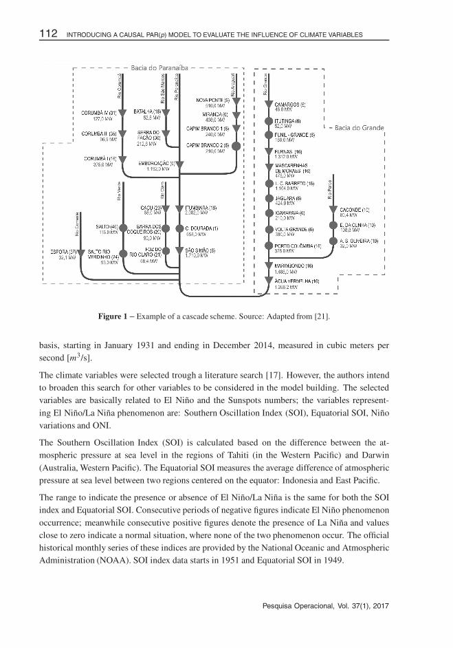
and these plants operate in a cascade scheme. As an illustration Figure 1 displays the cascadescheme for Paranaıba and Grande basins with 19 reservoirs, represented by triangles, and 15hydroelectric with no reservoir (circles).

This way decisions taken at the upstream reservoirs will impact the inflow of the downstream

reservoirs. The historical data available is the natural inflow4 for each reservoir, on a monthly

4The natural inflow is the average incoming water per unit of time at each generator’s reservoir from affluent rivers, lakesand its own drainage area.


�

�

“main” — 2017/5/2 — 20:06 — page 112 — #6�

�

�

�

�

�


Figure 1 – Example of a cascade scheme. Source: Adapted from [21].

basis, starting in January 1931 and ending in December 2014, measured in cubic meters persecond [m3/s].

The climate variables were selected trough a literature search [17]. However, the authors intendto broaden this search for other variables to be considered in the model building. The selectedvariables are basically related to El Nino and the Sunspots numbers; the variables represent-

ing El Nino/La Nina phenomenon are: Southern Oscillation Index (SOI), Equatorial SOI, Ninovariations and ONI.

The Southern Oscillation Index (SOI) is calculated based on the difference between the at-mospheric pressure at sea level in the regions of Tahiti (in the Western Pacific) and Darwin

(Australia, Western Pacific). The Equatorial SOI measures the average difference of atmosphericpressure at sea level between two regions centered on the equator: Indonesia and East Pacific.

The range to indicate the presence or absence of El Nino/La Nina is the same for both the SOIindex and Equatorial SOI. Consecutive periods of negative figures indicate El Nino phenomenon

occurrence; meanwhile consecutive positive figures denote the presence of La Nina and valuesclose to zero indicate a normal situation, where none of the two phenomenon occur. The officialhistorical monthly series of these indices are provided by the National Oceanic and AtmosphericAdministration (NOAA). SOI index data starts in 1951 and Equatorial SOI in 1949.


�

�

“main” — 2017/5/2 — 20:06 — page 113 — #7�

�

�

�

�

�


The sea surface temperature anomaly is a proxy for El Nino and La Nina. Thus, this index is

used to classify and quantify such phenomena in four Nino regions: Nino 1+2, Nino 3, Nino 4and Nino 3.4, defined as follows by NOAA in 2014. Through the location of the Nino regionsit is possible to conclude that regions Nino 1+2 and Nino 3 better identify temperature anoma-

lies for the Eastern Pacific Ocean sea surface and region Nino 4 for the Western Pacific. TheNino 3.4 region is centralized in the Pacific, which allows a better understanding of anomaliesacross it. Therefore, currently the Nino 3.4 region is the official measure used to represent SST

(Sea Surface Temperature). However, depending on the study, other regions may be a betteralternative.

The threshold for the normal state of this index is between −0.5◦C and +0.5◦C. The crite-ria commonly used to define an El Nino phenomenon consists of five consecutive averages of

SST anomalies above +0.5◦C. Similarly, for La Nina, this criterion remains, but now the SSTanomaly should be below −0.5◦C. The time series for all regions are provided by NOAA, on aweekly and monthly basis. For the weekly series, the data starts in 1990 and ends at the current

week and the monthly data starts at 1982 and ends up at the current month.

The Oceanic Nino Index (ONI) measures the average sea surface temperature anomalies for theregion Nino 3.4, removing the existing warming trend on it. The ONI uses multiple periodsbased on thirty years to perform the calculation for five successive years. The base periods uses

a fifteen year interval, for the lower and upper bound, for example, for 1950 and 1955 the baseperiod considered starts in 1936 and ends in 1965. The El Nino and La Nina are indicated in thesame manner as the SST index, the time series is monthly and is provided by NOAA.

Sunspots comprehends solar surface regions of high magnetic field, which have considerably

lower temperature than its surroundings and thus appears as a dark area. The magnetic fluxamount on the sun surface varies over eleven year periods, known as sunspot and solar cycles.During this cycle there is a minimum and a maximum magnetic flux, which is not only difficult

to identify the sunspots and but also they appear almost all the time. The cycle reachs its max-imum aproximately every eleven years, therefore the observed cycle duration corresponds toeleven years.

The daily and monthly number of sunsposts calculation is accomplished with the Relative Index

American number of sunspots. This index indicates the solar phenomenon occurrence takinginto account their relationship with the Earth, including geomagnetic variations and ionosphereeffects. The Solar Division from American Association of Variable Star Observers coordinatesthe data collection program and the analysis of this phenomenon. Thus, the National Geophysical

Data Center (NGDC), provides the historical data from the number of sunspots per month since1749 and forecasts have been produced until December 2019.

4 EXPLORATORY ANALYSIS

In order to provide a better understanding of the series used in this research, this section presentsan exploratory analysis that includes: evolution of the series through time using line’s graphic;


�

�

“main” — 2017/5/2 — 20:06 — page 114 — #8�

�

�

�

�

�


variables’ probability distribution using the histogram; descriptive statistics and correlation be-

tween the reservoir series and the climate variables.

Also, to reduce the problem dimension (currently with 192 reservoir inflow series), were selectedthe eight basins that present the biggest correlation with each one of the climate variables. Asan example, for the SOI Standard variable the reservoir Curua-una was the one with the highest

correlation among all 192 possibles. Table 1 presents the selected hydroelectric power plants andthe Pearson’s correlation5 with the climate variables.

Table 1 – Correlation between reservoir inflow series and climate variables.

SOI Eq. Nino Nino Nino Nino

Std. SOI 1+2 3 4 3.4ONI Suns.

Monjolinho –0.165 –0.272 0.353 0.327 0.170 0.268 0.281 –0.035

Sao Jose –0.160 –0.294 0.302 0.332 0.175 0.290 0.308 –0.018

Curua-una 0.254 0.288 –0.202 –0.220 –0.213 –0.234 –0.246 –0.011Balbina 0.252 0.294 –0.176 –0.219 –0.230 –0.251 –0.269 –0.023

Lajes 0.059 0.057 –0.004 –0.029 –0.066 –0.046 –0.051 –0.177Quebra-queixo –0.106 –0.242 0.369 0.293 0.134 0.218 0.226 0.115

Itauba –0.152 –0.286 0.320 0.340 0.165 0.286 0.300 0.004Jauru –0.102 –0.161 0.116 0.056 –0.035 0.024 0.037 0.211

Note that the biggest values were found between the reservoirs Quebra Queixo and Monjolinhowith variable Nino 1+2 (0.369 and 0.353, respectively). This does not mean that in the climatevariables selecting process this particular variable necessarily will be picket up in the modelformulation. This is due to the fact that the variable selection is carried out via a backward

process that selects only the significant variables.

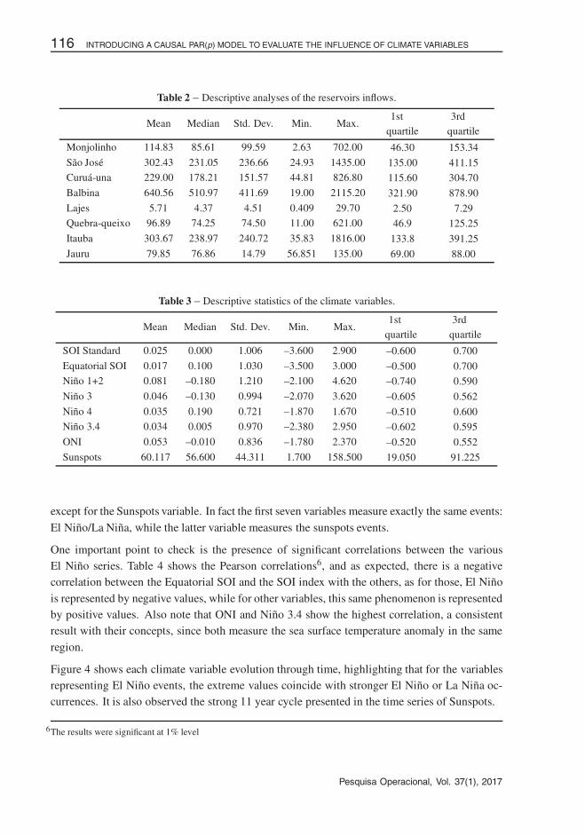
The descriptive statistics for each one of the selected reservoirs is shown in Table 2. See thatBalbina contains the higher values for mean, median, standard deviation and quartiles. On theother hand Lajes is the one with the lowest values.

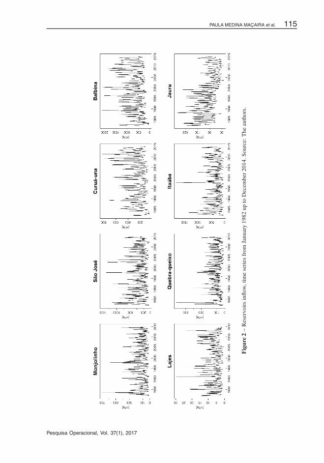
Observing Figure 2, which shows the reservoirs time series plot, it is possible to identify, a strongperiodicity in all inflow series.

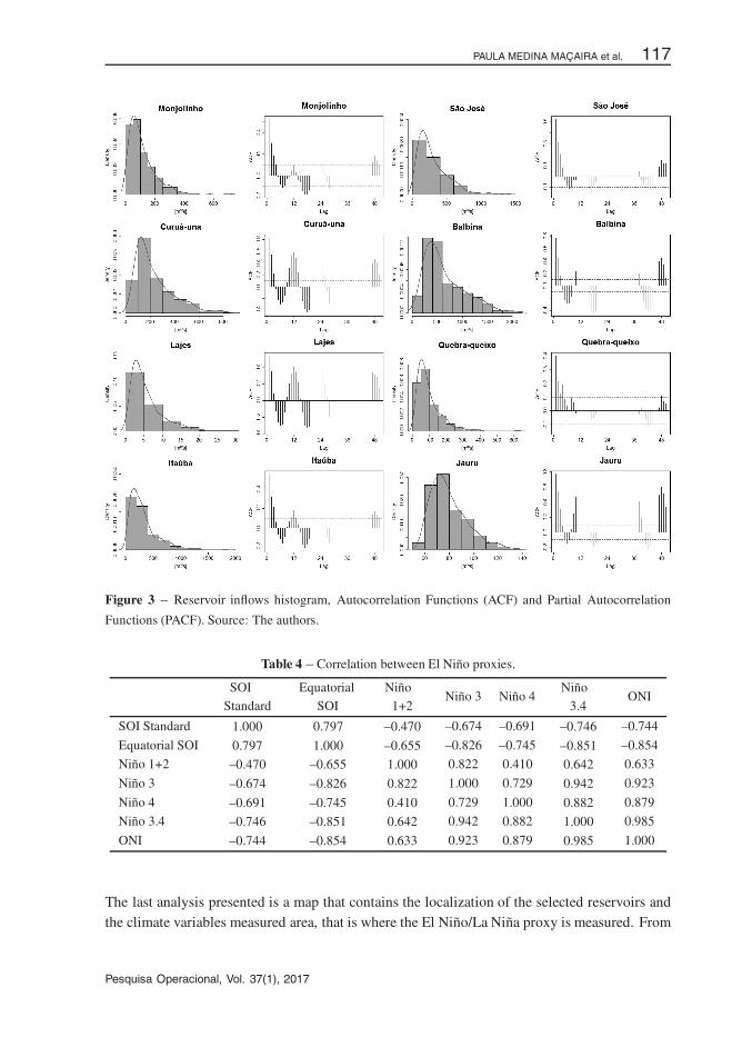
In the first and third columns of Figure 3 the histogram of each reservoir series is presented.It seems quite clear that there is a strong asymmetry indicating that the data might follow a

Weibull distribution, which is the distribution that usually models natural events. The secondand fourth columns shows the Autocorrelation Functions (ACF) and from them it is possible toconfirm the presence of periodicity by observing significantly picks each six months.

Moving now to the climate variables, in Table 3 it is presented the descriptive statistics for each

climate variables available. Note that the values presented in the table rely on the same range

5The results were significant at 1% level


�

�

“main” — 2017/5/2 — 20:06 — page 115 — #9�

�

�

�

�

�


Fig

ure

2–

Res

ervo

irs

infl

ow,t

ime

seri

esfr

omJa

nuar

y19

82up

toD

ecem

ber2

014.

Sou

rce:

The

auth

ors.


�

�

“main” — 2017/5/2 — 20:06 — page 116 — #10�

�

�

�

�

�


Table 2 – Descriptive analyses of the reservoirs inflows.

Mean Median Std. Dev. Min. Max.1st

quartile3rd

quartile

Monjolinho 114.83 85.61 99.59 2.63 702.00 46.30 153.34

Sao Jose 302.43 231.05 236.66 24.93 1435.00 135.00 411.15Curua-una 229.00 178.21 151.57 44.81 826.80 115.60 304.70

Balbina 640.56 510.97 411.69 19.00 2115.20 321.90 878.90

Lajes 5.71 4.37 4.51 0.409 29.70 2.50 7.29Quebra-queixo 96.89 74.25 74.50 11.00 621.00 46.9 125.25

Itauba 303.67 238.97 240.72 35.83 1816.00 133.8 391.25

Jauru 79.85 76.86 14.79 56.851 135.00 69.00 88.00

Table 3 – Descriptive statistics of the climate variables.

Mean Median Std. Dev. Min. Max.1st

quartile3rd

quartile

SOI Standard 0.025 0.000 1.006 –3.600 2.900 –0.600 0.700

Equatorial SOI 0.017 0.100 1.030 –3.500 3.000 –0.500 0.700Nino 1+2 0.081 –0.180 1.210 –2.100 4.620 –0.740 0.590

Nino 3 0.046 –0.130 0.994 –2.070 3.620 –0.605 0.562

Nino 4 0.035 0.190 0.721 –1.870 1.670 –0.510 0.600Nino 3.4 0.034 0.005 0.970 –2.380 2.950 –0.602 0.595

ONI 0.053 –0.010 0.836 –1.780 2.370 –0.520 0.552

Sunspots 60.117 56.600 44.311 1.700 158.500 19.050 91.225

except for the Sunspots variable. In fact the first seven variables measure exactly the same events:

El Nino/La Nina, while the latter variable measures the sunspots events.

One important point to check is the presence of significant correlations between the variousEl Nino series. Table 4 shows the Pearson correlations6, and as expected, there is a negativecorrelation between the Equatorial SOI and the SOI index with the others, as for those, El Nino

is represented by negative values, while for other variables, this same phenomenon is representedby positive values. Also note that ONI and Nino 3.4 show the highest correlation, a consistentresult with their concepts, since both measure the sea surface temperature anomaly in the same

region.

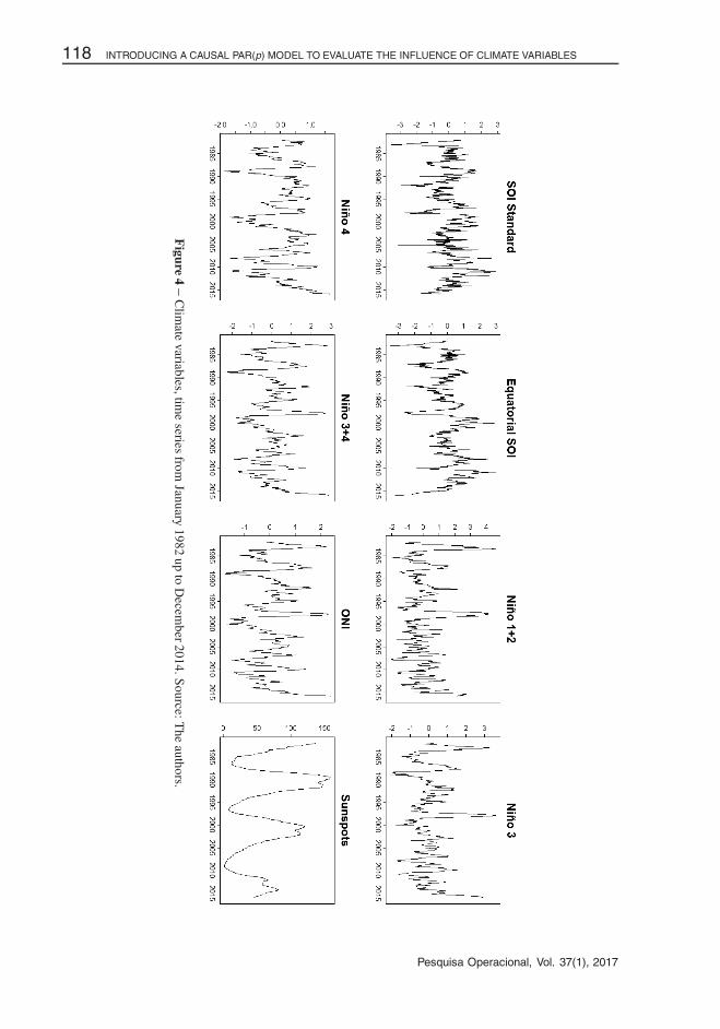
Figure 4 shows each climate variable evolution through time, highlighting that for the variablesrepresenting El Nino events, the extreme values coincide with stronger El Nino or La Nina oc-currences. It is also observed the strong 11 year cycle presented in the time series of Sunspots.

6The results were significant at 1% level


�

�

“main” — 2017/5/2 — 20:06 — page 117 — #11�

�

�

�

�

�


Figure 3 – Reservoir inflows histogram, Autocorrelation Functions (ACF) and Partial Autocorrelation

Functions (PACF). Source: The authors.

Table 4 – Correlation between El Nino proxies.

SOIStandard

EquatorialSOI

Nino1+2

Nino 3 Nino 4Nino

3.4ONI

SOI Standard 1.000 0.797 –0.470 –0.674 –0.691 –0.746 –0.744

Equatorial SOI 0.797 1.000 –0.655 –0.826 –0.745 –0.851 –0.854

Nino 1+2 –0.470 –0.655 1.000 0.822 0.410 0.642 0.633

Nino 3 –0.674 –0.826 0.822 1.000 0.729 0.942 0.923

Nino 4 –0.691 –0.745 0.410 0.729 1.000 0.882 0.879

Nino 3.4 –0.746 –0.851 0.642 0.942 0.882 1.000 0.985

ONI –0.744 –0.854 0.633 0.923 0.879 0.985 1.000

The last analysis presented is a map that contains the localization of the selected reservoirs andthe climate variables measured area, that is where the El Nino/La Nina proxy is measured. From


�

�

“main” — 2017/5/2 — 20:06 — page 118 — #12�

�

�

�

�

�


Figure

4–

Clim

atevariables,tim

eseries

fromJanuary

1982up

toD

ecember2014.S

ource:The

authors.


�

�

“main” — 2017/5/2 — 20:06 — page 119 — #13�

�

�

�

�

�


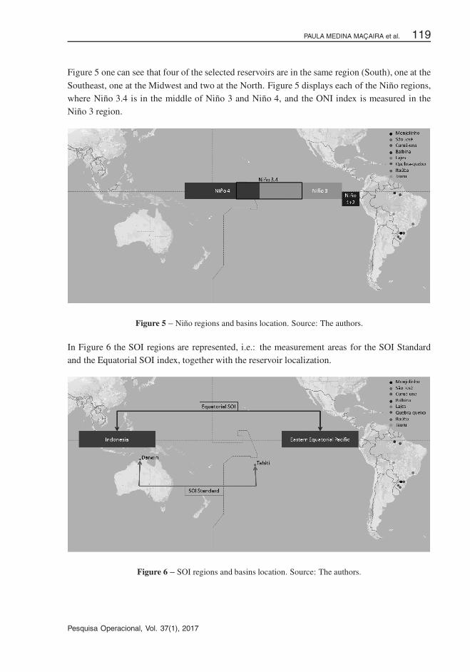
Figure 5 one can see that four of the selected reservoirs are in the same region (South), one at the

Southeast, one at the Midwest and two at the North. Figure 5 displays each of the Nino regions,where Nino 3.4 is in the middle of Nino 3 and Nino 4, and the ONI index is measured in theNino 3 region.

Figure 5 – Nino regions and basins location. Source: The authors.

In Figure 6 the SOI regions are represented, i.e.: the measurement areas for the SOI Standardand the Equatorial SOI index, together with the reservoir localization.

Figure 6 – SOI regions and basins location. Source: The authors.


�

�

“main” — 2017/5/2 — 20:06 — page 120 — #14�

�

�

�

�

�


5 RESULTS

In order to evaluate the proposed methodology, the causal PAR(p) approach was applied to modelthe eight reservoirs inflow series previously presented. The set of possible input variables are the

variables representing El Nino/La Nina and Sunspots phenomenon. Since the proposed approachhas been developed to improve the current model it will be shown comparisons between thetraditional PAR(p) and the causal. The last result obtained is the generation of scenarios with

both approaches and a comparison with real values.

In order to carry out an out-of-sample analysis, the last year of the available data (2014) wasomitted from the initial analysis. So, the modelling set is the data ranging from January 1982 upto December 2013, resulting in 384 observations or 32 years. It is worth mentioning that all the

results were generated using the R software [26] and the packages pear [15], TSA [4], tseries[30] and dynlm [33].

To estimate the models performance, three metrics were considered: the Mean Absolute ScaledError (MASE), given by

M AS E = 1

n

n∑t=1

(|Yt − Ft |

1n−1

∑ni=2 |Yi − Yi−1|

), (4)

the Mean Absolute Percentage Error (MAPE), given by

M AP E = 1

n

n∑t=1

∣∣∣∣Yt − Ft

Yt

∣∣∣∣ , (5)

and the Root Mean Squared Error (RMSE), given by

RM S E =√√√√1

n

n∑t=1

(Yt − Ft )2, (6)

where Yt is the observed value, Ft is the fitted value and n is the sample size.

5.1 Modelling reservoirs inflow series

As detailed before, the first step of the model is to fit the traditional PAR(p) to each of the

reservoir inflow series. There are many ways to select the best PAR(p) model, i.e. the model’sorder, [31], for example, applied a genetic algorithm, while [19] uses the Bootstrap technique.Using information criterion is a common approach to select the best model, more specifically

Akaike’s Information Criterion (AIC) and Schwarz’s Bayesian Information Criterion (BIC) [1].Both criteria are based on the likelihood function and a penalization term for the number ofparameters in the model, however AIC is better for prediction as it is asymptotically equivalent

to cross-validation, while BIC is best for explanation as it allows consistent estimation of theunderlying data generating process. Since the ultimate goal is to analyse the out-of-sample modelperformance, in this work it is used the AIC criterion to select the PAR(p) orders.


�

�

“main” — 2017/5/2 — 20:06 — page 121 — #15�

�

�

�

�

�


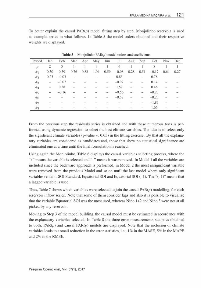
To better explain the causal PAR(p) model fitting step by step, Monjolinho reservoir is used

as example series in what follows. In Table 5 the model orders obtained and their respectiveweights are displayed.

Table 5 – Monjolinho PAR(p) model orders and coefficients.

Period Jan Feb Mar Apr May Jun Jul Aug Sep Oct Nov Dec

p 2 5 1 1 1 1 6 1 1 8 1 1

φ1 0.30 0.39 0.76 0.88 1.04 0.59 –0.08 0.28 0.51 –0.17 0.64 0.27φ2 0.23 –0.03 – – – – 0.83 – – 0.78 – –

φ3 – –0.07 – – – – –0.97 – – 0.14 – –φ4 – 0.38 – – – – 1.57 – – 0.46 – –

φ5 – –0.16 – – – – –0.56 – – –0.23 – –φ6 – – – – – – –0.57 – – –0.23 – –

φ7 – – – – – – – – – –1.83 – –φ8 – – – – – – – – – 1.66 – –

From the previous step the residuals series is obtained and with these numerous tests is per-formed using dynamic regression to select the best climate variables. The idea is to select only

the significant climate variables (p-value < 0.05) in the fitting exercise. By that all the explana-tory variables are considered as candidates and, those that show no statistical significance areeliminated one at a time until the final formulation is reached.

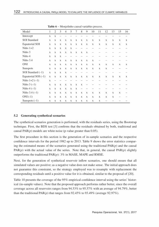
Using again the Monjolinho, Table 6 displays the causal variables selecting process, where the

“x” means the variable is selected and “–” means it was removed. In Model 1 all the variables areincluded since the backward approach is performed, in Model 2 the most insignificant variablewere removed from the previous Model and so on until the last model where only significant

variables remain: SOI Standard, Equatorial SOI and Equatorial SOI (–1). The “(–1)” means thata lagged variable is used.

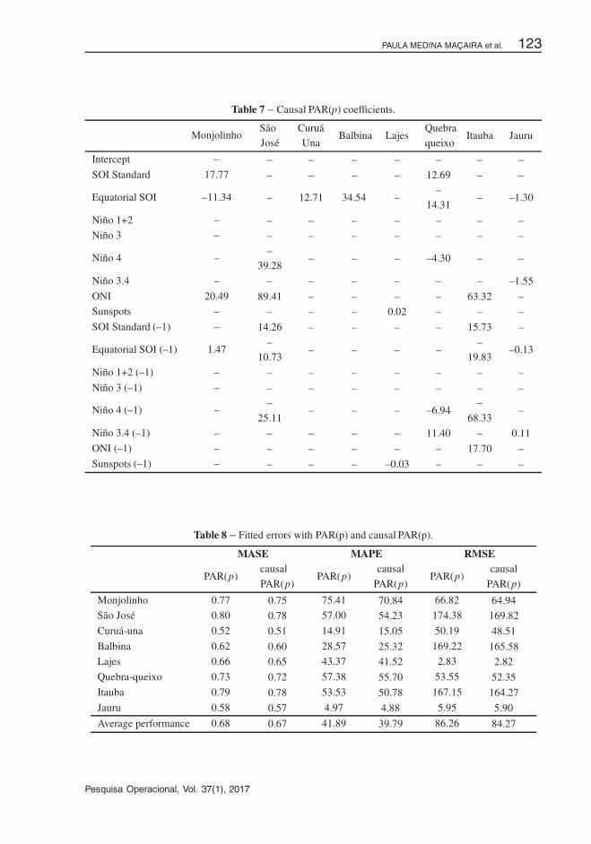
Thus, Table 7 shows which variables were selected to join the causal PAR(p) modelling, for eachreservoir inflow series. Note that some of them consider lags and also it is possible to visualize

that the variable Equatorial SOI was the most used, whereas Nino 1+2 and Nino 3 were not at allpicked by any reservoir.

Moving to Step 3 of the model building, the causal model must be estimated in accordance withthe explanatory variables selected. In Table 8 the three error measurements statistics obtained

to both, PAR(p) and causal PAR(p) models are displayed. Note that the inclusion of climatevariables leads to a small reduction in the error statistics, i.e., 1% in the MASE, 5% in the MAPEand 2% in the RMSE.


�

�

“main” — 2017/5/2 — 20:06 — page 122 — #16�

�

�

�

�

�


Table 6 – Monjolinho causal variables process.

Model 1 2 3 4 5 7 8 9 10 11 12 13 15 16

Intercept x x – – – – – – – – – – – –

SOI Standard x x x x x x x x x x x x x x

Equatorial SOI x x x x x x x x x x x x x xNino 1+2 x x x x x – – – – – – – – –

Nino 3 x x x x x x x x – – – – – –Nino 4 x x x – – – – – – – – – – –

Nino 3.4 x x x x x x x x x – – – – –ONI x x x x x x x x x x x x x x

Sunspots x x x x x x x x x x x – – –SOI Standard (–1) x x x x – – – – – – – – – –

Equatorial SOI (–1) x x x x x x x x x x x x x xNino 1+2 (–1) x – – – – – – – – – – – – –

Nino 3 (–1) x x x x x x x – – – – – – –Nino 4 (–1) x x x x x x – – – – – – – –

Nino 3.4 (–1) x x x x x x x x x x x x x –

ONI (-1) x x x x x x x x x x x x – –Sunspots (–1) x x x x x x x x x x – – – –

5.2 Generating synthetical scenarios

The synthetical scenarios generation is performed, with the residuals series, using the Bootstraptechnique. First, the BDS test [3] confirms that the residuals obtained by both, traditional andcausal PAR(p) models are white noise (p-value greater than 0.05).

The first procedure in this section is the generation of in-sample scenarios and the respective

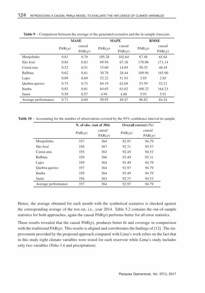
confidence intervals for the period 1982 up to 2013. Table 9 shows the error statistics compar-ing the estimated means of the scenarios generated using the traditional PAR(p) and the causalPAR(p) with the actual value of the series. Note that, in general, the causal PAR(p) slightly

outperforms the traditional PAR(p): 3% in MASE, MAPE and RMSE.

Next, for the generation of synthetical reservoir inflow scenarios, one should ensure that allsimulated values are positive; as a negative value does not make sense. The initial approach doesnot guarantee this constraint, so the strategy employed was to resample with replacement the

corresponding residuals until a positive value for it is obtained, similar to the proposal of [20].

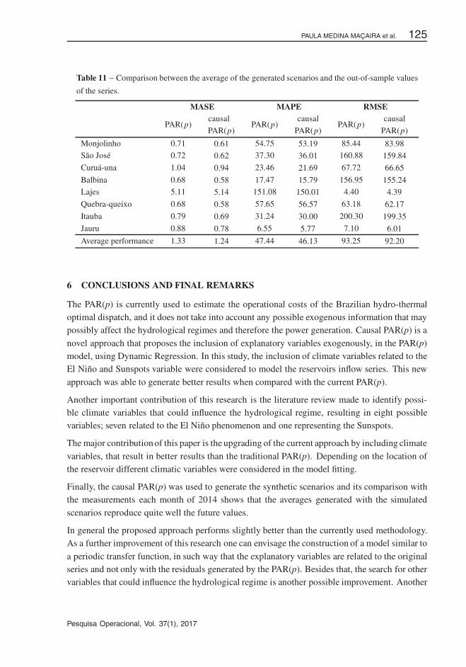
Table 10 presents the coverage of the 95% empirical confidence interval using the series’ histor-ical (in-sample values). Note that the proposed approach performs rather better, since the overallcoverage across all reservoirs ranges from 94.53% to 95.57% with an average of 94.79%, better

than the traditional PAR(p) that ranges from 92.45% to 93.49% (average 92.97%).


�

�

“main” — 2017/5/2 — 20:06 — page 123 — #17�

�

�

�

�

�


Table 7 – Causal PAR(p) coefficients.

MonjolinhoSaoJose

CuruaUna

Balbina LajesQuebraqueixo

Itauba Jauru

Intercept – – – – – – – –

SOI Standard 17.77 – – – – 12.69 – –

Equatorial SOI –11.34 – 12.71 34.54 ––

14.31– –1.30

Nino 1+2 – – – – – – – –Nino 3 – – – – – – – –

Nino 4 ––

39.28– – – –4.30 – –

Nino 3.4 – – – – – – – –1.55

ONI 20.49 89.41 – – – – 63.32 –Sunspots – – – – 0.02 – – –

SOI Standard (–1) – 14.26 – – – – 15.73 –

Equatorial SOI (–1) 1.47–

10.73– – – –

–19.83

–0.13

Nino 1+2 (–1) – – – – – – – –

Nino 3 (–1) – – – – – – – –

Nino 4 (–1) ––

25.11– – – –6.94

–

68.33–

Nino 3.4 (–1) – – – – – 11.40 – 0.11

ONI (–1) – – – – – – 17.70 –

Sunspots (–1) – – – – –0.03 – – –

Table 8 – Fitted errors with PAR(p) and causal PAR(p).

MASE MAPE RMSE

PAR(p)causal

PAR(p)PAR(p)

causal

PAR(p)PAR(p)

causal

PAR(p)

Monjolinho 0.77 0.75 75.41 70.84 66.82 64.94Sao Jose 0.80 0.78 57.00 54.23 174.38 169.82

Curua-una 0.52 0.51 14.91 15.05 50.19 48.51

Balbina 0.62 0.60 28.57 25.32 169.22 165.58Lajes 0.66 0.65 43.37 41.52 2.83 2.82

Quebra-queixo 0.73 0.72 57.38 55.70 53.55 52.35

Itauba 0.79 0.78 53.53 50.78 167.15 164.27

Jauru 0.58 0.57 4.97 4.88 5.95 5.90

Average performance 0.68 0.67 41.89 39.79 86.26 84.27


�

�

“main” — 2017/5/2 — 20:06 — page 124 — #18�

�

�

�

�

�


Table 9 – Comparison between the average of the generated scenarios and the in-sample forecasts.

MASE MAPE RMSE

PAR(p)causal

PAR(p)PAR(p)

causal

PAR(p)PAR(p)

causal

PAR(p)


Curua-una 0.52 0.51 15.60 14.95 50.35 48.45

Balbina 0.62 0.61 30.78 28.44 169.94 165.90Lajes 0.69 0.69 52.22 51.93 2.85 2.85

Quebra-queixo 0.75 0.73 64.19 62.69 53.59 52.21

Itauba 0.83 0.81 64.65 63.02 168.32 164.23Jauru 0.58 0.57 4.94 4.88 5.93 5.91


Table 10 – Accounting for the number of observations covered by the 95% confidence interval in-sample.

N. of obs. (out of 384) Overall correct (%)

PAR(p)causalPAR(p)

PAR(p)causalPAR(p)

Monjolinho 357 364 92.97 94.79

Sao Jose 356 367 92.71 95.57Curua-una 355 363 92.45 94.53

Balbina 359 366 93.49 95.31

Lajes 359 364 93.49 94.79Quebra-queixo 357 364 92.97 94.79

Itauba 359 364 93.49 94.79

Jauru 356 363 92.71 94.53

Average performance 357 364 92.97 94.79

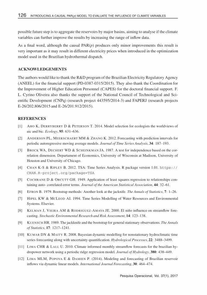
Hence, the average obtained for each month with the synthetical scenarios is checked against

the corresponding average of the test set, i.e., year 2014. Table 5.2 contains the out-of-samplestatistics for both approaches, again the causal PAR(p) performs better for all error statistics.

These results revealed that the causal PAR(p), produces better fit and coverage in comparisionwith the traditional PAR(p). This results is aligned and corroborates the findings of [12]. The im-

provement provided by the proposed approach compared with Lima’s work relies on the fact thatin this study eight climate variables were tested for each reservoir while Lima’s study includesonly two variables (Nino 3.4 and precipitation).


�

�

“main” — 2017/5/2 — 20:06 — page 125 — #19�

�

�

�

�

�


Table 11 – Comparison between the average of the generated scenarios and the out-of-sample values

of the series.

MASE MAPE RMSE

PAR(p)causal

PAR(p)PAR(p)

causal

PAR(p)PAR(p)

causal

PAR(p)


Curua-una 1.04 0.94 23.46 21.69 67.72 66.65

Balbina 0.68 0.58 17.47 15.79 156.95 155.24Lajes 5.11 5.14 151.08 150.01 4.40 4.39

Quebra-queixo 0.68 0.58 57.65 56.57 63.18 62.17

Itauba 0.79 0.69 31.24 30.00 200.30 199.35

Jauru 0.88 0.78 6.55 5.77 7.10 6.01


6 CONCLUSIONS AND FINAL REMARKS

The PAR(p) is currently used to estimate the operational costs of the Brazilian hydro-thermaloptimal dispatch, and it does not take into account any possible exogenous information that maypossibly affect the hydrological regimes and therefore the power generation. Causal PAR(p) is a

novel approach that proposes the inclusion of explanatory variables exogenously, in the PAR(p)model, using Dynamic Regression. In this study, the inclusion of climate variables related to theEl Nino and Sunspots variable were considered to model the reservoirs inflow series. This new

approach was able to generate better results when compared with the current PAR(p).

Another important contribution of this research is the literature review made to identify possi-ble climate variables that could influence the hydrological regime, resulting in eight possiblevariables; seven related to the El Nino phenomenon and one representing the Sunspots.

The major contribution of this paper is the upgrading of the current approach by including climate

variables, that result in better results than the traditional PAR(p). Depending on the location ofthe reservoir different climatic variables were considered in the model fitting.

Finally, the causal PAR(p) was used to generate the synthetic scenarios and its comparison withthe measurements each month of 2014 shows that the averages generated with the simulated

scenarios reproduce quite well the future values.

In general the proposed approach performs slightly better than the currently used methodology.As a further improvement of this research one can envisage the construction of a model similar to

a periodic transfer function, in such way that the explanatory variables are related to the originalseries and not only with the residuals generated by the PAR(p). Besides that, the search for othervariables that could influence the hydrological regime is another possible improvement. Another


�

�

“main” — 2017/5/2 — 20:06 — page 126 — #20�

�

�

�

�

�


possible future step is to aggregate the reservoirs by major basins, aiming to analyse if the climate

variables can further improve the results by increasing the range of inflow data.

As a final word, although the causal PAR(p) produces only minor improvements this result isvery important as it may result in different electricity prices when introduced in the optimizationmodel used in the Brazilian hydrothermal dispatch.

ACKNOWLEDGEMENTS

The authors would like to thank the R&D program of the Brazilian Electricity Regulatory Agency

(ANEEL) for the financial support (PD-0387-0315/2015). They also thank the Coordination forthe Improvement of Higher Education Personnel (CAPES) for the doctoral financial support. F.L. Cyrino Oliveira also thanks the support of the National Council of Technological and Sci-

entific Development (CNPq) (research project 443595/2014-3) and FAPERJ (research projectsE-26/202.806/2015 and E-26/201.912/2015).

REFERENCES

[1] AHO K, DERRYBERRY D & PETERSON T. 2014. Model selection for ecologists the worldviews of

aic and bic. Ecology, 95: 631–636.

[2] ANDERSON PL, MEERSCHAERT MM & ZHANG K. 2012. Forecasting with prediction intervals forperiodic autoregressive moving average models. Journal of Time Series Analysis, 34: 187–193.

[3] BROCK WA, DECHERT WD & SCHEINKMAN JA. 1987. A test for independence based on the cor-

relation dimension. Departament of Economics, University of Wisconsin at Madison, University ofHouston and University of Chicago.

[4] CHAN K-S & RIPLEY B. 2012. TSA: Time Series Analysis. R package version 1.01. https://

CRAN.R-project.org/package=TSA

[5] COCHRANE D & ORCUTT GH. 1949. Application of least squares regression to relationships con-taining auto- correlated error terms. Journal of the American Statistical Association, 44: 32–61.

[6] EFRON B. 1979. Bootstrap methods: Another look at the jacknife. The Annals of Statistics, 7: 1–26.

[7] HIPEL KW & MCLEOD AI. 1994. Time Series Modelling of Water Resources and EnvironmentalSystems. Elsevier.

[8] KELMAN J, VIEIRA AM & RODRIGUEZ-AMAYA JE. 2000. El nino influence on streamflow fore-

casting. Stochastic Environmental Research and Risk Assessment, 14: 123–138.

[9] KUENSCH HR. 1989. The jackknife and the bootstrap for general stationary observations. The Annals

of Statistics, 17: 1217–1241.

[10] KUMAR DN & MAITY R. 2008. Bayesian dynamic modelling for nonstationary hydroclimatic time

series forecasting along with uncertainty quantification. Hydrological Processes, 22: 3488–3499.

[11] LIMA CHR & LALL U. 2010. Climate informed monthly streamflow forecasts for the brazilian hy-

dropower network using a periodic ridge regression model. Journal of Hydrology, 380: 438–449.

[12] LIMA MLM, POPOVA E & DAMIEN P. (2014). Modeling and forecasting of Brazilian reservoirinflows via dynamic linear models. International Journal Forecasting, 30: 464–474.


�

�

“main” — 2017/5/2 — 20:06 — page 127 — #21�

�

�

�

�

�


[13] MACEIRA MEP & DAMAZIO JM. 2006. Use of the Par(p) Model in the Stochastic Dual Dynamic

Programming Optimization Scheme Used in the Operation Planning of the Brazilian HydropowerSystem. Probability in the Engineering and Informational Sciences, 20: 143–156.

[14] MAITY R & KUMAR DN. 2008. Basin-scale stream-flow forecasting using the information of

large-scale atmospheric circulation phenomena. Hydrological Processes, 22: 643–650.

[15] MCLEOD AI. 1994. Diagnostic checking periodic autoregression models with applications. Journal

of Time Series Analysis, 15: 221–233.

[16] MONDAL MS & WASIMI SA. 2006. Generating and forecasting monthly flows of the ganges river

with PAR model. Journal of Hydrology, 323: 41–56.

[17] NOAA. 2016. February. Climate Prediction Center. National Oceanic and Atmospheric Administra-

tion. www.cpc.ncep.noaa.gov/data/indices/

[18] OLIVEIRA FLC. 2010. Nova abordagem para geracao de cenarios de afluencias no planejamento daoperacao energetica de medio prazo. Pontifıcia Universidade Catolica do Rio de Janeiro.

[19] OLIVEIRA FLC & SOUZA RC. 2011. A new approach to identify the structural order of par (p)models. Pesquisa Opracional, 31: 487–498.

[20] OLIVEIRA FLC, SOUZA RC & MARCATO ALM. 2015. A time series model for building scenariostrees applied to stochastic optimisation. International Journal of Electrical Power & Energy Systems,

67: 16–38.

[21] ONS. 2014. October. Operador Nacional do Sistema Eletrico. www.ons.com.br

[22] ONS. 2015. Atualizacao de Series Historicas de Vazoes, perıodo 1931 a 2014. Technical report,

Operador Nacional do Sistema Eletrico.

[23] OTEXTS. 2016. February. Forecasting: principles and practice, advanced forecasting methods, dy-

namic regression models. Texts: online, open-access textbooks. https://www.otexts.org/fpp/9/1

[24] PEREIRA MVF. 1989. Optimal stochastic operations scheduling of large hydroeletric systems.International Journal of Eletric Power and Energy Systems, 11: 161–169.

[25] PINGUELLI LR, FIDELIS NS, GIANNINI MP & DIAS LL. 2013. Evolution of Global Electricity

Markets: New Paradigms, New Challenges, New Approaches. Academic Press. 435–459.

[26] R CORE TEAM. 2015. R: A Language and Environment for Statistical Computing. Vienna, Austria:

R Foundation for Statistical Computing. https://www.R-project.org/

[27] RAVINES RR, SCHMIDT AM, MIGON HS & RENNO CD. 2008. A joint model for rainfall-runoff:

the case of Rio Grande basin. Journal of Hydrology, 353: 189–200.

[28] SOUZA FILHO FA & LALL. 2003. Seasonal to interannual ensemble streamflow forecasts for Ceara,

Brazil: applications of a multivariate, semiparametric algorithm. Water Resources Research, 39(11):1–13.

[29] TERRY LA, PEREIRA MVF, NETO TA, SILVA LFCA & SALES PRH. 1986. Coordinating the

Energy Generation of the Brazilian National Hydrothermal Electrical Generating System. Interfaces,16: 16 p.

[30] TRAPLETTI A & HORNIK K. 2015. tseries: Time Series Analysis and Computational Finance. Rpackage version 0.10-34. http://CRAN.R-project.org/package=tseries


�

�

“main” — 2017/5/2 — 20:06 — page 128 — #22�

�

�

�

�

�


[31] URSU E & TURKMAN KF. 2012. Periodic autoregressive model identification using genetic algo-

rithms. Journal of Time Series Analysis, 33: 398–405.

[32] UVO CB & GRAHAM NE. 1998. Seasonal runoff forecast for northern South America: a statistical

model. Water Resources Research, 34(12): 3515–3524.

[33] ZEILEIS A. 2014. dynlm: Dynamic Linear Regression. R package version 0.3-3. http://CRAN.

R-project.org/package=dynlm


Paula Medina Mac¸aira , Fernando Luiz Cyrino Oliveira ... · Paula Medina Mac¸aira1*, Fernando...

Documents

Transcript of Paula Medina Mac¸aira , Fernando Luiz Cyrino Oliveira ... · Paula Medina Mac¸aira1*, Fernando...