Opportunistic Communication in Extreme Wireless Sensor ... · Networks (EWSNs), where resources are...
107
O PPORTUNISTIC C OMMUNICATION IN E XTREME WIRELESS S ENSOR N ETWORKS MARCO C ATTANI
Transcript of Opportunistic Communication in Extreme Wireless Sensor ... · Networks (EWSNs), where resources are...

OPPORTUNISTIC COMMUNICATION INEXTREME WIRELESS SENSOR NETWORKS
MARCO CATTANI


OPPORTUNISTIC COMMUNICATION INEXTREME WIRELESS SENSOR NETWORKS
MARCO CATTANI
Proefschrift
ter verkrijging van de graad van doctoraan de Technische Universiteit Delft,
op gezag van de Rector Magnificus prof. ir. K. C. A. M. Luyben,voorzitter van het College voor Promoties,
in het openbaar te verdedigen opwoensdag 28 september 2016 om 15:00 uur
door
Marco CATTANI
Laurea Informatica, Università degli Studi di Trento, Italiëgeboren te Trento, Italië.

This dissertation has been approved by the
promotor: Prof. Dr. K. G. Langendoen andcopromotor: Dr. M. A. Zúñiga
Composition of the doctoral committee:
Rector MagnificusProf. Dr. K. G. Langendoen, promotorDr. M. A. Zúñiga, copromotor
Independent members:
Prof. Dr. D. Epema, EEMCS, TU DelftDr. F. Kuipers, EEMCS, TU DelftDr. O. Landsiedel, Chalmers University of TechnologyProf. Dr. M. van Steen, University of TwenteProf. Dr. T. Voigt, Uppsala UniversityProf. Dr. G. J. Houben, EEMCS, TU Delft, reserve member
Copyright © 2016 by M. Cattani. All rights reserved. No part of the material protected bythis copyright may be reproduced or utilized in any form or by any means, without the priorpermission of the author.
ISBN 978-94-6233-386-4
An electronic version of this dissertation is available athttp://repository.tudelft.nl/.
This work was carried out in the TU Delft Graduate chool.
This work was carried out in the ASCI graduate school. ASCIdissertation series number 362.
This work was funded by the Dutch national programCOMMIT/ under the project P09 EWiDS.
“There are always possibilities”
Spock

CONTENTS
1 Introduction 11.1 Wireless Sensor Networks . . . . . . . . . . . . . . . . . . . . . . . . . . . . 21.2 Problem Statement . . . . . . . . . . . . . . . . . . . . . . . . . . . . . . . 51.3 Thesis Contributions and Outline . . . . . . . . . . . . . . . . . . . . . . . . 6
2 Medium Access Control and Data Dissemination 92.1 Related Work . . . . . . . . . . . . . . . . . . . . . . . . . . . . . . . . . . 102.2 Problem Statement . . . . . . . . . . . . . . . . . . . . . . . . . . . . . . . 112.3 Mechanism . . . . . . . . . . . . . . . . . . . . . . . . . . . . . . . . . . . 12
2.3.1 The basic idea . . . . . . . . . . . . . . . . . . . . . . . . . . . . . . 122.3.2 Short rendezvous phase . . . . . . . . . . . . . . . . . . . . . . . . . 132.3.3 Reliable push-pull data exchange . . . . . . . . . . . . . . . . . . . . 142.3.4 Random Peer sampling . . . . . . . . . . . . . . . . . . . . . . . . . 16
2.4 Implementation . . . . . . . . . . . . . . . . . . . . . . . . . . . . . . . . 162.5 Evaluation . . . . . . . . . . . . . . . . . . . . . . . . . . . . . . . . . . . 17
2.5.1 Performance metrics. . . . . . . . . . . . . . . . . . . . . . . . . . . 172.5.2 Results . . . . . . . . . . . . . . . . . . . . . . . . . . . . . . . . . . 182.5.3 Exploring SOFA parameters . . . . . . . . . . . . . . . . . . . . . . . 182.5.4 SOFA under extreme densities and in mobile scenarios . . . . . . . . . 20
2.6 Conclusions. . . . . . . . . . . . . . . . . . . . . . . . . . . . . . . . . . . 22
3 Neighborhood Cardinality Estimation 233.1 Problem Statement . . . . . . . . . . . . . . . . . . . . . . . . . . . . . . . 243.2 Mechanism . . . . . . . . . . . . . . . . . . . . . . . . . . . . . . . . . . . 24
3.2.1 Timing inaccuracies . . . . . . . . . . . . . . . . . . . . . . . . . . . 263.3 Implementation . . . . . . . . . . . . . . . . . . . . . . . . . . . . . . . . 27
3.3.1 Naive implementation . . . . . . . . . . . . . . . . . . . . . . . . . . 273.3.2 Correct observations . . . . . . . . . . . . . . . . . . . . . . . . . . . 283.3.3 Accurate measurements . . . . . . . . . . . . . . . . . . . . . . . . . 293.3.4 Improving the estimation process . . . . . . . . . . . . . . . . . . . . 30
3.4 Evaluation . . . . . . . . . . . . . . . . . . . . . . . . . . . . . . . . . . . 313.4.1 Results . . . . . . . . . . . . . . . . . . . . . . . . . . . . . . . . . . 33
3.5 Related work . . . . . . . . . . . . . . . . . . . . . . . . . . . . . . . . . . 373.6 Conclusion . . . . . . . . . . . . . . . . . . . . . . . . . . . . . . . . . . . 39
4 Opportunistic Data collection 414.1 Problem Statement . . . . . . . . . . . . . . . . . . . . . . . . . . . . . . . 434.2 Staffetta . . . . . . . . . . . . . . . . . . . . . . . . . . . . . . . . . . . . . 44
4.2.1 Activity Gradient. . . . . . . . . . . . . . . . . . . . . . . . . . . . . 454.2.2 Analysis . . . . . . . . . . . . . . . . . . . . . . . . . . . . . . . . . 464.2.3 Understanding Staffetta’s Performance Gains. . . . . . . . . . . . . . . 47
vii
viii CONTENTS
4.3 Implementation . . . . . . . . . . . . . . . . . . . . . . . . . . . . . . . . 494.3.1 Baseline . . . . . . . . . . . . . . . . . . . . . . . . . . . . . . . . . 494.3.2 Routing Metrics . . . . . . . . . . . . . . . . . . . . . . . . . . . . . 504.3.3 Staffetta . . . . . . . . . . . . . . . . . . . . . . . . . . . . . . . . . 52
4.4 Evaluation . . . . . . . . . . . . . . . . . . . . . . . . . . . . . . . . . . . 534.4.1 Methodology. . . . . . . . . . . . . . . . . . . . . . . . . . . . . . . 534.4.2 Comparison against the State of the Art . . . . . . . . . . . . . . . . . 544.4.3 Benefits across Diverse Routing Metrics . . . . . . . . . . . . . . . . . 554.4.4 Adaptiveness to Mobile Sink Dynamics . . . . . . . . . . . . . . . . . 594.4.5 Using Staffetta’s Activity Gradient for Efficient Routing. . . . . . . . . . 60
4.5 Related work . . . . . . . . . . . . . . . . . . . . . . . . . . . . . . . . . . 614.6 Conclusions. . . . . . . . . . . . . . . . . . . . . . . . . . . . . . . . . . . 63
5 Crowd Monitoring in The Wild 655.1 Related Work . . . . . . . . . . . . . . . . . . . . . . . . . . . . . . . . . . 68
5.1.1 Evaluated Methods. . . . . . . . . . . . . . . . . . . . . . . . . . . . 695.2 Density analysis. . . . . . . . . . . . . . . . . . . . . . . . . . . . . . . . . 70
5.2.1 Estimation accuracy . . . . . . . . . . . . . . . . . . . . . . . . . . . 705.2.2 Coverage versus Overlap . . . . . . . . . . . . . . . . . . . . . . . . . 715.2.3 Effects of Crowd Dynamics. . . . . . . . . . . . . . . . . . . . . . . . 73
5.3 Popularity Analysis . . . . . . . . . . . . . . . . . . . . . . . . . . . . . . . 755.3.1 Attractiveness . . . . . . . . . . . . . . . . . . . . . . . . . . . . . . 77
5.4 Conclusions. . . . . . . . . . . . . . . . . . . . . . . . . . . . . . . . . . . 78
6 Conclusions 796.1 Regard challenges as opportunities . . . . . . . . . . . . . . . . . . . . . . . 796.2 Building on top of opportunistic primitives . . . . . . . . . . . . . . . . . . . 806.3 Extreme Wireless Sensor Networks in practice . . . . . . . . . . . . . . . . . 806.4 Future Work. . . . . . . . . . . . . . . . . . . . . . . . . . . . . . . . . . . 81
References 83
Summary 93
Samenvatting 95
List of Publications 97
ACKNOWLEDGMENTS
This thesis is the result of few “eureka” moments, surrounded by much work, fun, coffee andpersonal experiences. For these vital ingredients, I need to thank a large crowd of extremelyspecial persons. To me, you are all colleagues, family and friends.
First of all, I want to thank my mentor and supervisor Koen Langendoen. Through yourkoenification and Dutch pragmatic attitude, you showed me how to be a better person anda more thorough researcher. You also provided me two inspiring supervisors that were keyto my first research successes. Matthias gave me the right research directions and taughtme how to fight for my ideas. Marco showed me the power of being perseverant and alwayspositive about things. Through his countless comments, Marco patiently taught me how todeeply analyze a problem and clearly present my solution (in proper English!).
Along with my supervisors, I had many brilliant colleagues and students who were al-ways available to listen to my weird ideas and to give me their feedback. I want to especiallythank Niels and Przemek for their blunt opinions and advices. Marco, Federico, Carlo andFrederick, whose exceptional research inspired and motivated me throughout my PhD. An-dreas, for the countless conversations we had about research, movies, books and food. Pla-ton and Dimitris, students who chose and trusted me as their supervisor and of whom I amreally proud. Claudio, who shared with me the experience of a PhD, with all its memorablemoments: from wild Dutch parties to boring experiments in deserted museums. Finally, Iwant to thank Ioannis, who is not just a colleague but also my hacking-mate and trustedconfidante. His hands-on experience and problem-solving attitude are something I greatlyenjoy and admire.
Outside of the working environment, my thanks go greatly towards my parents, sister,cousins and acquired relatives. You believed in me and fed me with love, and are responsiblefor the person I am today. In particular, I want to thank my father, who taught me how to fly,and my mother, who instead reminded me of keeping my feet on the ground. Finally, mybiggest gratitude goes to my wife Daniela, for her ever-present, powerful love. You are myfirst supporter and life companion, you boost my confidence and point me towards greatergoals. You can understand me, help me and make me better, teaching me the power ofemotions, empathy, selflessness and life.
Some special thanks go as well to the Netherlands and all its open-minded citizens: amodel of what a modern civilization should be. You welcomed me without prejudices andgave me the tools to achieve great thinks. In particular, I want to thank the student rugbyclub S.R.C. Thor and the 50th bestuur, who gifted me with many glorious moments andtrusted me to manage their historic clubhouse: a never-ending problem solving exercisethat helped me later on, through the harsh times of my PhD.
Marco CattaniDelft, September 2016
ix

1INTRODUCTION
“We often fear what we do not understand. Our best defense is knowledge.”
Lieutenant Tuvok
W HEN the idea of Smartdust was first presented in 1992 both researchers and indus-try got excited and inspired by the potential that such a technology could achieve. A
swarm of tiny electromechanical devices such as sensors and robots interconnected via awireless network that could sense the characteristics of the environment (e. g., light, tem-perature and vibration) and react accordingly.
The hype around Smartdust sparkled the research topic of Wireless Sensor Networks(WSNs): a wide literature of works focused on sensing and communication in resource-constrained devices. Nevertheless, compared to the initial conception of Smartdust, theseworks often tackled easier problems, simplifying some of the original challenges. In WSNssensors are bigger, with fewer constraints and more capabilities. Networks are often static,rather than mobile, with sizes in the order of hundreds of nodes, rather than thousands.Finally, the sensing and actuation tasks are often decoupled, removing the real-time con-strains from the problem.
While WSNs’ simpler challenges fit many application scenarios such as precision agri-culture [89] and building monitoring [18], they seldom cope with dense and dynamic sce-narios, typical of smart cities [104], vehicular [58] and crowd monitoring [66] networks, thatcloser resemble the Smartdust idea.
One of the dynamic scenarios, crowd monitoring, has in the recent years shown to beparticularly important for people’s safety. Before a large-scale event (festival, concert, etc. ),crowd managers use their experience to list all possible dangerous situations and plan a setof counteractions. During the actual gathering, crowds are continuously monitored in orderto assess their conditions, while managers decide which planned actions to take. In orderto be effective, the detection-reaction process for dangerous situations must be as timelyas possible. A delayed detection can lead to late reactions and, ultimately, to catastrophic
1
1
2 1. INTRODUCTION
results. In 2010, a crowd rush in a popular electronic dance festival in Germany ended upwith 21 deaths from suffocation and more than 500 injured people [42].
This thesis is motivated by such a scenario: the need to monitor a crowd during large-scale events, where several hundreds of people can gather within confined spaces. Thiswork is part of the EWiDS project1 aimed at providing participants with wearable devicesthat can actively monitor the density of their surroundings and issue alerts when crossingdangerous thresholds. According to crowd managers, density is one of the risk factors thathelps predicting dangerous situations.
To tackle the aforementioned problem, this thesis makes a step back towards the origi-nal Smartdust idea and explores the problem of communication in Extreme Wireless SensorNetworks (EWSNs), where resources are limited, nodes are mobile and densities can drasti-cally fluctuate in space and time.
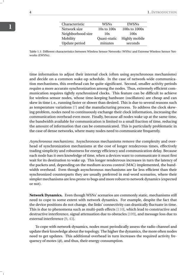
1.1. WIRELESS SENSOR NETWORKSIn order to understand the challenges of Extreme Wireless Sensor Networks (EWSNs), wewill first introduce some basic knowledge about traditional Wireless Sensor Networks (WSNs).By highlighting the differences between the two (summarized in Table 1.1), we define thecrucial characteristics of EWSNs and, more importantly, its challenges.
A Wireless Sensor Network comprises of a small set of battery-powered devices, the so-called motes, which periodically monitor the environment and cooperatively communicatethe sensed information via wireless links. WSNs are usually small in size, ranging from tensto hundreds of short-range devices. Enough to cover their usually modest deployment ar-eas. From a networking perspective, the maximum neighborhood cardinality is in the orderof a few tens of devices.
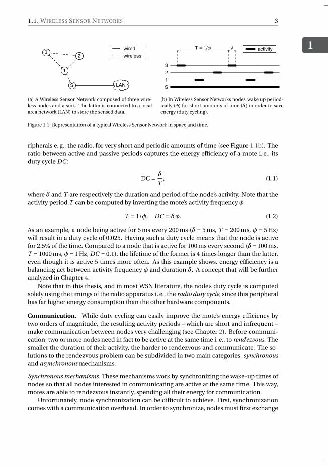
Data Collection. In WSNs, motes can diffuse and process the sensed information in a dis-tributed fashion (allowing the network to react autonomously) or can forward it to one ormore sink nodes (see Figure 1.1a). Sinks are special nodes that are usually connected to alarger network e. g., the Internet, and serve as gateways to store data and forward actuationcommands. In some cases, sink nodes act also as coordinators of the other nodes in thenetwork. Because WSNs usually involve static topologies, shortest-path routing trees canbe built in order to deliver the sensed information to sink nodes over a multi-hop wirelessconnection.
Energy Efficiency. Because in WSNs motes are often powered by small batteries, it is vitalto design communication mechanisms that are energy efficient and allow these wireless de-vices to operate long enough to meet the lifetime requirements imposed by the application(often in the order of days, months, or a few years).
Unfortunately, communication mechanisms are never energy efficient enough. Design-ers strive to reduce the cost, weight and size of motes, while batteries are among the com-ponents that are most expensive, heavy and difficult to miniaturize. Communicating withhigher efficiencies than needed allows thus to reduce the capacity of batteries i. e., their size,weight and cost, putting pressure on the efficiency of the communication.
The main mechanism employed by WSNs to improve the energy efficiency of wirelessdevices is called duty cycling and consists in limiting the use of the energy-demanding pe-
1http://www.commit-nl.nl/projects/very-large-wireless-sensor-networks-for-well-being
1.1. WIRELESS SENSOR NETWORKS
1
3
1
23
S LAN
wired wireless
(a) A Wireless Sensor Network composed of three wire-less nodes and a sink. The latter is connected to a localarea network (LAN) to store the sensed data.
T = 1/! " activity
321S
(b) In Wireless Sensor Networks nodes wake up period-ically (φ) for short amounts of time (δ) in order to saveenergy (duty cycling).
Figure 1.1: Representation of a typical Wireless Sensor Network in space and time.
ripherals e. g., the radio, for very short and periodic amounts of time (see Figure 1.1b). Theratio between active and passive periods captures the energy efficiency of a mote i. e., itsduty cycle DC :
DC = δ
T, (1.1)
where δ and T are respectively the duration and period of the node’s activity. Note that theactivity period T can be computed by inverting the mote’s activity frequency φ
T = 1/φ, DC = δφ. (1.2)
As an example, a node being active for 5 ms every 200 ms (δ = 5 ms, T = 200 ms, φ = 5 Hz)will result in a duty cycle of 0.025. Having such a duty cycle means that the node is activefor 2.5% of the time. Compared to a node that is active for 100 ms every second (δ = 100 ms,T = 1000 ms, φ = 1 Hz, DC = 0.1), the lifetime of the former is 4 times longer than the latter,even though it is active 5 times more often. As this example shows, energy efficiency is abalancing act between activity frequency φ and duration δ. A concept that will be furtheranalyzed in Chapter 4.
Note that in this thesis, and in most WSN literature, the node’s duty cycle is computedsolely using the timings of the radio apparatus i. e., the radio duty cycle, since this peripheralhas far higher energy consumption than the other hardware components.
Communication. While duty cycling can easily improve the mote’s energy efficiency bytwo orders of magnitude, the resulting activity periods – which are short and infrequent –make communication between nodes very challenging (see Chapter 2). Before communi-cation, two or more nodes need in fact to be active at the same time i. e., to rendezvous. Thesmaller the duration of their activity, the harder to rendezvous and communicate. The so-lutions to the rendezvous problem can be subdivided in two main categories, synchronousand asynchronous mechanisms.
Synchronous mechanisms. These mechanisms work by synchronizing the wake-up times ofnodes so that all nodes interested in communicating are active at the same time. This way,motes are able to rendezvous instantly, spending all their energy for communication.
Unfortunately, node synchronization can be difficult to achieve. First, synchronizationcomes with a communication overhead. In order to synchronize, nodes must first exchange
1
4 1. INTRODUCTION
Characteristic WSNs EWSNsNetwork size 10s to 100s 100s to 1000sNeighborhood size 10s 100sMobility Quasi-static Highly mobileUpdate period minutes seconds
Table 1.1: Different characteristics between Wireless Sensor Networks (WSNs) and Extreme Wireless Sensor Net-works (EWSNs).
time information to adjust their internal clock (often using asynchronous mechanisms)and decide on a common wake-up schedule. In the case of network-wide communica-tion mechanisms, this overhead can be quite significant. Second, smaller activity periodsrequire a more accurate synchronization among the nodes. Thus, extremely efficient com-munication requires tightly synchronized clocks. This feature can be difficult to achievefor wireless sensor nodes, whose time-keeping hardware (oscillators) are cheap and canskew in time i. e., running faster or slower than desired. This is due to several reasons suchas temperature variations [7] and the manufacturing process. To address the clock skew-ing problem, nodes need to continuously exchange their clock information, increasing thecommunication overhead even more. Finally, because all nodes wake up at the same time,the bandwidth available for communication is limited to a small fraction of time, reducingthe amount of information that can be communicated. This is particularly problematic inthe case of dense networks, where many nodes need to communicate frequently.
Asynchronous mechanisms. Asynchronous mechanisms remove the complexity and over-head of synchronization mechanisms at the cost of longer rendezvous times, effectivelytrading simplicity and robustness for energy efficiency and communication delay. Becauseeach node has it own knowledge of time, when a devices want to communicate it must firstwait for its destination to wake up. This longer rendezvous increases in turn the latency ofthe packets and, depending on the medium access control (MAC) implemented, the band-width overhead. Even though asynchronous mechanisms are far less efficient than theirsynchronized counterparts they are usually preferred in real-word scenarios, where theirsimpler mechanisms are less prone to bugs and more robust to network dynamics (expectedor not).
Network Dynamics. Even though WSNs’ scenarios are commonly static, mechanisms stillneed to cope to some extent with network dynamics. For example, despite the fact thatthe device positions do not change, the links’ connectivity can drastically fluctuate in time.This is due to phenomena such as multi-path effects [110], which lead to constructive anddestructive interference, signal attenuation due to obstacles [109], and message loss due toexternal interference [9, 43].
To cope with network dynamics, nodes must periodically assess the radio channel andupdate their knowledge about the topology. The higher the dynamics, the more often nodesneed to get updates. This additional overhead in turn increases the required activity fre-quency of motes (φ), and thus, their energy consumption.
1.2. PROBLEM STATEMENT
1
5
1.2. PROBLEM STATEMENTSimilar to traditional WSNs, in Extreme Wireless Sensor Networks (EWSNs) devices are equippedwith a low-power microcontroller and powered by small batteries or supercapacitors. Thus,they need to be highly energy efficient. Different from WSNs, Extreme Wireless Sensor Net-works (EWSNs) raise the challenges of their non-extreme counterparts on four main as-pects.
1) Scale. EWSNs comprise of thousands of devices, approximately an order of magnitudemore devices than traditional WSNs. Because of this, mechanisms that are centralized andrequire network-wide information have difficulties to scale.
2) Mobility. In EWSNs devices are highly mobile, instead of static, resulting in topolo-gies that continuously change over time. In these highly dynamic conditions, mechanismsbased on rigid topological structures must strive to timely adapt to the many changes, satu-rating the already scarce bandwidth and usually taking decisions based on wrong, outdatedinformation.
3) Density. Because in EWSNs the devices’ radio range and the deployment areas are sim-ilar in dimensions to the ones in WSNs – but nodes are far more numerous – the resultingneighborhood cardinalities are in the order of hundreds of neighbors, rather then tens. Thisincreased “network density” makes it difficult for communication mechanisms to efficientlyshare the wireless medium, straining the already limited bandwidth.
4) Variability. The combined effect of high network densities and dynamics makes the net-work’s characteristics fluctuate drastically both in space and time (see Chapter 5). Mech-anisms that require complex parameter tuning struggle to find the right settings and oftenunder-perform in the highly-variable conditions of EWSNs.
Given the aforementioned challenges, this thesis tries to answer the following question
Is it possible to efficiently communicate in Extreme Wireless Sensor Networks ?
Our take is that the conditions of EWSNs require communication mechanisms to reducetheir overhead as much as possible to free up the resources for actual data transmissions.This idea is distilled in the following four design principles.
1) State-less. Due to the scale of EWSNs, nodes cannot rely on methods that are centralizedor require up-to-date information from other nodes in the network, either far-away or in thedirect neighborhood. In EWSNs failures are the norm, rather than the exception, leading tonetwork partitions due to temporary node unreachability. Protocols should be resilient tothese failures and operate independently from the node and the network states.
2) Opportunistic. Communication mechanisms should be opportunistic and exploit exist-ing situations to their own advantage. Information should be extrapolated from passiveobservations (see Chapter 3) instead of being actively polled from neighbors. Mechanismsshould not be artificially orchestrated and they should rely as much as possible on emergingbehaviors that araise spontaneously with minimal message overhead (see Chapter 4).
1
6 1. INTRODUCTION
3) Anti-fragile. Communication mechanisms should embrace, rather than fight, the chal-lenges of EWSNs to the point that they perform better in extreme conditions – where othermechanisms show their fragility (see Chapter 2).
4) Robust. When scarce resources, such as bandwidth, saturate the performance of com-munication mechanisms must degrade gracefully without drastic disruptions. To this end,mechanisms should operate in a best-effort fashion, backing off whenever conditions be-come too harsh.
Using the four aforementioned principles as guidelines, we present and evaluate threenovel communication mechanisms for EWSNs. These mechanisms are able to operate overseveral hundreds of devices with minimal energy consumption and bandwidth overheadand show a remarkable resilience to network dynamics.
1.3. THESIS CONTRIBUTIONS AND OUTLINEBy using the crowd monitoring scenario as a reference, this thesis tackles the problem ofcommunication in extremely dense and dynamic scenarios, making a step back towardsthe original Smartdust idea.
Medium Access Control and Data Dissemination – Chapter 2 In this chapter we addressthe cornerstone problem of Extreme Wireless Sensor Networks: efficiently sharing the com-munication medium among hundreds of continuously changing neighbors. In EWSNs nodesare mobile, and up-to-date network information is limited and costly to obtain. To copewith these challenges we propose SOFA, a novel medium access control (MAC) protocol thatis specifically designed for EWSNs. SOFA does not require any neighborhood information(state-less principle) and performs better in dense rather than sparse networks (anti-fragileprinciple). To minimize the delay and overhead of communication SOFA nodes opportunis-tically forward their information to the first available neighbor i. e., the first to wake up whileduty cycling its radio. The more neighbors, the shorter the rendezvous time, the lower thecommunication overhead (opportunistic principle).
The randomized neighbor-selection of SOFA provides is ideal for epidemic mechanisms,such as Gossiping, that are particularly suitable for dense and mobile networks. The combi-nation of gossip mechanisms and SOFA is able to provide a method to process informationin EWSNs with minimal energy consumption (robustness principle).
Neighborhood Cardinality Estimation – Chapter 3 This chapter addresses the problemof estimating the neighborhood cardinality in dense and dynamic networks, where tradi-tional techniques based on neighbor discovery do not work. In these extreme conditions,the neighbor discovery process takes a lot of time and neighbors are simply too many to bediscovered before the network conditions change. To this end, we propose a mechanismcalled Estreme that estimates, rather than counts, the number of devices in the neighbor-hood. Estreme models the performance of asynchronous duty-cycled MAC protocols, suchas SOFA, with respect to the number of active neighbors and uses this model to estimate theneighborhood cardinality with minimal delay and overhead (opportunistic principle).
Estreme improves existing techniques with faster and more accurate estimations and,for the first time, allows all nodes to perform this process simultaneously without inter-fering with each other. The latter characteristic proves to be particularly useful for crowd-
1.3. THESIS CONTRIBUTIONS AND OUTLINE
1
7
monitoring applications, where crowd managers want, for example, to continuously moni-tor the changes in the crowd density.
Opportunistic Data Collection – Chapter 4 This chapter explores the challenges of datacollection in EWSNs. Traditional routing mechanisms for WSNs are based on rigid struc-tures and cannot cope with the ever-changing topologies of EWSNs. In these dynamic con-ditions, the communication overhead required to maintain the routing structures increasesup to the point that bandwidth saturates and mechanisms (mis)route data based on out-dated and wrong information. To cope with the aforementioned problems, in this chapterwe propose a data collection mechanism called Staffetta, whose routing structure is highlyadaptable and is spontaneously formed from local observations and with minimal over-head (state-less principle). Staffetta exploits the fact that in opportunistic mechanisms it ismore probable and efficient to communicate with the neighbors that wake up more ofteni. e., that are more active. In the presence of a fixed energy budget and a sink (which is al-ways active) Staffetta spontaneously creates an activity gradient, where nodes closer to thesink are more active than others and, thus, opportunistically attract more data. Comparedto existing data collection mechanisms, Staffetta shows higher delivery rates, lower energyconsumption and shorter packet latencies.
Crowd Monitoring in the Wild – Chapter 5 Finally, this chapter explores the deploymentchallenges of a real EWSN composed of several hundreds of mobile motes. This study ismotivated by the fact that many protocols for WSNs (extreme or not) are developed andtested under limited, controlled conditions. From high-level simulations to large and mo-bile testbeds. Even though these tools are highly valuable for the first-stage deploymentof wireless systems, many researchers stop their evaluation at these controlled conditions,often missing the variety of conditions that only real-word scenarios exhibit. This is partic-ularly true for monitoring applications and EWSNs.
This chapter reports our deployment experience running SOFA and Estreme as a mech-anism to monitor the popularity of exhibits in NEMO, a modern, open-space science mu-seum. Different from testbed and previous mobile experiments, the museum experimentexposed our mechanisms to drastic network changes, showing the importance of certainkinds of information, such as the unique node identifier, for the correct sensing and esti-mation of the crowd parameters.
Chapters 2, 3, and 4 are based on the following papers:
• M. Cattani, M. Zuniga, M. Woehrle, K.G. Langendoen, SOFA: Communication in Ex-treme Wireless Sensor Networks, in 11th European Conference on Wireless Sensor Net-works (EWSN) (2014)
• M. Cattani, M. Zuniga, A. Loukas, K.G. langendoen, Lightweight neighborhood cardi-nality estimation in dynamic wireless networks, in 13th ACM/IEEE International Con-ference on Information Processing in Sensor Networks (IPSN) (2014)
• M. Cattani, A. Loukas, M. Zimmerling, M. Zuniga, K. Langendoen, Staffetta: SmartDuty-Cycling for Opportunistic Data Collection, in 14th ACM Conference on EmbeddedNetworked Sensor Systems (SenSys) (2016).

2MEDIUM ACCESS CONTROL AND
DATA DISSEMINATION
“It was logical to cultivate multiple options”
Spock
T HE protocol stack of Wireless Sensor Networks (WSNs) has been mainly designed andoptimized for applications satisfying one or more of the following conditions: (i) low
traffic rates (a packet per node every few minutes), (ii) medium sized densities (tens ofneighbors), and (iii) static topologies. In Extreme Wireless Sensor Networks (EWSNs) how-ever, these relatively mild conditions do not hold and traditional protocol stacks simplycollapse: thousands of mobile nodes with hundreds of neighbors that need to disseminateinformation at a relatively high rate (a packet per node every few seconds, instead of everyfew minutes).
From a networking perspective, communication in these extreme scenarios poses threenon-trivial technical challenges. First, similar to traditional WSNs, EWSNs also work withdevices with limited energy resources and need to rely on radio duty-cycling techniquesto save energy. Second, due to the network scale and node mobility, we cannot rely onmethods that combine duty cycling techniques with central coordinators [33] or that re-quire some level of synchronization between the wake up periods of a given node and itsneighbors [32, 86]. The system must be asynchronous and fully distributed. Third, due totheir inefficient bandwidth utilization, traditional unicast and broadcast primitives – whichare asynchronous, distributed and built on top of duty cycling techniques [11, 85] – simplycollapse under the traffic-demands of EWSNs.
Henceforth, providing energy-efficient communication in EWSNs requires a careful eval-uation of the following problem: in asynchronous duty cycling techniques, much of thebandwidth is wasted in coordinating the rendezvous of the (sleeping) nodes. In EWSNs,
Parts of this chapter have been published in EWSN’14, Oxford, United Kingdom [17].
9
2
10 2. MEDIUM ACCESS CONTROL AND DATA DISSEMINATION
nodes need to reduce this overhead to free up the channel’s bandwidth for the actual datatransmissions.
To tackle this problem, we present SOFA (Stop On First Ack), a communication stack forEWSNs composed of a medium access control (MAC) layer based on a novel bi-directionalcommunication primitive that we call opportunistic anycast. This primitive establishes adata exchange with the first neighbor to wake up. In this way, SOFA avoids the need forneighborhood discovery and minimizes the inefficient rendezvous time typical of asyn-chronous MAC protocols.
By selecting opportunistically the next (random) neighbor to communicate with, SOFAprovides an ideal building block for algorithms based on random sampling [13] and gos-sip [8, 78, 79]. The latter ones are particularly suitable to process information in large-scaledistributed systems such as EWSNs and offer an alternative to the traditional protocol stack,that cannot operate in extreme network conditions.
After exploring the related work in Section 2.1, in Section 2.3 we present the design ofSOFA, a communication protocol that utilizes opportunistic anycast to overcome the limita-tions of inefficient rendezvous mechanisms. To scale in EWSNs, SOFA combines the energyefficiency typical of low-power MAC protocols with the robustness and versatility of gossip-like communication.
In Section 2.4 we explain how to efficiently implement SOFA on low-cost sensor nodesi. e., motes. Implementation is particularly important, since opportunistic mechanisms areknown to suffer when too many neighbors are available to forward the same packet (ac-knowledgments collision and duplicate packets).
Finally, in Section 2.5, we extensively evaluate SOFA both in simulations and testbedexperiments. Results show that SOFA can successfully deliver messages, regardless of mo-bility, in networks with densities of hundreds of nodes while maintaining the duty cycle atapproximately 2%.
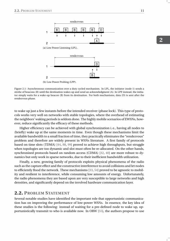
2.1. RELATED WORKThe constrained energy resources of WSNs led to a first generation of protocols that tradedbandwidth utilization for lower energy consumption. Such protocols are based on asyn-chronous node operations, which implies that senders need to wait for their receiver towake up (rendezvous phase) before sending their data. While in low power listening (LPL) [11]nodes send a beaconing sequence until the receiver wakes up, in low power probing (LPP) [30,85], the sender waits for a wake-up beacon from the receiver (see Figure 2.1).
Despite their high overhead – in asynchronous mechanisms, the expected rendezvoustakes half of the wake-up period [11, 71] – these protocols are good enough for traditionalWSNs, where the data rate is low (few senders, many receivers) and most of the bandwidthcan be used for coordination purposes, rather than data transmission. With a receiver’swake-up period T = 100 ms, for example, the rendezvous phase will last on average 50 ms, alot more than the few millisecond typically needed in WSNs for the data communication. Inthe best scenario, this will allow no more than 20 nodes to transmit their data every minute.Beyond this threshold, a typical case for EWSNs, the channel saturates.
The WSNs community is well aware of the limitations of the first generation of low-power protocols, which are significant even for the milder condition of non-extreme WSNs.To reduce the overhead of the rendezvous phase, protocols such as WiseMAC [32] and Con-tikiMAC [28] keep track of the wake-up periods of their neighbors and use this information
2.2. PROBLEM STATEMENT
2
11
rendezvous
B B B B B D
A
1
2(a) Low Power Listening (LPL).
rendezvous
D
B
1
2(b) Low Power Probing (LPP).
Figure 2.1: Asynchronous communication over a duty cycled mechanism. In LPL, the initiator (node 1) sends astrobe of beacons (B) until the destination wakes up and send an acknowledgment (A). In LPP, instead, the initia-tor simply waits for a wake-up beacon (B) from its destination. For both mechanisms, data (D) is sent after therendezvous phase.
to wake up just a few instants before the intended receiver (phase lock). This type of proto-cols works very well on networks with stable topologies, where the overhead of estimatingthe neighbors’ waking periods is seldom done. The highly mobile scenarios of EWSNs, how-ever, reduce significantly the efficacy of these methods.
Higher efficiency can be achieved with global synchronization i. e., having all nodes to(briefly) wake up at the same moments in time. Even though these mechanisms limit theavailable bandwidth to a small fraction of time, they practically eliminates the “rendezvous”problem and therefore are widely present in WSNs literature. A first family of protocolsbased on time slots (TDMA) [44, 88, 99] proved to achieve high throughputs, but strugglewhen topologies are too dynamic and slot must often be re-allocated. On the other hands,synchronized protocols based on random access (CDMA) [32, 40] are more robust to dy-namics but only work in sparse networks, due to their inefficient bandwidth utilization.
Finally, a new, growing family of protocols exploits physical phenomena of the radiosuch as the capture effect and the constructive interference to avoid collisions and let nodesto efficiently flood the network. These mechanisms [33, 54] proved to be agnostic to mobil-ity and resilient to interference, while consuming low amounts of energy. Unfortunately,the radio phenomena they are based upon are very susceptible to large networks and highdensities, and significantly depend on the involved hardware communication layer.
2.2. PROBLEM STATEMENTSeveral notable studies have identified the important role that opportunistic communica-tion has on improving the performance of low-power WSNs. In essence, the key idea ofthese studies is the following: instead of waiting for a pre-defined node to wake up, op-portunistically transmit to who is available now. In ORW [55], the authors propose to use
2
12 2. MEDIUM ACCESS CONTROL AND DATA DISSEMINATION
Node A
Node B
Node C
Node D
B B B D A
A D
Rendezvous Data exchange
(a) Normal conditions
Node A
Node B
Node C
Node D
B B B B B D A
A
A
A D
Collision
Rendezvous Data exchange
(b) Collision resolution (cf. Section 2.4)
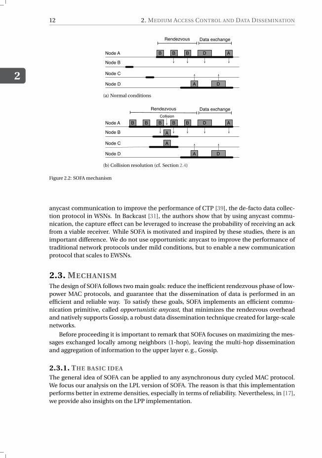
Figure 2.2: SOFA mechanism
anycast communication to improve the performance of CTP [39], the de-facto data collec-tion protocol in WSNs. In Backcast [31], the authors show that by using anycast commu-nication, the capture effect can be leveraged to increase the probability of receiving an ackfrom a viable receiver. While SOFA is motivated and inspired by these studies, there is animportant difference. We do not use opportunistic anycast to improve the performance oftraditional network protocols under mild conditions, but to enable a new communicationprotocol that scales to EWSNs.
2.3. MECHANISMThe design of SOFA follows two main goals: reduce the inefficient rendezvous phase of low-power MAC protocols, and guarantee that the dissemination of data is performed in anefficient and reliable way. To satisfy these goals, SOFA implements an efficient commu-nication primitive, called opportunistic anycast, that minimizes the rendezvous overheadand natively supports Gossip, a robust data dissemination technique created for large-scalenetworks.
Before proceeding it is important to remark that SOFA focuses on maximizing the mes-sages exchanged locally among neighbors (1-hop), leaving the multi-hop disseminationand aggregation of information to the upper layer e. g., Gossip.
2.3.1. THE BASIC IDEA
The general idea of SOFA can be applied to any asynchronous duty cycled MAC protocol.We focus our analysis on the LPL version of SOFA. The reason is that this implementationperforms better in extreme densities, especially in terms of reliability. Nevertheless, in [17],we provide also insights on the LPP implementation.
2.3. MECHANISM
2
13
Rendezvous phase. In traditional LPL protocols [11], when a sender wakes up, it trans-mits a series of short packets –called beacons– and waits for the receiver to wake up. Whenthe intended receiver wakes up, it hears the latest beacon and sends an acknowledgementback. SOFA follows a similar mechanism: the sender, node A in Figure 2.2a, also broad-casts a series of beacons but only waits until any neighbor wakes up. The main differencebetween the two mechanisms lays in the selection of the destination. While in LPL the des-tination is chosen by the upper layers in the stack, in SOFA the MAC protocol opportunisti-cally chooses the destination that is most efficient to reach: the first neighbor to wake up. Ifnodes B or C were to be chosen, node A would need to send beacons (jam the channel) untilthese nodes wake up again. By sending its data to the first neighbor that wakes up (node D),SOFA reduces the nodes’ rendezvous time, allowing low-power MAC protocols to efficientlyscale to EWSNs. We call this communication primitive opportunistic anycast.
Data exchange phase. Selecting the first (random) neighbor that wakes up as the destina-tion, has a strong relation with a family of randomized networking algorithms called gossip-ing [8, 79]. Gossip algorithms do not aim for traditional end-to-end communication (whereroutes are formed and maintained ahead of time), instead they exchange information ran-domly with a neighbor (or subset of neighbors). The relation between SOFA and Gossipingis fundamental for the practical impact of our work. Unicast and broadcast primitives allowthe development of a wide-range of algorithms and applications in WSNs such as routing,data collection, querying and clustering (to name a few). Unfortunately, under the stringentcharacteristics of EWSNs these basic primitives collapse. Our aim is to provide an alterna-tive communication protocol for extreme conditions. We hope that this effort will allowthe community to use SOFA as a basic building block for other gossip applications such asrouting in delay tolerant networks [81] and landscaping of data [62].
We will now describe the design of the three key characteristics of SOFA: short ren-dezvous phase, reliable push-pull data exchange, and random peer sampling. The designof a short rendezvous phase was influenced by the limitations of asynchronous duty cycledprotocols. The push-pull data exchange and the random peer sampling were designed tosatisfy the needs of general gossiping applications.
2.3.2. SHORT RENDEZVOUS PHASE
Stopping at the first encounter, instead of searching for a specific destination, has two im-portant consequences on the performance of SOFA. First, and most importantly, it elimi-nates the main limitation that LPL has under extreme networking conditions: channel inef-ficiency. By drastically reducing the length of the rendezvous phase, the channel no longergets easily saturated by medium/high traffic demands or medium/high node densities. Ashort rendezvous phase also reduces the duty cycle of the radio, which in turn, increasesthe lifetime of the node. Second, increasing the network’s density (up to a point) improvesthe performance of SOFA. With more neighbors, the probability that one will soon wake upis higher.
To quantify the benefits of a short rendezvous phase, we present a simple model thatcaptures the expected duration of the rendezvous phase as a function of the neighbor-hood size and the wake-up period (the time elapsed between two consecutive wake-upsof a node). Since nodes wake up periodically in a completely desynchronized way, we canmodel the inter-arrival times of the nodes’ wake-ups as a set of independent random vari-
2
14 2. MEDIUM ACCESS CONTROL AND DATA DISSEMINATION
ables with uniform distribution. The first order statistic U1 can then be used to estimate thelength of the rendezvous phase. The expected length E [U1] of N uniform random variables(neighbors) is given by the Beta random variable with parameters α=1 and β=N
U1 ∼ B(1, N ), E [U1] = 1
1+N
Given a wake-up period W and a neighborhood size N , the expected length of the ren-dezvous phase of SOFA can be computed as follows:
E [s] = W
1+N(2.1)
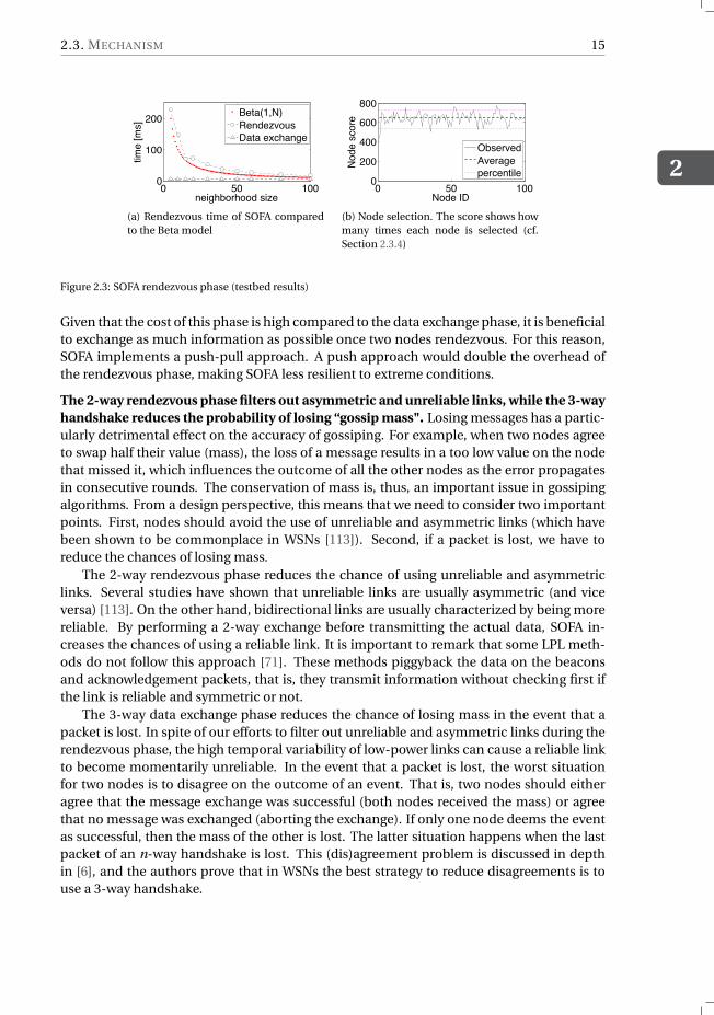
Considering that the expected rendezvous time of unicast E [u] is W /2 [11, 71] and thatthe time spent for the data exchange phase is negligible compared to the rendezvous (seeFigure 2.3a), we can model the gain G of SOFA compared to unicast as the following:
G = E [s]
E [u]= W
1+N
2
W= 2
1+N
For a node with 99 neighbors, this means that the expected rendezvous times of SOFA is 50times smaller than the one using unicast. Figure 2.3a compares the expected length of therendezvous phase using the proposed model with values observed in testbed experiments.In this example, W =1 s and the neighborhood size ranges from 5 to 100 nodes. The slightunderestimation is mainly due to collisions, which delay the detection of the first node bythe sender.
It is important to highlight three key points about the impact of density on SOFA. First,since the performance of SOFA is not significantly affected by changes in medium/highdensities, SOFA does not need to adapt to this type of density fluctuations in mobile net-works. Second, to reduce the duration of the rendezvous phase in low density networks,the wake-up period can be reduced (at the cost of increasing the duty cycle). This trade-offis studied in more detail in Section 2.5.3. Finally, in case the network switches from an ex-treme condition to a normal one (low density), the protocol stack can switch to the use ofstandard broadcast and unicast messages. To detect the density of the network, SOFA canexploit the tight correlation between the number of neighbors and the expected length ofthe rendezvous phase (see Chapter 3).
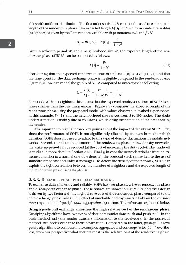
2.3.3. RELIABLE PUSH-PULL DATA EXCHANGETo exchange data efficiently and reliably, SOFA has two phases: a 2-way rendezvous phaseand a 3-way data exchange phase. These phases are shown in Figure 2.2a and their designis driven by two factors: (i) the high relative cost of the rendezvous phase compared to thedata-exchange phase, and (ii) the effect of unreliable and asymmetric links on the constantmass requirement of gossip’s data-aggregation algorithms. The effects are explained below.
Using a push-pull exchange amortizes the high relative cost of the rendezvous phase.Gossiping algorithms have two types of data communication: push and push-pull. In thepush method, only the sender transfers information to the receiver(s). In the push-pullmethod, two nodes exchange their information. Compared to the latter, push-pull allowsgossip algorithms to compute more complex aggregates and converge faster [22]. Neverthe-less, from our perspective what matters most is the relative cost of the rendezvous phase.
2.3. MECHANISM
2
15
0 50 1000
100
200
neighborhood size
time
[ms]
Beta(1,N)RendezvousData exchange
(a) Rendezvous time of SOFA comparedto the Beta model
0 50 1000
200
400
600
800
Node ID
Nod
e sc
ore
ObservedAveragepercentile
(b) Node selection. The score shows howmany times each node is selected (cf.Section 2.3.4)
Figure 2.3: SOFA rendezvous phase (testbed results)
Given that the cost of this phase is high compared to the data exchange phase, it is beneficialto exchange as much information as possible once two nodes rendezvous. For this reason,SOFA implements a push-pull approach. A push approach would double the overhead ofthe rendezvous phase, making SOFA less resilient to extreme conditions.
The 2-way rendezvous phase filters out asymmetric and unreliable links, while the 3-wayhandshake reduces the probability of losing “gossip mass". Losing messages has a partic-ularly detrimental effect on the accuracy of gossiping. For example, when two nodes agreeto swap half their value (mass), the loss of a message results in a too low value on the nodethat missed it, which influences the outcome of all the other nodes as the error propagatesin consecutive rounds. The conservation of mass is, thus, an important issue in gossipingalgorithms. From a design perspective, this means that we need to consider two importantpoints. First, nodes should avoid the use of unreliable and asymmetric links (which havebeen shown to be commonplace in WSNs [113]). Second, if a packet is lost, we have toreduce the chances of losing mass.
The 2-way rendezvous phase reduces the chance of using unreliable and asymmetriclinks. Several studies have shown that unreliable links are usually asymmetric (and viceversa) [113]. On the other hand, bidirectional links are usually characterized by being morereliable. By performing a 2-way exchange before transmitting the actual data, SOFA in-creases the chances of using a reliable link. It is important to remark that some LPL meth-ods do not follow this approach [71]. These methods piggyback the data on the beaconsand acknowledgement packets, that is, they transmit information without checking first ifthe link is reliable and symmetric or not.
The 3-way data exchange phase reduces the chance of losing mass in the event that apacket is lost. In spite of our efforts to filter out unreliable and asymmetric links during therendezvous phase, the high temporal variability of low-power links can cause a reliable linkto become momentarily unreliable. In the event that a packet is lost, the worst situationfor two nodes is to disagree on the outcome of an event. That is, two nodes should eitheragree that the message exchange was successful (both nodes received the mass) or agreethat no message was exchanged (aborting the exchange). If only one node deems the eventas successful, then the mass of the other is lost. The latter situation happens when the lastpacket of an n-way handshake is lost. This (dis)agreement problem is discussed in depthin [6], and the authors prove that in WSNs the best strategy to reduce disagreements is touse a 3-way handshake.

2
16 2. MEDIUM ACCESS CONTROL AND DATA DISSEMINATION
2.3.4. RANDOM PEER SAMPLING
Most gossip algorithms rely on the selection of a random neighbor (or subset of neighbors)at each round. Having a good random selection leads to a faster convergence. To ensure aproper random selection, SOFA introduces random values to the wake-up periods of eachnode. For a wake-up period of W seconds, nodes wake up uniformly at random between[0.5W , 1.5W ].
To validate the effectiveness of our approach, we performed an experiment on a 100-node testbed. For 10 minutes nodes exchange messages and count the number of timesthey are selected by their neighbors (their score). Figure 2.3b shows that the distribution ofthe scores is close to uniform, with the [5, 95] percentiles close to the average value. It isimportant to remark that this evaluation was performed on a static testbed. Mobility wouldfurther randomize the selection of neighbors, facilitating the dissemination of data, anddrastically reducing the convergence time of Gossip [78].
2.4. IMPLEMENTATIONWe implemented SOFA on the Contiki OS based on X-MAC [11]. Nodes were configured towake up every second for 10 ms. If a beacon is received within this 10 ms period, the nodesends an acknowledgement and starts the data exchange phase. Otherwise, the node goesback to sleep. Notice that these parameters set a minimum duty cycle of 1 %, hence, anyextra activity beyond this point is part of the overhead caused by the rendezvous and dataexchange phases. Below we describe the implementation of the most important features ofSOFA.
Transmit back-off. In traditional MAC protocols, before sending a packet, a transmitterfirst checks the signal level of the channel (CCA check) to see if there is any activity. If noactivity is detected the packet is sent. In SOFA, we do not perform a CCA check. Instead,a potential sender listens to the channel for 10 ms acting, practically, as a receiver. If afterthis period no packet is detected, the node starts the rendezvous phase. If the node detectsa packet that is part of an on-going data exchange, it goes back to sleep (collision avoid-ance). However, if the detected packet is a beacon, the node changes its role from senderto receiver. By performing a transmit back-off instead of a CCA check, SOFA transforms apossible collision between two senders into a successful message exchange with a very lowrendezvous cost.
Collision avoidance. One of the key challenges of operating under extreme density con-ditions is the higher likelihood of collisions due to higher traffic demands. SOFA follows asimple guideline to reduce the frequency of collisions: if a sender detects a packet loss –forinstance, by not receiving an ack–, instead of attempting a retransmission, the node goesback to sleep. This conservative approach reduces the traffic in highly dense networks. Themain caveat of this approach is when the lost packet is the last data ack. In this case, the twoparties will disagree on the data delivery, causing an information (mass) loss. Fortunately,our testbed results show that this is not a frequent event.
There is a collision event that is not avoided by the above mentioned approach andhas a higher probability of occurrence in SOFA. When two or more active receivers detect abeacon, their ACKs are likely to collide (cf. nodes B and C in Figure 2.2b). The sender willreceive neither of the ACKs and will consequently continue transmitting beacons. Upon
2.5. EVALUATION
2
17
receiving a subsequent beacon (not the expected data packet), the two colliding receiversinfer that a collision has occurred and both will go back to sleep. The first node to wake upafter the collision (node D) will acknowledge the beacon and exchanges its data. Finally,randomizing the wake up periods of nodes helps in reducing the chances that this type ofcollisions occurs repeatedly among the same couples of nodes.
Packet addressing. SOFA uses two main types of data packets. For the rendezvous phase,the beacons have no destination address, any node can receive and process the informa-tion. For the data exchange phase, the packets contain the destination address of the in-volved parties. The beacon packets are as small as possible (IEEE 802.15.4 header + 1 byteto define the packet type and 1 byte when addressing is needed).
2.5. EVALUATIONTo evaluate the effectiveness of SOFA we ran an extensive set of experiments and simula-tions. Our testbed has 108 nodes installed above the ceiling tiles of an office building. Thewireless nodes are equipped with a MSP430 micro-controller and a CC1101 radio chip. Toreach the highest possible neighborhood size, we set the transmission power to +10 dBm.With these settings, the network is almost a clique. For our simulations we used Cooja, thestandard simulator for Contiki. We tested network densities of up to 450 nodes and differ-ent mobility patterns. Simulations beyond this density value are not possible with normalcluster computing facilities. For both experiments and simulations, the baseline scenariowas configured to have a wake up period W =1 s and a transmission period T =2 s. That is,nodes wake up every second to act as receivers and every two seconds to act as senders.Considering that nodes listen for packet activity at each wake-up for 10 ms, the baselineduty-cycle is ≈ 1 %. Any extra consumption beyond 1 % is caused by SOFA. The evaluationresults presented in this section consider also other values for W and T , but unless statedotherwise the experiments are carried out using the baseline parameters. The results areaveraged over 20 runs of 10 minutes each.
2.5.1. PERFORMANCE METRICSThe evaluation of SOFA focuses on three key areas: energy consumption, bandwidth utiliza-tion and mass conservation. To capture the performance of SOFA in these areas, we utilizethe following metrics:
Duty cycle. The percentage of time that the radio is active. Duty-cycle is a widely utilizedproxy for energy consumption in WSNs because radio activity accounts for most of the en-ergy consumption in WSNs nodes.
Exchange rate. The number of successful data-exchanges (3-way handshakes) in a second.This is a per-node metric. If, instead, we count the total number of data exchanges in asecond over the entire network we refer to the global exchange rate.
Mass delivery ratio. The percentage of times that the data-exchange phase ends up with-out any information loss. Recall that if the ack of the data phase is lost, the receiver deemsthe exchange as successful, but the sender deems the exchange as unsuccessful and ignoresthe previously received packet (mass loss). The mass delivery ratio is a metric focused onevaluating the viability of SOFA as a basic communication primitive to gossip algorithms.
2
18 2. MEDIUM ACCESS CONTROL AND DATA DISSEMINATION
0 50 1000
5
10
15
neighborhood size
duty
cyc
le [%
]
LPL W=125msSOFA W=1000msSOFA W=125ms
0 50 1000
0.1
0.2
0.3
0.4
0.5
neighborhood size
[exc
hang
e/s/
node
]
LPL W=125msSOFA W=1000msSOFA W=125ms
Figure 2.4: SOFA compared to LPL (testbed results).
2.5.2. RESULTS
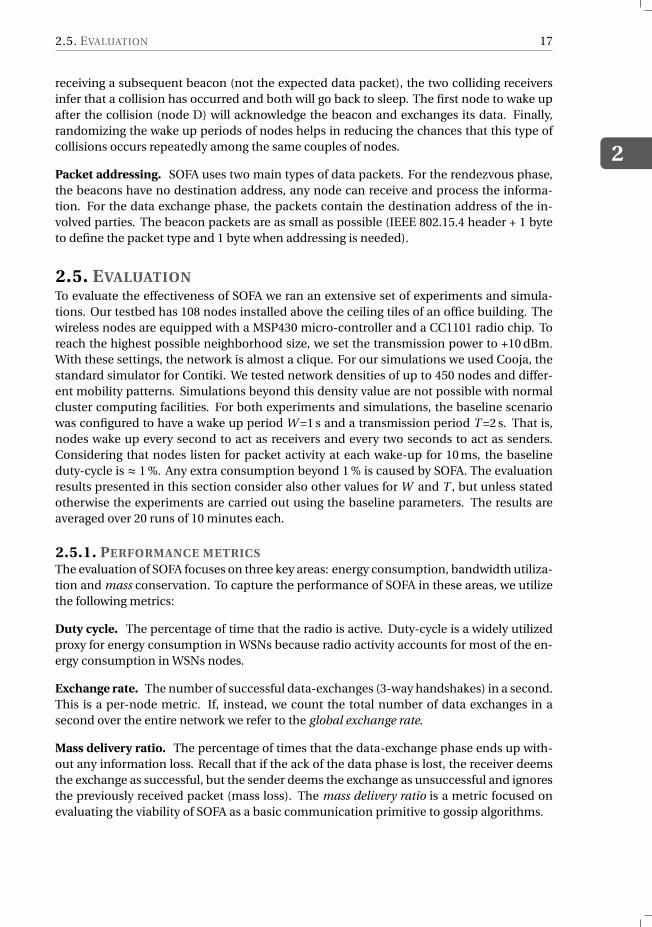
Previously in this paper, we argued that traditional low-power methods collapse under thestress imposed by extreme networking conditions. This subsection quantifies this claim. Wecompare SOFA with the standard Contiki implementation of LPL (X-MAC) on our testbed.To provide a fair comparison, LPL chooses a random neighbor from a pre-computed list ofdestinations at every transmission request. That is, we do not enforce on LPL the necessaryneighbor discovery process that would be needed to obtain the destination address (SOFAdoes not need an address to bootstrap the communication).
Figure 2.4 compares the duty cycle and the exchange rate of SOFA and LPL in our testbed.For LPL, the evaluation shows only the result for W =125 ms because LPL collapses with thebaseline W =1 s. This collapsing occurs because, with W =1 s, the rendezvous phase of LPLrequires on average 0.5 s. Hence, 5 nodes require on average a 2.5-seconds window to trans-mit their data, but the transmission period is 2 s, which leads to channel saturation. Com-paring the best parameter for LPL (W =125 ms) with the best parameter for SOFA (W =1 s)shows that SOFA widely outperforms LPL. For most neighborhood sizes (30 and above),SOFA uses four times less energy and delivers five times more packets for the same T .
It is important to remark that SOFA is not a substitute for traditional low power methods,as they aim at providing different services. SOFA cannot provide several of the functionali-ties required by applications relying on unicast and broadcast primitives. Most WSNs appli-cations are designed for data gathering applications sending a few packets per minute. Inthese scenarios, the state-of-the-art in WSNs research performs remarkably well. The aimof our comparison is to highlight that traditional methods were not designed to operateunder extreme conditions neither to efficiently support Gossip applications. We will nowanalyze the performance of SOFA based on different parameters and scenarios.
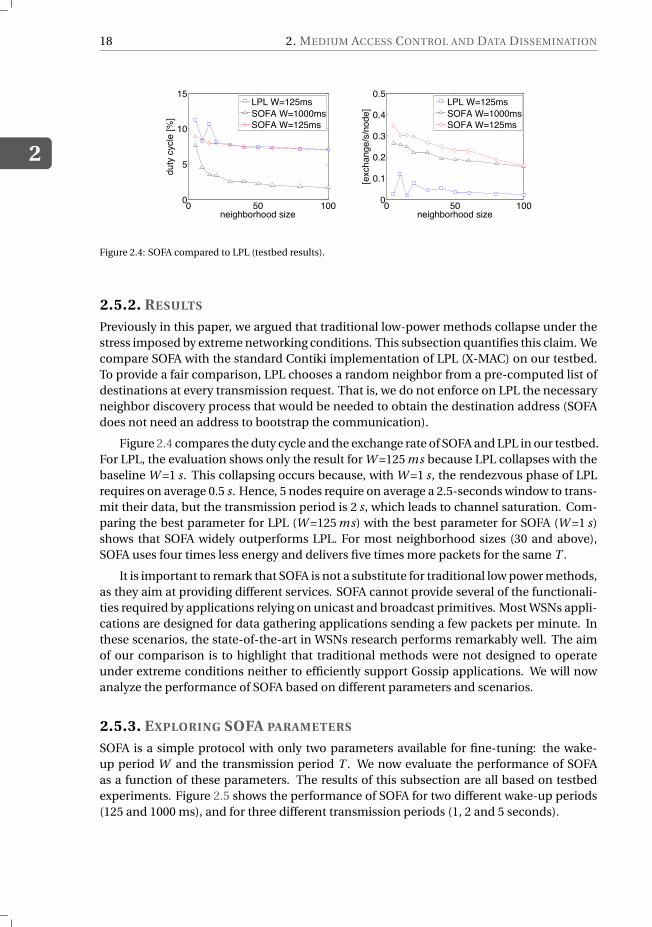
2.5.3. EXPLORING SOFA PARAMETERS
SOFA is a simple protocol with only two parameters available for fine-tuning: the wake-up period W and the transmission period T . We now evaluate the performance of SOFAas a function of these parameters. The results of this subsection are all based on testbedexperiments. Figure 2.5 shows the performance of SOFA for two different wake-up periods(125 and 1000 ms), and for three different transmission periods (1, 2 and 5 seconds).
2.5. EVALUATION
2
19
0 50 1000
5
10
15
neighborhood size
duty
cyc
le [%
]
T=1sT=2sT=5s
(a) Duty cycle, W =1000ms
0 50 1000
5
10
15
neighborhood size
duty
cyc
le [%
]
(b) Duty cycle, W =125ms
0 50 1000
50
100
neighborhood size
[%]
(c) Normalized Exchange rate,W =1000ms
0 50 1000
50
100
neighborhood size[%
](d) Normalized Exchange rate, W =125ms
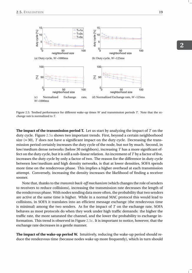
Figure 2.5: Testbed performance for different wake-up times W and transmission periods T . Note that the ex-change rate is normalized to T .
The impact of the transmission period T. Let us start by analyzing the impact of T on theduty cycle. Figure 2.5a shows two important trends. First, beyond a certain neighborhoodsize (≈30), T does not have a significant impact on the duty cycle. Decreasing the trans-mission period certainly increases the duty cycle of the node, but not by much. Second, inlow/medium dense networks (below 30 neighbors), increasing T has a more significant ef-fect on the duty cycle, but it is still a sub-linear relation. An increment of T by a factor of five,increases the duty cycle by only a factor of two. The reason for the difference in duty cyclebetween low/medium and high density networks, is that at lower densities, SOFA spendsmore time on the rendezvous phase. This implies a higher overhead at each transmissionattempt. Conversely, increasing the density increases the likelihood of finding a receiversooner.
Note that, thanks to the transmit back-off mechanism (which changes the role of sendersto receivers to reduce collisions), increasing the transmission rate decreases the length ofthe rendezvous phase. With nodes sending data more often, the probability that two sendersare active at the same time is higher. While in a normal MAC protocol this would lead tocollisions, in SOFA it translates into an efficient message exchange (the rendezvous timeis minimal) among the two senders. As for the impact of T on the exchange rate, SOFAbehaves as most protocols do when they work under high traffic demands: the higher thetraffic rate, the more saturated the channel, and the lower the probability to exchange in-formation. This trend is observed in Figure 2.5c. It is important to notice, however, that theexchange rate decreases in a gentle manner.
The impact of the wake-up period W. Intuitively, reducing the wake-up period should re-duce the rendezvous time (because nodes wake up more frequently), which in turn should
2
20 2. MEDIUM ACCESS CONTROL AND DATA DISSEMINATION
5 50 5000
5
10
15
neighborhood sizedu
ty c
ycle
[%]
Clique, SimulationClique, Testbed
(a) Duty cycle
5 50 5000.85
0.9
0.95
1
neighborhood size
deliv
ery
ratio
(b) Mass delivery ratio
5 50 5000
0.2
0.4
neighborhood size
[exc
hang
e/s/
node
]
(c) Exchange rate
5 50 5000
50
100
neighborhood size
[exc
hang
e/s]
Multihop, simulat.
(d) Global exchange rate
Figure 2.6: SOFA’s performance in extreme network conditions (testbed and simulation results).
free up bandwidth and allow a higher exchange rate. However, the trade-off for a more effi-cient use of bandwidth would be a higher duty cycle. Figures 2.5b and 2.5d show the perfor-mance of SOFA with a wake-up period W =125 ms. With this value, the baseline duty cycle is8 %. The figures show that reducing W does increase the relative exchange rate, but mainlyon low/medium dense networks (by ≈ 50%). Therefore, it is possible to improve the perfor-mance of SOFA in low density networks at the cost of increasing the energy consumption.For high density networks, however, we have a similar throughput but with a duty cycle thatis four times higher.
2.5.4. SOFA UNDER EXTREME DENSITIES AND IN MOBILE SCENARIOSThe previous testbed results show that SOFA performs well in densities as high as 100 neigh-bors. However, from a practical perspective it is important to determine (i) the saturationpoint of SOFA, i.e., how many nodes SOFA can handle before saturating the bandwidth, and(ii) the impact of mobility. Unfortunately, there are no large-scale mobile testbeds availablein the community, and hence, we rely on the Cooja simulator to investigate these aspects.
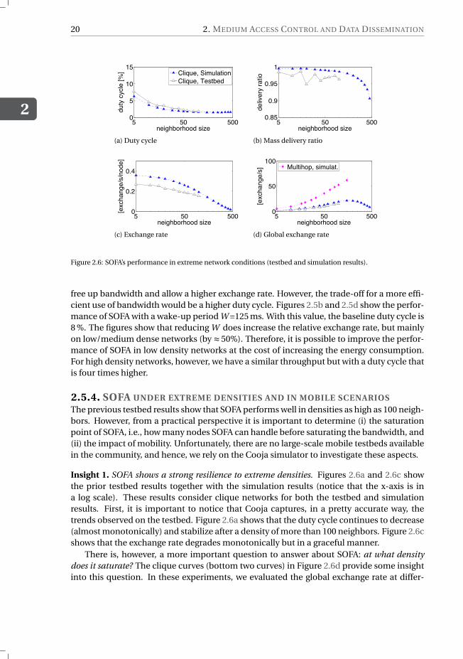
Insight 1. SOFA shows a strong resilience to extreme densities. Figures 2.6a and 2.6c showthe prior testbed results together with the simulation results (notice that the x-axis is ina log scale). These results consider clique networks for both the testbed and simulationresults. First, it is important to notice that Cooja captures, in a pretty accurate way, thetrends observed on the testbed. Figure 2.6a shows that the duty cycle continues to decrease(almost monotonically) and stabilize after a density of more than 100 neighbors. Figure 2.6cshows that the exchange rate degrades monotonically but in a graceful manner.
There is, however, a more important question to answer about SOFA: at what densitydoes it saturate? The clique curves (bottom two curves) in Figure 2.6d provide some insightinto this question. In these experiments, we evaluated the global exchange rate at differ-
2.5. EVALUATION
2
21
5 50 1000
5
10
15
neighborhood size
duty
cyc
le [%
]
StaticWalking speedBiking speed
(a) Duty cycle
5 50 1000.85
0.9
0.95
1
neighborhood size
deliv
ery
ratio
(b) Mass delivery ratio
5 50 1000
0.2
0.4
neighborhood size
[exc
hang
e/s/
node
]
(c) Exchange rate
Figure 2.7: SOFA performance under different mobility scenarios (simulation results).
ent densities. For the tested parameters, SOFA saturates when the density approaches 200neighbors per node. Note that these are clique scenarios. In multi-hop networks, SOFAcan exploit the well known spatial multiplexing effect (parallel data exchanges) and achievehigher global exchange rates. The top curve in 2.6d depicts this behavior. The highest pointrepresents a network with 450 nodes and an average density of 150 neighbors.
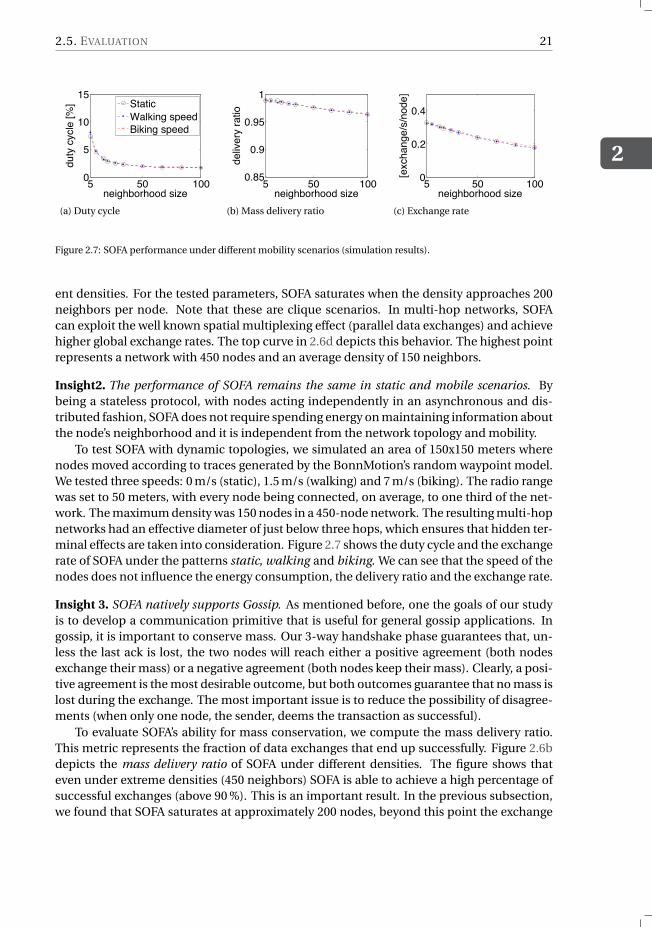
Insight2. The performance of SOFA remains the same in static and mobile scenarios. Bybeing a stateless protocol, with nodes acting independently in an asynchronous and dis-tributed fashion, SOFA does not require spending energy on maintaining information aboutthe node’s neighborhood and it is independent from the network topology and mobility.
To test SOFA with dynamic topologies, we simulated an area of 150x150 meters wherenodes moved according to traces generated by the BonnMotion’s random waypoint model.We tested three speeds: 0 m/s (static), 1.5 m/s (walking) and 7 m/s (biking). The radio rangewas set to 50 meters, with every node being connected, on average, to one third of the net-work. The maximum density was 150 nodes in a 450-node network. The resulting multi-hopnetworks had an effective diameter of just below three hops, which ensures that hidden ter-minal effects are taken into consideration. Figure 2.7 shows the duty cycle and the exchangerate of SOFA under the patterns static, walking and biking. We can see that the speed of thenodes does not influence the energy consumption, the delivery ratio and the exchange rate.
Insight 3. SOFA natively supports Gossip. As mentioned before, one the goals of our studyis to develop a communication primitive that is useful for general gossip applications. Ingossip, it is important to conserve mass. Our 3-way handshake phase guarantees that, un-less the last ack is lost, the two nodes will reach either a positive agreement (both nodesexchange their mass) or a negative agreement (both nodes keep their mass). Clearly, a posi-tive agreement is the most desirable outcome, but both outcomes guarantee that no mass islost during the exchange. The most important issue is to reduce the possibility of disagree-ments (when only one node, the sender, deems the transaction as successful).
To evaluate SOFA’s ability for mass conservation, we compute the mass delivery ratio.This metric represents the fraction of data exchanges that end up successfully. Figure 2.6bdepicts the mass delivery ratio of SOFA under different densities. The figure shows thateven under extreme densities (450 neighbors) SOFA is able to achieve a high percentage ofsuccessful exchanges (above 90 %). This is an important result. In the previous subsection,we found that SOFA saturates at approximately 200 nodes, beyond this point the exchange
2
22 2. MEDIUM ACCESS CONTROL AND DATA DISSEMINATION
rate decreases monotonically. But, Figure 2.6b shows that the few exchanges that are able tooccur beyond this point are able to be completed successfully. In other words, even underextremely demanding conditions SOFA has a remarkable ability to conserve mass. This featis due to the careful design of SOFA aimed at (i) selecting reliable links (rendezvous phase),(ii) implementing a transmit back-off instead of a CCA (to avoid sender-based collisions),(iii) avoiding the use of retransmissions (which would jam the channel) and (iv) providing amethod to reduce mass losses due to packet drops (3-way handshake).
2.6. CONCLUSIONSIn this chapter we made the first step towards communication in Extreme Wireless SensorNetworks, where nodes are mobile, density can reach hundreds of neighbors and band-width must be spared for the actual communication between nodes. With these challengesin mind, this chapter presented the design of SOFA, a medium access control protocol that,following the four design principles presented in Chapter 1, is able to diffuse and processinformation in EWSNs in a robust and lightweight fashion.
By communicating with the first duty-cycling neighbor to wake up (opportunistic prin-ciple), SOFA is more efficient in extreme conditions (high densities), rather than in milderones (anti-fragile principle). SOFA’s asynchronous and distributed mechanism is immuneto mobility and nodes’ failures (state-less principle) and reaches a bandwidth saturation atdensities close to 200 nodes. Over this point, it is still able to provide a reliable communica-tion for densities of up to 450 nodes (robustness principle).
As we will see in the next chapters, SOFA forms the base communication layer for othernetwork services and protocols for EWSNs, such as a lightweight density estimator (seeChapter 3) and an opportunistic data collection protocol (see Chapter 4).
3NEIGHBORHOOD CARDINALITY
ESTIMATION
“When every logical course of action is exhausted, the only option that remains is inaction”
Tudok
K NOWING the neighborhood cardinality in Wireless Sensor Networks is an essential build-ing block of many adaptive algorithms, such as resource allocation [12] and random-
access control [61]. Cardinality estimation is also a valuable tool on itself. It can be usedto monitor the surrounding environment, transforming the radio device into a smart sen-sor [90]. In crowd-monitoring, for example, the number of (personal) devices in the com-munication range can be used as an indicator of the crowd density and serve as an alarm incase such density crosses a dangerous threshold.
Unfortunately, cardinality estimation in Extreme Wireless Sensor Networks is hard. Dif-ferent from traditional studies, these networks are mobile, dense and require all nodes toestimate the cardinality concurrently. Moreover, due to devices’ limited capabilities, muchof the already limited bandwidth is used for communicating. Therefore, we need an estima-tor that is not only accurate, but also fast, asynchronous (due to mobility) and lightweight(due to concurrency and high density).
In this chapter we propose Estreme, a neighborhood cardinality estimator with extremelylow overhead that leverages the rendezvous time of low-power medium access control (MAC)protocols like SOFA (see Chapter 2).
In Section 3.2, we model the rendezvous time using order statistics and derive a neigh-borhood cardinality estimator. The model permits us to (a) provide four rules that are nec-essary and sufficient for using Estreme in a wide family of communication protocols, (b)gain insights into the performance of the estimator, and (c) derive bounds for the estima-tion error.
Parts of this chapter have been published in IPSN’14, Berlin, Germany [15].
23
3
24 3. NEIGHBORHOOD CARDINALITY ESTIMATION
In Section 3.3, we implement Estreme on top of SOFA, the low-power MAC protocolpresented in Chapter 2. Even though Estreme is conceptually simple, implementing it onreal nodes raises a number of challenges: observing the right event (first wake-up), mea-suring the rendezvous time accurately and exploiting spatial/temporal correlations in thesampling process. We thoroughly analyze these challenges and provide viable solutions.
Finally, in Section 3.4, we extensively evaluate Estreme on a testbed consisting of 100wireless nodes performing concurrent estimations. Our implementation achieves an esti-mation error of ≈ 10% with an overhead of just 4 bytes per estimation and a duty cycle of≈3%. Moreover, Estreme provides a good trade-off between agility and precision. For ex-ample, when the neighborhood size changes abruptly from 30 to 60 nodes, the estimatedcardinality of nodes converges within one minute to the 10% error range.
3.1. PROBLEM STATEMENTNeighborhood cardinality estimation is a broad and active research area, but for the pur-poses of our work, we are interested in studies that perform empirical evaluations on dy-namic networks, i. e., networks with frequent topology changes due to fluctuations in linkquality and node movement. Within this scope, the state-of-the-art achieves an accuracybetween 3% and 35% for 25 smartphones, relying on audio signals [49]. Other studies, us-ing bluetooth signals in smartphones [90] and radio signals in sensor nodes [105], achievecomparable results for similar settings. Nevertheless, only a fraction of the nodes performthe estimation process.
We advance the state-of-the-art in two ways. First, we move from scales of a few tensof neighboring nodes to one hundred nodes. Second, we allow all nodes to perform theestimation concurrently. Solving this novel estimation problem is challenging. Network dy-namics require estimations that are fast and asynchronous. These latter characteristics limitthe number of samples (i. e., information) that can be collected, which in turn decreases ac-curacy. On the other hand, higher density and concurrency pose an extra burden on thesampling process and necessitate an efficient use of bandwidth.
To cope with these challenges we propose Estreme, a low-overhead cardinality estimatorthat is robust to mobility and supports multiple estimators running simultaneously in anasynchronous manner. The key idea behind Estreme is simple: in networks where all nodesperform periodic but random events within a given period, the time difference betweentwo consecutive events (rendezvous time) captures the density of the neighborhood. Theshorter the rendezvous time, the higher the density, and vice-versa.
3.2. MECHANISMThe neighborhood set Vu of a node u in a wireless network consists of all nodes v in theradio vicinity of u. Our objective is to compute nu = |Vu | i. e., its cardinality. In the following,we use n instead of nu when u becomes implicit.
Cardinality estimator. We assume that, within a given period tw , all nodes in the networkperform an event in a random and desynchronized manner, as in Figure 3.1. Consideringa random point in time, the time sequence of the subsequent events can be modeled as aset of independent random variables following a uniform distribution (X1 . . . Xn). This ran-dom point in time represents the moment when a node, called initiator, wishes to estimatethe cardinality of its neighborhood. The rendezvous time with the first k neighbors (events)
3.2. MECHANISM
3
25
12
45
3
X5 X3X4 X2Tr (1)
6
X6Tr (2)X1
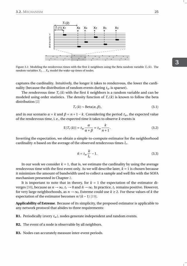
Figure 3.1: Modeling the rendezvous times with the first k neighbors using the Beta random variable Tr (k). Therandom variables X1 . . . Xn model the wake-up times of nodes.
captures the cardinality. Intuitively, the longer it takes to rendezvous, the lower the cardi-nality (because the distribution of random events during tw is sparser).
The rendezvous time Tr (k) with the first k neighbors is a random variable and can bemodeled using order statistics. The density function of Tr (k) is known to follow the betadistribution [2]
Tr (k) ∼ Beta(α,β), (3.1)
and in our scenario α= k and β= n +1−k. Considering the period tw , the expected valueof the rendezvous time, i. e., the expected time it takes to observe k events is
E[Tr (k)] = twα
α+β = twk
n +1. (3.2)
Inverting the expectation, we obtain a simple-to-compute estimator for the neighborhoodcardinality n based on the average of the observed rendezvous times t̄r .
n̂ = twk
t̄r−1. (3.3)
In our work we consider k = 1, that is, we estimate the cardinality by using the averagerendezvous time with the first event only. As we will describe later, k = 1 is chosen becauseit minimizes the amount of bandwidth used to collect a sample and well fits with the SOFAmechanism presented in Chapter 2.
It is important to note that in theory, for k = 1 the expectation of the estimator di-verges [38], because as n →∞, tr → 0 and n̂ →∞. In practice, tr remains positive. However,for very large neighborhoods, as n →∞, Estreme could use k ≥ 2. For these values of k theexpectation of the estimator becomes n/(k −1) [19].
Applicability of Estreme. Because of its simplicity, the proposed estimator is applicable toany network protocol that abides to three requirements:
R1. Periodically (every tw ), nodes generate independent and random events.
R2. The event of a node is observable by all neighbors.
R3. Nodes can accurately measure inter-event periods.
3
26 3. NEIGHBORHOOD CARDINALITY ESTIMATION
Requirement 1 guarantees that, given a random moment in time, we can model the oc-currence of the first event using a uniform random variable. Requirement 2 ensures thatan initiator node appropriately identifies the first k events. That is, it does not mistake alater event for an earlier one. For example, due to collisions, earlier events can be lost andEstreme would underestimate the cardinality. Requirement 3 ensures that the rendezvoustime is measured accurately. Otherwise an overestimation (shorter rendezvous than fac-tual) or underestimation (longer rendezvous than factual) of the cardinality would occur.
3.2.1. TIMING INACCURACIESAs we will observe in the next section, measuring accurately the rendezvous time is chal-lenging because several delays are introduced. Some of these delays can be measured andovercome, but others are difficult to track, such as computation and transmission delays.Analyzing the effects of these delays is central to understanding the performance of Es-treme in real scenarios. In this section we derive a bound for the cardinality (estimation)error caused by a positive delay ε in the rendezvous time.
Proposition 1. Given a timing error ε in the rendezvous time tr , the expected cardinalityerror is
E[en] = n̂ε−n
n=Θ
(− ρ
1+ρ)
,
where ρ = ε(n +1)/tw , and n̂ε is the expected value of the estimated cardinality consideringε.
Proof. The proof consists of two steps. First, we derive n̂ε based on an expected rendezvoustime delayed by ε. We then propose a bound on the resulting error en and show that it istight. Let us start with the derivation of en . Substituting the expression of n̂ε derived from(3.2) and (3.3) into the definition of E[en], we obtain
E[en] =− ε(n +1)2
n (tw +ε(n +1)). (3.4)
Observe that for ε> 0, the above is negative; any positive delay causes the underestimationof n. Unfortunately, even though exact, Equation (3.4) is not intuitive. It is easy to see that,the simpler and more insightful expression
Φ=− ε(n +1)2
(n +1)(tw +ε(n +1))
=− ε(n +1)/tw
1+ε(n +1)/tw=− ρ
1+ρ (3.5)
tightly bounds E[en]. It is sufficient to show that, for each n, positive k1, k2 exist such that
k1Φ≤ E[en] ≤ k2Φ, for all n ≥ 1.
Indeed, the above inequality holds for
k1 ≤ (n +1)/n and k2 ≥ (n +1)/n.
Setting ρ = ε(n +1)/tw in Equation (3.5) concludes our proof.
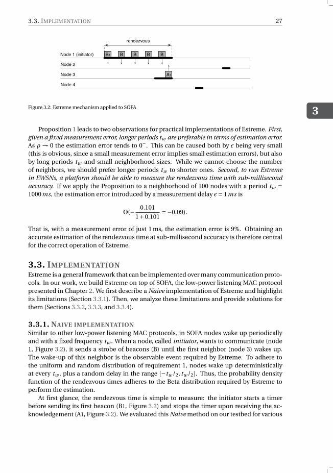
3.3. IMPLEMENTATION
3
27
Node 1 (initiator)
Node 2
B1
A1
BB B B
Node 3
Node 4
rendezvous
Figure 3.2: Estreme mechanism applied to SOFA
Proposition 1 leads to two observations for practical implementations of Estreme. First,given a fixed measurement error, longer periods tw are preferable in terms of estimation error.As ρ → 0 the estimation error tends to 0−. This can be caused both by ε being very small(this is obvious, since a small measurement error implies small estimation errors), but alsoby long periods tw and small neighborhood sizes. While we cannot choose the numberof neighbors, we should prefer longer periods tw to shorter ones. Second, to run Estremein EWSNs, a platform should be able to measure the rendezvous time with sub-millisecondaccuracy. If we apply the Proposition to a neighborhood of 100 nodes with a period tw =1000ms, the estimation error introduced by a measurement delay ε= 1ms is
Θ(− 0.101
1+0.101=−0.09).
That is, with a measurement error of just 1 ms, the estimation error is 9%. Obtaining anaccurate estimation of the rendezvous time at sub-millisecond accuracy is therefore centralfor the correct operation of Estreme.
3.3. IMPLEMENTATIONEstreme is a general framework that can be implemented over many communication proto-cols. In our work, we build Estreme on top of SOFA, the low-power listening MAC protocolpresented in Chapter 2. We first describe a Naive implementation of Estreme and highlightits limitations (Section 3.3.1). Then, we analyze these limitations and provide solutions forthem (Sections 3.3.2, 3.3.3, and 3.3.4).
3.3.1. NAIVE IMPLEMENTATIONSimilar to other low-power listening MAC protocols, in SOFA nodes wake up periodicallyand with a fixed frequency tw . When a node, called initiator, wants to communicate (node1, Figure 3.2), it sends a strobe of beacons (B) until the first neighbor (node 3) wakes up.The wake-up of this neighbor is the observable event required by Estreme. To adhere tothe uniform and random distribution of requirement 1, nodes wake up deterministicallyat every tw , plus a random delay in the range [−tw /2, tw /2]. Thus, the probability densityfunction of the rendezvous times adheres to the Beta distribution required by Estreme toperform the estimation.
At first glance, the rendezvous time is simple to measure: the initiator starts a timerbefore sending its first beacon (B1, Figure 3.2) and stops the timer upon receiving the ac-knowledgement (A1, Figure 3.2). We evaluated this Naive method on our testbed for various
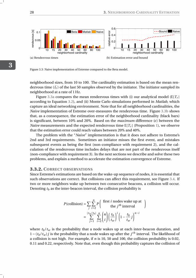
3
28 3. NEIGHBORHOOD CARDINALITY ESTIMATION
10 15 20 30 40 50 60 80 1000
0.05
0.1
neighborhood cardinality
rend
ezvo
us [s
]
Beta Matlab Naive
(a) Rendezvous times
10 15 20 30 40 50 60 80 1000
0.2
0.4
0.6
neighborhood cardinality
rela
tive
erro
r
Bound Naive
(b) Estimation error and bound
Figure 3.3: Naive implementation of Estreme compared to the Beta model.
neighborhood sizes, from 10 to 100. The cardinality estimation is based on the mean ren-dezvous time (t̄r ) of the last 50 samples observed by the initiator. The initiator sampled itsneighborhood at a rate of 1 Hz.
Figure 3.3a compares the mean rendezvous times with (i) our analytical model (E[Tr ]according to Equation 3.2), and (ii) Monte Carlo simulations performed in Matlab, whichcapture an ideal networking environment. Note that for all neighborhood cardinalities, theNaive implementation of Estreme over-measures the rendezvous time. Figure 3.3b showsthat, as a consequence, the estimation error of the neighborhood cardinality (black bars)is significant, between 10% and 20%. Based on the maximum difference (ε) between theNaive measurements and the expected rendezvous time E[Tr ] (Proposition 1), we observethat the estimation error could reach values between 20% and 40%.
The problem with the “Naive” implementation is that it does not adhere to Estreme’s2nd and 3rd requirements. Sometimes an initiator misses the first event, and mistakessubsequent events as being the first (non-compliance with requirement 2), and the cal-culation of the rendezvous time includes delays that are not part of the rendezvous itself(non-compliance with requirement 3). In the next sections we describe and solve these twoproblems, and explain a method to accelerate the estimation convergence of Estreme.
3.3.2. CORRECT OBSERVATIONSSince Estreme’s estimations are based on the wake-up sequence of nodes, it is essential thatsuch observations are correct. But collisions can affect this requirement, see Figure 3.4. Iftwo or more neighbors wake up between two consecutive beacons, a collision will occur.Denoting tb as the inter-beacon interval, the collision probability is
P (collision) =∑j
n∑i=2
P
(first i nodes wake up at
the j th interval
)
=btw /tbc∑
j=1
n∑i=2
(n
i
)(tb
tw
)i (1− tb
twj
)n−i
where tb/tw is the probability that a node wakes up at each inter-beacon duration, and1− (tb/tw ) j is the probability that a node wakes up after the j th interval. The likelihood ofa collision is not high. For example, if n is 10, 50 and 100, the collision probability is 0.02,0.11 and 0.22, respectively. Note that, even though this probability captures the collision of
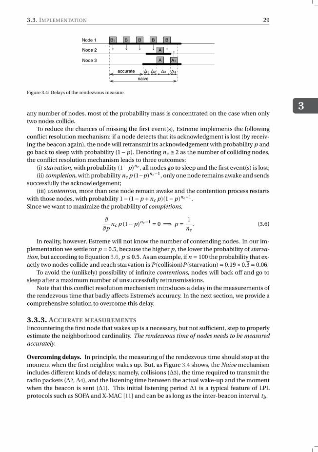
3.3. IMPLEMENTATION
3
29
Node 1
Node 2
Node 3
B B
A
naive
A
accurate
A1
B1 BB
Δ1 Δ2 Δ3 Δ4
Figure 3.4: Delays of the rendezvous measure.
any number of nodes, most of the probability mass is concentrated on the case when onlytwo nodes collide.
To reduce the chances of missing the first event(s), Estreme implements the followingconflict resolution mechanism: if a node detects that its acknowledgment is lost (by receiv-ing the beacon again), the node will retransmit its acknowledgement with probability p andgo back to sleep with probability (1−p). Denoting nc ≥ 2 as the number of colliding nodes,the conflict resolution mechanism leads to three outcomes:
(i) starvation, with probability (1−p)nc , all nodes go to sleep and the first event(s) is lost;(ii) completion, with probability nc p (1−p)nc−1, only one node remains awake and sends
successfully the acknowledgement;(iii) contention, more than one node remain awake and the contention process restarts
with those nodes, with probability 1− (1−p +nc p)(1−p)nc−1.Since we want to maximize the probability of completions,
∂
∂pnc p (1−p)nc−1 = 0 =⇒ p = 1
nc. (3.6)
In reality, however, Estreme will not know the number of contending nodes. In our im-plementation we settle for p = 0.5, because the higher p, the lower the probability of starva-tion, but according to Equation 3.6, p ≤ 0.5. As an example, if n = 100 the probability that ex-actly two nodes collide and reach starvation is P (collision)P (starvation) = 0.19×0.3 = 0.06.
To avoid the (unlikely) possibility of infinite contentions, nodes will back off and go tosleep after a maximum number of unsuccessfully retransmissions.
Note that this conflict resolution mechanism introduces a delay in the measurements ofthe rendezvous time that badly affects Estreme’s accuracy. In the next section, we provide acomprehensive solution to overcome this delay.
3.3.3. ACCURATE MEASUREMENTSEncountering the first node that wakes up is a necessary, but not sufficient, step to properlyestimate the neighborhood cardinality. The rendezvous time of nodes needs to be measuredaccurately.
Overcoming delays. In principle, the measuring of the rendezvous time should stop at themoment when the first neighbor wakes up. But, as Figure 3.4 shows, the Naive mechanismincludes different kinds of delays; namely, collisions (∆3), the time required to transmit theradio packets (∆2, ∆4), and the listening time between the actual wake-up and the momentwhen the beacon is sent (∆1). This initial listening period ∆1 is a typical feature of LPLprotocols such as SOFA and X-MAC [11] and can be as long as the inter-beacon interval tb .
3
30 3. NEIGHBORHOOD CARDINALITY ESTIMATION
To obtain an accurate measurement, we need to subtract these delays from the naivemeasurements. In our implementation, this is done through the receiver (node 3), by start-ing a timer once the receiver wakes up and piggybacking the elapsed time on the acknowl-edgments (∆1 + ∆2 + ∆3). Assuming a fixed bit rate and a fixed acknowledgement size, bothreasonable assumptions, ∆4 can be computed off-line as a constant and be systematicallysubtracted by the initiator after the acknowledgement is received. In our case ∆4 = 1.1 ms.
Accurate timing in Contiki OS. In Contiki, the clock library allows measurements with amaximum precision of 2.83 ms. This coarse-grained measure is not suitable for our esti-mation purposes. To ensure the maximum possible accuracy, we measured the rendezvoustimes using Contiki’s real-time module (rtimer). Its precision depends on the processor’sclock frequency (32 KHz in our devices) and allows to measure time-ranges with sub-milli-second accuracy.
3.3.4. IMPROVING THE ESTIMATION PROCESS
As any other estimator based on order statistics, Estreme is bound to the law of large num-bers: the larger the number of samples, the closer the mean gets to the expected value andthe more accurate the estimation. Unfortunately, in mobile networks nodes cannot col-lect many samples because they only have a limited amount of time to capture the currentstatus of their neighborhoods. The central question is hence, how can we facilitate a fastgathering of samples? Estreme’s design tackles this problem in the temporal (T-Estreme)and spatial (S-Estreme) domains.
Averaging samples in time. Intuitively, given a certain period T , we would like nodes togather as many samples as possible during that period. The key characteristic to achievethis goal is an efficient use of bandwidth, that is, to spend as little time as possible gatheringeach sample. By using SOFA’s primitive (opportunistic anycast), Estreme reduces the use ofbandwidth to the minimum time required to observe an event. To process these samples,T-Estreme utilizes a simple moving window average (MWA) filter, where the last w samplesof the rendezvous time are averaged to estimate the cardinality. We tried other robust sta-tistical methods based on the median and on alpha-trimmer filters, but there was not muchdifference with regards to MWA (because requirements 2 and 3 already remove most out-liers). Like most MWA estimations, the tradeoff in the time domain is between accuracy andadaptability: the bigger w , the more time it takes to adapt to changes in cardinality.
Averaging samples in space and time. Different from most cardinality estimators in theliterature, Estreme is designed from inception to allow all nodes to perform concurrent esti-mations. This characteristic is not only good because some practical applications require it,but perhaps more importantly because it can quadratically increase the convergence of theestimation. In S-Estreme, besides sending the delay information described in Section 3.3.3,a receiver also sends the average of its own time window. Every node is hence able to processw2 samples in the same time required to locally collect w samples. Note that in S-Estreme,it is preferable to choose w based on the expected cardinality of the neighborhood n. Withw > n, some nodes’ samples will be counted multiple times. With w < n, on the other hand,only part of the neighbors’ samples will be taken into account by the estimator. While in ourexperiments w is kept constant, it is also possible to dynamically adapt w ’s size based onthe cardinality estimation provided by T-Estreme. It is important to highlight that while in
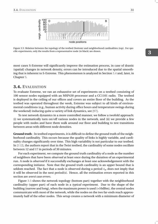
3.4. EVALUATION
3
31
020406080
100
neig
h. c
ardi
nalit
ynode positions
D B
Figure 3.5: Relation between the topology of the testbed (bottom) and neighborhood cardinalities (top). For spe-cific experiments, only the results from a representative node (in black) are shown.
most cases S-Estreme will significantly improve the estimation process, in case of drastic(spatial) changes in network density, errors can be introduced due to the spatial smooth-ing that is inherent to S-Estreme. This phenomenon is analyzed in Section 3.4 and, later, inChapter 5.
3.4. EVALUATIONTo evaluate Estreme, we ran an exhaustive set of experiments on a testbed consisting of100 sensor nodes equipped with an MSP430 processor and a CC1101 radio. The testbedis deployed in the ceiling of our offices and covers an entire floor of the building. As thetestbed was operated throughout the week, Estreme was subject to all kinds of environ-mental conditions (e.g., human activity during office hours and temperature swings duringthe weekend) inducing quite a variety of link dynamics, see [97].
To test network dynamics in a more controlled manner, we follow a twofold approach:(i) we systematically turn on/off various nodes in the network, and (ii) we provide a fewpeople with nodes and have them walk around our floor and building to test transitionsbetween areas with different node densities.
Ground truth : In testbed experiments, it is difficult to define the ground truth of the neigh-borhood cardinality. This occurs because the quality of links is highly variable, and cardi-nality changes significantly over time. This high variability is not particular to our testbed.In [112], the authors report that in the Twist testbed, the cardinality of some nodes oscillatebetween 12 and 17 in periods of 30 minutes.
For each experiment, we compute the ground truth cardinality of a node as the numberof neighbors that have been observed at least once during the duration of an experimentalrun. A node is observed if it successfully exchanges at least one acknowledgement with thecorresponding initiator. Note that the ground truth cardinality is an upper bound that isseldom reached. The fact that a node is observed during a period tw does not imply thatit will be observed in the next period(s). Hence, all the estimation errors reported in thissection are worst case errors.
Figure 3.5 shows the network topology (bottom part) together with the neighborhoodcardinality (upper part) of each node in a typical experiment. Due to the shape of thebuilding (narrow and long), when the maximum power is used (+10dBm), the central nodescommunicate with most of the network, while the nodes on the two far-ends reach approx-imately half of the other nodes. This setup creates a network with a minimum diameter of
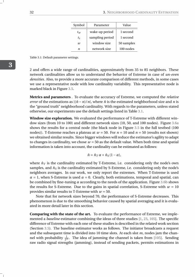
3
32 3. NEIGHBORHOOD CARDINALITY ESTIMATION
Symbol Parameter Value
tw wake-up period 1 second
ts sampling period 1 second
w window size 50 samples
n network size 100 nodes
Table 3.1: Default parameter settings.
2 and offers a wide range of cardinalities, approximately from 35 to 85 neighbors. Thesenetwork cardinalities allow us to understand the behavior of Estreme in case of un-evendensities. Also, to provide a more accurate comparison of different methods, in some caseswe use a representative node with low cardinality variability. This representative node ismarked black in Figure 3.5.
Metrics and parameters . To evaluate the accuracy of Estreme, we computed the relativeerror of the estimations as |(n̂ −n)/n|, where n̂ is the estimated neighborhood size and n isthe “ground truth” neighborhood cardinality. With regards to the parameters, unless statedotherwise, our experiments use the default settings listed in Table 3.1.
Window size exploration. We evaluated the performance of T-Estreme with different win-dow sizes (from 10 to 100) and different network sizes (10, 50, and 100 nodes). Figure 3.6ashows the results for a central node (the black node in Figure 3.5 in the full testbed (100nodes)). T-Estreme reaches a plateau at w = 50. For n = 10 and n = 50 (results not shown)we obtained similar results. Since bigger windows will reduce the estimator’s agility to adaptto changes in cardinality, we chose w = 50 as the default value. When both time and spatialinformation is taken into account, the cardinality can be estimated as follows:
n̂ = n̂T α+ n̂S (1−α),
where n̂T is the cardinality estimated by T-Estreme, i.e. considering only the node’s ownsamples, and n̂S is the cardinality estimated by S-Estreme, i.e. considering only the node’sneighbors averages. In our work, we only report the extremes. When T-Estreme is usedα = 1, when S-Estreme is used α = 0. Clearly, both estimations, temporal and spatial, canbe combined by fine-tuning α according to the needs of the application. Figure 3.6b showsthe results for S-Estreme. Due to the gains in spatial correlation, S-Estreme with w = 10provides similar results to T-Estreme with w = 50.
Note that for network sizes beyond 70, the performance of S-Estreme decreases. Thisphenomenon is due to the smoothing behavior caused by spatial averaging and it is evalu-ated in more detail later in this section.
Comparing with the state of the art. To evaluate the performance of Estreme, we imple-mented a baseline estimator combining the ideas of three studies [1, 23, 105]. The specificdifference of Estreme with each one of these studies is described in the related work section(Section 3.5). The baseline estimator works as follows. The initiator broadcasts a requestand the subsequent time is divided into 10 time slots. At each slot m, nodes jam the chan-nel with probability 1
2m . The idea of jamming the channel is taken from [105]. Sendingraw radio signal strengths (jamming), instead of sending packets, permits estimations in
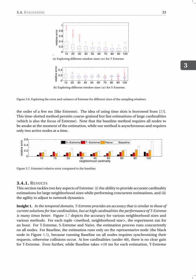
3.4. EVALUATION
3
33
. 10 20 30 40 50 60 70 80 90 1000
0.2
0.4
0.6
0.8
1
rela
tive
erro
r(a) Exploring different window sizes (w) for T-Estreme
10 20 30 40 50 60 70 80 90 1000
0.2
0.4
rela
tive
erro
r
(b) Exploring different window sizes (w) for S-Estreme.
Figure 3.6: Exploring the error and variance of Estreme for different sizes of the sampling windows.
the order of a few ms (like Estreme). The idea of using time slots is borrowed from [23].This time-slotted method permits coarse-grained but fast estimations of large cardinalities(which is also the focus of Estreme). Note that the baseline method requires all nodes tobe awake at the moment of the estimation, while our method is asynchronous and requiresonly two active nodes at a time.
10 15 20 30 40 50 60 80 1000
0.2
0.4
0.6
neighborhood cardinality
rela
tive
erro
r
S−Estreme T−Estreme Naive Baseline
Figure 3.7: Estreme’s relative error compared to the baseline.
3.4.1. RESULTSThis section tackles two key aspects of Estreme: (i) the ability to provide accurate cardinalityestimations for large neighborhood sizes while performing concurrent estimations, and (ii)the agility to adjust to network dynamics.
Insight 1. In the temporal domain, T-Estreme provides an accuracy that is similar to those ofcurrent solutions for low cardinalities, but at high cardinalities the performance of T-Estremeis many times better. Figure 3.7 depicts the accuracy for various neighborhood sizes andvarious methods. For each tuple <method, neighborhood size>, the experiment ran foran hour. For T-Estreme, S-Estreme and Naive, the estimation process runs concurrentlyon all nodes. For Baseline, the estimation runs only on the representative node (the blacknode in Figure 3.5), because running Baseline on all nodes requires synchronizing theirrequests, otherwise collisions occur. At low cardinalities (under 40), there is no clear gainfor T-Estreme. Even further, while Baseline takes ≈10 ms for each estimation, T-Estreme
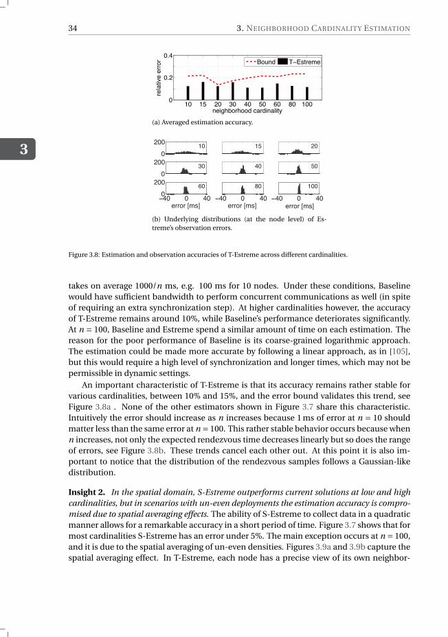
3
34 3. NEIGHBORHOOD CARDINALITY ESTIMATION
10 15 20 30 40 50 60 80 1000
0.2
0.4
neighborhood cardinality
rela
tive
erro
r
Bound T−Estreme
(a) Averaged estimation accuracy.
0200 10 15 20
0200 30 40 50
−40 0 400200 60
−40 0 4080
−40 0 40100
error [ms] error [ms] error [ms](b) Underlying distributions (at the node level) of Es-treme’s observation errors.
Figure 3.8: Estimation and observation accuracies of T-Estreme across different cardinalities.
takes on average 1000/n ms, e.g. 100 ms for 10 nodes. Under these conditions, Baselinewould have sufficient bandwidth to perform concurrent communications as well (in spiteof requiring an extra synchronization step). At higher cardinalities however, the accuracyof T-Estreme remains around 10%, while Baseline’s performance deteriorates significantly.At n = 100, Baseline and Estreme spend a similar amount of time on each estimation. Thereason for the poor performance of Baseline is its coarse-grained logarithmic approach.The estimation could be made more accurate by following a linear approach, as in [105],but this would require a high level of synchronization and longer times, which may not bepermissible in dynamic settings.
An important characteristic of T-Estreme is that its accuracy remains rather stable forvarious cardinalities, between 10% and 15%, and the error bound validates this trend, seeFigure 3.8a . None of the other estimators shown in Figure 3.7 share this characteristic.Intuitively the error should increase as n increases because 1 ms of error at n = 10 shouldmatter less than the same error at n = 100. This rather stable behavior occurs because whenn increases, not only the expected rendezvous time decreases linearly but so does the rangeof errors, see Figure 3.8b. These trends cancel each other out. At this point it is also im-portant to notice that the distribution of the rendezvous samples follows a Gaussian-likedistribution.
Insight 2. In the spatial domain, S-Estreme outperforms current solutions at low and highcardinalities, but in scenarios with un-even deployments the estimation accuracy is compro-mised due to spatial averaging effects. The ability of S-Estreme to collect data in a quadraticmanner allows for a remarkable accuracy in a short period of time. Figure 3.7 shows that formost cardinalities S-Estreme has an error under 5%. The main exception occurs at n = 100,and it is due to the spatial averaging of un-even densities. Figures 3.9a and 3.9b capture thespatial averaging effect. In T-Estreme, each node has a precise view of its own neighbor-
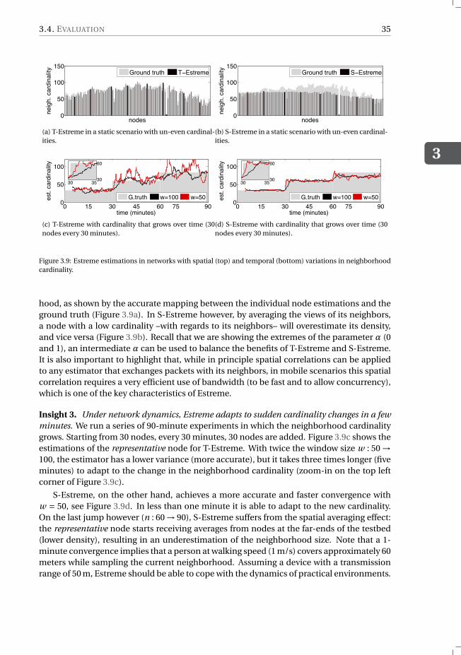
3.4. EVALUATION
3
35
0
50
100
150
nodes
neig
h. c
ardi
nalit
y
Ground truth T−Estreme
(a) T-Estreme in a static scenario with un-even cardinal-ities.
0
50
100
150
nodes
neig
h. c
ardi
nalit
y
Ground truth S−Estreme
(b) S-Estreme in a static scenario with un-even cardinal-ities.
0 15 30 45 60 75 900
50
100
time (minutes)
est.
card
inal
ity
G.truth w=100 w=50
30 3530
60
(c) T-Estreme with cardinality that grows over time (30nodes every 30 minutes).
0 15 30 45 60 75 900
50
100
time (minutes)es
t. ca
rdin
ality
G.truth w=100 w=50
30 3530
60
(d) S-Estreme with cardinality that grows over time (30nodes every 30 minutes).
Figure 3.9: Estreme estimations in networks with spatial (top) and temporal (bottom) variations in neighborhoodcardinality.
hood, as shown by the accurate mapping between the individual node estimations and theground truth (Figure 3.9a). In S-Estreme however, by averaging the views of its neighbors,a node with a low cardinality –with regards to its neighbors– will overestimate its density,and vice versa (Figure 3.9b). Recall that we are showing the extremes of the parameter α (0and 1), an intermediate α can be used to balance the benefits of T-Estreme and S-Estreme.It is also important to highlight that, while in principle spatial correlations can be appliedto any estimator that exchanges packets with its neighbors, in mobile scenarios this spatialcorrelation requires a very efficient use of bandwidth (to be fast and to allow concurrency),which is one of the key characteristics of Estreme.
Insight 3. Under network dynamics, Estreme adapts to sudden cardinality changes in a fewminutes. We run a series of 90-minute experiments in which the neighborhood cardinalitygrows. Starting from 30 nodes, every 30 minutes, 30 nodes are added. Figure 3.9c shows theestimations of the representative node for T-Estreme. With twice the window size w : 50 →100, the estimator has a lower variance (more accurate), but it takes three times longer (fiveminutes) to adapt to the change in the neighborhood cardinality (zoom-in on the top leftcorner of Figure 3.9c).
S-Estreme, on the other hand, achieves a more accurate and faster convergence withw = 50, see Figure 3.9d. In less than one minute it is able to adapt to the new cardinality.On the last jump however (n : 60 → 90), S-Estreme suffers from the spatial averaging effect:the representative node starts receiving averages from nodes at the far-ends of the testbed(lower density), resulting in an underestimation of the neighborhood size. Note that a 1-minute convergence implies that a person at walking speed (1 m/s) covers approximately 60meters while sampling the current neighborhood. Assuming a device with a transmissionrange of 50 m, Estreme should be able to cope with the dynamics of practical environments.
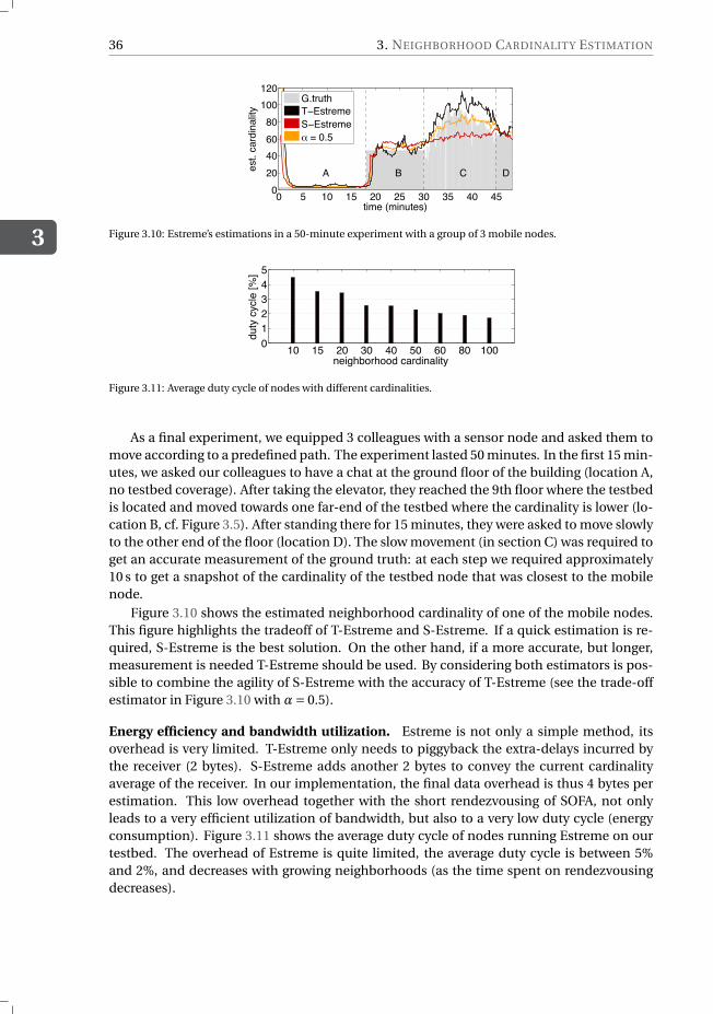
3
36 3. NEIGHBORHOOD CARDINALITY ESTIMATION
0 5 10 15 20 25 30 35 40 45020406080
100120
A B C D
time (minutes)
est.
card
inal
ity
G.truthT−EstremeS−Estreme_ = 0.5
Figure 3.10: Estreme’s estimations in a 50-minute experiment with a group of 3 mobile nodes.
10 15 20 30 40 50 60 80 100012345
neighborhood cardinality
duty
cyc
le [%
]
Figure 3.11: Average duty cycle of nodes with different cardinalities.
As a final experiment, we equipped 3 colleagues with a sensor node and asked them tomove according to a predefined path. The experiment lasted 50 minutes. In the first 15 min-utes, we asked our colleagues to have a chat at the ground floor of the building (location A,no testbed coverage). After taking the elevator, they reached the 9th floor where the testbedis located and moved towards one far-end of the testbed where the cardinality is lower (lo-cation B, cf. Figure 3.5). After standing there for 15 minutes, they were asked to move slowlyto the other end of the floor (location D). The slow movement (in section C) was required toget an accurate measurement of the ground truth: at each step we required approximately10 s to get a snapshot of the cardinality of the testbed node that was closest to the mobilenode.
Figure 3.10 shows the estimated neighborhood cardinality of one of the mobile nodes.This figure highlights the tradeoff of T-Estreme and S-Estreme. If a quick estimation is re-quired, S-Estreme is the best solution. On the other hand, if a more accurate, but longer,measurement is needed T-Estreme should be used. By considering both estimators is pos-sible to combine the agility of S-Estreme with the accuracy of T-Estreme (see the trade-offestimator in Figure 3.10 with α= 0.5).
Energy efficiency and bandwidth utilization. Estreme is not only a simple method, itsoverhead is very limited. T-Estreme only needs to piggyback the extra-delays incurred bythe receiver (2 bytes). S-Estreme adds another 2 bytes to convey the current cardinalityaverage of the receiver. In our implementation, the final data overhead is thus 4 bytes perestimation. This low overhead together with the short rendezvousing of SOFA, not onlyleads to a very efficient utilization of bandwidth, but also to a very low duty cycle (energyconsumption). Figure 3.11 shows the average duty cycle of nodes running Estreme on ourtestbed. The overhead of Estreme is quite limited, the average duty cycle is between 5%and 2%, and decreases with growing neighborhoods (as the time spent on rendezvousingdecreases).
3.5. RELATED WORK
3
37
Exploring the parameter space. Throughout our experiments, we used some default val-ues for the parameters of both the underlying MAC and Estreme itself, namely, the wake-upperiod (tw ) and the sampling period (ts ). These parameters influence the performance ofEstreme and, hence, it is important to assess them more thoroughly. We tested Estreme withtwo different wake-up periods, 0.5 and 1 second, and with five different sampling periods,0.5, 1, 2, 5 and 10 seconds. Each <ts , tw> tuple was run for an hour using 100 nodes. Ta-ble 3.2 show the result of our experiments. The metrics of interest are the relative error andthe relative sampling rate. The relative sampling rate captures the percentage of samplingrequests that are successfully completed.
Relative error. As predicted by our model, increasing tw decreases the error. Changingthe sampling period, instead, does not seem to have a clear consequence on the estimationerror, except for very low ts and tw , which may indicate some channel saturation.
Relative sampling rate . Ideally, we would like every request from an initiator to be com-pleted, but as ts decreases this is not possible due to channel saturation issues. For thedefault setup in our experiments <tw = 1s, ts = 1s> only approximately 30% of the requestsare successful. This relative low rate occurs because, in Estreme, an initiator that observesand on-going estimation goes back to sleep (according to SOFA’s back-off mechanism). Asthe channel saturates, more and more requests are silently canceled. It is important to high-light however that the fraction of requests that are successful provides the same rendezvousaccuracy as of those requests that are performed on lightly-loaded channels. In general, therelative sampling rate can be raised by reducing tw , but results in larger estimation errors,so is to be avoided.
3.5. RELATED WORKWe start by providing a comparison of Estreme within the (mobile) sensor network domain.We then broaden our scope and overview solutions proposed in RFID systems and mobilephone networks. For a concise overview of the related work see Table 3.3.
Mobile sensor networks. Although neighborhood cardinality estimation is an essentialbuilding block of various protocols, it has been little explored within the context of (mobile)sensor networks. We follow by comparing to the three overarching approaches:
(i) Polling and group testing mechanisms are the closest to Estreme. Their goal it to ef-ficiently estimate the cardinality of the n neighbors that hold a given property. Differentfrom Estreme, these mechanisms do not specifically target mobile networks and, in somecases, do not estimate the exact number of neighbors. Backcast [31] tests if n > 0, while [23]tries to asses if n crosses a certain threshold. If n > 0, Strawman [73] is able to efficientlyidentify one of the responders. Among the various polling mechanisms, the one that is themost related to our work is the study by Zeng et al. [105], where the authors propose twodifferent methods. LogPoll is able to estimate the logarithmic cardinality of a neighbor-hood, i. e., logn, in just 4ms, while LinearPoll is able to recognize all the identities of theresponders at the cost of spending more energy and time. This remarkable performancecomes at a high cost and relies on several assumptions. LogPoll and LinearPoll model andperiodically calibrate the signal strength of neighbors, effectively limiting the applicabilityof these estimators to static networks with minor link dynamics. Additionally, LinearPollcan only count a limited number of neighbors, because it requires neighbors to send radio
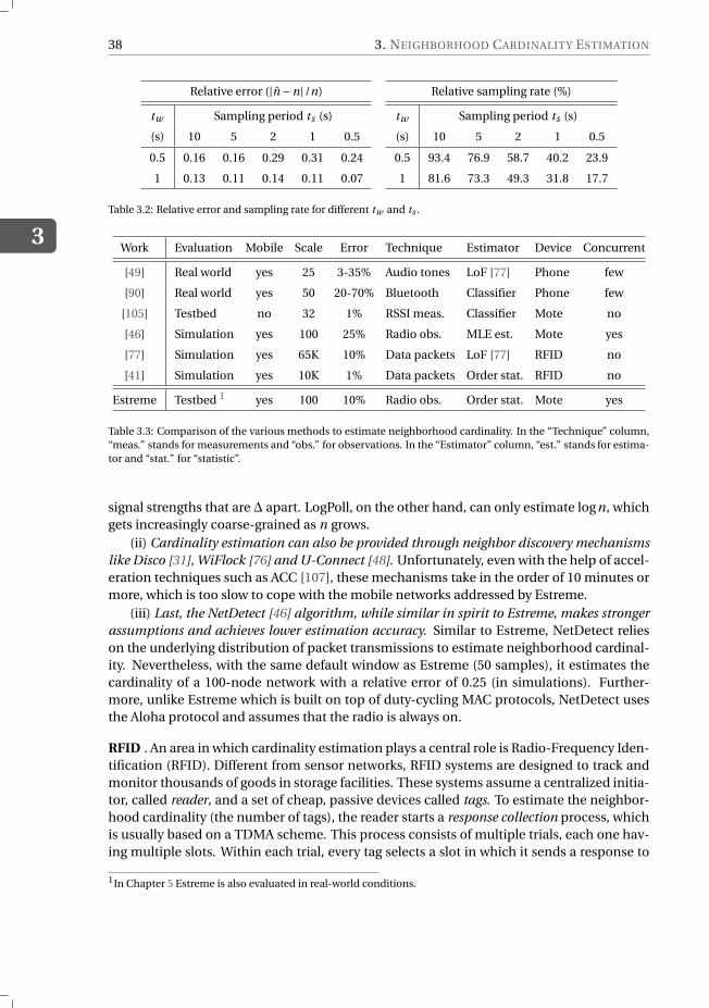
3
38 3. NEIGHBORHOOD CARDINALITY ESTIMATION
Relative error (|n̂ −n|/n)
tw Sampling period ts (s)
(s) 10 5 2 1 0.5
0.5 0.16 0.16 0.29 0.31 0.24
1 0.13 0.11 0.14 0.11 0.07
Relative sampling rate (%)
tw Sampling period ts (s)
(s) 10 5 2 1 0.5
0.5 93.4 76.9 58.7 40.2 23.9
1 81.6 73.3 49.3 31.8 17.7
Table 3.2: Relative error and sampling rate for different tw and ts .
Work Evaluation Mobile Scale Error Technique Estimator Device Concurrent
[49] Real world yes 25 3-35% Audio tones LoF [77] Phone few
[90] Real world yes 50 20-70% Bluetooth Classifier Phone few
[105] Testbed no 32 1% RSSI meas. Classifier Mote no
[46] Simulation yes 100 25% Radio obs. MLE est. Mote yes
[77] Simulation yes 65K 10% Data packets LoF [77] RFID no
[41] Simulation yes 10K 1% Data packets Order stat. RFID no
Estreme Testbed 1 yes 100 10% Radio obs. Order stat. Mote yes
Table 3.3: Comparison of the various methods to estimate neighborhood cardinality. In the “Technique” column,“meas.” stands for measurements and “obs.” for observations. In the “Estimator” column, “est.” stands for estima-tor and “stat.” for “statistic”.
signal strengths that are ∆ apart. LogPoll, on the other hand, can only estimate logn, whichgets increasingly coarse-grained as n grows.
(ii) Cardinality estimation can also be provided through neighbor discovery mechanismslike Disco [31], WiFlock [76] and U-Connect [48]. Unfortunately, even with the help of accel-eration techniques such as ACC [107], these mechanisms take in the order of 10 minutes ormore, which is too slow to cope with the mobile networks addressed by Estreme.
(iii) Last, the NetDetect [46] algorithm, while similar in spirit to Estreme, makes strongerassumptions and achieves lower estimation accuracy. Similar to Estreme, NetDetect relieson the underlying distribution of packet transmissions to estimate neighborhood cardinal-ity. Nevertheless, with the same default window as Estreme (50 samples), it estimates thecardinality of a 100-node network with a relative error of 0.25 (in simulations). Further-more, unlike Estreme which is built on top of duty-cycling MAC protocols, NetDetect usesthe Aloha protocol and assumes that the radio is always on.
RFID . An area in which cardinality estimation plays a central role is Radio-Frequency Iden-tification (RFID). Different from sensor networks, RFID systems are designed to track andmonitor thousands of goods in storage facilities. These systems assume a centralized initia-tor, called reader, and a set of cheap, passive devices called tags. To estimate the neighbor-hood cardinality (the number of tags), the reader starts a response collection process, whichis usually based on a TDMA scheme. This process consists of multiple trials, each one hav-ing multiple slots. Within each trial, every tag selects a slot in which it sends a response to
1In Chapter 5 Estreme is also evaluated in real-world conditions.
3.6. CONCLUSION
3
39
the reader. This slot is chosen based on the tag’s state, a random number, and a commandsent by the reader at the beginning of each trial.
Based on the number of observed responses, collisions, and empty slots the initiatoris able to estimate the population size [77]. This process is repeated iteratively multipletimes (trials) to improve the accuracy of the estimators. While usually the reader cannotterminate a trial until the last assigned slot is observed, in [41] the authors propose to useorder statistics to drastically reduce the trials’ duration (an initiator needs to observe onlythe first k responses). Compared to Estreme, this work is able to achieve an accuracy of 1%and scale to thousands of nodes. On the other hand, it has only been tested in simulationsand requires two orders of magnitude more samples than Estreme.
Adapting such a mechanism (and others from the RFID community) to wireless sensornetworks is possible but very challenging. For a correct observation, neighbors will needto be synchronized, so that responses in adjacent slots do not collide. Moreover, a globalscheduling mechanism should be in place to guarantee that at any moment in time onlyone node in the neighborhood can act as a reader (initiator).
Recently, Chen et al. [20] discovered that having a 2-phase estimation (a rough one fol-lowed by a more refined one) is the key to improve the estimation accuracy, independentlyof the chosen technique. In light of this, we plan to extend Estreme with a second estima-tion phase that will use the IDs of the encountered neighbors to improve the estimationaccuracy.
Mobile phones. Initial studies have used mobile phones to estimate the density of crowds.The most relevant work uses audio tones to count neighbor devices [49]. The main chal-lenge involved is to successfully transmit data packets using low-quality speakers/microphones,as well as to cope with the presence of environmental auditive noise. Thanks to the richercomputational capabilities of mobile phones, techniques such as Fast Fourier Transformcan be used to code the signal. Energy efficiency is also addressed, but on a different scalethan Estreme. Here the comparison is against the typical consumption of a WiFi networkinterface. Finally, similar to Estreme, this system is able to support multiple, concurrentestimations. While in theory the method scales to hundreds of devices by using multiplefrequencies, the system was only tested with two concurrent estimators.
An interesting alternative to cardinality estimation is proposed in [90]. The phones scanfor discoverable bluetooth devices and, based on the number of unique identifiers discov-ered, an estimation of the crowd density is performed. Different from Estreme and the otherrelated works, this work focuses on classifying the density into four classes instead of pro-viding a cardinality estimation. Even though the estimation task is simpler, unrealistic as-sumptions on the distribution of bluetooth-enabled devices results in estimation errors thatvary from 20 to 70%.
3.6. CONCLUSIONIn this chapter we addressed the issue of determining the neighborhood cardinality in Ex-treme Wireless Sensor Networks, where link quality fluctuations and node mobility ask for arobust and agile approach. An additional and important focus of our work is to handle highdensities and concurrent estimations, requirements that are necessary in public safety ap-plications such as crowd monitoring. Traditional approaches cannot meet these stringentrequirements, so we developed Estreme: a cardinality estimator based on monitoring the
3
40 3. NEIGHBORHOOD CARDINALITY ESTIMATION
inter-arrival times of (randomized) events raised by neighboring nodes i. e., SOFA’s wake-ups (Chapter 2).
To minimize channel usage, which is essential in EWSNs, Estreme leverages on the shortrendezvous time offered by SOFA’s opportunistic anycast. To obtain high accuracy, Estremeemploys a bag of tricks to account for various overheads, (transmission) latencies, colli-sions, and other factors that all distort the true rendezvous time with the first node to wakeup. We derived a theoretical model underlying the rendezvous times, and used it to gaininsight into the accuracy of Estreme as well as to derive bounds on the estimation error.
As a proof of concept, we implemented Estreme on the Contiki OS, and evaluated it ona testbed with node densities up to 100 nodes. Estreme achieves solid performance resultswith typical estimation errors below 10%, which compares favorably to state-of-the-art so-lutions. Estreme was also demonstrated to handle abrupt changes in density exemplifiedthrough an experiment involving few nodes moving through our testbed.
Later in Chapter 5 we will also evaluate Estreme on several hundreds of devices movingin a large-scale science museum, showing that Estreme is able to scale to extreme mobileenvironment as soon as the spatial changes in density are not too drastic.
4OPPORTUNISTIC DATA COLLECTION
Kal-toh is not about striving for balance. It is about finding the seeds of order, even in themidst of profound chaos.
Lieutenant Tuvok
I N Wireless Sensor Networks, data collection is a solved problem. That is, from the packet-reception perspective, with protocols reported to collect more than 99.9 % of all data.
However, data collection is still a challenge when viewed from the real-world perspective,where networks dynamics and energy conditions (see Chapter 1) play a major role. In thatlight, ORW is the first protocol to effectively use opportunistic anycast in WSNs [55] to per-form data collection. ORW shows that compared to traditional routing schemes, such asCTP [39], opportunistic forwarding decisions can significantly improve data collection per-formance in asynchronously duty-cycled networks in terms of end-to-end packet latencyand energy efficiency, while being more resilient to topology changes. The latter character-istic is essential for data collection mechanisms to scale to EWSNs.
As seen in Chapter 2, the idea of opportunistic routing is simple: instead of first makingthe routing decision and then waiting for the destination to wake up, nodes forward pack-ets opportunistically to the first neighbor that wakes up. The more potential forwarders anode has, the shorter the time it needs to wait before it communicates, and hence the moreefficient it can operate [55]
Opportunistic routing (ORW, SOFA, etc. ) typically assumes that all nodes have the sameduty cycle, and thus, they all end up having the same forwarding costs in terms of en-ergy and delay. But nodes play different roles. The closer a node is to the sink, the morepackets it has to forward, and hence, the lower its forwarding costs should be. Duty cy-cles should be adjusted to the local needs of each node. This is indeed the idea of var-ious adaptive duty-cycling mechanisms. However, these have only been studied analyti-cally [50, 51], thus lacking validation against the real-world dynamics of low-power wire-less, or have been designed for static networks and traditional communication primitives
Parts of this chapter have been published in SenSys’16, Stanford, USA [14].
41
4
42 4. OPPORTUNISTIC DATA COLLECTION
such as unicast [47, 69, 111], which renders them unusable in an opportunistic setting andextreme network conditions.
Inspired by the promising results of opportunistic protocols, we propose a tight integra-tion of duty cycling and opportunistic routing with a mechanism called Staffetta. Staffettais not another routing protocol, but a duty-cycle scheduling mechanism for opportunis-tic data collection that adapts the wake-up frequency of individual nodes such that nodescloser to the sink wake up more often than nodes at the edge of the network. The result-ing activity gradient drastically reduces routing costs and automatically “steers” packets inthe right direction, as the probability of finding an awake neighbor is highest in the direc-tion of the sink. Since Staffetta operates at the medium access control (MAC) layer, it canbe combined with different opportunistic data collection protocols that operate at the net-work layer, targeting real-world applications featuring dynamic multi-hop networks withdata rates on the order of one packet every few seconds [18, 30]. To the best of our knowl-edge, Staffetta is the first mechanism that applies the idea of dynamic duty cycling to op-portunistic data collection.
We implement Staffetta in Contiki and run extensive experiments on the FlockLab andIndriya testbeds to quantify the improvements of Staffetta underneath traditional oppor-tunistic protocols, which typically do not adjust the nodes’ wake-up frequency. We find that,despite its simplicity, Staffetta considerably improves data collection performance, mostnotably in terms of packet latency and network lifetime, while incurring minimal overhead.From a broader perspective, we show that Staffetta’s activity gradient can also be used as arouting metric by itself, achieving performance similar to other routing mechanisms em-powered by Staffetta, but without the need for maintaining a complex routing structure.
Contributions. This chapter makes three main contributions:
• Section 4.2 presents the design of Staffetta, a lightweight, generic mechanism thatadapts the duty cycle of individual nodes to improve opportunistic data collection.By studying the relation between duty cycling and opportunistic communication, weshow how Staffetta’s activity gradient reduces packet latency, while extending networklifetime.
• Section 4.3 describes how one can efficiently implement and combine Staffetta withexisting opportunistic routing protocols. As a paradigmatic case study, we choosethree opportunistic mechanisms inspired by state-of-the-art collection protocols andtheir routing metrics: Expected Duty Cycle [55], Queue Backlog [70], and SOFA’s Ran-dom Walk [16].
• Section 4.4 evaluates the above described routing metrics in combination with Staffettaon two testbeds. Our results show that Staffetta reduces end-to-end packet latency byan order of magnitude and halves energy consumption across the board. A case inpoint is the substantial improvement Staffetta brings to ORW in one of the testbeds:two to six times less energy consumption, 80 to 450 times shorter latencies and fasteradaptation to mobile sinks. These gains are obtained with a negligible overhead interms of memory and processing.
In light of our contributions, we review related work in Section 4.5 and conclude in Sec-tion 4.6.
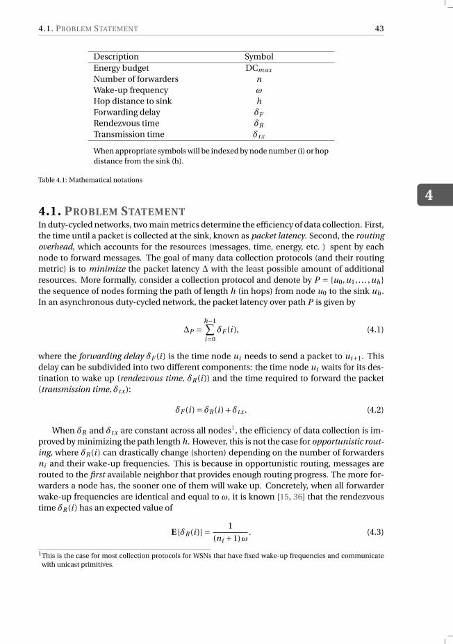
4.1. PROBLEM STATEMENT
4
43
Description SymbolEnergy budget DCmax
Number of forwarders nWake-up frequency ω
Hop distance to sink hForwarding delay δF
Rendezvous time δR
Transmission time δt x
When appropriate symbols will be indexed by node number (i) or hopdistance from the sink (h).
Table 4.1: Mathematical notations
4.1. PROBLEM STATEMENTIn duty-cycled networks, two main metrics determine the efficiency of data collection. First,the time until a packet is collected at the sink, known as packet latency. Second, the routingoverhead, which accounts for the resources (messages, time, energy, etc. ) spent by eachnode to forward messages. The goal of many data collection protocols (and their routingmetric) is to minimize the packet latency ∆ with the least possible amount of additionalresources. More formally, consider a collection protocol and denote by P = {u0,u1, . . . ,uh}the sequence of nodes forming the path of length h (in hops) from node u0 to the sink uh .In an asynchronous duty-cycled network, the packet latency over path P is given by
∆P =h−1∑i=0
δF (i ), (4.1)
where the forwarding delay δF (i ) is the time node ui needs to send a packet to ui+1. Thisdelay can be subdivided into two different components: the time node ui waits for its des-tination to wake up (rendezvous time, δR (i )) and the time required to forward the packet(transmission time, δt x ):
δF (i ) = δR (i )+δt x . (4.2)
When δR and δt x are constant across all nodes1, the efficiency of data collection is im-proved by minimizing the path length h. However, this is not the case for opportunistic rout-ing, where δR (i ) can drastically change (shorten) depending on the number of forwardersni and their wake-up frequencies. This is because in opportunistic routing, messages arerouted to the first available neighbor that provides enough routing progress. The more for-warders a node has, the sooner one of them will wake up. Concretely, when all forwarderwake-up frequencies are identical and equal to ω, it is known [15, 36] that the rendezvoustime δR (i ) has an expected value of
E [δR (i )] = 1
(ni +1)ω. (4.3)
1This is the case for most collection protocols for WSNs that have fixed wake-up frequencies and communicatewith unicast primitives.
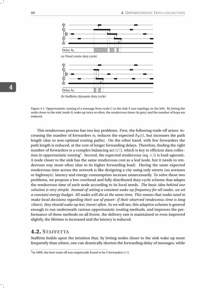
4
44 4. OPPORTUNISTIC DATA COLLECTION
Delay δR
S
A
B
C
D
(a) Fixed (static duty cycle)
Delay δR
S
A
B
C
D
(b) Staffetta (dynamic duty cycle)
Figure 4.1: Opportunistic routing of a message from node C to the sink S (see topology on the left). By letting thenode closer to the sink (node A) wake up twice as often, the rendezvous times (in grey) and the number of hops arereduced.
This rendezvous process has two key problems. First, the following trade off arises: in-creasing the number of forwarders ni reduces the expected δR (i ), but increases the pathlength (due to non-optimal routing paths). On the other hand, with few forwarders thepath length is reduced, at the cost of longer forwarding delays. Therefore, finding the rightnumber of forwarders is a complex balancing act [27], which is key to efficient data collec-tion in opportunistic routing2. Second, the expected rendezvous (eq. 4.3) is load-agnostic.A node closer to the sink has the same rendezvous cost as a leaf node, but it needs to ren-dezvous way more often (due to its higher forwarding load). Having the same expectedrendezvous time across the network is like designing a city using only streets (no avenuesor highways): latency and energy consumption increase unnecessarily. To solve these twoproblems, we propose a low-overhead and fully distributed duty-cycle scheme that adaptsthe rendezvous time of each node according to its local needs. The basic idea behind oursolution is very simple. Instead of setting a constant wake up frequency for all nodes, we seta constant energy budget. All nodes will die at the same time. This means that nodes need tomake local decisions regarding their use of power: if their observed rendezvous time is long(short), they should wake up less (more) often. As we will see, this adaptive scheme is generalenough to run underneath various opportunistic routing methods, and improves the per-formance of these methods on all fronts: the delivery rate is maintained or even improvedslightly, the lifetime is increased and the latency is reduced.
4.2. STAFFETTAStaffetta builds upon the intuition that, by letting nodes closer to the sink wake up morefrequently than others, one can drastically shorten the forwarding delay of messages, while
2In ORW, the best trade off was empirically found to be 5 forwarders [55]
4.2. STAFFETTA
4
45
reducing the average path length. As an example, Figure 4.1 compares an opportunistic col-lection mechanism with fixed wake-up frequency (4.1a) against one where the node closerto the sink i. e., node A, wakes up twice as frequently (4.1b). Since in Figure 4.1b A increasesits activity, it wakes up before B and gets selected as forwarder by C. This not only reducesthe forwarding delay of C, but also decreases the number of hops needed to deliver C’s mes-sage to the sink.
In opportunistic routing, the forwarding decisions of nodes are based on two aspects:i) the rendezvous time, and ii) the routing metric. Nodes forward their message to the firstnode that wakes-up and provides enough routing improvement (trading optimal routingdecision for lower forwarding delays). Thus, by making nodes closer to the sink wake upmore often, it is possible to improve opportunistic data collection in two ways: rendezvouswith nodes closer to the sink becomes i) more probable and ii) more efficient.
4.2.1. ACTIVITY GRADIENT.Staffetta adjusts the wake-up frequency of nodes in order to create an activity gradient,where nodes closer to the sink wake up more often than the ones further away. Staffettaachieves this in a fully distributed fashion and with minimal overhead, as explained next.
i) Fix an energy budget. Given a network operational lifetime, as required by the application,Staffetta imposes a maximum duty cycle DCmax , 0 < DCmax < 1, that is equal for all nodesin the network. This value determines the maximum fraction of time each node can keep itsradio on. Since the radio is often the most power-hungry component on a typical low-powersensor node, DCmax effectively ensures that nodes stay within a fixed energy budget.
ii) Adjust the wake-up frequency to meet the energy budget. Given an observed forwardingdelay δ̂F (i ), each node computes its wake-up frequency as
ωi ={ ∞ sink (always on)
DCmax / δ̂F (i ) otherwise.(4.4)
Note that, different from the model in Equation (4.2), δ̂F is based on the nodes’ observa-tions, thus it takes into account implementation specific delays such as packet retransmis-sion and channel sensing. Whenever the observed δ̂F changes, nodes update their wake-upfrequency.
How does this mechanism create an activity gradient? In the presence of a node that is al-ways on, e. g., a sink, the activity gradient emerges as follows. All nodes start with a fixedwake up frequency, as in traditional opportunistic routing. However, since the sink doesnot duty-cycle its radio, its neighbors experience extremely short forwarding delays that areapproximately equal to δt x (the rendezvous with the sink is almost instantaneous). Thus,any node residing 1-hop from the sink adapts its wake-up frequency to
ω1 ≈ DCmax /δt x . (4.5)
The higher activity of 1-hop nodes will, in turn, reduce the forwarding delay of 2-hop nodes,which will then increase their wake-up frequency. This cascading effect quickly propagates(with a decaying factor) throughout the network, creating what we call the activity gradientof Staffetta.
4
46 4. OPPORTUNISTIC DATA COLLECTION
4.2.2. ANALYSISWhile the behavior of a single entity (e.g., adjusting the wake-up frequency) is easy to de-scribe and understand, the emergent behavior of the system (e. g., the resulting activitygradient) is more complex and difficult to predict. To gain a further understanding aboutStaffetta’s gradient formation, we now present a numerical evaluation and a simple model.This analysis is not meant to define the assumptions or guidelines used for the practical im-plementation of Stafetta, but to use a clean setup to capture its macro properties. A thoroughdescription of Staffetta’s practical implementation is presented in the next section.
Figure 4.2 shows a numerical evaluation of opportunistic routing with and without Staf-fetta. The evaluation is based on the simple network shown at the bottom of the figure.Except for the sink’s neighbors, each node has 3 forwarders, an initial wake-up frequency ofω= 5 Hz, a data rate of 1 Hz and DCmax =0.15. For the case without Staffetta (white bars), thewake up frequency is constant and so is the forwarding delay, as captured by eq. (4.3). WithStaffetta (orange bars), the short rendezvous of the sink’s neighbors leads to a high wakeup frequency, as shown in eq. (4.4). The neighbors that are 2-hops away observe a higherforwarding delay than the one observed by the sink’s neighbors and adjust their wake upfrequency accordingly. This process continues further down the chain and has two impor-tant consequences. First, the packet delivery delay is reduced significantly, because end-to-end latency is determined by the sum of the forwarding delays at all hops, as described ineq. (4.2). Second, the energy consumption (duty cycle) is also reduced drastically, becausethe nodes with the heaviest loads spend less time and energy forwarding packets (the dutycycle can be roughly estimated as the forwarding delay times the forwarding load).
Another important trend is that the wake-up gradient decreases exponentially. We nowderive a simple model to understand how the gradient’s shape and steepness are controlledby the forwarding topology and the energy budget. For mathematical tractability, we as-sume that i) no collisions or message retransmissions occur, and ii) all nodes have the samenumber of forwarders n. Given that the forwarding delay perceived by nodes at h hops fromthe sink is E [δR (h)]+δt x , we can describe their activity gradient as
ωh ≈ DCmax
E [δR (h)]+δt x= DCmax
1/((n +1)ωh-1)+δt x. (4.6)
Since usually in duty-cycled networks δR À δt x , we can further simplify the above expres-sion by setting δt x = 0 for all nodes with h > 1. Thus, we obtain
ωh ≈ DCmax (n +1)ωh-1 = (DCmax (n +1))h-1ω1. (4.7)
Even though the resulting model is a simple approximation it captures the characteris-tics of the wake-up gradient. According to this model, the activity gradient attains the maxi-mum frequency at the sink’s neighbors (ω1) and decreases with geometric rate DCmax (n +1).This geometric rate maps the trend observed in Figure 4.2. Overall, eq. 4.7 conveys two im-portant points: i) smaller energy budgets DCmax result in steeper activity gradients, and ii)increasing the number of forwarders n flattens the gradient.
Thus, in case of dense networks, it is possible to increase the number of forwarders andlower the energy budget DCmax without affecting the resulting activity gradient. Loweringthe energy budget DCmax will extend the overall network lifetime, since in Staffetta the en-ergy budget drives the maximum energy consumption of all nodes in the network (see dutycycle in Figure 4.2).
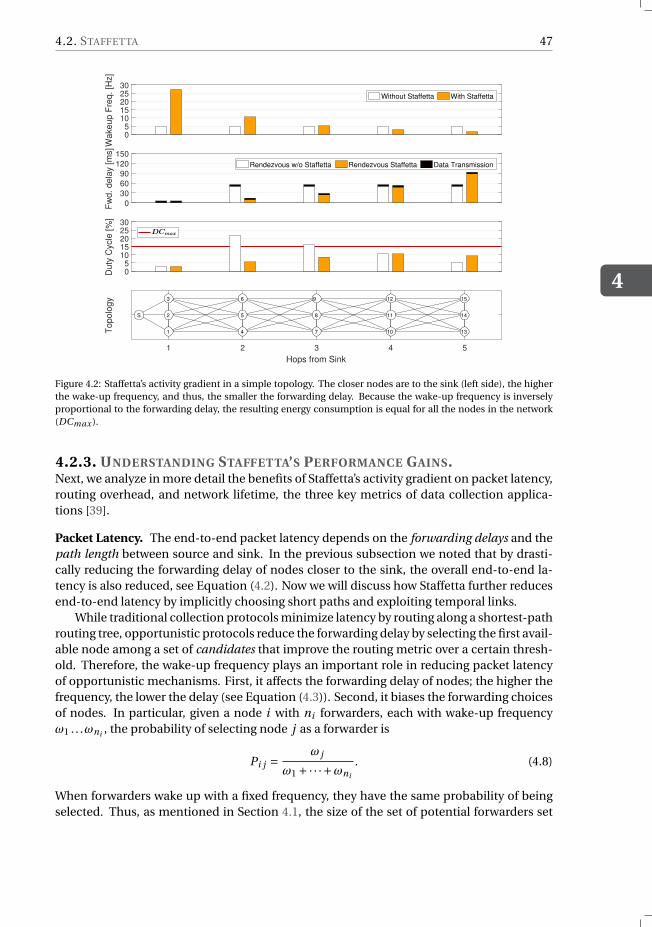
4.2. STAFFETTA
4
47
0 5
10 15 20 25 30
Wake
up
Fre
q.
[Hz]
Without Staffetta With Staffetta
0
30
60
90
120
150
Fw
d.
de
lay [
ms]
Rendezvous w/o Staffetta Rendezvous Staffetta Data Transmission
0 5
10 15 20 25 30
Du
ty C
ycle
[%
]
DCmax
1 2 3 4 5
Hops from Sink
To
po
log
y
1
2
3
4
5
6
7
8
9
10
11
12
13
14
15
S
Figure 4.2: Staffetta’s activity gradient in a simple topology. The closer nodes are to the sink (left side), the higherthe wake-up frequency, and thus, the smaller the forwarding delay. Because the wake-up frequency is inverselyproportional to the forwarding delay, the resulting energy consumption is equal for all the nodes in the network(DCmax ).
4.2.3. UNDERSTANDING STAFFETTA’S PERFORMANCE GAINS.Next, we analyze in more detail the benefits of Staffetta’s activity gradient on packet latency,routing overhead, and network lifetime, the three key metrics of data collection applica-tions [39].
Packet Latency. The end-to-end packet latency depends on the forwarding delays and thepath length between source and sink. In the previous subsection we noted that by drasti-cally reducing the forwarding delay of nodes closer to the sink, the overall end-to-end la-tency is also reduced, see Equation (4.2). Now we will discuss how Staffetta further reducesend-to-end latency by implicitly choosing short paths and exploiting temporal links.
While traditional collection protocols minimize latency by routing along a shortest-pathrouting tree, opportunistic protocols reduce the forwarding delay by selecting the first avail-able node among a set of candidates that improve the routing metric over a certain thresh-old. Therefore, the wake-up frequency plays an important role in reducing packet latencyof opportunistic mechanisms. First, it affects the forwarding delay of nodes; the higher thefrequency, the lower the delay (see Equation (4.3)). Second, it biases the forwarding choicesof nodes. In particular, given a node i with ni forwarders, each with wake-up frequencyω1 . . .ωni , the probability of selecting node j as a forwarder is
Pi j =ω j
ω1 +·· ·+ωni
. (4.8)
When forwarders wake up with a fixed frequency, they have the same probability of beingselected. Thus, as mentioned in Section 4.1, the size of the set of potential forwarders set
4
48 4. OPPORTUNISTIC DATA COLLECTION
must be chosen carefully. Too many forwarders and the performance will perform similarto a random walk (long paths, but short forwarding delays); too few forwarders and themechanism will resemble deterministic routing (short paths, but long forwarding delays).
With Staffetta, on the other hand, the number of forwarders becomes a secondary con-cern: forwarding choices are inherently biased towards the nodes that are closer to the sinki. e., the ones that wake up more often (see equations (4.7) and (4.8)). Therefore, Staffettaimproves opportunistic protocols by biasing the forwarding choices towards the candidatenodes that provide the highest routing progress, effectively reducing the path length of mes-sages.
Even if a “bad” node (i. e., a forwarder that offers little progress) is included in the for-warding set, the selection probability will be low as the wake-up frequency decreases withthe distance to the sink. The effect is that Staffetta “routes” along paths whose length iscomparable to mechanisms based on shortest-path routing trees, while maintaining thebenefits of opportunistic protocols, namely, shorter forwarding delays, better load balanc-ing, and exploitation of temporal links, that is, short-lived, long-distance connections [82].
The exploitation of temporal-links is particularly interesting, because in Staffetta tem-poral links that provide better progress towards the sink, will have a higher probability ofbeing selected. Consider for example node 8 in Figure 4.2, with three forwarders (nodes 4, 5and 6) each waking up at frequency ω4 =ω5 =ω6 = 11 Hz. According to Equation (4.8), theforwarding probabilities are P84 = P85 = P86 = 0.3̄. Now assume that, for a short period oftime, node 8 is able to communicate with node 2, waking up at frequency ω2 = 27 Hz. Theforwarding probabilities are now heavily biased towards the temporally-available new node,with P82 = 0.45, and P84 = P85 = P86 = 0.183̄. Note that, with a constant wake-up frequency(i. e., no Staffetta) the forwarding probabilities will be P82 = P84 = P85 = P86 = 0.25, almosthalving the probability of exploiting the temporal link between nodes 8 and 2. Therefore,Staffetta is able to drastically increase the probability of exploiting temporal links.
Routing Overhead. In static networks, routing overhead is usually a minor problem. Sincenodes must build the routing structure only once, they can spend a significant amount ofresources (energy, bandwidth) and amortize the costs over time. Unfortunately, in prac-tice it is difficult to have real static conditions. Even if nodes do not physically move, thetopology continuously changes due to link-quality fluctuations and uncontrolled sourcesof interference [18].
When the topology changes more often, nodes must constantly update their routingstructures. Amortizing the overhead over time becomes less and less possible, up to thepoint that the mechanism is continuously using part of the channel bandwidth to maintainthe routing structure. This itself limits the data rate of collection mechanisms, increases thechances of packet collisions, and incurs high energy overhead.
Staffetta overcomes these limitations as follows. First, Staffetta introduces only a min-imal overhead to the existing protocol stack. Staffetta’s mechanism requires just local ob-servations (of the forwarding delay). The overhead thus consists of a few bytes of memoryfor storing the latest observations and trivial computations to determine the wake-up fre-quency, whereas it utilizes no additional bandwidth at all. Therefore, empowering collectionprotocols with Staffetta comes with negligible overhead.
Second, Staffetta allows data collection protocols to reduce their own overhead. SinceStaffetta’s activity gradient biases the opportunistic selection of a forwarder already towardsthe sink, it is possible to exploit Staffetta in a cross-layer fashion. In particular, the contin-
4.3. IMPLEMENTATION
4
49
uous neighbor discovery, needed by collection protocols to maintain their routing struc-ture, can be avoided and substituted with the biased opportunistic forwarders providedby Staffetta. For example, to select the best forwarders in ORW [55], nodes must keep anup-to-date list of their neighbors’ routing metric. While the current metric can often be pig-gybacked (e.g., on beacons and acknowledgments), link dynamics could force nodes to ac-tively request their neighbors for updated metric information, increasing the routing over-head. Using Staffetta, the best forwarders are often the ones that wake up first, so nodes canavoid maintaining their neighbor’s routing metric and simply select the first node providedby the opportunistic mechanism, which is simpler and more efficient.
Network lifetime. Network lifetime, defined as the time until the first node in the networkdepletes its battery, is a very important metric for real-word deployments. This metric de-pends on the battery capacity of nodes and the average power consumption of the mostenergy-demanding node, the one that will deplete its energy first. To this end, it is morerewarding to reduce the maximum energy consumption among all nodes rather than theaverage energy consumption in the network. This is precisely what Staffetta achieves byimposing a fixed energy budget. However, note that although all nodes run with the samebudget, they spend it differently. Nodes next to the sink can forward messages without anyrendezvous delay, and spend the saved energy on waking up more frequently; nodes at theedge of the network do not need to forward any data and can spend their complete budgeton rendezvous with parent nodes that wake up at a low frequency.
4.3. IMPLEMENTATIONTo evaluate the performance gains and generality of Staffetta on real devices, we imple-mented it within a custom MAC protocol based on SOFA atop the Contiki operating systemas shown in Figure 4.3. Taking inspiration from state-of-the-art opportunistic data collec-tion protocols, we consider three different routing metrics: Expected Duty Cycle (EDC) [55],Queue Backlog (QB) [70], and SOFA’s Random Walk (RW) [16]. Using one of these metrics,we parametrize a generic data collection mechanism, called baseline, to create three dif-ferent opportunistic collection protocols. On the MAC layer, we implemented Staffetta’sadaptive duty-cycle scheduling mechanism. For comparison, we also use a non-adaptivemechanism with a fixed wake-up frequency.
The protocols, from which we take inspiration, are designed for different operating sys-tems and platforms, with many implementation details that may hide the real benefits oftheir core mechanism, which is in our opinion the routing metric. Using a common imple-mentation of the opportunistic data collection mechanism (baseline) allows us to performa fair, controlled comparison, where differences in performance are solely due to the rout-ing metric and the Staffetta mechanism. Our goal is not to state that Staffetta is better thanthe state of the art, but rather that it makes the state of the art better. That said, our imple-mentations provide competitive performance, as it will be shown in the next section.
In the following, we detail our baseline data collection mechanism, followed by a de-scription of the three routing metrics and a few implementation details of Staffetta.
4.3.1. BASELINEInspired by opportunistic protocols such as SOFA and ORW, our baseline mechanism isbased on low-power listening [74] and opportunistic anycast, and works as follows (see
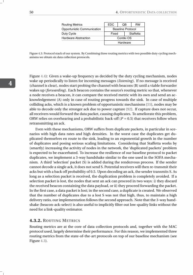
4
50 4. OPPORTUNISTIC DATA COLLECTION
Contiki OSFixed
Baseline ProtocolRWEDC QB
Opportunistic CommunicationDuty Cycle
Routing Metrics
Hardware AbstractionHardware
Staffetta
Figure 4.3: Protocol stack of our system. By Combining three routing metrics with two possible duty-cycling mech-anisms we obtain six data collection protocols.
Figure 4.4): Given a wake-up frequency as decided by the duty cycling mechanism, nodeswake up periodically to listen for incoming messages (listening). If no message is received(channel is clear), nodes start probing the channel with beacons (B) until a viable forwarderwakes up (forwarding). Each beacon contains the source’s routing metric so that, whenevera node receives a beacon, it can compare the received metric with its own and send an ac-knowledgement (A) only in case of routing progress towards the sink. In case of multiplecolliding acks, which is a known problem of opportunistic mechanisms [55], nodes may beable to decode only the stronger ack due to power capture [92]. If capture does not occur,all receivers would forward the data packet, causing duplicates. To ameliorate this problem,ORW relies on overhearing and a probabilistic back-off (P = 0.5) that receivers follow whenretransmitting an ack.
Even with these mechanisms, ORW suffers from duplicate packets, in particular in sce-narios with high data rates and high densities. In the worst case the duplicates get du-plicated themselves en route to the sink, leading to an exponential growth in the numberof duplicates and posing serious scaling limitations. Considering that Staffetta works by(smartly) increasing the activity of nodes in the network, the ‘duplicated packets’ problemis expected to be exacerbated. To increase the resilience of our baseline protocol to packetduplicates, we implement a 3-way handshake similar to the one used in the SOFA mecha-nism. A third ‘selection’ packet (S) is added during the rendezvous process. If the sendercannot decode a single ack, it does not send S. Potential receivers will then re-transmit theiracks but with a back off probability of 0.5. Upon decoding an ack, the sender transmits S. Aslong as a selection packet is received, the duplication problem is completely avoided. If aselection packet is lost, the nodes that sent an ack can proceed in two ways: i) they discardthe received beacon containing the data payload, or ii) they proceed forwarding the packet.In the first case, a data packet is lost; in the second case, a duplicate is created. We observedthat the number of duplicates due to a lost S was not that high, thus, to maintain a highdelivery ratio, our implementation follows the second approach. Note that the 3-way hand-shake (beacon-ack-select) is also useful to implicitly filter out low-quality links without theneed for a link-quality estimator.
4.3.2. ROUTING METRICS
Routing metrics are at the core of data collection protocols and, together with the MACprotocol used, largely determine their performance. For this reason, we implemented threerouting metrics from the state-of-the-art protocols on top of our baseline mechanism (seeFigure 4.3).
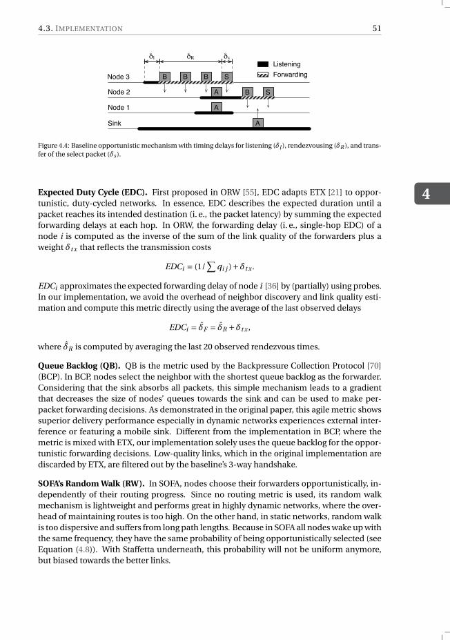
4.3. IMPLEMENTATION
4
51
Node 3
Node 2
Sink
A
B B S
A
B S
B ForwardingListening
Node 1 A
δR δs δl
Figure 4.4: Baseline opportunistic mechanism with timing delays for listening (δl ), rendezvousing (δR ), and trans-fer of the select packet (δs ).
Expected Duty Cycle (EDC). First proposed in ORW [55], EDC adapts ETX [21] to oppor-tunistic, duty-cycled networks. In essence, EDC describes the expected duration until apacket reaches its intended destination (i. e., the packet latency) by summing the expectedforwarding delays at each hop. In ORW, the forwarding delay (i. e., single-hop EDC) of anode i is computed as the inverse of the sum of the link quality of the forwarders plus aweight δt x that reflects the transmission costs
EDCi = (1/∑
qi j )+δt x .
EDCi approximates the expected forwarding delay of node i [36] by (partially) using probes.In our implementation, we avoid the overhead of neighbor discovery and link quality esti-mation and compute this metric directly using the average of the last observed delays
EDCi = δ̂F = δ̂R +δt x ,
where δ̂R is computed by averaging the last 20 observed rendezvous times.
Queue Backlog (QB). QB is the metric used by the Backpressure Collection Protocol [70](BCP). In BCP, nodes select the neighbor with the shortest queue backlog as the forwarder.Considering that the sink absorbs all packets, this simple mechanism leads to a gradientthat decreases the size of nodes’ queues towards the sink and can be used to make per-packet forwarding decisions. As demonstrated in the original paper, this agile metric showssuperior delivery performance especially in dynamic networks experiences external inter-ference or featuring a mobile sink. Different from the implementation in BCP, where themetric is mixed with ETX, our implementation solely uses the queue backlog for the oppor-tunistic forwarding decisions. Low-quality links, which in the original implementation arediscarded by ETX, are filtered out by the baseline’s 3-way handshake.
SOFA’s Random Walk (RW). In SOFA, nodes choose their forwarders opportunistically, in-dependently of their routing progress. Since no routing metric is used, its random walkmechanism is lightweight and performs great in highly dynamic networks, where the over-head of maintaining routes is too high. On the other hand, in static networks, random walkis too dispersive and suffers from long path lengths. Because in SOFA all nodes wake up withthe same frequency, they have the same probability of being opportunistically selected (seeEquation (4.8)). With Staffetta underneath, this probability will not be uniform anymore,but biased towards the better links.
4
52 4. OPPORTUNISTIC DATA COLLECTION
Note that, for the first two routing metrics (EDC and QB), nodes forward their informa-tion to the first neighbor that wakes up and provides routing progress. For SOFA’s RandomWalk, instead, nodes forward their message to the first neighbor that wakes up, indepen-dently of its distance to the sink.
4.3.3. STAFFETTAStaffetta’s mechanism consists of adapting the wake-up frequency of nodes based on theobserved forwarding delay δ̂F . For this reason, implementing Staffetta is straightforward.
Measuring the forwarding delay. We empirically measure the fixed communication delaysδt x . For the baseline mechanism, depicted in Figure 4.4, δt x includes the time needed tolisten to the channel to check if it is clear for transmission (δl ), and the time needed totransmit the selection packet (δs ).
To quantify the actual rendezvous time (δ̂R ), each node measures the period betweenthe first beacon sent and the first acknowledgment received. Due to the stochastic natureof the rendezvous delay, our implementation averages the last 20 measurement using a sim-ple moving average (SMA) to produce a stable, yet reasonably agile activity gradient that isrobust to small disturbances such as fast link fluctuations.
Computing the wake-up frequency. Once δt x and δ̂R are determined, the wake up fre-quency is computed according to Equation (4.4). In particular, after each successful mes-sage exchange, our implementation of Staffetta updates the average rendezvous time andthe wake-up frequency ω, and schedules the next wake-up in 1/ω seconds.
However, setting the wake-up frequency based on local information could lead to somecomplications. Different from traditional duty-cycling techniques, in which the activity ratedepends on the application’s traffic requirements, Staffetta bases the wake-up frequencysolely on the forwarding delay, which depends on the network topology. In effect, thewake-up frequency is a function of the distance to the sink and the (average) number offorwarders at each hop. This could be problematic in case of weakly connected nodes, lo-cated at the edge of a large network. For these nodes, communication could be so expensive(due to long rendezvous times) that maintaining the required data rate will make the nodeconsume more energy than budgeted. There are two approaches to handling this issue.
i) Give priority to the application requirements. This approach is based on the idea thatStaffetta may only set a wake-up frequency that is above the packet injection rate requiredby the application. Capping the minimum frequency has the consequence that Equation (4.4)will be violated, causing the energy budget to be exceeded as more data will be sent than canbe afforded (given the long rendezvous time with the forwarders). This effect is exacerbatedby a poor selection of forwarders, as the gradient is effectively flattened (negligible bias),leading to longer paths and extra traffic, hence, raising energy consumption even more.
ii) Give priority to the energy budget. Using this approach, nodes can adapt their wake-upfrequency to a value that is lower than the application requirements. The obvious conse-quence is that packets will be queued at the source, leading to longer latencies and eventu-ally packet drops, likely violating latency and delivery requirements. However, if the appli-cation is delay-tolerant, the problem can be mitigated by aggregating packets at the sourceas the energy costs are dictated by the rendezvous costs, not the actual data transfer. Aneven more important observation is that only the nodes at the edge of the network suffer
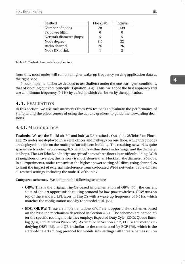
4.4. EVALUATION
4
53
Testbed FlockLab IndriyaNumber of nodes 28 139Tx power [dBm] 0 0Network diameter [hops] 5 5Node degree 8.5 22Radio channel 26 26Node ID of sink 1 2
Table 4.2: Testbed characteristics and settings
from this; most nodes will run on a higher wake-up frequency serving application data atthe right pace.
In our implementation we decided to test Staffetta under the most stringent conditions,that of violating our core principle: Equation (4.4). Thus, we adopt the first approach anduse a minimum frequency (0.1 Hz by default), which can be set by the application.
4.4. EVALUATIONIn this section, we use measurements from two testbeds to evaluate the performance ofStaffetta and the effectiveness of using the activity gradient to guide the forwarding deci-sions.
4.4.1. METHODOLOGY
Testbeds. We use the FlockLab [60] and Indriya [26] testbeds. Out of the 28 TelosB on Flock-Lab, 25 nodes are deployed in several offices and hallways on one floor, while three nodesare deployed outside on the rooftop of an adjacent building. The resulting network is quitesparse: each node has on average 8.5 neighbors within direct radio range, and the diameteris 5 hops. The 139 TelosB on Indriya are spread across three floors in an office building. With22 neighbors on average, the network is much denser than FlockLab; the diameter is 5 hops.In all experiments, nodes transmit at the highest power setting of 0dBm, using channel 26to limit the impact of external interference from co-located Wi-Fi networks. Table 4.2 listsall testbed settings, including the node ID of the sink.
Compared schemes. We compare the following schemes:
• ORW: This is the original TinyOS-based implementation of ORW [55], the currentstate-of-the-art opportunistic routing protocol for low-power wireless. ORW runs ontop of the standard LPL layer in TinyOS with a wake-up frequency of 0.5Hz, whichmatches the configuration used by Landsiedel et al. [55].
• EDC, QB, RW: These are implementations of different opportunistic schemes basedon the baseline mechanism described in Section 4.3.1. The schemes are named af-ter the specific routing metric they employ: Expected Duty Cyle (EDC), Queue Back-log (QB), and Random Walk (RW). As detailed in Section 4.3.2, EDC is the metric un-derlying ORW [55], and QB is similar to the metric used by BCP [70], which is thestate-of-the-art routing protocol for mobile sink settings. All three schemes run on
4
54 4. OPPORTUNISTIC DATA COLLECTION
top of the default LPL layer and opportunistic anycast in Contiki with a wake-up fre-quency of 1Hz.
• ST.EDC, ST.QB, ST.RW: These schemes are the same as EDC, QB, and RW above ex-cept that instead of using a fixed wake-up frequency Staffetta’s dynamic duty-cyclemechanism is employed to adjust the wake-up frequency at runtime, as described inSections 4.2 and 4.3.3.
• DIRECT: This scheme, implemented atop the baseline mechanism, fully exploits Staffettaby using the activity gradient directly as a “routing metric:” a node forwards a packetto the neighbor that wakes up first and has a wake-up frequency higher than itself. Inother words, instead of using an explicit routing metric, such as EDC or QB, to decidewhether a neighbor provides routing progress, DIRECT makes this decision using thegradient of wake-up frequencies inherent in Staffetta.
As discussed earlier, existing dynamic duty-cycle mechanisms are theoretical [50, 51] orexpressely designed for traditional non-opportunistic routing schemes [69, 111], renderingan experimental comparison against Staffetta impossible.
Energy budget. When Staffetta is enabled, we set the energy budget DCmax to 7.5% onFlockLab and to 6% on Indryia.
Metrics. Our evaluation uses the following three key performance metrics of real-worldapplications [18]:
• Latency: The time between when a packet is generated by the source node and whenthat packet is successfully received by the sink. To measure latency, we leverage thetime synchronization among nodes on FlockLab and the serial logging of Indriya totimestamp both the generation and the successful reception of each packet.
• Duty cycle: The fraction of time the radio is turned on. We measure duty cycle insoftware using Contiki’s accurate energy profiler.
• Delivery ratio: The fraction of packets generated by the source nodes that is deliveredto the sink. We determine delivery ratio based on the unique sequence numbers ofpackets successfully received at the sink.
We also measure path length, the number of times a message is relayed before reachingthe sink, to explain the behavior and performance of a given routing scheme. We computethese metrics based on three independent runs with the exact same settings. To allow eachprotocol to bootstrap its operation, we start measuring after an initial delay of 1 minute. Wealso give each protocol sufficient time (i. e., 1–5 minutes) to empty their packet queues be-fore the end of each run. Unless stated otherwise, we report the results as median, 25th and75th percentiles, and minimum and maximum values across all nodes in a testbed usingbox plots; statistical outliers are represented by crosses.
4.4.2. COMPARISON AGAINST THE STATE OF THE ARTWe begin by comparing ST.EDC against ORW to quantify the performance gains of Staffettaover the state of the art.
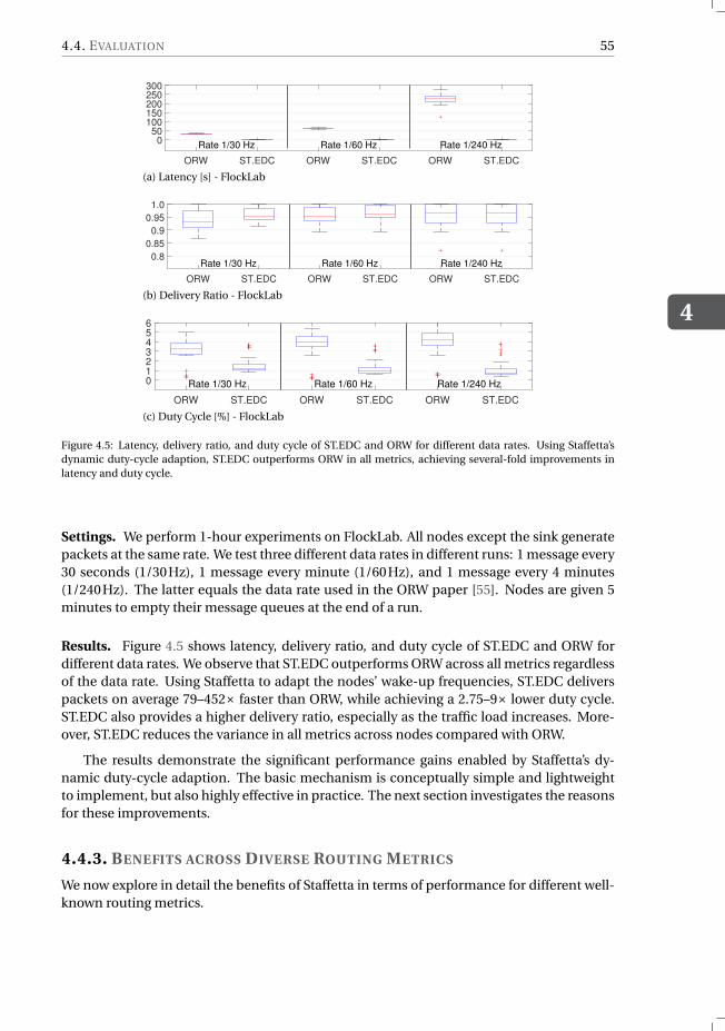
4.4. EVALUATION
4
55
ORW ST.EDC ORW ST.EDC ORW ST.EDC
050
100150200250300
Rate 1/30 Hz Rate 1/60 Hz Rate 1/240 Hz
(a) Latency [s] - FlockLab
ORW ST.EDC ORW ST.EDC ORW ST.EDC
0.8
0.85
0.9
0.95
1.0
Rate 1/30 Hz Rate 1/60 Hz Rate 1/240 Hz
(b) Delivery Ratio - FlockLab
ORW ST.EDC ORW ST.EDC ORW ST.EDC
0
1
2
3
4
5
6
Rate 1/30 Hz Rate 1/60 Hz Rate 1/240 Hz
(c) Duty Cycle [%] - FlockLab
Figure 4.5: Latency, delivery ratio, and duty cycle of ST.EDC and ORW for different data rates. Using Staffetta’sdynamic duty-cycle adaption, ST.EDC outperforms ORW in all metrics, achieving several-fold improvements inlatency and duty cycle.
Settings. We perform 1-hour experiments on FlockLab. All nodes except the sink generatepackets at the same rate. We test three different data rates in different runs: 1 message every30 seconds (1/30Hz), 1 message every minute (1/60Hz), and 1 message every 4 minutes(1/240Hz). The latter equals the data rate used in the ORW paper [55]. Nodes are given 5minutes to empty their message queues at the end of a run.
Results. Figure 4.5 shows latency, delivery ratio, and duty cycle of ST.EDC and ORW fordifferent data rates. We observe that ST.EDC outperforms ORW across all metrics regardlessof the data rate. Using Staffetta to adapt the nodes’ wake-up frequencies, ST.EDC deliverspackets on average 79–452× faster than ORW, while achieving a 2.75–9× lower duty cycle.ST.EDC also provides a higher delivery ratio, especially as the traffic load increases. More-over, ST.EDC reduces the variance in all metrics across nodes compared with ORW.
The results demonstrate the significant performance gains enabled by Staffetta’s dy-namic duty-cycle adaption. The basic mechanism is conceptually simple and lightweightto implement, but also highly effective in practice. The next section investigates the reasonsfor these improvements.
4.4.3. BENEFITS ACROSS DIVERSE ROUTING METRICS
We now explore in detail the benefits of Staffetta in terms of performance for different well-known routing metrics.
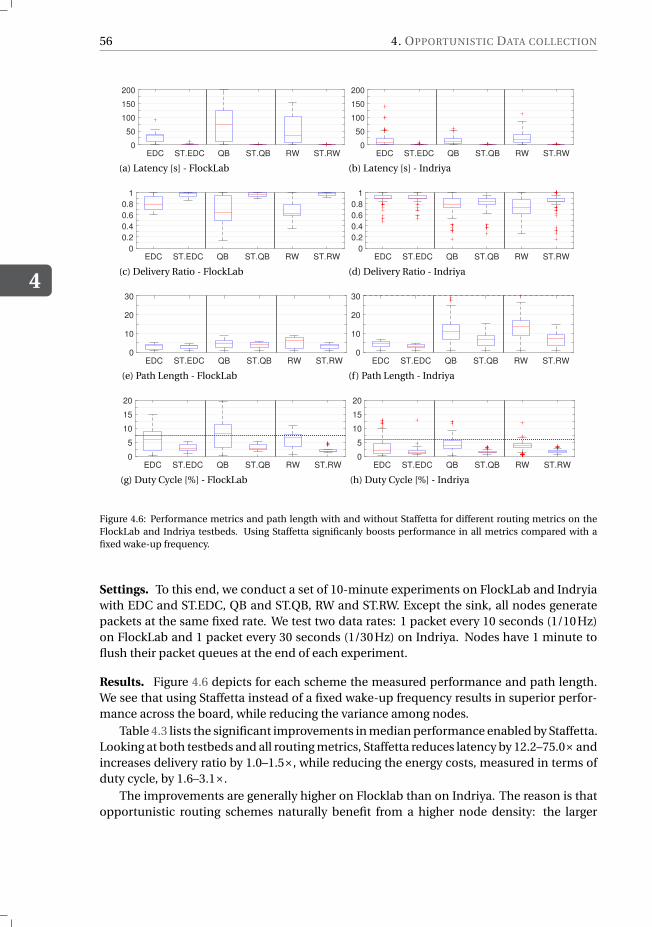
4
56 4. OPPORTUNISTIC DATA COLLECTION
EDC ST.EDC QB ST.QB RW ST.RW0
50
100
150
200
(a) Latency [s] - FlockLab
EDC ST.EDC QB ST.QB RW ST.RW0
50
100
150
200
(b) Latency [s] - Indriya
EDC ST.EDC QB ST.QB RW ST.RW0
0.2
0.4
0.6
0.8
1
(c) Delivery Ratio - FlockLab
EDC ST.EDC QB ST.QB RW ST.RW0
0.2
0.4
0.6
0.8
1
(d) Delivery Ratio - Indriya
EDC ST.EDC QB ST.QB RW ST.RW0
10
20
30
(e) Path Length - FlockLab
EDC ST.EDC QB ST.QB RW ST.RW0
10
20
30
(f) Path Length - Indriya
EDC ST.EDC QB ST.QB RW ST.RW0
5
10
15
20
(g) Duty Cycle [%] - FlockLab
EDC ST.EDC QB ST.QB RW ST.RW0
5
10
15
20
(h) Duty Cycle [%] - Indriya
Figure 4.6: Performance metrics and path length with and without Staffetta for different routing metrics on theFlockLab and Indriya testbeds. Using Staffetta significanly boosts performance in all metrics compared with afixed wake-up frequency.
Settings. To this end, we conduct a set of 10-minute experiments on FlockLab and Indryiawith EDC and ST.EDC, QB and ST.QB, RW and ST.RW. Except the sink, all nodes generatepackets at the same fixed rate. We test two data rates: 1 packet every 10 seconds (1/10Hz)on FlockLab and 1 packet every 30 seconds (1/30Hz) on Indriya. Nodes have 1 minute toflush their packet queues at the end of each experiment.
Results. Figure 4.6 depicts for each scheme the measured performance and path length.We see that using Staffetta instead of a fixed wake-up frequency results in superior perfor-mance across the board, while reducing the variance among nodes.
Table 4.3 lists the significant improvements in median performance enabled by Staffetta.Looking at both testbeds and all routing metrics, Staffetta reduces latency by 12.2–75.0× andincreases delivery ratio by 1.0–1.5×, while reducing the energy costs, measured in terms ofduty cycle, by 1.6–3.1×.
The improvements are generally higher on Flocklab than on Indriya. The reason is thatopportunistic routing schemes naturally benefit from a higher node density: the larger
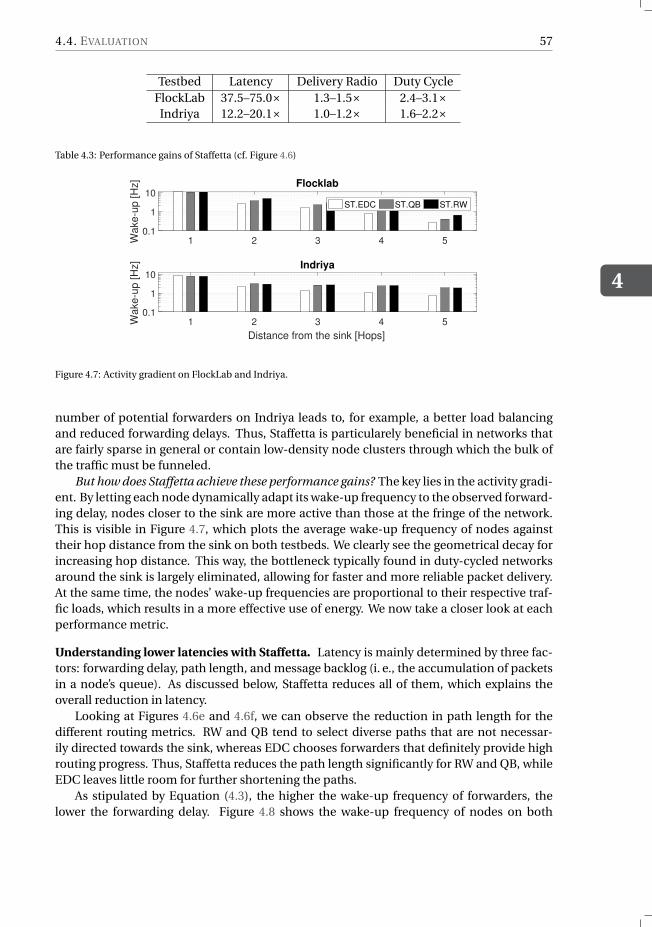
4.4. EVALUATION
4
57
Testbed Latency Delivery Radio Duty CycleFlockLab 37.5–75.0× 1.3–1.5× 2.4–3.1×Indriya 12.2–20.1× 1.0–1.2× 1.6–2.2×
Table 4.3: Performance gains of Staffetta (cf. Figure 4.6)
1 2 3 4 50.1
1
10
Wake-u
p [H
z] Flocklab
ST.EDC ST.QB ST.RW
1 2 3 4 5
Distance from the sink [Hops]
0.1
1
10
Wake-u
p [H
z] Indriya
Figure 4.7: Activity gradient on FlockLab and Indriya.
number of potential forwarders on Indriya leads to, for example, a better load balancingand reduced forwarding delays. Thus, Staffetta is particularely beneficial in networks thatare fairly sparse in general or contain low-density node clusters through which the bulk ofthe traffic must be funneled.
But how does Staffetta achieve these performance gains? The key lies in the activity gradi-ent. By letting each node dynamically adapt its wake-up frequency to the observed forward-ing delay, nodes closer to the sink are more active than those at the fringe of the network.This is visible in Figure 4.7, which plots the average wake-up frequency of nodes againsttheir hop distance from the sink on both testbeds. We clearly see the geometrical decay forincreasing hop distance. This way, the bottleneck typically found in duty-cycled networksaround the sink is largely eliminated, allowing for faster and more reliable packet delivery.At the same time, the nodes’ wake-up frequencies are proportional to their respective traf-fic loads, which results in a more effective use of energy. We now take a closer look at eachperformance metric.
Understanding lower latencies with Staffetta. Latency is mainly determined by three fac-tors: forwarding delay, path length, and message backlog (i. e., the accumulation of packetsin a node’s queue). As discussed below, Staffetta reduces all of them, which explains theoverall reduction in latency.
Looking at Figures 4.6e and 4.6f, we can observe the reduction in path length for thedifferent routing metrics. RW and QB tend to select diverse paths that are not necessar-ily directed towards the sink, whereas EDC chooses forwarders that definitely provide highrouting progress. Thus, Staffetta reduces the path length significantly for RW and QB, whileEDC leaves little room for further shortening the paths.
As stipulated by Equation (4.3), the higher the wake-up frequency of forwarders, thelower the forwarding delay. Figure 4.8 shows the wake-up frequency of nodes on both
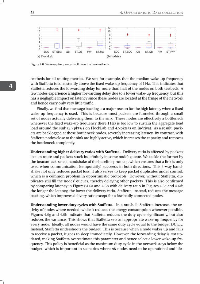
4
58 4. OPPORTUNISTIC DATA COLLECTION
EDC ST.EDC QB ST.QB RW ST.RW0
2
4
6
8
10
12
(a) FlockLab
EDC ST.EDC QB ST.QB RW ST.RW0
2
4
6
8
10
12
(b) Indriya
Figure 4.8: Wake-up frequency (in Hz) on the two testbeds.
testbeds for all routing metrics. We see, for example, that the median wake-up frequencywith Staffetta is consistently above the fixed wake-up frequency of 1Hz. This indicates thatStaffetta reduces the forwarding delay for more than half of the nodes on both testbeds. Afew nodes experience a higher forwarding delay due to a lower wake-up frequency, but thishas a negligible impact on latency since these nodes are located at the fringe of the networkand hence carry only very little traffic.
Finally, we find that message backlog is a major reason for the high latency when a fixedwake-up frequency is used. This is because most packets are funneled through a smallset of nodes actually delivering them to the sink. These nodes are effectively a bottleneckwhenever the fixed wake-up frequency (here 1Hz) is too low to sustain the aggregate loadload around the sink (2.7pkts/s on FlockLab and 4.5pkts/s on Indriya). As a result, pack-ets are backlogged at these bottleneck nodes, severely increasing latency. By contrast, withStaffetta nodes close to the sink are highly active, which increases the capacity and removesthe bottleneck completely.
Understanding higher delivery ratios with Staffetta. Delivery ratio is affected by packetslost en route and packets stuck indefinitely in some node’s queue. We tackle the former bythe beacon-ack-select handshake of the baseline protocol, which ensures that a link is onlyused when communication (temporarily) succeeds in both directions. This 3-way hand-shake not only reduces packet loss, it also serves to keep packet duplicates under control,which is a common problem in opportunistic protocols. However, without Staffetta, du-plicates still fill the nodes’ queues, thereby delaying other packets. This is also confirmedby comparing latency in Figures 4.6a and 4.6b with delivery ratio in Figures 4.6c and 4.6d:the longer the latency, the lower the delivery ratio. Staffetta, instead, reduces the messagebacklog, which improves delivery ratio except for a few badly connected nodes.
Understanding lower duty cycles with Staffetta. In a nutshell, Staffetta increases the ac-tivity of nodes where needed, while it reduces the energy consumption wherever possible.Figures 4.6g and 4.6h indicate that Staffetta reduces the duty cycle significantly, but alsoreduces the variance. This shows that Staffetta sets an appropriate wake-up frequency forevery node. Ideally, all nodes would have the same duty cycle equal to the budget DCmax.Instead, Staffetta undershoots the budget. This is because when a node wakes up and failsto receive a packet, it goes to sleep immediately. However, the forwarding delay is not up-dated, making Staffetta overestimate this parameter and hence select a lower wake-up fre-quency. This policy is beneficial as the maximum duty cycle in the network stays below thebudget, which is important in scenarios where all nodes need to be operational and life-
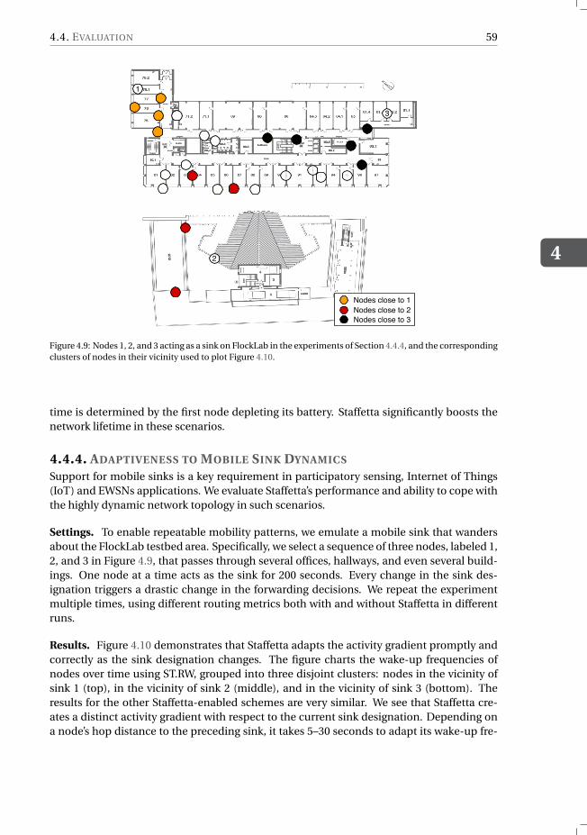
4.4. EVALUATION
4
59
1
2
3
Nodes close to 1Nodes close to 2Nodes close to 3
Figure 4.9: Nodes 1, 2, and 3 acting as a sink on FlockLab in the experiments of Section 4.4.4, and the correspondingclusters of nodes in their vicinity used to plot Figure 4.10.
time is determined by the first node depleting its battery. Staffetta significantly boosts thenetwork lifetime in these scenarios.
4.4.4. ADAPTIVENESS TO MOBILE SINK DYNAMICS
Support for mobile sinks is a key requirement in participatory sensing, Internet of Things(IoT) and EWSNs applications. We evaluate Staffetta’s performance and ability to cope withthe highly dynamic network topology in such scenarios.
Settings. To enable repeatable mobility patterns, we emulate a mobile sink that wandersabout the FlockLab testbed area. Specifically, we select a sequence of three nodes, labeled 1,2, and 3 in Figure 4.9, that passes through several offices, hallways, and even several build-ings. One node at a time acts as the sink for 200 seconds. Every change in the sink des-ignation triggers a drastic change in the forwarding decisions. We repeat the experimentmultiple times, using different routing metrics both with and without Staffetta in differentruns.
Results. Figure 4.10 demonstrates that Staffetta adapts the activity gradient promptly andcorrectly as the sink designation changes. The figure charts the wake-up frequencies ofnodes over time using ST.RW, grouped into three disjoint clusters: nodes in the vicinity ofsink 1 (top), in the vicinity of sink 2 (middle), and in the vicinity of sink 3 (bottom). Theresults for the other Staffetta-enabled schemes are very similar. We see that Staffetta cre-ates a distinct activity gradient with respect to the current sink designation. Depending ona node’s hop distance to the preceding sink, it takes 5–30 seconds to adapt its wake-up fre-
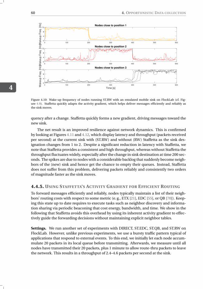
4
60 4. OPPORTUNISTIC DATA COLLECTION
0 100 200 300 400 500 6000
4
8
12
Wakeup F
req. [H
z]
Nodes close to position 1
0 100 200 300 400 500 6000
4
8
12
Wakeup F
req. [H
z]
Nodes close to position 2
0 100 200 300 400 500 600
Time [s]
0
4
8
12
Wakeup F
req. [H
z]
Nodes close to position 3
Figure 4.10: Wake-up frequency of nodes running ST.RW with an emulated mobile sink on FlockLab (cf. Fig-ure 4.9). Staffetta quickly adapts the activity gradient, which helps deliver messages efficiently and reliably asthe sink moves.
quency after a change. Staffetta quickly forms a new gradient, driving messages toward thenew sink.
The net result is an improved resilience against network dynamics. This is confirmedby looking at Figures 4.11 and 4.12, which display latency and throughput (packets receivedper second) at the current sink with (ST.RW) and without (RW) Staffetta as the sink des-ignation changes from 1 to 2. Despite a significant reduction in latency with Staffetta, wenote that Staffetta provides a consistent and high throughput, whereas without Staffetta thethroughput fluctuates widely, especially after the change in sink destination at time 200 sec-onds. The spikes are due to nodes with a considerable backlog that suddenly become neigh-bors of the (new) sink and hence get the chance to empty their queues. Instead, Staffettadoes not suffer from this problem, delivering packets reliably and consistently two ordersof magnitude faster as the sink moves.
4.4.5. USING STAFFETTA’S ACTIVITY GRADIENT FOR EFFICIENT ROUTING
To forward messages efficiently and reliably, nodes typically maintain a list of their neigh-bors’ routing costs with respect to some metric (e. g., ETX [21], EDC [55], or QB [70]). Keep-ing this state up to date requires to execute tasks such as neighbor discovery and informa-tion sharing via periodic beaconing that cost energy, bandwidth, and time. We show in thefollowing that Staffetta avoids this overhead by using its inherent activity gradient to effec-tively guide the forwarding decisions without maintaining explicit neighbor tables.
Settings. We run another set of experiments with DIRECT, ST.EDC, ST.QB, and ST.RW onFlockLab. However, unlike previous experiments, we use a bursty traffic pattern typical ofapplications that respond to external events. To this end, we initially let each node accum-mulate 20 packets in its local queue before transmitting. Afterwards, we measure until allnodes have transmitted their 20 packets, plus 1 minute to allow route-thru packets to leavethe network. This results in a throughput of 2.4–4.6 packets per second at the sink.
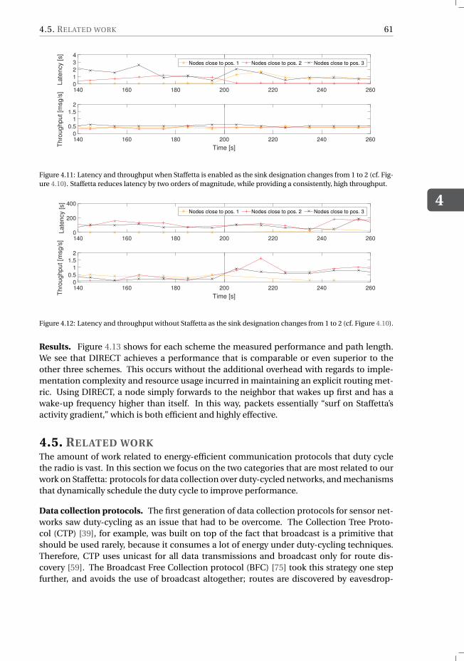
4.5. RELATED WORK
4
61
140 160 180 200 220 240 260 0
1
2
3
4L
ate
ncy [
s]
Nodes close to pos. 1 Nodes close to pos. 2 Nodes close to pos. 3
140 160 180 200 220 240 260
Time [s]
0
0.5
1
1.5
2
Th
rou
gh
pu
t [m
sg
/s]
Figure 4.11: Latency and throughput when Staffetta is enabled as the sink designation changes from 1 to 2 (cf. Fig-ure 4.10). Staffetta reduces latency by two orders of magnitude, while providing a consistently, high throughput.
140 160 180 200 220 240 2600
200
400
La
ten
cy [
s]
Nodes close to pos. 1 Nodes close to pos. 2 Nodes close to pos. 3
140 160 180 200 220 240 260
Time [s]
0
0.5
1
1.5
2
Th
rou
gh
pu
t [m
sg
/s]
Figure 4.12: Latency and throughput without Staffetta as the sink designation changes from 1 to 2 (cf. Figure 4.10).
Results. Figure 4.13 shows for each scheme the measured performance and path length.We see that DIRECT achieves a performance that is comparable or even superior to theother three schemes. This occurs without the additional overhead with regards to imple-mentation complexity and resource usage incurred in maintaining an explicit routing met-ric. Using DIRECT, a node simply forwards to the neighbor that wakes up first and has awake-up frequency higher than itself. In this way, packets essentially “surf on Staffetta’sactivity gradient,” which is both efficient and highly effective.
4.5. RELATED WORKThe amount of work related to energy-efficient communication protocols that duty cyclethe radio is vast. In this section we focus on the two categories that are most related to ourwork on Staffetta: protocols for data collection over duty-cycled networks, and mechanismsthat dynamically schedule the duty cycle to improve performance.
Data collection protocols. The first generation of data collection protocols for sensor net-works saw duty-cycling as an issue that had to be overcome. The Collection Tree Proto-col (CTP) [39], for example, was built on top of the fact that broadcast is a primitive thatshould be used rarely, because it consumes a lot of energy under duty-cycling techniques.Therefore, CTP uses unicast for all data transmissions and broadcast only for route dis-covery [59]. The Broadcast Free Collection protocol (BFC) [75] took this strategy one stepfurther, and avoids the use of broadcast altogether; routes are discovered by eavesdrop-
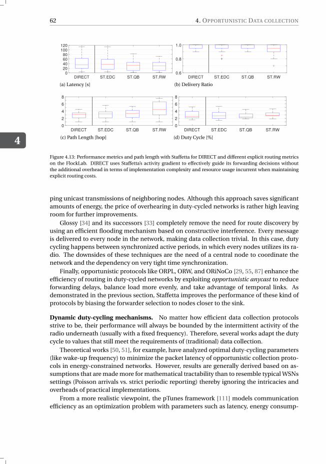
4
62 4. OPPORTUNISTIC DATA COLLECTION
DIRECT ST.EDC ST.QB ST.RW0
20
40
60
80
100
120
(a) Latency [s]
DIRECT ST.EDC ST.QB ST.RW0.6
0.8
1.0
(b) Delivery Ratio
DIRECT ST.EDC ST.QB ST.RW0
2
4
6
8
(c) Path Length [hop]
DIRECT ST.EDC ST.QB ST.RW0
2
4
6
8
(d) Duty Cycle [%]
Figure 4.13: Performance metrics and path length with Staffetta for DIRECT and different explicit routing metricson the FlockLab. DIRECT uses Staffetta’s activity gradient to effectively guide its forwarding decisions withoutthe additional overhead in terms of implementation complexity and resource usage incurrent when maintainingexplicit routing costs.
ping unicast transmissions of neighboring nodes. Although this approach saves significantamounts of energy, the price of overhearing in duty-cycled networks is rather high leavingroom for further improvements.
Glossy [34] and its successors [33] completely remove the need for route discovery byusing an efficient flooding mechanism based on constructive interference. Every messageis delivered to every node in the network, making data collection trivial. In this case, dutycycling happens between synchronized active periods, in which every nodes utilizes its ra-dio. The downsides of these techniques are the need of a central node to coordinate thenetwork and the dependency on very tight time synchronization.
Finally, opportunistic protocols like ORPL, ORW, and ORiNoCo [29, 55, 87] enhance theefficiency of routing in duty-cycled networks by exploiting opportunistic anycast to reduceforwarding delays, balance load more evenly, and take advantage of temporal links. Asdemonstrated in the previous section, Staffetta improves the performance of these kind ofprotocols by biasing the forwarder selection to nodes closer to the sink.
Dynamic duty-cycling mechanisms. No matter how efficient data collection protocolsstrive to be, their performance will always be bounded by the intermittent activity of theradio underneath (usually with a fixed frequency). Therefore, several works adapt the dutycycle to values that still meet the requirements of (traditional) data collection.
Theoretical works [50, 51], for example, have analyzed optimal duty-cycling parameters(like wake-up frequency) to minimize the packet latency of opportunistic collection proto-cols in energy-constrained networks. However, results are generally derived based on as-sumptions that are made more for mathematical tractability than to resemble typical WSNssettings (Poisson arrivals vs. strict periodic reporting) thereby ignoring the intricacies andoverheads of practical implementations.
From a more realistic viewpoint, the pTunes framework [111] models communicationefficiency as an optimization problem with parameters such as latency, energy consump-
4.6. CONCLUSIONS
4
63
tion and reliability. Through an efficient network dissemination technique (based on Glossy),pTunes periodically collects (centrally) network information and, based on the applicationrequirements, computes the optimal duty-cycling parameters and disseminates them tothe nodes. Staffetta complements this centralized approach by providing a good but non-optimal solution that is fully distributed, has minimal overhead and addresses the uniquecharacteristics of opportunistic protocols.
In a similar way, ZeroCal [69] balances the energy consumption of nodes by adaptingtheir wake-up frequency. Compared to ZeroCal, we believe that Staffetta has three maindifferences. First, ZeroCal requires radio and data traffic parameters to solve a distributedoptimization problem, while Staffetta requires only one parameter (the energy budget) anda simple operation to adapt the wake-up frequency locally. Second, ZeroCal incurs a higheroverhead since it requires to monitor the state of nodes’ children, while Staffetta does notrequire any such explicit input. Finally, ZeroCal focuses on the unicast primitive, whileStaffetta addresses opportunistic protocols and their anycast primitive.
4.6. CONCLUSIONSIn this chapter we addressed the fundamental issue of efficient data collection in dynamicnetworks, where protocol designers must balance flexibility with communication perfor-mance and energy efficiency. While opportunistic collection protocols successfully tradeoff these two antithetical goals, they do not exploit the full potential of the network, which isessential to scale to the demanding conditions of EWSNs (see Chapter 1). We have demon-strated that, instead of coping with the challenges of low-power communication, collectionprotocols can tame the duty-cycle mechanism and use it to their advantage (opportunis-tic principle), raising performance and reducing (average) energy consumption at the sametime.
Our low-level Staffetta mechanism sets the wake-up frequency according to the for-warding latency observed by the nodes; the less time is spent on forwarding, the more timecan be spent on servicing incoming traffic (i.e. waking up more frequently). The net effectis that Staffetta sets up a gradient with nodes close to the sink waking up more frequentlythan nodes at the edge of the network. This gradient automatically steers opportunisticanycast traffic towards the sink as the probability of finding an awake neighbor is highest inthe direction of the sink.
We implemented Staffetta in Contiki, and evaluated it with three opportunistic collec-tion protocols on two different testbeds. The extensive set of experiments showed thatStaffetta significantly reduces both packet latency and energy consumption, while main-taining high – or even improving – packet delivery ratios. As Staffetta does not need tomaintain complicated routing metrics spanning the entire network (state-less principle),it can also handle network dynamics like link-quality fluctuations and node mobility reallywell. We found that Staffetta adapts its gradient in just a matter of seconds.

5CROWD MONITORING IN THE WILD
“Infinite diversity... in infinite combinations.”
Vulcan Master and Young Tuvok
T HE achievements in the field of Wireless Sensor Networks have been steadily increas-ing in the last years, leaving less and less time to researchers for properly developing,
testing and publishing their ideas before they get obsolete. For this reason, many protocolsfor WSNs (extreme or not) have only been evaluated under limited and controlled condi-tions. From high-level simulations to mildly-mobile testbeds. Even though simulations andtestbeds are highly valuable tools for the initial deployment of wireless systems, many re-searchers stop their evaluation at these (controlled) conditions, often missing the varietyof challenges that only real-word scenarios can exhibit. This is particularly true for crowdmonitoring applications and EWSNs. For this reason, the following chapter completes thisthesis by testing some of the previously presented mechanisms under real world, extremeconditions.
During the Christmas break of 2015, we seized the opportunity to use a large-scale sci-ence museum in Amsterdam (NEMO) to evaluate a bunch of crowd monitoring systems,one of which was based on SOFA and Estreme. These systems had to track the density ofthe crowd around Points of Interest (PoI) to infer their popularity. Due to the size and com-plexity of the museum, the curators had difficulties quantifying the dynamics and interestsof thousands of daily visitors on the many activities and exhibits offered by the museum.
The NEMO museum.1 NEMO is the 5th most visited museum in the Netherlands, with halfa million visitors per year. What makes this museum interesting as a case-study is not onlyits numbers, but rather three characteristics that are seldom found in indoor environments:
A big open space. Unlike other museums, or buildings in general, that consist of clearly dif-ferentiated areas (rooms), the layout of this museum could be seen as an open 3D space de-
1This research was part of Science Live, the innovative research programme of Science Center NEMO that enablesscientists to carry out real, publishable, peer-reviewed research using NEMO visitors as volunteers.
65
5
66 5. CROWD MONITORING IN THE WILD
ployed over six stories with few boundaries (walls), see Figure 5.1. With more than 5,000 m2
of exhibition space, the lack of boundaries makes it difficult to estimate the number of peo-ple participating, or interested, in each particular exhibit.
Many random dynamics. The challenges posed by the open space layout are aggravatedby the large number of visitors and their “random” movement patterns. The museum istargeted mainly for kids and it does not have suggested routes. Visitors are free to roamaround, and we had many: more than three thousand visitors per day. The average visitlasted approximately three hours. At peak hours the museum had more than two thousandvisitors.
Heterogeneous events. The museum has different types of exhibitions. Some attract tensof visitors, other hundreds. Most of them are open experimentation areas where visitorsspend variable amounts of time. Other events are scheduled at particular times of the dayand have a rather constant duration. These scheduled events can take place in either openor closed areas.
The monitoring system. The monitoring system at our disposal was based on radio-frequencybeacons and had three main components: bracelets given to visitors, a network of anchorpoints placed at various points in the museum and a network of sniffers to collect the data.We now describe briefly each one of these components.
Bracelets. Visitors were asked to wear a bracelet equipped with a 2.4 GHz transceiver and amicrocontroller. The bracelets sent periodic beacons and were powered by a super capaci-tor that could be fully charged in less than 2 minutes. The lifetime of the bracelets was ap-proximately 8 hours with a duty cycle of 2%. The bracelets were charged and programmedjust before check-in, when visitors were informed of the experiment and decided whetherto participate or not (about 25 % did).
Anchor Points. The curators asked us to monitor 30 Points of Interest (PoIs) in the museum.At each point of interest, we placed an anchor node. These anchor nodes had the samehardware as the bracelets, but were powered by a larger battery (since they were static).This extra source of energy enabled anchor nodes to send beacons at a higher frequency,which increased the probability of being discovered by nearby bracelets and speed up thedensity-estimation process.
Sniffers. Upon a successful encounter between a bracelet and an anchor, a packet describ-ing this exchange was sent on a dedicated channel to the system’s backbone: the sniffers.Each sniffer consisted of bracelet hardware, to receive the packets, and a single-board com-puter that used either WiFi or Ethernet to commit the received information to a centraldatabase. The sniffers were placed uniformly in the museum in order to cover all areas.
In terms of privacy, the only requirement was for the data to be anonymous. Bracelets haveIDs, but as we purposely refrained from registering visitor details, these IDs could not beused to identify specific people.
Considering the needs and requirements of the museum’s curators and the monitoringsystem at hand, we proposed the use of energy-efficient neighbor discovery mechanisms.Having each anchor point monitor periodically the surrounding bracelets’ ID provides suf-ficient information to track the popularity of an exhibit.
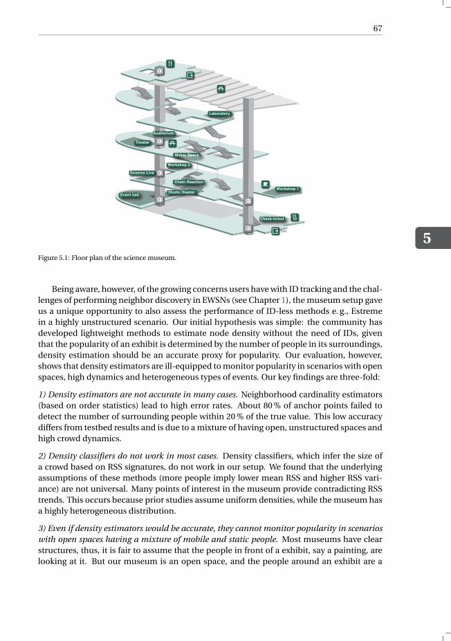
5
67
Event hall
Science Live
Workshop 2
Chain Reaction
Studio theater Workshop 1
Auditorium
Theater
Maker Space
Laboratory
Exit
Check-in/out
Figure 5.1: Floor plan of the science museum.
Being aware, however, of the growing concerns users have with ID tracking and the chal-lenges of performing neighbor discovery in EWSNs (see Chapter 1), the museum setup gaveus a unique opportunity to also assess the performance of ID-less methods e. g., Estremein a highly unstructured scenario. Our initial hypothesis was simple: the community hasdeveloped lightweight methods to estimate node density without the need of IDs, giventhat the popularity of an exhibit is determined by the number of people in its surroundings,density estimation should be an accurate proxy for popularity. Our evaluation, however,shows that density estimators are ill-equipped to monitor popularity in scenarios with openspaces, high dynamics and heterogeneous types of events. Our key findings are three-fold:
1) Density estimators are not accurate in many cases. Neighborhood cardinality estimators(based on order statistics) lead to high error rates. About 80 % of anchor points failed todetect the number of surrounding people within 20 % of the true value. This low accuracydiffers from testbed results and is due to a mixture of having open, unstructured spaces andhigh crowd dynamics.
2) Density classifiers do not work in most cases. Density classifiers, which infer the size ofa crowd based on RSS signatures, do not work in our setup. We found that the underlyingassumptions of these methods (more people imply lower mean RSS and higher RSS vari-ance) are not universal. Many points of interest in the museum provide contradicting RSStrends. This occurs because prior studies assume uniform densities, while the museum hasa highly heterogeneous distribution.
3) Even if density estimators would be accurate, they cannot monitor popularity in scenarioswith open spaces having a mixture of mobile and static people. Most museums have clearstructures, thus, it is fair to assume that the people in front of a exhibit, say a painting, arelooking at it. But our museum is an open space, and the people around an exhibit are a
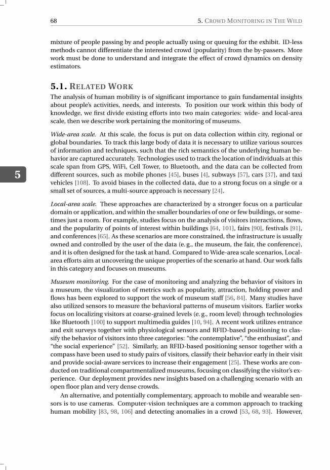
5
68 5. CROWD MONITORING IN THE WILD
mixture of people passing by and people actually using or queuing for the exhibit. ID-lessmethods cannot differentiate the interested crowd (popularity) from the by-passers. Morework must be done to understand and integrate the effect of crowd dynamics on densityestimators.
5.1. RELATED WORKThe analysis of human mobility is of significant importance to gain fundamental insightsabout people’s activities, needs, and interests. To position our work within this body ofknowledge, we first divide existing efforts into two main categories: wide- and local-areascale, then we describe work pertaining the monitoring of museums.
Wide-area scale. At this scale, the focus is put on data collection within city, regional orglobal boundaries. To track this large body of data it is necessary to utilize various sourcesof information and techniques, such that the rich semantics of the underlying human be-havior are captured accurately. Technologies used to track the location of individuals at thisscale span from GPS, WiFi, Cell Tower, to Bluetooth, and the data can be collected fromdifferent sources, such as mobile phones [45], buses [4], subways [57], cars [37], and taxivehicles [108]. To avoid biases in the collected data, due to a strong focus on a single or asmall set of sources, a multi-source approach is necessary [24].
Local-area scale. These approaches are characterized by a stronger focus on a particulardomain or application, and within the smaller boundaries of one or few buildings, or some-times just a room. For example, studies focus on the analysis of visitors interactions, flows,and the popularity of points of interest within buildings [64, 101], fairs [90], festivals [91],and conferences [65]. As these scenarios are more constrained, the infrastructure is usuallyowned and controlled by the user of the data (e. g., the museum, the fair, the conference),and it is often designed for the task at hand. Compared to Wide-area scale scenarios, Local-area efforts aim at uncovering the unique properties of the scenario at hand. Our work fallsin this category and focuses on museums.
Museum monitoring. For the case of monitoring and analyzing the behavior of visitors ina museum, the visualization of metrics such as popularity, attraction, holding power andflows has been explored to support the work of museum staff [56, 84]. Many studies havealso utilized sensors to measure the behavioral patterns of museum visitors. Earlier worksfocus on localizing visitors at coarse-grained levels (e. g., room level) through technologieslike Bluetooth [100] to support multimedia guides [10, 94]. A recent work utilizes entranceand exit surveys together with physiological sensors and RFID-based positioning to clas-sify the behavior of visitors into three categories: “the contemplative”, “the enthusiast”, and“the social experience” [52]. Similarly, an RFID-based positioning sensor together with acompass have been used to study pairs of visitors, classify their behavior early in their visitand provide social-aware services to increase their engagement [25]. These works are con-ducted on traditional compartmentalized museums, focusing on classifying the visitor’s ex-perience. Our deployment provides new insights based on a challenging scenario with anopen floor plan and very dense crowds.
An alternative, and potentially complementary, approach to mobile and wearable sen-sors is to use cameras. Computer-vision techniques are a common approach to trackinghuman mobility [83, 98, 106] and detecting anomalies in a crowd [53, 68, 93]. However,
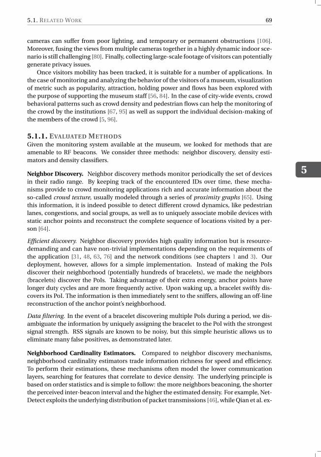
5.1. RELATED WORK
5
69
cameras can suffer from poor lighting, and temporary or permanent obstructions [106].Moreover, fusing the views from multiple cameras together in a highly dynamic indoor sce-nario is still challenging [80]. Finally, collecting large-scale footage of visitors can potentiallygenerate privacy issues.
Once visitors mobility has been tracked, it is suitable for a number of applications. Inthe case of monitoring and analyzing the behavior of the visitors of a museum, visualizationof metric such as popularity, attraction, holding power and flows has been explored withthe purpose of supporting the museum staff [56, 84]. In the case of city-wide events, crowdbehavioral patterns such as crowd density and pedestrian flows can help the monitoring ofthe crowd by the institutions [67, 95] as well as support the individual decision-making ofthe members of the crowd [5, 96].
5.1.1. EVALUATED METHODSGiven the monitoring system available at the museum, we looked for methods that areamenable to RF beacons. We consider three methods: neighbor discovery, density esti-mators and density classifiers.
Neighbor Discovery. Neighbor discovery methods monitor periodically the set of devicesin their radio range. By keeping track of the encountered IDs over time, these mecha-nisms provide to crowd monitoring applications rich and accurate information about theso-called crowd texture, usually modeled through a series of proximity graphs [65]. Usingthis information, it is indeed possible to detect different crowd dynamics, like pedestrianlanes, congestions, and social groups, as well as to uniquely associate mobile devices withstatic anchor points and reconstruct the complete sequence of locations visited by a per-son [64].
Efficient discovery. Neighbor discovery provides high quality information but is resource-demanding and can have non-trivial implementations depending on the requirements ofthe application [31, 48, 63, 76] and the network conditions (see chapters 1 and 3). Ourdeployment, however, allows for a simple implementation. Instead of making the PoIsdiscover their neighborhood (potentially hundreds of bracelets), we made the neighbors(bracelets) discover the PoIs. Taking advantage of their extra energy, anchor points havelonger duty cycles and are more frequently active. Upon waking up, a bracelet swiftly dis-covers its PoI. The information is then immediately sent to the sniffers, allowing an off-linereconstruction of the anchor point’s neighborhood.
Data filtering. In the event of a bracelet discovering multiple PoIs during a period, we dis-ambiguate the information by uniquely assigning the bracelet to the PoI with the strongestsignal strength. RSS signals are known to be noisy, but this simple heuristic allows us toeliminate many false positives, as demonstrated later.
Neighborhood Cardinality Estimators. Compared to neighbor discovery mechanisms,neighborhood cardinality estimators trade information richness for speed and efficiency.To perform their estimations, these mechanisms often model the lower communicationlayers, searching for features that correlate to device density. The underlying principle isbased on order statistics and is simple to follow: the more neighbors beaconing, the shorterthe perceived inter-beacon interval and the higher the estimated density. For example, Net-Detect exploits the underlying distribution of packet transmissions [46], while Qian et al. ex-
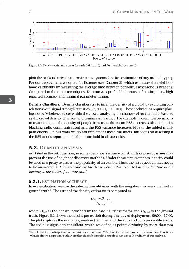
5
70 5. CROWD MONITORING IN THE WILD
Figure 5.2: Density estimation error for each PoI (1. . .30) and for the global system (G).
ploit the packets’ arrival patterns in RFID systems for a fast estimation of tag cardinality [77].For our deployment, we opted for Estreme (see Chapter 3), which estimates the neighbor-hood cardinality by measuring the average time between periodic, asynchronous beacons.Compared to the other techniques, Estreme was preferable because of its simplicity, highreported accuracy and minimal parameter tuning.
Density Classifiers. Density classifiers try to infer the density of a crowd by exploiting cor-relations with signal strength statistics [72, 90, 91, 102, 103]. These techniques require plac-ing a set of wireless devices within the crowd, analyzing the changes of several radio featuresas the crowd density changes, and training a classifier. For example, a common premise isto assume that as the density of people increases, the mean RSS decreases (due to bodiesblocking radio communication) and the RSS variance increases (due to the added multi-path effects). In our work we do not implement these classifiers, but focus on assessing ifthe RSS trends reported in the literature hold in all scenarios.
5.2. DENSITY ANALYSISAs stated in the introduction, in some scenarios, resource constraints or privacy issues mayprevent the use of neighbor discovery methods. Under these circumstances, density couldbe used as a proxy to assess the popularity of an exhibit. Thus, the first question that needsto be answered is: how accurate are the density estimators reported in the literature in theheterogeneous setup of our museum?
5.2.1. ESTIMATION ACCURACYIn our evaluation, we use the information obtained with the neighbor discovery method asground truth2. The error of the density estimator is computed as
Dest −D tr ue
D tr ue,
where Dest is the density provided by the cardinality estimator and D tr ue is the groundtruth. Figure 5.2 shows the results per exhibit during one day of deployment, 09:00 - 17:00.The plot captures the min, max, median (red line) and the 25th and 75th percentile errors.The red plus signs depict outliers, which we define as points deviating by more than two
2Recall that the participation rate of visitors was around 25%, thus the actual number of visitors was four timeswhat is shown as ground truth. Note that this sub-sampling rate does not affect the validity of our analysis.
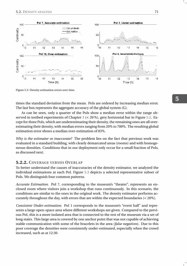
5.2. DENSITY ANALYSIS
5
71
Figure 5.3: Density estimation errors over time.
times the standard deviation from the mean. PoIs are ordered by increasing median error.The last box represents the aggregate accuracy of the global system (G).
As can be seen, only a quarter of the PoIs show a median error within the range ob-served in testbed experiments of Chapter 3 (< 20 %), grey horizontal bar in Figure 5.2. Ex-cept for three PoIs, which are underestimating their density, the remaining ones are all over-estimating their density, with median errors ranging from 20% to 700%. The resulting globalestimation error shows a median over-estimation of 83%.
Why is the estimator so inaccurate? The problem lies on the fact that previous work wasevaluated in a standard building, with clearly demarcated areas (rooms) and with homoge-neous densities. Conditions that in our deployment only occur for a small fraction of PoIs,as discussed next.
5.2.2. COVERAGE VERSUS OVERLAP
To better understand the causes of inaccuracies of the density estimator, we analyzed theindividual estimations at each PoI. Figure 5.3 depicts a selected representative subset ofPoIs. We distinguish four common patterns.
Accurate Estimation. PoI 7, corresponding to the museum’s “theater”, represents an en-closed room where visitors join a workshop that runs continuously. In this scenario, theconditions are similar to the ones in the original work. The density estimator performs ac-curately throughout the day, with errors that are within the expected boundaries (< 20%).
Consistent Under-estimation. PoI 1 corresponds to the museum’s “event hall” and repre-sents a large open-space area where different workshops are given. Compared to the previ-ous PoI, this is a more isolated area that is connected to the rest of the museum via a set oflong stairs. This large area is covered by one anchor point that was not capable of achievingstable communication with some of the bracelets in the area (false negatives). Due to thispoor coverage the densities were consistently under-estimated, especially when the crowdincreased, such as at 12:30.
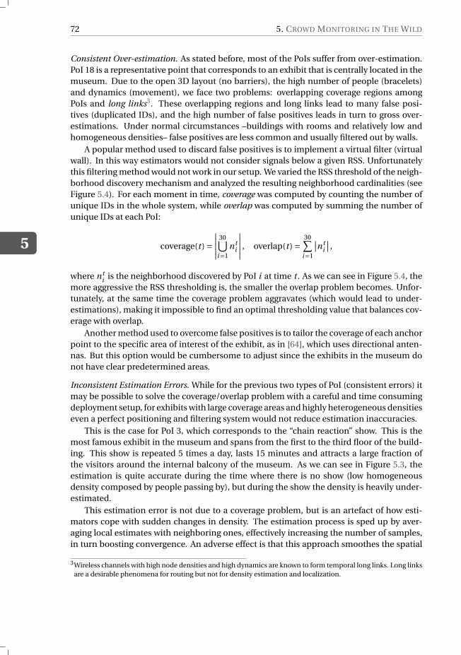
5
72 5. CROWD MONITORING IN THE WILD
Consistent Over-estimation. As stated before, most of the PoIs suffer from over-estimation.PoI 18 is a representative point that corresponds to an exhibit that is centrally located in themuseum. Due to the open 3D layout (no barriers), the high number of people (bracelets)and dynamics (movement), we face two problems: overlapping coverage regions amongPoIs and long links3. These overlapping regions and long links lead to many false posi-tives (duplicated IDs), and the high number of false positives leads in turn to gross over-estimations. Under normal circumstances –buildings with rooms and relatively low andhomogeneous densities– false positives are less common and usually filtered out by walls.
A popular method used to discard false positives is to implement a virtual filter (virtualwall). In this way estimators would not consider signals below a given RSS. Unfortunatelythis filtering method would not work in our setup. We varied the RSS threshold of the neigh-borhood discovery mechanism and analyzed the resulting neighborhood cardinalities (seeFigure 5.4). For each moment in time, coverage was computed by counting the number ofunique IDs in the whole system, while overlap was computed by summing the number ofunique IDs at each PoI:
coverage(t ) =∣∣∣∣∣ 30⋃i=1
nti
∣∣∣∣∣ , overlap(t ) =30∑
i=1
∣∣nti
∣∣ ,
where nti is the neighborhood discovered by PoI i at time t . As we can see in Figure 5.4, the
more aggressive the RSS thresholding is, the smaller the overlap problem becomes. Unfor-tunately, at the same time the coverage problem aggravates (which would lead to under-estimations), making it impossible to find an optimal thresholding value that balances cov-erage with overlap.
Another method used to overcome false positives is to tailor the coverage of each anchorpoint to the specific area of interest of the exhibit, as in [64], which uses directional anten-nas. But this option would be cumbersome to adjust since the exhibits in the museum donot have clear predetermined areas.
Inconsistent Estimation Errors. While for the previous two types of PoI (consistent errors) itmay be possible to solve the coverage/overlap problem with a careful and time consumingdeployment setup, for exhibits with large coverage areas and highly heterogeneous densitieseven a perfect positioning and filtering system would not reduce estimation inaccuracies.
This is the case for PoI 3, which corresponds to the “chain reaction” show. This is themost famous exhibit in the museum and spans from the first to the third floor of the build-ing. This show is repeated 5 times a day, lasts 15 minutes and attracts a large fraction ofthe visitors around the internal balcony of the museum. As we can see in Figure 5.3, theestimation is quite accurate during the time where there is no show (low homogeneousdensity composed by people passing by), but during the show the density is heavily under-estimated.
This estimation error is not due to a coverage problem, but is an artefact of how esti-mators cope with sudden changes in density. The estimation process is sped up by aver-aging local estimates with neighboring ones, effectively increasing the number of samples,in turn boosting convergence. An adverse effect is that this approach smoothes the spatial
3Wireless channels with high node densities and high dynamics are known to form temporal long links. Long linksare a desirable phenomena for routing but not for density estimation and localization.
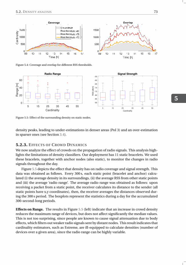
5.2. DENSITY ANALYSIS
5
73
Figure 5.4: Coverage and overlap for different RSS thresholds.
5 15 25 35 45 55
Cardinality
-90
-85
-80
-75
-70
-65
-60
-55
RS
S [dbm
]
Signal Strength
5 15 25 35 45 55
Cardinality
0
20
40
60
Range [m
]
Radio Range
Figure 5.5: Effect of the surrounding density on static nodes.
density peaks, leading to under-estimations in denser areas (PoI 3) and an over-estimationin sparser ones (see Section 3.4).
5.2.3. EFFECTS OF CROWD DYNAMICS
We now analyze the effect of crowds on the propagation of radio signals. This analysis high-lights the limitations of density classifiers. Our deployment has 11 static bracelets. We usedthese bracelets, together with anchor nodes (also static), to monitor the changes in radiosignals throughout the day.
Figure 5.5 depicts the effect that density has on radio coverage and signal strength. Thisdata was obtained as follows. Every 300 s, each static point (bracelet and anchor) calcu-lated (i) the average density in its surroundings, (ii) the average RSS from other static pointsand (iii) the average ‘radio range’. The average radio range was obtained as follows: uponreceiving a packet from a static point, the receiver calculates its distance to the sender (allstatic points have x,y coordinates), then, the receiver averages the distances observed dur-ing the 300 s period. The boxplots represent the statistics during a day for the accumulated300-second-long periods.
Effects on Range. The results in Figure 5.5 (left) indicate that an increase in crowd densityreduces the maximum range of devices, but does not affect significantly the median values.This is not too surprising, since people are known to cause signal attenuation due to bodyeffects, which filters out weaker radio signals sent by distant nodes. This result indicates thatcardinality estimators, such as Estreme, are ill-equipped to calculate densities (number ofdevices over a given area), since the radio range can be highly variable.
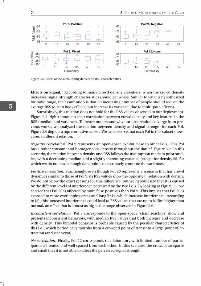
5
74 5. CROWD MONITORING IN THE WILD
5 15 25 35 45 55-95
-85
-75
-65
RS
S [
db
m]
PoI 9, Positive
5 15 25 35 45 55-95
-85
-75
-65PoI 20, Negative
5 15 25 35 45 55
Cardinality
-95
-85
-75
-65
RS
S [
db
m] PoI 3, Mixed
5 15 25 35 45 55
Cardinality
-95
-85
-75
-65PoI 12, None
Figure 5.6: Effect of the surrounding density on RSS characteristics.
Effects on Signal. According to many crowd density classifiers, when the crowd densityincreases, signal strength characteristics should get worse. Similar to what is hypothesizedfor radio range, the assumption is that an increasing number of people should reduce theaverage RSS (due to body effects) but increase its variance (due to multi-path effects).
Surprisingly, this relation does not hold for the RSS values observed in our deployment.Figure 5.5 (right) shows no clear correlation between crowd density and key features in theRSS (median and variance). To better understand why our observations diverge from pre-vious works, we analyzed the relation between density and signal strength for each PoI.Figure 5.6 depicts a representative subset. We can observe that each PoI in this subset show-cases a different relation.
Negative correlation. PoI 9 represents an open-space exhibit close to other PoIs. This PoIhas a rather constant and homogeneous density throughout the day, cf. Figure 5.2. In thisscenario, the relation between density and RSS follows the assumption made in prior stud-ies, with a decreasing median and a slightly increasing variance (except for density 55, forwhich we do not have enough data points to accurately compute the variance).
Positive correlation. Surprisingly, even though PoI 20 represents a scenario that has crowddynamics similar to those of PoI 9, its RSS values show the opposite (!) relation with density.We do not know the exact reasons for this difference, but we hypothesize that it is causedby the different levels of interference perceived by the two PoIs. By looking at Figure 5.2, wecan see that PoI 20 is affected by more false positives than PoI 9. This implies that PoI 20 isexposed to more overlapping areas and long links, which increase interference. Accordingto [3], this increased interference could lead to RSS values that are up to 8 dBm higher thannormal, an offset that is almost as big as the range observed in Figure 5.6.
Inconsistent correlation. PoI 3 corresponds to the open-space “chain reaction” show andpresents inconsistent behaviors, with median RSS values that both increase and decreasewith density. This bimodal behavior is probably caused by the peculiar characteristics ofthis PoI, which periodically morphs from a crowded point of transit to a large point of at-traction (and vice versa).
No correlation. Finally, PoI 12 corresponds to a laboratory with limited number of partic-ipants, all seated and well spaced from each other. In this scenario the crowd is so sparseand small that it is not able to affect the perceived signal strength.
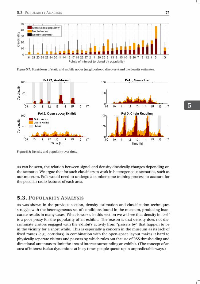
5.3. POPULARITY ANALYSIS
5
75
6 21 23 28 22 24 30 11 14 16 17 18 26 27 2 4 29 25 3 13 8 15 10 19 20 7 9 12 1 5 G
Points of Interest (ordered by popularity)
0
10
20
30
40
50
Card
inalit
y
Static Nodes (popularity)
Mobile Nodes
Density Estimator
Figure 5.7: Breakdown of static and mobile nodes (neighborhood discovery) and the density estimates.
Figure 5.8: Density and popularity over time.
As can be seen, the relation between signal and density drastically changes depending onthe scenario. We argue that for such classifiers to work in heterogeneous scenarios, such asour museum, PoIs would need to undergo a cumbersome training process to account forthe peculiar radio features of each area.
5.3. POPULARITY ANALYSIS
As was shown in the previous section, density estimation and classification techniquesstruggle with the heterogeneous set of conditions found in the museum, producing inac-curate results in many cases. What is worse, in this section we will see that density in itselfis a poor proxy for the popularity of an exhibit. The reason is that density does not dis-criminate visitors engaged with the exhibit’s activity from “passers by” that happen to bein the vicinity for a short while. This is especially a concern in the museum as its lack offixed routes (e.g., corridors) in combination with the open-space layout makes it hard tophysically separate visitors and passers by, which rules out the use of RSS thresholding anddirectional antennas to limit the area of interest surrounding an exhibit. (The concept of anarea of interest is also dynamic as at busy times people queue up in unpredictable ways.)
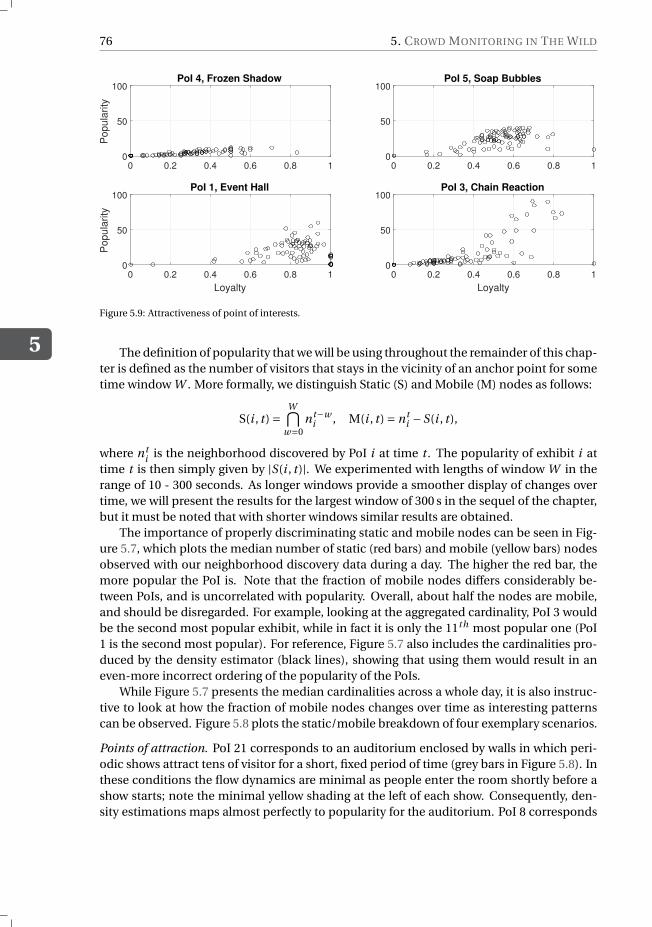
5
76 5. CROWD MONITORING IN THE WILD
0 0.2 0.4 0.6 0.8 10
50
100
Po
pu
larity
PoI 4, Frozen Shadow
0 0.2 0.4 0.6 0.8 10
50
100PoI 5, Soap Bubbles
0 0.2 0.4 0.6 0.8 1
Loyalty
0
50
100
Po
pu
larity
PoI 1, Event Hall
0 0.2 0.4 0.6 0.8 1
Loyalty
0
50
100PoI 3, Chain Reaction
Figure 5.9: Attractiveness of point of interests.
The definition of popularity that we will be using throughout the remainder of this chap-ter is defined as the number of visitors that stays in the vicinity of an anchor point for sometime window W . More formally, we distinguish Static (S) and Mobile (M) nodes as follows:
S(i , t ) =W⋂
w=0nt−w
i , M(i , t ) = nti −S(i , t ),
where nti is the neighborhood discovered by PoI i at time t . The popularity of exhibit i at
time t is then simply given by |S(i , t )|. We experimented with lengths of window W in therange of 10 - 300 seconds. As longer windows provide a smoother display of changes overtime, we will present the results for the largest window of 300 s in the sequel of the chapter,but it must be noted that with shorter windows similar results are obtained.
The importance of properly discriminating static and mobile nodes can be seen in Fig-ure 5.7, which plots the median number of static (red bars) and mobile (yellow bars) nodesobserved with our neighborhood discovery data during a day. The higher the red bar, themore popular the PoI is. Note that the fraction of mobile nodes differs considerably be-tween PoIs, and is uncorrelated with popularity. Overall, about half the nodes are mobile,and should be disregarded. For example, looking at the aggregated cardinality, PoI 3 wouldbe the second most popular exhibit, while in fact it is only the 11th most popular one (PoI1 is the second most popular). For reference, Figure 5.7 also includes the cardinalities pro-duced by the density estimator (black lines), showing that using them would result in aneven-more incorrect ordering of the popularity of the PoIs.
While Figure 5.7 presents the median cardinalities across a whole day, it is also instruc-tive to look at how the fraction of mobile nodes changes over time as interesting patternscan be observed. Figure 5.8 plots the static/mobile breakdown of four exemplary scenarios.
Points of attraction. PoI 21 corresponds to an auditorium enclosed by walls in which peri-odic shows attract tens of visitor for a short, fixed period of time (grey bars in Figure 5.8). Inthese conditions the flow dynamics are minimal as people enter the room shortly before ashow starts; note the minimal yellow shading at the left of each show. Consequently, den-sity estimations maps almost perfectly to popularity for the auditorium. PoI 8 corresponds
5.3. POPULARITY ANALYSIS
5
77
instead to a small bar outside the previously mentioned auditorium. Here density capturesthe visitors having a short snack (intended) as well as the ones passing by (unintended)clobbering the real popularity.
Point of passage. PoI 2, on the other hand, represents an exhibit located in an open space,close to a point of passage i. e., an area that is similar to a corridor but does not have walls. Inthis case most of its perceived density it is due to people passing by. To understand the pop-ularity of PoIs like this, it is therefore essential to distinguish between static and dynamicneighboring bracelets, especially since the fraction of mobile nodes varies across time.
Temporal hybrids. Finally, PoI 3 represents an exhibit (the “chain reaction”) that is normallya popular point of passage (amidst several staircases, see Figure 5.1), but periodically be-comes a point of attraction for short periods of time (show times are highlighted with a greybackground). The error, i. e., the amount of moving nodes taken into account, in this casedrastically fluctuates, with rather accurate estimations during the periodic shows (hardlyany yellow on top) and bad ones during the remaining periods (lots of yellow).
5.3.1. ATTRACTIVENESS
Besides differentiating static and mobile bracelets, which allowed for establishing the truepopularity of exhibits, we computed several other metrics to help the museum curatorsobtain a deeper understanding of the dynamics behind each PoI’s popularity.
The most interesting of these metrics is the loyalty of visitors at each PoI, defined as thefraction of static nodes (or ratio of popularity over density). The rationale for the loyaltymetric is that the more engaging a PoI is, the more people passing by will stop, and becomestatic (engaged). A loyalty of 0 denotes no interest as apparently all visitors in the vicinityof the PoI are “passers by”. On the other hand, a loyalty of 1 denotes a PoI that engages allvisitors in range.
Figure 5.9 compares the loyalty against the popularity for a few selected PoIs, showingthe remarkable diversity in scenarios found at the science museum. Each dot captures afive-minute interval.
Unpopular attractions. PoI 4 represents the “frozen shadow” room, a PoI with low loyaltyand popularity. This is not surprising, since the engagement in this PoI is usually short asthe attraction consists of a room with phosphorescent walls that captures the shadows via astrobing light (flashing once every 30 s). Even the most enthusiastic kids do not freeze theirshadow more than ten times, hence, limiting the popularity to near zero as that maximumtime equals the window size (300 s).
Popular attractions. Compared to PoI 4, the “soap bubbles” attraction (PoI 5) consists of anopen area were kids are able to make huge soap bubbles using a wide set of tools. As can beseen from Figure 5.9 this PoI shows both a higher loyalty and attractiveness i. e., it is able toengage passing by visitors.
Workshop areas. A similar popularity, but a higher loyalty is achieved by the “event hall” (PoI1), a slightly isolated open-area where several workshop are taught. The main differencebetween this PoI and the previous one, is that these workshops are very attractive and takemuch longer to complete, hence, capturing a particularly ‘long’ loyalty from visitors.
5
78 5. CROWD MONITORING IN THE WILD
Periodic attractions. Finally, PoI 3 represents the periodic “chain rection” show. In this case,one can observe (again) the bimodal behavior of this PoI: most of the time it serves as apoint of passage (low loyalty and popularity) and during shows as a point of attraction (highloyalty and popularity). Note that compared to the event hall, we have fewer dots on thehigh loyalty region of the plot. This is because the chain reaction lasts for 15 minutes (3dots) and it is scheduled only 5 times a day, while the workshops run continuously.
5.4. CONCLUSIONSIn this chapter we reported our experience in monitoring the popularity of exhibits at amodern, open-space science museum. During some of the museum’s most crowded days,we equipped visitors with bracelets emitting RF beacons, allowing us to study existing crowd-monitoring mechanisms such as neighbor discovery, cardinality estimators, and densityclassifiers in a diverse set of challenging real-world settings.
An in-depth analysis of the collected data (proximity detections and density estima-tions) provided a better understanding of the limitations of the existing mechanisms. Inparticular, the use of ID-based neighbor discovery allowed us to univocally associate eachbracelet to the point of interest, and distinguish static from mobile nodes. The latter provedkey to understanding the relation between density and popularity. Cardinality estimators,such as Estreme, cannot provide such differentiation, resulting in estimation errors far higherthan originally observed in the testbed experiments of Chapter 3.
An important downside of neighbor discovery is that it relies on identity information,which may not always be available because of privacy issues [35], network conditions andlimited resources (see Chapter 1). An important line of future research is thus to deviselightweight and privacy-preserving algorithms that can differentiate static and mobile nodes,allowing a precise estimation of popularity.
6CONCLUSIONS
Inspired by the need of monitoring large crowds with wireless wearable devices, this the-sis tackled the challenges of communication in Extreme Wireless Sensor Networks, wherethousands of mobile nodes gather together in highly confined areas and periodically needto exchange their sensed information. As we argued, in these extreme conditions, tradi-tional low-power mechanisms simply do not scale and collapse. Therefore, we proposed anovel communication stack that is based on opportunistic communication.
6.1. REGARD CHALLENGES AS OPPORTUNITIESThe mechanisms presented in this thesis originated from a simple idea presented in Chap-ter 1. Instead of adapting existing mechanisms to the challenges of EWSNs, it is better todesign new mechanisms that a) benefit from harsh network conditions (anti-fragile prin-ciple) and b) are able to spontaneously adapt when the same conditions change (oppor-tunistic principle). The resulting mechanisms, presented in chapters 2, 3 and 4 not onlyscale to EWSNs, but do so with a remarkable simplicity (state-less principle) and flexibility(robustness principle).
SOFA (Chapter 2) is the cornerstone of the communication stack presented in this the-sis and is an example of how opportunistic mechanisms can exploit extreme networks con-ditions to their own advantage. In particular, SOFA’s communication primitive exchangesdata with the first available neighbor, independently of its ID and topology location. Bygiving priority to efficiency, rather than the certainty of the routing path, nodes are ableto efficiently communicate throughout a wide range of network conditions (density, sizeand load) with low energy consumption (≈ 2 % duty cycle) and high delivery rates (above90 %). In other words, SOFA achieves performance that is similar to synchronous proto-cols, but with the simplicity and flexibility of the asynchronous ones. Moreover, becauseSOFA’s mechanism is stateless and does not require any information from the neighbors,it shows a remarkable resilience to mobility and link failures, which are common charac-teristics of EWSNs. SOFA’s flexibility has been particularly important during the real-worldexperiments at the NEMO science museum, where the mechanism had to reliably commu-nicate throughout a wide set of network conditions.
79
6
80 6. CONCLUSIONS
6.2. BUILDING ON TOP OF OPPORTUNISTIC PRIMITIVESEven though SOFA allows to communicate in EWSNs, not all network services can be adaptedto its novel communication primitive in a straightforward way. Opportunistic anycast re-quires in fact to rethink – from the ground up – many network services such as neighborsdiscovery and routing, which are normally based on deterministic primitives such as uni-cast and broadcast. To this end, in chapters 3 and 4 we proposed Estreme and Staffetta, twoalternatives to traditional neighbor discovery and data collection, respectively.
Estreme (Chapter 3) proposed to estimate, rather than count, the number of neighbor-ing devices, thus removing the need of explicitly discovering each device. Following theguidelines of Chapter 1, Estreme performs its estimation by exploiting the unique corre-lation present in SOFA between the rendezvous times and the neighborhood cardinality(opportunistic principle). The denser the network, the shorter these times are. BecauseEstreme is based only on passive observations (of the rendezvous time), it can perform itsestimations concurrently (up to 100 concurrent estimators) and can exploit the spatial cor-relation of density to speed up its estimation convergence. This way, Estreme is able tohandle abrupt changes in the network (robustness principle), with errors that are below10 % and stable across a wide set of conditions (from 10 to 100 neighbors).
Staffetta (Chapter 4), on the other hand, is able to bias the opportunistic communica-tion of SOFA in a desired direction, effectively providing data collection over opportunisticanycast. Staffetta achieves this bias due to the following phenomenon: because in SOFAmessages are forwarded to the first available neighbor, it is possible to bias the forwardingof data by making some nodes to wake up more often than others. In the case of data col-lection, Staffetta forms an activity gradient in which nodes are the more active, the closerthey are to the sink, i. e., the node collecting all the sensors’ data. Similar to the other mech-anisms proposed in this thesis, Staffetta’s activity gradient forms spontaneously from localnodes’ observations and, thus, can easily adapt to network changes with minimal overhead(state-less principle). The extensive set of experiments presented in Chapter 4 showed thatStaffetta significantly reduces both packet latency and energy consumption of data collec-tion over opportunistic primitives while maintaining high packet delivery ratios (robustnessprinciple). As Staffetta does not need to maintain complicated routing metrics spanning theentire network, it can also handle network dynamics like link-quality fluctuations and nodemobility really well. We found that Staffetta adapts its gradient in just a matter of seconds.
6.3. EXTREME WIRELESS SENSOR NETWORKS IN PRACTICEChapter 5 concluded this thesis by testing the previously-proposed mechanisms in a widerange of real-world conditions. In particular, we tested both SOFA and Estreme as a tool tomonitor the crowd characteristics in a six-stories science museum. The deployment data,collected over three of the most crowded days of the year with close to a thousand visitors,showed that both mechanisms are able scale to EWSNs even though some expected andunexpected challenges arose. First, similar to what we showed in Chapter 3, our density es-timator Estreme suffered when the network density drastically changed in space. We plan toaddress this accuracy problem in future work. Second, using the neighborhood cardinalityto estimate the crowd density provided inaccurate results. This is due to the fact that con-trolling the range of radio devices in heterogeneous environments (with walls, rooms andopen-spaces) is very challenging. More research must be done to efficiently solve the cover-
6.4. FUTURE WORK
6
81
age/overlap problem described in Section 5.2.2. Third, because our and others estimatorsdo not detect if a neighboring device is moving, they are not able to distinguish betweenvisitors who are interested, and stand, at an exhibit, and visitors who are not interested andare just passing by. This differentiation is essential, for example, to compute exhibit-relatedmetrics such as the popularity of a point of interest.
6.4. FUTURE WORKThe four principles presented in Chapter 1 served as guidelines to develop the solutionspresented in this thesis and resulted in mechanisms that are both simple and scalable toEWSNs. Nevertheless, we recognize that these principles could be improved to make EWSNs’mechanisms even more flexible and efficient.
Towards versatile mechanisms. Designing anti-fragile mechanisms i. e., mechanisms thatperform better in hard conditions, is the first step toward communication in EWSNs. Nev-ertheless, we argue that the next step is to make these mechanisms versatile to any networkcondition, from mild to extreme. Unfortunately, creating such mechanisms is difficult andpresents three main challenges. First, versatile mechanisms for EWSNs still needs to excelin extreme network conditions. Second, under mild conditions, these mechanisms needsto operate with performance that are comparable to traditional mechanisms – which werespecifically designed for the mild case. Failing in solving this challenge could impede theadoption of EWSNs technologies. In other words: “why should you use a technology thatdoes not work in non-challenging conditions?”. Third, versatile mechanisms should be ableto adapt rapidly to the abrupt changes between mild and extreme conditions. As we showedin this thesis, opportunistic behaviors could be a solution to this latter challenge.
As an example, according to the anti-fragile principle, SOFA is very efficient when theneighborhood cardinality crosses ≈ 20 neighbors. Under this density threshold, on the con-trary, SOFA’s rendezvous gets longer and longer, resulting in very high energy consumption.This inefficiency could have been problematic during the NEMO experiment (see Chap-ter 5) where low density conditions could have been temporarily present. In this case, tomake SOFA more versatile, we borrowed some ideas from Staffetta and imposed an energybudget on each node.
Integrating opportunistic mechanisms. Even though Estreme and Staffetta provide viable al-ternatives to their traditional protocol counterparts, their coexistence is not straightforwardand must be further analyzed. Estreme, for example, relies on the fact that all nodes in thenetwork wake up with the same frequency. Staffetta, instead, modifies this same frequencyto bias the direction of the forwarded messages. A possible solution to this conflict, whichshould be further analyzed in future work, could consist of distinguishing between differ-ent wake-up events (the ones of Estreme from the ones of Staffetta). Alternatively, Estreme’smodel could be extended in order to support an uneven set of wake-up frequencies. Nev-ertheless, we argue that similar integration issues could arise also in future mechanisms forEWSNs that opportunistically exploit the base communication layer (SOFA) to efficientlyfulfill their tasks.
Estimate the right type of information. Chapter 5 suggests that, for museum and crowdmonitoring applications, estimating the neighborhood cardinality is not enough to obtainmeaningful insights. In this case, for example, knowing the nodes’ identity proved to be
6
82 6. CONCLUSIONS
essential for the accurate estimation of the crowd density and the popularity of Points ofInterest. Unfortunately, as argued in chapters 2 and 3, discovering the neighbors’ identi-ties in EWSNs is very challenging and leaves the problem of crowd density estimation inEWSNs still open to the research community. Nevertheless, the results presented in Chap-ter 5 should inspire future work to explore which type of information is required by eachapplication and, based on the results, develop the corresponding estimators for our EWSNs’stack.
REFERENCES
[1] M. Ammar and G. Rouskas. On the performance of protocols for collecting responsesover a multiple-access channel. In 10th Conf. of the IEEE Computer and Communi-cations Societies (INFOCOM), pages 1490–1499, 1991.
[2] N. Balakrishnan, E. Castillo, and J.-M. Sarabia. Advances in Distribution Theory, OrderStatistics, and Inference. 2007.
[3] A. Behboodi, N. Wirstrom, F. Lemic, T. Voigt, and A. Wolisz. Interference effect onlocalization solutions: Signal feature perspective. IEEE Vehicular Technology Confer-ence, 2015, 2015.
[4] S. Bhattacharya, S. Phithakkitnukoon, P. Nurmi, A. Klami, M. Veloso, and C. Bento.Gaussian process-based predictive modeling for bus ridership. In ACM Conf. on Per-vasive and ubiquitous computing adjunct publication, pages 1189–1198. ACM, 2013.
[5] U. Blanke, G. Troster, T. Franke, and P. Lukowicz. Capturing crowd dynamics at largescale events using participatory gps-localization. In IEEE 9th Int. Conf. on IntelligentSensors, Sensor Networks and Information Processing (ISSNIP), pages 1–7. IEEE, 2014.
[6] C. Boano and M. Zuniga. JAG: Reliable and Predictable Wireless Agreement under Ex-ternal Radio Interference. In IEEE 33rd Real-Time Systems Symposium (RTSS), pages315–326, 2012.
[7] C. A. Boano, N. Tsiftes, T. Voigt, J. Brown, and U. Roedig. The impact of temperatureon outdoor industrial sensornet applications. IEEE Transactions on Industrial Infor-matics, 6(3):451–459, 2010.
[8] S. Boyd and A. Ghosh. Gossip algorithms: Design, analysis and applications. In IFO-COM 2005. 24th Annual Joint Conf. of the IEEE Computer and Communications Soci-eties, pages 1653–1664, 2005.
[9] J. Brown, U. Roedig, C. A. Boano, and K. Romer. Estimating packet reception ratein noisy environments. 39th Annual IEEE Conference on Local Computer NetworksWorkshops, pages 583–591, 2014.
[10] E. Bruns, B. Brombach, T. Zeidler, and O. Bimber. Enabling mobile phones to supportlarge-scale museum guidance. IEEE Multimedia, (2):16–25, 2007.
[11] M. Buettner, G. Yee, and E. Anderson. X-MAC: a short preamble MAC protocol forduty-cycled wireless sensor networks. In 4th ACM conf. on Embedded networked sen-sor systems (Sensys), pages 307–320, 2006.
[12] N. Burri. Dozer: ultra-low power data gathering in sensor networks. In 6th Int. Simp.on Information Processing in Sensor Networks. (IPSN), pages 450–459, 2007.
83
84 REFERENCES
[13] M. Cattani, S. Guna, and G. P. Picco. Group monitoring in mobile wireless sensornetworks. In Int. Conf. on Distributed Computing in Sensor Systems and Workshops(DCOSS), pages 1–8. Ieee, jun 2011.
[14] M. Cattani, A. Loukas, M. Zimmerling, M. Zuniga, and K. Langendoen. Staffetta:SmartDuty-Cycling for Opportunistic Data Collection. In 14th ACM Conf. on Embed-ded Networked Sensor Systems (SenSys), 2016.
[15] M. Cattani, M. Zuniga, A. Loukas, and K. G. Langendoen. Lightweight Cardinality Es-timation in Dynamic Wireless Networks. In 13th ACM/IEEE Int. Conf. on InformationProcessing in Sensor Networks (IPSN), pages 179–189, 2014.
[16] M. Cattani, M. Zuniga, M. Woehrle, and K. Langendoen. Poster: Communicationin Extreme Wireless Sensor Networks. In 11th ACM Conf. on Embedded NetworkedSensor Systems (SenSys), pages 1–2, 2013.
[17] M. Cattani, M. Zuniga, M. Woehrle, and K. Langendoen. SOFA: Communication inextreme wireless sensor networks. In 11th European Conf. Wireless Sensor Networks(EWSN), volume 8354 LNCS, pages 100–115, 2014.
[18] M. Ceriotti, L. Mottola, G. Picco, a.L. Murphy, S. Guna, M. Corra, M. Pozzi, D. Zonta,and P. Zanon. Monitoring heritage buildings with wireless sensor networks: The TorreAquila deployment. 2009 International Conference on Information Processing in Sen-sor Networks, pages 277–288, 2009.
[19] P. Chassaing and L. Gerin. Efficient estimation of the cardinality of large data sets. InarXiv preprint math/0701347, number 1, pages 1–15, 2007.
[20] B. Chen, Z. Zhou, and H. Yu. Understanding RFID counting protocols. In 19th int.conf. on Mobile computing & networking, pages 291–302, 2013.
[21] D. S. J. De Couto, D. Aguayo, J. Bicket, and R. Morris. A high-throughput path metricfor multi-hop wireless routing. Wireless Networks, 11:419–434, 2005.
[22] A. Demers, D. Greene, and C. Hauser. Epidemic algorithms for replicated databasemaintenance. In Sixth ACM Symposium on Principles of distributed computing, pages1–12, 1987.
[23] M. Demirbas, S. Tasci, H. Gunes, and A. Rudra. Singlehop Collaborative FeedbackPrimitives for Threshold Querying in Wireless Sensor Networks. In Int. Parallel &Distributed Processing Symposium, pages 322–333. Ieee, may 2011.
[24] Z. Desheng, J. Huang, Y. Li, F. Zhang, C. Xu, and T. He. Exploring Human Mobility withMulti-Source Data at Extremely Large Metropolitan Scales. In ACM 20th Int. Conf. onMobile computing and networking (Mobicom), pages 1–12, 2014.
[25] E. Dim and T. Kuflik. Automatic detection of social behavior of museum visitor pairs.ACM Transactions on Interactive Intelligent Systems (TiiS), 4(4):17, 2014.
[26] M. Doddavenkatappa, M. C. Chan, and a. L. Ananda. Indriya: A low-cost, 3D wirelesssensor network testbed. Lecture Notes of the Institute for Computer Sciences, Social-Informatics and Telecommunications Engineering, 90 LNICST:302–316, 2012.
REFERENCES 85
[27] H. Dubois-Ferrière, M. Grossglauser, and M. Vetterli. Valuable detours: Least-costanypath routing. IEEE/ACM Transactions on Networking, 19(2):333–346, 2011.
[28] A. Dunkels. The ContikiMAC Radio Duty Cycling Protocol. SICS Technical ReportT2011:13 , ISSN 1100-3154, pages 1–11, 2011.
[29] S. Duquennoy, O. Landsiedel, and T. Voigt. Let the Tree Bloom : Scalable Opportunis-tic Routing with ORPL. In 11th ACM Conf. on Embedded Networked Sensor Systems(Sensys), pages 2–14, 2013.
[30] P. Dutta, S. Dawson-Haggerty, Y. Chen, C.-J. M. Liang, and A. Terzis. Design and evalu-ation of a versatile and efficient receiver-initiated link layer for low-power wireless. InSensys ’10 8th ACM Conference on Embedded Networked Sensor Systems, pages 1–14.ACM Press, 2010.
[31] P. Dutta, R. Musaloiu-E, I. Stoica, and A. Terzis. Wireless ACK collisions not consideredharmful. In In HotNets-VII The Seventh Workshop on Hot Topics in Networks, 2008.
[32] A. El-Hoiydi. WiseMAC: an ultra low power MAC protocol for the downlink of infras-tructure wireless sensor networks. In Ninth Int. Symp. on Computers and Communi-cations (ISCC), pages 244–251, 2004.
[33] F. Ferrari, M. Zimmerling, L. Mottola, and L. Thiele. Low-power wireless bus. In 10thACM Conf. on Embedded Network Sensor Systems (SenSys), page 1, 2012.
[34] F. Ferrari, M. Zimmerling, L. Thiele, and O. Saukh. Efficient Network Flooding andTime Synchronization with Glossy. In 10th ACM/IEEE Int. Conf. on Information Pro-cessing in Sensor Networks (IPSN), pages 73–84, 2011.
[35] J. Freudiger. Short: How Talkative is your Mobile Device? An Experimental Study ofWi-Fi Probe Requests. In 8th ACM Conf. on Security & Privacy in Wireless and MobileNetworks (WiSec’), 2015.
[36] E. Ghadimi, O. Landsiedel, P. Soldati, S. Duquennoy, and M. Johansson. OpportunisticRouting in Low Duty-Cycled Wireless Sensor Networks. ACM Transactions on SensorNetworks (TOSN), 10(4):67, 2014.
[37] F. Giannotti, M. Nanni, D. Pedreschi, F. Pinelli, C. Renso, S. Rinzivillo, and R. Trasarti.Unveiling the complexity of human mobility by querying and mining massive trajec-tory data. The VLDB Journal, 20(5):695–719, 2011.
[38] F. Giroire. Order statistics and estimating cardinalities of massive data sets. DiscreteApplied Mathematics, 157(2):406–427, jan 2009.
[39] O. Gnawali, R. Fonseca, and K. Jamieson. Collection Tree Protocol. In 7th ACM Conf.on Embedded Networked Sensor Systems (Sensys), pages 1–14, 2009.
[40] G. Halkes and K. Langendoen. Crankshaft: An energy-efficient MAC-protocol fordense wireless sensor networks. In EWSN’07 Proceedings of the 4th European con-ference on Wireless sensor networks, pages 228–244, 2007.
86 REFERENCES
[41] H. Han, B. Sheng, and C. Tan. Counting RFID tags efficiently and anonymously. InINFOCOM, pages 1–9, 2010.
[42] D. Helbing and P. Mukerji. Crowd disasters as systemic failures: analysis of the LoveParade disaster. EPJ Data Science, 1(1):7, jun 2012.
[43] F. Hermans. Sensor Networks and Their Radio Environment: On Testbeds, Interference,and Broken Packets. PhD thesis, 2014.
[44] L. F. W. Hoesel and P. J. M. Havinga. A Lightweight Medium Access Protocol (LMAC) forWireless Sensor Networks: Reducing Preamble Transmissions and Transceiver StateSwitches. 1st International Workshop on Networked Sensing Systems, INSS 2004, pages205–208, 2004.
[45] S. Isaacman, R. Becker, R. Cáceres, M. Martonosi, J. Rowland, A. Varshavsky, andW. Willinger. Human mobility modeling at metropolitan scales. In 10th Int. Conf.on Mobile systems, applications, and services, pages 239–252. ACM, 2012.
[46] V. Iyer, A. Pruteanu, and S. Dulman. NetDetect: Neighborhood Discovery in Wire-less Networks Using Adaptive Beacons. In 5th Int. Conf. on Self-Adaptive and Self-Organizing Systems, pages 31–40, oct 2011.
[47] R. Jurdak, P. Baldi, and C. V. Lopes. Adaptive Low Power Listening. IEEE Transactionson Mobile Computing, 6(8):988–1004, 2007.
[48] A. Kandhalu, K. Lakshmanan, and R. Rajkumar. U-connect: a low-latency energy-efficient asynchronous neighbor discovery protocol. In 9th Int. Conf. on InformationProcessing in Sensor Networks, pages 350–361, 2010.
[49] P. Kannan and S. Venkatagiri. Low cost crowd counting using audio tones. In 10thACM Conf. on Embedded Network Sensor Systems (Sensys), pages 155–168, 2012.
[50] J. Kim, X. Lin, and N. Shroff. Optimal anycast technique for delay-sensitive energy-constrained asynchronous sensor networks. IEEE/ACM Transactions on Networking(TON), 19(2):484–497, 2011.
[51] J. Kim, X. Lin, N. B. Shroff, and P. Sinha. Minimizing Delay and Maximizing Lifetimefor Wireless Sensor Networks With Anycast. IEEE/ACM Transactions on Networking(TON), 18(2):515–528, 2010.
[52] V. Kirchberg and M. Tröndle. The museum experience: Mapping the experience offine art. Curator: The Museum Journal, 58(2):169–193, 2015.
[53] B. Krausz and C. Bauckhage. Loveparade 2010: Automatic video analysis of a crowddisaster. Computer Vision and Image Understanding, 116(3):307–319, 2012.
[54] O. Landsiedel, F. Ferrari, and M. Zimmerling. Chaos: Versatile and Efficient All-to-AllData Sharing and In-Network Processing at Scale. In 11th ACM Conf. on EmbeddedNetworked Sensor Systems (SenSys), pages 1–14, 2013.
REFERENCES 87
[55] O. Landsiedel, E. Ghadimi, S. Duquennoy, and M. Johansson. Low Power, Low Delay:Opportunistic Routing meets Duty Cycling. In 11th Int. Conf. on Information Process-ing in Sensor Networks (IPSN), pages 185–196, 2012.
[56] J. Lanir, P. Bak, and T. Kuflik. Visualizing proximity-based spatiotemporal behavior ofmuseum visitors using tangram diagrams. In Computer Graphics Forum, volume 33,pages 261–270. Wiley Online Library, 2014.
[57] N. Lathia and L. Capra. How smart is your smartcard?: measuring travel behaviours,perceptions, and incentives. In 13th Int. Conf. on Ubiquitous computing, pages 291–300. ACM, 2011.
[58] U. Lee, B. Zhou, M. Gerla, E. Magistretti, P. Bellavista, and A. Corradi. Mobeyes: Smartmobs for urban monitoring with a vehicular sensor network. IEEE Wireless Commu-nications, 13(5):52–57, 2006.
[59] P. Levis, N. Patel, D. Culler, and S. Shenker. Trickle: A self-regulating algorithm forcode propagation and maintenance in wireless sensor networks. In First Symposiumon Networked Systems Design and Implementation, pages 15–28. USENIX Association,2004.
[60] R. Lim, F. Ferrari, and M. Zimmerling. FlockLab: A testbed for distributed, synchro-nized tracing and profiling of wireless embedded systems. In 12th Int. Conf. on Infor-mation Processing in Sensor Networks (IPSN), pages 153–165, 2013.
[61] A. Loukas, M. Woehrle, M. Zuniga, and K. Langendoen. Fairness for All ; Rate Allo-cation for Mobile Wireless Networks. In 10th IEEE Int. Conf. on Mobile Ad-hoc andSensor Systems (MASS), 2013.
[62] A. Loukas, M. Zuniga, M. Woehrle, M. Cattani, and K. Langendoen. Think globally, actlocally: on the reshaping of information landscapes. In 12th Int. Conf. on InformationProcessing in Sensor Networks (IPSN), pages 265–276, 2013.
[63] C. Martella, M. Dobson, A. V. Halteren, and M. van Steen. From proximity sensing tospatio-temporal social graphs. In IEEE Int. Conf. on Pervasive Computing and Com-munications (PerCom), pages 78–87, 2014.
[64] C. Martella, A. Miraglia, M. Cattani, and M. V. Steen. Leveraging Proximity Sensing toMine the Behavior of Museum Visitors. In IEEE Int.Conf. on Pervasive Computing andCommunications (PerCom), 2016.
[65] C. Martella, M. van Steen, A. Halteren, C. Conrado, and J. Li. Crowd textures as prox-imity graphs. IEEE Communications Magazine, 52(1):114–121, 2014.
[66] C. Martella, M. Van Steen, A. Van Halteren, C. Conrado, and J. Li. Crowd textures asproximity graphs. IEEE Communications Magazine, 52(1):114–121, 2014.
[67] M. Martino, F. Calabrese, G. Di Lorenzo, C. Andris, L. Liang, and C. Ratti. Ocean ofinformation: fusing aggregate & individual dynamics for metropolitan analysis. In15th Int. Conf. on Intelligent user interfaces, pages 357–360. ACM, 2010.
88 REFERENCES
[68] R. Mehran, A. Oyama, and M. Shah. Abnormal crowd behavior detection using socialforce model. In IEEE Conf. on Computer Vision and Pattern Recognition (CVPR), pages935–942. IEEE, 2009.
[69] A. Meier, M. Woehrle, and M. Zimmerling. ZeroCal: Automatic MAC protocol calibra-tion. In 6th Int. Conf. on Distributed Computing in Sensor Systems (DCOSS), volume 1,pages 31–44, 2010.
[70] S. Moeller, A. Sridharan, B. Krishnamachari, and O. Gnawali. Routing without routes:The backpressure collection protocol. In 9th Int. Conf. on Information Processing inSensor Networks (IPSN), pages 279–290, 2010.
[71] D. Moss and P. Levis. Box-MACs: Exploiting physical and link layer boundaries inlow-power networking. Computer Systems Laboratory Stanford University, 2008.
[72] M. Nakatsuka, H. Iwatani, and J. Katto. A Study on Passive Crowd Density Estimationusing Wireless Sensors. 4th Intl. Conf. on Mobile Computing and Ubiquitous Network-ing (ICMU), (2):1–6, 2008.
[73] F. Österlind, L. Mottola, T. Voigt, N. Tsiftes, and A. Dunkels. Strawman : ResolvingCollisions in Bursty Low-Power Wireless Networks. In 11th Int. Conf. on InformationProcessing in Sensor Networks (IPSN), pages 161–172, 2012.
[74] J. Polastre, J. Hill, and D. Culler. Versatile low power media access for wireless sensornetworks. In 2nd Int Conf. on Embedded networked sensor systems (SenSys ’04), pages95–107, 2004.
[75] D. Puccinelli, S. Giordano, M. Zuniga, and P. J. Marrón. Broadcast-free collection pro-tocol. In 10th ACM Conf. on Embedded Network Sensor Systems (Sensys), pages 29–42,2012.
[76] A. Purohit, B. Priyantha, and J. Liu. WiFlock : Collaborative Group Discovery andMaintenance in Mobile Sensor Networks. In 10th Int. Conf. on Information Processingin Sensor Networks (IPSN), pages 37–48, 2011.
[77] C. Qian, H. Ngan, Y. Liu, and L. Ni. Cardinality Estimation for Large-Scale RFID Sys-tems. IEEE transactions on parallel and distributed systems, 22(9):1441–1454, 2011.
[78] A. D. Sarwate and A. G. Dimakis. The Impact of Mobility on Gossip Algorithms. IEEETransactions on Information Theory, 58(3):1731–1742, mar 2012.
[79] D. Shah. Gossip algorithms. Foundations and Trends in Networking, pages 1–125,2009.
[80] B. Song, R. J. Sethi, and A. K. Roy-Chowdhury. Wide area tracking in single and multi-ple views. In Visual Analysis of Humans, pages 91–107. Springer, 2011.
[81] T. Spyropoulos, K. Psounis, and C. S. Raghavendra. Spray and Wait : An EfficientRouting Scheme for intermittently connected mobile networks. In SIGCOMM 2005workshop on Delay-tolerant networking, pages 252–259, 2005.
REFERENCES 89
[82] K. Srinivasan, P. Dutta, A. Tavakoli, and P. Levis. An empirical study of low-powerwireless. ACM Transactions on Sensor Networks, 6(2):1–49, feb 2010.
[83] B. Steffen and A. Seyfried. Methods for measuring pedestrian density, flow, speed anddirection with minimal scatter. Physica A: Statistical mechanics and its applications,389(9):1902–1910, 2010.
[84] R. Strohmaier, G. Sprung, A. Nischelwitzer, and S. Schadenbauer. Using visitor-flowvisualization to improve visitor experience in museums and exhibitions. In Museumsand the Web (MW2015), 2015.
[85] Y. Sun and O. Gurewitz. RI-MAC: a receiver-initiated asynchronous duty cycle MACprotocol for dynamic traffic loads in wireless sensor networks. In SenSys ’08 6th ACMconf. on Embedded network sensor systems, pages 1–14, 2008.
[86] L. Tang, Y. Sun, O. Gurewitz, and D. B. Johnson. EM-MAC: a dynamic multichannelenergy-efficient MAC protocol for wireless sensor networks. In MobiHoc ’11 TwelfthACM Int. Symp. on Mobile Ad Hoc Networking and Computing, pages 23:1–23:11,2011.
[87] S. Untersch, C. Renner, and V. Turau. Opportunistic, Receiver-Initiated Data-Collection Protocol. In In 9th European Conf. on Wireless Sensor Networks (EWSN),pages 1–16, 2012.
[88] T. van Dam and K. Langendoen. An adaptive energy-efficient MAC protocol for wire-less sensor networks. Proc. 1st international conference on Embedded networked sen-sor systems (SenSys ’03), pages 171–180, 2003.
[89] T. Wark, P. Corke, P. Sikka, L. Klingbeil, G. Ying, C. Crossman, P. Valencia, D. Swain,and G. Bishop-Hurley. Transforming agriculture through pervasive wireless sensornetworks. IEEE Pervasive Computing, 6(2):50–57, 2007.
[90] J. Weppner and P. Lukowicz. Collaborative crowd density estimation with mobilephones. In 3rd Int. Workshop on Sensing Applications on Mobile Phones (PhoneSens),2011.
[91] J. Weppner and P. Lukowicz. Bluetooth based collaborative crowd density estimationwith mobile phones. In IEEE Int. Conf. on Pervasive Computing and Communications(PerCom), number March, pages 193–200, 2013.
[92] K. Whitehouse, a. Woo, F. Jiang, J. Polastre, and D. Culler. Exploiting the Capture Ef-fect for Collision Detection and Recovery. The Second IEEE Workshop on EmbeddedNetworked Sensors, 2005. EmNetS-II., pages 45–52.
[93] N. Wijermans, C. Conrado, M. van Steen, C. Martella, and J. Li. A landscape of crowd-management support: An integrative approach. Safety Science, 86:142 – 164, 2016.
[94] G. Wilson. Multimedia tour programme at tate modern. In Museums and the Web,volume 3, 2004.
90 REFERENCES
[95] M. Wirz, T. Franke, E. Mitleton-Kelly, D. Roggen, P. Lukowicz, and G. Tröster.Coenosense: A framework for real-time detection and visualization of collective be-haviors in human crowds by tracking mobile devices. In European Conf. on ComplexSystems, pages 353–361. Springer, 2013.
[96] M. Wirz, D. Roggen, and G. Tröster. User acceptance study of a mobile system forassistance during emergency situations at large-scale events. In IEEE 3rd Int. Conf.on Human-centric computing (HumanCom), pages 1–6, 2010.
[97] M. Woehrle, M. C. Bor, and K. G. Langendoen. 868 MHz: a noiseless environment,but no free lunch for protocol design. In 9th Int. Conf. on Networked Sensing Systems,number Section VIII in INSS, pages 1–8, 2012.
[98] S. Yaseen, A. Al-Habaibeh, D. Su, and F. Otham. Real-time crowd density mappingusing a novel sensory fusion model of infrared and visual systems. Safety science,57:313–325, 2013.
[99] W. Ye and J. Heidemann. An energy-efficient MAC protocol for wireless sensor net-works. Proceedings of the IEEE Infocom, 00(c):1567–1576, 2002.
[100] Y. Yoshimura, F. Girardin, J. P. Carrascal, C. Ratti, and J. Blat. New tools for studyingvisitor behaviours in museums: a case study at the louvre. In Int. Conf. on Informationand Communication Technologies in Tourism (ENTER 2012), pages 391–402, 2012.
[101] C.-W. You, C.-C. Wei, Y.-L. Chen, H.-H. Chu, and M.-S. Chen. Using mobile phonesto monitor shopping time at physical stores. IEEE Pervasive Computing, 10(2):37–43,2011.
[102] Y. Yuan, C. Qiu, W. Xi, and J. Zhao. Crowd Density Estimation Using Wireless SensorNetworks. In Int. Conf. on Mobile Ad-hoc and Sensor Networks, pages 138–145, 2011.
[103] Y. Yuan, J. Zhao, C. Qiu, and W. Xi. Estimating Crowd Density in an RF-Based DynamicEnvironment. IEEE Sensors Journal, 13(10):3837–3845, oct 2013.
[104] A. Zanella, N. Bui, A. Castellani, L. Vangelista, and M. Zorzi. Internet of Things forSmart Cities. IEEE Internet of Things Journal, 1(1):22–32, 2014.
[105] W. Zeng, A. Arora, and K. Srinivasan. Low power counting via collaborative wire-less communications. In 12th Int. Conf. on Information processing in sensor networks(IPSN), pages 43–54, New York, New York, USA, 2013. ACM Press.
[106] B. Zhan, D. N. Monekosso, P. Remagnino, S. A. Velastin, and L.-Q. Xu. Crowd analysis:a survey. Machine Vision and Applications, 19(5-6):345–357, 2008.
[107] D. Zhang, T. He, Y. Liu, Y. Gu, and F. Ye. Acc: generic on-demand accelerations forneighbor discovery in mobile applications. In 10th ACM Conf. on Embedded net-worked sensor systems (Sensys), pages 169–182, 2012.
[108] D. Zhang, Y. Li, F. Zhang, M. Lu, Y. Liu, and T. He. coride: carpool service with a win-win fare model for large-scale taxicab networks. In 11th ACM Conf. on EmbeddedNetworked Sensor Systems, page 9. ACM, 2013.
REFERENCES 91
[109] J. Zhao and R. Govindan. Understanding packet delivery performance in dense wire-less sensor. SenSys’03: Proceedings of the First International Conference on EmbeddedNetworked Sensor Systems, pages 1–13, 2003.
[110] G. Zhou, T. He, S. Krishnamurthy, and J. a. Stankovic. Impact of radio irregularity onwireless sensor networks. Proceedings of the 2nd international conference on Mobilesystems, applications, and services, page 125, 2004.
[111] M. Zimmerling, F. Ferrari, L. Mottola, and T. Voigt. pTunes: Runtime Parameter Adap-tation for Low-power MAC Protocols. In 11th Int. Conf. on Information Processing inSensor Networks (IPSN), pages 36–38, 2012.
[112] M. Zuniga, C. Avin, and M. Hauswirth. Querying Dynamic Wireless Sensor Networkswith Non-Revisiting Random Walks. In Wireless Sensor Networks, pages 49–64, 2010.
[113] M. Zuniga and B. Krishnamachari. An analysis of unreliability and asymmetry in low-power wireless links. ACM Trans. on Sensor Networks, 3(2):7, jun 2007.

SUMMARY
Sensor networks can nowadays deliver 99.9% of their data with duty cycles below 1%. Thisremarkable performance is, however, dependent on some important underlying assump-tions: low traffic rates, medium size densities and static nodes. In this thesis, we investi-gate the performance of these same resource-constrained devices, but under scenarios thatpresent extreme conditions: high traffic rates, high densities and mobility: the so-calledExtreme Wireless Sensor Networks (EWSNs).
From a networking perspective, communicating in these extreme scenarios is very chal-lenging. The combined effect of high network densities and dynamics makes the network’scharacteristics fluctuate drastically both in space and time. Traditional mechanisms strug-gle to cope with these sudden changes, resulting in a continuous exchange of informationthat saturates the bandwidth and increases the energy consumption. Once this saturationthreshold is reached, mechanisms take decisions based on wrong, outdated informationand soon stop working. Even flexible mechanisms have difficulties adapting their settingsto the fickly conditions of EWSNs and result in poor performance.
To efficiently communicate in EWSNs, mechanisms must therefore comply to a set of re-quirements i. e., design principles, which are explained next. First, they need to be resilientto local and remote failures and operate as independent as possible from the status of othernodes (state-less principle). Second, because in EWSNs bandwidth is a scarce resource, itshould be mainly used for the transmission of the actual data. Mechanisms should not beartificially orchestrated and should exploit each other in a cross-layer fashion to reduce asmuch as possible their communication overhead (opportunistic principle). Third, mech-anisms should support extreme network conditions from their inception. Adapting tradi-tional mechanisms, which are designed for milder conditions, would otherwise result incomplex and fragile mechanisms (anti-fragile principle). Fourth, in the case the resourcessaturate, mechanisms should operate in a conservative fashion, so that performance de-grades gracefully without drastic disruptions (robustness principle).
Inspired by these four principles, this thesis detaches from traditional communicationprimitives – which are deterministic and based on rigid structures – and proposes a novelcommunication stack based on opportunistic anycast. According to this primitive, nodescommunicate with the first available neighbor, independently of its location and identity.The more neighbors, the more efficient the communication.
At the foundation of this communication stack lays SOFA, a medium access control(MAC) protocol that exploits opportunistic anycast to handle extreme densities in an ef-ficient manner. Its implementation details are presented in Chapter 2. On top of the SOFAlayer, this thesis builds two essential network services: neighborhood cardinality (density)estimation and data collection. The former service is provided by Estreme, a mechanismpresented in Chapter 3, which exploits the rendezvous time of SOFA to estimate the numberof neighbors with almost zero overhead. The latter service is provided by Staffetta in Chap-ter 4, a mechanism that adapts the wake-up frequency of nodes to bias the opportunistic
93
94 SUMMARY
neighbor-selection of SOFA towards the desired direction e. g., towards the sink node col-lecting all data.
Finally, this thesis presents an extensive evaluation of a complete opportunistic stackon simulations, testbeds and a challenging real-world deployment in the form of the NEMOscience museum in Amsterdam. Results show that opportunistic behavior can lead to mech-anisms that are both lightweight and robust and, thus, are able to scale to EWSNs.
SAMENVATTING
Sensor netwerken kunnen tegenwoordig 99.9% van de gemeten data afleveren terwijl deduty cycle onder de 1% blijft. Deze opmerkelijke prestaties kunnen echter alleen gerea-liseerd worden onder gunstige voorwaarden: lage data snelheden, gematigde dichtheden(aantallen buren) en statische nodes. In dit proefschrift onderzoeken we de prestaties vandezelfde apparaten, maar dan in uitdagende scenario’s met hoge data snelheden, hogedichtheden en mobiele nodes, die bekend staan onder de naam Extreme Wireless SensorNetworks (EWSN).
Communiceren in zulke extreme scenario’s is zeer uitdagend. De combinatie van hogedichtheden en mobiliteit maakt dat de netwerkkarakteristieken sterk fluctueren in zowelruimte als tijd. Klassieke protocollen hebben het moeilijk met zulke plotselinge verande-ringen en vervallen in het continue uitwisselen van (topologie) informatie, wat kostbarebandbreedte in beslag neemt en het energieverbruik nodeloos verhoogt. Als de netwerkbelasting teveel stijgt resulteert dit in het nemen van beslissingen op basis van verouderdeinformatie, en komen deze protocollen effectief tot stilstand. Zelfs meer flexibele mecha-nismen hebben problemen met het zich aanpassen aan de snel veranderende omstandig-heden in EWSN en kampen met verminderde prestaties.
Om efficiënt te kunnen communiceren in EWSN’s is het noodzakelijk de volgende ont-werp principes in acht te nemen. Ten eerste moet men bestand zijn tegen storingen zowelin de nabijheid als verafgelegen, en zo min mogelijk afhangen van de toestand waarin an-dere nodes verkeren (toestandsonafhankelijkheid). Ten tweede, omdat de netwerk capaci-teit (bandbreedte) beperkt is, moet deze zoveel mogelijk gebruikt worden voor het verzen-den van data, en zo min mogelijk voor controle berichten. Protocollen dienen daarom zomin mogelijk kunstmatig georchestreerd te worden, en zoveel mogelijk met elkaar samente werken (cross layer) teneinde de communicatie-overhead tot een minimum te beper-ken (opportuniteit). Ten derde, mechanismen moeten per ontwerp om kunnen gaan metde extreme omstandigheden van EWSN’s. Het aanpassen van traditionele concepten, diegemaakt zijn voor mildere scenario’s, leidt te vaak tot complexe en broze oplossingen (anti-breekbaarheid). Ten vierde, als de limieten van het systeem bereikt worden moet het nietabrupt maar geleidelijk terug schalen zodanig dat er geen grote prestatieschommelingenoptreden (robuustheid).
Op basis van deze vier principes breekt dit proefschrift met de traditionele aanpak, dieis gebaseerd op deterministische en vaste structuren, en introduceert een nieuwe protocolstack op basis van opportunistic anycast. Trouw aan deze communicatie vorm, communi-ceren nodes met de eerst beschikbare buurnode, onafhankelijk van diens locatie en identi-teit. Hoe meer buurnodes, hoe efficiënter de communicatie.
Aan de basis van deze protocol stack light SOFA, een medium access control (MAC) pro-tocol dat opportunistic anycast benut om effectief met de hoge dichtheden van EWSN omte gaan. De implementatie details worden in hoofdstuk 2 behandeld. SOFA wordt gebruiktom twee essentiële netwerk services mee te implementeren: dichtheidsschatting (neigh-borhood cardinality) en datacollectie. De eerste service wordt geleverd door Estreme, zoals
95

96 SAMENVATTING
behandeld in hoofdstuk 3, die het rendez-vous mechanisme van SOFA gebruikt om het aan-tal buurnodes te schatten met minimale extra kosten. De tweede service wordt geleverddoor Staffetta, zoals beschreven in hoofdstuk 4, die de wake-up frequentie van de nodes in-stelt zodanig dat nodes dichter bij de uitgang van het netwerk (de sink node) vaker wakkerworden, en dus eerder gekozen worden door SOFA.
Het proefschrift besluit met een uitgebreide evaluatie van de complete opportunisti-sche protocol stack zowel in simulatie, een gecontroleerde testomgeving (met 100 nodes),als een uitdagend experiment in het NEMO science museum te Amsterdam. De resultatentonen aan dat een opportunistische benadering leidt tot mechanismen die zowel lichtge-wicht als robuust zijn, en derhalve uitermate geschikt zijn om de schaalgrootte van EWSN’ste adresseren.
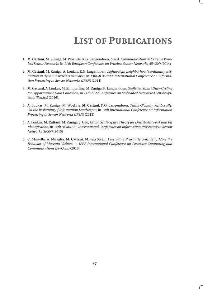
LIST OF PUBLICATIONS
1. M. Cattani, M. Zuniga, M. Woehrle, K.G. Langendoen, SOFA: Communication in Extreme Wire-less Sensor Networks, in 11th European Conference on Wireless Sensor Networks (EWSN) (2014)
2. M. Cattani, M. Zuniga, A. Loukas, K.G. langendoen, Lightweight neighborhood cardinality esti-mation in dynamic wireless networks, in 13th ACM/IEEE International Conference on Informa-tion Processing in Sensor Networks (IPSN) (2014)
3. M. Cattani, A. Loukas, M. Zimmerling, M. Zuniga, K. Langendoen, Staffetta: Smart Duty-Cyclingfor Opportunistic Data Collection, in 14th ACM Conference on Embedded Networked Sensor Sys-tems (SenSys) (2016).
4. A. Loukas, M. Zuniga, M. Woehrle, M. Cattani, K.G. Langendoen, Think Globally, Act Locally:On the Reshaping of Information Landscapes, in 12th International Conference on InformationProcessing in Sensor Networks (IPSN) (2013)
5. A. Loukas, M. Cattani, M. Zuniga, J. Gao, Graph Scale-Space Theory for Distributed Peak and PitIdentification, in 14th ACM/IEEE International Conference on Information Processing in SensorNetworks (IPSN) (2015)
6. C. Martella, A. Miraglia, M. Cattani, M. van Steen, Leveraging Proximity Sensing to Mine theBehavior of Museum Visitors, in IEEE International Conference on Pervasive Computing andCommunications (PerCom) (2016).
97


![arXiv:1107.1606v1 [astro-ph.CO] 8 Jul 2011€¦ · stalled on the Westerbork radio telescope (WSRT) will dramati-cally increase the survey speed for the WSRT. Combined surveys with](https://static.fdocuments.nl/doc/165x107/600feb6d2026a26a845c211c/arxiv11071606v1-astro-phco-8-jul-stalled-on-the-westerbork-radio-telescope.jpg)